Embed Size (px)
Citation preview

BioNLP 2019
SIGBioMed Workshop onBiomedical Natural Language Processing
Proceedings of the 18th BioNLP Workshop and Shared Task
August 1, 2019Florence, Italy
c©2019 The Association for Computational Linguistics
Order copies of this and other ACL proceedings from:
Association for Computational Linguistics (ACL)209 N. Eighth StreetStroudsburg, PA 18360USATel: +1-570-476-8006Fax: [email protected]
ISBN 978-1-950737-28-4
ii
Sesame Street at BioNLP 2019Dina Demner-Fushman, Kevin Bretonnel Cohen, Sophia Ananiadou, and Junichi Tsujii
Recent years have seen an explosion of workshops, community challenges, corpora and publiclyavailable tools in the biomedical and clinical language processing domain. That trend continues in2019. In a significant advance, this year the original BioNLP-ST challenge matured into an openplatform capable of providing technical support and sustaining any group that is interested in organizinga biomedical language processing challenge [1], while the BioNLP Special Interest Group continuessupporting Shared Tasks in emerging areas of research through the annual meeting. This year, BioNLP-ST presents research directions explored by 72 teams for inference and entailment in the medical domain,and their contribution to domain-specific information retrieval and question answering systems [2].
The BioNLP meeting has now been ongoing for 18 years. BioNLP continues to stay the flagship andthe generalist meeting in biomedical language processing, accepting noteworthy work independently ofthe tasks and sublanguages studied. BioNLP also continues promoting research in languages other thanEnglish, this year presenting work in Romanian, Portuguese, Spanish, and Chinese [3, 4, 5, 6], primarilycovering development of resources for these languages.
The quality of submissions continues to impress the program committee and the organizers. BioNLP2019 received 72 submissions to the workshop, and 21 for the Shared Task. Of the work submittedto the workshop, 14 papers were accepted for oral presentation and 24 as poster presentations. Thisyear, various deep learning architectures are explored in all papers, with continuing focus on interestingnew models and in-depth exploration of the state-of-the-art publicly available tools. Most of the workuses BERT [7] or BERT models trained on PubMed, with one paper exploring BERT and ELMo onten biomedical benchmarking datasets [8] and many others using and exploring embeddings and neuralnetworks for chemical recognition [9], concept extraction and coding [10], relation extraction [11, 12,13], and phenotyping [14].
As for the past several years, the themes in this year’s papers and posters continue to focus equally onclinical text and biological language processing. They also reveal sustained interest in social media andconsumer language processing [15].
As it has been for the past 18 years, the workshop is truly a community-wide effort of the authorsproducing high quality work that is already contributing to acceleration of foundational biomedicalresearch [16, 17, 18, 19] and clinical practice [20, 21, 22, 23] through improvements in informationretrieval and extraction, question answering, diagnosis and clinical decision support [24]. We are equallyhappy to see sustained contributions from those who started forming the field of BioNLP research, andfirst-time contributions that show the increasing interest in the domain. We are particularly indebted toour reviewers who reviewed a higher than usual workload in a very short time. Their judgments resultedin a program that will undoubtedly advance both the BioNLP research and the practical areas that itserves. Due to space and time constraints, we could only accept the papers that were recommended foracceptance by at least two reviewers. We hope that the authors of the papers that could not be acceptedreceived good feedback that will help them improve their work.
References
[1] BioNLP-OST https://2019.bionlp-ost.org. Last accessed 10 Jun 2019
[2] Ben Abacha A, Shivade C, Demner-Fushman D. Overview of the MEDIQA 2019 Shared Task onTextual Inference, Question Entailment and Question Answering.
iii
[3] Mitrofan M, et al. MoNERo: a Biomedical Gold Standard Corpus for the Romanian Language.
[4] Lopes F, et al. Contributions to Clinical Named Entity Recognition in Portuguese.
[5] Campillos-Llanos L. First Steps towards Building a Medical Lexicon for Spanish with Linguistic andSemantic Information.
[6] Tian Y, et al. ChiMed: A Chinese Medical Corpus for Question Answering.
[7] Devlin J, et al. BERT: Pre-training of Deep Bidirectional Transformers for Language Understanding.NAACL 2019 Proc.
[8] Peng Y, et al. Transfer Learning in Biomedical Natural Language Processing: An Evaluation ofBERT and ELMo on Ten Benchmarking Datasets.
[9] Zhai Z, et al. Improving Chemical Named Entity Recognition in Patents with Contextualized WordEmbeddings.
[10] Wiegreffe S, et al. Clinical Concept Extraction for Document-Level Coding.
[11] Koroleva A, Paroubek P. Extracting relations between outcomes and significance levels inRandomized Controlled Trials (RCTs) publications.
[12] Chauhan G, et al. REflex: Flexible Framework for Relation Extraction in Multiple Domains.
[13] Khachatrian H, et al. BioRelEx 1.0: Biological Relation Extraction Benchmark.
[14] Liu D, et al. Two-stage Federated Phenotyping and Patient Representation Learning.
[15] Alhuzali H, Ananiadou S. Improving classification of Adverse Drug Reactions through UsingSentiment Analysis and Transfer Learning.
[16] Mezaoui H, et al. Enhancing PIO Element Detection in Medical Text Using ContextualizedEmbedding.
[17] Neumann M, et al. ScispaCy: Fast and Robust Models for Biomedical Natural LanguageProcessing.
[18] Kotitsas S, et al. Embedding Biomedical Ontologies by Jointly Encoding Network Structure andTextual Node Descriptors. BioNLP 2019 Proc.
[19] Koptient A, et al. Simplification-induced transformations: typology and some characteristics.
[20] Ormerod M, et al. Analysing Representations of Memory Impairment in a Clinical NotesClassification Model.
[21] Yuwono SK., et al. Learning from the Experience of Doctors: Automated Diagnosis of AppendicitisBased on Clinical Notes.
[22] Newman-Griffis D, et al. Classifying the reported ability in clinical mobility descriptions.
[23] Soni S, Roberts K. A Paraphrase Generation System for EHR Question Answering.
[24] Apostolova E, et al. Combining Structured and Free-text Electronic Medical Record Data for Real-time Clinical Decision Support.
iv
Organizers:
Sophia Ananiadou, National Centre for Text Mining and University of Manchester, UKKevin Bretonnel Cohen, University of Colorado School of Medicine, USADina Demner-Fushman, US National Library of MedicineJun-ichi Tsujii, National Institute of Advanced Industrial Science and Technology, Japan
Program Committee:
Sophia Ananiadou, National Centre for Text Mining and University of Manchester, UKEmilia Apostolova, Language.ai, USAEiji Aramaki, University of Tokyo, JapanAsma Ben Abacha, US National Library of MedicineCosmin (Adi) Bejan, Vanderbilt University, Nashville, TNOlivier Bodenreider, US National Library of MedicineLeonardo Campillos Llanos, Universidad Autónoma de Madrid, SpainFenia Christopoulou, National Centre for Text Mining and University of Manchester, UKAaron Cohen, Oregon Health & Science University, USAKevin Bretonnel Cohen, University of Colorado School of Medicine, USABrian Connolly, Kroger Digital, USAViviana Cotik, University of Buenos Aires, ArgentinaDina Demner-Fushman, US National Library of MedicineTravis Goodwin, The University of Texas at Dallas, USANatalia Grabar, CNRS, FranceCyril Grouin, LIMSI - CNRS, FranceTudor Groza, The Garvan Institute of Medical Research, AustraliaSadid Hasan, Philips Research, Cambridge, MAAntonio Jimeno Yepes, IBM, Melbourne Area, AustraliaMeizhi Ju, National Centre for Text Mining and University of Manchester, UKWilliam Kearns, University of Washington, USAHalil Kilicoglu, US National Library of MedicineAri Klein, University of Pennsylvania, USAAndre Lamurias, University of Lisbon, PortugalAlberto Lavelli, FBK-ICT, ItalyRobert Leaman, US National Library of MedicineUlf Leser, Humboldt-Universität zu Berlin, GermanyGal Levy-Fix, Columbia University, NYMaolin Li, National Centre for Text Mining and University of Manchester, UKRamon Maldonado, The University of Texas at Dallas, USATimothy Miller, Children’s Hospital Boston, USAYassine Mrabet, US National Library of MedicineAurelie Neveol, LIMSI - CNRS, FranceMariana Neves, German Federal Institute for Risk Assessment, GermanyDenis Newman-Griffis, Clinical Center, National Institutes of Health, USANhung Nguyen, The University of Manchester, UKKaren O’Connor, University of Pennsylvania, USAYifan Peng, US National Library of MedicineLaura Plaza, UNED, Madrid, SpainSampo Pyysalo, University of Cambridge, UKFrancisco J. Ribadas-Pena, University of Vigo, SpainFabio Rinaldi, University of Zurich, Switzerland
v
Kirk Roberts, The University of Texas Health Science Center at Houston, USARoland Roller, DFKI GmbH, Berlin, GermanySumegh Roychowdhury, Indian Institute of Technology KharagpurChaitanya Shivade, IBM Research, Almaden, USANoha Seddik Tawfik, Arab Academy for Science and Technology, EgyptThy Thy Tran, National Centre for Text Mining and University of Manchester, UKSumithra Velupillai, King’s College London, UKDavy Weissenbacher, University of Pennsylvania, USAW John Wilbur, US National Library of MedicineAmir Yazdavar, Wright State University, USAChrysoula Zerva, National Centre for Text Mining and University of Manchester, UKPierre Zweigenbaum, LIMSI - CNRS, France
Additional Reviewers:
Hadi Amiri, Harvard Medical School, USASiamak Barzegar, Barcelona Supercomputing Center, SpainQingyu Chen, US National Library of MedicineZfania Tom Korach, Harvard Medical School, USAMajid Latifi, Trinity College Dublin, IrelandDanielle Mowery, VA Salt Lake City Health Care System, USAClaire Nedellec, INRA, FranceAlastair Rae, US National Library of MedicineMax Savery, US National Library of MedicineDiana Sousa, University of Lisbon, PortugalShankai Yan, US National Library of MedicineAyah Zirikly, Clinical Center, National Institutes of Health, USASeyedjamal Zolhavarieh, The University of Auckland, NZ
vi
Table of Contents
Classifying the reported ability in clinical mobility descriptionsDenis Newman-Griffis, Ayah Zirikly, Guy Divita and Bart Desmet . . . . . . . . . . . . . . . . . . . . . . . . . . . . 1
Learning from the Experience of Doctors: Automated Diagnosis of Appendicitis Based on Clinical NotesSteven Kester Yuwono, Hwee Tou Ng and Kee Yuan Ngiam. . . . . . . . . . . . . . . . . . . . . . . . . . . . . . . . .11
A Paraphrase Generation System for EHR Question AnsweringSarvesh Soni and Kirk Roberts . . . . . . . . . . . . . . . . . . . . . . . . . . . . . . . . . . . . . . . . . . . . . . . . . . . . . . . . . . . 20
REflex: Flexible Framework for Relation Extraction in Multiple DomainsGeeticka Chauhan, Matthew B.A. McDermott and Peter Szolovits . . . . . . . . . . . . . . . . . . . . . . . . . . . 30
Analysing Representations of Memory Impairment in a Clinical Notes Classification ModelMark Ormerod, Jesús Martínez-del-Rincón, Neil Robertson, Bernadette McGuinness and Barry
Devereux . . . . . . . . . . . . . . . . . . . . . . . . . . . . . . . . . . . . . . . . . . . . . . . . . . . . . . . . . . . . . . . . . . . . . . . . . . . . . . . . . . . 48
Transfer Learning in Biomedical Natural Language Processing: An Evaluation of BERT and ELMo onTen Benchmarking Datasets
Yifan Peng, Shankai Yan and Zhiyong Lu . . . . . . . . . . . . . . . . . . . . . . . . . . . . . . . . . . . . . . . . . . . . . . . . . 58
Combining Structured and Free-text Electronic Medical Record Data for Real-time Clinical DecisionSupport
Emilia Apostolova, Tony Wang, Tim Tschampel, Ioannis Koutroulis and Tom Velez . . . . . . . . . . . 66
MoNERo: a Biomedical Gold Standard Corpus for the Romanian LanguageMaria Mitrofan, Verginica Barbu Mititelu and Grigorina Mitrofan . . . . . . . . . . . . . . . . . . . . . . . . . . . 71
Domain Adaptation of SRL Systems for Biological ProcessesDheeraj Rajagopal, Nidhi Vyas, Aditya Siddhant, Anirudha Rayasam, Niket Tandon and Eduard
Hovy . . . . . . . . . . . . . . . . . . . . . . . . . . . . . . . . . . . . . . . . . . . . . . . . . . . . . . . . . . . . . . . . . . . . . . . . . . . . . . . . . . . . . . . 80
Deep Contextualized Biomedical Abbreviation ExpansionQiao Jin, Jinling Liu and Xinghua Lu . . . . . . . . . . . . . . . . . . . . . . . . . . . . . . . . . . . . . . . . . . . . . . . . . . . . . 88
RNN Embeddings for Identifying Difficult to Understand Medical WordsHanna Pylieva, Artem Chernodub, Natalia Grabar and Thierry Hamon . . . . . . . . . . . . . . . . . . . . . . . 97
A distantly supervised dataset for automated data extraction from diagnostic studiesChristopher Norman, Mariska Leeflang, René Spijker, Evangelos Kanoulas and Aurélie Névéol105
Query selection methods for automated corpora construction with a use case in food-drug interactionsGeorgeta Bordea, Tsanta Randriatsitohaina, Fleur Mougin, Natalia Grabar and Thierry Hamon 115
Enhancing biomedical word embeddings by retrofitting to verb clustersBilly Chiu, Simon Baker, Martha Palmer and Anna Korhonen . . . . . . . . . . . . . . . . . . . . . . . . . . . . . . 125
A Comparison of Word-based and Context-based Representations for Classification Problems in HealthInformatics
Aditya Joshi, Sarvnaz Karimi, Ross Sparks, Cecile Paris and C Raina MacIntyre . . . . . . . . . . . . . 135
vii
Constructing large scale biomedical knowledge bases from scratch with rapid annotation of interpretablepatterns
Julien Fauqueur, Ashok Thillaisundaram and Theodosia Togia . . . . . . . . . . . . . . . . . . . . . . . . . . . . . 142
First Steps towards Building a Medical Lexicon for Spanish with Linguistic and Semantic InformationLeonardo Campillos-Llanos . . . . . . . . . . . . . . . . . . . . . . . . . . . . . . . . . . . . . . . . . . . . . . . . . . . . . . . . . . . . 152
Incorporating Figure Captions and Descriptive Text in MeSH Term IndexingXindi Wang and Robert E. Mercer . . . . . . . . . . . . . . . . . . . . . . . . . . . . . . . . . . . . . . . . . . . . . . . . . . . . . . . 165
BioRelEx 1.0: Biological Relation Extraction BenchmarkHrant Khachatrian, Lilit Nersisyan, Karen Hambardzumyan, Tigran Galstyan, Anna Hakobyan,
Arsen Arakelyan, Andrey Rzhetsky and Aram Galstyan . . . . . . . . . . . . . . . . . . . . . . . . . . . . . . . . . . . . . . . . 176
Extraction of Lactation Frames from Drug Labels and LactMedHeath Goodrum, Meghana Gudala, Ankita Misra and Kirk Roberts . . . . . . . . . . . . . . . . . . . . . . . . . 191
Annotating Temporal Information in Clinical Notes for Timeline Reconstruction: Towards the Definitionof Calendar Expressions
Natalia Viani, Hegler Tissot, Ariane Bernardino and Sumithra Velupillai . . . . . . . . . . . . . . . . . . . . 201
Leveraging Sublanguage Features for the Semantic Categorization of Clinical TermsLeonie Grön, Ann Bertels and Kris Heylen . . . . . . . . . . . . . . . . . . . . . . . . . . . . . . . . . . . . . . . . . . . . . . . 211
Enhancing PIO Element Detection in Medical Text Using Contextualized EmbeddingHichem Mezaoui, Isuru Gunasekara and Aleksandr Gontcharov . . . . . . . . . . . . . . . . . . . . . . . . . . . . 217
Contributions to Clinical Named Entity Recognition in PortugueseFábio Lopes, César Teixeira and Hugo Gonçalo Oliveira . . . . . . . . . . . . . . . . . . . . . . . . . . . . . . . . . . . 223
Can Character Embeddings Improve Cause-of-Death Classification for Verbal Autopsy Narratives?Zhaodong Yan, Serena Jeblee and Graeme Hirst . . . . . . . . . . . . . . . . . . . . . . . . . . . . . . . . . . . . . . . . . . 234
Is artificial data useful for biomedical Natural Language Processing algorithms?Zixu Wang, Julia Ive, Sumithra Velupillai and Lucia Specia . . . . . . . . . . . . . . . . . . . . . . . . . . . . . . . . 240
ChiMed: A Chinese Medical Corpus for Question AnsweringYuanhe Tian, Weicheng Ma, Fei Xia and Yan Song. . . . . . . . . . . . . . . . . . . . . . . . . . . . . . . . . . . . . . . .250
Clinical Concept Extraction for Document-Level CodingSarah Wiegreffe, Edward Choi, Sherry Yan, Jimeng Sun and Jacob Eisenstein . . . . . . . . . . . . . . . 261
Clinical Case Reports for NLPCyril Grouin, Natalia Grabar, Vincent Claveau and Thierry Hamon . . . . . . . . . . . . . . . . . . . . . . . . . 273
Two-stage Federated Phenotyping and Patient Representation LearningDianbo Liu, Dmitriy Dligach and Timothy Miller . . . . . . . . . . . . . . . . . . . . . . . . . . . . . . . . . . . . . . . . . 283
Transfer Learning for Causal Sentence DetectionManolis Kyriakakis, Ion Androutsopoulos, Artur Saudabayev and Joan Ginés i Ametllé . . . . . . 292
Embedding Biomedical Ontologies by Jointly Encoding Network Structure and Textual Node DescriptorsSotiris Kotitsas, Dimitris Pappas, Ion Androutsopoulos, Ryan McDonald and Marianna Apidianaki
298
viii
Simplification-induced transformations: typology and some characteristicsAnaïs Koptient, Rémi Cardon and Natalia Grabar . . . . . . . . . . . . . . . . . . . . . . . . . . . . . . . . . . . . . . . . . 309
ScispaCy: Fast and Robust Models for Biomedical Natural Language ProcessingMark Neumann, Daniel King, Iz Beltagy and Waleed Ammar . . . . . . . . . . . . . . . . . . . . . . . . . . . . . . 319
Improving Chemical Named Entity Recognition in Patents with Contextualized Word EmbeddingsZenan Zhai, Dat Quoc Nguyen, Saber Akhondi, Camilo Thorne, Christian Druckenbrodt, Trevor
Cohn, Michelle Gregory and Karin Verspoor . . . . . . . . . . . . . . . . . . . . . . . . . . . . . . . . . . . . . . . . . . . . . . . . . . 328
Improving classification of Adverse Drug Reactions through Using Sentiment Analysis and TransferLearning
Hassan Alhuzali and Sophia Ananiadou . . . . . . . . . . . . . . . . . . . . . . . . . . . . . . . . . . . . . . . . . . . . . . . . . . 339
Exploring Diachronic Changes of Biomedical Knowledge using Distributed Concept RepresentationsGaurav Vashisth, Jan-Niklas Voigt-Antons, Michael Mikhailov and Roland Roller . . . . . . . . . . . .348
Extracting relations between outcomes and significance levels in Randomized Controlled Trials (RCTs)publications
Anna Koroleva and Patrick Paroubek . . . . . . . . . . . . . . . . . . . . . . . . . . . . . . . . . . . . . . . . . . . . . . . . . . . . 359
Overview of the MEDIQA 2019 Shared Task on Textual Inference, Question Entailment and QuestionAnswering
Asma Ben Abacha, Chaitanya Shivade and Dina Demner-Fushman . . . . . . . . . . . . . . . . . . . . . . . . . 370
PANLP at MEDIQA 2019: Pre-trained Language Models, Transfer Learning and Knowledge DistillationWei Zhu, Xiaofeng Zhou, Keqiang Wang, Xun Luo, Xiepeng Li, Yuan Ni and Guotong Xie . . . 380
Pentagon at MEDIQA 2019: Multi-task Learning for Filtering and Re-ranking Answers using LanguageInference and Question Entailment
Hemant Pugaliya, Karan Saxena, Shefali Garg, Sheetal Shalini, Prashant Gupta, Eric Nyberg andTeruko Mitamura . . . . . . . . . . . . . . . . . . . . . . . . . . . . . . . . . . . . . . . . . . . . . . . . . . . . . . . . . . . . . . . . . . . . . . . . . . . 389
DoubleTransfer at MEDIQA 2019: Multi-Source Transfer Learning for Natural Language Understand-ing in the Medical Domain
Yichong Xu, Xiaodong Liu, Chunyuan Li, Hoifung Poon and Jianfeng Gao. . . . . . . . . . . . . . . . . .399
Surf at MEDIQA 2019: Improving Performance of Natural Language Inference in the Clinical Domainby Adopting Pre-trained Language Model
Jiin Nam, Seunghyun Yoon and Kyomin Jung . . . . . . . . . . . . . . . . . . . . . . . . . . . . . . . . . . . . . . . . . . . . 406
WTMED at MEDIQA 2019: A Hybrid Approach to Biomedical Natural Language InferenceZhaofeng Wu, Yan Song, Sicong Huang, Yuanhe Tian and Fei Xia . . . . . . . . . . . . . . . . . . . . . . . . . . 415
KU_ai at MEDIQA 2019: Domain-specific Pre-training and Transfer Learning for Medical NLICemil Cengiz, Ulaş Sert and Deniz Yuret . . . . . . . . . . . . . . . . . . . . . . . . . . . . . . . . . . . . . . . . . . . . . . . . 427
DUT-NLP at MEDIQA 2019: An Adversarial Multi-Task Network to Jointly Model Recognizing QuestionEntailment and Question Answering
Huiwei Zhou, Xuefei Li, Weihong Yao, Chengkun Lang and Shixian Ning . . . . . . . . . . . . . . . . . . 437
DUT-BIM at MEDIQA 2019: Utilizing Transformer Network and Medical Domain-Specific Contextual-ized Representations for Question Answering
Huiwei Zhou, Bizun Lei, Zhe Liu and Zhuang Liu . . . . . . . . . . . . . . . . . . . . . . . . . . . . . . . . . . . . . . . . 446
ix
Dr.Quad at MEDIQA 2019: Towards Textual Inference and Question Entailment using contextualizedrepresentations
Vinayshekhar Bannihatti Kumar, Ashwin Srinivasan, Aditi Chaudhary, James Route, Teruko Mita-mura and Eric Nyberg . . . . . . . . . . . . . . . . . . . . . . . . . . . . . . . . . . . . . . . . . . . . . . . . . . . . . . . . . . . . . . . . . . . . . . 453
Sieg at MEDIQA 2019: Multi-task Neural Ensemble for Biomedical Inference and EntailmentSai Abishek Bhaskar, Rashi Rungta, James Route, Eric Nyberg and Teruko Mitamura . . . . . . . . 462
IIT-KGP at MEDIQA 2019: Recognizing Question Entailment using Sci-BERT stacked with a GradientBoosting Classifier
Prakhar Sharma and Sumegh Roychowdhury . . . . . . . . . . . . . . . . . . . . . . . . . . . . . . . . . . . . . . . . . . . . . 471
ANU-CSIRO at MEDIQA 2019: Question Answering Using Deep Contextual KnowledgeVincent Nguyen, Sarvnaz Karimi and Zhenchang Xing . . . . . . . . . . . . . . . . . . . . . . . . . . . . . . . . . . . . 478
MSIT_SRIB at MEDIQA 2019: Knowledge Directed Multi-task Framework for Natural Language Infer-ence in Clinical Domain.
Sahil Chopra, Ankita Gupta and Anupama Kaushik . . . . . . . . . . . . . . . . . . . . . . . . . . . . . . . . . . . . . . . 488
UU_TAILS at MEDIQA 2019: Learning Textual Entailment in the Medical DomainNoha Tawfik and Marco Spruit . . . . . . . . . . . . . . . . . . . . . . . . . . . . . . . . . . . . . . . . . . . . . . . . . . . . . . . . . . 493
UW-BHI at MEDIQA 2019: An Analysis of Representation Methods for Medical Natural LanguageInference
William Kearns, Wilson Lau and Jason Thomas . . . . . . . . . . . . . . . . . . . . . . . . . . . . . . . . . . . . . . . . . . 500
Saama Research at MEDIQA 2019: Pre-trained BioBERT with Attention Visualisation for Medical Nat-ural Language Inference
Kamal raj Kanakarajan, Suriyadeepan Ramamoorthy, Vaidheeswaran Archana, Soham Chatterjeeand Malaikannan Sankarasubbu . . . . . . . . . . . . . . . . . . . . . . . . . . . . . . . . . . . . . . . . . . . . . . . . . . . . . . . . . . . . . . 510
IITP at MEDIQA 2019: Systems Report for Natural Language Inference, Question Entailment and Ques-tion Answering
Dibyanayan Bandyopadhyay, Baban Gain, Tanik Saikh and Asif Ekbal . . . . . . . . . . . . . . . . . . . . . . 517
LasigeBioTM at MEDIQA 2019: Biomedical Question Answering using Bidirectional Transformers andNamed Entity Recognition
Andre Lamurias and Francisco M Couto . . . . . . . . . . . . . . . . . . . . . . . . . . . . . . . . . . . . . . . . . . . . . . . . . 523
NCUEE at MEDIQA 2019: Medical Text Inference Using Ensemble BERT-BiLSTM-Attention ModelLung-Hao Lee, Yi Lu, Po-Han Chen, Po-Lei Lee and Kuo-Kai Shyu . . . . . . . . . . . . . . . . . . . . . . . . 528
ARS_NITK at MEDIQA 2019:Analysing Various Methods for Natural Language Inference, RecognisingQuestion Entailment and Medical Question Answering System
Anumeha Agrawal, Rosa Anil George, Selvan Suntiha Ravi, Sowmya Kamath and Anand Kumar533
x
Conference Program
Thursday August 1, 2019
8:30–8:45 Opening remarks
8:45–10:30 Session 1: Clinical and Translational NLP
8:45–9:00 Classifying the reported ability in clinical mobility descriptionsDenis Newman-Griffis, Ayah Zirikly, Guy Divita and Bart Desmet
9:00–9:15 Learning from the Experience of Doctors: Automated Diagnosis of AppendicitisBased on Clinical NotesSteven Kester Yuwono, Hwee Tou Ng and Kee Yuan Ngiam
9:15–9:30 A Paraphrase Generation System for EHR Question AnsweringSarvesh Soni and Kirk Roberts
9:30–9:45 REflex: Flexible Framework for Relation Extraction in Multiple DomainsGeeticka Chauhan, Matthew B.A. McDermott and Peter Szolovits
9:45–10:00 Analysing Representations of Memory Impairment in a Clinical Notes ClassificationModelMark Ormerod, Jesús Martínez-del-Rincón, Neil Robertson, Bernadette McGuin-ness and Barry Devereux
10:00–10:15 Transfer Learning in Biomedical Natural Language Processing: An Evaluation ofBERT and ELMo on Ten Benchmarking DatasetsYifan Peng, Shankai Yan and Zhiyong Lu
10:15–10:30 Combining Structured and Free-text Electronic Medical Record Data for Real-timeClinical Decision SupportEmilia Apostolova, Tony Wang, Tim Tschampel, Ioannis Koutroulis and Tom Velez
10:30–11:00 Coffee Break
xi
Thursday August 1, 2019 (continued)
11:00–12:00 Poster Session
MoNERo: a Biomedical Gold Standard Corpus for the Romanian LanguageMaria Mitrofan, Verginica Barbu Mititelu and Grigorina Mitrofan
Domain Adaptation of SRL Systems for Biological ProcessesDheeraj Rajagopal, Nidhi Vyas, Aditya Siddhant, Anirudha Rayasam, Niket Tandonand Eduard Hovy
Deep Contextualized Biomedical Abbreviation ExpansionQiao Jin, Jinling Liu and Xinghua Lu
RNN Embeddings for Identifying Difficult to Understand Medical WordsHanna Pylieva, Artem Chernodub, Natalia Grabar and Thierry Hamon
A distantly supervised dataset for automated data extraction from diagnostic studiesChristopher Norman, Mariska Leeflang, René Spijker, Evangelos Kanoulas and Au-rélie Névéol
Query selection methods for automated corpora construction with a use case infood-drug interactionsGeorgeta Bordea, Tsanta Randriatsitohaina, Fleur Mougin, Natalia Grabar andThierry Hamon
Enhancing biomedical word embeddings by retrofitting to verb clustersBilly Chiu, Simon Baker, Martha Palmer and Anna Korhonen
A Comparison of Word-based and Context-based Representations for ClassificationProblems in Health InformaticsAditya Joshi, Sarvnaz Karimi, Ross Sparks, Cecile Paris and C Raina MacIntyre
Constructing large scale biomedical knowledge bases from scratch with rapid an-notation of interpretable patternsJulien Fauqueur, Ashok Thillaisundaram and Theodosia Togia
First Steps towards Building a Medical Lexicon for Spanish with Linguistic andSemantic InformationLeonardo Campillos-Llanos
Incorporating Figure Captions and Descriptive Text in MeSH Term IndexingXindi Wang and Robert E. Mercer
xii
Thursday August 1, 2019 (continued)
BioRelEx 1.0: Biological Relation Extraction BenchmarkHrant Khachatrian, Lilit Nersisyan, Karen Hambardzumyan, Tigran Galstyan, AnnaHakobyan, Arsen Arakelyan, Andrey Rzhetsky and Aram Galstyan
Extraction of Lactation Frames from Drug Labels and LactMedHeath Goodrum, Meghana Gudala, Ankita Misra and Kirk Roberts
Annotating Temporal Information in Clinical Notes for Timeline Reconstruction:Towards the Definition of Calendar ExpressionsNatalia Viani, Hegler Tissot, Ariane Bernardino and Sumithra Velupillai
Leveraging Sublanguage Features for the Semantic Categorization of ClinicalTermsLeonie Grön, Ann Bertels and Kris Heylen
Enhancing PIO Element Detection in Medical Text Using Contextualized Embed-dingHichem Mezaoui, Isuru Gunasekara and Aleksandr Gontcharov
Contributions to Clinical Named Entity Recognition in PortugueseFábio Lopes, César Teixeira and Hugo Gonçalo Oliveira
Can Character Embeddings Improve Cause-of-Death Classification for Verbal Au-topsy Narratives?Zhaodong Yan, Serena Jeblee and Graeme Hirst
Is artificial data useful for biomedical Natural Language Processing algorithms?Zixu Wang, Julia Ive, Sumithra Velupillai and Lucia Specia
ChiMed: A Chinese Medical Corpus for Question AnsweringYuanhe Tian, Weicheng Ma, Fei Xia and Yan Song
Clinical Concept Extraction for Document-Level CodingSarah Wiegreffe, Edward Choi, Sherry Yan, Jimeng Sun and Jacob Eisenstein
Clinical Case Reports for NLPCyril Grouin, Natalia Grabar, Vincent Claveau and Thierry Hamon
Two-stage Federated Phenotyping and Patient Representation LearningDianbo Liu, Dmitriy Dligach and Timothy Miller
xiii
Thursday August 1, 2019 (continued)
Transfer Learning for Causal Sentence DetectionManolis Kyriakakis, Ion Androutsopoulos, Artur Saudabayev and Joan Ginés iAmetllé
12:00–12:30 Session 2: Ontology and Typology
12:00–12:15 Embedding Biomedical Ontologies by Jointly Encoding Network Structure and Tex-tual Node DescriptorsSotiris Kotitsas, Dimitris Pappas, Ion Androutsopoulos, Ryan McDonald and Mari-anna Apidianaki
12:15–12:30 Simplification-induced transformations: typology and some characteristicsAnaïs Koptient, Rémi Cardon and Natalia Grabar
12:30–14:00 Lunch break
14:00–15:30 Session 3: Literature mining approaches and models
14:00–14:15 ScispaCy: Fast and Robust Models for Biomedical Natural Language ProcessingMark Neumann, Daniel King, Iz Beltagy and Waleed Ammar
14:15–14:30 Improving Chemical Named Entity Recognition in Patents with Contextualized WordEmbeddingsZenan Zhai, Dat Quoc Nguyen, Saber Akhondi, Camilo Thorne, Christian Druck-enbrodt, Trevor Cohn, Michelle Gregory and Karin Verspoor
14:30–14:45 Improving classification of Adverse Drug Reactions through Using Sentiment Anal-ysis and Transfer LearningHassan Alhuzali and Sophia Ananiadou
14:45–15:00 Exploring Diachronic Changes of Biomedical Knowledge using Distributed Con-cept RepresentationsGaurav Vashisth, Jan-Niklas Voigt-Antons, Michael Mikhailov and Roland Roller
15:00–15:15 Extracting relations between outcomes and significance levels in Randomized Con-trolled Trials (RCTs) publicationsAnna Koroleva and Patrick Paroubek
15:30–16:00 Coffee Break
xiv
Thursday August 1, 2019 (continued)
16:00–17:00 Session 4: Shared Task
16:00–16:15 Overview of the MEDIQA 2019 Shared Task on Textual Inference, Question Entail-ment and Question AnsweringAsma Ben Abacha, Chaitanya Shivade and Dina Demner-Fushman
16:15–16:30 PANLP at MEDIQA 2019: Pre-trained Language Models, Transfer Learning andKnowledge DistillationWei Zhu, Xiaofeng Zhou, Keqiang Wang, Xun Luo, Xiepeng Li, Yuan Ni and Guo-tong Xie
16:30–16:45 Pentagon at MEDIQA 2019: Multi-task Learning for Filtering and Re-ranking An-swers using Language Inference and Question EntailmentHemant Pugaliya, Karan Saxena, Shefali Garg, Sheetal Shalini, Prashant Gupta,Eric Nyberg and Teruko Mitamura
16:45–17:00 DoubleTransfer at MEDIQA 2019: Multi-Source Transfer Learning for NaturalLanguage Understanding in the Medical DomainYichong Xu, Xiaodong Liu, Chunyuan Li, Hoifung Poon and Jianfeng Gao
17:00–18:00 Shared Task Poster Session
Surf at MEDIQA 2019: Improving Performance of Natural Language Inference inthe Clinical Domain by Adopting Pre-trained Language ModelJiin Nam, Seunghyun Yoon and Kyomin Jung
WTMED at MEDIQA 2019: A Hybrid Approach to Biomedical Natural LanguageInferenceZhaofeng Wu, Yan Song, Sicong Huang, Yuanhe Tian and Fei Xia
KU_ai at MEDIQA 2019: Domain-specific Pre-training and Transfer Learning forMedical NLICemil Cengiz, Ulaş Sert and Deniz Yuret
DUT-NLP at MEDIQA 2019: An Adversarial Multi-Task Network to Jointly ModelRecognizing Question Entailment and Question AnsweringHuiwei Zhou, Xuefei Li, Weihong Yao, Chengkun Lang and Shixian Ning
DUT-BIM at MEDIQA 2019: Utilizing Transformer Network and Medical Domain-Specific Contextualized Representations for Question AnsweringHuiwei Zhou, Bizun Lei, Zhe Liu and Zhuang Liu
Dr.Quad at MEDIQA 2019: Towards Textual Inference and Question Entailmentusing contextualized representationsVinayshekhar Bannihatti Kumar, Ashwin Srinivasan, Aditi Chaudhary, JamesRoute, Teruko Mitamura and Eric Nyberg
xv
Thursday August 1, 2019 (continued)
Sieg at MEDIQA 2019: Multi-task Neural Ensemble for Biomedical Inference andEntailmentSai Abishek Bhaskar, Rashi Rungta, James Route, Eric Nyberg and Teruko Mita-mura
IIT-KGP at MEDIQA 2019: Recognizing Question Entailment using Sci-BERTstacked with a Gradient Boosting ClassifierPrakhar Sharma and Sumegh Roychowdhury
ANU-CSIRO at MEDIQA 2019: Question Answering Using Deep ContextualKnowledgeVincent Nguyen, Sarvnaz Karimi and Zhenchang Xing
MSIT_SRIB at MEDIQA 2019: Knowledge Directed Multi-task Framework for Nat-ural Language Inference in Clinical Domain.Sahil Chopra, Ankita Gupta and Anupama Kaushik
UU_TAILS at MEDIQA 2019: Learning Textual Entailment in the Medical DomainNoha Tawfik and Marco Spruit
UW-BHI at MEDIQA 2019: An Analysis of Representation Methods for MedicalNatural Language InferenceWilliam Kearns, Wilson Lau and Jason Thomas
Saama Research at MEDIQA 2019: Pre-trained BioBERT with Attention Visualisa-tion for Medical Natural Language InferenceKamal raj Kanakarajan, Suriyadeepan Ramamoorthy, Vaidheeswaran Archana, So-ham Chatterjee and Malaikannan Sankarasubbu
IITP at MEDIQA 2019: Systems Report for Natural Language Inference, QuestionEntailment and Question AnsweringDibyanayan Bandyopadhyay, Baban Gain, Tanik Saikh and Asif Ekbal
LasigeBioTM at MEDIQA 2019: Biomedical Question Answering using Bidirec-tional Transformers and Named Entity RecognitionAndre Lamurias and Francisco M Couto
NCUEE at MEDIQA 2019: Medical Text Inference Using Ensemble BERT-BiLSTM-Attention ModelLung-Hao Lee, Yi Lu, Po-Han Chen, Po-Lei Lee and Kuo-Kai Shyu
ARS_NITK at MEDIQA 2019:Analysing Various Methods for Natural Language In-ference, Recognising Question Entailment and Medical Question Answering SystemAnumeha Agrawal, Rosa Anil George, Selvan Suntiha Ravi, Sowmya Kamath andAnand Kumar
xvi
Proceedings of the BioNLP 2019 workshop, pages 1–10Florence, Italy, August 1, 2019. c©2019 Association for Computational Linguistics
Classifying the reported ability in clinical mobility descriptions
Denis Newman-Griffis1,2∗, Ayah Zirikly1∗, Guy Divita1∗, Bart Desmet11Rehabilitation Medicine Dept., Clinical Center, National Institutes of Health, Bethesda, MD
2Dept. of Computer Science and Engineering, The Ohio State University, Columbus, OH{denis.griffis, ayah.zirikly, guy.divita, bart.desmet}@nih.gov
AbstractAssessing how individuals perform differentactivities is key information for modelinghealth states of individuals and populations.Descriptions of activity performance in clini-cal free text are complex, including syntacticnegation and similarities to textual entailmenttasks. We explore a variety of methods for thenovel task of classifying four types of asser-tions about activity performance: Able, Un-able, Unclear, and None (no information). Wefind that ensembling an SVM trained with lexi-cal features and a CNN achieves 77.9% macroF1 score on our task, and yields nearly 80%recall on the rare Unclear and Unable sam-ples. Finally, we highlight several challengesin classifying performance assertions, includ-ing capturing information about sources of as-sistance, incorporating syntactic structure andnegation scope, and handling new modalitiesat test time. Our findings establish a strongbaseline for this novel task, and identify in-triguing areas for further research.
1 Introduction
Information on how individuals perform activi-ties and participate in social roles informs concep-tualizations of quality of life, disability, and so-cial well-being. Importantly, activity performanceand role participation are highly dependent on theenvironment in which they occur; for example,one individual may be able to walk around an of-fice without issue, but experience severe difficultywalking along mountain paths. Thus, determin-ing what level of performance an individual canachieve for activities in different environments iscritical for identifying ability to meet work re-quirements, and designing public policy to supportthe participation of all people.
However, the interaction between individualsand environments makes modeling performance
∗These authors contributed equally to this work.
information a complex task. Assessments of ac-tivity performance within clinical healthcare set-tings are typically recorded in free text (Bog-ardus et al., 2004; Nicosia et al., 2019), andexhibit high flexibility in structure. Syntac-tic negation can be present, but is not neces-sarily indicative of inability to perform an ac-tion; for example, Patient can walk withrolling walker and Patient cannotwalk without rolling walker are bothlikely to be used to assert the ability of the patientto walk with the use of an assistive device. Infor-mation about performance may also be given with-out a clear assertion, as in the cane makesit difficult to walk. Thus, extractionof performance information must not only distin-guish between positive and negative assertions, butalso those which cannot be clearly evaluated.
To the best of our knowledge, this is the firstwork to explore assertions of activity performancein health data. We explore a variety of meth-ods for classifying assertion types, including rule-based approaches, statistical methods using com-mon text features, and convolutional neural net-works. We find that machine learning approachesset a strong baseline for discriminating betweenfour assertion types, including rare negative as-sertions. While this work focuses on a relativelyconstrained and homogeneous corpus, error anal-ysis suggests several broader directions for futureresearch on classifying performance assertions.
2 Related Work
Though this is the first work focusing on the po-larity of activity performance, three areas of priorwork are particularly relevant to this research.
The first is concerned with applying NLP tech-niques and linguistic annotation to informationabout whole-person function, particularly activity
1
performance. Harris et al. (2003) experimentedwith term extraction for the purpose of terminol-ogy discovery to support information retrieval re-lating to functioning, disability and health, usinglinguistic, n-gram and hybrid techniques. Baleset al. (2005) and Kukafka et al. (2006) modifiedand applied the MedLEE NLP Extraction tool tocode Rehabilitation Discharge Summaries usingICF (World Health Organization, 2001) encod-ings. Kuang et al. (2015) studied UMLS termcoverage of functional status terms found in VAclinical notes and in social media sources, report-ing that there is a need to extend existing termi-nologies to cover this area. Finally, Thieu et al.(2017) reported on an effort to build an anno-tated corpus of Physical Therapy (PT) notes fromthe Clinical Center of the National Institutes ofHealth (NIH) with functional status information.This corpus was also used for an investigationinto using named entity recognition (NER) tech-niques to extract information about patient mobil-ity (Newman-Griffis and Zirikly, 2018).
The second area is research on negation. Nega-tion detection is a well-researched area (Moranteand Sporleder, 2012), and both negation and un-certainty have historically been studied in the clin-ical NLP context (Mowery et al., 2012; Peng et al.,2018). Previous work studied the use of incorpo-rating dependency parsers to help in identifyingthe scope (Sohn et al., 2012; Mehrabi et al., 2015).Recent work in this area involves the use of neuralnetwork models, where Long Short-Term Mem-ory (LSTM), or variations of it, yielded compet-itive results on negation (cues and scope) detec-tion (Taylor and Harabagiu, 2018).
One highly-related work to ours is Wu et al.(2014), which investigates detection of binary se-mantic negation status (i.e., the presence or ab-sence of a finding, as opposed to syntactic nega-tion) for clinical findings in EHR text. However,as Action Polarity is defined in terms of the in-teraction between an individual and a specific en-vironment, it adds a layer of complexity to non-interactive physiological observations. Gkotsiset al. (2016) investigate using parsing-based scop-ing limitations for negation detection in complexclinical statements, though their focus is specifi-cally on mentions of suicide.
Finally, classifying the assertion status of ac-tivity performance descriptions bears similaritiesto the problem of recognizing textual entailment
(RTE) (Dagan et al., 2006; Marelli et al., 2014).RTE asks whether a given premise entails a spe-cific hypothesis, and has historically been pursuedin the general domain, though, recent efforts havedeveloped datasets in biomedical literature (BenAbacha et al., 2015; Ben Abacha and Demner-Fushman, 2016) and in clinical text (Romanov andShivade, 2018). Our task, by asking whether agiven description entails ability to perform an ac-tion in the an environment, is more constrainedthan RTE, but poses a related research challenge.
3 Data
We use an extended version of the dataset initiallydescribed by Thieu et al. (2017), consisting of 400English-language Physical Therapy initial assess-ment and reassessment notes from the Rehabili-tation Medicine Department of the NIH ClinicalCenter. These text documents have been annotatedto identify descriptions and assessments of mo-bility status, typically including one or more spe-cific Actions; for example, Pt walked 300’with rolling walker (Action underlined).
Each Action annotation was assigned one offour Polarity values, indicating what (if any) in-formation the containing mobility description pro-vides about the subject’s ability to perform thegiven Action in the context of any described envi-ronmental factors.1 The Polarity labels are definedin the following paragraphs.
Able The subject is able to complete theactivity in the environment described. For ex-ample, She states she can walk 20minutes before tiring; in the case ofnow requires assistance of oneperson with transfers, it is unknownwhether the patient can perform the action in-dependently, but they are able to do so with theassistance described.
Unable The subject is not able to completethe activity in the environment described; forexample, He is unable to walk. Morespecific information may also be included,as in Pt is now unable to walk morethan 50 feet.
Unclear Some information is provided aboutthe subject’s ability to perform the action, but not
1It is important to note that the Polarity label is depen-dent on the environmental factors described. For example, anindividual may be able to walk a certain distance using an as-sistive device such as a rolling walker, but unable to walk thatsame distance independently.
2
Label Train Test TotalAble 1,536 446 1,982
Unable 54 23 77Unclear 158 48 206
None 1,784 478 2,262Total 3,532 995 4,527
Table 1: Number of samples with each Polarity label intrain and test data.
enough to make a definitive positive or negativejudgment. For example, in The cane makesit difficult to walk, it is undeterminedwhether the subject can or cannot walk. This labelalso includes some cases of negated environmen-tal factors; for example, unable to propelwheelchair independently.
None No direct information about abilityto perform the action is provided. Commonexamples of this label refer to a scale that iseither unavailable or distant in the document, asin Ambulation: 1. Other cases refer to aspecific aspect of performing an action, withoutevaluation, as in tendency during gaitto quickly extend the leg fromswing to stance.
We randomly split the 400 documents into 320training records and 80 testing records, stratifiedby distribution of Polarity labels. Table 1 providesfrequencies of each label in these splits.
4 Methods
We investigate a variety of methods to classify thePolarity values of Action annotations. Rule-basedmethods have been used to great effect in clinicalinformation extraction (Kang et al., 2013; Chap-man et al., 2007), and form an important baselinefor our task. We also make use of several com-mon machine learning methods, such as supportvector machines and k-nearest neighbors, alongwith more recent neural models such as convolu-tional neural networks (CNN). Finally, we exper-iment with ensembled combinations of our best-performing models. These approaches are de-scribed in the following subsections.
4.1 Rule-based
A UIMA (Ferrucci and Lally, 2004) basedpipeline was constructed to identify action polar-ity from components of v3NLP-Framework (Di-vita et al., 2016). Leveraging the relationship of
our task to detecting contextual attributes such asnegation, the conTEXT (Chapman et al., 2007) al-gorithm embedded in the v3NLP-Framework wasaugmented with a few additional entries including“able” and “independent” as asserted evidence and“unable” as negative evidence.
The conTEXT algorithm relies on a lexiconof evidence and accompanying clues to indicatewhen evidence found to the right or left of a rel-evant entity within a bounded window should beapplied. We used the sentence containing an Ac-tion mention as the bounds of its context window.An Action Polarity UIMA annotator was built toassign Polarity, given an Action annotation. Thisannotator is downstream from the conTEXT anno-tator that assigned negation, assertion, conditional,hypothetical, historical, and subject attributes tonamed entities. Within conTEXT-processed enti-ties, we assigned Unable polarities to actions thathad previously been attributed with negative andassigned Able polarities that had previously beenassigned only asserted attributes. Actions thatwere tagged as conditional or hypothetical werenot assigned a Polarity.
The v3NLP-Framework pipeline includes doc-ument decomposition annotators to identify sec-tions, section names, sentences, slots and values,questions and their answers, and to a lesser ex-tent checkboxes (Divita et al., 2014). Action men-tions in clinical text occur within the boundaries ofeach of these elements. ConTEXT addresses ac-tion mentions within prose, but is not relevant foraction mentions found in the semi-structured con-structs. The Action Polarity annotator was thusaugmented with additional rules to aid in polar-ity assignment based on where the mention wasfound. The most relevant rules are as follows:
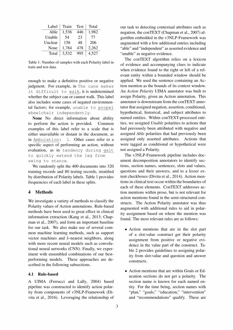
• Action mentions that are in the slot partof a slot:value construct get their polarityassignment from positive or negative evi-dence in the value part of the construct. Ta-ble 2 provides guidelines to assigning polar-ity from slot:value and question and answerconstructs.
• Action mentions that are within Goals or Ed-ucation sections do not get a polarity. Thesection name is known for each named en-tity. For the time being, section names with“plan,” “goals,” “education,” “intervention”and “recommendations” qualify. These are
3
Slot criteria Value criteria Assigned Polarity ExampleAsserted Action Asserted Evidence Able Transfers: IndependentAsserted Action Negated Evidence Unable Transfers: UnableNegated Action Negated Evidence Able Difficulty Walking: NoNegated Action Asserted Evidence Unable Unable to Walk: yesAsserted Action Numbers Unclear Transfers: 4Asserted Action No context evidence Unclear Sit to stand: minimal assistAsserted Action No value None Stand to sit:Multiple Actions Doesn’t matter None Difficulty with chores, shopping,
driving: Yes
Table 2: Table of slot:value rules for Action Polarity
considered to be hypothetical constructs. Theexception to this is if a goal is noted to havebeen met, it gets an Able Polarity.
• Action mentions within only the value partof the slot:value construct were handled thesame way as Action mentions within prose.
4.2 Machine learning models
We evaluated the following common machinelearning-based classification methods for our Po-larity labeling task:2
• Random forest (RF), using 100 estimators;
• Naı̈ve Bayes (NB), using Gaussian estima-tors;
• k-nearest neighbors (kNN), using k=5 withEuclidean distance;
• Support vector machine (SVM), with linearkernel;
• Deep neural network (DNN), using a 100-dimensional hidden layer followed by a 10-dimensional hidden layer.3
For a given Action mention a contained in aMobility description m, we explored using bothbag of binary unigram features4 and word em-bedding features as model input. For both kindsof features, we experimented with using the con-text words in m − a (i.e., all words in m exceptfor the Action mention itself) only, and includingthe text of the Action mention a. Word embed-ding features were calculated by averaging the em-beddings of all words used (either context aloneor averaging context words and Action mention
2We used the implementations of each method in Scikit-Learn (Pedregosa et al., 2011).
3We experimented with d ∈ 10, 100, and number of lay-ers ∈ 1, 2, 3.
4Binary unigram features consistently matched or outper-formed unigram counts in our experiments.
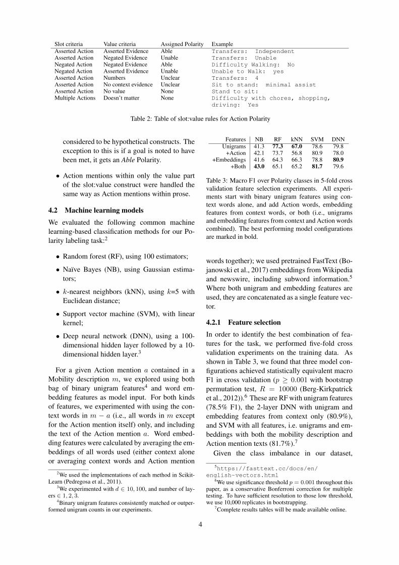
Features NB RF kNN SVM DNNUnigrams 41.3 77.3 67.0 78.6 79.8
+Action 42.1 73.7 56.8 80.9 78.0+Embeddings 41.6 64.3 66.3 78.8 80.9
+Both 43.0 65.1 65.2 81.7 79.6
Table 3: Macro F1 over Polarity classes in 5-fold crossvalidation feature selection experiments. All experi-ments start with binary unigram features using con-text words alone, and add Action words, embeddingfeatures from context words, or both (i.e., unigramsand embedding features from context and Action wordscombined). The best performing model configurationsare marked in bold.
words together); we used pretrained FastText (Bo-janowski et al., 2017) embeddings from Wikipediaand newswire, including subword information.5
Where both unigram and embedding features areused, they are concatenated as a single feature vec-tor.
4.2.1 Feature selectionIn order to identify the best combination of fea-tures for the task, we performed five-fold crossvalidation experiments on the training data. Asshown in Table 3, we found that three model con-figurations achieved statistically equivalent macroF1 in cross validation (p ≥ 0.001 with bootstrappermutation test, R = 10000 (Berg-Kirkpatricket al., 2012)).6 These are RF with unigram features(78.5% F1), the 2-layer DNN with unigram andembedding features from context only (80.9%),and SVM with all features, i.e. unigrams and em-beddings with both the mobility description andAction mention texts (81.7%).7
Given the class imbalance in our dataset,
5https://fasttext.cc/docs/en/english-vectors.html
6We use significance threshold p = 0.001 throughout thispaper, as a conservative Bonferroni correction for multipletesting. To have sufficient resolution to those low threshold,we use 10,000 replicates in bootstrapping.
7Complete results tables will be made available online.
4
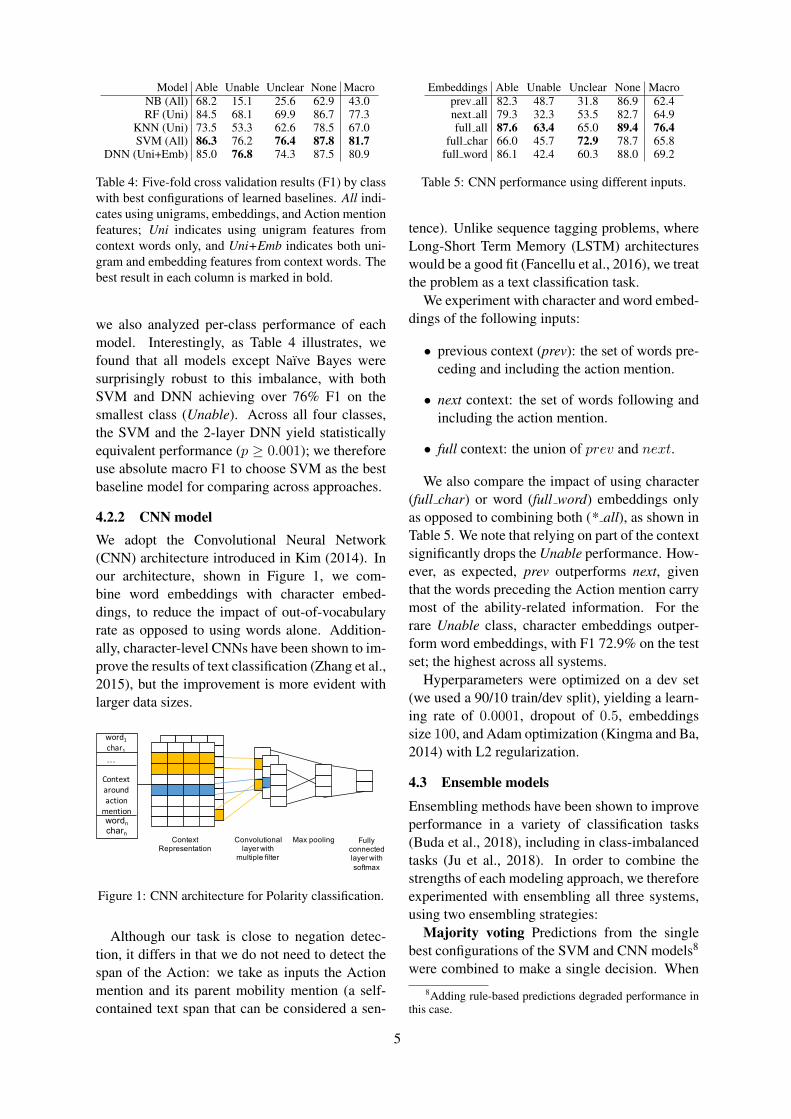
Model Able Unable Unclear None MacroNB (All) 68.2 15.1 25.6 62.9 43.0RF (Uni) 84.5 68.1 69.9 86.7 77.3
KNN (Uni) 73.5 53.3 62.6 78.5 67.0SVM (All) 86.3 76.2 76.4 87.8 81.7
DNN (Uni+Emb) 85.0 76.8 74.3 87.5 80.9
Table 4: Five-fold cross validation results (F1) by classwith best configurations of learned baselines. All indi-cates using unigrams, embeddings, and Action mentionfeatures; Uni indicates using unigram features fromcontext words only, and Uni+Emb indicates both uni-gram and embedding features from context words. Thebest result in each column is marked in bold.
we also analyzed per-class performance of eachmodel. Interestingly, as Table 4 illustrates, wefound that all models except Naı̈ve Bayes weresurprisingly robust to this imbalance, with bothSVM and DNN achieving over 76% F1 on thesmallest class (Unable). Across all four classes,the SVM and the 2-layer DNN yield statisticallyequivalent performance (p ≥ 0.001); we thereforeuse absolute macro F1 to choose SVM as the bestbaseline model for comparing across approaches.
4.2.2 CNN modelWe adopt the Convolutional Neural Network(CNN) architecture introduced in Kim (2014). Inour architecture, shown in Figure 1, we com-bine word embeddings with character embed-dings, to reduce the impact of out-of-vocabularyrate as opposed to using words alone. Addition-ally, character-level CNNs have been shown to im-prove the results of text classification (Zhang et al.,2015), but the improvement is more evident withlarger data sizes.
Context Representation
Convolutional layer with
multiple filter
Max pooling Fully connected layer with softmax
word1 char1
Context around action
mentionwordncharn
…
Figure 1: CNN architecture for Polarity classification.
Although our task is close to negation detec-tion, it differs in that we do not need to detect thespan of the Action: we take as inputs the Actionmention and its parent mobility mention (a self-contained text span that can be considered a sen-
Embeddings Able Unable Unclear None Macroprev all 82.3 48.7 31.8 86.9 62.4next all 79.3 32.3 53.5 82.7 64.9full all 87.6 63.4 65.0 89.4 76.4
full char 66.0 45.7 72.9 78.7 65.8full word 86.1 42.4 60.3 88.0 69.2
Table 5: CNN performance using different inputs.
tence). Unlike sequence tagging problems, whereLong-Short Term Memory (LSTM) architectureswould be a good fit (Fancellu et al., 2016), we treatthe problem as a text classification task.
We experiment with character and word embed-dings of the following inputs:
• previous context (prev): the set of words pre-ceding and including the action mention.
• next context: the set of words following andincluding the action mention.
• full context: the union of prev and next.
We also compare the impact of using character(full char) or word (full word) embeddings onlyas opposed to combining both (* all), as shown inTable 5. We note that relying on part of the contextsignificantly drops the Unable performance. How-ever, as expected, prev outperforms next, giventhat the words preceding the Action mention carrymost of the ability-related information. For therare Unable class, character embeddings outper-form word embeddings, with F1 72.9% on the testset; the highest across all systems.
Hyperparameters were optimized on a dev set(we used a 90/10 train/dev split), yielding a learn-ing rate of 0.0001, dropout of 0.5, embeddingssize 100, and Adam optimization (Kingma and Ba,2014) with L2 regularization.
4.3 Ensemble models
Ensembling methods have been shown to improveperformance in a variety of classification tasks(Buda et al., 2018), including in class-imbalancedtasks (Ju et al., 2018). In order to combine thestrengths of each modeling approach, we thereforeexperimented with ensembling all three systems,using two ensembling strategies:
Majority voting Predictions from the singlebest configurations of the SVM and CNN models8
were combined to make a single decision. When8Adding rule-based predictions degraded performance in
this case.
5
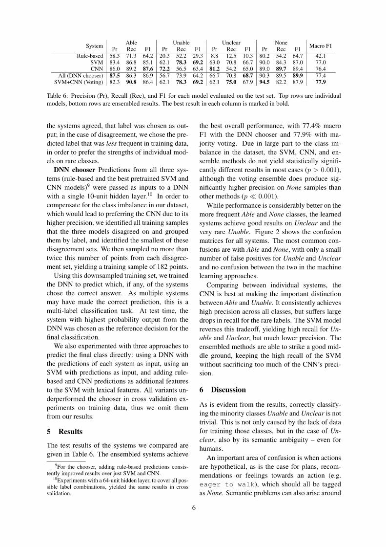
System Able Unable Unclear None Macro F1Pr Rec F1 Pr Rec F1 Pr Rec F1 Pr Rec F1Rule-based 58.3 71.3 64.2 20.3 52.2 29.3 8.8 12.5 10.3 80.2 54.2 64.7 42.1
SVM 83.4 86.8 85.1 62.1 78.3 69.2 63.0 70.8 66.7 90.0 84.3 87.0 77.0CNN 86.0 89.2 87.6 72.2 56.5 63.4 81.2 54.2 65.0 89.0 89.7 89.4 76.4
All (DNN chooser) 87.5 86.3 86.9 56.7 73.9 64.2 66.7 70.8 68.7 90.3 89.5 89.9 77.4SVM+CNN (Voting) 82.3 90.8 86.4 62.1 78.3 69.2 62.1 75.0 67.9 94.5 82.2 87.9 77.9
Table 6: Precision (Pr), Recall (Rec), and F1 for each model evaluated on the test set. Top rows are individualmodels, bottom rows are ensembled results. The best result in each column is marked in bold.
the systems agreed, that label was chosen as out-put; in the case of disagreement, we chose the pre-dicted label that was less frequent in training data,in order to prefer the strengths of individual mod-els on rare classes.
DNN chooser Predictions from all three sys-tems (rule-based and the best pretrained SVM andCNN models)9 were passed as inputs to a DNNwith a single 10-unit hidden layer.10 In order tocompensate for the class imbalance in our dataset,which would lead to preferring the CNN due to itshigher precision, we identified all training samplesthat the three models disagreed on and groupedthem by label, and identified the smallest of thesedisagreement sets. We then sampled no more thantwice this number of points from each disagree-ment set, yielding a training sample of 182 points.
Using this downsampled training set, we trainedthe DNN to predict which, if any, of the systemschose the correct answer. As multiple systemsmay have made the correct prediction, this is amulti-label classification task. At test time, thesystem with highest probability output from theDNN was chosen as the reference decision for thefinal classification.
We also experimented with three approaches topredict the final class directly: using a DNN withthe predictions of each system as input, using anSVM with predictions as input, and adding rule-based and CNN predictions as additional featuresto the SVM with lexical features. All variants un-derperformed the chooser in cross validation ex-periments on training data, thus we omit themfrom our results.
5 Results
The test results of the systems we compared aregiven in Table 6. The ensembled systems achieve
9For the chooser, adding rule-based predictions consis-tently improved results over just SVM and CNN.
10Experiments with a 64-unit hidden layer, to cover all pos-sible label combinations, yielded the same results in crossvalidation.
the best overall performance, with 77.4% macroF1 with the DNN chooser and 77.9% with ma-jority voting. Due in large part to the class im-balance in the dataset, the SVM, CNN, and en-semble methods do not yield statistically signifi-cantly different results in most cases (p > 0.001),although the voting ensemble does produce sig-nificantly higher precision on None samples thanother methods (p� 0.001).
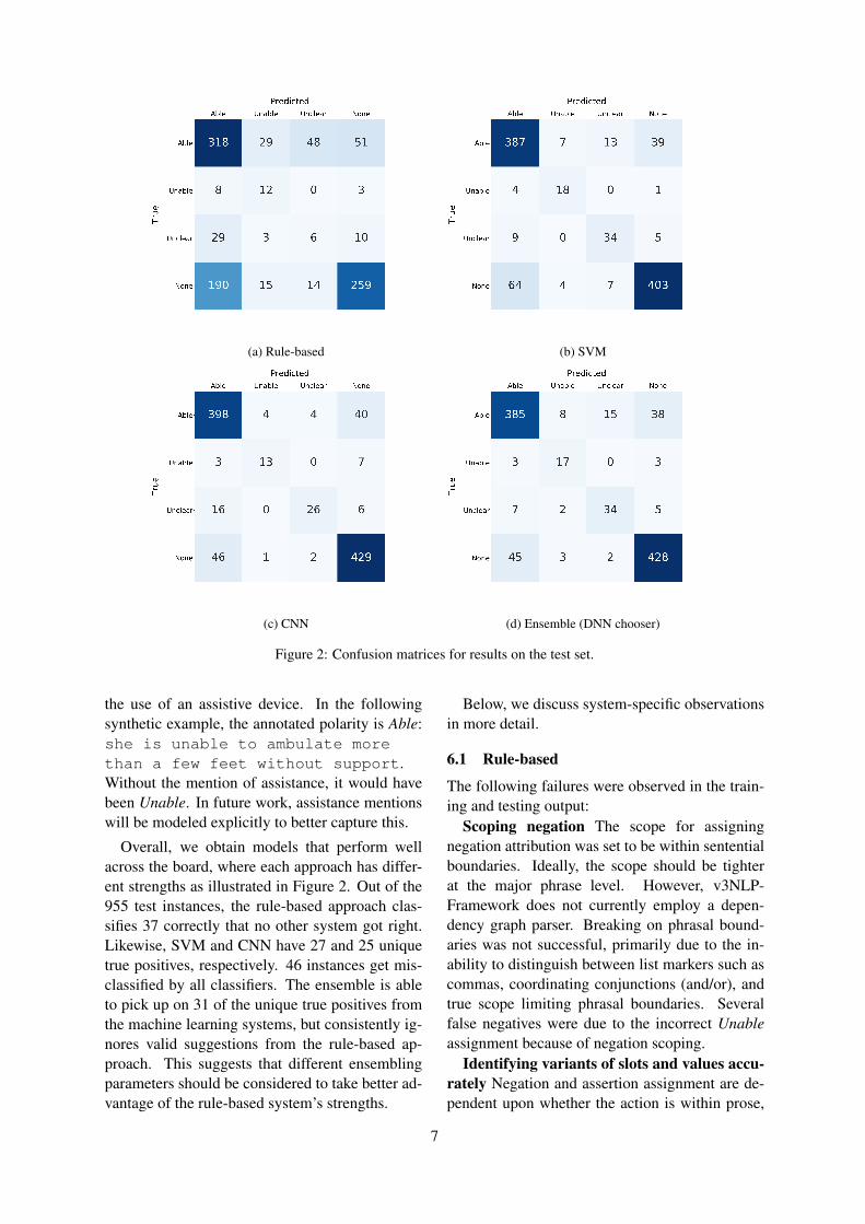
While performance is considerably better on themore frequent Able and None classes, the learnedsystems achieve good results on Unclear and thevery rare Unable. Figure 2 shows the confusionmatrices for all systems. The most common con-fusions are with Able and None, with only a smallnumber of false positives for Unable and Unclearand no confusion between the two in the machinelearning approaches.
Comparing between individual systems, theCNN is best at making the important distinctionbetween Able and Unable. It consistently achieveshigh precision across all classes, but suffers largedrops in recall for the rare labels. The SVM modelreverses this tradeoff, yielding high recall for Un-able and Unclear, but much lower precision. Theensembled methods are able to strike a good mid-dle ground, keeping the high recall of the SVMwithout sacrificing too much of the CNN’s preci-sion.
6 Discussion
As is evident from the results, correctly classify-ing the minority classes Unable and Unclear is nottrivial. This is not only caused by the lack of datafor training those classes, but in the case of Un-clear, also by its semantic ambiguity – even forhumans.
An important area of confusion is when actionsare hypothetical, as is the case for plans, recom-mendations or feelings towards an action (e.g.eager to walk), which should all be taggedas None. Semantic problems can also arise around
6
(a) Rule-based (b) SVM
(c) CNN (d) Ensemble (DNN chooser)
Figure 2: Confusion matrices for results on the test set.
the use of an assistive device. In the followingsynthetic example, the annotated polarity is Able:she is unable to ambulate morethan a few feet without support.Without the mention of assistance, it would havebeen Unable. In future work, assistance mentionswill be modeled explicitly to better capture this.
Overall, we obtain models that perform wellacross the board, where each approach has differ-ent strengths as illustrated in Figure 2. Out of the955 test instances, the rule-based approach clas-sifies 37 correctly that no other system got right.Likewise, SVM and CNN have 27 and 25 uniquetrue positives, respectively. 46 instances get mis-classified by all classifiers. The ensemble is ableto pick up on 31 of the unique true positives fromthe machine learning systems, but consistently ig-nores valid suggestions from the rule-based ap-proach. This suggests that different ensemblingparameters should be considered to take better ad-vantage of the rule-based system’s strengths.
Below, we discuss system-specific observationsin more detail.
6.1 Rule-based
The following failures were observed in the train-ing and testing output:
Scoping negation The scope for assigningnegation attribution was set to be within sententialboundaries. Ideally, the scope should be tighterat the major phrase level. However, v3NLP-Framework does not currently employ a depen-dency graph parser. Breaking on phrasal bound-aries was not successful, primarily due to the in-ability to distinguish between list markers such ascommas, coordinating conjunctions (and/or), andtrue scope limiting phrasal boundaries. Severalfalse negatives were due to the incorrect Unableassignment because of negation scoping.
Identifying variants of slots and values accu-rately Negation and assertion assignment are de-pendent upon whether the action is within prose,
7
a slot or a value. A number of errors were due tomultiple slot:value constructs within the same linemaking it difficult identifying the values, and/ornested constructs (i.e., the value of a slot:valueconstruct was also a slot:value construct).
Nested sections A number of missed None er-rors were the result of mis-identifying what sec-tion the annotation was within, and picking upan inner section name. Several other issues arosefrom the use of spaces as delimiters between slotsand values, as well as slots and values embeddedwithin bulleted lists.
Pertinent negatives (Divita et al., 2014) Astatement where the action mention had clear neg-ative evidence really meant the patient could per-form an action. For example, no troublewalking. An easy amelioration would be togather constructs like “no trouble” and add themto the assertion evidence lexicon.
6.2 Machine learning
The machine learning systems are prone to failuresin sentences that have multiple Action mentions, iftheir Polarity differs. This is because the systemsdo not take into account sentence structure. Sim-ilarly, sentence length seems to have a negativeeffect on performance, as it dilutes the informa-tion salient to the focus mention. In future work,we would limit the context information to excludeother mentions’ contexts, add parse tree informa-tion relevant to the focus mention, or improve theneural network architecture to better model the se-quential nature of the data.
The models would also benefit from better cap-turing semantic similarity. An example wouldbe Pt. is fearful to start walkingagain (class: None), where the modality ex-pressed by fearful might not have been learnedfrom the training data. Additionally, lemmati-zation, stemming and character embeddings canblunt the impact of such unseen tokens, but usingembeddings from large corpora would be more ro-bust.
Finally, one potential limitation in our machinelearning results is our use of pretrained embed-dings from web text. As Newman-Griffis andZirikly (2018) show, when only a small amountof text from the target domain is available, out-of-domain embeddings can roughly match perfor-mance with in-domain embedding features; how-ever, developing or tuning more targeted word em-
beddings for use in this dataset is a useful area offuture work.
6.3 Generalizability
It is important to note that the dataset used inthis study was derived from one specialty – Phys-ical Therapy – within a single institution – theNIH Clinical Center. Thus, the texts analyzedare likely to be more homogeneous than wouldbe a broader dataset. Evaluating generalizationof our findings to free text from other healthcaresubdomains and other institutions, and describingways in which performance assertions vary be-tween these sources, is a valuable area of futurework.
7 Conclusion
We have presented an evaluation of several ap-proaches for the task of classifying whether agiven description of an individual performing anactivity indicates that they are able to performit, unable, unclear, or insufficient information todetermine. We found that machine learning ap-proaches with lexical features perform surpris-ingly well on the task, including detecting the rarerlabels of Unable and Unclear, and that an en-sembled approach sets a strong baseline of 77.9%macro F1 for our dataset. In-depth analysis of sys-tem errors suggested several intriguing problemsfor future work. For instance, we intend to inves-tigate hybrid models and test how information re-lated to report formatting, section structure, slotinfo and assistive devices could improve the per-formance. To clarify the confusion of a patient’sability, we need models that can differentiate be-tween factual and hypothetical statements (e.g. Ptcan run vs. Pt dislikes running). Ad-ditionally, we would like to incorporate contextualrepresentations such as ELMo (Peters et al., 2018)and BERT (Devlin et al., 2018) into our models.
To our knowledge, this is the first work expand-ing on the problem of clinical negation detectionto complex interactions between individuals andtheir environments. This work joins a growingbody of research on application of NLP techniquesto information about activity performance and roleparticipation, and identifies several research chal-lenges in adapting NLP methods to this new do-main.
8
Acknowledgments
The authors would like to thank Pei-Shu Ho,Jonathan Camacho Maldonado, and MaryanneSacco for discussions about error analysis, and ouranonymous reviewers for their helpful comments.This research was supported in part by the Intra-mural Research Program of the National Institutesof Health, Clinical Research Center and throughan Inter-Agency Agreement with the US SocialSecurity Administration.
ReferencesMichael Bales, Rita Kukafka, Ann Burkhardt, and
Carol Friedman. 2005. Extending a medical lan-guage processing system to the functional status do-main. In AMIA Annual Symposium Proceedings,volume 2005, page 888. American Medical Infor-matics Association.
Asma Ben Abacha and Dina Demner-Fushman. 2016.Recognizing question entailment for medical ques-tion answering. AMIA Annual Symposium proceed-ings. AMIA Symposium, 2016:310–318.
Asma Ben Abacha, Duy Dinh, and Yassine Mrabet.2015. Semantic analysis and automatic corpus con-struction for entailment recognition in medical texts.In Artificial Intelligence in Medicine, pages 238–242, Cham. Springer International Publishing.
Taylor Berg-Kirkpatrick, David Burkett, and DanKlein. 2012. An empirical investigation of statisti-cal significance in NLP. In Proceedings of the 2012Joint Conference on Empirical Methods in NaturalLanguage Processing and Computational NaturalLanguage Learning, pages 995–1005. Associationfor Computational Linguistics.
Sidney T. Bogardus, Virginia Towle, Christianna S.Williams, Mayur M. Desai, and Sharon Inouye.2004. What does the medical record reveal aboutfunctional status? Journal of General InternalMedicine, 16(11):728–736.
Piotr Bojanowski, Edouard Grave, Armand Joulin, andTomas Mikolov. 2017. Enriching word vectors withsubword information. Transactions of the ACL,5:135–146.
Mateusz Buda, Atsuto Maki, and Maciej AMazurowski. 2018. A systematic study of theclass imbalance problem in convolutional neuralnetworks. Neural Networks, 106:249–259.
Wendy W Chapman, David Chu, and John N Dowling.2007. ConText: An algorithm for identifying con-textual features from clinical text. In Proceedings ofthe workshop on BioNLP 2007: biological, transla-tional, and clinical language processing, pages 81–88. Association for Computational Linguistics.
Ido Dagan, Oren Glickman, and Bernardo Magnini.2006. The PASCAL Recognising Textual Entail-ment Challenge. Lecture Notes in Computer Science(including subseries Lecture Notes in Artificial Intel-ligence and Lecture Notes in Bioinformatics), 3944LNAI:177–190.
Jacob Devlin, Ming-Wei Chang, Kenton Lee, andKristina Toutanova. 2018. Bert: Pre-training of deepbidirectional transformers for language understand-ing. arXiv preprint arXiv:1810.04805.
Guy Divita, Marjorie E Carter, Le-Thuy Tran, DougRedd, Qing T Zeng, Scott Duvall, Matthew HSamore, and Adi V Gundlapalli. 2016. v3NLPframework: tools to build applications for extractingconcepts from clinical text. eGEMs, 4(3).
Guy Divita, Shuying Shen, Marjorie Carter, AndrewRedd, Tyler Forbush, Miland N Palmer, Matthew HSamore, and Adi V Gundlapalli. 2014. Recognizingquestions and answers in EMR templates using nat-ural language processing. In ICIMTH, pages 149–152.
Federico Fancellu, Adam Lopez, and Bonnie Webber.2016. Neural networks for negation scope detection.In Proceedings of the 54th Annual Meeting of theAssociation for Computational Linguistics (Volume1: Long Papers), volume 1, pages 495–504.
David Ferrucci and Adam Lally. 2004. UIMA: anarchitectural approach to unstructured informationprocessing in the corporate research environment.Natural Language Engineering, 10(3-4):327–348.
George Gkotsis, Sumithra Velupillai, Anika Oellrich,Harry Dean, Maria Liakata, and Rina Dutta. 2016.Don’t let notes be misunderstood: A negation de-tection method for assessing risk of suicide in men-tal health records. In Proceedings of the ThirdWorkshop on Computational Lingusitics and Clin-ical Psychology, pages 95–105.
Marcelline R Harris, Guergana K Savova, Thomas MJohnson, and Christopher G Chute. 2003. A termextraction tool for expanding content in the do-main of functioning, disability, and health: proof ofconcept. Journal of biomedical informatics, 36(4-5):250–259.
Cheng Ju, Aurélien Bibaut, and Mark van der Laan.2018. The relative performance of ensemble meth-ods with deep convolutional neural networks for im-age classification. Journal of Applied Statistics,45(15):2800–2818.
Ning Kang, Bharat Singh, Zubair Afzal, Erik M vanMulligen, and Jan A Kors. 2013. Using rule-basednatural language processing to improve disease nor-malization in biomedical text. Journal of the Amer-ican Medical Informatics Association : JAMIA,20(5):876–81.
Yoon Kim. 2014. Convolutional neural net-works for sentence classification. arXiv preprintarXiv:1408.5882.
9
Diederik P Kingma and Jimmy Ba. 2014. Adam: Amethod for stochastic optimization. arXiv preprintarXiv:1412.6980.
Jinqiu Kuang, April F Mohanty, VH Rashmi, Char-lene R Weir, Bruce E Bray, and Qing Zeng-Treitler.2015. Representation of functional status conceptsfrom clinical documents and social media sourcesby standard terminologies. In AMIA Annual Sympo-sium Proceedings, volume 2015, page 795. Ameri-can Medical Informatics Association.
Rita Kukafka, Michael E Bales, Ann Burkhardt, andCarol Friedman. 2006. Human and automated cod-ing of rehabilitation discharge summaries accord-ing to the International Classification of Function-ing, Disability, and Health. Journal of the AmericanMedical Informatics Association, 13(5):508–515.
Marco Marelli, Luisa Bentivogli, Marco Baroni, Raf-faella Bernardi, Stefano Menini, and Roberto Zam-parelli. 2014. SemEval-2014 Task 1: Evaluation ofcompositional distributional semantic models on fullsentences through semantic relatedness and textualentailment. In Proceedings of the 8th InternationalWorkshop on Semantic Evaluation (SemEval 2014),pages 1–8, Dublin, Ireland. Association for Compu-tational Linguistics.
Saeed Mehrabi, Anand Krishnan, Sunghwan Sohn,Alexandra M Roch, Heidi Schmidt, Joe Kesterson,Chris Beesley, Paul Dexter, C Max Schmidt, Hong-fang Liu, et al. 2015. DEEPEN: A negation de-tection system for clinical text incorporating depen-dency relation into NegEx. Journal of biomedicalinformatics, 54:213–219.
Roser Morante and Caroline Sporleder. 2012. Modal-ity and negation: An introduction to the special is-sue. Comput. Linguist., 38(2):223–260.
Danielle L. Mowery, Sumithra Velupillai, andWendy W. Chapman. 2012. Medical diagnosis lostin translation: Analysis of uncertainty and negationexpressions in english and swedish clinical texts. InProceedings of the 2012 Workshop on BiomedicalNatural Language Processing, BioNLP ’12, pages56–64, Stroudsburg, PA, USA. Association forComputational Linguistics.
Denis Newman-Griffis and Ayah Zirikly. 2018. Em-bedding transfer for low-resource medical namedentity recognition: A case study on patient mobil-ity. In Proceedings of the BioNLP 2018 workshop,pages 1–11, Melbourne, Australia. Association forComputational Linguistics.
Francesca M Nicosia, Malena J Spar, Michael A Stein-man, Sei J Lee, and Rebecca T Brown. 2019. Mak-ing function part of the conversation: Clinician per-spectives on measuring functional status in primarycare. Journal of the American Geriatrics Society,67(3):493–502.
F Pedregosa, G Varoquaux, A Gramfort, V Michel,B Thirion, O Grisel, M Blondel, P Prettenhofer,R Weiss, V Dubourg, J Vanderplas, A Passos,D Cournapeau, M Brucher, M Perrot, and E Duch-esnay. 2011. Scikit-learn: Machine learning inPython. Journal of Machine Learning Research,12:2825–2830.
Yifan Peng, Xiaosong Wang, Le Lu, MohammadhadiBagheri, Ronald Summers, and Zhiyong Lu. 2018.NegBio: a high-performance tool for negation anduncertainty detection in radiology reports. AMIAJoint Summits on Translational Science proceed-ings. AMIA Joint Summits on Translational Science,2017:188–196.
Matthew E Peters, Mark Neumann, Mohit Iyyer, MattGardner, Christopher Clark, Kenton Lee, and LukeZettlemoyer. 2018. Deep contextualized word rep-resentations. arXiv preprint arXiv:1802.05365.
Alexey Romanov and Chaitanya Shivade. 2018.Lessons from natural language inference in the clin-ical domain. In Proceedings of the 2018 Conferenceon Empirical Methods in Natural Language Pro-cessing, pages 1586–1596, Brussels, Belgium. As-sociation for Computational Linguistics.
Sunghwan Sohn, Stephen Wu, and Christopher GChute. 2012. Dependency parser-based negationdetection in clinical narratives. AMIA Summits onTranslational Science Proceedings, 2012:1.
Stuart J Taylor and Sanda M Harabagiu. 2018. Therole of a deep-learning method for negation detec-tion in patient cohort identification from electroen-cephalography reports. In AMIA Annual SymposiumProceedings, volume 2018, page 1018. AmericanMedical Informatics Association.
Thanh Thieu, Jonathan Camacho, Pei-Shu Ho, JuliaPorcino, Min Ding, Lisa Nelson, Elizabeth Rasch,Chunxiao Zhou, Leighton Chan, Diane Brandt, De-nis Newman-Griffis, Ao Yuan, and Albert M Lai.2017. Inductive identification of functional statusinformation and establishing a gold standard cor-pus: A case study on the mobility domain. In 2017IEEE International Conference on Bioinformaticsand Biomedicine (BIBM), pages 2300–2302. IEEE.
World Health Organization. 2001. International Clas-sification of Functioning, Disability, and Health:ICF. World Health Organization, Geneva.
Stephen Wu, Timothy Miller, James Masanz, MattCoarr, Scott Halgrim, David Carrell, and CherylClark. 2014. Negation’s not solved: Generalizabil-ity versus optimizability in clinical natural languageprocessing. PLoS ONE, 9(11).
Xiang Zhang, Junbo Zhao, and Yann LeCun. 2015.Character-level convolutional networks for text clas-sification. In Advances in neural information pro-cessing systems, pages 649–657.
10
Proceedings of the BioNLP 2019 workshop, pages 11–19Florence, Italy, August 1, 2019. c©2019 Association for Computational Linguistics
Learning from the Experience of Doctors:Automated Diagnosis of Appendicitis Based on Clinical Notes
Steven Kester Yuwono Hwee Tou NgDepartment of Computer ScienceNational University of Singapore
[email protected]@comp.nus.edu.sg
Kee Yuan NgiamDepartment of Surgery
National University Hospitalkee yuan [email protected]
Abstract
The objective of this work is to develop anautomated diagnosis system that is able topredict the probability of appendicitis givena free-text emergency department (ED) noteand additional structured information (e.g., labtest results). Our clinical corpus consists ofabout 180,000 ED notes based on ten years ofpatient visits to the Accident and Emergency(A&E) Department of the National Univer-sity Hospital (NUH), Singapore. We proposea novel neural network approach that learnsto diagnose acute appendicitis based on doc-tors’ free-text ED notes without any featureengineering. On a test set of 2,000 ED noteswith equal number of appendicitis (positive)and non-appendicitis (negative) diagnosis andin which all the negative ED notes only con-sist of abdominal-related diagnosis, our modelis able to achieve a promising F0.5-score of0.895 while ED doctors achieve F0.5-score of0.900. Visualization shows that our modelis able to learn important features, signs, andsymptoms of patients from unstructured free-text ED notes, which will help doctors to makebetter diagnosis.
1 Introduction
Medical diagnosis is an important task which re-quires high accuracy and efficiency, especially forpatients admitted to the accident and emergency(A&E) department of a hospital. These patientshave a wide range of medical conditions. How-ever, it is highly improbable for a medical doctorto gain expertise in all medical fields. Therefore,it is very challenging for the attending doctors toperform quick and accurate diagnosis in order toprevent further complications.
Most of the relevant and useful information(e.g., signs and symptoms) is in the form offree text notes entered by medical doctors. Thetext does not consist of well-formed and well-
structured sentences, but rather sentence frag-ments containing medical abbreviations and fre-quent misspelling (due to the time constraints im-posed on doctors).
The task addressed in this paper is to diagnoseacute appendicitis, a binary classification task.Appendicitis was chosen because of the fact thatthe lifetime risk of having appendicitis is high(8.6% for males and 6.7% for females (Addisset al., 1990)). Furthermore, there would be highclinical impact if our system is successful. Besidesreducing the number of misdiagnoses, our systemis expected to help reduce cost by minimizing thenumber of patients requiring Computed Tomogra-phy (CT) scans. CT scans are performed by doc-tors when they are unsure whether a patient suffersfrom appendicitis. Although CT scans were foundto be 98% accurate in diagnosing acute appendici-tis (Rao et al., 1998), they are harmful to our body– one CT scan emits approximately 4001 times theradiation of a regular chest X-ray. Moreover, thereis an exponential increase (from 2.9% to 82.4% in22 years) in CT scan utilization without any im-provement in outcomes (Repplinger et al., 2016;Markar et al., 2014).
We propose a neural network model, which isa combination of a convolutional neural network(CNN) (LeCun et al., 1989), a recurrent neuralnetwork (RNN) (Elman, 1990), and a residual net-work (He et al., 2016) inspired by their recent suc-cesses in multiple tasks. RNN has proven to besuccessful in natural language processing (NLP)tasks such as machine translation (Bahdanau et al.,2015), automated essay scoring (Taghipour andNg, 2016), and question answering (Kundu and
1https://www.fda.gov/radiation-emittingproducts/radiationemittingproductsandprocedures/medicalimaging/medicalx-rays/ucm115329.htm (Accessed on 7 June, 2019)
11
Ng, 2018). CNN has also been successfully usedin NLP (Collobert et al., 2011; Chollampatt andNg, 2018). The main strength of neural networksis that we can train the model without any featureengineering. Therefore, the model is scalable andgeneralizable to learn other diseases.
2 Automated Diagnosis
In this section, we define the diagnosis task andthe evaluation metric used for measuring the per-formance of the automated diagnosis system.
2.1 Task Description
We formulate the task as a binary classificationproblem. Given a free-text ED note, and optionalreal-valued features (from the structured fields),the model is required to classify the ED note aspositive appendicitis (represented by a 1), or neg-ative appendicitis (represented by a 0). This is ac-complished by producing a probability score, andcomparing the score against a threshold, such thatthe class is positive if the probability score exceedsthe threshold.
The corpus of hospital ED notes used in this pa-per is obtained from the National University Hos-pital (NUH), Singapore, spanning a period of tenyears. However, the diagnosis stored in each EDnote is not the true diagnosis. The ground truthis stored in the discharge summary (DS) of a pa-tient after the patient is discharged from the hos-pital. Our corpus consists of about 180,000 EDnotes and DS pairs. Each ED note contains 440words on average.
The ED notes are written in sentence fragmentsand point forms, and very often contain abbre-viations, symbols, and misspelled words. Thisadds to the difficulty in diagnosing appendicitis.Moreover, the free-text ED notes contain patients’personal health information (PHI) such as name,identification number, and contact number. TheED notes need to be anonymized (by removing thePHI) before they are used for research purposes.We have developed a simple and efficient algo-rithm to anonymize the ED notes (Yuwono et al.,2016) and it is used in this work.
2.2 Evaluation Metric
The standard evaluation metrics of binary classi-fication are recall, precision, specificity, F1-score,and F0.5-score. The last two are shown in Equa-
tion 1.
F1 = 2× precision× recallprecision+ recall
F0.5 = (1 + 0.52)× precision× recall(0.52 × precision) + recall
(1)
Let TP, FP, FN, and TN denote true positive, falsepositive, false negative, and true negative respec-tively. The positive class refers to class 1 (appen-dicitis), while the negative class refers to class 0(not appendicitis). As clinicians favor precisionand specificity over recall, we have adopted F0.5-score as our main evaluation metric. We aim tohave FP as low as possible to prevent patients frombeing operated on when they do not have appen-dicitis. Clinicians view FN as more tolerable (ascompared to FP), because doctors are still requiredto investigate the condition of patients not diag-nosed as appendicitis until they recover.
3 Neural Networks
3.1 Model Architecture
We have created a novel neural network architec-ture named convolutional residual recurrent neuralnetwork (CR2). Our architecture is illustrated inFigure 1.
Lookup Table Layer: The first layer of ourneural network projects each word into a dLTdimensional space. Given a sequence of wordsW represented by their one-hot representations(w1,w2, ...,wM ), the output of the lookup tablelayer (LT ) is given by Equation 2.
LT (W) = (Ew1,Ew2, ...,EwM )
= (x1,x2, ...,xM )(2)
where E is the word embedding matrix which islearnt during training and M is the number ofwords in an ED note.
Convolution Layer: After the dense represen-tation of the input sequence is computed from thelookup table layer, it is fed as the input to a con-volution layer to extract local features. Given awindow of word representations of length l, (i.e.,x1,x2, ...,xl), they are first concatenated to formvector x̄, and then an output convolution vector cof length dc is computed as shown in Equation 3.
c = Wvx̄ + b (3)
12
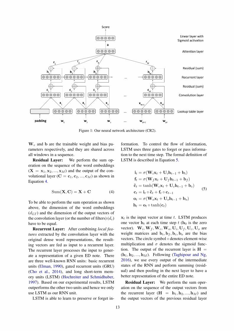
Figure 1: Our neural network architecture (CR2).
Wv and b are the trainable weight and bias pa-rameters respectively, and they are shared acrossall windows in a sequence.
Residual Layer: We perform the sum op-eration on the sequence of the word embeddings(X = x1,x2, ...,xM ) and the output of the con-volutional layer (C = c1, c2, ..., cM ) as shown inEquation 4.
Sum(X,C) = X + C (4)
To be able to perform the sum operation as shownabove, the dimension of the word embeddings(dLT ) and the dimension of the output vectors ofthe convolution layer (or the number of filters) (dc)have to be equal.
Recurrent Layer: After combining local fea-tures extracted by the convolution layer with theoriginal dense word representations, the result-ing vectors are fed as input to a recurrent layer.The recurrent layer processes the input to gener-ate a representation of a given ED note. Thereare three well-known RNN units: basic recurrentunits (Elman, 1990), gated recurrent units (GRU)(Cho et al., 2014), and long short-term mem-ory units (LSTM) (Hochreiter and Schmidhuber,1997). Based on our experimental results, LSTMoutperforms the other two units and hence we onlyuse LSTM as our RNN unit.
LSTM is able to learn to preserve or forget in-
formation. To control the flow of information,LSTM uses three gates to forget or pass informa-tion to the next time step. The formal definition ofLSTM is described in Equation 5.
it = σ(Wixt + Uiht−1 + bi)
ft = σ(Wfxt + Ufht−1 + bf )
c̃t = tanh(Wcxt + Ucht−1 + bc)
ct = it ◦ c̃t + ft ◦ ct−1ot = σ(Woxt + Uoht−1 + bo)
ht = ot ◦ tanh(ct)
(5)
xt is the input vector at time t. LSTM producesone vector ht at each time step t (h0 is the zerovector). Wi,Wf ,Wc,Wo,Ui,Uf ,Uc,Uo areweight matrices and bi,bf ,bc,bo are the biasvectors. The circle symbol ◦ denotes element-wisemultiplication and σ denotes the sigmoid func-tion. The output of the recurrent layer is H =(h1,h2, ...,hM ). Following (Taghipour and Ng,2016), we use every output of the intermediatestates of the RNN and perform summing (resid-ual) and then pooling in the next layer to have abetter representation of the entire ED note.
Residual Layer: We perform the sum oper-ation on the sequence of the output vectors fromthe recurrent layer (H = h1,h2, ...,hM ) andthe output vectors of the previous residual layer
13
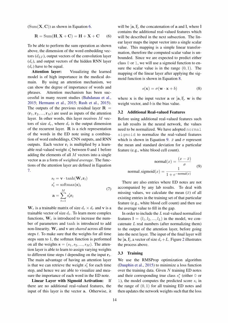
(Sum(X,C)) as shown in Equation 6.
R = Sum(H,X + C) = H + X + C (6)
To be able to perform the sum operation as shownabove, the dimension of the word embedding vec-tors (dLT ), output vectors of the convolution layer(dc), and output vectors of the hidden RNN layer(dr) have to be equal.
Attention layer: Visualizing the learnedmodel is of high importance in the medical do-main. By using an attention mechanism, wecan show the degree of importance of words andphrases. Attention mechanism has been suc-cessful in many recent studies (Bahdanau et al.,2015; Hermann et al., 2015; Rush et al., 2015).The outputs of the previous residual layer R =(r1, r2, ..., rM ) are used as inputs of the attentionlayer. In other words, this layer receives M vec-tors of size dr, where dr is the output dimensionof the recurrent layer. R is a rich representationof the words in the ED note using a combina-tion of word embeddings, CNN outputs, and RNNoutputs. Each vector rt is multiplied by a learn-able real-valued weight s′t between 0 and 1 beforeadding the elements of all M vectors into a singlevector a as a form of weighted average. The func-tions of the attention layer are defined in Equation7.
st = v · tanh(Wrrt)
s′t = softmax(s)t
a =M∑
t=1
s′trt
(7)
Wr is a trainable matrix of size dr × dr and v is atrainable vector of size dr. To learn more complexfunctions, Wr is introduced to increase the num-ber of parameters and tanh is introduced to addnon-linearity. Wr and v are shared across all timesteps t. To make sure that the weights for all timesteps sum to 1, the softmax function is performedon all the weights s = (s1, s2, ..., sM ). The atten-tion layer is able to learn to assign varying weightsto different time steps t depending on the input rt.The main advantage of having an attention layeris that we can retrieve the weight s′t for each timestep, and hence we are able to visualize and mea-sure the importance of each word in the ED note.
Linear Layer with Sigmoid Activation: Ifthere are no additional real-valued features, theinput of this layer is the vector a. Otherwise, it
will be [a, l], the concatenation of a and l, where lcontains the additional real-valued features whichwill be described in the next subsection. The lin-ear layer maps the input vector into a single scalarvalue. This mapping is a simple linear transfor-mation, therefore the computed scalar value is un-bounded. Since we are expected to predict eitherclass 0 or 1, we will use a sigmoid function to en-sure the scalar value is in the range (0, 1). Themapping of the linear layer after applying the sig-moid function is shown in Equation 8.
s(x) = σ(w · x + b) (8)
where x is the input vector a or [a, l], w is theweight vector, and b is the bias value.
3.2 Additional Real-valued FeaturesBefore using additional real-valued features suchas lab results in the neural network, the valuesneed to be normalized. We have adopted normalsigmoid to normalize the real-valued featureswhich is shown in Equation 9. x̄ and σ representthe mean and standard deviation for a particularfeature (e.g., white blood cell count).
normal(x) =(x− x̄)
σ
normal sigmoid(x) =1
1 + e−normal(x)
(9)
There are also entries where ED notes are notaccompanied by any lab results. To deal withmissing values, we calculate the mean (x̄) of allexisting entries in the training set of that particularfeature (e.g., white blood cell count) and then usethe average value to fill in the gap.
In order to include the L real-valued normalizedfeatures l = (l1, l2, ..., lL) in the model, we con-catenate L real numbers (after normalizing them)to the output of the attention layer, before goinginto the next layer. The input of the final layer willbe [a, l], a vector of size dr+L. Figure 2 illustratesthe process above.
3.3 TrainingWe use the RMSProp optimization algorithm(Dauphin et al., 2015) to minimize a loss functionover the training data. Given N training ED notesand their corresponding true class s∗i (either 0 or1), the model computes the predicted score si inthe range of (0, 1) for all training ED notes andthen updates the network weights such that the loss
14
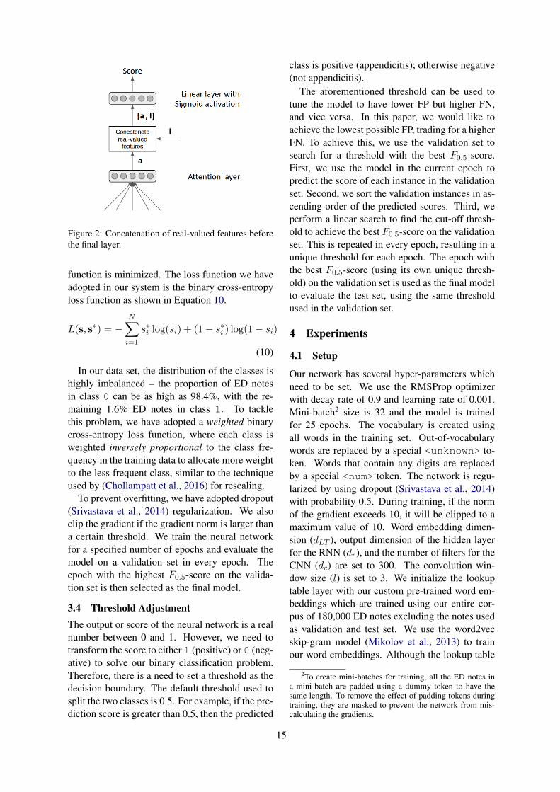
Figure 2: Concatenation of real-valued features beforethe final layer.
function is minimized. The loss function we haveadopted in our system is the binary cross-entropyloss function as shown in Equation 10.
L(s, s∗) = −N∑
i=1
s∗i log(si) + (1− s∗i ) log(1− si)
(10)
In our data set, the distribution of the classes ishighly imbalanced – the proportion of ED notesin class 0 can be as high as 98.4%, with the re-maining 1.6% ED notes in class 1. To tacklethis problem, we have adopted a weighted binarycross-entropy loss function, where each class isweighted inversely proportional to the class fre-quency in the training data to allocate more weightto the less frequent class, similar to the techniqueused by (Chollampatt et al., 2016) for rescaling.
To prevent overfitting, we have adopted dropout(Srivastava et al., 2014) regularization. We alsoclip the gradient if the gradient norm is larger thana certain threshold. We train the neural networkfor a specified number of epochs and evaluate themodel on a validation set in every epoch. Theepoch with the highest F0.5-score on the valida-tion set is then selected as the final model.
3.4 Threshold AdjustmentThe output or score of the neural network is a realnumber between 0 and 1. However, we need totransform the score to either 1 (positive) or 0 (neg-ative) to solve our binary classification problem.Therefore, there is a need to set a threshold as thedecision boundary. The default threshold used tosplit the two classes is 0.5. For example, if the pre-diction score is greater than 0.5, then the predicted
class is positive (appendicitis); otherwise negative(not appendicitis).
The aforementioned threshold can be used totune the model to have lower FP but higher FN,and vice versa. In this paper, we would like toachieve the lowest possible FP, trading for a higherFN. To achieve this, we use the validation set tosearch for a threshold with the best F0.5-score.First, we use the model in the current epoch topredict the score of each instance in the validationset. Second, we sort the validation instances in as-cending order of the predicted scores. Third, weperform a linear search to find the cut-off thresh-old to achieve the best F0.5-score on the validationset. This is repeated in every epoch, resulting in aunique threshold for each epoch. The epoch withthe best F0.5-score (using its own unique thresh-old) on the validation set is used as the final modelto evaluate the test set, using the same thresholdused in the validation set.
4 Experiments
4.1 Setup
Our network has several hyper-parameters whichneed to be set. We use the RMSProp optimizerwith decay rate of 0.9 and learning rate of 0.001.Mini-batch2 size is 32 and the model is trainedfor 25 epochs. The vocabulary is created usingall words in the training set. Out-of-vocabularywords are replaced by a special <unknown> to-ken. Words that contain any digits are replacedby a special <num> token. The network is regu-larized by using dropout (Srivastava et al., 2014)with probability 0.5. During training, if the normof the gradient exceeds 10, it will be clipped to amaximum value of 10. Word embedding dimen-sion (dLT ), output dimension of the hidden layerfor the RNN (dr), and the number of filters for theCNN (dc) are set to 300. The convolution win-dow size (l) is set to 3. We initialize the lookuptable layer with our custom pre-trained word em-beddings which are trained using our entire cor-pus of 180,000 ED notes excluding the notes usedas validation and test set. We use the word2vecskip-gram model (Mikolov et al., 2013) to trainour word embeddings. Although the lookup table
2To create mini-batches for training, all the ED notes ina mini-batch are padded using a dummy token to have thesame length. To remove the effect of padding tokens duringtraining, they are masked to prevent the network from mis-calculating the gradients.
15
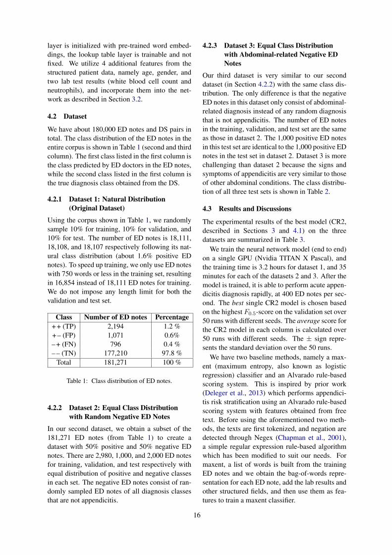
layer is initialized with pre-trained word embed-dings, the lookup table layer is trainable and notfixed. We utilize 4 additional features from thestructured patient data, namely age, gender, andtwo lab test results (white blood cell count andneutrophils), and incorporate them into the net-work as described in Section 3.2.
4.2 Dataset
We have about 180,000 ED notes and DS pairs intotal. The class distribution of the ED notes in theentire corpus is shown in Table 1 (second and thirdcolumn). The first class listed in the first column isthe class predicted by ED doctors in the ED notes,while the second class listed in the first column isthe true diagnosis class obtained from the DS.
4.2.1 Dataset 1: Natural Distribution(Original Dataset)
Using the corpus shown in Table 1, we randomlysample 10% for training, 10% for validation, and10% for test. The number of ED notes is 18,111,18,108, and 18,107 respectively following its nat-ural class distribution (about 1.6% positive EDnotes). To speed up training, we only use ED noteswith 750 words or less in the training set, resultingin 16,854 instead of 18,111 ED notes for training.We do not impose any length limit for both thevalidation and test set.
Class Number of ED notes Percentage+ + (TP) 2,194 1.2 %+ – (FP) 1,071 0.6%– + (FN) 796 0.4 %– – (TN) 177,210 97.8 %
Total 181,271 100 %
Table 1: Class distribution of ED notes.
4.2.2 Dataset 2: Equal Class Distributionwith Random Negative ED Notes
In our second dataset, we obtain a subset of the181,271 ED notes (from Table 1) to create adataset with 50% positive and 50% negative EDnotes. There are 2,980, 1,000, and 2,000 ED notesfor training, validation, and test respectively withequal distribution of positive and negative classesin each set. The negative ED notes consist of ran-domly sampled ED notes of all diagnosis classesthat are not appendicitis.
4.2.3 Dataset 3: Equal Class Distributionwith Abdominal-related Negative EDNotes
Our third dataset is very similar to our seconddataset (in Section 4.2.2) with the same class dis-tribution. The only difference is that the negativeED notes in this dataset only consist of abdominal-related diagnosis instead of any random diagnosisthat is not appendicitis. The number of ED notesin the training, validation, and test set are the sameas those in dataset 2. The 1,000 positive ED notesin this test set are identical to the 1,000 positive EDnotes in the test set in dataset 2. Dataset 3 is morechallenging than dataset 2 because the signs andsymptoms of appendicitis are very similar to thoseof other abdominal conditions. The class distribu-tion of all three test sets is shown in Table 2.
4.3 Results and Discussions
The experimental results of the best model (CR2,described in Sections 3 and 4.1) on the threedatasets are summarized in Table 3.
We train the neural network model (end to end)on a single GPU (Nvidia TITAN X Pascal), andthe training time is 3.2 hours for dataset 1, and 35minutes for each of the datasets 2 and 3. After themodel is trained, it is able to perform acute appen-dicitis diagnosis rapidly, at 400 ED notes per sec-ond. The best single CR2 model is chosen basedon the highest F0.5-score on the validation set over50 runs with different seeds. The average score forthe CR2 model in each column is calculated over50 runs with different seeds. The ± sign repre-sents the standard deviation over the 50 runs.
We have two baseline methods, namely a max-ent (maximum entropy, also known as logisticregression) classifier and an Alvarado rule-basedscoring system. This is inspired by prior work(Deleger et al., 2013) which performs appendici-tis risk stratification using an Alvarado rule-basedscoring system with features obtained from freetext. Before using the aforementioned two meth-ods, the texts are first tokenized, and negation aredetected through Negex (Chapman et al., 2001),a simple regular expression rule-based algorithmwhich has been modified to suit our needs. Formaxent, a list of words is built from the trainingED notes and we obtain the bag-of-words repre-sentation for each ED note, add the lab results andother structured fields, and then use them as fea-tures to train a maxent classifier.
16
Class Dataset 1 Dataset 2 Dataset 3# ED notes % # ED notes % # ED notes %
+ + (TP) 216 1.2 % 734 36.7 % 734 36.7 %+ – (FP) 104 0.6 % 6 0.3 % 36 1.8 %– + (FN) 78 0.4 % 266 13.3 % 266 13.3 %– – (TN) 17,709 97.8 % 994 49.7 % 964 48.2 %
Total 18,107 100 % 2,000 100 % 2,000 100 %
Table 2: Class distribution of ED notes in test sets.
model TP FP FN TN Rec Prec Spec F1 F0.5 AccDataset 1
ED 216 104 78 17,709 0.735 0.675 0.994 0.704 0.686 0.990ME 138 126 156 17,687 0.469 0.523 0.993 0.495 0.511 0.984Alv 124 90 170 17,723 0.422 0.579 0.995 0.488 0.539 0.986Best 141 90 153 17,723 0.480 0.610 0.995 0.537 0.579* 0.987Avg 154.8 109.2 139.2 17,703.8 0.527 0.588 0.994 0.553 0.573 0.986
±16.9 ±18.8 ±16.9 ±18.8 ±0.058 ±0.021 ±0.0011 ±0.030 ±0.016 ±0.00046Dataset 2
ED 734 6 266 994 0.734 0.992 0.994 0.844 0.927 0.864ME 952 62 48 938 0.952 0.939 0.938 0.945 0.941 0.945Alv 617 12 383 988 0.617 0.981 0.988 0.758 0.877 0.803Best 912 27 88 973 0.912 0.971 0.973 0.941 0.959* 0.943Avg 912.1 28.6 87.9 971.4 0.912 0.970 0.971 0.940 0.958 0.942
±17.1 ±6.1 ±17.1 ±6.1 ±0.017 ±0.0058 ±0.0061 ±0.0076 ±0.0037 ±0.0069Dataset 3
ED 734 36 266 964 0.734 0.953 0.964 0.829 0.900 0.849ME 880 125 120 875 0.880 0.876 0.875 0.878 0.876 0.878Alv 617 72 383 928 0.617 0.896 0.928 0.731 0.821 0.773Best 831 79 169 921 0.831 0.913 0.921 0.870 0.895* 0.876Avg 832.1 84.2 167.9 915.8 0.832 0.908 0.916 0.868 0.892 0.874
±28.8 ±12.2 ±28.8 ±12.2 ±0.029 ±0.0096 ±0.0122 ±0.0125 ±0.0045 ±0.0095
Table 3: Summary of the best model against ED doctors and the baselines on three datasets. The baseline for thestatistical significance tests is underlined and statistically significant improvements (p < 0.05) are marked with’*’. ME stands for Maxent, Alv stands for Alvarado, Best stands for Best CR2, and Avg stands for Avg CR2.
In acute appendicitis diagnosis, there is an ex-isting well-known scoring system, namely Al-varado score (Alvarado, 1986). It is also known asMANTRELS score, which is a mnemonic to re-member the score factors (signs, symptoms, andlab readings) – Migration of pain to the rightlower quadrant, Anorexia, Nausea or vomiting,Tenderness in the right lower quadrant, Reboundpain, Elevated temperature (fever), Leukocytosis(high white blood cell count), and Shift of neu-trophils to the left. The score for each factor is1(M), 1(A), 1(N), 2(T), 1(R), 1(E), 2(L), and 1(S)respectively. The score for each factor present ina patient will be added together to obtain the fi-nal score. A higher score indicates that a patientis more likely to have appendicitis. The aforemen-tioned 8 factors are detected through a regular ex-pression (with negation) on the ED notes that havebeen preprocessed with Negex. Different thresh-old values (scores strictly greater than the thresh-old will be classified as positive, and negative oth-erwise) are explored and the threshold with the
best F0.5-score is chosen. The thresholds for Al-varado scoring in datasets 1, 2, and 3 are 6, 5, and5 respectively.
Our neural network model (CR2) outperformsthe two baselines in F0.5-score on all threedatasets. We also perform a statistical signifi-cance test (p < 0.05) to determine whether theobtained improvement is statistically significant.We found that our neural network improvementsagainst maxent on all datasets are statistically sig-nificant. This shows that our neural networkmodel is superior to the maxent classifier and Al-varado scoring system.
Based on the first row in Table 3, we can see thatED doctors’ performance is better compared to ourmodel. This is mainly caused by class imbalance(1.6% positive and 98.4% negative). Learningand predicting on a dataset with extremely skewedclass distribution is challenging. However, as wecan see from the results, the performance of ourbest model is close to that of ED doctors, with 14fewer FP instances and 75 more FN instances out
17
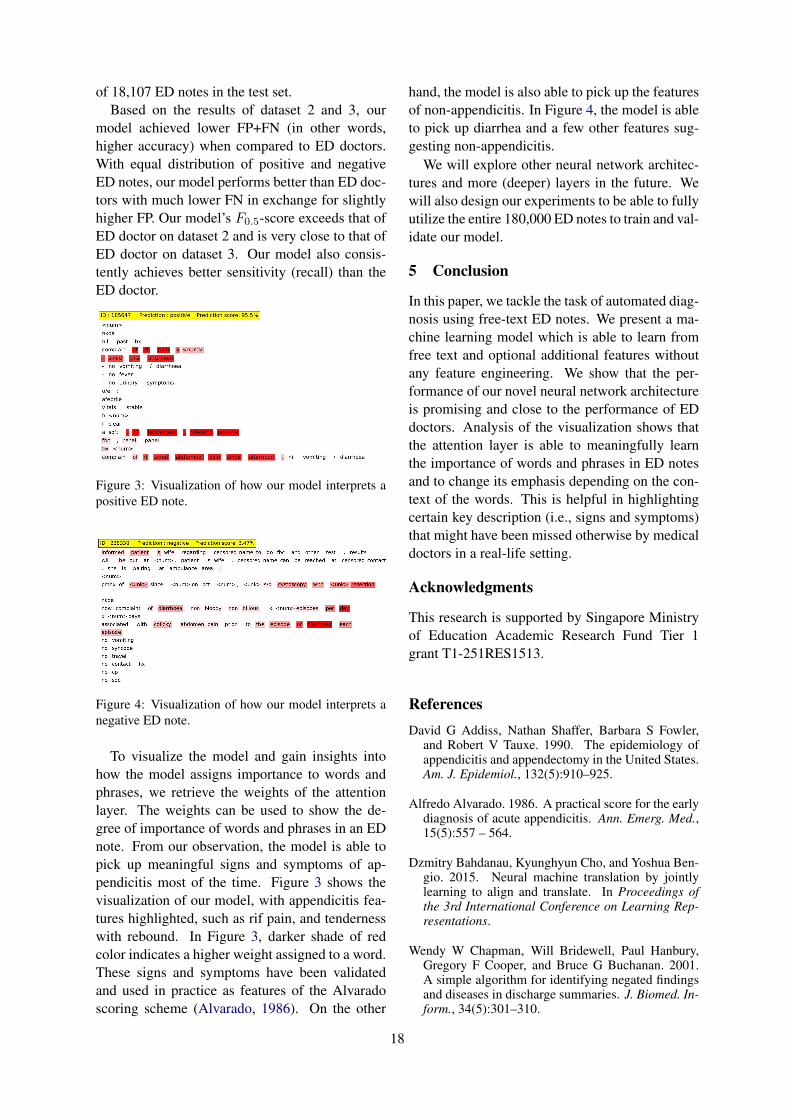
of 18,107 ED notes in the test set.Based on the results of dataset 2 and 3, our
model achieved lower FP+FN (in other words,higher accuracy) when compared to ED doctors.With equal distribution of positive and negativeED notes, our model performs better than ED doc-tors with much lower FN in exchange for slightlyhigher FP. Our model’s F0.5-score exceeds that ofED doctor on dataset 2 and is very close to that ofED doctor on dataset 3. Our model also consis-tently achieves better sensitivity (recall) than theED doctor.
Figure 3: Visualization of how our model interprets apositive ED note.
Figure 4: Visualization of how our model interprets anegative ED note.
To visualize the model and gain insights intohow the model assigns importance to words andphrases, we retrieve the weights of the attentionlayer. The weights can be used to show the de-gree of importance of words and phrases in an EDnote. From our observation, the model is able topick up meaningful signs and symptoms of ap-pendicitis most of the time. Figure 3 shows thevisualization of our model, with appendicitis fea-tures highlighted, such as rif pain, and tendernesswith rebound. In Figure 3, darker shade of redcolor indicates a higher weight assigned to a word.These signs and symptoms have been validatedand used in practice as features of the Alvaradoscoring scheme (Alvarado, 1986). On the other
hand, the model is also able to pick up the featuresof non-appendicitis. In Figure 4, the model is ableto pick up diarrhea and a few other features sug-gesting non-appendicitis.
We will explore other neural network architec-tures and more (deeper) layers in the future. Wewill also design our experiments to be able to fullyutilize the entire 180,000 ED notes to train and val-idate our model.
5 Conclusion
In this paper, we tackle the task of automated diag-nosis using free-text ED notes. We present a ma-chine learning model which is able to learn fromfree text and optional additional features withoutany feature engineering. We show that the per-formance of our novel neural network architectureis promising and close to the performance of EDdoctors. Analysis of the visualization shows thatthe attention layer is able to meaningfully learnthe importance of words and phrases in ED notesand to change its emphasis depending on the con-text of the words. This is helpful in highlightingcertain key description (i.e., signs and symptoms)that might have been missed otherwise by medicaldoctors in a real-life setting.
Acknowledgments
This research is supported by Singapore Ministryof Education Academic Research Fund Tier 1grant T1-251RES1513.
ReferencesDavid G Addiss, Nathan Shaffer, Barbara S Fowler,
and Robert V Tauxe. 1990. The epidemiology ofappendicitis and appendectomy in the United States.Am. J. Epidemiol., 132(5):910–925.
Alfredo Alvarado. 1986. A practical score for the earlydiagnosis of acute appendicitis. Ann. Emerg. Med.,15(5):557 – 564.
Dzmitry Bahdanau, Kyunghyun Cho, and Yoshua Ben-gio. 2015. Neural machine translation by jointlylearning to align and translate. In Proceedings ofthe 3rd International Conference on Learning Rep-resentations.
Wendy W Chapman, Will Bridewell, Paul Hanbury,Gregory F Cooper, and Bruce G Buchanan. 2001.A simple algorithm for identifying negated findingsand diseases in discharge summaries. J. Biomed. In-form., 34(5):301–310.
18
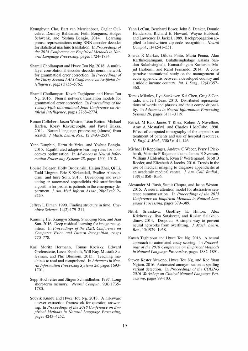
Kyunghyun Cho, Bart van Merrienboer, Caglar Gul-cehre, Dzmitry Bahdanau, Fethi Bougares, HolgerSchwenk, and Yoshua Bengio. 2014. Learningphrase representations using RNN encoder-decoderfor statistical machine translation. In Proceedings ofthe 2014 Conference on Empirical Methods in Nat-ural Language Processing, pages 1724–1734.
Shamil Chollampatt and Hwee Tou Ng. 2018. A multi-layer convolutional encoder-decoder neural networkfor grammatical error correction. In Proceedings ofthe Thirty-Second AAAI Conference on Artificial In-telligence, pages 5755–5762.
Shamil Chollampatt, Kaveh Taghipour, and Hwee TouNg. 2016. Neural network translation models forgrammatical error correction. In Proceedings of theTwenty-Fifth International Joint Conference on Ar-tificial Intelligence, pages 2768–2774.
Ronan Collobert, Jason Weston, Léon Bottou, MichaelKarlen, Koray Kavukcuoglu, and Pavel Kuksa.2011. Natural language processing (almost) fromscratch. J. Mach. Learn. Res., 12:2493–2537.
Yann Dauphin, Harm de Vries, and Yoshua Bengio.2015. Equilibrated adaptive learning rates for non-convex optimization. In Advances in Neural Infor-mation Processing Systems 28, pages 1504–1512.
Louise Deleger, Holly Brodzinski, Haijun Zhai, Qi Li,Todd Lingren, Eric S Kirkendall, Evaline Alessan-drini, and Imre Solti. 2013. Developing and eval-uating an automated appendicitis risk stratificationalgorithm for pediatric patients in the emergency de-partment. J. Am. Med. Inform. Assoc., 20(e2):e212–e220.
Jeffrey L Elman. 1990. Finding structure in time. Cog-nitive Science, 14(2):179–211.
Kaiming He, Xiangyu Zhang, Shaoqing Ren, and JianSun. 2016. Deep residual learning for image recog-nition. In Proceedings of the IEEE Conference onComputer Vision and Pattern Recognition, pages770–778.
Karl Moritz Hermann, Tomas Kocisky, EdwardGrefenstette, Lasse Espeholt, Will Kay, Mustafa Su-leyman, and Phil Blunsom. 2015. Teaching ma-chines to read and comprehend. In Advances in Neu-ral Information Processing Systems 28, pages 1693–1701.
Sepp Hochreiter and Jürgen Schmidhuber. 1997. Longshort-term memory. Neural Comput., 9(8):1735–1780.
Souvik Kundu and Hwee Tou Ng. 2018. A nil-awareanswer extraction framework for question answer-ing. In Proceedings of the 2018 Conference on Em-pirical Methods in Natural Language Processing,pages 4243–4252.
Yann LeCun, Bernhard Boser, John S. Denker, DonnieHenderson, Richard E. Howard, Wayne Hubbard,and Lawrence D. Jackel. 1989. Backpropagation ap-plied to handwritten zip code recognition. NeuralComput., 1(4):541–551.
Sheraz R Markar, Diluka Pinto, Marta Penna, AlanKarthikesalingam, Bulathsinghalage Kalana San-dun Bulathsinghala, Kumaralingam Kumaran, Ma-jid Hashemi, and Ranil Fernando. 2014. A com-parative international study on the management ofacute appendicitis between a developed country anda middle income country. Int. J. Surg., 12(4):357–360.
Tomas Mikolov, Ilya Sutskever, Kai Chen, Greg S Cor-rado, and Jeff Dean. 2013. Distributed representa-tions of words and phrases and their compositional-ity. In Advances in Neural Information ProcessingSystems 26, pages 3111–3119.
Patrick M Rao, James T Rhea, Robert A Novelline,Amy A Mostafavi, and Charles J McCabe. 1998.Effect of computed tomography of the appendix ontreatment of patients and use of hospital resources.N. Engl. J. Med., 338(3):141–146.
Michael D Repplinger, Andrew C Weber, Perry J Pick-hardt, Victoria P Rajamanickam, James E Svenson,William J Ehlenbach, Ryan P Westergaard, Scott BReeder, and Elizabeth A Jacobs. 2016. Trends in theuse of medical imaging to diagnose appendicitis atan academic medical center. J. Am. Coll. Radiol.,13(9):1050–1056.
Alexander M. Rush, Sumit Chopra, and Jason Weston.2015. A neural attention model for abstractive sen-tence summarization. In Proceedings of the 2015Conference on Empirical Methods in Natural Lan-guage Processing, pages 379–389.
Nitish Srivastava, Geoffrey E. Hinton, AlexKrizhevsky, Ilya Sutskever, and Ruslan Salakhut-dinov. 2014. Dropout: A simple way to preventneural networks from overfitting. J. Mach. Learn.Res., 15:1929–1958.
Kaveh Taghipour and Hwee Tou Ng. 2016. A neuralapproach to automated essay scoring. In Proceed-ings of the 2016 Conference on Empirical Methodsin Natural Language Processing, pages 1882–1891.
Steven Kester Yuwono, Hwee Tou Ng, and Kee YuanNgiam. 2016. Automated anonymization as spellingvariant detection. In Proceedings of the COLING2016 Workshop on Clinical Natural Language Pro-cessing, pages 99–103.
19
Proceedings of the BioNLP 2019 workshop, pages 20–29Florence, Italy, August 1, 2019. c©2019 Association for Computational Linguistics
A Paraphrase Generation System for EHR Question Answering
Sarvesh Soni, Kirk RobertsSchool of Biomedical Informatics
University of Texas Health Science Center at HoustonHouston TX, USA
{sarvesh.soni, kirk.roberts}@uth.tmc.edu
AbstractThis paper proposes a dataset and method forautomatically generating paraphrases for clin-ical questions relating to patient-specific in-formation in electronic health records (EHRs).Crowdsourcing is used to collect 10,578unique questions across 946 semantically dis-tinct paraphrase clusters. This corpus is thenused with a deep learning-based question para-phrasing method utilizing variational autoen-coder and LSTM encoder/decoder. The ulti-mate use of such a method is to improve theperformance of automatic question answeringmethods for EHRs.
1 Introduction
The useful information present in electronic healthrecords (EHRs) is hard to access due to many of itsusability issues (Zhang and Walji, 2014). Questionanswering (QA) systems have the potential to re-duce the time it takes for users to access informa-tion present in the EHRs. However, the effective-ness of such QA systems largely depends on thevariety of questions they are capable of handling.Automated paraphrasing techniques are known toimprove the performance of QA models in gen-eral domain by generating different variations ofa question (Duboue and Chu-Carroll, 2006; Faderet al., 2013; Berant and Liang, 2014; Bordes et al.,2014a,b; Dong et al., 2015; Narayan et al., 2016;Chen et al., 2016; Dong et al., 2017; Abujabalet al., 2018b). Thus, automatic generation of highquality paraphrases for patient-specific EHR ques-tions has the potential to improve performance ofthe clinical QA systems.
Paraphrasing is a technique of rewording agiven phrase such that its lexical and syntacticstructure is different but its semantic informationis retained (Bhagat and Hovy, 2013). For instance,the following two questions can be considered asparaphrases of each other.
• What medications am I currently taking?
• What are my current medications?
Such EHR-related questions are usuallytargeted toward specific clinical information(Roberts and Demner-Fushman, 2016). For ex-ample, the aforementioned questions are intendedto get information regarding medications. Insuch a scenario, paraphrases can be considered asdifferent ways of accessing the same medical data.As such, automatic clinical paraphrase generationcan help in increasing the breadth of questions fortraining a clinical QA system.
While automated paraphrase generation is well-studied in the general domain (Madnani and Dorr,2010; Androutsopoulos and Malakasiotis, 2010),very few studies have focused on clinical para-phrasing (Hasan et al., 2016; Adduru et al., 2018;Neuraz et al., 2018). On the other hand, clin-ical text simplification, which aims at generat-ing easier to read paraphrases, has received rela-tively more attention (Zeng-Treitler et al., 2007;Elhadad and Sutaria, 2007; Deléger and Zweigen-baum, 2008; Kandula et al., 2010; Pivovarov andElhadad, 2015; Qenam et al., 2017; Adduru et al.,2018; Bercken et al., 2019). However, theseworks in the clinical domain are not representa-tive of QA needs as the usefulness of paraphrasesis largely application-specific (Bhagat and Hovy,2013). Also, existing datasets for clinical para-phrasing consist of either short phrases (Hasanet al., 2016) or webpage title texts (Adduru et al.,2018), both of which are not suitable to builda paraphrase generator for QA. One can resortto using external tools such as Google Translatefor generating question paraphrases (Neuraz et al.,2018), but these general-purpose tools are not tai-lored to the medical domain (Liu and Cai, 2015).
In this paper, we propose a clinical paraphras-ing corpus CLINIQPARA with questions which
20
can be answered using EHR data1. We furtherpropose a deep learning-based automated clinicalparaphrasing system utilizing a variational autoen-coder (VAE) and a long short-term memory recur-rent neural network (LSTM) (Gupta et al., 2018).To our knowledge, this is the first work aimed atautomatically generating paraphrases without us-ing any external resource for questions specificallyfocused on retrieving patient-specific informationfrom EHRs. Our main contributions are summa-rized as follows:
• Crowdsourcing a large paraphrasing corpusof questions which are answerable using thedata from EHR.
• Application of VAE in context to clinicalparaphrasing task.
The rest of the paper is structured as follows.Section 2 explores related work in the domain ofclinical paraphrasing. Then, Sections 3 and 4 dis-cuss our dataset generation and model implemen-tation details respectively. Next, Section 5 eval-uates the results of our clinical paraphrasing sys-tem. Finally, Section 6 discusses our findings, andSection 7 provides a concluding summary.
2 Background
We begin this section by detailing work relatedto clinical text simplification and paraphrasing inSections 2.1 and 2.2 respectively. Then, we high-light some of the current work in general-domainparaphrasing for QA as part of Section 2.3.
2.1 Clinical Text SimplificationAs stated earlier, many studies have focused onclinical text simplification. Text simplification dif-fers from paraphrasing as the former is a uni-directional task whereas the latter can be consid-ered as bi-directional textual entailment (Androut-sopoulos and Malakasiotis, 2010), but the meth-ods nonetheless provide useful context for ourwork. Elhadad and Sutaria (2007) and Deléger andZweigenbaum (2008) relied on parallel or com-parable corpora to construct paraphrase pairs ofspecialized and lay medical texts. Zeng-Treitleret al. (2007) and Kandula et al. (2010) either re-placed the difficult clinical phrases in text withsimpler synonyms or included uncomplicated ex-planations for them. Qenam et al. (2017) concen-trated on just substituting the difficult terms with
1The corpus is available upon request.
more comprehensible ones. Much of the simplifi-cation work in the clinical domain has been tar-geted toward lexical methods to convert or ap-pend the complex phrases present in the origi-nal sentence with their simpler alternatives (Pivo-varov and Elhadad, 2015). Such simplification ap-proaches usually make use of external vocabular-ies to map the difficult clinical terms. While thesetechniques reduce the complexity of a sentence atthe lexical level, they generally leave the syntacticstructure of a sentence unchanged. For instance,
• Patient suffered from myocardial infarction.
• Patient suffered from heart attack.
These variations correspond to a specific cate-gory of paraphrases named synonym substitution(Bhagat and Hovy, 2013) and amount to a smallersubset of possible paraphrases.
Alternatively, Adduru et al. (2018) and Berckenet al. (2019) constructed clinical simplificationdatasets from various web-based sources suchas WebMD, MedicineNet, Wikipedia, and Sim-pleWikipedia utilizing sentence alignment tech-niques. While this approach is capable of gener-ating more variations of a given sentence, it is stilla simplification task and hence not suitable to beincorporated in a QA system (Bhagat and Hovy,2013).
2.2 Clinical Text ParaphrasingComparatively, less focus has been drawn to-ward clinical paraphrase generation. Hasan et al.(2016) built their dataset by combining an exist-ing general domain paraphrasing corpus PPDB2.0 (Pavlick et al., 2015) with the UMLS (Uni-fied Medical Language System) metathesaurus.Specifically, they utilized fully specified names ofmedical concepts present in UMLS. Though theircorpus contains medical terms, it comprises ofcomparatively shorter length phrases rather thancomplete sentences.
Adduru et al. (2018) also created a paraphras-ing corpus utilizing the titles of web articles fromMayo Clinic along with Wikipedia. While thisdataset consists of complete clinical sentences,they are atypical of the patient-specific EHR ques-tions.
Neuraz et al. (2018) used the Google Trans-late API to generate paraphrases for question tem-plates in French. They utilized these generatedtemplate paraphrases to augment the size of their
21
Scenario 18: You’ve been having some low back pain recently, and want to make an appointmentwith your doctor’s office through the doctor’s website, but the system isn’t clear. Write a short (upto 15 word), grammatical, one-sentence question asking how you make an appointment. No need tostate it is confusing, simply ask a question.Question: How do I make an appointment?Scenario 41: Your elderly mother has been taking Metformin (a diabetes drug). She is forgetful andrequires someone to organize her pills for each day. However, the person that normally organizes herpills hasn’t done it for this week, and you need to know what the instructions are for your mother’sMetformin prescription. Write a short (up to 15 word), grammatical, one-sentence question askingher doctor for this dosage information. You question must contain the word ’Metformin’.Question: What are my mother’s Metformin dosage instructions?Scenario 43: You recently had an automobile accident, and you’ve started taking physical therapyto help recover. Your first appointment went well, but you forgot to write down when your nextappointment was scheduled for. Write a short (up to 15 word), grammatical, one-sentence questionasking your doctor for this information. Your question must contain ’physical therapy’.Question: When is my next physical therapy appointment?
Table 1: Three scenarios used to build the CLINIQPARA corpus, along with a canonical question (not provided toannotators).
development dataset for natural language under-standing task without evaluating the quality ofthe paraphrases. Such general-purpose machinetranslation systems lack the ability to capture thedomain-specific nuances of biomedicine (Liu andCai, 2015). This suggests the need for a questionparaphrasing dataset targeted toward clinical do-main.
As discussed earlier, existing clinical paraphras-ing datasets are not suitable for building a para-phrase generation system for clinical questions.To the best of our knowledge, the proposed para-phrasing corpus is the first which aims at clinicalquestions.
2.3 Paraphrasing for Question Answering
There are several question paraphrasing corporaavailable for the general domain such as WikiAn-swers (Fader et al., 2013), PPDB (Ganitkevitchet al., 2013), PPDB 2.0 (Pavlick et al., 2015),GraphQuestions (Su et al., 2016), and ComQA(Abujabal et al., 2018a). However, there is ascarcity of such datasets for clinical questions.
The proposed corpus consists of questionswhich can be answered using EHR data. Such acorpus would have utility beyond QA systems aswell, like in question similarity (Luo et al., 2015;Nakov et al., 2017), and in particular could serveas a standard paraphrase corpus for the medicaldomain.
3 Dataset Construction
In order to quickly and efficiently collect hundredsof paraphrases, we utilized the crowdsourcingplatform Amazon Mechanical Turk (AMT). In-stead of prompting AMT workers with a questionand directly asking for paraphrases–which couldprime the workers and bias them toward very sim-ilar paraphrases–we presented them with a short,3-6 sentence imaginary scenario that placed themin a situation where a specific piece of informationwas required (such as their current medications).The workers were then asked to provide questionsdirected to their doctor to answer that informationneed. After the crowd-sourced questions were col-lected, they were manually organized into distinctparaphrase clusters. This was necessary becausesome questions address the information need butare not logically equivalent paraphrases. Thesesteps are discussed in more detail below.
3.1 Scenario Creation
To ensure a wide variety of EHR questions, wefirst came up with 11 top-level topic categoriespeople might ask about: medications, other treat-ments, labs, immunizations, imaging, other ex-ams, problem list, past medical history, familyhistory, appointments, and documents. For eachof these categories, 2-8 scenarios were created tocapture relevant questions about the topic. In total,50 scenarios were created. Table 1 shows three ofthese scenarios along with the canonical questionexpected by the scenario.
22
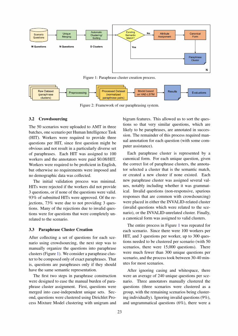
Figure 1: Paraphrase cluster creation process.
Figure 2: Framework of our paraphrasing system.
3.2 Crowdsourcing
The 50 scenarios were uploaded to AMT in threebatches, one scenario per Human Intelligence Task(HIT). Workers were required to provide threequestions per HIT, since first question might beobvious and not result in a particularly diverse setof paraphrases. Each HIT was assigned to 100workers and the annotators were paid $0.08/HIT.Workers were required to be proficient in English,but otherwise no requirements were imposed andno demographic data was collected.
The initial validation process was minimal.HITs were rejected if the workers did not provide3 questions, or if none of the questions were valid.93% of submitted HITs were approved. Of the re-jections, 73% were due to not providing 3 ques-tions. Many of the rejections due to invalid ques-tions were for questions that were completely un-related to the scenario.
3.3 Paraphrase Cluster Creation
After collecting a set of questions for each sce-nario using crowdsourcing, the next step was tomanually organize the questions into paraphraseclusters (Figure 1). We consider a paraphrase clus-ter to be composed only of exact paraphrases. Thatis, questions are paraphrases only if they shouldhave the same semantic representation.
The first two steps in paraphrase constructionwere designed to ease the manual burden of para-phrase cluster assignment. First, questions weremerged into case-independent unique sets. Sec-ond, questions were clustered using Dirichlet Pro-cess Mixture Model clustering with unigram and
bigram features. This allowed us to sort the ques-tions so that very similar questions, which arelikely to be paraphrases, are annotated in succes-sion. The remainder of this process required man-ual annotation for each question (with some com-puter assistance).
Each paraphrase cluster is represented by acanonical form. For each unique question, giventhe correct list of paraphrase clusters, the annota-tor selected a cluster that is the semantic match,or created a new cluster if none existed. Eachnew paraphrase cluster was assigned several val-ues, notably including whether it was grammat-ical. Invalid questions (non-responsive, spuriousresponses that are common with crowdsourcing)were placed in either the INVALID-related cluster(invalid questions which were related to the sce-nario), or the INVALID-unrelated cluster. Finally,a canonical form was assigned to valid clusters.
The entire process in Figure 1 was repeated foreach scenario. Since there were 100 workers perHIT, and 3 questions per worker, up to 300 ques-tions needed to be clustered per scenario (with 50scenarios, there were 15,000 questions). Therewere much fewer than 300 unique questions perscenario, and the process took between 30-40 min-utes for most scenarios.
After ignoring casing and whitespace, therewere an average of 240 unique questions per sce-nario. Three annotators manually clustered thequestions (three scenarios were clustered as agroup, with the remaining scenarios being cluster-ing individually). Ignoring invalid questions (9%),and ungrammatical questions (6%), there were a
23
Figure 3: Architecture of the paraphrasing model basedon VAE-LSTM.
median of 2.8 and mean of 5.6 paraphrase clus-ters, with a minimum of 5 questions, per scenario.Table 2 shows the paraphrase clusters for one ofthe scenarios.
4 Paraphrase Generator
An overall framework of our paraphrasing systemis presented in Figure 2.
4.1 Preprocessing
First, we normalize the medical concepts andmask the person references and digits present inthe question. This is carried out to make sure thequestions from different scenarios are consistent.Consider the following questions and their maskedversions:
• What types of cancer does my father have?→ What types of concept does my human have?• Was it in 2003 that I had my appendectomy?→ Was it in digits that I had my concept?
After this step, we further deduplicate the ques-tions and remove clusters with only 1 question (asa minimum of two questions are required for eval-uating paraphrasing).
We then construct paraphrase pairs using thecreated clusters of paraphrases. Specifically, wegenerate all combinations of questions which arepresent in the same cluster. This results inover 258,000 unique question-paraphrase pairs for10,578 questions distributed across 946 semanti-cally distinct paraphrase clusters.
4.2 Model
We use a deep learning model based on VAE-LSTM (Gupta et al., 2018), the architecture ofwhich is presented in Figure 3. One of the maincharacteristics of VAE that makes it a good choice
for paraphrasing task is that its latent representa-tion is continuous. In other words, the encoderoutputs a distribution rather than discrete values.This enables the decoder to produce naturalisticoutputs even in the cases where latent code doesnot correspond to any of the already viewed in-puts.
The model consists of two parts, namely, encod-ing and decoding. On the encoding side, the orig-inal sentence is first passed to an encoder LSTMwhich constructs a vector representation x for thesentence. Then, another encoder LSTM takesas input x along with the paraphrased sentencewhose vector representation y is generated as theoutput. Finally, a feedforward neural network gen-erates the VAE encoder’s mean (µ) and standarddeviation (σ) parameters using y.
Both original and paraphrased sentences are fedinto their respective encoder LSTMs using wordembeddings. We train the word embeddings onour paraphrasing corpus using word2vec (Mikolovet al., 2013) and keep them fixed while training theparaphrasing system.
In the decoding phase, we first generate a vectorrepresentation x by passing the original sentenceto an encoder LSTM. Ultimately, a decoder LSTMreconstructs the paraphrased sentence using x anda latent code z which is sampled from N (µ, σ).While x is fed to the decoder LSTM only at aninitial stage, z is taken as input at each of its stages.
During training, we aim to maximize the objec-tive function shown below in Equation 1, therebylearning the VAE parameters.
O(θ, φ;x, y) = Eqφ(z|x,y)[log(pθ(y|z, x))]−KL(qφ(z|x, y) || p(z)) (1)
where qφ(z|x, y) is a posterior distribution (en-coder model) on z that the VAE aims at keep-ing closer to its prior p(z) (commonly a standardnormal distribution). KL represents the Kullback-Leibler divergence which intuitively gives a simi-larity measure between the two distributions. Atthe decoder side, pθ(y|z, x) is a distribution ony, given the latent code z and vector x, whoseexpectation E is taken with respect to qφ(z|x, y).The objective function gives a lower bound on thetrue likelihood of the data. We follow the trainingmechanism proposed by Bowman et al. (2016).
During testing, the encoder part is ignored andparaphrases are generated for a given question us-ing z sampled from a standard normal distribution.
24
Scenario:You just realized you should have a doctor’s appointment coming up soon, but cannot find it on yourcalendar. Write a short (up to 15 word), grammatical, one-sentence question asking your doctor aboutyour next appointment.Cluster 1 (229 questions, 164 unique): When is my next appointment?When is my next appointment? (frequency = 32)What time is my next appointment? (6)When is my next scheduled appointment? (5)Can you tell me when my next appointment is? (4)When is my next appointment scheduled? (4)When is my next appointment scheduled for? (4)What is the date and time of my next appointment? (3)(... 157 more ...)Cluster 2 (38 questions, 33 unique): Do I have an appointment soon?Do I have an appointment coming up? (3)Do I have a doctor’s appointment coming up soon? (2)Do I have an appointment soon? (2)Do I have an upcoming appointment scheduled? (2)(... 29 more ...)Cluster 3 (3 questions): Do I have an appointment this week?Am I scheduled to come in to your office this week for an appointment?Do I have an appointment this week?Is my appointment scheduled for this week?Cluster 4 (2 questions): Can I make an appointment?Can I make an appointment?Will you be able to make an appointment any soon?Cluster 5 (1 question): How long until my next appointment?How long until my next doctor’s appointment?Cluster 6 (1 question): Is my appointment this week or next?Is my appointment scheduled for this week or next week?Cluster 7 (1 question): Is my appointment next week?Was my appointment scheduled for next week?Cluster 8 (1 question): Is my appointment on Tuesday?Is my scheduled appointment for Tuesday?Cluster 9 (1 question): Is my appointment this month?Do you have a record of my having made an appointment for later this month?Cluster INVALID-related (34 questions)Can you give me an appointment card?How long will this appointment last?What happens if I miss the appointment?What will you be discussing in regards to my next check up?Will I be meeting with you or with your assistant?(... 29 more ...)Cluster INVALID-unrelated (17 questions)According to my lab results, what vitamins or supplements should I be taking?Do you have the results of my mri?How is my BMI?What does this medicine do?What symptoms should I watch for?(... 12 more ...)
Table 2: Paraphrase Clusters for Scenario 3. Only a sample of questions are shown.
25
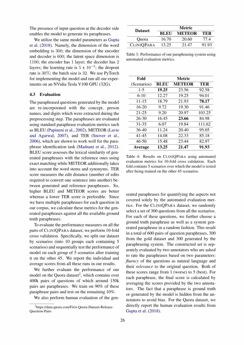
The presence of input question at the decoder sideenables the model to generate its paraphrases.
We utilize the same model parameters as Guptaet al. (2018). Namely, the dimension of the wordembedding is 300; the dimension of the encoderand decoder is 600; the latent space dimension is1100; the encoder has 1 layer; the decoder has 2layers; the learning rate is 5 x 10⁻⁵; the dropoutrate is 30%; the batch size is 32. We use PyTorchfor implementing the model and run all our exper-iments on an NVidia Tesla V100 GPU (32G).
4.3 Evaluation
The paraphrased questions generated by the modelare re-incorporated with the concept, personnames, and digits which were extracted during thepreprocessing step. The paraphrases are evaluatedusing standard paraphrase evaluation metrics suchas BLEU (Papineni et al., 2002), METEOR (Lavieand Agarwal, 2007), and TER (Snover et al.,2006), which are shown to work well for the para-phrase identification task (Madnani et al., 2012).BLEU score assesses the lexical similarity of gen-erated paraphrases with the reference ones usingexact matching while METEOR additionally takesinto account the word stems and synonyms. TERscore measures the edit distance (number of editsrequired to convert one sentence into another) be-tween generated and reference paraphrases. So,higher BLEU and METEOR scores are betterwhereas a lower TER score is preferable. Sincewe have multiple paraphrases for each question inour corpus, we calculate these metrics for the gen-erated paraphrases against all the available groundtruth paraphrases.
To evaluate the performance measures on all theparts of CLINIQPARA dataset, we perform 10-foldcross validation. Specifically, we split our datasetby scenarios (into 10 groups each containing 5scenarios) and sequentially test the performance ofmodel on each group of 5 scenarios after trainingit on the other 45. We report the individual andaverage scores from all these runs in our results.
We further evaluate the performance of ourmodel on the Quora dataset2, which contains over400k pairs of questions of which around 150kpairs are paraphrases. We train on 90% of theseparaphrase pairs and test on the remaining 10%.
We also perform human evaluation of the gen-
2https://data.quora.com/First-Quora-Dataset-Release-Question-Pairs
Dataset MetricBLEU METEOR TER
Quora 16.70 20.60 77.4CLINIQPARA 13.25 21.47 91.93
Table 3: Performance of our paraphrasing system usingautomated evaluation metrics.
Fold(Scenarios)
MetricBLEU METEOR TER
1-5 19.25 23.56 92.586-10 12.27 19.25 94.0111-15 18.79 21.93 78.1716-20 9.72 19.30 91.4621-25 9.20 20.97 103.2526-30 16.45 23.66 84.9831-35 6.07 19.84 111.6236-40 11.24 20.40 95.0541-45 14.08 22.33 85.1846-50 15.48 23.44 82.97
Average 13.25 21.47 91.93
Table 4: Results on CLINIQPARA using automatedevaluation metrics for 10-fold cross validation. Eachfold contains 5 scenarios over which the model is testedafter being trained on the other 45 scenarios.
erated paraphrases for quantifying the aspects notcovered solely by the automated evaluation met-rics. For the CLINIQPARA dataset, we randomlyselect a set of 300 questions from all the scenarios.For each of these questions, we further choose aground truth paraphrase as well as a system gen-erated paraphrase in a random fashion. This resultin a total of 600 pairs of question paraphrases, 300from the gold dataset and 300 generated by theparaphrasing system. The constructed set is sep-arately evaluated by two annotators who are askedto rate the paraphrases based on two parameters:fluency of the questions as natural language andtheir relevance to the original question. Both ofthese scores range from 1 (worse) to 5 (best). Foreach paraphrase, the final score is calculated byaveraging the scores provided by the two annota-tors. The fact that a paraphrase is ground truthor generated by the model is hidden from the an-notators to avoid bias. For the Quora dataset, wedirectly report the human evaluation results fromGupta et al. (2018).
26
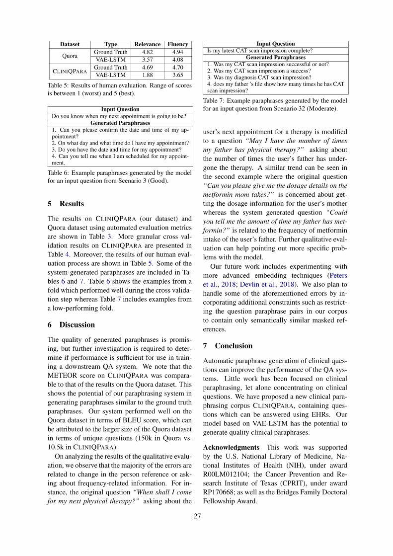
Dataset Type Relevance Fluency
QuoraGround Truth 4.82 4.94VAE-LSTM 3.57 4.08
CLINIQPARAGround Truth 4.69 4.70VAE-LSTM 1.88 3.65
Table 5: Results of human evaluation. Range of scoresis between 1 (worst) and 5 (best).
Input QuestionDo you know when my next appointment is going to be?
Generated Paraphrases1. Can you please confirm the date and time of my ap-pointment?2. On what day and what time do I have my appointment?3. Do you have the date and time for my appointment?4. Can you tell me when I am scheduled for my appoint-ment.
Table 6: Example paraphrases generated by the modelfor an input question from Scenario 3 (Good).
5 Results
The results on CLINIQPARA (our dataset) andQuora dataset using automated evaluation metricsare shown in Table 3. More granular cross val-idation results on CLINIQPARA are presented inTable 4. Moreover, the results of our human eval-uation process are shown in Table 5. Some of thesystem-generated paraphrases are included in Ta-bles 6 and 7. Table 6 shows the examples from afold which performed well during the cross valida-tion step whereas Table 7 includes examples froma low-performing fold.
6 Discussion
The quality of generated paraphrases is promis-ing, but further investigation is required to deter-mine if performance is sufficient for use in train-ing a downstream QA system. We note that theMETEOR score on CLINIQPARA was compara-ble to that of the results on the Quora dataset. Thisshows the potential of our paraphrasing system ingenerating paraphrases similar to the ground truthparaphrases. Our system performed well on theQuora dataset in terms of BLEU score, which canbe attributed to the larger size of the Quora datasetin terms of unique questions (150k in Quora vs.10.5k in CLINIQPARA).
On analyzing the results of the qualitative evalu-ation, we observe that the majority of the errors arerelated to change in the person reference or ask-ing about frequency-related information. For in-stance, the original question “When shall I comefor my next physical therapy?” asking about the
Input QuestionIs my latest CAT scan impression complete?
Generated Paraphrases1. Was my CAT scan impression successful or not?2. Was my CAT scan impression a success?3. Was my diagnosis CAT scan impression?4. does my father ’s file show how many times he has CATscan impression?
Table 7: Example paraphrases generated by the modelfor an input question from Scenario 32 (Moderate).
user’s next appointment for a therapy is modifiedto a question “May I have the number of timesmy father has physical therapy?” asking aboutthe number of times the user’s father has under-gone the therapy. A similar trend can be seen inthe second example where the original question“Can you please give me the dosage details on themetformin mom takes?” is concerned about get-ting the dosage information for the user’s motherwhereas the system generated question “Couldyou tell me the amount of time my father has met-formin?” is related to the frequency of metforminintake of the user’s father. Further qualitative eval-uation can help pointing out more specific prob-lems with the model.
Our future work includes experimenting withmore advanced embedding techniques (Peterset al., 2018; Devlin et al., 2018). We also plan tohandle some of the aforementioned errors by in-corporating additional constraints such as restrict-ing the question paraphrase pairs in our corpusto contain only semantically similar masked ref-erences.
7 Conclusion
Automatic paraphrase generation of clinical ques-tions can improve the performance of the QA sys-tems. Little work has been focused on clinicalparaphrasing, let alone concentrating on clinicalquestions. We have proposed a new clinical para-phrasing corpus CLINIQPARA, containing ques-tions which can be answered using EHRs. Ourmodel based on VAE-LSTM has the potential togenerate quality clinical paraphrases.
Acknowledgments This work was supportedby the U.S. National Library of Medicine, Na-tional Institutes of Health (NIH), under awardR00LM012104; the Cancer Prevention and Re-search Institute of Texas (CPRIT), under awardRP170668; as well as the Bridges Family DoctoralFellowship Award.
27
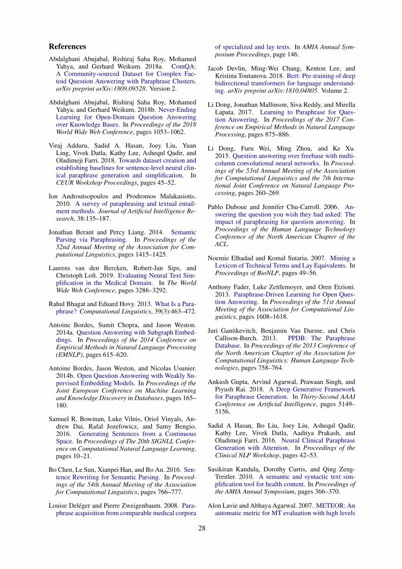
ReferencesAbdalghani Abujabal, Rishiraj Saha Roy, Mohamed
Yahya, and Gerhard Weikum. 2018a. ComQA:A Community-sourced Dataset for Complex Fac-toid Question Answering with Paraphrase Clusters.arXiv preprint arXiv:1809.09528. Version 2.
Abdalghani Abujabal, Rishiraj Saha Roy, MohamedYahya, and Gerhard Weikum. 2018b. Never-EndingLearning for Open-Domain Question Answeringover Knowledge Bases. In Proceedings of the 2018World Wide Web Conference, pages 1053–1062.
Viraj Adduru, Sadid A. Hasan, Joey Liu, YuanLing, Vivek Datla, Kathy Lee, Ashequl Qadir, andOladimeji Farri. 2018. Towards dataset creation andestablishing baselines for sentence-level neural clin-ical paraphrase generation and simplification. InCEUR Workshop Proceedings, pages 45–52.
Ion Androutsopoulos and Prodromos Malakasiotis.2010. A survey of paraphrasing and textual entail-ment methods. Journal of Artificial Intelligence Re-search, 38:135–187.
Jonathan Berant and Percy Liang. 2014. SemanticParsing via Paraphrasing. In Proceedings of the52nd Annual Meeting of the Association for Com-putational Linguistics, pages 1415–1425.
Laurens van den Bercken, Robert-Jan Sips, andChristoph Lofi. 2019. Evaluating Neural Text Sim-plification in the Medical Domain. In The WorldWide Web Conference, pages 3286–3292.
Rahul Bhagat and Eduard Hovy. 2013. What Is a Para-phrase? Computational Linguistics, 39(3):463–472.
Antoine Bordes, Sumit Chopra, and Jason Weston.2014a. Question Answering with Subgraph Embed-dings. In Proceedings of the 2014 Conference onEmpirical Methods in Natural Language Processing(EMNLP), pages 615–620.
Antoine Bordes, Jason Weston, and Nicolas Usunier.2014b. Open Question Answering with Weakly Su-pervised Embedding Models. In Proceedings of theJoint European Conference on Machine Learningand Knowledge Discovery in Databases, pages 165–180.
Samuel R. Bowman, Luke Vilnis, Oriol Vinyals, An-drew Dai, Rafal Jozefowicz, and Samy Bengio.2016. Generating Sentences from a ContinuousSpace. In Proceedings of The 20th SIGNLL Confer-ence on Computational Natural Language Learning,pages 10–21.
Bo Chen, Le Sun, Xianpei Han, and Bo An. 2016. Sen-tence Rewriting for Semantic Parsing. In Proceed-ings of the 54th Annual Meeting of the Associationfor Computational Linguistics, pages 766–777.
Louise Deléger and Pierre Zweigenbaum. 2008. Para-phrase acquisition from comparable medical corpora
of specialized and lay texts. In AMIA Annual Sym-posium Proceedings, page 146.
Jacob Devlin, Ming-Wei Chang, Kenton Lee, andKristina Toutanova. 2018. Bert: Pre-training of deepbidirectional transformers for language understand-ing. arXiv preprint arXiv:1810.04805. Volume 2.
Li Dong, Jonathan Mallinson, Siva Reddy, and MirellaLapata. 2017. Learning to Paraphrase for Ques-tion Answering. In Proceedings of the 2017 Con-ference on Empirical Methods in Natural LanguageProcessing, pages 875–886.
Li Dong, Furu Wei, Ming Zhou, and Ke Xu.2015. Question answering over freebase with multi-column convolutional neural networks. In Proceed-ings of the 53rd Annual Meeting of the Associationfor Computational Linguistics and the 7th Interna-tional Joint Conference on Natural Language Pro-cessing, pages 260–269.
Pablo Duboue and Jennifer Chu-Carroll. 2006. An-swering the question you wish they had asked: Theimpact of paraphrasing for question answering. InProceedings of the Human Language TechnologyConference of the North American Chapter of theACL.
Noemie Elhadad and Komal Sutaria. 2007. Mining aLexicon of Technical Terms and Lay Equivalents. InProceedings of BioNLP, pages 49–56.
Anthony Fader, Luke Zettlemoyer, and Oren Etzioni.2013. Paraphrase-Driven Learning for Open Ques-tion Answering. In Proceedings of the 51st AnnualMeeting of the Association for Computational Lin-guistics, pages 1608–1618.
Juri Ganitkevitch, Benjamin Van Durme, and ChrisCallison-Burch. 2013. PPDB: The ParaphraseDatabase. In Proceedings of the 2013 Conference ofthe North American Chapter of the Association forComputational Linguistics: Human Language Tech-nologies, pages 758–764.
Ankush Gupta, Arvind Agarwal, Prawaan Singh, andPiyush Rai. 2018. A Deep Generative Frameworkfor Paraphrase Generation. In Thirty-Second AAAIConference on Artificial Intelligence, pages 5149–5156.
Sadid A Hasan, Bo Liu, Joey Liu, Ashequl Qadir,Kathy Lee, Vivek Datla, Aaditya Prakash, andOladimeji Farri. 2016. Neural Clinical ParaphraseGeneration with Attention. In Proceedings of theClinical NLP Workshop, pages 42–53.
Sasikiran Kandula, Dorothy Curtis, and Qing Zeng-Treitler. 2010. A semantic and syntactic text sim-plification tool for health content. In Proceedings ofthe AMIA Annual Symposium, pages 366–370.
Alon Lavie and Abhaya Agarwal. 2007. METEOR: Anautomatic metric for MT evaluation with high levels
28
of correlation with human judgments. In Proceed-ings of the Second Workshop on Statistical MachineTranslation, pages 228–231.
Weisong Liu and Shu Cai. 2015. Translating Elec-tronic Health Record Notes from English to Spanish:A Preliminary Study. In Proceedings of BioNLP,pages 134–140.
Jake Luo, Guo-Qiang Zhang, Susan Wentz, LicongCui, and Rong Xu. 2015. SimQ: Real-Time Re-trieval of Similar Consumer Health Questions. JMed Internet Res, 17(2):e43.
Nitin Madnani and Bonnie J. Dorr. 2010. Generat-ing Phrasal and Sentential Paraphrases: A Survey ofData-Driven Methods. Computational Linguistics,36(3):341–387.
Nitin Madnani, Joel Tetreault, and Martin Chodorow.2012. Re-examining Machine Translation Metricsfor Paraphrase Identification. In Proceedings of the2012 Conference of the North American Chapter ofthe Association for Computational Linguistics: Hu-man Language Technologies, pages 182–190.
Tomas Mikolov, Ilya Sutskever, Kai Chen, Greg S Cor-rado, and Jeff Dean. 2013. Distributed representa-tions of words and phrases and their compositional-ity. In Advances in Neural Information ProcessingSystems 26, pages 3111–3119.
Preslav Nakov, Doris Hoogeveen, Lluı́s Màrquez,Alessandro Moschitti, Hamdy Mubarak, TimothyBaldwin, and Karin Verspoor. 2017. SemEval-2017Task 3: Community Question Answering. In Pro-ceedings of the 11th International Workshop on Se-mantic Evaluation (SemEval-2017), pages 27–48.
Shashi Narayan, Siva Reddy, and Shay B Cohen. 2016.Paraphrase Generation from Latent-Variable PCFGsfor Semantic Parsing. In Proceedings of the 9th In-ternational Natural Language Generation Confer-ence, pages 153–162.
Antoine Neuraz, Leonardo Campillos Llanos, AnitaBurgun, and Sophie Rosset. 2018. Natural lan-guage understanding for task oriented dialog inthe biomedical domain in a low resources context.arXiv preprint arXiv:1811.09417. Version 2.
Kishore Papineni, Salim Roukos, Todd Ward, and Wei-Jing Zhu. 2002. BLEU: a method for automaticevaluation of machine translation. In Proceedingsof the 40th Annual Meeting of the Association forComputational Linguistics, pages 311–318.
Ellie Pavlick, Pushpendre Rastogi, Juri Ganitkevitch,Benjamin Van Durme, and Chris Callison-Burch.2015. PPDB 2.0: Better paraphrase ranking, fine-grained entailment relations, word embeddings, andstyle classification. In Proceedings of the 53rd An-nual Meeting of the Association for ComputationalLinguistics and the 7th International Joint Confer-ence on Natural Language Processing, pages 425–430.
Matthew Peters, Mark Neumann, Mohit Iyyer, MattGardner, Christopher Clark, Kenton Lee, and LukeZettlemoyer. 2018. Deep Contextualized Word Rep-resentations. In Proceedings of the 2018 Conferenceof the North American Chapter of the Associationfor Computational Linguistics: Human LanguageTechnologies, pages 2227–2237.
Rimma Pivovarov and Nomie Elhadad. 2015. Auto-mated methods for the summarization of electronichealth records. Journal of the American Medical In-formatics Association, 22(5):938–947.
Basel Qenam, Tae Youn Kim, Mark J Carroll, andMichael Hogarth. 2017. Text Simplification UsingConsumer Health Vocabulary to Generate Patient-Centered Radiology Reporting: Translation andEvaluation. J Med Internet Res, 19(12):e417.
Kirk Roberts and Dina Demner-Fushman. 2016. An-notating logical forms for EHR questions. In Pro-ceedings of the Language Resources & EvaluationConference, pages 3772–3778.
Matthew Snover, Bonnie Dorr, Richard Schwartz, Lin-nea Micciulla, and John Makhoul. 2006. A Studyof Translation Edit Rate with Targeted Human An-notation. In Proceedings of 7th Conference of theAssociation for Machine Translation in the Ameri-cas, pages 223–231.
Yu Su, Huan Sun, Brian Sadler, Mudhakar Srivatsa,Izzeddin Gur, Zenghui Yan, and Xifeng Yan. 2016.On Generating Characteristic-rich Question Sets forQA Evaluation. In Proceedings of the 2016 Con-ference on Empirical Methods in Natural LanguageProcessing, pages 562–572.
Qing Zeng-Treitler, Sergey Goryachev, Hyeoneui Kim,Alla Keselman, and Douglas Rosendale. 2007.Making texts in electronic health records compre-hensible to consumers: a prototype translator. InProceedings of the AMIA Annual Symposium, pages846–850.
Jiajie Zhang and Muhammad Walji. 2014. Better EHR,Usability, Workflow and Cognitive Support in Elec-tronic Health Records. University of Texas Schoolof Biomedical Informatics at Houston.
29
Proceedings of the BioNLP 2019 workshop, pages 30–47Florence, Italy, August 1, 2019. c©2019 Association for Computational Linguistics
REflex: Flexible Framework for Relation Extraction in Multiple Domains
Geeticka ChauhanMIT CSAIL
Matthew B. A. McDermottMIT CSAIL
Peter SzolovitsMIT CSAIL
AbstractSystematic comparison of methods for relationextraction (RE) is difficult because many ex-periments in the field are not described pre-cisely enough to be completely reproducibleand many papers fail to report ablation stud-ies that would highlight the relative contribu-tions of their various combined techniques. Inthis work, we build a unifying framework forRE, applying this on three highly used datasets(from the general, biomedical and clinical do-mains) with the ability to be extendable to newdatasets. By performing a systematic explo-ration of modeling, pre-processing and train-ing methodologies, we find that choices of pre-processing are a large contributor performanceand that omission of such information can fur-ther hinder fair comparison. Other insightsfrom our exploration allow us to provide rec-ommendations for future research in this area.
1 Introduction
Relation Extraction (RE) has gained a lot of in-terest from the community with the introductionof the Semeval tasks from 2007 by (Girju et al.,2007) and 2010 by (Hendrickx et al., 2009). Thetask is a subset of information extraction (IE) withthe goal of finding semantic relationships betweenconcepts in a given sentence, and is an impor-tant component of Natural Language Understand-ing (NLU). Applications include automatic knowl-edge base creation, question answering, as well asanalysis of unstructured text data. Since the in-troduction of RE tasks in the general and medicaldomains, many researchers have explored the per-formance of different neural network architectureson the datasets (Socher et al., 2012; Zeng et al.,2014; Liu et al., 2016b; Sahu et al., 2016).
However, progress in RE is hampered by repro-ducibility issues as well as the difficulty in assess-ing which techniques in the literature will general-ize to novel tasks, datasets and contexts. To assess
the extent of these problems, we performed a man-ual review of 53 relevant neural RE papers1 citingthe three datasets (Hendrickx et al., 2009; Segura-Bedmar et al., 2013; Uzuner et al., 2011). Theprocedure for finding these papers is highlightedin (Chauhan, 2019).
Reproducibility Reproducibility is importantfor validating previous work and building upon it(Fokkens et al., 2013). Lack of reproducibility canbe attributed to many factors such as difficulty inavailability of source code (Ince et al., 2012) andomission of sources of variability such as hyperpa-rameter details (Claesen and De Moor, 2015). Wefound that only 16 out of the 53 relevant papershad released their source code. 14 out of 53 pa-pers were evaluated on multiple datasets, but thesource code was publicly available for only five ofthose. Despite this, much of this code was lack-ing in modularity to be easily extendable to newdatasets. In many cases, the process of reproduc-ing the paper results was often unclear and lackof documentation made this more difficult. Eventhough most papers mentioned some hyperparam-eter details, important details were missing suchas number of epochs, batch size, random initial-ization seed, if any, and details about early stop ifthat technique was applied.
Ablation Studies Lack of generalizability iscaused by a dearth of appropriate empirical evalu-ation to identify the source of modeling gains. Ab-lation studies are important for identifying sourcesof improvements in results. Among the 53 papersthat we looked at, 20 of the 24 papers in the gen-eral domain performed ablation studies. However,only 10 out of 29 papers in the medical domainperformed one. Among these ablation studies,
1The 53 papers were filtered from a list of 728 papersskimmed for relevance. Appendix A contains paper details.
30
key details related to pre-processing were missing,which we found critical in our experiments.
In the absence of such information about causesof large variability of results, fair comparison ofmodels becomes difficult. In this paper, we presentan open-source unifying framework enabling thecomparison of various training methodologies,pre-processing, modeling techniques, and evalu-ation metrics. The code is available at https://github.com/geetickachauhan/relation-extraction.
The experimental goals of this framework areidentification of sources of variability in resultsfor the three datasets and provide the field witha strong baseline model to compare against forfuture improvements. The design goals of thisframework are identification of best practices forrelation extraction and to be a guide for approach-ing new datasets.
By performing systematic comparison on threedatasets, we find that 1) pre-processing choicescan cause the largest variations in performance, 2)reporting scores on one test set split is problem-atic due to split bias. We perform other analysesin section 5 and also include recommendations forfuture research in this field in section 7.
Upon testing various combinations of our ap-proaches, we achieve results near state of the artranges for the three datasets: 85.89% macro F1for Semeval 2010 task 8 dataset (Hendrickx et al.,2009) i.e. semeval, 71.97% macro F1 for DDIExtraction 2013 (Segura-Bedmar et al., 2013) i.e.ddi and 71.01% micro F1 for i2b2/VA 2010 re-lation classification dataset (Uzuner et al., 2011)i.e. i2b2. We refer to ddi and i2b2 as medi-cal datasets, as they belong to the biomedical andclinical domains, respectively.
Dataset Rel Eval Agreement Detsemeval 18 Macro 0.6-0.95 Noddi 5 Macro >0.8; 0.55-0.72 Yesi2b2 8 Micro - Yes
Table 1: Dataset information, with columns Rel =number of relations, Eval = evaluation metric (all F1scores), Agreement = Inter-annotator agreement, Det =whether detection task from section 3.4 was evaluatedon. Rel column only includes relations used in offi-cial evaluation metric. ddi was built from two sep-arately annotated sources and therefore contains twointer-annotator agreements.
2 Datasets
We summarize important information about thesedatasets in table 1. We introduce detection andclassification tasks in section 3.4, but also indicatethe tasks evaluated for each dataset in table 1.
Semeval 2010 semeval consists of 8000 train-ing sentences and 2,717 test sentences for themulti-way classification of semantic relations be-tween pairs of nominals. Not included in the offi-cial evaluation is an Other class which is consid-ered noisy, with annotators choosing this class ifno fit was found in the other classes. It is impor-tant to note that this is a synthetically generateddataset, and detection scores were not calculateddue to the noisy nature of the Other class.
DDI Extraction ddi consists of 1,017 textswith 18,491 pharmacological substances and5,021 drug-drug interactions from Pubmed articlesin the pharmacological literature. None class in-dicating no interaction between the drug pairs isincluded in the evaluation metric calculation.
i2b2/VA 2010 relations i2b2 consists of dis-charge summaries from Partners Healthcare andthe MIMIC II Database (Saeed et al., 2011). Theyreleased 394 training reports, 477 test reports and877 unannotated reports. After the challenge, onlya part of the data was publicly released for re-search. None relation was present in the data andnot considered in the official evaluation.
3 Methodology
Our framework breaks up processing into dif-ferent stages, allowing for future modular addi-tion of components. First, a formatter con-verts the raw dataset into a common comma sep-arated value (CSV) input format accepted by thepre-processor, and this information is thenfed to the model, which performs the training, af-ter which evaluation is performed on the testset. With our framework, we test the followingvariations in the main components:
3.1 Pre-Processing
We test various pre-processing methods after per-forming simple tokenization and lower-casing ofthe words: entity blinding used by Liu et al.(2016b), stop-word and punctuation removal, anddigit normalization commonly applied for ddi in(Zhao et al., 2016), and named entity recognition
31
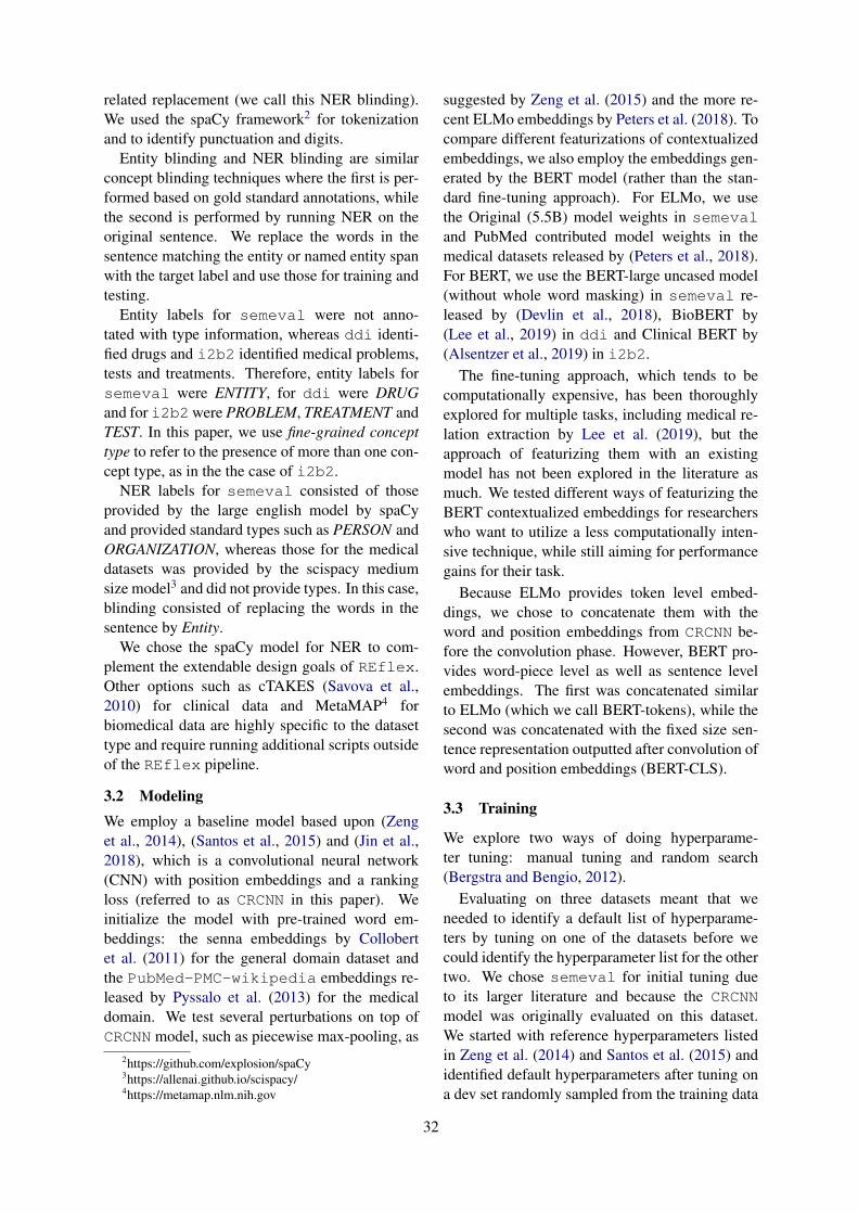
related replacement (we call this NER blinding).We used the spaCy framework2 for tokenizationand to identify punctuation and digits.
Entity blinding and NER blinding are similarconcept blinding techniques where the first is per-formed based on gold standard annotations, whilethe second is performed by running NER on theoriginal sentence. We replace the words in thesentence matching the entity or named entity spanwith the target label and use those for training andtesting.
Entity labels for semeval were not anno-tated with type information, whereas ddi identi-fied drugs and i2b2 identified medical problems,tests and treatments. Therefore, entity labels forsemeval were ENTITY, for ddi were DRUGand for i2b2were PROBLEM, TREATMENT andTEST. In this paper, we use fine-grained concepttype to refer to the presence of more than one con-cept type, as in the the case of i2b2.
NER labels for semeval consisted of thoseprovided by the large english model by spaCyand provided standard types such as PERSON andORGANIZATION, whereas those for the medicaldatasets was provided by the scispacy mediumsize model3 and did not provide types. In this case,blinding consisted of replacing the words in thesentence by Entity.
We chose the spaCy model for NER to com-plement the extendable design goals of REflex.Other options such as cTAKES (Savova et al.,2010) for clinical data and MetaMAP4 forbiomedical data are highly specific to the datasettype and require running additional scripts outsideof the REflex pipeline.
3.2 ModelingWe employ a baseline model based upon (Zenget al., 2014), (Santos et al., 2015) and (Jin et al.,2018), which is a convolutional neural network(CNN) with position embeddings and a rankingloss (referred to as CRCNN in this paper). Weinitialize the model with pre-trained word em-beddings: the senna embeddings by Collobertet al. (2011) for the general domain dataset andthe PubMed-PMC-wikipedia embeddings re-leased by Pyssalo et al. (2013) for the medicaldomain. We test several perturbations on top ofCRCNN model, such as piecewise max-pooling, as
2https://github.com/explosion/spaCy3https://allenai.github.io/scispacy/4https://metamap.nlm.nih.gov
suggested by Zeng et al. (2015) and the more re-cent ELMo embeddings by Peters et al. (2018). Tocompare different featurizations of contextualizedembeddings, we also employ the embeddings gen-erated by the BERT model (rather than the stan-dard fine-tuning approach). For ELMo, we usethe Original (5.5B) model weights in semevaland PubMed contributed model weights in themedical datasets released by (Peters et al., 2018).For BERT, we use the BERT-large uncased model(without whole word masking) in semeval re-leased by (Devlin et al., 2018), BioBERT by(Lee et al., 2019) in ddi and Clinical BERT by(Alsentzer et al., 2019) in i2b2.
The fine-tuning approach, which tends to becomputationally expensive, has been thoroughlyexplored for multiple tasks, including medical re-lation extraction by Lee et al. (2019), but theapproach of featurizing them with an existingmodel has not been explored in the literature asmuch. We tested different ways of featurizing theBERT contextualized embeddings for researcherswho want to utilize a less computationally inten-sive technique, while still aiming for performancegains for their task.
Because ELMo provides token level embed-dings, we chose to concatenate them with theword and position embeddings from CRCNN be-fore the convolution phase. However, BERT pro-vides word-piece level as well as sentence levelembeddings. The first was concatenated similarto ELMo (which we call BERT-tokens), while thesecond was concatenated with the fixed size sen-tence representation outputted after convolution ofword and position embeddings (BERT-CLS).
3.3 Training
We explore two ways of doing hyperparame-ter tuning: manual tuning and random search(Bergstra and Bengio, 2012).
Evaluating on three datasets meant that weneeded to identify a default list of hyperparame-ters by tuning on one of the datasets before wecould identify the hyperparameter list for the othertwo. We chose semeval for initial tuning dueto its larger literature and because the CRCNNmodel was originally evaluated on this dataset.We started with reference hyperparameters listedin Zeng et al. (2014) and Santos et al. (2015) andidentified default hyperparameters after tuning ona dev set randomly sampled from the training data
32
of the semeval dataset. These default hyperpa-rameters5 were used as starting points for manualtuning on the medical datasets as well as randomsearch for all datasets.
We perform manual tuning on a subset of thehyperparameters, mentioned in table 2. In or-der to avoid overfitting in cross validation pointedout by Cawley and Talbot (2010), we perform anested cross validation procedure, keeping a devfold for hyperparameter tuning and a held out foldfor score reporting.
On these dev folds, we perform paired t-tests foreach of the perturbations to the parameters listedin table 2. Our first pass involves changing one hy-perparameter per experiment and noting the onesthat cause a statistically significant improvement,which helps us identify a narrower list of hyperpa-rameters to tune on. We further refine the hyper-parameter values in our second pass by testing onvalues similar to those that were leading to statis-tically significant improvements in the first pass.For example, if we noticed that lower epoch val-ues were helpful in the first pass, we tested them incombination with the other optimal hyperparame-ter values (from first pass) in the second pass.
For each of the datasets, we tuned based on theirofficial challenge evaluation metrics listed in sec-tion 2. ddi and i2b2 had 5-fold nested crossvalidation performed on them, whereas semevalhad 10-fold cross validation performed.
Random search was performed based on theofficial evaluation metrics for each dataset, on afixed dev set randomly sampled from the trainingdata. Final distributions are listed in table 3.
3.4 Evaluation
The official challenge problems for all datasetscompared models based on multi-class classifica-tion, but for the medical datasets, we were alsointerested in looking at the changes in model per-formance if we treated the task as a binary classi-fication problem. This was based on the rationalethat in the drug literature, for example, pharma-cologists would not want to sacrifice the abilityto identify a potentially life threatening drug in-teraction pair, even if the type of the drug pair isnot known. Therefore, we report results for bothmulti-class and binary classification scenarios. Forclarity, we refer to them in the rest of the paper asclassification and detection respectively.
5listed in source code
Detection results were obtained using our eval-uation scripts by treating existing relations as oneclass, ignoring the types outputted by the model.The other class in this task was the None or Otherclass, representing non-existing relations. Notethat we did not re-train our model for this.
In addition to evaluating on two tasks for themedical and one task for the general dataset, wecomment on the implications of different evalua-tion metrics in section 5.5.
4 Results
For experiments on the medical datasets i.e. i2b2and ddi, we used hyperparameters found frommanual search individually performed on them.semeval had the default hyperparameters usedfor its experiments. These sets of hyperparame-ters were used in all experiments other than thosereported in table 6, where we compare hyperpa-rameter tuning methodologies.
Once we had a fixed set of hyperparameters foreach dataset, we tested the perturbations for pre-processing as well as modeling in tables 4 and5. Perturbations on the hyperparameter search arelisted in table 6 and compare performance withdifferent hyperparameter values found using dif-ferent tuning strategies.
We generate the standard classification and theadditional detection scores by the procedure de-scribed in section 3.4, and report these results un-der the Class and Detect columns.
We also report additional experiments in tables7 and 8 based on the improvements found in tables4 and 5. For all results tables, we report officialtest set results at the top, with accompanying crossvalidated results (averaged over all folds with theirstandard deviation) in smaller font below them.6
5 Discussion
Recently, CNNs have achieved strong perfor-mance for text classification and are typicallymore efficient than recurrent architectures (Baiet al., 2018; Kalchbrenner et al., 2014; Wang et al.,2015; Zhang et al., 2015b). The speed of our base-line CRCNN model allows us to explore multiplealternatives for every stage of our pipeline. Wediscuss these results pertaining to the classifica-tion task for all datasets and the detection task for
6Results tables for metrics other than the official oneswere omitted in the interest of space, but their analysis ex-ists in section 5.5.
33
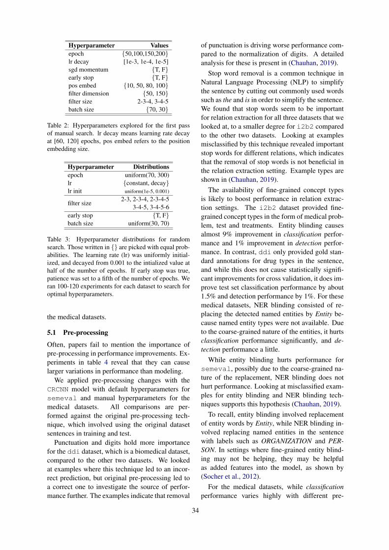
Hyperparameter Valuesepoch {50,100,150,200}lr decay [1e-3, 1e-4, 1e-5]sgd momentum {T, F}early stop {T, F}pos embed {10, 50, 80, 100}filter dimension {50, 150}filter size 2-3-4, 3-4-5batch size {70, 30}
Table 2: Hyperparameters explored for the first passof manual search. lr decay means learning rate decayat [60, 120] epochs, pos embed refers to the positionembedding size.
Hyperparameter Distributionsepoch uniform(70, 300)lr {constant, decay}lr init uniform(1e-5, 0.001)
filter size2-3, 2-3-4, 2-3-4-5
3-4-5, 3-4-5-6early stop {T, F}batch size uniform(30, 70)
Table 3: Hyperparameter distributions for randomsearch. Those written in {} are picked with equal prob-abilities. The learning rate (lr) was uniformly initial-ized, and decayed from 0.001 to the intialized value athalf of the number of epochs. If early stop was true,patience was set to a fifth of the number of epochs. Weran 100-120 experiments for each dataset to search foroptimal hyperparameters.
the medical datasets.
5.1 Pre-processing
Often, papers fail to mention the importance ofpre-processing in performance improvements. Ex-periments in table 4 reveal that they can causelarger variations in performance than modeling.
We applied pre-processing changes with theCRCNN model with default hyperparameters forsemeval and manual hyperparameters for themedical datasets. All comparisons are per-formed against the original pre-processing tech-nique, which involved using the original datasetsentences in training and test.
Punctuation and digits hold more importancefor the ddi dataset, which is a biomedical dataset,compared to the other two datasets. We lookedat examples where this technique led to an incor-rect prediction, but original pre-processing led toa correct one to investigate the source of perfor-mance further. The examples indicate that removal
of punctuation is driving worse performance com-pared to the normalization of digits. A detailedanalysis for these is present in (Chauhan, 2019).
Stop word removal is a common technique inNatural Language Processing (NLP) to simplifythe sentence by cutting out commonly used wordssuch as the and is in order to simplify the sentence.We found that stop words seem to be importantfor relation extraction for all three datasets that welooked at, to a smaller degree for i2b2 comparedto the other two datasets. Looking at examplesmisclassified by this technique revealed importantstop words for different relations, which indicatesthat the removal of stop words is not beneficial inthe relation extraction setting. Example types areshown in (Chauhan, 2019).
The availability of fine-grained concept typesis likely to boost performance in relation extrac-tion settings. The i2b2 dataset provided fine-grained concept types in the form of medical prob-lem, test and treatments. Entity blinding causesalmost 9% improvement in classification perfor-mance and 1% improvement in detection perfor-mance. In contrast, ddi only provided gold stan-dard annotations for drug types in the sentence,and while this does not cause statistically signifi-cant improvements for cross validation, it does im-prove test set classification performance by about1.5% and detection performance by 1%. For thesemedical datasets, NER blinding consisted of re-placing the detected named entities by Entity be-cause named entity types were not available. Dueto the coarse-grained nature of the entities, it hurtsclassification performance significantly, and de-tection performance a little.
While entity blinding hurts performance forsemeval, possibly due to the coarse-grained na-ture of the replacement, NER blinding does nothurt performance. Looking at misclassified exam-ples for entity blinding and NER blinding tech-niques supports this hypothesis (Chauhan, 2019).
To recall, entity blinding involved replacementof entity words by Entity, while NER blinding in-volved replacing named entities in the sentencewith labels such as ORGANIZATION and PER-SON. In settings where fine-grained entity blind-ing may not be helping, they may be helpfulas added features into the model, as shown by(Socher et al., 2012).
For the medical datasets, while classificationperformance varies highly with different pre-
34
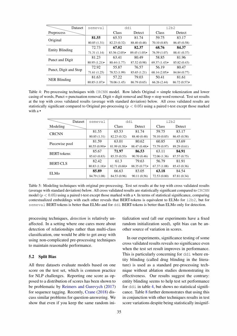
PreprocessDataset semeval ddi i2b2
Class Detect Class Detect
Original81.55 65.53 81.74 59.75 83.17
80.85 (1.31) 82.23 (0.32) 88.40 (0.48) 70.10 (0.85) 86.45 (0.58)
Entity Blinding72.73 67.02 82.37 68.76 84.37
71.31 (1.14) 83.56 (2.05)• 89.45 (1.05)• 76.59 (1.07) 88.41 (0.37)
Punct and Digit81.23 63.41 80.49 58.85 81.96
80.95 (1.21)• 80.44 (1.77) 87.52 (0.98) 69.37 (1.43)• 85.82 (0.43)
Punct, Digit and Stop72.92 55.87 76.57 56.19 80.47
71.61 (1.25) 78.52 (1.99) 85.65 (1.21) 68.14 (2.05)• 84.84 (0.77)
NER Blinding81.63 57.22 79.03 50.41 81.61
80.85 (1.07)• 78.06 (1.45) 86.79 (0.65) 66.26 (2.44) 86.72 (0.57)•
Table 4: Pre-processing techniques with CRCNN model. Row labels Original = simple tokenization and lowercasing of words, Punct = punctuation removal, Digit = digit removal and Stop = stop word removal. Test set resultsat the top with cross validated results (average with standard deviation) below. All cross validated results arestatistically significant compared to Original pre-processing (p < 0.05) using a paired t-test except those markedwith a •
ModelingDataset semeval ddi i2b2
Class Detect Class Detect
CRCNN81.55 65.53 81.74 59.75 83.17
80.85 (1.31) 82.23 (0.32) 88.40 (0.48) 70.10 (0.85) 86.45 (0.58)
Piecewise pool81.59 63.01 80.62 60.85 83.69
80.55 (0.99)• 81.99 (0.38)• 88.47 (0.48)• 73.79 (0.97) 89.29 (0.61)
BERT-tokens85.67 71.97 86.53 63.11 84.91
85.63 (0.83) 85.35 (0.53) 90.70 (0.46) 72.06 (1.36) 87.57 (0.75)
BERT-CLS82.42 61.3 79.63 56.79 81.91
80.83 (1.18)• 82.71 (0.68)• 88.35 (0.77)• 67.37 (1.08) 85.43 (0.36)
ELMo85.89 66.63 83.05 63.18 84.54
84.79 (1.08) 84.53 (0.96) 90.11 (0.56) 72.53 (0.80) 87.81 (0.34)
Table 5: Modeling techniques with original pre-processing. Test set results at the top with cross validated results(average with standard deviation) below. All cross validated results are statistically significant compared to CRCNNmodel (p < 0.05) using a paired t-test except those marked with a •. In terms of statistical significance, comparingcontextualized embeddings with each other reveals that BERT-tokens is equivalent to ELMo for i2b2, but forsemeval BERT-tokens is better than ELMo and for ddi BERT-tokens is better than ELMo only for detection.
processing techniques, detection is relatively un-affected. In a setting where one cares more aboutdetection of relationships rather than multi-classclassification, one would be able to get away withusing non-complicated pre-processing techniquesto maintain reasonable performance.
5.2 Split Bias
All three datasets evaluate models based on onescore on the test set, which is common practicefor NLP challenges. Reporting one score as op-posed to a distribution of scores has been shown tobe problematic by Reimers and Gurevych (2017)for sequence tagging. Recently, Crane (2018) dis-cuss similar problems for question-answering. Weshow that even if you keep the same random ini-
tialization seed (all our experiments have a fixedrandom initialization seed), split bias can be an-other source of variation in scores.
In our experiments, significance testing of somecross validated results reveals no significance evenwhen the test set result improves in performance.This is particularly concerning for ddi where en-tity blinding (called drug blinding in the litera-ture) is used as a standard pre-processing tech-nique without ablation studies demonstrating itseffectiveness. Our results suggest the contrary:entity blinding seems to help test set performancefor ddi in table 4, but shows no statistical signifi-cance. Table 8 further demonstrates that using thisin conjunction with other techniques results in testscore variations despite being statistically insignif-
35
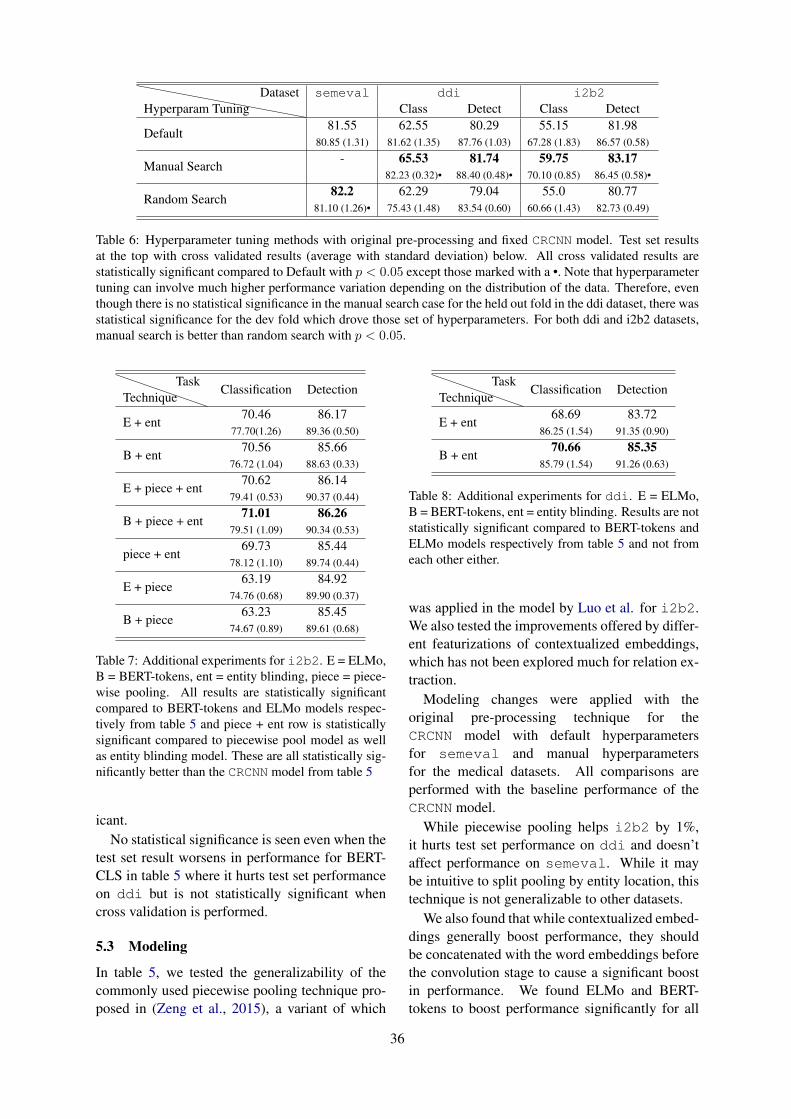
Hyperparam TuningDataset semeval ddi i2b2
Class Detect Class Detect
Default81.55 62.55 80.29 55.15 81.98
80.85 (1.31) 81.62 (1.35) 87.76 (1.03) 67.28 (1.83) 86.57 (0.58)
Manual Search- 65.53 81.74 59.75 83.17
82.23 (0.32)• 88.40 (0.48)• 70.10 (0.85) 86.45 (0.58)•
Random Search82.2 62.29 79.04 55.0 80.77
81.10 (1.26)• 75.43 (1.48) 83.54 (0.60) 60.66 (1.43) 82.73 (0.49)
Table 6: Hyperparameter tuning methods with original pre-processing and fixed CRCNN model. Test set resultsat the top with cross validated results (average with standard deviation) below. All cross validated results arestatistically significant compared to Default with p < 0.05 except those marked with a •. Note that hyperparametertuning can involve much higher performance variation depending on the distribution of the data. Therefore, eventhough there is no statistical significance in the manual search case for the held out fold in the ddi dataset, there wasstatistical significance for the dev fold which drove those set of hyperparameters. For both ddi and i2b2 datasets,manual search is better than random search with p < 0.05.
TechniqueTask
Classification Detection
E + ent70.46 86.17
77.70(1.26) 89.36 (0.50)
B + ent70.56 85.66
76.72 (1.04) 88.63 (0.33)
E + piece + ent70.62 86.14
79.41 (0.53) 90.37 (0.44)
B + piece + ent71.01 86.26
79.51 (1.09) 90.34 (0.53)
piece + ent69.73 85.44
78.12 (1.10) 89.74 (0.44)
E + piece63.19 84.92
74.76 (0.68) 89.90 (0.37)
B + piece63.23 85.45
74.67 (0.89) 89.61 (0.68)
Table 7: Additional experiments for i2b2. E = ELMo,B = BERT-tokens, ent = entity blinding, piece = piece-wise pooling. All results are statistically significantcompared to BERT-tokens and ELMo models respec-tively from table 5 and piece + ent row is statisticallysignificant compared to piecewise pool model as wellas entity blinding model. These are all statistically sig-nificantly better than the CRCNN model from table 5
icant.No statistical significance is seen even when the
test set result worsens in performance for BERT-CLS in table 5 where it hurts test set performanceon ddi but is not statistically significant whencross validation is performed.
5.3 Modeling
In table 5, we tested the generalizability of thecommonly used piecewise pooling technique pro-posed in (Zeng et al., 2015), a variant of which
TechniqueTask
Classification Detection
E + ent68.69 83.72
86.25 (1.54) 91.35 (0.90)
B + ent70.66 85.35
85.79 (1.54) 91.26 (0.63)
Table 8: Additional experiments for ddi. E = ELMo,B = BERT-tokens, ent = entity blinding. Results are notstatistically significant compared to BERT-tokens andELMo models respectively from table 5 and not fromeach other either.
was applied in the model by Luo et al. for i2b2.We also tested the improvements offered by differ-ent featurizations of contextualized embeddings,which has not been explored much for relation ex-traction.
Modeling changes were applied with theoriginal pre-processing technique for theCRCNN model with default hyperparametersfor semeval and manual hyperparametersfor the medical datasets. All comparisons areperformed with the baseline performance of theCRCNN model.
While piecewise pooling helps i2b2 by 1%,it hurts test set performance on ddi and doesn’taffect performance on semeval. While it maybe intuitive to split pooling by entity location, thistechnique is not generalizable to other datasets.
We also found that while contextualized embed-dings generally boost performance, they shouldbe concatenated with the word embeddings beforethe convolution stage to cause a significant boostin performance. We found ELMo and BERT-tokens to boost performance significantly for all
36
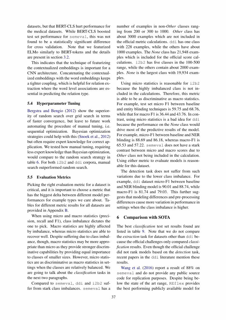
datasets, but that BERT-CLS hurt performance forthe medical datasets. While BERT-CLS boostedtest set performance for semeval, this was notfound to be a statistically significant differencefor cross validation. Note that we featurizedELMo similarly to BERT-tokens and the detailsare present in section 3.2.
This indicates that the technique of featurizingthe contextualized embeddings is important for aCNN architecture. Concatenating the contextual-ized embeddings with the word embeddings keepsa tighter coupling, which is helpful for relation ex-traction where the word level associations are es-sential in predicting the relation type.
5.4 Hyperparameter Tuning
Bergstra and Bengio (2012) show the superior-ity of random search over grid search in termsof faster convergence, but leave to future workautomating the procedure of manual tuning, i.e.sequential optimization. Bayesian optimizationstrategies could help with this (Snoek et al., 2012)but often require expert knowledge for correct ap-plication. We tested how manual tuning, requiringless expert knowledge than Bayesian optimization,would compare to the random search strategy intable 6. For both i2b2 and ddi corpora, manualsearch outperformed random search.
5.5 Evaluation Metrics
Picking the right evaluation metric for a dataset iscritical, and it is important to choose a metric thathas the biggest delta between different model per-formances for example types we care about. Ta-bles for different metric results for all datasets areprovided in Appendix B.
When using micro and macro statistics (preci-sion, recall and F1), class imbalance dictates theone to pick. Macro statistics are highly affectedby imbalance, whereas micro statistics are able torecover well. Despite suffering due to class imbal-ance, though, macro statistics may be more appro-priate than micro as they provide stronger discrim-inative capabilities by providing equal importanceto classes of smaller sizes. However, micro statis-tics are as discriminative as macro statistics in set-tings when the classes are relatively balanced. Weare going to talk about the classification tasks inthe next two paragraphs.
Compared to semeval, ddi and i2b2 suf-fer from stark class imbalances. semeval has a
number of examples in non-Other classes rang-ing from 200 or 300 to 1000. Other class hasabout 3000 examples which are not included inthe official metric calculations. ddi has one classwith 228 examples, while the others have about1000 examples. The None class has 21,948 exam-ples which is included for the official score cal-culations. i2b2 has five classes in the 100-500range, while the others contain about 2000 exam-ples. None is the largest class with 19,934 exam-ples.
Using micro statistics is reasonable for i2b2because the highly imbalanced class is not in-cluded in the calculations. Therefore, this metricis able to be as discriminative as macro statistics.For example, test set micro F1 between baselineand entity blinding techniques is 59.75 and 68.76,while that for macro F1 is 36.44 and 43.76. In con-trast, using micro statistics is a bad idea for ddibecause the performance on the None class woulddrive most of the predictive results of the model.For example, micro-F1 between baseline and NERblinding is 88.69 and 86.18, whereas macro-F1 is65.53 and 57.22. semeval does not have a starkcontrast between micro and macro scores due toOther class not being included in the calculation.Using either metric to evaluate models is reason-able for this dataset.
The detection task does not suffer from suchvariations due to the lower class imbalance. Forexample, ddi dataset micro-F1 between baselineand NER blinding model is 90.01 and 88.74, whilemacro-F1 is 81.74 and 79.03. This further sug-gests that modeling differences and pre-processingdifferences cause more variation in performance insettings when the class imbalance is higher.
6 Comparison with SOTA
The best classification test set results found arelisted in table 9. Note that we do not comparethe extraction task for datasets other than ddi be-cause the official challenges only compared classi-fication results. Even though the official challengedid not rank models based on the detection task,recent papers in the ddi literature mention theseresults.
Wang et al. (2016) report a result of 88% onsemeval and do not provide any public sourcecode for replication purposes. Despite being be-low the state of the art range, REflex providesthe best performing publicly available model for
37
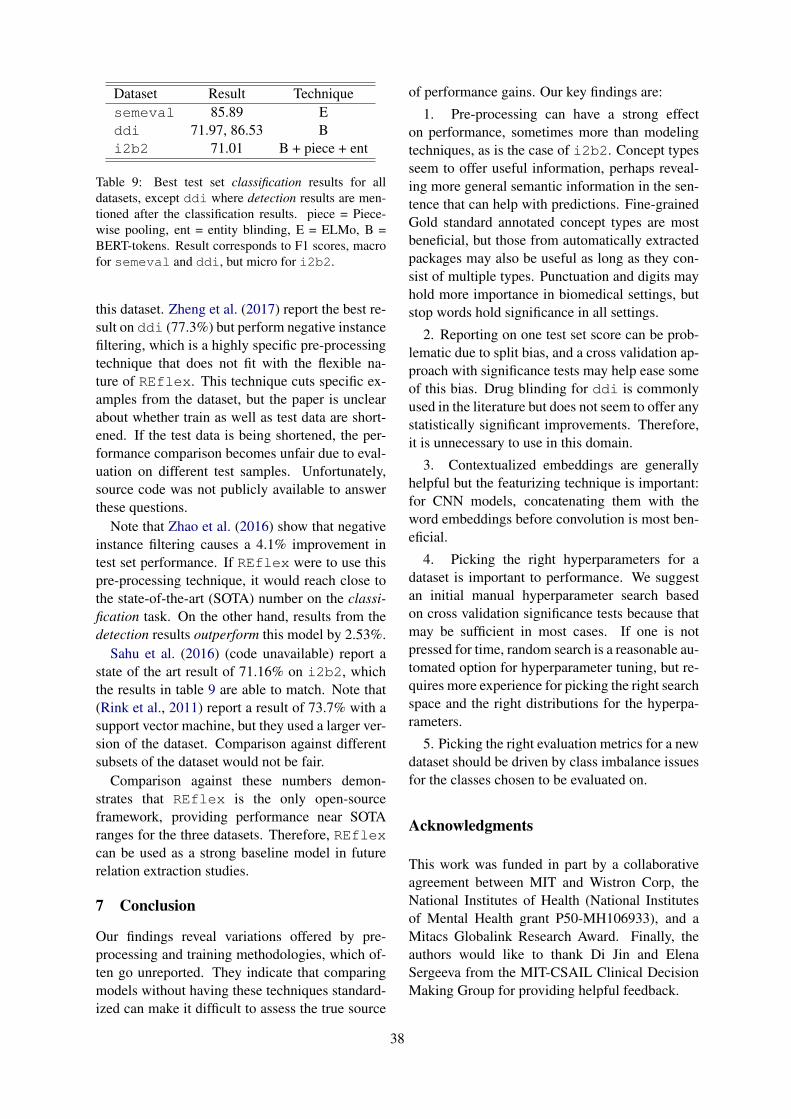
Dataset Result Techniquesemeval 85.89 Eddi 71.97, 86.53 Bi2b2 71.01 B + piece + ent
Table 9: Best test set classification results for alldatasets, except ddi where detection results are men-tioned after the classification results. piece = Piece-wise pooling, ent = entity blinding, E = ELMo, B =BERT-tokens. Result corresponds to F1 scores, macrofor semeval and ddi, but micro for i2b2.
this dataset. Zheng et al. (2017) report the best re-sult on ddi (77.3%) but perform negative instancefiltering, which is a highly specific pre-processingtechnique that does not fit with the flexible na-ture of REflex. This technique cuts specific ex-amples from the dataset, but the paper is unclearabout whether train as well as test data are short-ened. If the test data is being shortened, the per-formance comparison becomes unfair due to eval-uation on different test samples. Unfortunately,source code was not publicly available to answerthese questions.
Note that Zhao et al. (2016) show that negativeinstance filtering causes a 4.1% improvement intest set performance. If REflex were to use thispre-processing technique, it would reach close tothe state-of-the-art (SOTA) number on the classi-fication task. On the other hand, results from thedetection results outperform this model by 2.53%.
Sahu et al. (2016) (code unavailable) report astate of the art result of 71.16% on i2b2, whichthe results in table 9 are able to match. Note that(Rink et al., 2011) report a result of 73.7% with asupport vector machine, but they used a larger ver-sion of the dataset. Comparison against differentsubsets of the dataset would not be fair.
Comparison against these numbers demon-strates that REflex is the only open-sourceframework, providing performance near SOTAranges for the three datasets. Therefore, REflexcan be used as a strong baseline model in futurerelation extraction studies.
7 Conclusion
Our findings reveal variations offered by pre-processing and training methodologies, which of-ten go unreported. They indicate that comparingmodels without having these techniques standard-ized can make it difficult to assess the true source
of performance gains. Our key findings are:
1. Pre-processing can have a strong effecton performance, sometimes more than modelingtechniques, as is the case of i2b2. Concept typesseem to offer useful information, perhaps reveal-ing more general semantic information in the sen-tence that can help with predictions. Fine-grainedGold standard annotated concept types are mostbeneficial, but those from automatically extractedpackages may also be useful as long as they con-sist of multiple types. Punctuation and digits mayhold more importance in biomedical settings, butstop words hold significance in all settings.
2. Reporting on one test set score can be prob-lematic due to split bias, and a cross validation ap-proach with significance tests may help ease someof this bias. Drug blinding for ddi is commonlyused in the literature but does not seem to offer anystatistically significant improvements. Therefore,it is unnecessary to use in this domain.
3. Contextualized embeddings are generallyhelpful but the featurizing technique is important:for CNN models, concatenating them with theword embeddings before convolution is most ben-eficial.
4. Picking the right hyperparameters for adataset is important to performance. We suggestan initial manual hyperparameter search basedon cross validation significance tests because thatmay be sufficient in most cases. If one is notpressed for time, random search is a reasonable au-tomated option for hyperparameter tuning, but re-quires more experience for picking the right searchspace and the right distributions for the hyperpa-rameters.
5. Picking the right evaluation metrics for a newdataset should be driven by class imbalance issuesfor the classes chosen to be evaluated on.
Acknowledgments
This work was funded in part by a collaborativeagreement between MIT and Wistron Corp, theNational Institutes of Health (National Institutesof Mental Health grant P50-MH106933), and aMitacs Globalink Research Award. Finally, theauthors would like to thank Di Jin and ElenaSergeeva from the MIT-CSAIL Clinical DecisionMaking Group for providing helpful feedback.
38
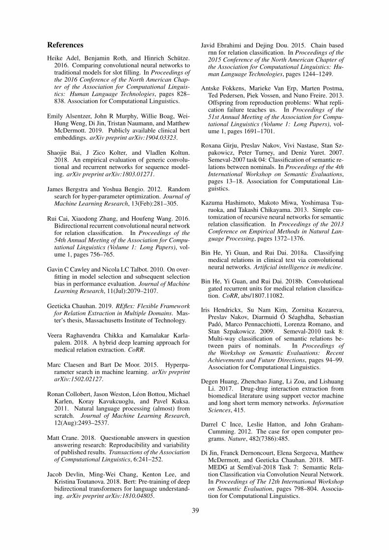
References
Heike Adel, Benjamin Roth, and Hinrich Schütze.2016. Comparing convolutional neural networks totraditional models for slot filling. In Proceedings ofthe 2016 Conference of the North American Chap-ter of the Association for Computational Linguis-tics: Human Language Technologies, pages 828–838. Association for Computational Linguistics.
Emily Alsentzer, John R Murphy, Willie Boag, Wei-Hung Weng, Di Jin, Tristan Naumann, and MatthewMcDermott. 2019. Publicly available clinical bertembeddings. arXiv preprint arXiv:1904.03323.
Shaojie Bai, J Zico Kolter, and Vladlen Koltun.2018. An empirical evaluation of generic convolu-tional and recurrent networks for sequence model-ing. arXiv preprint arXiv:1803.01271.
James Bergstra and Yoshua Bengio. 2012. Randomsearch for hyper-parameter optimization. Journal ofMachine Learning Research, 13(Feb):281–305.
Rui Cai, Xiaodong Zhang, and Houfeng Wang. 2016.Bidirectional recurrent convolutional neural networkfor relation classification. In Proceedings of the54th Annual Meeting of the Association for Compu-tational Linguistics (Volume 1: Long Papers), vol-ume 1, pages 756–765.
Gavin C Cawley and Nicola LC Talbot. 2010. On over-fitting in model selection and subsequent selectionbias in performance evaluation. Journal of MachineLearning Research, 11(Jul):2079–2107.
Geeticka Chauhan. 2019. REflex: Flexible Frameworkfor Relation Extraction in Multiple Domains. Mas-ter’s thesis, Massachusetts Institute of Technology.
Veera Raghavendra Chikka and Kamalakar Karla-palem. 2018. A hybrid deep learning approach formedical relation extraction. CoRR.
Marc Claesen and Bart De Moor. 2015. Hyperpa-rameter search in machine learning. arXiv preprintarXiv:1502.02127.
Ronan Collobert, Jason Weston, Léon Bottou, MichaelKarlen, Koray Kavukcuoglu, and Pavel Kuksa.2011. Natural language processing (almost) fromscratch. Journal of Machine Learning Research,12(Aug):2493–2537.
Matt Crane. 2018. Questionable answers in questionanswering research: Reproducibility and variabilityof published results. Transactions of the Associationof Computational Linguistics, 6:241–252.
Jacob Devlin, Ming-Wei Chang, Kenton Lee, andKristina Toutanova. 2018. Bert: Pre-training of deepbidirectional transformers for language understand-ing. arXiv preprint arXiv:1810.04805.
Javid Ebrahimi and Dejing Dou. 2015. Chain basedrnn for relation classification. In Proceedings of the2015 Conference of the North American Chapter ofthe Association for Computational Linguistics: Hu-man Language Technologies, pages 1244–1249.
Antske Fokkens, Marieke Van Erp, Marten Postma,Ted Pedersen, Piek Vossen, and Nuno Freire. 2013.Offspring from reproduction problems: What repli-cation failure teaches us. In Proceedings of the51st Annual Meeting of the Association for Compu-tational Linguistics (Volume 1: Long Papers), vol-ume 1, pages 1691–1701.
Roxana Girju, Preslav Nakov, Vivi Nastase, Stan Sz-pakowicz, Peter Turney, and Deniz Yuret. 2007.Semeval-2007 task 04: Classification of semantic re-lations between nominals. In Proceedings of the 4thInternational Workshop on Semantic Evaluations,pages 13–18. Association for Computational Lin-guistics.
Kazuma Hashimoto, Makoto Miwa, Yoshimasa Tsu-ruoka, and Takashi Chikayama. 2013. Simple cus-tomization of recursive neural networks for semanticrelation classification. In Proceedings of the 2013Conference on Empirical Methods in Natural Lan-guage Processing, pages 1372–1376.
Bin He, Yi Guan, and Rui Dai. 2018a. Classifyingmedical relations in clinical text via convolutionalneural networks. Artificial intelligence in medicine.
Bin He, Yi Guan, and Rui Dai. 2018b. Convolutionalgated recurrent units for medical relation classifica-tion. CoRR, abs/1807.11082.
Iris Hendrickx, Su Nam Kim, Zornitsa Kozareva,Preslav Nakov, Diarmuid Ó Séaghdha, SebastianPadó, Marco Pennacchiotti, Lorenza Romano, andStan Szpakowicz. 2009. Semeval-2010 task 8:Multi-way classification of semantic relations be-tween pairs of nominals. In Proceedings ofthe Workshop on Semantic Evaluations: RecentAchievements and Future Directions, pages 94–99.Association for Computational Linguistics.
Degen Huang, Zhenchao Jiang, Li Zou, and LishuangLi. 2017. Drug-drug interaction extraction frombiomedical literature using support vector machineand long short term memory networks. InformationSciences, 415.
Darrel C Ince, Leslie Hatton, and John Graham-Cumming. 2012. The case for open computer pro-grams. Nature, 482(7386):485.
Di Jin, Franck Dernoncourt, Elena Sergeeva, MatthewMcDermott, and Geeticka Chauhan. 2018. MIT-MEDG at SemEval-2018 Task 7: Semantic Rela-tion Classification via Convolution Neural Network.In Proceedings of The 12th International Workshopon Semantic Evaluation, pages 798–804. Associa-tion for Computational Linguistics.
39
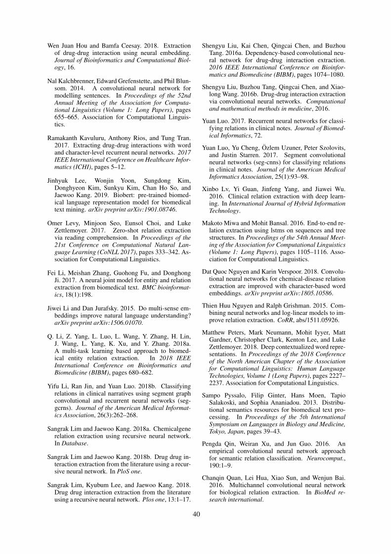
Wen Juan Hou and Bamfa Ceesay. 2018. Extractionof drug-drug interaction using neural embedding.Journal of Bioinformatics and Computational Biol-ogy, 16.
Nal Kalchbrenner, Edward Grefenstette, and Phil Blun-som. 2014. A convolutional neural network formodelling sentences. In Proceedings of the 52ndAnnual Meeting of the Association for Computa-tional Linguistics (Volume 1: Long Papers), pages655–665. Association for Computational Linguis-tics.
Ramakanth Kavuluru, Anthony Rios, and Tung Tran.2017. Extracting drug-drug interactions with wordand character-level recurrent neural networks. 2017IEEE International Conference on Healthcare Infor-matics (ICHI), pages 5–12.
Jinhyuk Lee, Wonjin Yoon, Sungdong Kim,Donghyeon Kim, Sunkyu Kim, Chan Ho So, andJaewoo Kang. 2019. Biobert: pre-trained biomed-ical language representation model for biomedicaltext mining. arXiv preprint arXiv:1901.08746.
Omer Levy, Minjoon Seo, Eunsol Choi, and LukeZettlemoyer. 2017. Zero-shot relation extractionvia reading comprehension. In Proceedings of the21st Conference on Computational Natural Lan-guage Learning (CoNLL 2017), pages 333–342. As-sociation for Computational Linguistics.
Fei Li, Meishan Zhang, Guohong Fu, and DonghongJi. 2017. A neural joint model for entity and relationextraction from biomedical text. BMC bioinformat-ics, 18(1):198.
Jiwei Li and Dan Jurafsky. 2015. Do multi-sense em-beddings improve natural language understanding?arXiv preprint arXiv:1506.01070.
Q. Li, Z. Yang, L. Luo, L. Wang, Y. Zhang, H. Lin,J. Wang, L. Yang, K. Xu, and Y. Zhang. 2018a.A multi-task learning based approach to biomed-ical entity relation extraction. In 2018 IEEEInternational Conference on Bioinformatics andBiomedicine (BIBM), pages 680–682.
Yifu Li, Ran Jin, and Yuan Luo. 2018b. Classifyingrelations in clinical narratives using segment graphconvolutional and recurrent neural networks (seg-gcrns). Journal of the American Medical Informat-ics Association, 26(3):262–268.
Sangrak Lim and Jaewoo Kang. 2018a. Chemicalgenerelation extraction using recursive neural network.In Database.
Sangrak Lim and Jaewoo Kang. 2018b. Drug drug in-teraction extraction from the literature using a recur-sive neural network. In PloS one.
Sangrak Lim, Kyubum Lee, and Jaewoo Kang. 2018.Drug drug interaction extraction from the literatureusing a recursive neural network. Plos one, 13:1–17.
Shengyu Liu, Kai Chen, Qingcai Chen, and BuzhouTang. 2016a. Dependency-based convolutional neu-ral network for drug-drug interaction extraction.2016 IEEE International Conference on Bioinfor-matics and Biomedicine (BIBM), pages 1074–1080.
Shengyu Liu, Buzhou Tang, Qingcai Chen, and Xiao-long Wang. 2016b. Drug-drug interaction extractionvia convolutional neural networks. Computationaland mathematical methods in medicine, 2016.
Yuan Luo. 2017. Recurrent neural networks for classi-fying relations in clinical notes. Journal of Biomed-ical Informatics, 72.
Yuan Luo, Yu Cheng, Özlem Uzuner, Peter Szolovits,and Justin Starren. 2017. Segment convolutionalneural networks (seg-cnns) for classifying relationsin clinical notes. Journal of the American MedicalInformatics Association, 25(1):93–98.
Xinbo Lv, Yi Guan, Jinfeng Yang, and Jiawei Wu.2016. Clinical relation extraction with deep learn-ing. In International Journal of Hybrid InformationTechnology.
Makoto Miwa and Mohit Bansal. 2016. End-to-end re-lation extraction using lstms on sequences and treestructures. In Proceedings of the 54th Annual Meet-ing of the Association for Computational Linguistics(Volume 1: Long Papers), pages 1105–1116. Asso-ciation for Computational Linguistics.
Dat Quoc Nguyen and Karin Verspoor. 2018. Convolu-tional neural networks for chemical-disease relationextraction are improved with character-based wordembeddings. arXiv preprint arXiv:1805.10586.
Thien Huu Nguyen and Ralph Grishman. 2015. Com-bining neural networks and log-linear models to im-prove relation extraction. CoRR, abs/1511.05926.
Matthew Peters, Mark Neumann, Mohit Iyyer, MattGardner, Christopher Clark, Kenton Lee, and LukeZettlemoyer. 2018. Deep contextualized word repre-sentations. In Proceedings of the 2018 Conferenceof the North American Chapter of the Associationfor Computational Linguistics: Human LanguageTechnologies, Volume 1 (Long Papers), pages 2227–2237. Association for Computational Linguistics.
Sampo Pyssalo, Filip Ginter, Hans Moen, TapioSalakoski, and Sophia Ananiadou. 2013. Distribu-tional semantics resources for biomedical text pro-cessing. In Proceedings of the 5th InternationalSymposium on Languages in Biology and Medicine,Tokyo, Japan, pages 39–43.
Pengda Qin, Weiran Xu, and Jun Guo. 2016. Anempirical convolutional neural network approachfor semantic relation classification. Neurocomput.,190:1–9.
Chanqin Quan, Lei Hua, Xiao Sun, and Wenjun Bai.2016. Multichannel convolutional neural networkfor biological relation extraction. In BioMed re-search international.
40
Nils Reimers and Iryna Gurevych. 2017. Reportingscore distributions makes a difference: Performancestudy of lstm-networks for sequence tagging. InProceedings of the 2017 Conference on EmpiricalMethods in Natural Language Processing, pages338–348, Copenhagen, Denmark. Association forComputational Linguistics.
Bryan Rink, Sanda Harabagiu, and Kirk Roberts. 2011.Automatic extraction of relations between medicalconcepts in clinical texts. Journal of the AmericanMedical Informatics Association, 18(5):594–600.
Jonathan Rotsztejn, Nora Hollenstein, and Ce Zhang.2018. Eth-ds3lab at semeval-2018 task 7: Effec-tively combining recurrent and convolutional neuralnetworks for relation classification and extraction.In Proceedings of The 12th International Workshopon Semantic Evaluation, pages 689–696. Associa-tion for Computational Linguistics.
Mohammed Saeed, Mauricio Villarroel, Andrew TReisner, Gari Clifford, Li-Wei Lehman, GeorgeMoody, Thomas Heldt, Tin H Kyaw, BenjaminMoody, and Roger G Mark. 2011. Multiparameterintelligent monitoring in intensive care ii (mimic-ii):a public-access intensive care unit database. Criticalcare medicine, 39(5):952.
Sunil Sahu, Ashish Anand, Krishnadev Oruganty, andMahanandeeshwar Gattu. 2016. Relation extractionfrom clinical texts using domain invariant convolu-tional neural network. In Proceedings of the 15thWorkshop on Biomedical Natural Language Pro-cessing, pages 206–215. Association for Computa-tional Linguistics.
Sunil Kumar Sahu and Ashish Anand. 2018. Drug-drug interaction extraction from biomedical texts us-ing long short-term memory network. Journal ofBiomedical Informatics, 86:15 – 24.
Cicero Nogueira dos Santos, Bing Xiang, and BowenZhou. 2015. Classifying relations by ranking withconvolutional neural networks. arXiv preprintarXiv:1504.06580.
Guergana K Savova, James J Masanz, Philip V Ogren,Jiaping Zheng, Sunghwan Sohn, Karin C Kipper-Schuler, and Christopher G Chute. 2010. Mayo clin-ical text analysis and knowledge extraction system(ctakes): architecture, component evaluation and ap-plications. Journal of the American Medical Infor-matics Association, 17(5):507–513.
Isabel Segura-Bedmar, Paloma Martı́nez, andMarı́a Herrero Zazo. 2013. Semeval-2013 task9: Extraction of drug-drug interactions frombiomedical texts (ddiextraction 2013). In SecondJoint Conference on Lexical and ComputationalSemantics (* SEM), Volume 2: Proceedings ofthe Seventh International Workshop on SemanticEvaluation (SemEval 2013), volume 2, pages341–350.
Jasper Snoek, Hugo Larochelle, and Ryan P Adams.2012. Practical bayesian optimization of machinelearning algorithms. In Advances in neural informa-tion processing systems, pages 2951–2959.
Richard Socher, Brody Huval, Christopher D Manning,and Andrew Y Ng. 2012. Semantic compositional-ity through recursive matrix-vector spaces. In Pro-ceedings of the 2012 joint conference on empiricalmethods in natural language processing and com-putational natural language learning, pages 1201–1211. Association for Computational Linguistics.
Simon Suster, Madhumita Sushil, and Walter Daele-mans. 2018. Revisiting neural relation classifica-tion in clinical notes with external information. InProceedings of the Ninth International Workshop onHealth Text Mining and Information Analysis, pages22–28. Association for Computational Linguistics.
Özlem Uzuner, Brett R South, Shuying Shen, andScott L DuVall. 2011. 2010 i2b2/va challenge onconcepts, assertions, and relations in clinical text.Journal of the American Medical Informatics Asso-ciation, 18(5):552–556.
Ngoc Thang Vu, Heike Adel, Pankaj Gupta, and Hin-rich Schütze. 2016. Combining recurrent and convo-lutional neural networks for relation classification.In Proceedings of the 2016 Conference of the NorthAmerican Chapter of the Association for Computa-tional Linguistics: Human Language Technologies,pages 534–539. Association for Computational Lin-guistics.
Linlin Wang, Zhu Cao, Gerard De Melo, and ZhiyuanLiu. 2016. Relation classification via multi-level at-tention CNNs. In Proceedings of the 54th annualmeeting of the Association for Computational Lin-guistics (volume 1: long papers), volume 1, pages1298–1307.
Peng Wang, Jiaming Xu, Bo Xu, Chenglin Liu, HengZhang, Fangyuan Wang, and Hongwei Hao. 2015.Semantic clustering and convolutional neural net-work for short text categorization. In Proceedingsof the 53rd Annual Meeting of the Association forComputational Linguistics and the 7th InternationalJoint Conference on Natural Language Processing(Volume 2: Short Papers), volume 2, pages 352–357.
Wei Wang, Xi Yang, Canqun Yang, Xiao-Wei Guo, Xi-ang Zhang, and Chengkun Wu. 2017. Dependency-based long short term memory network for drug-drug interaction extraction. BMC Bioinformatics,18.
Kun Xu, Yansong Feng, Songfang Huang, andDongyan Zhao. 2015a. Semantic relation clas-sification via convolutional neural networkswith simple negative sampling. arXiv preprintarXiv:1506.07650.
Yan Xu, Ran Jia, Lili Mou, Ge Li, Yunchuan Chen,Yangyang Lu, and Zhi Jin. 2016. Improved rela-tion classification by deep recurrent neural networks
41
with data augmentation. In Proceedings of COLING2016, the 26th International Conference on Compu-tational Linguistics: Technical Papers, pages 1461–1470. The COLING 2016 Organizing Committee.
Yan Xu, Lili Mou, Ge Li, Yunchuan Chen, Hao Peng,and Zhi Jin. 2015b. Classifying relations via longshort term memory networks along shortest depen-dency paths. In Proceedings of the 2015 conferenceon empirical methods in natural language process-ing, pages 1785–1794.
Wenpeng Yin, Katharina Kann, Mo Yu, and Hin-rich Schütze. 2017. Comparative study of cnnand rnn for natural language processing. CoRR,abs/1702.01923.
Mo Yu, Matthew Gormley, and Mark Dredze. 2014.Factor-based compositional embedding models. InNIPS Workshop on Learning Semantics, pages 95–101.
Daojian Zeng, Kang Liu, Yubo Chen, and Jun Zhao.2015. Distant supervision for relation extraction viapiecewise convolutional neural networks. In Pro-ceedings of the 2015 Conference on Empirical Meth-ods in Natural Language Processing, pages 1753–1762.
Daojian Zeng, Kang Liu, Siwei Lai, Guangyou Zhou,and Jun Zhao. 2014. Relation classification via con-volutional deep neural network. In Proceedings ofCOLING 2014, the 25th International Conferenceon Computational Linguistics: Technical Papers,pages 2335–2344.
Dongxu Zhang and Dong Wang. 2015. Relation classi-fication via recurrent neural network. arXiv preprintarXiv:1508.01006.
Shu Zhang, Dequan Zheng, Xinchen Hu, and MingYang. 2015a. Bidirectional long short-term memorynetworks for relation classification. In Proceedingsof the 29th Pacific Asia Conference on Language,Information and Computation, pages 73–78.
Xiang Zhang, Junbo Zhao, and Yann LeCun. 2015b.Character-level convolutional networks for text clas-sification. In Advances in neural information pro-cessing systems, pages 649–657.
Yuhao Zhang, Peng Qi, and Christopher D. Manning.2018. Graph convolution over pruned dependencytrees improves relation extraction. In Proceedings ofthe 2018 Conference on Empirical Methods in Nat-ural Language Processing, pages 2205–2215. Asso-ciation for Computational Linguistics.
Zhehuan Zhao, Zhihao Yang, Ling Luo, HongfeiLin, and Jian Wang. 2016. Drug drug interac-tion extraction from biomedical literature using syn-tax convolutional neural network. Bioinformatics,32(22):3444–3453.
Wei Zheng, Hongfei Lin, Ling Luo, Zhehuan Zhao,Zhengguang Li, Yijia Zhang, Zhihao Yang, andJian Wang. 2017. An attention-based effective neu-ral model for drug-drug interactions extraction. InBMC Bioinformatics.
42
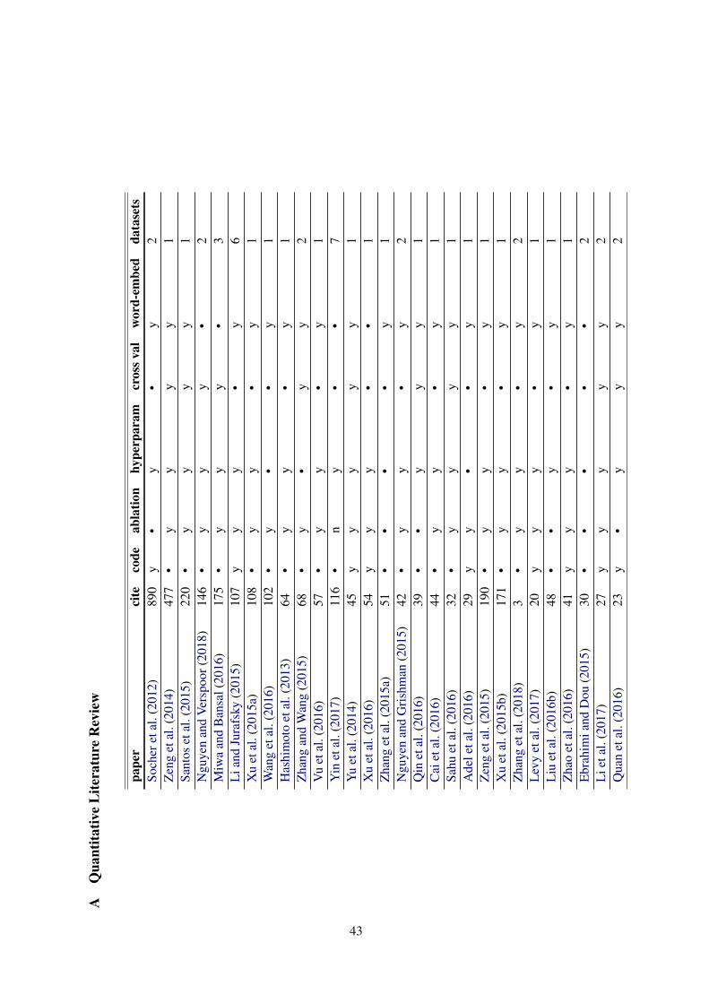
AQ
uant
itativ
eL
itera
ture
Rev
iew
pape
rci
teco
deab
latio
nhy
perp
aram
cros
sval
wor
d-em
bed
data
sets
Soch
eret
al.(
2012
)89
0y
•y
•y
2Z
eng
etal
.(20
14)
477
•y
yy
y1
Sant
oset
al.(
2015
)22
0•
yy
yy
1N
guye
nan
dV
ersp
oor(
2018
)14
6•
yy
y•
2M
iwa
and
Ban
sal(
2016
)17
5•
yy
y•
3L
iand
Jura
fsky
(201
5)10
7y
yy
•y
6X
uet
al.(
2015
a)10
8•
yy
•y
1W
ang
etal
.(20
16)
102
•y
••
y1
Has
him
oto
etal
.(20
13)
64•
yy
•y
1Z
hang
and
Wan
g(2
015)
68•
y•
yy
2V
uet
al.(
2016
)57
•y
y•
y1
Yin
etal
.(20
17)
116
•n
y•
•7
Yu
etal
.(20
14)
45y
yy
yy
1X
uet
al.(
2016
)54
yy
y•
•1
Zha
nget
al.(
2015
a)51
••
••
y1
Ngu
yen
and
Gri
shm
an(2
015)
42•
yy
•y
2Q
inet
al.(
2016
)39
••
yy
y1
Cai
etal
.(20
16)
44•
yy
•y
1Sa
huet
al.(
2016
)32
•y
yy
y1
Ade
leta
l.(2
016)
29y
y•
•y
1Z
eng
etal
.(20
15)
190
•y
y•
y1
Xu
etal
.(20
15b)
171
•y
y•
y1
Zha
nget
al.(
2018
)3
•y
y•
y2
Lev
yet
al.(
2017
)20
yy
y•
y1
Liu
etal
.(20
16b)
48•
•y
•y
1Z
hao
etal
.(20
16)
41y
yy
•y
1E
brah
imia
ndD
ou(2
015)
30•
••
••
2L
ieta
l.(2
017)
27y
yy
yy
2Q
uan
etal
.(20
16)
23y
•y
yy
2
43
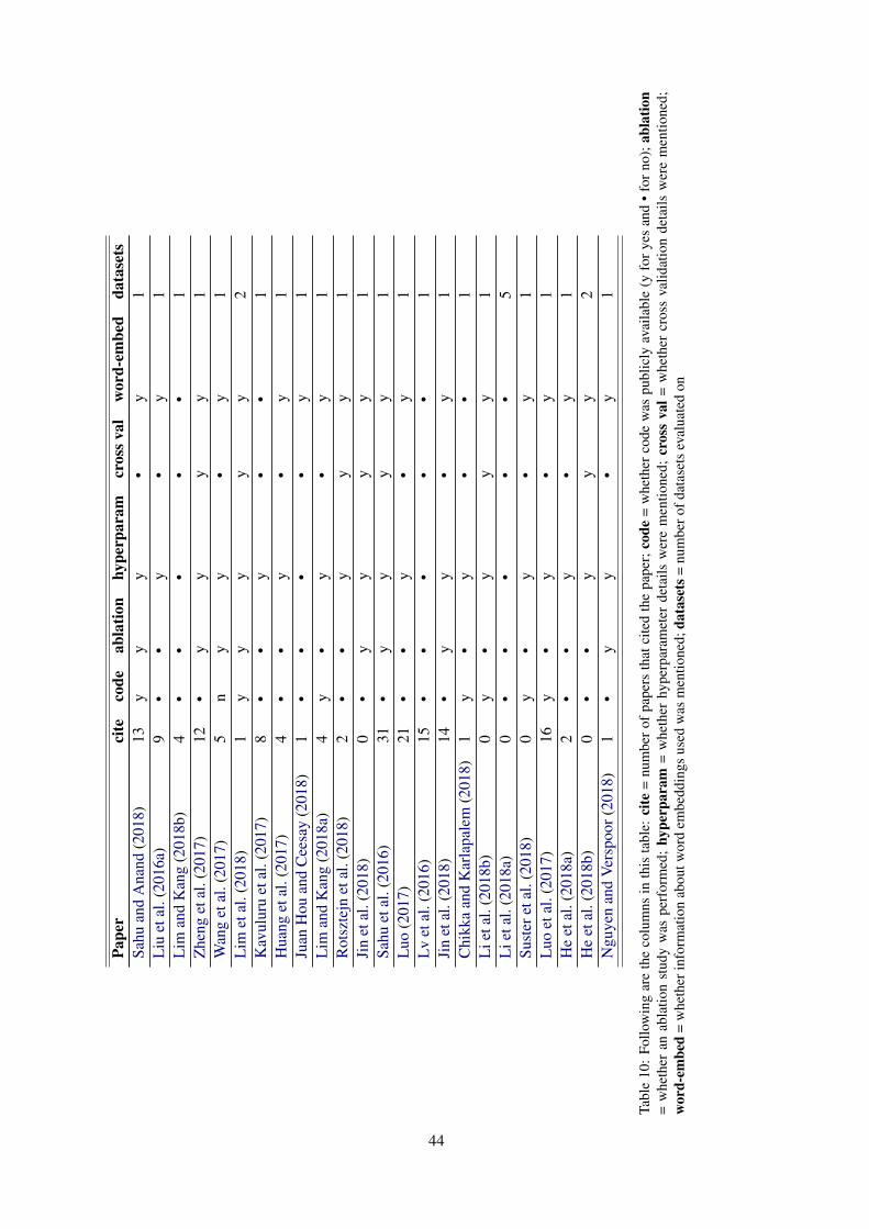
Pape
rci
teco
deab
latio
nhy
perp
aram
cros
sval
wor
d-em
bed
data
sets
Sahu
and
Ana
nd(2
018)
13y
yy
•y
1L
iuet
al.(
2016
a)9
••
y•
y1
Lim
and
Kan
g(2
018b
)4
••
••
•1
Zhe
nget
al.(
2017
)12
•y
yy
y1
Wan
get
al.(
2017
)5
ny
y•
y1
Lim
etal
.(20
18)
1y
yy
yy
2K
avul
uru
etal
.(20
17)
8•
•y
••
1H
uang
etal
.(20
17)
4•
•y
•y
1Ju
anH
ouan
dC
eesa
y(2
018)
1•
••
•y
1L
iman
dK
ang
(201
8a)
4y
•y
•y
1R
otsz
tejn
etal
.(20
18)
2•
•y
yy
1Ji
net
al.(
2018
)0
•y
yy
y1
Sahu
etal
.(20
16)
31•
yy
yy
1L
uo(2
017)
21•
•y
•y
1L
vet
al.(
2016
)15
••
••
•1
Jin
etal
.(20
18)
14•
yy
•y
1C
hikk
aan
dK
arla
pale
m(2
018)
1y
•y
••
1L
ieta
l.(2
018b
)0
y•
yy
y1
Lie
tal.
(201
8a)
0•
••
••
5Su
ster
etal
.(20
18)
0y
•y
•y
1L
uoet
al.(
2017
)16
y•
y•
y1
He
etal
.(20
18a)
2•
•y
•y
1H
eet
al.(
2018
b)0
••
yy
y2
Ngu
yen
and
Ver
spoo
r(20
18)
1•
yy
•y
1
Tabl
e10
:Fo
llow
ing
are
the
colu
mns
inth
ista
ble:
cite
=nu
mbe
rof
pape
rsth
atci
ted
the
pape
r;co
de=
whe
ther
code
was
publ
icly
avai
labl
e(y
for
yes
and
•fo
rno
);ab
latio
n=
whe
ther
anab
latio
nst
udy
was
perf
orm
ed;
hype
rpar
am=
whe
ther
hype
rpar
amet
erde
tails
wer
em
entio
ned;
cros
sva
l=w
heth
ercr
oss
valid
atio
nde
tails
wer
em
entio
ned;
wor
d-em
bed
=w
heth
erin
form
atio
nab
outw
ord
embe
ddin
gsus
edw
asm
entio
ned;
data
sets
=nu
mbe
rofd
atas
ets
eval
uate
don
44
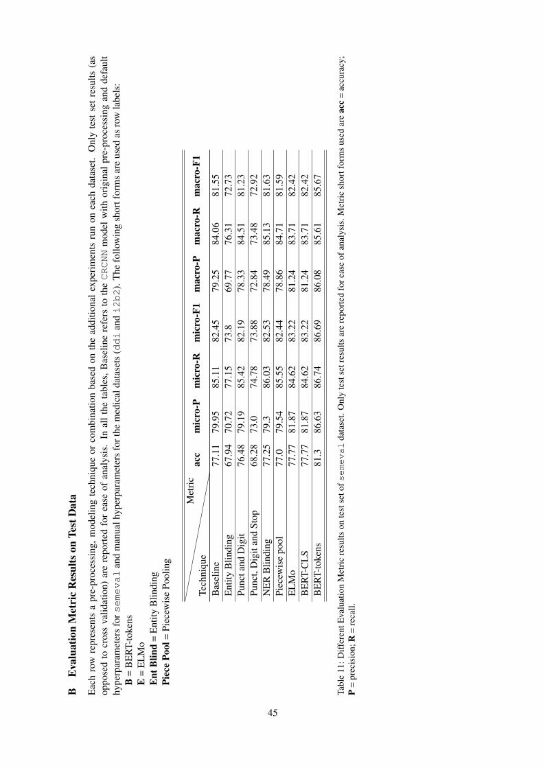
BE
valu
atio
nM
etri
cR
esul
tson
Test
Dat
a
Eac
hro
wre
pres
ents
apr
e-pr
oces
sing
,m
odel
ing
tech
niqu
eor
com
bina
tion
base
don
the
addi
tiona
lex
peri
men
tsru
non
each
data
set.
Onl
yte
stse
tre
sults
(as
oppo
sed
tocr
oss
valid
atio
n)ar
ere
port
edfo
rea
seof
anal
ysis
.In
all
the
tabl
es,B
asel
ine
refe
rsto
theCRCNN
mod
elw
ithor
igin
alpr
e-pr
oces
sing
and
defa
ult
hype
rpar
amet
ers
forsemeval
and
man
ualh
yper
para
met
ers
fort
hem
edic
alda
tase
ts(ddi
andi2b2
).T
hefo
llow
ing
shor
tfor
ms
are
used
asro
wla
bels
:B
=B
ER
T-to
kens
E=
EL
Mo
Ent
Blin
d=
Ent
ityB
lindi
ngPi
ece
Pool
=Pi
ecew
ise
Pool
ing
Tech
niqu
eM
etri
cac
cm
icro
-Pm
icro
-Rm
icro
-F1
mac
ro-P
mac
ro-R
mac
ro-F
1
Bas
elin
e77
.11
79.9
585
.11
82.4
579
.25
84.0
681
.55
Ent
ityB
lindi
ng67
.94
70.7
277
.15
73.8
69.7
776
.31
72.7
3Pu
ncta
ndD
igit
76.4
879
.19
85.4
282
.19
78.3
384
.51
81.2
3Pu
nct,
Dig
itan
dSt
op68
.28
73.0
74.7
873
.88
72.8
473
.48
72.9
2N
ER
Blin
ding
77.2
579
.386
.03
82.5
378
.49
85.1
381
.63
Piec
ewis
epo
ol77
.079
.54
85.5
582
.44
78.8
684
.71
81.5
9E
LM
o77
.77
81.8
784
.62
83.2
281
.24
83.7
182
.42
BE
RT-
CL
S77
.77
81.8
784
.62
83.2
281
.24
83.7
182
.42
BE
RT-
toke
ns81
.386
.63
86.7
486
.69
86.0
885
.61
85.6
7
Tabl
e11
:Diff
eren
tEva
luat
ion
Met
ric
resu
ltson
test
seto
fsemeval
data
set.
Onl
yte
stse
tres
ults
are
repo
rted
fore
ase
ofan
alys
is.M
etri
csh
ortf
orm
sus
edar
eac
c=
accu
racy
;P
=pr
ecis
ion;
R=
reca
ll.
45
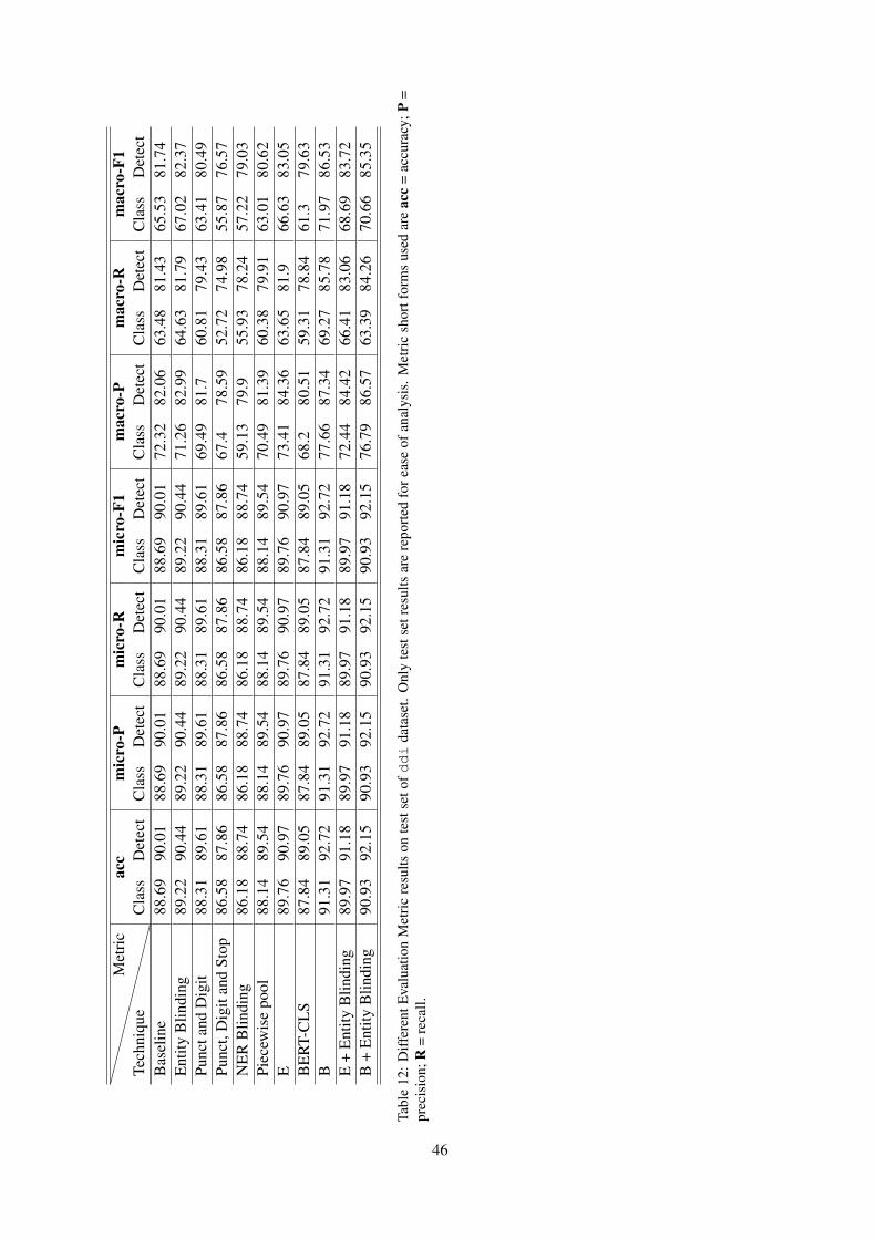
Tech
niqu
eM
etri
cac
cm
icro
-Pm
icro
-Rm
icro
-F1
mac
ro-P
mac
ro-R
mac
ro-F
1C
lass
Det
ect
Cla
ssD
etec
tC
lass
Det
ect
Cla
ssD
etec
tC
lass
Det
ect
Cla
ssD
etec
tC
lass
Det
ect
Bas
elin
e88
.69
90.0
188
.69
90.0
188
.69
90.0
188
.69
90.0
172
.32
82.0
663
.48
81.4
365
.53
81.7
4E
ntity
Blin
ding
89.2
290
.44
89.2
290
.44
89.2
290
.44
89.2
290
.44
71.2
682
.99
64.6
381
.79
67.0
282
.37
Punc
tand
Dig
it88
.31
89.6
188
.31
89.6
188
.31
89.6
188
.31
89.6
169
.49
81.7
60.8
179
.43
63.4
180
.49
Punc
t,D
igit
and
Stop
86.5
887
.86
86.5
887
.86
86.5
887
.86
86.5
887
.86
67.4
78.5
952
.72
74.9
855
.87
76.5
7N
ER
Blin
ding
86.1
888
.74
86.1
888
.74
86.1
888
.74
86.1
888
.74
59.1
379
.955
.93
78.2
457
.22
79.0
3Pi
ecew
ise
pool
88.1
489
.54
88.1
489
.54
88.1
489
.54
88.1
489
.54
70.4
981
.39
60.3
879
.91
63.0
180
.62
E89
.76
90.9
789
.76
90.9
789
.76
90.9
789
.76
90.9
773
.41
84.3
663
.65
81.9
66.6
383
.05
BE
RT-
CL
S87
.84
89.0
587
.84
89.0
587
.84
89.0
587
.84
89.0
568
.280
.51
59.3
178
.84
61.3
79.6
3B
91.3
192
.72
91.3
192
.72
91.3
192
.72
91.3
192
.72
77.6
687
.34
69.2
785
.78
71.9
786
.53
E+
Ent
ityB
lindi
ng89
.97
91.1
889
.97
91.1
889
.97
91.1
889
.97
91.1
872
.44
84.4
266
.41
83.0
668
.69
83.7
2B
+E
ntity
Blin
ding
90.9
392
.15
90.9
392
.15
90.9
392
.15
90.9
392
.15
76.7
986
.57
63.3
984
.26
70.6
685
.35
Tabl
e12
:D
iffer
entE
valu
atio
nM
etri
cre
sults
onte
stse
tofd
di
data
set.
Onl
yte
stse
tres
ults
are
repo
rted
fore
ase
ofan
alys
is.
Met
ric
shor
tfor
ms
used
are
acc
=ac
cura
cy;P
=pr
ecis
ion;
R=
reca
ll.
46
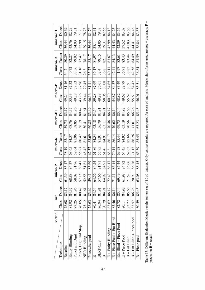
Tech
niqu
eM
etri
cac
cm
icro
-Pm
icro
-Rm
icro
-F1
mac
ro-P
mac
ro-R
mac
ro-F
1C
lass
Det
ect
Cla
ssD
etec
tC
lass
Det
ect
Cla
ssD
etec
tC
lass
Det
ect
Cla
ssD
etec
tC
lass
Det
ect
Bas
elin
e78
.68
83.1
761
.39
83.1
758
.19
83.1
759
.75
83.1
749
.24
81.1
634
.280
.29
36.4
480
.69
Ent
ityB
lindi
ng81
.92
84.3
768
.88
84.3
768
.65
84.3
768
.76
84.3
753
.33
82.3
240
.72
82.2
743
.76
82.2
9Pu
ncta
ndD
igit
77.2
581
.96
58.0
981
.96
59.6
481
.96
58.8
581
.96
49.2
879
.53
33.5
679
.92
34.9
379
.71
Punc
t,D
igit
and
Stop
76.0
580
.47
57.1
580
.47
55.2
780
.47
56.1
980
.47
43.2
677
.96
31.1
677
.47
32.9
977
.7N
ER
Blin
ding
75.1
281
.61
52.5
881
.61
48.4
281
.61
50.4
181
.61
39.4
479
.45
26.3
78.1
729
.15
78.7
3Pi
ecew
ise
pool
78.6
383
.69
59.4
183
.69
62.3
783
.69
60.8
583
.69
46.1
681
.41
35.7
782
.17
36.4
481
.76
E80
.484
.54
64.5
684
.54
61.8
684
.54
63.1
884
.54
59.2
882
.69
36.1
781
.97
38.1
82.3
1B
ER
T-C
LS
76.9
481
.91
57.6
681
.91
55.9
581
.91
56.7
981
.91
49.8
876
.61
32.4
79.1
534
.05
79.3
7B
80.7
984
.91
64.9
284
.91
61.4
84.9
163
.11
84.9
158
.05
83.0
836
.882
.139
.31
82.5
5E
+E
ntity
Blin
ding
83.6
286
.17
72.4
386
.17
68.6
86.1
770
.46
86.1
760
.79
84.6
540
.11
83.6
742
.99
84.1
3E
+Pi
ece
Pool
+E
ntB
lind
83.4
686
.14
71.1
186
.14
70.1
486
.14
70.6
286
.14
54.8
784
.37
42.4
184
.13
44.4
384
.25
Ent
Blin
d+
Piec
ePo
ol82
.72
85.4
469
.49
85.4
469
.98
85.4
469
.73
85.4
448
.82
83.4
941
.97
83.6
142
.89
83.5
5E
+Pi
ece
Pool
80.1
84.9
261
.98
84.9
264
.45
84.9
263
.19
84.9
249
.68
82.7
936
.91
83.4
337
.52
83.0
9B
+E
ntB
lind
83.2
785
.66
71.5
285
.66
69.6
385
.66
70.5
685
.66
55.6
283
.938
.82
83.4
441
.83
83.6
6B
+E
ntB
lind
+Pi
ece
pool
83.5
786
.26
70.9
86.2
671
.13
86.2
671
.01
86.2
655
.684
.43
42.5
884
.49
44.4
84.4
6B
+Pi
ece
pool
80.5
985
.45
63.0
885
.45
63.3
985
.45
63.2
385
.45
56.0
183
.51
36.8
483
.59
38.8
483
.55
Tabl
e13
:Diff
eren
tEva
luat
ion
Met
ric
resu
ltson
test
seto
fi2b2
data
set.
Onl
yte
stse
tres
ults
are
repo
rted
fore
ase
ofan
alys
is.M
etri
csh
ortf
orm
sus
edar
eac
c=
accu
racy
;P=
prec
isio
n;R
=re
call.
47
Proceedings of the BioNLP 2019 workshop, pages 48–57Florence, Italy, August 1, 2019. c©2019 Association for Computational Linguistics
Analysing Representations of Memory Impairment in a Clinical NotesClassification Model
Mark Ormerod, Jesús Martı́nez del Rincón, Neil RobertsonBernadette McGuinness, Barry Devereux
Queen’s University Belfast{mormerod01, j.martinez-del-rincon, n.robertson, b.mcguinness, b.devereux}@qub.ac.uk
Abstract
Despite recent advances in the application ofdeep neural networks to various kinds of med-ical data, extracting information from unstruc-tured textual sources remains a challengingtask. The challenges of training and interpret-ing document classification models are ampli-fied when dealing with small and highly tech-nical datasets, as are common in the clinicaldomain. Using a dataset of de-identified clini-cal letters gathered at a memory clinic, we con-struct several recurrent neural network mod-els for letter classification, and evaluate themon their ability to build meaningful represen-tations of the documents and predict patients’diagnoses. Additionally, we probe sentenceembedding models in order to build a human-interpretable representation of the neural net-work’s features, using a simple and intuitivetechnique based on perturbative approaches tosentence importance. In addition to showingwhich sentences in a document are most in-formative about the patient’s condition, thismethod reveals the types of sentences that leadthe model to make incorrect diagnoses. Fur-thermore, we identify clusters of sentences inthe embedding space that correlate stronglywith importance scores for each clinical diag-nosis class.
1 Introduction
While the majority of clinical data is made upof structured information (Jee and Kim, 2013),which can often be readily integrated into datamodels for research, there is a significant amountof semi-structured and unstructured data whichis increasingly being targeted by machine learn-ing practitioners for analysis. As a general rule,this unstructured data is more difficult to analysedue to an absence of a standardised data model(Ann Alexander and Wang, 2018). Unstructuredclinical data includes a variety of media, suchas video, audio, image and text-based data, withthe majority of such data being made up of text
and images. Recently, there has been a series ofbreakthroughs in the application of machine learn-ing techniques for medical imaging data in or-der to achieve expert-level performance on diag-nosis tasks (Rajpurkar et al., 2017). However, ma-chine learning models using semi-structured andunstructured textual data from the clinical domainhave received less attention and to date have notseen the same degree of successful application.Examples of unstructured medical data featuring“free text” include discharge summaries, nursingreports and progress notes. Historically, one ofthe challenges of applying natural language pro-cessing (NLP) methods to clinical data has beenthe often limited amount of data available, whichhas traditionally necessitated a reliance on manualfeature engineering and relatively shallow textualfeatures (Shickel et al., 2018).
Taking a novel dataset of labelled clinical letterscompiled at a memory clinic as the target data do-main, we build state-of-the-art deep learning mod-els for the task of clinical text classification, andevaluate them on their ability to predict a clin-ician’s diagnosis of the patient. However, deeplearning models generally require very large train-ing datasets. Our approach to the problem there-fore incorporates transfer learning, and we makeuse of embedding data from pre-trained modelstrained on large corpora. In order to investigatethe relative usefulness of word-level and sentence-level information, we train and evaluate severalmodels, including a ULMFiT model (Howardand Ruder, 2018) and two long short-term mem-ory (LSTM) (Hochreiter and Schmidhuber, 1997)models: one trained on word embedding repre-sentations of the documents and one trained onsentence embedding representations (Basile et al.,2012).
An infamous problem of deep neural networksis that they are “black boxes”, with the detailsof how they represent and process information
48
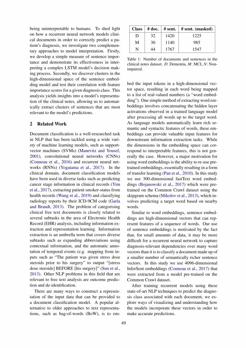
being uninterpretable to humans. To shed lighton how a recurrent neural network models clini-cal documents in order to correctly predict a pa-tient’s diagnosis, we investigate two complemen-tary approaches to model interpretation. Firstly,we develop a simple measure of sentence impor-tance and demonstrate its effectiveness in inter-preting a complex LSTM model’s decision mak-ing process. Secondly, we discover clusters in thehigh-dimensional space of the sentence embed-ding model and test their correlation with featureimportance scores for a given diagnosis class. Thisanalysis yields insights into a model’s representa-tion of the clinical notes, allowing us to automat-ically extract clusters of sentences that are mostrelevant to the model’s predictions.
2 Related Work
Document classification is a well-researched taskin NLP that has been tackled using a wide vari-ety of machine learning models, such as support-vector machines (SVMs) (Manevitz and Yousef,2001), convolutional neural networks (CNNs)(Conneau et al., 2016) and recurrent neural net-works (RNNs) (Yogatama et al., 2017). In theclinical domain, document classification modelshave been used in diverse tasks such as predictingcancer stage information in clinical records (Yimet al., 2017), extracting patient smoker-status fromhealth records (Wang et al., 2019) and classifyingradiology reports by their ICD-9CM code (Garlaand Brandt, 2013). The problem of categorisingclinical free text documents is closely related toseveral subtasks in the area of Electronic HealthRecord (EHR) analysis, including information ex-traction and representation learning. Informationextraction is an umbrella term that covers diversesubtasks such as expanding abbreviations usingcontextual information, and the automatic anno-tation of temporal events (e.g. mapping from in-puts such as “The patient was given stress dosesteroids prior to his surgery” to output “[stressdose steroids] BEFORE [his surgery]” (Sun et al.,2013). Other NLP problems in this field that arerelevant to free text analysis are outcome predic-tion and de-identification.
There are many ways to construct a represen-tation of the input data that can be provided toa document classification model. A popular al-ternative to older approaches to text representa-tions, such as bag-of-words (BoW), is to em-
Class # doc. # sent. # sent. (masked)D 32 1420 1225M 30 1140 985N 44 1767 1547
Table 1: Number of documents and sentences in theclinical notes dataset. D: Dementia, M: MCI, N: Non-impaired.
bed the input tokens in a high-dimensional vec-tor space, resulting in each word being mappedto a list of real-valued numbers (a “word embed-ding”). One simple method of extracting word em-beddings involves concatenating the hidden layeractivations observed in a trained language modelafter processing all words up to the target word.As language models automatically learn rich se-mantic and syntactic features of words, these em-beddings can provide valuable input features fordownstream information extraction tasks. Whilethe dimensions in the embedding space can cor-respond to interpretable features, this is not gen-erally the case. However, a major motivation forusing word embeddings is the ability to re-use pre-trained embeddings, essentially resulting in a formof transfer learning (Pan et al., 2010). In this studywe use 300-dimensional fastText word embed-dings (Bojanowski et al., 2017) which were pre-trained on the Common Crawl dataset using theskipgram schema (Mikolov et al., 2013), which in-volves predicting a target word based on nearbywords.
Similar to word embeddings, sentence embed-dings are high-dimensional vectors that can rep-resent features of a sequence of words. Our useof sentence embeddings is motivated by the factthat, for small amounts of data, it may be moredifficult for a recurrent neural network to capturediagnosis-relevant dependencies over many wordvectors than it is to classify a document made up ofa smaller number of semantically richer sentencevectors. In this study we use 4096-dimensionalInferSent embeddings (Conneau et al., 2017) thatwere extracted from a model pre-trained on theCommon Crawl dataset.
After training recurrent models using thesestate-of-art NLP techniques to predict the diagno-sis class associated with each document, we ex-plore ways of visualizing and understanding howthe models incorporate these vectors in order tomake accurate predictions.
49
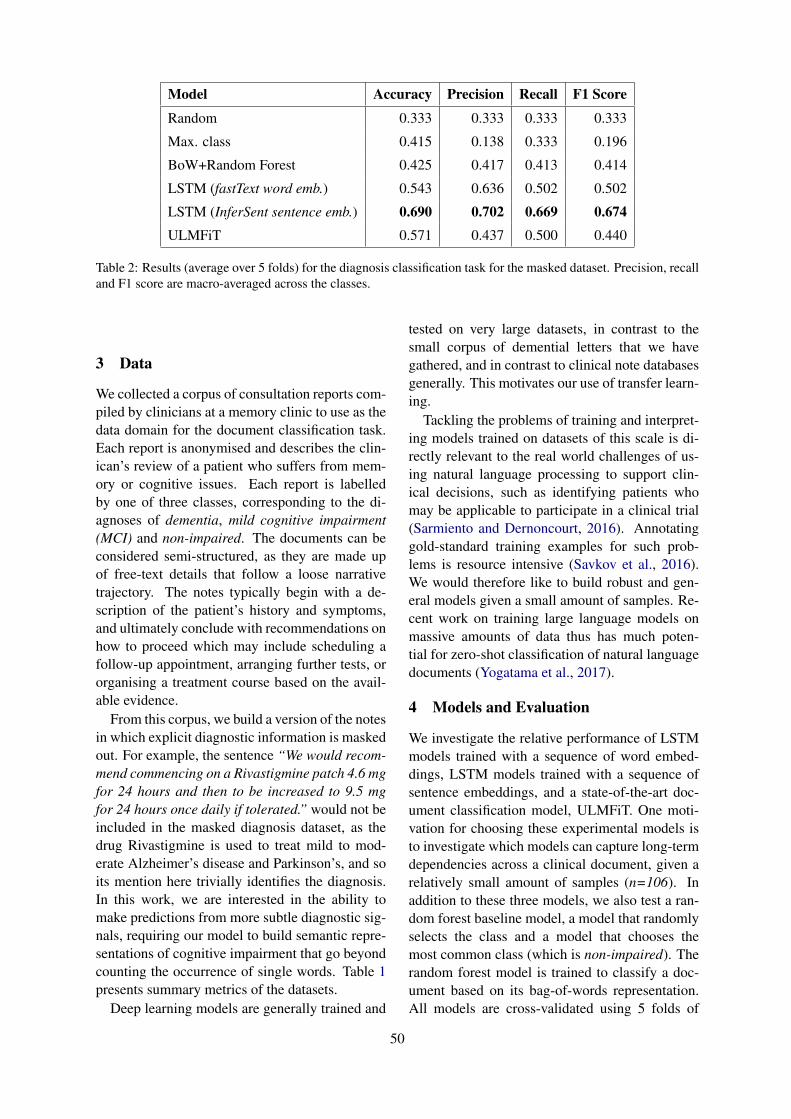
Model Accuracy Precision Recall F1 Score
Random 0.333 0.333 0.333 0.333
Max. class 0.415 0.138 0.333 0.196
BoW+Random Forest 0.425 0.417 0.413 0.414
LSTM (fastText word emb.) 0.543 0.636 0.502 0.502
LSTM (InferSent sentence emb.) 0.690 0.702 0.669 0.674ULMFiT 0.571 0.437 0.500 0.440
Table 2: Results (average over 5 folds) for the diagnosis classification task for the masked dataset. Precision, recalland F1 score are macro-averaged across the classes.
3 Data
We collected a corpus of consultation reports com-piled by clinicians at a memory clinic to use as thedata domain for the document classification task.Each report is anonymised and describes the clin-ican’s review of a patient who suffers from mem-ory or cognitive issues. Each report is labelledby one of three classes, corresponding to the di-agnoses of dementia, mild cognitive impairment(MCI) and non-impaired. The documents can beconsidered semi-structured, as they are made upof free-text details that follow a loose narrativetrajectory. The notes typically begin with a de-scription of the patient’s history and symptoms,and ultimately conclude with recommendations onhow to proceed which may include scheduling afollow-up appointment, arranging further tests, ororganising a treatment course based on the avail-able evidence.
From this corpus, we build a version of the notesin which explicit diagnostic information is maskedout. For example, the sentence “We would recom-mend commencing on a Rivastigmine patch 4.6 mgfor 24 hours and then to be increased to 9.5 mgfor 24 hours once daily if tolerated.” would not beincluded in the masked diagnosis dataset, as thedrug Rivastigmine is used to treat mild to mod-erate Alzheimer’s disease and Parkinson’s, and soits mention here trivially identifies the diagnosis.In this work, we are interested in the ability tomake predictions from more subtle diagnostic sig-nals, requiring our model to build semantic repre-sentations of cognitive impairment that go beyondcounting the occurrence of single words. Table 1presents summary metrics of the datasets.
Deep learning models are generally trained and
tested on very large datasets, in contrast to thesmall corpus of demential letters that we havegathered, and in contrast to clinical note databasesgenerally. This motivates our use of transfer learn-ing.
Tackling the problems of training and interpret-ing models trained on datasets of this scale is di-rectly relevant to the real world challenges of us-ing natural language processing to support clin-ical decisions, such as identifying patients whomay be applicable to participate in a clinical trial(Sarmiento and Dernoncourt, 2016). Annotatinggold-standard training examples for such prob-lems is resource intensive (Savkov et al., 2016).We would therefore like to build robust and gen-eral models given a small amount of samples. Re-cent work on training large language models onmassive amounts of data thus has much poten-tial for zero-shot classification of natural languagedocuments (Yogatama et al., 2017).
4 Models and Evaluation
We investigate the relative performance of LSTMmodels trained with a sequence of word embed-dings, LSTM models trained with a sequence ofsentence embeddings, and a state-of-the-art doc-ument classification model, ULMFiT. One moti-vation for choosing these experimental models isto investigate which models can capture long-termdependencies across a clinical document, given arelatively small amount of samples (n=106). Inaddition to these three models, we also test a ran-dom forest baseline model, a model that randomlyselects the class and a model that chooses themost common class (which is non-impaired). Therandom forest model is trained to classify a doc-ument based on its bag-of-words representation.All models are cross-validated using 5 folds of
50
Figure 1: Visualisation of sentence importance with respect to the successful classification of non-impaired for asubset of a document. Sentences that were found to be important for the classification of non-impaired are colouredgreen while a sentence that increases the chance of a misclassification (i.e. an incorrect MCI diagnosis) is colouredred. The saturation of the colours corresponds to how much a given word contributes to a sentence’s InferSentembedding
the dataset, ensuring that the class distribution isequal across all folds. The ULMFiT model is pre-trained on the Wikitext-103 dataset (Merity et al.,2017) and fine-tuned using default hyperparam-eters (fine-tuning epochs=25, fine-tuning batchsize=8, fine-tuning learning rate=0.004, train-ing epochs=50, training batch size=32, traininglearning rate=0.01) which have been shown to berobust across various tasks (Howard and Ruder,2018). The LSTM model’s hyperparameters werechosen by a grid-search. Both the sentence em-bedding LSTM and the word embedding LSTMwere made up of one hidden layer with 256 hid-den units.
The classification results for the models for themasked dataset are presented in Table 2. Eachof our three models perform significantly betterthan chance and better than the random forestbaseline model, with the LSTM model trainedwith sentence-embedding sequential input achiev-ing the best performance. For this amount oftraining data, we would expect models that aretrained on shorter sequences of more semanticallyenriched pre-trained vectors (i.e. sentence em-beddings) to perform better than much longer se-quences of vectors with less dimensions (i.e. wordembeddings). This is because much of the workof combining word-level tokens into a contextualrepresentation that is relevant to a statistical modelof human language has already been done whentraining with pretrained representations extractedat the sentence-level. Somewhat surprisingly, themodel trained on sentence embeddings outper-formed the fine-tuned ULMFiT. Future work mayshed light on how the amount of training samples
can affect the choice of whether to use fine-tuningor pre-trained embedding representations as modelinput.
5 Model Interpretability: CalculatingSentence Importance Scores
After demonstrating the effectiveness of usingpre-trained sentence embeddings to classify theclinical documents, we investigated model inter-pretability by calculating a measure of the impor-tance of each sentence in the sequence of sen-tences to the model’s prediction for a document.We propose a measure of feature importance basedon perturbative approaches to variable importance(Breiman, 2001), which estimate the importanceof variables by iteratively randomly perturbingeach variable and observing the change in loss.This technique is similar to measuring informa-tion gain (Quinlan, 1986), but rather than selectingimportant components of fixed input, we rate theimportance of a sentence vector in the sequenceof sentence vectors presented to our sequentialLSTM classifier. For example, in order to gener-ate the importance score for the first sentence in adocument made up of m sentence embeddings, weconstruct an augmented version of the documentcontaining all but the first sentence, and examinethe resulting change in the prediction for that doc-ument. More formally, for sentence n, we gener-ate the following version of the document d (withground truth label c) with sentence n removed:
dn = [s0, s1, . . . , sn−1, sn+1, . . . , sm−1]
Next, the augmented document dn is fed intothe trained LSTM (using the best-in-fold model
51
Ratio Sentence-3.469 “He and his wife both report agitation disinhibition and irritability”0.078 “He would say that he feels depressed at times”0.149 “She was tremulous which <NAME> felt was most likely due to anxiety”
. . .
2.108 “He had an equivalent score of 19 / 30 on the MMSE”8.105 “He had an equivalent score of 29 / 30 on the MMSE”
12.887 “He had an equivalent score of 22 / 30 on the MMSE”
Table 3: Sentences sorted by feature importance for a correct diagnosis of non-impaired. Sentences with lowscores do not support a prediction of non-impaired within the context of the corresponding clinical letter.
from Section 3, which achieved an accuracy of73%) and we measure the network’s output logitfor the correct class. The importance score is cal-culated as the ratio of the model’s output for thecorrect class excluding the sentence to the model’soutput for the correct class including a given sen-tence.
ration =logit(c | dn)logit(c | d)
The most important sentences minimise this ra-tio. When the ratio is over 1, the inclusion ofthe sentence in the document leads to a smallerprobability of selecting the correct class, and sosentences that maximise the ratio are the mostmisleading sentences with respect to the correctclassification. Examples of highly important andhighly misleading sentences across the corpus fora diagnosis of non-impaired are presented in Ta-ble 3. The average sentence importance trajectoryover each class was also investigated and is pre-sented in in Figure 2.
Figure 1 presents a section of a clinical letterfor a patient with a diagnosis of non-impaired,with sentences coloured green or red dependingon whether they increase or decrease the chanceof correctly classifying the document. Withineach sentence, the contribution of a word to theInferSent sentence embedding is visualised bycolour saturation. We can see that the importancemeasure provides intuitive insights into how therecurrent neural network models the document.For example, the final sentence in Figure 1 de-creases the chance of classifying the documentas non-impaired because it states that the patientsometimes forgets to take their medicine – in iso-lation this sentence could naively be considered toimply a diagnosis of memory impairment, but asthe model processes the full document it is able to
Figure 2: Average sentence importance over each class,as a function of sentences’ position in the texts. Sen-tence importance ratios are normalised within eachdocument and split by in-document position into 20bins. For each class, we plot the negative of the av-erage for each bin.
accumulate evidence and predict the correct diag-nosis. By examining the contribution of each wordto the InferSent vectors, we can see that negat-ing words such as “not” are handled appropriatelywithin the sentence embedding (e.g. “not clini-cally depressed” increases the probability of a cor-rect non-impaired classification). Our model in-terpretation technique therefore demonstrates howthe LSTM sentence embedding model improveson the simple bag-of-words baseline, where theword “depressed” would be incorrectly taken asnegative evidence for a non-impaired diagnosis.
6 Cluster Analysis
In order to investigate the relationship betweensentence importance and the sentence embeddingspace, we performed a cluster analysis. The 4096-dimensional sentence embeddings were projected
52
(a) t-SNE clustering of sentence embedding vectors (b) Feature importance for class dementia
(c) Feature importance for class MCI (d) Feature importance for class non-impaired
Figure 3: 2-dimensional projection of sentence embedding vectors. (a): 30 clusters were identified and labelledusing mean shift clustering. (b) - (d): Heat maps of sentence vectors coloured by sentence importance for eachclass reveal clusters of sentences that are relevant to a given diagnosis. Colour scales indicate normalised values;brighter colours indicate more important sentences.
to two dimensions using t-SNE (van der Maatenand Hinton, 2008). We used the mean shift clus-tering technique (Yizong Cheng, 1995), an algo-rithm that does not require the number of clustersto be specified in advance, to discover clusters ofsimilarly represented sentences in this space (Fig.3(a)). Sentences that are important for the model’sclassification of a specific diagnosis are visualisedby colouring the sentences using the correspond-ing importance score. This step was performed foreach of the three classes (Fig. 3(b)-(d)).
Correlation tests were used to investigate the re-lationship between sentence clusters and their im-portance to a model’s prediction for each class.
For each class c and for each cluster cl, we firstgather the sentences that appear in documents ofclass c. Next, we assign each sentence a value of 1or 0 depending on whether the sentence is in clus-ter cl. Using Spearman’s Rho, we calculate thecorrelation between this value and the sentences’importance scores for the given class. In eachtrial, sentences that do not appear in documentsof the target class are excluded. The results re-ported in Table 4 show the clusters that were foundto be significantly correlated with at least one ofthe classes’ importance scores. It was found that15 out of the 30 automatically discovered sentenceclusters can be considered significantly important
53
in the model’s decision making.To assist in interpreting the information cap-
tured by each cluster, we depict the clusters usingthe most frequent bigrams across all of that clus-ter’s sentences (Table 4). For example, one cluster(corresponding to cluster 20 in Figure 3(a)) con-tains sentences that mention the individual’s fam-ily (significantly positively associated with a non-impaired diagnosis), while cluster 22 correspondsto sentences about the patient’s blood pressure andheart rate (significantly negatively associated witha non-impaired diagnosis). Again, these resultsshow the utility of combining sentence importancemeasures with sentence embeddings to reveal theclinically relevant detail in the documents.
7 Discussion
The results presented in Table 3 demonstrate thesentences that are most significant and most mis-leading for the LSTM InferSent model with re-spect to the diagnosis of non-impairment. Wecan see that the most significant sentences arethose that refer to patients’ mood and anxietydisorders. These types of sentences are over-represented in the non-impaired group. The typesof sentences that are most misleading to the di-agnosis of non-impaired are those of the format“[pronoun] had an equivalent score of [score] /30 on the MMSE”. An obvious question regardingthis result is whether information about MMSEscores can be represented by the InferSent em-beddings in such a way as to distinguish it fromother sentences that differ only, but importantly,by a single integer value. We can see that the rela-tionship between the significance of the sentenceto the actual results in the sentence is non-linear.The 84 mentions of the Mini-Mental State Exami-nation (MMSE) test are equally divided across the3 classes; as there are more non-impaired docu-ments in the dataset overall, the model benefitsfrom learning not to predict this diagnosis when itencounters any sentence embedding in the MMSEcluster (cluster 17 in Figure 3(a); the correspond-ing points in Figure 3(d) indicate their decreasedimportance for this category). Further analysismay include using diagnostic classifiers (Hupkeset al., 2018) to test whether a model can accuratelydecide whether the first of two given sentence em-beddings reports a larger score.
Figure 2 shows the average sentence signifi-cance across the documents for each of the three
classes. For all classes, we can see that the im-portance of sentences tends to increase with theirin-document position. This trend may correspondto the semi-structured nature of the documents, re-flecting information becoming more relevant to adiagnosis towards the end of a document. An-other possible explanation could be that the re-current neural network is unable to capture long-distance dependencies given the small amount ofsamples in the dataset, resulting in a kind of re-cency bias in the model’s processing (since themodel only makes its prediction at the end of thesequence of sentences). Further work may involvesystematically changing the position of each sen-tence within each document in order to investigatethe effect that this has on the importance scoresassociated with each sentence.
Table 4 shows that no clusters were significantlycorrelated with the class dementia, with all re-ported clusters being significantly correlated withat least one of MCI or non-impaired. Exclud-ing cluster 18, all of the clusters that are signif-icant for both MCI and non-impaired form pairsof negative vs. positive correlations between thesetwo classes, suggesting that the model learns pri-marily to discriminate between these classes. Ex-amining the confusion matrix for the model, wefound that the model has a true positive rate of1.0 and 0.89 for MCI and non-impaired, and min-imises the amount of false positives between thesetwo classes. However, the model performs poorlywhen the actual document corresponds to a di-agnosis of dementia (with a true positive rate of0.29). This is consistent with the observation thatnone of the clusters significantly correlate withthis class. While this insight could be gained fromexamining the confusion matrix alone, the advan-tage of employing the interpretation methods de-veloped in this paper is that they allow us to gainan understanding of how the model’s processingof sentences over time leads to these inequalities,suggesting avenues of attack for constructing moreaccurate representations of the documents goingforward.
In future work, we plan to gather more clini-cal documents that describe patients with mem-ory impairment and continue our analysis of lan-guage modelling and classification in this distri-bution. We hope to subsequently apply state of theart contextualised embeddings such as ELMO (Pe-ters et al., 2018) and BERT (Devlin et al., 2018)
54
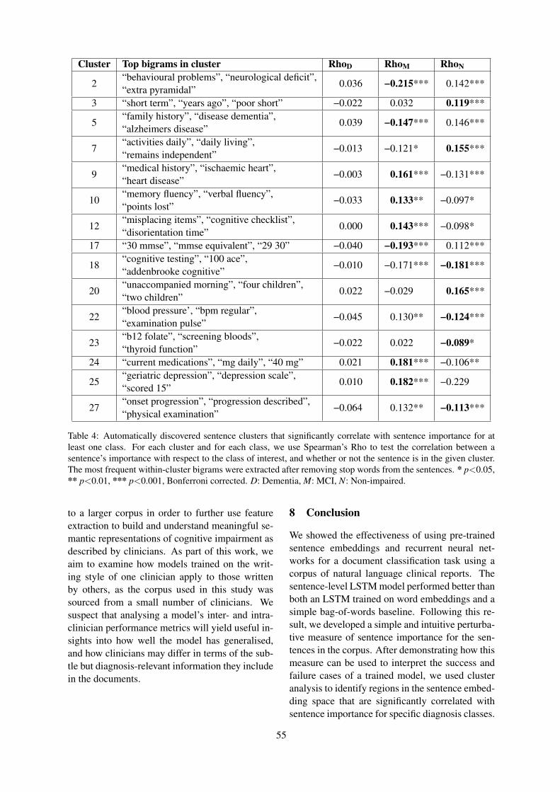
Cluster Top bigrams in cluster RhoD RhoM RhoN
2“behavioural problems”, “neurological deficit”,“extra pyramidal”
0.036 −0.215*** 0.142***
3 “short term”, “years ago”, “poor short” −0.022 0.032 0.119***
5“family history”, “disease dementia”,“alzheimers disease”
0.039 −0.147*** 0.146***
7“activities daily”, “daily living”,“remains independent”
−0.013 −0.121* 0.155***
9“medical history”, “ischaemic heart”,“heart disease”
−0.003 0.161*** −0.131***
10“memory fluency”, “verbal fluency”,“points lost”
−0.033 0.133** −0.097*
12“misplacing items”, “cognitive checklist”,“disorientation time”
0.000 0.143*** −0.098*
17 “30 mmse”, “mmse equivalent”, “29 30” −0.040 −0.193*** 0.112***
18“cognitive testing”, “100 ace”,“addenbrooke cognitive”
−0.010 −0.171*** −0.181***
20“unaccompanied morning”, “four children”,“two children”
0.022 −0.029 0.165***
22“blood pressure’, “bpm regular”,“examination pulse”
−0.045 0.130** −0.124***
23“b12 folate”, “screening bloods”,“thyroid function”
−0.022 0.022 −0.089*
24 “current medications”, “mg daily”, “40 mg” 0.021 0.181*** −0.106**
25“geriatric depression”, “depression scale”,“scored 15”
0.010 0.182*** −0.229
27“onset progression”, “progression described”,“physical examination”
−0.064 0.132** −0.113***
Table 4: Automatically discovered sentence clusters that significantly correlate with sentence importance for atleast one class. For each cluster and for each class, we use Spearman’s Rho to test the correlation between asentence’s importance with respect to the class of interest, and whether or not the sentence is in the given cluster.The most frequent within-cluster bigrams were extracted after removing stop words from the sentences. * p<0.05,** p<0.01, *** p<0.001, Bonferroni corrected. D: Dementia, M: MCI, N: Non-impaired.
to a larger corpus in order to further use featureextraction to build and understand meaningful se-mantic representations of cognitive impairment asdescribed by clinicians. As part of this work, weaim to examine how models trained on the writ-ing style of one clinician apply to those writtenby others, as the corpus used in this study wassourced from a small number of clinicians. Wesuspect that analysing a model’s inter- and intra-clinician performance metrics will yield useful in-sights into how well the model has generalised,and how clinicians may differ in terms of the sub-tle but diagnosis-relevant information they includein the documents.
8 Conclusion
We showed the effectiveness of using pre-trainedsentence embeddings and recurrent neural net-works for a document classification task using acorpus of natural language clinical reports. Thesentence-level LSTM model performed better thanboth an LSTM trained on word embeddings and asimple bag-of-words baseline. Following this re-sult, we developed a simple and intuitive perturba-tive measure of sentence importance for the sen-tences in the corpus. After demonstrating how thismeasure can be used to interpret the success andfailure cases of a trained model, we used clusteranalysis to identify regions in the sentence embed-ding space that are significantly correlated withsentence importance for specific diagnosis classes.
55
By reviewing the most frequent bigrams in eachcluster and examining the sign of Spearman’s Rhofor each corresponding correlated class, we caninterpret how differential processing of sentencevectors within each cluster can lead to class im-balances in the model’s predictions, demonstratingthe power of our approach for model interpretabil-ity and evaluation.
Acknowledgements
We would like to thank the three anonymous re-viewers, Stuart Millar, and Steven Derby for theirfeedback and suggestions. This work was part-funded by a Data Analytics Dementia PathfinderProgramme Grant from the Northern IrelandHSCB eHealth Directorate.
ReferencesCheryl Ann Alexander and Lidong Wang. 2018. Big
Data and Data-Driven Healthcare Systems. Journalof Business and Management Sciences, 6(3):104–111.
Pierpaolo Basile, Annalina Caputo, and Giovanni Se-meraro. 2012. A Study on Compositional Semanticsof Words in Distributional Spaces. In 2012 IEEESixth International Conference on Semantic Com-puting, pages 154–161. IEEE.
Piotr Bojanowski, Edouard Grave, Armand Joulin, andTomas Mikolov. 2017. Enriching Word Vectors withSubword Information. Transactions of the Associa-tion for Computational Linguistics, 5:135–146.
Leo Breiman. 2001. Random Forests. Machine Learn-ing, 45(1):5–32.
Alexis Conneau, Douwe Kiela, Holger Schwenk, LoicBarrault, and Antoine Bordes. 2017. SupervisedLearning of Universal Sentence Representationsfrom Natural Language Inference Data. arXivpreprint arXiv:1705.02364.
Alexis Conneau, Holger Schwenk, Loı̈c Barrault,and Yann Lecun. 2016. Very deep convolutionalnetworks for text classification. arXiv preprintarXiv:1606.01781.
Jacob Devlin, Ming-Wei Chang, Kenton Lee, andKristina Toutanova. 2018. Bert: Pre-training of deepbidirectional transformers for language understand-ing. arXiv preprint arXiv:1810.04805.
Vijay N Garla and Cynthia Brandt. 2013. Knowledge-based biomedical word sense disambiguation: anevaluation and application to clinical document clas-sification. Journal of the American Medical Infor-matics Association, 20(5):882–886.
Sepp Hochreiter and Jürgen Schmidhuber. 1997.Long short-term memory. Neural computation,9(8):1735–1780.
Jeremy Howard and Sebastian Ruder. 2018. UniversalLanguage Model Fine-tuning for Text Classification.Proceedings of the 56th Annual Meeting of the As-sociation for Computational Linguistics (Volume 1:Long Papers), 1:328–339.
Dieuwke Hupkes, Sara Veldhoen, and WillemZuidema. 2018. Visualisation and ’diagnostic classi-fiers’ reveal how recurrent and recursive neural net-works process hierarchical structure. Journal of Ar-tificial Intelligence Research.
Kyoungyoung Jee and Gang-Hoon Kim. 2013. Poten-tiality of Big Data in the Medical Sector: Focus onHow to Reshape the Healthcare System. HealthcareInformatics Research, 19(2):79.
Laurens van der Maaten and Geoffrey Hinton. 2008.Visualizing Data using t-SNE. Journal of MachineLearning Research, 9(Nov):2579–2605.
Larry M Manevitz and Malik Yousef. 2001. One-classSVMs for document classification. Journal of ma-chine Learning research, 2(Dec):139–154.
Stephen Merity, Nitish Shirish Keskar, and RichardSocher. 2017. Regularizing and Optimiz-ing LSTM Language Models. arXiv preprintarXiv:1708.02182.
Tomas Mikolov, Kai Chen, Greg Corrado, and JeffreyDean. 2013. Efficient Estimation of Word Represen-tations in Vector Space. preprint arXiv:1301.3781.
Sinno Jialin Pan, Qiang Yang, and Others. 2010. Asurvey on transfer learning. IEEE Transactionson knowledge and data engineering, 22(10):1345–1359.
Matthew E Peters, Mark Neumann, Mohit Iyyer, MattGardner, Christopher Clark, Kenton Lee, and LukeZettlemoyer. 2018. Deep contextualized word rep-resentations. arXiv preprint arXiv:1802.05365.
J. R. Quinlan. 1986. Induction of decision trees. Ma-chine Learning, 1(1):81–106.
Pranav Rajpurkar, Jeremy Irvin, Kaylie Zhu, Bran-don Yang, Hershel Mehta, Tony Duan, Daisy Ding,Aarti Bagul, Curtis Langlotz, Katie Shpanskaya,Matthew P. Lungren, and Andrew Y. Ng. 2017.CheXNet: Radiologist-Level Pneumonia Detectionon Chest X-Rays with Deep Learning. arXivpreprint arXiv:1711.05225.
Raymond Francis Sarmiento and Franck Dernoncourt.2016. Improving patient cohort identification usingnatural language processing. In Secondary anal-ysis of electronic health records, pages 405–417.Springer.
56
Aleksandar Savkov, John Carroll, Rob Koeling, andJackie Cassell. 2016. Annotating patient clinicalrecords with syntactic chunks and named entities:the harvey corpus. Language resources and eval-uation, 50(3):523–548.
Benjamin Shickel, Patrick James Tighe, Azra Biho-rac, and Parisa Rashidi. 2018. Deep EHR: A Sur-vey of Recent Advances in Deep Learning Tech-niques for Electronic Health Record (EHR) Analy-sis. IEEE Journal of Biomedical and Health Infor-matics, 22(5):1589–1604.
Weiyi Sun, Anna Rumshisky, and Ozlem Uzuner. 2013.Temporal reasoning over clinical text: the state ofthe art. Journal of the American Medical Informat-ics Association : JAMIA, 20(5):814–9.
Yanshan Wang, Sunghwan Sohn, Sijia Liu, FeichenShen, Liwei Wang, Elizabeth J. Atkinson, ShreyaseeAmin, and Hongfang Liu. 2019. A clinical text clas-sification paradigm using weak supervision and deeprepresentation. BMC Medical Informatics and De-cision Making, 19(1):1.
Wen-Wai Yim, Sharon W Kwan, Guy Johnson, andMeliha Yetisgen. 2017. Classification of hepatocel-lular carcinoma stages from free-text clinical and ra-diology reports. AMIA ... Annual Symposium pro-ceedings. AMIA Symposium, 2017:1858–1867.
Yizong Cheng. 1995. Mean shift, mode seeking, andclustering. IEEE Transactions on Pattern Analysisand Machine Intelligence, 17(8):790–799.
Dani Yogatama, Chris Dyer, Wang Ling, and Phil Blun-som. 2017. Generative and discriminative text clas-sification with recurrent neural networks. arXivpreprint arXiv:1703.01898.
57
Proceedings of the BioNLP 2019 workshop, pages 58–65Florence, Italy, August 1, 2019. c©2019 Association for Computational Linguistics
Transfer Learning in Biomedical Natural Language Processing: AnEvaluation of BERT and ELMo on Ten Benchmarking Datasets
Yifan Peng Shankai Yan Zhiyong LuNational Center for Biotechnology Information
National Library of Medicine, National Institutes of HealthBethesda, MD, USA
{yifan.peng, shankai.yan, zhiyong.lu}@nih.gov
Abstract
Inspired by the success of the General Lan-guage Understanding Evaluation benchmark,we introduce the Biomedical Language Un-derstanding Evaluation (BLUE) benchmarkto facilitate research in the development ofpre-training language representations in thebiomedicine domain. The benchmark consistsof five tasks with ten datasets that cover bothbiomedical and clinical texts with differentdataset sizes and difficulties. We also evaluateseveral baselines based on BERT and ELMoand find that the BERT model pre-trainedon PubMed abstracts and MIMIC-III clinicalnotes achieves the best results. We make thedatasets, pre-trained models, and codes pub-licly available at https://github.com/ncbi-nlp/BLUE_Benchmark.
1 Introduction
With the growing amount of biomedical informa-tion available in textual form, there have beensignificant advances in the development of pre-training language representations that can be ap-plied to a range of different tasks in the biomedi-cal domain, such as pre-trained word embeddings,sentence embeddings, and contextual representa-tions (Chiu et al., 2016; Chen et al., 2019; Peterset al., 2017; Lee et al., 2019; Smalheiser et al.,2019).
In the general domain, we have recently ob-served that the General Language Understand-ing Evaluation (GLUE) benchmark (Wang et al.,2018a) has been successfully promoting the de-velopment of language representations of generalpurpose (Peters et al., 2017; Radford et al., 2018;Devlin et al., 2019). To the best of our knowledge,however, there is no publicly available bench-marking in the biomedicine domain.
To facilitate research on language representa-tions in the biomedicine domain, we present the
Biomedical Language Understanding Evaluation(BLUE) benchmark, which consists of five dif-ferent biomedicine text-mining tasks with ten cor-pora. Here, we rely on preexisting datasets be-cause they have been widely used by the BioNLPcommunity as shared tasks (Huang and Lu, 2015).These tasks cover a diverse range of text genres(biomedical literature and clinical notes), datasetsizes, and degrees of difficulty and, more impor-tantly, highlight common biomedicine text-miningchallenges. We expect that the models that per-form better on all or most tasks in BLUE will ad-dress other biomedicine tasks more robustly.
To better understand the challenge posed byBLUE, we conduct experiments with two base-lines: One makes use of the BERT model (Devlinet al., 2019) and one makes use of ELMo (Peterset al., 2017). Both are state-of-the-art languagerepresentation models and demonstrate promisingresults in NLP tasks of general purpose. We findthat the BERT model pre-trained on PubMed ab-stracts (Fiorini et al., 2018) and MIMIC-III clini-cal notes (Johnson et al., 2016) achieves the bestresults, and is significantly superior to other mod-els in the clinical domain. This demonstrates theimportance of pre-training among different textgenres.
In summary, we offer: (i) five tasks with tenbiomedical and clinical text-mining corpora withdifferent sizes and levels of difficulty, (ii) codesfor data construction and model evaluation forfair comparisons, (iii) pretrained BERT models onPubMed abstracts and MIMIC-III, and (iv) base-line results.
2 Related work
There is a long history of using shared lan-guage representations to capture text semantics inbiomedical text and data mining research. Such re-
58
search utilizes a technique, termed transfer learn-ing, whereby the language representations are pre-trained on large corpora and fine-tuned in a varietyof downstream tasks, such as named entity recog-nition and relation extraction.
One established trend is a form of word embed-dings that represent the semantic, using high di-mensional vectors (Chiu et al., 2016; Wang et al.,2018c; Zhang et al., 2019). Similar methodsalso have been derived to improve embeddings ofword sequences by introducing sentence embed-dings (Chen et al., 2019). They always, however,require complicated neural networks to be effec-tively used in downstream applications.
Another popular trend, especially in recentyears, is the context-dependent representation.Different from word embeddings, it allows themeaning of a word to change according to the con-text in which it is used (Melamud et al., 2016; Pe-ters et al., 2017; Devlin et al., 2019; Dai et al.,2019). In the scientific domain, Beltagy et al. re-leased SciBERT which is trained on scientific text.In the biomedical domain, BioBERT (Lee et al.,2019) and BioELMo (Jin et al., 2019) were pre-trained and applied to several specific tasks. In theclinical domain, Alsentzer et al. (2019) released aclinical BERT base model trained on the MIMIC-III database. Most of these works, however, wereevaluated on either different datasets or the samedataset with slightly different sizes of examples.This makes it challenging to fairly compare vari-ous language models.
Based on these reasons, a standard benchmark-ing is urgently required. Parallel to our work, Leeet al. (2019) introduced three tasks: named en-tity recognition, relation extraction, and QA, whileJin et al. (2019) introduced NLI in addition tonamed entity recognition. To this end, we deemthat BLUE is different in three ways. First, BLUEis selected to cover a diverse range of text genres,including both biomedical and clinical domains.Second, BLUE goes beyond sentence or sentencepairs by including document classification tasks.Third, BLUE provides a comprehensive suite ofcodes to reconstruct dataset from scratch withoutremoving any instances.
3 Tasks
BLUE contains five tasks with ten corpora thatcover a broad range of data quantities and diffi-culties (Table 1). Here, we rely on preexisting
datasets because they have been widely used bythe BioNLP community as shared tasks.
3.1 Sentence similarity
The sentence similarity task is to predict simi-larity scores based on sentence pairs. Followingcommon practice, we evaluate similarity by usingPearson correlation coefficients.
BIOSSES is a corpus of sentence pairsselected from the Biomedical SummarizationTrack Training Dataset in the biomedical do-main (Soğancıoğlu et al., 2017).1 To developBIOSSES, five curators judged their similarity, us-ing scores that ranged from 0 (no relation) to 4(equivalent). Here, we randomly select 80% fortraining and 20% for testing because there is nostandard splits in the released data.
MedSTS is a corpus of sentence pairs se-lected from Mayo Clinic’s clinical data ware-house (Wang et al., 2018b). To develop MedSTS,two medical experts graded the sentence’s seman-tic similarity scores from 0 to 5 (low to high sim-ilarity). We use the standard training and testingsets in the shared task.
3.2 Named entity recognition
The aim of the named entity recognition task isto predict mention spans given in the text (Ju-rafsky and Martin, 2008). The results are evalu-ated through a comparison of the set of mentionspans annotated within the document with the setof mention spans predicted by the model. We eval-uate the results by using the strict version of preci-sion, recall, and F1-score. For disjoint mentions,all spans also must be strictly correct. To constructthe dataset, we used spaCy2 to split the text into asequence of tokens when the original datasets donot provide such information.
BC5CDR is a collection of 1,500 PubMed titlesand abstracts selected from the CTD-Pfizer cor-pus and was used in the BioCreative V chemical-disease relation task (Li et al., 2016).3 The dis-eases and chemicals mentioned in the articles wereannotated independently by two human expertswith medical training and curation experience.We use the standard training and test set in the
1http://tabilab.cmpe.boun.edu.tr/BIOSSES/
2https://spacy.io/3https://biocreative.bioinformatics.
udel.edu/tasks/biocreative-v/track-3-cdr/
59
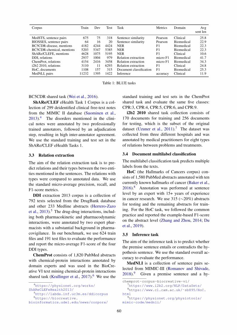
Corpus Train Dev Test Task Metrics Domain Avgsent len
MedSTS, sentence pairs 675 75 318 Sentence similarity Pearson Clinical 25.8BIOSSES, sentence pairs 64 16 20 Sentence similarity Pearson Biomedical 22.9BC5CDR-disease, mentions 4182 4244 4424 NER F1 Biomedical 22.3BC5CDR-chemical, mentions 5203 5347 5385 NER F1 Biomedical 22.3ShARe/CLEFE, mentions 4628 1075 5195 NER F1 Clinical 10.6DDI, relations 2937 1004 979 Relation extraction micro F1 Biomedical 41.7ChemProt, relations 4154 2416 3458 Relation extraction micro F1 Biomedical 34.3i2b2 2010, relations 3110 11 6293 Relation extraction F1 Clinical 24.8HoC, documents 1108 157 315 Document classification F1 Biomedical 25.3MedNLI, pairs 11232 1395 1422 Inference accuracy Clinical 11.9
Table 1: BLUE tasks
BC5CDR shared task (Wei et al., 2016).ShARe/CLEF eHealth Task 1 Corpus is a col-
lection of 299 deidentified clinical free-text notesfrom the MIMIC II database (Suominen et al.,2013).4 The disorders mentioned in the clini-cal notes were annotated by two professionallytrained annotators, followed by an adjudicationstep, resulting in high inter-annotator agreement.We use the standard training and test set in theShARe/CLEF eHealth Tasks 1.
3.3 Relation extraction
The aim of the relation extraction task is to pre-dict relations and their types between the two enti-ties mentioned in the sentences. The relations withtypes were compared to annotated data. We usethe standard micro-average precision, recall, andF1-score metrics.
DDI extraction 2013 corpus is a collection of792 texts selected from the DrugBank databaseand other 233 Medline abstracts (Herrero-Zazoet al., 2013).5 The drug-drug interactions, includ-ing both pharmacokinetic and pharmacodynamicinteractions, were annotated by two expert phar-macists with a substantial background in pharma-covigilance. In our benchmark, we use 624 trainfiles and 191 test files to evaluate the performanceand report the micro-average F1-score of the fourDDI types.
ChemProt consists of 1,820 PubMed abstractswith chemical-protein interactions annotated bydomain experts and was used in the BioCre-ative VI text mining chemical-protein interactionsshared task (Krallinger et al., 2017).6 We use the
4https://physionet.org/works/ShAReCLEFeHealth2013/
5http://labda.inf.uc3m.es/ddicorpus6https://biocreative.
bioinformatics.udel.edu/news/corpora/
standard training and test sets in the ChemProtshared task and evaluate the same five classes:CPR:3, CPR:4, CPR:5, CPR:6, and CPR:9.
i2b2 2010 shared task collection consists of170 documents for training and 256 documentsfor testing, which is the subset of the originaldataset (Uzuner et al., 2011).7 The dataset wascollected from three different hospitals and wasannotated by medical practitioners for eight typesof relations between problems and treatments.
3.4 Document multilabel classificationThe multilabel classification task predicts multiplelabels from the texts.
HoC (the Hallmarks of Cancers corpus) con-sists of 1,580 PubMed abstracts annotated with tencurrently known hallmarks of cancer (Baker et al.,2016).8 Annotation was performed at sentencelevel by an expert with 15+ years of experiencein cancer research. We use 315 (∼20%) abstractsfor testing and the remaining abstracts for train-ing. For the HoC task, we followed the commonpractice and reported the example-based F1-scoreon the abstract level (Zhang and Zhou, 2014; Duet al., 2019).
3.5 Inference taskThe aim of the inference task is to predict whetherthe premise sentence entails or contradicts the hy-pothesis sentence. We use the standard overall ac-curacy to evaluate the performance.
MedNLI is a collection of sentence pairs se-lected from MIMIC-III (Romanov and Shivade,2018).9 Given a premise sentence and a hy-
chemprot-corpus-biocreative-vi/7https://www.i2b2.org/NLP/DataSets/8https://www.cl.cam.ac.uk/˜sb895/HoC.
html9https://physionet.org/physiotools/
mimic-code/mednli/
60
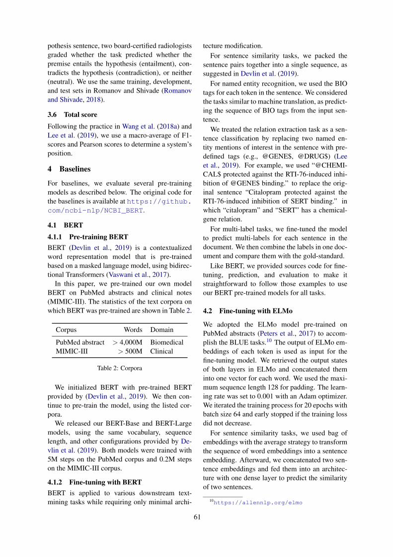
pothesis sentence, two board-certified radiologistsgraded whether the task predicted whether thepremise entails the hypothesis (entailment), con-tradicts the hypothesis (contradiction), or neither(neutral). We use the same training, development,and test sets in Romanov and Shivade (Romanovand Shivade, 2018).
3.6 Total scoreFollowing the practice in Wang et al. (2018a) andLee et al. (2019), we use a macro-average of F1-scores and Pearson scores to determine a system’sposition.
4 Baselines
For baselines, we evaluate several pre-trainingmodels as described below. The original code forthe baselines is available at https://github.com/ncbi-nlp/NCBI_BERT.
4.1 BERT4.1.1 Pre-training BERTBERT (Devlin et al., 2019) is a contextualizedword representation model that is pre-trainedbased on a masked language model, using bidirec-tional Transformers (Vaswani et al., 2017).
In this paper, we pre-trained our own modelBERT on PubMed abstracts and clinical notes(MIMIC-III). The statistics of the text corpora onwhich BERT was pre-trained are shown in Table 2.
Corpus Words Domain
PubMed abstract > 4,000M BiomedicalMIMIC-III > 500M Clinical
Table 2: Corpora
We initialized BERT with pre-trained BERTprovided by (Devlin et al., 2019). We then con-tinue to pre-train the model, using the listed cor-pora.
We released our BERT-Base and BERT-Largemodels, using the same vocabulary, sequencelength, and other configurations provided by De-vlin et al. (2019). Both models were trained with5M steps on the PubMed corpus and 0.2M stepson the MIMIC-III corpus.
4.1.2 Fine-tuning with BERTBERT is applied to various downstream text-mining tasks while requiring only minimal archi-
tecture modification.For sentence similarity tasks, we packed the
sentence pairs together into a single sequence, assuggested in Devlin et al. (2019).
For named entity recognition, we used the BIOtags for each token in the sentence. We consideredthe tasks similar to machine translation, as predict-ing the sequence of BIO tags from the input sen-tence.
We treated the relation extraction task as a sen-tence classification by replacing two named en-tity mentions of interest in the sentence with pre-defined tags (e.g., @GENE$, @DRUG$) (Leeet al., 2019). For example, we used “@CHEMI-CAL$ protected against the RTI-76-induced inhi-bition of @GENE$ binding.” to replace the orig-inal sentence “Citalopram protected against theRTI-76-induced inhibition of SERT binding.” inwhich “citalopram” and “SERT” has a chemical-gene relation.
For multi-label tasks, we fine-tuned the modelto predict multi-labels for each sentence in thedocument. We then combine the labels in one doc-ument and compare them with the gold-standard.
Like BERT, we provided sources code for fine-tuning, prediction, and evaluation to make itstraightforward to follow those examples to useour BERT pre-trained models for all tasks.
4.2 Fine-tuning with ELMo
We adopted the ELMo model pre-trained onPubMed abstracts (Peters et al., 2017) to accom-plish the BLUE tasks.10 The output of ELMo em-beddings of each token is used as input for thefine-tuning model. We retrieved the output statesof both layers in ELMo and concatenated theminto one vector for each word. We used the maxi-mum sequence length 128 for padding. The learn-ing rate was set to 0.001 with an Adam optimizer.We iterated the training process for 20 epochs withbatch size 64 and early stopped if the training lossdid not decrease.
For sentence similarity tasks, we used bag ofembeddings with the average strategy to transformthe sequence of word embeddings into a sentenceembedding. Afterward, we concatenated two sen-tence embeddings and fed them into an architec-ture with one dense layer to predict the similarityof two sentences.
10https://allennlp.org/elmo
61
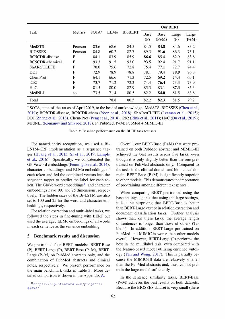
Task Metrics SOTA* ELMo BioBERTOur BERT
Base Base Large Large(P) (P+M) (P) (P+M)
MedSTS Pearson 83.6 68.6 84.5 84.5 84.8 84.6 83.2BIOSSES Pearson 84.8 60.2 82.7 89.3 91.6 86.3 75.1BC5CDR-disease F 84.1 83.9 85.9 86.6 85.4 82.9 83.8BC5CDR-chemical F 93.3 91.5 93.0 93.5 92.4 91.7 91.1ShARe/CLEFE F 70.0 75.6 72.8 75.4 77.1 72.7 74.4DDI F 72.9 78.9 78.8 78.1 79.4 79.9 76.3ChemProt F 64.1 66.6 71.3 72.5 69.2 74.4 65.1i2b2 F 73.7 71.2 72.2 74.4 76.4 73.3 73.9HoC F 81.5 80.0 82.9 85.3 83.1 87.3 85.3MedNLI acc 73.5 71.4 80.5 82.2 84.0 81.5 83.8
Total 78.8 80.5 82.2 82.3 81.5 79.2* SOTA, state-of-the-art as of April 2019, to the best of our knowledge: MedSTS, BIOSSES (Chen et al.,2019); BC5CDR-disease, BC5CDR-chem (Yoon et al., 2018); ShARe/CLEFE (Leaman et al., 2015);DDI (Zhang et al., 2018). Chem-Prot (Peng et al., 2018); i2b2 (Rink et al., 2011); HoC (Du et al., 2019);MedNLI (Romanov and Shivade, 2018). P: PubMed, P+M: PubMed + MIMIC-III
Table 3: Baseline performance on the BLUE task test sets.
For named entity recognition, we used a Bi-LSTM-CRF implementation as a sequence tag-ger (Huang et al., 2015; Si et al., 2019; Lampleet al., 2016). Specifically, we concatenated theGloVe word embeddings (Pennington et al., 2014),character embeddings, and ELMo embeddings ofeach token and fed the combined vectors into thesequence tagger to predict the label for each to-ken. The GloVe word embeddings11 and characterembeddings have 100 and 25 dimensions, respec-tively. The hidden sizes of the Bi-LSTM are alsoset to 100 and 25 for the word and character em-beddings, respectively.
For relation extraction and multi-label tasks, wefollowed the steps in fine-tuning with BERT butused the averaged ELMo embeddings of all wordsin each sentence as the sentence embedding.
5 Benchmark results and discussion
We pre-trained four BERT models: BERT-Base(P), BERT-Large (P), BERT-Base (P+M), BERT-Large (P+M) on PubMed abstracts only, and thecombination of PubMed abstracts and clinicalnotes, respectively. We present performance onthe main benchmark tasks in Table 3. More de-tailed comparison is shown in the Appendix A.
11https://nlp.stanford.edu/projects/glove/
Overall, our BERT-Base (P+M) that were pre-trained on both PubMed abstract and MIMIC-IIIachieved the best results across five tasks, eventhough it is only slightly better than the one pre-trained on PubMed abstracts only. Compared tothe tasks in the clinical domain and biomedical do-main, BERT-Base (P+M) is significantly superiorto other models. This demonstrates the importanceof pre-training among different text genres.
When comparing BERT pre-trained using thebase settings against that using the large settings,it is a bit surprising that BERT-Base is betterthan BERT-Large except in relation extraction anddocument classification tasks. Further analysisshows that, on these tasks, the average lengthof sentences is longer than those of others (Ta-ble 1). In addition, BERT-Large pre-trained onPubMed and MIMIC is worse than other modelsoverall. However, BERT-Large (P) performs thebest in the multilabel task, even compared withthe feature-based model utilizing enriched ontol-ogy (Yan and Wong, 2017). This is partially be-cause the MIMIC-III data are relatively smallerthan the PubMed abstracts and, thus, cannot pre-train the large model sufficiently.
In the sentence similarity tasks, BERT-Base(P+M) achieves the best results on both datasets.Because the BIOSSES dataset is very small (there
62
are only 16 sentence pairs in the test set), all BERTmodels’ performance was unstable. This prob-lem has also been noted in the work of Devlinet al. (2019) when the model was evaluated on theGLUE benchmarking. Here, we obtained the bestresults by following the same strategy: selectingthe best model on the development set after sev-eral runs. Other possible ways to overcome thisissue include choosing the model with the best per-formance from multiple runs or averaging resultsfrom multiple fine-tuned models.
In the named entity recognition tasks, BERT-Base (P) achieved the best results on two biomedi-cal datasets, whereas BERT-Base (P+M) achievedthe best results on the clinical dataset. In allcases, we observed that the winning model ob-tained higher recall than did the others. Given thatwe use the pre-defined vocabulary in the originalBERT and that this task relies heavily on the to-kenization, it is possible that using BERT as per-taining to a custom sentence piece tokenizer mayfurther improve the model’s performance.
6 Conclusion
In this study, we introduce BLUE, a collection ofresources for evaluating and analyzing biomedicalnatural language representation models. We findthat the BERT models pre-trained on PubMed ab-stracts and clinical notes see better performancethan do most state-of-the-art models. Detailedanalysis shows that our benchmarking can be usedto evaluate the capacity of the models to un-derstand the biomedicine text and, moreover, toshed light on the future directions for developingbiomedicine language representations.
Acknowledgments
This work was supported by the Intramural Re-search Programs of the NIH National Libraryof Medicine. This work was supported bythe National Library of Medicine of the Na-tional Institutes of Health under award numberK99LM013001-01. We are also grateful to sharedtask organizers and the authors of BERT andELMo to make the data and codes publicly avail-able.
ReferencesEmily Alsentzer, John R. Murphy, Willie Boag, Wei-
Hung Weng, Di Jin, Tristan Naumann, and Matthew
B. A. McDermott. 2019. Publicly available clinicalBERT embeddings. arXiv:1904.03323.
Simon Baker, Ilona Silins, Yufan Guo, Imran Ali, Jo-han Högberg, Ulla Stenius, and Anna Korhonen.2016. Automatic semantic classification of scien-tific literature according to the hallmarks of cancer.Bioinformatics (Oxford, England), 32:432–440.
Iz Beltagy, Arman Cohan, and Kyle Lo. Scibert:Pretrained contextualized embeddings for scientifictext. arXiv preprint arXiv:1903.10676.
Qingyu Chen, Yifan Peng, and Zhiyong Lu. 2019.BioSentVec: creating sentence embeddings forbiomedical texts. In Proceedings of the 7th IEEE In-ternational Conference on Healthcare Informatics.
Billy Chiu, Gamal Crichton, Anna Korhonen, andSampo Pyysalo. 2016. How to train good word em-beddings for biomedical NLP. In Proceedings ofBioNLP Workshop, pages 166–174.
Zihang Dai, Zhilin Yang, Yiming Yang, William WCohen, Jaime Carbonell, Quoc V Le, and Rus-lan Salakhutdinov. 2019. Transformer-XL: Atten-tive language models beyond a fixed-length context.arXiv preprint arXiv:1901.02860.
Jacob Devlin, Ming-Wei Chang, Kenton Lee, andKristina Toutanova. 2019. BERT: Pre-training ofdeep bidirectional transformers for language under-standing. arXiv preprint arXiv:1810.04805.
Jingcheng Du, Qingyu Chen, Yifan Peng, Yang Xiang,Cui Tao, and Zhiyong Lu. 2019. ML-Net: multi-label classification of biomedical texts with deepneural networks. Journal of the American MedicalInformatics Association (JAMIA).
Nicolas Fiorini, Robert Leaman, David J Lipman, andZhiyong Lu. 2018. How user intelligence is improv-ing pubmed. Nature biotechnology, 36:937–945.
Marı́a Herrero-Zazo, Isabel Segura-Bedmar, PalomaMartı́nez, and Thierry Declerck. 2013. The DDIcorpus: an annotated corpus with pharmacologicalsubstances and drug-drug interactions. Journal ofbiomedical informatics, 46:914–920.
Chung-Chi Huang and Zhiyong Lu. 2015. Communitychallenges in biomedical text mining over 10 years:success, failure and the future. Briefings in Bioin-formatics, 17(1):132–144.
Zhiheng Huang, Wei Xu, and Kai Yu. 2015. Bidi-rectional LSTM-CRF models for sequence tagging.arXiv preprint arXiv:1508.01991.
Qiao Jin, Bhuwan Dhingra, William W. Cohen, andXinghua Lu. 2019. Probing biomedical embeddingsfrom language models. arXiv:1904.02181.
Alistair E. W. Johnson, Tom J. Pollard, Lu Shen, Li-Wei H. Lehman, Mengling Feng, Mohammad Ghas-semi, Benjamin Moody, Peter Szolovits, Leo An-thony Celi, and Roger G. Mark. 2016. MIMIC-III,
63
a freely accessible critical care database. Scientificdata, 3:160035.
Daniel Jurafsky and James H. Martin. 2008. Speechand language processing: an introduction to naturallanguage processing, computational linguistics, andspeech recognition, 2 edition. Prentice Hall.
Martin Krallinger, Obdulia Rabal, Saber A. Akhondi,Martı́n Pérez Pérez, Jesús Santamarı́a, Gael PérezRodrı́guez, Georgios Tsatsaronis, Ander Intxau-rrondo, José Antonio López1 Umesh Nandal,Erin Van Buel, Akileshwari Chandrasekhar, Mar-leen Rodenburg, Astrid Laegreid, Marius Doornen-bal, Julen Oyarzabal, Analia Lourenço, and AlfonsoValencia. 2017. Overview of the BioCreative VIchemical-protein interaction track. In Proceedingsof BioCreative, pages 141–146.
Guillaume Lample, Miguel Ballesteros, Sandeep Sub-ramanian, Kazuya Kawakami, and Chris Dyer. 2016.Neural architectures for named entity recognition.In Proceedings of NAACL-HLT, pages 260–270.
Robert Leaman, Ritu Khare, and Zhiyong Lu. 2015.Challenges in clinical natural language processingfor automated disorder normalization. Journal ofbiomedical informatics, 57:28–37.
Jinhyuk Lee, Wonjin Yoon, Sungdong Kim,Donghyeon Kim, Sunkyu Kim, Chan Ho So,and Jaewoo Kang. 2019. BioBERT: a pre-trainedbiomedical language representation model forbiomedical text mining. arXiv:1901.08746.
Jiao Li, Yueping Sun, Robin J Johnson, Daniela Sci-aky, Chih-Hsuan Wei, Robert Leaman, Allan PeterDavis, Carolyn J Mattingly, Thomas C Wiegers, andZhiyong Lu. 2016. BioCreative V CDR task corpus:a resource for chemical disease relation extraction.Database: the journal of biological databases andcuration, 2016.
Oren Melamud, David McClosky, Siddharth Patward-han, and Mohit Bansal. 2016. The role of contexttypes and dimensionality in learning word embed-dings. In Proceedings of NAACL-HLT, pages 1030–1040.
Yifan Peng, Anthony Rios, Ramakanth Kavuluru, andZhiyong Lu. 2018. Extracting chemical-protein re-lations with ensembles of SVM and deep learn-ing models. Database: the journal of biologicaldatabases and curation, 2018.
Jeffrey Pennington, Richard Socher, and ChristopherManning. 2014. Glove: Global vectors for wordrepresentation. In Proceedings of EMNLP, pages1532–1543.
Matthew E. Peters, Waleed Ammar, Chandra Bhaga-vatula, and Russell Power. 2017. Semi-supervisedsequence tagging with bidirectional language mod-els. In Proceedings of ACL, pages 1756–1765.
Alec Radford, Karthik Narasimhan, Tim Salimans, andIlya Sutskever. 2018. Improving language under-standing by generative pre-training.
Bryan Rink, Sanda Harabagiu, and Kirk Roberts. 2011.Automatic extraction of relations between medicalconcepts in clinical texts. Journal of the AmericanMedical Informatics Association, 18:594–600.
Alexey Romanov and Chaitanya Shivade. 2018.Lessons from natural language inference in the clini-cal domain. In Proceedings of EMNLP, pages 1586–1596.
Yuqi Si, Jingqi Wang, Hua Xu, and Kirk Roberts. 2019.Enhancing clinical concept extraction with contex-tual embedding. arXiv preprint arXiv:1902.08691.
Neil R Smalheiser, Aaron M Cohen, and Gary Boni-field. 2019. Unsupervised low-dimensional vectorrepresentations for words, phrases and text that aretransparent, scalable, and produce similarity met-rics that are not redundant with neural embeddings.Journal of biomedical informatics, 90:103096.
Gizem Soğancıoğlu, Hakime Öztürk, and ArzucanÖzgür. 2017. BIOSSES: a semantic sentence sim-ilarity estimation system for the biomedical domain.Bioinformatics (Oxford, England), 33:i49–i58.
Hanna Suominen, Sanna Salanterä, Sumithra Velupil-lai, Wendy W Chapman, Guergana Savova, NoemieElhadad, Sameer Pradhan, Brett R South, Danielle LMowery, Gareth JF Jones, et al. 2013. Overviewof the ShARe/CLEF eHealth evaluation lab 2013.In International Conference of the Cross-LanguageEvaluation Forum for European Languages, pages212–231. Springer.
Özlem Uzuner, Brett R South, Shuying Shen, andScott L DuVall. 2011. 2010 i2b2/va challenge onconcepts, assertions, and relations in clinical text.Journal of the American Medical Informatics Asso-ciation (JAMIA), 18:552–556.
Ashish Vaswani, Noam Shazeer, Niki Parmar, JakobUszkoreit, Llion Jones, Aidan N Gomez, ŁukaszKaiser, and Illia Polosukhin. 2017. Attention is allyou need. In Advances in Neural Information Pro-cessing Systems, pages 5998–6008.
Alex Wang, Amanpreet Singh, Julian Michael, FelixHill, Omer Levy, and Samuel R. Bowman. 2018a.GLUE: A multi-task benchmark and analysis plat-form for natural language understanding. arXivpreprint arXiv:1804.07461.
Yanshan Wang, Naveed Afzal, Sunyang Fu, LiweiWang, Feichen Shen, Majid Rastegar-Mojarad, andHongfang Liu. 2018b. MedSTS: a resource forclinical semantic textual similarity. Language Re-sources and Evaluation, pages 1–16.
Yanshan Wang, Sijia Liu, Naveed Afzal, MajidRastegar-Mojarad, Liwei Wang, Feichen Shen, Paul
64
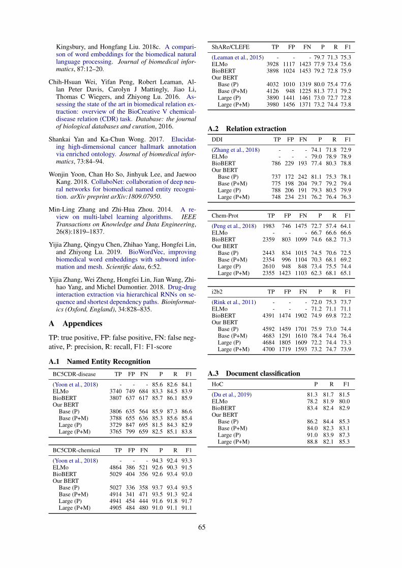
Kingsbury, and Hongfang Liu. 2018c. A compari-son of word embeddings for the biomedical naturallanguage processing. Journal of biomedical infor-matics, 87:12–20.
Chih-Hsuan Wei, Yifan Peng, Robert Leaman, Al-lan Peter Davis, Carolyn J Mattingly, Jiao Li,Thomas C Wiegers, and Zhiyong Lu. 2016. As-sessing the state of the art in biomedical relation ex-traction: overview of the BioCreative V chemical-disease relation (CDR) task. Database: the journalof biological databases and curation, 2016.
Shankai Yan and Ka-Chun Wong. 2017. Elucidat-ing high-dimensional cancer hallmark annotationvia enriched ontology. Journal of biomedical infor-matics, 73:84–94.
Wonjin Yoon, Chan Ho So, Jinhyuk Lee, and JaewooKang. 2018. CollaboNet: collaboration of deep neu-ral networks for biomedical named entity recogni-tion. arXiv preprint arXiv:1809.07950.
Min-Ling Zhang and Zhi-Hua Zhou. 2014. A re-view on multi-label learning algorithms. IEEETransactions on Knowledge and Data Engineering,26(8):1819–1837.
Yijia Zhang, Qingyu Chen, Zhihao Yang, Hongfei Lin,and Zhiyong Lu. 2019. BioWordVec, improvingbiomedical word embeddings with subword infor-mation and mesh. Scientific data, 6:52.
Yijia Zhang, Wei Zheng, Hongfei Lin, Jian Wang, Zhi-hao Yang, and Michel Dumontier. 2018. Drug-druginteraction extraction via hierarchical RNNs on se-quence and shortest dependency paths. Bioinformat-ics (Oxford, England), 34:828–835.
A Appendices
TP: true positive, FP: false positive, FN: false neg-ative, P: precision, R: recall, F1: F1-score
A.1 Named Entity Recognition
BC5CDR-disease TP FP FN P R F1
(Yoon et al., 2018) - - - 85.6 82.6 84.1ELMo 3740 749 684 83.3 84.5 83.9BioBERT 3807 637 617 85.7 86.1 85.9Our BERT
Base (P) 3806 635 564 85.9 87.3 86.6Base (P+M) 3788 655 636 85.3 85.6 85.4Large (P) 3729 847 695 81.5 84.3 82.9Large (P+M) 3765 799 659 82.5 85.1 83.8
BC5CDR-chemical TP FP FN P R F1
(Yoon et al., 2018) - - - 94.3 92.4 93.3ELMo 4864 386 521 92.6 90.3 91.5BioBERT 5029 404 356 92.6 93.4 93.0Our BERT
Base (P) 5027 336 358 93.7 93.4 93.5Base (P+M) 4914 341 471 93.5 91.3 92.4Large (P) 4941 454 444 91.6 91.8 91.7Large (P+M) 4905 484 480 91.0 91.1 91.1
ShARe/CLEFE TP FP FN P R F1
(Leaman et al., 2015) - - - 79.7 71.3 75.3ELMo 3928 1117 1423 77.9 73.4 75.6BioBERT 3898 1024 1453 79.2 72.8 75.9Our BERT
Base (P) 4032 1010 1319 80.0 75.4 77.6Base (P+M) 4126 948 1225 81.3 77.1 79.2Large (P) 3890 1441 1461 73.0 72.7 72.8Large (P+M) 3980 1456 1371 73.2 74.4 73.8
A.2 Relation extractionDDI TP FP FN P R F1
(Zhang et al., 2018) - - - 74.1 71.8 72.9ELMo - - - 79.0 78.9 78.9BioBERT 786 229 193 77.4 80.3 78.8Our BERT
Base (P) 737 172 242 81.1 75.3 78.1Base (P+M) 775 198 204 79.7 79.2 79.4Large (P) 788 206 191 79.3 80.5 79.9Large (P+M) 748 234 231 76.2 76.4 76.3
Chem-Prot TP FP FN P R F1
(Peng et al., 2018) 1983 746 1475 72.7 57.4 64.1ELMo - - - 66.7 66.6 66.6BioBERT 2359 803 1099 74.6 68.2 71.3Our BERT
Base (P) 2443 834 1015 74.5 70.6 72.5Base (P+M) 2354 996 1104 70.3 68.1 69.2Large (P) 2610 948 848 73.4 75.5 74.4Large (P+M) 2355 1423 1103 62.3 68.1 65.1
i2b2 TP FP FN P R F1
(Rink et al., 2011) - - - 72.0 75.3 73.7ELMo - - - 71.2 71.1 71.1BioBERT 4391 1474 1902 74.9 69.8 72.2Our BERT
Base (P) 4592 1459 1701 75.9 73.0 74.4Base (P+M) 4683 1291 1610 78.4 74.4 76.4Large (P) 4684 1805 1609 72.2 74.4 73.3Large (P+M) 4700 1719 1593 73.2 74.7 73.9
A.3 Document classificationHoC P R F1
(Du et al., 2019) 81.3 81.7 81.5ELMo 78.2 81.9 80.0BioBERT 83.4 82.4 82.9Our BERT
Base (P) 86.2 84.4 85.3Base (P+M) 84.0 82.3 83.1Large (P) 91.0 83.9 87.3Large (P+M) 88.8 82.1 85.3
65
Proceedings of the BioNLP 2019 workshop, pages 66–70Florence, Italy, August 1, 2019. c©2019 Association for Computational Linguistics
Combining Structured and Free-text Electronic Medical Record Data forReal-time Clinical Decision Support
Emilia Apostolova1, Tony Wang2, Ioannis Koutroulis3, Tim Tschampel4, Tom Velez4
1 Language.ai, Chicago, IL [email protected] Imedacs, Ann Arbor, MI [email protected]
3 Children’s National Health System, Washington, DC [email protected] Computer Technology Associates, Ridgecrest, CA [email protected], [email protected]
Abstract
The goal of this work is to utilize ElectronicMedical Record (EMR) data for real-timeClinical Decision Support (CDS). We presenta deep learning approach to combining in realtime available diagnosis codes (ICD codes)and free-text notes: Patient Context Vectors.Patient Context Vectors are created by averag-ing ICD code embeddings, and by predictingthe same from free-text notes via a Convolu-tional Neural Network. The Patient ContextVectors were then simply appended to avail-able structured data (vital signs and lab results)to build prediction models for a specific condi-tion. Experiments on predicting ARDS, a rareand complex condition, demonstrate the utilityof Patient Context Vectors as a means of sum-marizing the patient history and overall condi-tion, and improve significantly the predictionmodel results.
1 IntroductionA key goal in critical care medicine is the early
identification and timely treatment of rapidly pro-gressive, life-threatening conditions, such as Sep-sis, Septic Shock, and Acute Respiratory DistressSyndrome (ARDS). Such life-threatening condi-tions, are both rare, and at the same time, com-plex and heterogeneous, involving the interactionof multiple risk factors, comorbidities, and currentsymptoms. Hospital alert systems typically relyon screening of structured data such as vital signsand lab results, and, in the case of such rare condi-tions, are often associated with “alert fatigue” andrequire manually entered clinical judgement.
The information needed for a reliable risk eval-uation of such rare and complex conditions is typi-cally dispersed across the patient EMR, and avail-able at different times throughout the patient stay.The patient demographics, past medical and visithistory, chronic conditions, risk factors, currentsigns and symptoms can be found in the form of
clinical notes (e.g. nursing notes, radiology re-ports, etc.), diagnosis and procedure codes, vitalsigns, lab orders and results. The challenge ofreal-time CDS systems is the variability and theavailability of real-time EMR data, resulting fromdifferent charting behaviors, health care deliverymodels, hospital settings, etc.
The goal of this work is to utilize all availableEMR patient information for real-time predictivemodelling. While our experiments are focused onidentifying ARDS cases, the described method isapplicable to a variety of use cases needing infor-mation dispersed across the EMR patient record.The primary contribution of this work is the useof low-dimensional representation of the patient’shistory, current symptoms and conditions, whichwe refer to as Patient Context Vector. At pre-diction time, Patient Context Vectors are gener-ated from the combination of available up-to-dateICD codes (if any) and available nursing notes.Patient Context Vectors (vectors of real numbers)are then simply added to the list of existing struc-tured data variables (vital signs and lab results)and used to identify patients at risk of developinglife-threatening conditions that require rapid inter-vention.
2 MethodIn this work, we combine ICD codes, clinical
notes, vital signs, lab results, and demographic in-formation to build a real-time ARDS predictionmodel. Low-dimensional representation of ICDcodes (ICD embeddings) is generated from a largecorpus of patient ICD records. Patient visit EMRdata is used to look up recorded up-to-date ICDcodes, clinical notes, vital signs, and lab results.The visit ICD codes are converted to embeddingsand averaged to produce Patient Context Vectors.
Pertinent patient information might not be nec-essarily ”ICD-coded” during prediction time, but
66
can be available in the form of nursing notes. Adeep learning model was trained to predict the pa-tient’s Patient Context Vector from nursing notes.The Patient Context Vectors obtained from avail-able in the system ICD codes, and from free-textnotes are then used in conjunction with vital signs,and lab results to predict the patient’s outcome.Details for each step of the approach are providedin subsequent sections.2.1 Dataset
We utilized the freely available database com-prising deidentified health-related data associatedwith over 40,000 patients who stayed in criticalcare units of the Beth Israel Deaconess MedicalCenter between 2001 and 2012: the MIMIC3 In-tensive Care Unit (ICU) database (Johnson et al.,2016). The dataset contains over 2 million free-text clinical notes and over 650,000 diagnosiscodes for over 58,000 visits. Included ICUs aremedical, surgical, trauma-surgical, coronary, andcardiac surgery recovery units. EMR data includesvital signs, laboratory results, diagnosis codes,free text nursing notes, radiology reports, medi-cations, discharge summaries, treatments, etc.2.2 ICD Embeddings and Patient Context
VectorsClinicians viewing properly coded patient di-
agnosis codes (ICD9 and ICD10 codes1) are typ-ically capable of deducing the overall condition,history, and risk factors associated with a patient.Intuitively, the totality of patient’s diagnosis codesrepresent a meaningful medical summary of thepatient. Diagnosis codes are used to describeboth current diagnoses (e.g. Community-acquiredPneumonia ), but also a variety of additional facts.For example, ICD codes can describe patient’s his-tory and chronic conditions (e.g. Chronic kid-ney disease; Personal history of traumatic frac-ture; etc.); information regarding past and currenttreatments and procedures (e.g. Infection due toother bariatric procedure). In some cases, ICDcodes contain information such as the patient agegroup (e.g. Sepsis of newborn; Elderly multi-gravida); expected outcome (Encounter for pal-liative care); patient’s social history (e.g. Adultemotional/psychological abuse); the reason for thevisit, (e.g. Railway accidents; Motor Vehicle acci-dents, etc).
While there are a large number of ICD codes(around 15,000 ICD9 codes and around 68,000
1The International Classification of Diseases, c©The World Health Orga-nization.
ICD10 codes), they tend to be interdependent,and to co-occur. For example, Pneumonia ICDcodes are often accompanied with ICD codesdescribing Cough, Fever, Pleural effusion, etc.Inspired by word embeddings (Mikolov et al.,2013), it has been suggested that this medical codeco-occurence can be exploited to generate low-dimensional representations of ICD codes: ICDEmbeddings (Choi et al., 2016b,a; Kartchner et al.,2017).
All available MIMIC3 patient data was used togenerate the ICD embeddings following the ap-proach of (Choi et al., 2016b). In our approach, weattempted to generate a low-dimensional represen-tation of the patient history, symptoms, risk fac-tors, diagnosis, etc, by averaging the patient ICDcode embeddings (creating Patient Context Vec-tors). The optimum size of the vectors was deter-mined to be 50.2.3 Predicting Patient Context Vectors from
Clinical TextsWhile averaged ICD embeddings appear to be a
useful summary of the overall patient history, con-dition, symptoms, and risk factors, ICD code datais not necessarily available for real-time CDS sys-tems. Some ICD codes associated with patients’history and symptoms might be entered early onin the EMR system. However, diagnosis ICDcodes are typically obtained after tests and lab re-sults and might not be available during predictiontime. Similarly, not all relevant patient history andsymptoms are necessarily ICD-coded.
At the same time, nursing notes typically con-tain all currently available information, even if notpresent in the form of ICD codes. Nursing notesinclude information such as past medical history,reason for visit, current symptoms, summary oftest outcomes, etc.
In order to capture information present in free-text notes, we also built a word-level CNN modelthat predicts the patient Patient Context Vectorfrom the note text. The model was trainedon available nursing and discharge notes andachieved a mean squared error of 0.179 on the val-idation set. The network was trained on 1,081,176free-text notes, with pre-trained word-embeddingsof size 100. The texts were truncated/padded tothe 90th percentile length (785 tokens). The net-work consists of a Convolutional, Max Poolinglayers, followed by 2 hidden layers of size 500.The last layer uses linear activation with loss func-
67
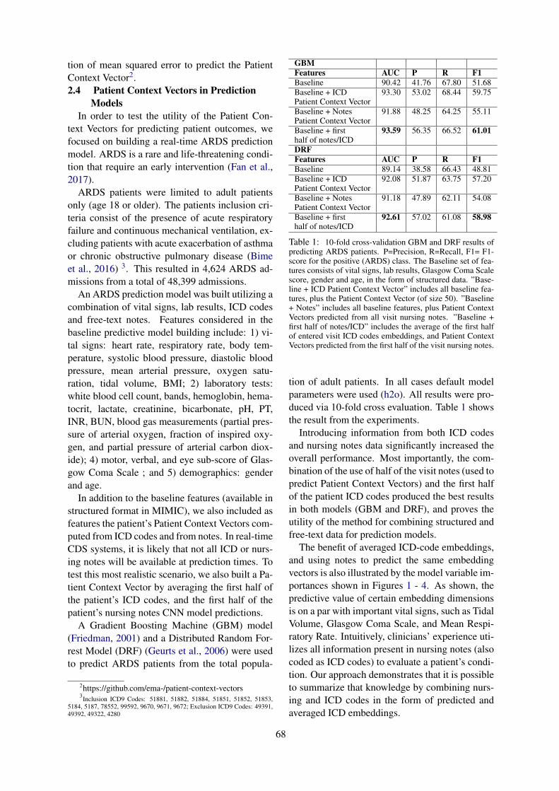
tion of mean squared error to predict the PatientContext Vector2.2.4 Patient Context Vectors in Prediction
ModelsIn order to test the utility of the Patient Con-
text Vectors for predicting patient outcomes, wefocused on building a real-time ARDS predictionmodel. ARDS is a rare and life-threatening condi-tion that require an early intervention (Fan et al.,2017).
ARDS patients were limited to adult patientsonly (age 18 or older). The patients inclusion cri-teria consist of the presence of acute respiratoryfailure and continuous mechanical ventilation, ex-cluding patients with acute exacerbation of asthmaor chronic obstructive pulmonary disease (Bimeet al., 2016) 3. This resulted in 4,624 ARDS ad-missions from a total of 48,399 admissions.
An ARDS prediction model was built utilizing acombination of vital signs, lab results, ICD codesand free-text notes. Features considered in thebaseline predictive model building include: 1) vi-tal signs: heart rate, respiratory rate, body tem-perature, systolic blood pressure, diastolic bloodpressure, mean arterial pressure, oxygen satu-ration, tidal volume, BMI; 2) laboratory tests:white blood cell count, bands, hemoglobin, hema-tocrit, lactate, creatinine, bicarbonate, pH, PT,INR, BUN, blood gas measurements (partial pres-sure of arterial oxygen, fraction of inspired oxy-gen, and partial pressure of arterial carbon diox-ide); 4) motor, verbal, and eye sub-score of Glas-gow Coma Scale ; and 5) demographics: genderand age.
In addition to the baseline features (available instructured format in MIMIC), we also included asfeatures the patient’s Patient Context Vectors com-puted from ICD codes and from notes. In real-timeCDS systems, it is likely that not all ICD or nurs-ing notes will be available at prediction times. Totest this most realistic scenario, we also built a Pa-tient Context Vector by averaging the first half ofthe patient’s ICD codes, and the first half of thepatient’s nursing notes CNN model predictions.
A Gradient Boosting Machine (GBM) model(Friedman, 2001) and a Distributed Random For-rest Model (DRF) (Geurts et al., 2006) were usedto predict ARDS patients from the total popula-
2https://github.com/ema-/patient-context-vectors3Inclusion ICD9 Codes: 51881, 51882, 51884, 51851, 51852, 51853,
5184, 5187, 78552, 99592, 9670, 9671, 9672; Exclusion ICD9 Codes: 49391,49392, 49322, 4280
GBMFeatures AUC P R F1Baseline 90.42 41.76 67.80 51.68Baseline + ICD 93.30 53.02 68.44 59.75Patient Context VectorBaseline + Notes 91.88 48.25 64.25 55.11Patient Context VectorBaseline + first 93.59 56.35 66.52 61.01half of notes/ICDDRFFeatures AUC P R F1Baseline 89.14 38.58 66.43 48.81Baseline + ICD 92.08 51.87 63.75 57.20Patient Context VectorBaseline + Notes 91.18 47.89 62.11 54.08Patient Context VectorBaseline + first 92.61 57.02 61.08 58.98half of notes/ICD
Table 1: 10-fold cross-validation GBM and DRF results ofpredicting ARDS patients. P=Precision, R=Recall, F1= F1-score for the positive (ARDS) class. The Baseline set of fea-tures consists of vital signs, lab results, Glasgow Coma Scalescore, gender and age, in the form of structured data. ”Base-line + ICD Patient Context Vector” includes all baseline fea-tures, plus the Patient Context Vector (of size 50). ”Baseline+ Notes” includes all baseline features, plus Patient ContextVectors predicted from all visit nursing notes. ”Baseline +first half of notes/ICD” includes the average of the first halfof entered visit ICD codes embeddings, and Patient ContextVectors predicted from the first half of the visit nursing notes.
tion of adult patients. In all cases default modelparameters were used (h2o). All results were pro-duced via 10-fold cross evaluation. Table 1 showsthe result from the experiments.
Introducing information from both ICD codesand nursing notes data significantly increased theoverall performance. Most importantly, the com-bination of the use of half of the visit notes (used topredict Patient Context Vectors) and the first halfof the patient ICD codes produced the best resultsin both models (GBM and DRF), and proves theutility of the method for combining structured andfree-text data for prediction models.
The benefit of averaged ICD-code embeddings,and using notes to predict the same embeddingvectors is also illustrated by the model variable im-portances shown in Figures 1 - 4. As shown, thepredictive value of certain embedding dimensionsis on a par with important vital signs, such as TidalVolume, Glasgow Coma Scale, and Mean Respi-ratory Rate. Intuitively, clinicians’ experience uti-lizes all information present in nursing notes (alsocoded as ICD codes) to evaluate a patient’s condi-tion. Our approach demonstrates that it is possibleto summarize that knowledge by combining nurs-ing and ICD codes in the form of predicted andaveraged ICD embeddings.
68
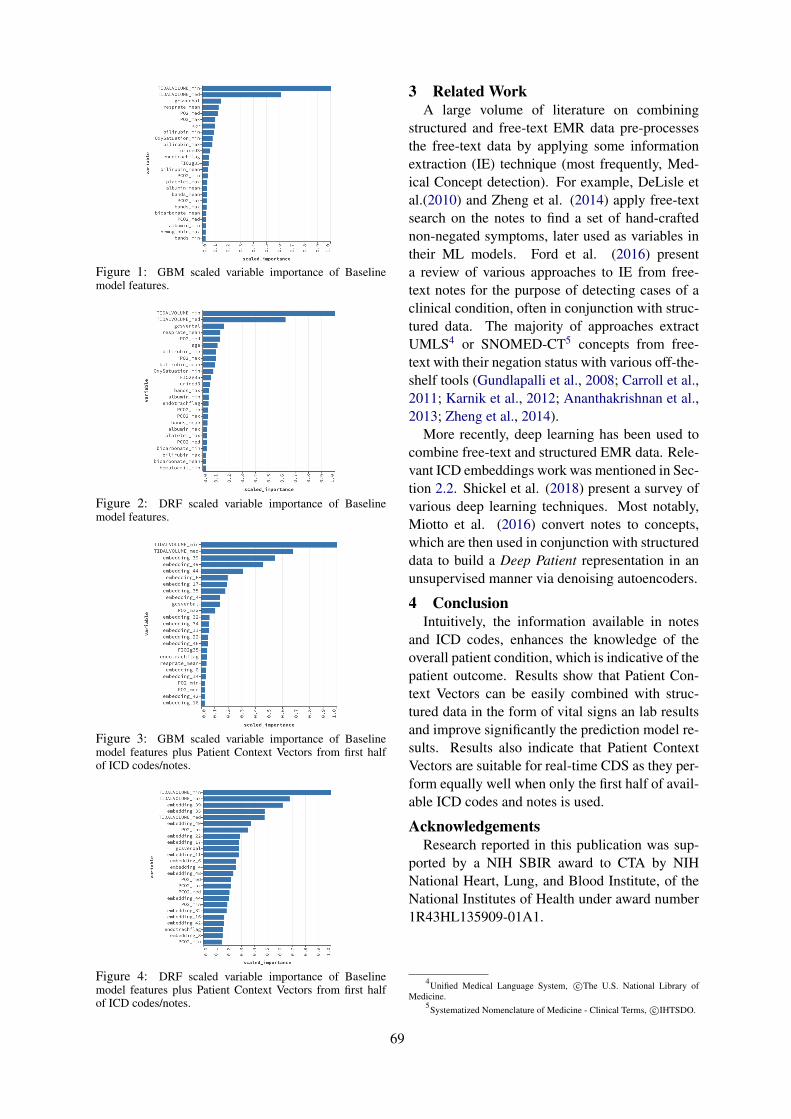
Figure 1: GBM scaled variable importance of Baselinemodel features.
Figure 2: DRF scaled variable importance of Baselinemodel features.
Figure 3: GBM scaled variable importance of Baselinemodel features plus Patient Context Vectors from first halfof ICD codes/notes.
Figure 4: DRF scaled variable importance of Baselinemodel features plus Patient Context Vectors from first halfof ICD codes/notes.
3 Related WorkA large volume of literature on combining
structured and free-text EMR data pre-processesthe free-text data by applying some informationextraction (IE) technique (most frequently, Med-ical Concept detection). For example, DeLisle etal.(2010) and Zheng et al. (2014) apply free-textsearch on the notes to find a set of hand-craftednon-negated symptoms, later used as variables intheir ML models. Ford et al. (2016) presenta review of various approaches to IE from free-text notes for the purpose of detecting cases of aclinical condition, often in conjunction with struc-tured data. The majority of approaches extractUMLS4 or SNOMED-CT5 concepts from free-text with their negation status with various off-the-shelf tools (Gundlapalli et al., 2008; Carroll et al.,2011; Karnik et al., 2012; Ananthakrishnan et al.,2013; Zheng et al., 2014).
More recently, deep learning has been used tocombine free-text and structured EMR data. Rele-vant ICD embeddings work was mentioned in Sec-tion 2.2. Shickel et al. (2018) present a survey ofvarious deep learning techniques. Most notably,Miotto et al. (2016) convert notes to concepts,which are then used in conjunction with structureddata to build a Deep Patient representation in anunsupervised manner via denoising autoencoders.
4 ConclusionIntuitively, the information available in notes
and ICD codes, enhances the knowledge of theoverall patient condition, which is indicative of thepatient outcome. Results show that Patient Con-text Vectors can be easily combined with struc-tured data in the form of vital signs an lab resultsand improve significantly the prediction model re-sults. Results also indicate that Patient ContextVectors are suitable for real-time CDS as they per-form equally well when only the first half of avail-able ICD codes and notes is used.
AcknowledgementsResearch reported in this publication was sup-
ported by a NIH SBIR award to CTA by NIHNational Heart, Lung, and Blood Institute, of theNational Institutes of Health under award number1R43HL135909-01A1.
4Unified Medical Language System, c©The U.S. National Library ofMedicine.
5Systematized Nomenclature of Medicine - Clinical Terms, c©IHTSDO.
69
Referencesh2o.ai. https://www.h2o.ai/. Accessed: 2019-
01-30.
Ashwin N Ananthakrishnan, Tianxi Cai, GuerganaSavova, Su-Chun Cheng, Pei Chen, Raul GuzmanPerez, Vivian S Gainer, Shawn N Murphy, PeterSzolovits, Zongqi Xia, et al. 2013. Improving casedefinition of crohn’s disease and ulcerative colitisin electronic medical records using natural languageprocessing: a novel informatics approach. Inflam-matory bowel diseases, 19(7):1411–1420.
Christian Bime, Chithra Poongkunran, MarkBorgstrom, Bhupinder Natt, Hem Desai, SairamParthasarathy, and Joe GN Garcia. 2016. Racial dif-ferences in mortality from severe acute respiratoryfailure in the united states, 2008–2012. Annals ofthe American Thoracic Society, 13(12):2184–2189.
Robert J Carroll, Anne E Eyler, and Joshua C Denny.2011. Naı̈ve electronic health record phenotypeidentification for rheumatoid arthritis. In AMIA an-nual symposium proceedings, volume 2011, page189. American Medical Informatics Association.
Edward Choi, Mohammad Taha Bahadori, Eliza-beth Searles, Catherine Coffey, Michael Thomp-son, James Bost, Javier Tejedor-Sojo, and JimengSun. 2016a. Multi-layer representation learningfor medical concepts. In Proceedings of the 22ndACM SIGKDD International Conference on Knowl-edge Discovery and Data Mining, pages 1495–1504.ACM.
Youngduck Choi, Chill Yi-I Chiu, and David Sontag.2016b. Learning low-dimensional representationsof medical concepts. AMIA Summits on Transla-tional Science Proceedings, 2016:41.
Sylvain DeLisle, Brett South, Jill A Anthony, ErickaKalp, Adi Gundlapallli, Frank C Curriero, Greg EGlass, Matthew Samore, and Trish M Perl. 2010.Combining free text and structured electronic med-ical record entries to detect acute respiratory infec-tions. PloS one, 5(10):e13377.
Eddy Fan, Lorenzo Del Sorbo, Ewan C Goligher,Carol L Hodgson, Laveena Munshi, Allan J Walkey,Neill KJ Adhikari, Marcelo BP Amato, RichardBranson, Roy G Brower, et al. 2017. An officialamerican thoracic society/european society of inten-sive care medicine/society of critical care medicineclinical practice guideline: mechanical ventilationin adult patients with acute respiratory distress syn-drome. American journal of respiratory and criticalcare medicine, 195(9):1253–1263.
Elizabeth Ford, John A Carroll, Helen E Smith, DoniaScott, and Jackie A Cassell. 2016. Extracting infor-mation from the text of electronic medical records toimprove case detection: a systematic review. Jour-nal of the American Medical Informatics Associa-tion, 23(5):1007–1015.
Jerome H Friedman. 2001. Greedy function approx-imation: a gradient boosting machine. Annals ofstatistics, pages 1189–1232.
Pierre Geurts, Damien Ernst, and Louis Wehenkel.2006. Extremely randomized trees. Machine learn-ing, 63(1):3–42.
Adi V Gundlapalli, Brett R South, Shobha Phansalkar,Anita Y Kinney, Shuying Shen, Sylvain Delisle, Tr-ish Perl, and Matthew H Samore. 2008. Applica-tion of natural language processing to va electronichealth records to identify phenotypic characteristicsfor clinical and research purposes. Summit on trans-lational bioinformatics, 2008:36.
Alistair EW Johnson, Tom J Pollard, Lu Shen,H Lehman Li-wei, Mengling Feng, Moham-mad Ghassemi, Benjamin Moody, Peter Szolovits,Leo Anthony Celi, and Roger G Mark. 2016.Mimic-iii, a freely accessible critical care database.Scientific data, 3:160035.
Shreyas Karnik, Sin Lam Tan, Bess Berg, IngridGlurich, Jinfeng Zhang, Humberto J Vidaillet,C David Page, and Rajesh Chowdhary. 2012. Pre-dicting atrial fibrillation and flutter using electronichealth records. In Engineering in Medicine and Bi-ology Society (EMBC), 2012 Annual InternationalConference of the IEEE, pages 5562–5565. IEEE.
David Kartchner, Tanner Christensen, JeffreyHumpherys, and Sean Wade. 2017. Code2vec:Embedding and clustering medical diagnosis data.In Healthcare Informatics (ICHI), 2017 IEEEInternational Conference on, pages 386–390. IEEE.
Tomas Mikolov, Kai Chen, Greg Corrado, and Jef-frey Dean. 2013. Efficient estimation of wordrepresentations in vector space. arXiv preprintarXiv:1301.3781.
Riccardo Miotto, Li Li, Brian A Kidd, and Joel T Dud-ley. 2016. Deep patient: an unsupervised represen-tation to predict the future of patients from the elec-tronic health records. Scientific reports, 6:26094.
Benjamin Shickel, Patrick James Tighe, Azra Bihorac,and Parisa Rashidi. 2018. Deep ehr: a survey of re-cent advances in deep learning techniques for elec-tronic health record (ehr) analysis. IEEE journalof biomedical and health informatics, 22(5):1589–1604.
Hongzhang Zheng, Holly Gaff, Gary Smith, and Syl-vain DeLisle. 2014. Epidemic surveillance using anelectronic medical record: an empiric approach toperformance improvement. PloS one, 9(7):e100845.
70
Proceedings of the BioNLP 2019 workshop, pages 71–79Florence, Italy, August 1, 2019. c©2019 Association for Computational Linguistics
MoNERo: a Biomedical Gold Standard Corpus for the RomanianLanguage
Maria MitrofanRACAI, Bucharest, Romania
Verginica Barbu MititeluRACAI, Bucharest, Romania
Grigorina MitrofanNIDMD “N.C. Paulescu”
Bucharest, [email protected]
Abstract
In an era when large amounts of data are gen-erated daily in various fields, the biomedicalfield among others, linguistic resources canbe exploited for various tasks of Natural Lan-guage Processing. Moreover, increasing num-ber of biomedical documents are available inlanguages other than English. To be able toextract information from natural language freetext resources, methods and tools are neededfor a variety of languages. This paper presentsthe creation of the MoNERo corpus, a goldstandard biomedical corpus for Romanian, an-notated with both part of speech tags andnamed entities. MoNERo comprises 154,825morphologically annotated tokens and 23,188entity annotations belonging to four entity se-mantic groups corresponding to UMLS Se-mantic Groups.
1 Introduction
Natural Language Processing (NLP) is a researcharea that provides methods to convert (human-understandable) unstructured textual informationinto (machine-readable) structured data and usesit for different objectives. NLP techniques canbe used to process and exploit the large amountof biomedical information which is continuouslygenerated. Examples of such repositories areMEDLINE1, which contains more than 25 mil-lion documents belonging to the biomedical do-main, or PubMed Central2, which is an archiveof biomedical journal literature and contains morethan 5 million full-text articles. These resourcescan be exploited and used together with differentNLP systems previously adapted to the biomedi-cal field to improve the quality of the health care
1https://www.nlm.nih.gov/bsd/medline.html
2https://www.nlm.nih.gov/bsd/medline.html
process, to further develop research in the fieldand benefit both physicians and patients. Infor-mation Extraction (IE) tools can be used to ex-tract relevant information from biomedical textualresources (Goeuriot et al., 2017; Li et al., 2017).Reaching suitable results for this NLP subtask isnot trivial and there is still room for improve-ment of results. Advances of these IE tools de-pend on the existence of annotated resources spe-cific to the field of study (Wilbur et al., 2006;Thompson et al., 2009; Kilicoglu, 2017), anno-tated corpora being relevant in both phases: de-velopment of the models that will determine thebehaviour of the system and system performanceevaluation. Even though the availability of theseresources has increased lately, the main part of theefforts have been directed to the development ofannotated corpora for English in different subdo-mains. However, MoNERo is a resource createdfor the Romanian language that helps the develop-ment of named entity recognition and classifica-tion task especially for this language. Romanianbenefits from the existence of other corpora cre-ated in our institute: the representative corpus ofcontemporary language (CoRoLa) (Barbu Mititeluet al., 2018), a balanced corpus (ROMBAC) (Ionet al., 2012), the corpus annotated with verbal mul-tiword expressions (Barbu Mititelu et al., 2019).Just like all of these, MoNERo is annotated at themorphological level. However, it stands out givenits annotation with four types of Named Entities(NEs) for the medical domain, which are relevantto the identification of: anatomy parts, diseasesand disorders, chemicals and drugs, and medicalprocedures.
This paper has four main objectives: (i) topresent the construction of a biomedical gold stan-dard corpus annotated both with part-of-speechtags and named entities; (ii) to present generalstatistics over the corpus; (iii) to release the final
71
version of the corpus to the scientific community,(iv) to show the contribution in the developmentof NLP tools for Romanian language. All the re-sults are discussed in parallel for the two types ofannotations.
2 Related Work
This section reviews relevant corpora annotatedwith NEs specific to the biomedical domain.
1. For English we mention:
• CLEF corpus (Roberts et al., 2009) –it contains 150 documents of clinicalnarratives, histopathology reports andimaging reports. It was subtracted froma corpus of 565,000 documents andmanually annotated with six types ofNEs (condition, intervention, investiga-tion, result, drug or device, locus);• i2b2 corpus (Uzuner et al., 2010) – it
contains 1243 discharge summaries au-tomatically pre-annotated, out of whicha subset of 251 was manually revised.This corpus contains seven types of NEs(medications, dosages, modes, frequen-cies, durations, reasons of administra-tion, list/narrative);• NCBI corpus (Doğan et al., 2014) – a
gold-standard corpus for disease men-tions and concepts that contains 793 ab-stracts extracted from PubMed;• CHEMDNER corpus (Krallinger et al.,
2015) – a corpus of 10,000 abstracts col-lected from PubMed annotated with twotypes of NEs: chemicals and drugs.
2. For French there is the Quaero corpus(Névéol et al., 2014) which contains 103,056words collected from three types of docu-ments: texts with information on drugs ex-tracted from European Medicines Agency(EMEA), titles from research articles com-prised in MEDLINE and patents. This corpuswas annotated with ten types of NEs definedusing UMLS: anatomy, chemical and drugs,devices, disorders, geographic areas, livingbeings, objects, phenomena, physiology, pro-cedures.
3. For Spanish the following corpora exist:
• IxaMedGS corpus (Oronoz et al., 2015)– it is composed of 142,154 dischargerecords out of which 75 were annotatedwith two types of NEs: diseases anddrugs;• DrugSemantics corpus (Moreno et al.,
2017) – it has 226,729 tokens anno-tated with ten types of NEs: chemi-cal composition, disease, drug, excipi-ent, food, medicament, pharmaceuticalform, route, therapeutic action, and unitof measurement.
All these corpora are available and have had asignificant role in information extraction research,especially in named entity recognition (NER) re-search and were developed for well-establishedpurposes, having in mind the possibility of re-usability.
3 Corpus Development Description
3.1 Selection of Corpus Documents
The gold standard morphologically and named en-tity annotated Romanian medical corpus (MoN-ERo) was extracted from the BioRo corpus(Mitrofan and Tufiş, 2018), a Romanian biomed-ical corpus. MoNERo contains texts extractedfrom three types of documents: scientific medi-cal literature books, scientific medical journal ar-ticles and medical blog posts, but predominant arethose coming from medical literature. The medi-cal books were chosen as the main source becausethey contain descriptive materials, full of domain-specific terms. In addition, the texts are of goodquality and the use of medical terms is correct.The medical journal3 from which a part of the textswere extracted is a scientific journal that addressesthe specialists, so the language used is specific tothe medical domain. In the case of blog posts thosecollected were texts of popularization and aware-ness of various medical problems.
The texts were selected so that they belong tothree medical subdomains: cardiology, diabetesand endocrinology (see table 3). The main mo-tivation behind choosing these three medical do-mains is that our textual resources available werecentered around the pathology of Diabetes. SinceDiabetes is an endocrine disorder it is naturally in-cluded in the Endocrinology category. In the same
3https://rmj.com.ro/
72
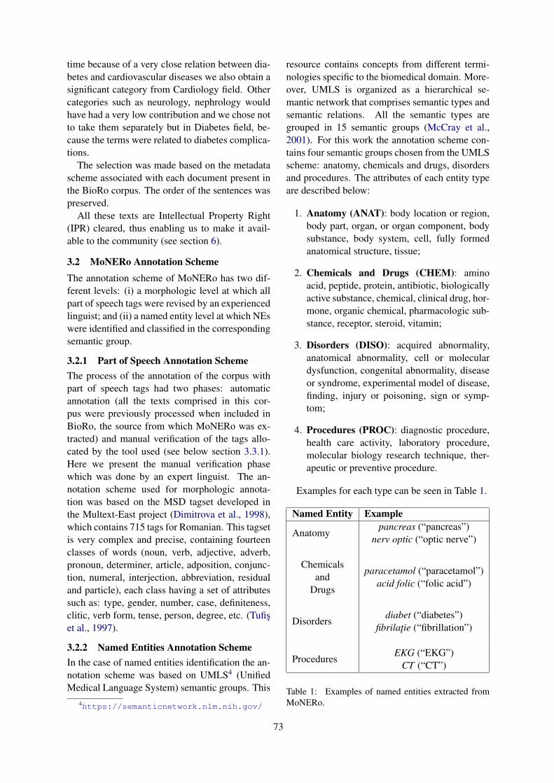
time because of a very close relation between dia-betes and cardiovascular diseases we also obtain asignificant category from Cardiology field. Othercategories such as neurology, nephrology wouldhave had a very low contribution and we chose notto take them separately but in Diabetes field, be-cause the terms were related to diabetes complica-tions.
The selection was made based on the metadatascheme associated with each document present inthe BioRo corpus. The order of the sentences waspreserved.
All these texts are Intellectual Property Right(IPR) cleared, thus enabling us to make it avail-able to the community (see section 6).
3.2 MoNERo Annotation SchemeThe annotation scheme of MoNERo has two dif-ferent levels: (i) a morphologic level at which allpart of speech tags were revised by an experiencedlinguist; and (ii) a named entity level at which NEswere identified and classified in the correspondingsemantic group.
3.2.1 Part of Speech Annotation SchemeThe process of the annotation of the corpus withpart of speech tags had two phases: automaticannotation (all the texts comprised in this cor-pus were previously processed when included inBioRo, the source from which MoNERo was ex-tracted) and manual verification of the tags allo-cated by the tool used (see below section 3.3.1).Here we present the manual verification phasewhich was done by an expert linguist. The an-notation scheme used for morphologic annota-tion was based on the MSD tagset developed inthe Multext-East project (Dimitrova et al., 1998),which contains 715 tags for Romanian. This tagsetis very complex and precise, containing fourteenclasses of words (noun, verb, adjective, adverb,pronoun, determiner, article, adposition, conjunc-tion, numeral, interjection, abbreviation, residualand particle), each class having a set of attributessuch as: type, gender, number, case, definiteness,clitic, verb form, tense, person, degree, etc. (Tufişet al., 1997).
3.2.2 Named Entities Annotation SchemeIn the case of named entities identification the an-notation scheme was based on UMLS4 (UnifiedMedical Language System) semantic groups. This
4https://semanticnetwork.nlm.nih.gov/
resource contains concepts from different termi-nologies specific to the biomedical domain. More-over, UMLS is organized as a hierarchical se-mantic network that comprises semantic types andsemantic relations. All the semantic types aregrouped in 15 semantic groups (McCray et al.,2001). For this work the annotation scheme con-tains four semantic groups chosen from the UMLSscheme: anatomy, chemicals and drugs, disordersand procedures. The attributes of each entity typeare described below:
1. Anatomy (ANAT): body location or region,body part, organ, or organ component, bodysubstance, body system, cell, fully formedanatomical structure, tissue;
2. Chemicals and Drugs (CHEM): aminoacid, peptide, protein, antibiotic, biologicallyactive substance, chemical, clinical drug, hor-mone, organic chemical, pharmacologic sub-stance, receptor, steroid, vitamin;
3. Disorders (DISO): acquired abnormality,anatomical abnormality, cell or moleculardysfunction, congenital abnormality, diseaseor syndrome, experimental model of disease,finding, injury or poisoning, sign or symp-tom;
4. Procedures (PROC): diagnostic procedure,health care activity, laboratory procedure,molecular biology research technique, ther-apeutic or preventive procedure.
Examples for each type can be seen in Table 1.
Named Entity Example
Anatomypancreas (“pancreas”)
nerv optic (“optic nerve”)
Chemicalsand
Drugs
paracetamol (“paracetamol”)acid folic (“folic acid”)
Disordersdiabet (“diabetes”)
fibrilaţie (“fibrillation”)
ProceduresEKG (“EKG”)
CT (“CT”)
Table 1: Examples of named entities extracted fromMoNERo.
73
The main reason for choosing these four typesof entities was a trade off between the minimumnumber of entities (due to an increased complex-ity of the annotation process) and the maximumrelevance for our corpus. However we had somechallenges. For example, Physiology was a cate-gory that could be included, but due to the fact thatthe medical texts available were mainly related topathology, the contribution would have been lim-ited (less than 5%).
Having a tokenized corpus with each token ona separate line, we chose IOB2 (Insid-Outside-Beginning) (Sang and Veenstra, 1999) as the an-notation format for named entities. Lately, thisformat has become popular within the scientificcommunity, being also supported by the CoNLLchallenges 5. The B-tag is used for the first tokenof every NE, I-tag indicates the token that is insidea named entity and O-tag is used for surroundingtokens that do not belong to a NE (În/O schimb/O,HDL-colesterolul/ B-CHEM, apolipoproteinele/B-CHEM A/I-CHEM şi/O B/I-CHEM sunt/O su-periori/O ca/O indicatori/O de/O risc/B-DISOcardiovascular/I-DISO ./O) (“On the other hand,HDL-cholesterol and lipoproteins A and B are su-perior as cardiovascular risk indicators.”). For easeof reading, in all the examples below we chose notto mention the O-tag, but only the B- and I-tags.
3.3 Annotation Guidelines3.3.1 Part of SpeechIn the initial phase the corpus was automaticallypreprocessed (sentence split, tokenized, lemma-tized) and annotated with POS tags using theTTL annotator (Ion, 2007; Mitrofan and Tufiş,2018), which was trained on news corpora ofabout 200,000 tokens with POS labeling checkedby trained linguists (Tufiş, 2000). The accuracyfor this task was 98.23%. When TTL was trainedin order to perform domain adaptation for biomed-ical domain the accuracy was 97.83% (Mitrofanand Ion, 2017). Therefore, in order to annotatethis corpus with POS tags the baseline model waschosen. The second phase of the annotation pro-cess, which makes the focus of this paper, was tomanually check all the automatically assigned la-bels. A trained and experienced linguist revised allthe tokens included in MoNERo. For this task theguidelines were:
1. correct the token if needed;5http://www.conll.org/previous-tasks
2. correct the lemma if needed;
3. correct the POS tag if needed;
4. compounds written as separate words shouldbe split.
3.3.2 Named EntitiesThe guidelines for named entity annotation were:
1. a complex entity will not be decomposed intosimpler entities belonging to different seman-tic groups; only one semantic group will beassociated to the longest entity (cancer de fi-cat (“liver cancer”) will be annotated only asa disorder, not as a disorder (cancer/B-DISOde/I-DISO ficat/I-DISO (“cancer”/B-DISO)“of”/I-DISO “liver”/I-DISO) and an anatom-ical part (ficat/B-ANAT (“liver”/B-ANAT));so, there is no embedded annotation;
2. in cases when one head noun is sharedby two or more biomedical named enti-ties (coordinations or disjunctions) the an-notation will be done as follows: in caseof coordinations ateroscleroza aortei şi avaselor periferice (“atherosclerosis of theaorta and peripheral vessels”), should beannotated as ateroscleroza/B-DISO aortei/I-DISO şi vaselor/I-DISO periferice/I-DISO orin case of disjunctions celule beta pancre-atice sau hepatice (“pancreatic beta or hep-atic cells”) should be annotated as celule/B-ANAT beta/I-ANAT pancreatice/I-ANAT sauhepatice/I-ANAT);
3. discontinuous entities will be annotatedas contiguous terms and classified in thesame semantic group: in the examplesAnevrismele/B-DISO pot fi fusiforme/I-DISO (aspect cilindric al vasului/B-ANATsangvin/I-ANAT) sau sacciforme/I-DISO(“Aneurysms/B-DISO may be fusiforms/I-DISO (cylindrical appearance of the blood/B-ANAT vessel/I-ANAT) or sacciforms/I-DISO”) the NEs Anevrismele fusiforme andanevrismele sacciforme are discontinuous;
4. in case of cascaded constructions when oneentity is incorporated in another entity (eg.parenthetical constructions) the annotationwill be done as: Anevrismele/B-DISOpot fi fusiforme/I-DISO (aspect cilindrical vasului/B-ANAT sangvin/I-ANAT) sau
74
sacciforme/I-DISO (“Aneurysms/B-DISOmay be fusiforms/I-DISO (cylindricalappearance of the blood/B-ANAT vessel/I-ANAT) or sacciforms/I-DISO”). Within thediscontinuous NE Anevrismele sacciformethere is another NE, vasului sangvin.
3.4 Annotation Development
3.4.1 Part of Speech TagsEven though the accuracy of the automatic anno-tation with POS tags was very high (subsection3.3.1), given the high number of POS tags in theRomanian MSD tagset, there was a lot of manualwork to be done by the linguist. This task involvedmanual validation of tokenization, lemmatization,and also correcting the errors of part of speech anderrors of morphological categories (see 3.5.1) foreach token.
3.4.2 Named EntitiesFor the named entities annotation task two annota-tors were employed: one physician and one expe-rienced annotator, both having Romanian as nativelanguage. The physician was chosen as annotatordue to her capacity of understanding the medicalfield. Prior to the annotation process there was atraining period for both annotators. In this phasethey debated issues such as whether or not to anno-tate overlapping terms, when and if complex termsshould be decomposed, how conjunctions shouldbe treated.
Even though the initial guidelines gave them in-structions on what should and should not be anno-tated, they collaborated and discussed throughoutthe annotation process. Even if the identificationof a biomedical entity was a relatively easy task,fitting it into the correct semantic group some-times required prior knowledge of the biomedicalvocabulary. Therefore the experienced annotatorhas accessed various terminological resources inorder to better understand the terms and to cate-gorized them into the correct semantic group. Ina post-annotation phase, the two annotators dis-cussed the annotation differences in order to reachagreement.
3.5 Discussion Over the Annotation Process
3.5.1 Part of SpeechDuring the manual correction process of the partof speech tags the annotator encountered severaltypes of errors generated by the tool used:
1. tokenization errors: wrong segmentation oftime intervals (2000-2001) was annotated asa single token), typos that led to wrong tok-enization of the word (fi cat instead of ficat(“liver”));
2. lemmatization errors: in case of the unknownwords (adenoamă instead of adenom (“ade-noma”)) or in case of morphologically am-biguous forms: the form copii can be theplural indefinite of either the masculine nouncopil (“child”) or of the feminine noun copie(“copy”); given this homography, the lemma-tizer mistakes one of the words with the otherone;
3. tagging errors where classified in two cate-gories:
• errors of part of speech – wrong auto-matic identification of the part of speech(nouns as adjectives, adjectives as ad-verbs and vice versa, verbs as adjec-tives);• wrong identification of the morphologi-
cal class – the part of speech is correctlyidentified but some of the specificationsare wrongly identified: gender, number,case, etc.
Even though the overall error rate of the toolused was low (1.77% see section 3.3.1) and pre-annotation with POS tags of the corpus was use-ful, the task of correcting it was a difficult onedue to the complexity of the tag set and the labori-ous manual work needed to determine if the token,lemma and POS tag are correct for each word inthe corpus. Annotation time ranges between 17 to-kens per minute (at the beginning of the task) and33 tokens per minute (after the annotator becameaccustomed with the task and the types of errors).The use of only one annotator for correcting thePOS tags is justified, on the one hand, by the lowerror rate and, on the other, by the expense of thetask. However, we are aware of the limitation rep-resented by the lack of inter-annotator agreementmeasurements (even on a sample) on the morpho-logical annotation.
3.6 Named Entities
The task of annotating the corpus with named en-tities had an increased difficulty due to several fac-tors such as:
75
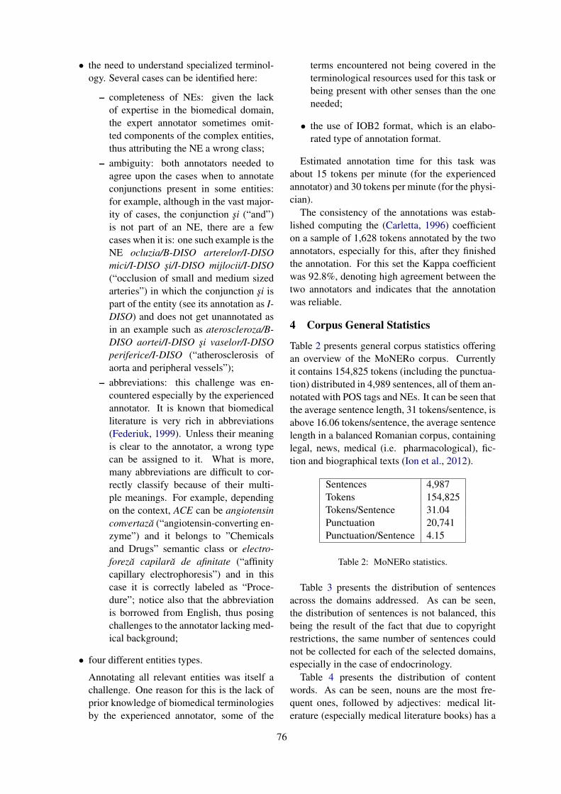
• the need to understand specialized terminol-ogy. Several cases can be identified here:
– completeness of NEs: given the lackof expertise in the biomedical domain,the expert annotator sometimes omit-ted components of the complex entities,thus attributing the NE a wrong class;
– ambiguity: both annotators needed toagree upon the cases when to annotateconjunctions present in some entities:for example, although in the vast major-ity of cases, the conjunction şi (“and”)is not part of an NE, there are a fewcases when it is: one such example is theNE ocluzia/B-DISO arterelor/I-DISOmici/I-DISO şi/I-DISO mijlocii/I-DISO(“occlusion of small and medium sizedarteries”) in which the conjunction şi ispart of the entity (see its annotation as I-DISO) and does not get unannotated asin an example such as ateroscleroza/B-DISO aortei/I-DISO şi vaselor/I-DISOperiferice/I-DISO (“atherosclerosis ofaorta and peripheral vessels”);
– abbreviations: this challenge was en-countered especially by the experiencedannotator. It is known that biomedicalliterature is very rich in abbreviations(Federiuk, 1999). Unless their meaningis clear to the annotator, a wrong typecan be assigned to it. What is more,many abbreviations are difficult to cor-rectly classify because of their multi-ple meanings. For example, dependingon the context, ACE can be angiotensinconvertază (“angiotensin-converting en-zyme”) and it belongs to ”Chemicalsand Drugs” semantic class or electro-foreză capilară de afinitate (“affinitycapillary electrophoresis”) and in thiscase it is correctly labeled as “Proce-dure”; notice also that the abbreviationis borrowed from English, thus posingchallenges to the annotator lacking med-ical background;
• four different entities types.
Annotating all relevant entities was itself achallenge. One reason for this is the lack ofprior knowledge of biomedical terminologiesby the experienced annotator, some of the
terms encountered not being covered in theterminological resources used for this task orbeing present with other senses than the oneneeded;
• the use of IOB2 format, which is an elabo-rated type of annotation format.
Estimated annotation time for this task wasabout 15 tokens per minute (for the experiencedannotator) and 30 tokens per minute (for the physi-cian).
The consistency of the annotations was estab-lished computing the (Carletta, 1996) coefficienton a sample of 1,628 tokens annotated by the twoannotators, especially for this, after they finishedthe annotation. For this set the Kappa coefficientwas 92.8%, denoting high agreement between thetwo annotators and indicates that the annotationwas reliable.
4 Corpus General Statistics
Table 2 presents general corpus statistics offeringan overview of the MoNERo corpus. Currentlyit contains 154,825 tokens (including the punctua-tion) distributed in 4,989 sentences, all of them an-notated with POS tags and NEs. It can be seen thatthe average sentence length, 31 tokens/sentence, isabove 16.06 tokens/sentence, the average sentencelength in a balanced Romanian corpus, containinglegal, news, medical (i.e. pharmacological), fic-tion and biographical texts (Ion et al., 2012).
Sentences 4,987Tokens 154,825Tokens/Sentence 31.04Punctuation 20,741Punctuation/Sentence 4.15
Table 2: MoNERo statistics.
Table 3 presents the distribution of sentencesacross the domains addressed. As can be seen,the distribution of sentences is not balanced, thisbeing the result of the fact that due to copyrightrestrictions, the same number of sentences couldnot be collected for each of the selected domains,especially in the case of endocrinology.
Table 4 presents the distribution of contentwords. As can be seen, nouns are the most fre-quent ones, followed by adjectives: medical lit-erature (especially medical literature books) has a
76
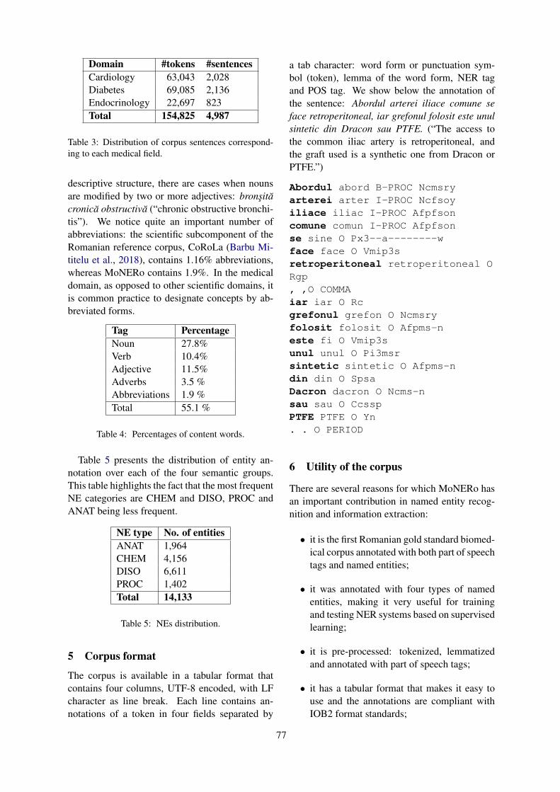
Domain #tokens #sentencesCardiology 63,043 2,028Diabetes 69,085 2,136Endocrinology 22,697 823Total 154,825 4,987
Table 3: Distribution of corpus sentences correspond-ing to each medical field.
descriptive structure, there are cases when nounsare modified by two or more adjectives: bronşităcronică obstructivă (“chronic obstructive bronchi-tis”). We notice quite an important number ofabbreviations: the scientific subcomponent of theRomanian reference corpus, CoRoLa (Barbu Mi-titelu et al., 2018), contains 1.16% abbreviations,whereas MoNERo contains 1.9%. In the medicaldomain, as opposed to other scientific domains, itis common practice to designate concepts by ab-breviated forms.
Tag PercentageNoun 27.8%Verb 10.4%Adjective 11.5%Adverbs 3.5 %Abbreviations 1.9 %Total 55.1 %
Table 4: Percentages of content words.
Table 5 presents the distribution of entity an-notation over each of the four semantic groups.This table highlights the fact that the most frequentNE categories are CHEM and DISO, PROC andANAT being less frequent.
NE type No. of entitiesANAT 1,964CHEM 4,156DISO 6,611PROC 1,402Total 14,133
Table 5: NEs distribution.
5 Corpus format
The corpus is available in a tabular format thatcontains four columns, UTF-8 encoded, with LFcharacter as line break. Each line contains an-notations of a token in four fields separated by
a tab character: word form or punctuation sym-bol (token), lemma of the word form, NER tagand POS tag. We show below the annotation ofthe sentence: Abordul arterei iliace comune seface retroperitoneal, iar grefonul folosit este unulsintetic din Dracon sau PTFE. (“The access tothe common iliac artery is retroperitoneal, andthe graft used is a synthetic one from Dracon orPTFE.”)
Abordul abord B-PROC Ncmsryarterei arter I-PROC Ncfsoyiliace iliac I-PROC Afpfsoncomune comun I-PROC Afpfsonse sine O Px3--a--------wface face O Vmip3sretroperitoneal retroperitoneal ORgp, ,O COMMAiar iar O Rcgrefonul grefon O Ncmsryfolosit folosit O Afpms-neste fi O Vmip3sunul unul O Pi3msrsintetic sintetic O Afpms-ndin din O SpsaDacron dacron O Ncms-nsau sau O CcsspPTFE PTFE O Yn. . O PERIOD
6 Utility of the corpus
There are several reasons for which MoNERo hasan important contribution in named entity recog-nition and information extraction:
• it is the first Romanian gold standard biomed-ical corpus annotated with both part of speechtags and named entities;
• it was annotated with four types of namedentities, making it very useful for trainingand testing NER systems based on supervisedlearning;
• it is pre-processed: tokenized, lemmatizedand annotated with part of speech tags;
• it has a tabular format that makes it easy touse and the annotations are compliant withIOB2 format standards;
77
• it is a resource in a language other than En-glish, which can help to train and test NERsystems to perform language and domainadaptation;
• it is freely available for download6 and non-commercial use. The archive contains threefiles, one for each medical domain, and an-other file containing all the other ones.
To prove the maturity and utility of this re-source we used it to train and test a NER sys-tem (Boroş et al., 2018) for biomedical namedentity recognition task for Romanian language.The architecture used is based on BidirectionalLong-Short-Term Memory (BDLSTM) networks(Graves, 2012). The system is trained to pro-duce fully connected subgraphs. The feature-setis composed of word embeddings and character-level embeddings. In order to train the system thecorpus was split in three sets: training set 80%,development set 10% and test set 10%. The eval-uation of the performance of the system was donecomputing the F1 score and a score of 81.4 wasobtained 7. This experiment represents a startingpoint for the development/adaptation of NER sys-tems for biomedical domain in Romanian.
7 Conclusions
We presented the MoNERo corpus, a gold stan-dard biomedical corpus for Romanian languageenhanced with two types of annotations: morpho-logical and named entities specific to the biomedi-cal field. To our knowledge this is the first biomed-ical corpus of this type for the Romanian language.This resource has already proven its value and util-ity, having been used in the development of theNER systems for the Romanian language. TheMoNERo corpus is freely available for downloadand non-commercial use, which makes it evenmore valuable for the community.
8 Acknowledgements
Part of the work presented here was supported bya grant of the Romanian Ministry of Research andInnovation, PCCDI - UEFISCDI, project num-ber PN-III-P1-1.2-PCCDI-2017-0818/72, within
6The corpus is accessible at http://www.racai.ro/en/tools/text/
7The tool trained can be accessed at the following ad-dress: http://89.38.230.23/teprolin/index.php?path=teprolin/custom
PNCDI III. We would like to thank the threeanonymous reviewers for the valuable suggestionsand hard work.
ReferencesVerginica Barbu Mititelu, Mihaela Cristescu, and Mi-
haela Onofrei. 2019. The Romanian Corpus Anno-tated with Verbal Multiword Expressions. In Pro-ceedings of the Joint Workshop on Multiword Ex-pressions and WordNet (MWE-WN 2019), Florence,Italy.
Verginica Barbu Mititelu, Dan Tufiş, and Elena Irimia.2018. The Reference Corpus of the Contempo-rary Romanian Language (CoRoLa). In Proceed-ings of the Eleventh International Conference onLanguage Resources and Evaluation (LREC 2018),pages 1178–1185, Miyazaki, Japan. European Lan-guage Resources Association (ELRA).
Tiberiu Boroş, Stefan Daniel Dumitrescu, and Ruxan-dra Burtica. 2018. NLP-cube: End-to-end raw textprocessing with neural networks. In Proceedings ofthe CoNLL 2018 Shared Task: Multilingual Pars-ing from Raw Text to Universal Dependencies, pages171–179, Brussels, Belgium. Association for Com-putational Linguistics.
Jean Carletta. 1996. Assessing agreement on classifi-cation tasks: the kappa statistic. Computational lin-guistics, 22(2):249–254.
Ludmila Dimitrova, Nancy Ide, Vladimir Petkevic,Tomaz Erjavec, Heiki Jaan Kaalep, and Dan Tufiş.1998. Multext-east: Parallel and comparable cor-pora and lexicons for six central and eastern euro-pean languages. In Proceedings of the 36th AnnualMeeting of the Association for Computational Lin-guistics and 17th International Conference on Com-putational Linguistics - Volume 1, ACL ’98/COL-ING ’98, pages 315–319, Stroudsburg, PA, USA.Association for Computational Linguistics.
Rezarta Islamaj Doğan, Robert Leaman, and ZhiyongLu. 2014. Ncbi disease corpus: a resource for dis-ease name recognition and concept normalization.Journal of biomedical informatics, 47:1–10.
Carol S Federiuk. 1999. The effect of abbreviations onmedline searching. Academic emergency medicine,6(4):292–296.
Lorraine Goeuriot, Liadh Kelly, Hanna Suominen,Aurélie Névéol, Aude Robert, Evangelos Kanoulas,Rene Spijker, Joao Palotti, and Guido Zuccon. 2017.Clef 2017 ehealth evaluation lab overview. In Inter-national Conference of the Cross-Language Evalu-ation Forum for European Languages, pages 291–303. Springer.
Alex Graves. 2012. Supervised sequence labelling. InSupervised sequence labelling with recurrent neuralnetworks, pages 5–13. Springer.
78
Radu Ion. 2007. Word Sense Disambiguation MethodsApplied to English and Romanian (in Romanian).Ph.D. thesis, Romanian Academy.
Radu Ion, Elena Irimia, Dan Stefanescu, and Dan Tufiş.2012. Rombac: The romanian balanced annotatedcorpus. In LREC, pages 339–344. Citeseer.
Halil Kilicoglu. 2017. Biomedical text mining forresearch rigor and integrity: tasks, challenges, di-rections. Briefings in bioinformatics, 19(6):1400–1414.
Martin Krallinger, Obdulia Rabal, Florian Leitner,Miguel Vazquez, David Salgado, Zhiyong Lu,Robert Leaman, Yanan Lu, Donghong Ji, Daniel MLowe, et al. 2015. The chemdner corpus of chemi-cals and drugs and its annotation principles. Journalof cheminformatics, 7(1):S2.
Fei Li, Meishan Zhang, Guohong Fu, and DonghongJi. 2017. A neural joint model for entity and relationextraction from biomedical text. BMC bioinformat-ics, 18(1):198.
Alexa T McCray, Anita Burgun, and Olivier Boden-reider. 2001. Aggregating umls semantic types forreducing conceptual complexity. Studies in healthtechnology and informatics, 84(0 1):216.
Maria Mitrofan and Radu Ion. 2017. Adapting the ttlromanian pos tagger to the biomedical domain. InBiomedicalNLP@ RANLP, pages 8–14.
Maria Mitrofan and Dan Tufiş. 2018. Bioro: Thebiomedical corpus for the romanian language. InProceedings of the Eleventh International Con-ference on Language Resources and Evaluation(LREC-2018).
Isabel Moreno, Ester Boldrini, Paloma Moreda, andM Teresa Romá-Ferri. 2017. Drugsemantics: acorpus for named entity recognition in spanishsummaries of product characteristics. Journal ofbiomedical informatics, 72:8–22.
Aurélie Névéol, Cyril Grouin, Jeremy Leixa, SophieRosset, and Pierre Zweigenbaum. 2014. The quaerofrench medical corpus: A ressource for medical en-tity recognition and normalization. In In Proc Bio-TextM, Reykjavik. Citeseer.
Maite Oronoz, Koldo Gojenola, Alicia Pérez,Arantza Dı́az de Ilarraza, and Arantza Casillas.2015. On the creation of a clinical gold standardcorpus in spanish: Mining adverse drug reactions.Journal of biomedical informatics, 56:318–332.
Angus Roberts, Robert Gaizauskas, Mark Hepple,George Demetriou, Yikun Guo, Ian Roberts, andAndrea Setzer. 2009. Building a semantically anno-tated corpus of clinical texts. Journal of biomedicalinformatics, 42(5):950–966.
Erik F Sang and Jorn Veenstra. 1999. Representing textchunks. In Proceedings of the ninth conference onEuropean chapter of the Association for Computa-tional Linguistics, pages 173–179. Association forComputational Linguistics.
Paul Thompson, Syed A Iqbal, John McNaught, andSophia Ananiadou. 2009. Construction of an anno-tated corpus to support biomedical information ex-traction. BMC bioinformatics, 10(1):349.
Dan Tufiş. 2000. Using a large set of eagles-compliantmorpho-syntactic descriptors as a tagset for proba-bilistic tagging. In Proceedings of LREC.
D Tufiş, AM Barbu, V Pătraşcu, G Rotariu, andC Popescu. 1997. Corpora and corpus-basedmorpho-lexical processing. Recent Advances in Ro-manian Language Technology, Editura Academiei,pages 35–56.
Özlem Uzuner, Imre Solti, Fei Xia, and EithonCadag. 2010. Community annotation experimentfor ground truth generation for the i2b2 medicationchallenge. Journal of the American Medical Infor-matics Association, 17(5):519–523.
W John Wilbur, Andrey Rzhetsky, and Hagit Shatkay.2006. New directions in biomedical text annota-tion: definitions, guidelines and corpus construction.BMC bioinformatics, 7(1):356.
79
Proceedings of the BioNLP 2019 workshop, pages 80–87Florence, Italy, August 1, 2019. c©2019 Association for Computational Linguistics
Domain Adaptation of SRL Systems for Biological Processes
Dheeraj Rajagopal♠∗ Nidhi Vyas♠∗ Aditya Siddhant♠ Anirudha Rayasam♠Niket Tandon♣ Eduard Hovy♠♠Carnegie Mellon University
♣Allen Institute for Artificial Intelligence{dheeraj,nkvyas,asiddhan,arayasam}@andrew.cmu.edu
[email protected], [email protected]
Abstract
Domain adaptation remains one of the mostchallenging aspects in the wide-spread useof Semantic Role Labeling (SRL) systems.Current state-of-the-art methods are typicallytrained on large-scale datasets, but their per-formances do not directly transfer to low-resource domain-specific settings. In thispaper, we propose two approaches for do-main adaptation in biological domain that in-volve pre-training LSTM-CRF based on ex-isting large-scale datasets and adapting it fora low-resource corpus of biological processes.Our first approach defines a mapping betweenthe source labels and the target labels, and theother approach modifies the final CRF layerin sequence-labeling neural network architec-ture. We perform our experiments on Pro-cessBank (Berant et al., 2014) dataset whichcontains less than 200 paragraphs on biologi-cal processes. We improve over the previousstate-of-the-art system on this dataset by 21F1 points. We also show that, by incorporat-ing event-event relationship in ProcessBank,we are able to achieve an additional 2.6 F1gain, giving us possible insights into how toimprove SRL systems for biological processusing richer annotations.
1 Introduction
Semantic Role Labeling (SRL) is shallow seman-tic representation of a sentence, that allows us tocapture the roles of arguments that anchor aroundan event. Despite significant recent progress inDeep SRL systems (He et al., 2017; Tan et al.,2017), there has been limited work in adaptingsuch systems to low resource domain-specific sce-narios where the label space of both domains arecompletely different. Additionally, existing do-main adaptation for SRL requires an overhead ofannotating the new corpus using guidelines similar
∗∗Both authors equally contributed to the paper.
to the source dataset, and every domain-specificcorpora might not necessarily adhere to the samelabel structure and similar annotation guidelines.
We present two different domain adaptationstrategies that rely on training the model on a largecorpora (source dataset) and fine-tuning on a low-resource domain-specific corpus (target dataset),more specifically biological processes domain.The first approach uses mappings from the sourcelabel space to the target label space. For this, wepresent DeepSRL-CRF, which incorporates a CRFlayer over the DeepSRL model (He et al., 2017)with an intermediate step of mapping labels fromsource to target domain. For the second approach,we use a CNN-LSTM-CRF model to pre-train theneural network weights on the source domain, andadapt the final CRF layer of the network based onthe target label space. We then fine-tune the modelon the target dataset.
For empirical evaluation, we explore the chal-lenge of SRL in ProcessBank dataset, where thetarget domain (biological processes) is drasticallydifferent compared to the source domain (news).Both of our approaches are effective for adapt-ing SRL systems for biological processes. Com-pared to the previous best system, we get an im-provement of about 24 F1 points when we uselabel-mapping approach, and about 21 F1 pointimprovement when we adapt the final CRF layer.Our contributions can be summarized as follows:
1. Two different approaches for domain adap-tation of SRL for biological processes, with ourcode and models publicly available 1
2. An in-depth analysis for each of the do-main adaptation strategies, both perform signifi-cantly better in low-resource SRL for biologicalprocesses
3. Analysis of the model performance when the
1https://github.com/dheerajrajagopal/SciQA
80
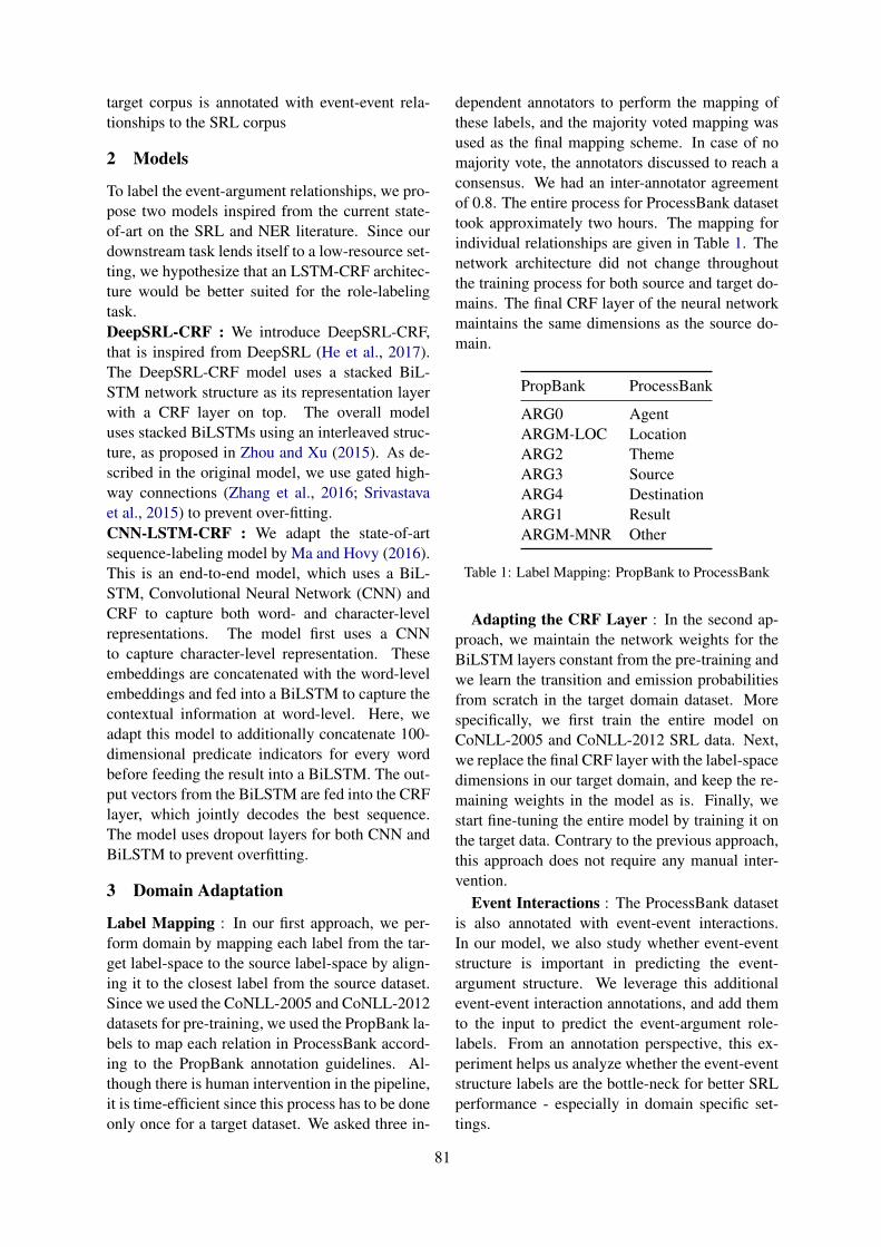
target corpus is annotated with event-event rela-tionships to the SRL corpus
2 Models
To label the event-argument relationships, we pro-pose two models inspired from the current state-of-art on the SRL and NER literature. Since ourdownstream task lends itself to a low-resource set-ting, we hypothesize that an LSTM-CRF architec-ture would be better suited for the role-labelingtask.DeepSRL-CRF : We introduce DeepSRL-CRF,that is inspired from DeepSRL (He et al., 2017).The DeepSRL-CRF model uses a stacked BiL-STM network structure as its representation layerwith a CRF layer on top. The overall modeluses stacked BiLSTMs using an interleaved struc-ture, as proposed in Zhou and Xu (2015). As de-scribed in the original model, we use gated high-way connections (Zhang et al., 2016; Srivastavaet al., 2015) to prevent over-fitting.CNN-LSTM-CRF : We adapt the state-of-artsequence-labeling model by Ma and Hovy (2016).This is an end-to-end model, which uses a BiL-STM, Convolutional Neural Network (CNN) andCRF to capture both word- and character-levelrepresentations. The model first uses a CNNto capture character-level representation. Theseembeddings are concatenated with the word-levelembeddings and fed into a BiLSTM to capture thecontextual information at word-level. Here, weadapt this model to additionally concatenate 100-dimensional predicate indicators for every wordbefore feeding the result into a BiLSTM. The out-put vectors from the BiLSTM are fed into the CRFlayer, which jointly decodes the best sequence.The model uses dropout layers for both CNN andBiLSTM to prevent overfitting.
3 Domain Adaptation
Label Mapping : In our first approach, we per-form domain by mapping each label from the tar-get label-space to the source label-space by align-ing it to the closest label from the source dataset.Since we used the CoNLL-2005 and CoNLL-2012datasets for pre-training, we used the PropBank la-bels to map each relation in ProcessBank accord-ing to the PropBank annotation guidelines. Al-though there is human intervention in the pipeline,it is time-efficient since this process has to be doneonly once for a target dataset. We asked three in-
dependent annotators to perform the mapping ofthese labels, and the majority voted mapping wasused as the final mapping scheme. In case of nomajority vote, the annotators discussed to reach aconsensus. We had an inter-annotator agreementof 0.8. The entire process for ProcessBank datasettook approximately two hours. The mapping forindividual relationships are given in Table 1. Thenetwork architecture did not change throughoutthe training process for both source and target do-mains. The final CRF layer of the neural networkmaintains the same dimensions as the source do-main.
PropBank ProcessBank
ARG0 AgentARGM-LOC LocationARG2 ThemeARG3 SourceARG4 DestinationARG1 ResultARGM-MNR Other
Table 1: Label Mapping: PropBank to ProcessBank
Adapting the CRF Layer : In the second ap-proach, we maintain the network weights for theBiLSTM layers constant from the pre-training andwe learn the transition and emission probabilitiesfrom scratch in the target domain dataset. Morespecifically, we first train the entire model onCoNLL-2005 and CoNLL-2012 SRL data. Next,we replace the final CRF layer with the label-spacedimensions in our target domain, and keep the re-maining weights in the model as is. Finally, westart fine-tuning the entire model by training it onthe target data. Contrary to the previous approach,this approach does not require any manual inter-vention.
Event Interactions : The ProcessBank datasetis also annotated with event-event interactions.In our model, we also study whether event-eventstructure is important in predicting the event-argument structure. We leverage this additionalevent-event interaction annotations, and add themto the input to predict the event-argument role-labels. From an annotation perspective, this ex-periment helps us analyze whether the event-eventstructure labels are the bottle-neck for better SRLperformance - especially in domain specific set-tings.
81
4 Experiments
Experimental Setup : For evaluation, we usethe CoNLL-2005 (Carreras and Màrquez, 2005)and CoNLL-2012 (Pradhan et al., 2013) datasetsas our primary large-scale datasets with the stan-dard splits. For the domain adaptation scenario,we use the ProcessBank dataset (Berant et al.,2014)2. We used 134 annotated paragraphs fortraining, 19 for development and 50 for test-ing. Each passage in the ProcessBank datasetdescribes a process, defined by a directed graph(T,A,Ett, Eta), where nodes T denote eventtriggers and A denote their corresponding argu-ments. Ett represents labeled edges event-eventrelations and Eta describe event-argument rela-tions. The edges Eta are annotated with seman-tic roles AGENT, THEME, SOURCE, DESTINA-TION, LOCATION, RESULT and OTHER. EachEtt edge between event and another event is an-notated with the relations CAUSE, ENABLE andPREVENT. Our experiments primarily focus onthe prediction of the event-argument structuresEta since the source datasets that we use for do-main adaption do not contain any event-event re-lationship annotation.Baselines : In our first set of baselines, we com-pare our models on the CoNLL-2005 and CoNLL-2012 tasks. We use the previous state-of-the-artSRL system from He et al. (2018) as our baseline.3. Since our model is based on LSTM-CRF hybridarchitecture, we implement two other baselines forour approach. We use a standard BiLSTM-CRFmodel (Huang et al., 2015), and a model basedon the structured attention proposed in Liu andLapata (2017) which uses CRF style structure inthe intermediate layer. For a fair comparison, weaugmented this structured attention based networkwith a CRF layer on top. We use 300D GLoVe em-beddings (Pennington et al., 2014) across all mod-els. For domain adaptation, we use the originalsystem from Berant et al. (2014) as the baseline.It uses the approach in Punyakanok et al. (2008),where for each trigger, a set of argument candi-dates are first determined, and then a binary classi-fier uses argument identification features to prune
2For dataset statistics, we refer readers to Berant et al.(2014), Table 1. We use the same training and test split pro-vided in the original dataset. We further split the training setinto training and development set.
3Due to resource limitations, we were unable to run thesame model for 500 epochs, so we report results from theirpaper for CoNLL-2005 and CoNLL-2012 datasets
this set with high recall.
5 Results
Semantic Role Labeling : Table 2 shows theSRL results4 for the CoNLL-2005 and CoNLL-2012 datasets across all baseline models. Fromthe table, it is evident that our DeepSRL-CRFmodel with ELMo embeddings performs slightlylesser than the current state-of-the-art SRL modelDeepSRL with ELMo. We were able to per-form significantly better than the other baselines –BiLSTM-CRF and Strucutured Attention model.Our DeepSRL-CRF model without ELMo per-formed significantly lower and the improvementwas notably higher with ELMo.Domain Adaptation : For all our domain adapta-tion experiments, we found that the DeepSRL andDeepSRL-CRF models reach similar F1 scoreswithout any pre-training. Table 3 shows the re-sults for the set of models that were trained for do-main adaptation using label mapping. After pre-training it on the CoNLL 2005 and CoNLL-2012dataset for 50 epochs, we fine-tuned the weightson the ProcessBank dataset without making anychanges to the network. The results signify thatthe models that were effective for a large dataset,might not achieve similar gains when restrictedto specific low-resource domains. The DeepSRL-CRF model, after incorporating event-event rela-tionships, outperforms the previous system fromBerant et al. (2014) by about 24 F1 points.
In our second domain adaptation approach,we test the CNN-LSTM-CRF model by learn-ing the final CRF layer with transition andemission probabilities for the target label space.The CNN-LSTM-CRF model, without any pre-training achieves 40.62 F1 which is similar toprevious performance from Berant et al. (2014).However, after pre-training it on CoNLL 2005 andCoNLL-2012 dataset for 50 epochs, the modelsoutperforms by about 21.7 F1 points. Adapting theCRF layer, with transition and emission probabili-ties for the target domain data in its label space,shows impressive gains in the low-resource set-ting, specially when there is a limitation for usingany human-intervention in the domain adaptationprocess. Although empirically effective, we be-lieve that there is immense scope to understandingthe impact of better initialization from a theoreti-cal perspective. We also observe that pretraining
4We use span-based precision, recall and F1 measure
82
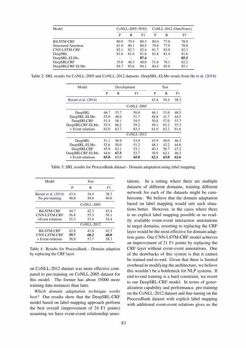
Model CoNLL-2005 (WSJ) CoNLL-2012 (OntoNotes)
P R F1 P R F1
BiLSTM-CRF 80.9 79.4 80.3 80.0 77.8 78.9Structured Attention 81.0 80.1 80.5 79.6 77.9 78.8CNN-LSTM-CRF 82.1 82.7 82.4 81.7 83.0 82.3DeepSRL 81.6 81.6 81.6 81.8 81.4 81.6DeepSRL-ELMo - - 87.4 - - 85.5DeepSRLCRF 35.0 46.3 40.0 51.6 78.1 62.2DeepSRLCRF-ELMo 84.7 83.6 84.1 84.4 85.8 85.1
Table 2: SRL results for CoNLL-2005 and CoNLL-2012 datasets. DeepSRL-ELMo resuls from He et al. (2018)
Model Development Test
P R F1 P R F1
Berant et al. (2014) - - - 43.4 34.4 38.3
CoNLL-2005
DeepSRL 46.7 53.7 50.0 46.1 51.0 48.5DeepSRL-ELMo 55.0 48.0 51.7 48.8 41.7 44.5
DeepSRLCRF 51.4 58.1 54.5 50.8 57.0 53.7DeepSRLCRF-ELMo 53.5 66.2 59.2 49.1 63.2 55.3
+ Event relations 63.0 63.7 63.3 61.0 62.2 61.6CoNLL-2012
DeepSRL 51.1 56.9 53.9 43.9 49.0 46.3DeepSRL-ELMo 52.6 50.0 51.2 48.1 43.2 44.6
DeepSRLCRF 45.9 63.1 53.1 40.3 56.7 47.2DeepSRLCRF-ELMo 44.6 67.5 53.7 36.9 62.1 46.3
+ Event relations 65.0 65.0 65.0 62.1 63.0 62.6
Table 3: SRL results for ProcessBank dataset - Domain adaptation using label mapping.
Model Test
P R F1
Berant et al. (2014) 43.4 34.4 38.3No pre-training 40.6 40.6 40.6
CoNLL-2005
BiLSTM-CRF 44.7 42.3 43.4CNN-LSTM-CRF 56.8 55.5 56.1+Event relations 55.3 53.4 54.4
CoNLL-2012
BiLSTM-CRF 42.8 41.0 42.3CNN-LSTM-CRF 59.7 60.2 60.0+ Event relations 58.8 57.7 58.3
Table 4: Results for ProcessBank - Domain adaptionby replacing the CRF layer
on CoNLL-2012 dataset was more effective com-pared to pre-training on CoNLL-2005 dataset forthis model. The former has about 35000 moretraining data instances than later.
Which domain adaptation technique worksbest? Our results show that the DeepSRL-CRFmodel based on label mapping approach performthe best overall (improvement of 24 F1 points)assuming we have event-event relationship anno-
tations. In a setting where there are multipledatasets of different domains, training differentnetwork for each of the datasets might be cum-bersome. We believe that the domain adaptationbased on label mapping would suit such situa-tions better. However, in the cases where thereis no explicit label mapping possible or no read-ily available event-event interaction annotationsin target domains, resorting to replacing the CRFlayer would be the most effective for domain adap-tion gains. Our CNN-LSTM-CRF model achievesan improvement of 21 F1 points by replacing theCRF layer without event-event annotations. Oneof the drawbacks of this system is that it cannotbe trained end-to-end. Given that there is limitedoverhead in modifying the architecture, we believethis wouldn’t be a bottleneck for NLP systems. Ifend-to-end training is a hard constraint, we resortto our DeepSRL-CRF model. In terms of gener-alization capability and performance, pre-trainingon the CoNLL-2012 dataset and fine-tuning on theProcessBank dataset with explicit label mappingwith additional event-event relations gives us the
83
best results. 5
6 Related Work
Domain adaptation leverages on large-scaledatasets to help improve the performance on othersmaller and similar tasks. From the SRL perspec-tive, one of the earliest work from Daume III andMarcu (2006) showed simple but effective waysfor ‘transferring the learning’ from a source toa target domain. Building on strong feature-richmodels, Dahlmeier and Ng (2010) analyzed vari-ous features and techniques that are used for do-main adaptation and conducted an extensive studyfor biological SRL task. Later, Lim et al. (2014)proposed a model that uses structured learningfor domain adaptation. Although effective, thesemethods rely on hand-annotated features. Re-cently, there have been neural-network based at-tempts at Domain adaptation in SRL. Do et al.(2015) combined the knowledge from a neural lan-guage model and external linguistic resource fordomain adaptation for biomedical corpora. Ourwork closely aligns to this work from a modelingstand-point. Our target domain is biological pro-cess descriptions from high-school biology with-out restrictions of PropBank style annotations.
Our work builds on multiple existing works,especially the dataset from Berant et al. (2014),using the thematic roles defined in Palmer et al.(2005). Our approach is inspired by the recentsuccess in including structured representations indeep neural networks (He et al., 2017; Ma andHovy, 2016) for structured prediction tasks. Ourprimary motivation is to improve the system per-formance for low-resource domain-specific event-argument labeling tasks, particularly biologicalprocesses. Argument labeling, specifically, SRLas been used for biomedical domain previously.E.g. Shah and Bork (2006) applied SRL in theLSAT system to identify sentences with gene tran-scripts, and Bethard et al. (2008) applied SRLto extract information about protein movement.However, developing annotated SRL data for eachtask can be expensive.
7 Conclusion
In this work, we present two new approachesto adapt deep learning models trained on large
5Please refer to the supplemental material 9 for a detaileddiscussion on results
scale datasets, to smaller domain-specific biolog-ical process dataset. We present a LSTM-CRFbased architectures which perform on-par with thestate-of-the-art models for SRL but significantlybetter than them in low-resource domain-specificsettings. We show significant improvement of ap-proximately 24 F1 points over current best modelfor role-labeling on the ProcessBank - notably dif-ferent in nature compared to CoNLL dataset.
ReferencesJonathan Berant, Vivek Srikumar, Pei-Chun Chen,
Abby Vander Linden, Brittany Harding, BradHuang, Peter Clark, and Christopher D Manning.2014. Modeling biological processes for readingcomprehension. In EMNLP, pages 1499–1510.
Steven Bethard, Zhiyong Lu, James H Martin, andLawrence Hunter. 2008. Semantic role labeling forprotein transport predicates. BMC bioinformatics,9(1):277.
Xavier Carreras and Lluı́s Màrquez. 2005. Introductionto the conll-2005 shared task: Semantic role label-ing. pages 152–164. Association for ComputationalLinguistics.
Daniel Dahlmeier and Hwee Tou Ng. 2010. Domainadaptation for semantic role labeling in the biomed-ical domain. Bioinformatics, 26(8):1098–1104.
Hal Daume III and Daniel Marcu. 2006. Domain adap-tation for statistical classifiers. Journal of artificialIntelligence research, 26:101–126.
Quynh Ngoc Thi Do, Steven Bethard, and Marie-Francine Moens. 2015. Domain adaptation in se-mantic role labeling using a neural language modeland linguistic resources. IEEE/ACM Trans. Audio,Speech & Language Processing, pages 1812–1823.
Xavier Glorot and Yoshua Bengio. 2010. Understand-ing the difficulty of training deep feedforward neuralnetworks. In AISTATS, pages 249–256.
Kaiming He, Xiangyu Zhang, Shaoqing Ren, and JianSun. 2015. Delving deep into rectifiers: Surpass-ing human-level performance on imagenet classifi-cation. In ICCV, pages 1026–1034.
Luheng He, Kenton Lee, Omer Levy, and Luke Zettle-moyer. 2018. Jointly predicting predicates and ar-guments in neural semantic role labeling. arXivpreprint arXiv:1805.04787.
Luheng He, Kenton Lee, Mike Lewis, and Luke Zettle-moyer. 2017. Deep semantic role labeling: Whatworks and whats next. In ACL, volume 1, pages473–483.
Zhiheng Huang, Wei Xu, and Kai Yu. 2015. Bidirec-tional lstm-crf models for sequence tagging. arXivpreprint arXiv:1508.01991.
84
Soojong Lim, Changki Lee, Pum-Mo Ryu, HyunkiKim, Sang Kyu Park, and Dongyul Ra. 2014.Domain-adaptation technique for semantic role la-beling with structural learning. ETRI Journal,36(3):429–438.
Yang Liu and Mirella Lapata. 2017. Learning struc-tured text representations. CoRR, abs/1705.09207.
Xuezhe Ma and Eduard Hovy. 2016. End-to-end se-quence labeling via bi-directional lstm-cnns-crf. InACL, volume 1, pages 1064–1074.
Martha Palmer, Daniel Gildea, and Paul Kingsbury.2005. The proposition bank: An annotated cor-pus of semantic roles. Computational linguistics,31(1):71–106.
Jeffrey Pennington, Richard Socher, and ChristopherManning. 2014. Glove: Global vectors for wordrepresentation. In Proceedings of the 2014 confer-ence on empirical methods in natural language pro-cessing (EMNLP), pages 1532–1543.
Sameer Pradhan, Alessandro Moschitti, Nianwen Xue,Hwee Tou Ng, Anders Björkelund, Olga Uryupina,Yuchen Zhang, and Zhi Zhong. 2013. Towards ro-bust linguistic analysis using ontonotes. In CoNLL,pages 143–152.
Vasin Punyakanok, Dan Roth, and Wen-tau Yih. 2008.The importance of syntactic parsing and inference insemantic role labeling. Computational Linguistics,34(2):257–287.
Parantu K Shah and Peer Bork. 2006. Lsat: learningabout alternative transcripts in medline. Bioinfor-matics, 22(7):857–865.
Rupesh K Srivastava, Klaus Greff, and Jürgen Schmid-huber. 2015. Training very deep networks. In Ad-vances in neural information processing systems,pages 2377–2385.
Zhixing Tan, Mingxuan Wang, Jun Xie, YidongChen, and Xiaodong Shi. 2017. Deep semanticrole labeling with self-attention. arXiv preprintarXiv:1712.01586.
Yu Zhang, Guoguo Chen, Dong Yu, Kaisheng Yaco,Sanjeev Khudanpur, and James Glass. 2016. High-way long short-term memory rnns for distant speechrecognition. In ICASSP.
Jie Zhou and Wei Xu. 2015. End-to-end learning ofsemantic role labeling using recurrent neural net-works. In ACL, volume 1, pages 1127–1137.
8 Appendices
8.1 Parameter Settings
CNN-LSTM-CRF : The words that are ab-sent in GloVe embeddings are replaced with<UNK> and intialized randomly. The character-embeddings are intialized with uniform samples asproposed in He et al. (2015). Weight matrices areinitialized using Glorot initialization (Glorot andBengio, 2010). Bias vectors are initialized to zeroexcept the bias vector of Bi-LSTM (bf ) which isinitialized to 1. Parameter optimization is per-formed using Adam optimizer with batch size of32 and learning rate of 0.0001. We use a non-variational dropout of 0.5 on CNN and BiLSTMlayers. We use a hidden size of 512, and use 5layers for the BiLSTM. For character embeddings,we use a hidden size of 30. The CNN’s use 30 fil-ters.DeepSRL-CRF : We maintain most of the exper-imental settings similar to He et al. (2017). Weconvert all tokens to lower-case, initialize with theembeddings. We use the Adadelta with ε = 1e−6
and ρ = 0.95 with mini-batch size 64. Thedropout probability was set to 0.1 and gradientclipping at 1. The models are trained for 50 epochs(compared to 500 epochs in the original DeepSRLmodel) and use the best model from 50 epochs forpretraining. We do not add any constraints for de-coding and we use the viterbi decoding to get ouroutput tags.
9 Supplemental Material
9.1 Additional Discussion
DeepSRL-CRF: The DeepSRL-CRF modelachieves comparable but slightly lower perfor-mance compared to the current state-of-the-art inthe CoNLL-2005 and CoNLL-2012 SRL datasets.We observed that these performances did notdirectly translate to the ProcessBank dataset. Inthe limited-resource domain of ProcessBank,the final CRF layer had a more pronouncedperformance improvements. Adding CRF layer toDeepSRL model improves performance by atleast4 F1 points when pre-trained using CoNLL-2005and 1 F1 point when pre-training using CoNLL-2012 dataset. Adding ELMo embeddings tothe DeepSRL and DeepSRL-CRF models didnot result in performance gains in ProcessBankexcept for one experimental setup (DeepSRL-CRF pre-trained on CoNLL-2005). Across both
85
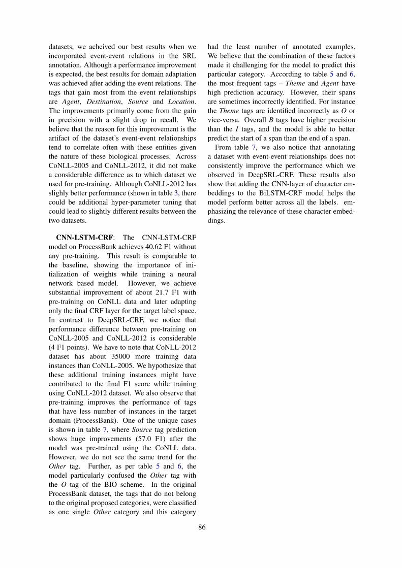
datasets, we acheived our best results when weincorporated event-event relations in the SRLannotation. Although a performance improvementis expected, the best results for domain adaptationwas achieved after adding the event relations. Thetags that gain most from the event relationshipsare Agent, Destination, Source and Location.The improvements primarily come from the gainin precision with a slight drop in recall. Webelieve that the reason for this improvement is theartifact of the dataset’s event-event relationshipstend to correlate often with these entities giventhe nature of these biological processes. AcrossCoNLL-2005 and CoNLL-2012, it did not makea considerable difference as to which dataset weused for pre-training. Although CoNLL-2012 hasslighly better performance (shown in table 3, therecould be additional hyper-parameter tuning thatcould lead to slightly different results between thetwo datasets.
CNN-LSTM-CRF: The CNN-LSTM-CRFmodel on ProcessBank achieves 40.62 F1 withoutany pre-training. This result is comparable tothe baseline, showing the importance of ini-tialization of weights while training a neuralnetwork based model. However, we achievesubstantial improvement of about 21.7 F1 withpre-training on CoNLL data and later adaptingonly the final CRF layer for the target label space.In contrast to DeepSRL-CRF, we notice thatperformance difference between pre-training onCoNLL-2005 and CoNLL-2012 is considerable(4 F1 points). We have to note that CoNLL-2012dataset has about 35000 more training datainstances than CoNLL-2005. We hypothesize thatthese additional training instances might havecontributed to the final F1 score while trainingusing CoNLL-2012 dataset. We also observe thatpre-training improves the performance of tagsthat have less number of instances in the targetdomain (ProcessBank). One of the unique casesis shown in table 7, where Source tag predictionshows huge improvements (57.0 F1) after themodel was pre-trained using the CoNLL data.However, we do not see the same trend for theOther tag. Further, as per table 5 and 6, themodel particularly confused the Other tag withthe O tag of the BIO scheme. In the originalProcessBank dataset, the tags that do not belongto the original proposed categories, were classifiedas one single Other category and this category
had the least number of annotated examples.We believe that the combination of these factorsmade it challenging for the model to predict thisparticular category. According to table 5 and 6,the most frequent tags – Theme and Agent havehigh prediction accuracy. However, their spansare sometimes incorrectly identified. For instancethe Theme tags are identified incorrectly as O orvice-versa. Overall B tags have higher precisionthan the I tags, and the model is able to betterpredict the start of a span than the end of a span.
From table 7, we also notice that annotatinga dataset with event-event relationships does notconsistently improve the performance which weobserved in DeepSRL-CRF. These results alsoshow that adding the CNN-layer of character em-beddings to the BiLSTM-CRF model helps themodel perform better across all the labels. em-phasizing the relevance of these character embed-dings.
86
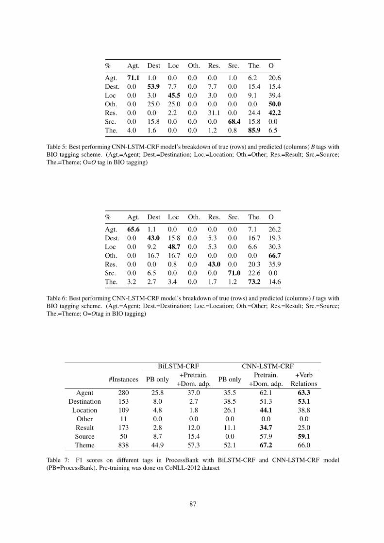
% Agt. Dest Loc Oth. Res. Src. The. O
Agt. 71.1 1.0 0.0 0.0 0.0 1.0 6.2 20.6Dest. 0.0 53.9 7.7 0.0 7.7 0.0 15.4 15.4Loc 0.0 3.0 45.5 0.0 3.0 0.0 9.1 39.4Oth. 0.0 25.0 25.0 0.0 0.0 0.0 0.0 50.0Res. 0.0 0.0 2.2 0.0 31.1 0.0 24.4 42.2Src. 0.0 15.8 0.0 0.0 0.0 68.4 15.8 0.0The. 4.0 1.6 0.0 0.0 1.2 0.8 85.9 6.5
Table 5: Best performing CNN-LSTM-CRF model’s breakdown of true (rows) and predicted (columns) B tags withBIO tagging scheme. (Agt.=Agent; Dest.=Destination; Loc.=Location; Oth.=Other; Res.=Result; Src.=Source;The.=Theme; O=O tag in BIO tagging)
% Agt. Dest Loc Oth. Res. Src. The. O
Agt. 65.6 1.1 0.0 0.0 0.0 0.0 7.1 26.2Dest. 0.0 43.0 15.8 0.0 5.3 0.0 16.7 19.3Loc 0.0 9.2 48.7 0.0 5.3 0.0 6.6 30.3Oth. 0.0 16.7 16.7 0.0 0.0 0.0 0.0 66.7Res. 0.0 0.0 0.8 0.0 43.0 0.0 20.3 35.9Src. 0.0 6.5 0.0 0.0 0.0 71.0 22.6 0.0The. 3.2 2.7 3.4 0.0 1.7 1.2 73.2 14.6
Table 6: Best performing CNN-LSTM-CRF model’s breakdown of true (rows) and predicted (columns) I tags withBIO tagging scheme. (Agt.=Agent; Dest.=Destination; Loc.=Location; Oth.=Other; Res.=Result; Src.=Source;The.=Theme; O=Otag in BIO tagging)
BiLSTM-CRF CNN-LSTM-CRF
#Instances PB only+Pretrain.
+Dom. adp.PB only
Pretrain.+Dom. adp.
+VerbRelations
Agent 280 25.8 37.0 35.5 62.1 63.3Destination 153 8.0 2.7 38.5 51.3 53.1
Location 109 4.8 1.8 26.1 44.1 38.8Other 11 0.0 0.0 0.0 0.0 0.0Result 173 2.8 12.0 11.1 34.7 25.0Source 50 8.7 15.4 0.0 57.9 59.1Theme 838 44.9 57.3 52.1 67.2 66.0
Table 7: F1 scores on different tags in ProcessBank with BiLSTM-CRF and CNN-LSTM-CRF model(PB=ProcessBank). Pre-training was done on CoNLL-2012 dataset
87
Proceedings of the BioNLP 2019 workshop, pages 88–96Florence, Italy, August 1, 2019. c©2019 Association for Computational Linguistics
Deep Contextualized Biomedical Abbreviation Expansion
Qiao JinUniversity of [email protected]
Jinling LiuUniversity of [email protected]
Xinghua LuUniversity of [email protected]
Abstract
Automatic identification and expansion ofambiguous abbreviations are essential forbiomedical natural language processing ap-plications, such as information retrieval andquestion answering systems. In this paper,we present DEep Contextualized BiomedicalAbbreviation Expansion (DECBAE) model.DECBAE automatically collects substantialand relatively clean annotated contexts for 950ambiguous abbreviations from PubMed ab-stracts using a simple heuristic. Then it uti-lizes BioELMo (Jin et al., 2019) to extractthe contextualized features of words, and feedthose features to abbreviation-specific bidi-rectional LSTMs, where the hidden states ofthe ambiguous abbreviations are used to as-sign the exact definitions. Our DECBAEmodel outperforms other baselines by largemargins, achieving average accuracy of 0.961and macro-F1 of 0.917 on the dataset. It alsosurpasses human performance for expanding asample abbreviation, and remains robust in im-balanced, low-resources and clinical settings.
1 Introduction
Abbreviations are shortened forms of text-strings.They are prevalent in biomedical literature such asscientific articles, clinical notes and user queries ininformation retrieval systems. Abbreviations canbe ambiguous (e.g.: ER can refer to estrogen re-ceptor, endoplasmic reticulum, emergency roometc.), especially when they appear in short or pro-fessional texts where the definitions are not given.For instance, about 15% of PubMed queries in-clude abbreviations (Islamaj Dogan et al., 2009),and about 14.8% of all tokens in a clinical notedataset are abbreviations (Xu et al., 2007). Inboth cases, the definitions of the abbreviations arerarely provided. Thus, automatic expansion of am-biguous abbreviations to their full forms is vital
in biomedical natural language processing (NLP)systems.
In this paper, we focus on the cases where defi-nitions of ambiguous abbreviations are not directlyavailable in the contexts, so reasoning over thecontexts is required for disambiguation. Under theconditions where definitions are provided in thecontexts, one can easily extract them using rule-based methods.
We present DEep Contextualized Biomedi-cal Abbreviation Expansion (DECBAE) model.DECBAE uses a simple heuristic to automati-cally construct large supervised disambiguationdatasets for 950 abbreviations from PubMed ab-stracts: In scientific writing, authors define abbre-viations the first time they are used, and the sameabbreviations in the following sentences have thesame definitions as those of the first ones. We ex-tract all the sentences containing the same abbre-viations in each PubMed abstract, and use the def-inition given in the first sentence as the full formlabel of abbreviations in the following sentences.We group the definitions for each abbreviation andformulate abbreviation expansion as a classifica-tion task, where input is an ambiguous abbrevia-tion with its context, and the output is one of itspossible definitions.
Recent breakthroughs of language models (LM)pre-trained on large corpora like ELMo (Peterset al., 2018) and BERT (Devlin et al., 2018)clearly show that unsupervised LM pre-trainingcan vastly improve performance of downstreammodels. To fully utilize the knowledge encodedin PubMed abstracts, DECBAE uses BioELMo(Jin et al., 2019), a domain adapation verison ofELMo, to embed the words. After the embed-ding layer, DECBAE applies abbreviation-specificbidirectional LSTM (biLSTM) classifiers to do theabbreviation expansion, where the biLSTM pa-rameters are trained separately for each abbrevi-
88
ation. We train DECBAE from the automaticallycollected dataset of 950 ambiguous abbreviations.
At inference time, DECBAE feeds theBioELMo embeddings of the whole sentenceand uses the corresponding abbreviation-specificbiLSTM classifiers to perform disambiguationof abbreviations in the sentence. We show thatDECBAE outperforms other baselines by largemargins and even performs better than singlehuman expert. Although training instances ofDECBAE are collected from PubMed, it covers85% of clinically related abbreviations mentionedin a previous work (Xu et al., 2012). Moreover,DECBAE remains robust in low-resource andimbalanced settings.
2 Related Work
Contextualized word embeddings: Recently,contextualized word representations pre-trainedby large corpora like ELMo (Peters et al., 2018)and BERT (Devlin et al., 2018) significantly im-prove the performance of various NLP tasks.ELMo is a pre-trained biLSTM language model.ELMo word embeddings are calculated by aweighted sum of the hidden states of each biLSTMlayer. The weights are task-specific learnableparameters while biLSTM layers are fixed. In-domain trained contextual embeddings further im-prove the performance on domain-specific tasks.In this paper, we use BioELMo, which is abiomedical version of ELMo trained on 10MPubMed abstracts (Jin et al., 2019). BioELMooutperforms general ELMo by large margins onseveral biomedical NLP tasks.
We don’t use BERT for contextualized embed-dings due to its fine-tuning nature: users just needto download 1 BioELMo and N abbreviation-specifc biLSTM weights to run DECBAE locally,which takes significantly less disk size than Nfine-tuned BERTs for each abbreviation. N is thenumber of abbreviations.
Word sense disambiguation (WSD): The goalof WSD is to determine the correct sense of wordsin different contexts. Abbreviation expansion is aspecific case of WSD where the ambiguous wordsare abbreviations. In this paper, we use abbre-viation expansion and abbreviation disambigua-tion interchangeably. Several human-annotateddatasets are available for supervised WSD (Nav-igli et al., 2013; Camacho-Collados et al., 2016;Raganato et al., 2017b). However, human anno-
tations could be expensive, especially in domainspecific settings. To address this problem, someautomatic dataset collection methods have beenproposed (Yu et al., 2007; Ciosici et al., 2019),where abbreviations are automatically labeled ifthey are defined previously in the same docu-ments. We use a similar approach in this work.
Peters et al. (2018) report that just matchingthe ELMo embedding of the target words with thenearest sense representations, calculated by aver-aging their ELMo embeddings, leads to compara-ble WSD performance with state-of-the-art mod-els using hand crafted features (Iacobacci et al.,2016) or task-specific biLSTM trained with mul-tiple tasks (Raganato et al., 2017a). Instead ofsearching the nearest contextualized embeddingsneighbors of the abbreviation and definitions, wemodel abbreviation expansion as classification.
Biomedical abbreviation expansion: Variousmethods have been introduced for automaticallyexpanding biomedical abbreviations. Yu et al.(2007) train naive Bayes and SVM classifiers withbag-of-word features on an automatically col-lected dataset from PubMed. Some works dis-ambiguate abbreviations to their senses in con-trolled vocabularies like Medical Subject Head-ings1 (MeSH) and Unified Medical Language Sys-tem2 (UMLS). Xu et al. (2015) use pooled neigh-bor word embeddings of the abbreviations as fea-tures to train SVM classifiers for clinical abbrevi-aiton disambiguation. Jimeno-Yepes et al. (2011)introduced MSH WSD dataset to test the perfor-mance of supervised biomedical WSD systemsand several supervised models have been proposedon it (Antunes and Matos; Yepes, 2017). Re-cently Pesaranghader et al. (2019) presented deep-BioWSD which sets new state-of-the-art perfor-mance on it. DeepBioWSD uses a single biLSTMencoder for disambiguation of all abbreviations bycalculating the pairwise similarity between con-text representations and sense representations.
To the best of our knowledge, DECBAE is thefirst model that uses deep contextualized word em-beddings for biomedical abbreviation expansion.
3 Methods
Figure 1 shows the architecture of DECBAE. Dur-ing training, we first construct abbreviation ex-
1https://www.nlm.nih.gov/mesh2https://www.nlm.nih.gov/research/
umls/
89
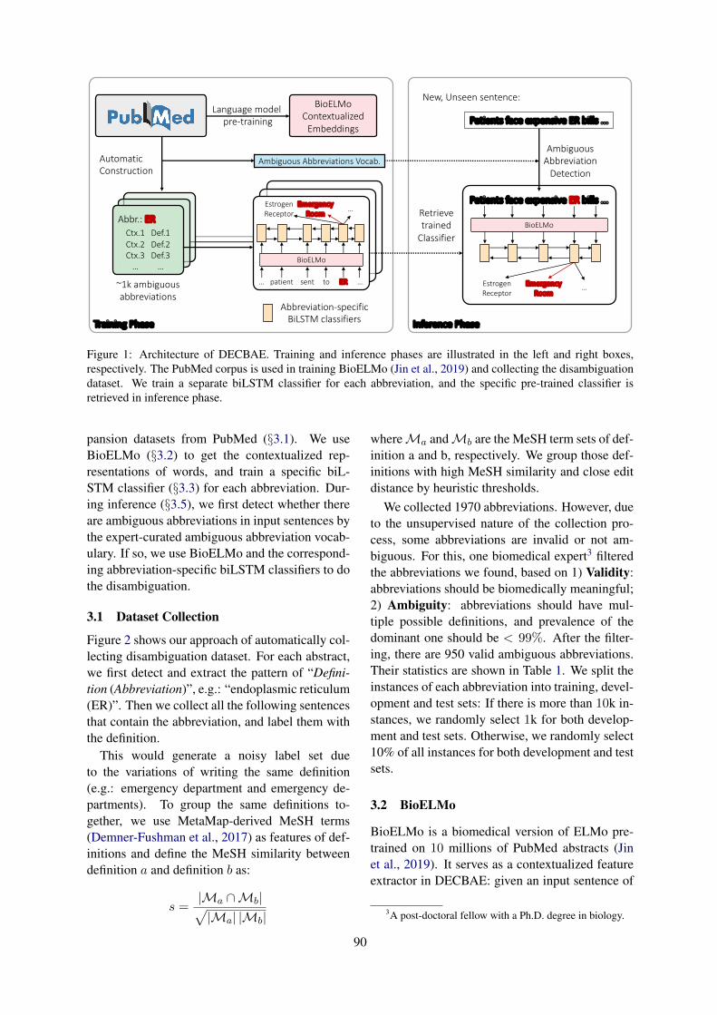
Language model pre-training
BioELMoContextualized
Embeddings
Abbr.: ERCtx.1 Def.1Ctx.2 Def.2Ctx.3 Def.3
… …
AutomaticConstruction
… patient sent to ER …
EstrogenReceptor
EmergencyRoom
…
Abbreviation-specificBiLSTM classifiers
BioELMo
Training Phase
~1k ambiguousabbreviations
Inference Phase
Ambiguous Abbreviations Vocab.
Patients face expensive ER bills ...
New, Unseen sentence:
AmbiguousAbbreviation
Detection
Patients face expensive ER bills ...Retrievetrained
ClassifierBioELMo
EmergencyRoom
EstrogenReceptor
…
Figure 1: Architecture of DECBAE. Training and inference phases are illustrated in the left and right boxes,respectively. The PubMed corpus is used in training BioELMo (Jin et al., 2019) and collecting the disambiguationdataset. We train a separate biLSTM classifier for each abbreviation, and the specific pre-trained classifier isretrieved in inference phase.
pansion datasets from PubMed (§3.1). We useBioELMo (§3.2) to get the contextualized rep-resentations of words, and train a specific biL-STM classifier (§3.3) for each abbreviation. Dur-ing inference (§3.5), we first detect whether thereare ambiguous abbreviations in input sentences bythe expert-curated ambiguous abbreviation vocab-ulary. If so, we use BioELMo and the correspond-ing abbreviation-specific biLSTM classifiers to dothe disambiguation.
3.1 Dataset Collection
Figure 2 shows our approach of automatically col-lecting disambiguation dataset. For each abstract,we first detect and extract the pattern of “Defini-tion (Abbreviation)”, e.g.: “endoplasmic reticulum(ER)”. Then we collect all the following sentencesthat contain the abbreviation, and label them withthe definition.
This would generate a noisy label set dueto the variations of writing the same definition(e.g.: emergency department and emergency de-partments). To group the same definitions to-gether, we use MetaMap-derived MeSH terms(Demner-Fushman et al., 2017) as features of def-initions and define the MeSH similarity betweendefinition a and definition b as:
s =|Ma ∩Mb|√|Ma| |Mb|
whereMa andMb are the MeSH term sets of def-inition a and b, respectively. We group those def-initions with high MeSH similarity and close editdistance by heuristic thresholds.
We collected 1970 abbreviations. However, dueto the unsupervised nature of the collection pro-cess, some abbreviations are invalid or not am-biguous. For this, one biomedical expert3 filteredthe abbreviations we found, based on 1) Validity:abbreviations should be biomedically meaningful;2) Ambiguity: abbreviations should have mul-tiple possible definitions, and prevalence of thedominant one should be < 99%. After the filter-ing, there are 950 valid ambiguous abbreviations.Their statistics are shown in Table 1. We split theinstances of each abbreviation into training, devel-opment and test sets: If there is more than 10k in-stances, we randomly select 1k for both develop-ment and test sets. Otherwise, we randomly select10% of all instances for both development and testsets.
3.2 BioELMo
BioELMo is a biomedical version of ELMo pre-trained on 10 millions of PubMed abstracts (Jinet al., 2019). It serves as a contextualized featureextractor in DECBAE: given an input sentence of
3A post-doctoral fellow with a Ph.D. degree in biology.
90
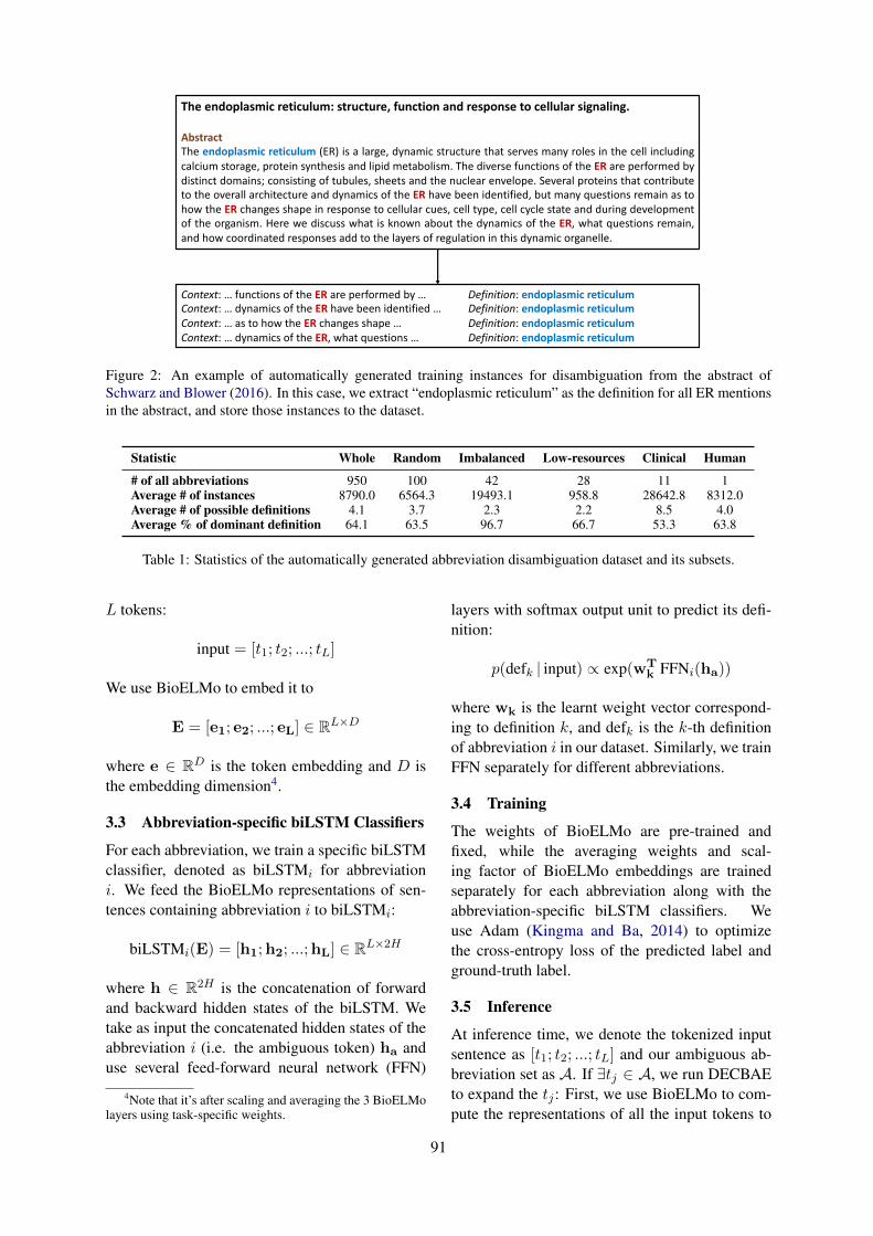
The endoplasmic reticulum: structure, function and response to cellular signaling.
AbstractThe endoplasmic reticulum (ER) is a large, dynamic structure that serves many roles in the cell includingcalcium storage, protein synthesis and lipid metabolism. The diverse functions of the ER are performed bydistinct domains; consisting of tubules, sheets and the nuclear envelope. Several proteins that contributeto the overall architecture and dynamics of the ER have been identified, but many questions remain as tohow the ER changes shape in response to cellular cues, cell type, cell cycle state and during developmentof the organism. Here we discuss what is known about the dynamics of the ER, what questions remain,and how coordinated responses add to the layers of regulation in this dynamic organelle.
Context: … functions of the ER are performed by … Definition: endoplasmic reticulumContext: … dynamics of the ER have been identified … Definition: endoplasmic reticulum Context: … as to how the ER changes shape … Definition: endoplasmic reticulumContext: … dynamics of the ER, what questions … Definition: endoplasmic reticulum
Automatically generate training contexts of abbreviations, labeled by their extracted definitionsFigure 2: An example of automatically generated training instances for disambiguation from the abstract ofSchwarz and Blower (2016). In this case, we extract “endoplasmic reticulum” as the definition for all ER mentionsin the abstract, and store those instances to the dataset.
Statistic Whole Random Imbalanced Low-resources Clinical Human
# of all abbreviations 950 100 42 28 11 1Average # of instances 8790.0 6564.3 19493.1 958.8 28642.8 8312.0Average # of possible definitions 4.1 3.7 2.3 2.2 8.5 4.0Average % of dominant definition 64.1 63.5 96.7 66.7 53.3 63.8
Table 1: Statistics of the automatically generated abbreviation disambiguation dataset and its subsets.
L tokens:
input = [t1; t2; ...; tL]
We use BioELMo to embed it to
E = [e1; e2; ...; eL] ∈ RL×D
where e ∈ RD is the token embedding and D isthe embedding dimension4.
3.3 Abbreviation-specific biLSTM Classifiers
For each abbreviation, we train a specific biLSTMclassifier, denoted as biLSTMi for abbreviationi. We feed the BioELMo representations of sen-tences containing abbreviation i to biLSTMi:
biLSTMi(E) = [h1;h2; ...;hL] ∈ RL×2H
where h ∈ R2H is the concatenation of forwardand backward hidden states of the biLSTM. Wetake as input the concatenated hidden states of theabbreviation i (i.e. the ambiguous token) ha anduse several feed-forward neural network (FFN)
4Note that it’s after scaling and averaging the 3 BioELMolayers using task-specific weights.
layers with softmax output unit to predict its defi-nition:
p(defk | input) ∝ exp(wTk FFNi(ha))
where wk is the learnt weight vector correspond-ing to definition k, and defk is the k-th definitionof abbreviation i in our dataset. Similarly, we trainFFN separately for different abbreviations.
3.4 Training
The weights of BioELMo are pre-trained andfixed, while the averaging weights and scal-ing factor of BioELMo embeddings are trainedseparately for each abbreviation along with theabbreviation-specific biLSTM classifiers. Weuse Adam (Kingma and Ba, 2014) to optimizethe cross-entropy loss of the predicted label andground-truth label.
3.5 Inference
At inference time, we denote the tokenized inputsentence as [t1; t2; ...; tL] and our ambiguous ab-breviation set as A. If ∃tj ∈ A, we run DECBAEto expand the tj : First, we use BioELMo to com-pute the representations of all the input tokens to
91
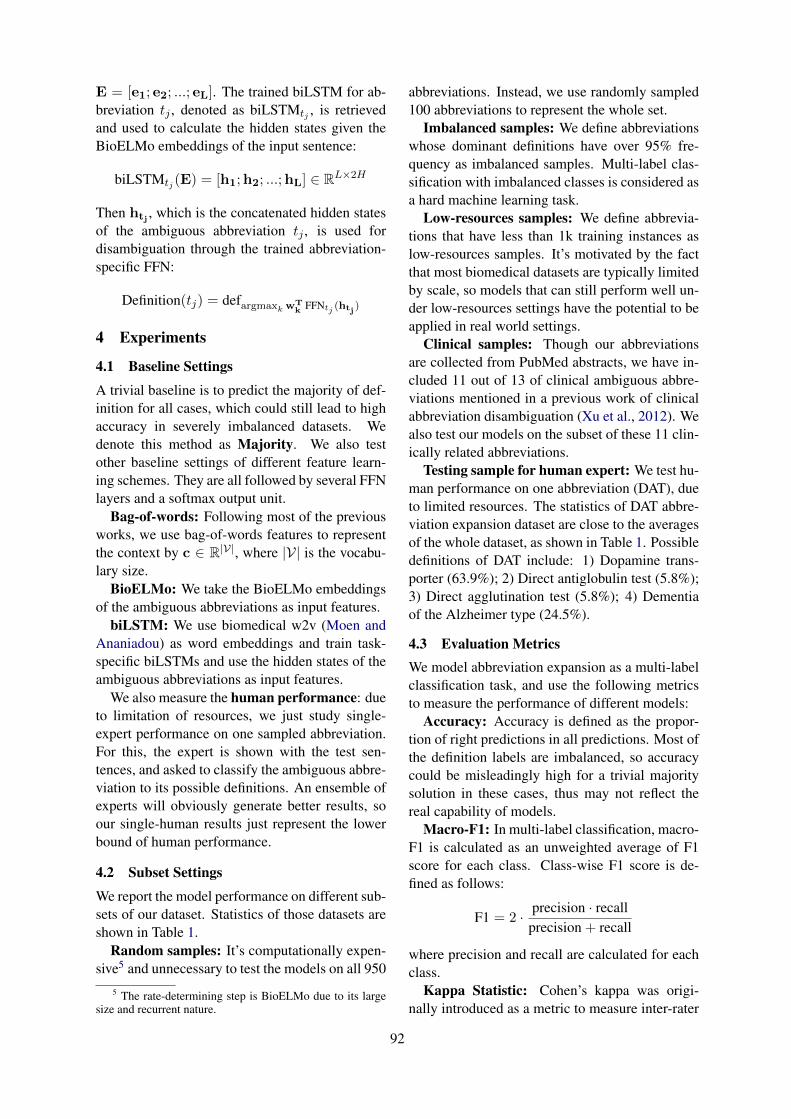
E = [e1; e2; ...; eL]. The trained biLSTM for ab-breviation tj , denoted as biLSTMtj , is retrievedand used to calculate the hidden states given theBioELMo embeddings of the input sentence:
biLSTMtj (E) = [h1;h2; ...;hL] ∈ RL×2H
Then htj , which is the concatenated hidden statesof the ambiguous abbreviation tj , is used fordisambiguation through the trained abbreviation-specific FFN:
Definition(tj) = defargmaxk wTk FFNtj (htj
)
4 Experiments
4.1 Baseline Settings
A trivial baseline is to predict the majority of def-inition for all cases, which could still lead to highaccuracy in severely imbalanced datasets. Wedenote this method as Majority. We also testother baseline settings of different feature learn-ing schemes. They are all followed by several FFNlayers and a softmax output unit.
Bag-of-words: Following most of the previousworks, we use bag-of-words features to representthe context by c ∈ R|V|, where |V| is the vocabu-lary size.
BioELMo: We take the BioELMo embeddingsof the ambiguous abbreviations as input features.
biLSTM: We use biomedical w2v (Moen andAnaniadou) as word embeddings and train task-specific biLSTMs and use the hidden states of theambiguous abbreviations as input features.
We also measure the human performance: dueto limitation of resources, we just study single-expert performance on one sampled abbreviation.For this, the expert is shown with the test sen-tences, and asked to classify the ambiguous abbre-viation to its possible definitions. An ensemble ofexperts will obviously generate better results, soour single-human results just represent the lowerbound of human performance.
4.2 Subset Settings
We report the model performance on different sub-sets of our dataset. Statistics of those datasets areshown in Table 1.
Random samples: It’s computationally expen-sive5 and unnecessary to test the models on all 950
5 The rate-determining step is BioELMo due to its largesize and recurrent nature.
abbreviations. Instead, we use randomly sampled100 abbreviations to represent the whole set.
Imbalanced samples: We define abbreviationswhose dominant definitions have over 95% fre-quency as imbalanced samples. Multi-label clas-sification with imbalanced classes is considered asa hard machine learning task.
Low-resources samples: We define abbrevia-tions that have less than 1k training instances aslow-resources samples. It’s motivated by the factthat most biomedical datasets are typically limitedby scale, so models that can still perform well un-der low-resources settings have the potential to beapplied in real world settings.
Clinical samples: Though our abbreviationsare collected from PubMed abstracts, we have in-cluded 11 out of 13 of clinical ambiguous abbre-viations mentioned in a previous work of clinicalabbreviation disambiguation (Xu et al., 2012). Wealso test our models on the subset of these 11 clin-ically related abbreviations.
Testing sample for human expert: We test hu-man performance on one abbreviation (DAT), dueto limited resources. The statistics of DAT abbre-viation expansion dataset are close to the averagesof the whole dataset, as shown in Table 1. Possibledefinitions of DAT include: 1) Dopamine trans-porter (63.9%); 2) Direct antiglobulin test (5.8%);3) Direct agglutination test (5.8%); 4) Dementiaof the Alzheimer type (24.5%).
4.3 Evaluation MetricsWe model abbreviation expansion as a multi-labelclassification task, and use the following metricsto measure the performance of different models:
Accuracy: Accuracy is defined as the propor-tion of right predictions in all predictions. Most ofthe definition labels are imbalanced, so accuracycould be misleadingly high for a trivial majoritysolution in these cases, thus may not reflect thereal capability of models.
Macro-F1: In multi-label classification, macro-F1 is calculated as an unweighted average of F1score for each class. Class-wise F1 score is de-fined as follows:
F1 = 2 · precision · recallprecision + recall
where precision and recall are calculated for eachclass.
Kappa Statistic: Cohen’s kappa was origi-nally introduced as a metric to measure inter-rater
92
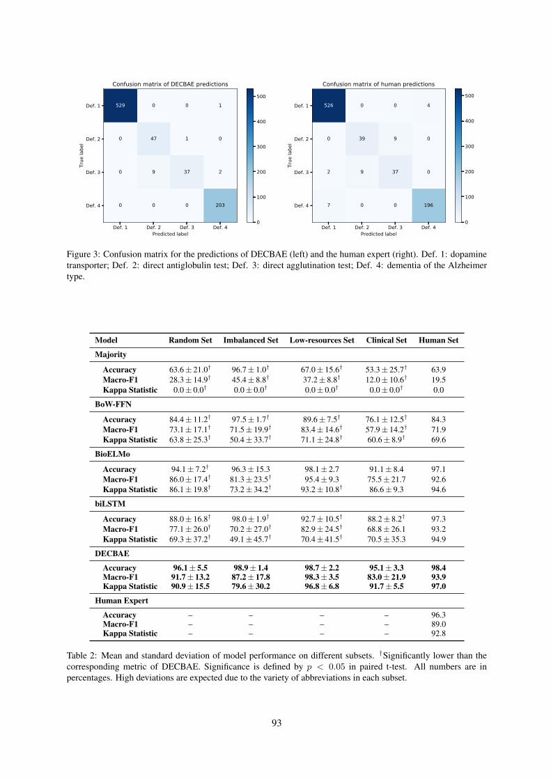
Def. 1 Def. 2 Def. 3 Def. 4Predicted label
Def. 1
Def. 2
Def. 3
Def. 4
True
labe
l
529 0 0 1
0 47 1 0
0 9 37 2
0 0 0 203
Confusion matrix of DECBAE predictions
0
100
200
300
400
500
Def. 1 Def. 2 Def. 3 Def. 4Predicted label
Def. 1
Def. 2
Def. 3
Def. 4
True
labe
l
526 0 0 4
0 39 9 0
2 9 37 0
7 0 0 196
Confusion matrix of human predictions
0
100
200
300
400
500
Figure 3: Confusion matrix for the predictions of DECBAE (left) and the human expert (right). Def. 1: dopaminetransporter; Def. 2: direct antiglobulin test; Def. 3: direct agglutination test; Def. 4: dementia of the Alzheimertype.
Model Random Set Imbalanced Set Low-resources Set Clinical Set Human Set
Majority
Accuracy 63.6± 21.0† 96.7± 1.0† 67.0± 15.6† 53.3± 25.7† 63.9Macro-F1 28.3± 14.9† 45.4± 8.8† 37.2± 8.8† 12.0± 10.6† 19.5Kappa Statistic 0.0± 0.0† 0.0± 0.0† 0.0± 0.0† 0.0± 0.0† 0.0
BoW-FFN
Accuracy 84.4± 11.2† 97.5± 1.7† 89.6± 7.5† 76.1± 12.5† 84.3Macro-F1 73.1± 17.1† 71.5± 19.9† 83.4± 14.6† 57.9± 14.2† 71.9Kappa Statistic 63.8± 25.3† 50.4± 33.7† 71.1± 24.8† 60.6± 8.9† 69.6
BioELMo
Accuracy 94.1± 7.2† 96.3± 15.3 98.1± 2.7 91.1± 8.4 97.1Macro-F1 86.0± 17.4† 81.3± 23.5† 95.4± 9.3 75.5± 21.7 92.6Kappa Statistic 86.1± 19.8† 73.2± 34.2† 93.2± 10.8† 86.6± 9.3 94.6
biLSTM
Accuracy 88.0± 16.8† 98.0± 1.9† 92.7± 10.5† 88.2± 8.2† 97.3Macro-F1 77.1± 26.0† 70.2± 27.0† 82.9± 24.5† 68.8± 26.1 93.2Kappa Statistic 69.3± 37.2† 49.1± 45.7† 70.4± 41.5† 70.5± 35.3 94.9
DECBAE
Accuracy 96.1± 5.5 98.9± 1.4 98.7± 2.2 95.1± 3.3 98.4Macro-F1 91.7± 13.2 87.2± 17.8 98.3± 3.5 83.0± 21.9 93.9Kappa Statistic 90.9± 15.5 79.6± 30.2 96.8± 6.8 91.7± 5.5 97.0
Human Expert
Accuracy – – – – 96.3Macro-F1 – – – – 89.0Kappa Statistic – – – – 92.8
Table 2: Mean and standard deviation of model performance on different subsets. †Significantly lower than thecorresponding metric of DECBAE. Significance is defined by p < 0.05 in paired t-test. All numbers are inpercentages. High deviations are expected due to the variety of abbreviations in each subset.
93
agreement (Cohen, 1960). It can also be used toevaluate predictions of multi-label classification:
κ =po − pe1− pe
where po is the observed agreement and in the caseof classification po = accuracy, pe is the expectedagreement which can be achieved by pure chance:
pe =∑
c
pcp̂c
pc and p̂c refer to the proportion of class c inground truth labels and predictions, respectively.Empirical results in Table 2 show that Kappastatistics are often lower than accuracy and macro-F1, and thus serving as a more distinctive metricfor our task.
4.4 Results
In Table 2, we report means and standard devi-ations of each model’s performance on differentsubsets evaluated by the three metrics. In all sub-sets, DECBAE performs significantly better thanmost other models by large margins. A generaltrend of DECBAE > BioELMo > biLSTM >BoW-FFN > Majority conserves across subsets.
In the Random subset which represents thewhole dataset, all metrics of DECBAE exceed0.90, setting very promising state-of-the-art per-formance despite the potential noise of the dataset.
In the Imbalanced subset where the most fre-quent definitions consist of over 95% of all the la-bels, a trivial Majority solution gets over 95% ac-curacy. However, for macro-F1 and kappa statis-tic, performance of the baselines drop dramaticallywhile DECBAE can still generate decent results.
DECBAE and BioELMo alone remain robust inLow-resources setting. This is due to the trans-fer learning nature of BioELMo, which utilizes theknowledge encoded in the PubMed abstracts.
Our abbreviation expansion dataset coversroughly 85% of clinical abbreviations mentionedin Xu et al. (2012). On this Clinical subset,DECBAE gets pretty good results and vastly out-perform other baselines despite its variety in pos-sible definitions (8.5 possible definitions per ab-breviation, as shown in Table 1).
On the testset for human performance (i.e.:abbreviation expansion for DAT), DECBAE andeven some neural baselines outperform single hu-man expert.
5 Analysis
In Fig. 3, we use confusion matrices to visual-ize the differences between DECBAE or the hu-man expert and the ground truth labels, for disam-biguation of abbreviation “DAT”. The high agree-ment level between human expert predictions andthe automatically assigned labels indicates thatour pipeline of collecting the abbreviation disam-biguation dataset is valid.
In general, both DECBAE and the human expertperform well in the task, with only few misclassi-fications. Specifically, DECBAE, and even otherneural baselines like biLSTM and BioELMo, out-perform the human expert in all metrics. Com-pared to DECBAE, the human expert is morelikely to misclassify direct agglutination test withdirect antiglobulin test (9 v.s. 1), and misclassifydementia of the Alzheimer type with dopaminetransporter (7 v.s. 0). We show several instancesof human and DECBAE’s errors in Table 3.
One limitation of this work is that we just testDECBAE on our automatically collected dataset.Since the proposed model can also be used onother biomedical abbreviation expansion datasetsas well, evaluating on other datasets like MSHWSD is a clear future work to do.
Another potential direction for improvementis to accelerate the inference speed. CurrentlyDECBAE uses BioELMo for embedding andabbreviation-specific biLSTM for classification,resulting in two recurrent models in total. Our re-sults show that just BioELMo with several FFNlayers also generates decent results, so in somecases we might use only BioELMo as a compro-mise for faster inference.
6 Conclusion
We present DECBAE, a state-of-the-art biomedi-cal abbreviation expansion model on the automat-ically collected dataset from PubMed. The resultsshow that, with only minimum expert involve-ment, we can still perform well in such a domain-specific task by automatically collecting trainingdata from a large corpus and utilize embeddingsfrom pre-trained biomedical language models.
7 Acknowledgement
We are grateful for the annonymous reviewers ofBioNLP 2019 who gave us very insightful com-ments and suggestions. J.L. is supported by NLMtraining grant 5T15LM007059-32.
94
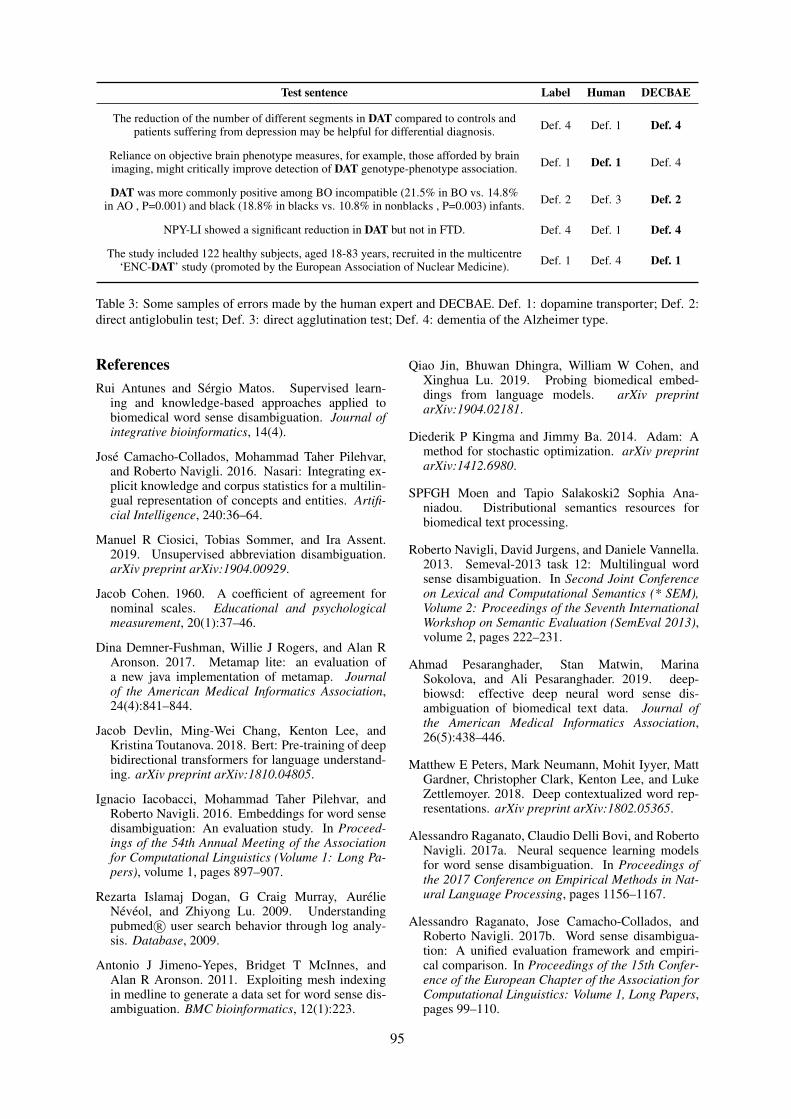
Test sentence Label Human DECBAE
The reduction of the number of different segments in DAT compared to controls andpatients suffering from depression may be helpful for differential diagnosis. Def. 4 Def. 1 Def. 4
Reliance on objective brain phenotype measures, for example, those afforded by brainimaging, might critically improve detection of DAT genotype-phenotype association. Def. 1 Def. 1 Def. 4
DAT was more commonly positive among BO incompatible (21.5% in BO vs. 14.8%in AO , P=0.001) and black (18.8% in blacks vs. 10.8% in nonblacks , P=0.003) infants. Def. 2 Def. 3 Def. 2
NPY-LI showed a significant reduction in DAT but not in FTD. Def. 4 Def. 1 Def. 4
The study included 122 healthy subjects, aged 18-83 years, recruited in the multicentre‘ENC-DAT’ study (promoted by the European Association of Nuclear Medicine). Def. 1 Def. 4 Def. 1
Table 3: Some samples of errors made by the human expert and DECBAE. Def. 1: dopamine transporter; Def. 2:direct antiglobulin test; Def. 3: direct agglutination test; Def. 4: dementia of the Alzheimer type.
ReferencesRui Antunes and Sérgio Matos. Supervised learn-
ing and knowledge-based approaches applied tobiomedical word sense disambiguation. Journal ofintegrative bioinformatics, 14(4).
José Camacho-Collados, Mohammad Taher Pilehvar,and Roberto Navigli. 2016. Nasari: Integrating ex-plicit knowledge and corpus statistics for a multilin-gual representation of concepts and entities. Artifi-cial Intelligence, 240:36–64.
Manuel R Ciosici, Tobias Sommer, and Ira Assent.2019. Unsupervised abbreviation disambiguation.arXiv preprint arXiv:1904.00929.
Jacob Cohen. 1960. A coefficient of agreement fornominal scales. Educational and psychologicalmeasurement, 20(1):37–46.
Dina Demner-Fushman, Willie J Rogers, and Alan RAronson. 2017. Metamap lite: an evaluation ofa new java implementation of metamap. Journalof the American Medical Informatics Association,24(4):841–844.
Jacob Devlin, Ming-Wei Chang, Kenton Lee, andKristina Toutanova. 2018. Bert: Pre-training of deepbidirectional transformers for language understand-ing. arXiv preprint arXiv:1810.04805.
Ignacio Iacobacci, Mohammad Taher Pilehvar, andRoberto Navigli. 2016. Embeddings for word sensedisambiguation: An evaluation study. In Proceed-ings of the 54th Annual Meeting of the Associationfor Computational Linguistics (Volume 1: Long Pa-pers), volume 1, pages 897–907.
Rezarta Islamaj Dogan, G Craig Murray, AurélieNévéol, and Zhiyong Lu. 2009. Understandingpubmed R© user search behavior through log analy-sis. Database, 2009.
Antonio J Jimeno-Yepes, Bridget T McInnes, andAlan R Aronson. 2011. Exploiting mesh indexingin medline to generate a data set for word sense dis-ambiguation. BMC bioinformatics, 12(1):223.
Qiao Jin, Bhuwan Dhingra, William W Cohen, andXinghua Lu. 2019. Probing biomedical embed-dings from language models. arXiv preprintarXiv:1904.02181.
Diederik P Kingma and Jimmy Ba. 2014. Adam: Amethod for stochastic optimization. arXiv preprintarXiv:1412.6980.
SPFGH Moen and Tapio Salakoski2 Sophia Ana-niadou. Distributional semantics resources forbiomedical text processing.
Roberto Navigli, David Jurgens, and Daniele Vannella.2013. Semeval-2013 task 12: Multilingual wordsense disambiguation. In Second Joint Conferenceon Lexical and Computational Semantics (* SEM),Volume 2: Proceedings of the Seventh InternationalWorkshop on Semantic Evaluation (SemEval 2013),volume 2, pages 222–231.
Ahmad Pesaranghader, Stan Matwin, MarinaSokolova, and Ali Pesaranghader. 2019. deep-biowsd: effective deep neural word sense dis-ambiguation of biomedical text data. Journal ofthe American Medical Informatics Association,26(5):438–446.
Matthew E Peters, Mark Neumann, Mohit Iyyer, MattGardner, Christopher Clark, Kenton Lee, and LukeZettlemoyer. 2018. Deep contextualized word rep-resentations. arXiv preprint arXiv:1802.05365.
Alessandro Raganato, Claudio Delli Bovi, and RobertoNavigli. 2017a. Neural sequence learning modelsfor word sense disambiguation. In Proceedings ofthe 2017 Conference on Empirical Methods in Nat-ural Language Processing, pages 1156–1167.
Alessandro Raganato, Jose Camacho-Collados, andRoberto Navigli. 2017b. Word sense disambigua-tion: A unified evaluation framework and empiri-cal comparison. In Proceedings of the 15th Confer-ence of the European Chapter of the Association forComputational Linguistics: Volume 1, Long Papers,pages 99–110.
95
Dianne S Schwarz and Michael D Blower. 2016. Theendoplasmic reticulum: structure, function and re-sponse to cellular signaling. Cellular and MolecularLife Sciences, 73(1):79–94.
Hua Xu, Peter D Stetson, and Carol Friedman. 2007.A study of abbreviations in clinical notes. In AMIAannual symposium proceedings, volume 2007, page821. American Medical Informatics Association.
Hua Xu, Peter D Stetson, and Carol Friedman. 2012.Combining corpus-derived sense profiles with esti-mated frequency information to disambiguate clini-cal abbreviations. In AMIA Annual Symposium Pro-ceedings, volume 2012, page 1004. American Med-ical Informatics Association.
Jun Xu, Yaoyun Zhang, Hua Xu, et al. 2015. Clinicalabbreviation disambiguation using neural word em-beddings. Proceedings of BioNLP 15, pages 171–176.
Antonio Jimeno Yepes. 2017. Word embeddings andrecurrent neural networks based on long-short termmemory nodes in supervised biomedical word sensedisambiguation. Journal of biomedical informatics,73:137–147.
Hong Yu, Won Kim, Vasileios Hatzivassiloglou, andW John Wilbur. 2007. Using medline as a knowl-edge source for disambiguating abbreviations andacronyms in full-text biomedical journal articles.Journal of biomedical informatics, 40(2):150–159.
96
Proceedings of the BioNLP 2019 workshop, pages 97–104Florence, Italy, August 1, 2019. c©2019 Association for Computational Linguistics
RNN Embeddings for Identifying Difficult to Understand Medical WordsHanna Pylieva1, Artem Chernodub1, 2, Natalia Grabar3, and Thierry Hamon4,5
1Faculty of Applied Sciences, Ukrainian Catholic University, Lviv, Ukraine{pylieva,chernodub}@ucu.edu.ua
2Grammarly, Kyiv, Ukraine3CNRS, Univ. Lille, UMR 8163 - STL - Savoirs Textes Langage, F-59000, Lille, France
[email protected], CNRS, Université Paris-Saclay, F-91405, Orsay, France
[email protected]́ Paris 13, Sorbonne Paris Cité, F-93430, Villetaneuse, France
Abstract
Patients and their families often require a bet-ter understanding of medical information pro-vided by doctors. We currently address thisissue by improving the identification of diffi-cult to understand medical words. We intro-duce novel embeddings received from RNN- FrnnMUTE (French RNN Medical Under-standability Text Embeddings) which allow toreach up to 87.0 F1 score in identificationof difficult words. We also note that addingpre-trained FastText word embeddings to thefeature set substantially improves the perfor-mance of the model which classifies words ac-cording to their difficulty. We study the gen-eralizability of different models through threecross-validation scenarios which allow test-ing classifiers in real-world conditions: under-standing of medical words by new users, andclassification of new unseen words by the au-tomatic models. The RNN - FrnnMUTE em-beddings and the categorization code are beingmade available for the research.
1 Introduction
Specialized areas, such as medical area, conveyand use technical words, or terms, which are typi-cally related to knowledge developed within theseareas. In the medical area, this specific knowledgeoften corresponds to fundamental medical notionsrelated to disorders, procedures, treatments, andhuman anatomy. For instance, technical terms likeblepharospasm (abnormal contraction or twitch ofthe eyelid), alexithymia (inability to identify anddescribe emotions in the self), appendicectomy(surgical removal of the vermiform appendix fromintestine), or lombalgia (low back pain) are fre-quently used by experts in the medical area texts.As in any specialized areas, two main kinds ofusers exist in the medical area: experts of the do-main, i.e. medical doctors, both researchers orpractitioners; consumers of the healthcare process,
i.e. patients and their relatives. The latter usuallydo not have expert knowledge in the medical do-main, while it is important that they understand thepurpose and issues of their healthcare process.
The existing literature provides several stud-ies dedicated to the understanding of medical no-tions and terms by non-expert users, and of howthe level of health literacy of patients impacts ona successful healthcare process (McCray, 2005;Eysenbach, 2007), as indeed it is quite commonthat patients and their relatives must face technicalhealth documents and information. These obser-vations provide the main motivation for our work.Hence, we address the need of non-specializedusers in the medical domain to understand medi-cal and health information.
In this paper, we propose to apply deep learningtechniques to improve identification of readabilityand understandability of medical words by non-expert users. In particular, we will tackle the wordcategorization task and compare the performanceof classification model on different feature sets:standard linguistic and non-linguistic features de-scribed in section 4, features obtained using dif-ferent deep learning approaches, and the combi-nations of all of them. We also investigate howdifferent feature sets perform with three differentcross-validation settings, described in section 5.The medical data used in this work are in French.Three human annotators participated in the cre-ation of the reference data (specifying the under-standability of words).
2 Related Work
Related work is globally positioned in the textsimplification task which involves the detection ofcomplex contents in documents and their adapta-tion for the target population. We are also inter-ested in the first aspect with additional constraints:
97
detection and diagnosis of technical contents intexts from medical domain.
Traditional readability measures rely on twomain factors: the familiarity of semantic unitssuch as words or phrases, and the complexityof syntax. To make these measures straightfor-ward for applications, some simplifying assump-tions were used. As a result, final formulas mostlyrely on the number of letters and/or of syllablesa word contains and on linear regression mod-els (Flesch, 1948; Gunning, 1973). While suchreadability measures are easy to compute, theyare based on shallow characteristics of text, ig-noring deeper levels of text processing which areimportant factors in readability, such as cohesion,syntactic ambiguity, rhetorical organization, andpropositional density (Collins-Thompson, 2014).Moreover, traditional readability measures weredemonstrated to be unreliable for non-traditionaldocuments (Si and P. Callan, 2001). As a resultof such limitations and due to the recent growthof computational and data resources, the focus ofNLP researchers moved to computational read-ability measurements, which rely on the use of ma-chine learning algorithms on richer linguistic fea-tures (Malmasi et al., 2016; Ronzano et al., 2016;Bingel et al., 2016).
Not so much effort has been devoted to the ex-ploitation of NLP potential in the measurementof readability of medical texts. In the biomed-ical domain, as well as in general language, thereadability assessment is currently approached asa classification task. The difference is that inthe former a much smaller variety of features hasbeen tested: a combination of classical readabil-ity formulas with medical terminologies (Kokki-nakis and Toporowska Gronostaj, 2006); n-gramsof characters (Poprat et al., 2006); stylistic (Grabaret al., 2007) or discursive (Goeuriot et al., 2008)features; morphological features (Chmielik andGrabar, 2011); combinations of different featuresfrom those listed above (Zeng-Treiler et al., 2007).Among the recent experiments dedicated to read-ability study in the medical domain are, for exam-ple, manual rating of medical words (Zheng et al.,2002), automatic rating of medical words on thebasis of their presence in different vocabularies(Borst et al., 2008), exploitation of machine learn-ing approach with various features (Grabar et al.,2014). The last experiment achieved up to 85.0F-score on individual annotations.
Due to the recent significant advance in read-ability study in general language and relativelyslow progress with the task in the medical area,there is a great potential of experimenting withthe machine learning-based approaches on medi-cal texts. This fact motivated us for choosing thiskind of methodology.
3 Materials
For the experiments, we used the publicly avail-able set of words with annotations1. The processof words collection and annotation is briefly de-scribed below.
3.1 Linguistic data description
The set of required biomedical terms was obtainedfrom the French part of Snomed International2
(Côté et al., 1993). Snomed Int contains 151,104medical terms organized into eleven semantic axessuch as disorders and abnormalities, procedures,chemical products, living organisms, anatomy, so-cial status, etc. For the word understandabilitystudy, five axes related to the main medical no-tions were chosen: disorders, abnormalities, pro-cedures, functions, and anatomy. These cate-gories are assumed to be faced frequently by lay-man. In contrast, chemical products and living or-ganisms are excluded because they mainly corre-spond to Latin borrowings and are typically non-understandable by laypeople.
The 104,649 selected terms were then pro-cessed. First, they were tokenized, POS-taggedand lemmatized using TreeTagger (Schmid, 1994).Then the lemmatization was checked withFLEMM (Namer, 2000). After that we received29,641 unique words. For instance, the term trisul-fure d’hydrogène provided three words (trisulfure,de, hydrogène). The final dataset contains com-pound words which contain several bases (ab-dominoplastie (abdominoplasty), dermabrasion(dermabrasion)), constructed words which containone base and at least one affix (lipoı̈de (lipoid),cardiaque (cardiac)), simple words which con-tain one base, no affixes and possibly infectionswhen the lemmatization fails (acné (acne), frag-ment (fragment)).
1http://natalia.grabar.free.fr/resources.php#rated
2https://esante.gouv.fr/terminologie-snomed-35vf
98
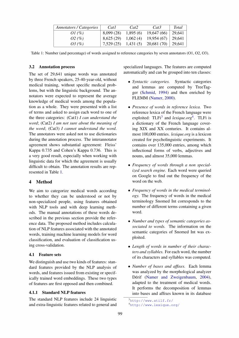
Annotators / Categories Cat1 Cat2 Cat3 TotalO1 (%) 8,099 (28) 1,895 (6) 19,647 (66) 29,641O2 (%) 8,625 (29) 1,062 (4) 19,954 (67) 29,641O3 (%) 7,529 (25) 1,431 (5) 20,681 (70) 29,641
Table 1: Number (and percentage) of words assigned to reference categories by seven annotators (O1, O2, O3).
3.2 Annotation process
The set of 29,641 unique words was annotatedby three French speakers, 25-40-year-old, withoutmedical training, without specific medical prob-lems, but with the linguistic background. The an-notators were expected to represent the averageknowledge of medical words among the popula-tion as a whole. They were presented with a listof terms and asked to assign each word to one ofthe three categories: (Cat1) I can understand theword; (Cat2) I am not sure about the meaning ofthe word; (Cat3) I cannot understand the word.The annotators were asked not to use dictionariesduring the annotation process. The interannotatoragreement shows substantial agreement: Fleiss’Kappa 0.735 and Cohen’s Kappa 0.736. This isa very good result, especially when working withlinguistic data for which the agreement is usuallydifficult to obtain. The annotation results are rep-resented in Table 1.
4 Method
We aim to categorize medical words accordingto whether they can be understood or not bynon-specialized people, using features obtainedwith NLP tools and with deep learning meth-ods. The manual annotations of these words de-scribed in the previous section provide the refer-ence data. The proposed method includes calcula-tion of NLP features associated with the annotatedwords, training machine learning models for wordclassification, and evaluation of classification us-ing cross-validation.
4.1 Feature sets
We distinguish and use two kinds of features: stan-dard features provided by the NLP analysis ofwords, and features issued from existing or specif-ically trained word embeddings. These two typesof features are first opposed and then combined.
4.1.1 Standard NLP featuresThe standard NLP features include 24 linguisticand extra-linguistic features related to general and
specialized languages. The features are computedautomatically and can be grouped into ten classes:
• Syntactic categories. Syntactic categoriesand lemmas are computed by TreeTag-ger (Schmid, 1994) and then enriched byFLEMM (Namer, 2000).
• Presence of words in reference lexica. Tworeference lexica of the French language wereexploited: TLFi3 and lexique.org4. TLFi isa dictionary of the French language cover-ing XIX and XX centuries. It contains al-most 100,000 entries. lexique.org is a lexiconcreated for psycholinguistic experiments. Itcontains over 135,000 entries, among whichinflectional forms of verbs, adjectives andnouns, and almost 35,000 lemmas.
• Frequency of words through a non special-ized search engine. Each word were queriedon Google to find out the frequency of theword on the web.
• Frequency of words in the medical terminol-ogy. The frequency of words in the medicalterminology Snomed Int corresponds to thenumber of different terms containing a givenword.
• Number and types of semantic categories as-sociated to words. The information on thesemantic categories of Snomed Int was ex-ploited.
• Length of words in number of their charac-ters and syllables. For each word, the numberof its characters and syllables was computed.
• Number of bases and affixes. Each lemmawas analyzed by the morphological analyzerDérif (Namer and Zweigenbaum, 2004),adapted to the treatment of medical words.It performs the decomposition of lemmasinto bases and affixes known in its database
3http://www.atilf.fr/4http://www.lexique.org/
99
and it provides also semantic explanation ofthe analyzed lexemes. The morphologicaldecomposition information (number of af-fixes and bases) was exploited. For instance,hématomètre (haemometer) is analyzed anddecomposed into two basis (hémato mean-ing blood and mètre meaning measure, whilemyélite (myelitis) is decomposed into myélmeaning marrow and ite meaning inflamma-tion.
• Initial and final substrings of the words. Ini-tial and final substrings of different length,from three to five characters, were computed.
• Number and percentage of consonants, vow-els and other characters. The number and thepercentage of consonants, vowels and othercharacters (i.e., hyphen, apostrophe, comas)was computed.
• Classical readability scores. Two classicalreadability measures were applied: Flesch(Flesch, 1948) and its variant Flesch-Kincaid(Kincaid et al., 1975). Such measures aretypically used for evaluating the difficultylevel of a text.
4.1.2 FastText word embeddings usage.FastText word embeddings (Bojanowski et al.,2017) is a good candidate feature for the detec-tion of word difficulty because they are able to usethe morphological information of words and gen-eralize over it. Since the word embeddings cap-ture context and morphological information, weassume that using them as features will improveclassification accuracy for our specific problem.
We note that FastText word embeddings trainedon Wikipedia and Common Crawl5 texts have animportant part of words from our dataset. Accord-ing to our analysis, the currently published Fast-Text6 model for French contains 44.26% (13,118out of 29,641) medical words from our dataset andup to 56.00% (16,598 out of 29,641) lowercasedmedical words from our dataset.
4.1.3 French RNN MedicalUnderstandability Text Embeddings(FrnnMUTE).
According to the general functionality of RNNs,the final hidden state aggregates the informa-
5http://commoncrawl.org/6https://fasttext.cc
tion about all input sequence. This idea is fre-quently used to receive hidden representations ofsequences. Sequence-to-sequence model is a well-known example of how this idea works in practice(Sutskever et al., 2014). Such models consist oftwo parts: an encoder is an RNN which encodesthe input sequence into a representation in hiddenspace (which is also called thought vector), and adecoder which generates a new sequence out ofthe hidden representations.
We used this idea for representing words fromour dataset. To receive words representations froman RNN, we first trained it to classify words basedon labels by one annotator (we choseO1), then foreach word we collect values of the last hidden stateof the RNN and use this vector as features duringthe detection of words understandability for dif-ferent users (or annotators). Train/test split was70%/30% of randomly shuffled samples.
As a direct classifier, we trained a character-level RNN using PyTorch framework7 and oneGPU Tesla K80. We lowercased all words, lem-matized them and substituted all Unicode symbolswith their ASCII analogs. We tested several RNNarchitectures and hyperparameter sets. The bestperformance was reached with a model consist-ing of two unidirectional long short-term mem-ory (LSTM) units, each with 50 hidden units. Thedropout of the model is 0.7. The input size is 57 asthe number of unique characters in lowercased andconverted to ASCII input words. The output size is3 as the number of classes in our data. This modelreached the best performance on the eighth epochwith F1 = 78.94 and accuracy = 81.21% on de-velopment set. Using this model we received 50-dimensional word representations which we calledFrnnMUTE (French RNN Medical Understand-ability Text Embeddings).
5 Experiments and Results
We study the impact of adding words embeddingsas features for identifying difficult for understand-ing words. First, we observe how FastText wordembeddings influence the quality of classificationin different cross-validation scenarios. Then, westudy how FrnnMUTE used as features impacton classification quality in all the same cross-validation scenarios. The quality of the classifi-cations is evaluated using four standard macroav-eraging (Sebastiani, 2002) measures: accuracy A,
7https://pytorch.org/
100
precision P , recall R and F1-measure F .
5.1 Cross-validation scenarios
For a thorough study of generalization abilities ofthe classification models, we propose to considerthree distinct cross-validation scenarios based ondifferent combinations of users and vocabulary intrain and test sets.
5.1.1 User-in vocabulary-out cross-validationThe cross-validation is performed on each dataset(i.e., each user annotation) separately. We aim tomeasure the ability of the classification model togeneralize class recognition on the known user andto predict annotations for unknown words. Fromthe practical perspective, user-in means learningthe profile of a user. Hence, a model trained bysuch scenario represents the word understandingor knowledge of the annotator.
The experiments use (i) the standard featuresonly, (ii) the FastText word embeddings only and(iii) their combination. The experiments with iso-lated FastText word embeddings as features re-sulted in poor F1 scores (Table 2), that can beexplained by the fact that contextual information,which is dominant in these word embeddings, isnot enough to define the word understandability.Adding the FastText word embeddings to the stan-dard feature set resulted in up to 1.0 higher F1score due to higher Precision (up to 1.8), meaningthat contextual information slightly impacts on theunderstandability of a word by a given person.
5.1.2 User-out vocabulary-in cross-validationWe then learn from all the annotations of one userand then test the model on annotations of anotheruser. Thereby, in such a setting, we measure theability of the classifier to generalize on all knownwords, but for unknown users. This scenario is re-alistic to a real-world situation: the reference an-notations can be obtained only from a couple ofusers, presumably representing the overall popu-lation, but not from all the possible users. In thisscenario, the model learns the profile of a user andwe want to identify whether a new user has thesame profile as another user. Then it can be usedfor identification of not understandable words forthe new users.
These experiments show a substantial improve-ment of combined features in comparison to thestandard features (Table 3). When knowledge ofwords understandability of one user is used to
predict it for another user, adding the FastTextword embeddings provides up to 2.9 better F1score. Used separately, standard features and em-beddings show similar performance as in user-invocabulary-out cross-validation (Table 2). We as-sume that there exists a robust nonlinear depen-dency between some subsets of standard featuresand subword-level components of FastText wordembeddings. Testing this hypothesis is the topicof future work.
5.1.3 User-out vocabulary-outcross-validation
Finally, we consider (k-1) folds of data from oneuser for training and use k-th fold for testing fromthe remaining user. We aim to measure the abil-ity of the method to generalize both on unknownusers and unknown vocabulary. This experimentshould be helpful in identifying the number ofwords needed for determining whether the profileof one user is the same as profile of other users incase the model achieves good performance.
In these experiments, FastText word embed-dings provide approximately 0.5% higher F1 scorein case of learning on users O1 and O3 (Table 4).When learning on user O2, embeddings decreaseF by 0.5, which means that annotations and healthliteracy of user O2 are different from users O1 andO3. It seems that adding embeddings makes over-fitting the machine learning model to the dataset.As a result, tests on other ”kind of word under-standability” and combined features are less suc-cessful compared to using standard features onlyfor learning. This may also be due to the lack ofsystematicity in annotations of O2.
5.2 FrnnMUTE impact study
The FrnnMUTE embeddings were used separatelyand in combination with standard features andwith FastText word embeddings for classifyingmedical words with the decision tree algorithm.To simplify the process of analyzing and compar-ing the results of this and the previous part, we ag-gregated the resulting F1 scores for combinationsof a feature set and cross-validation scenario overall available users (Table 5). We observed that,in all cross-validation scenarios, our FrnnMUTEperforms better when used separately by compari-son with the FastText word embeddings used sepa-rately. FrnnMUTE provides the maximal F1 score(79.5) among user pairs versus the F1 score pro-vided by the FastText word embeddings in user-in
101
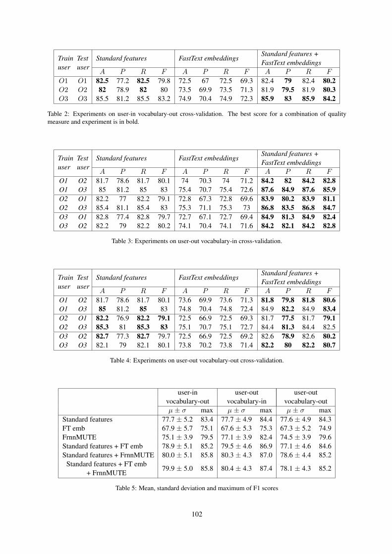
Trainuser
Testuser
Standard features FastText embeddingsStandard features +FastText embeddings
A P R F A P R F A P R F
O1 O1 82.5 77.2 82.5 79.8 72.5 67 72.5 69.3 82.4 79 82.4 80.2O2 O2 82 78.9 82 80 73.5 69.9 73.5 71.3 81.9 79.5 81.9 80.3O3 O3 85.5 81.2 85.5 83.2 74.9 70.4 74.9 72.3 85.9 83 85.9 84.2
Table 2: Experiments on user-in vocabulary-out cross-validation. The best score for a combination of qualitymeasure and experiment is in bold.
Trainuser
Testuser
Standard features FastText embeddingsStandard features +FastText embeddings
A P R F A P R F A P R F
O1 O2 81.7 78.6 81.7 80.1 74 70.3 74 71.2 84.2 82 84.2 82.8O1 O3 85 81.2 85 83 75.4 70.7 75.4 72.6 87.6 84.9 87.6 85.9O2 O1 82.2 77 82.2 79.1 72.8 67.3 72.8 69.6 83.9 80.2 83.9 81.1O2 O3 85.4 81.1 85.4 83 75.3 71.1 75.3 73 86.8 83.5 86.8 84.7O3 O1 82.8 77.4 82.8 79.7 72.7 67.1 72.7 69.4 84.9 81.3 84.9 82.4O3 O2 82.2 79 82.2 80.2 74.1 70.4 74.1 71.6 84.2 82.1 84.2 82.8
Table 3: Experiments on user-out vocabulary-in cross-validation.
Trainuser
Testuser
Standard features FastText embeddingsStandard features +FastText embeddings
A P R F A P R F A P R F
O1 O2 81.7 78.6 81.7 80.1 73.6 69.9 73.6 71.3 81.8 79.8 81.8 80.6O1 O3 85 81.2 85 83 74.8 70.4 74.8 72.4 84.9 82.2 84.9 83.4O2 O1 82.2 76.9 82.2 79.1 72.5 66.9 72.5 69.3 81.7 77.5 81.7 79.1O2 O3 85.3 81 85.3 83 75.1 70.7 75.1 72.7 84.4 81.3 84.4 82.5O3 O2 82.7 77.3 82.7 79.7 72.5 66.9 72.5 69.2 82.6 78.9 82.6 80.2O3 O3 82.1 79 82.1 80.1 73.8 70.2 73.8 71.4 82.2 80 82.2 80.7
Table 4: Experiments on user-out vocabulary-out cross-validation.
user-in user-out user-outvocabulary-out vocabulary-in vocabulary-outµ ± σ max µ ± σ max µ ± σ max
Standard features 77.7 ± 5.2 83.4 77.7 ± 4.9 84.4 77.6 ± 4.9 84.3FT emb 67.9 ± 5.7 75.1 67.6 ± 5.3 75.3 67.3 ± 5.2 74.9FrnnMUTE 75.1 ± 3.9 79.5 77.1 ± 3.9 82.4 74.5 ± 3.9 79.6Standard features + FT emb 78.9 ± 5.1 85.2 79.5 ± 4.6 86.9 77.1 ± 4.6 84.6Standard features + FrnnMUTE 80.0 ± 5.1 85.8 80.3 ± 4.3 87.0 78.6 ± 4.4 85.2
Standard features + FT emb+ FrnnMUTE
79.9 ± 5.0 85.8 80.4 ± 4.3 87.4 78.1 ± 4.3 85.2
Table 5: Mean, standard deviation and maximum of F1 scores
102
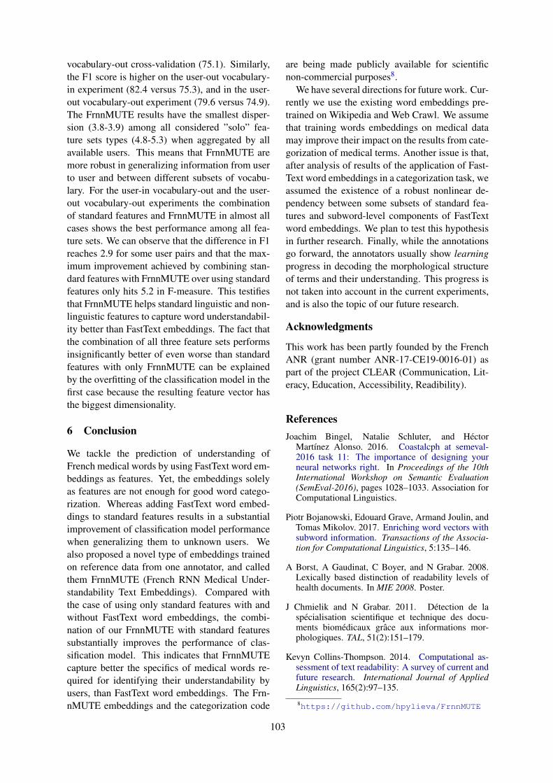
vocabulary-out cross-validation (75.1). Similarly,the F1 score is higher on the user-out vocabulary-in experiment (82.4 versus 75.3), and in the user-out vocabulary-out experiment (79.6 versus 74.9).The FrnnMUTE results have the smallest disper-sion (3.8-3.9) among all considered ”solo” fea-ture sets types (4.8-5.3) when aggregated by allavailable users. This means that FrnnMUTE aremore robust in generalizing information from userto user and between different subsets of vocabu-lary. For the user-in vocabulary-out and the user-out vocabulary-out experiments the combinationof standard features and FrnnMUTE in almost allcases shows the best performance among all fea-ture sets. We can observe that the difference in F1reaches 2.9 for some user pairs and that the max-imum improvement achieved by combining stan-dard features with FrnnMUTE over using standardfeatures only hits 5.2 in F-measure. This testifiesthat FrnnMUTE helps standard linguistic and non-linguistic features to capture word understandabil-ity better than FastText embeddings. The fact thatthe combination of all three feature sets performsinsignificantly better of even worse than standardfeatures with only FrnnMUTE can be explainedby the overfitting of the classification model in thefirst case because the resulting feature vector hasthe biggest dimensionality.
6 Conclusion
We tackle the prediction of understanding ofFrench medical words by using FastText word em-beddings as features. Yet, the embeddings solelyas features are not enough for good word catego-rization. Whereas adding FastText word embed-dings to standard features results in a substantialimprovement of classification model performancewhen generalizing them to unknown users. Wealso proposed a novel type of embeddings trainedon reference data from one annotator, and calledthem FrnnMUTE (French RNN Medical Under-standability Text Embeddings). Compared withthe case of using only standard features with andwithout FastText word embeddings, the combi-nation of our FrnnMUTE with standard featuressubstantially improves the performance of clas-sification model. This indicates that FrnnMUTEcapture better the specifics of medical words re-quired for identifying their understandability byusers, than FastText word embeddings. The Frn-nMUTE embeddings and the categorization code
are being made publicly available for scientificnon-commercial purposes8.
We have several directions for future work. Cur-rently we use the existing word embeddings pre-trained on Wikipedia and Web Crawl. We assumethat training words embeddings on medical datamay improve their impact on the results from cate-gorization of medical terms. Another issue is that,after analysis of results of the application of Fast-Text word embeddings in a categorization task, weassumed the existence of a robust nonlinear de-pendency between some subsets of standard fea-tures and subword-level components of FastTextword embeddings. We plan to test this hypothesisin further research. Finally, while the annotationsgo forward, the annotators usually show learningprogress in decoding the morphological structureof terms and their understanding. This progress isnot taken into account in the current experiments,and is also the topic of our future research.
Acknowledgments
This work has been partly founded by the FrenchANR (grant number ANR-17-CE19-0016-01) aspart of the project CLEAR (Communication, Lit-eracy, Education, Accessibility, Readibility).
ReferencesJoachim Bingel, Natalie Schluter, and Héctor
Martı́nez Alonso. 2016. Coastalcph at semeval-2016 task 11: The importance of designing yourneural networks right. In Proceedings of the 10thInternational Workshop on Semantic Evaluation(SemEval-2016), pages 1028–1033. Association forComputational Linguistics.
Piotr Bojanowski, Edouard Grave, Armand Joulin, andTomas Mikolov. 2017. Enriching word vectors withsubword information. Transactions of the Associa-tion for Computational Linguistics, 5:135–146.
A Borst, A Gaudinat, C Boyer, and N Grabar. 2008.Lexically based distinction of readability levels ofhealth documents. In MIE 2008. Poster.
J Chmielik and N Grabar. 2011. Détection de laspécialisation scientifique et technique des docu-ments biomédicaux grâce aux informations mor-phologiques. TAL, 51(2):151–179.
Kevyn Collins-Thompson. 2014. Computational as-sessment of text readability: A survey of current andfuture research. International Journal of AppliedLinguistics, 165(2):97–135.
8https://github.com/hpylieva/FrnnMUTE
103
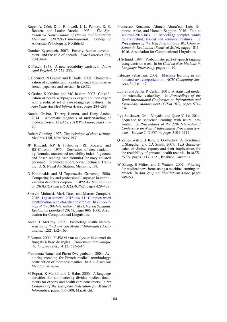
Roger A. Côté, D. J. Rothwell, J. L. Palotay, R. S.Beckett, and Louise Brochu. 1993. The Sys-tematised Nomenclature of Human and VeterinaryMedicine: SNOMED International. College ofAmerican Pathologists, Northfield.
Gunther Eysenbach. 2007. Poverty, human develop-ment, and the role of ehealth. J Med Internet Res,9(4):34–4.
R Flesch. 1948. A new readability yardstick. JournAppl Psychol, 23:221–233.
L Goeuriot, N Grabar, and B Daille. 2008. Characteri-zation of scientific and popular science discourse infrench, japanese and russian. In LREC.
N Grabar, S Krivine, and MC Jaulent. 2007. Classifi-cation of health webpages as expert and non expertwith a reduced set of cross-language features. InAnn Symp Am Med Inform Assoc, pages 284–288.
Natalia Grabar, Thierry Hamon, and Dany Amiot.2014. Automatic diagnosis of understanding ofmedical words. In EACL PITR Workshop, pages 11–20.
Robert Gunning. 1973. The technique of clear writing.McGraw Hill, New York, NY.
JP Kincaid, RP Jr Fishburne, RL Rogers, andBS Chissom. 1975. Derivation of new readabil-ity formulas (automated readability index, fog countand flesch reading ease formula) for navy enlistedpersonnel. Technical report, Naval Technical Train-ing, U. S. Naval Air Station, Memphis, TN.
D Kokkinakis and M Toporowska Gronostaj. 2006.Comparing lay and professional language in cardio-vascular disorders corpora. In WSEAS Transactionson BIOLOGY and BIOMEDICINE, pages 429–437.
Shervin Malmasi, Mark Dras, and Marcos Zampieri.2016. Ltg at semeval-2016 task 11: Complex wordidentification with classifier ensembles. In Proceed-ings of the 10th International Workshop on SemanticEvaluation (SemEval-2016), pages 996–1000. Asso-ciation for Computational Linguistics.
Alexa T. McCray. 2005. Promoting health literacy.Journal of the American Medical Informatics Asso-ciation, 12(2):152–163.
F Namer. 2000. FLEMM : un analyseur flexionnel dufrançais à base de règles. Traitement automatiquedes langues (TAL), 41(2):523–547.
Fiammetta Namer and Pierre Zweigenbaum. 2004. Ac-quiring meaning for French medical terminology:contribution of morphosemantics. In Ann Symp AmMed Inform Assoc.
M Poprat, K Markó, and U Hahn. 2006. A languageclassifier that automatically divides medical docu-ments for experts and health care consumers. In IntCongress of the European Federation for MedicalInformatics, pages 503–508, Maastricht.
Francesco Ronzano, Ahmed Abura’ed, Luis Es-pinosa Anke, and Horacio Saggion. 2016. Taln atsemeval-2016 task 11: Modelling complex wordsby contextual, lexical and semantic features. InProceedings of the 10th International Workshop onSemantic Evaluation (SemEval-2016), pages 1011–1016. Association for Computational Linguistics.
H Schmid. 1994. Probabilistic part-of-speech taggingusing decision trees. In Int Conf on New Methods inLanguage Processing, pages 44–49.
Fabrizio Sebastiani. 2002. Machine learning in au-tomated text categorization. ACM Computing Sur-veys, 34(1):1–47.
Luo Si and James P. Callan. 2001. A statistical modelfor scientific readability. In Proceedings of theTenth International Conference on Information andKnowledge Management (CIKM ’01), pages 574–576.
Ilya Sutskever, Oriol Vinyals, and Quoc V. Le. 2014.Sequence to sequence learning with neural net-works. In Proceedings of the 27th InternationalConference on Neural Information Processing Sys-tems - Volume 2, NIPS’14, pages 3104–3112.
Q Zeng-Treiler, H Kim, S Goryachev, A Keselman,L Slaugther, and CA Smith. 2007. Text character-istics of clinical reports and their implications forthe readability of personal health records. In MED-INFO, pages 1117–1121, Brisbane, Australia.
W Zheng, E Milios, and C Watters. 2002. Filteringfor medical news items using a machine learning ap-proach. In Ann Symp Am Med Inform Assoc, pages949–53.
104
Proceedings of the BioNLP 2019 workshop, pages 105–114Florence, Italy, August 1, 2019. c©2019 Association for Computational Linguistics
A distantly supervised dataset for automated data extraction fromdiagnostic studies
Christopher Norman,1,2 Mariska Leeflang,2 René Spijker,3,4
Evangelos Kanoulas,5 and Aurélie Névéol11 LIMSI, CNRS, Université Paris-Saclay
2 KEBB, Amsterdam Public Health, Amsterdam UMC, University of Amsterdam3 Medical Library, Amsterdam Public Health, Amsterdam UMC, University of Amsterdam
4 Cochrane Netherlands, Julius Center for Health Sciences and Primary Care, UMCU, Utrecht University5 Informatics Institute and Amsterdam Business School, University of Amsterdam
[email protected], [email protected],[email protected], [email protected],
AbstractSystematic reviews are important in evidencebased medicine, but are expensive to produce.Automating or semi-automating the data ex-traction of index test, target condition, and ref-erence standard from articles has the potentialto decrease the cost of conducting systematicreviews of diagnostic test accuracy, but rele-vant training data is not available. We create adistantly supervised dataset of approximately90,000 sentences, and let two experts manu-ally annotate a small subset of around 1,000sentences for evaluation. We evaluate the per-formance of BioBERT and logistic regressionfor ranking the sentences, and compare theperformance for distant and direct supervision.Our results suggest that distant supervision canwork as well as, or better than direct supervi-sion on this problem, and that distantly trainedmodels can perform as well as, or better thanhuman annotators.
1 Background
Evidence based medicine is founded on system-atic reviews, which synthesize all published evi-dence addressing a given research question. Byexamining multiple studies, a systematic reviewcan examine the variation between different stud-ies, the discrepancies between them, as well aslook at the quality of evidence across studies ina way that is difficult in a single trial. Since a sys-tematic review needs to consider the entire bodyof published literature, producing a systematic re-view is expensive and labor-intensive process, of-ten requiring months of manual work (O’Mara-Eves et al., 2015).
To ensure that the results of a systematic re-view are as comprehensive and unbiased as pos-sible, their production follows a strict and sys-
tematic procedure. To catch and resolve disagree-ments, all steps of the process are performed induplicate by at least two reviewers. There have re-cently been examples of systematic reviews usingautomation in a limited capacity (Bannach-Brownet al., 2019; Przybyła et al., 2018; Lerner et al.,2019), but the impact of automation on the relia-bility of systematic reviews is not yet fully under-stood. Automation is not part of accepted practicein current guidelines (De Vet et al., 2008).
After a set of potentially included studies havebeen identified, systematic reviewers complete aso-called data extraction form for each study.These forms comprise a semi-structured summaryof the studies, identifying and extracting a consis-tent, pre-specified set of data items from abstractsor full-text articles in a coherent format (see theleft part of Table 1 for sample exerpts). The coher-ent format allows the data from the studies to besynthesized qualitatively or quantitatively to ad-dress the research question of the review.
In this study we will focus on systematic re-views of diagnostic test accuracy (DTA), which ex-amine the accuracy of tests and procedures for di-agnosing medical conditions, and which have seenlittle attention in previous literature on automateddata extraction. To compare and synthesize re-sults across studies, reviewers extract diagnosticaccuracy from each study, but also determine theindex test (the specific diagnostic test or proce-dure that is being tested), what target condition thetest seeks to diagnose, and the reference standard(the diagnostic test or procedure that is being usedas the gold standard) (see Fig 1 for an example).These data must be determined for each study toknow if the diagnostic accuracy in different stud-ies can be compared.
105
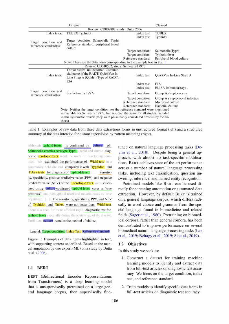
Original CleanedReview: CD008892, study: Dutta 2006
Index tests: TUBEX Typhidot Index test: TUBEXIndex test: Typhidot
Target condition andreference standard(s):
Target condition Salmonella TyphiReference standard: peripheral bloodculture
Target condition: Salmonella TyphiTarget condition: Typhoid fever
Reference standard: Peripheral blood cultureNote: These are the data items corresponding to the example text in Fig. 1
Review: CD010502, study: Schwartz 1997b
Index tests:
Throat swab: not reported Commer-cial name of the RADT: QuickVue In-Line Strep A (Quidel) Type of RADT:EIA
Index test: QuickVue In-Line Strep A
Index test: EIAIndex test: ELISA Immunoassays
Target condition andreference standard(s): See Schwartz 1997a Target condition: Group A streptococcus
Target condition: Group A streptococcal infectionReference standard: Microbial cultureReference standard: Bacterial culture
Note: Neither the target condition nor the reference standard were mentionedin the table for Schwartz 1997a, but assumed the same for all studies includedin this systematic review (they were presumably considered obvious by the au-thors).
Table 1: Examples of raw data from three data extractions forms in unstructured format (left) and a structuredsummary of the data intended for distant supervision by pattern matching (right).
Although typhoid fever is confirmed by culture of
Salmonella enterica serotype Typhi , rapid and simple diag-
nostic serologic tests would be useful in developing coun-
tries. We examined the performance of Widal test in a
community field site and compared it with Typhidot and
Tubex tests for diagnosis of typhoid fever . [...] Sensitiv-
ity, specificity, positive predictive value (PPV), and negative
predictive value (NPV) of the 3 serologic tests were calcu-
lated using culture-confirmed typhoid fever cases as ”true
positives” and paratyphoid fever and malaria cases as ”true
negatives”. [...] The sensitivity, specificity, PPV, and NPV
of Typhidot and Tubex were not better than Widal test.
There is a need for more efficient rapid diagnostic test for
typhoid fever especially during the acute stage of the disease.
Until then, culture remains the method of choice.
Legend: Target condition Index Test Reference standard
Figure 1: Examples of data items highlighted in text,with supporting context underlined. Based on the man-ual annotation by one expert (ML) on a study by Duttaet al. (2006).
1.1 BERT
BERT (Bidirectional Encoder Representationsfrom Transformers) is a deep learning modelthat is unsupervisedly pretrained on a large gen-eral language corpus, then supervisedly fine-
tuned on natural language processing tasks (De-vlin et al., 2018). Despite being a general ap-proach, with almost no task-specific modifica-tions, BERT achieves state-of-the-art performanceacross a number of natural language processingtasks, including text classification, question an-swering, inference, and named entity recognition.
Pretrained models like BERT can be used di-rectly for screening automation or automated dataextraction. However, by default BERT is trainedon a general language corpus, which differs radi-cally in word choice and grammar from the spe-cial language found in biomedicine and relatedfields (Sager et al., 1980). Pretraining on biomed-ical corpora, rather than general corpora, has beendemonstrated to improve performance on severalbiomedical natural language processing tasks (Leeet al., 2019; Beltagy et al., 2019; Si et al., 2019).
1.2 ObjectivesIn this study we seek to:
1. Construct a dataset for training machinelearning models to identify and extract datafrom full-text articles on diagnostic test accu-racy. We focus on the target condition, indextest, and reference standard.
2. Train models to identify specific data items infull-text articles on diagnostic test accuracy
106
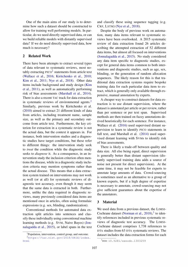
One of the main aims of our study is to deter-mine how such a dataset should be constructed toallow for training well performing models. In par-ticular, do we need directly supervised data, or canwe build reliable models with distantly superviseddata? If we do need directly supervised data, howmuch is necessary?
2 Related Work
There have been attempts to extract several typesof data relevant to systematic reviews, most no-tably extracting PICO1 statements from article text(Wallace et al., 2016; Kiritchenko et al., 2010;Kim et al., 2011; Nye et al., 2018). Other dataitems include background and study design (Kimet al., 2011), as well as automatically performingrisk of bias assessments (Marshall et al., 2014).There is also a recent TAC track for data extractionin systematic reviews of environmental agents.2
Similarly, previous work by Kiritchenko et al.(2010) aimed to extract 21 different kinds of datafrom articles, including treatment name, samplesize, as well as the primary and secondary out-come from article text. Furthermore, the key cri-terion for extraction in a systematic review is notthe actual data, but the context it appears in. Forinstance, both intervention studies and a diagnos-tic studies have target conditions, but these referto different things: the intervention study seekto treat the condition while the diagnostic studyseeks to diagnose it. As a consequence, in an in-tervention study the inclusion criterion often men-tions the disease, while in a diagnostic study inclu-sion criteria may mention symptoms rather thanthe actual disease. This means that a data extrac-tion system trained on interventions may not workas well (or at all) for systematic reviews of di-agnostic test accuracy, even though it may seemthat the same data is extracted in both. Further-more, unlike the data required in diagnostic re-views, many previously considered data items arementioned once in articles, often using formulaicexpressions (e.g. sex, blinding, randomization).
Conventional methods for automated data ex-traction split articles into sentences and clas-sify these individually using conventional machinelearning methods (e.g. SVM, Naive Bayes) (Jon-nalagadda et al., 2015), or label spans in the text
1Population, intervention, control group, and outcome.2https://tac.nist.gov/2018/SRIE/index.
html
and classify these using sequence tagging (e.g.CRF, LSTM) (Nye et al., 2018).
Despite the body of previous work on automa-tion, many data items relevant to systematic re-views have been overlooked. A 2015 systematicreview of data extraction found 26 articles de-scribing the attempted extraction of 52 differentdata items, but almost all focused on interventions(Jonnalagadda et al., 2015). No study consideredany data item specific to diagnostic studies, ex-cept for general data items common to both inter-ventions and diagnostic studies, such as age, sex,blinding, or the generation of random allocationsequences. The likely reason for this is that tra-ditional data extraction systems require bespoketraining data for each particular data item to ex-tract, which is generally only available through ex-pensive, manual annotation by experts.
A cheaper way to construct datasets for data ex-traction is to use distant supervision, where thedataset is annotated per article or per review, ratherthan per sentence or per text span. Supervisedmethods are then trained on fuzzy annotations de-rived heuristically for each sentence. For instance,Wallace et al. (2016) used supervised distant su-pervision to learn to identify PICO statements infull text, and Marshall et al. (2014) used super-vised distant learning with SVMs to identify riskof bias assessments.
There is likely a trade-off between quality anddata size. All else being equal, direct supervisionis generally better than distant supervision (dis-tantly supervised training data adds a source ofnoise not present for direct supervision). At thesame time, it may not be feasible for experts toannotate large amounts of data. Crowd-sourcingis sometimes used as an alternative to a group ofknown experts, but if a high degree of expertiseis necessary to annotate, crowd-sourcing may notgive sufficient guarantees about the expertise ofthe annotators.
3 Material
We used data from a previous dataset, the LIMSI-Cochrane dataset (Norman et al., 2018),3 to iden-tify references included in previous systematic re-views of diagnostic test accuracy. The LIMSI-Cochrane dataset comprises 1,738 references toDTA studies from 63 DTA systematic reviews. Thedataset includes the data extraction forms for each
3DOI: 10.5281/zenodo.1303259
107
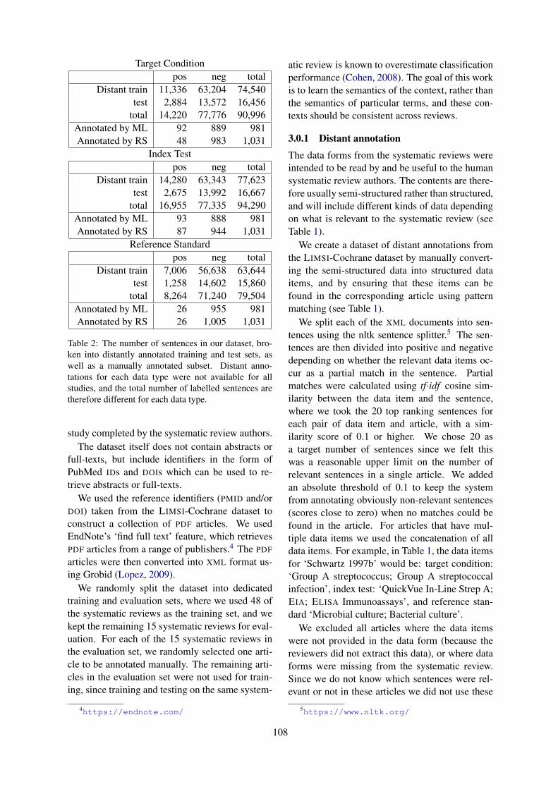
Target Conditionpos neg total
Distant train 11,336 63,204 74,540test 2,884 13,572 16,456
total 14,220 77,776 90,996Annotated by ML 92 889 981Annotated by RS 48 983 1,031
Index Testpos neg total
Distant train 14,280 63,343 77,623test 2,675 13,992 16,667
total 16,955 77,335 94,290Annotated by ML 93 888 981Annotated by RS 87 944 1,031
Reference Standardpos neg total
Distant train 7,006 56,638 63,644test 1,258 14,602 15,860
total 8,264 71,240 79,504Annotated by ML 26 955 981Annotated by RS 26 1,005 1,031
Table 2: The number of sentences in our dataset, bro-ken into distantly annotated training and test sets, aswell as a manually annotated subset. Distant anno-tations for each data type were not available for allstudies, and the total number of labelled sentences aretherefore different for each data type.
study completed by the systematic review authors.The dataset itself does not contain abstracts or
full-texts, but include identifiers in the form ofPubMed IDs and DOIs which can be used to re-trieve abstracts or full-texts.
We used the reference identifiers (PMID and/orDOI) taken from the LIMSI-Cochrane dataset toconstruct a collection of PDF articles. We usedEndNote’s ‘find full text’ feature, which retrievesPDF articles from a range of publishers.4 The PDF
articles were then converted into XML format us-ing Grobid (Lopez, 2009).
We randomly split the dataset into dedicatedtraining and evaluation sets, where we used 48 ofthe systematic reviews as the training set, and wekept the remaining 15 systematic reviews for eval-uation. For each of the 15 systematic reviews inthe evaluation set, we randomly selected one arti-cle to be annotated manually. The remaining arti-cles in the evaluation set were not used for train-ing, since training and testing on the same system-
4https://endnote.com/
atic review is known to overestimate classificationperformance (Cohen, 2008). The goal of this workis to learn the semantics of the context, rather thanthe semantics of particular terms, and these con-texts should be consistent across reviews.
3.0.1 Distant annotation
The data forms from the systematic reviews wereintended to be read by and be useful to the humansystematic review authors. The contents are there-fore usually semi-structured rather than structured,and will include different kinds of data dependingon what is relevant to the systematic review (seeTable 1).
We create a dataset of distant annotations fromthe LIMSI-Cochrane dataset by manually convert-ing the semi-structured data into structured dataitems, and by ensuring that these items can befound in the corresponding article using patternmatching (see Table 1).
We split each of the XML documents into sen-tences using the nltk sentence splitter.5 The sen-tences are then divided into positive and negativedepending on whether the relevant data items oc-cur as a partial match in the sentence. Partialmatches were calculated using tf·idf cosine sim-ilarity between the data item and the sentence,where we took the 20 top ranking sentences foreach pair of data item and article, with a sim-ilarity score of 0.1 or higher. We chose 20 asa target number of sentences since we felt thiswas a reasonable upper limit on the number ofrelevant sentences in a single article. We addedan absolute threshold of 0.1 to keep the systemfrom annotating obviously non-relevant sentences(scores close to zero) when no matches could befound in the article. For articles that have mul-tiple data items we used the concatenation of alldata items. For example, in Table 1, the data itemsfor ‘Schwartz 1997b’ would be: target condition:‘Group A streptococcus; Group A streptococcalinfection’, index test: ‘QuickVue In-Line Strep A;EIA; ELISA Immunoassays’, and reference stan-dard ‘Microbial culture; Bacterial culture’.
We excluded all articles where the data itemswere not provided in the data form (because thereviewers did not extract this data), or where dataforms were missing from the systematic review.Since we do not know which sentences were rel-evant or not in these articles we did not use these
5https://www.nltk.org/
108
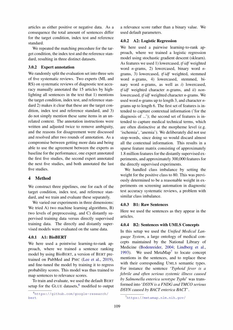
articles as either positive or negative data. As aconsequence the total amount of sentences differfor the target condition, index test and referencestandard.
We repeated the matching precedure for the tar-get condition, the index test and the reference stan-dard, resulting in three distinct datasets.
3.0.2 Expert annotationWe randomly split the evaluation set into three setsof five systematic reviews. Two experts (ML andRS) on systematic reviews of diagnostic test accu-racy manually annotated the 15 articles by high-lighting all sentences in the text that 1) mentionsthe target condition, index test, and reference stan-dard 2) makes it clear that these are the target con-dition, index test and reference standard, and 3)do not simply mention these same items in an un-related context. The annotation instructions werewritten and adjusted twice to remove ambiguity,and the reasons for disagreement were discussedand resolved after two rounds of annotation. As acompromise between getting more data and beingable to use the agreement between the experts asbaseline for the performance, one expert annotatedthe first five studies, the second expert annotatedthe next five studies, and both annotated the lastfive studies.
4 Method
We construct three pipelines, one for each of thetarget condition, index test, and reference stan-dard, and we train and evaluate these separately.
We varied our experiments in three dimensions:We tried A) two machine learning algorithms, B)two levels of preprocessing, and C) distantly su-pervised training data versus directly supervisedtraining data. The directly and distantly super-vised models were evaluated on the same data.
4.0.1 A1: BioBERTWe here used a pointwise learning-to-rank ap-proach, where we trained a sentence rankingmodel by using BioBERT, a version of BERT pre-trained on PubMed and PMC (Lee et al., 2019),and fine-tuned the model by training it to regressprobability scores. This model was thus trained tomap sentences to relevance scores.
To train and evaluate, we used the default BERT
setup for the GLUE datasets,6 modified to output6https://github.com/google-research/
bert
a relevance score rather than a binary value. Weused default parameters.
4.0.2 A2: Logistic RegressionWe here used a pairwise learning-to-rank ap-proach, where we trained a logistic regressionmodel using stochastic gradient descent (sklearn).As features we used 1) lowercased, tf·idf weightedword n-grams, 2) lowercased, binary word n-grams, 3) lowercased, tf·idf weighted, stemmedword n-grams, 4) lowercased, stemmed, bi-nary word n-grams, as well as i) lowercased,tf·idf weighted character n-grams, and ii) non-lowercased, tf·idf weighted character n-grams. Weused word n-grams up to length 3, and character n-grams up to length 6. The first set of features is in-tended to capture contextual information (’for thediagnosis of ...’); the second set of features is in-tended to capture medical technical terms, whichare often distinctive at the morpheme level (e.g.‘ischemia’, ‘anemia’). We deliberately did not usestop-words, since doing so would discard almostall the contextual information. This results in asparse feature matrix consisting of approximately1.8 million features for the distantly supervised ex-periments, and approximately 300,000 features forthe directly supervised experiments.
We handled class imbalance by setting theweight for the positive class to 80. This was previ-ously determined to be a reasonable weight in ex-periments on screening automation in diagnostictest accuracy systematic reviews, a problem withsimilar class imbalance.
4.0.3 B1: Raw SentencesHere we used the sentences as they appear in thearticles.
4.0.4 B2: Sentences with UMLS ConceptsIn this setup we used the Unified Medical Lan-guage System, a large ontology of medical con-cepts maintained by the National Library ofMedicine (Bodenreider, 2004; Lindberg et al.,1993). We used MetaMap7 to locate conceptmentions in the sentences, and to replace thesewith their corresponding UMLS semantic types.For instance the sentence ‘Typhoid fever is afebrile and often serious systemic illness causedby Salmonella enterica serotype Typhi’ was trans-formed into ‘DSYN is a FNDG and TMCO seriousDSYN caused by BACT enterica BACT’.
7https://metamap.nlm.nih.gov/
109
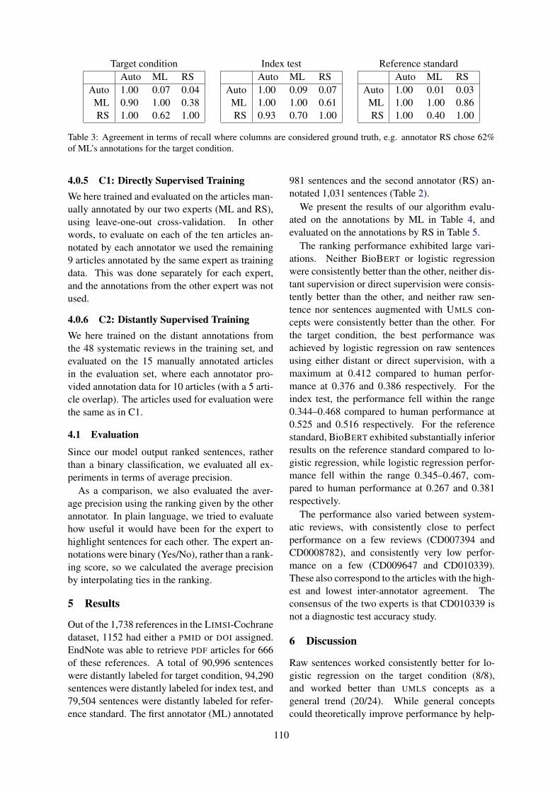
Target conditionAuto ML RS
Auto 1.00 0.07 0.04ML 0.90 1.00 0.38RS 1.00 0.62 1.00
Index testAuto ML RS
Auto 1.00 0.09 0.07ML 1.00 1.00 0.61RS 0.93 0.70 1.00
Reference standardAuto ML RS
Auto 1.00 0.01 0.03ML 1.00 1.00 0.86RS 1.00 0.40 1.00
Table 3: Agreement in terms of recall where columns are considered ground truth, e.g. annotator RS chose 62%of ML’s annotations for the target condition.
4.0.5 C1: Directly Supervised TrainingWe here trained and evaluated on the articles man-ually annotated by our two experts (ML and RS),using leave-one-out cross-validation. In otherwords, to evaluate on each of the ten articles an-notated by each annotator we used the remaining9 articles annotated by the same expert as trainingdata. This was done separately for each expert,and the annotations from the other expert was notused.
4.0.6 C2: Distantly Supervised TrainingWe here trained on the distant annotations fromthe 48 systematic reviews in the training set, andevaluated on the 15 manually annotated articlesin the evaluation set, where each annotator pro-vided annotation data for 10 articles (with a 5 arti-cle overlap). The articles used for evaluation werethe same as in C1.
4.1 Evaluation
Since our model output ranked sentences, ratherthan a binary classification, we evaluated all ex-periments in terms of average precision.
As a comparison, we also evaluated the aver-age precision using the ranking given by the otherannotator. In plain language, we tried to evaluatehow useful it would have been for the expert tohighlight sentences for each other. The expert an-notations were binary (Yes/No), rather than a rank-ing score, so we calculated the average precisionby interpolating ties in the ranking.
5 Results
Out of the 1,738 references in the LIMSI-Cochranedataset, 1152 had either a PMID or DOI assigned.EndNote was able to retrieve PDF articles for 666of these references. A total of 90,996 sentenceswere distantly labeled for target condition, 94,290sentences were distantly labeled for index test, and79,504 sentences were distantly labeled for refer-ence standard. The first annotator (ML) annotated
981 sentences and the second annotator (RS) an-notated 1,031 sentences (Table 2).
We present the results of our algorithm evalu-ated on the annotations by ML in Table 4, andevaluated on the annotations by RS in Table 5.
The ranking performance exhibited large vari-ations. Neither BioBERT or logistic regressionwere consistently better than the other, neither dis-tant supervision or direct supervision were consis-tently better than the other, and neither raw sen-tence nor sentences augmented with UMLS con-cepts were consistently better than the other. Forthe target condition, the best performance wasachieved by logistic regression on raw sentencesusing either distant or direct supervision, with amaximum at 0.412 compared to human perfor-mance at 0.376 and 0.386 respectively. For theindex test, the performance fell within the range0.344–0.468 compared to human performance at0.525 and 0.516 respectively. For the referencestandard, BioBERT exhibited substantially inferiorresults on the reference standard compared to lo-gistic regression, while logistic regression perfor-mance fell within the range 0.345–0.467, com-pared to human performance at 0.267 and 0.381respectively.
The performance also varied between system-atic reviews, with consistently close to perfectperformance on a few reviews (CD007394 andCD0008782), and consistently very low perfor-mance on a few (CD009647 and CD010339).These also correspond to the articles with the high-est and lowest inter-annotator agreement. Theconsensus of the two experts is that CD010339 isnot a diagnostic test accuracy study.
6 Discussion
Raw sentences worked consistently better for lo-gistic regression on the target condition (8/8),and worked better than UMLS concepts as ageneral trend (20/24). While general conceptscould theoretically improve performance by help-
110
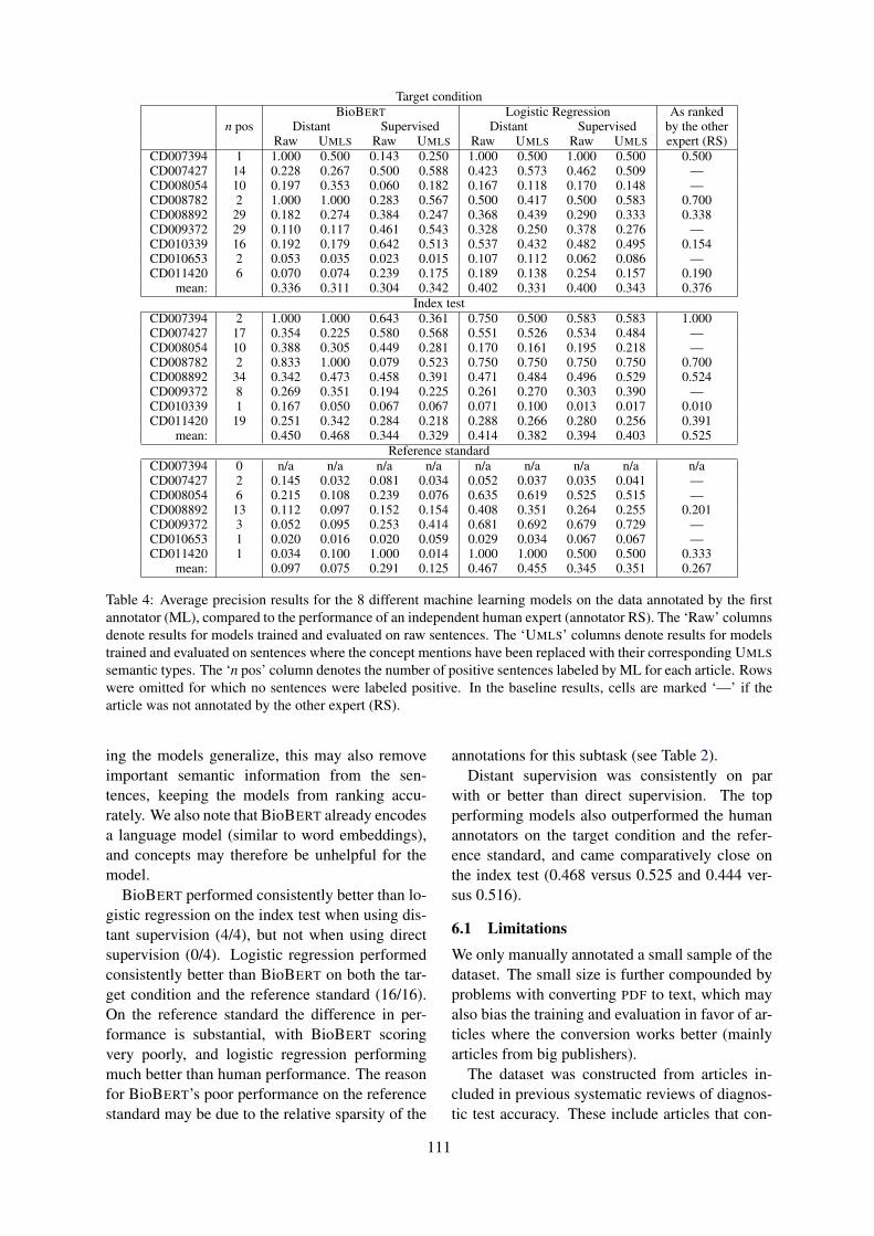
Target conditionBioBERT Logistic Regression As ranked
n pos Distant Supervised Distant Supervised by the otherRaw UMLS Raw UMLS Raw UMLS Raw UMLS expert (RS)
CD007394 1 1.000 0.500 0.143 0.250 1.000 0.500 1.000 0.500 0.500CD007427 14 0.228 0.267 0.500 0.588 0.423 0.573 0.462 0.509 —CD008054 10 0.197 0.353 0.060 0.182 0.167 0.118 0.170 0.148 —CD008782 2 1.000 1.000 0.283 0.567 0.500 0.417 0.500 0.583 0.700CD008892 29 0.182 0.274 0.384 0.247 0.368 0.439 0.290 0.333 0.338CD009372 29 0.110 0.117 0.461 0.543 0.328 0.250 0.378 0.276 —CD010339 16 0.192 0.179 0.642 0.513 0.537 0.432 0.482 0.495 0.154CD010653 2 0.053 0.035 0.023 0.015 0.107 0.112 0.062 0.086 —CD011420 6 0.070 0.074 0.239 0.175 0.189 0.138 0.254 0.157 0.190
mean: 0.336 0.311 0.304 0.342 0.402 0.331 0.400 0.343 0.376Index test
CD007394 2 1.000 1.000 0.643 0.361 0.750 0.500 0.583 0.583 1.000CD007427 17 0.354 0.225 0.580 0.568 0.551 0.526 0.534 0.484 —CD008054 10 0.388 0.305 0.449 0.281 0.170 0.161 0.195 0.218 —CD008782 2 0.833 1.000 0.079 0.523 0.750 0.750 0.750 0.750 0.700CD008892 34 0.342 0.473 0.458 0.391 0.471 0.484 0.496 0.529 0.524CD009372 8 0.269 0.351 0.194 0.225 0.261 0.270 0.303 0.390 —CD010339 1 0.167 0.050 0.067 0.067 0.071 0.100 0.013 0.017 0.010CD011420 19 0.251 0.342 0.284 0.218 0.288 0.266 0.280 0.256 0.391
mean: 0.450 0.468 0.344 0.329 0.414 0.382 0.394 0.403 0.525Reference standard
CD007394 0 n/a n/a n/a n/a n/a n/a n/a n/a n/aCD007427 2 0.145 0.032 0.081 0.034 0.052 0.037 0.035 0.041 —CD008054 6 0.215 0.108 0.239 0.076 0.635 0.619 0.525 0.515 —CD008892 13 0.112 0.097 0.152 0.154 0.408 0.351 0.264 0.255 0.201CD009372 3 0.052 0.095 0.253 0.414 0.681 0.692 0.679 0.729 —CD010653 1 0.020 0.016 0.020 0.059 0.029 0.034 0.067 0.067 —CD011420 1 0.034 0.100 1.000 0.014 1.000 1.000 0.500 0.500 0.333
mean: 0.097 0.075 0.291 0.125 0.467 0.455 0.345 0.351 0.267
Table 4: Average precision results for the 8 different machine learning models on the data annotated by the firstannotator (ML), compared to the performance of an independent human expert (annotator RS). The ‘Raw’ columnsdenote results for models trained and evaluated on raw sentences. The ‘UMLS’ columns denote results for modelstrained and evaluated on sentences where the concept mentions have been replaced with their corresponding UMLSsemantic types. The ‘n pos’ column denotes the number of positive sentences labeled by ML for each article. Rowswere omitted for which no sentences were labeled positive. In the baseline results, cells are marked ‘—’ if thearticle was not annotated by the other expert (RS).
ing the models generalize, this may also removeimportant semantic information from the sen-tences, keeping the models from ranking accu-rately. We also note that BioBERT already encodesa language model (similar to word embeddings),and concepts may therefore be unhelpful for themodel.
BioBERT performed consistently better than lo-gistic regression on the index test when using dis-tant supervision (4/4), but not when using directsupervision (0/4). Logistic regression performedconsistently better than BioBERT on both the tar-get condition and the reference standard (16/16).On the reference standard the difference in per-formance is substantial, with BioBERT scoringvery poorly, and logistic regression performingmuch better than human performance. The reasonfor BioBERT’s poor performance on the referencestandard may be due to the relative sparsity of the
annotations for this subtask (see Table 2).Distant supervision was consistently on par
with or better than direct supervision. The topperforming models also outperformed the humanannotators on the target condition and the refer-ence standard, and came comparatively close onthe index test (0.468 versus 0.525 and 0.444 ver-sus 0.516).
6.1 LimitationsWe only manually annotated a small sample of thedataset. The small size is further compounded byproblems with converting PDF to text, which mayalso bias the training and evaluation in favor of ar-ticles where the conversion works better (mainlyarticles from big publishers).
The dataset was constructed from articles in-cluded in previous systematic reviews of diagnos-tic test accuracy. These include articles that con-
111
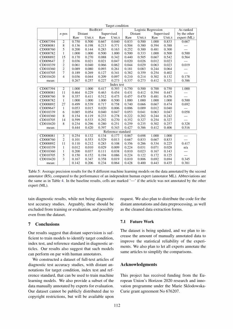
Target conditionBioBERT Logistic Regression As ranked
n pos Distant Supervised Distant Supervised by the otherRaw UMLS Raw UMLS Raw UMLS Raw UMLS expert (ML)
CD007394 2 0.750 0.500 0.667 0.040 0.833 0.500 1.000 0.833 0.667CD008081 8 0.136 0.198 0.213 0.371 0.504 0.380 0.394 0.388 —CD008760 5 0.200 0.144 0.283 0.163 0.252 0.300 0.481 0.300 —CD008782 1 1.000 1.000 0.500 1.000 0.500 0.333 1.000 0.500 0.500CD008892 15 0.170 0.270 0.088 0.342 0.440 0.505 0.667 0.542 0.564CD009647 2 0.036 0.021 0.021 0.047 0.020 0.026 0.012 0.023 —CD010339 2 0.061 0.040 0.066 0.062 0.044 0.029 0.063 0.023 0.019CD010360 2 0.089 0.080 0.093 0.261 0.181 0.083 0.244 0.064 —CD010705 7 0.189 0.269 0.127 0.341 0.382 0.359 0.254 0.402 —CD010420 4 0.036 0.044 0.209 0.097 0.210 0.214 0.302 0.132 0.178
mean: 0.267 0.257 0.227 0.273 0.337 0.273 0.412 0.321 0.386Index test
CD007394 2 1.000 1.000 0.417 0.393 0.750 0.500 0.700 0.750 1.000CD008081 11 0.464 0.229 0.463 0.454 0.431 0.412 0.394 0.447 —CD008760 9 0.357 0.411 0.512 0.475 0.457 0.470 0.481 0.476 —CD008782 1 1.000 1.000 1.000 0.500 1.000 1.000 1.000 1.000 0.500CD008892 27 0.499 0.539 0.717 0.758 0.740 0.666 0.667 0.474 0.692CD009647 1 0.053 0.015 0.020 0.006 0.006 0.009 0.012 0.040 —CD010339 6 0.085 0.054 0.040 0.047 0.053 0.041 0.063 0.047 0.058CD010360 8 0.154 0.119 0.233 0.278 0.222 0.202 0.244 0.242 —CD010705 14 0.599 0.533 0.292 0.270 0.352 0.327 0.254 0.327 —CD010420 8 0.234 0.296 0.280 0.251 0.259 0.235 0.302 0.257 0.328
mean: 0.444 0.420 0.397 0.343 0.427 0.386 0.412 0.406 0.516Reference standard
CD008081 3 0.254 0.132 0.134 0.177 0.867 0.698 1.000 1.000 —CD008760 2 0.101 0.553 0.529 0.013 0.667 0.833 0.667 0.833 —CD008892 11 0.110 0.212 0.283 0.108 0.356 0.286 0.334 0.225 0.417CD010339 1 0.012 0.010 0.029 0.009 0.224 0.031 0.071 0.028 n/aCD010360 1 0.200 0.037 0.111 0.038 0.810 0.023 0.167 0.143 —CD010705 5 0.150 0.152 0.194 0.086 0.224 0.122 0.172 0.125 —CD010420 3 0.167 0.347 0.358 0.019 0.810 0.806 0.692 0.694 0.345
mean: 0.142 0.206 0.234 0.064 0.428 0.400 0.443 0.435 0.381
Table 5: Average precision results for the 8 different machine learning models on the data annotated by the secondannotator (RS), compared to the performance of an independent human expert (annotator ML). Abbreviations arethe same as in Table 4. In the baseline results, cells are marked ’—’ if the article was not annotated by the otherexpert (ML).
tain diagnostic results, while not being diagnostictest accuracy studies. Arguably, these should beexcluded from training or evaluation, and possiblyeven from the dataset.
7 Conclusions
Our results suggest that distant supervision is suf-ficient to train models to identify target condition,index test, and reference standard in diagnostic ar-ticles. Our results also suggest that such modelscan perform on par with human annotators.
We constructed a dataset of full-text articles ofdiagnostic test accuracy studies, with distant an-notations for target condition, index test and ref-erence standard, that can be used to train machinelearning models. We also provide a subset of thedata manually annotated by experts for evaluation.Our dataset cannot be publicly distributed due tocopyright restrictions, but will be available upon
request. We also plan to distribute the code for thedistant annotations and data preprocessing, as wellas the cleaned data extraction forms.
7.1 Future Work
The dataset is being updated, and we plan to in-crease the amount of manually annotated data toimprove the statistical reliability of the experi-ments. We also plan to let all experts annotate thesame articles to simplify the comparisons.
Acknowledgments
This project has received funding from the Eu-ropean Union’s Horizon 2020 research and inno-vation programme under the Marie Sklodowska-Curie grant agreement No 676207.
112
ReferencesAlexandra Bannach-Brown, Piotr Przybyła, James
Thomas, Andrew SC Rice, Sophia Ananiadou, JingLiao, and Malcolm Robert Macleod. 2019. Machinelearning algorithms for systematic review: reducingworkload in a preclinical review of animal studiesand reducing human screening error. Systematic re-views, 8(1):23.
Iz Beltagy, Arman Cohan, and Kyle Lo. 2019. SciB-ERT: Pretrained contextualized embeddings for sci-entific text. arXiv preprint arXiv:1903.10676.
Olivier Bodenreider. 2004. The unified medicallanguage system (UMLS): integrating biomed-ical terminology. Nucleic acids research,32(suppl 1):D267–D270.
Aaron M Cohen. 2008. Optimizing feature represen-tation for automated systematic review work prior-itization. AMIA Annual Symposium proceedings,pages 121–5.
HCW De Vet, A Eisinga, II Riphagen, B Aertgeerts,D Pewsner, and R Mitchell. 2008. Chapter 7:searching for studies. Cochrane handbook for sys-tematic reviews of diagnostic test accuracy version0.4 [updated September 2008]. The Cochrane Col-laboration.
Jacob Devlin, Ming-Wei Chang, Kenton Lee, andKristina Toutanova. 2018. BERT: Pre-training ofdeep bidirectional transformers for language under-standing. arXiv preprint arXiv:1810.04805.
Shanta Dutta, Dipika Sur, Byomkesh Manna, BhaswatiSen, Alok Kumar Deb, Jacqueline L Deen, JohnWain, Lorenz Von Seidlein, Leon Ochiai, John DClemens, et al. 2006. Evaluation of new-generationserologic tests for the diagnosis of typhoid fever:data from a community-based surveillance in cal-cutta, india. Diagnostic microbiology and infectiousdisease, 56(4):359–365.
Siddhartha R Jonnalagadda, Pawan Goyal, and Mark DHuffman. 2015. Automating data extraction in sys-tematic reviews: a systematic review. Systematic re-views, 4(1):78.
Su Nam Kim, David Martinez, Lawrence Cavedon, andLars Yencken. 2011. Automatic classification ofsentences to support evidence based medicine. InBMC bioinformatics, volume 12, page S5. BioMedCentral.
Svetlana Kiritchenko, Berry de Bruijn, Simona Carini,Joel Martin, and Ida Sim. 2010. ExaCT: automaticextraction of clinical trial characteristics from jour-nal publications. BMC medical informatics and de-cision making, 10:56.
Jinhyuk Lee, Wonjin Yoon, Sungdong Kim,Donghyeon Kim, Sunkyu Kim, Chan Ho So, andJaewoo Kang. 2019. BioBERT: pre-trained biomed-ical language representation model for biomedicaltext mining. arXiv preprint arXiv:1901.08746.
Ivan Lerner, Perrine Créquit, Philippe Ravaud, and Ig-nacio Atal. 2019. Automatic screening using wordembeddings achieved high sensitivity and work-load reduction for updating living network meta-analyses. Journal of clinical epidemiology, 108:86–94.
Donald AB Lindberg, Betsy L Humphreys, andAlexa T McCray. 1993. The unified medical lan-guage system. Yearbook of Medical Informatics,2(01):41–51.
Patrice Lopez. 2009. Grobid: Combining automaticbibliographic data recognition and term extractionfor scholarship publications. In International con-ference on theory and practice of digital libraries,pages 473–474. Springer.
Iain J. Marshall, Joël Kuiper, and Byron C. Wallace.2014. Automating risk of bias assessment for clin-ical trials. Proceedings of the 5th ACM Confer-ence on Bioinformatics, Computational Biology, andHealth Informatics - BCB ’14, pages 88–95.
Christopher Norman, Mariska Leeflang, and AurélieNévéol. 2018. Data extraction and synthesis insystematic reviews of diagnostic test accuracy: Acorpus for automating and evaluating the process.In AMIA Annual Symposium Proceedings, volume2018, page 817. American Medical Informatics As-sociation.
Benjamin Nye, Junyi Jessy Li, Roma Patel, YinfeiYang, Iain J Marshall, Ani Nenkova, and Byron CWallace. 2018. A corpus with multi-level annota-tions of patients, interventions and outcomes to sup-port language processing for medical literature. InProceedings of the conference. Association for Com-putational Linguistics. Meeting, volume 2018, page197. NIH Public Access.
Alison O’Mara-Eves, James Thomas, John McNaught,Makoto Miwa, and Sophia Ananiadou. 2015. Us-ing text mining for study identification in systematicreviews: a systematic review of current approaches.Systematic reviews, 4(1):5.
Piotr Przybyła, Austin J Brockmeier, Georgios Konto-natsios, Marie-Annick Le Pogam, John McNaught,Erik von Elm, Kay Nolan, and Sophia Ananiadou.2018. Prioritising references for systematic reviewswith robotanalyst: A user study. Research synthesismethods, 9(3):470–488.
Juan C Sager, David Dungworth, Peter F McDonald,et al. 1980. English special languages: principlesand practice in science and technology. John Ben-jamins Pub Co.
Yuqi Si, Jingqi Wang, Hua Xu, and Kirk Roberts. 2019.Enhancing clinical concept extraction with contex-tual embedding. arXiv preprint arXiv:1902.08691.
Byron C Wallace, Joël Kuiper, Aakash Sharma,Mingxi Brian Zhu, and Iain J Marshall. 2016. Ex-tracting PICO sentences from clinical trial reports
113

using supervised distant supervision. Journal ofMachine Learning Research, 17(132):1–25.
114
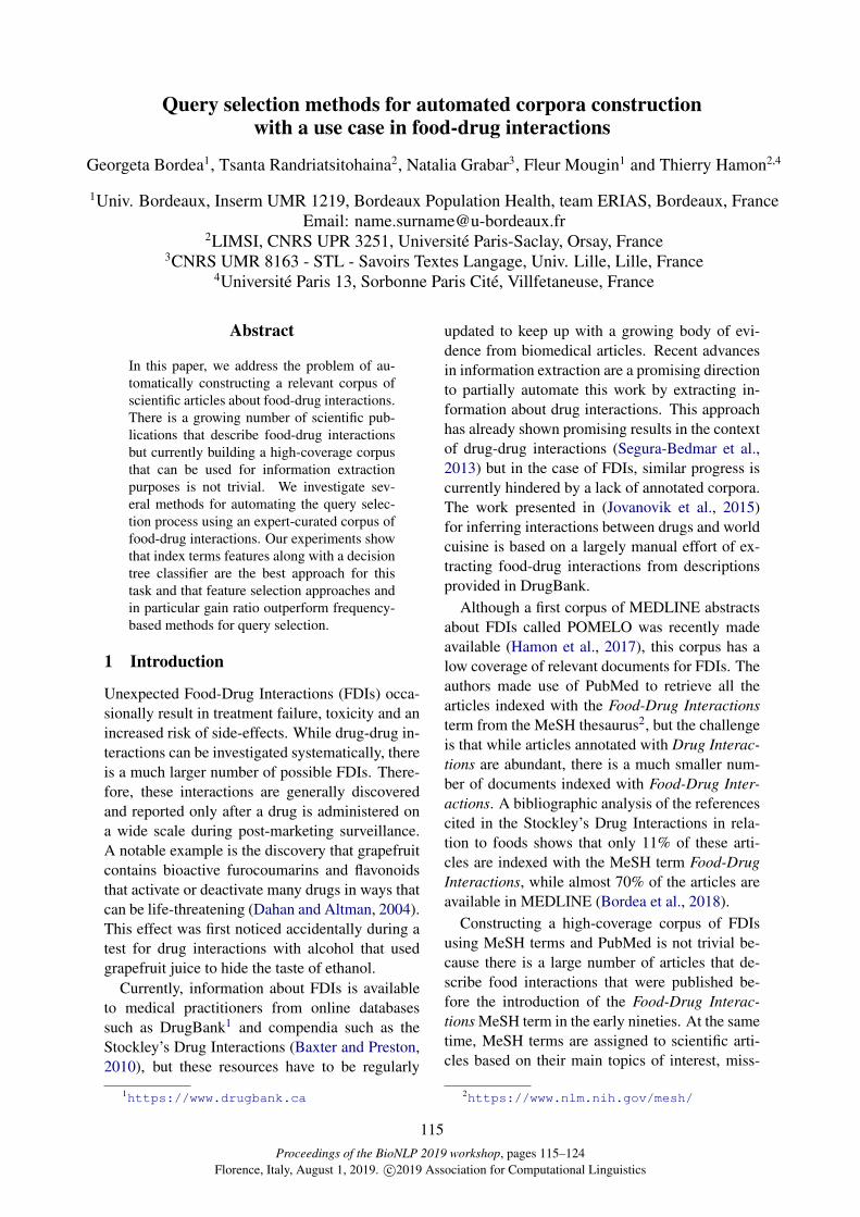
Proceedings of the BioNLP 2019 workshop, pages 115–124Florence, Italy, August 1, 2019. c©2019 Association for Computational Linguistics
Query selection methods for automated corpora constructionwith a use case in food-drug interactions
Georgeta Bordea1, Tsanta Randriatsitohaina2, Natalia Grabar3, Fleur Mougin1 and Thierry Hamon2,4
1Univ. Bordeaux, Inserm UMR 1219, Bordeaux Population Health, team ERIAS, Bordeaux, FranceEmail: [email protected]
2LIMSI, CNRS UPR 3251, Université Paris-Saclay, Orsay, France3CNRS UMR 8163 - STL - Savoirs Textes Langage, Univ. Lille, Lille, France
4Université Paris 13, Sorbonne Paris Cité, Villfetaneuse, France
Abstract
In this paper, we address the problem of au-tomatically constructing a relevant corpus ofscientific articles about food-drug interactions.There is a growing number of scientific pub-lications that describe food-drug interactionsbut currently building a high-coverage corpusthat can be used for information extractionpurposes is not trivial. We investigate sev-eral methods for automating the query selec-tion process using an expert-curated corpus offood-drug interactions. Our experiments showthat index terms features along with a decisiontree classifier are the best approach for thistask and that feature selection approaches andin particular gain ratio outperform frequency-based methods for query selection.
1 Introduction
Unexpected Food-Drug Interactions (FDIs) occa-sionally result in treatment failure, toxicity and anincreased risk of side-effects. While drug-drug in-teractions can be investigated systematically, thereis a much larger number of possible FDIs. There-fore, these interactions are generally discoveredand reported only after a drug is administered ona wide scale during post-marketing surveillance.A notable example is the discovery that grapefruitcontains bioactive furocoumarins and flavonoidsthat activate or deactivate many drugs in ways thatcan be life-threatening (Dahan and Altman, 2004).This effect was first noticed accidentally during atest for drug interactions with alcohol that usedgrapefruit juice to hide the taste of ethanol.
Currently, information about FDIs is availableto medical practitioners from online databasessuch as DrugBank1 and compendia such as theStockley’s Drug Interactions (Baxter and Preston,2010), but these resources have to be regularly
1https://www.drugbank.ca
updated to keep up with a growing body of evi-dence from biomedical articles. Recent advancesin information extraction are a promising directionto partially automate this work by extracting in-formation about drug interactions. This approachhas already shown promising results in the contextof drug-drug interactions (Segura-Bedmar et al.,2013) but in the case of FDIs, similar progress iscurrently hindered by a lack of annotated corpora.The work presented in (Jovanovik et al., 2015)for inferring interactions between drugs and worldcuisine is based on a largely manual effort of ex-tracting food-drug interactions from descriptionsprovided in DrugBank.
Although a first corpus of MEDLINE abstractsabout FDIs called POMELO was recently madeavailable (Hamon et al., 2017), this corpus has alow coverage of relevant documents for FDIs. Theauthors made use of PubMed to retrieve all thearticles indexed with the Food-Drug Interactionsterm from the MeSH thesaurus2, but the challengeis that while articles annotated with Drug Interac-tions are abundant, there is a much smaller num-ber of documents indexed with Food-Drug Inter-actions. A bibliographic analysis of the referencescited in the Stockley’s Drug Interactions in rela-tion to foods shows that only 11% of these arti-cles are indexed with the MeSH term Food-DrugInteractions, while almost 70% of the articles areavailable in MEDLINE (Bordea et al., 2018).
Constructing a high-coverage corpus of FDIsusing MeSH terms and PubMed is not trivial be-cause there is a large number of articles that de-scribe food interactions that were published be-fore the introduction of the Food-Drug Interac-tions MeSH term in the early nineties. At the sametime, MeSH terms are assigned to scientific arti-cles based on their main topics of interest, miss-
2https://www.nlm.nih.gov/mesh/
115
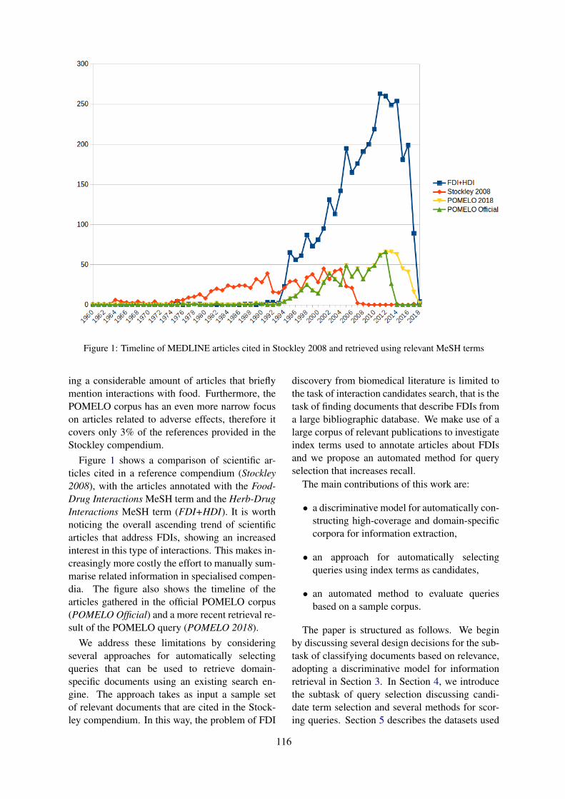
Figure 1: Timeline of MEDLINE articles cited in Stockley 2008 and retrieved using relevant MeSH terms
ing a considerable amount of articles that brieflymention interactions with food. Furthermore, thePOMELO corpus has an even more narrow focuson articles related to adverse effects, therefore itcovers only 3% of the references provided in theStockley compendium.
Figure 1 shows a comparison of scientific ar-ticles cited in a reference compendium (Stockley2008), with the articles annotated with the Food-Drug Interactions MeSH term and the Herb-DrugInteractions MeSH term (FDI+HDI). It is worthnoticing the overall ascending trend of scientificarticles that address FDIs, showing an increasedinterest in this type of interactions. This makes in-creasingly more costly the effort to manually sum-marise related information in specialised compen-dia. The figure also shows the timeline of thearticles gathered in the official POMELO corpus(POMELO Official) and a more recent retrieval re-sult of the POMELO query (POMELO 2018).
We address these limitations by consideringseveral approaches for automatically selectingqueries that can be used to retrieve domain-specific documents using an existing search en-gine. The approach takes as input a sample setof relevant documents that are cited in the Stock-ley compendium. In this way, the problem of FDI
discovery from biomedical literature is limited tothe task of interaction candidates search, that is thetask of finding documents that describe FDIs froma large bibliographic database. We make use of alarge corpus of relevant publications to investigateindex terms used to annotate articles about FDIsand we propose an automated method for queryselection that increases recall.
The main contributions of this work are:
• a discriminative model for automatically con-structing high-coverage and domain-specificcorpora for information extraction,
• an approach for automatically selectingqueries using index terms as candidates,
• an automated method to evaluate queriesbased on a sample corpus.
The paper is structured as follows. We beginby discussing several design decisions for the sub-task of classifying documents based on relevance,adopting a discriminative model for informationretrieval in Section 3. In Section 4, we introducethe subtask of query selection discussing candi-date term selection and several methods for scor-ing queries. Section 5 describes the datasets used
116
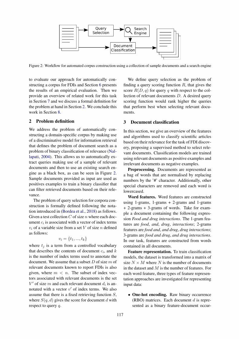
Figure 2: Workflow for automated corpus construction using a collection of sample documents and a search engine
to evaluate our approach for automatically con-structing a corpus for FDIs and Section 6 presentsthe results of an empirical evaluation. Then weprovide an overview of related work for this taskin Section 7 and we discuss a formal definition forthe problem at hand in Section 2. We conclude thiswork in Section 8.
2 Problem definition
We address the problem of automatically con-structing a domain-specific corpus by making useof a discriminative model for information retrievalthat defines the problem of document search as aproblem of binary classification of relevance (Nal-lapati, 2004). This allows us to automatically ex-tract queries making use of a sample of relevantdocuments and then to use an existing search en-gine as a black box, as can be seen in Figure 2.Sample documents provided as input are used aspositives examples to train a binary classifier thatcan filter retrieved documents based on their rele-vance.
The problem of query selection for corpora con-struction is formally defined following the nota-tion introduced in (Bordea et al., 2018) as follows.Given a test collection C of size n where each doc-ument ci is associated with a vector of index termsvi of a variable size from a set V of size n definedas follows:
vi = {t1, ..., tk}where tj is a term from a controlled vocabularythat describes the contents of document ci, and kis the number of index terms used to annotate thedocument. We assume that a subset D of size m ofrelevant documents known to report FDIs is alsogiven, where m < n. The subset of index vec-tors associated with relevant documents is the setV ′ of size m and each relevant document di is an-notated with a vector v′ of index terms. We alsoassume that there is a fixed retrieving function S,where S(q, d) gives the score for document d withrespect to query q.
We define query selection as the problem offinding a query scoring function R, that gives thescore R(D, q) for query q with respect to the col-lection of relevant documents D. A desired queryscoring function would rank higher the queriesthat perform best when selecting relevant docu-ments.
3 Document classification
In this section, we give an overview of the featuresand algorithms used to classify scientific articlesbased on their relevance for the task of FDI discov-ery, proposing a supervised method to select rele-vant documents. Classification models are trainedusing relevant documents as positive examples andirrelevant documents as negative examples.
Preprocessing. Documents are represented asa bag of words that are normalised by replacingnumbers by the ’#’ character. Additionally, otherspecial characters are removed and each word islowercased.
Word features. Word features are constructedusing 1-grams, 1-grams + 2-grams and 1-grams+ 2-grams + 3-grams of words. Take for exam-ple a document containing the following expres-sion Food and drug interactions. The 1-gram fea-tures are food, and, drug, interactions; 2-gramsfeatures are food and, and drug, drug interactions;3-grams are food and drug, and drug interactions.In our task, features are constructed from wordscontained in all documents.
Feature representation. To train classificationmodels, the dataset is transformed into a matrix ofsize N ×M where N is the number of documentsin the dataset and M is the number of features. Foreach word feature, three types of feature represen-tation approaches are investigated for representinginput data:
• One-hot encoding. Raw binary occurrence(RBO) matrices. Each document d is repre-sented as a binary feature-document occur-
117
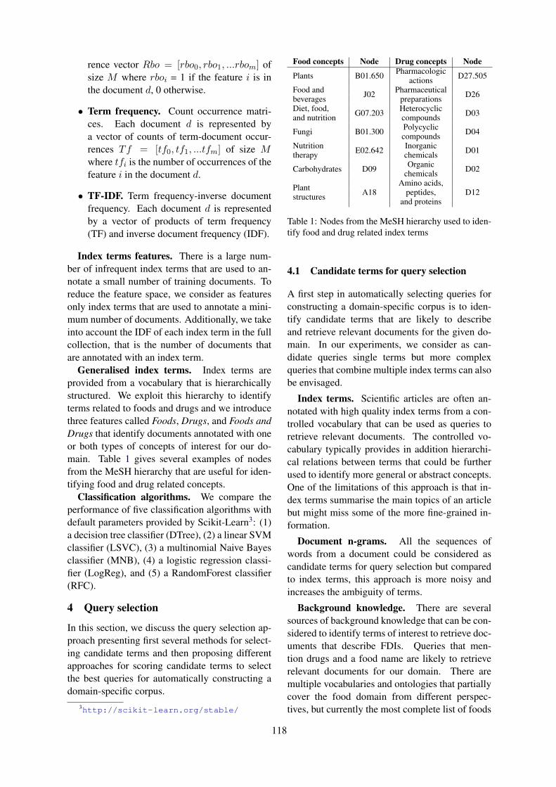
rence vector Rbo = [rbo0, rbo1, ...rbom] ofsize M where rboi = 1 if the feature i is inthe document d, 0 otherwise.
• Term frequency. Count occurrence matri-ces. Each document d is represented bya vector of counts of term-document occur-rences Tf = [tf0, tf1, ...tfm] of size Mwhere tfi is the number of occurrences of thefeature i in the document d.
• TF-IDF. Term frequency-inverse documentfrequency. Each document d is representedby a vector of products of term frequency(TF) and inverse document frequency (IDF).
Index terms features. There is a large num-ber of infrequent index terms that are used to an-notate a small number of training documents. Toreduce the feature space, we consider as featuresonly index terms that are used to annotate a mini-mum number of documents. Additionally, we takeinto account the IDF of each index term in the fullcollection, that is the number of documents thatare annotated with an index term.
Generalised index terms. Index terms areprovided from a vocabulary that is hierarchicallystructured. We exploit this hierarchy to identifyterms related to foods and drugs and we introducethree features called Foods, Drugs, and Foods andDrugs that identify documents annotated with oneor both types of concepts of interest for our do-main. Table 1 gives several examples of nodesfrom the MeSH hierarchy that are useful for iden-tifying food and drug related concepts.
Classification algorithms. We compare theperformance of five classification algorithms withdefault parameters provided by Scikit-Learn3: (1)a decision tree classifier (DTree), (2) a linear SVMclassifier (LSVC), (3) a multinomial Naive Bayesclassifier (MNB), (4) a logistic regression classi-fier (LogReg), and (5) a RandomForest classifier(RFC).
4 Query selection
In this section, we discuss the query selection ap-proach presenting first several methods for select-ing candidate terms and then proposing differentapproaches for scoring candidate terms to selectthe best queries for automatically constructing adomain-specific corpus.
3http://scikit-learn.org/stable/
Food concepts Node Drug concepts Node
Plants B01.650 Pharmacologic D27.505actionsFood and J02 Pharmaceutical D26beverages preparationsDiet, food, G07.203 Heterocyclic D03and nutrition compounds
Fungi B01.300 Polycyclic D04compoundsNutrition E02.642 Inorganic D01therapy chemicals
Carbohydrates D09 Organic D02chemicals
Plant A18Amino acids,
D12structures peptides,and proteins
Table 1: Nodes from the MeSH hierarchy used to iden-tify food and drug related index terms
4.1 Candidate terms for query selection
A first step in automatically selecting queries forconstructing a domain-specific corpus is to iden-tify candidate terms that are likely to describeand retrieve relevant documents for the given do-main. In our experiments, we consider as can-didate queries single terms but more complexqueries that combine multiple index terms can alsobe envisaged.
Index terms. Scientific articles are often an-notated with high quality index terms from a con-trolled vocabulary that can be used as queries toretrieve relevant documents. The controlled vo-cabulary typically provides in addition hierarchi-cal relations between terms that could be furtherused to identify more general or abstract concepts.One of the limitations of this approach is that in-dex terms summarise the main topics of an articlebut might miss some of the more fine-grained in-formation.
Document n-grams. All the sequences ofwords from a document could be considered ascandidate terms for query selection but comparedto index terms, this approach is more noisy andincreases the ambiguity of terms.
Background knowledge. There are severalsources of background knowledge that can be con-sidered to identify terms of interest to retrieve doc-uments that describe FDIs. Queries that men-tion drugs and a food name are likely to retrieverelevant documents for our domain. There aremultiple vocabularies and ontologies that partiallycover the food domain from different perspec-tives, but currently the most complete list of foods
118
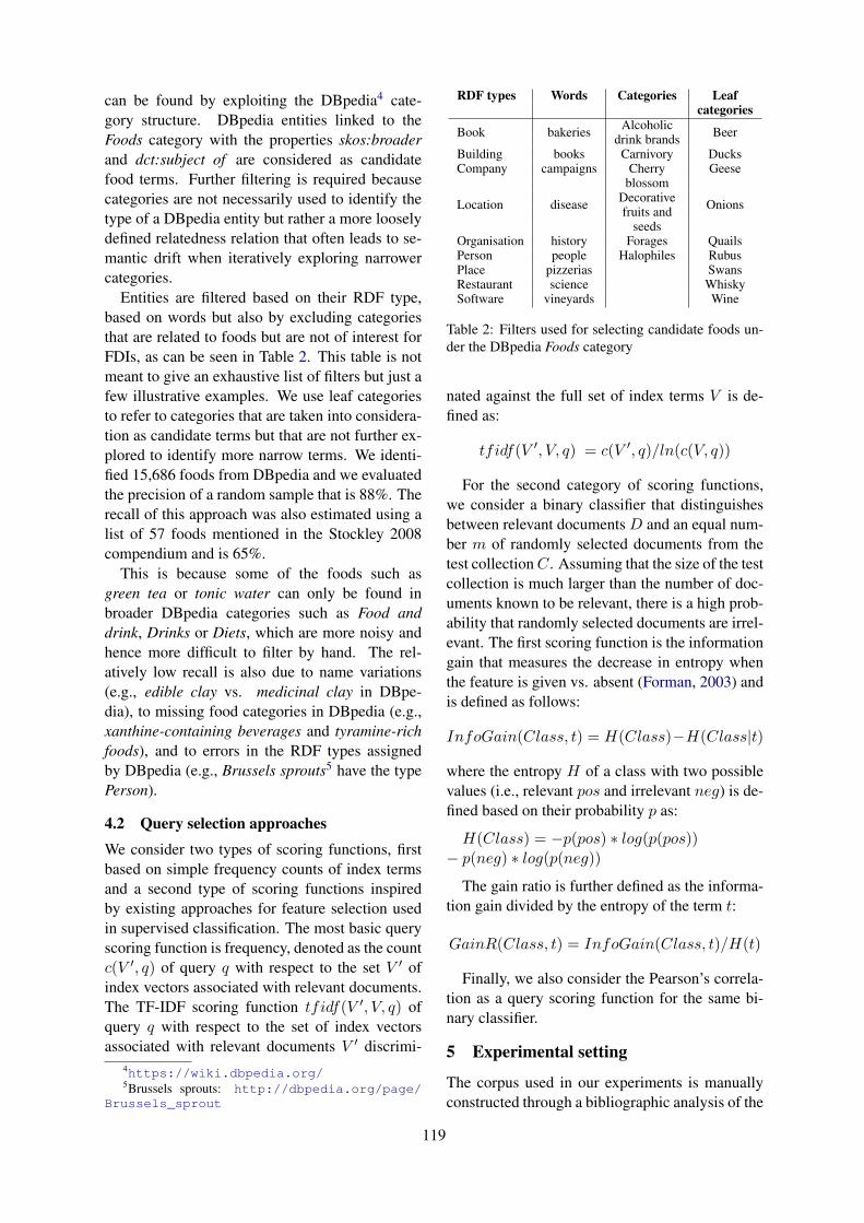
can be found by exploiting the DBpedia4 cate-gory structure. DBpedia entities linked to theFoods category with the properties skos:broaderand dct:subject of are considered as candidatefood terms. Further filtering is required becausecategories are not necessarily used to identify thetype of a DBpedia entity but rather a more looselydefined relatedness relation that often leads to se-mantic drift when iteratively exploring narrowercategories.
Entities are filtered based on their RDF type,based on words but also by excluding categoriesthat are related to foods but are not of interest forFDIs, as can be seen in Table 2. This table is notmeant to give an exhaustive list of filters but just afew illustrative examples. We use leaf categoriesto refer to categories that are taken into considera-tion as candidate terms but that are not further ex-plored to identify more narrow terms. We identi-fied 15,686 foods from DBpedia and we evaluatedthe precision of a random sample that is 88%. Therecall of this approach was also estimated using alist of 57 foods mentioned in the Stockley 2008compendium and is 65%.
This is because some of the foods such asgreen tea or tonic water can only be found inbroader DBpedia categories such as Food anddrink, Drinks or Diets, which are more noisy andhence more difficult to filter by hand. The rel-atively low recall is also due to name variations(e.g., edible clay vs. medicinal clay in DBpe-dia), to missing food categories in DBpedia (e.g.,xanthine-containing beverages and tyramine-richfoods), and to errors in the RDF types assignedby DBpedia (e.g., Brussels sprouts5 have the typePerson).
4.2 Query selection approaches
We consider two types of scoring functions, firstbased on simple frequency counts of index termsand a second type of scoring functions inspiredby existing approaches for feature selection usedin supervised classification. The most basic queryscoring function is frequency, denoted as the countc(V ′, q) of query q with respect to the set V ′ ofindex vectors associated with relevant documents.The TF-IDF scoring function tfidf(V ′, V, q) ofquery q with respect to the set of index vectorsassociated with relevant documents V ′ discrimi-
4https://wiki.dbpedia.org/5Brussels sprouts: http://dbpedia.org/page/
Brussels_sprout
RDF types Words Categories Leafcategories
Book bakeries Alcoholic Beerdrink brandsBuilding books Carnivory DucksCompany campaigns Cherry Geese
blossom
Location disease Decorative Onionsfruits andseeds
Organisation history Forages QuailsPerson people Halophiles RubusPlace pizzerias SwansRestaurant science WhiskySoftware vineyards Wine
Table 2: Filters used for selecting candidate foods un-der the DBpedia Foods category
nated against the full set of index terms V is de-fined as:
tfidf(V ′, V, q) = c(V ′, q)/ln(c(V, q))
For the second category of scoring functions,we consider a binary classifier that distinguishesbetween relevant documents D and an equal num-ber m of randomly selected documents from thetest collection C. Assuming that the size of the testcollection is much larger than the number of doc-uments known to be relevant, there is a high prob-ability that randomly selected documents are irrel-evant. The first scoring function is the informationgain that measures the decrease in entropy whenthe feature is given vs. absent (Forman, 2003) andis defined as follows:
InfoGain(Class, t) = H(Class)−H(Class|t)
where the entropy H of a class with two possiblevalues (i.e., relevant pos and irrelevant neg) is de-fined based on their probability p as:
H(Class) = −p(pos) ∗ log(p(pos))− p(neg) ∗ log(p(neg))
The gain ratio is further defined as the informa-tion gain divided by the entropy of the term t:
GainR(Class, t) = InfoGain(Class, t)/H(t)
Finally, we also consider the Pearson’s correla-tion as a query scoring function for the same bi-nary classifier.
5 Experimental setting
The corpus used in our experiments is manuallyconstructed through a bibliographic analysis of the
119
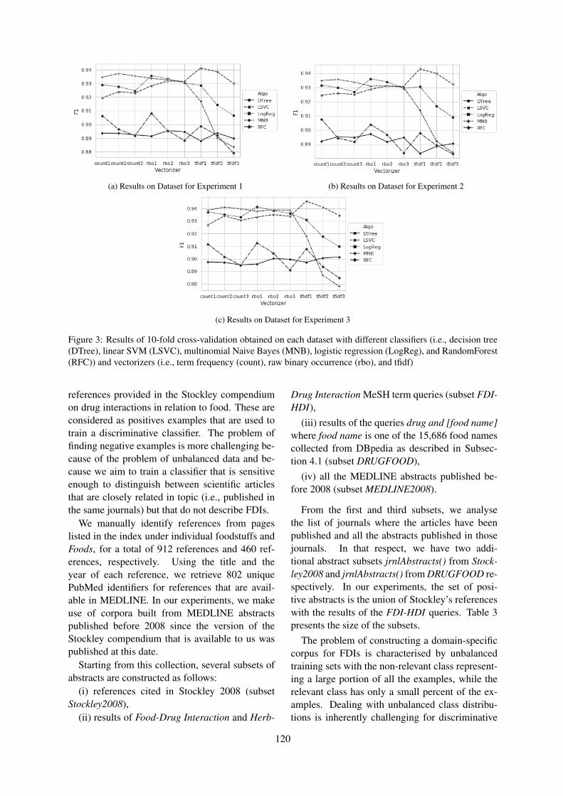
(a) Results on Dataset for Experiment 1 (b) Results on Dataset for Experiment 2
(c) Results on Dataset for Experiment 3
Figure 3: Results of 10-fold cross-validation obtained on each dataset with different classifiers (i.e., decision tree(DTree), linear SVM (LSVC), multinomial Naive Bayes (MNB), logistic regression (LogReg), and RandomForest(RFC)) and vectorizers (i.e., term frequency (count), raw binary occurrence (rbo), and tfidf)
references provided in the Stockley compendiumon drug interactions in relation to food. These areconsidered as positives examples that are used totrain a discriminative classifier. The problem offinding negative examples is more challenging be-cause of the problem of unbalanced data and be-cause we aim to train a classifier that is sensitiveenough to distinguish between scientific articlesthat are closely related in topic (i.e., published inthe same journals) but that do not describe FDIs.
We manually identify references from pageslisted in the index under individual foodstuffs andFoods, for a total of 912 references and 460 ref-erences, respectively. Using the title and theyear of each reference, we retrieve 802 uniquePubMed identifiers for references that are avail-able in MEDLINE. In our experiments, we makeuse of corpora built from MEDLINE abstractspublished before 2008 since the version of theStockley compendium that is available to us waspublished at this date.
Starting from this collection, several subsets ofabstracts are constructed as follows:
(i) references cited in Stockley 2008 (subsetStockley2008),
(ii) results of Food-Drug Interaction and Herb-
Drug Interaction MeSH term queries (subset FDI-HDI),
(iii) results of the queries drug and [food name]where food name is one of the 15,686 food namescollected from DBpedia as described in Subsec-tion 4.1 (subset DRUGFOOD),
(iv) all the MEDLINE abstracts published be-fore 2008 (subset MEDLINE2008).
From the first and third subsets, we analysethe list of journals where the articles have beenpublished and all the abstracts published in thosejournals. In that respect, we have two addi-tional abstract subsets jrnlAbstracts() from Stock-ley2008 and jrnlAbstracts() from DRUGFOOD re-spectively. In our experiments, the set of posi-tive abstracts is the union of Stockley’s referenceswith the results of the FDI-HDI queries. Table 3presents the size of the subsets.
The problem of constructing a domain-specificcorpus for FDIs is characterised by unbalancedtraining sets with the non-relevant class represent-ing a large portion of all the examples, while therelevant class has only a small percent of the ex-amples. Dealing with unbalanced class distribu-tions is inherently challenging for discriminative
120
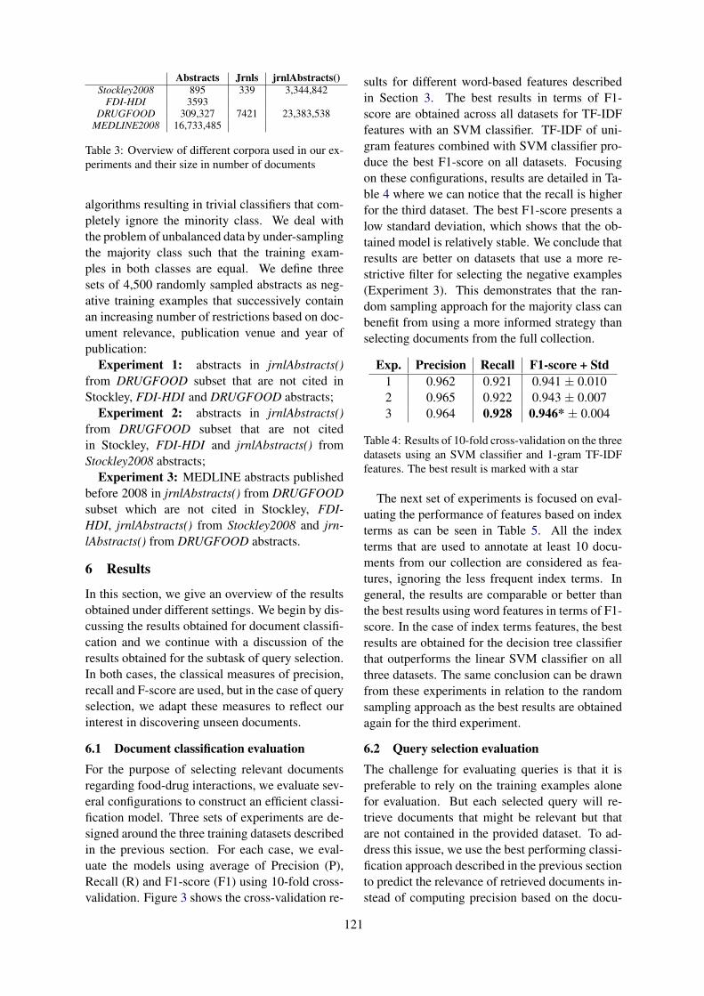
Abstracts Jrnls jrnlAbstracts()Stockley2008 895 339 3,344,842
FDI-HDI 3593DRUGFOOD 309,327 7421 23,383,538
MEDLINE2008 16,733,485
Table 3: Overview of different corpora used in our ex-periments and their size in number of documents
algorithms resulting in trivial classifiers that com-pletely ignore the minority class. We deal withthe problem of unbalanced data by under-samplingthe majority class such that the training exam-ples in both classes are equal. We define threesets of 4,500 randomly sampled abstracts as neg-ative training examples that successively containan increasing number of restrictions based on doc-ument relevance, publication venue and year ofpublication:
Experiment 1: abstracts in jrnlAbstracts()from DRUGFOOD subset that are not cited inStockley, FDI-HDI and DRUGFOOD abstracts;
Experiment 2: abstracts in jrnlAbstracts()from DRUGFOOD subset that are not citedin Stockley, FDI-HDI and jrnlAbstracts() fromStockley2008 abstracts;
Experiment 3: MEDLINE abstracts publishedbefore 2008 in jrnlAbstracts() from DRUGFOODsubset which are not cited in Stockley, FDI-HDI, jrnlAbstracts() from Stockley2008 and jrn-lAbstracts() from DRUGFOOD abstracts.
6 Results
In this section, we give an overview of the resultsobtained under different settings. We begin by dis-cussing the results obtained for document classifi-cation and we continue with a discussion of theresults obtained for the subtask of query selection.In both cases, the classical measures of precision,recall and F-score are used, but in the case of queryselection, we adapt these measures to reflect ourinterest in discovering unseen documents.
6.1 Document classification evaluationFor the purpose of selecting relevant documentsregarding food-drug interactions, we evaluate sev-eral configurations to construct an efficient classi-fication model. Three sets of experiments are de-signed around the three training datasets describedin the previous section. For each case, we eval-uate the models using average of Precision (P),Recall (R) and F1-score (F1) using 10-fold cross-validation. Figure 3 shows the cross-validation re-
sults for different word-based features describedin Section 3. The best results in terms of F1-score are obtained across all datasets for TF-IDFfeatures with an SVM classifier. TF-IDF of uni-gram features combined with SVM classifier pro-duce the best F1-score on all datasets. Focusingon these configurations, results are detailed in Ta-ble 4 where we can notice that the recall is higherfor the third dataset. The best F1-score presents alow standard deviation, which shows that the ob-tained model is relatively stable. We conclude thatresults are better on datasets that use a more re-strictive filter for selecting the negative examples(Experiment 3). This demonstrates that the ran-dom sampling approach for the majority class canbenefit from using a more informed strategy thanselecting documents from the full collection.
Exp. Precision Recall F1-score + Std1 0.962 0.921 0.941 ± 0.0102 0.965 0.922 0.943 ± 0.0073 0.964 0.928 0.946* ± 0.004
Table 4: Results of 10-fold cross-validation on the threedatasets using an SVM classifier and 1-gram TF-IDFfeatures. The best result is marked with a star
The next set of experiments is focused on eval-uating the performance of features based on indexterms as can be seen in Table 5. All the indexterms that are used to annotate at least 10 docu-ments from our collection are considered as fea-tures, ignoring the less frequent index terms. Ingeneral, the results are comparable or better thanthe best results using word features in terms of F1-score. In the case of index terms features, the bestresults are obtained for the decision tree classifierthat outperforms the linear SVM classifier on allthree datasets. The same conclusion can be drawnfrom these experiments in relation to the randomsampling approach as the best results are obtainedagain for the third experiment.
6.2 Query selection evaluationThe challenge for evaluating queries is that it ispreferable to rely on the training examples alonefor evaluation. But each selected query will re-trieve documents that might be relevant but thatare not contained in the provided dataset. To ad-dress this issue, we use the best performing classi-fication approach described in the previous sectionto predict the relevance of retrieved documents in-stead of computing precision based on the docu-
121
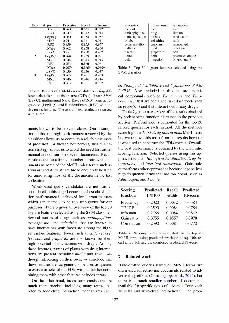
Exp. Algorithm Precision Recall F1-score
1
DTree 0.963 0.961 0.962LSVC 0.947 0.942 0.944
LogReg 0.960 0.954 0.957MNB 0.941 0.941 0.941RFC 0.959 0.955 0.957
2
DTree 0.962 0.958 0.960LSVC 0.954 0.950 0.952
LogReg 0.964 0.959 0.961MNB 0.944 0.943 0.943RFC 0.963 0.960 0.961
3
DTree 0.967* 0.965* 0.966*LSVC 0.959 0.956 0.957
LogReg 0.965 0.961 0.963MNB 0.946 0.946 0.946RFC 0.963 0.961 0.962
Table 5: Results of 10-fold cross-validation using dif-ferent classifiers: decision tree (DTree), linear SVM(LSVC), multinomial Naive Bayes (MNB), logistic re-gression (LogReg), and RandomForest (RFC) with in-dex terms features. The overall best results are markedwith a star
ments known to be relevant alone. Our assump-tion is that the high performance achieved by theclassifier allows us to compute a reliable estimateof precision. Although not perfect, this evalua-tion strategy allows us to avoid the need for furthermanual annotation or relevant documents. Recallis calculated for a limited number of retrieved doc-uments as some of the MeSH index terms such asHumans and Animals are broad enough to be usedfor annotating most of the documents in the testcollection.
Word-based query candidates are not furtherconsidered at this stage because the best classifica-tion performance is achieved for 1-gram featureswhich are deemed to be too ambiguous for ourpurposes. Table 6 gives an overview of the top 301-gram features selected using the SVM classifier.Several names of drugs such as aminophylline,cyclosporine, and ephedrine that are known tohave interactions with foods are among the high-est ranked features. Foods such as caffeine, cof-fee, cola and grapefruit are also known for theirhigh potential of interactions with drugs. Amongthese features, names of plants with drug interac-tions are present including biloba and kava. Al-though interesting on their own, we conclude thatthese features are too generic to be used as queriesto extract articles about FDIs without further com-bining them with other features or index terms.
On the other hand, index term candidates aremuch more precise, including many terms thatrefer to food-drug interaction mechanisms such
absorption cyclosporine interactionalcohol diet kavaaminophylline drug lithiumanticoagulation effects medicationbiloba ephedrine milkbioavailability ergotism monographcaffeine food nutritioncheese grapefruit oralcoffee herb pharmacokineticcola ingestion phytotherapy
Table 6: Top 30 1-gram features selected using theSVM classifier
as Biological Availability and Cytochrome P-450CYP3A. Also included in this list are chemi-cal compounds such as Flavanones and Furo-coumarins that are contained in certain foods suchas grapefruit and that interact with many drugs.
Table 7 gives an overview of the results obtainedby each scoring function discussed in the previoussection. Performance is computed for the top 20ranked queries for each method. All the methodsscore high the Food-Drug interactions MeSH termbut we remove this term from the results becauseit was used to construct the FDIs corpus. Overall,the best performance is obtained by the Gain ratioscoring function. Selected queries using this ap-proach include: Biological Availability, Drug In-teractions, and Intestinal Absorption. Gain ratiooutperforms other approaches because it penalizeshigh frequency terms that are too broad, such asAdult, Aged, and Female.
Scoring Predicted Recall Predictedfunction P@100 @16k F1-score
Frequency 0.2020 0.0032 0.0584TF-IDF 0.2590 0.0084 0.0784Info gain 0.2755 0.0084 0.0812Gain ratio 0.3755 0.0557 0.0970Correlation 0.2590 0.0081 0.0770
Table 7: Scoring functions evaluated for the top 20MeSH terms using predicted precision at top 100, re-call at top 16k and the combined predicted F1-score
7 Related work
Hand-crafted queries based on MeSH terms areoften used for retrieving documents related to ad-verse drug effects (Gurulingappa et al., 2012), butthere is a much smaller number of documentsavailable for specific types of adverse effects suchas FDIs and herb-drug interactions. The prob-
122
lem of building queries for finding documents re-lated to drug interactions has been recently tack-led for herb-drug interactions (Lin et al., 2016).This work addresses a less challenging usagescenario where users have in mind a pair ofherbs and drugs and are interested in finding ev-idences of interaction. Queries are manually con-structed by a domain expert using MeSH syn-onyms for herbs and drugs together with the fol-lowing MeSH qualifiers: adverse effects, pharma-cokinetics, and chemistry. Two additional heuris-tics rank higher retrieved articles that are anno-tated with the MeSH terms Drug Interactions andPlant Extracts/pharmacology. Another limitationof this work is the size of the evaluation datasetthat is based on a single review paper (Izzo andErnst, 2009) that provides about 100 references.In contrast, we propose an automated approach forquery selection and we make use of a considerablylarger dataset of relevant publications for trainingand evaluation.
The food-drug interaction discovery task pro-posed here is similar in setting with the subtaskon prior art candidates search from the intellec-tual property domain (Piroi et al., 2011). In theCLEF-IP datasets, topics are constructed using apatent application and the task is to identify pre-viously published patents that potentially invali-date this application. Keyphrase extraction ap-proaches were successfully applied to generatequeries from patent applications (Lopez and Ro-mary, 2010; Verma and Varma, 2011). The input ismuch larger for our task, that is a corpus of scien-tific articles describing FDIs manually annotatedwith index terms from the MeSH thesaurus. Amain difference between our work and the CLEF-IP task is that we mainly focus on evaluating dif-ferent methods for query selection by relying onthe PubMed search engine. This makes our taskmore similar to the term extraction task (Aubinand Hamon, 2006), as we aim to identify relevantterms for a broad domain rather than for a specificdocument, as done in keyphrase extraction.
The dataset used in (Jovanovik et al., 2015) toinfer interactions between drugs and world cuisineis based on textual information from DrugBankabout food-drug interactions and optimum drugintake time with respect to food. But this informa-tion was manually extracted and structured. Themost closely related work to ours is (Bordea et al.,2018) where the authors propose an approach for
query selection based on index terms. We extendthis work by considering multiple types of classifi-cation algorithms and by analysing different querycandidates beyond index terms.
8 Conclusion and future work
In this paper, we introduced a large dataset ofarticles that describe food-drug interactions an-notated with index terms to investigate an ap-proach for query selection that allows us to dis-cover other food-drug interactions using an exist-ing search engine. We investigated different strate-gies for addressing the problem of unbalanced dataand we showed that a more informed approachthat takes into consideration publication venue andyear gives better results than a naive approachfor random sampling. We proposed an auto-matic evaluation of retrieved results using a high-performance classifier and we showed that featureselection approaches outperform frequency-basedapproaches for this task, with an approach basedon gain ratio achieving the best results in terms ofpredicted F1-score.
In our experiments mainly focused on queriesconstructed using a single index term, therefore afirst direction for future work is to investigate morecomplex queries that combine multiple terms. Thenumber of queries that have to be evaluated wouldincrease considerably especially for combinationswith word-based features. Another improvementwould be to compare our results with keyphraseextraction approaches instead of analysing all then-grams and to generate queries using backgroundknowledge about drugs and foods. Finally, thedatasets proposed here are based on an older ver-sion of the Stockley compendium from 2008. Theresults presented in this work could be more rele-vant if a more recent version is considered as thisis a highly dynamic field of research.
9 Acknowledgments
This work was supported by the MIAM projectand Agence Nationale de la Recherche throughthe grant ANR-16-CE23-0012 France and bythe KaNNa project and the European Commis-sion through grant H2020 MSCA-IF-217 number800578.
123
ReferencesSophie Aubin and Thierry Hamon. 2006. Improving
term extraction with terminological resources. InAdvances in Natural Language Processing, pages380–387. Springer.
Karen Baxter and CL Preston. 2010. Stockley’s druginteractions, volume 495. Pharmaceutical PressLondon.
Georgeta Bordea, Frantz Thiessard, Thierry Hamon,and Fleur Mougin. 2018. Automatic query selec-tion for acquisition and discovery of food-drug inter-actions. In International Conference of the Cross-Language Evaluation Forum for European Lan-guages, pages 115–120. Springer.
Arik Dahan and Hamutal Altman. 2004. Food–drug interaction: grapefruit juice augments drugbioavailability-mechanism, extent and relevance.European journal of clinical nutrition, 58(1):1.
George Forman. 2003. An extensive empiricalstudy of feature selection metrics for text classi-fication. Journal of machine learning research,3(Mar):1289–1305.
Harsha Gurulingappa, Abdul Mateen Rajput, AngusRoberts, Juliane Fluck, Martin Hofmann-Apitius,and Luca Toldo. 2012. Development of a bench-mark corpus to support the automatic extrac-tion of drug-related adverse effects from medicalcase reports. Journal of biomedical informatics,45(5):885–892.
Thierry Hamon, Vincent Tabanou, Fleur Mougin, Na-talia Grabar, and Frantz Thiessard. 2017. Pomelo:Medline corpus with manually annotated food-druginteractions. In Recent Advances in Natural Lan-guage Processing (RANLP), pages 73–80.
Angelo A Izzo and Edzard Ernst. 2009. Interactionsbetween herbal medicines and prescribed drugs.Drugs, 69(13):1777–1798.
Milos Jovanovik, Aleksandra Bogojeska, Dimitar Tra-janov, and Ljupco Kocarev. 2015. Inferring cuisine-drug interactions using the linked data approach.Scientific reports, 5:9346.
Kuo Lin, Carol Friedman, and Joseph Finkelstein.2016. An automated system for retrieving herb-druginteraction related articles from medline. AMIASummits on Translational Science Proceedings,2016:140–149.
Patrice Lopez and Laurent Romary. 2010. Experimentswith citation mining and key-term extraction forprior art search. In CLEF 2010-Conference on Mul-tilingual and Multimodal Information Access Eval-uation.
Ramesh Nallapati. 2004. Discriminative models for in-formation retrieval. In Proceedings of the 27th an-nual international ACM SIGIR conference on Re-search and development in information retrieval,pages 64–71. ACM.
Florina Piroi, Mihai Lupu, Allan Hanbury, andVeronika Zenz. 2011. Clef-ip 2011: Retrieval in theintellectual property domain. In CLEF (notebookpapers/labs/workshop).
Isabel Segura-Bedmar, Paloma Martı́nez, andMarı́a Herrero Zazo. 2013. Semeval-2013 task9: Extraction of drug-drug interactions frombiomedical texts (ddiextraction 2013). In SecondJoint Conference on Lexical and ComputationalSemantics (*SEM), Volume 2: Proceedings ofthe Seventh International Workshop on SemanticEvaluation (SemEval 2013), volume 2, pages341–350.
Manisha Verma and Vasudeva Varma. 2011. Explor-ing keyphrase extraction and ipc classification vec-tors for prior art search. In CLEF (Notebook Pa-pers/Labs/Workshop).
124
Proceedings of the BioNLP 2019 workshop, pages 125–134Florence, Italy, August 1, 2019. c©2019 Association for Computational Linguistics
Enhancing biomedical word embeddings by retrofitting to verb clusters
Billy Chiu1 Simon Baker1 Martha Palmer2 Anna Korhonen1
1 Language Technology Lab, University of Cambridge, 9 West Road, Cambridge, CB3 9DB, UK2 Department of Lingusitics, University of Colorado at Boulder, Colorado, 80309–0295, USA
{hwc25,sb895,alk23}@[email protected]
Abstract
Verbs play a fundamental role in many biomed-ical tasks and applications such as relation andevent extraction. We hypothesize that per-formance on many downstream tasks can beimproved by aligning the input pretrained em-beddings according to semantic verb classes.In this work, we show that by using semanticclusters for verbs, a large lexicon of verbclasses derived from biomedical literature, weare able to improve the performance of com-mon pretrained embeddings in downstreamtasks by retrofitting them to verb classes. Wepresent a simple and computationally efficientapproach using a widely-available “off-the-shelf” retrofitting algorithm to align pretrainedembeddings according to semantic verb clus-ters. We achieve state-of-the-art results on textclassification and relation extraction tasks.
1 Introduction
Core tasks in biomedical natural language process-ing (BioNLP) such as relation and event extraction,text classification, syntactic and semantic parsing,natural language inference, and entailment canall benefit from rich computational lexiconscontaining information about the behaviour andmeaning of words in biomedical texts. Verbs areespecially important in many of these tasks (Cohenet al., 2008); for example, describing protein–protein interactions in biomedical text can oftenrely on a wide range of verbs, such as “bind,”“activate,” “carry,” “facilitate,” “interact,” etc. inorder to determine the specific type of interaction.
Lexical semantic classes for verbs can be used toabstract away from individual words, or to build alexical structure (taxonomy) which predicts muchof the behaviour of a new word by associating itwith an appropriate class (Levin, 1993; Kipperet al., 2008). For example, the verbs “assess,”“evaluate,” “estimate,” “explore,” and “analyze”
belong to the class examine, while the verbs“utilize,” “employ,” and “exploit” belong to theclass use. In addition to simple synonyms of verbs,semantic classes capture similarity in their use andbehaviour in text by analysing their contexts (Levin,1993).
In the past, lexical verb classes have beensuccessfully shown to improve the performanceclassifiers in a variety of tasks and down streamapplications in the biomedical domain; suchas relation extraction (Sharma et al., 2010),biomedical fact extraction (Rupp et al., 2010),text classification for cancer (Baker et al., 2015),biomedical discourse analysis (Cox et al., 2017),and biomedical information retrieval (Mahalak-shmi, 2015).
Lexical classes are useful for their ability tocapture generalizations about a range of linguisticproperties (Kipper et al., 2000); our hypothesis istherefore that by retrofitting embedded word repre-sentations to semantic verb classes, semantically-similar verbs (i.e. member verbs within the samelexical class) like “suppress” and “inhibit” will bepulled together in vector space, whereas verbs like“collect” and “examine” will not. Consequently,this allows NLP systems to generalize away fromindividual verbs, alleviating the data sparsenessproblem of representing each verb in the corpusindividually.
Retrofitting is a graph-based learning techniquefor using lexical relational resources to obtainhigher quality semantic vectors (Faruqui et al.,2015). It is applied as a post-processing step byrunning belief propagation on a graph constructedfrom lexicon-derived relational information toupdate word vectors. It can be applied to anypretrained word embedding vectors. The intuitionbehind retrofitting is to encourage the retrofittedvectors to be similar to the vectors of related word
125
types and similar to their original distributionalrepresentations.
Using a standard “off-the-shelf” retrofittingalgorithm, we apply the idea of retrofitting toverb clusters to two sets of widely-used pretrainedembedding vectors in BioNLP (those by Pyysaloet al. (2013a) and by Chiu et al. (2016)) toobtain improved embeddings. We show thatby doing nothing more than using this simpleapproach, we achieve state-of-the-art results ontwo text classification tasks (both tasks evaluatedon document and sentence level classification),and a relation extraction task. We make ourretrofitted embeddings freely available to theBioNLP community along with our code.1
The main contribution of this work is to be thefirst of its kind to apply verb-based retrofitting inthe biomedical domain. Retrofitting has thus faronly been applied for aligning vectors to MedicalSubject Headings (MeSH) (Yu et al., 2016), andbeen validated only in an extrinsic setting. Weshow that with very little effort, we can achievestate-of-the art results on various downstream tasksin a range of biomedical subdomains.
This paper will first describe relevant work onretrofitting to lexical resources in BioNLP; wethen briefly give an overview of two verb clusterand lexicons that we use in our methodology, andthen our task-based evaluation. We end with adiscussion of the evaluation results.
2 Related work
Lexical resources can be used to enrich represen-tation models by providing them other sources oflinguistics information beyond the distributionalstatistics obtained from corpora. In recent literature,various methods to leverage knowledge availablein human- and automatically-constructed lexicalresources have been proposed.
One such method involves modifying the ob-jectives in the original representation learningprocedures so that they can jointly learn both dis-tributional and lexical information—for example,Yu and Dredze (2014) modify the CBOW objectivefunction by introducing semantic constraints as ob-tained from the paraphrase database (Ganitkevitchet al., 2013) to train word representations whichfocus on word similarity over word relatedness.
1Our retrofitted embeddings and code arereleased under an open license and can be foundhere: https://github.com/cambridgeltl/retrofitted-bio-embeddings
Another class of methods incorporates lexicalinformation into the vector representations as apost-processing procedure. The method fine-tunesthe pretrained word vectors to satisfy linguisticconstraints from the external resources. Themethod can be applied to any off-the-shelf modelswithout requiring large corpora for (re-)trainingas the joint-learning models do. Among thesemethods, retrofitting (Faruqui et al., 2015) is widelyused.
Given any (pretrained) vector-space representa-tions, the goal of retrofitting is to bring closer wordswhich are connected via a relation (e.g. synonyms)in a given semantic network or lexical resource (i.e.linguistic constraints). For example, Yu et al. (2016,2017) retrofit word vector spaces of MeSH termsby using additional linkage information from theUMNSRS hierarchy to improve the representationsof biomedical concepts. Building on retrofitting,Lengerich et al. (2018) generalize retrofitting meth-ods by explicitly modelling individual linguisticconstraints that are commonly found in healthand clinical-related lexicons (e.g. causal-relationsbetween diseases and drugs).
In theory, the joint-learning models could beas effective (or better) as those produced by fine-tuning distributional vectors. However, the perfor-mance of joint-learning models has not surpassedthat of fine-tuning methods.2 Furthermore, thejoint-learning objectives are usually model-specificand are tailored to a particular model, making itdifficult to use them with other methods. In thiswork, we will use retrofitting to incorporate ourlexical features into the word representations.
3 Verb clusters
In this work, we investigate retrofitting popularword embeddings to two publicly available3
lexicons for verb clusters. The first is composedof 192 relatively frequent verbs from a corpusof 2230 biomedical journal articles which havebeen hierarchically classified into three levels: 16,34, and 50 verb classes. The three levels reflectdifferent granularity in the semantics of the verbclasses as illustrated in Figure 1. These clusterswere annotated by 4 domain experts and 2 linguists,were used to create the gold standard (Korhonen
2The SimLex-999 home page (www.cl.cam.ac.uk/˜fh295/simlex.html) lists state-of-the-art performancemodels, none of which have learned representations jointly
3https://github.com/cambridgeltl/bio-verbnet
126
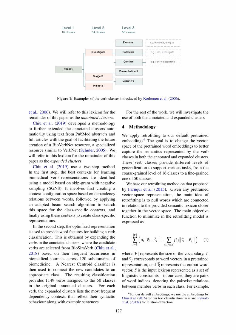
Report
Investigate
Examine
Suggest
Presentational
Indicate
Establish
Confirm
Cognitive
e.g. evaluate, analyze
e.g. test, investigate
e.g. verify, determine
Level 2
34 classes
Level 1
16 classes
Level 3
50 classes
Created by Unlicensed Version
Created by Unlicensed Version
Created by Unlicensed Version
Figure 1: Examples of the verb classes introduced by Korhonen et al. (2006).
et al., 2006). We will refer to this lexicon for theremainder of this paper as the annotated clusters.
Chiu et al. (2019) developed a methodologyto further extended the annotated clusters auto-matically using text from PubMed abstracts andfull articles with the goal of facilitating the futurecreation of a BioVerbNet resource, a specializedresource similar to VerbNet (Schuler, 2005). Wewill refer to this lexicon for the remainder of thispaper as the expanded clusters.
Chiu et al. (2019) use a two-step method.In the first step, the best contexts for learningbiomedical verb representations are identifiedusing a model based on skip-gram with negativesampling (SGNS). It involves first creating acontext configuration space based on dependencyrelations between words, followed by applyingan adapted beam search algorithm to searchthis space for the class-specific contexts, andfinally using these contexts to create class-specificrepresentations.
In the second step, the optimized representationis used to provide word features for building a verbclassification. This is obtained by expanding theverbs in the annotated clusters, where the candidateverbs are selected from BioSimVerb (Chiu et al.,2018) based on their frequent occurrence inbiomedical journals across 120 subdomains ofbiomedicine. A Nearest Centroid classifier isthen used to connect the new candidates to anappropriate class. The resulting classificationprovides 1149 verbs assigned to the 50 classesin the original annotated clusters. For eachverb, the expanded clusters lists the most frequentdependency contexts that reflect their syntacticbehaviour along with example sentences.
For the rest of the work, we will investigate theuse of both the annotated and expanded clusters
4 Methodology
We apply retrofitting to our default pretrainedembeddings4 The goal is to change the vector-space of the pretrained word embeddings to bettercapture the semantics represented by the verbclasses in both the annotated and expanded clusters.These verb classes provide different levels ofgeneralization to support various tasks, from thecoarse-grained level of 16 classes to a fine-grainedone of 50 classes.
We base our retrofitting method on that proposedby Faruqui et al. (2015). Given any pretrainedvector-space representation, the main idea ofretrofitting is to pull words which are connectedin relation to the provided semantic lexicon closertogether in the vector space. The main objectivefunction to minimize in the retrofitting model isexpressed as
|V |∑i=1
(αi
∥∥∥~vi−~̂vi
∥∥∥+ ∑(i, j)∈S
βi j∥∥~vi−~v j
∥∥)
(1)
where |V | represents the size of the vocabulary,~vi
and~v j corresponds to word vectors in a pretrainedrepresentation, and ~̂iv represents the output wordvector. S is the input lexicon represented as a set oflinguistic constraints—in our case, they are pairsof word indices, denoting the pairwise relationsbetween member verbs in each class. For example,
4For our default embeddings, we use the embeddings byChiu et al. (2016) for our text classification tasks and Pyysaloet al. (2013a) for relation extraction.
127
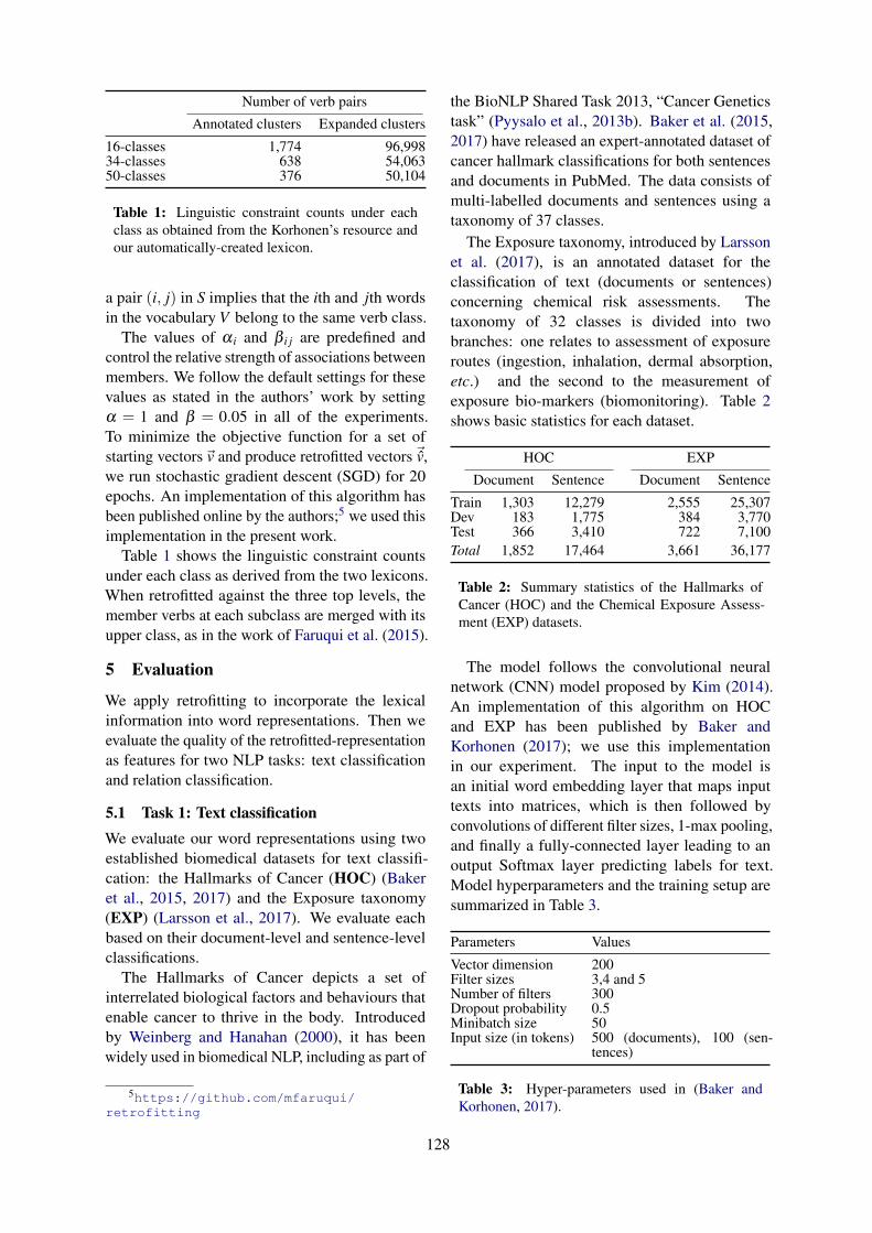
Number of verb pairs
Annotated clusters Expanded clusters
16-classes 1,774 96,99834-classes 638 54,06350-classes 376 50,104
Table 1: Linguistic constraint counts under eachclass as obtained from the Korhonen’s resource andour automatically-created lexicon.
a pair (i, j) in S implies that the ith and jth wordsin the vocabulary V belong to the same verb class.
The values of α i and β i j are predefined andcontrol the relative strength of associations betweenmembers. We follow the default settings for thesevalues as stated in the authors’ work by settingα = 1 and β = 0.05 in all of the experiments.To minimize the objective function for a set ofstarting vectors~v and produce retrofitted vectors ~̂v,we run stochastic gradient descent (SGD) for 20epochs. An implementation of this algorithm hasbeen published online by the authors;5 we used thisimplementation in the present work.
Table 1 shows the linguistic constraint countsunder each class as derived from the two lexicons.When retrofitted against the three top levels, themember verbs at each subclass are merged with itsupper class, as in the work of Faruqui et al. (2015).
5 Evaluation
We apply retrofitting to incorporate the lexicalinformation into word representations. Then weevaluate the quality of the retrofitted-representationas features for two NLP tasks: text classificationand relation classification.
5.1 Task 1: Text classificationWe evaluate our word representations using twoestablished biomedical datasets for text classifi-cation: the Hallmarks of Cancer (HOC) (Bakeret al., 2015, 2017) and the Exposure taxonomy(EXP) (Larsson et al., 2017). We evaluate eachbased on their document-level and sentence-levelclassifications.
The Hallmarks of Cancer depicts a set ofinterrelated biological factors and behaviours thatenable cancer to thrive in the body. Introducedby Weinberg and Hanahan (2000), it has beenwidely used in biomedical NLP, including as part of
5https://github.com/mfaruqui/retrofitting
the BioNLP Shared Task 2013, “Cancer Geneticstask” (Pyysalo et al., 2013b). Baker et al. (2015,2017) have released an expert-annotated dataset ofcancer hallmark classifications for both sentencesand documents in PubMed. The data consists ofmulti-labelled documents and sentences using ataxonomy of 37 classes.
The Exposure taxonomy, introduced by Larssonet al. (2017), is an annotated dataset for theclassification of text (documents or sentences)concerning chemical risk assessments. Thetaxonomy of 32 classes is divided into twobranches: one relates to assessment of exposureroutes (ingestion, inhalation, dermal absorption,etc.) and the second to the measurement ofexposure bio-markers (biomonitoring). Table 2shows basic statistics for each dataset.
HOC EXP
Document Sentence Document Sentence
Train 1,303 12,279 2,555 25,307Dev 183 1,775 384 3,770Test 366 3,410 722 7,100Total 1,852 17,464 3,661 36,177
Table 2: Summary statistics of the Hallmarks ofCancer (HOC) and the Chemical Exposure Assess-ment (EXP) datasets.
The model follows the convolutional neuralnetwork (CNN) model proposed by Kim (2014).An implementation of this algorithm on HOCand EXP has been published by Baker andKorhonen (2017); we use this implementationin our experiment. The input to the model isan initial word embedding layer that maps inputtexts into matrices, which is then followed byconvolutions of different filter sizes, 1-max pooling,and finally a fully-connected layer leading to anoutput Softmax layer predicting labels for text.Model hyperparameters and the training setup aresummarized in Table 3.
Parameters Values
Vector dimension 200Filter sizes 3,4 and 5Number of filters 300Dropout probability 0.5Minibatch size 50Input size (in tokens) 500 (documents), 100 (sen-
tences)
Table 3: Hyper-parameters used in (Baker andKorhonen, 2017).
128
For both tasks, we use the embeddings6 by Chiuet al. (2016). Performance is evaluated using thestandard precision, recall, and F1-score metrics ofthe labels in the model using the one-vs.-rest setup:we train and evaluate K independent binary CNNclassifiers (i.e. a single classifier per class with theinstances of that class as positive samples and allother instances as negatives). Due to their randominitialization, we repeat each CNN experiment20 times and report the mean of the evaluationresults to account for variances in neural networks.To address overfitting in the CNN, we follow theauthors’ early stopping approach, testing only themodel that achieved the highest results on thedevelopment dataset.
5.2 Task 2: Relation classificationWe evaluate our retrofitted representations on theBio-Creative VI Chemical–Protein relation ex-traction dataset (CHEMPROT) (Krallinger et al.,2017). The corpus provides mention and relationannotations for complex events related to chemical–protein interaction in molecular biology. The goalof this task is to predict whether a given chemical–protein pair is related or not, and to then verify itscorresponding relation type. There are five types ofrelations: Up-regulator, Down-regulator, Agonist,Antagonist, and Substrate. The corpus is providedin the Turku Event Extraction System (TEES) XMLformat and are installed with the Turku ExtractionSystem (Björne, 2014). It is parsed with thethe BLLIP parser (Charniak and Johnson, 2005)with the McClosky bio-model (Mcclosky, 2010),followed by conversion of the constituency parsesinto dependency parses using the Stanford Tools(MacCartney et al., 2006). Table 4 summarizes keystatistics for the dataset.
Documents Entities Relations
Train 1,020 25,769 4,157Dev 612 15,571 2,416Test 800 20,829 3,458Total 2,432 62,169 10,031
Table 4: Summary statistics of the Chemical-Protein interaction dataset (CHEMPROT).
The model follows the CNN model proposed byBjörne and Salakoski (2018). We directly use theirpublished implementation. The model input is an
6https://github.com/cambridgeltl/BioNLP-2016
initial word embedding layer that maps input textsinto matrices, followed by convolutions of differentfilter sizes and 1-max pooling, and finally a fullyconnected layer, leading to an output Softmax layerfor predicting labels. Performance is evaluatedusing the standard precision, recall, and F1-scoremetrics of the labels in the model. Classificationis performed as multilabel classification whereeach example may have 0 to n positive labels.Model hyperparameters and the training setup aresummarized in Table 5.
Parameters Values
Vector dimension 200Filter sizes 1, 3, 5 and 7Number of filters 400 (100 of each size)Dropout probability 0.5Learning rate 0.001Minibatch size 50
Table 5: Hyperparameters used by Björne andSalakoski (2018).
To account for variance in neural networks due totheir random initialization, we adopt the ensemblesettings used by Björne and Salakoski (2018). Wetrain 20 models and take the n best ones (n = 5),ranked with their F1-score on the development set,and use their averaged predictions. The ensemblepredictions are calculated for each label as theaverage predicted confidence scores from all themodels. We also incorporate the authors’ earlystopping approach where the model is trained untilthe development loss no longer decreases. We trainfor up to 500 epochs, stopping once validationloss has no longer decreased for 10 consecutiveepochs. To focus on the effect of verb classeson biomedical representations, we experimentwith word representations induced on biomedicaltexts; this diverges from the authors who use theembeddings7 by Pyysalo et al. (2013a), induced ona combination of biomedical and general-domaindata (PubMed, PMC and Wikipedia texts).
6 Results
We compare the performance of the baseline withthe retrofitted embeddings models by measuringtheir precision (P), recall (R), and F1-scores in textclassification and relation extraction when used asinput features.
For the text classification tasks, Tables 6 and 7show the micro-averaged scores for the HOC and
7obtained from: http://bio.nlplab.org
129
the EXP tasks respectively. Each table showsthe performance on document- and sentence-levelclassification (as columns) with different semanticlexicons (as rows).
For the relation classification task (CHEM-PROT), Table 8 shows the micro-averaged scores.The best results are shown in bold and statisticallysignificant scores are shown with an asterisk. Allstatistical tests are performed using a two-tailedt-test with α = 0.05.
We first describe experiments measuring im-provements from the retrofitting method, followedby comparisons against using different sets oflexicons during retrofitting.
6.1 Retrofitting
We use Equation 1 to retrofit word representationsusing linguistic constraints derived from verblexicons. Overall, the retrofitted models showimprovements in most tasks.
For text classification, the scores have improvedin three out of the four cases. For the HOC task(Table 6) all retrofitted models outperform thebaseline in F1-score, which is largely attributedto a substantial improvement in recall (particularlyfor document-level classification, where there is a15 point increase over the baseline). In total, fiveout of the twelve improved scores reported are alsostatistically significant.
The results for the EXP task (Table 7) are moremixed. At the document level, all retrofitted modelsachieve a slight F1-score gain and half of the scoresare significant. There is an improvement in recallat the cost of lower precision when compared tothe baseline.
However, we can see that sentence-level classifi-cation is more difficult, due to the smaller amountof context information available. On the sentencelevel, the baseline seems to outperform all others,and only two out of six cases are significant. Itindicates that the lexicons did not aid sentence-level classification in this particular task.
In relation classification, the word representationachieves the state-of-the-art result after incorpo-rating our lexical information (34 classes). FromTable 8, there is approximately a 1.5 point F1-score increase over the baseline, and half of theimprovements reported are significant. The resultsfrom both tasks suggest that the class-featuresprovided by verb lexicons improve performanceover the raw verb features.
6.2 Semantic lexicons
We compare the performance of our retro-fittedembeddings using both expanded clusters and themanually annotated clusters lexicon. The expandedclusters retrofitted embeddings outperform theoriginal annotated clusters retrofitted embeddingsin all evaluated tasks. This is likely due to thelarger size of the expanded clusters in comparisonto annotated clusters (Table 1), thus providingfeatures for more verbs.
Lexical resources can be useful for NLP tasksfor their abilities to capture generalizations about arange of linguistic properties; however, the degreeof generalization needed may vary from task totask. When experimenting with retrofitting withdifferent levels of verb classes, we observe anotable difference (1–2 points in F1-score) betweenmodels retrofitted with the coarse-grained level of16 classes and the fine-grained level of 50 classes.
For document-level text classification in bothdatasets (Tables 6 and 7), models appear to benefitfrom a finer-grained classification of 50 classes; onthe sentence level a medium level of generalization(34 classes) seems optimal. The best result forrelation classification (Table 8) is also obtainedwith 34 classes.
7 Discussion
The task-based evaluations suggest that verbclusters and a verb-optimized representation, canbe a useful resource to support biomedical NLPtasks. In text classification, it has been observedthat the occurrence patterns of verbs can be “topic-related” and certain set of verbs frequently appearwithin a specific topic of documents (Doan et al.,2009; Hatzivassiloglou and Weng, 2002; Sekimizuet al., 1998). Regarding this, expanded clustersappears to have captured some of these topic-related properties. On the HOC dataset, we notethat some frequent verbs (such as “proliferate”and “grow”) appearing in documents relatingto the topic Sustaining proliferative signalingalso share the same classes in our automatically-created lexicon. Similarly, for exposure assessmentdocuments describing air monitoring data in EXP,we can frequently see member verbs such as“inhale” and “breathe” in the proceed class.
Entities–relations described in the biomedicalliterature are often expressed in a predicative formwhere a trigger word (most commonly a verb)connects two or more entities; here a range of
130
Document classification Sentence classification
Lexicon P R F1 P R F1
No lexicon & SOTA 77.8 51.7 62.1 56.8 30.7 39.9
Annotated clusters16-classes 75.1 56.4 64.8 47.1 34.6 39.934-classes 74.2 56.6 64.3 48.4 35.5 41.050-classes 74.9 59.2 66.2 48.4 35.2 *40.7
Expanded clusters16-classes 75.5 64.4 *69.5 45.2 36.5 *40.434-classes 74.3 63.5 *68.5 52.7 35.6 42.550-classes 73.9 66.1 *69.8 50.9 34.7 41.3
Table 6: Performance results for the Hallmarks of Cancer task (HOC) when different sets of lexicons are usedfor retrofitting the baseline model. Baseline denotes a skip-gram model generated with our optimized trainingsettings. Scores are adopted from Baker and Korhonen (2017). All figures are micro-averages expressed aspercentages (Bold: the best score, *: statistically significant).
Document classification Sentence classification
Lexicon P R F1 P R F1
No lexicon & SOTA 89.5 87.1 88.3 66.2 62.8 64.5
Annotated clusters16-classes 88.9 87.7 *88.3 67.1 58.9 62.734-classes 89.4 87.8 *88.6 67.2 58.2 *62.450-classes 88.9 88.7 88.8 65.6 55.7 60.3
Expanded clusters16-classes 89.2 87.9 88.5 66.7 60.0 63.234-classes 88.7 88.9 *88.8 67.3 58.7 62.750-classes 88.6 89.1 88.9 67.5 58.6 *62.7
Table 7: Performance results for the Chemical Exposure Assessment task (EXP). Baseline denotes a skip-gram model generated with our optimized training settings. The “No lexicon” scores are from Baker andKorhonen (2017). All figures are micro-averages expressed as percentages. (Bold: the best score, *: statisticallysignificant).
verbs can be used to describe similar relations.Understanding the commonalities shared amongindividual verbs helps NLP systems to identify theparticular type of relation the text is describing.Consider as an example the suppress class in ourverb lexicons. It captures the fact that its membersare similar in terms of syntax and semantics, andthey can be used to make similar statements whichdescribe similar events. In CHEMPROT, memberverbs in the suppress class such as “suppress” and“inhibit” can often be found in sentences depictingthe down-regulation relation between chemicalsand proteins.
For many NLP applications, lexical classesare useful for their ability to capture general-izations about a range of linguistic properties:by retrofitting word representations to lexicalresources, semantically similar verbs (i.e. memberverbs within the same lexical class) like “suppress”and “inhibit” will be pulled together in the vector
space, whereas verbs like “collect” and “examine”will not. Consequently, this allows NLP systems togeneralize away from individual verbs, alleviatingthe data sparseness problem of representing eachverb in the corpus individually. The lexical classesprovide different levels of generalization to supporttasks of various needs, from the coarse-grainedlevel of 16 classes to a fine-grained level of 50. Anotable performance difference is observed whenwe evaluate models retrofitted with different levelsof verb classes. Among all three classes, weobserve a larger improvement over models at thefiner-grained levels of 34 or 50 classes, whichreveal that finer-grained levels of verb semanticdistinction seem more contributive in our assessedtasks.
131
Lexicon P R F1
No lexicon 76.9 63.5 *69.5SOTA 75.1 65.1 69.7
Annotated clusters16-classes 76.5 64.6 70.134-classes 78.2 63.8 *70.350-classes 76.5 65.0 *70.3
Expanded clusters16-classes 76.3 65.2 70.334-classes 77.5 65.6 71.050-classes 76.2 65.9 *70.7
Table 8: Performance results for the Chemical-Protein Interaction (CHEMPROT) when differentsets of lexicons are used for retrofitting the baselinemodel. Baseline denotes a skip-gram model gen-erated with our optimized training settings. SOTAdenotes the state-of-the-art result reported by Björneand Salakoski (2018) using the embeddings byPyysalo et al. (2013a). All figures are micro-averages expressed as percentages. (Bold: the bestscore for the task, *: statistically significant).
8 Conclusions
Many core NLP tasks and applications in thebiomedical domain such as relation and eventextraction, text classification, and text mining maybenefit from accurate embedded representation ofverbs.
Verb semantic classes capture generalizationsabout a range of linguistic properties, by retrofittingembedded word representations to semantic verbclasses, semantically similar verbs (i.e. verbsthat are members of the same lexical class) arepulled together in the vector space. Consequently,this allows NLP systems to generalize away fromindividual verbs, reducing the problem of datasparseness in representing less frequent verbs.
The key contribution of this work is to showthat by using semantic classes for verbs (suchas those provided by both the annotated andexpanded clusters) we can improve the downstreamperformance on several tasks in the biomedicaldomain by aligning word embeddings according tosemantic verb classes.
This is achieved by a post-processing retrofittingprocedure, using a standard “off-the-shelf” method,by running belief propagation on a graph con-structed from lexicon-derived relational informa-tion to update word vectors. It can be applied toany pretrained word embedding vectors.
We applied two lexicons of semantic verbclusters to two sets of widely used pretrained em-
bedding vectors in BioNLP on several downstreamtasks: two text classification tasks (the Hallmarksof Cancer, and Chemical Exposure Assessment)with both document and sentence classification, aswell as a relation extraction task (CHEMPROT).We used a standard “off-the-shelf” retrofittingalgorithm to obtain improved embeddings, and wefeed the retrofitted representation to the currentstate-of-the-art models for their respective tasks.We controlled the experimental setup by using thesame model implementation, as well as the sametraining, development and test data folds.
The results show that using verb clusters toretrofit embeddings, we achieved new state-of-the-art performance in the evaluated downstreamtasks (with statistically significant scores); the onlyexception being sentence level classification for theChemical Exposure Assessment task (however wedo improve SOTA in document level classificationfor the same task). We also note a performancedifference when retrofitting with different levels ofverb classes, where we see a larger improvementwhen using finer-grained levels of verb semanticclasses (30 or 50 classes), which seem morecontributive.
For future work, we will further investigate thepossibility of using verb lexicons for retrofittingnew generations of word representation modelssuch as contextualized embeddings; we will furtherevaluate on other downstream biomedical tasks, forinstance event and pathway extraction and medicalquestion answering.
Acknowledgement
This work is supported by the Medical ResearchCouncil [grant number MR/M013049/1], the ERCConsolidator Grant LEXICAL [grant number:648909], the ESRC Doctoral Fellowship [grantnumber: ES/J500033/1] and the Defense AdvancedResearch Projects Agency [DARPA 15-18-CwC-FP-032].
We would like to thank our reviewers for theirconstructive feedback. We are very grateful toTyler Griffiths for helping with proofreading andtypesetting this paper.
132
ReferencesSimon Baker, Imran Ali, Ilona Silins, Sampo Pyysalo,
Yufan Guo, Johan Högberg, Ulla Stenius, and AnnaKorhonen. 2017. Cancer hallmarks analytics tool(chat): a text mining approach to organize and eval-uate scientific literature on cancer. Bioinformatics,33(24):3973–3981.
Simon Baker and Anna Korhonen. 2017. Initializingneural networks for hierarchical multi-label textclassification. BioNLP 2017, pages 307–315.
Simon Baker, Ilona Silins, Yufan Guo, Imran Ali,Johan Högberg, Ulla Stenius, and Anna Korhonen.2015. Automatic semantic classification of scien-tific literature according to the hallmarks of cancer.Bioinformatics, 32(3):432–440.
Jari Björne. 2014. Biomedical Event Extraction withMachine Learning. Ph.D. thesis, University ofTurku.
Jari Björne and Tapio Salakoski. 2018. Biomedicalevent extraction using convolutional neural net-works and dependency parsing. In Proceedings ofthe BioNLP 2018 workshop, pages 98–108.
Eugene Charniak and Mark Johnson. 2005. Coarse-to-fine n-best parsing and maxent discriminativereranking. In Proceedings of the 43rd annualmeeting on association for computational linguis-tics, pages 173–180. Association for ComputationalLinguistics.
Billy Chiu, Gamal Crichton, Anna Korhonen, andSampo Pyysalo. 2016. How to train good wordembeddings for biomedical nlp. In Proceedings ofthe 15th Workshop on Biomedical Natural LanguageProcessing, pages 166–174.
Billy Chiu, Olga Majewska, Sampo Pyysalo, LauraWey, Ulla Stenius, Anna Korhonen, and MarthaPalmer. 2019. A neural classification method forsupporting the creation of bioverbnet. Journal ofBiomedical Semantics, 10(1):2.
Billy Chiu, Sampo Pyysalo, Ivan Vulić, and AnnaKorhonen. 2018. Bio-simverb and bio-simlex:wide-coverage evaluation sets of word similarity inbiomedicine. BMC bioinformatics, 19(1):33.
K Bretonnel Cohen, Martha Palmer, and LawrenceHunter. 2008. Nominalization and alternations inbiomedical language. PloS one, 3(9):e3158.
Jessica Cox, Corey A Harper, and Anita de Waard.2017. Optimized machine learning methods predictdiscourse segment type in biological research arti-cles. In Semantics, Analytics, Visualization, pages95–109. Springer.
Son Doan, Ai Kawazoe, Mike Conway, and NigelCollier. 2009. Towards role-based filtering ofdisease outbreak reports. Journal of BiomedicalInformatics, 42(5):773–780.
Manaal Faruqui, Jesse Dodge, Sujay K. Jauhar, ChrisDyer, Eduard Hovy, and Noah A. Smith. 2015.Retrofitting word vectors to semantic lexicons. InProc. of NAACL.
Juri Ganitkevitch, Benjamin Van Durme, and ChrisCallison-Burch. 2013. Ppdb: The paraphrasedatabase. In Proceedings of the 2013 Conferenceof the North American Chapter of the Associationfor Computational Linguistics: Human LanguageTechnologies, pages 758–764.
Vasileios Hatzivassiloglou and Wubin Weng. 2002.Learning anchor verbs for biological interactionpatterns from published text articles. InternationalJournal of Medical Informatics, 67(1-3):19–32.
Yoon Kim. 2014. Convolutional neural networksfor sentence classification. In Proceedings of the2014 Conference on Empirical Methods in NaturalLanguage Processing (EMNLP), pages 1746–1751.
Karin Kipper, Hoa Trang Dang, Martha Palmer, et al.2000. Class-based construction of a verb lexicon.
Karin Kipper, Anna Korhonen, Neville Ryant, andMartha Palmer. 2008. A large-scale classification ofenglish verbs. Language Resources and Evaluation,42(1):21–40.
Anna Korhonen, Yuval Krymolowski, and Nigel Col-lier. 2006. Automatic classification of verbs inbiomedical texts. In Proceedings of the 21st Inter-national Conference on Computational Linguisticsand the 44th annual meeting of the Association forComputational Linguistics, pages 345–352. Associ-ation for Computational Linguistics.
Martin Krallinger, Obdulia Rabal, Saber A Akhondi,et al. 2017. Overview of the biocreative vi chemical-protein interaction track. In Proceedings of thesixth BioCreative challenge evaluation workshop,volume 1, pages 141–146.
Kristin Larsson, Simon Baker, Ilona Silins, YufanGuo, Ulla Stenius, Anna Korhonen, and MarikaBerglund. 2017. Text mining for improved exposureassessment. PloS one, 12(3):e0173132.
Ben Lengerich, Andrew Maas, and Christopher Potts.2018. Retrofitting distributional embeddings toknowledge graphs with functional relations. InProceedings of the 27th International Conferenceon Computational Linguistics, pages 2423–2436.Association for Computational Linguistics.
Beth Levin. 1993. English verb classes and alterna-tions: A preliminary investigation. University ofChicago press.
Bill MacCartney, Christopher D Manning, andMC de Marneffe. 2006. Generating typed depen-dency parses from phrase structure parses. InProceedings LREC.
133
G Suryanarayanan Mahalakshmi. 2015. Content-basedinformation retrieval by named entity recognitionand verb semantic role labelling. Journal ofuniversal computer science, 21(13):1830.
David Mcclosky. 2010. Any Domain Parsing: Au-tomatic Domain Adaptation for Natural LanguageParsing. Ph.D. thesis, Brown University, Provi-dence, RI, USA. AAI3430199.
Sampo Pyysalo, Filip Ginter, Hans Moen, TapioSalakoski, and Sophia Ananiadou. 2013a. Dis-tributional semantics resources for biomedical textprocessing. Proceedings of LBM.
Sampo Pyysalo, Tomoko Ohta, and Sophia Ananiadou.2013b. Overview of the cancer genetics (cg) taskof bionlp shared task 2013. In Proceedings of theBioNLP Shared Task 2013 Workshop, pages 58–66.
CJ Rupp, Paul Thompson, William Black, John Mc-Naught, and Sophia Ananiadou. 2010. A specialisedverb lexicon as the basis of fact extraction in thebiomedical domain. Proceedings of Verb 2010, page188.
Karin Kipper Schuler. 2005. Verbnet: A broad-coverage, comprehensive verb lexicon.
Takeshi Sekimizu, Hyun S Park, and Jun’ichi Tsujii.1998. Identifying the interaction between genesand gene products based on frequently seen verbsin medline abstracts. Genome informatics, 9:62–71.
Abhishek Sharma, Rajesh Swaminathan, and Hui Yang.2010. A verb-centric approach for relationshipextraction in biomedical text. In 2010 IEEE FourthInternational Conference on Semantic Computing,pages 377–385. IEEE.
RA Weinberg and Douglas Hanahan. 2000. Thehallmarks of cancer. Cell, 100(1):57–70.
Mo Yu and Mark Dredze. 2014. Improving lexicalembeddings with semantic knowledge. In Proceed-ings of the 52nd Annual Meeting of the Associationfor Computational Linguistics (Volume 2: ShortPapers), volume 2, pages 545–550.
Zhiguo Yu, Trevor Cohen, Byron Wallace, ElmerBernstam, and Todd Johnson. 2016. Retrofittingword vectors of mesh terms to improve semanticsimilarity measures. In Proceedings of the SeventhInternational Workshop on Health Text Mining andInformation Analysis, pages 43–51.
Zhiguo Yu, Byron C Wallace, Todd Johnson, andTrevor Cohen. 2017. Retrofitting concept vectorrepresentations of medical concepts to improveestimates of semantic similarity and relatedness.arXiv preprint arXiv:1709.07357.
134
Proceedings of the BioNLP 2019 workshop, pages 135–141Florence, Italy, August 1, 2019. c©2019 Association for Computational Linguistics
A Comparison of Word-based and Context-based Representations forClassification Problems in Health Informatics
Aditya Joshi♠, Sarvnaz Karimi♠, Ross Sparks♠, Cécile Paris♠, C Raina MacIntyre♣♠CSIRO Data61, Sydney, Australia
♣Kirby Institute, University of New South Wales, Sydney, Australia{firstname.lastname}@csiro.au , [email protected]
AbstractDistributed representations of text can be usedas features when training a statistical classi-fier. These representations may be created asa composition of word vectors or as context-based sentence vectors. We compare the twokinds of representations (word versus context)for three classification problems: influenzainfection classification, drug usage classifi-cation and personal health mention classifi-cation. For statistical classifiers trained foreach of these problems, context-based rep-resentations based on ELMo, Universal Sen-tence Encoder, Neural-Net Language Modeland FLAIR are better than Word2Vec, GloVeand the two adapted using the MESH ontol-ogy. There is an improvement of 2-4% in theaccuracy when these context-based represen-tations are used instead of word-based repre-sentations.
1 Introduction
Distributed representations (also known as ‘em-beddings’) are dense, real-valued vectors that cap-ture semantics of concepts (Mikolov et al., 2013).When learned from a large corpus, embeddingsof related words are expected to be closer thanthose of unrelated words. When a statistical clas-sifier is trained, distributed representations of tex-tual units (such as sentences or documents) inthe training set can be used as feature represen-tations of the textual unit. This technique of sta-tistical classification that uses embeddings as fea-tures has been shown to be useful for many Natu-ral Language Processing (NLP) problems (Zhanget al., 2015; Joshi et al., 2016; Chou et al., 2016;Simova and Uszkoreit, 2017; Fu et al., 2016; Bus-caldi and Priego, 2017) and biomedical NLP prob-lems (Yadav et al., 2017; Kholghi et al., 2016).In this paper, we experiment with three classifica-tion problems in health informatics: influenza in-fection classification, drug usage classification and
personal health mention classification. We use sta-tistical classifiers trained on tweet vectors as fea-tures. To compute a tweet vector, i.e., a distributedrepresentation for tweets, typical alternatives are:(a) tweet vector as a function of word embeddingsof the content words1 in the tweet; or, (b) a con-textualised representation that computes sentencevectors using language models. The former con-siders meanings of words in isolation, while thelatter takes into account the order of these wordsin addition to their meaning. We compare word-based and context-based representations for thethree classification problems. This paper investi-gates the question:
‘When statistical classifiers are trainedon vectors of tweets for health informat-ics, how should the vector be computed:using word-based representations thatconsider words in isolation or context-based representations that account forword order using language models?’
For these classification problems, we comparefive approaches that use word-based representa-tions with four approaches that use context-basedrepresentations.
2 Related Work
Distributed representations as features forstatistical classification have been used formany NLP problems: semantic relation ex-traction (Hashimoto et al., 2015), sarcasmdetection (Joshi et al., 2016), sentiment analy-sis (Zhang et al., 2015; Tkachenko et al., 2018),co-reference resolution (Simova and Uszkoreit,2017), grammatical error correction (Chou et al.,2016), emotion intensity determination (Buscaldi
1Content words refers to all words except stop words.
135
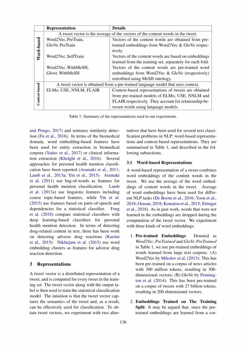
Representation DetailsA tweet vector is the average of the vectors of the content words in the tweet.
Wor
d-ba
sed Word2Vec PreTrain,
GloVe PreTrainVectors of the content words are obtained from pre-trained embeddings from Word2Vec & GloVe respec-tively.
Word2Vec SelfTrain Vectors of the content words are based on embeddingslearned from the training set, separately for each fold.
Word2Vec WithMeSH,Glove WithMeSH
Vectors of the content words are pre-trained wordembeddings from Word2Vec & GloVe (respectively)retrofitted using MeSH ontology.
Con
text
-bas
ed A tweet vector is obtained from a pre-trained language model that uses context.ELMo, USE, NNLM, FLAIR Context-based representations of tweets are obtained
from pre-trained models of ELMo, USE, NNLM andFLAIR respectively. They account for relationship be-tween words using language models.
Table 1: Summary of the representations used in our experiments.
and Priego, 2017) and sentence similarity detec-tion (Fu et al., 2016). In terms of the biomedicaldomain, word embedding-based features havebeen used for entity extraction in biomedicalcorpora (Yadav et al., 2017) or clinical informa-tion extraction (Kholghi et al., 2016). Severalapproaches for personal health mention classifi-cation have been reported (Aramaki et al., 2011;Lamb et al., 2013a; Yin et al., 2015). Aramakiet al. (2011) use bag-of-words as features forpersonal health mention classification. Lambet al. (2013a) use linguistic features includingcoarse topic-based features, while Yin et al.(2015) use features based on parts-of-speech anddependencies for a statistical classifier. Fenget al. (2018) compare statistical classifiers withdeep learning-based classifiers for personalhealth mention detection. In terms of detectingdrug-related content in text, there has been workon detecting adverse drug reactions (Karimiet al., 2015). Nikfarjam et al. (2015) use wordembedding clusters as features for adverse drugreaction detection.
3 Representations
A tweet vector is a distributed representation of atweet, and is computed for every tweet in the train-ing set. The tweet vector along with the output la-bel is then used to train the statistical classificationmodel. The intuition is that the tweet vector cap-tures the semantics of the tweet and, as a result,can be effectively used for classification. To ob-tain tweet vectors, we experiment with two alter-
natives that have been used for several text classi-fication problems in NLP: word-based representa-tions and context-based representations. They aresummarised in Table 1, and described in the fol-lowing subsections.
3.1 Word-based Representations
A word-based representation of a tweet combinesword embeddings of the content words in thetweet. We use the average of the word embed-dings of content words in the tweet. Averageof word embeddings have been used for differ-ent NLP tasks (De Boom et al., 2016; Yoon et al.,2018; Orasan, 2018; Komatsu et al., 2015; Ettingeret al., 2018). As in past work, words that were notlearned in the embeddings are dropped during thecomputation of the tweet vector. We experimentwith three kinds of word embeddings:
1. Pre-trained Embeddings: Denoted asWord2Vec PreTrained and GloVe PreTrainedin Table 1, we use pre-trained embeddings ofwords learned from large text corpora: (A)Word2Vec by Mikolov et al. (2013): This hasbeen pre-trained on a corpus of news articleswith 300 million tokens, resulting in 300-dimensional vectors; (B) GloVe by Penning-ton et al. (2014): This has been pre-trainedon a corpus of tweets with 27 billion tokens,resulting in 200-dimensional vectors.
2. Embeddings Trained on The TrainingSplit: It may be argued that, since the pre-trained embeddings are learned from a cor-
136
Classification # tweets (# true tweets)
IIC 9,006 (2,306)DUC 13,409 (3,167)PHMC 2,661 (1,304)
Table 2: Dataset statistics.
pus from an unrelated domain (news and gen-eral, in the case of Word2Vec and GloVerespectively), they may not capture the se-mantics of the domain of the specific clas-sification problem. Therefore, we also usethe Word2Vec Model available in the gensimlibrary (Řehůřek and Sojka, 2010) to learnword embeddings from the documents. Foreach split, the corresponding training set isused to learn the embeddings. The embed-dings are then used to compute the tweet vec-tors and train the classifier. We refer to theseas Word2Vec SelfTrain.
3. Pre-trained embeddings retrofitted withmedical ontologies: Another alternative toadapt word embeddings for a classificationproblem is to use structured resources (suchas ontologies) from a domain same as thatof the classification problem. Faruqui et al.(2015) show that word embeddings can beretrofitted to capture relationships in an on-tology. We use the Medical Subject Head-ings (MeSH) ontology (Nelson et al., 2001),maintained by the U.S. National Library ofMedicine, which provides a hierarchically-organised terminology of medical concepts.Using the algorithm by Faruqui et al.(2015), we retrofit pre-trained embeddingsfrom Word2Vec and GloVe, with the MeSHontology. The retrofitted embeddings forWord2Vec and GloVe are referred to asWord2Vec WithMeSH, and GloVe WithMeSHrespectively.
The three kinds of word-based representations re-sult in five configurations: Word2Vec PreTrained,GloVe PreTrained, Word2Vec SelfTrain,Word2Vec WithMeSH, and GloVe WithMeSH.
3.2 Context-based Representations
Context-based representations may use languagemodels to generate vectors of sentences. There-fore, instead of learning vectors for individual
words in the sentence, they compute a vector forsentences on the whole, by taking into account theorder of words and the set of co-occurring words.
We experiment with four deep contextualisedvectors: (A) Embeddings from Language Mod-els (ELMo) by Peters et al. (2018): ELMo usescharacter-based word representations and bidi-rectional LSTMs. The pre-trained model com-putes a contextualised vector of 1024 dimensions.ELMo is available in the Tensorflow Hub2, arepository of machine learning modules; (B) Uni-versal Sentence Encoder (USE) by Cer et al.(2018): The encoder uses a Transformer archi-tecture that uses attention mechanism to incorpo-rate information about the order and the collectionof words (Vaswani et al., 2017). The pre-trainedmodel of USE that returns a vector of 512 di-mensions is also available on Tensorflow Hub; (C)Neural-Net Language Model (NNLM) by Ben-gio et al. (2003): The model simultaneously learnsrepresentations of words and probability functionsfor word sequences, allowing it to capture seman-tics of a sentence. We use a pre-trained modelavailable on Tensorflow Hub, that is trained onthe English Google News 200B corpus, and com-putes a vector of 128 dimensions; (D) FLAIR byAkbik et al. (2018): This library by Zalando re-search3 uses character-level language models tolearn contextualised representations. We use thepooling option to create sentence vectors. This isa concatenation of GloVe embeddings and the for-ward/backward language model. The resultant isa vector of 4196 dimensions.
Table 1 refers to the four configurations asELMo, USE, NNLM and FLAIR respectively.
4 Experiment Setup
We conduct our experiments on three booleanclassification problems in health informatics: (A)Influenza Infection Classification (IIC): Thegoal is to predict if a tweet reports an influenzainfection (‘I have been coughing all day’, for ex-ample) or describes information about influenza(‘flu outbreaks are common in this month of theyear’, for example). We use the dataset pre-sented in Lamb et al. (2013b); (B) Drug UsageClassification (DUC): The objective here is to
2https://www.tensorflow.org/hub/; Ac-cessed on 3rd June, 2019.
3https://github.com/zalandoresearch/flair; Accessed on 3rd June, 2019.
137
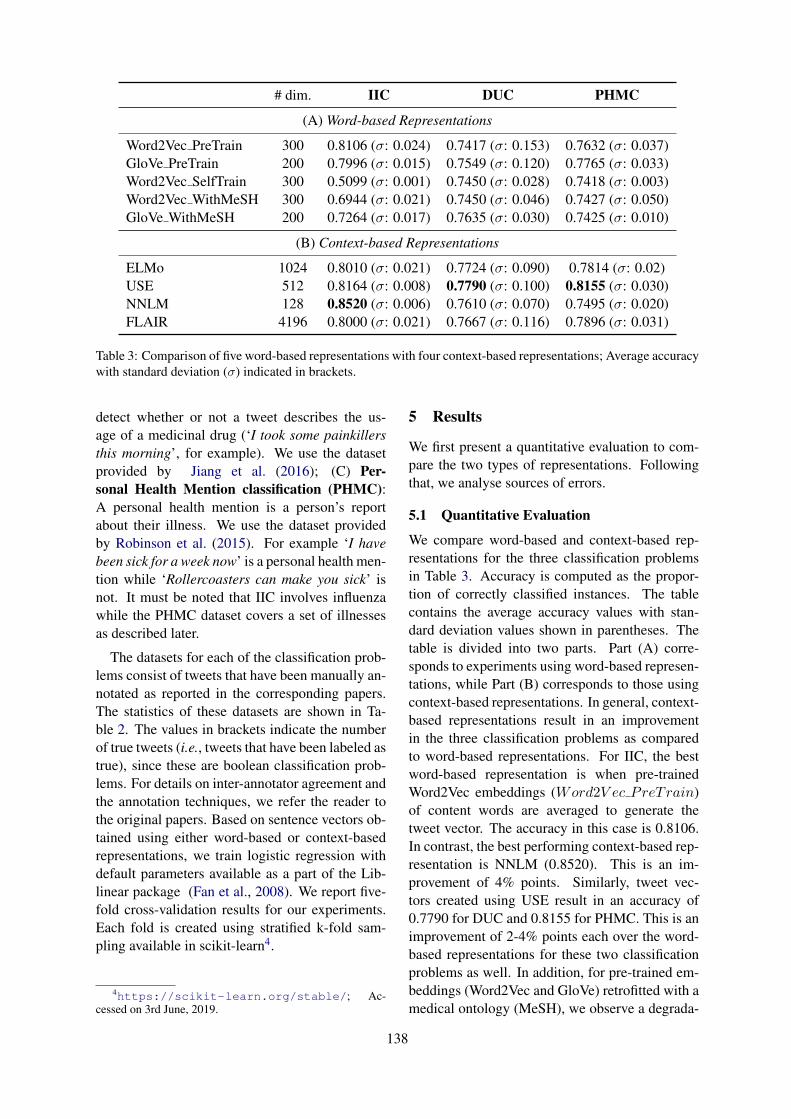
# dim. IIC DUC PHMC
(A) Word-based Representations
Word2Vec PreTrain 300 0.8106 (σ: 0.024) 0.7417 (σ: 0.153) 0.7632 (σ: 0.037)GloVe PreTrain 200 0.7996 (σ: 0.015) 0.7549 (σ: 0.120) 0.7765 (σ: 0.033)Word2Vec SelfTrain 300 0.5099 (σ: 0.001) 0.7450 (σ: 0.028) 0.7418 (σ: 0.003)Word2Vec WithMeSH 300 0.6944 (σ: 0.021) 0.7450 (σ: 0.046) 0.7427 (σ: 0.050)GloVe WithMeSH 200 0.7264 (σ: 0.017) 0.7635 (σ: 0.030) 0.7425 (σ: 0.010)
(B) Context-based Representations
ELMo 1024 0.8010 (σ: 0.021) 0.7724 (σ: 0.090) 0.7814 (σ: 0.02)USE 512 0.8164 (σ: 0.008) 0.7790 (σ: 0.100) 0.8155 (σ: 0.030)NNLM 128 0.8520 (σ: 0.006) 0.7610 (σ: 0.070) 0.7495 (σ: 0.020)FLAIR 4196 0.8000 (σ: 0.021) 0.7667 (σ: 0.116) 0.7896 (σ: 0.031)
Table 3: Comparison of five word-based representations with four context-based representations; Average accuracywith standard deviation (σ) indicated in brackets.
detect whether or not a tweet describes the us-age of a medicinal drug (‘I took some painkillersthis morning’, for example). We use the datasetprovided by Jiang et al. (2016); (C) Per-sonal Health Mention classification (PHMC):A personal health mention is a person’s reportabout their illness. We use the dataset providedby Robinson et al. (2015). For example ‘I havebeen sick for a week now’ is a personal health men-tion while ‘Rollercoasters can make you sick’ isnot. It must be noted that IIC involves influenzawhile the PHMC dataset covers a set of illnessesas described later.
The datasets for each of the classification prob-lems consist of tweets that have been manually an-notated as reported in the corresponding papers.The statistics of these datasets are shown in Ta-ble 2. The values in brackets indicate the numberof true tweets (i.e., tweets that have been labeled astrue), since these are boolean classification prob-lems. For details on inter-annotator agreement andthe annotation techniques, we refer the reader tothe original papers. Based on sentence vectors ob-tained using either word-based or context-basedrepresentations, we train logistic regression withdefault parameters available as a part of the Lib-linear package (Fan et al., 2008). We report five-fold cross-validation results for our experiments.Each fold is created using stratified k-fold sam-pling available in scikit-learn4.
4https://scikit-learn.org/stable/; Ac-cessed on 3rd June, 2019.
5 Results
We first present a quantitative evaluation to com-pare the two types of representations. Followingthat, we analyse sources of errors.
5.1 Quantitative Evaluation
We compare word-based and context-based rep-resentations for the three classification problemsin Table 3. Accuracy is computed as the propor-tion of correctly classified instances. The tablecontains the average accuracy values with stan-dard deviation values shown in parentheses. Thetable is divided into two parts. Part (A) corre-sponds to experiments using word-based represen-tations, while Part (B) corresponds to those usingcontext-based representations. In general, context-based representations result in an improvementin the three classification problems as comparedto word-based representations. For IIC, the bestword-based representation is when pre-trainedWord2Vec embeddings (Word2V ec PreTrain)of content words are averaged to generate thetweet vector. The accuracy in this case is 0.8106.In contrast, the best performing context-based rep-resentation is NNLM (0.8520). This is an im-provement of 4% points. Similarly, tweet vec-tors created using USE result in an accuracy of0.7790 for DUC and 0.8155 for PHMC. This is animprovement of 2-4% points each over the word-based representations for these two classificationproblems as well. In addition, for pre-trained em-beddings (Word2Vec and GloVe) retrofitted with amedical ontology (MeSH), we observe a degrada-
138
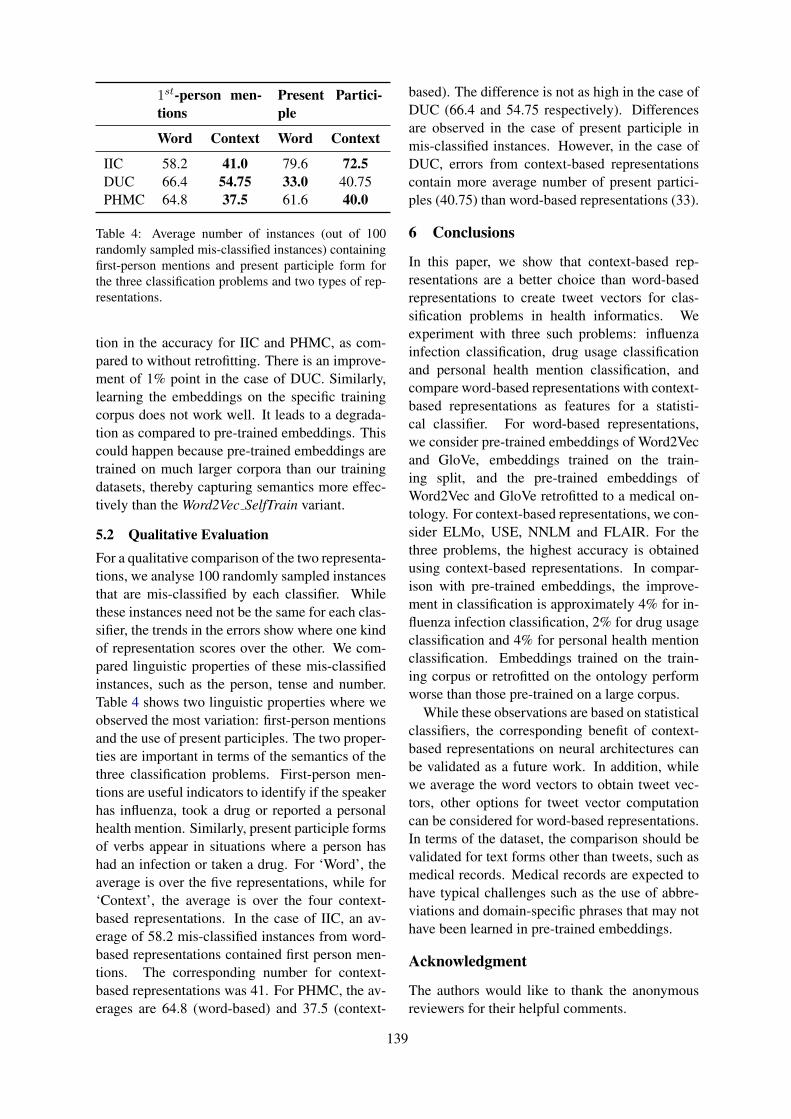
1st-person men-tions
Present Partici-ple
Word Context Word Context
IIC 58.2 41.0 79.6 72.5DUC 66.4 54.75 33.0 40.75PHMC 64.8 37.5 61.6 40.0
Table 4: Average number of instances (out of 100randomly sampled mis-classified instances) containingfirst-person mentions and present participle form forthe three classification problems and two types of rep-resentations.
tion in the accuracy for IIC and PHMC, as com-pared to without retrofitting. There is an improve-ment of 1% point in the case of DUC. Similarly,learning the embeddings on the specific trainingcorpus does not work well. It leads to a degrada-tion as compared to pre-trained embeddings. Thiscould happen because pre-trained embeddings aretrained on much larger corpora than our trainingdatasets, thereby capturing semantics more effec-tively than the Word2Vec SelfTrain variant.
5.2 Qualitative EvaluationFor a qualitative comparison of the two representa-tions, we analyse 100 randomly sampled instancesthat are mis-classified by each classifier. Whilethese instances need not be the same for each clas-sifier, the trends in the errors show where one kindof representation scores over the other. We com-pared linguistic properties of these mis-classifiedinstances, such as the person, tense and number.Table 4 shows two linguistic properties where weobserved the most variation: first-person mentionsand the use of present participles. The two proper-ties are important in terms of the semantics of thethree classification problems. First-person men-tions are useful indicators to identify if the speakerhas influenza, took a drug or reported a personalhealth mention. Similarly, present participle formsof verbs appear in situations where a person hashad an infection or taken a drug. For ‘Word’, theaverage is over the five representations, while for‘Context’, the average is over the four context-based representations. In the case of IIC, an av-erage of 58.2 mis-classified instances from word-based representations contained first person men-tions. The corresponding number for context-based representations was 41. For PHMC, the av-erages are 64.8 (word-based) and 37.5 (context-
based). The difference is not as high in the case ofDUC (66.4 and 54.75 respectively). Differencesare observed in the case of present participle inmis-classified instances. However, in the case ofDUC, errors from context-based representationscontain more average number of present partici-ples (40.75) than word-based representations (33).
6 Conclusions
In this paper, we show that context-based rep-resentations are a better choice than word-basedrepresentations to create tweet vectors for clas-sification problems in health informatics. Weexperiment with three such problems: influenzainfection classification, drug usage classificationand personal health mention classification, andcompare word-based representations with context-based representations as features for a statisti-cal classifier. For word-based representations,we consider pre-trained embeddings of Word2Vecand GloVe, embeddings trained on the train-ing split, and the pre-trained embeddings ofWord2Vec and GloVe retrofitted to a medical on-tology. For context-based representations, we con-sider ELMo, USE, NNLM and FLAIR. For thethree problems, the highest accuracy is obtainedusing context-based representations. In compar-ison with pre-trained embeddings, the improve-ment in classification is approximately 4% for in-fluenza infection classification, 2% for drug usageclassification and 4% for personal health mentionclassification. Embeddings trained on the train-ing corpus or retrofitted on the ontology performworse than those pre-trained on a large corpus.
While these observations are based on statisticalclassifiers, the corresponding benefit of context-based representations on neural architectures canbe validated as a future work. In addition, whilewe average the word vectors to obtain tweet vec-tors, other options for tweet vector computationcan be considered for word-based representations.In terms of the dataset, the comparison should bevalidated for text forms other than tweets, such asmedical records. Medical records are expected tohave typical challenges such as the use of abbre-viations and domain-specific phrases that may nothave been learned in pre-trained embeddings.
Acknowledgment
The authors would like to thank the anonymousreviewers for their helpful comments.
139
ReferencesAlan Akbik, Duncan Blythe, and Roland Vollgraf.
2018. Contextual string embeddings for sequencelabeling. In Proceedings of the 27th InternationalConference on Computational Linguistics, pages1638–1649.
Eiji Aramaki, Sachiko Maskawa, and Mizuki Morita.2011. Twitter catches the flu: Detecting influenzaepidemics using Twitter. In Empirical Methods inNatural Language Processing, pages 1568–1576,Edinburgh, UK. Association for Computational Lin-guistics.
Yoshua Bengio, Réjean Ducharme, Pascal Vincent, andChristian Jauvin. 2003. A neural probabilistic lan-guage model. Journal of machine learning research,3(Feb):1137–1155.
Davide Buscaldi and Belem Priego. 2017. Lipn-uamat emoint-2017:combination of lexicon-based fea-tures and sentence-level vector representations foremotion intensity determination. In 8th Workshopon Computational Approaches to Subjectivity, Sen-timent and Social Media Analysis, pages 255–258,Copenhagen, Denmark.
Daniel Cer, Yinfei Yang, Sheng-yi Kong, Nan Hua,Nicole Limtiaco, Rhomni St John, Noah Constant,Mario Guajardo-Cespedes, Steve Yuan, Chris Tar,et al. 2018. Universal sentence encoder. arXivpreprint arXiv:1803.11175.
Wei-Chieh Chou, Chin-Kui Lin, Yuan-Fu Liao, andYih-Ru Wang. 2016. Word order sensitive embed-ding features/conditional random field-based chi-nese grammatical error detection. In 3rd Workshopon Natural Language Processing Techniques for Ed-ucational Applications, pages 73–81, Osaka, Japan.The COLING 2016 Organizing Committee.
Cedric De Boom, Steven Van Canneyt, Thomas De-meester, and Bart Dhoedt. 2016. Representationlearning for very short texts using weighted wordembedding aggregation. Pattern Recognition Let-ters, 80:150–156.
Allyson Ettinger, Ahmed Elgohary, Colin Phillips, andPhilip Resnik. 2018. Assessing composition in sen-tence vector representations. In 27th InternationalConference on Computational Linguistics, pages1790–1801, Santa Fe, New Mexico.
Rong-En Fan, Kai-Wei Chang, Cho-Jui Hsieh, Xiang-Rui Wang, and Chih-Jen Lin. 2008. Liblinear: Alibrary for large linear classification. Journal of ma-chine learning research, 9:1871–1874.
Manaal Faruqui, Jesse Dodge, Sujay Kumar Jauhar,Chris Dyer, Eduard Hovy, and Noah Smith. 2015.Retrofitting word vectors to semantic lexicons. InConference of the North American Chapter of theAssociation for Computational Linguistics: HumanLanguage Technologies, pages 1606–1615.
Shichao Feng, Keyuan Jiang, Jiyun Li, Ricardo ACalix, and Matrika Gupta. 2018. Detecting personalexperience tweets for health surveillance using un-supervised feature learning and recurrent neural net-works. In Workshops at the 32nd AAAI Conferenceon Artificial Intelligence, pages 425–430, New Or-leans, Louisiana.
Cheng Fu, Bo An, Xianpei Han, and Le Sun. 2016. Is-cas nlp at semeval-2016 task 1: Sentence similar-ity based on support vector regression using multiplefeatures. In 10th International Workshop on Seman-tic Evaluation, pages 645–649, San Diego, Califor-nia.
Kazuma Hashimoto, Pontus Stenetorp, Makoto Miwa,and Yoshimasa Tsuruoka. 2015. Task-orientedlearning of word embeddings for semantic relationclassification. arXiv preprint arXiv:1503.00095.
Keyuan Jiang, Ricardo Calix, and Matrika Gupta.2016. Construction of a personal experience tweetcorpus for health surveillance. In ACL Workshopon biomedical natural language processing, pages128–135, Berlin, Germany.
Aditya Joshi, Vaibhav Tripathi, Kevin Patel, PushpakBhattacharyya, and Mark Carman. 2016. Are wordembedding-based features useful for sarcasm detec-tion? In Empirical Methods in Natural LanguageProcessing, pages 1006–1011, Austin, Texas.
Sarvnaz Karimi, Chen Wang, Alejandro Metke-Jimenez, Raj Gaire, and Cecile Paris. 2015. Textand data mining techniques in adverse drug reactiondetection. ACM Computing Surveys, 47(4):56.
Mahnoosh Kholghi, Lance De Vine, Laurianne Sit-bon, Guido Zuccon, and Anthony Nguyen. 2016.The benefits of word embeddings features for activelearning in clinical information extraction. In Aus-tralasian Language Technology Association Work-shop, pages 25–34, Melbourne, Australia.
Hiroya Komatsu, Ran Tian, Naoaki Okazaki, and Ken-taro Inui. 2015. Reducing lexical features in parsingby word embeddings. In Pacific Asia Conferenceon Language, Information and Computation, pages106–113, Shanghai, China.
Alex Lamb, Michael J Paul, and Mark Dredze. 2013a.Separating fact from fear: Tracking flu infections ontwitter. In North American Chapter of the Associ-ation for Computational Linguistics: Human Lan-guage Technologies, pages 789–795, Atlanta, Geor-gia.
Alex Lamb, Michael J. Paul, and Mark Dredze. 2013b.Separating fact from fear: Tracking flu infections ontwitter. In North American Chapter of the Associ-ation for Computational Linguistics: Human Lan-guage Technologies.
140
Tomas Mikolov, Ilya Sutskever, Kai Chen, Greg S Cor-rado, and Jeff Dean. 2013. Distributed representa-tions of words and phrases and their compositional-ity. In Advances in neural information processingsystems, pages 3111–3119.
Stuart J Nelson, W Douglas Johnston, and Betsy LHumphreys. 2001. Relationships in medical subjectheadings (mesh). In Relationships in the Organiza-tion of Knowledge, pages 171–184.
Azadeh Nikfarjam, Abeed Sarker, Karen Oconnor,Rachel Ginn, and Graciela Gonzalez. 2015. Phar-macovigilance from social media: mining adversedrug reaction mentions using sequence labelingwith word embedding cluster features. Journalof the American Medical Informatics Association,22(3):671–681.
Constantin Orasan. 2018. Aggressive language identi-fication using word embeddings and sentiment fea-tures. In 1st Workshop on Trolling, Aggression andCyberbullying, pages 113–119, Santa Fe, New Mex-ico.
Jeffrey Pennington, Richard Socher, and Christo-pher D. Manning. 2014. Glove: Global vectors forword representation. In Empirical Methods in Natu-ral Language Processing, pages 1532–1543.
Matthew Peters, Mark Neumann, Mohit Iyyer, MattGardner, Christopher Clark, Kenton Lee, and LukeZettlemoyer. 2018. Deep contextualized word rep-resentations. In North American Chapter of theAssociation for Computational Linguistics: HumanLanguage Technologies, pages 2227–2237, New Or-leans, Louisiana.
Radim Řehůřek and Petr Sojka. 2010. Software Frame-work for Topic Modelling with Large Corpora.In LREC Workshop on New Challenges for NLPFrameworks, pages 45–50, Valletta, Malta. http://is.muni.cz/publication/884893/en.
Bella Robinson, Ross Sparks, Robert Power, and MarkCameron. 2015. Social media monitoring for healthindicators. In International Congress on Modellingand Simulation, Gold Coast, Australia.
Iliana Simova and Hans Uszkoreit. 2017. Word em-beddings as features for supervised coreference res-olution. In Recent Advances in Natural LanguageProcessing, pages 686–693, Varna, Bulgaria.
Maksim Tkachenko, Chong Cher Chia, and HadyLauw. 2018. Searching for the x-factor: Exploringcorpus subjectivity for word embeddings. In AnnualMeeting of the Association for Computational Lin-guistics, pages 1212–1221, Melbourne, Australia.
Ashish Vaswani, Noam Shazeer, Niki Parmar, JakobUszkoreit, Llion Jones, Aidan N Gomez, ŁukaszKaiser, and Illia Polosukhin. 2017. Attention is allyou need. In Advances in Neural Information Pro-cessing Systems, pages 5998–6008.
Shweta Yadav, Asif Ekbal, Sriparna Saha, and PushpakBhattacharyya. 2017. Entity extraction in biomedi-cal corpora: An approach to evaluate word embed-ding features with pso based feature selection. InEuropean Chapter of the Association for Computa-tional Linguistics, pages 1159–1170.
Zhijun Yin, Daniel Fabbri, S Trent Rosenbloom, andBradley Malin. 2015. A scalable framework to de-tect personal health mentions on twitter. Journal ofmedical Internet research, 17(6).
Su-Youn Yoon, Anastassia Loukina, Chong Min Lee,Matthew Mulholland, Xinhao Wang, and IkkyuChoi. 2018. Word-embedding based content fea-tures for automated oral proficiency scoring. In 3rdWorkshop on Semantic Deep Learning, pages 12–22, Santa Fe, New Mexico.
Zhihua Zhang, Guoshun Wu, and Man Lan. 2015.Ecnu: Multi-level sentiment analysis on twitter us-ing traditional linguistic features and word embed-ding features. In 9th International Workshop onSemantic Evaluation, pages 561–567, Denver, Col-orado.
141
Proceedings of the BioNLP 2019 workshop, pages 142–151Florence, Italy, August 1, 2019. c©2019 Association for Computational Linguistics
Constructing large scale biomedical knowledge bases from scratch withrapid annotation of interpretable patterns
Julien Fauqueur∗BenevolentAI
4-8 Maple St, LondonW1T 5HD
Ashok Thillaisundaram∗BenevolentAI
4-8 Maple St, LondonW1T 5HD
Theodosia Togia∗BenevolentAI
4-8 Maple St, LondonW1T 5HD
Abstract
Knowledge base construction is crucial forsummarising, understanding and inferring re-lationships between biomedical entities. How-ever, for many practical applications such asdrug discovery, the scarcity of relevant facts(e.g. gene X is therapeutic target for dis-ease Y) severely limits a domain expert’s abil-ity to create a usable knowledge base, eitherdirectly or by training a relation extractionmodel. In this paper, we present a simple andeffective method of extracting new facts with apre-specified binary relationship type from thebiomedical literature, without requiring anytraining data or hand-crafted rules. Our sys-tem discovers, ranks and presents the mostsalient patterns to domain experts in an inter-pretable form. By marking patterns as com-patible with the desired relationship type, ex-perts indirectly batch-annotate candidate pairswhose relationship is expressed with such pat-terns in the literature. Even with a completeabsence of seed data, experts are able to dis-cover thousands of high-quality pairs with thedesired relationship within minutes. When asmall number of relevant pairs do exist - evenwhen their relationship is more general (e.g.gene X is biologically associated with diseaseY) than the relationship of interest - our sys-tem leverages them in order to i) learn a betterranking of the patterns to be annotated or ii)generate weakly labelled pairs in a fully auto-mated manner. We evaluate our method bothintrinsically and via a downstream knowledge∗Equal contribution. Listing order is alphabetical. Theo-
dosia proposed and co-ordinated the research project, builtthe early prototypes and contributed the different methods forextracting and lexicalising patterns. Ashok provided concep-tual work on the metrics for ranking simplifications and forthe intrinsic evaluation, developed the simplification extrac-tion module, ran the experiments for the automated workflow(with all the parameter variations) and performed all the ex-trinsic evaluations. Julien was mainly responsible for the sys-tem architecture and workflow, the intrinsic evaluation (in-cluding interacting with the experts), handling negation andspeculation and the clustering algorithm.
base completion task, and show that it is an ef-fective way of constructing knowledge baseswhen few or no relevant facts are already avail-able.
1 Introduction
In many important biomedical applications, ex-perts seek to extract facts that are often complexand tied to particular tasks, hence data that aretruly fit for purpose are scarce or simply non-existent. Even when only binary relations aresought, useful facts tend to be more specific (e.g.mutation of gene X has a causal effect on diseaseY in an animal model) than associations typicallyfound in widely available knowledge bases. Ex-tracting facts with a pre-specified relationship typefrom the literature in the absence of training dataoften relies on handcrafted rules, which are labo-rious, ad-hoc and hardly reusable for other typesof relations. Recent attempts to create relationaldata from scratch by denoising the output of mul-tiple hand-written rules (Ratner et al., 2016) or byaugmenting existing data through the induction ofnew black-box heuristics (Varma and Ré, 2018)are still dependent on ad-hoc human effort or pre-existing data. Our approach involves discoveringand recommending, rather than prescribing, rules.Importantly, our rules are presented as text-likepatterns whose meaning is transparent to humanannotators, enabling integration of an automaticdata generation (or augmentation) system with adomain expert feedback loop.
In this work, we make the following contribu-tions:
• We propose a number of methods for extract-ing patterns from a sentence in which twoeligible entities co-occur; different types ofpatterns have different trade-offs between ex-pressive power and coverage.
142
• We propose a simple method for presentingpatterns in a readable way, enabling faster,more reliable human annotation
• For cases where a small number of seed pairsare already available, we propose a methodwhich utilises these seed pairs to rank newlydiscovered patterns in terms of their compat-ibility with the existing data. The resultingpatterns can be used with or without a humanin the loop.
The rest of the paper is organised as follows.Section 2 describes some related work. Section 3explains the relationship between patterns and la-belling rules and presents some pattern types alongwith techniques for rendering them interpretable.Section 4 provides a high-level overview of thesystem and covers details of our different work-flows (with and without seed data; with and with-out human feedback). Section 5 explains how wemeasure the system’s performance both intrinsi-cally and via a downstream knowledge base com-pletion task. In section 6, we report the detailsof our main experiments while in sections 7 and8 we present some analysis along with further ex-periments. The paper ends with conclusions andproposals for further work in section 9.
2 Related work
The idea of extracting entity pairs by discoveringtextual patterns dates back to early work on boot-strapping for relation extraction with the DIPREsystem (Brin, 1999). This system was designed tofind co-occurrences of seed entity pairs of a knownrelationship type inside unlabelled text, then ex-tract simple patterns (exact string matches) fromthese occurrences and use them to discover newentity pairs. Agichtein et al. (2000) introduced apattern evaluation methodology based on the pre-cision of a pattern on the set of entity pairs whichhad already been discovered; they also used thedot product between word vectors instead of anexact string match to allow for slight variationsin text. Later work (Greenwood and Stevenson,2006; Xu et al., 2007; Alfonseca et al., 2012)has proposed more sophisticated pattern extrac-tion methods (based on dependency graphs or ker-nel methods on word vectors) and different pat-tern evaluation frameworks (document relevancescores).
Two recent weak supervision techniques, DataProgramming (Ratner et al., 2016) and the method
underlying the Snuba system (Varma and Ré,2018) have attempted to combine the results ofhandcrafted rules and weak base classifiers respec-tively. Data Programming involves modelling theaccuracy of ideally uncorrelated rules devised bydomain experts, then combining their output intoweak labels. Although this approach does not re-quire any seed data, it does rely on handwrittenrules, which are both time consuming and ad-hocdue to the lack of a data-driven mechanism for ex-ploring the space of possible rules. Snuba learnsblack-box heuristics (parameters for different clas-sifiers) given seed pairs of the desired relationship.This method avoids the need for manually com-posing rules, however, the rules it learns are notinterpretable, which makes the pipeline harder tocombine with an active learning step. Second, thesystem requires gold standard pairs. In contrast,while our system can leverage gold standard an-notations, if available, in order to reduce the spaceof discovered rules, as well as tune the rankingof newly discovered patterns, it is entirely capa-ble of starting without any gold data if ranking isheuristics-based (e.g. prioritisation by frequency)and a human assesses the quality of the highestcoverage rules suggested. Our method does notpreclude use within a data programming setup asa way of discovering labelling functions or withina system like Snuba, as a way of generating seedpairs. Another body of work, distant supervision(Verga et al., 2018; Lin et al., 2016) has been arecent popular way to extract relationships fromweak labels, but does not give the user any controlon the model performance.
A well known body of work, OpenIE (Bankoet al., 2007; Fader et al., 2011; Mausam et al.,2012; Angeli et al., 2015) aims to extract patternsbetween entity mentions in sentences, thereby dis-covering new surface forms which can be clus-tered (Mohamed et al., 2011; Nakashole et al.,2012) in order to reveal new meaningful relation-ship types. In the biomedical domain, Percha andAltman (2018) attempt something similar by ex-tracting and clustering dependency patterns be-tween pairs of biomedical entities (e.g. chemical-gene, chemical-disease, gene-disease). Our workdiffers from these approaches in that we extractpairs for a pre-specified relationship type (eitherfrom scratch or by augmenting existing data writ-ten with specific guidelines), which is not guaran-teed to correspond to a cluster of discovered sur-
143
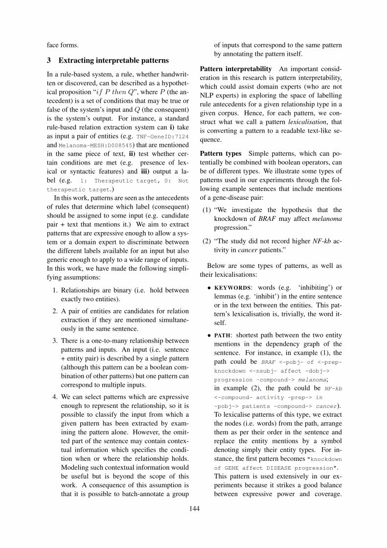
face forms.
3 Extracting interpretable patterns
In a rule-based system, a rule, whether handwrit-ten or discovered, can be described as a hypothet-ical proposition “if P then Q”, where P (the an-tecedent) is a set of conditions that may be true orfalse of the system’s input and Q (the consequent)is the system’s output. For instance, a standardrule-based relation extraction system can i) takeas input a pair of entities (e.g. TNF-GeneID:7124
and Melanoma-MESH:D008545) that are mentionedin the same piece of text, ii) test whether cer-tain conditions are met (e.g. presence of lex-ical or syntactic features) and iii) output a la-bel (e.g. 1: Therapeutic target, 0: Not
therapeutic target.)In this work, patterns are seen as the antecedents
of rules that determine which label (consequent)should be assigned to some input (e.g. candidatepair + text that mentions it.) We aim to extractpatterns that are expressive enough to allow a sys-tem or a domain expert to discriminate betweenthe different labels available for an input but alsogeneric enough to apply to a wide range of inputs.In this work, we have made the following simpli-fying assumptions:
1. Relationships are binary (i.e. hold betweenexactly two entities).
2. A pair of entities are candidates for relationextraction if they are mentioned simultane-ously in the same sentence.
3. There is a one-to-many relationship betweenpatterns and inputs. An input (i.e. sentence+ entity pair) is described by a single pattern(although this pattern can be a boolean com-bination of other patterns) but one pattern cancorrespond to multiple inputs.
4. We can select patterns which are expressiveenough to represent the relationship, so it ispossible to classify the input from which agiven pattern has been extracted by exam-ining the pattern alone. However, the omit-ted part of the sentence may contain contex-tual information which specifies the condi-tion when or where the relationship holds.Modeling such contextual information wouldbe useful but is beyond the scope of thiswork. A consequence of this assumption isthat it is possible to batch-annotate a group
of inputs that correspond to the same patternby annotating the pattern itself.
Pattern interpretability An important consid-eration in this research is pattern interpretability,which could assist domain experts (who are notNLP experts) in exploring the space of labellingrule antecedents for a given relationship type in agiven corpus. Hence, for each pattern, we con-struct what we call a pattern lexicalisation, thatis converting a pattern to a readable text-like se-quence.
Pattern types Simple patterns, which can po-tentially be combined with boolean operators, canbe of different types. We illustrate some types ofpatterns used in our experiments through the fol-lowing example sentences that include mentionsof a gene-disease pair:
(1) “We investigate the hypothesis that theknockdown of BRAF may affect melanomaprogression.”
(2) “The study did not record higher NF-kb ac-tivity in cancer patients.”
Below are some types of patterns, as well astheir lexicalisations:
• KEYWORDS: words (e.g. ‘inhibiting’) orlemmas (e.g. ‘inhibit’) in the entire sentenceor in the text between the entities. This pat-tern’s lexicalisation is, trivially, the word it-self.
• PATH: shortest path between the two entitymentions in the dependency graph of thesentence. For instance, in example (1), thepath could be BRAF <-pobj- of <-prep-
knockdown <-nsubj- affect -dobj->
progression -compound-> melanoma;in example (2), the path could be NF-kb
<-compound- activity -prep-> in
-pobj-> patients -compound-> cancer).To lexicalise patterns of this type, we extractthe nodes (i.e. words) from the path, arrangethem as per their order in the sentence andreplace the entity mentions by a symboldenoting simply their entity types. For in-stance, the first pattern becomes "knockdownof GENE affect DISEASE progression".This pattern is used extensively in our ex-periments because it strikes a good balancebetween expressive power and coverage.
144
We call its lexicalisation a simplificationbecause it is a text-like piece that simplifiesa sentence by discarding all but the mostessential information.
• PATH ROOT: the root (word with no in-coming edges) of the shortest path betweenthe two entities (e.g. ‘affect’ and ‘activ-ity’ in examples (1) and (2) respectively).The lexicalisation could be trivial (i.e. theroot itself) or, alternatively, if this pattern isused in an AND boolean combination with thePATH pattern, the root can simply be high-lighted (e.g. "knockdown of GENE affect
DISEASE progression")
• SENTENCE ROOT: the root of the depen-dency graph of the entire sentence (e.g.‘investigate’ and ‘record’ in the examplesabove), which is often not the same as rootof the path connecting the two entities. It canbe lexicalised similarly to the pattern above.
• PATH BETWEEN ROOTS: the path betweenthe root of the entire sentence and theroot of the path between the two entities(e.g. investigate -dobj-> hypothesis
-acl-> affect and record -dobj->
activity for examples (1) and (2) re-spectively). The pattern can be lexicalisedas what we have called “simplification”(e.g. investigate hypothesis affect,or, if AND-ed with the PATH pattern, all thewords from both patterns can be merged andarranged as per their original order in thesentence, potentially with some highlightingto differentiate the two simpler patterns (e.g."investigate hypothesis knockdown of
GENE affect DISEASE progression")
• SENTENCE ROOT DESCENDANTS: thedirect descendants of the SENTENCE ROOT,for instance, ‘did’, ‘not’ and ‘activity’ inthe example (1), because of the edges did
<-aux- record, not <-neg- record andrecord -dobj-> activity. To lexicalisethis pattern, we can extract the words andmerge them with words of other patterns.Alternatively, we can devise some simplersub-patterns, for instance, descendants withaux, that is auxiliary, edges, such as ‘may’,or descendants with neg edges such as ‘not’and place them outside any simplification:"investigate hypothesis knockdown
of GENE affect DISEASE progression +
hedging:[may]"
• PATH ROOT DESCENDANTS: the direct de-scendants of the root of the path betweenthe entities (e.g. ‘may’ and ‘progres-sion’ in example (1) because may <-aux-
affect and affect -dobj-> progression;‘higher’ and ‘in’ in the example (2) becausehigher <-amod- activity and activity
-prep-> in). Its lexicalisation can be thesame as that of the previous pattern type.
Other examples of patterns could be regu-lar expressions or rules informed by an ex-ternal biomedical ontology (e.g. GENE is a
Rhodopsin-like receptor) or with lexical in-formation from databases like WordNet (Miller,1995) (e.g. for increasing pattern coverage lever-aging synonyms or hypernyms of words in a pat-tern.)
It should be obvious that the more expressive apattern becomes (for instance by AND-ing multipleother patterns), the less capable it is of subsumingmany sentences. It is important to discover pat-terns with this trade-off in mind.
4 System overview
In this section, we will describe each step of oursystem, outlined in Figure 1.
4.1 Data preparation
Extracting named entities and patterns Thefirst step is performing named entity recognition(NER) on the sentences in the corpus to enableus to identify all the sentences which contain en-tity pairs of interest. Our experiments are focusedon gene-therapeutic target pairs, however, the sys-tem is designed to be agnostic to different typesof entities and relationships between them. Wethen extract the desired patterns from each of thesesentences, as described in section 3. For simplic-ity, we limited our experiments to sentences thatcontain exactly one gene-disease pair, however,extending the system to handle multiple pairs isstraightforward.
We index each sentence in a database along withthe lexicalisation for its pattern (e.g. the ‘simpli-fication’ for PATH or PATH BETWEEN ROOTS pat-terns) and the entity pair found. This allows us toeasily query this database i) for all entity pairs thatcorrespond to a pattern (which is now lexicalised
145
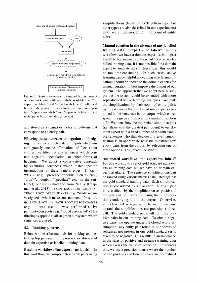
extraction of named entities and patterns
filter out sentences
rank patterns
labels
expert annotates top patterns
generate new pairs from good patterns(intrinsic evaluation)
downstream task: KB completion(extrinsic evaluation)
Figure 1: System overview. Diamond box is presentonly in workflows with seed labels available (i.e. “noexpert but labels” and “expert with labels”), ellipticalbox is only present in workflows involving an expert(i.e. “expert - no labels” and “expert with labels”) andrectangular boxes are always present.
and stored as a string) or ii) for all patterns thatcorrespond to an entity pair.
Filtering out sentences with negation and hedg-ing. Since we are interested in inputs which un-ambiguously encode affirmations of facts aboutentities, we filter out any sentences which con-tain negation, speculation, or other forms ofhedging. We adopt a conservative approachby excluding sentences which match specificinstantiations of these pattern types: i) KEY-WORDS (e.g. presence of terms such as “no”,“didn’t”, “doubt”, “speculate” etc. in the sen-tence); our list is modified from NegEx (Chap-man et al., 2013), ii) SENTENCE ROOT AND SEN-TENCE ROOT DESCENDANTS (e.g. “study we in-vestigated”, which makes no statement of results),iii) PATH ROOT AND PATH ROOT DESCENDANTS
(e.g. “was used”, “was performed”), iv)path between roots (e.g. “found associated”) Thisfiltering is applied at all stages in our system wheresentences are used.
4.2 Ranking patternsBelow we describe methods for ranking and se-lecting top patterns in the presence or absence ofdomain expertise or labelled training data.
Baseline workflow: “no expert - no labels” Inthis workflow, we simply extract new pairs using
simplifications (from the PATH pattern type, butother types are also described in our experiments)that have a high enough (>= 5) count of entitypairs.
Manual curation in the absence of any labelledtraining data: “expert - no labels” In thisworkflow, we have a domain expert (a biologist)available for manual curation but there is no la-belled training data. It is not possible for a domainexpert to annotate all simplifications; this wouldbe too time-consuming. In such cases, activelearning can be helpful in deciding which simplifi-cations should be shown to the domain experts formanual curation to best improve the output of oursystem. The approach that we adopt here is sim-ple but the system could be extended with moresophisticated active learning strategies. We rankthe simplifications by their count of entity pairs;by this we mean the number of unique pairs con-tained in the sentences in our corpus which corre-spond to a given simplification (similar to section4.2). We then show the top ranked simplifications(i.e. those with the greatest pair count) to our do-main expert with a fixed number of random exam-ple sentences who then decides if a given simpli-fication is an appropriate heuristic to extract newentity pairs from the corpus, by selecting one ofthree options “Yes”, “No”, “Maybe”.
Automated workflow: “no expert but labels”For this workflow, a set of gold standard pairs ex-ists as training data but we have no domain ex-perts available. The sentence simplifications canbe ranked using various metrics calculated againstthe gold standard training data. Each simplifica-tion is considered as a classifier: A given pairis ‘classified’ by the simplification as positive ifthe pair can be discovered using the simplifica-tion’s underlying rule in the corpus. Otherwise,it is classified as negative. The metrics we useto rank the simplifications are precision and re-call. The gold standard pairs will form the pos-itive pairs in our training data. To obtain nega-tive pairs, we operate under the closed world as-sumption: any entity pair found in our corpus ofsentences not present in our gold standard set istaken to be negative. This results in an imbalancein the sizes of positive and negative training datawhich skews the value of precision. To addressthis, we use a precision metric where the numberof true positives and false positives are normalised
146
by the total number of positive and negative pairsrespectively in our training data. For each simpli-fication S we define true positives (TPS) and falsepositives (FPS) as the sets of correctly and incor-rectly positive-labelled entity pairs respectively.Our variant of precision for a simplification S isthen, precisionS = |TPS |/NP
|TPS |/NP+|FPS |/NNwhere
NP and NN are the number of positive and neg-ative pairs respectively in the training data. Withthis metric, if a simplification classifies 10% of thepositive pairs as true positives and 10% of the neg-ative pairs as false positives then precisionS =
0.10.1+0.1 = 0.5. The metric utilises the percent-age of each class instead of the absolute numberof pairs, as would be the case for the standard pre-cision metric. The definition of recall for a givensimplification S is with respect to just the positivetraining data and is thus unaffected by an imbal-ance in the sizes.
Manual curation with labelled data: “expertwith labels” For this workflow, both domain ex-perts and labelled training data are available to us.We improve on our methodology in the “expert -no labels” workflow by making use of the metricsdiscussed in the “no expert but labels” workflowwhich are calculated using the labelled trainingdata. As we want to maximise the number and pre-cision of new pairs extracted, we keep only sim-plifications with recall and precision above certainrespective thresholds and present them to domainexperts ranked by pair count to ensure they see themost impactful simplifications first.
4.3 Generating new pairs
All previous stages aim at generating a list of goodsimplifications. We now have a collection of ruleswhich can be used to extract new entity pairs fromthe corpus. Any simplification selected as usefulimplies that all entity pairs recovered from the cor-pus using this rule can be added as positive ex-amples to the dataset. With the selected simplifi-cations, we can batch-annotate thousands of sen-tences, and hence pairs, with minimal effort. Wesimply query our database for all new pairs whichare found in a sentence expressing any of our se-lected simplifications.
Clustering simplifications We found that manysimplifications can be very similar up to a fewcharacters. We create clusters of quasi-identicalsimplifications, and use them i) to enforce diver-
sity in the selection of simplifications for the userto annotate, by picking only one simplification percluster and, ii) to safely extend the selection ofpositive simplification to other simplification inthe cluster. We create clusters of simplifications bydetecting connected components in a graph wherethe nodes are the simplifications and the edges arebetween simplifications which are at a maximumLevenshtein distance of 2. This allows us to be in-variant to plural forms, upper/lower case, to shortwords like in/of etc. Note that some (not all) ofthese variations could be captured with a lemma-tiser. Example of a distance 2 cluster:{GENE effects on DISEASE,GENE effect on DISEASE,GENE effects in DISEASE}With a distance of 2, we typically increase thenumber of positive simplifications by 50%, whichsignificantly increases the recall on new pairs.
5 Evaluation
We implement two evaluation frameworks. Thefirst is an intrinsic evaluation of the quality of thenew extracted pairs. The second is extrinsic; weconsider how the inclusion of the new pairs dis-covered by our system affects the performance ofa downstream knowledge base completion task.∗
5.1 Intrinsic evaluation
Pair-level Our aim in this subsection is to con-struct an intrinsic evaluation framework whichcan directly measure the quality of the discoveredpairs. We do this by holding out a fraction of thegold standard positive pairs and the negative pairs(under the closed world assumption) to be used asa test set. The remaining fraction is used as train-ing data. We evaluate our system by measuringits recall, specificity (true negative rate), precision,and F-score against this test set. In more detail,the new pairs discovered by our selected simplifi-cations are taken to be the positive pairs predictedby our system. The overlap between these newpairs and the positive test set are the true positives(TP ) while the overlap with the negative test setare the false positives (FP ). Recall and specificitytake their standard definitions. Again, we considera precision score which is normalised to correct
∗We consider the second type of evaluation extrinsic be-cause knowledge base completion aims to recover latent re-lationships, whereas knowledge base construction, which thesystem is built for, is limited to extracting pairs from the lit-erature.
147
for the imbalance in numbers between positive andnegative pairs, precision = |TP |/NP
|TP |/NP+|FP |/NN,
where NP and NN are the numbers of positive andnegative pairs respectively present in the test set(as described in section 4.2). We take the F-scoreto be the harmonic mean of this precision variantand recall.
Simplification-level For the manual workflows,we also consider the expert annotations while as-sessing the quality of the simplifications. Wereport MSP , the manual simplification preci-sion, based on NY es, NNo and NMaybe, the num-ber of simplifications that the expert has anno-tated as “Yes”, “No” and “Maybe”. MSP =
NY esNY es+NNo+NMaybe
. We expect MSP to be as highas possible.
Extrinsic evaluation via knowledge base com-pletion The setup for our extrinsic evaluationframework is straightforward and intuitive. Theinitial gold standard set of positive pairs is splitinto training and test data. A graph completionmodel is then trained using the training data andevaluated to determine whether it can predict theexistence of the pairs in the test data. To de-termine whether our knowledge base constructionsystem can add value, we use the new pairs foundfrom our system to augment the training data forthe graph completion model, and observe whetherthis improves its performance against the testset. We use ComplEx (Trouillon et al., 2017), awell-established tensor factorisation model, as ourknowledge base completion model. We providestandard information retrieval metrics to quantifythe performance of the graph completion model.These are the precision, P (k), and recall, R(k),calculated for the top k predictions along with themean average precision (mAP ). For gene-diseaseentity pairs, for example, mAP = 1
Nd
∑dAveP ,
where the sum is over the diseases d with Nd be-ing the total number of diseases, and AveP =∑kP (k) (R(k)−R(k − 1)) with P (k) and R(k)
as defined above.
6 Main experiments and results
6.1 Datasets
For all the following experiments, our data wasdrawn from the following datasets: DisGeNET(Pinero et al., 2016) and Comparative Toxicoge-nomics Database (CTD) (Davis et al., 2018). CTD
contains two relation types: ‘marker/mechanism’and ‘therapeutic’. We use both the entire CTDdataset and the subset of therapeutic gene-diseasepairs which we refer to as CTD therapeutic.
The datasets above are first restricted to humangenes and then to the gene-disease pairs which ap-pear in our corpus of sentences; this corpus con-sists of sentences from PubMed articles whichhave been restricted, for simplicity, to sentenceswhich contain just one gene-disease pair each.With these restrictions in effect, the CTD datasethas 8828 gene-disease pairs, CTD therapeutic has169 pairs, and Disgenet has 33844 pairs.
6.2 Intrinsic evaluation resultsIn table 1, we report the pair-level metrics (see sec-tion 5.1) for our three proposed workflows and abaseline (see section 4). We also report the expert-based metric MSP (see section 5.1) for the twomanual workflows. The CTD therapeutic datasetwas the most suitable dataset for this evaluationbecause i) it is very relevant to crucial domains ofapplication such as drug discovery, and ii) its smallsize makes it a good candidate for expansion. Ineach session, the expert annotated 200 simplifica-tions accompanied by 20 sentences. It took theexpert about 3 hours to annotate the first session,which is a rapid way to generate thousands of newpairs from scratch.
We find that our three main proposed workflows(‘expert - with labels’, ‘expert - no labels’, and thefully automated ‘no expert but labels’) all discovera significant number of new gene-disease thera-peutic pairs. As confirmed by both pair-level anduser-based metrics, incorporating the use of do-main expert’s time and the use of labelled data re-sults in higher precision at the expense of recall.
6.3 Extrinsic evaluation resultsIn table 2, we list the results of the downstreamknowledge base completion task for the fully auto-mated workflow and the baseline. We compare theperformance of our knowledge base completionmodel when trained with just the initial seed train-ing data versus the seed training data augmentedwith the new pairs discovered by our fully auto-mated workflow (and baseline workflow).
The addition of new pairs from the fully auto-mated workflow gives us a higher mean averageprecision (mAP ) than with just the seed dataset.We obtain a higher precision (for the top 100 andtop 1000 predictions) while maintaining the same
148
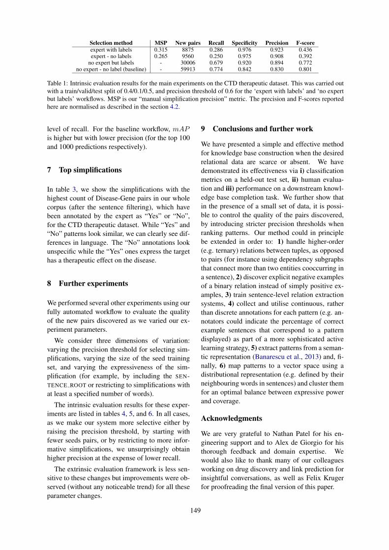
Selection method MSP New pairs Recall Specificity Precision F-scoreexpert with labels 0.315 8875 0.286 0.976 0.923 0.436expert - no labels 0.265 9560 0.250 0.975 0.908 0.392
no expert but labels - 30006 0.679 0.920 0.894 0.772no expert - no label (baseline) - 59913 0.774 0.842 0.830 0.801
Table 1: Intrinsic evaluation results for the main experiments on the CTD therapeutic dataset. This was carried outwith a train/valid/test split of 0.4/0.1/0.5, and precision threshold of 0.6 for the ‘expert with labels’ and ‘no expertbut labels’ workflows. MSP is our “manual simplification precision” metric. The precision and F-scores reportedhere are normalised as described in the section 4.2.
level of recall. For the baseline workflow, mAPis higher but with lower precision (for the top 100and 1000 predictions respectively).
7 Top simplifications
In table 3, we show the simplifications with thehighest count of Disease-Gene pairs in our wholecorpus (after the sentence filtering), which havebeen annotated by the expert as “Yes” or “No”,for the CTD therapeutic dataset. While “Yes” and“No” patterns look similar, we can clearly see dif-ferences in language. The “No” annotations lookunspecific while the “Yes” ones express the targethas a therapeutic effect on the disease.
8 Further experiments
We performed several other experiments using ourfully automated workflow to evaluate the qualityof the new pairs discovered as we varied our ex-periment parameters.
We consider three dimensions of variation:varying the precision threshold for selecting sim-plifications, varying the size of the seed trainingset, and varying the expressiveness of the sim-plification (for example, by including the SEN-TENCE ROOT or restricting to simplifications withat least a specified number of words).
The intrinsic evaluation results for these exper-iments are listed in tables 4, 5, and 6. In all cases,as we make our system more selective either byraising the precision threshold, by starting withfewer seeds pairs, or by restricting to more infor-mative simplifications, we unsurprisingly obtainhigher precision at the expense of lower recall.
The extrinsic evaluation framework is less sen-sitive to these changes but improvements were ob-served (without any noticeable trend) for all theseparameter changes.
9 Conclusions and further work
We have presented a simple and effective methodfor knowledge base construction when the desiredrelational data are scarce or absent. We havedemonstrated its effectiveness via i) classificationmetrics on a held-out test set, ii) human evalua-tion and iii) performance on a downstream knowl-edge base completion task. We further show thatin the presence of a small set of data, it is possi-ble to control the quality of the pairs discovered,by introducing stricter precision thresholds whenranking patterns. Our method could in principlebe extended in order to: 1) handle higher-order(e.g. ternary) relations between tuples, as opposedto pairs (for instance using dependency subgraphsthat connect more than two entities cooccurring ina sentence), 2) discover explicit negative examplesof a binary relation instead of simply positive ex-amples, 3) train sentence-level relation extractionsystems, 4) collect and utilise continuous, ratherthan discrete annotations for each pattern (e.g. an-notators could indicate the percentage of correctexample sentences that correspond to a patterndisplayed) as part of a more sophisticated activelearning strategy, 5) extract patterns from a seman-tic representation (Banarescu et al., 2013) and, fi-nally, 6) map patterns to a vector space using adistributional representation (e.g. defined by theirneighbouring words in sentences) and cluster themfor an optimal balance between expressive powerand coverage.
Acknowledgments
We are very grateful to Nathan Patel for his en-gineering support and to Alex de Giorgio for histhorough feedback and domain expertise. Wewould also like to thank many of our colleaguesworking on drug discovery and link prediction forinsightful conversations, as well as Felix Krugerfor proofreading the final version of this paper.
149
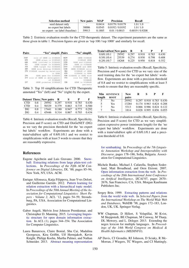
Selection method New pairs MAP Precision Recallseed dataset only - 0.0414 0.0179 / 0.0179 1.0 / 1.0
no expert but labels 30006 0.0545 0.0192 / 0.0192 1.0 / 1.0no expert - no label (baseline) 59913 0.1885 0.01 / 0.0015 0.6019 / 0.9208
Table 2: Extrinsic evaluation results for the CTD therapeutic dataset. The experiment parameters are the same asthose given in table 1. Precision figures are given as ‘top 100 / top 1000’ and similarly for recall.
Pairs “Yes” simplif.3345 role of GENE in DISEASE
839 GENE plays in DISEASE648 GENE involved in DISEASE321 GENE target in DISEASE318 GENE target for DISEASE289 GENE mice develop DISEASE279 DISEASE caused by mutations
in GENE276 GENE gene for DISEASE273 role of GENE in development
of DISEASE237 GENE promotes DISEASE
Pairs “No” simplif.6629 GENE DISEASE4110 DISEASE GENE3350 GENE and DISEASE2370 GENE in DISEASE2333 DISEASE and GENE1228 GENE DISEASE cells904 DISEASE of GENE879 DISEASE in GENE638 DISEASE in GENE mice572 role for GENE in
DISEASE528 GENE in DISEASE
patients
Table 3: Top 10 simplifications for CTD Therapeuticannotated “Yes” (left) and “No” (right) by the expert.
Dataset Thres. New pairs R S P FCTD 0.8 29592 0.297 0.918 0.783 0.430CTD 0.4 50329 0.379 0.863 0.735 0.500DG 0.8 17441 0.180 0.947 0.773 0.292DG 0.4 45446 0.314 0.867 0.703 0.434
Table 4: Intrinsic evaluation results (Recall, Specificity,Precision and F-score) on CTD and DisGeNET (DG)as we vary the precision threshold for the ‘no expertbut labels’ workflow. Experiments are done with atrain/valid/test split of 0.8/0.1/0.1 and we restrict tosimplifications with at least 5 words to ensure that theyare reasonably expressive.
ReferencesEugene Agichtein and Luis Gravano. 2000. Snow-
ball: Extracting relations from large plain-text col-lections. In Proceedings of the Fifth ACM Con-ference on Digital Libraries, DL ’00, pages 85–94,New York, NY, USA. ACM.
Enrique Alfonseca, Katja Filippova, Jean-Yves Delort,and Guillermo Garrido. 2012. Pattern learning forrelation extraction with a hierarchical topic model.In Proceedings of the 50th Annual Meeting of the As-sociation for Computational Linguistics: Short Pa-pers - Volume 2, ACL ’12, pages 54–59, Strouds-burg, PA, USA. Association for Computational Lin-guistics.
Gabor Angeli, Melvin Jose Johnson Premkumar, andChristopher D. Manning. 2015. Leveraging linguis-tic structure for open domain information extrac-tion. In ACL (1), pages 344–354. The Associationfor Computer Linguistics.
Laura Banarescu, Claire Bonial, Shu Cai, MadalinaGeorgescu, Kira Griffitt, Ulf Hermjakob, KevinKnight, Philipp Koehn, Martha Palmer, and NathanSchneider. 2013. Abstract meaning representation
Train/val/test New pairs R S P F0.8/0.1/0.1 29592 0.297 0.918 0.783 0.4300.5/0.1/0.4 25539 0.274 0.930 0.798 0.4080.2/0.1/0.7 18268 0.225 0.950 0.818 0.352
Table 5: Intrinsic evaluation results (Recall, Specificity,Precision and F-score) for CTD as we vary size of theseed training data for the ‘no expert but labels’ work-flow. Experiments are done with a precision thresholdof 0.8 and we restrict to simplifications with at least 5words to ensure that they are reasonably specific.
Minlength
SENTENCEROOT
Newpairs
R S P F
5 No 29592 0.297 0.918 0.783 0.4305 Yes 13284 0.174 0.963 0.824 0.2887 No 5313 0.066 0.986 0.824 0.1227 Yes 1814 0.028 0.995 0.856 0.055
Table 6: Intrinsic evaluation results (Recall, Specificity,Precision and F-score) for CTD as we vary simplifi-cation expressive power (minimum length) for the ‘noexpert but labels’ workflow. Experiments are donewith a train/valid/test split of 0.8/0.1/0.1 and a preci-sion threshold of 0.8.
for sembanking. In Proceedings of the 7th Linguis-tic Annotation Workshop and Interoperability withDiscourse, pages 178–186, Sofia, Bulgaria. Associ-ation for Computational Linguistics.
Michele Banko, Michael J. Cafarella, Stephen Soder-land, Matt Broadhead, and Oren Etzioni. 2007.Open information extraction from the web. In Pro-ceedings of the 20th International Joint Conferenceon Artifical Intelligence, IJCAI’07, pages 2670–2676, San Francisco, CA, USA. Morgan KaufmannPublishers Inc.
Sergey Brin. 1999. Extracting patterns and relationsfrom the world wide web. In Selected Papers fromthe International Workshop on The World Wide Weband Databases, WebDB ’98, pages 172–183, Lon-don, UK, UK. Springer-Verlag.
WW Chapman, D Hillert, S Velupillai, M Kvist,M Skeppstedt, BE Chapman, M Conway, M Tharp,DL Mowery, and L. Deleger. 2013. Extending thenegex lexicon for multiple languages. In Proceed-ings of the 14th World Congress on Medical &Health Informatics (MEDINFO).
AP Davis, CJ Grondin, RJ Johnson, D Sciaky, R Mc-Morran, J Wiegers, TC Wiegers, and CJ Mattingly.
150
2018. The comparative toxicogenomics database:update 2019. Nucleic Acids Res.
Anthony Fader, Stephen Soderland, and Oren Etzioni.2011. Identifying relations for open information ex-traction. In Proceedings of the Conference on Em-pirical Methods in Natural Language Processing,EMNLP ’11, pages 1535–1545, Stroudsburg, PA,USA. Association for Computational Linguistics.
MA Greenwood and Mark Stevenson. 2006. Improv-ing semi-supervised acquisition of relation extrac-tion patterns. In Proceedings of the Workshop on In-formation Extraction Beyond The Document, IEBe-yondDoc ’06, pages 29–35, Stroudsburg, PA, USA.Association for Computational Linguistics.
Yankai Lin, Zhiyuan Liu, Shiqi Shen, Huanbo Luan,and Maosong Sun. 2016. Neural relation extractionwith selective attention over instances. In Proceed-ings of the 54th Annual Meeting of the Associationfor Computational Linguistics (Volume 1: Long Pa-pers), pages 2124–2133. Association for Computa-tional Linguistics.
Mausam, Michael Schmitz, Robert Bart, StephenSoderland, and Oren Etzioni. 2012. Open languagelearning for information extraction. In Proceedingsof the 2012 Joint Conference on Empirical Methodsin Natural Language Processing and ComputationalNatural Language Learning, EMNLP-CoNLL ’12,pages 523–534, Stroudsburg, PA, USA. Associationfor Computational Linguistics.
George Miller. 1995. Wordnet A lexical database forEnglish. Communications of ACM, 38(11):39–41.
Thahir P Mohamed, Estevam R Hruschka Jr, andTom M Mitchell. 2011. Discovering relations be-tween noun categories. In Proceedings of the Con-ference on Empirical Methods in Natural LanguageProcessing, pages 1447–1455. Association for Com-putational Linguistics.
Ndapandula Nakashole, Gerhard Weikum, andFabian M. Suchanek. 2012. Discovering and explor-ing relations on the web. PVLDB, 5(12):1982–1985.
Bethany Percha and Russ B. Altman. 2018. A globalnetwork of biomedical relationships derived fromtext. Bioinformatics, 34(15):2614–2624.
Janet Pinero, Alex Bravo, Nuria Queralt-Rosinach,Alba Gutierrez-Sacristan, Jordi Deu-Pons, EmilioCenteno, Javier Garcia-Garcia, Ferran Sanz, andLaura I. Furlong. 2016. Disgenet: a comprehensiveplatform integrating information on human disease-associated genes and variants. Nucl. Acids Res.
Alexander Ratner, Christopher De Sa, Sen Wu, DanielSelsam, and Christopher Ré. 2016. Data Program-ming: Creating Large Training Sets, Quickly. arXive-prints, page arXiv:1605.07723.
Theo Trouillon, Christopher R Dance, Johannes Welbl,Sebastian Riedel, Eric Gaussier, and GuillaumeBouchard. 2017. Knowledge graph completion viacomplex tensor factorization. JMLR.
Paroma Varma and Christopher Ré. 2018. Snuba: Au-tomating weak supervision to label training data.Proc. VLDB Endow., 12(3):223–236.
P Verga, E Strubell, and A McCallum. 2018. Si-multaneously self-attending to all mentions for full-abstract biological relation extraction. In NorthAmerican Chapter of the Association for Computa-tional Linguistics (NAACL).
Feiyu Xu, Hans Uszkoreit, and Hong Li. 2007. A seed-driven bottom-up machine learning framework forextracting relations of various complexity. In ACL,pages 584–591.
151
Proceedings of the BioNLP 2019 workshop, pages 152–164Florence, Italy, August 1, 2019. c©2019 Association for Computational Linguistics
First Steps towards a Medical Lexicon for Spanishwith Linguistic and Semantic Information
Leonardo Campillos-LlanosComputational Linguistics Laboratory, Universidad Autónoma de Madrid
Abstract
We report the work-in-progress of collectingMedLexSp, an unified medical lexicon forthe Spanish language, featuring terms and in-flected word forms mapped to Unified MedicalLanguage System (UMLS) Concept UniqueIdentifiers (CUIs), semantic types and groups.First, we leveraged a list of term lemmas andforms from a previous project, and mappedthem to UMLS terms and CUIs. To en-rich the lexicon, we used both domain-corpora(e.g. Summaries of Product Characteristicsand MedlinePlus) and natural language pro-cessing techniques such as string distancemethods or generation of syntactic variants ofmulti-word terms. We also added term vari-ants by mapping their CUIs to missing itemsavailable in the Spanish versions of standardthesauri (e.g. Medical Subject Headings andWorld Health Organization Adverse Drug Re-actions terminology). We enhanced the vo-cabulary coverage by gathering missing termsfrom resources such as the Anatomical Thera-peutical Classification, the National Cancer In-stitute (NCI) Dictionary of Cancer Terms, Or-phaData, or the Nomenclátor de Prescripciónfor drug names. Part-of-Speech informationis being included in the lexicon, and the cur-rent version amounts up to 76 454 lemmas and203 043 inflected forms (including conjugatedverbs, number and gender variants), corre-sponding to 30 647 UMLS CUIs. MedLexSpis distributed freely for research purposes.
1 Introduction
Current machine-learning and deep-learning-based methods are data-intensive; however, in do-mains such as Medicine, sufficient data are not al-ways available—due to ethical concerns or privacyissues, especially when dealing with Patient Pro-tected Information. Moreover, some tasks demandhigh precision outcomes, which either need super-vised approaches with annotated data or hybrid
methods (e.g. rule-based and dictionary-based).In order to overcome the data bottleneck, richly-structured terminological thesauri enhance the an-notation and concept normalization of domain cor-pora to be used subsequently in supervised mod-els. More importantly, to achieve comparablebenchmarks, domain resources should integratestandard terminologies and coding schemes.
In this context, we aim at providing a computa-tional lexicon to be used in the pre-processing oftext data used in more complex Natural LanguageProcessing (NLP) tasks. The work here presentedreports the first steps towards building the Medi-cal Lexicon for Spanish (MedLexSp). MedLexSpis conceived as an unified resource with linguis-tic information (lemmas, inflected forms and part-of-speech), concepts mapped to Unified MedicalLanguage System R© (hereafter, UMLS) (Boden-reider, 2004) Concept Unique Identifiers (CUIs),and semantic information (UMLS types andgroups). Figure 1 is a sample of the lexicon.MedLexSp is firstly aimed at named entity recog-nition (NER), and it can be used in the pre-annotation step of an NER pipeline. It can alsohelp lemmatization and feed general-purpose Part-of-Speech taggers applied to medical texts—asdone in previous works (Oronoz et al., 2013).1 Be-cause it gathers semantic data of terms, it can easerelation extraction tasks.
Our work makes several contributions. Weprovide a resource to be distributed for researchpurposes in the BioNLP community. MedLexSpincludes inflected forms (singular/plural, mascu-line/feminine) and conjugated verb forms of termlemmas, which are mapped to UMLS ConceptUnique Identifiers. Verb terms are also mappedto Concept Unique Identifiers; this is the line ofcurrent works for expanding terminologies by in-
1https://zenodo.org/record/2621286
152
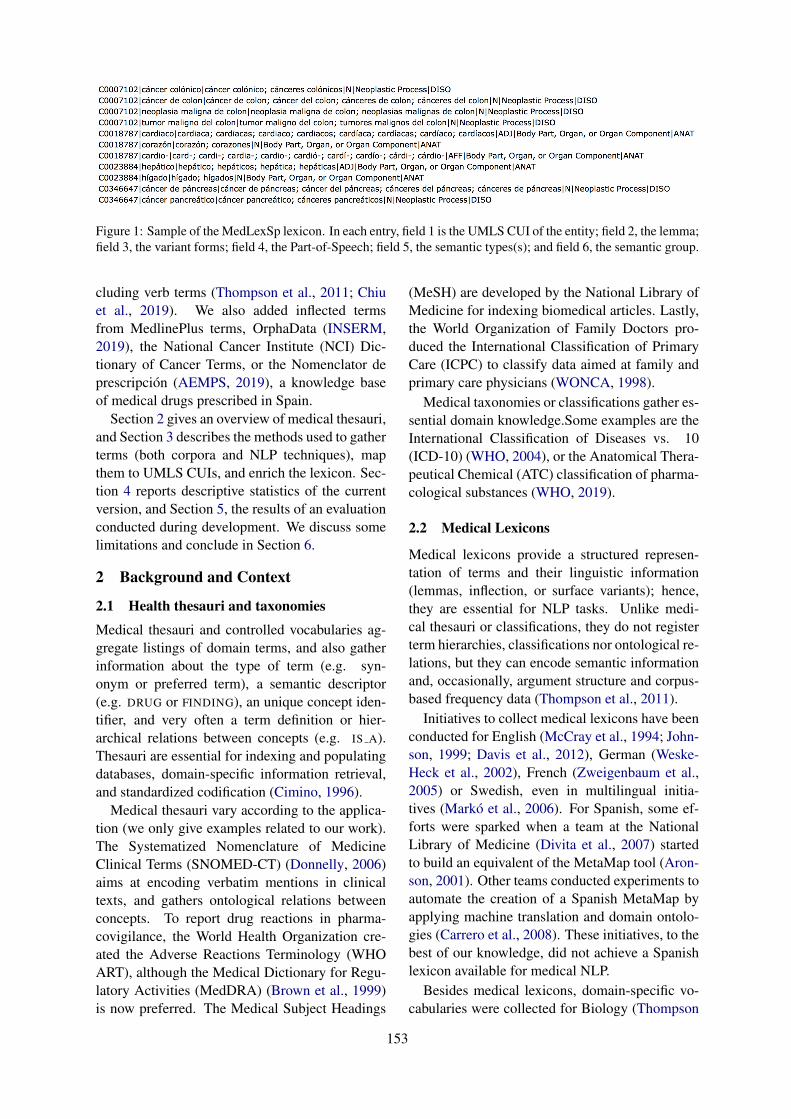
Figure 1: Sample of the MedLexSp lexicon. In each entry, field 1 is the UMLS CUI of the entity; field 2, the lemma;field 3, the variant forms; field 4, the Part-of-Speech; field 5, the semantic types(s); and field 6, the semantic group.
cluding verb terms (Thompson et al., 2011; Chiuet al., 2019). We also added inflected termsfrom MedlinePlus terms, OrphaData (INSERM,2019), the National Cancer Institute (NCI) Dic-tionary of Cancer Terms, or the Nomenclator deprescripción (AEMPS, 2019), a knowledge baseof medical drugs prescribed in Spain.
Section 2 gives an overview of medical thesauri,and Section 3 describes the methods used to gatherterms (both corpora and NLP techniques), mapthem to UMLS CUIs, and enrich the lexicon. Sec-tion 4 reports descriptive statistics of the currentversion, and Section 5, the results of an evaluationconducted during development. We discuss somelimitations and conclude in Section 6.
2 Background and Context
2.1 Health thesauri and taxonomies
Medical thesauri and controlled vocabularies ag-gregate listings of domain terms, and also gatherinformation about the type of term (e.g. syn-onym or preferred term), a semantic descriptor(e.g. DRUG or FINDING), an unique concept iden-tifier, and very often a term definition or hier-archical relations between concepts (e.g. IS A).Thesauri are essential for indexing and populatingdatabases, domain-specific information retrieval,and standardized codification (Cimino, 1996).
Medical thesauri vary according to the applica-tion (we only give examples related to our work).The Systematized Nomenclature of MedicineClinical Terms (SNOMED-CT) (Donnelly, 2006)aims at encoding verbatim mentions in clinicaltexts, and gathers ontological relations betweenconcepts. To report drug reactions in pharma-covigilance, the World Health Organization cre-ated the Adverse Reactions Terminology (WHOART), although the Medical Dictionary for Regu-latory Activities (MedDRA) (Brown et al., 1999)is now preferred. The Medical Subject Headings
(MeSH) are developed by the National Library ofMedicine for indexing biomedical articles. Lastly,the World Organization of Family Doctors pro-duced the International Classification of PrimaryCare (ICPC) to classify data aimed at family andprimary care physicians (WONCA, 1998).
Medical taxonomies or classifications gather es-sential domain knowledge.Some examples are theInternational Classification of Diseases vs. 10(ICD-10) (WHO, 2004), or the Anatomical Thera-peutical Chemical (ATC) classification of pharma-cological substances (WHO, 2019).
2.2 Medical Lexicons
Medical lexicons provide a structured represen-tation of terms and their linguistic information(lemmas, inflection, or surface variants); hence,they are essential for NLP tasks. Unlike medi-cal thesauri or classifications, they do not registerterm hierarchies, classifications nor ontological re-lations, but they can encode semantic informationand, occasionally, argument structure and corpus-based frequency data (Thompson et al., 2011).
Initiatives to collect medical lexicons have beenconducted for English (McCray et al., 1994; John-son, 1999; Davis et al., 2012), German (Weske-Heck et al., 2002), French (Zweigenbaum et al.,2005) or Swedish, even in multilingual initia-tives (Markó et al., 2006). For Spanish, some ef-forts were sparked when a team at the NationalLibrary of Medicine (Divita et al., 2007) startedto build an equivalent of the MetaMap tool (Aron-son, 2001). Other teams conducted experiments toautomate the creation of a Spanish MetaMap byapplying machine translation and domain ontolo-gies (Carrero et al., 2008). These initiatives, to thebest of our knowledge, did not achieve a Spanishlexicon available for medical NLP.
Besides medical lexicons, domain-specific vo-cabularies were collected for Biology (Thompson
153
et al., 2011). With a different perspective and goal,Consumer Health Vocabularies have been col-lected to bridge the gap between patients’ expres-sions and healthcare professionals’ jargon (Zengand Tse, 2006; Keselman et al., 2007).
2.3 The Unified Medical Language SystemThe Unified Medical Language System R©
(UMLS) (Bodenreider, 2004) MetaThesaurusincludes thesauri. The version we used (2018AB)gathers 210 sources and over 3.82 millions ofconcepts in 23 languages. Synonym terms areencoded with Concept Unique Identifiers (CUIs);and concepts are assigned a semantic type andgroup (McCray et al., 2001).
2.4 Methods for Creating Medical LexiconsWe will restrict us here to a shallow overview ofapproaches and will not consider taxonomy norontology building. Methods for widening medi-cal vocabularies range from generating syntactic-level variants of multi-word terms (Jacquemin,1999), inferring derivation rules from string sim-ilarity matches and morphological relations be-tween derivational variants (Grabar and Zweigen-baum, 2000), gathering inflected variants semi-automatically (Cartoni and Zweigenbaum, 2010),or deriving terms from corpora (more below).
Graeco-Latin components are very productivefor coining medical terms; thus, several BioNLPsystems integrate morphology-based lexical re-sources. For example, for decomposing termsmorphosemantically and deriving their defini-tions (Namer and Zweigenbaum, 2004), or map-ping queries to concepts and indexing documentsin cross-lingual information retrieval, based on asubword-based morpheme thesaurus (Markó et al.,2005). In this line, generating paraphrase equiv-alents of neoclassical compounds (e.g. thyrome-galia→ enlarged thyroid) is an approach with po-tential for deriving new terms, and concept nor-malization systems (Thompson and Ananiadou,2018) already implement it. Because string simi-larity measures and edit distance patterns are usedfor normalization—e.g (Tsuruoka et al., 2007;Kate, 2015)—and terminology mapping (Dziadeket al., 2017), these approaches are also powerfulfor expanding medical lexicons from a set of ref-erence terms. Decomposition of multi-word termsand synonym expansion of their components arealso alternative strategies applied in normalizationsystems (Tseytlin et al., 2016).
Corpus-derived medical terminology construc-tion requires collecting domain texts and applyingterm extraction methods, among others: comput-ing graphs of relations between parse trees andword dependency similarities (Nazarenko et al.,2001), using parallel corpora to map cognates oraligned words (Sbrissia et al., 2004; Deléger et al.,2009), linking terms or abbreviations to their def-initions or expanded word forms in the text wherethey occur (Yu and Agichtein, 2003; McCrae andCollier, 2008), using dictionary features to iden-tify polysemy (Pezik et al., 2008), combiningtext mining techniques with databases (Thomp-son et al., 2011), or having experts review terms,a method which has been used to build disease-specific vocabularies (Wang et al., 2016).
Approaches based on the Firthian Distribu-tional hypothesis exploit distributional similaritymetrics (Carroll et al., 2012). Among them, morerecent distributional semantics methods representterms in the vector space, or calculate word-embeddings to compute similarity measures be-tween vectors, thus allowing the unsupervised ex-pansion of domain terms (Pyysalo et al., 2013;Skeppstedt et al., 2013; Henriksson et al., 2014;Wang et al., 2015; Ahltorp et al., 2016; Segura-Bedmar and Martı́nez, 2017) or concept normal-ization (Limsopatham and Collier, 2016).
Lastly, to develop Consumer Health Vocabular-ies (CHV), a variety of techniques have been used:analysis by experts of Medline queries (Zengand Tse, 2006), term recognition methods andcollaborative review of user logs in medicalsites (Zeng et al., 2007), hybrid methods com-bining n-grams extraction, the C-value, and dic-tionary look-up (Doing-Harris and Zeng-Treitler,2011), co-occurrence analysis of terms and seedwords (Jiang and Yang, 2013), or approachesbased of similarity measures between CHV lexi-cons and reference lexicons (Seedorff et al., 2013).
3 Methods
Figure 2 depicts the methods used to collect theMedLexSp lexicon. In a first step (left part of Fig-ure 2), we leveraged the lemmas and word formsobtained from a Spanish medical lexicon, mostlycorpus-derived; we will refer to it as the base list.We only used the subset of lemmas and forms thatcould be mapped authomatically to UMLS CUIs(exact string match). In a second step, we addedmissing variants of terms using different methods:
154
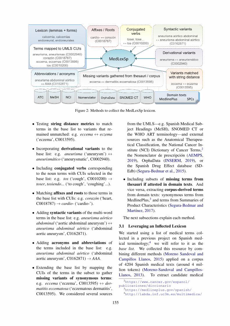
Figure 2: Methods to collect the MedLexSp lexicon.
• Testing string distance metrics to matchterms in the base list to variants that re-mained unmatched: e.g. eccema ↔ eczema(’eczema’, C0013595).
• Incorporating derivational variants to thebase list: e.g. aneurisma (‘aneurysm’) ↔aneurismático (‘aneurysmatic’, C0002940).
• Including conjugated verbs correspondingto the noun terms with CUIs selected in thebase list: e.g. tos (‘cough’, C0010200) →toser, tosiendo... (‘to cough’, ‘coughing’...).
• Matching affixes and roots to those terms inthe base list with CUIs: e.g. corazón (‘heart,C0018787)→ cardio- (‘cardio-’).
• Adding syntactic variants of the multi-wordterms in the base list: e.g. aneurisma aórticoabdominal (‘aortic abdominal aneurysm’)↔aneurisma abdominal aórtico (‘abdominalaortic aneurysm’, C0162871).
• Adding acronyms and abbreviations ofthe terms included in the base list: e.g.aneurisma abdominal aórtico (‘abdominalaortic aneurysm’, C0162871)→ AAA.
• Extending the base list by mapping theCUIs of the terms in the subset to gathermissing variants of synonymous terms:e.g. eccema (‘eczema’, C0013595) ↔ der-matitis eccematosa (‘eczematous dermatitis’,C0013595). We considered several sources
from the UMLS—e.g. Spanish Medical Sub-ject Headings (MeSH), SNOMED CT orthe WHO ART terminology—and externalsources such as the Anatomical Therapeu-tical Classification, the National Cancer In-stitute (NCI) Dictionary of Cancer Terms,2
the Nomenclator de prescripción (AEMPS,2019), OrphaData (INSERM, 2019), orthe Spanish Drug Effect database (SD-Edb) (Segura-Bedmar et al., 2015).
• Including subsets of missing terms fromthesauri if attested in domain texts. Andvice versa, extracting corpus-derived termsfrom domain texts: synonymous terms fromMedlinePlus,3 and terms from Summaries ofProduct Characteristics (Segura-Bedmar andMartı́nez, 2017).
The next subsections explain each method.
3.1 Leveraging an Inflected LexiconWe started using a list of medical terms col-lected in a previous project on Spanish med-ical terminology;4 we will refer to it as thebase list. We collected this resource by com-bining different methods (Moreno Sandoval andCampillos Llanos, 2015) applied on a corpusof 4204 Spanish medical texts (around 4 mil-lion tokens) (Moreno-Sandoval and Campillos-Llanos, 2013). To extract candidate medical
2https://www.cancer.gov/espanol/publicaciones/diccionario
3https://medlineplus.gov/spanish/4http://labda.inf.uc3m.es/multimedica/
155
terms for the base list, we combined rule-basedtechniques (Part-of-Speech tagging and filteringthrough medical affixes), corpus-based methods(comparing word forms from a general corpus andfrom the domain corpus), and statistical methods,namely the Log-Likelihood ratio (Dunning, 1993).We checked in medical sources—e.g. the dictio-nary published by the Spanish Royal Academy ofMedicine (RANME, 2011)—the terms selected bymeans of those three methods, before being in-cluded in the list. This base list was used to buildan automatic term extractor (Campillos Llanoset al., 2013), and amounted to 38 354 entries.
Because one of the goals of MedLexSp isconcept normalization by using standard domainterminologies, we did not include the full baselist. We only used terms that could be assignedUMLS Concept Unique Identifiers (CUIs) in theUMLS MetaThesaurus version 2018AB, namelyfrom those terminologies of special biomedical orclinical interest (e.g. SNOMED CT, WHO ART orMedical Subject Headings) with available Span-ish translations. We mapped 18 263 lemmas toCUIs, which means 47.61% entries of the originallexicon. CUIs were assigned according to an ex-act match criterion. For example, donación (‘do-nation’) is not matched with donación de tejido(‘Tissue Donation’, C0080231), because the lattermakes reference to a donation subtype. Note thatthe current version of MedLexSp does not includethe full list of terms from MeSH or SNOMED CT,but only those which were originally mapped fromthe base list to UMLS terms with CUIs.
3.2 Enriching the Lexicon
String distance metrics We tested mappingterms from the subset of entities with CUIs toterms in the UMLS by applying distance met-rics (Levenshtein, 1966) of less than 2. This al-lowed us mapping hyphenated variants to termswithout hyphen (e.g. creatina-cinasa ↔ creatinacinasa, ‘creatine kinase’, C0010287), compoundterms that are often written as single-words (dietiléter ↔ dietiléter, ‘diethyl ether’, C0014994), ormatching terms with minimal morphological vari-ation (eccema ↔ eczema, ‘eczema’, C0013595).A total of 1463 terms with CUIs were matched tothe original base list.
Derivational variants In line with previouswork (Grabar and Zweigenbaum, 2000), we col-lected a list of equivalent derivational variants of
terms. Using this list, we assigned a CUI to thecorresponding derivational variant: e.g. the CUIof páncreas (C0030274) was also ascribed to pan-creático (‘pancreatic’). The current version gath-ers a total of 801 derivational variants with CUIs.
Conjugated verbs Most terms in the UMLSor standard terminologies are noun or adjectivephrases. This limits the named entity recogni-tion of medical concepts expressed with verbs infree text; given a context such as el paciente tose(‘the patient coughs’), the concept of ‘coughing’would not be identified. To widen the scope ofconcept normalization, verb terms were mappedto CUIs from derived nouns: e.g. tos (‘cough-ing’, C0010200)→ toser (‘to cough’, C0010200).We again used a list of correspondences betweenverbs and deverbal nouns. We included the conju-gated forms of verb lemmas in each verb entry ofthe lexicon. We used a python script that relieson the lexicon of a Spanish Part-of-Speech tag-ger (Moreno Sandoval and Guirao, 2006) to gener-ate all conjugated forms of verb terms: e.g. toser(‘to cough’) → tose (‘he/she coughs’), tosiendo(‘coughing’), etc. The current version includes atotal of 295 single- or multi-word verb items.
Affixes and lexical roots In a first step, wecollected affixes and roots from several sources.Firstly, we leveraged a list used in a previous ex-periment (Sandoval et al., 2013). This list amountsto 1719 forms and considers morphological vari-ants of affixes (e.g. prefix cardio- may have ac-cented variant forms in Spanish, such as cardió-).Secondly, we translated to Spanish several affixesand roots from the Specialist Lexicon R© (McCrayet al., 1994) and then added variant forms. In asecond step, we assigned UMLS CUIs to affixesand roots in the list. The current list gathers a totalof 161 entries (82 prefixes and 79 suffixes) with134 different CUIs and 386 variant forms. Notethat many affixes and roots were not included be-cause they are too underspecified to be assigned toa CUI, or are not restricted to the medical domain(e.g. kilo- expresses a quantitative concept).
Abbreviations and acronyms Firstly, we gath-ered a list of equivalences between full formsand abbreviations and acronyms; we used threesources: 1) the collection of Spanish abbre-viations and acronyms used in hospitals, col-lected by medical doctors (Yetano and Alberola,2003); 2) abbreviations and acronyms used in
156
the 2nd IberEval Challenge 2018 on Biomedi-cal Abbreviation Recognition and Resolution (In-txaurrondo et al., 2018); and 3) Spanish abbre-viations and acronyms from Wikipedia.5 Sec-ondly, we matched the resulting list of equivalentterms (acronyms and full forms) to UMLS terms,adding the corresponding CUIs to those miss-ing acronyms. For example, the full term virusde Epstein-Barr (‘Epstein-Barr virus’) has CUIC0014644, and we also assigned this code to thecorresponding acronym in Spanish (VEB). Withthis method, we assigned CUIs to 1225 items.
Syntactic variants of terms To widen the cov-erage of terms mapped to CUIs, we generatedvariants of multiword entities by swapping theword order of their components. Then, we triedto match each new variant to entities with CUIs.For example, aneurisma aórtico abdominal (‘aor-tic abdominal aneurysm’) has CUI C0162871, andwe assigned the same CUI to the generated variantaneurisma abdominal aórtico (‘abdominal aorticaneurysm’). With this method, we gathered a totalof 154 variants of terms with CUIs in the base list.
Mapping UMLS term variants through CUIsWe gathered synonymous variants referring toeach corresponding concept by using the UMLSCUIs from the terms included in the base list. Toavoid including noisy terms adequate for biomedi-cal natural language processing, we first cleanedthe terms from the terminologies we used. Todo so, we applied methods for cleaning termstrings (Aronson et al., 2008; Hettne et al., 2010;Névéol et al., 2012; Hellrich et al., 2015). Wedeleted paraphrastic terms that include a descrip-tion or specification of the entity type in theterm string. These terms commonly come fromSpanish SNOMED CT. For example, we deletedtos (hallazgo), ‘cough (finding)’ (CUI C0010200)and kept the term (cough, ‘cough’). Likewise,we removed most anatomic terms beginning withestructura de (‘structure of’): e.g. regardingterm estructura del ojo (‘structure of eyeball’,C0015392), we only kept the synonym ojo (‘eye-ball’). Lastly, terms in the WHO ART terminol-ogy needed to be accented and reversed regardingword order: e.g. disociativa, reaccion→ reaccióndisociativa (’dissociative reaction’, C0012746).
We also applied an exact-match mapping of
5https://es.wikipedia.org/wiki/Anexo:Acrnimos_en_medicina
Spanish terms from the base list to the Englishcomponent of the UMLS. This method allowedus to obtain the CUIs of terms unavailable inSpanish terminologies, which remain unchangedin the Spanish language. Namely, Latin scien-tific names (e.g. Campylobacter fetus, C0006814),compound terms with Graeco-Latin roots (e.g. ab-dominalgia, C0000737), English acronyms thatare broadly used in the medical discourse with-out Spanish translation (e.g. GABA, ‘gamma-aminobutyric acid’, C0016904), or internationalbrand drug names (e.g. abilify R©). In these cases,the same word is used in both English and Spanish.We manually revised the list of mapped terms todiscard homonymous terms with a different mean-ing in English (e.g. TIP R© is a brand name of amedical drug, but it also means ‘point’ or ‘sugges-tion’ in English).
We extended the list of terms by extractingthe information related to rare diseases fromOrphaData (INSERM, 2019).6 We also addedterms of pharmacological substances and inter-national non-proprietary names from the SpanishDrug Effect database (SDEdb) (Segura-Bedmaret al., 2015) and the Nomenclator de pre-scripción (AEMPS, 2019), a resource publishedand updated regularly by the Spanish Agency ofDrugs and Food Products.7
For all these procedures and sources, we appliedsemiautomatic methods to generate the singularand plural inflected forms of the missing terms thatwere mapped through CUIs. We used the Patternpython library (Smedt and Daelemans, 2012) tocreate plural forms of terms, which were revisedmanually before being included in MedLexSp.
Corpus-derived terms When we started addingvariant terms from thesauri, the question of whereto stop adding terms came up. In the first version,we decided not to include all terms available inMeSH or SNOMED CT terminologies, given thatthese thesauri contain terms that are often not nec-essary in clinical or biomedical NER tasks (e.g.names of trees, wild animals, professions or ab-stract concepts). On the other hand, to make the
6http://www.orphadata.org/data/xml/es_product1.xml We make availablethe script used to extract terms from OrphaData:https://github.com/lcampillos/bionlp2019The code can be adapted to process OrphaData in otherlanguages (e.g. English, French, Italian or Portuguese).
7http://listadomedicamentos.aemps.gob.es/prescripcion.zip.
157
resource comprehensive, we needed to comple-ment the base list with supplementary terms fromthesauri. Hence, in order to decide which items toinclude in a first version, we computed term fre-quencies using a medical corpus from a previousproject (4 million tokens) (Moreno-Sandoval andCampillos-Llanos, 2013). We currently includeterms from the Spanish MeSH and SNOMED CTthat were missing in the base list, if they were doc-umented in that corpus. By limiting the inclusionof such subset of terms, we aim at providing qual-ity enriched data (i.e. with revised inflected forms)in a reasonable time and manner.
In a different vein, and similarly to for-mer work (Calleja et al., 2017), we extractedterms from Summaries of Product Characteristics(SPCs). We used Easy Drug Package Leaflets(EasyDPL), a corpus of 306 texts annotated withmedical drugs and pathological entities (1400 drugeffects) (Segura-Bedmar and Martı́nez, 2017). Weannotated these texts and compared our output an-notation with regard to this dataset. We used apurely dictionary-based named-entity recogniserwith modules for normalization (e.g. lower-casing), tokenization and lemmatization, imple-mented in spaCy;8 then, the MedLexSp lexiconwas used for exact string matching. We did not usepre- or post-processing rules in the current version(e.g. rules of term composition).
In several iterative rounds, we annotated thetexts, identified the unannotated entities, andadded them to the lexicon. We did not add (al-though annotated in the corpus) entities withouta CUI, e.g. coordinated entities (e.g. pies ymanos frı́as, ‘cold hands and feet’) or too spe-cific, post-modified terms (e.g. dolor de cabezaintenso, ‘intense headache’; only ‘headache’ hasCUI C0018681). By using SPCs, we added 837term entries to MedLexSp, and we ensure that itincludes common terms referring to adverse drugreactions and medical drugs.
Lastly, for Consumer Health Vocabulary terms,we extracted synonyms in MedlinePlus Spanish.This resource provides terms in patient languagethat were missing: e.g. ojo vago (‘lazy eye’) is asynonym of ambliopı́a (‘amblyopia’, C0002418).We added 783 term entries from this resource. Inaddition, we collected 6110 cancer-related termsfrom the Spanish version of the National CancerInstitute Dictionary.
8https://spacy.io/
3.3 Semantic and linguistic information
We added to each CUI and lexical entry the cor-responding semantic type(s) and group from theUMLS. To avoid noise when annotating biomed-ical texts semantically, we disfavoured semantictypes of the semantic group Concepts and Ideas(CONC, e.g. Quantitative Concept, FunctionalConcept or Qualitative Concept), which are ratherunspecified. We only included terms from thatgroup if no other semantic label was available.If a concept or term can be assigned to two dif-ferent groups, the element labelled with CONCis not included in our lexicon. For example,the term inhalación (‘inhalation’) can be relatedto concept C0004048 (semantic type OrganismFunction, and group PHYS) and also to con-cept C4521689 (semantic type Intellectual Prod-uct, and group CONC). In this case, we only pre-serve the lexical entry of concept C0004048 andwe rule out the entry of concept C4521689.
We have also started adding the Part-of-Speech(PoS) category of each entry in the lexicon. Formultiword terms, the category of the head term isselected; e.g. enfermedad de Crohn (‘Crohn’s dis-ease’) is categorized as N (‘noun’). We are cur-rently testing different techniques to predict thePoS and automate the assignment of categories toeach entry, which is still not fully satisfactory.
4 Statistics
Table 1 shows the count of entries in the lexiconaccording to each source or procedure applied tomap terms to UMLS CUIs. Note that the fullcount exceeds the count of term entries in the cur-rent version of MedLexSp, given that some termswere gathered through different methods simulta-neously. Table 2 shows the descriptive statisticsof the lexicon: counts of lemmas and word forms,and total number of CUIs. Lastly, Table 3 showsa preliminary count of PoS categories in the cur-rent version of the lexicon. Note that most entriesare nouns or need revision (UNKN stands for ‘un-known’); this task is currently being undertaken.
Finally, Figure 3 depicts the distribution of se-mantic groups. Of note, some groups are under-represented, due to the corpora and thesauri usedto collect terms. For example, few entities belongto the GENE group, which implies that the cov-erage of the current version of MedLexSp is notadequate for tasks in the Genomics domain.
The amount of lemmas/word forms is lower
158
Method # entriesAbbreviations / acronyms 1225Affixes / roots 161Derived adjectives 801Conjugated verb forms 295Base list mapped to UMLS CUIs:
Exact match to Spanish UMLS 18 263Exact match to English UMLS 2534String distance method 1463Syntactic variants 134
Terms from thesauri and corpora:ATC + Nomenclátor + SDEdb 2931ICD-10 1299ICPC 55MedDRA 5015MedlinePlus 783MeSH 6831NCI 6110OrphaData 10 741SNOMED CT 23 096SPCs (EasyDLP corpus) 837
Table 1: Count of lexical entries according to eachsource or procedure to map terms to UMLS CUIs.
Lemmas Forms CUIsSingle-words 23 572 23 592 -Multi-words 52 882 179 451 -Total 76 454 203 043 30 647
Table 2: Descriptive statistics of the lexicon
PoS Example CountN pancreas 58 830UNKN - 13 618ADJ abdominal 2283ADJ/N gemelo (‘twin’) 700NPR Filoviridae 549V toser (‘to cough’) 295AFF cardio- 161ADV gravemente (‘severely’) 20
Table 3: Preliminary counts of Part-of-Speech (PoS)categories. N: ‘noun’; UNKN: ‘unknown’; ADJ: ‘adjec-tive’; ADJ/N: a term that can be an adjective or a noun(depending on the context); NPR: ‘proper name’; AFF:‘affix’; ADV: ‘adverb’
than in other UMLS-based resources because: 1)we did not include the full thesauri, but only termsfrom the original base list that were mapped to
Figure 3: Distribution of semantic groups in the lexicon
UMLS CUIs; and 2) we cleaned noisy terms.As explained, descriptors and qualifiers were re-moved: e.g. SNOMED CT term fiebre (hal-lazgo) (‘fever (finding)’, C0015967) was short-ened to fiebre. We also ruled out some con-cepts belonging to semantic groups that we canbe noisy for clinical or medical NER tasks, suchas CONC or GEOG; e.g. hierro is related toconcept C0302583, ‘iron’, CHEM; or to conceptC0454671, ‘Island of Hierro’, GEOG (the latterconcept was discarded).
5 Development Evaluation
We analysed the coverage of the lexicon with re-gard to UMLS semantic groups. We applied thedictionary-based NER tool explained below to agold standard available in the community. We fo-cused on analysing the annotation of few UMLSgroups (DISO, CHEM, PROC and ANAT) andassessed how well the lexicon annotated themwith regard to the gold standard. We quanti-fied the matched annotations in terms of preci-sion, recall and F1-measure by using the BRAT-Eval script (Verspoor et al., 2013).
A first version of MedLexSp was evaluated withthe Spanish texts from the MANTRA corpus (Korset al., 2015), which gathers 100 texts from the Eu-ropean Medicines Agency (1961 tokens) and 100texts from Medline (1087 tokens). These texts areavailable in BRAT format and were annotated withUMLS CUIs, semantic types and groups. We pre-processed the annotated texts for mapping refer-ence annotations to UMLS semantic groups.
With this dataset, we achieved an overall F-measure of 0.83 (exact match) and of 0.87 (ap-proximate match), although the performance var-
159
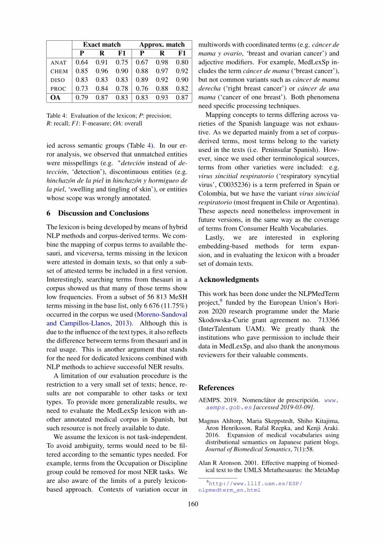
Exact match Approx. matchP R F1 P R F1
ANAT 0.64 0.91 0.75 0.67 0.98 0.80CHEM 0.85 0.96 0.90 0.88 0.97 0.92DISO 0.83 0.83 0.83 0.89 0.92 0.90PROC 0.73 0.84 0.78 0.76 0.88 0.82OA 0.79 0.87 0.83 0.83 0.93 0.87
Table 4: Evaluation of the lexicon; P: precision;R: recall; F1: F-measure; OA: overall
ied across semantic groups (Table 4). In our er-ror analysis, we observed that unmatched entitieswere misspellings (e.g. ∗deteción instead of de-tección, ‘detection’), discontinuous entities (e.g.hinchazón de la piel in hinchazón y hormigueo dela piel, ‘swelling and tingling of skin’), or entitieswhose scope was wrongly annotated.
6 Discussion and Conclusions
The lexicon is being developed by means of hybridNLP methods and corpus-derived terms. We com-bine the mapping of corpus terms to available the-sauri, and viceversa, terms missing in the lexiconwere attested in domain texts, so that only a sub-set of attested terms be included in a first version.Interestingly, searching terms from thesauri in acorpus showed us that many of those terms showlow frequencies. From a subset of 56 813 MeSHterms missing in the base list, only 6 676 (11.75%)occurred in the corpus we used (Moreno-Sandovaland Campillos-Llanos, 2013). Although this isdue to the influence of the text types, it also reflectsthe difference betweem terms from thesauri and inreal usage. This is another argument that standsfor the need for dedicated lexicons combined withNLP methods to achieve successful NER results.
A limitation of our evaluation procedure is therestriction to a very small set of texts; hence, re-sults are not comparable to other tasks or texttypes. To provide more generalizable results, weneed to evaluate the MedLexSp lexicon with an-other annotated medical corpus in Spanish, butsuch resource is not freely available to date.
We assume the lexicon is not task-independent.To avoid ambiguity, terms would need to be fil-tered according to the semantic types needed. Forexample, terms from the Occupation or Disciplinegroup could be removed for most NER tasks. Weare also aware of the limits of a purely lexicon-based approach. Contexts of variation occur in
multiwords with coordinated terms (e.g. cáncer demama y ovario, ‘breast and ovarian cancer’) andadjective modifiers. For example, MedLexSp in-cludes the term cáncer de mama (‘breast cancer’),but not common variants such as cáncer de mamaderecha (‘right breast cancer’) or cáncer de unamama (‘cancer of one breast’). Both phenomenaneed specific processing techniques.
Mapping concepts to terms differing across va-rieties of the Spanish language was not exhaus-tive. As we departed mainly from a set of corpus-derived terms, most terms belong to the varietyused in the texts (i.e. Peninsular Spanish). How-ever, since we used other terminological sources,terms from other varieties were included: e.g.virus sincitial respiratorio (‘respiratory syncytialvirus’, C0035236) is a term preferred in Spain orColombia, but we have the variant virus sincicialrespiratorio (most frequent in Chile or Argentina).These aspects need nonetheless improvement infuture versions, in the same way as the coverageof terms from Consumer Health Vocabularies.
Lastly, we are interested in exploringembedding-based methods for term expan-sion, and in evaluating the lexicon with a broaderset of domain texts.
Acknowledgments
This work has been done under the NLPMedTermproject,9 funded by the European Union’s Hori-zon 2020 research programme under the MarieSkodowska-Curie grant agreement no. 713366(InterTalentum UAM). We greatly thank theinstitutions who gave permission to include theirdata in MedLexSp, and also thank the anonymousreviewers for their valuable comments.
ReferencesAEMPS. 2019. Nomenclátor de prescripción. www.aemps.gob.es [accessed 2019-03-09].
Magnus Ahltorp, Maria Skeppstedt, Shiho Kitajima,Aron Henriksson, Rafal Rzepka, and Kenji Araki.2016. Expansion of medical vocabularies usingdistributional semantics on Japanese patient blogs.Journal of Biomedical Semantics, 7(1):58.
Alan R Aronson. 2001. Effective mapping of biomed-ical text to the UMLS Metathesaurus: the MetaMap
9http://www.lllf.uam.es/ESP/nlpmedterm_en.html
160
program. In Proc. of the AMIA Symposium, pages17–21. American Medical Informatics Association.
Alan R Aronson, James G Mork, Aurélie Névéol,Sonya E Shooshan, and Dina Demner-Fushman.2008. Methodology for creating UMLS contentviews appropriate for biomedical natural languageprocessing. In Proc. of the AMIA Annual Sympo-sium, pages 21–25. American Medical InformaticsAssociation.
Olivier Bodenreider. 2004. The Unified MedicalLanguage System (UMLS): integrating biomedi-cal terminology. Nucleic acids research, 32(suppl1):D267–D270.
Elliot G Brown, Louise Wood, and Sue Wood. 1999.The Medical Dictionary for Regulatory Activities(MedDRA). Drug safety, 20(2):109–117.
Pablo Calleja, Raúl Garcı́a-Castro, Guadalupe Aguado-de Cea, and Asunción Gómez-Pérez. 2017. Ex-panding SNOMED-CT through Spanish Drug Sum-maries of Product Characteristics. In Proc. ofthe Knowledge Capture Conference, pages 29–37.ACM.
L Campillos Llanos, A Moreno Sandoval, andJM Guirao. 2013. An automatic term extractor forbiomedical terms in Spanish. In Proc. of the 5th Int.Symposium on Languages in Biology and Medicine,Tokyo, Japan.
Francisco Carrero, José Carlos Cortizo, and José Marı́aGómez. 2008. Building a Spanish MMTx by usingautomatic translation and biomedical ontologies. InInternational Conference on Intelligent Data Engi-neering and Automated Learning, pages 346–353.Springer.
John Carroll, Rob Koeling, and Shivani Puri. 2012.Lexical acquisition for clinical text mining using dis-tributional similarity. In International Conferenceon Intelligent Text Processing and ComputationalLinguistics, pages 232–246. Springer.
Bruno Cartoni and Pierre Zweigenbaum. 2010. Semi-Automated Extension of a Specialized Medical Lex-icon for French. In Proc. of LREC, Valletta, Malta.
Billy Chiu, Olga Majewska, Sampo Pyysalo, LauraWey, Ulla Stenius, Anna Korhonen, and MarthaPalmer. 2019. A neural classification method forsupporting the creation of BioVerbNet. Journal ofBiomedical Semantics, 10(1):2:1–2:12.
James J Cimino. 1996. Coding systems in health care.Methods of information in medicine, 35(04/05):273–284.
Allan Peter Davis, Thomas C Wiegers, Michael CRosenstein, and Carolyn J Mattingly. 2012.MEDIC: a practical disease vocabulary used at theComparative Toxicogenomics Database. Database,2012.
Louise Deléger, Magnus Merkel, and Pierre Zweigen-baum. 2009. Translating medical terminologiesthrough word alignment in parallel text corpora.Journal of Biomedical Informatics, 42(4):692–701.
Guy Divita, Graciela Rosemblat, and Allen C Browne.2007. Building a Medical Spanish Lexicon. InProc. of the AMIA Symposium, page 941.
Kristina M Doing-Harris and Qing Zeng-Treitler. 2011.Computer-assisted update of a consumer health vo-cabulary through mining of social network data.Journal of Medical Internet Research, 13(2):e37.
Kevin Donnelly. 2006. SNOMED-CT: The advancedterminology and coding system for eHealth. Studiesin health technology and informatics, 121:279–290.
Ted Dunning. 1993. Accurate methods for the statisticsof surprise and coincidence. Computational linguis-tics, 19(1):61–74.
Juliusz Dziadek, Aron Henriksson, and Martin Duneld.2017. Improving terminology mapping in clinicaltext with context-sensitive spelling correction. In-formatics for Health: Connected Citizen-Led Well-ness and Population Health, 235:241.
Natalia Grabar and Pierre Zweigenbaum. 2000. A gen-eral method for sifting linguistic knowledge fromstructured terminologies. In Proc. of the AMIA Sym-posium, pages 310–314. American Medical Infor-matics Association.
Johannes Hellrich, Stefan Schulz, Sven Buechel, andUdo Hahn. 2015. Jufit: A configurable rule enginefor filtering and generating new multilingual UMLSterms. In Proc. of the AMIA Symposium, pages 604–610. American Medical Informatics Association.
Aron Henriksson, Hans Moen, Maria Skeppstedt, Vi-das Daudaravičius, and Martin Duneld. 2014. Syn-onym extraction and abbreviation expansion withensembles of semantic spaces. Journal of Biomedi-cal Semantics, 5(1):6–.
Kristina M Hettne, Erik M van Mulligen, Martijn JSchuemie, Bob JA Schijvenaars, and Jan A Kors.2010. Rewriting and suppressing UMLS terms forimproved biomedical term identification. Journal ofBiomedical Semantics, 1(1):5.
INSERM. 2019. Orphadata: Free access datafrom Orphanet. Data version (XML data ver-sion). http://www.orphadata.org [ac-cessed 2019-05-10].
Ander Intxaurrondo, Montserrat Marimón, AitorGonzález-Agirre, José Antonio López-Martı́n,H Rodrı́guez Betanco, J Santamarı́a, Marta Villegas,and Martin Krallinger. 2018. Finding mentionsof abbreviations and their definitions in SpanishClinical Cases: the BARR2 shared task evalua-tion results. In Proc. of IberEval@SEPLN 2018.SEPLN.
161
Christian Jacquemin. 1999. Syntagmatic and paradig-matic representations of term variation. In Proc. ofthe 37th Annual Meeting of the Association for Com-putational Linguistics, pages 341–348.
Ling Jiang and Christopher C Yang. 2013. Using co-occurrence analysis to expand consumer health vo-cabularies from social media data. In 2013 IEEE In-ternational Conference on Healthcare Informatics,pages 74–81. IEEE.
Stephen B Johnson. 1999. A semantic lexicon for med-ical language processing. Journal of the AmericanMedical Informatics Association, 6(3):205–218.
Rohit J Kate. 2015. Normalizing clinical terms usinglearned edit distance patterns. Journal of the Amer-ican Medical Informatics Association, 23(2):380–386.
Alla Keselman, Tony Tse, Jon Crowell, Allen Browne,Long Ngo, and Qing Zeng. 2007. Assessing con-sumer health vocabulary familiarity: an exploratorystudy. Journal of Medical Internet Research,9(1):e5.
Jan A Kors, Simon Clematide, Saber A Akhondi,Erik M van Mulligen, and Dietrich Rebholz-Schuhmann. 2015. A multilingual gold-standardcorpus for biomedical concept recognition: theMantra GSC. Journal of the American Medical In-formatics Association, 22(5):948–956.
Vladimir Levenshtein. 1966. Binary codes capable ofcorrecting deletions, insertions, and reversals. In So-viet Physics Doklady, volume 10, pages 707–710.
Nut Limsopatham and Nigel Collier. 2016. Normalis-ing medical concepts in social media texts by learn-ing semantic representation. In Proc. of the 54th An-nual Meeting of the Association for ComputationalLinguistics (Volume 1: Long Papers), volume 1,pages 1014–1023.
Kornél Markó, Robert Baud, Pierre Zweigenbaum,Lars Borin, Magnus Merkel, and Stefan Schulz.2006. Towards a multilingual medical lexicon. InProc. of the AMIA Annual Symposium, pages 534–538. American Medical Informatics Association.
Kornél Markó, Stefan Schulz, and Udo Hahn.2005. MorphoSaurus. Design and evaluation ofan interlingua-based, cross-language document re-trieval engine for the medical domain. Methods ofinformation in medicine, 44(04):537–545.
John McCrae and Nigel Collier. 2008. Synonym setextraction from the biomedical literature by lexicalpattern discovery. BMC Bioinformatics, 9(1):159.
Alexa T McCray, Anita Burgun, and Olivier Bodenrei-der. 2001. Aggregating UMLS semantic types forreducing conceptual complexity. Studies in healthtechnology and informatics, 84(0 1):216–220.
Alexa T McCray, Suresh Srinivasan, and Allen CBrowne. 1994. Lexical methods for managing varia-tion in biomedical terminologies. In Proc. of the An-nual Symposium on Computer Application in Medi-cal Care, pages 235–239. American Medical Infor-matics Association.
Antonio Moreno-Sandoval and Leonardo Campillos-Llanos. 2013. Design and Annotation ofMultiMedica–A Multilingual Text Corpus of theBiomedical Domain. Procedia-Social and Behav-ioral Sciences, 95:33–39.
Antonio Moreno Sandoval and Leonardo Campil-los Llanos. 2015. Combinación de estrategiasléxicas y estadı́sticas para el reconocimiento au-tomático de términos: aplicación a un corpus demedicina. Lingüı́stica Española Actual, 37:173–197.
Antonio Moreno Sandoval and José Marı́a Guirao.2006. Morphosyntactic tagging of the Spanish C-ORAL-ROM corpus: Methodology, tools and eval-uation. Spoken language corpus and linguistic in-formatics, 5:199–218.
Fiammetta Namer and Pierre Zweigenbaum. 2004. Ac-quiring meaning for French medical terminology:contribution of morphosemantics. In Proc. of Med-Info, pages 535–539.
Adeline Nazarenko, Pierre Zweigenbaum, Benoı̂tHabert, and Jacques Bouaud. 2001. Corpus-basedextension of a terminological semantic lexicon. Re-cent Advances in Computational Terminology, pages327–351.
Aurélie Névéol, Jiao Li, and Zhiyong Lu. 2012.Linking multiple disease-related resources throughUMLS. In Proc. of the 2nd ACM SIGHIT inter-national health informatics symposium, pages 767–772. ACM.
Maite Oronoz, Arantza Casillas, Koldo Gojenola, andAlicia Perez. 2013. Automatic annotation of med-ical records in Spanish with disease, drug and sub-stance names. In Iberoamerican Congress on Pat-tern Recognition, pages 536–543. Springer.
Piotr Pezik, A Jimeno-Yepes, V Lee, and D Rebholz-Schuhmann. 2008. Static dictionary features forterm polysemy identification. In Proc. of Buildingand Evaluating Resources for Biomedical Text Min-ing LREC Workshop, Marrakech, Morocco.
Sampo Pyysalo, Filip Ginter, Hans Moen, SalakoskiTapio, and Sophia Ananiadou. 2013. Distributionalsemantics resources for biomedical text processing.Proc. of Languages in Biology and Medicine, pages39–44.
RANME. 2011. Diccionario de Términos Médicos.Editorial Panamericana.
162
A Moreno Sandoval, L Campillos Llanos, A Gon-zlez Martnez, and JM Guirao. 2013. An affix-basedmethod for automatic term recognition from a med-ical corpus of Spanish. In Proc. of the 7th CorpusLinguistics Conference 2013, Lancaster University.
Eduardo Sbrissia, Percy Nohama, Stefan Schulz, andKornél Markó. 2004. Semi-Supervised Acquisitionof a Spanish Lexicon from a Portuguese Seed Lexi-con. Proc. of COLING.
Michael Seedorff, Kevin J Peterson, Laurie A Nelsen,Cristian Cocos, Jennifer B McCormick, Christo-pher G Chute, and Jyotishman Pathak. 2013. Incor-porating expert terminology and disease risk factorsinto consumer health vocabularies. In Biocomputing2013, pages 421–432. World Scientific.
Isabel Segura-Bedmar and Paloma Martı́nez. 2017.Simplifying drug package leaflets written in Span-ish by using word embedding. Journal of Biomedi-cal Semantics, 8(1):45.
Isabel Segura-Bedmar, Paloma Martı́nez, Ricardo Re-vert, and Julián Moreno-Schneider. 2015. Explor-ing Spanish health social media for detecting drugeffects. In BMC medical informatics and decisionmaking, volume 15, page S6. BioMed Central.
Maria Skeppstedt, Magnus Ahltorp, and Aron Henriks-son. 2013. Vocabulary expansion by semantic ex-traction of medical terms. Proc. of Languages inBiology and Medicine, pages 63–67.
Tom De Smedt and Walter Daelemans. 2012. Patternfor python. Journal of Machine Learning Research,13(Jun):2063–2067.
Paul Thompson and Sophia Ananiadou. 2018. Hyphen.Terminology., 24(1):91–121.
Paul Thompson, John McNaught, Simonetta Monte-magni, Nicoletta Calzolari, Riccardo Del Gratta, Vi-vian Lee, Simone Marchi, Monica Monachini, PiotrPezik, Valeria Quochi, et al. 2011. The BioLexicon:a large-scale terminological resource for biomedicaltext mining. BMC Bioinformatics, 12(1):397.
Eugene Tseytlin, Kevin Mitchell, Elizabeth Legowski,Julia Corrigan, Girish Chavan, and Rebecca S Ja-cobson. 2016. Noble–flexible concept recognitionfor large-scale biomedical natural language process-ing. BMC Bioinformatics, 17(1):32.
Yoshimasa Tsuruoka, John McNaught, Junichi Tsujii,and Sophia Ananiadou. 2007. Learning string sim-ilarity measures for gene/protein name dictionarylook-up using logistic regression. Bioinformatics,23(20):2768–2774.
Karin Verspoor, Antonio Jimeno Yepes, LawrenceCavedon, Tara McIntosh, Asha Herten-Crabb, ZoëThomas, and John-Paul Plazzer. 2013. Annotat-ing the biomedical literature for the human variome.Database, 2013.
Chang Wang, Liangliang Cao, and Bowen Zhou. 2015.Medical synonym extraction with concept spacemodels. In Proc. of the Twenty-Fourth InternationalJoint Conference on Artificial Intelligence, pages989–995.
Liqin Wang, Bruce E Bray, Jianlin Shi, GuilhermeDel Fiol, and Peter J Haug. 2016. A method for thedevelopment of disease-specific reference standardsvocabularies from textual biomedical literature re-sources. Artificial intelligence in medicine, 68:47–57.
Gesa Weske-Heck, Albrecht Zaiss, Matthias Zabel,Stefan Schulz, Wolfgang Giere, Michael Schopen,and Rüdiger Klar. 2002. The German specialist lex-icon. In Proceedings of the AMIA Symposium, pages884–888. American Medical Informatics Associa-tion.
WHO. 2004. International Statistical Classificationof Diseases and Related Health Problems. WorldHealth Organization.
WHO. 2019. Anatomical Therapeutical Chemi-cal classification. Uppsala: Nordic Council onMedicines.
WONCA. 1998. International Classification of Pri-mary Care 2nd ed. Oxford: Oxford UniversityPress, 1998.
Javier Yetano and Vincent Alberola. 2003. Diccionariode siglas médicas y otras abreviaturas, epónimos ytérminos médicos relacionados con la codificaciónde las altas hospitalarias. SEDOM.
Hong Yu and Eugene Agichtein. 2003. Extracting syn-onymous gene and protein terms from biological lit-erature. Bioinformatics, 19(suppl 1):i340–i349.
Qing Zeng and Tony Tse. 2006. Exploring and de-veloping consumer health vocabularies. Journalof the American Medical Informatics Association,13(1):24–29.
Qing Zeng, Tony Tse, Guy Divita, Alla Keselman,Jonathan Crowell, Allen Browne, Sergey Gory-achev, and Long Ngo. 2007. Term identifica-tion methods for consumer health vocabulary de-velopment. Journal of Medical Internet Research,9(1):e4.
Pierre Zweigenbaum, Robert Baud, Anita Burgun, Fi-ammetta Namer, Éric Jarrousse, Natalia Grabar,Patrick Ruch, Franck Le Duff, Jean-Franois Forget,Magaly Douyère, and Stéfan Darmoni. 2005. A uni-fied medical lexicon for French. International Jour-nal of Medical Informatics, 74(2–4):119–124.
A Appendix - Copyright and Usage
MedLexSp is distributed freely for research pur-poses; contact for a license at the email addressprovided or through the project page. Some
163
thesauri included in MedLexSp were obtainedthrough a distribution and usage agreement fromthe corresponding institutions who develop them.In addition, some material in the UMLS Metathe-saurus is from copyrighted sources of the re-spective copyright holders. Users of the UMLSMetathesaurus are solely responsible for compli-ance with any copyright, patent or trademark re-strictions and are referred to the copyright, patentor trademark notices appearing in the originalsources, all of which are hereby incorporated byreference.
The version of MedLexSp freely available forresearch does not include terms nor coding datafrom terminological sources with copyright rights;only the subset of data in MedLexSp without us-age restrictions is accessible.
We acknowledge the intellectual property rightsof the institutions who develop the sources fromwhich we extracted subsets of terms to compile thelexicon, and who gave permission (or provide a li-cence to reuse their data) to distribute these sub-sets of terms: the National Library of Medicinemaintains the MedLinePlus resource and the Med-ical Subject Headings, and BIREME/OPS (Latin-American and Caribbean Center on Health Sci-ences Information) is in charge of the Spanishtranslation (Descriptores en Ciencias de la Salud,DeCS); the National Cancer Institute publishesthe Dictionary of Cancer Terms; the French Na-tional Institute of Health and Medical Research(INSERM) supports OrphaNet and gathers theinformation provided in OrphaData; the WorldHealth Organization produces the Adverse DrugReactions terminology, the International Classifi-cation of Diseases vs. 10, and the AnatomicalTherapeutical Classification; the Spanish transla-tion of the International Classification of PrimaryCare (ICPC) is supported by the World Organiza-tion of Family Doctors; and the Spanish Agencyof Drugs and Food Products (AEMPS) publishesthe Nomenclátor de prescripción. MedLexSpalso gathers some terms from the Spanish ver-sion of the Medical Dictionary for RegulatoryActivities (MedDRA), which is maintained bythe Maintenance and Support Services Organiza-tion (MSSO). However, the distributed version ofMedLexSp does not include terms coming solelyfrom the MedDRA sources, because of copyrightrestrictions. In addition, MedLexSp includes asubset of the Spanish version of SNOMED Clini-
cal Terms R©, which is used by permission of theInternational Health Terminology Standards De-velopment Organization (IHTSDO; all rights re-served). SNOMED CT R© was originally createdby The College of American Pathologists.
164
Proceedings of the BioNLP 2019 workshop, pages 165–175Florence, Italy, August 1, 2019. c©2019 Association for Computational Linguistics
Incorporating Figure Captions and Descriptive Text in MeSH TermIndexing
Xindi WangDepartment of Computer ScienceThe University of Western Ontario
London, Ontario, [email protected]
Robert E. MercerDepartment of Computer ScienceThe University of Western Ontario
London, Ontario, [email protected]
Abstract
The goal of text classification is to automat-ically assign categories to documents. Deeplearning automatically learns effective featuresfrom data instead of adopting human-designedfeatures. In this paper, we focus specificallyon biomedical document classification using adeep learning approach. We present a novelmultichannel TextCNN model for MeSH termindexing. Beyond the normal use of the textfrom the abstract and title for model training,we also consider figure and table captions, aswell as paragraphs associated with the figuresand tables. We demonstrate that these lat-ter text sources are important feature sourcesfor our method. A new dataset consisting ofthese text segments curated from 257,590 fulltext articles together with the articles’ MED-LINE/PubMed MeSH terms is publicly avail-able.
1 Introduction
Text classification is a process that assigns labelsor tags to text according to its contents. It can bedone manually or automatically. Most text clas-sification tasks were done by human annotatorsprior to the information age. A human annotatorreads and interprets the content of the text and thenclassifies it into certain categories. Traditional textclassification is time consuming and expensive,especially when dealing with a large number ofdocuments.
Currently, there is a trend to support text clas-sification through automatic tools as it does thesame job as human annotators, but accomplishesit in more accurate and efficient ways. Automatictext classification is an important application andresearch topic in natural language processing be-cause of the exponentially increasing number ofonline documents. It saves time and money in gen-eral, leading to its continued and enthusiastic us-age in both business and research.
MEDLINE1 and PubMed2 are databases thatcan access publications of life sciences andbiomedical topics. They are maintained bythe United States National Library of Medicine(NLM).
The MEDLINE database includes bibliographicinformation for articles in various disciplines oflife sciences and biomedicine, such as medicine,health care, biology, biochemistry and molecularevolution. The database contains more than 25million records in over 5,200 worldwide journals.More than 800,000 citations were added to MED-LINE in 2017, which is more than 2,000 updatesdaily1.
PubMed has a web server that can freely ac-cess the MEDLINE database of references andabstracts. Some PubMed records have full textarticles available on PubMed Central3. Journalarticles in MEDLINE are indexed according toMedical subject headings (MeSH)4, which are theNLM’s controlled vocabulary thesaurus.
MeSH is a hierarchically-organized terminol-ogy indexing system that categorizes biomedicaldocuments in the NLM databases. It is updatedannually. The 2018 version of MeSH contains28,939 headings5. Among these MeSH terms,there are 29 check tags which are a special groupof MeSH terms describing subjects of research(human or animal; mice or rats, etc.). MeSHterms are distinctive features of MEDLINE, whichare great tools for indexers and searchers. Index-ers from NLM use MeSH terms to classify doc-uments based on the contents of journal articlesin the MEDLINE database. Searchers and re-searchers use MeSH terms to assist subject search-ing in MEDLINE, PubMed and other databases.
1https://www.nlm.nih.gov/bsd/medline.html2https://www.nlm.nih.gov/bsd/pubmed.html3https://en.wikipedia.org/wiki/PubMed Central4https://www.nlm.nih.gov/mesh/meshhome.html5https://www.nlm.nih.gov/pubs/techbull/nd17/
nd17 mesh.html
165
Currently MeSH term indexing is performed bya large number of human annotators, who reviewfull text documents and assign suitable MeSHterms to each article. Human annotation is timeconsuming and costly. Research shows that theaverage cost of annotation per document is around$9.40 (Mork et al., 2013), which translates intoa huge cost for indexing a large number of doc-uments. Meanwhile, there is a large number ofdocuments uploaded to MEDLINE and PubMeddatabases every day (approximately 2,000–4,000on a daily basis)2. It is challenging to annotateall new incoming documents in a relatively shorttime. Therefore, a computational system that canassist the indexing of a large number of biomedi-cal articles is highly desired.
In this paper, we focus on the task of auto-matic MeSH indexing. We propose a novel deeplearning based discriminative method, multichan-nel TextCNN, which uses convolutional neuralnetwork based feature selection to extract impor-tant information from the article to be indexed.In addition to extracting information from the ti-tle and abstract of the article, our innovation inte-grates figure and table captions, as well as relevantparagraphs into the indexing process. We summa-rize the most major contributions as follows:
• We explore the use of multichannel deeplearning architectures for the automaticMeSH indexing task.
• Experimental results show that incorporat-ing figure and table information improves theperformance of automatic MeSH indexing.
• We make available a labeled full text biomed-ical document dataset (including title, ab-stract, figure and table captions, as well asparagraphs related to the figures and tables)to the research community.
2 Related Work
Due to the growth in the number of documents inMEDLINE, and the increasing number of MeSHterms every year, automatic MeSH indexing isa difficult challenge. The Medical Text In-dexer (MTI) (Aronson et al., 2004) produced bythe U.S. National Library of Medicine (NLM),is the first program that automatically producesMeSH indexing recommendations. Given thetitle and abstract for an article in MEDLINE,
MTI will provide a ranked list of MeSH terms.The initial MTI system was developed in 2002,and has been continuously improved over theyears. There are two main components in MTI,namely, MetaMap (Aronson and Lang, 2010), andPubMed Related Citations (PRC) (Lin and Wilbur,2007). MetaMap analyzes documents and anno-tates them using the Unified Medical LanguageSystem (UMLS)6. The PRC algorithm7 with k-nearest neighbours (k-NN) uses document simi-larity to find MeSH terms. MTI is an importanttool in MeSH indexing, and indexers can use MTIsuggestions for documents that they are annotat-ing. Another method, Restrict-To-Mesh (Kin-Wah Fung, 2007) also maps from UMLS to MeSHterms.
BioASQ8, a European Union-funded project,has organized challenges on automatic MeSH in-dexing since 2013. Participants are required to an-notate unlabelled PubMed citations with abstractsand titles using their models before these articlesare indexed by human annotators. The winningsystem in 2013, for example, used the MetaLa-beler algorithm (Tang et al., 2009) to learn twomodels, one for ranking and the other for predict-ing the number of related labels. MeSHLabeler(Liu et al., 2015) won first place in 2014. It alsohas two components: MeSHRanker and MeSH-Number. MeSHRanker returns a ranked list ofcandidate MeSH terms. MeSHNumber predictsthe number of output MeSH terms. DeepMeSH(Peng et al., 2016) was the best system in 2017.It incorporates deep semantic information intoMeSHLabeler using a dense semantic representa-tion for documents, namely document to vectors(D2V). In addition, DeepMeSH has a second clas-sifier to find the number of MeSH terms returned.AttentionMeSH (Jin et al., 2018), also proposed in2017, uses a bi-direction recurrent gated unit (Bi-GRU) architecture to capture contextual features,and attention mechanisms to select MeSH termsfrom the candidate list.
Rios and Kavuluru (2015) used a convolutionalneural network (CNN) to classify the 29 most fre-quent MeSH terms on a small dataset comprisedof 9,000 citations. Gargiulo et al. (2018) applieddeep CNN on the abstracts and titles of 1,115,090articles. Besides deep learning approaches, other
6https://www.nlm.nih.gov/research/umls/7https://ii.nlm.nih.gov/MTI/Details/related.shtml8http://bioasq.org
166
machine learning algorithms have also been ex-plored in the hopes of solving MeSH indexingtasks. A few examples are: Naı̈ve Bayes (NB),support vector machines (SVM), linear regression,and AdaBoost (Jimeno-Yepes et al., 2012, 2013).
3 Proposed Model
3.1 Problem Statement
Multi-label classification studies the problemwhere each document is associated with a set oflabels (Zhang and Zhou, 2014). In the MeSH in-dexing problem, each MeSH term can be treated asa class label and each biomedical article can havemultiple MeSH terms. Because of the large num-ber of MeSH terms we regard automatic MeSHterm indexing as an extreme multi-label classifi-cation problem.
The learning framework is defined as follows.Suppose X is a set of biomedical documents (atthis point we won’t prejudice how these docu-ments are represented, these representational de-tails are discussed below) and Y is the set ofMeSH terms. Multi-label classification studies thelearning function f : X → 2Y using the trainingsetD = (xi, Yi), i = 1 . . . D, whereD is the num-ber of documents in the set X . Each instance xi isan n-dimensional vector, where n is the numberof words in document xi, and Yi ⊆ Y is the set oflabels associated with instance xi. The objectiveof multi-label classification is to predict the properlabel set Yk for any unseen instance xk (Zhang andZhou, 2014).
Two challenges should be considered whensolving automatic MeSH indexing tasks (Zhaiet al., 2015). First, the number of MeSH termsis large and they have widely varying occurrencefrequencies. There are around 29,000 MeSH termand they are updated annually. The frequency ofeach MeSH term appearing as a document label isquite biased. For instance, of the 29,000 MeSHterms, the most frequent term “Humans”, appearsin 8,152,852 citations; and “Pandanaceae”, on theother hand, only appears in 31 documents (Zhaiet al., 2015). Second, the number of MeSH termsassigned to each document varies. Some docu-ments have more than 30 MeSH terms and somehave fewer than 5. In this paper, we have usedthe 2018 version of MeSH which contains 28,939headings in total.
3.2 Model OverviewWe propose multichannel TextCNN, a novel deeplearning approach to assign proper MeSH termsto given documents. To make use of multimodalfeatures, our model has two input channels:
• Channel 1: word embeddings from abstractand title
• Channel 2: word embeddings from figure andtable captions and corresponding paragraphsthat mention the figures and tables
As promised above, we now discuss the repre-sentational details of a document. A documentis composed of n words. We use d-dimensionalword embeddings to represent the words. Theword embedding matrix e for each document isthen e ∈ Rd×n. For each document, we havetwo texts: the abstract and title, and the captionsand paragraphs. These two texts are representedby two embedding matrices, namely eAT, the wordembedding matrix for the abstract and title text,and eCP, the word embedding matrix for the cap-tions and paragraphs.
The model structure, shown in Figure 1, isa variant convolutional neural network (CNN)with multichannel inputs, which is inspired byTextCNN (Kim, 2014). We have chosen the CNN-based model because it has been successful in var-ious text classification tasks. For each channel,the architecture is similar to TextCNN. The repre-sentation of abstract and title, eAT, is input to onechannel. The representation of captions and para-graphs, eCP, is input to the other. We also use asingle channel architecture by concatenating thesetwo representations as input to one of the channels.
The model learns feature representations bypassing embedded documents to the convolutionallayer. The entire input document in each channelcan be represented as e1:n = [e1, e2, . . . , en] ∈Rd×n, where n is the length of the document andei ∈ Rd, where ei represents the i-th word in thedocument. The convolutional layer is composed of128 convolutional filters each with sizes 3, 4, and5. Recalling, we have d-dimensional word embed-ding vectors. So, the convolutional windows arem× d, where m ∈ {3, 4, 5}.
In the convolutional layer, we have 128 featuremaps for each filter size. The feature maps are thenpassed to a pooling layer which takes the maxi-mum value for each associated feature map. Af-ter pooling, we get the feature map for each chan-
167
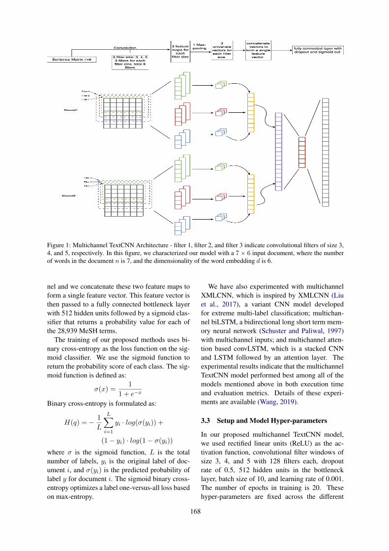
Figure 1: Multichannel TextCNN Architecture - filter 1, filter 2, and filter 3 indicate convolutional filters of size 3,4, and 5, respectively. In this figure, we characterized our model with a 7 × 6 input document, where the numberof words in the document n is 7, and the dimensionality of the word embedding d is 6.
nel and we concatenate these two feature maps toform a single feature vector. This feature vector isthen passed to a fully connected bottleneck layerwith 512 hidden units followed by a sigmoid clas-sifier that returns a probability value for each ofthe 28,939 MeSH terms.
The training of our proposed methods uses bi-nary cross-entropy as the loss function on the sig-moid classifier. We use the sigmoid function toreturn the probability score of each class. The sig-moid function is defined as:
σ(x) =1
1 + e−x
Binary cross-entropy is formulated as:
H(q) =− 1
L
L∑
i=1
yi · log(σ(yi)) +
(1− yi) · log(1− σ(yi))
where σ is the sigmoid function, L is the totalnumber of labels, yi is the original label of doc-ument i, and σ(yi) is the predicted probability oflabel y for document i. The sigmoid binary cross-entropy optimizes a label one-versus-all loss basedon max-entropy.
We have also experimented with multichannelXMLCNN, which is inspired by XMLCNN (Liuet al., 2017), a variant CNN model developedfor extreme multi-label classification; multichan-nel biLSTM, a bidirectional long short term mem-ory neural network (Schuster and Paliwal, 1997)with multichannel inputs; and multichannel atten-tion based convLSTM, which is a stacked CNNand LSTM followed by an attention layer. Theexperimental results indicate that the multichannelTextCNN model performed best among all of themodels mentioned above in both execution timeand evaluation metrics. Details of these experi-ments are available (Wang, 2019).
3.3 Setup and Model Hyper-parameters
In our proposed multichannel TextCNN model,we used rectified linear units (ReLU) as the ac-tivation function, convolutional filter windows ofsize 3, 4, and 5 with 128 filters each, dropoutrate of 0.5, 512 hidden units in the bottlenecklayer, batch size of 10, and learning rate of 0.001.The number of epochs in training is 20. Thesehyper-parameters are fixed across the different
168
datasets. In each dataset, we used 90% of thedata as the training set and 10% to test the per-formance of the model. We reserved 20% of thetraining data, chosen randomly, as the validationset, and the remaining 80% is used for trainingthe model. All experiments are performed on theNvidia GeForce 1080Ti GPU. Models for Fulltext(Large) are trained on 2 GPUs and training withthe other datasets is performed on a single GPU.
For word embeddings in our proposed modelwe used the pre-trained 200-dimensional BioASQword embedding vectors (Pavlopoulos et al.,2019) to represent the words in our vocabu-lary. These pre-trained word vectors are trainedon 10,876,004 English biomedical abstracts fromPubMed, and represent 1,701,632 distinct words.
4 Experiments
4.1 Datasets
Most existing approaches in automatic MeSH in-dexing are performed on datasets with abstractsand titles only. In this paper, we created a fulltext dataset which is composed of table and fig-ure captions as well as associated paragraphs, aswe believe figures and tables might provide im-portant MeSH features for classification. The twodatasets that were used to build our four datasetsare described below:
• 2015 Subject Extraction Test Collection(SETC2015): SETC2015 contains 14,828PMC full text articles used by Demner-Fushman and Mork (2015). We used thisdataset to create the following two Small (S)datasets:
– AT (S): labelled documents fromSETC2015 which contain abstract andtitle only
– Full (S): labelled documents fromSETC2015 which contain abstract, title,figure and table captions, and associatedparagraphs
• PMC Full Text Collection9 (PMC Collec-tion): We used a downloaded dataset of257,590 PMC full text documents in XMLformat, and used this dataset to create the fol-lowing two Large (L) datasets:
9https://www.ncbi.nlm.nih.gov/pmc/tools/ftp/
– AT (L): labelled documents from PMCCollection which are composed of ab-stract and title only
– Full (L): labelled documents from PMCCollection which are composed of ab-stract, title, figure and table captions,and associated paragraphs
Datasets D F L L̄ L̃
AT (S) 14828 63004 14365 13.15 13.5Full (S) 14828 148330 14365 13.15 13.5AT (L) 257590 188693 22881 13.34 150Full (L) 257590 669999 22881 13.34 150
Table 1: Statistics of Datasets: D is the total numberof documents (90% training, 10% testing); F repre-sents the number of unique tokens contained in all ofthe documents; L is the number of class labels; L̄ isthe average number of labels per document; L̃ is theaverage number of documents per label
Table 1 provides statistical information for thedescribed datasets. Our labeled datasets are using28,939 MeSH terms in total. To assist in our un-derstanding of the hierarchical evaluation, we ex-plored the MeSH hierarchical structure and splitthem into 5 levels to see how many MeSH termsexist at each level (it should be noted that there issome overlap of MeSH terms between levels). Thenumber of MeSH terms in the first, the second, thethird, the fourth and the fifth level, are: 16, 120,1903, 6,808, and 11,127, respectively.
4.2 Data pre-processing
The full text source files from PMC are in XMLformat. We extracted article information (includ-ing PMID, abstract, title, captions, and figure andtable related paragraphs) from these downloadedXML files. Paragraphs are considered related tofigures or tables if they contain the words “Fig-ure” or “Table”. MeSH terms for each articlewere scraped from its citation on PubMed by lo-cating the citation using its PMID, the unique arti-cle identifier number used in PubMed.
In pre-processing, we first did word level tok-enization of our input documents, to split the doc-uments into a list of words. Then we prepared ourdata by using the following process: set all char-acters to lowercase; convert numbers to “NUM”,percentage sign “%” to “PERCENTAGE”, chem-ical notations (i.e., H2O) to “CHEM”, and rela-tion symbols, namely “=”, “<”, “>”, “≤”, “≥”,
169
to “EQUAL”, “LESS”, “GREATER”, “LessAnd-Equal”, “GreaterAndEqual”; remove punctuation.
After the above process, we utilized the Keras(Chollet et al., 2015) Tokenizer API to vectorizeour data into a sequence of integers. Each integerrepresents the index of a token in the dictionarygenerated from the dataset.
4.3 Evaluation Metrics
There is generally no accepted standard for theevaluation of multi-label classifications. Eval-uation metrics adopted from multi-class clas-sification and binary classification are used tomeasure multi-label classification in an effectiveway. In automatic MeSH indexing, even if thelabel space is very large, only relatively fewMeSH terms match each document. To evalu-ate the performance of our proposed model, wepresent three groups of measurements suggestedby Tsoumakas et al. (2010) and Kosmopouloset al. (2015), namely bipartition-based, ranking-based and hierarchy-based evaluation.
To set the stage to discuss the three metrics,we define a test set of N document-label pairs{xi, yi}Ni=1 taken from the dataset, where xi is thedocument text and yi ∈ {0, 1}L. The vector yidenotes the set of true labels (i.e., MeSH terms)for each document i (0 meaning the label is notin the set, 1 meaning it is in the set), N denotesthe number of test examples, and L is the totalnumber of labels. Given a document xi, the setof labels predicted by the classifiers is denoted as{ŷi}Ni=1, where ŷi ∈ {0, 1}L, and the ranking in-dexes of predicted labels among the top k is de-noted as rk (ŷ), where ŷ = {ŷi}Ni=1.
Bipartition evaluation is further divided intoexample-based and label-based metrics. Example-based measurements calculate precision, recall,and F-score over (in our evaluation) the top 5,top 10, and top 15 ranked labels over all of thedocuments of the test set. The measurements in-clude example-based precision (EBP), example-based recall (EBR) and example-based F-score(EBF). The metrics are defined as:
EBP =1
N
N∑
i=1
|yi ∩ ŷi||ŷi|
EBR =1
N
N∑
i=1
|yi ∩ ŷi||yi|
EBF =1
N
N∑
i=1
2× |yi ∩ ŷi||yi|+ |ŷi|
Label-based evaluation is calculated for each labelin the label set. The measurements include macro-and micro-average precision (MaP, MiP), macro-and micro-average recall (MaR, MiR),and macro-and micro-average F-score (MaF, MiF). The met-rics are defined as:
MaP =1
L
L∑
j=1
TPj
TPj + FPj
MiP =
∑Lj=1 TPj
∑Lj=1 TPj +
∑Lj=1 FPj
MaR =1
L
L∑
j=1
TPj
TPj + FNj
MiR =
∑Lj=1 TPj
∑Lj=1 TPj +
∑Lj=1 FNj
MaF =2×MaR×MaP
MaR + MaP
MiF =2×MiR×MiP
MiR + MiPwhere TPj , FPj and FNj as true positives, falsepositives, and false negatives respectively for eachlabel lj in the set of total labels L.
Ranking-based evaluation, including precisionat k (p@k), and normalized discounted cumulativegain (nDCG), ranks the predicted labels and aimsto rank the relevant labels higher than the irrele-vant ones. The metrics are defined as follows:
p@k =1
k
∑
l∈rk(ŷ)yl
DCG@k =∑
l∈rk(ŷ)
yllog (l + 1)
IDCG =
min(k,‖y‖0)∑
l=1
1
log (l + 1)
nDCG@k =DCG@k
IDCGHierarchy-based evaluation, including hierar-
chical precision (HP) and hierarchical recall (HR),is used to measure a hierarchical classification thatclassifies elements into a hierarchy of classes. Itmeasures performance based on the gold standardlabels and the predicted labels augmented with
170
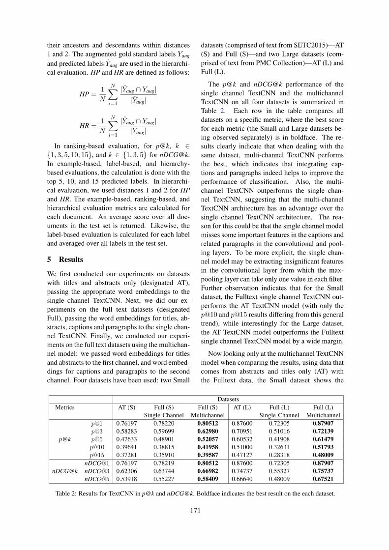
their ancestors and descendants within distances1 and 2. The augmented gold standard labels Yaug
and predicted labels Ŷaug are used in the hierarchi-cal evaluation. HP and HR are defined as follows:
HP =1
N
N∑
i=1
|Ŷaug ∩ Yaug||Ŷaug|
HR =1
N
N∑
i=1
|Ŷaug ∩ Yaug||Yaug|
In ranking-based evaluation, for p@k, k ∈{1, 3, 5, 10, 15}, and k ∈ {1, 3, 5} for [email protected] example-based, label-based, and hierarchy-based evaluations, the calculation is done with thetop 5, 10, and 15 predicted labels. In hierarchi-cal evaluation, we used distances 1 and 2 for HPand HR. The example-based, ranking-based, andhierarchical evaluation metrics are calculated foreach document. An average score over all doc-uments in the test set is returned. Likewise, thelabel-based evaluation is calculated for each labeland averaged over all labels in the test set.
5 Results
We first conducted our experiments on datasetswith titles and abstracts only (designated AT),passing the appropriate word embeddings to thesingle channel TextCNN. Next, we did our ex-periments on the full text datasets (designatedFull), passing the word embeddings for titles, ab-stracts, captions and paragraphs to the single chan-nel TextCNN. Finally, we conducted our experi-ments on the full text datasets using the multichan-nel model: we passed word embeddings for titlesand abstracts to the first channel, and word embed-dings for captions and paragraphs to the secondchannel. Four datasets have been used: two Small
datasets (comprised of text from SETC2015)—AT(S) and Full (S)—and two Large datasets (com-prised of text from PMC Collection)—AT (L) andFull (L).
The p@k and nDCG@k performance of thesingle channel TextCNN and the multichannelTextCNN on all four datasets is summarized inTable 2. Each row in the table compares alldatasets on a specific metric, where the best scorefor each metric (the Small and Large datasets be-ing observed separately) is in boldface. The re-sults clearly indicate that when dealing with thesame dataset, multi-channel TextCNN performsthe best, which indicates that integrating cap-tions and paragraphs indeed helps to improve theperformance of classification. Also, the multi-channel TextCNN outperforms the single chan-nel TextCNN, suggesting that the multi-channelTextCNN architecture has an advantage over thesingle channel TextCNN architecture. The rea-son for this could be that the single channel modelmisses some important features in the captions andrelated paragraphs in the convolutional and pool-ing layers. To be more explicit, the single chan-nel model may be extracting insignificant featuresin the convolutional layer from which the max-pooling layer can take only one value in each filter.Further observation indicates that for the Smalldataset, the Fulltext single channel TextCNN out-performs the AT TextCNN model (with only thep@10 and p@15 results differing from this generaltrend), while interestingly for the Large dataset,the AT TextCNN model outperforms the Fulltextsingle channel TextCNN model by a wide margin.
Now looking only at the multichannel TextCNNmodel when comparing the results, using data thatcomes from abstracts and titles only (AT) withthe Fulltext data, the Small dataset shows the
DatasetsMetrics AT (S) Full (S) Full (S) AT (L) Full (L) Full (L)
Single Channel Multichannel Single Channel Multichannel
p@k
p@1 0.76197 0.78220 0.80512 0.87600 0.72305 0.87907p@3 0.58283 0.59699 0.62980 0.70951 0.51016 0.72139p@5 0.47633 0.48901 0.52057 0.60532 0.41908 0.61479p@10 0.39641 0.38815 0.41958 0.51000 0.32631 0.51793p@15 0.37281 0.35910 0.39587 0.47127 0.28318 0.48009
nDCG@knDCG@1 0.76197 0.78219 0.80512 0.87600 0.72305 0.87907nDCG@3 0.62306 0.63744 0.66982 0.74737 0.55327 0.75737nDCG@5 0.53918 0.55227 0.58409 0.66640 0.48009 0.67521
Table 2: Results for TextCNN in p@k and nDCG@k. Boldface indicates the best result on the each dataset.
171
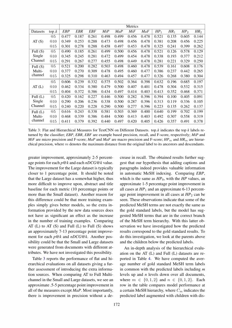
MetricsDatasets top k EBP EBR EBF MiP MaP MiF MaF HP1 HR1 HP2 HR2
AT (S)@5 0.477 0.187 0.261 0.498 0.499 0.456 0.478 0.521 0.135 0.605 0.144@10 0.349 0.253 0.288 0.473 0.498 0.456 0.478 0.381 0.208 0.456 0.225@15 0.301 0.278 0.288 0.458 0.497 0.453 0.478 0.325 0.241 0.399 0.262
Full (S)Single
Channel
@5 0.490 0.185 0.261 0.499 0.500 0.456 0.478 0.521 0.126 0.578 0.129@10 0.345 0.245 0.281 0.472 0.499 0.454 0.478 0.338 0.193 0.377 0.212@15 0.291 0.267 0.277 0.455 0.498 0.449 0.478 0.281 0.221 0.329 0.250
Full (S)Multi-
channel
@5 0.521 0.200 0.282 0.503 0.498 0.460 0.478 0.539 0.161 0.608 0.176@10 0.377 0.270 0.309 0.478 0.495 0.460 0.477 0.386 0.237 0.442 0.265@15 0.325 0.298 0.310 0.463 0.494 0.457 0.477 0.326 0.268 0.380 0.304
AT (L)@5 0.606 0.239 0.332 0.575 0.502 0.364 0.398 0.632 0.196 0.685 0.197@10 0.462 0.334 0.380 0.479 0.500 0.407 0.401 0.478 0.304 0.532 0.315@15 0.404 0.372 0.386 0.434 0.497 0.414 0.403 0.413 0.352 0.468 0.371
Full (L)Single
Channel
@5 0.420 0.162 0.227 0.446 0.500 0.282 0.396 0.394 0.100 0.405 0.091@10 0.290 0.206 0.236 0.338 0.500 0.287 0.396 0.313 0.119 0.336 0.105@15 0.240 0.220 0.228 0.290 0.500 0.277 0.396 0.223 0.135 0.262 0.137
Full (L)Multi-
channel
@5 0.616 0.243 0.338 0.581 0.503 0.369 0.400 0.640 0.199 0.702 0.199@10 0.468 0.339 0.386 0.484 0.500 0.413 0.403 0.492 0.307 0.558 0.319@15 0.411 0.379 0.392 0.440 0.497 0.420 0.405 0.426 0.357 0.491 0.378
Table 3: Flat and Hierarchical Measures for TextCNN on Different Datasets. top k indicates the top k labels re-turned by the classifier; EBP, EBR, EBF are example based precision, recall, and F-score, respectively; MiP andMiF are micro precision and F-score; MaP and MaF are macro precision and F-score; HPm and HRm are hierar-chical precision, where m denotes the maximum distance from the original label to its ancestors and descendants.
greater improvement, approximately 2-5 percent-age points for each p@k and each nDCG@k value.The improvement for the Large dataset is typicallycloser to 1 percentage point. It should be notedthat the Large dataset has a somewhat higher, thusmore difficult to improve upon, abstract and titlebaseline for each metric (10 percentage points ormore than the Small dataset). Another reason forthis difference could be that more training exam-ples simply gives better models, so the extra in-formation provided by the new data sources doesnot have as significant an effect as the increasein the number of training examples. ComparingAT (L) to AT (S) and Full (L) to Full (S) showsan approximately 7-13 percentage point improve-ment for each p@k and nDCG@k. Another pos-sibility could be that the Small and Large datasetswere generated from documents with different at-tributes. We have not investigated this possibility.
Table 3 reports the performance of flat and hi-erarchical evaluations on all datasets giving a fur-ther assessment of introducing the extra informa-tion sources. When comparing AT to Full Multi-channel in the Small and Large datasets, we see anapproximate .5-5 percentage point improvement inall of the measures except MaP. Most importantly,there is improvement in precision without a de-
crease in recall. The obtained results further sug-gest that our hypothesis that adding captions andparagraphs indeed provides valuable informationin automatic MeSH indexing. Comparing EBP,which is the same as HP0, with the HP values, anapproximate 1-5 percentage point improvement inall cases at HP1 and an approximate 6-13 percent-age point improvement in all cases at HP2 can beseen. These observations indicate that some of thepredicted MeSH terms are not exactly the same asthe gold standard labels, but the model has sug-gested MeSH terms that are in the correct branchof the MeSH term hierarchy. With this latter ob-servation we have investigated how the predictedresults correspond to the gold standard results. Todo this investigation, we look at the parents aboveand the children below the predicted labels.
An in-depth analysis of the hierarchical evalu-ation on the AT (L) and Full (L) datasets are re-ported in Table 4. We have computed the aver-age number of gold standard MeSH term labelsin common with the predicted labels including mlevels up and n levels down over all documents,where m ∈ {0, 1, 2} and n ∈ {0, 1, 2}. Eachrow in the table compares model performance ata certain MeSH hierarchy, where Cm indicates thepredicted label augmented with children with dis-
172
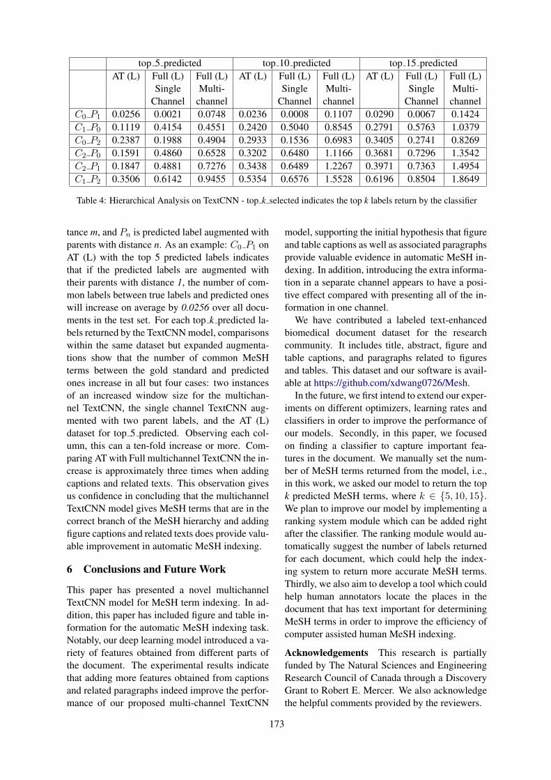
top 5 predicted top 10 predicted top 15 predictedAT (L) Full (L) Full (L) AT (L) Full (L) Full (L) AT (L) Full (L) Full (L)
Single Multi- Single Multi- Single Multi-Channel channel Channel channel Channel channel
C0 P1 0.0256 0.0021 0.0748 0.0236 0.0008 0.1107 0.0290 0.0067 0.1424C1 P0 0.1119 0.4154 0.4551 0.2420 0.5040 0.8545 0.2791 0.5763 1.0379C0 P2 0.2387 0.1988 0.4904 0.2933 0.1536 0.6983 0.3405 0.2741 0.8269C2 P0 0.1591 0.4860 0.6528 0.3202 0.6480 1.1166 0.3681 0.7296 1.3542C2 P1 0.1847 0.4881 0.7276 0.3438 0.6489 1.2267 0.3971 0.7363 1.4954C1 P2 0.3506 0.6142 0.9455 0.5354 0.6576 1.5528 0.6196 0.8504 1.8649
Table 4: Hierarchical Analysis on TextCNN - top k selected indicates the top k labels return by the classifier
tance m, and Pn is predicted label augmented withparents with distance n. As an example: C0 P1 onAT (L) with the top 5 predicted labels indicatesthat if the predicted labels are augmented withtheir parents with distance 1, the number of com-mon labels between true labels and predicted oneswill increase on average by 0.0256 over all docu-ments in the test set. For each top k predicted la-bels returned by the TextCNN model, comparisonswithin the same dataset but expanded augmenta-tions show that the number of common MeSHterms between the gold standard and predictedones increase in all but four cases: two instancesof an increased window size for the multichan-nel TextCNN, the single channel TextCNN aug-mented with two parent labels, and the AT (L)dataset for top 5 predicted. Observing each col-umn, this can a ten-fold increase or more. Com-paring AT with Full multichannel TextCNN the in-crease is approximately three times when addingcaptions and related texts. This observation givesus confidence in concluding that the multichannelTextCNN model gives MeSH terms that are in thecorrect branch of the MeSH hierarchy and addingfigure captions and related texts does provide valu-able improvement in automatic MeSH indexing.
6 Conclusions and Future Work
This paper has presented a novel multichannelTextCNN model for MeSH term indexing. In ad-dition, this paper has included figure and table in-formation for the automatic MeSH indexing task.Notably, our deep learning model introduced a va-riety of features obtained from different parts ofthe document. The experimental results indicatethat adding more features obtained from captionsand related paragraphs indeed improve the perfor-mance of our proposed multi-channel TextCNN
model, supporting the initial hypothesis that figureand table captions as well as associated paragraphsprovide valuable evidence in automatic MeSH in-dexing. In addition, introducing the extra informa-tion in a separate channel appears to have a posi-tive effect compared with presenting all of the in-formation in one channel.
We have contributed a labeled text-enhancedbiomedical document dataset for the researchcommunity. It includes title, abstract, figure andtable captions, and paragraphs related to figuresand tables. This dataset and our software is avail-able at https://github.com/xdwang0726/Mesh.
In the future, we first intend to extend our exper-iments on different optimizers, learning rates andclassifiers in order to improve the performance ofour models. Secondly, in this paper, we focusedon finding a classifier to capture important fea-tures in the document. We manually set the num-ber of MeSH terms returned from the model, i.e.,in this work, we asked our model to return the topk predicted MeSH terms, where k ∈ {5, 10, 15}.We plan to improve our model by implementing aranking system module which can be added rightafter the classifier. The ranking module would au-tomatically suggest the number of labels returnedfor each document, which could help the index-ing system to return more accurate MeSH terms.Thirdly, we also aim to develop a tool which couldhelp human annotators locate the places in thedocument that has text important for determiningMeSH terms in order to improve the efficiency ofcomputer assisted human MeSH indexing.
Acknowledgements This research is partiallyfunded by The Natural Sciences and EngineeringResearch Council of Canada through a DiscoveryGrant to Robert E. Mercer. We also acknowledgethe helpful comments provided by the reviewers.
173
ReferencesAlan R Aronson and François-Michel Lang. 2010. An
overview of MetaMap: Historical perspective andrecent advances. Journal of the American MedicalInformatics Association, 17(3):229–236.
Alan R. Aronson, James G. Mork, Clifford W. Gay,Susanne M. Humphrey, and Willie J. Rogers. 2004.The NLM Indexing Initiative’s Medical Text In-dexer. Studies in Health Technology and Informat-ics, 107 Pt 1:268–272.
François Chollet et al. 2015. Keras. https://github.com/fchollet/keras.
Dina Demner-Fushman and James G. Mork. 2015. Ex-tracting characteristics of the study subjects fromfull-text articles. In Proceedings of the Ameri-can Medical Informatics Association (AMIA) An-nual Symposium, pages 484–491.
Francesco Gargiulo, Stefano Silvestri, and MarioCiampi. 2018. Deep convolution neural network forextreme multi-label text classification. In Proceed-ings of the 11th International Joint Conference onBiomedical Engineering Systems and Technologies– Volume 5: AI4Health, pages 641–650.
Antonio Jimeno-Yepes, James G. Mork, Dina Demner-Fushman, and Alan R. Aronson. 2012. A one-size-fits-all indexing method does not exist: Automaticselection based on meta-learning. Journal of Com-puting Science and Engineering, 6(2):151–160.
Antonio Jimeno-Yepes, James G. Mork, Dina Demner-Fushman, and Alan R. Aronson. 2013. Compari-son and combination of several MeSH indexing ap-proaches. In Proceedings of the American MedicalInformatics Association (AMIA) Annual Symposium,pages 709–718.
Qiao Jin, Bhuwan Dhingra, and William W. Cohen.2018. AttentionMeSH: Simple, effective and in-terpretable automatic MeSH indexer. In Proceed-ings of the 2018 EMNLP Workshop BioASQ: Large-scale Biomedical Semantic Indexing and QuestionAnswering, pages 47–56.
Yoon Kim. 2014. Convolutional neural networks forsentence classification. In Proceedings of the 2014Conference on Empirical Methods in Natural Lan-guage Processing (EMNLP), pages 1746–1751.
Olivier Bodenreider KinWah Fung. 2007. Utilizing theumls for semantic mapping between terminologies.In Proceedings of the American Medical InformaticsAssociation (AMIA) Annual Symposium, pages 266–270.
Aris Kosmopoulos, Ioannis Partalas, Eric Gaussier,Georgios Paliouras, and Ion Androutsopoulos. 2015.Evaluation measures for hierarchical classification:A unified view and novel approaches. Data Miningand Knowledge Discovery, 29(3):820–865.
Jimmy Lin and W. John Wilbur. 2007. Pubmed relatedarticles: A probabilistic topic-based model for con-tent similarity. BMC Bioinformatics, 8(1):423.
Jingzhou Liu, Wei-Cheng Chang, Yuexin Wu, andYiming Yang. 2017. Deep learning for extrememulti-label text classification. In Proceedings of the40th International ACM SIGIR Conference on Re-search and Development in Information Retrieval,pages 115–124.
Ke Liu, Shengwen Peng, Junqiu Wu, ChengXiangZhai, Hiroshi Mamitsuka, and Shanfeng Zhu. 2015.MeSHLabeler: Improving the accuracy of large-scale mesh indexing by integrating diverse evidence.Bioinformatics, 31(12):i339–i347.
James G. Mork, Antonio Jimeno-Yepes, and Alan R.Aronson. 2013. The NLM Medical Text In-dexer system for indexing biomedical literature.In Proceedings of the first Workshop on Bio-Medical Semantic Indexing and Question Answering(BioASQ). CEUR-WS.org, online http://CEUR-WS.org/Vol-1094/bioasq2013 submission 3.pdf.
Ioannis Pavlopoulos, Aris Kosmopoulos, and Ion An-droutsopoulos. 2019. Continuous space word vec-tors obtained by applying word2vec to abstracts ofbiomedical articles. Retrieved from http://bioasq.lip6.fr/info/BioASQword2vec/.
Shengwen Peng, Ronghui You, Hongning Wang,ChengXiang Zhai, Hiroshi Mamitsuka, and Shan-feng Zhu. 2016. Deepmesh: deep semantic repre-sentation for improving large-scale mesh indexing.Bioinformatics, 32(12):i70–i79.
Anthony Rios and Ramakanth Kavuluru. 2015. Con-volutional neural networks for biomedical text clas-sification: Application in indexing biomedical arti-cles. In Proceedings of the 6th ACM Conference onBioinformatics, Computational Biology and HealthInformatics, pages 258–267.
Mike Schuster and Kuldip K. Paliwal. 1997. Bidirec-tional recurrent neural networks. IEEE Transactionson Signal Processing, 45(11):2673–2681.
Lei Tang, Suju Rajan, and Vijay K. Narayanan. 2009.Large scale multi-label classification via MetaLa-beler. In Proceedings of the 18th InternationalWorld Wide Web Conference (WWW), pages 211–220.
Grigorios Tsoumakas, Ioannis Katakis, and Ioannis P.Vlahavas. 2010. Mining multi-label data. In DataMining and Knowledge Discovery Handbook (2nded.), pages 667–685. Springer, Boston, MA.
Xindi Wang. 2019. Incorporating figure captions anddescriptive text in mesh term indexing: A deeplearning approach. Master’s thesis, The Universityof Western Ontario.
174

Chengxiang Zhai, Hiroshi Mamitsuka, Junqiu Wu,Ke Liu, Shanfeng Zhu, and Shengwen Peng. 2015.MeSHLabeler: Improving the accuracy of large-scale MeSH indexing by integrating diverse evi-dence. Bioinformatics, 31(12):i339–i347.
M. Zhang and Z. Zhou. 2014. A review on multi-labellearning algorithms. IEEE Transactions on Knowl-edge and Data Engineering, 26(8):1819–1837.
175
Proceedings of the BioNLP 2019 workshop, pages 176–190Florence, Italy, August 1, 2019. c©2019 Association for Computational Linguistics
BioRelEx 1.0: Biological Relation Extraction Benchmark
Hrant Khachatrian1,2, Lilit Nersisyan3, Karen Hambardzumyan1,2, Tigran Galstyan1,2,Anna Hakobyan3, Arsen Arakelyan3, Andrey Rzhetsky4, and Aram Galstyan5
1YerevaNN, Yerevan, Armenia2Department of Informatics and Applied Mathematics, Yerevan State University, Yerevan, Armenia
3Bioinformatics Group, Institute of Molecular Biology, NAS RA, Yerevan, Armenia4Institute for Genomics and Systems Biology, Departments of Medicine and
Human Genetics, University of Chicago, Chicago, Illinois, USA5USC Information Sciences Institute, Marina Del Rey, California, USA
AbstractAutomatic extraction of relations and interac-tions between biological entities from scien-tific literature remains an extremely challeng-ing problem in biomedical information extrac-tion and natural language processing in gen-eral. One of the reasons for slow progress isthe relative scarcity of standardized and pub-licly available benchmarks. In this paper weintroduce BioRelEx, a new dataset of fully an-notated sentences from biomedical literaturethat capture binding interactions between pro-teins and/or biomolecules. To foster repro-ducible research on the interaction extractiontask, we define a precise and transparent eval-uation process, tools for error analysis and sig-nificance tests. Finally, we conduct exten-sive experiments to evaluate several baselines,including SciIE, a recently introduced neuralmulti-task architecture that has demonstratedstate-of-the-art performance on several tasks.
1 Introduction
Biological interaction databases capture a smallportion of knowledge depicted in biomedical pa-pers, due to time consuming nature of manual in-formation extraction. As experimental methodolo-gies to identify such interactions tend to increasein scale and throughput, the problem stands torapidly update these databases for relevant appli-cations (Oughtred et al., 2018). The long-term aimof our efforts is to provide bases for filling this gapautomatically.
Despite significant progress in recent years, ex-tracting relationships and interactions between dif-ferent biological entities is still an extremely chel-lenging problem. Some of those challenges are
due to objective reasons such as lack of very largeannotated datasets for training complex models, orwide variability in biomedical literature which canlead to domain mismatch and poor generalization.Another important challenge, which is the mainfocus of the present paper, is the scarcity of pub-licly available datasets. Indeed, with despite somenotable exceptions (Kim et al., 2003; Dogan et al.,2017), there is a relative lack of adequate, high-quality benchmark datasets which would facilitatereproducible research and allow for robust com-parative evaluation of existing approaches.
Here we have processed biological texts to an-notate biological entities and interaction pairs. Incontrast to other related databases, our efforts werefocused on delineation of biological entities fromexperimental ones, and on distinguishing betweenindirect regulatory interactions and direct physi-cal interactions. Furthermore, we have performedgrounding via cross-reference of annotated entitieswith external databases. This allows for merginginteractions from different sources into a singlenetwork of biomolecular interactions.
The main contributions of this work are:
1. We publish a dataset of 2010 sentences withcomplete annotations of biological entitiesand binding interactions between the entities,
2. We propose a benchmark task with a well-defined evaluation system, which follows thebest practices of machine learning research,
3. We perform extensive evaluation of severalcompeting methods on the dataset and reportthe results.
176
2 Related work
In this section we briefly summarize prior work onrelation extraction from unstructured text.
Since 2009, NIST has organized KnowledgeBase Population evaluations as part of Text Anal-ysis Conferences (TAC KPB). Thousands of sen-tences from newswire and informal web pageswere annotated for training and evaluation pur-poses (Getman et al., 2018). In 2017, a team fromStanford released TACRED (Zhang et al., 2017),a dataset of 106 264 sentences with 42 relationtypes. The relations are mainly between people,places and organizations.
A large number of papers focused on biologi-cal relation extraction. (Bunescu et al., 2005) builta manually annotated corpus of 225 abstracts toevaluate various extraction methods. This datasetis referred as AIMed in subsequent papers. Later,(Pyysalo et al., 2007) developed a smaller datasetcalled BioInfer with more detailed annotations. Inparticular, the authors developed large ontologiesfor biological entities and relations between themand attempted to classify each entity and relationaccording to these ontologies. The small numberof sentences and interactions is 1100 and 2662,respectively, so for many types of relations therewere too few samples. Because of that, almost allsubsequent papers that applied machine learningtechniques on BioInfer discarded the detailed la-bels and used it as a dataset of binary relations. In2008, (Pyysalo et al., 2008a) presented a detailedcomparison of AIMed, BioInfer and three otherdatasets (IEPA, HPRD50 and LLL) and found sig-nificant differences in the data collection and eval-uation procedures.
In (Pyysalo et al., 2008b), the authors concludedthat the results on the five datasets reported in dif-ferent papers are incomparable and suggested tounify the datasets in a common format with a pre-cise evaluation procedure. This proved to be suc-cessful as a large number of subsequent papers usethe unified versions of the datasets. On the otherhand, these datasets are currently used only forbinary relation classification, as the unified ver-sions keep the lowest common level of annotations(only entity locations and binary labels betweenthe pairs). It means that the models trained onthese datasets cannot be used for end-to-end rela-tion extraction from text. Moreover, many recentpapers violate evaluation strategies (e.g. performcross-validation on splits that do not respect doc-
ument boundaries) and report unrealistically highscores (Hsieh et al., 2017; Ahmed et al., 2019).
One of the highest quality datasets is devel-oped as part of GENIA project (Kim et al., 2003).It involves annotations of entities, syntactic fea-tures, wide variety of events, including around2500 binding interactions (Thompson et al., 2017).GENIA does not have a training/test split, but vari-ous subsets of it have been used as training and testsets of BioNLP Shared Tasks in 2009 (Kim et al.,2009), 2011 (Kim et al., 2011) and 2013 (Nédellecet al., 2013). Several protein-protein interaction(PPI) datasets appeared in BioCreative series ofshared tasks. There was a track on PPI extractionin BioCreative II, including a binary relation ex-traction subtask from full texts and another sub-task for finding evidence sentences for the giveninteraction (Krallinger et al., 2008). BioCreativeV Track 4 included a subtask on extraction of morecomplex data structures called Biological Expres-sion Language (BEL) statements (Rinaldi et al.,2016).
Other biological relation extraction datasets in-clude ADE (Gurulingappa et al., 2012), a datasetof adverse drug effects; BB3 (Deléger et al.,2016), a dataset of relations between bacteria andtheir habitats, which was used in BioNLP SharedTask 2016; SeeDev, a dataset of sentences aboutseed development of plants; AGAC, a dataset ongene mutations and diseases. The latter threedatasets are included in BioNLP 2019 SharedTasks. Precision Medicine Track of BioCreativeVI (Dogan et al., 2017) introduced a large datasetof protein-protein interactions that are affected bymutations.
SemEval 2017 Task 10 (Augenstein et al., 2017)was about extracting relations from scientific pa-per abstracts (physics, computer science and ma-terials science). SemEval 2018 Task 7 focused onsentences from computational linguistics papers.SciERC (Luan et al., 2018) is a dataset consist-ing of 500 research paper abstracts from major AIconferences with annotated entities, coreferencelinks and relations between entities.
3 Dataset description
3.1 The choice of sentences
We have annotated 2010 sentences for binding in-teractions between biological entities. Those sen-tences came from a much larger set of 40,000 sen-tences that were automatically extracted from var-
177
ious biomedical journals and underwent minimalmanual post-processing (Rzhetsky et. al., 2019).While the original set contained numerous inter-action types, here our focus is on binding interac-tions only. The text of the sentences are mostlycopied from the journal websites and can includeuncommon Unicode symbols. In rare cases wehad to copy the sentences from PDF versions ofthe papers and manually fix incorrect characters.
As stated above, the current version of thedataset is focused on binding interactions. All sen-tences in the dataset contain one of the followingwords: “bind”, “binds”, “binding”, “bound”. Thiswill potentially limit the applicability of the mod-els trained on this dataset on other sentences thatcontain information about binding interactions.
3.2 Entities
3.2.1 Entity definitionEvery annotated entity is a continuous span ofcharacters in the sentence surrounded by non-alphanumeric symbols (can include spaces, hy-phens etc.).
Tokenization of biomedical texts can be a chal-lenging task. To ensure consistency, we have ver-ified that all annotated entities in the dataset aresurrounded by the symbols described in Table 3of Appendix A.3. Note that all these symbols canalso appear inside an entity name.
3.2.2 Entity typesWe have annotated 33 types of entities. Forclassification of entities we were governed both,by biological function and by chemical structure.More specifically, we distinguish between biolog-ical and experimental entities. For example, ifthe sentence refers to an oligonucleotide in an ex-periment, we do not annotate it as DNA, but asan experimental-construct. Furthermore, we de-fine main organic entity types as protein, protein-family, protein-complex, DNA and RNA, whilerefer to the rest of organic compounds as chemi-cals. The complete list of entity types is listed inAppendix A.4.
These decisions were motivated by two mainreasons: (a) only biological entities should be an-notated and cross-referenced in order to arrive atbiologically meaningful interaction networks; (b)a higher level of annotation that disregards details(e.g. chemicals) significantly reduces annotationresources with no loss to our targetted aim. This
contrasts to the Genia ontology, where entity an-notation was only based on chemical structure ofsubstances (Thompson et al., 2017).
Note that while the majority of entities are an-notated to a single type, two entities with thesame name may be annotated to different types(e.g. protein or protein-family) depending onthe context, and sometimes these cases may co-occur in the same sentence (e.g. protein and gene(1.0.train.166)).
3.2.3 CoreferencePairs of entities may be in is a or part of rela-tionships. We have undertaken two approachesto mark such relationships for unambigous place-ment of entities when merging relations from oneor many sentences.
3.2.4 Links between entities1. Sometimes the same entity appears in multi-
ple forms in the sentence. We annotate themwith a “synonym” link. Sometimes, one ofthe forms is just an acronym for another form,in which case we use “abbreviation” link.
2. Biologically nested entities are linked with apart of link. For example, protein-domainsand protein-regions are part of proteins, whileprotein subunits are part of complexes. Theselinks correspond to the substrate chemicalstructure ontology presented in Genia dataset(Thompson et al., 2017).
3.2.5 GroundingEntities of types gene, protein, protein-family andchemical have been cross-referenced with externaldatabase identifiers. The aim of grounding is tointroduce unique naming/identification of entities.This is particularly useful for unambiguous identi-fication of entities in the process of merging rela-tions derived from different sentences into a singlenetwork.
Notably, as a side effect, the process of ground-ing increased the quality of entity annotation forthe specified entity types.
3.2.6 AmbiguitiesEntity annotation is not a straightforward task, asentities usually appear in a variety of grammati-cal and biological forms. Therefore, we have de-veloped the following guidelines for standardizedannotations. Formation of these guidelines was a
178
result of iterative annotations followed by resolu-tion of inter-annotator conflicts.
1. Entity modifications
Sometimes the text contains an entity whichis a mutated form of another entity, or it isan entity in an unusual state. In these caseswe tag the entity with “mutant” and/or “state”labels (Appendix A.1, example 1).
2. Spanned and nested entities
If an entity contains multiple tokens, thosemay be separated by other words in the text,or may themselves contain nested simpler en-tities. In cases when the same token is sharedbetween multiple complex entities, we anno-tate the shared tokens only as part of the firstentity (Appendix A.1, example 2). A bettersolution to these cases would be to annotatethe shared tokens in all the entities that theyare part of and use a text-span notation tomark those cases. However, considering thesmall number of such cases, we didn’t findthis worthwhile. Sometimes a complex entityname contains a name of another entity. Weannotate both, and both can appear in inter-actions. In extreme cases, the second entitycan be a single digit. In contrast to our ap-proach, entity recognizer systems that do notsupport nested entities are not be able to findthese cases. In evaluation, we have a separatescore that reports performance on the nestedentities (Appendix A.1, examples 3-5).
3. A/B syntax
In many cases A/B means a complex of theproteins A and B. In other cases it refers toseparate proteins A and B, and the interac-tion with A/B means interactions with bothof them. In both cases, we annotate A and Bas individual entities. In case of complexes,we also annotate A/B as a complex. If A/Bis involved in an interaction with a protein C,we annotate an interaction between A/B andC only if A/B is a complex. If A/B is nota complex, we annotate two interactions be-tween A and C, and B and C. (Appendix A.1,example 6)
4. Hidden entity names and implicit corefer-ences
Sometimes the sentence is about an entitywhich is not explicitly mentioned, but thereare words that refer to it. We do not anno-tate these words as entities and do not an-notate corresponding interactions (AppendixA.1, example 7).
3.3 Interactions
We annotate binding interactions between severaltypes of entities.
3.3.1 Interaction typesWe use three labels: 1 if the interaction exists, 0for speculations (if the sentence does not concludewhether the interaction exists or not), and −1 fornegations (if the sentence concludes that there isno binding interaction between the entities).
We conclude that an interaction exists (1) if wefind explicit triggers describing direct physical in-teractions, such as A binds/ associates with/ in-teracts with /recuits /phosphorylates B, and theirgrammatical varieties.
Speculative interactions (Appendix A.2, exam-ples 1-2) arise either due to lack of experimentalevidence or due to the sentence not reaching theconlusion yet. We mark such cases with a “hy-pothesis” label. Other cases may be sentences thatare actually titles of the sections or even the pa-pers. In practice, title of the paper might be ex-tracted both from the title section of the paper andfrom the reference sections of other papers. Wetag the sentences extracted from paper, section orfigure titles by “title” label (Appendix A.2, exam-ples 3-4).
3.3.2 Ambiguities1. Entity polymorphisms
When an entity participating in an interac-tion appears in multiple forms in the sentence(e.g. plural forms, synonyms, etc.), we anno-tate the one which is the most obvious fromthe sentence. In evaluation, we do not penal-ize the predictions with another form of thesame entity (Appendix A.2, example 5).
2. Static interactions: protein complexes anddomains
Static or implicit interactions refer to caseswhere an interaction is inferred from the con-text, but is not mentioned with any explicittrigger.
179
When the sentence contains a complex of twoor more proteins, and the components of thecomplex are present in the sentence, we an-notate a binding interaction between themand tag it with a “complex” label. In rarecases, the same sentence contains another ex-plicit mention of the interaction between twoproteins. In this cases we do not tag the inter-action with “complex” label (Appendix A.2,examples 6-7). In evaluation, we additionallyreport the performance on such implicit bind-ing interactions inside complexes.
Sometimes we annotate a (positive) bindinginteraction between entities A and B, whereB is a region (part of ) of another entity C.The most common scenario is when B is aprotein domain and A and C are proteins. Inthis case, we annotate another interaction be-tween A and C and tag it with an “implicit”label. The full list of entity types that canget involved in similar implicit interactions ispresented in Appendix A.4. We have auto-matically verified that all such implicit inter-actions are annotated (Appendix A.2, exam-ples 8-9).
3. Self interactions
There are cases when an entity binds to itself,especially when the entity is a protein-familyand the binding can refer to different mem-bers of the same family (Appendix A.2, ex-ample 10).
In rare cases, the sentence talks about homod-imers or oligomerization, which implies thatthere is a protein which binds to itself. Wetag these cases with an “implicit” label (Ap-pendix A.2, example 11-12).
4. Interactions with implicit entities
Sometimes the sentences contain interactionswith entities without naming them. Weexclude these interactions from the dataset(A.2, example 13).
3.4 Dataset statistics
The lengths of sentences vary from 3 to 138. Themedian length is 29, the mean is around 30. 95%of all sentences have less than 50. The averagenumber of entity clusters per sentence is 3.92,while the average number of entity mentions per
sentence is 4.91. On average, there are 1.61 inter-action per sentence.
We used Cytoscape (Shannon et al., 2003) toconstruct a graph based on positive interactionsannotated from our dataset. It has 2248 nodes(entities) and 3235 edges (interactions) (see Fig-ure 2 in Appendix A.5). The graph had a largeconnected component, containing 65% (1475) ofnodes and 81% (2635) of edges. Many interac-tions were annotated multiple times, with 67%(2177) of unique interactions, and up to 11 dupli-cations per entity pair. The graph showed small-world properties, with average shortest path be-tween any pairs of nodes being 5, and with veryfew hub nodes. Degrees range from 1 to 83 withmedian 1.
3.5 Comparison with other datasets
Table 1 compares BioRelEx 1.0 with the popularrelated datasets. The original version of AIMedhas similar number of sentences to BioRelEx, butthe number of annotated relations is significantlylower due to different annotation guidelines andchoice of sentences. BioInfer contains fewer sen-tences with a lot more detailed annotations, whichis not suitable for the current machine learningtechniques, hence most of the models designedfor BioInfer simply ignore the details of annota-tions. Both datasets do not have correspondingwell-defined benchmarks. The five datasets in aunified format from (Pyysalo et al., 2008a) suitbetter for machine learning research, but they arelimited to relation classification tasks.
The dataset for BioCreative VI PrecisionMedicine Track has 6.5 times more sentences thanBioRelEx 1.0, but has two times less relations, asit is focused on a more rare kind of interactions.
GENIA corpus is the closest in spirit to ours.It has more detailed annotations and covers morerelation types. As a result, the density of bindinginteractions in GENIA is much lower (only 2448binding interactions in 9372 sentences). Also,there is a slight difference in the goals of GENIAand BioRelEx. GENIA is best suited for func-tional annotation and biomedical search optimiza-tion. We however, had a different aim in mind -to retrieve interactions in a way to make them use-ful for interaction network generation. This dif-ference affected the way we have designed the an-notation guidelines, as described in the previoussubsections. Because of these differences we did
180
not use the ontologies developed in GENIA.In contrast to all mentioned datasets, BioRelEx
includes grounding information for most of the la-beled entities.
4 Benchmark
We propose a relation extraction benchmark on topof our dataset. The task is to take the raw text in-put and produce clusters of entity mentions alongwith binding interactions between the clusters. Wedefine two main evaluation metrics, one for entityrecognition and one for relation extraction. In ad-dition to these, we define several other evaluationmetrics that can be helpful in error analysis.
The main evaluation metrics are:
• Entity recognition performance in terms ofmicro-averaged precision, recall and F-score.In this metric we count each occurence ofan entity as a separate item, and measure ifthe system could find all mentions in the sen-tence.
• Relation extraction performance in terms ofmicro-averaged precision, recall and F-score.Relation extraction is measured between en-tity clusters. Each cluster can be representedby multiple entity names in the sentence. Weconsider a relation between two entity clus-ters correctly detected, if the system predictsa relation between all pairs of entity namesfrom the two clusters.
Two common problems of experimental setupsused in relation extraction literature, as describedin (Pyysalo et al., 2008b), are the inconsistenttraining/dev/test splits and hyperparameter tuningon the test set. To prevent these issues, we en-force a precise evaluation procedure. Following(Luan et al., 2018), we randomly split the datasetinto training/dev/test sets with 70%/10%/20% ra-tio. The training, dev and test sets contain 1405,201 and 404 sentences, respectively. Training anddev parts are publicly available as JSON files. Wewill set up a publicly available evaluation server toensure having a truly blind test set. Additionally,we have released the evalution script used in theserver1. We encourage everyone to use the dev setfor model selection only.
1The dataset files along with the description of the JSONstructure and the evaluation scripts are available at https://github.com/YerevaNN/BioRelEx/
4.1 Error analysis
To help with error analysis, we propose few moreevaluation metrics.
Entity names: Each entity name can be men-tioned multiple times in the sentence. If a modelfinds only one of the mentions, it is considered asa match for this score. This metric helps to verifythe consistency of entity recognition in differentparts of the sentence.
Flat entities: Many relation extraction systemsdo not support recognition of nested entities. Thisscore acts as if there are no flat entities. More pre-cisely, we do two modifications before calculatingprecision and recall:
1. If an entity mention was found by a system,we remove all entity mentions that intersectwith that one from the prediction and groundtruth.
2. For the remaining entity mentions we keeponly the ones which do not contain anothermention (e.g., only shortest mentions).
Entity coreferences: Sometimes, several entitynames refer to the same actual entity. For eachsentence we construct a graph, where entity namesare the vertices, and two vertices are joined withan edge if they refer to the same underlying entity(are synonyms or abbreviations). This graph con-sists of one or more connected components, whereeach component is a clique and refers to a singleunique entity. We measure precision, recall and f-score of the edges of the abovementioned graph.This metric helps to measure the impact of syn-onym or abbreviation detection.
Relation extraction (any): This metric mea-sures relation extraction in a weaker form. Weconsider a relation between two entity clusters cor-rectly detected, if the system predicts a relation be-tween any pair of entity names from the two clus-ters.
Relation extraction (positive): Annotated rela-tions have one of the three labels: 1 if the sentenceconfirms there is an interaction,−1 if the sentenceconfirms there is no interaction, and 0 if the sen-tence is inconclusive. We report scores that do notpenalize if relations with labels 0 or −1 are notdetected.
Relation extraction (non-implicit): Some ofthe interactions are marked as “implicit” by the an-notators. These are the interactions which can be
181
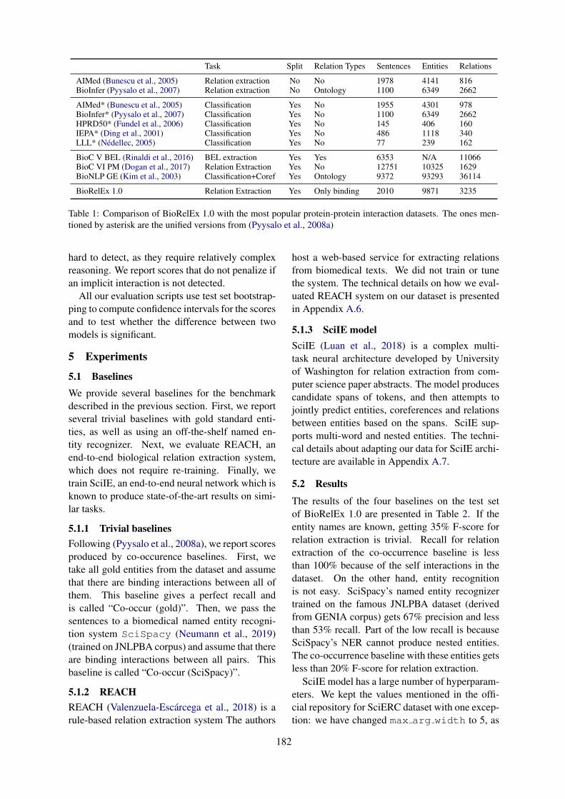
Task Split Relation Types Sentences Entities Relations
AIMed (Bunescu et al., 2005) Relation extraction No No 1978 4141 816BioInfer (Pyysalo et al., 2007) Relation extraction No Ontology 1100 6349 2662
AIMed* (Bunescu et al., 2005) Classification Yes No 1955 4301 978BioInfer* (Pyysalo et al., 2007) Classification Yes No 1100 6349 2662HPRD50* (Fundel et al., 2006) Classification Yes No 145 406 160IEPA* (Ding et al., 2001) Classification Yes No 486 1118 340LLL* (Nédellec, 2005) Classification Yes No 77 239 162
BioC V BEL (Rinaldi et al., 2016) BEL extraction Yes Yes 6353 N/A 11066BioC VI PM (Dogan et al., 2017) Relation Extraction Yes No 12751 10325 1629BioNLP GE (Kim et al., 2003) Classification+Coref Yes Ontology 9372 93293 36114
BioRelEx 1.0 Relation Extraction Yes Only binding 2010 9871 3235
Table 1: Comparison of BioRelEx 1.0 with the most popular protein-protein interaction datasets. The ones men-tioned by asterisk are the unified versions from (Pyysalo et al., 2008a)
hard to detect, as they require relatively complexreasoning. We report scores that do not penalize ifan implicit interaction is not detected.
All our evaluation scripts use test set bootstrap-ping to compute confidence intervals for the scoresand to test whether the difference between twomodels is significant.
5 Experiments
5.1 BaselinesWe provide several baselines for the benchmarkdescribed in the previous section. First, we reportseveral trivial baselines with gold standard enti-ties, as well as using an off-the-shelf named en-tity recognizer. Next, we evaluate REACH, anend-to-end biological relation extraction system,which does not require re-training. Finally, wetrain SciIE, an end-to-end neural network which isknown to produce state-of-the-art results on simi-lar tasks.
5.1.1 Trivial baselinesFollowing (Pyysalo et al., 2008a), we report scoresproduced by co-occurence baselines. First, wetake all gold entities from the dataset and assumethat there are binding interactions between all ofthem. This baseline gives a perfect recall andis called “Co-occur (gold)”. Then, we pass thesentences to a biomedical named entity recogni-tion system SciSpacy (Neumann et al., 2019)(trained on JNLPBA corpus) and assume that thereare binding interactions between all pairs. Thisbaseline is called “Co-occur (SciSpacy)”.
5.1.2 REACHREACH (Valenzuela-Escárcega et al., 2018) is arule-based relation extraction system The authors
host a web-based service for extracting relationsfrom biomedical texts. We did not train or tunethe system. The technical details on how we eval-uated REACH system on our dataset is presentedin Appendix A.6.
5.1.3 SciIE modelSciIE (Luan et al., 2018) is a complex multi-task neural architecture developed by Universityof Washington for relation extraction from com-puter science paper abstracts. The model producescandidate spans of tokens, and then attempts tojointly predict entities, coreferences and relationsbetween entities based on the spans. SciIE sup-ports multi-word and nested entities. The techni-cal details about adapting our data for SciIE archi-tecture are available in Appendix A.7.
5.2 Results
The results of the four baselines on the test setof BioRelEx 1.0 are presented in Table 2. If theentity names are known, getting 35% F-score forrelation extraction is trivial. Recall for relationextraction of the co-occurrence baseline is lessthan 100% because of the self interactions in thedataset. On the other hand, entity recognitionis not easy. SciSpacy’s named entity recognizertrained on the famous JNLPBA dataset (derivedfrom GENIA corpus) gets 67% precision and lessthan 53% recall. Part of the low recall is becauseSciSpacy’s NER cannot produce nested entities.The co-occurrence baseline with these entities getsless than 20% F-score for relation extraction.
SciIE model has a large number of hyperparam-eters. We kept the values mentioned in the offi-cial repository for SciERC dataset with one excep-tion: we have changed max arg width to 5, as
182
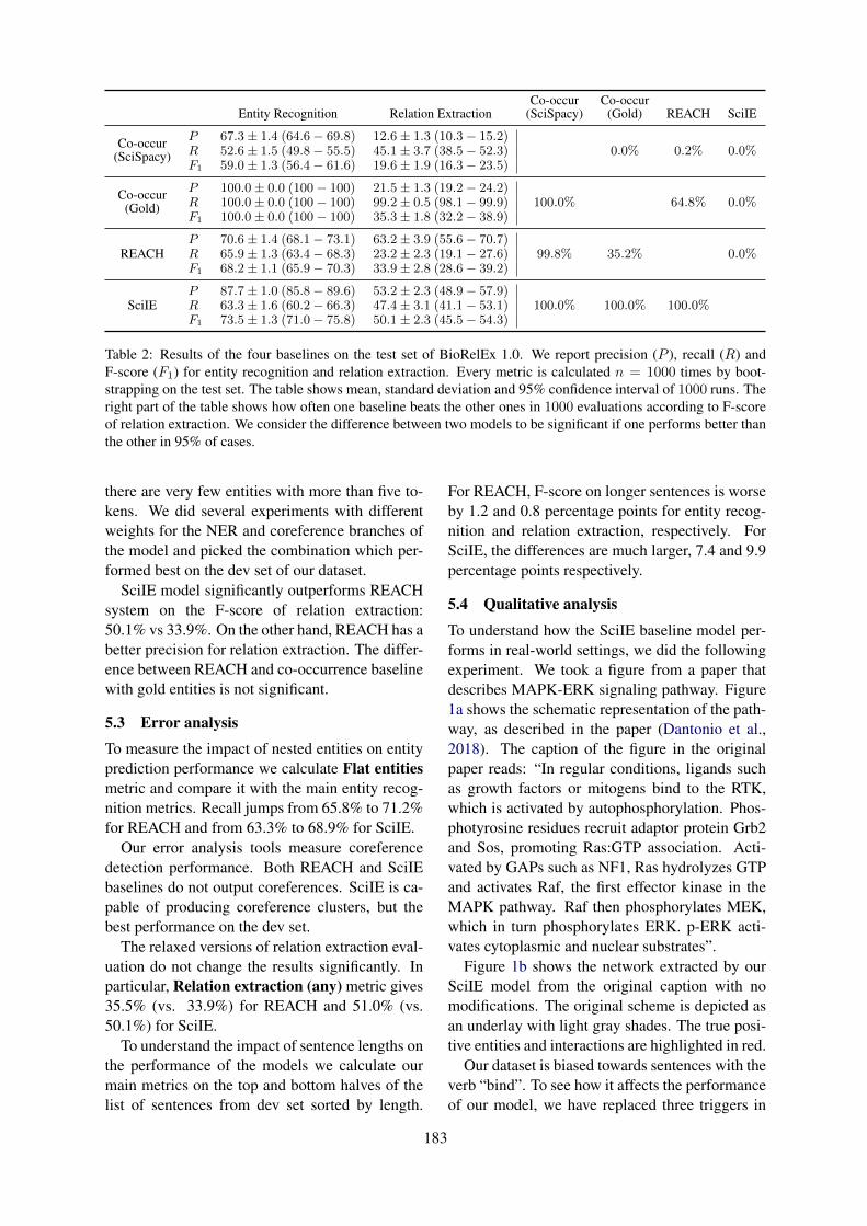
Entity Recognition Relation ExtractionCo-occur
(SciSpacy)Co-occur
(Gold) REACH SciIE
Co-occur(SciSpacy)
P 67.3± 1.4 (64.6− 69.8) 12.6± 1.3 (10.3− 15.2)0.0% 0.2% 0.0%R 52.6± 1.5 (49.8− 55.5) 45.1± 3.7 (38.5− 52.3)
F1 59.0± 1.3 (56.4− 61.6) 19.6± 1.9 (16.3− 23.5)
Co-occur(Gold)
P 100.0± 0.0 (100− 100) 21.5± 1.3 (19.2− 24.2)100.0% 64.8% 0.0%R 100.0± 0.0 (100− 100) 99.2± 0.5 (98.1− 99.9)
F1 100.0± 0.0 (100− 100) 35.3± 1.8 (32.2− 38.9)
REACHP 70.6± 1.4 (68.1− 73.1) 63.2± 3.9 (55.6− 70.7)
99.8% 35.2% 0.0%R 65.9± 1.3 (63.4− 68.3) 23.2± 2.3 (19.1− 27.6)F1 68.2± 1.1 (65.9− 70.3) 33.9± 2.8 (28.6− 39.2)
SciIEP 87.7± 1.0 (85.8− 89.6) 53.2± 2.3 (48.9− 57.9)
100.0% 100.0% 100.0%R 63.3± 1.6 (60.2− 66.3) 47.4± 3.1 (41.1− 53.1)F1 73.5± 1.3 (71.0− 75.8) 50.1± 2.3 (45.5− 54.3)
Table 2: Results of the four baselines on the test set of BioRelEx 1.0. We report precision (P ), recall (R) andF-score (F1) for entity recognition and relation extraction. Every metric is calculated n = 1000 times by boot-strapping on the test set. The table shows mean, standard deviation and 95% confidence interval of 1000 runs. Theright part of the table shows how often one baseline beats the other ones in 1000 evaluations according to F-scoreof relation extraction. We consider the difference between two models to be significant if one performs better thanthe other in 95% of cases.
there are very few entities with more than five to-kens. We did several experiments with differentweights for the NER and coreference branches ofthe model and picked the combination which per-formed best on the dev set of our dataset.
SciIE model significantly outperforms REACHsystem on the F-score of relation extraction:50.1% vs 33.9%. On the other hand, REACH has abetter precision for relation extraction. The differ-ence between REACH and co-occurrence baselinewith gold entities is not significant.
5.3 Error analysis
To measure the impact of nested entities on entityprediction performance we calculate Flat entitiesmetric and compare it with the main entity recog-nition metrics. Recall jumps from 65.8% to 71.2%for REACH and from 63.3% to 68.9% for SciIE.
Our error analysis tools measure coreferencedetection performance. Both REACH and SciIEbaselines do not output coreferences. SciIE is ca-pable of producing coreference clusters, but thebest performance on the dev set.
The relaxed versions of relation extraction eval-uation do not change the results significantly. Inparticular, Relation extraction (any) metric gives35.5% (vs. 33.9%) for REACH and 51.0% (vs.50.1%) for SciIE.
To understand the impact of sentence lengths onthe performance of the models we calculate ourmain metrics on the top and bottom halves of thelist of sentences from dev set sorted by length.
For REACH, F-score on longer sentences is worseby 1.2 and 0.8 percentage points for entity recog-nition and relation extraction, respectively. ForSciIE, the differences are much larger, 7.4 and 9.9percentage points respectively.
5.4 Qualitative analysis
To understand how the SciIE baseline model per-forms in real-world settings, we did the followingexperiment. We took a figure from a paper thatdescribes MAPK-ERK signaling pathway. Figure1a shows the schematic representation of the path-way, as described in the paper (Dantonio et al.,2018). The caption of the figure in the originalpaper reads: “In regular conditions, ligands suchas growth factors or mitogens bind to the RTK,which is activated by autophosphorylation. Phos-photyrosine residues recruit adaptor protein Grb2and Sos, promoting Ras:GTP association. Acti-vated by GAPs such as NF1, Ras hydrolyzes GTPand activates Raf, the first effector kinase in theMAPK pathway. Raf then phosphorylates MEK,which in turn phosphorylates ERK. p-ERK acti-vates cytoplasmic and nuclear substrates”.
Figure 1b shows the network extracted by ourSciIE model from the original caption with nomodifications. The original scheme is depicted asan underlay with light gray shades. The true posi-tive entities and interactions are highlighted in red.
Our dataset is biased towards sentences with theverb “bind”. To see how it affects the performanceof our model, we have replaced three triggers in
183
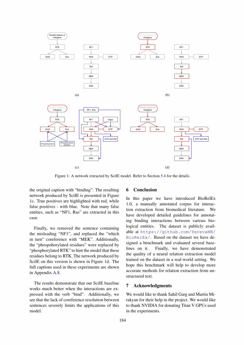
Growth factors ormitogens
RTK
Grb2 Sos
NF1
RAS
Raf
MEK
ERK
GTP
(a)
Growth factors ormitogens
RTK
Grb2 Sos
NF1
RAS
Raf
MEK
ERK
GTP
(b)
Growth factors ormitogens
RTK
Grb2 Sos
Phosphotyrosine Phosphotyrosineresidues
GapsNF1
RAS
Raf
MEK
ERK
GTP and Raf
GTP
NF1, Ras
(c)
Growth factors ormitogens
RTK
Grb2 Sos
NF1
RAS
Raf
MEK
ERK
GTP and Raf
GTP
(d)
Figure 1: A network extracted by SciIE model. Refer to Section 5.4 for the details.
the original caption with “binding”. The resultingnetwork produced by SciIE is presented in Figure1c. True positives are highlighted with red, whilefalse positives - with blue. Note that many falseentities, such as “NF1, Ras” are extracted in thiscase.
Finally, we removed the sentence containingthe misleading “NF1”, and replaced the ”whichin turn” coreference with “MEK”. Additionally,the “phospohorylated residues” were replaced by“phosphorylated RTK” to hint the model that theseresidues belong to RTK. The network produced bySciIE on this version is shown in Figure 1d. Thefull captions used in these experiments are shownin Appendix A.8.
The results demonstrate that our SciIE baselineworks much better when the interactions are ex-pressed with the verb “bind”. Additionally, wesee that the lack of coreference resolution betweensentences severely limits the applications of thismodel.
6 Conclusion
In this paper we have introduced BioRelEx1.0, a manually annotated corpus for interac-tion extraction from biomedical literature. Wehave developed detailed guidelines for annotat-ing binding interactions between various bio-logical entities. The dataset is publicly avail-able at https://github.com/YerevaNN/BioRelEx/. Based on the dataset we have de-signed a benchmark and evaluated several base-lines on it. Finally, we have demonstratedthe quality of a neural relation extraction modeltrained on the dataset in a real-world setting. Wehope this benchmark will help to develop moreaccurate methods for relation extraction from un-structured text.
7 Acknowledgments
We would like to thank Sahil Garg and Martin Mi-rakyan for their help in the project. We would liketo thank NVIDIA for donating Titan V GPUs usedin the experiments.
184
ReferencesMahtab Ahmed, Jumayel Islam, Muhammad Rifayat
Samee, and Robert E Mercer. 2019. Identifyingprotein-protein interaction using tree lstm and struc-tured attention. In 2019 IEEE 13th InternationalConference on Semantic Computing (ICSC), pages224–231. IEEE.
Andrey Rzhetsky et. al. 2019. in preparation.
Isabelle Augenstein, Mrinal Das, Sebastian Riedel,Lakshmi Vikraman, and Andrew McCallum. 2017.Semeval 2017 task 10: Scienceie - extractingkeyphrases and relations from scientific publica-tions. CoRR, abs/1704.02853.
Razvan Bunescu, Ruifang Ge, Rohit J Kate, Edward MMarcotte, Raymond J Mooney, Arun K Ramani, andYuk Wah Wong. 2005. Comparative experimentson learning information extractors for proteins andtheir interactions. Artificial intelligence in medicine,33(2):139–155.
Paola M. Dantonio, Marianne O. Klein, Maria Re-nata V.B. Freire, Camila N. Araujo, Ana CarolinaChiacetti, and Ricardo G. Correa. 2018. Exploringmajor signaling cascades in melanomagenesis: a ra-tionale route for targetted skin cancer therapy. Bio-science Reports, 38(5).
Louise Deléger, Robert Bossy, Estelle Chaix,Mouhamadou Ba, Arnaud Ferré, Philippe Bessières,and Claire Nédellec. 2016. Overview of the bacteriabiotope task at bionlp shared task 2016. In Pro-ceedings of the 4th BioNLP Shared Task Workshop,pages 12–22, Berlin, Germany. Association forComputational Linguistics.
Jing Ding, Daniel Berleant, Dan Nettleton, and EveWurtele. 2001. Mining medline: abstracts, sen-tences, or phrases? In Biocomputing 2002, pages326–337. World Scientific.
Rezarta Islamaj Dogan, Andrew Chatr-aryamontri,Sun Kim, Chih-Hsuan Wei, Yifan Peng, DonaldComeau, and Zhiyong Lu. 2017. Biocreative vi pre-cision medicine track: creating a training corpus formining protein-protein interactions affected by mu-tations. In BioNLP 2017, pages 171–175.
Katrin Fundel, Robert Küffner, and Ralf Zimmer.2006. Relexrelation extraction using dependencyparse trees. Bioinformatics, 23(3):365–371.
Jeremy Getman, Joe Ellis, Stephanie Strassel, ZhiyiSong, and Jennifer Tracey. 2018. Laying thegroundwork for knowledge base population: Nineyears of linguistic resources for tac kbp. In Proceed-ings of the Eleventh International Conference onLanguage Resources and Evaluation (LREC-2018).
Harsha Gurulingappa, Abdul Mateen Rajput, AngusRoberts, Juliane Fluck, Martin Hofmann-Apitius,and Luca Toldo. 2012. Development of a bench-mark corpus to support the automatic extrac-tion of drug-related adverse effects from medical
case reports. Journal of Biomedical Informatics,45(5):885–892.
Yu Lun Hsieh, Yung-Chun Chang, Nai Wen Chang,and Wen Lian Hsu. 2017. Identifying protein-protein interactions in biomedical literature using re-current neural networks with long short-term mem-ory. In Proceedings of the Eighth InternationalJoint Conference on Natural Language Processing,pages 240–245. Asian Federation of Natural Lan-guage Processing.
J.-D. Kim, T. Ohta, Y. Tateisi, and J. Tsujii. 2003. GE-NIA corpusa semantically annotated corpus for bio-textmining. Bioinformatics, 19:i180–i182.
Jin-Dong Kim, Tomoko Ohta, Sampo Pyysalo, Yoshi-nobu Kano, and Jun’ichi Tsujii. 2009. Overview ofBioNLP’09 shared task on event extraction. In Pro-ceedings of the BioNLP 2009 Workshop CompanionVolume for Shared Task, pages 1–9, Boulder, Col-orado. Association for Computational Linguistics.
Jin-Dong Kim, Sampo Pyysalo, Tomoko Ohta, RobertBossy, Ngan Nguyen, and Jun’ichi Tsujii. 2011.Overview of BioNLP shared task 2011. In Proceed-ings of BioNLP Shared Task 2011 Workshop, pages1–6, Portland, Oregon, USA. Association for Com-putational Linguistics.
Martin Krallinger, Florian Leitner, Carlos Rodriguez-Penagos, and Alfonso Valencia. 2008. Overview ofthe protein-protein interaction annotation extractiontask of biocreative ii. Genome biology, 9(2):S4.
Yi Luan, Luheng He, Mari Ostendorf, and HannanehHajishirzi. 2018. Multi-task identification of enti-ties, relations, and coreference for scientific knowl-edge graph construction. In Proceedings of the 2018Conference on Empirical Methods in Natural Lan-guage Processing, pages 3219–3232. Associationfor Computational Linguistics.
Claire Nédellec. 2005. Learning language in logic-genic interaction extraction challenge. In Proceed-ings of the 4th Learning Language in Logic Work-shop (LLL05), volume 7, pages 1–7. Citeseer.
Claire Nédellec, Robert Bossy, Jin-Dong Kim, Jung-Jae Kim, Tomoko Ohta, Sampo Pyysalo, and PierreZweigenbaum. 2013. Overview of bionlp sharedtask 2013. In Proceedings of the BioNLP SharedTask 2013 Workshop, pages 1–7.
Mark Neumann, Daniel King, Iz Beltagy, and WaleedAmmar. 2019. Scispacy: Fast and robust models forbiomedical natural language processing.
Rose Oughtred, Chris Stark, Bobby-Joe Breitkreutz,Jennifer Rust, Lorrie Boucher, Christie Chang, Na-dine Kolas, Lara ODonnell, Genie Leung, RochelleMcAdam, Frederick Zhang, Sonam Dolma, AndrewWillems, Jasmin Coulombe-Huntington, AndrewChatr-aryamontri, Kara Dolinski, and Mike Tyers.2018. The BioGRID interaction database: 2019 up-date. Nucleic Acids Research, 47(D1):D529–D541.
185
Sampo Pyysalo, Antti Airola, Juho Heimonen, JariBjörne, Filip Ginter, and Tapio Salakoski. 2008a.Comparative analysis of five protein-protein interac-tion corpora. BMC Bioinformatics, 9(3):S6.
Sampo Pyysalo, Filip Ginter, Juho Heimonen, JariBjörne, Jorma Boberg, Jouni Järvinen, and TapioSalakoski. 2007. Bioinfer: a corpus for informationextraction in the biomedical domain. BMC bioinfor-matics, 8(1):50.
Sampo Pyysalo, Rune Sætre, Junichi Tsujii, and TapioSalakoski. 2008b. Why biomedical relation extrac-tion results are incomparable and what to do aboutit. In Proceedings of the Third International Sym-posium on Semantic Mining in Biomedicine (SMBM2008). Turku, pages 149–152. Citeseer.
Fabio Rinaldi, Tilia Renate Ellendorff, Sumit Madan,Simon Clematide, Adrian Van der Lek, Theo Mevis-sen, and Juliane Fluck. 2016. Biocreative v track 4:a shared task for the extraction of causal network in-formation using the biological expression language.Database, 2016.
Paul Shannon, Andrew Markiel, Owen Ozier, Nitin S.Baliga, Jonathan T. Wang, Daniel Ramage, NadaAmin, Benno Schwikowski, and Trey Ideker. 2003.Cytoscape: A software environment for inte-grated models of biomolecular interaction networks.Genome Research, 13(11):2498–2504.
Paul Thompson, Sophia Ananiadou, and Junichi Tsu-jii. 2017. The genia corpus: Annotation levels andapplications. In Handbook of Linguistic Annotation,pages 1395–1432. Springer.
Marco A Valenzuela-Escárcega, Özgün Babur, GusHahn-Powell, Dane Bell, Thomas Hicks, EnriqueNoriega-Atala, Xia Wang, Mihai Surdeanu, EmekDemir, and Clayton T Morrison. 2018. Large-scaleautomated machine reading discovers new cancerdriving mechanisms. Database: The Journal of Bi-ological Databases and Curation.
Yuhao Zhang, Victor Zhong, Danqi Chen, Gabor An-geli, and Christopher D. Manning. 2017. Position-aware attention and supervised data improve slotfilling. In Proceedings of the 2017 Conference onEmpirical Methods in Natural Language Processing(EMNLP 2017), pages 35–45.
A Appendices
A.1 Examples of entity annotationambiguities
1. (1.0.train.104) “The inability oftyrosine-phosphorylated SLP-76 to interactwith nck(SH2*)”. We annotate “nck” as aprotein and “nck(SH2*)” as a protein withlabel “mutant”.
2. (1.0.train.45) “... equal amounts ofREGs α and β bound to the proteasome ...”.We annotate “REGs α” as a protein and linkit to the implicit “REG α”, and annotate “β”as a protein and link it to the implicit “REGβ”.
3. (1.0.dev.118) “NF-Y binds the HSP70promoter in vivo.”. We annotate three en-tities in this sentence: “NF-Y” is a protein,“HSP70” is a gene, and “HSP70 promoter”is a DNA. There is a binding interaction be-tween “NF-Y” and “HSP70 promoter”, butnot with “HSP70”.
4. (1.0.train.964) “...the binding of cor-tactin to the Arp2/3 complex....”. Here,“Arp2/3” is annotated as a complex, “Arp2”is a protein, while “3” is annotated as a pro-tein and is linked to an implicit entity “Arp3”.
5. (1.0.train.430) “A18 hnRNP BindsSpecifically to RPA2 and Thioredoxin 3’-UTRs”. Here, “RPA2 3’-UTR” is a regionof “RPA2” RNA. But it is not a continuousspan of characters, so we are forced to anno-tate only “RPA2”. As a result, the same se-quence of characters “RPA” is annotated bothas an RNA and as an RNA-region.
6. (1.0.train.121) “JNK/SAPK Binds andPhosphorylates a MEKK1 Fragment InVitro”. Here JNK and SAPK are separateentities. We annotate binding interaction be-tween “JNK” and “MEKK1” and between“SAPK” and “MEKK”.
7. (1.0.train.50) “... Apaf-1 binds cy-tochrome c and dATP, and this complex re-cruits caspase-9 ...”. “This complex” refersto an implicit complex with three entities. Wedo not annotate the complex and its interac-tions.
A.2 Examples of interaction annotationambiguities
1. (1.0.train.540) “We also attempted toexamine the actin-binding ability of partiallyphosphorylated F-rad.” This sentence moti-vates the performed experiment, but does nottalk about the outcome.
186
Space, full stop “S. cerevisiae” (cell), “S-1.MgADP.Pi” (protein-domain)Question mark No examplesComma, colon, semicolon “PI(4,5)P2” (chemical), “f:TFIID” (fusion-protein)Round brackets “NAD(H)” (chemical), “HMG-1(A-B)” (protein region)Square brackets “DB[a,l]PDE” (chemical), “[3H]LY341495” (drug)Hyphen-like symbols “IGF-II promoter” (DNA), “hTcf-4-(180)” (protein-region)Apostrophe “3’UTR” (RNA), “3’dE5” (chemical)Asterisk “Rh*” (protein), “C2A* mutant” (protein-domain)Plus “Ca2+” (chemical), “Na+,K+-ATPase” (protein-complex)Dot-like symbols “DBAD” (protein-region), “actinϕ” (protein-family)
Table 3: All entities in the dataset are surrounded by any of the symbols described in the first column. On the otherhand, most of these symbols can appear inside entity names. The second column of the table shows examples ofentities which contain these symbols.
2. (1.0.train.755) “We expect that in theintact BAF complex, the actin monomer isbound to Brg1 at both of these sites.” Thissentence does not confirm the existence of abinding interaction.
3. (1.0.train.1397) “Binding of Hairyderivatives to Gro in vitro.”. This is a titlethat uses an indefinite verb, and the contentsof the following paragraphs might imply bothexistence and non-existence of the bindinginteraction. We annotate the binding interac-tion between “Hairy derivatives” and “Gro”with label 0.
4. (1.0.train.1234) “Phosphorylation ofL1 Y1176 inhibits L1 binding to AP-2.” Thisis a subsection title, but it clearly implies that“L1” binds to “AP-2” (which is inhibited byphosphorylation), so we annotate this inter-action with label 1.
5. (1.0.train.1154) “... the ORC-Cdc6pcomplex (and perhaps other proteins) re-cruits the six minichromosome maintenance(MCM) proteins ...”. Here “minichromo-some maintenance” and “MCM” refer to thesame protein family and are annotated assynonyms. We annotate binding interactionbetween “MCM” and “ORC-Cdc6p”, andthe evaluation script does not penalize themodel if it predicts an interaction between“minichromosome maintenance” and “ORC-Cdc6p”.
6. (1.0.train.785) “... TR/RXR binds tothe TRE ...”. Here we annotate a binding in-
teraction between ”TR” and ”RXR” and tagit as “complex”.
7. (1.0.train.1154) “... Cdc6p most likelybinds to ORC and then the ORC-Cdc6p com-plex ...”. Here the binding interaction be-tween “ORC” and “Cdc6p” can be inferredexplicitly from the first part of the sentenceand implicitly from the name of the complex.In these cases we do not tag the interactionwith “complex” label.
8. (1.0.train.630) “hTcf-4-(180) interactsdirectly with the Armadillo repeats of β-catenin”. Here “hTcf-4-(180)” is annotatedas a domain of “hTcf-4” protein, and “Ar-madillo repeats” is annotated as a region of“β-catenin” protein. We annotate the interac-tion between “hTcf-4-(180)” and “Armadillorepeats”. Additionally, we annotate threeother interactions: “hTcf-4-(180)” and “β-catenin”, “hTcf-4” and “Armadillo repeats”,“hTcf-4” and “β-catenin”, and tag them withan “implicit” label.
9. (1.0.train.758) “Synaptotagmin bindsβ-SNAP, but not α-SNAP...”. Here “Synap-totagmin” and “SNAP” are annotated as pro-teins, while “α-SNAP” and “β-SNAP” areannotated as isoforms of “SNAP”. We anno-tate a negative binding interaction between“α-SNAP” and “Synaptotagmin”, but it doesnot imply that “Synaptotagmin” does notbind “SNAP”. This shows that the implicit“transfer” of an interaction does not hold ifthe interaction is negative.
10. (1.0.test.171) “Myozenin binds to both
187
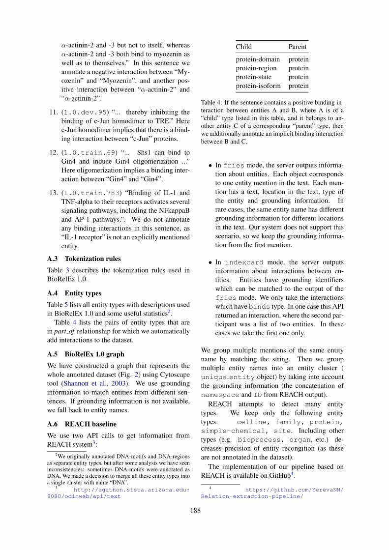
α-actinin-2 and -3 but not to itself, whereasα-actinin-2 and -3 both bind to myozenin aswell as to themselves.” In this sentence weannotate a negative interaction between “My-ozenin” and “Myozenin”, and another pos-itive interaction between “α-actinin-2” and“α-actinin-2”.
11. (1.0.dev.95) “... thereby inhibiting thebinding of c-Jun homodimer to TRE.” Herec-Jun homodimer implies that there is a bind-ing interaction between “c-Jun” proteins.
12. (1.0.train.69) “... Shs1 can bind toGin4 and induce Gin4 oligomerization ...”Here oligomerization implies a binding inter-action between “Gin4” and “Gin4”.
13. (1.0.train.783) “Binding of IL-1 andTNF-alpha to their receptors activates severalsignaling pathways, including the NFkappaBand AP-1 pathways.”. We do not annotateany binding interactions in this sentence, as“IL-1 receptor” is not an explicitly mentionedentity.
A.3 Tokenization rulesTable 3 describes the tokenization rules used inBioRelEx 1.0.
A.4 Entity typesTable 5 lists all entity types with descriptions usedin BioRelEx 1.0 and some useful statistics2.
Table 4 lists the pairs of entity types that arein part of relationship for which we automaticallyadd interactions to the dataset.
A.5 BioRelEx 1.0 graphWe have constructed a graph that represents thewhole annotated dataset (Fig. 2) using Cytoscapetool (Shannon et al., 2003). We use groundinginformation to match entities from different sen-tences. If grounding information is not available,we fall back to entity names.
A.6 REACH baselineWe use two API calls to get information fromREACH system3:
2We originally annotated DNA-motifs and DNA-regionsas separate entity types, but after some analysis we have seeninconsistencies: sometimes DNA-motifs were annotated asDNA. We made a decision to merge all these entity types intoa single cluster with name “DNA”.
3 http://agathon.sista.arizona.edu:8080/odinweb/api/text
Child Parent
protein-domain proteinprotein-region proteinprotein-state proteinprotein-isoform protein
Table 4: If the sentence contains a positive binding in-teraction between entities A and B, where A is of a“child” type listed in this table, and it belongs to an-other entity C of a corresponding “parent” type, thenwe additionally annotate an implicit binding interactionbetween B and C.
• In fries mode, the server outputs informa-tion about entities. Each object correspondsto one entity mention in the text. Each men-tion has a text, location in the text, type ofthe entity and grounding information. Inrare cases, the same entity name has differentgrounding information for different locationsin the text. Our system does not support thisscenario, so we keep the grounding informa-tion from the first mention.
• In indexcard mode, the server outputsinformation about interactions between en-tities. Entities have grounding identifierswhich can be matched to the output of thefries mode. We only take the interactionswhich have binds type. In one case this APIreturned an interaction, where the second par-ticipant was a list of two entities. In thesecases we take the first one only.
We group multiple mentions of the same entityname by matching the string. Then we groupmultiple entity names into an entity cluster (unique entity object) by taking into accountthe grounding information (the concatenation ofnamespace and ID from REACH output).
REACH attempts to detect many entitytypes. We keep only the following entitytypes: celline, family, protein,simple-chemical, site. Including othertypes (e.g. bioprocess, organ, etc.) de-creases precision of entity recongition (as theseare not annotated in the dataset).
The implementation of our pipeline based onREACH is available on GitHub4.
4 https://github.com/YerevaNN/Relation-extraction-pipeline/
188
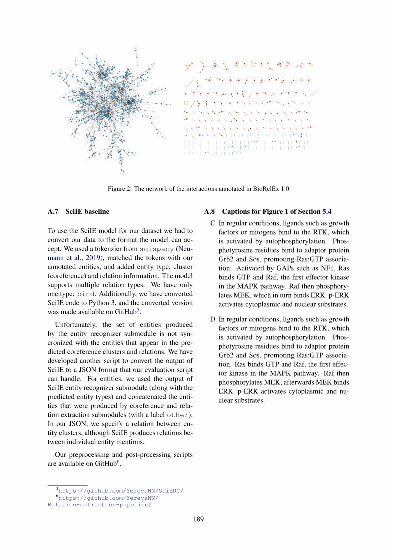
Figure 2: The network of the interactions annotated in BioRelEx 1.0
A.7 SciIE baseline
To use the SciIE model for our dataset we had toconvert our data to the format the model can ac-cept. We used a tokenzier from scispacy (Neu-mann et al., 2019), matched the tokens with ourannotated entities, and added entity type, cluster(coreference) and relation information. The modelsupports multiple relation types. We have onlyone type: bind. Additionally, we have convertedSciIE code to Python 3, and the converted versionwas made available on GitHub5.
Unfortunately, the set of entities producedby the entity recognizer submodule is not syn-cronized with the entities that appear in the pre-dicted coreference clusters and relations. We havedeveloped another script to convert the output ofSciIE to a JSON format that our evaluation scriptcan handle. For entities, we used the output ofSciIE entity recognizer submodule (along with thepredicted entity types) and concatenated the enti-ties that were produced by coreference and rela-tion extraction submodules (with a label other).In our JSON, we specify a relation between en-tity clusters, although SciIE produces relations be-tween individual entity mentions.
Our preprocessing and post-processing scriptsare available on GitHub6.
5https://github.com/YerevaNN/SciERC/6https://github.com/YerevaNN/
Relation-extraction-pipeline/
A.8 Captions for Figure 1 of Section 5.4C In regular conditions, ligands such as growth
factors or mitogens bind to the RTK, whichis activated by autophosphorylation. Phos-photyrosine residues bind to adaptor proteinGrb2 and Sos, promoting Ras:GTP associa-tion. Activated by GAPs such as NF1, Rasbinds GTP and Raf, the first effector kinasein the MAPK pathway. Raf then phosphory-lates MEK, which in turn binds ERK. p-ERKactivates cytoplasmic and nuclear substrates.
D In regular conditions, ligands such as growthfactors or mitogens bind to the RTK, whichis activated by autophosphorylation. Phos-photyrosine residues bind to adaptor proteinGrb2 and Sos, promoting Ras:GTP associa-tion. Ras binds GTP and Raf, the first effec-tor kinase in the MAPK pathway. Raf thenphosphorylates MEK, afterwards MEK bindsERK. p-ERK activates cytoplasmic and nu-clear substrates.
189
Entity type Statistics Description
protein 3640 / 3777 /82 / 147
Entities either represented with protein names; or with gene names (X) but factuallystanding as actual proteins in the sentence (either explicitly: X protein; or implicitlyX binds the promoter)
protein-family 1086 / 1017 /0 / 0
Entities represented with protein-family names (e.g. actin) or representing a groupof protein with common properties (e.g. globular proteins; x-domain containingproteins, etc)
chemical 532 / 295 / 0 /0
Any chemical compound other than protein or DNA or RNA, excluding experi-mental reagents/antibodies.
DNA 506 / 468 / 2 /0
Any entity type that represents a region of or full DNA molecule, except for genenames. These include explicit ‘DNA’ mentions; DNA-regions, such as gene pro-moters, DNA elements; DNA sequences represented with nucleotides and DNA-motifs represented with names; chromosomes and plastids.
protein-complex 419 / 294 / 1 /0
Protein complexes are either explicitlly mentioned with name followed by ‘com-plex’ suffix, or with name containing subunits seperated with slashes or dashes, orwith names that do not contain the members, but are known to be complexes.
protein-domain 318 / 134 / 2 /1
Domains may or may not be explicitly annotated with the suffix ‘domain’. Theymay be specific domains of proteins present in the sentence, or general domainnames without reference to the proteins they belong to.
cell 152 / 1 / 3 / 2 Explicit mentions of a cell or entities representing cell names, cell-line, bacterium,as well as viruses.
experimental-construct 141 / 60 / 0 / 0 Entities refering to artificially merged molecules, including tagged proteins, taggedRNA and DNA and chemically modified proteins/RNA/DNA.
RNA 137 / 105 / 0 /0
All the entities representing physical RNA molecules (mRNA, tRNA, rRNA, etc.),or RNA-motifs (represented by RNA sequence or motif name) or RNA regions(represented by region names). mRNAs presented in text with corresponding genenames are also annotated as RNA.
experiment-tag 128 / 35 / 0 / 0 Chemicals or proteins experimentally added to proteins (e.g. GST tag).reagent 128 / 43 / 0 / 0 Chemicals/biomolecules used in experimental settings (e.g. antibody)protein-motif 122 / 43 / 0 / 0 Amino acid sequence patterns represented either by motif names or amino acid
sequences, which may or may not be followed by explicit ‘motif’ mention.gene 109 / 6 / 2 / 0 Entities represented with gene names.amino-acid 69 / 2 / 0 / 0 Amino acids represented by amino acid names or explicit amino acid mentions.protein-region 66 / 37 / 0 / 0 Protein regions are entities refering to amino-acid sequences (motif names or actual
sequence representations); or regions on the protein not refering to whole domains.assay 55 / 0 / 0 / 0 Entities refering to exprimental method names or assays or procedures.organelle 51 / 20 / 0 / 0 Subcellular entities represented with their names (e.g. ribosome).peptide 37 / 24 / 0 / 0 Short amino-acid polymers represented by their names, which may or may not be
followed by explict ‘peptide’ mentions.fusion-protein 32 / 25 / 0 / 0 Fusion-proteinsprotein-isoform 32 / 33 / 0 / 0 Protein sub-types encoded by the same gene, but resulting from its differential
post-processing. These entities may or may not appear in a sentence with explicitisoform mentions.
process 31 / 0 / 0 / 0 Entities refering to sequences of events at molecular, cellular or organismal lev-els. These may be pathway names (represented either by member gene namesor target process names, with or without explicit ‘pathway’ mentions); processnames/descriptions (e.g. autophagy); disorders and biological phenotypes.
mutation 20 / 0 / 0 / 0 Specifications of mutations in the form of nucleotide-to-nucleotide (A55G) oramino acid-to-amino acid transitions (Ala55Ser) or sequence to sequence transi-tions (ACGT to AGGT).
protein-RNA-complex 20 / 11 / 0 / 0 Complexes composed of proteins and RNA, mentioned either with componentnames or the complex alias, with or without explicit ‘protein-RNA’ mention.
drug 18 / 8 / 0 / 0 Drug namesorganism 7 / 0 / 0 / 0 Multi-cellular organisms (i.e. excluding cells, bacteria and viruses)disease 6 / 0 / 0 / 0 Entities representing disease names.protein-DNA-complex 5 / 7 / 0 / 0 Complexes composed of proteins and DNA, mentioned either with component
names or the complex alias, with or without explicit ‘protein-DNA’ mention.brand 4 / 0 / 0 / 0 Entities representing company names or reagent/drug brands.tissue 2 / 0 / 0 / 0 Entities representing tissues.RNA-family 2 / 1 / 0 / 0 Entities representing groups of RNA with common properties.gene-family 2 / 0 / 0 / 0 Entities representing sets of genes encoding for protein-families or combined by a
common characteristic. Usually mentioned with name followed by ‘gene family’.fusion-gene 1 / 1 / 0 / 0 Entities representing fusion products of two genes. Usually represented by gene
names separated with dashes followed (or not) by ‘fusion’ suffix.
Table 5: Entity types annotated in the dataset. The second column shows the number of mentions of those entitiesin the sentences, number of binding interactions involving those entities, number of mutated entities and numberof entities that appear in a special state (e.g. phosphorylated).
190
Proceedings of the BioNLP 2019 workshop, pages 191–200Florence, Italy, August 1, 2019. c©2019 Association for Computational Linguistics
Extraction of Lactation Frames from Drug Labels and LactMed
Heath Goodrum, Meghana Gudala, Ankita Misra, Kirk RobertsSchool of Biomedical Informatics
University of Texas Health Science Center at Houston{heath.goodrum,kirk.roberts}@uth.tmc.edu
Abstract
This paper describes a natural languageprocessing (NLP) approach to extractinglactation-specific drug information from twosources: FDA-mandated drug labels andthe NLM Drugs and Lactation Database(LactMed). A frame semantic approach isutilized, and the paper describes the selectedframes, their annotation on a set of 900 sec-tions from drug labels and LactMed articles,and the NLP system to extract such frame in-stances automatically. The ultimate goal of theproject is to use such a system to identify dis-crepancies in lactation-related drug informa-tion between these resources.
1 Introduction
Medical information about prescription drugs ispublicly available in a variety of sources, includ-ing the biomedical literature, consumer-focusedwebsites, and the drug labels mandated by theU.S. Food & Drug Administration (FDA). Butthe rapid advances in biomedicine—especiallyrecently-approved drugs—threatens to make thesesources discordant. Synchronizing such sources isdifficult due to their unstructured nature and thewide variety of ways in which they are organized.This paper presents initial work in an effort toalign two such sources—drug labels and a singleconsumer health website—for information partic-ular to a single sub-population—nursing mothers.
This is a critical sub-population for providingvalidated health information to, especially for pre-scription drugs. Notably, randomized trials, thegold standard in drug evaluation, contain few ifany nursing mothers in their trial populations.Thus, the information that a pharmaceutical sub-stance has on such mothers and their children isscarce and of poor evidence quality, which onlyserves to promote misinformation and discourage
mothers from taking needed medications. Author-itative guidance is critical in regards to what issupported or contradicted by the limited evidence,as well as what is simply unknown. Several pub-lic sources attempt to provide such authoritativeinformation. Here, two such sources are studied:a section of drug labels specific to nursing moth-ers and a government website specific to drugs andlactation, LactMed. By identifying discrepanciesin the free text narratives of these sources, furtherreview can pinpoint information gaps, conflictingopinions, and out-of-date guidance.
The general strategy proposed in this paper in-volves (a) identifying seven key information typesof drug information specific to nursing mothers,(b) utilizing linguistically-motivated frame seman-tic representations for these information types, (c)annotating instances of these frames on both lacta-tion information sources, and (d) developing natu-ral language processing (NLP) methods to extractthis information automatically from these sources.
Our specific contributions include:
1. The first NLP method to focus specifically ondrug information for nursing mothers.
2. Development of frame representations forlactation-specific drug information.
3. Application of a deep learning-based sys-tem on two separate lactation informationsources, drug labels and LactMed.
4. Evaluation of cross-corpus similarity in termsof important lactation information.
While this paper’s scope is quite narrow, justlactation information from two sources, we positthe techniques described here are generalizable toother lactation information sources (with minimalannotation/training) as well as to other importantpharmaceutical sub-populations (with, albeit, con-siderable annotation effort).
191
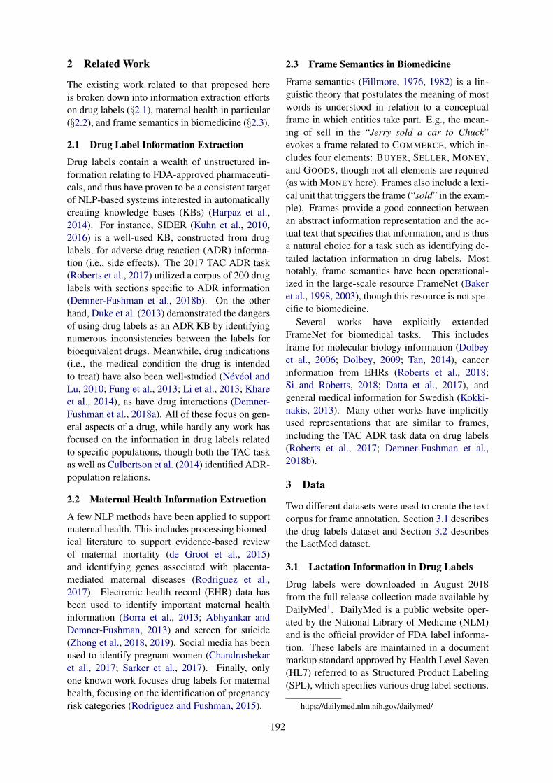
2 Related Work
The existing work related to that proposed hereis broken down into information extraction effortson drug labels (§2.1), maternal health in particular(§2.2), and frame semantics in biomedicine (§2.3).
2.1 Drug Label Information Extraction
Drug labels contain a wealth of unstructured in-formation relating to FDA-approved pharmaceuti-cals, and thus have proven to be a consistent targetof NLP-based systems interested in automaticallycreating knowledge bases (KBs) (Harpaz et al.,2014). For instance, SIDER (Kuhn et al., 2010,2016) is a well-used KB, constructed from druglabels, for adverse drug reaction (ADR) informa-tion (i.e., side effects). The 2017 TAC ADR task(Roberts et al., 2017) utilized a corpus of 200 druglabels with sections specific to ADR information(Demner-Fushman et al., 2018b). On the otherhand, Duke et al. (2013) demonstrated the dangersof using drug labels as an ADR KB by identifyingnumerous inconsistencies between the labels forbioequivalent drugs. Meanwhile, drug indications(i.e., the medical condition the drug is intendedto treat) have also been well-studied (Névéol andLu, 2010; Fung et al., 2013; Li et al., 2013; Khareet al., 2014), as have drug interactions (Demner-Fushman et al., 2018a). All of these focus on gen-eral aspects of a drug, while hardly any work hasfocused on the information in drug labels relatedto specific populations, though both the TAC taskas well as Culbertson et al. (2014) identified ADR-population relations.
2.2 Maternal Health Information Extraction
A few NLP methods have been applied to supportmaternal health. This includes processing biomed-ical literature to support evidence-based reviewof maternal mortality (de Groot et al., 2015)and identifying genes associated with placenta-mediated maternal diseases (Rodriguez et al.,2017). Electronic health record (EHR) data hasbeen used to identify important maternal healthinformation (Borra et al., 2013; Abhyankar andDemner-Fushman, 2013) and screen for suicide(Zhong et al., 2018, 2019). Social media has beenused to identify pregnant women (Chandrashekaret al., 2017; Sarker et al., 2017). Finally, onlyone known work focuses drug labels for maternalhealth, focusing on the identification of pregnancyrisk categories (Rodriguez and Fushman, 2015).
2.3 Frame Semantics in Biomedicine
Frame semantics (Fillmore, 1976, 1982) is a lin-guistic theory that postulates the meaning of mostwords is understood in relation to a conceptualframe in which entities take part. E.g., the mean-ing of sell in the “Jerry sold a car to Chuck”evokes a frame related to COMMERCE, which in-cludes four elements: BUYER, SELLER, MONEY,and GOODS, though not all elements are required(as with MONEY here). Frames also include a lexi-cal unit that triggers the frame (“sold” in the exam-ple). Frames provide a good connection betweenan abstract information representation and the ac-tual text that specifies that information, and is thusa natural choice for a task such as identifying de-tailed lactation information in drug labels. Mostnotably, frame semantics have been operational-ized in the large-scale resource FrameNet (Bakeret al., 1998, 2003), though this resource is not spe-cific to biomedicine.
Several works have explicitly extendedFrameNet for biomedical tasks. This includesframe for molecular biology information (Dolbeyet al., 2006; Dolbey, 2009; Tan, 2014), cancerinformation from EHRs (Roberts et al., 2018;Si and Roberts, 2018; Datta et al., 2017), andgeneral medical information for Swedish (Kokki-nakis, 2013). Many other works have implicitlyused representations that are similar to frames,including the TAC ADR task data on drug labels(Roberts et al., 2017; Demner-Fushman et al.,2018b).
3 Data
Two different datasets were used to create the textcorpus for frame annotation. Section 3.1 describesthe drug labels dataset and Section 3.2 describesthe LactMed dataset.
3.1 Lactation Information in Drug Labels
Drug labels were downloaded in August 2018from the full release collection made available byDailyMed1. DailyMed is a public website oper-ated by the National Library of Medicine (NLM)and is the official provider of FDA label informa-tion. These labels are maintained in a documentmarkup standard approved by Health Level Seven(HL7) referred to as Structured Product Labeling(SPL), which specifies various drug label sections.
1https://dailymed.nlm.nih.gov/dailymed/
192
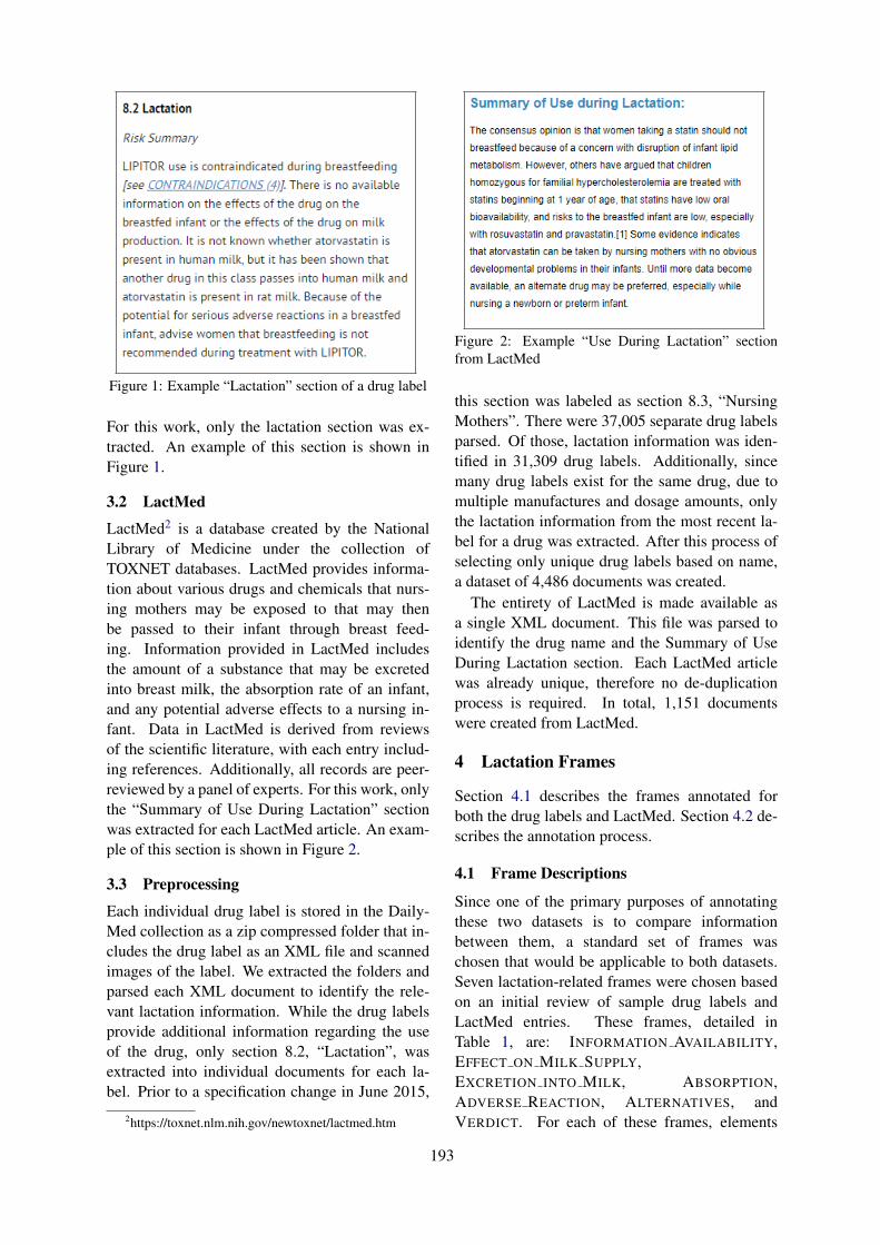
Figure 1: Example “Lactation” section of a drug label
For this work, only the lactation section was ex-tracted. An example of this section is shown inFigure 1.
3.2 LactMed
LactMed2 is a database created by the NationalLibrary of Medicine under the collection ofTOXNET databases. LactMed provides informa-tion about various drugs and chemicals that nurs-ing mothers may be exposed to that may thenbe passed to their infant through breast feed-ing. Information provided in LactMed includesthe amount of a substance that may be excretedinto breast milk, the absorption rate of an infant,and any potential adverse effects to a nursing in-fant. Data in LactMed is derived from reviewsof the scientific literature, with each entry includ-ing references. Additionally, all records are peer-reviewed by a panel of experts. For this work, onlythe “Summary of Use During Lactation” sectionwas extracted for each LactMed article. An exam-ple of this section is shown in Figure 2.
3.3 Preprocessing
Each individual drug label is stored in the Daily-Med collection as a zip compressed folder that in-cludes the drug label as an XML file and scannedimages of the label. We extracted the folders andparsed each XML document to identify the rele-vant lactation information. While the drug labelsprovide additional information regarding the useof the drug, only section 8.2, “Lactation”, wasextracted into individual documents for each la-bel. Prior to a specification change in June 2015,
2https://toxnet.nlm.nih.gov/newtoxnet/lactmed.htm
Figure 2: Example “Use During Lactation” sectionfrom LactMed
this section was labeled as section 8.3, “NursingMothers”. There were 37,005 separate drug labelsparsed. Of those, lactation information was iden-tified in 31,309 drug labels. Additionally, sincemany drug labels exist for the same drug, due tomultiple manufactures and dosage amounts, onlythe lactation information from the most recent la-bel for a drug was extracted. After this process ofselecting only unique drug labels based on name,a dataset of 4,486 documents was created.
The entirety of LactMed is made available asa single XML document. This file was parsed toidentify the drug name and the Summary of UseDuring Lactation section. Each LactMed articlewas already unique, therefore no de-duplicationprocess is required. In total, 1,151 documentswere created from LactMed.
4 Lactation Frames
Section 4.1 describes the frames annotated forboth the drug labels and LactMed. Section 4.2 de-scribes the annotation process.
4.1 Frame Descriptions
Since one of the primary purposes of annotatingthese two datasets is to compare informationbetween them, a standard set of frames waschosen that would be applicable to both datasets.Seven lactation-related frames were chosen basedon an initial review of sample drug labels andLactMed entries. These frames, detailed inTable 1, are: INFORMATION AVAILABILITY,EFFECT ON MILK SUPPLY,EXCRETION INTO MILK, ABSORPTION,ADVERSE REACTION, ALTERNATIVES, andVERDICT. For each of these frames, elements
193
Table 1: Frames and Frame Elements
Element Description
Non-Core Elements - Elements that are common across all/most frames.
ANIMAL Marks non-humans to which the frame applies. Frequently information is onlyavailable in animals studies and as not been verified/observed in human studies.
CONDITION A condition (specific circumstance) under which the rest of the frame applies.DRUG The name of the drug or the class of drugs to which the frame applies.INFORMATION Any reference to how the information was obtained/published or the
information quality that results in the frame’s information.LIKELIHOOD Any expression that suggests the frame is less than 100% positive, including
hedging (“possible”), infrequency (“sometimes”), and negation (“no evidence”).??? Marks any span that the annotator feels is important but does not currently have
an annotation to match.
INFORMATION AVAILABILITY - The quantity/quality of lactation information for the drug.
QUALITY A reference to the quality of information available. (e.g., observational studies,randomized controlled trials)
QUANTITY A reference to the quantity of information available (e.g., a large number ofstudies, minimal information)
SOURCE The source of information (e.g., journal article, post marketing surveillance)
EFFECT ON MILK SUPPLY - The impact the drug has on the overall milk supply.
QUALITY A reference to the change in quality of the breast milk due to the drug.QUANTITY A quantitative expression of the impact of the drug on the milk supply.TREND The generalized trend (e.g., increases, decreases) in milk supply due to the drug.
EXCRETION INTO MILK - Information that the drug is excreted into the breast milk.
QUANTITY A quantitative expression of how much of the drug (or other substance) is excretedinto the breast milk.
TIMEFRAME Either the span of time from taking the medication till initial excretion (e.g.,“2 hours after taking”) or the span of time (possibly half-life) until the drug willno longer be excreted (e.g., “within 4 days”)
ABSORPTION - Information that the nursing infant absorbs the drug from the breast milk.
QUANTITY A quantitative expression of how much of the drug (or other substance) is actuallyabsorbed by the infant from the breast milk.
TIMEFRAME Some span of time related to the absorption of the drug/substance by the infant.
ADVERSE REACTION - Reactions the infant may have from being exposed to the drug.
REACTION The adverse reaction resulting from the drug.
ALTERNATIVES - Alternative drug options for breastfeeding mothers.
ALTERNATIVE The name of the alternative drug, drug class, or agent.PREFERENCE A statement about the preference for the alternative, which can be positive
(“preferred”) or negative (“not recommended”).
VERDICT - Recommendations for nursing mothers using the drug.
POLARITY Positive or negative verdict.DECISION What the nursing mother taking the drug should do (or not do).MONITOR Statement that the mother/child should be monitored (e.g., for adverse reactions).REASON The particular reason leading to the verdict decision.
194
DL LM Total LengthFRAMESEXCRETION INTO 631 222 853 1.24
MILKVERDICT 492 360 852 1.10ADVERSE 376 351 727 1.84
REACTIONEFFECT ON MILK 132 52 184 1.70
SUPPLYINFORMATION 15 113 128 1.09
AVAILABILITYABSORPTION 30 96 126 1.09ALTERNATIVES 3 111 114 1.33ELEMENTSDRUG 1452 901 2353 1.31CONDITION 603 639 1242 4.66REACTION 606 554 1160 1.92DECISION 669 357 1026 2.84INFORMATION 563 341 904 2.53REASON 310 283 593 5.57QUANTITY 202 315 517 2.15MONITOR 37 118 155 1.97ANIMAL 128 3 131 1.09PREFERENCE 2 101 103 1.62TREND 45 42 87 1.31TIMEFRAME 21 12 33 4.79POLARITY 3 26 29 1.41QUALITY 16 1 17 1.08SOURCE 3 14 17 1.50ALTERNATIVE 0 17 17 2.67
Table 2: Frame and Element Frequency and averagenumber of tokens. DL: drug labels, LM: LactMed,Length: Average length of each lexical unit or frameelement (in tokens)
were selected that describe the individual at-tributes and relations for the frame. Theseelements are where the detailed semantic infor-mation is located. Certain elements were selectedthat exist across all frames, these are referred toas Non-Core Elements.
4.2 AnnotationA random subset of equal amounts of documentsfrom the drug labels dataset and LactMed datasetwere selected for manual annotation. Example an-notations from LactMed articles and the drug la-bels are shown in Figure 3.
The annotation process was completed by threeindividuals using BRAT (Stenetorp et al., 2013).Documents were double-annotated with a pair ofindividuals first annotating a collection of docu-ments independently and then meeting to recon-cile any differences. In cases where annotationscould not be easily reconciled, the case was pre-sented to two other individuals to help establishrules which could be used in similar situationsmoving forward. Annotation guidelines, whichincluded frequently occurring lexical units for agiven frame and example annotations, were devel-
LM DL DL + LMFRAMESINFORMATION 73.64 28.57 64.24
AVAILABILITYEFFECT ON MILK 62.30 92.00 83.41
SUPPLYEXCRETION INTO MILK 85.14 72.47 76.39ABSORPTION 74.84 63.64 72.36ADVERSE REACTION 66.24 63.10 64.84ALTERNATIVES 30.25 0.00 27.69VERDICT 56.77 64.56 61.09ELEMENTSDRUG 88.22 81.92 84.79ANIMAL 66.67 77.91 77.71QUANTITY 72.66 35.16 60.67INFORMATION 56.77 62.92 60.40TREND 60.38 57.63 58.93MONITOR 63.77 40.00 58.43LIKELIHOOD 67.52 31.19 53.52REASON 29.31 61.84 47.76DECISION 41.78 48.63 46.30QUALITY 0.00 50.00 46.15REACTION 41.94 39.31 45.77ALTERNATIVE 38.71 0.00 36.36CONDITION 43.29 24.62 32.62TIMEFRAME 47.62 12.90 26.92PREFERENCE 29.21 0.00 26.53POLARITY 40.00 0.00 24.49SOURCE 31.58 13.33 23.53
Table 3: Inter-Annotator Agreement, measured by F1.
oped in order to identify and ensure consistency.
After annotation of each subset of documentswas completed and reconciled, a final review wasperformed by one of the annotators to ensure thatany newly-established guidelines were consistentthroughout all documents.
In total, 900 documents were double-annotated,450 drug labels and 450 LactMed entries. Withinthese 900 documents a total of 2,984 framesand 8,384 frame elements were annotated. Thefrequency breakdown for each frame and frameelement type is shown in Table 2. Themost frequently identified frames were EXCRE-TION INTO MILK with 853 frames, VERDICT
with 852 frames, and ADVERSE REACTION with727 frames.
Table 3 shows the inter-annotator agreementfor each frame and frame element. When deter-mining the inter-annotator agreement, only exactmatches are considered, though partial disagree-ments were quite common. For example if oneannotator choose the lexical unit “breast milk” foran EXCRETION INTO MILK frame and the secondannotator choose “milk”, this would be considereda mismatch. (The annotation guidelines specifythat “breast milk” is the correct lexical unit in sucha case.)
195
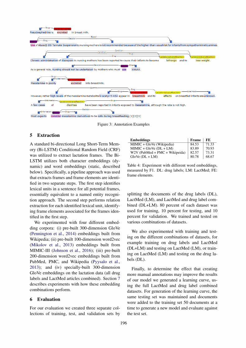
Figure 3: Annotation Examples
5 Extraction
A standard bi-directional Long Short-Term Mem-ory (Bi-LSTM) Conditional Random Field (CRF)was utilized to extract lactation frames. The Bi-LSTM utilizes both character embeddings (dy-namic) and word embeddings (static, describedbelow). Specifically, a pipeline approach was usedthat extracts frames and frame elements are identi-fied in two separate steps. The first step identifieslexical units in a sentence for all potential frames,essentially equivalent to a named entity recogni-tion approach. The second step performs relationextraction for each identified lexical unit, identify-ing frame elements associated for the frames iden-tified in the first step.
We experimented with four different embed-ding corpora: (i) pre-built 300-dimension GloVe(Pennington et al., 2014) embeddings built fromWikipedia; (ii) pre-built 100-dimension word2vec(Mikolov et al., 2013) embeddings built fromMIMIC-III (Johnson et al., 2016); (iii) pre-built200-dimension word2vec embeddings built fromPubMed, PMC, and Wikipedia (Pyysalo et al.,2013); and (iv) specially-built 300-dimensionGloVe embeddings on the lactation data (all druglabels and LactMed articles combined). Section 7describes experiments with how these embeddingcombinations perform.
6 Evaluation
For our evaluation we created three separate col-lections of training, test, and validation sets by
Embeddings Frame FEMIMIC + GloVe (Wikipedia) 84.53 71.33MIMIC + GloVe (DL + LM) 83.89 70.93W2V (PubMed + PMC + Wikipeida) 82.57 73.31GloVe (DL + LM) 80.78 68.67
Table 4: Experiment with different word embeddings,measured by F1. DL: drug labels; LM: LactMed; FE:frame elements.
splitting the documents of the drug labels (DL),LactMed (LM), and LactMed and drug label com-bined (DL+LM). 80 percent of each dataset wasused for training, 10 percent for testing, and 10percent for validation. We trained and tested onvarious combinations of datasets.
We also experimented with training and test-ing on the different combinations of datasets, forexample training on drug labels and LactMed(DL+LM) and testing on LactMed (LM), or train-ing on LactMed (LM) and testing on the drug la-bels (DL).
Finally, to determine the effect that creatingmore manual annotations may improve the resultsof our model we generated a learning curve, us-ing the full LactMed and drug label combineddatasets. For generation of the learning curve, thesame testing set was maintained and documentswere added to the training set 50 documents at atime to generate a new model and evaluate againstthe test set.
196
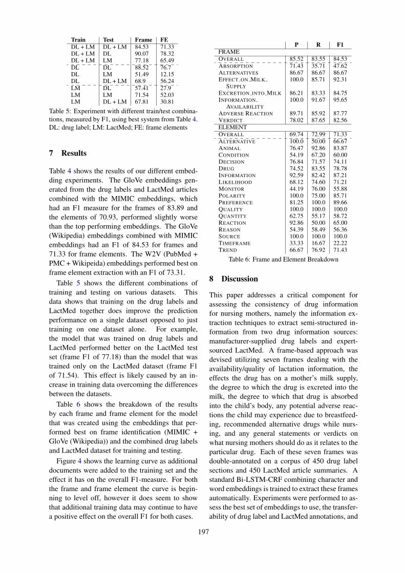
Train Test Frame FEDL + LM DL + LM 84.53 71.33DL + LM DL 90.07 78.32DL + LM LM 77.18 65.49DL DL 88.52 76.7DL LM 51.49 12.15DL DL + LM 68.9 56.24LM DL 57.41 27.9LM LM 71.54 52.03LM DL + LM 67.81 30.81
Table 5: Experiment with different train/test combina-tions, measured by F1, using best system from Table 4.DL: drug label; LM: LactMed; FE: frame elements
7 Results
Table 4 shows the results of our different embed-ding experiments. The GloVe embeddings gen-erated from the drug labels and LactMed articlescombined with the MIMIC embeddings, whichhad an F1 measure for the frames of 83.89 andthe elements of 70.93, performed slightly worsethan the top performing embeddings. The GloVe(Wikipedia) embeddings combined with MIMICembeddings had an F1 of 84.53 for frames and71.33 for frame elements. The W2V (PubMed +PMC + Wikipeida) embeddings performed best onframe element extraction with an F1 of 73.31.
Table 5 shows the different combinations oftraining and testing on various datasets. Thisdata shows that training on the drug labels andLactMed together does improve the predictionperformance on a single dataset opposed to justtraining on one dataset alone. For example,the model that was trained on drug labels andLactMed performed better on the LactMed testset (frame F1 of 77.18) than the model that wastrained only on the LactMed dataset (frame F1of 71.54). This effect is likely caused by an in-crease in training data overcoming the differencesbetween the datasets.
Table 6 shows the breakdown of the resultsby each frame and frame element for the modelthat was created using the embeddings that per-formed best on frame identification (MIMIC +GloVe (Wikipedia)) and the combined drug labelsand LactMed dataset for training and testing.
Figure 4 shows the learning curve as additionaldocuments were added to the training set and theeffect it has on the overall F1-measure. For boththe frame and frame element the curve is begin-ning to level off, however it does seem to showthat additional training data may continue to havea positive effect on the overall F1 for both cases.
P R F1FRAMEOVERALL 85.52 83.55 84.53ABSORPTION 71.43 35.71 47.62ALTERNATIVES 86.67 86.67 86.67EFFECT ON MILK 100.0 85.71 92.31
SUPPLYEXCRETION INTO MILK 86.21 83.33 84.75INFORMATION 100.0 91.67 95.65
AVAILABILITYADVERSE REACTION 89.71 85.92 87.77VERDICT 78.02 87.65 82.56ELEMENTOVERALL 69.74 72.99 71.33ALTERNATIVE 100.0 50.00 66.67ANIMAL 76.47 92.86 83.87CONDITION 54.19 67.20 60.00DECISION 76.84 71.57 74.11DRUG 74.52 83.55 78.78INFORMATION 92.59 82.42 87.21LIKELIHOOD 68.12 74.60 71.21MONITOR 44.19 76.00 55.88POLARITY 100.0 75.00 85.71PREFERENCE 81.25 100.0 89.66QUALITY 100.0 100.0 100.0QUANTITY 62.75 55.17 58.72REACTION 92.86 50.00 65.00REASON 54.39 58.49 56.36SOURCE 100.0 100.0 100.0TIMEFRAME 33.33 16.67 22.22TREND 66.67 76.92 71.43
Table 6: Frame and Element Breakdown
8 Discussion
This paper addresses a critical component forassessing the consistency of drug informationfor nursing mothers, namely the information ex-traction techniques to extract semi-structured in-formation from two drug information sources:manufacturer-supplied drug labels and expert-sourced LactMed. A frame-based approach wasdevised utilizing seven frames dealing with theavailability/quality of lactation information, theeffects the drug has on a mother’s milk supply,the degree to which the drug is excreted into themilk, the degree to which that drug is absorbedinto the child’s body, any potential adverse reac-tions the child may experience due to breastfeed-ing, recommended alternative drugs while nurs-ing, and any general statements or verdicts onwhat nursing mothers should do as it relates to theparticular drug. Each of these seven frames wasdouble-annotated on a corpus of 450 drug labelsections and 450 LactMed article summaries. Astandard Bi-LSTM-CRF combining character andword embeddings is trained to extract these framesautomatically. Experiments were performed to as-sess the best set of embeddings to use, the transfer-ability of drug label and LactMed annotations, and
197
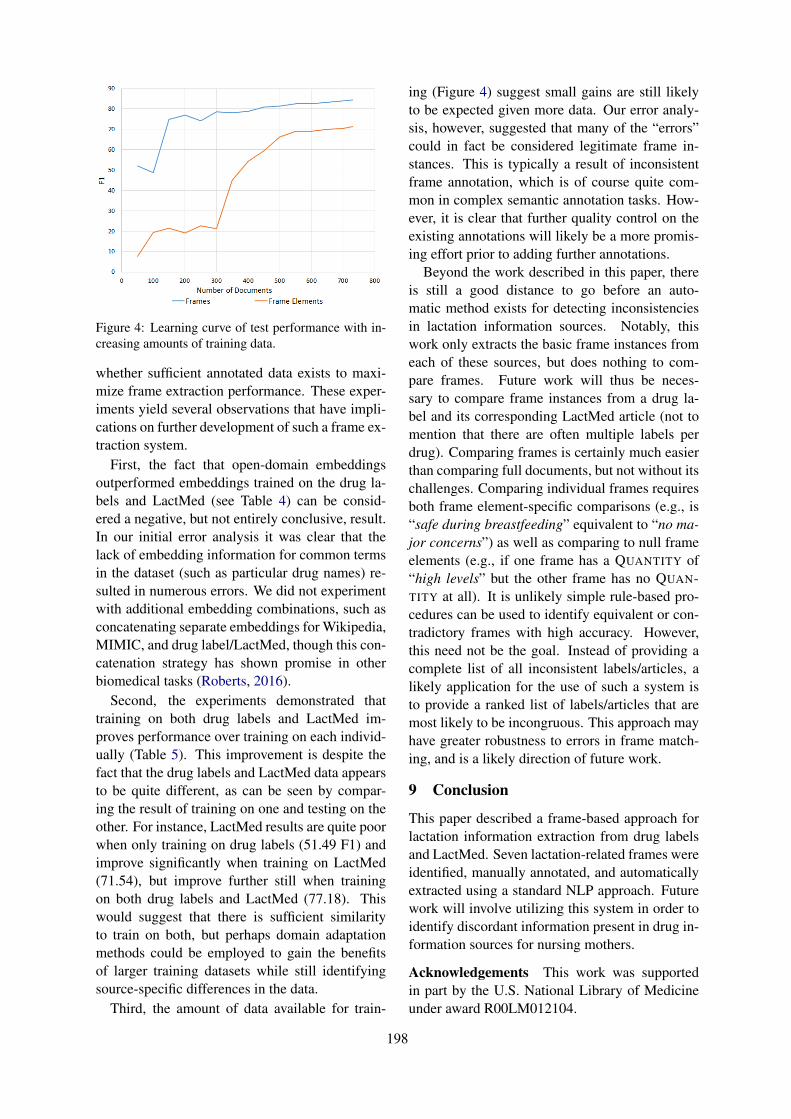
Figure 4: Learning curve of test performance with in-creasing amounts of training data.
whether sufficient annotated data exists to maxi-mize frame extraction performance. These exper-iments yield several observations that have impli-cations on further development of such a frame ex-traction system.
First, the fact that open-domain embeddingsoutperformed embeddings trained on the drug la-bels and LactMed (see Table 4) can be consid-ered a negative, but not entirely conclusive, result.In our initial error analysis it was clear that thelack of embedding information for common termsin the dataset (such as particular drug names) re-sulted in numerous errors. We did not experimentwith additional embedding combinations, such asconcatenating separate embeddings for Wikipedia,MIMIC, and drug label/LactMed, though this con-catenation strategy has shown promise in otherbiomedical tasks (Roberts, 2016).
Second, the experiments demonstrated thattraining on both drug labels and LactMed im-proves performance over training on each individ-ually (Table 5). This improvement is despite thefact that the drug labels and LactMed data appearsto be quite different, as can be seen by compar-ing the result of training on one and testing on theother. For instance, LactMed results are quite poorwhen only training on drug labels (51.49 F1) andimprove significantly when training on LactMed(71.54), but improve further still when trainingon both drug labels and LactMed (77.18). Thiswould suggest that there is sufficient similarityto train on both, but perhaps domain adaptationmethods could be employed to gain the benefitsof larger training datasets while still identifyingsource-specific differences in the data.
Third, the amount of data available for train-
ing (Figure 4) suggest small gains are still likelyto be expected given more data. Our error analy-sis, however, suggested that many of the “errors”could in fact be considered legitimate frame in-stances. This is typically a result of inconsistentframe annotation, which is of course quite com-mon in complex semantic annotation tasks. How-ever, it is clear that further quality control on theexisting annotations will likely be a more promis-ing effort prior to adding further annotations.
Beyond the work described in this paper, thereis still a good distance to go before an auto-matic method exists for detecting inconsistenciesin lactation information sources. Notably, thiswork only extracts the basic frame instances fromeach of these sources, but does nothing to com-pare frames. Future work will thus be neces-sary to compare frame instances from a drug la-bel and its corresponding LactMed article (not tomention that there are often multiple labels perdrug). Comparing frames is certainly much easierthan comparing full documents, but not without itschallenges. Comparing individual frames requiresboth frame element-specific comparisons (e.g., is“safe during breastfeeding” equivalent to “no ma-jor concerns”) as well as comparing to null frameelements (e.g., if one frame has a QUANTITY of“high levels” but the other frame has no QUAN-TITY at all). It is unlikely simple rule-based pro-cedures can be used to identify equivalent or con-tradictory frames with high accuracy. However,this need not be the goal. Instead of providing acomplete list of all inconsistent labels/articles, alikely application for the use of such a system isto provide a ranked list of labels/articles that aremost likely to be incongruous. This approach mayhave greater robustness to errors in frame match-ing, and is a likely direction of future work.
9 Conclusion
This paper described a frame-based approach forlactation information extraction from drug labelsand LactMed. Seven lactation-related frames wereidentified, manually annotated, and automaticallyextracted using a standard NLP approach. Futurework will involve utilizing this system in order toidentify discordant information present in drug in-formation sources for nursing mothers.
Acknowledgements This work was supportedin part by the U.S. National Library of Medicineunder award R00LM012104.
198
ReferencesSwapna Abhyankar and Dina Demner-Fushman. 2013.
A simple method to extract key maternal data fromneonatal clinical notes. In Proceedings of the AMIAAnnual Symposium, pages 2–9.
Collin F Baker, Charles J Fillmore, and Beau Cronin.2003. The Structure of the Framenet Database.International Journal of Lexicography, 16(3):281–296.
Collin F. Baker, Charles J. Fillmore, and John B. Lowe.1998. The Berkeley FrameNet project.
Allan Borra, Karla Delos Santos, Daniel Gonzales, andAlden Reyes. 2013. Maternal Medication Informa-tion Extraction (MaMIE) System. In Proceedings ofthe 9th National Natural Language Processing Re-search Symposium, pages 25–29.
Pramod Bharadwaj Chandrashekar, Arjun Magge,Abeed Sarker, and Graciela Gonzalez. 2017. So-cial media mining for identification and explorationof health-related information from pregnant women.CoRR, abs/1702.02261.
Adam Culbertson, Marcelo Fiszman, Dongwook Shin,and Thomas C. Rindflesch. 2014. Semantic Pro-cessing to Identify Adverse Drug Event Informationfrom Black Box Warnings. In Proceedings of theAMIA Annual Symposium, pages 442–448.
Surabhi Datta, Elmer V Bernstam, and Kirk Roberts.2017. A frame semantic overview of NLP-based in-formation extraction for cancer-related EHR notes.CoRR, abs/1904.01655.
Christianne J. M. de Groot, Thed van Leeuwen, BenWillem J. Mol, and Ludo Waltman. 2015. ALongitudinal Analysis of Publications on MaternalMortality. Paediatric and Perinatal Epidemiology,29(6):481–489.
Dina Demner-Fushman, Kin Wah Fung, Phong Do,Richard D. Boyce, and Travis R. Goodwin. 2018a.Overview of the TAC 2018 Drug-Drug InteractionExtraction from Drug Labels Track. In Proceedingsof the Text Analysis Conference.
Dina Demner-Fushman, Sonya E. Shooshan, LaritzaRodriguez, Alan R. Aronson, Francois Lang, WillieRogers, Kirk Roberts, and Joseph Tonning. 2018b.A dataset of 200 structured product labels anno-tated for adverse drug reactions. Scientific Data,5:180001.
A. Dolbey. 2009. BioFrameNet: A FrameNet Exten-sion to the Domain of Molecular Biology. Ph.D.thesis, UC Berkeley.
A. Dolbey, M. Ellsworth, and J. Scheffzyk. 2006.BioFrameNet: A Domain-specific FrameNet Ex-tension with Links to Biomedical Ontologies. InProceedings of the Biomedical Ontology in ActionWorkshop at KR-MED, pages 86–94.
Jon Duke, Jeff Friedlin, and Xiaochun Li. 2013. Con-sistency in the safety labeling of bioequivalent med-ications. Pharmacoepidemiology Drug Safety,22(3):294–301.
Charles J Fillmore. 1976. Frame Semantics and theNature of Language. Annals of the New YorkAcademy of Sciences, 280(1):20–32.
Charles J Fillmore. 1982. Frame semantics. Linguis-tics in the Morning Calm, pages 111–137.
Kin Wah Fung, Chiang S Jao, and Dina Demner-Fushman. 2013. Extracting drug indication infor-mation from structured product labels using naturallanguage processing. Journal of the American Med-ical Informatics Association, 20(3):482–488.
Rave Harpaz, Alison Callahan, Suzanne Tamang, YenLow, David Odgers, Sam Finlayson, Kenneth Jung,Paea LePendu, and Nigam H. Shah. 2014. TextMining for Adverse Drug Events: the Promise,Challenges, and State of the Art. Drug Safety,37(10):777–790.
Alistair E.W. Johnson, Tom J. Pollard, Lu Shen, Li weiH. Lehman, Mengling Feng, Mohammad Ghassemi,Benjamin Moody, Peter Szolovits, Leo AnthonyCeli, , and Roger G. Mark. 2016. MIMIC-III, afreely accessible critical care database. ScientificData, 3:160035.
Ritu Khare, Jiao Li, and Zhiyong Lu. 2014. LabeledIn:Cataloging Labeled Indications for Human Drugs.Journal of Biomedical Informatics, 52:448–456.
Dimitrios Kokkinakis. 2013. Medical Event Extractionusing Frame Semantics – Challenges and Opportu-nities. International Journal of Computational Lin-guistics and Applications, 4(2):121–133.
Michael Kuhn, Monica Campillos, Ivica Letunic,Lars Juhl Jensen, and Peer Bork. 2010. A side ef-fect resource to capture phenotypic effects of drugs.Molecular Systems Biology, 6:343.
Michael Kuhn, Ivica Letunic, Lars Juhl Jensen,and Peer Bork. 2016. The SIDER database ofdrugs and side effects. Nucleic Acids Research,44(D1):D1075–D1079.
Qi Li, Louise Deleger, Todd Lingren, Haijun Zhai,Megan Kaiser, Laura Stoutenborough, Anil G Jegga,Kevin Bretonnel Cohen, and Imre Solti. 2013. Min-ing FDA drug labels for medical conditions. BMCMedical Informatics and Decision Making, 13(53).
Tomas Mikolov, Ilya Sutskever, Kai Chen, Greg Cor-rado, and Jeffrey Dean. 2013. Distributed Repre-sentations of Words and Phrases and their Compo-sitionality. In Proceedings of the 26th InternationalConference on Neural Information Processing Sys-tems, pages 3111–3119.
199
Aurélie Névéol and Zhiyong Lu. 2010. Automatic In-tegration of Drug Indications from Multiple HealthResources. In Proceedings of the 1st ACM Inter-national Health Informatics Symposium, pages 666–673.
Jeffrey Pennington, Richard Socher, and Christopher DManning. 2014. GloVe: Global Vectors for WordRepresentation. In Proceedings of the 2014 Con-ference on Empirical Methods in Natural LanguageProcessing, pages 1532–1543.
Sampo Pyysalo, Filip Ginter, Hans Moen, TapioSalakoski, and Sophia Ananiadou. 2013. Distri-butional Semantics Resources for Biomedical TextProcessing. In Proceedings of Languages in Biol-ogy and Medicine.
Kirk Roberts. 2016. Assessing the Corpus Size vs Sim-ilarity Trade-off for Word Embeddings in ClinicalNLP. In Proceedings of the COLING Workshop onClinical Natural Language Processing.
Kirk Roberts, Dina Demner-Fushman, and Joseph Ton-ning. 2017. Overview of the TAC 2017 Adverse Re-action Extraction from Drug Labels Track. In Pro-ceedings of the Text Analysis Conference (TAC).
Kirk Roberts, Yuqi Si, Anshul Gandhi, and ElmerBernstam. 2018. A FrameNet for Cancer Informa-tion in Clinical Narratives: Schema and Annota-tion. In Proceedings of the Language Resources andEvaluation Conference, pages 272–279.
Laritza M. Rodriguez and Dina Demner Fushman.2015. Automatic Classification of Structured Prod-uct Labels for Pregnancy Risk Drug Categories, aMachine Learning Approach. In Proceedings of theAMIA Annual Symposium, pages 1093–1102.
Laritza M. Rodriguez, Stephanie M. Morrison, Kath-leen Greenberg, and Dina Demner Fushman. 2017.Mining the literature for genes associated withplacenta-mediated maternal diseases. In Proceed-ings of the AMIA Annual Symposium, pages 1498–1506.
Abeed Sarker, Pramod Chandrashekar, Arjun Magge,Haitao Cai, Ari Klein, and Graciela Gonzalez. 2017.Discovering Cohorts of Pregnant Women From So-cial Media for Safety Surveillance and Analysis.Journal of Medical Internet Research, 19(10):e361.
Yuqi Si and Kirk Roberts. 2018. A Frame-Based NLPSystem for Cancer-Related Information Extraction.In Proceedings of the AMIA Annual Symposium.
Pontus Stenetorp, Sampo Pyysalo, Goran Topic,Tomoko Ohta, Sophia Ananiadou, and Junichi Tsu-jii. 2013. BRAT: a Web-based Tool for NLP-Assisted Text Annotation. In Proceedings of the13th Conference of the European Chapter of the As-sociation for Computational Linguistics, pages 102–107.
He Tan. 2014. A System for Building FrameNet-likeCorpus for the Biomedical Domain. In Proceedingsof the 5th International Workshop on Health TextMining and Information Analysis (Louhi), pages 46–53.
Qiu-Yue Zhong, Elizabeth W. Karlson, Bizu Gelaye,Sean Finan, Paul Avillach, Jordan W. Smoller,Tianxi Cai, and Michelle A. Williams. 2018.Screening pregnant women for suicidal behavior inelectronic medical records: diagnostic codes vs.clinical notes processed by natural language pro-cessing. BMC Medical Informatics and DecisionMaking, 18:30.
Qiu-Yue Zhong, Leena P. Mittal Margo D. Nathan,Kara M. Brown, Deborah Knudson Gonzlez, Tian-run Cai, Sean Finan, Bizu Gelaye, Paul Avillach,Jordan W. Smoller, Elizabeth W. Karlson, TianxiCai, and Michelle A. Williams. 2019. Use of naturallanguage processing in electronic medical recordsto identify pregnant women with suicidal behav-ior: towards a solution to the complex classifica-tion problem. European Journal of Epidemiology,34(2):153–162.
200
Proceedings of the BioNLP 2019 workshop, pages 201–210Florence, Italy, August 1, 2019. c©2019 Association for Computational Linguistics
Annotating Temporal Information in Clinical Notes for TimelineReconstruction: Towards the Definition of Calendar Expressions
Natalia VianiIoPPN, King’s College London
London, UK
Hegler TissotUniversity College London
London, UK
Ariane BernardinoIoPPN, King’s College London
London, UK
Sumithra VelupillaiIoPPN, King’s College London
London, UKEECS, KTH, Stockholm, Sweden
Abstract
To automatically analyse complex trajectoryinformation enclosed in clinical text (e.g. tim-ing of symptoms, duration of treatment), it isimportant to understand the related temporalaspects, anchoring each event on an absolutepoint in time. In the clinical domain, fewtemporally annotated corpora are currentlyavailable. Moreover, underlying annotationschemas - which mainly rely on the TimeMLstandard - are not necessarily easily applicablefor applications such as patient timeline recon-struction. In this work, we investigated howtemporal information is documented in clini-cal text by annotating a corpus of medical re-ports with time expressions (TIMEXes), basedon TimeML. The developed corpus is avail-able to the NLP community. Starting from ourannotations, we analysed the suitability of theTimeML TIMEX schema for capturing time-line information, identifying challenges andpossible solutions. As a result, we proposea novel annotation schema that could be use-ful for timeline reconstruction: CALendar EX-pression (CALEX).
1 Introduction and Background
When applying natural language processing(NLP) methods to the analysis of clinical notes,understanding the temporal aspects of narrativesis crucial (e.g. when the patient experienced a cer-tain symptom, or when a particular drug was pre-scribed). To model and extract the temporal in-formation enclosed in free text, the developmentof suitable annotation schemas and reliably anno-tated corpora is essential.
The TimeML specification language was devel-oped to enable the recognition of events and theirtemporal ordering in general-domain texts (Puste-jovsky et al., 2003a). In the original schema,four major elements are modelled: time expres-
sions (TIMEXes), events, signals, and their re-lations. Signals are function words (e.g. “dur-ing”, “before”) that indicate how temporal objectscan be related to each other. Relations are rep-resented by either temporal links (e.g. “before”,“simultaneous”), subordination links (e.g. “inten-sional”, “factive”), or aspectual links (e.g. “initi-ates, “continues”). The TimeML schema was usedto develop the TimeBank corpus, consisting of 183news articles (Pustejovsky et al., 2003b). Gold an-notations were reused in the TempEval tasks ontemporal information extraction (Verhagen et al.,2007; Pustejovsky and Verhagen, 2009), where asimplified TimeML annotation was applied.
The TimeML specification language providesa standard model for the mark-up of time ex-pressions (with type Date, Time, Duration, orSet), events (mostly verbs or noun phrases), andtheir temporal ordering (Pustejovsky et al., 2010),and it can be in principle applied to any type oftext. In the clinical domain, two reference cor-pora based on TimeML are available. The 2012i2b2 corpus (310 discharge summaries) includesannotations for time expressions, clinical events,and eight types of temporal relations (Sun et al.,2013a). In addition, a section time (SECTIME) isused to keep track of section creation dates. TheTHYME corpus (1,254 oncology notes) containsannotations for events, time expressions (with twoadditional types), and 5 types of temporal rela-tions (Styler IV et al., 2014). In this corpus, narra-tive containers were introduced, representing tem-poral buckets (mostly dates) containing a set ofevents. Figure 1 provides a graphical representa-tion of the main changes introduced by i2b2 2012and THYME on the original TimeML model.
Most clinical NLP development based on avail-able corpora have focused on the three separatemain tasks: detecting and classifying 1) events and
201
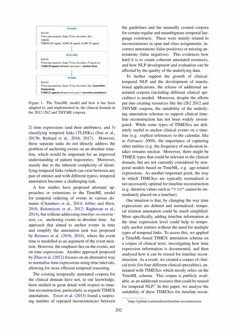
Figure 1: The TimeML model and how it has beenadapted to, and implemented in, the clinical domain inthe 2012 i2b2 and THYME corpora.
2) time expressions (and their attributes), and 3)classifying temporal links (TLINKs) (Sun et al.,2013b; Bethard et al., 2016, 2017). However,these separate tasks do not directly address theproblem of anchoring events on an absolute time-line, which would be important for an improvedunderstanding of patient trajectories. Moreover,mainly due to the inherent complexity of identi-fying temporal links (which can exist between anypair of entities and with different types), temporalannotation becomes a challenging task.
A few studies have proposed alternate ap-proaches or extensions to the TimeML modelfor temporal ordering of events in various do-mains (Chambers et al., 2014; Jeblee and Hirst,2018; Kolomiyets et al., 2012; Raghavan et al.,2014), but without addressing timeline reconstruc-tion, i.e. anchoring events in absolute time. Anapproach that aimed to anchor events in timeand simplify the annotation task was proposedby Reimers et al. (2016, 2018), where the eventtime is modelled as an argument of the event men-tion. However, the emphasis lies on the events, noton time expressions. Another approach proposedby Zhao et al. (2012) focuses on an alternative wayto normalise time expressions using time intervals,allowing for more efficient temporal reasoning.
The existing temporally annotated corpora forthe clinical domain have not, to our knowledge,been studied in great detail with respect to time-line reconstruction, particularly as regards TIMEXannotations. Tissot et al. (2015) found a surpris-ing number of repeated inconsistencies between
the guidelines and the manually created corporafor certain regular and unambiguous temporal lan-guage constructs. These were mainly related toinconsistencies in span and class assignments, in-correct annotations (false positives) or missing an-notations (false negatives). This evidences howhard it is to create coherent annotated resources,and how NLP development and evaluation can beaffected by the quality of the underlying data.
To further support the growth of clinical-temporal NLP and the development of transla-tional applications, the release of additional an-notated corpora (including different clinical spe-cialties) is needed. Moreover, despite the effortsput into creating resources like the i2b2 2012 andTHYME corpora, the suitability of the underly-ing annotation schemas to support clinical time-line reconstruction has not been widely investi-gated. While some types of TIMEXes are defi-nitely useful to anchor clinical events on a time-line (e.g. explicit references to the calendar, likein February 2009), the importance of capturingother entities (e.g. the frequency of medication in-take) remains unclear. Moreover, there might beTIMEX types that could be relevant in the clinicaldomain, but are not currently considered by tem-poral models based on TimeML, e.g. age-relatedexpressions. As another important point, the wayin which TIMEXes are typically normalised isnot necessarily optimal for timeline reconstruction(e.g. duration values such as "P4M" cannot be im-mediately placed on a timeline).
Our intuition is that, by changing the way timeexpressions are defined and normalised, tempo-ral relation annotation could be much simplified.More specifically, adding timeline information atthe time expression level could help to tempo-rally anchor entities without the need for multipletypes of temporal links. To assess this, we applieda TimeML-based TIMEX annotation schema ona corpus of clinical texts, investigating how timeexpression information is documented, and thenanalysed how it can be reused for timeline recon-struction. As a result, we created a corpus of clini-cal texts (for four different clinical specialties), an-notated with TIMEXes which mostly relies on theTimeML schema. This corpus is publicly avail-able, as an additional resource that could be reusedfor temporal NLP.1 In this paper, we analyse thesuitability of these TIMEXes for timeline recon-
1https://github.com/medesto/timeline-reconstruction
202
struction, and from this analysis propose an in-novative way to annotate temporal information infree text: CALendar EXpressions (CALEX).
2 Materials and Methods
2.1 DatasetWe downloaded and extracted documents fromMTSamples,2 a collection of Medical Transcrip-tion Sample reports for multiple clinical special-ties (where the same document can belong to dif-ferent groups), created for educational purposesand for working transcriptionists.
In the MTSamples resource, there is no avail-ability of document creation times (DCTs). Mostdocuments follow a semi-structured format, in-cluding different section headings/textual con-tent depending on the specific clinical specialty.We selected the following specialties for man-ual annotation and analysis: discharge summaries(108 documents), psychiatry-psychology (53 doc-uments), paediatrics (70 documents), and emer-gency (75 documents).3
2.2 Manual AnnotationAll MTSamples subsets were double-annotatedfor five types of time expressions: Date, Time,Duration, Frequency (from TimeML (Pustejovskyet al., 2010)), and Age-related (at the age of 16, inhis teens (Viani et al., 2018)). Identified expres-sions were also normalised to a standard temporalvalue (e.g. "2011-05" for May 2011). Manualannotations were performed by two annotators: anative English-speaker undergraduate student anda non-native English-speaker researcher. To guidethe annotation process, we created specific anno-tation guidelines, which we refined by adding rele-vant examples from the text. Resulting guidelinesare available on our repository.
Besides including an Age-related time expres-sion type, our annotation task differed fromTimeML in two ways. First, we includedas TIMEXes domain-specific (and temporally-anchored) concepts, e.g. On the day of admis-sion. This is similar to the Prepostexp type usedin the THYME corpus, but instead of creating adifferent category, we included these expressionsamong existing types (e.g. Date). Depending onthe clinical specialty (and more generally, on thedomain), different concepts could be considered as
2www.mtsamples.com3The number of unique documents is 286.
temporal anchors within temporal annotation (e.g.discharge for discharge summaries, pregnancy forpaediatrics notes). Second, we allowed annotatorsto use relative values in the normalisation phase, ifneeded. These relative values, or formulas, caneither refer to the document creation date (e.g."DCT-P2D" for Two days ago) or to the domain-specific concepts (e.g. "OP+P2D" for postopera-tive day #2).
To compute inter-annotator agreement (IAA)on textual spans, we used the F1 score (allowingoverlapping annotations). Expressions identifiedby both annotators (overlap) were used to com-pute IAA on types and normalised values (accu-racy). For IAA on types, we also report the Co-hen’s Kappa measure (K), to take the possibility ofchance agreement into account.
2.3 Annotation Analysis for TimelineReconstruction
To analyse the suitability of using the TimeML-based TIMEX annotations for timeline reconstruc-tion, we based our analysis on the following: 1)timeline properties of the TIMEX type Frequency,2) properties of normalised values for Date anno-tations, and 3) properties of common annotationdisagreements.
Our hypothesis regarding Frequency annota-tions was that these would not be necessarily use-ful as temporal references on an absolute time-line, as they would be mostly related to drug pre-scriptions. To assess this, we applied the MedEx-UIMA tool (Jiang et al., 2014) on the text sur-rounding each Frequency expression (the con-text),4 and quantified the proportion of annotationsclose to drug mentions.
Normalised values for Date can represent a spe-cific point on a timeline, e.g. "YYYY-MM-DD","YYYY-MM" or "YYYY". However, they canalso represent other less straightforward points intime, e.g. DCT-related (yesterday), vague refer-ences (in the past), incomplete dates (on the 13th),and concept-related (on the day of admission). Tobetter understand these latter types of normalisedDate values and their relation to timeline recon-struction, we analysed annotations marked as suchby at least one annotator.
Finally, to inform the development of a new an-notation schema for timeline reconstruction based
4We considered a window of 50 characters before and af-ter the annotation.
203
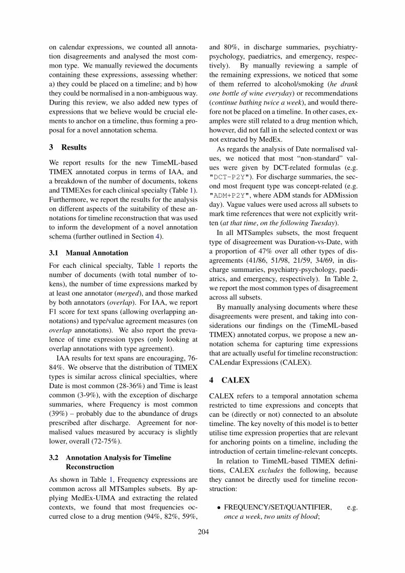
on calendar expressions, we counted all annota-tion disagreements and analysed the most com-mon type. We manually reviewed the documentscontaining these expressions, assessing whether:a) they could be placed on a timeline; and b) howthey could be normalised in a non-ambiguous way.During this review, we also added new types ofexpressions that we believe would be crucial ele-ments to anchor on a timeline, thus forming a pro-posal for a novel annotation schema.
3 Results
We report results for the new TimeML-basedTIMEX annotated corpus in terms of IAA, anda breakdown of the number of documents, tokensand TIMEXes for each clinical specialty (Table 1).Furthermore, we report the results for the analysison different aspects of the suitability of these an-notations for timeline reconstruction that was usedto inform the development of a novel annotationschema (further outlined in Section 4).
3.1 Manual Annotation
For each clinical specialty, Table 1 reports thenumber of documents (with total number of to-kens), the number of time expressions marked byat least one annotator (merged), and those markedby both annotators (overlap). For IAA, we reportF1 score for text spans (allowing overlapping an-notations) and type/value agreement measures (onoverlap annotations). We also report the preva-lence of time expression types (only looking atoverlap annotations with type agreement).
IAA results for text spans are encouraging, 76-84%. We observe that the distribution of TIMEXtypes is similar across clinical specialties, whereDate is most common (28-36%) and Time is leastcommon (3-9%), with the exception of dischargesummaries, where Frequency is most common(39%) – probably due to the abundance of drugsprescribed after discharge. Agreement for nor-malised values measured by accuracy is slightlylower, overall (72-75%).
3.2 Annotation Analysis for TimelineReconstruction
As shown in Table 1, Frequency expressions arecommon across all MTSamples subsets. By ap-plying MedEx-UIMA and extracting the relatedcontexts, we found that most frequencies oc-curred close to a drug mention (94%, 82%, 59%,
and 80%, in discharge summaries, psychiatry-psychology, paediatrics, and emergency, respec-tively). By manually reviewing a sample ofthe remaining expressions, we noticed that someof them referred to alcohol/smoking (he drankone bottle of wine everyday) or recommendations(continue bathing twice a week), and would there-fore not be placed on a timeline. In other cases, ex-amples were still related to a drug mention which,however, did not fall in the selected context or wasnot extracted by MedEx.
As regards the analysis of Date normalised val-ues, we noticed that most “non-standard” val-ues were given by DCT-related formulas (e.g."DCT-P2Y"). For discharge summaries, the sec-ond most frequent type was concept-related (e.g."ADM+P2Y", where ADM stands for ADMissionday). Vague values were used across all subsets tomark time references that were not explicitly writ-ten (at that time, on the following Tuesday).
In all MTSamples subsets, the most frequenttype of disagreement was Duration-vs-Date, witha proportion of 47% over all other types of dis-agreements (41/86, 51/98, 21/59, 34/69, in dis-charge summaries, psychiatry-psychology, paedi-atrics, and emergency, respectively). In Table 2,we report the most common types of disagreementacross all subsets.
By manually analysing documents where thesedisagreements were present, and taking into con-siderations our findings on the (TimeML-basedTIMEX) annotated corpus, we propose a new an-notation schema for capturing time expressionsthat are actually useful for timeline reconstruction:CALendar Expressions (CALEX).
4 CALEX
CALEX refers to a temporal annotation schemarestricted to time expressions and concepts thatcan be (directly or not) connected to an absolutetimeline. The key novelty of this model is to betterutilise time expression properties that are relevantfor anchoring points on a timeline, including theintroduction of certain timeline-relevant concepts.
In relation to TimeML-based TIMEX defini-tions, CALEX excludes the following, becausethey cannot be directly used for timeline recon-struction:
• FREQUENCY/SET/QUANTIFIER, e.g.once a week, two units of blood;
204
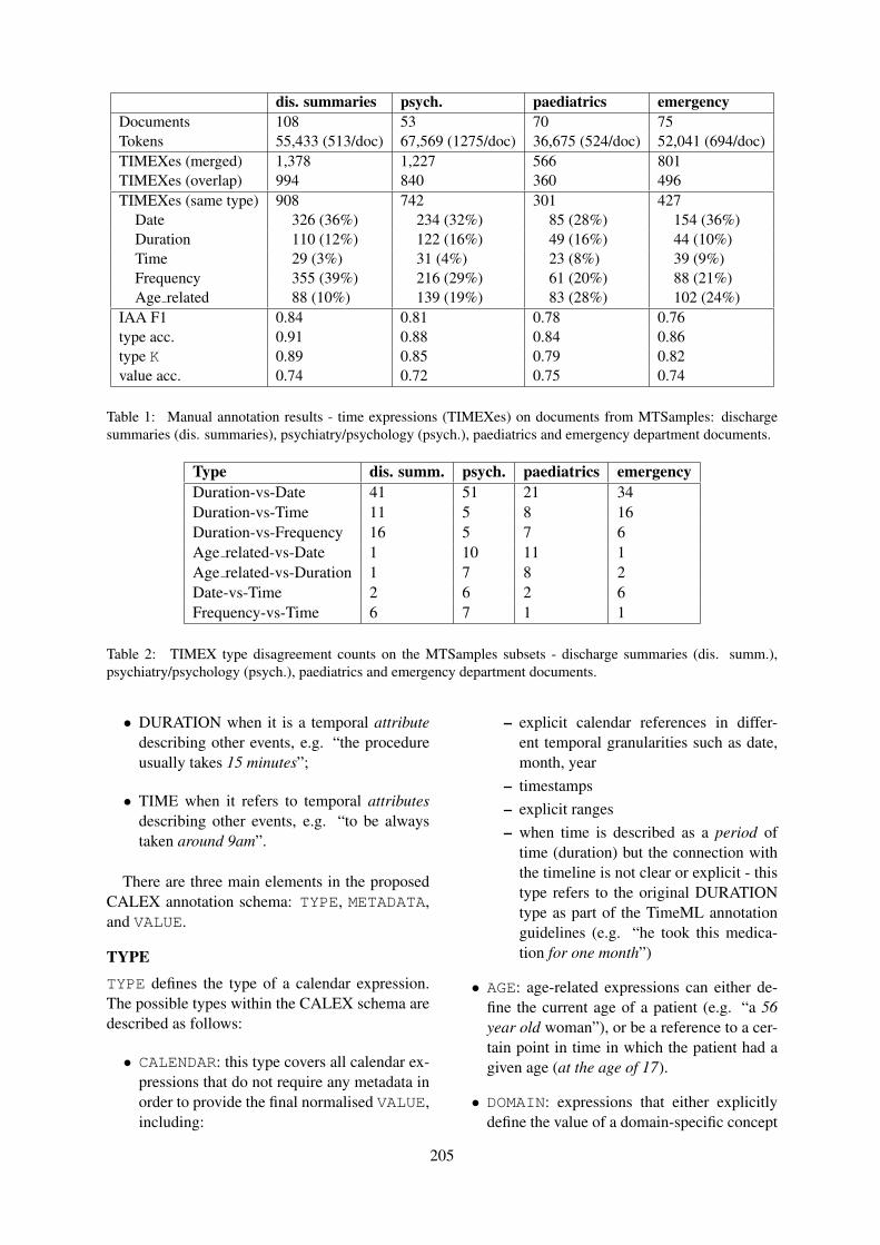
dis. summaries psych. paediatrics emergencyDocuments 108 53 70 75Tokens 55,433 (513/doc) 67,569 (1275/doc) 36,675 (524/doc) 52,041 (694/doc)TIMEXes (merged) 1,378 1,227 566 801TIMEXes (overlap) 994 840 360 496TIMEXes (same type) 908 742 301 427
Date 326 (36%) 234 (32%) 85 (28%) 154 (36%)Duration 110 (12%) 122 (16%) 49 (16%) 44 (10%)Time 29 (3%) 31 (4%) 23 (8%) 39 (9%)Frequency 355 (39%) 216 (29%) 61 (20%) 88 (21%)Age related 88 (10%) 139 (19%) 83 (28%) 102 (24%)
IAA F1 0.84 0.81 0.78 0.76type acc. 0.91 0.88 0.84 0.86type K 0.89 0.85 0.79 0.82value acc. 0.74 0.72 0.75 0.74
Table 1: Manual annotation results - time expressions (TIMEXes) on documents from MTSamples: dischargesummaries (dis. summaries), psychiatry/psychology (psych.), paediatrics and emergency department documents.
Type dis. summ. psych. paediatrics emergencyDuration-vs-Date 41 51 21 34Duration-vs-Time 11 5 8 16Duration-vs-Frequency 16 5 7 6Age related-vs-Date 1 10 11 1Age related-vs-Duration 1 7 8 2Date-vs-Time 2 6 2 6Frequency-vs-Time 6 7 1 1
Table 2: TIMEX type disagreement counts on the MTSamples subsets - discharge summaries (dis. summ.),psychiatry/psychology (psych.), paediatrics and emergency department documents.
• DURATION when it is a temporal attributedescribing other events, e.g. “the procedureusually takes 15 minutes”;
• TIME when it refers to temporal attributesdescribing other events, e.g. “to be alwaystaken around 9am”.
There are three main elements in the proposedCALEX annotation schema: TYPE, METADATA,and VALUE.
TYPETYPE defines the type of a calendar expression.The possible types within the CALEX schema aredescribed as follows:
• CALENDAR: this type covers all calendar ex-pressions that do not require any metadata inorder to provide the final normalised VALUE,including:
– explicit calendar references in differ-ent temporal granularities such as date,month, year
– timestamps– explicit ranges– when time is described as a period of
time (duration) but the connection withthe timeline is not clear or explicit - thistype refers to the original DURATIONtype as part of the TimeML annotationguidelines (e.g. “he took this medica-tion for one month”)
• AGE: age-related expressions can either de-fine the current age of a patient (e.g. “a 56year old woman”), or be a reference to a cer-tain point in time in which the patient had agiven age (at the age of 17).
• DOMAIN: expressions that either explicitlydefine the value of a domain-specific concept
205
(admitted on 2010 Jun 6th), or are referencesto a given domain-specific concept (on post-operative day #4).
• DCT: expressions that require informationabout the document creation time in order tobe normalised (last month).
• TENSE: imprecise expressions that refer toconditions in the past, present or future (re-cently).
• CONTEXT: expressions that refer to a tem-poral context, represented by either the lastmentioned temporal reference or the most re-cent temporal reference available within thedocument. 5 This type includes times/periodsof the day where the connection to the time-line is not clear and relies on the tempo-ral context (e.g. the previous night). How-ever, times/periods of the day representingfrequencies (e.g. “one tablet at night”) areNOT considered as CALEXes.
METADATAWe introduce METADATA as a feature to allow fora computationally more efficient way of calculat-ing a particular time reference for CALEXes thatare not explicitly anchored in time. An essentialaspect of this feature is that it can include conceptsin its definition. These can also be explicitly setwithin the METADATA feature, to ensure the orig-inal values are used in order to normalise the finalcalendar expression.
Document-related concepts include thedocument creation time {doc.DCT} and con-textualised references to the last or more recenttemporal mentions within the text ({doc.LAST}and {doc.RECENT}). Patient-related con-cepts are used to describe patient demo-graphic features, such as {patient.AGE},{patient.DOB}, {patient.DOD}, thelater possibly useful when analysing deathcertificates.6 Patient-stay-related concepts willbasically refer to the period within admissionand discharge ({patient.ADMISSION} and{patient.DISCHARGE}).
One important concept that may require somedisambiguation is related to the pregnancy period.
5Other specific contextual references can be required fordocuments in different domains.
6{patient.AGE} and {patient.DOB} represent comple-mentary concepts.
The terms Pregnancy and Prenatal are generallyinterchangeably used when referring either to themother or the child. We formalise Pregnancy asbeing the period of time used when referring tothe mother as a patient, whereas Prenatal refersto the period of time (usually 40 weeks) before{patient.DOB}, which refers to the child asa patient. This way, {patient.PREGNANCY}can occur at any time in the patient’s life, whereas{patient.PRENATAL} is the period of 40weeks preceding the patient’s date of birth.
Finally, some social- and family-related con-cepts can be used in order to refer to some tem-poral values regarding the patient’s relatives, suchas {mother.AGE} or {father.DOB}.
Besides making use of timeline-relevant con-cepts, METADATA also contains functions that areused to derive values:
• .set(): for explicitly defining the value ofdomain-specific concepts;
• .add(): adds a period of time to a givenpoint in the calendar, moving to a later pointin time;
• .sub(): subtracts a period of time from agiven point in the calendar, moving to an ear-lier point in time;
• .next(): finds the next occurrence of atemporal granularity based on an anchor cal-endar expression;
• .prev(): finds the previous occurrence of atemporal granularity based on an anchor cal-endar expression.
For example, a reference to DCT cannot beproperly normalised when DCT is unknown.However, the metadata can keep the definition fora calendar expression, to be converted to an actualvalue when DCT is given: instead of parsing theentire document, only the metadata has to be re-evaluated – e.g. metadata for the expression “yes-terday” is "{doc.DCT}.sub(P1D)".
VALUEThis component gives a normalised value of a cal-endar expression, mostly following the previousTimeML notation, with an extension: range val-ues are used to normalise periods of time in theform of [begin,end].7
7To indicate included endpoints, we use standard squarebrackets: [A,B]. To indicate excluded endpoints, we use re-
206
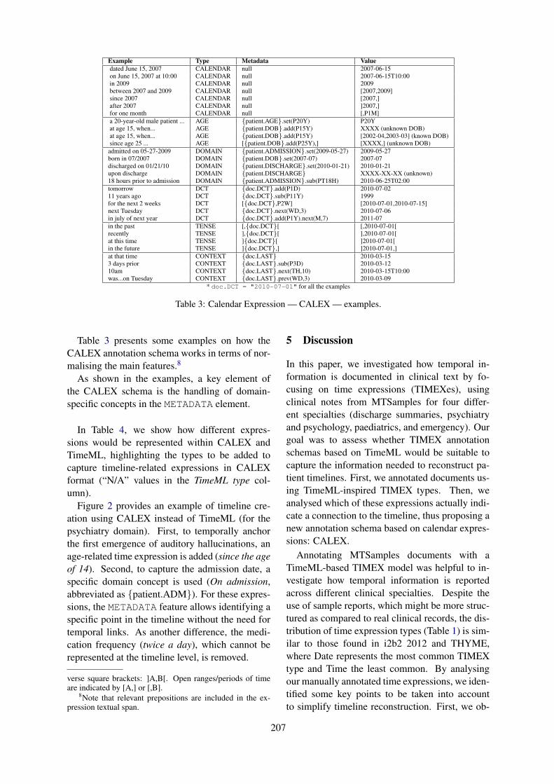
Example Type Metadata Valuedated June 15, 2007 CALENDAR null 2007-06-15on June 15, 2007 at 10:00 CALENDAR null 2007-06-15T10:00in 2009 CALENDAR null 2009between 2007 and 2009 CALENDAR null [2007,2009]since 2007 CALENDAR null [2007,]after 2007 CALENDAR null ]2007,]for one month CALENDAR null [,P1M]a 20-year-old male patient ... AGE {patient.AGE}.set(P20Y) P20Yat age 15, when... AGE {patient.DOB}.add(P15Y) XXXX (unknown DOB)at age 15, when... AGE {patient.DOB}.add(P15Y) [2002-04,2003-03] (known DOB)since age 25 ... AGE [{patient.DOB}.add(P25Y),] [XXXX,] (unknown DOB)admitted on 05-27-2009 DOMAIN {patient.ADMISSION}.set(2009-05-27) 2009-05-27born in 07/2007 DOMAIN {patient.DOB}.set(2007-07) 2007-07discharged on 01/21/10 DOMAIN {patient.DISCHARGE}.set(2010-01-21) 2010-01-21upon discharge DOMAIN {patient.DISCHARGE} XXXX-XX-XX (unknown)18 hours prior to admission DOMAIN {patient.ADMISSION}.sub(PT18H) 2010-06-25T02:00tomorrow DCT {doc.DCT}.add(P1D) 2010-07-0211 years ago DCT {doc.DCT}.sub(P11Y) 1999for the next 2 weeks DCT [{doc.DCT},P2W] [2010-07-01,2010-07-15]next Tuesday DCT {doc.DCT}.next(WD,3) 2010-07-06in july of next year DCT {doc.DCT}.add(P1Y).next(M,7) 2011-07in the past TENSE [,{doc.DCT}[ [,2010-07-01[recently TENSE ],{doc.DCT}[ ],2010-07-01[at this time TENSE ]{doc.DCT}[ ]2010-07-01[in the future TENSE ]{doc.DCT},] ]2010-07-01,]at that time CONTEXT {doc.LAST} 2010-03-153 days prior CONTEXT {doc.LAST}.sub(P3D) 2010-03-1210am CONTEXT {doc.LAST}.next(TH,10) 2010-03-15T10:00was...on Tuesday CONTEXT {doc.LAST}.prev(WD,3) 2010-03-09
* doc.DCT = "2010-07-01" for all the examples
Table 3: Calendar Expression — CALEX — examples.
Table 3 presents some examples on how theCALEX annotation schema works in terms of nor-malising the main features.8
As shown in the examples, a key element ofthe CALEX schema is the handling of domain-specific concepts in the METADATA element.
In Table 4, we show how different expres-sions would be represented within CALEX andTimeML, highlighting the types to be added tocapture timeline-related expressions in CALEXformat (“N/A” values in the TimeML type col-umn).
Figure 2 provides an example of timeline cre-ation using CALEX instead of TimeML (for thepsychiatry domain). First, to temporally anchorthe first emergence of auditory hallucinations, anage-related time expression is added (since the ageof 14). Second, to capture the admission date, aspecific domain concept is used (On admission,abbreviated as {patient.ADM}). For these expres-sions, the METADATA feature allows identifying aspecific point in the timeline without the need fortemporal links. As another difference, the medi-cation frequency (twice a day), which cannot berepresented at the timeline level, is removed.
verse square brackets: ]A,B[. Open ranges/periods of timeare indicated by [A,] or [,B].
8Note that relevant prepositions are included in the ex-pression textual span.
5 Discussion
In this paper, we investigated how temporal in-formation is documented in clinical text by fo-cusing on time expressions (TIMEXes), usingclinical notes from MTSamples for four differ-ent specialties (discharge summaries, psychiatryand psychology, paediatrics, and emergency). Ourgoal was to assess whether TIMEX annotationschemas based on TimeML would be suitable tocapture the information needed to reconstruct pa-tient timelines. First, we annotated documents us-ing TimeML-inspired TIMEX types. Then, weanalysed which of these expressions actually indi-cate a connection to the timeline, thus proposing anew annotation schema based on calendar expres-sions: CALEX.
Annotating MTSamples documents with aTimeML-based TIMEX model was helpful to in-vestigate how temporal information is reportedacross different clinical specialties. Despite theuse of sample reports, which might be more struc-tured as compared to real clinical records, the dis-tribution of time expression types (Table 1) is sim-ilar to those found in i2b2 2012 and THYME,where Date represents the most common TIMEXtype and Time the least common. By analysingour manually annotated time expressions, we iden-tified some key points to be taken into accountto simplify timeline reconstruction. First, we ob-
207
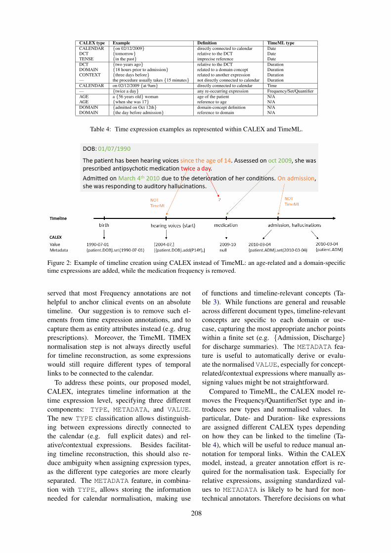
CALEX type Example Definition TimeML typeCALENDAR {on 02/12/2009} directly connected to calendar DateDCT {tomorrow} relative to the DCT DateTENSE {in the past} imprecise reference DateDCT {two years ago} relative to the DCT DurationDOMAIN {18 hours prior to admission} related to a domain concept DurationCONTEXT {three days before} related to another expression Duration— the procedure usually takes {15 minutes} not directly connected to calendar DurationCALENDAR on 02/12/2009 {at 9am} directly connected to calendar Time— {twice a day} any re-occurring expression Frequency/Set/QuantifierAGE a {56 years old} woman age of the patient N/AAGE {when she was 17} reference to age N/ADOMAIN {admitted on Oct 12th} domain-concept definition N/ADOMAIN {the day before admission} reference to domain N/A
Table 4: Time expression examples as represented within CALEX and TimeML.
Figure 2: Example of timeline creation using CALEX instead of TimeML: an age-related and a domain-specifictime expressions are added, while the medication frequency is removed.
served that most Frequency annotations are nothelpful to anchor clinical events on an absolutetimeline. Our suggestion is to remove such el-ements from time expression annotations, and tocapture them as entity attributes instead (e.g. drugprescriptions). Moreover, the TimeML TIMEXnormalisation step is not always directly usefulfor timeline reconstruction, as some expressionswould still require different types of temporallinks to be connected to the calendar.
To address these points, our proposed model,CALEX, integrates timeline information at thetime expression level, specifying three differentcomponents: TYPE, METADATA, and VALUE.The new TYPE classification allows distinguish-ing between expressions directly connected tothe calendar (e.g. full explicit dates) and rel-ative/contextual expressions. Besides facilitat-ing timeline reconstruction, this should also re-duce ambiguity when assigning expression types,as the different type categories are more clearlyseparated. The METADATA feature, in combina-tion with TYPE, allows storing the informationneeded for calendar normalisation, making use
of functions and timeline-relevant concepts (Ta-ble 3). While functions are general and reusableacross different document types, timeline-relevantconcepts are specific to each domain or use-case, capturing the most appropriate anchor pointswithin a finite set (e.g. {Admission, Discharge}for discharge summaries). The METADATA fea-ture is useful to automatically derive or evalu-ate the normalised VALUE, especially for concept-related/contextual expressions where manually as-signing values might be not straightforward.
Compared to TimeML, the CALEX model re-moves the Frequency/Quantifier/Set type and in-troduces new types and normalised values. Inparticular, Date- and Duration- like expressionsare assigned different CALEX types dependingon how they can be linked to the timeline (Ta-ble 4), which will be useful to reduce manual an-notation for temporal links. Within the CALEXmodel, instead, a greater annotation effort is re-quired for the normalisation task. Especially forrelative expressions, assigning standardized val-ues to METADATA is likely to be hard for non-technical annotators. Therefore decisions on what
208
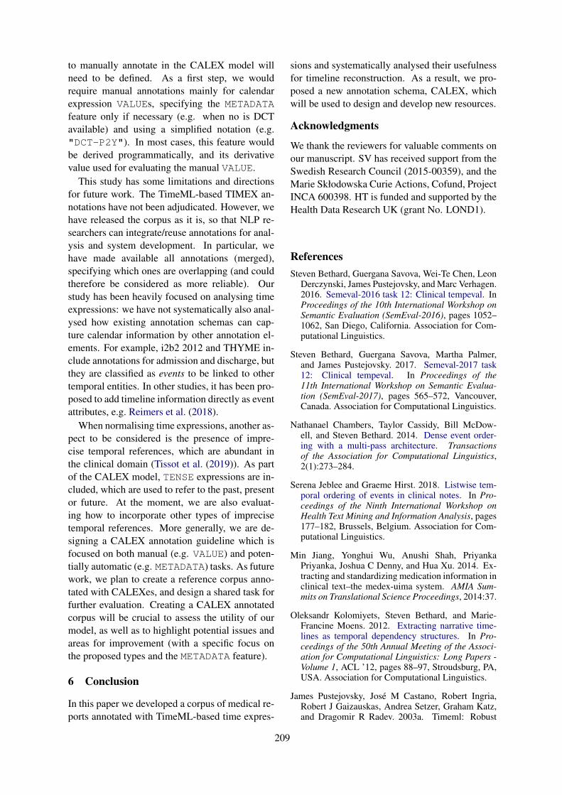
to manually annotate in the CALEX model willneed to be defined. As a first step, we wouldrequire manual annotations mainly for calendarexpression VALUEs, specifying the METADATAfeature only if necessary (e.g. when no is DCTavailable) and using a simplified notation (e.g."DCT-P2Y"). In most cases, this feature wouldbe derived programmatically, and its derivativevalue used for evaluating the manual VALUE.
This study has some limitations and directionsfor future work. The TimeML-based TIMEX an-notations have not been adjudicated. However, wehave released the corpus as it is, so that NLP re-searchers can integrate/reuse annotations for anal-ysis and system development. In particular, wehave made available all annotations (merged),specifying which ones are overlapping (and couldtherefore be considered as more reliable). Ourstudy has been heavily focused on analysing timeexpressions: we have not systematically also anal-ysed how existing annotation schemas can cap-ture calendar information by other annotation el-ements. For example, i2b2 2012 and THYME in-clude annotations for admission and discharge, butthey are classified as events to be linked to othertemporal entities. In other studies, it has been pro-posed to add timeline information directly as eventattributes, e.g. Reimers et al. (2018).
When normalising time expressions, another as-pect to be considered is the presence of impre-cise temporal references, which are abundant inthe clinical domain (Tissot et al. (2019)). As partof the CALEX model, TENSE expressions are in-cluded, which are used to refer to the past, presentor future. At the moment, we are also evaluat-ing how to incorporate other types of imprecisetemporal references. More generally, we are de-signing a CALEX annotation guideline which isfocused on both manual (e.g. VALUE) and poten-tially automatic (e.g. METADATA) tasks. As futurework, we plan to create a reference corpus anno-tated with CALEXes, and design a shared task forfurther evaluation. Creating a CALEX annotatedcorpus will be crucial to assess the utility of ourmodel, as well as to highlight potential issues andareas for improvement (with a specific focus onthe proposed types and the METADATA feature).
6 Conclusion
In this paper we developed a corpus of medical re-ports annotated with TimeML-based time expres-
sions and systematically analysed their usefulnessfor timeline reconstruction. As a result, we pro-posed a new annotation schema, CALEX, whichwill be used to design and develop new resources.
Acknowledgments
We thank the reviewers for valuable comments onour manuscript. SV has received support from theSwedish Research Council (2015-00359), and theMarie Skłodowska Curie Actions, Cofund, ProjectINCA 600398. HT is funded and supported by theHealth Data Research UK (grant No. LOND1).
ReferencesSteven Bethard, Guergana Savova, Wei-Te Chen, Leon
Derczynski, James Pustejovsky, and Marc Verhagen.2016. Semeval-2016 task 12: Clinical tempeval. InProceedings of the 10th International Workshop onSemantic Evaluation (SemEval-2016), pages 1052–1062, San Diego, California. Association for Com-putational Linguistics.
Steven Bethard, Guergana Savova, Martha Palmer,and James Pustejovsky. 2017. Semeval-2017 task12: Clinical tempeval. In Proceedings of the11th International Workshop on Semantic Evalua-tion (SemEval-2017), pages 565–572, Vancouver,Canada. Association for Computational Linguistics.
Nathanael Chambers, Taylor Cassidy, Bill McDow-ell, and Steven Bethard. 2014. Dense event order-ing with a multi-pass architecture. Transactionsof the Association for Computational Linguistics,2(1):273–284.
Serena Jeblee and Graeme Hirst. 2018. Listwise tem-poral ordering of events in clinical notes. In Pro-ceedings of the Ninth International Workshop onHealth Text Mining and Information Analysis, pages177–182, Brussels, Belgium. Association for Com-putational Linguistics.
Min Jiang, Yonghui Wu, Anushi Shah, PriyankaPriyanka, Joshua C Denny, and Hua Xu. 2014. Ex-tracting and standardizing medication information inclinical text–the medex-uima system. AMIA Sum-mits on Translational Science Proceedings, 2014:37.
Oleksandr Kolomiyets, Steven Bethard, and Marie-Francine Moens. 2012. Extracting narrative time-lines as temporal dependency structures. In Pro-ceedings of the 50th Annual Meeting of the Associ-ation for Computational Linguistics: Long Papers -Volume 1, ACL ’12, pages 88–97, Stroudsburg, PA,USA. Association for Computational Linguistics.
James Pustejovsky, José M Castano, Robert Ingria,Robert J Gaizauskas, Andrea Setzer, Graham Katz,and Dragomir R Radev. 2003a. Timeml: Robust
209
specification of event and temporal expressions intext.
James Pustejovsky, Patrick Hanks, Roser Sauri, An-drew See, Robert Gaizauskas, Andrea Setzer,Dragomir Radev, Beth Sundheim, David Day, LisaFerro, et al. 2003b. The timebank corpus. In Corpuslinguistics, volume 2003, page 40. Lancaster, UK.
James Pustejovsky, Kiyong Lee, Harry Bunt, and Lau-rent Romary. 2010. Iso-timeml: An internationalstandard for semantic annotation. In LREC, vol-ume 10, pages 394–397.
James Pustejovsky and Marc Verhagen. 2009.Semeval-2010 task 13: evaluating events, timeexpressions, and temporal relations (tempeval-2).In Proceedings of the Workshop on Semantic Evalu-ations: Recent Achievements and Future Directions(SEW-2009), pages 112–116.
Preethi Raghavan, Eric Fosler-Lussier, Noémie El-hadad, and Albert M. Lai. 2014. Cross-narrativetemporal ordering of medical events. In Proceed-ings of the 52nd Annual Meeting of the Associationfor Computational Linguistics (Volume 1: Long Pa-pers), pages 998–1008, Baltimore, Maryland. Asso-ciation for Computational Linguistics.
Nils Reimers, Nazanin Dehghani, and Iryna Gurevych.2016. Temporal anchoring of events for the time-bank corpus. In Proceedings of the 54th AnnualMeeting of the Association for Computational Lin-guistics (Volume 1: Long Papers), pages 2195–2204, Berlin, Germany. Association for Computa-tional Linguistics.
Nils Reimers, Nazanin Dehghani, and Iryna Gurevych.2018. Event time extraction with a decision tree ofneural classifiers. Transactions of the Associationfor Computational Linguistics, 6:77–89.
William F Styler IV, Steven Bethard, Sean Finan,Martha Palmer, Sameer Pradhan, Piet C de Groen,Brad Erickson, Timothy Miller, Chen Lin, GuerganaSavova, and James Pustejovsky. 2014. Temporal an-notation in the clinical domain. Transactions of theAssociation for Computational Linguistics, 2:143–154.
Weiyi Sun, Anna Rumshisky, and Ozlem Uzuner.2013a. Annotating temporal information in clini-cal narratives. Journal of biomedical informatics,46:S5–S12.
Weiyi Sun, Anna Rumshisky, and Ozlem Uzuner.2013b. Evaluating temporal relations in clinicaltext: 2012 i2b2 Challenge. Journal of the AmericanMedical Informatics Association, 20(5):806–813.
Hegler Tissot, Marcos Didonet Del Fabro, Leon Der-czynski, and Angus Roberts. 2019. Normalisationof imprecise temporal expressions extracted fromtext. Knowledge and Information Systems.
Hegler Tissot, Angus Roberts, Leon Derczynski,Genevieve Gorrell, and Marcos Didonet Del Fabro.2015. Analysis of temporal expressions annotatedin clinical notes. In Proceedings of 11th Joint ACL-ISO Workshop on Interoperable Semantic Annota-tion, pages 93–102, London, UK. ACL.
Marc Verhagen, Robert Gaizauskas, Frank Schilder,Mark Hepple, Graham Katz, and James Pustejovsky.2007. Semeval-2007 task 15: Tempeval tempo-ral relation identification. In Proceedings of thefourth international workshop on semantic evalua-tions (SemEval-2007), pages 75–80.
Natalia Viani, Lucia Yin, Joyce Kam, Ayunni Alawi,André Bittar, Rina Dutta, Rashmi Patel, RobertStewart, and Sumithra Velupillai. 2018. Time ex-pressions in mental health records for symptom on-set extraction. In Proceedings of the Ninth Interna-tional Workshop on Health Text Mining and Infor-mation Analysis, pages 183–192, Brussels, Belgium.Association for Computational Linguistics.
Ran Zhao, Quang Do, and Dan Roth. 2012. A robustshallow temporal reasoning system. In Proceedingsof the Demonstration Session at the Conference ofthe North American Chapter of the Association forComputational Linguistics: Human Language Tech-nologies, pages 29–32, Montréal, Canada. Associa-tion for Computational Linguistics.
210
Proceedings of the BioNLP 2019 workshop, pages 211–216Florence, Italy, August 1, 2019. c©2019 Association for Computational Linguistics
Abstract
The automatic processing of clinical docu-
ments, such as Electronic Health Records
(EHRs), could benefit substantially from
the enrichment of medical terminologies
with terms encountered in clinical practice.
To integrate such terms into existing
knowledge sources, they must be linked to
corresponding concepts. We present a
method for the semantic categorization of
clinical terms based on their surface form.
We find that features based on sublanguage
properties can provide valuable cues for the
classification of term variants.
1 Background
Structured terminologies and ontologies play a
pivotal role in the automatic processing of health
data, as they provide the framework for mapping
unstructured information into a machine-readable
format. Moreover, the term bases themselves can
serve as input for the identification of medical en-
tities in free text. Even though methods from ma-
chine learning are gaining popularity, many state-
of-the-art systems rely strongly on pre-compiled
terminologies (e.g. Savova et al. 2010). The per-
formance of such applications thus relies crucially
on the lexical coverage of the term base. However,
the major biomedical terminologies, such as the
1 https://browser.ihtsdotools.org/?
Systematic Nomenclature of Medicine – Clinical
Terms (SNOMED CT)1 and the Unified Medical
Language System (UMLS)2 do not adequately re-
flect the range of term variants encountered in
clinical practice. Especially in languages other
than English, where the available terminologies
are less comprehensive, this discrepancy can harm
performance (Henriksson et al. 2014; Skeppstedt
et al. 2014). One strategy to overcome this bottle-
neck is to enrich the available terminologies with
additional variants acquired from domain corpora.
Concretely, this involves the recognition of vari-
ants in text, and their association with the semantic
classes or concepts provided by the respective ter-
minology.
The focus of this paper is on the second task, i.e.
the semantic categorization of term variants. In
particular, we investigate whether the features of a
given sublanguage can be leveraged to associate
individual variants with semantic classes. Accord-
ing to sublanguage theory, specialized languages
can be characterized by semantic constraints, as
well as stylistic preferences and distinctive syntac-
tic patterns (Friedman, Kra, and Rzhetsky 2002;
Harris 1982, 1991; 2002). In the medical domain,
such differences manifest themselves at fine-
grained levels, e.g. between clinical specialties and
different document types (Feldman, Hazekamp,
2 https://uts.nlm.nih.gov/home.html
Leveraging Sublanguage Features for the
Semantic Categorization of Clinical Terms
Leonie Grön
Quantitative Linguistics and
Lexical Variation (QLVL)
KU Leuven [email protected]
Ann Bertels
Leuven Language Institute (ILT)
Quantitative Linguistics and
Lexical Variation (QLVL)
KU Leuven [email protected]
Kris Heylen
Quantitative Linguistics and
Lexical Variation (QLVL)
KU Leuven [email protected]
211
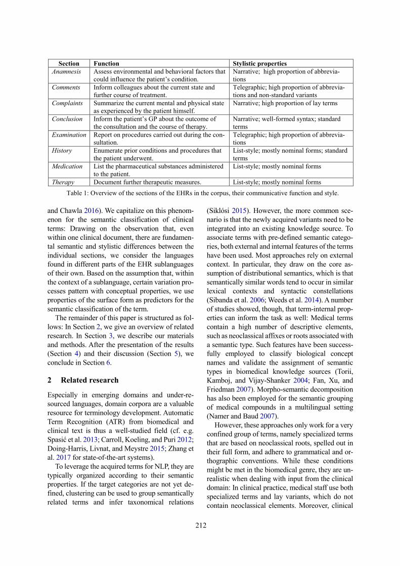
and Chawla 2016). We capitalize on this phenom-
enon for the semantic classification of clinical
terms: Drawing on the observation that, even
within one clinical document, there are fundamen-
tal semantic and stylistic differences between the
individual sections, we consider the languages
found in different parts of the EHR sublanguages
of their own. Based on the assumption that, within
the context of a sublanguage, certain variation pro-
cesses pattern with conceptual properties, we use
properties of the surface form as predictors for the
semantic classification of the term.
The remainder of this paper is structured as fol-
lows: In Section 2, we give an overview of related
research. In Section 3, we describe our materials
and methods. After the presentation of the results
(Section 4) and their discussion (Section 5), we
conclude in Section 6.
2 Related research
Especially in emerging domains and under-re-
sourced languages, domain corpora are a valuable
resource for terminology development. Automatic
Term Recognition (ATR) from biomedical and
clinical text is thus a well-studied field (cf. e.g.
Spasić et al. 2013; Carroll, Koeling, and Puri 2012;
Doing-Harris, Livnat, and Meystre 2015; Zhang et
al. 2017 for state-of-the-art systems).
To leverage the acquired terms for NLP, they are
typically organized according to their semantic
properties. If the target categories are not yet de-
fined, clustering can be used to group semantically
related terms and infer taxonomical relations
(Siklósi 2015). However, the more common sce-
nario is that the newly acquired variants need to be
integrated into an existing knowledge source. To
associate terms with pre-defined semantic catego-
ries, both external and internal features of the terms
have been used. Most approaches rely on external
context. In particular, they draw on the core as-
sumption of distributional semantics, which is that
semantically similar words tend to occur in similar
lexical contexts and syntactic constellations
(Sibanda et al. 2006; Weeds et al. 2014). A number
of studies showed, though, that term-internal prop-
erties can inform the task as well: Medical terms
contain a high number of descriptive elements,
such as neoclassical affixes or roots associated with
a semantic type. Such features have been success-
fully employed to classify biological concept
names and validate the assignment of semantic
types in biomedical knowledge sources (Torii,
Kamboj, and Vijay-Shanker 2004; Fan, Xu, and
Friedman 2007). Morpho-semantic decomposition
has also been employed for the semantic grouping
of medical compounds in a multilingual setting
(Namer and Baud 2007).
However, these approaches only work for a very
confined group of terms, namely specialized terms
that are based on neoclassical roots, spelled out in
their full form, and adhere to grammatical and or-
thographic conventions. While these conditions
might be met in the biomedical genre, they are un-
realistic when dealing with input from the clinical
domain: In clinical practice, medical staff use both
specialized terms and lay variants, which do not
contain neoclassical elements. Moreover, clinical
Section Function Stylistic properties
Anamnesis Assess environmental and behavioral factors that
could influence the patient’s condition.
Narrative; high proportion of abbrevia-
tions
Comments Inform colleagues about the current state and
further course of treatment.
Telegraphic; high proportion of abbrevia-
tions and non-standard variants
Complaints Summarize the current mental and physical state
as experienced by the patient himself.
Narrative; high proportion of lay terms
Conclusion Inform the patient’s GP about the outcome of
the consultation and the course of therapy.
Narrative; well-formed syntax; standard
terms
Examination Report on procedures carried out during the con-
sultation.
Telegraphic; high proportion of abbrevia-
tions
History Enumerate prior conditions and procedures that
the patient underwent.
List-style; mostly nominal forms; standard
terms
Medication List the pharmaceutical substances administered
to the patient.
List-style; mostly nominal forms
Therapy Document further therapeutic measures. List-style; mostly nominal forms
Table 1: Overview of the sections of the EHRs in the corpus, their communicative function and style.
212
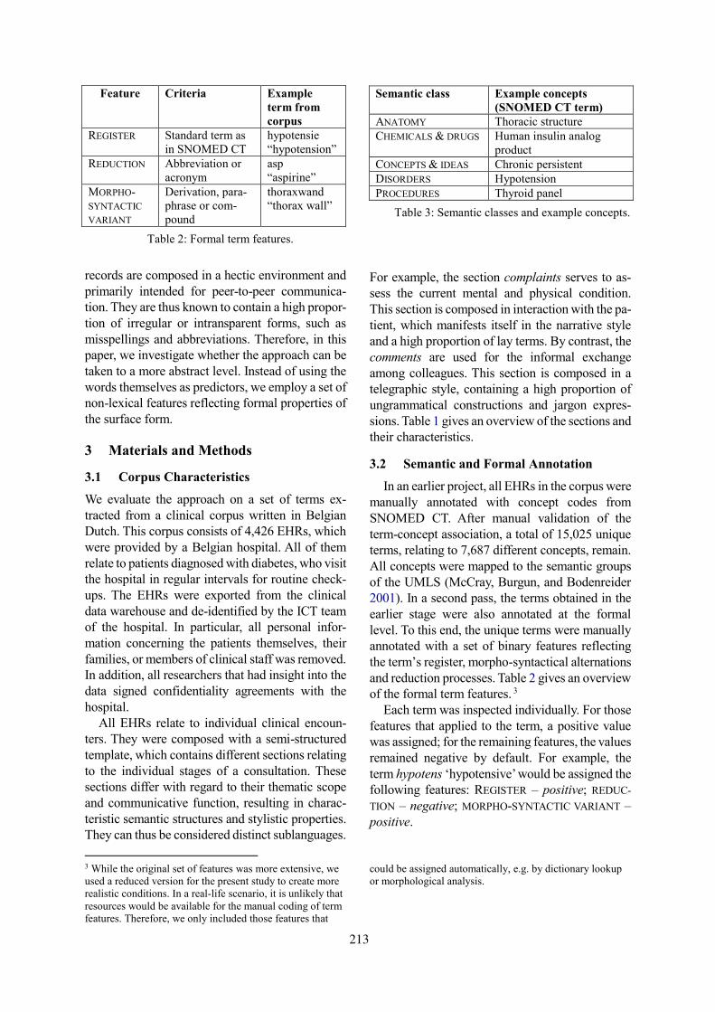
records are composed in a hectic environment and
primarily intended for peer-to-peer communica-
tion. They are thus known to contain a high propor-
tion of irregular or intransparent forms, such as
misspellings and abbreviations. Therefore, in this
paper, we investigate whether the approach can be
taken to a more abstract level. Instead of using the
words themselves as predictors, we employ a set of
non-lexical features reflecting formal properties of
the surface form.
3 Materials and Methods
3.1 Corpus Characteristics
We evaluate the approach on a set of terms ex-
tracted from a clinical corpus written in Belgian
Dutch. This corpus consists of 4,426 EHRs, which
were provided by a Belgian hospital. All of them
relate to patients diagnosed with diabetes, who visit
the hospital in regular intervals for routine check-
ups. The EHRs were exported from the clinical
data warehouse and de-identified by the ICT team
of the hospital. In particular, all personal infor-
mation concerning the patients themselves, their
families, or members of clinical staff was removed.
In addition, all researchers that had insight into the
data signed confidentiality agreements with the
hospital.
All EHRs relate to individual clinical encoun-
ters. They were composed with a semi-structured
template, which contains different sections relating
to the individual stages of a consultation. These
sections differ with regard to their thematic scope
and communicative function, resulting in charac-
teristic semantic structures and stylistic properties.
They can thus be considered distinct sublanguages.
3 While the original set of features was more extensive, we
used a reduced version for the present study to create more
realistic conditions. In a real-life scenario, it is unlikely that
resources would be available for the manual coding of term
features. Therefore, we only included those features that
For example, the section complaints serves to as-
sess the current mental and physical condition.
This section is composed in interaction with the pa-
tient, which manifests itself in the narrative style
and a high proportion of lay terms. By contrast, the
comments are used for the informal exchange
among colleagues. This section is composed in a
telegraphic style, containing a high proportion of
ungrammatical constructions and jargon expres-
sions. Table 1 gives an overview of the sections and
their characteristics.
3.2 Semantic and Formal Annotation
In an earlier project, all EHRs in the corpus were
manually annotated with concept codes from
SNOMED CT. After manual validation of the
term-concept association, a total of 15,025 unique
terms, relating to 7,687 different concepts, remain.
All concepts were mapped to the semantic groups
of the UMLS (McCray, Burgun, and Bodenreider
2001). In a second pass, the terms obtained in the
earlier stage were also annotated at the formal
level. To this end, the unique terms were manually
annotated with a set of binary features reflecting
the term’s register, morpho-syntactical alternations
and reduction processes. Table 2 gives an overview
of the formal term features. 3
Each term was inspected individually. For those
features that applied to the term, a positive value
was assigned; for the remaining features, the values
remained negative by default. For example, the
term hypotens ‘hypotensive’ would be assigned the
following features: REGISTER – positive; REDUC-
TION – negative; MORPHO-SYNTACTIC VARIANT –
positive.
could be assigned automatically, e.g. by dictionary lookup
or morphological analysis.
Feature Criteria Example
term from
corpus
REGISTER Standard term as
in SNOMED CT
hypotensie
“hypotension”
REDUCTION Abbreviation or
acronym
asp
“aspirine”
MORPHO-
SYNTACTIC
VARIANT
Derivation, para-
phrase or com-
pound
thoraxwand
“thorax wall”
Table 2: Formal term features.
Semantic class Example concepts
(SNOMED CT term)
ANATOMY Thoracic structure
CHEMICALS & DRUGS Human insulin analog
product
CONCEPTS & IDEAS Chronic persistent
DISORDERS Hypotension
PROCEDURES Thyroid panel
Table 3: Semantic classes and example concepts.
213
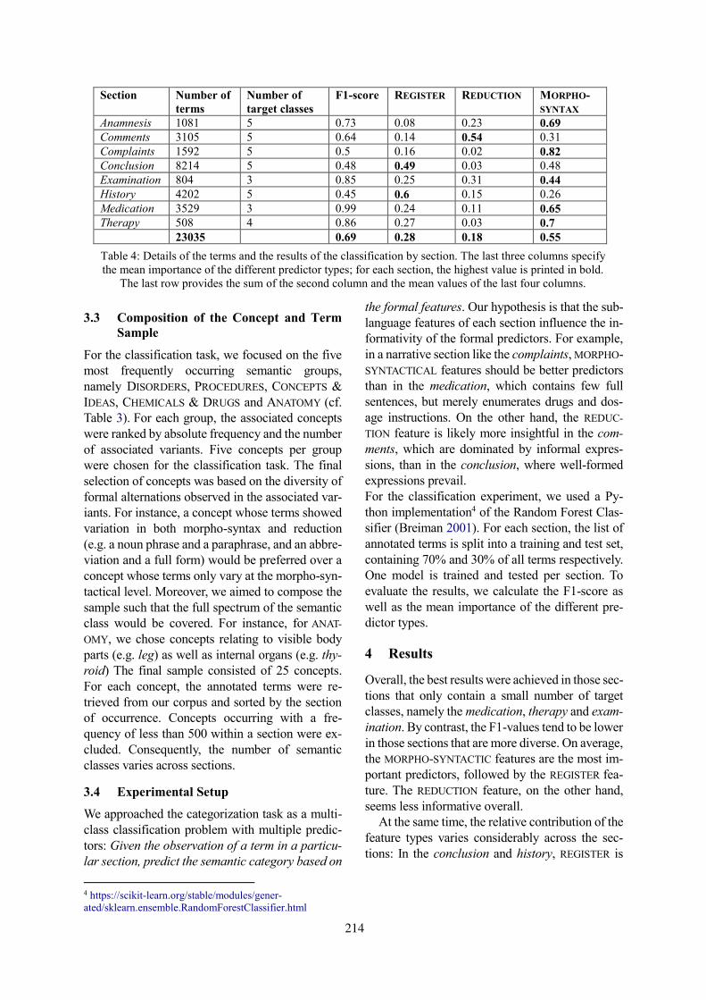
3.3 Composition of the Concept and Term
Sample
For the classification task, we focused on the five
most frequently occurring semantic groups,
namely DISORDERS, PROCEDURES, CONCEPTS &
IDEAS, CHEMICALS & DRUGS and ANATOMY (cf.
Table 3). For each group, the associated concepts
were ranked by absolute frequency and the number
of associated variants. Five concepts per group
were chosen for the classification task. The final
selection of concepts was based on the diversity of
formal alternations observed in the associated var-
iants. For instance, a concept whose terms showed
variation in both morpho-syntax and reduction
(e.g. a noun phrase and a paraphrase, and an abbre-
viation and a full form) would be preferred over a
concept whose terms only vary at the morpho-syn-
tactical level. Moreover, we aimed to compose the
sample such that the full spectrum of the semantic
class would be covered. For instance, for ANAT-
OMY, we chose concepts relating to visible body
parts (e.g. leg) as well as internal organs (e.g. thy-
roid) The final sample consisted of 25 concepts.
For each concept, the annotated terms were re-
trieved from our corpus and sorted by the section
of occurrence. Concepts occurring with a fre-
quency of less than 500 within a section were ex-
cluded. Consequently, the number of semantic
classes varies across sections.
3.4 Experimental Setup
We approached the categorization task as a multi-
class classification problem with multiple predic-
tors: Given the observation of a term in a particu-
lar section, predict the semantic category based on
4 https://scikit-learn.org/stable/modules/gener-
ated/sklearn.ensemble.RandomForestClassifier.html
the formal features. Our hypothesis is that the sub-
language features of each section influence the in-
formativity of the formal predictors. For example,
in a narrative section like the complaints, MORPHO-
SYNTACTICAL features should be better predictors
than in the medication, which contains few full
sentences, but merely enumerates drugs and dos-
age instructions. On the other hand, the REDUC-
TION feature is likely more insightful in the com-
ments, which are dominated by informal expres-
sions, than in the conclusion, where well-formed
expressions prevail.
For the classification experiment, we used a Py-
thon implementation4 of the Random Forest Clas-
sifier (Breiman 2001). For each section, the list of
annotated terms is split into a training and test set,
containing 70% and 30% of all terms respectively.
One model is trained and tested per section. To
evaluate the results, we calculate the F1-score as
well as the mean importance of the different pre-
dictor types.
4 Results
Overall, the best results were achieved in those sec-
tions that only contain a small number of target
classes, namely the medication, therapy and exam-
ination. By contrast, the F1-values tend to be lower
in those sections that are more diverse. On average,
the MORPHO-SYNTACTIC features are the most im-
portant predictors, followed by the REGISTER fea-
ture. The REDUCTION feature, on the other hand,
seems less informative overall.
At the same time, the relative contribution of the
feature types varies considerably across the sec-
tions: In the conclusion and history, REGISTER is
Section Number of
terms
Number of
target classes
F1-score REGISTER REDUCTION MORPHO-
SYNTAX
Anamnesis 1081 5 0.73 0.08 0.23 0.69
Comments 3105 5 0.64 0.14 0.54 0.31
Complaints 1592 5 0.5 0.16 0.02 0.82
Conclusion 8214 5 0.48 0.49 0.03 0.48
Examination 804 3 0.85 0.25 0.31 0.44
History 4202 5 0.45 0.6 0.15 0.26
Medication 3529 3 0.99 0.24 0.11 0.65
Therapy 508 4 0.86 0.27 0.03 0.7
23035 0.69 0.28 0.18 0.55
Table 4: Details of the terms and the results of the classification by section. The last three columns specify
the mean importance of the different predictor types; for each section, the highest value is printed in bold.
The last row provides the sum of the second column and the mean values of the last four columns.
214
the strongest predictor; however, in the conclusion,
the MORPHO-SYNTACTIC features are almost on par
with REGISTER. While REDUCTION is most im-
portant in the comments, it also has a substantial
effect in the examination. The MORPHO-SYNTAC-
TIC features make the strongest contribution in the
complaints, therapy, anamnesis and medication;
they are also strongest, but not quite as dominant,
in the examination. Table 4 provides the full re-
sults.
5 Discussion
The results show that the semantic complexity of
the respective sublanguage influences classifica-
tion performance. The best F1-scores were
achieved in those sections devoted to a very con-
fined topic, while the values were lower in the
more heterogeneous ones. This tendency corrobo-
rates the findings of previous work studying the ef-
fect of sublanguage properties on NLP in the clini-
cal domain (Doing-Harris et al. 2013).
However, we found striking differences in the
relative importance of the predictor types. On the
whole, the contribution of the predictors patterns
with the stylistic properties of the respective sub-
languages: For instance, MORPHO-SYNTACTIC fea-
tures are most informative in those sections com-
posed in a narrative style; REDUCTION is strongest
in the informal parts of the document. This finding
confirms our initial hypothesis. At a closer look,
though, another effect emerges: In semantically
homogeneous sections, infrequent features can
serve to identify conceptual outliers. For instance,
in the therapy-centered sections, which are domi-
nated by nouns relating to pharmaceutical sub-
stances, the presence of non-nominal morphologi-
cal properties, such as an adjective ending, is a
strong predictor for a term belonging to another se-
mantic class, such as a temporal modifier.
Our study has its limitations, as it only considers
a very small sample of highly frequent concepts.
Possibly, for low-frequency concepts, the formal
features would not be informative enough to allow
a reliable classification. Therefore, in future work,
we plan to replicate the experiment at a larger
scale, including a more diverse concept sample.
Besides, in order to test the generalizability of the
method, it would be interesting to evaluate the per-
formance on data from different clinical special-
ties, and from multiple clinical institutions.
6 Conclusion
We presented a first attempt for the classification
of clinical terms by formal features alone. While
there is much variation in the results, our experi-
ment demonstrates that sublanguage properties can
be exploited to associate terms acquired from do-
main corpora with semantic categories. This ap-
proach could be integrated with other systems to
support the enrichment of medical terminologies.
In further research, we plan to replicate the study
at a larger scale.
Acknowledgements
This work was supported by Internal Funds KU
Leuven.
References
Breiman, Leo. 2001. “Random Forests.” Machine
Learning 45: 5–32.
https://doi.org/10.1023/A:1010933404324.
Carroll, John, Rob Koeling, and Shivani Puri. 2012.
“Lexical Acquisition for Clinical Text Mining Us-
ing Distributional Similarity.” Lexical Computa-
tional Linguistics and Intelligent Text Processing.
CICLing 2012, 232–4. https://doi.org/10.1007/978-
3-642-28601-8_20.
Doing-Harris, Kristina, Olga Patterson, Sean Igo, and
John Hurdle. 2013. “Document Sublanguage Clus-
tering to Detect Medical Specialty in Cross-Institu-
tional Clinical Texts.” Proc ACM Int Workshop
Data Text Min Biomed Inform, 9–12.
https://doi.org/10.1145/2512089.2512101.
Doing-Harris, Kristina, Yarden Livnat, and Stephane
Meystre. 2015. “Automated Concept and Relation-
ship Extraction for the Semi-Automated Ontology
Management (SEAM) System.” J Biomed Sem 6:
15. https://doi.org/10.1186/s13326-015-0011-7.
Fan, Jung Wei, Hua Xu, and Carol Friedman. 2007.
“Using Contextual and Lexical Features to Restruc-
ture and Validate the Classification of Biomedical
Concepts.” BMC Bioinform 8: 264.
https://doi.org/10.1186/1471-2105-8-264.
Feldman, Keith, Nicholas Hazekamp, and Nitesh V.
Chawla. 2016. “Mining the Clinical Narrative: All
Text Are Not Equal.” 2016 IEEE International Con-
ference on Healthcare Informatics (ICHI), 271–80.
https://doi.org/10.1109/ICHI.2016.37.
Friedman, Carol, Pauline Kra, and Andrey Rzhetsky.
2002. “Two Biomedical Sublanguages: A Descrip-
tion Based on the Theories of Zellig Harris.” J Bio-
med Inform 35 (4): 222–35.
https://doi.org/10.1016/S1532-0464(03)00012-1.
215

Harris, Zellig. 1982. “Discourse and Sublanguage.” In
Sublanguage. Studies of Language in Restricted Se-
mantic Domains, edited by Richard Kittredge and
John Lehrberger, 231–36. Berlin/New York: De
Gruyter.
Harris, Zellig. 1991. A Theory of Language and Infor-
mation. A Mathematical Approach. Oxford: Claren-
don Press.
Harris, Zellig. 2002. “The Structure of Science Infor-
mation.” J Biomed Inform 35 (4): 215–21.
https://doi.org/10.1016/S1532-0464(03)00011-X.
Henriksson, Aron, Hans Moen, Maria Skeppstedt,
Vidas Daudaravičius, and Martin Duneld. 2014.
“Synonym Extraction and Abbreviation Expansion
with Ensembles of Semantic Spaces.” J Biomed
Sem 5: 6. https://doi.org/10.1186/2041-1480-5-6.
McCray, Alexa T., Anita Burgun, and Olivier Boden-
reider. 2001. “Aggregating UMLS Semantic Types
for Reducing Conceptual Complexity.” Stud Health
Technol Inform 84 (0 1): 216–20.
https://doi.org/10.3233/978-1-60750-928-8-216.
Namer, Fiammetta, and Robert Baud. 2007. “Defining
and Relating Biomedical Terms: Towards a Cross-
Language Morphosemantics-Based System.” Int J
Med Inform 76 (2–3): 226–33.
https://doi.org/10.1016/j.ijmedinf.2006.05.001.
Savova, Guergana K, James J Masanz, Philip V Ogren,
Jiaping Zheng, Sunghwan Sohn, Karin C Kipper-
Schuler, Christopher G Chute. 2010. “Mayo Clini-
cal Text Analysis and Knowledge Extraction Sys-
tem (CTAKES): Architecture, Component Evalua-
tion and Applications.” J Am Med Inform Assoc 17
(5): 507–13. https://doi:10.1136/ja-
mia.2009.001560 .
Sibanda, Tawanda, Tian He, Peter Szolovits, and
Ozlem Uzuner. 2006. “Syntactically-Informed Se-
mantic Category Recognizer for Discharge Sum-
maries.” AMIA Annu Symp Proc 2006, 714–18.
Siklósi, Borbála. 2015. “Clustering Relevant Terms
and Identifying Types of Statements in Clinical
Records.” Computational Linguistics and Intelli-
gent Text Processing. CICLing 2015. 619–30.
https://doi.org/10.1007/978-3-319-18117-2_46.
Skeppstedt, Maria, Maria Kvist, Gunnar H. Nilsson,
and Hercules Dalianis. 2014. “Automatic Recogni-
tion of Disorders, Findings, Pharmaceuticals and
Body Structures from Clinical Text: An Annotation
and Machine Learning Study.” J Biomed Inform 49:
148–58. https://doi.org/10.1016/j.jbi.2014.01.012.
Spasić, Irena, Mark Greenwood, Alun Preece, Nick
Francis, and Glyn Elwyn. 2013. “FlexiTerm: A
Flexible Term Recognition Method.” J Biomed Sem
4: 27. https://doi.org/10.1186/2041-1480-4-27.
Torii, Manabu, Sachin Kamboj, and K. Vijay-Shanker.
2004. “Using Name-Internal and Contextual Fea-
tures to Classify Biological Terms.” J Biomed In-
form 37: 498–511.
https://doi.org/10.1016/j.jbi.2004.08.007.
Weeds, Julie, James Dowdall, Gerold Schneider, Bill
Keller, and David J. Weir. 2014. “Using Distribu-
tional Similarity to Organise BioMedical Terminol-
ogy.” Terminology 11 (1): 107–41.
https://doi.org/10.1075/bct.2.07wee.
Zhang, Rui, Jialin Liu, Yong Huang, Miye Wang,
Qingke Shi, Jun Chen, and Zhi Zeng. 2017. “En-
riching the International Clinical Nomenclature
with Chinese Daily Used Synonyms and Concept
Recognition in Physician Notes.” BMC Med Inform
Decis Mak 17: 54. https://doi.org/10.1186/s12911-
017-0455-z.
216
Proceedings of the BioNLP 2019 workshop, pages 217–222Florence, Italy, August 1, 2019. c©2019 Association for Computational Linguistics
Enhancing PIO Element Detection in Medical Text Using ContextualizedEmbedding
Hichem MezaouiIMRSV Data Labs
Ottawa, [email protected]
Aleksandr GontcharovIMRSV Data Labs
Ottawa, [email protected]
Isuru GunasekaraIMRSV Data Labs
Ottawa, [email protected]
Abstract
In this paper, we investigate a new approach toPopulation, Intervention and Outcome (PIO)element detection, a common task in EvidenceBased Medicine (EBM). The purpose of thisstudy is two-fold: to build a training dataset forPIO element detection with minimum redun-dancy and ambiguity and to investigate pos-sible options in utilizing state of the art em-bedding methods for the task of PIO elementdetection. For the former purpose, we build anew and improved dataset by investigating theshortcomings of previously released datasets.For the latter purpose, we leverage the state ofthe art text embedding, Bidirectional EncoderRepresentations from Transformers (BERT),and build a multi-label classifier. We showthat choosing a domain specific pre-trainedembedding further optimizes the performanceof the classifier. Furthermore, we show thatthe model could be enhanced by using ensem-ble methods and boosting techniques providedthat features are adequately chosen.
1 Introduction
Evidence-based medicine (EBM) is of primaryimportance in the medical field. Its goal is topresent statistical analyses of issues of clinical fo-cus based on retrieving and analyzing numerouspapers in the medical literature (Haynes et al.,1997). The PubMed database is one of the mostcommonly used databases in EBM (Sackett et al.,1996).
Biomedical papers, describing randomized con-trolled trials in medical intervention, are publishedat a high rate every year. The volume of these pub-lications makes it very challenging for physiciansto find the best medical intervention for a givenpatient group and condition (Borah et al., 2017).Computational methods and natural language pro-cessing (NLP) could be adopted in order to expe-dite the process of biomedical evidence synthesis.Specifically, NLP tasks applied to well structured
documents and queries can help physicians extractappropriate information to identify the best avail-able evidence in the context of medical treatment.
Clinical questions are formed using the PIOframework, where clinical issues are broken downinto four components: Population/Problem (P),Intervention (I), Comparator (C), and Outcome(O). We will refer to these categories as PIO el-ements, by using the common practice of mergingthe C and I categories. In (Rathbone et al., 2017)a literature screening performed in 10 systematicreviews was studied. It was found that using thePIO framework can significantly improve litera-ture screening efficacy. Therefore, efficient extrac-tion of PIO elements is a key feature of many EBMapplications and could be thought of as a multi-label sentence classification problem.
Previous works on PIO element extraction fo-cused on classical NLP methods, such as NaiveBayes (NB), Support Vector Machines (SVM) andConditional Random Fields (CRF) (Chung, 2009;Boudin et al., 2010). These models are shallowand limited in terms of modeling capacity. Fur-thermore, most of these classifiers are trained toextract PIO elements one by one which is sub-optimal since this approach does not allow the useof shared structure among the individual classi-fiers.
Deep neural network models have increased inpopularity in the field of NLP. They have pushedthe state of the art of text representation and in-formation retrieval. More specifically, these tech-niques enhanced NLP algorithms through the useof contextualized text embeddings at word, sen-tence, and paragraph levels (Mikolov et al., 2013;Le and Mikolov, 2014; Peters et al., 2017; Devlinet al., 2018; Logeswaran and Lee, 2018; Radfordet al., 2018).
More recently, Jin and Szolovits (2018) pro-posed a bidirectional long short term memory(LSTM) model to simultaneously extract PIO
217
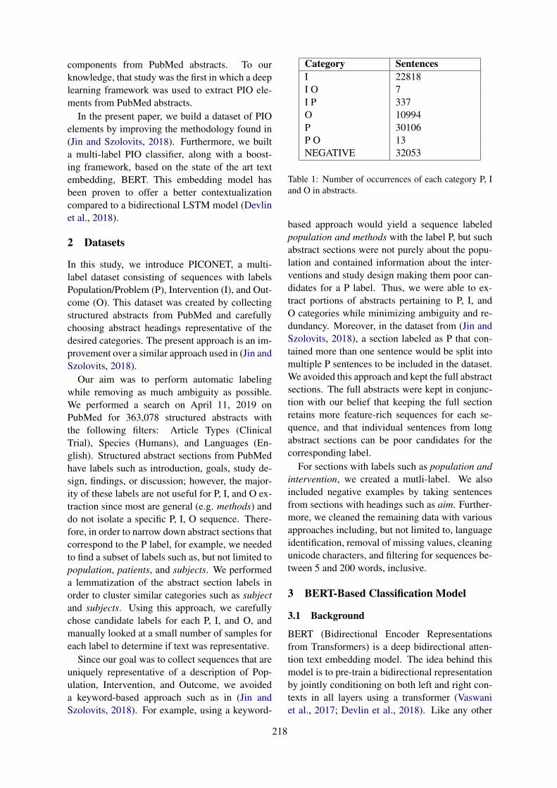
components from PubMed abstracts. To ourknowledge, that study was the first in which a deeplearning framework was used to extract PIO ele-ments from PubMed abstracts.
In the present paper, we build a dataset of PIOelements by improving the methodology found in(Jin and Szolovits, 2018). Furthermore, we builta multi-label PIO classifier, along with a boost-ing framework, based on the state of the art textembedding, BERT. This embedding model hasbeen proven to offer a better contextualizationcompared to a bidirectional LSTM model (Devlinet al., 2018).
2 Datasets
In this study, we introduce PICONET, a multi-label dataset consisting of sequences with labelsPopulation/Problem (P), Intervention (I), and Out-come (O). This dataset was created by collectingstructured abstracts from PubMed and carefullychoosing abstract headings representative of thedesired categories. The present approach is an im-provement over a similar approach used in (Jin andSzolovits, 2018).
Our aim was to perform automatic labelingwhile removing as much ambiguity as possible.We performed a search on April 11, 2019 onPubMed for 363,078 structured abstracts withthe following filters: Article Types (ClinicalTrial), Species (Humans), and Languages (En-glish). Structured abstract sections from PubMedhave labels such as introduction, goals, study de-sign, findings, or discussion; however, the major-ity of these labels are not useful for P, I, and O ex-traction since most are general (e.g. methods) anddo not isolate a specific P, I, O sequence. There-fore, in order to narrow down abstract sections thatcorrespond to the P label, for example, we neededto find a subset of labels such as, but not limited topopulation, patients, and subjects. We performeda lemmatization of the abstract section labels inorder to cluster similar categories such as subjectand subjects. Using this approach, we carefullychose candidate labels for each P, I, and O, andmanually looked at a small number of samples foreach label to determine if text was representative.
Since our goal was to collect sequences that areuniquely representative of a description of Pop-ulation, Intervention, and Outcome, we avoideda keyword-based approach such as in (Jin andSzolovits, 2018). For example, using a keyword-
Category SentencesI 22818I O 7I P 337O 10994P 30106P O 13NEGATIVE 32053
Table 1: Number of occurrences of each category P, Iand O in abstracts.
based approach would yield a sequence labeledpopulation and methods with the label P, but suchabstract sections were not purely about the popu-lation and contained information about the inter-ventions and study design making them poor can-didates for a P label. Thus, we were able to ex-tract portions of abstracts pertaining to P, I, andO categories while minimizing ambiguity and re-dundancy. Moreover, in the dataset from (Jin andSzolovits, 2018), a section labeled as P that con-tained more than one sentence would be split intomultiple P sentences to be included in the dataset.We avoided this approach and kept the full abstractsections. The full abstracts were kept in conjunc-tion with our belief that keeping the full sectionretains more feature-rich sequences for each se-quence, and that individual sentences from longabstract sections can be poor candidates for thecorresponding label.
For sections with labels such as population andintervention, we created a mutli-label. We alsoincluded negative examples by taking sentencesfrom sections with headings such as aim. Further-more, we cleaned the remaining data with variousapproaches including, but not limited to, languageidentification, removal of missing values, cleaningunicode characters, and filtering for sequences be-tween 5 and 200 words, inclusive.
3 BERT-Based Classification Model
3.1 Background
BERT (Bidirectional Encoder Representationsfrom Transformers) is a deep bidirectional atten-tion text embedding model. The idea behind thismodel is to pre-train a bidirectional representationby jointly conditioning on both left and right con-texts in all layers using a transformer (Vaswaniet al., 2017; Devlin et al., 2018). Like any other
218
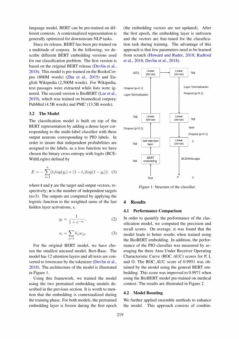
language model, BERT can be pre-trained on dif-ferent contexts. A contextualized representation isgenerally optimized for downstream NLP tasks.
Since its release, BERT has been pre-trained ona multitude of corpora. In the following, we de-scribe different BERT embedding versions usedfor our classification problem. The first version isbased on the original BERT release (Devlin et al.,2018). This model is pre-trained on the BooksCor-pus (800M words) (Zhu et al., 2015) and En-glish Wikipedia (2,500M words). For Wikipedia,text passages were extracted while lists were ig-nored. The second version is BioBERT (Lee et al.,2019), which was trained on biomedical corpora:PubMed (4.5B words) and PMC (13.5B words).
3.2 The Model
The classification model is built on top of theBERT representation by adding a dense layer cor-responding to the multi-label classifier with threeoutput neurons corresponding to PIO labels. Inorder to insure that independent probabilities areassigned to the labels, as a loss function we havechosen the binary cross entropy with logits (BCE-WithLogits) defined by
E = −n∑
i=1
(tilog(yi)+ (1− ti)log(1− yi)); (1)
where t and y are the target and output vectors, re-spectively; n is the number of independent targets(n=3). The outputs are computed by applying thelogistic function to the weighted sums of the lasthidden layer activations, s,
yi =1
1 + e−si, (2)
si =∑
j=1
hjwji. (3)
For the original BERT model, we have cho-sen the smallest uncased model, Bert-Base. Themodel has 12 attention layers and all texts are con-verted to lowercase by the tokenizer (Devlin et al.,2018). The architecture of the model is illustratedin Figure 1.
Using this framework, we trained the modelusing the two pretrained embedding models de-scribed in the previous section. It is worth to men-tion that the embedding is contextualized duringthe training phase. For both models, the pretrainedembedding layer is frozen during the first epoch
(the embedding vectors are not updated). Afterthe first epoch, the embedding layer is unfrozenand the vectors are fine-tuned for the classifica-tion task during training. The advantage of thisapproach is that few parameters need to be learnedfrom scratch (Howard and Ruder, 2018; Radfordet al., 2018; Devlin et al., 2018).
Figure 1: Structure of the classifier.
4 Results
4.1 Performance Comparison
In order to quantify the performance of the clas-sification model, we computed the precision andrecall scores. On average, it was found that themodel leads to better results when trained usingthe BioBERT embedding. In addition, the perfor-mance of the PIO classifier was measured by av-eraging the three Area Under Receiver OperatingCharacteristic Curve (ROC AUC) scores for P, I,and O. The ROC AUC score of 0.9951 was ob-tained by the model using the general BERT em-bedding. This score was improved to 0.9971 whenusing the BioBERT model pre-trained on medicalcontext. The results are illustrated in Figure 2.
4.2 Model Boosting
We further applied ensemble methods to enhancethe model. This approach consists of combin-
219
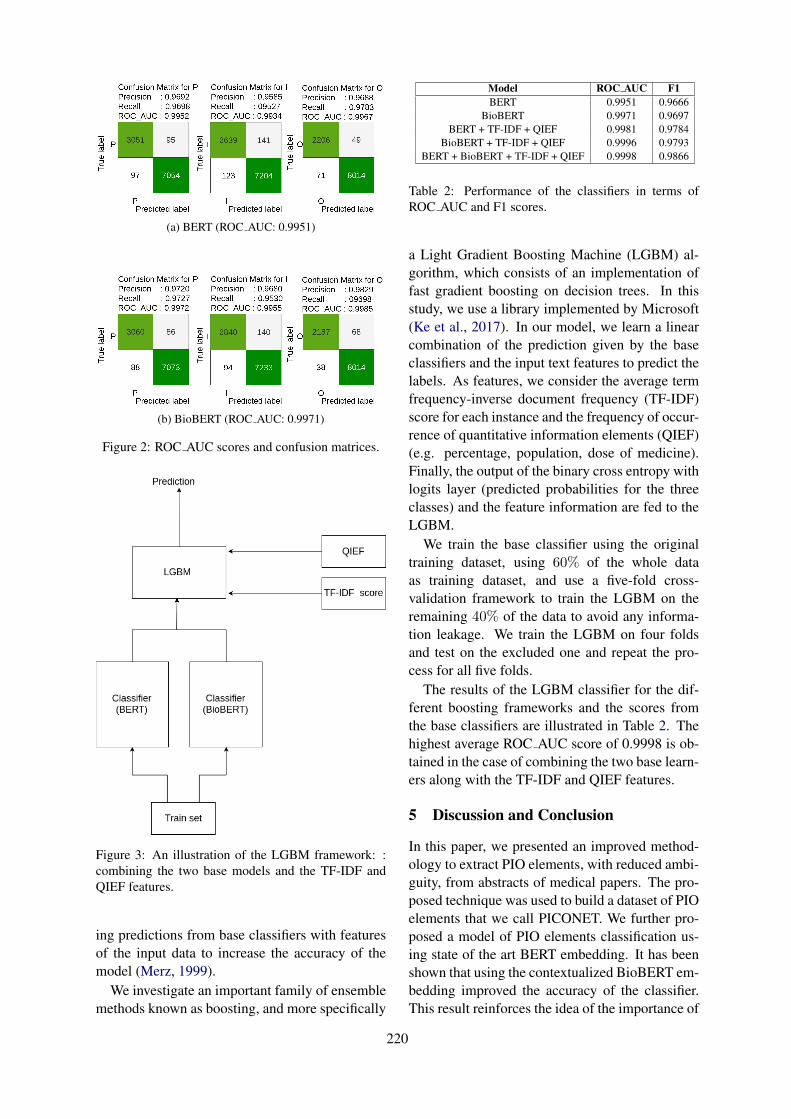
(a) BERT (ROC AUC: 0.9951)
(b) BioBERT (ROC AUC: 0.9971)
Figure 2: ROC AUC scores and confusion matrices.
Figure 3: An illustration of the LGBM framework: :combining the two base models and the TF-IDF andQIEF features.
ing predictions from base classifiers with featuresof the input data to increase the accuracy of themodel (Merz, 1999).
We investigate an important family of ensemblemethods known as boosting, and more specifically
Model ROC AUC F1BERT 0.9951 0.9666
BioBERT 0.9971 0.9697BERT + TF-IDF + QIEF 0.9981 0.9784
BioBERT + TF-IDF + QIEF 0.9996 0.9793BERT + BioBERT + TF-IDF + QIEF 0.9998 0.9866
Table 2: Performance of the classifiers in terms ofROC AUC and F1 scores.
a Light Gradient Boosting Machine (LGBM) al-gorithm, which consists of an implementation offast gradient boosting on decision trees. In thisstudy, we use a library implemented by Microsoft(Ke et al., 2017). In our model, we learn a linearcombination of the prediction given by the baseclassifiers and the input text features to predict thelabels. As features, we consider the average termfrequency-inverse document frequency (TF-IDF)score for each instance and the frequency of occur-rence of quantitative information elements (QIEF)(e.g. percentage, population, dose of medicine).Finally, the output of the binary cross entropy withlogits layer (predicted probabilities for the threeclasses) and the feature information are fed to theLGBM.
We train the base classifier using the originaltraining dataset, using 60% of the whole dataas training dataset, and use a five-fold cross-validation framework to train the LGBM on theremaining 40% of the data to avoid any informa-tion leakage. We train the LGBM on four foldsand test on the excluded one and repeat the pro-cess for all five folds.
The results of the LGBM classifier for the dif-ferent boosting frameworks and the scores fromthe base classifiers are illustrated in Table 2. Thehighest average ROC AUC score of 0.9998 is ob-tained in the case of combining the two base learn-ers along with the TF-IDF and QIEF features.
5 Discussion and Conclusion
In this paper, we presented an improved method-ology to extract PIO elements, with reduced ambi-guity, from abstracts of medical papers. The pro-posed technique was used to build a dataset of PIOelements that we call PICONET. We further pro-posed a model of PIO elements classification us-ing state of the art BERT embedding. It has beenshown that using the contextualized BioBERT em-bedding improved the accuracy of the classifier.This result reinforces the idea of the importance of
220
embedding contextualization in subsequent classi-fication tasks in this specific context.
In order to enhance the accuracy of the model,we investigated an ensemble method based on theLGBM algorithm. We trained the LGBM model,with the above models as base learners, to opti-mize the classification by learning a linear combi-nation of the predicted probabilities, for the threeclasses, with the TF-IDF and QIEF scores. Theresults indicate that these text features were ade-quate for boosting the contextualized classificationmodel. We compared the performance of the clas-sifier when using the features with one of the baselearners and the case where we combine the baselearners along with the features. We obtained thebest performance in the latter case.
The present work resulted in the creation of aPIO elements dataset, PICONET, and a classifi-cation tool. These constitute an important compo-nent of our system of automatic mining of medicalabstracts. We intend to extend the dataset to fullmedical articles. The model will be modified totake into account the higher complexity of full textdata and more efficient features for model boost-ing will be investigated.
ReferencesRohit Borah, Andrew W Brown, Patrice L Capers, and
Kathryn A Kaiser. 2017. Analysis of the time andworkers needed to conduct systematic reviews ofmedical interventions using data from the prosperoregistry. BMJ open, 7(2):e012545.
Florian Boudin, Jian-Yun Nie, Joan C Bartlett, RolandGrad, Pierre Pluye, and Martin Dawes. 2010. Com-bining classifiers for robust pico element detec-tion. BMC medical informatics and decision mak-ing, 10(1):29.
Grace Y Chung. 2009. Sentence retrieval for abstractsof randomized controlled trials. BMC medical infor-matics and decision making, 9(1):10.
Jacob Devlin, Ming-Wei Chang, Kenton Lee, andKristina Toutanova. 2018. Bert: Pre-training of deepbidirectional transformers for language understand-ing. arXiv preprint arXiv:1810.04805.
R Brian Haynes, David L Sackett, W Scott Richard-son, William Rosenberg, and G Ross Langley. 1997.Evidence-based medicine: How to practice & teachebm. Canadian Medical Association. Journal,157(6):788.
Jeremy Howard and Sebastian Ruder. 2018. Universallanguage model fine-tuning for text classification.arXiv preprint arXiv:1801.06146.
Di Jin and Peter Szolovits. 2018. Pico element detec-tion in medical text via long short-term memory neu-ral networks. In Proceedings of the BioNLP 2018workshop, pages 67–75.
Guolin Ke, Qi Meng, Thomas Finley, Taifeng Wang,Wei Chen, Weidong Ma, Qiwei Ye, and Tie-Yan Liu.2017. Lightgbm: A highly efficient gradient boost-ing decision tree. In Advances in Neural Informa-tion Processing Systems, pages 3146–3154.
Quoc Le and Tomas Mikolov. 2014. Distributed repre-sentations of sentences and documents. In Interna-tional conference on machine learning, pages 1188–1196.
Jinhyuk Lee, Wonjin Yoon, Sungdong Kim,Donghyeon Kim, Sunkyu Kim, Chan Ho So, andJaewoo Kang. 2019. Biobert: pre-trained biomed-ical language representation model for biomedicaltext mining. arXiv preprint arXiv:1901.08746.
Lajanugen Logeswaran and Honglak Lee. 2018. Anefficient framework for learning sentence represen-tations. arXiv preprint arXiv:1803.02893.
Christopher J Merz. 1999. Using correspondence anal-ysis to combine classifiers. Machine Learning,36(1-2):33–58.
Tomas Mikolov, Ilya Sutskever, Kai Chen, Greg S Cor-rado, and Jeff Dean. 2013. Distributed representa-tions of words and phrases and their compositional-ity. In Advances in neural information processingsystems, pages 3111–3119.
Matthew E Peters, Waleed Ammar, Chandra Bhagavat-ula, and Russell Power. 2017. Semi-supervised se-quence tagging with bidirectional language models.arXiv preprint arXiv:1705.00108.
Alec Radford, Karthik Narasimhan, Time Salimans,and Ilya Sutskever. 2018. Improving language un-derstanding with unsupervised learning. Technicalreport, Technical report, OpenAI.
John Rathbone, Loai Albarqouni, Mina Bakhit, ElaineBeller, Oyungerel Byambasuren, Tammy Hoffmann,Anna Mae Scott, and Paul Glasziou. 2017. Expe-diting citation screening using pico-based title-onlyscreening for identifying studies in scoping searchesand rapid reviews. Systematic reviews, 6(1):233.
David L Sackett, William MC Rosenberg, JA MuirGray, R Brian Haynes, and W Scott Richardson.1996. Evidence based medicine: what it is and whatit isn’t.
Ashish Vaswani, Noam Shazeer, Niki Parmar, JakobUszkoreit, Llion Jones, Aidan N Gomez, ŁukaszKaiser, and Illia Polosukhin. 2017. Attention is allyou need. In Advances in neural information pro-cessing systems, pages 5998–6008.
221

Yukun Zhu, Ryan Kiros, Rich Zemel, Ruslan Salakhut-dinov, Raquel Urtasun, Antonio Torralba, and SanjaFidler. 2015. Aligning books and movies: Towardsstory-like visual explanations by watching moviesand reading books. In Proceedings of the IEEEinternational conference on computer vision, pages19–27.
222
Proceedings of the BioNLP 2019 workshop, pages 223–233Florence, Italy, August 1, 2019. c©2019 Association for Computational Linguistics
Contributions to Clinical Named Entity Recognition in Portuguese
Fábio LopesCISUC, DEI
University of CoimbraPortugal
César TeixeiraCISUC, DEI
University of CoimbraPortugal
Hugo Gonçalo OliveiraCISUC, DEI
University of CoimbraPortugal
Abstract
Having in mind that different languagesmight present different challenges, this paperpresents the following contributions to the areaof Information Extraction from clinical text,targeting the Portuguese language: a collec-tion of 281 clinical texts in this language, withmanually-annotated named entities; word em-beddings trained in a larger collection of sim-ilar texts; results of using BiLSTM-CRF neu-ral networks for named entity recognition onthe annotated collection, including a compari-son of using in-domain or out-of-domain wordembeddings in this task. Although learnedwith much less data, performance is higherwhen using in-domain embeddings. Whentested in 20 independent clinical texts, thismodel achieved better results than a model us-ing larger out-of-domain embeddings.
1 Introduction
In recent years, much data has been produced ondifferent areas, including healthcare, which, be-sides its general relation to well-being, is alsoeconomically-relevant (Folland et al., 2017). Wefocus on the clinical field, where valuable infor-mation is hidden on produced admission notes, di-agnostic test reports, patient discharge letters orclinical case reports. The latter contain informa-tion about patient clinical histories, such as theircondition; diagnostic tests and respective results;or treatments and how they were administered.Such data is very useful for clinical profession-als in their future decisions about what diagnos-tic tests or therapies a patient has to do, basedon past clinical information. However, manuallyprocessing all available texts and looking for im-portant information is impractical for humans. Tomake it more tractable, Natural Language Process-ing (NLP) tools have been developed for automat-ing tasks such as Information Extraction (IE), in-
cluding Named Entity Recognition (NER), and ul-timately store acquired information in relationaldatabases, where queries should be more efficient.
Similarly to many other NLP-related tasks,the field of clinical NLP has been growing.This is both reflected in the organization ofshared tasks (Uzuner et al., 2011; Stubbs andUzuner, 2015; Doğan et al., 2014; Pestian et al.,2007; Elhadad et al., 2015; Bethard et al., 2016;Kelly et al., 2016), which made available severaldatasets, such as Informatics for Integrating Bi-ology & the Bedside (i2b2); or in the adoptionof deep neural network architectures that lead tostate-of-the-art results, namely Bidirectional LongShort Term Memory with a stacked ConditionalRandom Fields layer (BiLSTM-CRF) (Xu et al.,2017; Unanue et al., 2017). However, most ofthe work going on targets text written in English.When it comes to other languages, such as Por-tuguese, the number of studies on this field ismuch lower (Névéol et al., 2018).
This work aims to boost clinical NLP in Por-tuguese with three main contributions: (i) A col-lection of Portuguese clinical texts with manually-labelled named entities; (ii) A model of wordembeddings learned from a larger collection ofPortuguese clinical text (i.e., Neurology clinicalcase descriptions); (iii) An analysis of the per-formance of state-of-the-art models in Portugueseclinical NER, namely BiLSTM-CRF neural net-works (Lample et al., 2016), tested on the labelledcollection, either using the previous word embed-dings or general-language word embeddings.
In the next section, we introduce deep learningarchitectures and word embedding (WE) modelsthat have been used in NER. Section 3 describeshow texts were labelled and provides some figureson the resulting dataset and its revision. Further-more, we explain how the in-domain WE modelwas trained and its qualitative difference towards
223
the pre-trained out-of-domain WE model used.Finally, we explain the architecture of our deeplearning model. Section 4 reports the results forhyperparameters grid search. After choosing thebest model for both in-domain and out-of-domainWEs, we tested it on an independent test set. Wereport micro-averaged relaxed F1-score and strictF1-score of 70.41% and 62.71%, respectively. Weconclude with a brief discussion.
2 Related Work
Training a model for clinical NER requires accessto much clinical textual data. Although much textof this kind is produced everyday, its availabilityis highly limited due to strict ethical regulationsthat constrain using data with personal informa-tion, as in clinical case or diagnostic test reports.Still, when available, such texts constitute valu-able sources of data, and may be used in the de-velopment of models for Information Extraction,including Named Entity Recognition (NER).
In order to create machine learning models thatidentify and classify named entities (NEs), the lat-ter have to be annotated on a collection of texts,which can be used as training and/or testing data.That is generally done manually, as several au-thors did. For instance, Uzuner et al. (2011) anno-tated 871 medical records with Medical Problems,Treatments and Tests, in order to provide a datasetfor the 2010 i2b2/VA concept extraction sharedtask; and Stubbs and Uzuner (2015) labelled1,304 individual longitudinal records with heart-risk NEs (e.g. Diabetes references or Hyperten-sion) with 0.95 agreement ratio. Beyond English,some studies involved the creation of datasets inother languages. Skeppstedt et al. (2014) anno-tated Disorders, Findings, Body Structures andPharmaceutical Drugs, in 1,104 clinical notes inSwedish, with agreement ratios of 0.79, 0.66, 0.80and 0.90, respectively. Mykowiecka et al. (2009)annotated 700 mammography reports and 100 di-abetic discharge documents, in Polish, with NEsthat carry information about Pathological Find-ings, Breast Tissue, and Crucial Health informa-tion about diabetic patients. Ferreira et al. (2010)manually labelled 90 clinical notes in Portuguesewith NEs such as Condition, Anatomical Site andFinding. Although in Portuguese, the previousdataset is not publicly available due to ethical reg-ulations, but the annotation guidelines followedare published (Ferreira, 2011).
In recent years, deep learning approaches havebeen used for NER, leading to state-of-the-art re-sults. Clinical NER is not an exception, withsuch models used for extracting data from Elec-tronic Medical Records (EMR). Adopted architec-tures include Recurrent Neural Networks (RNN),with simple RNN layers, LSTM layers, BiLSTMlayers or Gated Recurrent Unit (GRU) layers;Convolutional Neural Networks (CNN); and alsoFeed-Forward Networks (FFN). Luu et al. (2018)showed that a vanilla RNN outperforms a FNN us-ing the same features on clinical texts provided inthe CLEF eHealth 2016 task (Kelly et al., 2016) onthe extraction of relevant information from nurs-ing shift changes notes. This was expected be-cause FNNs do not consider past information.
Chokwijitkul et al. (2018) assessed the per-formance of CNN, RNN, LSTM, BiLSTM andGRU networks for identifying heart risk factors inEMRs and found that BiLSTM networks achievedthe best F-measure. They further show that suchmodels perform near the rule-based and shallowmachine learning models, but do not resort togazetteers or knowledge bases. Wu et al. (2018)compared different classifiers (CRF, CNN andBiLSTM) for NER, using the dataset of the 2010i2b2 NLP challenge. They also compared theirmodels with the best models at the time (Struc-tured SVM) and trained during the competition(Semi-Markov model), and used pre-trained wordembeddings (WEs) as features for the BiLSTMnetwork and the CNN. For the CRF, they usedthree different feature sets: only word and n-gram features; the previous plus linguistic fea-tures and document level features, such as sec-tion names; and all the previous plus featuresfrom general clinical NLP systems (MedLEE,MetaMap, KnowledgeMap) and gazetteer featuresfrom the UMLS terminology. Similarly to Chok-wijitkul et al. (2018), they report that the BiLSTMnetwork outperformed all the others.
Others developed a BiLSTM network with acharacter embedding layer, a WE layer and a CRFlayer. Xu et al. (2017) evaluated their architectureon the NCBI Disease Corpus (793 PubMed medi-cal literature abstracts), while Unanue et al. (2017)evaluated their models with three different datasets(2010 i2b2/VA dataset, DrugBank and MedLine).Both showed that the CRF layer and the characterembedding feature have great importance on theperformance of a BiLSTM network.
224
Although these models became the trend inNER, they rely heavily on the quality of the WEmodels for converting each word to its embed-ding vector. On the clinical domain, Newman-Griffis and Zirikly (2018) compared WEs usingin-domain and out-of-domain corpora. In-domaincorpora consisted of two different datasets, onewith 154,967 Electronic Health Records (EHR)and a subset with 17,952 EHR documents fo-cused on Physical Therapy (PT) and OccupationalTherapy (OT). Out-of-domain corpora were con-stituted by 14.7 million abstracts from the 2016PubMed baseline and two million free-text doc-uments released as part of the MIMIC-III crit-ical care DB. Besides those, they used a Fast-Text model, pre-trained on Wikipedia 2017 docu-ments. They reported that, with WEs trained withsmall in-domain corpora, results were similar tothose achieved with the large out-of-domain cor-pora. Unanue et al. (2017) additionally showedthat re-training WE models with domain-specifictexts improves the performance of the model.
Although not on the clinical domain, there issome related work on Portuguese. On generalNER, de Castro et al. (2018) recently achievedstate-of-art results using a BiLSTM-CRF model.On distributional similarity, Hartmann et al.(2017) compared Portuguese word WEs, learnedwith different methods, in both intrinsic (syntac-tic and semantic analogies) and extrinsic (PoS tag-ging and sentence similarity) tasks. There are alsostudies suggesting that, in tasks such as PoS tag-ging and NER, combining character embeddingwith pre-trained WE outperforms approaches thatuse only WEs (Santos and Zadrozny, 2014; dosSantos and Guimarães, 2015).
3 Experimental Set-up
This section presents the textual data used, theguidelines followed for its annotation and charac-terizes the resulting dataset with some numbers onits contents and revision. It further explains howthe WE models used were learned and the archi-tecture of the NER model, including how its hy-perparameters grid search was made.
3.1 DatasetThree different datasets were used in differentstages of this work:
• For training and validation, 281 clinical casetexts collected from the numbers 1 and 2
of volume 17 of the clinical journal Sinapse(Sinapse, 2017a,b), published by the Por-tuguese Society of Neurology. Neurologytexts were used because the testing texts, thatoriginally motivated this work, were obtainedfrom the Neurology service.
• For testing, a small set of 20 clinicaltexts obtained from the Neurology serviceof the Coimbra University Hospital Centre(CHUC), in Coimbra, Portugal. These in-clude admission notes, diagnostic test reportsand patient discharge letters and were orig-inally used in the development of the Euro-pean Epilepsy Database (Klatt et al., 2012).
• For training the in-domain WE model, a totalof 3,377 clinical texts were collected from allthe volumes of the Sinapse journal, publishedbetween 2001 and 20181. Although the jour-nal contains clinical cases and experimentalreports we just collected the clinical cases.
As all the texts used for training, validationand test were in a raw format, they were pre-processed with tools in NLPPort (Rodrigues et al.,2018), a NLP toolkit for Portuguese, based onOpenNLP – each text was tokenized with Tok-Port, PoS-tagged with TagPort, and lemmas foreach token-PoS pair obtained with LemPort. Afterpreprocessing, manual NE annotation was basedon the guidelines described in Ferreira’s PhD The-sis (Ferreira, 2011), originally developed with thehelp of physicians and linguists and used in theannotation of Ferreira’s dataset. All the NEs inthe guidelines were considered, with the exceptionof Location, because it represents geographical lo-cations, e.g, “Coimbra” (a city) or “domicı́lio”(home, in Portuguese), which does not representimportant clinical information. Although Date-Time does not represent clinical information aswell, it is important to know what temporal in-formation is related to diseases or therapies, e.g.,their frequency or duration. Furthermore, two newNE classes were introduced, namely Genetics andAdditional Observations. The former was used forinformation about genes related to diseases (e.g.,“...o estudo do gene PMP22 identificou...” (...studyof the gene PMP22 identified...)), and the latterfor all clinically-relevant information that did notsuit any of the other classes (e.g. “...medicada e
1http://www.sinapse.pt/archive.php
225
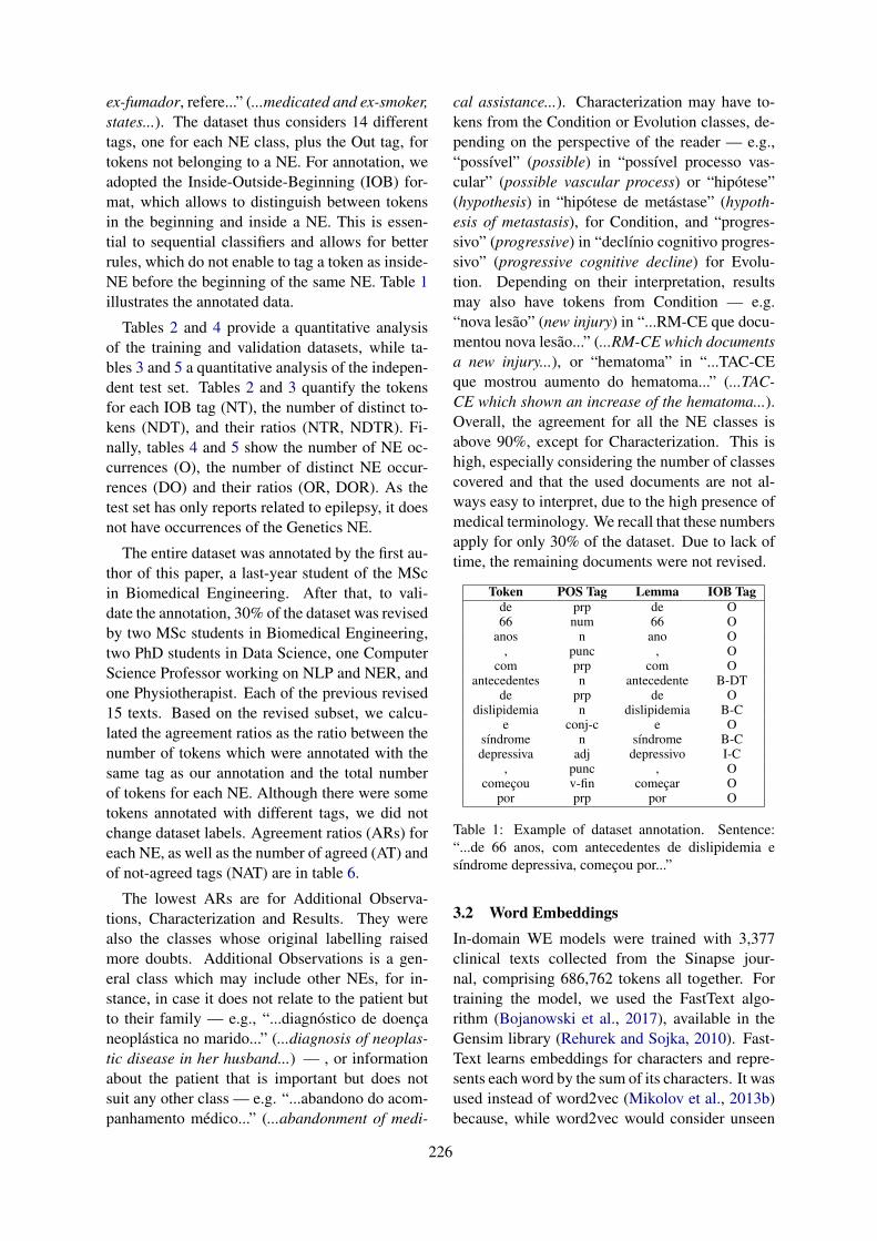
ex-fumador, refere...” (...medicated and ex-smoker,states...). The dataset thus considers 14 differenttags, one for each NE class, plus the Out tag, fortokens not belonging to a NE. For annotation, weadopted the Inside-Outside-Beginning (IOB) for-mat, which allows to distinguish between tokensin the beginning and inside a NE. This is essen-tial to sequential classifiers and allows for betterrules, which do not enable to tag a token as inside-NE before the beginning of the same NE. Table 1illustrates the annotated data.
Tables 2 and 4 provide a quantitative analysisof the training and validation datasets, while ta-bles 3 and 5 a quantitative analysis of the indepen-dent test set. Tables 2 and 3 quantify the tokensfor each IOB tag (NT), the number of distinct to-kens (NDT), and their ratios (NTR, NDTR). Fi-nally, tables 4 and 5 show the number of NE oc-currences (O), the number of distinct NE occur-rences (DO) and their ratios (OR, DOR). As thetest set has only reports related to epilepsy, it doesnot have occurrences of the Genetics NE.
The entire dataset was annotated by the first au-thor of this paper, a last-year student of the MScin Biomedical Engineering. After that, to vali-date the annotation, 30% of the dataset was revisedby two MSc students in Biomedical Engineering,two PhD students in Data Science, one ComputerScience Professor working on NLP and NER, andone Physiotherapist. Each of the previous revised15 texts. Based on the revised subset, we calcu-lated the agreement ratios as the ratio between thenumber of tokens which were annotated with thesame tag as our annotation and the total numberof tokens for each NE. Although there were sometokens annotated with different tags, we did notchange dataset labels. Agreement ratios (ARs) foreach NE, as well as the number of agreed (AT) andof not-agreed tags (NAT) are in table 6.
The lowest ARs are for Additional Observa-tions, Characterization and Results. They werealso the classes whose original labelling raisedmore doubts. Additional Observations is a gen-eral class which may include other NEs, for in-stance, in case it does not relate to the patient butto their family — e.g., “...diagnóstico de doençaneoplástica no marido...” (...diagnosis of neoplas-tic disease in her husband...) — , or informationabout the patient that is important but does notsuit any other class — e.g. “...abandono do acom-panhamento médico...” (...abandonment of medi-
cal assistance...). Characterization may have to-kens from the Condition or Evolution classes, de-pending on the perspective of the reader — e.g.,“possı́vel” (possible) in “possı́vel processo vas-cular” (possible vascular process) or “hipótese”(hypothesis) in “hipótese de metástase” (hypoth-esis of metastasis), for Condition, and “progres-sivo” (progressive) in “declı́nio cognitivo progres-sivo” (progressive cognitive decline) for Evolu-tion. Depending on their interpretation, resultsmay also have tokens from Condition — e.g.“nova lesão” (new injury) in “...RM-CE que docu-mentou nova lesão...” (...RM-CE which documentsa new injury...), or “hematoma” in “...TAC-CEque mostrou aumento do hematoma...” (...TAC-CE which shown an increase of the hematoma...).Overall, the agreement for all the NE classes isabove 90%, except for Characterization. This ishigh, especially considering the number of classescovered and that the used documents are not al-ways easy to interpret, due to the high presence ofmedical terminology. We recall that these numbersapply for only 30% of the dataset. Due to lack oftime, the remaining documents were not revised.
Token POS Tag Lemma IOB Tagde prp de O66 num 66 O
anos n ano O, punc , O
com prp com Oantecedentes n antecedente B-DT
de prp de Odislipidemia n dislipidemia B-C
e conj-c e Osı́ndrome n sı́ndrome B-Cdepressiva adj depressivo I-C
, punc , Ocomeçou v-fin começar O
por prp por O
Table 1: Example of dataset annotation. Sentence:“...de 66 anos, com antecedentes de dislipidemia esı́ndrome depressiva, começou por...”
3.2 Word EmbeddingsIn-domain WE models were trained with 3,377clinical texts collected from the Sinapse jour-nal, comprising 686,762 tokens all together. Fortraining the model, we used the FastText algo-rithm (Bojanowski et al., 2017), available in theGensim library (Rehurek and Sojka, 2010). Fast-Text learns embeddings for characters and repre-sents each word by the sum of its characters. It wasused instead of word2vec (Mikolov et al., 2013b)because, while word2vec would consider unseen
226
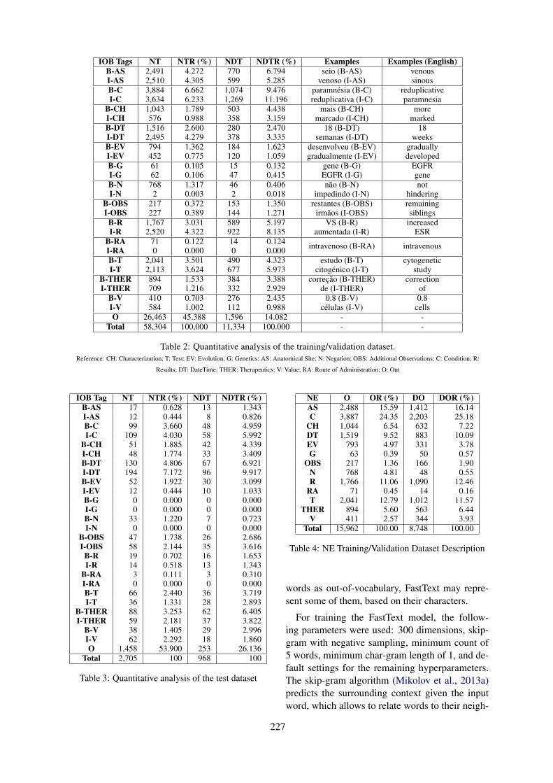
IOB Tags NT NTR (%) NDT NDTR (%) Examples Examples (English)B-AS 2,491 4.272 770 6.794 seio (B-AS)
venoso (I-AS)venoussinousI-AS 2,510 4.305 599 5.285
B-C 3,884 6.662 1,074 9.476 paramnésia (B-C)reduplicativa (I-C)
reduplicativeparamnesiaI-C 3,634 6.233 1,269 11.196
B-CH 1,043 1.789 503 4.438 mais (B-CH)marcado (I-CH)
moremarkedI-CH 576 0.988 358 3.159
B-DT 1,516 2.600 280 2.470 18 (B-DT)semanas (I-DT)
18weeksI-DT 2,495 4.279 378 3.335
B-EV 794 1.362 184 1.623 desenvolveu (B-EV)gradualmente (I-EV)
graduallydevelopedI-EV 452 0.775 120 1.059
B-G 61 0.105 15 0.132 gene (B-G)EGFR (I-G)
EGFRgeneI-G 62 0.106 47 0.415
B-N 768 1.317 46 0.406 não (B-N)impedindo (I-N)
nothinderingI-N 2 0.003 2 0.018
B-OBS 217 0.372 153 1.350 restantes (B-OBS)irmãos (I-OBS)
remainingsiblingsI-OBS 227 0.389 144 1.271
B-R 1,767 3.031 589 5.197 VS (B-R)aumentada (I-R)
increasedESRI-R 2,520 4.322 922 8.135
B-RA 71 0.122 14 0.124 intravenoso (B-RA) intravenousI-RA 0 0.000 0 0.000B-T 2,041 3.501 490 4.323 estudo (B-T)
citogénico (I-T)cytogenetic
studyI-T 2,113 3.624 677 5.973B-THER 894 1.533 384 3.388 correção (B-THER)
de (I-THER)correction
ofI-THER 709 1.216 332 2.929B-V 410 0.703 276 2.435 0.8 (B-V)
células (I-V)0.8
cellsI-V 584 1.002 112 0.988O 26,463 45.388 1,596 14.082 - -
Total 58,304 100,000 11,334 100.000 - -
Table 2: Quantitative analysis of the training/validation dataset.Reference: CH: Characterization; T: Test; EV: Evolution; G: Genetics; AS: Anatomical Site; N: Negation; OBS: Additional Observations; C: Condition; R:
Results; DT: DateTime; THER: Therapeutics; V: Value; RA: Route of Administration; O: Out
IOB Tag NT NTR (%) NDT NDTR (%)B-AS 17 0.628 13 1.343I-AS 12 0.444 8 0.826B-C 99 3.660 48 4.959I-C 109 4.030 58 5.992
B-CH 51 1.885 42 4.339I-CH 48 1.774 33 3.409B-DT 130 4.806 67 6.921I-DT 194 7.172 96 9.917B-EV 52 1.922 30 3.099I-EV 12 0.444 10 1.033B-G 0 0.000 0 0.000I-G 0 0.000 0 0.000B-N 33 1.220 7 0.723I-N 0 0.000 0 0.000
B-OBS 47 1.738 26 2.686I-OBS 58 2.144 35 3.616
B-R 19 0.702 16 1.653I-R 14 0.518 13 1.343
B-RA 3 0.111 3 0.310I-RA 0 0.000 0 0.000B-T 66 2.440 36 3.719I-T 36 1.331 28 2.893
B-THER 88 3.253 62 6.405I-THER 59 2.181 37 3.822
B-V 38 1.405 29 2.996I-V 62 2.292 18 1.860O 1,458 53.900 253 26.136
Total 2,705 100 968 100
Table 3: Quantitative analysis of the test dataset
NE O OR (%) DO DOR (%)AS 2,488 15.59 1,412 16.14C 3,887 24.35 2,203 25.18
CH 1,044 6.54 632 7.22DT 1,519 9.52 883 10.09EV 793 4.97 331 3.78G 63 0.39 50 0.57
OBS 217 1.36 166 1.90N 768 4.81 48 0.55R 1,766 11.06 1,090 12.46
RA 71 0.45 14 0.16T 2,041 12.79 1,012 11.57
THER 894 5.60 563 6.44V 411 2.57 344 3.93
Total 15,962 100.00 8,748 100.00
Table 4: NE Training/Validation Dataset Description
words as out-of-vocabulary, FastText may repre-sent some of them, based on their characters.
For training the FastText model, the follow-ing parameters were used: 300 dimensions, skip-gram with negative sampling, minimum count of5 words, minimum char-gram length of 1, and de-fault settings for the remaining hyperparameters.The skip-gram algorithm (Mikolov et al., 2013a)predicts the surrounding context given the inputword, which allows to relate words to their neigh-
227
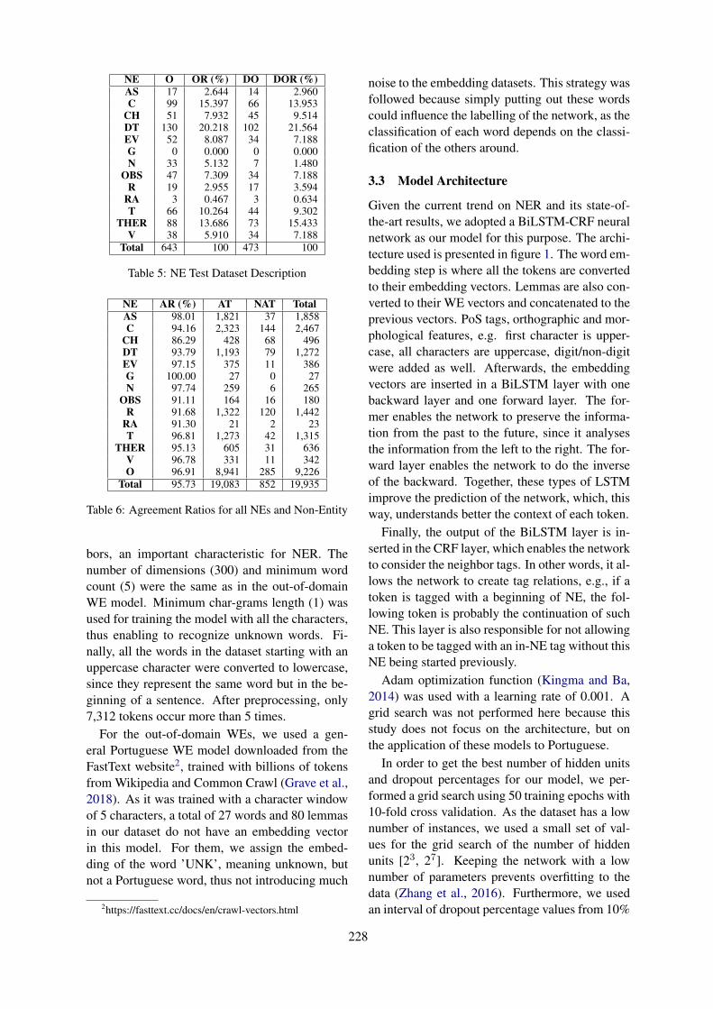
NE O OR (%) DO DOR (%)AS 17 2.644 14 2.960C 99 15.397 66 13.953
CH 51 7.932 45 9.514DT 130 20.218 102 21.564EV 52 8.087 34 7.188G 0 0.000 0 0.000N 33 5.132 7 1.480
OBS 47 7.309 34 7.188R 19 2.955 17 3.594
RA 3 0.467 3 0.634T 66 10.264 44 9.302
THER 88 13.686 73 15.433V 38 5.910 34 7.188
Total 643 100 473 100
Table 5: NE Test Dataset Description
NE AR (%) AT NAT TotalAS 98.01 1,821 37 1,858C 94.16 2,323 144 2,467
CH 86.29 428 68 496DT 93.79 1,193 79 1,272EV 97.15 375 11 386G 100.00 27 0 27N 97.74 259 6 265
OBS 91.11 164 16 180R 91.68 1,322 120 1,442
RA 91.30 21 2 23T 96.81 1,273 42 1,315
THER 95.13 605 31 636V 96.78 331 11 342O 96.91 8,941 285 9,226
Total 95.73 19,083 852 19,935
Table 6: Agreement Ratios for all NEs and Non-Entity
bors, an important characteristic for NER. Thenumber of dimensions (300) and minimum wordcount (5) were the same as in the out-of-domainWE model. Minimum char-grams length (1) wasused for training the model with all the characters,thus enabling to recognize unknown words. Fi-nally, all the words in the dataset starting with anuppercase character were converted to lowercase,since they represent the same word but in the be-ginning of a sentence. After preprocessing, only7,312 tokens occur more than 5 times.
For the out-of-domain WEs, we used a gen-eral Portuguese WE model downloaded from theFastText website2, trained with billions of tokensfrom Wikipedia and Common Crawl (Grave et al.,2018). As it was trained with a character windowof 5 characters, a total of 27 words and 80 lemmasin our dataset do not have an embedding vectorin this model. For them, we assign the embed-ding of the word ’UNK’, meaning unknown, butnot a Portuguese word, thus not introducing much
2https://fasttext.cc/docs/en/crawl-vectors.html
noise to the embedding datasets. This strategy wasfollowed because simply putting out these wordscould influence the labelling of the network, as theclassification of each word depends on the classi-fication of the others around.
3.3 Model Architecture
Given the current trend on NER and its state-of-the-art results, we adopted a BiLSTM-CRF neuralnetwork as our model for this purpose. The archi-tecture used is presented in figure 1. The word em-bedding step is where all the tokens are convertedto their embedding vectors. Lemmas are also con-verted to their WE vectors and concatenated to theprevious vectors. PoS tags, orthographic and mor-phological features, e.g. first character is upper-case, all characters are uppercase, digit/non-digitwere added as well. Afterwards, the embeddingvectors are inserted in a BiLSTM layer with onebackward layer and one forward layer. The for-mer enables the network to preserve the informa-tion from the past to the future, since it analysesthe information from the left to the right. The for-ward layer enables the network to do the inverseof the backward. Together, these types of LSTMimprove the prediction of the network, which, thisway, understands better the context of each token.
Finally, the output of the BiLSTM layer is in-serted in the CRF layer, which enables the networkto consider the neighbor tags. In other words, it al-lows the network to create tag relations, e.g., if atoken is tagged with a beginning of NE, the fol-lowing token is probably the continuation of suchNE. This layer is also responsible for not allowinga token to be tagged with an in-NE tag without thisNE being started previously.
Adam optimization function (Kingma and Ba,2014) was used with a learning rate of 0.001. Agrid search was not performed here because thisstudy does not focus on the architecture, but onthe application of these models to Portuguese.
In order to get the best number of hidden unitsand dropout percentages for our model, we per-formed a grid search using 50 training epochs with10-fold cross validation. As the dataset has a lownumber of instances, we used a small set of val-ues for the grid search of the number of hiddenunits [23, 27]. Keeping the network with a lownumber of parameters prevents overfitting to thedata (Zhang et al., 2016). Furthermore, we usedan interval of dropout percentage values from 10%
228
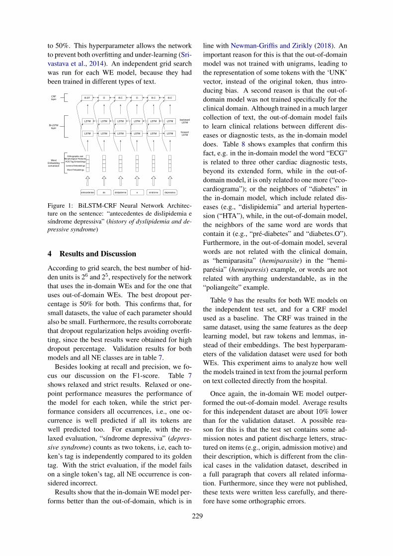
to 50%. This hyperparameter allows the networkto prevent both overfitting and under-learning (Sri-vastava et al., 2014). An independent grid searchwas run for each WE model, because they hadbeen trained in different types of text.
antecedentes de dislipidemia síndromee depressiva
WordEmbeddingconversion
LSTM LSTM LSTMLSTMLSTM LSTM
LSTM LSTM LSTMLSTMLSTM LSTMBi-LSTM
layerforward LSTM
backward LSTM
B-DT O B-C O B-C B-CCRF layer
Orthographic andMorphological FeaturesPOS Tag Embeddings
Lemma Embeddings
Word Embeddings
Figure 1: BiLSTM-CRF Neural Network Architec-ture on the sentence: “antecedentes de dislipidemia esı́ndrome depressiva” (history of dyslipidemia and de-pressive syndrome)
4 Results and Discussion
According to grid search, the best number of hid-den units is 26 and 25, respectively for the networkthat uses the in-domain WEs and for the one thatuses out-of-domain WEs. The best dropout per-centage is 50% for both. This confirms that, forsmall datasets, the value of each parameter shouldalso be small. Furthermore, the results corroboratethat dropout regularization helps avoiding overfit-ting, since the best results were obtained for highdropout percentage. Validation results for bothmodels and all NE classes are in table 7.
Besides looking at recall and precision, we fo-cus our discussion on the F1-score. Table 7shows relaxed and strict results. Relaxed or one-point performance measures the performance ofthe model for each token, while the strict per-formance considers all occurrences, i.e., one oc-currence is well predicted if all its tokens arewell predicted too. For example, with the re-laxed evaluation, “sı́ndrome depressiva” (depres-sive syndrome) counts as two tokens, i.e, each to-ken’s tag is independently compared to its goldentag. With the strict evaluation, if the model failson a single token’s tag, all NE occurrence is con-sidered incorrect.
Results show that the in-domain WE model per-forms better than the out-of-domain, which is in
line with Newman-Griffis and Zirikly (2018). Animportant reason for this is that the out-of-domainmodel was not trained with unigrams, leading tothe representation of some tokens with the ‘UNK’vector, instead of the original token, thus intro-ducing bias. A second reason is that the out-of-domain model was not trained specifically for theclinical domain. Although trained in a much largercollection of text, the out-of-domain model failsto learn clinical relations between different dis-eases or diagnostic tests, as the in-domain modeldoes. Table 8 shows examples that confirm thisfact, e.g. in the in-domain model the word “ECG”is related to three other cardiac diagnostic tests,beyond its extended form, while in the out-of-domain model, it is only related to one more (“eco-cardiograma”); or the neighbors of “diabetes” inthe in-domain model, which include related dis-eases (e.g., “dislipidemia” and arterial hyperten-sion (“HTA”), while, in the out-of-domain model,the neighbors of the same word are words thatcontain it (e.g., “pré-diabetes” and “diabetes.O”).Furthermore, in the out-of-domain model, severalwords are not related with the clinical domain,as “hemiparasita” (hemiparasite) in the “hemi-parésia” (hemiparesis) example, or words are notrelated with anything understandable, as in the“poliangeı́te” example.
Table 9 has the results for both WE models onthe independent test set, and for a CRF modelused as a baseline. The CRF was trained in thesame dataset, using the same features as the deeplearning model, but raw tokens and lemmas, in-stead of their embeddings. The best hyperparam-eters of the validation dataset were used for bothWEs. This experiment aims to analyze how wellthe models trained in text from the journal performon text collected directly from the hospital.
Once again, the in-domain WE model outper-formed the out-of-domain model. Average resultsfor this independent dataset are about 10% lowerthan for the validation dataset. A possible rea-son for this is that the test set contains some ad-mission notes and patient discharge letters, struc-tured on items (e.g., origin, admission motive) andtheir description, which is different from the clin-ical cases in the validation dataset, described ina full paragraph that covers all related informa-tion. Furthermore, since they were not published,these texts were written less carefully, and there-fore have some orthographic errors.
229
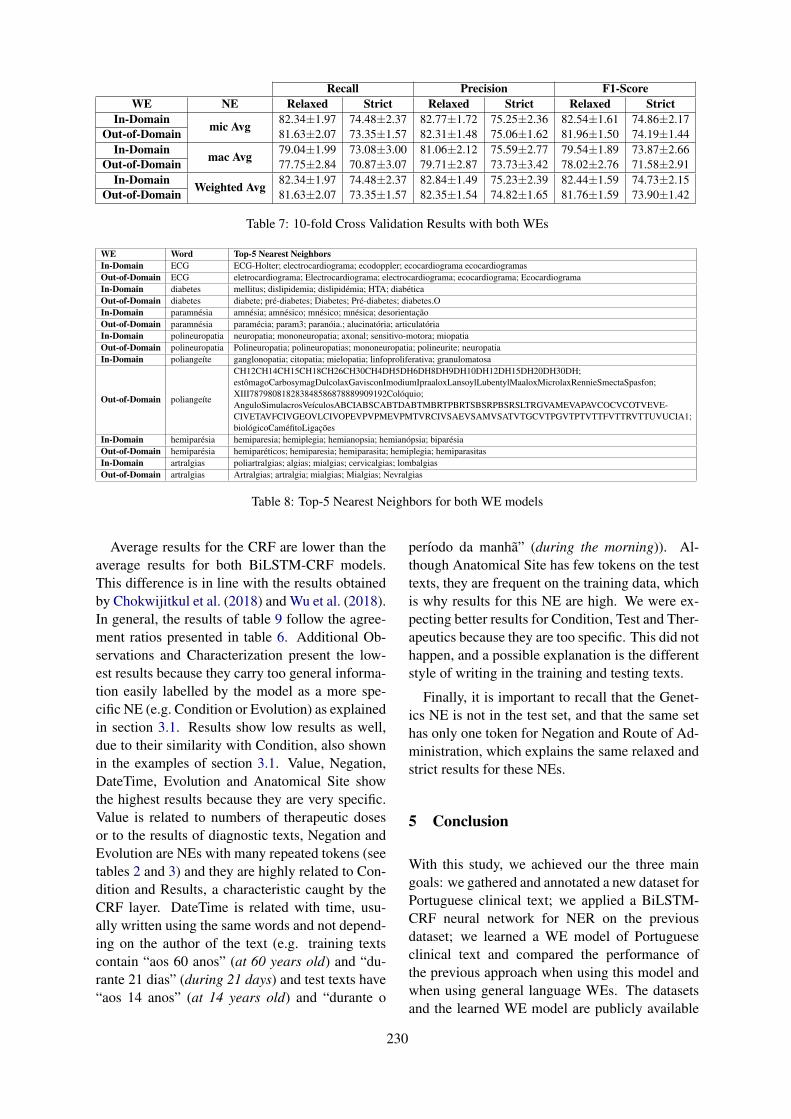
Recall Precision F1-ScoreWE NE Relaxed Strict Relaxed Strict Relaxed Strict
In-Domain mic Avg 82.34±1.97 74.48±2.37 82.77±1.72 75.25±2.36 82.54±1.61 74.86±2.17Out-of-Domain 81.63±2.07 73.35±1.57 82.31±1.48 75.06±1.62 81.96±1.50 74.19±1.44
In-Domain mac Avg 79.04±1.99 73.08±3.00 81.06±2.12 75.59±2.77 79.54±1.89 73.87±2.66Out-of-Domain 77.75±2.84 70.87±3.07 79.71±2.87 73.73±3.42 78.02±2.76 71.58±2.91
In-Domain Weighted Avg 82.34±1.97 74.48±2.37 82.84±1.49 75.23±2.39 82.44±1.59 74.73±2.15Out-of-Domain 81.63±2.07 73.35±1.57 82.35±1.54 74.82±1.65 81.76±1.59 73.90±1.42
Table 7: 10-fold Cross Validation Results with both WEs
WE Word Top-5 Nearest NeighborsIn-Domain ECG ECG-Holter; electrocardiograma; ecodoppler; ecocardiograma ecocardiogramasOut-of-Domain ECG eletrocardiograma; Electrocardiograma; electrocardiograma; ecocardiograma; EcocardiogramaIn-Domain diabetes mellitus; dislipidemia; dislipidémia; HTA; diabéticaOut-of-Domain diabetes diabete; pré-diabetes; Diabetes; Pré-diabetes; diabetes.OIn-Domain paramnésia amnésia; amnésico; mnésico; mnésica; desorientaçãoOut-of-Domain paramnésia paramécia; param3; paranóia.; alucinatória; articulatóriaIn-Domain polineuropatia neuropatia; mononeuropatia; axonal; sensitivo-motora; miopatiaOut-of-Domain polineuropatia Polineuropatia; polineuropatias; mononeuropatia; polineurite; neuropatiaIn-Domain poliangeı́te ganglonopatia; citopatia; mielopatia; linfoproliferativa; granulomatosa
Out-of-Domain poliangeı́te
CH12CH14CH15CH18CH26CH30CH4DH5DH6DH8DH9DH10DH12DH15DH20DH30DH;estômagoCarbosymagDulcolaxGavisconImodiumIpraaloxLansoylLubentylMaaloxMicrolaxRennieSmectaSpasfon;XIII787980818283848586878889909192Colóquio;AnguloSimulacrosVeı́culosABCIABSCABTDABTMBRTPBRTSBSRPBSRSLTRGVAMEVAPAVCOCVCOTVEVE-CIVETAVFCIVGEOVLCIVOPEVPVPMEVPMTVRCIVSAEVSAMVSATVTGCVTPGVTPTVTTFVTTRVTTUVUCIA1;biológicoCaméfitoLigações
In-Domain hemiparésia hemiparesia; hemiplegia; hemianopsia; hemianópsia; biparésiaOut-of-Domain hemiparésia hemiparéticos; hemiparesia; hemiparasita; hemiplegia; hemiparasitasIn-Domain artralgias poliartralgias; algias; mialgias; cervicalgias; lombalgiasOut-of-Domain artralgias Artralgias; artralgia; mialgias; Mialgias; Nevralgias
Table 8: Top-5 Nearest Neighbors for both WE models
Average results for the CRF are lower than theaverage results for both BiLSTM-CRF models.This difference is in line with the results obtainedby Chokwijitkul et al. (2018) and Wu et al. (2018).In general, the results of table 9 follow the agree-ment ratios presented in table 6. Additional Ob-servations and Characterization present the low-est results because they carry too general informa-tion easily labelled by the model as a more spe-cific NE (e.g. Condition or Evolution) as explainedin section 3.1. Results show low results as well,due to their similarity with Condition, also shownin the examples of section 3.1. Value, Negation,DateTime, Evolution and Anatomical Site showthe highest results because they are very specific.Value is related to numbers of therapeutic dosesor to the results of diagnostic texts, Negation andEvolution are NEs with many repeated tokens (seetables 2 and 3) and they are highly related to Con-dition and Results, a characteristic caught by theCRF layer. DateTime is related with time, usu-ally written using the same words and not depend-ing on the author of the text (e.g. training textscontain “aos 60 anos” (at 60 years old) and “du-rante 21 dias” (during 21 days) and test texts have“aos 14 anos” (at 14 years old) and “durante o
perı́odo da manhã” (during the morning)). Al-though Anatomical Site has few tokens on the testtexts, they are frequent on the training data, whichis why results for this NE are high. We were ex-pecting better results for Condition, Test and Ther-apeutics because they are too specific. This did nothappen, and a possible explanation is the differentstyle of writing in the training and testing texts.
Finally, it is important to recall that the Genet-ics NE is not in the test set, and that the same sethas only one token for Negation and Route of Ad-ministration, which explains the same relaxed andstrict results for these NEs.
5 Conclusion
With this study, we achieved our the three maingoals: we gathered and annotated a new dataset forPortuguese clinical text; we applied a BiLSTM-CRF neural network for NER on the previousdataset; we learned a WE model of Portugueseclinical text and compared the performance ofthe previous approach when using this model andwhen using general language WEs. The datasetsand the learned WE model are publicly available
230
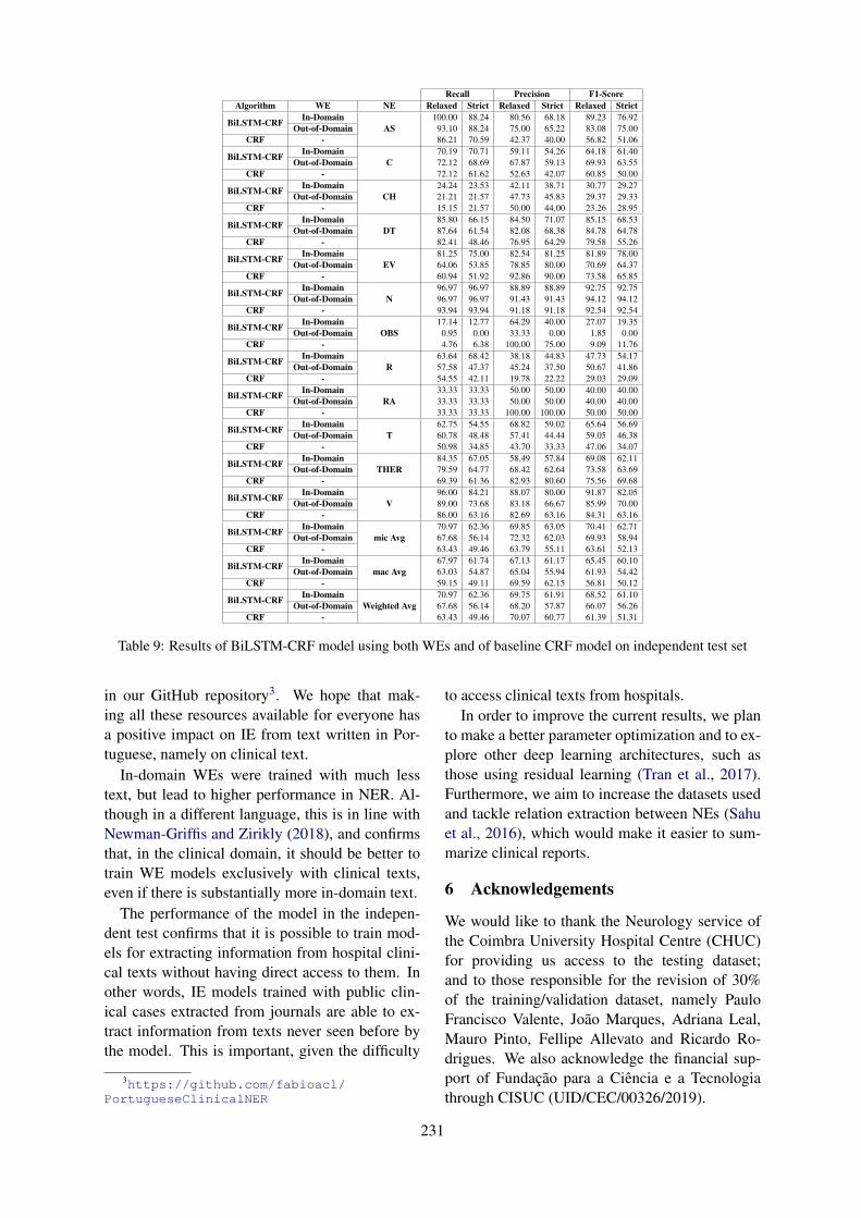
Recall Precision F1-ScoreAlgorithm WE NE Relaxed Strict Relaxed Strict Relaxed Strict
BiLSTM-CRF In-DomainAS
100.00 88.24 80.56 68.18 89.23 76.92Out-of-Domain 93.10 88.24 75.00 65.22 83.08 75.00
CRF - 86.21 70.59 42.37 40.00 56.82 51.06
BiLSTM-CRF In-DomainC
70.19 70.71 59.11 54.26 64.18 61.40Out-of-Domain 72.12 68.69 67.87 59.13 69.93 63.55
CRF - 72.12 61.62 52.63 42.07 60.85 50.00
BiLSTM-CRF In-DomainCH
24.24 23.53 42.11 38.71 30.77 29.27Out-of-Domain 21.21 21.57 47.73 45.83 29.37 29.33
CRF - 15.15 21.57 50.00 44.00 23.26 28.95
BiLSTM-CRF In-DomainDT
85.80 66.15 84.50 71.07 85.15 68.53Out-of-Domain 87.64 61.54 82.08 68.38 84.78 64.78
CRF - 82.41 48.46 76.95 64.29 79.58 55.26
BiLSTM-CRF In-DomainEV
81.25 75.00 82.54 81.25 81.89 78.00Out-of-Domain 64.06 53.85 78.85 80.00 70.69 64.37
CRF - 60.94 51.92 92.86 90.00 73.58 65.85
BiLSTM-CRF In-DomainN
96.97 96.97 88.89 88.89 92.75 92.75Out-of-Domain 96.97 96.97 91.43 91.43 94.12 94.12
CRF - 93.94 93.94 91.18 91.18 92.54 92.54
BiLSTM-CRF In-DomainOBS
17.14 12.77 64.29 40.00 27.07 19.35Out-of-Domain 0.95 0.00 33.33 0.00 1.85 0.00
CRF - 4.76 6.38 100.00 75.00 9.09 11.76
BiLSTM-CRF In-DomainR
63.64 68.42 38.18 44.83 47.73 54.17Out-of-Domain 57.58 47.37 45.24 37.50 50.67 41.86
CRF - 54.55 42.11 19.78 22.22 29.03 29.09
BiLSTM-CRF In-DomainRA
33.33 33.33 50.00 50.00 40.00 40.00Out-of-Domain 33.33 33.33 50.00 50.00 40.00 40.00
CRF - 33.33 33.33 100.00 100.00 50.00 50.00
BiLSTM-CRF In-DomainT
62.75 54.55 68.82 59.02 65.64 56.69Out-of-Domain 60.78 48.48 57.41 44.44 59.05 46.38
CRF - 50.98 34.85 43.70 33.33 47.06 34.07
BiLSTM-CRF In-DomainTHER
84.35 67.05 58.49 57.84 69.08 62.11Out-of-Domain 79.59 64.77 68.42 62.64 73.58 63.69
CRF - 69.39 61.36 82.93 80.60 75.56 69.68
BiLSTM-CRF In-DomainV
96.00 84.21 88.07 80.00 91.87 82.05Out-of-Domain 89.00 73.68 83.18 66.67 85.99 70.00
CRF - 86.00 63.16 82.69 63.16 84.31 63.16
BiLSTM-CRF In-Domainmic Avg
70.97 62.36 69.85 63.05 70.41 62.71Out-of-Domain 67.68 56.14 72.32 62.03 69.93 58.94
CRF - 63.43 49.46 63.79 55.11 63.61 52.13
BiLSTM-CRF In-Domainmac Avg
67.97 61.74 67.13 61.17 65.45 60.10Out-of-Domain 63.03 54.87 65.04 55.94 61.93 54.42
CRF - 59.15 49.11 69.59 62.15 56.81 50.12
BiLSTM-CRF In-DomainWeighted Avg
70.97 62.36 69.75 61.91 68.52 61.10Out-of-Domain 67.68 56.14 68.20 57.87 66.07 56.26
CRF - 63.43 49.46 70.07 60.77 61.39 51.31
Table 9: Results of BiLSTM-CRF model using both WEs and of baseline CRF model on independent test set
in our GitHub repository3. We hope that mak-ing all these resources available for everyone hasa positive impact on IE from text written in Por-tuguese, namely on clinical text.
In-domain WEs were trained with much lesstext, but lead to higher performance in NER. Al-though in a different language, this is in line withNewman-Griffis and Zirikly (2018), and confirmsthat, in the clinical domain, it should be better totrain WE models exclusively with clinical texts,even if there is substantially more in-domain text.
The performance of the model in the indepen-dent test confirms that it is possible to train mod-els for extracting information from hospital clini-cal texts without having direct access to them. Inother words, IE models trained with public clin-ical cases extracted from journals are able to ex-tract information from texts never seen before bythe model. This is important, given the difficulty
3https://github.com/fabioacl/PortugueseClinicalNER
to access clinical texts from hospitals.In order to improve the current results, we plan
to make a better parameter optimization and to ex-plore other deep learning architectures, such asthose using residual learning (Tran et al., 2017).Furthermore, we aim to increase the datasets usedand tackle relation extraction between NEs (Sahuet al., 2016), which would make it easier to sum-marize clinical reports.
6 Acknowledgements
We would like to thank the Neurology service ofthe Coimbra University Hospital Centre (CHUC)for providing us access to the testing dataset;and to those responsible for the revision of 30%of the training/validation dataset, namely PauloFrancisco Valente, João Marques, Adriana Leal,Mauro Pinto, Fellipe Allevato and Ricardo Ro-drigues. We also acknowledge the financial sup-port of Fundação para a Ciência e a Tecnologiathrough CISUC (UID/CEC/00326/2019).
231
ReferencesSteven Bethard, Guergana Savova, Wei-Te Chen, Leon
Derczynski, James Pustejovsky, and Marc Verhagen.2016. Semeval-2016 task 12: Clinical TempEval. InProceedings of the 10th International Workshop onSemantic Evaluation (SemEval-2016), pages 1052–1062.
Piotr Bojanowski, Edouard Grave, Armand Joulin, andTomas Mikolov. 2017. Enriching Word Vectors withSubword Information. Transactions of the Associa-tion for Computational Linguistics, 5:135–146.
Pedro Vitor Quinta de Castro, Nádia Félix Felipeda Silva, and Anderson da Silva Soares. 2018. Por-tuguese named entity recognition using LSTM-CRF.In Computational Processing of the Portuguese Lan-guage - 13th International Conference, PROPOR2018, Canela, Brazil, September 24-26, 2018, Pro-ceedings, pages 83–92.
Thanat Chokwijitkul, Anthony Nguyen, Hamed Has-sanzadeh, and Siegfried Perez. 2018. Identifyingrisk factors for heart disease in electronic medicalrecords: A deep learning approach. In Proceedingsof the BioNLP 2018 workshop, pages 18–27, Mel-bourne, Australia. Association for ComputationalLinguistics.
Rezarta Islamaj Doğan, Robert Leaman, and ZhiyongLu. 2014. NCBI disease corpus: a resource for dis-ease name recognition and concept normalization.Journal of biomedical informatics, 47:1–10.
Noémie Elhadad, Sameer Pradhan, Sharon Gorman,Suresh Manandhar, Wendy Chapman, and GuerganaSavova. 2015. SemEval-2015 task 14: Analysis ofclinical text. In Proceedings of the 9th InternationalWorkshop on Semantic Evaluation (SemEval 2015),pages 303–310.
Liliana Ferreira, António J. S. Teixeira, and João PauloCunha. 2010. Information Extraction from Por-tuguese Hospital Discharge Letters. VI Jornadas enTechnologia del Habla and II Iberian SL Tech Work-shop, (January):39–42.
Liliana da Silva Ferreira. 2011. Medical InformationExtraction in European Portuguese. Ph.D. thesis,Universidade de Aveiro.
Sherman Folland, Allen C Goodman, and Miron Stano.2017. Introduction. In The Economics of Healthand Health Care, 8th edition, chapter 1, pages 29–54. Pearson Prentice Hall Upper Saddle River, NJ.
Edouard Grave, Piotr Bojanowski, Prakhar Gupta, Ar-mand Joulin, and Tomas Mikolov. 2018. LearningWord Vectors for 157 Languages. In Proceedingsof the International Conference on Language Re-sources and Evaluation (LREC 2018).
Nathan S. Hartmann, Erick R. Fonseca, Christopher D.Shulby, Marcos V. Treviso, Jéssica S. Rodrigues,
and Sandra M. Aluı́sio. 2017. Portuguese word em-beddings: Evaluating on word analogies and naturallanguage tasks. In Proceedings the 11th BrazilianSymposium in Information and Human LanguageTechnology, STIL 2017.
Liadh Kelly, Lorraine Goeuriot, Hanna Suominen,Aurélie Névéol, Joao Palotti, and Guido Zuccon.2016. Overview of the CLEF eHealth evaluationlab 2016. In International Conference of the Cross-Language Evaluation Forum for European Lan-guages, pages 255–266. Springer.
Diederik P Kingma and Jimmy Ba. 2014. Adam: Amethod for stochastic optimization. arXiv preprintarXiv:1412.6980, page 13.
Juliane Klatt, Hinnerk Feldwisch-Drentrup, MatthiasIhle, Vincent Navarro, Markus Neufang, Ce-sar Teixeira, Claude Adam, Mario Valderrama,Catalina Alvarado-Rojas, Adrien Witon, et al.2012. The epilepsiae database: An extensive elec-troencephalography database of epilepsy patients.Epilepsia, 53(9):1669–1676.
Guillaume Lample, Miguel Ballesteros, Sandeep Sub-ramanian, Kazuya Kawakami, and Chris Dyer. 2016.Neural architectures for named entity recognition.In Proceedings of the 2016 Conference of the NorthAmerican Chapter of the Association for Computa-tional Linguistics: Human Language Technologies,pages 260–270, San Diego, California. Associationfor Computational Linguistics.
Thoai Man Luu, Robert Phan, and Rachel Davey. 2018.Clinical Name Entity Recognition Based on Recur-rent Neural Networks. 2018 18th International Con-ference on Computational Science and Applications(ICCSA), pages 1–9.
Tomas Mikolov, Kai Chen, Greg Corrado, and Jef-frey Dean. 2013a. Efficient estimation of wordrepresentations in vector space. arXiv preprintarXiv:1301.3781.
Tomas Mikolov, Ilya Sutskever, Kai Chen, Greg Cor-rado, and Jeffrey Dean. 2013b. Distributed repre-sentations of words and phrases and their composi-tionality. In Proceedings of the 26th InternationalConference on Neural Information Processing Sys-tems - Volume 2, NIPS’13, pages 3111–3119, USA.Curran Associates Inc.
Agnieszka Mykowiecka, Małgorzata Marciniak, andAnna Kupść. 2009. Rule-based information extrac-tion from patients’ clinical data. Journal of Biomed-ical Informatics, 42(5):923–936.
Aurélie Névéol, Hercules Dalianis, Sumithra Velupil-lai, Guergana Savova, and Pierre Zweigenbaum.2018. Clinical natural language processing in lan-guages other than english: opportunities and chal-lenges. Journal of biomedical semantics, 9(1):12.
232
Denis Newman-Griffis and Ayah Zirikly. 2018. Em-bedding transfer for low-resource medical namedentity recognition: A case study on patient mobil-ity. In Proceedings of the BioNLP 2018 workshop,pages 1–11, Melbourne, Australia. Association forComputational Linguistics.
John P Pestian, Christopher Brew, Dj J MatykiewiczPawełand Hovermale, Neil Johnson, K BretonnelCohen, and Włodzisław Duch. 2007. A shared taskinvolving multi-label classification of clinical freetext. In Proceedings of the Workshop on BioNLP2007: Biological, Translational, and Clinical Lan-guage Processing, pages 97–104. Association forComputational Linguistics.
Radim Rehurek and Petr Sojka. 2010. Software Frame-work for Topic Modelling with Large Corpora. InProceedings of the LREC 2010 Workshop on NewChallenges for NLP Frameworks, pages 45–50, Val-letta, Malta. ELRA.
Ricardo Rodrigues, Hugo Gonçalo Oliveira, and PauloGomes. 2018. NLPPort: A Pipeline for Por-tuguese NLP (Short Paper). In 7th Symposium onLanguages, Applications and Technologies (SLATE2018), volume 62 of OpenAccess Series in Infor-matics (OASIcs), pages 18:1—-18:9, Dagstuhl, Ger-many. Schloss Dagstuhl–Leibniz-Zentrum fuer In-formatik.
Sunil Sahu, Ashish Anand, Krishnadev Oruganty, andMahanandeeshwar Gattu. 2016. Relation extractionfrom clinical texts using domain invariant convolu-tional neural network. In Proceedings of the 15thWorkshop on Biomedical Natural Language Pro-cessing, pages 206–215, Berlin, Germany. Associ-ation for Computational Linguistics.
Cicero dos Santos and Victor Guimarães. 2015. Boost-ing named entity recognition with neural characterembeddings. In Proceedings of the Fifth Named En-tity Workshop, pages 25–33, Beijing, China. Associ-ation for Computational Linguistics.
Cicero D Santos and Bianca Zadrozny. 2014. Learningcharacter-level representations for part-of-speechtagging. In Proceedings of the 31st InternationalConference on Machine Learning (ICML-14), pages1818–1826.
Sinapse. 2017a. Publicações da Sociedade Portuguesade Neurologia, volume 17:1. Sociedade Portuguesade Neurologia, Lisbon.
Sinapse. 2017b. Publicações da Sociedade Portuguesade Neurologia, volume 17:2. Sociedade Portuguesade Neurologia, Lisbon.
Maria Skeppstedt, Maria Kvist, Gunnar H. Nilsson,and Hercules Dalianis. 2014. Automatic recognitionof disorders, findings, pharmaceuticals and bodystructures from clinical text: An annotation and ma-chine learning study. Journal of Biomedical Infor-matics, 49:148–158.
Nitish Srivastava, Geoffrey Hinton, Alex Krizhevsky,Ilya Sutskever, and Ruslan Salakhutdinov. 2014.Dropout: a simple way to prevent neural networksfrom overfitting. The Journal of Machine LearningResearch, 15(1):1929–1958.
Amber Stubbs and Özlem Uzuner. 2015. Annotatingrisk factors for heart disease in clinical narratives fordiabetic patients. Journal of biomedical informatics,58:S78–S91.
Quan Tran, Andrew MacKinlay, and Antonio JimenoYepes. 2017. Named Entity Recognition with StackResidual LSTM and Trainable Bias Decoding. InProceedings of the Eighth International Joint Con-ference on Natural Language Processing (Volume 1:Long Papers), pages 566–575, Taipei, Taiwan. AsianFederation of Natural Language Processing.
Inigo Jauregi Unanue, Ehsan Zare Borzeshi, andMassimo Piccardi. 2017. Recurrent neural net-works with specialized word embeddings for health-domain named-entity recognition. Journal ofBiomedical Informatics, 76(June):102–109.
Özlem Uzuner, Scott L DuVall, Brett R South, andShuying Shen. 2011. 2010 i2b2/VA challenge onconcepts, assertions, and relations in clinical text.Journal of the American Medical Informatics Asso-ciation, 18(5):552–556.
Yonghui Wu, Min Jiang, Jun Xu, Degui Zhi, and HuaXu. 2018. Clinical Named Entity Recognition Us-ing Deep Learning Models. AMIA Annual Sympo-sium Proceedings, pages 1812–1819.
Kai Xu, Zhanfan Zhou, Tianyong Hao, and WenyinLiu. 2017. A Bidirectional LSTM and ConditionalRandom Fields Approach to Medical Named En-tity Recognition. International Conference on Ad-vanced Intelligent Systems and Informatics, pages355–365.
Chiyuan Zhang, Samy Bengio, Moritz Hardt, Ben-jamin Recht, and Oriol Vinyals. 2016. Understand-ing deep learning requires rethinking generalization.arXiv preprint arXiv:1611.03530.
233
Proceedings of the BioNLP 2019 workshop, pages 234–239Florence, Italy, August 1, 2019. c©2019 Association for Computational Linguistics
Can Character Embeddings Improve Cause-of-Death Classification forVerbal Autopsy Narratives?
Zhaodong YanDept of Electrical andComputer EngineeringUniversity of Toronto
Toronto, Ontario, [email protected]
Serena JebleeDept of Computer Science
University of TorontoToronto, Ontario, Canada
Graeme HirstDept of Computer Science
University of TorontoToronto, Ontario, [email protected]
Abstract
We present two models for combining wordand character embeddings for cause-of-deathclassification of verbal autopsy reports usingthe text of the narratives. We find that forsmaller datasets (500 to 1000 records), addingcharacter information to the model improvesclassification, making character-based CNNsa promising method for automated verbal au-topsy coding.
1 Introduction
1.1 Verbal autopsiesEach year, two-thirds of the 60 million deathsin low-and-middle-income countries do not havea known cause of death (CoD), usually becausethey occurred outside of health facilities and nophysical autopsy was performed (United Nations,2013). Verbal autopsy (VA) surveys are onemethod of assessing the true distribution of CoDsin these regions. These surveys are conductedby lay interviewers and typically include demo-graphic data, multiple-choice questions, and afree-text narrative, which details the events lead-ing up to the person’s death. These records arelater coded by physicians for cause of death.
Although several attempts have been made toautomate this coding process, including systemssuch as InterVA (Byass et al., 2012), InSilicoVA(McCormick et al., 2016), the Tariff method (Se-rina et al., 2015), and others (Miasnikof et al.,2015), the results have not been adequate, in partbecause they have focused only on the multiple-choice questions and not at all, or only to a limitedextent, on the narrative text. However, using thenarrative is more convenient because it does notrequire a specific questionnaire format, and alsobecause it takes less time to collect a short ques-tionnaire and narrative than a long, very detailedsurvey. Although the narratives present some text
processing problems, they allow for more detailand explanation than the structured data alone.
Only a few methods have used the full text ofthe narrative for CoD classification. Danso et al.(2013) used term frequency and TF-IDF (termfrequency–inverse document frequency) featuresto classify CoD from VA narratives of neonataldeaths. The Tariff method (Serina et al., 2015)uses a small set of word occurrence features fromthe narrative, but both of these methods ignoreword order. Jeblee et al. (2018) used VA narrativetext to jointly predict CoD and a list of keywordsfor each record using a neural network model withword embeddings.
In our work, we therefore focus on the narrativetext. However, the models that have been devel-oped to date for VA classification using the nar-rative, including SVMs (Danso et al., 2013) andneural networks (Jeblee et al., 2018), have usedonly word-level information. However, recent re-search has shown that character-level informationcan improve text classification models, especiallyin cases where there are many spelling errors andvariations, which is the case with VA narratives.Therefore, we investigate here the use of characterembeddings for the VA CoD classification task.
1.2 Character embedding models
Instead of representing each word as a vector, as istypically done with word embeddings, we can rep-resent each character in the text as a vector. Withtraditional word embeddings, any word that is notfound in the vocabulary is represented as a vec-tor of zeros, essentially losing all the informationfrom that word. The character-based model doesnot have this limitation, and therefore can repre-sent unseen words as well as misspelled words.
Another benefit to character-based models isthat because of the much smaller vocabulary size,they result in less variation in the input representa-
234
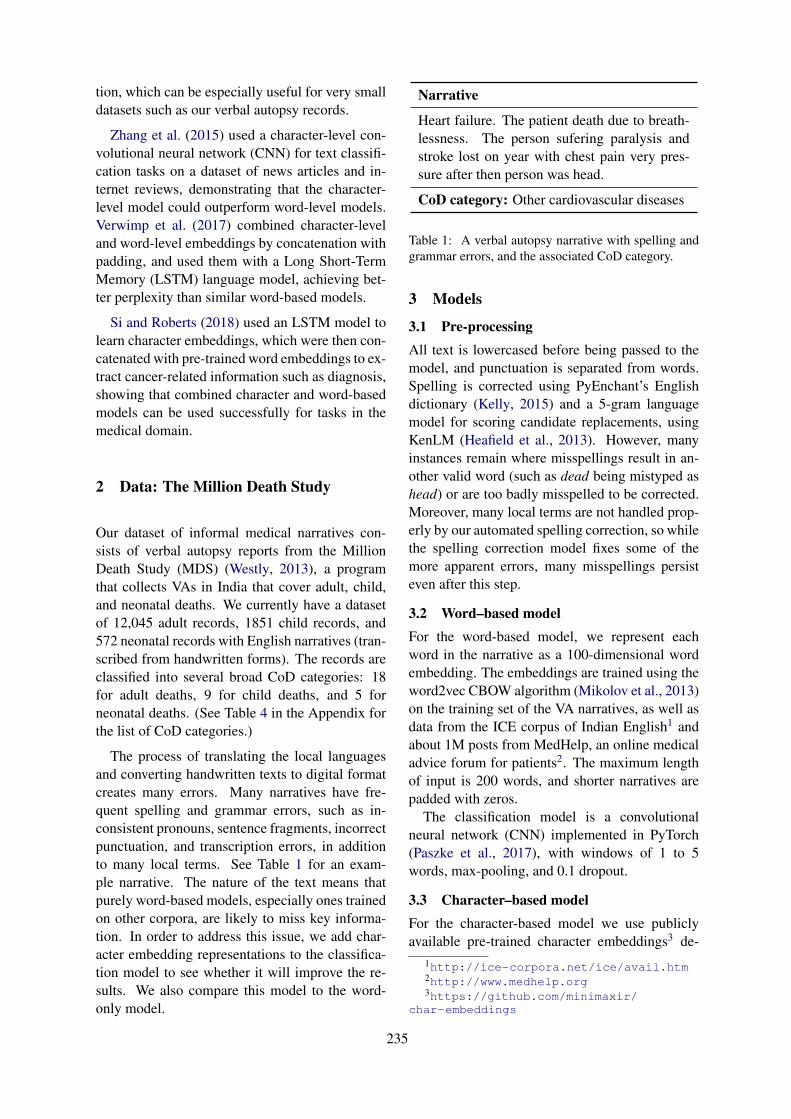
tion, which can be especially useful for very smalldatasets such as our verbal autopsy records.
Zhang et al. (2015) used a character-level con-volutional neural network (CNN) for text classifi-cation tasks on a dataset of news articles and in-ternet reviews, demonstrating that the character-level model could outperform word-level models.Verwimp et al. (2017) combined character-leveland word-level embeddings by concatenation withpadding, and used them with a Long Short-TermMemory (LSTM) language model, achieving bet-ter perplexity than similar word-based models.
Si and Roberts (2018) used an LSTM model tolearn character embeddings, which were then con-catenated with pre-trained word embeddings to ex-tract cancer-related information such as diagnosis,showing that combined character and word-basedmodels can be used successfully for tasks in themedical domain.
2 Data: The Million Death Study
Our dataset of informal medical narratives con-sists of verbal autopsy reports from the MillionDeath Study (MDS) (Westly, 2013), a programthat collects VAs in India that cover adult, child,and neonatal deaths. We currently have a datasetof 12,045 adult records, 1851 child records, and572 neonatal records with English narratives (tran-scribed from handwritten forms). The records areclassified into several broad CoD categories: 18for adult deaths, 9 for child deaths, and 5 forneonatal deaths. (See Table 4 in the Appendix forthe list of CoD categories.)
The process of translating the local languagesand converting handwritten texts to digital formatcreates many errors. Many narratives have fre-quent spelling and grammar errors, such as in-consistent pronouns, sentence fragments, incorrectpunctuation, and transcription errors, in additionto many local terms. See Table 1 for an exam-ple narrative. The nature of the text means thatpurely word-based models, especially ones trainedon other corpora, are likely to miss key informa-tion. In order to address this issue, we add char-acter embedding representations to the classifica-tion model to see whether it will improve the re-sults. We also compare this model to the word-only model.
Narrative
Heart failure. The patient death due to breath-lessness. The person sufering paralysis andstroke lost on year with chest pain very pres-sure after then person was head.
CoD category: Other cardiovascular diseases
Table 1: A verbal autopsy narrative with spelling andgrammar errors, and the associated CoD category.
3 Models
3.1 Pre-processingAll text is lowercased before being passed to themodel, and punctuation is separated from words.Spelling is corrected using PyEnchant’s Englishdictionary (Kelly, 2015) and a 5-gram languagemodel for scoring candidate replacements, usingKenLM (Heafield et al., 2013). However, manyinstances remain where misspellings result in an-other valid word (such as dead being mistyped ashead) or are too badly misspelled to be corrected.Moreover, many local terms are not handled prop-erly by our automated spelling correction, so whilethe spelling correction model fixes some of themore apparent errors, many misspellings persisteven after this step.
3.2 Word–based modelFor the word-based model, we represent eachword in the narrative as a 100-dimensional wordembedding. The embeddings are trained using theword2vec CBOW algorithm (Mikolov et al., 2013)on the training set of the VA narratives, as well asdata from the ICE corpus of Indian English1 andabout 1M posts from MedHelp, an online medicaladvice forum for patients2. The maximum lengthof input is 200 words, and shorter narratives arepadded with zeros.
The classification model is a convolutionalneural network (CNN) implemented in PyTorch(Paszke et al., 2017), with windows of 1 to 5words, max-pooling, and 0.1 dropout.
3.3 Character–based modelFor the character-based model we use publiclyavailable pre-trained character embeddings3 de-
1http://ice-corpora.net/ice/avail.htm2http://www.medhelp.org3https://github.com/minimaxir/
char-embeddings
235
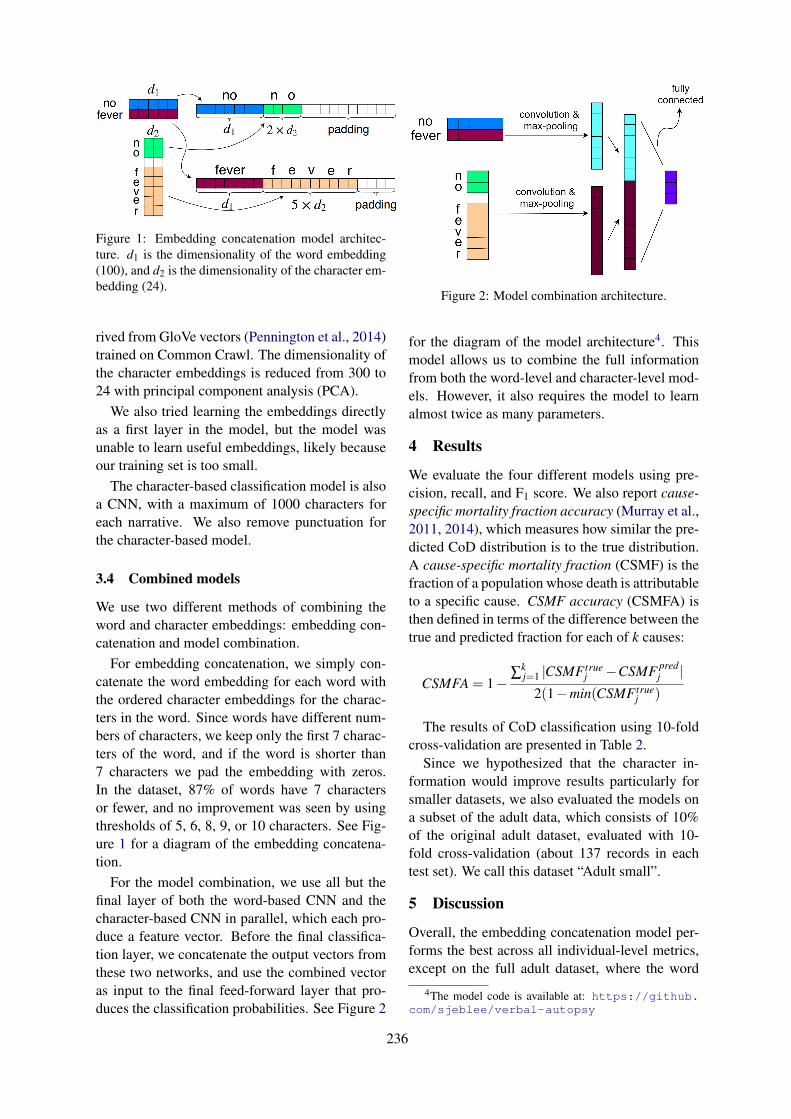
Figure 1: Embedding concatenation model architec-ture. d1 is the dimensionality of the word embedding(100), and d2 is the dimensionality of the character em-bedding (24).
rived from GloVe vectors (Pennington et al., 2014)trained on Common Crawl. The dimensionality ofthe character embeddings is reduced from 300 to24 with principal component analysis (PCA).
We also tried learning the embeddings directlyas a first layer in the model, but the model wasunable to learn useful embeddings, likely becauseour training set is too small.
The character-based classification model is alsoa CNN, with a maximum of 1000 characters foreach narrative. We also remove punctuation forthe character-based model.
3.4 Combined models
We use two different methods of combining theword and character embeddings: embedding con-catenation and model combination.
For embedding concatenation, we simply con-catenate the word embedding for each word withthe ordered character embeddings for the charac-ters in the word. Since words have different num-bers of characters, we keep only the first 7 charac-ters of the word, and if the word is shorter than7 characters we pad the embedding with zeros.In the dataset, 87% of words have 7 charactersor fewer, and no improvement was seen by usingthresholds of 5, 6, 8, 9, or 10 characters. See Fig-ure 1 for a diagram of the embedding concatena-tion.
For the model combination, we use all but thefinal layer of both the word-based CNN and thecharacter-based CNN in parallel, which each pro-duce a feature vector. Before the final classifica-tion layer, we concatenate the output vectors fromthese two networks, and use the combined vectoras input to the final feed-forward layer that pro-duces the classification probabilities. See Figure 2
Figure 2: Model combination architecture.
for the diagram of the model architecture4. Thismodel allows us to combine the full informationfrom both the word-level and character-level mod-els. However, it also requires the model to learnalmost twice as many parameters.
4 Results
We evaluate the four different models using pre-cision, recall, and F1 score. We also report cause-specific mortality fraction accuracy (Murray et al.,2011, 2014), which measures how similar the pre-dicted CoD distribution is to the true distribution.A cause-specific mortality fraction (CSMF) is thefraction of a population whose death is attributableto a specific cause. CSMF accuracy (CSMFA) isthen defined in terms of the difference between thetrue and predicted fraction for each of k causes:
CSMFA = 1− ∑kj=1 |CSMF true
j −CSMF predj |
2(1−min(CSMF truej )
The results of CoD classification using 10-foldcross-validation are presented in Table 2.
Since we hypothesized that the character in-formation would improve results particularly forsmaller datasets, we also evaluated the models ona subset of the adult data, which consists of 10%of the original adult dataset, evaluated with 10-fold cross-validation (about 137 records in eachtest set). We call this dataset “Adult small”.
5 Discussion
Overall, the embedding concatenation model per-forms the best across all individual-level metrics,except on the full adult dataset, where the word
4The model code is available at: https://github.com/sjeblee/verbal-autopsy
236
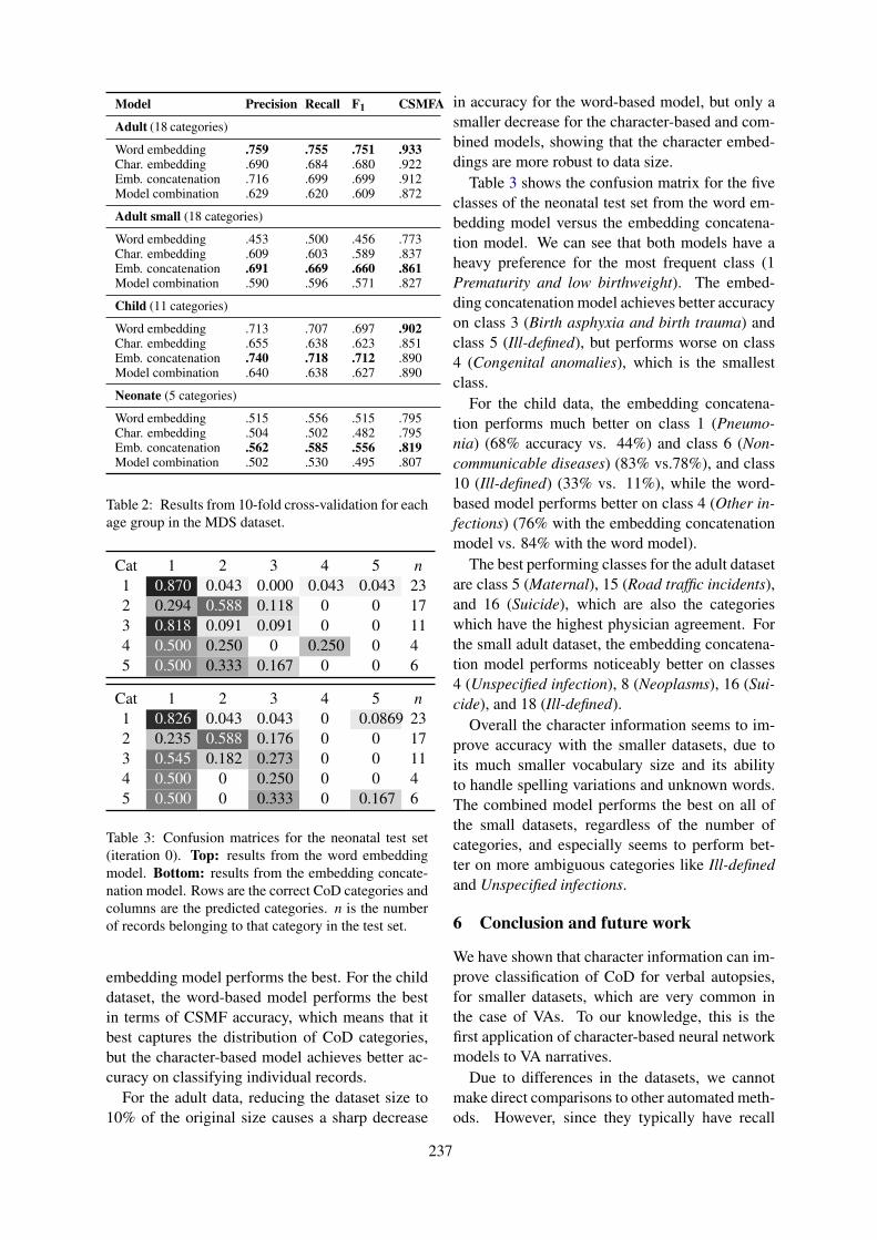
Model Precision Recall F1 CSMFA
Adult (18 categories)
Word embedding .759 .755 .751 .933Char. embedding .690 .684 .680 .922Emb. concatenation .716 .699 .699 .912Model combination .629 .620 .609 .872
Adult small (18 categories)
Word embedding .453 .500 .456 .773Char. embedding .609 .603 .589 .837Emb. concatenation .691 .669 .660 .861Model combination .590 .596 .571 .827
Child (11 categories)
Word embedding .713 .707 .697 .902Char. embedding .655 .638 .623 .851Emb. concatenation .740 .718 .712 .890Model combination .640 .638 .627 .890
Neonate (5 categories)
Word embedding .515 .556 .515 .795Char. embedding .504 .502 .482 .795Emb. concatenation .562 .585 .556 .819Model combination .502 .530 .495 .807
Table 2: Results from 10-fold cross-validation for eachage group in the MDS dataset.
Cat 1 2 3 4 5 n1 0.870 0.043 0.000 0.043 0.043 232 0.294 0.588 0.118 0 0 173 0.818 0.091 0.091 0 0 114 0.500 0.250 0 0.250 0 45 0.500 0.333 0.167 0 0 6
Cat 1 2 3 4 5 n1 0.826 0.043 0.043 0 0.0869 232 0.235 0.588 0.176 0 0 173 0.545 0.182 0.273 0 0 114 0.500 0 0.250 0 0 45 0.500 0 0.333 0 0.167 6
Table 3: Confusion matrices for the neonatal test set(iteration 0). Top: results from the word embeddingmodel. Bottom: results from the embedding concate-nation model. Rows are the correct CoD categories andcolumns are the predicted categories. n is the numberof records belonging to that category in the test set.
embedding model performs the best. For the childdataset, the word-based model performs the bestin terms of CSMF accuracy, which means that itbest captures the distribution of CoD categories,but the character-based model achieves better ac-curacy on classifying individual records.
For the adult data, reducing the dataset size to10% of the original size causes a sharp decrease
in accuracy for the word-based model, but only asmaller decrease for the character-based and com-bined models, showing that the character embed-dings are more robust to data size.
Table 3 shows the confusion matrix for the fiveclasses of the neonatal test set from the word em-bedding model versus the embedding concatena-tion model. We can see that both models have aheavy preference for the most frequent class (1Prematurity and low birthweight). The embed-ding concatenation model achieves better accuracyon class 3 (Birth asphyxia and birth trauma) andclass 5 (Ill-defined), but performs worse on class4 (Congenital anomalies), which is the smallestclass.
For the child data, the embedding concatena-tion performs much better on class 1 (Pneumo-nia) (68% accuracy vs. 44%) and class 6 (Non-communicable diseases) (83% vs.78%), and class10 (Ill-defined) (33% vs. 11%), while the word-based model performs better on class 4 (Other in-fections) (76% with the embedding concatenationmodel vs. 84% with the word model).
The best performing classes for the adult datasetare class 5 (Maternal), 15 (Road traffic incidents),and 16 (Suicide), which are also the categorieswhich have the highest physician agreement. Forthe small adult dataset, the embedding concatena-tion model performs noticeably better on classes4 (Unspecified infection), 8 (Neoplasms), 16 (Sui-cide), and 18 (Ill-defined).
Overall the character information seems to im-prove accuracy with the smaller datasets, due toits much smaller vocabulary size and its abilityto handle spelling variations and unknown words.The combined model performs the best on all ofthe small datasets, regardless of the number ofcategories, and especially seems to perform bet-ter on more ambiguous categories like Ill-definedand Unspecified infections.
6 Conclusion and future work
We have shown that character information can im-prove classification of CoD for verbal autopsies,for smaller datasets, which are very common inthe case of VAs. To our knowledge, this is thefirst application of character-based neural networkmodels to VA narratives.
Due to differences in the datasets, we cannotmake direct comparisons to other automated meth-ods. However, since they typically have recall
237
scores around 0.6, our method is competitive. Inaddition, this method can be applied to any VAdataset with narratives, regardless of the countryof origin or the specific survey form.
Future work may include using a languagemodel with character information, such as ELMo(Peters et al., 2018), but we would have to relyon out-of-domain data since the VA dataset is toosmall to effectively train ELMo or a similar model.The paucity of VA data is one of the biggest obsta-cles to automated coding.
In the future we also plan to expand thesemodels to other languages, as there are largerVA datasets in languages such as Portuguese andHindi. We will also investigate using the struc-tured data in addition to the narrative to improveperformance.
Acknowledgments
We thank Prabhat Jha of the Centre for GlobalHealth Research for providing the dataset. Ourwork is supported by funding from the NaturalSciences and Engineering Research Council ofCanada and by a Google Faculty Research Award.
ReferencesPeter Byass, Daniel Chandramohan, Samuel Clark,
Lucia D’Ambruoso, Edward Fottrell, Wendy Gra-ham, Abraham Herbst, Abraham Hodgson, Sen-nen Hounton, Kathleen Kahn, Anand Krishnan, Jor-dana Leitao, Frank Odhiambo, Osman Sankoh, andStephen Tollman. 2012. Strengthening standard-ised interpretation of verbal autopsy data: The newInterVA-4 tool. Global Health Action, 5:19281.
Samuel Danso, Eric Atwell, and Owen Johnson. 2013.A comparative study of machine learning methodsfor verbal autopsy text classification. InternationalJournal of Computer Science Issues, 10(6).
Kenneth Heafield, Ivan Pouzyrevsky, Jonathan H.Clark, and Philipp Koehn. 2013. Scalable modi-fied Kneser-Ney language model estimation. In Pro-ceedings of the 51st Annual Meeting of the Associa-tion for Computational Linguistics, pages 690–696,Sofia, Bulgaria.
Serena Jeblee, Mireille Gomes, and Graeme Hirst.2018. Multi-task learning for interpretable cause ofdeath classification using key phrase prediction. InProceedings of the BioNLP 2018 Workshop, pages12–17, Melbourne, Australia. Association for Com-putational Linguistics.
Ryan Kelly. 2015. Pyenchant. http://pythonhosted.org/pyenchant/.
Tyler H McCormick, Zehang Richard Li, Clara Calvert,Amelia C Crampin, Kathleen Kahn, and SamuelClark. 2016. Probabilistic cause-of-death assign-ment using verbal autopsies. Journal of the Amer-ican Statistical Association, 111(15):1036–1049.
Pierre Miasnikof, Vasily Giannakeas, Mireille Gomes,Lukasz Aleksandrowicz, Alexander Y Shestopaloff,Dewan Alam, Stephen Tollman, Akram Samarikha-laj, and Prabhat Jha. 2015. Naı̈ve Bayes classifiersfor verbal autopsies: Comparison to physician-basedclassification for 21,000 child and adult deaths.BMC Medicine, 13(1):286–294.
Tomas Mikolov, Ilya Sutskever, Kai Chen, Greg Cor-rado, and Jeffrey Dean. 2013. Distributed represen-tations of words and phrases and their composition-ality. In Proceedings of the 26th International Con-ference on Neural Information Processing Systems -Volume 2, NIPS’13, pages 3111–3119.
Christopher JL Murray, Rafael Lozano, Abraham DFlaxman, Alireza Vahdatpour, and Alan D Lopez.2011. Robust metrics for assessing the performanceof different verbal autopsy cause assignment meth-ods in validation studies. Population Health Met-rics, 9:28. Erratum (Murray et al., 2014).
Christopher JL Murray, Rafael Lozano, Abraham DFlaxman, Alireza Vahdatpour, and Alan D Lopez.2014. Erratum to: Robust metrics for assessing theperformance of different verbal autopsy cause as-signment methods in validation studies. PopulationHealth Metrics, 12:7.
Adam Paszke, Sam Gross, Soumith Chintala, Gre-gory Chanan, Edward Yang, Zachary DeVito, Zem-ing Lin, Alban Desmaison, Luca Antiga, and AdamLerer. 2017. Automatic differentiation in PyTorch.In NIPS 2017 Autodiff Workshop, pages 1–4.
Jeffrey Pennington, Richard Socher, and Christo-pher D. Manning. 2014. GloVe: global vectors forword representation. In Proceedings of the Con-ference on Empirical Methods in Natural LanguageProcessing (EMNLP), pages 1532–1543.
Matthew E. Peters, Mark Neumann, Mohit Iyyer, MattGardner, Christopher Clark, Kenton Lee, and LukeZettlemoyer. 2018. Deep contextualized word rep-resentations. In Proceedings of NAACL-HLT 2018,pages 2227–2237.
Peter Serina et al. 2015. Improving performance of theTariff method for assigning causes of death to verbalautopsies. BMC Medicine, 13(1):291.
Yuqi Si and Kirk Roberts. 2018. A frame-based NLPsystem for cancer-related information extraction.AMIA Annual Symposium Proceedings, 2018:1524–1533.
Department of Economic and Social Affairs, Pop-ulation Division, United Nations. 2013. WorldPopulation Prospects: The 2012 revision.ST/ESA/SER.A/334.
238
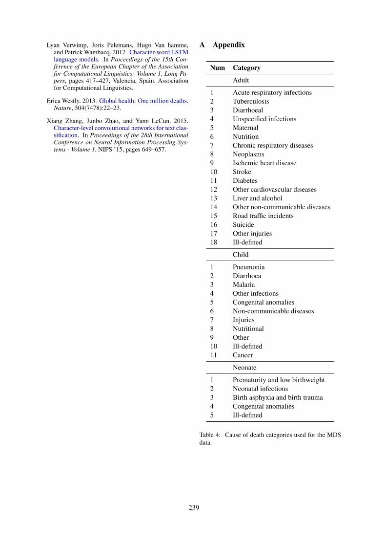
Lyan Verwimp, Joris Pelemans, Hugo Van hamme,and Patrick Wambacq. 2017. Character-word LSTMlanguage models. In Proceedings of the 15th Con-ference of the European Chapter of the Associationfor Computational Linguistics: Volume 1, Long Pa-pers, pages 417–427, Valencia, Spain. Associationfor Computational Linguistics.
Erica Westly. 2013. Global health: One million deaths.Nature, 504(7478):22–23.
Xiang Zhang, Junbo Zhao, and Yann LeCun. 2015.Character-level convolutional networks for text clas-sification. In Proceedings of the 28th InternationalConference on Neural Information Processing Sys-tems - Volume 1, NIPS ’15, pages 649–657.
A Appendix
Num Category
Adult
1 Acute respiratory infections2 Tuberculosis3 Diarrhoeal4 Unspecified infections5 Maternal6 Nutrition7 Chronic respiratory diseases8 Neoplasms9 Ischemic heart disease10 Stroke11 Diabetes12 Other cardiovascular diseases13 Liver and alcohol14 Other non-communicable diseases15 Road traffic incidents16 Suicide17 Other injuries18 Ill-defined
Child
1 Pneumonia2 Diarrhoea3 Malaria4 Other infections5 Congenital anomalies6 Non-communicable diseases7 Injuries8 Nutritional9 Other10 Ill-defined11 Cancer
Neonate
1 Prematurity and low birthweight2 Neonatal infections3 Birth asphyxia and birth trauma4 Congenital anomalies5 Ill-defined
Table 4: Cause of death categories used for the MDSdata.
239
Proceedings of the BioNLP 2019 workshop, pages 240–249Florence, Italy, August 1, 2019. c©2019 Association for Computational Linguistics
Is artificial data useful for biomedical Natural Language Processingalgorithms?
Zixu Wang1, Julia Ive2, Sumithra Velupillai3 and Lucia Specia1
1Department of Computing, Imperial College London, UK2DCS, University of Sheffield, UK
3IoPPN, King’s College London, UK and KTH, [email protected]
[email protected]@kcl.ac.uk
Abstract
A major obstacle to the development of Natu-ral Language Processing (NLP) methods in thebiomedical domain is data accessibility. Thisproblem can be addressed by generating medi-cal data artificially. Most previous studies havefocused on the generation of short clinical text,and evaluation of the data utility has been lim-ited. We propose a generic methodology toguide the generation of clinical text with keyphrases. We use the artificial data as additionaltraining data in two key biomedical NLP tasks:text classification and temporal relation extrac-tion. We show that artificially generated train-ing data used in conjunction with real trainingdata can lead to performance boosts for data-greedy neural network algorithms. We alsodemonstrate the usefulness of the generateddata for NLP setups where it fully replaces realtraining data.
1 Introduction
Data availability is a major obstacle in the devel-opment of more powerful Natural Language Pro-cessing (NLP) methods in the biomedical domain.In particular, current state-of-the-art (SOTA) neu-ral techniques used for NLP rely on substantialamounts of training data.
In the NLP community, this low-resource prob-lem is typically addressed by generating comple-mentary data artificially (Poncelas et al., 2018;Edunov et al., 2018). This approach is also gainingattention in biomedical NLP. Most of these stud-ies present work on the generation of short text(typically under 20 tokens), given structural infor-mation to guide this generation (e.g., chief com-plaints using basic patient and diagnosis informa-tion (Lee, 2018)). Evaluation scenarios for theutility of the artificial text usually involve a sin-gle downstream NLP task (typically, text classifi-cation).
SOTA approaches tackle other language gener-ation tasks by applying neural models: variationsof the encoder-decoder architecture (ED) model(Sutskever et al., 2014; Bahdanau et al., 2015),a.k.a sequence to sequence (seq2seq), e.g., theTransformer model (Vaswani et al., 2017). Inthis work, we follow these approaches and guidethe generation process with key phrases in theTransformer model.
Our main contribution is thus twofold: (1) asingle methodology to generate medical text fora series of downstream NLP tasks; (2) an assess-ment of the utility of the generated data as comple-mentary training data in two important biomedicalNLP tasks: text classification (phenotype classi-fication) and temporal relation evaluation. Addi-tionally, we thoroughly study the usefulness of thegenerated data in a set of scenarios where it fullyreplaces real training data.
2 Related Work
Natural Language Generation. Natural lan-guage generation is an NLP area with a rangeof applications such as dialogue generation,question-answering, machine translation (MT),summarisation, simplification, storytelling, etc.
SOTA approaches attempt to solve these tasksby using neural models. One of the most widelyused models is the encoder-decoder architecture(ED) (Sutskever et al., 2014; Bahdanau et al.,2015). In this architecture, the decoder is a con-ditional language model. It generates a new wordat a timestep taking into account the previouslygenerated words, as well as the information pro-vided by the encoder (a sequence of hidden states,roughly speaking, a set of automatically learnedfeatures).
For different tasks, the input to the encoder maybe different: questions for question-answering,
240
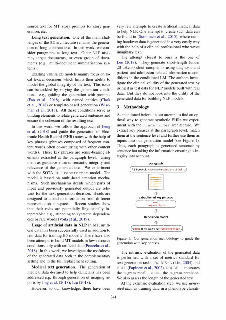
source text for MT, story prompts for story gen-eration, etc.
Long text generation. One of the main chal-lenges of the ED architecture remains the genera-tion of long coherent text. In this work, we con-sider paragraphs as long text. Other NLP tasksmay target documents, or even group of docu-ments (e.g., multi-document summarisation sys-tems).
Existing vanilla ED models mainly focus on lo-cal lexical decisions which limits their ability tomodel the global integrity of the text. This issuecan be tackled by varying the generation condi-tions: e.g., guiding the generation with prompts(Fan et al., 2018), with named entities (Clarket al., 2018) or template-based generation (Wise-man et al., 2018). All these conditions serve asbinding elements to relate generated sentences andensure the cohesion of the resulting text.
In this work, we follow the approach of Penget al. (2018) and guide the generation of Elec-tronic Health Record (EHR) notes with the help ofkey phrases (phrases composed of frequent con-tent words often co-occurring with other contentwords). These key phrases are sense-bearing el-ements extracted at the paragraph level. Usingthem as guidance ensures semantic integrity andrelevance of the generated text. We experimentwith the SOTA ED Transformer model. Themodel is based on multi-head attention mecha-nisms. Such mechanisms decide which parts ofinput and previously generated output are rele-vant for the next generation decision. Heads aredesigned to attend to information from differentrepresentation subspaces. Recent studies showthat their roles are potentially linguistically in-tepretable: e.g., attending to syntactic dependen-cies or rare words (Voita et al., 2019).
Usage of artificial data in NLP In MT, artifi-cial data has been successfully used in addition toreal data for training ED models. There have alsobeen attempts to build MT models in low-resourceconditions only with artificial data (Poncelas et al.,2018). In this work, we investigate the usefulnessof the generated data both in the complementarysetting and in the full replacement setting.
Medical text generation. The generation ofmedical data destined to help clinicians has beenaddressed e.g. through generation of imaging re-ports by Jing et al. (2018); Liu (2018).
However, to our knowledge, there have been
very few attempts to create artificial medical datato help NLP. One attempt to create such data canbe found in (Suominen et al., 2015), where nurs-ing handover data is generated in a very costly waywith the help of a clinical professional who wroteimaginary text.
The attempt closest to ours is the one ofLee (2018). They generate short-length (under20 tokens) chief complaints using diagnosis andpatient- and admission-related information as con-ditions in the conditional LM. The authors inves-tigate the clinical validity of the generated text byusing it as test data for NLP models built with realdata. But they do not look into the utility of thegenerated data for building NLP models.
3 Methodology
As mentioned before, in our attempt to find an op-timal way to generate synthetic EHRs we exper-iment with the Transformer architecture. Weextract key phrases at the paragraph level, matchthem at the sentence level and further use them asinputs into our generation model (see Figure 1).Thus, each paragraph is generated sentence bysentence but taking the information ensuring its in-tegrity into account.
Figure 1: Our generation methodology to guide thegeneration with key phrases.
The intrinsic evaluation of the generated datais performed with a set of metrics standard fortext generation tasks: ROUGE-L (Lin, 2004) andBLEU (Papineni et al., 2002). ROUGE-Lmeasuresthe n-gram recall, BLEU– the n-gram precision.We also assess the length of the generated text.
At the extrinsic evaluation step, we use gener-ated data as training data in a phenotype classifi-
241
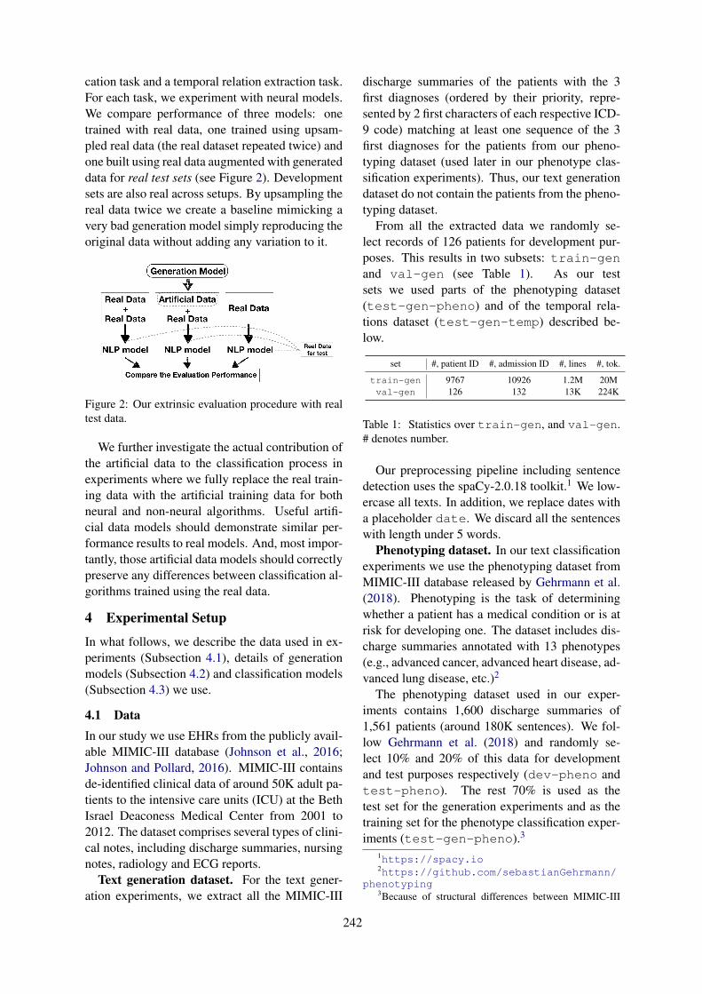
cation task and a temporal relation extraction task.For each task, we experiment with neural models.We compare performance of three models: onetrained with real data, one trained using upsam-pled real data (the real dataset repeated twice) andone built using real data augmented with generateddata for real test sets (see Figure 2). Developmentsets are also real across setups. By upsampling thereal data twice we create a baseline mimicking avery bad generation model simply reproducing theoriginal data without adding any variation to it.
Figure 2: Our extrinsic evaluation procedure with realtest data.
We further investigate the actual contribution ofthe artificial data to the classification process inexperiments where we fully replace the real train-ing data with the artificial training data for bothneural and non-neural algorithms. Useful artifi-cial data models should demonstrate similar per-formance results to real models. And, most impor-tantly, those artificial data models should correctlypreserve any differences between classification al-gorithms trained using the real data.
4 Experimental Setup
In what follows, we describe the data used in ex-periments (Subsection 4.1), details of generationmodels (Subsection 4.2) and classification models(Subsection 4.3) we use.
4.1 DataIn our study we use EHRs from the publicly avail-able MIMIC-III database (Johnson et al., 2016;Johnson and Pollard, 2016). MIMIC-III containsde-identified clinical data of around 50K adult pa-tients to the intensive care units (ICU) at the BethIsrael Deaconess Medical Center from 2001 to2012. The dataset comprises several types of clini-cal notes, including discharge summaries, nursingnotes, radiology and ECG reports.
Text generation dataset. For the text gener-ation experiments, we extract all the MIMIC-III
discharge summaries of the patients with the 3first diagnoses (ordered by their priority, repre-sented by 2 first characters of each respective ICD-9 code) matching at least one sequence of the 3first diagnoses for the patients from our pheno-typing dataset (used later in our phenotype clas-sification experiments). Thus, our text generationdataset do not contain the patients from the pheno-typing dataset.
From all the extracted data we randomly se-lect records of 126 patients for development pur-poses. This results in two subsets: train-genand val-gen (see Table 1). As our testsets we used parts of the phenotyping dataset(test-gen-pheno) and of the temporal rela-tions dataset (test-gen-temp) described be-low.
set #, patient ID #, admission ID #, lines #, tok.
train-gen 9767 10926 1.2M 20Mval-gen 126 132 13K 224K
Table 1: Statistics over train-gen, and val-gen.# denotes number.
Our preprocessing pipeline including sentencedetection uses the spaCy-2.0.18 toolkit.1 We low-ercase all texts. In addition, we replace dates witha placeholder date. We discard all the sentenceswith length under 5 words.
Phenotyping dataset. In our text classificationexperiments we use the phenotyping dataset fromMIMIC-III database released by Gehrmann et al.(2018). Phenotyping is the task of determiningwhether a patient has a medical condition or is atrisk for developing one. The dataset includes dis-charge summaries annotated with 13 phenotypes(e.g., advanced cancer, advanced heart disease, ad-vanced lung disease, etc.)2
The phenotyping dataset used in our exper-iments contains 1,600 discharge summaries of1,561 patients (around 180K sentences). We fol-low Gehrmann et al. (2018) and randomly se-lect 10% and 20% of this data for developmentand test purposes respectively (dev-pheno andtest-pheno). The rest 70% is used as thetest set for the generation experiments and as thetraining set for the phenotype classification exper-iments (test-gen-pheno).3
1https://spacy.io2https://github.com/sebastianGehrmann/
phenotyping3Because of structural differences between MIMIC-III
242
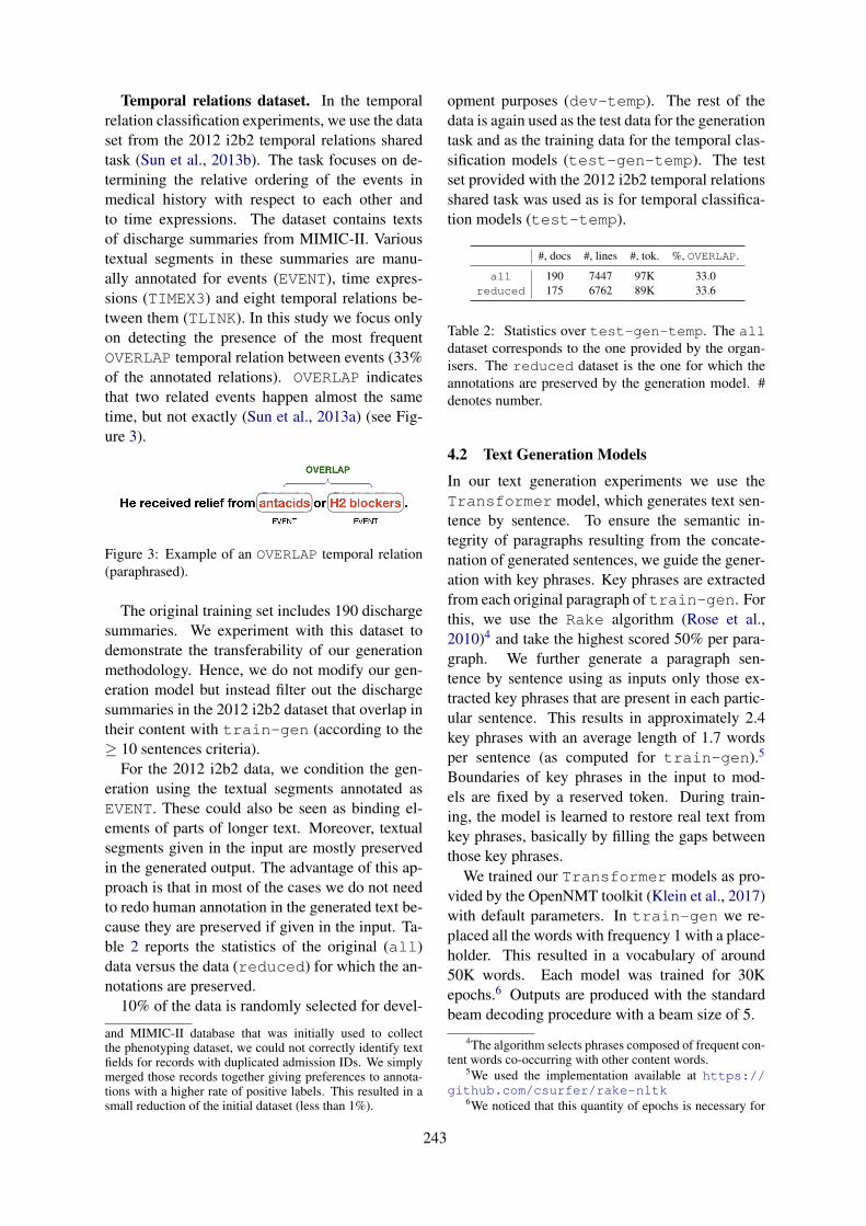
Temporal relations dataset. In the temporalrelation classification experiments, we use the dataset from the 2012 i2b2 temporal relations sharedtask (Sun et al., 2013b). The task focuses on de-termining the relative ordering of the events inmedical history with respect to each other andto time expressions. The dataset contains textsof discharge summaries from MIMIC-II. Varioustextual segments in these summaries are manu-ally annotated for events (EVENT), time expres-sions (TIMEX3) and eight temporal relations be-tween them (TLINK). In this study we focus onlyon detecting the presence of the most frequentOVERLAP temporal relation between events (33%of the annotated relations). OVERLAP indicatesthat two related events happen almost the sametime, but not exactly (Sun et al., 2013a) (see Fig-ure 3).
Figure 3: Example of an OVERLAP temporal relation(paraphrased).
The original training set includes 190 dischargesummaries. We experiment with this dataset todemonstrate the transferability of our generationmethodology. Hence, we do not modify our gen-eration model but instead filter out the dischargesummaries in the 2012 i2b2 dataset that overlap intheir content with train-gen (according to the≥ 10 sentences criteria).
For the 2012 i2b2 data, we condition the gen-eration using the textual segments annotated asEVENT. These could also be seen as binding el-ements of parts of longer text. Moreover, textualsegments given in the input are mostly preservedin the generated output. The advantage of this ap-proach is that in most of the cases we do not needto redo human annotation in the generated text be-cause they are preserved if given in the input. Ta-ble 2 reports the statistics of the original (all)data versus the data (reduced) for which the an-notations are preserved.
10% of the data is randomly selected for devel-
and MIMIC-II database that was initially used to collectthe phenotyping dataset, we could not correctly identify textfields for records with duplicated admission IDs. We simplymerged those records together giving preferences to annota-tions with a higher rate of positive labels. This resulted in asmall reduction of the initial dataset (less than 1%).
opment purposes (dev-temp). The rest of thedata is again used as the test data for the generationtask and as the training data for the temporal clas-sification models (test-gen-temp). The testset provided with the 2012 i2b2 temporal relationsshared task was used as is for temporal classifica-tion models (test-temp).
#, docs #, lines #, tok. %, OVERLAP.
all 190 7447 97K 33.0reduced 175 6762 89K 33.6
Table 2: Statistics over test-gen-temp. The alldataset corresponds to the one provided by the organ-isers. The reduced dataset is the one for which theannotations are preserved by the generation model. #denotes number.
4.2 Text Generation Models
In our text generation experiments we use theTransformer model, which generates text sen-tence by sentence. To ensure the semantic in-tegrity of paragraphs resulting from the concate-nation of generated sentences, we guide the gener-ation with key phrases. Key phrases are extractedfrom each original paragraph of train-gen. Forthis, we use the Rake algorithm (Rose et al.,2010)4 and take the highest scored 50% per para-graph. We further generate a paragraph sen-tence by sentence using as inputs only those ex-tracted key phrases that are present in each partic-ular sentence. This results in approximately 2.4key phrases with an average length of 1.7 wordsper sentence (as computed for train-gen).5
Boundaries of key phrases in the input to mod-els are fixed by a reserved token. During train-ing, the model is learned to restore real text fromkey phrases, basically by filling the gaps betweenthose key phrases.
We trained our Transformer models as pro-vided by the OpenNMT toolkit (Klein et al., 2017)with default parameters. In train-gen we re-placed all the words with frequency 1 with a place-holder. This resulted in a vocabulary of around50K words. Each model was trained for 30Kepochs.6 Outputs are produced with the standardbeam decoding procedure with a beam size of 5.
4The algorithm selects phrases composed of frequent con-tent words co-occurring with other content words.
5We used the implementation available at https://github.com/csurfer/rake-nltk
6We noticed that this quantity of epochs is necessary for
243
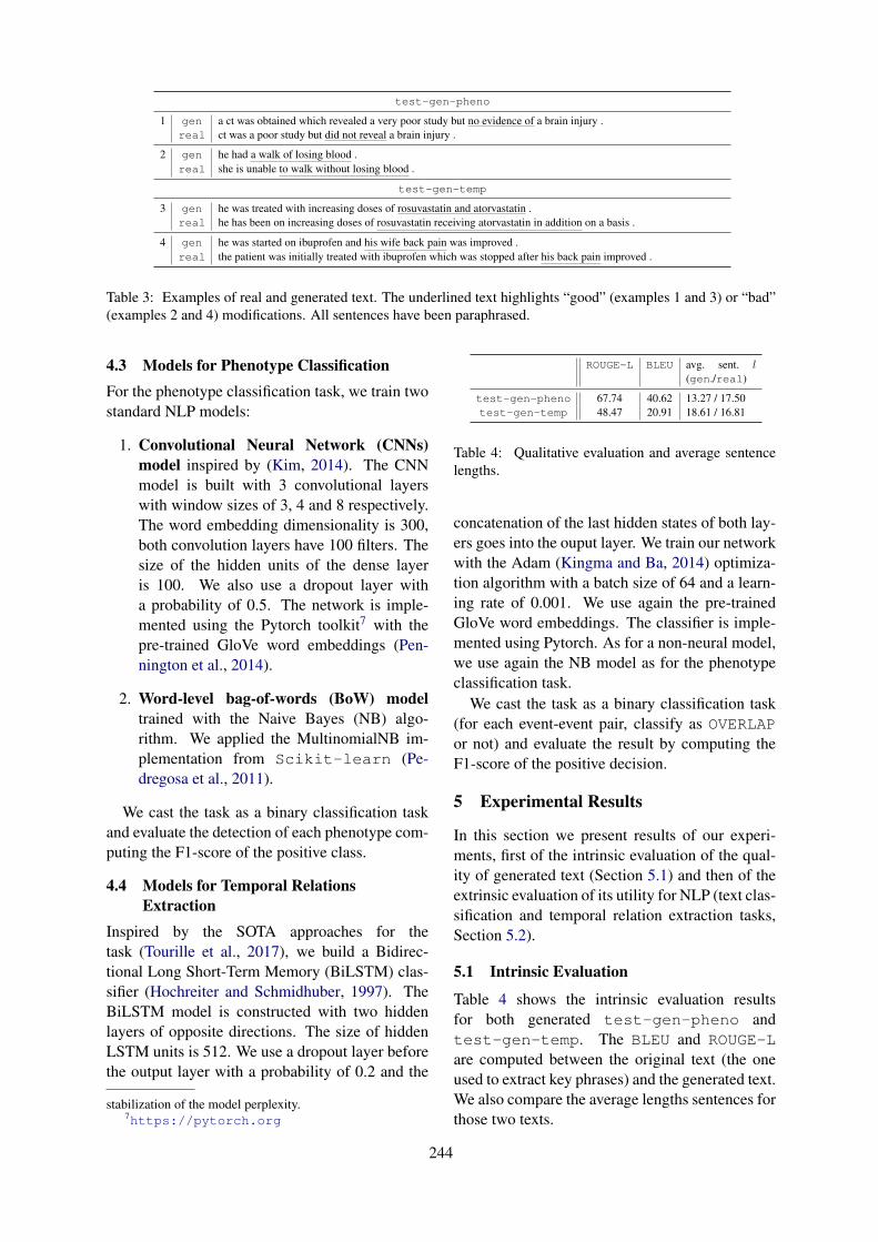
test-gen-pheno
1 gen a ct was obtained which revealed a very poor study but no evidence of a brain injury .real ct was a poor study but did not reveal a brain injury .
2 gen he had a walk of losing blood .real she is unable to walk without losing blood .
test-gen-temp
3 gen he was treated with increasing doses of rosuvastatin and atorvastatin .real he has been on increasing doses of rosuvastatin receiving atorvastatin in addition on a basis .
4 gen he was started on ibuprofen and his wife back pain was improved .real the patient was initially treated with ibuprofen which was stopped after his back pain improved .
Table 3: Examples of real and generated text. The underlined text highlights “good” (examples 1 and 3) or “bad”(examples 2 and 4) modifications. All sentences have been paraphrased.
4.3 Models for Phenotype ClassificationFor the phenotype classification task, we train twostandard NLP models:
1. Convolutional Neural Network (CNNs)model inspired by (Kim, 2014). The CNNmodel is built with 3 convolutional layerswith window sizes of 3, 4 and 8 respectively.The word embedding dimensionality is 300,both convolution layers have 100 filters. Thesize of the hidden units of the dense layeris 100. We also use a dropout layer witha probability of 0.5. The network is imple-mented using the Pytorch toolkit7 with thepre-trained GloVe word embeddings (Pen-nington et al., 2014).
2. Word-level bag-of-words (BoW) modeltrained with the Naive Bayes (NB) algo-rithm. We applied the MultinomialNB im-plementation from Scikit-learn (Pe-dregosa et al., 2011).
We cast the task as a binary classification taskand evaluate the detection of each phenotype com-puting the F1-score of the positive class.
4.4 Models for Temporal RelationsExtraction
Inspired by the SOTA approaches for thetask (Tourille et al., 2017), we build a Bidirec-tional Long Short-Term Memory (BiLSTM) clas-sifier (Hochreiter and Schmidhuber, 1997). TheBiLSTM model is constructed with two hiddenlayers of opposite directions. The size of hiddenLSTM units is 512. We use a dropout layer beforethe output layer with a probability of 0.2 and the
stabilization of the model perplexity.7https://pytorch.org
ROUGE-L BLEU avg. sent. l(gen./real)
test-gen-pheno 67.74 40.62 13.27 / 17.50test-gen-temp 48.47 20.91 18.61 / 16.81
Table 4: Qualitative evaluation and average sentencelengths.
concatenation of the last hidden states of both lay-ers goes into the ouput layer. We train our networkwith the Adam (Kingma and Ba, 2014) optimiza-tion algorithm with a batch size of 64 and a learn-ing rate of 0.001. We use again the pre-trainedGloVe word embeddings. The classifier is imple-mented using Pytorch. As for a non-neural model,we use again the NB model as for the phenotypeclassification task.
We cast the task as a binary classification task(for each event-event pair, classify as OVERLAPor not) and evaluate the result by computing theF1-score of the positive decision.
5 Experimental Results
In this section we present results of our experi-ments, first of the intrinsic evaluation of the qual-ity of generated text (Section 5.1) and then of theextrinsic evaluation of its utility for NLP (text clas-sification and temporal relation extraction tasks,Section 5.2).
5.1 Intrinsic Evaluation
Table 4 shows the intrinsic evaluation resultsfor both generated test-gen-pheno andtest-gen-temp. The BLEU and ROUGE-Lare computed between the original text (the oneused to extract key phrases) and the generated text.We also compare the average lengths sentences forthose two texts.
244
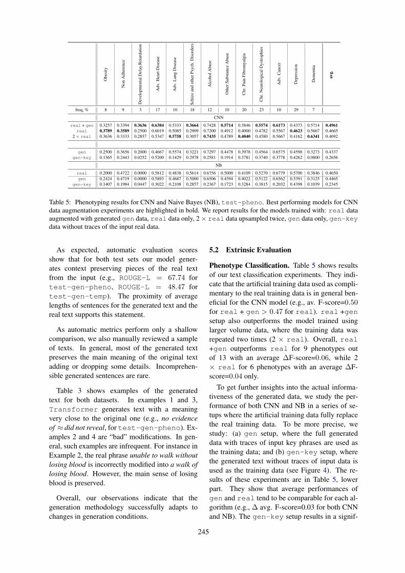
Obe
sity
Non
Adh
eren
ce
Dev
elop
men
tal.D
elay
.Ret
arda
tion
Adv
.Hea
rtD
isea
se
Adv
.Lun
gD
isea
se
Schi
zoan
dot
herP
sych
.Dis
orde
rs
Alc
ohol
Abu
se
Oth
erSu
bsta
nce
Abu
se
Chr
.Pai
nFi
brom
yalg
ia
Chr
.Neu
rolo
gica
lDys
trop
hies
Adv
.Can
cer
Dep
ress
ion
Dem
entia
avg.
freq, % 8 9 3 17 10 18 12 10 20 23 10 29 7
CNN
real + gen 0.3257 0.3394 0.3636 0.6384 0.5333 0.3664 0.7428 0.5714 0.3846 0.5574 0.6173 0.4373 0.5714 0.4961real 0.3789 0.3589 0.2500 0.6019 0.5085 0.2909 0.7200 0.4912 0.4000 0.4782 0.5567 0.4623 0.5667 0.4665
2 × real 0.3636 0.3333 0.2857 0.5347 0.5758 0.3057 0.7435 0.4789 0.4040 0.4580 0.5667 0.4162 0.6341 0.4692
gen 0.2500 0.3656 0.2000 0.4667 0.5574 0.3221 0.7297 0.4478 0.3978 0.4564 0.6575 0.4598 0.3273 0.4337gen-key 0.1365 0.2443 0.0252 0.5200 0.1429 0.2978 0.2581 0.1914 0.3781 0.3740 0.3778 0.4262 0.0800 0.2656
NB
real 0.2000 0.4722 0.0000 0.5812 0.4838 0.5614 0.6756 0.5000 0.4109 0.5270 0.6779 0.5700 0.3846 0.4650gen 0.2424 0.4719 0.0000 0.5893 0.4687 0.5000 0.6506 0.4594 0.4022 0.5122 0.6562 0.5391 0.3125 0.4465
gen-key 0.1407 0.1984 0.0447 0.3022 0.2108 0.2857 0.2367 0.1723 0.3284 0.3815 0.2032 0.4398 0.1039 0.2345
Table 5: Phenotyping results for CNN and Naive Bayes (NB), test-pheno. Best performing models for CNNdata augmentation experiments are highlighted in bold. We report results for the models trained with: real dataaugmented with generated gen data, real data only, 2 × real data upsampled twice, gen data only, gen-keydata without traces of the input real data.
As expected, automatic evaluation scoresshow that for both test sets our model gener-ates context preserving pieces of the real textfrom the input (e.g., ROUGE-L = 67.74 fortest-gen-pheno, ROUGE-L = 48.47 fortest-gen-temp). The proximity of averagelengths of sentences for the generated text and thereal text supports this statement.
As automatic metrics perform only a shallowcomparison, we also manually reviewed a sampleof texts. In general, most of the generated textpreserves the main meaning of the original textadding or dropping some details. Incomprehen-sible generated sentences are rare.
Table 3 shows examples of the generatedtext for both datasets. In examples 1 and 3,Transformer generates text with a meaningvery close to the original one (e.g., no evidenceof ≈ did not reveal, for test-gen-pheno). Ex-amples 2 and 4 are “bad” modifications. In gen-eral, such examples are infrequent. For instance inExample 2, the real phrase unable to walk withoutlosing blood is incorrectly modified into a walk oflosing blood. However, the main sense of losingblood is preserved.
Overall, our observations indicate that thegeneration methodology successfully adapts tochanges in generation conditions.
5.2 Extrinsic Evaluation
Phenotype Classification. Table 5 shows resultsof our text classification experiments. They indi-cate that the artificial training data used as compli-mentary to the real training data is in general ben-eficial for the CNN model (e.g., av. F-score=0.50for real + gen > 0.47 for real). real +gensetup also outperforms the model trained usinglarger volume data, where the training data wasrepeated two times (2 × real). Overall, real+gen outperforms real for 9 phenotypes outof 13 with an average ∆F-score=0.06, while 2× real for 6 phenotypes with an average ∆F-score=0.04 only.
To get further insights into the actual informa-tiveness of the generated data, we study the per-formance of both CNN and NB in a series of se-tups where the artificial training data fully replacethe real training data. To be more precise, westudy: (a) gen setup, where the full generateddata with traces of input key phrases are used asthe training data; and (b) gen-key setup, wherethe generated text without traces of input data isused as the training data (see Figure 4). The re-sults of these experiments are in Table 5, lowerpart. They show that average performances ofgen and real tend to be comparable for each al-gorithm (e.g., ∆ avg. F-score=0.03 for both CNNand NB). The gen-key setup results in a signif-
245
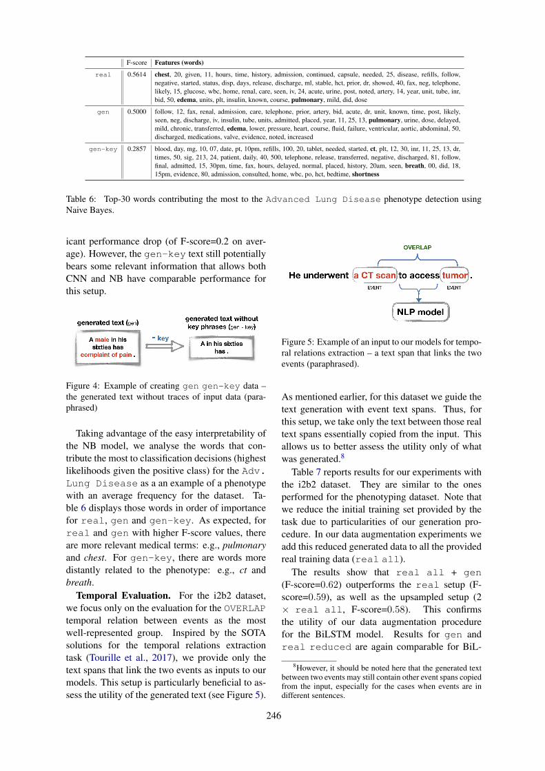
F-score Features (words)
real 0.5614 chest, 20, given, 11, hours, time, history, admission, continued, capsule, needed, 25, disease, refills, follow,negative, started, status, disp, days, release, discharge, ml, stable, hct, prior, dr, showed, 40, fax, neg, telephone,likely, 15, glucose, wbc, home, renal, care, seen, iv, 24, acute, urine, post, noted, artery, 14, year, unit, tube, inr,bid, 50, edema, units, plt, insulin, known, course, pulmonary, mild, did, dose
gen 0.5000 follow, 12, fax, renal, admission, care, telephone, prior, artery, bid, acute, dr, unit, known, time, post, likely,seen, neg, discharge, iv, insulin, tube, units, admitted, placed, year, 11, 25, 13, pulmonary, urine, dose, delayed,mild, chronic, transferred, edema, lower, pressure, heart, course, fluid, failure, ventricular, aortic, abdominal, 50,discharged, medications, valve, evidence, noted, increased
gen-key 0.2857 blood, day, mg, 10, 07, date, pt, 10pm, refills, 100, 20, tablet, needed, started, ct, plt, 12, 30, inr, 11, 25, 13, dr,times, 50, sig, 213, 24, patient, daily, 40, 500, telephone, release, transferred, negative, discharged, 81, follow,final, admitted, 15, 30pm, time, fax, hours, delayed, normal, placed, history, 20am, seen, breath, 00, did, 18,15pm, evidence, 80, admission, consulted, home, wbc, po, hct, bedtime, shortness
Table 6: Top-30 words contributing the most to the Advanced Lung Disease phenotype detection usingNaive Bayes.
icant performance drop (of F-score=0.2 on aver-age). However, the gen-key text still potentiallybears some relevant information that allows bothCNN and NB have comparable performance forthis setup.
Figure 4: Example of creating gen gen-key data –the generated text without traces of input data (para-phrased)
Taking advantage of the easy interpretability ofthe NB model, we analyse the words that con-tribute the most to classification decisions (highestlikelihoods given the positive class) for the Adv.Lung Disease as a an example of a phenotypewith an average frequency for the dataset. Ta-ble 6 displays those words in order of importancefor real, gen and gen-key. As expected, forreal and gen with higher F-score values, thereare more relevant medical terms: e.g., pulmonaryand chest. For gen-key, there are words moredistantly related to the phenotype: e.g., ct andbreath.
Temporal Evaluation. For the i2b2 dataset,we focus only on the evaluation for the OVERLAPtemporal relation between events as the mostwell-represented group. Inspired by the SOTAsolutions for the temporal relations extractiontask (Tourille et al., 2017), we provide only thetext spans that link the two events as inputs to ourmodels. This setup is particularly beneficial to as-sess the utility of the generated text (see Figure 5).
Figure 5: Example of an input to our models for tempo-ral relations extraction – a text span that links the twoevents (paraphrased).
As mentioned earlier, for this dataset we guide thetext generation with event text spans. Thus, forthis setup, we take only the text between those realtext spans essentially copied from the input. Thisallows us to better assess the utility only of whatwas generated.8
Table 7 reports results for our experiments withthe i2b2 dataset. They are similar to the onesperformed for the phenotyping dataset. Note thatwe reduce the initial training set provided by thetask due to particularities of our generation pro-cedure. In our data augmentation experiments weadd this reduced generated data to all the providedreal training data (real all).
The results show that real all + gen(F-score=0.62) outperforms the real setup (F-score=0.59), as well as the upsampled setup (2× real all, F-score=0.58). This confirmsthe utility of our data augmentation procedurefor the BiLSTM model. Results for gen andreal reduced are again comparable for BiL-
8However, it should be noted here that the generated textbetween two events may still contain other event spans copiedfrom the input, especially for the cases when events are indifferent sentences.
246
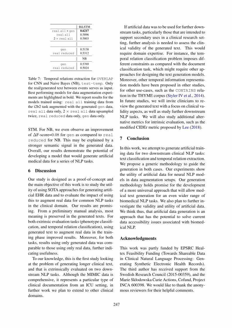
BiLSTMreal all + gen 0.6217
real all 0.58962 × real all 0.5803
gen 0.5138real reduced 0.5312
NB
gen 0.5769real reduced 0.5024
Table 7: Temporal relations extraction for OVERLAPfor CNN and Naive Bayes (NB), test-temp. Onlythe real/generated text between events serves as input.Best performing models for data augmentation experi-ments are highlighted in bold. We report results for themodels trained using: real all training data fromthe i2b2 task augmented with the generated gen data,real all data only, 2 × real all data upsampledtwice, real reduced data only, gen data only.
STM. For NB, we even observe an improvementof ∆F-score=0.08 for gen as compared to realreduced for NB. This may be explained by astronger semantic signal in the generated data.Overall, our results demonstrate the potential ofdeveloping a model that would generate artificialmedical data for a series of NLP tasks.
6 Discussion
Our study is designed as a proof-of-concept andthe main objective of this work is to study the util-ity of using SOTA approaches for generating artifi-cial EHR data and to evaluate the impact of usingthis to augment real data for common NLP tasksin the clinical domain. Our results are promis-ing. From a preliminary manual analysis, mostmeaning is preserved in the generated texts. Forboth extrinsic evaluation tasks (phenotype classifi-cation, and temporal relation classification), usinggenerated text to augment real data in the train-ing phase improved results. Moreover, for bothtasks, results using only generated data was com-parable to those using only real data, further indi-cating usefulness.
To our knowledge, this is the first study lookingat the problem of generating longer clinical text,and that is extrinsically evaluated on two down-stream NLP tasks. Although the MIMIC data iscomprehensive, it represents a particular type ofclinical documentation from an ICU setting, infurther work we plan to extend to other clinicaldomains.
If artificial data was to be used for further down-stream tasks, particularly those that are intended tosupport secondary uses in a clinical research set-ting, further analysis is needed to assess the clin-ical validity of the generated text. This wouldrequire domain expertise. For instance, the tem-poral relation classification problem imposes dif-ferent constraints as compared with the documentclassification task, which might require other ap-proaches for designing the text generation models.Moreover, other temporal information representa-tion models have been proposed in other studies,for other use-cases, such as the CONTAINS rela-tion in the THYME corpus (Styler IV et al., 2014).In future studies, we will invite clinicians to re-view the generated text with a focus on clinical va-lidity aspects, as well as study further downstreamNLP tasks. We will also study additional alter-native metrics for intrinsic evaluation, such as themodified CIDEr metric proposed by Lee (2018).
7 Conclusion
In this work, we attempt to generate artificial train-ing data for two downstream clinical NLP tasks:text classification and temporal relation extraction.We propose a generic methodology to guide thegeneration in both cases. Our experiments showthe utility of artificial data for neural NLP mod-els in data augmentation setups. Our generationmethodology holds promise for the developmentof a more universal approach that will allow med-ical text generation for an even wider range ofbiomedical NLP tasks. We also plan to further in-vestigate the validity and utility of artificial data.We think thus, that artificial data generation is anapproach that has the potential to solve currentdata accessibility issues associated with biomed-ical NLP.
Acknowledgments
This work was partly funded by EPSRC Heal-tex Feasibility Funding (Towards Shareable Datain Clinical Natural Language Processing: Gen-erating Synthetic Electronic Health Records).The third author has received support from theSwedish Research Council (2015-00359), and theMarie Skłodowska Curie Actions, Cofund, ProjectINCA 600398. We would like to thank the anony-mous reviewers for their helpful comments.
247
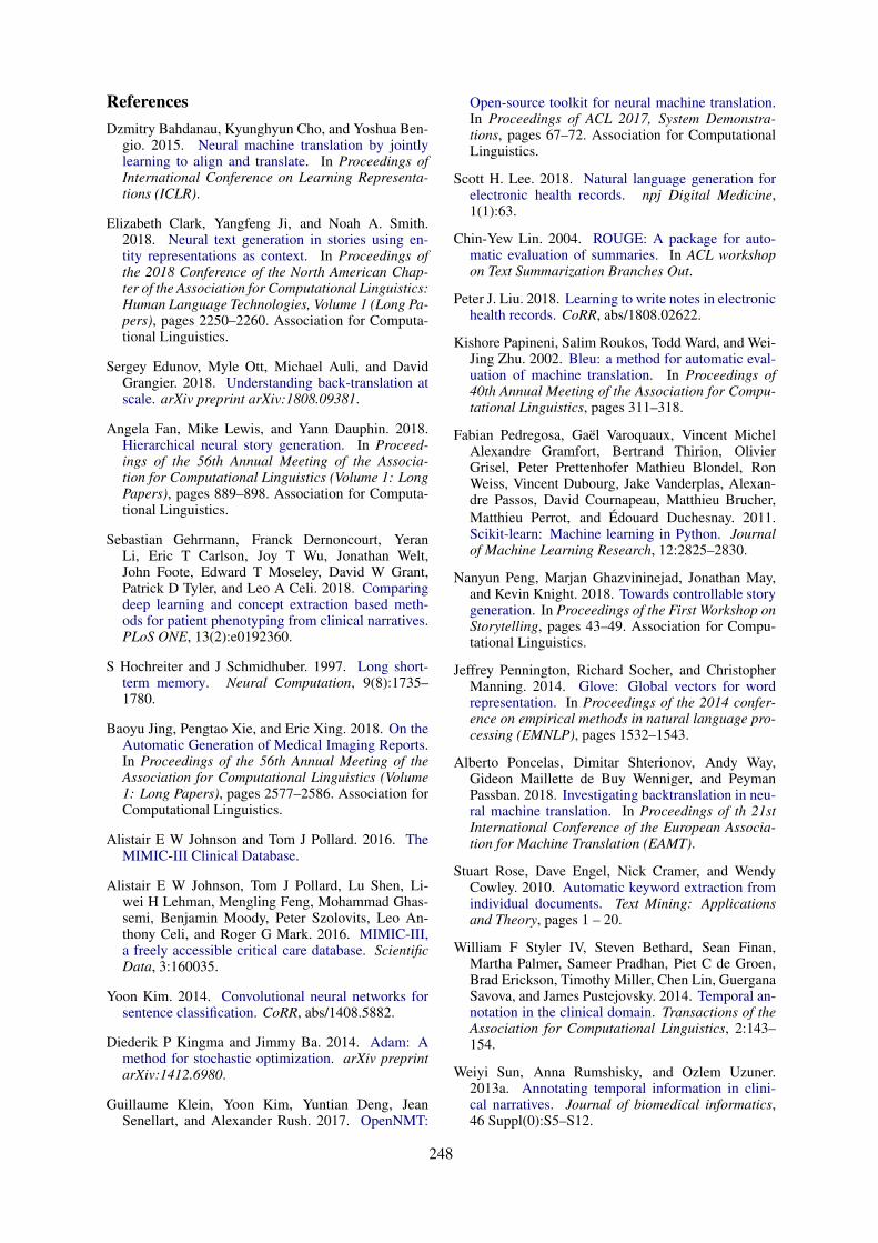
ReferencesDzmitry Bahdanau, Kyunghyun Cho, and Yoshua Ben-
gio. 2015. Neural machine translation by jointlylearning to align and translate. In Proceedings ofInternational Conference on Learning Representa-tions (ICLR).
Elizabeth Clark, Yangfeng Ji, and Noah A. Smith.2018. Neural text generation in stories using en-tity representations as context. In Proceedings ofthe 2018 Conference of the North American Chap-ter of the Association for Computational Linguistics:Human Language Technologies, Volume 1 (Long Pa-pers), pages 2250–2260. Association for Computa-tional Linguistics.
Sergey Edunov, Myle Ott, Michael Auli, and DavidGrangier. 2018. Understanding back-translation atscale. arXiv preprint arXiv:1808.09381.
Angela Fan, Mike Lewis, and Yann Dauphin. 2018.Hierarchical neural story generation. In Proceed-ings of the 56th Annual Meeting of the Associa-tion for Computational Linguistics (Volume 1: LongPapers), pages 889–898. Association for Computa-tional Linguistics.
Sebastian Gehrmann, Franck Dernoncourt, YeranLi, Eric T Carlson, Joy T Wu, Jonathan Welt,John Foote, Edward T Moseley, David W Grant,Patrick D Tyler, and Leo A Celi. 2018. Comparingdeep learning and concept extraction based meth-ods for patient phenotyping from clinical narratives.PLoS ONE, 13(2):e0192360.
S Hochreiter and J Schmidhuber. 1997. Long short-term memory. Neural Computation, 9(8):1735–1780.
Baoyu Jing, Pengtao Xie, and Eric Xing. 2018. On theAutomatic Generation of Medical Imaging Reports.In Proceedings of the 56th Annual Meeting of theAssociation for Computational Linguistics (Volume1: Long Papers), pages 2577–2586. Association forComputational Linguistics.
Alistair E W Johnson and Tom J Pollard. 2016. TheMIMIC-III Clinical Database.
Alistair E W Johnson, Tom J Pollard, Lu Shen, Li-wei H Lehman, Mengling Feng, Mohammad Ghas-semi, Benjamin Moody, Peter Szolovits, Leo An-thony Celi, and Roger G Mark. 2016. MIMIC-III,a freely accessible critical care database. ScientificData, 3:160035.
Yoon Kim. 2014. Convolutional neural networks forsentence classification. CoRR, abs/1408.5882.
Diederik P Kingma and Jimmy Ba. 2014. Adam: Amethod for stochastic optimization. arXiv preprintarXiv:1412.6980.
Guillaume Klein, Yoon Kim, Yuntian Deng, JeanSenellart, and Alexander Rush. 2017. OpenNMT:
Open-source toolkit for neural machine translation.In Proceedings of ACL 2017, System Demonstra-tions, pages 67–72. Association for ComputationalLinguistics.
Scott H. Lee. 2018. Natural language generation forelectronic health records. npj Digital Medicine,1(1):63.
Chin-Yew Lin. 2004. ROUGE: A package for auto-matic evaluation of summaries. In ACL workshopon Text Summarization Branches Out.
Peter J. Liu. 2018. Learning to write notes in electronichealth records. CoRR, abs/1808.02622.
Kishore Papineni, Salim Roukos, Todd Ward, and Wei-Jing Zhu. 2002. Bleu: a method for automatic eval-uation of machine translation. In Proceedings of40th Annual Meeting of the Association for Compu-tational Linguistics, pages 311–318.
Fabian Pedregosa, Gaël Varoquaux, Vincent MichelAlexandre Gramfort, Bertrand Thirion, OlivierGrisel, Peter Prettenhofer Mathieu Blondel, RonWeiss, Vincent Dubourg, Jake Vanderplas, Alexan-dre Passos, David Cournapeau, Matthieu Brucher,Matthieu Perrot, and Édouard Duchesnay. 2011.Scikit-learn: Machine learning in Python. Journalof Machine Learning Research, 12:2825–2830.
Nanyun Peng, Marjan Ghazvininejad, Jonathan May,and Kevin Knight. 2018. Towards controllable storygeneration. In Proceedings of the First Workshop onStorytelling, pages 43–49. Association for Compu-tational Linguistics.
Jeffrey Pennington, Richard Socher, and ChristopherManning. 2014. Glove: Global vectors for wordrepresentation. In Proceedings of the 2014 confer-ence on empirical methods in natural language pro-cessing (EMNLP), pages 1532–1543.
Alberto Poncelas, Dimitar Shterionov, Andy Way,Gideon Maillette de Buy Wenniger, and PeymanPassban. 2018. Investigating backtranslation in neu-ral machine translation. In Proceedings of th 21stInternational Conference of the European Associa-tion for Machine Translation (EAMT).
Stuart Rose, Dave Engel, Nick Cramer, and WendyCowley. 2010. Automatic keyword extraction fromindividual documents. Text Mining: Applicationsand Theory, pages 1 – 20.
William F Styler IV, Steven Bethard, Sean Finan,Martha Palmer, Sameer Pradhan, Piet C de Groen,Brad Erickson, Timothy Miller, Chen Lin, GuerganaSavova, and James Pustejovsky. 2014. Temporal an-notation in the clinical domain. Transactions of theAssociation for Computational Linguistics, 2:143–154.
Weiyi Sun, Anna Rumshisky, and Ozlem Uzuner.2013a. Annotating temporal information in clini-cal narratives. Journal of biomedical informatics,46 Suppl(0):S5–S12.
248
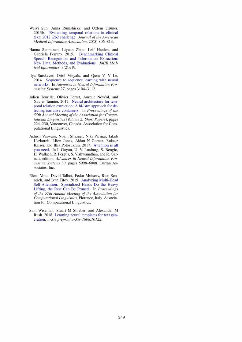
Weiyi Sun, Anna Rumshisky, and Ozlem Uzuner.2013b. Evaluating temporal relations in clinicaltext: 2012 i2b2 challenge. Journal of the AmericanMedical Informatics Association, 20(5):806–813.
Hanna Suominen, Liyuan Zhou, Leif Hanlen, andGabriela Ferraro. 2015. Benchmarking ClinicalSpeech Recognition and Information Extraction:New Data, Methods, and Evaluations. JMIR Med-ical Informatics, 3(2):e19.
Ilya Sutskever, Oriol Vinyals, and Quoc V. V Le.2014. Sequence to sequence learning with neuralnetworks. In Advances in Neural Information Pro-cessing Systems 27, pages 3104–3112.
Julien Tourille, Olivier Ferret, Aurélie Névéol, andXavier Tannier. 2017. Neural architecture for tem-poral relation extraction: A bi-lstm approach for de-tecting narrative containers. In Proceedings of the55th Annual Meeting of the Association for Compu-tational Linguistics (Volume 2: Short Papers), pages224–230, Vancouver, Canada. Association for Com-putational Linguistics.
Ashish Vaswani, Noam Shazeer, Niki Parmar, JakobUszkoreit, Llion Jones, Aidan N Gomez, ŁukaszKaiser, and Illia Polosukhin. 2017. Attention is allyou need. In I. Guyon, U. V. Luxburg, S. Bengio,H. Wallach, R. Fergus, S. Vishwanathan, and R. Gar-nett, editors, Advances in Neural Information Pro-cessing Systems 30, pages 5998–6008. Curran As-sociates, Inc.
Elena Voita, David Talbot, Fedor Moiseev, Rico Sen-nrich, and Ivan Titov. 2019. Analyzing Multi-HeadSelf-Attention: Specialized Heads Do the HeavyLifting, the Rest Can Be Pruned. In Proceedingsof the 57th Annual Meeting of the Association forComputational Linguistics, Florence, Italy. Associa-tion for Computational Linguistics.
Sam Wiseman, Stuart M Shieber, and Alexander MRush. 2018. Learning neural templates for text gen-eration. arXiv preprint arXiv:1808.10122.
249
Proceedings of the BioNLP 2019 workshop, pages 250–260Florence, Italy, August 1, 2019. c©2019 Association for Computational Linguistics
ChiMed: A Chinese Medical Corpus for Question Answering
Yuanhe TianDepartment of LinguisticsUniversity of Washington
Weicheng MaComputer Science Department
New York [email protected]
Fei XiaDepartment of LinguisticsUniversity of Washington
Yan SongTencent AI Lab
Abstract
Question answering (QA) is a challenging taskin natural language processing (NLP), espe-cially when it is applied to specific domains.While models trained in the general domaincan be adapted to a new target domain, theirperformance often degrades significantly dueto domain mismatch. Alternatively, one canrequire a large amount of domain-specific QAdata, but such data are rare, especially for themedical domain. In this study, we first col-lect a large-scale Chinese medical QA corpuscalled ChiMed; second we annotate a smallfraction of the corpus to check the quality ofthe answers; third, we extract two datasetsfrom the corpus and use them for the rele-vancy prediction task and the adoption predic-tion task. Several benchmark models are ap-plied to the datasets, producing good resultsfor both tasks.
1 Introduction
In the big data era, it is often challenging to lo-cate the most helpful information in many real-world applications, such as search engine, cus-tomer service, personal assistant, etc. A series ofNLP tasks, such as text representation, text classi-fication, summarization, keyphrase extraction, andanswer ranking, are able to help QA systems infinding relevant information (Siddiqi and Sharan,2015; Allahyari et al., 2017; Yang et al., 2016;Joulin et al., 2016; Song et al., 2017, 2018).
Currently, most QA corpora are built for thegeneral domain focusing on extracting/generatinganswers from articles, such as CNN/Daily Mail(Hermann et al., 2015), SQuAD (Rajpurkar et al.,2016), Dureader (He et al., 2017), SearchQA(Dunn et al., 2017), CoQA (Reddy et al., 2018),etc., with few others from community QA forums,
such as TrecQA (Wang et al., 2007), WikiQA(Yang et al., 2015), and SemEval-2015 (Nakovet al., 2015).
In the medical domain, most medial QA cor-pora consist of scientific articles, such as BioASQ(Tsatsaronis et al., 2012), emrQA (Pampari et al.,2018), and CliCR (Šuster and Daelemans, 2018).Although some studies were done for conversa-tional datasets (Wang et al., 2018a,b), corporadesigned for community QA are extremely rare.Meanwhile, given that many online medical ser-vice forums have emerged (e.g. MedHelp1), thereare increasing demands from users to search foranswers for their medical concerns. One might betempted to build QA corpora from such forums.However, in doing so, one must address a seriesof challenges such as how to ensure the quality ofthe derived corpus despite the noise in the originalforum data.
In this paper, we introduce our work on build-ing a Chinese medical QA corpus named ChiMedby crawling data from a big Chinese medical fo-rum2. In the forum, the questions are asked byweb users and all the answers are provided by ac-credited physicians. In addition to (Q, A) pairs,the corpus contains rich information such as the ti-tle of the question, key phrases, age and gender ofthe user, the name and affiliation of the accreditedphysicians who answer the question, and so on.As a result, the corpus can be used for many NLPtasks. In this study, we focus on two tasks: rel-evancy prediction (whether an answer is relevantto a question) and adoption prediction (whether ananswer will be adopted).
1https://www.medhelp.org2The code for constructing the corpus and the datasets
used in this study are available at https://github.com/yuanheTian/ChiMed.
250
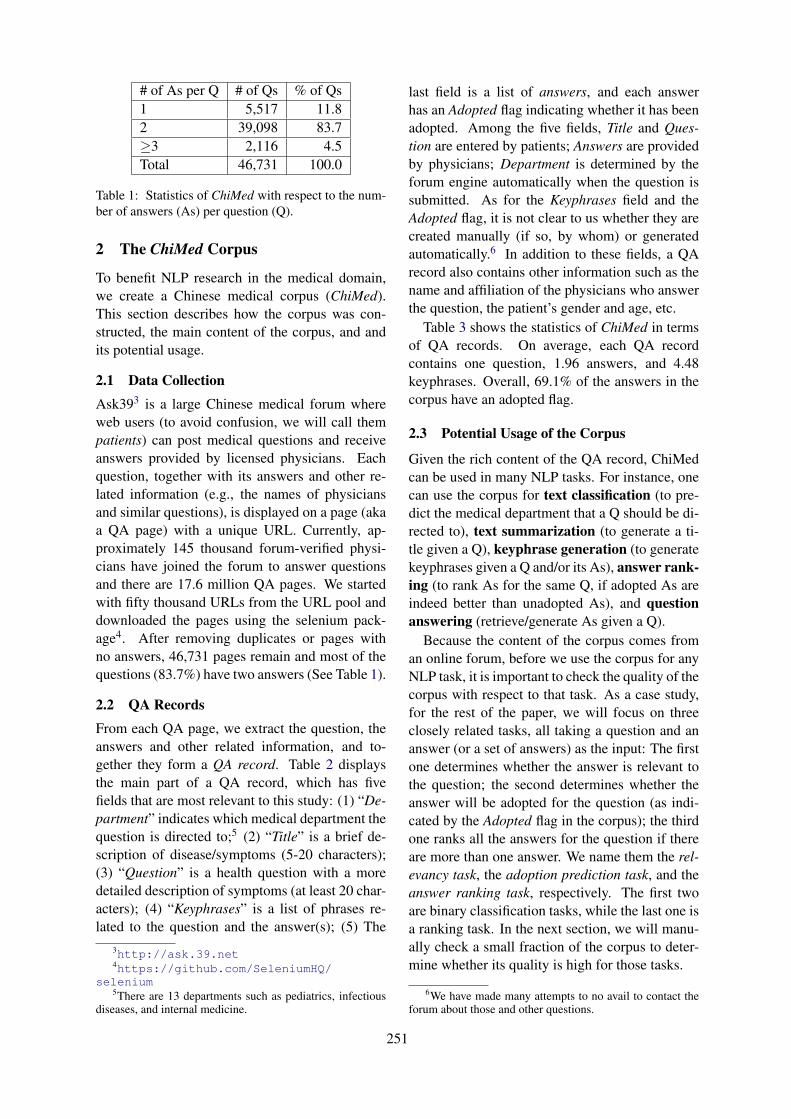
# of As per Q # of Qs % of Qs1 5,517 11.82 39,098 83.7≥3 2,116 4.5Total 46,731 100.0
Table 1: Statistics of ChiMed with respect to the num-ber of answers (As) per question (Q).
2 The ChiMed Corpus
To benefit NLP research in the medical domain,we create a Chinese medical corpus (ChiMed).This section describes how the corpus was con-structed, the main content of the corpus, and andits potential usage.
2.1 Data Collection
Ask393 is a large Chinese medical forum whereweb users (to avoid confusion, we will call thempatients) can post medical questions and receiveanswers provided by licensed physicians. Eachquestion, together with its answers and other re-lated information (e.g., the names of physiciansand similar questions), is displayed on a page (akaa QA page) with a unique URL. Currently, ap-proximately 145 thousand forum-verified physi-cians have joined the forum to answer questionsand there are 17.6 million QA pages. We startedwith fifty thousand URLs from the URL pool anddownloaded the pages using the selenium pack-age4. After removing duplicates or pages withno answers, 46,731 pages remain and most of thequestions (83.7%) have two answers (See Table 1).
2.2 QA Records
From each QA page, we extract the question, theanswers and other related information, and to-gether they form a QA record. Table 2 displaysthe main part of a QA record, which has fivefields that are most relevant to this study: (1) “De-partment” indicates which medical department thequestion is directed to;5 (2) “Title” is a brief de-scription of disease/symptoms (5-20 characters);(3) “Question” is a health question with a moredetailed description of symptoms (at least 20 char-acters); (4) “Keyphrases” is a list of phrases re-lated to the question and the answer(s); (5) The
3http://ask.39.net4https://github.com/SeleniumHQ/
selenium5There are 13 departments such as pediatrics, infectious
diseases, and internal medicine.
last field is a list of answers, and each answerhas an Adopted flag indicating whether it has beenadopted. Among the five fields, Title and Ques-tion are entered by patients; Answers are providedby physicians; Department is determined by theforum engine automatically when the question issubmitted. As for the Keyphrases field and theAdopted flag, it is not clear to us whether they arecreated manually (if so, by whom) or generatedautomatically.6 In addition to these fields, a QArecord also contains other information such as thename and affiliation of the physicians who answerthe question, the patient’s gender and age, etc.
Table 3 shows the statistics of ChiMed in termsof QA records. On average, each QA recordcontains one question, 1.96 answers, and 4.48keyphrases. Overall, 69.1% of the answers in thecorpus have an adopted flag.
2.3 Potential Usage of the Corpus
Given the rich content of the QA record, ChiMedcan be used in many NLP tasks. For instance, onecan use the corpus for text classification (to pre-dict the medical department that a Q should be di-rected to), text summarization (to generate a ti-tle given a Q), keyphrase generation (to generatekeyphrases given a Q and/or its As), answer rank-ing (to rank As for the same Q, if adopted As areindeed better than unadopted As), and questionanswering (retrieve/generate As given a Q).
Because the content of the corpus comes froman online forum, before we use the corpus for anyNLP task, it is important to check the quality of thecorpus with respect to that task. As a case study,for the rest of the paper, we will focus on threeclosely related tasks, all taking a question and ananswer (or a set of answers) as the input: The firstone determines whether the answer is relevant tothe question; the second determines whether theanswer will be adopted for the question (as indi-cated by the Adopted flag in the corpus); the thirdone ranks all the answers for the question if thereare more than one answer. We name them the rel-evancy task, the adoption prediction task, and theanswer ranking task, respectively. The first twoare binary classification tasks, while the last one isa ranking task. In the next section, we will manu-ally check a small fraction of the corpus to deter-mine whether its quality is high for those tasks.
6We have made many attempts to no avail to contact theforum about those and other questions.
251
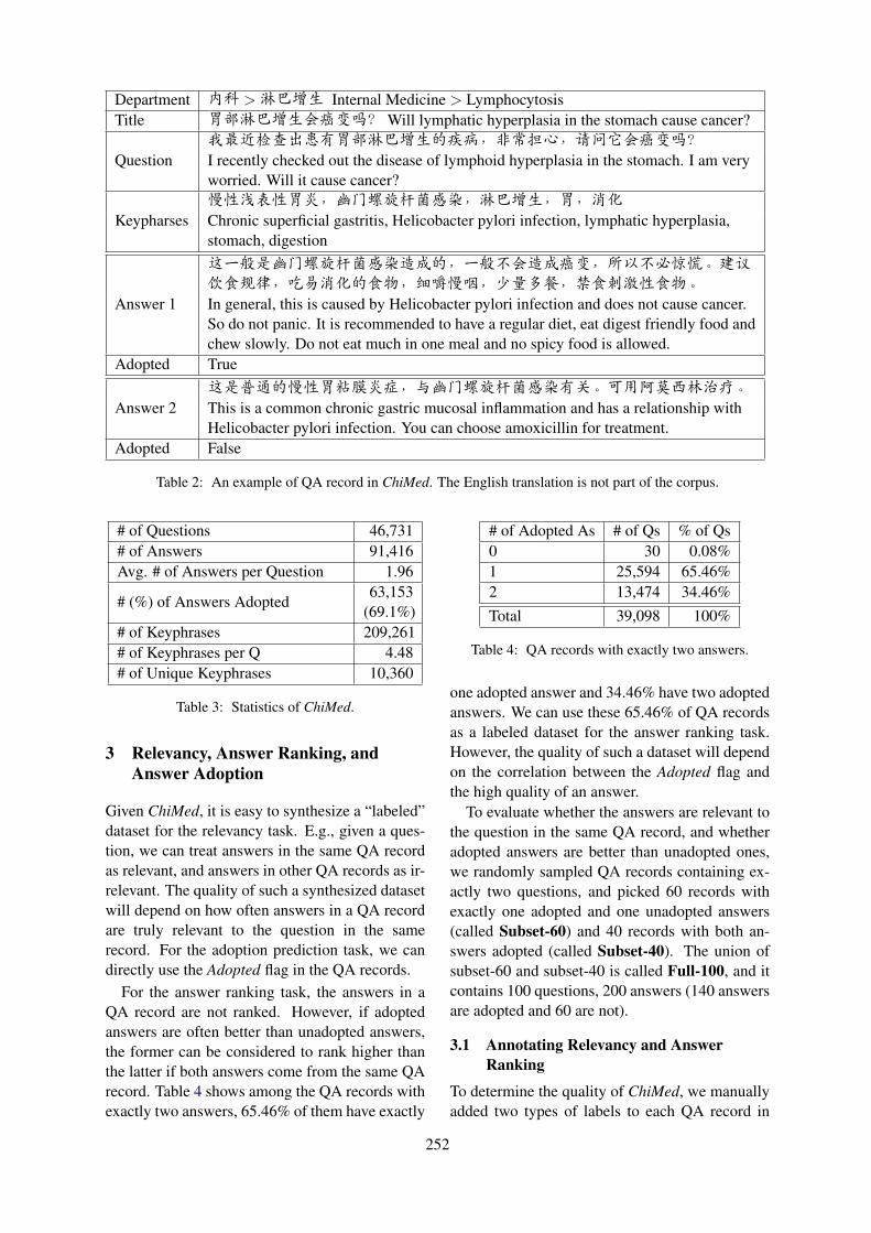
Department 内科 >淋巴增生 Internal Medicine > LymphocytosisTitle 胃部淋巴增生会癌变吗?Will lymphatic hyperplasia in the stomach cause cancer?
Question我最近检查出患有胃部淋巴增生的疾病,非常担心,请问它会癌变吗?I recently checked out the disease of lymphoid hyperplasia in the stomach. I am veryworried. Will it cause cancer?
Keypharses慢性浅表性胃炎,幽门螺旋杆菌感染,淋巴增生,胃,消化Chronic superficial gastritis, Helicobacter pylori infection, lymphatic hyperplasia,stomach, digestion
Answer 1
这一般是幽门螺旋杆菌感染造成的,一般不会造成癌变,所以不必惊慌。建议饮食规律,吃易消化的食物,细嚼慢咽,少量多餐,禁食刺激性食物。In general, this is caused by Helicobacter pylori infection and does not cause cancer.So do not panic. It is recommended to have a regular diet, eat digest friendly food andchew slowly. Do not eat much in one meal and no spicy food is allowed.
Adopted True
Answer 2这是普通的慢性胃粘膜炎症,与幽门螺旋杆菌感染有关。可用阿莫西林治疗。This is a common chronic gastric mucosal inflammation and has a relationship withHelicobacter pylori infection. You can choose amoxicillin for treatment.
Adopted False
Table 2: An example of QA record in ChiMed. The English translation is not part of the corpus.
# of Questions 46,731# of Answers 91,416Avg. # of Answers per Question 1.96
# (%) of Answers Adopted63,153
(69.1%)# of Keyphrases 209,261# of Keyphrases per Q 4.48# of Unique Keyphrases 10,360
Table 3: Statistics of ChiMed.
3 Relevancy, Answer Ranking, andAnswer Adoption
Given ChiMed, it is easy to synthesize a “labeled”dataset for the relevancy task. E.g., given a ques-tion, we can treat answers in the same QA recordas relevant, and answers in other QA records as ir-relevant. The quality of such a synthesized datasetwill depend on how often answers in a QA recordare truly relevant to the question in the samerecord. For the adoption prediction task, we candirectly use the Adopted flag in the QA records.
For the answer ranking task, the answers in aQA record are not ranked. However, if adoptedanswers are often better than unadopted answers,the former can be considered to rank higher thanthe latter if both answers come from the same QArecord. Table 4 shows among the QA records withexactly two answers, 65.46% of them have exactly
# of Adopted As # of Qs % of Qs0 30 0.08%1 25,594 65.46%2 13,474 34.46%Total 39,098 100%
Table 4: QA records with exactly two answers.
one adopted answer and 34.46% have two adoptedanswers. We can use these 65.46% of QA recordsas a labeled dataset for the answer ranking task.However, the quality of such a dataset will dependon the correlation between the Adopted flag andthe high quality of an answer.
To evaluate whether the answers are relevant tothe question in the same QA record, and whetheradopted answers are better than unadopted ones,we randomly sampled QA records containing ex-actly two questions, and picked 60 records withexactly one adopted and one unadopted answers(called Subset-60) and 40 records with both an-swers adopted (called Subset-40). The union ofsubset-60 and subset-40 is called Full-100, and itcontains 100 questions, 200 answers (140 answersare adopted and 60 are not).
3.1 Annotating Relevancy and AnswerRanking
To determine the quality of ChiMed, we manuallyadded two types of labels to each QA record in
252
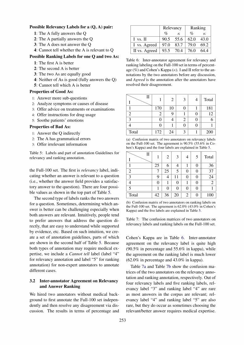
Possible Relevancy Labels for a (Q, A) pair:1: The A fully answers the Q2: The A partially answers the Q3: The A does not answer the Q4: Cannot tell whether the A is relevant to Q
Possible Ranking Labels for one Q and two As:1: The first A is better2: The second A is better3: The two As are equally good4: Neither of As is good (fully answers the Q)5: Cannot tell which A is better
Properties of Good As:1: Answer more sub-questions2: Analyze symptoms or causes of disease3: Offer advice on treatments or examinations4: Offer instructions for drug usage5: Soothe patients’ emotions
Properties of Bad As:1: Answer the Q indirectly2: The A has grammatical errors3: Offer irrelevant information
Table 5: Labels and part of annotation Guidelines forrelevancy and ranking annotation.
the Full-100 set. The first is relevancy label, indi-cating whether an answer is relevant to a question(i.e., whether the answer field provides a satisfac-tory answer to the question). There are four possi-ble values as shown in the top part of Table 5.
The second type of labels ranks the two answersfor a question. Sometimes, determining which an-swer is better can be challenging especially whenboth answers are relevant. Intuitively, people tendto prefer answers that address the question di-rectly, that are easy to understand while supportedby evidence, etc. Based on such intuition, we cre-ate a set of annotation guidelines, parts of whichare shown in the second half of Table 5. Becauseboth types of annotation may require medical ex-pertise, we include a Cannot tell label (label “4”for relevancy annotation and label “5” for rankingannotation) for non-expert annotators to annotatedifferent cases.
3.2 Inter-annotator Agreement on Relevancyand Answer Ranking
We hired two annotators without medical back-ground to first annotate the Full-100 set indepen-dently and then resolve any disagreement via dis-cussion. The results in terms of percentage and
Relevancy Ranking% κ % κ
I vs. II 90.5 55.6 62.0 43.0I vs. Agreed 97.0 83.7 79.0 69.2II vs. Agreed 93.5 70.4 76.0 64.4
Table 6: Inter-annotator agreement for relevancy andranking labeling on the Full-100 set in terms of percent-age (%) and Cohen’s Kappa (κ). I and II refer to the an-notations by the two annotators before any discussion,and Agreed is the annotation after the annotators haveresolved their disagreement.
III
1 2 3 4 Total
1 170 10 0 1 1812 2 9 1 0 123 0 4 2 0 64 0 1 0 0 1Total 172 24 3 1 200
(a) Confusion matrix of two annotators on relevancy labelson the Full-100 set. The agreement is 90.5% (55.6% in Co-hen’s Kappa) and the four labels are explained in Table 5.
III
1 2 3 4 5 Total
1 25 6 4 1 0 362 7 25 5 0 0 373 9 4 11 0 0 244 0 1 0 1 0 25 1 0 0 0 0 1Total 42 36 20 2 0 100
(b) Confusion matrix of two annotators on ranking labels onthe Full-100 set. The agreement is 62.0% (43.0% in Cohen’sKappa) and the five labels are explained in Table 5.
Table 7: The confusion matrices of two annotators onrelevancy labels and ranking labels on the Full-100 set.
Cohen’s Kappa are in Table 6. Inter-annotatoragreement on the relevancy label is quite high(90.5% in percentage and 55.6% in kappa), whilethe agreement on the ranking label is much lower(62.0% in percentage and 43.0% in kappa).
Table 7a and Table 7b show the confusion ma-trices of the two annotators on the relevancy anno-tation and ranking annotation, respectively. Out offour relevancy labels and five ranking labels, rel-evancy label “3” and ranking label “4” are rareas most answers in the corpus are relevant; rel-evancy label “4” and ranking label “5” are alsorare, but they do occur as sometimes choosing therelevant/better answer requires medical expertise.
253
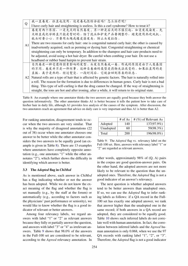
Q我一直卷发,拉直也没用,这是卷毛性综合症吗?怎么治疗呢?I have curly hair and straightening is useless. Is this a curl syndrome? How to treat it?
A1
卷发有两个原因,一是先天的自然卷发;另一种是后天的不慎引起,如烫发或染发。先天矫直或化学矫直只能是暂时的。除了洗头和护发产品要调整外,避免使用热吹风机。梳头时要小心。不要用头绳或橡皮筋发夹,防止头发拉伤。There are two reasons for curly hair: one is congenital natural curly hair; the other is caused byinadvertently acquired, such as perming or dyeing hair. Congenital straightening or chemicalstraightening can only be temporary. In addition to the shampoo and hair care products need tobe adjusted, avoid using a hot hair dryer. Be careful when combing your hair. Do not use aheadband or rubber band hairpin to prevent hair strain.
A2
自然卷是一种受遗传因素影响的发型。头发自然卷成一卷。形成的原因是由于人类基因的不同。卷发并不是一件坏事。这种自卷曲的类型是药物无法改变的。如果拉直用的是直板,离子是热的,经过熨烫,一段时间后,它就会回到原来的状态。Natural rolls are a type of hair that is affected by genetic factors. The hair is naturally rolled intoa roll. The reason for the formation is due to differences in human genes. Curly hair is not a badthing. This type of self-curling is that the drug cannot be changed. If the way of straightening isstraight, the ions are hot and after ironing, after a while, it will return to its original state.
Table 8: An example where one annotator thinks the two answers are equally good because they both answer thequestion informatively. The other annotator thinks A1 is better because it tells the patient how to take care ofhis/her hair in daily life, although A1 provides less analysis of the causes of the symptom. After discussion, thetwo annotators reach an agreement that advice on daily care is very important and thus A1 is better than A2.
For ranking annotation, disagreement tends to oc-cur when the two answers are very similar. Thatis why the majority of disagreed annotations (22out of 38) occur when one annotator chooses oneanswer to be better while the other annotator con-siders the two answers to be equally good (an ex-ample is given in Table 8). There are 13 exampleswhere annotators have completely opposite anno-tation (e.g., one annotates “1” while the other an-notates “2”), which further shows the difficulty inidentifying which answer is better.
3.3 The Adopted flag in ChiMed
As is mentioned above, each answer in ChiMedhas a flag indicating whether or not the answerhas been adopted. While we do not know the ex-act meaning of the flag and whether the flag isset manually (e.g., by the staff at the forum) orautomatically (e.g., according to factors such asthe physicians’ past performance or seniority), wewould like to know whether the flag is a good in-dicator of relevant or better answers.
Among four relevancy labels, we regard an-swers with label “1” or “2” as relevant answersbecause they fully or partially answer the question,and answers with label ”3” or ”4” as irrelevant an-swers. Table 9 shows that 98.0% of the answersin the Full-100 set are considered to be relevant,according to the Agreed relevancy annotation. In
# of As # (%) of Relevant AsAdopted 140 137(97.9%)Unadopted 60 59(98.3%)Total 200 196(98.0%)
Table 9: The Adopted flag vs. relevancy label on theFull-100 set. Here, answers with relevancy label “1” or“2” are regarded as relevant answers.
other words, approximately 98% of (Q, A) pairsin the corpus are good question-answer pairs. Onthe other hand, the adopted answers are not morelikely to be relevant to the question than the un-adopted ones. Therefore, the Adopted flag is not agood indicator of an answer’s relevancy.
The next question is whether adopted answerstend to be better answers than unadopted ones.If so, we can use the Adopted flag to infer rank-ing labels as follows: if a QA record in the Full-100 set has exactly one adopted answer, we rankthat answer higher than the unadopted one in thesame record; if both answers in a QA record areadopted, they are considered to be equally good.Table 10 shows such inferred labels do not corre-late well with human annotation. In fact, the corre-lation between inferred labels and the Agreed hu-man annotation is only 0.068, when we use the 97QA records with ranking label “1”, “2”, or “3”.Therefore, the Adopted flag is not a good indicator
254
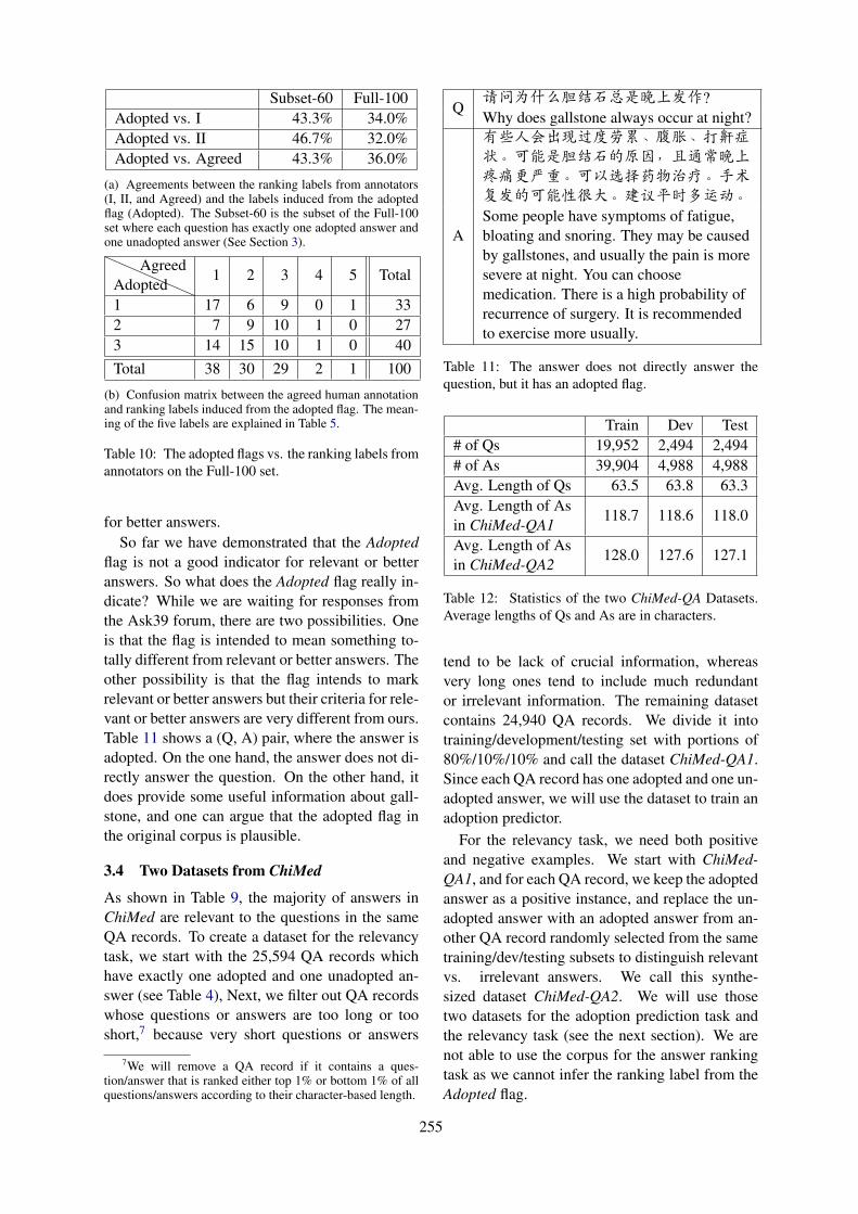
Subset-60 Full-100Adopted vs. I 43.3% 34.0%Adopted vs. II 46.7% 32.0%Adopted vs. Agreed 43.3% 36.0%
(a) Agreements between the ranking labels from annotators(I, II, and Agreed) and the labels induced from the adoptedflag (Adopted). The Subset-60 is the subset of the Full-100set where each question has exactly one adopted answer andone unadopted answer (See Section 3).
AdoptedAgreed
1 2 3 4 5 Total
1 17 6 9 0 1 332 7 9 10 1 0 273 14 15 10 1 0 40Total 38 30 29 2 1 100
(b) Confusion matrix between the agreed human annotationand ranking labels induced from the adopted flag. The mean-ing of the five labels are explained in Table 5.
Table 10: The adopted flags vs. the ranking labels fromannotators on the Full-100 set.
for better answers.So far we have demonstrated that the Adopted
flag is not a good indicator for relevant or betteranswers. So what does the Adopted flag really in-dicate? While we are waiting for responses fromthe Ask39 forum, there are two possibilities. Oneis that the flag is intended to mean something to-tally different from relevant or better answers. Theother possibility is that the flag intends to markrelevant or better answers but their criteria for rele-vant or better answers are very different from ours.Table 11 shows a (Q, A) pair, where the answer isadopted. On the one hand, the answer does not di-rectly answer the question. On the other hand, itdoes provide some useful information about gall-stone, and one can argue that the adopted flag inthe original corpus is plausible.
3.4 Two Datasets from ChiMed
As shown in Table 9, the majority of answers inChiMed are relevant to the questions in the sameQA records. To create a dataset for the relevancytask, we start with the 25,594 QA records whichhave exactly one adopted and one unadopted an-swer (see Table 4), Next, we filter out QA recordswhose questions or answers are too long or tooshort,7 because very short questions or answers
7We will remove a QA record if it contains a ques-tion/answer that is ranked either top 1% or bottom 1% of allquestions/answers according to their character-based length.
Q请问为什么胆结石总是晚上发作?Why does gallstone always occur at night?
A
有些人会出现过度劳累、腹胀、打鼾症状。可能是胆结石的原因,且通常晚上疼痛更严重。可以选择药物治疗。手术复发的可能性很大。建议平时多运动。Some people have symptoms of fatigue,bloating and snoring. They may be causedby gallstones, and usually the pain is moresevere at night. You can choosemedication. There is a high probability ofrecurrence of surgery. It is recommendedto exercise more usually.
Table 11: The answer does not directly answer thequestion, but it has an adopted flag.
Train Dev Test# of Qs 19,952 2,494 2,494# of As 39,904 4,988 4,988Avg. Length of Qs 63.5 63.8 63.3Avg. Length of As
118.7 118.6 118.0in ChiMed-QA1Avg. Length of As
128.0 127.6 127.1in ChiMed-QA2
Table 12: Statistics of the two ChiMed-QA Datasets.Average lengths of Qs and As are in characters.
tend to be lack of crucial information, whereasvery long ones tend to include much redundantor irrelevant information. The remaining datasetcontains 24,940 QA records. We divide it intotraining/development/testing set with portions of80%/10%/10% and call the dataset ChiMed-QA1.Since each QA record has one adopted and one un-adopted answer, we will use the dataset to train anadoption predictor.
For the relevancy task, we need both positiveand negative examples. We start with ChiMed-QA1, and for each QA record, we keep the adoptedanswer as a positive instance, and replace the un-adopted answer with an adopted answer from an-other QA record randomly selected from the sametraining/dev/testing subsets to distinguish relevantvs. irrelevant answers. We call this synthe-sized dataset ChiMed-QA2. We will use thosetwo datasets for the adoption prediction task andthe relevancy task (see the next section). We arenot able to use the corpus for the answer rankingtask as we cannot infer the ranking label from theAdopted flag.
255
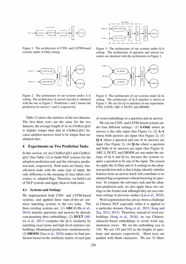
Figure 1: The architecture of CNN- and LSTM-basedsystems under A-Only setting.
Figure 2: The architecture of our systems under A-Asetting. The architecture of answer encoder is identicalwith the one in Figure 1. Prediction 1 and 2 means theprediction for answer 1 and 2, respectively.
Table 12 shows the statistics of the two datasets.The first three rows are the same for the twodatasets; the average length of As in ChiMed-QA2is slightly longer than that in ChiMed-QA1 be-cause adopted answers tend to be longer than un-adopted ones.
4 Experiments on Two Prediction Tasks
In this section, we use ChiMed-QA1 and ChiMed-QA2 (See Table 12) to build NLP systems for theadoption prediction task and the relevancy predic-tion task, respectively. Both tasks are binary clas-sification tasks with the same type of input; theonly difference is the meaning of class labels (rel-evancy vs. adopted flag). Therefore, we build a setof NLP systems and apply them to both tasks.
4.1 Systems and SettingsWe implemented both CNN- and LSTM-basedsystems, and applied three state-of-the-art sen-tence matching systems to the two tasks. Thethree existing systems are: (1) ARC-I (Hu et al.,2014) matches questions and answers by directlyconcatenating their embeddings; (2) DUET (Mi-tra et al., 2017) computes the Q-A similarity bymatching exact terms and high-level sentence em-beddings (Hadamard production) simultaneously;(3) DRMM (Guo et al., 2016) makes its final pre-diction based on the similarity matrix of each pair
Figure 3: The architecture of our systems under Q-Asetting. The architecture of question and answer en-coders are identical with the architecture in Figure 1.
Figure 4: The architecture of our systems under Q-Assetting. The architecture of Q-A matcher is shown inFigure 3. We use five Q-A matchers in our experiment:CNN, LSTM, ARC-I, DUET, and DRMM.
of word embeddings in a question and an answer.We run our CNN- and LSTM-based systems un-
der four different settings: (1) A-Only where ananswer is the only input (See Figure 1); (2) A-Awhere both answers are input (See Figure 2); (3)Q-A where a question and one of its answers areinput (See Figure 3); (4) Q-As where a questionand both of its answers are input (See Figure 4).ARC-I, DUET, and DRMM are run under the set-tings of Q-A and Q-As, because the systems re-quire a question to be one of the input. The reasonwe apply the A-Only and A-A settings to the adop-tion prediction task is that it helps identify whetherfeatures from an answer itself will contribute to itsadopted flag assignment without knowing its ques-tion. To compare the relevancy task and the adop-tion prediction task, we also apply these two set-tings to the former task although they are not com-mon settings in previous studies (Lai et al., 2018).
Word segmentation has always been a challengein Chinese NLP especially when it is applied toa particular domain (Song et al., 2012; Song andXia, 2012, 2013). Therefore, instead of word em-beddings (Song et al., 2018), we use Chinese-character-based embeddings to avoid word seg-mentation errors. We set the embedding size to150. We use 155 and 245 as the lengths of ques-tions and answers respectively. Short texts arepadded with blank characters. We use 32 filters
256
SysID
InputSetting
NLPSystem
RelevancyPrediction
AdoptionPrediction
-CR +CR -CR +CR1 A-Only CNN 50.80 51.64 74.10 81.642 LSTM 50.66 50.72 74.24 82.003 A-A CNN 49.40 - 84.20 -4 LSTM 50.28 - 85.00 -5
Q-A
CNN 74.32 81.84 74.84 81.076 LSTM 80.19 87.09 75.28 83.647 ARC-I 50.34 50.60 75.20 82.648 DUET 81.03 91.74 75.28 82.489 DRMM 93.60 98.16 71.49 83.88
10
Q-As
CNN 76.98 - 83.52 -11 LSTM 88.41 - 84.24 -12 ARC-I 48.84 - 83.88 -13 DUET 87.17 - 83.36 -14 DRMM 98.32 - 83.28 -
Table 13: Results of all systems under different set-tings with respect to (Q, A) pair prediction accuracywith (+CR) and without (-CR) conflict resolution. Wedo not present results of +CR in A-A and Q-As settingsbecause they are equivalent to the results of -CR.
with the kernel size 3 for every CNN layer andwe set the LSTM hidden size to 32. We apply apooling size of 2 to all max pooling layers. Be-sides, the activation function of the output layersunder A-Only and Q-A settings is sigmoid, thatof output layers under A-A and Q-As settings issoftmax, and that of all other layers is tanh.
In addition, noting that the two answers forthe same question have opposite labels in bothtasks, we evaluate all systems in terms of (Q, A)pair predication accuracy with and without con-flict resolution (CR), with which the model re-solves conflicts when either two relevant/adoptedanswers or two irrelevant/unadopted answers arepredicted. Because the activation function of theoutput layers under A-A and Q-As settings issoftmax and because there are always two an-swers for each question, systems under these twosettings never generate conflict predictions. Wedo not apply MAP (Mean Average Precision) (Laiet al., 2018) to the tasks because the number ofcandidate answers of each question in the datasetsis limited to 2.
4.2 Experimental Results
Table 13 shows the experimental results of runningthe five predictors on the testing set under four dif-ferent settings. There are a few observations.
First, for the relevancy task, by designing onlyhalf of the (Q, A) pairs in ChiMed-QA2 come fromthe same QA records. When Q is not given aspart of the input (System 1-4), it is impossible forthe predictors to determine whether an answer is
relevant; therefore, the system performances areno better than random guesses. In contrast, forthe adoption prediction task, by designing all the(Q, A) pairs in ChiMed-QA1 come from the sameQA records, and according to Table 9 we alsoknow that about 98% of the answers, regardlessof whether they are adopted or not, are relevant.Therefore, the absence of Qs in System 1-4 doesnot affect system performance a lot.
Second, when both Q and A are present (System5-9), the accuracy of relevancy prediction is higherthan that of adoption prediction, because the for-mer is an easier task (at least for humans). Theonly exception is ARC-I (System 7), whose resultson relevancy is close to random guess (50.34% and50.60%) while the result on adoption is compara-ble with other systems. This is due to the way thatARC-I matches questions and answers. Becauseembeddings of a question and an answer are di-rectly concatenated in ARC-I, Q-A similarity arenot fully captured, leading to low performance onrelevancy. On the contrary, the adoption predic-tion does not rely much on the Q-A similarity (asexplained above).
Third, for the relevancy task, systems that cap-ture more features of Q-A similarity tend to havea better result. For example, under the Q-A set-ting, DUET (System 8) outperforms CNN, LSTMand ARC-I (System 5-7) because DUET has anadditional model of exact phrase matching be-tween questions and answers. DRMM (System 9)performs better than DUET (System 8) becauseDRMM uses word embedding instead of exactphrase when matching pairs of phrases between aquestion and an answer. In contrast, the perfor-mances of the five systems on the adoption taskare very similar.
In addition, except for the relevancy task eval-uated with CR, the contrast between System 10-14 vs. System 5-9 indicates comparing two Asalways helps predictors in both tasks because in-tuitively knowing both answers would help us todecide which one is relevant/adopted. On thecontrary, the comparison between the same twogroups of systems with CR in the relevancy taskindicates comparing two As may hurt the rele-vancy predictors (System 5, 7, 8) because the rel-evancy is really between Q and A, which might beaffected by the existence of other As.
Finally, all the systems under A-Only and Q-Asettings (Systems 1-2 and 5-9) benefit from CR. It
257
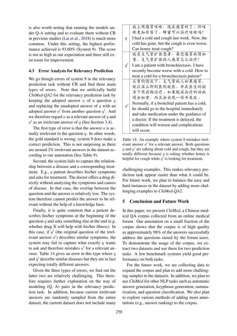
is also worth noting that running the models un-der Q-A setting and to evaluate them without CRin previous studies (Lai et al., 2018) is much morecommon. Under this setting, the highest perfor-mance achieved is 93.60% (System 9). The scoreis not as high as our expectation and there still ex-ist room for improvement.
4.3 Error Analysis for Relevancy Prediction
We go though errors of system 9 in the relevancyprediction task without CR and find three maintypes of errors. Note that we artificially buildChiMed-QA2 for the relevancy prediction task bykeeping the adopted answer a of a question qand replacing the unadopted answer of q with anadopted answer a′ from another question q′. Andwe therefore regard a as a relevant answer of q anda′ as an irrelevant answer of q (See Section 3.4).
The first type of error is that the answer a is ac-tually irrelevant to the question q. In other words,the gold standard is wrong; system 9 does make acorrect prediction. This is not surprising as thereare around 2% irrelevant answers in the dataset ac-cording to our annotation (See Table 9).
Second, the system fails to capture the relation-ship between a disease and a corresponding treat-ment. E.g., a patient describes his/her symptomsand asks for treatment. The doctor offers a drug di-rectly without analyzing the symptoms and causesof disease. In that case, the overlap between thequestion and the answer is relatively low. The sys-tem therefore cannot predict the answer to be rel-evant without the help of a knowledge base.
Finally, it is quite common that a patient de-scribes his/her symptoms at the beginning of thequestion q and asks something else at the end (e.g.whether drug X will help with his/her illness). Inthis case, if q′ (the original question of the irrel-evant answer a′) describes similar symptoms, thesystem may fail to capture what exactly q wantsto ask and therefore mistakes a′ for a relevant an-swer. Table 14 gives an error in this type where qand q′ describe similar diseases but they are in factexpecting totally different answers.
Given the three types of errors, we find out thelatter two are relatively challenging. This there-fore requires further exploration on the way ofmodeling (Q, A) pairs in the relevancy predic-tion task. In addition, because current irrelevantanswers are randomly sampled from the entiredataset, the current dataset does not include many
q
我上周感冒咳嗽,现在感冒好了,但咳嗽更加厉害了。蜂蜜可以治疗咳嗽吗?I had a cold and cough last week. Now, thecold has gone, but the cough is even worse.Can honey treat cough?
q′
我是支气管扩张患者,最近感冒病情加重。支气管扩张病人感冒怎么治疗?I am a patient with bronchiectasis. I haverecently become worse with a cold. How totreat a cold for a bronchiectasis patient?
a′
正常的情况下,支气管病人如果感冒,就应该立即到医院就医,并在医生的指导下用药物治疗。如果耽误治疗的话病情会加重,而且会出现一些并发症。Normally, if a bronchial patient has a cold,he should go to the hospital immediatelyand take medication under the guidance ofa doctor. If the treatment is delayed, thecondition will worsen and complicationswill occur.
Table 14: An example where system 9 mistakes irrel-evant answer a′ for a relevant answer. Both questionsq and q′ are talking about cold and cough, but they aretotally different because q is asking whether honey ishelpful for cough while q′ is looking for treatment.
challenging examples. This makes relevancy pre-diction task appear easier than what it could be.For future work, we plan to balance the easy andhard instances in the dataset by adding more chal-lenging examples to ChiMed-QA2.
5 Conclusion and Future Work
In this paper, we present ChiMed, a Chinese med-ical QA corpus collected from an online medicalforum. Our annotation on a small fraction of thecorpus shows that the corpus is of high qualityas approximately 98% of the answers successfullyaddress the questions raised by the forum users.To demonstrate the usage of the corpus, we ex-tract two datasets and use them for two predictiontasks. A few benchmark systems yield good per-formance on both tasks.
For the future work, we are collecting data toexpand the corpus and plan to add more challeng-ing samples to the datasets. In addition, we plan touse ChiMed for other NLP tasks such as automaticanswer generation, keyphrase generation, summa-rization, and question classification. We also planto explore various methods of adding more anno-tations (e.g., answer ranking) to the corpus.
258
References
Mehdi Allahyari, Seyedamin Pouriyeh, Mehdi Assefi,Saeid Safaei, Elizabeth D Trippe, Juan B Gutier-rez, and Krys Kochut. 2017. Text summariza-tion techniques: a brief survey. arXiv preprintarXiv:1707.02268.
Matthew Dunn, Levent Sagun, Mike Higgins, V UgurGuney, Volkan Cirik, and Kyunghyun Cho. 2017.Searchqa: A new q&a dataset augmented withcontext from a search engine. arXiv preprintarXiv:1704.05179.
Jiafeng Guo, Yixing Fan, Qingyao Ai, and W BruceCroft. 2016. A deep relevance matching modelfor ad-hoc retrieval. In Proceedings of the 25thACM International on Conference on Informationand Knowledge Management, pages 55–64. ACM.
Wei He, Kai Liu, Jing Liu, Yajuan Lyu, ShiqiZhao, Xinyan Xiao, Yuan Liu, Yizhong Wang,Hua Wu, Qiaoqiao She, et al. 2017. Dureader:a chinese machine reading comprehension datasetfrom real-world applications. arXiv preprintarXiv:1711.05073.
Karl Moritz Hermann, Tomas Kocisky, EdwardGrefenstette, Lasse Espeholt, Will Kay, Mustafa Su-leyman, and Phil Blunsom. 2015. Teaching ma-chines to read and comprehend. In Advances inneural information processing systems, pages 1693–1701.
Baotian Hu, Zhengdong Lu, Hang Li, and QingcaiChen. 2014. Convolutional neural network architec-tures for matching natural language sentences. InAdvances in neural information processing systems,pages 2042–2050.
Armand Joulin, Edouard Grave, Piotr Bojanowski, andTomas Mikolov. 2016. Bag of tricks for efficient textclassification. arXiv preprint arXiv:1607.01759.
Tuan Manh Lai, Trung Bui, and Sheng Li. 2018. Areview on deep learning techniques applied to an-swer selection. In Proceedings of the 27th Inter-national Conference on Computational Linguistics,pages 2132–2144.
Bhaskar Mitra, Fernando Diaz, and Nick Craswell.2017. Learning to match using local and distributedrepresentations of text for web search. In Proceed-ings of the 26th International Conference on WorldWide Web, pages 1291–1299. International WorldWide Web Conferences Steering Committee.
Preslav Nakov, Lluı́s Màrquez, Walid Magdy, Alessan-dro Moschitti, Jim Glass, and Bilal Randeree. 2015.Semeval-2015 task 3: Answer selection in com-munity question answering. In Proceedings of the9th International Workshop on Semantic Evaluation(SemEval 2015), pages 269–281.
Anusri Pampari, Preethi Raghavan, Jennifer Liang, andJian Peng. 2018. emrqa: A large corpus for ques-tion answering on electronic medical records. arXivpreprint arXiv:1809.00732.
Pranav Rajpurkar, Jian Zhang, Konstantin Lopyrev, andPercy Liang. 2016. Squad: 100,000+ questionsfor machine comprehension of text. arXiv preprintarXiv:1606.05250.
Siva Reddy, Danqi Chen, and Christopher D Manning.2018. Coqa: A conversational question answeringchallenge. arXiv preprint arXiv:1808.07042.
Sifatullah Siddiqi and Aditi Sharan. 2015. Keywordand keyphrase extraction techniques: a literature re-view. International Journal of Computer Applica-tions, 109(2).
Yan Song, Prescott Klassen, Fei Xia, and Chunyu Kit.2012. Entropy-based training data selection for do-main adaptation. In Proceedings of COLING 2012:Posters, pages 1191–1200, Mumbai, India.
Yan Song, Chia-Jung Lee, and Fei Xia. 2017. Learn-ing word representations with regularization fromprior knowledge. In Proceedings of the 21st Confer-ence on Computational Natural Language Learning(CoNLL 2017), pages 143–152, Vancouver, Canada.
Yan Song, Shuming Shi, Jing Li, and Haisong Zhang.2018. Directional skip-gram: Explicitly distinguish-ing left and right context for word embeddings. InProceedings of the 2018 Conference of the NorthAmerican Chapter of the Association for Computa-tional Linguistics: Human Language Technologies,Volume 2, pages 175–180, New Orleans, Louisiana.
Yan Song and Fei Xia. 2012. Using a goodness mea-surement for domain adaptation: A case study onChinese word segmentation. In Proceedings of theEighth International Conference on Language Re-sources and Evaluation (LREC-2012), pages 3853–3860, Istanbul, Turkey.
Yan Song and Fei Xia. 2013. A common case of jekylland hyde: The synergistic effect of using dividedsource training data for feature augmentation. InProceedings of the Sixth International Joint Confer-ence on Natural Language Processing, pages 623–631, Nagoya, Japan.
Simon Šuster and Walter Daelemans. 2018. Clicr: adataset of clinical case reports for machine readingcomprehension. arXiv preprint arXiv:1803.09720.
George Tsatsaronis, Michael Schroeder, GeorgiosPaliouras, Yannis Almirantis, Ion Androutsopoulos,Eric Gaussier, Patrick Gallinari, Thierry Artieres,Michael R Alvers, Matthias Zschunke, et al. 2012.Bioasq: A challenge on large-scale biomedical se-mantic indexing and question answering. In 2012AAAI Fall Symposium Series.
259
Mengqiu Wang, Noah A Smith, and Teruko Mita-mura. 2007. What is the jeopardy model? a quasi-synchronous grammar for qa. In Proceedings ofthe 2007 Joint Conference on Empirical Methodsin Natural Language Processing and ComputationalNatural Language Learning (EMNLP-CoNLL).
Nan Wang, Yan Song, and Fei Xia. 2018a. Cod-ing structures and actions with the COSTA schemein medical conversations. In Proceedings of theBioNLP 2018 workshop, pages 76–86, Melbourne,Australia.
Nan Wang, Yan Song, and Fei Xia. 2018b. Construct-ing a Chinese medical conversation corpus anno-tated with conversational structures and actions. InProceedings of the 11th Language Resources andEvaluation Conference, Miyazaki, Japan.
Liu Yang, Qingyao Ai, Jiafeng Guo, and W BruceCroft. 2016. anmm: Ranking short answer textswith attention-based neural matching model. In Pro-ceedings of the 25th ACM international on confer-ence on information and knowledge management,pages 287–296. ACM.
Yi Yang, Wen-tau Yih, and Christopher Meek. 2015.Wikiqa: A challenge dataset for open-domain ques-tion answering. In Proceedings of the 2015 Con-ference on Empirical Methods in Natural LanguageProcessing, pages 2013–2018.
260
Proceedings of the BioNLP 2019 workshop, pages 261–272Florence, Italy, August 1, 2019. c©2019 Association for Computational Linguistics
Clinical Concept Extraction for Document-Level Coding
Sarah Wiegreffe1, Edward Choi1∗, Sherry Yan2, Jimeng Sun1, Jacob Eisenstein1
1Georgia Institute of Technology2Sutter Health
∗ Current Affiliation: Google [email protected], [email protected], [email protected],
[email protected], [email protected]
AbstractThe text of clinical notes can be a valuablesource of patient information and clinical as-sessments. Historically, the primary approachfor exploiting clinical notes has been informa-tion extraction: linking spans of text to con-cepts in a detailed domain ontology. How-ever, recent work has demonstrated the poten-tial of supervised machine learning to extractdocument-level codes directly from the rawtext of clinical notes. We propose to bridgethe gap between the two approaches with twonovel syntheses: (1) treating extracted con-cepts as features, which are used to supple-ment or replace the text of the note; (2) treatingextracted concepts as labels, which are used tolearn a better representation of the text. Un-fortunately, the resulting concepts do not yieldperformance gains on the document-level clin-ical coding task. We explore possible explana-tions and future research directions.
1 Introduction
Clinical decision support from raw-text notes takenby clinicians about patients has proven to be avaluable alternative to state-of-the-art models builtfrom structured EHRs. Clinical notes contain valu-able information that the structured part of theEHR does not provide, and do not rely on expen-sive and time-consuming human annotation (Torreset al., 2017; American Academy of ProfessionalCoders, 2019). Impressive advances using deeplearning have allowed for modeling on the raw textalone (Mullenbach et al., 2018; Rios and Kavuluru,2018a; Baumel et al., 2018). However, there existsome shortcomings to these approaches: clinicaltext is noisy, and often contains heavy amounts ofabbreviations and acronyms, a challenge for ma-chine reading (Nguyen and Patrick, 2016). Addi-tionally, rare words replaced with "UNK" tokensfor better generalization may be crucial for predict-ing rare labels.
Clinical concept extraction tools abstract overthe noise inherent in surface representations ofclinical text by linking raw text to standardizedconcepts in clinical ontologies. The Apache clin-ical Text Analysis Knowledge Extraction System(cTAKES, Savova et al., 2010) is the most widely-used such tool, with over 1000 citations. Based onrules and non-neural machine learning methods andengineered for almost a decade, cTAKES providesan easily-obtainable source of human-encoded do-main knowledge, although it cannot leverage deeplearning to make document-level predictions.
Our goal in this paper is to maximize the predic-tive power of clinical notes by bridging the gapbetween information extraction and deep learn-ing models. We address the following researchquestions: how can we best leverage tools such ascTAKES on clinical text? Can we show the valueof these tools in linking unstructured data to struc-tured codes in an existing ontology for downstreamprediction?
We explore two novel hybrids of these meth-ods: data augmentation (augmenting text with ex-tracted concepts) and multi-task learning (learningto predict the output of cTAKES). Unfortunately,in neither case does cTAKES improve downstreamperformance on the document-level clinical cod-ing task. We probe this negative result through anextensive series of ablations, and suggest possibleexplanations, such as the lack of word variationcaptured through concept assignment.
2 Related Work
Clinical Ontologies Clinical concept ontologiesfacilitate the maintenance of EHR systems withstandardized and comprehensive code sets, allow-ing consistency across healthcare institutions andpractitioners. The Unified Medical Language Sys-tem (UMLS) (Lindberg et al., 1993) maintains
261
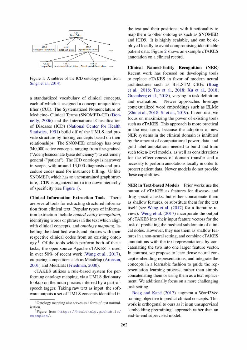
Figure 1: A subtree of the ICD ontology (figure fromSingh et al., 2014).
a standardized vocabulary of clinical concepts,each of which is assigned a concept unique iden-tifier (CUI). The Systematized Nomenclature ofMedicine- Clinical Terms (SNOMED-CT) (Don-nelly, 2006) and the International Classificationof Diseases (ICD) (National Center for HealthStatistics, 1991) build off of the UMLS and pro-vide structure by linking concepts based on theirrelationships. The SNOMED ontology has over340,000 active concepts, ranging from fine-grained("Adenylosuccinate lyase deficiency") to extremelygeneral ("patient"). The ICD ontology is narrowerin scope, with around 13,000 diagnosis and pro-cedure codes used for insurance billing. UnlikeSNOMED, which has an unconstrained graph struc-ture, ICD9 is organized into a top-down hierarchyof specificity (see Figure 1).
Clinical Information Extraction Tools Thereare several tools for extracting structured informa-tion from clinical text. Popular types of informa-tion extraction include named-entity recognition,identifying words or phrases in the text which alignwith clinical concepts, and ontology mapping, la-belling the identified words and phrases with theirrespective clinical codes from an existing ontol-ogy.1 Of the tools which perform both of thesetasks, the open-source Apache cTAKES is usedin over 50% of recent work (Wang et al., 2017),outpacing competitors such as MetaMap (Aronson,2001) and MedLEE (Friedman, 2000).
cTAKES utilizes a rule-based system for per-forming ontology mapping, via a UMLS dictionarylookup on the noun phrases inferred by a part-of-speech tagger. Taking raw text as input, the soft-ware outputs a set of UMLS concepts identified in
1Ontology mapping also serves as a form of text normal-ization.
2Figure from https://healthnlp.github.io/examples/.
the text and their positions, with functionality tomap them to other ontologies such as SNOMEDand ICD9. It is highly scalable, and can be de-ployed locally to avoid compromising identifiablepatient data. Figure 2 shows an example cTAKESannotation on a clinical record.
Clinical Named-Entity Recognition (NER)Recent work has focused on developing toolsto replace cTAKES in favor of modern neuralarchitectures such as Bi-LSTM CRFs (Boaget al., 2018; Tao et al., 2018; Xu et al., 2018;Greenberg et al., 2018), varying in task definitionand evaluation. Newer approaches leveragecontextualized word embeddings such as ELMo(Zhu et al., 2018; Si et al., 2019). In contrast, wefocus on maximizing the power of existing toolssuch as cTAKES. This approach is more practicalin the near-term, because the adoption of newNER systems in the clinical domain is inhibitedby the amount of computational power, data, andgold-label annotations needed to build and trainsuch token-level models, as well as considerationsfor the effectiveness of domain transfer and anecessity to perform annotations locally in order toprotect patient data. Newer models do not providethese capabilities.
NER in Text-based Models Prior works use theoutput of cTAKES as features for disease- anddrug-specific tasks, but either concatenate themas shallow features, or substitute them for the textitself (see Wang et al. (2017) for a literature re-view). Weng et al. (2017) incorporate the outputof cTAKES into their input feature vectors for thetask of predicting the medical subdomain of clini-cal notes. However, they use them as shallow fea-tures in a non-neural setting, and combine cTAKESannotations with the text representations by con-catenating the two into one larger feature vector.In contrast, we propose to learn dense neural con-cept embedding representations, and integrate theconcepts in a learnable fashion to guide the rep-resentation learning process, rather than simplyconcatenating them or using them as a text replace-ment. We additionally focus on a more challengingtask setting.
Boag and Kané (2017) augment a Word2Vectraining objective to predict clinical concepts. Thiswork is orthogonal to ours as it is an unsupervised"embedding pretraining" approach rather than anend-to-end supervised model.
262
Figure 2: An example of cTAKES annotation output with part-of-speech tags and UMLS CUIs for named entities.2
Automated Clinical Coding The automatedclinical coding task is to predict from the raw textof a hospital discharge summary describing a pa-tient encounter all of the possible ICD9 (diagnosisand procedure) codes which a human annotatorwould assign to the visit. Because these annotatorsare trained professionals, the ICD codes assignedserve as a natural label set for describing a patientrecord, and the task can be seen as a proxy fora general patient outcome or treatment predictiontask. State-of-the-art methods such as CAML (Mul-lenbach et al., 2018) treat each label prediction asa separate task, performing many binary classifi-cations over the many-thousand-dimensional labelspace. The model is described in more detail in thenext section.
The label space is very large (tens of thousandsof possible codes) and frequency is long-tailed.Rios and Kavuluru (2018b) find that CAML per-forms weakly on rare labels.
3 Problem Setup
Task Notation A given discharge summary isrepresented as a matrix X ∈ Rde×N .3 The set ofdiagnosis and procedure codes assigned to the visitis represented as the one-hot vector y ∈ {0, 1}L.The task can be framed as L = |L| binary classifi-cations: predict yl ∈ {0, 1} for code l in labelspaceL.
Data We use the publically-available MIMIC-IIIdataset, a collection of deidentified discharge sum-maries describing patient stays in the Beth IsraelDeaconess Medical Center ICU between 2001 and2012 (Johnson et al., 2016; Pollard and Johnson,2016). Each discharge summary has been taggedwith a set of ICD9 codes. See Figure 3 for an exam-ple of a record, and Appendix A for a descriptionof the dataset and preprocessing.
Concept Annotation We run cTAKES on thedischarge summaries (described in Appendix B).
3We use notation for a single instance throughout.
Results on the extracted concepts are presented inTable 1. Note the difference in number of anno-tations provided by using the SNOMED ontologycompared to ICD9.4
ICD9Total concepts extracted 1,005,756Mean # extracted concepts per document 19.10Mean % words assigned a concept per document 1.26%
SNOMEDTotal concepts extracted 28,090,075Mean # extracted concepts per document 532.76Mean % words assigned a concept per document 35.21%
Mean # tokens per document 1513.00
Table 1: Descriptive Statistics on concept extraction forthe MIMIC-III corpus.
Base model We evaluate against CAML (Mul-lenbach et al., 2018), a state-of-the-art text-basedmodel for the clinical coding task. The model lever-ages a convolutional neural network (CNN) withper-label attention to predict the combination ofcodes to assign to a diven discharge summary. Ap-plying convolution overX results in a convolvedinput representationH ∈ Rdc×N (with dc < de) inwhich the column-dimensionality N is preserved.H is then used to predict y, by attentional poolingover the columns.
We include implementation details of all meth-ods, including hyperparameters and training, inAppendix A.
4 Approach 1: Augmentation Model
One limitation of learning-based models is theirtendency to lose uncommon words to "UNK" to-kens, or to suffer from poor representation learningfor them. We hypothesize that rare words are impor-tant for predicting rare labels, and that text-based
4Preliminary experiments with sparser ontologies(RXNORM) were not promising, leading us to choose thesetwo ontologies based on their annotation richness (SNOMED)and direct relation to the prediction task (ICD9).
263
Figure 3: An example clinical discharge summary and associated ICD codes.
models may be improved by augmenting word em-beddings with concept embeddings as a means tostrengthen representations of rare or unseen words.We additionally hypothesize that linking multiplewords to a shared concept via cTAKES annotationwill reduce textual noise by grouping word variantsto a shared representation in a smaller and morefrequently updated parameter space.
4.1 Method
Given a discharge summary containing wordsw1, w2, ..., wN ∈ W∗ and an embedding func-tion γ : W → Rde , we construct input ma-trix X = [xT
1 ,xT2 , ...,x
TN ] ∈ Rde×N as column-
stacked word embeddings, where xn = γ(wn).We additionally assume a code embedding func-
tion φ : C → Rde and a set of annotated codesfor a given document c1, c2, . . . , cN ∈ C∗, whereC is the full codeset for the ontology used to anno-tate the document, and cn is the code annotated forword tokenwn, if one exists (else cn = ∅, by abuseof notation). We construct a representation for eachdocument, D, of the same dimensionality as X ,by learning one representation leveraging both theconcept and word embedding at each position:
For token n,
dn =βwn,cnφ(cn) + (1− βwn,cn)xn, (1)
βwn,cn ∈ [0, 1] is a learned parameter specific toeach observed word+concept pair, including UNKtokens.5 Intuitively, if there is a concept associ-ated with index n, a concept embedding φ(cn) isgenerated and a linear combination of the wordand concept embedding is learned, using a learned
5We experimented with models in which this gate wascomputed element-wise and shared by all word+concept pairs(e.g. by passing xn and φ(cn) through a linear layer or sim-ple multi-layer perceptron to compute dn), but this did notimprove performance.
parameter specific to that word+concept pair.6 Wefix βwn,cn=∅ = 0, which reverts to the word em-bedding when there is no concept assigned.
We additionally propose a simpler version of thismethod, full replace, in which word embeddingsare completely replaced with concept embeddingsif they exist (i.e. βwn,cn = 1, ∀wn, cn 6= ∅). Inthis formulation, if a concept spans multiple words,all of those words are represented by the same vec-tor. Conversely, the CAML baseline correspondsto a model in which βwn,cn = 0, ∀wn, cn.
4.2 Evaluation Setup
Metrics In addition to the metrics reported inprior work, we report average precision score (AP),which is a preferred metric to AUC for imbal-anced classes (Saito and Rehmsmeier, 2015; Davisand Goadrich, 2006). We report both macro- andmicro- metrics, with the former being more favor-able toward rare labels by weighting all classesequally. We additionally focus on the precision-at-k (P@k) metric, representing the fraction of thek highest-scored predicted labels that are presentin the ground truth. Both macro-metrics and P@kare useful in a computer-assisted coding use-case,where the desired outcome is to correctly identifyneedle-in-the-haystack labels as opposed to morefrequent ones, and to accurately suggest a smallsubset of codes with the highest confidence as an-notation suggestions (Mullenbach et al., 2018).
Baselines Along with CAML, we evaluate on araw codes baseline where the ICD9 annotationsgenerated by cTAKES c1, c2, . . . , cN are used di-rectly as the document-level predictions. Formally,
6A single token may have multiple concept annotationsassociated with it. We experiment with an attention mecha-nism for this case (see Appendix C), but find a heuristic ofarbitrarily selecting the first concept assigned to each wordperforms just as well.
264
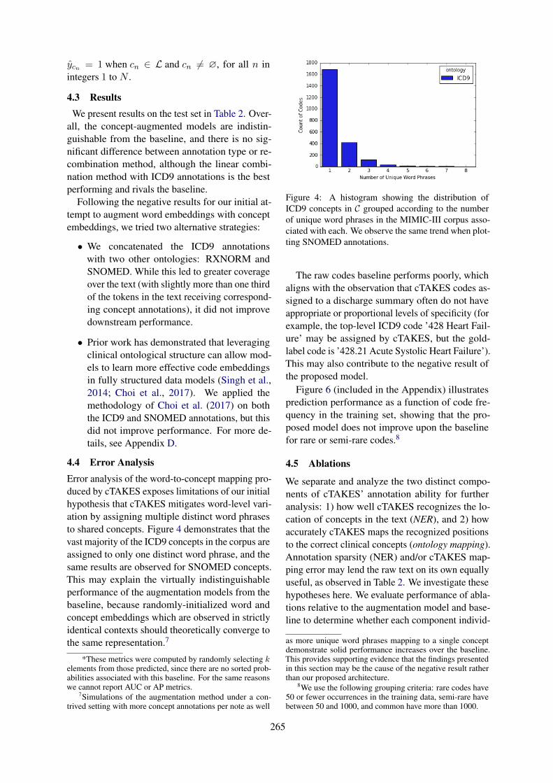
ŷcn = 1 when cn ∈ L and cn 6= ∅, for all n inintegers 1 to N .
4.3 ResultsWe present results on the test set in Table 2. Over-
all, the concept-augmented models are indistin-guishable from the baseline, and there is no sig-nificant difference between annotation type or re-combination method, although the linear combi-nation method with ICD9 annotations is the bestperforming and rivals the baseline.
Following the negative results for our initial at-tempt to augment word embeddings with conceptembeddings, we tried two alternative strategies:
• We concatenated the ICD9 annotationswith two other ontologies: RXNORM andSNOMED. While this led to greater coverageover the text (with slightly more than one thirdof the tokens in the text receiving correspond-ing concept annotations), it did not improvedownstream performance.
• Prior work has demonstrated that leveragingclinical ontological structure can allow mod-els to learn more effective code embeddingsin fully structured data models (Singh et al.,2014; Choi et al., 2017). We applied themethodology of Choi et al. (2017) on boththe ICD9 and SNOMED annotations, but thisdid not improve performance. For more de-tails, see Appendix D.
4.4 Error AnalysisError analysis of the word-to-concept mapping pro-duced by cTAKES exposes limitations of our initialhypothesis that cTAKES mitigates word-level vari-ation by assigning multiple distinct word phrasesto shared concepts. Figure 4 demonstrates that thevast majority of the ICD9 concepts in the corpus areassigned to only one distinct word phrase, and thesame results are observed for SNOMED concepts.This may explain the virtually indistinguishableperformance of the augmentation models from thebaseline, because randomly-initialized word andconcept embeddings which are observed in strictlyidentical contexts should theoretically converge tothe same representation.7
*These metrics were computed by randomly selecting kelements from those predicted, since there are no sorted prob-abilities associated with this baseline. For the same reasonswe cannot report AUC or AP metrics.
7Simulations of the augmentation method under a con-trived setting with more concept annotations per note as well
Figure 4: A histogram showing the distribution ofICD9 concepts in C grouped according to the numberof unique word phrases in the MIMIC-III corpus asso-ciated with each. We observe the same trend when plot-ting SNOMED annotations.
The raw codes baseline performs poorly, whichaligns with the observation that cTAKES codes as-signed to a discharge summary often do not haveappropriate or proportional levels of specificity (forexample, the top-level ICD9 code ’428 Heart Fail-ure’ may be assigned by cTAKES, but the gold-label code is ’428.21 Acute Systolic Heart Failure’).This may also contribute to the negative result ofthe proposed model.
Figure 6 (included in the Appendix) illustratesprediction performance as a function of code fre-quency in the training set, showing that the pro-posed model does not improve upon the baselinefor rare or semi-rare codes.8
4.5 Ablations
We separate and analyze the two distinct compo-nents of cTAKES’ annotation ability for furtheranalysis: 1) how well cTAKES recognizes the lo-cation of concepts in the text (NER), and 2) howaccurately cTAKES maps the recognized positionsto the correct clinical concepts (ontology mapping).Annotation sparsity (NER) and/or cTAKES map-ping error may lend the raw text on its own equallyuseful, as observed in Table 2. We investigate thesehypotheses here. We evaluate performance of abla-tions relative to the augmentation model and base-line to determine whether each component individ-
as more unique word phrases mapping to a single conceptdemonstrate solid performance increases over the baseline.This provides supporting evidence that the findings presentedin this section may be the cause of the negative result ratherthan our proposed architecture.
8We use the following grouping criteria: rare codes have50 or fewer occurrences in the training data, semi-rare havebetween 50 and 1000, and common have more than 1000.
265
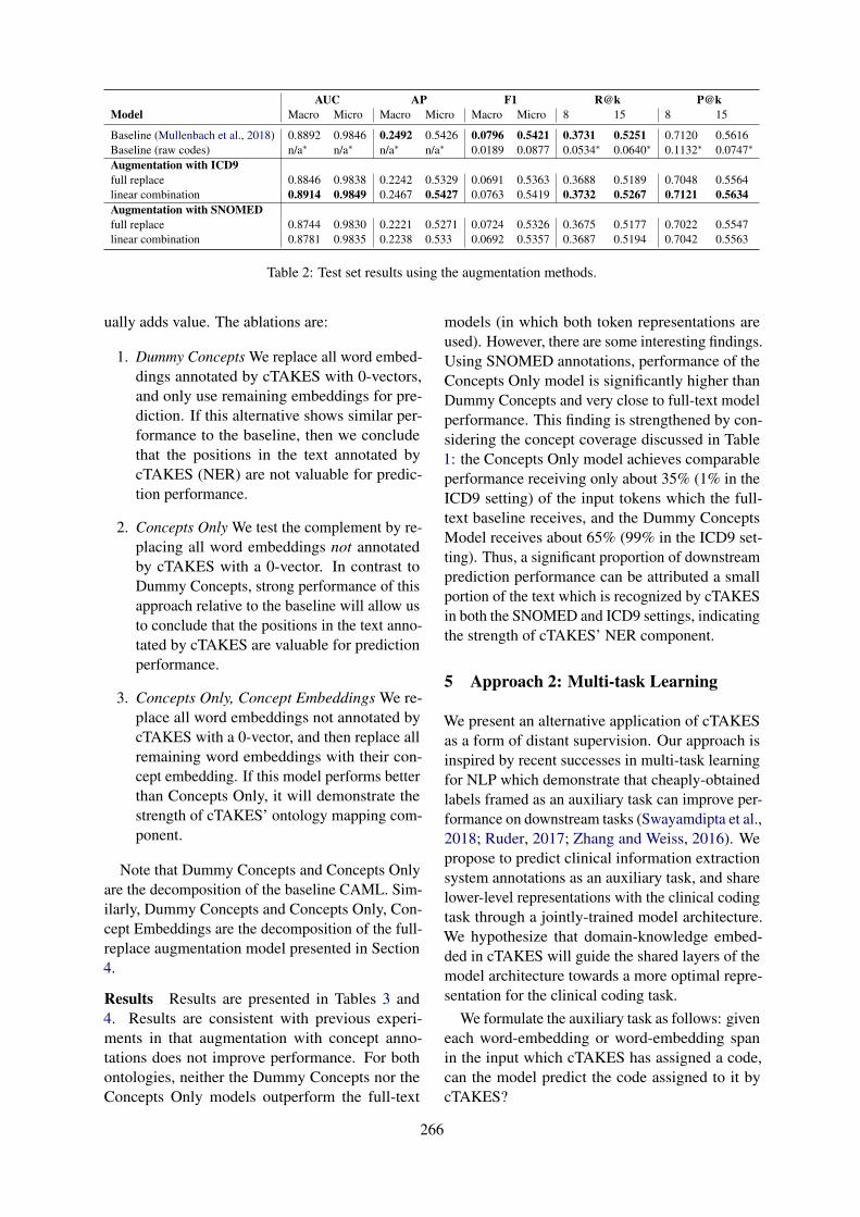
AUC AP F1 R@k P@kModel Macro Micro Macro Micro Macro Micro 8 15 8 15
Baseline (Mullenbach et al., 2018) 0.8892 0.9846 0.2492 0.5426 0.0796 0.5421 0.3731 0.5251 0.7120 0.5616Baseline (raw codes) n/a∗ n/a∗ n/a∗ n/a∗ 0.0189 0.0877 0.0534∗ 0.0640∗ 0.1132∗ 0.0747∗
Augmentation with ICD9full replace 0.8846 0.9838 0.2242 0.5329 0.0691 0.5363 0.3688 0.5189 0.7048 0.5564linear combination 0.8914 0.9849 0.2467 0.5427 0.0763 0.5419 0.3732 0.5267 0.7121 0.5634Augmentation with SNOMEDfull replace 0.8744 0.9830 0.2221 0.5271 0.0724 0.5326 0.3675 0.5177 0.7022 0.5547linear combination 0.8781 0.9835 0.2238 0.533 0.0692 0.5357 0.3687 0.5194 0.7042 0.5563
Table 2: Test set results using the augmentation methods.
ually adds value. The ablations are:
1. Dummy Concepts We replace all word embed-dings annotated by cTAKES with 0-vectors,and only use remaining embeddings for pre-diction. If this alternative shows similar per-formance to the baseline, then we concludethat the positions in the text annotated bycTAKES (NER) are not valuable for predic-tion performance.
2. Concepts Only We test the complement by re-placing all word embeddings not annotatedby cTAKES with a 0-vector. In contrast toDummy Concepts, strong performance of thisapproach relative to the baseline will allow usto conclude that the positions in the text anno-tated by cTAKES are valuable for predictionperformance.
3. Concepts Only, Concept Embeddings We re-place all word embeddings not annotated bycTAKES with a 0-vector, and then replace allremaining word embeddings with their con-cept embedding. If this model performs betterthan Concepts Only, it will demonstrate thestrength of cTAKES’ ontology mapping com-ponent.
Note that Dummy Concepts and Concepts Onlyare the decomposition of the baseline CAML. Sim-ilarly, Dummy Concepts and Concepts Only, Con-cept Embeddings are the decomposition of the full-replace augmentation model presented in Section4.
Results Results are presented in Tables 3 and4. Results are consistent with previous experi-ments in that augmentation with concept anno-tations does not improve performance. For bothontologies, neither the Dummy Concepts nor theConcepts Only models outperform the full-text
models (in which both token representations areused). However, there are some interesting findings.Using SNOMED annotations, performance of theConcepts Only model is significantly higher thanDummy Concepts and very close to full-text modelperformance. This finding is strengthened by con-sidering the concept coverage discussed in Table1: the Concepts Only model achieves comparableperformance receiving only about 35% (1% in theICD9 setting) of the input tokens which the full-text baseline receives, and the Dummy ConceptsModel receives about 65% (99% in the ICD9 set-ting). Thus, a significant proportion of downstreamprediction performance can be attributed a smallportion of the text which is recognized by cTAKESin both the SNOMED and ICD9 settings, indicatingthe strength of cTAKES’ NER component.
5 Approach 2: Multi-task Learning
We present an alternative application of cTAKESas a form of distant supervision. Our approach isinspired by recent successes in multi-task learningfor NLP which demonstrate that cheaply-obtainedlabels framed as an auxiliary task can improve per-formance on downstream tasks (Swayamdipta et al.,2018; Ruder, 2017; Zhang and Weiss, 2016). Wepropose to predict clinical information extractionsystem annotations as an auxiliary task, and sharelower-level representations with the clinical codingtask through a jointly-trained model architecture.We hypothesize that domain-knowledge embed-ded in cTAKES will guide the shared layers of themodel architecture towards a more optimal repre-sentation for the clinical coding task.
We formulate the auxiliary task as follows: giveneach word-embedding or word-embedding spanin the input which cTAKES has assigned a code,can the model predict the code assigned to it bycTAKES?
266
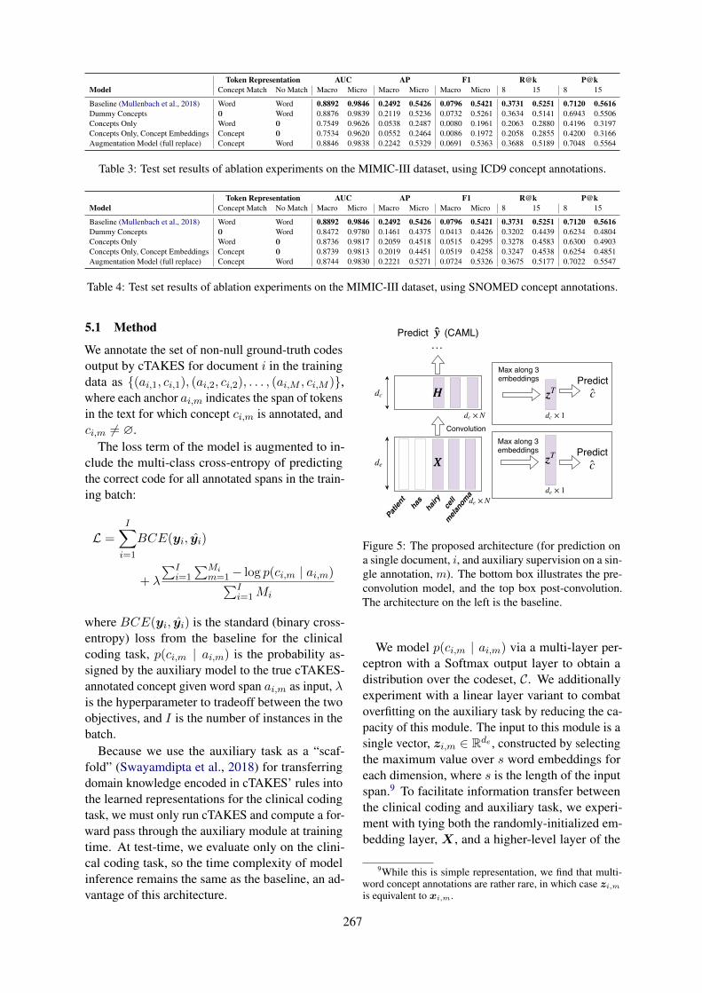
Token Representation AUC AP F1 R@k P@kModel Concept Match No Match Macro Micro Macro Micro Macro Micro 8 15 8 15
Baseline (Mullenbach et al., 2018) Word Word 0.8892 0.9846 0.2492 0.5426 0.0796 0.5421 0.3731 0.5251 0.7120 0.5616Dummy Concepts 0 Word 0.8876 0.9839 0.2119 0.5236 0.0732 0.5261 0.3634 0.5141 0.6943 0.5506Concepts Only Word 0 0.7549 0.9626 0.0538 0.2487 0.0080 0.1961 0.2063 0.2880 0.4196 0.3197Concepts Only, Concept Embeddings Concept 0 0.7534 0.9620 0.0552 0.2464 0.0086 0.1972 0.2058 0.2855 0.4200 0.3166Augmentation Model (full replace) Concept Word 0.8846 0.9838 0.2242 0.5329 0.0691 0.5363 0.3688 0.5189 0.7048 0.5564
Table 3: Test set results of ablation experiments on the MIMIC-III dataset, using ICD9 concept annotations.
Token Representation AUC AP F1 R@k P@kModel Concept Match No Match Macro Micro Macro Micro Macro Micro 8 15 8 15
Baseline (Mullenbach et al., 2018) Word Word 0.8892 0.9846 0.2492 0.5426 0.0796 0.5421 0.3731 0.5251 0.7120 0.5616Dummy Concepts 0 Word 0.8472 0.9780 0.1461 0.4375 0.0413 0.4426 0.3202 0.4439 0.6234 0.4804Concepts Only Word 0 0.8736 0.9817 0.2059 0.4518 0.0515 0.4295 0.3278 0.4583 0.6300 0.4903Concepts Only, Concept Embeddings Concept 0 0.8739 0.9813 0.2019 0.4451 0.0519 0.4258 0.3247 0.4538 0.6254 0.4851Augmentation Model (full replace) Concept Word 0.8744 0.9830 0.2221 0.5271 0.0724 0.5326 0.3675 0.5177 0.7022 0.5547
Table 4: Test set results of ablation experiments on the MIMIC-III dataset, using SNOMED concept annotations.
5.1 Method
We annotate the set of non-null ground-truth codesoutput by cTAKES for document i in the trainingdata as {(ai,1, ci,1), (ai,2, ci,2), . . . , (ai,M , ci,M )},where each anchor ai,m indicates the span of tokensin the text for which concept ci,m is annotated, andci,m 6= ∅.
The loss term of the model is augmented to in-clude the multi-class cross-entropy of predictingthe correct code for all annotated spans in the train-ing batch:
L =I∑
i=1
BCE(yi, ŷi)
+ λ
∑Ii=1
∑Mim=1− log p(ci,m | ai,m)
∑Ii=1Mi
where BCE(yi, ŷi) is the standard (binary cross-entropy) loss from the baseline for the clinicalcoding task, p(ci,m | ai,m) is the probability as-signed by the auxiliary model to the true cTAKES-annotated concept given word span ai,m as input, λis the hyperparameter to tradeoff between the twoobjectives, and I is the number of instances in thebatch.
Because we use the auxiliary task as a “scaf-fold” (Swayamdipta et al., 2018) for transferringdomain knowledge encoded in cTAKES’ rules intothe learned representations for the clinical codingtask, we must only run cTAKES and compute a for-ward pass through the auxiliary module at trainingtime. At test-time, we evaluate only on the clini-cal coding task, so the time complexity of modelinference remains the same as the baseline, an ad-vantage of this architecture.
HH
Convolution× Ndc
de
Patient has
hairy
cell
melanoma
y ̂ y ̂
XX
…
dc
Max along 3embeddings
zzT
c ̂ Predict
Predict
× 1de
× Nde
Max along 3embeddings
zzT c ̂ Predict
× 1dc
(CAML)
Figure 5: The proposed architecture (for prediction ona single document, i, and auxiliary supervision on a sin-gle annotation, m). The bottom box illustrates the pre-convolution model, and the top box post-convolution.The architecture on the left is the baseline.
We model p(ci,m | ai,m) via a multi-layer per-ceptron with a Softmax output layer to obtain adistribution over the codeset, C. We additionallyexperiment with a linear layer variant to combatoverfitting on the auxiliary task by reducing the ca-pacity of this module. The input to this module is asingle vector, zi,m ∈ Rde , constructed by selectingthe maximum value over s word embeddings foreach dimension, where s is the length of the inputspan.9 To facilitate information transfer betweenthe clinical coding and auxiliary task, we experi-ment with tying both the randomly-initialized em-bedding layer, X , and a higher-level layer of the
9While this is simple representation, we find that multi-word concept annotations are rather rare, in which case zi,m
is equivalent to xi,m.
267
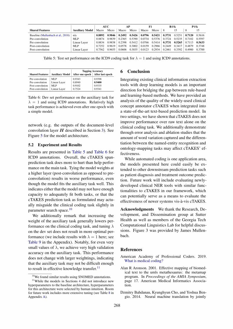
AUC AP F1 R@k P@kShared Features Auxiliary Model Macro Micro Macro Micro Macro Micro 8 15 8 15
Baseline (Mullenbach et al., 2018) n/a 0.8892 0.9846 0.2492 0.5426 0.0796 0.5421 0.3731 0.5251 0.7120 0.5616Pre-convolution MLP 0.8874 0.9839 0.2365 0.5390 0.0734 0.5376 0.3724 0.5235 0.7102 0.5597Pre-convolution Linear Layer 0.8834 0.9838 0.2398 0.5412 0.0766 0.5414 0.3731 0.5265 0.7113 0.5633Post-convolution MLP 0.7252 0.9619 0.0578 0.3002 0.0159 0.2966 0.2449 0.3417 0.4879 0.3748Post-convolution Linear Layer 0.7562 0.9655 0.0606 0.3035 0.0123 0.2934 0.2461 0.3392 0.4900 0.3700
Table 5: Test set performance on the ICD9 coding task for λ = 1 and using ICD9 annotations.
Tagging AccuracyShared Features Auxiliary Model After one epoch After last epoch
Pre-convolution MLP 0.9343 0.9398Pre-convolution Linear Layer 0.8940 0.9400Post-convolution MLP 0.9102 0.9335Post-convolution Linear Layer 0.7524 0.9341
Table 6: Dev set performance on the auxiliary task forλ = 1 and using ICD9 annotations. Relatively hightask performance is achieved even after one epoch witha simple model.
network (e.g. the outputs of the document-levelconvolution layerH described in Section 3). SeeFigure 5 for the model architecture.
5.2 Experiment and Results
Results are presented in Table 5 and Table 6 forICD9 annotations. Overall, the cTAKES span-prediction task does more to hurt than help perfor-mance on the main task. Tying the model weights ata higher layer (post-convolution as opposed to pre-convolution) results in worse performance, eventhough the model fits the auxiliary task well. Thisindicates either that the model may not have enoughcapacity to adequately fit both tasks, or that thecTAKES prediction task as formulated may actu-ally misguide the clinical coding task slightly inparameter search space.10
We additionally remark that increasing theweight of the auxiliary task generally lowers per-formance on the clinical coding task, and tuning λon the dev set does not result in more optimal per-formance (we include results with λ = 1 here; seeTable 9 in the Appendix). Notably, for even verysmall values of λ, we achieve very high validationaccuracy on the auxiliary task. This performancedoes not change with larger weightings, indicatingthat the auxiliary task may not be difficult enoughto result in effective knowledge transfer.11
10We found similar results using SNOMED annotations.11While the models in Sections 4 did not introduce new
hyperparameters to the baseline architecture, hyperparametersfor this architecture were selected by human intuition. Roomfor future work includes more extensive tuning (see Table 8 inAppendix A).
6 Conclusion
Integrating existing clinical information extractiontools with deep learning models is an importantdirection for bridging the gap between rule-basedand learning-based methods. We have provided ananalysis of the quality of the widely-used clinicalconcept annotator cTAKES when integrated intoa state-of-the-art text-based prediction model. Intwo settings, we have shown that cTAKES does notimprove performance over raw text alone on theclinical coding task. We additionally demonstratethrough error analysis and ablation studies that theamount of word variation captured and the differen-tiation between the named-entity recognition andontology-mapping tasks may affect cTAKES’ ef-fectiveness.
While automated coding is one application area,the models presented here could easily be ex-tended to other downstream prediction tasks suchas patient diagnosis and treatment outcome predic-tion. Future work will include evaluating newly-developed clinical NER tools with similar func-tionalities to cTAKES in our framework, whichcan potentially serve as a means to evaluate theeffectiveness of newer systems vis-à-vis cTAKES.
Acknowledgments We thank the Research, De-velopment, and Dissemination group at SutterHealth as well as members of the Georgia TechComputational Linguistics Lab for helpful discus-sions. Figure 3 was provided by James Mullen-bach.
ReferencesAmerican Academy of Professional Coders. 2019.
What is medical coding?
Alan R Aronson. 2001. Effective mapping of biomed-ical text to the umls metathesaurus: the metamapprogram. In Proceedings of the AMIA Symposium,page 17. American Medical Informatics Associa-tion.
Dzmitry Bahdanau, Kyunghyun Cho, and Yoshua Ben-gio. 2014. Neural machine translation by jointly
268
learning to align and translate. arXiv preprintarXiv:1409.0473.
Tal Baumel, Jimena Nassour-Kassis, Raphael Co-hen, Michael Elhadad, and Noémie Elhadad. 2018.Multi-label classification of patient notes a casestudy on icd code assignment. In Proceedings of the2018 AAAI Joint Workshop on Health Intelligence.
Willie Boag and Hassan Kané. 2017. Awe-cm vec-tors: Augmenting word embeddings with a clinicalmetathesaurus. arXiv preprint arXiv:1712.01460.
Willie Boag, Elena Sergeeva, Saurabh Kulshreshtha,Peter Szolovits, Anna Rumshisky, and Tristan Nau-mann. 2018. Cliner 2.0: Accessible and accu-rate clinical concept extraction. arXiv preprintarXiv:1803.02245.
Edward Choi, Mohammad Taha Bahadori, Le Song,Walter F Stewart, and Jimeng Sun. 2017. Gram:graph-based attention model for healthcare represen-tation learning. In Proceedings of the 23rd ACMSIGKDD International Conference on KnowledgeDiscovery and Data Mining, pages 787–795. ACM.
Jesse Davis and Mark Goadrich. 2006. The relation-ship between precision-recall and roc curves. In Pro-ceedings of the 23rd international conference on Ma-chine learning, pages 233–240. ACM.
Kevin Donnelly. 2006. Snomed-ct: The advanced ter-minology and coding system for ehealth. Studies inhealth technology and informatics, 121:279.
Carol Friedman. 2000. A broad-coverage natural lan-guage processing system. In Proceedings of theAMIA Symposium, page 270. American Medical In-formatics Association.
Nathan Greenberg, Trapit Bansal, Patrick Verga, andAndrew McCallum. 2018. Marginal likelihood train-ing of bilstm-crf for biomedical named entity recog-nition from disjoint label sets. In Proceedings of the2018 Conference on Empirical Methods in NaturalLanguage Processing, pages 2824–2829.
Alistair EW Johnson, Tom J Pollard, Lu Shen,H Lehman Li-wei, Mengling Feng, Moham-mad Ghassemi, Benjamin Moody, Peter Szolovits,Leo Anthony Celi, and Roger G Mark. 2016. Mimic-iii, a freely accessible critical care database. Scien-tific data, 3:160035.
Donald AB Lindberg, Betsy L Humphreys, andAlexa T McCray. 1993. The unified medical lan-guage system. Methods of information in medicine,32(04):281–291.
James Mullenbach, Sarah Wiegreffe, Jon Duke, JimengSun, and Jacob Eisenstein. 2018. Explainable pre-diction of medical codes from clinical text. In Pro-ceedings of the 2018 Conference of the North Amer-ican Chapter of the Association for ComputationalLinguistics: Human Language Technologies, vol-ume 1.
National Center for Health Statistics. 1991. The In-ternational Classification of Diseases: 9th Revision,Clinical Modification: ICD-9-CM.
Hoang Nguyen and Jon Patrick. 2016. Text mining inclinical domain: Dealing with noise. In Proceed-ings of the 22nd ACM SIGKDD international con-ference on knowledge discovery and data mining,pages 549–558. ACM.
T.J. Pollard and A.E.W. Johnson. 2016. The MIMIC-III clinical database.
Anthony Rios and Ramakanth Kavuluru. 2018a. Emrcoding with semi-parametric multi-head matchingnetworks. In Proceedings of the 2018 Conference ofthe North American Chapter of the Association forComputational Linguistics: Human Language Tech-nologies, volume 1, pages 2081–2091.
Anthony Rios and Ramakanth Kavuluru. 2018b. Few-shot and zero-shot multi-label learning for structuredlabel spaces. In Proceedings of the 2018 Conferenceon Empirical Methods in Natural Language Process-ing, pages 3132–3142.
Sebastian Ruder. 2017. An overview of multi-tasklearning in deep neural networks. arXiv preprintarXiv:1706.05098.
Takaya Saito and Marc Rehmsmeier. 2015. Theprecision-recall plot is more informative than theroc plot when evaluating binary classifiers on imbal-anced datasets. PloS one, 10(3):e0118432.
Guergana K Savova, James J Masanz, Philip V Ogren,Jiaping Zheng, Sunghwan Sohn, Karin C Kipper-Schuler, and Christopher G Chute. 2010. Mayo clin-ical text analysis and knowledge extraction system(ctakes): architecture, component evaluation and ap-plications. Journal of the American Medical Infor-matics Association, 17(5):507–513.
Yuqi Si, Jingqi Wang, Hua Xu, and Kirk Roberts. 2019.Enhancing clinical concept extraction with contex-tual embedding. arXiv preprint arXiv:1902.08691.
Anima Singh, Girish Nadkarni, John Guttag, and Er-win Bottinger. 2014. Leveraging hierarchy in med-ical codes for predictive modeling. In Proceedingsof the 5th ACM conference on Bioinformatics, Com-putational Biology, and Health Informatics, pages96–103. ACM.
Swabha Swayamdipta, Sam Thomson, Kenton Lee,Luke Zettlemoyer, Chris Dyer, and Noah A. Smith.2018. Syntactic scaffolds for semantic structures.CoRR, abs/1808.10485.
Yifeng Tao, Bruno Godefroy, Guillaume Genthial, andChristopher Potts. 2018. Effective feature represen-tation for clinical text concept extraction. arXivpreprint arXiv:1811.00070.
269
Jacqueline M Torres, John Lawlor, Jeffrey D Colvin,Marion R Sills, Jessica L Bettenhausen, Am-ber Davidson, Gretchen J Cutler, Matt Hall, andLaura M Gottlieb. 2017. Icd social codes. Medicalcare, 55(9):810–816.
Yanshan Wang, Liwei Wang, Majid Rastegar-Mojarad,Sungrim Moon, Feichen Shen, Naveed Afzal, SijiaLiu, Yuqun Zeng, Saeed Mehrabi, Sunghwan Sohn,et al. 2017. Clinical information extraction appli-cations: a literature review. Journal of biomedicalinformatics.
Wei-Hung Weng, Kavishwar B Wagholikar, Alexa TMcCray, Peter Szolovits, and Henry C Chueh. 2017.Medical subdomain classification of clinical notesusing a machine learning-based natural languageprocessing approach. BMC medical informatics anddecision making, 17(1):155.
Kai Xu, Zhanfan Zhou, Tao Gong, Tianyong Hao,and Wenyin Liu. 2018. Sblc: a hybrid modelfor disease named entity recognition based on se-mantic bidirectional lstms and conditional randomfields. BMC medical informatics and decision mak-ing, 18(5):114.
Yuan Zhang and David Weiss. 2016. Stack-propagation: Improved representation learning forsyntax. arXiv preprint arXiv:1603.06598.
Henghui Zhu, Ioannis Ch Paschalidis, and AmirTahmasebi. 2018. Clinical concept extractionwith contextual word embedding. arXiv preprintarXiv:1810.10566.
270
A Experimental Details
Data Following Mullenbach et al. (2018), weuse the same train/test/validation splits for theMIMIC-III dataset, and concatenate all supplemen-tal text for a patient discharge summary into onerecord. We use the authors’ provided data pro-cessing pipeline12 to preprocess the corpus. Thevocubulary includes all words occurring in at least3 training documents. See Table 7 for descriptivestatistics of the dataset.
We construct a concept vocabulary for embed-ding initialization following the same specificationas the word vocabulary: any concept which doesnot occur in at least 3 training documents is re-placed with an UNK token. Details on the size ofthe vocabulary can be found in Table 8.
# training documents 47,723# test documents 3,372# dev documents 1,631
Mean # tokens per document 1,513.0Mean # labels per document 16.09Total # labels (L) 8,921
Table 7: Dataset Descriptive Statistics.
Training We train with the same specificationsas Mullenbach et al. (2018) unless otherwise spec-ified, with dropout performed after concept aug-mentation for the models in Sections 4, and earlystopping with a patience of 10 epochs on the pre-cision at 8 metric, for a maximum of 200 epochs(note that in the multi-task learning models the stop-ping criterion is only a function of performance onthe clinical coding task). Unlike previous work, wereduce the batch size to 12 in order to allow eachbatch to fit on a single GPU, and we do not usepretrained embeddings as we find this improvesperformance. All models are trained on a singleNVIDIA Titan X GPU with 12,189 MiB of RAM.
We port the optimal hyperparameters reported inMullenbach et al. (2018) to our experiments. Withmore extensive hyperparameter tuning, we may ex-pect to see a potential increase in the performanceof our models over the baseline. See Table 8 forhyperparameters and other details specific to ourproposed model architectures. All neural models
12https://github.com/jamesmullenbach/caml-mimic/blob/master/notebooks/dataproc_mimic_III.ipynb
are implemented using PyTorch13, and built on theopen-source implementation of CAML.14
Parameter Value
Vocabulary Size 51,917SNOMED Concept Vocabulary (C) Size 20,775ICD9 Concept Vocabulary (C) Size 1,529Embedding Size (de) 100Post-convolution Embedding Size (dc) 50Dropout Probability 0.2Learning Rate 0.0001Attention Mechanism Hidden State Size 20Attention Mechanism Activation Function ReLUAuxiliary hidden layer size 700Auxiliary activation function ReLU
Table 8: Model details.
B Concept Extraction
We build a custom dictionary from the UMLSMetathesaurus that includes mappings from UMLSCUIs to SNOMED-CT and ICD9-CM concepts.We run the cTAKES annotator in advance of train-ing for all 3 dataset splits using the resulting dic-tionary, allowing us to obtain annotations for eachnote in the dataset, and the positions of the anno-tations in the raw text. Note that for the multi-task learning experiments (Section 5), we only re-quire annotations for training data. Annotatingthe MIMIC-III datafiles using these specificationstakes between 4 and 5 hours for 3,000 dischargesummaries on a single CPU, and can be parallelizedfor efficiency.
C Attention for Overlapping Concepts
We implement an attention mechanism (Bahdanauet al., 2014) to compute a single concept embed-ding φ(Cn) ∈ Rde when Cn = {c1, c2, . . . , cJ}represents a set of concepts annotated at positionn instead of a single concept. Intuitively, we wantto more heavily weight those concepts in the setwhich have the most similarity to the surroundingtext. We define a context vector for position n as:
vn = [xn−2,xn−1,xn+1,xn+2] ∈ R4de
The context is defined as the concatenated wordembeddings surrounding position n. We use a con-text size of n+ /− 2, where 2 is a hyperparameter.We choose to use a smaller value for computationalefficiency.
13https://github.com/pytorch/pytorch14https://github.com/jamesmullenbach/
caml-mimic
271
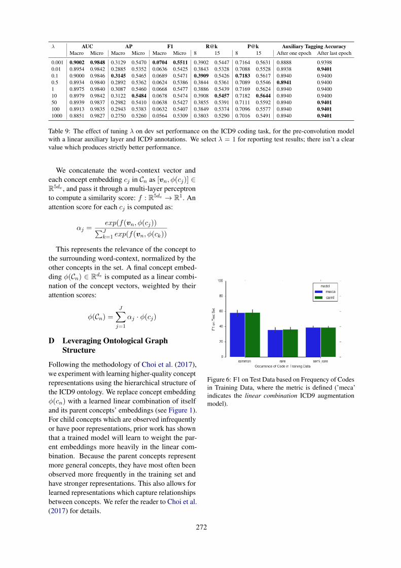
λ AUC AP F1 R@k P@k Auxiliary Tagging AccuracyMacro Micro Macro Micro Macro Micro 8 15 8 15 After one epoch After last epoch
0.001 0.9002 0.9848 0.3129 0.5470 0.0704 0.5511 0.3902 0.5447 0.7164 0.5631 0.8888 0.93980.01 0.8954 0.9842 0.2885 0.5352 0.0636 0.5425 0.3843 0.5328 0.7088 0.5528 0.8938 0.94010.1 0.9000 0.9846 0.3145 0.5465 0.0689 0.5471 0.3909 0.5426 0.7183 0.5617 0.8940 0.94000.5 0.8934 0.9840 0.2892 0.5362 0.0624 0.5386 0.3844 0.5361 0.7089 0.5546 0.8941 0.94001 0.8975 0.9840 0.3087 0.5460 0.0668 0.5477 0.3886 0.5439 0.7169 0.5624 0.8940 0.940010 0.8979 0.9842 0.3122 0.5484 0.0678 0.5474 0.3908 0.5457 0.7182 0.5644 0.8940 0.940050 0.8939 0.9837 0.2982 0.5410 0.0638 0.5427 0.3855 0.5391 0.7111 0.5592 0.8940 0.9401100 0.8913 0.9835 0.2943 0.5383 0.0632 0.5407 0.3849 0.5374 0.7096 0.5577 0.8940 0.94011000 0.8851 0.9827 0.2750 0.5260 0.0564 0.5309 0.3803 0.5290 0.7016 0.5491 0.8940 0.9401
Table 9: The effect of tuning λ on dev set performance on the ICD9 coding task, for the pre-convolution modelwith a linear auxiliary layer and ICD9 annotations. We select λ = 1 for reporting test results; there isn’t a clearvalue which produces strictly better performance.
We concatenate the word-context vector andeach concept embedding cj in Cn as [vn, φ(cj)] ∈R5de , and pass it through a multi-layer perceptronto compute a similarity score: f : R5de → R1. Anattention score for each cj is computed as:
αj =exp(f(vn, φ(cj))∑Jk=1 exp(f(vn, φ(ck))
This represents the relevance of the concept tothe surrounding word-context, normalized by theother concepts in the set. A final concept embed-ding φ(Cn) ∈ Rde is computed as a linear combi-nation of the concept vectors, weighted by theirattention scores:
φ(Cn) =J∑
j=1
αj · φ(cj)
D Leveraging Ontological GraphStructure
Following the methodology of Choi et al. (2017),we experiment with learning higher-quality conceptrepresentations using the hierarchical structure ofthe ICD9 ontology. We replace concept embeddingφ(cn) with a learned linear combination of itselfand its parent concepts’ embeddings (see Figure 1).For child concepts which are observed infrequentlyor have poor representations, prior work has shownthat a trained model will learn to weight the par-ent embeddings more heavily in the linear com-bination. Because the parent concepts representmore general concepts, they have most often beenobserved more frequently in the training set andhave stronger representations. This also allows forlearned representations which capture relationshipsbetween concepts. We refer the reader to Choi et al.(2017) for details.
Figure 6: F1 on Test Data based on Frequency of Codesin Training Data, where the metric is defined (’meca’indicates the linear combination ICD9 augmentationmodel).
272
Proceedings of the BioNLP 2019 workshop, pages 273–282Florence, Italy, August 1, 2019. c©2019 Association for Computational Linguistics
Clinical Case Reports for NLPCyril Grouin
LIMSI, CNRS, Université Paris SaclayCampus universitaire d’Orsay
91405 Orsay cedex, [email protected]
Natalia GrabarSTL, CNRS, Université de Lille
Domaine du Pont-de-Bois59653 Villeneuve-d’Ascq cedex, [email protected]
Vincent ClaveauIRISA, CNRS
Czampus universitaire de Beaulieu35042 Rennes cedex, France
Thierry HamonLIMSI, CNRS, Université Paris Saclay
Université Paris 1399 avenue Jean-Baptiste Clément
93430 Villetaneuse, [email protected]
Abstract
Textual data are useful to access expert infor-mation. Since the texts are representative ofdistinct language uses, it is necessary to buildspecific corpora in order to be able to designsuitable NLP tools. In some domains, such asmedical domain, it may be complicated to ac-cess the representative textual data and theirsemantic annotations, while there exists a realneed for providing efficient tools and methods.In this paper, we present a corpus of 717 clin-ical cases written in French. We manually an-notated this corpus into four general categories(age, gender, outcome, and origin) for a to-tal number of 2,835 annotations. The valuesof age, gender, and outcome have been nor-malized. We also manually annotated a subsetof 70 files into 27 fine-grained categories, fora total number of 5,198 annotations. In addi-tion, we present a few basic experiments madeon those annotations in order to highlight theirusefulness.
1 Introduction
In Natural Language Processing (NLP), texts areuseful to access information, especially expert in-formation. Nevertheless, the linguistic diversity(type of narratives, common or specialized vo-cabulary, regular or complex syntactic structures,etc.) requires robust tools to access the infor-mation present in those texts. In order to buildsuitable NLP-based tools, to model linguistic el-ements (machine-learning, word-embeddings), orto produce gold standards for evaluating automaticsystems, texts are needed (Nadkarni et al., 2011).However, due to privacy and ethical reasons, doc-uments from specialized domains (e.g., clinicalnotes or justice decisions) are not easily accessi-ble unless authorization (Chapman et al., 2011).
When such data exist for the research, they aregenerally limited to English language, such as theMIMIC-III database (Johnson et al., 2016) and de-rived corpora. For French language, the Quaeromedical corpus (Névéol et al., 2014) is composedof a limited number of documents (13 documentsfrom the European Medicines Agency, 25 docu-ments from the European Patent Organization) orvery short documents (2,500 Medline titles).
In order to make available documents con-cerned by privacy issues, de-identification tech-niques have been widely used to replace nomina-tive data by plausible information (Meystre et al.,2010; Kayaalp, 2017). Despite the recent im-provements of these techniques, especially basedon artificial neural networks (Dernoncourt et al.,2017), one can not assure that all nominativedata have been removed and humans must furthercheck those documents. Another solution relieson the production of synthetic data (Lohr et al.,2018). Originally, they were generated and usedto train OCR systems for handwriting recognition(Doermann and Yao, 1995). They are now usedwhen original data are missing or to provide moredata, despite their artificial character (Eger et al.,2019). Besides, whether the texts are de-identifiedor artificially generated, their linguistic specificitywill have an impact on further designed NLP rule-based and statistically-based approaches.
In this paper, we present the semantic annota-tions we made on a corpus of clinical cases writ-ten in French by domain experts. Since this cor-pus is composed of already published and freelyaccessible clinical cases, our aim is to make thisannotated corpus available for the research. In or-der to present the usefulness of those annotations,we present a few basic experiments we made.
273
2 Corpus and annotation guidelines
2.1 CorpusIn the clinical domain, in order to overcome theprivacy and ethical issues when working on elec-tronic health records, one solution consists in us-ing clinical case reports. Indeed, it is quite com-mon to find freely available publications from sci-entific journals which report in clinical cases ofreal de-identified or fake patients. Such clinicalcases are usually published and discussed to im-prove medical knowledge (Atkinson, 1992) of col-leagues and medical students. One may find sci-entific journals specifically dedicated to case re-ports, such as the Journal of Medical Case Reportslaunched in 2006 (Rison et al., 2017). Clinicalcases consist of a detailed and hierarchically struc-tured description of history, signs and symptoms,diseases, tests, treatments, follow-up and outcomeof a given patient or of a cohort of patients (Rison,2013). As pinpointed by Lysanets et al. (2017),clinical cases are composed of linguistic particu-larities which constitute a specific genre of medi-cal texts: active voice sentences, past simple tense,personal pronouns, and modal verbs. Beyond thiswarning, they represent both an available and use-ful clinical content, especially for the NLP com-munity for which the access to EHRs is becomingharder and harder.
We assume that this new orientation to tacklethe medical data accessibility problem may be-come popular in the years to come within thebiomedical domain. Let’s for instance mention thework by Satomura and Amaral (1992), which pro-duced back in 90’s an automatic system designedfor the indexing of clinical cases with ICD-9codes. These clinical cases written in English havebeen extracted from the New England Journal ofMedicine and permitted the researchers to developtheir NLP system and to test it. More recently,Gurulingappa et al. (2012) produced a benchmarkcorpus composed of 3,000 clinical case reports inEnglish, which has been then annotated into sev-eral categories (drug, dosage, and adverse effects),and relationships among them in order to providementions of adverse drug reactions.
The corpus we present in this work is composedof 717 clinical case reports written in French (seetable 1 for general statistics). These cases havebeen previously published and are freely acces-sible. The cases from scientific literature oftengo with their discussion and keywords. In this
work, we only focus on the clinical case descrip-tion. This set has been manually annotated withgeneral and fine-grained information, which is de-scribed in the two following sections. This cor-pus is part of a larger and yet growing corpus,which currently contains over 4,100 clinical cases(Grabar et al., 2018).
Element NumberDocuments 717Sentences 1,124Words (occurrences) 26,787Words (forms) 5,030
Table 1: General statistics on the corpus annotated inthis work
2.2 Annotations of general informationWe considered four general categories of informa-tion for the annotation. They are related to de-mographic data (age and gender) and to medicaldata (the starting medical problem or origin andthe outcome). Most of the clinical cases describethe clinical events of one patient. Yet, some clin-ical cases may be dedicated to the description ofseveral patients, in which case, all relevant infor-mation are annotated for each patient. For this rea-son, the total number of annotations may be higherthan the number of clinical cases. For three outof four categories, the values are normalized andtaken from finite sets:
• Age ∈ N: numerical value rounded in years;age in letters is converted into numericalvalue;
• Gender ∈ { feminine, masculine };
• Outcome ∈ { recovery, improvement, stablecondition, worsening, death }.
Besides, when several ages are given for the samepatient, only the age at the moment of the mainclinical event is considered. For the category Ori-gin, the values correspond to text spans describingthe initial medical problem.
Two scientists with a biomedical computer sci-ence background created the annotations indepen-dently, and then elaborated consensual annota-tions. Hence, all spans of text providing the ex-pected information were annotated. For the cat-egory origin, the most inclusive text spans havebeen chosen.
274
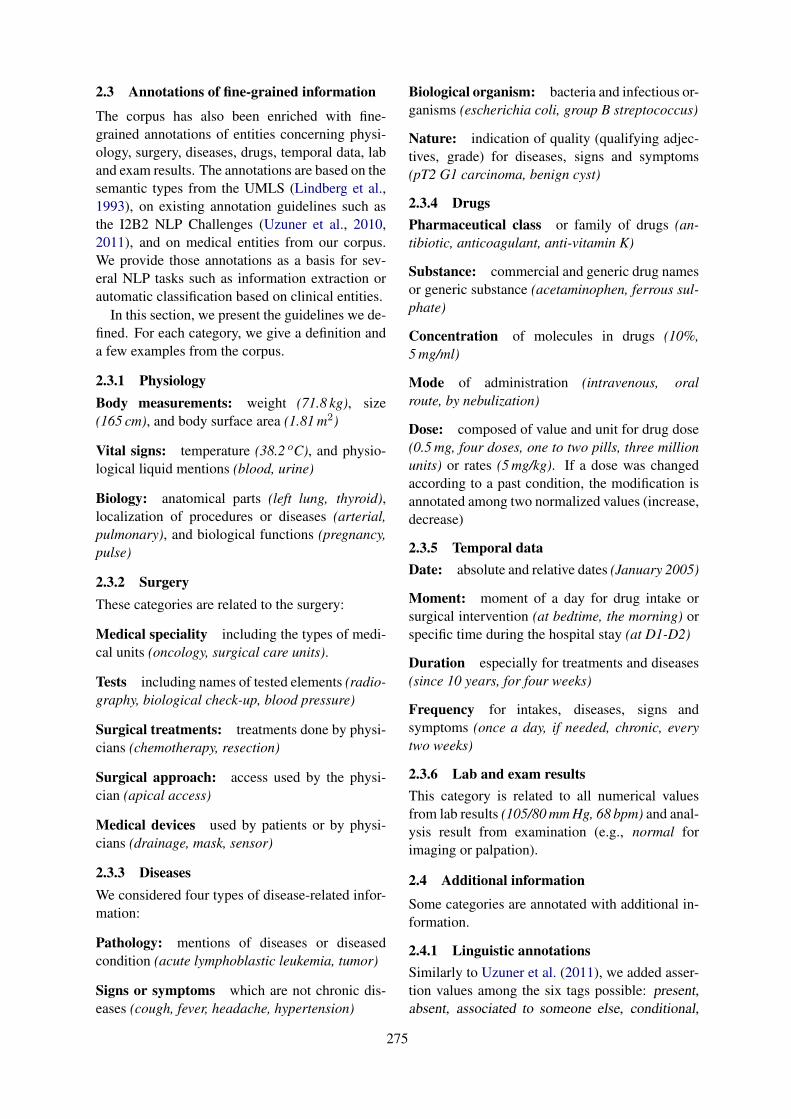
2.3 Annotations of fine-grained information
The corpus has also been enriched with fine-grained annotations of entities concerning physi-ology, surgery, diseases, drugs, temporal data, laband exam results. The annotations are based on thesemantic types from the UMLS (Lindberg et al.,1993), on existing annotation guidelines such asthe I2B2 NLP Challenges (Uzuner et al., 2010,2011), and on medical entities from our corpus.We provide those annotations as a basis for sev-eral NLP tasks such as information extraction orautomatic classification based on clinical entities.
In this section, we present the guidelines we de-fined. For each category, we give a definition anda few examples from the corpus.
2.3.1 PhysiologyBody measurements: weight (71.8 kg), size(165 cm), and body surface area (1.81 m2)
Vital signs: temperature (38.2 oC), and physio-logical liquid mentions (blood, urine)
Biology: anatomical parts (left lung, thyroid),localization of procedures or diseases (arterial,pulmonary), and biological functions (pregnancy,pulse)
2.3.2 SurgeryThese categories are related to the surgery:
Medical speciality including the types of medi-cal units (oncology, surgical care units).
Tests including names of tested elements (radio-graphy, biological check-up, blood pressure)
Surgical treatments: treatments done by physi-cians (chemotherapy, resection)
Surgical approach: access used by the physi-cian (apical access)
Medical devices used by patients or by physi-cians (drainage, mask, sensor)
2.3.3 DiseasesWe considered four types of disease-related infor-mation:
Pathology: mentions of diseases or diseasedcondition (acute lymphoblastic leukemia, tumor)
Signs or symptoms which are not chronic dis-eases (cough, fever, headache, hypertension)
Biological organism: bacteria and infectious or-ganisms (escherichia coli, group B streptococcus)
Nature: indication of quality (qualifying adjec-tives, grade) for diseases, signs and symptoms(pT2 G1 carcinoma, benign cyst)
2.3.4 DrugsPharmaceutical class or family of drugs (an-tibiotic, anticoagulant, anti-vitamin K)
Substance: commercial and generic drug namesor generic substance (acetaminophen, ferrous sul-phate)
Concentration of molecules in drugs (10%,5 mg/ml)
Mode of administration (intravenous, oralroute, by nebulization)
Dose: composed of value and unit for drug dose(0.5 mg, four doses, one to two pills, three millionunits) or rates (5 mg/kg). If a dose was changedaccording to a past condition, the modification isannotated among two normalized values (increase,decrease)
2.3.5 Temporal dataDate: absolute and relative dates (January 2005)
Moment: moment of a day for drug intake orsurgical intervention (at bedtime, the morning) orspecific time during the hospital stay (at D1-D2)
Duration especially for treatments and diseases(since 10 years, for four weeks)
Frequency for intakes, diseases, signs andsymptoms (once a day, if needed, chronic, everytwo weeks)
2.3.6 Lab and exam resultsThis category is related to all numerical valuesfrom lab results (105/80 mm Hg, 68 bpm) and anal-ysis result from examination (e.g., normal forimaging or palpation).
2.4 Additional information
Some categories are annotated with additional in-formation.
2.4.1 Linguistic annotationsSimilarly to Uzuner et al. (2011), we added asser-tion values among the six tags possible: present,absent, associated to someone else, conditional,
275
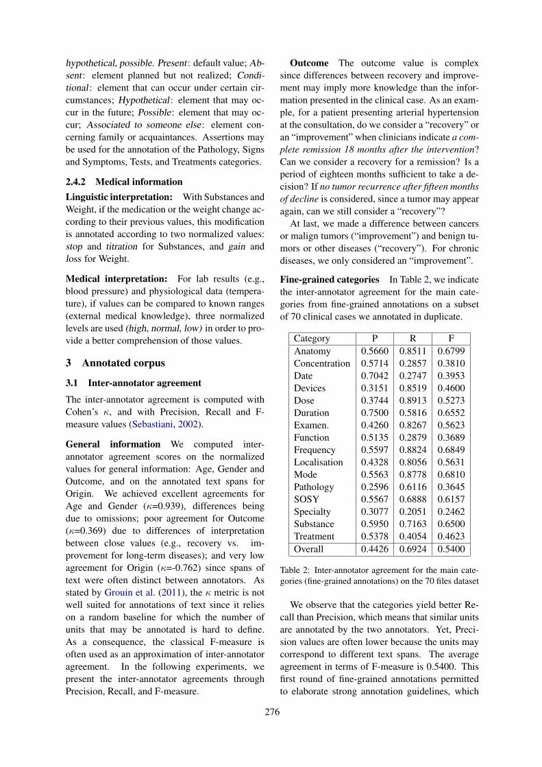
hypothetical, possible. Present : default value; Ab-sent : element planned but not realized; Condi-tional : element that can occur under certain cir-cumstances; Hypothetical : element that may oc-cur in the future; Possible: element that may oc-cur; Associated to someone else: element con-cerning family or acquaintances. Assertions maybe used for the annotation of the Pathology, Signsand Symptoms, Tests, and Treatments categories.
2.4.2 Medical informationLinguistic interpretation: With Substances andWeight, if the medication or the weight change ac-cording to their previous values, this modificationis annotated according to two normalized values:stop and titration for Substances, and gain andloss for Weight.
Medical interpretation: For lab results (e.g.,blood pressure) and physiological data (tempera-ture), if values can be compared to known ranges(external medical knowledge), three normalizedlevels are used (high, normal, low) in order to pro-vide a better comprehension of those values.
3 Annotated corpus
3.1 Inter-annotator agreement
The inter-annotator agreement is computed withCohen’s κ, and with Precision, Recall and F-measure values (Sebastiani, 2002).
General information We computed inter-annotator agreement scores on the normalizedvalues for general information: Age, Gender andOutcome, and on the annotated text spans forOrigin. We achieved excellent agreements forAge and Gender (κ=0.939), differences beingdue to omissions; poor agreement for Outcome(κ=0.369) due to differences of interpretationbetween close values (e.g., recovery vs. im-provement for long-term diseases); and very lowagreement for Origin (κ=-0.762) since spans oftext were often distinct between annotators. Asstated by Grouin et al. (2011), the κ metric is notwell suited for annotations of text since it relieson a random baseline for which the number ofunits that may be annotated is hard to define.As a consequence, the classical F-measure isoften used as an approximation of inter-annotatoragreement. In the following experiments, wepresent the inter-annotator agreements throughPrecision, Recall, and F-measure.
Outcome The outcome value is complexsince differences between recovery and improve-ment may imply more knowledge than the infor-mation presented in the clinical case. As an exam-ple, for a patient presenting arterial hypertensionat the consultation, do we consider a “recovery” oran “improvement” when clinicians indicate a com-plete remission 18 months after the intervention?Can we consider a recovery for a remission? Is aperiod of eighteen months sufficient to take a de-cision? If no tumor recurrence after fifteen monthsof decline is considered, since a tumor may appearagain, can we still consider a “recovery”?
At last, we made a difference between cancersor malign tumors (“improvement”) and benign tu-mors or other diseases (“recovery”). For chronicdiseases, we only considered an “improvement”.
Fine-grained categories In Table 2, we indicatethe inter-annotator agreement for the main cate-gories from fine-grained annotations on a subsetof 70 clinical cases we annotated in duplicate.
Category P R FAnatomy 0.5660 0.8511 0.6799Concentration 0.5714 0.2857 0.3810Date 0.7042 0.2747 0.3953Devices 0.3151 0.8519 0.4600Dose 0.3744 0.8913 0.5273Duration 0.7500 0.5816 0.6552Examen. 0.4260 0.8267 0.5623Function 0.5135 0.2879 0.3689Frequency 0.5597 0.8824 0.6849Localisation 0.4328 0.8056 0.5631Mode 0.5563 0.8778 0.6810Pathology 0.2596 0.6116 0.3645SOSY 0.5567 0.6888 0.6157Specialty 0.3077 0.2051 0.2462Substance 0.5950 0.7163 0.6500Treatment 0.5378 0.4054 0.4623Overall 0.4426 0.6924 0.5400
Table 2: Inter-annotator agreement for the main cate-gories (fine-grained annotations) on the 70 files dataset
We observe that the categories yield better Re-call than Precision, which means that similar unitsare annotated by the two annotators. Yet, Preci-sion values are often lower because the units maycorrespond to different text spans. The averageagreement in terms of F-measure is 0.5400. Thisfirst round of fine-grained annotations permittedto elaborate strong annotation guidelines, which
276
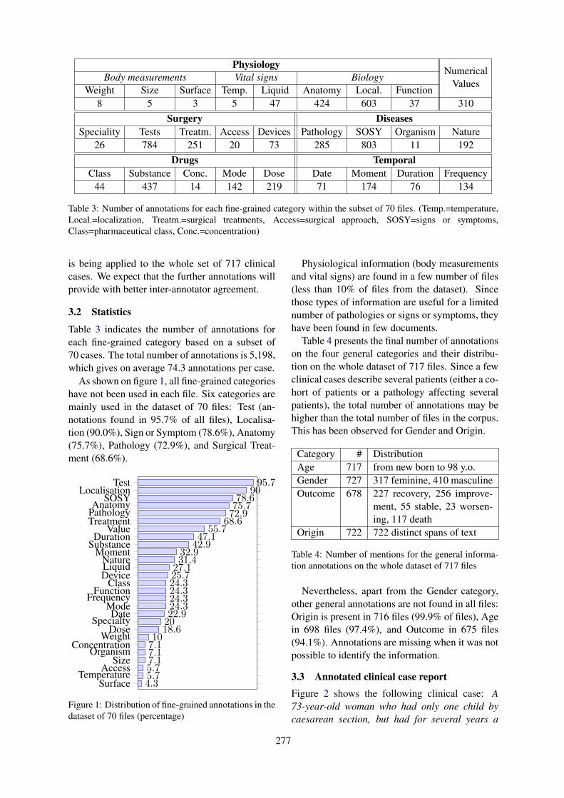
PhysiologyNumerical
Body measurements Vital signs BiologyValues
Weight Size Surface Temp. Liquid Anatomy Local. Function8 5 3 5 47 424 603 37 310
Surgery DiseasesSpeciality Tests Treatm. Access Devices Pathology SOSY Organism Nature
26 784 251 20 73 285 803 11 192Drugs Temporal
Class Substance Conc. Mode Dose Date Moment Duration Frequency44 437 14 142 219 71 174 76 134
Table 3: Number of annotations for each fine-grained category within the subset of 70 files. (Temp.=temperature,Local.=localization, Treatm.=surgical treatments, Access=surgical approach, SOSY=signs or symptoms,Class=pharmaceutical class, Conc.=concentration)
is being applied to the whole set of 717 clinicalcases. We expect that the further annotations willprovide with better inter-annotator agreement.
3.2 Statistics
Table 3 indicates the number of annotations foreach fine-grained category based on a subset of70 cases. The total number of annotations is 5,198,which gives on average 74.3 annotations per case.
As shown on figure 1, all fine-grained categorieshave not been used in each file. Six categories aremainly used in the dataset of 70 files: Test (an-notations found in 95.7% of all files), Localisa-tion (90.0%), Sign or Symptom (78.6%), Anatomy(75.7%), Pathology (72.9%), and Surgical Treat-ment (68.6%).
SurfaceTemperature
AccessSize
OrganismConcentration
WeightDose
SpecialtyDate
ModeFrequency
FunctionClass
DeviceLiquidNature
MomentSubstance
DurationValue
TreatmentPathologyAnatomy
SOSYLocalisation
Test
4.35.75.77.17.17.110
18.62022.924.324.324.324.325.727.131.432.9
42.947.1
55.768.672.975.778.6
9095.7
Figure 1: Distribution of fine-grained annotations in thedataset of 70 files (percentage)
Physiological information (body measurementsand vital signs) are found in a few number of files(less than 10% of files from the dataset). Sincethose types of information are useful for a limitednumber of pathologies or signs or symptoms, theyhave been found in few documents.
Table 4 presents the final number of annotationson the four general categories and their distribu-tion on the whole dataset of 717 files. Since a fewclinical cases describe several patients (either a co-hort of patients or a pathology affecting severalpatients), the total number of annotations may behigher than the total number of files in the corpus.This has been observed for Gender and Origin.
Category # DistributionAge 717 from new born to 98 y.o.Gender 727 317 feminine, 410 masculineOutcome 678 227 recovery, 256 improve-
ment, 55 stable, 23 worsen-ing, 117 death
Origin 722 722 distinct spans of text
Table 4: Number of mentions for the general informa-tion annotations on the whole dataset of 717 files
Nevertheless, apart from the Gender category,other general annotations are not found in all files:Origin is present in 716 files (99.9% of files), Agein 698 files (97.4%), and Outcome in 675 files(94.1%). Annotations are missing when it was notpossible to identify the information.
3.3 Annotated clinical case reportFigure 2 shows the following clinical case: A73-year-old woman who had only one child bycaesarean section, but had for several years a
277
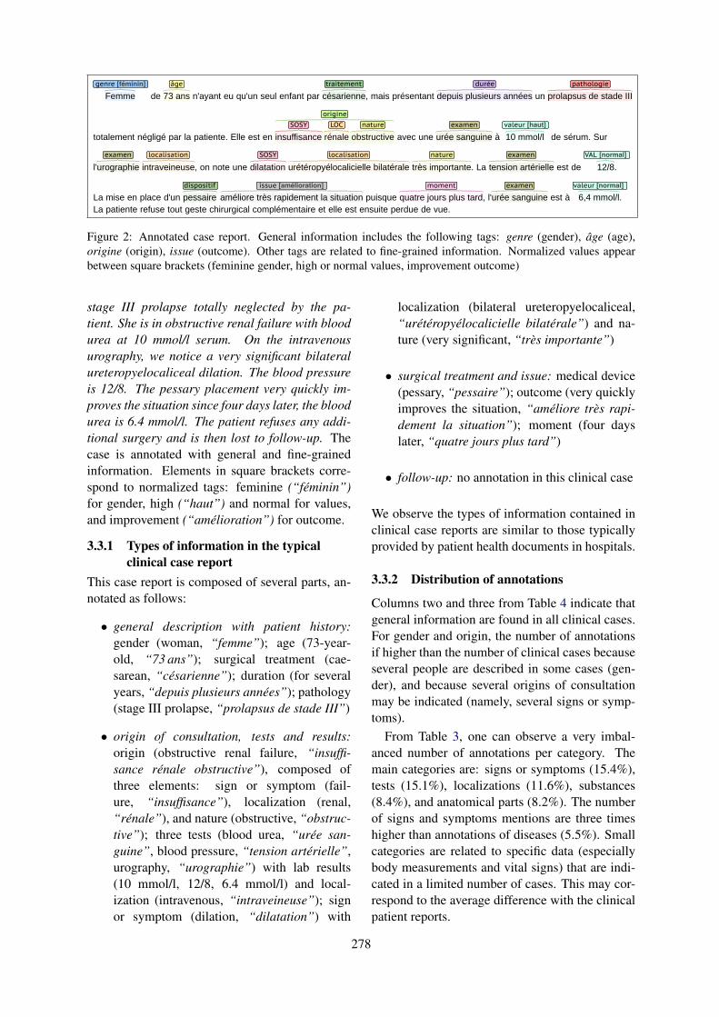
06/05/2019 11)41brat
Page 1 sur 1http://127.0.0.1)8001/index.xhtml#/deft2019/70-fichiers_cg-propa/filepdf-6-4-cas
Femme de 73 ans n'ayant eu qu'un seul enfant par césarienne, mais présentant depuis plusieurs années un prolapsus de stade III
totalement négligé par la patiente. Elle est en insuffisance rénale obstructive avec une urée sanguine à 10 mmol/l de sérum. Sur
l'urographie intraveineuse, on note une dilatation urétéropyélocalicielle bilatérale très importante. La tension artérielle est de 12/8.
La mise en place d'un pessaire améliore très rapidement la situation puisque quatre jours plus tard, l'urée sanguine est à 6,4 mmol/l. La patiente refuse tout geste chirurgical complémentaire et elle est ensuite perdue de vue.
genre [féminin] âge traitement durée pathologie
LOC natureSOSY
origine
examen valeur [haut]
examen localisation SOSY localisation nature examen VAL [normal]
dispositif issue [amélioration] moment examen valeur [normal]
1
brat/deft2019/70-fichiers_cg-propa/filepdf-6-4-cas
Figure 2: Annotated case report. General information includes the following tags: genre (gender), âge (age),origine (origin), issue (outcome). Other tags are related to fine-grained information. Normalized values appearbetween square brackets (feminine gender, high or normal values, improvement outcome)
stage III prolapse totally neglected by the pa-tient. She is in obstructive renal failure with bloodurea at 10 mmol/l serum. On the intravenousurography, we notice a very significant bilateralureteropyelocaliceal dilation. The blood pressureis 12/8. The pessary placement very quickly im-proves the situation since four days later, the bloodurea is 6.4 mmol/l. The patient refuses any addi-tional surgery and is then lost to follow-up. Thecase is annotated with general and fine-grainedinformation. Elements in square brackets corre-spond to normalized tags: feminine (“féminin”)for gender, high (“haut”) and normal for values,and improvement (“amélioration”) for outcome.
3.3.1 Types of information in the typicalclinical case report
This case report is composed of several parts, an-notated as follows:
• general description with patient history:gender (woman, “femme”); age (73-year-old, “73 ans”); surgical treatment (cae-sarean, “césarienne”); duration (for severalyears, “depuis plusieurs années”); pathology(stage III prolapse, “prolapsus de stade III”)
• origin of consultation, tests and results:origin (obstructive renal failure, “insuffi-sance rénale obstructive”), composed ofthree elements: sign or symptom (fail-ure, “insuffisance”), localization (renal,“rénale”), and nature (obstructive, “obstruc-tive”); three tests (blood urea, “urée san-guine”, blood pressure, “tension artérielle”,urography, “urographie”) with lab results(10 mmol/l, 12/8, 6.4 mmol/l) and local-ization (intravenous, “intraveineuse”); signor symptom (dilation, “dilatation”) with
localization (bilateral ureteropyelocaliceal,“urétéropyélocalicielle bilatérale”) and na-ture (very significant, “très importante”)
• surgical treatment and issue: medical device(pessary, “pessaire”); outcome (very quicklyimproves the situation, “améliore très rapi-dement la situation”); moment (four dayslater, “quatre jours plus tard”)
• follow-up: no annotation in this clinical case
We observe the types of information contained inclinical case reports are similar to those typicallyprovided by patient health documents in hospitals.
3.3.2 Distribution of annotations
Columns two and three from Table 4 indicate thatgeneral information are found in all clinical cases.For gender and origin, the number of annotationsif higher than the number of clinical cases becauseseveral people are described in some cases (gen-der), and because several origins of consultationmay be indicated (namely, several signs or symp-toms).
From Table 3, one can observe a very imbal-anced number of annotations per category. Themain categories are: signs or symptoms (15.4%),tests (15.1%), localizations (11.6%), substances(8.4%), and anatomical parts (8.2%). The numberof signs and symptoms mentions are three timeshigher than annotations of diseases (5.5%). Smallcategories are related to specific data (especiallybody measurements and vital signs) that are indi-cated in a limited number of cases. This may cor-respond to the average difference with the clinicalpatient reports.
278
4 Experiments and analysis
The annotated corpus has been exploited to per-form similar annotations automatically and fortheir evaluation. Our aim is to verify the adequate-ness of the annotations for this information extrac-tion task, as well as to serve as baseline for futurework. We specify we do not aim to provide newmethods, nor to improve existing systems, but topresent a few use cases that may be done on theannotations presented in section 2.
4.1 Linguistic analysis
Syntax. Depending on the outcome observed inclinical cases, we studied the distribution of a fewverbal tenses based on the POS annotations pro-vided by the TreeTagger system (Schmid, 1994).As presented in Table 5, past perfect is the maintense for death outcome while present is the maintense for both improvement and stable conditionoutcomes. Conversely, we observe no future tensein case reports concerned by death.
Verbal tense R I S W Dfuture 0.01 0.01 0.01 0.02 0.00imperfect 0.19 0.15 0.12 0.13 0.16past perfect 0.41 0.41 0.41 0.41 0.45present 0.23 0.29 0.29 0.24 0.26
Table 5: Percentage of verbal tenses use dependingon the outcome value (R=recovery, I=improvement,S=stable, W=worsening, D=death)
Table 6 presents the distribution of demonstra-tive pronouns (PRO:dem) vs. personal pronouns(PRO:per) depending on the outcome. We observethat impersonal linguistic constructions are mainlyused for stable condition outcomes (less personalpronouns and more demonstrative pronouns) thanin other outcome types, as if the uncertainty of thestable condition (no improvement nor worsening)would prevent from a too much personal represen-tation of the case.
POS tag R I S W DPRO:dem 0.19 0.19 0.24 0.21 0.18PRO:per 0.52 0.50 0.47 0.48 0.51
Table 6: Percentage of types of pronoun use(PRO:dem=demonstrative, PRO:per=personal)depending on the outcome value (R=recovery,I=improvement, S=stable, W=worsening, D=death)
Semantics. Table 7 presents the main elementsannotated as anatomical parts, pathologies, signsor symptoms, and surgical treatments dependingon the gender. The observed differences of med-ical entities mainly highlight differences due toanatomical parts specific to men or women, or todistinct prevalences of pathologies. We observeless differences in surgical treatments than in othercategories.
Category F/M Annotated spans
AnatomyF kidney, bladder, torsoM testicle, bladder, prostate
Pathology
Facute pyelonephristis, ade-nocarcinoma, carcinoma,edema, mydriasis, tumor
Madenocarcinoma, fistula,rhabdomyosarcoma, tuber-culosis, tumor, ulcer
Signs orF
dilation, hematuria, hyper-sensitivity, lesion, mass,pain, rash, stone, vomiting
SymptomsM
fever, infection, lesion, mass,nodule, pain, pneumonia, re-lapse, retention, trouble
Treatments
Fchemotherapy, curettage,desensitization, exeresis,lumpectomy, nephrectomy
M
ablation, chemotherapy,clamping, desensitization,exeresis, orchiectomy,plasma exchange, resection
Table 7: Most used anatomical parts, pathologies, signsor symptoms, and surgical treatments depending on thegender (F=feminine, M=masculine)
4.2 Information extraction
The information extraction experiments rely onthe Wapiti tool (Lavergne et al., 2010) that im-plements linear chain CRF (Lafferty et al., 2001).We trained a model on the 16 fine-grained cat-egories presented in Table 2, through a 10 foldcross-validation process, using a l1 regularization.We used the following features: unigrams andbigrams of tokens, number of characters, typo-graphic case, presence of punctuation and digit,Soundex code1 value of each token, relative po-sition of token within the document (beginning,middle, end), POS tags from the TreeTagger sys-
1https://en.wikipedia.org/wiki/Soundex
279
tem (Schmid, 1994) and syntactic chunks based onthose tags, presence of the token in a dictionaryof 251k inflected forms for French, and cluster id(120 classes) of each token using the clusteringalgorithm from Brown et al. (1992) implementedby Liang (2005). The results that we achieved arepresented in table 8. Overall, we obtain 0.76 Pre-cision, 0.45 Recall and 0.67 F-measure.
Category P R FAnatomy 0.7260 0.4823 0.5795Concentration 0.5000 0.0714 0.1250Date 1.0000 0.4507 0.6214Devices 0.3077 0.0548 0.0930Dose 0.7805 0.5818 0.6667Duration 0.9545 0.2692 0.4200Examen. 0.8308 0.6303 0.7168Function 0.8889 0.2162 0.3478Frequency 0.9630 0.1955 0.3250Localisation 0.7812 0.5795 0.6654Mode 0.8929 0.5245 0.6608Pathology 0.5918 0.2086 0.3085SOSY 0.6067 0.3639 0.4549Specialty 1.0000 0.3846 0.5556Substance 0.8490 0.3721 0.5175Treatment 0.8190 0.3785 0.5177Overall 0.7640 0.4492 0.5658
Table 8: Results achieved using a CRF through a 10folds cross-validation
5 Discussion
Corpus. One contribution of this work is relatedto the availability of the annotated corpus from themedical domain for French. We based our annota-tion schema on both existing ones (semantic typesfrom the UMLS, i2b2 NLP Challenges) and ontypes of elements found in our corpus. This an-notated corpus will be made available for the re-search purposes and may be of interest for severalNLP tasks related to the biomedical domain: in-formation extraction, relationships identification,classification, discourse analysis, temporality, etc.
Human annotations vs. CRF. We observedthat results obtained by the designed CRF sys-tem are in line with results obtained by humanswhen annotating the corpus. More specifically,while humans were producing the gold standard,they had to deal with categories harder to processthan others. We also observe that those categories
are generally difficult to retrieve and annotate withthe CRF model as well: Concentration (F=0.38vs. 0.13), Function (F=0.37 vs. 0.35), and Pathol-ogy (F=0.36 vs. 0.31). An explanation is the lackof regularity (for the CRF system) and ambiguouscontent w.r.t. content from other categories.
Yet, two categories considered as hard for hu-mans yielded better results than expected with theCRF model: Specialty (F=0.25 vs. 0.56) andDates (F=0.40 vs. 0.67). The differences observedbetween humans which produce those bad resultswere mainly due to omissions. Conversely, hu-mans outperformed the CRF model on Frequency(F=0.68 vs. 0.33), Duration (F=0.66 vs. 0.42),and Devices (F=0.46 vs. 0.09). Those categoriesare composed of distinct elements with low fre-quencies of use which are complex to process fora probability-based system, but basic for humans.
As future work, we plan to continue the fine-grained annotation of the whole corpus. We alsoplan to define relationships between the existingentities, in order to provide annotations of rela-tions. Despite the absence of relationships anno-tations, the corpus can still serve to perform unsu-pervised experiments. Such results may be usedfor automatic pre-annotation of relationships, inorder to make it easier the human annotation work.
6 Conclusion
In this paper, we presented a corpus composedof 717 medical clinical case reports, written inFrench, with two levels of annotations (generaland fine-grained annotations). Our annotationschema is composed of four general categories(age, gender, outcome, origin) for a total of2,835 annotations, and 27 fine-grained categoriesdealing with five domains (physiology, surgery,diseases, drugs, temporal) for a total of 5,198 an-notations on a subset of 70 files. For certain cat-egories, the annotations are provided under a nor-malized format (age, gender, outcome) while othercategories are associated with additional informa-tion based on a human judgement, either of lin-guistic nature (assertions, change of conditions)or medical nature (lab results compared to knownranges). The corpus and its annotations will bemade available for the research. We expect that theavailability of this corpus may boost the researchon biomedical textual data in French, and providethe domain with more robust and stable tools lead-ing to a better reproducibility of the results.
280
Acknowledgments
This work has been founded by the French ANR(grant number ANR-17-CE19-0016-01) as partof the project CLEAR (Communication, Literacy,Education, Accessibility, Readibility) and by theFrench government support, granted to the Comin-Labs LabEx, managed by the ANR in Investingfor the Future program (grant number ANR-10-LABX-07-01).
ReferencesDwight Atkinson. 1992. The evolution of medical
research writing from 1735 to 1985: The case ofthe Edinburgh medical journal. Applied Linguistics,13(4):337–74.
Peter F Brown, Vincent J Della Pietra, Peter V deSouza, Jenifer C Lai, and Robert L Mercer. 1992.Class-based n-gram models of natural language.Computational Linguistics, 18(4):467–79.
Wendy W Chapman, Prakash M Nadkarni, LynetteHirschman, Leonardo W D’Avolio, Guergana KSavova, and Özlem Uzuner. 2011. Overcoming bar-riers to NLP for clinical text: the role of shared tasksand the need for additional creative solutions. J AmMed Inform Assoc, 18(5):540–3.
Franck Dernoncourt, Ji Young Lee, Özlem Uzuner, andPeter Szolovits. 2017. De-identification of patientnotes with recurrent neural networks. J Am Med In-form Assoc, 24(3):596–606.
David Doermann and Shee Yao. 1995. Generating syn-thetic data for text analysis systems. In Symposiumon Document Analysis and Information Retrieval,Las Vegas, USA.
Steffen Eger, Gözde Gül Şahin, Andreas Rücklé, Ji-Ung Lee, Claudia Schulz, Mohsen Mesgar, Kr-ishnkant Swarnkar, Edwin Simpson, and IrynaGurevych. 2019. Text processing like humansdo: Visually attacking and shielding NLP systems.ArXiv:1903.11508v1.
Natalia Grabar, Vincent Claveau, and Clément Dal-loux. 2018. Cas: French corpus with clinical cases.In Proc of LOUHI, pages 122–128, Brussels, Bel-gium.
Cyril Grouin, Sophie Rosset, Pierre Zweigenbaum,Karën Fort, Olivier Galibert, and Ludovic Quintard.2011. Proposal for an extension of traditional namedentities: From guidelines to evaluation, an overview.In Proc of Linguistic Annotation Workshop (LAW-V),pages 92–100, Portland, OR. Association for Com-putational Linguistics.
Harsha Gurulingappa, Abdul Mateen-Rajput, AngusRoberts, Juliane Fluck, Martin Hofmann-Apitius,
and Luca Toldo. 2012. Development of a bench-mark corpus to support the automatic extraction ofdrug-related adverse effects from medical case re-ports. J Biomed Inform, 45(5):885–92.
Alistair EW Johnson, Tom J Pollard, Lu Shen, Li-Wei H Lehman, Mengling Feng, Mohammad Ghas-semi, Benjamin Moody, Peter Szolovits, Leo An-thony Celi, and Roger G Mark. 2016. MIMIC-III,a freely accessible critical care database. ScientificData, 3.
Mehmet Kayaalp. 2017. Modes of de-identification. InAMIA Annu Symp Proc, pages 1044–50, San Fran-cisco, USA.
John D. Lafferty, Andrew McCallum, and FernandoC. N. Pereira. 2001. Conditional Random Fields:Probabilistic models for segmenting and labelingsequence data. In Proc of ICML, pages 282–9,Williamstown, MA.
Thomas Lavergne, Olivier Cappé, and François Yvon.2010. Practical very large scale CRFs. In Proc ofACL, pages 504–13, Uppsala, Sweden.
Percy Liang. 2005. Semi-supervised learning for nat-ural language. Master’s thesis, Massachusetts Insti-tute of Technology.
Donald A. Lindberg, Betsy L. Humphreys, andAlexa T. McRay. 1993. The Unified Medical Lan-guage System. Methods Inf Med, 32(4):281–91.
Christina Lohr, Sven Buechel, and Udo Hahn. 2018.Sharing copies of synthetic clinical corpora withoutphysical distribution – A case study to get aroundIPRs and privacy constraints featuring the GermanJSynCC corpus. In Proc of LREC, pages 1259–66,Miyazaki, Japan.
Yuliia Lysanets, Halyna Morokhovets, and Olena Bieli-aieva. 2017. Stylistic features of case reports as agenre of medical discourse. J Med Case Rep, 11:83.
Stéphane M Meystre, F Jeffrey Friedlin, Brett R South,Shuying Shen, and Matthew H Samore. 2010. Au-tomatic de-identification of textual documents in theelectronic health record: a review of recent research.BMC Med Res Method, 10(70).
Prakash M Nadkarni, Lucila Ohno-Machado, andWendy W Chapman. 2011. Natural languague pro-cessing: an introduction. J Am Med Inform Assoc,18(5):544–51.
Aurélie Névéol, Cyril Grouin, Jeremy Leixa, So-phie Rosset, and Pierre Zweigenbaum. 2014. TheQUAERO French medical corpus: A ressource formedical entity recognition and normalization. InProc of BioTextMining Work, pages 24–30.
Richard A Rison. 2013. A guide to writing case reportsfor the journal of medical case reports and biomedcentral research notes. J Med Case Rep, 7:239.
281
Richard A Rison, Jennifer Kelly Shepphird, andMichael R Kidd. 2017. How to choose the best jour-nal for your case report. J Med Case Rep, 11:198.
Yoichi Satomura and Marcio Biczyk Do Amaral. 1992.Automated diagnostic indexing by natural languageprocessing. Med Inform, 17(3):149–63.
Helmut Schmid. 1994. Probabilistic part-of-speechtagging using decision trees. In Proc of Interna-tional Conference on New Methods in Language.
F Sebastiani. 2002. Machine learning in automated textcategorization. ACM Computing Surveys, 34(1):1–47.
Özlem Uzuner, Imre Solti, and Eithon Cadag. 2010.Extracting medication information from clinicaltext. J Am Med Inform Assoc, 17(5):514–8.
Özlem Uzuner, Brett R South, Shuying Shen, andScott L. DuVall. 2011. 2010 i2b2/VA challenge onconcepts, assertions, and relations in clinical text. JAm Med Inform Assoc, 18(5):552–6.
282
Proceedings of the BioNLP 2019 workshop, pages 283–291Florence, Italy, August 1, 2019. c©2019 Association for Computational Linguistics
Two-stage Federated Phenotyping and Patient Representation Learning
Dianbo LiuCHIP
Boston Children’s HospitalHarvard Medical School
Boston, MA, USA, [email protected]
Dmitriy Dligachloyola university chicagoChicago, IL ,USA [email protected]
Timothy MillerCHIP
Boston Children’s HospitalHarvard Medical School
Boston, MA, USA, [email protected]
Abstract
A large percentage of medical information isin unstructured text format in electronic med-ical record systems. Manual extraction ofinformation from clinical notes is extremelytime consuming. Natural language process-ing has been widely used in recent years forautomatic information extraction from med-ical texts. However, algorithms trained ondata from a single healthcare provider are notgeneralizable and error-prone due to the het-erogeneity and uniqueness of medical docu-ments. We develop a two-stage federated nat-ural language processing method that enablesutilization of clinical notes from different hos-pitals or clinics without moving the data, anddemonstrate its performance using obesity andcomorbities phenotyping as medical task. Thisapproach not only improves the quality of aspecific clinical task but also facilitates knowl-edge progression in the whole healthcare sys-tem, which is an essential part of learninghealth system. To the best of our knowledge,this is the first application of federated ma-chine learning in clinical NLP.
1 Introduction
Clinical notes and other unstructured data in plaintext are valuable resources for medical informat-ics studies and machine learning applications inhealthcare. In clinical settings, more than 70% ofinformation are stored as unstructured text. Con-verting the unstructured data into useful structuredrepresentations will not only help data analysis butalso improve efficiency in clinical practice (Jagan-nathan et al., 2009; Kreimeyer et al., 2017; Fordet al., 2016; Demner-Fushman et al., 2009; Murffet al., 2011; Friedman et al., 2004). Manual ex-traction of information from the vast volume ofnotes from electronic health record (EHR) systemsis too time consuming.
To automatically retrieve information fromunstructured notes, natural language processing(NLP) has been widely used. NLP is a subfieldof computer science, that has been developingfor more than 50 years, focusing on intelligentprocessing of human languages (Manning et al.,1999). A combination of hard-coded rules andmachine learning methods have been used in thefield, with machine learning currently being thedominant paradigm.
Automatic phenotyping is a task in clinical NLPthat aims to identify cohorts of patients that matcha predefined set of criteria. Supervised machinelearning is curently the main approach to pheno-typing, but availability of annotated data hindersthe progress for this task. In this work, we con-sider a scenario where multiple instituitions haveaccess to relatively small amounts of annotateddata for a particular phenotype and this amount isnot sufficient for training an accurate classifier. Onthe other hand, combining data from these institu-tions can lead to a high accuracy classifier, but di-rect data sharing is not possible due to operationaland privacy concerns.
Another problem we are considering is learn-ing patient representations that can be used to trainaccurate phenotyping classifiers. The goal of pa-tient representation learning is mapping the text ofnotes for a patient to a fixed-length dense vector(embedding). Patient representation learning hasbeen done in a supervised (Dligach and Miller,2018) and unsupervised (Miotto et al., 2016) set-ting. In both cases, patient representation learn-ing requires massive amounts of data. As in thescenario we outlined in the previous paragraph,combining data from several institutions can leadto higher quality patient representations, whichin turn will improve the accuracy of phenotypingclassifiers. However, direct data sharing, again, isdifficult or impossible.
283
To tackle the challenges we mentioned above,we developed a federated machine learningmethod to utilize clinical notes from multiplesources, both for learning patient representationsand phenotype classifiers.
Federated machine learning is a concept thatmachine learning models are trained in a dis-tributed and collaborative manner without cen-tralised data (Liu et al., 2018a; McMahan et al.,2016; Bonawitz et al., 2019; Konečnỳ et al., 2016;Huang et al., 2018; Huang and Liu, 2019). Thestrategy of federated learning has been recentlyadopted in the medical field in structured data-based machine learning tasks (Liu et al., 2018a;Huang et al., 2018; Liu et al., 2018b). However,to the best of our knowledge, this work is the firsttime a federated learning strategy has been used inmedical NLP.
We developed our two-stage federated natu-ral language processing method based on previ-ous work on patient representation (Dligach andMiller, 2018). The first stage of our proposed fed-erated learning scheme is supervised patient rep-resentation learning. Machine learning models aretrained using medical notes from a large number ofhospitals or clinics without moving or aggregatingthe notes. The notes used in this stage need not bedirectly relevant to a specific medical task of in-terest. At the second stage, representations fromthe clinical notes directly related to the phenotyp-ing task are extracted using the algorithm obtainedfrom stage 1 and a machine learning model spe-cific to the medical task is trained.
Clinicians spend a significant amount of timereviewing clinical notes. This time can be savedor reduced with reasonably designed NLP tech-nologies. One such task is phenotying from med-ical notes. In this study, we demonstrated, usingphenotyping from clinical note as a clinical task(Conway et al., 2011; Dligach and Miller, 2018),that the method we developed will make it possi-ble to utilize notes from a wide range of hospitalswithout moving the data.
The ability to utilize clinical notes distributedat different healthcare providers not only benefitsa specific clinical practice task but also facilitatesbuilding a learning healthcare system, in whichmeaningful use of knowledge in distributed clin-ical notes will speed up progression of medicalknowledge to translational research, tool develop-ment, and healthcare quality assessment (Fried-
man et al., 2010; Blumenthal and Tavenner, 2010).Without the needs of data movement, the speed ofinformation flow can approach real time and makea rapid learning healthcare system possible (Slut-sky, 2007; Friedman et al., 2014; Abernethy et al.,2010).
2 Methods
2.1 Study Cohorts
Two datasets were used in this study. The MIMIC-III corpus (Johnson et al., 2016) was used forrepresentation learning. This corpus contains in-formation for more than 58,000 admissions formore than 45,000 patients admitted to Beth Is-rael Deaconess Medical Center in Boston between2001 and 2012. Relevant to this study, MIMIC-III includes clinical notes, ICD9 diagnostic codes,ICD9 procedure codes, and CPT codes. Thenotes were processed with cTAKES1 to extractUMLS2 unique concept identifiers (CUIs). Fol-lowing the cohort selection protocol from (Dligachand Miller, 2018), patients with over 10,000 CUIswere excluded from this study. We obtained a co-hort of 44,211 patients in total.
The Informatics for Integrating Biology to theBedside (i2b2) Obesity challenge dataset was usedto train phenotyping models (Uzuner, 2009). Thedataset consists of 1237 discharge summaries fromPartners HealthCare in Boston. Patients in this co-hort were annotated with respect to obesity andits comorbidities. In this study we consider themore challenging intuitive version of the task. Thedischarge summaries were annotated with obe-sity and its 15 most common comorbidities, thepresence, absence or uncertainty (questionable) ofwhich were used as ground truth label in the phe-notyping task in this study. Table 1 shows thenumber of examples of each class for each phe-notype. Thus, we build phenotyping models for16 different diseases.
2.2 Data Extraction and feature choice
At the representation learning stage (stage 1), allnotes for a patient were aggregated into a singledocument. CUIs extracted from the text were usedas input features. ICD-9 and CPT codes for thepatient were used as labels for supervised repre-sentation learning.
1https://ctakes.apache.org2https://www.nlm.nih.gov/research/
umls/
284
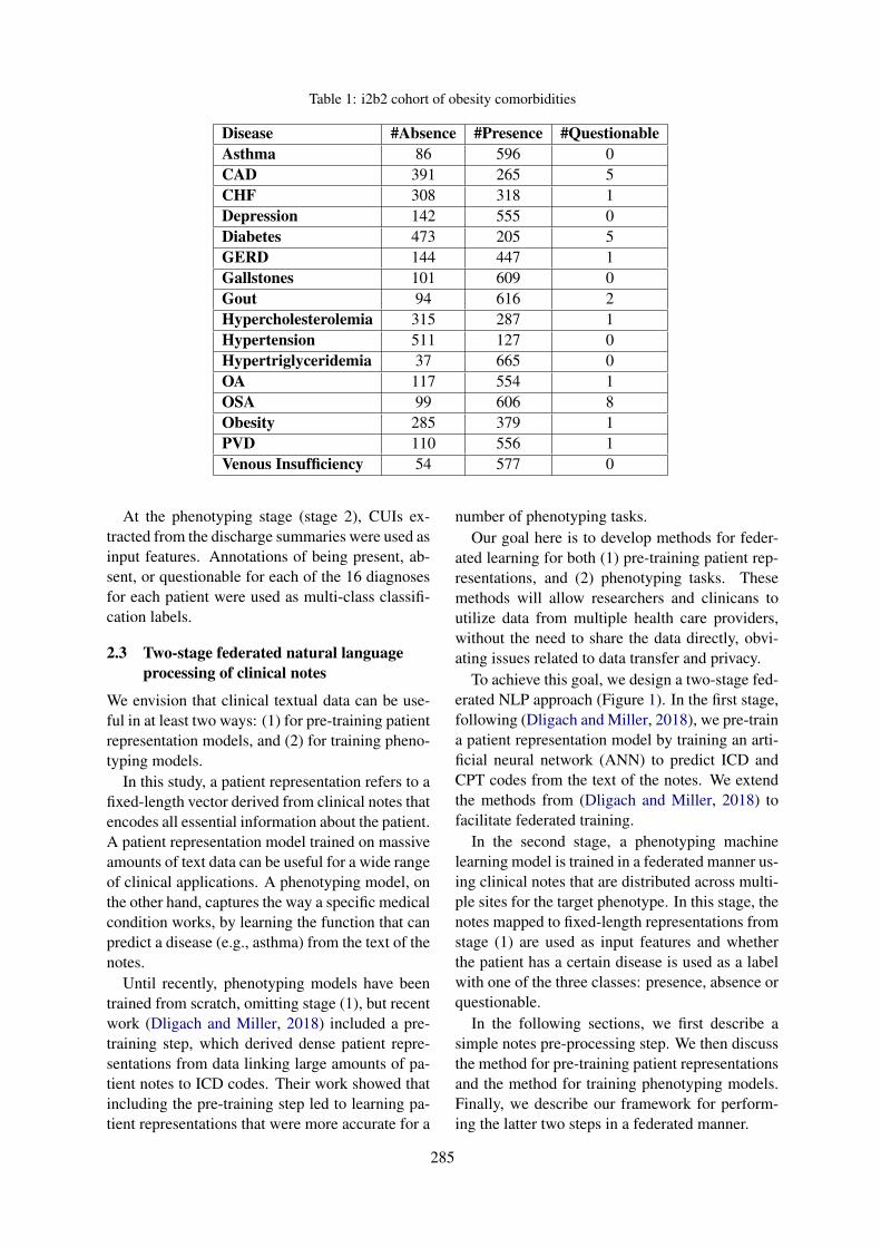
Table 1: i2b2 cohort of obesity comorbidities
Disease #Absence #Presence #QuestionableAsthma 86 596 0CAD 391 265 5CHF 308 318 1Depression 142 555 0Diabetes 473 205 5GERD 144 447 1Gallstones 101 609 0Gout 94 616 2Hypercholesterolemia 315 287 1Hypertension 511 127 0Hypertriglyceridemia 37 665 0OA 117 554 1OSA 99 606 8Obesity 285 379 1PVD 110 556 1Venous Insufficiency 54 577 0
At the phenotyping stage (stage 2), CUIs ex-tracted from the discharge summaries were used asinput features. Annotations of being present, ab-sent, or questionable for each of the 16 diagnosesfor each patient were used as multi-class classifi-cation labels.
2.3 Two-stage federated natural languageprocessing of clinical notes
We envision that clinical textual data can be use-ful in at least two ways: (1) for pre-training patientrepresentation models, and (2) for training pheno-typing models.
In this study, a patient representation refers to afixed-length vector derived from clinical notes thatencodes all essential information about the patient.A patient representation model trained on massiveamounts of text data can be useful for a wide rangeof clinical applications. A phenotyping model, onthe other hand, captures the way a specific medicalcondition works, by learning the function that canpredict a disease (e.g., asthma) from the text of thenotes.
Until recently, phenotyping models have beentrained from scratch, omitting stage (1), but recentwork (Dligach and Miller, 2018) included a pre-training step, which derived dense patient repre-sentations from data linking large amounts of pa-tient notes to ICD codes. Their work showed thatincluding the pre-training step led to learning pa-tient representations that were more accurate for a
number of phenotyping tasks.Our goal here is to develop methods for feder-
ated learning for both (1) pre-training patient rep-resentations, and (2) phenotyping tasks. Thesemethods will allow researchers and clinicans toutilize data from multiple health care providers,without the need to share the data directly, obvi-ating issues related to data transfer and privacy.
To achieve this goal, we design a two-stage fed-erated NLP approach (Figure 1). In the first stage,following (Dligach and Miller, 2018), we pre-traina patient representation model by training an arti-ficial neural network (ANN) to predict ICD andCPT codes from the text of the notes. We extendthe methods from (Dligach and Miller, 2018) tofacilitate federated training.
In the second stage, a phenotyping machinelearning model is trained in a federated manner us-ing clinical notes that are distributed across multi-ple sites for the target phenotype. In this stage, thenotes mapped to fixed-length representations fromstage (1) are used as input features and whetherthe patient has a certain disease is used as a labelwith one of the three classes: presence, absence orquestionable.
In the following sections, we first describe asimple notes pre-processing step. We then discussthe method for pre-training patient representationsand the method for training phenotyping models.Finally, we describe our framework for perform-ing the latter two steps in a federated manner.
285
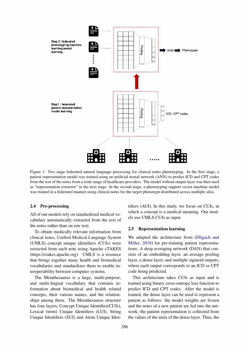
Figure 1: Two stage federated natural language processing for clinical notes phenotyping. In the first stage, apatient representation model was trained using an artificial neural network (ANN) to predict ICD and CPT codesfrom the text of the notes from a wide range of healthcare providers. The model without output layer was then usedas ”representation extractor” in the next stage. In the second stage, a phenotyping support vector machine modelwas trained in a federated manner using clinical notes for the target phenotype distributed across multiple silos.
2.4 Pre-processing
All of our models rely on standardized medical vo-cabulary automatically extracted from the text ofthe notes rather than on raw text.
To obtain medically relevant information fromclinical notes, Unified Medical Language System(UMLS) concept unique identifiers (CUIs) wereextracted from each note using Apache cTAKES(https://ctakes.apache.org). UMLS is a resourcethat brings together many health and biomedicalvocabularies and standardizes them to enable in-teroperability between computer systems.
The Metathesaurus is a large, multi-purpose,and multi-lingual vocabulary that contains in-formation about biomedical and health relatedconcepts, their various names, and the relation-ships among them. The Metathesaurus structurehas four layers, Concept Unique Identifies(CUIs),Lexical (term) Unique Identifiers (LUI), StringUnique Identifiers (SUI) and Atom Unique Iden-
tifiers (AUI). In this study, we focus on CUIs, inwhich a concept is a medical meaning. Our mod-els use UMLS CUIs as input.
2.5 Representation learning
We adapted the architecture from (Dligach andMiller, 2018) for pre-training patient representa-tions. A deep averaging network (DAN) that con-sists of an embedding layer, an average poolinglayer, a dense layer, and multiple sigmoid outputs,where each output corresponds to an ICD or CPTcode being predicted.
This architecture takes CUIs as input and istrained using binary cross-entropy loss function topredict ICD and CPT codes. After the model istrained, the dense layer can be used to represent apatient as follows: the model weights are frozenand the notes of a new patient are fed into the net-work; the patient representation is collected fromthe values of the units of the dense layer. Thus, the
286
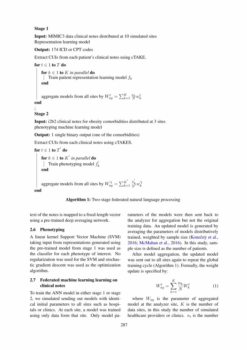
Stage 1
Input: MIMIC3 data clinical notes distributed at 10 simulated sitesRepresentation learning model
Output: 174 ICD or CPT codes
Extract CUIs from each patient’s clinical notes using cTAKE.
for t ∈ 1 to T do
for k ∈ 1 to K in parallel doTrain patient representation learning model fk
end
aggregate models from all sites by W tag =
∑Kk=1
nkN wt
k
end;Stage 2
Input: i2b2 clinical notes for obesity comorbidities distributed at 3 sitesphenotyping machine learning model
Output: 1 single binary output (one of the comorbidities)
Extract CUIs from each clinical notes using cTAKES.
for t ∈ 1 to T′ do
for k ∈ 1 to K′
in parallel doTrain phenotyping model f
′k
end
aggregate models from all sites by W′tag =
∑K′
k=1n′k
N ′ w′tk
end
Algorithm 1: Two-stage federated natural language processing
text of the notes is mapped to a fixed-length vectorusing a pre-trained deep averaging network.
2.6 PhenotypingA linear kernel Support Vector Machine (SVM)taking input from representations generated usingthe pre-trained model from stage 1 was used asthe classifer for each phenotype of interest. Noregularization was used for the SVM and stochas-tic gradient descent was used as the optimizationalgorithm.
2.7 Federated machine learning learning onclinical notes
To train the ANN model in either stage 1 or stage2, we simulated sending out models with identi-cal initial parameters to all sites such as hospi-tals or clinics. At each site, a model was trainedusing only data form that site. Only model pa-
rameters of the models were then sent back tothe analyzer for aggregation but not the originaltraining data. An updated model is generated byaveraging the parameters of models distributivelytrained, weighted by sample size (Konečnỳ et al.,2016; McMahan et al., 2016). In this study, sam-ple size is defined as the number of patients.
After model aggregation, the updated modelwas sent out to all sites again to repeat the globaltraining cycle (Algorithm 1). Formally, the weightupdate is specified by:
W tag =
K∑
k=1
nk
NW t
k (1)
where Wag is the parameter of aggregatedmodel at the analyzer site, K is the number ofdata sites, in this study the number of simulatedhealthcare providers or clinics. ni is the number
287
of samples at the ith site, N is the total number ofsamples across all sites, and Wi is the parameterslearned from the ith data site alone. t is the globalcycle number in the range of [1,T]. The algorithmtries to minimize the following objective function:
argminf
(−N∑
j=1
M∑
p=1
[yjplogf(xjp)+
(1− yjp)log(1− f(xjp))])
Where xj is the feature vector of CUIs. and yis the class label. p is the output number and Mis the total number of outputs. f is the machinelearning model such as artificial neural networkor SVM.Codes that accompany this article can befound at our github repository 3.
3 Experiments
To imitate real world medical setting where dataare distributed with different healthcare providers,we randomly split patients in MIMIC-III data into10 sites for stage 1 (federated representation learn-ing). The training data of i2b2 was split into 3sites for stage 2 (phenotype learning) to mimicobesity related notes distributed with three differ-ent healthcare providers. i2b2 notes were not in-cluded in the representation learning as in clinicsettings information exchange routes for disease-specific records are often not the same as generalmedical information and ICD/CPT codes were notavailable for i2b2 dataset.
Experiments were designed to answer threequestions:
1. Whether clinical notes distributed in differentsilos can be utilized for patient representationlearning without data sharing
2. Whether utilizing data from a wide rangeof sources will help improve performance ofphenotyping from clinical notes
3. Whether models trained in a two-stage fed-erated manner will have inferior performanceto models trained with centralized data.
To answer these questions, two-stage NLP al-gorithms were trained. Performance of modelstrained using only i2b2 notes from one of the
3https://github.com/kaiyuanmifen/FederatedNLP
three sites were compared with two-stage fed-erated NLP results. Furthermore, performanceof machine learning models using distributed orcentralized data at patient representation learningstage or phenotyping stage were compared.
4 Results
4.1 Two-stage federated natural languageprocessing improves performance ofautomatic phenotyping
We looked at the scenarios where no represen-tation learning was performed. In those cases,the standard TF-IDF weighted sparse bag-of-CUIsvectors were used to represent i2b2 notes. Thesparse vectors were used as input into the pheno-typing SVM model. We also looked at the scenar-ios where representation learning was performedby predicting ICD codes. For each of these con-ditions, we trained our phenotyping models us-ing centralized vs. federated learning. Finally,we considered a scenario where the phenotypingmodel was trained using the notes from a singlesite (the metrics we report were averaged acrossthree sites).
To summarize, seven experiments were con-ducted:
1. No representation learning + centralized phe-notyping learning
2. No representation learning + federated phe-notyping learning where i2b2 training datawere randomly split into 3 silos
3. No representation learning + single sourcephenotyping learning, where i2b2 data wererandomly split into 3 silos, but phenotypingalgorithm was only trained using data fromone of the silos
4. Centralized representation learning + central-ized phenotyping learning
5. Centralized representation learning + feder-ated phenotyping learning
6. Federated representation learning + central-ized phenotyping learning,where MIMIC-IIIdata were randomly split into 10 silos
7. Federated representation learning + federatedphenotyping learning, where MIMIC-III datawere randomly split into 10 silos and i2b2data into 3 silos (Table 2).
288
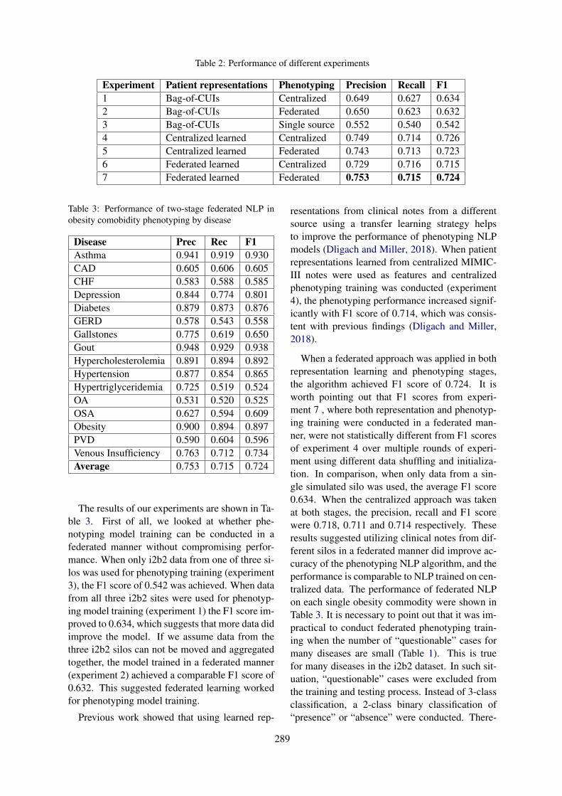
Table 2: Performance of different experiments
Experiment Patient representations Phenotyping Precision Recall F11 Bag-of-CUIs Centralized 0.649 0.627 0.6342 Bag-of-CUIs Federated 0.650 0.623 0.6323 Bag-of-CUIs Single source 0.552 0.540 0.5424 Centralized learned Centralized 0.749 0.714 0.7265 Centralized learned Federated 0.743 0.713 0.7236 Federated learned Centralized 0.729 0.716 0.7157 Federated learned Federated 0.753 0.715 0.724
Table 3: Performance of two-stage federated NLP inobesity comobidity phenotyping by disease
Disease Prec Rec F1Asthma 0.941 0.919 0.930CAD 0.605 0.606 0.605CHF 0.583 0.588 0.585Depression 0.844 0.774 0.801Diabetes 0.879 0.873 0.876GERD 0.578 0.543 0.558Gallstones 0.775 0.619 0.650Gout 0.948 0.929 0.938Hypercholesterolemia 0.891 0.894 0.892Hypertension 0.877 0.854 0.865Hypertriglyceridemia 0.725 0.519 0.524OA 0.531 0.520 0.525OSA 0.627 0.594 0.609Obesity 0.900 0.894 0.897PVD 0.590 0.604 0.596Venous Insufficiency 0.763 0.712 0.734Average 0.753 0.715 0.724
The results of our experiments are shown in Ta-ble 3. First of all, we looked at whether phe-notyping model training can be conducted in afederated manner without compromising perfor-mance. When only i2b2 data from one of three si-los was used for phenotyping training (experiment3), the F1 score of 0.542 was achieved. When datafrom all three i2b2 sites were used for phenotyp-ing model training (experiment 1) the F1 score im-proved to 0.634, which suggests that more data didimprove the model. If we assume data from thethree i2b2 silos can not be moved and aggregatedtogether, the model trained in a federated manner(experiment 2) achieved a comparable F1 score of0.632. This suggested federated learning workedfor phenotyping model training.
Previous work showed that using learned rep-
resentations from clinical notes from a differentsource using a transfer learning strategy helpsto improve the performance of phenotyping NLPmodels (Dligach and Miller, 2018). When patientrepresentations learned from centralized MIMIC-III notes were used as features and centralizedphenotyping training was conducted (experiment4), the phenotyping performance increased signif-icantly with F1 score of 0.714, which was consis-tent with previous findings (Dligach and Miller,2018).
When a federated approach was applied in bothrepresentation learning and phenotyping stages,the algorithm achieved F1 score of 0.724. It isworth pointing out that F1 scores from experi-ment 7 , where both representation and phenotyp-ing training were conducted in a federated man-ner, were not statistically different from F1 scoresof experiment 4 over multiple rounds of experi-ment using different data shuffling and initializa-tion. In comparison, when only data from a sin-gle simulated silo was used, the average F1 score0.634. When the centralized approach was takenat both stages, the precision, recall and F1 scorewere 0.718, 0.711 and 0.714 respectively. Theseresults suggested utilizing clinical notes from dif-ferent silos in a federated manner did improve ac-curacy of the phenotyping NLP algorithm, and theperformance is comparable to NLP trained on cen-tralized data. The performance of federated NLPon each single obesity commodity were shown inTable 3. It is necessary to point out that it was im-practical to conduct federated phenotyping train-ing when the number of “questionable” cases formany diseases are small (Table 1). This is truefor many diseases in the i2b2 dataset. In such sit-uation, “questionable” cases were excluded fromthe training and testing process. Instead of 3-classclassification, a 2-class binary classification of“presence” or “absence” were conducted. There-
289
fore, the performance metrics can not be directlycompared with results in the original i2b2 chal-lenge, though the scores were similar.
5 Conclusion
In this article, we presented a two-stage methodthat conducts patient representation learning andobesity comorbidity phenotyping, both in a feder-ated manner. The experimental results suggest thatfederated training of machine learning models ondistributed datasets does improve performance ofNLP on clinical notes compared with algorithmstrained on data from a single site. In this study, weused CUIs as input features into machine learningmodels, but the same federated learning strategiescan also be applied to raw text.
ReferencesAmy P Abernethy, Lynn M Etheredge, Patricia A Ganz,
Paul Wallace, Robert R German, Chalapathy Neti,Peter B Bach, and Sharon B Murphy. 2010. Rapid-learning system for cancer care. Journal of ClinicalOncology, 28(27):4268.
David Blumenthal and Marilyn Tavenner. 2010. Themeaningful use regulation for electronic healthrecords. New England Journal of Medicine,363(6):501–504.
Keith Bonawitz, Hubert Eichner, Wolfgang Grieskamp,Dzmitry Huba, Alex Ingerman, Vladimir Ivanov,Chloe Kiddon, Jakub Konecny, Stefano Mazzocchi,H Brendan McMahan, et al. 2019. Towards feder-ated learning at scale: System design. arXiv preprintarXiv:1902.01046.
Mike Conway, Richard L Berg, David Carrell,Joshua C Denny, Abel N Kho, Iftikhar J Kullo,James G Linneman, Jennifer A Pacheco, PeggyPeissig, Luke Rasmussen, et al. 2011. Analyzing theheterogeneity and complexity of electronic healthrecord oriented phenotyping algorithms. In AMIAannual symposium proceedings, volume 2011, page274. American Medical Informatics Association.
Dina Demner-Fushman, Wendy W Chapman, andClement J McDonald. 2009. What can natural lan-guage processing do for clinical decision support?Journal of biomedical informatics, 42(5):760–772.
Dmitriy Dligach and Timothy Miller. 2018. Learn-ing patient representations from text. arXiv preprintarXiv:1805.02096.
Elizabeth Ford, John A Carroll, Helen E Smith, DoniaScott, and Jackie A Cassell. 2016. Extracting infor-mation from the text of electronic medical records toimprove case detection: a systematic review. Jour-nal of the American Medical Informatics Associa-tion, 23(5):1007–1015.
Carol Friedman, Lyudmila Shagina, Yves Lussier, andGeorge Hripcsak. 2004. Automated encoding ofclinical documents based on natural language pro-cessing. Journal of the American Medical Informat-ics Association, 11(5):392–402.
Charles Friedman, Joshua Rubin, Jeffrey Brown,Melinda Buntin, Milton Corn, Lynn Etheredge, CarlGunter, Mark Musen, Richard Platt, William Stead,et al. 2014. Toward a science of learning systems:a research agenda for the high-functioning learninghealth system. Journal of the American Medical In-formatics Association, 22(1):43–50.
Charles P Friedman, Adam K Wong, and David Blu-menthal. 2010. Achieving a nationwide learn-ing health system. Science translational medicine,2(57):57cm29–57cm29.
Li Huang and Dianbo Liu. 2019. Patient clustering im-proves efficiency of federated machine learning topredict mortality and hospital stay time using dis-tributed electronic medical records. arXiv preprintarXiv:1903.09296.
Li Huang, Yifeng Yin, Zeng Fu, Shifa Zhang, HaoDeng, and Dianbo Liu. 2018. Loadaboost: Loss-based adaboost federated machine learning on med-ical data. arXiv preprint arXiv:1811.12629.
Vasudevan Jagannathan, Charles J Mullett, James GArbogast, Kevin A Halbritter, Deepthi Yellapragada,Sushmitha Regulapati, and Pavani Bandaru. 2009.Assessment of commercial nlp engines for medi-cation information extraction from dictated clinicalnotes. International journal of medical informatics,78(4):284–291.
Alistair EW Johnson, Tom J Pollard, Lu Shen,H Lehman Li-wei, Mengling Feng, Moham-mad Ghassemi, Benjamin Moody, Peter Szolovits,Leo Anthony Celi, and Roger G Mark. 2016.Mimic-iii, a freely accessible critical care database.Scientific data, 3:160035.
Jakub Konečnỳ, H Brendan McMahan, Felix X Yu, Pe-ter Richtárik, Ananda Theertha Suresh, and DaveBacon. 2016. Federated learning: Strategies for im-proving communication efficiency. arXiv preprintarXiv:1610.05492.
Kory Kreimeyer, Matthew Foster, Abhishek Pandey,Nina Arya, Gwendolyn Halford, Sandra F Jones,Richard Forshee, Mark Walderhaug, and TaxiarchisBotsis. 2017. Natural language processing systemsfor capturing and standardizing unstructured clini-cal information: a systematic review. Journal ofbiomedical informatics, 73:14–29.
Dianbo Liu, Timothy Miller, Raheel Sayeed, and Ken-neth Mandl. 2018a. Fadl: Federated-autonomousdeep learning for distributed electronic healthrecord. arXiv preprint arXiv:1811.11400.
290
Dianbo Liu, Nestor Sepulveda, and Ming Zheng.2018b. Artificial neural networks condensation: Astrategy to facilitate adaption of machine learning inmedical settings by reducing computational burden.arXiv preprint arXiv:1812.09659.
Christopher D Manning, Christopher D Manning, andHinrich Schütze. 1999. Foundations of statisticalnatural language processing. MIT press.
H Brendan McMahan, Eider Moore, Daniel Ram-age, Seth Hampson, et al. 2016. Communication-efficient learning of deep networks from decentral-ized data. arXiv preprint arXiv:1602.05629.
Riccardo Miotto, Li Li, Brian A Kidd, and Joel T Dud-ley. 2016. Deep patient: an unsupervised represen-tation to predict the future of patients from the elec-tronic health records. Scientific reports, 6:26094.
Harvey J Murff, Fern FitzHenry, Michael E Matheny,Nancy Gentry, Kristen L Kotter, Kimberly Crimin,Robert S Dittus, Amy K Rosen, Peter L Elkin,Steven H Brown, et al. 2011. Automated identifica-tion of postoperative complications within an elec-tronic medical record using natural language pro-cessing. Jama, 306(8):848–855.
Jean R Slutsky. 2007. Moving closer to a rapid-learning health care system. Health affairs,26(2):w122–w124.
Özlem Uzuner. 2009. Recognizing obesity and co-morbidities in sparse data. Journal of the AmericanMedical Informatics Association, 16(4):561–570.
291
Proceedings of the BioNLP 2019 workshop, pages 292–297Florence, Italy, August 1, 2019. c©2019 Association for Computational Linguistics
Transfer Learning for Causal Sentence Detection
Manolis Kyriakakis1, Ion Androutsopoulos2, Joan Ginés i Ametllé1, Artur Saudabayev 1
1Causaly, London, UK2Department of Informatics, Athens University of Economics and Business, Greece{m.kyriakakis,joan.g,artur}@causaly.com, [email protected]
Abstract
We consider the task of detecting sentencesthat express causality, as a step towards min-ing causal relations from texts. To bypassthe scarcity of causal instances in relation ex-traction datasets, we exploit transfer learning,namely ELMO and BERT, using a bidirectionalGRU with self-attention (BIGRUATT) as a base-line. We experiment with both generic publicrelation extraction datasets and a new biomed-ical causal sentence detection dataset, a sub-set of which we make publicly available. Wefind that transfer learning helps only in verysmall datasets. With larger datasets, BIGRU-ATT reaches a performance plateau, then largerdatasets and transfer learning do not help.
1 Introduction
A wide range of biomedical questions, from whatcauses a disease to what drug dosages shouldbe recommended and which side effects mightbe triggered, center around detecting particularcausal relationships between biomedical entities.Causality, therefore, has long been a focus ofbiomedical research, e.g., in medical diagnos-tics (Rizzi, 1994), pharmacovigilance (Agbabi-aka et al., 2008), and epidemiology (Karhausen,2000). The most common way to detect causalrelationships is by carrying highly controlled ran-domized controlled trials, but it is also possibleto mine evidence from observational studies andmeta-analyses (Ward and Johnson, 2008), whereinformation is often expressed in natural language(e.g., journal articles or clinical study reports).
In natural language processing (NLP), causalitydetection is often viewed as a type of relation ex-traction, where the goal is to determine which re-lations (e.g., part-whole, content-container, cause-effect), if any, hold between two entities in a text(Hendrickx et al., 2009), using deep learning inmost recent works (Bekoulis et al., 2018; Zhang
et al., 2018). The same view of causality detectionis typically adopted in biomedical NLP (Cohen andDemner-Fushman, 2014; Li and Mao, 2019).
Existing relation extraction datasets, however,contain few causal instances, which may not al-low relation extraction methods to learn to infercausality reliably. Note that causality can be ex-pressed in many ways, from using explicit lex-ical markers (e.g., “smoking causes cancer”) tomarkers that do not always express causality (e.g.,“heavy smoking led to cancer” vs. “the nurse ledthe patient to her room”) to no explicit mark-ers (“she was infected by a virus and admittedto a hospital”). Also, existing relation extrac-tion datasets contain sentences from generic, notbiomedical documents.
In this paper, we focus on detecting causal sen-tences, i.e., sentences conveying at least one causalrelation. This is a first step towards mining causalrelations from texts. Once causal sentences havebeen detected, computationally more intensive re-lation extraction methods can be used to identifythe exact entities that participate in the causal re-lations and their roles (cause, effect). To bypassthe scarcity of causal instances in relation extrac-tion datasets, we exploit transfer learning, namelyELMO (Peters et al., 2018) and BERT (Devlin et al.,2018), comparing against a bidirectional GRU withself-attention (Cho et al., 2014; Bahdanau et al.,2015). We experiment with generic public rela-tion extraction datasets and a new larger biomed-ical causal sentence detection dataset, a subset ofwhich we make publicly available.1
Unlike recently reported results in other NLP
tasks (Peters et al., 2018; Devlin et al., 2018; Pe-ters et al., 2019), we find that transfer learning
1We cannot provide the entire biomedical dataset, becauseit is used to develop commercial products. We report, how-ever, results for both the entire biomedical dataset and thepublicly available subset.
292
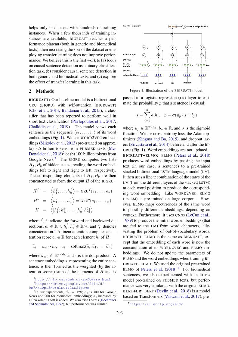
helps only in datasets with hundreds of traininginstances. When a few thousands of training in-stances are available, BIGRUATT reaches a per-formance plateau (both in generic and biomedicaltexts), then increasing the size of the dataset or em-ploying transfer learning does not improve perfor-mance. We believe this is the first work to (a) focuson causal sentence detection as a binary classifica-tion task, (b) consider causal sentence detection inboth generic and biomedical texts, and (c) explorethe effect of transfer learning in this task.
2 Methods
BIGRUATT: Our baseline model is a bidirectionalGRU (BIGRU) with self-attention (BIGRUATT)(Cho et al., 2014; Bahdanau et al., 2015), a clas-sifier that has been reported to perform well inshort text classification (Pavlopoulos et al., 2017;Chalkidis et al., 2019). The model views eachsentence as the sequence 〈e1, . . . , en〉 of its wordembeddings (Fig. 1). We use WORD2VEC embed-dings (Mikolov et al., 2013) pre-trained on approx.(a) 3.5 billion tokens from PUBMED texts (Mc-Donald et al., 2018)2 or (b) 100 billion tokens fromGoogle News.3 The BIGRU computes two listsHf , Hb of hidden states, reading the word embed-dings left to right and right to left, respectively.The corresponding elements of Hf , Hb are thenconcatenated to form the output H of the BIGRU:
Hf =⟨hf1 , . . . , h
fn
⟩= GRUf (e1, . . . , en)
Hb =⟨hb1, . . . , h
bn
⟩= GRUb(e1, . . . , en)
H =⟨[hf1 ;h
b1], . . . , [h
fn;h
bn]⟩
where f , b indicate the forward and backward di-rections, ei ∈ Rde , hfi , h
bi ∈ Rdh , and ‘;’ denotes
concatenation.4 A linear attention computes an at-tention score ai ∈ R for each element hi of H:
ãi = uatt · hi, ai = softmax(ãi; ã1, . . . , ãn)
where uatt ∈ R2×dh and · is the dot product. Asentence embedding s, representing the entire sen-tence, is then formed as the weighted (by the at-tention scores) sum of the elements of H and is
2http://nlp.cs.aueb.gr/software.html3https://drive.google.com/file/d/
0B7XkCwpI5KDYNlNUTTlSS21pQmM4In our experiments, dh = 128; de is 300 for Google
News and 200 for biomedical embeddings; de increases by1,024 when ELMO is added. We also tried LSTMs (Hochreiterand Schmidhuber, 1997), but performance was similar.
Figure 1: Illustration of the BIGRUATT model.
passed to a logistic regression (LR) layer to esti-mate the probability p that a sentence is causal:
s =n∑
i=1
aihi, p = σ(up · s+ bp)
where up ∈ R2×dh , bp ∈ R, and σ is the sigmoidfunction. We use cross-entropy loss, the Adam op-timizer (Kingma and Ba, 2015), and dropout lay-ers (Srivastava et al., 2014) before and after the BI-GRU (Fig. 1). Word embeddings are not updated.BIGRUATT+ELMO: ELMO (Peters et al., 2018)produces word embeddings by passing the inputtext (in our case, a sentence) to a pre-trainedstacked bidirectional LSTM language model (LM).It then uses a linear combination of the states of theLM (from the different layers of the stacked LSTM)at each word position to produce the correspond-ing word embedding. Like WORD2VEC, ELMO
(its LM) is pre-trained on large corpora. How-ever, ELMO maps occurrences of the same wordto possibly different embeddings, depending oncontext. Furthermore, it uses CNNs (LeCun et al.,1989) to produce the initial word embeddings (thatare fed to the LM) from word characters, alle-viating the problem of out-of-vocabulary words.BIGRUATT+ELMO is the same as BIGRUATT, ex-cept that the embedding of each word is now theconcatenation of its WORD2VEC and ELMO em-beddings. We do not update the parameters ofELMO and the word embeddings when training BI-GRUATT+ELMO. We used the original pre-trainedELMO of Peters et al. (2018).5 For biomedicalsentences, we also experimented with an ELMO
model pre-trained on PUBMED texts, but perfor-mance was very similar as with the original ELMO.BERT+LR: BERT (Devlin et al., 2018) is a modelbased on Transformers (Vaswani et al., 2017), pre-
5https://allennlp.org/elmo
293
trained on large corpora to predict (a) maskedwords from their left and right contexts, and (b)the next sentence. For a new NLP task, a task-specific layer is added on top of a pre-trained BERT
model. The extra layer is trained jointly with BERT
on task-specific data (in our case, a causal sentencedetection dataset), a process that also fine-tunesthe parameters of the pre-trained BERT for the newtask. In BERT+LR, we add a logistic regression(LR) layer on top of BERT, which estimates theprobability that the input sentence is causal. TheLR layer is fed with the embedding of the ‘classifi-cation’ token, which BERT also produces for eachsentence. We used the pre-trained ‘base’ BERT
model of Devlin et al. (2018), which we fine-tunedjointly with the LR layer. For biomedical sen-tences, we also experimented with BIOBERT (Leeet al., 2019), a BERT model pre-trained on biomed-ical texts, but performance was very similar.BERT+BIGRUATT: Common practice (Devlinet al., 2018; Peters et al., 2019) is to combine BERT
with very shallow task-specific models, usuallyonly an LR layer. To explore if deeper task-specificmodels can yield improved performance, we re-placed the LR layer of BERT+LR with BIGRUATT,leading to BERT+BIGRUATT. This is the same asBIGRUATT, but uses the context-aware word em-beddings that BERT produces at its top layer as theinput to BIGRUATT, instead of WORD2VEC em-beddings. Again, we use the ‘base’ pre-trainedBERT model of (Devlin et al., 2018), and wefine-tune the entire BERT+BIGRUATT network oncausal sentence detection datasets.LR (n-grams): A plain LR classifier with TF-IDF
n-gram features (word n-grams, n = 1, 2, 3).6
3 Datasets
SemEval-2010 (Task 8): This dataset contains10,674 samples, of which 1,325 causal (Hendrickxet al., 2009). Each sample is a sentence annotatedwith a pair of entities and the type of their relation-ship. Since we are only interested in causality, wetreat sentences with a Cause-Effect relationship ascausal, and all the others as non-causal.Causal-TimeBank (CausalTB): In this dataset(Mirza et al., 2014), we identified causal sentencesusing C-SIGNAL (causal signal) and CLINK (causal
6We used the LR code of SCIKIT-LEARN (https://scikit-learn.org/). For all other methods, we usedour own PyTorch implementations (https://pytorch.org/), with the BERT API of https://github.com/huggingface/pytorch-pretrained-BERT .
link) tags, discarding causal relationships betweenentities from different sentences, following Li andMao (2019). The resulting dataset contains 2,470sentences, of which 244 are causal.Event StoryLine (EventSL): In this dataset(Caselli and Vossen, 2017), we detected causalsentences by examining the CAUSES andCAUSED BY attributes in the PLOT LINK tags,again following Li and Mao (2019). Again, wediscarded causal relationships between entitiesfrom different sentences. The resulting datasetcontains 4,107 sentences, of which 77 are causal.BioCausal: The full biomedical causal detectiondataset we developed (BioCausal-Large) con-tains 13,342 sentences from PUBMED, of which7,562 causal. Each sentence was annotated by asingle annotator familiar with biomedical texts.7
The publicly available subset (BioCausal-Small)contains 2,000 sentences, of which 1,113 causal.8
Li and Mao (2019) report that SemEval-2010contains a large number of causal samples with ex-plicit causal markers; by contrast, CausalTB andEventSL contain more complex causal relationswith no explicit clues. BioCausal includes causalsentences both with and without explicit clues.
SemEval-2010, CausalTB, and EventSL arehighly imbalanced, with the vast majority of sen-tences being non-causal. To prevent a high biastowards the non-causal class, in our experimentswe randomly selected 2500, 500, 200 non-causalsentences respectively, discarding the rest. The re-sulting causal to non-causal ratios (Table 1) are,thus, roughly 1:2 (SemEval, CausalTB) or 1:3(EventSL). By contrast, the BioCausal (Large andSmall) datasets are roughly balanced. All fivedatasets were then split into train (70%), valida-tion (15%) and test (15%) subsets, maintaining thesame ratio between the two classes in the threesubsets.
4 Experimental results
Tables 1–2 report our experimental results. Foreach neural model, we performed 10 repetitions(with different random seeds) and report averagesand standard deviations. For completeness, weshow precision, recall, F1, and area under theprecision-recall curve (AUC), though AUC scoresare the main ones to consider, since they examine
7The average inter-annotator agreement on a sample of300 sentences was 79.36%. Cohen’s Kappa was 0.56.
8BioCausal-Small is available at https://archive.org/details/CausalySmall.
294
Dataset (causal:non-causal) SemEval (1,325 : 2,500) CausalTB (244 : 500) EventSL (77 : 200) BioCausal-Small (1,113 : 887)Model F1 P R AUC F1 P R AUC F1 P R AUC F1 P R AUC
LR (n-grams) 76.22 88.67 66.83 87.50 36.36 100.00 22.22 65.02 42.86 100.00 27.27 73.55 77.49 73.91 81.44 87.65
BIGRUATT90.64±0.70
93.96±1.71
87.59±1.52
96.57±0.32
69.98±3.58
67.04±5.16
73.89±6.60
74.38±4.16
63.65±10.12
70.09±7.47
60.91±17.28
70.36±9.84
85.97±0.90
83.57±2.03
88.62±2.69
93.91±0.88
BIGRUATT+ELMO92.81±0.78
94.45±0.94
91.26±1.77
97.03±1.44
75.08±4.20
81.29±5.43
70.28±6.81
82.06*±3.59
66.55±7.82
77.47±5.05
59.09±10.17
77.31±4.84
87.32±0.78
89.46±2.34
85.39±2.50
94.95±0.33
BERT+LR91.55±0.53
86.62±1.16
97.09±0.67
96.94±2.25
80.55±3.62
71.17±6.02
93.33±3.33
82.26*±3.41
72.35±5.36
62.44±8.21
87.17±4.58
78.15*±9.48
85.64±0.61
78.87±1.16
93.71±1.54
90.75±3.69
BERT+BIGRUATT91.45±0.59
86.80±1.28
96.63±0.60
97.61±0.29
80.06±2.94
74.52±4.46
86.94±5.56
84.27*±1.71
73.09±5.27
66.15±7.86
83.64±10.60
84.17*±4.04
85.87±0.88
79.43±1.53
93.47±1.08
93.75±0.45
Table 1: Precision, recall, F1, AUC on the four publicly available datasets, averaged over 10 repetitions, withstandard deviations (±). Next to each dataset name, we show in brackets the total causal and non-causal sentencesthat we used. The best results are shown in bold. The best AUC results are also shown in gray background. In theAUC columns, stars indicate statistically significant (p ≤ 0.05) differences compared to BIGRUATT.
performance at multiple classification thresholds;the other measures are computed only for a partic-ular threshold, which was 0.5 in our experiments.
Model F1 P R AUCLR (n-grams) 79.21 76.75 81.82 86.54
BIGRUATT 85.84±0.36
84.28±0.66
87.47±0.75
93.71±0.15
BIGRUATT+ELMO 86.77±0.52
87.46±1.29
86.12±1.49
94.64*±0.26
BERT+LR 87.33±0.47
82.11±0.89
93.27±0.67
92.77±1.57
BERT+BIGRUATT 87.09±0.34
81.70±0.58
93.25±0.40
94.70±0.24
Table 2: Results on BioCausal-Large (7,562 : 5,780).
Focusing on AUC scores, BIGRUATT outper-forms the simpler LR with n-grams by a widemargin, with the exception of EventSL, which isprobably too small for the capacity of BIGRU-ATT.9 The precision of LR is perfect on CausalTBand EventSL, at the expense of very low recall,suggesting that LR learned perfectly few high-precision n-grams in those datasets. Transferlearning (ELMO, BERT) improves the AUC of BI-GRUATT by a wide margin in the two small-est datasets (CausalTB, EventSL), which containonly hundreds of instances, and the AUC differ-ences from BIGRUATT are statistically significant(stars in Table 1), except for BIGRUATT+ELMO inEventSL.10 However, in the other three datasetswhich contain thousands of instances, the AUC
differences between transfer learning and plainBIGRUATT are small, with no statistical signifi-cance in most cases. Also, the AUC scores of allmethods on BioCausal-Large are close to those onBioCausal-Small, despite the fact that BioCausal-Large is approx. seven times larger. Similar obser-vations can be made by looking at the F1 scores.
9Indeed BIGRUATT overfits the training set of EventSL.10We performed two-tailed Approximate Randomization
tests (Dror et al., 2018), p ≤ 0.05, with 10k iterations, ran-domly swapping in each iteration 50% of the decisions (overall tested sentences) across the two compared methods. Whentesting statistical significance, for each method we use therepetition (among the 10) with the best validation F1 score.
It seems that causal sentence detection, at leastwith the neural methods we considered, reaches aplateau with few thousands of training sentencesboth in generic and biomedical texts; then increas-ing the dataset size or employing transfer learn-ing does not help. The latter finding is not inline with previously reported results (Peters et al.,2018; Devlin et al., 2018; Peters et al., 2019),where ELMO and BERT were found to improveperformance in most NLP tasks without studying,however, the effect of dataset size. Furthermore,BERT+BIGRUATT consistently performed betterthan BERT+LR in AUC (but not in F1), which castsdoubts on the practice of adding only shallow task-specific models to BERT.11 BIGRUATT+ELMO
is competitive in AUC to BERT+BIGRUATT (withthe exception of EventSL). Mainly comprised ofsentences with simple explicit causal statements(Li and Mao, 2019), SemEval expectedly demon-strated the best classification performance acrossdatasets.
5 Related and Future Work
Recent work on (causal) relation extraction usesLSTMs (Zhang et al., 2017) or CNNs (Li and Mao,2019), assuming however that the spans of the twoentities (cause, effect) are known. A notable ex-ception is the model of Bekoulis et al. (2018),which jointly infers the spans of the entities andtheir relationships. Such finer relation extractionmethods, however, are computationally more ex-pensive than our causal sentence detection meth-ods, especially when they involve parsing (Zhanget al., 2018). We plan to consider pipelines wherecomputationally cheaper causal sentence detectioncomponents will first detect sentences likely to ex-press causality, and then finer relation extractioncomponents will pinpoint the entities, the type of
11We note, however, that the AUC difference betweenBERT+LR and BERT+BIGRUATT is statistically significant(p ≤ 0.05) only in BioCausal-Large.
295
causality (e.g., up-regulate), and entity roles.
Appendix
A Hyper-parameters
Batch sizes of 128, 32, 16, 32 and 256 were usedfor Semeval, CausalTB, EventSL, BioCausal-Small and BioCausal-Large, respectively, for allneural models. Trainable parameters were initial-ized using the default PyTorch initialization meth-ods except from self-attention weights where themethod of Glorot and Bengio (2010) was used.
BIGRU and BIGRUATT+ELMO were trained for100 epochs using Adam (Kingma and Ba, 2015)with initial learning rate 2e-3 , β1/β2 = 0.9/0.999and eps = 1e−8. The learning rate was decayedlinearly every 20 epochs as lrnew ← lrprev · 0.75.Gradients were clipped using a clip norm thresh-old of 0.25. The GRU’s hidden size was set to 128and its depth to 1. A dropout of 0.5 was appliedto the input and output connections of the BIGRU
encoder. Validation F1 was checked periodicallyin order to keep the model’s checkpoint with thebest validation performance.
BERT and BERT+BIGRUATT used the BERT-BASE uncased pre-trained model, which has 12layers, 768 hidden size, 12 attention heads, and110M parameters. For both models the entire net-work was fine-tuned for 10 epochs using Adamwith a very small learning rate of 2e-5, β1/β2 =0.9/0.999, eps = 1e−6, L2 weight decay of0.01 and linear warmup of 0.1. A dropout of0.1 was applied to all BERT-specific layers. ForBERT+BIGRUATT, an additional dropout of 0.5was applied to the input and output connectionsof its BIGRU encoder. Similarly to BIGRU and BI-GRUATT+ELMO, the hidden size of the GRU wasset to 128 and its depth to 1.
ReferencesTaofikat B. Agbabiaka, Jelena Savović, and Edzard
Ernst. 2008. Methods for causality assessment ofadverse drug reactions. Drug Safety, 31(1):21–37.
Dzmitry Bahdanau, Kyunghyun Cho, and Yoshua Ben-gio. 2015. Neural machine translation by jointlylearning to align and translate. In 3rd Interna-tional Conference on Learning Representations, SanDiego, California.
Giannis Bekoulis, Johannes Deleu, Thomas Demeester,and Chris Develder. 2018. Adversarial training formulti-context joint entity and relation extraction. In
Proceedings of the Conference on Empirical Meth-ods in Natural Language Processing, pages 2830–2836, Brussels, Belgium.
Tommaso Caselli and Piek Vossen. 2017. The eventstoryline corpus: A new benchmark for causal andtemporal relation extraction. In Proceedings of theEvents and Stories in the News Workshop, pages 77–86, Vancouver, Canada.
Ilias Chalkidis, Manos Fergadiotis, ProdromosMalakasiotis, Nikolaos Aletras, and Ion Androut-sopoulos. 2019. Extreme multi-label legal textclassification:a case study in EU legislation. InNAACL Workshop in Natural Legal LanguageProcessing.
Kyunghyun Cho, Bart van Merrienboer, Caglar Gul-cehre, Dzmitry Bahdanau, Fethi Bougares, HolgerSchwenk, and Yoshua Bengio. 2014. Learningphrase representations using RNN encoder-decoderfor statistical machine translation. In Proceedingsof the Conference on Empirical Methods in Natu-ral Language Processing, pages 1724–1734, Doha,Qatar.
Kevin Bretonnel Cohen and Dina Demner-Fushman.2014. Biomedical Natural Language Processing.John Benjamins.
Jacob Devlin, Ming-Wei Chang, Kenton Lee, andKristina Toutanova. 2018. BERT: Pre-training ofdeep bidirectional transformers for language under-standing. arXiv preprint arXiv:1810.04805.
Rotem Dror, Gili Baumer, Segev Shlomov, and Roi Re-ichart. 2018. The hitchhiker’s guide to testing statis-tical significance in natural language processing. InProceedings of the 56th Annual Meeting of the ACL(Volume 1: Long Papers), pages 1383–1392.
Xavier Glorot and Yoshua Bengio. 2010. Understand-ing the difficulty of training deep feedforward neu-ral networks. In Proceedings of the Thirteenth In-ternational Conference on Artificial Intelligence andStatistics, pages 249–256.
Iris Hendrickx, Su Nam Kim, Zornitsa Kozareva,Preslav Nakov, Diarmuid Ó Séaghdha, SebastianPadó, Marco Pennacchiotti, Lorenza Romano, andStan Szpakowicz. 2009. SemEval-2010 Task 8:Multi-way classification of semantic relations be-tween pairs of nominals. In Proceedings ofthe Workshop on Semantic Evaluations: RecentAchievements and Future Directions, pages 94–99,Boulder, Colorado.
Sepp Hochreiter and Jürgen Schmidhuber. 1997. Longshort-term memory. Neural Computation, 9:1735–1780.
Lucien R. Karhausen. 2000. Causation: The elusivegrail of epidemiology. Medicine, Health Care andPhilosophy, 3(1):59–67.
296
Diederik P. Kingma and Jimmy Ba. 2015. Adam:A method for stochastic optimization. CoRR,abs/1412.6980.
Yann LeCun, Bernhard E. Boser, John S. Denker, DonHenderson, R. E. Howard, W. Hubbard, and LarryJackel. 1989. Backpropagation applied to hand-written zip code recognition. Neural Computation,1(4):541–551.
Jinhyuk Lee, Wonjin Yoon, Sungdong Kim,Donghyeon Kim, Sunkyu Kim, Chan Ho So, andJaewoo Kang. 2019. Biobert: a pre-trained biomed-ical language representation model for biomedicaltext mining. arXiv preprint arXiv:1901.08746.
Pengfei Li and Kezhi Mao. 2019. Knowledge-orientedconvolutional neural network for causal relation ex-traction from natural language texts. Expert Systemswith Applications, 115:512–523.
Ryan McDonald, Georgios-Ioannis Brokos, and IonAndroutsopoulos. 2018. Deep relevance ranking us-ing enhanced document-query interactions. In Pro-ceedings of the Conference on Empirical Methodsin Natural Language Processing, pages 1849–1860,Brussels, Belgium.
Tomas Mikolov, Ilya Sutskever, Kai Chen, Greg S Cor-rado, and Jeff Dean. 2013. Distributed representa-tions of words and phrases and their composition-ality. In C. J. C. Burges, L. Bottou, M. Welling,Z. Ghahramani, and K. Q. Weinberger, editors, Ad-vances in Neural Information Processing Systems26, pages 3111–3119.
Paramita Mirza, Rachele Sprugnoli, Sara Tonelli, andManuela Speranza. 2014. Annotating causality inthe tempeval-3 corpus. In Proceedings of the EACLWorkshop on Computational Approaches to Causal-ity in Language (CAtoCL), pages 10–19.
John Pavlopoulos, Prodromos Malakasiotis, and IonAndroutsopoulos. 2017. Deeper attention to abu-sive user content moderation. In Proceedings of theConference on Empirical Methods in Natural Lan-guage Processing, pages 1125–1135, Copenhagen,Denmark.
Matthew Peters, Mark Neumann, Mohit Iyyer, MattGardner, Christopher Clark, Kenton Lee, and LukeZettlemoyer. 2018. Deep contextualized word rep-resentations. In Proceedings of the Conference ofthe NAACL: Human Language Technologies, Vol-ume 1 (Long Papers), pages 2227–2237, New Or-leans, Louisiana.
Matthew Peters, Sebastian Ruder, and Noah A. Smith.2019. To tune or not to tune? adapting pre-trained representations to diverse tasks. CoRR,abs/1903.05987.
Dominick A. Rizzi. 1994. Causal reasoning and thediagnostic process. Theoretical medicine, 15:315–33.
Nitish Srivastava, Geoffrey Hinton, Alex Krizhevsky,Ilya Sutskever, and Ruslan Salakhutdinov. 2014.Dropout: A simple way to prevent neural networksfrom overfitting. Journal of Machine Learning Re-search, 15:1929–1958.
Ashish Vaswani, Noam Shazeer, Niki Parmar, JakobUszkoreit, Llion Jones, Aidan N Gomez, Ł ukaszKaiser, and Illia Polosukhin. 2017. Attention is allyou need. In I. Guyon, U. V. Luxburg, S. Bengio,H. Wallach, R. Fergus, S. Vishwanathan, and R. Gar-nett, editors, Advances in Neural Information Pro-cessing Systems 30, pages 5998–6008.
Andrew Ward and Pamela Jo Johnson. 2008. Ad-dressing confounding errors when using non-experimental, observational data to make causalclaims. Synthese, 163(3):419–432.
Yuhao Zhang, Peng Qi, and Christopher D. Manning.2018. Graph convolution over pruned dependencytrees improves relation extraction. In Proceedingsof the Conference on Empirical Methods in NaturalLanguage Processing, pages 2205–2215, Brussels,Belgium.
Yuhao Zhang, Victor Zhong, Danqi Chen, Gabor An-geli, and Christopher D. Manning. 2017. Position-aware attention and supervised data improve slot fill-ing. In Proceedings of the Conference on Empiri-cal Methods in Natural Language Processing, pages35–45, Copenhagen, Denmark.
297
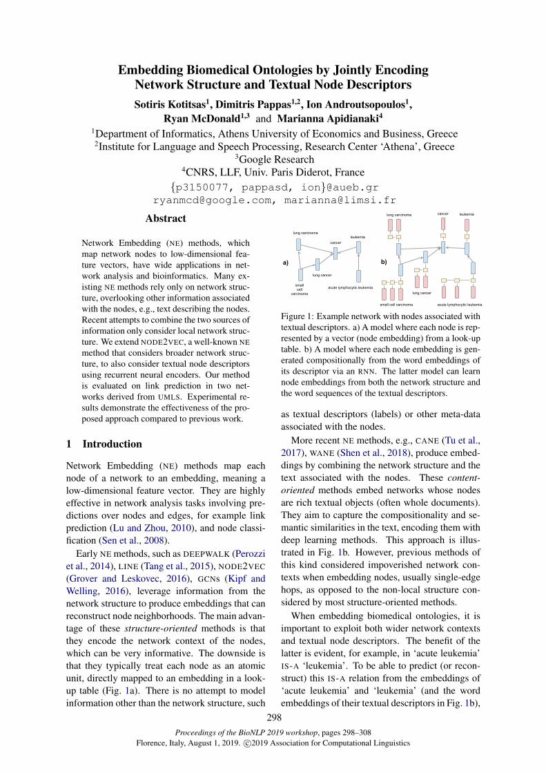
Proceedings of the BioNLP 2019 workshop, pages 298–308Florence, Italy, August 1, 2019. c©2019 Association for Computational Linguistics
Embedding Biomedical Ontologies by Jointly EncodingNetwork Structure and Textual Node DescriptorsSotiris Kotitsas1, Dimitris Pappas1,2, Ion Androutsopoulos1,
Ryan McDonald1,3 and Marianna Apidianaki4
1Department of Informatics, Athens University of Economics and Business, Greece2Institute for Language and Speech Processing, Research Center ‘Athena’, Greece
3Google Research4CNRS, LLF, Univ. Paris Diderot, France
{p3150077, pappasd, ion}@[email protected], [email protected]
Abstract
Network Embedding (NE) methods, whichmap network nodes to low-dimensional fea-ture vectors, have wide applications in net-work analysis and bioinformatics. Many ex-isting NE methods rely only on network struc-ture, overlooking other information associatedwith the nodes, e.g., text describing the nodes.Recent attempts to combine the two sources ofinformation only consider local network struc-ture. We extend NODE2VEC, a well-known NEmethod that considers broader network struc-ture, to also consider textual node descriptorsusing recurrent neural encoders. Our methodis evaluated on link prediction in two net-works derived from UMLS. Experimental re-sults demonstrate the effectiveness of the pro-posed approach compared to previous work.
1 Introduction
Network Embedding (NE) methods map eachnode of a network to an embedding, meaning alow-dimensional feature vector. They are highlyeffective in network analysis tasks involving pre-dictions over nodes and edges, for example linkprediction (Lu and Zhou, 2010), and node classi-fication (Sen et al., 2008).
Early NE methods, such as DEEPWALK (Perozziet al., 2014), LINE (Tang et al., 2015), NODE2VEC
(Grover and Leskovec, 2016), GCNs (Kipf andWelling, 2016), leverage information from thenetwork structure to produce embeddings that canreconstruct node neighborhoods. The main advan-tage of these structure-oriented methods is thatthey encode the network context of the nodes,which can be very informative. The downside isthat they typically treat each node as an atomicunit, directly mapped to an embedding in a look-up table (Fig. 1a). There is no attempt to modelinformation other than the network structure, such
lung cancer
cancerlung carcinoma leukemia
small cell carcinoma
lung cancer
cancer
acute lymphocytic leukemia
lung carcinomaleukemia
smallcell
carcinoma
a) b)
acute lymphocytic leukemia
Figure 1: Example network with nodes associated withtextual descriptors. a) A model where each node is rep-resented by a vector (node embedding) from a look-uptable. b) A model where each node embedding is gen-erated compositionally from the word embeddings ofits descriptor via an RNN. The latter model can learnnode embeddings from both the network structure andthe word sequences of the textual descriptors.
as textual descriptors (labels) or other meta-dataassociated with the nodes.
More recent NE methods, e.g., CANE (Tu et al.,2017), WANE (Shen et al., 2018), produce embed-dings by combining the network structure and thetext associated with the nodes. These content-oriented methods embed networks whose nodesare rich textual objects (often whole documents).They aim to capture the compositionality and se-mantic similarities in the text, encoding them withdeep learning methods. This approach is illus-trated in Fig. 1b. However, previous methods ofthis kind considered impoverished network con-texts when embedding nodes, usually single-edgehops, as opposed to the non-local structure con-sidered by most structure-oriented methods.
When embedding biomedical ontologies, it isimportant to exploit both wider network contextsand textual node descriptors. The benefit of thelatter is evident, for example, in ‘acute leukemia’IS-A ‘leukemia’. To be able to predict (or recon-struct) this IS-A relation from the embeddings of‘acute leukemia’ and ‘leukemia’ (and the wordembeddings of their textual descriptors in Fig. 1b),
298
a NE method only needs to model the role of‘acute’ as a modifier that can be included in the de-scriptor of a node (e.g., a disease node) to specifya sub-type. This property can be learned (and en-coded in the word embedding of ‘acute’) if severalsimilar IS-A edges, with ‘acute’ being the onlyextra word in the descriptor of the sub-type, ex-ist in the network. This strategy would not how-ever be successful in ‘p53’ (a protein) IS-A ‘tumorsuppressor’, where no word in the descriptors fre-quently denotes sub-typing. Instead, by consider-ing the broader network context of the nodes (i.e.longer paths that connect them), a NE method candetect that the two nodes have common neighborsand, hence, adjust the two node embeddings (andthe word embeddings of their descriptors) to beclose in the representation space, making it morelikely to predict an IS-A relation between them.
We propose a new NE method that leverages thestrengths of both structure and content-orientedapproaches. To exploit wide network contexts, wefollow NODE2VEC (Grover and Leskovec, 2016)and generate random walks to construct the net-work neighborhood of each node. The SKIP-GRAM model (Mikolov et al., 2013) is then usedto learn node embeddings that successfully pre-dict the nodes in each walk, from the node at thebeginning of the walk. To enrich the node em-beddings with information from their textual de-scriptors, we replace the NODE2VEC look-up ta-ble with various architectures that operate on theword embeddings of the descriptors. These in-clude simply averaging the word embeddings ofa descriptor, and applying recurrent deep learningencoders. The proposed method can be seen as anextension of NODE2VEC that incorporates textualnode descriptors. We evaluate several variants ofthe proposed method on link prediction, a stan-dard evaluation task for NE methods. We use twobiomedical networks extracted from UMLS (Bo-denreider, 2004), with PART-OF and IS-A rela-tions, respectively. Our method outperforms sev-eral existing structure and content-oriented meth-ods on both datasets. We make our datasets andsource code available.1
2 Related work
Network Embedding (NE) methods, a type of rep-resentation learning, are highly effective in net-
1https://github.com/SotirisKot/Content-Aware-N2V
work analysis tasks involving predictions overnodes and edges. Link prediction has been ex-tensively studied in social networks (Wang et al.,2015), and is particularly relevant to bioinfor-matics where it can help, for example, to dis-cover interactions between proteins, diseases, andgenes (Lei and Ruan, 2013; Shojaie, 2013; Groverand Leskovec, 2016). Node classification canalso help analyze large networks by automati-cally assigning roles or labels to nodes (Ahmedet al., 2018; Sen et al., 2008). In bioinformat-ics, this approach has been used to identify pro-teins whose mutations are linked with particulardiseases (Agrawal et al., 2018).
A typical structure-oriented NE method isDEEPWALK (Perozzi et al., 2014), which learnsnode embeddings by applying WORD2VEC’sSKIPGRAM model (Mikolov et al., 2013) to nodesequences generated via random walks on thenetwork. NODE2VEC (Grover and Leskovec,2016) explores different strategies to perform ran-dom walks, introducing hyper-parameters to guidethem and generate more flexible neighborhoods.LINE (Tang et al., 2015) learns node embeddingsby exploiting first- and second-order proximity in-formation in the network. Wang et al. (2016)learn node embeddings that preserve the proxim-ity between 2-hop neighbors using a deep autoen-coder. Yu et al. (2018) encode node sequencesgenerated via random walks, by mapping thewalks to low dimensional embeddings, through anLSTM autoencoder. To avoid overfitting, they usea generative adversarial training process as regu-larization. Graph Convolutional Networks (GCNs)are a graph encoding framework that also fallswithin this paradigm (Kipf and Welling, 2016;Schlichtkrull et al., 2018). Unlike other meth-ods that use random walks or static neighbour-hoods, GCNs use iterative neighbourhood averag-ing strategies to account for non-local graph struc-ture. All the aforementioned methods only encodethe structural information into node embeddings,ignoring textual or other information that can beassociated with the nodes of the network.
Previous work on biomedical ontologies (e.g.,Gene Ontology, GO) suggested that their terms,which are represented through textual descriptors,have compositional structure. By modeling it, wecan create richer representations of the data en-coded in the ontologies (Mungall, 2004; Ogrenet al., 2003, 2004). Ogren et al. (2003) strengthen
299
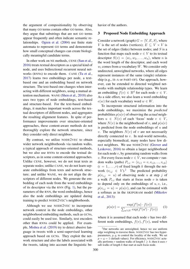
the argument of compositionality by observingthat many GO terms contain other GO terms. Also,they argue that substrings that are not GO termsappear frequently and often indicate semantic re-lationships. Ogren et al. (2004) use finite stateautomata to represent GO terms and demonstratehow small conceptual changes can create biologi-cally meaningful candidate terms.
In other work on NE methods, CENE (Sun et al.,2016) treats textual descriptors as a special kind ofnode, and uses bidirectional recurrent neural net-works (RNNs) to encode them. CANE (Tu et al.,2017) learns two embeddings per node, a text-based one and an embedding based on networkstructure. The text-based one changes when inter-acting with different neighbors, using a mutual at-tention mechanism. WANE (Shen et al., 2018) alsouses two types of node embeddings, text-basedand structure-based. For the text-based embed-dings, it matches important words across the tex-tual descriptors of different nodes, and aggregatesthe resulting alignment features. In spite of per-formance improvements over structure-orientedapproaches, these content-aware methods do notthoroughly explore the network structure, sincethey consider only direct neighbors.
By contrast, we utilize NODE2VEC to obtainwider network neighborhoods via random walks,a typical approach of structure-oriented methods,but we also use RNNs to encode the textual de-scriptors, as in some content-oriented approaches.Unlike CENE, however, we do not treat texts asseparate nodes; unlike CANE, we do not learn sep-arate embeddings from texts and network struc-ture; and unlike WANE, we do not align the de-scriptors of different nodes. We generate the em-bedding of each node from the word embeddingsof its descriptor via the RNN (Fig. 1), but the pa-rameters of the RNN, the word embeddings, hencealso the node embeddings are updated duringtraining to predict NODE2VEC’s neighborhoods.
Although we use NODE2VEC to incorporatenetwork context in the node embeddings, otherneighborhood embedding methods, such as GCNs,could easily be used too. Similarly, text encodersother than RNNs could be applied. For exam-ple, Mishra et al. (2019) try to detect abusive lan-guage in tweets with a semi-supervised learningapproach based on GCNs. They exploit the net-work structure and also the labels associated withthe tweets, taking into account the linguistic be-
havior of the authors.
3 Proposed Node Embedding Approach
Consider a network (graph)G = 〈V,E, S〉, whereV is the set of nodes (vertices); E ⊆ V × V isthe set of edges (links) between nodes; and S is afunction that maps each node v ∈ V to its textualdescriptor S(v) = 〈w1, w2, . . . , wn〉, where n isthe word length of the descriptor, and each wordwi comes from a vocabularyW . We consider onlyundirected, unweighted networks, where all edgesrepresent instances of the same (single) relation-ship (e.g., IS-A or PART-OF). Our approach, how-ever, can be extended to directed weighted net-works with multiple relationship types. We learnan embedding f(v) ∈ Rd for each node v ∈ V .As a side effect, we also learn a word embeddinge(w) for each vocabulary word w ∈W .
To incorporate structural information into thenode embeddings, we maximize the predictedprobabilities p(u|v) of observing the actual neigh-bors u ∈ N(v) of each ‘focus’ node v ∈ V ,where N(v) is the neighborhood of v, and p(u|v)is predicted from the node embeddings of u andv. The neighbors N(v) of v are not necessarilydirectly connected to v. In real-world networks,especially biomedical, many nodes have few di-rect neighbors. We use NODE2VEC (Grover andLeskovec, 2016) to obtain a larger neighborhoodfor each node v, by generating random walks fromv. For every focus node v ∈ V , we compute r ran-dom walks (paths) Pv,i = 〈vi,1 = v, vi,2, ..., vi,k〉(i = 1, . . . , r) of fixed length k through the net-work (vi,j ∈ V ).2 The predicted probabilityp(vi,j = u) of observing node u at step j ofa walk Pv,i that starts at focus node v is takento depend only on the embeddings of u, v, i.e.,p(vi,j = u) = p(u|v), and can be estimated witha softmax as in the SKIPGRAM model (Mikolovet al., 2013):
p(u|v) = exp(f ′(u) · f(v))∑u′∈V exp(f ′(u′) · f(v)) (1)
where it is assumed that each node v has two dif-ferent node embeddings, f(v), f ′(v), used when
2Our networks are unweighted, hence we use uniformedge weighting to traverse them. NODE2VEC has two hyper-parameters, p, q, to control the locality of the walk. We setp = q = 1 (default values). For efficiency, NODE2VEC actu-ally performs r random walks of length l ≥ k; then it uses rsub-walks of length k that start at each focus node.
300
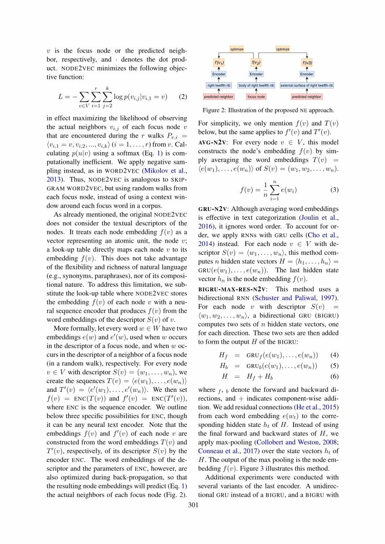
v is the focus node or the predicted neigh-bor, respectively, and · denotes the dot prod-uct. NODE2VEC minimizes the following objec-tive function:
L = −∑
v∈V
r∑
i=1
k∑
j=2
log p(vi,j |vi,1 = v) (2)
in effect maximizing the likelihood of observingthe actual neighbors vi,j of each focus node vthat are encountered during the r walks Pv,i =〈vi,1 = v, vi,2, ..., vi,k〉 (i = 1, . . . , r) from v. Cal-culating p(u|v) using a softmax (Eq. 1) is com-putationally inefficient. We apply negative sam-pling instead, as in WORD2VEC (Mikolov et al.,2013). Thus, NODE2VEC is analogous to SKIP-GRAM WORD2VEC, but using random walks fromeach focus node, instead of using a context win-dow around each focus word in a corpus.
As already mentioned, the original NODE2VEC
does not consider the textual descriptors of thenodes. It treats each node embedding f(v) as avector representing an atomic unit, the node v;a look-up table directly maps each node v to itsembedding f(v). This does not take advantageof the flexibility and richness of natural language(e.g., synonyms, paraphrases), nor of its composi-tional nature. To address this limitation, we sub-stitute the look-up table where NODE2VEC storesthe embedding f(v) of each node v with a neu-ral sequence encoder that produces f(v) from theword embeddings of the descriptor S(v) of v.
More formally, let every wordw ∈W have twoembeddings e(w) and e′(w), used when w occursin the descriptor of a focus node, and when w oc-curs in the descriptor of a neighbor of a focus node(in a random walk), respectively. For every nodev ∈ V with descriptor S(v) = (w1, . . . , wn), wecreate the sequences T (v) = 〈e(w1), . . . , e(wn)〉and T ′(v) = 〈e′(w1), . . . , e
′(wn)〉. We then setf(v) = ENC(T (v)) and f ′(v) = ENC(T ′(v)),where ENC is the sequence encoder. We outlinebelow three specific possibilities for ENC, thoughit can be any neural text encoder. Note that theembeddings f(v) and f ′(v) of each node v areconstructed from the word embeddings T (v) andT ′(v), respectively, of its descriptor S(v) by theencoder ENC. The word embeddings of the de-scriptor and the parameters of ENC, however, arealso optimized during back-propagation, so thatthe resulting node embeddings will predict (Eq. 1)the actual neighbors of each focus node (Fig. 2).
right twelfth rib body of right twelfth rib external surface of right twelfth rib
focus nodepredicted neighbor
Encoder Encoder Encoder
f'(v1) f(v2) f'(v3)
optimize optimize
predicted neighbor
Figure 2: Illustration of the proposed NE approach.
For simplicity, we only mention f(v) and T (v)below, but the same applies to f ′(v) and T ′(v).AVG-N2V: For every node v ∈ V , this modelconstructs the node’s embedding f(v) by sim-ply averaging the word embeddings T (v) =〈e(w1), . . . , e(wn)〉 of S(v) = (w1, w2, . . . , wn).
f(v) =1
n
n∑
i=1
e(wi) (3)
GRU-N2V: Although averaging word embeddingsis effective in text categorization (Joulin et al.,2016), it ignores word order. To account for or-der, we apply RNNs with GRU cells (Cho et al.,2014) instead. For each node v ∈ V with de-scriptor S(v) = 〈w1, . . . , wn〉, this method com-putes n hidden state vectors H = 〈h1, . . . , hn〉 =GRU(e(w1), . . . , e(wn)). The last hidden statevector hn is the node embedding f(v).BIGRU-MAX-RES-N2V: This method uses abidirectional RNN (Schuster and Paliwal, 1997).For each node v with descriptor S(v) =〈w1, w2, . . . , wn〉, a bidirectional GRU (BIGRU)computes two sets of n hidden state vectors, onefor each direction. These two sets are then addedto form the output H of the BIGRU:
Hf = GRUf (e(w1), . . . , e(wn)) (4)
Hb = GRUb(e(w1), . . . , e(wn)) (5)
H = Hf +Hb (6)
where f , b denote the forward and backward di-rections, and + indicates component-wise addi-tion. We add residual connections (He et al., 2015)from each word embedding e(wt) to the corre-sponding hidden state ht of H . Instead of usingthe final forward and backward states of H , weapply max-pooling (Collobert and Weston, 2008;Conneau et al., 2017) over the state vectors ht ofH . The output of the max pooling is the node em-bedding f(v). Figure 3 illustrates this method.
Additional experiments were conducted withseveral variants of the last encoder. A unidirec-tional GRU instead of a BIGRU, and a BIGRU with
301
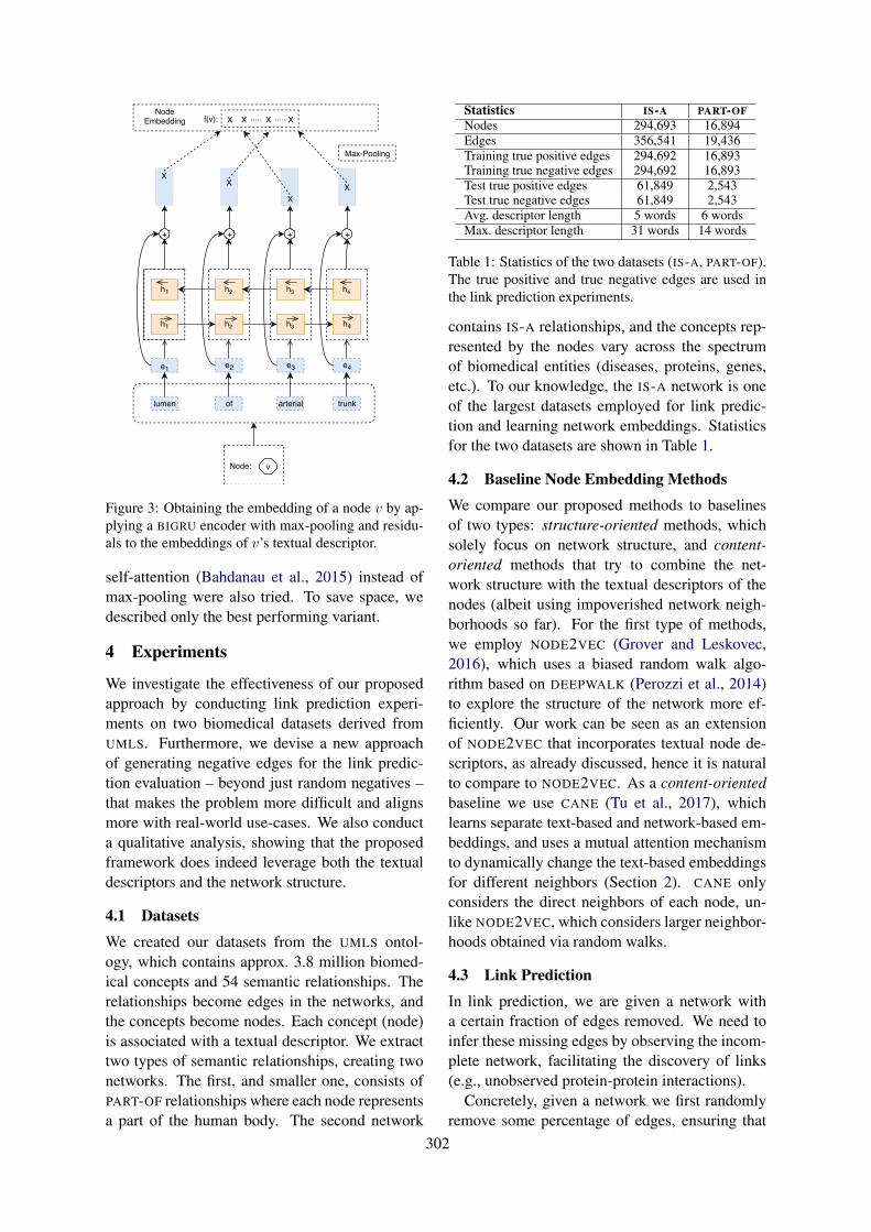
Node: v
lumen of arterial trunk
e1 e2 e3 e4
h1
h1
h2
h2
h3
h3
h4
h4
+ + + +
XX
XX
Node Embedding
f(v): X X ..... X ..... X
Max-Pooling
Figure 3: Obtaining the embedding of a node v by ap-plying a BIGRU encoder with max-pooling and residu-als to the embeddings of v’s textual descriptor.
self-attention (Bahdanau et al., 2015) instead ofmax-pooling were also tried. To save space, wedescribed only the best performing variant.
4 Experiments
We investigate the effectiveness of our proposedapproach by conducting link prediction experi-ments on two biomedical datasets derived fromUMLS. Furthermore, we devise a new approachof generating negative edges for the link predic-tion evaluation – beyond just random negatives –that makes the problem more difficult and alignsmore with real-world use-cases. We also conducta qualitative analysis, showing that the proposedframework does indeed leverage both the textualdescriptors and the network structure.
4.1 Datasets
We created our datasets from the UMLS ontol-ogy, which contains approx. 3.8 million biomed-ical concepts and 54 semantic relationships. Therelationships become edges in the networks, andthe concepts become nodes. Each concept (node)is associated with a textual descriptor. We extracttwo types of semantic relationships, creating twonetworks. The first, and smaller one, consists ofPART-OF relationships where each node representsa part of the human body. The second network
Statistics IS-A PART-OFNodes 294,693 16,894Edges 356,541 19,436Training true positive edges 294,692 16,893Training true negative edges 294,692 16,893Test true positive edges 61,849 2,543Test true negative edges 61,849 2,543Avg. descriptor length 5 words 6 wordsMax. descriptor length 31 words 14 words
Table 1: Statistics of the two datasets (IS-A, PART-OF).The true positive and true negative edges are used inthe link prediction experiments.
contains IS-A relationships, and the concepts rep-resented by the nodes vary across the spectrumof biomedical entities (diseases, proteins, genes,etc.). To our knowledge, the IS-A network is oneof the largest datasets employed for link predic-tion and learning network embeddings. Statisticsfor the two datasets are shown in Table 1.
4.2 Baseline Node Embedding Methods
We compare our proposed methods to baselinesof two types: structure-oriented methods, whichsolely focus on network structure, and content-oriented methods that try to combine the net-work structure with the textual descriptors of thenodes (albeit using impoverished network neigh-borhoods so far). For the first type of methods,we employ NODE2VEC (Grover and Leskovec,2016), which uses a biased random walk algo-rithm based on DEEPWALK (Perozzi et al., 2014)to explore the structure of the network more ef-ficiently. Our work can be seen as an extensionof NODE2VEC that incorporates textual node de-scriptors, as already discussed, hence it is naturalto compare to NODE2VEC. As a content-orientedbaseline we use CANE (Tu et al., 2017), whichlearns separate text-based and network-based em-beddings, and uses a mutual attention mechanismto dynamically change the text-based embeddingsfor different neighbors (Section 2). CANE onlyconsiders the direct neighbors of each node, un-like NODE2VEC, which considers larger neighbor-hoods obtained via random walks.
4.3 Link Prediction
In link prediction, we are given a network witha certain fraction of edges removed. We need toinfer these missing edges by observing the incom-plete network, facilitating the discovery of links(e.g., unobserved protein-protein interactions).
Concretely, given a network we first randomlyremove some percentage of edges, ensuring that
302
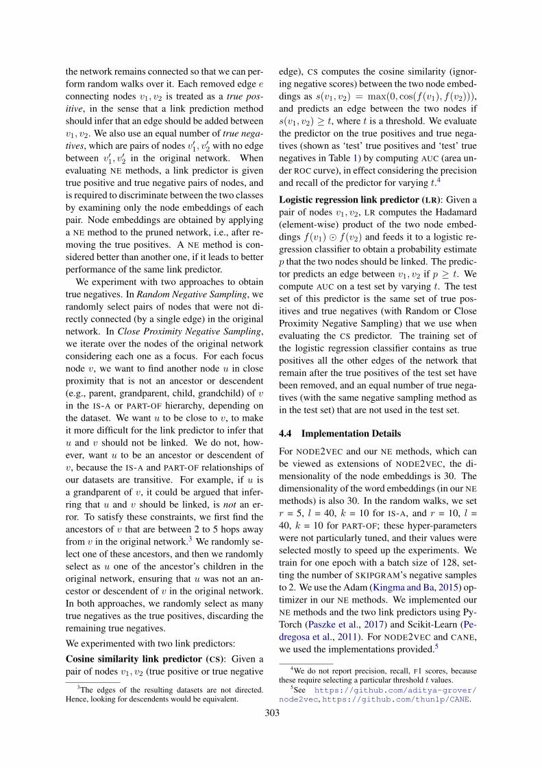
the network remains connected so that we can per-form random walks over it. Each removed edge econnecting nodes v1, v2 is treated as a true pos-itive, in the sense that a link prediction methodshould infer that an edge should be added betweenv1, v2. We also use an equal number of true nega-tives, which are pairs of nodes v′1, v
′2 with no edge
between v′1, v′2 in the original network. When
evaluating NE methods, a link predictor is giventrue positive and true negative pairs of nodes, andis required to discriminate between the two classesby examining only the node embeddings of eachpair. Node embeddings are obtained by applyinga NE method to the pruned network, i.e., after re-moving the true positives. A NE method is con-sidered better than another one, if it leads to betterperformance of the same link predictor.
We experiment with two approaches to obtaintrue negatives. In Random Negative Sampling, werandomly select pairs of nodes that were not di-rectly connected (by a single edge) in the originalnetwork. In Close Proximity Negative Sampling,we iterate over the nodes of the original networkconsidering each one as a focus. For each focusnode v, we want to find another node u in closeproximity that is not an ancestor or descendent(e.g., parent, grandparent, child, grandchild) of vin the IS-A or PART-OF hierarchy, depending onthe dataset. We want u to be close to v, to makeit more difficult for the link predictor to infer thatu and v should not be linked. We do not, how-ever, want u to be an ancestor or descendent ofv, because the IS-A and PART-OF relationships ofour datasets are transitive. For example, if u isa grandparent of v, it could be argued that infer-ring that u and v should be linked, is not an er-ror. To satisfy these constraints, we first find theancestors of v that are between 2 to 5 hops awayfrom v in the original network.3 We randomly se-lect one of these ancestors, and then we randomlyselect as u one of the ancestor’s children in theoriginal network, ensuring that u was not an an-cestor or descendent of v in the original network.In both approaches, we randomly select as manytrue negatives as the true positives, discarding theremaining true negatives.
We experimented with two link predictors:
Cosine similarity link predictor (CS): Given apair of nodes v1, v2 (true positive or true negative
3The edges of the resulting datasets are not directed.Hence, looking for descendents would be equivalent.
edge), CS computes the cosine similarity (ignor-ing negative scores) between the two node embed-dings as s(v1, v2) = max(0, cos(f(v1), f(v2))),and predicts an edge between the two nodes ifs(v1, v2) ≥ t, where t is a threshold. We evaluatethe predictor on the true positives and true nega-tives (shown as ‘test’ true positives and ‘test’ truenegatives in Table 1) by computing AUC (area un-der ROC curve), in effect considering the precisionand recall of the predictor for varying t.4
Logistic regression link predictor (LR): Given apair of nodes v1, v2, LR computes the Hadamard(element-wise) product of the two node embed-dings f(v1) � f(v2) and feeds it to a logistic re-gression classifier to obtain a probability estimatep that the two nodes should be linked. The predic-tor predicts an edge between v1, v2 if p ≥ t. Wecompute AUC on a test set by varying t. The testset of this predictor is the same set of true pos-itives and true negatives (with Random or CloseProximity Negative Sampling) that we use whenevaluating the CS predictor. The training set ofthe logistic regression classifier contains as truepositives all the other edges of the network thatremain after the true positives of the test set havebeen removed, and an equal number of true nega-tives (with the same negative sampling method asin the test set) that are not used in the test set.
4.4 Implementation Details
For NODE2VEC and our NE methods, which canbe viewed as extensions of NODE2VEC, the di-mensionality of the node embeddings is 30. Thedimensionality of the word embeddings (in our NE
methods) is also 30. In the random walks, we setr = 5, l = 40, k = 10 for IS-A, and r = 10, l =40, k = 10 for PART-OF; these hyper-parameterswere not particularly tuned, and their values wereselected mostly to speed up the experiments. Wetrain for one epoch with a batch size of 128, set-ting the number of SKIPGRAM’s negative samplesto 2. We use the Adam (Kingma and Ba, 2015) op-timizer in our NE methods. We implemented ourNE methods and the two link predictors using Py-Torch (Paszke et al., 2017) and Scikit-Learn (Pe-dregosa et al., 2011). For NODE2VEC and CANE,we used the implementations provided.5
4We do not report precision, recall, F1 scores, becausethese require selecting a particular threshold t values.
5See https://github.com/aditya-grover/node2vec, https://github.com/thunlp/CANE.
303
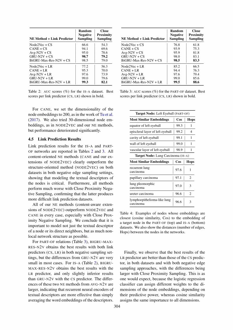
Random CloseNegative Proximity
NE Method + Link Predictor Sampling Sampling
Node2Vec + CS 66.6 54.3CANE + CS 94.1 69.6Avg-N2V + CS 95.0 78.6GRU-N2V + CS 98.7 79.2BiGRU-Max-Res-N2V + CS 98.5 79.0
Node2Vec + LRCANE + LRAvg-N2V + LRGRU-N2V + LRBiGRU-Max-Res-N2V + LR
77.295.397.699.099.3
56.370.073.979.682.1
Table 2: AUC scores (%) for the IS-A dataset. Bestscores per link predictor (CS, LR) shown in bold.
For CANE, we set the dimensionality of thenode embeddings to 200, as in the work of Tu et al.(2017). We also tried 30-dimensional node em-beddings, as in NODE2VEC and our NE methods,but performance deteriorated significantly.
4.5 Link Prediction ResultsLink prediction results for the IS-A and PART-OF networks are reported in Tables 2 and 3. Allcontent-oriented NE methods (CANE and our ex-tensions of NODE2VEC) clearly outperform thestructure-oriented method (NODE2VEC) on bothdatasets in both negative edge sampling settings,showing that modeling the textual descriptors ofthe nodes is critical. Furthermore, all methodsperform much worse with Close Proximity Nega-tive Sampling, confirming that the latter producesmore difficult link prediction datasets.
All of our NE methods (content-aware exten-sions of NODE2VEC) outperform NODE2VEC andCANE in every case, especially with Close Prox-imity Negative Sampling. We conclude that it isimportant to model not just the textual descriptorof a node or its direct neighbors, but as much non-local network structure as possible.
For PART-OF relations (Table 3), BIGRU-MAX-RES-N2V obtains the best results with both linkpredictors (CS, LR) in both negative sampling set-tings, but the differences from GRU-N2V are verysmall in most cases. For IS-A (Table 2), BIGRU-MAX-RES-N2V obtains the best results with theLR predictor, and only slightly inferior resultsthan GRU-N2V with the CS predictor. The differ-ences of these two NE methods from AVG-N2V arelarger, indicating that recurrent neural encoders oftextual descriptors are more effective than simplyaveraging the word embeddings of the descriptors.
Random CloseNegative Proximity
NE Method + Link Predictor Sampling Sampling
Node2Vec + CS 76.8 61.8CANE + CS 93.9 75.3Avg-N2V + CS 95.9 81.8GRU-N2V + CS 98.0 83.1BiGRU-Max-Res-N2V + CS 98.5 83.3
Node2Vec + LRCANE + LRAvg-N2V + LRGRU-N2V + LRBiGRU-Max-Res-N2V + LR
85.294.497.699.099.5
66.576.379.485.688.6
Table 3: AUC scores (%) for the PART-OF dataset. Bestscores per link predictor (CS, LR) shown in bold.
Target Node: Left Eyeball (PART-OF)
Most Similar Embeddings Cos Hops
equator of left eyeball 99.3 1
episcleral layer of left eyeball 99.2 4
cavity of left eyeball 99.1 1
wall of left eyeball 99.0 1
vascular layer of left eyeball 98.9 1
Target Node: Lung Carcinoma (IS-A)
Most Similar Embeddings Cos Hops
recurrent lungcarcinoma 97.6 1
papillary carcinoma 97.1 2
lung pleomorphiccarcinoma 97.0 3
ureter carcinoma 96.6 2
lymphoepithelioma-like lungcarcinoma 96.6 3
Table 4: Examples of nodes whose embeddings areclosest (cosine similarity, Cos) to the embedding ofa target node in the PART-OF (top) and IS-A (bottom)datasets. We also show the distances (number of edges,Hops) between the nodes in the networks.
Finally, we observe that the best results of theLR predictor are better than those of the CS predic-tor, in both datasets and with both negative edgesampling approaches, with the differences beinglarger with Close Proximity Sampling. This is asone would expect, because the logistic regressionclassifier can assign different weights to the di-mensions of the node embeddings, depending ontheir predictive power, whereas cosine similarityassigns the same importance to all dimensions.
304
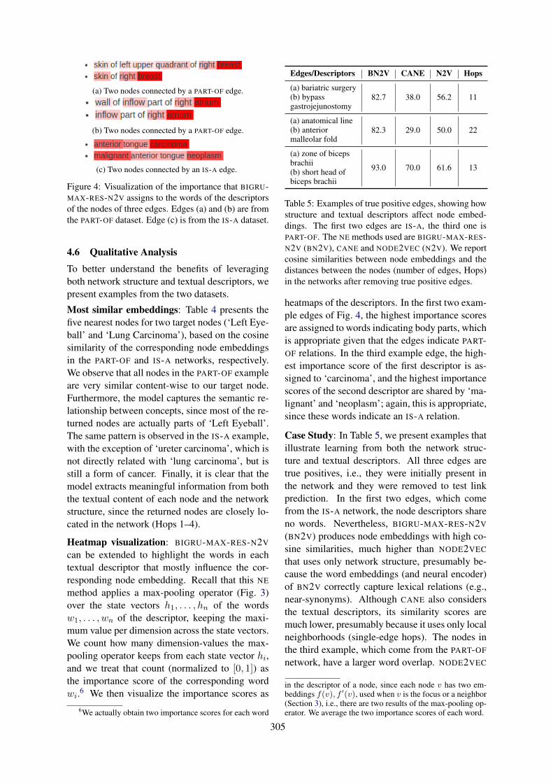
(a) Two nodes connected by a PART-OF edge.
(b) Two nodes connected by a PART-OF edge.
(c) Two nodes connected by an IS-A edge.
Figure 4: Visualization of the importance that BIGRU-MAX-RES-N2V assigns to the words of the descriptorsof the nodes of three edges. Edges (a) and (b) are fromthe PART-OF dataset. Edge (c) is from the IS-A dataset.
4.6 Qualitative Analysis
To better understand the benefits of leveragingboth network structure and textual descriptors, wepresent examples from the two datasets.
Most similar embeddings: Table 4 presents thefive nearest nodes for two target nodes (‘Left Eye-ball’ and ‘Lung Carcinoma’), based on the cosinesimilarity of the corresponding node embeddingsin the PART-OF and IS-A networks, respectively.We observe that all nodes in the PART-OF exampleare very similar content-wise to our target node.Furthermore, the model captures the semantic re-lationship between concepts, since most of the re-turned nodes are actually parts of ‘Left Eyeball’.The same pattern is observed in the IS-A example,with the exception of ‘ureter carcinoma’, which isnot directly related with ‘lung carcinoma’, but isstill a form of cancer. Finally, it is clear that themodel extracts meaningful information from boththe textual content of each node and the networkstructure, since the returned nodes are closely lo-cated in the network (Hops 1–4).
Heatmap visualization: BIGRU-MAX-RES-N2V
can be extended to highlight the words in eachtextual descriptor that mostly influence the cor-responding node embedding. Recall that this NE
method applies a max-pooling operator (Fig. 3)over the state vectors h1, . . . , hn of the wordsw1, . . . , wn of the descriptor, keeping the maxi-mum value per dimension across the state vectors.We count how many dimension-values the max-pooling operator keeps from each state vector hi,and we treat that count (normalized to [0, 1]) asthe importance score of the corresponding wordwi.6 We then visualize the importance scores as
6We actually obtain two importance scores for each word
Edges/Descriptors BN2V CANE N2V Hops
(a) bariatric surgery(b) bypassgastrojejunostomy
82.7 38.0 56.2 11
(a) anatomical line(b) anteriormalleolar fold
82.3 29.0 50.0 22
(a) zone of bicepsbrachii(b) short head ofbiceps brachii
93.0 70.0 61.6 13
Table 5: Examples of true positive edges, showing howstructure and textual descriptors affect node embed-dings. The first two edges are IS-A, the third one isPART-OF. The NE methods used are BIGRU-MAX-RES-N2V (BN2V), CANE and NODE2VEC (N2V). We reportcosine similarities between node embeddings and thedistances between the nodes (number of edges, Hops)in the networks after removing true positive edges.
heatmaps of the descriptors. In the first two exam-ple edges of Fig. 4, the highest importance scoresare assigned to words indicating body parts, whichis appropriate given that the edges indicate PART-OF relations. In the third example edge, the high-est importance score of the first descriptor is as-signed to ‘carcinoma’, and the highest importancescores of the second descriptor are shared by ‘ma-lignant’ and ‘neoplasm’; again, this is appropriate,since these words indicate an IS-A relation.
Case Study: In Table 5, we present examples thatillustrate learning from both the network struc-ture and textual descriptors. All three edges aretrue positives, i.e., they were initially present inthe network and they were removed to test linkprediction. In the first two edges, which comefrom the IS-A network, the node descriptors shareno words. Nevertheless, BIGRU-MAX-RES-N2V
(BN2V) produces node embeddings with high co-sine similarities, much higher than NODE2VEC
that uses only network structure, presumably be-cause the word embeddings (and neural encoder)of BN2V correctly capture lexical relations (e.g.,near-synonyms). Although CANE also considersthe textual descriptors, its similarity scores aremuch lower, presumably because it uses only localneighborhoods (single-edge hops). The nodes inthe third example, which come from the PART-OF
network, have a larger word overlap. NODE2VEC
in the descriptor of a node, since each node v has two em-beddings f(v), f ′(v), used when v is the focus or a neighbor(Section 3), i.e., there are two results of the max-pooling op-erator. We average the two importance scores of each word.
305
is unaware of this overlap and produces the lowestscore. The two content-oriented methods (BN2V,CANE) produce higher scores, but again BN2V
produces a much higher similarity, presumablybecause it uses larger neighborhoods. In all threeedges, the two nodes are distant (>10 hops), yetBN2V produces high similarity scores.
5 Conclusions and Future Work
We proposed a new method to learn content-awarenode embeddings, which extends NODE2VEC byconsidering the textual descriptors of the nodes.The proposed approach leverages the strengthsof both structure- and content-oriented node em-bedding methods. It exploits non-local networkneighborhoods generated by random walks, as inthe original NODE2VEC, and allows integratingvarious neural encoders of the textual descrip-tors. We evaluated our models on two biomed-ical networks extracted from UMLS, which con-sist of PART-OF and IS-A edges. Experimentalresults with two link predictors, cosine similar-ity and logistic regression, demonstrated that ourapproach is effective and outperforms previousmethods which rely on structure alone, or modelcontent along with local network context only.
In future work, we plan to experiment with net-works extracted from other biomedical ontologiesand knowledge bases. We also plan to explore ifthe word embeddings that our methods generatecan improve biomedical question answering sys-tems (McDonald et al., 2018).
Acknowledgements
This work was partly supported by the ResearchCenter of the Athens University of Economics andBusiness. The work was also supported by theFrench National Research Agency under projectANR-16-CE33-0013.
ReferencesMonica Agrawal, Marinka Zitnik, and Jure Leskovec.
2018. Large-scale analysis of disease pathwaysin the human interactome. Pacific Symposium onBiocomputing. Pacific Symposium on Biocomput-ing, 23:111–122.
Nesreen K. Ahmed, Ryan A. Rossi, John Boaz Lee, Xi-angnan Kong, Theodore L. Willke, Rong Zhou, andHoda Eldardiry. 2018. Learning role-based graphembeddings. CoRR, abs/1802.02896.
Dzmitry Bahdanau, Kyunghyun Cho, and Yoshua Ben-gio. 2015. Neural machine translation by jointlylearning to align and translate. In 3rd Inter-national Conference on Learning Representations,ICLR 2015, San Diego, CA, USA, May 7-9, 2015,Conference Track Proceedings.
James Bergstra, Daniel L K Yamins, and David D.Cox. 2013. Hyperopt: A python library for opti-mizing the hyperparameters of machine learning al-gorithms.
Olivier Bodenreider. 2004. The unified medical lan-guage system (UMLS): integrating biomedical ter-minology. Nucleic Acids Research, 32(Database-Issue):267–270.
Kyunghyun Cho, Bart van Merrienboer, ÇaglarGülçehre, Dzmitry Bahdanau, Fethi Bougares, Hol-ger Schwenk, and Yoshua Bengio. 2014. Learningphrase representations using RNN encoder-decoderfor statistical machine translation. In Proceedings ofthe 2014 Conference on Empirical Methods in Nat-ural Language Processing, EMNLP 2014, October25-29, 2014, Doha, Qatar, A meeting of SIGDAT,a Special Interest Group of the ACL, pages 1724–1734.
Ronan Collobert and Jason Weston. 2008. A unifiedarchitecture for natural language processing: deepneural networks with multitask learning. In Ma-chine Learning, Proceedings of the Twenty-Fifth In-ternational Conference (ICML 2008), Helsinki, Fin-land, June 5-9, 2008, pages 160–167.
Alexis Conneau, Douwe Kiela, Holger Schwenk, Loı̈cBarrault, and Antoine Bordes. 2017. Supervisedlearning of universal sentence representations fromnatural language inference data. In Proceedings ofthe 2017 Conference on Empirical Methods in Nat-ural Language Processing, EMNLP 2017, Copen-hagen, Denmark, September 9-11, 2017, pages 670–680.
Aditya Grover and Jure Leskovec. 2016. node2vec:Scalable feature learning for networks. In KDD,pages 855–864. ACM.
Kaiming He, Xiangyu Zhang, Shaoqing Ren, and JianSun. 2015. Deep residual learning for image recog-nition. CoRR, abs/1512.03385.
Armand Joulin, Edouard Grave, Piotr Bojanowski, andTomas Mikolov. 2016. Bag of tricks for efficienttext classification. CoRR, abs/1607.01759.
Diederik P. Kingma and Jimmy Ba. 2015. Adam:A method for stochastic optimization. CoRR,abs/1412.6980.
Thomas N. Kipf and Max Welling. 2016. Semi-supervised classification with graph convolutionalnetworks. CoRR, abs/1609.02907.
306
Chengwei Lei and Jianhua Ruan. 2013. A novellink prediction algorithm for reconstructing protein-protein interaction networks by topological similar-ity. Bioinformatics, 29(3):355–364.
Linyuan Lu and Tao Zhou. 2010. Link predic-tion in complex networks: A survey. CoRR,abs/1010.0725.
Ryan McDonald, Georgios-Ioannis Brokos, and IonAndroutsopoulos. 2018. Deep relevance ranking us-ing enhanced document-query interactions. In Pro-ceedings of the Conference on Empirical Methodsin Natural Language Processing, pages 1849–1860,Brussels, Belgium.
Tomas Mikolov, Ilya Sutskever, Kai Chen, Gregory S.Corrado, and Jeffrey Dean. 2013. Distributed repre-sentations of words and phrases and their composi-tionality. In NIPS, pages 3111–3119.
Pushkar Mishra, Marco Del Tredici, Helen Yan-nakoudakis, and Ekaterina Shutova. 2019. Abusivelanguage detection with graph convolutional net-works. CoRR, abs/1904.04073.
Christopher J Mungall. 2004. Obol: Integrating lan-guage and meaning in bio-ontologies. Comparativeand Functional Genomics, 5:509 – 520.
Philip V. Ogren, K. Bretonnel Cohen, George K.Acquaah-Mensah, Jens Eberlein, and Lawrence EHunter. 2003. The compositional structure of geneontology terms. Pacific Symposium on Biocom-puting. Pacific Symposium on Biocomputing, pages214–25.
Philip V. Ogren, K. Bretonnel Cohen, and Lawrence EHunter. 2004. Implications of compositionality inthe gene ontology for its curation and usage. PacificSymposium on Biocomputing. Pacific Symposium onBiocomputing, pages 174–85.
Adam Paszke, Sam Gross, Soumith Chintala, Gre-gory Chanan, Edward Yang, Zachary DeVito, Zem-ing Lin, Alban Desmaison, Luca Antiga, and AdamLerer. 2017. Automatic differentiation in pytorch.
Fabian Pedregosa, Gaël Varoquaux, Alexandre Gram-fort, Vincent Michel, Bertrand Thirion, OlivierGrisel, Mathieu Blondel, Peter Prettenhofer,Ron Weiss, Vincent Dubourg, Jacob VanderPlas,Alexandre Passos, David Cournapeau, MatthieuBrucher, Matthieu Perrot, and Edouard Duch-esnay. 2011. Scikit-learn: Machine learning inpython. Journal of Machine Learning Research,12:2825–2830.
Bryan Perozzi, Rami Al-Rfou, and Steven Skiena.2014. Deepwalk: online learning of social repre-sentations. In KDD, pages 701–710. ACM.
Michael Schlichtkrull, Thomas N Kipf, Peter Bloem,Rianne Van Den Berg, Ivan Titov, and Max Welling.2018. Modeling relational data with graph convolu-tional networks. In European Semantic Web Con-ference, pages 593–607. Springer.
Mike Schuster and Kuldip K. Paliwal. 1997. Bidirec-tional recurrent neural networks. IEEE Trans. Sig-nal Processing, 45:2673–2681.
Prithviraj Sen, Galileo Namata, Mustafa Bilgic, LiseGetoor, Brian Gallagher, and Tina Eliassi-Rad.2008. Collective classification in network data. AIMagazine, 29(3):93–106.
Dinghan Shen, Xinyuan Zhang, Ricardo Henao, andLawrence Carin. 2018. Improved semantic-awarenetwork embedding with fine-grained word align-ment. In Proceedings of the 2018 Conference onEmpirical Methods in Natural Language Process-ing, Brussels, Belgium, October 31 - November 4,2018, pages 1829–1838.
Ali Shojaie. 2013. Link prediction in biological net-works using multi-mode exponential random graphmodels.
Xiaofei Sun, Jiang Guo, Xiao Ding, and TingLiu. 2016. A general framework for content-enhanced network representation learning. CoRR,abs/1610.02906.
Jian Tang, Meng Qu, Mingzhe Wang, Ming Zhang, JunYan, and Qiaozhu Mei. 2015. LINE: large-scale in-formation network embedding. In Proceedings ofthe 24th International Conference on World WideWeb, WWW 2015, Florence, Italy, May 18-22, 2015,pages 1067–1077.
Cunchao Tu, Han Liu, Zhiyuan Liu, and Maosong Sun.2017. CANE: context-aware network embeddingfor relation modeling. In Proceedings of the 55thAnnual Meeting of the Association for Computa-tional Linguistics, ACL 2017, Vancouver, Canada,July 30 - August 4, Volume 1: Long Papers, pages1722–1731.
Daixin Wang, Peng Cui, and Wenwu Zhu. 2016. Struc-tural deep network embedding. In Proceedings ofthe 22nd ACM SIGKDD International Conferenceon Knowledge Discovery and Data Mining, SanFrancisco, CA, USA, August 13-17, 2016, pages1225–1234.
Peng Wang, Baowen Xu, Yurong Wu, and XiaoyuZhou. 2015. Link prediction in social networks: thestate-of-the-art. SCIENCE CHINA Information Sci-ences, 58(1):1–38.
Wenchao Yu, Cheng Zheng, Wei Cheng, Charu C. Ag-garwal, Dongjin Song, Bo Zong, Haifeng Chen, andWei Wang. 2018. Learning deep network represen-tations with adversarially regularized autoencoders.In Proceedings of the 24th ACM SIGKDD Interna-tional Conference on Knowledge Discovery & DataMining, KDD 2018, London, UK, August 19-23,2018, pages 2663–2671.
307
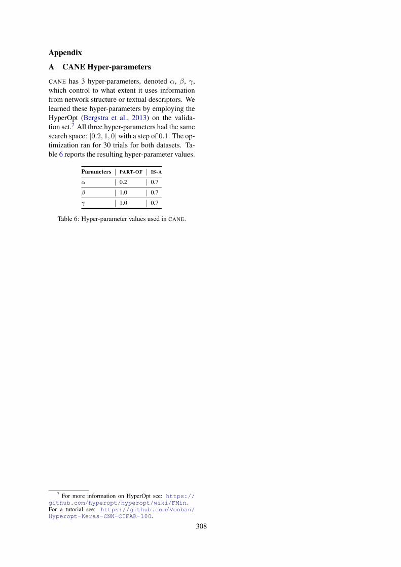
Appendix
A CANE Hyper-parameters
CANE has 3 hyper-parameters, denoted α, β, γ,which control to what extent it uses informationfrom network structure or textual descriptors. Welearned these hyper-parameters by employing theHyperOpt (Bergstra et al., 2013) on the valida-tion set.7 All three hyper-parameters had the samesearch space: [0.2, 1, 0] with a step of 0.1. The op-timization ran for 30 trials for both datasets. Ta-ble 6 reports the resulting hyper-parameter values.
Parameters PART-OF IS-A
α 0.2 0.7
β 1.0 0.7
γ 1.0 0.7
Table 6: Hyper-parameter values used in CANE.
7 For more information on HyperOpt see: https://github.com/hyperopt/hyperopt/wiki/FMin.For a tutorial see: https://github.com/Vooban/Hyperopt-Keras-CNN-CIFAR-100.
308
Proceedings of the BioNLP 2019 workshop, pages 309–318Florence, Italy, August 1, 2019. c©2019 Association for Computational Linguistics
Simplification-induced transformations: typology and somecharacteristics
Anaı̈s Koptient1 Rémi Cardon2
1. {firstname.lastname}[email protected]. {firstname.lastname}@univ-lille.fr
CNRS, Univ. Lille, UMR 8163 STL - Savoirs Textes Langage F-59000 Lille, France
Natalia Grabar2
AbstractThe purpose of automatic text simplificationis to transform technical or difficult to under-stand texts into a more friendly version. Thesemantics must be preserved during this trans-formation. Automatic text simplification canbe done at different levels (lexical, syntactic,semantic, stylistic...) and relies on the cor-responding knowledge and resources (lexicon,rules...). Our objective is to propose methodsand material for the creation of transformationrules from a small set of parallel sentences dif-ferentiated by their technicity. We also pro-pose a typology of transformations and quan-tify them. We work with French-language datarelated to the medical domain, although we as-sume that the method can be exploited on textsin any language and from any domain.
1 Introduction
The purpose of automatic text simplification is toprovide a simplified version for a given text. Sim-plification can be done at lexical, syntactic, seman-tic but also pragmatic and stylistic levels. Sim-plification can be useful in two main contexts: ashelp provided to human readers, which guaranteesbetter access and understanding of the content ofdocuments (Son et al., 2008; Paetzold and Specia,2016; Chen et al., 2016; Arya et al., 2011; Leroyet al., 2013), and as a pre-processing step for otherNLP tasks and applications, which makes easierthe work of other NLP modules and may improvethe overall results (Chandrasekar and Srinivas,1997; Vickrey and Koller, 2008; Blake et al., 2007;Stymne et al., 2013; Wei et al., 2014; BeigmanKlebanov et al., 2004). We can see that potentiallythis task may play an important role.
Three main types of methods are currently ex-ploited in text simplification:
• Methods based on knowledge and rules. Forinstance, the use of WordNet (Miller et al.,
1993) may provide equivalent expressions fordifficult words (Carroll et al., 1998; Bautistaet al., 2009), or help with the choice ofsynonyms using their frequency (Devlin andTait, 1998; De Belder and Moens, 2010; Drn-darevic et al., 2012) or their length (Bautistaet al., 2009). One limitation of such methodsis their weak recall performance (De Belderand Moens, 2010) and confusion betweendifficult and simple words (Shardlow, 2014);
• Methods based on distribution probabilities,like word embeddings (Mikolov et al., 2013;Pennington et al., 2014), are used to ac-quire a lexicon and substitution rules forsimplification. When trained on relevantdata (Wikipedia, Simple Wikipedia, PubMedCentral...), word embeddings can containsimpler equivalents, that can be exploited toperform the simplification (Glavas and Sta-jner, 2015; Kim et al., 2016). Nonetheless,such methods require consequent filtering tokeep only the best candidates. Those meth-ods generally provide good coverage and,when the filtering is efficient, good precision;
• Methods issued from machine translationtackle the problem as translation from tech-nical to simple text. A growing numberof works propose to exploit this type ofmethod to English texts (Zhao et al., 2010;Zhu et al., 2010; Wubben et al., 2012; Sen-nrich et al., 2016; Xu et al., 2016; Wanget al., 2016a,b; Zhang and Lapata, 2017; Ni-sioi et al., 2017). They exploit corpora madeof parallel and aligned sentences, that mainlyderive from the Simple English Wikipedia -English Wikipedia corpus (SEW-EW). Glob-ally, those methods seem to maintain a bal-ance between the quality of the simplifica-tion, good coverage and precision.
309
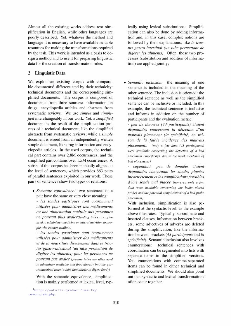
Almost all the existing works address text sim-plification in English, while other languages arepoorly described. Yet, whatever the method andlanguage it is necessary to have available suitableresources for making the transformations requiredby the task. This work is intended as a basis to de-sign a method and to use it for preparing linguisticdata for the creation of transformation rules.
2 Linguistic Data
We exploit an existing corpus with compara-ble documents1 differentiated by their technicity:technical documents and the corresponding sim-plified documents. The corpus is composed ofdocuments from three sources: information ondrugs, encyclopedia articles and abstracts fromsystematic reviews. We use simple and simpli-fied interchangeably in our work. Yet, a simplifieddocument is the result of the simplification pro-cess of a technical document, like the simplifiedabstracts from systematic reviews; while a simpledocument is issued from an independently writtensimple document, like drug information and ency-clopedia articles. In the used corpus, the techni-cal part contains over 2.8M occurrences, and thesimplified part contains over 1.5M occurrences. Asubset of this corpus has been manually aligned atthe level of sentences, which provides 663 pairsof parallel sentences exploited in our work. Thesepairs of sentences show two types of relations:
• Semantic equivalence: two sentences of apair have the same or very close meaning:- les sondes gastriques sont courammentutilisées pour administrer des médicamentsou une alimentation entérale aux personnesne pouvant plus avaler(feeding tubes are often
used to administer medicine or enteral nutrition to peo-
ple who cannot swallow)
- les sondes gastriques sont courammentutilisées pour administrer des médicamentset de la nourriture directement dans le trac-tus gastro-intestinal (un tube permettant dedigérer les aliments) pour les personnes nepouvant pas avaler (feeding tubes are often used
to administer medicine and food directly into the gas-
trointestinal tract (a tube that allows to digest food))
With the semantic equivalence, simplifica-tion is mainly performed at lexical level, typ-
1http://natalia.grabar.free.fr/resources.php
ically using lexical substitutions. Simplifi-cation can also be done by adding informa-tion and, in this case, complex notions arefollowed by their explanations, like le trac-tus gastro-intestinal (un tube permettant dedigérer les aliments). Often, those two pro-cesses (substitution and addition of informa-tion) are applied jointly;
• Semantic inclusion: the meaning of onesentence is included in the meaning of theother sentence. The inclusion is oriented: thetechnical sentence as well as the simplifiedsentence can be inclusive or included. In thisexample, the technical sentence is inclusiveand informs in addition on the number ofparticipants and the evaluation metric:- peu de données (43 participants) étaientdisponibles concernant la détection d’unmauvais placement (la spécificité) en rai-son de la faible incidence des mauvaisplacements (only a few data (43 participants)
were available concerning the detection of a bad
placement (specificity), due to the weak incidence of
bad placements)
- cependant, peu de données étaientdisponibles concernant les sondes placéesincorrectement et les complications possiblesd’une sonde mal placée (however, only a few
data were available concerning the badly placed
probes and the potential complications of a bad probe
placement)
With inclusion, simplification is also pe-formed at the syntactic level, as the exampleabove illustrates. Typically, subordinate andinserted clauses, information between brack-ets, some adjectives of adverbs are deletedduring the simplification, like the informa-tion between brackets (43 participants and laspécificité). Semantic inclusion also involvesenumerations: technical sentences withcoordination can be segmented into lists withseparate items in the simplified versions.Yet, enumerations with comma-separateditems can be found in either technical andsimplified documents. We should also pointout that syntactic and lexical transformationsoften occur together.
310
Figure 1: Matrix-based alignment of words within YAWAT
3 Methods
The methods for annotating and preparing the lin-guistic data for the description of simplification-induced transformations rely on three main dimen-sions: (1) control of the semantic inclusion re-lations, when sentences are split or merged dur-ing the simplification (Section 3.1); (2) semanticannotation of pairs of sentences to describe moreprecisely the transformations (Section 3.2); and(3) syntactic tagging and analysis for joining thesemantic and syntactic information (Section 3.3).
3.1 Merging and Splitting of SentencesOne typical strategy applied during text simplifi-cation consists in merging or splitting the tech-nical sentences when creating simple sentences(Brouwers et al., 2014). When merged, the techni-cal sentences become shorted, which allows theirmerging into one sentence which yet remains read-able in the simplified version. On contrary, whena given technical sentence contains more than oneclause, like one main and one secondary, it can besplit into two sentences by transforming the sec-ondary clause into the main clause of another sen-tence. Sometimes, the splitting should be blockedbecause it can make the understanding of the mainclause more difficult (Brunato et al., 2014).
In our corpus, merged and split sentences aredetected using their proximity in the corpus andmultiple alignments, like in these examples:
T1 elle impose l’ arrêt du traitement et contre-indique toute nouvelle administration de clin-damycine. (It forces the stopping of the cure and it
is contra-indicated to administer once again the clin-
damycin.)
S1 prévenez votre médecin immédiatement carcela impose l’ arrêt du traitement. (tell it to
your doctor immediately for it forces the stopping of
the cure.)
cette réaction va contre-indiquer toute nou-velle administration de clindamycine. (this re-
sponse contra-indicates any new administration of the
clindamycin.)
T2 abcès. (abscess)
douleurs. (pain)
S2 douleurs ou accumulation de pus au niveaudu site d’ injection (pain or accumulation of pus at
the injection site)
Note that in the case of merging, the complexsentences when they are merged get also othersimplifications, such as synonymy for instance.
3.2 Semantic Annotation
The simplification-induced transformations areannotated semantically using YAWAT (Yet An-other Word Alignment Tool) (Germann, 2008).YAWAT permits to visualize and manipulate paral-lel texts. The tool was designed for working withparallel bilingual texts related to mutual transla-tions (Yu et al., 2012). We propose to exploit itwith monolingual parallel texts related to simpli-fication. YAWAT displays the two parallel andaligned sentences side by side. The annotator canthen align the words using the matrix (Figure 1),and to assign the type of transformation to eachpair of text segments considered. The numberof squares displayed vertically correspond to thenumber of words that are counted in the sentenceon the left (that is, the technical sentence). Thenumber of squares displayed horizontally corre-spond to the number of words that are countedin the sentence on the right (that is, the simplesentence). Then, in order to match word/group
311
Figure 2: Annotation scheme within YAWAT
of words that correspond to a simplification phe-nomenon, the user has to click on the square thatcorresponds in both sentences. The fact that thetext in the two columns are the same permits theuser to click on the right square easily. The trans-formation types permits to describe more preciselytheir semantic nature. We defined a set of trans-formation types using previous similar work andobservations on our corpus (Brunato et al., 2014).The proposed typology contains up to 25 transfor-mations (Figure 2):
• literal is the default value which is kept whenthe words are identical in both sentences,
• synonym: substitution of technical term byits synonym {effets négligeables ; effetsdélétères} ({insignificant effects ; deleterious ef-
fects}),
• hyperonym: technical term is replaced byits hyperonym {clindamicine ; médicament}({clindamycin ; drug}),
• hyponym: technical term is replaced by itshyponym {benzodiazépines ; bromazepam}({benzodiazepine ; bromazepam})
• p2a (and a2p): verb in passive voice in tech-nical sentence is replaced by its active voice{ne doit jamais être utilisé ; ne prenez ja-mais} ({should never be used ; never use}), andthe contrary {n’a aucun ; n’est pas attendu}({does not have ; is not expected})
• pronominalization: substitution by pronouns{l’antibioprophylaxie ; elle} ({the antibiotic
prophylaxis ; it}),
• p2n: substitution of pronoun by its reference{elles ; ce médicament} ({they ; this drug}),
• v2n (and n2v): substitution of verbs by nouns{conduire ; conduite} ({to drive ; driving}), andthe contrary {l’arrêt du traitement ; arrêterbrutalement} ({cessation of treatment ; stop at
once})
• n2a (and a2n): substitution of nouns by theiradjectives {allergies ; allergiques} ({allergies ;
allergic}), and the contrary {cardiaque ; ducoeur} ({cardiac ; of the heart}),
• s2p (and p2s): substitution of singularforms by plural forms {de tout antibio-tique ; d’antibiotiques} ({of any antibiotic ; of
antibiotics}), and the contrary {les enfants ;l’enfant} ({the children ; the child}),
• specification: adding explanation to techni-cal term {bêta-lactamines ; bêta-lactamines(pénicilline, céphalosporine)} ({beta-lactam ;
beta-lactam (penicillin, cephalosporins)}). The dif-ference with synonymy is that, instead of sub-stitution, the technical term remains and itsexplanation (definition, examples) is added,
• generalization: removal of some information{arrêt du traitement et contre indique toutenouvelle administration du clindamycine ;arrêt du traitement} ({cessation of treatment
and contra-indicate any new administration of clin-
damycine ; cessation of treatment}),
• duplication: two or more occurrences of agiven term in simple sentence,
312
• adj2adv (and adv2adj): substitution of ad-jectives by adverbs {récente ; récemment}({recent ; recently}), and the contrary {tardif ;tard} ({late ; late}),
• agt2act (and act2agt): substitution ofagent by the action {conducteurs ; con-duite} ({drivers ; driving}), and the contrary{conduite ; conducteurs} ({driving ; drivers}),
• cau2eff (and eff2cau): substitution of causeby its effect {prescrits ; utilisés} ({prescribed ;
used}), and the contrary {dans le traitement ;chez les patients atteints} ({during the treatment ;
in affected patients}),
• aff2neg (and neg2aff): substitution of affir-mative form of information by negative formwith the same meaning {présentant une ab-sence complète ; n’avez aucune} ({indicating
total absence ; you have no}), and the contrary {nepas ; éviter} ({should not ; avoid}).
Since it is common that some sequences canbe tagged with several concurrent tags, we de-fined the priority rules, such as a2n > synonym,like in {cardiaque ; du coeur} ({cardiac ; of the
heart}), because it describes the transformationmore precisely. Since it is common that somesequences can be tagged with several concurrenttags, we prioritized part-of-speech related tagsover synonymy because it is more precize, like in{cardiaque ; du coeur} ({cardiac ; of the heart}). Sim-ilarly, pronominalization is prioritized over verbalfeatures, and also all the lexical transformationsover syntactic transformations.
3.3 Syntactic Analysis
Syntactic analysis permits to linguistically anno-tate the parallel sentences and to mark within themthe syntactic groups. Syntactic processing is donewith Cordial (Laurent et al., 2009), which per-forms tokenization, POS-tagging, lemmatisationand syntactic analysis into constituents. In Ta-ble 1, we provide an example of Cordial taggingand analysis for the sentence dalacine n’a aucuneffet ou qu’un effet négligeable sur l’aptitude àconduire des véhicules et à utiliser des machines.(dalacine has no effect or the effect is insignificant on the ca-
pacity to drive vehicles and to use machines.) We can seethat the sequence un effet négligeble (insignificant ef-
fect) belongs to the same syntactic group, stated incolumn synt. group. Besides, the syntactic head is
nb. form POS tag synt. group1 dalacine NCI 12 n’ ADV 33 a VINDP3S 34 aucun ADJIND 55 effet NCMS 56 ou COO -7 qu’ ADV 38 un DETIMS 99 effet NCMS 910 négligeable ADJSIG 911 sur PREP 1312 l’ DETDFS 1313 aptitude NCFS 1314 à PREP 1515 conduire VINF 1516 des DETDPIG 1717 véhicules NCMP 1718 et COO -19 à PREP 2020 utiliser VINF 2021 des DETDPIG 2222 machines NCFP 2223 . PCTFORTE -
Table 1: Example of syntactic annotation by Cordial(word position in the sentence, word form, POS tag,and syntactic group)
effet (effect), which has the same number as the syn-tactic groupe (9) and, being common noun (NC),it characterizes this group as nominal phrase.
4 Results and Discussion
4.1 Merging and Splitting of Sentences
We counted 51 cases in which two of more techni-cal sentences are merged into one simple sentence,and 16 cases in which technical sentences are splitinto two or more simple sentences. In a previouswork, it was noticed that the merging of sentencesduring the simplification is rare (Brouwers et al.,2014). Yet, in our corpus, we observe the con-trary: much more technical sentences are mergedthan split. We can see several explanations:
• The cited work (Brouwers et al., 2014) isdone on articles from Wikipedia and Vikidia.Vikidia is designed for 8-13 year old childrenand relies on strong guidelines when creatingthe articles. One of the rules is to use shortand clear sentences. In our work, Wikipedia
313
and Vikidia correspond to the encycopediapart of the corpus. The two other subcorpora(drug leaflets and scientific abstracts) do notrespect same writing principles.
• Drug leaflets frequently use coordinationswith disorders, known adverse effects, func-tions, etc. Often, they are presented as item-ized lists in technical documents, while insimplified documents then occur within co-ordinated sentences.
• In abstracts of systematic reviews, techni-cal sentences are often shortened during theirsimplification in order to keep the main in-formation. Then, possibly as consequence ofit, the sentences may be merged. Notice alsothat there is no clear guidelines when writingplain-language abstracts and that each editormay apply its own principles.
4.2 Semantic AnnotationIn Figure 3, we present the typology of thesimplification-induced transformations. The Fig-ure also contains information on prevalence ofeach transformation in terms of its frequenceand percentage. We distinguish several high-level transformations, which may also be presentin the existing typologies (Brunato et al., 2014;Brouwers et al., 2014): lexical substitution, lex-ical addition, lexical deletion, syntactic substitu-tion, pronominalization and use of affirmative andnegated forms. The biggest set of transformations(965 occurrences, 69%) is related to lexical sub-stitutions, within which we differentiate substitu-tions with semantic shift (hyponymy and hyper-onymy) and without semantic shift (synonymy andmorphological transformation). We subsequentlyhave lexical additions or specifications (199 oc-currences, 14%), when explanations are added totechnical terms in simplifed sentences, and lexi-cal deletions or generalizations (132 occurrences,9%), when some information is shortened and re-moved during the simplification. Then we con-sider that the only pure syntactic substitutions cor-repospond to active and passive voices of verbs.Hence, singular/plural and other verbal featuresbelong to lexical substitutions without semanticshift. Pronominalization, and use of positive andnegative equivalent expressions correspond to dis-tinct small types of transformations.
By comparison with the typology from (Brouw-ers et al., 2014), we separated synonymy from hy-
peronymy because they have fundamental differ-ences (semantic equivalence or subsumption) andrequire specific methods and resources. We differ-entiate several syntactic and morphological trans-formations, while in the citetd work, only the pas-sive/active transformation is considered. Anotherdifference is that we do not differentiate betweellexical and semantic transformations: semanticsbecomes a feature of lexical substitutions.
By comparison with the typology from(Brunato et al., 2014), the authors differentiateseveral types of word insertion and deletion,according to the syntactic nature of these words(verb, noun...). We do not make this differen-tiation because, in most cases, insertions anddeletions apply to syntactic clauses. Besides, weconsidered the shift of grammatical categories aslexical substitution, which we describe with detailaccording to the POS categories. Unlike in thecited work, we consider separately hyperonymy,hyponymy and synonymy, because they havefundamental differences and require specificmethods and resources.
Finally, by comparison with the typology from(Vila et al., 2011), which is dedicated to thegeneral description of paraphrases and does notspecifically aim transformations due to the simpli-fication, we notice several similarities. The maindifference is that the authors separated lexical sub-stitutions and morphological derivations, whichwe keep together because they all apply at theword level. Yet, we can differentiate them throughthe use of syntactic infomartion.
On the whole, we count 1,394 transformations,which gives 2.1 transformations per pair of sen-tences on average. In Table 2, we indicate thefrequency of the most frequent types of transfor-mations according to whether they occur in splitor merged sentences, or generally in the corpus(the total column). As in Figure 3, the most fre-quent transformations are related to the use of syn-onyms, and the specification and generalization ofcontents. These types are frequent in the wholecorpus and, by consequence, in merged and splitsentences. There is no real association betweensentence splitting or merging and transformations.At the more fine-grained level, we observe that:
• a2n (adjective → noun) transformations (53occ.) may be necessary to replace adjectives,often coined on suppletive bases (cardiac),by the corresponding nouns, often coined on
314
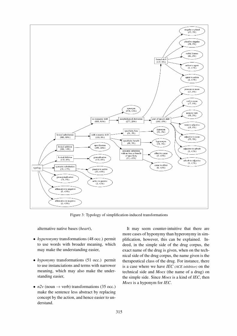
Figure 3: Typology of simplification-induced transformations
alternative native bases (heart),
• hyperonymy transformations (48 occ.) permitto use words with broader meaning, whichmay make the understanding easier,
• hyponymy transformations (51 occ.) permitto use instanciations and terms with narrowermeaning, which may also make the under-standing easier,
• n2v (noun→ verb) transformations (35 occ.)make the sentence less abstract by replacingconcept by the action, and hence easier to un-derstand.
It may seem counter-intuitive that there aremore cases of hyponymy than hyperonymy in sim-plification, however, this can be explained. In-deed, in the simple side of the drug corpus, theexact name of the drug is given, when on the tech-nical side of the drug corpus, the name given is thetherapeutical class of the drug. For instance, thereis a case where we have IEC (ACE inhibitor) on thetechnical side and Moex (the name of a drug) onthe simple side. Since Moex is a kind of IEC, thenMoex is a hyponym for IEC.
315
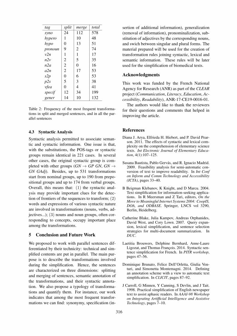
tag split merge totalsyno 24 112 578hypero 1 10 48hypo 0 13 51pronoun 9 2 74v2n 1 1 17n2v 2 5 35n2a 2 0 16a2n 2 17 53s2p 0 6 53p2s 5 3 38vfea 0 4 41specif 12 34 199gener 14 10 132
Table 2: Frequency of the most frequent transforma-tions in split and merged sentences, and in all the par-allel sentences
4.3 Syntactic AnalysisSyntactic analysis permitted to associate seman-tic and syntactic information. One issue is that,with the substitutions, the POS-tags or syntacticgroups remain identical in 221 cases. In severalother cases, the original syntactic group is com-pleted with other groups (GN → GP GN, GN →GN GAdj). Besides, up to 531 transformationsstart from nominal groups, up to 190 from prepo-sitional groups and up to 174 from verbal groups.Overall, this means that: (1) the syntactic anal-ysis may provide important clues for the detec-tion of frontiers of the sequences to transform; (2)words and expressions of various syntactic natureare involved in transformations (nouns, verbs, ad-jectives...); (3) nouns and noun groups, often cor-responding to concepts, occupy important placeamong the transformations.
5 Conclusion and Future Work
We proposed to work with parallel sentences dif-ferentiated by their technicity: technical and sim-plified contents are put in parallel. The main pur-pose is to describe the transformations involvedduring the simplification. Hence, the sentencesare characterized on three dimensions: splittingand merging of sentences, semantic annotation ofthe transformations, and their syntactic annota-tion. We also propose a typology of transforma-tions and quantify them. For instance, our workindicates that among the most frequent transfor-mations we can find: synonymy, specification (in-
sertion of additional information), generalization(removal of information), pronominalization, sub-stitution of adjectives by the corresponding nouns,and swich between singular and plural forms. Thematerial prepared will be used for the creation oftransformation rules joining syntactic, lexical andsemantic information. These rules will be laterused for the simplification of biomedical texts.
Acknowledgments
This work was funded by the French NationalAgency for Research (ANR) as part of the CLEARproject (Communication, Literacy, Education, Ac-cessibility, Readability), ANR-17-CE19-0016-01.
The authors would like to thank the reviewersfor their questions and comments that helped inimproving the article.
ReferencesDiana J. Arya, Elfrieda H. Hiebert, and P. David Pear-
son. 2011. The effects of syntactic and lexical com-plexity on the comprehension of elementary sciencetexts. Int Electronic Journal of Elementary Educa-tion, 4(1):107–125.
Susana Bautista, Pablo Gervás, and R. Ignacio Madrid.2009. Feasibility analysis for semi-automatic con-version of text to improve readability. In Int Confon Inform and Comm Technology and Accessibility(ICTA), pages 33–40.
B Beigman Klebanov, K Knight, and D Marcu. 2004.Text simplification for information-seeking applica-tions. In R Meersman and Z Tari, editors, On theMove to Meaningful Internet Systems 2004: CoopIS,DOA, and ODBASE. Springer, LNCS vol 3290,Berlin, Heidelberg.
Catherine Blake, Julia Kampov, Andreas Orphanides,David West, and Cory Lown. 2007. Query expan-sion, lexical simplification, and sentence selectionstrategies for multi-document summarization. InDUC.
Laetitia Brouwers, Delphine Bernhard, Anne-LaureLigozat, and Thomas François. 2014. Syntactic sen-tence simplification for French. In PITR workshop,pages 47–56.
Dominique Brunato, Felice Dell’Orletta, Giulia Ven-turi, and Simonetta Montemagni. 2014. Definingan annotation scheme with a view to automatic textsimplification. In CLICIT, pages 87–92.
J Carroll, G Minnen, Y Canning, S Devlin, and J Tait.1998. Practical simplification of English newspapertext to assist aphasic readers. In AAAI-98 Workshopon Integrating Artifficial Intelligence and AssistiveTechnology, pages 7–10.
316
R Chandrasekar and B Srinivas. 1997. Automatic in-duction of rules for text simplification. KnowledgeBased Systems, 10(3):183–190.
Ping Chen, John Rochford, David N. Kennedy, Sous-san Djamasbi, Peter Fay, and Will Scott. 2016. Au-tomatic text simplification for people with intellec-tual disabilities. In AIST, pages 1–9.
Jan De Belder and Marie-Francine Moens. 2010. Textsimplification for children. In Workshop on Accessi-ble Search Systems of SIGIR, pages 1–8.
Siobhan Devlin and John Tait. 1998. The use of psy-cholinguistic database in the simplification of textfor aphasic readers. In Linguistic Database, pages161–173.
B Drndarevic, S Stajner, and H Saggion. 2012. Re-porting simply: A lexical simplification strategy forenhancing text accessibility. In Easy to read on theweb, pages 1–6.
Ulrich Germann. 2008. Yawat: Yet another word align-ment tool. In ACL-08: HLT Demo Session, pages20–23, Columbus, USA.
Goran Glavas and Sanja Stajner. 2015. Simplifyinglexical simplification: Do we need simplified cor-pora? In ACL-COLING, pages 63–68.
Yea-Seul Kim, Jessica Hullman, Matthew Burgess, andEytan Adar. 2016. SimpleScience: Lexical simpli-fication of scientific terminology. In EMNLP, pages1–6.
D Laurent, S Nègre, and P Séguéla. 2009. L’analyseursyntaxique Cordial dans Passage. In Traitement Au-tomatique des Langues Naturelles (TALN).
Gondy Leroy, David Kauchak, and Obay Mouradi.2013. A user-study measuring the effects of lexicalsimplification and coherence enhancement on per-ceived and actual text difficulty. Int J Med Inform,82(8):717–730.
T Mikolov, K Chen, G Corrado, and J Dean. 2013. Ef-ficient estimation of word representations in vectorspace. In Workshop at ICLR.
George A. Miller, Richard Beckwith, Christiane Fell-baum, Derek Gross, and Katherine Miller. 1993. In-troduction to wordnet: An on-line lexical database.Technical report, WordNet.
Sergiu Nisioi, Sanja Stajner, Simone Paolo Ponzetto,and Liviu P. Dinu. 2017. Exploring neural text sim-plification models. In Ann Meeting of the Assoc forComp Linguistics, pages 85–91.
Gustavo H. Paetzold and Lucia Specia. 2016. Bench-marking lexical simplification systems. In LREC,pages 3074–3080.
Jeffrey Pennington, Richard Socher, and Christopher DManning. 2014. Glove: Global vectors for wordrepresentation. In EMNLP 2014, pages 1532–1543.
Rico Sennrich, Barry Haddow, and Alexandra Birch.2016. Improving neural machine translation modelswith monolingual data. In Proc of the Ann Meet-ing of the Assoc for Comp Linguistics, pages 86–96,Berlin, Germany.
Matthew Shardlow. 2014. A survey of automated textsimplification. Int J Advanced Computer Scienceand Applications, 1:1–13.
Ji Y. Son, Linda B. Smith, and Robert L. Gold-stone. 2008. Simplicity and generalization: Short-cutting abstraction in children’s object categoriza-tions. Cognition, 108:626–638.
S Stymne, J Tiedemann, C Hardmeier, and J Nivre.2013. Statistical machine translation with readabil-ity constraints. In NODALIDA, pages 1–12.
D Vickrey and D Koller. 2008. Sentence simplifica-tion for semantic role labeling. In Annual Meeting ofthe Association for Computational Linguistics-HLT,pages 344–352.
Marta Vila, M Antònia Mart, and Horacio Rodrı́guez.2011. Paraphrase concept and typology. A linguisti-cally based and computationally oriented approach.Procesamiento del Lenguaje Natural, 46:83–90.
Tong Wang, Ping Chen, Kevin Amaral, and JipengQiang. 2016a. An experimental study of LSTMencoder-decoder model for text simplification. InIJCAI, pages 1–7.
Tong Wang, Ping Chen, John Rochford, and JipengQiang. 2016b. Text simplification using neural ma-chine translation. In Proc of the AAAI Conference onArtificial Intelligence (AAAI-16), pages 4270–4271.
Chih-Hsuan Wei, Robert Leaman, and Zhiyong Lu.2014. SimConcept: A hybrid approach for simpli-fying composite named entities in biomedicine. InBCB ’14, pages 138–146.
S Wubben, A van den Bosch, and E Krahmer. 2012.Sentence simplification by monolingual machinetranslation. In Annual Meeting of the Associationfor Computational Linguistics, pages 1015–1024.
Wei Xu, Courtney Napoles, Ellie Pavlick, QuanzeChen, and Chris Callison-Burch. 2016. Optimizingstatistical machine translation for text simplification.Transactions of the Association for ComputationalLinguistics, 4:401–415.
Qian Yu, Aurélien Max, and François Yvon. 2012.Revisiting sentence alignment algorithms for align-ment visualization and evaluation. In BUCC work-shop, pages 1–7.
Xingxing Zhang and Mirella Lapata. 2017. Sentencesimplification with deep reinforcement learning. InProc of the Conf on Empirical Methods in NaturalLanguage Processing, pages 584–594, Copenhagen,Denmark.
317

S Zhao, H Wang, and T Liu. 2010. Leveraging multipleMT engines for paraphrase generation. In COLING,pages 1326–1334.
Z Zhu, D Bernhard, and I Gurevych. 2010. A monolin-gual tree-based translation model for sentence sim-plification. In COLING 2010, pages 1353–1361.
318
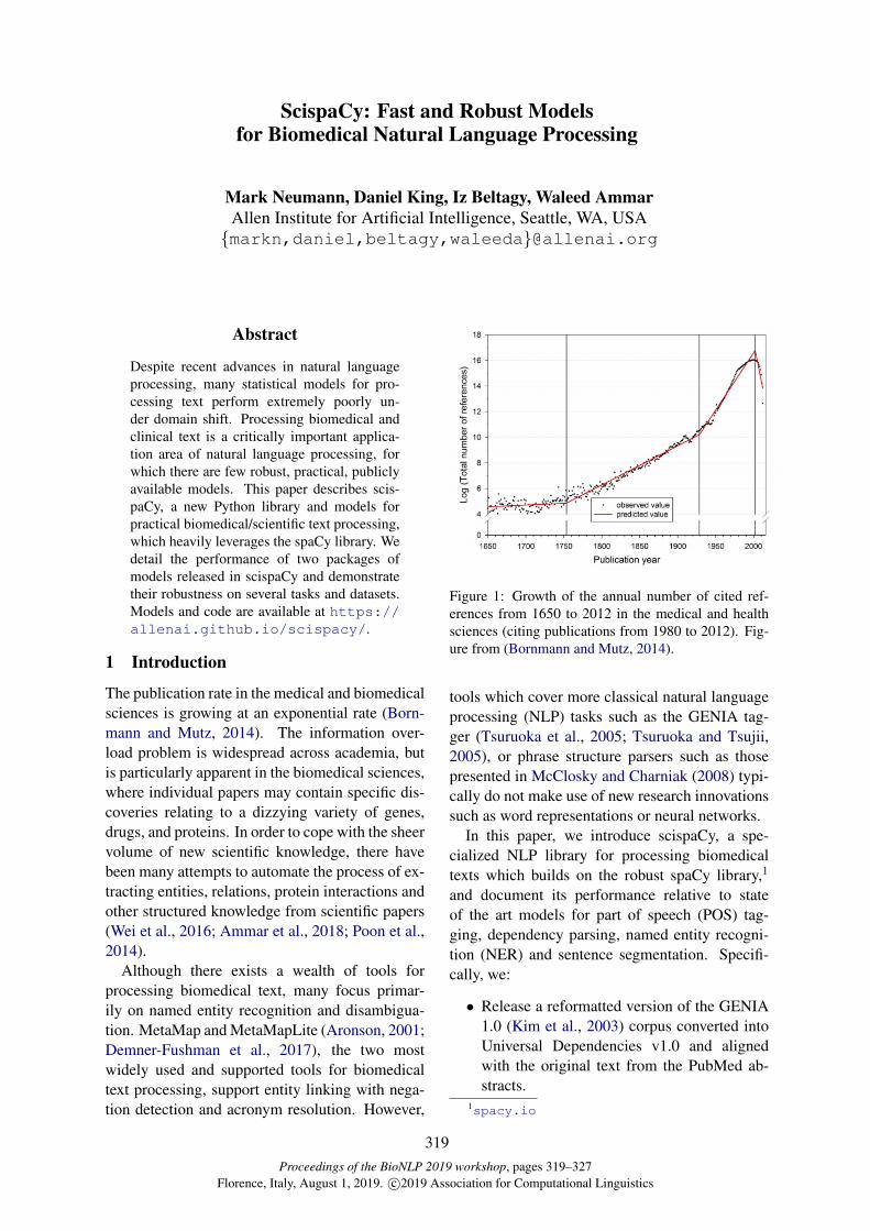
Proceedings of the BioNLP 2019 workshop, pages 319–327Florence, Italy, August 1, 2019. c©2019 Association for Computational Linguistics
ScispaCy: Fast and Robust Modelsfor Biomedical Natural Language Processing
Mark Neumann, Daniel King, Iz Beltagy, Waleed AmmarAllen Institute for Artificial Intelligence, Seattle, WA, USA{markn,daniel,beltagy,waleeda}@allenai.org
Abstract
Despite recent advances in natural languageprocessing, many statistical models for pro-cessing text perform extremely poorly un-der domain shift. Processing biomedical andclinical text is a critically important applica-tion area of natural language processing, forwhich there are few robust, practical, publiclyavailable models. This paper describes scis-paCy, a new Python library and models forpractical biomedical/scientific text processing,which heavily leverages the spaCy library. Wedetail the performance of two packages ofmodels released in scispaCy and demonstratetheir robustness on several tasks and datasets.Models and code are available at https://allenai.github.io/scispacy/.
1 Introduction
The publication rate in the medical and biomedicalsciences is growing at an exponential rate (Born-mann and Mutz, 2014). The information over-load problem is widespread across academia, butis particularly apparent in the biomedical sciences,where individual papers may contain specific dis-coveries relating to a dizzying variety of genes,drugs, and proteins. In order to cope with the sheervolume of new scientific knowledge, there havebeen many attempts to automate the process of ex-tracting entities, relations, protein interactions andother structured knowledge from scientific papers(Wei et al., 2016; Ammar et al., 2018; Poon et al.,2014).
Although there exists a wealth of tools forprocessing biomedical text, many focus primar-ily on named entity recognition and disambigua-tion. MetaMap and MetaMapLite (Aronson, 2001;Demner-Fushman et al., 2017), the two mostwidely used and supported tools for biomedicaltext processing, support entity linking with nega-tion detection and acronym resolution. However,
Figure 1: Growth of the annual number of cited ref-erences from 1650 to 2012 in the medical and healthsciences (citing publications from 1980 to 2012). Fig-ure from (Bornmann and Mutz, 2014).
tools which cover more classical natural languageprocessing (NLP) tasks such as the GENIA tag-ger (Tsuruoka et al., 2005; Tsuruoka and Tsujii,2005), or phrase structure parsers such as thosepresented in McClosky and Charniak (2008) typi-cally do not make use of new research innovationssuch as word representations or neural networks.
In this paper, we introduce scispaCy, a spe-cialized NLP library for processing biomedicaltexts which builds on the robust spaCy library,1
and document its performance relative to stateof the art models for part of speech (POS) tag-ging, dependency parsing, named entity recogni-tion (NER) and sentence segmentation. Specifi-cally, we:
• Release a reformatted version of the GENIA1.0 (Kim et al., 2003) corpus converted intoUniversal Dependencies v1.0 and alignedwith the original text from the PubMed ab-stracts.
1spacy.io
319
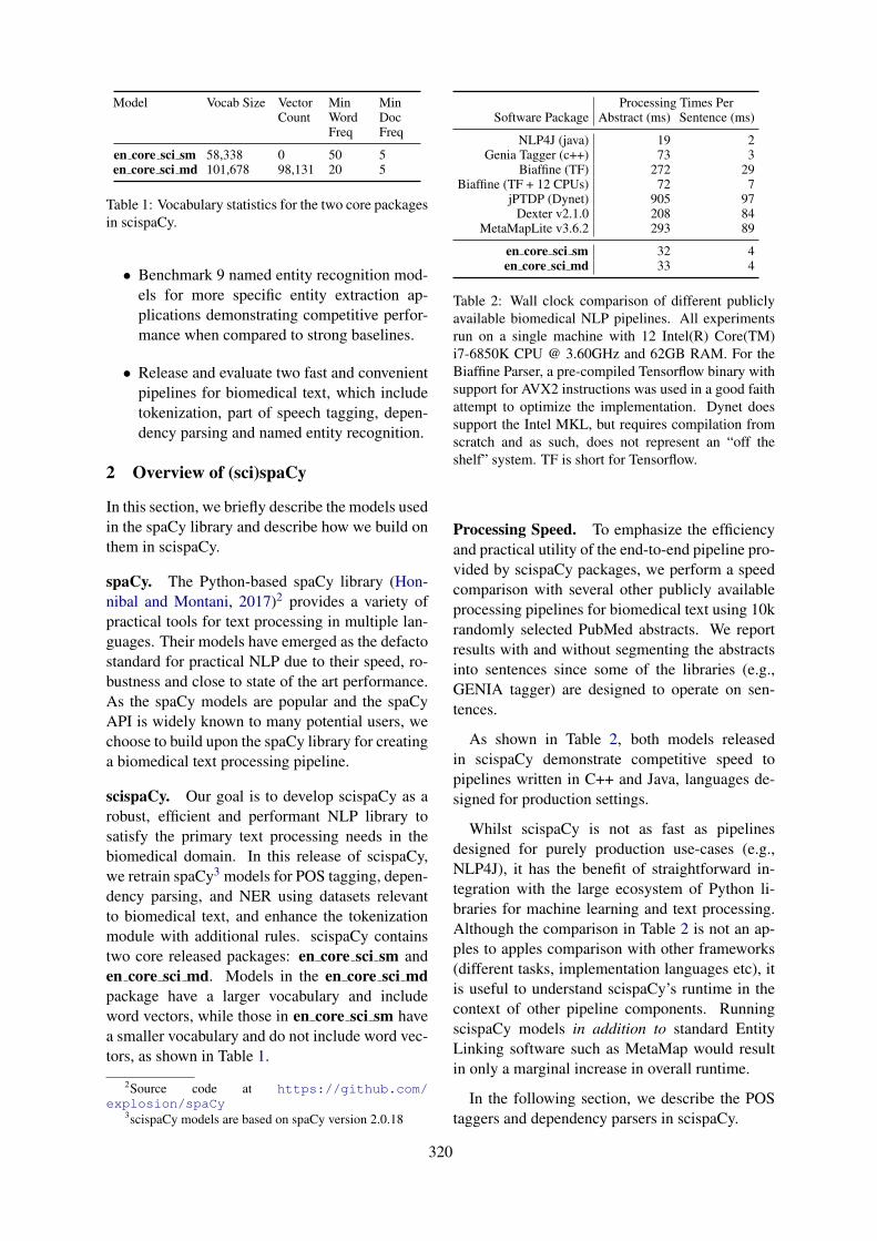
Model Vocab Size VectorCount
MinWordFreq
MinDocFreq
en core sci sm 58,338 0 50 5en core sci md 101,678 98,131 20 5
Table 1: Vocabulary statistics for the two core packagesin scispaCy.
• Benchmark 9 named entity recognition mod-els for more specific entity extraction ap-plications demonstrating competitive perfor-mance when compared to strong baselines.
• Release and evaluate two fast and convenientpipelines for biomedical text, which includetokenization, part of speech tagging, depen-dency parsing and named entity recognition.
2 Overview of (sci)spaCy
In this section, we briefly describe the models usedin the spaCy library and describe how we build onthem in scispaCy.
spaCy. The Python-based spaCy library (Hon-nibal and Montani, 2017)2 provides a variety ofpractical tools for text processing in multiple lan-guages. Their models have emerged as the defactostandard for practical NLP due to their speed, ro-bustness and close to state of the art performance.As the spaCy models are popular and the spaCyAPI is widely known to many potential users, wechoose to build upon the spaCy library for creatinga biomedical text processing pipeline.
scispaCy. Our goal is to develop scispaCy as arobust, efficient and performant NLP library tosatisfy the primary text processing needs in thebiomedical domain. In this release of scispaCy,we retrain spaCy3 models for POS tagging, depen-dency parsing, and NER using datasets relevantto biomedical text, and enhance the tokenizationmodule with additional rules. scispaCy containstwo core released packages: en core sci sm anden core sci md. Models in the en core sci mdpackage have a larger vocabulary and includeword vectors, while those in en core sci sm havea smaller vocabulary and do not include word vec-tors, as shown in Table 1.
2Source code at https://github.com/explosion/spaCy
3scispaCy models are based on spaCy version 2.0.18
Processing Times PerSoftware Package Abstract (ms) Sentence (ms)
NLP4J (java) 19 2Genia Tagger (c++) 73 3
Biaffine (TF) 272 29Biaffine (TF + 12 CPUs) 72 7
jPTDP (Dynet) 905 97Dexter v2.1.0 208 84
MetaMapLite v3.6.2 293 89
en core sci sm 32 4en core sci md 33 4
Table 2: Wall clock comparison of different publiclyavailable biomedical NLP pipelines. All experimentsrun on a single machine with 12 Intel(R) Core(TM)i7-6850K CPU @ 3.60GHz and 62GB RAM. For theBiaffine Parser, a pre-compiled Tensorflow binary withsupport for AVX2 instructions was used in a good faithattempt to optimize the implementation. Dynet doessupport the Intel MKL, but requires compilation fromscratch and as such, does not represent an “off theshelf” system. TF is short for Tensorflow.
Processing Speed. To emphasize the efficiencyand practical utility of the end-to-end pipeline pro-vided by scispaCy packages, we perform a speedcomparison with several other publicly availableprocessing pipelines for biomedical text using 10krandomly selected PubMed abstracts. We reportresults with and without segmenting the abstractsinto sentences since some of the libraries (e.g.,GENIA tagger) are designed to operate on sen-tences.
As shown in Table 2, both models releasedin scispaCy demonstrate competitive speed topipelines written in C++ and Java, languages de-signed for production settings.
Whilst scispaCy is not as fast as pipelinesdesigned for purely production use-cases (e.g.,NLP4J), it has the benefit of straightforward in-tegration with the large ecosystem of Python li-braries for machine learning and text processing.Although the comparison in Table 2 is not an ap-ples to apples comparison with other frameworks(different tasks, implementation languages etc), itis useful to understand scispaCy’s runtime in thecontext of other pipeline components. RunningscispaCy models in addition to standard EntityLinking software such as MetaMap would resultin only a marginal increase in overall runtime.
In the following section, we describe the POStaggers and dependency parsers in scispaCy.
320
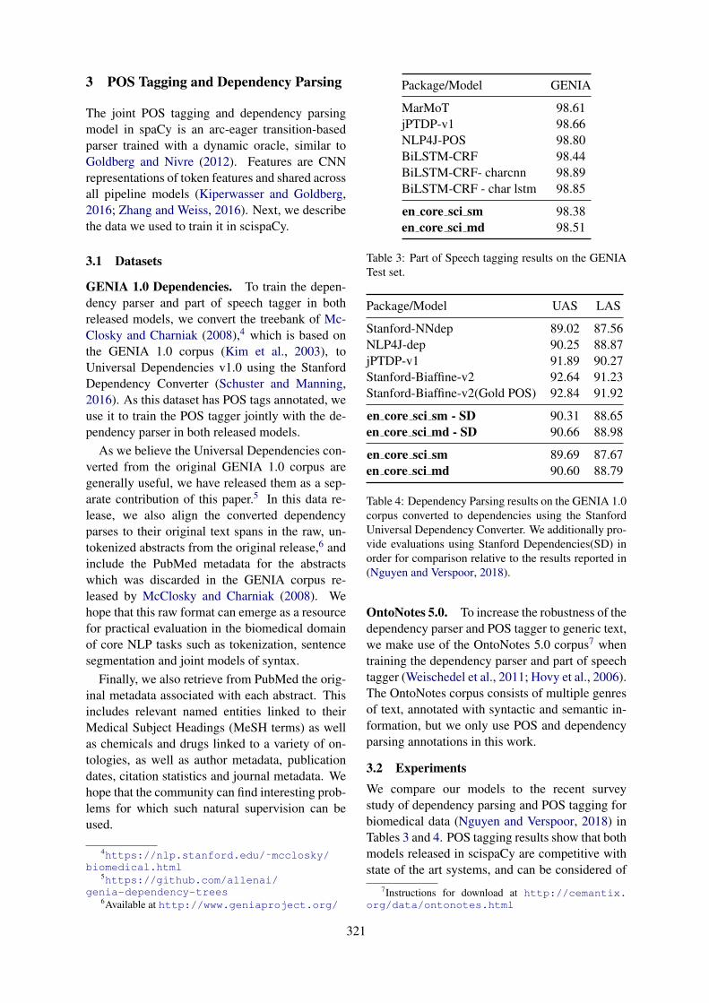
3 POS Tagging and Dependency Parsing
The joint POS tagging and dependency parsingmodel in spaCy is an arc-eager transition-basedparser trained with a dynamic oracle, similar toGoldberg and Nivre (2012). Features are CNNrepresentations of token features and shared acrossall pipeline models (Kiperwasser and Goldberg,2016; Zhang and Weiss, 2016). Next, we describethe data we used to train it in scispaCy.
3.1 Datasets
GENIA 1.0 Dependencies. To train the depen-dency parser and part of speech tagger in bothreleased models, we convert the treebank of Mc-Closky and Charniak (2008),4 which is based onthe GENIA 1.0 corpus (Kim et al., 2003), toUniversal Dependencies v1.0 using the StanfordDependency Converter (Schuster and Manning,2016). As this dataset has POS tags annotated, weuse it to train the POS tagger jointly with the de-pendency parser in both released models.
As we believe the Universal Dependencies con-verted from the original GENIA 1.0 corpus aregenerally useful, we have released them as a sep-arate contribution of this paper.5 In this data re-lease, we also align the converted dependencyparses to their original text spans in the raw, un-tokenized abstracts from the original release,6 andinclude the PubMed metadata for the abstractswhich was discarded in the GENIA corpus re-leased by McClosky and Charniak (2008). Wehope that this raw format can emerge as a resourcefor practical evaluation in the biomedical domainof core NLP tasks such as tokenization, sentencesegmentation and joint models of syntax.
Finally, we also retrieve from PubMed the orig-inal metadata associated with each abstract. Thisincludes relevant named entities linked to theirMedical Subject Headings (MeSH terms) as wellas chemicals and drugs linked to a variety of on-tologies, as well as author metadata, publicationdates, citation statistics and journal metadata. Wehope that the community can find interesting prob-lems for which such natural supervision can beused.
4https://nlp.stanford.edu/˜mcclosky/biomedical.html
5https://github.com/allenai/genia-dependency-trees
6Available at http://www.geniaproject.org/
Package/Model GENIA
MarMoT 98.61jPTDP-v1 98.66NLP4J-POS 98.80BiLSTM-CRF 98.44BiLSTM-CRF- charcnn 98.89BiLSTM-CRF - char lstm 98.85
en core sci sm 98.38en core sci md 98.51
Table 3: Part of Speech tagging results on the GENIATest set.
Package/Model UAS LAS
Stanford-NNdep 89.02 87.56NLP4J-dep 90.25 88.87jPTDP-v1 91.89 90.27Stanford-Biaffine-v2 92.64 91.23Stanford-Biaffine-v2(Gold POS) 92.84 91.92
en core sci sm - SD 90.31 88.65en core sci md - SD 90.66 88.98
en core sci sm 89.69 87.67en core sci md 90.60 88.79
Table 4: Dependency Parsing results on the GENIA 1.0corpus converted to dependencies using the StanfordUniversal Dependency Converter. We additionally pro-vide evaluations using Stanford Dependencies(SD) inorder for comparison relative to the results reported in(Nguyen and Verspoor, 2018).
OntoNotes 5.0. To increase the robustness of thedependency parser and POS tagger to generic text,we make use of the OntoNotes 5.0 corpus7 whentraining the dependency parser and part of speechtagger (Weischedel et al., 2011; Hovy et al., 2006).The OntoNotes corpus consists of multiple genresof text, annotated with syntactic and semantic in-formation, but we only use POS and dependencyparsing annotations in this work.
3.2 ExperimentsWe compare our models to the recent surveystudy of dependency parsing and POS tagging forbiomedical data (Nguyen and Verspoor, 2018) inTables 3 and 4. POS tagging results show that bothmodels released in scispaCy are competitive withstate of the art systems, and can be considered of
7Instructions for download at http://cemantix.org/data/ontonotes.html
321
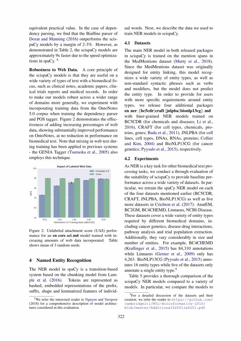
equivalent practical value. In the case of depen-dency parsing, we find that the Biaffine parser ofDozat and Manning (2016) outperforms the scis-paCy models by a margin of 2-3%. However, asdemonstrated in Table 2, the scispaCy models areapproximately 9x faster due to the speed optimiza-tions in spaCy. 8
Robustness to Web Data. A core principle ofthe scispaCy models is that they are useful on awide variety of types of text with a biomedical fo-cus, such as clinical notes, academic papers, clin-ical trials reports and medical records. In orderto make our models robust across a wider rangeof domains more generally, we experiment withincorporating training data from the OntoNotes5.0 corpus when training the dependency parserand POS tagger. Figure 2 demonstrates the effec-tiveness of adding increasing percentages of webdata, showing substantially improved performanceon OntoNotes, at no reduction in performance onbiomedical text. Note that mixing in web text dur-ing training has been applied to previous systems- the GENIA Tagger (Tsuruoka et al., 2005) alsoemploys this technique.
Figure 2: Unlabeled attachment score (UAS) perfor-mance for an en core sci md model trained with in-creasing amounts of web data incorporated. Tableshows mean of 3 random seeds.
4 Named Entity Recognition
The NER model in spaCy is a transition-basedsystem based on the chunking model from Lam-ple et al. (2016). Tokens are represented ashashed, embedded representations of the prefix,suffix, shape and lemmatized features of individ-
8We refer the interested reader to Nguyen and Verspoor(2018) for a comprehensive description of model architec-tures considered in this evaluation.
ual words. Next, we describe the data we used totrain NER models in scispaCy.
4.1 Datasets
The main NER model in both released packagesin scispaCy is trained on the mention spans inthe MedMentions dataset (Murty et al., 2018).Since the MedMentions dataset was originallydesigned for entity linking, this model recog-nizes a wide variety of entity types, as well asnon-standard syntactic phrases such as verbsand modifiers, but the model does not predictthe entity type. In order to provide for userswith more specific requirements around entitytypes, we release four additional packagesen ner {bc5cdr|craft |jnlpba|bionlp13cg} mdwith finer-grained NER models trained onBC5CDR (for chemicals and diseases; Li et al.,2016), CRAFT (for cell types, chemicals, pro-teins, genes; Bada et al., 2011), JNLPBA (for celllines, cell types, DNAs, RNAs, proteins; Collierand Kim, 2004) and BioNLP13CG (for cancergenetics; Pyysalo et al., 2015), respectively.
4.2 Experiments
As NER is a key task for other biomedical text pro-cessing tasks, we conduct a through evaluation ofthe suitability of scispaCy to provide baseline per-formance across a wide variety of datasets. In par-ticular, we retrain the spaCy NER model on eachof the four datasets mentioned earlier (BC5CDR,CRAFT, JNLPBA, BioNLP13CG) as well as fivemore datasets in Crichton et al. (2017): AnatEM,BC2GM, BC4CHEMD, Linnaeus, NCBI-Disease.These datasets cover a wide variety of entity typesrequired by different biomedical domains, in-cluding cancer genetics, disease-drug interactions,pathway analysis and trial population extraction.Additionally, they vary considerably in size andnumber of entities. For example, BC4CHEMD(Krallinger et al., 2015) has 84,310 annotationswhile Linnaeus (Gerner et al., 2009) only has4,263. BioNLP13CG (Pyysalo et al., 2015) anno-tates 16 entity types while five of the datasets onlyannotate a single entity type.9
Table 5 provides a thorough comparison of thescispaCy NER models compared to a variety ofmodels. In particular, we compare the models to
9For a detailed discussion of the datasets and theircreation, we refer the reader to https://github.com/cambridgeltl/MTL-Bioinformatics-2016/blob/master/Additional%20file%201.pdf
322
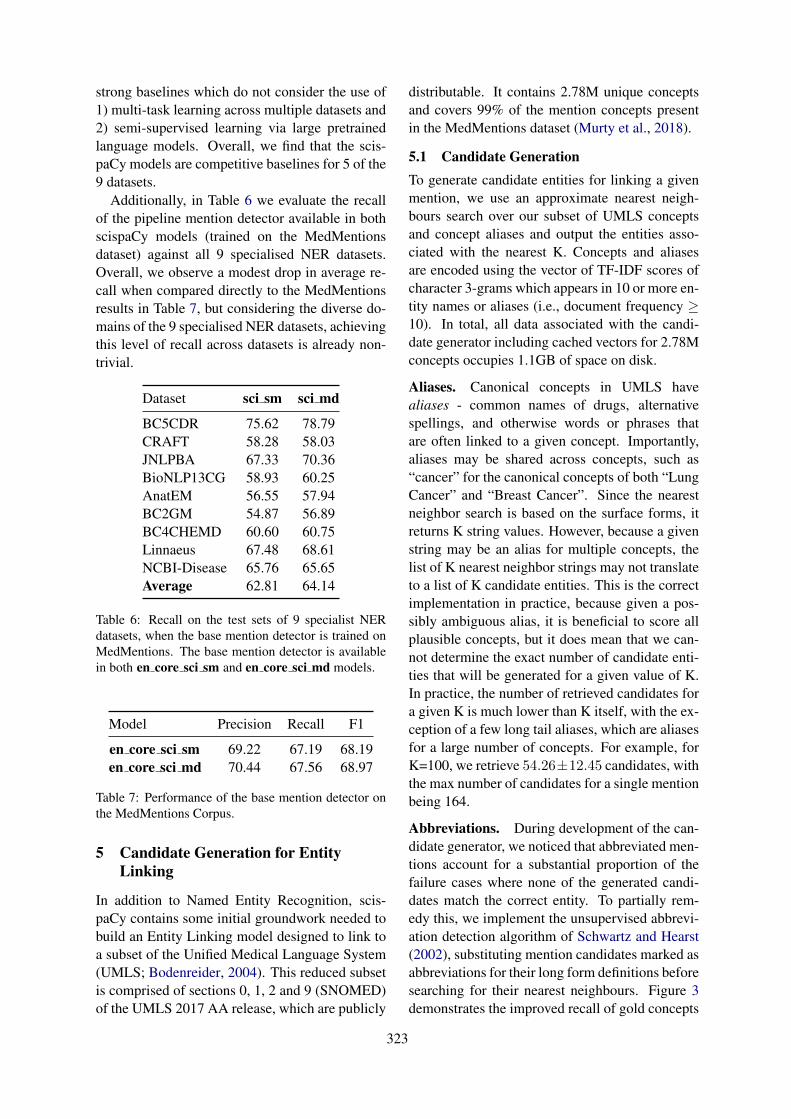
strong baselines which do not consider the use of1) multi-task learning across multiple datasets and2) semi-supervised learning via large pretrainedlanguage models. Overall, we find that the scis-paCy models are competitive baselines for 5 of the9 datasets.
Additionally, in Table 6 we evaluate the recallof the pipeline mention detector available in bothscispaCy models (trained on the MedMentionsdataset) against all 9 specialised NER datasets.Overall, we observe a modest drop in average re-call when compared directly to the MedMentionsresults in Table 7, but considering the diverse do-mains of the 9 specialised NER datasets, achievingthis level of recall across datasets is already non-trivial.
Dataset sci sm sci md
BC5CDR 75.62 78.79CRAFT 58.28 58.03JNLPBA 67.33 70.36BioNLP13CG 58.93 60.25AnatEM 56.55 57.94BC2GM 54.87 56.89BC4CHEMD 60.60 60.75Linnaeus 67.48 68.61NCBI-Disease 65.76 65.65Average 62.81 64.14
Table 6: Recall on the test sets of 9 specialist NERdatasets, when the base mention detector is trained onMedMentions. The base mention detector is availablein both en core sci sm and en core sci md models.
Model Precision Recall F1
en core sci sm 69.22 67.19 68.19en core sci md 70.44 67.56 68.97
Table 7: Performance of the base mention detector onthe MedMentions Corpus.
5 Candidate Generation for EntityLinking
In addition to Named Entity Recognition, scis-paCy contains some initial groundwork needed tobuild an Entity Linking model designed to link toa subset of the Unified Medical Language System(UMLS; Bodenreider, 2004). This reduced subsetis comprised of sections 0, 1, 2 and 9 (SNOMED)of the UMLS 2017 AA release, which are publicly
distributable. It contains 2.78M unique conceptsand covers 99% of the mention concepts presentin the MedMentions dataset (Murty et al., 2018).
5.1 Candidate GenerationTo generate candidate entities for linking a givenmention, we use an approximate nearest neigh-bours search over our subset of UMLS conceptsand concept aliases and output the entities asso-ciated with the nearest K. Concepts and aliasesare encoded using the vector of TF-IDF scores ofcharacter 3-grams which appears in 10 or more en-tity names or aliases (i.e., document frequency ≥10). In total, all data associated with the candi-date generator including cached vectors for 2.78Mconcepts occupies 1.1GB of space on disk.
Aliases. Canonical concepts in UMLS havealiases - common names of drugs, alternativespellings, and otherwise words or phrases thatare often linked to a given concept. Importantly,aliases may be shared across concepts, such as“cancer” for the canonical concepts of both “LungCancer” and “Breast Cancer”. Since the nearestneighbor search is based on the surface forms, itreturns K string values. However, because a givenstring may be an alias for multiple concepts, thelist of K nearest neighbor strings may not translateto a list of K candidate entities. This is the correctimplementation in practice, because given a pos-sibly ambiguous alias, it is beneficial to score allplausible concepts, but it does mean that we can-not determine the exact number of candidate enti-ties that will be generated for a given value of K.In practice, the number of retrieved candidates fora given K is much lower than K itself, with the ex-ception of a few long tail aliases, which are aliasesfor a large number of concepts. For example, forK=100, we retrieve 54.26±12.45 candidates, withthe max number of candidates for a single mentionbeing 164.
Abbreviations. During development of the can-didate generator, we noticed that abbreviated men-tions account for a substantial proportion of thefailure cases where none of the generated candi-dates match the correct entity. To partially rem-edy this, we implement the unsupervised abbrevi-ation detection algorithm of Schwartz and Hearst(2002), substituting mention candidates marked asabbreviations for their long form definitions beforesearching for their nearest neighbours. Figure 3demonstrates the improved recall of gold concepts
323
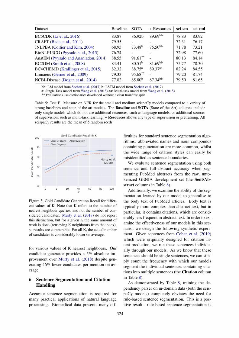
Dataset Baseline SOTA + Resources sci sm sci md
BC5CDR (Li et al., 2016) 83.87 86.92b 89.69bb 78.83 83.92CRAFT (Bada et al., 2011) 79.55 - - 72.31 76.17JNLPBA (Collier and Kim, 2004) 68.95 73.48b 75.50bb 71.78 73.21BioNLP13CG (Pyysalo et al., 2015) 76.74 - - 72.98 77.60AnatEM (Pyysalo and Ananiadou, 2014) 88.55 91.61** - 80.13 84.14BC2GM (Smith et al., 2008) 84.41 80.51b 81.69bb 75.77 78.30BC4CHEMD (Krallinger et al., 2015) 82.32 88.75a 89.37aa 82.24 84.55Linnaeus (Gerner et al., 2009) 79.33 95.68** - 79.20 81.74NCBI-Disease (Dogan et al., 2014) 77.82 85.80b 87.34bb 79.50 81.65
bb: LM model from Sachan et al. (2017) b: LSTM model from Sachan et al. (2017)a: Single Task model from Wang et al. (2018) aa: Multi-task model from Wang et al. (2018)** Evaluations use dictionaries developed without a clear train/test split.
Table 5: Test F1 Measure on NER for the small and medium scispaCy models compared to a variety ofstrong baselines and state of the art models. The Baseline and SOTA (State of the Art) columns includeonly single models which do not use additional resources, such as language models, or additional sourcesof supervision, such as multi-task learning. + Resources allows any type of supervision or pretraining. AllscispaCy results are the mean of 5 random seeds.
Figure 3: Gold Candidate Generation Recall for differ-ent values of K. Note that K refers to the number ofnearest neighbour queries, and not the number of con-sidered candidates. Murty et al. (2018) do not reportthis distinction, but for a given K the same amount ofwork is done (retrieving K neighbours from the index),so results are comparable. For all K, the actual numberof candidates is considerably lower on average.
for various values of K nearest neighbours. Ourcandidate generator provides a 5% absolute im-provement over Murty et al. (2018) despite gen-erating 46% fewer candidates per mention on av-erage.
6 Sentence Segmentation and CitationHandling
Accurate sentence segmentation is required formany practical applications of natural languageprocessing. Biomedical data presents many dif-
ficulties for standard sentence segmentation algo-rithms: abbreviated names and noun compoundscontaining punctuation are more common, whilstthe wide range of citation styles can easily bemisidentified as sentence boundaries.
We evaluate sentence segmentation using bothsentence and full-abstract accuracy when seg-menting PubMed abstracts from the raw, unto-kenized GENIA development set (the Sent/Ab-stract columns in Table 8).
Additionally, we examine the ability of the seg-mentation learned by our model to generalise tothe body text of PubMed articles. Body text istypically more complex than abstract text, but inparticular, it contains citations, which are consid-erably less frequent in abstract text. In order to ex-amine the effectiveness of our models in this sce-nario, we design the following synthetic experi-ment. Given sentences from Cohan et al. (2019)which were originally designed for citation in-tent prediction, we run these sentences individu-ally through our models. As we know that thesesentences should be single sentences, we can sim-ply count the frequency with which our modelssegment the individual sentences containing cita-tions into multiple sentences (the Citation columnin Table 8).
As demonstrated by Table 8, training the de-pendency parser on in-domain data (both the scis-paCy models) completely obviates the need forrule-based sentence segmentation. This is a pos-itive result - rule based sentence segmentation is
324
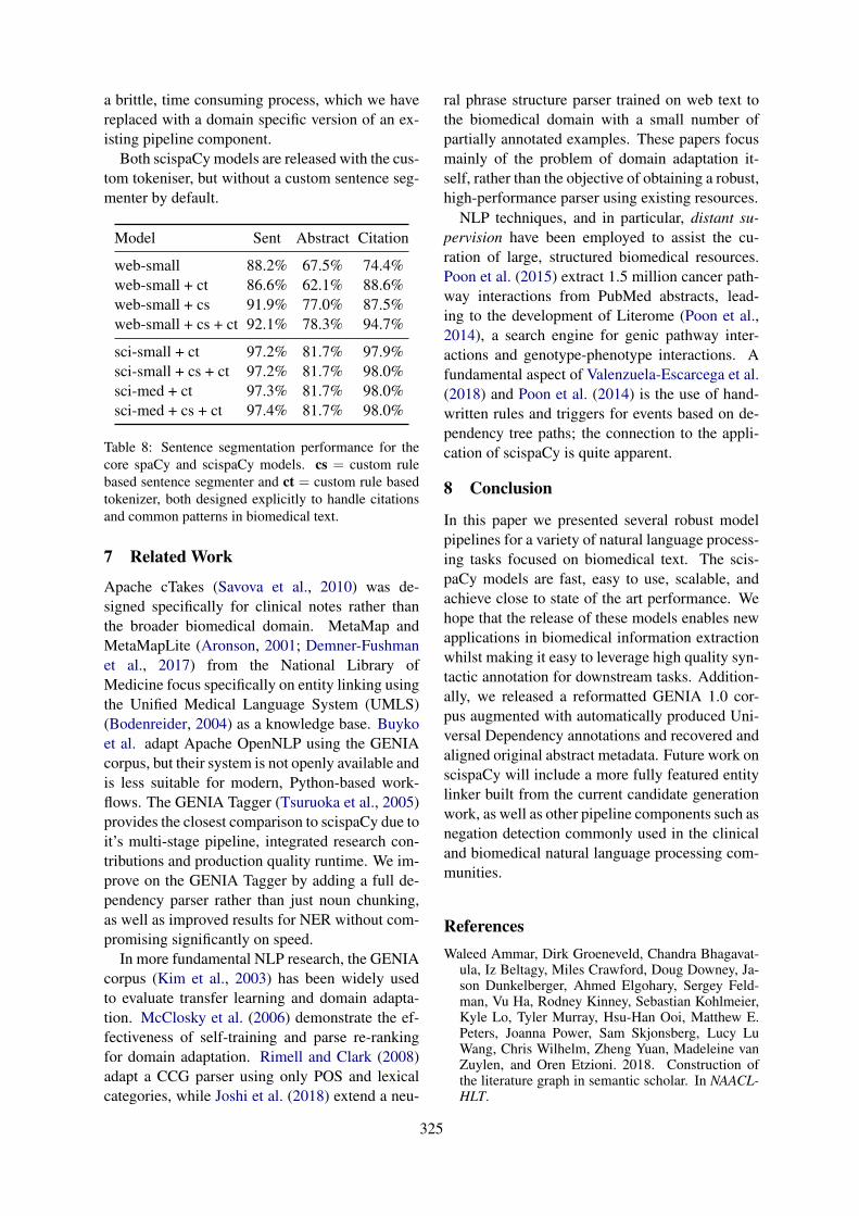
a brittle, time consuming process, which we havereplaced with a domain specific version of an ex-isting pipeline component.
Both scispaCy models are released with the cus-tom tokeniser, but without a custom sentence seg-menter by default.
Model Sent Abstract Citation
web-small 88.2% 67.5% 74.4%web-small + ct 86.6% 62.1% 88.6%web-small + cs 91.9% 77.0% 87.5%web-small + cs + ct 92.1% 78.3% 94.7%
sci-small + ct 97.2% 81.7% 97.9%sci-small + cs + ct 97.2% 81.7% 98.0%sci-med + ct 97.3% 81.7% 98.0%sci-med + cs + ct 97.4% 81.7% 98.0%
Table 8: Sentence segmentation performance for thecore spaCy and scispaCy models. cs = custom rulebased sentence segmenter and ct = custom rule basedtokenizer, both designed explicitly to handle citationsand common patterns in biomedical text.
7 Related Work
Apache cTakes (Savova et al., 2010) was de-signed specifically for clinical notes rather thanthe broader biomedical domain. MetaMap andMetaMapLite (Aronson, 2001; Demner-Fushmanet al., 2017) from the National Library ofMedicine focus specifically on entity linking usingthe Unified Medical Language System (UMLS)(Bodenreider, 2004) as a knowledge base. Buykoet al. adapt Apache OpenNLP using the GENIAcorpus, but their system is not openly available andis less suitable for modern, Python-based work-flows. The GENIA Tagger (Tsuruoka et al., 2005)provides the closest comparison to scispaCy due toit’s multi-stage pipeline, integrated research con-tributions and production quality runtime. We im-prove on the GENIA Tagger by adding a full de-pendency parser rather than just noun chunking,as well as improved results for NER without com-promising significantly on speed.
In more fundamental NLP research, the GENIAcorpus (Kim et al., 2003) has been widely usedto evaluate transfer learning and domain adapta-tion. McClosky et al. (2006) demonstrate the ef-fectiveness of self-training and parse re-rankingfor domain adaptation. Rimell and Clark (2008)adapt a CCG parser using only POS and lexicalcategories, while Joshi et al. (2018) extend a neu-
ral phrase structure parser trained on web text tothe biomedical domain with a small number ofpartially annotated examples. These papers focusmainly of the problem of domain adaptation it-self, rather than the objective of obtaining a robust,high-performance parser using existing resources.
NLP techniques, and in particular, distant su-pervision have been employed to assist the cu-ration of large, structured biomedical resources.Poon et al. (2015) extract 1.5 million cancer path-way interactions from PubMed abstracts, lead-ing to the development of Literome (Poon et al.,2014), a search engine for genic pathway inter-actions and genotype-phenotype interactions. Afundamental aspect of Valenzuela-Escarcega et al.(2018) and Poon et al. (2014) is the use of hand-written rules and triggers for events based on de-pendency tree paths; the connection to the appli-cation of scispaCy is quite apparent.
8 Conclusion
In this paper we presented several robust modelpipelines for a variety of natural language process-ing tasks focused on biomedical text. The scis-paCy models are fast, easy to use, scalable, andachieve close to state of the art performance. Wehope that the release of these models enables newapplications in biomedical information extractionwhilst making it easy to leverage high quality syn-tactic annotation for downstream tasks. Addition-ally, we released a reformatted GENIA 1.0 cor-pus augmented with automatically produced Uni-versal Dependency annotations and recovered andaligned original abstract metadata. Future work onscispaCy will include a more fully featured entitylinker built from the current candidate generationwork, as well as other pipeline components such asnegation detection commonly used in the clinicaland biomedical natural language processing com-munities.
ReferencesWaleed Ammar, Dirk Groeneveld, Chandra Bhagavat-
ula, Iz Beltagy, Miles Crawford, Doug Downey, Ja-son Dunkelberger, Ahmed Elgohary, Sergey Feld-man, Vu Ha, Rodney Kinney, Sebastian Kohlmeier,Kyle Lo, Tyler Murray, Hsu-Han Ooi, Matthew E.Peters, Joanna Power, Sam Skjonsberg, Lucy LuWang, Chris Wilhelm, Zheng Yuan, Madeleine vanZuylen, and Oren Etzioni. 2018. Construction ofthe literature graph in semantic scholar. In NAACL-HLT.
325
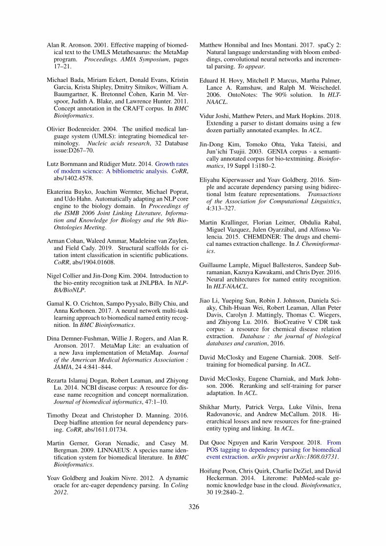
Alan R. Aronson. 2001. Effective mapping of biomed-ical text to the UMLS Metathesaurus: the MetaMapprogram. Proceedings. AMIA Symposium, pages17–21.
Michael Bada, Miriam Eckert, Donald Evans, KristinGarcia, Krista Shipley, Dmitry Sitnikov, William A.Baumgartner, K. Bretonnel Cohen, Karin M. Ver-spoor, Judith A. Blake, and Lawrence Hunter. 2011.Concept annotation in the CRAFT corpus. In BMCBioinformatics.
Olivier Bodenreider. 2004. The unified medical lan-guage system (UMLS): integrating biomedical ter-minology. Nucleic acids research, 32 Databaseissue:D267–70.
Lutz Bornmann and Rüdiger Mutz. 2014. Growth ratesof modern science: A bibliometric analysis. CoRR,abs/1402.4578.
Ekaterina Buyko, Joachim Wermter, Michael Poprat,and Udo Hahn. Automatically adapting an NLP coreengine to the biology domain. In Proceedings ofthe ISMB 2006 Joint Linking Literature, Informa-tion and Knowledge for Biology and the 9th Bio-Ontologies Meeting.
Arman Cohan, Waleed Ammar, Madeleine van Zuylen,and Field Cady. 2019. Structural scaffolds for ci-tation intent classification in scientific publications.CoRR, abs/1904.01608.
Nigel Collier and Jin-Dong Kim. 2004. Introduction tothe bio-entity recognition task at JNLPBA. In NLP-BA/BioNLP.
Gamal K. O. Crichton, Sampo Pyysalo, Billy Chiu, andAnna Korhonen. 2017. A neural network multi-tasklearning approach to biomedical named entity recog-nition. In BMC Bioinformatics.
Dina Demner-Fushman, Willie J. Rogers, and Alan R.Aronson. 2017. MetaMap Lite: an evaluation ofa new Java implementation of MetaMap. Journalof the American Medical Informatics Association :JAMIA, 24 4:841–844.
Rezarta Islamaj Dogan, Robert Leaman, and ZhiyongLu. 2014. NCBI disease corpus: A resource for dis-ease name recognition and concept normalization.Journal of biomedical informatics, 47:1–10.
Timothy Dozat and Christopher D. Manning. 2016.Deep biaffine attention for neural dependency pars-ing. CoRR, abs/1611.01734.
Martin Gerner, Goran Nenadic, and Casey M.Bergman. 2009. LINNAEUS: A species name iden-tification system for biomedical literature. In BMCBioinformatics.
Yoav Goldberg and Joakim Nivre. 2012. A dynamicoracle for arc-eager dependency parsing. In Coling2012.
Matthew Honnibal and Ines Montani. 2017. spaCy 2:Natural language understanding with bloom embed-dings, convolutional neural networks and incremen-tal parsing. To appear.
Eduard H. Hovy, Mitchell P. Marcus, Martha Palmer,Lance A. Ramshaw, and Ralph M. Weischedel.2006. OntoNotes: The 90% solution. In HLT-NAACL.
Vidur Joshi, Matthew Peters, and Mark Hopkins. 2018.Extending a parser to distant domains using a fewdozen partially annotated examples. In ACL.
Jin-Dong Kim, Tomoko Ohta, Yuka Tateisi, andJun’ichi Tsujii. 2003. GENIA corpus - a semanti-cally annotated corpus for bio-textmining. Bioinfor-matics, 19 Suppl 1:i180–2.
Eliyahu Kiperwasser and Yoav Goldberg. 2016. Sim-ple and accurate dependency parsing using bidirec-tional lstm feature representations. Transactionsof the Association for Computational Linguistics,4:313–327.
Martin Krallinger, Florian Leitner, Obdulia Rabal,Miguel Vazquez, Julen Oyarzábal, and Alfonso Va-lencia. 2015. CHEMDNER: The drugs and chemi-cal names extraction challenge. In J. Cheminformat-ics.
Guillaume Lample, Miguel Ballesteros, Sandeep Sub-ramanian, Kazuya Kawakami, and Chris Dyer. 2016.Neural architectures for named entity recognition.In HLT-NAACL.
Jiao Li, Yueping Sun, Robin J. Johnson, Daniela Sci-aky, Chih-Hsuan Wei, Robert Leaman, Allan PeterDavis, Carolyn J. Mattingly, Thomas C. Wiegers,and Zhiyong Lu. 2016. BioCreative V CDR taskcorpus: a resource for chemical disease relationextraction. Database : the journal of biologicaldatabases and curation, 2016.
David McClosky and Eugene Charniak. 2008. Self-training for biomedical parsing. In ACL.
David McClosky, Eugene Charniak, and Mark John-son. 2006. Reranking and self-training for parseradaptation. In ACL.
Shikhar Murty, Patrick Verga, Luke Vilnis, IrenaRadovanovic, and Andrew McCallum. 2018. Hi-erarchical losses and new resources for fine-grainedentity typing and linking. In ACL.
Dat Quoc Nguyen and Karin Verspoor. 2018. FromPOS tagging to dependency parsing for biomedicalevent extraction. arXiv preprint arXiv:1808.03731.
Hoifung Poon, Chris Quirk, Charlie DeZiel, and DavidHeckerman. 2014. Literome: PubMed-scale ge-nomic knowledge base in the cloud. Bioinformatics,30 19:2840–2.
326
Hoifung Poon, Kristina Toutanova, and Chris Quirk.2015. Distant supervision for cancer pathway ex-traction from text. Pacific Symposium on Biocom-puting. Pacific Symposium on Biocomputing, pages120–31.
Sampo Pyysalo and Sophia Ananiadou. 2014.Anatomical entity mention recognition at literaturescale. In Bioinformatics.
Sampo Pyysalo, Tomoko Ohta, Rafal Rak, AndrewRowley, Hong-Woo Chun, Sung-Jae Jung, Sung-PilChoi, Jun’ichi Tsujii, and Sophia Ananiadou. 2015.Overview of the cancer genetics and pathway cu-ration tasks of BioNLP shared task 2013. In BMCBioinformatics.
Laura Rimell and Stephen Clark. 2008. Adapting alexicalized-grammar parser to contrasting domains.In EMNLP.
Devendra Singh Sachan, Pengtao Xie, MrinmayaSachan, and Eric P. Xing. 2017. Effective use ofbidirectional language modeling for transfer learn-ing in biomedical named entity recognition. InMLHC.
Guergana K. Savova, James J. Masanz, Philip V.Ogren, Jiaping Zheng, Sunghwan Sohn, Karin Kip-per Schuler, and Christopher G. Chute. 2010. Mayoclinical text analysis and knowledge extraction sys-tem (cTAKES): architecture, component evaluationand applications. Journal of the American MedicalInformatics Association : JAMIA, 17 5:507–13.
Sebastian Schuster and Christopher D. Manning. 2016.Enhanced english universal dependencies: An im-proved representation for natural language under-standing tasks. In LREC.
Ariel S. Schwartz and Marti A. Hearst. 2002. A sim-ple algorithm for identifying abbreviation definitionsin biomedical text. Pacific Symposium on Biocom-puting. Pacific Symposium on Biocomputing, pages451–62.
Larry Smith, Lorraine K. Tanabe, Rie Johnson neeAndo, Cheng-Ju Kuo, I-Fang Chung, Chun-NanHsu, Y Lin, Roman Klinger, Christoph M. Friedrich,Kuzman Ganchev, Manabu Torii, Hongfang Liu,Barry Haddow, Craig A. Struble, Richard J.Povinelli, Andreas Vlachos, William A. Baumgart-ner, Lawrence E. Hunter, Bob Carpenter, RichardTzong-Han Tsai, Hong-Jie Dai, Feng Liu, YifeiChen, Chengjie Sun, Sophia Katrenko, Pieter Adri-aans, Christian Blaschke, Rafael Torres, MarianaNeves, Preslav Nakov, Anna Divoli, Manuel Maña-López, Jacinto Mata, and W. John Wilbur. 2008.Overview of BioCreative II gene mention recogni-tion. Genome Biology, 9:S2 – S2.
Yoshimasa Tsuruoka, Yuka Tateishi, Jin-Dong Kim,Tomoko Ohta, John McNaught, Sophia Ananiadou,and Jun’ichi Tsujii. 2005. Developing a robust part-of-speech tagger for biomedical text. In PanhellenicConference on Informatics.
Yoshimasa Tsuruoka and Jun’ichi Tsujii. 2005. Bidi-rectional inference with the easiest-first strategy fortagging sequence data. In HLT/EMNLP.
Marco Antonio Valenzuela-Escarcega, Ozgun Babur,Gus Hahn-Powell, Dane Bell, Thomas Hicks, En-rique Noriega-Atala, Xia Wang, Mihai Surdeanu,Emek Demir, and Clayton T. Morrison. 2018.Large-scale automated machine reading discoversnew cancer-driving mechanisms. In Database.
Xuan Wang, Yu Zhang, Xiang Ren, Yuhao Zhang,Marinka Zitnik, Jingbo Shang, Curtis P. Langlotz,and Jiawei Han. 2018. Cross-type biomedicalnamed entity recognition with deep multi-task learn-ing. Bioinformatics.
Chih-Hsuan Wei, Yifan Peng, Robert Leaman, Al-lan Peter Davis, Carolyn J. Mattingly, Jiao Li,Thomas C. Wiegers, and Zhiyong Lu. 2016. As-sessing the state of the art in biomedical relation ex-traction: overview of the BioCreative V chemical-disease relation (CDR) task. Database : the journalof biological databases and curation, 2016.
Ralph Weischedel, Eduard Hovy, Martha Palmer,Mitch Marcus, Robert Belvin adn Sameer Prad-han, Lance Ramshaw, and Nianwen Xue. 2011.OntoNotes: A large training corpus for enhancedprocessing. In Joseph Olive, Caitlin Christian-son, and John McCary, editors, Handbook of Natu-ral Language Processing and Machine Translation.Springer.
Yuan Zhang and David I Weiss. 2016. Stack-propagation: Improved representation learning forsyntax. CoRR, abs/1603.06598.
327
Proceedings of the BioNLP 2019 workshop, pages 328–338Florence, Italy, August 1, 2019. c©2019 Association for Computational Linguistics
Improving Chemical Named Entity Recognition in Patentswith Contextualized Word Embeddings
Zenan Zhai1, Dat Quoc Nguyen1, Saber A. Akhondi2, Camilo Thorne2,Christian Druckenbrodt2, Trevor Cohn1, Michelle Gregory2, Karin Verspoor1
1The University of Melbourne, Australia; 2Elsevier1{zenan.zhai,dqnguyen,trevor.cohn,karin.verspoor}@unimelb.edu.au
2{s.akhondi,c.thorne.1,c.druckenbrodt,m.gregory}@elsevier.com
Abstract
Chemical patents are an important resource forchemical information. However, few chemi-cal Named Entity Recognition (NER) systemshave been evaluated on patent documents, duein part to their structural and linguistic com-plexity. In this paper, we explore the NERperformance of a BiLSTM-CRF model utilis-ing pre-trained word embeddings, character-level word representations and contextual-ized ELMo word representations for chemi-cal patents. We compare word embeddingspre-trained on biomedical and chemical patentcorpora. The effect of tokenizers optimizedfor the chemical domain on NER performancein chemical patents is also explored. The re-sults on two patent corpora show that contex-tualized word representations generated fromELMo substantially improve chemical NERperformance w.r.t. the current state-of-the-art.We also show that domain-specific resourcessuch as word embeddings trained on chemicalpatents and chemical-specific tokenizers havea positive impact on NER performance.
1 Introduction
Chemical patents are an important starting pointfor understanding of chemical compound purpose,properties, and novelty. New chemical compoundsare often initially disclosed in patent documents;however it may take 1-3 years for these chemi-cals to be mentioned in chemical literature (Sengeret al., 2015), suggesting that patents are a valuablebut underutilized resource. As the number of newchemical patent applications is drastically increas-ing every year (Muresan et al., 2011), it is becom-ing increasingly important to develop automaticnatural language processing (NLP) approaches en-abling information extraction from these patents(Akhondi et al., 2019). Chemical Named-EntityRecognition (NER) is a fundamental step for in-formation extraction from chemical-related texts,
supporting relation extraction (Wei et al., 2016),reaction prediction (Schwaller et al., 2018) andretro-synthesis (Segler et al., 2018).
However, performing NER in chemical patentscan be challenging (Akhondi et al., 2014). As le-gal documents, patents are written in a very differ-ent way compared to scientific literature. Whenwriting scientific papers, authors strive to maketheir words as clear and straight-forward as pos-sible, whereas patent authors often seek to pro-tect their knowledge from being fully disclosed(Valentinuzzi, 2017).
In tension with this is the need to claim broadscope for intellectual property reasons, and hencepatents typically contain more details and aremore exhaustive than scientific papers (Lupu et al.,2011).
There are a number of characteristics of patenttexts that create challenges for NLP in this con-text. Long sentences listing names of compoundsin chemical patents are frequently used. The struc-ture of sentences in patent claims is usually com-plex, and syntactic parsing in patents can be diffi-cult (Hu et al., 2016). A quantitative analysis byVerberne et al. (2010) showed that the average sen-tence length in a patent corpus is much longer thanin general language use. That work also showedthat the lexicon used in patents usually includesdomain-specific and novel terms that are difficultto understand. Some patent authorities use Op-tical Character Recognition (OCR) for digitizingpatents, which can be problematic when applyingautomatic NLP approaches as the OCR errors in-troduces extra noise to the data (Akhondi et al.,2019).
Most NER systems for the chemical domainwere developed, trained and tested on either chem-ical literature or only the title and abstract ofchemical patents (Akhondi et al., 2019). Thereare substantial linguistic differences between ab-
328
stracts and the corresponding full text publications(Cohen et al., 2010). The performance of NERapproaches on full patent documents has still notbeen fully explored (Krallinger et al., 2015).
Hence, this paper will focus on presenting thebest NER performance achieved to date on fullchemical patent corpus.
We use a combination of pre-trained word em-beddings, a CNN-based character-level word rep-resentation and contextualized word representa-tions generated from ELMo, trained on a patentcorpus, as input to a BiLSTM-CRF model. Theresults show that contextualized word represen-tations help improve chemical NER performancesubstantially. In addition, the impact of the choiceof pre-trained word embeddings and tokenizers isassessed.
The results show that word embeddings that arepre-trained on chemical patents outperform em-beddings pre-trained on biomedical datasets, andusing tokenizers optimized for the chemical do-main can improve NER performance in chemicalpatent corpora.
2 Related work
In this section, we summarize previous methodsand empirical studies on NER in chemical patents.
Two existing Conditional Random Field (CRF)-based systems for chemical named entity recog-nition are tmChem (Leaman et al., 2015) andChemSpot (Rocktäschel et al., 2012); each makesuse of numerous hand-crafted features includ-ing word shape, prefix, suffix, part-of-speech andcharacter N-grams in an algorithm based on mod-elling of tag sequences. A previous detailedempirical study explored the generalization per-formance of these systems and their ensembles(Habibi et al., 2016). The application of the tm-Chem model trained on chemical literature cor-pora of the BioCreative IV CHEMDNER task(Krallinger et al., 2015) and the ChemSpot modeltrained on a subset of the SCAI corpus (Klingeret al., 2008) resulted in a significant performancedrop over chemical patent corpora.
Zhang et al. (2016) compared the performanceof CRF- and Support Vector Machine (SVM)-based models on the CHEMDNER-patents corpus(Krallinger et al., 2015). The features constructedin that work included the binarized embedding(Guo et al., 2014), Brown clustering (Brown et al.,1992) and domain-specific features extracted by
detecting common prefixes/suffixes in chemicalwords. The obtained results show that the per-formance of CRF and SVM models can be sig-nificantly improved by incorporating unsupervisedfeatures (e.g. word embeddings, word cluster-ing). The study also showed that the SVM modelslightly outperformed the CRF model in the chem-ical NER task.
To perform chemical NER on the CHEMD-NER patents corpus, Akhondi et al. (2016)proposed an ensemble approach combining agazetteer-based method and a modified versionof tmChem. Here, the gazetteer-based methodutilized a wide range of chemical dictionaries,while additional features such as stems, pre-fixes/suffixes, chemical elements were added tothe original feature set of tmChem. In the en-semble approach, tokens were predicted as chem-ical mentions if recognized as positive by eithertmChem or the gazetteer-based method. The re-sults showed that both gazetteer-based and ensem-ble approaches were outperformed by the modi-fied tmChem version in terms of overall F1 score,although these two approaches can obtain higherrecall.
Huang et al. (2015) proposed a BiLSTM-CRFbased on the use of a bidirectional long-shortterm memory network – BiLSTM (Schuster andPaliwal, 1997) – to extract (latent) features for aCRF classifier. The BiLSTM encodes the input inboth forward and backward directions and passesthe concatenation of outputs from both directionsas input to a linear-chain CRF sequence tagginglayer. In this approach, the BiLSTM selectivelyencodes information and long-distance dependen-cies observed while processing input sentences inboth directions, while the CRF layer globally opti-mizes the model by using information from neigh-bor labels.
The morphological structures within words arealso important clues for identifying named enti-ties in biological domain. Such morphologicalstructures are widely used in systematic chemicalname formats (e.g. IUPAC names) and hence par-ticularly informative for chemical NER (Klingeret al., 2008). Character-level word representa-tions have been developed to leverage informationfrom these structures by encoding the character se-quences within tokens. Ma and Hovy (2016) usesConvolutional Neural Networks (CNNs) to encodecharacter sequences while Lample et al. (2016)
329
developed a LSTM-based approach for encodingcharacter level information.
Habibi et al. (2017) presented an empiricalstudy comparing three NER models on a large col-lection of biomedical corpora including the BioSe-mantics patent corpus: (1) tmChem–the CRF-based model with hand-crafted features–used asthe baseline; (2) a second CRF model based onCRFSuite (Okazaki, 2007) using pre-trained wordembeddings; (3) and a BiLSTM-CRF model withadditional LSTM-based character-level word em-beddings (Lample et al., 2016). The performanceof CRFSuite- and BiLSTM-CRF-based modelswith different sets of pre-trained biomedical wordembeddings (Pyysalo et al., 2013) were also ex-plored. The results showed that the BiLSTM-CRF model with the combination of domain-specific pre-trained word embedding and LSTM-based character-level word embeddings outper-formed the two CRF-based models on chemicalNER tasks in both chemical literature and chem-ical patent corpora. However, this work used onlya general tokenizer (i.e. OpenNLP) and word em-beddings pre-trained on biomedical corpora.
Corbett and Boyle (2018) presented word-leveland character-level BiLSTM networks for chem-ical NER in literature domain. The word-levelmodel employed word embeddings learned byGloVe (Pennington et al., 2014) on a corpus ofpatent titles and abstracts. The character-levelmodel used two different transfer learning ap-proaches to pre-train its character-level encoder.The first approach attempts to predict neighborcharacters at each time step, while the other triesto predict whether a given character sequence isan entry in the chemical database ChEBI (Degt-yarenko et al., 2007). Experimental results showthat the character-level model can produce betterNER performance than word-level model by lever-aging transfer learning. In addition, for the word-level model, using pre-trained word embeddingslearned from a patent corpus helps produce bet-ter performance than using the pre-trained oneslearned from a general corpus.
3 Our empirical methodology
This section presents our empirical study of NERchemical on patent datasets. We first outline theexperimental datasets (Section 3.1) and the to-kenizers (Section 3.2) used to pre-process thesedatasets, and then we introduce the BiLSTM-
CRF-based models (Section 3.3) with pre-trainedword embeddings (Section 3.4), character-levelword embeddings (Section 3.5), contextualizedword embeddings (Section 3.6) and implementa-tion details (Section 3.7).
3.1 Dataset
We conduct experiments on 2 patent corpora: theBioSemantics patent corpus (Akhondi et al., 2014)and Reaxys gold set (Akhondi et al., 2019).
The BioSemantics patent corpus (Akhondiet al., 2014) consists of 200 full chemical patentdocuments with 9 different entity classes. In par-ticular, this corpus has 170K sentences and and360K entity annotations, which is much largerthan previously used datasets, e.g. the CHEMD-NER patent abstract corpus (Krallinger et al.,2015). Therefore, this corpus can be considered asa more suitable resource for evaluating deep learn-ing methods in which a large amount of trainingdata is required (LeCun et al., 2015). A subset of47 patents were annotated by multiple groups (atleast 3) of annotators and evaluated through inner-annotator agreement. By harmonizing the anno-tations from different annotator groups, these 47patents formed the “harmonized” set in the BioSe-mantics patent corpus. We use the harmonized setfor both hyper-parameter tuning and error analysisas it has known high-quality annotations.
The Reaxys gold set (Akhondi et al., 2019) con-tains 131 patent snippets (parts of full chemicalpatent documents) from several different patentoffices. The tagging scheme of this corpus in-cludes 2 coarse-grained labels chemical class andchemical compounds, and 7 fine-grained labels ofchemical compound (e.g. mixture-part, prophetic)and chemical class (e.g. bio-molecule, Markush,mixture, mixture-part). This corpus is relativelysmall in size, approximately 20,000 sentences intotal, but very richly annotated. The relevancyscore of each chemical entity and the relations be-tween them were also annotated, which allows thiscorpus to be used in other tasks beyond named en-tity recognition.
In our experiments, each corpus is used sep-arately. We follow Habibi et al. (2017) touse a ratio split of 60%/10%/30% for train-ing/development/test. Note that on the BioSeman-tic patent corpus, our sampling of datasets may notbe exactly the same as in Habibi et al. (2017).
330
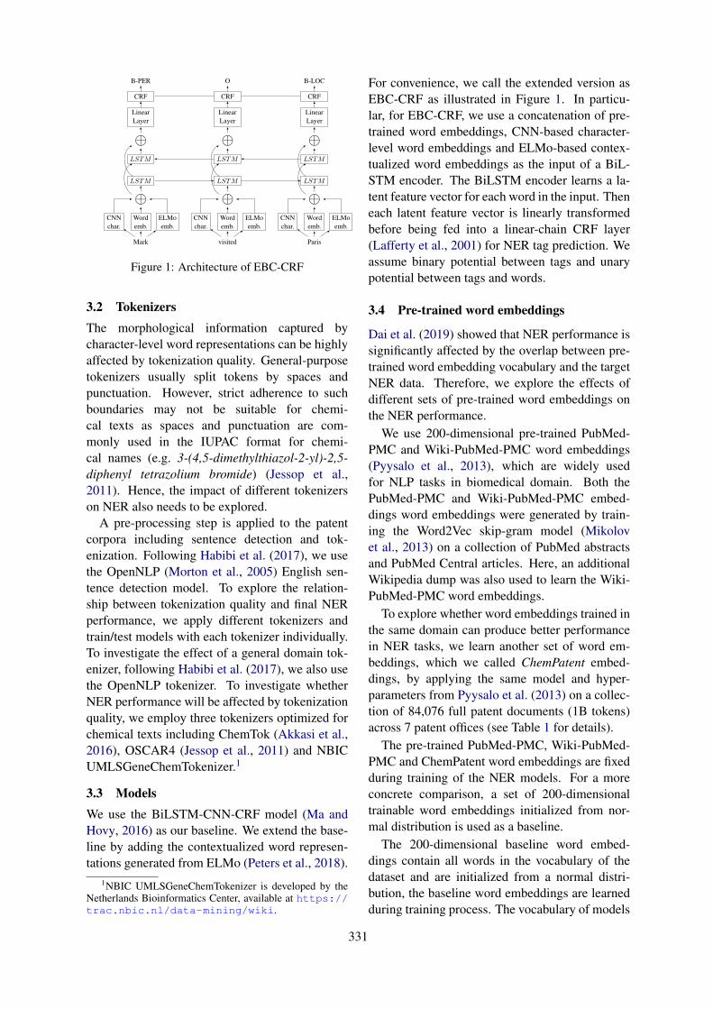
B-PER O B-LOC
CRF CRF CRF
LinearLayer
LinearLayer
LinearLayer
⊕ ⊕ ⊕LSTM LSTM LSTM
LSTM LSTM LSTM
⊕ ⊕ ⊕Wordemb.
CNNchar.
ELMoemb.
Wordemb.
CNNchar.
ELMoemb.
Wordemb.
CNNchar.
ELMoemb.
Mark visited Paris
Figure 1: Architecture of EBC-CRF
3.2 TokenizersThe morphological information captured bycharacter-level word representations can be highlyaffected by tokenization quality. General-purposetokenizers usually split tokens by spaces andpunctuation. However, strict adherence to suchboundaries may not be suitable for chemi-cal texts as spaces and punctuation are com-monly used in the IUPAC format for chemi-cal names (e.g. 3-(4,5-dimethylthiazol-2-yl)-2,5-diphenyl tetrazolium bromide) (Jessop et al.,2011). Hence, the impact of different tokenizerson NER also needs to be explored.
A pre-processing step is applied to the patentcorpora including sentence detection and tok-enization. Following Habibi et al. (2017), we usethe OpenNLP (Morton et al., 2005) English sen-tence detection model. To explore the relation-ship between tokenization quality and final NERperformance, we apply different tokenizers andtrain/test models with each tokenizer individually.To investigate the effect of a general domain tok-enizer, following Habibi et al. (2017), we also usethe OpenNLP tokenizer. To investigate whetherNER performance will be affected by tokenizationquality, we employ three tokenizers optimized forchemical texts including ChemTok (Akkasi et al.,2016), OSCAR4 (Jessop et al., 2011) and NBICUMLSGeneChemTokenizer.1
3.3 ModelsWe use the BiLSTM-CNN-CRF model (Ma andHovy, 2016) as our baseline. We extend the base-line by adding the contextualized word represen-tations generated from ELMo (Peters et al., 2018).
1NBIC UMLSGeneChemTokenizer is developed by theNetherlands Bioinformatics Center, available at https://trac.nbic.nl/data-mining/wiki.
For convenience, we call the extended version asEBC-CRF as illustrated in Figure 1. In particu-lar, for EBC-CRF, we use a concatenation of pre-trained word embeddings, CNN-based character-level word embeddings and ELMo-based contex-tualized word embeddings as the input of a BiL-STM encoder. The BiLSTM encoder learns a la-tent feature vector for each word in the input. Theneach latent feature vector is linearly transformedbefore being fed into a linear-chain CRF layer(Lafferty et al., 2001) for NER tag prediction. Weassume binary potential between tags and unarypotential between tags and words.
3.4 Pre-trained word embeddings
Dai et al. (2019) showed that NER performance issignificantly affected by the overlap between pre-trained word embedding vocabulary and the targetNER data. Therefore, we explore the effects ofdifferent sets of pre-trained word embeddings onthe NER performance.
We use 200-dimensional pre-trained PubMed-PMC and Wiki-PubMed-PMC word embeddings(Pyysalo et al., 2013), which are widely usedfor NLP tasks in biomedical domain. Both thePubMed-PMC and Wiki-PubMed-PMC embed-dings word embeddings were generated by train-ing the Word2Vec skip-gram model (Mikolovet al., 2013) on a collection of PubMed abstractsand PubMed Central articles. Here, an additionalWikipedia dump was also used to learn the Wiki-PubMed-PMC word embeddings.
To explore whether word embeddings trained inthe same domain can produce better performancein NER tasks, we learn another set of word em-beddings, which we called ChemPatent embed-dings, by applying the same model and hyper-parameters from Pyysalo et al. (2013) on a collec-tion of 84,076 full patent documents (1B tokens)across 7 patent offices (see Table 1 for details).
The pre-trained PubMed-PMC, Wiki-PubMed-PMC and ChemPatent word embeddings are fixedduring training of the NER models. For a moreconcrete comparison, a set of 200-dimensionaltrainable word embeddings initialized from nor-mal distribution is used as a baseline.
The 200-dimensional baseline word embed-dings contain all words in the vocabulary of thedataset and are initialized from a normal distri-bution, the baseline word embeddings are learnedduring training process. The vocabulary of models
331
Patent Office Document Sentence TokensAU 7,743 4,662,375 156,137,670CA 1,962 463,123 16,109,776EP 19,274 3,478,258 117,992,191GB 918 182,627 6,038,837IN 1,913 261,260 9,015,238US 41,131 19,800,123 628,256,609WO 11,135 4,830,708 159,286,325Total 84,076 33,687,474 1,092,836,646
Table 1: Statistics of the unannotated patent corpusused for training ChemPatent embeddings and ELMo.
using pre-trained word embeddings is built by tak-ing the union of words in the pre-traied word em-bedding file and words with frequency more than3 in training and development sets. We do not up-date weights for word embeddings if pre-trainedword embeddings were used.
3.5 Character-level representation
The BiLSTM-CRF model with character-levelword representations (Lample et al., 2016; Ma andHovy, 2016) has been shown to have state-of-the-art performance in NER tasks on chemical patentdatasets (Habibi et al., 2017). It has been shownthat the choice of using LSTM-based or CNN-based character-level word representation has lit-tle effect on final NER performance in both gen-eral and biomedical domain while the CNN-basedapproach has the advantage of reduced trainingtime (Reimers and Gurevych, 2017b; Zhai et al.,2018). Hence, we use the CNN-based approachwith the same hyper-parameter settings of Reimersand Gurevych (2017b) for capturing character-level information (see Table 2 for details).
3.6 ELMo
ELMo (Peters et al., 2018) and BERT (Devlinet al., 2019) can be used to generate contextu-alized word representations by combining inter-nal states of different layers in neural languagemodels. Contextualized word representation canhelp to improve performance in various NLP tasksby incorporating contextual information, essen-tially allowing for the same word to have distinctcontext-dependent meanings. This could be par-ticularly powerful for chemical NER since genericchemical names (e.g. salts, acid) may have dif-ferent meanings in other domains. We thereforeexplore the impact of using contextualized wordrepresentations for chemical patents.
We train ELMo on the same corpus of 84K
Hyper-para. ValueOptimizer AdamLearning rate 0.001Mini-batch size 16Clip Norm(L2) 1Dropout [0.25, 0.25]
Hyper-para. ValuecharEmbedSize 50filter length 3# of filters 30output size 30
(a) BiLSTM-CRF (b) CNN-char
Table 2: Fixed hyper-parameter configurations.
patents (detailed in Table 1), which we use fortraining the ChemPatent embeddings (describedin Section 3.4). We use the ELMo implementa-tion provided by Peters et al. (2018) with defaulthyper-parameters.2 Such neural language modelsrequire a large amount of computational resourcesto train. In ELMo, a maximum character sequencelength of tokens is set to make training feasible.However, systematic chemical names in chemicalpatents are often longer than the typical maximumsequence length of these neural language models.As very long tokens tend to be systematic chem-ical names, we reduced the max length of wordfrom 50 to 25 and replace tokens longer than 25characters by a special token “Long Token”.
3.7 Implementation details
Our NER model implementation is based on theAllenNLP system (Gardner et al., 2017). We learnmodel parameters using the training set, and weuse the overall F1 score over development set asindicator for performance improvement. All mod-els in this paper are trained with 50 epochs in max-imum, and an early stopping is applied if there areno overall F1 score improvement observed after10 epochs.
In Reimers and Gurevych (2017a) and Zhaiet al. (2018), optimal hyper-parameters ofBiLSTM-CRF models in NER tasks were ex-plored. Hence, we fix the hyper-parameters shownin Table 2 to the suggested values in our exper-iments, which means that only models with 2-stacked LSTM of size 250 are evaluated.
In this study, we also consider the choice oftokenizer and word embedding source as hyper-parameters. To compare the performance of dif-ferent tokenizers, we tokenize the same split ofdatasets with different tokenizers and evaluate theoverall F1 score over development set. After thebest tokenizer for pre-processing patent corpus isdetermined, we use datasets tokenized by the best
2https://github.com/allenai/bilm-tf
332
Tokenizer BioSemantics Reaxys Avg.OpenNLP 89.36 89.43 89.40NBIC +0.86 -0.13 +0.37ChemTok +0.04 +1.68 +0.86OSCAR4 +0.08 +1.86 +0.97
Table 3: Best F1 of EBC-CRF model with differ-ent tokenizations on development sets of BioSeman-tics patent (harmonized set) and Reaxys Gold withChemPatent embeddings in use. Recall that the har-monized set of 47 patents is a subset of BioSemantics,which were annotated by multiple groups (i.e. betterannotation quality than remaining patents).
Embeddings BioSemantics Reaxys Avg.Baseline 88.54 90.05 89.30PubMed-PMC +0.61 +1.03 +0.82Wiki-PubMed-PMC +1.24 +0.95 +1.10ChemPatent +1.68 +1.24 +1.46
Table 4: Best F1 of EBC-CRF model with differentword embeddings on development sets of BioSeman-tics patent (harmonized set) and Reaxys Gold (tok-enized by NBIC and OSCAR 4 tokenizer respectively)
tokenizer to train models with different pre-trainedword embeddings. The best set of pre-trainedword embeddings for patent corpus is determinedbased on the overall F1 score over developmentset. We then take the best performing tokenizerand pre-trained word embeddings by comparingthe marco-average F1 score improvement on bothexperimental datasets.
4 Results
4.1 Main ResultsEffects of different tokenizers: Table 3 showsthat all 3 tokenizers optimized for the chemical do-main outperform the baseline general-purpose to-kenizer (i.e. OpenNLP). The best performance onBioSemantics and Reaxys Gold are achieved byusing the NBIC tokenizer (+1.86 F1 score) and theOSCAR4 tokenizer (+0.86 F1 score), respectively.The best overall tokenizer is OSCAR4 which ob-tains about 1.0 absolute macro-averaged F1 im-provement in comparison to the baseline.
Effects of different sets of word embeddings:Table 4 shows results obtained by training EBC-CRF with different sets of pre-trained word em-beddings. On both BioSemantics and ReaxysGold, it is not surprising that our ChemPatentword embeddings help produce the best perfor-mance on the development set, obtaining (on av-erage) a higher F1 score of 1.5 as compared to the
Model P R F1
tmChem 72.56 78.37 75.35CRFSuite 81.93 78.38 80.12BiLSTM-CRF + LSTM-char 79.72 84.42 82.01BiLSTM-CNN-CRF 83.76 85.01 84.38EBC-CRF 84.30 87.11 85.68
Table 5: NER scores on full BioSemantics test set(Akhondi et al., 2014). Results in the first 3 rowswere reported in Habibi et al. (2017). BiLSTM-CRF +LSTM-char denotes the BiLSTM-CRF model with ad-ditional LSTM-based character-level word embeddings(Lample et al., 2016). Recall that our models use theOSCAR4 tokenizer and pre-trained ChemPatent wordembeddings.
baseline embeddings. Specifically, ChemPatentdoes better than the second best Wiki-PubMed-PMC with about 0.4 improvement. In the restof the Results section, obtained results are re-ported with the use of the OSCAR4 tokenizer andthe ChemPatent embeddings on both experimentaldatasets.3
Final results: Table 5 compared results reportedin Habibi et al. (2017) and our approach on thefull BioSemantics test set. It is clear that all neu-ral models outperform conventional CRF-basedmodels tmChem and CRFSuite. Our EBC-CRFmodel outperforms the BiLSTM-CRF + LSTM-char model with a 3.7 F1 score improvement.Compared to the baseline model BiLSTM-CNN-CRF, the ELMo-based contextualized word em-beddings help to produce an F1 improvement of1.3 points.
Table 6 details our F1 scores for BiLSTM-CNN-CRF and EBC-CRF with respect to each en-tity label on both the BioSemantics patent cor-pus and the Reaxys Gold set. The overall resultsshow that ELMo-based contextualized word em-beddings help improve the baseline by 1.3 and 4.8absolute F1 score on BioSemantics and Reaxys,respectively.
In BioSemantics patent corpus, we obtain 1+F1 score improvements on frequent entity labels(i.e. > 3, 000 instances) except for the entity la-bel Formula, which has 0.4 absolute improvement.Higher improvements can be observed on rare en-tity labels (e.g. 4 points on Mode of Actions, 6points on Registry numbers and Trademarks). Thehighest improvement at 9 points is found for themost rare entity label CAS Number.
3OSCAR4 helped produce the highest “macro-averaged”improvement on both datasets.
333
Entity label Count† BiLSTM-CNN-CRF +ELMo∆F1# % P R F1 P R F1
B (Abbreviation) 6,558 5.78 85.90 87.02 86.46 85.78 89.98 87.83 +1.37C (CAS Number) 13 0.01 54.55 46.15 50.00 57.14 61.54 59.26 +9.26D (Trademark) 2,290 2.01 62.58 61.79 62.18 66.44 71.40 68.83 +6.65F (Formula) 7,935 6.99 86.05 86.81 86.42 83.07 90.91 86.82 +0.40G (Generic) 51,313 45.20 81.45 84.56 82.98 83.84 84.44 84.14 +1.16M (IUPAC) 39,896 35.14 88.40 87.77 88.09 87.25 91.20 89.18 +1.09MOA (Mode of Action) 1,137 1.00 68.97 63.32 66.02 67.62 72.74 70.08 +4.06R (Registry #) 96 0.08 55.68 51.04 53.26 65.82 54.17 59.43 +6.17T (Target) 4,290 3.78 77.77 77.32 77.55 77.21 82.68 79.85 +2.30Micro Avg. 113,528 100.0 83.76 85.01 84.38 84.30 87.11 85.68 +1.30
(a) BioSemantics
Entity label Count† BiLSTM-CNN-CRF +ELMo∆F1# % P R F1 P R F1
1 (chemClass) 1,476 12.36 78.35 66.46 71.92 81.96 75.75 78.73 +6.812 (chemClassbiomolecule) 951 7.96 71.86 70.50 71.17 76.27 78.76 77.50 +6.333 (chemClassmarkush) 38 0.32 42.86 47.37 45.00 42.86 47.37 45.00 +0.004 (chemClassmixture) 387 3.24 76.49 59.69 67.05 74.18 64.60 69.06 +2.015 (chemClassmixture-part) 161 1.35 71.00 44.10 54.41 78.10 50.93 61.65 +7.246 (chemClasspolymer) 609 5.10 81.40 72.82 76.87 89.20 84.07 86.56 +13.747 (chemCompound) 6,988 58.53 89.02 92.01 90.49 91.01 94.58 92.76 +2.278 (chemCompoundmixture-part) 904 7.57 90.02 81.86 85.75 90.63 85.62 88.05 +2.279 (chemCompoundprophetics) 426 3.57 18.52 2.35 4.17 77.75 79.58 78.65 +74.48Micro Avg. 11,940 100.0 85.12 80.36 82.67 87.41 87.53 87.47 +4.80
(b) Reaxys Gold
Table 6: F1 score with respect to each entity label. “Count†” denotes gold-entity counts in test sets.“+ELMo”denotes scores obtained by EBC-CRF.
In the Reaxys Gold set, with ELMo we obtain2+ F1 score improvements on entity labels chem-Compound, chemCompound-mixture part andchemClass-mixture. Higher improvements (>6 points) can be seen on some rare entity la-bels such as chemClass, chemClass-biomolecule,chemclass-mixture-part and chemClass-polymer.The improvements on entity label chemClass-Markush and chemCompound-prophetics are ir-regular compared to others. In particular, an abso-lute F1 improvement of 74+ is achieved on entitylabel chemCompound-prophetics, while we do notfind any improvement on chemClass-Markush.
4.2 Error Analysis
To perform error analysis on BioSemantics, weuse its harmonized subset. Figure 2 (a) shows thatmost of the errors are confusions between non-chemical words and generic chemical names (e.g.water, salt, acid). For example, as illustrated inFigure 3 (a), the word “salt” which appears atthe end of a systematic name should be identi-fied as a part of the systematic name. However,
the same word is also widely used to describe aclass of chemicals, e.g. “pharmaceutically accept-able salt” in Figure 3 (b). Disambiguation be-tween chemical class and chemical compound isa challenging task even for human annotators, andis thus particularly difficult for a statistical modelto learn. The confusion matrix of Reaxys Goldset in Figure 2 (b) also supports this point sincemost confusions are between non-chemical words,chemical classes and chemical compounds.
The Reaxys Gold set has a more complex tagset than the BioSemantics patent corpus, as it as-signs separate fine-grained tags for subcategoriesof chemical classes (chemClass) and chemicalcompounds (chemCompound). As illustrated inTable 6, there is not sufficient training data forfine-grained sub-category labels. It is difficult fora high complexity neural model to learn charac-teristics of these sub-category labels and the keydifference between the main categories and theirsubcategories. Figure 2 (b) shows that 50% the er-rors for “chemical compound prophetics” and 80%errors for “chemical compound mixture part” are
334
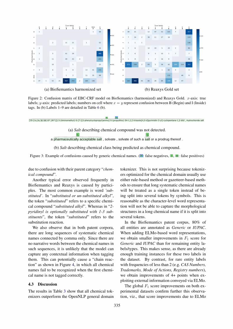
B C D F G M R T MOA OTrue labels
BC
DF
GM
RT
MOA
OPr
edict
ed la
bels
1 1 68
2 11 21 1 52
2 1 46
2 5 41 29 485
1 11 49 43 4 241
10 1 23
3 6 5 8 13 41 231
1 1 2 11 35 88
37 1 52 21 567 254 2 184 136
100
200
300
400
500
1 2 3 4 5 6 7 8 9 OTrue labels
12
34
56
78
9O
Pred
icted
labe
ls
39 21 12 47 52 101 7 317
7 24 2 38 11 27 16 119
1 1 1 136
7 6 10 19 5 20 2 90
7 6 9 3 10 1 7 7
1 8 1 2 16 9 48
271 158 2 93 5 56 42 190 114 312
5 28 1 82 3 4
132 46 9
165 366 50 80 28 84 199 12 47
80
160
240
320
(a) BioSemantics harmonized set (b) Reaxys Gold set
Figure 2: Confusion matrix of EBC-CRF model on BioSemantics (harmonized) and Reaxys Gold. x-axis: truelabels; y-axis: predicted labels; numbers on cell where x = y represent confusion between B (Begin) and I (Inside)tags. In (b) Labels 1–9 are detailed in Table 6 (b).
09/05/2019 brat
127.0.0.1:8001/index.xhtml#/harmonized_oscar4_merged/BRATFile0004 7/8
Aqueous liquid compositions of the invention also are particularly useful .No .08 / 189,479 , referred to above .
The crude product was purified by column chromatography on silica gel using dichloromethane : methanol ( 98 : 2 ) as eluant to afford the title compound as a colourless oil , 162mg , 67% ; < 1 > H NMR ( CDCl3 , 400MHz ) delta : 1.381.53 ( m , 2H ) , 3.27 ( m , 2H ) , 4.35 ( s , 2H ) , 4.61 ( m , 1H ) , 7.287.36 The invention further provides a process for the preparation of a combination product as hereinbefore defined , which process comprises bringing into association a compound of formula I , as hereinbefore defined ( but , for example , without the proviso ) , or a pharmaceutically acceptable salt thereof with the other therapeutic agent that is useful in the treatment of inflammation , and at least one pharmaceutically acceptable adjuvant , diluent or carrier .
Alkenyl is , for example , vinyl or prop2enyl .
The title indoline ( 28mg ) which was collected by filtration was isolated as a colourless solid , m.p.140142°C .( canceled ) 12 .
The solid residue was dissolved in THF ( 5 mL ) , 2amino1phenylethanone hydrochloride ( 0.97 g , 5.7 mmol ) and triethylamine ( 2 mL , 14.3 mmol ) was added and the mixture stirred at 40° C . for 19 h .( 1H , m ) , 2.342.27 IR(Nujol Mull ) ν890,1200 , 1490 , 3400 , 3640 cm1 .
In vivo cleavable esters are just one type of prodrug of the parent molecule .IR (KBr)(Cm"1) : 3306 , 2938 , 1633 , 1563 , 1483 , 1453 , 1317 , 1274 , 1236 , 1205 , 1149 , 1069 , 947 , 847 , 754 .
The combined extracts were dried and evaporated to dryness , and the residue was purified by flash chromatography using methanol ( 2% by volume ) in chloroform as eluant ,
to give 2,2'[5(5formylimidazol1yl)1,3phenylene]di(2methylpropiononitrile) , mp 108°111° .
The ATP and cydic AMP were separated on a double column chromatography system ( Anal .
The method of claim 7 , wherein said antidepressant is a monoamine oxidase inhibitor .The vial was capped and put in the microwave oven ( Smith synthesiser ) . [ 075 ] The phrase " linear chain of atoms " refers to the longest straight chain of atoms independently selected from carbon , nitrogen , oxygen and sulfur .Preferably compounds of Formula I are administered orally .MS ( APCI ) 482 ( M + H+ , 100% ) b )
[1S[1α,2α,3β,5β(1S*,2R*)]]3(Aminomethyl)5[7[(2phenylcyclopropyl)amino]5(propylthio)3H1,2,3triazolo[4,5d]pyrimidin3yl]cyclopentane1,2diol , Hydrochloride salt
A solution of the product from step ( a ) ( 0.22 g ) in ethanol ( 7 ml ) was treated with 10% palladium on carbon ( 0.03 g ) and the resultant suspension was stirred under 4 atmospheres pressure of hydrogen for 24 hours .( m , 2H ) , 3.15 ( ddd , J = 12.9 , 5.1 , 2.4 Hz , 1H ) 3.303.50 Other movement disorders related to dysfunction of the basal ganglia include tardive dyskinesia , progressive
supranuclear palsy and cerebral palsy , corticobasal degeneration , multiple system atrophy , Wilson disease , dystonia , tics , and chorea . dioxan ) , an amide ( e.g. J .Med . , 229 , 111115 .
A compound of claim 9 which is N,Ndimethyl1[1(4chlorophenyl)cyclobutyl]3methylbutylamine or a pharmaceutically acceptable salt thereof .MS ( ES ) [ M + H ] calculated for C16H18ClN5O2 , 348 ; found 348 .
After standing at about 0° C . for about 16 hours , the crystals of the hydrochloride salt containing isopropanol ( needles ) are filtered off and dried .
1HNMR ( DMSO d6 ) : d 6.80 ( s , 1 H ) , 4.40 ( br s , 1 H ) .
G M M
G
M
B M M
G
M M
M
B B
MOA MOAT MOA
M M
M
G
M
M
B
757677
78
79
808182
83
84
8586
87
88
8990
9192
93
94
9596
97
98
bratbrat/harmonized_oscar4_merged/BRATFile0004
Login required to perform "searchTextInCollection"
(a) Salt describing chemical compound was not detected.
20/04/2019 brat
127.0.0.1:8001/index.xhtml#/harmonized_oscar4_merged/BRATFile0004 5/6
1,1-Dioxo-3,3-dibutyl-5-phenyl-7-methylthio-8-(N-{(R)-α-[N-((S)-1-carboxypropyl)carbamoyl]-4-hydroxybenzyl}carbamoylmethoxy)-2,3,4,5-tetrahydro-1,2,5-benzothiadiazepine ;
1,1-Dioxo-3,3-dibutyl-5-phenyl-7-methylthio-8-[N-((R / S)-α-{N-[1-(R)-2-(S)-1-hydroxy-1-(3,4-dihydroxyphenyl)prop-2-yl]carbamoyl}-4-hydroxybenzyl)carbamoylmethoxy)-2,3,4,5-tetrah;
1,1-Dioxo-3,3-dibutyl-5-phenyl-7-methylthio-8-(N-{(R)-α-[N-(2-(S)-3-(R)-4-(R)-5-(R)-2,3,4,5,6-pentahydroxyhexyl)carbarnoyl]-4-hydroxybenzyl}carbamoylmethoxy)-2,3,4,5-tetrahydro-1; and
1,1-Dioxo-3,3-dibutyl-5-phenyl-7-methylthio-8-(N-{(R)-α-[N-(2-(S)-3-(R)-4)-5-(R)-2,3,4,5,6-pentahydroxyhexyl)carbamoyl]benzyl}carbamoylmethoxy)-2,3,4,5-tetrahydro-1,2,5-benzothia
; or a pharmaceutically acceptable salt , solvate , solvate of such a salt or a prodrug thereof .
The residue is taken up in water and diethyl ether .C26 H25 N7 02 ( 467.53 ) [ 8SJ-GTP?S was then added at a final concentration of 100 pM and the samples incubated for 30 min at 30°C .( m , 4H ) ppm .Aqueous liquid compositions of the invention also are particularly useful .No .08 / 189,479 , referred to above .
The crude product was purified by column chromatography on silica gel using dichloromethane : methanol ( 98 : 2 ) as eluant to afford the title compound as a colourless oil , 162mg , 67% ; < 1 > H NMR ( CDCl3 , 400MHz ) delta : 1.38-1.53 ( m , 2H ) , 3.27 ( m , 2H ) , 4.35 ( s , 2H ) , 4.61 ( m , 1H ) , 7.28-7.36 The invention further provides a process for the preparation of a combination product as hereinbefore defined , which process comprises bringing into association a compound of formula I , as hereinbefore defined ( but , for example , without the proviso ) , or a pharmaceutically acceptable salt thereof with the other therapeutic agent that is useful in the treatment of inflammation , and at least one pharmaceutically - acceptable adjuvant , diluent or carrier .
Alkenyl is , for example , vinyl or prop-2-enyl .
The title indoline ( 28mg ) which was collected by filtration was isolated as a colourless solid , m.p.140-142°C .( canceled ) 12 .
The solid residue was dissolved in THF ( 5 mL ) , 2-amino-1-phenylethanone hydrochloride ( 0.97 g , 5.7 mmol ) and triethylamine ( 2 mL , 14.3 mmol ) was added and the mixture stirred at 40° C . for 19 h .( 1H , m ) , 2.34-2.27 IR(Nujol Mull ) ν890,1200 , 1490 , 3400 , 3640 cm-1 .
In vivo cleavable esters are just one type of prodrug of the parent molecule .IR (KBr)(Cm"1) : 3306 , 2938 , 1633 , 1563 , 1483 , 1453 , 1317 , 1274 , 1236 , 1205 , 1149 , 1069 , 947 , 847 , 754 .
The combined extracts were dried and evaporated to dryness , and the residue was purified by flash chromatography using methanol ( 2% by volume ) in
chloroform as eluant , to give 2,2'-[5-(5-formylimidazol-1-yl)-1,3-phenylene]di(2-methylpropiononitrile) , mp 108°-111° .
The ATP and cydic AMP were separated on a double column chromatography system ( Anal .
The method of claim 7 , wherein said antidepressant is a monoamine oxidase inhibitor .The vial was capped and put in the microwave oven ( Smith synthesiser ) . [ 075 ] The phrase " linear chain of atoms " refers to the longest straight chain of atoms independently selected from carbon , nitrogen , oxygen and sulfur .Preferably compounds of Formula I are administered orally .MS ( APCI ) 482 ( M + H+ , 100% ) b )
[1S-[1α,2α,3β,5β(1S*,2R*)]]-3-(Aminomethyl)-5-[7-[(2-phenylcyclopropyl)amino]-5-(propylthio)-3H-1,2,3-triazolo[4,5-d]pyrimidin-3-yl]-cyclopentane-1,2-diol , Hydrochloride salt
A solution of the product from step ( a ) ( 0.22 g ) in ethanol ( 7 ml ) was treated with 10% palladium on carbon ( 0.03 g ) and the resultant suspension was stirred under 4 atmospheres pressure of hydrogen for 24 hours .( m , 2H ) , 3.15 ( ddd , J = 12.9 , 5.1 , 2.4 Hz , 1H ) 3.30-3.50 Other movement disorders related to dysfunction of the basal ganglia include tardive dyskinesia , progressive supranuclear palsy and cerebral palsy , corticobasal degeneration , multiple system atrophy , Wilson disease , dystonia , tics , and chorea .
dioxan ) , an amide ( e.g. J .Med . , 229 , 111-115 .
A compound of claim 9 which is N,N-dimethyl-1-[1-(4-chlorophenyl)cyclobutyl]-3-methylbutylamine or a pharmaceutically acceptable salt thereof .MS ( ES ) [ M + H ] calculated for C16H18ClN5O2 , 348 ; found 348 .
After standing at about 0° C . for about 16 hours , the crystals of the hydrochloride salt containing isopropanol ( needles ) are filtered off and dried .
1H-NMR ( DMSO -d6 ) : d 6.80 ( s , 1 H ) , 4.40 ( br s , 1 H ) .The method of Claim 21 in which the divalent metal cation is zinc .( m , 2H ) ppm .14 , p .859-869 ( 2005 ) .
EXAMPLE 59 A solution of 1,2,4-triazole ( 0.69 g ) in trifluoroacetic acid ( 3.12 ml ) was added to
2,2'-[5-(1-hydroxy-1-methylethyl)-1,3-phenylene]-di(2-methylpropiononitrile) , ( 0.27 g ) , and the resulting solution was stirred at room temperature for 18 hr and
M
M
M
M
G G
M M
G M M
G
M
B M M
G
M
M M
B B
MOA MOAT MOA
M M
M
G
M
M
B
M M
M
727374757677
78
79
808182
83
84
8586
87
88
8990
9192
93
94
9596
97
9899
100101102
103
bratbrat/harmonized_oscar4_merged/BRATFile0004
(b) Salt describing chemical class being predicted as chemical compound.
Figure 3: Example of confusions caused by generic chemical names. (
09/05/2019 brat
127.0.0.1:8001/index.xhtml#/harmonized_oscar4_merged/BRATFile0004 7/8
Aqueous liquid compositions of the invention also are particularly useful .No .08 / 189,479 , referred to above .
The crude product was purified by column chromatography on silica gel using dichloromethane : methanol ( 98 : 2 ) as eluant to afford the title compound as a colourless oil , 162mg , 67% ; < 1 > H NMR ( CDCl3 , 400MHz ) delta : 1.381.53 ( m , 2H ) , 3.27 ( m , 2H ) , 4.35 ( s , 2H ) , 4.61 ( m , 1H ) , 7.287.36 The invention further provides a process for the preparation of a combination product as hereinbefore defined , which process comprises bringing into association a compound of formula I , as hereinbefore defined ( but , for example , without the proviso ) , or a pharmaceutically acceptable salt thereof with the other therapeutic agent that is useful in the treatment of inflammation , and at least one pharmaceutically acceptable adjuvant , diluent or carrier .
Alkenyl is , for example , vinyl or prop2enyl .
The title indoline ( 28mg ) which was collected by filtration was isolated as a colourless solid , m.p.140142°C .( canceled ) 12 .
The solid residue was dissolved in THF ( 5 mL ) , 2amino1phenylethanone hydrochloride ( 0.97 g , 5.7 mmol ) and triethylamine ( 2 mL , 14.3 mmol ) was added and the mixture stirred at 40° C . for 19 h .( 1H , m ) , 2.342.27 IR(Nujol Mull ) ν890,1200 , 1490 , 3400 , 3640 cm1 .
In vivo cleavable esters are just one type of prodrug of the parent molecule .IR (KBr)(Cm"1) : 3306 , 2938 , 1633 , 1563 , 1483 , 1453 , 1317 , 1274 , 1236 , 1205 , 1149 , 1069 , 947 , 847 , 754 .
The combined extracts were dried and evaporated to dryness , and the residue was purified by flash chromatography using methanol ( 2% by volume ) in chloroform as eluant ,
to give 2,2'[5(5formylimidazol1yl)1,3phenylene]di(2methylpropiononitrile) , mp 108°111° .
The ATP and cydic AMP were separated on a double column chromatography system ( Anal .
The method of claim 7 , wherein said antidepressant is a monoamine oxidase inhibitor .The vial was capped and put in the microwave oven ( Smith synthesiser ) . [ 075 ] The phrase " linear chain of atoms " refers to the longest straight chain of atoms independently selected from carbon , nitrogen , oxygen and sulfur .Preferably compounds of Formula I are administered orally .MS ( APCI ) 482 ( M + H+ , 100% ) b )
[1S[1α,2α,3β,5β(1S*,2R*)]]3(Aminomethyl)5[7[(2phenylcyclopropyl)amino]5(propylthio)3H1,2,3triazolo[4,5d]pyrimidin3yl]cyclopentane1,2diol , Hydrochloride salt
A solution of the product from step ( a ) ( 0.22 g ) in ethanol ( 7 ml ) was treated with 10% palladium on carbon ( 0.03 g ) and the resultant suspension was stirred under 4 atmospheres pressure of hydrogen for 24 hours .( m , 2H ) , 3.15 ( ddd , J = 12.9 , 5.1 , 2.4 Hz , 1H ) 3.303.50 Other movement disorders related to dysfunction of the basal ganglia include tardive dyskinesia , progressive
supranuclear palsy and cerebral palsy , corticobasal degeneration , multiple system atrophy , Wilson disease , dystonia , tics , and chorea . dioxan ) , an amide ( e.g. J .Med . , 229 , 111115 .
A compound of claim 9 which is N,Ndimethyl1[1(4chlorophenyl)cyclobutyl]3methylbutylamine or a pharmaceutically acceptable salt thereof .MS ( ES ) [ M + H ] calculated for C16H18ClN5O2 , 348 ; found 348 .
After standing at about 0° C . for about 16 hours , the crystals of the hydrochloride salt containing isopropanol ( needles ) are filtered off and dried .
1HNMR ( DMSO d6 ) : d 6.80 ( s , 1 H ) , 4.40 ( br s , 1 H ) .
G M M
G
M
B M M
G
M M
M
B B
MOA MOAT MOA
M M
M
G
M
M
B
757677
78
79
808182
83
84
8586
87
88
8990
9192
93
94
9596
97
98
bratbrat/harmonized_oscar4_merged/BRATFile0004
Login required to perform "searchTextInCollection"
: false negatives,
20/04/2019 brat
127.0.0.1:8001/index.xhtml#/harmonized_oscar4_merged/BRATFile0002 4/4
A compound according to claim 1 wherein An+ is Na+ .
Salts deπved from organic bases include , but are not limited to , salts of primary , secondary and tertiary amines , such as alkyl amines , dialkyl amines , tπalkyl amines ,
substituted alkyl amines , di(substituted alkyl ) amines , tπ(substituted alkyl ) amines , alkenyl amines , dialkenyl amines , trialkenyl amines , substituted alkenyl amines ,
di(substituted alkenyl ) amines , tri(substituted alkenyl ) amines , cycloalkyl amines , di(cycloalkyl) amines , tπ(cycloalkyl) amines , substituted cycloalkyl amines ,
disubstituted cycloalkyl amine , tπsubstituted cycloalkyl amines , cycloalkenyl amines , di(cycloalkenyl) amines , tri(cycloalkenyl) amines , substituted cycloalkenyl amines ,
disubstituted cycloalkenyl amine , tπsubstituted cycloalkenyl amines , aryl amines , diaryl amines , tπaryl amines , heteroaryl amines , diheteroaryl amines , tπheteroaryl amines
, heterocyclic amines , diheterocyclic amines , tπheterocychc amines , mixed di - and tπ-ammes where at least two of the substituents on the amine are different and are
selected from the group consisting of alkyl , substituted alkyl , alkenyl , substituted alkenyl , cycloalkyl , substituted cycloalkyl , cycloalkenyl , substituted cycloalkenyl , aryl ,
heteroaryl , heterocyclic , and the like .
Acceptable inorganic bases include aluminum hydroxide , calcium hydroxide , potassium hydroxide , sodium carbonate and sodium hydroxide .
MS ( APCI ) 382 ( M + H+ , 100% ) NMR δH ( d6 - DMSO ) 9.08 ( 1H , t ) , 8.50 ( 3H , s ) , 5.00 ( 3H , m ) , 4.46 ( 1H , t ) , 4.14 ( 1H , t ) , 3.50 ( 3H , m ) , 3.08 ( 2H , m ) , 2.64 ( 1H , m ) , 2.14 ( 1H , m ) , 1.72 ( 2H , m ) , 1.61 ( 2H , m ) , 1.34 ( 2H , m ) , 1.00 ( 3H , t ) , 0.91 ( 3H , t ) .13 .The crude product was used directly .These reduction reactions are carried out at temperatures ranging from about 0° C . to the reflux temperature of the solvent , and the reaction time varies from about 0.5 to 8 hours .[ 0496 ] The protein concentration of the microsomal preparation was determined by BCA assay ( Pierce ) and the microsomes were ahquoted and stored at -80 0C .No .09 / 097,338 , filed Jun .15 , 1998 ( Attorney Docket No . QA202b ) , Ser .
The compound of claim 9 where Ra is hydrogen or hydroxyl and Rb is hydroxyalkyl , alkoxyalkyl , cycloalkyl , alkyl , or optionally substituted heteroaryl .The suspension was hydrogenated at 50 psi overnight , then filtered through celite and the solvent evaporated in vacuo .
The phases were separated and the aqueous layer was extracted with ethyl acetate ( 2 × ) .( m , 1H ) , 2.56-2.64 found [ M + 1 ] 424.9 86 .
Of those compounds which were tested in this assay , the ECso values for the 5-HTiDa receptor obtained for the compounds of the accompanying Examples were 500 nM or less in each case .
The solvent was removed by evaporation to give 3.825 g of [4-(2-{[2-(methoxycarbonyl)phenyl]-thio}ethyl)-phenoxy]acetic acid ( yield for two steps 63.9% overall ) .
F
G G G G G G G G
GG
G
GG GG G G G G G
G
GG GG G G G G G
G
GG GG G G G G G G
GG G G G G G G G G G
G G G G G
G G G G G G G G G G
G G
M M M M M
B
G G G G G G
M
T
M
81
82
83
84
858687
88899091
9293
9495
96
97
bratbrat/harmonized_oscar4_merged/BRATFile0002
,
20/04/2019 brat
127.0.0.1:8001/index.xhtml#/harmonized_oscar4_merged/BRATFile0004 5/5
The vial was capped and put in the microwave oven ( Smith synthesiser ) . [ 075 ] The phrase " linear chain of atoms " refers to the longest straight chain of atoms independently secarbon , nitrogen , oxygen and sulfur .Preferably compounds of Formula I are administered orally .MS ( APCI ) 482 ( M + H+ , 100% ) b )
[1S-[1α,2α,3β,5β(1S*,2R*)]]-3-(Aminomethyl)-5-[7-[(2-phenylcyclopropyl)amino]-5-(propylthio)-3H-1,2,3-triazolo[4,5-d]pyrimidin-3-yl]-cyclopentane-1,2-diol , Hydrochloride salt A solut
product from step ( a ) ( 0.22 g ) in ethanol ( 7 ml ) was treated with 10% palladium on carbon ( 0.03 g ) and the resultant suspension was stirred under 4 atmospheres pressure of hhours .( m , 2H ) , 3.15 ( ddd , J = 12.9 , 5.1 , 2.4 Hz , 1H ) 3.30-3.50 Other movement disorders related to dysfunction of the basal ganglia include tardive dyskinesia , progressive supranu
cerebral palsy , corticobasal degeneration , multiple system atrophy , Wilson disease , dystonia , tics , and chorea . dioxan ) , an amide ( e.g. J .Med . , 229 , 111-115 .
A compound of claim 9 which is N,N-dimethyl-1-[1-(4-chlorophenyl)cyclobutyl]-3-methylbutylamine or a pharmaceutically acceptable salt thereof .MS ( ES ) [ M + H ] calculated for C16H18ClN5O2 , 348 ; found 348 .
After standing at about 0° C . for about 16 hours , the crystals of the hydrochloride salt containing isopropanol ( needles ) are filtered off and dried .
1H-NMR ( DMSO -d6 ) : d 6.80 ( s , 1 H ) , 4.40 ( br s , 1 H ) .The method of Claim 21 in which the divalent metal cation is zinc .( m , 2H ) ppm .14 , p .859-869 ( 2005 ) .
EXAMPLE 59 A solution of 1,2,4-triazole ( 0.69 g ) in trifluoroacetic acid ( 3.12 ml ) was added to 2,2'-[5-(1-hydroxy-1-methylethyl)-1,3-phenylene]-di(2-methylpropiononitrile) , ( 0.27resulting solution was stirred at room temperature for 18 hr and then evaporated to dryness .In a sixth aspect W represents S .
The term unbranched C2-7alkyl denotes a straight - chain , saturated aliphatic hydrocarbon having from 2 to 7 carbon atoms .
M M
M
G
M
M
B
M M M
G
90
9192
93
94
9596
97
9899
100101102
103
104
105
bratbrat/harmonized_oscar4_merged/BRATFile0004
: false positives)
due to confusion with their parent category “chem-ical compound”.
Another typical error observed frequently inBioSemantics and Reaxys is caused by partici-ples. The most common example is word ’sub-stituted’. In “substituted or un-substituted alkyl”,the token “substituted” refers to a specific chemi-cal compound “substituted alkyl”. Whereas in “2-pyridinyl is optionally substituted with 1-3 sub-stituents”, the token “substituted” refers to thesubstitution reaction.
We also observe that in both patent corpora,there are long sequences of systematic chemicalnames connected by comma only. Since there areno narrative words between the chemical names insuch sequences, it is unlikely that the model cancapture any contextual information when taggingthem. This can potentially cause a “chain reac-tion” as shown in Figure 4, in which all chemicalnames fail to be recognized when the first chemi-cal name is not tagged correctly.
4.3 Discussion
The results in Table 3 show that all chemical tok-enizers outperform the OpenNLP general domain
tokenizer. This is not surprising because tokeniz-ers optimized for the chemical domain usually useeither rule-based method or gazetteer-based meth-ods to ensure that long systematic chemical nameswill be treated as a single token instead of be-ing split into several tokens by symbols. This isreasonable as the character-level word representa-tion will not be able to capture the morphologicalstructures in a long chemical name if it is split intoseveral tokens.
In the BioSemantics patent corpus, 80% ofall entities are annotated as Generic or IUPAC.When adding ELMo-based word representations,we obtain smaller improvements in F1 score forGeneric and IUPAC than for remaining entity la-bels/types. This makes sense, as there are alreadyenough training instances for these two labels inthe dataset. By contrast, for rare entity labelswith frequencies of less than 2 (e.g. CAS Numbers,Trademarks, Mode of Actions, Registry numbers),we obtain improvements of 4+ points when ex-ploiting external information conveyed via ELMo.
The global F1 score improvements on both ex-perimental datasets confirm further this observa-tion, viz., that score improvements due to ELMo
335
09/05/2019 brat
127.0.0.1:8001/index.xhtml#/harmonized_oscar4_merged/BRATFile0002 5/6
Rx and Ry is independently hydrogen or C1C4 alkyl ; ( b ) 1 or 2naphthyl which is unsubstituted or substituted with from 1 to 3 substituents selected from C1C4 alkyl , C1C4
alkoxy , C1C4 alkylthio , hydroxy , halo , nitro , cyano , trifluoromethyl , COOH , COOalkyl wherein alkyl has from 1 to 4 carbon atoms and which is straight or branched ,
(CH2)mNRxRy wherein m is 0 or 1 , and each of Rx and Ry is independently hydrogen or C1C4 alkyl ; ( c ) the group ( d ) the group wherein R8 and R9 independently are
C1C4 alkyl or phenyl , and R10 is a straight or branched hydrocarbon group having from 1 to 18 carbon atoms which is saturated or is unsaturated containing one double bond
or two nonadjacent double bonds ; phenyl ; phenyl substituted with from 1 to 3 substituents selected from C1C4 alkyl , C1C4 alkoxy , hydroxy , halo , nitro , cyano ,
trifluoromethyl , COOH , COOalkyl wherein alkyl has from 1 to 4 carbon atoms and is straight or branched , (CH2)mNRxRy wherein m , Rx , and Ry are as defined above ; or a
heterocyclic group selected from 2 , 3 , or 4pyridyl , 2 , 4 , or 5pyrimidinyl , 2 , or 3pyrazinyl , 2 , 3 , 4 , 5 , 6 , 7 , or 8quinolinyl , 3 or 4pyridazinyl , and
the Noxides thereof ; ( e ) the group ( f ) a straight or branched hydrocarbon group having from 1 to 18 carbon atoms which is saturated or is unsaturated containing one double
bond or two nonadjacent double bonds ; ( g ) a cycloalkyl group having from 3 to 10 carbon atoms ; ( h ) the group wherein denotes a single or double bond ; Q and Z are
each independently hydrogen , C1C4 alkyl , C1C4 alkoxy , or halo ; W is oxygen or two hydrogen atoms ; R11 is hydrogen or C1C4 alkyl , and n ' is 0 or 1 ; (i) is selected from
the group wherein R12 , R13 , R14 , and R15 are each independently hydrogen , halo , The determination of optimum dosages for a particular situation is within the skill of the art .( 6H , m , 3 of CH2 ) ; 3.32 ( 6H , s , CH(OMe)2 ) ; 3.413.45 3 .
A compound according to claim 1 wherein An+ is Na+ .
Salts deπved from organic bases include , but are not limited to , salts of primary , secondary and tertiary amines , such as alkyl amines , dialkyl amines , tπalkyl amines ,
substituted alkyl amines , di(substituted alkyl ) amines , tπ(substituted alkyl ) amines , alkenyl amines , dialkenyl amines , trialkenyl amines , substituted alkenyl amines ,
di(substituted alkenyl ) amines , tri(substituted alkenyl ) amines , cycloalkyl amines , di(cycloalkyl) amines , tπ(cycloalkyl) amines , substituted cycloalkyl amines ,
disubstituted cycloalkyl amine , tπsubstituted cycloalkyl amines , cycloalkenyl amines , di(cycloalkenyl) amines , tri(cycloalkenyl) amines , substituted cycloalkenyl amines ,
disubstituted cycloalkenyl amine , tπsubstituted cycloalkenyl amines , aryl amines , diaryl amines , tπaryl amines , heteroaryl amines , diheteroaryl amines , tπheteroaryl amines
, heterocyclic amines , diheterocyclic amines , tπheterocychc amines , mixed di and tπammes where at least two of the substituents on the amine are different and are
selected from the group consisting of alkyl , substituted alkyl , alkenyl , substituted alkenyl , cycloalkyl , substituted cycloalkyl , cycloalkenyl , substituted cycloalkenyl , aryl ,
heteroaryl , heterocyclic , and the like .
Acceptable inorganic bases include aluminum hydroxide , calcium hydroxide , potassium hydroxide , sodium carbonate and sodium hydroxide .
MS ( APCI ) 382 ( M + H+ , 100% ) NMR δH ( d6 DMSO ) 9.08 ( 1H , t ) , 8.50 ( 3H , s ) , 5.00 ( 3H , m ) , 4.46 ( 1H , t ) , 4.14 ( 1H , t ) , 3.50 ( 3H , m ) , 3.08 ( 2H , m ) , 2.64 ( 1H , m ) , 2.14 ( 1H , m ) , 1.72 ( 2H , m ) , 1.61 ( 2H , m ) , 1.34 ( 2H , m ) , 1.00 ( 3H , t ) , 0.91 ( 3H , t ) .13
G G G G
G
G G
G G G G
G
G
G
G
G G G G
G
F
G G G G G G G G
GG G GG GG G G G G GG
GG GG G G G G GG
GG GG G G G G G G
GG G G G G G G G G G
G G G G G
G G G G G G G G G G
G G
M M M M M
B
79
80
81
82
83
84
85
bratbrat/harmonized_oscar4_merged/BRATFile0002
Login required to perform "searchTextInCollection"
Figure 4: Example of “chain reaction” like errors. (
09/05/2019 brat
127.0.0.1:8001/index.xhtml#/harmonized_oscar4_merged/BRATFile0002 5/6
Rx and Ry is independently hydrogen or C1C4 alkyl ; ( b ) 1 or 2naphthyl which is unsubstituted or substituted with from 1 to 3 substituents selected from C1C4 alkyl , C1C4
alkoxy , C1C4 alkylthio , hydroxy , halo , nitro , cyano , trifluoromethyl , COOH , COOalkyl wherein alkyl has from 1 to 4 carbon atoms and which is straight or branched ,
(CH2)mNRxRy wherein m is 0 or 1 , and each of Rx and Ry is independently hydrogen or C1C4 alkyl ; ( c ) the group ( d ) the group wherein R8 and R9 independently are
C1C4 alkyl or phenyl , and R10 is a straight or branched hydrocarbon group having from 1 to 18 carbon atoms which is saturated or is unsaturated containing one double bond
or two nonadjacent double bonds ; phenyl ; phenyl substituted with from 1 to 3 substituents selected from C1C4 alkyl , C1C4 alkoxy , hydroxy , halo , nitro , cyano ,
trifluoromethyl , COOH , COOalkyl wherein alkyl has from 1 to 4 carbon atoms and is straight or branched , (CH2)mNRxRy wherein m , Rx , and Ry are as defined above ; or a
heterocyclic group selected from 2 , 3 , or 4pyridyl , 2 , 4 , or 5pyrimidinyl , 2 , or 3pyrazinyl , 2 , 3 , 4 , 5 , 6 , 7 , or 8quinolinyl , 3 or 4pyridazinyl , and
the Noxides thereof ; ( e ) the group ( f ) a straight or branched hydrocarbon group having from 1 to 18 carbon atoms which is saturated or is unsaturated containing one double
bond or two nonadjacent double bonds ; ( g ) a cycloalkyl group having from 3 to 10 carbon atoms ; ( h ) the group wherein denotes a single or double bond ; Q and Z are
each independently hydrogen , C1C4 alkyl , C1C4 alkoxy , or halo ; W is oxygen or two hydrogen atoms ; R11 is hydrogen or C1C4 alkyl , and n ' is 0 or 1 ; (i) is selected from
the group wherein R12 , R13 , R14 , and R15 are each independently hydrogen , halo , The determination of optimum dosages for a particular situation is within the skill of the art .( 6H , m , 3 of CH2 ) ; 3.32 ( 6H , s , CH(OMe)2 ) ; 3.413.45 3 .
A compound according to claim 1 wherein An+ is Na+ .
Salts deπved from organic bases include , but are not limited to , salts of primary , secondary and tertiary amines , such as alkyl amines , dialkyl amines , tπalkyl amines ,
substituted alkyl amines , di(substituted alkyl ) amines , tπ(substituted alkyl ) amines , alkenyl amines , dialkenyl amines , trialkenyl amines , substituted alkenyl amines ,
di(substituted alkenyl ) amines , tri(substituted alkenyl ) amines , cycloalkyl amines , di(cycloalkyl) amines , tπ(cycloalkyl) amines , substituted cycloalkyl amines ,
disubstituted cycloalkyl amine , tπsubstituted cycloalkyl amines , cycloalkenyl amines , di(cycloalkenyl) amines , tri(cycloalkenyl) amines , substituted cycloalkenyl amines ,
disubstituted cycloalkenyl amine , tπsubstituted cycloalkenyl amines , aryl amines , diaryl amines , tπaryl amines , heteroaryl amines , diheteroaryl amines , tπheteroaryl amines
, heterocyclic amines , diheterocyclic amines , tπheterocychc amines , mixed di and tπammes where at least two of the substituents on the amine are different and are
selected from the group consisting of alkyl , substituted alkyl , alkenyl , substituted alkenyl , cycloalkyl , substituted cycloalkyl , cycloalkenyl , substituted cycloalkenyl , aryl ,
heteroaryl , heterocyclic , and the like .
Acceptable inorganic bases include aluminum hydroxide , calcium hydroxide , potassium hydroxide , sodium carbonate and sodium hydroxide .
MS ( APCI ) 382 ( M + H+ , 100% ) NMR δH ( d6 DMSO ) 9.08 ( 1H , t ) , 8.50 ( 3H , s ) , 5.00 ( 3H , m ) , 4.46 ( 1H , t ) , 4.14 ( 1H , t ) , 3.50 ( 3H , m ) , 3.08 ( 2H , m ) , 2.64 ( 1H , m ) , 2.14 ( 1H , m ) , 1.72 ( 2H , m ) , 1.61 ( 2H , m ) , 1.34 ( 2H , m ) , 1.00 ( 3H , t ) , 0.91 ( 3H , t ) .13
G G G G
G
G G
G G G G
G
G
G
G
G G G G
G
F
G G G G G G G G
GG G GG GG G G G G GG
GG GG G G G G GG
GG GG G G G G G G
GG G G G G G G G G G
G G G G G
G G G G G G G G G G
G G
M M M M M
B
79
80
81
82
83
84
85
bratbrat/harmonized_oscar4_merged/BRATFile0002
Login required to perform "searchTextInCollection"
: false negatives,
20/04/2019 brat
127.0.0.1:8001/index.xhtml#/harmonized_oscar4_merged/BRATFile0002 4/4
A compound according to claim 1 wherein An+ is Na+ .
Salts deπved from organic bases include , but are not limited to , salts of primary , secondary and tertiary amines , such as alkyl amines , dialkyl amines , tπalkyl amines ,
substituted alkyl amines , di(substituted alkyl ) amines , tπ(substituted alkyl ) amines , alkenyl amines , dialkenyl amines , trialkenyl amines , substituted alkenyl amines ,
di(substituted alkenyl ) amines , tri(substituted alkenyl ) amines , cycloalkyl amines , di(cycloalkyl) amines , tπ(cycloalkyl) amines , substituted cycloalkyl amines ,
disubstituted cycloalkyl amine , tπsubstituted cycloalkyl amines , cycloalkenyl amines , di(cycloalkenyl) amines , tri(cycloalkenyl) amines , substituted cycloalkenyl amines ,
disubstituted cycloalkenyl amine , tπsubstituted cycloalkenyl amines , aryl amines , diaryl amines , tπaryl amines , heteroaryl amines , diheteroaryl amines , tπheteroaryl amines
, heterocyclic amines , diheterocyclic amines , tπheterocychc amines , mixed di - and tπ-ammes where at least two of the substituents on the amine are different and are
selected from the group consisting of alkyl , substituted alkyl , alkenyl , substituted alkenyl , cycloalkyl , substituted cycloalkyl , cycloalkenyl , substituted cycloalkenyl , aryl ,
heteroaryl , heterocyclic , and the like .
Acceptable inorganic bases include aluminum hydroxide , calcium hydroxide , potassium hydroxide , sodium carbonate and sodium hydroxide .
MS ( APCI ) 382 ( M + H+ , 100% ) NMR δH ( d6 - DMSO ) 9.08 ( 1H , t ) , 8.50 ( 3H , s ) , 5.00 ( 3H , m ) , 4.46 ( 1H , t ) , 4.14 ( 1H , t ) , 3.50 ( 3H , m ) , 3.08 ( 2H , m ) , 2.64 ( 1H , m ) , 2.14 ( 1H , m ) , 1.72 ( 2H , m ) , 1.61 ( 2H , m ) , 1.34 ( 2H , m ) , 1.00 ( 3H , t ) , 0.91 ( 3H , t ) .13 .The crude product was used directly .These reduction reactions are carried out at temperatures ranging from about 0° C . to the reflux temperature of the solvent , and the reaction time varies from about 0.5 to 8 hours .[ 0496 ] The protein concentration of the microsomal preparation was determined by BCA assay ( Pierce ) and the microsomes were ahquoted and stored at -80 0C .No .09 / 097,338 , filed Jun .15 , 1998 ( Attorney Docket No . QA202b ) , Ser .
The compound of claim 9 where Ra is hydrogen or hydroxyl and Rb is hydroxyalkyl , alkoxyalkyl , cycloalkyl , alkyl , or optionally substituted heteroaryl .The suspension was hydrogenated at 50 psi overnight , then filtered through celite and the solvent evaporated in vacuo .
The phases were separated and the aqueous layer was extracted with ethyl acetate ( 2 × ) .( m , 1H ) , 2.56-2.64 found [ M + 1 ] 424.9 86 .
Of those compounds which were tested in this assay , the ECso values for the 5-HTiDa receptor obtained for the compounds of the accompanying Examples were 500 nM or less in each case .
The solvent was removed by evaporation to give 3.825 g of [4-(2-{[2-(methoxycarbonyl)phenyl]-thio}ethyl)-phenoxy]acetic acid ( yield for two steps 63.9% overall ) .
F
G G G G G G G G
GG
G
GG GG G G G G G
G
GG GG G G G G G
G
GG GG G G G G G G
GG G G G G G G G G G
G G G G G
G G G G G G G G G G
G G
M M M M M
B
G G G G G G
M
T
M
81
82
83
84
858687
88899091
9293
9495
96
97
bratbrat/harmonized_oscar4_merged/BRATFile0002
: false positives,
20/04/2019 brat
127.0.0.1:8001/index.xhtml#/harmonized_oscar4_merged/BRATFile0002 4/4
A compound according to claim 1 wherein An+ is Na+ .
Salts deπved from organic bases include , but are not limited to , salts of primary , secondary and tertiary amines , such as alkyl amines , dialkyl amines , tπalkyl amines ,
substituted alkyl amines , di(substituted alkyl ) amines , tπ(substituted alkyl ) amines , alkenyl amines , dialkenyl amines , trialkenyl amines , substituted alkenyl amines ,
di(substituted alkenyl ) amines , tri(substituted alkenyl ) amines , cycloalkyl amines , di(cycloalkyl) amines , tπ(cycloalkyl) amines , substituted cycloalkyl amines ,
disubstituted cycloalkyl amine , tπsubstituted cycloalkyl amines , cycloalkenyl amines , di(cycloalkenyl) amines , tri(cycloalkenyl) amines , substituted cycloalkenyl amines ,
disubstituted cycloalkenyl amine , tπsubstituted cycloalkenyl amines , aryl amines , diaryl amines , tπaryl amines , heteroaryl amines , diheteroaryl amines , tπheteroaryl amines
, heterocyclic amines , diheterocyclic amines , tπheterocychc amines , mixed di - and tπ-ammes where at least two of the substituents on the amine are different and are
selected from the group consisting of alkyl , substituted alkyl , alkenyl , substituted alkenyl , cycloalkyl , substituted cycloalkyl , cycloalkenyl , substituted cycloalkenyl , aryl ,
heteroaryl , heterocyclic , and the like .
Acceptable inorganic bases include aluminum hydroxide , calcium hydroxide , potassium hydroxide , sodium carbonate and sodium hydroxide .
MS ( APCI ) 382 ( M + H+ , 100% ) NMR δH ( d6 - DMSO ) 9.08 ( 1H , t ) , 8.50 ( 3H , s ) , 5.00 ( 3H , m ) , 4.46 ( 1H , t ) , 4.14 ( 1H , t ) , 3.50 ( 3H , m ) , 3.08 ( 2H , m ) , 2.64 ( 1H , m ) , 2.14 ( 1H , m ) , 1.72 ( 2H , m ) , 1.61 ( 2H , m ) , 1.34 ( 2H , m ) , 1.00 ( 3H , t ) , 0.91 ( 3H , t ) .13 .The crude product was used directly .These reduction reactions are carried out at temperatures ranging from about 0° C . to the reflux temperature of the solvent , and the reaction time varies from about 0.5 to 8 hours .[ 0496 ] The protein concentration of the microsomal preparation was determined by BCA assay ( Pierce ) and the microsomes were ahquoted and stored at -80 0C .No .09 / 097,338 , filed Jun .15 , 1998 ( Attorney Docket No . QA202b ) , Ser .
The compound of claim 9 where Ra is hydrogen or hydroxyl and Rb is hydroxyalkyl , alkoxyalkyl , cycloalkyl , alkyl , or optionally substituted heteroaryl .The suspension was hydrogenated at 50 psi overnight , then filtered through celite and the solvent evaporated in vacuo .
The phases were separated and the aqueous layer was extracted with ethyl acetate ( 2 × ) .( m , 1H ) , 2.56-2.64 found [ M + 1 ] 424.9 86 .
Of those compounds which were tested in this assay , the ECso values for the 5-HTiDa receptor obtained for the compounds of the accompanying Examples were 500 nM or less in each case .
The solvent was removed by evaporation to give 3.825 g of [4-(2-{[2-(methoxycarbonyl)phenyl]-thio}ethyl)-phenoxy]acetic acid ( yield for two steps 63.9% overall ) .
F
G G G G G G G G
GG
G
GG GG G G G G G
G
GG GG G G G G G
G
GG GG G G G G G G
GG G G G G G G G G G
G G G G G
G G G G G G G G G G
G G
M M M M M
B
G G G G G G
M
T
M
81
82
83
84
858687
88899091
9293
9495
96
97
bratbrat/harmonized_oscar4_merged/BRATFile0002
: true positives)
decrease in inverse proportion to label frequencyand training set size. Since the BioSemanticspatent corpus contains 10 times more training in-stances than the Reaxys Gold set, we obtain an ab-solute improvement of 4.8 on Reaxys Gold set butof 1.3 points on the BioSemantics patent corpus.
Adding ELMo substantially improves the F1
score on chemCompound-prophetics. This is be-cause chemCompound-prophetics named entitiesare all long systematic chemical names whichare arranged in lists. Since we replace all to-kens longer than 25 characters with “Long Token”when training ELMo, almost all sentences con-taining chemCompound-prophetics entities appearin the “Long Token” style. This makes the ELMo-based representations of such long entities almostidentical, and particularly easy to predict, thus re-sulting in an F1 score improvement of 74 pointsfor chemCompound-prophetics. We also observeno improvement for the chemClass-Markush la-bel. The Markush structures are figures describ-ing the structure of chemical compounds in whichonly a few parts/functional groups are labeled.When transforming to text, only the textual labelsin the Markush structure are preserved. Thus, it isdifficult for ELMo to learn any useful informationfrom the broken Markush structures.
5 Conclusions
In this paper, we have made the following contri-butions towards improved chemical named entityrecognition in chemical patents:
1. We improve on the current state-of-art forchemical NER in patents by +2.67 F1 score.
2. We confirm that tokenizers optimized forchemical domain have a positive effect onNER performance by preserving informative
morphological structures in systematic chem-ical names.
3. We demonstrate that word embeddings pre-trained on an in-domain chemical patent cor-pus help produce better performance than theword embeddings pre-trained on biomedicalliterature corpora.
4. We show that chemical NER performancecan be improved by using contextualizedword representations.
5. We release our ChemPatent word embed-dings and an ELMo model trained fromscratch on a newly collected corpus of 84Kunannotated chemical patents, which can beutilized for downstream NLP tasks on chem-ical patents.4
Inspired by the patterns uncovered by our er-ror analysis, our future work on chemical NERwill focus on developing models which can beused to support disambiguation of general chem-ical words. In addition, it would be interesting toexplore contextualized word embeddings learnedby other neural models such as BERT (Devlinet al., 2019) or OpenAI GPT models (Radfordet al., 2019) in future work.
Acknowledgments
This work was supported by an AustralianResearch Council Linkage Project grant(LP160101469) and Elsevier BV. We appre-ciate the contributions of the Content andInnovation team at Elsevier, including GeorgiosTsatsaronis, Mark Sheehan, Marius Doornenbal,Michael Maier, and Ralph Hössel.
4https://github.com/zenanz/ChemPatentEmbeddings
336
ReferencesSaber A Akhondi, Alexander G Klenner, Christian Tyr-
chan, Anil K Manchala, Kiran Boppana, DanielLowe, Marc Zimmermann, Sarma ARP Jagarlapudi,Roger Sayle, Jan A Kors, et al. 2014. Annotatedchemical patent corpus: a gold standard for text min-ing. PloS one, 9(9):e107477.
Saber A Akhondi, Ewoud Pons, Zubair Afzal, Hermanvan Haagen, Benedikt FH Becker, Kristina M Het-tne, Erik M van Mulligen, and Jan A Kors. 2016.Chemical entity recognition in patents by com-bining dictionary-based and statistical approaches.Database, 2016.
Saber A. Akhondi, Hinnerk Rey, Markus Schwörer,Michael Maier, John P. Toomey, Heike Nau,Gabriele Ilchmann, Mark Sheehan, Matthias Irmer,Claudia Bobach, Marius A. Doornenbal, MichelleGregory, and Jan A. Kors. 2019. Automatic iden-tification of relevant chemical compounds frompatents. Database, 2019:baz001.
Abbas Akkasi, Ekrem Varoğlu, and Nazife Dimililer.2016. Chemtok: a new rule based tokenizer forchemical named entity recognition. BioMed re-search international, 2016.
Peter F Brown, Peter V Desouza, Robert L Mercer,Vincent J Della Pietra, and Jenifer C Lai. 1992.Class-based n-gram models of natural language.Computational linguistics, 18(4):467–479.
K. Bretonnel Cohen, Helen L. Johnson, Karin Ver-spoor, Christophe Roeder, and Lawrence E. Hunter.2010. The structural and content aspects of abstractsversus bodies of full text journal articles are differ-ent. BMC Bioinformatics, 11(1):492.
Peter Corbett and John Boyle. 2018. Chemlistem:chemical named entity recognition using recur-rent neural networks. Journal of cheminformatics,10(1):59.
Xiang Dai, Sarvnaz Karimi, Ben Hachey, and Ce-cile Paris. 2019. Using Similarity Measures to Se-lect Pretraining Data for NER. In Proceedings ofNAACL-HLT 2019, pages 1460–1470.
Kirill Degtyarenko, Paula De Matos, Marcus Ennis,Janna Hastings, Martin Zbinden, Alan McNaught,Rafael Alcántara, Michael Darsow, Mickaël Guedj,and Michael Ashburner. 2007. Chebi: a databaseand ontology for chemical entities of biological in-terest. Nucleic acids research, 36(suppl 1):D344–D350.
Jacob Devlin, Ming-Wei Chang, Kenton Lee, andKristina Toutanova. 2019. BERT: Pre-training ofdeep bidirectional transformers for language under-standing. In Proceedings of the 2019 Conference ofthe North American Chapter of the Association forComputational Linguistics: Human Language Tech-nologies, pages 4171–4186.
Matt Gardner, Joel Grus, Mark Neumann, OyvindTafjord, Pradeep Dasigi, Nelson F. Liu, MatthewPeters, Michael Schmitz, and Luke S. Zettlemoyer.2017. Allennlp: A deep semantic natural languageprocessing platform. In arXiv:1803.07640.
Jiang Guo, Wanxiang Che, Haifeng Wang, and TingLiu. 2014. Revisiting embedding features for sim-ple semi-supervised learning. In Proceedings of the2014 Conference on Empirical Methods in NaturalLanguage Processing (EMNLP), pages 110–120.
Maryam Habibi, Leon Weber, Mariana Neves,David Luis Wiegandt, and Ulf Leser. 2017. Deeplearning with word embeddings improves biomed-ical named entity recognition. Bioinformatics,33(14):i37–i48.
Maryam Habibi, David Luis Wiegandt, FlorianSchmedding, and Ulf Leser. 2016. Recognizingchemicals in patents: a comparative analysis. Jour-nal of cheminformatics, 8(1):59.
Mengke Hu, David Cinciruk, and John MacLarenWalsh. 2016. Improving automated patent claimparsing: Dataset, system, and experiments. arXivpreprint arXiv:1605.01744.
Zhiheng Huang, Wei Xu, and Kai Yu. 2015. Bidi-rectional LSTM-CRF models for sequence tagging.arXiv preprint arXiv:1508.01991.
David M Jessop, Sam E Adams, Egon L Willigha-gen, Lezan Hawizy, and Peter Murray-Rust. 2011.OSCAR4: a flexible architecture for chemical text-mining. Journal of cheminformatics, 3(1):41.
Roman Klinger, Corinna Kolářik, Juliane Fluck, MartinHofmann-Apitius, and Christoph M Friedrich. 2008.Detection of iupac and iupac-like chemical names.Bioinformatics, 24(13):i268–i276.
Martin Krallinger, Obdulia Rabal, Analia Lourenço,Martin Perez Perez, Gael Perez Rodriguez, MiguelVazquez, Florian Leitner, Julen Oyarzabal, and Al-fonso Valencia. 2015. Overview of the CHEMD-NER patents task. In Proceedings of the FifthBioCreative challenge evaluation workshop, pages63–75.
John D. Lafferty, Andrew McCallum, and FernandoC. N. Pereira. 2001. Conditional Random Fields:Probabilistic Models for Segmenting and LabelingSequence Data. In Proceedings of the Eighteenth In-ternational Conference on Machine Learning, pages282–289.
Guillaume Lample, Miguel Ballesteros, Sandeep Sub-ramanian, Kazuya Kawakami, and Chris Dyer. 2016.Neural Architectures for Named Entity Recognition.In Proceedings of the 2016 Conference of the NorthAmerican Chapter of the Association for Computa-tional Linguistics: Human Language Technologies,pages 260–270.
337
Robert Leaman, Chih-Hsuan Wei, and Zhiyong Lu.2015. tmChem: a high performance approach forchemical named entity recognition and normaliza-tion. Journal of Cheminformatics, 7(1):S3.
Yann LeCun, Yoshua Bengio, and Geoffrey Hinton.2015. Deep learning. nature, 521(7553):436.
Mihai Lupu, Katja Mayer, John Tait, and Anthony JTrippe. 2011. Current challenges in patent informa-tion retrieval, volume 29. Springer.
Xuezhe Ma and Eduard Hovy. 2016. End-to-end Se-quence Labeling via Bi-directional LSTM-CNNs-CRF. In Proceedings of the 54th Annual Meeting ofthe Association for Computational Linguistics (Vol-ume 1: Long Papers), pages 1064–1074.
Tomas Mikolov, Ilya Sutskever, Kai Chen, Greg S Cor-rado, and Jeff Dean. 2013. Distributed representa-tions of words and phrases and their compositional-ity. In Advances in neural information processingsystems, pages 3111–3119.
Thomas Morton, Joern Kottmann, Jason Baldridge, andGann Bierner. 2005. Opennlp: A java-based nlptoolkit. In Proceeding of the 10th Conference of theEuropean Chapter of the Association of Computa-tional Linguistics.
Sorel Muresan, Plamen Petrov, Christopher Southan,Magnus J Kjellberg, Thierry Kogej, Christian Tyr-chan, Peter Varkonyi, and Paul Hongxing Xie. 2011.Making every sar point count: the development ofchemistry connect for the large-scale integration ofstructure and bioactivity data. Drug Discovery To-day, 16(23-24):1019–1030.
Naoaki Okazaki. 2007. Crfsuite: a fast implementationof conditional random fields.
Jeffrey Pennington, Richard Socher, and ChristopherManning. 2014. Glove: Global vectors for wordrepresentation. In Proceedings of the 2014 confer-ence on empirical methods in natural language pro-cessing (EMNLP), pages 1532–1543.
Matthew E Peters, Mark Neumann, Mohit Iyyer, MattGardner, Christopher Clark, Kenton Lee, and LukeZettlemoyer. 2018. Deep contextualized word rep-resentations. arXiv preprint arXiv:1802.05365.
Sampo Pyysalo, Filip Ginter, Hans Moen, TapioSalakoski, and Sophia Ananiadou. 2013. Distribu-tional semantics resources for biomedical text pro-cessing. In Proceedings of the 5th InternationalSymposium on Languages in Biology and Medicine,Tokyo, Japan, pages 39–43.
Alec Radford, Jeff Wu, Rewon Child, David Luan,Dario Amodei, and Ilya Sutskever. 2019. Languagemodels are unsupervised multitask learners.
Nils Reimers and Iryna Gurevych. 2017a. Opti-mal Hyperparameters for Deep LSTM-Networksfor Sequence Labeling Tasks. arXiv preprint,arXiv:1707.06799.
Nils Reimers and Iryna Gurevych. 2017b. Report-ing Score Distributions Makes a Difference: Perfor-mance Study of LSTM-networks for Sequence Tag-ging. In Proceedings of the 2017 Conference onEmpirical Methods in Natural Language Process-ing, pages 338–348.
Tim Rocktäschel, Michael Weidlich, and Ulf Leser.2012. Chemspot: a hybrid system for chem-ical named entity recognition. Bioinformatics,28(12):1633–1640.
Mike Schuster and Kuldip K Paliwal. 1997. Bidirec-tional recurrent neural networks. IEEE Transactionson Signal Processing, 45(11):2673–2681.
Philippe Schwaller, Theophile Gaudin, David Lanyi,Costas Bekas, and Teodoro Laino. 2018. “foundin translation”: predicting outcomes of complex or-ganic chemistry reactions using neural sequence-to-sequence models. Chemical science, 9(28):6091–6098.
Marwin HS Segler, Mike Preuss, and Mark P Waller.2018. Planning chemical syntheses with deep neuralnetworks and symbolic ai. Nature, 555(7698):604.
Stefan Senger, Luca Bartek, George Papadatos, andAnna Gaulton. 2015. Managing expectations: as-sessment of chemistry databases generated by au-tomated extraction of chemical structures frompatents. Journal of cheminformatics, 7(1):49.
Max E Valentinuzzi. 2017. Patents and scientific pa-pers: Quite different concepts: The reward is foundin giving, not in keeping [retrospectroscope]. IEEEPulse, 8(1):49–53.
S Verberne, EKL D’hondt, NHJ Oostdijk, and CHAKoster. 2010. Quantifying the challenges in pars-ing patent claims. In Proceedings of the 1st Interna-tional Workshop on Advances in Patent InformationRetrieval at ECIR 2010, pages 14–21.
Chih-Hsuan Wei, Yifan Peng, Robert Leaman, Al-lan Peter Davis, Carolyn J Mattingly, Jiao Li,Thomas C Wiegers, and Zhiyong Lu. 2016. Assess-ing the state of the art in biomedical relation extrac-tion: overview of the biocreative v chemical-diseaserelation (cdr) task. Database, 2016.
Zenan Zhai, Dat Quoc Nguyen, and Karin Verspoor.2018. Comparing cnn and lstm character-level em-beddings in bilstm-crf models for chemical and dis-ease named entity recognition. In Proceedings ofthe 9th International Workshop on Health Text Min-ing and Information Analysis (LOUHI 2018), pages38–43.
Yaoyun Zhang, Jun Xu, Hui Chen, Jingqi Wang,Yonghui Wu, Manu Prakasam, and Hua Xu. 2016.Chemical named entity recognition in patents by do-main knowledge and unsupervised feature learning.Database, 2016.
338
Proceedings of the BioNLP 2019 workshop, pages 339–347Florence, Italy, August 1, 2019. c©2019 Association for Computational Linguistics
Improving classification of Adverse Drug Reactions through UsingSentiment Analysis and Transfer Learning
Hassan Alhuzali Sophia AnaniadouNational Centre for Text Mining
School of Computer Science, The University of Manchester, United Kingdom{hassan.alhuzali, sophia.ananiadou}@manchester.ac.uk
Abstract
The availability of large-scale and real-timedata on social media has motivated researchinto adverse drug reactions (ADRs). ADRclassification helps to identify negative effectsof drugs, which can guide health profession-als and pharmaceutical companies in mak-ing medications safer and advocating patients’safety. Based on the observation that in so-cial media, negative sentiment is frequentlyexpressed towards ADRs, this study presents aneural model that combines sentiment analysiswith transfer learning techniques to improveADR detection in social media postings. Oursystem is firstly trained to classify sentimentin tweets concerning current affairs, using theSemEval17-task4A corpus. We then applytransfer learning to adapt the model to the taskof detecting ADRs in social media postings.We show that, in combination with rich repre-sentations of words and their contexts, trans-fer learning is beneficial, especially given thelarge degree of vocabulary overlap betweenthe current affairs posts in the SemEval17-task4A corpus and posts about ADRs. Wecompare our results with previous approaches,and show that our model can outperform themby up to 3% F-score.
1 Introduction
Social media generate a huge amount of datafor health and are considered to be an impor-tant source of information for pharmacovigilance(Sloane et al., 2015; Harpaz et al., 2014; Kass-Hout and Alhinnawi, 2013). ADR detection fromsocial media has attracted a large amount of inter-est as a source of information regarding morbid-ity and mortality. In this respect, social networksare an invaluable source of information, allowingus to extract and analyse ADRs from health com-munication threads between thousands of users inreal-time.
Several ADR systems have utilised features re-lated to the sentiment of words to boost their sys-tem performance (Wu et al., 2018; Kiritchenkoet al., 2017; Alimova and Tutubalina, 2017; Ko-rkontzelos et al., 2016; Sarker and Gonzalez,2015). Korkontzelos et al. (2016) analyse theimpact of sentiment analysis features on extract-ing ADR from tweets. The authors observed thatusers frequently express negative sentiments whentweeting/posting about ADRs and they found theuse of sentiment-aware features could improveADR sequence labelling and classification.
It may be observed that the language used to ex-press sentiment is often common across differentdomains. Consider, for example, the tweet “I hatehow Vyvanse makes me over think everything andit makes me angry about things that I shouldn’teven be angry about”. The keywords used in thistweet to express the authors negative sentiment to-wards an ADR, i.e., hate and anger, are not specificto ADRs, and may be used to express sentimenttowards many different kinds of topics. Based onthis observation, we hypothesise that we can lever-age transfer learning techniques by using senti-ment analysis data to boost the detection of ADRs.
Our main research contribution is a new neu-ral model that detects ADRs by firstly learning toclassify sentiment, using a publicly available cor-pus of Tweets that is annotated with sentiment in-formation and then using transfer learning to adaptthis classifier to the detection of ADRs in socialmedia postings.
Our new ADR detection model firstly trains aclassifier on the SemEval17-task4A data, whichconsists of Tweets on the subject of current affairs.This pre-trained classifier then is adapted to thetask of detecting ADRs, using datasets of socialmedia postings that are annotated according to thepresence or absence of ADRs. To our knowledge,this is the first attempt to apply transfer learning
339
techniques to adapt a sentiment analysis classifierto the task of detecting ADRs. In contrast to pre-vious research, we use generalised neural methodsthat avoid the use of hand-crafted features, sincethese are time-consuming to generate, and are usu-ally domain-dependent. We also explore differentfine-tuning methods, (Howard and Ruder, 2018;Felbo et al., 2017), to determine which one per-forms best in our scenario.
The rest of the paper is organised as follows:Section 2 provides a review of related work. Sec-tion 3 presents the two datasets used to create ourmodel. Section 4 describes our method and model.Section 5 reports on the analysis of results whileSection 6 provides some conclusions.
2 Related Work
There is a growing body of literature concernedwith the detection and classification of ADRs insocial media texts (Wang et al., 2018; Huynh et al.,2016; Ebrahimi et al., 2016; Liu and Chen, 2015).Recent work has employed sentiment analysis fea-tures to improve the classification of ADRs (Wuet al., 2018; Kiritchenko et al., 2017; Alimovaand Tutubalina, 2017; Korkontzelos et al., 2016;Sarker and Gonzalez, 2015).
Nikfarjam et al. (2015) exploited a set of fea-tures, including context features, ADR lexicon,part of speech (POS) and negation, to enhancethe performance of ADR extraction. The au-thors chose Conditional Random Field as theirclassifier (CRF). Korkontzelos et al. (2016) fol-lowed the same research hypothesis, but focusedon the evaluation of sentiment analysis featuresas an aid to extracting ADRs, based on the cor-relation between negative sentiments and ADRs.Alimova and Tutubalina (2017) built a classifica-tion system for the detection of ADRs for whichthey used a Support Vector Machine (SVM), in-stead of CRF. The authors also explored differ-ent types of features, including sentiment featuresand demonstrated that they improved the perfor-mance of ADR identification. Wu et al. (2018)utilised a set of hand-crafted features (i.e. senti-ment features learned from lexica), similar to allof the other studies introduced above. However,the main difference is that the model is based ona neural network architecture, including word andcharacter embeddings, Convolutional neural net-work (CNN), Long Short-Term Memory (LSTM)and multi-head attentions. This was the best per-
forming system in the 2018 ADRs shared-task1,which is part of the social media mining for healthworkshop (SMM4H).
In contrast to the models proposed in the abovestudies, it is possible to leverage sentiment analy-sis features automatically, without relying on anyhand-crafted features. One common approach isto pre-train a classifier on a corpus annotated withsentiment information and then to adapt this pre-trained classifier to the detection of ADRs. Theadvantage of this approach is that the target sys-tem only needs access to the pre-trained model,but not the original sentiment corpus, which canbe important for storage and data regulation is-sues. This method has been investigated by var-ious researchers (Devlin et al., 2018; Howard andRuder, 2018; Felbo et al., 2017). Felbo et al.(2017) learned a rich representation for detect-ing sentiment, sarcasm, and emotion using mil-lions of emojis’ dataset, acquired from Twitter.They demonstrated that this approach performswell and can achieve results that are competitivewith state of the art systems. Recently, Devlinet al. (2018) built a deep bidirectional represen-tation from transformers, which can be fine-tunedto different target tasks with an additional outputlayer. The model, which is called “Bert”, showedsignificant improvements for a wide array of tasks,such as text classification, textual entailment andquestion answering, among others.
Compared to the above approaches, our workuses a simpler network architecture and does notrequire any feature engineering. Furthermore, wetake advantage of transfer learning techniques ac-quired knowledge from sentiment analysis data.Our work is motivated by Felbo et al. (2017) whoconstructed a pre-trained classifier on emoji’s dataand then adapted to sentiment and emotion detec-tion. The full details of our architecture are de-scribed in section 4.1.
3 Data
Several datasets have been created for ADRs.Some of these are gathered from specialised socialnetworking forums for health (Thompson et al.,2018; Sampathkumar et al., 2014; Yates and Go-harian, 2013; Yang et al., 2012), while others arecollected from social media (Ginn et al., 2014;Jiang and Zheng, 2013; Bian et al., 2012).
1https://healthlanguageprocessing.org/smm4h/
340
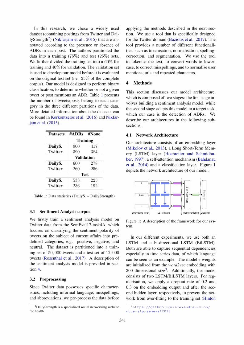
In this research, we chose a widely useddataset (containing postings from Twitter and Dai-lyStrength2) (Nikfarjam et al., 2015) that are an-notated according to the presence or absence ofADRs in each post. The authors partitioned thedata into a training (75%) and test (25%) sets.We further divided the training set into a 60% fortraining and 40% for validation. The validation setis used to develop our model before it is evaluatedon the original test set (i.e. 25% of the completecorpus). Our model is designed to perform binaryclassification, to determine whether or not a giventweet or post mentions an ADR. Table 1 presentsthe number of tweets/posts belong to each cate-gory in the three different partitions of the data.More detailed information about the datasets canbe found in Korkontzelos et al. (2016) and Nikfar-jam et al. (2015).
Datasets #ADRs #NoneTraining
DailyS. 900 417Twitter 390 384
ValidationDailyS. 600 278Twitter 260 256
TestDailyS. 533 225Twitter 236 192
Table 1: Data statistics (DailyS. = DailyStrength)
3.1 Sentiment Analysis corpus
We firstly train a sentiment analysis model onTwitter data from the SemEval17-task4A, whichfocuses on classifying the sentiment polarity oftweets on the subject of current affairs into pre-defined categories, e.g. positive, negative, andneutral. The dataset is partitioned into a train-ing set of 50, 000 tweets and a test set of 12, 000tweets (Rosenthal et al., 2017). A description ofthe sentiment analysis model is provided in sec-tion 4.
3.2 Preprocessing
Since Twitter data possesses specific character-istics, including informal language, misspellings,and abbreviations, we pre-process the data before
2DailyStrength is a specialised social networking websitefor health.
applying the methods described in the next sec-tion. We use a tool that is specifically designedfor the Twitter domain (Baziotis et al., 2017). Thetool provides a number of different functionali-ties, such as tokenisation, normalisation, spelling-correction, and segmentation. We use the toolto tokenise the text, to convert words to lower-case, to correct misspellings, and to normalise usermentions, urls and repeated-characters.
4 Methods
This section discusses our model architecture,which is composed of two stages: the first stage in-volves building a sentiment analysis model, whilethe second stage adapts this model to a target task,which our case is the detection of ADRs. Wedescribe our architectures in the following sub-sections.
4.1 Network Architecture
Our architecture consists of an embedding layer(Mikolov et al., 2013), a Long Short-Term Mem-ory (LSTM) layer (Hochreiter and Schmidhu-ber, 1997), a self-attention mechanism (Bahdanauet al., 2014) and a classification layer. Figure 1depicts the network architecture of our model.
Figure 1: A description of the framework for our sys-tem.
In our different experiments, we use both anLSTM and a bi-directional LSTM (BiLSTM).Both are able to capture sequential dependenciesespecially in time series data, of which languagecan be seen as an example. The model’s weightsare initialized from the word2vec embedding with300 dimensional size3. Additionally, the modelconsists of two LSTM/BiLSTM layers. For reg-ularisation, we apply a dropout rate of 0.2 and0.3 on the embedding output and after the sec-ond hidden layer, respectively, to prevent the net-work from over-fitting to the training set (Hinton
3https://github.com/alexandra-chron/ntua-slp-semeval2018
341
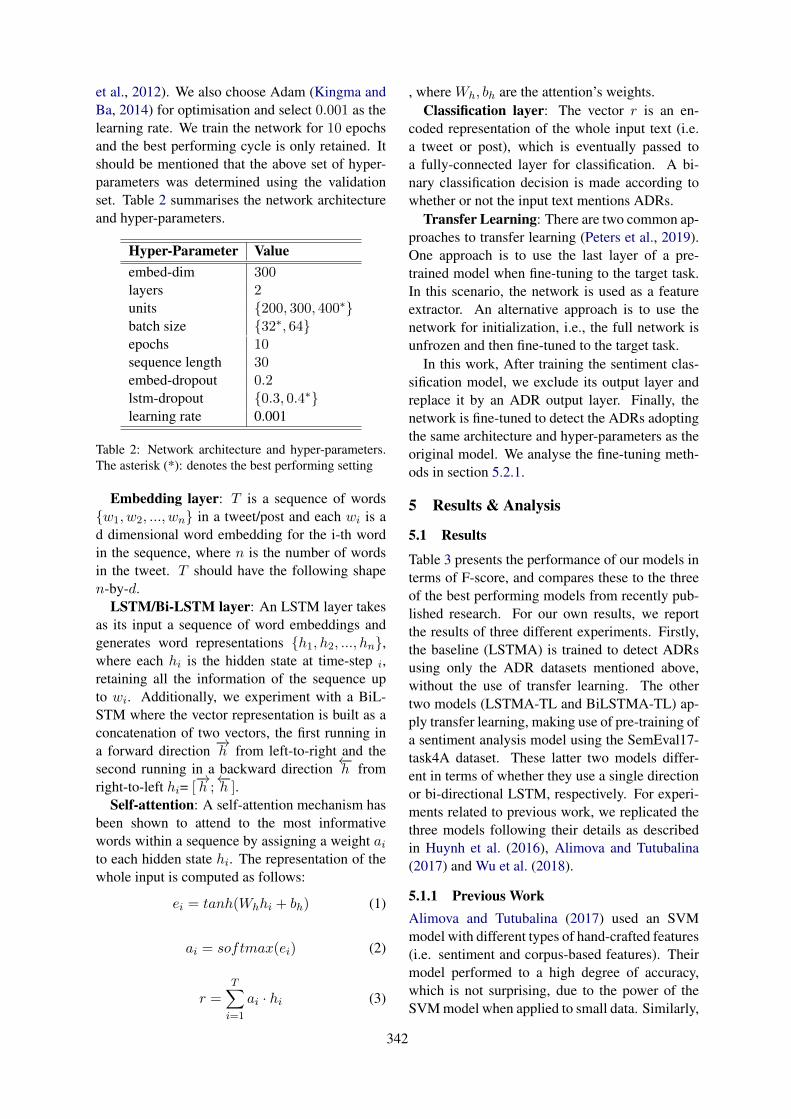
et al., 2012). We also choose Adam (Kingma andBa, 2014) for optimisation and select 0.001 as thelearning rate. We train the network for 10 epochsand the best performing cycle is only retained. Itshould be mentioned that the above set of hyper-parameters was determined using the validationset. Table 2 summarises the network architectureand hyper-parameters.
Hyper-Parameter Valueembed-dim 300layers 2units {200, 300, 400∗}batch size {32∗, 64}epochs 10sequence length 30embed-dropout 0.2lstm-dropout {0.3, 0.4∗}learning rate 0.001
Table 2: Network architecture and hyper-parameters.The asterisk (*): denotes the best performing setting
Embedding layer: T is a sequence of words{w1, w2, ..., wn} in a tweet/post and each wi is ad dimensional word embedding for the i-th wordin the sequence, where n is the number of wordsin the tweet. T should have the following shapen-by-d.
LSTM/Bi-LSTM layer: An LSTM layer takesas its input a sequence of word embeddings andgenerates word representations {h1, h2, ..., hn},where each hi is the hidden state at time-step i,retaining all the information of the sequence upto wi. Additionally, we experiment with a BiL-STM where the vector representation is built as aconcatenation of two vectors, the first running ina forward direction
−→h from left-to-right and the
second running in a backward direction←−h from
right-to-left hi= [−→h ;←−h ].
Self-attention: A self-attention mechanism hasbeen shown to attend to the most informativewords within a sequence by assigning a weight aito each hidden state hi. The representation of thewhole input is computed as follows:
ei = tanh(Whhi + bh) (1)
ai = softmax(ei) (2)
r =T∑
i=1
ai · hi (3)
, where Wh, bh are the attention’s weights.Classification layer: The vector r is an en-
coded representation of the whole input text (i.e.a tweet or post), which is eventually passed toa fully-connected layer for classification. A bi-nary classification decision is made according towhether or not the input text mentions ADRs.
Transfer Learning: There are two common ap-proaches to transfer learning (Peters et al., 2019).One approach is to use the last layer of a pre-trained model when fine-tuning to the target task.In this scenario, the network is used as a featureextractor. An alternative approach is to use thenetwork for initialization, i.e., the full network isunfrozen and then fine-tuned to the target task.
In this work, After training the sentiment clas-sification model, we exclude its output layer andreplace it by an ADR output layer. Finally, thenetwork is fine-tuned to detect the ADRs adoptingthe same architecture and hyper-parameters as theoriginal model. We analyse the fine-tuning meth-ods in section 5.2.1.
5 Results & Analysis
5.1 Results
Table 3 presents the performance of our models interms of F-score, and compares these to the threeof the best performing models from recently pub-lished research. For our own results, we reportthe results of three different experiments. Firstly,the baseline (LSTMA) is trained to detect ADRsusing only the ADR datasets mentioned above,without the use of transfer learning. The othertwo models (LSTMA-TL and BiLSTMA-TL) ap-ply transfer learning, making use of pre-training ofa sentiment analysis model using the SemEval17-task4A dataset. These latter two models differ-ent in terms of whether they use a single directionor bi-directional LSTM, respectively. For experi-ments related to previous work, we replicated thethree models following their details as describedin Huynh et al. (2016), Alimova and Tutubalina(2017) and Wu et al. (2018).
5.1.1 Previous WorkAlimova and Tutubalina (2017) used an SVMmodel with different types of hand-crafted features(i.e. sentiment and corpus-based features). Theirmodel performed to a high degree of accuracy,which is not surprising, due to the power of theSVM model when applied to small data. Similarly,
342
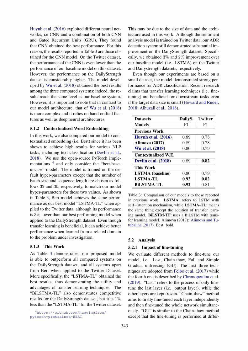
Huynh et al. (2016) exploited different neural net-works, i.e CNN and a combination of both CNNand Gated Recurrent Units (GRU). They foundthat CNN obtained the best performance. For thisreason, the results reported in Table 3 are those ob-tained for the CNN model. On the Twitter dataset,the performance of the CNN is even lower than theperformance of our baseline model on this dataset.However, the performance on the DailyStrengthdataset is considerably higher. The model devel-oped by Wu et al. (2018) obtained the best resultsamong the three compared systems; indeed, the re-sults reach the same level as our baseline system.However, it is important to note that in contrast toour model architecture, that of Wu et al. (2018)is more complex and it relies on hand-crafted fea-tures as well as deep neural architectures.
5.1.2 Contextualised Word EmbeddingIn this work, we also compared our model to con-textualized embedding (i.e. Bert) since it has beenshown to achieve high results for various NLPtasks, including text classification (Devlin et al.,2018). We use the open-source PyTorch imple-mentations 4 and only consider the “bert-base-uncase” model. The model is trained on the de-fault hyper-parameters except that the number ofbatch-size and sequence length are chosen as fol-lows 32 and 30, respectively, to match our modelhyper-parameters for these two values. As shownin Table 3, Bert model achieves the same perfor-mance as our best model “LSTMA-TL” when ap-plied to the Twitter data, although its performanceis 3% lower than our best performing model whenapplied to the DailyStrength dataset. Even thoughtransfer learning is beneficial, it can achieve betterperformance when learned from a related domainto the problem under investigation.
5.1.3 This WorkAs Table 3 demonstrates, our proposed modelis able to outperform all compared systems onthe DailyStrength dataset, and all systems apartfrom Bert when applied to the Twitter Dataset.More specifically, the “LSTMA-TL” obtained thebest results, thus demonstrating the utility andadvantages of transfer learning techniques. The“BiLSTMA-TL” also demonstrates competitiveresults for the DailyStrength dataset, but it is 1%less than the “LSTMA-TL” for the Twitter dataset.
4https://github.com/huggingface/pytorch-pretrained-BERT
This may be due to the size of data and the archi-tecture used in this work. Although the sentimentanalysis model is trained on Twitter data, our ADRdetection system still demonstrated substantial im-provement on the DailyStrength dataset. Specifi-cally, we obtained 3% and 2% improvement overour baseline model (i.e. LSTMA) on the Twitterand Dailystrength datasets, respectively.
Even though our experiments are based on asmall dataset, the model demonstrated strong per-formance for ADR classification. Recent researchclaims that transfer learning techniques (i.e. fine-tuning) are beneficial for downstream tasks evenif the target data size is small (Howard and Ruder,2018; Alhuzali et al., 2018).
Datasets DailyS. TwitterModels F1 F1Previous WorkHuynh et al. (2016) 0.89 0.75Alimova (2017) 0.89 0.78Wu et al. (2018) 0.90 0.79
Contextualized W.E.Devlin et al. (2018) 0.89 0.82This WorkLSTMA (baseline) 0.90 0.79LSTMA-TL 0.92 0.82BiLSTMA-TL 0.92 0.81
Table 3: Comparison of our models to those reportedin previous work. LSTMA: refers to LSTM withself−attention mechanism, while LSTMA-TL: meansthe same thing except the addition of transfer learn-ing model. BiLSTM-TF: uses a BiLSTM with trans-fer learning model. Alimova (2017): Alimova and Tu-tubalina (2017). Best: bold.
5.2 Analysis5.2.1 Impact of fine-tuningWe evaluate different methods to fine-tune ourmodel, i.e. Last, Chain-thaw, Full and SimpleGradual unfreezing (GU). The first three tech-niques are adopted from Felbo et al. (2017) whilethe fourth one is described by Chronopoulou et al.(2019). “Last” refers to the process of only fine-tune the last layer (i.e. output layer), while theother layers are kept frozen. “Chain-thaw” methodaims to firstly fine-tuned each layer independentlyand then fine-tuned the whole network simultane-ously. “GU” is similar to the Chain-thaw methodexcept that the fine-tuning is performed at differ-
343
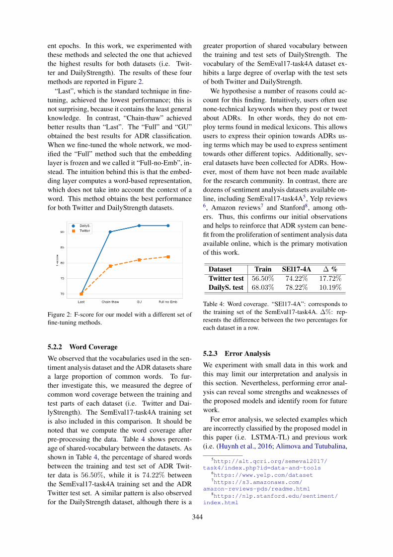
ent epochs. In this work, we experimented withthese methods and selected the one that achievedthe highest results for both datasets (i.e. Twit-ter and DailyStrength). The results of these fourmethods are reported in Figure 2.
“Last”, which is the standard technique in fine-tuning, achieved the lowest performance; this isnot surprising, because it contains the least generalknowledge. In contrast, “Chain-thaw” achievedbetter results than “Last”. The “Full” and “GU”obtained the best results for ADR classification.When we fine-tuned the whole network, we mod-ified the “Full” method such that the embeddinglayer is frozen and we called it “Full-no-Emb”, in-stead. The intuition behind this is that the embed-ding layer computes a word-based representation,which does not take into account the context of aword. This method obtains the best performancefor both Twitter and DailyStrength datasets.
Figure 2: F-score for our model with a different set offine-tuning methods.
5.2.2 Word CoverageWe observed that the vocabularies used in the sen-timent analysis dataset and the ADR datasets sharea large proportion of common words. To fur-ther investigate this, we measured the degree ofcommon word coverage between the training andtest parts of each dataset (i.e. Twitter and Dai-lyStrength). The SemEval17-task4A training setis also included in this comparison. It should benoted that we compute the word coverage afterpre-processing the data. Table 4 shows percent-age of shared-vocabulary between the datasets. Asshown in Table 4, the percentage of shared wordsbetween the training and test set of ADR Twit-ter data is 56.50%, while it is 74.22% betweenthe SemEval17-task4A training set and the ADRTwitter test set. A similar pattern is also observedfor the DailyStrength dataset, although there is a
greater proportion of shared vocabulary betweenthe training and test sets of DailyStrength. Thevocabulary of the SemEval17-task4A dataset ex-hibits a large degree of overlap with the test setsof both Twitter and DailyStrength.
We hypothesise a number of reasons could ac-count for this finding. Intuitively, users often usenone-technical keywords when they post or tweetabout ADRs. In other words, they do not em-ploy terms found in medical lexicons. This allowsusers to express their opinion towards ADRs us-ing terms which may be used to express sentimenttowards other different topics. Additionally, sev-eral datasets have been collected for ADRs. How-ever, most of them have not been made availablefor the research community. In contrast, there aredozens of sentiment analysis datasets available on-line, including SemEval17-task4A5, Yelp reviews6, Amazon reviews7 and Stanford8, among oth-ers. Thus, this confirms our initial observationsand helps to reinforce that ADR system can bene-fit from the proliferation of sentiment analysis dataavailable online, which is the primary motivationof this work.
Dataset Train SEl17-4A ∆ %Twitter test 56.50% 74.22% 17.72%DailyS. test 68.03% 78.22% 10.19%
Table 4: Word coverage. “SEl17-4A”: corresponds tothe training set of the SemEval17-task4A. ∆%: rep-resents the difference between the two percentages foreach dataset in a row.
5.2.3 Error AnalysisWe experiment with small data in this work andthis may limit our interpretation and analysis inthis section. Nevertheless, performing error anal-ysis can reveal some strengths and weaknesses ofthe proposed models and identify room for futurework.
For error analysis, we selected examples whichare incorrectly classified by the proposed model inthis paper (i.e. LSTMA-TL) and previous work(i.e. (Huynh et al., 2016; Alimova and Tutubalina,
5http://alt.qcri.org/semeval2017/task4/index.php?id=data-and-tools
6https://www.yelp.com/dataset7https://s3.amazonaws.com/
amazon-reviews-pds/readme.html8https://nlp.stanford.edu/sentiment/
index.html
344
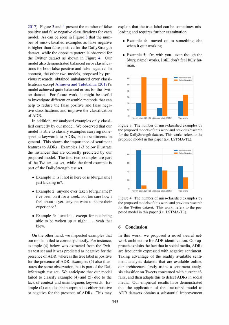
2017). Figure 3 and 4 present the number of falsepositive and false negative classifications for eachmodel. As can be seen in Figure 3 that the num-ber of miss-classified examples as false negativeis higher than false positive for the DailyStrengthdataset, while the opposite pattern is observed forthe Twitter dataset as shown in Figure 4. Ourmodel also demonstrated balanced error classifica-tions for both false positive and false negative. Incontrast, the other two models, proposed by pre-vious research, obtained unbalanced error classi-fications except Alimova and Tutubalina (2017)’smodel achieved quite balanced errors for the Twit-ter dataset. For future work, it might be usefulto investigate different ensemble methods that canhelp to reduce the false positive and false nega-tive classifications and improve the classificationof ADR.
In addition, we analysed examples only classi-fied correctly by our model. We observed that ourmodel is able to classify examples carrying none-specific keywords to ADRs, but to sentiments ingeneral. This shows the importance of sentimentfeatures to ADRs. Examples 1-3 below illustratethe instances that are correctly predicted by ourproposed model. The first two examples are partof the Twitter test set, while the third example ispart of the DailyStrength test set.
• Example 1: is it hot in here or is [durg name]just kicking in?.
• Example 2: anyone ever taken [durg name]?i’ve been on it for a week, not too sure how ifeel about it yet. anyone want to share theirexperience?.
• Example 3: loved it , except for not beingable to be woken up at night . . yeah thatblew.
On the other hand, we inspected examples thatour model failed to correctly classify. For instance,example (4) below was extracted from the Twit-ter test set and it was predicted as negative for thepresence of ADR, whereas the true label is positivefor the presence of ADR. Examples (5) also illus-trates the same observation, but is part of the Dai-lyStrength test set. We anticipate that our modelfailed to classify example (4) and (5) due to thelack of context and unambiguous keywords. Ex-ample (4) can also be interpreted as either positiveor negative for the presence of ADRs. This may
explain that the true label can be sometimes mis-leading and requires further examination.
• Example 4: moved on to something elsewhen it quit working.
• Example 5: i’m with you. even though the[durg name] works, i still don’t feel fully hu-man.
Figure 3: The number of miss-classified examples bythe proposed models of this work and previous researchfor the DailyStrength dataset. This work: refers to theproposed model in this paper (i.e. LSTMA-TL).
Figure 4: The number of miss-classified examples bythe proposed models of this work and previous researchfor the Twitter dataset. This work: refers to the pro-posed model in this paper (i.e. LSTMA-TL).
6 Conclusion
In this work, we proposed a novel neural net-work architecture for ADR identification. Our ap-proach exploits the fact that in social media, ADRsare frequently expressed with negative sentiment.Taking advantage of the readily available senti-ment analysis datasets that are available online,our architecture firstly trains a sentiment analy-sis classifier on Tweets concerned with current af-fairs, and then adapts this to detect ADRs in socialmedia. Our empirical results have demonstratedthat the application of the fine-tuned model toADR datasets obtains a substantial improvement
345
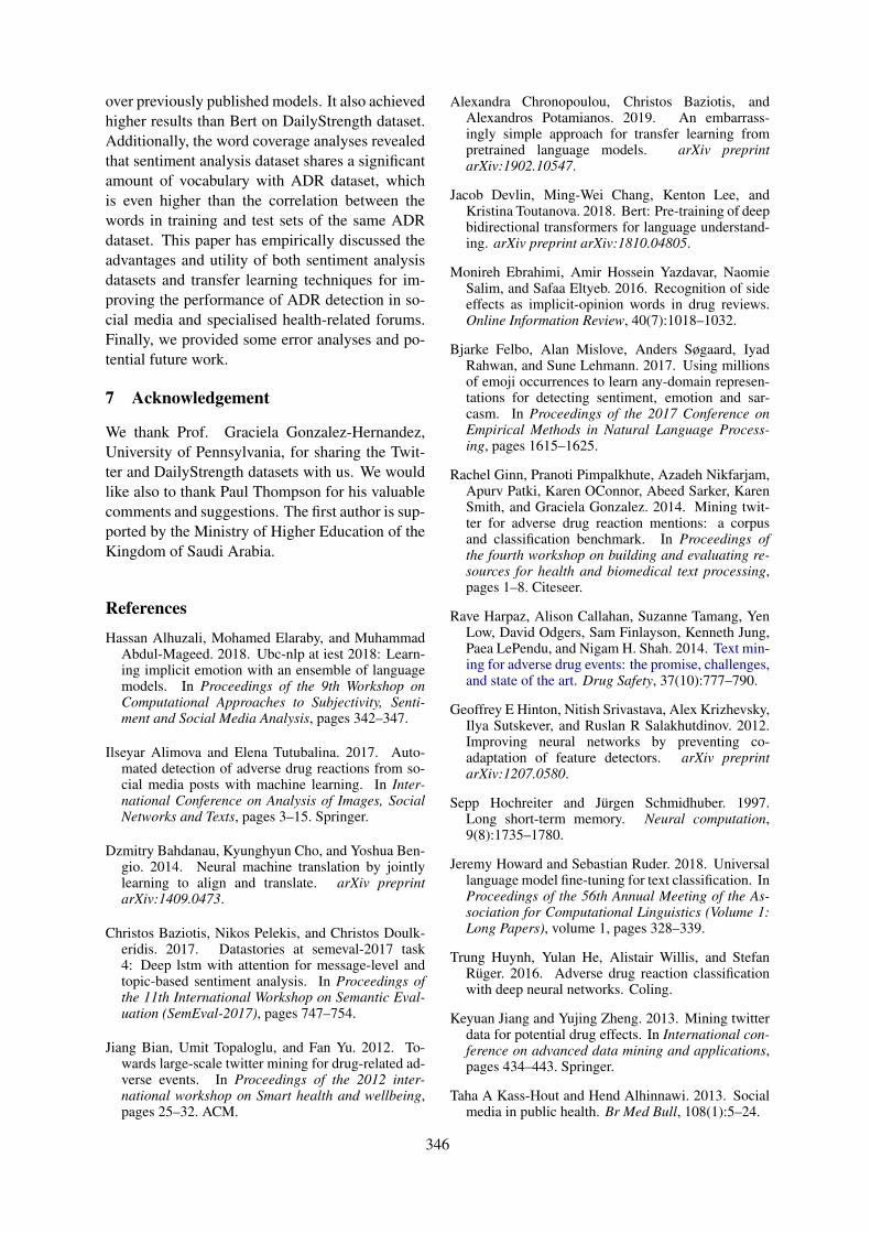
over previously published models. It also achievedhigher results than Bert on DailyStrength dataset.Additionally, the word coverage analyses revealedthat sentiment analysis dataset shares a significantamount of vocabulary with ADR dataset, whichis even higher than the correlation between thewords in training and test sets of the same ADRdataset. This paper has empirically discussed theadvantages and utility of both sentiment analysisdatasets and transfer learning techniques for im-proving the performance of ADR detection in so-cial media and specialised health-related forums.Finally, we provided some error analyses and po-tential future work.
7 Acknowledgement
We thank Prof. Graciela Gonzalez-Hernandez,University of Pennsylvania, for sharing the Twit-ter and DailyStrength datasets with us. We wouldlike also to thank Paul Thompson for his valuablecomments and suggestions. The first author is sup-ported by the Ministry of Higher Education of theKingdom of Saudi Arabia.
References
Hassan Alhuzali, Mohamed Elaraby, and MuhammadAbdul-Mageed. 2018. Ubc-nlp at iest 2018: Learn-ing implicit emotion with an ensemble of languagemodels. In Proceedings of the 9th Workshop onComputational Approaches to Subjectivity, Senti-ment and Social Media Analysis, pages 342–347.
Ilseyar Alimova and Elena Tutubalina. 2017. Auto-mated detection of adverse drug reactions from so-cial media posts with machine learning. In Inter-national Conference on Analysis of Images, SocialNetworks and Texts, pages 3–15. Springer.
Dzmitry Bahdanau, Kyunghyun Cho, and Yoshua Ben-gio. 2014. Neural machine translation by jointlylearning to align and translate. arXiv preprintarXiv:1409.0473.
Christos Baziotis, Nikos Pelekis, and Christos Doulk-eridis. 2017. Datastories at semeval-2017 task4: Deep lstm with attention for message-level andtopic-based sentiment analysis. In Proceedings ofthe 11th International Workshop on Semantic Eval-uation (SemEval-2017), pages 747–754.
Jiang Bian, Umit Topaloglu, and Fan Yu. 2012. To-wards large-scale twitter mining for drug-related ad-verse events. In Proceedings of the 2012 inter-national workshop on Smart health and wellbeing,pages 25–32. ACM.
Alexandra Chronopoulou, Christos Baziotis, andAlexandros Potamianos. 2019. An embarrass-ingly simple approach for transfer learning frompretrained language models. arXiv preprintarXiv:1902.10547.
Jacob Devlin, Ming-Wei Chang, Kenton Lee, andKristina Toutanova. 2018. Bert: Pre-training of deepbidirectional transformers for language understand-ing. arXiv preprint arXiv:1810.04805.
Monireh Ebrahimi, Amir Hossein Yazdavar, NaomieSalim, and Safaa Eltyeb. 2016. Recognition of sideeffects as implicit-opinion words in drug reviews.Online Information Review, 40(7):1018–1032.
Bjarke Felbo, Alan Mislove, Anders Søgaard, IyadRahwan, and Sune Lehmann. 2017. Using millionsof emoji occurrences to learn any-domain represen-tations for detecting sentiment, emotion and sar-casm. In Proceedings of the 2017 Conference onEmpirical Methods in Natural Language Process-ing, pages 1615–1625.
Rachel Ginn, Pranoti Pimpalkhute, Azadeh Nikfarjam,Apurv Patki, Karen OConnor, Abeed Sarker, KarenSmith, and Graciela Gonzalez. 2014. Mining twit-ter for adverse drug reaction mentions: a corpusand classification benchmark. In Proceedings ofthe fourth workshop on building and evaluating re-sources for health and biomedical text processing,pages 1–8. Citeseer.
Rave Harpaz, Alison Callahan, Suzanne Tamang, YenLow, David Odgers, Sam Finlayson, Kenneth Jung,Paea LePendu, and Nigam H. Shah. 2014. Text min-ing for adverse drug events: the promise, challenges,and state of the art. Drug Safety, 37(10):777–790.
Geoffrey E Hinton, Nitish Srivastava, Alex Krizhevsky,Ilya Sutskever, and Ruslan R Salakhutdinov. 2012.Improving neural networks by preventing co-adaptation of feature detectors. arXiv preprintarXiv:1207.0580.
Sepp Hochreiter and Jürgen Schmidhuber. 1997.Long short-term memory. Neural computation,9(8):1735–1780.
Jeremy Howard and Sebastian Ruder. 2018. Universallanguage model fine-tuning for text classification. InProceedings of the 56th Annual Meeting of the As-sociation for Computational Linguistics (Volume 1:Long Papers), volume 1, pages 328–339.
Trung Huynh, Yulan He, Alistair Willis, and StefanRüger. 2016. Adverse drug reaction classificationwith deep neural networks. Coling.
Keyuan Jiang and Yujing Zheng. 2013. Mining twitterdata for potential drug effects. In International con-ference on advanced data mining and applications,pages 434–443. Springer.
Taha A Kass-Hout and Hend Alhinnawi. 2013. Socialmedia in public health. Br Med Bull, 108(1):5–24.
346
Diederik P Kingma and Jimmy Ba. 2014. Adam: Amethod for stochastic optimization. arXiv preprintarXiv:1412.6980.
Svetlana Kiritchenko, Saif M Mohammad, JasonMorin, and Berry de Bruijn. 2017. Nrc-canada atsmm4h shared task: classifying tweets mentioningadverse drug reactions and medication intake. arXivpreprint arXiv:1805.04558.
Ioannis Korkontzelos, Azadeh Nikfarjam, MatthewShardlow, Abeed Sarker, Sophia Ananiadou, andGraciela H Gonzalez. 2016. Analysis of the effectof sentiment analysis on extracting adverse drug re-actions from tweets and forum posts. Journal ofbiomedical informatics, 62:148–158.
Xiao Liu and Hsinchun Chen. 2015. A research frame-work for pharmacovigilance in health social media:identification and evaluation of patient adverse drugevent reports. Journal of biomedical informatics,58:268–279.
Tomas Mikolov, Ilya Sutskever, Kai Chen, Greg S Cor-rado, and Jeff Dean. 2013. Distributed representa-tions of words and phrases and their compositional-ity. In Advances in neural information processingsystems, pages 3111–3119.
Azadeh Nikfarjam, Abeed Sarker, Karen Oconnor,Rachel Ginn, and Graciela Gonzalez. 2015. Phar-macovigilance from social media: mining adversedrug reaction mentions using sequence labelingwith word embedding cluster features. Journalof the American Medical Informatics Association,22(3):671–681.
Matthew Peters, Sebastian Ruder, and Noah A. Smith.2019. To tune or not to tune? adapting pre-trained representations to diverse tasks. CoRR,abs/1903.05987.
Sara Rosenthal, Noura Farra, and Preslav Nakov.2017. Semeval-2017 task 4: Sentiment analysis intwitter. In Proceedings of the 11th InternationalWorkshop on Semantic Evaluation (SemEval-2017),pages 502–518.
Hariprasad Sampathkumar, Xue-wen Chen, andBo Luo. 2014. Mining adverse drug reactionsfrom online healthcare forums using hidden markovmodel. BMC medical informatics and decision mak-ing, 14(1):91.
Abeed Sarker and Graciela Gonzalez. 2015. Portableautomatic text classification for adverse drug reac-tion detection via multi-corpus training. Journal ofbiomedical informatics, 53:196–207.
Richard Sloane, Orod Osanlou, David Lewis,Danushka Bollegala, Simon Maskell, and MunirPirmohamed. 2015. Social media and pharma-covigilance: a review of the opportunities andchallenges. British journal of clinical pharmacol-ogy, 80(4):910–920.
Paul Thompson, Sophia Daikou, Kenju Ueno, RizaBatista-Navarro, Junichi Tsujii, and Sophia Ana-niadou. 2018. Annotation and detection of drugeffects in text for pharmacovigilance. Journal ofcheminformatics, 10(1):37.
C. Wang, H. Dai, F. Wang, and E. C. Su. 2018. Ad-verse drug reaction post classification with imbal-anced classification techniques. In 2018 Conferenceon Technologies and Applications of Artificial Intel-ligence (TAAI), pages 5–9.
Chuhan Wu, Fangzhao Wu, Junxin Liu, Sixing Wu,Yongfeng Huang, and Xing Xie. 2018. Detect-ing tweets mentioning drug name and adverse drugreaction with hierarchical tweet representation andmulti-head self-attention. In Proceedings of the2018 EMNLP Workshop SMM4H: The 3rd SocialMedia Mining for Health Applications Workshopand Shared Task, pages 34–37.
Christopher C Yang, Haodong Yang, Ling Jiang, andMi Zhang. 2012. Social media mining for drugsafety signal detection. In Proceedings of the 2012international workshop on Smart health and wellbe-ing, pages 33–40. ACM.
Andrew Yates and Nazli Goharian. 2013. Adrtrace: de-tecting expected and unexpected adverse drug reac-tions from user reviews on social media sites. In Eu-ropean Conference on Information Retrieval, pages816–819. Springer.
347
Proceedings of the BioNLP 2019 workshop, pages 348–358Florence, Italy, August 1, 2019. c©2019 Association for Computational Linguistics
Exploring Diachronic Changes of Biomedical Knowledge usingDistributed Concept Representations
Gaurav Vashisth1,2, Jan-Niklas Voigt-Antons1,2, Michael Mikhailov1 and Roland Roller11German Research Center for Artificial Intelligence (DFKI), Berlin, Germany
2Technische Universität [email protected]
AbstractIn research best practices can change over timeas new discoveries are made and novel meth-ods are implemented. Scientific publicationsreporting about the latest facts and currentstate-of-the-art can be possibly outdated aftersome years or even proved to be false. A pub-lication usually sheds light only on the knowl-edge of the period it has been published. Thus,the aspect of time can play an essential rolein the reliability of the presented information.In Natural Language Processing many meth-ods focus on information extraction from text,such as detecting entities and their relationshipto each other. Those methods mostly focus onthe facts presented in the text itself and not onthe aspects of knowledge which changes overtime.
This work instead examines the evolution inbiomedical knowledge over time using scien-tific literature in terms of diachronic change.Mainly the usage of temporal and distribu-tional concept representations are exploredand evaluated by a proof-of-concept.
1 Introduction
Scientific literature presents knowledge for a par-ticular time period it has been published. Vari-ous studies have been performed to explore suchknowledge from scientific literature, where workby Swanson (1986) led to the discovery of a newdrug to treat Raynaud’s disease. Similarly, a studyby Zhu et al. (2013) has concluded that drug dis-covery using scientific literature plays a pivotalrole in the treatment of cancer, which can im-prove the quality of life of patients (Cummingset al., 2011). Although scientific literature is anexcellent source of information, there has beenan explosion in the number of publications eachyear. This poses a challenge for biomedical re-searchers and practitioners to keep themselves in-formed of recent developments. The increasing
number at the same time provides an opportunityto automatically explore the data on how a changein knowledge has evolved. Some studies havetried to explore such changed knowledge by inves-tigating temporal information (Zhou and Hripc-sak, 2007; He and Chen, 2018), studying the di-achronic change in the meaning of the word. Adiachronic semantic change in language is associ-ated with progression in the meaning of the wordwhich is estimated by exploring its usage overtime.
This work aims to automatically explore theadvances in medical knowledge extracted fromthe abstracts of scientific research by usingword/concept embeddings. Especially, we ex-amine how treatments of pathological conditionshave changed over time. For this reason we fo-cus on concepts rather than words, as biomedi-cal concepts can be mentioned in text in differentways (e.g. ‘headache’, ‘cephalgia’ or ‘pain in thehead’). Moreover, biomedical concepts help to en-capsulate noun phrases represented by more thanone word, for example, ‘eye lens’ or ‘lung cancer’.An analysis on word level instead would take allsituations the single words occur into account, andtherefore would be more general. To quantify suchchanges we measure how the usage of a biomedi-cal concept has (semantically) changed over timeby comparing different embedding periods.
The rest of the work is structured as follows:The next section presents related work in thecontext of diachronic changes in and outside thebiomedical domain. Then, in Section 3 we presenthow the biomedical concept embeddings are gen-erated and how the time aspect is taken into ac-count. Section 4 shows the usage of our embed-dings to explore diachronic changes as a proof-of-concept. Then we apply the temporal embed-dings to explore some exemplary relational dataof UMLS, followed by a conclusion.
348
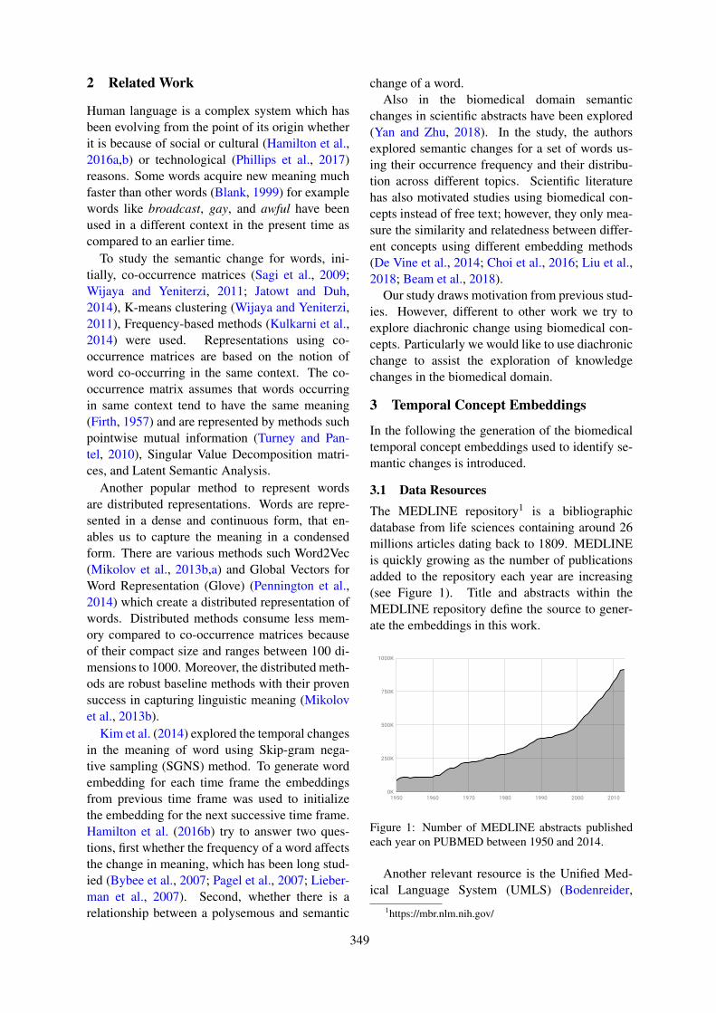
2 Related Work
Human language is a complex system which hasbeen evolving from the point of its origin whetherit is because of social or cultural (Hamilton et al.,2016a,b) or technological (Phillips et al., 2017)reasons. Some words acquire new meaning muchfaster than other words (Blank, 1999) for examplewords like broadcast, gay, and awful have beenused in a different context in the present time ascompared to an earlier time.
To study the semantic change for words, ini-tially, co-occurrence matrices (Sagi et al., 2009;Wijaya and Yeniterzi, 2011; Jatowt and Duh,2014), K-means clustering (Wijaya and Yeniterzi,2011), Frequency-based methods (Kulkarni et al.,2014) were used. Representations using co-occurrence matrices are based on the notion ofword co-occurring in the same context. The co-occurrence matrix assumes that words occurringin same context tend to have the same meaning(Firth, 1957) and are represented by methods suchpointwise mutual information (Turney and Pan-tel, 2010), Singular Value Decomposition matri-ces, and Latent Semantic Analysis.
Another popular method to represent wordsare distributed representations. Words are repre-sented in a dense and continuous form, that en-ables us to capture the meaning in a condensedform. There are various methods such Word2Vec(Mikolov et al., 2013b,a) and Global Vectors forWord Representation (Glove) (Pennington et al.,2014) which create a distributed representation ofwords. Distributed methods consume less mem-ory compared to co-occurrence matrices becauseof their compact size and ranges between 100 di-mensions to 1000. Moreover, the distributed meth-ods are robust baseline methods with their provensuccess in capturing linguistic meaning (Mikolovet al., 2013b).
Kim et al. (2014) explored the temporal changesin the meaning of word using Skip-gram nega-tive sampling (SGNS) method. To generate wordembedding for each time frame the embeddingsfrom previous time frame was used to initializethe embedding for the next successive time frame.Hamilton et al. (2016b) try to answer two ques-tions, first whether the frequency of a word affectsthe change in meaning, which has been long stud-ied (Bybee et al., 2007; Pagel et al., 2007; Lieber-man et al., 2007). Second, whether there is arelationship between a polysemous and semantic
change of a word.Also in the biomedical domain semantic
changes in scientific abstracts have been explored(Yan and Zhu, 2018). In the study, the authorsexplored semantic changes for a set of words us-ing their occurrence frequency and their distribu-tion across different topics. Scientific literaturehas also motivated studies using biomedical con-cepts instead of free text; however, they only mea-sure the similarity and relatedness between differ-ent concepts using different embedding methods(De Vine et al., 2014; Choi et al., 2016; Liu et al.,2018; Beam et al., 2018).
Our study draws motivation from previous stud-ies. However, different to other work we try toexplore diachronic change using biomedical con-cepts. Particularly we would like to use diachronicchange to assist the exploration of knowledgechanges in the biomedical domain.
3 Temporal Concept Embeddings
In the following the generation of the biomedicaltemporal concept embeddings used to identify se-mantic changes is introduced.
3.1 Data ResourcesThe MEDLINE repository1 is a bibliographicdatabase from life sciences containing around 26millions articles dating back to 1809. MEDLINEis quickly growing as the number of publicationsadded to the repository each year are increasing(see Figure 1). Title and abstracts within theMEDLINE repository define the source to gener-ate the embeddings in this work.
Figure 1: Number of MEDLINE abstracts publishedeach year on PUBMED between 1950 and 2014.
Another relevant resource is the Unified Med-ical Language System (UMLS) (Bodenreider,
1https://mbr.nlm.nih.gov/
349
2004), a biomedical knowledge base which de-fines a large number of biomedical concepts andtheir relations to each other. Each concept is rep-resented by a unique concept identifier known asCUI and includes word variations and synonyms.As we focus on the generation of concept em-beddings, we normalize text mentions from MED-LINE abstracts to UMLS.
The concept normalization is carried out usingMetaMap (Aronson, 2001), a popular named en-tity recognition system for biomedical text. How-ever, to avoid processing millions of sentenceswith MetaMap, we use the MetaMapped 2015MEDLINE Baseline Results, a MEDLINE sub-set already enriched by MetaMap Machine Out-put (MMO). In addition to that, we also use an-nual baseline files from the MEDLINE/PUBMEDBaseline Repository (MBR) which contain meta-information about each publication such as publi-cation ID, publication year and author name(s).
3.2 Data Preprocessing
First, publications from MMO are enriched withpublication year (PubYear) by using the publica-tion ID and the information from the MBR files.Then, the text occurrence of each medical abstractand its title are mapped and replaced with theirconcept ID, using the offset information providedin MMO (Figure 2). In this way, we create a textto train our embeddings. Since we do not considercharacter embeddings, we can treat concept IDs aswords without any disadvantage.
Figure 2: Shows mapping of medical text to their cor-responding concept ID for Publication ID:20895112.
To create temporal embeddings, the prepro-cessed MEDLINE abstracts are split into differ-ent time depended subsets using PubYear. Em-beddings are then trained on those splits. Ide-ally, we would like to train models using equallysized time ranges, such as embeddings per year ordecade. However, this is not easily possible forvarious reasons: Firstly, as seen in Figure 1 thenumber of publications is constantly increasing.A consistent split into equal time frames wouldresult in highly unbalanced splits regarding the
number of included abstracts. In addition to thatPUBMED includes mainly titles and no abstractsbefore 1975, which further reduces the number oftext for the lower represented period.
Period # Publications
1809-1970 3,374,0991971-1975 1,162,0301976-1980 1,346,8331981-1985 1,528,4751986-1990 1,863,6591991-1995 2,065,3861996-2000 2,297,0062001-2005 2,938,8552006-2010 3,721,1662011-2012 1,762,6032013-2015 1,283,218
Table 1: Distribution of publications in each period
Conversely, the generation of equallysized splits (according to the number of ab-stracts/sentences) has the disadvantage that itwill be more challenging to differentiate betweenparticular years. Rounding up or down thenumber of included publications might also benot a satisfying solution, as the time rangesmight differ too much. For this reason, wemainly focus on time range splits including 5years of MEDLINE abstracts. As the number ofpublications is lower at the beginning of the 20thcentury and publications often do not containany abstract, we combine the ‘early’ MEDLINEdata into one big split (1809-1970). Moreover, asthe number of publications steadily increase wecreate smaller splits from 2011. The final splitinto periods is presented in Table 1, includingtheir corresponding number of abstracts.
3.3 Temporal Embeddings
To generate temporal embeddings, we use Fast-Text (Bojanowski et al., 2016) in Skip-gram nega-tive sampling (SGNS) mode, which predicts con-text words corresponding to a given target wordoccurring in its neighborhood. The values of thehyperparameters base on the recommendation ofLevy et al. (2015). The authors did an extensiveset of experiments using different representationmethods and analyzed the effect of hyperparam-eters on the embeddings generated by them. Wechose negative samples as 10, the minimum occur-
350
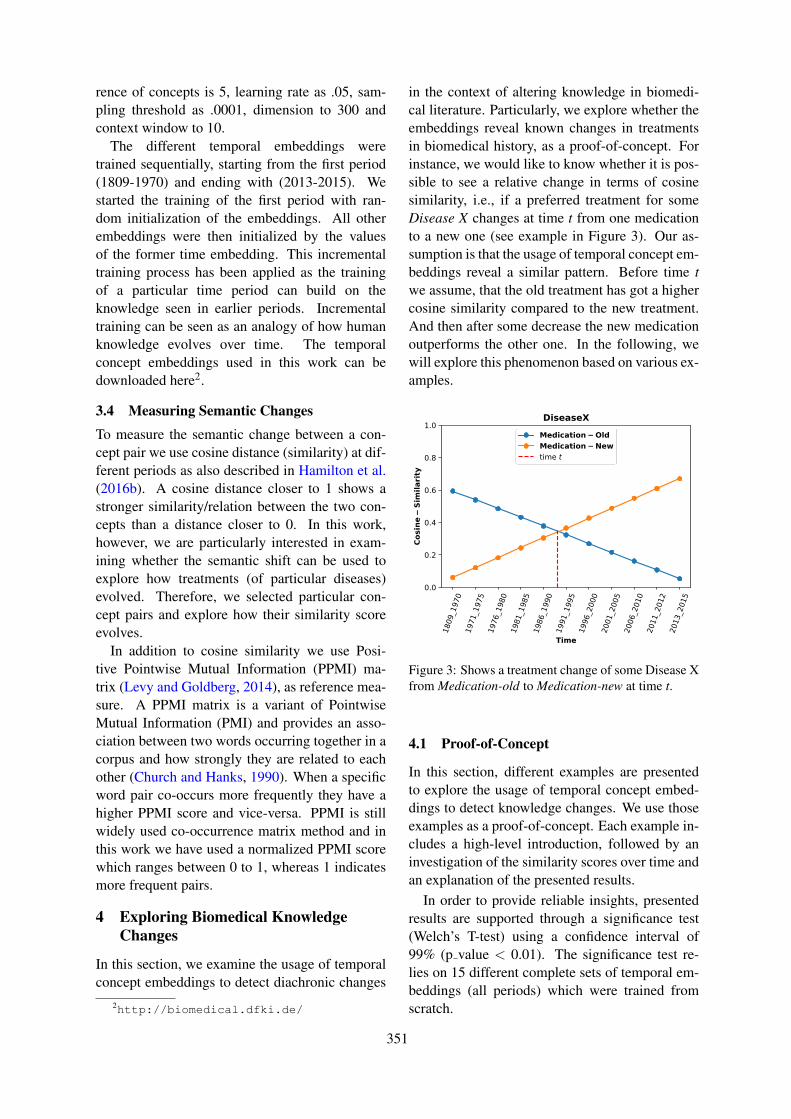
rence of concepts is 5, learning rate as .05, sam-pling threshold as .0001, dimension to 300 andcontext window to 10.
The different temporal embeddings weretrained sequentially, starting from the first period(1809-1970) and ending with (2013-2015). Westarted the training of the first period with ran-dom initialization of the embeddings. All otherembeddings were then initialized by the valuesof the former time embedding. This incrementaltraining process has been applied as the trainingof a particular time period can build on theknowledge seen in earlier periods. Incrementaltraining can be seen as an analogy of how humanknowledge evolves over time. The temporalconcept embeddings used in this work can bedownloaded here2.
3.4 Measuring Semantic Changes
To measure the semantic change between a con-cept pair we use cosine distance (similarity) at dif-ferent periods as also described in Hamilton et al.(2016b). A cosine distance closer to 1 shows astronger similarity/relation between the two con-cepts than a distance closer to 0. In this work,however, we are particularly interested in exam-ining whether the semantic shift can be used toexplore how treatments (of particular diseases)evolved. Therefore, we selected particular con-cept pairs and explore how their similarity scoreevolves.
In addition to cosine similarity we use Posi-tive Pointwise Mutual Information (PPMI) ma-trix (Levy and Goldberg, 2014), as reference mea-sure. A PPMI matrix is a variant of PointwiseMutual Information (PMI) and provides an asso-ciation between two words occurring together in acorpus and how strongly they are related to eachother (Church and Hanks, 1990). When a specificword pair co-occurs more frequently they have ahigher PPMI score and vice-versa. PPMI is stillwidely used co-occurrence matrix method and inthis work we have used a normalized PPMI scorewhich ranges between 0 to 1, whereas 1 indicatesmore frequent pairs.
4 Exploring Biomedical KnowledgeChanges
In this section, we examine the usage of temporalconcept embeddings to detect diachronic changes
2http://biomedical.dfki.de/
in the context of altering knowledge in biomedi-cal literature. Particularly, we explore whether theembeddings reveal known changes in treatmentsin biomedical history, as a proof-of-concept. Forinstance, we would like to know whether it is pos-sible to see a relative change in terms of cosinesimilarity, i.e., if a preferred treatment for someDisease X changes at time t from one medicationto a new one (see example in Figure 3). Our as-sumption is that the usage of temporal concept em-beddings reveal a similar pattern. Before time twe assume, that the old treatment has got a highercosine similarity compared to the new treatment.And then after some decrease the new medicationoutperforms the other one. In the following, wewill explore this phenomenon based on various ex-amples.
Figure 3: Shows a treatment change of some Disease Xfrom Medication-old to Medication-new at time t.
4.1 Proof-of-Concept
In this section, different examples are presentedto explore the usage of temporal concept embed-dings to detect knowledge changes. We use thoseexamples as a proof-of-concept. Each example in-cludes a high-level introduction, followed by aninvestigation of the similarity scores over time andan explanation of the presented results.
In order to provide reliable insights, presentedresults are supported through a significance test(Welch’s T-test) using a confidence interval of99% (p value < 0.01). The significance test re-lies on 15 different complete sets of temporal em-beddings (all periods) which were trained fromscratch.
351
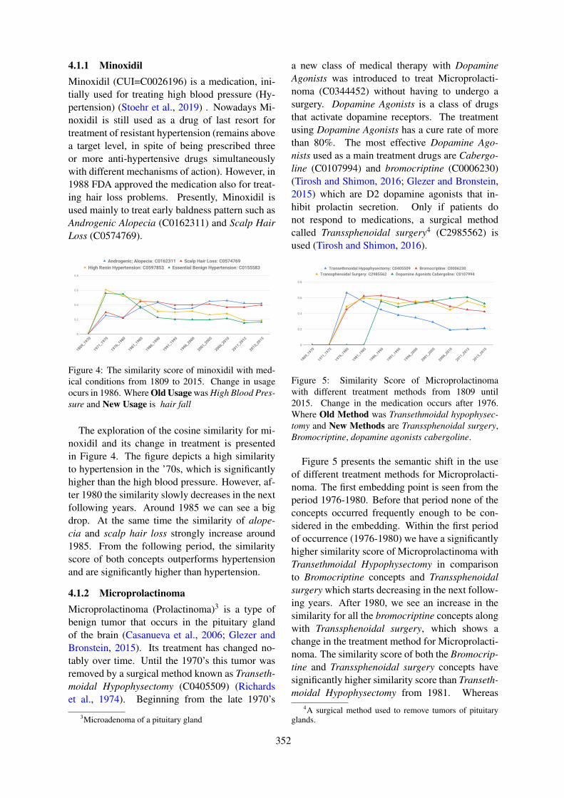
4.1.1 MinoxidilMinoxidil (CUI=C0026196) is a medication, ini-tially used for treating high blood pressure (Hy-pertension) (Stoehr et al., 2019) . Nowadays Mi-noxidil is still used as a drug of last resort fortreatment of resistant hypertension (remains abovea target level, in spite of being prescribed threeor more anti-hypertensive drugs simultaneouslywith different mechanisms of action). However, in1988 FDA approved the medication also for treat-ing hair loss problems. Presently, Minoxidil isused mainly to treat early baldness pattern such asAndrogenic Alopecia (C0162311) and Scalp HairLoss (C0574769).
Figure 4: The similarity score of minoxidil with med-ical conditions from 1809 to 2015. Change in usageocurs in 1986. Where Old Usage was High Blood Pres-sure and New Usage is hair fall
The exploration of the cosine similarity for mi-noxidil and its change in treatment is presentedin Figure 4. The figure depicts a high similarityto hypertension in the ’70s, which is significantlyhigher than the high blood pressure. However, af-ter 1980 the similarity slowly decreases in the nextfollowing years. Around 1985 we can see a bigdrop. At the same time the similarity of alope-cia and scalp hair loss strongly increase around1985. From the following period, the similarityscore of both concepts outperforms hypertensionand are significantly higher than hypertension.
4.1.2 MicroprolactinomaMicroprolactinoma (Prolactinoma)3 is a type ofbenign tumor that occurs in the pituitary glandof the brain (Casanueva et al., 2006; Glezer andBronstein, 2015). Its treatment has changed no-tably over time. Until the 1970’s this tumor wasremoved by a surgical method known as Transeth-moidal Hypophysectomy (C0405509) (Richardset al., 1974). Beginning from the late 1970’s
3Microadenoma of a pituitary gland
a new class of medical therapy with DopamineAgonists was introduced to treat Microprolacti-noma (C0344452) without having to undergo asurgery. Dopamine Agonists is a class of drugsthat activate dopamine receptors. The treatmentusing Dopamine Agonists has a cure rate of morethan 80%. The most effective Dopamine Ago-nists used as a main treatment drugs are Cabergo-line (C0107994) and bromocriptine (C0006230)(Tirosh and Shimon, 2016; Glezer and Bronstein,2015) which are D2 dopamine agonists that in-hibit prolactin secretion. Only if patients donot respond to medications, a surgical methodcalled Transsphenoidal surgery4 (C2985562) isused (Tirosh and Shimon, 2016).
Figure 5: Similarity Score of Microprolactinomawith different treatment methods from 1809 until2015. Change in the medication occurs after 1976.Where Old Method was Transethmoidal hypophysec-tomy and New Methods are Transsphenoidal surgery,Bromocriptine, dopamine agonists cabergoline.
Figure 5 presents the semantic shift in the useof different treatment methods for Microprolacti-noma. The first embedding point is seen from theperiod 1976-1980. Before that period none of theconcepts occurred frequently enough to be con-sidered in the embedding. Within the first periodof occurrence (1976-1980) we have a significantlyhigher similarity score of Microprolactinoma withTransethmoidal Hypophysectomy in comparisonto Bromocriptine concepts and Transsphenoidalsurgery which starts decreasing in the next follow-ing years. After 1980, we see an increase in thesimilarity for all the bromocriptine concepts alongwith Transsphenoidal surgery, which shows achange in the treatment method for Microprolacti-noma. The similarity score of both the Bromocrip-tine and Transsphenoidal surgery concepts havesignificantly higher similarity score than Transeth-moidal Hypophysectomy from 1981. Whereas
4A surgical method used to remove tumors of pituitaryglands.
352
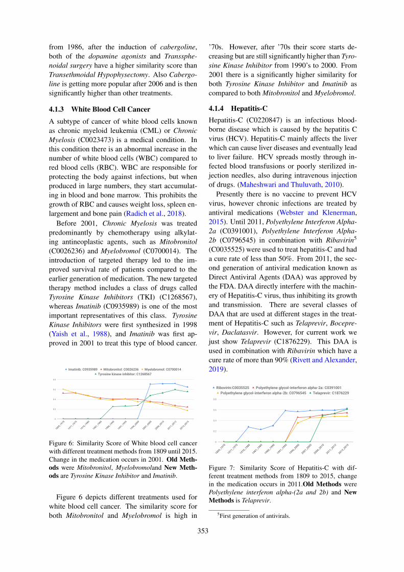
from 1986, after the induction of cabergoline,both of the dopamine agonists and Transsphe-noidal surgery have a higher similarity score thanTransethmoidal Hypophysectomy. Also Cabergo-line is getting more popular after 2006 and is thensignificantly higher than other treatments.
4.1.3 White Blood Cell Cancer
A subtype of cancer of white blood cells knownas chronic myeloid leukemia (CML) or ChronicMyelosis (C0023473) is a medical condition. Inthis condition there is an abnormal increase in thenumber of white blood cells (WBC) compared tored blood cells (RBC). WBC are responsible forprotecting the body against infections, but whenproduced in large numbers, they start accumulat-ing in blood and bone marrow. This prohibits thegrowth of RBC and causes weight loss, spleen en-largement and bone pain (Radich et al., 2018).
Before 2001, Chronic Myelosis was treatedpredominantly by chemotherapy using alkylat-ing antineoplastic agents, such as Mitobronitol(C0026236) and Myelobromol (C0700014). Theintroduction of targeted therapy led to the im-proved survival rate of patients compared to theearlier generation of medication. The new targetedtherapy method includes a class of drugs calledTyrosine Kinase Inhibitors (TKI) (C1268567),whereas Imatinib (C0935989) is one of the mostimportant representatives of this class. TyrosineKinase Inhibitors were first synthesized in 1998(Yaish et al., 1988), and Imatinib was first ap-proved in 2001 to treat this type of blood cancer.
Figure 6: Similarity Score of White blood cell cancerwith different treatment methods from 1809 until 2015.Change in the medication occurs in 2001. Old Meth-ods were Mitobronitol, Myelobromoland New Meth-ods are Tyrosine Kinase Inhibitor and Imatinib.
Figure 6 depicts different treatments used forwhite blood cell cancer. The similarity score forboth Mitobronitol and Myelobromol is high in
’70s. However, after ’70s their score starts de-creasing but are still significantly higher than Tyro-sine Kinase Inhibitor from 1990’s to 2000. From2001 there is a significantly higher similarity forboth Tyrosine Kinase Inhibitor and Imatinib ascompared to both Mitobronitol and Myelobromol.
4.1.4 Hepatitis-CHepatitis-C (C0220847) is an infectious blood-borne disease which is caused by the hepatitis Cvirus (HCV). Hepatitis-C mainly affects the liverwhich can cause liver diseases and eventually leadto liver failure. HCV spreads mostly through in-fected blood transfusions or poorly sterilized in-jection needles, also during intravenous injectionof drugs. (Maheshwari and Thuluvath, 2010).
Presently there is no vaccine to prevent HCVvirus, however chronic infections are treated byantiviral medications (Webster and Klenerman,2015). Until 2011, Polyethylene Interferon Alpha-2a (C0391001), Polyethylene Interferon Alpha-2b (C0796545) in combination with Ribavirin5
(C0035525) were used to treat hepatitis-C and hada cure rate of less than 50%. From 2011, the sec-ond generation of antiviral medication known asDirect Antiviral Agents (DAA) was approved bythe FDA. DAA directly interfere with the machin-ery of Hepatitis-C virus, thus inhibiting its growthand transmission. There are several classes ofDAA that are used at different stages in the treat-ment of Hepatitis-C such as Telaprevir, Bocepre-vir, Daclatasvir. However, for current work wejust show Telaprevir (C1876229). This DAA isused in combination with Ribavirin which have acure rate of more than 90% (Rivett and Alexander,2019).
Figure 7: Similarity Score of Hepatitis-C with dif-ferent treatment methods from 1809 to 2015, changein the medication occurs in 2011.Old Methods werePolyethylene interferon alpha-(2a and 2b) and NewMethods is Telaprevir.
5First generation of antivirals.
353
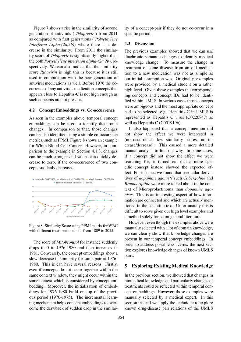
Figure 7 shows a rise in the similarity of secondgeneration of antivirals ( Telaprevir ) from 2011as compared with first generations ( PolyethyleneInterferon Alpha-(2a,2b)) where there is a de-crease in the similarity. From 2011 the similar-ity score of Telaprevir is significantly higher thanthe both Polyethylene interferon alpha-(2a,2b), re-spectively. We can also notice, that the similarityscore Ribavirin is high this is because it is stillused in combination with the new generation ofantiviral medications as well. Before 1976 the oc-currence of any antivirals medication concepts thatappears close to Hepatitis-C is not high enough assuch concepts are not present.
4.2 Concept Embeddings vs. Co-occurrence
As seen in the examples above, temporal conceptembeddings can be used to identify diachronicchanges. In comparison to that, those changescan be also identified using a simple co-occurencemetrics, such as PPMI. Figure 8 shows an examplefor White Blood Cell Cancer. However, in com-parison to the example in Section 4.1.3, changescan be much stronger and values can quickly de-crease to zero, if the co-occurrence of two con-cepts suddenly decreases.
Figure 8: Similarity Score using PPMI matrix for WBCwith different treatment methods from 1809 to 2015.
The score of Mitobronitol for instance suddenlydrops to 0 in 1976-1980 and then increases in1981. Conversely, the concept embeddings show aslow decrease in similarity for same pair at 1976-1980. This is can have several reasons: Firstly,even if concepts do not occur together within thesame context window, they might occur within thesame context which is considered by concept em-bedding. Moreover, the initialization of embed-dings for 1976-1980 build on top of the previ-ous period (1970-1975). The incremental learn-ing mechanism helps concept embeddings to over-come the drawback of sudden drop in the similar-
ity of a concept-pair if they do not co-occur in aspecific period.
4.3 Discussion
The previous examples showed that we can usediachronic semantic changes to identify medicalknowledge change. To measure the change intreatment of some disease from an old medica-tion to a new medication was not as simple asour initial assumption was. Originally, exampleswere provided by a medical student on a ratherhigh level. Given these examples the correspond-ing concepts and concept IDs had to be identi-fied within UMLS. In various cases those conceptswere ambiguous and the most appropriate concepthad to be selected, e.g. Hepatitis-C in UMLS isrepresented as Hepatitis C virus (C0220847) aswell as Hepatitis C (C0019196).
It also happened that a concept mention didnot show the effect we were interested in(no occurrence, low similarity scores, no in-crease/decrease). This caused a more detailedmanual analysis to find out why. In some cases,if a concept did not show the effect we weresearching for, it turned out that a more spe-cific concept instead showed the expected ef-fect. For instance we found that particular deriva-tives of dopamine agonists such Cabergoline andBromocriptine were more talked about in the con-text of Microprolactinoma than dopamine ago-nists. This is an interesting aspect of how infor-mation are connected and which are actually men-tioned in the scientific text. Unfortunately this isdifficult to solve given our high level examples anda method solely based on general literature.
However, even though the examples above weremanually selected with a lot of domain knowledge,we can clearly show that knowledge changes arepresent in our temporal concept embeddings. Inorder to address possible concerns, the next sec-tion explores knowledge changes of known UMLSpairs.
5 Exploring Existing Medical Knowledge
In the previous section, we showed that changes inbiomedical knowledge and particularly changes oftreatments could be reflected within temporal con-cept embeddings. However, those examples weremanually selected by a medical expert. In thissection instead we apply the technique to exploreknown drug-disease pair relations of the UMLS
354
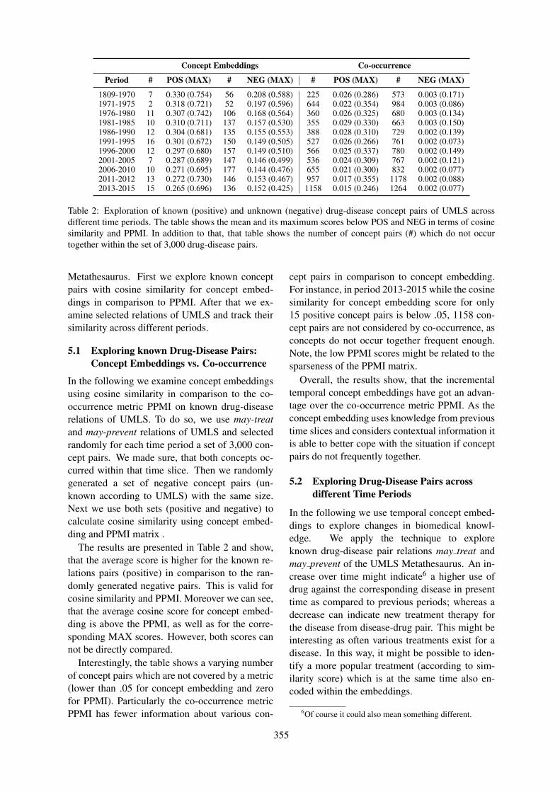
Concept Embeddings Co-occurrence
Period # POS (MAX) # NEG (MAX) # POS (MAX) # NEG (MAX)
1809-1970 7 0.330 (0.754) 56 0.208 (0.588) 225 0.026 (0.286) 573 0.003 (0.171)1971-1975 2 0.318 (0.721) 52 0.197 (0.596) 644 0.022 (0.354) 984 0.003 (0.086)1976-1980 11 0.307 (0.742) 106 0.168 (0.564) 360 0.026 (0.325) 680 0.003 (0.134)1981-1985 10 0.310 (0.711) 137 0.157 (0.530) 355 0.029 (0.330) 663 0.003 (0.150)1986-1990 12 0.304 (0.681) 135 0.155 (0.553) 388 0.028 (0.310) 729 0.002 (0.139)1991-1995 16 0.301 (0.672) 150 0.149 (0.505) 527 0.026 (0.266) 761 0.002 (0.073)1996-2000 12 0.297 (0.680) 157 0.149 (0.510) 566 0.025 (0.337) 780 0.002 (0.149)2001-2005 7 0.287 (0.689) 147 0.146 (0.499) 536 0.024 (0.309) 767 0.002 (0.121)2006-2010 10 0.271 (0.695) 177 0.144 (0.476) 655 0.021 (0.300) 832 0.002 (0.077)2011-2012 13 0.272 (0.730) 146 0.153 (0.467) 957 0.017 (0.355) 1178 0.002 (0.088)2013-2015 15 0.265 (0.696) 136 0.152 (0.425) 1158 0.015 (0.246) 1264 0.002 (0.077)
Table 2: Exploration of known (positive) and unknown (negative) drug-disease concept pairs of UMLS acrossdifferent time periods. The table shows the mean and its maximum scores below POS and NEG in terms of cosinesimilarity and PPMI. In addition to that, that table shows the number of concept pairs (#) which do not occurtogether within the set of 3,000 drug-disease pairs.
Metathesaurus. First we explore known conceptpairs with cosine similarity for concept embed-dings in comparison to PPMI. After that we ex-amine selected relations of UMLS and track theirsimilarity across different periods.
5.1 Exploring known Drug-Disease Pairs:Concept Embeddings vs. Co-occurrence
In the following we examine concept embeddingsusing cosine similarity in comparison to the co-occurrence metric PPMI on known drug-diseaserelations of UMLS. To do so, we use may-treatand may-prevent relations of UMLS and selectedrandomly for each time period a set of 3,000 con-cept pairs. We made sure, that both concepts oc-curred within that time slice. Then we randomlygenerated a set of negative concept pairs (un-known according to UMLS) with the same size.Next we use both sets (positive and negative) tocalculate cosine similarity using concept embed-ding and PPMI matrix .
The results are presented in Table 2 and show,that the average score is higher for the known re-lations pairs (positive) in comparison to the ran-domly generated negative pairs. This is valid forcosine similarity and PPMI. Moreover we can see,that the average cosine score for concept embed-ding is above the PPMI, as well as for the corre-sponding MAX scores. However, both scores cannot be directly compared.
Interestingly, the table shows a varying numberof concept pairs which are not covered by a metric(lower than .05 for concept embedding and zerofor PPMI). Particularly the co-occurrence metricPPMI has fewer information about various con-
cept pairs in comparison to concept embedding.For instance, in period 2013-2015 while the cosinesimilarity for concept embedding score for only15 positive concept pairs is below .05, 1158 con-cept pairs are not considered by co-occurrence, asconcepts do not occur together frequent enough.Note, the low PPMI scores might be related to thesparseness of the PPMI matrix.
Overall, the results show, that the incrementaltemporal concept embeddings have got an advan-tage over the co-occurrence metric PPMI. As theconcept embedding uses knowledge from previoustime slices and considers contextual information itis able to better cope with the situation if conceptpairs do not frequently together.
5.2 Exploring Drug-Disease Pairs acrossdifferent Time Periods
In the following we use temporal concept embed-dings to explore changes in biomedical knowl-edge. We apply the technique to exploreknown drug-disease pair relations may treat andmay prevent of the UMLS Metathesaurus. An in-crease over time might indicate6 a higher use ofdrug against the corresponding disease in presenttime as compared to previous periods; whereas adecrease can indicate new treatment therapy forthe disease from disease-drug pair. This might beinteresting as often various treatments exist for adisease. In this way, it might be possible to iden-tify a more popular treatment (according to sim-ilarity score) which is at the same time also en-coded within the embeddings.
6Of course it could also mean something different.
355
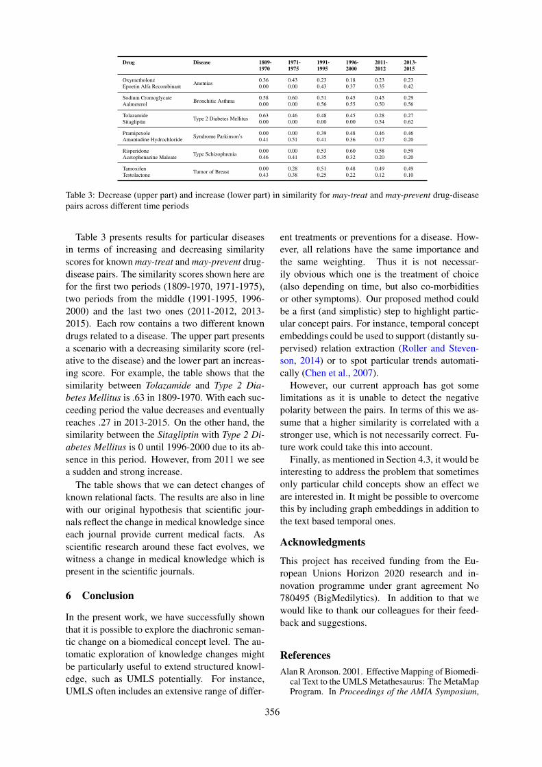
Drug Disease 1809-1970
1971-1975
1991-1995
1996-2000
2011-2012
2013-2015
Oxymetholone Anemias 0.36 0.43 0.23 0.18 0.23 0.23Epoetin Alfa Recombinant 0.00 0.00 0.43 0.37 0.35 0.42
Sodium Cromoglycate Bronchitic Asthma 0.58 0.60 0.51 0.45 0.45 0.29Aalmeterol 0.00 0.00 0.56 0.55 0.50 0.56
Tolazamide Type 2 Diabetes Mellitus 0.63 0.46 0.48 0.45 0.28 0.27Sitagliptin 0.00 0.00 0.00 0.00 0.54 0.62
Pramipexole Syndrome Parkinson’s 0.00 0.00 0.39 0.48 0.46 0.46Amantadine Hydrochloride 0.41 0.51 0.41 0.36 0.17 0.20
Risperidone Type Schizophrenia 0.00 0.00 0.53 0.60 0.58 0.59Acetophenazine Maleate 0.46 0.41 0.35 0.32 0.20 0.20
Tamoxifen Tumor of Breast 0.00 0.28 0.51 0.48 0.49 0.49Testolactone 0.43 0.38 0.25 0.22 0.12 0.10
Table 3: Decrease (upper part) and increase (lower part) in similarity for may-treat and may-prevent drug-diseasepairs across different time periods
Table 3 presents results for particular diseasesin terms of increasing and decreasing similarityscores for known may-treat and may-prevent drug-disease pairs. The similarity scores shown here arefor the first two periods (1809-1970, 1971-1975),two periods from the middle (1991-1995, 1996-2000) and the last two ones (2011-2012, 2013-2015). Each row contains a two different knowndrugs related to a disease. The upper part presentsa scenario with a decreasing similarity score (rel-ative to the disease) and the lower part an increas-ing score. For example, the table shows that thesimilarity between Tolazamide and Type 2 Dia-betes Mellitus is .63 in 1809-1970. With each suc-ceeding period the value decreases and eventuallyreaches .27 in 2013-2015. On the other hand, thesimilarity between the Sitagliptin with Type 2 Di-abetes Mellitus is 0 until 1996-2000 due to its ab-sence in this period. However, from 2011 we seea sudden and strong increase.
The table shows that we can detect changes ofknown relational facts. The results are also in linewith our original hypothesis that scientific jour-nals reflect the change in medical knowledge sinceeach journal provide current medical facts. Asscientific research around these fact evolves, wewitness a change in medical knowledge which ispresent in the scientific journals.
6 Conclusion
In the present work, we have successfully shownthat it is possible to explore the diachronic seman-tic change on a biomedical concept level. The au-tomatic exploration of knowledge changes mightbe particularly useful to extend structured knowl-edge, such as UMLS potentially. For instance,UMLS often includes an extensive range of differ-
ent treatments or preventions for a disease. How-ever, all relations have the same importance andthe same weighting. Thus it is not necessar-ily obvious which one is the treatment of choice(also depending on time, but also co-morbiditiesor other symptoms). Our proposed method couldbe a first (and simplistic) step to highlight partic-ular concept pairs. For instance, temporal conceptembeddings could be used to support (distantly su-pervised) relation extraction (Roller and Steven-son, 2014) or to spot particular trends automati-cally (Chen et al., 2007).
However, our current approach has got somelimitations as it is unable to detect the negativepolarity between the pairs. In terms of this we as-sume that a higher similarity is correlated with astronger use, which is not necessarily correct. Fu-ture work could take this into account.
Finally, as mentioned in Section 4.3, it would beinteresting to address the problem that sometimesonly particular child concepts show an effect weare interested in. It might be possible to overcomethis by including graph embeddings in addition tothe text based temporal ones.
Acknowledgments
This project has received funding from the Eu-ropean Unions Horizon 2020 research and in-novation programme under grant agreement No780495 (BigMedilytics). In addition to that wewould like to thank our colleagues for their feed-back and suggestions.
ReferencesAlan R Aronson. 2001. Effective Mapping of Biomedi-
cal Text to the UMLS Metathesaurus: The MetaMapProgram. In Proceedings of the AMIA Symposium,
356
page 17. American Medical Informatics Associa-tion.
Andrew L. Beam, Benjamin Kompa, Inbar Fried,Nathan P. Palmer, Xu Shi, Tianxi Cai, and Isaac S.Kohane. 2018. Clinical Concept EmbeddingsLearned from Massive Sources of Medical Data.CoRR, abs/1804.01486.
Andreas Blank. 1999. Why do new meanings occur? Acognitive typology of the motivations for lexical se-mantic change. Historical semantics and cognition,13:6.
Olivier Bodenreider. 2004. The Unified Medical Lan-guage System (UMLS): Integrating Biomedical Ter-minology. Nucleic acids research, 32(Databaseissue):D267–70.
Piotr Bojanowski, Edouard Grave, Armand Joulin,and Tomas Mikolov. 2016. Enriching Word Vec-tors with Subword Information. arXiv preprintarXiv:1607.04606.
Joan Bybee et al. 2007. Frequency of Use and the Or-ganization of Language. Oxford University Press onDemand.
Felipe F Casanueva, Mark E Molitch, Janet ASchlechte, Roger Abs, Vivien Bonert, Marcello DBronstein, Thierry Brue, Paolo Cappabianca, Anna-maria Colao, Rudolf Fahlbusch, et al. 2006. Guide-lines of the Pituitary Society for the diagnosis andmanagement of prolactinomas. Clinical endocrinol-ogy, 65(2):265–273.
Elizabeth S Chen, Peter D Stetson, Yves A Lussier,Marianthi Markatou, George Hripcsak, and CarolFriedman. 2007. Detection of practice pattern trendsthrough natural language processing of clinical nar-ratives and biomedical literature. In AMIA AnnualSymposium Proceedings, volume 2007, page 120.American Medical Informatics Association.
Youngduck Choi, Chill Yi-I Chiu, and David Sontag.2016. Learning Low-Dimensional Representationsof Medical Concepts. AMIA Summits on Transla-tional Science Proceedings, 2016:41.
Kenneth Ward Church and Patrick Hanks. 1990. WordAssociation Norms, Mutual Information, and Lexi-cography. Computational linguistics, 16(1):22–29.
Greta G. Cummings, Susan Armijo Olivo, Patricia D.Biondo, Carla R. Stiles, Ozden Yurtseven, Robin L.Fainsinger, and Neil A. Hagen. 2011. Effectivenessof Knowledge Translation Interventions to ImproveCancer Pain Management. J. Pain Symptom Man-age., 41(5):915–939.
Lance De Vine, Guido Zuccon, Bevan Koopman, Lau-rianne Sitbon, and Peter Bruza. 2014. Medical Se-mantic Similarity with a Neural Language Model. InProceedings of the 23rd ACM International Confer-ence on Conference on Information and KnowledgeManagement, pages 1819–1822. ACM.
John R Firth. 1957. A Synopsis of Linguistic Theory,1930-1955. Studies in linguistic analysis.
Andrea Glezer and Marcello D. Bronstein. 2015. Pro-lactinomas. Endocrinol. Metab. Clin. North Am.,44(1):71–78.
William L. Hamilton, Jure Leskovec, and Dan Juraf-sky. 2016a. Cultural Shift or Linguistic Drift? Com-paring Two Computational Measures of SemanticChange. Proceedings of the 2016 Conference onEmpirical Methods in Natural Language Process-ing.
William L. Hamilton, Jure Leskovec, and Dan Juraf-sky. 2016b. Diachronic Word Embeddings RevealStatistical Laws of Semantic Change. In Proc. As-soc. Comput. Ling. (ACL).
Jiangen He and Chaomei Chen. 2018. Predictive Ef-fects of Novelty Measured by Temporal Embed-dings on the Growth of Scientific Literature. Fron-tiers in Research Metrics and Analytics, 3:9.
Adam Jatowt and Kevin Duh. 2014. A Frameworkfor Analyzing Semantic Change of Words acrossTime. In Proceedings of the 14th ACM/IEEE-CSJoint Conference on Digital Libraries, pages 229–238. IEEE Press.
Yoon Kim, Yi-I Chiu, Kentaro Hanaki, Darshan Hegde,and Slav Petrov. 2014. Temporal Analysis of Lan-guage through Neural Language Models. In Pro-ceedings of the Workshop on Language Technolo-gies and Computational Social Science@ACL 2014,Baltimore, MD, USA, June 26, 2014, pages 61–65.Association for Computational Linguistics.
Vivek Kulkarni, Rami Al-Rfou, Bryan Perozzi, andSteven Skiena. 2014. Statistically Significant Detec-tion of Linguistic Change. CoRR, abs/1411.3315.
Omer Levy and Yoav Goldberg. 2014. Neural WordEmbedding as Implicit Matrix Factorization. In Ad-vances in Neural Information Processing Systems,pages 2177–2185.
Omer Levy, Yoav Goldberg, and Ido Dagan. 2015.Improving Distributional Similarity with LessonsLearned from Word Embeddings. Transactionsof the Association for Computational Linguistics,3:211–225.
Erez Lieberman, Jean-Baptiste Michel, Joe Jackson,Tina Tang, and Martin A Nowak. 2007. Quantifyingthe Evolutionary Dynamics of Language. Nature,449(7163):713.
Yue Liu, Tao Ge, Kusum S Mathews, Heng Ji, andDeborah L McGuinness. 2018. Exploiting Task-Oriented Resources to Learn Word Embeddings forClinical Abbreviation Expansion. arXiv preprintarXiv:1804.04225.
Anurag Maheshwari and Paul J. Thuluvath. 2010.Management of acute hepatitis C. Clin. Liver Dis.,14(1):169–176.
357
Tomas Mikolov, Kai Chen, Greg Corrado, and Jef-frey Dean. 2013a. Efficient Estimation of WordRepresentations in Vector Space. arXiv preprintarXiv:1301.3781.
Tomas Mikolov, Quoc V Le, and Ilya Sutskever. 2013b.Exploiting similarities among languages for ma-chine translation. arXiv preprint arXiv:1309.4168.
Mark Pagel, Quentin D Atkinson, and Andrew Meade.2007. Frequency of Word-Use Predicts Rates ofLexical Evolution throughout Indo-European His-tory. Nature, 449(7163):717.
Jeffrey Pennington, Richard Socher, and Christo-pher D. Manning. 2014. Glove: Global Vectors forWord Representation. In Proceedings of the 2014Conference on Empirical Methods in Natural Lan-guage Processing, EMNLP 2014, October 25-29,2014, Doha, Qatar, A Meeting of SIGDAT, a Spe-cial Interest Group of the ACL, pages 1532–1543.ACL.
Lawrence Phillips, Kyle Shaffer, Dustin Arendt,Nathan Hodas, and Svitlana Volkova. 2017. Intrin-sic and extrinsic evaluation of spatiotemporal textrepresentations in Twitter streams. In Proceedingsof the 2nd Workshop on Representation Learning forNLP, pages 201–210.
Jerald P Radich, Michael Deininger, Camille N Ab-boud, Jessica K Altman, Ellin Berman, Ravi Bhatia,Bhavana Bhatnagar, Peter Curtin, Daniel J DeAn-gelo, Jason Gotlib, et al. 2018. Chronic myeloidleukemia, version 1.2019, nccn clinical practiceguidelines in oncology. Journal of the NationalComprehensive Cancer Network, 16(9):1108–1135.
S H Richards, J P Thomas, and D Kilby. 1974.Transethmoidal hypophysectomy for pituitary tu-mours. Proceedings of the Royal Society ofMedicine, 67(9):889–892.
Lucy Rivett and Graeme Alexander. 2019. Is the con-quest of hepatitis c imminent? Expert reviews inmolecular medicine, 21.
Roland Roller and Mark Stevenson. 2014. Self-supervised Relation Extraction Using UMLS. In In-formation Access Evaluation. Multilinguality, Mul-timodality, and Interaction, pages 116–127, Cham.Springer International Publishing.
Eyal Sagi, Stefan Kaufmann, and Brady Clark. 2009.Semantic density analysis: Comparing word mean-ing across time and phonetic space. In Proceedingsof the Workshop on Geometrical Models of Natu-ral Language Semantics, pages 104–111. Associa-tion for Computational Linguistics.
Jenna R Stoehr, Jennifer N Choi, Maria Colavincenzo,and Stefan Vanderweil. 2019. Off-label use of topi-cal minoxidil in alopecia: A review. American jour-nal of clinical dermatology, pages 1–14.
Don R Swanson. 1986. Fish oil, raynaud’s syndrome,and undiscovered public knowledge. Perspectives inbiology and medicine, 30(1):7–18.
Amit Tirosh and Ilan Shimon. 2016. Current ap-proach to treatments for prolactinomas. MinervaEndocrinol., 41(3):316–323.
Peter D Turney and Patrick Pantel. 2010. From Fre-quency to Meaning: Vector Space Models of Se-mantics. Journal of artificial intelligence research,37:141–188.
Daniel P Webster and Paul Klenerman. 2015. Hepatitisc. Hepatitis C. Lancet, 385(9973):1124–1135.
Derry Tanti Wijaya and Reyyan Yeniterzi. 2011. Un-derstanding Semantic Change of Words over Cen-turies. In Proceedings of the 2011 InternationalWorkshop on DETecting and Exploiting Cultural di-versiTy on the Social Web, pages 35–40. ACM.
P. Yaish, A. Gazit, C. Gilon, and A. Levitzki.1988. Blocking of EGF-dependent cell prolifera-tion by EGF receptor kinase inhibitors. Science,242(4880):933–935.
Erjia Yan and Yongjun Zhu. 2018. Tracking Word Se-mantic Change in Biomedical Literature. Interna-tional journal of medical informatics, 109:76–86.
Li Zhou and George Hripcsak. 2007. Temporal Rea-soning with Medical Data—a Review with Empha-sis on Medical Natural Language Processing. Jour-nal of biomedical informatics, 40(2):183–202.
Fei Zhu, Preecha Patumcharoenpol, Cheng Zhang,Yang Yang, Jonathan Chan, Asawin Meechai,Wanwipa Vongsangnak, and Bairong Shen. 2013.Biomedical Text Mining and Its Applications inCancer Research. Journal of biomedical informat-ics, 46(2):200–211.
358
Proceedings of the BioNLP 2019 workshop, pages 359–369Florence, Italy, August 1, 2019. c©2019 Association for Computational Linguistics
Extracting relations between outcomes and significance levelsin Randomized Controlled Trials (RCTs) publications
Anna KorolevaLIMSI, CNRS, Université Paris-Saclay,
F-91405 Orsay, France
Academic Medical Center, University of Amsterdam,
Amsterdam, the Netherlands
Patrick ParoubekLIMSI, CNRS,
Université Paris-Saclay,
F-91405 Orsay, France
Abstract
Randomized controlled trials assess the effectsof an experimental intervention by comparingit to a control intervention with regard to somevariables - trial outcomes. Statistical hypoth-esis testing is used to test if the experimentalintervention is superior to the control. Statis-tical significance is typically reported for themeasured outcomes and is an important char-acteristic of the results. We propose a machinelearning approach to automatically extract re-ported outcomes, significance levels and therelation between them. We annotated a cor-pus of 663 sentences with 2,552 outcome -significance level relations (1,372 positive and1,180 negative relations). We compared sev-eral classifiers, using a manually crafted fea-ture set, and a number of deep learning mod-els. The best performance (F-measure of 94%)was shown by the BioBERT fine-tuned model.
1 Introduction
In clinical trials, outcomes are the dependent vari-ables that are monitored to assess how they areinfluenced by other, independent, variables (treat-ment used, dosage, patient characteristics). Out-comes are a central notion for clinical trials.
To assess the impact of different variables onthe outcomes, statistical hypothesis testing is com-monly used, giving an estimation of statistical sig-nificance – the likelihood that a relationship be-tween two or more variables is caused by some-thing other than a chance (Schindler, 2015). Sta-tistical significance levels are typically reportedalong with the trial outcomes as p-values, with acertain set threshold, where a p-value below thethreshold means that the results are statisticallysignificant, while a p-value above the thresholdpresents non-significant results. Hypothesis test-ing in clinical trials is used in two main cases:
1. In a trial comparing several treatments given
to different groups of patients, a differencein value of an outcome observed between thegroups at the end of the trial is evaluated byhypothesis testing to determine if the differ-ence is due to the difference in medication. Ifthe difference is statistically significant, thenull hypothesis (the difference between treat-ments is due to a chance) is rejected, i.e. thesuperiority of one treatment over the other isconsidered to be proved.
2. When an improvement of an outcome is ob-served within a group of patients taking atreatment, hypothesis testing is used to deter-mine if the difference in the outcome at dif-ferent time points within the group is due tothe treatment. If the results are statisticallysignificant, it is considered to be proven thatthe treatment has a positive effect on the out-come in the given group of patients.
Although p-values are often misused and misinter-preted (Head et al., 2015), extracting significancelevels for trial outcomes is still vital for a num-ber of tasks, such as systematic reviews, detec-tion of bias and spin. In particular, our applicationof interest is automatic detection of spin, or dis-torted reporting of research results, that consistsin presenting an intervention studied in a trial ashaving higher beneficial effects than the researchhas proved. Spin is an alarming problem in healthcare as it causes overestimation of the interventionby clinicians (Boutron et al., 2014) and unjustifiedpositive claims regarding the intervention is healthnews and press releases (Haneef et al., 2015; Yav-chitz et al., 2012).
Spin is often related to a focus on significantoutcomes, and occurs when the primary outcome(the main variable monitored during a trial) is notsignificant. Thus, to detect spin, it is importantto identify the significance of outcomes, and espe-
359
cially of the primary outcome. To our best knowl-edge, no previous work addressed the extractionof the relation between outcomes and significancelevels. In this paper, we present our approach to-wards extracting outcomes, significance levels andrelations between them, that can be incorporatedinto a spin detection pipeline.
2 State of the art
Extraction of outcome - significance level rela-tions consists of two parts: entity extraction (re-ported outcomes and significance levels) and ex-traction of the relationship between the entities.In this section, we present the previous works onthese or similar tasks.
2.1 Entity extraction
The number of works addressing automatic extrac-tion of significance levels is limited.
(Hsu et al., 2012) used regular expressions toextract statistical interpretation, p-values, confi-dence intervals, and comparison groups from sen-tences categorized as ”outcomes and estimation”.The authors report precision of 93%, recall of 88%and F-measure of 90% for this type of information.
(Chavalarias et al., 2016) applied text miningto evaluate the p-values reported in the abstractsand full texts of biomedical articles published in1990 – 2015. The authors also assessed how fre-quently statistical information is presented in waysother than p-values. P-values were extracted usinga regular expression; the system was evaluated ona manually annotated dataset. The reported sensi-tivity (true positive rate) is 96.3% and specificity(true negative rate) is 99.8%. P-values and qual-itative statements about significance were morecommon ways of reporting significance than con-fidence intervals, Bayes factors, or effect sizes.
A few works focused on extracting outcome-related information, addressing it either as a sen-tence classification, or as entity extraction task.
(Demner-Fushman et al., 2006) defined an out-come as ”The sentence(s) that best summarizesthe consequences of an intervention” and thusadopted a sentence classification approach to ex-tract outcome-related information from medicalarticles, using a corpus of 633 MEDLINE cita-tions. The authors tested Naive Bayes, linear SVMand decision-tree classifiers. Naive Bayes showedthe best performance. The reported classificationaccuracy ranged from 88% to 93%.
One of the notable recent works addressing out-come identification as an entity extraction task,rather than sentence classification, is (Blake andLucic, 2015). The authors addressed a partic-ular type of syntactic constructions – compara-tive sentences – to extract three items: the com-pared entities, referred to as the agent and the ob-ject, and the ground for comparison, referred to asthe endpoint (synonymous to outcome). The aimof this work was to extract corresponding nounphrases. The dataset was based on full-text med-ical articles and included only the sentences thatcontain all the three entities (agent, object andendpoint). The training set comprised 100 sen-tences that contain 656 noun phrases. The algo-rithm proceeds in two steps: first, comparativesentences are detected with the help of a set ofadjectives and lexico-syntactic patterns. Second,the noun phrases are classified according to theirrole (agent, object, endpoint) using SVM and gen-eralized linear model (GLM). On the training set,SVM showed better performance than GLM, withan F-measure of 78% for the endpoint. However,on the test set the performance was significantlylower: SVM showed an F-measure of only 51%for the endpoint. The performance was higheron shorter sentences (up to 30 words) than on thelonger ones.
A following work (Lucic and Blake, 2016)aimed at improving the recognition of the firstentity and of the endpoint. The authors pro-pose to use in the classification the informationon whether the head noun of the candidate nounphrase denotes an amount or a measure. The an-notation of the corpus was enriched by the cor-responding information. As a result, precision ofthe endpoint detection improved to 56% on longersentences and 58% on shorter ones; recall im-proved to 71% on longer sentences and 74% onshorter ones.
2.2 Relation extraction
To our knowledge, extraction of the relationbetween outcomes and significance levels hasnot been addressed yet. In this section, weoverview some frameworks for relation extractionand outline some common features of different ap-proaches in the biomedical relation extraction.
A substantial number of works addressed ex-tracting binary relations, such as protein-proteininteractions or gene-phenotype relation, or com-
360
plex relations, such as biomolecular events. Acommon feature of the works in this domain, notedby (Zhou et al., 2014; Lever and Jones, 2017) andstill relevant for recent works e.g. (Peng and Lu,2017; Asada et al., 2017), consists in assumingthat entities of interest are already extracted andprovided to the relation extraction system as input.Thus, the relation extraction is assessed separately,without taking into account the performance of en-tity extraction. We adopt this approach for relationextraction evaluation in our work, but we provideseparate assessment for our algorithms of entityextraction.
One of the general frameworks for relation ex-traction in the biomedical domain is proposed by(Zhou et al., 2014). The authors suggest usingtrigger words to determine the type of a relation,noting that for some relation types trigger wordscan be extracted simply with a dictionary, whilefor other types, rule-based or machine-learning ap-proaches may be required. For relation extrac-tion, rule-based methods can be applied, often em-ploying regular expressions using words or POStags. Rules can be crafted manually or learnedautomatically. The machine learning approachesto binary relation extraction, as the authors note,usually treat the task as a classification problem.Features for classification often use output of tex-tual analysis algorithms such as POS-tagging andsyntactic parsing. Machine learning approachescan be divided into feature-based approaches (us-ing syntactic and semantic features) and kernel ap-proaches (calculating similarity between input se-quences based on string or syntactic representationof the input). Supervised machine learning is ahighly successful approach for binary relation ex-traction, but its main drawback consists in the needof large amount of annotated data.
A framework for pattern-based relation extrac-tion is introduced by (Peng et al., 2014). The ap-proach aims at reducing the need for manual anno-tation. The approach is based on a user-providedlist of trigger words and specifications (the defini-tion of arguments for each trigger). Variations oflexico-syntactic patterns are derived using this in-formation and are matched with the input text, de-tecting the target relations. Some interesting fea-tures of the framework include the following: theuse of text simplification to avoid writing rules forall existing constructions; the use of referential re-lations to find the best phrase referring to an entity.
The authors state that their system is characterizedby good generalizability due to the use of languageproperties and not of task-specific knowledge.
A recent work (Björne and Salakoski, 2018) re-ports on the development of convolutional neuralnetworks (CNNs) for event and relation extrac-tion, using Keras (Chollet et al., 2015) with Ten-sorflow backend (Abadi et al., 2016). Parallel con-volutional layers process the input, using sequencewindows centered around the candidate entity, re-lation or event. Vector space embeddings are builtfor input tokens, including features such as wordvectors, POS, entity features, relative position, etc.The system was tested on several tasks and showedimproved performance and good generalizability.
3 Our dataset
3.1 Corpus creation and annotation
In our previous work on outcome extraction, wemanually annotated a corpus for reported out-comes comprising 1,940 sentences from the Re-sults and Conclusions sections of PMC article ab-stracts. We used this corpus as a basis for a corpuswith annotations for outcome significance levelrelations.
Our corpus contains 2,551 annotated outcomes.Out of the sentences with outcomes, we selectedthose where statistical significance levels are sup-posedly reported (using regular expressions) andmanually annotated relations between outcomesand significance levels. The annotation was doneby one annotator (AK), in consultation with anumber of domain experts, due to infeasibility ofrecruiting several annotators with sufficient levelof expertise within a reasonable time frame.
The final corpus contains 663 sentences with2,552 annotated relations, out of which 1,372 rela-tions are positive (the significance level is relatedto the outcome) and 1,180 relations are negative(the significance level is not related to the out-come). The corpus is publicly available (Anna,2019).
3.2 Data description
There are three types of data relevant for this work:outcomes, significance levels, and relationship be-tween them. In this section, we describe thesetypes of data and the observed variability in theways of presenting them.
1. Outcomes
361
A trial outcome is, in broad sense, a mea-sure or variable monitored during a trial. Itcan be binary (presence of a symptom orstate), numerical (”temperature”) or qualita-tive (”burden of disease”). Apart from thegeneral term denoting the outcome, there areseveral aspects that define it: a measure-ment tool (questionnaire, score, etc.) used tomeasure the outcome; time points at whichthe outcome is measured; patient-level anal-ysis metrics (change from baseline, time toevent); population-level aggregation method(mean, median, proportion of patients withsome characteristic).
Generally, there are two main contexts inwhich outcomes of a clinical trial can bementioned: a definition of what the outcomesof a trial were (”Quality of life was selectedas the primary outcome.”), and reporting re-sults for an outcome (”Quality of life washigher in the experimental group than in thecontrol group.”). In both cases, a mentionof an outcome may contain the aspects listedabove, but does not necessarily include all ofthem. In this work, we are interested in thesecond type of context.
The ways of reporting outcomes are highlydiverse. Results for an outcome may bereported as a value of the outcome mea-sure: for binary outcomes, it refers to pres-ence/absence of an event or state; for numeri-cal outcome, it is a numerical value; for qual-itative outcome, it is often a value obtained onthe associated measurement tool. As the pri-mary goal of RCTs is to compare two or moreinterventions, results for an outcome can bereported as a comparison between the inter-ventions/patient groups, with or without ac-tual values of the outcome measure. Syntac-tically, an outcome may be represented by anoun phrase, a verb phrase, an adjective ora clause. We provide here some examples ofoutcome reporting, to give an idea of variabil-ity of expressions.
The outcome is reported as a numericalvalue:
a) The median progression-free survival was32 days.
The outcome is reported as a comparison be-tween groups, without the values for groups:
b) MMS resulted in more stunting than stan-dard Fe60F (p = 0.02).
The outcome is reported as a numerical valuewith comparison between groups:
c) The average birth weight was 2694 g andbirth length was 47.7 cm, with no differenceamong intervention groups.
d) The crude incidence of late rectal toxic-ity ≥ G2 was 14.0% and 12.3% for the armA and B, respectively.
e) More than 96% of patients who receivedDPT were apyrexial 48 hours after treatmentcompared to 83.5% in the AL group (p <0.001).
f) The proportion of patients who remainedrelapse-free at Week 26 did not differ sig-nificantly between the placebo group (5/16,31%) and the IFN beta-1a 44 mcg biw (6/17,35%; p = 0.497), 44 mcg tw (7/16, 44%; p =0.280) or 66 mcg tw (2/18, 11%; p = 0.333)groups.
In the latter case, the variation is especiallyhigh, and the same outcome may be reportedin several different ways (cf. the examplesd, e and f that all talk about a percentage ofpatients in which a certain event occurred, butthe structure of the phrases differs).
Identifying the textual boundaries of an out-come presents a challenge: for the exam-ple d, it can be ”the crude incidence of laterectal toxicity ≥ G2” or ”late rectal toxic-ity ≥ G2”; for the example f, it can be ”theproportion of patents who remained relapse-free at Week 26”, or ”remained relapse-freeat Week 26”, or simply ”relapse-free”. Thisvariability poses difficulties for both annota-tion and extraction of reported outcomes. Inour annotation, we aimed at annotating theminimal possible text span describing an out-come, not including time points, aggregationand analysis metrics.
2. Significance levels
The ways of presenting significance levelsare less diverse than the ways of reportingoutcomes. Typically, significance levels arereported via p-values. Another way of deter-mining significance of the results is the con-fidence interval (CI), where a CI comprising
362
zero denotes non-significant results. In thiswork, we do not address CIs as they are lessfrequently reported (Chavalarias et al., 2016).
Statistical significance can be reported asan exact value of P (”p=0.02”), as P-valuerelative to a pre-set threshold (”p<0.05”),or in qualitative form (”significant”/”non-significant”). We address all these forms ofreporting significance.
Although in general the ways of present-ing statistical significance are rather uniform,there are a few cases to be noted:
• Coordinated p-values:For the non-HPD stratum, the intent-to-treat relative risks of spontaneous pre-mature birth at < 34 and < 37 weeks’gestation were 0.33 (0.03, 3.16) and0.49 (0.17, 1.44), respectively, and theywere non-significant (ns) with p = 0.31and 0.14.• Significance level in score of a negation:
The respiratory rate, chest indrawing,cyanosis, stridor, nasal flaring, wheezeand fever in both groups recorded at en-rollment and parameters did not differsignificantly between the two groups.A particular difficulty is presented bythe cases in which a negation markeroccurs in the main clause and a signifi-cance level in the dependent clause, thusthe significance level is within the scopeof the negation, but there is a big lineardistance between them:Results There was no evidence that anincentive (52% versus 43%, Risk Dif-ference (RD) -8.8 (95%CI 22.5, 4.8);or abridged questionnaire (46% versus43%, RD 2.9 (95%CI 16.5, 10.7); sta-tistically significantly improved dentistresponse rates compared to a full lengthquestionnaire in RCT A.
3. Relationship between outcomes and signifi-cance levels
The correspondence between outcomes andsignificance levels in a sentence is often notone-to-one: multiple outcomes can be linkedto the same significance level, and vice versa.Several outcomes are linked to one signifi-cance level when outcomes are coordinated:
No significant improvements in lung func-tion, symptoms, or quality of life were seen.
Several significance levels can be associatedto one outcome in a number of cases:
• one outcome is linked to two signifi-cance levels when a significance level ispresented in both qualitative and numer-ical form:Results The response rates were notsignificantly different Odds Ratio 0.88(95% confidence intervals 0.48 to 1.63)p = 0.69.• in the case of comparison between pa-
tient groups taking different medica-tions, when there are more than 2groups, significance can be reported forall pairs of groups;• significance level for difference ob-
served within groups of patients receiv-ing a particular medication:[Na] increased significantly in the 0.9%group (+0.20 mmol/L/h [IQR +0.03,+0.4]; P = 0.02) and increased, butnot significantly, in the 0.45% group(+0.08 mmol/L/h [IQR -0.15, +0.16]; P= 0.07).• significance reported for both between-
and within-group comparison:PTEF increased significantly both afteralbuterol and saline treatments but thedifference between the two treatmentswas not significant (P = 0.6).• significance for differences within sub-
groups of patients (e.g. gender or agesubgroups) receiving a medication;• significance for different types of analy-
sis: intention-to-treat / per protocol:Results For BMD, no intent-to-treatanalyses were statistically significant;however, per protocol analyses (ie, onlyincluding TC participants who com-pleted ≥ 75% training requirements) offemoral neck BMD changes were sig-nificantly different between TC and UC(+0.04 vs -0.98%; P = 0.05).• significance for several time points:
Results A significant main effect of time( p < 0.001) was found for step-countsattributable to significant increases insteps/day between: pre-intervention ( M
363
= 6941, SD = 3047) and 12 weeks ( M= 9327, SD = 4136), t (78) = - 6.52, p< 0.001, d = 0.66; pre-intervention and24 weeks ( M = 8804, SD = 4145), t (78)= - 4.82, p < 0.001, d = 0.52; and pre-intervention and 48 weeks ( M = 8450,SD = 3855), t (78) = - 4.15, p < 0.001,d = 0.44.• significance level for comparison of var-
ious analysis metrics (mean, AUC, etc.)
4 Methods
To extract the relation between an outcome and itssignificance level, we propose a 3-step algorithm:1) extracting reported outcomes; 2) extracting sig-nificance levels; 3) classification of pairs of out-comes and significance levels to detect those re-lated to each other.
As significance levels are not characterized byhigh variability, we follow the previous researchin using rules (regular expressions and sequentialrules using information from pos-tagging) to ex-tract significance levels.
We present our methods and results for outcomeextraction in detail elsewhere, here we providea brief summary. We tested several approaches:a baseline approach using sequential rules usinginformation from pos-tagging; an approach us-ing rules based on syntactic structure provided byspaCy dependency parser (Honnibal and Johnson,2015); a combination of bi-LSTM, CNN and CRFusing GloVe(Pennington et al., 2014) word em-beddings and character-level representations (Maand Hovy, 2016); and a fine-tuned bi-LSTM usingBERT (Devlin et al., 2018) vector word represen-tations.
BERT (Bidirectional Encoder Representationsfrom Transformers) is a recently introduced ap-proach to pre-training language representations,using a masked language model (MLM) whichrandomly masks some input tokens, allowing topre-train a deep bidirectional Transformer usingboth left and right context. The pre-trained BERTmodels can be fine-tuned for supervised down-stream tasks by adding one output layer.
BERT was trained on a dataset of 3.3B wordscombining English Wikipedia and BooksCorpus.Two domain-specific versions of BERT are avail-able, pre-trained on a combination of the ini-tial BERT corpus and additional domain-specificdatasets: BioBERT (Lee et al., 2019), adding a
large biomedical corpus of PubMed abstracts andPMC full-text articles comprising 18B tokens; andSciBERT (Beltagy et al., 2019), adding a corpusof 1.14M full-text papers from Semantic Scholarwith the total of 3.1B tokens. Both BioBERT andSciBERT outperform BERT on biomedical tasks.
BERT provides several models: uncased(trained on lower-cased data) and cased (trainedon unchanged data); base and large (differing inmodel sizes). BioBERT is based on the BERT-base cased model and provides three versionsof models: pre-trained on PubMed abstracts, onPMC full-text articles, or on combination of both.SciBERT has both cased and uncased models andprovides two versions of vocabulary: BaseVocab(the initial BERT vocabulary) and SciVocab (thevocabulary from the SciBERT corpus). We fine-tuned and tested the BioBERT model trained onthe whole corpus, and both cased and uncased basemodels for BERT and SciBERT (using SciVocab).We did not perform experiments with BERT-Largeas we do not have enough resources. We used thecode provided by BioBERT for the entity extrac-tion task1.
The relation extraction assumes that the entitieshave already been extracted and are given as aninput to the algorithm, with the sentence in whichthey occur. To predict the tag for outcome - signif-icance level pair, we use machine learning.
As the first approach, we compared several clas-sifiers available in the Python scikit-learn library(Pedregosa et al., 2011): Support Vector Ma-chine (SVM) (Cortes and Vapnik, 1995); Deci-sionTreeClassifier (Rokach and Maimon, 2008);MLPClassifier(von der Malsburg, 1986); Kneigh-borsClassifier (Altman, 1992); GaussianProcess-Classifier (Rasmussen and Williams, 2005); Ran-domForestClassifier (Breiman, 2001); AdaBoost-Classifier (Freund and Schapire, 1997); Extra-TreesClassifier (Geurts et al., 2006); Gradient-BoostingClassifier (Friedman, 2002). Feature en-gineering was performed manually and was basedon our observations on the corpus.
Evaluation was performed using 10-fold cross-validation. To account for different random states,the experiments were run 10 times, we report theaverage results of the 10 runs. We performed hy-perparameters tuning via exhaustive grid search(with the help of the scikit-learn GridSearchCV
1https://github.com/dmis-lab/biobert/blob/master/run ner.py
364
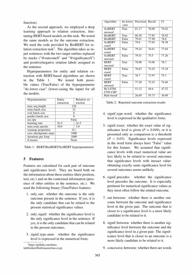
function).As the second approach, we employed a deep
learning approach to relation extraction, fine-tuning BERT-based models on this task. We testedthe same models as for the outcome extraction.We used the code provided by BioBERT for re-lation extraction task2. The algorithm takes as in-put sentences with the two target entities replacedby masks (”@outcome$” and ”@significance$”)and positive/negative relation labels assigned tothe sentence.
Hyperparameters for entity and relation ex-traction with BERT-based algorithms are shownin the Table 1. We tested both possi-ble values (True/False) of the hyperparameter”do lower case” (lower-casing the input) for allthe models.
Hyperparameter Entityextraction
Relation ex-traction
max seq length 128train batch size 32eval batch size 8predict batch size 8use tpu Falselearning rate 5e-5 2e-5num train epochs 10.0 3.0warmup proportion 0.1save checkpoints steps 1000iterations per loop 1000tf.master None
Table 1: BERT/BioBERT/SciBERT hyperparameters
5 Features
Features are calculated for each pair of outcomeand significance level. They are based both onthe information about these entities (their position,text, etc.) and on the contextual information (pres-ence of other entities in the sentence, etc.). Weused the following binary (True/False) features:
1. only out: whether the outcome is the onlyoutcome present in the sentence. If yes, it isthe only candidate that can be related to thepresent statistical significance values.
2. only signif: whether the significance level isthe only significance level in the sentence. Ifyes, it is the only candidate that can be relatedto the present outcomes.
3. signif type num: whether the significancelevel is expressed in the numerical form;
2https://github.com/dmis-lab/biobert/blob/master/run re.py
Algorithm do lowercase
Precision Recall F1
SciBERTuncased
True 81.17 78.09 79.42
BioBERT True 80.38 77.85 78.92BioBERT False 79.61 77.98 78.6SciBERTcased
False 79.6 77.65 78.38
SciBERTcased
True 79.24 76.61 77.64
SciBERTuncased
False 79.51 75.5 77.26
BERTuncased
True 78.98 74.96 76.7
BERTcased
False 76.63 74.25 75.18
BERTcased
True 76.7 73.97 75.1
BERTuncased
False 77.28 72.25 74.46
Bi-LSTM-CNN-CRF
51.12 44.6 47.52
Rule-based 26.69 55.73 36.09
Table 2: Reported outcome extraction results
4. signif type word: whether the significancelevel is expressed in the qualitative form;
5. signif exact: whether the exact value of sig-nificance level is given (P = 0.049), or it ispresented only as comparison to a threshold(P < 0.05). Significance levels expressedin the word form always have ”False” valuefor this feature. We assumed that signifi-cance levels with exact numerical value areless likely to be related to several outcomesthat significance levels with inexact value:obtaining exactly same significance level forseveral outcomes seems unlikely.
6. signif precedes: whether the significancelevel precedes the outcome. It is especiallypertinent for numerical significance values asthey most often follow the related outcome.
7. out between: whether there is another out-come between the outcome and significancelevel in the given pair. The outcome that iscloser to a significance level is a more likelycandidate to be related to it.
8. signif between: whether there is another sig-nificance level between the outcome and thesignificance level in a given pair. The signif-icance level that is closer to an outcome is amore likely candidate to be related to it.
9. concessive between: whether there are words
365
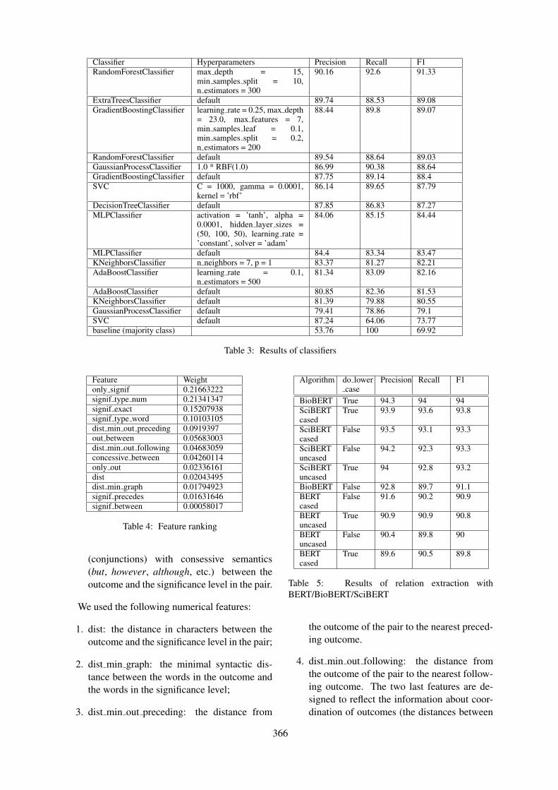
Classifier Hyperparameters Precision Recall F1RandomForestClassifier max depth = 15,
min samples split = 10,n estimators = 300
90.16 92.6 91.33
ExtraTreesClassifier default 89.74 88.53 89.08GradientBoostingClassifier learning rate = 0.25, max depth
= 23.0, max features = 7,min samples leaf = 0.1,min samples split = 0.2,n estimators = 200
88.44 89.8 89.07
RandomForestClassifier default 89.54 88.64 89.03GaussianProcessClassifier 1.0 * RBF(1.0) 86.99 90.38 88.64GradientBoostingClassifier default 87.75 89.14 88.4SVC C = 1000, gamma = 0.0001,
kernel = ’rbf’86.14 89.65 87.79
DecisionTreeClassifier default 87.85 86.83 87.27MLPClassifier activation = ’tanh’, alpha =
0.0001, hidden layer sizes =(50, 100, 50), learning rate =’constant’, solver = ’adam’
84.06 85.15 84.44
MLPClassifier default 84.4 83.34 83.47KNeighborsClassifier n neighbors = 7, p = 1 83.37 81.27 82.21AdaBoostClassifier learning rate = 0.1,
n estimators = 50081.34 83.09 82.16
AdaBoostClassifier default 80.85 82.36 81.53KNeighborsClassifier default 81.39 79.88 80.55GaussianProcessClassifier default 79.41 78.86 79.1SVC default 87.24 64.06 73.77baseline (majority class) 53.76 100 69.92
Table 3: Results of classifiers
Feature Weightonly signif 0.21663222signif type num 0.21341347signif exact 0.15207938signif type word 0.10103105dist min out preceding 0.0919397out between 0.05683003dist min out following 0.04683059concessive between 0.04260114only out 0.02336161dist 0.02043495dist min graph 0.01794923signif precedes 0.01631646signif between 0.00058017
Table 4: Feature ranking
(conjunctions) with consessive semantics(but, however, although, etc.) between theoutcome and the significance level in the pair.
We used the following numerical features:
1. dist: the distance in characters between theoutcome and the significance level in the pair;
2. dist min graph: the minimal syntactic dis-tance between the words in the outcome andthe words in the significance level;
3. dist min out preceding: the distance from
Algorithm do lowercase
Precision Recall F1
BioBERT True 94.3 94 94SciBERTcased
True 93.9 93.6 93.8
SciBERTcased
False 93.5 93.1 93.3
SciBERTuncased
False 94.2 92.3 93.3
SciBERTuncased
True 94 92.8 93.2
BioBERT False 92.8 89.7 91.1BERTcased
False 91.6 90.2 90.9
BERTuncased
True 90.9 90.9 90.8
BERTuncased
False 90.4 89.8 90
BERTcased
True 89.6 90.5 89.8
Table 5: Results of relation extraction withBERT/BioBERT/SciBERT
the outcome of the pair to the nearest preced-ing outcome.
4. dist min out following: the distance fromthe outcome of the pair to the nearest follow-ing outcome. The two last features are de-signed to reflect the information about coor-dination of outcomes (the distances between
366
coordinated entities is typically small), as co-ordinated outcomes are likely to be related tothe same significance level.
We assessed the importance of the features withthe attribute ”feature importances ” of the Ran-domForestClassifier classifier. The results are pre-sented in the Table 4.
6 Evaluation
6.1 Entity extraction
The rule-based extraction of significance levelsshows the following per-token performance: pre-cision of 99.18%, recall of 96.58% and F-measureof 97.86%.
The results of all the tested approaches to theextraction of reported outcomes are reported in theTable 2. The best performance was achieved bythe fine-tuned SciBERT uncased model: precisionwas 81.17%, recall was 78.09% and F-measurewas 79.42%.
6.2 Relation extraction
The baseline value is based on assigning the ma-jority (positive) class to all the entity pairs. Base-line precision is 53.76%, recall is 100% and F-measure is 69.95%.
The results of the classifiers are presented inthe Table 3. We present the performance ofthe default classifiers and of the classifiers withtuned hyperparameters. All the classifiers out-performed the baseline. Random Forest Clas-sifier with tuned hyperparameters (max depth= 15, min samples split = 10, n estimators =300) showed the best results, with F-measure of91.33%, which is by 21.41% higher than the base-line.
It is interesting to compare the deep learning ap-proach using BERT-based fine-tuned models (Ta-ble 5) to the feature-based classifiers: none of theGoogle BERT models outperformed the RandomForest Classifier, neither did BioBERT with un-changed input data. However, all the SciBERTfine-tuned models and the BioBERT model withlower-cased input outperformed the Random For-est Classifier. Interestingly, BioBERT, which onlyhas a cased model pre-trained on unchanged dataand is thus meant to work with unchanged input,showed the best performance on lower-cased in-put for the relation extraction task, achieving theF-measure of 94%.
7 Conclusion and future work
In this paper, we presented a first approach to-wards the extraction of the relation between out-comes of clinical trials and their reported signifi-cance levels. We presented our annotated corpusfor this task and described the ways of reportingoutcomes, significance levels and their relation ina text. We pointed out the difficulties posed by thehigh diversity of the data.
We crafted a feature set for relation extractionand trained and tested a number of classifiers forthis task. The best performance was shown bythe Random Forest classifier, with the F-measureof 91.33%. Further, we fine-tuned and evalu-ated a few deep learning models (BERT, SciBERT,BioBERT). The best performance was achievedby the BioBERT model fine-tuned on lower-caseddata, with F-measure of 94%.
Our relation extraction algorithm assumes thatthe entities have been previously extracted andprovided as input. An interesting direction for fu-ture experiments is building an end-to-end systemextracting both entities and relations, as proposedby (Miwa and Bansal, 2016) or (Pawar et al.,2017).
As in our algorithm the extraction of the rele-vant entities (reported outcomes and significancelevels) is essential for extracting the relations,we reported the results of our experiments forextracting this task. Extraction of significancelevels reaches the F-measure of 97.86%, whilethe extraction of reported outcomes shows the F-measure of only 79.42%. Thus, improving the out-come extraction is the main direction of the futurework.
Besides, a very important task for clinical trialdata analysis consists in determining the signifi-cance level for the primary outcome. This taskrequires two additional steps: 1) identifying theprimary outcome, and 2) establishing the corre-spondence between the primary outcome and a re-ported outcome. We will present our algorithmsfor these tasks in a separate paper.
8 Acknowledgements
We thank Sanjay Kamath for his help in conduct-ing experiments with BERT.
This project has received funding from the Eu-ropean Unions Horizon 2020 research and inno-vation programme under the Marie Sklodowska-Curie grant agreement No 676207.
367
ReferencesM. Abadi, P. Barham, J. Chen, Z. Chen, A. Davis,
J. Dean, M. Devin, S. Ghemawat, G. Irving, M. Is-ard, M. Kudlur, J. Levenberg, R. Monga, S. Moore,D. G. Murray, B. Steiner, P. Tucker, V. Vasudevan,P. Warden, M. Wicke, Y. Yu, and X. Zheng. 2016.Tensorflow: A system for large-scale machine learn-ing.
N.S. Altman. 1992. An introduction to kernel andnearest-neighbor nonparametric regression. Amer-ican Statistician - AMER STATIST, 46:175–185.
Koroleva Anna. 2019. Annotated corpus for the re-lation between reported outcomes and their signif-icance levels.
Masaki Asada, Makoto Miwa, and Yutaka Sasaki.2017. Extracting drug-drug interactions with atten-tion CNNs. In BioNLP 2017, pages 9–18, Vancou-ver, Canada,. Association for Computational Lin-guistics.
Iz Beltagy, Arman Cohan, and Kyle Lo. 2019. Scibert:Pretrained contextualized embeddings for scientifictext.
Jari Björne and Tapio Salakoski. 2018. Biomedi-cal event extraction using convolutional neural net-works and dependency parsing. In BioNLP 2018workshop, pages 98–108, Melbourne, Australia.ACL.
C. Blake and A. Lucic. 2015. Automatic endpoint de-tection to support the systematic review process. J.Biomed. Inform.
Isabelle Boutron, Douglas Altman, Sally Hopewell,Francisco Vera-Badillo, Ian Tannock, and PhilippeRavaud. 2014. Impact of spin in the abstracts of ar-ticles reporting results of randomized controlled tri-als in the field of cancer: the spiin randomized con-trolled trial. Journal of Clinical Oncology.
Leo Breiman. 2001. Random forests. Mach. Learn.,45(1):5–32.
David Chavalarias, Joshua D Wallach, Alvin Ho TingLi, and John P. A. Ioannidis. 2016. Evolution of re-porting p values in the biomedical literature, 1990-2015. JAMA, 315 11:1141–8.
François Chollet et al. 2015. Keras.
Corinna Cortes and Vladimir Vapnik. 1995. Support-vector networks. Machine Learning, 20(3):273–297.
D. Demner-Fushman, B. Few, S.E. Hauser, andG. Thoma. 2006. Automatically identifying healthoutcome information in medline records. Journal ofthe American Medical Informatics Association.
Jacob Devlin, Ming-Wei Chang, Kenton Lee, andKristina Toutanova. 2018. BERT: pre-training ofdeep bidirectional transformers for language under-standing. CoRR, abs/1810.04805.
Yoav Freund and Robert E Schapire. 1997. A decision-theoretic generalization of on-line learning and anapplication to boosting. Journal of Computer andSystem Sciences, 55(1):119 – 139.
Jerome H. Friedman. 2002. Stochastic gradient boost-ing. Comput. Stat. Data Anal., 38(4):367–378.
Pierre Geurts, Damien Ernst, and Louis Wehenkel.2006. Extremely randomized trees. Mach. Learn.,63(1):3–42.
R. Haneef, C. Lazarus, P. Ravaud, A. Yavchitz, andI. Boutron. 2015. Interpretation of results of stud-ies evaluating an intervention highlighted in googlehealth news: a cross-sectional study of news. PLoSONE.
Megan L Head, Luke Holman, Rob Lanfear, Andrew T.Kahn, and Michael D. Jennions. 2015. The extentand consequences of p-hacking in science. In PLoSbiology.
Matthew Honnibal and Mark Johnson. 2015. An im-proved non-monotonic transition system for depen-dency parsing. In Proc. of EMNLP 2015, pages1373–1378, Lisbon, Portugal. Association for Com-putational Linguistics.
William Hsu, William Speier, and Ricky K. Taira.2012. Automated extraction of reported statisti-cal analyses: Towards a logical representation ofclinical trial literature. AMIA Annual Symposium,2012:350–359.
Jinhyuk Lee, Wonjin Yoon, Sungdong Kim,Donghyeon Kim, Sunkyu Kim, Chan Ho So, andJaewoo Kang. 2019. Biobert: a pre-trained biomed-ical language representation model for biomedicaltext mining. arXiv preprint arXiv:1901.08746.
Jake Lever and Steven Jones. 2017. Painless rela-tion extraction with kindred. In BioNLP 2017,pages 176–183, Vancouver, Canada,. Associationfor Computational Linguistics.
A. Lucic and C. Blake. 2016. Improving endpoint de-tection to support automated systematic reviews. InAMIA Annu Symp Proc.
Xuezhe Ma and Eduard Hovy. 2016. End-to-end se-quence labeling via bi-directional lstm-cnns-crf. InProceedings of the 54th Annual Meeting of the ACL(Volume 1: Long Papers), pages 1064–1074, Berlin,Germany. Association for Computational Linguis-tics.
Christoph von der Malsburg. 1986. Frank rosenblatt:Principles of neurodynamics: Perceptrons and thetheory of brain mechanisms. Brain Theory, pages245–248.
Makoto Miwa and Mohit Bansal. 2016. End-to-end re-lation extraction using LSTMs on sequences and treestructures. In Proceedings of the 54th Annual Meet-ing of the Association for Computational Linguistics
368
(Volume 1: Long Papers), pages 1105–1116, Berlin,Germany. Association for Computational Linguis-tics.
Sachin Pawar, Pushpak Bhattacharyya, and Girish Pal-shikar. 2017. End-to-end relation extraction usingneural networks and Markov logic networks. In Pro-ceedings of the 15th Conference of the EuropeanChapter of the Association for Computational Lin-guistics: Volume 1, Long Papers, pages 818–827,Valencia, Spain. Association for Computational Lin-guistics.
F. Pedregosa, G. Varoquaux, A. Gramfort, V. Michel,B. Thirion, O. Grisel, M. Blondel, P. Pretten-hofer, R. Weiss, V. Dubourg, J. Vanderplas, A. Pas-sos, D. Cournapeau, M. Brucher, M. Perrot, andE. Duchesnay. 2011. Scikit-learn: Machine learningin Python. Journal of Machine Learning Research,12:2825–2830.
Yifan Peng and Zhiyong Lu. 2017. Deep learning forextracting protein-protein interactions from biomed-ical literature. In BioNLP 2017, pages 29–38,Vancouver, Canada,. Association for ComputationalLinguistics.
Yifan Peng, Manabu Torii, Cathy Wu, and K Vijay-Shanker. 2014. A generalizable nlp frameworkfor fast development of pattern-based biomedicalrelation extraction systems. BMC bioinformatics,15:285.
Jeffrey Pennington, Richard Socher, and ChristopherManning. 2014. Glove: Global vectors for wordrepresentation. In Proc. of EMNLP 2014, pages1532–1543, Doha, Qatar. Association for Computa-tional Linguistics.
Carl Edward Rasmussen and Christopher K. I.Williams. 2005. Gaussian Processes for Ma-chine Learning (Adaptive Computation and Ma-chine Learning). The MIT Press.
Lior Rokach and Oded Maimon. 2008. Data Min-ing with Decision Trees: Theroy and Applications.World Scientific Publishing Co., Inc., River Edge,NJ, USA.
Thomas M. Schindler. 2015. Hypothesis testing inclinical trials. AMWA Journal, 30(2).
A. Yavchitz, I. Boutron, A. Bafeta, I. Marroun,P. Charles, J. Mantz, and P. Ravaud. 2012. Misrep-resentation of randomized controlled trials in pressreleases and news coverage: a cohort study. PLoSMed.
Deyu Zhou, Dayou Zhong, and Yulan He. 2014.Biomedical relation extraction: From binary to com-plex. In Comp. Math. Methods in Medicine.
369
Proceedings of the BioNLP 2019 workshop, pages 370–379Florence, Italy, August 1, 2019. c©2019 Association for Computational Linguistics
Overview of the MEDIQA 2019 Shared Task on Textual Inference,Question Entailment and Question Answering
Asma Ben Abacha1
Chaitanya Shivade2
[email protected], NLM, Bethesda, MD 2IBM, Almaden Research Center, San Jose, CA
Dina Demner-Fushman1
Abstract
This paper presents the MEDIQA 2019 sharedtask organized at the ACL-BioNLP work-shop. The shared task is motivated by aneed to develop relevant methods, techniquesand gold standards for inference and entail-ment in the medical domain, and their ap-plication to improve domain specific infor-mation retrieval and question answering sys-tems. MEDIQA 2019 includes three tasks:Natural Language Inference (NLI), Recogniz-ing Question Entailment (RQE), and QuestionAnswering (QA) in the medical domain. 72teams participated in the challenge, achievingan accuracy of 98% in the NLI task, 74.9% inthe RQE task, and 78.3% in the QA task. Inthis paper, we describe the tasks, the datasets,and the participants’ approaches and results.We hope that this shared task will attract fur-ther research efforts in textual inference, ques-tion entailment, and question answering in themedical domain.
1 Introduction
The first open-domain challenge in RecognizingTextual Entailment (RTE) was launched in 2005(Dagan et al., 2005) and has prompted the de-velopment of a wide range of approaches (Bar-Haim et al., 2014). Recently, large-scale datasetssuch as SNLI (Bowman et al., 2015) and MultiNLI(Williams et al., 2018) were introduced for thetask of Natural Language Inference (NLI) target-ing three relations between sentences: Entailment,Neutral, and Contradiction. Few efforts have stud-ied the benefits of RTE and NLI in other NLP taskssuch as text exploration (Adler et al., 2012), identi-fying evidence for eligibility criteria satisfaction inclinical trials (Shivade et al., 2015), and the sum-marization of PMC articles (Chachra et al., 2016).
NLI can also be beneficial for Question An-swering (QA). Harabagiu and Hickl (2006) pre-sented entailment-based methods to filter and rankanswers and showed that RTE can enhance the
performance of open-domain QA systems andprovide the inferential information needed to val-idate the answers. Çelikyilmaz et al. (2009) pre-sented a graph-based semi-supervised method forQA exploiting entailment relations between ques-tions and candidate answers and demonstratedthat the use of unlabeled entailment data can im-prove answer ranking. Ben Abacha and Demner-Fushman (2016) noted that the requirements ofquestion entailment in QA are different from gen-eral question similarity, and introduced the taskof Recognizing Question Entailment (RQE) in or-der to answer new questions by retrieving entailedquestions with pre-existing answers. Ben Abachaand Demner-Fushman (2019) proposed a novelQA approach based on RQE, with the introductionof the MedQuAD medical question-answer collec-tion, and showed empirical evidence supportingquestion entailment for QA.
Although the idea of using entailment in QA hasbeen introduced, research investigating methods toincorporate textual inference and question entail-ment into QA systems is still limited in the litera-ture. Moreover, despite a few recent efforts to de-sign RTE methods and datasets from MEDLINEabstracts (Ben Abacha et al., 2015) and to createthe MedNLI dataset from clinical data (Romanovand Shivade, 2018), the entailment and inferencetasks remain less studied in the medical domain.
MEDIQA 20191 aims to highlight further theNLI and RQE tasks in the medical domain,and their applications in QA and NLP. Figure 2presents the MEDIQA tasks in the AIcrowd plat-form2. For the QA task, participants were taskedto filter and re-rank the provided answers. Reuseof the systems developed in the first and secondtasks was highly encouraged.
1https://sites.google.com/view/mediqa2019
2https://www.aicrowd.com/organizers/mediqa-acl-bionlp
370
Figure 1: MEDIQA tasks on AIcrowd
2 Tasks
2.1 Natural Language Inference (NLI)
The first task focuses on Natural Language Infer-ence (NLI) in the medical domain. We use threelabels for the relation between two sentences: En-tailment, Neutral and Contradiction.
2.2 Recognizing Question entailment (RQE)
The second task tackles Recognizing Question en-tailment (RQE) in the medical domain. We use thefollowing definition tailored to QA: “a question Aentails a question B if every answer to B is also acomplete or partial answer to A” (Ben Abacha andDemner-Fushman, 2016).
2.3 Question Answering (QA)
The objective of this task is to filter and im-prove the ranking of automatically retrieved an-swers. The input ranks are generated by themedical QA system CHiQA3. We highly recom-mended the reuse of the RQE and NLI systems(first tasks). For instance (i) the RQE system couldbe used to retrieve answered questions (e.g. fromthe MedQuAD dataset4) that are entailed from theoriginal questions and use their answers to validatethe system’s answers and re-rank them; and (ii) theNLI system could be used to identify the relations(i.e. entailment, contradiction, neutral) betweenthe answers of the same question, as well as theanswers of the questions related by the entailmentrelation. We encouraged all other ideas and ap-proaches for using textual inference and questionentailment to filter and re-rank the retrieved an-swers.
3https://chiqa.nlm.nih.gov/4github.com/abachaa/MedQuAD
3 Data Description
3.1 NLI Datasets
The MEDIQA-NLI test set consists of 405 text-hypothesis pairs. The training set is the MedNLIdataset, which includes 14,049 clinical sentencepairs derived from the MIMIC-III database (Ro-manov and Shivade, 2018). Both datasets are pub-licly available5.
3.2 RQE Datasets
The MEDIQA-RQE test set consists of 230 pairsof Consumer Health Questions (CHQs) receivedby the U.S. National Library of Medicine (NLM)and Frequently Asked Questions (FAQs) fromNIH institutes. The collection was created auto-matically and double validated manually by med-ical experts. Table 1 presents positive and nega-tive examples from the test set. The RQE train-ing and validation sets contain respectively 8,890and 302 medical question pairs created by (BenAbacha and Demner-Fushman, 2016) using a col-lection of clinical questions (Ely et al., 2000) forthe training set and pairs of CHQs and FAQs pairsfor the validation set. All the RQE training, vali-dation and test sets are publicly available6.
3.3 QA Datasets
The MEDIQA-QA training, validation and testsets were created by submitting medical ques-tions to the consumer health QA system CHiQA(Demner-Fushman et al., 2019), and then ratingand re-ranking the retrieved answers manually bymedical experts to provide reference ranks (1 to11) and scores (4: Excellent Answer, 3: Correctbut Incomplete, 2: Related, 1: Incorrect).
We provided two training sets for the QA task:
• 104 consumer health questions from theTREC-2017-LiveQA medical data (BenAbacha et al., 2017) covering differenttopics such as diseases and drugs, and 839associated answers retrieved by CHiQA andmanually rated and re-ranked.
• 104 simple questions about the most frequentdiseases (dataset named Alexa), and 862 as-sociated answers.
5https://alpha.physionet.org/content/mednli-bionlp19/1.0.0/
6https://github.com/abachaa/MEDIQA2019/tree/master/MEDIQA_Task2_RQE
371
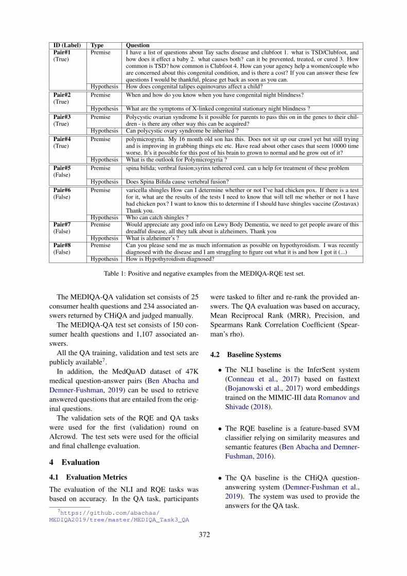
ID (Label) Type QuestionPair#1(True)
Premise I have a list of questions about Tay sachs disease and clubfoot 1. what is TSD/Clubfoot, andhow does it effect a baby 2. what causes both? can it be prevented, treated, or cured 3. Howcommon is TSD? how common is Clubfoot 4. How can your agency help a women/couple whoare concerned about this congenital condition, and is there a cost? If you can answer these fewquestions I would be thankful, please get back as soon as you can.
Hypothesis How does congenital talipes equinovarus affect a child?Pair#2(True)
Premise When and how do you know when you have congenital night blindness?
Hypothesis What are the symptoms of X-linked congenital stationary night blindness ?Pair#3(True)
Premise Polycystic ovarian syndrome Is it possible for parents to pass this on in the genes to their chil-dren - is there any other way this can be acquired?
Hypothesis Can polycystic ovary syndrome be inherited ?Pair#4(True)
Premise polymicrogyria. My 16 month old son has this. Does not sit up our crawl yet but still tryingand is improving in grabbing things etc etc. Have read about other cases that seem 10000 timeworse. It’s it possible for this post of his brain to grown to normal and he grow out of it?
Hypothesis What is the outlook for Polymicrogyria ?Pair#5(False)
Premise spina bifida; vertbral fusion;syrinx tethered cord. can u help for treatment of these problem
Hypothesis Does Spina Bifida cause vertebral fusion?Pair#6(False)
Premise varicella shingles How can I determine whether or not I’ve had chicken pox. If there is a testfor it, what are the results of the tests I need to know that will tell me whether or not I havehad chicken pox? I want to know this to determine if I should have shingles vaccine (Zostavax)Thank you.
Hypothesis Who can catch shingles ?Pair#7(False)
Premise Would appreciate any good info on Lewy Body Dementia, we need to get people aware of thisdreadful disease, all they talk about is alzheimers. Thank you
Hypothesis What is alzheimer’s ?Pair#8(False)
Premise Can you please send me as much information as possible on hypothyroidism. I was recentlydiagnosed with the disease and I am struggling to figure out what it is and how I got it (...)
Hypothesis How is Hypothyroidism diagnosed?
Table 1: Positive and negative examples from the MEDIQA-RQE test set.
The MEDIQA-QA validation set consists of 25consumer health questions and 234 associated an-swers returned by CHiQA and judged manually.
The MEDIQA-QA test set consists of 150 con-sumer health questions and 1,107 associated an-swers.
All the QA training, validation and test sets arepublicly available7.
In addition, the MedQuAD dataset of 47Kmedical question-answer pairs (Ben Abacha andDemner-Fushman, 2019) can be used to retrieveanswered questions that are entailed from the orig-inal questions.
The validation sets of the RQE and QA taskswere used for the first (validation) round onAIcrowd. The test sets were used for the officialand final challenge evaluation.
4 Evaluation
4.1 Evaluation Metrics
The evaluation of the NLI and RQE tasks wasbased on accuracy. In the QA task, participants
7https://github.com/abachaa/MEDIQA2019/tree/master/MEDIQA_Task3_QA
were tasked to filter and re-rank the provided an-swers. The QA evaluation was based on accuracy,Mean Reciprocal Rank (MRR), Precision, andSpearmans Rank Correlation Coefficient (Spear-man’s rho).
4.2 Baseline Systems
• The NLI baseline is the InferSent system(Conneau et al., 2017) based on fasttext(Bojanowski et al., 2017) word embeddingstrained on the MIMIC-III data Romanov andShivade (2018).
• The RQE baseline is a feature-based SVMclassifier relying on similarity measures andsemantic features (Ben Abacha and Demner-Fushman, 2016).
• The QA baseline is the CHiQA question-answering system (Demner-Fushman et al.,2019). The system was used to provide theanswers for the QA task.
372
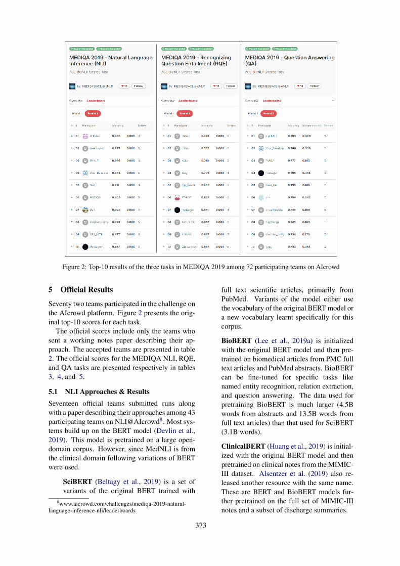
Figure 2: Top-10 results of the three tasks in MEDIQA 2019 among 72 participating teams on AIcrowd
5 Official Results
Seventy two teams participated in the challenge onthe AIcrowd platform. Figure 2 presents the orig-inal top-10 scores for each task.
The official scores include only the teams whosent a working notes paper describing their ap-proach. The accepted teams are presented in table2. The official scores for the MEDIQA NLI, RQE,and QA tasks are presented respectively in tables3, 4, and 5.
5.1 NLI Approaches & ResultsSeventeen official teams submitted runs alongwith a paper describing their approaches among 43participating teams on NLI@AIcrowd8. Most sys-tems build up on the BERT model (Devlin et al.,2019). This model is pretrained on a large open-domain corpus. However, since MedNLI is fromthe clinical domain following variations of BERTwere used.
SciBERT (Beltagy et al., 2019) is a set ofvariants of the original BERT trained with
8www.aicrowd.com/challenges/mediqa-2019-natural-language-inference-nli/leaderboards
full text scientific articles, primarily fromPubMed. Variants of the model either usethe vocabulary of the original BERT model ora new vocabulary learnt specifically for thiscorpus.
BioBERT (Lee et al., 2019a) is initializedwith the original BERT model and then pre-trained on biomedical articles from PMC fulltext articles and PubMed abstracts. BioBERTcan be fine-tuned for specific tasks likenamed entity recognition, relation extraction,and question answering. The data used forpretraining BioBERT is much larger (4.5Bwords from abstracts and 13.5B words fromfull text articles) than that used for SciBERT(3.1B words).
ClinicalBERT (Huang et al., 2019) is initial-ized with the original BERT model and thenpretrained on clinical notes from the MIMIC-III dataset. Alsentzer et al. (2019) also re-leased another resource with the same name.These are BERT and BioBERT models fur-ther pretrained on the full set of MIMIC-IIInotes and a subset of discharge summaries.
373
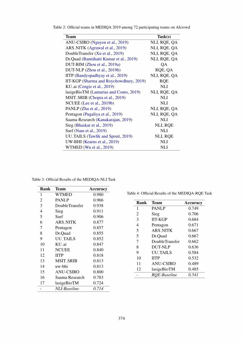
Table 2: Official teams in MEDIQA 2019 among 72 participating teams on AIcrowd
Team Task(s)ANU-CSIRO (Nguyen et al., 2019) NLI, RQE, QAARS NITK (Agrawal et al., 2019) NLI, RQE, QADoubleTransfer (Xu et al., 2019) NLI, RQE, QADr.Quad (Bannihatti Kumar et al., 2019) NLI, RQE, QADUT-BIM (Zhou et al., 2019a) QADUT-NLP (Zhou et al., 2019b) RQE, QAIITP (Bandyopadhyay et al., 2019) NLI, RQE, QAIIT-KGP (Sharma and Roychowdhury, 2019) RQEKU ai (Cengiz et al., 2019) NLIlasigeBioTM (Lamurias and Couto, 2019) NLI, RQE, QAMSIT SRIB (Chopra et al., 2019) NLINCUEE (Lee et al., 2019b) NLIPANLP (Zhu et al., 2019) NLI, RQE, QAPentagon (Pugaliya et al., 2019) NLI, RQE, QASaama Research (Kanakarajan, 2019) NLISieg (Bhaskar et al., 2019) NLI, RQESurf (Nam et al., 2019) NLIUU TAILS (Tawfik and Spruit, 2019) NLI, RQEUW-BHI (Kearns et al., 2019) NLIWTMED (Wu et al., 2019) NLI
Table 3: Official Results of the MEDIQA-NLI Task
Rank Team Accuracy1 WTMED 0.9802 PANLP 0.9663 DoubleTransfer 0.9384 Sieg 0.9115 Surf 0.9066 ARS NITK 0.8777 Pentagon 0.8578 Dr.Quad 0.8559 UU TAILS 0.85210 KU ai 0.84711 NCUEE 0.84012 IITP 0.81813 MSIT SRIB 0.81314 uw-bhi 0.81315 ANU-CSIRO 0.80016 Saama Research 0.78317 lasigeBioTM 0.724- NLI-Baseline 0.714
Table 4: Official Results of the MEDIQA-RQE Task
Rank Team Accuracy1 PANLP 0.7492 Sieg 0.7063 IIT-KGP 0.6844 Pentagon 0.6715 ARS NITK 0.6675 Dr.Quad 0.6677 DoubleTransfer 0.6628 DUT-NLP 0.6369 UU TAILS 0.58410 IITP 0.53211 ANU-CSIRO 0.48912 lasigeBioTM 0.485- RQE-Baseline 0.541
374
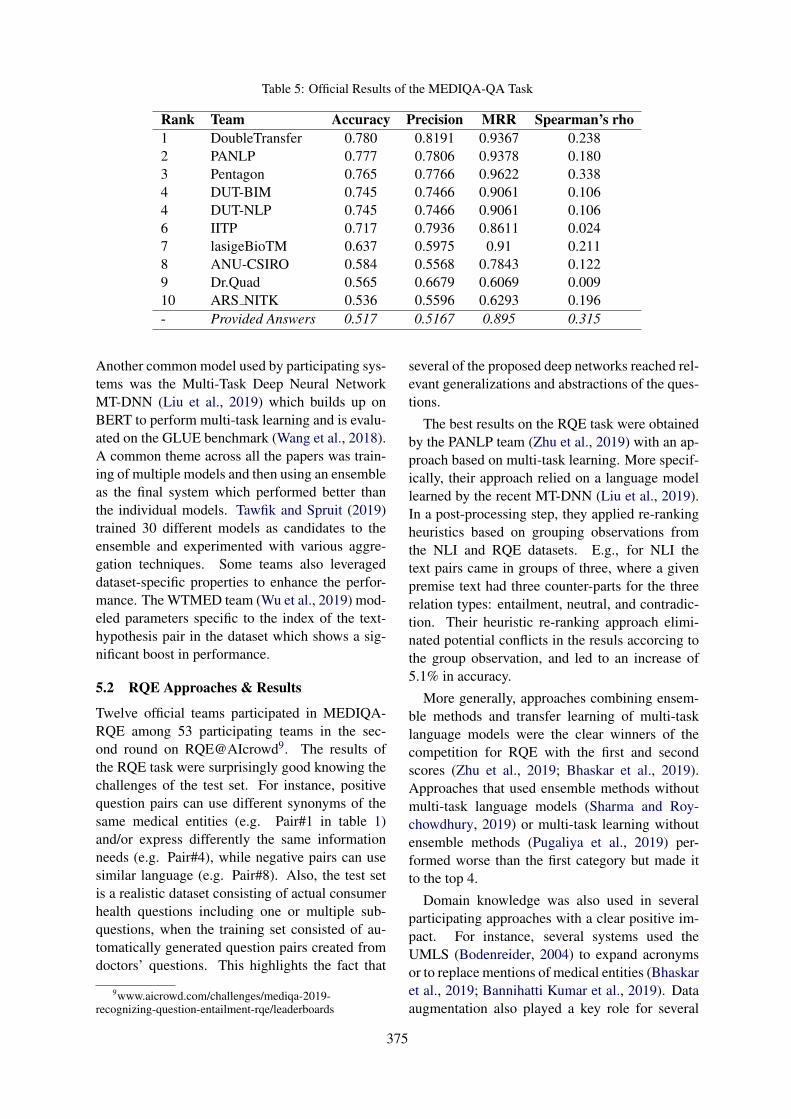
Table 5: Official Results of the MEDIQA-QA Task
Rank Team Accuracy Precision MRR Spearman’s rho1 DoubleTransfer 0.780 0.8191 0.9367 0.2382 PANLP 0.777 0.7806 0.9378 0.1803 Pentagon 0.765 0.7766 0.9622 0.3384 DUT-BIM 0.745 0.7466 0.9061 0.1064 DUT-NLP 0.745 0.7466 0.9061 0.1066 IITP 0.717 0.7936 0.8611 0.0247 lasigeBioTM 0.637 0.5975 0.91 0.2118 ANU-CSIRO 0.584 0.5568 0.7843 0.1229 Dr.Quad 0.565 0.6679 0.6069 0.00910 ARS NITK 0.536 0.5596 0.6293 0.196- Provided Answers 0.517 0.5167 0.895 0.315
Another common model used by participating sys-tems was the Multi-Task Deep Neural NetworkMT-DNN (Liu et al., 2019) which builds up onBERT to perform multi-task learning and is evalu-ated on the GLUE benchmark (Wang et al., 2018).A common theme across all the papers was train-ing of multiple models and then using an ensembleas the final system which performed better thanthe individual models. Tawfik and Spruit (2019)trained 30 different models as candidates to theensemble and experimented with various aggre-gation techniques. Some teams also leverageddataset-specific properties to enhance the perfor-mance. The WTMED team (Wu et al., 2019) mod-eled parameters specific to the index of the text-hypothesis pair in the dataset which shows a sig-nificant boost in performance.
5.2 RQE Approaches & Results
Twelve official teams participated in MEDIQA-RQE among 53 participating teams in the sec-ond round on RQE@AIcrowd9. The results ofthe RQE task were surprisingly good knowing thechallenges of the test set. For instance, positivequestion pairs can use different synonyms of thesame medical entities (e.g. Pair#1 in table 1)and/or express differently the same informationneeds (e.g. Pair#4), while negative pairs can usesimilar language (e.g. Pair#8). Also, the test setis a realistic dataset consisting of actual consumerhealth questions including one or multiple sub-questions, when the training set consisted of au-tomatically generated question pairs created fromdoctors’ questions. This highlights the fact that
9www.aicrowd.com/challenges/mediqa-2019-recognizing-question-entailment-rqe/leaderboards
several of the proposed deep networks reached rel-evant generalizations and abstractions of the ques-tions.
The best results on the RQE task were obtainedby the PANLP team (Zhu et al., 2019) with an ap-proach based on multi-task learning. More specif-ically, their approach relied on a language modellearned by the recent MT-DNN (Liu et al., 2019).In a post-processing step, they applied re-rankingheuristics based on grouping observations fromthe NLI and RQE datasets. E.g., for NLI thetext pairs came in groups of three, where a givenpremise text had three counter-parts for the threerelation types: entailment, neutral, and contradic-tion. Their heuristic re-ranking approach elimi-nated potential conflicts in the resuls accorcing tothe group observation, and led to an increase of5.1% in accuracy.
More generally, approaches combining ensem-ble methods and transfer learning of multi-tasklanguage models were the clear winners of thecompetition for RQE with the first and secondscores (Zhu et al., 2019; Bhaskar et al., 2019).Approaches that used ensemble methods withoutmulti-task language models (Sharma and Roy-chowdhury, 2019) or multi-task learning withoutensemble methods (Pugaliya et al., 2019) per-formed worse than the first category but made itto the top 4.
Domain knowledge was also used in severalparticipating approaches with a clear positive im-pact. For instance, several systems used theUMLS (Bodenreider, 2004) to expand acronymsor to replace mentions of medical entities (Bhaskaret al., 2019; Bannihatti Kumar et al., 2019). Dataaugmentation also played a key role for several
375
systems that used external data to extend batchesof in-domain data (Xu et al., 2019), created syn-thetic data (Bannihatti Kumar et al., 2019), orused models trained on external datasets (e.g.MultiNLI) in ensemble methods (Bhaskar et al.,2019; Sharma and Roychowdhury, 2019).
5.3 QA Approaches & Results
Ten official teams participated in the QA taskamong 23 participating teams in the second roundon QA@AIcrowd10. The relevant answer classifi-cation problem was relatively challenging with abest accuracy of 78%, however most systems didwell on the first answer ranking with a best MRRof 96.22%. Precision also ranged from 79.3% to81.9% for the six first systems. Many teams usedtheir RQE and/or NLI models in the QA task (Ban-nihatti Kumar et al., 2019; Pugaliya et al., 2019;Zhu et al., 2019; Nguyen et al., 2019). The DUT-NLP team (Zhou et al., 2019b) used an adversarialmulti-task network to jointly model RQE and QA.
The approach that had the best accuracy andprecision in the QA task (Xu et al., 2019) reliedon multi-task language models (MT-DNN) and en-semble methods. To avoid overfitting, the Double-Transfer team proposed a method, called Multi-Source, that enriches the data batches during train-ing from external datasets by a 50% ratio and ran-dom selection. The final ensemble method fur-ther combines the Multi-Source method with pre-trained MT-DNN and SciBERT models by takingthe majority vote from their predictions and re-solving ties by summing the prediction probabil-ities for each label. The PANLP team’s best run(Zhu et al., 2019) ranked second in the QA task de-spite the fact that the QA data do not have a groupstructure that could be used in re-ranking heuris-tics. This shows that their core model is a strongapproach, and highlights further the outstandingperformance of ensemble methods and multi-tasklanguage models for transfer learning for naturallanguage understanding tasks.
Interestingly, the runs that did best on accuracyand precision did not have the best performancein terms of MRR and Spearman’s rank correla-tion coefficient. The best team on these two met-rics, Pentagon (Pugaliya et al., 2019), used theMedQuAD and the iCliniq datasets to retrieve en-tailed answers and used them to build more gen-
10www.aicrowd.com/challenges/mediqa-2019-question-answering-qa/leaderboards
eral embeddings of the considered answer. Theyalso integrated the top-3 RQE candidates fromthese datasets for the considered question to buildjoint embeddings. The final answer embeddingswere enriched with metadata such as the candi-date answer source, answer length, and the orig-inal system rank. The same joint embeddings arethen used in a filtering classifier for answer rel-evance and in a binary answer-to-answer classi-fier that decides if an answer is better than an-other. These generalized joint answer embeddingsand the focus on the answer-to-answer relation-ship are likely to be the key elements that led tothe best performance in MRR and Spearman’s rho,despite the fact that the approach did not rely onthe state-of-the-art ensemble models from the NLIand RQE tasks.
5.4 Multi-Tasking & External Resources
One of the aims of the MEDIQA 2019 shared taskwas to investigate ideas that can be reused acrossthe three tasks. Of the twenty working notes pa-pers, ten papers describe systems attempting morethan one task. Eight papers describe systems at-tempting all three tasks. The multi-task nature ofMEDIQA 2019 was leveraged by teams to trainmodels such as MT-DNN (e.g. (Bannihatti Kumaret al., 2019; Xu et al., 2019; Zhu et al., 2019)). TheSieg team (Bhaskar et al., 2019) trained a modelwith shared layers being trained for the NLI andRQE tasks. Some teams also reused models acrossthe three tasks. Pugaliya et al. (2019) used modelsdeveloped for NLI and RQE as feature extractorsin the QA task, which led to the best performancein MRR and Spearman’s rho.
The shared task also encouraged the use ofexternal resources other than the training dataprovided for the three tasks. Below is a non-exhaustive list resources used by various teams.
• Abbreviation expansion Many teams pre-processed the training data with UMLS forabbreviation expansion. While Nguyen et al.(2019) used the ADAM database (Zhou et al.,2006) for this task, Bannihatti Kumar et al.(2019) used a CAMC11 gazzeteer.
• External datasets Bannihatti Kumar et al.(2019) used the Quora question pairs dataset(Shankar Iyer and Csernai, 2017) to boostthe training for the RQE task, applied
11http://www.camc.org
376
MetaMap12 to recognize medical entities,and synthetically created new questions andparaphrases. Bhaskar et al. (2019) and Pu-galiya et al. (2019) used the online iCliniqforum to augment training data for the RQEtask. Pugaliya et al. (2019), Xu et al. (2019),Lamurias and Couto (2019), and Nguyenet al. (2019) used the MedQuAD13 dataset ofmedical questions and answers (Ben Abachaand Demner-Fushman, 2019).
• Word Embeddings While many teams usedBERT (Lamurias and Couto, 2019; Zhouet al., 2019a; Bandyopadhyay et al., 2019;Nguyen et al., 2019; Sharma and Roychowd-hury, 2019)14, some teams also used wordembeddings as the input to their models.Bhaskar et al. (2019) used biomedical wordembeddings from Chen et al. (2018) whileKearns et al. (2019) used cui2vec (Beamet al., 2018).
6 Conclusions
We presented the MEDIQA 2019 shared task onNatural Language Inference (NLI), RecognizingQuestion Entailment (RQE), and Question an-swering (QA) in the medical domain. The runssubmitted to the challenge by 20 official teamsamong 72 participating teams achieved promisingresults and highlighted the strength of multi-tasklanguage models, transfer learning, and ensemblemethods. Integrating domain knowledge and tar-geted data augmentation were also key factors forbest performing systems. We hope that further re-search works and insights will be developed in thefuture from the MEDIQA tasks and their publiclyavailable datasets.
Acknowledgments
This work was supported by the intramural re-search program at the U.S. National Library ofMedicine, National Institutes of Health.We would like to thank Sharada Mohanty, CEOand co-founder of AIcrowd, and Yassine Mrabetfrom the NLM for his support with the CHiQAsystem. We are also thankful to Vandana Mukher-jee from IBM Research for supporting the project.
12metamap.nlm.nih.gov13github.com/abachaa/MedQuAD14github.com/Team-IIT-KGP/Qspider
ReferencesMeni Adler, Jonathan Berant, and Ido Dagan. 2012.
Entailment-based text exploration with applicationto the health-care domain. In The 50th Annual Meet-ing of the Association for Computational Linguis-tics, System Demonstrations, 2012, Korea.
Anumeha Agrawal, Rosa Anil George, Selvan SunithaRavi, Sowmya Kamath, and Anand Kumar. 2019.Ars nitk at mediqa 2019:analysing various methodsfor natural language inference, recognising questionentailment and medical question answering system.In Proceedings of the BioNLP 2019 workshop, Flo-rence, Italy, August 1, 2019. Association for Com-putational Linguistics.
Emily Alsentzer, John R Murphy, Willie Boag, Wei-Hung Weng, Di Jin, Tristan Naumann, and MatthewMcDermott. 2019. Publicly available clinical bertembeddings. arXiv preprint arXiv:1904.03323.
Dibyanayan Bandyopadhyay, Baban Gain, TanikSaikh, and Asif Ekbal. 2019. Iitp at mediqa 2019:Systems report for natural language inference, ques-tion entailment and question answering. In Proceed-ings of the BioNLP 2019 workshop, Florence, Italy,August 1, 2019. Association for Computational Lin-guistics.
Vinayshekhar Bannihatti Kumar, Ashwin Srinivasan,Aditi Chaudhary, James Route, Teruko Mitamura,and Eric Nyberg. 2019. Dr.quad at mediqa 2019:Towards textual inference and question entailmentusing contextualized representations. In Proceed-ings of the BioNLP 2019 workshop, Florence, Italy,August 1, 2019. Association for Computational Lin-guistics.
Roy Bar-Haim, Ido Dagan, and Idan Szpektor. 2014.Benchmarking applied semantic inference: ThePASCAL recognising textual entailment challenges.In Language, Culture, Computation. Computing -Theory and Technology - Essays Dedicated to Yaa-cov Choueka on the Occasion of His 75th Birthday.
Andrew L Beam, Benjamin Kompa, Inbar Fried,Nathan P Palmer, Xu Shi, Tianxi Cai, and Isaac SKohane. 2018. Clinical concept embeddings learnedfrom massive sources of multimodal medical data.arXiv preprint arXiv:1804.01486.
Iz Beltagy, Arman Cohan, and Kyle Lo. 2019. Scibert:Pretrained contextualized embeddings for scientifictext. arXiv preprint arXiv:1903.10676.
Asma Ben Abacha, Eugene Agichtein, Yuval Pinter,and Dina Demner-Fushman. 2017. Overview ofthe medical question answering task at TREC 2017LiveQA. In Proceedings of The Twenty-Sixth TextREtrieval Conference, TREC 2017, Gaithersburg,Maryland, USA, November 15-17, 2017.
Asma Ben Abacha and Dina Demner-Fushman. 2016.Recognizing question entailment for medical ques-tion answering. In AMIA 2016, American Med-
377
ical Informatics Association Annual Symposium,Chicago, IL, USA, November 12-16, 2016.
Asma Ben Abacha and Dina Demner-Fushman. 2019.A question-entailment approach to question answer-ing. CoRR, abs/1901.08079.
Asma Ben Abacha, Duy Dinh, and Yassine Mrabet.2015. Semantic analysis and automatic corpus con-struction for entailment recognition in medical texts.In Artificial Intelligence in Medicine - 15th Confer-ence on Artificial Intelligence in Medicine, AIME2015, Pavia, Italy, June 17-20, 2015.
Sai Abishek Bhaskar, Rashi Rungta, James Route,Eric Nyberg, and Teruko Mitamura. 2019. Siegat mediqa 2019: Multi-task neural ensemble forbiomedical inference and entailment. In Proceed-ings of the BioNLP 2019 workshop, Florence, Italy,August 1, 2019. Association for Computational Lin-guistics.
Olivier Bodenreider. 2004. The unified medical lan-guage system (UMLS): integrating biomedical ter-minology. Nucleic Acids Research, 32(Database-Issue):267–270.
Piotr Bojanowski, Edouard Grave, Armand Joulin, andTomas Mikolov. 2017. Enriching word vectors withsubword information. Transactions of the Associa-tion for Computational Linguistics, 5:135–146.
Samuel R. Bowman, Gabor Angeli, Christopher Potts,and Christopher D. Manning. 2015. A large anno-tated corpus for learning natural language inference.In Proceedings of the 2015 Conference on EmpiricalMethods in Natural Language Processing, EMNLP2015, Lisbon, Portugal.
Asli Çelikyilmaz, Marcus Thint, and Zhiheng Huang.2009. A graph-based semi-supervised learning forquestion-answering. In ACL 2009, Proceedingsof the 47th Annual Meeting of the Association forComputational Linguistics and the 4th InternationalJoint Conference on Natural Language Processingof the AFNLP, 2-7 August 2009, Singapore.
Cemil Cengiz, Ula Sert, and Deniz Yuret. 2019. Ku aiat mediqa 2019: Domain-specific pre-training andtransfer learning for medical nli. In Proceedings ofthe BioNLP 2019 workshop, Florence, Italy, August1, 2019. Association for Computational Linguistics.
Suchet K. Chachra, Asma Ben Abacha, Sonya E.Shooshan, Laritza Rodriguez, and Dina Demner-Fushman. 2016. A hybrid approach to generation ofmissing abstracts in biomedical literature. In COL-ING 2016, 26th International Conference on Com-putational Linguistics, 2016, Osaka, Japan.
Qingyu Chen, Yifan Peng, and Zhiyong Lu. 2018.Biosentvec: creating sentence embeddings forbiomedical texts. arXiv preprint arXiv:1810.09302.
Sahil Chopra, Ankita Gupta, and Anupama Kaushik.2019. Msit srib at mediqa 2019: Knowledge di-rected multi-task framework for natural language in-ference in clinical domain. In Proceedings of theBioNLP 2019 workshop, Florence, Italy, August 1,2019. Association for Computational Linguistics.
Alexis Conneau, Douwe Kiela, Holger Schwenk, Loı̈cBarrault, and Antoine Bordes. 2017. Supervisedlearning of universal sentence representations fromnatural language inference data. In Proceedings ofthe 2017 Conference on Empirical Methods in Nat-ural Language Processing, pages 670–680, Copen-hagen, Denmark. Association for ComputationalLinguistics.
Ido Dagan, Oren Glickman, and Bernardo Magnini.2005. The PASCAL recognising textual entailmentchallenge. In Machine Learning Challenges, Eval-uating Predictive Uncertainty, Visual Object Clas-sification and Recognizing Textual Entailment, FirstPASCAL Machine Learning Challenges Workshop,MLCW 2005, Southampton, UK.
Dina Demner-Fushman, Asma Ben Abacha, and Yas-sine Mrabet. 2019. Consumer health informationand question answering: Helping consumers find an-swers to their health-related information needs. Sub-mitted to the Journal of the American Medical Infor-matics Association (JAMIA).
Jacob Devlin, Ming-Wei Chang, Kenton Lee, andKristina Toutanova. 2019. Bert: Pre-training of deepbidirectional transformers for language understand-ing. In Proceedings of NAACL.
John W. Ely, Jerome A. Osheroff, Paul N. Gorman,Mark H. Ebell, M. Lee Chambliss, Eric A. Pifer, andP. Zoe Stavri. 2000. A taxonomy of generic clini-cal questions: classification study. British MedicalJournal, 321:429–432.
Sanda M. Harabagiu and Andrew Hickl. 2006. Meth-ods for using textual entailment in open-domainquestion answering. In ACL 2006, 21st Interna-tional Conference on Computational Linguistics and44th Annual Meeting of the Association for Compu-tational Linguistics, Sydney, Australia.
Kexin Huang, Jaan Altosaar, and Rajesh Ranganath.2019. Clinicalbert: Modeling clinical notes and pre-dicting hospital readmission. arXiv:1904.05342.
Kamal raj Kanakarajan. 2019. Saama research atmediqa 2019: Pre-trained biobert with attention vi-sualisation for medical natural language inference.In Proceedings of the BioNLP 2019 workshop, Flo-rence, Italy, August 1, 2019. Association for Com-putational Linguistics.
William Kearns, Wilson Lau, and Jason Thomas. 2019.Uw-bhi at mediqa 2019: An analysis of representa-tion methods for medical natural language inference.In Proceedings of the BioNLP 2019 workshop, Flo-rence, Italy, August 1, 2019. Association for Com-putational Linguistics.
378
Andre Lamurias and Francisco Couto. 2019. Lasige-biotm at mediqa 2019: Biomedical question answer-ing using bidirectional transformers and named en-tity recognition. In Proceedings of the BioNLP 2019workshop, Florence, Italy, August 1, 2019. Associa-tion for Computational Linguistics.
Jinhyuk Lee, Wonjin Yoon, Sungdong Kim,Donghyeon Kim, Sunkyu Kim, Chan Ho So, andJaewoo Kang. 2019a. Biobert: pre-trained biomed-ical language representation model for biomedicaltext mining. arXiv preprint arXiv:1901.08746.
Lung-Hao Lee, Yi Lu, Po-Han Chen, Po-Lei Lee, andKuo-Kai Shyu. 2019b. Ncuee at mediqa 2019:Medical text inference using ensemble bert-bilstm-attention model. In Proceedings of the BioNLP 2019workshop, Florence, Italy, August 1, 2019. Associa-tion for Computational Linguistics.
Xiaodong Liu, Pengcheng He, Weizhu Chen, and Jian-feng Gao. 2019. Multi-task deep neural networksfor natural language understanding. arXiv preprintarXiv:1901.11504.
Jiin Nam, Seunghyun Yoon, and Kyomin Jung. 2019.Surf at mediqa 2019: Improving performance of nat-ural language inference in the clinical domain byadopting pre-trained language model. In Proceed-ings of the BioNLP 2019 workshop, Florence, Italy,August 1, 2019. Association for Computational Lin-guistics.
Vincent Nguyen, Sarvnaz Karimi, and ZhenchangXing. 2019. Anu-csiro at mediqa 2019: Questionanswering using deep contextual knowledge. InProceedings of the BioNLP 2019 workshop, Flo-rence, Italy, August 1, 2019. Association for Com-putational Linguistics.
Hemant Pugaliya, Karan Saxena, Shefali Garg, SheetalShalini, Prashant Gupta, Eric Nyberg, and TerukoMitamura. 2019. Pentagon at mediqa 2019: Multi-task learning for filtering and re-ranking answers us-ing language inference and question entailment. InProceedings of the BioNLP 2019 workshop, Flo-rence, Italy, August 1, 2019. Association for Com-putational Linguistics.
Alexey Romanov and Chaitanya Shivade. 2018.Lessons from natural language inference in the clin-ical domain. In Proceedings of the 2018 Conferenceon Empirical Methods in Natural Language Pro-cessing, Brussels, Belgium, 2018.
Nikhil Dandekar Shankar Iyer and Kornl Csernai.2017. First quora dataset release: Question pairs.
Prakhar Sharma and Sumegh Roychowdhury. 2019.Iit-kgp at mediqa 2019: Recognizing question en-tailment using sci-bert stacked with a gradient boost-ing classifier. In Proceedings of the BioNLP 2019workshop, Florence, Italy, August 1, 2019. Associa-tion for Computational Linguistics.
Chaitanya Shivade, Courtney Hebert, Marcelo A.Lopetegui, Marie-Catherine de Marneffe, Eric
Fosler-Lussier, and Albert M. Lai. 2015. Textual in-ference for eligibility criteria resolution in clinicaltrials. Journal of Biomedical Informatics, 58.
Noha Tawfik and Marco Spruit. 2019. Uu tails atmediqa 2019: Learning textual entailment in themedical domain. In Proceedings of the BioNLP2019 workshop, Florence, Italy, August 1, 2019. As-sociation for Computational Linguistics.
Alex Wang, Amapreet Singh, Julian Michael, FelixHill, Omer Levy, and Samuel R Bowman. 2018.GLUE: A multi-task benchmark and analysis plat-form for natural language understanding. arXivpreprint arXiv:1804.07461.
Adina Williams, Nikita Nangia, and Samuel R. Bow-man. 2018. A broad-coverage challenge corpusfor sentence understanding through inference. InProceedings of the 2018 Conference of the NorthAmerican Chapter of the Association for Computa-tional Linguistics: Human Language Technologies,NAACL-HLT 2018, New Orleans, Louisiana, USA.
Zhaofeng Wu, Yan Song, Sicong Huang, Yuanhe Tian,and Fei Xia. 2019. Wtmed at mediqa 2019: A hy-brid approach to biomedical natural language infer-ence. In Proceedings of the BioNLP 2019 work-shop, Florence, Italy, August 1, 2019. Associationfor Computational Linguistics.
Yichong Xu, Xiaodong Liu, Chunyuan Li, HoifungPoon, and Jianfeng Gao. 2019. Doubletransfer atmediqa 2019: Multi-source transfer learning for nat-ural language understanding in the medical domain.In Proceedings of the BioNLP 2019 workshop, Flo-rence, Italy, August 1, 2019. Association for Com-putational Linguistics.
Huiwei Zhou, Bizun Lei, Zhe Liu, and Zhuang Liu.2019a. Dut-bim at mediqa 2019: Utilizing trans-former network and medical domain-specific con-textualized representations for question answering.In Proceedings of the BioNLP 2019 workshop, Flo-rence, Italy, August 1, 2019. Association for Com-putational Linguistics.
Huiwei Zhou, Weihong Yao Xuefei Li, ChengkunLang, and Shixian Ning. 2019b. Dut-nlp at mediqa2019:an adversarial multi-task network to jointlymodel recognizing question entailment and ques-tion answering. In Proceedings of the BioNLP 2019workshop, Florence, Italy, August 1, 2019. Associa-tion for Computational Linguistics.
Wei Zhou, Vetle I Torvik, and Neil R Smalheiser. 2006.Adam: another database of abbreviations in med-line. Bioinformatics, 22(22):2813–2818.
Wei Zhu, Xiaofeng Zhou, Keqiang Wang, Xun Luo,Xiepeng Li, Yuan Ni, and Guotong Xie. 2019. Panlpat mediqa 2019: Pre-trained language models, trans-fer learning and knowledge distillation. In Proceed-ings of the BioNLP 2019 workshop, Florence, Italy,
August 1, 2019.
379
Proceedings of the BioNLP 2019 workshop, pages 380–388Florence, Italy, August 1, 2019. c©2019 Association for Computational Linguistics
PANLP at MEDIQA 2019: Pre-trained Language Models, TransferLearning and Knowledge Distillation
Wei Zhu, Xiaofeng Zhou, Keqiang Wang, Xun Luo, Xiepeng Li, Yuan Ni, Guotong XiePingan Health Tech, Shanghai, China
{zhuwei972, zhouxiaofeng824, wangkeqiang265, luoxun492, lixiepeng538,niyuan442, xieguotong}@pingan.com.cn
Abstract
This paper describes the models designated forthe MEDIQA 2019 shared tasks by the teamPANLP. We take advantages of the recent ad-vances in pre-trained bidirectional transformerlanguage models such as BERT (Devlin et al.,2018) and MT-DNN (Liu et al., 2019b). Wefind that pre-trained language models can sig-nificantly outperform traditional deep learningmodels. Transfer learning from the NLI taskto the RQE task is also experimented, whichproves to be useful in improving the results offine-tuning MT-DNN large. A knowledge dis-tillation process is implemented, to distill theknowledge contained in a set of models andtransfer it into an single model, whose perfor-mance turns out to be comparable with that ob-tained by the ensemble of that set of models.Finally, for test submissions, model ensembleand a re-ranking process are implemented toboost the performances. Our models partici-pated in all three tasks and ranked the 1st placefor the RQE task, and the 2nd place for the NLItask, and also the 2nd place for the QA task.
1 Introduction
There are three tasks in the MEDIQA 2019 sharedtasks (see Ben Abacha et al. (2019) for details ofthe tasks). The first one, NLI, consists in identi-fying three inference relations between two sen-tences: Entailment, Neutral and Contradiction.The second one, RQE, requires one to identifywhether one question entails the other, where thedefinition of entailment is that a question A entailsa question B if every answer to B is also a com-plete or partial answer to A. The third task, QA,considers not only the identification of entailmentfor the asked question among a set of retrievedquestions, but also the ranks of retrieved answers.
In this work, we demonstrate that we canachieve significant performance gains over tra-ditional deep learning models like ESIM (Chen
et al., 2016), by adapting pre-trained languagemodels into the medical domain. Language modelpre-training has shown to be effective for learn-ing universal language representations by lever-aging large amounts of unlabeled data. Some ofthe most famous examples are GPT-V2 (see Rad-ford et al., 2019) and BERT ( by Devlin et al.,2018). These are neural network language modelstrained on text data using unsupervised objectives.For example, BERT is based on a multi-layer bidi-rectional Transformer, and is trained on plain textfor masked word prediction and next sentence pre-diction tasks. To apply a pre-trained model tospecific NLU tasks such as tasks for MEDIQA2019 shared tasks, we often need to fine-tune themodel with additional task-specific layers usingtask-specific training data. For example, Devlinet al. (2018) show that BERT can be fine-tunedthis way to create state-of-the-art models for arange of NLU tasks, such as question answeringand natural language inference.
We also tryout a transfer learning procedure,where an intermediate model obtained on the NLItask is used to be fine-tuned on the RQE task. Al-though this procedure cannot consistently improvethe dev set performance for all the models, it isproven to be beneficial on the test set by addingvariety to the model pool.
To further improve the performance of sin-gle models, we implement a knowledge distil-lation procedure on the RQE task and the NLItask. Knowledge distillation distills or transfersthe knowledge from a (set of) large, cumber-some model(s) to a lighter, easier-to-deploy sin-gle model, without significant loss in performance(Liu et al., 2019a; Tan et al., 2019). Knowledgedistillation recently has attracted a lot of atten-tions. We believe it is interesting and of greatimportance to explore this method on the appli-cations of the medical domain.
380
For test submissions, model ensemble is used toobtain more stable and unbiased predictions. Weonly adopt a simple ensemble model, that is, av-eraging the class probabilities of different models.After obtaining test predictions, for the NLI andRQE task, simple re-ranking operations amongpairs with the same premise are used to boost theperformance metrics.
The rest of the paper is organized as follows. InSection 2 , we demonstrate our experiments on thethree tasks. In Section 3, transfer learning fromNLI to RQE is presented. Section 4 elaborateson the knowledge distillation and the correspond-ing experimental results. Section 5 and Section 6present the model ensemble technique and the re-ranking strategies. Section 7 explains our submis-sion records in detail. Section 8 concludes and dis-cusses future work.
2 Pairwise Text Modeling
This section elaborates on the fundamental meth-ods we used for the three tasks.
2.1 RQE
The RQE task, as a pairwise text classifica-tion task, defined here involves a premise P =(p1, p2, ..., pm) of m words, which is a medicalquestion posted online, and a hypothesis H =(h1, h2, ..., hn) of n words, which is a standardfrequently asked question that is collected to builda QA system, and aims to find a logical relation-ship R between P and H . For the RQE task,relationship R is either true or false, indicatingwhether the premise entails the hypothesis or not.We mainly experiment on two groups of models,one using fixed pre-trained embedding1, the otheremploying pre-trained language models.
Traditional deep learning models typically usea fixed pre-trained word embedding to map wordsinto low-dimensional vector space, and then usesome kind of encoders to encode and pool thecontexts of the premise to vector r1 and hy-pothesis H to r2. And the features providedto the classification layer is concat(r1, r2, ||r1 −r2||, r1 ∗ r2). (see Bowman et al., 2015) Thenthe classification output layer is usually a denselayer with soft-max output. We experiment withthe following 4 traditional deep learning models.The first model, which will be called Weighted-
1We will refer to this type of models as traditional deeplearning models
Transformer-NLI model, encodes the sentencesvia a shared Weighted Transformer module (seeAhmed et al., 2017 for details). The second model,called RCNN-NLI, encodes the premise and hy-pothesis via the RCNN model (see Lai et al.,2015). The third model we consider, is the decom-posable attention model by Parikh et al. (2016).The fourth model is the ESIM model by Chen et al.(2016), which is one of the most popular modelsin the natural language inference task. We willnot elaborate on the specific architecture of the lasttwo models since readers can refer to the originalpapers for details.
For the RQE task, the pre-trained languagemodels we considered are as follows: (a) the orig-inal BERT models (both base and large models);(b) the Bio-BERT model by Lee et al. (2019)which is pre-trained on scientific literature in bio-medical domain; (c) the Sci-BERT model by Belt-agy et al. (2019) which is trained on academic pa-pers from the corpus of semanticscholar.org; (d)MT-DNN models (see Liu et al., 2019b), whichare based on BERT and go through a multi-tasklearning procedure on the GLUE benchmark. Ontop of the transformer encoders from the pre-trained language model, we implement two kindsof output modules: (a) linear projection, whichwill be referred to as LP0, which is to take the hid-den state corresponding to the first token [CLS]of the sentence pair; (b) a more sophisticatedclassification module called stochastic answer net-work (henceforth SAN) proposed by Liu et al.(2017). Rather than directly predicting the entail-ment given the input, SAN maintains a state anditeratively refines its predictions.
When implementing the traditional deep learn-ing models, the Glove embedding (Penningtonet al., 2014) is used. Before training, we usethe Unified Medical System (UMLS) provided byprovided by the National Library of Medicine 2 toreplace all the abbreviations (e.g., IBS) of a med-ical concept or entity to its full name, or to thesame name that appears in the same pair. We tunethe hyper-parameters on the dev set, and report thebest performance obtained by each model in Ta-ble 1.
Among the four traditional models, RCNN-NLI performs the worst. Although a power-ful model as shown in Ahmed et al. (2017),
2https://www.nlm.nih.gov/research/umls/
381
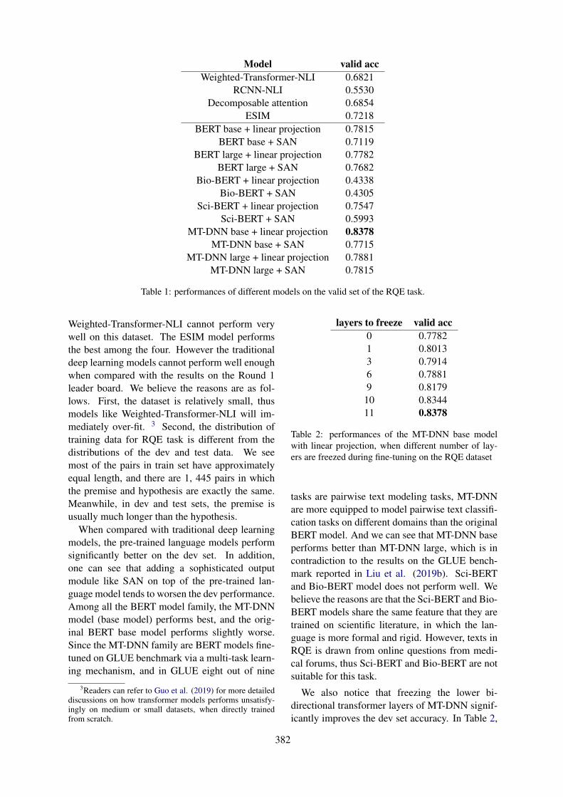
Model valid accWeighted-Transformer-NLI 0.6821
RCNN-NLI 0.5530Decomposable attention 0.6854
ESIM 0.7218BERT base + linear projection 0.7815
BERT base + SAN 0.7119BERT large + linear projection 0.7782
BERT large + SAN 0.7682Bio-BERT + linear projection 0.4338
Bio-BERT + SAN 0.4305Sci-BERT + linear projection 0.7547
Sci-BERT + SAN 0.5993MT-DNN base + linear projection 0.8378
MT-DNN base + SAN 0.7715MT-DNN large + linear projection 0.7881
MT-DNN large + SAN 0.7815
Table 1: performances of different models on the valid set of the RQE task.
Weighted-Transformer-NLI cannot perform verywell on this dataset. The ESIM model performsthe best among the four. However the traditionaldeep learning models cannot perform well enoughwhen compared with the results on the Round 1leader board. We believe the reasons are as fol-lows. First, the dataset is relatively small, thusmodels like Weighted-Transformer-NLI will im-mediately over-fit. 3 Second, the distribution oftraining data for RQE task is different from thedistributions of the dev and test data. We seemost of the pairs in train set have approximatelyequal length, and there are 1, 445 pairs in whichthe premise and hypothesis are exactly the same.Meanwhile, in dev and test sets, the premise isusually much longer than the hypothesis.
When compared with traditional deep learningmodels, the pre-trained language models performsignificantly better on the dev set. In addition,one can see that adding a sophisticated outputmodule like SAN on top of the pre-trained lan-guage model tends to worsen the dev performance.Among all the BERT model family, the MT-DNNmodel (base model) performs best, and the orig-inal BERT base model performs slightly worse.Since the MT-DNN family are BERT models fine-tuned on GLUE benchmark via a multi-task learn-ing mechanism, and in GLUE eight out of nine
3Readers can refer to Guo et al. (2019) for more detaileddiscussions on how transformer models performs unsatisfy-ingly on medium or small datasets, when directly trainedfrom scratch.
layers to freeze valid acc0 0.77821 0.80133 0.79146 0.78819 0.817910 0.834411 0.8378
Table 2: performances of the MT-DNN base modelwith linear projection, when different number of lay-ers are freezed during fine-tuning on the RQE dataset
tasks are pairwise text modeling tasks, MT-DNNare more equipped to model pairwise text classifi-cation tasks on different domains than the originalBERT model. And we can see that MT-DNN baseperforms better than MT-DNN large, which is incontradiction to the results on the GLUE bench-mark reported in Liu et al. (2019b). Sci-BERTand Bio-BERT model does not perform well. Webelieve the reasons are that the Sci-BERT and Bio-BERT models share the same feature that they aretrained on scientific literature, in which the lan-guage is more formal and rigid. However, texts inRQE is drawn from online questions from medi-cal forums, thus Sci-BERT and Bio-BERT are notsuitable for this task.
We also notice that freezing the lower bi-directional transformer layers of MT-DNN signif-icantly improves the dev set accuracy. In Table 2,
382
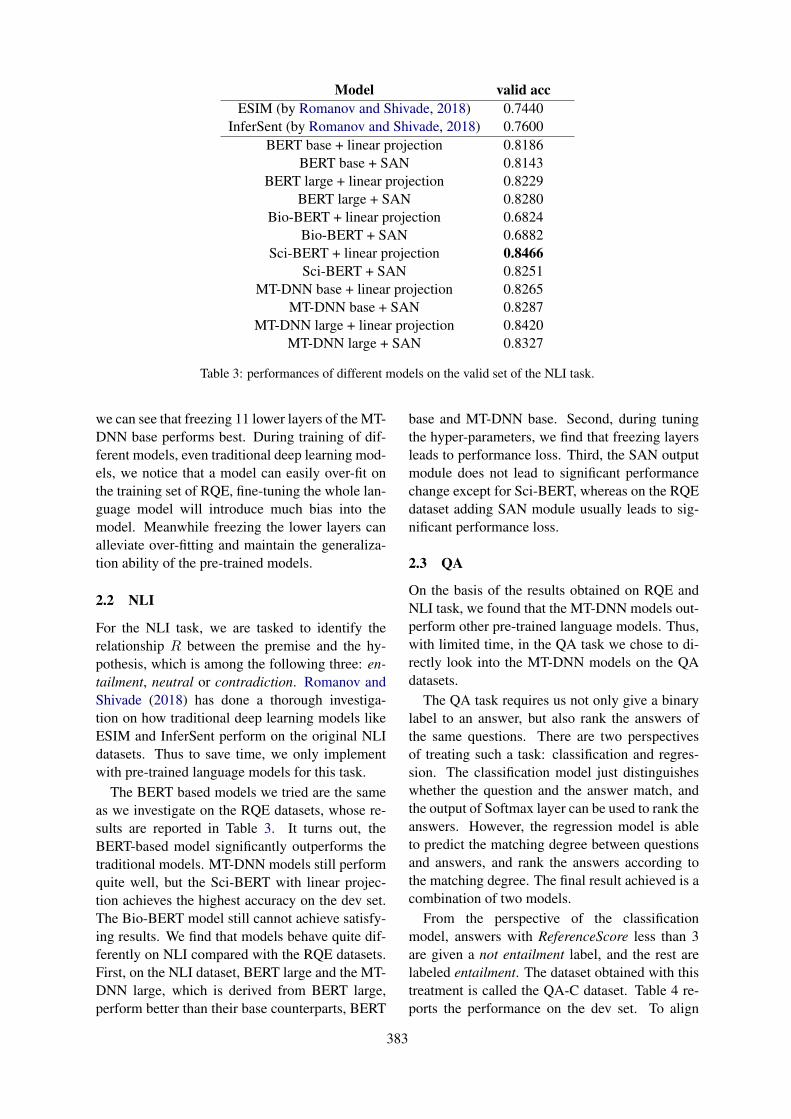
Model valid accESIM (by Romanov and Shivade, 2018) 0.7440
InferSent (by Romanov and Shivade, 2018) 0.7600BERT base + linear projection 0.8186
BERT base + SAN 0.8143BERT large + linear projection 0.8229
BERT large + SAN 0.8280Bio-BERT + linear projection 0.6824
Bio-BERT + SAN 0.6882Sci-BERT + linear projection 0.8466
Sci-BERT + SAN 0.8251MT-DNN base + linear projection 0.8265
MT-DNN base + SAN 0.8287MT-DNN large + linear projection 0.8420
MT-DNN large + SAN 0.8327
Table 3: performances of different models on the valid set of the NLI task.
we can see that freezing 11 lower layers of the MT-DNN base performs best. During training of dif-ferent models, even traditional deep learning mod-els, we notice that a model can easily over-fit onthe training set of RQE, fine-tuning the whole lan-guage model will introduce much bias into themodel. Meanwhile freezing the lower layers canalleviate over-fitting and maintain the generaliza-tion ability of the pre-trained models.
2.2 NLI
For the NLI task, we are tasked to identify therelationship R between the premise and the hy-pothesis, which is among the following three: en-tailment, neutral or contradiction. Romanov andShivade (2018) has done a thorough investiga-tion on how traditional deep learning models likeESIM and InferSent perform on the original NLIdatasets. Thus to save time, we only implementwith pre-trained language models for this task.
The BERT based models we tried are the sameas we investigate on the RQE datasets, whose re-sults are reported in Table 3. It turns out, theBERT-based model significantly outperforms thetraditional models. MT-DNN models still performquite well, but the Sci-BERT with linear projec-tion achieves the highest accuracy on the dev set.The Bio-BERT model still cannot achieve satisfy-ing results. We find that models behave quite dif-ferently on NLI compared with the RQE datasets.First, on the NLI dataset, BERT large and the MT-DNN large, which is derived from BERT large,perform better than their base counterparts, BERT
base and MT-DNN base. Second, during tuningthe hyper-parameters, we find that freezing layersleads to performance loss. Third, the SAN outputmodule does not lead to significant performancechange except for Sci-BERT, whereas on the RQEdataset adding SAN module usually leads to sig-nificant performance loss.
2.3 QA
On the basis of the results obtained on RQE andNLI task, we found that the MT-DNN models out-perform other pre-trained language models. Thus,with limited time, in the QA task we chose to di-rectly look into the MT-DNN models on the QAdatasets.
The QA task requires us not only give a binarylabel to an answer, but also rank the answers ofthe same questions. There are two perspectivesof treating such a task: classification and regres-sion. The classification model just distinguisheswhether the question and the answer match, andthe output of Softmax layer can be used to rank theanswers. However, the regression model is ableto predict the matching degree between questionsand answers, and rank the answers according tothe matching degree. The final result achieved is acombination of two models.
From the perspective of the classificationmodel, answers with ReferenceScore less than 3are given a not entailment label, and the rest arelabeled entailment. The dataset obtained with thistreatment is called the QA-C dataset. Table 4 re-ports the performance on the dev set. To align
383
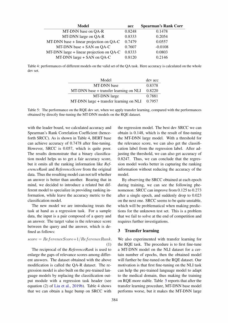
Model acc Spearman’s Rank CorrMT-DNN base on QA-R 0.8248 0.1478MT-DNN large on QA-R 0.8333 0.2054
MT-DNN base + linear projection on QA-C 0.7479 0.0557MT-DNN base + SAN on QA-C 0.7607 -0.0108
MT-DNN large + linear projection on QA-C 0.8333 0.0803MT-DNN large + SAN on QA-C 0.8120 0.2146
Table 4: performances of different models on the valid set of the QA task. Here accuracy is calculated on the wholedev set.
Model dev accMT-DNN base 0.8378
MT-DNN base + transfer learning on NLI 0.8220MT-DNN large 0.7881
MT-DNN large + transfer learning on NLI 0.7957
Table 5: The performance on the RQE dev set, when we apply transfer learning, compared with the performancesobtained by directly fine-tuning the MT-DNN models on the RQE dataset.
with the leader board, we calculated accuracy andSpearman’s Rank Correlation Coefficient (hence-forth SRCC). As is shown in Table 4, BERT basecan achieve accuracy of 0.7478 after fine-tuning.However, SRCC is 0.057, which is quite poor.The results demonstrate that a binary classifica-tion model helps us to get a fair accuracy score,but it omits all the ranking information like Ref-erenceRank and ReferenceScore from the originaldata. Thus the resulting model can not tell whetheran answer is better than another. Bearing that inmind, we decided to introduce a related but dif-ferent model to specialize in providing ranking in-formation, while leave the accuracy metric to theclassification model.
The new model we are introducing treats thetask at hand as a regression task. For a sampledata, the input is a pair composed of a query andan answer. The target value is the relevance scorebetween the query and the answer, which is de-fined as follows:
score = ReferenceScore+1/ReferenceRank.(1)
The reciprocal of the ReferenceRank is used toenlarge the gaps of relevance scores among differ-ent answers. The dataset obtained with the abovemodification is called the QA-R dataset. The re-gression model is also built on the pre-trained lan-guage models by replacing the classification out-put module with a regression task header (seeequation (2) of Liu et al., 2019b). Table 4 showsthat we can obtain a huge bump on SRCC with
the regression model. The best dev SRCC we canobtain is 0.148, which is the result of fine-tuningthe MT-DNN large model. With a threshold forthe relevance score, we can also get the classifi-cation label from the regression label. After ad-justing the threshold, we can also get accuracy of0.8247. Thus, we can conclude that the regres-sion model works better in capturing the rankinginformation without reducing the accuracy of themodel.
By observing the SRCC obtained at each epochduring training, we can see the following phe-nomenon: SRCC can improve from 0.125 to 0.273after a single epoch, and suddenly drop to 0.023on the next one. SRCC seems to be quite unstable,which will be problematical when making predic-tions for the unknown test set. This is a problemthat we fail to solve at the end of competition andrequires further investigations.
3 Transfer learning
We also experimented with transfer learning forthe RQE task. The procedure is to first fine-tunea MT-DNN model on the NLI dataset for a cer-tain number of epochs, then the obtained modelwill further be fine-tuned on the RQE dataset. Ourmotivation is that first fine-tuning on the NLI taskcan help the pre-trained language model to adaptto the medical domain, thus making the trainingon RQE more stable. Table 5 reports that after thetransfer learning procedure, MT-DNN base modelperforms worse, but it makes the MT-DNN large
384
model perform slightly better.
4 knowledge distillation
In this section, we experiment on the idea ofknowledge distillation (Hinton et al., 2015), tofurther boost the performance of single models.We implement knowledge distillation on each taskseparately.4 The procedure is as follows:
• train a set of models on each tasks. Follow-ing Liu et al. (2019a), the set of models are:MT-DNN base and MT-DNN large, with dif-ferent dropout rates ranged in 0.1, 0.3, 0.5 forthe task specific output layers, while keep-ing the hyper-parameters of lower BERT en-coders the same with those in the previoussection.
• ensemble the above models to get a labelmodel (Ratner et al., 2018)5. This so-calledlabel model is constructed by modeling agenerative model over all the label func-tions, i.e., the single models, to maximize thelog likelihood, give the label matrix (Ratneret al., 2017). The label model is a general-ization of the so-called teacher model in (Liuet al., 2019a), where the teacher model is sim-ply the average of class probabilities.
• The end model (or called the student modelby Liu et al., 2019a) is trained on the softtargets given out by the label model. Here,training on the soft targets means the cross-entropy loss is averaged with the class prob-abilities as weights.
• Inference is the same for end model withother normal models.
In Table 6, we can see that knowledge distilla-tion can significantly improve the performance onthe NLI task, and can even achieve better resultsthan model ensemble. However, on the RQE task,knowledge distillation cannot perform better thanmodel ensemble, but still outperforms the best sin-gle model.
4Liu et al. (2019a) extends the knowledge distillation tomulti-task learning setting, which is a direction we need toexplore in future work.
5There are alternative terminologies for knowledge distil-lation. We mainly follow Ratner et al. (2018).
5 Ensemble
Since the test set is small, one single model is toobiased to achieve great results on the test dataset.Ensemble learning is an effective approach to im-prove model generalization, and has been used toachieve new state-of-the-art results in a wide rangeof natural language understanding (NLU) tasks(Devlin et al., 2018, Liu et al., 2017).
For the MEDIQA 2019 shared task, we onlyadopt a simple ensemble approach, that is, aver-aging the softmax outputs from different models,or different runs or epochs of the same model, andmakes prediction based on these averaged classprobabilities. All our submissions follow this en-semble strategy. 6
6 Re-ranking strategies for the NLI andRQE tasks
The previous sections demonstrate how deeplearning models perform on the task datasets.However, in order to obtain more competitive re-sults, one could adopt some simple heuristics.
For the NLI task, after observing the taskdatasets, we can see that one premise is groupedwith three different hypothesis, and the latter arelabeled with entailment, neutral and contradictionrespectively. We call the three pairs with the samepremise a group. Our sentence pair model doesnot know the idea of groups, thus the labels corre-sponding to the maximum class probabilities ob-tained by soft-max layer can conflict with one an-other. For example, two pairs in the same groupmay both be labeled as entailment. To eliminatethe above conflicts, we adopt the following heuris-tic post-processing procedure:
• obtain the label predictions directly from thesoftmax output. If there is no conflict in agroup, accept the predictions. Otherwise, inthis group:
• Give the contradiction label to the pair withthe highest score for this label
• Between the remaining two pairs, decidewhich one should get the neutral label via thescores for this label
6We definitely can try some more sophisticated ensem-ble methods, but we believe experimenting different learn-ing strategies like MTL and knowledge distillation is moremeaningful for research purpose, and is in alignment with theobjective of the MEDIQA 2019 share tasks.
385
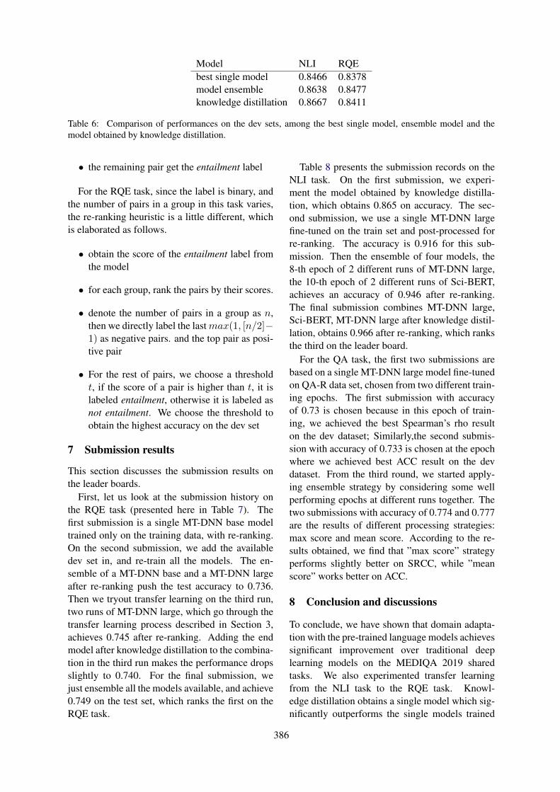
Model NLI RQEbest single model 0.8466 0.8378model ensemble 0.8638 0.8477knowledge distillation 0.8667 0.8411
Table 6: Comparison of performances on the dev sets, among the best single model, ensemble model and themodel obtained by knowledge distillation.
• the remaining pair get the entailment label
For the RQE task, since the label is binary, andthe number of pairs in a group in this task varies,the re-ranking heuristic is a little different, whichis elaborated as follows.
• obtain the score of the entailment label fromthe model
• for each group, rank the pairs by their scores.
• denote the number of pairs in a group as n,then we directly label the last max(1, [n/2]−1) as negative pairs. and the top pair as posi-tive pair
• For the rest of pairs, we choose a thresholdt, if the score of a pair is higher than t, it islabeled entailment, otherwise it is labeled asnot entailment. We choose the threshold toobtain the highest accuracy on the dev set
7 Submission results
This section discusses the submission results onthe leader boards.
First, let us look at the submission history onthe RQE task (presented here in Table 7). Thefirst submission is a single MT-DNN base modeltrained only on the training data, with re-ranking.On the second submission, we add the availabledev set in, and re-train all the models. The en-semble of a MT-DNN base and a MT-DNN largeafter re-ranking push the test accuracy to 0.736.Then we tryout transfer learning on the third run,two runs of MT-DNN large, which go through thetransfer learning process described in Section 3,achieves 0.745 after re-ranking. Adding the endmodel after knowledge distillation to the combina-tion in the third run makes the performance dropsslightly to 0.740. For the final submission, wejust ensemble all the models available, and achieve0.749 on the test set, which ranks the first on theRQE task.
Table 8 presents the submission records on theNLI task. On the first submission, we experi-ment the model obtained by knowledge distilla-tion, which obtains 0.865 on accuracy. The sec-ond submission, we use a single MT-DNN largefine-tuned on the train set and post-processed forre-ranking. The accuracy is 0.916 for this sub-mission. Then the ensemble of four models, the8-th epoch of 2 different runs of MT-DNN large,the 10-th epoch of 2 different runs of Sci-BERT,achieves an accuracy of 0.946 after re-ranking.The final submission combines MT-DNN large,Sci-BERT, MT-DNN large after knowledge distil-lation, obtains 0.966 after re-ranking, which ranksthe third on the leader board.
For the QA task, the first two submissions arebased on a single MT-DNN large model fine-tunedon QA-R data set, chosen from two different train-ing epochs. The first submission with accuracyof 0.73 is chosen because in this epoch of train-ing, we achieved the best Spearman’s rho resulton the dev dataset; Similarly,the second submis-sion with accuracy of 0.733 is chosen at the epochwhere we achieved best ACC result on the devdataset. From the third round, we started apply-ing ensemble strategy by considering some wellperforming epochs at different runs together. Thetwo submissions with accuracy of 0.774 and 0.777are the results of different processing strategies:max score and mean score. According to the re-sults obtained, we find that ”max score” strategyperforms slightly better on SRCC, while ”meanscore” works better on ACC.
8 Conclusion and discussions
To conclude, we have shown that domain adapta-tion with the pre-trained language models achievessignificant improvement over traditional deeplearning models on the MEDIQA 2019 sharedtasks. We also experimented transfer learningfrom the NLI task to the RQE task. Knowl-edge distillation obtains a single model which sig-nificantly outperforms the single models trained
386
Submission No. test acc details1 0.675 1 * MT-DNN base (trained on train set) + re-rank2 0.736 1 * MT-DNN base + 1 * MT-DNN large + re-rank3 0.745 2 * MT-DNN large (TL) + re-rank4 0.740 1 * MT-DNN large (KD) + 2 * MT-DNN large (TL) + re-rank5 0.749 2 * MT-DNN base + 2 * MT-DNN large (TL)
+ 1 * MT-DNN large (KD) + 1 * MT-DNN large+ re-rank
Table 7: The submission results on the RQE task. Multiplication symbol ”*” here means multiple runs or epochsof the same model (with different random seed). ”TL” means the model go through transfer learning on the NLItask. ”KD” means the model is obtained via knowledge distillation. Without declaration, all the models here aretrained on the train and dev set.
Submission No. test acc details1 0.865 1 * MT-DNN large (KD)2 0.916 1 * MT-DNN large (on train set) + re-rank3 0.946 2 * MT-DNN large + 2 * Sci-BERT + re-rank4 0.966 4 * MT-DNN large + 4 * Sci-BERT
+ 2 * MT-DNN large (KD) + re-rank
Table 8: The submission records on the NLI task. Multiplication symbol ”*” here means multiple runs or epochsof the same model (with different random seed). ”KD” means the model is obtained via knowledge distillation.Without declaration, all the models here are trained on the train and dev set.
Submission No. test acc test Spearman’s rho details1 0.730 0.236 MT-DNN large (epoch with best training SRCC)2 0.736 0.204 MT-DNN large (epoch with best training ACC)3 0.774 0.22 MT-DNN large ensemble(rank by max socre)4 0.777 0.18 MT-DNN large ensemble(rank by mean socre)5 0.772 0.204 MT-DNN large ensemble(rank by mean socre)
Table 9: The submission results on the QA task.
in the usual way. Our submission results, al-though including model ensemble and re-ranking,are strong demonstration of the power of languagemodel pre-training, transfer learning and knowl-edge distillation.
However, due to the limited time and the factthat we participate all three tasks at once, wehaven’t exhaustively explore all the possible waysto boost the performance on the leader board,e.g., utilizing external sources such as medicalknowledge bases to rule out false positive answers.Multi-task learning is also a direction that we needto pay more attention to.
In addition, the heuristics adopted in the re-ranking strategies resemble the relevance rankingtask (Huang et al., 2013), where one comparesdifferent pairs in a group to obtain the final deci-sions. Due to time constraint, we didn’t implementa pairwise relevance ranking model on top of the
MT-DNN model, but this research direction willbe investigated by us in future work.
ReferencesKarim Ahmed, Nitish Shirish Keskar, and Richard
Socher. 2017. Weighted Transformer Networkfor Machine Translation. arXiv e-prints, pagearXiv:1711.02132.
Iz Beltagy, Arman Cohan, and Kyle Lo. 2019.SciBERT: Pretrained Contextualized Embed-dings for Scientific Text. arXiv e-prints, pagearXiv:1903.10676.
Asma Ben Abacha, Chaitanya Shivade, and DinaDemner-Fushman. 2019. Overview of the mediqa2019 shared task on textual inference, question en-tailment and question answering. In Proceedings ofthe BioNLP 2019 workshop, Florence, Italy, August1, 2019. Association for Computational Linguistics.
Samuel R. Bowman, Gabor Angeli, Christopher Potts,
387
and Christopher D. Manning. 2015. A large anno-tated corpus for learning natural language inference.In Proceedings of the 2015 Conference on Empiri-cal Methods in Natural Language Processing, pages632–642, Lisbon, Portugal. Association for Compu-tational Linguistics.
Qian Chen, Xiaodan Zhu, Zhenhua Ling, Si Wei, HuiJiang, and Diana Inkpen. 2016. Enhanced LSTM forNatural Language Inference. arXiv e-prints, pagearXiv:1609.06038.
Jacob Devlin, Ming-Wei Chang, Kenton Lee, andKristina Toutanova. 2018. BERT: Pre-trainingof Deep Bidirectional Transformers for Lan-guage Understanding. arXiv e-prints, pagearXiv:1810.04805.
Qipeng Guo, Xipeng Qiu, Pengfei Liu, Yun-fan Shao, Xiangyang Xue, and Zheng Zhang.2019. Star-Transformer. arXiv e-prints, pagearXiv:1902.09113.
Geoffrey Hinton, Oriol Vinyals, and Jeff Dean. 2015.Distilling the Knowledge in a Neural Network.arXiv e-prints, page arXiv:1503.02531.
Po-Sen Huang, Xiaodong He, Jianfeng Gao, Li Deng,Alex Acero, and Larry Heck. 2013. Learning deepstructured semantic models for web search usingclickthrough data. In Proceedings of the 22nd ACMinternational conference on Information & Knowl-edge Management, pages 2333–2338. ACM.
Siwei Lai, Liheng Xu, Kang Liu, and Jun Zhao. 2015.Recurrent convolutional neural networks for textclassification.
Jinhyuk Lee, Wonjin Yoon, Sungdong Kim,Donghyeon Kim, Sunkyu Kim, Chan Ho So,and Jaewoo Kang. 2019. BioBERT: a pre-trainedbiomedical language representation model forbiomedical text mining. arXiv e-prints, pagearXiv:1901.08746.
Xiaodong Liu, Pengcheng He, Weizhu Chen, and Jian-feng Gao. 2019a. Improving Multi-Task Deep Neu-ral Networks via Knowledge Distillation for Natu-ral Language Understanding. arXiv e-prints, pagearXiv:1904.09482.
Xiaodong Liu, Pengcheng He, Weizhu Chen, and Jian-feng Gao. 2019b. Multi-Task Deep Neural Net-works for Natural Language Understanding. arXive-prints, page arXiv:1901.11504.
Xiaodong Liu, Yelong Shen, Kevin Duh, and JianfengGao. 2017. Stochastic Answer Networks for Ma-chine Reading Comprehension. arXiv e-prints, pagearXiv:1712.03556.
Ankur P. Parikh, Oscar Täckström, Dipanjan Das, andJakob Uszkoreit. 2016. A Decomposable AttentionModel for Natural Language Inference. arXiv e-prints, page arXiv:1606.01933.
Jeffrey Pennington, Richard Socher, and Christo-pher D. Manning. 2014. Glove: Global vectors forword representation. In Empirical Methods in Nat-ural Language Processing (EMNLP), pages 1532–1543.
Alec Radford, Jeffrey Wu, Rewon Child, David Luan,Dario Amodei, and Ilya Sutskever. 2019. Languagemodels are unsupervised multitask learners. OpenAIBlog, 1:8.
Alexander Ratner, Stephen H. Bach, Henry Ehren-berg, Jason Fries, Sen Wu, and Christopher Ré.2017. Snorkel: Rapid Training Data Creationwith Weak Supervision. arXiv e-prints, pagearXiv:1711.10160.
Alexander Ratner, Braden Hancock, Jared Dunnmon,Frederic Sala, Shreyash Pandey, and ChristopherRé. 2018. Training Complex Models with Multi-Task Weak Supervision. arXiv e-prints, pagearXiv:1810.02840.
Alexey Romanov and Chaitanya Shivade. 2018.Lessons from Natural Language Inference inthe Clinical Domain. arXiv e-prints, pagearXiv:1808.06752.
Xu Tan, Yi Ren, Di He, Tao Qin, Zhou Zhao, and Tie-Yan Liu. 2019. Multilingual Neural Machine Trans-lation with Knowledge Distillation. arXiv e-prints,page arXiv:1902.10461.
388
Proceedings of the BioNLP 2019 workshop, pages 389–398Florence, Italy, August 1, 2019. c©2019 Association for Computational Linguistics
Pentagon at MEDIQA 2019: Multi-task Learning for Filtering andRe-ranking Answers using Language Inference and Question Entailment
Hemant Pugaliya∗, Karan Saxena∗, Shefali Garg∗, Sheetal Shalini∗,Prashant Gupta∗, Eric Nyberg, Teruko Mitamura
{hpugaliy, karansax, shefalig, sshalini, prashang, ehn, teruko}@cs.cmu.edu
Language Technologies Institute (LTI),Carnegie Mellon University (CMU)
Abstract
Parallel deep learning architectures like fine-tuned BERT and MT-DNN, have quickly be-come the state of the art, bypassing previ-ous deep and shallow learning methods by alarge margin. More recently, pre-trained mod-els from large related datasets have been ableto perform well on many downstream tasksby just fine-tuning on domain-specific datasets(similar to transfer learning).However, using powerful models on non-trivial tasks, such as ranking and large docu-ment classification, still remains a challengedue to input size limitations1 of parallel archi-tecture and extremely small datasets (insuffi-cient for fine-tuning).In this work, we introduce an end-to-end sys-tem, trained in a multi-task setting, to filterand re-rank answers in medical domain. Weuse task-specific pre-trained models as deepfeature extractors. Our model achieves thehighest Spearman’s Rho and Mean Recipro-cal Rank of 0.338 and 0.9622 respectively, onthe ACL-BioNLP workshop MediQA Ques-tion Answering shared-task.
1 Introduction
In this work, we study the problem of re-rankingand filtering in medical domain Information Re-trieval (IR) systems. Historically, re-ranking isgenerally treated as a ‘Learning to Rank’ prob-lem while filtering is posed as a ‘Binary Classi-fication’ problem. Traditional methods have usedhandcrafted features to train such systems. How-ever, recently deep learning methods have gained
∗* Equal contribution, randomly sorted. Karan and She-fali took ownership of the NLI module while Sheetal andPrashant worked on the RQE module. Hemant researchedand implemented the Question-Answering system includingbaseline and multi-task learning. Sheetal and Hemant workedon scraping data from icliniq. Karan and Prashant helpedwith integration of NLI and RQE module respectively intothe multi-task system.
1https://github.com/google-research/bert/issues/27
popularity in the Information retrieval (IR) domain(Mitra and Craswell, 2017).
The ACL-BioNLP workshop MediQA sharedtask (Ben Abacha et al., 2019) aims to developrelevant techniques for inference and entailmentin medical domain to improve domain specific IRand QA systems. The challenge consists of threetasks which are evaluated separately.
The first task is the Natural Language Inference(NLI) task which focuses on determining whethera natural language hypothesis can be inferred froma natural language premise. The second task isto recognize question entailment (RQE) betweena pair of questions. The third task is to filter andimprove the ranking of automatically retrieved an-swers.
For the NLI and RQE tasks, we use trans-fer learning on prevalent pre-trained models likeBERT (Devlin et al., 2018) and MT-DNN (Liuet al., 2019). These models play a pivotal roleto gain deeper semantic understanding of the con-tent for the final task (filtering and re-ranking) ofthe challenge (Demszky et al., 2018). Besides us-ing usual techniques for candidate answer selec-tion and re-ranking, we use features obtained fromNLI and RQE models. We majorly concentrate onthe novel multi-task approach in this paper. Wealso succinctly describe our NLI and RQE modelsand their performance on the final leaderboard.
2 Related Work
Past research demonstrates a simple architecturefor filtering and re-ranking, where the system re-turns the best answer based on the InformationRetrieval and Question Entailment Scores [froma corpus of FAQs scraped from medical websitesMediQUAD (Ben Abacha and Demner-Fushman,2019)]. This system outperformed all the systemsparticipating in the TREC Medical LiveQA17
389
challenges. (Harabagiu and Hickl, 2006) success-fully shows the use of Natural Language Inference(NLI) in passage retrieval, answer selection andanswer re-ranking to advance open-domain ques-tion answering. (Tari et al., 2007) shows effectiveuse of UMLS (Bodenreider, 2004), a Unified Med-ical Language System to asses passage relevancythrough semantic relatedness. All these methodswork well independently, but to the best of ourknowledge, there hasn’t been much work in usingNLI and RQE systems in tandem for the tasks offiltering and re-ranking.
As noted in (Romanov and Shivade, 2018), thetask of Natural Language Inference is not domainagnostic, and thus is not able to transfer well toother domains. The authors use a gradient boost-ing classifier (Mason et al., 2000) with a variety ofhand crafted features for baselines. They then useInfersent (Conneau et al., 2017) as a sentence en-coder. The paper also reports results on the ESIMModel (Chen et al., 2017) but with no visible im-provements. They also discuss transfer learningand external knowledge based methods.
Most traditional approaches to Question Entail-ment use bag-of-word pair classifiers (Tung andXu, 2017) using only lexical similarity. How-ever, in the recent past, neural models (Mishraand Bhattacharyya, 2018) have been employed todetermine entailment between questions incorpo-rating their semantic similarity as well. Thesetechniques work by generating word-level repre-sentations for both the questions, which are thencombined into independent question representa-tions by passing it through a recurrent cell like Bi-LSTM (Liu et al., 2016). However, current state-of-the-art methods like BERT (Devlin et al., 2018)and MT-DNN (Huang et al., 2013) learn a jointembedding of the two questions, which is thenused for classification.
(Abacha and Demner-Fushman, 2016) imple-mented the SVM, Logistic Regression, NaiveBayes and J48 models as baselines for QuestionEntailment task. They use a set of handcraftedlexical features, like word overlap and bigramsimilarity, and semantic features like number ofmedical entities (problems, treatments, tests) us-ing a CRF classifier trained on i2b2 (Uzuner et al.,2011) and NCBI corpus (Doğan et al., 2014).
3 Dataset & Evaluation
The dataset for re-ranking and filtering has beenprovided by the MediQA Shared task (BenAbacha et al., 2019) in ACL-BioNLP 2019 work-shop. It consists of medical questions and their as-sociated answers retrieved by CHiQA 2. The train-ing dataset consists of 208 questions while the val-idation and test datasets have 25 and 150 questionsrespectivley. Each question has upto 10 candidateanswers, with each answer having the followingattributes :
1. SystemRank: It corresponds to CHiQA’srank.
2. ReferenceRank: It corresponds to the correctrank.
3. ReferenceScore: This is an additional scorethat is provided only in the training and vali-dation sets, which corresponds to the manualjudgment/rating of the answer [4: Excellent,3: Correct but Incomplete, 2: Related, 1: In-correct].
For the answer classification task, answers withscores 1 and 2 are considered as incorrect (label0), and answers with scores 3 and 4 are consideredas correct (label 1). The evaluation metrics for fil-tering task is Accuracy and Precision while met-rics for re-ranking task is Mean Reciprocal Rank(MRR) and Spearman’s Rank Correlation Coeffi-cient.
To train the Natural Language Inference andQuestion Entailment module of our system weagain use the data from MediQA shared task (BenAbacha et al., 2019).
For Natural Language Inference (NLI), we useMedNLI (Romanov and Shivade, 2018) dataset. Itis a dataset for natural language inference in clin-ical domain that is analogous to SNLI. It includes15,473 annotated clinical sentence pairs. For ourmodel, we create a training set of 14,050 pairs anda held out validation set of 1,423 pairs. The evalu-ation metric for NLI is accuracy.
The dataset used for Question Entailment(RQE) consists of paired customer health ques-tions (CHQ) and Frequently Asked Questions(FAQ) (Ben Abacha and Demner-Fushman, 2016).We are provided labels for whether FAQ entailsCHQ or not. The RQE training dataset consists
2https://chiqa.nlm.nih.gov/
390
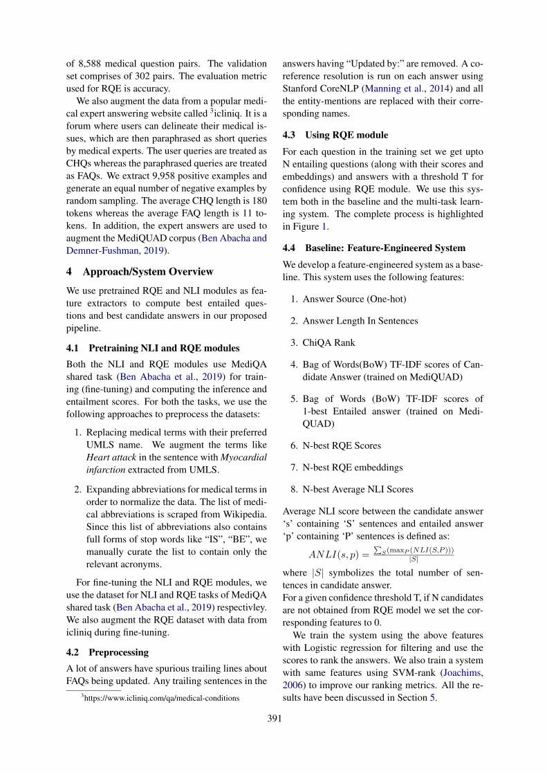
of 8,588 medical question pairs. The validationset comprises of 302 pairs. The evaluation metricused for RQE is accuracy.
We also augment the data from a popular medi-cal expert answering website called 3icliniq. It is aforum where users can delineate their medical is-sues, which are then paraphrased as short queriesby medical experts. The user queries are treated asCHQs whereas the paraphrased queries are treatedas FAQs. We extract 9,958 positive examples andgenerate an equal number of negative examples byrandom sampling. The average CHQ length is 180tokens whereas the average FAQ length is 11 to-kens. In addition, the expert answers are used toaugment the MediQUAD corpus (Ben Abacha andDemner-Fushman, 2019).
4 Approach/System Overview
We use pretrained RQE and NLI modules as fea-ture extractors to compute best entailed ques-tions and best candidate answers in our proposedpipeline.
4.1 Pretraining NLI and RQE modulesBoth the NLI and RQE modules use MediQAshared task (Ben Abacha et al., 2019) for train-ing (fine-tuning) and computing the inference andentailment scores. For both the tasks, we use thefollowing approaches to preprocess the datasets:
1. Replacing medical terms with their preferredUMLS name. We augment the terms likeHeart attack in the sentence with Myocardialinfarction extracted from UMLS.
2. Expanding abbreviations for medical terms inorder to normalize the data. The list of medi-cal abbreviations is scraped from Wikipedia.Since this list of abbreviations also containsfull forms of stop words like “IS”, “BE”, wemanually curate the list to contain only therelevant acronyms.
For fine-tuning the NLI and RQE modules, weuse the dataset for NLI and RQE tasks of MediQAshared task (Ben Abacha et al., 2019) respectivley.We also augment the RQE dataset with data fromicliniq during fine-tuning.
4.2 PreprocessingA lot of answers have spurious trailing lines aboutFAQs being updated. Any trailing sentences in the
3https://www.icliniq.com/qa/medical-conditions
answers having “Updated by:” are removed. A co-reference resolution is run on each answer usingStanford CoreNLP (Manning et al., 2014) and allthe entity-mentions are replaced with their corre-sponding names.
4.3 Using RQE module
For each question in the training set we get uptoN entailing questions (along with their scores andembeddings) and answers with a threshold T forconfidence using RQE module. We use this sys-tem both in the baseline and the multi-task learn-ing system. The complete process is highlightedin Figure 1.
4.4 Baseline: Feature-Engineered System
We develop a feature-engineered system as a base-line. This system uses the following features:
1. Answer Source (One-hot)
2. Answer Length In Sentences
3. ChiQA Rank
4. Bag of Words(BoW) TF-IDF scores of Can-didate Answer (trained on MediQUAD)
5. Bag of Words (BoW) TF-IDF scores of1-best Entailed answer (trained on Medi-QUAD)
6. N-best RQE Scores
7. N-best RQE embeddings
8. N-best Average NLI Scores
Average NLI score between the candidate answer‘s’ containing ‘S’ sentences and entailed answer‘p’ containing ‘P’ sentences is defined as:
ANLI(s, p) =∑
S(maxP (NLI(S,P )))|S|
where |S| symbolizes the total number of sen-tences in candidate answer.For a given confidence threshold T, if N candidatesare not obtained from RQE model we set the cor-responding features to 0.
We train the system using the above featureswith Logistic regression for filtering and use thescores to rank the answers. We also train a systemwith same features using SVM-rank (Joachims,2006) to improve our ranking metrics. All the re-sults have been discussed in Section 5.
391
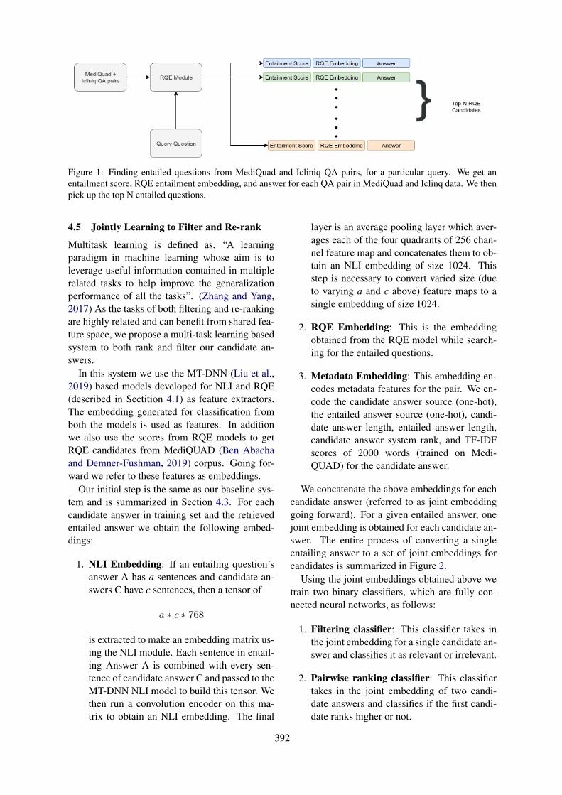
Figure 1: Finding entailed questions from MediQuad and Icliniq QA pairs, for a particular query. We get anentailment score, RQE entailment embedding, and answer for each QA pair in MediQuad and Iclinq data. We thenpick up the top N entailed questions.
4.5 Jointly Learning to Filter and Re-rank
Multitask learning is defined as, “A learningparadigm in machine learning whose aim is toleverage useful information contained in multiplerelated tasks to help improve the generalizationperformance of all the tasks”. (Zhang and Yang,2017) As the tasks of both filtering and re-rankingare highly related and can benefit from shared fea-ture space, we propose a multi-task learning basedsystem to both rank and filter our candidate an-swers.
In this system we use the MT-DNN (Liu et al.,2019) based models developed for NLI and RQE(described in Sectition 4.1) as feature extractors.The embedding generated for classification fromboth the models is used as features. In additionwe also use the scores from RQE models to getRQE candidates from MediQUAD (Ben Abachaand Demner-Fushman, 2019) corpus. Going for-ward we refer to these features as embeddings.
Our initial step is the same as our baseline sys-tem and is summarized in Section 4.3. For eachcandidate answer in training set and the retrievedentailed answer we obtain the following embed-dings:
1. NLI Embedding: If an entailing question’sanswer A has a sentences and candidate an-swers C have c sentences, then a tensor of
a ∗ c ∗ 768
is extracted to make an embedding matrix us-ing the NLI module. Each sentence in entail-ing Answer A is combined with every sen-tence of candidate answer C and passed to theMT-DNN NLI model to build this tensor. Wethen run a convolution encoder on this ma-trix to obtain an NLI embedding. The final
layer is an average pooling layer which aver-ages each of the four quadrants of 256 chan-nel feature map and concatenates them to ob-tain an NLI embedding of size 1024. Thisstep is necessary to convert varied size (dueto varying a and c above) feature maps to asingle embedding of size 1024.
2. RQE Embedding: This is the embeddingobtained from the RQE model while search-ing for the entailed questions.
3. Metadata Embedding: This embedding en-codes metadata features for the pair. We en-code the candidate answer source (one-hot),the entailed answer source (one-hot), candi-date answer length, entailed answer length,candidate answer system rank, and TF-IDFscores of 2000 words (trained on Medi-QUAD) for the candidate answer.
We concatenate the above embeddings for eachcandidate answer (referred to as joint embeddinggoing forward). For a given entailed answer, onejoint embedding is obtained for each candidate an-swer. The entire process of converting a singleentailing answer to a set of joint embeddings forcandidates is summarized in Figure 2.
Using the joint embeddings obtained above wetrain two binary classifiers, which are fully con-nected neural networks, as follows:
1. Filtering classifier: This classifier takes inthe joint embedding for a single candidate an-swer and classifies it as relevant or irrelevant.
2. Pairwise ranking classifier: This classifiertakes in the joint embedding of two candi-date answers and classifies if the first candi-date ranks higher or not.
392
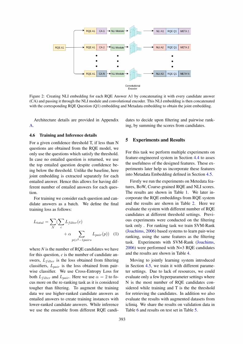
Figure 2: Creating NLI embedding for each RQE Answer A1 by concatenating it with every candidate answer(CA) and passing it through the NLI module and convolutional encoder. This NLI embedding is then concatenatedwith the corresponding RQE Question (Q1) embedding and Metadata embedding to obtain the joint embedding.
Architecture details are provided in AppendixA.
4.6 Training and Inference details
For a given confidence threshold T, if less than Nquestions are obtained from the RQE model, weonly use the questions which satisfy the threshold.In case no entailed question is returned, we usethe top entailed question despite confidence be-ing below the threshold. Unlike the baseline, herejoint embedding is extracted separately for eachentailed answer. Hence this allows for having dif-ferent number of entailed answers for each ques-tion.
For training we consider each question and can-didate answers as a batch. We define the finaltraining loss as follows:
Ltotal =∑
N
(∑
c
Lfilter(c)
+ α∑
p∈c2−1pairsLpair(p)) (1)
where N is the number of RQE candidates we havefor this question, c is the number of candidate an-swers, Lfilter is the loss obtained from filteringclassifiers, Lpair is the loss obtained from pair-wise classifier. We use Cross-Entropy Loss forboth Lfilter and Lpair. Here we use α = 2 to fo-cus more on the re-ranking task as it is consideredtougher than filtering. To augment the trainingdata we use higher-ranked candidate answers asentailed answers to create training instances withlower-ranked candidate answers. While inferencewe use the ensemble from different RQE candi-
dates to decide upon filtering and pairwise rank-ing, by summing the scores from candidates.
5 Experiments and Results
For this task we perform multiple experiments onfeature-engineered system in Section 4.4 to assesthe usefulness of the designed features. These ex-periments later help us incorporate these featuresinto Metadata Embedding defined in Section 4.5.
Firstly we run the experiments on Metedata fea-tures, BoW, Coarse-grained RQE and NLI scores.The results are shown in Table 1. We later in-corporate the RQE embeddings from RQE systemand the results are shown in Table 2. Here weevaluate the system with different number of RQEcandidates at different threshold settings. Previ-ous experiments were conducted on the filteringtask only . For ranking task we train SVM-Rank(Joachims, 2006) based systems to learn pair-wiseranking, using the same features as the filteringtask. Experiments with SVM-Rank (Joachims,2006) were performed with N=3 RQE candidatesand the results are shown in Table 4.
Moving to jointly learning system introducedin Section 4.5, we train it with different parame-ter settings. Due to lack of resources, we couldevaluate only a few hyperparameter settings whereN is the most number of RQE candidates con-sidered while training and T is the the thresholdfor retrieving the candidates. In addition we alsoevaluate the results with augmented datasets fromicliniq. We share the results on validation data inTable 6 and results on test set in Table 5.
393
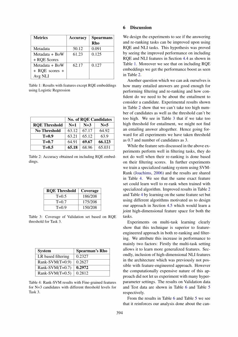
Metrics Accuracy SpearmansRho
Metadata 50.12 0.091Metadata + BoW+ RQE Scores
61.23 0.125
Metadata + BoW+ RQE scores +Avg NLI
62.17 0.127
Table 1: Results with features except RQE embeddingsusing Logistic Regression
No. of RQE CandidatesRQE Threshold N=1 N=3 N=5No Threshold 63.12 67.17 64.92
T=0.9 63.21 65.12 63.9T=0.7 64.91 69.67 66.123T=0.5 65.18 68.96 65.031
Table 2: Accuracy obtained on including RQE embed-dings.
RQE Threshold CoverageT=0.5 186/208T=0.7 175/208T=0.9 150/208
Table 3: Coverage of Validation set based on RQEthreshold for Task 3.
System Spearman’s RhoLR based filtering 0.2327Rank-SVM(T=0.9) 0.2627Rank-SVM(T=0.7) 0.2972Rank-SVM(T=0.5) 0.2812
Table 4: Rank-SVM results with Fine-grained featuresfor N=3 candidates with different threshold levels forTask 3.
6 Discussion
We design the experiments to see if the answeringand re-ranking tasks can be improved upon usingRQE and NLI tasks. This hypothesis was provedby seeing the improved performance on includingRQE and NLI features in Section 4.4 as shown inTable 1. Moreover we see that on including RQEembeddings we get the performance boost as seenin Table 2.
Another question which we can ask ourselves ishow many entailed answers are good enough forperforming filtering and re-ranking and how con-fident do we need to be about the entailment toconsider a candidate. Experimental results shownin Table 2 show that we can’t take too high num-ber of candidates as well as the threshold can’t betoo high. We see in Table 3 that if we take toohigh threshold for entailment, we might not findan entailing answer altogether. Hence going for-ward for all experiments we have taken thresholdas 0.7 and number of candidates as 3.
While the feature sets discussed in the above ex-periments perform well in filtering tasks, they donot do well when their re-ranking is done basedon their filtering scores. In further experimentswe train a specialized ranking system using SVM-Rank (Joachims, 2006) and the results are sharedin Table 4. We see that the same exact featureset could learn well to re-rank when trained withspecialized algorithm. Improved results in Table 2and Table 4 by learning on the same feature set butusing different algorithms motivated us to designour approach in Section 4.5 which would learn ajoint high-dimensional feature space for both thetasks.
Experiments on multi-task learning clearlyshow that this technique is superior to feature-engineered approach in both re-ranking and filter-ing. We attribute this increase in performance tomainly two factors: Firstly the multi-task settingallows it to learn more generalized features. Sec-ondly, inclusion of high-dimensional NLI featuresin the architecture which was previously not pos-sible with feature-engineered approach. Howeverthe computationally expensive nature of this ap-proach did not let us experiment with many hyper-parameter settings. The results on Validation dataand Test data are shown in Table 6 and Table 5respectively.
From the results in Table 6 and Table 5 we seethat it reinforces our analysis done about the can-
394
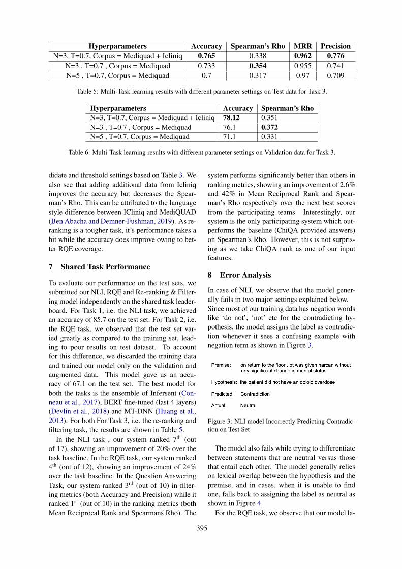
Hyperparameters Accuracy Spearman’s Rho MRR PrecisionN=3, T=0.7, Corpus = Mediquad + Icliniq 0.765 0.338 0.962 0.776
N=3 , T=0.7 , Corpus = Mediquad 0.733 0.354 0.955 0.741N=5 , T=0.7, Corpus = Mediquad 0.7 0.317 0.97 0.709
Table 5: Multi-Task learning results with different parameter settings on Test data for Task 3.
Hyperparameters Accuracy Spearman’s RhoN=3, T=0.7, Corpus = Mediquad + Icliniq 78.12 0.351N=3 , T=0.7 , Corpus = Mediquad 76.1 0.372N=5 , T=0.7, Corpus = Mediquad 71.1 0.331
Table 6: Multi-Task learning results with different parameter settings on Validation data for Task 3.
didate and threshold settings based on Table 3. Wealso see that adding additional data from Icliniqimproves the accuracy but decreases the Spear-man’s Rho. This can be attributed to the languagestyle difference between ICliniq and MediQUAD(Ben Abacha and Demner-Fushman, 2019). As re-ranking is a tougher task, it’s performance takes ahit while the accuracy does improve owing to bet-ter RQE coverage.
7 Shared Task Performance
To evaluate our performance on the test sets, wesubmitted our NLI, RQE and Re-ranking & Filter-ing model independently on the shared task leader-board. For Task 1, i.e. the NLI task, we achievedan accuracy of 85.7 on the test set. For Task 2, i.e.the RQE task, we observed that the test set var-ied greatly as compared to the training set, lead-ing to poor results on test dataset. To accountfor this difference, we discarded the training dataand trained our model only on the validation andaugmented data. This model gave us an accu-racy of 67.1 on the test set. The best model forboth the tasks is the ensemble of Infersent (Con-neau et al., 2017), BERT fine-tuned (last 4 layers)(Devlin et al., 2018) and MT-DNN (Huang et al.,2013). For both For Task 3, i.e. the re-ranking andfiltering task, the results are shown in Table 5.
In the NLI task , our system ranked 7th (outof 17), showing an improvement of 20% over thetask baseline. In the RQE task, our system ranked4th (out of 12), showing an improvement of 24%over the task baseline. In the Question AnsweringTask, our system ranked 3rd (out of 10) in filter-ing metrics (both Accuracy and Precision) while itranked 1st (out of 10) in the ranking metrics (bothMean Reciprocal Rank and Spearmanś Rho). The
system performs significantly better than others inranking metrics, showing an improvement of 2.6%and 42% in Mean Reciprocal Rank and Spear-man’s Rho respectively over the next best scoresfrom the participating teams. Interestingly, oursystem is the only participating system which out-performs the baseline (ChiQA provided answers)on Spearman’s Rho. However, this is not surpris-ing as we take ChiQA rank as one of our inputfeatures.
8 Error Analysis
In case of NLI, we observe that the model gener-ally fails in two major settings explained below.Since most of our training data has negation wordslike ‘do not’, ‘not’ etc for the contradicting hy-pothesis, the model assigns the label as contradic-tion whenever it sees a confusing example withnegation term as shown in Figure 3.
Figure 3: NLI model Incorrectly Predicting Contradic-tion on Test Set
The model also fails while trying to differentiatebetween statements that are neutral versus thosethat entail each other. The model generally relieson lexical overlap between the hypothesis and thepremise, and in cases, when it is unable to findone, falls back to assigning the label as neutral asshown in Figure 4.
For the RQE task, we observe that our model la-
395
Figure 4: NLI model Incorrectly Predicting Neutral onTest Set
bels the CHQ-FAQ pairs as entailment when theyhave a high lexical overlap of the medical enti-ties and not entailment otherwise. We confirm thiswith some examples from the RQE test set.
Figure 5: RQE model incorrectly predicting True ontest set
Figure 6: RQE model incorrectly predicting False ontest set
The example shown in Figure 5 has a uni-gram overlap of 6 and bigram overlap of 3. Soour model predicts the label as True, whereas theground truth label is False because even though thesame disease is being referred to in both the CHQand FAQ, the questions being asked about it aredifferent.
The example shown in Figure 6 has a unigramoverlap of 2 and bigram overlap of 0. So ourmodel predicts the label as False, whereas theground truth label is True because the FAQ is sortof like an abstractive summary of the CHQ withless lexical overlap.
Above analysis suggests that RQE or NLI mod-els are baised to the lexical overlap of medical en-tities. To overcome this, we could extract medicalentities using Metamap (Aronson, 2006) and mask
them randomly during training so that the modellearns the semantic representation even withoutthe medical entities. Masking entities has beenshown to generalize better in ERNIE(Zhang et al.,2019) in comparison to BERT(Devlin et al., 2018).
For the re-ranking and filtering tasks we lookinto the macro-trends and investigate what quali-fies as tougher problems for both the tasks. FromFigure 7, it is clear that lower ranked valid answersare generally harder answers for filtering. Observ-ing the valid answers with low ranks, we see thatthey generally have only 1-2 relevant sentenceseach, which might be hard for the model especiallyin cases where the answers have a lot of sentences.Similar analysis for the filtering tasks based on the
Figure 7: Relationship between the rank of the validanswer and it’s filtering recall. The number in paren-thesis denotes number of such examples seen in the testdataset.
number of sentences in the answers show some in-teresting trends, as shown in Figure 8. Interest-ingly, the model performs really well for filteringlonger answers with more than 80 sentences. Onfurther analysis, it is seen that generally the en-tailed answers can be entirely found in these largecandidate answers for the valid answers.
We also observe that the spearman’s rho is sen-sitive to the number of valid candidates for eachquestion. Especially when the number of validcandidates are less, the metric can vary consid-erably even with a small error. When analyzingthe spearman’s rho on per question basis, it is seenthat the questions with just two valid answers geta score of -1 on getting the order wrong, whilethe score is 1 if the order is right. This variabil-ity is captured in Figure 9. The accuracy however,varies only slightly based on the number of validanswers.
396
Figure 8: Relationship between the number of sen-tences in an answer and the filtering accuracy. Thenumber in parenthesis denotes number of such exam-ples seen in the test dataset.
Figure 9: Trends in accuracy and spearman’s rho basedon the number of valid answers for a question. In caseof 1 valid answer, spearman’s rho is always taken as0. The number in parenthesis denotes number of suchexamples seen in the test dataset.
9 Conclusion and Future work
Our results show that learning to re-rank and fil-ter answers in a multi-task setting help learn ajoint feature space which improves performanceon both the tasks. In addition, we show that we canharness the power of pre-trained models by fine-tuning them for a specific task and using them asfeature extractors to assist in non-trivial tasks suchas re-ranking and large document classification.We see that an increase in the size of the corpuswith augmented data leads to improved results,hence some more work can be done to build uponthe work of (Ben Abacha and Demner-Fushman,2019). Additionally, we could improve the NLIand RQE systems by tackling the bias created dueto the lexical overlap of medical entities amongthe two sentences/questions, as these were the pre-dominant errors made by our models. This would
indirectly translate to an improved performance ofthe filtering and re-ranking system.
References
Asma Ben Abacha and Dina Demner-Fushman. 2016.Recognizing question entailment for medical ques-tion answering. In AMIA Annual Symposium Pro-ceedings, volume 2016, page 310. American Medi-cal Informatics Association.
Alan R Aronson. 2006. Metamap: Mapping text tothe umls metathesaurus. Bethesda, MD: NLM, NIH,DHHS, pages 1–26.
Asma Ben Abacha and Dina Demner-Fushman. 2016.Recognizing question entailment for medical ques-tion answering. In AMIA 2016, American Med-ical Informatics Association Annual Symposium,Chicago, IL, USA, November 12-16, 2016.
Asma Ben Abacha and Dina Demner-Fushman. 2019.A question-entailment approach to question answer-ing. arXiv e-prints.
Asma Ben Abacha, Chaitanya Shivade, and DinaDemner-Fushman. 2019. Overview of the mediqa2019 shared task on textual inference, question en-tailment and question answering. In ACL-BioNLP2019.
Olivier Bodenreider. 2004. The unified medical lan-guage system (umls): Integrating biomedical termi-nology. Nucleic acids research, 32:D267–70.
Qian Chen, Xiaodan Zhu, Zhen-Hua Ling, Si Wei, HuiJiang, and Diana Inkpen. 2017. Enhanced lstm fornatural language inference. Proceedings of the 55thAnnual Meeting of the Association for Computa-tional Linguistics (Volume 1: Long Papers).
Alexis Conneau, Douwe Kiela, Holger Schwenk, LoicBarrault, and Antoine Bordes. 2017. Supervisedlearning of universal sentence representations fromnatural language inference data. arXiv preprintarXiv:1705.02364.
Dorottya Demszky, Kelvin Guu, and Percy Liang.2018. Transforming Question Answering DatasetsInto Natural Language Inference Datasets. arXiv e-prints, page arXiv:1809.02922.
Jacob Devlin, Ming-Wei Chang, Kenton Lee, andKristina Toutanova. 2018. Bert: Pre-training of deepbidirectional transformers for language understand-ing. arXiv preprint arXiv:1810.04805.
Rezarta Islamaj Doğan, Robert Leaman, and ZhiyongLu. 2014. Ncbi disease corpus: a resource for dis-ease name recognition and concept normalization.Journal of biomedical informatics, 47:1–10.
397
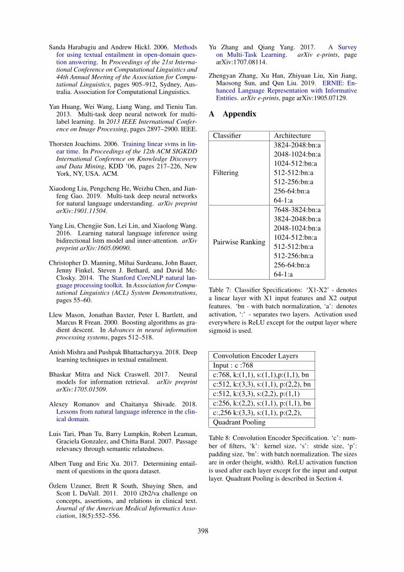
Sanda Harabagiu and Andrew Hickl. 2006. Methodsfor using textual entailment in open-domain ques-tion answering. In Proceedings of the 21st Interna-tional Conference on Computational Linguistics and44th Annual Meeting of the Association for Compu-tational Linguistics, pages 905–912, Sydney, Aus-tralia. Association for Computational Linguistics.
Yan Huang, Wei Wang, Liang Wang, and Tieniu Tan.2013. Multi-task deep neural network for multi-label learning. In 2013 IEEE International Confer-ence on Image Processing, pages 2897–2900. IEEE.
Thorsten Joachims. 2006. Training linear svms in lin-ear time. In Proceedings of the 12th ACM SIGKDDInternational Conference on Knowledge Discoveryand Data Mining, KDD ’06, pages 217–226, NewYork, NY, USA. ACM.
Xiaodong Liu, Pengcheng He, Weizhu Chen, and Jian-feng Gao. 2019. Multi-task deep neural networksfor natural language understanding. arXiv preprintarXiv:1901.11504.
Yang Liu, Chengjie Sun, Lei Lin, and Xiaolong Wang.2016. Learning natural language inference usingbidirectional lstm model and inner-attention. arXivpreprint arXiv:1605.09090.
Christopher D. Manning, Mihai Surdeanu, John Bauer,Jenny Finkel, Steven J. Bethard, and David Mc-Closky. 2014. The Stanford CoreNLP natural lan-guage processing toolkit. In Association for Compu-tational Linguistics (ACL) System Demonstrations,pages 55–60.
Llew Mason, Jonathan Baxter, Peter L Bartlett, andMarcus R Frean. 2000. Boosting algorithms as gra-dient descent. In Advances in neural informationprocessing systems, pages 512–518.
Anish Mishra and Pushpak Bhattacharyya. 2018. Deeplearning techniques in textual entailment.
Bhaskar Mitra and Nick Craswell. 2017. Neuralmodels for information retrieval. arXiv preprintarXiv:1705.01509.
Alexey Romanov and Chaitanya Shivade. 2018.Lessons from natural language inference in the clin-ical domain.
Luis Tari, Phan Tu, Barry Lumpkin, Robert Leaman,Graciela Gonzalez, and Chitta Baral. 2007. Passagerelevancy through semantic relatedness.
Albert Tung and Eric Xu. 2017. Determining entail-ment of questions in the quora dataset.
Özlem Uzuner, Brett R South, Shuying Shen, andScott L DuVall. 2011. 2010 i2b2/va challenge onconcepts, assertions, and relations in clinical text.Journal of the American Medical Informatics Asso-ciation, 18(5):552–556.
Yu Zhang and Qiang Yang. 2017. A Surveyon Multi-Task Learning. arXiv e-prints, pagearXiv:1707.08114.
Zhengyan Zhang, Xu Han, Zhiyuan Liu, Xin Jiang,Maosong Sun, and Qun Liu. 2019. ERNIE: En-hanced Language Representation with InformativeEntities. arXiv e-prints, page arXiv:1905.07129.
A Appendix
Classifier Architecture
Filtering
3824-2048:bn:a2048-1024:bn:a1024-512:bn:a512-512:bn:a512-256:bn:a256-64:bn:a64-1:a
Pairwise Ranking
7648-3824:bn:a3824-2048:bn:a2048-1024:bn:a1024-512:bn:a512-512:bn:a512-256:bn:a256-64:bn:a64-1:a
Table 7: Classifier Specifications: ‘X1-X2’ - denotesa linear layer with X1 input features and X2 outputfeatures. ‘bn - with batch normalization, ‘a’: denotesactivation, ‘:’ - separates two layers. Activation usedeverywhere is ReLU except for the output layer wheresigmoid is used.
Convolution Encoder LayersInput : c :768c:768, k:(1,1), s:(1,1),p:(1,1), bnc:512, k:(3,3), s:(1,1), p:(2,2), bnc:512, k:(3,3), s:(2,2), p:(1,1)c:256, k:(2,2), s:(1,1), p:(1,1), bnc:,256 k:(3,3), s:(1,1), p:(2,2),Quadrant Pooling
Table 8: Convolution Encoder Specification. ‘c’: num-ber of filters, ‘k’: kernel size, ‘s’: stride size, ‘p’:padding size, ‘bn’: with batch normalization. The sizesare in order (height, width). ReLU activation functionis used after each layer except for the input and outputlayer. Quadrant Pooling is described in Section 4.
398

Proceedings of the BioNLP 2019 workshop, pages 399–405Florence, Italy, August 1, 2019. c©2019 Association for Computational Linguistics
DoubleTransfer at MEDIQA 2019:Multi-Source Transfer Learning for Natural Language Understanding
in the Medical Domain
Yichong Xu1, Xiaodong Liu2, Chunyuan Li2, Hoifung Poon2 and Jianfeng Gao2
1 Carnegie Mellon University2 Microsoft Research
[email protected]{xiaodl, Chunyuan.Li, hoifung, jfgao}@microsoft.com
Abstract
This paper describes our competing system toenter the MEDIQA-2019 competition. We usea multi-source transfer learning approach totransfer the knowledge from MT-DNN (Liuet al., 2019b) and SciBERT (Beltagy et al.,2019) to natural language understanding tasksin the medical domain. For transfer learn-ing fine-tuning, we use multi-task learning onNLI, RQE and QA tasks on general and medi-cal domains to improve performance. The pro-posed methods are proved effective for natu-ral language understanding in the medical do-main, and we rank the first place on the QAtask.
1 Background
The MEDIQA 2019 shared tasks (Ben Abachaet al., 2019) aim to improve the current state-of-the-art systems for textual inference, question en-tailment and question answering in the medicaldomain. This ACL-BioNLP 2019 shared task ismotivated by a need to develop relevant methods,techniques and gold standards for inference andentailment in the medical domain and their ap-plication to improve domain-specific informationretrieval and question answering systems. Theshared task consists of three parts: i) natural lan-guage inference (NLI) on MedNLI, ii) Recogniz-ing Question Entailment (RQE), and iii) QuestionAnswering (QA).
Recent advancement in NLP such as BERT(Devlin et al., 2018) has facilitated great improve-ments in many Natural Language Understanding(NLU) tasks (Liu et al., 2019b). BERT first trainsa language model on an unsupervised large-scalecorpus, and then the pretrained model is fine-tunedto adapt to downstream NLU tasks. This fine-tuning process can be seen as a form of transferlearning, where BERT learns knowledge from the
large-scale corpus and transfer it to downstreamtasks.
We investigate NLU in the medical (scientific)domain. From BERT, we need to adapt to i) Thechange from general domain corpus to scientificlanguage; ii) The change from low-level languagemodel tasks to complex NLU tasks. Althoughthere is limited training data in NLU in the medi-cal domain, we fortunately have pre-trained mod-els from two intermediate steps:
• General NLU embeddings: We use MT-DNN(Liu et al., 2019b) trained on GLUE bench-mark(Wang et al., 2019). MT-DNN is trainedon 10 tasks including NLI, question equiv-alence, and machine comprehension. Thesetasks correspond well to the target MEDIQAtasks but in different domains.
• Scientific embeddings: We use SciBERT(Beltagy et al., 2019), which is a BERTmodel, but trained on SemanticScholar sci-entific papers. Although SciBERT obtainedstate-of-the-art results on several single-sentence tasks, it lacks knowledge from otherNLU tasks such as GLUE.
In this paper, we investigate different methodsto combine and transfer the knowledge from thetwo different sources and illustrate our results onthe MEDIQA shared task. We name our methodas DoubleTransfer, since it transfers knowledgefrom two different sources. Our method is basedon fine-tuning both MT-DNN and SciBERT usingmulti-task learning, which has demonstrated theefficiency of knowledge transformation (Caruana,1997; Liu et al., 2015; Xu et al., 2018; Liu et al.,2019b), and integrating models from both domainswith ensembles.Related Works. Transfer learning has beenwidely used in training models in the medical do-
399
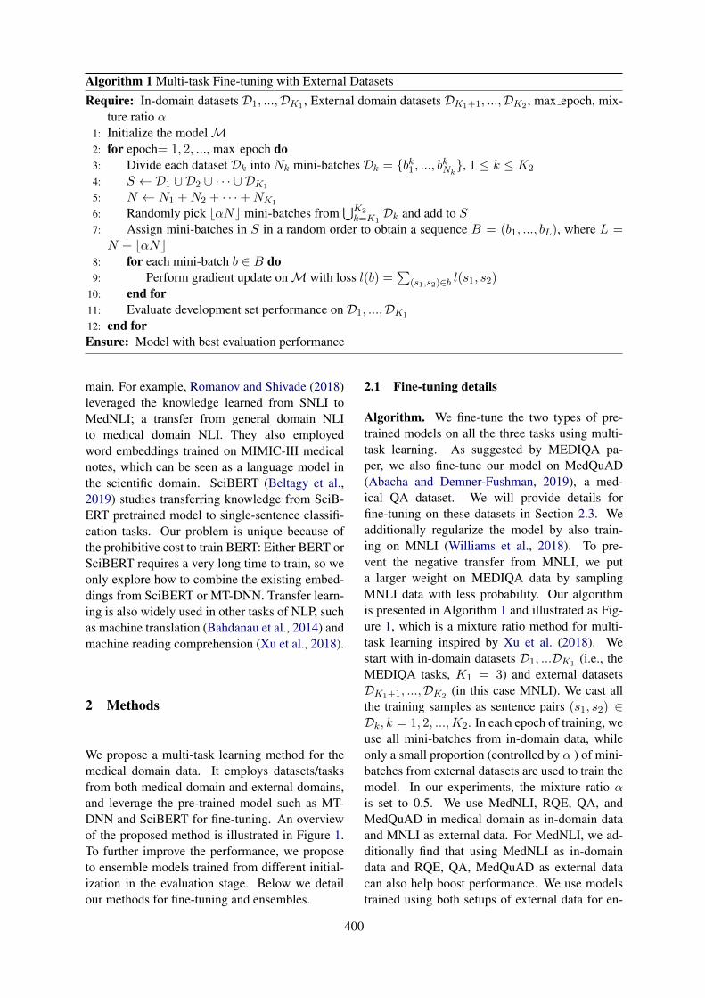
Algorithm 1 Multi-task Fine-tuning with External Datasets
Require: In-domain datasets D1, ...,DK1 , External domain datasets DK1+1, ...,DK2 , max epoch, mix-ture ratio α
1: Initialize the modelM2: for epoch= 1, 2, ..., max epoch do3: Divide each dataset Dk into Nk mini-batches Dk = {bk1, ..., bkNk
}, 1 ≤ k ≤ K2
4: S ← D1 ∪ D2 ∪ · · · ∪ DK1
5: N ← N1 +N2 + · · ·+NK1
6: Randomly pick bαNc mini-batches from⋃K2
k=K1Dk and add to S
7: Assign mini-batches in S in a random order to obtain a sequence B = (b1, ..., bL), where L =N + bαNc
8: for each mini-batch b ∈ B do9: Perform gradient update onM with loss l(b) =
∑(s1,s2)∈b l(s1, s2)
10: end for11: Evaluate development set performance on D1, ...,DK1
12: end forEnsure: Model with best evaluation performance
main. For example, Romanov and Shivade (2018)leveraged the knowledge learned from SNLI toMedNLI; a transfer from general domain NLIto medical domain NLI. They also employedword embeddings trained on MIMIC-III medicalnotes, which can be seen as a language model inthe scientific domain. SciBERT (Beltagy et al.,2019) studies transferring knowledge from SciB-ERT pretrained model to single-sentence classifi-cation tasks. Our problem is unique because ofthe prohibitive cost to train BERT: Either BERT orSciBERT requires a very long time to train, so weonly explore how to combine the existing embed-dings from SciBERT or MT-DNN. Transfer learn-ing is also widely used in other tasks of NLP, suchas machine translation (Bahdanau et al., 2014) andmachine reading comprehension (Xu et al., 2018).
2 Methods
We propose a multi-task learning method for themedical domain data. It employs datasets/tasksfrom both medical domain and external domains,and leverage the pre-trained model such as MT-DNN and SciBERT for fine-tuning. An overviewof the proposed method is illustrated in Figure 1.To further improve the performance, we proposeto ensemble models trained from different initial-ization in the evaluation stage. Below we detailour methods for fine-tuning and ensembles.
2.1 Fine-tuning details
Algorithm. We fine-tune the two types of pre-trained models on all the three tasks using multi-task learning. As suggested by MEDIQA pa-per, we also fine-tune our model on MedQuAD(Abacha and Demner-Fushman, 2019), a med-ical QA dataset. We will provide details forfine-tuning on these datasets in Section 2.3. Weadditionally regularize the model by also train-ing on MNLI (Williams et al., 2018). To pre-vent the negative transfer from MNLI, we puta larger weight on MEDIQA data by samplingMNLI data with less probability. Our algorithmis presented in Algorithm 1 and illustrated as Fig-ure 1, which is a mixture ratio method for multi-task learning inspired by Xu et al. (2018). Westart with in-domain datasets D1, ...DK1 (i.e., theMEDIQA tasks, K1 = 3) and external datasetsDK1+1, ...,DK2 (in this case MNLI). We cast allthe training samples as sentence pairs (s1, s2) ∈Dk, k = 1, 2, ...,K2. In each epoch of training, weuse all mini-batches from in-domain data, whileonly a small proportion (controlled by α ) of mini-batches from external datasets are used to train themodel. In our experiments, the mixture ratio αis set to 0.5. We use MedNLI, RQE, QA, andMedQuAD in medical domain as in-domain dataand MNLI as external data. For MedNLI, we ad-ditionally find that using MedNLI as in-domaindata and RQE, QA, MedQuAD as external datacan also help boost performance. We use modelstrained using both setups of external data for en-
400
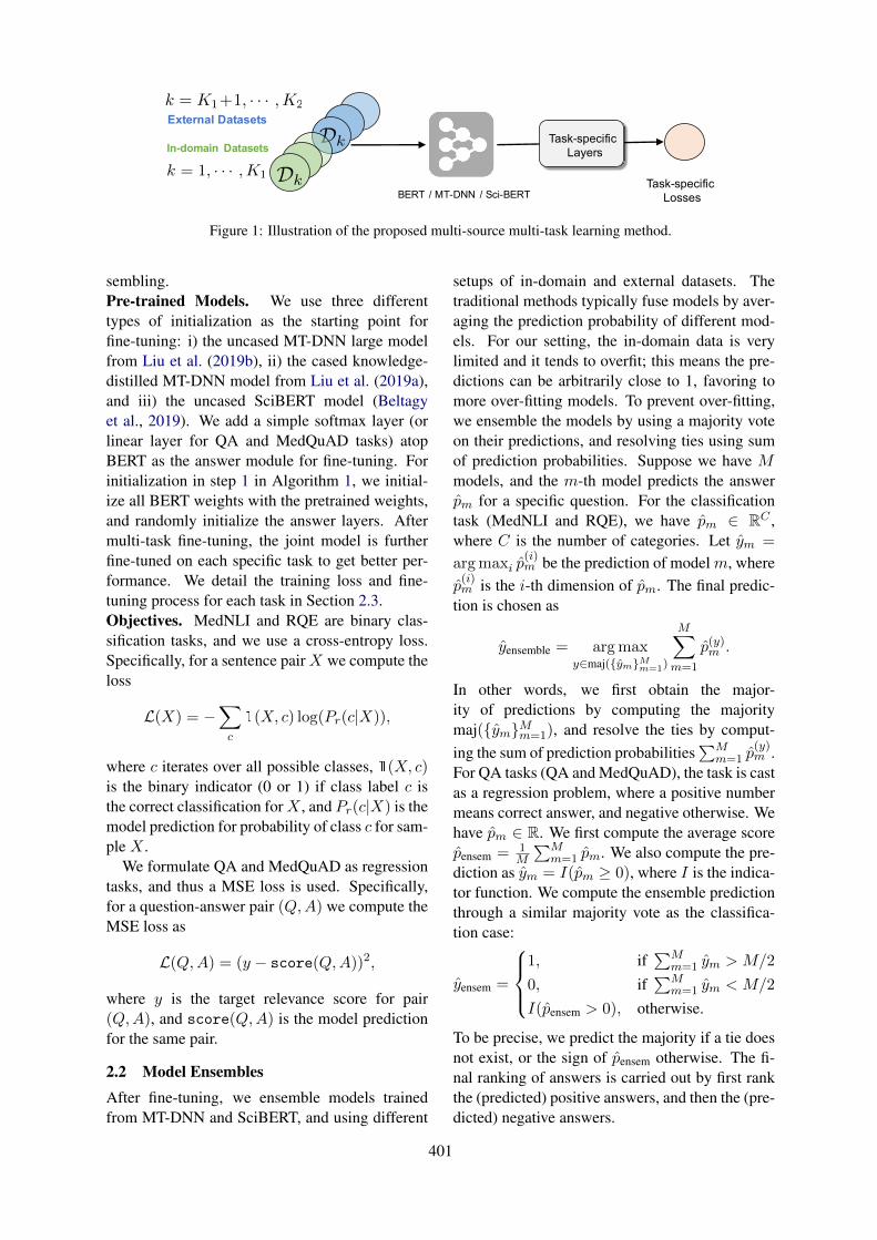
Dk<latexit sha1_base64="nIWvIpXPUYnZ1CkSaNqDEtL1dAU=">AAAB9HicbVDLSgMxFL1TX7W+qi7dBIvgqsyIoMuiLlxWsA9oh3InTdvQTGZMMoUy9DvcuFDErR/jzr8x085CWw8EDufcyz05QSy4Nq777RTW1jc2t4rbpZ3dvf2D8uFRU0eJoqxBIxGpdoCaCS5Zw3AjWDtWDMNAsFYwvs381oQpzSP5aKYx80McSj7gFI2V/G6IZkRRpHez3rhXrrhVdw6ySrycVCBHvVf+6vYjmoRMGipQ647nxsZPURlOBZuVuolmMdIxDlnHUokh0346Dz0jZ1bpk0Gk7JOGzNXfGymGWk/DwE5mIfWyl4n/eZ3EDK79lMs4MUzSxaFBIoiJSNYA6XPFqBFTS5AqbrMSOkKF1NieSrYEb/nLq6R5UfXcqvdwWand5HUU4QRO4Rw8uIIa3EMdGkDhCZ7hFd6cifPivDsfi9GCk+8cwx84nz/6SZI4</latexit><latexit sha1_base64="nIWvIpXPUYnZ1CkSaNqDEtL1dAU=">AAAB9HicbVDLSgMxFL1TX7W+qi7dBIvgqsyIoMuiLlxWsA9oh3InTdvQTGZMMoUy9DvcuFDErR/jzr8x085CWw8EDufcyz05QSy4Nq777RTW1jc2t4rbpZ3dvf2D8uFRU0eJoqxBIxGpdoCaCS5Zw3AjWDtWDMNAsFYwvs381oQpzSP5aKYx80McSj7gFI2V/G6IZkRRpHez3rhXrrhVdw6ySrycVCBHvVf+6vYjmoRMGipQ647nxsZPURlOBZuVuolmMdIxDlnHUokh0346Dz0jZ1bpk0Gk7JOGzNXfGymGWk/DwE5mIfWyl4n/eZ3EDK79lMs4MUzSxaFBIoiJSNYA6XPFqBFTS5AqbrMSOkKF1NieSrYEb/nLq6R5UfXcqvdwWand5HUU4QRO4Rw8uIIa3EMdGkDhCZ7hFd6cifPivDsfi9GCk+8cwx84nz/6SZI4</latexit><latexit sha1_base64="nIWvIpXPUYnZ1CkSaNqDEtL1dAU=">AAAB9HicbVDLSgMxFL1TX7W+qi7dBIvgqsyIoMuiLlxWsA9oh3InTdvQTGZMMoUy9DvcuFDErR/jzr8x085CWw8EDufcyz05QSy4Nq777RTW1jc2t4rbpZ3dvf2D8uFRU0eJoqxBIxGpdoCaCS5Zw3AjWDtWDMNAsFYwvs381oQpzSP5aKYx80McSj7gFI2V/G6IZkRRpHez3rhXrrhVdw6ySrycVCBHvVf+6vYjmoRMGipQ647nxsZPURlOBZuVuolmMdIxDlnHUokh0346Dz0jZ1bpk0Gk7JOGzNXfGymGWk/DwE5mIfWyl4n/eZ3EDK79lMs4MUzSxaFBIoiJSNYA6XPFqBFTS5AqbrMSOkKF1NieSrYEb/nLq6R5UfXcqvdwWand5HUU4QRO4Rw8uIIa3EMdGkDhCZ7hFd6cifPivDsfi9GCk+8cwx84nz/6SZI4</latexit><latexit sha1_base64="nIWvIpXPUYnZ1CkSaNqDEtL1dAU=">AAAB9HicbVDLSgMxFL1TX7W+qi7dBIvgqsyIoMuiLlxWsA9oh3InTdvQTGZMMoUy9DvcuFDErR/jzr8x085CWw8EDufcyz05QSy4Nq777RTW1jc2t4rbpZ3dvf2D8uFRU0eJoqxBIxGpdoCaCS5Zw3AjWDtWDMNAsFYwvs381oQpzSP5aKYx80McSj7gFI2V/G6IZkRRpHez3rhXrrhVdw6ySrycVCBHvVf+6vYjmoRMGipQ647nxsZPURlOBZuVuolmMdIxDlnHUokh0346Dz0jZ1bpk0Gk7JOGzNXfGymGWk/DwE5mIfWyl4n/eZ3EDK79lMs4MUzSxaFBIoiJSNYA6XPFqBFTS5AqbrMSOkKF1NieSrYEb/nLq6R5UfXcqvdwWand5HUU4QRO4Rw8uIIa3EMdGkDhCZ7hFd6cifPivDsfi9GCk+8cwx84nz/6SZI4</latexit>
BERT / MT'DNN / Sci'BERT
External Datasets
In,domain Datasets
Dk<latexit sha1_base64="nIWvIpXPUYnZ1CkSaNqDEtL1dAU=">AAAB9HicbVDLSgMxFL1TX7W+qi7dBIvgqsyIoMuiLlxWsA9oh3InTdvQTGZMMoUy9DvcuFDErR/jzr8x085CWw8EDufcyz05QSy4Nq777RTW1jc2t4rbpZ3dvf2D8uFRU0eJoqxBIxGpdoCaCS5Zw3AjWDtWDMNAsFYwvs381oQpzSP5aKYx80McSj7gFI2V/G6IZkRRpHez3rhXrrhVdw6ySrycVCBHvVf+6vYjmoRMGipQ647nxsZPURlOBZuVuolmMdIxDlnHUokh0346Dz0jZ1bpk0Gk7JOGzNXfGymGWk/DwE5mIfWyl4n/eZ3EDK79lMs4MUzSxaFBIoiJSNYA6XPFqBFTS5AqbrMSOkKF1NieSrYEb/nLq6R5UfXcqvdwWand5HUU4QRO4Rw8uIIa3EMdGkDhCZ7hFd6cifPivDsfi9GCk+8cwx84nz/6SZI4</latexit><latexit sha1_base64="nIWvIpXPUYnZ1CkSaNqDEtL1dAU=">AAAB9HicbVDLSgMxFL1TX7W+qi7dBIvgqsyIoMuiLlxWsA9oh3InTdvQTGZMMoUy9DvcuFDErR/jzr8x085CWw8EDufcyz05QSy4Nq777RTW1jc2t4rbpZ3dvf2D8uFRU0eJoqxBIxGpdoCaCS5Zw3AjWDtWDMNAsFYwvs381oQpzSP5aKYx80McSj7gFI2V/G6IZkRRpHez3rhXrrhVdw6ySrycVCBHvVf+6vYjmoRMGipQ647nxsZPURlOBZuVuolmMdIxDlnHUokh0346Dz0jZ1bpk0Gk7JOGzNXfGymGWk/DwE5mIfWyl4n/eZ3EDK79lMs4MUzSxaFBIoiJSNYA6XPFqBFTS5AqbrMSOkKF1NieSrYEb/nLq6R5UfXcqvdwWand5HUU4QRO4Rw8uIIa3EMdGkDhCZ7hFd6cifPivDsfi9GCk+8cwx84nz/6SZI4</latexit><latexit sha1_base64="nIWvIpXPUYnZ1CkSaNqDEtL1dAU=">AAAB9HicbVDLSgMxFL1TX7W+qi7dBIvgqsyIoMuiLlxWsA9oh3InTdvQTGZMMoUy9DvcuFDErR/jzr8x085CWw8EDufcyz05QSy4Nq777RTW1jc2t4rbpZ3dvf2D8uFRU0eJoqxBIxGpdoCaCS5Zw3AjWDtWDMNAsFYwvs381oQpzSP5aKYx80McSj7gFI2V/G6IZkRRpHez3rhXrrhVdw6ySrycVCBHvVf+6vYjmoRMGipQ647nxsZPURlOBZuVuolmMdIxDlnHUokh0346Dz0jZ1bpk0Gk7JOGzNXfGymGWk/DwE5mIfWyl4n/eZ3EDK79lMs4MUzSxaFBIoiJSNYA6XPFqBFTS5AqbrMSOkKF1NieSrYEb/nLq6R5UfXcqvdwWand5HUU4QRO4Rw8uIIa3EMdGkDhCZ7hFd6cifPivDsfi9GCk+8cwx84nz/6SZI4</latexit><latexit sha1_base64="nIWvIpXPUYnZ1CkSaNqDEtL1dAU=">AAAB9HicbVDLSgMxFL1TX7W+qi7dBIvgqsyIoMuiLlxWsA9oh3InTdvQTGZMMoUy9DvcuFDErR/jzr8x085CWw8EDufcyz05QSy4Nq777RTW1jc2t4rbpZ3dvf2D8uFRU0eJoqxBIxGpdoCaCS5Zw3AjWDtWDMNAsFYwvs381oQpzSP5aKYx80McSj7gFI2V/G6IZkRRpHez3rhXrrhVdw6ySrycVCBHvVf+6vYjmoRMGipQ647nxsZPURlOBZuVuolmMdIxDlnHUokh0346Dz0jZ1bpk0Gk7JOGzNXfGymGWk/DwE5mIfWyl4n/eZ3EDK79lMs4MUzSxaFBIoiJSNYA6XPFqBFTS5AqbrMSOkKF1NieSrYEb/nLq6R5UfXcqvdwWand5HUU4QRO4Rw8uIIa3EMdGkDhCZ7hFd6cifPivDsfi9GCk+8cwx84nz/6SZI4</latexit>
k = 1, · · · ,K1<latexit sha1_base64="9EtKC8Uxdh3q9J1tp9a9r97APpE=">AAAB+HicbVDLSgMxFM34rPXRUZdugkVwUcpEBN0IRTeCmwr2Ae0wZDKZNjSTDElGqEO/xI0LRdz6Ke78G9N2Ftp64MLhnHu5954w5Uwbz/t2VlbX1jc2S1vl7Z3dvYq7f9DWMlOEtojkUnVDrClngrYMM5x2U0VxEnLaCUc3U7/zSJVmUjyYcUr9BA8EixnBxkqBWxldoVqfRNLoGrwLUOBWvbo3A1wmqCBVUKAZuF/9SJIsocIQjrXuIS81fo6VYYTTSbmfaZpiMsID2rNU4IRqP58dPoEnVolgLJUtYeBM/T2R40TrcRLazgSboV70puJ/Xi8z8aWfM5FmhgoyXxRnHBoJpynAiClKDB9bgoli9lZIhlhhYmxWZRsCWnx5mbTP6siro/vzauO6iKMEjsAxOAUIXIAGuAVN0AIEZOAZvII358l5cd6dj3nrilPMHII/cD5/ANkykeY=</latexit><latexit sha1_base64="9EtKC8Uxdh3q9J1tp9a9r97APpE=">AAAB+HicbVDLSgMxFM34rPXRUZdugkVwUcpEBN0IRTeCmwr2Ae0wZDKZNjSTDElGqEO/xI0LRdz6Ke78G9N2Ftp64MLhnHu5954w5Uwbz/t2VlbX1jc2S1vl7Z3dvYq7f9DWMlOEtojkUnVDrClngrYMM5x2U0VxEnLaCUc3U7/zSJVmUjyYcUr9BA8EixnBxkqBWxldoVqfRNLoGrwLUOBWvbo3A1wmqCBVUKAZuF/9SJIsocIQjrXuIS81fo6VYYTTSbmfaZpiMsID2rNU4IRqP58dPoEnVolgLJUtYeBM/T2R40TrcRLazgSboV70puJ/Xi8z8aWfM5FmhgoyXxRnHBoJpynAiClKDB9bgoli9lZIhlhhYmxWZRsCWnx5mbTP6siro/vzauO6iKMEjsAxOAUIXIAGuAVN0AIEZOAZvII358l5cd6dj3nrilPMHII/cD5/ANkykeY=</latexit><latexit sha1_base64="9EtKC8Uxdh3q9J1tp9a9r97APpE=">AAAB+HicbVDLSgMxFM34rPXRUZdugkVwUcpEBN0IRTeCmwr2Ae0wZDKZNjSTDElGqEO/xI0LRdz6Ke78G9N2Ftp64MLhnHu5954w5Uwbz/t2VlbX1jc2S1vl7Z3dvYq7f9DWMlOEtojkUnVDrClngrYMM5x2U0VxEnLaCUc3U7/zSJVmUjyYcUr9BA8EixnBxkqBWxldoVqfRNLoGrwLUOBWvbo3A1wmqCBVUKAZuF/9SJIsocIQjrXuIS81fo6VYYTTSbmfaZpiMsID2rNU4IRqP58dPoEnVolgLJUtYeBM/T2R40TrcRLazgSboV70puJ/Xi8z8aWfM5FmhgoyXxRnHBoJpynAiClKDB9bgoli9lZIhlhhYmxWZRsCWnx5mbTP6siro/vzauO6iKMEjsAxOAUIXIAGuAVN0AIEZOAZvII358l5cd6dj3nrilPMHII/cD5/ANkykeY=</latexit><latexit sha1_base64="9EtKC8Uxdh3q9J1tp9a9r97APpE=">AAAB+HicbVDLSgMxFM34rPXRUZdugkVwUcpEBN0IRTeCmwr2Ae0wZDKZNjSTDElGqEO/xI0LRdz6Ke78G9N2Ftp64MLhnHu5954w5Uwbz/t2VlbX1jc2S1vl7Z3dvYq7f9DWMlOEtojkUnVDrClngrYMM5x2U0VxEnLaCUc3U7/zSJVmUjyYcUr9BA8EixnBxkqBWxldoVqfRNLoGrwLUOBWvbo3A1wmqCBVUKAZuF/9SJIsocIQjrXuIS81fo6VYYTTSbmfaZpiMsID2rNU4IRqP58dPoEnVolgLJUtYeBM/T2R40TrcRLazgSboV70puJ/Xi8z8aWfM5FmhgoyXxRnHBoJpynAiClKDB9bgoli9lZIhlhhYmxWZRsCWnx5mbTP6siro/vzauO6iKMEjsAxOAUIXIAGuAVN0AIEZOAZvII358l5cd6dj3nrilPMHII/cD5/ANkykeY=</latexit>
k = K1+1, · · · ,K2<latexit sha1_base64="gg82fn5PwbpGh2te5lm987yANFg=">AAACAHicbVDLSsNAFJ3UV62vqAsXbqYWQbCUpAi6EYpuhG4q2Ac0IUwmk3boJBNmJkIJ3fgrblwo4tbPcOffOG2z0NYDFw7n3Mu99/gJo1JZ1rdRWFldW98obpa2tnd298z9g47kqcCkjTnjoucjSRiNSVtRxUgvEQRFPiNdf3Q79buPREjK4wc1TogboUFMQ4qR0pJnHo2um57tlM+dsl11cMCVrMKmV/fMilWzZoDLxM5JBeRoeeaXE3CcRiRWmCEp+7aVKDdDQlHMyKTkpJIkCI/QgPQ1jVFEpJvNHpjAU60EMORCV6zgTP09kaFIynHk684IqaFc9Kbif14/VeGVm9E4SRWJ8XxRmDKoOJymAQMqCFZsrAnCgupbIR4igbDSmZV0CPbiy8ukU6/ZVs2+v6g0bvI4iuAYnIAzYINL0AB3oAXaAIMJeAav4M14Ml6Md+Nj3low8plD8AfG5w8zMpQ3</latexit><latexit sha1_base64="gg82fn5PwbpGh2te5lm987yANFg=">AAACAHicbVDLSsNAFJ3UV62vqAsXbqYWQbCUpAi6EYpuhG4q2Ac0IUwmk3boJBNmJkIJ3fgrblwo4tbPcOffOG2z0NYDFw7n3Mu99/gJo1JZ1rdRWFldW98obpa2tnd298z9g47kqcCkjTnjoucjSRiNSVtRxUgvEQRFPiNdf3Q79buPREjK4wc1TogboUFMQ4qR0pJnHo2um57tlM+dsl11cMCVrMKmV/fMilWzZoDLxM5JBeRoeeaXE3CcRiRWmCEp+7aVKDdDQlHMyKTkpJIkCI/QgPQ1jVFEpJvNHpjAU60EMORCV6zgTP09kaFIynHk684IqaFc9Kbif14/VeGVm9E4SRWJ8XxRmDKoOJymAQMqCFZsrAnCgupbIR4igbDSmZV0CPbiy8ukU6/ZVs2+v6g0bvI4iuAYnIAzYINL0AB3oAXaAIMJeAav4M14Ml6Md+Nj3low8plD8AfG5w8zMpQ3</latexit><latexit sha1_base64="gg82fn5PwbpGh2te5lm987yANFg=">AAACAHicbVDLSsNAFJ3UV62vqAsXbqYWQbCUpAi6EYpuhG4q2Ac0IUwmk3boJBNmJkIJ3fgrblwo4tbPcOffOG2z0NYDFw7n3Mu99/gJo1JZ1rdRWFldW98obpa2tnd298z9g47kqcCkjTnjoucjSRiNSVtRxUgvEQRFPiNdf3Q79buPREjK4wc1TogboUFMQ4qR0pJnHo2um57tlM+dsl11cMCVrMKmV/fMilWzZoDLxM5JBeRoeeaXE3CcRiRWmCEp+7aVKDdDQlHMyKTkpJIkCI/QgPQ1jVFEpJvNHpjAU60EMORCV6zgTP09kaFIynHk684IqaFc9Kbif14/VeGVm9E4SRWJ8XxRmDKoOJymAQMqCFZsrAnCgupbIR4igbDSmZV0CPbiy8ukU6/ZVs2+v6g0bvI4iuAYnIAzYINL0AB3oAXaAIMJeAav4M14Ml6Md+Nj3low8plD8AfG5w8zMpQ3</latexit><latexit sha1_base64="gg82fn5PwbpGh2te5lm987yANFg=">AAACAHicbVDLSsNAFJ3UV62vqAsXbqYWQbCUpAi6EYpuhG4q2Ac0IUwmk3boJBNmJkIJ3fgrblwo4tbPcOffOG2z0NYDFw7n3Mu99/gJo1JZ1rdRWFldW98obpa2tnd298z9g47kqcCkjTnjoucjSRiNSVtRxUgvEQRFPiNdf3Q79buPREjK4wc1TogboUFMQ4qR0pJnHo2um57tlM+dsl11cMCVrMKmV/fMilWzZoDLxM5JBeRoeeaXE3CcRiRWmCEp+7aVKDdDQlHMyKTkpJIkCI/QgPQ1jVFEpJvNHpjAU60EMORCV6zgTP09kaFIynHk684IqaFc9Kbif14/VeGVm9E4SRWJ8XxRmDKoOJymAQMqCFZsrAnCgupbIR4igbDSmZV0CPbiy8ukU6/ZVs2+v6g0bvI4iuAYnIAzYINL0AB3oAXaAIMJeAav4M14Ml6Md+Nj3low8plD8AfG5w8zMpQ3</latexit>
Task'specificLayers
Task'specificLosses
Figure 1: Illustration of the proposed multi-source multi-task learning method.
sembling.Pre-trained Models. We use three differenttypes of initialization as the starting point forfine-tuning: i) the uncased MT-DNN large modelfrom Liu et al. (2019b), ii) the cased knowledge-distilled MT-DNN model from Liu et al. (2019a),and iii) the uncased SciBERT model (Beltagyet al., 2019). We add a simple softmax layer (orlinear layer for QA and MedQuAD tasks) atopBERT as the answer module for fine-tuning. Forinitialization in step 1 in Algorithm 1, we initial-ize all BERT weights with the pretrained weights,and randomly initialize the answer layers. Aftermulti-task fine-tuning, the joint model is furtherfine-tuned on each specific task to get better per-formance. We detail the training loss and fine-tuning process for each task in Section 2.3.Objectives. MedNLI and RQE are binary clas-sification tasks, and we use a cross-entropy loss.Specifically, for a sentence pairX we compute theloss
L(X) = −∑
c
1(X, c) log(Pr(c|X)),
where c iterates over all possible classes, 1(X, c)is the binary indicator (0 or 1) if class label c isthe correct classification forX , and Pr(c|X) is themodel prediction for probability of class c for sam-ple X .
We formulate QA and MedQuAD as regressiontasks, and thus a MSE loss is used. Specifically,for a question-answer pair (Q,A) we compute theMSE loss as
L(Q,A) = (y − score(Q,A))2,
where y is the target relevance score for pair(Q,A), and score(Q,A) is the model predictionfor the same pair.
2.2 Model EnsemblesAfter fine-tuning, we ensemble models trainedfrom MT-DNN and SciBERT, and using different
setups of in-domain and external datasets. Thetraditional methods typically fuse models by aver-aging the prediction probability of different mod-els. For our setting, the in-domain data is verylimited and it tends to overfit; this means the pre-dictions can be arbitrarily close to 1, favoring tomore over-fitting models. To prevent over-fitting,we ensemble the models by using a majority voteon their predictions, and resolving ties using sumof prediction probabilities. Suppose we have Mmodels, and the m-th model predicts the answerp̂m for a specific question. For the classificationtask (MedNLI and RQE), we have p̂m ∈ RC ,where C is the number of categories. Let ŷm =
argmaxi p̂(i)m be the prediction of modelm, where
p̂(i)m is the i-th dimension of p̂m. The final predic-
tion is chosen as
ŷensemble = argmaxy∈maj({ŷm}Mm=1)
M∑
m=1
p̂(y)m .
In other words, we first obtain the major-ity of predictions by computing the majoritymaj({ŷm}Mm=1), and resolve the ties by comput-ing the sum of prediction probabilities
∑Mm=1 p̂
(y)m .
For QA tasks (QA and MedQuAD), the task is castas a regression problem, where a positive numbermeans correct answer, and negative otherwise. Wehave p̂m ∈ R. We first compute the average scorep̂ensem = 1
M
∑Mm=1 p̂m. We also compute the pre-
diction as ŷm = I(p̂m ≥ 0), where I is the indica-tor function. We compute the ensemble predictionthrough a similar majority vote as the classifica-tion case:
ŷensem =
1, if∑M
m=1 ŷm > M/2
0, if∑M
m=1 ŷm < M/2
I(p̂ensem > 0), otherwise.
To be precise, we predict the majority if a tie doesnot exist, or the sign of p̂ensem otherwise. The fi-nal ranking of answers is carried out by first rankthe (predicted) positive answers, and then the (pre-dicted) negative answers.
401
2.3 Dataset-Specific Details
MedNLI: Since the MEDIQA shared task uses adifferent test set than the original MedNLI dataset,we merge the original MedNLI development setinto the training set and use evaluation perfor-mance on the original MedNLI test set. Further-more, MedNLI and MNLI are the same NLI tasks,thus, we shared final-layer classifiers for these twotasks. For MedNLI, we find that each consecutive3 samples in all the training set contain the samepremise with different hypothesizes, and containsexactly 1 entail, 1 neutral and 1 contradiction. Tothe end, in our prediction, we constrain the threepredictions to be one of each kind, and use themost likely prediction from the model predictionprobabilities.RQE: We use the clinical question as the premiseand question from FAQ as the hypothesis. We findthat the test data distribution is quite different fromthe train data distribution. To mitigate this effect,we randomly shuffle half of the evaluation datainto the training set and evaluate on the remain-ing half.QA: We use the answer as the premise and thequestion as the hypothesis. The QA task is castas both a ranking task and a classification task.Each question is associated with a relevance scorein {1, 2, 3, 4}, and an additional rank over allthe answers for a specific question is given. Weuse a modified score to incorporate both informa-tion: suppose there arem questions with relevancescore s ∈ {1, 2, 3, 4}. Then the i-th most relevantanswer in these m questions get modified scores− i−1
m . In this way the scores are uniformly dis-tributed in (s− 1, s]. We shift all scores by −2 sothat a positive score leads to a correct answer andvice versa. We also tried pairwise losses to incor-porate the ranking but did not find it to boost theperformance very much.
We find that the development set distribution isinconsistent with test data - the training and test setconsist of both LiveQAMed and Alexa questions,whereas the development set seems to only con-tain LiveQAMed questions. We shuffle the train-ing and development set to make them similar: Weuse the last 25 questions in original developmentset (LiveQAMed questions) and the last 25 Alexaquestions (from the original training set) as our de-velopment set, and use the remaining questions asour training set. This results in 1,504 training pairsand 431 validation pairs. Due to the limited size
of the QA dataset, we use cross-validation that di-vides all pairs into 5 slices and train 5 models byusing each slice as a validation set. We train MT-DNN and SciBERT on both these 5 setups and ob-tain 10 models, and ensemble all the 10 modelsobtained.MedQuAD: We use 10,109 questions fromMedQuAD because the remaining questions arenot available due to copyright issues. The originalMedQuAD dataset only contains positive questionpairs. We add negative samples to the dataset byrandomly sampling an answer from the same webpage. For each positive QA pair, we add two neg-ative samples. The resulting 30,327 pairs are ran-domly divided into 27,391 training pairs and 2,936evaluation pairs. Then we use the same method asQA to train MedQuAD; we also share the sameanswer module between QA and MedQuAD.
2.4 Implementation and Hyperparameters
We implement our method using PyTorch1 andPytorch-pretrained-BERT2, as an extension toMT-DNN3. We also use the pytorch-compatibleSciBERT pretrained model provided by Al-lenNLP4. Each training example is pruned to atmost 384 tokens for MT-DNN models and 512 to-kens for SciBERT models. We use a batch size of16 for MT-DNN, and 40 for SciBERT. For fine-tuning, we train the models for 20 epochs usinga learning rate of 5 × 10⁻⁵. After that, we fur-ther fine-tune the model from the best multi-taskmodel for 6 epochs for each dataset, using a learn-ing rate of 5×10⁻⁶. We ensemble all models withan accuracy larger than 87.7 for MedNLI, 83.5 forshuffled RQE, and 83.0 for QA. We ensemble 4models for MedNLI, 14 models for RQE. For QA,we ensemble 10 models from cross-validation and7 models using the normal training-validation ap-proach.
3 Results
In this section, we provide the leaderboard perfor-mance and conduct an analysis of the effect of en-semble models from different sources.
1https://pytorch.org/2https://github.com/huggingface/
pytorch-pretrained-BERT3https://github.com/namisan/mt-dnn4https://github.com/allenai/scibert
402
Model Dev Set Test SetWTMed - 98.0PANLP - 96.6Ours 91.7 93.8Sieg - 91.1SOTA 76.6 -
Table 1: The leaderboard for MedNLI task (link).Scores are accuracy(%). Our method ranked the 3rdon the leaderboard. Previous SOTA method was from(Romanov and Shivade, 2018), on the original MedNLItest set (used as dev set here).
Model Dev Set Test SetPANLP - 74.9Sieg - 70.6IIT-KGP - 68.4Ours 91.7 66.2
Table 2: The leaderboard for RQE task (link). Scoresare accuracy(%). Our method ranked the 7th on theleaderboard.
3.1 Test Set Performance and LeaderBoards
The results for MedNLI dataset is summarized inTable 1. Our method ends up the 3rd place on theleaderboard and substantially improving upon pre-vious state-of-the-art (SOTA) methods.
The results for RQE dataset is summarized inTable 2. Our method ends up the 7th place on theleaderboard. Our method has a very large discrep-ancy between the dev set performance and test setperformance. We think this is because the test setis quite different from dev set, and that the dev setis very small and easy to overfit to.
The results for QA dataset is summarized in Ta-ble 3. Our method reaches the first place on theleaderboard based on accuracy and precision scoreand 3rd-highest MRR. We note that the Spearmanscore is not consistent with other scores in theleaderboard; actually, the Spearman score is com-puted just based on the predicted positive answers,and a method can get very high Spearman score bynever predict positive labels.
3.2 Ensembles from Different Sources
We compare the effect of ensembling from dif-ferent sources in Table 4. We train 6 differentmodels with different randomizations, with ini-tializations from MT-DNN (#1,#2,#3) and SciB-ERT (#4, #5,#6) respectively. If we ensemble
Model Acc Spearman Precision MRROurs 78.0 0.238 81.91 0.937PANLP 77.7 0.180 78.1 0.938Pentagon 76.5 0.338 77.7 0.962DUT-BIM 74.5 0.106 74.7 0.906
Table 3: The leaderboard for QA task (link). Ourmethod ranked #1 on the leaderboard in terms of Acc(accuracy). The Spearman score is not consistent withother scores in the leaderboard.
models with the same MT-DNN architecture, theresulting model only has around 1.5% improve-ment in accuracy, compared to the numerical aver-age of the ensemble model accuracies (#1+#2+#3and #4+#5+#6 in Table 4). On the other hand, ifwe ensemble three models from different sources(#1+#2+#5 and #1+#5+#6 in Table 4), the result-ing model gains more than 3% in accuracy com-pared to the numerical average. This shows thatensembling from different sources has a great ad-vantage than ensembling from single-source mod-els.
Model Avg. Acc Esm. AccSingle Model
#1, MT-DNN - 88.61#2, MT-DNN - 88.33#3, MT-DNN - 87.84#4, SciBERT - 88.19#5, SciBERT - 87.70#6, SciBERT - 87.21
Ensemble Model#1+#2+#3, MT-DNN 88.26 89.7#4+#5+#6, SciBERT 87.70 89.2#1+#2+#5, MultiSource 88.21 91.6#1+#5+#6, MultiSource 87.84 90.4#1-6, MultiSource 87.98 91.3
Table 4: Comparison of ensembles from differentsources. Avg.Acc stands for average accuracy, the nu-merical average of each individual model’s accuracy.Esm.Acc stands for ensemble accuracy, the accuracyof the resulting ensemble model. For ensembles, MT-DNN means all the three models are from MT-DNN,and similarly for SciBERT; MultiSource denotes theensemble models come from two different sources.
3.3 Single-Model Performance
For completeness, we report the single-model per-formance on the MedNLI development set under
403
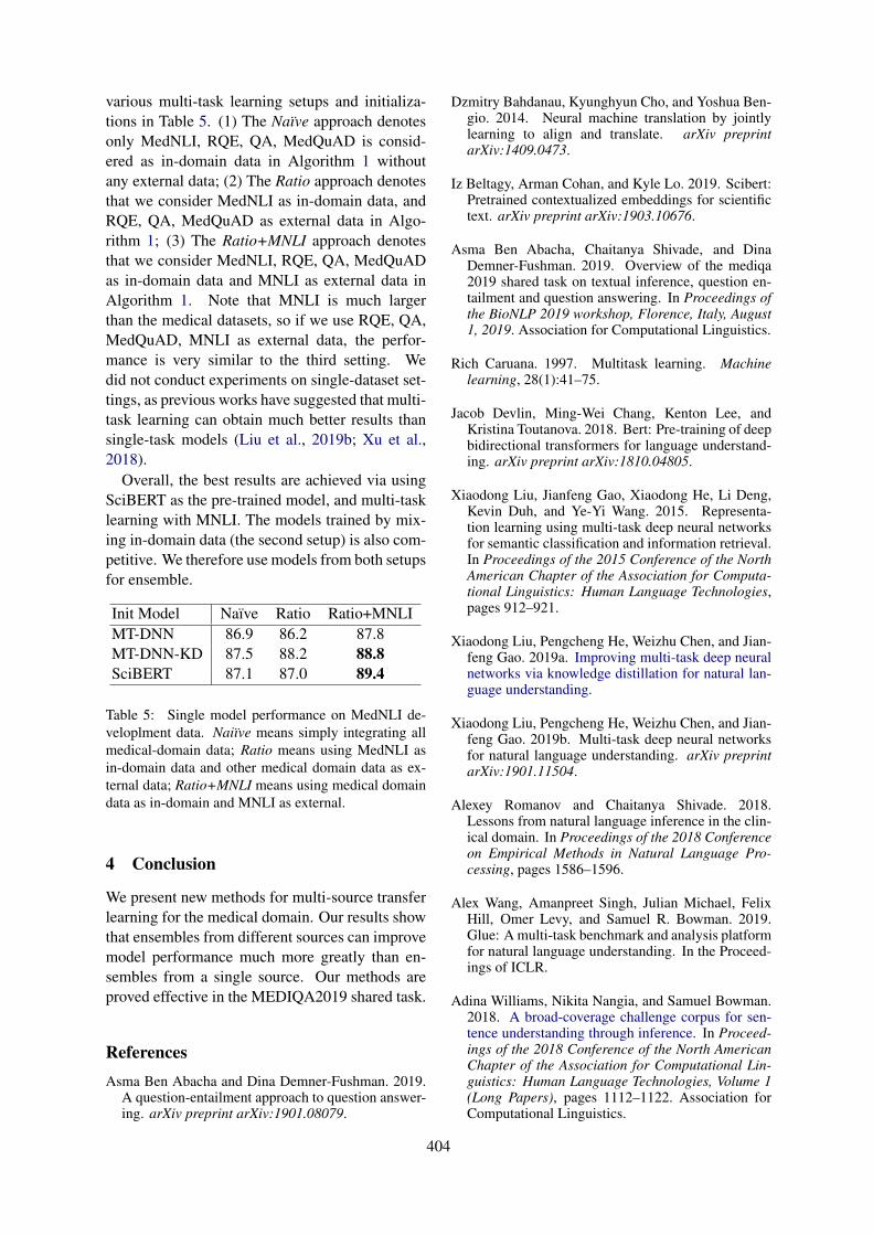
various multi-task learning setups and initializa-tions in Table 5. (1) The Naı̈ve approach denotesonly MedNLI, RQE, QA, MedQuAD is consid-ered as in-domain data in Algorithm 1 withoutany external data; (2) The Ratio approach denotesthat we consider MedNLI as in-domain data, andRQE, QA, MedQuAD as external data in Algo-rithm 1; (3) The Ratio+MNLI approach denotesthat we consider MedNLI, RQE, QA, MedQuADas in-domain data and MNLI as external data inAlgorithm 1. Note that MNLI is much largerthan the medical datasets, so if we use RQE, QA,MedQuAD, MNLI as external data, the perfor-mance is very similar to the third setting. Wedid not conduct experiments on single-dataset set-tings, as previous works have suggested that multi-task learning can obtain much better results thansingle-task models (Liu et al., 2019b; Xu et al.,2018).
Overall, the best results are achieved via usingSciBERT as the pre-trained model, and multi-tasklearning with MNLI. The models trained by mix-ing in-domain data (the second setup) is also com-petitive. We therefore use models from both setupsfor ensemble.
Init Model Naı̈ve Ratio Ratio+MNLIMT-DNN 86.9 86.2 87.8MT-DNN-KD 87.5 88.2 88.8SciBERT 87.1 87.0 89.4
Table 5: Single model performance on MedNLI de-veloplment data. Naiı̈ve means simply integrating allmedical-domain data; Ratio means using MedNLI asin-domain data and other medical domain data as ex-ternal data; Ratio+MNLI means using medical domaindata as in-domain and MNLI as external.
4 Conclusion
We present new methods for multi-source transferlearning for the medical domain. Our results showthat ensembles from different sources can improvemodel performance much more greatly than en-sembles from a single source. Our methods areproved effective in the MEDIQA2019 shared task.
ReferencesAsma Ben Abacha and Dina Demner-Fushman. 2019.
A question-entailment approach to question answer-ing. arXiv preprint arXiv:1901.08079.
Dzmitry Bahdanau, Kyunghyun Cho, and Yoshua Ben-gio. 2014. Neural machine translation by jointlylearning to align and translate. arXiv preprintarXiv:1409.0473.
Iz Beltagy, Arman Cohan, and Kyle Lo. 2019. Scibert:Pretrained contextualized embeddings for scientifictext. arXiv preprint arXiv:1903.10676.
Asma Ben Abacha, Chaitanya Shivade, and DinaDemner-Fushman. 2019. Overview of the mediqa2019 shared task on textual inference, question en-tailment and question answering. In Proceedings ofthe BioNLP 2019 workshop, Florence, Italy, August1, 2019. Association for Computational Linguistics.
Rich Caruana. 1997. Multitask learning. Machinelearning, 28(1):41–75.
Jacob Devlin, Ming-Wei Chang, Kenton Lee, andKristina Toutanova. 2018. Bert: Pre-training of deepbidirectional transformers for language understand-ing. arXiv preprint arXiv:1810.04805.
Xiaodong Liu, Jianfeng Gao, Xiaodong He, Li Deng,Kevin Duh, and Ye-Yi Wang. 2015. Representa-tion learning using multi-task deep neural networksfor semantic classification and information retrieval.In Proceedings of the 2015 Conference of the NorthAmerican Chapter of the Association for Computa-tional Linguistics: Human Language Technologies,pages 912–921.
Xiaodong Liu, Pengcheng He, Weizhu Chen, and Jian-feng Gao. 2019a. Improving multi-task deep neuralnetworks via knowledge distillation for natural lan-guage understanding.
Xiaodong Liu, Pengcheng He, Weizhu Chen, and Jian-feng Gao. 2019b. Multi-task deep neural networksfor natural language understanding. arXiv preprintarXiv:1901.11504.
Alexey Romanov and Chaitanya Shivade. 2018.Lessons from natural language inference in the clin-ical domain. In Proceedings of the 2018 Conferenceon Empirical Methods in Natural Language Pro-cessing, pages 1586–1596.
Alex Wang, Amanpreet Singh, Julian Michael, FelixHill, Omer Levy, and Samuel R. Bowman. 2019.Glue: A multi-task benchmark and analysis platformfor natural language understanding. In the Proceed-ings of ICLR.
Adina Williams, Nikita Nangia, and Samuel Bowman.2018. A broad-coverage challenge corpus for sen-tence understanding through inference. In Proceed-ings of the 2018 Conference of the North AmericanChapter of the Association for Computational Lin-guistics: Human Language Technologies, Volume 1(Long Papers), pages 1112–1122. Association forComputational Linguistics.
404

Yichong Xu, Xiaodong Liu, Yelong Shen, JingjingLiu, and Jianfeng Gao. 2018. Multi-task learningfor machine reading comprehension. arXiv preprintarXiv:1809.06963.
405
Proceedings of the BioNLP 2019 workshop, pages 406–414Florence, Italy, August 1, 2019. c©2019 Association for Computational Linguistics
Surf at MEDIQA 2019: Improving Performance ofNatural Language Inference in the Clinical Domain
by Adopting Pre-trained Language Model
Jiin NamAI Core Team
Samsung ResearchSeoul, Korea
Seunghyun YoonDept. ECE
Seoul National UniversitySeoul, Korea
Kyomin JungDept. ECE
Seoul National UniversitySeoul, Korea
Abstract
While deep learning techniques have shownpromising results in many natural languageprocessing (NLP) tasks, it has not been widelyapplied to the clinical domain. The lackof large datasets and the pervasive use ofdomain-specific language (i.e. abbreviationsand acronyms) in the clinical domain causesslower progress in NLP tasks than that of thegeneral NLP tasks. To fill this gap, we employword/subword-level based models that adoptlarge-scale data-driven methods such as pre-trained language models and transfer learningin analyzing text for the clinical domain. Em-pirical results demonstrate the superiority ofthe proposed methods by achieving 90.6% ac-curacy in medical domain natural language in-ference task. Furthermore, we inspect the inde-pendent strengths of the proposed approachesin quantitative and qualitative manners. Thisanalysis will help researchers to select neces-sary components in building models for themedical domain.
1 Introduction
Natural language processing (NLP) has broadenedits applications rapidly in recent years such asquestion answering, neural machine translation,natural language inference, and other language-related tasks. Unlike other tasks in NLP area, thelack of large labeled datasets and restricted accessin the clinical domain have discouraged active par-ticipation of NLP researchers for this domain (Ro-manov and Shivade, 2018). Furthermore, the per-vasive use of abbreviations and acronyms in theclinical domain causes the difficulty of text nor-malization and makes the related tasks more diffi-cult (Pakhomov, 2002).
In building NLP models, a word embeddinglayer that transforms a sequence of tokens in textinto a vector representation is considered as one
of the fundamental components. In recent stud-ies, it has been shown that the pre-trained lan-guage models by using a huge diversity of corpus(i.e. BERT (Devlin et al., 2018) and ELMo (Peterset al., 2018)) generate deep contextualized wordrepresentations. These methods have shown to bevery effective for improving the performance of awide range of NLP tasks by enabling better textunderstanding and have become a crucial part ofthe tasks since they have published.
To stimulate the research in the clinical domain,researchers have further investigated to transformthe pre-trained language models from general pur-pose version into the medical domain-specific ver-sion. Lee et al. (2019) propose BioBERT that uti-lizes large-scale bio-medical corpora, PubMed ab-stracts (PubMed) and PubMed Central full-text ar-ticles (PMC), to obtain a medical domain spe-cific language representation through fine-tuningthe BERT. Similarity, a PubMed-ELMo1, trainedwith medical domain corpus, is released as oneof the contributed ELMo models for medical do-main researchers. However, these models are notyet fully explored in medical domain tasks.
Besides these general efforts in building bet-ter word representations, Romanov and Shivade(2018) introduce a large and publicly availablenatural language inference (NLI) dataset, calledMedNLI, for the medical domain (see table 1).Considering the expensive annotation cost of med-ical text due to the sparsity of the clinical-domainexperts, the medical NLI task plays an import rolein boosting existing datasets for medical ques-tion answering systems by retrieving similar ques-tions that are already answered by human ex-perts. Along with this effort, ACL-BioNLP 2019committee announced a shared task, NLI for themedical domain, motivated by a need to develop
1https://allennlp.org/elmo
406
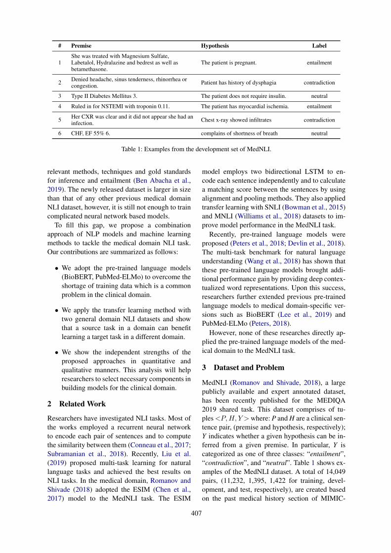
# Premise Hypothesis Label
1She was treated with Magnesium Sulfate,Labetalol, Hydralazine and bedrest as well asbetamethasone.
The patient is pregnant. entailment
2 Denied headache, sinus tenderness, rhinorrhea orcongestion. Patient has history of dysphagia contradiction
3 Type II Diabetes Mellitus 3. The patient does not require insulin. neutral
4 Ruled in for NSTEMI with troponin 0.11. The patient has myocardial ischemia. entailment
5 Her CXR was clear and it did not appear she had aninfection. Chest x-ray showed infiltrates contradiction
6 CHF, EF 55% 6. complains of shortness of breath neutral
Table 1: Examples from the development set of MedNLI.
relevant methods, techniques and gold standardsfor inference and entailment (Ben Abacha et al.,2019). The newly released dataset is larger in sizethan that of any other previous medical domainNLI dataset, however, it is still not enough to traincomplicated neural network based models.
To fill this gap, we propose a combinationapproach of NLP models and machine learningmethods to tackle the medical domain NLI task.Our contributions are summarized as follows:
• We adopt the pre-trained language models(BioBERT, PubMed-ELMo) to overcome theshortage of training data which is a commonproblem in the clinical domain.
• We apply the transfer learning method withtwo general domain NLI datasets and showthat a source task in a domain can benefitlearning a target task in a different domain.
• We show the independent strengths of theproposed approaches in quantitative andqualitative manners. This analysis will helpresearchers to select necessary components inbuilding models for the clinical domain.
2 Related Work
Researchers have investigated NLI tasks. Most ofthe works employed a recurrent neural networkto encode each pair of sentences and to computethe similarity between them (Conneau et al., 2017;Subramanian et al., 2018). Recently, Liu et al.(2019) proposed multi-task learning for naturallanguage tasks and achieved the best results onNLI tasks. In the medical domain, Romanov andShivade (2018) adopted the ESIM (Chen et al.,2017) model to the MedNLI task. The ESIM
model employs two bidirectional LSTM to en-code each sentence independently and to calculatea matching score between the sentences by usingalignment and pooling methods. They also appliedtransfer learning with SNLI (Bowman et al., 2015)and MNLI (Williams et al., 2018) datasets to im-prove model performance in the MedNLI task.
Recently, pre-trained language models wereproposed (Peters et al., 2018; Devlin et al., 2018).The multi-task benchmark for natural languageunderstanding (Wang et al., 2018) has shown thatthese pre-trained language models brought addi-tional performance gain by providing deep contex-tualized word representations. Upon this success,researchers further extended previous pre-trainedlanguage models to medical domain-specific ver-sions such as BioBERT (Lee et al., 2019) andPubMed-ELMo (Peters, 2018).
However, none of these researches directly ap-plied the pre-trained language models of the med-ical domain to the MedNLI task.
3 Dataset and Problem
MedNLI (Romanov and Shivade, 2018), a largepublicly available and expert annotated dataset,has been recently published for the MEDIQA2019 shared task. This dataset comprises of tu-ples<P,H, Y >where: P and H are a clinical sen-tence pair, (premise and hypothesis, respectively);Y indicates whether a given hypothesis can be in-ferred from a given premise. In particular, Y iscategorized as one of three classes: “entailment”,“contradiction”, and “neutral”. Table 1 shows ex-amples of the MedNLI dataset. A total of 14,049pairs, (11,232, 1,395, 1,422 for training, devel-opment, and test, respectively), are created basedon the past medical history section of MIMIC-
407
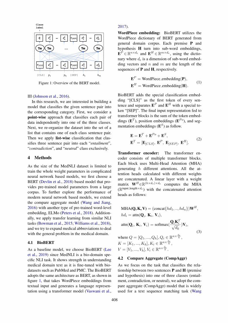
𝒆𝒆𝟏𝟏𝒑𝒑 𝒆𝒆𝒏𝒏
𝒑𝒑 𝒆𝒆[𝑪𝑪𝑪𝑪𝑪𝑪]
[CLS] 𝑝𝑝1 𝑝𝑝𝑛𝑛 [SEP] ℎ1 ℎ𝑚𝑚
𝒆𝒆𝟏𝟏𝒉𝒉 𝒆𝒆𝒎𝒎𝒉𝒉 𝒆𝒆[𝑪𝑪𝑺𝑺𝑺𝑺]
Tm Tm Tm Tm
…
. . .
…
𝒕𝒕𝟏𝟏𝒑𝒑 𝒕𝒕𝒏𝒏
𝒑𝒑 C 𝒕𝒕𝟏𝟏𝒉𝒉 𝒕𝒕𝒎𝒎𝒉𝒉 𝒕𝒕[𝑪𝑪𝑺𝑺𝑺𝑺] … …
Class label
Figure 1: Overview of the BERT model.
III (Johnson et al., 2016).In this research, we are interested in building a
model that classifies the given sentence pair intothe corresponding category. First, we consider apoint-wise approach that classifies each pair ofdata independently into one of the three classes.Next, we re-organize the dataset into the set of alist that contains one of each class sentence pair.Then we apply list-wise classification that clas-sifies three sentence pair into each “entailment”,“contradiction”, and “neutral” class exclusively.
4 Methods
As the size of the MedNLI dataset is limited totrain the whole weight parameters in complicatedneural network based models, we first choose aBERT (Devlin et al., 2018) based model that pro-vides pre-trained model parameters from a largecorpus. To further explore the performance ofmodern neural network based models, we extendthe compare aggregate model (Wang and Jiang,2016) with another type of pre-trained word-levelembedding, ELMo (Peters et al., 2018). Addition-ally, we apply transfer learning from similar NLItasks (Bowman et al., 2015; Williams et al., 2018),and we try to expand medical abbreviations to dealwith the general problem in the medical domain.
4.1 BioBERT
As a baseline model, we choose BioBERT (Leeet al., 2019) since MedNLI is a bio-domain spe-cific NLI task. It shows strength in understandingmedical domain text as it is fine-tuned with bio-datasets such as PubMed and PMC. The BioBERTadopts the same architecture as BERT, as shown infigure 1, that takes WordPiece embeddings fromtextual input and generates a language represen-tation using a transformer model (Vaswani et al.,
2017).
WordPiece embedding: BioBERT utilizes theWordPiece dictionary of BERT generated fromgeneral domain corpus. Each premise P andhypothesis H turn into sub-word embeddings,EP ∈Rn×de and EH ∈Rm×de , using the dictio-nary where de is a dimension of sub-word embed-ding vectors and n and m are the length of thesequences of P and H, respectively.
EP = WordPiece embedding(P),
EH = WordPiece embedding(H).(1)
BioBERT adds the special classification embed-ding “[CLS]” as the first token of every sen-tence and separates EP and EH with a special to-ken “[SEP]”. The final input representation fed totransformer blocks is the sum of the token embed-dings (ET ), position embeddings (EPo), and seg-mentation embeddings (ES) as follow.
E = ET + EPo + ES ,
ET = [E[CLS], EP , E[SEP ], EH ].(2)
Transformer encoder: The transformer en-coder consists of multiple transformer blocks.Each block uses Multi-Head Attention (MHA)generating h different attentions. All the at-tention heads calculated with different weightsare concatenated. A linear layer with a weightmatrix WH∈R(h×dv)×de computes the MHA(Rinput length×de) with the concatenated attentionheads as follows:
MHA(Q, K, V) = (concat{hd1, .., hdn})WH ,
hdi = attn(Qi, Ki, Vi),
attn(Qi, Ki, Vi) = softmax(QiKT
i√dk
)Vi,
(3)where Q = [Q1, ..., Qh], Qi ∈ Rn× de
h ,
K = [K1, ...,Kh],Ki ∈ Rn× deh ,
V = [V1, ..., Vh], Vi ∈ Rn× deh .
4.2 Compare Aggregate (CompAggr)
As we focus on the task that classifies the rela-tionship between two sentences P and H (premiseand hypothesis) into one of three classes (entail-ment, contradiction, or neutral), we adopt the com-pare aggregate (CompAggr) model that is widelyused for a text sequence matching task (Wang
408
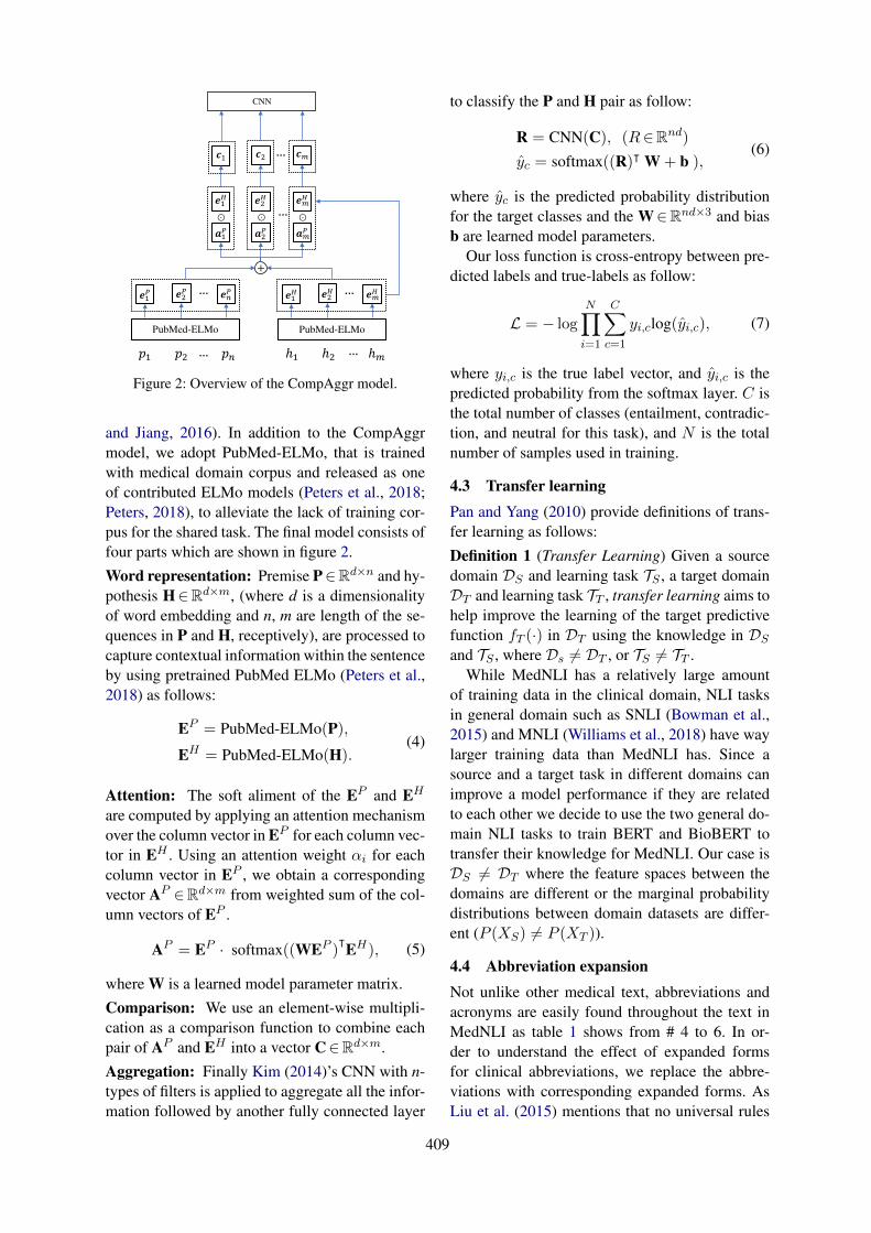
𝑝𝑝1 𝑝𝑝2 𝑝𝑝𝑛𝑛
PubMed-ELMo
+
𝒆𝒆1𝑃𝑃 𝒆𝒆2𝑃𝑃 𝒆𝒆𝑛𝑛𝑃𝑃
𝒂𝒂1𝑃𝑃
𝒆𝒆1𝐻𝐻
⊙
𝒂𝒂2𝑃𝑃
𝒆𝒆2𝐻𝐻
⊙
𝒂𝒂𝑚𝑚𝑃𝑃
𝒆𝒆𝑚𝑚𝐻𝐻
⊙
𝒄𝒄1
CNN
𝒆𝒆1𝐻𝐻 𝒆𝒆2𝐻𝐻 𝒆𝒆𝑚𝑚𝐻𝐻
ℎ1 ℎ2 ℎ𝑚𝑚
𝒄𝒄2 𝒄𝒄𝑚𝑚
…
…
…
…
PubMed-ELMo
…
…
Figure 2: Overview of the CompAggr model.
and Jiang, 2016). In addition to the CompAggrmodel, we adopt PubMed-ELMo, that is trainedwith medical domain corpus and released as oneof contributed ELMo models (Peters et al., 2018;Peters, 2018), to alleviate the lack of training cor-pus for the shared task. The final model consists offour parts which are shown in figure 2.Word representation: Premise P∈Rd×n and hy-pothesis H∈Rd×m, (where d is a dimensionalityof word embedding and n, m are length of the se-quences in P and H, receptively), are processed tocapture contextual information within the sentenceby using pretrained PubMed ELMo (Peters et al.,2018) as follows:
EP = PubMed-ELMo(P),
EH = PubMed-ELMo(H).(4)
Attention: The soft aliment of the EP and EH
are computed by applying an attention mechanismover the column vector in EP for each column vec-tor in EH . Using an attention weight αi for eachcolumn vector in EP , we obtain a correspondingvector AP ∈Rd×m from weighted sum of the col-umn vectors of EP .
AP = EP · softmax((WEP )ᵀEH), (5)
where W is a learned model parameter matrix.Comparison: We use an element-wise multipli-cation as a comparison function to combine eachpair of AP and EH into a vector C∈Rd×m.Aggregation: Finally Kim (2014)’s CNN with n-types of filters is applied to aggregate all the infor-mation followed by another fully connected layer
to classify the P and H pair as follow:
R = CNN(C), (R∈Rnd)
ŷc = softmax((R)ᵀ W + b ),(6)
where ŷc is the predicted probability distributionfor the target classes and the W∈Rnd×3 and biasb are learned model parameters.
Our loss function is cross-entropy between pre-dicted labels and true-labels as follow:
L = − logN∏
i=1
C∑
c=1
yi,clog(ŷi,c), (7)
where yi,c is the true label vector, and ŷi,c is thepredicted probability from the softmax layer. C isthe total number of classes (entailment, contradic-tion, and neutral for this task), and N is the totalnumber of samples used in training.
4.3 Transfer learningPan and Yang (2010) provide definitions of trans-fer learning as follows:
Definition 1 (Transfer Learning) Given a sourcedomain DS and learning task TS , a target domainDT and learning task TT , transfer learning aims tohelp improve the learning of the target predictivefunction fT (·) in DT using the knowledge in DS
and TS , where Ds 6= DT , or TS 6= TT .While MedNLI has a relatively large amount
of training data in the clinical domain, NLI tasksin general domain such as SNLI (Bowman et al.,2015) and MNLI (Williams et al., 2018) have waylarger training data than MedNLI has. Since asource and a target task in different domains canimprove a model performance if they are relatedto each other we decide to use the two general do-main NLI tasks to train BERT and BioBERT totransfer their knowledge for MedNLI. Our case isDS 6= DT where the feature spaces between thedomains are different or the marginal probabilitydistributions between domain datasets are differ-ent (P (XS) 6= P (XT )).
4.4 Abbreviation expansionNot unlike other medical text, abbreviations andacronyms are easily found throughout the text inMedNLI as table 1 shows from # 4 to 6. In or-der to understand the effect of expanded formsfor clinical abbreviations, we replace the abbre-viations with corresponding expanded forms. AsLiu et al. (2015) mentions that no universal rules
409
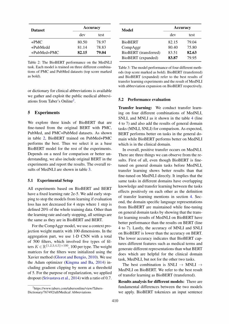
Dataset Accuracy
dev test
+PMC 80.50 78.97+PubMedd 81.14 78.83+PubMed+PMC 82.15 79.04
Table 2: The BioBERT performance on the MedNLItask. Each model is trained on three different combina-tions of PMC and PubMed datasets (top score markedas bold).
or dictionary for clinical abbreviations is availablewe gather and exploit the public medical abbrevi-ations from Taber’s Online2.
5 Experiments
We explore three kinds of BioBERT that arefine-tuned from the original BERT with PMC,PubMed, and PMC+PubMed datasets. As shownin table 2, BioBERT trained on PubMed+PMCperforms the best. Thus we select it as a baseBioBERT model for the rest of the experiments.Depends on a need for comparison or better un-derstanding, we also include original BERT in theexperiments and report the results. The overall re-sults of MedNLI are shown in table 3.
5.1 Experimental Setup
All experiments based on BioBERT and BERThave a fixed learning rate 2e-5. We add early stop-ping to stop the models from learning if evaluationloss has not decreased for 4 steps where 1 step isdefined 20% of the whole training data. Other thanthe learning rate and early stopping, all settings arethe same as they are in BioBERT and BERT.
For the CompAggr model, we use a context pro-jection weight matrix with 100 dimensions. In theaggregation part, we use 1-D CNN with a totalof 500 filters, which involved five types of fil-tersK ∈R{1,2,3,4,5}×100, 100 per type. The weightmatrices for the filters were initialized using theXavier method (Glorot and Bengio, 2010). We usethe Adam optimizer (Kingma and Ba, 2014) in-cluding gradient clipping by norm at a thresholdof 5. For the purpose of regularization, we applieddropout (Srivastava et al., 2014) with a ratio of 0.7.
2https://www.tabers.com/tabersonline/view/Tabers-Dictionary/767492/all/Medical˙Abbreviations
Model Accuracy
dev test
BioBERT 82.15 79.04CompAggr 80.40 75.80BioBERT (transferred) 83.51 82.63BioBERT (expanded) 83.87 79.95
Table 3: The model performance of four different meth-ods (top score marked as bold). BioBERT (transferred)and BioBERT (expanded) refer to the best results oftransfer learning experiments and the result of MedNLIwith abbreviation expansion on BioBERT respectively.
5.2 Performance evaluation
Transfer learning: We conduct transfer learn-ing on four different combinations of MedNLI,SNLI, and MNLI as it shown in the table 4 (line4 to 7) and also add the results of general domaintasks (MNLI, SNLI) for comparison. As expected,BERT performs better on tasks in the general do-main while BioBERT performs better on MedNLIwhich is in the clinical domain.
In overall, positive transfer occurs on MedNLI.There are three things we can observe from the re-sults. First of all, even though BioBERT is fine-tuned on general domain tasks before MedNLI,transfer learning shows better results than thatfine-tuned on MedNLI directly. It implies that thesame tasks in different domains have overlappingknowledge and transfer learning between the taskseffects positively on each other as the definitionof transfer learning mentions in section 4. Sec-ond, the domain specific language representationsfrom BioBERT are maintained while fine-tuningon general domain tasks by showing that the trans-fer learning results of MedNLI on BioBERT havebetter performance than the results on BERT (line4 to 7). Lastly, the accuracy of MNLI and SNLIon BioBERT is lower than the accuracy on BERT.The lower accuracy indicates that BioBERT cap-tures different features such as medical terms andgenerate different representations than what BERTdoes which are helpful for the clinical domaintask, MedNLI, but not for the other two tasks.
The best combination is SNLI → MNLI →MedNLI on BioBERT. We refer to the best resultof transfer learning as BioBERT (transferred).
Results analysis for different models: There arefundamental differences between the two modelswe apply. BioBERT tokenizes an input sentence
410
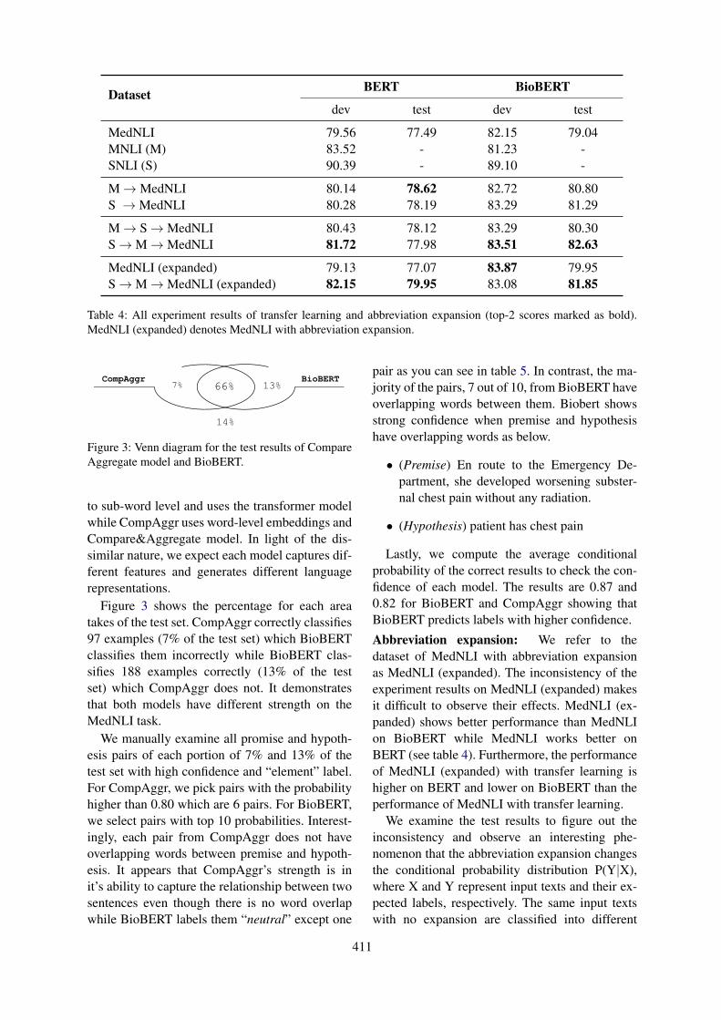
Dataset BERT BioBERT
dev test dev test
MedNLI 79.56 77.49 82.15 79.04MNLI (M) 83.52 - 81.23 -SNLI (S) 90.39 - 89.10 -
M→MedNLI 80.14 78.62 82.72 80.80S →MedNLI 80.28 78.19 83.29 81.29
M→ S→MedNLI 80.43 78.12 83.29 80.30S→M→MedNLI 81.72 77.98 83.51 82.63
MedNLI (expanded) 79.13 77.07 83.87 79.95S→M→MedNLI (expanded) 82.15 79.95 83.08 81.85
Table 4: All experiment results of transfer learning and abbreviation expansion (top-2 scores marked as bold).MedNLI (expanded) denotes MedNLI with abbreviation expansion.
7% BioBERT CompAggr
66% 13%
14%
Figure 3: Venn diagram for the test results of CompareAggregate model and BioBERT.
to sub-word level and uses the transformer modelwhile CompAggr uses word-level embeddings andCompare&Aggregate model. In light of the dis-similar nature, we expect each model captures dif-ferent features and generates different languagerepresentations.
Figure 3 shows the percentage for each areatakes of the test set. CompAggr correctly classifies97 examples (7% of the test set) which BioBERTclassifies them incorrectly while BioBERT clas-sifies 188 examples correctly (13% of the testset) which CompAggr does not. It demonstratesthat both models have different strength on theMedNLI task.
We manually examine all promise and hypoth-esis pairs of each portion of 7% and 13% of thetest set with high confidence and “element” label.For CompAggr, we pick pairs with the probabilityhigher than 0.80 which are 6 pairs. For BioBERT,we select pairs with top 10 probabilities. Interest-ingly, each pair from CompAggr does not haveoverlapping words between premise and hypoth-esis. It appears that CompAggr’s strength is init’s ability to capture the relationship between twosentences even though there is no word overlapwhile BioBERT labels them “neutral” except one
pair as you can see in table 5. In contrast, the ma-jority of the pairs, 7 out of 10, from BioBERT haveoverlapping words between them. Biobert showsstrong confidence when premise and hypothesishave overlapping words as below.
• (Premise) En route to the Emergency De-partment, she developed worsening subster-nal chest pain without any radiation.
• (Hypothesis) patient has chest pain
Lastly, we compute the average conditionalprobability of the correct results to check the con-fidence of each model. The results are 0.87 and0.82 for BioBERT and CompAggr showing thatBioBERT predicts labels with higher confidence.
Abbreviation expansion: We refer to thedataset of MedNLI with abbreviation expansionas MedNLI (expanded). The inconsistency of theexperiment results on MedNLI (expanded) makesit difficult to observe their effects. MedNLI (ex-panded) shows better performance than MedNLIon BioBERT while MedNLI works better onBERT (see table 4). Furthermore, the performanceof MedNLI (expanded) with transfer learning ishigher on BERT and lower on BioBERT than theperformance of MedNLI with transfer learning.
We examine the test results to figure out theinconsistency and observe an interesting phe-nomenon that the abbreviation expansion changesthe conditional probability distribution P(Y|X),where X and Y represent input texts and their ex-pected labels, respectively. The same input textswith no expansion are classified into different
411
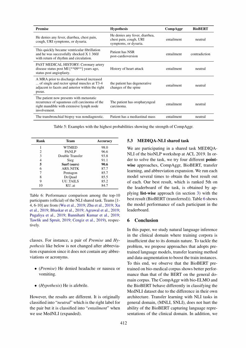
Premise Hypothesis CompAggr BioBERT
He denies any fever, diarrhea, chest pain,cough, URI symptoms, or dysuria.
He denies any fever, diarrhea,chest pain, cough, URIsymptoms, or dysuria.
entailment neutral
This quickly became ventricular fibrillationand he was successfully shocked X 1 360Jwith return of rhythm and circulation.
Patient has NSRpost-cardioversion entailment contradiction
PAST MEDICAL HISTORY: Coronary arterydisease status post MI [**09**] years ago,status post angioplasty.
History of heart attack entailment neutral
A MRA prior to discharge showed increased... of single and rector spinal muscles at T3-4adjacent to facets and anterior within the rightpsoas.
the patient has degenerativechanges of the spine entailment neutral
The patient now presents with metastaticrecurrence of squamous cell carcinoma of theright mandible with extensive lymph nodeinvolvement.
The patient has oropharyngealcarcinoma. entailment neutral
The transbronchial biopsy was nondiagnostic. Patient has a mediastinal mass entailment neutral
Table 5: Examples with the highest probabilities showing the strength of CompAggr.
Rank Team Accuracy
1 WTMED 98.02 PANLP 96.63 Double Transfer 93.84 Sieg 91.15 Surf (ours) 90.66 ARS NITK 87.77 Pentagon 85.78 Dr.Quad 85.59 UU TAILS 85.2
10 KU ai 84.7
Table 6: Performance comparison among the top-10participants (official) of the NLI shared task. Teams [1-4, 6-10] are from (Wu et al., 2019; Zhu et al., 2019; Xuet al., 2019; Bhaskar et al., 2019; Agrawal et al., 2019;Pugaliya et al., 2019; Bannihatti Kumar et al., 2019;Tawfik and Spruit, 2019; Cengiz et al., 2019), respec-tively.
classes. For instance, a pair of Premise and Hy-pothesis like below is not changed after abbrevia-tion expansion since it does not contain any abbre-viations or acronyms.
• (Premise) He denied headache or nausea orvomiting.
• (Hypothesis) He is afebrile.
However, the results are different. It is originallyclassified into “neutral” which is the right label forthe pair but it is classified into “entailment” whenwe use MedNLI (expanded).
5.3 MEDIQA-NLI shared task
We are participating in a shared task MEDIQA-NLI of the bioNLP workshop at ACL 2019. In or-der to solve the task, we try four different point-wise approaches, CompAggr, BioBERT, transferlearning, and abbreviation expansion. We run eachmodel several times to obtain the best result outof each. Our best result, which is ranked 5th onthe leaderboard of the task, is obtained by ap-plying list-wise approach (in section 3) with thebest result (BioBERT (transferred)). Table 6 showsthe model performance of each participant in theleaderboard.
6 Conclusion
In this paper, we study natural language inferencein the clinical domain where training corpora isinsufficient due to its domain nature. To tackle theproblem, we propose approaches that adopts pre-trained language models, transfer learning methodand data-augmentation to boost the train instances.To this end, we observe that the BioBERT pre-trained on bio-medical corpus shows better perfor-mance than that of the BERT on the general do-main corpus. The CompAggr with bio-ELMO andthe BioBERT behave differently in classifying theMedNLI dataset due to the difference in their ownarchitecture. Transfer learning with NLI tasks ingeneral domain, (MNLI, SNLI), does not hurt theability of the BioBERT capturing language repre-sentations of the clinical domain. In addition, we
412
observe that it transfers positive knowledge fromgeneral NLI tasks to the MedNLI task. In contrast,a abbreviation expansion method needs particularcare when adopting since it may hurt the model topredict the conditional probability distribution ofthe task.
Acknowledgments
We sincerely thank the reviewers for their in depthfeedback that helped improve the paper. K. Jung iswith Automation and Systems Research Institute(ASRI), Seoul National University, Seoul, Korea,and was supported by the Ministry of Trade, In-dustry & Energy (MOTIE, Korea) under IndustrialTechnology Innovation Program (No.10073144).
ReferencesAnumeha Agrawal, Rosa Anil George, Selvan Sunitha
Ravi, Sowmya Kamath, and Anand Kumar. 2019.Ars nitk at mediqa 2019:analysing various methodsfor natural language inference, recognising questionentailment and medical question answering system.In Proceedings of the BioNLP 2019 workshop, Flo-rence, Italy, August 1, 2019. Association for Com-putational Linguistics.
Vinayshekhar Bannihatti Kumar, Ashwin Srinivasan,Aditi Chaudhary, James Route, Teruko Mitamura,and Eric Nyberg. 2019. Dr.quad at mediqa 2019:Towards textual inference and question entailmentusing contextualized representations. In Proceed-ings of the BioNLP 2019 workshop, Florence, Italy,August 1, 2019. Association for Computational Lin-guistics.
Asma Ben Abacha, Chaitanya Shivade, and DinaDemner-Fushman. 2019. Overview of the mediqa2019 shared task on textual inference, question en-tailment and question answering. In Proceedings ofthe BioNLP 2019 workshop, Florence, Italy, August1, 2019. Association for Computational Linguistics.
Sai Abishek Bhaskar, Rashi Rungta, James Route,Eric Nyberg, and Teruko Mitamura. 2019. Siegat mediqa 2019: Multi-task neural ensemble forbiomedical inference and entailment. In Proceed-ings of the BioNLP 2019 workshop, Florence, Italy,August 1, 2019. Association for Computational Lin-guistics.
Samuel R Bowman, Gabor Angeli, Christopher Potts,and Christopher D Manning. 2015. A large anno-tated corpus for learning natural language inference.In Proceedings of the 2015 Conference on Empiri-cal Methods in Natural Language Processing, pages632–642.
Cemil Cengiz, Ulaş Sert, and Deniz Yuret. 2019. Ku aiat mediqa 2019: Domain-specific pre-training and
transfer learning for medical nli. In Proceedings ofthe BioNLP 2019 workshop, Florence, Italy, August1, 2019. Association for Computational Linguistics.
Qian Chen, Xiaodan Zhu, Zhen-Hua Ling, Si Wei, HuiJiang, and Diana Inkpen. 2017. Enhanced lstm fornatural language inference. In Proceedings of the55th Annual Meeting of the Association for Compu-tational Linguistics (Volume 1: Long Papers), pages1657–1668.
Alexis Conneau, Douwe Kiela, Holger Schwenk, Loı̈cBarrault, and Antoine Bordes. 2017. Supervisedlearning of universal sentence representations fromnatural language inference data. In Proceedings ofthe 2017 Conference on Empirical Methods in Nat-ural Language Processing, pages 670–680.
Jacob Devlin, Ming-Wei Chang, Kenton Lee, andKristina Toutanova. 2018. Bert: Pre-training of deepbidirectional transformers for language understand-ing. arXiv preprint arXiv:1810.04805.
Xavier Glorot and Yoshua Bengio. 2010. Understand-ing the difficulty of training deep feedforward neuralnetworks. In Proceedings of the AISTATS.
Alistair EW Johnson, Tom J Pollard, Lu Shen,H Lehman Li-wei, Mengling Feng, Moham-mad Ghassemi, Benjamin Moody, Peter Szolovits,Leo Anthony Celi, and Roger G Mark. 2016.Mimic-iii, a freely accessible critical care database.Scientific data, 3:160035.
Yoon Kim. 2014. Convolutional neural networks forsentence classification. In Proceedings of the 2014Conference on Empirical Methods in Natural Lan-guage Processing (EMNLP), pages 1746–1751.
Diederik Kingma and Jimmy Ba. 2014. Adam: Amethod for stochastic optimization. arXiv preprintarXiv:1412.6980.
Jinhyuk Lee, Wonjin Yoon, Sungdong Kim,Donghyeon Kim, Sunkyu Kim, Chan Ho So, andJaewoo Kang. 2019. Biobert: pre-trained biomed-ical language representation model for biomedicaltext mining. arXiv preprint arXiv:1901.08746.
Xiaodong Liu, Pengcheng He, Weizhu Chen, and Jian-feng Gao. 2019. Multi-task deep neural networksfor natural language understanding. arXiv preprintarXiv:1901.11504.
Yue Liu, Tao Ge, Kusum Mathews, Heng Ji, and Deb-orah McGuinness. 2015. Exploiting task-orientedresources to learn word embeddings for clinical ab-breviation expansion. In Proceedings of BioNLP 15,pages 92–97.
Serguei Pakhomov. 2002. Semi-supervised maximumentropy based approach to acronym and abbrevia-tion normalization in medical texts. In Proceedingsof the 40th annual meeting on association for com-putational linguistics, pages 160–167. Associationfor Computational Linguistics.
413
Sinno Jialin Pan and Qiang Yang. 2010. A survey ontransfer learning. IEEE Transactions on knowledgeand data engineering, 22(10):1345–1359.
Matthew Peters. 2018. PubMed ELMo. https://allennlp.org/elmo. [Online; accessed 09-May-2019].
Matthew Peters, Mark Neumann, Mohit Iyyer, MattGardner, Christopher Clark, Kenton Lee, and LukeZettlemoyer. 2018. Deep contextualized word rep-resentations. In Proceedings of the 2018 Confer-ence of the North American Chapter of the Asso-ciation for Computational Linguistics: Human Lan-guage Technologies, Volume 1 (Long Papers), pages2227–2237.
Hemant Pugaliya, Karan Saxena, Shefali Garg, Shee-tal Shalini, Prashant Gupta, Eric Nyberg, and TerukoMitamura. 2019. Pentagon at mediqa 2019: Multi-task learning for filtering and re-ranking answers us-ing language inference and question entailment. InProceedings of the BioNLP 2019 workshop, Flo-rence, Italy, August 1, 2019. Association for Com-putational Linguistics.
Alexey Romanov and Chaitanya Shivade. 2018.Lessons from natural language inference in the clin-ical domain. In Proceedings of the 2018 Conferenceon Empirical Methods in Natural Language Pro-cessing, pages 1586–1596.
Nitish Srivastava, Geoffrey E Hinton, Alex Krizhevsky,Ilya Sutskever, and Ruslan Salakhutdinov. 2014.Dropout: a simple way to prevent neural networksfrom overfitting. Journal of machine learning re-search, 15(1):1929–1958.
Sandeep Subramanian, Adam Trischler, Yoshua Ben-gio, and Christopher J Pal. 2018. Learning gen-eral purpose distributed sentence representations vialarge scale multi-task learning. In ICLR.
Noha Tawfik and Marco Spruit. 2019. Uu tails atmediqa 2019: Learning textual entailment in themedical domain. In Proceedings of the BioNLP2019 workshop, Florence, Italy, August 1, 2019. As-sociation for Computational Linguistics.
Ashish Vaswani, Noam Shazeer, Niki Parmar, JakobUszkoreit, Llion Jones, Aidan N Gomez, ŁukaszKaiser, and Illia Polosukhin. 2017. Attention is allyou need. In Advances in neural information pro-cessing systems, pages 5998–6008.
Alex Wang, Amapreet Singh, Julian Michael, FelixHill, Omer Levy, and Samuel R Bowman. 2018.Glue: A multi-task benchmark and analysis platformfor natural language understanding. arXiv preprintarXiv:1804.07461.
Shuohang Wang and Jing Jiang. 2016. A compare-aggregate model for matching text sequences. arXivpreprint arXiv:1611.01747.
Adina Williams, Nikita Nangia, and Samuel Bowman.2018. A broad-coverage challenge corpus for sen-tence understanding through inference. In Proceed-ings of the 2018 Conference of the North AmericanChapter of the Association for Computational Lin-guistics: Human Language Technologies, Volume 1(Long Papers), pages 1112–1122.
Zhaofeng Wu, Yan Song, Sicong Huang, Yuanhe Tian,and Fei Xia. 2019. A hybrid approach to biomedicalnatural language inference. In Proceedings of theBioNLP 2019 workshop, Florence, Italy, August 1,2019. Association for Computational Linguistics.
Yichong Xu, Xiaodong Liu, Chunyuan Li, HoifungPoon, and Jianfeng Gao. 2019. Doubletransfer atmediqa 2019: Multi-source transfer learning for nat-ural language understanding in the medical domain.In Proceedings of the BioNLP 2019 workshop, Flo-rence, Italy, August 1, 2019. Association for Com-putational Linguistics.
Wei Zhu, Xiaofeng Zhou, Keqiang Wang, Xun Luo,Xiepeng Li, Yuan Ni, and Guotong Xie. 2019. Panlpat mediqa 2019: Pre-trained language models, trans-fer learning and knowledge distillation. In Proceed-ings of the BioNLP 2019 workshop, Florence, Italy,August 1, 2019. Association for Computational Lin-guistics.
414
Proceedings of the BioNLP 2019 workshop, pages 415–426Florence, Italy, August 1, 2019. c©2019 Association for Computational Linguistics
WTMED at MEDIQA 2019: A Hybrid Approach to BiomedicalNatural Language Inference
Zhaofeng WuPaul G. Allen School of CSE
University of [email protected]
Yan SongTencent AI Lab
Sicong HuangDepartment of ECE
University of [email protected]
Yuanhe TianDepartment of LinguisticsUniversity of Washington
Fei XiaDepartment of LinguisticsUniversity of Washington
AbstractNatural language inference (NLI) is challeng-ing, especially when it is applied to techni-cal domains such as biomedical settings. Inthis paper, we propose a hybrid approach tobiomedical NLI where different types of in-formation are exploited for this task. Ourbase model includes a pre-trained text en-coder as the core component, and a syntax en-coder and a feature encoder to capture syn-tactic and domain-specific information. Thenwe combine the output of different base mod-els to form more powerful ensemble mod-els. Finally, we design two conflict resolu-tion strategies when the test data contain mul-tiple (premise, hypothesis) pairs with the samepremise. We train our models on the MedNLIdataset, yielding the best performance on thetest set of the MEDIQA 2019 Task 1.
1 Introduction
Natural language inference (NLI) (MacCartneyand Manning, 2009), also known as textual entail-ment, is an important natural language process-ing (NLP) task that has long been studied (Bow-man et al., 2015; Parikh et al., 2016; Chen et al.,2016; Conneau et al., 2017; Tay et al., 2018).It aims to capture the relationship between twosentences, identifying whether a given premiseentails, contradicts, or is neutral to a given hy-pothesis. Success in NLI is crucial for achiev-ing semantic comprehension of human language,which in turn is a prerequisite to accomplish natu-ral language understanding (NLU). In general, ac-curate NLI systems facilitate many downstreamtasks, such as commonsense reasoning (Zellerset al., 2018) and question answering (Abacha andDemner-Fushman, 2016, 2017).
Most of existing NLI studies are conducted inthe general domain (Marelli et al., 2014; Bowman
et al., 2015; Williams et al., 2018), with limitedattention paid to domain-specific scenarios. Nev-ertheless, there has been increasing demand forinformation processing in the biomedical domainsuch as biomedical question answering (Abachaand Demner-Fushman, 2019) and cohort selec-tion (Glicksberg et al., 2018). Many biomedicalNLP applications require automatic understand-ing of symptom descriptions and examination re-ports (Abacha and Demner-Fushman, 2016, 2017)and therefore can greatly benefit from accuratebiomedical NLI systems.
In this study, we propose a hybrid approach tobiomedical NLI, which includes three main com-ponents, as illustrated in Figure 1. The main com-ponent is the base model (the largest box in the fig-ure), which includes three encoders: an MT-DNN(Liu et al., 2019c) based text encoder, a syntax en-coder that captures structural information, and afeature encoder which injects some degree of do-main knowledge into the model (see §3). We con-duct unsupervised pre-training for the text encoderon biomedical corpora to compensate for the lackof domain-specific supervision (Lee et al., 2019).To enhance our model, we also use model ensem-ble and conflict resolution strategies, correspond-ing to the two top dashed boxes in Figure 1 and areexplained in §4. The datasets and implementationdetail are described in §5. The experimental re-sults on the MedNLI dataset (Romanov and Shiv-ade, 2018) and the MEDIQA 2019 shared task 1(Ben Abacha et al., 2019) are reported in §6.1
2 Related Work
A common neural network approach to addressthe NLI task is sentence pair modeling (Lan and
1Our code is publicly available at https://github.com/ZhaofengWu/MEDIQA_WTMED
415
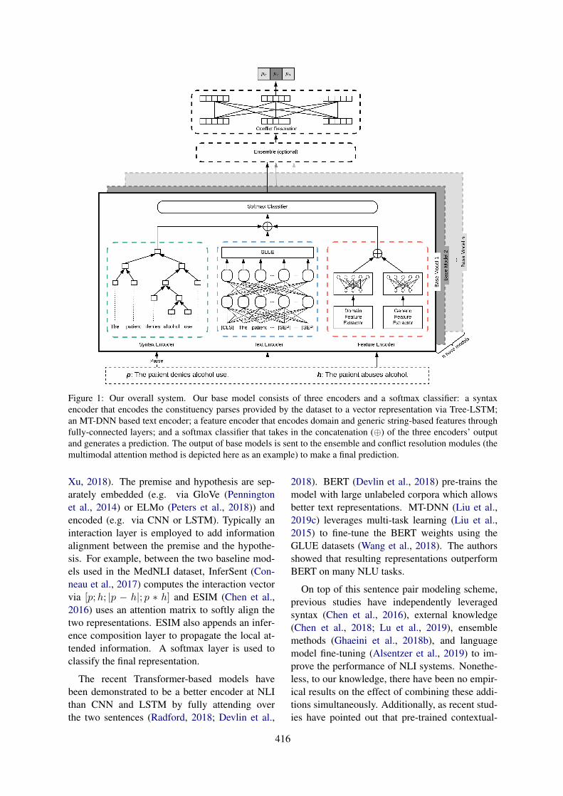
Figure 1: Our overall system. Our base model consists of three encoders and a softmax classifier: a syntaxencoder that encodes the constituency parses provided by the dataset to a vector representation via Tree-LSTM;an MT-DNN based text encoder; a feature encoder that encodes domain and generic string-based features throughfully-connected layers; and a softmax classifier that takes in the concatenation (⊕) of the three encoders’ outputand generates a prediction. The output of base models is sent to the ensemble and conflict resolution modules (themultimodal attention method is depicted here as an example) to make a final prediction.
Xu, 2018). The premise and hypothesis are sep-arately embedded (e.g. via GloVe (Penningtonet al., 2014) or ELMo (Peters et al., 2018)) andencoded (e.g. via CNN or LSTM). Typically aninteraction layer is employed to add informationalignment between the premise and the hypothe-sis. For example, between the two baseline mod-els used in the MedNLI dataset, InferSent (Con-neau et al., 2017) computes the interaction vectorvia [p;h; |p − h|; p ∗ h] and ESIM (Chen et al.,2016) uses an attention matrix to softly align thetwo representations. ESIM also appends an infer-ence composition layer to propagate the local at-tended information. A softmax layer is used toclassify the final representation.
The recent Transformer-based models havebeen demonstrated to be a better encoder at NLIthan CNN and LSTM by fully attending overthe two sentences (Radford, 2018; Devlin et al.,
2018). BERT (Devlin et al., 2018) pre-trains themodel with large unlabeled corpora which allowsbetter text representations. MT-DNN (Liu et al.,2019c) leverages multi-task learning (Liu et al.,2015) to fine-tune the BERT weights using theGLUE datasets (Wang et al., 2018). The authorsshowed that resulting representations outperformBERT on many NLU tasks.
On top of this sentence pair modeling scheme,previous studies have independently leveragedsyntax (Chen et al., 2016), external knowledge(Chen et al., 2018; Lu et al., 2019), ensemblemethods (Ghaeini et al., 2018b), and languagemodel fine-tuning (Alsentzer et al., 2019) to im-prove the performance of NLI systems. Nonethe-less, to our knowledge, there have been no empir-ical results on the effect of combining these addi-tions simultaneously. Additionally, as recent stud-ies have pointed out that pre-trained contextual-
416
ized representations contain rich linguistic signals(Hewitt and Manning, 2019; Liu et al., 2019b), itis reasonable to ask whether explicitly integratingknowledge will continue to augment such repre-sentations. Our work can be seen as an empiricalstudy to examine the efficacy of applying multipleadditions on top of Transformer-based models.
3 Base Model
NLI is generally treated as a three-way classifica-tion task that models whether a given premise pentails, contradicts, or is neutral to a hypothesis h.A classifier f is learned taking p and h as input topredict the class probabilities
f(p, h) =[Pe Pc Pn
]> (1)
with Pr; r ∈ {e, c, n} representing the probabilityfor entailment, contradiction, and neutral. The fi-nal result is the class with the highest probability
yp,h = argmaxr∈{e,c,n}
Pr (2)
As illustrated in Figure 1, our base model con-tains three modules. The widely used pre-trainedTransformer model (Devlin et al., 2018; Liu et al.,2019c) serves as the basic text encoder to representp and h. A syntax encoder and a feature encoderare also utilized to augment the basic representa-tion by extracting and encoding more informationfrom the input. The details of these encoders andhow they are combined for f are discussed in thefollowing subsections.
3.1 Text EncoderText representation is crucial to facilitate down-stream tasks (Song et al., 2017, 2018). As a partof recent advancements in NLP, pre-trained mod-els provide strong baselines for sentence represen-tations and allow great generalizability for the rep-resented text. Therefore, to represent p and h,we adopt a pre-trained Transformer model, MT-DNN (Liu et al., 2019c), as the text encoder in ourbase model. MT-DNN is based on BERT (Devlinet al., 2018) and additionally fine-tuned on GLUE(Wang et al., 2018), a set of NLU datasets includ-ing NLI subsets. Through its multi-task learningobjective, MT-DNN allows a more general andpowerful representation for natural language un-derstanding than BERT (Liu et al., 2019c). For-mally, one can briefly describe the encoder as
VTE(p, h) = MT-DNN(p, h) (3)
with VTE(p, h) referring to the output of the textencoder, a vector representing p and h.
Pre-training on large unlabeled corpora with alanguage modeling objective has facilitated manyrecent state-of-the-art advancements (Peters et al.,2018; Radford, 2018; Devlin et al., 2018; Leeet al., 2019; Radford et al., 2019). Inspired bythese results, we enhance the MT-DNN represen-tation by further fine-tuning on unlabeled biomed-ical data to mitigate the lack of in-domain super-vision.
3.2 Syntax Encoder
Linguistic understandings, for example corefer-ence relations (Zhang et al., 2019a,b), could aidthe interpretation of a sentence. Syntactic struc-tures are often useful for deciding the entailmentof a sentence pair (Chen et al., 2016). There ex-ist numerous NLI examples where a hypothesisis merely the premise with adjunct phrases re-moved. The syntax encoder also mitigates the out-of-vocabulary issue which is common in specificdomains (Liu et al., 2019a) by capturing the struc-tural information. Therefore, we include a syntaxencoder in our base model.
We use Tree-LSTM (Tai et al., 2015) to modelconstituency parse trees of p and h. For each sen-tence, we encode it according to its tree structureand take the final state of the root node to repre-sent the entire sentence. Formally, taking p as anexample, the syntax encoder can be formulated as
VSE(p) = Tree-LSTM(Parse(p)) (4)
where VSE(p) is the output vector. Once p and hare encoded, the final output of this encoder is theconcatenation of the two output vectors
VSE(p, h) = VSE(p)⊕ VSE(h) (5)
3.3 Feature Encoder
The explicit integration of entity-level externalknowledge has been used to improve many NLPmodels’ performance (Das et al., 2017; Sun et al.,2018). Domain knowledge has also been demon-strated to be useful for in-domain tasks (Romanovand Shivade, 2018; Lu et al., 2019). There-fore, in addition to generic encoders such as MT-DNN and Tree-LSTM, we further enhance themodel with domain-specific knowledge throughindirectly leveraging labeled biomedical data for
417
other tasks. To do that, we propose a domain fea-ture encoder that identifies and vectorizes biomed-ical named entities using pre-trained medical tag-gers and counts (1) the number of each entity typein p and h; and (2) the number of shared entitiesand shared entity types in a (p, h) pair.
In addition to domain knowledge, inspired byBowman et al. (2015) and Abacha and Demner-Fushman (2016), we also extract generic stringfeatures and use them to capture the similarity be-tween p and h and then convert the results intovectors. Such similarity information includes n-gram overlap, Levenshtein distance (Levenshtein,1966), Jaccard similarity (Jaccard, 1901), ROUGE(Lin, 2004) and BLEU (Papineni et al., 2001)scores, and absolute length difference.2
To encode the aforementioned features into vec-tors, each extracted feature is represented by a sin-gle scalar and then grouped with others into anarray, denoted by v(d) and v(g) for domain andgeneric features, respectively. Later, they are con-verted into dense representations by linear trans-formations and a ReLU nonlinearty. For domainfeatures, this process can be formulated by
V(d)FE(p, h) = ReLU(W(d)v(d) + b(d)) (6)
and V(g)FE(p, h) is obtained for generic features in asimilar way. As a result, the final output of the fea-ture encoder is the concatenation of vectors withdomain and generic knowledge
VFE(p, h) = V(d)FE(p, h)⊕ V(g)FE(p, h) (7)
3.4 Softmax ClassifierOnce the outputs from the aforementioned en-coders are obtained, a final representation of p andh is concatenated using the encoded vectors
V(p, h) =
VTE(p, h)VSE(p, h)VFE(p, h)
(8)
Then, a softmax classifier is used to compute theclass-wise probability distribution from V(p, h)
f(p, h) = softmax(WV(p, h) + b) (9)
Among the three encoders, our base model al-ways includes the text encoder. The other two en-coders are optional, leading to different base mod-els, whose performance will be compared in §6.1.
2The choices of metrics are intended to capture a widerange of similarity information, e.g. BLEU for n-gram preci-sion and ROUGE for n-gram recall.
4 Model Enhancement
We enhance the base models discussed above withtwo techniques, namely model ensemble and con-flict resolution: ensemble models combine predic-tions made by different base models, and conflictresolution takes advantage of NLI datasets wheremultiple (p, h) pairs share the same premise p.
4.1 Model Ensemble
Model ensemble is a common technique to com-bine predictions of multiple classifiers for betterresults (Maclin and Opitz, 1999). In NLI, modelensemble has also been proven helpful (Ghaeiniet al., 2018a). In our work, when multiple basemodels are trained, we follow the strategy in Leeet al. (2015) and Lakshminarayanan et al. (2017)and average the models’ predictions by
f (ME)(p, h) =1
n
n∑
i=1
fi(p, h) (10)
with n denoting the number of ensembled basemodels and fi(p, h) being the probability distri-bution produced by the ith base model.
4.2 Conflict Resolution
Due to the special data collection strategy ofMedNLI (see Romanov and Shivade (2018)), eachpremise is always paired with three hypotheses,each forming an entailment, a neutral, and a con-tradiction pair with the premise. For example, thepremise “Labs were notable for Cr 1.7 (baseline0.5 per old records) and lactate 2.4.” appears threetimes in the dataset, each pairing with a differenthypothesis: (1) “Patient has elevated Cr” (2) “Pa-tient has normal Cr” and (3) “Patient has elevatedBUN”. The three hypotheses each forms a distinctrelationship with the premise. We say the three(p, h) pairs with the same premise form a group.
For every group, there are six possible non-conflicting combinations of predictions: C ={〈e,c,n〉, 〈e,n,c〉, 〈n,e,c〉, 〈n,c,e〉, 〈c,n,e〉, 〈c,e,n〉}.Ideally, a model should yield non-conflictinggroup predictions; that is, 〈yp,h1 , yp,h2 , yp,h3〉 ∈C where h1, h2, h3 are the three hypotheses ina group. However, our model determines the la-bel of each pair independently from other pairs inthe same group, and thus the three labels could bein conflict. To resolve this conflict, we proposetwo methods: heuristic processing and multimodalattention. Note that when resolving the conflict,
418
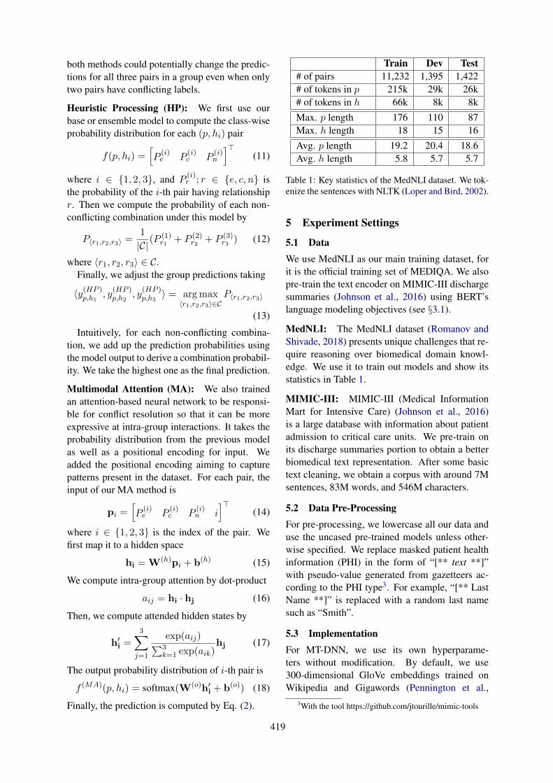
both methods could potentially change the predic-tions for all three pairs in a group even when onlytwo pairs have conflicting labels.
Heuristic Processing (HP): We first use ourbase or ensemble model to compute the class-wiseprobability distribution for each (p, hi) pair
f(p, hi) =[P
(i)e P
(i)c P
(i)n
]>(11)
where i ∈ {1, 2, 3}, and P(i)r ; r ∈ {e, c, n} is
the probability of the i-th pair having relationshipr. Then we compute the probability of each non-conflicting combination under this model by
P〈r1,r2,r3〉 =1
|C|(P(1)r1 + P (2)
r2 + P (3)r3 ) (12)
where 〈r1, r2, r3〉 ∈ C.Finally, we adjust the group predictions taking
〈y(HP )p,h1
, y(HP )p,h2
, y(HP )p,h3〉 = argmax
〈r1,r2,r3〉∈CP〈r1,r2,r3〉
(13)
Intuitively, for each non-conflicting combina-tion, we add up the prediction probabilities usingthe model output to derive a combination probabil-ity. We take the highest one as the final prediction.
Multimodal Attention (MA): We also trainedan attention-based neural network to be responsi-ble for conflict resolution so that it can be moreexpressive at intra-group interactions. It takes theprobability distribution from the previous modelas well as a positional encoding for input. Weadded the positional encoding aiming to capturepatterns present in the dataset. For each pair, theinput of our MA method is
pi =[P
(i)e P
(i)c P
(i)n i
]>(14)
where i ∈ {1, 2, 3} is the index of the pair. Wefirst map it to a hidden space
hi = W(h)pi + b(h) (15)
We compute intra-group attention by dot-product
aij = hi · hj (16)
Then, we compute attended hidden states by
h′i =3∑
j=1
exp(aij)∑3k=1 exp(aik)
hj (17)
The output probability distribution of i-th pair is
f (MA)(p, hi) = softmax(W(o)h′i + b(o)) (18)
Finally, the prediction is computed by Eq. (2).
Train Dev Test# of pairs 11,232 1,395 1,422# of tokens in p 215k 29k 26k# of tokens in h 66k 8k 8kMax. p length 176 110 87Max. h length 18 15 16Avg. p length 19.2 20.4 18.6Avg. h length 5.8 5.7 5.7
Table 1: Key statistics of the MedNLI dataset. We tok-enize the sentences with NLTK (Loper and Bird, 2002).
5 Experiment Settings
5.1 DataWe use MedNLI as our main training dataset, forit is the official training set of MEDIQA. We alsopre-train the text encoder on MIMIC-III dischargesummaries (Johnson et al., 2016) using BERT’slanguage modeling objectives (see §3.1).
MedNLI: The MedNLI dataset (Romanov andShivade, 2018) presents unique challenges that re-quire reasoning over biomedical domain knowl-edge. We use it to train out models and show itsstatistics in Table 1.
MIMIC-III: MIMIC-III (Medical InformationMart for Intensive Care) (Johnson et al., 2016)is a large database with information about patientadmission to critical care units. We pre-train onits discharge summaries portion to obtain a betterbiomedical text representation. After some basictext cleaning, we obtain a corpus with around 7Msentences, 83M words, and 546M characters.
5.2 Data Pre-ProcessingFor pre-processing, we lowercase all our data anduse the uncased pre-trained models unless other-wise specified. We replace masked patient healthinformation (PHI) in the form of “[** text **]”with pseudo-value generated from gazetteers ac-cording to the PHI type3. For example, “[** LastName **]” is replaced with a random last namesuch as “Smith”.
5.3 ImplementationFor MT-DNN, we use its own hyperparame-ters without modification. By default, we use300-dimensional GloVe embeddings trained onWikipedia and Gigawords (Pennington et al.,
3With the tool https://github.com/jtourille/mimic-tools
419
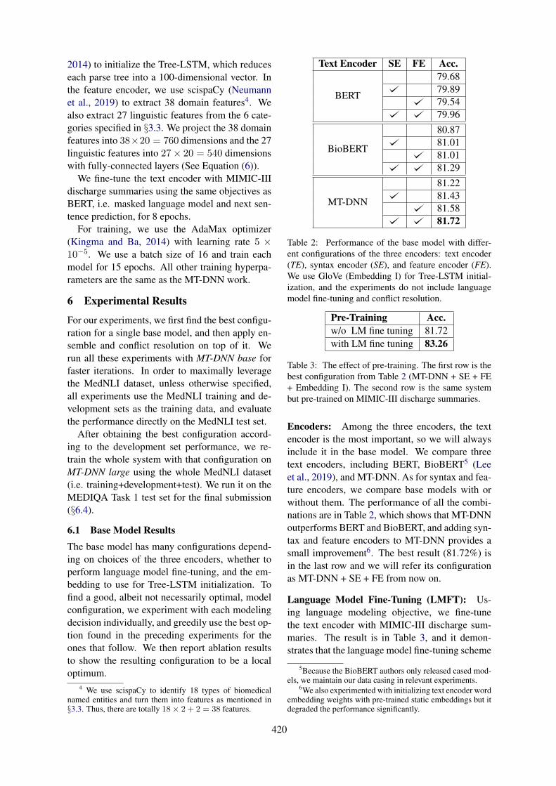
2014) to initialize the Tree-LSTM, which reduceseach parse tree into a 100-dimensional vector. Inthe feature encoder, we use scispaCy (Neumannet al., 2019) to extract 38 domain features4. Wealso extract 27 linguistic features from the 6 cate-gories specified in §3.3. We project the 38 domainfeatures into 38×20 = 760 dimensions and the 27linguistic features into 27× 20 = 540 dimensionswith fully-connected layers (See Equation (6)).
We fine-tune the text encoder with MIMIC-IIIdischarge summaries using the same objectives asBERT, i.e. masked language model and next sen-tence prediction, for 8 epochs.
For training, we use the AdaMax optimizer(Kingma and Ba, 2014) with learning rate 5 ×10⁻⁵. We use a batch size of 16 and train eachmodel for 15 epochs. All other training hyperpa-rameters are the same as the MT-DNN work.
6 Experimental Results
For our experiments, we first find the best configu-ration for a single base model, and then apply en-semble and conflict resolution on top of it. Werun all these experiments with MT-DNN base forfaster iterations. In order to maximally leveragethe MedNLI dataset, unless otherwise specified,all experiments use the MedNLI training and de-velopment sets as the training data, and evaluatethe performance directly on the MedNLI test set.
After obtaining the best configuration accord-ing to the development set performance, we re-train the whole system with that configuration onMT-DNN large using the whole MedNLI dataset(i.e. training+development+test). We run it on theMEDIQA Task 1 test set for the final submission(§6.4).
6.1 Base Model ResultsThe base model has many configurations depend-ing on choices of the three encoders, whether toperform language model fine-tuning, and the em-bedding to use for Tree-LSTM initialization. Tofind a good, albeit not necessarily optimal, modelconfiguration, we experiment with each modelingdecision individually, and greedily use the best op-tion found in the preceding experiments for theones that follow. We then report ablation resultsto show the resulting configuration to be a localoptimum.
4 We use scispaCy to identify 18 types of biomedicalnamed entities and turn them into features as mentioned in§3.3. Thus, there are totally 18× 2 + 2 = 38 features.
Text Encoder SE FE Acc.
BERT
79.6879.8979.5479.96
BioBERT
80.8781.0181.0181.29
MT-DNN
81.2281.4381.5881.72
Table 2: Performance of the base model with differ-ent configurations of the three encoders: text encoder(TE), syntax encoder (SE), and feature encoder (FE).We use GloVe (Embedding I) for Tree-LSTM initial-ization, and the experiments do not include languagemodel fine-tuning and conflict resolution.
Pre-Training Acc.w/o LM fine tuning 81.72with LM fine tuning 83.26
Table 3: The effect of pre-training. The first row is thebest configuration from Table 2 (MT-DNN + SE + FE+ Embedding I). The second row is the same systembut pre-trained on MIMIC-III discharge summaries.
Encoders: Among the three encoders, the textencoder is the most important, so we will alwaysinclude it in the base model. We compare threetext encoders, including BERT, BioBERT5 (Leeet al., 2019), and MT-DNN. As for syntax and fea-ture encoders, we compare base models with orwithout them. The performance of all the combi-nations are in Table 2, which shows that MT-DNNoutperforms BERT and BioBERT, and adding syn-tax and feature encoders to MT-DNN provides asmall improvement6. The best result (81.72%) isin the last row and we will refer its configurationas MT-DNN + SE + FE from now on.
Language Model Fine-Tuning (LMFT): Us-ing language modeling objective, we fine-tunethe text encoder with MIMIC-III discharge sum-maries. The result is in Table 3, and it demon-strates that the language model fine-tuning scheme
5Because the BioBERT authors only released cased mod-els, we maintain our data casing in relevant experiments.
6We also experimented with initializing text encoder wordembedding weights with pre-trained static embeddings but itdegraded the performance significantly.
420
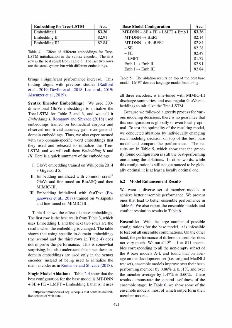
Embedding for Tree-LSTM Acc.Embedding I 83.26Embedding II 82.91Embedding III 82.84
Table 4: Effect of different embeddings for Tree-LSTM initialization in the syntax encoder. The firstrow is the best result from Table 3. The last two rowsare the same system but with different embeddings.
brings a significant performance increase. Thisfinding aligns with previous studies (Radfordet al., 2019; Devlin et al., 2018; Lee et al., 2019;Alsentzer et al., 2019).
Syntax Encoder Embeddings: We used 300-dimensional GloVe embeddings to initialize theTree-LSTM for Table 2 and 3, and we call itEmbedding I. Romanov and Shivade (2018) usedembeddings trained on biomedical corpora andobserved non-trivial accuracy gain over general-domain embeddings. Thus, we also experimentedwith two domain-specific word embeddings thatthey used and released to initialize the Tree-LSTM, and we will call them Embedding II andIII. Here is a quick summary of the embeddings:
I. GloVe embedding trained on Wikipedia 2014+ Gigaword 5;
II. Embedding initialized with common crawl7
GloVe and fine-tuned on BioASQ and thenMIMIC-III;
III. Embedding initialized with fastText (Bo-janowski et al., 2017) trained on Wikipediaand fine-tuned on MIMIC-III.
Table 4 shows the effect of these embeddings.The first row is the best result from Table 3, whichuses Embedding I, and the next two rows are theresults when the embedding is changed. The tableshows that using specific in-domain embeddings(the second and the third rows in Table 4) doesnot improve the performance. This is somewhatsurprising, but also understandable since these in-domain embeddings are used only in the syntaxencoder, instead of being used to initialize themain encoder as in Romanov and Shivade (2018).
Single Model Ablation: Table 2-4 show that thebest configuration for the base model is MT-DNN+ SE + FE + LMFT + Embedding I; that is, it uses
7https://commoncrawl.org, a corpus that contains 840 bil-lion tokens of web data.
Base Model Configuration Acc.MT-DNN + SE + FE + LMFT + Emb I 83.26MT-DNN→ BERT 82.14MT-DNN→ BioBERT 82.84– SE 82.28– FE 82.49– LMFT 81.72Emb I→ Emb II 82.91Emb I→ Emb III 82.84
Table 5: The ablation results on top of the best basemodel. LMFT denotes language model fine tuning.
all three encoders, is fine-tuned with MIMIC-IIIdischarge summaries, and uses regular GloVe em-beddings to initialize the Tree-LSTM.
Because we followed a greedy process for vari-ous modeling decisions, there is no guarantee thatthis configuration is globally or even locally opti-mal. To test the optimality of the resulting model,we conducted ablations by individually changingeach modeling decision on top of the best basemodel and compare the performance. The re-sults are in Table 5, which show that the greed-ily found configuration is still the best-performingone among the ablations. In other words, whilethis configuration is still not guaranteed to be glob-ally optimal, it is at least a locally optimal one.
6.2 Model Enhancement Results
We want a diverse set of member models toachieve better ensemble performance. We presentones that lead to better ensemble performance inTable 6. We also report the ensemble models andconflict resolution results in Table 6.
Ensemble: With the large number of possibleconfigurations for the base model, it is infeasibleto test out all ensemble combinations. On the otherhand, the performance of different ensembles doesnot vary much. We ran all 29 − 1 = 511 ensem-bles corresponding to all the non-empty subset ofthe 9 base models A-I, and found that on aver-age on the development set (i.e. original MedNLItest set), ensemble models improve over their best-performing member by 0.86%± 0.51%, and overthe member average by 1.47% ± 0.60%. Theseresults demonstrate the general usefulness of theensemble stage. In Table 6, we show some of theensemble models, most of which outperform theirmember models.
421
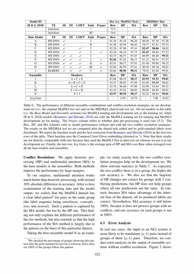
Model ID Dev (i.e. MedNLI Test) MEDIQA Test(R & S, 2018) TE SE FE LMFT Emb Prepro Raw HP MA Raw HP MA
InferSent * 73.5 - - - - -InferSent III 76.6 - - - - -
Base Model TE SE FE LMFT Emb Prepro Raw HP MA Raw HP MAA MT-DNN I 81.36 85.16 96.20 80.49 87.16 97.28B MT-DNN II 81.50 85.94 96.62 78.77 87.41 97.53C MT-DNN I 82.28 87.90 97.61 82.47 90.86 98.02D MT-DNN I 82.49 86.36 97.75 82.47 88.64 97.53E MT-DNN I 82.35 86.57 97.47 80.99 88.40 99.51F MT-DNN I 83.26 87.62 98.17 81.23 86.91 97.53G MT-DNN II 82.91 86.57 97.61 81.48 89.88 98.52H MT-DNN III 82.84 86.50 97.61 80.49 89.38 98.02I BioBERT I 82.84 88.96 98.31 78.03 83.46 99.01
Ensemble Members Raw HP MA Raw HP MAJ A + C + E 83.68 88.19 98.17 83.95 93.33 99.01K A + B + C + E 83.47 88.82 97.68 83.46 93.33 98.02L A + C + D 83.76 88.40 97.89 82.96 92.84 98.52M F + G + H 83.54 87.62 98.03 80.99 88.89 98.02N F + I 83.97 89.94 98.17 82.22 88.64 99.01
Avg Gain - - 4.59 14.79 - 7.80 16.82
Table 6: The performance of different ensemble combinations and conflict resolution strategies on our develop-ment set (i.e., the original MedNLI test set) and on the MEDIQA shared task test set. All our models in this table(i.e. the Base Model and Ensemble sections) use MedNLI training and development sets as the training set, while(R & S, 2018) models (Romanov and Shivade, 2018) use only the MedNLI training set for training and MedNLIdevelopment set for tuning. The Prepro column refers to whether data pre-processing is used (see §5.2). TheRaw, HP, and MA columns refer to model performance without and with the two conflict resolution strategies.The results on the MEDIQA test set are computed after the shared task ended and its gold-standard labels weredistributed. We report the baseline result and the best extension from Romanov and Shivade (2018) in the first tworows of the table. Their baseline uses the Common Crawl Glove embedding (denoted as *). Note that their resultsare not directly comparable with ours because they used the MedNLI Test as their test set whereas we use it as ourdevelopment set. Finally, the last row, Avg Gain, is the average gain of HP and MA over Raw when averaged overall the base models and ensembles.
Conflict Resolution: We apply heuristic pro-cessing (HP) and multimodal attention (MA) tothe base models or the ensembles. Both methodsimprove the performance by large margins.
To our surprise, multimodal attention worksmuch better than heuristic processing, with around10% absolute difference in accuracy. After a closeexamination of the training data and the modeloutput, we realize that the MedNLI dataset hasa clear label pattern8 for pairs in the same group(the label sequence being entailment, contradic-tion, and neutral). Such a pattern is captured bythe MA model, but not by the HP one. This find-ing not only explains the different performance ofthe two methods, but also reminds us that the highperformance of the MA method is largely due tothe pattern (or the bias) of this particular dataset.
Taking the best ensemble model N as an exam-
8We checked the percentage of groups observing this pat-tern after the gold standard for test set is released, and it turnsout 100% of the groups follow this pattern.
ple, we study exactly how the two conflict reso-lution strategies help on the development set. Weshow relevant statistics in Table 7. As expected,the less conflict there is in a group, the higher theraw accuracy is. We also see that the majorityof HP changes are correct for groups with 2 con-flicting predictions, but HP does not help groupswhere all raw predictions are the same. In con-trast, because MA takes advantage of the inher-ent bias of the dataset, all its produced labels arecorrect. Nevertheless, MA accuracy is still below100%, because it does not process groups with noconflicts, and raw accuracy on such groups is notat 100%.
6.3 Error Analysis
In real use cases, the input to an NLI system ismore likely to be standalone (p, h) pairs instead ofgroups of three (p, h) pairs. Therefore, we con-duct error analysis on the output of ensemble sys-tems without conflict resolution. Figure 2 shows
422
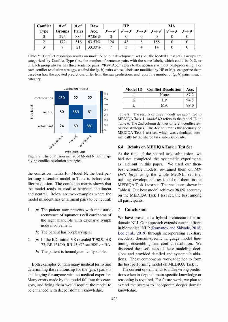
Conflict # of # of Raw HP MAType Groups Pairs Acc. 7→ 3 3→ 7 7→ 7 7→ 3 3→ 7 7→ 7
0 295 885 97.06% 0 0 0 0 0 02 172 516 63.57% 124 43 8 188 0 03 7 21 33.33% 7 3 4 14 0 0
Table 7: Conflict resolution results on model N on our development set (i.e., the MedNLI test set). Groups arecategorized by Conflict Type (i.e., the number of sentence pairs with the same label), which could be 0, 2, or3. Each group always has three sentence pairs. “Raw Acc.” refers to the accuracy without post-processing. Foreach conflict resolution strategy, we find the (p, h) pairs whose labels are modified by HP or MA, categorize thembased on how the updated predictions differ from the raw predictions, and report the number of (p, h) pairs in eachcategory.
Figure 2: The confusion matrix of Model N before ap-plying conflict resolution strategies.
the confusion matrix for Model N, the best per-forming ensemble model in Table 6, before con-flict resolution. The confusion matrix shows thatthe model tends to confuse between entailmentand neutral. Below are two examples where themodel misidentifies entailment pairs to be neutral:
1. p: The patient now presents with metastaticrecurrence of squamous cell carcinoma ofthe right mandible with extensive lymphnode involvement.
h: The patient has oropharyngeal
2. p: In the ED, initial VS revealed T 98.9, HR73, BP 121/90, RR 15, O2 sat 98% on RA.
h: The patient is hemodynamically stable.
Both examples contain many medical terms anddetermining the relationship for the (p, h) pairs ischallenging for anyone without medical expertise.Many errors made by the model fall into this cate-gory, and fixing them would require the model tobe enhanced with deeper domain knowledge.
Model ID Conflict Resolution Acc.J None 87.2K HP 94.8L MA 98.0
Table 8: The results of three models we submitted toMEDIQA Task 1. Model ID refers to the model ID inTable 6. The 2nd column denotes different conflict res-olution strategies. The Acc column is the accuracy onMEDIQA Task 1 test set, which was calculated auto-matically by the shared task submission site.
6.4 Results on MEDIQA Task 1 Test SetAt the time of the shared task submission, wehad not completed the systematic experimentsas laid out in this paper. We used our then-best ensemble models, re-trained them on MT-DNN large using the whole MedNLI set (i.e.training+development+test), and ran them on theMEDIQA Task 1 test set. The results are shown inTable 8. Our best model achieves 98.0% accuracyon the MEDIQA Task 1 test set, the best amongall participants.
7 Conclusion
We have presented a hybrid architecture for in-domain NLI. Our approach extends current effortsin biomedical NLP (Romanov and Shivade, 2018;Lee et al., 2019) through incorporating auxiliaryencoders, domain-specific language model fine-tuning, ensembling, and conflict resolution. Wedissected the usefulness of these modeling deci-sions and provided detailed and systematic abla-tions. These components work together to formthe best performing model on MEDIQA Task 1.
The current system tends to make wrong predic-tions when in-depth domain-specific knowledge orreasoning is required. For future work, we plan toextend the system to incorporate deeper domainknowledge.
423
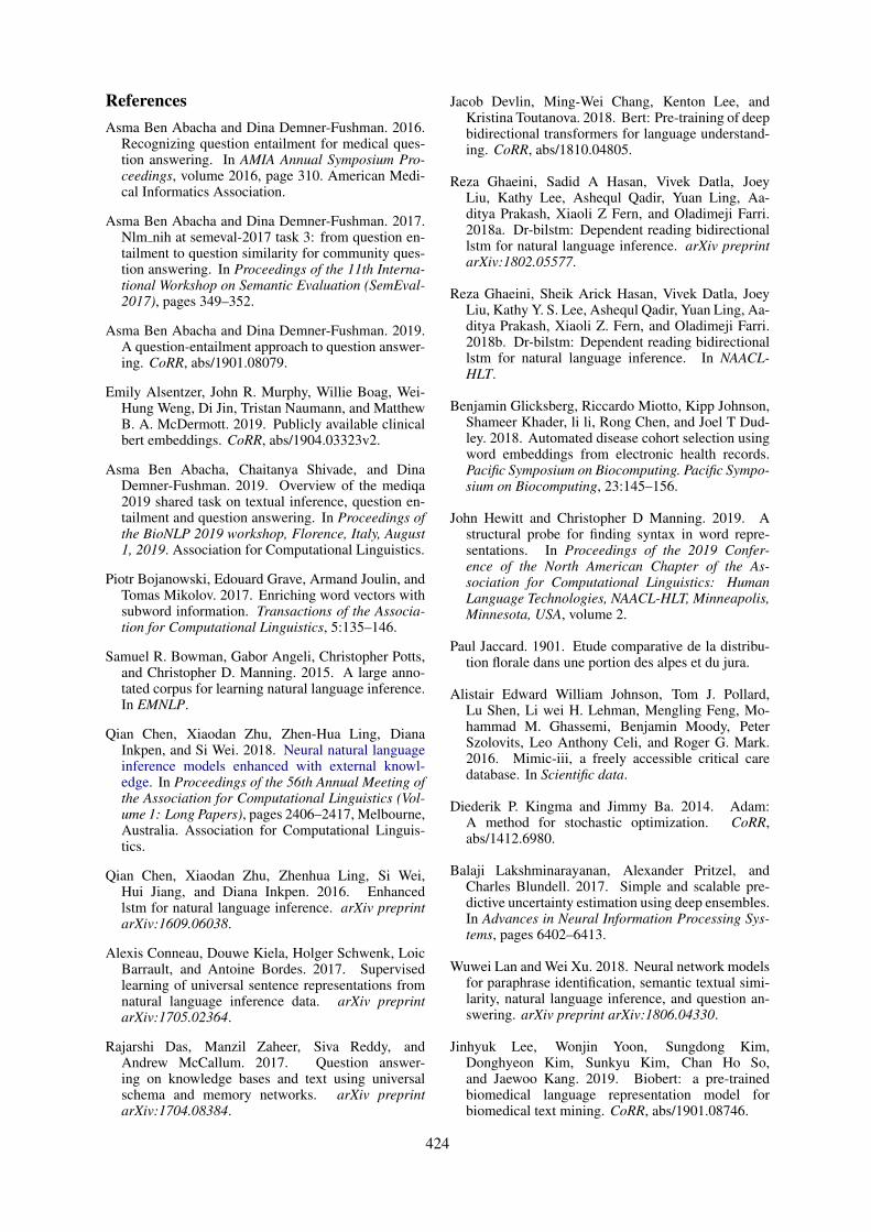
ReferencesAsma Ben Abacha and Dina Demner-Fushman. 2016.
Recognizing question entailment for medical ques-tion answering. In AMIA Annual Symposium Pro-ceedings, volume 2016, page 310. American Medi-cal Informatics Association.
Asma Ben Abacha and Dina Demner-Fushman. 2017.Nlm nih at semeval-2017 task 3: from question en-tailment to question similarity for community ques-tion answering. In Proceedings of the 11th Interna-tional Workshop on Semantic Evaluation (SemEval-2017), pages 349–352.
Asma Ben Abacha and Dina Demner-Fushman. 2019.A question-entailment approach to question answer-ing. CoRR, abs/1901.08079.
Emily Alsentzer, John R. Murphy, Willie Boag, Wei-Hung Weng, Di Jin, Tristan Naumann, and MatthewB. A. McDermott. 2019. Publicly available clinicalbert embeddings. CoRR, abs/1904.03323v2.
Asma Ben Abacha, Chaitanya Shivade, and DinaDemner-Fushman. 2019. Overview of the mediqa2019 shared task on textual inference, question en-tailment and question answering. In Proceedings ofthe BioNLP 2019 workshop, Florence, Italy, August1, 2019. Association for Computational Linguistics.
Piotr Bojanowski, Edouard Grave, Armand Joulin, andTomas Mikolov. 2017. Enriching word vectors withsubword information. Transactions of the Associa-tion for Computational Linguistics, 5:135–146.
Samuel R. Bowman, Gabor Angeli, Christopher Potts,and Christopher D. Manning. 2015. A large anno-tated corpus for learning natural language inference.In EMNLP.
Qian Chen, Xiaodan Zhu, Zhen-Hua Ling, DianaInkpen, and Si Wei. 2018. Neural natural languageinference models enhanced with external knowl-edge. In Proceedings of the 56th Annual Meeting ofthe Association for Computational Linguistics (Vol-ume 1: Long Papers), pages 2406–2417, Melbourne,Australia. Association for Computational Linguis-tics.
Qian Chen, Xiaodan Zhu, Zhenhua Ling, Si Wei,Hui Jiang, and Diana Inkpen. 2016. Enhancedlstm for natural language inference. arXiv preprintarXiv:1609.06038.
Alexis Conneau, Douwe Kiela, Holger Schwenk, LoicBarrault, and Antoine Bordes. 2017. Supervisedlearning of universal sentence representations fromnatural language inference data. arXiv preprintarXiv:1705.02364.
Rajarshi Das, Manzil Zaheer, Siva Reddy, andAndrew McCallum. 2017. Question answer-ing on knowledge bases and text using universalschema and memory networks. arXiv preprintarXiv:1704.08384.
Jacob Devlin, Ming-Wei Chang, Kenton Lee, andKristina Toutanova. 2018. Bert: Pre-training of deepbidirectional transformers for language understand-ing. CoRR, abs/1810.04805.
Reza Ghaeini, Sadid A Hasan, Vivek Datla, JoeyLiu, Kathy Lee, Ashequl Qadir, Yuan Ling, Aa-ditya Prakash, Xiaoli Z Fern, and Oladimeji Farri.2018a. Dr-bilstm: Dependent reading bidirectionallstm for natural language inference. arXiv preprintarXiv:1802.05577.
Reza Ghaeini, Sheik Arick Hasan, Vivek Datla, JoeyLiu, Kathy Y. S. Lee, Ashequl Qadir, Yuan Ling, Aa-ditya Prakash, Xiaoli Z. Fern, and Oladimeji Farri.2018b. Dr-bilstm: Dependent reading bidirectionallstm for natural language inference. In NAACL-HLT.
Benjamin Glicksberg, Riccardo Miotto, Kipp Johnson,Shameer Khader, li li, Rong Chen, and Joel T Dud-ley. 2018. Automated disease cohort selection usingword embeddings from electronic health records.Pacific Symposium on Biocomputing. Pacific Sympo-sium on Biocomputing, 23:145–156.
John Hewitt and Christopher D Manning. 2019. Astructural probe for finding syntax in word repre-sentations. In Proceedings of the 2019 Confer-ence of the North American Chapter of the As-sociation for Computational Linguistics: HumanLanguage Technologies, NAACL-HLT, Minneapolis,Minnesota, USA, volume 2.
Paul Jaccard. 1901. Etude comparative de la distribu-tion florale dans une portion des alpes et du jura.
Alistair Edward William Johnson, Tom J. Pollard,Lu Shen, Li wei H. Lehman, Mengling Feng, Mo-hammad M. Ghassemi, Benjamin Moody, PeterSzolovits, Leo Anthony Celi, and Roger G. Mark.2016. Mimic-iii, a freely accessible critical caredatabase. In Scientific data.
Diederik P. Kingma and Jimmy Ba. 2014. Adam:A method for stochastic optimization. CoRR,abs/1412.6980.
Balaji Lakshminarayanan, Alexander Pritzel, andCharles Blundell. 2017. Simple and scalable pre-dictive uncertainty estimation using deep ensembles.In Advances in Neural Information Processing Sys-tems, pages 6402–6413.
Wuwei Lan and Wei Xu. 2018. Neural network modelsfor paraphrase identification, semantic textual simi-larity, natural language inference, and question an-swering. arXiv preprint arXiv:1806.04330.
Jinhyuk Lee, Wonjin Yoon, Sungdong Kim,Donghyeon Kim, Sunkyu Kim, Chan Ho So,and Jaewoo Kang. 2019. Biobert: a pre-trainedbiomedical language representation model forbiomedical text mining. CoRR, abs/1901.08746.
424
Stefan Lee, Senthil Purushwalkam, Michael Cogswell,David Crandall, and Dhruv Batra. 2015. Whym heads are better than one: Training a di-verse ensemble of deep networks. arXiv preprintarXiv:1511.06314.
VI Levenshtein. 1966. Binary Codes Capable of Cor-recting Deletions, Insertions and Reversals. SovietPhysics Doklady, 10:707.
Chin-Yew Lin. 2004. Rouge: A package for automaticevaluation of summaries. In ACL 2004.
Miaofeng Liu, Yan Song, Hongbin Zou, and TongZhang. 2019a. Reinforced training data selection fordomain adaptation. In Proceedings of ACL, 2019.
Nelson F Liu, Matt Gardner, Yonatan Belinkov,Matthew Peters, and Noah A Smith. 2019b. Lin-guistic knowledge and transferability of contextualrepresentations. arXiv preprint arXiv:1903.08855.
Xiaodong Liu, Jianfeng Gao, Xiaodong He, Li Deng,Kevin Duh, and Ye-Yi Wang. 2015. Representationlearning using multi-task deep neural networks forsemantic classification and information retrieval. InHLT-NAACL.
Xiaodong Liu, Pengcheng He, Weizhu Chen, andJianfeng Gao. 2019c. Multi-task deep neural net-works for natural language understanding. CoRR,abs/1901.11504.
Edward Loper and Steven Bird. 2002. Nltk: The natu-ral language toolkit. CoRR, cs.CL/0205028.
Mingming Lu, Yu Fang, Fengqi Yan, and Maozhen Li.2019. Incorporating domain knowledge into naturallanguage inference on clinical texts. IEEE Access.
Bill MacCartney and Christopher D Manning. 2009.Natural language inference. Stanford UniversityStanford.
Richard Maclin and David W. Opitz. 1999. Popular en-semble methods: An empirical study. J. Artif. Intell.Res., 11:169–198.
Marco Marelli, Stefano Menini, Marco Baroni, LuisaBentivogli, Raffaella Bernardi, Roberto Zamparelli,et al. 2014. A sick cure for the evaluation of com-positional distributional semantic models. In LREC,pages 216–223.
Mark Neumann, Daniel King, Iz Beltagy, and WaleedAmmar. 2019. Scispacy: Fast and robust modelsfor biomedical natural language processing. CoRR,abs/1902.07669.
Kishore Papineni, Salim Roukos, Todd Ward, and Wei-Jing Zhu. 2001. Bleu: a method for automatic eval-uation of machine translation. In ACL.
Ankur P Parikh, Oscar Täckström, Dipanjan Das, andJakob Uszkoreit. 2016. A decomposable attentionmodel for natural language inference. arXiv preprintarXiv:1606.01933.
Jeffrey Pennington, Richard Socher, and ChristopherManning. 2014. Glove: Global vectors for wordrepresentation. In Proceedings of the 2014 confer-ence on empirical methods in natural language pro-cessing (EMNLP), pages 1532–1543.
Matthew E. Peters, Mark Neumann, Mohit Iyyer, MattGardner, Christopher Clark, Kenton Lee, and LukeZettlemoyer. 2018. Deep contextualized word rep-resentations. In Proc. of NAACL.
Alec Radford. 2018. Improving language understand-ing by generative pre-training.
Alec Radford, Jeff Wu, Rewon Child, David Luan,Dario Amodei, and Ilya Sutskever. 2019. Languagemodels are unsupervised multitask learners.
Alexey Romanov and Chaitanya Shivade. 2018.Lessons from natural language inference in the clin-ical domain. In EMNLP.
Yan Song, Chia-Jung Lee, and Fei Xia. 2017. Learn-ing word representations with regularization fromprior knowledge. In Proceedings of the 21st Confer-ence on Computational Natural Language Learning(CoNLL 2017), pages 143–152, Vancouver, Canada.
Yan Song, Shuming Shi, Jing Li, and Haisong Zhang.2018. Directional skip-gram: Explicitly distinguish-ing left and right context for word embeddings. InProceedings of the 2018 Conference of the NorthAmerican Chapter of the Association for Computa-tional Linguistics: Human Language Technologies,Volume 2, pages 175–180, New Orleans, Louisiana.
Haitian Sun, Bhuwan Dhingra, Manzil Zaheer, KathrynMazaitis, Ruslan Salakhutdinov, and William W Co-hen. 2018. Open domain question answering us-ing early fusion of knowledge bases and text. arXivpreprint arXiv:1809.00782.
Kai Sheng Tai, Richard Socher, and Christopher D.Manning. 2015. Improved semantic representationsfrom tree-structured long short-term memory net-works. In ACL.
Yi Tay, Anh Tuan Luu, and Siu Cheung Hui. 2018.Compare, compress and propagate: Enhancing neu-ral architectures with alignment factorization fornatural language inference. In Proceedings of the2018 Conference on Empirical Methods in NaturalLanguage Processing, pages 1565–1575.
Alex Wang, Amanpreet Singh, Julian Michael, FelixHill, Omer Levy, and Samuel R. Bowman. 2018.Glue: A multi-task benchmark and analysis plat-form for natural language understanding. In Black-boxNLP@EMNLP.
Adina Williams, Nikita Nangia, and Samuel Bowman.2018. A broad-coverage challenge corpus for sen-tence understanding through inference. In Proceed-ings of the 2018 Conference of the North AmericanChapter of the Association for Computational Lin-guistics: Human Language Technologies, Volume 1
425

(Long Papers), pages 1112–1122. Association forComputational Linguistics.
Rowan Zellers, Yonatan Bisk, Roy Schwartz, and YejinChoi. 2018. Swag: A large-scale adversarial datasetfor grounded commonsense inference. In Proceed-ings of the 2018 Conference on Empirical Methodsin Natural Language Processing (EMNLP).
Hongming Zhang, Yan Song, and Yangqiu Song.2019a. Incorporating Context and External Knowl-edge for Pronoun Coreference Resolution. In Pro-ceedings of NAACL-HLT, 2019.
Hongming Zhang, Yan Song, Yangqiu Song, and DongYu. 2019b. Knowledge-aware Pronoun CoreferenceResolution. In Proceedings of ACL, 2019.
426
Proceedings of the BioNLP 2019 workshop, pages 427–436Florence, Italy, August 1, 2019. c©2019 Association for Computational Linguistics
KU ai at MEDIQA 2019: Domain-specific Pre-training and TransferLearning for Medical NLI
Cemil Cengiz Ulaş SertKoç University
Artificial Intelligence Laboratoryİstanbul, Turkey
ccengiz17,usert17,[email protected]
Deniz Yuret
Abstract
In this paper, we describe our system and re-sults submitted for the Natural Language In-ference (NLI) track of the MEDIQA 2019Shared Task (Ben Abacha et al., 2019). AsKU ai team, we used BERT (Devlin et al.,2018) as our baseline model and pre-processedthe MedNLI dataset to mitigate the negativeimpact of de-identification artifacts. More-over, we investigated different pre-training andtransfer learning approaches to improve theperformance. We show that pre-training thelanguage model on rich biomedical corporahas a significant effect in teaching the modeldomain-specific language. In addition, train-ing the model on large NLI datasets such asMultiNLI and SNLI helps in learning task-specific reasoning. Finally, we ensembledour highest-performing models, and achieved84.7% accuracy on the unseen test dataset andranked 10th out of 17 teams in the official re-sults.
1 Introduction
Natural Language Inference (NLI) is one of thecentral problems in artificial intelligence. It re-quires understanding two input sentences andforming an inference relationship between them.Concretely, given a premise sentence p, and a hy-pothesis sentence h, NLI is the task of determiningthe inference relationship from p to h. In MedNLI,this relationship is one of the neutral, entailmentand contradiction labels. Therefore, our task canbe considered as a three-class sentence pair classi-fication problem.
In previous research, sequence encoders con-nected with a classifier head have been commonlyused as NLI systems (Conneau et al., 2017). Tradi-tionally, the encoder layer has been an RNN-basedmodel such as LSTM (Hochreiter and Schmidhu-ber, 1997). Vaswani et al. (2017) proposed the
Transformer as an alternative model to the RNN.Since the Transformer is based on a self-attentionmechanism rather than recurrent layers, it is muchfaster to train in parallel and can capture distantdependencies better. Therefore, the recent modelsoriginated from Transformer replaced the RNN-based encoders in many systems trained for nat-ural language understanding tasks such as NLI,Question Answering, Common Sense Reasoning(Radford et al., 2018), and Neural Machine Trans-lation (Lakew et al., 2018). As a Transformerbased model, BERT uses self-attention to capturethe relationships within the text during encoding,which can include one or more sentences (Devlinet al., 2018). Therefore, it can learn a joint repre-sentation for a premise-hypothesis pair, which canbe fed to a classifier layer to predict the inferencerelation between them.
Recent studies have explored different ways ofinference prediction instead of a straightforwardclassifier layer. Liu et al. (2018) proposed to usean answer module performing multi-step inferenceby iteratively refining its prediction. Likewise,models that aim to solve multiple problems simul-taneously have gained attention due to their im-pressive performances (Liu et al., 2019). However,we concentrated on a single task, and wanted tokeep the prediction layer simple. Therefore, weused neither of these approaches.
To succeed in NLI, a system must have strongreasoning skills and a good understanding of thelanguage (MacCartney, 2009). If a large annotateddataset is available, the system can be trained fromscratch for NLI, learning both the language andreasoning simultaneously. However, such data isoften not available. Without seeing many syntac-tic variation and inference relation combinations,learning both is a hard task. Separating the twoby training a language model first, and adjusting itfor NLI later is a more effective approach. Due
427
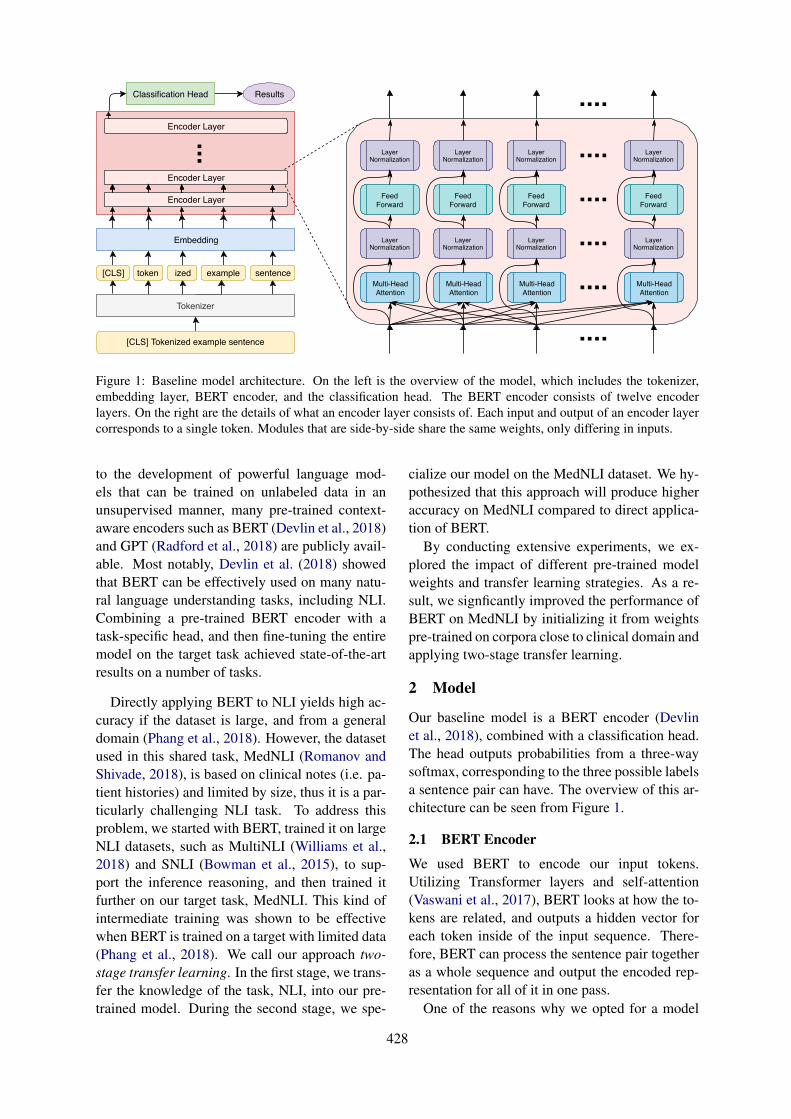
[CLS] Tokenized example sentence
token ized example sentence
Tokenizer
Embedding
[CLS]
Classification Head Results
Encoder Layer
Multi-HeadAttention
Multi-HeadAttention
Multi-HeadAttention
Multi-HeadAttention
LayerNormalization
LayerNormalization
LayerNormalization
LayerNormalization
FeedForward
FeedForward
FeedForward
FeedForward
LayerNormalization
LayerNormalization
LayerNormalization
LayerNormalization
Encoder Layer
Encoder Layer
Figure 1: Baseline model architecture. On the left is the overview of the model, which includes the tokenizer,embedding layer, BERT encoder, and the classification head. The BERT encoder consists of twelve encoderlayers. On the right are the details of what an encoder layer consists of. Each input and output of an encoder layercorresponds to a single token. Modules that are side-by-side share the same weights, only differing in inputs.
to the development of powerful language mod-els that can be trained on unlabeled data in anunsupervised manner, many pre-trained context-aware encoders such as BERT (Devlin et al., 2018)and GPT (Radford et al., 2018) are publicly avail-able. Most notably, Devlin et al. (2018) showedthat BERT can be effectively used on many natu-ral language understanding tasks, including NLI.Combining a pre-trained BERT encoder with atask-specific head, and then fine-tuning the entiremodel on the target task achieved state-of-the-artresults on a number of tasks.
Directly applying BERT to NLI yields high ac-curacy if the dataset is large, and from a generaldomain (Phang et al., 2018). However, the datasetused in this shared task, MedNLI (Romanov andShivade, 2018), is based on clinical notes (i.e. pa-tient histories) and limited by size, thus it is a par-ticularly challenging NLI task. To address thisproblem, we started with BERT, trained it on largeNLI datasets, such as MultiNLI (Williams et al.,2018) and SNLI (Bowman et al., 2015), to sup-port the inference reasoning, and then trained itfurther on our target task, MedNLI. This kind ofintermediate training was shown to be effectivewhen BERT is trained on a target with limited data(Phang et al., 2018). We call our approach two-stage transfer learning. In the first stage, we trans-fer the knowledge of the task, NLI, into our pre-trained model. During the second stage, we spe-
cialize our model on the MedNLI dataset. We hy-pothesized that this approach will produce higheraccuracy on MedNLI compared to direct applica-tion of BERT.
By conducting extensive experiments, we ex-plored the impact of different pre-trained modelweights and transfer learning strategies. As a re-sult, we signficantly improved the performance ofBERT on MedNLI by initializing it from weightspre-trained on corpora close to clinical domain andapplying two-stage transfer learning.
2 Model
Our baseline model is a BERT encoder (Devlinet al., 2018), combined with a classification head.The head outputs probabilities from a three-waysoftmax, corresponding to the three possible labelsa sentence pair can have. The overview of this ar-chitecture can be seen from Figure 1.
2.1 BERT Encoder
We used BERT to encode our input tokens.Utilizing Transformer layers and self-attention(Vaswani et al., 2017), BERT looks at how the to-kens are related, and outputs a hidden vector foreach token inside of the input sequence. There-fore, BERT can process the sentence pair togetheras a whole sequence and output the encoded rep-resentation for all of it in one pass.
One of the reasons why we opted for a model
428
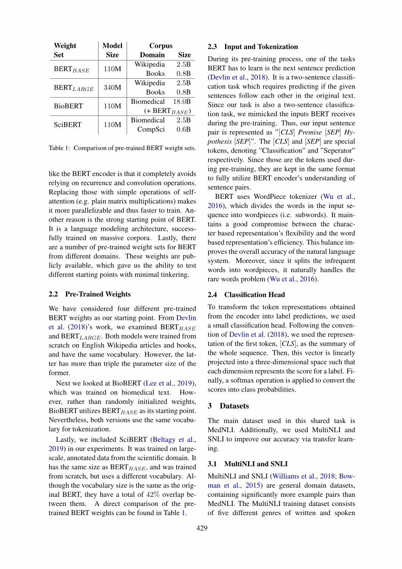
Weight Model CorpusSet Size Domain Size
BERTBASE 110MWikipedia 2.5B
Books 0.8B
BERTLARGE 340MWikipedia 2.5B
Books 0.8B
BioBERT 110MBiomedical 18.0B
(+ BERTBASE)
SciBERT 110MBiomedical 2.5B
CompSci 0.6B
Table 1: Comparison of pre-trained BERT weight sets.
like the BERT encoder is that it completely avoidsrelying on recurrence and convolution operations.Replacing those with simple operations of self-attention (e.g. plain matrix multiplications) makesit more parallelizable and thus faster to train. An-other reason is the strong starting point of BERT.It is a language modeling architecture, success-fully trained on massive corpora. Lastly, thereare a number of pre-trained weight sets for BERTfrom different domains. These weights are pub-licly available, which gave us the ability to testdifferent starting points with minimal tinkering.
2.2 Pre-Trained Weights
We have considered four different pre-trainedBERT weights as our starting point. From Devlinet al. (2018)’s work, we examined BERTBASE
and BERTLARGE . Both models were trained fromscratch on English Wikipedia articles and books,and have the same vocabulary. However, the lat-ter has more than triple the parameter size of theformer.
Next we looked at BioBERT (Lee et al., 2019),which was trained on biomedical text. How-ever, rather than randomly initialized weights,BioBERT utilizes BERTBASE as its starting point.Nevertheless, both versions use the same vocabu-lary for tokenization.
Lastly, we included SciBERT (Beltagy et al.,2019) in our experiments. It was trained on large-scale, annotated data from the scientific domain. Ithas the same size as BERTBASE , and was trainedfrom scratch, but uses a different vocabulary. Al-though the vocabulary size is the same as the orig-inal BERT, they have a total of 42% overlap be-tween them. A direct comparison of the pre-trained BERT weights can be found in Table 1.
2.3 Input and Tokenization
During its pre-training process, one of the tasksBERT has to learn is the next sentence prediction(Devlin et al., 2018). It is a two-sentence classifi-cation task which requires predicting if the givensentences follow each other in the original text.Since our task is also a two-sentence classifica-tion task, we mimicked the inputs BERT receivesduring the pre-training. Thus, our input sentencepair is represented as ”[CLS] Premise [SEP] Hy-pothesis [SEP]”. The [CLS] and [SEP] are specialtokens, denoting ”Classification” and ”Seperator”respectively. Since those are the tokens used dur-ing pre-training, they are kept in the same formatto fully utilize BERT encoder’s understanding ofsentence pairs.
BERT uses WordPiece tokenizer (Wu et al.,2016), which divides the words in the input se-quence into wordpieces (i.e. subwords). It main-tains a good compromise between the charac-ter based representation’s flexibility and the wordbased representation’s efficiency. This balance im-proves the overall accuracy of the natural languagesystem. Moreover, since it splits the infrequentwords into wordpieces, it naturally handles therare words problem (Wu et al., 2016).
2.4 Classification Head
To transform the token representations obtainedfrom the encoder into label predictions, we useda small classification head. Following the conven-tion of Devlin et al. (2018), we used the represen-tation of the first token, [CLS], as the summary ofthe whole sequence. Then, this vector is linearlyprojected into a three-dimensional space such thateach dimension represents the score for a label. Fi-nally, a softmax operation is applied to convert thescores into class probabilities.
3 Datasets
The main dataset used in this shared task isMedNLI. Additionally, we used MultiNLI andSNLI to improve our accuracy via transfer learn-ing.
3.1 MultiNLI and SNLI
MultiNLI and SNLI (Williams et al., 2018; Bow-man et al., 2015) are general domain datasets,containing significantly more example pairs thanMedNLI. The MultiNLI training dataset consistsof five different genres of written and spoken
429
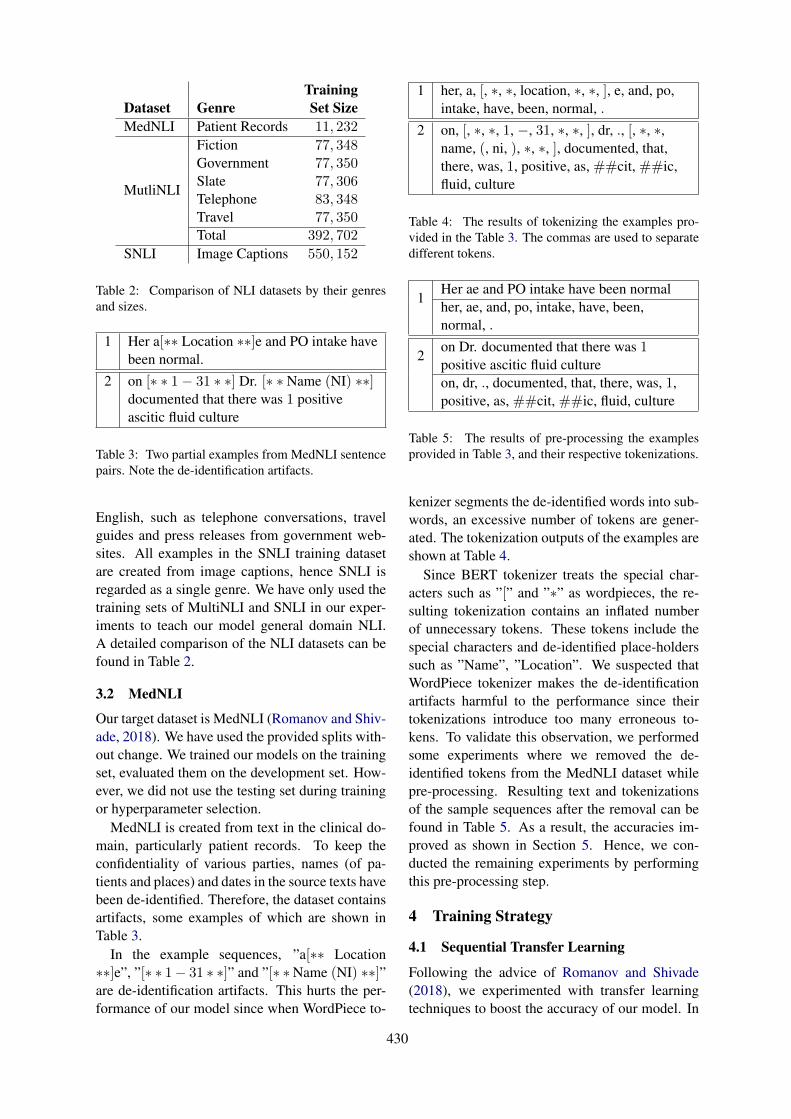
TrainingDataset Genre Set SizeMedNLI Patient Records 11, 232
MutliNLI
Fiction 77, 348Government 77, 350Slate 77, 306Telephone 83, 348Travel 77, 350Total 392, 702
SNLI Image Captions 550, 152
Table 2: Comparison of NLI datasets by their genresand sizes.
1 Her a[∗∗ Location ∗∗]e and PO intake havebeen normal.
2 on [∗ ∗ 1− 31 ∗ ∗] Dr. [∗ ∗ Name (NI) ∗∗]documented that there was 1 positiveascitic fluid culture
Table 3: Two partial examples from MedNLI sentencepairs. Note the de-identification artifacts.
English, such as telephone conversations, travelguides and press releases from government web-sites. All examples in the SNLI training datasetare created from image captions, hence SNLI isregarded as a single genre. We have only used thetraining sets of MultiNLI and SNLI in our exper-iments to teach our model general domain NLI.A detailed comparison of the NLI datasets can befound in Table 2.
3.2 MedNLI
Our target dataset is MedNLI (Romanov and Shiv-ade, 2018). We have used the provided splits with-out change. We trained our models on the trainingset, evaluated them on the development set. How-ever, we did not use the testing set during trainingor hyperparameter selection.
MedNLI is created from text in the clinical do-main, particularly patient records. To keep theconfidentiality of various parties, names (of pa-tients and places) and dates in the source texts havebeen de-identified. Therefore, the dataset containsartifacts, some examples of which are shown inTable 3.
In the example sequences, ”a[∗∗ Location∗∗]e”, ”[∗ ∗ 1− 31 ∗ ∗]” and ”[∗ ∗Name (NI) ∗∗]”are de-identification artifacts. This hurts the per-formance of our model since when WordPiece to-
1 her, a, [, ∗, ∗, location, ∗, ∗, ], e, and, po,intake, have, been, normal, .
2 on, [, ∗, ∗, 1, −, 31, ∗, ∗, ], dr, ., [, ∗, ∗,name, (, ni, ), ∗, ∗, ], documented, that,there, was, 1, positive, as, ##cit, ##ic,fluid, culture
Table 4: The results of tokenizing the examples pro-vided in the Table 3. The commas are used to separatedifferent tokens.
1Her ae and PO intake have been normalher, ae, and, po, intake, have, been,normal, .
2on Dr. documented that there was 1positive ascitic fluid cultureon, dr, ., documented, that, there, was, 1,positive, as, ##cit, ##ic, fluid, culture
Table 5: The results of pre-processing the examplesprovided in Table 3, and their respective tokenizations.
kenizer segments the de-identified words into sub-words, an excessive number of tokens are gener-ated. The tokenization outputs of the examples areshown at Table 4.
Since BERT tokenizer treats the special char-acters such as ”[” and ”∗” as wordpieces, the re-sulting tokenization contains an inflated numberof unnecessary tokens. These tokens include thespecial characters and de-identified place-holderssuch as ”Name”, ”Location”. We suspected thatWordPiece tokenizer makes the de-identificationartifacts harmful to the performance since theirtokenizations introduce too many erroneous to-kens. To validate this observation, we performedsome experiments where we removed the de-identified tokens from the MedNLI dataset whilepre-processing. Resulting text and tokenizationsof the sample sequences after the removal can befound in Table 5. As a result, the accuracies im-proved as shown in Section 5. Hence, we con-ducted the remaining experiments by performingthis pre-processing step.
4 Training Strategy
4.1 Sequential Transfer Learning
Following the advice of Romanov and Shivade(2018), we experimented with transfer learningtechniques to boost the accuracy of our model. In
430
Pre-trained BERTModel
NLI TunedModel
MedNLI TunedModel
Train on largeNLI dataset
Evaluate onMedNLI
Train onMedNLI
Evaluate onMedNLI
Figure 2: Two-stage sequential transfer learning strat-egy.
fact, our baseline approach is itself a type of se-quential transfer learning. We take a pre-trainedBERT, append a classifier head on top of it, andfine-tune the whole model on the MedNLI train-ing dataset. Since BERT is a powerful sequenceencoder, this approach alone yielded better resultson the MedNLI development dataset compared tothe published baselines (Romanov and Shivade,2018). However, because the dataset is limitedin size, performances of these approaches are re-stricted. Therefore, instead of training our modeldirectly on the target task, we added an interme-diate training step. During this step, the modelis trained on a large NLI dataset from a generaldomain such as MultiNLI and SNLI. Our aim isto help the model learn task specific reasoningskills using the large number of training exam-ples. Then, the model is further fine-tuned on theMedNLI training dataset so that it can adapt its pa-rameters to the clinical domain and MedNLI style.We call this strategy two-stage sequential trans-fer learning, which is shown in Figure 2. In bothstages of the learning, the model is trained until itsaccuracy on the MedNLI development set is max-imized.
Since there are multiple large and general do-main NLI datasets available, we wanted to lever-age them. Therefore, we also experimented withthree-stage transfer learning. In the first twostages, we trained our model on MultiNLI andSNLI successively. In the third stage, we finallytrained it on MedNLI. However, this configuration
Model 1
InputPair
Model 2 Model N
LabelProbabilities
LabelProbabilities
LabelProbabilities
Element-wiseFunction
LabelScores
Figure 3: Ensembling procedure of N different modelsfor an input premise-hypothesis pair.
yielded slightly worse results compared to two-stage transfer, as discussed in Section 5. There-fore, we changed our method and utilized an en-sembling approach to combine the benefits of theavailable datasets.
4.2 Ensembling
We perform ensembling on independently trainedmodels to get the benefit of multiple datasets.First, these models are fully trained by two-stagetransfer learning with different general domaindatasets. After that, we compute a set of la-bel probabilities for the sentence pairs using thesemodels. Then, we combine the probabilities withan element-wise operation such as sum, product,or max to obtain a single score for each label. Fig-ure 3 summarizes this process for a single input.Finally, we report the label corresponding to thehighest score as our prediction for each example.This approach might be regarded as a soft ver-sion of majority voting, a commonly used ensem-bling method. As Section 5 shows, this approachyielded the best results obtained by our models.
5 Results and Discussion
5.1 Implementation Details
We used PyTorch (Paszke et al., 2017) as our deeplearning framework and the BERT implementa-tion provided by Hugging Face1. Our models arebased on the BertForSequenceClassification class.We used the BertAdam optimizer from the same
1https://github.com/huggingface/pytorch-pretrained-BERT
431
Training Training Sequence Batch InitialStrategy Set Length Size Optimizer Learning RateDirect Training
MedNLI 256 16 BertAdam 2× 10⁻⁵
Task pre-trainingMultiNLI 256 32 BertAdam 2× 10⁻⁵
SNLI 256 32 BertAdam 2× 10⁻⁵
Domain fine-tuningMedNLI 256 16 BertAdam 2× 10⁻⁵
Table 6: The hyperparameters for different training settings.
repository, which imitates the Adam implementa-tion of the original BERT.
We always evaluated our models according tothe accuracy on the MedNLI development set. Forall experiments, we trained a model until its accu-racy in the last four epochs did not improve overits best accuracy. If a model kept improving, westopped the training after 80 epochs. All modelweights are updated during the training phases ofthe experiments.
The training procedure was stable, there wereno serious failure cases with unexpectedly low ac-curacies. Nevertheless, to mitigate the possiblenegative effects of the randomness on the opti-mization, we repeated each experiment with threedifferent seeds and selected the run with the bestaccuracy.
The primary hyperparameters of our model arethe sequence length of the encoder layers, thebatch size, and the initial learning rate of the opti-mizer, BertAdam. We kept the remaining hyperpa-rameters such as dropout rate the same as the orig-inal implementation. To determine the sequencelength, we counted the number of resulting to-kens from MultiNLI, SNLI, and MedNLI sentencepairs after tokenization. Since the maximum tokencount is 256, we naturally set the sequence lengthto 256. When we trained the model on MedNLI,we used batches with size of 16. In contrast, whena large dataset (e.g. MultiNLI and SNLI) is used,we used batch size of 32 to speed up the train-ing process. In the initial experiments, we tried2 ∗ 10−5 , 3 ∗ 10−5 , and 5 ∗ 10−5 as BertAdam’sinitial learning rate which resulted in very similaraccuracies. Nevertheless, since 2 ∗ 10−5 gener-ally yielded slightly better results, we conductedthe remaining experiments with this initial learn-ing rate. Table 6 summarizes the hyperparameters
Weight Set Dev AccuracyBERTBASE 82.3%BERTLARGE 82.9%BioBERT 83.4%SciBERT 83.7%
Table 7: Results of directly training on MedNLI data,starting from various pre-trained weight sets. The high-est accuracy is indicated with bold.
used in the training phases.
5.2 Experiments
We have conducted a number of experiments totest our model and the effectiveness of differenttraining strategies. We report the resulting percentaccuracies on the MedNLI development dataset.
To start with, we trained our model on MedNLIdirectly. We initialized it with various pre-trainedweights to compare their performances. The re-sults of the experiment can be seen from Table 7.It shows that the weights pre-trained on domainsrelated to the task, such as biomedical or scien-tific data, have a noticeable advantage over theweights obtained from general text corpora, suchas Wikipedia. Moreover, the effect of pre-trainingis more significant compared to the model size.BioBERT and SciBERT surpassed BERTLARGE
although they are three times smaller.Next, we tested the two-stage sequential trans-
fer learning method using all combinations of pre-trained weights and rich NLI datasets mentionedbefore. Table 8 shows the results of this experi-ment. As expected, all models benefit from two-stage transfer learning. Moreover, the trend of spe-cialized pre-trained weights having an advantagecontinues on this experiment as well. However,BioBERT outperforms SciBERT, unlike the pre-
432
Weight Set MultiNLI SNLIBERTBASE 82.9% 82.4%BERTLARGE 83.7% 84.4%BioBERT 85.6% 85.8%SciBERT 85.4% 85.6%
Table 8: Development set accuracies achieved by per-forming two-stage sequential transfer learning, utiliz-ing different intermediary datasets, and starting fromvarious pre-trained weights. The highest accuracy isindicated with bold.
MultiNLI SNLIBERTBASE +0.7% ±0.0%BERTLARGE +0.6% +2.2%BioBERT +1.2% +0.6%SciBERT +0.4% +1.3%
Table 9: Accuracies gained by pre-processing theMedNLI dataset, after performing two-stage sequen-tial transfer learning with different starting points anddatasets.
vious results. We suspect that since BioBERT ispre-trained starting from BERTBASE , it benefitsmore from general domain task training.
In order to test the effect of pre-processingdescribed in Section 3.2, we repeated the two-stage training experiment without removing thede-identification artifacts. We compared the re-sults of this experiment with the previous resultsto see how the accuracy is affected. The improve-ments obtained from the pre-processing can befound in Table 9. It increases the accuracy in allcases, except for BERTBASE - SNLI, where theaccuracy is unchanged. Note that all other experi-ments are conducted with the pre-processing is en-abled.
We have also tested the performance of three-stage sequential transfer learning on BioBERT.Training on SNLI and MultiNLI sequentially be-fore MedNLI produced lower accuracies com-pared to the two-stage transfer learning experi-ment. Moreover, switching the training order ofSNLI and MultiNLI did not change the resultingaccuracy. We suspect that further training on a sec-ond intermediate dataset brings the model closerto a worse local optimum. A comparison betweendifferent training strategies on BioBERT can befound in Table 10.
Lastly, we experimented with ensembling. Wetested four ensemble models, one for each pre-
DevTraining Strategy AccuracyDirect Training on MedNLI 83.4%
Two-Stage Transfer:MultiNLI→MedNLI 85.6%SNLI→MedNLI 85.8%
Three-Stage Transfer:MultiNLI→ SNLI→MedNLI 84.9%SNLI→MultiNLI→MedNLI 84.9%
Table 10: Single model development set accuraciesof different training strategies, starting from BioBERT.The highest accuracy is indicated with bold.
Weight Set Sum Product MaxBERTBASE 83.3% 83.4% 83.3%BERTLARGE 85.1% 85.0% 85.2%BioBERT 86.1% 86.0% 86.1%SciBERT 85.9% 85.8% 85.8%
Table 11: Development set accuracies resulting fromensembling two models starting from the same pre-trained weights. The highest accuracies are indicatedwith bold.
trained BERT variant. For each of these start-ing points, we combined the two models obtainedfrom the two-stage transfer learning experiment.One of these models is trained with MultiNLI, theother with SNLI. We tried three different element-wise operations for ensembling, and comparedtheir effects. Table 11 shows that this approachyielded better results compared to the two-stagetransfer methods. Therefore, we effectively com-bined the benefits of training on different, richdatasets.
Among all the experiments, the best resultwe obtained is 86.1% accuracy by ensemblingBioBERT models trained with two-stage transferlearning. That accuracy was obtained by combin-ing the output probabilities with element-wise sumoperation.
Therefore, we participated in the shared taskwith that ensembled model. Consequently, ourmodel achieved 84.7% accuracy on the unseen testdataset reserved for the shared task.
5.3 Error AnalysisFollowing Romanov and Shivade (2018), we con-ducted a similar error analysis on MedNLI devel-opment set to understand how the different meth-ods improve the baseline. We chose BioBERT for
433
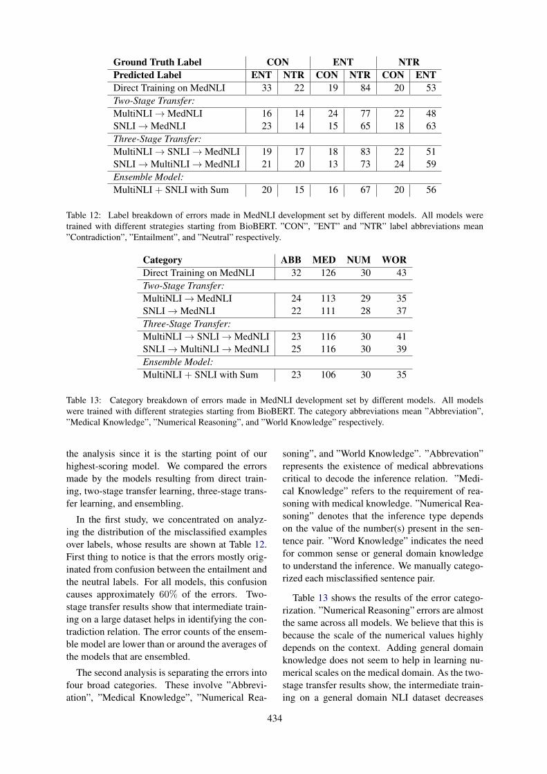
Ground Truth Label CON ENT NTRPredicted Label ENT NTR CON NTR CON ENTDirect Training on MedNLI 33 22 19 84 20 53Two-Stage Transfer:MultiNLI→MedNLI 16 14 24 77 22 48SNLI→MedNLI 23 14 15 65 18 63Three-Stage Transfer:MultiNLI→ SNLI→MedNLI 19 17 18 83 22 51SNLI→MultiNLI→MedNLI 21 20 13 73 24 59Ensemble Model:MultiNLI + SNLI with Sum 20 15 16 67 20 56
Table 12: Label breakdown of errors made in MedNLI development set by different models. All models weretrained with different strategies starting from BioBERT. ”CON”, ”ENT” and ”NTR” label abbreviations mean”Contradiction”, ”Entailment”, and ”Neutral” respectively.
Category ABB MED NUM WORDirect Training on MedNLI 32 126 30 43Two-Stage Transfer:MultiNLI→MedNLI 24 113 29 35SNLI→MedNLI 22 111 28 37Three-Stage Transfer:MultiNLI→ SNLI→MedNLI 23 116 30 41SNLI→MultiNLI→MedNLI 25 116 30 39Ensemble Model:MultiNLI + SNLI with Sum 23 106 30 35
Table 13: Category breakdown of errors made in MedNLI development set by different models. All modelswere trained with different strategies starting from BioBERT. The category abbreviations mean ”Abbreviation”,”Medical Knowledge”, ”Numerical Reasoning”, and ”World Knowledge” respectively.
the analysis since it is the starting point of ourhighest-scoring model. We compared the errorsmade by the models resulting from direct train-ing, two-stage transfer learning, three-stage trans-fer learning, and ensembling.
In the first study, we concentrated on analyz-ing the distribution of the misclassified examplesover labels, whose results are shown at Table 12.First thing to notice is that the errors mostly orig-inated from confusion between the entailment andthe neutral labels. For all models, this confusioncauses approximately 60% of the errors. Two-stage transfer results show that intermediate train-ing on a large dataset helps in identifying the con-tradiction relation. The error counts of the ensem-ble model are lower than or around the averages ofthe models that are ensembled.
The second analysis is separating the errors intofour broad categories. These involve ”Abbrevi-ation”, ”Medical Knowledge”, ”Numerical Rea-
soning”, and ”World Knowledge”. ”Abbrevation”represents the existence of medical abbrevationscritical to decode the inference relation. ”Medi-cal Knowledge” refers to the requirement of rea-soning with medical knowledge. ”Numerical Rea-soning” denotes that the inference type dependson the value of the number(s) present in the sen-tence pair. ”Word Knowledge” indicates the needfor common sense or general domain knowledgeto understand the inference. We manually catego-rized each misclassified sentence pair.
Table 13 shows the results of the error catego-rization. ”Numerical Reasoning” errors are almostthe same across all models. We believe that this isbecause the scale of the numerical values highlydepends on the context. Adding general domainknowledge does not seem to help in learning nu-merical scales on the medical domain. As the two-stage transfer results show, the intermediate train-ing on a general domain NLI dataset decreases
434
the error rates on the remaining three categories.However, training with three-stage transfer learn-ing does not improve the ”Medical Knowledge”and ”World Knowledge” categories as much asthe two-stage transfer. Although getting poorer re-sults after training with more data seems counter-intuitive, Romanov and Shivade (2018) observeda similar trend on transfer learning using SNLI,and the genres of MultiNLI. In both findings,the model performance does not directly correlatewith the size of the intermediate training data.
Lastly, most of the improvements introducedby ensembling fall under ”Medical Knowledge”.Since the component models are trained on dif-ferent datasets on intermediate training step, theerrors they made on the MedNLI development setdiffer. We suspect that the models are not veryconfident in some of their ”Medical Knowledge”errors, hence the other model may correct thesemistakes to an extent.
6 Conclusion
In this paper, we showed that a pre-trained BERTencoder, combined with a classifier head forms astrong baseline for MedNLI task. More impor-tantly, we also demonstrated that the model’s ac-curacy can be remarkably improved by utilizing atwo-stage transfer learning strategy. The successof the final model depends on the initial BERTweights, as well as the particular transfer learningmethod. Finally, we showed that ensembling twoseparate models trained on different NLI datasetsis more effective than using these datasets to traina single model. Our best model, BioBERT ensem-bled, achieved 86.1% accuracy on the MedNLI de-velopment set, and 84.7% accuracy on the unseentest dataset reserved for the MEDIQA 2019’s NLIShared Task.
While empirical results show that contextual-ized sequence encoders enhanced with transferlearning are strong, their performances might befurther improved with external knowledge integra-tion. As future work, we would like to extendBERT’s contextualized word vectors using seman-tic relationships.
Acknowledgments
Cemil Cengiz is supported by Huawei TurkeyR&D Center through the Huawei Graduate Re-search Support Scholarship.
ReferencesIz Beltagy, Arman Cohan, and Kyle Lo. 2019. Scib-
ert: Pretrained contextualized embeddings for sci-entific text. Computing Research Repository,arXiv:1903.10676.
Asma Ben Abacha, Chaitanya Shivade, and DinaDemner-Fushman. 2019. Overview of the mediqa2019 shared task on textual inference, question en-tailment and question answering. In Proceedings ofthe BioNLP 2019 workshop, Florence, Italy, August1, 2019. Association for Computational Linguistics.
Samuel R. Bowman, Gabor Angeli, Christopher Potts,and Christopher D. Manning. 2015. A large anno-tated corpus for learning natural language inference.In Proceedings of the 2015 Conference on EmpiricalMethods in Natural Language Processing. Associa-tion for Computational Linguistics.
Alexis Conneau, Douwe Kiela, Holger Schwenk, LocBarrault, and Antoine Bordes. 2017. Supervisedlearning of universal sentence representations fromnatural language inference data. In Proceedings ofthe 2017 Conference on Empirical Methods in Nat-ural Language Processing. Association for Compu-tational Linguistics.
Jacob Devlin, Ming-Wei Chang, Kenton Lee, andKristina Toutanova. 2018. BERT: Pre-trainingof Deep Bidirectional Transformers for LanguageUnderstanding. Computing Research Repository,arXiv:1810.04805.
Sepp Hochreiter and Jrgen Schmidhuber. 1997.Long short-term memory. Neural Computation,9(8):1735–1780.
Surafel Melaku Lakew, Mauro Cettolo, and MarcelloFederico. 2018. A comparison of transformer andrecurrent neural networks on multilingual neuralmachine translation. In Proceedings of the 27th In-ternational Conference on Computational Linguis-tics, pages 641–652, Santa Fe, New Mexico, USA.Association for Computational Linguistics.
Jinhyuk Lee, Wonjin Yoon, Sungdong Kim,Donghyeon Kim, Sunkyu Kim, Chan Ho So,and Jaewoo Kang. 2019. Biobert: a pre-trainedbiomedical language representation model forbiomedical text mining. Computing ResearchRepository, arXiv:1901.08746.
Xiaodong Liu, Kevin Duh, and Jianfeng Gao.2018. Stochastic answer networks for natural lan-guage inference. Computing Research Repository,arXiv:1804.07888.
Xiaodong Liu, Pengcheng He, Weizhu Chen, and Jian-feng Gao. 2019. Multi-task deep neural networksfor natural language understanding. Computing Re-search Repository, arXiv:1901.11504.
Bill MacCartney. 2009. Natural Language Inference.Ph.D. thesis, Stanford University, Stanford, CA,USA. AAI3364139.
435
Adam Paszke, Sam Gross, Soumith Chintala, Gre-gory Chanan, Edward Yang, Zachary DeVito, Zem-ing Lin, Alban Desmaison, Luca Antiga, and AdamLerer. 2017. Automatic differentiation in pytorch.In NIPS-W.
Jason Phang, Thibault Févry, and Samuel R. Bowman.2018. Sentence encoders on stilts: Supplementarytraining on intermediate labeled-data tasks. Com-puting Research Repository, arXiv:1811.01088.
Alec Radford, Karthik Narasimhan, Tim Salimans, andIlya Sutskever. 2018. Improving language under-standing by generative pre-training.
Alexey Romanov and Chaitanya Shivade. 2018.Lessons from natural language inference in the clin-ical domain. In Proceedings of the 2018 Conferenceon Empirical Methods in Natural Language Pro-cessing, pages 1586–1596, Brussels, Belgium. As-sociation for Computational Linguistics.
Ashish Vaswani, Noam Shazeer, Niki Parmar, JakobUszkoreit, Llion Jones, Aidan N Gomez, ŁukaszKaiser, and Illia Polosukhin. 2017. Attention is allyou need. In I. Guyon, U. V. Luxburg, S. Bengio,H. Wallach, R. Fergus, S. Vishwanathan, and R. Gar-nett, editors, Advances in Neural Information Pro-cessing Systems 30, pages 5998–6008. Curran As-sociates, Inc.
Adina Williams, Nikita Nangia, and Samuel Bowman.2018. A broad-coverage challenge corpus for sen-tence understanding through inference. In Proceed-ings of the 2018 Conference of the North AmericanChapter of the Association for Computational Lin-guistics: Human Language Technologies, Volume 1(Long Papers). Association for Computational Lin-guistics.
Yonghui Wu, Mike Schuster, Zhifeng Chen, Quoc V.Le, Mohammad Norouzi, Wolfgang Macherey,Maxim Krikun, Yuan Cao, Qin Gao, KlausMacherey, Jeff Klingner, Apurva Shah, MelvinJohnson, Xiaobing Liu, Lukasz Kaiser, StephanGouws, Yoshikiyo Kato, Taku Kudo, HidetoKazawa, Keith Stevens, George Kurian, NishantPatil, Wei Wang, Cliff Young, Jason Smith, JasonRiesa, Alex Rudnick, Oriol Vinyals, Greg Corrado,Macduff Hughes, and Jeffrey Dean. 2016. Google’sneural machine translation system: Bridging the gapbetween human and machine translation. Comput-ing Research Repository, arXiv:1609.08144.
436
Proceedings of the BioNLP 2019 workshop, pages 437–445Florence, Italy, August 1, 2019. c©2019 Association for Computational Linguistics1
Abstract
In this paper, we propose a novel model called Adversarial Multi-Task Network (AMTN) for jointly modeling Recognizing Question Entailment (RQE) and medical Question Answering (QA) tasks. AMTN utilizes a pre-trained BioBERT model and an Interactive Transformer to learn the shared semantic representations across different task through parameter sharing mechanism. Meanwhile, an adversarial training strategy is introduced to separate the private features of each task from the shared representations. Experiments on BioNLP 2019 RQE and QA shared task datasets show that our model benefits from the shared representations of both tasks provided by multi-task learning and adversarial training, and obtains significant improvements upon the single-task models.
1 Introduction
With the rapid development of Internet and medical care, online health queries are increasing at a high rate. In 2012, 59% of U.S. adults looked for health information online 1 . However, it is always difficult for search engines to return relevant and trustworthy health information every time if the symptoms are not accurately described (Pletneva et al., 2012; Scantlebury et al., 2017). Therefore, many websites provide online doctor consultation services, which can answer questions or give advice from doctors or experts to the
1 http://www.pewinternet.org/2013/01/15/health-online-2013/
customers. Unfortunately, manually answering some simple queries or answering similar questions multiple times is quite time-consuming and wasteful. A Question Answering (QA) system that can automatically understand and answer the health care questions asked by customers is urgently needed (Wren, 2012).
To this end, BioNLP 2019 (Abacha et al., 2019) provides a series of challenging shared tasks, including: (1) Natural Language Inference (NLI) in the clinical domain; (2) Recognizing Question
Entailment (RQE); (3) medical Question Answering (QA). This paper mainly focuses on RQE and QA task.
RQE task aims at identifying entailment relation between two questions in the context of QA (Abacha and Fushman, 2016), which can be represented as “a question Q1 entails a question Q2 if every answer to Q2 is also a complete or partial answer to Q1”.
QA task aims at automatically filtering and improving the ranking of automatically retrieved answers (Abacha and Fushman, 2019). There are two targets for QA: (1) determining whether the given sentence could answer the given question; (2) ranking all the right answers according to their relevance to the question.
Neural networks and deep learning (DL) currently provide the best solutions for RQE and QA tasks. Among various neural networks, such as traditional Convolutional Neural Networks (CNN) (LeCun et al., 1998) and Long Short-Term Memory (LSTM) networks (Hochreiter and Schmidhuber, 1997), Transformer (Vaswani et al., 2017) has demonstrated superiority in multiple
DUT-NLP at MEDIQA 2019:An Adversarial Multi-Task Network to Jointly Model Recognizing Question Entailment
and Question Answering
Huiwei Zhou, Xuefei Li, Weihong Yao, Chengkun Lang, Shixian Ning
School of Computer Science and Technology Dalian University of Technology
116024 Dalian, China {zhouhuiwei, weihongy}@dlut.edu.cn
{lixuefei, kunkun, ningshixian}@mail.dlut.edu.cn
437
2
natural language processing tasks (Verga et al., 2017; Shen et al., 2017; Yu et al., 2018). Transformer (Vaswani et al., 2017) is based solely on attention mechanisms and it can effectively capture the long-range dependencies between words.
More recently, the pre-trained language models, such as ELMo (Matthew et al., 2018), OpenAI GPT 2 , and BERT (Devlin et al., 2018), have shown their effectiveness to capture the deep semantic and syntactic information of words. BioBERT (Lee et al., 2019) is one of the BERT-based pre-trained language model for biomedical domain, and it achieves great improvement in many biomedical tasks. For this reason, we believe that the pre-trained language models, especially the BioBERT, should be valid for RQE and QA under reasonable use.
Most previous researches train the model of RQE task or QA task separately based on a single training set. However, such single-task method cannot provide essential mutual supports between the two tasks. The inherent interactions between the two tasks might help us do even better on the RQE and QA tasks. RQE task can find Frequently Asked Questions (FAQs) similar to a consumer health question, providing consumers with appropriate FAQs and enabling QA systems to identify the right answers with greater precision and higher speed (Harabagiu and Hickl, 2006).
Multi-Task Learning (MTL) is a learning paradigm in machine learning and its aim is to leverage shared representations contained in multiple related tasks to help improve the generalization performance of all the tasks. MTL is usually done with parameter sharing of hidden layers. Hard parameter sharing is the most commonly used approach to MTL in neural networks. It is generally applied by sharing the hidden layers between all tasks, while keeping several task-specific output layers. However, it is difficult for MTL to distinguish the commonalities and differences between different tasks.
A common way to improve the robustness of the system is to train the system using different datasets through adversarial training (Goodfellow et al., 2014). Chen et al. (2017) propose a shared-private model, which extracts shared features and
2 https://s3-us-west-2.amazonaws.com/openai-assets/research-covers/language-unsupervised/language_understanding_paper.pdf
private features from multiple corpus, and introduces adversarial training for shared representation learning. Drawing on the practices of previous studies, we plan to use an adversarial multi-task framework to extract the noise-robust shared representation directly.
Considering the similarity between RQE and QA tasks, this paper proposes a novel Adversarial Multi-Task Network (AMTN) to jointly model these two tasks. Specifically, AMTN first utilizes BioBERT as an embedding layer to generate context-dependent word representations. Then, a common Interactive Transformer layer is introduced for sentence representation learning and inter-sentence relationship modeling, which allows knowledge transfer from other tasks. Finally, two specific classifiers are used for RQE and QA tasks respectively. Here, we only consider the target (1) of QA task for the multi-task learning to ensure the consistency between RQE and QA tasks. Furthermore, to prevent the shared and private feature spaces from interfering with each other, an adversarial training strategy is introduced to make the shared feature representations to be more compatible and task-invariant among different tasks. Experimental results show that our AMTN model is effective to improve the performance for both RQE and QA tasks upon the single-task models, which demonstrates the superiority of the adversarial multi-task strategy.
Our contributions can be summarized into two folds.
A well-designed Interactive Transformer layer is introduced for sentence representation learning and inter-sentence relationship modeling.
A novel adversarial multi-task strategy is introduced to jointly model RQE and QA tasks, in which multi-task learning is proposed for shared representation learning and adversarial training is used to force the shared representation purer and task-invariant.
2 Method
This section gives a detailed description of the proposed AMTN, which is shown in Figure 1. AMTN mainly consists of three parts: a shared
438
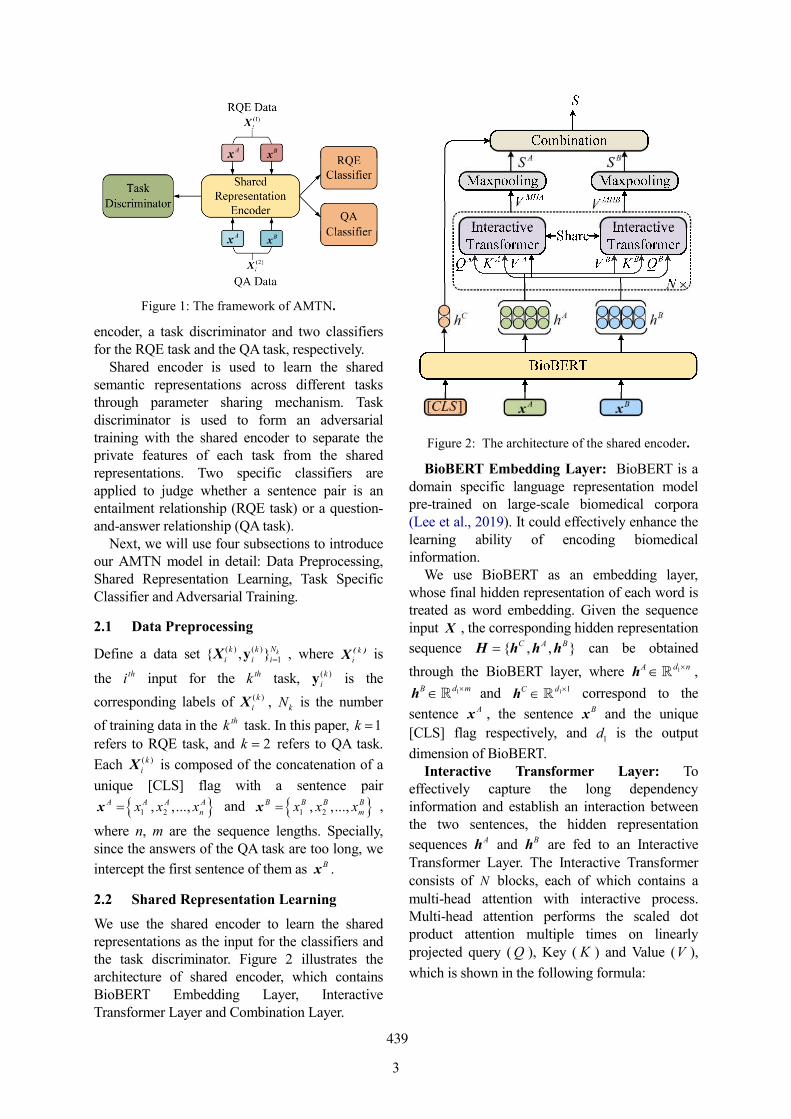
3
encoder, a task discriminator and two classifiers for the RQE task and the QA task, respectively.
Shared encoder is used to learn the shared semantic representations across different tasks through parameter sharing mechanism. Task discriminator is used to form an adversarial training with the shared encoder to separate the private features of each task from the shared representations. Two specific classifiers are applied to judge whether a sentence pair is an entailment relationship (RQE task) or a question-and-answer relationship (QA task).
Next, we will use four subsections to introduce our AMTN model in detail: Data Preprocessing, Shared Representation Learning, Task Specific Classifier and Adversarial Training.
2.1 Data Preprocessing
Define a data set ( ) ( )1{ , }X kNk k
i i iy , where ( )X ki
is
the thi input for the thk task, ( )kiy is the
corresponding labels of ( )X ki , kN is the number
of training data in the thk task. In this paper, 1k
refers to RQE task, and 2k refers to QA task.
Each ( )X ki is composed of the concatenation of a
unique [CLS] flag with a sentence pair
1 2, ,...,x A A A Anx x x and 1 2, ,...,x B B B B
mx x x ,
where n, m are the sequence lengths. Specially, since the answers of the QA task are too long, we
intercept the first sentence of them as xB .
2.2 Shared Representation Learning
We use the shared encoder to learn the shared representations as the input for the classifiers and the task discriminator. Figure 2 illustrates the architecture of shared encoder, which contains BioBERT Embedding Layer, Interactive Transformer Layer and Combination Layer.
BioBERT Embedding Layer: BioBERT is a domain specific language representation model pre-trained on large-scale biomedical corpora (Lee et al., 2019). It could effectively enhance the learning ability of encoding biomedical information.
We use BioBERT as an embedding layer, whose final hidden representation of each word is treated as word embedding. Given the sequence input X , the corresponding hidden representation
sequence { , , }H h h hC A B can be obtained
through the BioBERT layer, where 1h d nA , 1h d mB and 1 1h dC correspond to the
sentence x A , the sentence xB and the unique
[CLS] flag respectively, and 1d is the output
dimension of BioBERT. Interactive Transformer Layer: To
effectively capture the long dependency information and establish an interaction between the two sentences, the hidden representation
sequences hA and hB are fed to an Interactive Transformer Layer. The Interactive Transformer consists of N blocks, each of which contains a multi-head attention with interactive process. Multi-head attention performs the scaled dot product attention multiple times on linearly projected query ( Q ), Key ( K ) and Value (V ),
which is shown in the following formula:
Figure 1: The framework of AMTN.
Figure 2: The architecture of the shared encoder.
439
4
Attention( , , ) softmax( )T
K
Q KQ K V V
d (1)
where Kd is the dimension of K . Vaswani et al.
(2017) point out that the input of softmax grows large in magnitude, pushing the softmax function into regions where it has extremely small gradients. Therefore, the dot productions are
scaled by 1 Kd to counteract this effect.
For the first sentence x A , we take its hidden
representation hA as Q and hB as K , V . In this
way, the information flow inside features of the
sentence x B are dynamically conditioned on the
features of the sentence x A . The inputs for the
first sentence x A can be represented as:
1 2
1 2
1 2
, ,..., ,
, ,..., ,
, ,..., .
A A A An
A B B Bm
A B B Bm
Q h h h
K h h h
V h h h
(2)
For the second sentence x B , we take hB as Q
and take hA as K , V , which can be represented as:
1 2
1 2
1 2
, ,..., ,
, ,..., ,
, ,...,
B B B Bm
B A A An
B A A An
Q h h h
K h h h
V h h h
。
(3)
Therefore, the multi-head attentions with interactive process for the given pair of sentences can be formulated as:
( , , )A Q A K A V Al l l lhead Attention Q K V W W W (4)
( , , )B Q B K B V Bl l l lhead Attention Q K V W W W (5)
1 2[ ; ;...; ]MHA H A A ALV head head head W (6)
1 2[ ; ;...; ]MHB H B B BLV head head head W (7)
where 1headd dQl
W , 1headd dKl
W ,
1headd dVl
W and 1 headd LdH W are trainable
shared parameters. 1 2; ;...; Lhead head head is a
concatenation of outputs of L heads. Different from the original Transformer, in
which the input of Q , K and V are all the same,
Interactive Transformer takes different sentences as the inputs of Q and K , V . In this way, we
expect to effectively compute dependencies
between any two words of the sentence pairs and encode the abundant semantic information for each sequence word.
Combination Layer: After modeling the association between the two sentences, we utilize the max pooling operation to obtain the final
shared semantic representations of x A and x B respectively:
( )A MHAS Maxpooling V (8)
( )B MHBS Maxpooling V (9)
Then, we perform vector combination on AS , BS , and flag representation hC through a dense
layer to generate the sentence pair representation S for classification, which is calculated as follows:
0
0
ReLU( [ ; ; ;
; ] )h
A B A B
A B C
S S S S S
S S b
W
(10)
where 0 150
d dW and 0 10
db are trainable
parameters.
2.3 Task Specific Classifier
For each task, a specific classifier is employed to judge whether a sentence pair is an entailment relationship (RQE) or a question-and-answer relationship (QA). Each classifier is composed of a two-layer fully-connected neural network, which uses a ReLU nonlinearity after the first fully connected layer and a softmax nonlinearity after the second fully connected layer. It can be written as follows:
( )2 1 1 2
ˆ ReLUmi softmax S b b y W W (11)
The classifier takes the sentence pair representation S as input and outputs a probability distribution to predict whether the current sentence pair is entailment relation or question-and-answer relation.
Both classifiers are trained by optimizing the cross-entropy loss as follows:
( ) ( ), ,1 1
ˆlogkN C k kclassifier i j i ji j
J
y y (12)
where C is the number of categories of
classification label, ,ˆ
i jy is the predicted
probability of the thj category of the thi sentence
pair.
440
5
2.4 Adversarial Training
In order to make shared representations contain more common information and reduce the mixing of task-specific information, adversarial training is introduced into the above multi-task framework.
The goal of the proposed adversarial training strategy is to form an adversary with shared representation learning by introducing a task discriminator. In this paper, we take the shared encoder as generative network G and the task discriminator as discriminative model D , in which G needs to learn as much semantic information as possible from the shared data distribution between the two tasks and D aims to determine which task (RQE or QA) the input sentence belongs to by using the shared representations.
Specifically, we first use the shared encoder
G( , )X s , which is mentioned in section 2.2, to
get the sentence pair representation S . s is the
shared parameter need to be trained. Then, the shared representations will be fed to the task discriminator D to determine the task to which the current input belongs. D can be expressed by the following formula:
4 3 3 4D , ReLUW W dS softmax S b b (13)
Besides the task loss for RQE and QA, we
additionally introduce an adversarial loss advJ to
prevent task-specific feature from creeping into shared space and thus get a purer shared
representation. The adversarial loss advJ is trained
in alternating fashion as shown below:
2
( )
1 1
log D G , ,Xk
s d
Nk
adv i s dk i
J min max
t
(14)
where ( )kit is the correct task label (RQE task or
QA task) of the given sentence pair X . Here the basic idea is that, the shared representations learned by the shared encoder need to mislead the task discriminator. At the same time, the task discriminator needs to predict the task (RQE or QA) to which the data belongs as accurately as possible. The two are adversarial to each other and alternately optimized to separate the private features from the shared representations.
Finally, the shared encoder and the task discriminator reach a balance point and achieve mutual promotion.
3 Experiments
3.1 Dataset
Our experiments are conducted on the BioNLP RQE and QA shared tasks. The QA dataset contains a total of 3042 question-answer pairs: 1701 for training, 234 for validation, and 1107 for test. The RQE dataset contains a total of 9120 question pairs: 8588 for training, 302 for validation, and 230 for test. The statistic of the two datasets are shown in Table 1.
3.2 Experimental settings and metric
In the shared encoder module, we use the pre-trained uncased BioBERTbase
3 for computational
complexity considerations. The number of its Transformer blocks and multiple heads are both 12. For the Interactive Transformer, we use 3 blocks with 16 heads. The hidden layer dimension of BioBERTbase and Interactive Transformer are both set to 768. We use a mini batch size of 8 and epoch of 30. Adam optimizer (Kingma and Ba, 2014) is used for both shared encoder and task discriminator to tune the parameters at the
learning rates of 1 1e 5 and 2 1e 4 ,
respectively. Specially, due to the small quantity of QA training data, we oversample it three times during training in order to balance the dataset of two tasks. The hyper-parameters settings used in this paper are shown in Table 2. The performance RQE and QA tasks are evaluated by the official evaluation scripts4, which adopt accuracy as the evaluation metric.
3 https://github.com/naver/biobert-pretrained 4 https://github.com/abachaa/MEDIQA2019/tree/master/Eval
_Scripts
Task Train Validation Test
RQE 8588 302 230 QA 1701 234 1107
Table 1: Statistic of sentence pairs in RQE and QA datasets.
441
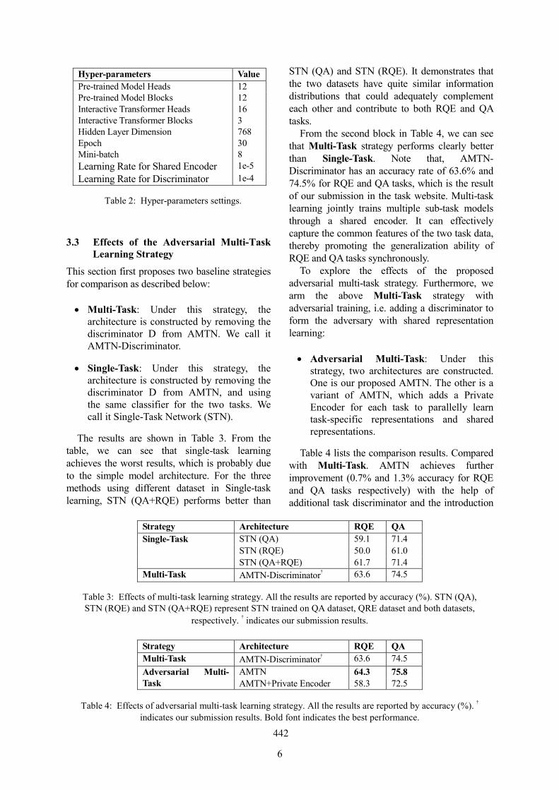
6
3.3 Effects of the Adversarial Multi-Task Learning Strategy
This section first proposes two baseline strategies for comparison as described below:
Multi-Task: Under this strategy, the architecture is constructed by removing the discriminator D from AMTN. We call it AMTN-Discriminator.
Single-Task: Under this strategy, the architecture is constructed by removing the discriminator D from AMTN, and using the same classifier for the two tasks. We call it Single-Task Network (STN).
The results are shown in Table 3. From the table, we can see that single-task learning achieves the worst results, which is probably due to the simple model architecture. For the three methods using different dataset in Single-task learning, STN (QA+RQE) performs better than
STN (QA) and STN (RQE). It demonstrates that the two datasets have quite similar information distributions that could adequately complement each other and contribute to both RQE and QA tasks.
From the second block in Table 4, we can see that Multi-Task strategy performs clearly better than Single-Task. Note that, AMTN-Discriminator has an accuracy rate of 63.6% and 74.5% for RQE and QA tasks, which is the result of our submission in the task website. Multi-task learning jointly trains multiple sub-task models through a shared encoder. It can effectively capture the common features of the two task data, thereby promoting the generalization ability of RQE and QA tasks synchronously.
To explore the effects of the proposed adversarial multi-task strategy. Furthermore, we arm the above Multi-Task strategy with adversarial training, i.e. adding a discriminator to form the adversary with shared representation learning:
Adversarial Multi-Task: Under this strategy, two architectures are constructed. One is our proposed AMTN. The other is a variant of AMTN, which adds a Private Encoder for each task to parallelly learn task-specific representations and shared representations.
Table 4 lists the comparison results. Compared with Multi-Task. AMTN achieves further improvement (0.7% and 1.3% accuracy for RQE and QA tasks respectively) with the help of additional task discriminator and the introduction
Strategy Architecture RQE QA
Single-Task STN (QA) 59.1 71.4
STN (RQE) 50.0 61.0
STN (QA+RQE) 61.7 71.4
Multi-Task AMTN-Discriminator† 63.6 74.5
Table 3: Effects of multi-task learning strategy. All the results are reported by accuracy (%). STN (QA), STN (RQE) and STN (QA+RQE) represent STN trained on QA dataset, QRE dataset and both datasets,
respectively. † indicates our submission results.
Strategy Architecture RQE QA
Multi-Task AMTN-Discriminator† 63.6 74.5
Adversarial Multi-Task
AMTN 64.3 75.8 AMTN+Private Encoder 58.3 72.5
Table 4: Effects of adversarial multi-task learning strategy. All the results are reported by accuracy (%). †
indicates our submission results. Bold font indicates the best performance.
Hyper-parameters Value
Pre-trained Model Heads 12 Pre-trained Model Blocks 12 Interactive Transformer Heads 16 Interactive Transformer Blocks 3 Hidden Layer Dimension 768 Epoch 30 Mini-batch 8
Learning Rate for Shared Encoder 1e-5
Learning Rate for Discriminator 1e-4
Table 2: Hyper-parameters settings.
442
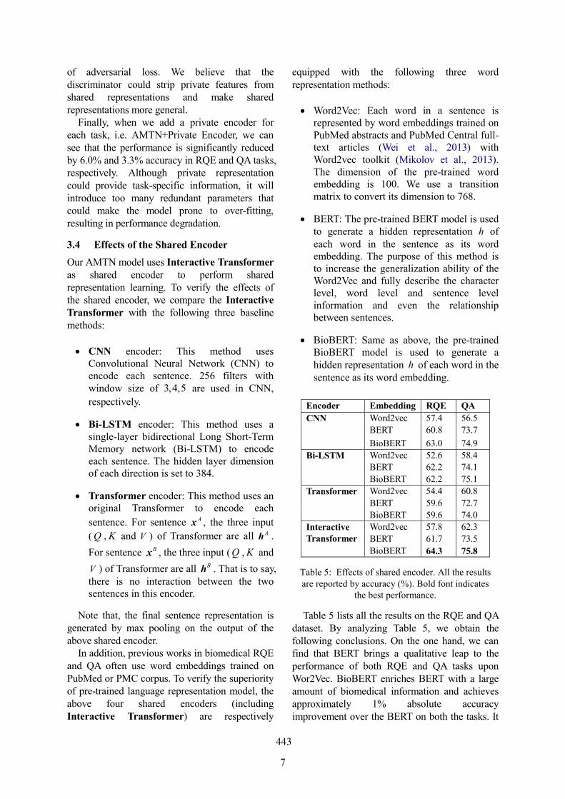
7
of adversarial loss. We believe that the discriminator could strip private features from shared representations and make shared representations more general.
Finally, when we add a private encoder for each task, i.e. AMTN+Private Encoder, we can see that the performance is significantly reduced by 6.0% and 3.3% accuracy in RQE and QA tasks, respectively. Although private representation could provide task-specific information, it will introduce too many redundant parameters that could make the model prone to over-fitting, resulting in performance degradation.
3.4 Effects of the Shared Encoder
Our AMTN model uses Interactive Transformer as shared encoder to perform shared representation learning. To verify the effects of the shared encoder, we compare the Interactive Transformer with the following three baseline methods:
CNN encoder: This method uses Convolutional Neural Network (CNN) to encode each sentence. 256 filters with window size of 3,4,5 are used in CNN,
respectively.
Bi-LSTM encoder: This method uses a single-layer bidirectional Long Short-Term Memory network (Bi-LSTM) to encode each sentence. The hidden layer dimension of each direction is set to 384.
Transformer encoder: This method uses an original Transformer to encode each
sentence. For sentence x A , the three input
( Q , K and V ) of Transformer are all hA .
For sentence xB , the three input ( Q , K and
V ) of Transformer are all hB . That is to say, there is no interaction between the two sentences in this encoder.
Note that, the final sentence representation is generated by max pooling on the output of the above shared encoder.
In addition, previous works in biomedical RQE and QA often use word embeddings trained on PubMed or PMC corpus. To verify the superiority of pre-trained language representation model, the above four shared encoders (including Interactive Transformer) are respectively
equipped with the following three word representation methods:
Word2Vec: Each word in a sentence is represented by word embeddings trained on PubMed abstracts and PubMed Central full-text articles (Wei et al., 2013) with Word2vec toolkit (Mikolov et al., 2013). The dimension of the pre-trained word embedding is 100. We use a transition matrix to convert its dimension to 768.
BERT: The pre-trained BERT model is used to generate a hidden representation h of each word in the sentence as its word embedding. The purpose of this method is to increase the generalization ability of the Word2Vec and fully describe the character level, word level and sentence level information and even the relationship between sentences.
BioBERT: Same as above, the pre-trained BioBERT model is used to generate a hidden representation h of each word in the sentence as its word embedding.
Table 5 lists all the results on the RQE and QA dataset. By analyzing Table 5, we obtain the following conclusions. On the one hand, we can find that BERT brings a qualitative leap to the performance of both RQE and QA tasks upon Wor2Vec. BioBERT enriches BERT with a large amount of biomedical information and achieves approximately 1% absolute accuracy improvement over the BERT on both the tasks. It
Encoder Embedding RQE QA
CNN Word2vec 57.4 56.5
BERT 60.8 73.7
BioBERT 63.0 74.9
Bi-LSTM Word2vec 52.6 58.4
BERT 62.2 74.1
BioBERT 62.2 75.1
Transformer Word2vec 54.4 60.8
BERT 59.6 72.7
BioBERT 59.6 74.0
Interactive Transformer
Word2vec 57.8 62.3
BERT 61.7 73.5
BioBERT 64.3 75.8
Table 5: Effects of shared encoder. All the results are reported by accuracy (%). Bold font indicates
the best performance.
443
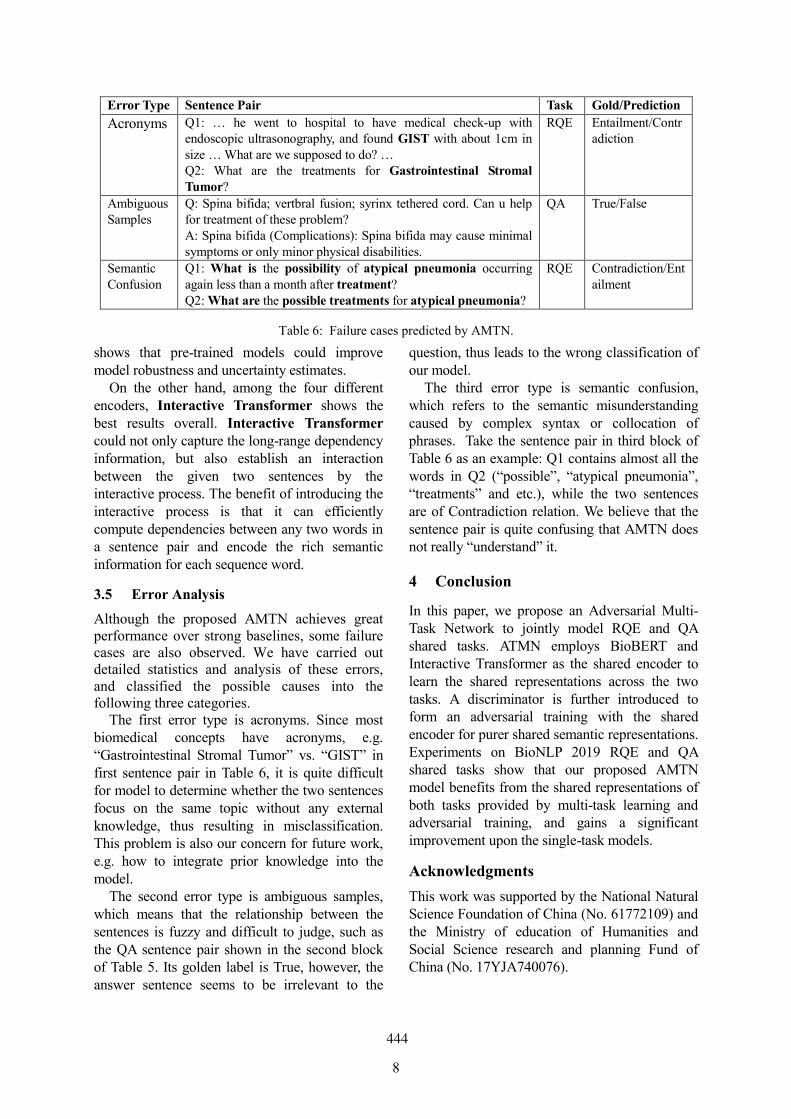
8
shows that pre-trained models could improve model robustness and uncertainty estimates.
On the other hand, among the four different encoders, Interactive Transformer shows the best results overall. Interactive Transformer could not only capture the long-range dependency information, but also establish an interaction between the given two sentences by the interactive process. The benefit of introducing the interactive process is that it can efficiently compute dependencies between any two words in a sentence pair and encode the rich semantic information for each sequence word.
3.5 Error Analysis
Although the proposed AMTN achieves great performance over strong baselines, some failure cases are also observed. We have carried out detailed statistics and analysis of these errors, and classified the possible causes into the following three categories.
The first error type is acronyms. Since most biomedical concepts have acronyms, e.g. “Gastrointestinal Stromal Tumor” vs. “GIST” in first sentence pair in Table 6, it is quite difficult for model to determine whether the two sentences focus on the same topic without any external knowledge, thus resulting in misclassification. This problem is also our concern for future work, e.g. how to integrate prior knowledge into the model.
The second error type is ambiguous samples, which means that the relationship between the sentences is fuzzy and difficult to judge, such as the QA sentence pair shown in the second block of Table 5. Its golden label is True, however, the answer sentence seems to be irrelevant to the
question, thus leads to the wrong classification of our model.
The third error type is semantic confusion, which refers to the semantic misunderstanding caused by complex syntax or collocation of phrases. Take the sentence pair in third block of Table 6 as an example: Q1 contains almost all the words in Q2 (“possible”, “atypical pneumonia”, “treatments” and etc.), while the two sentences are of Contradiction relation. We believe that the sentence pair is quite confusing that AMTN does not really “understand” it.
4 Conclusion
In this paper, we propose an Adversarial Multi-Task Network to jointly model RQE and QA shared tasks. ATMN employs BioBERT and Interactive Transformer as the shared encoder to learn the shared representations across the two tasks. A discriminator is further introduced to form an adversarial training with the shared encoder for purer shared semantic representations. Experiments on BioNLP 2019 RQE and QA shared tasks show that our proposed AMTN model benefits from the shared representations of both tasks provided by multi-task learning and adversarial training, and gains a significant improvement upon the single-task models.
Acknowledgments
This work was supported by the National Natural Science Foundation of China (No. 61772109) and the Ministry of education of Humanities and Social Science research and planning Fund of China (No. 17YJA740076).
Error Type Sentence Pair Task Gold/Prediction
Acronyms Q1: … he went to hospital to have medical check-up with endoscopic ultrasonography, and found GIST with about 1cm in size … What are we supposed to do? … Q2: What are the treatments for Gastrointestinal Stromal Tumor?
RQE Entailment/Contradiction
Ambiguous Samples
Q: Spina bifida; vertbral fusion; syrinx tethered cord. Can u help for treatment of these problem? A: Spina bifida (Complications): Spina bifida may cause minimal symptoms or only minor physical disabilities.
QA True/False
Semantic Confusion
Q1: What is the possibility of atypical pneumonia occurring again less than a month after treatment? Q2: What are the possible treatments for atypical pneumonia?
RQE Contradiction/Entailment
Table 6: Failure cases predicted by AMTN.
444
9
References
Natalia Pletneva, Alejandro Vargas, Konstantina Kalogianni, and Celia Boyer. 2012. Online health information search: what struggles and empowers the users? Results of an online survey. Studies in health technology and informatics, 180:843-847.
Arabella Scantlebury, Alison M. Booth, and Bec Hanley. 2017. Experiences, practices and barriers to accessing health information: a qualitative study. International Journal of Medical Informatics, 103:103-8.
Jonathan D. Wren. 2011. Question answering systems in biology and medicine--the time is now. Bioinformatics, 27(14):2025-2026.
Asma B. Abacha, Chaitanya Shivade, and Dina D. Fushman. 2019. Overview of the MEDIQA 2019 Shared Task on Textual Inference, Question Entailment and Question Answering. In Proceedings of the MEDIQA 2019.Asma B. Abacha and Dina D. Fushman. 2016. Recognizing question entailment for medical question answering. AMIA. In Proceedings of the AMIA Symposium, pages 310-318.
Asma B. Abacha and Dina D. 2019. A question-entailment approach to question answering. arXiv preprint arXiv:1901.08079.
Yann LeCun, Leon Bottou, Yoshua Bengio, and PatrickHaffner. 1998. Gradient-based learning applied to document recognition. In Proceedings of the IEEE, pages 2278-2324.
Sepp Hochreiter and Jürgen Schmidhuber. 1997. Long short-term memory. Neural Computation, 9(8):1735-1780.
Ashish Vaswani, Noam Shazeer, Niki Parmar, Jakob Uszkoreit, Llion Jones, Aidan N. Gomez, Łukasz Kaiser, and Illia Polosukhin. 2017. Attention is all you need. In Advances in Neural Information Processing Systems, pages 6000–6010.
Patrick Verga, Emma Strubell, Ofer Shai, and Andrew McCallum. 2017. Attending to all mention pairs for full abstract biological relation extraction. arXiv preprint arXiv:1710.08312.
Tao Shen, Tianyi Zhou, Guodong Long, Jing Jiang, Shirui Pan, and Chengqi Zhang. 2017. DiSAN: Directional self-attention network for rnn/cnn-free language understanding. arXiv preprint arXiv:1709.04696.
Adams Wei Yu, David Dohan, Minh-Thang Luong, Rui Zhao, Kai Chen, Mohammad Norouzi, and Quoc V. Le. 2018. QANet: Combining local convolution with global self-attention for reading comprehension. arXiv preprint arXiv:1804.09541.
Matthew E. Peters, Mark Neumann, Mohit Iyyer, Matt Gardner, Christopher Clark, Kenton Lee, and Luke Zettlemoyer. 2018. Deep contextualized word representations. arXiv preprint arXiv:1802.05365.
Jacob Devlin, Ming-Wei Chang, Kenton Lee, and Kristina Toutanova. 2018. Bert: Pre-training of deep bidirectional transformers for language understanding. arXiv preprint arXiv:1810.048055.
Jinhyuk Lee, Wonjin Yoon, Sungdong Kim, Donghyeon Kim, Sunkyu Kim, Chan Ho So, and Jaewoo Kang. 2019. Biobert: A pre-trained biomedical language representation model for biomedical text mining. arXiv preprint arXiv:1901.08746.
Sanda Harabagiu and Andrew Hickl. 2006. Methods for Using Textual Entailment in Open-Domain Question Answering. In Proceedings of the 21st International Conference on Computational Linguistics and the 44th Annual Meeting of the Association for Computational Linguistics. Association for Computational Linguistics, pages 905-912.
Rich Caruana. 1998. Multitask Learning. Autonomous Agents and Multi-Agent Systems, 27(1):95–133.
Ian Goodfellow, Jean P. Abadie, Mehdi Mirza, Bing Xu, David W. Farley, Sherjil Ozair, Aaron Courville, and Yoshua Bengio. 2014. Generative adversarial nets. In Advances in Neural Information Processing Systems, pages 2672–2680.
Xinchi Chen, Zhan Shi, Xipeng Qiu, and Xuanjing Huang. 2017. Adversarial Multi-Criteria Learning for Chinese Word Segmentation. In Proceedings of the 55th Annual Meeting of the Association for Computational Linguistics (Volume 1: Long Papers), pages 1193-1203.
Diederik P. Kingma and Jimmy Ba. 2014. Adam: A method for stochastic optimization. arXiv preprint arXiv:1412.6980.
Chih-Hsuan Wei, Hung-Yu Kao, and Zhiyong Lu. 2013. PubTator: A web-based text mining tool for assisting biocuration. Nucleic Acids Research, 41(W1):W518-W522.
Tomas Mikolov, Ilya Sutskever, Kai Chen, Greg S Corrado, and Jeff Dean. 2013. Distributed representations of words and phrases and their compositionality. In Advances in neural information processing systems, pages 3111–3119.
445
Proceedings of the BioNLP 2019 workshop, pages 446–452Florence, Italy, August 1, 2019. c©2019 Association for Computational Linguistics
Abstract
In medical domain, given a medical question, it is difficult to manually select the most relevant information from a large number of search results. BioNLP 2019 proposes Question Answering (QA) task, which encourages the use of text mining technology to automatically judge whether a search result is an answer to the medical question. The main challenge of QA task is how to mine the semantic relation between question and answer. We propose BioBERT Transformer model to tackle this challenge, which applies Transformers to extract semantic relation between different words in questions and answers. Furthermore, BioBERT is utilized to encode medical domain-specific contextualized word representations. Our method has reached the accuracy of 76.24% and spearman of 17.12% on the BioNLP 2019 QA task.
1 Introduction
In medical field, the professional vocabulary is large and the semantics are complex, which makes manually selecting answers to a medical question from search results time consuming. The question answering (QA) task proposed by BioNLP 2019 (BEN ABACHA et al., 2019) aims to automatically extract answers to a medical question by using text mining technology. This task consists of two objectives: one is to determine whether each candidate answer can be used as the correct answer to a question, and the other is to rank the retrieved answers according to the relevance to a question.
The nature of QA task is to match the meaning rather than only match words between question and
answer sentences. Several QA approaches based on syntax information have been developed to match the meaning between question and answer. Wang et.al. (2007) propose a statistical syntax-based model that softly aligns a question sentence with a candidate answer sentence. Tymoshenko and Moschitti (2015) encode semantic knowledge directly into syntactic tree representations of a pair of questions and answers for answers ranking. However, all these models rely on dependency parsers, suffering from error propagation.
Neural network-based methods can automatically learn the inherent semantic features and have achieved good performance on QA task. Wang and Nyberg (2017) employ an attentional encoder-decoder model based on long short-term memory (LSTM) (Hochreiter and Schmidhuber, 1997) for answer ranking, and their model achieves the best performance of 63.7% average score on the TREC LiveQA 2017 challenge (Agichtein et al., 2017). Yang et al. (2017) use a convolutional neural network (CNN) model to classify a question into a restricted set of 10 question types and crawl relevant online web pages to find the answers. However, all the models described above neglect the long range dependency between words in question and answer, limiting their capacity when question and answer sequences are long.
Transformer (Vaswani et al., 2017) is a model based entirely on attention mechanisms and has achieved success on several natural language processing (NLP) tasks, such as machine translation (Vaswani et al., 2017) and language understanding (Devlin et al., 2018). Transformer uses multi-head attention mechanisms to effectively capture the long-range dependency
DUT-BIM at MEDIQA 2019: Utilizing Transformer Network and Medical Domain-Specific Contextualized Representations for
Question Answering
Huiwei Zhou, Bizun Lei, Zhe Liu, Zhuang Liu School of Computer Science and Technology
Dalian University of Technology 116024 Dalian, China
[email protected] {leibzun, njjnlz, zhuangliu1992}@mail.dlut.edu.cn
446
information in context sequences, which is vital for question answering task.
Recently, language models (LM) based on large-scale corpus pre-training have made great progress in several NLP tasks, such as machine translation and natural language inference (NLI). ELMo (Peters et al., 2018) learns two unidirectional LMs based on LSTM networks which is able to capture both sub-word information and contextual clues. OpenAI GPT (Radford et al., 2018) uses a left-to-right Transformer (Vaswani et al., 2017), which introduces minimal task-specific parameters and is trained on the downstream tasks by simply fine-tuning the pre-trained parameters. The major limitation of pre-trained model above is that they are unidirectional, which limits the choice of architectures that can be used during pre-training. BERT (Devlin et al., 2018) employs a bidirectional Transformer encoder to fuse both the left and the right context and can explicitly model the relationship of a pair of text. Thus, it can make progress in paired NLP tasks, such as NLI and QA. Based on the BERT architecture, BioBERT (Lee et al., 2019) is a domain-specific language representation model pre-trained on large-scale biomedical corpora and effectively transfers the knowledge from biomedical texts to biomedical text mining models.
Corpus of QA task proposed by BioNLP 2019 contains answers with long text, which requires models to capture the long range dependency information across words in both question and answer sentences. Thus, we propose BioBERT Transformer (BBERT-T) model based on Transformer to model the associations between question and answer. Specifically, question and answer sequences are first passed to BioBERT to generate medical domain-specific contextualized representations. Then, the question and answer representations are fed into two Transformers, respectively, to capture the long range dependency information and semantic relation between question and answer. Finally, a weighted cross entropy loss is applied to further improve the performance. Our method achieves accuracy of 76.24% and spearman of 17.12% on the BioNLP 2019 QA task.
1 https://github.com/huggingface/pytorch-pretrained-BERT
2 System Description
In MEDIQA2019 medical Question Answering
(QA) task, given a question q and an candidate
answers 1 2{ , ,..., }ana a a , we need build model to
rank all candidate answers and to recognize correct answers to the question. Let T be the set of all the question-answer pairs. For each question-answer pair ( , )q a , we use BioBERT to encode the
contextual information, which improves the model generalization capability. Then we propose two Transformers to learn the long range dependency information between words in question and answer, respectively. In this section, we introduce our approach for QA task in two steps: (1) the preprocessing of the corpus; (2) the structure of the model.
2.1 Preprocessing
Firstly, we lowercase all the questions and answers. Then, following (Fajcik et al., 2019), for each text of questions and answers, we use the tokenizer, that comes from Hugging Face PyTorch re-implementation of BERT1, to split input words into most frequent n-grams in the pre-training corpus, effectively representing text at the sub-word level. Next, following (Vaswani et al., 2017), ( , )q a pair
sequences are truncated to have at most 300 tokens. At last, we use the truncated pair sequence
1 2 1 2[ , ,..., , , ,..., ]q al lq q q a a a as input, where ql is the
length of question, al is the length of a candidate
answer and 300q al l .
2.2 BioBERT Transformer Model (BBERT-T)
Structure of the proposed model is shown in Figure 1, which is composed of three layers: (1) BioBERT layer; (2) Transformer layer; (3) classification and ranking layer. Take the question-answer pair sequence 1 2 1 2[ , ,..., , , ,..., ]
q al lq q q a a a as input to the
BioBERT layer, achieving the question representation and answer representation. Then the two representations are fed to Transformer layer to extract the long range dependency information between words in question and answer, respectively. Finally, the outputs of Transformer layer are passed to a max pooling layer to generate features used to perform classification and ranking.
447
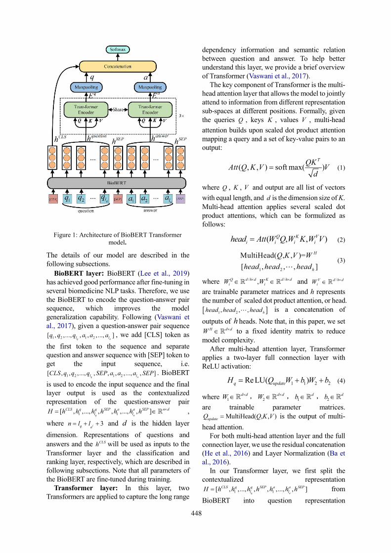
The details of our model are described in the following subsections.
BioBERT layer: BioBERT (Lee et al., 2019) has achieved good performance after fine-tuning in several biomedicine NLP tasks. Therefore, we use the BioBERT to encode the question-answer pair sequence, which improves the model generalization capability. Following (Vaswani et al., 2017), given a question-answer pair sequence
1 2 1 2[ , ,..., , , ,..., ]q al lq q q a a a , we add [CLS] token as
the first token to the sequence and separate question and answer sequence with [SEP] token to get the input sequence, i.e.
1 2 1 2[ , , ,..., , , , , ..., , ]q al lCLS q q q SEP a a a SEP . BioBERT
is used to encode the input sequence and the final layer output is used as the contextualized representation of the question-answer pair
1 1[ , ,..., , , ,..., , ]q a
CLS q q SEP a a SEP n dl lH h h h h h h h ,
where 3iq an l l and d is the hidden layer
dimension. Representations of questions and
answers and the CLSh will be used as inputs to the Transformer layer and the classification and ranking layer, respectively, which are described in following subsections. Note that all parameters of the BioBERT are fine-tuned during training.
Transformer layer: In this layer, two Transformers are applied to capture the long range
dependency information and semantic relation between question and answer. To help better understand this layer, we provide a brief overview of Transformer (Vaswani et al., 2017).
The key component of Transformer is the multi-head attention layer that allows the model to jointly attend to information from different representation sub-spaces at different positions. Formally, given the queries Q , keys K , values V , multi-head
attention builds upon scaled dot product attention mapping a query and a set of key-value pairs to an output:
( , , ) soft max( )TQK
Att Q K V Vd
(1)
where Q , K , V and output are all list of vectors
with equal length, and d is the dimension size of K. Multi-head attention applies several scaled dot product attentions, which can be formulized as follows:
( , , ) Q K Vi i i ihead Att W Q W K W V (2)
1 2
MultiHead( , , )=
[ , , , ]
H
h
Q K V W
head head head (3)
where / /,Q d h d K d h di iW W and /V d h d
iW
are trainable parameter matrices and h represents the number of scaled dot product attention, or head.
1 2, , , hhead head head is a concatenation of
outputs of h heads. Note that, in this paper, we set H d dW to a fixed identity matrix to reduce
model complexity. After multi-head attention layer, Transformer
applies a two-layer full connection layer with ReLU activation:
1 1 2 2ReLU( )q updateH Q W b W b (4)
where 1d dW , 2
d dW , 1db , 2
db
are trainable parameter matrices. MultiHead( , , )updateQ Q K V is the output of multi-
head attention. For both multi-head attention layer and the full
connection layer, we use the residual concatenation (He et al., 2016) and Layer Normalization (Ba et al., 2016).
In our Transformer layer, we first split the contextualized representation
1 1[ , ,..., , , ,..., , ]q a
CLS q q SEP a a SEPl lH h h h h h h h from
BioBERT into question representation
Figure 1: Architecture of BioBERT Transformer model.
448
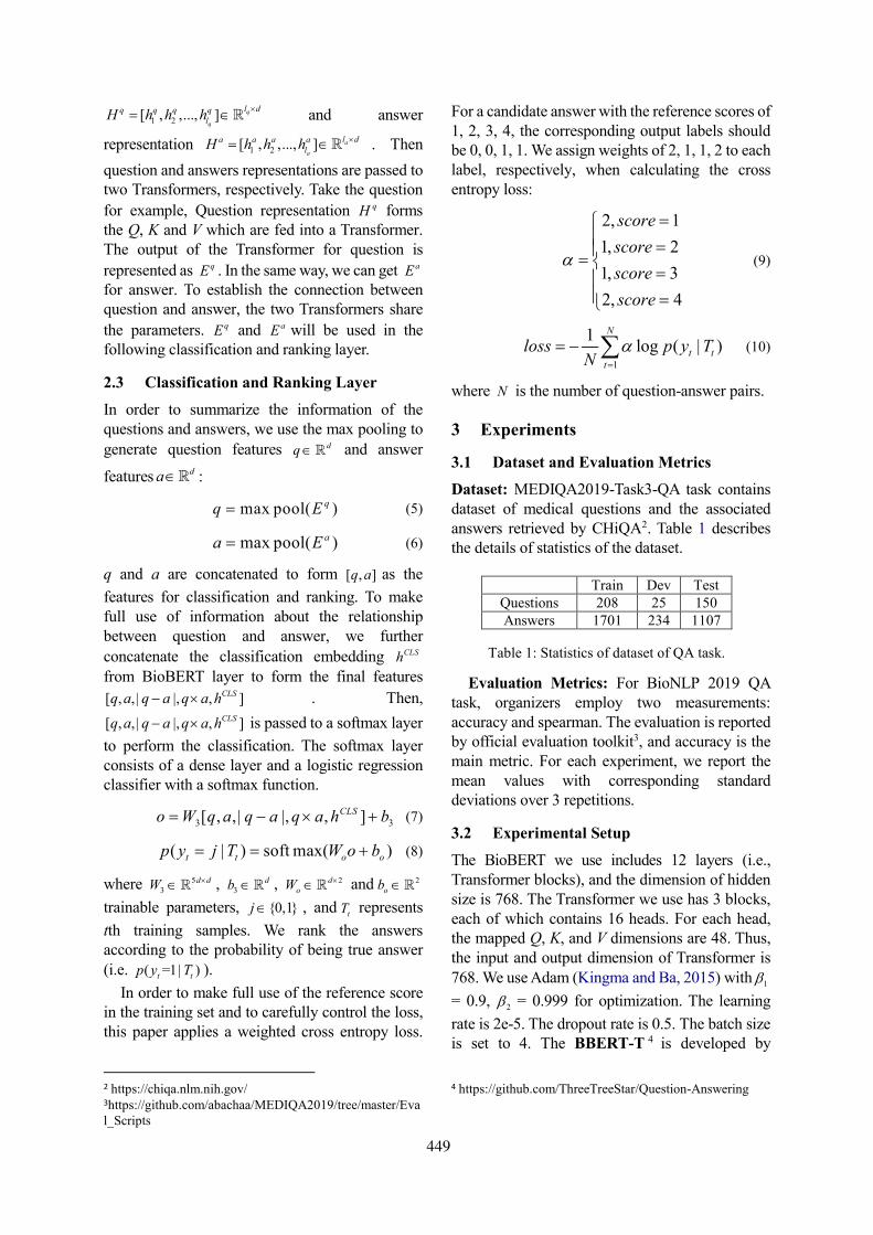
1 2[ , ,..., ] q
q
l dq q q qlH h h h
and answer
representation 1 2[ , ,..., ] a
a
l da a a alH h h h . Then
question and answers representations are passed to two Transformers, respectively. Take the question
for example, Question representation qH forms the Q, K and V which are fed into a Transformer. The output of the Transformer for question is
represented as qE . In the same way, we can get aE for answer. To establish the connection between question and answer, the two Transformers share
the parameters. qE and aE will be used in the following classification and ranking layer.
2.3 Classification and Ranking Layer
In order to summarize the information of the questions and answers, we use the max pooling to generate question features dq and answer
features da :
max pool( )qq E (5)
max pool( )aa E (6)
q and a are concatenated to form [ , ]q a as the
features for classification and ranking. To make full use of information about the relationship between question and answer, we further
concatenate the classification embedding CLSh
from BioBERT layer to form the final features
[ , ,| |, , ]CLSq a q a q a h . Then,
[ , ,| |, , ]CLSq a q a q a h is passed to a softmax layer
to perform the classification. The softmax layer consists of a dense layer and a logistic regression classifier with a softmax function.
3 3[ , , | |, , ]CLSo W q a q a q a h b (7)
( | ) soft max( )t t o op y j T W o b (8)
where 53
d dW , 3db , 2d
oW and 2ob
trainable parameters, {0,1}j , and tT represents
tth training samples. We rank the answers according to the probability of being true answer (i.e. ( =1| )t tp y T ).
In order to make full use of the reference score in the training set and to carefully control the loss, this paper applies a weighted cross entropy loss.
2 https://chiqa.nlm.nih.gov/ 3https://github.com/abachaa/MEDIQA2019/tree/master/Eval_Scripts
For a candidate answer with the reference scores of 1, 2, 3, 4, the corresponding output labels should be 0, 0, 1, 1. We assign weights of 2, 1, 1, 2 to each label, respectively, when calculating the cross entropy loss:
2, 1
1, 2
1, 3
2, 4
score
score
score
score
(9)
1
1log ( | )
N
t tt
loss p y TN
(10)
where N is the number of question-answer pairs.
3 Experiments
3.1 Dataset and Evaluation Metrics
Dataset: MEDIQA2019-Task3-QA task contains dataset of medical questions and the associated answers retrieved by CHiQA2 . Table 1 describes the details of statistics of the dataset.
Evaluation Metrics: For BioNLP 2019 QA task, organizers employ two measurements: accuracy and spearman. The evaluation is reported by official evaluation toolkit3, and accuracy is the main metric. For each experiment, we report the mean values with corresponding standard deviations over 3 repetitions.
3.2 Experimental Setup
The BioBERT we use includes 12 layers (i.e., Transformer blocks), and the dimension of hidden size is 768. The Transformer we use has 3 blocks, each of which contains 16 heads. For each head, the mapped Q, K, and V dimensions are 48. Thus, the input and output dimension of Transformer is 768. We use Adam (Kingma and Ba, 2015) with 1
= 0.9, 2 = 0.999 for optimization. The learning
rate is 2e-5. The dropout rate is 0.5. The batch size is set to 4. The BBERT-T 4 is developed by
4 https://github.com/ThreeTreeStar/Question-Answering
Train Dev Test Questions 208 25 150 Answers 1701 234 1107
Table 1: Statistics of dataset of QA task.
449
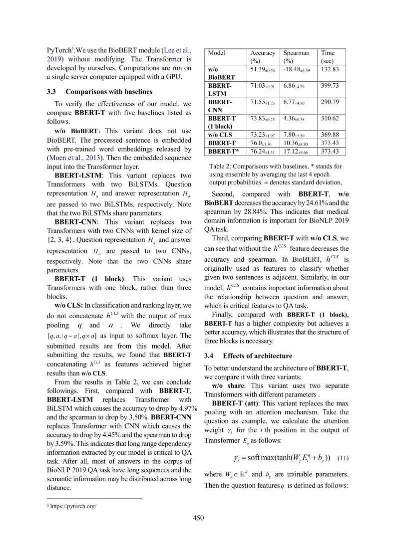
PyTorch5.We use the BioBERT module (Lee et al., 2019) without modifying. The Transformer is developed by ourselves. Computations are run on a single server computer equipped with a GPU.
3.3 Comparisons with baselines
To verify the effectiveness of our model, we compare BBERT-T with five baselines listed as follows.
w/o BioBERT:This variant does not use
BioBERT. The processed sentence is embedded with pre-trained word embeddings released by (Moen et al., 2013). Then the embedded sequence input into the Transformer layer.
BBERT-LSTM: This variant replaces two Transformers with two BiLSTMs. Question representation qH and answer representation aH
are passed to two BiLSTMs, respectively. Note that the two BiLSTMs share parameters.
BBERT-CNN: This variant replaces two Transformers with two CNNs with kernel size of {2, 3, 4}. Question representation qH and answer
representation aH are passed to two CNNs,
respectively. Note that the two CNNs share parameters.
BBERT-T (1 block): This variant uses Transformers with one block, rather than three blocks.
w/o CLS: In classification and ranking layer, we
do not concatenate CLSh with the output of max
pooling q and a . We directly take
[ , ,| |, ]q a q a q a as input to softmax layer. The
submitted results are from this model. After submitting the results, we found that BBERT-T
concatenating CLSh as features achieved higher results than w/o CLS.
From the results in Table 2, we can conclude followings. First, compared with BBERT-T, BBERT-LSTM replaces Transformer with BiLSTM which causes the accuracy to drop by 4.97% and the spearman to drop by 3.50%. BBERT-CNN replaces Transformer with CNN which causes the accuracy to drop by 4.45% and the spearman to drop by 3.59%. This indicates that long range dependency information extracted by our model is critical to QA task. After all, most of answers in the corpus of BioNLP 2019 QA task have long sequences and the semantic information may be distributed across long distance.
5 https://pytorch.org/
Second, compared with BBERT-T, w/o BioBERT decreases the accuracy by 24.61% and the spearman by 28.84%. This indicates that medical domain information is important for BioNLP 2019 QA task.
Third, comparing BBERT-T with w/o CLS, we
can see that without the CLSh feature decreases the
accuracy and spearman. In BioBERT, CLSh is originally used as features to classify whether given two sentences is adjacent. Similarly, in our
model, CLSh contains important information about the relationship between question and answer, which is critical features to QA task.
Finally, compared with BBERT-T (1 block), BBERT-T has a higher complexity but achieves a better accuracy, which illustrates that the structure of three blocks is necessary.
3.4 Effects of architecture
To better understand the architecture of BBERT-T, we compare it with three variants:
w/o share: This variant uses two separate Transformers with different parameters .
BBERT-T (att): This variant replaces the max pooling with an attention mechanism. Take the question as example, we calculate the attention weight i for the i th position in the output of
Transformer qE as follows:
soft max(tanh( ))qi iW E b (11)
where dW and b are trainable parameters.
Then the question features q is defined as follows:
Model Accuracy (%)
Spearman (%)
Time (sec)
w/o BioBERT
51.39±0.56 -18.48±3.39 132.83
BBERT-LSTM
71.03±0.91 6.86±4.29 399.73
BBERT-CNN
71.55±1.73 6.77±4.80 290.79
BBERT-T (1 block)
73.83±0.25 4.36±9.38 310.62
w/o CLS 73.23±1.97 7.80±5.50 369.88
BBERT-T 76.0±1.30 10.36±8.80 373.43
BBERT-T* 76.24±1.31 17.12±9.66 373.43
Table 2: Comparisons with baselines, * stands for using ensemble by averaging the last 4 epoch output probabilities. ± denotes standard deviation, and bold font indicates best performance. Time
450
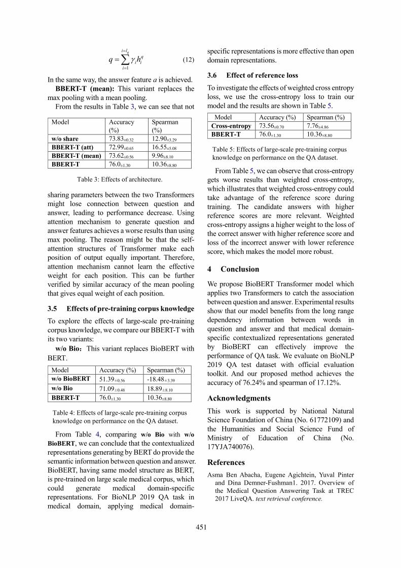
1
qi l
qi i
i
q h
(12)
In the same way, the answer feature a is achieved. BBERT-T (mean): This variant replaces the
max pooling with a mean pooling. From the results in Table 3, we can see that not
sharing parameters between the two Transformers might lose connection between question and answer, leading to performance decrease. Using attention mechanism to generate question and answer features achieves a worse results than using max pooling. The reason might be that the self-attention structures of Transformer make each position of output equally important. Therefore, attention mechanism cannot learn the effective weight for each position. This can be further verified by similar accuracy of the mean pooling that gives equal weight of each position.
3.5 Effects of pre-training corpus knowledge
To explore the effects of large-scale pre-training corpus knowledge, we compare our BBERT-T with its two variants:
w/o Bio:This variant replaces BioBERT with
BERT.
From Table 4, comparing w/o Bio with w/o
BioBERT, we can conclude that the contextualized representations generating by BERT do provide the semantic information between question and answer. BioBERT, having same model structure as BERT, is pre-trained on large scale medical corpus, which could generate medical domain-specific representations. For BioNLP 2019 QA task in medical domain, applying medical domain-
specific representations is more effective than open domain representations.
3.6 Effect of reference loss
To investigate the effects of weighted cross entropy loss, we use the cross-entropy loss to train our model and the results are shown in Table 5.
From Table 5, we can observe that cross-entropy
gets worse results than weighted cross-entropy, which illustrates that weighted cross-entropy could take advantage of the reference score during training. The candidate answers with higher reference scores are more relevant. Weighted cross-entropy assigns a higher weight to the loss of the correct answer with higher reference score and loss of the incorrect answer with lower reference score, which makes the model more robust.
4 Conclusion
We propose BioBERT Transformer model which applies two Transformers to catch the association between question and answer. Experimental results show that our model benefits from the long range dependency information between words in question and answer and that medical domain-specific contextualized representations generated by BioBERT can effectively improve the performance of QA task. We evaluate on BioNLP 2019 QA test dataset with official evaluation toolkit. And our proposed method achieves the accuracy of 76.24% and spearman of 17.12%.
Acknowledgments
This work is supported by National Natural Science Foundation of China (No. 61772109) and the Humanities and Social Science Fund of Ministry of Education of China (No. 17YJA740076).
References
Asma Ben Abacha, Eugene Agichtein, Yuval Pinter and Dina Demner-Fushman1. 2017. Overview of the Medical Question Answering Task at TREC 2017 LiveQA. text retrieval conference.
Model Accuracy (%) Spearman (%)
Cross-entropy 73.56±0.70 7.76±4.86
BBERT-T 76.0±1.30 10.36±8.80
Table 5: Effects of large-scale pre-training corpus knowledge on performance on the QA dataset.
Model Accuracy (%)
Spearman (%)
w/o share 73.83±0.32 12.90±3.29
BBERT-T (att) 72.99±0.65 16.55±5.08
BBERT-T (mean) 73.62±0.56 9.96±8.10
BBERT-T 76.0±1.30 10.36±8.80
Table 3: Effects of architecture.
Model Accuracy (%) Spearman (%)
w/o BioBERT 51.39±0.56 -18.48±3.39
w/o Bio 71.09±0.48 18.89±8.10
BBERT-T 76.0±1.30 10.36±8.80
Table 4: Effects of large-scale pre-training corpus knowledge on performance on the QA dataset.
451
Alec Radford, Karthik Narasimhan, Tim Salimans, and Ilya Sutskever. 2018. Improving language understanding by generative pre-training.
Ashish Vaswani, Noam Shazeer, Niki Parmar, Jakob Uszkoreit, Llion Jones, Aidan N Gomez, Lukasz Kaiser, and Illia Polosukhin. 2017. Attention is all you need. In Advances in Neural Information Processing Systems, pages 6000–6010.
Asma Ben Abacha, Chaitanya Shivade, and Dina Demner-Fushman. 2019. Overview of the MEDIQA 2019 Shared Task on Textual Inference, Question Entailment and Question Answering. ACL-BioNLP 2019.
Di Wang, and Eric Nyberg. 2017. Cmu oaqa at trec 2017 liveqa: A neural dual entailment approach for question paraphrase identi_cation. In Proceedings of The Twenty-Sixth Text REtrieval Conference, TREC 2017, Gaithersburg, Maryland, USA.
Jacob Devlin, Ming-Wei Chang, Kenton Lee, and Kristina Toutanova. 2018. Bert: Pre-training of deep bidirectional transformers for language understanding. arXiv preprint arXiv:1810.04805.
Jimmy Lei Ba, Jamie Ryan Kiros and Geoffrey E. Hinton. 2016. Layer normalization. arXiv preprint arXiv:1607.06450.
Jinhyuk Lee, Wonjin Yoon, Sungdong Kim, Donghyeon Kim, Sunkyu Kim, Chan Ho So, and Jaewoo Kang. 2019. Biobert: pre-trained biomedical language representation model for biomedicaltext mining. arXiv preprint arXiv: 1901.08746.
Kaiming He, Xiangyu Zhang, Shaoqing Ren and Jian Sun. 2016. Deep Residual Learning for Image Recognition. computer vision and pattern recognition,770-778.
Kateryna Tymoshenko and Alessandro Moschitti. 2015 Assessing the Impact of Syntactic and Semantic Structures for Answer Passages Reranking. conference on information and knowledge management: 1451-1460.
Kingma, Diederik P., and Jimmy Ba. 2014. Adam: A method for stochastic optimization. arXiv preprint arXiv:1412.6980.
Martin Fajcik, Lukáš, Burget, and Pavel Smrz. 2019. BUT-FIT at SemEval-2019 Task 7: Determining the Rumour Stance with Pre-Trained Deep Bidirectional Transformers. arXiv preprint arXiv:1902.10126.
Matthew E Peters, Waleed Ammar, Chandra Bhagavatula, and Russell Power. 2017. Semi-supervised sequence tagging with bidirectional language models. arXiv preprint arXiv:1705.00108.
Mengqiu Wang, Noah A. Smith and Teruko Mitamura. 2007. What is the Jeopardy Model? A Quasi-Synchronous Grammar for QA. empirical methods in natural language processing, 2007: 22-32.
Nitish Srivastava, Geoffrey Hinton, Alex Krizhevsky, Ilya Sutskever, Ruslan Salakhutdinov. 2014. Dropout: a simple way to prevent neural networks from overfitting. Journal of Machine Learning Research, 15(1): 1929-1958.
Peng Gao, Zhengkai Jiang, Haoxuan You, Pan Lu, Steven Hoi, Xiaogang Wang and Hongsheng Li. 2018. Dynamic Fusion with Intra- and Inter- Modality Attention Flow for Visual Question Answering. arXiv: Computer Vision and Pattern Recognition.
Peter Turney. 2000. Types of cost in inductive concept learning. In Proceedings of the Cost-sensitive Learning Workshop at the 17th International Conference on Machine Learning, Stanford, CA.
Rodrigo Nogueira and Kyunghyun Cho. 2019. Passage Re-ranking with BERT. arXiv preprint arXiv:1901.04085 (2019).
Sampo Pyysalo, Filip Ginter, Hans Moen, Tapio Salakoski, and Sophia Ananiadou. 2013. Distribu-tional semantics resources for biomedical text pro-cessing.Proceedings of LBM.
Sepp Hochreiter and Jurgen Schmidhuber. 1997. Longshort-term memory. Neural Computation, 9:1735–1780.
Yuan Yang, Jingcheng Yu, Ye Hu, Xiaoyao Xu, and Eric Nyberg. 2017. Cmu livemedqa at trec 2017 liveqa: A consumer health question answering system. In Proceedings of The Twenty-Sixth Text REtrieval Conference, TREC 2017, Gaithersburg, Maryland, USA.
452
Proceedings of the BioNLP 2019 workshop, pages 453–461Florence, Italy, August 1, 2019. c©2019 Association for Computational Linguistics
Dr.Quad at MEDIQA 2019: Towards Textual Inferenceand Question Entailment using contextualized representations
Vinayshekhar Bannihatti Kumar ∗ Ashwin Srinivasan∗ Aditi Chaudhary∗
James Route Teruko Mitamura Eric Nyberg{vbkumar, ashwinsr, aschaudh, jroute, teruko, ehn}@cs.cmu.edu
Language Technologies InstituteCarnegie Mellon University
Abstract
This paper presents the submissions by TeamDr.Quad to the ACL-BioNLP 2019 shared taskon Textual Inference and Question Entailmentin the Medical Domain. Our system is basedon the prior work Liu et al. (2019) which usesa multi-task objective function for textual en-tailment. In this work, we explore differentstrategies for generalizing state-of-the-art lan-guage understanding models to the specializedmedical domain. Our results on the shared taskdemonstrate that incorporating domain knowl-edge through data augmentation is a power-ful strategy for addressing challenges posed byspecialized domains such as medicine.
1 Introduction
The ACL-BioNLP 2019 (Ben Abacha et al., 2019)shared task focuses on improving the followingthree tasks for medical domain: 1) Natural Lan-guage Inference (NLI) 2) Recognizing QuestionEntailment (RQE) and 3) Question-Answering re-ranking system. Our team has made submissionsto all the three tasks. We note that in this work wefocus more on the task 1 and task 2 as improve-ments in these two tasks reflect directly on the task3. However, as per the shared task guidelines, wedo submit one model for the task 3 to complete oursubmission.
Our approach for both task 1 and task 2 isbased on the state-of-the-art natural language un-derstanding model MT-DNN (Liu et al., 2019),which combines the strength of multi-task learn-ing (MTL) and language model pre-training. MTLin deep networks has shown performance gainswhen related tasks are trained together resultingin better generalization to new domains (Ruder,2017). Recent works such as BERT (Devlin et al.,2018), ELMO (Peters et al., 2018) have shown
∗ equal contribution
the efficacy of learning universal language repre-sentations in providing a decent warm start to atask-specific model, by leveraging large amountsof unlabeled data. MT-DNN uses BERT as the en-coder and uses MTL to fine-tune the multiple task-specific layers. This model has obtained state-of-the-art results on several natural language un-derstanding tasks such as SNLI (Bowman et al.,2015), SciTail (Khot et al., 2018) and hence formsthe basis of our approach. For the task 3, we usea simple model to combine the task 1 and task 2models as shown in §2.5.
As discussed above, state-of-the-art models us-ing deep neural networks have shown significantperformance gains across various natural languageprocessing (NLP) tasks. However, their general-ization to specialized domains such as the medicaldomain still remains a challenge. Romanov andShivade (2018) introduce a new dataset MedNLI,a natural language inference dataset for the med-ical domain and show the importance of incor-porating domain-specific resources. Inspired bytheir observations, we explore several techniquesof augmenting domain-specific features with thestate-of-the-art methods. We hope that the deepneural networks will help the model learn aboutthe task itself and the domain-specific features willassist the model in tacking the issues associatedwith such specialized domains. For instance, themedical domain has a distinct sublanguage (Fried-man et al., 2002) and it presents challenges suchas abbreviations, inconsistent spellings, relation-ship between drugs, diseases, symptoms.
Our resulting models perform fairly on the un-seen test data of the ACL-MediQA shared task.On Task 1, our best model achieves +14.1 gainabove the baseline. On Task 2, our five-model en-semble achieved +12.6 gain over the baseline andfor Task 3 our model achieves a a +4.9 gain.
453
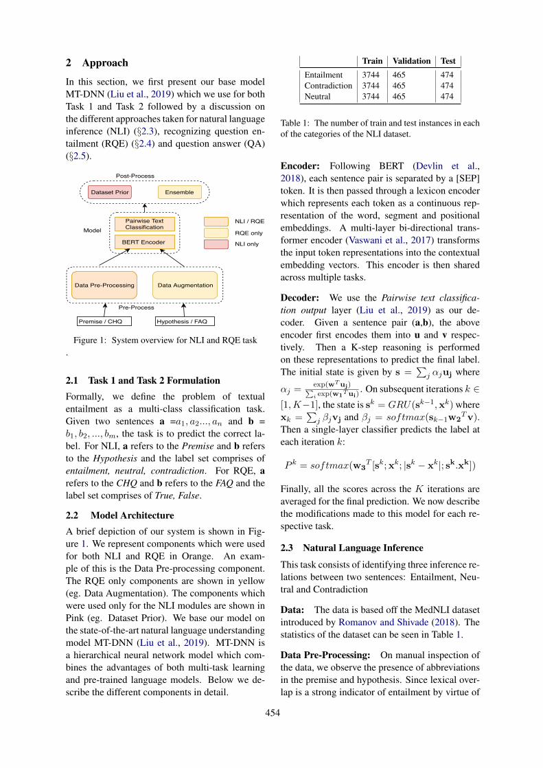
2 Approach
In this section, we first present our base modelMT-DNN (Liu et al., 2019) which we use for bothTask 1 and Task 2 followed by a discussion onthe different approaches taken for natural languageinference (NLI) (§2.3), recognizing question en-tailment (RQE) (§2.4) and question answer (QA)(§2.5).
Data Pre-Processing Data Augmentation
BERT Encoder
Premise / CHQ Hypothesis / FAQ
Pairwise TextClassification
EnsembleDataset Prior
Post-Process
Model
Pre-Process
NLI / RQE
RQE only
NLI only
Figure 1: System overview for NLI and RQE task.
2.1 Task 1 and Task 2 FormulationFormally, we define the problem of textualentailment as a multi-class classification task.Given two sentences a =a1, a2..., an and b =b1, b2, ..., bm, the task is to predict the correct la-bel. For NLI, a refers to the Premise and b refersto the Hypothesis and the label set comprises ofentailment, neutral, contradiction. For RQE, arefers to the CHQ and b refers to the FAQ and thelabel set comprises of True, False.
2.2 Model ArchitectureA brief depiction of our system is shown in Fig-ure 1. We represent components which were usedfor both NLI and RQE in Orange. An exam-ple of this is the Data Pre-processing component.The RQE only components are shown in yellow(eg. Data Augmentation). The components whichwere used only for the NLI modules are shown inPink (eg. Dataset Prior). We base our model onthe state-of-the-art natural language understandingmodel MT-DNN (Liu et al., 2019). MT-DNN isa hierarchical neural network model which com-bines the advantages of both multi-task learningand pre-trained language models. Below we de-scribe the different components in detail.
Train Validation TestEntailment 3744 465 474Contradiction 3744 465 474Neutral 3744 465 474
Table 1: The number of train and test instances in eachof the categories of the NLI dataset.
Encoder: Following BERT (Devlin et al.,2018), each sentence pair is separated by a [SEP]token. It is then passed through a lexicon encoderwhich represents each token as a continuous rep-resentation of the word, segment and positionalembeddings. A multi-layer bi-directional trans-former encoder (Vaswani et al., 2017) transformsthe input token representations into the contextualembedding vectors. This encoder is then sharedacross multiple tasks.
Decoder: We use the Pairwise text classifica-tion output layer (Liu et al., 2019) as our de-coder. Given a sentence pair (a,b), the aboveencoder first encodes them into u and v respec-tively. Then a K-step reasoning is performedon these representations to predict the final label.The initial state is given by s =
∑j αjuj where
αj =exp(wTuj)∑i exp(w1
Tui). On subsequent iterations k ∈
[1,K−1], the state is sk = GRU(sk−1,xk) wherexk =
∑j βjvj and βj = softmax(sk−1w2
Tv).Then a single-layer classifier predicts the label ateach iteration k:
P k = softmax(w3T [sk;xk; |sk − xk|; sk.xk])
Finally, all the scores across the K iterations areaveraged for the final prediction. We now describethe modifications made to this model for each re-spective task.
2.3 Natural Language Inference
This task consists of identifying three inference re-lations between two sentences: Entailment, Neu-tral and Contradiction
Data: The data is based off the MedNLI datasetintroduced by Romanov and Shivade (2018). Thestatistics of the dataset can be seen in Table 1.
Data Pre-Processing: On manual inspection ofthe data, we observe the presence of abbreviationsin the premise and hypothesis. Since lexical over-lap is a strong indicator of entailment by virtue of
454
pre-trained embeddings on large corpora, the pres-ence of abbreviations makes it challenging. There-fore, we expand the abbreviations using the fol-lowing two strategies:
1. Local Context: We observe that often an ab-breviation is composed of the first letters ofcontiguous words. Therefore, we first con-struct potential abbreviations by concatenat-ing first letter of all words in an sequence, af-ter tokenization. For instance, for the premiseshown below we get {CXR, CXRS, XRS,CXRSI, XRSI, RSI, etc}. This is done forboth the premise and the hypothesis. We thencheck if this n-gram exists in the hypothesis(or the premise). If yes, then we replace thatabbreviation with all the words that make upthe n-gram. Now the model has more scopeof matching two strings lexically. We demon-strate an example below:
Premise: Her CXR was clear and it did notappear she had an infection.Hypothesis: Chest X-Ray showed infil-trates.
Premise Modified: Her Chest X-Ray wasclear and it did not appear she had an infec-tion.
2. Gazetteer: If either the premise/hypothesisdoes not contain the abbreviation expansionor contains only partial expansion, the LocalContext technique will fail to expand thoseabbreviations. Hence, we use an externalgazetteer extracted from CAMC1 to expandcommonly occurring medical terms. Therewere 1373 entries in the gazetteer, cover-ing common medical and clinical expansions.For instance,Premise: On arrival to the MICU , patient ishemodynamically stable .Premise Modified: On arrival to the Medi-cal Intensive Care Unit , patient is hemody-namically stable .
We first performed the local context replace-ment as they are more specific to a given premise-hypothesis pair. If there was no local contextmatch, then we did a gazetteer lookup. It is to benoted that one abbreviation can have multiple ex-pansions in the gazatteer and thus we hypothesized
1https://www.camc.org/
that local context should get preference while ex-panding the abbreviation.
Training Procedure: For training the MT-DNNmodel, we use the same hyper-parameters pro-vided by the authors (Liu et al., 2019). We trainmodel for 4 epochs and early stop when the modelreaches the highest validation accuracy.
Baselines: We use the following baselines simi-lar to Romanov and Shivade (2018).
• CBOW: We use a Continuous-Bag-Of-Words(CBOW) model as our first baseline. We takeboth the premise and the hypothesis and sumthe word embeddings of the respective state-ments to form the input layer to our CBOWmodel. We used 2 hidden layers and usedsoftmax as the decision layer.
• Infersent: Inferesent is a sentence encodingmodel which encodes a sentence by doinga max-pool on all the hidden states of theLSTM across time steps. We follow the au-thors of Romanov and Shivade (2018) by us-ing shared weights LSTM cell to get the sen-tence representation of the premise(U) andthe hypothesis(V). We feed these represen-tations U and V to an MLP to perform a3 way prediction. For our experiments, weuse the pre-trained embeddings trained onthe MIMIC dataset by Romanov and Shivade(2018). We used the same hyperparameters.
• BERT: Since MT-DNN is based off of theBERT (Devlin et al., 2018) model as the en-coder, we also compare results using justthe pre-trained BERT. We used bert-base-uncased model which was trained for 3epochs with a learning rate of 2e-5 and abatch size of 16 with a maximum sequencelength of 128. WE used the last 12 pre-trained layers of the model.
2.3.1 Results and DiscussionIn this section we discuss the results of all of ourexperiments on the NLI task.
Ablation Study: First, we conduct an ablationstudy to study the effect of abbreviation expan-sion. Table 2 shows the results of the two ab-breviation expansion techniques for the Infersentmodel. We observe the best performance withthe Gazetteer strategy. This is because most sen-tences in the dataset did not have the abbreviation
455
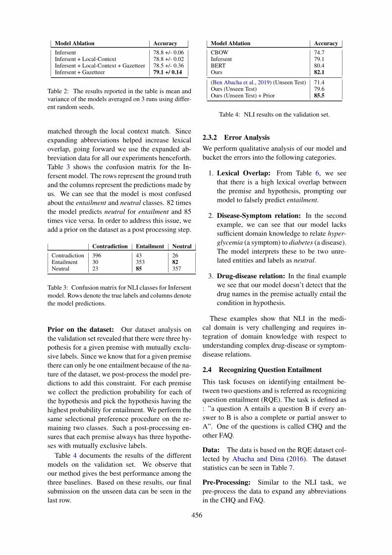
Model Ablation AccuracyInfersent 78.8 +/- 0.06Infersent + Local-Context 78.8 +/- 0.02Infersent + Local-Context + Gazetteer 78.5 +/- 0.36Infersent + Gazetteer 79.1 +/ 0.14
Table 2: The results reported in the table is mean andvariance of the models averaged on 3 runs using differ-ent random seeds.
matched through the local context match. Sinceexpanding abbreviations helped increase lexicaloverlap, going forward we use the expanded ab-breviation data for all our experiments henceforth.Table 3 shows the confusion matrix for the In-fersent model. The rows represent the ground truthand the columns represent the predictions made byus. We can see that the model is most confusedabout the entailment and neutral classes. 82 timesthe model predicts neutral for entailment and 85times vice versa. In order to address this issue, weadd a prior on the dataset as a post processing step.
Contradiction Entailment NeutralContradiction 396 43 26Entailment 30 353 82Neutral 23 85 357
Table 3: Confusion matrix for NLI classes for Infersentmodel. Rows denote the true labels and columns denotethe model predictions.
Prior on the dataset: Our dataset analysis onthe validation set revealed that there were three hy-pothesis for a given premise with mutually exclu-sive labels. Since we know that for a given premisethere can only be one entailment because of the na-ture of the dataset, we post-process the model pre-dictions to add this constraint. For each premisewe collect the prediction probability for each ofthe hypothesis and pick the hypothesis having thehighest probability for entailment. We perform thesame selectional preference procedure on the re-maining two classes. Such a post-processing en-sures that each premise always has three hypothe-ses with mutually exclusive labels.
Table 4 documents the results of the differentmodels on the validation set. We observe thatour method gives the best performance among thethree baselines. Based on these results, our finalsubmission on the unseen data can be seen in thelast row.
Model Ablation AccuracyCBOW 74.7Infersent 79.1BERT 80.4Ours 82.1
(Ben Abacha et al., 2019) (Unseen Test) 71.4Ours (Unseen Test) 79.6Ours (Unseen Test) + Prior 85.5
Table 4: NLI results on the validation set.
2.3.2 Error AnalysisWe perform qualitative analysis of our model andbucket the errors into the following categories.
1. Lexical Overlap: From Table 6, we seethat there is a high lexical overlap betweenthe premise and hypothesis, prompting ourmodel to falsely predict entailment.
2. Disease-Symptom relation: In the secondexample, we can see that our model lackssufficient domain knowledge to relate hyper-glycemia (a symptom) to diabetes (a disease).The model interprets these to be two unre-lated entities and labels as neutral.
3. Drug-disease relation: In the final examplewe see that our model doesn’t detect that thedrug names in the premise actually entail thecondition in hypothesis.
These examples show that NLI in the medi-cal domain is very challenging and requires in-tegration of domain knowledge with respect tounderstanding complex drug-disease or symptom-disease relations.
2.4 Recognizing Question Entailment
This task focuses on identifying entailment be-tween two questions and is referred as recognizingquestion entailment (RQE). The task is defined as: ”a question A entails a question B if every an-swer to B is also a complete or partial answer toA”. One of the questions is called CHQ and theother FAQ.
Data: The data is based on the RQE dataset col-lected by Abacha and Dina (2016). The datasetstatistics can be seen in Table 7.
Pre-Processing: Similar to the NLI task, wepre-process the data to expand any abbreviationsin the CHQ and FAQ.
456
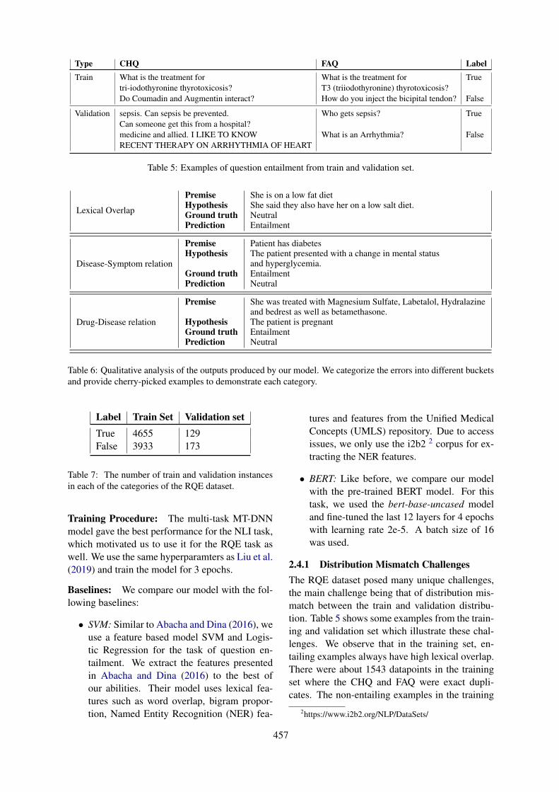
Type CHQ FAQ LabelTrain What is the treatment for What is the treatment for True
tri-iodothyronine thyrotoxicosis? T3 (triiodothyronine) thyrotoxicosis?Do Coumadin and Augmentin interact? How do you inject the bicipital tendon? False
Validation sepsis. Can sepsis be prevented. Who gets sepsis? TrueCan someone get this from a hospital?medicine and allied. I LIKE TO KNOW What is an Arrhythmia? FalseRECENT THERAPY ON ARRHYTHMIA OF HEART
Table 5: Examples of question entailment from train and validation set.
Lexical Overlap
PremiseHypothesisGround truthPrediction
She is on a low fat dietShe said they also have her on a low salt diet.NeutralEntailment
Disease-Symptom relation
PremiseHypothesis
Ground truthPrediction
Patient has diabetesThe patient presented with a change in mental statusand hyperglycemia.EntailmentNeutral
Drug-Disease relation
Premise
HypothesisGround truthPrediction
She was treated with Magnesium Sulfate, Labetalol, Hydralazineand bedrest as well as betamethasone.The patient is pregnantEntailmentNeutral
Table 6: Qualitative analysis of the outputs produced by our model. We categorize the errors into different bucketsand provide cherry-picked examples to demonstrate each category.
Label Train Set Validation setTrue 4655 129False 3933 173
Table 7: The number of train and validation instancesin each of the categories of the RQE dataset.
Training Procedure: The multi-task MT-DNNmodel gave the best performance for the NLI task,which motivated us to use it for the RQE task aswell. We use the same hyperparamters as Liu et al.(2019) and train the model for 3 epochs.
Baselines: We compare our model with the fol-lowing baselines:
• SVM: Similar to Abacha and Dina (2016), weuse a feature based model SVM and Logis-tic Regression for the task of question en-tailment. We extract the features presentedin Abacha and Dina (2016) to the best ofour abilities. Their model uses lexical fea-tures such as word overlap, bigram propor-tion, Named Entity Recognition (NER) fea-
tures and features from the Unified MedicalConcepts (UMLS) repository. Due to accessissues, we only use the i2b2 2 corpus for ex-tracting the NER features.
• BERT: Like before, we compare our modelwith the pre-trained BERT model. For thistask, we used the bert-base-uncased modeland fine-tuned the last 12 layers for 4 epochswith learning rate 2e-5. A batch size of 16was used.
2.4.1 Distribution Mismatch ChallengesThe RQE dataset posed many unique challenges,the main challenge being that of distribution mis-match between the train and validation distribu-tion. Table 5 shows some examples from the train-ing and validation set which illustrate these chal-lenges. We observe that in the training set, en-tailing examples always have high lexical overlap.There were about 1543 datapoints in the trainingset where the CHQ and FAQ were exact dupli-cates. The non-entailing examples in the training
2https://www.i2b2.org/NLP/DataSets/
457
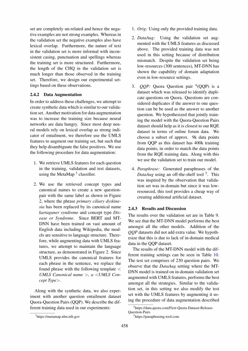
set are completely un-related and hence the nega-tive examples are not strong examples. Whereas inthe validation set the negative examples also havelexical overlap. Furthermore, the nature of textin the validation set is more informal with incon-sistent casing, punctuation and spellings whereasthe training set is more structured. Furthermore,the length of the CHQ in the validation set ismuch longer than those observed in the trainingset. Therefore, we design our experimental set-tings based on these observations.
2.4.2 Data AugmentationIn order to address these challenges, we attempt tocreate synthetic data which is similar to our valida-tion set. Another motivation for data augmentationwas to increase the training size because neuralnetworks are data hungry. Since most deep neu-ral models rely on lexical overlap as strong indi-cator of entailment, we therefore use the UMLSfeatures to augment our training set, but such thatthey help disambiguate the false positives. We usethe following procedure for data augmentation:
1. We retrieve UMLS features for each questionin the training, validation and test datasets,using the MetaMap 3 classifier.
2. We use the retrieved concept types andcanonical names to create a new question-pair with the same label as shown in Figure2, where the phrase primary ciliary dyskine-sia has been replaced by its canonical namekartaganer syndrome and concept type Dis-ease or Syndrome. Since BERT and MT-DNN have been trained on vast amount ofEnglish data including Wikipedia, the mod-els are sensitive to language structure. There-fore, while augmenting data with UMLS fea-tures, we attempt to maintain the languagestructure, as demonstrated in Figure 2. SinceUMLS provides the canonical features foreach phrase in the sentence, we replace thefound phrase with the following template <UMLS Canonical name >, a <UMLS Con-cept Type>.
Along with the synthetic data, we also exper-iment with another question entailment datasetQuora-Question Pairs (QQP). We describe the dif-ferent training data used in our experiments:
3https://metamap.nlm.nih.gov
1. Orig: Using only the provided training data.
2. DataAug: Using the validation set aug-mented with the UMLS features as discussedabove. The provided training data was notused in this setting because of distributionmismatch. Despite the validation set beinglow-resources (300 sentences), MT-DNN hasshown the capability of domain adaptationeven in low-resource settings.
3. QQP: Quora Question pair 4(QQP) is adataset which was released to identify dupli-cate questions on Quora. Questions are con-sidered duplicates if the answer to one ques-tion can be be used as the answer to anotherquestion. We hypothesized that jointly train-ing the model with the Quora-Question Pairsdataset should help as it is closest to our RQEdataset in terms of online forum data. Wechoose a subset of approx. 9k data pointsfrom QQP as this dataset has 400k trainingdata points, in order to match the data pointsfrom the RQE training data. Along with thiswe use the validation set to train our model.
4. Paraphrase: Generated paraphrases of theDataAug using an off-the-shelf tool 5. Thiswas inspired by the observation that valida-tion set was in-domain but since it was low-resourced, this tool provides a cheap way ofcreating additional artificial dataset.
2.4.3 Results and DiscussionThe results over the validation set are in Table 9.We see that the MT-DNN model performs the bestamongst all the other models. Addition of theQQP datasets did not add extra value. We hypoth-esize that this is due to lack of in-domain medicaldata in the QQP dataset.
The results of the MT-DNN model with the dif-ferent training settings can be seen in Table 10.The test set comprises of 230 question pairs. Weobserve that the DataAug setting where the MT-DNN model is trained on in-domain validation setaugmented with UMLS features, performs the bestamongst all the strategies. Similar to the valida-tion set, in this setting we also modify the testset with the UMLS features by augmenting it us-ing the procedure of data augmentation described
4https://data.quora.com/First-Quora-Dataset-Release-Question-Pairs
5https://paraphrasing-tool.com
458
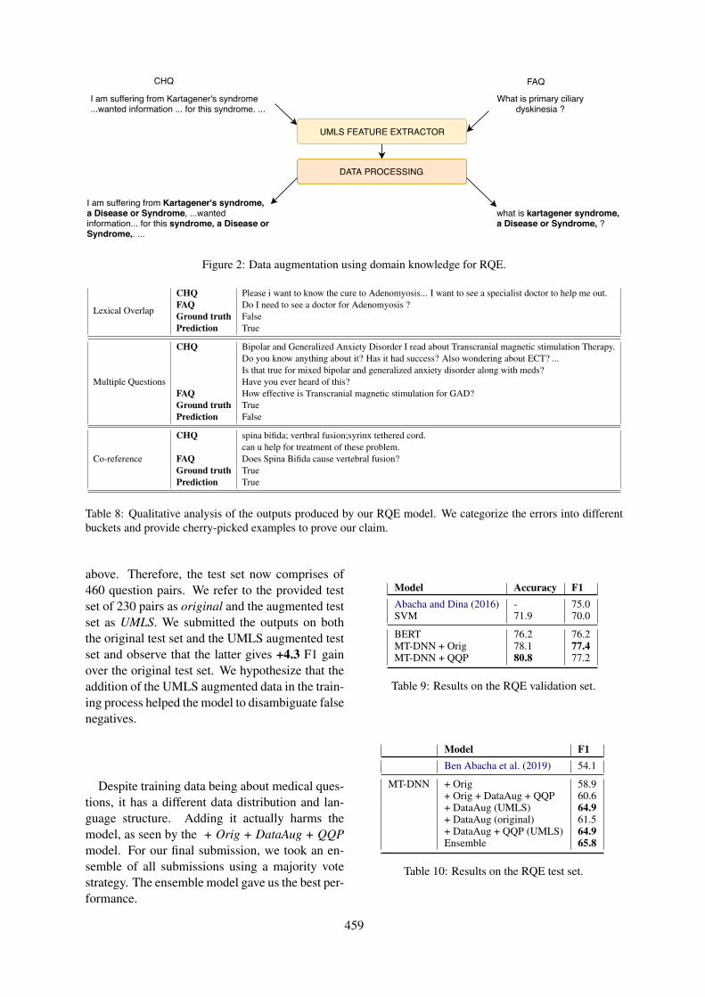
CHQ FAQ
UMLS FEATURE EXTRACTOR
DATA PROCESSING
I am suffering from Kartagener's syndrome...wanted information ... for this syndrome. ...
What is primary ciliarydyskinesia ?
I am suffering from Kartagener's syndrome, a Disease or Syndrome, ...wantedinformation... for this syndrome, a Disease orSyndrome,. ...
what is kartagener syndrome,a Disease or Syndrome, ?
Figure 2: Data augmentation using domain knowledge for RQE.
Lexical Overlap
CHQFAQGround truthPrediction
Please i want to know the cure to Adenomyosis... I want to see a specialist doctor to help me out.Do I need to see a doctor for Adenomyosis ?FalseTrue
Multiple Questions
CHQ
FAQGround truthPrediction
Bipolar and Generalized Anxiety Disorder I read about Transcranial magnetic stimulation Therapy.Do you know anything about it? Has it had success? Also wondering about ECT? ...Is that true for mixed bipolar and generalized anxiety disorder along with meds?Have you ever heard of this?How effective is Transcranial magnetic stimulation for GAD?TrueFalse
Co-reference
CHQ
FAQGround truthPrediction
spina bifida; vertbral fusion;syrinx tethered cord.can u help for treatment of these problem.Does Spina Bifida cause vertebral fusion?TrueTrue
Table 8: Qualitative analysis of the outputs produced by our RQE model. We categorize the errors into differentbuckets and provide cherry-picked examples to prove our claim.
above. Therefore, the test set now comprises of460 question pairs. We refer to the provided testset of 230 pairs as original and the augmented testset as UMLS. We submitted the outputs on boththe original test set and the UMLS augmented testset and observe that the latter gives +4.3 F1 gainover the original test set. We hypothesize that theaddition of the UMLS augmented data in the train-ing process helped the model to disambiguate falsenegatives.
Despite training data being about medical ques-tions, it has a different data distribution and lan-guage structure. Adding it actually harms themodel, as seen by the + Orig + DataAug + QQPmodel. For our final submission, we took an en-semble of all submissions using a majority votestrategy. The ensemble model gave us the best per-formance.
Model Accuracy F1Abacha and Dina (2016) - 75.0SVM 71.9 70.0
BERT 76.2 76.2MT-DNN + Orig 78.1 77.4MT-DNN + QQP 80.8 77.2
Table 9: Results on the RQE validation set.
Model F1Ben Abacha et al. (2019) 54.1
MT-DNN + Orig 58.9+ Orig + DataAug + QQP 60.6+ DataAug (UMLS) 64.9+ DataAug (original) 61.5+ DataAug + QQP (UMLS) 64.9Ensemble 65.8
Table 10: Results on the RQE test set.
459
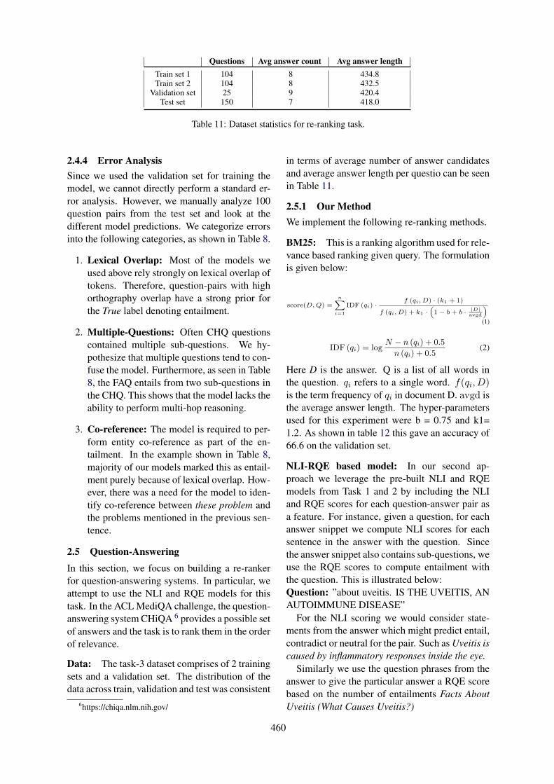
Questions Avg answer count Avg answer lengthTrain set 1 104 8 434.8Train set 2 104 8 432.5
Validation set 25 9 420.4Test set 150 7 418.0
Table 11: Dataset statistics for re-ranking task.
2.4.4 Error AnalysisSince we used the validation set for training themodel, we cannot directly perform a standard er-ror analysis. However, we manually analyze 100question pairs from the test set and look at thedifferent model predictions. We categorize errorsinto the following categories, as shown in Table 8.
1. Lexical Overlap: Most of the models weused above rely strongly on lexical overlap oftokens. Therefore, question-pairs with highorthography overlap have a strong prior forthe True label denoting entailment.
2. Multiple-Questions: Often CHQ questionscontained multiple sub-questions. We hy-pothesize that multiple questions tend to con-fuse the model. Furthermore, as seen in Table8, the FAQ entails from two sub-questions inthe CHQ. This shows that the model lacks theability to perform multi-hop reasoning.
3. Co-reference: The model is required to per-form entity co-reference as part of the en-tailment. In the example shown in Table 8,majority of our models marked this as entail-ment purely because of lexical overlap. How-ever, there was a need for the model to iden-tify co-reference between these problem andthe problems mentioned in the previous sen-tence.
2.5 Question-AnsweringIn this section, we focus on building a re-rankerfor question-answering systems. In particular, weattempt to use the NLI and RQE models for thistask. In the ACL MediQA challenge, the question-answering system CHiQA 6 provides a possible setof answers and the task is to rank them in the orderof relevance.
Data: The task-3 dataset comprises of 2 trainingsets and a validation set. The distribution of thedata across train, validation and test was consistent
6https://chiqa.nlm.nih.gov/
in terms of average number of answer candidatesand average answer length per questio can be seenin Table 11.
2.5.1 Our MethodWe implement the following re-ranking methods.
BM25: This is a ranking algorithm used for rele-vance based ranking given query. The formulationis given below:
score(D,Q) =n∑
i=1
IDF (qi) ·f (qi, D) · (k1 + 1)
f (qi, D) + k1 ·(1 − b + b · |D|
avgd
)
(1)
IDF (qi) = logN − n (qi) + 0.5
n (qi) + 0.5(2)
Here D is the answer. Q is a list of all words inthe question. qi refers to a single word. f(qi, D)is the term frequency of qi in document D. avgd isthe average answer length. The hyper-parametersused for this experiment were b = 0.75 and k1=1.2. As shown in table 12 this gave an accuracy of66.6 on the validation set.
NLI-RQE based model: In our second ap-proach we leverage the pre-built NLI and RQEmodels from Task 1 and 2 by including the NLIand RQE scores for each question-answer pair asa feature. For instance, given a question, for eachanswer snippet we compute NLI scores for eachsentence in the answer with the question. Sincethe answer snippet also contains sub-questions, weuse the RQE scores to compute entailment withthe question. This is illustrated below:Question: ”about uveitis. IS THE UVEITIS, ANAUTOIMMUNE DISEASE”
For the NLI scoring we would consider state-ments from the answer which might predict entail,contradict or neutral for the pair. Such as Uveitis iscaused by inflammatory responses inside the eye.
Similarly we use the question phrases from theanswer to give the particular answer a RQE scorebased on the number of entailments Facts AboutUveitis (What Causes Uveitis?)
460
Finally, we use the BM25 score for the given an-swer and concatenate with the above features anduse SVM as the classifier.
Model Accuracy %BM-25 66.6
RQE+NLI+Source 67.5
Ben Abacha et al. (2019) (Unseen Test) 51.7Ours 56.5
Table 12: Accuracy for task 3 on both validation set(top) and test set (bottom).
2.5.2 ResultsTable 12 documents the results of our experiments.We observe that adding NLI and RQE as featuresshow some improvement over the BM25 model.
3 Conclusion and Future Work
In this work, we present a multi-task learning ap-proach for textual inference and question entail-ment tailored for the medical domain. We observethat incorporating domain knowledge for special-ized domains such as the medical domain is nec-essary. This is because models such as BERT andMT-DNN have been pre-trained on large amountsof generic domains, leading to possible domainmismatch. In order to achieve domain adaptation,we explore techniques such as data augmentationusing UMLS features, abbreviation expansion andobserve a gain of +10.8 F1 for RQE. There arestill many standing challenges such as incorporat-ing common-sense knowledge apart from domainknowledge and multi-hop reasoning which pose aninteresting future direction.
In the future, we also plan to explore otherranking methods based on relevancy feedback orpriority ranking for task 3. We believe usingMedQuad (Ben Abacha and Demner-Fushman,2019) as training set could further help improvethe performance.
Acknowledgement
We are thankful to the anonymous reviewers fortheir valuable suggestions.
ReferencesAsma Ben Abacha and Demner-Fushman Dina. 2016.
Recognizing question entailment for medical ques-tion answering. In AMIA Annual Symposium Pro-
ceedings, volume 2016, page 310. American Medi-cal Informatics Association.
Asma Ben Abacha and Dina Demner-Fushman. 2019.A question-entailment approach to question answer-ing. arXiv e-prints.
Asma Ben Abacha, Chaitanya Shivade, and DinaDemner-Fushman. 2019. Overview of the mediqa2019 shared task on textual inference, question en-tailment and question answering. In Proceedings ofthe BioNLP 2019 workshop, Florence, Italy, August1, 2019. Association for Computational Linguistics.
Samuel R Bowman, Gabor Angeli, Christopher Potts,and Christopher D Manning. 2015. A large anno-tated corpus for learning natural language inference.arXiv preprint arXiv:1508.05326.
Jacob Devlin, Ming-Wei Chang, Kenton Lee, andKristina Toutanova. 2018. Bert: Pre-training of deepbidirectional transformers for language understand-ing. arXiv preprint arXiv:1810.04805.
Carol Friedman, Pauline Kra, and Andrey Rzhetsky.2002. Two biomedical sublanguages: a descriptionbased on the theories of zellig harris. Journal ofbiomedical informatics, 35(4):222–235.
Tushar Khot, Ashish Sabharwal, and Peter Clark. 2018.Scitail: A textual entailment dataset from sciencequestion answering. In Thirty-Second AAAI Con-ference on Artificial Intelligence.
Xiaodong Liu, Pengcheng He, Weizhu Chen, and Jian-feng Gao. 2019. Multi-task deep neural networksfor natural language understanding. arXiv preprintarXiv:1901.11504.
Matthew E Peters, Mark Neumann, Mohit Iyyer, MattGardner, Christopher Clark, Kenton Lee, and LukeZettlemoyer. 2018. Deep contextualized word rep-resentations. arXiv preprint arXiv:1802.05365.
Alexey Romanov and Chaitanya Shivade. 2018.Lessons from natural language inference in the clin-ical domain. arXiv preprint arXiv:1808.06752.
Sebastian Ruder. 2017. An overview of multi-tasklearning in deep neural networks. arXiv preprintarXiv:1706.05098.
Ashish Vaswani, Noam Shazeer, Niki Parmar, JakobUszkoreit, Llion Jones, Aidan N Gomez, ŁukaszKaiser, and Illia Polosukhin. 2017. Attention is allyou need. In Advances in neural information pro-cessing systems, pages 5998–6008.
461
Proceedings of the BioNLP 2019 workshop, pages 462–470Florence, Italy, August 1, 2019. c©2019 Association for Computational Linguistics
Sieg at MEDIQA 2019: Multi-task Neural Ensemble for BiomedicalInference and Entailment
Sai Abishek Bhaskar∗, Rashi Rungta∗, James Route, Eric Nyberg, Teruko MitamuraLanguage Technologies Institute, Carnegie Mellon University
{sabhaska, rashir, jroute, ehn, teruko}@cs.cmu.edu
AbstractThis paper presents a multi-task learning ap-proach to natural language inference (NLI)and question entailment (RQE) in the biomed-ical domain. Recognizing textual inference re-lations and question similarity can address theissue of answering new consumer health ques-tions by mapping them to Frequently AskedQuestions on reputed websites like the NIH1.We show that leveraging information from par-allel tasks across domains along with medi-cal knowledge integration allows our modelto learn better biomedical feature representa-tions. Our final models for the NLI and RQEtasks achieve the 4th and 2nd rank on theshared-task leaderboard respectively.
1 Introduction
The MEDIQA challenge (Abacha et al., 2019)aims to improve textual inference and entailmentin the medical domain to build better domain-specific Information Retrieval and Question An-swering systems. There are three subtasks (NLI,RQE, QA), out of which we focus on -
1. Natural Language Inference (NLI): Iden-tifying the three types of inference relations(Entailment, Neutral and Contradiction) be-tween two sentences.
2. Recognizing Question Entailment (RQE):Predicting entailment between two questions(if every answer for question 1 is at least apartial answer for question 2) in the contextof QA.
The task is motivated by the need to exploreand develop better question answering systemsin the medical domain. Identifying the type of
∗*denotes equal contribution1https://www.nih.gov/
correlation between questions as well as medicalsentences will help the biomedical communitycope with the increasing number of consumerhealth questions posted on community questionanswering websites, many of which have alreadybeen asked before and can easily be answered bylinking them with a previously answered questionby an expert.
In this paper, we start with a discussion ofthe previous work done on multi-task learning andtextual inference and entailment in the biomedicaldomain in Section 2, followed by the datasetdescription in Section 3. The baselines and ourproposed approach are detailed in Section 4 and5 respectively. We conclude with the discussionof our results in Section 6 and a detailed erroranalysis in Section 7.
2 Related Work
2.1 Multi-Task Learning
Multi-task Learning (MTL) is inspired by the ideathat it is useful to jointly learn multiple relatedtasks so that the knowledge gained in one task canbenefit other tasks. Recently, there is growing in-terest in using deep neural networks (DNNs) toapply MTL to representation learning (Collobertet al. 2011, Liu et al. 2017). MTL provides an ef-fective way to use supervised data from a numberof related tasks and also provides for a regulariza-tion effect by not overfitting to a specific task, thusmaking the learned representations more robust.
2.2 Biomedical Textual Inference
The initial approaches for predicting inference re-lations between two sentences in the medical do-main involved several neural architectures. (Ro-
462
manov and Shivade, 2018) details the curation ofthe MedNLI dataset, and describes multiple base-line approaches. A Feature-based, Bag-of-Words(BOW), the ESIM model (Chen et al., 2016) andthe InferSent model (Conneau et al., 2017) beingamong them.
2.3 Biomedical Question Entailment
The initial work (Ben Abacha and Demner-Fushman, 2017), in addition to creating the work-ing dataset for RQE, uses handcrafted lexical andsemantic features as an input to traditional ma-chine learning models like SVM, Logistic Regres-sion, and Naive Bayes for question entailment inthe clinical domain. The lexical features includeword overlap, bigram similarity and best similarityfrom a set of 5 similarity measures (Levenshtein,Jaccard, Cosine, Bigram, Word Overlap) while se-mantic features include the number of overlappingmedical entities and problems based on a CRFclassifier trained across different corpora. BenAbacha and Demner-Fushman 2019 use questionanalysis based features such as question type andfocus recognition which helps identify the differ-ent focus points of consumer health questions suchas information, symptoms, or treatments based onspecific trigger words.
3 Datasets
3.0.1 NLI
MedNLI (Romanov and Shivade) is a dataset an-notated by doctors for NLI in the clinical domain.It is available through the MIMIC-III derived datarepository.
• Train: 11232 sentence pairs
• Validation: 1395 sentence pairs
• Test: 1422 sentence pairs
• Test (Leaderboard): 230 sentence pairs
Labels: {contradiction, entailment, neutral}Evaluation Metric: Accuracy
Since the train, validation and test sets are fromthe same distribution, we combined them and tooka subset of 90% to be the new training set and therest 10% to be the held-out validation set.
3.0.2 RQE
The RQE dataset comprises of consumer healthquestions (CHQs) received by the National Li-brary of Medicine and frequently asked questions(FAQs) collected from the National Institutes ofHealth (NIH) websites (Ben Abacha and Demner-Fushman, 2017).
• Training Set: 8,588 medical question pairs
• Test: 302 medical question pairs
• Test Set (Leaderboard): 230 medical ques-tion pairs
Labels: {true, false}Evaluation Metric: Accuracy
On further analysis of the RQE train and test data,we found that the two datasets come from differentdistributions. The CHQs in the training set followa more formal third person based language struc-ture while CHQs in the test set are verbose withmore colloquial language phrases. For example,a CHQ from the training set is - ”How should Itreat polymenorrhea in a 14-year-old girl?” whilea CHQ from the test set is - ”lupus. Hi, I wantto know about Lupus and its treatment. Best,Mehrnaz”.In light of this, we modify our training set to con-tain 302 examples from the original training set,all the 302 examples in the test set and 930 ques-tions from icliniq as explained in section 5.1.3. Aswith NLI, we took a subset of 90% to be the newtraining set and the rest 10% to be the held-outvalidation set.
4 Baselines
4.1 NLI
InferSent (Romanov and Shivade, 2018) is a sen-tence encoder model that has given near state-of-the-art results across the NLP (including NLI)and computer vision domains. For the MedNLIdataset, the model uses a Bi-directional LSTMwith domain knowledge incorporated throughretrofitting and attention. We use this InferSentmodel as our baseline for the NLI task. Are-implementation using data preprocessed withUMLS (5.2.3) and abbreviation expansion (5.2.5),along with different word embeddings (5.2.2)gives a slight bump in the accuracy value.
463
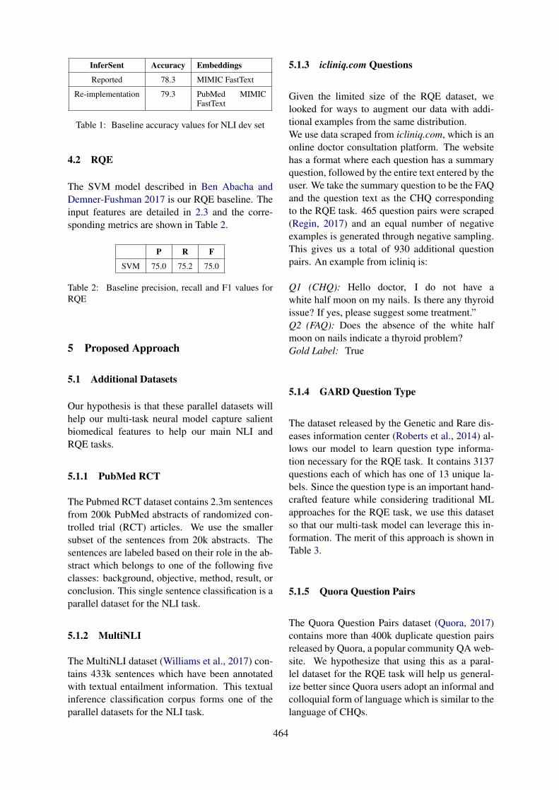
InferSent Accuracy Embeddings
Reported 78.3 MIMIC FastText
Re-implementation 79.3 PubMed MIMICFastText
Table 1: Baseline accuracy values for NLI dev set
4.2 RQE
The SVM model described in Ben Abacha andDemner-Fushman 2017 is our RQE baseline. Theinput features are detailed in 2.3 and the corre-sponding metrics are shown in Table 2.
P R F
SVM 75.0 75.2 75.0
Table 2: Baseline precision, recall and F1 values forRQE
5 Proposed Approach
5.1 Additional Datasets
Our hypothesis is that these parallel datasets willhelp our multi-task neural model capture salientbiomedical features to help our main NLI andRQE tasks.
5.1.1 PubMed RCT
The Pubmed RCT dataset contains 2.3m sentencesfrom 200k PubMed abstracts of randomized con-trolled trial (RCT) articles. We use the smallersubset of the sentences from 20k abstracts. Thesentences are labeled based on their role in the ab-stract which belongs to one of the following fiveclasses: background, objective, method, result, orconclusion. This single sentence classification is aparallel dataset for the NLI task.
5.1.2 MultiNLI
The MultiNLI dataset (Williams et al., 2017) con-tains 433k sentences which have been annotatedwith textual entailment information. This textualinference classification corpus forms one of theparallel datasets for the NLI task.
5.1.3 icliniq.com Questions
Given the limited size of the RQE dataset, welooked for ways to augment our data with addi-tional examples from the same distribution.We use data scraped from icliniq.com, which is anonline doctor consultation platform. The websitehas a format where each question has a summaryquestion, followed by the entire text entered by theuser. We take the summary question to be the FAQand the question text as the CHQ correspondingto the RQE task. 465 question pairs were scraped(Regin, 2017) and an equal number of negativeexamples is generated through negative sampling.This gives us a total of 930 additional questionpairs. An example from icliniq is:
Q1 (CHQ): Hello doctor, I do not have awhite half moon on my nails. Is there any thyroidissue? If yes, please suggest some treatment.”Q2 (FAQ): Does the absence of the white halfmoon on nails indicate a thyroid problem?Gold Label: True
5.1.4 GARD Question Type
The dataset released by the Genetic and Rare dis-eases information center (Roberts et al., 2014) al-lows our model to learn question type informa-tion necessary for the RQE task. It contains 3137questions each of which has one of 13 unique la-bels. Since the question type is an important hand-crafted feature while considering traditional MLapproaches for the RQE task, we use this datasetso that our multi-task model can leverage this in-formation. The merit of this approach is shown inTable 3.
5.1.5 Quora Question Pairs
The Quora Question Pairs dataset (Quora, 2017)contains more than 400k duplicate question pairsreleased by Quora, a popular community QA web-site. We hypothesize that using this as a paral-lel dataset for the RQE task will help us general-ize better since Quora users adopt an informal andcolloquial form of language which is similar to thelanguage of CHQs.
464
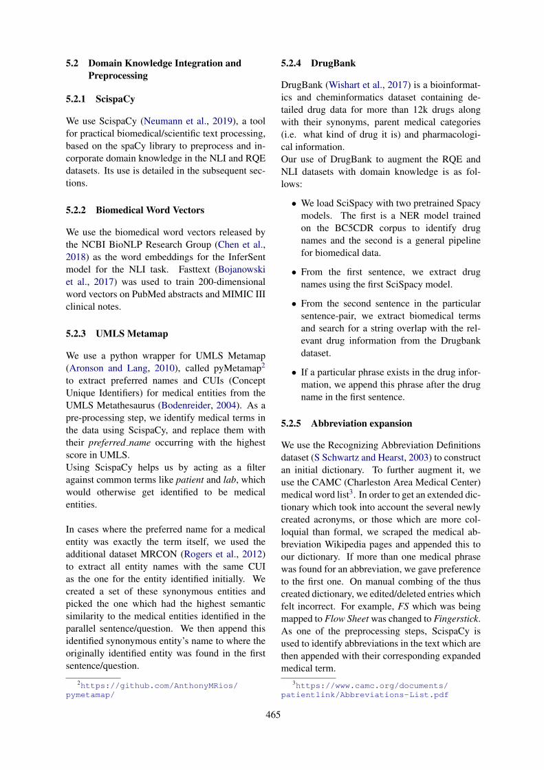
5.2 Domain Knowledge Integration andPreprocessing
5.2.1 ScispaCy
We use ScispaCy (Neumann et al., 2019), a toolfor practical biomedical/scientific text processing,based on the spaCy library to preprocess and in-corporate domain knowledge in the NLI and RQEdatasets. Its use is detailed in the subsequent sec-tions.
5.2.2 Biomedical Word Vectors
We use the biomedical word vectors released bythe NCBI BioNLP Research Group (Chen et al.,2018) as the word embeddings for the InferSentmodel for the NLI task. Fasttext (Bojanowskiet al., 2017) was used to train 200-dimensionalword vectors on PubMed abstracts and MIMIC IIIclinical notes.
5.2.3 UMLS Metamap
We use a python wrapper for UMLS Metamap(Aronson and Lang, 2010), called pyMetamap2
to extract preferred names and CUIs (ConceptUnique Identifiers) for medical entities from theUMLS Metathesaurus (Bodenreider, 2004). As apre-processing step, we identify medical terms inthe data using ScispaCy, and replace them withtheir preferred name occurring with the highestscore in UMLS.Using ScispaCy helps us by acting as a filteragainst common terms like patient and lab, whichwould otherwise get identified to be medicalentities.
In cases where the preferred name for a medicalentity was exactly the term itself, we used theadditional dataset MRCON (Rogers et al., 2012)to extract all entity names with the same CUIas the one for the entity identified initially. Wecreated a set of these synonymous entities andpicked the one which had the highest semanticsimilarity to the medical entities identified in theparallel sentence/question. We then append thisidentified synonymous entity’s name to where theoriginally identified entity was found in the firstsentence/question.
2https://github.com/AnthonyMRios/pymetamap/
5.2.4 DrugBank
DrugBank (Wishart et al., 2017) is a bioinformat-ics and cheminformatics dataset containing de-tailed drug data for more than 12k drugs alongwith their synonyms, parent medical categories(i.e. what kind of drug it is) and pharmacologi-cal information.Our use of DrugBank to augment the RQE andNLI datasets with domain knowledge is as fol-lows:
• We load SciSpacy with two pretrained Spacymodels. The first is a NER model trainedon the BC5CDR corpus to identify drugnames and the second is a general pipelinefor biomedical data.
• From the first sentence, we extract drugnames using the first SciSpacy model.
• From the second sentence in the particularsentence-pair, we extract biomedical termsand search for a string overlap with the rel-evant drug information from the Drugbankdataset.
• If a particular phrase exists in the drug infor-mation, we append this phrase after the drugname in the first sentence.
5.2.5 Abbreviation expansion
We use the Recognizing Abbreviation Definitionsdataset (S Schwartz and Hearst, 2003) to constructan initial dictionary. To further augment it, weuse the CAMC (Charleston Area Medical Center)medical word list3. In order to get an extended dic-tionary which took into account the several newlycreated acronyms, or those which are more col-loquial than formal, we scraped the medical ab-breviation Wikipedia pages and appended this toour dictionary. If more than one medical phrasewas found for an abbreviation, we gave preferenceto the first one. On manual combing of the thuscreated dictionary, we edited/deleted entries whichfelt incorrect. For example, FS which was beingmapped to Flow Sheet was changed to Fingerstick.As one of the preprocessing steps, ScispaCy isused to identify abbreviations in the text which arethen appended with their corresponding expandedmedical term.
3https://www.camc.org/documents/patientlink/Abbreviations-List.pdf
465
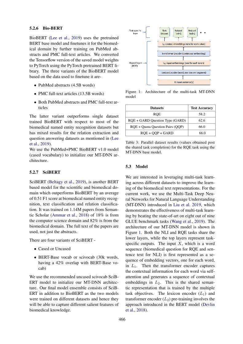
5.2.6 Bio-BERT
BioBERT (Lee et al., 2019) uses the pretrainedBERT base model and finetunes it for the biomed-ical domain by further training on PubMed ab-stracts and PMC full-text articles. We convertedthe Tensorflow version of the saved model weightsto PyTorch using the PyTorch pretrained BERT li-brary. The three variants of the BioBERT modelbased on the data used to finetune it are-
• PubMed abstracts (4.5B words)
• PMC full-text articles (13.5B words)
• Both PubMed abstracts and PMC full-text ar-ticles
The latter variant outperforms single datasettrained BioBERT with respect to most of thebiomedical named entity recognition datasets buthas mixed results for the relation extraction andquestion answering datasets as mentioned in (Leeet al., 2019).We use the PubMed+PMC BioBERT v1.0 model(cased vocabulary) to initialize our MT-DNN ar-chitecture.
5.2.7 SciBERT
SciBERT (Beltagy et al., 2019), is another BERTbased model for the scientific and biomedical do-main which outperforms BioBERT by an averageof 0.51 F1 score at biomedical named entity recog-nition, text classification and relation classifica-tion. It was trained on 1.14M papers from Seman-tic Scholar (Ammar et al., 2018) of 18% is fromthe computer science domain and 82% is from thebiomedical domain. The full text of the papers areused, not just the abstracts.
There are four variants of SciBERT -
• Cased or Uncased
• BERT-Base vocab or scivocab (30k words,having a 42% overlap with BERT-Base vo-cab)
We use the recommended uncased scivocab SciB-ERT model to initialize our MT-DNN architec-ture. Our final model ensemble consists of SciB-ERT in addition to BioBERT as the two modelswere trained on different datasets and hence theywill be able to capture different salient features ofbiomedical knowledge.
Figure 1: Architecture of the multi-task MT-DNNmodel
Datasets Test Accuracy
RQE 58.2
RQE + GARD Question Type (GARD) 62.6
RQE + Quora Question Pairs (QQP) 66.0
RQE + QQP + GARD 66.0
Table 3: Parallel dataset results (values obtained postthe shared task completion) for the RQE task using theMT-DNN base model.
5.3 Model
We are interested in leveraging multi-task learn-ing across different datasets to improve the learn-ing of the biomedical text representations. For thecurrent work, we use the Multi-Task Deep Neu-ral Networks for Natural Language Understanding(MT-DNN) introduced in Liu et al. 2019, whichdemonstrates the effectiveness of multi-task learn-ing by beating the state-of-art on eight out of nineGLUE benchmark tasks (Wang et al., 2019). Thearchitecture of our MT-DNN model is shown inFigure 1. Both the NLI and RQE tasks share thelower layers, while the top layers represent task-specific outputs. The input X , which is a wordsequence (biomedical question for RQE and sen-tence text for NLI) is first represented as a se-quence of embedding vectors, one for each word,in L1. Then the transformer encoder capturesthe contextual information for each word via self-attention and generates a sequence of contextualembeddings in L2. This is the shared seman-tic representation that is trained by the multipletask objectives. The lexicon encoder (L1) andtransformer encoder (L2) pre-training involves theapproach introduced in the BERT model (Devlinet al., 2018).
466
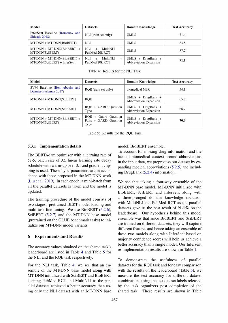
Model Datasets Domain Knowledge Test Accuracy
InferSent Baseline (Romanov andShivade 2018) NLI (train set only) UMLS 71.4
MT-DNN + MT-DNN(BioBERT) NLI UMLS 83.5
MT-DNN + MT-DNN(BioBERT) +MT-DNN(SciBERT)
NLI + MultiNLI +PubMed 20k RCT UMLS 87.2
MT-DNN + MT-DNN(BioBERT) +MT-DNN(SciBERT) + InferSent
NLI + MultiNLI +PubMed 20k RCT
UMLS + DrugBank +Abbreviation Expansion 91.1
Table 4: Results for the NLI Task
Model Datasets Domain Knowledge Test Accuracy
SVM Baseline (Ben Abacha andDemner-Fushman 2017) RQE (train set only) biomedical NER 54.1
MT-DNN + MT-DNN(SciBERT) RQE UMLS + DrugBank +Abbreviation Expansion 65.8
MT-DNN + MT-DNN(SciBERT) RQE + GARD QuestionType
UMLS + DrugBank +Abbreviation Expansion 66.7
MT-DNN + MT-DNN(BioBERT) +MT-DNN(SciBERT)
RQE + Quora QuestionPairs + GARD QuestionType
UMLS + DrugBank +Abbreviation Expansion 70.6
Table 5: Results for the RQE Task
5.3.1 Implementation details
The BERTAdam optimizer with a learning rate of5e-5, batch size of 32, linear learning rate decayschedule with warm-up over 0.1 and gradient clip-ping is used. These hyperparameters are in accor-dance with those proposed in the MT-DNN work(Liu et al. 2019). In each epoch, a mini-batch fromall the parallel datasets is taken and the model isupdated.
The training procedure of the model consists oftwo stages: pretrained BERT model loading andmulti-task fine-tuning. We use BioBERT (5.2.6),SciBERT (5.2.7) and the MT-DNN base model(pretrained on the GLUE benchmark tasks) to ini-tialize our MT-DNN model variants.
6 Experiments and Results
The accuracy values obtained on the shared task’sleaderboard are listed in Table 4 and Table 5 forthe NLI and the RQE task respectively.
For the NLI task, Table 4, we see that an en-semble of the MT-DNN base model along withMT-DNN initialized with SciBERT and BioBERTkeeping PubMed RCT and MultiNLI as the par-allel datasets achieved a better accuracy than us-ing only the NLI dataset with an MT-DNN base
model, BioBERT ensemble.To account for missing drug information and thelack of biomedical context around abbreviationsin the input data, we preprocess our dataset by ex-panding medical abbreviations (5.2.5) and includ-ing DrugBank (5.2.4) information.
We see that taking a four-way ensemble of theMT-DNN base model, MT-DNN initialized withBioBERT, SciBERT and InferSent along witha three-pronged domain knowledge inclusionwith MultiNLI and PubMed RCT as the paralleldatasets gave us the best result of 91.1% on theleaderboard. Our hypothesis behind this modelensemble was that since BioBERT and SciBERTare trained on different datasets, they will capturedifferent features and hence taking an ensemble ofthese two models along with InferSent based onmajority confidence scores will help us achieve abetter accuracy than a single model. Our Infersentre-implementation results are shown in Table 1.
To demonstrate the usefulness of paralleldatasets for the RQE task and for easy comparisonwith the results on the leaderboard (Table 5), wemeasure the test accuracy for different datasetcombinations using the test dataset labels releasedby the task organizers post completion of theshared task. These results are shown in Table
467
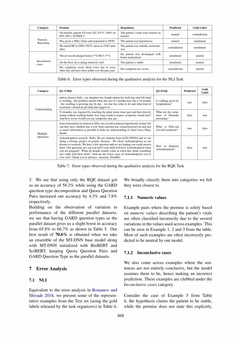
Category Premise Hypothesis Predicted Gold Label
NumericReasoning
On transfer, patient VS were 102, 87/33, 100% on60% 450 x 18 PEEP 5.
The patient’s vitals were normal ontransfer neutral contradiction
Was given a 500cc bolus and responded to 89/50. The patient was hypotensive. neutral entailment
His initial BP at OSH 130/75, down to 93/63 afternitro.
The patient was initially normoten-sive. contradiction entailment
Inconclusivecases
The pt was discharged home [**2188-5-3**]. the patient was discharged withhome medications entailment neutral
On the floor, he is doing relatively well. The patient is stable. entailment neutral
His symptoms occur about every day to everyother day and have been stable over the past year. His symptoms are severe. contradiction neutral
Table 6: Error types observed during the qualitative analysis for the NLI Task
Category Q1 (CHQ) Q2 (FAQ) Predicted GoldLabel
Understanding
milroy disease hello , my daughter has lymph edema her both legs and left handis swelling , this problem started when she was of 3 months now she is 16 months, her swelling is growing day by day , im clue less what to do and what kind oftreatment i should do plz help and suggest us
Is walking good forlymphedema? true false
If oleandor was ingested by touching the plant stems inner part and then directlyeating without washing hands, how long would u exspect symptoms would start?And how severe would you say symptoms may get.
What are the symp-toms of Oleanderpoisoning?
false true
MultipleQuestions
more information in relation to Ellis van creveld syndrome Specifically in later lifecan they have children has it ever been reported any researchcarried out and justas much information as possible to help my understanding of what I have Manythanks
What is Ellis-vanCreveld syndrome? true false
Achondroplasia research. Hello, We are students from [LOCATION] and we aredoing a biology project of genetic diseases. We chose Achondroplasia as ourdisease to research. We have a few question and we are hoping you could answerthem. Our questions are, can you tell if your child will have Achondroplasia whenyou are pregnant? When do people usually come in when they think somethingisn’t right with their child? what are the worse cases of Achondroplasia you’veever seen? Thank you in advance. sincerely, [NAME]
How to diagnoseAchondroplasia? false true
Table 7: Error types observed during the qualitative analysis for the RQE Task
3. We see that using only the RQE dataset gotus an accuracy of 58.2% while using the GARDquestion type decomposition and Quora QuestionPairs increased our accuracy by 4.3% and 7.8%respectively.Building on the observation of variation inperformance of the different parallel datasets,we see that having GARD question types as theparallel dataset gives us a slight boost in accuracyfrom 65.8% to 66.7% as shown in Table 5. Ourbest result of 70.6% is obtained when we takean ensemble of the MT-DNN base model alongwith MT-DNN initialized with BioBERT andSciBERT, keeping Quora Question Pairs andGARD Question Type as the parallel datasets.
7 Error Analysis
7.1 NLI
Equivalent to the error analysis in Romanov andShivade 2018, we present some of the represen-tative examples from the Test set (using the goldlabels released by the task organizers) in Table 6.
We broadly classify them into categories we feltthey were closest to.
7.1.1 Numeric values
Example pairs where the premise is solely basedon numeric values describing the patient’s vitalsare often classified incorrectly due to the severalvariations in the values used across examples. Thiscan be seen in Example 1, 2 and 3 from the table.Most of such examples are often incorrectly pre-dicted to be neutral by our model.
7.1.2 Inconclusive cases
We also come across examples where the sen-tences are not entirely conclusive, but the modelassumes them to be, hence making an incorrectprediction. These examples are clubbed under theInconclusive cases category.
Consider the case of Example 5 from Table6, the hypothesis claims the patient to be stable,while the premise does not state this explicitly,
468
thus leaving a margin for a less definite hypothe-sis. Our model predicts entailment for this pair,when the expected label is neutral.
7.2 RQE
Table 7 shows a few examples representative ofthe two broad categories of errors observed in theTest set (using the gold labels released by the taskorganizers) for the RQE task.
7.2.1 Understanding
The CHQ from Example 1 in the table is askingfor treatment suggestions for the condition lym-phedema, and the FAQ is a question verifying ifwalking is good for lymphedema. The expectedlabel is false, while the model predicts it to betrue. The two questions are semantically differentbecause of which one does not entail the other,but the model might be confusing a suggestivequestion (FAQ in this example) to be a part of thebroader question (CHQ) thus failing to understandthe subtle difference between the two.
In Example 2, the CHQ asks about two questionsrelated to the symptoms - how long they willtake to occur, and how severe they would get.The FAQ inquires about what the symptoms are.These questions have the same focus, but couldbe understood as being different when comparedsemantically. However, since the answer tothe FAQ might partially answer the CHQ, theexpected label is true, while our model predictedthis as false.
7.2.2 Multiple Questions
The other kind of errors we observed were whenthe CHQs had multiple questions within them.For instance in Example 3, in the CHQ the userseems to have decent knowledge about the saidsyndrome and wants more in-depth knowledge onthe subject. The repeated questions about moreinformation might have misled the model intopredicting this as true, when the expected labelwas false.
In Example 4, we see that the several ques-tions contained in the CHQ confuse our classifierto predict false when the FAQ is actually entailed.
8 Future Work
Going forward, this work could be improved bymore intensive domain knowledge incorporation.To start with, using medical side effects relationsfrom SIDER (Kuhn et al., 2015) and leveragingthe ontology relations in UMLS (Bodenreider,2004) would be appropriate steps to strengthenthe proposed system. We would like to thank ouranonymous reviewers for these inputs.
A large part of the success of this work canbe attributed to preprocessing the input data toincorporate biomedical knowledge which, at thesame time makes it harder to generalize thispipeline to other domains. Therefore, investigat-ing the performance of our proposed approach innon-biomedical domains by training with differentparallel datasets to enforce generalization is aninteresting avenue for future research.
9 Conclusion
In this paper, we investigate various preprocess-ing pipelines along with parallel dataset combina-tions in a multi-task learning setup for efficientlanguage processing in the biomedical domain.We demonstrate the effectiveness of using trans-former based neural models for predicting natu-ral language inference and recognizing questionentailment in the medical domain which beat thebaselines (as shown in Table 4 and Table 5) by amargin of 19.7% and 16.5% for the NLI and RQEtasks respectively.
References
Asma Ben Abacha, Chaitanya Shivade, and DinaDemner-Fushman. 2019. Overview of the mediqa2019 shared task on textual inference, question entail-ment and question answering. ACL-BioNLP 2019.
Waleed Ammar, Dirk Groeneveld, Chandra Bhagavat-ula, Iz Beltagy, Miles Crawford, Doug Downey, Ja-son Dunkelberger, Ahmed Elgohary, Sergey Feldman,Vu Ha, Rodney Kinney, Sebastian Kohlmeier, Kyle Lo,Tyler Murray, Hsu-Han Ooi, Matthew E. Peters, JoannaPower, Sam Skjonsberg, Lucy Lu Wang, Chris Wil-helm, Zheng Yuan, Madeleine van Zuylen, and OrenEtzioni. 2018. Construction of the literature graph insemantic scholar. CoRR, abs/1805.02262.
Alan Aronson and Franois-Michel Lang. 2010. Anoverview of metamap: Historical perspective and re-
469
cent advances. Journal of the American Medical Infor-matics Association : JAMIA, 17:229–36.
Iz Beltagy, Arman Cohan, and Kyle Lo. 2019. Scib-ert: Pretrained contextualized embeddings for scien-tific text.
Asma Ben Abacha and Dina Demner-Fushman. 2017.Recognizing question entailment for medical questionanswering. American Medical Informatics Associa-tion.
Asma Ben Abacha and Dina Demner-Fushman. 2019.A question-entailment approach to question answering.CoRR, abs/1901.08079.
Olivier Bodenreider. 2004. The unified medical lan-guage system (umls): Integrating biomedical terminol-ogy. Nucleic acids research, 32.
Piotr Bojanowski, Edouard Grave, Armand Joulin, andTomas Mikolov. 2017. Enriching word vectors withsubword information. Transactions of the Associationfor Computational Linguistics, 5:135–146.
Qian Chen, Xiaodan Zhu, Zhen-Hua Ling, Si Wei, andHui Jiang. 2016. Enhancing and combining sequentialand tree LSTM for natural language inference. CoRR,abs/1609.06038.
Qingyu Chen, Yifan Peng, and Zhiyong Lu. 2018.Biosentvec: creating sentence embeddings for biomed-ical texts. CoRR, abs/1810.09302.
Ronan Collobert, Jason Weston, Léon Bottou, MichaelKarlen, Koray Kavukcuoglu, and Pavel P. Kuksa. 2011.Natural language processing (almost) from scratch.CoRR, abs/1103.0398.
Alexis Conneau, Douwe Kiela, Holger Schwenk, Loı̈cBarrault, and Antoine Bordes. 2017. Supervised learn-ing of universal sentence representations from naturallanguage inference data. CoRR, abs/1705.02364.
Jacob Devlin, Ming-Wei Chang, Kenton Lee, andKristina Toutanova. 2018. BERT: pre-training of deepbidirectional transformers for language understanding.CoRR, abs/1810.04805.
Michael Kuhn, Ivica Letunic, Lars Juhl Jensen, andPeer Bork. 2015. The SIDER database of drugs andside effects. Nucleic Acids Research, 44(D1):D1075–D1079.
Jinhyuk Lee, Wonjin Yoon, Sungdong Kim,Donghyeon Kim, Sunkyu Kim, Chan Ho So, andJaewoo Kang. 2019. Biobert: a pre-trained biomedicallanguage representation model for biomedical textmining. CoRR, abs/1901.08746.
Xiaodong Liu, Pengcheng He, Weizhu Chen, andJianfeng Gao. 2019. Multi-task deep neural net-works for natural language understanding. CoRR,abs/1901.11504.
Xiaodong Liu, Yelong Shen, Kevin Duh, and JianfengGao. 2017. Stochastic answer networks for machinereading comprehension. CoRR, abs/1712.03556.
Mark Neumann, Daniel King, Iz Beltagy, and WaleedAmmar. 2019. Scispacy: Fast and robust models forbiomedical natural language processing.
Quora. 2017. Quora question pairs - kaggle. Kag-gle.com.
Lasse Regin. 2017. Medical question answerdata. https://github.com/LasseRegin/medical-question-answer-data.
Kirk Roberts, Halil Kilicoglu, Marcelo Fiszman, andDina Demner-Fushman. 2014. Decomposing con-sumer health questions. Proceedings of BioNLP 2014,pages 29–37.
Willie Rogers, Francois-Michel Lang, andCliff Gay. 2012. Metamap data file builder.metamap.nlm.nih.gov, page 6.
Alexey Romanov and Chaitanya Shivade. Lessonsfrom natural language inference in the clinical domain.
Alexey Romanov and Chaitanya Shivade. 2018.Lessons from natural language inference in the clini-cal domain. CoRR, abs/1808.06752.
Ariel S Schwartz and Marti Hearst. 2003. A sim-ple algorithm for identifying abbreviation definitions inbiomedical text. Pacific Symposium on Biocomputing.Pacific Symposium on Biocomputing, 4:451–62.
Alex Wang, Amanpreet Singh, Julian Michael, Fe-lix Hill, Omer Levy, and Samuel R. Bowman. 2019.GLUE: A multi-task benchmark and analysis platformfor natural language understanding. In the Proceedingsof ICLR.
Adina Williams, Nikita Nangia, and Samuel R. Bow-man. 2017. A broad-coverage challenge corpus forsentence understanding through inference. CoRR,abs/1704.05426.
David S Wishart, Yannick D Feunang, An C Guo,Elvis J Lo, Ana Marcu, Jason R Grant, Tanvir Sajed,Daniel Johnson, Carin Li, Zinat Sayeeda, Nazanin As-sempour, Ithayavani Iynkkaran, Yifeng Liu, Adam Ma-ciejewski, Nicola Gale, Alex Wilson, Lucy Chin, RyanCummings, Diana Le, Allison Pon, Craig Knox, andMichael Wilson. 2017. DrugBank 5.0: a major updateto the DrugBank database for 2018. Nucleic Acids Re-search, 46(D1):D1074–D1082.
470
Proceedings of the BioNLP 2019 workshop, pages 471–477Florence, Italy, August 1, 2019. c©2019 Association for Computational Linguistics
IIT-KGP at MEDIQA 2019: Recognizing Question Entailment usingSci-BERT stacked with a Gradient Boosting Classifier
Prakhar Sharma, Sumegh RoychowdhuryIndian Institute of Technology Kharagpur,
India{prakharsharma, sumegh01}@iitkgp.ac.in
Abstract
The number of people turning to the Internetto search for a diverse range of health-relatedsubjects continues to grow and with this multi-tude of information available, duplicate ques-tions become more frequent and finding themost appropriate answers becomes problem-atic. This issue is important for question-answering platforms as it complicates the re-trieval of all information relevant to the sametopic, particularly when questions similar inessence are expressed differently, and answer-ing a given medical question by retrieving sim-ilar questions that are already answered by hu-man experts seems to be a promising solution.In this paper we present our novel approachto detect question entailment by determiningthe type of question asked rather than focusingon the type of the ailment given. This uniquemethodology makes the approach robust to-wards examples which have different ailmentnames but are synonyms of each other. Also itenables us to check entailment at a much morefine-grained level.
1 Introduction
Seeking health-related information is one of thetop activities of todays online users via both per-sonal computers and mobile devices. In all,80 percent of Internet users, or about 93 mil-lion Americans, have searched for a health-relatedtopic online, according to a study released on 16thJuly 2018 by the Pew Internet & American LifeProject (Weaver, 2016) .Thats up from 62 percentof Internet users who said they went online to re-search health topics in 2001, the Washington re-search firm found. China (Guo et al., 2018) alsohas 194.76 million Internet health users in 2016,increased 28.0% compared with that in 2015. De-spite the widespread need, the search enginesoften fail in returning relevant and trustworthyhealth information (Natalia et al., 2012)(Arabella
et al., 2017). In this paper we try to bridge thisgap by predicting entailment between questions.We particularly tackle this problem by check-ing entailment of a given consumer health ques-tion (CHQ) with most similar Frequently AskedQuestion (FAQ). Given two general English sen-tences this Question Entailment system can con-clude whether answer of one question implies theother question’s answer.
Q1: ”Can you mail me patient informationabout Glaucoma, I was recently diagnosed andwant to learn all I can about the disease.”
Q2: ”What is glaucoma?”In the above two questions the answer of Q1 im-
plies the answer of Q2. (Entailment)Detecting Question Entailment is a challeng-
ing task as it involves an amalgamation of taskslike Question Answering and Textual Entailment(Abacha and Demner-Fushman, 2019). Questionanswering is used to generate answers for both thequestions and then checking textual entailment be-tween the answers to give predictions possibly in-tegrating Named Entity Recognition(NER) to ouradvantage. In this paper, we experiment on theMEDIQA 2019 task (Ben Abacha et al., 2019)by presenting an all-together different approachQSpider which overcomes these challenges bydetecting question types instead of treating it likea pure Textual entailment or Question answeringtask.
Attempts have been made to tackle this prob-lem, the most notable one being (Abacha andDemner-Fushman, 2016) which is the baseline forthis task. The Baseline method uses supervisedmethods like SVM, Logistic Regression, NaiveBayes and used manual feature engineering but itfails to explore over the semantic space of the sen-tence. In this paper, we propose our model QSpi-der to tackle this problem.
QSpider is a staged system consisting of state-
471
of-the-art model Sci-BERT used as a multi-classclassifier aimed at capturing both question typesand semantic relations stacked with a GradientBoosting Classifier which checks for entailment.QSpider achieves an accuracy score of 68.4%which outperforms the baseline model (54.1%) byan accuracy score of 14.3%.
2 Related Work
2.1 Quora Question Pairs
Quora Question Pairs1 is a binary classificationtask where the goal is to determine if two ques-tions asked on Quora are semantically equiva-lent (Chen et al., 2018). Several works are doneon this task with best performing ones being(MT-DNN (Liu et al., 2019), DIIN (Gong et al.,2018)). With MT-DNN’s model incorporatinga pre-trained bidirectional transformer languagemodel similar to BERT (Devlin et al., 2018) whilethe fine-tuning part is leveraging multi-task learn-ing. The DIIN model uses encoders to encode boththe sentences and uses an interaction layer on topof it which is fed into a feature extraction layer.Finally the output layer decodes the acquired fea-tures to give predictions.
2.2 Recognizing Question Entailment
While textual entailment in open-domain has beenextensively addressed in the literature, RQE hasbeen less addressed for more restricted and spe-cialized fields such as the medical domain. In Rec-ognizing Question Entailment for Medical Ques-tion Answering (Abacha and Demner-Fushman,2016) lexical features like Word Overlap and Bi-gram Similarity measures are used. It also triedto account for semantic features by using Nega-tion Scope for Q1 and Q2, recognizing medicalentities of 3 type: Problem, Treatment and Test.A different approach of using entailment in theQA problem is done in both the Pascal-RTE Chal-lenge (Dagan et al., 2007), and in the CLEFAVEtask (Kouylekov et al., 2006), by considering aquestion Q turned into an affirmative sentence asthe hypothesis, and a text passage containing acandidate answer A as the text (i.e.systems haveto decide whether A supports, or entails, Q).
1https://www.kaggle.com/c/quora-question-pairs
3 Task Description & Dataset
The objective of this task is to identify entailmentbetween two questions in the context of QuestionAnswering. We use the following definition ofquestion entailment: Question A entails a Ques-tion B if every answer to B is also a complete orpartial answer to A. So, basically we need to pre-dict, given two questions, if they entail each otheror not.
The training corpus of MEDIQA 2019 RQEShared Task (Ben Abacha et al., 2019) consistsof 8,588 training pairs, containing 54.2% positivepairs. The remaining pairs (3,933) are negativeexamples collected by associating a random shortform of NLM dataset question (JW et al., 2000)having at least one common keyword and at leastone different keyword for each original question.The validation test corpus contains 302 pairs ofquestions consisting of 173 negative pairs and 129positive pairs. Also the hidden test set had in total230 pairs of questions of which 115 (50%) weretrue pairs and rest (115) false pairs. The ques-tion pairs in validation and hidden test set had itsfirst question a Consumer asked Health Question(CHQ) and second question a Frequently AskedQuestion (FAQ). Upon doing an elementary anal-ysis of the task dataset, we observe there are ex-amples in validation and test set where medicalentities are not in same form (either synonyms orabbreviation) in both questions but they still entaileach other and vice versa.
Validation Set Positive NegativeSame Medical Entity 112 54Different Medical Entity 17 119
Test Set Positive NegativeSame Medical Entity 87 101Different Medical Entity 28 14
Table 1: Dataset Statistics : Positive means Entailment& Negative means Not Entailment.
We additionally used an annotated corpus ofconsumer health questions (Roberts et al., 2014) tobuild our question type prediction classifier. Thecorpus consists of 1,467 consumer-generated re-quests for disease information, containing a to-tal of 2,937 questions. The dataset has these re-quests classified into 13 question types or classesnamely: Anatomy, Cause, Complication, Diag-nosis, Information, Management, Manifestation,
472
Other effects, PersonOrg, Prognosis, Susceptibil-ity, Other, Not Disease.
4 Models
In this section we will discuss about the variousapproaches we have used for building our Ques-tion Entailment detection model.
• Dependency Tree-LSTM (Tai et al., 2015):A generalization of LSTM (Long Short-TermMemory) to tree-structured network topolo-gies. The model was aimed to capture thesyntactic relations between two questions.
• BERTLarge, uncased (Devlin et al., 2018):BERT which stands for Bidirectional En-coder Representations from Transformers isdesigned to train deep bidirectional represen-tations by jointly conditioning on both leftand right context in all layers. Languagemodels have demonstrated that rich, unsuper-vised pre-training is an integral part of manylanguage understanding systems. Hence, wetry fine-tuning BERT to obtain better resultson this task.
• Bio-BERT (Lee et al., 2019): Domain spe-cific language representation model based onBERT and pre-trained on large-scale bio-medical corpora.
• Sci-BERT + Hinge loss (Beltagy et al.,2019) : A pre-trained contextualized em-bedding model based on BERT to addressthe lack of high-quality, large-scale labeledscientific data, fine-tuned with a Hinge lossfunction. This outperformed all other sys-tems during the validation phase.
Now we describe all our approaches in-detail.
4.1 Dependency Tree-LSTMWe refer to a Child-Sum Tree-LSTM(Tai et al.,2015) applied to a dependency tree as a De-pendency Tree-LSTM. We produced dependencyparses2 of the questions in the dataset for our De-pendency Tree-LSTM model. Each Tree-LSTMunit (indexed by j) contains input and outputgates ij and oj , a memory cell cj and hiddenstate hj . The difference between the standardLSTM unit and Tree-LSTM units is that gating
2Dependency parses produced by the Stanford NeuralNetwork Dependency Parser (Chen and Manning, 2014)
vectors and memory cell updates are dependenton the states of possibly many child units. Ad-ditionally, instead of a single forget gate, the Tree-LSTM unit contains one forget gate fjk for eachchild k. This allows the Tree-LSTM unit to se-lectively incorporate information from each child.Each Tree-LSTM unit takes an input vector xj .We took, each xj as a vector representation of aword in a sentence. The input word at each nodedepends on the tree structure used for the network.
We first produce sentence representations hLand hR for question1 and question2 respectivelyin the pair using a Tree-LSTM model overquestion’s parse tree. Given these sentence repre-sentations, we calculate the entailment probabilityp̂θ using a neural network that considers both thedistance and angle between the pair (hL, hR):
h× = hL � hR,
h+ = |hL − hR|,
hs = σ(W (×)h× +W (+)h+ + b(h)
),
p̂θ = softmax(W (p)hs + b(p)
),
We want p̂θ given model parameters θ to beclose to the p. Here y denotes whether it is anentailment. Hence we decide the cost function asthe regularized KL-divergence between p and p̂θ:
pi =|| i− y | −1 | i = {0, 1}
J(θ) = 1m
∑mk=1KL
(p(k)
∥∥∥ p̂(k)θ)+ λ
2‖θ‖22,
where m is the number of training pairs and thesuperscript k indicates the k-th sentence pair.
4.2 BERT
We chose BERTLarge, uncased as our underlyingBERT model. It consists of 24-layers, 1024-hidden, 16-heads, and 340M parameters. It wastrained on the BookCorpus (800M words) and theEnglish Wikipedia (2,500M words). The two in-put sentences in form of question1 and question2were first tokenized with the BERT basic tokenizerto perform punctuation splitting, lower casing andinvalid characters removal. The maximum se-quence length was defined as 128, with shorter se-quences padded and longer sequences truncated tothis length.
473
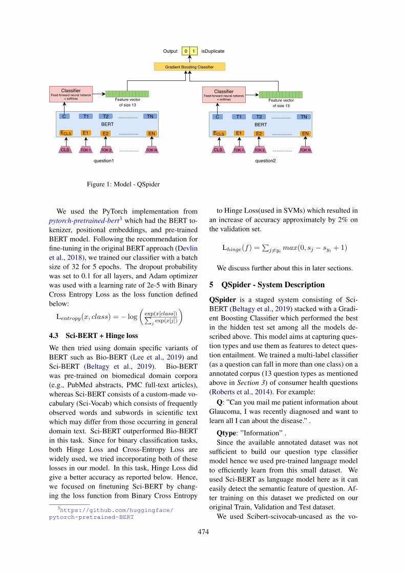
question1 question2
ClassifierFeed-forward neural netwrok
+ softmax
CLS
BERT
TOK 1 TOK 2 ...............
ECLS E1 E2
C T1 T2 TN
EN...............
...............
TOK N
Feature vectorof size 13
ClassifierFeed-forward neural netwrok
+ softmax
CLS
BERT
TOK 1 TOK 2 ...............
ECLS E1 E2
C T1 T2 TN
EN...............
...............
TOK N
Feature vectorof size 13
Gradient Boosting Classifier
0 1 isDuplicateOutput
Figure 1: Model - QSpider
We used the PyTorch implementation frompytorch-pretrained-bert3 which had the BERT to-kenizer, positional embeddings, and pre-trainedBERT model. Following the recommendation forfine-tuning in the original BERT approach (Devlinet al., 2018), we trained our classifier with a batchsize of 32 for 5 epochs. The dropout probabilitywas set to 0.1 for all layers, and Adam optimizerwas used with a learning rate of 2e-5 with BinaryCross Entropy Loss as the loss function definedbelow:
Lentropy(x, class) = − log
(exp(x[class])∑
jexp(x[j])
)
4.3 Sci-BERT + Hinge loss
We then tried using domain specific variants ofBERT such as Bio-BERT (Lee et al., 2019) andSci-BERT (Beltagy et al., 2019). Bio-BERTwas pre-trained on biomedical domain corpora(e.g., PubMed abstracts, PMC full-text articles),whereas Sci-BERT consists of a custom-made vo-cabulary (Sci-Vocab) which consists of frequentlyobserved words and subwords in scientific textwhich may differ from those occurring in generaldomain text. Sci-BERT outperformed Bio-BERTin this task. Since for binary classification tasks,both Hinge Loss and Cross-Entropy Loss arewidely used, we tried incorporating both of theselosses in our model. In this task, Hinge Loss didgive a better accuracy as reported below. Hence,we focused on finetuning Sci-BERT by chang-ing the loss function from Binary Cross Entropy
3https://github.com/huggingface/pytorch-pretrained-BERT
......................................................................................................................................................................................................................................
to Hinge Loss(used in SVMs) which resulted inan increase of accuracy approximately by 2% onthe validation set.
Lhinge(f) =∑j 6=yi max(0, sj − syi + 1)
We discuss further about this in later sections.
5 QSpider - System Description
QSpider is a staged system consisting of Sci-BERT (Beltagy et al., 2019) stacked with a Gradi-ent Boosting Classifier which performed the bestin the hidden test set among all the models de-scribed above. This model aims at capturing ques-tion types and use them as features to detect ques-tion entailment. We trained a multi-label classifier(as a question can fall in more than one class) on aannotated corpus (13 question types as mentionedabove in Section 3) of consumer health questions(Roberts et al., 2014). For example:
Q: ”Can you mail me patient information aboutGlaucoma, I was recently diagnosed and want tolearn all I can about the disease.” .
Qtype: ”Information” .Since the available annotated dataset was not
sufficient to build our question type classifiermodel hence we used pre-trained language modelto efficiently learn from this small dataset. Weused Sci-BERT as language model here as it caneasily detect the semantic feature of question. Af-ter training on this dataset we predicted on ouroriginal Train, Validation and Test dataset.
We used Scibert-scivocab-uncased as the vo-
474
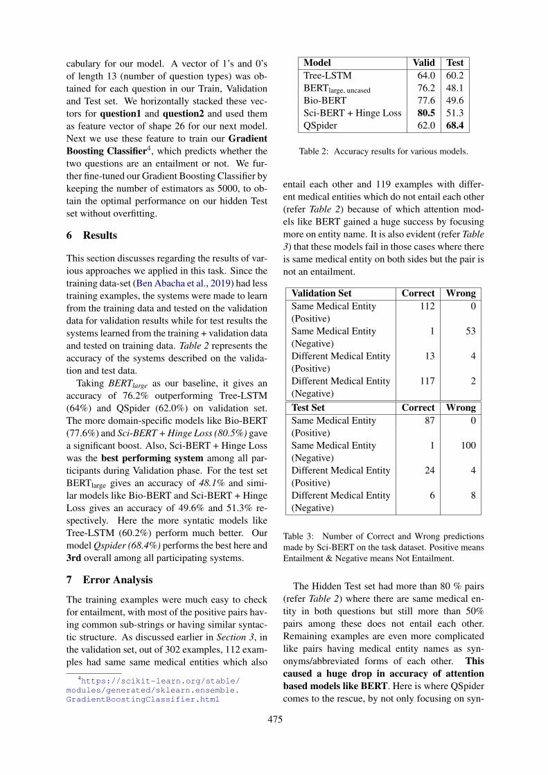
cabulary for our model. A vector of 1’s and 0’sof length 13 (number of question types) was ob-tained for each question in our Train, Validationand Test set. We horizontally stacked these vec-tors for question1 and question2 and used themas feature vector of shape 26 for our next model.Next we use these feature to train our GradientBoosting Classifier4, which predicts whether thetwo questions are an entailment or not. We fur-ther fine-tuned our Gradient Boosting Classifier bykeeping the number of estimators as 5000, to ob-tain the optimal performance on our hidden Testset without overfitting.
6 Results
This section discusses regarding the results of var-ious approaches we applied in this task. Since thetraining data-set (Ben Abacha et al., 2019) had lesstraining examples, the systems were made to learnfrom the training data and tested on the validationdata for validation results while for test results thesystems learned from the training + validation dataand tested on training data. Table 2 represents theaccuracy of the systems described on the valida-tion and test data.
Taking BERTlarge as our baseline, it gives anaccuracy of 76.2% outperforming Tree-LSTM(64%) and QSpider (62.0%) on validation set.The more domain-specific models like Bio-BERT(77.6%) and Sci-BERT + Hinge Loss (80.5%) gavea significant boost. Also, Sci-BERT + Hinge Losswas the best performing system among all par-ticipants during Validation phase. For the test setBERTlarge gives an accuracy of 48.1% and simi-lar models like Bio-BERT and Sci-BERT + HingeLoss gives an accuracy of 49.6% and 51.3% re-spectively. Here the more syntatic models likeTree-LSTM (60.2%) perform much better. Ourmodel Qspider (68.4%) performs the best here and3rd overall among all participating systems.
7 Error Analysis
The training examples were much easy to checkfor entailment, with most of the positive pairs hav-ing common sub-strings or having similar syntac-tic structure. As discussed earlier in Section 3, inthe validation set, out of 302 examples, 112 exam-ples had same same medical entities which also
4https://scikit-learn.org/stable/modules/generated/sklearn.ensemble.GradientBoostingClassifier.html
Model Valid TestTree-LSTM 64.0 60.2BERTlarge, uncased 76.2 48.1Bio-BERT 77.6 49.6Sci-BERT + Hinge Loss 80.5 51.3QSpider 62.0 68.4
Table 2: Accuracy results for various models.
entail each other and 119 examples with differ-ent medical entities which do not entail each other(refer Table 2) because of which attention mod-els like BERT gained a huge success by focusingmore on entity name. It is also evident (refer Table3) that these models fail in those cases where thereis same medical entity on both sides but the pair isnot an entailment.
Validation Set Correct WrongSame Medical Entity 112 0(Positive)Same Medical Entity 1 53(Negative)Different Medical Entity 13 4(Positive)Different Medical Entity 117 2(Negative)Test Set Correct WrongSame Medical Entity 87 0(Positive)Same Medical Entity 1 100(Negative)Different Medical Entity 24 4(Positive)Different Medical Entity 6 8(Negative)
Table 3: Number of Correct and Wrong predictionsmade by Sci-BERT on the task dataset. Positive meansEntailment & Negative means Not Entailment.
The Hidden Test set had more than 80 % pairs(refer Table 2) where there are same medical en-tity in both questions but still more than 50%pairs among these does not entail each other.Remaining examples are even more complicatedlike pairs having medical entity names as syn-onyms/abbreviated forms of each other. Thiscaused a huge drop in accuracy of attentionbased models like BERT. Here is where QSpidercomes to the rescue, by not only focusing on syn-
475
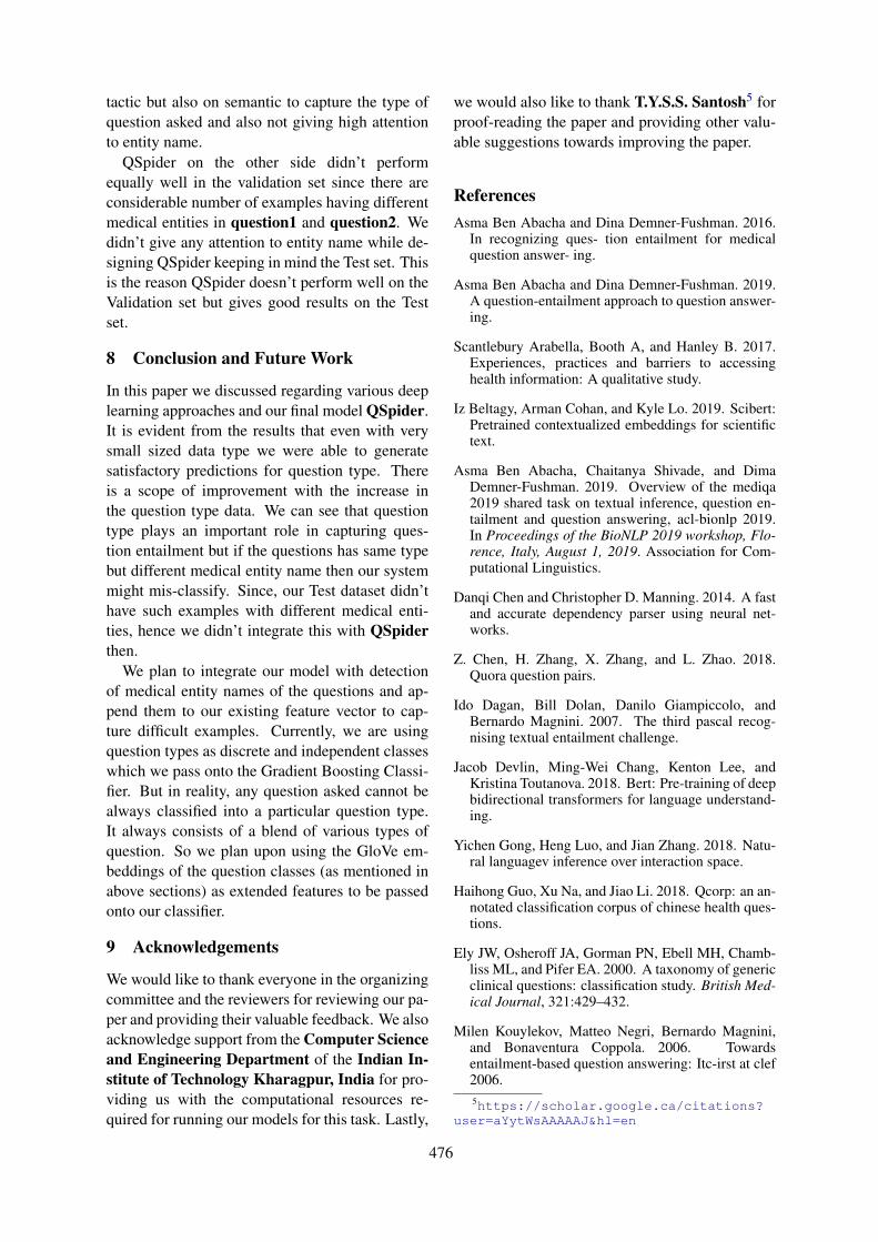
tactic but also on semantic to capture the type ofquestion asked and also not giving high attentionto entity name.
QSpider on the other side didn’t performequally well in the validation set since there areconsiderable number of examples having differentmedical entities in question1 and question2. Wedidn’t give any attention to entity name while de-signing QSpider keeping in mind the Test set. Thisis the reason QSpider doesn’t perform well on theValidation set but gives good results on the Testset.
8 Conclusion and Future Work
In this paper we discussed regarding various deeplearning approaches and our final model QSpider.It is evident from the results that even with verysmall sized data type we were able to generatesatisfactory predictions for question type. Thereis a scope of improvement with the increase inthe question type data. We can see that questiontype plays an important role in capturing ques-tion entailment but if the questions has same typebut different medical entity name then our systemmight mis-classify. Since, our Test dataset didn’thave such examples with different medical enti-ties, hence we didn’t integrate this with QSpiderthen.
We plan to integrate our model with detectionof medical entity names of the questions and ap-pend them to our existing feature vector to cap-ture difficult examples. Currently, we are usingquestion types as discrete and independent classeswhich we pass onto the Gradient Boosting Classi-fier. But in reality, any question asked cannot bealways classified into a particular question type.It always consists of a blend of various types ofquestion. So we plan upon using the GloVe em-beddings of the question classes (as mentioned inabove sections) as extended features to be passedonto our classifier.
9 Acknowledgements
We would like to thank everyone in the organizingcommittee and the reviewers for reviewing our pa-per and providing their valuable feedback. We alsoacknowledge support from the Computer Scienceand Engineering Department of the Indian In-stitute of Technology Kharagpur, India for pro-viding us with the computational resources re-quired for running our models for this task. Lastly,
we would also like to thank T.Y.S.S. Santosh5 forproof-reading the paper and providing other valu-able suggestions towards improving the paper.
ReferencesAsma Ben Abacha and Dina Demner-Fushman. 2016.
In recognizing ques- tion entailment for medicalquestion answer- ing.
Asma Ben Abacha and Dina Demner-Fushman. 2019.A question-entailment approach to question answer-ing.
Scantlebury Arabella, Booth A, and Hanley B. 2017.Experiences, practices and barriers to accessinghealth information: A qualitative study.
Iz Beltagy, Arman Cohan, and Kyle Lo. 2019. Scibert:Pretrained contextualized embeddings for scientifictext.
Asma Ben Abacha, Chaitanya Shivade, and DimaDemner-Fushman. 2019. Overview of the mediqa2019 shared task on textual inference, question en-tailment and question answering, acl-bionlp 2019.In Proceedings of the BioNLP 2019 workshop, Flo-rence, Italy, August 1, 2019. Association for Com-putational Linguistics.
Danqi Chen and Christopher D. Manning. 2014. A fastand accurate dependency parser using neural net-works.
Z. Chen, H. Zhang, X. Zhang, and L. Zhao. 2018.Quora question pairs.
Ido Dagan, Bill Dolan, Danilo Giampiccolo, andBernardo Magnini. 2007. The third pascal recog-nising textual entailment challenge.
Jacob Devlin, Ming-Wei Chang, Kenton Lee, andKristina Toutanova. 2018. Bert: Pre-training of deepbidirectional transformers for language understand-ing.
Yichen Gong, Heng Luo, and Jian Zhang. 2018. Natu-ral languagev inference over interaction space.
Haihong Guo, Xu Na, and Jiao Li. 2018. Qcorp: an an-notated classification corpus of chinese health ques-tions.
Ely JW, Osheroff JA, Gorman PN, Ebell MH, Chamb-liss ML, and Pifer EA. 2000. A taxonomy of genericclinical questions: classification study. British Med-ical Journal, 321:429–432.
Milen Kouylekov, Matteo Negri, Bernardo Magnini,and Bonaventura Coppola. 2006. Towardsentailment-based question answering: Itc-irst at clef2006.5https://scholar.google.ca/citations?
user=aYytWsAAAAAJ&hl=en
476
Jinhyuk Lee, Wonjin Yoon, Sungdong Kim,Donghyeon Kim, Sunkyu Kim, Chan Ho So,and Jaewoo Kang. 2019. Biobert: a pre-trainedbiomedical languagerepresentation model forbiomedical text mining.
Xiadong Liu, Pengcheng He, Weizhu Chen, and Jian-feng Gao. 2019. Multi-task deep neural networksfor natural language understanding.
Pletneva Natalia, Vargas A, Kalogianni K, and BoyerC. 2012. Online health information search: whatstruggles and empowers the users?
Kirk Roberts, Kate Masterton, Marcelo Fiszman, HalilKilicoglu, and Dina Demner-Fushman. 2014. An-notating question types for consumer health ques-tions.
Kai Sheng Tai, Richard Socher, and Christopher D.Manning. 2015. Improved semantic representationsfrom tree-structured long short-term memory net-works.
Jane Weaver. 2016. More people search for health on-line.
A Supplemental Material
This is the link to our classifier code for QSpi-der which can be used to reproduce the resultsclaimed in the Results section above for QSpider- https://github.com/Team-IIT-KGP/Qspider. The README section is updated forinstructions to run the code.
477
Proceedings of the BioNLP 2019 workshop, pages 478–487Florence, Italy, August 1, 2019. c©2019 Association for Computational Linguistics
ANU-CSIRO at MEDIQA 2019:Question Answering Using Deep Contextual Knowledge
Vincent NguyenAustralian National University
CSIRO [email protected]
Sarvnaz KarimiCSIRO Data61
Sydney, [email protected]
Zhenchang XingAustralian National University
Canberra, [email protected]
Abstract
We report on our system for textual inferenceand question entailment in the medical do-main for the ACL BioNLP 2019 Shared Task,MEDIQA. Textual inference is the task of find-ing the semantic relationships between pairsof text. Question entailment involves iden-tifying pairs of questions which have similarsemantic content. To improve upon medicalnatural language inference and question en-tailment approaches to further medical ques-tion answering, we propose a system that in-corporates open-domain and biomedical do-main approaches to improve semantic under-standing and ambiguity resolution. Our mod-els achieve 80% accuracy on medical naturallanguage inference (6.5% absolute improve-ment over the original baseline), 48.9% accu-racy on recognising medical question entail-ment, 0.248 Spearman’s rho for question an-swering ranking and 68.6% accuracy for ques-tion answering classification.
1 Introduction
Medical health search is the second most searchedthematic query, representing 5% of all queries onGoogle (Cocco et al., 2018). However, manyqueries are semantically identical and are poten-tially already answered by experts (Abacha andDemner-Fushman, 2016). However, these ques-tions may not be directly retrievable due to se-mantic ambiguity involving abbreviations (Wuet al., 2017), patient colloquialism (Graham andBrookey, 2008) or esoteric terminology (Lee et al.,2019). Furthermore, in regards to disease, tempo-rality is a key factor in determining the relevanceof retrieved answers (Lee et al., 2019). For ex-ample, it is more appropriate to retrieve answersrelating to the summer cold in the summer.
As a means to retrieve these questions thatare already answered by experts, question en-tailment has been proposed to discern relation-ships between pairs of questions. Recognising
Question Entailment (RQE) is the task of deter-mining the relationship between a question pair,RQE(Q1, Q2), as either entailment or not en-tailment, where Abacha and Demner-Fushman(2016) define question entailment as the situationwhere “a question, Q1, entails another question,Q2, if every answer to Q2 is also a complete orpartial answer to Q1.”
Natural Language Inference (NLI) is determin-ing the relationship between pairs of sentences,not just questions. NLI is the task of determin-ing whether a hypothesis, H , is inferred (entail-ment), not inferred (contradiction) or neither (neu-tral), given a premise. In the context of questionanswering (QA), it can be used to validate if theanswer can be inferred from the question.
Though RQE and NLI have thrived in the open-domain setting (Bowman et al., 2015; Rajpurkaret al., 2016), there are unique challenges in apply-ing these tasks directly to the biomedical questionanswering field. Previous models in the medicaldomain that used NLI and RQE relied on mod-els which were shallowly bidirectional (Romanovand Shivade, 2018) or rule-based approaches withshallow keyword matching techniques (Abachaand Demner-Fushman, 2016) which would notgeneralise well.
The MEDIQA (Ben Abacha et al., 2019) chal-lenge, as part of the ACL BioNLP workshop, aimsto further research efforts in NLI and RQE by in-troducing their applications to Biomedical QA.
In this paper, we detail our approach inMEDIQA which addresses some of the problemswith biomedical text such as utilising deep contex-tual relationships between words within a sentencefor semantic understanding and ambiguity associ-ated with esoteric terminology, abbreviations, andpatient colloquialism. We combine biomedicaland open-domain approaches as a means to im-prove generalisation and bridge the gap betweenpatient colloquialism and biomedical terminology.
478
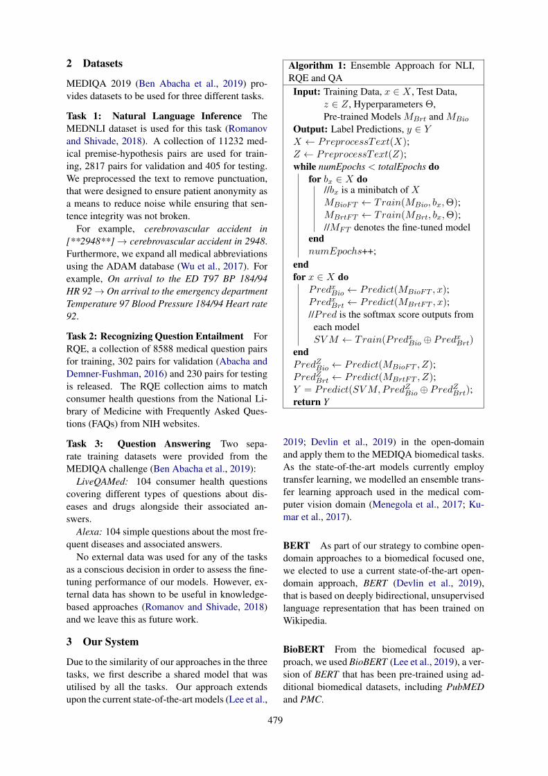
2 Datasets
MEDIQA 2019 (Ben Abacha et al., 2019) pro-vides datasets to be used for three different tasks.
Task 1: Natural Language Inference TheMEDNLI dataset is used for this task (Romanovand Shivade, 2018). A collection of 11232 med-ical premise-hypothesis pairs are used for train-ing, 2817 pairs for validation and 405 for testing.We preprocessed the text to remove punctuation,that were designed to ensure patient anonymity asa means to reduce noise while ensuring that sen-tence integrity was not broken.
For example, cerebrovascular accident in[**2948**]→ cerebrovascular accident in 2948.Furthermore, we expand all medical abbreviationsusing the ADAM database (Wu et al., 2017). Forexample, On arrival to the ED T97 BP 184/94HR 92→ On arrival to the emergency departmentTemperature 97 Blood Pressure 184/94 Heart rate92.
Task 2: Recognizing Question Entailment ForRQE, a collection of 8588 medical question pairsfor training, 302 pairs for validation (Abacha andDemner-Fushman, 2016) and 230 pairs for testingis released. The RQE collection aims to matchconsumer health questions from the National Li-brary of Medicine with Frequently Asked Ques-tions (FAQs) from NIH websites.
Task 3: Question Answering Two sepa-rate training datasets were provided from theMEDIQA challenge (Ben Abacha et al., 2019):
LiveQAMed: 104 consumer health questionscovering different types of questions about dis-eases and drugs alongside their associated an-swers.
Alexa: 104 simple questions about the most fre-quent diseases and associated answers.
No external data was used for any of the tasksas a conscious decision in order to assess the fine-tuning performance of our models. However, ex-ternal data has shown to be useful in knowledge-based approaches (Romanov and Shivade, 2018)and we leave this as future work.
3 Our System
Due to the similarity of our approaches in the threetasks, we first describe a shared model that wasutilised by all the tasks. Our approach extendsupon the current state-of-the-art models (Lee et al.,
Algorithm 1: Ensemble Approach for NLI,RQE and QAInput: Training Data, x ∈ X , Test Data,
z ∈ Z, Hyperparameters Θ,Pre-trained Models MBrt and MBio
Output: Label Predictions, y ∈ YX ← PreprocessText(X);Z ← PreprocessText(Z);while numEpochs < totalEpochs do
for bx ∈ X do//bx is a minibatch of XMBioFT ← Train(MBio, bx,Θ);MBrtFT ← Train(MBrt, bx,Θ);//MFT denotes the fine-tuned model
endnumEpochs++;
endfor x ∈ X do
PredxBio ← Predict(MBioFT , x);PredxBrt ← Predict(MBrtFT , x);//Pred is the softmax score outputs fromeach modelSVM ← Train(PredxBio ⊕ PredxBrt)
endPredZBio ← Predict(MBioFT , Z);PredZBrt ← Predict(MBrtFT , Z);Y = Predict(SVM,PredZBio ⊕ PredZBrt);return Y
2019; Devlin et al., 2019) in the open-domainand apply them to the MEDIQA biomedical tasks.As the state-of-the-art models currently employtransfer learning, we modelled an ensemble trans-fer learning approach used in the medical com-puter vision domain (Menegola et al., 2017; Ku-mar et al., 2017).
BERT As part of our strategy to combine open-domain approaches to a biomedical focused one,we elected to use a current state-of-the-art open-domain approach, BERT (Devlin et al., 2019),that is based on deeply bidirectional, unsupervisedlanguage representation that has been trained onWikipedia.
BioBERT From the biomedical focused ap-proach, we used BioBERT (Lee et al., 2019), a ver-sion of BERT that has been pre-trained using ad-ditional biomedical datasets, including PubMEDand PMC.
479
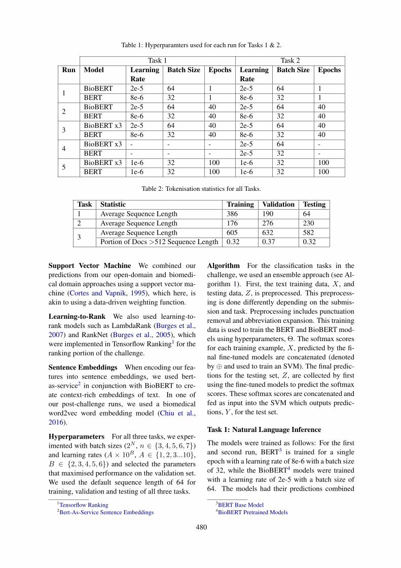
Table 1: Hyperparamters used for each run for Tasks 1 & 2.
Task 1 Task 2Run Model Learning
RateBatch Size Epochs Learning
RateBatch Size Epochs
1BioBERT 2e-5 64 1 2e-5 64 1BERT 8e-6 32 1 8e-6 32 1
2BioBERT 2e-5 64 40 2e-5 64 40BERT 8e-6 32 40 8e-6 32 40
3BioBERT x3 2e-5 64 40 2e-5 64 40BERT 8e-6 32 40 8e-6 32 40
4BioBERT x3 - - - 2e-5 64 -BERT - - - 2e-5 32 -
5BioBERT x3 1e-6 32 100 1e-6 32 100BERT 1e-6 32 100 1e-6 32 100
Table 2: Tokenisation statistics for all Tasks.
Task Statistic Training Validation Testing1 Average Sequence Length 386 190 642 Average Sequence Length 176 276 230
3Average Sequence Length 605 632 582Portion of Docs >512 Sequence Length 0.32 0.37 0.32
Support Vector Machine We combined ourpredictions from our open-domain and biomedi-cal domain approaches using a support vector ma-chine (Cortes and Vapnik, 1995), which here, isakin to using a data-driven weighting function.
Learning-to-Rank We also used learning-to-rank models such as LambdaRank (Burges et al.,2007) and RankNet (Burges et al., 2005), whichwere implemented in Tensorflow Ranking1 for theranking portion of the challenge.
Sentence Embeddings When encoding our fea-tures into sentence embeddings, we used bert-as-service2 in conjunction with BioBERT to cre-ate context-rich embeddings of text. In one ofour post-challenge runs, we used a biomedicalword2vec word embedding model (Chiu et al.,2016).
Hyperparameters For all three tasks, we exper-imented with batch sizes (2N , n ∈ {3, 4, 5, 6, 7})and learning rates (A × 10B , A ∈ {1, 2, 3...10},B ∈ {2, 3, 4, 5, 6}) and selected the parametersthat maximised performance on the validation set.We used the default sequence length of 64 fortraining, validation and testing of all three tasks.
1Tensorflow Ranking2Bert-As-Service Sentence Embeddings
Algorithm For the classification tasks in thechallenge, we used an ensemble approach (see Al-gorithm 1). First, the text training data, X , andtesting data, Z, is preprocessed. This preprocess-ing is done differently depending on the submis-sion and task. Preprocessing includes punctuationremoval and abbreviation expansion. This trainingdata is used to train the BERT and BioBERT mod-els using hyperparameters, Θ. The softmax scoresfor each training example, X , predicted by the fi-nal fine-tuned models are concatenated (denotedby ⊕ and used to train an SVM). The final predic-tions for the testing set, Z, are collected by firstusing the fine-tuned models to predict the softmaxscores. These softmax scores are concatenated andfed as input into the SVM which outputs predic-tions, Y , for the test set.
Task 1: Natural Language Inference
The models were trained as follows: For the firstand second run, BERT3 is trained for a singleepoch with a learning rate of 8e-6 with a batch sizeof 32, while the BioBERT4 models were trainedwith a learning rate of 2e-5 with a batch size of64. The models had their predictions combined
3BERT Base Model4BioBERT Pretrained Models
480
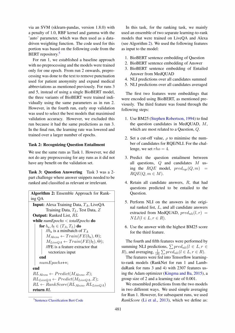
via an SVM (sklearn-pandas, version 1.8.0) witha penalty of 1.0, RBF kernel and gamma with the’auto’ parameter, which was then used as a data-driven weighting function. The code used for thisportion was based on the following code from theBERT repository.5
For run 1, we established a baseline approachwith no preprocessing and the models were trainedonly for one epoch. From run 2 onwards, prepro-cessing was done to the text to remove punctuationused for patient anonymity and expand medicalabbreviations as mentioned previously. For runs 3and 5, instead of using a single BioBERT model,the three variants of BioBERT were trained indi-vidually using the same parameters as in run 2.However, in the fourth run, early stop validationwas used to select the best models that maximisedvalidation accuracy. However, we excluded thisrun because it had the same predictions as run 3.In the final run, the learning rate was lowered andtrained over a larger number of epochs.
Task 2: Recognizing Question Entailment
We use the same runs as Task 1. However, we didnot do any preprocessing for any runs as it did nothave any benefit on the validation set.
Task 3: Question Answering Task 3 was a 2-part challenge where answer snippets needed to beranked and classified as relevant or irrelevant.
Algorithm 2: Ensemble Approach for Rank-ing QAInput: Alexa Training Data, TA, LiveQA
Training Data, TL, Test Data, ZOutput: Ranked List, RLwhile numEpochs < totalEpochs do
for ba, bl ∈ (TA, TL) do//ba is a minibatch of TAMAlexa ← Train(FE(ba),Θ);MLiveQA ← Train(FE(bl),Θ);//FE is a feature extractor that
vectorizes inputendnumEpochs++;
endRLAlexa ← Predict(MAlexa, Z);RLLiveQA ← Predict(MLiveQA, Z);RL← RankScore(RLAlexa, RLLiveQA)return RL
5Sentence Classification Bert Code
In this task, for the ranking task, we mainlyused an ensemble of two separate learning-to-rankmodels that were trained on LiveQA and Alexa(see Algorithm 2). We used the following featuresas input to the model:
1. BioBERT sentence embedding of Question2. BioBERT sentence embedding of Answer3. BioBERT sentence embedding of Entailed
Answer from MedQUAD4. NLI predictions over all candidates summed5. NLI predictions over all candidates averaged
The first two features were embeddings thatwere encoded using BioBERT, as mentioned pre-viously. The third feature was found through thefollowing steps:
1. Use BM25 (Stephen Robertson, 1994) to findthe question candidates in MedQUAD, M ,which are most related to a Question, Q.
2. Set a cut-off value, ρ to minimise the num-ber of candidates for RQE/NLI. For the chal-lenge, we set rho = 4.
3. Predict the question entailment betweenall questions, Q and candidates M us-ing the RQE model, predrqe(Q,m) =RQE(Q,m ∈M).
4. Retain all candidate answers, R, that hadquestions predicted to be entailed to theQuestion.
5. Perform NLI on the answers in the origi-nal ranked list, L, and all candidate answersextracted from MedQUAD, prednli(l, r) =NLI(l ∈ L, r ∈ R).
6. Use the answer with the highest BM25 scorefor the third feature.
The fourth and fifth features were performed bysumming NLI predictions,
∑prednli(l ∈ L, r ∈
R), and averaging, 1|R|
∑prednli(l ∈ L, r ∈ R).
The features were fed into Tensorflow learning-to-rank models (RankNet for run 1 and Lamb-daRank for runs 3 and 4) with 2307 features us-ing the Adam optimizer (Kingma and Ba, 2015), agroup size of 2 and a learning rate of 0.001.
We ensembled predictions from the two modelsin two different ways. We used simple averagingfor Run 1. However, for subsequent runs, we usedRankScore (Li et al., 2013), which we define as:
481
Table 3: Results for all 3 tasks in the MEDIQA shared task, additional post challenge runs are included. Note:With the exception of Task 1, all post challenge runs were evaluated using the official evaluation script.
Task 1 Task 2 Task 3Run Accuracy Accuracy Accuracy Spearman’s Rho Precision@11 0.751 0.481 0.581 0.093 0.5802 0.800 0.485 0.584 0.122 0.6403 0.796 0.481 0.584 -0.007 0.5204 - 0.489 0.584 -0.043 0.5335 0.768 0.485 0.577 0.162 0.593
Post Challenge RunsTask Description Accuracy Spearman’s Rho Precision1 Run 5 + Maximum Sequence
Length (Validation Set)0.827 (+0.016) - -
2 Run 5 + Maximum Seq. Length 0.489 (+0.004) - -3 Run 5 (Corrected Submission) 0.686 (+0.109) 0.0513 (-0.111) 0.771 (+0.178)3 Run 5 (Corrected Submission) +
Max Seq. Length0.663 (-0.023) 0.0971 (+0.046) 0.749 (-0.022)
3 Run 1 with word2vec embed-ding
- 0.284 (+0.189) -
3 Run 5 (Corrected Submission)with UMLS concept expansion
0.659 (-0.027) 0.0200 (-0.0313) 0.749 (-0.022)
Rs(d ∈ D) = 1/dr. We use RankScore to scoreeach item in the ranked lists of Alexa and LiveQAmodels. We then combine the items by summingthe documents RankScore from each model andsorting.
For classification, the same architecture fromTasks 1 and 2 for Runs 3 - 5 was used (4-ensemblewith SVM layer). For runs 2 and 5, we use soft-max scores output from the classification to rankdocuments.
4 Results and Discussion
Ensembles have been successfully utilised in otherbiomedical domains (Kumar et al., 2017; Bri-jesh and Zahid, 2011), with the main idea behindusing these being to incorporate complementarystrengths of the members of the ensemble. Thus,BERT is used in conjunction with BioBERT in or-der to correct the mistakes that the model makesby injecting non-domain specific knowledge. Thisidea was supported in our baseline experimentson task 1 where BioBERT scored 0.7913 on val-idation, while BERT scored 0.7715 on validation,but ensembling resulted in a higher final score of0.7950.
NLI Baseline System Problems Our baselinesystem made characteristic mistakes on the vali-
dation set, which is shown in Table 4 for Task 1.We found that our system had trouble with nu-merical interpretation and, for instance, was notable to determine the difference between type 1and type 2 diabetes. Furthermore, this problemis exacerbated when abbreviations and numeri-cal interpretation are required in phrases such asT97 BP 184/94. Thus, to aid the system in dis-ambiguating abbreviations, we expanded all ab-breviations using the ADAM database of com-mon clinical abbreviations and resulted in an 0.049increase in accuracy. Furthermore, the systemwould struggle with medical forms of negation.However, due to the use of BERT/BioBERT, con-ventional techniques such as NegEx or removalwould break sentence integrity and reduce com-prehension, thereby affecting word context, andthus were not viable. Furthermore, punctuation,in terms of patient anonymisation, is also a prob-lem as the punctuation does not carry meaningfulsemantic content and will confuse the classifiers.
RQE Baseline System Problems In task 2, wefound that our baseline system made similar mis-takes for different reasons (see Table 5). We foundexamples of what we consider near miss where thedefinition of partial entailment depends on inter-pretation. For example, in this question, the user
482
Table 4: Common mistakes made by the baseline system in Task 1.
Type Premise HypothesisNumericalInterpretation
PAST MEDICAL HISTORY: Type 2 diabetesmellitus.
the patient has type 1 diabetes
Abbreviationand NumericalInterpretation
On arrival to the ED T97 BP 184/94 HR 92RR 24 88% on RA ->98% on NRB.
The patient was hypertensive inthe ED
Negation He denied headache or nausea or vomiting. He has no head painSemantic Gap HISTORY OF PRESENT ILLNESS:,The pa-
tient is a 54 year old male with endstage re-nal disease secondary to type 1 diabetes whopresents for kidney transplant from wife.
patient is on insulin
wants information on hypertension (high bloodpressure). However, according to the gold stan-dard, this is not a form of entailment, partial orotherwise. We hypothesise that this lies on theborderline of the entailment definition or may bedue to bias. Furthermore, our system struggleswith abbreviations. However, the examples in thesecond task dataset are more related to problemswith co-reference resolution where abbreviationsappear in the original question but not in the FAQquestion.
Furthermore, phrases like “come out of” shouldbe aligned to terms such as “discharge”, which isan example of a semantic gap and require com-mon sense comprehension. This is problematic asBERT is known to struggle with this sort of rea-soning (Talmor et al., 2018). Also, we did notadjust the sequence length parameter (set to 64),which may have been a source of error. How-ever, a later investigation through a post-challengerun that shows that only Task 1 benefits from anincrease in sequence length (see Table 3). Fi-nally, patient colloquialism presents a unique chal-lenge where “hole in lung” is to be interpreted as“pleurisy” (lung inflammation). Although we didnot address this complex problem, it could be po-tentially solved through crowd-sourcing of medi-cal forum data. This may be suitable as an area toinvestigate for future work.
We found that in all our submissions on thetest set of the challenge, although our system wasable to achieve high results on the validation set of79%, the models were not well suited for the testset. Our model predicted entailment 92% of thetime on the test set, suggesting that the model isoverfitting, even though our baseline was trainedfor only one epoch. We found that the cases where
the models make errors are cases where the ques-tion contains words such as diagnosis and the dis-ease is mentioned, but the semantic content of thequestion might be about treatment rather than thediagnosis. This is very different from the trainingand validation datasets that were provided, whichwere much more straightforward and did not re-quire as much comprehension. An example il-lustrating this difficulty is Question A: Glaucoma:Can you mail me patient information about Glau-coma, I was recently diagnosed and want to learnall I can about the disease.” and Question B: Howis glaucoma diagnosed?
Question Answering Submission ProblemsFor the third Task, we incorrectly trained our mod-els to recognise documents with a relevance scoreof one as irrelevant. In contrast, the task is definedto classify documents of relevance score one andtwo as irrelevant. By fixing this error, we foundthat we had over a 10% increase in accuracy (Ta-ble 3). However, interestingly, we found that theranking quality (shown through Spearman’s Rho)decreased. Upon investigation, we found two rea-sons why this problem occurred: (1) our systemwas able to differentiate the relevance of one fromthe other three labels much better than differenti-ating between labels of one/two against three/four.This was reflected in the validation accuracy of ourinitial incorrect model, which achieved an accu-racy of 95% whereas the corrected model scoresonly 70% on the validation set, (2) we found thatthe longer the models were trained, the worse theranking quality became. We hypothesise that theproblem is due to how cross entropy loss and soft-max functions work. Since the models are min-imising KL-Divergence, the softmax scores be-come more extreme, falling close to 1 or very
483
Table 5: Common mistakes made by the baseline system in Task 2.
Type Question A Question BNear Miss I want more information on Hypertension and
fibromyalgia, I seem to be getting only topicson diabetes and I do not have this. I enjoyreading the current info.
What is high blood pressure?
Abbreviation Hi I have retinitis pigmentosa for 3years, Imsuffering from this disease. Please intoduceme any way to treat mg eyes such as stem cell... Thank you
Are there treatments for RP?
Semantic Gap Which drug we I take to stop water come outof my nipple
How to Treat Nipple Discharge
SequenceLength
... The problem is my binocular vision is notgood enough ... is there any operation that canfix this?
What is Vision Therapy Whenand why is it needed [for binoc-ular vision]?
Patient Collo-quialism
Cure for hole in lung. I certainly would liketo request for medical for hole in the lung
How Are Pleurisy and OtherPleural Disorders Treated?
close to 0. This results in the differences betweenscores of the documents to be very low (formingdense clusters) which reduces ranking quality asthe ranking becomes more sensitive to noise anduncertainty (Siddhant and Lipton, 2018).
Question Answering Baseline System ProblemsDue to the error of our submissions for Task 3, wewill not discuss the mistakes that occurred withinthe challenge for the pointwise ranking runs. In-stead, we will look at the mistakes that the post-challenge run encountered for those. However, forthe pairwise runs within the challenge, we foundthat it performed much worse than expected. Weattribute this ranking deficit to two important fac-tors.
The first is that BERT sentence embeddings arenot useful to represent sentences because the vec-tor space is too condensed (vector representationsare very close together). The second is that ourvector representations were too large, with BERTsentence embeddings producing embeddings up to800 dimensions. Using 3 of these embeddings re-sults in a very large input which would take toolong to train or hinder convergence. This effectwas observed in a post-challenge run where weused Chiu et al. (2016)’s biomedical word2vecembeddings and achieved a much higher Spear-man’s Rho. The second factor was that the Lamb-daLoss (Burges et al., 2007) function was not asuitable objective function as the RankNet modelperformed better.
From Table 2, we find that Task 3 is more ver-
bose than the other two tasks and presents uniquechallenges as almost a third of the documents willhave information loss due to the limitation of max-imum sequence length by BERT being 512 dueto quadratic memory explosion (Liu et al., 2018).However, we did a post-challenge run where weincreased the sequence length with no noticeabledifference. This is because the majority of infor-mation in these long sequence can be safely dis-carded. Furthermore, the BERT truncation strat-egy is to truncate from the end of the sentence, im-plying that the important information is typicallyat the start of the answer.
We also find that there are unique challengesin Task 3 due to the use of real patient ques-tions shown in Table 6. We found that problemssuch as typos, grammar and spellings mistakeswere not directly fixed by the BERT/BioBERTensemble as the collections were pretrained onacademic or formal language (Pubmed, PMC andWikipedia). However, problems such as synonyms(for example, abetalipoproteinemia and Bassen-Kornzweig syndrome) which should be addressedby the model were also not addressable due to alimitation in the vocabulary of the models, whichis discussed below. Furthermore, we found casesof near miss, for example, the model identifiesanemia and treatment options, but it is not the tar-get disease of the question. To address these prob-lems, we use a heuristic to expand UMLS terms inthe question and answer, and add these to the startof the sentence to combat the mentioned problems.
484
Table 6: Common mistakes made by baseline system in Task 3
Type Question AnswerTypo abetalipoproteimemia hi, I would like to know
if there is any support for those suffering withabetalipoproteinemia ... keen to learn how toget it diagnosed...
abetalipoproteinemia: Abetal-ipoproteinemia is an inheriteddisorder that affects the absorp-tion of dietary fats, cholesterol,and fat-soluble vitamins...
Synonyms abetalipoproteimemia hi, I would like to knowif there is any support for those suffering withabetalipoproteinemia...
Bassen-Kornzweig syndrome(Exams and Tests): There maybe damage to the retina ofthe eye (retinitis pigmentosa).Tests that may be done tohelp diagnose this conditioninclude...
Near miss about thalassemia treatment sir,my friend issuffering from thalassemia ,in that majorlyred blood anemia,white blood anemia and theblood is comming out from mouth when shegot cough .her condition is very severe...
Anemia (Treatment): Anemiatreatment depends on the cause.- Iron deficiency anemia. Treat-ment for this form of anemia...
Grammarand spellingmistakes
Absence seizures Does any damage occurrefrom these spells. Mental or physical
Seizures: A seizure is a sud-den, uncontrolled electrical dis-turbance in the brain. It cancause changes in your behavior,movements or feelings, and inlevels of consciousness. If youhave two...
Semantic Gap Bad Breath I have very bad breath and attimes it can make myself and others sick. Ineed some advice as to what I need to do.
Breath odor (Home Care): Useproper dental hygiene, espe-cially flossing. Remember thatmouthwashes are not effectivein treating the underlying prob-lem...
We found that the model performs better on thevalidation set than any of the post-challenge runs(79% accuracy, a 5% absolute increase over theother runs), but did not perform substantially bet-ter on the test set (see Table 3).
Problems with Underlying Models One prob-lem in using models such as BERT and BioBERTis the limitation in the maximum sequence length.This is demonstrated in the test portion of the chal-lenge, where test set answers were much longerthan those seen in the training and validation col-lection. These sequences were longer than the 512sequence length limit allowed by the BERT ar-chitecture, which is constrained due to a problemknown as the quadratic memory explosion (Liuet al., 2018) leading to exponentially longer train-ing times and memory usage.
Though there are ways to overcome these re-strictions such as striding the sentences pairs andlabels, this results in contextual information beinglost and label imbalance. This restriction also hin-ders the encoding of long-range dependencies be-tween sequences as only contexts within a fixedlength can be considered (Dai et al., 2019).
In addition, we use BioBERT as a means of con-tributing deep clinical contextual understanding ofsentences. However, we find that during Word-Piece Tokenisation (Devlin et al., 2019), medicalterms are always split into their sub-word rep-resentations as they are out-of-vocabulary, e.g.,arthralgias → art hra al gia s. Wordpiece to-kenisation relies on the idea that morphemes carrymeaning. However, due to the use of this non-medical vocabulary, specific medical related mor-
485
phemes are not being learned. For instance, arthr-(where - denotes prefix), means joints and -algiasmeans pain, so the correct tokenisation should bearthralgias→ arthr algia s so that the model cancurrently learn the semantic meaning behind themorpheme. We find that these limitations hinderedthe use of these models and their application to theMEDIQA tasks.
We emphasise that there is a real-world appli-cation with the models and methods in this chal-lenge. However, if we were to scale our ap-proach to real-world application, we would requireexternal data. Therefore for future work, givenmore time, we would like to use external datasetssuch as emrQA (Pampari et al., 2018) and exploremulti-task learning due to the similarity of thethree tasks and aim to incorporate other medicaltasks for a better generalisation of the biomedicalquestion answering. We would also want to trainthe BERT models on biomedical-focused vocabu-lary and additional data in the future as a baselineto compare against multi-task learning.
5 Conclusions
In this shared task, we use and improve upon NLIand RQE techniques for medical question answer-ing. Our approach involves utilising deep con-textual relationships between words emphasisingsemantic understanding and resolving ambiguity.We combine biomedical and open-domain strate-gies to improve generalisation and bridge the gapbetween the open-domain and biomedical domainquestion answering.
Acknowledgements
This research is supported by the Australian Re-search Training Program and the CSIRO Postgrad-uate Scholarship.
References
Ben Abacha and Demner-Fushman. 2016. Recogniz-ing Question Entailment for Medical Question An-swering. American Medical Informatics AssociationAnnual Symposium Proceedings, 2016:310–318.
Asma Ben Abacha, Chaitanya Shivade, and DinaDemner-Fushman. 2019. Overview of the MEDIQA2019 shared task on textual inference, question en-tailment and question answering. In Proceedings ofthe BioNLP 2019 workshop, Florence, Italy. Associ-ation for Computational Linguistics.
Samuel Bowman, Gabor Angeli, Christopher Potts, andChristopher Manning. 2015. A large annotated cor-pus for learning natural language inference. In Pro-ceedings of the 2015 Conference on Empirical Meth-ods in Natural Language Processing (EMNLP), Lis-bon, Portugal. Association for Computational Lin-guistics.
Verma Brijesh and Hassan Syed Zahid. 2011. Hybridensemble approach for classification. Applied Intel-ligence, 34(2):258–278.
Chris Burges, Tal Shaked, Erin Renshaw, Ari Lazier,Matt Deeds, Nicole Hamilton, and Greg Hullender.2005. Learning to rank using gradient descent. InProceedings of the 22Nd International Conferenceon Machine Learning, ICML ’05, pages 89–96, NewYork, NY. ACM.
Christopher Burges, Robert Ragno, and Quoc Le. 2007.Learning to rank with nonsmooth cost functions. InAdvances in Neural Information Processing Systems19, pages 193–200.
Billy Chiu, Gamal Crichton, Anna Korhonen, andSampo Pyysalo. 2016. How to train good word em-beddings for biomedical NLP. In Proceedings ofthe 15th Workshop on Biomedical Natural LanguageProcessing, pages 166–174, Berlin, Germany.
Anthony Cocco, Rachel Zordan, David Taylor, TraceyWeiland, Stuart Dilley, Joyce Kant, Mahesha Dom-bagolla, Andreas Hendarto, Fiona Lai, and JennieHutton. 2018. Dr Google in the ED: searching foronline health information by adult emergency de-partment patients. The Medical Journal of Aus-tralia, 209:342–347.
Corinna Cortes and Vladimir Vapnik. 1995. Support-vector networks. Machine Learning, 20(3):273–297.
Zihang Dai, Zhilin Yang, Yiming Yang, Jaime Car-bonell, Quoc Le, and Ruslan Salakhutdinov. 2019.Transformer-xl: Attentive language models beyonda fixed-length context. Computing Research Repos-itory, abs/1901.02860.
Jacob Devlin, Ming-Wei Chang, Kenton Lee, andKristina Toutanova. 2019. BERT: Pre-training ofdeep bidirectional transformers for language un-derstanding. In Proceedings of the Conference ofthe North American Chapter of the Association forComputational Linguistics: Human Language Tech-nologies, Minneapolis, MN.
Suzanne Graham and John Brookey. 2008. Do patientsunderstand? The Permanente journal, 12(3):67–69.
Diederik Kingma and Jimmy Ba. 2015. Adam: Amethod for stochastic optimization. In 3rd Interna-tional Conference on Learning Representations, SanDiego, CA.
486
Ashnil Kumar, Jinman Kim, David Lyndon, MichaelFulham, and Dagan Feng. 2017. An ensemble offine-tuned convolutional neural networks for medi-cal image classification. IEEE Journal of Biomedi-cal and Health Informatics, 21(1):31–40.
Jinhyuk Lee, Wonjin Yoon, Sungdong Kim,Donghyeon Kim, Sunkyu Kim, Chan Ho So,and Jaewoo Kang. 2019. BioBERT: A pre-trainedbiomedical language representation model forbiomedical text mining. arXiv e-prints, pagearXiv:1901.08746.
Vincent Li, Paul Thomas, and David Hawking. 2013.Merging algorithms for enterprise search. ACMInternational Conference Proceeding Series, pages42–49.
Peter Liu, Mohammad Saleh, Etienne Pot, BenGoodrich, Ryan Sepassi, Lukasz Kaiser, and NoamShazeer. 2018. Generating wikipedia by summariz-ing long sequences. Computing Research Reposi-tory, abs/1801.10198.
Afonso Menegola, Julia Tavares, Michel Fornaciali,Lin Li, Sandra Fontes de Avila, and Eduardo Valle.2017. Recod titans at isic challenge 2017. Comput-ing Research Repository, abs/1703.04819.
Anusri Pampari, Preethi Raghavan, Jennifer Liang, andJian Peng. 2018. emrqa: A large corpus for questionanswering on electronic medical records. Comput-ing Research Repository, abs/1809.00732.
Pranav Rajpurkar, Jian Zhang, Konstantin Lopyrev, andPercy Liang. 2016. Squad: 100, 000+ questionsfor machine comprehension of text. Computing Re-search Repository, abs/1606.05250.
Alexey Romanov and Chaitanya Shivade. 2018.Lessons from natural language inference in theclinical domain. Computing Research Repository,abs/1808.06752.
Aditya Siddhant and Zachary Lipton. 2018. Deepbayesian active learning for natural language pro-cessing: Results of a large-scale empirical study.In Proceedings of the 2018 Conference on Empiri-cal Methods in Natural Language Processing, pages2904–2909, Brussels, Belgium.
Susan Jones Micheline Hancock-Beaulieu Mike Gat-ford Stephen Robertson, Steve Walker. 1994. Okapiat trec-3. In Proceedings of the Third Text REtrievalConference (TREC 1994), Gaithersburg, MD.
Alon Talmor, Jonathan Herzig, Nicholas Lourie, andJonathan Berant. 2018. Commonsenseqa: Aquestion answering challenge targeting common-sense knowledge. Computing Research Repository,abs/1811.00937.
Yonghui Wu, Joshua Denny, Rosenbloom Trent, Ran-dolph Miller, Dario Giuse, Lulu Wang, CarmeloBlanquicett, Ergin Soysal, Jun Xu, and Hua Xu.
2017. A long journey to short abbreviations: de-veloping an open-source framework for clinical ab-breviation recognition and disambiguation (CARD).Journal of the American Medical Informatics Asso-ciation, 24(e1):e79–e86.
487
Proceedings of the BioNLP 2019 workshop, pages 488–492Florence, Italy, August 1, 2019. c©2019 Association for Computational Linguistics
MSIT SRIB at MEDIQA 2019: Knowledge Directed Multi-taskFramework for Natural Language Inference in Clinical Domain
Sahil Chopra1, Ankita Gupta2, and Anupama Kaushik1
1Maharaja Surajmal Institute of Technology, Delhi .2 Samsung Research Institute, Bangalore.{sahilchopra, anupama}@msit.in
Abstract
In this paper, we present Biomedical Multi-Task Deep Neural Network (Bio-MTDNN) onthe NLI task of MediQA 2019 challenge (BenAbacha et al., 2019). Bio-MTDNN utilizes”transfer learning” based paradigm where notonly the source and target domains are differ-ent but also the source and target tasks are var-ied, although related. Further, Bio-MTDNNintegrates knowledge from external sourcessuch as clinical databases (UMLS) enhanc-ing its performance on the clinical domain.Our proposed method outperformed the offi-cial baseline and other prior models (such asESIM and Infersent on dev set) by a consider-able margin as evident from our experimentalresults.
1 Introduction
The task of natural language inference (NLI) in-tends to determine whether a given hypothesiscan be inferred from a given premise. This taskalso referred to as recognizing textual entailment(RTE), is one of the most prevalent tasks amongNLP researchers . It has been one of the signifi-cant components for several other language appli-cations such as Information Extraction (IE), Ques-tion Answering (QA) or Document Summariza-tion. For example, Harabagiu and Hickl (2006)argue that RTE can enable QA systems to iden-tify correct answers by allowing filtering and re-ranking them w.r.t a given question. Another ap-proach is proposed by Ben Abacha and Demner-Fushman (2016), whereby the authors employRTE in IE/QA domain to answer a given ques-tion (queried by a consumer) by retrieving similarquestions that are already well responded by pro-fessionals.
In order to address this simple yet challeng-ing task of NLI, several open domain datasets
have been proposed, with Stanford Natural Lan-guage Inference (SNLI) (Bowman et al., 2015)and MultiNLI (Williams et al., 2018) being themost popular ones. They serve as a standardto assess recent NLI systems. However, therehave been only a few resources available in spe-cialized domains such as biomedical or medicine.Language inference in the medical domain is ex-tremely complex and remains less explored by theML community. This scantiness of adequate re-sources (in terms of datasets) can be attributedto the fact that patient’s data is sensitive, is ac-cessible to authorized medical professionals only,and requires domain experts to annotate it, unlikegeneric domains where one can rely on crowd-sourcing based techniques to acquire annotations.
To this end, Ben Abacha et al. (2019) releaseda new dataset made available through MIMIC-IIIderived data repository, named MedNLI, for NLIin the clinical domain which has been annotatedby experts. Along these lines, the MediQA 2019challenge aims to foster the development of appro-priate methods, techniques and standards for in-ference/entailment in the medical domain, specif-ically on MedNLI dataset through a shared task.The task intends to recognize three inference rela-tions between two sentences: Entailment, Neutraland Contradiction.
Previous research associated with the presenttask, such as work by Romanov and Shivade(2018) analyzed several state-of-the-art open do-main models for NLI on the MedNLI dataset. Thesame has been utilized as a baseline for compar-ison in the above mentioned shared task. Priorto this, efforts have been made towards the auto-matic construction of RTE datasets (Ben Abachaand Demner-Fushman, 2016; Abacha et al., 2015),application of active learning on small RTEdata (Shivade et al., 2015).
Our approach to solving the NLI task on the
488
MedNLI data is based on leveraging transfer learn-ing paradigm integrated with direct incorpora-tion of domain-specific knowledge from medi-cal knowledge bases (KB). Unlike Romanov andShivade (2018) which utilizes transfer learning toutilize standard NLI models (such as InferSent andESIM trained specifically on NLI task only) inthe clinical domain, we employ Mutli-task learn-ing (MTL) framework with domain adaptation tolearn representations across multiple natural lan-guage understanding (NLU) tasks. This approachnot only leverages vast amounts of cross-task databut also benefits from a regularization effect thatleads to better generalization and facilitates adap-tation to new tasks and domains. Besides domainadaptation, we also directly infuse domain specificknowledge from database of medical terminolo-gies so as to enable the system to perform well inthe clinical domain.
The rest of the paper is organized as follows:Section 2 describe the details of our approach.Section 3 demonstrates the experimental results.We conclude in Section 4.
2 Approach
This section elaborates on the various methodswe experimented with for the NLI task. In or-der to establish a simple baseline first, we utilizea feature-based system. The extracted features in-clude word containment (Lyon et al., 2001) andJaccard similarity (unigram, bigram, and trigram)based features. We also use similarity measure ofdistributed sentence representations obtained us-ing universal sentence encoder (Cer et al., 2018).We consider Levenshtein, and Euclidean distance,negations and cosine function as similarity mea-sures. In order to find the n-grams, we utilizeNLTK and scispaCy tokenizer (Neumann et al.,2019). We train a 3-class logistic regression clas-sifier with above-mentioned features to output theinference relations. Apart from this baseline, Wenow elaborate on the transfer learning and exter-nal knowledge integration based method in the fol-lowing subsections.
2.1 Transfer Learning
Given the vast amounts of data available in theopen-domain NLU tasks, we leverage them to at-tack the NLI task on MedNLI. Given a source do-main DS , a corresponding source task TS , as wellas a target domain DT and a target task TT , the
objective of transfer learning is to learn the targetconditional probability distribution P (YT |XT ) inDT with the information gained from DS and TSwhere DS 6= DT and/or TS 6= TT . X and Y arefeature and label space respectively.
We consider the scenario when DS 6= DT
(DS being open-domain andDT being clinical do-main) and TS 6= TT , with two possibilities for tar-get task TT . In the first scenario, we consider a sin-gle related TT and in the second scenario we lever-age multi-task framework where we augment theTT with multiple but related NLU tasks. For boththe scenarios, we utilize the method of sequentialtransfer where a model is pre-trained on the largesource domain data and fine-tuned on limited tar-get domain data (clinical here). Next, we describethe neural network based models that we utilize.
2.1.1 Bi-CNN-MIWe leverage Bi-CNN-MI model (Yin and Schütze,2015) to realize the single transfer task scenario.This DNN model is trained on a similar NLU taskof paraphrase identification (PI) which is formal-ized as a binary classification task: for given twosentences, determine whether they both conveyroughly the same meaning.
Bi-CNN-MI compares two sentences on mul-tiple levels of granularity (word, short n-gram,long n-gram and sentence) and learns correspond-ing sentence representations using a convolutionalneural network (CNN) based Siamese network.It also captures the sentence interactions betweentwo sentences by computing an interaction matrixat each level of granularity. This model has beenreported to outperform various earlier approacheson PI (Yin and Schütze, 2015).
We leverage this model for sequential transferby learning the model parameters on the PI taskand fine-tuning them on MedNLI dataset. Notethat the classification task in MedNLI can alsobenefit by capturing interactions at various levelsof granularity making it related to PI task but atthe same time different from PI as the objective ofMedNLI is not only to determine if a pair of sen-tences convey the same meaning but also segregateif they oppose each other or are unrelated.
2.1.2 MT-DNNIn the second scenario of transfer learning, weaugment the target task TT by various related NLUtasks and train the model to perform on all ofthem. This approach not only leverages exten-
489
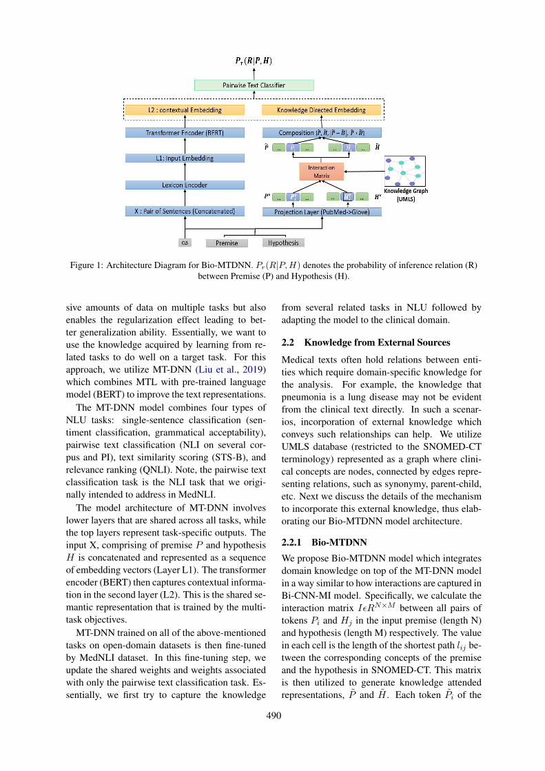
Figure 1: Architecture Diagram for Bio-MTDNN. Pr(R|P,H) denotes the probability of inference relation (R)between Premise (P) and Hypothesis (H).
sive amounts of data on multiple tasks but alsoenables the regularization effect leading to bet-ter generalization ability. Essentially, we want touse the knowledge acquired by learning from re-lated tasks to do well on a target task. For thisapproach, we utilize MT-DNN (Liu et al., 2019)which combines MTL with pre-trained languagemodel (BERT) to improve the text representations.
The MT-DNN model combines four types ofNLU tasks: single-sentence classification (sen-timent classification, grammatical acceptability),pairwise text classification (NLI on several cor-pus and PI), text similarity scoring (STS-B), andrelevance ranking (QNLI). Note, the pairwise textclassification task is the NLI task that we origi-nally intended to address in MedNLI.
The model architecture of MT-DNN involveslower layers that are shared across all tasks, whilethe top layers represent task-specific outputs. Theinput X, comprising of premise P and hypothesisH is concatenated and represented as a sequenceof embedding vectors (Layer L1). The transformerencoder (BERT) then captures contextual informa-tion in the second layer (L2). This is the shared se-mantic representation that is trained by the multi-task objectives.
MT-DNN trained on all of the above-mentionedtasks on open-domain datasets is then fine-tunedby MedNLI dataset. In this fine-tuning step, weupdate the shared weights and weights associatedwith only the pairwise text classification task. Es-sentially, we first try to capture the knowledge
from several related tasks in NLU followed byadapting the model to the clinical domain.
2.2 Knowledge from External Sources
Medical texts often hold relations between enti-ties which require domain-specific knowledge forthe analysis. For example, the knowledge thatpneumonia is a lung disease may not be evidentfrom the clinical text directly. In such a scenar-ios, incorporation of external knowledge whichconveys such relationships can help. We utilizeUMLS database (restricted to the SNOMED-CTterminology) represented as a graph where clini-cal concepts are nodes, connected by edges repre-senting relations, such as synonymy, parent-child,etc. Next we discuss the details of the mechanismto incorporate this external knowledge, thus elab-orating our Bio-MTDNN model architecture.
2.2.1 Bio-MTDNNWe propose Bio-MTDNN model which integratesdomain knowledge on top of the MT-DNN modelin a way similar to how interactions are captured inBi-CNN-MI model. Specifically, we calculate theinteraction matrix IεRN×M between all pairs oftokens Pi and Hj in the input premise (length N)and hypothesis (length M) respectively. The valuein each cell is the length of the shortest path lij be-tween the corresponding concepts of the premiseand the hypothesis in SNOMED-CT. This matrixis then utilized to generate knowledge attendedrepresentations, P̃ and H̃ . Each token P̃i of the
490
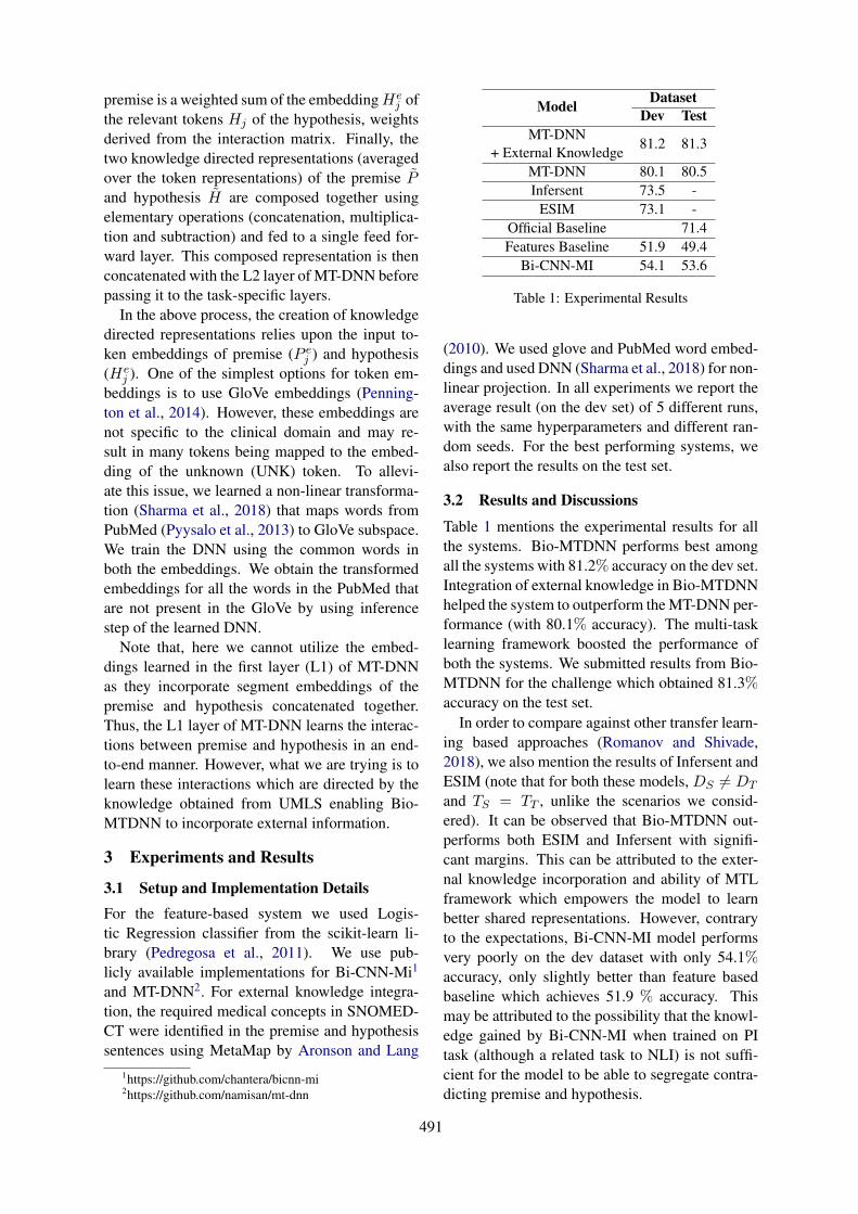
premise is a weighted sum of the embeddingHej of
the relevant tokens Hj of the hypothesis, weightsderived from the interaction matrix. Finally, thetwo knowledge directed representations (averagedover the token representations) of the premise P̃and hypothesis H̃ are composed together usingelementary operations (concatenation, multiplica-tion and subtraction) and fed to a single feed for-ward layer. This composed representation is thenconcatenated with the L2 layer of MT-DNN beforepassing it to the task-specific layers.
In the above process, the creation of knowledgedirected representations relies upon the input to-ken embeddings of premise (P e
j ) and hypothesis(He
j ). One of the simplest options for token em-beddings is to use GloVe embeddings (Penning-ton et al., 2014). However, these embeddings arenot specific to the clinical domain and may re-sult in many tokens being mapped to the embed-ding of the unknown (UNK) token. To allevi-ate this issue, we learned a non-linear transforma-tion (Sharma et al., 2018) that maps words fromPubMed (Pyysalo et al., 2013) to GloVe subspace.We train the DNN using the common words inboth the embeddings. We obtain the transformedembeddings for all the words in the PubMed thatare not present in the GloVe by using inferencestep of the learned DNN.
Note that, here we cannot utilize the embed-dings learned in the first layer (L1) of MT-DNNas they incorporate segment embeddings of thepremise and hypothesis concatenated together.Thus, the L1 layer of MT-DNN learns the interac-tions between premise and hypothesis in an end-to-end manner. However, what we are trying is tolearn these interactions which are directed by theknowledge obtained from UMLS enabling Bio-MTDNN to incorporate external information.
3 Experiments and Results
3.1 Setup and Implementation DetailsFor the feature-based system we used Logis-tic Regression classifier from the scikit-learn li-brary (Pedregosa et al., 2011). We use pub-licly available implementations for Bi-CNN-Mi1
and MT-DNN2. For external knowledge integra-tion, the required medical concepts in SNOMED-CT were identified in the premise and hypothesissentences using MetaMap by Aronson and Lang
1https://github.com/chantera/bicnn-mi2https://github.com/namisan/mt-dnn
Model DatasetDev Test
MT-DNN+ External Knowledge
81.2 81.3
MT-DNN 80.1 80.5Infersent 73.5 -
ESIM 73.1 -Official Baseline 71.4Features Baseline 51.9 49.4
Bi-CNN-MI 54.1 53.6
Table 1: Experimental Results
(2010). We used glove and PubMed word embed-dings and used DNN (Sharma et al., 2018) for non-linear projection. In all experiments we report theaverage result (on the dev set) of 5 different runs,with the same hyperparameters and different ran-dom seeds. For the best performing systems, wealso report the results on the test set.
3.2 Results and Discussions
Table 1 mentions the experimental results for allthe systems. Bio-MTDNN performs best amongall the systems with 81.2% accuracy on the dev set.Integration of external knowledge in Bio-MTDNNhelped the system to outperform the MT-DNN per-formance (with 80.1% accuracy). The multi-tasklearning framework boosted the performance ofboth the systems. We submitted results from Bio-MTDNN for the challenge which obtained 81.3%accuracy on the test set.
In order to compare against other transfer learn-ing based approaches (Romanov and Shivade,2018), we also mention the results of Infersent andESIM (note that for both these models, DS 6= DT
and TS = TT , unlike the scenarios we consid-ered). It can be observed that Bio-MTDNN out-performs both ESIM and Infersent with signifi-cant margins. This can be attributed to the exter-nal knowledge incorporation and ability of MTLframework which empowers the model to learnbetter shared representations. However, contraryto the expectations, Bi-CNN-MI model performsvery poorly on the dev dataset with only 54.1%accuracy, only slightly better than feature basedbaseline which achieves 51.9 % accuracy. Thismay be attributed to the possibility that the knowl-edge gained by Bi-CNN-MI when trained on PItask (although a related task to NLI) is not suffi-cient for the model to be able to segregate contra-dicting premise and hypothesis.
491
4 Conclusion
In this paper, we introduce Bio-MTDNN , whichis a knowledge directed, multi-task learning basedlanguage inference model for biomedical text min-ing. While MT-DNN was built for general purposelanguage understanding, Bio-MTDNN effectivelyleverages domain specific knowledge from UMLSas demonstrated by our experimental study. Wepresented our results on the MedNLI dataset un-der MediQA challenge. Incorporation of knowl-edge from external sources such as UMLS givesperformance advantage to Bio-MTDNN. Our pro-posed system outperformed the official baselineand other prior models (ESIM and Infersent on devset) by a great margin.
ReferencesAsma Ben Abacha, Duy Dinh, and Yassine Mrabet.
2015. Semantic analysis and automatic corpus con-struction for entailment recognition in medical texts.In Conference on Artificial Intelligence in Medicinein Europe, pages 238–242. Springer.
Alan R Aronson and François-Michel Lang. 2010. Anoverview of metamap: historical perspective and re-cent advances. Journal of the American Medical In-formatics Association, 17(3):229–236.
Asma Ben Abacha and Dina Demner-Fushman. 2016.Recognizing question entailment for medical ques-tion answering. In AMIA Annual Symposium Pro-ceedings, volume 2016, page 310. American Medi-cal Informatics Association.
Asma Ben Abacha, Chaitanya Shivade, and DinaDemner-Fushman. 2019. Overview of the mediqa2019 shared task on textual inference, question en-tailment and question answering. In Proceedings ofthe BioNLP 2019 workshop, Florence, Italy, August1, 2019. Association for Computational Linguistics.
Samuel R Bowman, Gabor Angeli, Christopher Potts,and Christopher D Manning. 2015. A large anno-tated corpus for learning natural language inference.arXiv preprint arXiv:1508.05326.
Daniel Cer, Yinfei Yang, Sheng-yi Kong, Nan Hua,Nicole Limtiaco, Rhomni St John, Noah Constant,Mario Guajardo-Cespedes, Steve Yuan, Chris Tar,et al. 2018. Universal sentence encoder. arXivpreprint arXiv:1803.11175.
Sanda Harabagiu and Andrew Hickl. 2006. Methodsfor using textual entailment in open-domain ques-tion answering. In Proceedings of the 21st Interna-tional Conference on Computational Linguistics andthe 44th annual meeting of the Association for Com-putational Linguistics, pages 905–912. Associationfor Computational Linguistics.
Xiaodong Liu, Pengcheng He, Weizhu Chen, andJianfeng Gao. 2019. Multi-task deep neural net-works for natural language understanding. CoRR,abs/1901.11504.
Caroline Lyon, James Malcolm, and Bob Dickerson.2001. Detecting short passages of similar text inlarge document collections. In Proceedings of the2011 conference on empirical methods in naturallanguage processing (EMNLP), pages 118–125.
Mark Neumann, Daniel King, Iz Beltagy, and WaleedAmmar. 2019. Scispacy: Fast and robust models forbiomedical natural language processing.
Fabian Pedregosa, Gaël Varoquaux, Alexandre Gram-fort, Vincent Michel, Bertrand Thirion, OlivierGrisel, Mathieu Blondel, Peter Prettenhofer, RonWeiss, Vincent Dubourg, et al. 2011. Scikit-learn:Machine learning in python. Journal of machinelearning research, 12(Oct):2825–2830.
Jeffrey Pennington, Richard Socher, and ChristopherManning. 2014. Glove: Global vectors for wordrepresentation. In Proceedings of the 2014 confer-ence on empirical methods in natural language pro-cessing (EMNLP), pages 1532–1543.
Sampo Pyysalo, Filip Ginter, Hans Moen, TapioSalakoski, and Sophia Ananiadou. 2013. Distribu-tional semantics resources for biomedical text pro-cessing. In Proceedings of the 5th InternationalSymposium on Languages in Biology and Medicine.
Alexey Romanov and Chaitanya Shivade. 2018.Lessons from natural language inference in the clin-ical domain. arXiv preprint arXiv:1808.06752.
Vasu Sharma, Nitish Kulkarni, Srividya Pranavi,Gabriel Bayomi, Eric Nyberg, and Teruko Mita-mura. 2018. Bioama: Towards an end to endbiomedical question answering system. In Proceed-ings of the BioNLP 2018 workshop, pages 109–117.
Chaitanya Shivade, Courtney Hebert, MarceloLopetegui, Marie-Catherine De Marneffe, EricFosler-Lussier, and Albert M Lai. 2015. Tex-tual inference for eligibility criteria resolution inclinical trials. Journal of biomedical informatics,58:S211–S218.
Adina Williams, Nikita Nangia, and Samuel Bowman.2018. A broad-coverage challenge corpus for sen-tence understanding through inference. In Proceed-ings of the 2018 Conference of the North AmericanChapter of the Association for Computational Lin-guistics: Human Language Technologies, Volume 1(Long Papers), pages 1112–1122.
Wenpeng Yin and Hinrich Schütze. 2015. Convolu-tional neural network for paraphrase identification.In Proceedings of the 2015 Conference of the NorthAmerican Chapter of the Association for Computa-tional Linguistics: Human Language Technologies,pages 901–911.
492
Proceedings of the BioNLP 2019 workshop, pages 493–499Florence, Italy, August 1, 2019. c©2019 Association for Computational Linguistics
UU TAILS at MEDIQA 2019: Learning Textual Entailment in the MedicalDomain
Noha S. TawfikArab Academy for Science & Technology
Alexandria 1029, [email protected]
Utrecht University3584CC Utrecht, The Netherlands
Marco R. SpruitUtrecht University
3584 CC Utrecht, The [email protected]
Abstract
This article describes the participation of theUU TAILS team in the 2019 MEDIQA chal-lenge intended to improve domain-specificmodels in medical and clinical NLP. The chal-lenge consists of 3 tasks: medical languageinference (NLI), recognizing textual entail-ment (RQE) and question answering (QA).Our team participated in tasks 1 and 2 andour best runs achieved a performance accu-racy of 0.852 and 0.584 respectively for thetest sets. The models proposed for task 1 reliedon BERT embeddings and different ensembletechniques. For the RQE task, we trained a tra-ditional multilayer perceptron network basedon embeddings generated by the universal sen-tence encoder.
1 Introduction
Detecting semantic relations between sentencepairs is a long-standing challenge for computa-tional semantics. Given two snippets of text:Premise P and Hypothesis H, textual entailmentrecognition determines if the meaning of H canbe inferred from that of P (Dagan et al., 2013).The significance of modeling text inference is ev-ident since it evaluates the capability of Natu-ral language Processing (NLP) to grasp meaningand interprets the linguistic variability of the lan-guage. Natural language inference (NLI) tasks,also known as Recognizing Textual Entailment(RTE) require a deep understanding of the se-mantic similarity between the hypothesis and thepremise. Moreover, they overlap with other lin-guistic problems such as question answering andsemantic text similarity. The recent years wit-nessed regular organization of shared tasks tar-geting the RTE/NLI task, which consequently ledto advances in the field. More complex mod-els were developed that rely on deep neural net-works, this was feasible with the availability of
large amounts of annotated datasets such as SNLIand MultiNLI (Bowman et al., 2015; ?). However,most models fail to generalize across different NLIbenchmarks (Talman and Chatzikyriakidis, 2018).Additionally, they do not perform accurately ondomain-specific datasets. This is specifically truein the medical and clinical domain. Compared toopen domain data, the language used to describebiomedical events is usually complex, rich in clin-ical semantics and contains conceptual overlap.And hence, it is difficult to adapt any of the for-mer models directly.The MEDIQA challenge (Ben Abacha et al., 2019)addresses the above limitations through its threeproposed tasks. The first task aims at identify-ing inference relations between clinical sentencepairs and introduces the medical natural languageinference benchmark dataset MedNLI (Romanovand Shivade, 2018). Its creation process is sim-ilar to the creation of the gold-standard SNLIdataset with adaptation to the clinical domain.Expert annotators were presented 4,638 premisesextracted from the MIMIC-III database (Johnsonet al., 2016) and were asked to write three hy-potheses with a true, false and neutral descrip-tion of the premise. The final dataset comprises14,049 sentence pairs divided into 11,232, 1,395and 1,422 for training, development and testing re-spectively. An additional test batch was providedby the challenge organizers with 405 unlabelledinstances. to the biomedical domain.Similarly, the second task, Recognizing QuestionEntailment (RQE), tackles the problem of findingduplicate questions by labeling questions basedon their similarity (Ben Abacha and Demner-Fushman, 2016). Extending the earlier NLI def-inition, the authors define question entailment as”Question A entails Question B if every answerto B is also a correct answer to A exactly or par-tially”. The dataset is specifically designed to
493
find the most similar frequently asked question(FAQ) to a given question. The training set wasconstructed from the questions provided by fam-ily doctors on the National Library of Medicine(NLM) platform resulting in 8,588 question pairswhere 54.2% are positive pairs. For validation,two sources of questions were used: validatedquestions from the NLM collections and FAQsretrieved from the National Institutes of Health(NIH) website. The validation set has 302 pairsof questions with 42.7% pairs positively labelled.The test set for the challenge was balanced andcomprised of 230 question pairs.The rest of the paper is organized as follows: Sec-tion 2 briefly discusses related work. We limitour summary to textual inference research in thebiomedical domain only. In Section 3, we describeour proposed model and the implementation de-tails for both tasks. In Section 4, we show the ex-periment results of our proposed models. Finally,we conclude our analysis of the challenge, as wellas some additional discussions of the future direc-tions in Section 5.
2 Related Work
In (Ben Abacha and Demner-Fushman, 2016), theauthors introduce a baseline model for the RQEdataset. The feature-based model relies on nega-tion, medical concepts overlap and lexical similar-ity measures to detect entailment among medicalquestion pairs. Romanov and Shivade conductedmultiple experiments on the MedNLI dataset toevaluate the transferability of existing methodsin adapting to clinical RTE tasks (Romanov andShivade, 2018). The best performing was the bidi-rectional LSTM encoder of the inferSent. Theirfindings also showed that transfer learning overthe larger SNLI set did not improve the results.In a previous work, we tried to model textual en-tailment found in biomedical literature by restruc-turing an existing YES/NO question-answeringdataset extracted from PubMed(2019). The newlyformed dataset aligned with standard NLI datasetsformat. Further on, we combined hand-craftedfeatures with the inferSent model to detect infer-ence.To the best of our knowledge, other than the workpreviously mentioned, there has been minimal re-search conducted directly on the textual entail-ment task in the biomedical domain. Below, wesummarize scattered attempts to extract contradic-
tions and conflicting statements found in medi-cal documents. Sarafraz et al. (2012), extractednegated molecular events from biomedical litera-ture using a hybrid of machine learning featuresand semantic rules. Similiarly, De Silve et al.(2017), extracted inconsistencies found in miRNAresearch articles. The system extracts relevanttriples and scores them according to an apposite-ness metric suggested by the authors. Alamriet al. (2016), introduced a dataset of 259 con-tradictory claims that answer 10 medical ques-tions related to cardiovascular diseases. Their pro-posed model relied on n-grams, negation, senti-ment and directionality features while in (Taw-fik and Spruit, 2018), the authors exploited se-mantic features and biomedical word embeddingsto detect contradictions using the same dataset.Zadrozny et al. (2018) suggested a conceptualframework based on the mathematical sheaf modelto highlight conflicting and contradictory criteriain guidelines published by accredited medical in-stitutes. It transforms natural language sentencesto formulas with parameters, creates partial orderbased on common predicates and builds sheaveson these partial orders.
3 Exploratory Embedding Analysis
With the fast developmental pace of text embed-ding methods, there is a lack of unified method-ology to assess these different techniques in thebiomedical domain. We attempted to conduct acomprehensive evaluation of different text repre-sentations for both tasks, prior to submission ofround 2 of the challenge. We use the MedSentE-val1 toolkit, a python-based toolkit that supportsdifferent embedding techniques including tradi-tional word embeddings like GloVe and FastText,contextualized embeddings like Embeddings fromLanguage Models (ELMO) and Bidirectional En-coder Representations from Transformers (BERT)and dedicated sentence encoders such as inferSentand Universal Sentence Encoder (USE). To evalu-ate the sentence representations fairly, we adopta straightforward method that extracts embed-dings from different techniques and feeds themto a logistic regression classifier. Our analy-sis showed that for the NLI task, embeddingsfrom the inferSent model achieved the best per-formance. This is not surprising, and aligns
1https://github.com/nstawfik/MedSentEval
494
with the results reported by the benchmark cre-ator (Romanov and Shivade, 2018). Moreover, wenotice that embeddings acquired from languagemodels such as ELMO and BERT, were the sec-ond best performing with minimal accuracy dif-ference. For the RQE task, the transformer en-coder of the USE model outperformed all othermethods by a clear margin followed by inferSenttrained with GloVe embeddings. This might becontributed to the multi-type training data em-ployed by USE with questions and entailment sen-tence pairs among others. As observed in the Gen-eral Language Understanding Evaluation (GLUE)benchmark dataset, BERT-based models are cur-rently the state-of-the art models for the NLI task.Accordingly, we have tried to further investigatethe performance of BERT in the biomedical NLIdomain. We also employed USE and inferSentsentence embeddings for task 2.
Bidirectional Encoder Representations fromTransformers BERT is a neural model devel-oped by Google, that makes heavy use of lan-guage representation models designed to pre-traindeep bidirectional representations (Devlin et al.,2018). It is trained in an unsupervised mannerover an enormous amount of publicly availableplain text data. Language Modeling (LM) servesas an unsupervised pre-training stage that can gen-erate the next word in a sentence with knowledgeof previous words in a sentence. BERT is differ-ent from other LM-based models because it targetsa different training objective, it uses masked lan-guage modeling instead of traditional LM. It re-places words in a sentence randomly and inserts a”masked” token. The transformer generates pre-dictions for the masked words by jointly condi-tioning on both left and right context in all layers.
Universal Sentence Encoder USE is referredto as ”universal” since, in theory, it is supposedto encode general properties of sentences giventhe large size of datasets it is trained on (Ceret al., 2018). The multi-task learning encoderuses several annotated and unannotated datasetsfor training. Training data consisted of supervisedand unsupervised sources such as Wikipedia arti-cles, news, discussion forums, dialogues and ques-tion/answers pairs. It has two variants of the en-coding architectures; The transformer model is de-signed for higher accuracy, but the encoding re-quires more memory and computational time. The
Deep Averaging Network (DAN) model on theother hand is designed for speed and efficiency,and some accuracy is compromised. When in-tegrated in any downstream task, USE should beable to represent sentences efficiently without theneed for any domain specific knowledge. This isa great advantage when limited training resourcesare available for specific tasks.
4 Methods
4.1 Task 1: Natural Language Inference(NLI)
Experimental Settings We take advantage oftwo newly released BERT models trained on dif-ferent biomedical data. The following mod-els were initialized from the original bert-base-uncased setting pre-trained with 12 transformerlayers, hidden unit size of d=768, 12 attentionheads and 110M parameters.
• SciBERT2 trained on a random sample of1.14M scientific articles available in the se-mantic scholar repository. The training dataconsists of full-text papers from the biomed-ical and computer sciences domain witha 2.5B and 0.6B word count, respectively(Beltagy et al., 2019).
• ClinicalBERT3 trained on approximately 2Mclinical records. The training data consistsof intensive care notes distributed among15 types available in the MIMIC database(Alsentzer et al., 2019).
We combined both training and evaluation recordsto form a new training set of 12627 sentencepairs. The original test set was used for evalu-ation and development. We experimented withall models in pytorch, using the HuggingFace4
re-implementation of the original BERT pythonpackage. We convert the SciBERT models tomake it compatible with PyTorch. We use the fine-tuning script to train the model on the MEDNLIdataset in an end-to-end fashion. We trained a totalof 30 models with variations of the model config-uration. All models with accuracy less than 0.786
2The pre-trained weights for for the SciBERT modelare available at https://github.com/allenai/scibert
3The pre-trained weights for the ClinicalBERTmodel are available at https://github.com/EmilyAlsentzer/clinicalBERT
4https://github.com/huggingface/pytorch-pretrained-BERT
495
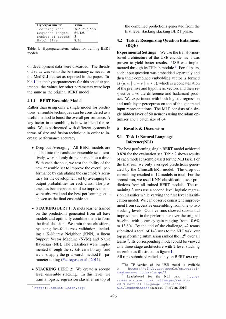
Hyperparameter ValueLearning rate 3e-5, 2e-5, 5e-5Sequence length 64, 128Number of Epochs 3Batch Size 8, 16
Table 1: Hyperparameters values for training BERTmodels
on development data were discarded. The thresh-old value was set to the best accuracy achieved forthe MedNLI dataset as reported in the paper. Ta-ble 1 list the hyperparameters for this set of exper-iments, the values for other parameters were keptthe same as the original BERT model.
4.1.1 BERT Ensemble ModelRather than using only a single model for predic-tions, ensemble techniques can be considered as auseful method to boost the overall performance. Akey factor in ensembling is how to blend the re-sults. We experimented with different systems interms of size and fusion technique in order to in-crease performance accuracy:
• Drop-out Averaging: All BERT models areadded into the candidate ensemble set. Itera-tively, we randomly drop one model at a time.With each dropout, we test the ability of thenew ensemble set to improve the overall per-formance by calculating the ensemble’s accu-racy for the development set by averaging theoutput probabilities for each class. The pro-cess has been repeated until no improvementswere observed and the best performing set ischosen as the final ensemble set.
• STACKING BERT 1: A meta learner trainedon the predictions generated from all basemodels and optimally combine them to formthe final decision. We train three classifiers,by using five-fold cross validation, includ-ing a K-Nearest Neighbor (KNN), a linearSupport Vector Machine (SVM) and NaiveBayesian (NB). The classifiers were imple-mented through the scikit-learn library 5andwe also apply the grid search method for pa-rameter tuning (Pedregosa et al., 2011).
• STACKING BERT 2: We create a secondlevel ensemble stacking. In this level, wetrain a logistic regression classifier on top of
5 https://scikit-learn.org/
the combined predictions generated from thefirst level stacking stacking BERT phase.
4.2 Task 2: Recognizing Question Entailment(RQE)
Experimental Settings We use the transformer-based architecture of the USE encoder as it wasproven to yield better results. USE was imple-mented through its TF hub module 6. For all pairs,each input question was embedded separately andthen their combined embedding vector is formedas (u, v, | u− v |, u ∗ v), which is a concatenationof the premise and hypothesis vectors and their re-spective absolute difference and hadamard prod-uct. We experiment with both logistic regressionand multilayer perceptron on top of the generatedinput representations. The MLP consists of a sin-gle hidden layer of 50 neurons using the adam op-timizer and a batch size of 64.
5 Results & Discussion
5.1 Task 1: Natural LanguageInference(NLI)
The best performing single BERT model achieved0.828 for the evaluation set. Table 2 shows resultsof each model ensemble used for the NLI task. Forthe first run, we only averaged predictions gener-ated by the ClinicalBERT model. The drop-outensembling resulted in 12 models in total. For thesecond run, we used KNN classification over pre-dictions from all trained BERT models. The re-maining 3 runs use a second level logistic regres-sion classifier while varying the first level classifi-cation model. We can observe consistent improve-ment from successive ensembling from one to twostacking levels. Our five runs showed substantialimprovement in the performance over the originalbaseline with accuracy gain ranging from 10.6%to 13.8%. By the end of the challenge, 42 teamssubmitted a total of 143 runs to the NLI task. ourtop performing submission ranked the 12th over allteams 7. Its corresponding model could be viewedas a three-stage architecture with 2 level stackingensemble as illustrated in figure 1.All runs submitted relied solely on BERT text rep-
6The TF version of the USE model is availableat https://tfhub.dev/google/universal-sentence-encoder-large/3
7 Leaderboard for the NLI task: https://www.aicrowd.com/challenges/mediqa-2019-natural-language-inference-nli/leaderboards (accessed 1st of June 2019)
496
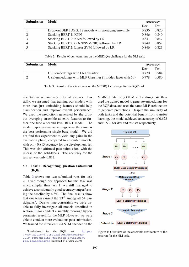
Submission Model AccuracyDev Test
1 Drop-out BERT AVG: 12 models with averaging ensemble 0.836 0.8202 Stacking BERT 1: KNN 0.846 0.8403 Stacking BERT 2: KNN followed by LR 0.847 0.8474 Stacking BERT 2: (KNN/SVM/NB) followed by LR 0.849 0.8525 Stacking BERT 2: Linear SVM followed by LR 0.846 0.823
Table 2: Results of our team runs on the MEDIQA challenge for the NLI task.
Submission Model AccuracyDev Test
1 USE embeddings with LR Classifier 0.770 0.5842 USE embeddings with MLP Classifier (1 hidden layer with 50) 0.778 0.580
Table 3: Results of our team runs on the MEDIQA challenge for the RQE task.
resentations without any external features. Ini-tially, we assumed that training our models withmore than just embedding features should helpclassification and improve overall performance.We used the predictions generated by the drop-out averaging ensemble as extra features to fur-ther fine-tune a second-level BERT model. Themodel hyperparameters settings were the same asthe best performing single base model. We didnot find this experiment to yield any gains in theevaluation phase, compared to ensemble models,with only 0.815 accuracy for the development set.This was also affirmed post submission, with therelease of the gold-labels. The accuracy for thetest set was only 0.812.
5.2 Task 2: Recognizing Question Entailment(RQE)
Table 3 shows our two submitted runs for task2. Even though our approach for this task wasmuch simpler than task 1, we still managed toachieve a considerably good accuracy outperform-ing the baseline by 4.3%. The final results showthat our team ranked the 23rd among all 54 par-ticipants8. Due to time constraints we were un-able to fully investigate all models described insection 3, nor conduct a suitably thorough hyper-parameter search for the MLP. However, we wereable to conduct more evaluations post submission.We trained the inferSent Bi-LSTM encoder on the
8Leaderboard for the RQE task: https://www.aicrowd.com/challenges/mediqa-2019-recognizing-question-entailment-rqe/leaderboards (accessed 1st of June 2019)
MedNLI data using GloVe embeddings. We thenused the trained model to generate embeddings forthe RQE data, and used the same MLP architectureto generate predictions. Despite the similarity ofboth tasks and the potential benefit from transferlearning, the model achieved an accuracy of 0.623and 0.532 for dev and test set respectively.
Figure 1: Overview of the ensemble architecture of thebest run for the NLI task.
497
6 Conclusion
In this paper, we presented our solution for tex-tual entailment detection in the clinical domain.Our proposed approach for the NLI task relieson BERT contextual embeddings features and ma-chine learning algorithms such as KNN, SVM andLR for ensembling. We use two different pre-trained BERT weights to train the base models andgenerate corresponding probabilities for the testset. Then, we adopt a 5-fold stacking strategy tolearn and combine predictions. In the third andfinal level of the ensemble, we use a logistic re-gression over the outputs from level-1 stacking, topredict the final class labels. A future extensionof our model is to use BERT in feature extractionmode instead of fine-tuning the end-to-end modelon the MedNLI dataset. This would allow the se-lection of layers from which to extract embeddingsand/or the combination of multiple layers. In theformer scenario, different neural networks couldbe used to generate the base model predictions be-fore applying ensemble techniques.For the RQE task, we train an MLP classifier ontop of USE embeddings. The results obtainedwere promising, given the simplicity of the model.More complex and deeper networks could be em-ployed with the combination of USE embeddings.We also experimented with transfer learning bytraining the inferSent model on MedNLI beforefine-tuning on the RQE corpus. While this ap-proach did not improve the results, we aim at fur-ther investigating other inferSent architectures andtraining on clinical word embedding.
ReferencesAbdulaziz Alamri. 2016. The Detection of Contradic-
tory Claims in Biomedical Abstracts. Ph.D. thesis,University of Sheffield.
Emily Alsentzer, John R. Murphy, Willie Boag, Wei-Hung Weng, Di Jin, Tristan Naumann, and MatthewB. A. McDermott. 2019. Publicly Available Clin-ical BERT Embeddings. arXiv e-prints, pagearXiv:1904.03323.
Iz Beltagy, Arman Cohan, and Kyle Lo. 2019. SCIB-ERT: Pretrained Contextualized Embeddings forScientific Text. Technical report.
Asma Ben Abacha and Dina Demner-Fushman.2016. Recognizing Question Entailment for Med-ical Question Answering. AMIA ... Annual Sym-posium proceedings. AMIA Symposium, 2016:310–318.
Asma Ben Abacha, Chaitanya Shivade, and DinaDemner-Fushman. 2019. Overview of the MEDIQA2019 Shared Task on Textual Inference, QuestionEntailment and Question Answering. In ACL-BioNLP, Florence.
Samuel R. Bowman, Gabor Angeli, Christopher Potts,and Christopher D. Manning. 2015. A large an-notated corpus for learning natural language infer-ence. In Proceedings of the 2015 Conference onEmpirical Methods in Natural Language Processing(EMNLP)., Lisbon. Association for ComputationalLinguistics.
Daniel Cer, Yinfei Yang, Sheng-yi Kong, Nan Hua,Nicole Limtiaco, Rhomni St John, Noah Constant,Mario Guajardo-Céspedes, Steve Yuan, Chris Tar,Yun-Hsuan Sung, Brian Strope, and Ray KurzweilGoogle Research Mountain View. 2018. Univer-sal Sentence Encoder. In Proceedings of the 2018Conference on Empirical Methods in Natural Lan-guage Processing: System Demonstrations, pages169–174, Brussels. Association for ComputationalLinguistics.
Ido Dagan, Dan Roth, Mark Sammons, and Fabio Mas-simo Zanzotto. 2013. Recognizing Textual Entail-ment: Models and Applications. Synthesis Lectureson Human Language Technologies, 6(4):1–220.
Jacob Devlin, Ming-Wei Chang, Kenton Lee,Kristina Toutanova Google, and A I Language.2018. BERT: Pre-training of Deep BidirectionalTransformers for Language Understanding. arXive-prints.
Alistair E.W. Johnson, Tom J. Pollard, Lu Shen, Li-wei H. Lehman, Mengling Feng, Mohammad Ghas-semi, Benjamin Moody, Peter Szolovits, Leo An-thony Celi, and Roger G. Mark. 2016. MIMIC-III,a freely accessible critical care database. ScientificData, 3:160035.
F Pedregosa, G Varoquaux, A Gramfort, V Michel,B Thirion, O Grisel, M Blondel, P Prettenhofer,R Weiss, V Dubourg, J Vanderplas, A Passos,D Cournapeau, M Brucher, M Perrot, and E Duch-esnay. 2011. Scikit-learn: Machine Learning inPython. Journal of Machine Learning Research,12:2825–2830.
Alexey Romanov and Chaitanya Shivade. 2018.Lessons from Natural Language Inference in theClinical Domain. Proceedings of the 2018 Con-ference on Empirical Methods in Natural LanguageProcessing, pages 1586–1596.
Noha S. Tawfik and Marco R. Spruit. 2019. TowardsRecognition of Textual Entailment in the Biomed-ical Domain. In International Conference on Ap-plications of Natural Language to Information Sys-tems, Manchester. Springer.
Farzaneh Sarafraz. 2012. Finding conflicting state-ments in the biomedical literature. Ph.D. thesis,University of Manchester.
498
Nisansa de Silva, Dejing Dou, and Jingshan Huang.2017. Discovering inconsistencies in pubmed ab-stracts through ontology-based information extrac-tion. In ACM Conference on Bioinformatics, Com-putational Biology, and Health Informatics (ACMBCB).
Aarne Talman and Stergios Chatzikyriakidis. 2018.Testing the Generalization Power of Neural NetworkModels Across NLI Benchmarks. Technical report.
Noha S. Tawfik and Marco R. Spruit. 2018. Auto-mated Contradiction Detection in Biomedical Liter-ature. In Proceedings of international Conferenceon Machine Learning and Data Mining in PatternRecognition, pages 138–148. Springer, Cham.
Wlodek Zadrozny and Luciana Garbayo. 2018. ASheaf Model of Contradictions and Disagreements.Preliminary Report and Discussion. In InternationalSymposium on Artificial Intelligence and Mathemat-ics,, Florida.
499
Proceedings of the BioNLP 2019 workshop, pages 500–509Florence, Italy, August 1, 2019. c©2019 Association for Computational Linguistics
UW-BHI at MEDIQA 2019: An Analysis of Representation Methods forMedical Natural Language Inference
William R. Kearns†, Wilson Lau†, and Jason A. Thomas ††Department of Biomedical Informatics and Medical Education, University of Washington
850 Republican StreetSeattle, WA
{kearnsw, wlau, thomasjt}@uw.edu
Abstract
Recent advances in distributed language mod-eling have led to large performance increaseson a variety of natural language processing(NLP) tasks. However, it is not well under-stood how these methods may be augmentedby knowledge-based approaches. This pa-per compares the performance and internalrepresentation of an Enhanced Sequential In-ference Model (ESIM) between three experi-mental conditions based on the representationmethod: Bidirectional Encoder Representa-tions from Transformers (BERT), Embeddingsof Semantic Predications (ESP), or Cui2Vec.The methods were evaluated on the MedicalNatural Language Inference (MedNLI) sub-task of the MEDIQA 2019 shared task. Thistask relied heavily on semantic understandingand thus served as a suitable evaluation set forthe comparison of these representation meth-ods.
1 Introduction
This paper describes our approach to the Nat-ural Language Inference (NLI) subtask of theMEDIQA 2019 shared task (Ben Abacha et al.,2019). As it is not yet clear the extent towhich knowledge-based embeddings may providetask-specific improvement over recent advancesin contextual embeddings, we provide an anal-ysis of the differences in performance betweenthese two methods. Additionally, it is not yetclear from the literature the extent to which in-formation stored in contextual embeddings over-laps with that in knowledge-based embeddings forwhich we provide a preliminary analysis of the at-tention weights of models that use these two rep-resentation methods as input. We compare BERTfine-tuned to MIMIC-III (Johnson et al., 2016) andPubMed to Embeddings of Semantic Predications(ESP) trained on SemMedDB and a baseline that
uses Cui2Vec embeddings trained on clinical andbiomedical text.
Two recent advances in the unsupervised mod-eling of natural language, Embeddings of Lan-guage Models (ELMo) (Peters et al., 2018)and Bidirectional Encoder Representations fromTransformers (BERT) (Devlin et al., 2018), haveled to drastic improvements across a variety ofshared tasks. Both of these methods use transferlearning, a method whereby a multi-layered lan-guage model is first trained on a large unlabeledcorpus. The weights of the model are then frozenand used as input to a task specific model (Peterset al., 2018; Devlin et al., 2018; Liu et al., 2019).This method is particularly well-suited for workin the medical domain where datasets tend to berelatively small due to the high cost of expert an-notation.
However, whereas clinical free-text is difficultto access and share in bulk due to privacy con-cerns, the biomedical domain is characterized bya significant amount of manually-curated struc-tured knowledge bases. The BioPortal reposi-tory currently hosts 773 different biomedical on-tologies comprised of over 9.4 million classes.SemMedDB is a triple store that consists of over94 million predications extracted from PubMedby SemRep, a semantic parser for biomedical text(Rindflesch and Fiszman, 2003; Kilicoglu et al.,2012). These available resources make a strongcase for the evaluation of knowledge-based meth-ods for the Medical Natural Language Inference(MedNLI) task (Romanov and Shivade, 2018).
2 Related Work
In this section, we provide a brief overview ofmethods for distributional and frame-based se-mantic representation of natural language. For amore detailed synthesis, we refer the reader to the
500
review of Vector Space Models (VSMs) by Turneyand Pantel (2010).
2.1 Distributional Semantics
The distributed representation of words has along history in computational linguistics, begin-ning with latent semantic indexing (LSI) (Deer-wester et al., 1990; Hofmann, 1999; Kanerva et al.,2000), maximum entropy methods (Berger et al.,1996), and latent Dirichlet allocation (LDA) (Bleiet al., 2003). More recently, neural network meth-ods have been applied to model natural language(Bengio et al., 2003; Weston et al., 2008; Turianet al., 2010). These methods have been broadlyapplied as a method of improving supervisedmodel performance by learning word-level fea-tures from large unlabeled datasets with more re-cent work using either Word2Vec (Mikolov et al.,2013; Pavlopoulos et al., 2014) or GloVe (Pen-nington et al., 2014) embeddings. Recent workhas learned a continuous representation of Uni-fied Medical Language System (UMLS) (Aron-son, 2006) concepts by applying the Word2Vecmethod to a large corpus of insurance claims, clin-ical notes, and biomedical text where UMLS con-cepts were replaced with their Concept UniqueIdentifiers (CUIs) (Beam et al., 2018).
Models that incorporate sub-word informationare particularly useful in the medical domainfor representing medical terminology and out-of-vocabulary terms common in clinical notes andconsumer health questions (Romanov and Shiv-ade, 2018). Most approaches use a temporal con-volution over a sliding window of characters andhave been shown to improve performance on a va-riety of tasks (Kim et al., 2015; Zhang et al., 2015;Seo et al., 2016; Bojanowski et al., 2017).
Embeddings from Language Models (ELMo)computes word representations using a bidirec-tional language model that consist of a character-level embedding layer followed by a deep bidirec-tional long short-term memory (LSTM) network(Peters et al., 2018). Bidirectional Encoder Rep-resentations from Transformers (BERT) replacesthe each forward and backward LSTMs with a sin-gle Transformer that simultaneously computes at-tention in both the forward and backward direc-tions and is regarded as the current state-of-the-art method for language representation (Vaswaniet al., 2017; Devlin et al., 2018). This method ad-ditionally substitutes two new unsupervised train-
ing objectives in place of the classical languagemodels, i.e., masked language modeling (MLM)and next sentence prediction (NSP). In the case ofMLM, a percentage of the words in the corpus arereplaced by a [MASK] token. The task is then forthe system to predict the masked token. For NSP,the task is given two sentences, s1 and s2, froma document to determine whether s2 is the nextsentence following s1.
While ELMo has been shown to outperformGloVe and Word2Vec on consumer health ques-tion answering (Kearns and Thomas, 2018), BERThas outperformed ELMo on various clinical tasks(Si et al., 2019) and has been fine-tuned and ap-plied to the biomedical literature and clinical notes(Alsentzer et al., 2019; Huang et al., 2019; Si et al.,2019; Lee et al., 2019). BERT supports the trans-fer of a pretrained general purpose language modelto a task-specific application through fine-tuning.The next sentence prediction objective in the pre-training process suggests this method would be in-herently suitable for NLI. In addition, BERT uti-lizes character-based and WordPiece tokenization(Wu et al., 2016) to learn the morphological pat-terns among inflections. The subword segmen-tation such as ##nea in the word dyspnea makesit capable to understand the context of an out-of-vocabulary word making it a particularly suitablerepresentation for clinical text.
2.2 Frame-based Semantics
FrameNet is a database of sentence-level frame-based semantics that proposes human understand-ing of natural language is the result of framesin which certain roles are expected to be filled(Baker et al., 1998). For example, the predicate“replace” has at least two such roles, the thingbeing replaced and the new object. A sentencesuch as “The table was replaced.” raises the ques-tion “With what was the table replaced?”. Frame-based semantics is a popular approach for seman-tic role labeling (SRL) (Swayamdipta et al., 2018),question answering (QA) (Shen and Lapata, 2007;Roberts and Demner-fushman, 2016; He, 2015;Michael et al., 2018), and dialog systems (Larssonand Traum, 2000; Gupta et al., 2018).
Vector symbolic architectures (VSA) are an ap-proach that seeks to represent semantic predi-cations by applying binding operators that de-fine a directional transformation between entities(Levy and Gayler, 2008). Early approaches in-
501
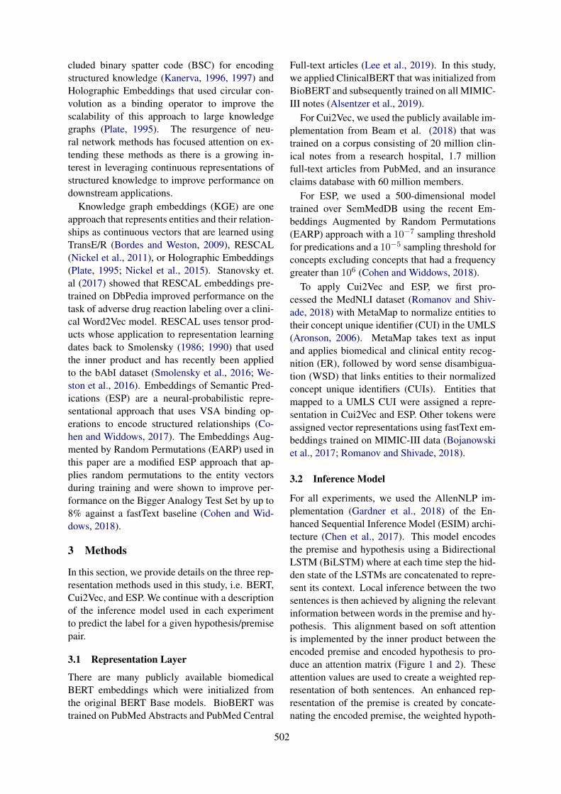
cluded binary spatter code (BSC) for encodingstructured knowledge (Kanerva, 1996, 1997) andHolographic Embeddings that used circular con-volution as a binding operator to improve thescalability of this approach to large knowledgegraphs (Plate, 1995). The resurgence of neu-ral network methods has focused attention on ex-tending these methods as there is a growing in-terest in leveraging continuous representations ofstructured knowledge to improve performance ondownstream applications.
Knowledge graph embeddings (KGE) are oneapproach that represents entities and their relation-ships as continuous vectors that are learned usingTransE/R (Bordes and Weston, 2009), RESCAL(Nickel et al., 2011), or Holographic Embeddings(Plate, 1995; Nickel et al., 2015). Stanovsky et.al (2017) showed that RESCAL embeddings pre-trained on DbPedia improved performance on thetask of adverse drug reaction labeling over a clini-cal Word2Vec model. RESCAL uses tensor prod-ucts whose application to representation learningdates back to Smolensky (1986; 1990) that usedthe inner product and has recently been appliedto the bAbI dataset (Smolensky et al., 2016; We-ston et al., 2016). Embeddings of Semantic Pred-ications (ESP) are a neural-probabilistic repre-sentational approach that uses VSA binding op-erations to encode structured relationships (Co-hen and Widdows, 2017). The Embeddings Aug-mented by Random Permutations (EARP) used inthis paper are a modified ESP approach that ap-plies random permutations to the entity vectorsduring training and were shown to improve per-formance on the Bigger Analogy Test Set by up to8% against a fastText baseline (Cohen and Wid-dows, 2018).
3 Methods
In this section, we provide details on the three rep-resentation methods used in this study, i.e. BERT,Cui2Vec, and ESP. We continue with a descriptionof the inference model used in each experimentto predict the label for a given hypothesis/premisepair.
3.1 Representation Layer
There are many publicly available biomedicalBERT embeddings which were initialized fromthe original BERT Base models. BioBERT wastrained on PubMed Abstracts and PubMed Central
Full-text articles (Lee et al., 2019). In this study,we applied ClinicalBERT that was initialized fromBioBERT and subsequently trained on all MIMIC-III notes (Alsentzer et al., 2019).
For Cui2Vec, we used the publicly available im-plementation from Beam et al. (2018) that wastrained on a corpus consisting of 20 million clin-ical notes from a research hospital, 1.7 millionfull-text articles from PubMed, and an insuranceclaims database with 60 million members.
For ESP, we used a 500-dimensional modeltrained over SemMedDB using the recent Em-beddings Augmented by Random Permutations(EARP) approach with a 10−7 sampling thresholdfor predications and a 10−5 sampling threshold forconcepts excluding concepts that had a frequencygreater than 106 (Cohen and Widdows, 2018).
To apply Cui2Vec and ESP, we first pro-cessed the MedNLI dataset (Romanov and Shiv-ade, 2018) with MetaMap to normalize entities totheir concept unique identifier (CUI) in the UMLS(Aronson, 2006). MetaMap takes text as inputand applies biomedical and clinical entity recog-nition (ER), followed by word sense disambigua-tion (WSD) that links entities to their normalizedconcept unique identifiers (CUIs). Entities thatmapped to a UMLS CUI were assigned a repre-sentation in Cui2Vec and ESP. Other tokens wereassigned vector representations using fastText em-beddings trained on MIMIC-III data (Bojanowskiet al., 2017; Romanov and Shivade, 2018).
3.2 Inference Model
For all experiments, we used the AllenNLP im-plementation (Gardner et al., 2018) of the En-hanced Sequential Inference Model (ESIM) archi-tecture (Chen et al., 2017). This model encodesthe premise and hypothesis using a BidirectionalLSTM (BiLSTM) where at each time step the hid-den state of the LSTMs are concatenated to repre-sent its context. Local inference between the twosentences is then achieved by aligning the relevantinformation between words in the premise and hy-pothesis. This alignment based on soft attentionis implemented by the inner product between theencoded premise and encoded hypothesis to pro-duce an attention matrix (Figure 1 and 2). Theseattention values are used to create a weighted rep-resentation of both sentences. An enhanced rep-resentation of the premise is created by concate-nating the encoded premise, the weighted hypoth-
502
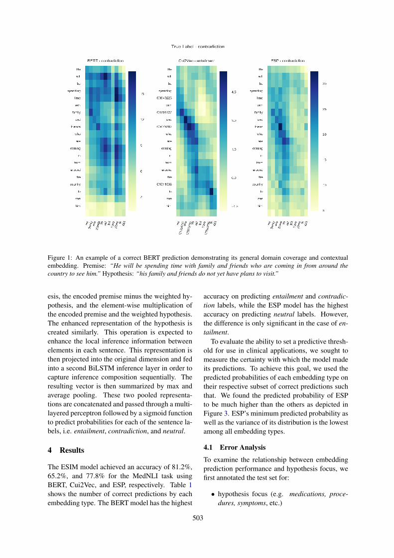
Figure 1: An example of a correct BERT prediction demonstrating its general domain coverage and contextualembedding. Premise: “He will be spending time with family and friends who are coming in from around thecountry to see him.” Hypothesis: “his family and friends do not yet have plans to visit.”
esis, the encoded premise minus the weighted hy-pothesis, and the element-wise multiplication ofthe encoded premise and the weighted hypothesis.The enhanced representation of the hypothesis iscreated similarly. This operation is expected toenhance the local inference information betweenelements in each sentence. This representation isthen projected into the original dimension and fedinto a second BiLSTM inference layer in order tocapture inference composition sequentially. Theresulting vector is then summarized by max andaverage pooling. These two pooled representa-tions are concatenated and passed through a multi-layered perceptron followed by a sigmoid functionto predict probabilities for each of the sentence la-bels, i.e. entailment, contradiction, and neutral.
4 Results
The ESIM model achieved an accuracy of 81.2%,65.2%, and 77.8% for the MedNLI task usingBERT, Cui2Vec, and ESP, respectively. Table 1shows the number of correct predictions by eachembedding type. The BERT model has the highest
accuracy on predicting entailment and contradic-tion labels, while the ESP model has the highestaccuracy on predicting neutral labels. However,the difference is only significant in the case of en-tailment.
To evaluate the ability to set a predictive thresh-old for use in clinical applications, we sought tomeasure the certainty with which the model madeits predictions. To achieve this goal, we used thepredicted probabilities of each embedding type ontheir respective subset of correct predictions suchthat. We found the predicted probability of ESPto be much higher than the others as depicted inFigure 3. ESP’s minimum predicted probability aswell as the variance of its distribution is the lowestamong all embedding types.
4.1 Error Analysis
To examine the relationship between embeddingprediction performance and hypothesis focus, wefirst annotated the test set for:
• hypothesis focus (e.g. medications, proce-dures, symptoms, etc.)
503
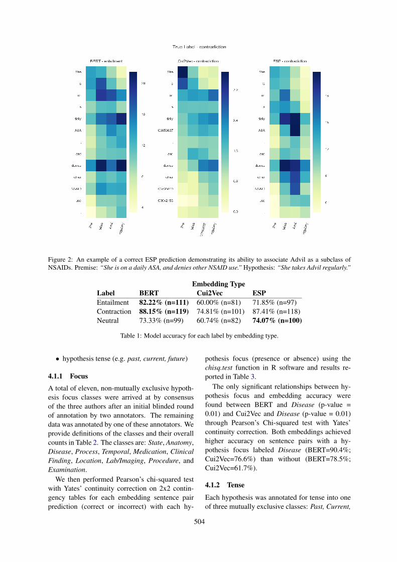
Figure 2: An example of a correct ESP prediction demonstrating its ability to associate Advil as a subclass ofNSAIDs. Premise: “She is on a daily ASA, and denies other NSAID use.” Hypothesis: “She takes Advil regularly.”
Embedding TypeLabel BERT Cui2Vec ESPEntailment 82.22% (n=111) 60.00% (n=81) 71.85% (n=97)Contraction 88.15% (n=119) 74.81% (n=101) 87.41% (n=118)Neutral 73.33% (n=99) 60.74% (n=82) 74.07% (n=100)
Table 1: Model accuracy for each label by embedding type.
• hypothesis tense (e.g. past, current, future)
4.1.1 Focus
A total of eleven, non-mutually exclusive hypoth-esis focus classes were arrived at by consensusof the three authors after an initial blinded roundof annotation by two annotators. The remainingdata was annotated by one of these annotators. Weprovide definitions of the classes and their overallcounts in Table 2. The classes are: State, Anatomy,Disease, Process, Temporal, Medication, ClinicalFinding, Location, Lab/Imaging, Procedure, andExamination.
We then performed Pearson’s chi-squared testwith Yates’ continuity correction on 2x2 contin-gency tables for each embedding sentence pairprediction (correct or incorrect) with each hy-
pothesis focus (presence or absence) using thechisq.test function in R software and results re-ported in Table 3.
The only significant relationships between hy-pothesis focus and embedding accuracy werefound between BERT and Disease (p-value =0.01) and Cui2Vec and Disease (p-value = 0.01)through Pearson’s Chi-squared test with Yates’continuity correction. Both embeddings achievedhigher accuracy on sentence pairs with a hy-pothesis focus labeled Disease (BERT=90.4%;Cui2Vec=76.6%) than without (BERT=78.5%;Cui2Vec=61.7%).
4.1.2 Tense
Each hypothesis was annotated for tense into oneof three mutually exclusive classes: Past, Current,
504
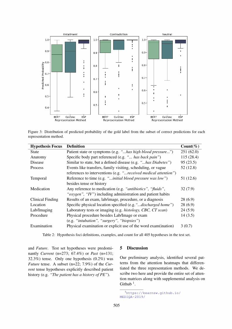
Figure 3: Distribution of predicted probability of the gold label from the subset of correct predictions for eachrepresentation method.
Hypothesis Focus Definition Count(%)State Patient state or symptoms (e.g. “...has high blood pressure...”) 251 (62.0)Anatomy Specific body part referenced (e.g. “... has back pain”) 115 (28.4)Disease Similar to state, but a defined disease (e.g. “...has Diabetes”) 95 (23.5)Process Events like transfers, family visiting, scheduling, or vague 52 (12.8)
references to interventions (e.g. “...received medical attention”)Temporal Reference to time (e.g. “...initial blood pressure was low”) 51 (12.6)
besides tense or historyMedication Any reference to medication (e.g. “antibiotics”, “fluids”, 32 (7.9)
“oxygen”, “IV”) including administration and patient habitsClinical Finding Results of an exam, lab/image, procedure, or a diagnosis 28 (6.9)Location Specific physical location specified (e.g.“...discharged home”) 28 (6.9)Lab/Imaging Laboratory tests or imaging (e.g. histology, CBC, CT scan) 24 (5.9)Procedure Physical procedure besides Lab/Image or exam 14 (3.5)
(e.g. “intubation”, “surgery”, “biopsies”)Examination Physical examination or explicit use of the word exam(ination) 3 (0.7)
Table 2: Hypothesis foci definitions, examples, and count for all 405 hypotheses in the test set.
and Future. Test set hypotheses were predomi-nantly Current (n=273; 67.4%) or Past (n=131;32.3%) tense. Only one hypothesis (0.2%) wasFuture tense. A subset (n=22; 7.9%) of the Cur-rent tense hypotheses explicitly described patienthistory (e.g. “The patient has a history of PE”).
5 Discussion
Our preliminary analysis, identified several pat-terns from the attention heatmaps that differen-tiated the three representation methods. We de-scribe two here and provide the entire set of atten-tion matrices along with supplemental analysis onGithub 1.
1https://kearnsw.github.io/MEDIQA-2019/
505
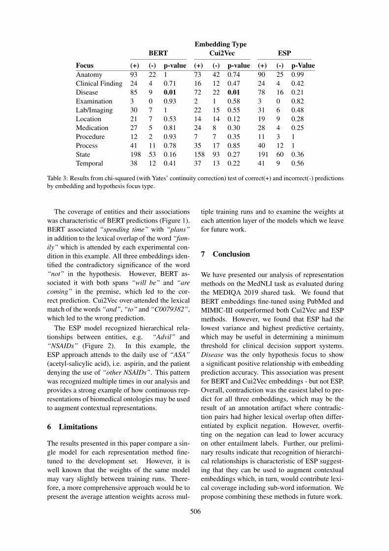
Embedding TypeBERT Cui2Vec ESP
Focus (+) (-) p-value (+) (-) p-value (+) (-) p-ValueAnatomy 93 22 1 73 42 0.74 90 25 0.99Clinical Finding 24 4 0.71 16 12 0.47 24 4 0.42Disease 85 9 0.01 72 22 0.01 78 16 0.21Examination 3 0 0.93 2 1 0.58 3 0 0.82Lab/Imaging 30 7 1 22 15 0.55 31 6 0.48Location 21 7 0.53 14 14 0.12 19 9 0.28Medication 27 5 0.81 24 8 0.30 28 4 0.25Procedure 12 2 0.93 7 7 0.35 11 3 1Process 41 11 0.78 35 17 0.85 40 12 1State 198 53 0.16 158 93 0.27 191 60 0.36Temporal 38 12 0.41 37 13 0.22 41 9 0.56
Table 3: Results from chi-squared (with Yates’ continuity correction) test of correct(+) and incorrect(-) predictionsby embedding and hypothesis focus type.
The coverage of entities and their associationswas characteristic of BERT predictions (Figure 1).BERT associated “spending time” with “plans”in addition to the lexical overlap of the word “fam-ily” which is attended by each experimental con-dition in this example. All three embeddings iden-tified the contradictory significance of the word“not” in the hypothesis. However, BERT as-sociated it with both spans “will be” and “arecoming” in the premise, which led to the cor-rect prediction. Cui2Vec over-attended the lexicalmatch of the words “and”, “to” and “C0079382”,which led to the wrong prediction.
The ESP model recognized hierarchical rela-tionships between entities, e.g. “Advil” and“NSAIDs” (Figure 2). In this example, theESP approach attends to the daily use of “ASA”(acetyl-salicylic acid), i.e. aspirin, and the patientdenying the use of “other NSAIDs”. This patternwas recognized multiple times in our analysis andprovides a strong example of how continuous rep-resentations of biomedical ontologies may be usedto augment contextual representations.
6 Limitations
The results presented in this paper compare a sin-gle model for each representation method fine-tuned to the development set. However, it iswell known that the weights of the same modelmay vary slightly between training runs. There-fore, a more comprehensive approach would be topresent the average attention weights across mul-
tiple training runs and to examine the weights ateach attention layer of the models which we leavefor future work.
7 Conclusion
We have presented our analysis of representationmethods on the MedNLI task as evaluated duringthe MEDIQA 2019 shared task. We found thatBERT embeddings fine-tuned using PubMed andMIMIC-III outperformed both Cui2Vec and ESPmethods. However, we found that ESP had thelowest variance and highest predictive certainty,which may be useful in determining a minimumthreshold for clinical decision support systems.Disease was the only hypothesis focus to showa significant positive relationship with embeddingprediction accuracy. This association was presentfor BERT and Cui2Vec embeddings - but not ESP.Overall, contradiction was the easiest label to pre-dict for all three embeddings, which may be theresult of an annotation artifact where contradic-tion pairs had higher lexical overlap often differ-entiated by explicit negation. However, overfit-ting on the negation can lead to lower accuracyon other entailment labels. Further, our prelimi-nary results indicate that recognition of hierarchi-cal relationships is characteristic of ESP suggest-ing that they can be used to augment contextualembeddings which, in turn, would contribute lexi-cal coverage including sub-word information. Wepropose combining these methods in future work.
506
Acknowledgments
We would like to acknowledge Trevor Cohen forsharing the Embeddings of Semantic Predicationsused in this study. Author Jason A. Thomas’ workwas supported, in part, by the National Library ofMedicine (NLM) Training Grant T15LM007442.This work was facilitated, in part, through theuse of the advanced computational, storage,and networking infrastructure managed by theResearch Computing Club at the University ofWashington and funded by an STF award.
ReferencesEmily Alsentzer, John R. Murphy, Willie Boag, Wei-
Hung Weng, Di Jin, Tristan Naumann, and MatthewB. A. McDermott. 2019. Publicly available clinicalBERT embeddings. CoRR, abs/1904.03323.
Alan R Aronson. 2006. Metamap: Mapping text tothe umls metathesaurus. Bethesda MD NLM NIHDHHS, pages 1–26.
Collin F. Baker, Charles J. Fillmore, and John B. Lowe.1998. The berkeley framenet project. In Pro-ceedings of the 36th Annual Meeting of the Asso-ciation for Computational Linguistics and 17th In-ternational Conference on Computational Linguis-tics - Volume 1, ACL ’98/COLING ’98, pages 86–90, Stroudsburg, PA, USA. Association for Com-putational Linguistics. https://doi.org/10.3115/980845.980860.
Andrew L. Beam, Benjamin Kompa, Inbar Fried,Nathan P. Palmer, Xu Shi, Tianxi Cai, and Isaac S.Kohane. 2018. Clinical concept embeddings learnedfrom massive sources of medical data. CoRR,abs/1804.01486.
Asma Ben Abacha, Chaitanya Shivade, and DinaDemner-Fushman. 2019. Overview of the mediqa2019 shared task on textual inference, question en-tailment and question answering. In Proceedings ofthe BioNLP 2019 workshop, Florence, Italy, August1, 2019. Association for Computational Linguistics.
Yoshua Bengio, Réjean Ducharme, Pascal Vincent, andChristian Janvin. 2003. A neural probabilistic lan-guage model. J. Mach. Learn. Res., 3:1137–1155.
Adam L. Berger, Vincent J. Della Pietra, and StephenA. Della Pietra. 1996. A maximum entropy ap-proach to natural language processing. Comput.Linguist., 22(1):39–71.
David M. Blei, Andrew Y. Ng, and Michael I. Jordan.2003. Latent dirichlet allocation. J. Mach. Learn.Res., 3:993–1022.
Piotr Bojanowski, Edouard Grave, Armand Joulin,and Tomas Mikolov. 2017. Enriching word vec-tors with subword information. Transactions of theAssociation for Computational Linguistics, 5:135–146. https://doi.org/10.1162/tacl_a_00051.
Antoine Bordes and Jason Weston. 2009. Learn-ing Structured Embeddings of KnowledgeBases. Artificial Intelligence, (Bengio):301–306.https://doi.org/10.1016/j.procs.2017.05.045.
Qian Chen, Xiaodan Zhu, Zhen-Hua Ling, Si Wei, HuiJiang, and Diana Inkpen. 2017. Enhanced LSTM fornatural language inference. In Proceedings of the55th Annual Meeting of the Association for Com-putational Linguistics (Volume 1: Long Papers),pages 1657–1668, Vancouver, Canada. Associationfor Computational Linguistics. https://doi.org/10.18653/v1/P17-1152.
Trevor Cohen and Dominic Widdows. 2017. Embed-ding of semantic predications. Journal of Biomed-ical Informatics, 68:150–166. https://doi.org/10.1016/j.jbi.2017.03.003.
Trevor Cohen and Dominic Widdows. 2018. Bring-ing order to neural word embeddings with embed-dings augmented by random permutations (EARP).In Proceedings of the 22nd Conference on Computa-tional Natural Language Learning, pages 465–475,Brussels, Belgium. Association for ComputationalLinguistics.
Scott C. Deerwester, Susan T. Dumais, Thomas K. Lan-dauer, George W. Furnas, and Richard A. Harshman.1990. Indexing by latent semantic analysis. JASIS,41:391–407.
Jacob Devlin, Ming-Wei Chang, Kenton Lee, andKristina Toutanova. 2018. BERT: pre-training ofdeep bidirectional transformers for language under-standing. CoRR, abs/1810.04805.
Matt Gardner, Joel Grus, Mark Neumann, OyvindTafjord, Pradeep Dasigi, Nelson F. Liu, Matthew Pe-ters, Michael Schmitz, and Luke Zettlemoyer. 2018.AllenNLP: A deep semantic natural language pro-cessing platform. In Proceedings of Workshop forNLP Open Source Software (NLP-OSS), pages 1–6, Melbourne, Australia. Association for Computa-tional Linguistics.
Sonal Gupta, Rushin Shah, Mrinal Mohit, Anuj Ku-mar, and Mike Lewis. 2018. Semantic parsing fortask oriented dialog using hierarchical representa-tions. CoRR, abs/1810.07942.
Luheng He. 2015. Question-Answer Driven Se-mantic Role Labeling : Using Natural Lan-guage to Annotate Natural Language. Emnlp2015,(September):643–653. https://doi.org/10.18653/v1/D15-1076.
507
Thomas Hofmann. 1999. Probabilistic latent semanticindexing. In Proceedings of the 22Nd Annual Inter-national ACM SIGIR Conference on Research andDevelopment in Information Retrieval, SIGIR ’99,pages 50–57, New York, NY, USA. ACM. https://doi.org/10.1145/312624.312649.
Kexin Huang, Jaan Altosaar, and Rajesh Ran-ganath. 2019. ClinicalBERT: Modeling Clini-cal Notes and Predicting Hospital Readmission.arXiv:1904.05342 [cs]. ArXiv: 1904.05342.
Alistair E W Johnson, Tom J Pollard, Lu Shen, Li-wei H Lehman, Mengling Feng, Mohammad Ghas-semi, Benjamin Moody, Peter Szolovits, Leo An-thony Celi, and Roger G Mark. 2016. MIMIC-III,a freely accessible critical care database. pages 1–9.
Pentti Kanerva. 1996. Binary spatter-coding of orderedk-tuples. In Proceedings of the 1996 InternationalConference on Artificial Neural Networks, ICANN96, pages 869–873, London, UK, UK. Springer-Verlag.
Pentti Kanerva. 1997. Fully distributed representation.In In Proceedings Real World Computing Sympo-sium (Report TR-96001), pages 358–365.
Pentti Kanerva, Jan Kristoferson, and Anders Holst.2000. Random indexing of text samples for latentsemantic analysis. In In Proceedings of the 22ndAnnual Conference of the Cognitive Science Society,pages 103–6. Erlbaum.
William R Kearns and Jason A Thomas. 2018. Re-source and response type classification for consumerhealth question answering. AMIA Annual Sym-posium proceedings. AMIA Symposium, 2018:634–643.
Halil Kilicoglu, Dongwook Shin, Marcelo Fiszman,Graciela Rosemblat, and Thomas C. Rindflesch.2012. SemMedDB: A PubMed-scale repositoryof biomedical semantic predications. Bioinfor-matics, 28(23):3158–3160. https://doi.org/10.1093/bioinformatics/bts591.
Yoon Kim, Yacine Jernite, David Sontag, and Alexan-der M. Rush. 2015. Character-aware neural lan-guage models. CoRR, abs/1508.06615.
Staffan Larsson and David R. Traum. 2000. In-formation state and dialogue management in thetrindi dialogue move engine toolkit. Nat. Lang.Eng., 6(3-4):323–340. https://doi.org/10.1017/S1351324900002539.
Jinhyuk Lee, Wonjin Yoon, Sungdong Kim,Donghyeon Kim, Sunkyu Kim, Chan Ho So,and Jaewoo Kang. 2019. BioBERT: a pre-trainedbiomedical language representation model forbiomedical text mining. arXiv:1901.08746 [cs].
Simon D. Levy and Ross Gayler. 2008. Vector sym-bolic architectures: A new building material for ar-tificial general intelligence. In Proceedings of the
2008 Conference on Artificial General Intelligence2008: Proceedings of the First AGI Conference,pages 414–418, Amsterdam, The Netherlands, TheNetherlands. IOS Press.
Xiaodong Liu, Pengcheng He, Weizhu Chen, andJianfeng Gao. 2019. Multi-task deep neural net-works for natural language understanding. CoRR,abs/1901.11504.
Julian Michael, Gabriel Stanovsky, Luheng He, IdoDagan, and Luke Zettlemoyer. 2018. Crowdsourc-ing question-answer meaning representations. InProceedings of the 2018 Conference of the NorthAmerican Chapter of the Association for Compu-tational Linguistics: Human Language Technolo-gies, Volume 2 (Short Papers), pages 560–568, NewOrleans, Louisiana. Association for ComputationalLinguistics. https://doi.org/10.18653/v1/N18-2089.
Tomas Mikolov, Ilya Sutskever, Kai Chen, Greg Cor-rado, and Jeffrey Dean. 2013. Distributed represen-tations of words and phrases and their composition-ality. In Proceedings of the 26th International Con-ference on Neural Information Processing Systems -Volume 2, NIPS’13, pages 3111–3119, USA. CurranAssociates Inc.
Maximilian Nickel, Lorenzo Rosasco, and Tomaso A.Poggio. 2015. Holographic embeddings of knowl-edge graphs. CoRR, abs/1510.04935.
Maximilian Nickel, Volker Tresp, and Hans-PeterKriegel. 2011. A three-way model for collectivelearning on multi-relational data. In Proceedings ofthe 28th International Conference on InternationalConference on Machine Learning, ICML’11, pages809–816, USA. Omnipress.
Ioannis Pavlopoulos, Aris Kosmopoulos, and Ion An-droutsopoulos. 2014. Continuous Space WordVectors Obtained by Applying Word2Vec to Ab-stracts of Biomedical Articles. http://bioasq.lip6.fr/info/BioASQword2vec/.
Jeffrey Pennington, Richard Socher, and Christo-pher Manning. 2014. Glove: Global vectorsfor word representation. In Proceedings of the2014 Conference on Empirical Methods in NaturalLanguage Processing (EMNLP), pages 1532–1543,Doha, Qatar. Association for Computational Lin-guistics. https://doi.org/10.3115/v1/D14-1162.
Matthew E. Peters, Mark Neumann, Mohit Iyyer, MattGardner, Christopher Clark, Kenton Lee, and LukeZettlemoyer. 2018. Deep contextualized word rep-resentations. CoRR, abs/1802.05365.
T. A. Plate. 1995. Holographic reduced represen-tations. IEEE Transactions on Neural Networks,6(3):623–641. https://doi.org/10.1109/72.377968.
508
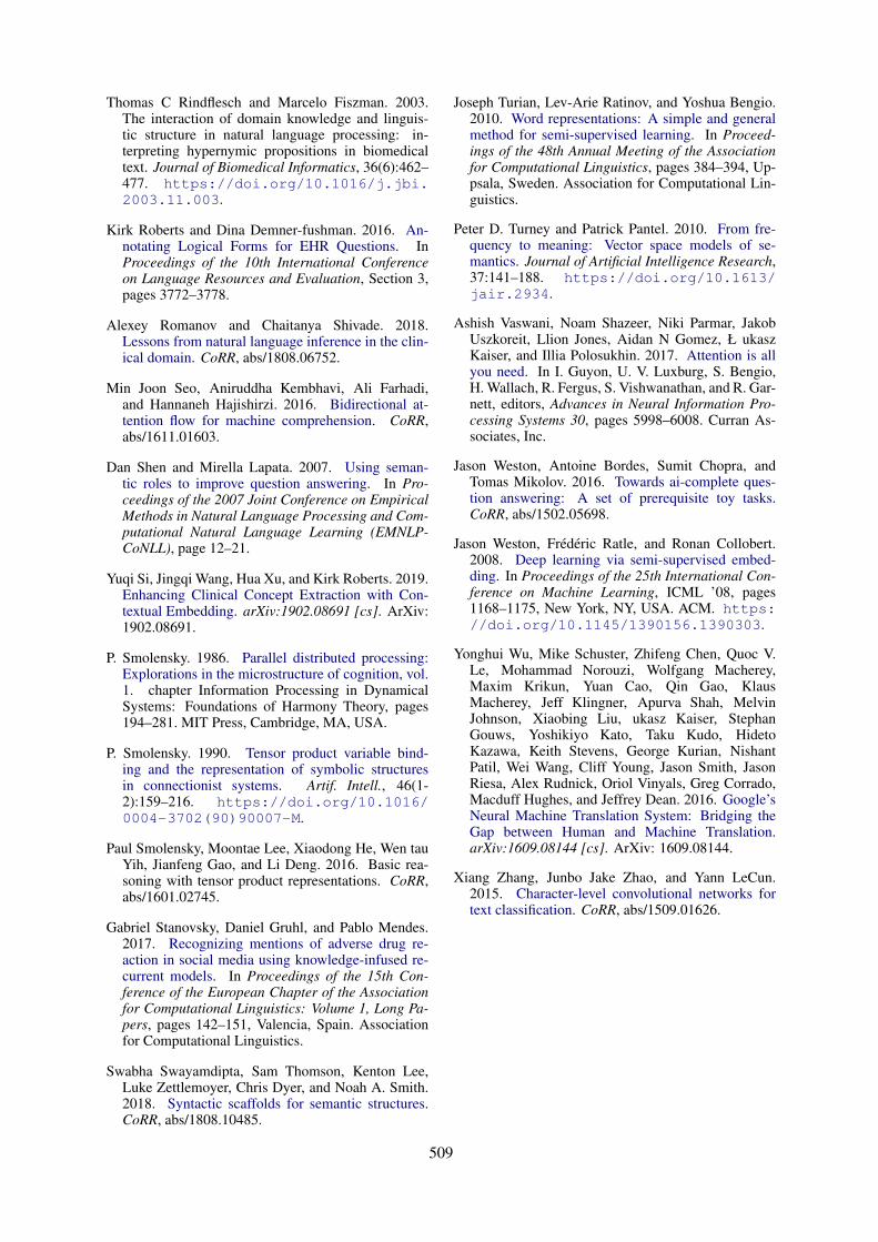
Thomas C Rindflesch and Marcelo Fiszman. 2003.The interaction of domain knowledge and linguis-tic structure in natural language processing: in-terpreting hypernymic propositions in biomedicaltext. Journal of Biomedical Informatics, 36(6):462–477. https://doi.org/10.1016/j.jbi.2003.11.003.
Kirk Roberts and Dina Demner-fushman. 2016. An-notating Logical Forms for EHR Questions. InProceedings of the 10th International Conferenceon Language Resources and Evaluation, Section 3,pages 3772–3778.
Alexey Romanov and Chaitanya Shivade. 2018.Lessons from natural language inference in the clin-ical domain. CoRR, abs/1808.06752.
Min Joon Seo, Aniruddha Kembhavi, Ali Farhadi,and Hannaneh Hajishirzi. 2016. Bidirectional at-tention flow for machine comprehension. CoRR,abs/1611.01603.
Dan Shen and Mirella Lapata. 2007. Using seman-tic roles to improve question answering. In Pro-ceedings of the 2007 Joint Conference on EmpiricalMethods in Natural Language Processing and Com-putational Natural Language Learning (EMNLP-CoNLL), page 12–21.
Yuqi Si, Jingqi Wang, Hua Xu, and Kirk Roberts. 2019.Enhancing Clinical Concept Extraction with Con-textual Embedding. arXiv:1902.08691 [cs]. ArXiv:1902.08691.
P. Smolensky. 1986. Parallel distributed processing:Explorations in the microstructure of cognition, vol.1. chapter Information Processing in DynamicalSystems: Foundations of Harmony Theory, pages194–281. MIT Press, Cambridge, MA, USA.
P. Smolensky. 1990. Tensor product variable bind-ing and the representation of symbolic structuresin connectionist systems. Artif. Intell., 46(1-2):159–216. https://doi.org/10.1016/0004-3702(90)90007-M.
Paul Smolensky, Moontae Lee, Xiaodong He, Wen tauYih, Jianfeng Gao, and Li Deng. 2016. Basic rea-soning with tensor product representations. CoRR,abs/1601.02745.
Gabriel Stanovsky, Daniel Gruhl, and Pablo Mendes.2017. Recognizing mentions of adverse drug re-action in social media using knowledge-infused re-current models. In Proceedings of the 15th Con-ference of the European Chapter of the Associationfor Computational Linguistics: Volume 1, Long Pa-pers, pages 142–151, Valencia, Spain. Associationfor Computational Linguistics.
Swabha Swayamdipta, Sam Thomson, Kenton Lee,Luke Zettlemoyer, Chris Dyer, and Noah A. Smith.2018. Syntactic scaffolds for semantic structures.CoRR, abs/1808.10485.
Joseph Turian, Lev-Arie Ratinov, and Yoshua Bengio.2010. Word representations: A simple and generalmethod for semi-supervised learning. In Proceed-ings of the 48th Annual Meeting of the Associationfor Computational Linguistics, pages 384–394, Up-psala, Sweden. Association for Computational Lin-guistics.
Peter D. Turney and Patrick Pantel. 2010. From fre-quency to meaning: Vector space models of se-mantics. Journal of Artificial Intelligence Research,37:141–188. https://doi.org/10.1613/jair.2934.
Ashish Vaswani, Noam Shazeer, Niki Parmar, JakobUszkoreit, Llion Jones, Aidan N Gomez, Ł ukaszKaiser, and Illia Polosukhin. 2017. Attention is allyou need. In I. Guyon, U. V. Luxburg, S. Bengio,H. Wallach, R. Fergus, S. Vishwanathan, and R. Gar-nett, editors, Advances in Neural Information Pro-cessing Systems 30, pages 5998–6008. Curran As-sociates, Inc.
Jason Weston, Antoine Bordes, Sumit Chopra, andTomas Mikolov. 2016. Towards ai-complete ques-tion answering: A set of prerequisite toy tasks.CoRR, abs/1502.05698.
Jason Weston, Frédéric Ratle, and Ronan Collobert.2008. Deep learning via semi-supervised embed-ding. In Proceedings of the 25th International Con-ference on Machine Learning, ICML ’08, pages1168–1175, New York, NY, USA. ACM. https://doi.org/10.1145/1390156.1390303.
Yonghui Wu, Mike Schuster, Zhifeng Chen, Quoc V.Le, Mohammad Norouzi, Wolfgang Macherey,Maxim Krikun, Yuan Cao, Qin Gao, KlausMacherey, Jeff Klingner, Apurva Shah, MelvinJohnson, Xiaobing Liu, ukasz Kaiser, StephanGouws, Yoshikiyo Kato, Taku Kudo, HidetoKazawa, Keith Stevens, George Kurian, NishantPatil, Wei Wang, Cliff Young, Jason Smith, JasonRiesa, Alex Rudnick, Oriol Vinyals, Greg Corrado,Macduff Hughes, and Jeffrey Dean. 2016. Google’sNeural Machine Translation System: Bridging theGap between Human and Machine Translation.arXiv:1609.08144 [cs]. ArXiv: 1609.08144.
Xiang Zhang, Junbo Jake Zhao, and Yann LeCun.2015. Character-level convolutional networks fortext classification. CoRR, abs/1509.01626.
509
Proceedings of the BioNLP 2019 workshop, pages 510–516Florence, Italy, August 1, 2019. c©2019 Association for Computational Linguistics
Saama Research at MEDIQA 2019: Pre-trained BioBERT with AttentionVisualisation for Medical Natural Language Inference
Kamal Raj Kanakarajan , Suriyadeepan Ramamoorthy, Vaidheeswaran Archana,Soham Chatterjee, Malaikannan Sankarasubbu∗
SAAMA AI Research Lab, Chennai, India{kamal.raj, suriyadeepan.ramamoorthy, archana.iyer, soham.chatterjee,
malaikannan.sankarasubbu}@saama.com
Abstract
Natural Language inference is the task of iden-tifying relation between two sentences as en-tailment, contradiction or neutrality. MedNLIis a biomedical flavour of NLI for clini-cal domain. This paper explores the useof Bidirectional Encoder Representation fromTransformer (BERT) for solving MedNLI.The proposed model, BERT pre-trained onPMC, PubMed and fine-tuned on MIMIC-III v1.4, achieves state of the art results onMedNLI (83.45%) and an accuracy of 78.5%in MEDIQA challenge. The authors present ananalysis of the attention patterns that emergedas a result of training BERT on MedNLI usinga visualization tool, bertviz.
1 Introduction
Natural Language Inference (NLI) is a fundamen-tal task in Natural Language Processing in whichthe objective is to determine if the hypothesisis true (entailment), false (contradiction) or un-determined (neutral), given a premise. Entail-ment, Contradiction and Neutral (semantic inde-pendence) are semantic concepts that represent therelationship between sentences. The ability to in-fer these relations between sentences or pieces oftext, is crucial in tasks like Information Retrieval,Semantic Parsing, Commonsense Reasoning, etc.NLI, like most NLP tasks, is challenging due to theambiguous nature of natural language. A particu-lar meaning can be expressed in multiple linguis-tic forms. This calls for methods that can capturemeaningful semantic concepts from text.
Stanford Natural Language Inference (SNLI)corpus (Bowman et al., 2015) is a collection of
∗*Equal Contribution: Kamal had sole access to MIMICand MEDIQA data, focussed on the algorithm developmentand implementation. Suriyadeepan and Archana focussed onthe attention visualisation and writing. Soham and Malaikan-nan focussed on reviewing
sentence pairs labeled for entailment, contradic-tion, and semantic independence. It contains ap-proximately 550,000 labeled hypothesis/premisepairs. Multi-Genre Natural Language Inference(Multi-NLI) corpus (Williams et al., 2017) con-tains 433,000 samples, covering a wide range of(10) genres of written and spoken English. Multi-NLI, in its complexity, is closer to Natural Lan-guage than SNLI.
MedNLI (Romanov and Shivade) is a datasetfor natural language inference in clinical domain,analogous to SNLI. Romanov et al in (Romanovand Shivade), used InferSent (Conneau et al.,2017), a bidirectional LSTM based model forachieving an accuracy of 73.5% in MedNLI. In(Jin et al., 2019), Jin et al make use of BioBERT(Lee et al., 2019), a biomedical version of BERTalong with pre-trained LMs(Language Models) asfeature extractors, to achieve an accuracy of 81.7%on MedNLI.
This work uses BERT pre-trained on PMC andPubMed corpus, and fine-tuned on MIMIC-IIIv1.4 data (BioBERT) to solve MedNLI. This ap-proach achieves new state of the art results whenevaluated on MedNLI test set (83.4%). Evalua-tion on MEDIQA (Ben Abacha et al., 2019) testset (Shivade, 2019) results in an accuracy of 78.5%.
2 Data
2.1 MedNLI
MedNLI or Medical Natural Language Inferenceis a publicly annotated dataset in the clinical do-main. MedNLI was created as a NLI dataset com-parable to SNLI, adjusted for the clinical domain(Table 1).
510
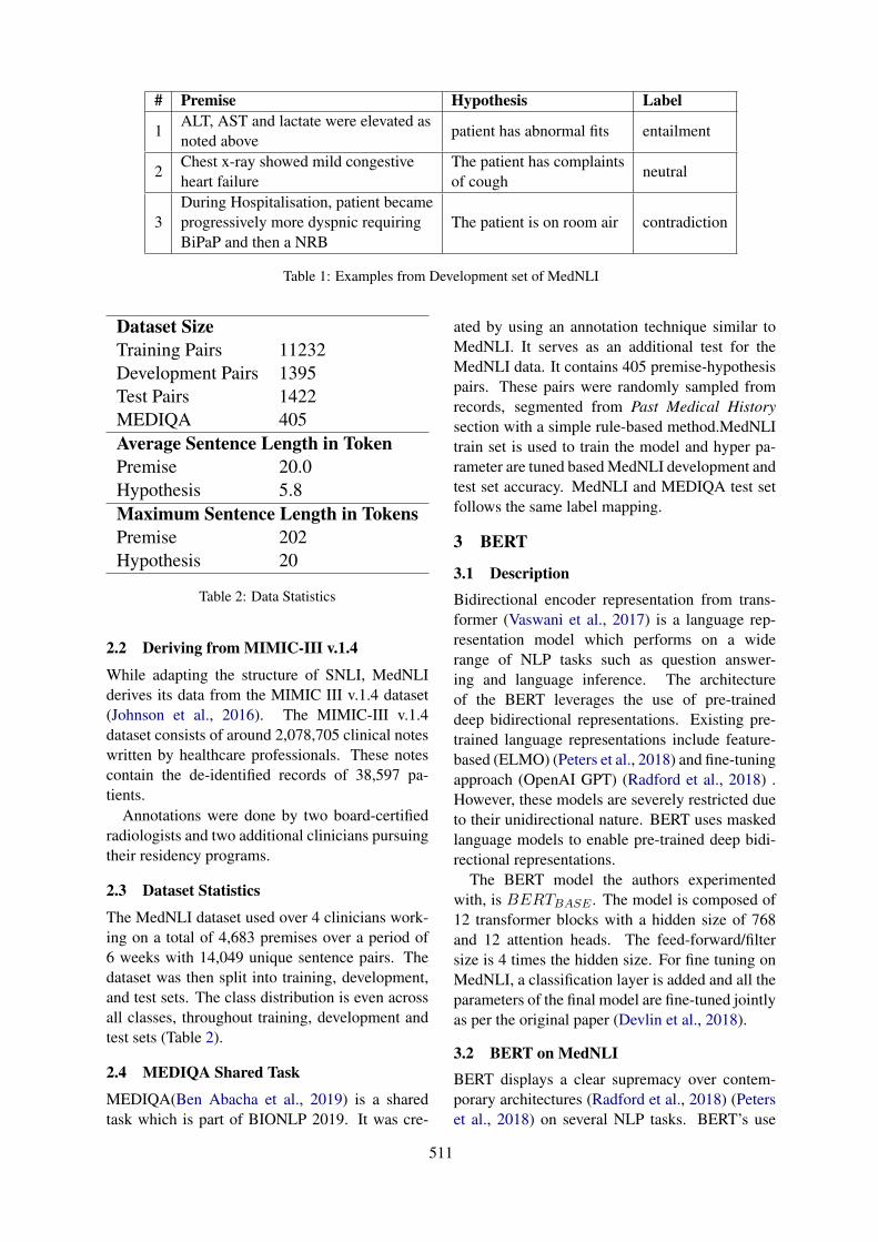
# Premise Hypothesis Label
1ALT, AST and lactate were elevated asnoted above
patient has abnormal fits entailment
2Chest x-ray showed mild congestiveheart failure
The patient has complaintsof cough
neutral
3During Hospitalisation, patient becameprogressively more dyspnic requiringBiPaP and then a NRB
The patient is on room air contradiction
Table 1: Examples from Development set of MedNLI
Dataset SizeTraining Pairs 11232Development Pairs 1395Test Pairs 1422MEDIQA 405Average Sentence Length in TokenPremise 20.0Hypothesis 5.8Maximum Sentence Length in TokensPremise 202Hypothesis 20
Table 2: Data Statistics
2.2 Deriving from MIMIC-III v.1.4
While adapting the structure of SNLI, MedNLIderives its data from the MIMIC III v.1.4 dataset(Johnson et al., 2016). The MIMIC-III v.1.4dataset consists of around 2,078,705 clinical noteswritten by healthcare professionals. These notescontain the de-identified records of 38,597 pa-tients.
Annotations were done by two board-certifiedradiologists and two additional clinicians pursuingtheir residency programs.
2.3 Dataset Statistics
The MedNLI dataset used over 4 clinicians work-ing on a total of 4,683 premises over a period of6 weeks with 14,049 unique sentence pairs. Thedataset was then split into training, development,and test sets. The class distribution is even acrossall classes, throughout training, development andtest sets (Table 2).
2.4 MEDIQA Shared Task
MEDIQA(Ben Abacha et al., 2019) is a sharedtask which is part of BIONLP 2019. It was cre-
ated by using an annotation technique similar toMedNLI. It serves as an additional test for theMedNLI data. It contains 405 premise-hypothesispairs. These pairs were randomly sampled fromrecords, segmented from Past Medical Historysection with a simple rule-based method.MedNLItrain set is used to train the model and hyper pa-rameter are tuned based MedNLI development andtest set accuracy. MedNLI and MEDIQA test setfollows the same label mapping.
3 BERT
3.1 DescriptionBidirectional encoder representation from trans-former (Vaswani et al., 2017) is a language rep-resentation model which performs on a widerange of NLP tasks such as question answer-ing and language inference. The architectureof the BERT leverages the use of pre-traineddeep bidirectional representations. Existing pre-trained language representations include feature-based (ELMO) (Peters et al., 2018) and fine-tuningapproach (OpenAI GPT) (Radford et al., 2018) .However, these models are severely restricted dueto their unidirectional nature. BERT uses maskedlanguage models to enable pre-trained deep bidi-rectional representations.
The BERT model the authors experimentedwith, is BERTBASE . The model is composed of12 transformer blocks with a hidden size of 768and 12 attention heads. The feed-forward/filtersize is 4 times the hidden size. For fine tuning onMedNLI, a classification layer is added and all theparameters of the final model are fine-tuned jointlyas per the original paper (Devlin et al., 2018).
3.2 BERT on MedNLIBERT displays a clear supremacy over contem-porary architectures (Radford et al., 2018) (Peterset al., 2018) on several NLP tasks. BERT’s use
511
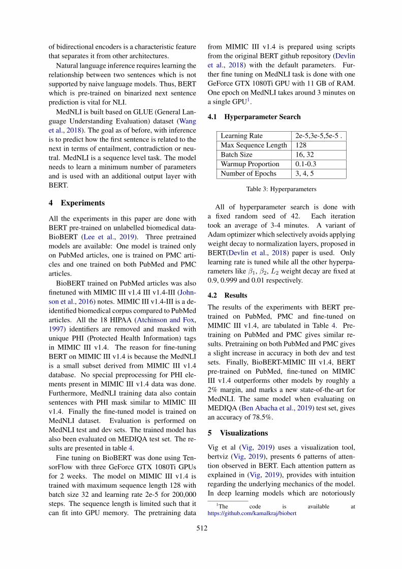
of bidirectional encoders is a characteristic featurethat separates it from other architectures.
Natural language inference requires learning therelationship between two sentences which is notsupported by naive language models. Thus, BERTwhich is pre-trained on binarized next sentenceprediction is vital for NLI.
MedNLI is built based on GLUE (General Lan-guage Understanding Evaluation) dataset (Wanget al., 2018). The goal as of before, with inferenceis to predict how the first sentence is related to thenext in terms of entailment, contradiction or neu-tral. MedNLI is a sequence level task. The modelneeds to learn a minimum number of parametersand is used with an additional output layer withBERT.
4 Experiments
All the experiments in this paper are done withBERT pre-trained on unlabelled biomedical data-BioBERT (Lee et al., 2019). Three pretrainedmodels are available: One model is trained onlyon PubMed articles, one is trained on PMC arti-cles and one trained on both PubMed and PMCarticles.
BioBERT trained on PubMed articles was alsofinetuned with MIMIC III v1.4 III v1.4-III (John-son et al., 2016) notes. MIMIC III v1.4-III is a de-identified biomedical corpus compared to PubMedarticles. All the 18 HIPAA (Atchinson and Fox,1997) identifiers are removed and masked withunique PHI (Protected Health Information) tagsin MIMIC III v1.4. The reason for fine-tuningBERT on MIMIC III v1.4 is because the MedNLIis a small subset derived from MIMIC III v1.4database. No special preprocessing for PHI ele-ments present in MIMIC III v1.4 data was done.Furthermore, MedNLI training data also containsentences with PHI mask similar to MIMIC IIIv1.4. Finally the fine-tuned model is trained onMedNLI dataset. Evaluation is performed onMedNLI test and dev sets. The trained model hasalso been evaluated on MEDIQA test set. The re-sults are presented in table 4.
Fine tuning on BioBERT was done using Ten-sorFlow with three GeForce GTX 1080Ti GPUsfor 2 weeks. The model on MIMIC III v1.4 istrained with maximum sequence length 128 withbatch size 32 and learning rate 2e-5 for 200,000steps. The sequence length is limited such that itcan fit into GPU memory. The pretraining data
from MIMIC III v1.4 is prepared using scriptsfrom the original BERT github repository (Devlinet al., 2018) with the default parameters. Fur-ther fine tuning on MedNLI task is done with oneGeForce GTX 1080Ti GPU with 11 GB of RAM.One epoch on MedNLI takes around 3 minutes ona single GPU1.
4.1 Hyperparameter Search
Learning Rate 2e-5,3e-5,5e-5 .Max Sequence Length 128Batch Size 16, 32Warmup Proportion 0.1-0.3Number of Epochs 3, 4, 5
Table 3: Hyperparameters
All of hyperparameter search is done witha fixed random seed of 42. Each iterationtook an average of 3-4 minutes. A variant ofAdam optimizer which selectively avoids applyingweight decay to normalization layers, proposed inBERT(Devlin et al., 2018) paper is used. Onlylearning rate is tuned while all the other hyperpa-rameters like β1, β2, L2 weight decay are fixed at0.9, 0.999 and 0.01 respectively.
4.2 ResultsThe results of the experiments with BERT pre-trained on PubMed, PMC and fine-tuned onMIMIC III v1.4, are tabulated in Table 4. Pre-training on PubMed and PMC gives similar re-sults. Pretraining on both PubMed and PMC givesa slight increase in accuracy in both dev and testsets. Finally, BioBERT-MIMIC III v1.4, BERTpre-trained on PubMed, fine-tuned on MIMICIII v1.4 outperforms other models by roughly a2% margin, and marks a new state-of-the-art forMedNLI. The same model when evaluating onMEDIQA (Ben Abacha et al., 2019) test set, givesan accuracy of 78.5%.
5 Visualizations
Vig et al (Vig, 2019) uses a visualization tool,bertviz (Vig, 2019), presents 6 patterns of atten-tion observed in BERT. Each attention pattern asexplained in (Vig, 2019), provides with intuitionregarding the underlying mechanics of the model.In deep learning models which are notoriously
1The code is available athttps://github.com/kamalkraj/biobert
512
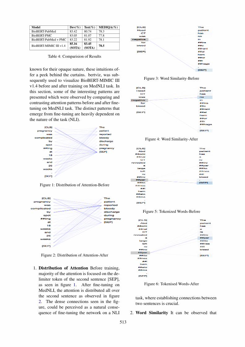
Model Dev(%) Test(%) MEDIQA(%)BioBERT-PubMed 83.42 80.74 78.3BioBERT-PMC 83.05 81.07 77.8BioBERT-PubMed + PMC 83.22 81.92 78.1
BioBERT-MIMIC III v1.485.16(SOTA)
83.45(SOTA) 78.5
Table 4: Comparision of Results
known for their opaque nature, these intuitions of-fer a peek behind the curtains. bertviz, was sub-sequently used to visualize BioBERT-MIMIC IIIv1.4 before and after training on MedNLI task. Inthis section, some of the interesting patterns arepresented which were observed by comparing andcontrasting attention patterns before and after fine-tuning on MedNLI task. The distinct patterns thatemerge from fine-tuning are heavily dependent onthe nature of the task (NLI).
Figure 1: Distribution of Attention-Before
Figure 2: Distribution of Attention-After
1. Distribution of Attention Before training,majority of the attention is focused on the de-limiter token of the second sentence [SEP],as seen in figure 1. After fine-tuning onMedNLI, the attention is distributed all overthe second sentence as observed in figure2. The dense connections seen in the fig-ure, could be perceived as a natural conse-quence of fine-tuning the network on a NLI
Figure 3: Word Similarity-Before
Figure 4: Word Similarity-After
Figure 5: Tokenized Words-Before
Figure 6: Tokenised Words-After
task, where establishing connections betweentwo sentences is crucial.
2. Word Similarity It can be observed that
513
words similar to source word gets more atten-tion. Notice the words negative and no, ex-pressing similar sentiments (negative), con-nected via attention flow in figure 4. Word-level similarity, although not always, is agood indicator of entailment. Upon encoun-tering sentences with similar words, it is rea-sonable for a network to be biased towardsentailment.
3. Tokenized Words In BERT, OOV (Out ofVocabulary) words are identified and splitinto segments. This way, the morphologi-cal information is maintained, which comesin handy in tasks such as textual entailmentwhere word-level similarity is an importantaspect to notice. Before fine-tuning, the OOV(Out of Vocabulary) words split into multi-ple tokens receive weak attention from sourcetokens, as observed in figure 5. After fine-tuning on MedNLI, a strong attention flowbetween the tokenized words across two sen-tences can be seen. As mentioned above,these connections as seen in figure 6, helpin identifying word-level similarity betweensentences.
The authors have presented a error analysisstudy based on attention patterns in Appendix A.Based on the intuitions gained from error analysis,the authors propose a list of changes that could im-prove the performance of the model. A limitationsof the proposed approach and a list of possible im-provements are presented in Appendix B.
6 Conclusion
In this paper, a variant of BERT, fine-tuned onMIMIC III v1.4, is proposed to solve the task ofMedNLI, a Natural Language Inference task de-signed for clinical domain. The experiments in-clude evaluation of BERT pre-trained on PMC,PubMed and MIMIC III v1.4, on MedNLI testand dev sets, and MEDIQA test set for MedNLI.State-of-the-Art results (83.45%) in MedNLI isachieved by pre-training BERT on PubMed fol-lowed by fine-tuning on MIMIC III v1.4. Thesame model achieves an accuracy of 78.5% onMEDIQA test set. The authors have identifieddistinct attention patterns in BERT trained onMedNLI and have explored the origin and signifi-cance of those patterns in the context of NLI.
Acknowledgments
The authors would like to thank Bhuvana Kundu-mani for reviewing the manuscript and for provid-ing her technical inputs. The authors would alsolike to extend their gratitude to Saama Technolo-gies Inc. for providing the perfect research andinnovation environment.
ReferencesBrian K Atchinson and Daniel M Fox. 1997. From the
field: The politics of the health insurance portabilityand accountability act. Health Affairs, 16(3):146–150.
Asma Ben Abacha, Chaitanya Shivade, and DinaDemner-Fushman. 2019. Overview of the mediqa2019 shared task on textual inference, question en-tailment and question answering. In Proceedings ofthe BioNLP 2019 workshop, Florence, Italy, August1, 2019. Association for Computational Linguistics.
Samuel R Bowman, Gabor Angeli, Christopher Potts,and Christopher D Manning. 2015. A large anno-tated corpus for learning natural language inference.arXiv preprint arXiv:1508.05326.
Alexis Conneau, Douwe Kiela, Holger Schwenk, LoicBarrault, and Antoine Bordes. 2017. Supervisedlearning of universal sentence representations fromnatural language inference data. arXiv preprintarXiv:1705.02364.
Jacob Devlin, Ming-Wei Chang, Kenton Lee, andKristina Toutanova. 2018. Bert: Pre-training of deepbidirectional transformers for language understand-ing. arXiv preprint arXiv:1810.04805.
Qiao Jin, Bhuwan Dhingra, William W Cohen, andXinghua Lu. 2019. Probing biomedical embed-dings from language models. arXiv preprintarXiv:1904.02181.
Alistair E. W. Johnson, Tom J. Pollard, Lu Shen, Li-wei H. Lehman, Mengling Feng, Mohammad Ghas-semi, Benjamin Moody, Peter Szolovits, Leo An-thony Celi, and Roger G. Mark. 2016. Mimic-iii,a freely accessible critical care database. ScientificData, 3:160035 EP –. Data Descriptor.
Jinhyuk Lee, Wonjin Yoon, Sungdong Kim,Donghyeon Kim, Sunkyu Kim, Chan Ho So, andJaewoo Kang. 2019. Biobert: a pre-trained biomed-ical language representation model for biomedicaltext mining. arXiv preprint arXiv:1901.08746.
Matthew E. Peters, Mark Neumann, Mohit Iyyer, MattGardner, Christopher Clark, Kenton Lee, and LukeZettlemoyer. 2018. Deep contextualized word rep-resentations. In Proc. of NAACL.
514
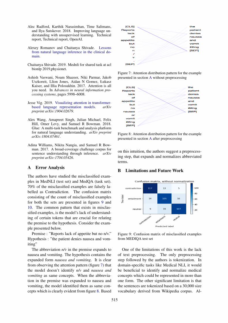
Alec Radford, Karthik Narasimhan, Time Salimans,and Ilya Sutskever. 2018. Improving language un-derstanding with unsupervised learning. Technicalreport, Technical report, OpenAI.
Alexey Romanov and Chaitanya Shivade. Lessonsfrom natural language inference in the clinical do-main.
Chaitanya Shivade. 2019. Mednli for shared task at aclbionlp 2019,physionet.
Ashish Vaswani, Noam Shazeer, Niki Parmar, JakobUszkoreit, Llion Jones, Aidan N Gomez, ŁukaszKaiser, and Illia Polosukhin. 2017. Attention is allyou need. In Advances in neural information pro-cessing systems, pages 5998–6008.
Jesse Vig. 2019. Visualizing attention in transformer-based language representation models. arXivpreprint arXiv:1904.02679.
Alex Wang, Amapreet Singh, Julian Michael, FelixHill, Omer Levy, and Samuel R Bowman. 2018.Glue: A multi-task benchmark and analysis platformfor natural language understanding. arXiv preprintarXiv:1804.07461.
Adina Williams, Nikita Nangia, and Samuel R Bow-man. 2017. A broad-coverage challenge corpus forsentence understanding through inference. arXivpreprint arXiv:1704.05426.
A Error Analysis
The authors have studied the misclassified exam-ples in MedNLI (test set) and MedQA (task set).70% of the misclassified examples are falsely la-belled as Contradiction. The confusion matrixconsisting of the count of misclassified examplesfor both the sets are presented in figures 9 and10. The common pattern that exists in misclas-sified examples, is the model’s lack of understand-ing of certain tokens that are crucial for relatingthe premise to the hypothesis. Consider the exam-ple presented below.
Premise : ”Reports lack of appetite but no n/v.”Hypothesis : ”the patient denies nausea and vom-iting”
The abbreviation n/v in the premise expands tonausea and vomiting. The hypothesis contains theexpanded form nausea and vomiting. It is clearfrom observing the attention pattern (figure 7) thatthe model doesn’t identify n/v and nausea andvomiting as same concepts. When the abbrevia-tion in the premise was expanded to nausea andvomiting, the model identified them as same con-cepts which is clearly evident from figure 8. Based
Figure 7: Attention distribution pattern for the examplepresented in section A without preprocessing
Figure 8: Attention distribution pattern for the examplepresented in section A after preprocessing
on this intuition, the authors suggest a preprocess-ing step, that expands and normalizes abbreviatedterms.
B Limitations and Future Work
Figure 9: Confusion matrix of misclassified examplesfrom MEDIQA test set
One of the limitations of this work is the lackof text preprocessing. The only preprocessingstep followed by the authors is tokenization. Indomain-specific tasks like Medical NLI, it wouldbe beneficial to identify and normalize medicalconcepts which could be represented in more thanone form. The other significant limitation is thatthe sentences are tokenized based on a 30,000 sizevocabulary derived from Wikipedia corpus. Al-
515
Figure 10: Confusion matrix of misclassified examplesfrom MedNLI task set
though the fine-tuning is done on Pubmed, thecommonly occurring medical terms are identifiedas unknown words and split into tokens.
The authors suggest a preprocessing step thatidentifies and normalizes medical concepts. Thevocabulary could be built based on PubMed cor-pus which ensures that most common medicalterms are part of the vocabulary. Along thoselines, the authors suggest the use of entity embed-dings to learn medical concepts and make use ofthe information contained in them.
516
Proceedings of the BioNLP 2019 workshop, pages 517–522Florence, Italy, August 1, 2019. c©2019 Association for Computational Linguistics
IITP at MEDIQA 2019: Systems Report for Natural Language Inference,Question Entailment and Question Answering
Dibyanayan Bandyopadhyay1 Baban Gain1 Tanik Saikh2 Asif Ekbal2Government College Of Engineering And Textile Technology, Berhampore1
Indian Institute of Technology Patna2
{dibyanayan,gainbaban}@gmail.com1
{1821cs08, asif}@iitp.ac.in2
Abstract
This paper presents the experiments accom-plished as a part of our participation in theMEDIQA challenge, an (Abacha et al., 2019)shared task. We participated in all the threetasks defined in this particular shared task.The tasks are viz. i. Natural Language In-ference (NLI) ii. Recognizing Question En-tailment(RQE) and their application in medi-cal Question Answering (QA). We submittedruns using multiple deep learning based sys-tems (runs) for each of these three tasks. Wesubmitted five system results in each of theNLI and RQE tasks, and four system resultsfor the QA task. The systems yield encourag-ing results in all the three tasks. The highestperformance obtained in NLI, RQE and QAtasks are 81.8%, 53.2%, and 71.7%, respec-tively.
1 Introduction
Natural Language Processing (NLP) in biomedi-cal domain is an essential and challenging task.With the availability of the data in electronic formit is possible to apply Artificial intelligence (AI),machine learning and deep learning technologiesto build data driven automated tools. These au-tomated tools will be helpful in the field of med-ical science. An ACL-BioNLP 2019 shared task,namely the MEDIQA challenge aims to attract fur-ther research efforts in NLI, RQE and their ap-plication in QA in medical domain. The mo-tivation of this shared task is in a need to de-velop relevant methods, techniques, and gold stan-dard data for inference and recognizing questionentailment in medical domain and their applica-tion to improve domain specific Information Re-trieval (IR) and Question Answering (QA) sys-tems. The MEDIQA has defined several tasks re-lated to Natural Language Inference, Question En-tailment and Question Answering in medical do-
main. We participated in all the three tasks de-fined in this shared task. We offer multiple sys-tems for each the tasks. The workshop comprisesof three tasks namely viz. i. Natural LanguageInference (NLI): This task involves in identifyingthree inference relations between two sentences:i.e. Entailment, Neutral and Contradiction (Ro-manov and Shivade, 2018) ii. Recognizing Ques-tion Entailment (RQE): This task focuses on iden-tifying entailment relation between two questionsin the context of QA. The definition of questionentailment is as follows: ”a question A entails aquestion B if every answer to B is also a com-plete and/or partial answer to A” (Abacha andDemner-Fushman, 2019) and iii. Question An-swering (QA): The goal of this task is to filter andimprove the ranking of automatically retrieved an-swers. The existing medical QA system namelyCHiQA is applied to generate the input ranks.(Harabagiu and Hickl, 2006; Abacha et al., 2017;Abacha and Demner-Fushman, 2019). We partic-ipated in all the three tasks defined above and sub-mitted the results. Our proposed systems produceencouraging results.
2 Proposed Method
We propose multiple runs for each of the threetasks. The following subsections will discuss themethods applied to tackle each of these tasks.
2.1 Natural Language Inference
In the task 1 the system has to decide the entail-ment relationship between a pair of texts i.e. ei-ther they are Entailment, Contradiction or Neu-tral. The input to this task are sentence pairs andas output we wish to get the entailment relation be-tween those two pieces of texts. We propose fiveruns for this task. The following set of hyper pa-rameters are applied for the following runs. Batch
517
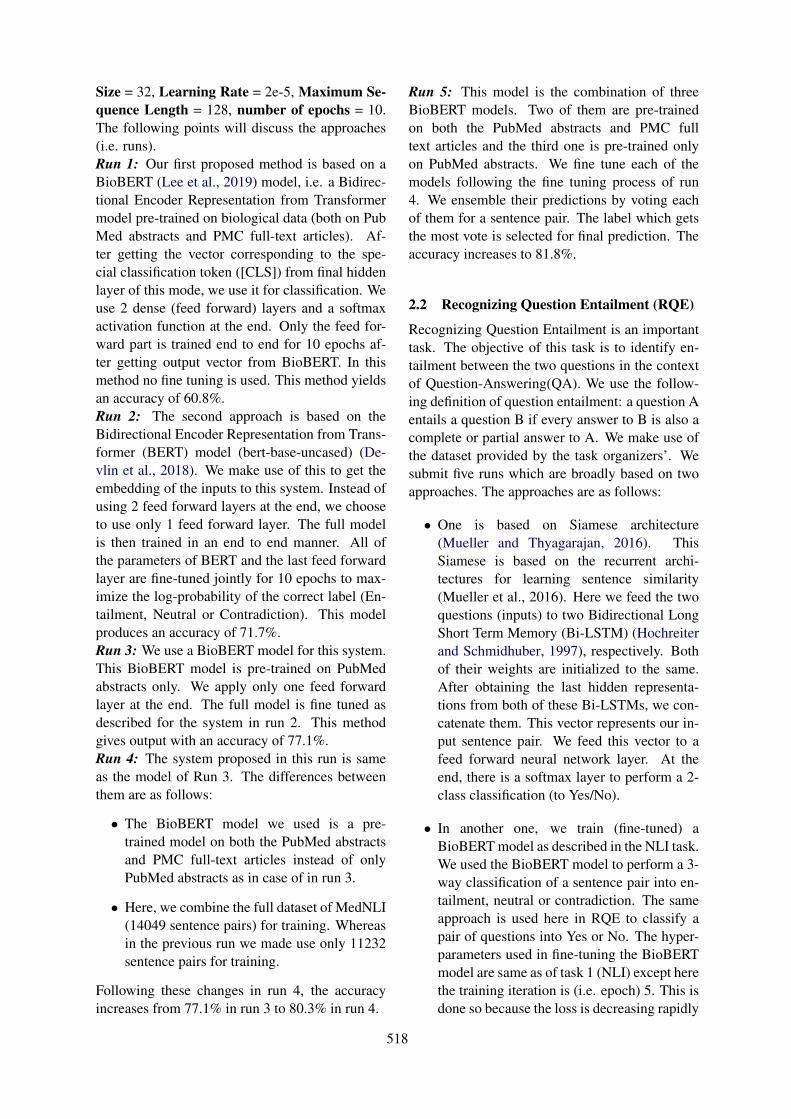
Size = 32, Learning Rate = 2e-5, Maximum Se-quence Length = 128, number of epochs = 10.The following points will discuss the approaches(i.e. runs).Run 1: Our first proposed method is based on aBioBERT (Lee et al., 2019) model, i.e. a Bidirec-tional Encoder Representation from Transformermodel pre-trained on biological data (both on PubMed abstracts and PMC full-text articles). Af-ter getting the vector corresponding to the spe-cial classification token ([CLS]) from final hiddenlayer of this mode, we use it for classification. Weuse 2 dense (feed forward) layers and a softmaxactivation function at the end. Only the feed for-ward part is trained end to end for 10 epochs af-ter getting output vector from BioBERT. In thismethod no fine tuning is used. This method yieldsan accuracy of 60.8%.Run 2: The second approach is based on theBidirectional Encoder Representation from Trans-former (BERT) model (bert-base-uncased) (De-vlin et al., 2018). We make use of this to get theembedding of the inputs to this system. Instead ofusing 2 feed forward layers at the end, we chooseto use only 1 feed forward layer. The full modelis then trained in an end to end manner. All ofthe parameters of BERT and the last feed forwardlayer are fine-tuned jointly for 10 epochs to max-imize the log-probability of the correct label (En-tailment, Neutral or Contradiction). This modelproduces an accuracy of 71.7%.Run 3: We use a BioBERT model for this system.This BioBERT model is pre-trained on PubMedabstracts only. We apply only one feed forwardlayer at the end. The full model is fine tuned asdescribed for the system in run 2. This methodgives output with an accuracy of 77.1%.Run 4: The system proposed in this run is sameas the model of Run 3. The differences betweenthem are as follows:
• The BioBERT model we used is a pre-trained model on both the PubMed abstractsand PMC full-text articles instead of onlyPubMed abstracts as in case of in run 3.
• Here, we combine the full dataset of MedNLI(14049 sentence pairs) for training. Whereasin the previous run we made use only 11232sentence pairs for training.
Following these changes in run 4, the accuracyincreases from 77.1% in run 3 to 80.3% in run 4.
Run 5: This model is the combination of threeBioBERT models. Two of them are pre-trainedon both the PubMed abstracts and PMC fulltext articles and the third one is pre-trained onlyon PubMed abstracts. We fine tune each of themodels following the fine tuning process of run4. We ensemble their predictions by voting eachof them for a sentence pair. The label which getsthe most vote is selected for final prediction. Theaccuracy increases to 81.8%.
2.2 Recognizing Question Entailment (RQE)
Recognizing Question Entailment is an importanttask. The objective of this task is to identify en-tailment between the two questions in the contextof Question-Answering(QA). We use the follow-ing definition of question entailment: a question Aentails a question B if every answer to B is also acomplete or partial answer to A. We make use ofthe dataset provided by the task organizers’. Wesubmit five runs which are broadly based on twoapproaches. The approaches are as follows:
• One is based on Siamese architecture(Mueller and Thyagarajan, 2016). ThisSiamese is based on the recurrent archi-tectures for learning sentence similarity(Mueller et al., 2016). Here we feed the twoquestions (inputs) to two Bidirectional LongShort Term Memory (Bi-LSTM) (Hochreiterand Schmidhuber, 1997), respectively. Bothof their weights are initialized to the same.After obtaining the last hidden representa-tions from both of these Bi-LSTMs, we con-catenate them. This vector represents our in-put sentence pair. We feed this vector to afeed forward neural network layer. At theend, there is a softmax layer to perform a 2-class classification (to Yes/No).
• In another one, we train (fine-tuned) aBioBERT model as described in the NLI task.We used the BioBERT model to perform a 3-way classification of a sentence pair into en-tailment, neutral or contradiction. The sameapproach is used here in RQE to classify apair of questions into Yes or No. The hyper-parameters used in fine-tuning the BioBERTmodel are same as of task 1 (NLI) except herethe training iteration is (i.e. epoch) 5. This isdone so because the loss is decreasing rapidly
518
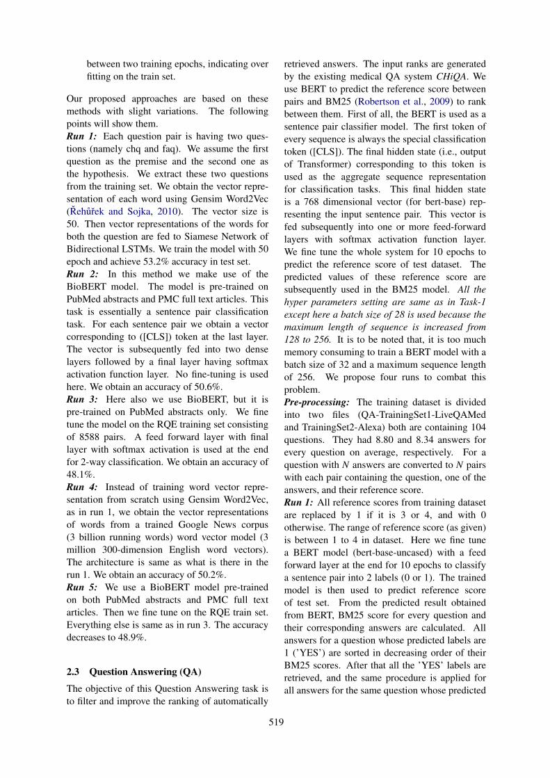
between two training epochs, indicating overfitting on the train set.
Our proposed approaches are based on thesemethods with slight variations. The followingpoints will show them.Run 1: Each question pair is having two ques-tions (namely chq and faq). We assume the firstquestion as the premise and the second one asthe hypothesis. We extract these two questionsfrom the training set. We obtain the vector repre-sentation of each word using Gensim Word2Vec(Řehůřek and Sojka, 2010). The vector size is50. Then vector representations of the words forboth the question are fed to Siamese Network ofBidirectional LSTMs. We train the model with 50epoch and achieve 53.2% accuracy in test set.Run 2: In this method we make use of theBioBERT model. The model is pre-trained onPubMed abstracts and PMC full text articles. Thistask is essentially a sentence pair classificationtask. For each sentence pair we obtain a vectorcorresponding to ([CLS]) token at the last layer.The vector is subsequently fed into two denselayers followed by a final layer having softmaxactivation function layer. No fine-tuning is usedhere. We obtain an accuracy of 50.6%.Run 3: Here also we use BioBERT, but it ispre-trained on PubMed abstracts only. We finetune the model on the RQE training set consistingof 8588 pairs. A feed forward layer with finallayer with softmax activation is used at the endfor 2-way classification. We obtain an accuracy of48.1%.Run 4: Instead of training word vector repre-sentation from scratch using Gensim Word2Vec,as in run 1, we obtain the vector representationsof words from a trained Google News corpus(3 billion running words) word vector model (3million 300-dimension English word vectors).The architecture is same as what is there in therun 1. We obtain an accuracy of 50.2%.Run 5: We use a BioBERT model pre-trainedon both PubMed abstracts and PMC full textarticles. Then we fine tune on the RQE train set.Everything else is same as in run 3. The accuracydecreases to 48.9%.
2.3 Question Answering (QA)
The objective of this Question Answering task isto filter and improve the ranking of automatically
retrieved answers. The input ranks are generatedby the existing medical QA system CHiQA. Weuse BERT to predict the reference score betweenpairs and BM25 (Robertson et al., 2009) to rankbetween them. First of all, the BERT is used as asentence pair classifier model. The first token ofevery sequence is always the special classificationtoken ([CLS]). The final hidden state (i.e., outputof Transformer) corresponding to this token isused as the aggregate sequence representationfor classification tasks. This final hidden stateis a 768 dimensional vector (for bert-base) rep-resenting the input sentence pair. This vector isfed subsequently into one or more feed-forwardlayers with softmax activation function layer.We fine tune the whole system for 10 epochs topredict the reference score of test dataset. Thepredicted values of these reference score aresubsequently used in the BM25 model. All thehyper parameters setting are same as in Task-1except here a batch size of 28 is used because themaximum length of sequence is increased from128 to 256. It is to be noted that, it is too muchmemory consuming to train a BERT model with abatch size of 32 and a maximum sequence lengthof 256. We propose four runs to combat thisproblem.Pre-processing: The training dataset is dividedinto two files (QA-TrainingSet1-LiveQAMedand TrainingSet2-Alexa) both are containing 104questions. They had 8.80 and 8.34 answers forevery question on average, respectively. For aquestion with N answers are converted to N pairswith each pair containing the question, one of theanswers, and their reference score.Run 1: All reference scores from training datasetare replaced by 1 if it is 3 or 4, and with 0otherwise. The range of reference score (as given)is between 1 to 4 in dataset. Here we fine tunea BERT model (bert-base-uncased) with a feedforward layer at the end for 10 epochs to classifya sentence pair into 2 labels (0 or 1). The trainedmodel is then used to predict reference scoreof test set. From the predicted result obtainedfrom BERT, BM25 score for every question andtheir corresponding answers are calculated. Allanswers for a question whose predicted labels are1 (’YES’) are sorted in decreasing order of theirBM25 scores. After that all the ’YES’ labels areretrieved, and the same procedure is applied forall answers for the same question whose predicted
519
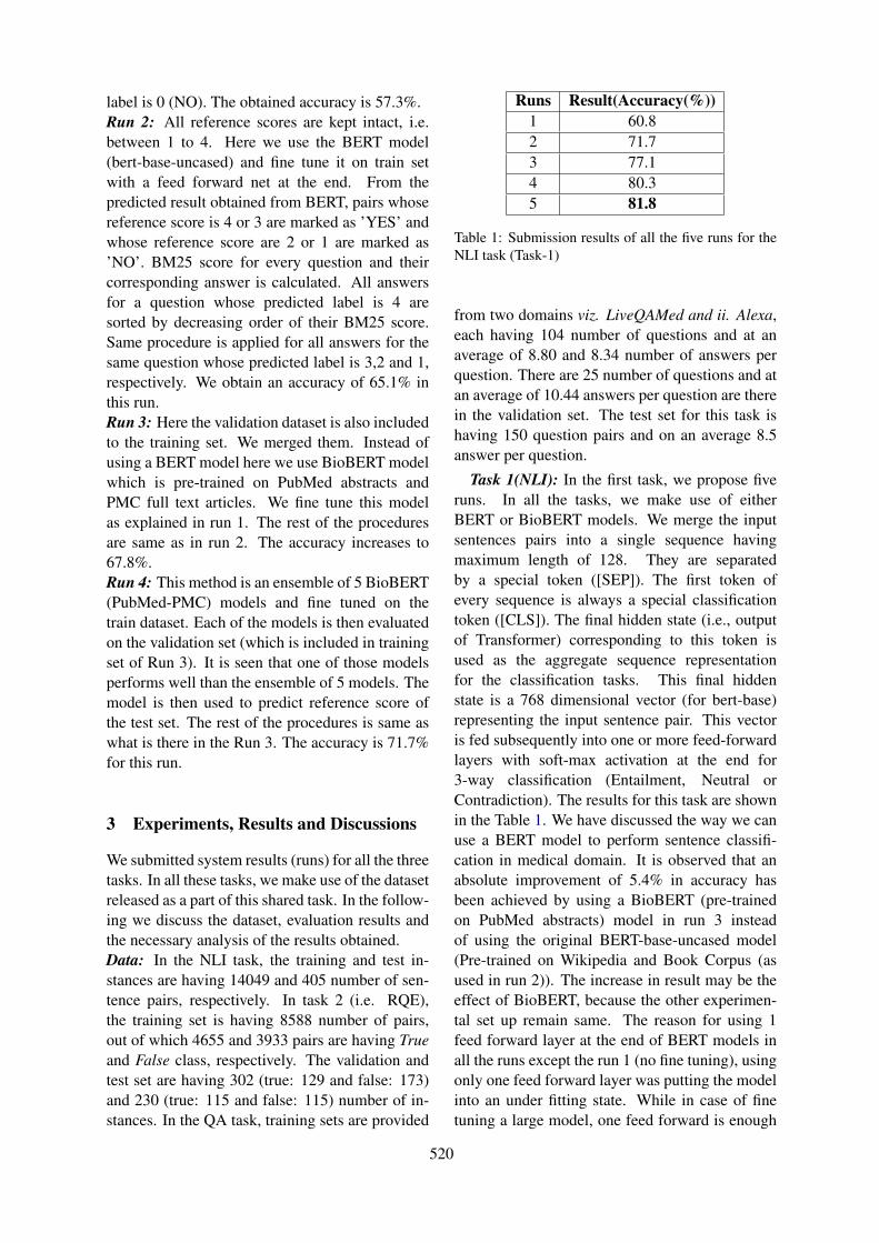
label is 0 (NO). The obtained accuracy is 57.3%.Run 2: All reference scores are kept intact, i.e.between 1 to 4. Here we use the BERT model(bert-base-uncased) and fine tune it on train setwith a feed forward net at the end. From thepredicted result obtained from BERT, pairs whosereference score is 4 or 3 are marked as ’YES’ andwhose reference score are 2 or 1 are marked as’NO’. BM25 score for every question and theircorresponding answer is calculated. All answersfor a question whose predicted label is 4 aresorted by decreasing order of their BM25 score.Same procedure is applied for all answers for thesame question whose predicted label is 3,2 and 1,respectively. We obtain an accuracy of 65.1% inthis run.Run 3: Here the validation dataset is also includedto the training set. We merged them. Instead ofusing a BERT model here we use BioBERT modelwhich is pre-trained on PubMed abstracts andPMC full text articles. We fine tune this modelas explained in run 1. The rest of the proceduresare same as in run 2. The accuracy increases to67.8%.Run 4: This method is an ensemble of 5 BioBERT(PubMed-PMC) models and fine tuned on thetrain dataset. Each of the models is then evaluatedon the validation set (which is included in trainingset of Run 3). It is seen that one of those modelsperforms well than the ensemble of 5 models. Themodel is then used to predict reference score ofthe test set. The rest of the procedures is same aswhat is there in the Run 3. The accuracy is 71.7%for this run.
3 Experiments, Results and Discussions
We submitted system results (runs) for all the threetasks. In all these tasks, we make use of the datasetreleased as a part of this shared task. In the follow-ing we discuss the dataset, evaluation results andthe necessary analysis of the results obtained.Data: In the NLI task, the training and test in-stances are having 14049 and 405 number of sen-tence pairs, respectively. In task 2 (i.e. RQE),the training set is having 8588 number of pairs,out of which 4655 and 3933 pairs are having Trueand False class, respectively. The validation andtest set are having 302 (true: 129 and false: 173)and 230 (true: 115 and false: 115) number of in-stances. In the QA task, training sets are provided
Runs Result(Accuracy(%))1 60.82 71.73 77.14 80.35 81.8
Table 1: Submission results of all the five runs for theNLI task (Task-1)
from two domains viz. LiveQAMed and ii. Alexa,each having 104 number of questions and at anaverage of 8.80 and 8.34 number of answers perquestion. There are 25 number of questions and atan average of 10.44 answers per question are therein the validation set. The test set for this task ishaving 150 question pairs and on an average 8.5answer per question.
Task 1(NLI): In the first task, we propose fiveruns. In all the tasks, we make use of eitherBERT or BioBERT models. We merge the inputsentences pairs into a single sequence havingmaximum length of 128. They are separatedby a special token ([SEP]). The first token ofevery sequence is always a special classificationtoken ([CLS]). The final hidden state (i.e., outputof Transformer) corresponding to this token isused as the aggregate sequence representationfor the classification tasks. This final hiddenstate is a 768 dimensional vector (for bert-base)representing the input sentence pair. This vectoris fed subsequently into one or more feed-forwardlayers with soft-max activation at the end for3-way classification (Entailment, Neutral orContradiction). The results for this task are shownin the Table 1. We have discussed the way we canuse a BERT model to perform sentence classifi-cation in medical domain. It is observed that anabsolute improvement of 5.4% in accuracy hasbeen achieved by using a BioBERT (pre-trainedon PubMed abstracts) model in run 3 insteadof using the original BERT-base-uncased model(Pre-trained on Wikipedia and Book Corpus (asused in run 2)). The increase in result may be theeffect of BioBERT, because the other experimen-tal set up remain same. The reason for using 1feed forward layer at the end of BERT models inall the runs except the run 1 (no fine tuning), usingonly one feed forward layer was putting the modelinto an under fitting state. While in case of finetuning a large model, one feed forward is enough
520
Runs Result(Accuracy(%))1 53.22 50.63 48.14 50.25 48.9
Table 2: Submission results in all the five runs for theRQE Task (Task-2)
as suggested by (Devlin et al., 2018). Up to run3, we make use of 11232 sentence pairs for thetraining. Those sentence pairs are same as the oneused to train several models used in (Romanovand Shivade, 2018). We use the remaining 2817sentence pairs for validation. The validation setaccuracy is always around 3-4% higher than thetest case accuracy for all the runs up to run 3. Forgetting the higher accuracy we combine all the14049 pairs in the subsequent run. We get theaccuracy of 81.8 % which is the highest amongall the proposed methods. As per our knowledge,in the official results of NLI task we stand at12th position among the 17 official teams whichparticipated for the NLI task.
Task 2 (RQE): In the second task i.e. task ofRecognising Question Entailment, we proposefive runs. The results are shown in the Table 2. Itis interesting to note the variation in accuracy forthe different runs. Siamese architecture performsmuch better here. Another peculiarity is that finetuning BERT hurts the performance while usingpre-trained BERT embedding without fine tuningseems to be more useful. This is concluded byobserving the results of run 2 and run 3. In run2, we used only pre-trained BERT embedding for([CLS]) token for classification, whereas in run3, we fine tuned the BERT model. The highestaccuracy is achieved by a Siamese Model con-sisting of 2 Bi-LSTMs with shared weights anda dense layers. In this task, 12 teams submittedtheir systems, and we stood the 10th position.
Task 3 (QA): In this task, we offer 4 runs totackle the problem. The results for this are shownin the Table 3. As we can see from the abovediscussions, the systems we build for this taskcomprises of two components, they are BERTand BM25. The BERT is used to predict thereference score of the test dataset. We rank the
ResultsRuns Accuracy(%) Spearmans Rho MRR Precision
1 57.3 0.053 0.8241 0.56102 65.1 0.042 0.7811 0.72353 67.8 0.034 0.8366 0.74214 71.7 0.024 0.8611 0.7936
Table 3: Results obtained in all the four runs for the QATask (Task - 3), where, MRR: Mean Reciprocal Rank
predicted scores using BM25. The BM25 partof the system is same for all the runs. In thistask, participants are encouraged to compute theMean Reciprocal Rank (MRR), Precision, andSpearman’s Rank Correlation Coefficient as theevaluation measures in addition to Accuracy. Weactually used BioBERT instead of original BERTfrom the run 3, which increases the accuracywith an absolute margin of 2.7% (65.1 to 67.8%).Using BioBERT we observe an improvement inMRR by 5.5%. Our best run with an accuracy of71.7% attains the position of 6th among 10 teamsin the official result.
4 Conclusion and Future Work
In this paper, we present our system details andthe results of various runs that reported as a partof our participation in the MEDIQA challenge. Inthis shared task three tasks, namely viz. i. NaturalLanguage Inference ii. Question Entailment andiii. Question Answering were introduced in themedical domain. We offer multiple systems (runs)for each of these tasks. Most of the proposed mod-els are based on BERT/Bio-BERT embedding andBM25. These models yields encouraging perfor-mance in all the tasks.In future we would like toextend our work as follows:
• Detailed analysis of the top-scoring modelsto understand their techniques and findings.
• We can do the task of NLI by fostering anEmbedding from Language model (EMLo)based model and do a comparative analysiswith BERT based model.
ReferencesAsma Ben Abacha, Eugene Agichtein, Yuval Pinter,
and Dina Demner-Fushman. 2017. Overview ofthe medical question answering task at TREC 2017LiveQA. In Proceedings of The Twenty-Sixth TextREtrieval Conference, TREC, pages 15–17.
521
Asma Ben Abacha and Dina Demner-Fushman. 2019.A question-entailment approach to question answer-ing. arXiv preprint arXiv:1901.08079.
Asma Ben Abacha, Chaitanya Shivade, and DinaDemner-Fushman. 2019. Overview of the MediQA2019 shared task on textual inference, question en-tailment and question answering. In Proceedings ofthe BioNLP 2019 workshop, Florence, Italy, August1, 2019. Association for Computational Linguistics.
Jacob Devlin, Ming-Wei Chang, Kenton Lee, andKristina Toutanova. 2018. BERT: pre-training ofdeep bidirectional transformers for language under-standing. CoRR, abs/1810.04805.
Sanda Harabagiu and Andrew Hickl. 2006. Methodsfor using textual entailment in open-domain ques-tion answering. In Proceedings of the 21st Interna-tional Conference on Computational Linguistics and44th Annual Meeting of the Association for Compu-tational Linguistics, pages 905–912, Sydney, Aus-tralia. Association for Computational Linguistics.
Sepp Hochreiter and Jürgen Schmidhuber. 1997.Long short-term memory. Neural computation,9(8):1735–1780.
Jinhyuk Lee, Wonjin Yoon, Sungdong Kim,Donghyeon Kim, Sunkyu Kim, Chan Ho So, andJaewoo Kang. 2019. BioBERT: pre-trained biomed-ical language representation model for biomedicaltext mining. arXiv preprint arXiv:1901.08746.
Jonas Mueller and Aditya Thyagarajan. 2016. Siameserecurrent architectures for learning sentence similar-ity. In Thirtieth AAAI Conference on Artificial Intel-ligence.
Radim Řehůřek and Petr Sojka. 2010. Software Frame-work for Topic Modelling with Large Corpora. InProceedings of the LREC 2010 Workshop on NewChallenges for NLP Frameworks, pages 45–50, Val-letta, Malta. ELRA.
Stephen Robertson, Hugo Zaragoza, et al. 2009. Theprobabilistic relevance framework: BM25 and be-yond. Foundations and Trends R© in Information Re-trieval, 3(4):333–389.
Alexey Romanov and Chaitanya Shivade. 2018.Lessons from natural language inference in the clin-ical domain. In Proceedings of the 2018 Conferenceon Empirical Methods in Natural Language Pro-cessing, pages 1586–1596, Brussels, Belgium. As-sociation for Computational Linguistics.
522
Proceedings of the BioNLP 2019 workshop, pages 523–527Florence, Italy, August 1, 2019. c©2019 Association for Computational Linguistics
LasigeBioTM at MEDIQA 2019: Biomedical Question Answering usingBidirectional Transformers and Named Entity Recognition
Andre Lamurias∗ and Francisco M. Couto
LASIGE, Faculdade de Ciências, Universidade de Lisboa, Portugal
Abstract
Biomedical Question Answering (QA) aimsat providing automated answers to user ques-tions, regarding a variety of biomedical topics.For example, these questions may ask for re-lated to diseases, drugs, symptoms, or medicalprocedures. Automated biomedical QA sys-tems could improve the retrieval of informa-tion necessary to answer these questions. TheMEDIQA challenge consisted of three tasksconcerning various aspects of biomedical QA.This challenge aimed at advancing approachesto Natural Language Inference (NLI) and Rec-ognizing Question Entailment (RQE), whichwould then result in enhanced approaches tobiomedical QA.
Our approach explored a commonTransformer-based architecture that could beapplied to each task. This approach shared thesame pre-trained weights, but which were thenfine-tuned for each task using the providedtraining data. Furthermore, we augmentedthe training data with external datasets andenriched the question and answer texts usingMER, a named entity recognition tool. Ourapproach obtained high levels of accuracy, inparticular on the NLI task, which classifiedpairs of text according to their relation. Forthe QA task, we obtained higher Spearman’srank correlation values using the entitiesrecognized by MER.
1 Introduction
Question Answering (QA) is a text mining taskfor which several systems have been proposed(Hirschman and Gaizauskas, 2001). This task isparticularly challenging in the biomedical domainsince this is a complex subject as answers maynot be as straightforward compared to other do-mains. However, clinical and health care informa-tion systems could benefit greatly from automated
biomedical QA systems, which could improve theretrieval of information necessary to answer thesequestions.
To help progress on this topic, the MEDIQAchallenge proposed three tasks in the biomedicaldomain(Ben Abacha et al., 2019):
1. Natural Language Inference (NLI) - classifythe relation between two sentences as eitherentailment, neutral or contradiction;
2. Recognizing Question Entailment (RQE) -classify if two questions are entailed witheach other or not;
3. Question Answering (QA) - classify whichanswers are correct for a given answer andrank them.
We applied the same approach to all threetasks since they all could be modelled as textclassification tasks. The objectives of the taskswere to classify pairs of text: sentence-sentence(NLI), question-question (RQE), and question-answer (QA). For the NLI task, we had three pos-sible labels for each pair (entailment, neutral orcontradiction), while the RQE task was a binaryclassification. For the QA task, each pair shouldbe given a reference score representing how wellthe question is answered, which ranged between 1and 4.
QA is a complex task that involves various com-ponents, and can be approached in several ways.While real-world scenarios require the retrieval ofcorrect answers from larger databases, the QA taskof this challenge simplified this problem by pro-viding up to 10 answers retrieved by the medicalQA system CHiQA. This system also provided aranking to each answer, however, we observed thatthis ranking did not follow the manual ranking inmost cases. We also observed that the retrieved
523
answers could consist of one or more sentences.While in some QA scenarios, systems are requiredto select the text span that contains the answer (Ra-jpurkar et al., 2016), in this case it was only re-quested to re-rank the retrieved answers and clas-sify which ones were correct. Although specificranking algorithms exist (Radev et al., 2000), dueto the nature of the task and the fact that the othertwo tasks involved comparison of text, we decidedto train a classifier that compared each questionwith a potential answer, i.e., we predicted howgood a text is at answering a given question.
Our approach uses pre-trained weights as astarting point, to fine-tune deep learning modelsbased on the Transformer architecture for each ofthe challenge tasks (Vaswani et al., 2017). Weused the BioBERT weights, trained on PubMedabstracts and PMC full articles, as the type of textshould be more similar to the challenge data thanthe standard BERT models, which were trained onWikipedia and BookCorpus. Furthermore, we in-corporated other datasets into the RQE and QAtasks, and enrich the training data with seman-tic information obtained using MER (MinimalNamed-Entity Recognizer) (Couto and Lamurias,2018), a high computing performance named en-tity recognition tool.
2 Related Work
Deep learning approaches have lead to state-of-the-art results in various text mining tasks. Theseapproaches make use of intermediary representa-tions of the data to then fine-tune the weights todifferent tasks. Various models have been pro-posed, and, recently, the most successful oneshave been based around the Transformer archi-tecture (Vaswani et al., 2017). An advantage ofthis type of models is that we can use pre-trainedweights such as those provided by BERT (Devlinet al., 2018) as a starting point to train a model fora specific task. These weights are tuned on largecorpora using the Transformer architecture andhave been shown to be effective language models.Different models were made available by the au-thors, with two variations of the architecture, andwhether the true case and accent markers of thetokens are taken into account.
Due to the effectiveness of the BERT architec-ture, it has been already adapted for other do-mains. Lee et al. (2019) presented a model specificto biomedical language, which was trained on a
large-scale biomedical corpora: 200k PubMed ab-stracts, 270k PMC full texts, and a combination ofthese two. Although the BioBERT models use thesame vocabulary as the BERT models, the sameWordPiece tokenization is performed. This way,even if biomedical documents contain words thatwere not in the original vocabulary, the tokenizerwill separate these words into frequent subwords,minimizing out-of-vocabulary issues and keepingcompatibility with the original models. The au-thors tested these models on several biomedicaltext mining tasks, obtaining competitive perfor-mance when compared with other state-of-the-artmodels.
One of the most common text mining tasks isentity recognition. This task is important becauseit is often the first step to other tasks, such as entitylinking and relation extraction. MER is a simplebut efficient approach to entity recognition, whichuses vocabularies that can be extracted from on-tologies to identify and link entities. MER focuseson simplicity and flexibility to reduce the process-ing time and the time necessary to adapt to otherdomains and entity types.
3 Methodology
3.1 Data PreparationWe participated in the three tasks using the sameapproach by modeling each one as a text classifi-cation problem. We used the training data of eachtasks as document pairs, where a document couldbe a sentence, paragraph, question or answer. TheNLI and RQE data had obvious labels, while forthe QA data we used the reference scores. How-ever, to distinguish between correct answers withmore detail, we also incorporated the manually as-signed ranks to the answers with reference scores3 and 4:
FinalScore = ReferenceScore +11− Rank
10
As there are up to 10 possible answers to eachquestion, the final score will range between 1 and5.
We removed instances where each element ofthe pair contained the same text, which happenedsometimes in the RQE training set. Further-more, we performed named entity recognition us-ing MER to identify several types of entities men-tion in both questions and answers. We used MERsince it can provide reliable entity mention anno-tations at a reasonable speed. We appended the
524
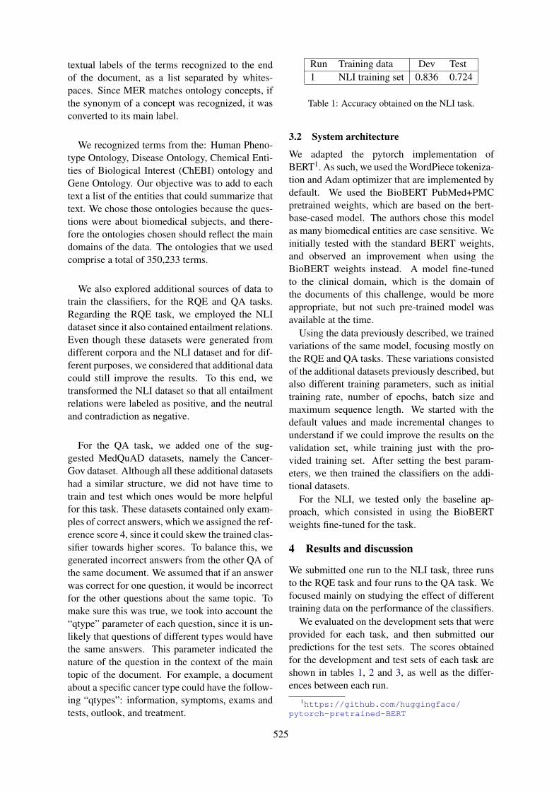
textual labels of the terms recognized to the endof the document, as a list separated by whites-paces. Since MER matches ontology concepts, ifthe synonym of a concept was recognized, it wasconverted to its main label.
We recognized terms from the: Human Pheno-type Ontology, Disease Ontology, Chemical Enti-ties of Biological Interest (ChEBI) ontology andGene Ontology. Our objective was to add to eachtext a list of the entities that could summarize thattext. We chose those ontologies because the ques-tions were about biomedical subjects, and there-fore the ontologies chosen should reflect the maindomains of the data. The ontologies that we usedcomprise a total of 350,233 terms.
We also explored additional sources of data totrain the classifiers, for the RQE and QA tasks.Regarding the RQE task, we employed the NLIdataset since it also contained entailment relations.Even though these datasets were generated fromdifferent corpora and the NLI dataset and for dif-ferent purposes, we considered that additional datacould still improve the results. To this end, wetransformed the NLI dataset so that all entailmentrelations were labeled as positive, and the neutraland contradiction as negative.
For the QA task, we added one of the sug-gested MedQuAD datasets, namely the Cancer-Gov dataset. Although all these additional datasetshad a similar structure, we did not have time totrain and test which ones would be more helpfulfor this task. These datasets contained only exam-ples of correct answers, which we assigned the ref-erence score 4, since it could skew the trained clas-sifier towards higher scores. To balance this, wegenerated incorrect answers from the other QA ofthe same document. We assumed that if an answerwas correct for one question, it would be incorrectfor the other questions about the same topic. Tomake sure this was true, we took into account the“qtype” parameter of each question, since it is un-likely that questions of different types would havethe same answers. This parameter indicated thenature of the question in the context of the maintopic of the document. For example, a documentabout a specific cancer type could have the follow-ing “qtypes”: information, symptoms, exams andtests, outlook, and treatment.
Run Training data Dev Test1 NLI training set 0.836 0.724
Table 1: Accuracy obtained on the NLI task.
3.2 System architecture
We adapted the pytorch implementation ofBERT1. As such, we used the WordPiece tokeniza-tion and Adam optimizer that are implemented bydefault. We used the BioBERT PubMed+PMCpretrained weights, which are based on the bert-base-cased model. The authors chose this modelas many biomedical entities are case sensitive. Weinitially tested with the standard BERT weights,and observed an improvement when using theBioBERT weights instead. A model fine-tunedto the clinical domain, which is the domain ofthe documents of this challenge, would be moreappropriate, but not such pre-trained model wasavailable at the time.
Using the data previously described, we trainedvariations of the same model, focusing mostly onthe RQE and QA tasks. These variations consistedof the additional datasets previously described, butalso different training parameters, such as initialtraining rate, number of epochs, batch size andmaximum sequence length. We started with thedefault values and made incremental changes tounderstand if we could improve the results on thevalidation set, while training just with the pro-vided training set. After setting the best param-eters, we then trained the classifiers on the addi-tional datasets.
For the NLI, we tested only the baseline ap-proach, which consisted in using the BioBERTweights fine-tuned for the task.
4 Results and discussion
We submitted one run to the NLI task, three runsto the RQE task and four runs to the QA task. Wefocused mainly on studying the effect of differenttraining data on the performance of the classifiers.
We evaluated on the development sets that wereprovided for each task, and then submitted ourpredictions for the test sets. The scores obtainedfor the development and test sets of each task areshown in tables 1, 2 and 3, as well as the differ-ences between each run.
1https://github.com/huggingface/pytorch-pretrained-BERT
525
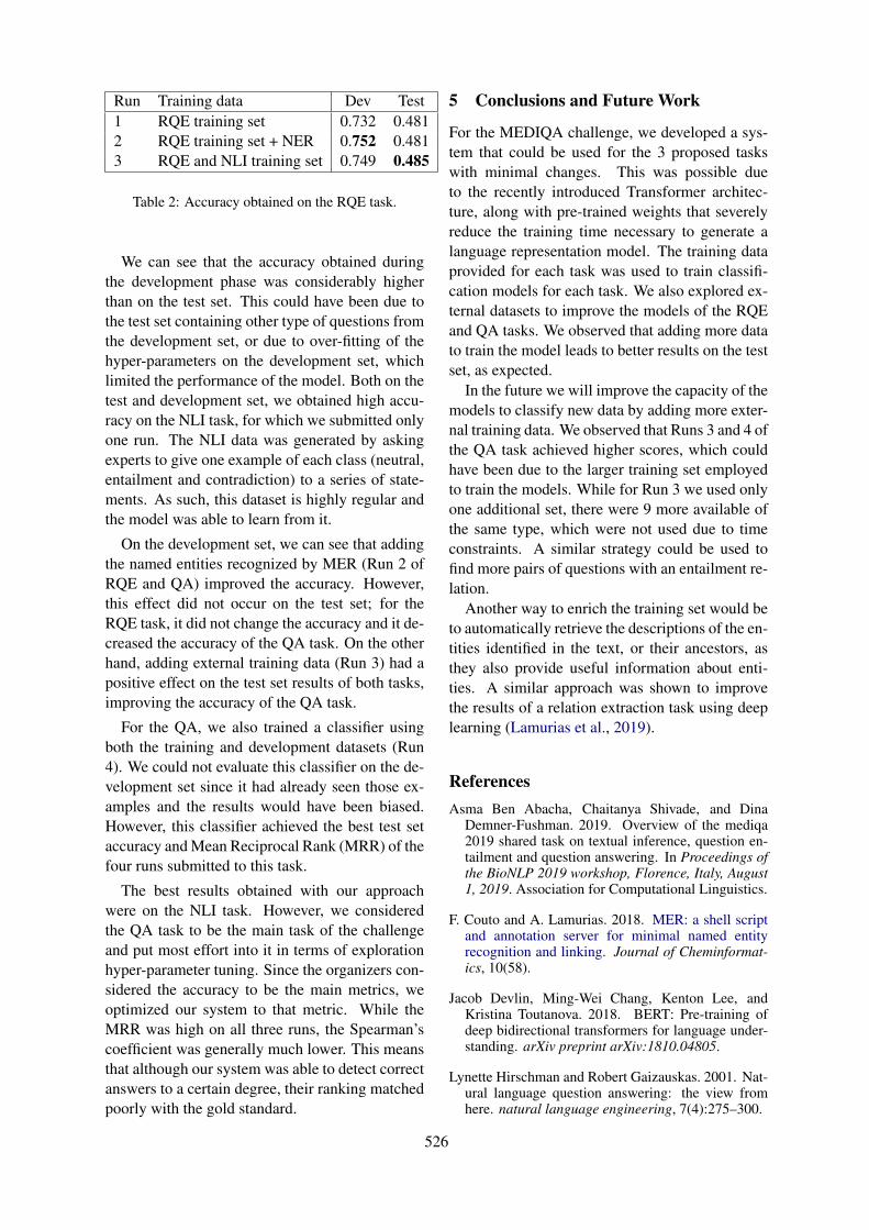
Run Training data Dev Test1 RQE training set 0.732 0.4812 RQE training set + NER 0.752 0.4813 RQE and NLI training set 0.749 0.485
Table 2: Accuracy obtained on the RQE task.
We can see that the accuracy obtained duringthe development phase was considerably higherthan on the test set. This could have been due tothe test set containing other type of questions fromthe development set, or due to over-fitting of thehyper-parameters on the development set, whichlimited the performance of the model. Both on thetest and development set, we obtained high accu-racy on the NLI task, for which we submitted onlyone run. The NLI data was generated by askingexperts to give one example of each class (neutral,entailment and contradiction) to a series of state-ments. As such, this dataset is highly regular andthe model was able to learn from it.
On the development set, we can see that addingthe named entities recognized by MER (Run 2 ofRQE and QA) improved the accuracy. However,this effect did not occur on the test set; for theRQE task, it did not change the accuracy and it de-creased the accuracy of the QA task. On the otherhand, adding external training data (Run 3) had apositive effect on the test set results of both tasks,improving the accuracy of the QA task.
For the QA, we also trained a classifier usingboth the training and development datasets (Run4). We could not evaluate this classifier on the de-velopment set since it had already seen those ex-amples and the results would have been biased.However, this classifier achieved the best test setaccuracy and Mean Reciprocal Rank (MRR) of thefour runs submitted to this task.
The best results obtained with our approachwere on the NLI task. However, we consideredthe QA task to be the main task of the challengeand put most effort into it in terms of explorationhyper-parameter tuning. Since the organizers con-sidered the accuracy to be the main metrics, weoptimized our system to that metric. While theMRR was high on all three runs, the Spearman’scoefficient was generally much lower. This meansthat although our system was able to detect correctanswers to a certain degree, their ranking matchedpoorly with the gold standard.
5 Conclusions and Future Work
For the MEDIQA challenge, we developed a sys-tem that could be used for the 3 proposed taskswith minimal changes. This was possible dueto the recently introduced Transformer architec-ture, along with pre-trained weights that severelyreduce the training time necessary to generate alanguage representation model. The training dataprovided for each task was used to train classifi-cation models for each task. We also explored ex-ternal datasets to improve the models of the RQEand QA tasks. We observed that adding more datato train the model leads to better results on the testset, as expected.
In the future we will improve the capacity of themodels to classify new data by adding more exter-nal training data. We observed that Runs 3 and 4 ofthe QA task achieved higher scores, which couldhave been due to the larger training set employedto train the models. While for Run 3 we used onlyone additional set, there were 9 more available ofthe same type, which were not used due to timeconstraints. A similar strategy could be used tofind more pairs of questions with an entailment re-lation.
Another way to enrich the training set would beto automatically retrieve the descriptions of the en-tities identified in the text, or their ancestors, asthey also provide useful information about enti-ties. A similar approach was shown to improvethe results of a relation extraction task using deeplearning (Lamurias et al., 2019).
ReferencesAsma Ben Abacha, Chaitanya Shivade, and Dina
Demner-Fushman. 2019. Overview of the mediqa2019 shared task on textual inference, question en-tailment and question answering. In Proceedings ofthe BioNLP 2019 workshop, Florence, Italy, August1, 2019. Association for Computational Linguistics.
F. Couto and A. Lamurias. 2018. MER: a shell scriptand annotation server for minimal named entityrecognition and linking. Journal of Cheminformat-ics, 10(58).
Jacob Devlin, Ming-Wei Chang, Kenton Lee, andKristina Toutanova. 2018. BERT: Pre-training ofdeep bidirectional transformers for language under-standing. arXiv preprint arXiv:1810.04805.
Lynette Hirschman and Robert Gaizauskas. 2001. Nat-ural language question answering: the view fromhere. natural language engineering, 7(4):275–300.
526
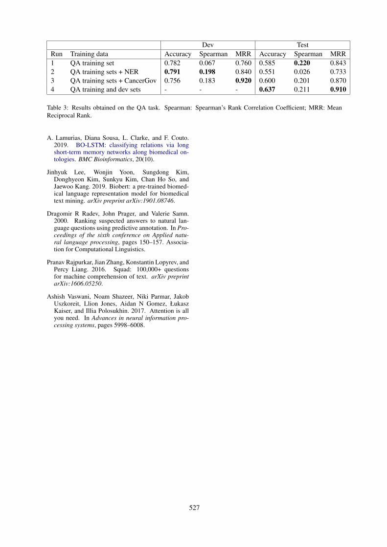
Dev TestRun Training data Accuracy Spearman MRR Accuracy Spearman MRR1 QA training set 0.782 0.067 0.760 0.585 0.220 0.8432 QA training sets + NER 0.791 0.198 0.840 0.551 0.026 0.7333 QA training sets + CancerGov 0.756 0.183 0.920 0.600 0.201 0.8704 QA training and dev sets - - - 0.637 0.211 0.910
Table 3: Results obtained on the QA task. Spearman: Spearman’s Rank Correlation Coefficient; MRR: MeanReciprocal Rank.
A. Lamurias, Diana Sousa, L. Clarke, and F. Couto.2019. BO-LSTM: classifying relations via longshort-term memory networks along biomedical on-tologies. BMC Bioinformatics, 20(10).
Jinhyuk Lee, Wonjin Yoon, Sungdong Kim,Donghyeon Kim, Sunkyu Kim, Chan Ho So, andJaewoo Kang. 2019. Biobert: a pre-trained biomed-ical language representation model for biomedicaltext mining. arXiv preprint arXiv:1901.08746.
Dragomir R Radev, John Prager, and Valerie Samn.2000. Ranking suspected answers to natural lan-guage questions using predictive annotation. In Pro-ceedings of the sixth conference on Applied natu-ral language processing, pages 150–157. Associa-tion for Computational Linguistics.
Pranav Rajpurkar, Jian Zhang, Konstantin Lopyrev, andPercy Liang. 2016. Squad: 100,000+ questionsfor machine comprehension of text. arXiv preprintarXiv:1606.05250.
Ashish Vaswani, Noam Shazeer, Niki Parmar, JakobUszkoreit, Llion Jones, Aidan N Gomez, ŁukaszKaiser, and Illia Polosukhin. 2017. Attention is allyou need. In Advances in neural information pro-cessing systems, pages 5998–6008.
527
Proceedings of the BioNLP 2019 workshop, pages 528–532Florence, Italy, August 1, 2019. c©2019 Association for Computational Linguistics
Abstract
This study describes the model design of the NCUEE system for the MEDIQA challenge at the ACL-BioNLP 2019 workshop. We use the BERT (Bidirectional Encoder Representations from Transformers) as the word embedding method to integrate the BiLSTM (Bidirectional Long Short-Term Memory) network with an attention mechanism for medical text inferences. A total of 42 teams participated in natural language inference task at MEDIQA 2019. Our best accuracy score of 0.84 ranked the top-third among all submissions in the leaderboard.
1 Introduction
Natural Language Inference (NLI) is the task of determining whether a given hypothesis is true (entailment), false (contradiction) or undetermined (neutral) by inferring a given premise. The Stanford Natural Language Inference (SNLI) corpus is a well-known dataset and serves as a benchmark for NLI system evaluations (Bowman et al., 2015). However, it is restricted to a single text genre. Therefore, the MedNLI dataset, which is annotated by doctors and grounded in patients’ medical histories, was built to perform NLI tasks in the clinical domain (Romanov and Shivade, 2018). In addition to feature-based methods and bag-of-words (BOW) models, other experiments have tested several modern neural networks-based models for the specialized and knowledge intensive field of medicine, including InferSent (Conneau et al., 2017) and ESIM (Chen et al., 2017)
The MEDIQA challenge focuses on attracting research efforts in Natural Language Inference (NLI), Recognizing Question Entailment (RQE) and their applications in medical Question
Answering (QA). The MEDIQA challenge includes three tasks: 1) NLI: identifying three inference relations between two medical sentences, that is, entailment, neutral and contradiction. 2) RQE: identifying entailment between two questions in the context of QA. 3) QA: filtering and improving the input ranks of retrieved answers, generated by the medical QA system CHiQA. The reuse of NLI and/or RQE systems for this task is highly recommended.
Under the policies of the MEDIQA challenge, we only participated in the first NLI task. Recently, a new method of pre-training language representations named BERT (Bidirectional Encoder Representations from Transformers) has obtained groundbreaking results on a wide array of natural language processing tasks (Devlin et al., 2018). This achievement motivates us to explore using a BERT based model to tackle the textual inference problem in the medical domain.
This paper describes the NCUEE (National Central University, Dept. of Electrical Engineering) system for the NLI task of the MEDIQA challenge at the ACL-BioNLP 2019 workshop. Our solution explores a BERT-based model, in which the BiLSTM network with attention mechanism is integrated for textual inference. The input sentence-pair is represented as a sequence of words. Each word refers to distributed vectors from a pre-trained BERT to form as an embedding matrix. The datasets provided by the task organizers are used to train the BiLSTM network with attention model for the prediction task. The output is a value from 0 to 1 representing the estimated class probability. The class with the highest probability (that is, one of entailment, neutral and contradiction) will be regarded as the inference result. Our best accuracy score of 0.84 ranked in the top-third of all 42 submissions in the leaderboard.
NCUEE at MEDIQA 2019: Medical Text Inference Using Ensemble BERT-BiLSTM-Attention Model
Lung-Hao Lee*, Yi Lu, Po-Han Chen, Po-Lei Lee and Kuo-Kai Shyu Department of Electrical Engineering, National Central University, Taiwan
Pervasive Artificial Intelligence Research (PAIR) Labs, Taiwan *[email protected]
528
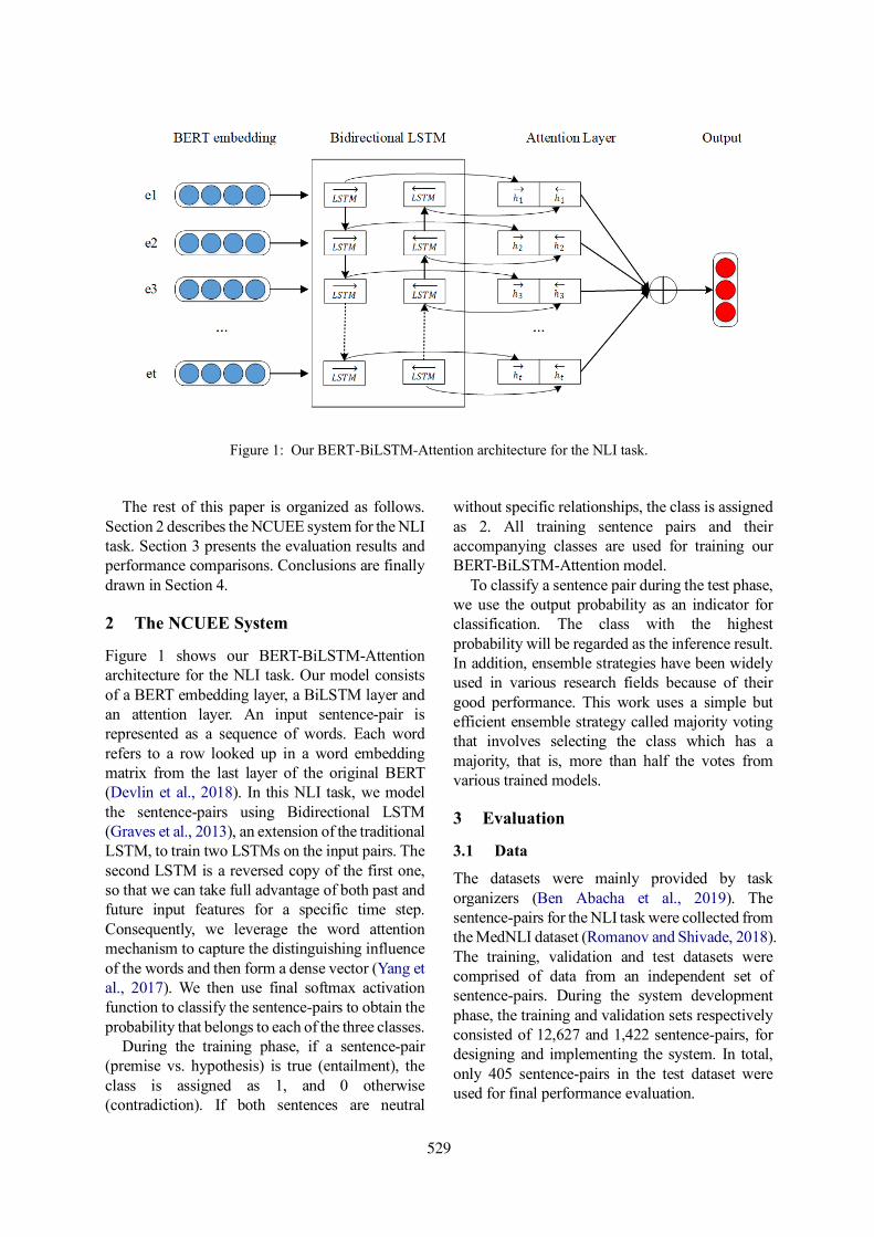
The rest of this paper is organized as follows. Section 2 describes the NCUEE system for the NLI task. Section 3 presents the evaluation results and performance comparisons. Conclusions are finally drawn in Section 4.
2 The NCUEE System
Figure 1 shows our BERT-BiLSTM-Attention architecture for the NLI task. Our model consists of a BERT embedding layer, a BiLSTM layer and an attention layer. An input sentence-pair is represented as a sequence of words. Each word refers to a row looked up in a word embedding matrix from the last layer of the original BERT (Devlin et al., 2018). In this NLI task, we model the sentence-pairs using Bidirectional LSTM (Graves et al., 2013), an extension of the traditional LSTM, to train two LSTMs on the input pairs. The second LSTM is a reversed copy of the first one, so that we can take full advantage of both past and future input features for a specific time step. Consequently, we leverage the word attention mechanism to capture the distinguishing influence of the words and then form a dense vector (Yang et al., 2017). We then use final softmax activation function to classify the sentence-pairs to obtain the probability that belongs to each of the three classes.
During the training phase, if a sentence-pair (premise vs. hypothesis) is true (entailment), the class is assigned as 1, and 0 otherwise (contradiction). If both sentences are neutral
without specific relationships, the class is assigned as 2. All training sentence pairs and their accompanying classes are used for training our BERT-BiLSTM-Attention model.
To classify a sentence pair during the test phase, we use the output probability as an indicator for classification. The class with the highest probability will be regarded as the inference result. In addition, ensemble strategies have been widely used in various research fields because of their good performance. This work uses a simple but efficient ensemble strategy called majority voting that involves selecting the class which has a majority, that is, more than half the votes from various trained models.
3 Evaluation
3.1 Data
The datasets were mainly provided by task organizers (Ben Abacha et al., 2019). The sentence-pairs for the NLI task were collected from the MedNLI dataset (Romanov and Shivade, 2018). The training, validation and test datasets were comprised of data from an independent set of sentence-pairs. During the system development phase, the training and validation sets respectively consisted of 12,627 and 1,422 sentence-pairs, for designing and implementing the system. In total, only 405 sentence-pairs in the test dataset were used for final performance evaluation.
Figure 1: Our BERT-BiLSTM-Attention architecture for the NLI task.
529
The pre-trained word vectors are publicly available for download at the official BERT website 1 . We also used pre-trained weights of BioBERT (Lee et al., 2019), a language representation model for the biomedical domain and publicly available at the GitHub site2.
3.2 Results
During system development phase, in addition to pre-trained word vectors, we only use the training set to train the system parameters and evaluate the result on the validation set.
In the first set of experiments, the following fine-tuning BERT models were compared to demonstrate their performance for classification.
• BERT-Base, Uncased: 12-layer, 768-hidden,
12-heads, 110M parameters.
• BERT-Base, Cased: 12-layer, 768-hidden, 12-heads, 110M parameters.
• BERT-Large, Uncased: 24-layer, 1024-hidden, 16-heads, 340M parameters.
• BERT-Large, Cased: 24-layer, 1024-hidden, 16-heads, 340M parameters.
Google Research has released the BERT-Base and BERT-Large models (12-layer/24-layer Transformer). Uncased means that the text has been lowercased before WordPiece tokenization and any accept markers have also been removed. Cased means that the true case and accent markers are preserved. The same setups are used for comparisons. The maximum sequence is 128. The training batch size is 32. The learning rate is 2e-5. The number of training epochs is 10.
Table 1 shows the results. The BERT-Large models achieved relatively better accuracy than the BERT-Base models, regardless of case-sensitivity.
1 https://github.com/google-research/bert
The best accuracy was obtained by the Uncased BERT-Large model.
In the second set of experiments, the objective is to compare the performance of both BERT and BioBERT models. The BioBERT is based on the same vocabulary as the Cased BERT-Base model. Hence, we selected the pre-trained weights of BioBERT with PubMed 200K and PMC 270K comparing with the Cased BERT-Base model. Note that both models have been fine-tuned with optimal parameter settings.
Table 2 shows the performance comparisons, where the BioBERT outperforms the BERT model, suggesting that the BioBERT model is more suitable for biomedical text mining tasks through incorporating biomedical corpora such as PubMed and PMC.
In the third set of experiments, we evaluated our proposed model based on the previous results. Since the BERT-Large and BioBERT-Base achieved better accuracy, we fine-tuned these two models and sought to identify seek the optimal system parameters. Moreover, we adopted the last layers of these two models as the word embedding to integrate the BiLSTM network with attention mechanism. The setups of the BiLSTM is follows. The hidden size is 256. The dropout rate is 0.5.
Table 3 compares the results. The BioBERT models outperformed the BERT models, regardless of whether BioBERT was used as the word embedding or fine-tuning its original model. In addition, our integrated architecture with the BiLSTM-Attention was found to produce a slight
2 https://github.com/naver/biobert-pretrained
Models Accuracy
Fine-tuning BERT-Base, Uncased 0.759 Fine-tuning BERT-Base, Cased 0.751 Fine-tuning BERT-Large, Uncased 0.796 Fine-tuning BERT-Large, Cased 0.793
Table 1: Results of fine-tuning BERT models
Models Accuracy
Fine-tuning BERT-Base, Cased 0.792 Fine-tuning BioBERT-Base, Cased 0.822
Table 2: Results of BERT vs. BioBERT
Models Accuracy
Fine-tuning BioBERT-Base 0.822 BioBERT-Base + BiLSTM-Attention 0.824
Fine-tuning BERT-Large 0.809 BERT-Large + BiLSTM-Attention 0.809
Table 3: Results of BERT-BiLSTM with attention
530
performance enhancement. The best accuracy was obtained by the BioBERT-Base + BiLSTM-Attention model.
3.3 Comparisons
During final testing phase of the NLI task, we used the training set to train the models and the validation set for parameter optimization. Each participating team was allowed to submit a maximum of 5 runs for each task. We submitted the four abovementioned models accompanying with the ensemble model. For our ensemble strategy, we have trained the models 5 times using the BioBERT-Base + BiLSTM-Attention. The final inference result is the majority voting of the class with the highest probability.
Table 4 shows the results of our testing models. In addition to the BioBERT-Base model, the other models achieved promising accuracy. As expected, our ensemble strategy has the better performance. Our ensemble BioBERT+BiLSTM-Attention model achieved a high accuracy score of 0.84, ranking it in the top-third of all 42 participating teams participated the NLI task in the leaderboard. After excluding invalid submissions, including those did not report their team information (name, affiliation, and so on) and/or submit their working notes papers, our best accuracy score of 0.84 ranked the 11th among all 17 valid submissions.
The test set (405 instances) is extremely small, but the testing period (15 days) is relatively long. Human intervention can be used to manipulate the results. In addition, the test set is arranged with an obvious pattern. One premise always accompanies with three hypotheses respectively denoting each class (entailment, contradiction and neutral). Base on this observation, it’s easy to upgrade the final ranking of this task through a post-editing rule. For example, if two testing instances in the three-class group are predicted as the same class, the former is changed as the class entailment. Consequently, in
the same condition, if the class entailment has been determined, then the former is changed as the class contradiction. With this post-editing rule, our best model can be enhanced to achieve a high accuracy score of 0.975.
4 Conclusions
This study describes the NCUEE system in the ACL-BioNLP’19 shared task, including system design, implementation and evaluation. We present our first exploration of this research topic in medical text inference. Future work will exploit other textual features to improve performance.
Acknowledgments This study is partially supported by the Ministry of Science and Technology, under the grant MOST 108-2218-E-008-017-MY3 and MOST 108-2634-F-008-003- through Pervasive Artificial Intelligence Research (PAIR) Labs, Taiwan.
References Alex Graves, Abdel-rahman Mohamed, and Geoffrey
Hinton. 2013. Speech recognition with deep recurrent neural networks. In Proceedings of the 2013 IEEE International Conference on Acoustics, Speech and Signal Processing. Institute of Electrical and Electronics Engineers, pages 6645-6649. https://doi.org/10.1109/ICASSP.2013.6638947
Alexey Romanov, and Chaitanya Shivade. 2018. Lessons from natural language inference in the clinical domain. In Proceedings of the 2018 Conference on Empirical Methods in Natural Language Processing. Association for Computational Linguistics, pages 1586-1596. https://www.aclweb.org/anthology/D18-1187
Alexis Conneau, Douwe Kiela, Holger Schwenk, Loic Barrault, and Antoine Bordes. 2017. Supervised learning of universal sentence representations from natural language inference data. In Proceedings of the 2017 Conference on Empirical Methods in Natural Language Processing. Association for Computational Linguistics, pages 670-680. https://www.aclweb.org/anthology/papers/D/D17/D17-1070/
Asma Ben Abacha, Chaitanya Shivade, and Dina Demner-Fushman. 2019. Overview of the MEDIQA 2019 shared task on textual inference, question entailment and question answering. In Proceedings of the 2019 Workshop on Biomedical Natural Language Processing. Association for Computational Linguistics.
Models Accuracy
BioBERT-Base 0.786 BioBERT-Base + BiLSTM-Attention 0.805
BERT-Large 0.805 BERT-Large + BiLSTM-Attention 0.808
Ensemble BioBERT+BiLSTM-Attetion 0.840
Table 4: Results of our testing modes.
531
Jacob Devlin, Ming-Wei Chang, Kenton Lee, and Kristina Toutanova. 2018. BERT: Pre-training of deep bidirectional transformers for language understanding. arXiv Preprint. Cornell University, https://arxiv.org/abs/1810.04805v1
Jinhyuk Lee, Wonjin Yoon, Sungdong Kim, Donghyeon Kim, Sunkyu Kim, and Chan So. BioBERT: a pre-trained biomedical language representation model for biomedical text domain. arXiv Preprint. Cornell University, https://arxiv.org/abs/1901.08746
Qian Chen, Xiaodan Zhu, Zhen-Hua Ling, Si Wei, Hui Jiang, and Diana Inkpen. 2017. Enhanced LSTM for natural language inference. In Proceedings of the 55th Annual Meeting of the Association for Computational Linguistics (Volume 1: Long Papers). Association for Computational Linguistics, pages 1657-1668. https://www.aclweb.org/anthology/papers/P/P17/P17-1152/
Samuel R. Bowman, Gabor Angeli, Christopher Potts, and Christopher D. Manning. 2015. A large annotated corpus for learning natural language inference. In Proceedings of the 2015 Conference on Empirical Methods in Natural Language Processing. Association for Computational Linguistics, pages 632-642. https://aclweb.org/anthology/papers/D/D15/D15-1075/
Zichao Yang, Diyi Yang, Chris Dyer, Xiaodong He, Alex Smola, and Eduard Hovy. 2017. Hierarchical attention networks for document classification. In Proceedings of the 2017 Conference of the North American Chapter of the Association for Computational Linguistics: Human Language Technologies. Association for Computational Linguistics, pages 1480-1489. https://www.aclweb.org/anthology/N16-1174
532
Proceedings of the BioNLP 2019 workshop, pages 533–540Florence, Italy, August 1, 2019. c©2019 Association for Computational Linguistics
ARS NITK at MEDIQA 2019:Analysing Various Methods for NaturalLanguage Inference, Recognising Question Entailment and Medical
Question Answering System
Anumeha Agrawal, Rosa Anil George, Selvan Sunitha Ravi, Sowmya Kamath S andAnand Kumar M
Department of Information TechnologyNational Institute of Technology Karnataka, Surathkal, India 575025
{anumehaagrawal29, [email protected], sunitha98selvan}@gmail.com,{sowmyakamath, m anandkumar}@nitk.edu.in
Abstract
This paper includes approaches we havetaken for Natural Language Inference, Ques-tion Entailment Recognition and Question-Answering tasks to improve domain-specificInformation Retrieval. Natural Language In-ference (NLI) is a task that aims to determine ifa given hypothesis is an entailment, contradic-tion or is neutral to the given premise. Recog-nizing Question Entailment (RQE) focuses onidentifying entailment between two questionswhile the objective of Question-Answering(QA) is to filter and improve the ranking of au-tomatically retrieved answers. For addressingthe NLI task, the UMLS Metathesaurus wasused to find the synonyms of medical termsin given sentences, on which the InferSentmodel was trained to predict if the given sen-tence is an entailment, contradictory or neu-tral. We also introduce a new Extreme gra-dient boosting model built on PubMed em-beddings to perform RQE. Further, a closed-domain Question Answering technique thatuses Bi-directional LSTMs trained on theSquAD dataset to determine relevant ranks ofanswers for a given question is also discussed.Experimental validation showed that the pro-posed models achieved promising results.
1 Introduction
Recent studies have shown that patient-specificdata can be utilized for the development of intel-ligent Healthcare Information Management Sys-tems (HIMS), that support a wide range of sup-porting applications that enhance healthcare deliv-ery platforms. The application of natural languageprocessing, sophisticated data modeling, and pre-dictive algorithms make it a highly interesting areaof research. Patient data is continuously gener-ated in large volume and variety, given the mul-tiple modalities, it is available in (e.g., discharge
summaries, physician’s notes, clinical reports, labreports etc). With an abundance of such diverseinformation sources available in the medical do-main, sophisticated solutions that can adapt tothe heterogeneity and specific manifold nature ofhealth-related information are a critical require-ment for HIMS development.
In clinical text, a commonly occurring prob-lem would be to understand the correlation andassociation between various factors like disease,symptoms, diagnoses and treatment. Clinical textis inherently unstructured and written in naturallanguage, and hence is prone to significant is-sues in effective interpretability and utilization.Challenges like paraphrase detection, anaphoraresolution, natural language inference etc mustbe effectively dealt with in order to extract use-ful knowledge that can be used to build intelli-gent decision support applications. Such supportsystems require extensive evidence-based anal-ysis, and context-sensitive processing, in orderto enable higher-level functionalities like clinicalquestion-answering. Thus, dealing with such is-sues is paramount importance.
Natural Language Inference is used to deter-mine whether a given hypothesis can be inferredfrom a given premise (Ben Abacha et al. (2019)).The three inference relations to be identified be-tween the statements are Entailment, Neutralityand Contradiction. If a statement is a true descrip-tion of the other then it is labelled Entailment. If itis a false description then it is labelled Contradic-tion, otherwise, it is considered to be Neutral. Thegoal of Recognizing Question Entailment(RQE) isto retrieve answers to a premise question by re-trieving inferred or entailed questions, called hy-pothesis questions that already have associated an-swers. Therefore, we define the entailment rela-tion between two questions as: a question A en-
533
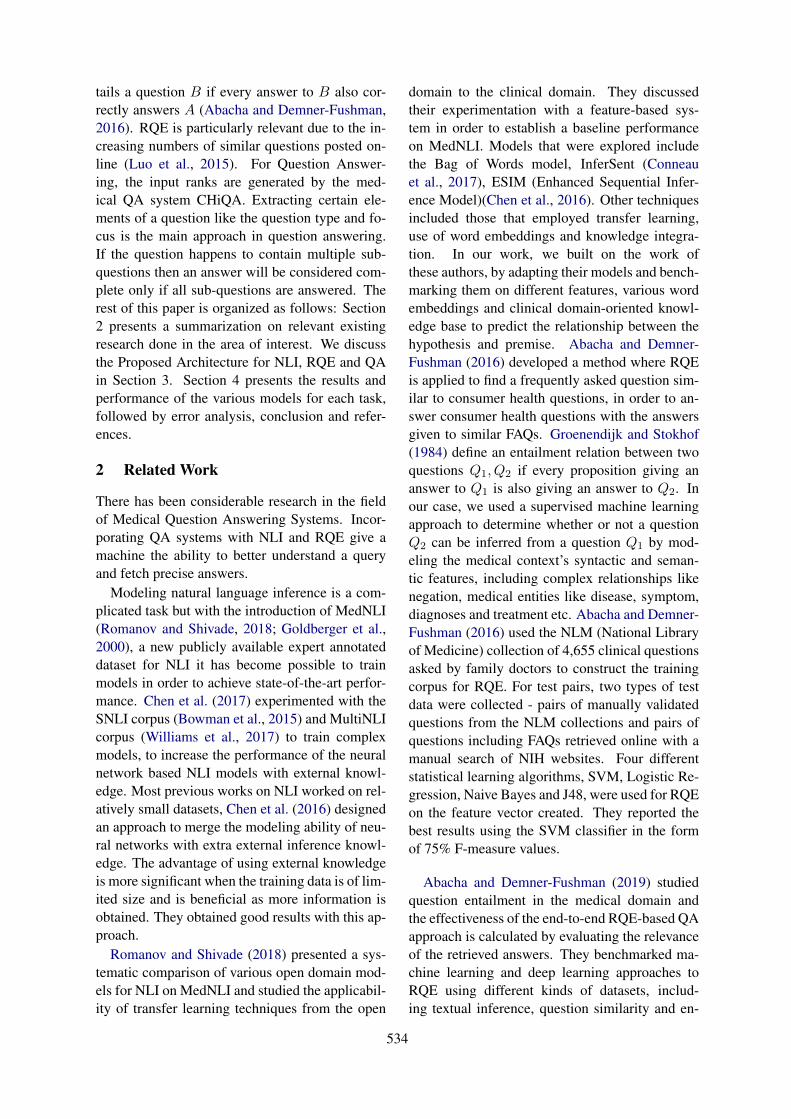
tails a question B if every answer to B also cor-rectly answers A (Abacha and Demner-Fushman,2016). RQE is particularly relevant due to the in-creasing numbers of similar questions posted on-line (Luo et al., 2015). For Question Answer-ing, the input ranks are generated by the med-ical QA system CHiQA. Extracting certain ele-ments of a question like the question type and fo-cus is the main approach in question answering.If the question happens to contain multiple sub-questions then an answer will be considered com-plete only if all sub-questions are answered. Therest of this paper is organized as follows: Section2 presents a summarization on relevant existingresearch done in the area of interest. We discussthe Proposed Architecture for NLI, RQE and QAin Section 3. Section 4 presents the results andperformance of the various models for each task,followed by error analysis, conclusion and refer-ences.
2 Related Work
There has been considerable research in the fieldof Medical Question Answering Systems. Incor-porating QA systems with NLI and RQE give amachine the ability to better understand a queryand fetch precise answers.
Modeling natural language inference is a com-plicated task but with the introduction of MedNLI(Romanov and Shivade, 2018; Goldberger et al.,2000), a new publicly available expert annotateddataset for NLI it has become possible to trainmodels in order to achieve state-of-the-art perfor-mance. Chen et al. (2017) experimented with theSNLI corpus (Bowman et al., 2015) and MultiNLIcorpus (Williams et al., 2017) to train complexmodels, to increase the performance of the neuralnetwork based NLI models with external knowl-edge. Most previous works on NLI worked on rel-atively small datasets, Chen et al. (2016) designedan approach to merge the modeling ability of neu-ral networks with extra external inference knowl-edge. The advantage of using external knowledgeis more significant when the training data is of lim-ited size and is beneficial as more information isobtained. They obtained good results with this ap-proach.
Romanov and Shivade (2018) presented a sys-tematic comparison of various open domain mod-els for NLI on MedNLI and studied the applicabil-ity of transfer learning techniques from the open
domain to the clinical domain. They discussedtheir experimentation with a feature-based sys-tem in order to establish a baseline performanceon MedNLI. Models that were explored includethe Bag of Words model, InferSent (Conneauet al., 2017), ESIM (Enhanced Sequential Infer-ence Model)(Chen et al., 2016). Other techniquesincluded those that employed transfer learning,use of word embeddings and knowledge integra-tion. In our work, we built on the work ofthese authors, by adapting their models and bench-marking them on different features, various wordembeddings and clinical domain-oriented knowl-edge base to predict the relationship between thehypothesis and premise. Abacha and Demner-Fushman (2016) developed a method where RQEis applied to find a frequently asked question sim-ilar to consumer health questions, in order to an-swer consumer health questions with the answersgiven to similar FAQs. Groenendijk and Stokhof(1984) define an entailment relation between twoquestions Q1, Q2 if every proposition giving ananswer to Q1 is also giving an answer to Q2. Inour case, we used a supervised machine learningapproach to determine whether or not a questionQ2 can be inferred from a question Q1 by mod-eling the medical context’s syntactic and seman-tic features, including complex relationships likenegation, medical entities like disease, symptom,diagnoses and treatment etc. Abacha and Demner-Fushman (2016) used the NLM (National Libraryof Medicine) collection of 4,655 clinical questionsasked by family doctors to construct the trainingcorpus for RQE. For test pairs, two types of testdata were collected - pairs of manually validatedquestions from the NLM collections and pairs ofquestions including FAQs retrieved online with amanual search of NIH websites. Four differentstatistical learning algorithms, SVM, Logistic Re-gression, Naive Bayes and J48, were used for RQEon the feature vector created. They reported thebest results using the SVM classifier in the formof 75% F-measure values.
Abacha and Demner-Fushman (2019) studiedquestion entailment in the medical domain andthe effectiveness of the end-to-end RQE-based QAapproach is calculated by evaluating the relevanceof the retrieved answers. They benchmarked ma-chine learning and deep learning approaches toRQE using different kinds of datasets, includ-ing textual inference, question similarity and en-
534
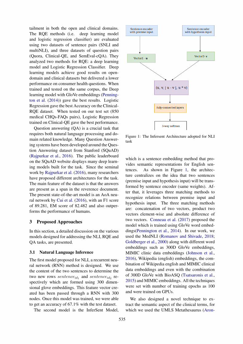
tailment in both the open and clinical domains.The RQE methods (i.e. deep learning modeland logistic regression classifier) are evaluatedusing two datasets of sentence pairs (SNLI andmultiNLI), and three datasets of question pairs(Quora, Clinical-QE, and SemEval-cQA). Theyanalyzed two methods for RQE: a deep learningmodel and Logistic Regression Classifier. Deeplearning models achieve good results on open-domain and clinical datasets but delivered a lowerperformance on consumer health questions. Whentrained and tested on the same corpus, the Deeplearning model with GloVe embeddings (Penning-ton et al. (2014)) gave the best results. LogisticRegression gave the best Accuracy on the Clinical-RQE dataset. When tested on our test set (850medical CHQs-FAQs pairs), Logistic Regressiontrained on Clinical-QE gave the best performance.
Question answering (QA) is a crucial task thatrequires both natural language processing and do-main related knowledge. Many Question Answer-ing systems have been developed around the Ques-tion Answering dataset from Stanford (SQuAD)(Rajpurkar et al., 2016). The public leaderboardon the SQuAD website displays many deep learn-ing models built for the task. Since the seminalwork by Rajpurkar et al. (2016), many researchershave proposed different architectures for the task.The main feature of the dataset is that the answersare present as a span in the reverence document.The present state-of-the-art model is an AoA neu-ral network by Cui et al. (2016), with an F1 scoreof 89.281, EM score of 82.482 and also outper-forms the performance of humans.
3 Proposed Approaches
In this section, a detailed discussion on the variousmodels designed for addressing the NLI, RQE andQA tasks, are presented.
3.1 Natural Language Inference
The first model proposed for NLI, a recurrent neu-ral network (RNN) method is designed. We usethe content of the two sentences to determine thetwo new rows sentenceid1 and sentenceid2 re-spectively which are formed using 300 dimen-sional glove embeddings. This feature vector cre-ated has been passed through a RNN with 300nodes. Once this model was trained, we were ableto get an accuracy of 67.1% with the test dataset.
The second model is the InferSent Model,
Figure 1: The Infersent Architecture adopted for NLItask
which is a sentence embedding method that pro-vides semantic representations for English sen-tences. As shown in Figure 1, the architec-ture centralizes on the idea that two sentences(premise input and hypothesis input) will be trans-formed by sentence encoder (same weights). Af-ter that, it leverages three matching methods torecognize relations between premise input andhypothesis input. The three matching methodsare: concatenation of two vectors, product twovectors element-wise and absolute difference oftwo vectors. Conneau et al. (2017) proposed themodel which is trained using GloVe word embed-dings(Pennington et al., 2014). In our work, weused the MedNLI (Romanov and Shivade, 2018;Goldberger et al., 2000) along with different wordembeddings such as 300D GloVe embeddings,MIMIC clinic data embeddings (Johnson et al.,2016), Wikipedia (english) embeddings, the com-bination of Wikipedia english and MIMIC clinicaldata embeddings and even with the combinationof 300D GloVe with BioASQ (Tsatsaronis et al.,2015) and MIMIC embeddings. All the techniqueswere set with number of training epochs as 100and were trained on GPUs.
We also designed a novel technique to ex-tract the semantic aspect of the clinical terms, forwhich we used the UMLS Metathesaurus (Aron-
535
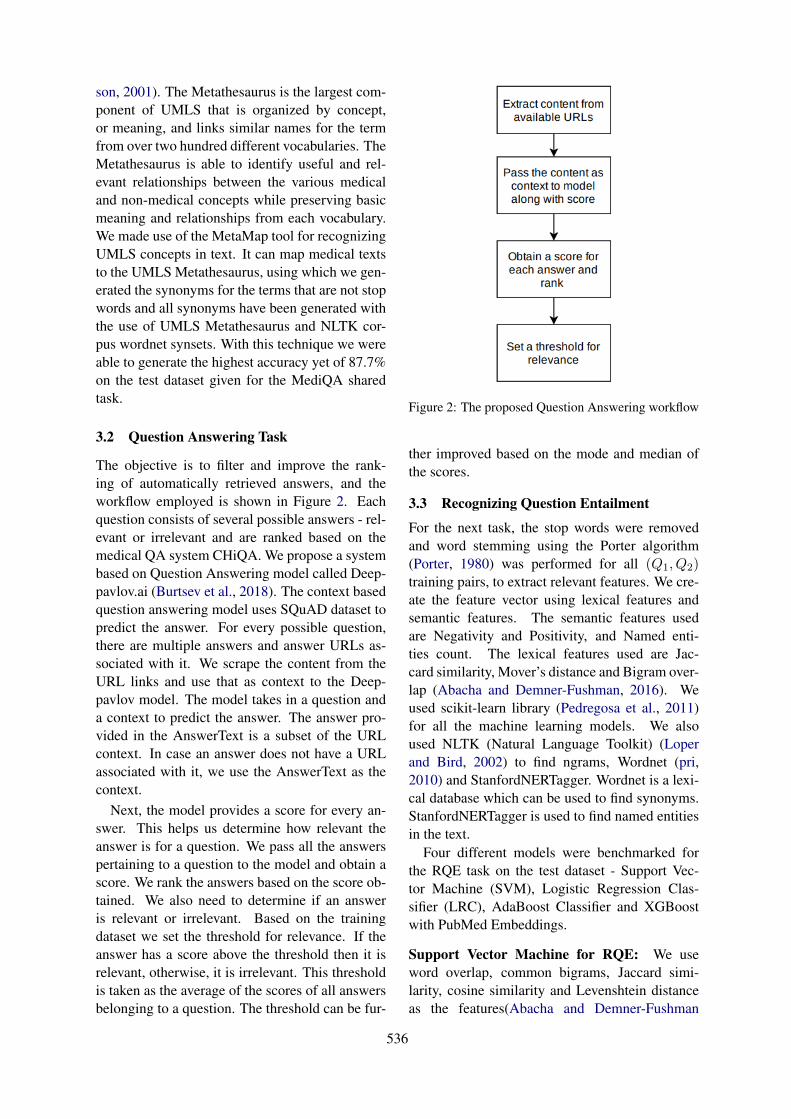
son, 2001). The Metathesaurus is the largest com-ponent of UMLS that is organized by concept,or meaning, and links similar names for the termfrom over two hundred different vocabularies. TheMetathesaurus is able to identify useful and rel-evant relationships between the various medicaland non-medical concepts while preserving basicmeaning and relationships from each vocabulary.We made use of the MetaMap tool for recognizingUMLS concepts in text. It can map medical textsto the UMLS Metathesaurus, using which we gen-erated the synonyms for the terms that are not stopwords and all synonyms have been generated withthe use of UMLS Metathesaurus and NLTK cor-pus wordnet synsets. With this technique we wereable to generate the highest accuracy yet of 87.7%on the test dataset given for the MediQA sharedtask.
3.2 Question Answering Task
The objective is to filter and improve the rank-ing of automatically retrieved answers, and theworkflow employed is shown in Figure 2. Eachquestion consists of several possible answers - rel-evant or irrelevant and are ranked based on themedical QA system CHiQA. We propose a systembased on Question Answering model called Deep-pavlov.ai (Burtsev et al., 2018). The context basedquestion answering model uses SQuAD dataset topredict the answer. For every possible question,there are multiple answers and answer URLs as-sociated with it. We scrape the content from theURL links and use that as context to the Deep-pavlov model. The model takes in a question anda context to predict the answer. The answer pro-vided in the AnswerText is a subset of the URLcontext. In case an answer does not have a URLassociated with it, we use the AnswerText as thecontext.
Next, the model provides a score for every an-swer. This helps us determine how relevant theanswer is for a question. We pass all the answerspertaining to a question to the model and obtain ascore. We rank the answers based on the score ob-tained. We also need to determine if an answeris relevant or irrelevant. Based on the trainingdataset we set the threshold for relevance. If theanswer has a score above the threshold then it isrelevant, otherwise, it is irrelevant. This thresholdis taken as the average of the scores of all answersbelonging to a question. The threshold can be fur-
Figure 2: The proposed Question Answering workflow
ther improved based on the mode and median ofthe scores.
3.3 Recognizing Question Entailment
For the next task, the stop words were removedand word stemming using the Porter algorithm(Porter, 1980) was performed for all (Q1, Q2)training pairs, to extract relevant features. We cre-ate the feature vector using lexical features andsemantic features. The semantic features usedare Negativity and Positivity, and Named enti-ties count. The lexical features used are Jac-card similarity, Mover’s distance and Bigram over-lap (Abacha and Demner-Fushman, 2016). Weused scikit-learn library (Pedregosa et al., 2011)for all the machine learning models. We alsoused NLTK (Natural Language Toolkit) (Loperand Bird, 2002) to find ngrams, Wordnet (pri,2010) and StanfordNERTagger. Wordnet is a lexi-cal database which can be used to find synonyms.StanfordNERTagger is used to find named entitiesin the text.
Four different models were benchmarked forthe RQE task on the test dataset - Support Vec-tor Machine (SVM), Logistic Regression Clas-sifier (LRC), AdaBoost Classifier and XGBoostwith PubMed Embeddings.
Support Vector Machine for RQE: We useword overlap, common bigrams, Jaccard simi-larity, cosine similarity and Levenshtein distanceas the features(Abacha and Demner-Fushman
536
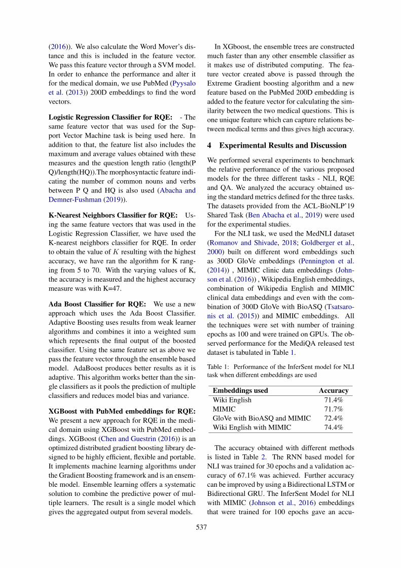
(2016)). We also calculate the Word Mover’s dis-tance and this is included in the feature vector.We pass this feature vector through a SVM model.In order to enhance the performance and alter itfor the medical domain, we use PubMed (Pyysaloet al. (2013)) 200D embeddings to find the wordvectors.
Logistic Regression Classifier for RQE: - Thesame feature vector that was used for the Sup-port Vector Machine task is being used here. Inaddition to that, the feature list also includes themaximum and average values obtained with thesemeasures and the question length ratio (length(PQ)/length(HQ)).The morphosyntactic feature indi-cating the number of common nouns and verbsbetween P Q and HQ is also used (Abacha andDemner-Fushman (2019)).
K-Nearest Neighbors Classifier for RQE: Us-ing the same feature vectors that was used in theLogistic Regression Classifier, we have used theK-nearest neighbors classifier for RQE. In orderto obtain the value of K resulting with the highestaccuracy, we have ran the algorithm for K rang-ing from 5 to 70. With the varying values of K,the accuracy is measured and the highest accuracymeasure was with K=47.
Ada Boost Classifier for RQE: We use a newapproach which uses the Ada Boost Classifier.Adaptive Boosting uses results from weak learneralgorithms and combines it into a weighted sumwhich represents the final output of the boostedclassifier. Using the same feature set as above wepass the feature vector through the ensemble basedmodel. AdaBoost produces better results as it isadaptive. This algorithm works better than the sin-gle classifiers as it pools the prediction of multipleclassifiers and reduces model bias and variance.
XGBoost with PubMed embeddings for RQE:We present a new approach for RQE in the medi-cal domain using XGBoost with PubMed embed-dings. XGBoost (Chen and Guestrin (2016)) is anoptimized distributed gradient boosting library de-signed to be highly efficient, flexible and portable.It implements machine learning algorithms underthe Gradient Boosting framework and is an ensem-ble model. Ensemble learning offers a systematicsolution to combine the predictive power of mul-tiple learners. The result is a single model whichgives the aggregated output from several models.
In XGboost, the ensemble trees are constructedmuch faster than any other ensemble classifier asit makes use of distributed computing. The fea-ture vector created above is passed through theExtreme Gradient boosting algorithm and a newfeature based on the PubMed 200D embedding isadded to the feature vector for calculating the sim-ilarity between the two medical questions. This isone unique feature which can capture relations be-tween medical terms and thus gives high accuracy.
4 Experimental Results and Discussion
We performed several experiments to benchmarkthe relative performance of the various proposedmodels for the three different tasks - NLI, RQEand QA. We analyzed the accuracy obtained us-ing the standard metrics defined for the three tasks.The datasets provided from the ACL-BioNLP’19Shared Task (Ben Abacha et al., 2019) were usedfor the experimental studies.
For the NLI task, we used the MedNLI dataset(Romanov and Shivade, 2018; Goldberger et al.,2000) built on different word embeddings suchas 300D GloVe embeddings (Pennington et al.(2014)) , MIMIC clinic data embeddings (John-son et al. (2016)) , Wikipedia English embeddings,combination of Wikipedia English and MIMICclinical data embeddings and even with the com-bination of 300D GloVe with BioASQ (Tsatsaro-nis et al. (2015)) and MIMIC embeddings. Allthe techniques were set with number of trainingepochs as 100 and were trained on GPUs. The ob-served performance for the MediQA released testdataset is tabulated in Table 1.
Table 1: Performance of the InferSent model for NLItask when different embeddings are used
Embeddings used AccuracyWiki English 71.4%MIMIC 71.7%GloVe with BioASQ and MIMIC 72.4%Wiki English with MIMIC 74.4%
The accuracy obtained with different methodsis listed in Table 2. The RNN based model forNLI was trained for 30 epochs and a validation ac-curacy of 67.1% was achieved. Further accuracycan be improved by using a Bidirectional LSTM orBidirectional GRU. The InferSent Model for NLIwith MIMIC (Johnson et al., 2016) embeddingsthat were trained for 100 epochs gave an accu-
537
Table 2: Comparative performance of the proposed ap-proaches for the NLI, RQE and QA tasks
Methology Used Task AccuracyRNN NLI 67.1%Infersent+MIMIC NLI 71.7%Infersent+MIMIC+Wiki NLI 74.4%UMLS Metathesaurus NLI 87.7%SVM RQE 62%Logistic Regression RQE 64.5%KNN RQE 62.4%Naive Bayes RQE 65%Ada Boosting RQE 66%XgBoost RQE 66.7%Closed domain QA QA 53.6%
racy of 71.7% This is because the medical contextof the sentences was taken care of by the MIMICword embeddings. The InferSent Model for NLIwith MIMIC and Wikipedia english words em-beddings gave an accuracy of 74.4% when trainedfor 100 epochs. This is because the medical andgrammatical concepts were given special empha-sis during the modeling phase. The model built onUMLS Metathesaurus and NLTK wordnet synsetsmodel achieved an accuracy of 87.7% on the testdata and 93.2% on validation data.
In the case of the RQE task, the SVM modelwas trained using a few features like semantic fea-tures, bigram overlap, word movers distance andcosine similarity. An accuracy of 62% achieved.The Logistic Regression model was trained usingseveral handcrafted features and an accuracy of64.5% was achieved. The KNN algorithm wasalso used for this classification task and an ac-curacy of 62.4% was obtained with K=47. TheNaive Bayes model was fine-tuned and trained us-ing the constructed feature vector. This gave anaccuracy of 64%. The Naive Bayes model fea-ture vector was modified again to include a fea-ture which will consider the content of both thequestions, which improved the accuracy by 1%.The AdaBoost classifier was used and this ensem-ble based method performed better than the naivemethods and gave an accuracy of 66%. The XG-Boost method performed the best and gave an ac-curacy of 66.7% on the test set.
As can be seen from Table 2, the closed do-main question answering model gave an accu-racy of 53.6% which is much above the baselinefixed at 51%. This accuracy was achieved because
this method focuses on finding the specific answerin the given context which is more relevant to agiven question. Based on the scores obtained fromthe closed domain model, the answers have beenranked accordingly. The model achieved an accu-racy of 53.6%, precision of 55.9% and Mean Re-ciprocal Rank of 62.93%.
4.1 Discussion
Based on the experimental results, we herebypresent several observations and insights into theproposed models. In the case of the NLI task,we performed error analysis for the InferSentmodel by varying the embeddings and incorporat-ing UMLS Metathesaurus and found that the er-ror ratio also varies. The ratio of the error ratebetween neutral, entailment and contradiction wasobserved to be 5 : 4 : 3, when the MIMIC wordembeddings (Johnson et al. (2016)) were used.However, it changed to 2 : 1 : 1 when the UMLSMetathesaurus with WordNet (pri, 2010) synsetsare used. Thus, it can be concluded that the neu-tral label was the hardest to predict and differen-tiating between entailment and neutrality is alsochallenging. In our current implementation, ifsimilar terms are present in the hypothesis andpremise, then the label of entailment is still pre-dicted, whereas the statements could actually beneutral. We also noticed that, by using clinicaldomain-specific embeddings, the predictions be-come more accurate.
Table 4 shows the Precision and Recall valuesfor RQE using XgBoost. XgBoost provides a par-allel tree boosting which improves the accuracy.Also, it uses continued training so it can furtherboost an already fitted model on new data, thus asignificant improvement in accuracy is observed.
Table 3: Confusion Matrix for NLI
Label True FalseEntailment 121 14
Neutral 114 21Contradiction 128 15
Table 4: Confusion Matrix for RQE
Parameters True FalsePrecision 0.68 0.66
Recall 0.65 0.69
538
5 Concluding Remarks
In this paper, several techniques for the NLI, RQEand QA tasks were discussed. For addressing theNLI task, the UMLS Metathesaurus was used tofind the synonyms of medical terms in given sen-tences, on which the InferSent model was trainedto predict if the given sentence is an entailment,contradictory and neutral. We also designed anew Extreme gradient boosting model built onPubMed embeddings to perform RQE. Further,a closed-domain Question Answering techniquethat uses Bi-directional LSTMs trained on theSquAD dataset to determine relevant ranks of an-swers for a given question was also presented.Among the proposed models, the UMLS Metathe-saurus and NLTK wordnet synsets model achievedthe highest accuracy of 87.7% on the test datasetprovided by the MediQA Challenge (Ben Abachaet al., 2019). For RQE, the highest accuracy of66.7% was achieved using the XGBoost method.For the QA task, we achieved an accuracy of53.6%, precision of 55.9% and Mean ReciprocalRank of 62.93%.
As future work, we intend to extend the tex-tual inference model for the clinical domain to de-velop decision support applications so that treat-ment methods can be simplified by grouping sim-ilar diseases and problems together. This can beachieved by using RQE which can aid in analyz-ing if two different health conditions are similarenough to have the same treatment. The model canalso be trained on MedQuAD dataset (Abacha andDemner-Fushman (2019)) to improve the accuracyso that the model can perform more accurately inreal-world hospital scenarios.
ReferencesPrinceton university ”about wordnet.” wordnet. prince-
ton university. [online]. 2010.
Asma Ben Abacha and Dina Demner-Fushman. 2016.Recognizing question entailment for medical ques-tion answering. In AMIA Annual Symposium Pro-ceedings, volume 2016, page 310. American Medi-cal Informatics Association.
Asma Ben Abacha and Dina Demner-Fushman. 2019.A question-entailment approach to question answer-ing. arXiv preprint arXiv:1901.08079.
Alan R Aronson. 2001. Effective mapping of biomed-ical text to the umls metathesaurus: the metamapprogram. In Proceedings of the AMIA Symposium,page 17. American Medical Informatics Associa-tion.
Asma Ben Abacha, Chaitanya Shivade, and DinaDemner-Fushman. 2019. Overview of the mediqa2019 shared task on textual inference, question en-tailment and question answering. In Proceedings ofthe BioNLP 2019 workshop, Florence, Italy, August1, 2019. Association for Computational Linguistics.
Samuel R Bowman, Gabor Angeli, Christopher Potts,and Christopher D Manning. 2015. A large anno-tated corpus for learning natural language inference.arXiv preprint arXiv:1508.05326.
Mikhail Burtsev, Alexander Seliverstov, RafaelAirapetyan, Mikhail Arkhipov, Dilyara Baymurz-ina, Nickolay Bushkov, Olga Gureenkova, TarasKhakhulin, Yuri Kuratov, Denis Kuznetsov, et al.2018. Deeppavlov: Open-source library for dia-logue systems. In Proceedings of ACL 2018, SystemDemonstrations, pages 122–127.
Qian Chen, Xiaodan Zhu, Zhen-Hua Ling, DianaInkpen, and Si Wei. 2017. Neural natural languageinference models enhanced with external knowl-edge. arXiv preprint arXiv:1711.04289.
Qian Chen, Xiaodan Zhu, Zhenhua Ling, Si Wei,Hui Jiang, and Diana Inkpen. 2016. Enhancedlstm for natural language inference. arXiv preprintarXiv:1609.06038.
Tianqi Chen and Carlos Guestrin. 2016. Xg-boost: A scalable tree boosting system. CoRR,abs/1603.02754.
Alexis Conneau, Douwe Kiela, Holger Schwenk, LoicBarrault, and Antoine Bordes. 2017. Supervisedlearning of universal sentence representations fromnatural language inference data. arXiv preprintarXiv:1705.02364.
Yiming Cui, Zhipeng Chen, Si Wei, Shijin Wang,Ting Liu, and Guoping Hu. 2016. Attention-over-attention neural networks for reading comprehen-sion. arXiv preprint arXiv:1607.04423.
Ary L Goldberger, Luis AN Amaral, Leon Glass, Jef-frey M Hausdorff, Plamen Ch Ivanov, Roger GMark, Joseph E Mietus, George B Moody, Chung-Kang Peng, and H Eugene Stanley. 2000. Phys-iobank, physiotoolkit, and physionet: componentsof a new research resource for complex physiologicsignals. Circulation, 101(23):e215–e220.
Jeroen Antonius Gerardus Groenendijk and Martin Jo-han Bastiaan Stokhof. 1984. Studies on the Seman-tics of Questions and the Pragmatics of Answers.Ph.D. thesis, Univ. Amsterdam.
Alistair EW Johnson, Tom J Pollard, Lu Shen,H Lehman Li-wei, Mengling Feng, Moham-mad Ghassemi, Benjamin Moody, Peter Szolovits,Leo Anthony Celi, and Roger G Mark. 2016.Mimic-iii, a freely accessible critical care database.Scientific data, 3:160035.
539
Edward Loper and Steven Bird. 2002. Nltk: The nat-ural language toolkit. In In Proceedings of the ACLWorkshop on Effective Tools and Methodologies forTeaching Natural Language Processing and Compu-tational Linguistics. Philadelphia: Association forComputational Linguistics.
Jake Luo, Guo-Qiang Zhang, Susan Wentz, LicongCui, and Rong Xu. 2015. Simq: Real-time retrievalof similar consumer health questions. J Med Inter-net Res.
Fabian Pedregosa, Gaël Varoquaux, Alexandre Gram-fort, Vincent Michel, Bertrand Thirion, OlivierGrisel, Mathieu Blondel, Peter Prettenhofer, RonWeiss, Vincent Dubourg, et al. 2011. Scikit-learn:Machine learning in python. Journal of machinelearning research, 12(Oct):2825–2830.
Jeffrey Pennington, Richard Socher, and Christo-pher D. Manning. 2014. Glove: Global vectors forword representation. In Empirical Methods in Nat-ural Language Processing (EMNLP), pages 1532–1543.
M.F. Porter. 1980. An algorithm for suffix stripping.Program, 14(3):130–137.
Sampo Pyysalo, Filip Ginter, Hans Moen, TapioSalakoski, and Sophia Ananiadou. 2013. Distribu-
tional semantics resources for biomedical text pro-cessing.
Pranav Rajpurkar, Jian Zhang, Konstantin Lopyrev, andPercy Liang. 2016. Squad: 100,000+ questionsfor machine comprehension of text. arXiv preprintarXiv:1606.05250.
Alexey Romanov and Chaitanya Shivade. 2018.Lessons from natural language inference in the clin-ical domain. arXiv preprint arXiv:1808.06752.
George Tsatsaronis, Georgios Balikas, ProdromosMalakasiotis, Ioannis Partalas, Matthias Zschunke,Michael R. Alvers, Dirk Weissenborn, AnastasiaKrithara, Sergios Petridis, Dimitris Polychronopou-los, Yannis Almirantis, John Pavlopoulos, Nico-las Baskiotis, Patrick Gallinari, Thierry Artiéres,Axel-Cyrille Ngonga Ngomo, Norman Heino, EricGaussier, Liliana Barrio-Alvers, Michael Schroeder,Ion Androutsopoulos, and Georgios Paliouras. 2015.An overview of the bioasq large-scale biomedicalsemantic indexing and question answering compe-tition. BMC Bioinformatics.
Adina Williams, Nikita Nangia, and Samuel R Bow-man. 2017. A broad-coverage challenge corpus forsentence understanding through inference. arXivpreprint arXiv:1704.05426.
540
Author Index
Agrawal, Anumeha, 533Akhondi, Saber, 328Alhuzali, Hassan, 339Ammar, Waleed, 319Ananiadou, Sophia, 339Androutsopoulos, Ion, 292, 298Anil George, Rosa, 533Apidianaki, Marianna, 298Apostolova, Emilia, 66Arakelyan, Arsen, 176Archana, Vaidheeswaran, 510
Baker, Simon, 125Bandyopadhyay, Dibyanayan, 517Bannihatti Kumar, Vinayshekhar, 453Barbu Mititelu, Verginica, 71Beltagy, Iz, 319Ben Abacha, Asma, 370Bernardino, Ariane, 201Bertels, Ann, 211Bhaskar, Sai Abishek, 462Bordea, Georgeta, 115
Campillos-Llanos, Leonardo, 152Cardon, Rémi, 309Cengiz, Cemil, 427Chatterjee, Soham, 510Chaudhary, Aditi, 453Chauhan, Geeticka, 30Chen, Po-Han, 528Chernodub, Artem, 97Chiu, Billy, 125Choi, Edward, 261Chopra, Sahil, 488Claveau, Vincent, 273Cohn, Trevor, 328Couto, Francisco M, 523
Demner-Fushman, Dina, 370Desmet, Bart, 1Devereux, Barry, 48Divita, Guy, 1Dligach, Dmitriy, 283Druckenbrodt, Christian, 328
Eisenstein, Jacob, 261Ekbal, Asif, 517
Fauqueur, Julien, 142
Gain, Baban, 517Galstyan, Aram, 176Galstyan, Tigran, 176Gao, Jianfeng, 399Garg, Shefali, 389Ginés i Ametllé, Joan, 292Gonçalo Oliveira, Hugo, 223Gontcharov, Aleksandr, 217Goodrum, Heath, 191Grabar, Natalia, 97, 115, 273, 309Gregory, Michelle, 328Grön, Leonie, 211Grouin, Cyril, 273Gudala, Meghana, 191Gunasekara, Isuru, 217Gupta, Ankita, 488Gupta, Prashant, 389
Hakobyan, Anna, 176Hambardzumyan, Karen, 176Hamon, Thierry, 97, 115, 273Heylen, Kris, 211Hirst, Graeme, 234Hovy, Eduard, 80Huang, Sicong, 415
Ive, Julia, 240
Jeblee, Serena, 234Jin, Qiao, 88Joshi, Aditya, 135Jung, Kyomin, 406
Kamath, Sowmya, 533Kanakarajan, Kamal raj, 510Kanoulas, Evangelos, 105Karimi, Sarvnaz, 135, 478Kaushik, Anupama, 488Kearns, William, 500Khachatrian, Hrant, 176
541
King, Daniel, 319Koptient, Anaïs, 309Korhonen, Anna, 125Koroleva, Anna, 359Kotitsas, Sotiris, 298Koutroulis, Ioannis, 66Kumar, Anand, 533Kyriakakis, Manolis, 292
Lamurias, Andre, 523Lang, Chengkun, 437Lau, Wilson, 500Lee, Lung-Hao, 528Lee, Po-Lei, 528Leeflang, Mariska, 105Lei, Bizun, 446Li, Chunyuan, 399Li, Xiepeng, 380Li, Xuefei, 437Liu, Dianbo, 283Liu, Jinling, 88Liu, Xiaodong, 399Liu, Zhe, 446Liu, Zhuang, 446Lopes, Fábio, 223Lu, Xinghua, 88Lu, Yi, 528Lu, Zhiyong, 58Luo, Xun, 380
Ma, Weicheng, 250MacIntyre, C Raina, 135Martínez-del-Rincón, Jesús, 48McDermott, Matthew B.A., 30McDonald, Ryan, 298McGuinness, Bernadette, 48Mercer, Robert E., 165Mezaoui, Hichem, 217Mikhailov, Michael, 348Miller, Timothy, 283Misra, Ankita, 191Mitamura, Teruko, 389, 453, 462Mitrofan, Grigorina, 71Mitrofan, Maria, 71Mougin, Fleur, 115
Nam, Jiin, 406Nersisyan, Lilit, 176Neumann, Mark, 319Névéol, Aurélie, 105Newman-Griffis, Denis, 1Ng, Hwee Tou, 11
Ngiam, Kee Yuan, 11Nguyen, Dat Quoc, 328Nguyen, Vincent, 478Ni, Yuan, 380Ning, Shixian, 437Norman, Christopher, 105Nyberg, Eric, 389, 453, 462
Ormerod, Mark, 48
Palmer, Martha, 125Pappas, Dimitris, 298Paris, Cecile, 135Paroubek, Patrick, 359Peng, Yifan, 58Poon, Hoifung, 399Pugaliya, Hemant, 389Pylieva, Hanna, 97
Rajagopal, Dheeraj, 80Ramamoorthy, Suriyadeepan, 510Randriatsitohaina, Tsanta, 115Ravi, Selvan Suntiha, 533Rayasam, Anirudha, 80Roberts, Kirk, 20, 191Robertson, Neil, 48Roller, Roland, 348Route, James, 453, 462Roychowdhury, Sumegh, 471Rungta, Rashi, 462Rzhetsky, Andrey, 176
Saikh, Tanik, 517Sankarasubbu, Malaikannan, 510Saudabayev, Artur, 292Saxena, Karan, 389Sert, Ulaş, 427Shalini, Sheetal, 389Sharma, Prakhar, 471Shivade, Chaitanya, 370Shyu, Kuo-Kai, 528Siddhant, Aditya, 80Song, Yan, 250, 415Soni, Sarvesh, 20Sparks, Ross, 135Specia, Lucia, 240Spijker, René, 105Spruit, Marco, 493Srinivasan, Ashwin, 453Sun, Jimeng, 261Szolovits, Peter, 30
Tandon, Niket, 80
Tawfik, Noha, 493Teixeira, César, 223Thillaisundaram, Ashok, 142Thomas, Jason, 500Thorne, Camilo, 328Tian, Yuanhe, 250, 415Tissot, Hegler, 201Togia, Theodosia, 142Tschampel, Tim, 66
Vashisth, Gaurav, 348Velez, Tom, 66Velupillai, Sumithra, 201, 240Verspoor, Karin, 328Viani, Natalia, 201Voigt-Antons, Jan-Niklas, 348Vyas, Nidhi, 80
Wang, Keqiang, 380Wang, Tony, 66Wang, Xindi, 165Wang, Zixu, 240Wiegreffe, Sarah, 261Wu, Zhaofeng, 415
Xia, Fei, 250, 415Xie, Guotong, 380Xing, Zhenchang, 478Xu, Yichong, 399
Yan, Shankai, 58Yan, Sherry, 261Yan, Zhaodong, 234Yao, Weihong, 437Yoon, Seunghyun, 406Yuret, Deniz, 427Yuwono, Steven Kester, 11
Zhai, Zenan, 328Zhou, Huiwei, 437, 446Zhou, Xiaofeng, 380Zhu, Wei, 380Zirikly, Ayah, 1


