KEK-PROC—91-13 JP9206376

PROCEEDINGS OF THE FIFTH WORKSHOP

ON ELEMENTARY-PARTICLE PICTURE OF THE UNIVERSE

Izu, November 19-21, 1990

NATIONAL LABORATORY FOR HIGH ENERGY PHYSICS, KEK

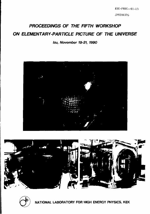
Cover photograph Top Bottom Left

Right

Kamiokande Detector INS Air-Core /?-Ray Spectrometer BESS (Balloon Experiment with Superconducting Solenoid) Detector

Proceedings of the Fifth Workshop

on Elementary-Particle Picture

of the Universe

Izu, November 19-21, 1990

Editors: Masataka Fukugita R.IFP, Kyoto Univ. Atsuto Suzuki KEK

KEK Proceedings 91-13 H

National Laboratory for High Energy Phy

KEK Reports are available from:

Technical Information & Library National Laboratory for High Energy Physii 1-1 Oho, Tsukuba-shi Ibaraki-ken, 305 JAPAN

Phone: 0298-64-1171 Telex: 3652-534

(0)3652-534 Fax: 0298-64-4604 Cable: KEKOHO

(Domestic) (International)

Foreword

The Fifth Workshop on the Elementary-Particle Picture of the Universe was held at the Izu National Rest House, Minami- Izu, from 19 to 21, November, 1990. The 80 participants included high-energy physicists, nuclear physicists, cosmic-ray physicists and astrophysicists. Both theorists and experimentalists were participated. This was the concluding workshop of a series that started in February, 1987. It was supported by a Grant-in-Aid for "Scientific Research on Priority Areas" by the Ministry of Education "Elementary-Particle Picture of the Universe", after having a few sporadic workshops held over the preceding few years. At that time there was a growing interest in interdisciplinary fields among particle physics and astrophysics: there were large activities searching for proton decay, as a decisive test for grand unification theories, which are closely related to our understanding of the baryon number generation in the universe. 1MB, Kamiokande, Frejus, NUSEX and KGF renewed their results every year. Stimulated by the idea of Mikheyev and Smirnov revived interest was focused on the solar neutrino problem from a particle physics point of view. Interest was even amplified by an announcement made by Davis in the Toyama Symposium (1986) that solar neutrino captures may be correlated with solar activity. Kamiokande-11 was ready for detecting solar neutrinos by the end of 1986. Sliortly after this lime, actually two weeks after our first workshop, we experienced the celebrated supernova SN1987A in the Large Magel­lanic Cloud. The neutrino signal from that supernova was detected by the Kamiokande-Il and 1MB detectors. It was the first moment in the history of science that theoretically the speculated dynamics of stellcr collapse could be confirmed, with the use of detectors designed for particle physics studies. This neutrino observation triggered a burst of studies in this interdisciplenary field. The ITEP results (1980) for a finite electron neutrino mass, which initiated intensive studies for a "dark matter dominated universe", were still alive. The experimental effort, including a Japanese experiment, was being made to push down a new limit below the window claimed by the ITEP group. Motivated by the successes and failures of a neutrino dark-matter universe, and also by the prediction of an inflationary universe — which itself is also a possible consequence of grand unification — cosmologists were busy try­ing to understand the large-scale structure of the universe in terms of the hypothetical "cold dark matter" which provides the mass density that makes the universe flat. This "success" promoted a search for cold dark-matter candidates; axions, heavy neutrinos or other -inos. A Japanese sounding rocket which was launched in Feb. 1987, "discovered" a significant distortion in the cosmic microwave background spectrum, which required energetics greater than astrophysicists could account for. A number of speculations were proposed to account for such a distortion. More pure theorists were dedicating their life to the study of super-

string theory; many of them optimistically hoped that all of the forces of particle physics could be unified, and even the long-standing particle mass spectrum problem could be solved soon. The Grant-in-Aid project called "Elementary Particle Picture of the Universe started under pressure of these physical backgrounds.

The last 5 years since then have provided us with the following results: (1) No evidence has been found for proton decay. The minimal SU(5) model has encountered trouble; (2) The upper limit on the electron neutrino mass has been lowered down to 10 oV. This excludes the finite-mass result of the 1TEP experiment; (;i) The GOBI-/ satellite has undoubtedly disproved the Japanese rocket, discovery. There is no distortion in the cosmic microwave background spectrum; (4) LEP experiments have definitely shown that there are only three generations associated with light neutrinos. This, at the same lime, rules out most of exotic particles with mass < '15 GeV, which would be a candidate for dark matter. Any hypothetical particle henceforth allowed must be weak (SU('2))-charge neutral as well as electric-charge neutral and SU(3) f neutral. Many of the proposed particle models were excluded by this observa­tion; (5) The "prediction" of inflation (Q0 = 1) is not. supported by the observations. They strongly point towards n o < 1; (C) A decline and fall of suporstring studies. The theory was not unique as hoped. The vacuum is not unique either, which requires a non-perturbative study beyond the currently available technique. Suporstring "inspired" phenomenology also turned out to be rather suporstring "independent" phenomenology. Most significant of all, very few people study superstrings any more.

These observations clearly consolidated our views, and have forced us to believe that the real world is very close to what the standard theory predicts. Old problems remain intact both in particle physics and astrophysics. Our frustration is that cosmology has not pro­vided us with any testing grounds for particle theories, nor could particle physics help us to solve any problems in astrophysics so far. There are, however, a few positive aspects which have been clarified during this period: (1) The solar neutrino experiments of Kamiokande-II, when combined with the Homestake result, strongly suggests that the solar neutrino problem originates in neutrino properties that are unexpected from the standard model. The SAGE experiment also supports this view. We should await more confirmative results from SAGE and GALLEX; (2) Precise mass measurements of V and Z lead to an accurate determination of sin 2 0|v, which shows a clear deviation from the value predicted in the original minimal SIF(O) grand unified theory. The value, however, shows remarkable agreement with that pre­dicted in the minimal SUSY SU(5) model. There are, however, other models ( e.g., SO(10)) which also account for the experiment. In any case this seems to indicate the existence of some new energy scale of the unified theory, which deserves further study.

In this workshop most of the time was given to reviews of the present status and prospects of the subjects of the present project as well as some others, in order to find future directions.

In the same spirit we held a detector symposium at which we discussed frontier of technology, with the purpose to explore the interdisciplcnary applicability of new technology now being developed. A special session was also arranged for a progress report by representatives of the major experimental groups who received support under the present project. We believe that the workshop was useful to know the status where we are. We hope that the next workshop, when newly held on some other occasions, will bring more success.

As organizers we would like to express our gratitude to all of the people who contributed to the workshop; in particular we thank the lecturers and the chairmen as well as younger members of the Kamiokandc group for their assistance in both technical and administrative work. Finally, we would like to acknowledge the support by a Grant-in-Aid for Scientific Research from the Japanese Ministry of Education, Science and Culture.

November 1991 M. Fukugita A. Suzuki

Workshop Record of "Elementary Particle Picture of the Universe"

1st Workshop: 6-7 February 1987, KEK (Proceedings editted by M.Yoshimura, Y.Totsuka and K.Nakamura)

2nd Workshop: 4-6 February 1988, KEK (Proceedings editted by M.Yoshimura, Y.Totsiika, K.Nakamura and C.S.Lim)

3rd Workshop: 17-19 October 1988, Fujiyoshida (Proceedings cditted by C.S.Lim, M.Mori, A.Suzuki and T.Tanimori)

4th Workshop: 22-25 November 1989, Tateyama (Proceedings editted by K.Hikasa, T.Nakamura T.Ohshima and A.Suzuki)

5th Workshop: 19-21 November 1990, Minami-Izu (Proceedings cditted by M.Fukugita and A.Suzuki)

Previous Related Workshop

• 13-M February 1979, KEK The Unified Theory and the Baryon Number in the Universe, KEK-79-18 (1979), edit­ted by O.Sawada and A.Sugamoto

• 18-20 October, 1982, Kamioka Monopolcs and Proton Decay, KEK-83-12 (1983), ediUed by J.Arafune and H.Sugawara

• 25-27 January, 1983, KEK Grand Unified Theories and Early Universe, KEK-83-13 (1983), editted by M.Fukugita and M.Yoshimura

• 7-10 December, 1983, KEK Grand Unified Theories and Cosmology, KEK-84-12 (1984), edittcd by K.Odaka and A.Sugamoto

• 15-17 November, 1984, Takayama Towards Unification and its Verification, KEK-S5-4 (1985), editted by Y.Kazama and T.Koikawa

• 16-18 April, 1986, Toyama Seventh Workshop on Grand Unification/ICOBAN'SG, World Scientific (1986), editted by J.Arafune

Reports on Workshop Related to the Present Project

• Proceedings of Workshop on Dark Matter and the Structure of the Universe, Research Institute for Theoretical Physics (RITP), Hiroshima Univ., Takehara 725, Japan, Jan­uary 29- February 1, 1989, RRK 89-28.

• Proceedings of the Summer Workshop on Supcrstrings, KICK, Tsukuba, Japan, August 29- September 3, 1988, KEK Report 88-12.

• Proceedings jf the Workshop "Topology, Field Theory and Superstrings", KICK, Tsukuba, Japan, November 6-10, 1989, KEK Report 89-22.

• Proceedings of the Second Workshop on Dark Matter and the Structure of the Universe, Uji Research Center Yukawa Institute for Theoretical Physics (YITP), Kyoto Univ., Uji 611, Japan, October •1-5, 1990, YITP/U-91-19.

• Proceedings of the Workshop "Superslrings and Oonformal Field Theories", KICK, Tsukuba, Japan, December 18-21, 1990, KEK Proceedings 91-6.

Workshop Program M o n d a y , N o v e m b e r 1 9

I. Solar Neutrino Problem Chairman : II. Minakata (Tokyo Metropolitan Univ.)

The Status of Solar Neutrino Experiments M. Ta.kit.ii (Osaka Univ.)

Future Solar Neutrino Experiments M. Mori (KEK)

Indium Loaded Liquid Scintillator for 7Be and pep Solar Neutrino Detection K. Inoue (ICRR, Univ. of Tokyo)

Neutrino Astronomy Y. 7bt.su/ca (ICRR, Univ. of Tokyo)

II. Detector Symposium Chairman: Y. Suzuki (ICRR, Univ of Tokyo)

New Silicon-Based Low-Noise Photon Detectors T. A'amae (Univ. of Tokyo) R. Enomoto (KEK)

Development of Analog VLSI for High Energy Physics Experiment //. Ikcda (KEK)

Development of Infrared Camera M. Ucno (National Astronomical Observatory)

Optical CCD M. Sokiguchi (National Astronomical Observatory) S. Okamura (Univ. of Tokyo)

H I . As t rophys ic s Chairman : II. Kodama (Kyoto Univ.)

Hubble Space Telescope and Japan National Large Telescope M. lye (National Astronomical Observatory)

Measurement of the Neutron Capture Rate of Light Nuclei Y. Nugai (Tokyo Institute of Technology)

Comment : Primordial Nucleosynthesis K. Sato (Univ. of Tokyo)

Paradigm Lost? — Role of Theoretical Prejudices in Cosmology — Y. Suto (RIFP, Kyoto Univ.)

i

Cosmic Background Radiation Experiments T. THJahiilo (Waseda Univ.)

Prospects of Gravitational Wave Astronomy T. Nakiinwra (RIFP, Kyoto Univ.)

Tuesday, November 20

IV. Atmospheric Neutrinos Chairman : K. Kasa.ha.ra. (Kanagawa Univ.)

Review of Atmospheric Neutrino Problem T. Kiijitu (1CRR, Univ. of Tokyo)

Calculation of Atmospheric Neutrino Fluxes S. Mixuin (Tohoku Univ.)

The Anomalous Atmospheric Neutrino Flux and the Possibility of Neutrino Oscillation

M. Honda (ICRIl, Univ. of Tokyo) Experimental Study of Atmospheric Electrons at Airplane Altitude

R. Enainoio (KEK)

V. Observations of High Energy Cosmic Rays Chairman : A'. Hika.su (KEK)

Experimental Results Obtained from the Akcno Giant Air Shower Array M. Teshima (1CRR, Univ. of Tokyo)

Recent Status of CANGAROO Project T. Taniinwri (Tokyo Institute of Technology)

VI. X-Ray Astronomy Chairman : S. Okamura. (Univ. of Tokyo)

X-Ray Emissions from Clusters of Galaxies K. Koyama. (Nagoya Univ.)

VII. Elementary Particle and Universe I Chairman : Y. Totsuka, (ICRR, Univ. of Tokyo)

Stellar Neutrinos and Cosmic Rays M. Knshiba (Tokai Univ.)

Prospects of Neutrino Physics T. Yanagida (Tohoku Univ.)

Recent. Progress in the Cosmic Dark Matter Problem //. Kodama (Kyoto Univ. )

Supergravity and Supersymmetric Dark Matter M. Nojiri (KEK)

Wednesday, November 21

Birth and Early Evolution of Our Universe K. Sato (Univ. of Tokyo)

V I I I . R e p o r t s on P ro jec t Researches (Gran t - in Aid for Scientific Research on Pr ior i ty Areas)

Chairman : A. Suzuki (KEK)

New Upper Bound on Electron Anti-Neutrino Mass S. Shibata (INS, Univ. of Tokyo)

Liquid Xenon Ionization Drift Chamber for Detection of Neul riuo-Less l)uul>l< Beta-Decay of 1 3 6 X e and Related Research Programs

M. Miyajima (KEK) BESS Experiment

M. Nozaki (Univ. of Tokyo) Detection of Galactic Axion with Rydberg Atoms

S. Matsuki (RINP, Osaka Univ.) A Cryogenic Detector Using Superheated Superconducting Tin Granules

T. Ebisu (Kobe Univ.)

IX. E l emen ta ry Par t ic le and Universe II Chairman : M. Fukugita (RIFP, Kyoto Univ.)

Elementary Particle and Universe M. Yos/n'mura (Tohoku Univ.)

Summary A. Suzuki (KEK)

/ , ,

TABLE OF CONTENTS

Workshop Program

The Status of Solar Neutrino Experiments M. Tnkita, 1

Future Solar Neutrino Experiments M, Mori 15

Indium Loaded Liquid Scintillator for 7Be and pep Solar Neutrino Detection K. Inone 28

Neutrino Astronomy Y. Totsuka. 45

New Silicon-Based Low-Noise Photon Detectors T. A'amae R. Enomoto 68

Development of Analog VLSI for High Energy Physics Experiment H. JA-eda 82

Development of Infrared Camera M. Ueno 93

Optical CCD M. Sekiguchi 99 S. O/camura 105

Hubble Space Telescope and Japan National Large Telescope M. lye 108

Measurement of the Neutron Capture Rate of Light Nuclei Y. Nagai 123

Comment : Primordial Nucleosynthesis K. Sato 130

Nature of the QCD Phase Transition at Finite Temperatures M. FuJvugita 145

— v -

Paradigm Lost? — Role of Theoretical Prejudices in Cosmology — Y. Suto 147

Review of Atmospheric Neutrino Problem T. Kajita 154

Calculation of Atmospheric Neutrino Fluxes S. Mizuta 169

The Anomalous Atmospheric Neutrino Flux and the Possibility of Neutrino Oscillation

M. Honda. 184

Experimental Study of Atmospheric Electrons at Airplane Altitude R. Enomoto 190

Experimental Results Obtained from the Akeno Giant Air Shower Array M. Tcshima. 199

Recent Status of CANGAROO Project T. Tunimori 211

X-Ray Emissions from Clusters of Galaxies K, Koyama 221

Stellar Neutrinos and Cosmic Rays M. Koshiba, 228

Recent Progress in the Cosmic Dark Matter Problem H. Kodama 250

Supergravity and Supersymmetric Dark Matter M. Nojiri 265

Birth and Early Evolution of Our Universe K. Sato 277

New Upper Bound on Electron Anti-Neutrino Mass S. Shibnta 289

Liquid Xenon Ionization Drift Chamber for Detection of Neutrino-Less Double Beta-Decay of 1 3 6 X e and Related Research Programs

M. Miyajima. 306

- vi

Detection of Galactic Axion with Rydberg Atoms S. Matsuki 319

A Cryogenic Detector Using Superheated Superconducting Tin Granules T. Ebisu 332

Elementary Particle and Universe M. Yashimura 344

T h e S t a t u s of Solar Neu t r ino E x p e r i m e n t s

Presented by M. Takita

Osaka University

The observation of solar neutrinos provide extremely important opportunities in view of particle physics beyond the standard model. Non-trivial neutrino properties may be required to explain the various aspects of the presently available solar neutrino data' '.

(!) Solar Neutrino problem.

The Sun is a copious source of electron neutrinos produced in the nuclear fusion reactions which generate the solar energy. Figure J shows the fluxes of solar neutrinos at the surface of the Earth from various nuclear fusion reactions. The shapes of these distributions are nothing but the beta decay spectra, but their absolute normalization are given by the standard solar model (SSM) prediction by Bahcall and UliichW.

Since 1970 Davis and his collaborators have been conducting a radiochemical solar neutrino experiment at the llomestake gold mine using the reaction i/,.+ 3 ,('l —»e _ i 'Ar' 1 The threshold of this reaction is 0.8M McV, and the captured neutrinos are mainly those from the decay of S B nuclei.

More recently, the Kamiokande-II (Kam-Il) collaboration succeeded in observing the 8 B solar neutrinos using the elastic, scattering i\.i.\—*i',v in a water Cerenkov detector.' ' In contrast with a radiochemical method, this experiment is a real time one measuring not only the recoil electron spectrum also directional correlation with respect to the Sun. The last, feature greatly helps to separate clearly the solar neutrino signal from the flat, background.

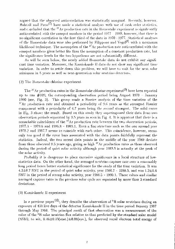
There are two aspects which arc particularly interesting in the solar neutrino data of Davis ct al.t '. First, their data over two decades indicated deficit in solar neutrinos; The observe average solar neutrino capture rat.c by •''f'l over the period March 1970 March 1988 was 2.3±0.'< SNU (solar neutrino units) as compared with the SSM prediction of 7.9 SNU. This is the famous "solar neutrino problem"'. The recent Kam-II result also indicated that the observed solar neutrino flux is less than a half of that predicted by the SSM. Second, a. possible time variation of the 3 ' ( j l capture rate, anticorrelated with the suuspot numbers which represent the 11-year cycle ol solar activity, has been pointed out by a number of authors. Figure 2 shows the 5 point running averages of the ' ! ' ( ' l neutrino capture rate compared with the siinspot numbers. It seems that the antieorrclation exists after 1977. These two problems arc the central issues of the current solar nent rino studies.

The first issue, i.e., the solar neutrino deficit has been customarily discussed relative to the central value of the SSM calculation by Bahcall and Ulrich'"'. However, there is another recent SSM calculation by Turck-C'liiezet''! which gives Hiout '!"> % less S B solar neutrino flux than that of Bahcall and Ulrich. Table 1 compares the results ol" these two SSM calculations. Turck-Chiczc. In view of the large theoretical uncertainties of the SSM, this deficit might not be so significant.

The possibility of the time variation of the sol sr neut rino capture rate by ' '( 'I has been a subject of statistical analysis by several authors. In i987, Bahcall, Field, and Press ' '

I

argued that the observed anticorrelalion was statistically marginal. Recently, however. Hahcall and Press' ' have made a statistical analysis with use of rank-order statistics, and concluded that the 3 'A r production rate in the llomestake experiment is significantly anticorrelated with the sunspot numbers in the period 1977 1989, however, that there is no significant correlation in the first third of the data in 1970 -1977. Statistical analyses of the Hornestake data were also performed by Filippone and Vogcl' ' with a maximum likelihood technique. The assumption of the 3 'Ar production rate auticorrclated with the sunspot numbers gives better fits than the assumption of a constant production rate, but the significance levels for the two hypotheses are not substantially different.

As will be seen below, the newly added Homestake data do not exhibit any signifi­cant time variation. Moreover, the Kainiokande 11 data do not show any significant time variation. In order to settle down this problem, we will have to wait for the next solar minimum in 5 years as well as next-generation solar neutrino detectors.

(2) The Homestake chlorine experiment

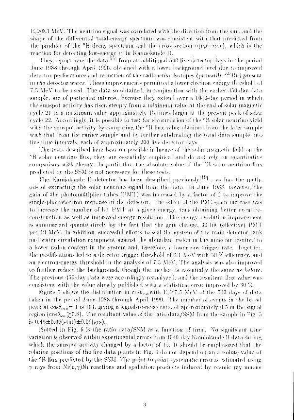
The 3 7 A r production rates in (lie Homestake chlorine experiment' ' have been reported up to run #109, Die corresponding observation period being August 1970 - January 1990 (see, Fig. 3). This group made a Fourier analysis of the time variation of the

3 'A r production rate and obtained a periodicity of 9.6 years as the strongest Fourier component with a periodicity of 4.7 years being the second strongest. The solid curve in Fig. 3 show.: the result. Based on this study they superimposed their data from two observation periods separated by 9.5 years as seen in Fig. -1. It is apparent that there is a remarkable coincidence of the 3 'A r production rate between the two observation periods, 1977..1 - 1979.6 and 198G.8 - 1989.1. Even a fine structure such as the one around year 1978.'J and 19S7.7 seems to coincide with each other. This coincidence, however, seems only too good if the error bars associated with the data points faithfully represent the statistics. Indeed, the two recent data points in the middle of (lie year 1989 deviate from those observed 9.5 years ago, giving a.s high 3 'Ar production rates a.s those observed during the period of cjuiet solar activity although year 1989.5 is actually at the peak of the solar activity.

Probably it is dangerous to place excessive significance in a local structure of low-statistics data. On the other hand, the averaged neutrino capture rate over a reasonably long period bears better statistical significance for the study of the time variation. It. was -l.2±0.7 SNU in the period of quiet, solar activity, year 1986.7 - 1988.5, and was 1.2±0.6 SNU in the period of strong solar activity, year 1988.5 - 1990.1. These values and similar averaged capture rates in the previous solar cycle are separated by more than 3 standard deviations.

(3) Kainiokande II experiment

In a previous paper' ', they describe the observation of 8 B solar neutrinos during an exposure of 150 live days of the detector Kamiokande II in the time period January 1987 through May 1988. The principal result of that observation was a measurement of the value of the 8 B solar neutrino flux relative to that predicted by the standard solar model (SSM), to wit, 0.-lG±0.13(stat.)±0.08(sys.), for observed recoil electron total energy of

]'-,.>!).3 MeV. T h e neut r ino signal was correlated with the direction from the sun. and the shape of the differential total-energy spec t rum was consistent, with that predicted from the product of the K B decay spec t rum and the cross section n(i'ev—n',.c), which is the reaction for delect ing low-energy v.. in Kamiokande 11.

They report, here the da ta ' ' from an additional 590 live detector days in the period June 1988 through April 1990. obtained with a lower background level due to improved detector performance and reduction of the radioactive isotopes (primarily """Tin) present in the de tec tor water. These improvements permit ted a lower elect ion eneigy threshold (.1 7.5 MeY to he used. The da ta so obtained, in conjunction with the earlier 150-day da t a sample , are of part icular interest., because they extend over a 1010-day period in which the sunspof activity has risen steeply from a minimum value at the end of solar magnetic cycle 21 to a max imum value approximately 15 t imes larger at the present peak of solar cycle 22. Accordingly, it is possible to test, for a correlation of the "H solar neutr ino yield with the sunspot activity by compar ing the ' B llux value obtained from the later sample with that from (lie earlier sample and by lur lher subdividing the total da t a sample into live t ime intervals, each of approximately 200 live detector days.

T h e tests described here bear on possible influence of the solar magnetic Held on the "H solar neut r ino flux, they are essentially empirical and do riot rely on quan t i t a t ive comparison with theory. In part icular , the absolute value of the "B solar neutr ino flux predicted by the SSM is not necessary for these tests .

The Kamiokande II detector has been described previously' ' . as has l he meth­ods o| ex t rac t ing the solar neutr ino signal from (he da ta . In June 19SS. however, the gain of the photomult ipl ier tubes ( P M T ) was increased by a factor of 2 to improve the singie-photoelect-con response of the detector . The ell'ect of tin- I 'M'I-gain increase was to increase the number of hit I'M F at a given energy, thus obtaining bet ter event re­const ruct ion as well as improved energy resolution. The energy resolution improvement is summar ized quant i ta t ively by the fact that the gain change, 30 hit (effective) I'M I per 10 MeV. In addi t ion, successful efforts to seal the system of the main detector l ank and water circulation equipment against the abundant radon in the mine air resulted in a lower radon content in the system and, therefore, a lower raw trigger rate . Together, the modifications led to a detector trigger threshold of (i. 1 MeV with 50 % eflieiency, and an electron-energy threshold in the analysis of 7.5 MeV. The analysis was also impioved to further reduce the background, though the method is essentially (lie same as before. The previous -150-day d a t a were accordingly reanalyzed, and the resultant, flux value was

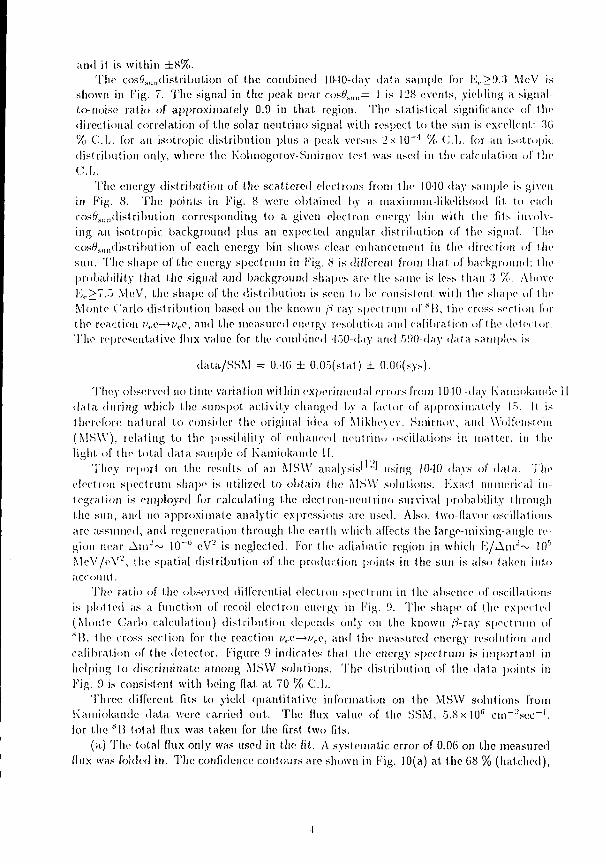
consistent with the value already published with a statist ical error improved by 30 '/(. Figure 5 shows the dis t r ibut ion in cos# s l l „wilh K,.>7.5 MeY of the 500 days .if da t a

taken in the period June I OSS through April 1000. The number of eveuls in the bread peak at c o s # s „ n = 1 is 10!, giving a signal-to-noise rat io of approximately 0.5 in the signal region (cos9 s „„>0.S) . The resultant value of the rat io d a t a / S S M from the sample in Fig. 5 is 0.-l5±0.0G(st 'at)±0.0(i(sys).

Plot ted in Fig. (i is the rat io d a t a / S S M as a function of t ime. N'o significant t ime variation is observed within experimental errors from 10-10-day Kamiokande 11 da ta dur ing which (lie sunspot activity changed by a factor of 15. It should be emphasized tha t the relative posit ions of the five data, points in Fig. (> do not depend on an absolute value of the "B flux predicted by the SSM. The point-to-point sys temat ic error is es t imated using 7 rays from Ni(n,7)Ni reactions and spallation products induced by cosmic ray unions

3

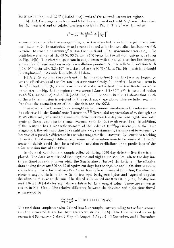
and it is within ± 8 % . T h e cos6l s, u ldistril>ution of the combined 1010-day da ta sample for l\,.>!)..'J MeV is

shown in Fig. 7. T h e signal in the peak near cos# s„„ = I is 128 events, yielding a signal-to-noiso rat io of approximate ly 0.9 in that, region. T h e stat ist ical significance of the directional correlation of the solar neutr ino signal wit.li respect to the sun is excellent: 'Hi % C.L. for an isotropic dis t r ibut ion plus a peak versus 2 x l 0 - ' 1 % C L . for an isotropic dis t r ibut ion only, where the Kolmogorov-Smiruov test was used in the calculation of the C.L.

The energy dis t r ibut ion of the scat tered electrons from the 10-10-day sample is given in Fig. 8. The points in Fig. 8 were obtained by a maximum-likelihood fit to each cos(? s„„distribution corresponding to a given electron energy bin with (he fits involv­ing an isotropic background plus an expected angular dis t r ibut ion of the signal. The cos$ s , 1 M distr ibut ion of each energy bin shows clear enhancement in the direction of the sun. T h e shape of the energy spec t rum in Fig. 8 is different from tha t of background; the probabil i ty that the signal and background shapes are the same is less than .'.! %. Above 1V>7.."J MeV, the shape of the dis t r ibut ion is seen to be consistent with the shape of tin-Monte Car lo dis t r ibut ion based on the known fl ray spec t rum of " B , the cross section lor the reaction i',.v—M/Cc, and the measured energy resolution and calibration of the detector . T h e representat ive flux value for the combined '|. r)0-day and .r>!)0-dny da ta samples is

d a t a / S S M = 0.-16 ± 0.05(stat) ± O.Oti(sys).

They observed no t ime variation within experimental errors from 10 10-day Kamiokaude 11 d a t a (luring which the sunspot. activity changed by a factor of approximately |.r>. It is therefore na tura l to consider the original idea of Miklieyev, Smimov , and Woll'enstein ( M S W ) , relat ing to the possibility of enhanced neutr ino oscillations in mat te r , in the light of the total da t a sample of Kamiokaude II.

They report on the results of an MSW analysis ' ' using 10-10 days of da ta . The electron spec t rum shape is utilized to obtain the MSVV solutions. Kxac.t numerical in­tegrat ion is employed for calculat ing the eleci ron-nentr ino survival probabili ty through the sun, and no approximate analyt ic expressions are used. Also, two-llavor oscillations are assumed, and regeneration through the ear th which affects the large-mixing-angle re­gion near A n r ~ 10~G e V 2 is neglected. For the adiabatic region in which K / i A n r ~ !()'' McV/oV-' , the spatial d is t r ibut ion of the product ion points in the sun is also taken into account .

The ratio of the observed differential election spec t rum in the absence of oscillations is plot ted as a function of recoil electron energy in Fig. !). The shape of the expected (Monte Car lo calculat ion) d is t r ibut ion depends only on the known /'"?-ray spec t rum of " B . the cross section for the reaction ;/,.c—>iv, and the measured energy resolution and cal ibrat ion of the detector . Figure 9 indicates that (ho energy spec t rum is impor tant in helping to discr iminate among MSW solutions. The distr ibution of the da ta points in Fig. 9 is consistent with being flat at 70 % C.L.

Three different fits to yield quant i ta t ive information on the MSW solutions from Kamiokandc da ta were carried out . T h e flux value of the SSM, S .SxIO 6 c i n - ~ s e c ~ \ lor the 8 B total flux was taken for the first two fits.

(a) T h e total (lux only was used in (lie fit. A systemat ic error of 0.06 on the measured flux was folded in. T h e confidence contours are shown in Fig. 10(a) at. the 68 % (hatched) ,

I

00 % (solid line), and 95 % (dashed line) levels of the allowed parameter regions. (I)) Both the energy spectrum and total flux were used in the fit A \" was determined

for (he measured and calculated electron spectra in Fig. 9. The \ " was defined as

where ; runs over electron-energy bins, r, is the expected ratio from a given neutrino oscillation, a, is the statistical error in each bin, and n is the normalization factor which is varied to reach a minimum \ 2 within the constraint of the systematic error of o„. The confidence contours at the 68 %, 90 %, and 95 % levels for the allowed regions are shown in Fig. 10(b). The electron spectrum in conjunction with the total neutrino flux imposes an additional constraint on neutrino-oscillation parameters. The adiabnlic solution with (i.:!x lO"4 < sin 2 26k 2.2x 10~2 is disfavored at the 90 % C.I,, in Fig. 10(b) which, it should be emphasized, uses only Kamiokaude II data.

(c) A \"' lit without the constraint, of the normalization (total flux) was performed to see the effectiveness of the electron spectrum more clearly. In practice, the second term in the \ 2 definition in (b) above, was removed and a in the first term was treated as a free parameter. In Fig. 11 the region shown around A n r ~ l. 'ixl0~' ! eV-' is excluded region at <JS % (dashed line) and 90 % (solid line) C.b. The result in Fig. 11 shows that much of the adiabatie region is rejected by the spectrum shape alone. This excluded region is free from the normalization of both the data and the SSM.

The next topic is to search for day-night and semiannual variations in the solar neutrino flux observed in the Kamiokande II detector.' ' Terrestrial regeneration of )>,. through the MSW effect may give rise to a small difference between the daytime and night-time solar neutrino fluxes, and also to a small seasonal variation in (he observed flux. In addition, if the neutrino has a magnetic moment of the order of I0~ l o/in (where \t\\ is the Bohr magneton), the solar neutrino [lux might also vary semiannually (as opposed to seasonally) because of a possible difference in the solar magnetic held traversed by neutrinos reaching the earth. If a day-night difference or semiannual variation were to be observed, the solar neutrino deficit, could then be ascribed to neutrino oscillations or to predictions of the solar neutrino flux of the SSM.

hi the analysis, the data sample collected during 1040-day detector live time is em­ployed. The data were divided into daytime and night-time samples, where the daytime (night-time) sample is taken while the Sun is above (below) the horizon. The effective data-taking times are 500 and 540 equivalent days for the daytime and night-time samples, respectively. The solar neutrino flux for each sample is measured by fitting the observed electron angular distribution with an isotropic background plus and expected angular distribution relative to the sun. The fluxed so obtained are 0.91±0.15 (stat) for daytime and 1.07±0.1(i (stat) for night-time relative to the averaged value. These are shown as circles in Fig. 12(a). The relative difference between (he daytime and night-time fluxed is expressed by

' ! a y : '" 6 ?' ' = -0.08±0.il±0.0.'i(sys).

The total data sample was also divided into four samples corresponding to the four seasons and the measured fluxes for them are shown in Fig. 12(b). The time interval for each season is 4 February - 5 May, 6 May - 4 August, 5 August 'l November, and 4 November

:5 February for spring, summer, fall, and winter, respectively. A correction for llie small variation (<(> %) of the flux induced by I lie eccentricity of the earth's orbit was made. Within statistical errors, there is no significant difference between the daytime and night­time fluxed, nor any seasonal variation.

A semiannual variation of the solar neutrino (lux is possible because the solar equatorial plane and the ecliptic plane cross with an opening angle of 7° IV twice per year. A line from the earth to the center of the sun crossed the equatorial plane around 7 June and 8 December. At these times, the detector views the core of the sun through the solar equator, where the magnetic field is expected to be weaker than at a higher solar latitude. The strength of (he interaction of a neutrino magnetic moment with the solar magnetic field would be less at those times and consequently a maximum modulation of the solar neutrino flux might occur.

To search for this effect the year was divided into tow periods: period 1, 22 April 21 July and 21 October - 20 .January and period II, 21 .January 21 April and 22 July

20 October. Period I (II) corresponds to the time interval in which the earth is near (far from) the intersection of the ecliptic plane with the solar equatorial plane. The solar neutrino (luxes during these periods were obtained as described above, awl the results art1

0.!M±0. Hi(stat) and ].0(i±0.15(stat.) relative to the averaged value for periods 1 and !1, respectively, as is shown in Fig. 12(c). Thus, the relative difference is expressed by

To study the effect further, more restricted time intervals were selected. The fluxes from one-mouth time periods around the times when the earth is nearest, and farthest from tin-intersection are ().71±0.27(stat) and 1.12±().2(>, respectively. These results do not indicate a significant, aiiticorrelalioii with the strength of the magnetic field, and consequently contain no evidence for a magnetic interaction ol i-\, in the Sun.

A day-night difference would at some level be correlated with a semiannual variation, because the day and night durations vary with the time of year. Accordinglv. (hey searched for a semiannual variation using the day and night, samples separately to distinguish any day-night effect from any semiannual variation. The resultant, fluxes are shown in Fig. 12(d) and 12(e), which confirm the negative result, in Fig. 12(c), and justify using the total data sample to extract the implication of the null day-night result, for the MSW eflect.

Any day-night difference? or seasonal variation induced by regeneration in the earth of /',. that have been converted, say, to wtl by the MSW effect in the sun would depend on the different path lengths and density profiles experienced by the neutrinos passing through the earth. The path length (and density profiles) has a one-to-one correspondence with the angle of the sun relative to the detector coordinate system, e.g., the angle (Sslll,l>e1\veen the radius vector from the sun and the sun and the z axis of the defector. (Here, As,m = 0 corresponds to the direction in which the sun is just below the detector.) Hence, they divided the data into six subsamples based on cosfSsllll, which are cos<cis,ln< (daytime sample), and cose s l i n = 0 0.2, 0.2 \)A, (HI (Hi, (Hi 0.8, and 0.8 1.0. The fluxes obtained from the data subsamples are shown in Fig. IT The reduced \ 2 calculated under the assumption of constant flux with respect to cosil>sl,„is O.Tf for five degrees of freedom, which corresponds to an 8.'J % O.L

(i

To connect the results in Figs. 12 and 13 with the MSW parameters, the propagation of neutrinos through the Sun and the earth was calculated numerically. Comparison of data and theory was performed with a standard \~ function defined by

2 _ - p | F o b , ( c o ^ , u „ ) - . r F o s c ( c o s ^ , „ n ) ] 2

where F0bs(cos<551ln) and F o s c (cos5 s u n ) are the observe<l and calculated fluxes, the latter for each pair of oscillation parameters, Am 2 and sitr 2d and Oy is the experimental error quadratic sum of statistical and systematic errors) in the observed (luxes. The quantity x is the scale factor which is varied to reach a minimum \ 2 - Note that this procedure exploits the null time dependence of the observed flux, and does not rely directly on the absolute value of the predicted flux.

The cosi5 s u ndepcndence of the solar neutrino flux for two pairs of oscillation parameters [3'F o s c(cos£ s u n)] is shown as the histograms in Fig. 13 to illustrate the nature of the results of the calculation. The region excluded at 90 % confidence by the analysis of the day-night effect alone is shown by the crossmatched region in Fig. 14. The previously allowed region in the MSW parameter space which was obtained from Kamiokande II measurements of the total flux and the recoil-electron energy spectrum is shown by the dotted region in Fig. 14.

(4) Sage experiment

Soviet-American Gallium Experiment. (SAGE)' ^ uses the reaction //<, ''Ga—>o~ ' 'Ge. The threshold of this reaction is 233 keV. The SSM predicts a neutrino capture rate of 132 SNU, of which pp neutrinos contribute 70.8 SNU, 7Bc neutrino 34.3 SNU, and 8 B neutrinos 14.0 SNU.'-l It should be noted that the pp neutrino flux to be produced in the Sun is closely connected with the observed solar luminosity, and therefore it should be calculated with little ambiguity in the SSM. Presently, metallic gallium of 30 tons is available, although a total amount of 60 tons will be reached in the near future. The tar­get gallium is exposed to solar neutrinos for 1 month and then 7 1 Ge atoms are extracted and counted in a low-background proportional counter. Many checks are carefully per­formed; for example, the extraction efficiency is calibrated by adding known amount of natural germanium which is extracted and analyzed chemically, and also by adding 7 1 G e which is extracted and counted in the same way as the really produced 7 1 Ge by neutrino captures. The extraction efficiency is estimated to be about 80 %. The 7 1 Ge counting system is checked and calibrated with a counter filled with 7 1 Ge and with use of external 5 5 Fe source. If the neutrino capture rate is as predicted by the SSM, about 4 counts are expected in each run. Preliminary results of five runs, January, February, March, April, and May of 1990 are reported. Figure 15 shows a decay distribution in.the K-peak (10.37 keV) region of the extracted n G e summed over the first four runs.I 1 5! As apparent from this figure, no decaying signal of 7 1 Ge with a half life of 11.43 days can be seen. Using all the five runs, a maximum-likelihood fit gives the best fit result of 0 count, while 18 counts are expected from the SSM prediction of 132 SNU. Taking the systematic errors into account in a rather conservative way, a 68 (95) % C.L. upper limit is 70 (135) SNU. The most recent resu I t ' 1 6 ! analyzing 5 runs (January, February, March, April, and July 1990) gives a best fit value of 20 SNU and also a 68 (90) % C.L. upper limit of 47 (72)

7 -

SNU. Tins result might imply a real neutrino deficit, though the experiment needs ac­cumulating more statistics, reducing systematic errors, and calibrating the whole system with neutrinos from an intense 5 ! C r source.

(5) Conclusions.

The llomestakc experiment records 2.3±0.3 SNU (7.9±2.(i SNU predicted by the SSM). The Kamiokande II also observe a smaller "B neutrino flux (0.-lG±0.05±0.0G of the predicted value by the SSM) than the flux predicted by the SSM. The llomestake experiment is sensitive to 'Be neutrinos and should have observed a larger flux ratio (experiment/theory) than the Kamiokandc II, if the discrepancy were due to deficit in 'SB neutrinos. Therefore, the attempts to attribute the solar neutrino problem to the low temperature in the solar core seems to be difficult. The preliminary result, from the SAGE experiment gives a best. fit. value of 20 SNU (90 % C.L. upper limit=72 SNU), while 132 SNU is expected by the SSM. These results all seem to suggest the existence of "solar neutrino problem". Figure 16 shows the 90 % C.L. allowed region in the neutrino oscillation parameter space for the llomestake result, and for the Kamiokande II result. In this figure are also shown the iso-SNU contours of the neutrino capture rate by ' 'Ga. The final confirmation will be provided by on-going experiments (SAGE and GALLEX' J) and future experiments (Superkamiokandcl 1 7!, SNO' 1 7J. BOREX' 1 7 ) , etc.).

Although the long-term time variation (9.0-year-period, 1.7-year-period':') of 3 'A r pro­duction rate in the llomest.ake experiment, anticorrelated with the sun spot numbers, is statistically favored at least in the period 1977 •- 1989, it is by no means conclusive. Moreover Kamiokande II result (January 1987 April 1990) covering a solar maximum exhibits no significant time (day/night, seasonal, semiannual, and long-term) variation. The next solar minimum (about 5 years later) will clarify the existence of long-term (9.G years, '1.7 years?) time variation.

References [I] K. Nakamura, talk given at the 25th International Conference of High Energy Physics,

Singapore, August 1990; ICRR -Report -224 -90 -17.

[2] .1. N. Bahcall and R. K. Ulrich, Rev. Mod. Phys. GO (1988) 297.

[3] R. Davis rt al., In Proceedings of the 13the International Conference on Neutrino Physics and Astrophysics, Boston, 1988, edited by .1. Schncps, T. Kafka, W. A. Mann, and P. Nath (World Scientific, Singapore, 1989), P. 518.

[•1] K . S . i l i r a t a et al., Phys . Rev. Let t . G3 (1989) 16.

[5] Turck -Ch ieze et al . , A s t r o p h y s . J. 335 (198S) •115.

[G] .1. N. Bahcal l , G. B . Press and VV. II. Press , A s t r o p h y s . J. 320 (1987) L(i9.

[7] J. N. Bahcall and G. B. Press, Princeton Univ. preprint IASSNS-AST 90/11, 1990.

[8] B. W. Filipponc and P. Vogel, Phys. Lett. B2-1G (1990) 5-1G.

K

[9] K. Lande, talk presented at tlie 2-11li International Conference on High Energy Physics, Singapore, August 1990.

[10] K. S. i l i ra ta el. al., Phys. Rev. Lett. GH (IDS!)) Hi.

[I I] K. S. I l irata et al., I'liys. Rev. Lett. « (1990) IL>!)7.

[12] K. S. Hirata et. al., Rhys. Rev. Lett. 65 (1990) l.'tOI.

[I.'i] K. S. Ilirata. et a!., I'liys. Rev. Lett . Mi (1!)!)1) !).

[ I I ] V. N. ( iavr in , talk presented a t the 2• 11.11 Interiiatioiial Conference on High Energy Physics, Singapore, August 1990.

[Ifj] V. N. Cavr in , talk presented at the Lll.li Internat ional Conference on Neutr ino Physics and Astrophysics, C E R N , June 19!)0.

[III] V. N. Cavr in , talk presented at the lnternalional School "PA RTICLKS AND COS-MOLOC.Y", Baksan, USSR, May, (i LJ, MM I.

[17] M. Mori, this workshop.

F i g u r e c a p t i o u s

Fig. I. T h e solid <:ueves show the energy spectra of solar neutrinos Irom pp chain and the dashed curves show those from (lie C N O cycle.

Fig. 2. Lime dependence of (he 5-poiiit running average o| I he neut r ino cap ture rate in (he l loinestake chlorine exper iment . The snnspot numbers are also plot ted, bu t in the direction opposi te to (.lie cap ture rate .

Fig. •'!. The l lomestake '' A r product ion rate as a funclion of lime. The curve shows the Lest-fit result of the Fourier analysis of the l ime variation of the ' 'A r product ion ra le .

Fig. 1. The lloniesfake ' ' 'Ar product ion rates observed in the two periods, 1977 MXS.'l and l!)<S(i..r> 1990.1 are shown super imposed. Fig. !>. Distriluition in cos^m.of the 590-day sample for )\.>7..r> MeV. fc)s„„ is the angle Letweeu the m o m e n t u m vector of an electron observed at a given t ime and the direction from the sun relative to (he defector at thai l ime. The isotropic background (roughly 0.1 e v e n t / d a y bin ) is due to spallat ion products induced by cosmic-ray unions, 7 rays outside thi ' detector , and radioact ivi ty in the detector water. T h e his togram is the calculated signal d is t r ibut ion based on the full value of the SSM and includes multiple sca t te r ing and the angular resolution of the detector .

Fig. (>. Plot showing the l ime variation of the "Bsolar neutr ino signal in the Kamiokande II de tec tor . Threshold for the two earlier points is K,.>9..'! MeV, while for the three later points F,,.>7..r, MeV.

Fig. 7. Distr ibution in cos(9S M nof the combined HMO-day sample for E<.>!).'! MeV. T h e value of the ra t io d a t a / S S M from this figure is O.TliO.OO.

Fig. 8. Differential energy distr ibution of tho recoil electron from i>,.o—> IJ.O from I ho 1010-day sample . The last bin <'orrospoiids to \\. ~ 11 'JO \1oV. The solid histogram show the area and the shape of I ho di.striluil.ion predicted by t he SSM. The dashed i lis tog ram is the best fit (O.d(ixSSM) of I he ex ported Monte Carlo-calculated distr ibution to the da ta .

Fig. 9. The points are the ratio of the Kamiokando II differential recoil-electron energy spec t rum to the expected spec t rum, a.s a function of the observed recoil-elect roll energy. The lines are the dis torted electron s p e d ra due to neutr ino osc illations with representative pa ramete r s (s in 2 2,<5, A n r ) : ( G / i x U r 1 . I t )- ' ) for solid line, (10~ J , .12 x ID" 1 ) for the dash . lot ted line, and (2x 10~ J . 1.1 x 10" 1 ) for the dash line.

Fig. 10. The confidence-level contours at. the (i,S 7: (hatched) , 90 % (solid line), and 'Jo % levels lor the allowed regions of the MSW solutions which were obtained (a) from only the total flux measured by Kamiokande II relative to the SSM predicted (lux, and (l>) from both the total tlux and the measured recoil-elect run energy spec t rum.

Fig. 11. Tho excluded region est imated from the recoil-electron energy spec t rum alone. These contours show the (ifi % (dashed) and 90 % (solid) confidence, levels for the excluded regions. T h e hatched region shows the allowed region. This excluded region is obtained from the relative .diape of the energy spec t rum and does not depend on the absolute flux value predicted by the SSM.

Fig. IT Measured solar neutr ino fluxes relative to the averaged value: (a) day t ime , night­t ime; (b) spring, summer , fall, winter; (c) periods 1 and II; (d) periods 1 and II, dayt ime; (e) periods I and II, night- t ime.

Fig. ].'!. Measured solar neutr ino fluxes of dayt ime and subdivided night- t ime relative to the average value (solid circles). The horizontal axis (cosi\ s u„) is the cosine of the zenith angle of the sun relative to the z axis o| the detector . <",,„„= 0 corresponds to the direction in which the sun is jus t below the detector . The solid-line his togram with open squares is tho flux calculated for A n r ' = .15 x 10~1 , oV" and sin"''if'--- 0.1 I; the dashed-linc his togram with open triangles is for i\ur= 7.9 x K) - 1 ' oY" and sin*' 2f?= 0.05.

F ig .M. Region excluded at 90 % C.b . in the MSVV A u r - sin" 2(9space by the null day-night result (crosslialchcd region). T h e dot ted region shows the 90 %-coufidene.e-levcl contour for the allowed region which was obtained from the total flux and the recoil-electron energy spec t rum, measured in the Kamiokande 11 detector .

Fig. 15. Decay dis t r ibut ion of the extracted ' ' G e in the SAGE experiment.. Summed counts from four runs , January, February, March, April 1990 are plot ted.

Fig. l(i. T h e 90 % C L . allowed regions in the two-flavor neut r ino oscillation paramete r plane for the I lomestake 3 7 0 1 result (hatched area inside the dashed curves) and the Kamiokande [1 result (area inside the thick solid curves). T h e iso-SNU contours for the ' ' G a exper iment arc also shown by the thin solid curves. The central values of t lie Bahcall and (Jlrich's SSM calculat ions are assumed for the solar neutr ino fluxes.

in

'able 1 Comparison of the two standard solar model calculations

K a h c a J ! ar id Ulr ic l i "> Tuicli-CJuczc cl a l . 1 ' Cap tu re rate (SNU)

j r C ! 7.9 ± 2.5 S.S ± 1.3 " G a 132 -i 20 125 i: 5

Flux ( c m " J s " ' ) PP

pep 6.0 (I ± 0 02) X 1 0 1 0

1A x 10 s

5.9S (1 ± 0 03) X 10 1 G

1.30 X 10 s

' B e 4.7 (] ± 0 . 1 5 ) X 10 ' •LIS X 10" 6B 5.8(1 ± 0 . 3 7 ) X 10° 3.8 (J ± 0.29) x 10°

a) The quoted errors arc theoretical three standard deviation errors b) The quoted errors are theoretical one standard deviation errors.

01 0.5 1 5 10 NEUTRINO ENERGY (MeV)

'-> \i)

CL t i !

3

n 6

- 0

— SUNSI'OT NUMBERS -~ NEUTRINO CAPTURE RATE

i v v % m T

^ - l - M - ^ M - t - l - t ^ t - f

K,} U—i re

' cu 50 I I ! n

• i c o ! *

•150 !lo

YEAR

Fig. 1. l-'ig.

• 157/-1933 • 15B6S-

1977 1979 1979 I960 1961 1982 1993 1936 5 1937.S I93S.5 19695 1990.5 I9SI.5 1S3J 5

V£AR

Fie. 3. Pig. -1.

i i

250

< 2 0 0 Q

§ 150

^ ' 0 0

50

Ee § 7.5 MeV

5 9 0 DAYS (Jun.1988-Apr.1990)

^tWWVttn^V^-

-1.0 -0.5 0.0 COS(0sun)

Fig. 5.

0.5 1.0

1.0 1 i i i 1 1 1 1 1 1 | 111 M 111 i i i | i i i 1 1 1 1 1 1 1 1 1 1 1 1 1

0.8 " 2 1/1 06 \

I 1

i—i

|f 0.4 < o

0.2

I 1

i—i

I | ' |f 0.4 < o

0.2

II l i m i L i M u l l l l . 1 . . . . i - 1 JAN JUL JAN JUL JAN JUL JAN 1987 1988 1989 1990

Fig. 6.

0.12 150

>-i 100 o N Z m 50-

Z >

Ee a 9.3 MeV

1040 DAYS (Jan.1987-Apr.1990)

• . y . Y i y . y ^ / v ^ l . . ^ t ' i . ' . H

'1.0 -0.5 0.0 0.5 C0S(6sun)

Fig. 7.

1.0

9 10 11 12 13 14 Ee (MeV)

Fig. 8.

4

i •

! , - 1 - . • • i - | . . - l . . . . . . 1 .

7.0 8.0 9.0 10.0 11.0 12.0 13.0

Energy(MeV)

Fig. 9. 12

10"* 10" a 10"E 10

Sin' 26

2.0

0.0

Doy/NighT DifTertnce

Seasonol Voriot ion

Semiannual Var ia t ion I : (Apr.22-Jui.2l)S(Oct.21-Jon.20> II ( J a n . 2 1 - A p r . 2 H i ( J u \ . 2 2 - 0 c 1 . 2 0 ) Doy/NighT

DifTertnce Seasonol Voriot ion

Day*Nigti t Day Night

' Q Z

•i }

y »

i S

prin

g l i t 1 } }

I II I II

} f I II •

(0) (b) (c) (d) (e) 0.0

0.0 0.2 0.4 0.6 0.8 1.0 COSSsun

Fig. 12. Fig. 13.

- 13

> CD

E <3

10" 1 10" 3 I 0 " 2 10"' 1 sin 229

Fig. M.

SUM OF JAN., FEB., MAR, & APR. RUNS

u > < 1/1

I 2

u 1

L _ 1

10 20 30 40 50 60 DAY

Fig. 15.

10"' 10° 10~2 10' s i n 2 2 9

Fig. 16.

14

Future Solar Neutrino Experiments Masaki Mori

National Laboratory for High Energy Pliyzics (KEKj. Tsukuba, lbaraki 305. Japan

Various experiments to detect solar neutrinos arc under construction or have been proposed. They are briefly reviewed.

1 Introduction oolar neutrino experiments are roughly classified into three types: radiochemical experi­ments, geochemical ones and direct counting ones. For examples, the chlorine experiment by \\. Davis Jr. et al. is a radiochemical one and the KAMIOKANDE is a direct counting type detector. Before turning into details of each experiments, a comment on the neutrino absorption cross section follows [1,2]:

The 3 7 C1 is an exceptional case, as there is a well-studied mirror nucleus: 3 'Ca . In this case the neutrino absorption cross section is rather accurately evaluated using data from the decay of 3 'C'a. For other targets, various methods are used to estimate their cross sections. The ground state transition //-value can be inferred from the electron capture process. For excited states, some //-values are estimated from the decay of similar nucleus: e.g. 7 l C a ( f ) - -+ 7 1 Ge*(f) - is estimated from the /?+ decay 0 9 G c ( f ) - -> f i 9 Ga*(§)-. Sometimes the one-particle approximation is used to obtain the wave function of the nucleus. Also the (p,n) cross section - p decay strength relation is utilized to calculate transitions to excited state. This relation is not simple to extrapolate or interpolate existing data and the calibration is limited to light nucleus [A < 42) experimentally [3]. So Dahcall and Ulrich state that they quote ''factor-of-two" uncertainty (—50%,+100%) when (p, n) reaction data are used [2]. One should bear in mind these uncertainties to use the standard solar model prediction value of the event rate. On the other hand, for direct counting experiments, the neutrino scattering cross section is accurately calculable especially for proton (hydrogen) or helium.

2 Radiochemical experiments

2.1 7Li The 7 Li(i / c ,e~) 'Be reaction has an energy threshold (E„ > 0.S62 MeV) and is unique as it is sensible to pep and CNO neutrinos [1]. The expected capture rate 1 can be estimated

'When we refer expected rates, calculation based on the Standard Solar Model is assumed.

- 15

accurately as 51.8(1 ±0.31) SNU [2]. The 7 Be atoms can be extracted chemically and decay with a half-life of 53.4 days. The problem is that about 90% of decays lead to the emission of an only 50 eV Auger electron. This experiment is not feasible if one cannot detect the 7De atoms before they decay.

2.2 3 7 C1

This is a well-known target and is not discussed here (see ref.[4]). At the Daksan laboratory in USSR the Super C^-Ar experiment using 3000 tonnes of C 2 C£ 4 is in preparation and will start in 1995 [5].

2.3 7 1 G a The 7 1 Ga(i / e , e~) ' l Ge reaction has a very low energy threshold {£„ > 0.233 MeV) and can be caused by pp-neutrinos. The expected rate is 132JTf? SNU (1 SNU= 1 0 - 3 0 capture/s/atom) [2] or 1.09 capture/day for natural gallium (natural abundance of ' 'Ga is 39.6%). i he major uncertainty comes from the neutrino absorption cross section (lg 6SNU). The produced germanium nucleus decays via electron capture with a half-life of 11.4 days. The Soviet-American collaboration (SAGE) started an experiment with 30 tons of metal gallium and the preliminary result is reported (see ref. [4]). Another experiment GALLEX is mentioned in the following.

The GALLEX uses 30 tons of gallium as GaC^3 solution in HC^ in one tank located at the Gran Sasso National Laboratory (LNGS) in Italy [6] (Fig. 1, 2). The contamination (Ra, U, Th) in GaC<?3 is measured and they will contribute less than 1 SNU. The counter background is measured as 0.15, 0.09 count/day for L- and K- peaks respectively in germa­nium decay. The muon rate in LNGS is 11 muons/day/m 2 and it is estimated as 2.1 ± 0.7 SNU contribution. A possible source of background comes from the reaction ' 'Ga(7J,n) 7 1Ge (Eih = 1.02MeV). The calibration using a 5 , C r neutrino source (90% 746 keV, 10% 426 keV from 5 1Cr(;/ ,

e , e~) 5 1 V) is under study. A 600 kCi source (12 kg) has been made as a prototype, but actually 120 kg of such a source is required. The GALLEX has begun test runs, but the result is not reported yet [7].

2 . 4 8 1 B r

The 8 1 Br( ; ; c , e~) 8 l Kr reaction has a low energy threshold [Ev > 0.470 MeV) and is sensitive to the most solar neutrino sources except the pp neutrinos. The capture rate is predicted as 27.Si}i SNU [2]. The natural abundance of 8 1 B r is 49.3% and the bromine is abundant ma­terial. The chemical extraction of 8 1 K r is similar to the process used in the 37C( experiment. The half-life of 8 l K r is 2 x 105 years and can be counted using the techniques of resonance ionization spectroscopy as in tiie proposal by Hurst et ai. [8]. Kuzminov et al. reviewed the

Hi

possible geochemical experiment using deep underground water wit.li a high bromine content, sensitive to the average neutrino flux over the past. 10 s ' s years [9].

2 . 5 1 2 7 I

The , 2 ' I ( ; / e ,c~) 1 2 7 Xe reaction has an energy threshold /','„ > 0.7S9 MeV and can detect 'He and 8 B neutrinos. I lax ton argues that the capture cross section may be an order of magnitude larger than that for 3lCC and it may be attractive [10]. The extraction of 1 2 'Xe is similar to that of 3'CC. The 1 2 ' X e atoms decay with a half-life of 36.4 days and can be counted with a counter.

3 Geochemical experiments 3 . 1 9 8 M o

The 9 8 Mo(;/ F , e~) ; , 8Tc reaction has an energy threshold E„ > 1.68 MeV. The expected rate is IT.-ltj 8" 5 SNU [2] (natural abundance of 9 8 Mo is 2'1.]%). The major uncertainty comes from the neutrino absorption cross section (ig.'sSNU). The produced technetium nucleus decays with a half-life of 4.2 x 10h year and it is not suitable for counting their decays directly. Instead, Haxton et al. tried to count technetium atoms directly by mass spectromctric techniques [11]. They claim they can count 10 6 Tc atoms with 10% accuracy efliciently (>80%). In order to gel 10G Tc atoms, 100 tons of MoS-2 ore must, be processed. The suspected background on this experiment conies from 9 SMo(/), ;«)1W'1V reaction by protons produced by S[a,p)C£ process and 9 7 Ru(e , i/t)9'Tc reaction via neutron capture of 9 C Hu. They began to process onc-kiloton ore from Henderson mine in Colorado and we are waiting for their results.

3.2 1 2 6 T e The 1 2 6 Te( ; / ( . , e _ ) 1 2 G l reaction has a rather high energy threshold (/•,'„ > 2.15 MeV). However, the fi-decay product, 1 2 6 X e , of 1 2 G I is the rarest stable isotope of Xenon (0.089% natural abundance), so its separation may be within our reach. Haxton estimated the capture rate as 12.2 SNU [12]. He argues that the background 1 2 0 X e atoms may be produced in processes such as 1 2 7 I (n ,7 i7 i ) , 2 6 I ( /?- ) 1 2 G Xeand , 2 3 T e ( a , » ) 1 2 0 X c .

3.3 2 0 5 T I The 2 0 5 ' iY ( i / c , c - ) 2 0 5 Pb reaction has a very low energy threshold {E„ > 0.054 MeV). The expected capture rate is 263 SNU but it is very uncertain as the absorption cross section into excited states is hard to estimate [2]. Nevertheless, this process is important to monitor

IT

pp-neutrino ov-r 10 7 year {Ti/2 = 1.5 x 107 year). Argonnc-T.U. Miinchen-GSl group applied an accelerator mass spectrometry technique to separate one 2 0 5 P b atom from 10 ' 3 ~ 1 0 H

(normal) Pb atoms or 103 ~ 10 5 2 0 5 T £ atoms [13] (Fig. 3). They proved that level of separation is possible using UNILAC accelerator at GSI Darmstadt, but the major problem concerns the ions source. The present efficiency of 1 0 - 6 ~ 1CT7 means that only one 2 0 5 P b atom i.s counted from a few tons of thallium ore!

4 Direct counting experiments 4.1 H 2 0 This type of experiment is well-known as the success of the KAMIOKANDE-II experiment and we do not repeat the explanation here (see rcf. [14,15]). In short, it is based on the reaction

vx + e~ —> vx + e~

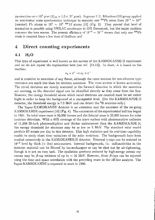
and is sensitive to neutrinos of any flavor, although the cross sections for non-electron type neutrinos are much less than for electron neutrinos. The cross section is known accurately. The recoil electrons are mostly scattered in the forward direction in which the neutrinos are arriving, so the detected signal can be identified directly as they come from the Sun. However, the energy threshold above which recoil electrons are counted must be set rather hight in order to keep the background at a manageable level. (For the KAMIOKANDE-II detector, the threshold energy is 7.5 MeV and can detect the 8 B neutrino only.)

The Super-KAMIOKANDE detector is an extension and the successor of the on-going KAMIOKANDE experiment [16] (Fig. 4). The excavation of the experimental hall has begun in 1991. Its total mass mass is 50,000 tonnes and the fiducial mass is 22,000 tonnes for solar neutrino detection. With a 40% coverage of the inner surface with photosensitive cathodes of 11,200 20-inch photomultiplicrs and thicker anticounters than the KAMIOKANDE-II, the energy threshold for electrons may be as low as 5 MeV. The standard solar model predicts 67 events per day in this detector. This high statistics and its real-time capability enable to study short time variations of the solar neutrinos. The backgrounds have been studied extensively in the KAMIOKANDE-II detector. External 7-rays can be reduced to 10~6 level by thick (> 2m) anticounters. Internal backgrounds, i.e. radioactivities in the detector material can be filtered by ion-exchangers or can be shut out by air-tightening, though it is not an easy task. The spallation products induced by high-energy cosmic ray niuons may be /?-ray emitters of up to ~ 16 MeV. However, these /3-rays can be rejected using the time and space correlation with the preceding muon in the off-line analysis. The Super-KAMIOKANDE is expected to start in 1996.

18

4.2 D.O Besides the elastic scattering process which is the same as one in II-jO, two other processes are relevant, in a \)>Q detector. One is the charged current process

in which the produced electrons carry the neutrino energy information (lir ~ I\. — 1.44 MeV). The angular distribution is a little backward-peaked (ex 1 — i<:os0 r). The expected rate for the threshold of 5 MeV is G.01 (1 ± 0.38) SNU [2]. Another process is the neutral current reaction

i's + <l —• I'T + p + n and d(n,f)t. The threshold is 2.2 MeV and the resultant 7-ray is monochromatic (6'.2-r> MeV). The cross section is independent of neutrino type and corresponds to '1.5(1 ± O.'JS) x JO'1

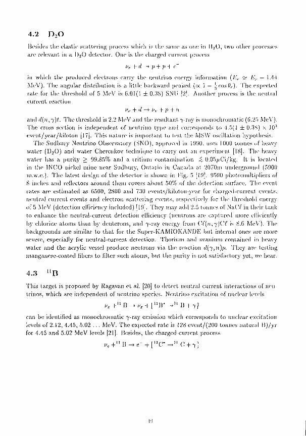
event/year/kilotou [17]. This nature is important to test the MSVV oscillation hypothesis. The Sudbury Neutrino Observatory (SNO), approved in 1990, uses 1000 tonnes of heavy

water (D2O) and water Cherenkov technic|ue to cany out an exi>erimen1. [18]. The heavy wafer has a purity > 99.85% and a tritium contamination 4, 0.05/;Ci/kg. It is located in the INCO nickel mine near Sudbury, Ontario in Canada at 2070m underground (5900 m.w.e.). The latest design of the detector is shown in Fig. 5 [19]. 9500 pliotomultiplicrs of 8 inches and reflectors around them covers about 50% of the detection surface. The event rates are estimated as 6500, 2800 and 730 eveuts/kiloton-year for charged-currcul events, neutral-current events and electron scattering events, respectively for the threshold energy of 5 MeV (detection elficiency included) [19]. They may add 2.5 tonnes of Na('/° in their tank to enhance the neutral-current detection efficiency (neutrons are captured more efficiently by chlorine atoms than by deuterons, and 7-ray energy from CC(n,~f)CC is 8.(1 MeV). The backgrounds arc similar to that, for the Super-KAMIOKANDK but internal ones arc more severe, especially for neutral-current detection. Thorium and uranium contained in heavy water and the acrylic vessel produce neutrons via the rea.cl.ion d(y,ii)p. They are testing manganese-coated fibers to filter such atoms, but the purity is not satisfactory yet, we hear.

4.3 n B This target is proposed by Ragavan et al. [20] to detect neutral-current interactions of neu­trinos, which arc independent, of neutrino species. Neutrino excitation of nuclear levels

can be identified as monochromatic 7-ray emission which corresponds to nuclear excitation levels of 2.12, 4.45, 5.02 .. . MeV. The expected rate is 128 event/(20() tonnes natural B)/yr for 4.45 and 5.02 MeV levels [21]. Besides, the charged-current process

U.I

can be used to detect electron neutrinos (E„ > 1.982 MeV) and the electron scattering process as in I I 2 0 target is observable. The expected rate for the charged current process is 2373 event/(200 tonnes natural B)/yr for Ec > 3.5 MeV [21].

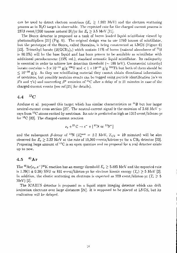
The Borex detector is proposed as a tank of boron loaded liquid scintillator viewed by photomultipliers [21] (Fig. G). The original design was to use 17C0 tonnes of scintillator, but the prototype of the Borex, called Borexino, is being constructed at LNGS (Figure 6) [22]. Trimcthyl borate (B(0CIl3)3) which contain 11% of boron (natural abundance of n B is 80.2%) will be the base liquid and has been proven to be available as scintillator with additional pseudocumene (15% vol.), standard aromatic liquid scintillator. Its radiopurity is essential in order to achieve low detection threshold (~ 100 keV). Commercial trimethyl borate contains ~ 5 x 10~ 1 5 g/g 2 3 8 U and < 1 x 1 0 - 1 5 g/g 2 3 2 T h but both of them should be < 1 0 - 1 6 g/g. As they use scintillating material they cannot obtain directional information of neutrinos, but possibly neutrino events can be tagged using particle identification (a's vs ,£f's and 7's) and succeeding / 3 + emission of llC after a delay of ~ 21 minutes in case of the charged-current events (see ref.[21] for details).

4.4 1 3 C Arafune ct al. proposed this target which has similar characteristics as " B but has larger neutral-current cross section [23]. The neutral-current signal is the emission of 3.68 MeV 7-rays from 1 3 C atoms excited by neutrinos. Its rate is predicted as high as 1315 event/kiloton-yr for I 3 C [23]. The charged-current reaction

i / e + 1 3 C ^ e - + [ , 3 N o r , 3 N - ]

and the subsequent /?-decay of 1 3 N [E™*x — 2.2 MeV, ']\/2 = 10 minutes) will be also observed for Ev > 2.22 MeV at the rate of 10,300 events/kiloton-yr for a CHj detector [23]. Preparing large amount of 1 3 C is an open question and no proposal for a real detector exists up to now.

4.5 4 0 A r

The 4 0 Ar( j ' e , e - ) ' 1 0 K reaction has an energy threshold E„ > 5.885 MeV and the expected rate is 1.70(1 ± 0.38) SNU or 831 cvent/kiloton-yr for electron kinetic energy (Tc) > 5 MeV [2]. In addition, the elastic scattering on electrons is expected as 920 event/kiloton-yr (Te > 5 MeV) [2],

The ICARUS detector is proposed as a liquid argon imaging detector which can drift ionization electrons over large distances [24]. It is supposed to be placed at LNGS, but its realization will be delayed.

•JO

4.6 1 1 5 I n The charged-current reaction

„ e + " * l n _ e - + [ n s s „ . ^ i i s S n + 7 i + 7 a ]

has a very low energy threshold (/?„ > 0.119 MeV) and the expected rate is very high (but uncertain): 639132° SNU [2]. Its use for a real-time electronic experiment to measure the differential neutrino energy spectrum was first proposed by Raghavan [25], but the exper­iment is very difficult because the natural /3~ radioactivity of n 5 I n (J5m*x = 0.494 MeV, T1/2 = 4.4 x 10 1 4 years) is a formidable background in low energy region. Now this target is being studied so as to detect the fluxes of the neutrino line sources, i.e. the 'Be neutrinos (862 keV) and the pep neutrinos (1442 keV).

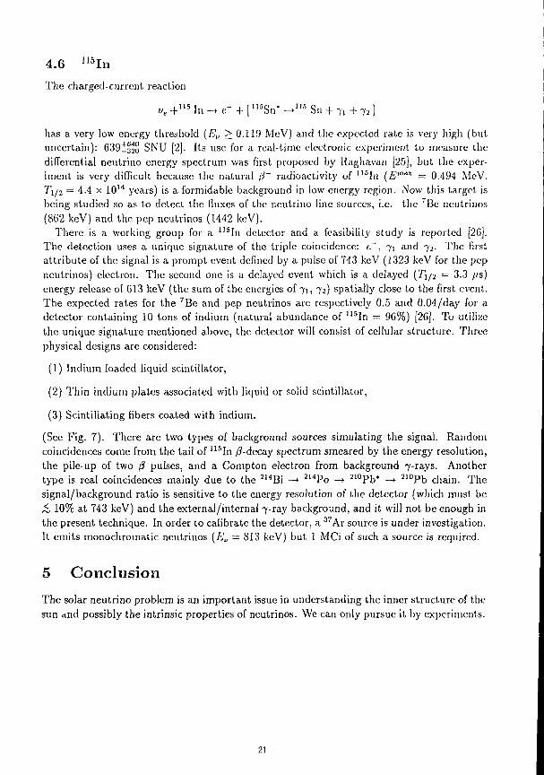
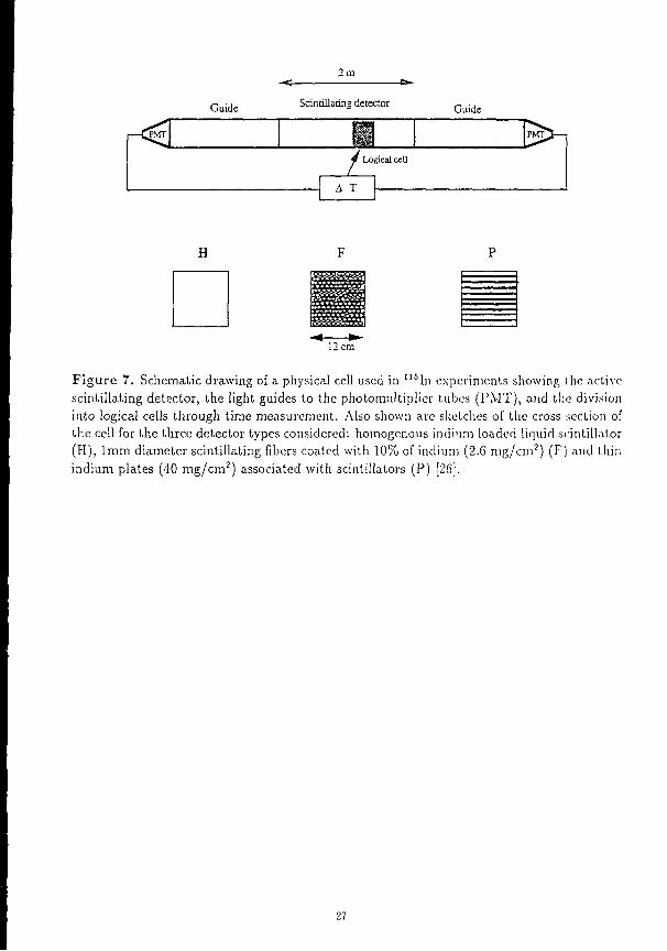
There is a working group for a 1 I 5 I n detector and a feasibility study is reported [26]. The detection uses a unique signature of the triple coincidence: t~, 71 and 72. The first attribute of the signal is a prompt event defined by a pulse of 743 keV (1323 keV for the pep neutrinos) electron. The second one is a delayed event which is a delayed (T1/2 = 3.3 /;s) energy release of 613 keV (the sum of the energies of 71, 72) spatially close to the first event. The expected rates for the 7 Be and pep neutrinos are respectively 0.5 and 0.04/day for a detector containing 10 tons of indium (natural abundance of 1 1 5 In = 96%) [26]. To utilize the unique signature mentioned above, the detector will consist of cellular structure. Three physical designs are considered:

(1) Indium loaded liquid scintillator,

(2) Thin indium plates associated with liquid or solid scintillator,

(3) Scintillating fibers coated with indium.

(See Fig. 7). There are two types of background sources simulating the signal. Random coincidences come from the tail of 1 1 5 I n /?-dccay spectrum smeared by the energy resolution, the pile-up of two /? pulses, and a Compton electron from background 7-rays. Another type is real coincidences mainly due to the 2 H B i -> 2 1 4 P o -> 2 1 0 P b * -+ 2 1 0 P b chain. The signal/background ratio is sensitive to the energy resolution oi the detector (which must be ,$, 10% at 743 keV) and the external/internal 7-ray background, and it will not be enough in the present technique. In order to calibrate the detector, a 3 ' A r source is under investigation. It emits monochromatic neutrinos (E„ = 813 keV) but 1 MCi of such a source is required.

5 Conclusion The solar neutrino problem is an important issue in understanding the inner structure of the sun and possibly the intrinsic properties of neutrinos. We can only pursue it by experiments.

21

Besides on-going Homest.ake ( ! 'Cf) , KAMIOKANDF and SAGE, many experiments are in preparation. 'I he GALLKX experiment has begun the exposure, though some problems must be solved before the results appear. The Super Cf.-Ai detector will be constructed in Baksan, USSR and will start in 1995. The SNO detector may complete in 1994. The Super-KAMIOKANDH will start in 1996. The Borexino is aimed to start in 199-1.

We believe the solar neutrino problem is worth investigating more extensively by various targets and techniques. Future experiments are required to have a low detection energy threshold, high counting rate, neutral current capability and long term operation stability to solve the problem in a complete way.

Acknowledgement

The author would like to thank Atsuto Suzuki for valuable informations, discussions and comments.

References |1] J.N. Bali.all, Pet: Mod. Phys. 50,881 (1978).

[2j J.N. Bahcall and R.K. (Uriel), llcv. Mod. Phys. 60, 308 (1988).

[:!] T.N. Taddeuchi et al., Nurl. Phys. V1G9, 125 (1987).

(•(J M. Takita. in this proceedings.

[5j A. Pomansky. talk at Third Workshop on Neutrino Trliseopi. Venice, 26-28 Feb. 1991.

[6] ']". Kirst.en. in ''Inside the Sun", ods. (.!. Bcrthomieu and M. Cribier (Kluwer Academic Publishers, 1990) pl87.

[7] I']. Belloti, talk at Third Workshop on Neutrino Telescope. Venice, 26-28 Feb. 11)91.

[8] G.S. Hurst et, al., Phys. Per. Lett. 53, 1116 (1981); in Solar Neutrinos and Neutrino Astronomy, eds. M.L. Cherry, VV.A. howler and K. Lande (AIP, New York, 1985) pi52.

[9] V'.V. Kuzminov,A.A, Pomansky and V.L. Chihladze, Nucl. Inst. Mcth. A271, 257 (1988).

flO) W'.C. Ilaxton, Phys. Per. Lett. 00. 768 (1.988).

[11] K. Wolfsberg et al.. in Solar Neutrinos and Ntnlrino Astronomy, eds. M.L. Cherry. W.A. Fowler and K. Lande (AIP, New York, 1985) 1)196.

[12] W.C. Haxton, Phys. lieu. Lett. 65, 809 (1990).

[13] W. Henning et al., in Solar Neutrinos and Neutrino Astronomy, eds. M.L. Cherry, W.A. Fowler and K. Land? (AIP, New York. 1985) p'203.

[14] K.S. Hirata et al., Phys. Rev. Lett. 63 , 16 (1989).

[15] K.S. Hirata et al., Phys. Rev. Lett. 65, 1297 (1990).

[16] Y. Totsuka, in Proceedings oj the Seventh Workshop on Grand Unification / ICOBAN'86, cd. J. Arafune (World Scientific, Singapore, 1987) pi 18; Institute for Cos­mic Ray Research (Univ. Tokyo) preprint ICRR-Report-227-90-20 (1990).

[17] J.N. Bahcali, K. Kubodera and S. Nozawa, Phys. Rev. D38, 1030 (1988).

[18] G. Aardsma et al., Phys. Lett. B194, 321 (1987).

[19] E.W. Beier, private communication (1990).

[20] R.S. Raghavan, S. Pakvasa and B.A. Brown, Phys. Rev. Lett. 57, 1801 (1986).

[21] R.S. Raghavan et al., AT&T Bell Laboratory preprint ATT-BX-88-01 (1988).

[22] R.S. Raghavan, Informal Status Report, AT&T Bell Laboratory (April, 1990).

[23] J. Arafune et al., Phys. Lett. B217, 86 (1989).

[24] D. Cline, in Proceedings of the Seventh Workshop on Grand Unification /ICOBAN'86, ed. J. Arafune (World Scientific, Singapore, 1987) pi 39.

[25] R.S. Raghavan, Phys. Rev. Lett. 37, 259 (1976).

26] A. de Bellefon et al., Saclay preprint DPhPE 89-17 (updated, January 1990).

23

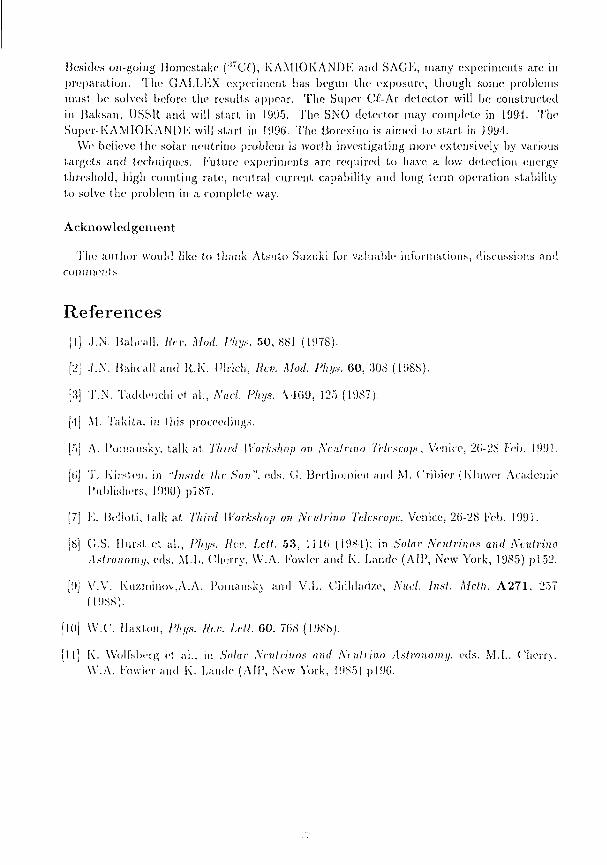
GALLEX TARGET TANK

Figure 1. Sketch of the GALLEX target tank. For acid resistance it is teflon-lined. The insert to accommodate the calibration source will be narrower as shown [6].

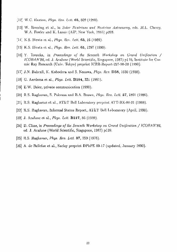
F igure 2. Scheme of the low level counting arrangement of the GALLEX. A Pb-filled steel tank with movable side ends (top) houses a well type Nal crystal (interior left), a plastic scintillator shield (above and below) and a plastic scintillator block (right). The Nal-well accommodate up to S counters encapsulated, together with the preamp, in a Cu-box (mid­dle and bottom left). The scintillator block can accommodate 21 additional counters for operation without NaJ crystal (top and bottom right). Plastic scintillators operate in anti­coincidence, NaT either in coincidence or anticoincidence. Multipliers arc specially selected low potnsium nips [fij.

:'•!

1/2

ionization chamber

windowfoil

stop (scintillator foil

magnetic spectrograph

passive gas absorber

Y',v/\ • * -

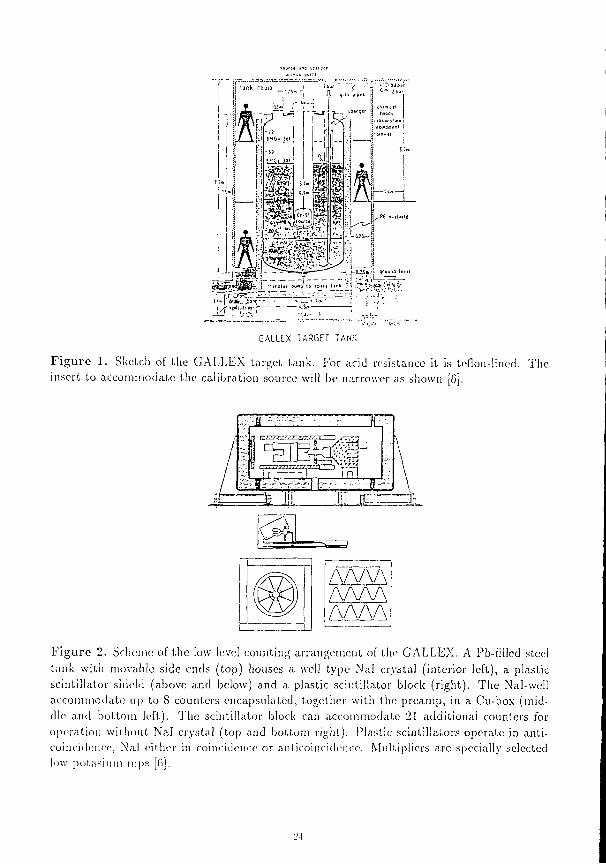
~6.4MeV/u start detector (channel plate)

l l .4MeV/u 2 0 5 T | ) 2 0 6 p b

Figure 3 . Schematic, of the heavy-ion detection system. Isoharic * 0 ; >l >b and M!iTC ions of identical energy experience different energy losses in a gas absorber tine to their different nuclear charges. This energy-loss difference is determined by the magnetic spectrograph in a high-resolution measurement ol the remaining energy [J 3].

Eloc l ion i t s Hut

\

;ft«3lifiil -«#Sf : s l 3 - r

IP! ;-t^ik^

' j i U i ' ' J-l 'ftilHS^'.il:/ '-^' Anti-Counter feHjfiliTIJjirfei!!-- X i'oo 20'va'M'r: m\-iMi±m

^j SifiCiCS ISP""'

• 39.3m«i —

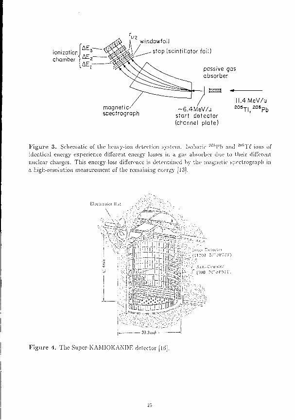
F i g u r e 4. The Supcr-KAMIOKANDE detector [161.

t A a v W H SUQ OtUc-Uv

CROSS SECTION OF NEUTRINO DETECTOR

| f " " >

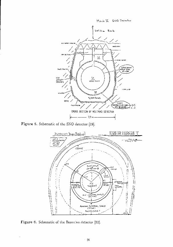
Figure 5. Schematic of the SNO detector [19].

snwiiM im& T

MINIMUM SJTERNAL $MIEL5

PoLycTiriyLejjf> , - - M Figure 6. Schematic of the Borexino detector [22].

26

2m

Guide Scintillating detector

r ^ Guide

/

^h Logical c^U

A T

H

12cm

F i g u r e 7. Schematic drawing of a physical cell used in I I S I n experiments showing I he active scintillating detector, the light guides to the photomultiplier tubes (PMT), and the division into logical cells through time measurement. Also shown arc sketches of the cross section of the cell for the three detector types considered: homogenous indium loaded liquid scintillator (H), 1mm diameter scintillating fibers coated with 10% of indium (2.6 mg /cn r ) (F) and thin indium plates (40 mg/cm 2 ) associated with scintillators (P) [26].

27

Indium loaded liquid scintillator for 7 Be and pep solar neutrino detection

K.Inoue and Y.Suzuki Institute for Cosmic Ray Research, University of Tokyo, Tanashi, Tokyo 188 Japan

T.Inagaki KEK, National Laboratory for High Energy Physics, Tsukuba, Ibaraki 305 Japan

Y.Nagashima Department of Physics, Osaka University, Toyonaka, Osaka 560 Japan

S.Hashimoto Department of Physics, Kyoto University of Education, Fushimi-ku, Kyoto 612 Japan

(Presented by K.Inoue, November 19, 1990)

Abst rac t

There is a long standing solar neutrino problem that the experimentally measured flux of the solar neutrino is less than a half of the theoretical prediction. One of the means to solve this problem is the observation of 7 Be solar neutrino flux and its time variations. The real time measurement of the 7 Be solar neutrino can be accomplished by a 1 1 5 l n . We have succeeded in developing an indium loaded liquid scintillator based on xylene which has long attenuation length (155cm) and good energy resolution (<r/E=13%(In7.1Wt%) @477keV). Another scintillator based on l-2-4trimelhylbenzene, which does not attack an acrylic con­tainer and has higher flash point (54°C) has also developed. Acceptable contamination level of the radio-active impurities for a solar neutrino detector by the indium loaded liquid scin­tillator was estimated to be 0.2~2ppb and 0.5~5ppb for 2 3 8 U and 2 3 2 T h contamination, respectively. This requirement is not so serious. Radio-active impurities of the solute of the liquid scintillator, lnCb^HsO, was found from the measurement by the mass spectrometry to be less than the requirement (O.lppb for 2 3 8 U and <0.1ppb for 2 3 2 T h ) . The result of the measurement of the indium beta decay spectrum with the indium loaded liquid scintillator based on l-2-4trimethylbenzene is also presented.

1 Introduction The solar neutrino experiments, the 3 'C1 [1] and Kaimokande-II [2] experiment, revealed that

only a part of solar neutrinos compared to the standard solar model predictions [3] is coming from the sun. This is the so-called solar neutrino problem. The new-coming SAGE experiment which uses 7 1 G a nuclei, sensitive to the p-p fusion neutrinos, also reported the lower flux value [4]. Models of neutrino oscillations [5] are vigorously studied in order to explain this problem. The following three choices are possible to explain the solar neutrino problem within a frame work of two neutrino oscillation hypothesis;

(a)nonadiabatic matter enhanced oscillation (5m2fJ2 ~ W~seV2,6m2 ~ 3x ] 0 - 8 - 2 x ] 0 - 5 e V 2 ) ,

(b)matter enhanced oscillation with large mixing (&?n2 ~ 1 0 - 7 - lO~' t eV / 2 , s in 2 20 > 0.5), and

(c)long wavelength vacuum oscillation (6m2 ~ 0.5 - 2 . 5 x 1 0 _ 1 0 e V 2 , s i n 2 20 > 0.7).

The observation of 7 B e neutrinos can possibly distinguish those three solutions since the effect of the neutrino oscillations on the expected flux of 'Be neutrinos is quite different in each case. We could expect a seasonal variation of the 'Be neutrino flux in the case of the vacuum oscillation (c). We would observe a day/night variation by matter enhanced oscillation through the regeneration effect of the earth instead of a seasonal variation in the case of (a) and (b)

28

[6], The real time observation of 7Be neutrinos plays an important role to distinguish these solutions.

Indium detector is very suitable for this purpose because it can detect 7Be neutrinos in real time and the measurement of the incident neutrino energy is possible. 1 1 5 In captures a neutrino through the following reactions [7],

1 1 5 In + ue -* U 5 Sn* + e~ (prompt signal) l l s S i T - m S n

+7i(116keV,delayed signal ], 50% internal conversion) +72(498keV,delayed signal 2) ( T 1 / 2 = 3.26ftsec)

This reaction has the following good characteristics.

(1) Ability to measure the energy of the incident neutrino.

(2) Capability to observe neutrinos in real time.

(3) Low capture threshold(128keV).

(4) Large neutrino capture rate.

(5) Strong back ground rejection properties resulting from a 3-fold coincidence with a charac­teristic time structure.

However, it has a severe background due to the beta decay of m I n (E<486keV). Most of the early effort in developing indium detectors dedicated on the purpose to detect

p-p neutrinos (E<420keV) by virtue of its low energy threshold of 128keV. But the serious background problem mentioned above have not been overcome yet.

We set our goal of the development of indium detector to detect ?Be (861keV) and pep(1442keV) neutrinos instead of p-p neutrinos. Those neutrinos have higher energies well above the beta decay background spectrum and have monochromatic energies. The development of the indium detector, then, becomes realistic and relatively easier. The standard solar model predicts that the capture rate of rBe(861keV) neutrino by 1 1 5 In is about 120SNU. We can expect 0.54captures/day with only lOtons of indium (95% n 5 I n ) .

2 Indium loaded liquid scintillator (ILLS) Indium loaded liquid scintillator (ILLS, hereafter) is suitable for the purpose explained in

the previous section since a large volume detector can be easily made. But it turned out to be very difficult to make ILLS. The first development of such detector was done by Pfeiffer et al.(1978) [8]. They used Phenethyl Alcohol as solvent and indium trifluoroacetate as solute. The early development used an oil-soluble indium compound or a hydrophilic solvent. But so far, no such scintillator could satisfy our requirement. Especially, it has been very difficult to obtain a liquid scintillator with good light transparency.

Recently development of a scintillator cocktail has made a big progress, in which the surfac­tant, oil-soluble and hydrophilic, are added to a solvent.

We have developed a few kind of ILLS made of scintillator cocktails; one based on a com­mercially available scintillator cocktail (xylene + surfactant); and the other home-made combi­nations of a solvent (toluene or l-2-4trimethylbenzenc) and a surfactant.

Following qualities and characteristics have to be considered to develop a new ILLS;

- 2 9 -

(l)transparency,

(2)light output,

(3)solubility of indium,

(4)chemical reaction to a container,

(5)safety (flash point etc.), and

(6)stability.

We first developed xylene based indium loaded liquid scintillator and tested its performance such as energy resolution, Hght attenuation and so on. Two commercially available scintillator cocktails were used in the development, EX-H and Scintisole-500 (made by Dojindo lab., Ku-mamoto Japan). We tried to resolve several inorganic indium compounds into them, and found that I11CI34H2O can be resolved in EX-H up to 7.5% by weight in terms of indium concentration and in S500 up to 14% by weight with reasonably good transparency. Only a few kinds of mate­rials are used for a container of the xylene based scintillator, for example, something like glass, teflon coated metal and so on, because of its strong chemical reactions. Furthermore xylene has low flash point of 27°C. Practically those scintillator are not suited for the large scale detector, because glass, the best suited container is very fragile.

Another ILLS we have developed are made with l-2-4trimethylbenzene (pseudo cumene (PC)) which has high flash point(54°C) and is chemically not so active. We chose the combination of solvent, surfactant and solute with l-2-4trimethylbenzene, Liponox-NC95 (Lion corp.) or Nonion-NS210 (Nippon oil k fats co.ltd) and I11CI34H2O. The weight ratio of the surfactant in the scintillator cocktail is 30%. We found that this scintillator cocktail has a same light output as EX-H. I11CI34H2O is resolved into the scintillator cocktail up to 6Wt% of indium concentration.

A container which is suited for the new liquid scintillator was also developed. It was confirmed that this solvent does not attack the acrylic container(UVT) containing no ultraviolet absorbent processed in the following way. The UVT is jointed with acrylic monomer, and the container is well annealed before gluing together.

This new liquid scintillator was used for measuring the beta decay spectrum of J l i I n which will be explained in section 5.

The solubility of indium and light output we have made, relative to pure EX-H are shown in figure 1 and 2, respectively.

2.1 Quality of ILLS [9]

As we will discuss later, one can use an assembly of 14,000 cells with the size of 10cm x 10cm x 100cm as a practical neutrino detector with lOtons of indium. A quartz cell of 5cm(6xlOOcm was prepared to measure performance under a realistic condition. The measurement of the energy resolution and the light attenuation were performed on the EX-II based ILLS with In 7.lWt%.

A compton back-scattering of 662keV gamma rays from 1 3 7 Cs was used for the measurement. The experimental arrangement is shown in figure 3. Taking a coincidence between a 185keV back scattered gamma ray observed in the Nal detector and a recoil electron which has a kinetic energy of 477keV in the liquid scintillator, we can measure a response for the monochromatic energy deposition (477keV) as if a radio-active source is placed inside the detector.

From the dependence of light output on the position of the source, we obtained the attenu­ation curve of the following formula,

L(x) = 0.55cxp(-^) +0A5cxp(—fL).

30

There found two components in the attenuation curve. Roughly 50% of the light output con­tributes to each component. The attenuation length of 155cm is an great achievement and it solves one of the severe problems in developing an indium loaded liquid scintillator. The obtained performance is listed in table 1 together with those of the other groups [8] [10] [1]].

We got a position resolution of a=5cm by reconstructing the vertex position from the timing difference of the PMTs attached to the each end of the liquid scintillator. We reconstructed the energy by the formula, Qo=(Qi+Q:?)/(L(x)+L(l-x)), where x is the vertex position calculated from the timing difference of each PMTs and Q, is the pulse height of each PMT. Obtained energy resolution at various position are shown in figure 4. We obtained the uniform energy resolution of cr/E=13% (@477keV) through the entire detector length. The energy resolution is slightly worth around the each end of the detector that is supposed to come from the rapid change of the light output due to the short component of the attenuation curve, and the effect of the acceptance which strongly varies near the end. We made a same measurement by using EX-ll;ln5.0% and found an energy resolution of < T / E = 1 2 % (@477keV).

3 M . C . S imula t ion

3.1 Inputs and Outcomes of M.C. simulation

The expected neutrino capture rate of the 'Be(861ke\') neutrinos is about 120SNU for the SSM of .l.N.Bahcall and R.K.Ulrich. That is about 0.54 captures/day for 10 tons of indium. But the beta decay rate for the entire detector volume becomes 2.2MHz. We therefore have to segment the detectors to achieve a 3-fold coincidence which is a unique neutrino capture signature of indium. The 3-fold coincidence is accomplished by detecting the electron (prompt signal) from the reaction m I n + i>c —* U 5 S n * + c~ and the delayed two gamma rays (delayed signal 1,2) emitted from the subsequent decay of Sn" — Sn + 71 + 72 (T]/ 2= :S-2G/jsec).

The mass attenuation lengths of two gamma rays, 116 and 498keV, emitted from the excited state of Sn atom, are about 5cm and 15cm in the ILLS (5% ~ 10% concentration), respectively. Then the cross section of the detector less than 15cm x 15cm is suitable to detect above two gamma rays in different cells as shown in figure 5, and larger than ]0cm x 10cm is necessary to delect the 116keV gamma rays in the vertex cell in which the prompt signal is observed. Therefore a practical size of the detector unit ranges something like lOcmxlOcmx 100cm to ]5cmx ]5cmx200cm. The length of the unit was determined by the measured attenuation length of 155cm. It is possible to make virtual segmentation of about 20cm to 30cm along the longitudinal direction by virtue of the timing information. The number of segmentation then becomes 3,000 to 14,000 by 10 tons of indium.

We assumed the unit cell size is lOcmxlOcmxlOOcm in the Monte Carlo calculation by which the feasibility of the indium detector was estimated using parameters (energy and vertex resolution) measured for the 5cm<£x 100cm quartz cell.

Outputs from the simulation are signal to noise ratio (S/N) in terms of the background gamma ray rate and detection efficiency of the neutrino signal. The background gamma rate in this report, terminologically, defined by the rate of the environmental gamma ray flux around SOOkeV in /g /keV/sec .

3.2 Selection criteria for the neutrino capture signal

3 x 3 , 5 x 5 , 7x7 or 9x9 cells surrounding the vertex cell were considered as a region of interest. We take the 9 selection criteria listed in table 2 to select the unique delayed coincidence signature of indium neutrino detector. The coincident time width between prompt signal and

- 3 1

delayed signal is set to lO^sec considering the Sn* half life of 3.26/xsec. Trigger threshold is set to be at 20keV. Fiducial volume was also set by 0cm<z<100cm, 5cm<z<95cm or 10cm<z<90cm along the longitudinal direction, because the gamma ray which interact in the shallow part of the detector often escape the detector without depositing its energy in any other cells and those events which cannot be identified as a gamma ray might increase the background rate for the prompt signal.

3.3 Detection efficiency of the neutrino signal

From the M.C. simulation using the selection criteria described above, the detection efficiency of the neutrino signal was obtained and listed in table 3. As far as the efficiency is concerned, it turns out to be most appropriate to measure the signal up to 7x7 or 9x9 cells. If we introduce a restriction of 5]0 to 750keV energy window, we should better to take 9x9 cells to minimize the escape of 498keV 72. The requirement of 70 to ]70keV energy window in the vertex cell makes the detection efficiency less than half. This is due to the additional energy deposit of the compton scattering of 72 in the vertex cell. Selection no. 4,5,6 would be best as selection criteria for the delayed signal. The decrease of the detection efficiency caused by the fiducial cut to a prompt signal was almost proportional to the decrease of the fiducial volume. The practical selection criteria has to be determined by considering background contamination.

3.4 Background consideration

Following backgrounds arc considered for the detection of 7Be(861keV) neutrino.

3.4.1 Background to the prompt signal

(fl)A tail of indium beta decay spectrum (Emax=486keV) smeared by a finite energy resolution; Event rate of 51 Hz arc expected for lOtons of indium in the energy window of G50 to 850keV. (see figure 6) (cf. Neutrino capture signal rate is expected to be 6.3 x 10~6llz.) (f2)Accidental coincidence of two beta decays which occurs almost at the same time (within 5nsec) and are taken as a single output; Only fine segmentation could avoid this background. This background is estimated to be 0.16Hz. (f3)Gamma rays (or beta rays) come from radio-active impurities in the detector (f-J)External gamma rays; If the background gamma ray rate of 10~9/g/keV/sec, background due to (f3),(fl) becomes 4.4xlO~3Hz in the entire detector volume (10 tons of indium). (f5)Alpha rays come from the impurities in the detector (fG)Radioactive isotopes produced by cosmic rays passing through the detector (f7)Bota and gamma ray produced by the neutron capture of indium The contribution of (f5),(f6),(fT) is negligible compared to (fl).

3.4.2 Background to the delayed signal

(dl)Multiplc complon scattering of a gamma ray which emanates from an radio-active impurity in the detector deposits its energy both in the "same" and "vicinity" cell. (d2)Multiple compton scattering of an external gamma ray yields energy deposits in both the "same" and the "vicinity" cell. (d3)Two beta decays accidentally occur in the "same" cell and in the "vicinity" cell within 10 usee interval. (d4)Heta ray emitted by the decay of indium radiates a photon by bremsstrahlung, and the beta

:c'

ray and the photon are detected in the "same" cell and also in the "vicinity" cell. (d5)Olher decays accompanying gamma rays, etc. mimic a delayed coincidence signal.

We calculate the reduction probability of these background for the nine selection criteria using the 3-fold coincidence technique. The probabilities that the main background to the delayed signal (dl)~(d. 'l) accidentally satisfies the selection condition within 10/jsec from a prompt signal are listed in table -1, assuming that the gamma ray rale is a typical value 10~ 9/g/keV'/sec around 500keV.

3.4.3 T i m e correlated background

In the above calculation, we found (hat the main background to the prompt and to the delayed signal are then indium beta decay and a multiple compton scattering of the background gamma ray, respectively. But there are short half life nuclei in the decay chains of I'-lla and Th series. Unfortunately, an energy deposit from alpha particle (~5\ leV) gives the similar light output by e /7 in the energy region of ~50()kcV. The decay chain of such nucleus may incidentally satisfy both of the condition for a prompt and a delayed signal at once. And the possibility thai we mis-identify such background as a neutrino capture signal may be larger than the accidental coincidence of an indium beta decay and a multiple compton scattering.

Decay chains considered as a source of possible time correlated background are listed in table ">. The rhai/i (5) looks like the most serious lime correlated background. But -°-sTl emits high energy gamma rays (2.61f>MeV) after the beta decay, then we could suppress the coincidence probability less than 1/3 by identifying those high energy gamma ray. Moreover, the branching ratio is only 36.0%. Kurt her reduction may be possible by using the PSD (Pulse Shape Discrimination) technique to separate alpha, particles from electrons. Then it can be expected that the probability becomes less than I0~ ! 1 and this decay chain becomes ineffective comparing the possibility of about 1 0 - 9 ~ 1 0 - ' that an accidental coincidence of two indium beta decays satisfies selection condition as a delayed signal. We can therefore conclude that any other decay chains of U-Ra and Th series do not become a source of the lime correlated background.

The nucleus excited by a through-going cosmic ray or a neutron is a possible source of the time correlated background, too. We estimate that we can reduce those backgrounds by choosing the site of the experiment in deep underground and placing the detector in a water tank.

It is concluded that no serious time correlated background exisls for an Indium ' Be-neutrino-detector.

3 .5 A c c e p t a b l e b a c k g r o u n d g a m m a ray r a t e ( R e s u l t s o f M . C . c a l c u l a t i o n )

We obtained the energy spectrum and the vertex distribution of the background processes of (fl)~(f7) mimicking the prompt signal. And the probabilities that backgrounds (dl)~(df>) satisfies the selection criteria as the delayed signal, to make a faked 3-fold coincidence were; obtained by the M.C'. simulation.

The relation between S/N and the background gamma rate was deduced(see figure 7) from the detection efficiency of neutrino capture and the background event rate.

Acceptable limit of the level of the background gamma ray is defined by the level in which S/N becomes equal to 1. The S/N is determined as the signal lo background ratio with the energy window of 6.r>0 lo S,r>()keV (or 778 lo f)7RkeV in neutrino energy) in order to contain the prompt signal (see table 6).

It was found that the acceptable background gamma ray rate ranges K ) - 8 ~ 10 _ ! > with a reasonable detection efficiency of 20 ~ 60%.

:«

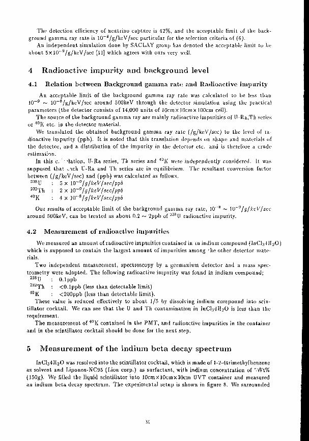
The detection efficiency of neutrino capture is 42%, and the acceptable limit of the back­ground gamma ray rate is 10 - 8/g/keV/sec particular for the selection criteria of (6).

An independent simulation done by SACLAY group has denoted the acceptable limit to be about 5xlO _ 9/g/keV/sec [13] which agrees with ours very well.

4 Radioactive impurity and background level

4.1 Relation between Background gamma rate and Radioactive impurity An acceptable limit of the background gamma ray rate was calculated to be less than

10~9 ~ 10~8/g/keV/sec around SOOkeV through the detector simulation using the practical parameters (the detector consists of 14,000 units of lOcmx lOcmx 100cm cell).

The source of the background gamma ray are mainly radioactive impurities of U-Ra,Th series or 4 0 K etc. in the detector material.

We translated the obtained background gamma ray rate (/g/keV/scc) to the level of ra­dioactive impurity (ppb). It is noted that this translation depends on shape and materials of the detector, and a distribution of the impurity in the detector etc. and is therefore a crude estimation.

In this c. •'lation, U-Ra series, Th series and 4 0 K were independently considered. It was supposed that ..rich U-Ra and Th series are in equilibrium. The resultant conversion factor between (/g/keV/sec) and (ppb) was calculated as follows.

2 3 8 U : 5 x lO-9/g/keV/sec/ppb 2 3 2 T h : 2 x ltr9fg/keVfsecfppb 4 0 K : 4 x 10~s/gfice.V/sec/ppb

Our results of acceptable limit of the background gamma ray rate, 10 - 8 ~ \0~9/g/keV/scc around 500keV, can be treated as about 0.2 ~ 2ppb of-'3 8U radioactive impurity.

4.2 Measurement of radioactive impurities

We measured an amount of radioactive impurities contained in m indium compound (InClj UI2O) which is supposed to contain the largest amount of impurities among 'he other detector mate­rials.

Two independent measurement, spectroscopy by a germanium detector and a mass spec­trometry were adopted. The following radioactive impurity was found in indium compound;

2 3 8 U : O.lppb 2 3 2 T h : <0.1ppb (less than detectable limit) 4 0 K : <200ppb (less than detectable limit).

These value is reduced effectively to about 1/5 by dissolving indium compound into scin­tillator cocktail. We can see that the U and Th contamination in J11CI34II2O is less than the requirement.

The measurement of 4 0 K contained in the PMT, and radioactive impurities in the container and in the scintillator cocktail should be done for the next step.

5 Measurement of the indium beta decay spectrum I n C ^ l ^ O was resolved into the scintillator cocktail, which is made of l-2-4trimethyIbenzene

as solvent and Liponox-NC95 (Lion corp.) as surfactant, with indium concentration of ". Wt% (J50g). We filled the liquid scintillator into j0cmxl0cmx30cm UVT container and measured an indium beta decay spectrum. The experimental setup is shown in figure 8. We surrounded

•M

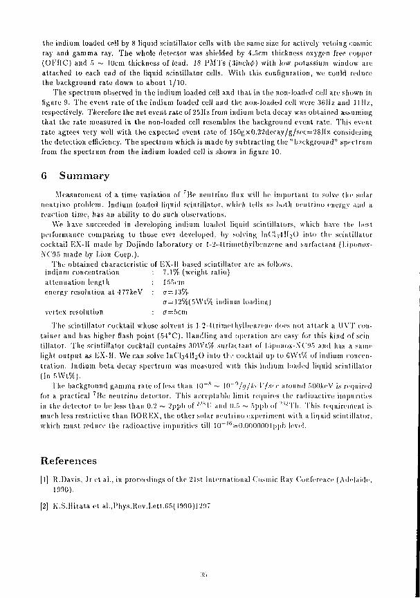
the indium loaded cell by 8 liquid scintillator cells with the same size for actively vetoing cosmic ray and gamma ray. The whole detector was shielded by 4.5cm thickness oxygen free copper (OFHC) and 5 ~ 10cm thickness of lead. 18 PMTs (.'liricli</') with low potassium window are attached to each end of the liquid scintillator cells. With this configuration, we could reduce the background rate down to about 1/10.

The spectrum observed in the indium loaded cell and that in the non-loaded cell are shown in figure 9. The event rate of the indium loaded cell and the non-loaded cell were 36Hz and Ul l z , respectively. Therefore the net event rate of 25Hz from indium beta decay was obtained assuming that the rate measured in the non-loaded cell resembles the background event rate. This event rate agrees very well with the expected event rate of 150gx0.22dccay/g/scc=2Sllz considering the detection efficiency. The spectrum which is made by subtracting the "background" spectrum from the spectrum from the indium loaded cell is shown in figure 10.

6 Summary Measurement of a time variation of 'Be neutrino flux will be important to solve the solar

neutrino problem. Indium loaded liquid scintillator, which tells us both neutrino energy and a reaction time, has an ability to do such observations.

We have succeeded in developing indium loaded liquid scintillators, which have the best performance comparing to those ever developed, by solving I U C I I I I I T O into the scintillator cocktail EX-ll made by Dojindo laboratory or 1-2-ttrimethylbenzene and surfactant (biponox-NC95 made by Lion Corp.).

Tlit; obtained characteristic of EX-ll based scintillator are as follows, indium concentration : 7.1% (weight ratio) attenuation length : 155cm energy resolution at -177keV : cr = 1.3%

cr = 12%(5\Vt% indium loading) vertex resolution : <7=:5cm

The scintillator cocktail whose solvent is 1-2-llrinicthvlben/eiie does not attack a UVT con­tainer and has higher flash point (51°C). Handling and operation are easy for this kind of scin­tillator. The scintillator cocktail contains .10Wt% surfactant of Liponox-NC95 and ha.s a same light output as EX-H. We can solve I11CI34II2O into t i e cocktail up to GWt'X of indium concen­tration. Indium beta decay spectrum was measured with this indium loaded liquid scintillator (In 5Wt%).

The background gamma rate of less than l ( ) _ " — W~n/ri/lrr\'/.irr around 5()0keV is required for a practical 'He neutrino detector. This acceptable limit requires the radioactive impurities in the detector to be less than 0.2 ~ 2ppb of 2 W l : and 0.5 ~ 5ppb of -'•'JTli. This requirement is much less restrictive than BOREX, the other solar neutrino experiment with a liquid scintillator, which must reduce the radioactive impurities till 10 - 1 ' '=0.000000l])pb level.

References [l] R.Davis, Jr et al., in proceedings of the 21st International Cosmic Ray Conference (Adelaide,

1990).

[2] K.S.Hirata et al.J'hys.Rev.Lett.05(1990)1297

:ir>

[3] J.N.Bahcall et al., Rev. of Mod. Phys. 60(1988)297; S.Turck-Chieze et al., Astrophys. J. 335(1988)415.

[4] A.l.Abazov et al., in Proceedings of the 14th International Conference on Neutrino Physics and Astrophysics CERN, Geneva, Switzerland 10-1". June 1990, p84.

[5] L.Wolfenstein, Phys. Rev. 1)17(1978)2369, 1)20(1979)2364; S.P.Mikheyev and A.Yu.Smirnov, Sov. J. Nucl. Phys. 42(1985)913: S.P.Rosen and J.M.Gelb, Phys. Rev. 1)34(1986)969; V.Barger el al., Phys. Rev. D34( 1986)980; VV.C.Haxton, Phys. Rev. D35(1987)2352: A.S.Joshipura and M.V.N.Murthy, IMiys. Rev. 1)37(1988)1374; D.S.Dearborn and G.M.Fuller, Phys. Rev. D39( 1989)3543; T.K.Kuo J.Pantaleone, Phys. Rev. D39( 1989)1930; H.A.Bethe, Phys. Rev. Lett. 56(1986)1305; J.N.Bahcall and W.C.Haxton, Phys. Rev. 1)40(1989)931; L.Glashow et al. Pliys. Lett. B190(1987)199.

[6] V.Barger et al., Re examination of Neutrino Oscillation Solutions to the Solar Neutrino Problem MAD/PH/587 (1990).

[7] R.S.Raghavan, Phys.Rev.Lett. 37(1976)259.

[8] L.Pfeiffer et al., Phys.Rev.Lett. 41(1978)63, Phys.Rev.CJ9( 1979)1035.

[9] Y.Suzuki et al., Nuclear Instruments and Methods A293( 1990)615-622.

[10] First workshop on solar neutrino detection, KEK, Japan (1986) KEK report 86-7; A.G.D.Payne and N.E.Booth, Tests of some Prototype Indium-loaded Scintillators for Solar Neutrino Detection (1989).

[11] A de Bellefon et al., Feasibility study of an Indium Scintillator Solar Neutrino Experiment DPhPE 89-17 (Saclay) (1989).

3(i

Table 1 Performances of Indium Contained Scintillator

Indium Attenuation Energy Position Loading Length Resolution Resolution Remarks (Wl%) (cm) a (%) at 477keV <7 (cm)

7 1SS 13 5 liquid; 100cm ceJJ " O u r Development" (1989)

5 - "10"' - liquid; 10cm cell L.PfeifTer el a!. (1378)

5 S4 26 - liquid; 100cm cell "Univ. of Oxford" (1989)

10 45 44 - liquid; 100cm ceil "Univ. of Oxford" (1989)

5 - 16 - liquid; 100cm cell "NE technology Ltd." (1989)

6 - 14 - plate; 100cm R.Raghavan (1978)

- - 16 - plate; 100cm N.Booth (1989)

0 - 21(17) - fiber; 200cm(100cm) "Saclay" (1989)

10 9 - - Indium loaded plastic T.lnagaki (1986)

The energy resolutions are for 477keV, assuming that a = - 7 = . •JE

(t) The container used for their measurement is so small (10cm) that the efTect of light attenuation cannot be seen.

Table 2 Selection criteria for the delayed signal

(l)SAME AND VICINITY

(2JSAME AND VICINITY AND dZ<I5

(3JSAME AND VICINITY AND dZ<10

(4JSAME AND VICINITY AND TOTAL=614

(5)SAME AND VICINITY AND TOTAL=6H AND dZ<)5

(6JSAME AND VICINITY AND TOTAL=614 AND dZ<10

(7)SAME=116 AND VICINITY AND TOTAL=614

(8)SA.ME=I16 AND VICINITY AND TOTAL=614 AND dZ<15

(9)SAME=116 AND VICINITY AND TOTAL=6H AND dZ<10

"SAME" require another signal in the same cell within the lOpsec time window in which

the prompt signal observed.

"VICINITY" require the signal in another cell surrounding the vertex cell.

"TOTAL=614" means the total energy deposited is 510 to 750keV (E„ + E 7 , -• 614keV).

"SA.ME-116" means the energy observed as a delayed signal in the same cell is 70 to

n 0 k e V ( E , , = 116keV).

n dZ" is the distance between the vertex of prompt signal (733kcV beta ray) and conversion

point of 116keV 71 along the logiludinal direction of the cell (see figure 6).

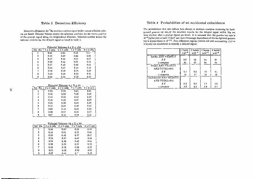
Table 3 Detection Efficiency

Detection efficiencies for 7 Be neutrino capture signal under various selection crite­ria are listed. Fiducial Volume means the selection condition for the vertex position of the prompt signal along the longitudinal direction. Selection number means the selection criteria for the delayed signal as listed in table 2.

Fiducial Volume 0 < Z < 100 Sel. No. 3 x 3 cells 5 x 5 cells 7 x 7 cells 9 x 9 cells

1 0.55 0.64 0.66 0.67 2 0.53 0.62 0.64 0.65 3 0.47 0.54 0.57 0.57 4 0.29 0.44 0.51 0.54 5 0.27 0.42 0.49 0.52 6 0.24 0.37 0.43 0.46 7 0.10 0.19 0.24 0.26 8 0.10 0.18 0.23 0.25 9 0.08 0.16 0.20 0.22

Fiducial Volume 5 < Z < s s Sel. No. 3 x 3 cells 5 x 5 cells 7 x 7 cells 9 x 9 cells

1 0.50 0.58 0.61 0.61 2 0.48 0.56 0.58 0.53 3 0.43 0.50 0.52 0.52 4 0.26 0.40 0.47 0.50 5 0.25 0.39 0.45 0.48 6 0.22 0.34 0.40 0.42 7 0.09 0.18 0.22 0.24 8 0.08 0.17 0.21 0.23 9 0.07 0.15 0.19 0.21

Fiducial Volume 10 < Z < 00 Sel. No. 3x3 cells 5 x 5 cells 7 x 7 cells 9xS cells

1 0.46 0.53 0.55 0.56 2 0.44 0.51 0.53 0.54 3 0.39 0.45 0.47 0.47 i 0.24 0.37 0.43 0.46 5 0.23 0.36 0.42 0.44 6 0.20 0.32 0.37 0.39 T 0.09 0.16 0.20 0.22 8 0.08 0.16 0.20 0.22 9 0.07 0.14 0.7- 0.19

Table 4 Probabilities of an accidental coincidence

The probabilities that iwo indium beta decays or multiple compton scattering by back­ground gamma ray satisfy the selection criteria for the delayed signal within lOy sec time window after a prompt signal are listed. It is assumed that the gamma ray rate is 10~ 9/g/kev/sec around cQUke V and that the energy dependence of the background gamma ray is proportional tc E - 1 5 . Four difference regions (vertex cell and surrounding 3,2,3 or 4 layers) are considered to identify a delayed signal.

1 layer x l O " 9

2 layers x l O - 9

3 layers x i o - '

4 layers x l 0 ~ 3

SAME AND VICINITY PP

7 compton 9.0 83

28 92

54 94

91 S4

SAME AND VICINITY AND-TOTAL=614

PP 7 compton

2.1 14

6.3 17

12 18

21 18

SAME=116 AND VICINITY AND TOTAL=614

PP 7 compton

0.2 3.S

0.5 5.3

1.1 5.6

1.8 5.7

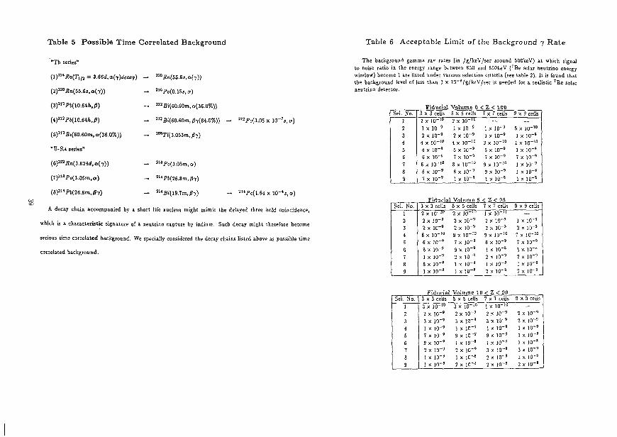
Table 5 Possible Time Correlated Background

"Th series"

( ] ) 2 2 *i?a( r 1 / 2 = 3.66rf,cr(T)^cay) - ^RniSS.SsMj))

{2)™Rn(&S.6s,a{y)) - 2 l 6 Fo(0 .15j , a)

(3)2liPb(lO.64h,0) - 3 nSi(60.60m,a(36.07o))

(4 ) 2 l 2 P&(10 .64M) — 2 1 2B.*(60.60m,^7(64.0%)) — 2".Po(3.05 x ICT' j .a)

(5) 2 1 2 Bi(60.60m,a(36.0%)) - 2 O 8 Tl(3.O53m,0 7 )

"U-Ra series"

(6) 2 2 3 i2n(3.824d,o( 7 )) - 2 1 8 Po(3.05m, o)

(T) 2 3 8 .Po(3.05m,a) — 2 U Pi (26 .8 rn , ^7 )

(8) 2 M P6(26-8m,^7) — 2 U Bt(19 .7m t J 67) - 2 l 4 Fo(1 .64 x 10"^,or) CO CD

A decay chain accompanied by a short life nucleus might mimic the delayed three hold coincidence,

which is a characteristic signature of a neutrino capture by indium. Such decay might therefore become

serious time correlated background. We specially considered the decay chains listed above as possible time

correlated background.

Table 6 Acceptable Limit of the Background 7 Rate

The background gamma ray rates (in /g/kcV/sec around 500keV) at which signal to noise ratio in the energy range between 650 and 850keV ('Be solar neutrino energy window) become 1 ate listed under various selection criteria (see table 2). It is found that the background level of less than 1 x ]0 _ B /g /keV/sec is needed for a realistic 7 B e solar neutrino detector.

Fiducial Volume 0 < Z < 100 Sel. No. 3 x 3 cells 5 x 5 cells T x T cells 9x9 cells

] 1 x 1 0 - ' u 2 x 1 0 " " — — 2 1 x N T 9 1 x 10" 9 1 x icr 9 5 X l O " 1 0

3 2 x 10" 9 2 x 1CT9 l x icr 9 1 x JO" 9

4 4 x I 0 - i 0 4 x 10 - 1° 3 x l 0 - 1 0 1 x 1 0 " 1 0

5 4 x 10 - ' 5 x 10~ 9 5 x I 0 " 9 1 x I0~ 9

6 6 x I0~ 9 7 x JO" 9 7 x ] 0 " 9 7 x 10- 9

7 6x 10-'° 8x 10"'° 9 x 10-'° 1 x 10 - ' 8 6 x J O - 9 s x ]<r 9 ) x ] 0 - 9 1 x JO" 8

9 7 x JO" 9 1 x 10"a ) x J O - 8 1 x JO" 8

Fiducial Volume 5 < Z < 95 Sel. No. 3 x 3 cells 5 x 5 cells 7 x 7 cells 9 x 9 cells

1 2 x I 0 - , u 2 x I 0 _ , u 1 x 1 0 _ ) J — 2 2 x JO" 9 2 x 10- 9 2 x I 0 - 9 1 x lO" 9

3 2 x ID" 9 2 x J O - 9 2 x 10" 9 2 X 10- ' 4 8 x JO" 1 0 9 x 10-'° 9 x 1 0 " I 0 7 x 1 0 - 1 0

5 6 x JO" 9 7 x 10- 9 8 x 10- 9 7 x JO" 9

6 8 x 10" 9 9 x 10" 9 1 x 10- s 1 X 10~" 7 1 x 10~9 2 x JO""9 2 x lO" 9 2 X ! 0 " 9

8 8 x 10" 9 1 x I 0 _ s 1 x Ifl- e 1 X 10" B

9 1 x JO" 8 1 x 10 _ " 2 x 10~ 8 2 X 1 0 - 8

Fiducial Volume 10 < Z < 90 Sel. No. 3 x 3 cells 5 x 5 cells 7 x 7 cells 9 x 9 cells

1 3 x lO" 1 0 3 x 10-'° I x 1 0 - 1 0 — 2 2 x 10" 9 2 x I 0 " 9 2 x ICT9 2 x 10" 9

3 3 x JO" 9 3 x J O - 9 3 x 1 0 - 9 2 x ID" 9

4 1 x 10" 9 1 x JO" 9 1 x 10" 9 1 x lO" 9

5 7 x JO" 9 9 x 10- 9 9 x 1 0 - 9 I x I0~ 8

6 9 x JO ' 9 1 x 10" 8 1 x ]0~ 8 1 x 10~* 7 2 x JO - 9 2 x 1 0 - 9 3 x JO" 9 3 x 10- 9

8 I x 10" 8 1 x 10- ' 2 x 10- ' 2 x ]0~ 8

9 ! x lO - " 2 x 10~8 2 x I0~ 8 2 x I 0 - 8

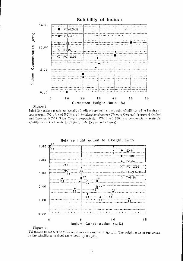
c o

c (U o c o o E 3 '•5 c

1 5 . 0 0

10 .00

5.00

0.1*0

So ubility of Indium

•~~ • PC y t X H l ; —

•

c • • •

j ' : : : : : : : : : : . . : • •

. . . .

: : : : : : : : : :

«

-y t X H l ; —

•

c • • •

j ' : : : : : : : : : : . . : • •

. . . .

: : : : : : : : : :

«

-— • pc + IA

•

c • • •

j ' : : : : : : : : : : . . : • •

. . . .

: : : : : : : : : :

«

-+ IA

•

c • • •

j ' : : : : : : : : : : . . : • •

. . . .

: : : : : : : : : :

« IEIEE' I

+ IA

•

c • • •

j ' : : : : : : : : : : . . : • •

. . . .

: : : : : : : : : :

« IEIEE' I .. I l l * "ILEX ^ =

•

c • • •

j ' : : : : : : : : : : . . : • •

. . . .

: : : : : : : : : :

« IEIEE' I ^ =

•

c • • •

j ' : : : : : : : : : : . . : • •

. . . .

: : : : : : : : : :

«

""" X S5'UU

•

c • • •

j ' : : : : : : : : : : . . : • •

. . . .

+NC95 " •

c • • •

j ' : : : : : : : : : : . . : • •

. . . .

O PC +NC95 " •

c • • •

j ' : : : : : : : : : : . . : • •

. . . .

t >

• 1 , ,

+NC95 " •

c • • •

j ' : : : : : : : : : : . . : • •

. . . .

t >

• 1 , ,

•

c • • •

j ' : : : : : : : : : : . . : • •

. . . .

t >

• 1 , ,

a

•

c • • •

j ' : : : : : : : : : : . . : • •

. . . .

t >

• 1 , ,

a

•

c • • •

j ' : : : : : : : : : : . . : • •

. . . .

t >

• 1 , , i i . i ' i

•

c • • •

j ' : : : : : : : : : : . . : • •

. . . .

t >

• 1 , , i i . i ' i

•

c • • •

j ' : : : : : : : : : : . . : • •

. . . .

>

• 1 , ,

6 0 0 10 20 30 4 0 5 0 Surfactant Weight Ratio (%)

Figure 1 Solubility means maximum weight o[ indium resolved in the liquid scintillator while keeping it transparent. PC, IA and NC95 are ]-2-1trimelhylcbcn7,cne (Pseudo Cumene), isopropyl alcohol and Liponox NC-D5 (Lion Corp.), respectively. EX-il and S500 arc commercially available scintillator cocktail made by Dojindo Lab. (Kumamoto Japan).

1.00

0 .80

0 .60

0 .40

0 .20

0 .00

2 9 Rela t ive l ight ou tpu t to EX-H I n 0 . 0 w t %

- 3 0

7 1......

• "EX-H

•••-S500 - -

zyz...?cZ\\zzz..z. X PC+NC95

-K.- PC+(EX-H)' -

A Tol + IA

- -

7 1......

• "EX-H

•••-S500 - -

zyz...?cZ\\zzz..z. X PC+NC95

-K.- PC+(EX-H)' -

A Tol + IA

- -

7 1......

• "EX-H

•••-S500 - -

zyz...?cZ\\zzz..z. X PC+NC95

-K.- PC+(EX-H)' -

A Tol + IA

+ 3 0

7 1......

• "EX-H

•••-S500 - -

zyz...?cZ\\zzz..z. X PC+NC95

-K.- PC+(EX-H)' -

A Tol + IA

7 1......

• "EX-H

•••-S500 - -

zyz...?cZ\\zzz..z. X PC+NC95

-K.- PC+(EX-H)' -

A Tol + IA

^ 3 1 5

0

.2 9

* x i 3

3 0

3iTZ 2 6

• ~

7 1......

• "EX-H

•••-S500 - -

zyz...?cZ\\zzz..z. X PC+NC95

-K.- PC+(EX-H)' -

A Tol + IA

^ 3 1 5

0

.2 9

* x i 3

3 0

3iTZ 2 6

• ~

— A

_,_... 1 A

3 2

7 1......

• "EX-H

•••-S500 - -

zyz...?cZ\\zzz..z. X PC+NC95

-K.- PC+(EX-H)' -

A Tol + IA * A 20 18

0

.2 9

* x i 3

3 0

3iTZ 2 6

• ~

— A

_,_... 1 A

3 2

7 1......

• "EX-H

•••-S500 - -

zyz...?cZ\\zzz..z. X PC+NC95

-K.- PC+(EX-H)' -

A Tol + IA * A 20 18

0

.2 9

* x i 3

3 0

3iTZ 2 6

• ~

— A

_,_... 1 A

3 2

7 1......

- .# 30

0

.2 9

* x i 3

3 0

3iTZ 2 6

• ~

— A

_,_... 1 A

3 2

7 1......

35 " "4 •"•" 4 0

— A

_,_... 1 A

3 2

7 1......

• _ 35 " "4 •"•" 4 0

— A

_,_... 1 A

3 2

7 1......

_ 1 7 35 " "4

•"•" 4 0

— A

_,_... 1 A

3 2

7 1......

_ 1 7

— A

_,_... 1 A

3 2

- -.

— A

_,_... 1 A

3 2

- -

1 5 0 5 10 Indium Concentration (wt%)

Figure 2 To] means toluene. The other notations are same with figure 1. The weight ratio of surfactant in the scintillator cocktail are written by Die plot.

•Ill

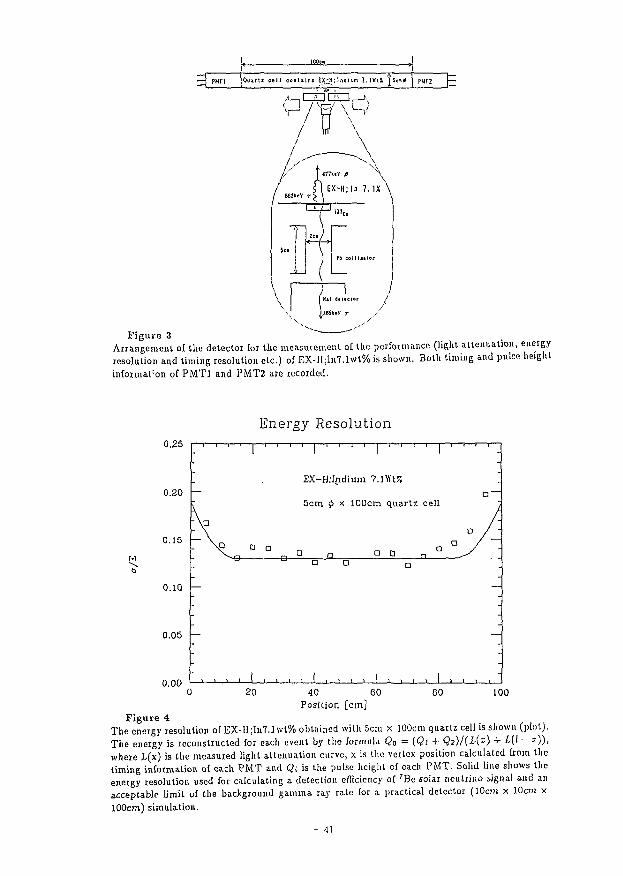
3 PMTt Qui f t i ce l l conUIns EX;H:tndlum 7. IWtJt [Sen* PHT2 P

o j d o . -

/ < I EX-ll;In 7.1S \

re coJJisttor

Ktl dcitcior

las*** T

Figure 3 Arrangement of the detector for the measurement of the performance (light attenuation, energy resolution and liming resolution etc.) of EX-lI;ln7.1wt% is shown. Both timing and puko height informat :on of PMTl and PMT2 are recorded.

Energy Resolution 0.25

0.20

0.15

0.10 —

0.05

0.00

-T 1 ' l " " l " " l " " l " M .

- EX-H:Indium 7.1Yft% \

- a 5om $ x 100cm quartz cell ',

"\p o / -

-\D a ° ° a ° " a ° " ° ^y ' -\D

a D a

- -

1 , 1 1 I l 1 1 t I l l 1 1 1 1 1 l l 1 I 1 t l

20 80 100 40 60 Position [cm]

Figure 4 The energy resolution of EX-H;In7.]\vt% obtained with 5cm x 100cm quartz cell is shown (plot). The energy is reconstructed for each event by the formula Qa = (Qi + Q2)l(L{x) + L(l - x)), where L(x) is the measured light attenuation curve, x is the vertex position calculated from the timing information of each PMT and Q; is the pulse height of each PMT. Solid line shows the energy resolution used for calculating a detection efficiency of 7Be solar neutrino signal and an acceptable limit of the background gamma ray rate for a practical detector (30cm x 10cm x 100cm) simulation.

- 41

t „ e=E s- + 128keV

E r ,+ E r 2 = 614keV

F i rst Tr i gger

1 e 1 1 -?f

Delayed Trigger —* — r 2 i

ft" • • • • :

r i i ft" • • • • :

10

*l ..- - ^ 10 sec !

l O ^ s e c

11 me-ax I s

jlOnsec

EJ PMT ^ T c i z i

<h

IN y

/ ^ ^

0' -axis „. z-axls ' Figure 5

Schematic picture of the detection mechanism of neutrino capture signal by indium loaded liquid scintillator is illustrated. Neutrino capture reaction by an indium atom occurs in the center cell. The electron emitted from the indium then deposits its energy (E„)-12gkeV) in the center cell. Delayed t : o gamma rays are emitted from tiic excited tin atom from the capture reaction with a half life of 3.26/isec (lOtisec time window is used). The lower energy gamma-ray (HGkeV or internal conversion electron (50%)) deposits its energy in the "same" center cell. Its vertex is apart from the prompt electron vertex along Z-axis by dZ. Another (198keV gamma) escapes from the center cell and deposits its energy in the surrounding "vicinity" cell.

Count-Rates for First-Signal

[keV] 2000

Figure G Differential energy spectrum of the background for the prompt signal obtained from the detector simulation are shown. In the calculation smeared tail of indium beta decay, pile up of two indium beta decays and gamma (or beta) rays due to radio-active impurities are considered.

\2

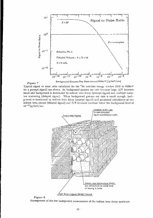
1 0 l

1 0 u

2

1'" 10 - 2

in nuiTi—i—rrnnn 1 - r n r n n — i - m m t i ™ riiumi-i i i n i i i i i i i IIIHI - l

: -

: - ~ ^ Signal to INoise Ratio -

\ \ P X 7-compton

[

- Selection No.5 \ -

" Fidusial Volume : 5 < Z < 95 \ :

~ 9 x 9 cells \ -

— \ —

i n t i l i | i i i n i ! i i i i m i l i i 1 ill i i l i m i t i i l i m i l I*

10 - 1 2 10 -11 10' -10 10 -9 1 0 " 10" 10"

Background Gamma-Ray Rate nround SOOkeV [/g/keV/sec] Figure 7

Typical signal to noise ratio calculated for the 7Be neutrino energy window (G50 to SSOkeV for a prompt signal) are shown. As background gamma ray rate becomes large, S/N becomes small and background is dominated by indium beta decay (prompt signal) and multiple comp-ton scattering (delayed signal). When background gamma ray rate is small enough, back­ground is dominated by indium beta decay (prompt signal) and accidental coincidence of two indium beta decays (delayed signal) and S/N becomes constant below the background level of 10-10/g/keV/scc.

Ind ium 5.07. cell I is su r rounded

ScmLeod Shield / by 0 sc in t i l l a to r cel ls

Figure 8 Arrangement of the low background measurement of the indium beta decay spectr

43

~i 1 1—I—i—r

c

>>

<

1.00

0.50

0.10

0.05

0.01 J | L£1J

500 1000 5000 Figure 9

The energy spectrum from the cell which contains indium is shown by solid histogram, and that from the cell which does not contained indium is shown by the dotted histogram.

c ID

CO • + ^ x» <

1.0

0.5

0.0

~i 1 1 r- - i 1 1 r

0 t 0

1000

250

2000

500

3000

(keV)

4000

Figure 10 The spectrum of indium beta decay obtained by subtracting the dotted spectrum from the solid spectrum in Fig.9. The observed event rate of 25Hz/150g is well agreed with the known indium decay rate of 0.22decays/g.

44

Future Prospects

of

v - Astronomy

Y. Totsuka

(ICRR, Univ. of Tokyo)

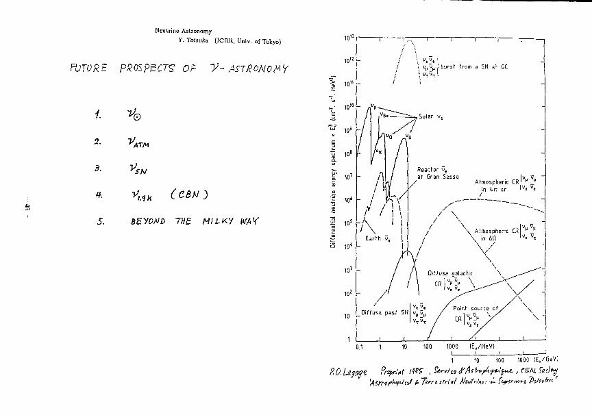
Neutrino Astronomy Y. TolsuU (ICRR, Univ. of Tokyo)

FUTURE PROSPECTS OP V- ArrfiONOtfY

"O

2 - ^ T A ,

* *SN

4. V,.,K £C5A/J

5. BEYDND TrlE MILKY WAY

1 10 100 1000 (Ev/GeVi

P.O.Uwi P/spn'nt ttt$ , ferrft* J'Arfo/tftt'pu. , CSH tol<y

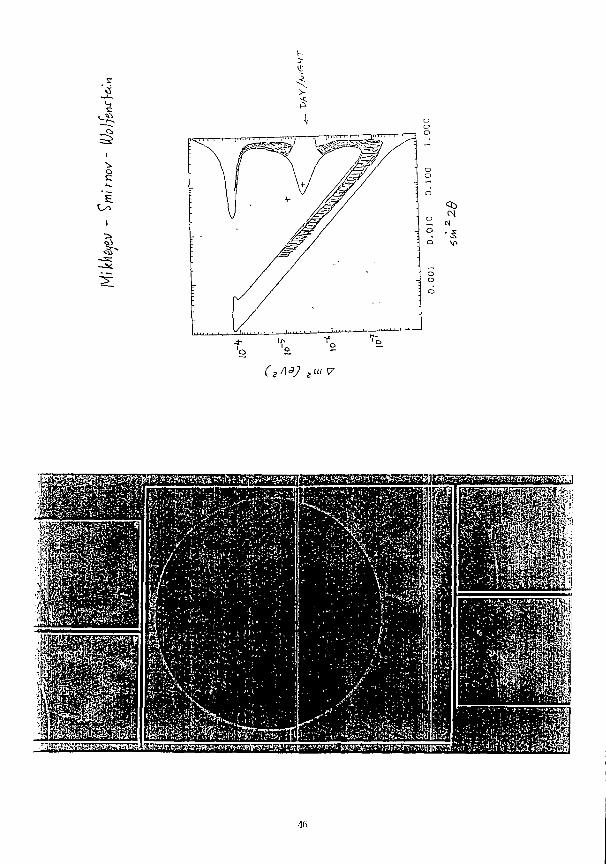
31

5

(l/\9) t^V

'•^^mP^t^^^^^s^^i^^SMJS^im,

m

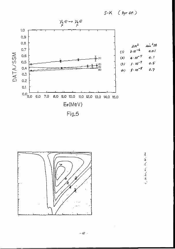
S-K C Byr OP )

CO CO \ < I— <

Am' 3-lo~

4./0 /. to S-io'

,~7

, -7

CO I

o.£-0.7

5.0 6.0 7.0 8.0 9.0 10.0 11.0 12.0 13.0 14.0 15.0

Ee(MeV)

Fig.5

• 4 7 -

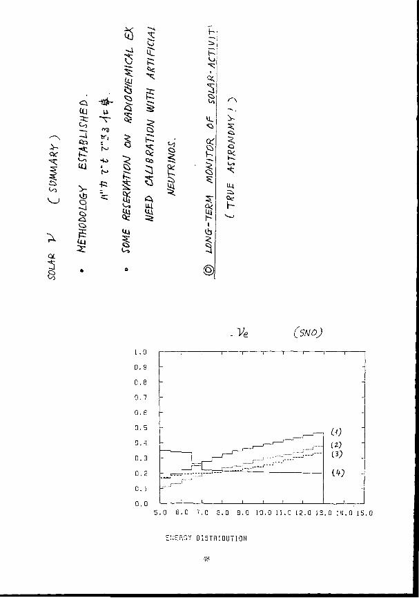
a.

>

8

<-o

to

o

UJ 2:

-«&-

S3

«5.

^ ^ >

<vj c5 *r, £ f M Q

-w -? Qa >C> CJ

•f= 1 5 ^ a; A

<~* UJ Ui u.\ <t 5>

i~

s

I

I -4

o

ft;

Ve (SNOj

5 .0 6 .o 7.o a .o g.o 10.0 n . o t a . a 13.0 i n . o i s . o

ENERGY DISTRIBUTION

•IK

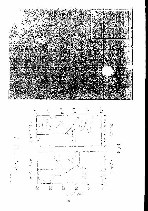
o

A I

V

( i H i

i j

o

en

l-M 0>

A I

CD I — /

o Cvi

o o

U\*':

V.t

STELLAR CORES PRESENTED IN THIS PAPER

Main-Sequence Iron Core Neutron Star Binding Encray Mass Model Mass Mass (10 3 3 «gs)

12 C B

1.31 1.63

1.26 1.58

1.6 25

C B

1.31 1.63

1.26 1.58 4.5

->i C 2.05 1.96-B.H.? 8.6 50 A 1.79 1.60 4.7 100 A 1.S5 B.H.?

uC(cc, y ) l 6 0 reaction rate. These rate variations were classified as follows: Model A, Fowler, Caughlan, Zimmerman (1975) rate;

Mode! B, 2.5 times the rate of model A; Model C, 3 times the rate of model A;

)5 M<?

Cko"^^^ MP si, m fry ^ = £,7£ \ Q

Z H 0 Y^c.Jf 4 C7A!o

25 M Q MODEL" C

0.4 0.6 0.8 time (sec)

en

0 0

in

(UiD) tJ

&

12 Mo CC ) 28F

24 •

20-

16 -

12-

. / i . r r -0 0.2 0.4 0.6 0.8 1.0 1.2

t (sec)

0.2 0.4 0.6 0.8 1.0 1.2

t (sec)

2? M© Cc )

Q.4 O.o 0.9 1.0

Msec!

/oo Ms < A ;

i • I • I • I • i •

20 - -S I G -£ 12 J\J\

o

~ 8

_ ) 4

0 , , 1 . 1 . 1 . 1 ,

0.4 0.6 0.8 !.0 1.2

t (sec

\e<Afo™ 2-cvKcn p2aU = 1 r ^ . J > c I )

M ^

GRAVITATIONAL COLLAPSE

r.f, ^ , u. Mm. e^k, fyj jiL, H(*O

CT

8*1

• «

*

o

Uj

%

v ii

? •x E

• J

It

+

4-

I" II

fc

t 4

«v

it

^ So N

n

Pi ^

vo

11

11 II

>

r V J

L_ n § ut ^

s c» & 5 • ^ <o

GRAVITATIONAL COLLAPSE

•O s

1 1

. " D O O M Q r-

1 1 1 10 M Q

1 1 1 1

Time intcgrotcd . aruincucrino

^ spectra

-

-

/ 1/-SX 105 M 0

\ \ A 1 5 M 0

-

1 1 I W I i 1 1 1 \ l

e (McVI l r n;. I.—*t iiii^-ijilcyfytvd niiiineuiiiuti spectra from s i \ stun (liui nave umlist^unn ^r;ivi\;nioin>i cnllupsc. In ;dl case* the spcclia ha\o l»e«n misruled until

ciicnliulljr nil neutrino emission had ceased. The tpianiiiy {illi/MiU\iU is llic tuial energy emitted in I lie [n-iu of electron aiiiiiicutrtiuis having individual cuer^ie. between < ami € + il< divided by ilw iniul stellar mas* in solar mas* tilth*. The JU-:I umlcr each curve multiplied hy I he ma** of the star to solar manses i l l l iul llic total elccifuu uiiti i ieuinno energy emil led JMMHC the event. The 1(1. 15. and 25 M>. Mars produce super HO vac with neutron 5iar reiuicitiis. The ISO. 5CXI, ;md } « 10* .W* i i a u collapse it* (thick hales. Since the code t t«J u> cilculaie llit-se s|Ktira dvtci not include ilic ^raviuiiiunal rcdiltifl |e.\c<pi Utt llic J x 10^ <^/0 (lar), ilie curve thown Uavc liccn feiiufuialined hy (lie ainuums sluiwii ht Tattle I.

53 -

TABLE 3. Maximum Joint Likelihood Results for the Exponential Cooling Model Quantity With BC Without BG

a 2.25 2.7? 7"„(MeV) • 4.47 4.20 T(S) 4.15 4.59 /V„„ (Kll) 12.5 + 5.6* 13.6 Wdt, (1MB) 5.53 5.38 R(km) 22.5 27.2 £,,(10" ergs) Z85 3£9

"The two values are the expected numbers of signal and background events, respectively.

I .O I t r iX ) A L A M B : NLTTRINOS FROM SN 19S7A

FIGURE 5c. ProJL-ciions of ihc M7n and 95^- confidence volumes for the exponential couiir.y model calculated from ilie joint likelihood function including background. Projections omo the (7. o) plane. The best-lit values, (r, n) - (-4 15 s. 2-25). arc indicated by a cross.

T„ (MeV)

FIGURE 6a. Projections of the 68Tr and 9 5 ^ confidence volumes for the exponential cooling model calculated from the joint likelihood function without backcround. Projections onto the t T. 7) plane The bo l - l i t values. (T. r i - (•! 20 MeV. 4.5*> s). are indicated by ;i CTKSN

ANNALS NEW YORK ACADEMY OF SCIENCES

",-!-, | . ' ' 1 ' ' ' ' 1 ' ' ' ' " 1 ' ' • •

" -6 1 -

1 \ r \ «. \

-

4 r \ \ \ \ -

1 r r L

-

r 0 ' = 1 ' 1 • • 1 . 1 . , , .

T 0 (MeV)

FIGURE 6b. Projections of the 6S% and 95^. confidence volumes for the exponent 1.1 i coulins. model calculated from thy joint likelihood function without background Projections onio the ( T . « ) plane. Thcbesi-fn v ;,lucs. (7".«) - {4.20 McV. 2.72). arc indicated by ;i cross.

0?

FIGURE 6c. Projections of the 68% and 95?c confidence volumes for the esponcntia cooling model calculated from the join! likelihood function without background. Projections onto the (r.,») plane The bc>i- c '. v ; i luev Ir . <>) - (4.59 s. 2.72). .ire indicated b\ a cross.

M 0 (M 0 )

FIGUHK8. (Af n , /•;,,) curves for the neutron star models shown in FIGURES 5:i-c, with tlic portion of each curve that lies within the projected 95% confidence volume drawn more thickly, indicating the allowed range of neutron star gravitational mass for each model.

W

Rob> ( k m )

FKiUKE 7. Comparison of the best-fit values and the 95% confidence volumes projected onto the ( f t „ b I . £») plane and the (/<„b,, Eh) curves for neutron star models based on a representative set of equations of slate. The solid curve indicates the projected confidence volume calculated using the joint likelihood function incorporating ail data and the K l l background spectrum. The corresponding best-lit point, (/?„(,.. £») - {22.5 km, 2.85 x I0 5 j crgs) , is indicated by a cross. The dashed curve indicates the projected confidence volume calculated using the joint likelihood function based on censored K l l data, zero K l l background, and o K l l detector culofT energy of 7.5 MeV. The corresponding best-fit point, (/?„,„, £„) - (27.2 km, 3.59 x 10" ergs), is indicated by an " x ".

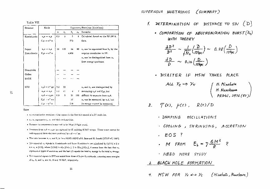
Table VII

Delecior Mode Sup ernova Neutrinos (d=10kpc) Delecior Mode

rc ». Vt »* Remarks

Kamiokande Vtp — e+ n

0.0 9 3

270

6 Calculated based on the SN1987A

da ta .

Super- i-,e — i>ce 13 no 44 80 i/c can be separated from Vt by llie

KamioJjande Vep —• e + n 4,000 angular correlation to SN.

vt can be distinguished from vx

from energy spect rum.

Homcstake — ~ - -Gallex - - - -SAGE — - - -

SNO v.d — e" pp 2.3 23 f« and Vt are distinguished by

»,t — ",t 1.1 11 i 7 measuring vtd and Vtp, but

f,d —• fxpn

V.d - t+ nn

0.9 9 21

37

210

no difficult to separate from vxd.

vs can be measured by v.d, but

its energy cannot be measured.

n; neutroni=alion neutrinos •viiich appear in the first 0.01 second of a SN expleiion.

"it vi represents "u, vr and their anii-parlici«.

> Distance to a supernova is assumed to be lOVpc (3 light years}.

i Neutrons from vtd — i;pn are captured by CI emitting 8 Me-V 7-rays. These 7-rays cannot be

well separated from electrons produced by \>,d — e"pp.

> The ratio between it, i; and 7, is from M 15C+M25C of K. Salo and H. Suzuki (UTAP-47, 1967).

• The expected i-, signals in Kamiokande tnd Super-Kamiokande are calculated by (1/G.5) X 2 X

4 x v, x (1/2), where (1/6,5) rs »(*,)/tf{i-,), 2 is £(u,)/E{vt), 4 comes from the fact thai V .

represents 4 types of neutrinos, and the last 1/2 equals the total vt energy to the total v, energy.

' The erpected signals in SNO are scaled from those o! Super-Ka.-niokande. assuming mean energies

of v,t T, and u, arc 10, 15 and 20 MeV, respectively.

SUPERNOVA hiVBT RINGS (SUMMARY)

/. l>£TERMiNBT)ON OF DISTANCE TV SA/ ^ 1 ) }

» COAiPARISOAJ OF NSQTRON&ATfON BVRST(K) IV/7W Wf£DRY

3>2 fbut/Okpc/ l ^ Wipe J

2>/sv*sreR /F MSW TAKES PLACE

ALL y e - 5 V T / //. H/„aUH H- fJitflokaoNi PRPQ-I, 297£{fo)J

3. fC*), f*(t) , RC+l/D

• VAMPINa 0SC\LLt\TIDKS

• COO UN 6- , S'H R.INUIN6, ACCR£TIDK>

. EOS ? • M FROM Ey = j6p.

• AJEED MORS STOOY

B. BLACK HOLE FORMATION

z

V. M£W FOR Ye <e~> Y- (H.'nakttti., N'Moia^)

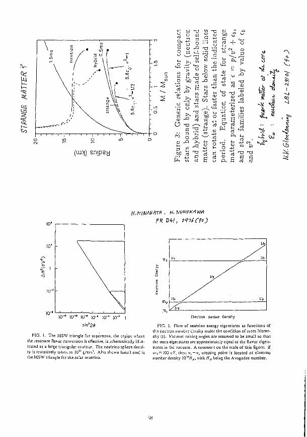
(ai>i) snipey

cj

P4 S O u

a)

a)

bO

O R

•£ o

•-1 -a

O

co 13

cj

3 3 o .s CO

•^ j Pi ^ 3 CT3

co " 3

CO to

R O

CO " " ^

!3 ^

a) hO O

co r bo c?

g + +» CM CO 2 ,

r-> + J CO

i- ^ T3 <U ° 0)

3 fi rd o

a)

> • >

0)

rf 03

ft - d S3 o -a

f - 1 erf

P. S

~ts

^ °

a a cd n3

vis i s

ft Ml VAX ATA , H. NVMKAWA PR 0W, 2n(Cf°)

\Q"1 10"° 10"' 10"'

s'm'29

FIG. 1. The MSW triangle for supernova, the region where llie resonant flavor conversion is effective, is schematically illus­trated as a large triangular contour. The neutrino sphere densi­ty is tentatively taken as 10" g/cm1. Also shown (small one) is the MSW triangle for the soiar neutrino.

Vj.

IA ^ ^ \h

Vz/

iv / v» /dz

Electron Number Density

FIG. 2. Flow of neutrino energy eigenstates as functions of the electron number density under the condition of mass hierar­chy CI). Vacuum mixing angles are assumed lo be small so that the mass eigenslales are approximately equal lo the flavor eigen­states in the vacuum. A comment on the scale of this figure: if /)•)*= 100 cV, then vt — v r crossing poitil is located «it electron number density 10'°//,,, with NA being the Avogadro number.

F>8

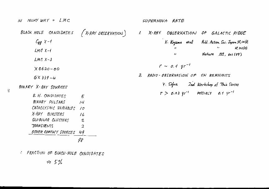
lu mow WAY + LMC

BLACK HOLE CAM 01 DATES fX'RAY OSSERVAVO^

LfAS X-<

LM(L X-3

X06ZO-00

BifjARY X-RAY SOURCES

B. H- CANDIDATES 5 BlHARY PULSARS lif

CATACLYSMIC VARIABLES /O X-RAY BURSTERS U GL08ULAR CLUSTERS % 1RANSIEMS 2 OTHER COMPACT SOURCES 4?

ft

FKACT/OM OF BLACK-HOLE C4HD)PA-TFS

SVpBRhJCVfr RATE

/- X-R/\Y OBSERVAT/OAJ Of GALACTIC RIDGE

" Haiure M, 6»i (e9)

r ~ o. •/ fr~'

Z RADIO - OBSERVATION OF SN REMMAMTS

V. &f*i 2nd IVorkhp of 7hu> Series

r > 0-0 3 Iff'' POSSIBLY 0.1 yr'1

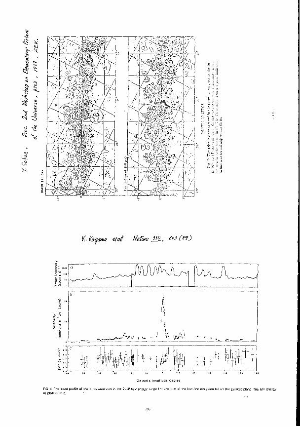
-£ <A> V

Ul $ * • •H

J5 * TK

* ^ $ \

R > <i •n ^

1-1

-* -, £ i

,"* > *-N c>

t j ~? C? *-

<i

(u <~£ 0? >c

-7< frflg'

iitr ^

^

1 / ( W O ' >-

1

y ^ >>

\°) rfy 7 *

i

^

> / I

K-t&</a*a era? Ma&e J™, 6°j (e?)

y „ V U ! , rV +

f:.;( {fl M#p m ! , IP GBlactIc lonrjltuao deor»e

FlG. 1 The scan profile of ihe X-ray emission jn Hie 2-J8keV energy rdnge is> und li.at ol trie iron-line emission (fj) on inc galactic plane The lirv energy is plotted in c.

(ill

o o

©

I

>

Q

EN

^ -2

i£ U

I

+-a

€ ?

N O

^ O

+ I Mi Q

Q II

o ~b

^ Oi

i ^ I£

I

G 5

o II

£.

o II

•k

i f

3 in

2.

s

3

•s -£

^

o vL

0 ^ 8 _ <N O »» 6* >»

«* »h 4

J* IN V

»U ^ 01 s v» o te r\> %|\o •*>

1 1 Vo !

§ o II

Q: w ^

S ^

3 i

3 LC

u.

s» 3f

"3

8

•J c

& *

0

A

2 s:

<a

a.

^ W

o ^

h

4:

•61

RBUC SUPERNOVA ANTl-ELECTRON NEUTRINOS CHECBN)

KS. HtrcU, 2>achr Thesis C1991 J

v = ^S r A J ^° —^~ c

71y ... DEAJC/TV OF GALAXIES C Mpc^)

Rs» - SN RfiT£ C fr'1 ycUxfl)

ia — A6E C G</r)

Lyt - JOTM ENBRG-Y CARRIED BY Ve

By, -• AVERAGE % EHERCrY

Evf r *• tc_ ds E$0 J o Ho O O */"/+!£?

NOTE

^ir^E1]^ Rate) -pL= \fClM£,r)r&)ii \_ ' Burst

E F t - ? Me\/ cn*o = 6S AW CJl = o)

ASSUMPTIONS

0> MO CMAN&E IN RSNl 7)g /M TJHB

n9 to - c i+»5 mf

Cb BUIPT)CALS NOT /NCLVbED /N Tlo

let*")?-, •il t U C.

t i n u I T .

'1MIIU=. • n« in on te s*uuix » y * - ; r

utx «?/ i--7 'u. "?-*-fl;" liirwiMt utiioi • AQiurino etui t v ^ u i n t in* it-r. (fisswaios), ;: uGAUIIHC)aMAI* flria CtuuerSH;(:*3< W - i l ^ H ^ O - i S f l L U r . I«

ni.no. •p.iati-iiQ). a 6i:. WKwHiiiWam** t i ') o'jfc'i. X V -f 3 r - mGCmaci f lh t rd l-r»i. ItBJmiurd i i l U J i X ^ a * ' r f t i : T N ' J ) t ie CiuticrOitlltlHil <«*! «luitero<. nnl cluHcri: I t ^ T S iU T

II It cj)) IT! • WJ7.

. anojjuiutortivi;«LT. mso n x s w i i f t «T . a.iuau

H I i;. neitfiiATQnilUliif a ^ m t ' n l 1'f. aal tmit *IS JCHB J; T « a * r > Hi iint: J: 0 ffl Shfti.TJHTT. taint " U ^ ' u C t t - i • •; •/x. i • 0*!iiO( w»'|.t«n8Ja'6«M/'it ( + n< it t: it IS). Hint L A c/i'um ucuwj t f f l j i i i r iau i r . wnwox+ «.**-«. 1.7 ke* r f t i : t n ;»ft , F) * uft.

»J*»<oaithErtt:»7-4llHM)llir4?Hli*J£ LT*y£ . W 2 nllc 'J ') I T . M/i '6116/i ' l i iU. nn*«itKrt)>t:lt-:T. SUC'CCCflfC L T K I V . cnaiKnauEttni *«trt 1111-117*1. iiftasiO'iio*'!'* •n T 1" W £ Jir W ? A X T .

: ; i : i i « t t H ! i i u . -tojtwu t 'J 4tu«'jiAiifc QH-JII 6 n* r .

je.w pro/i/c 0^ Tc line wiciiW/ PRCUMINA R Y

I "i •H,

+ J.

-1 1-

_ i ^ s _ . — 1 + j±*=±^

,1 .ID •>! ->a -at ao «i .c '3 10 n position .i/i^/c fJc|J

f c //Vie equivalent II-IJWI (kc V) PRELIMINARY

poniion in$lt (dc°)

'J-

S.fakmo eh&, HaCurtM, 211 (ei) ( t _JS z _UJO|,-S 6JO) ssauiL)6uq goEj jns

6 , 10 12 14 16 18 20

...o - - . r i .'• :V.^ ; . ••-M87 " . ' ••.

1 2 h 4 2 m i n 3 4 m i n 2 6 m i n I f l m i n

Right ascens ion ( 1 9 5 0 ) FK3. i The scan path ol the Gin to LAC superimposed on tlie map of the member (afaiies of the Vlito cluster'. The diamond intticaies tfie FWtf.t lieio ot view at the LAC experiment. The galaxies, loim two subctusienngs around M87 and M49 the symbol s i « shows [he apparent blue magnitude

(PUOOQS Jed siunoo) SJEJ junoQ

Q> C C

M Ul w

s i a « » j . •3J 2 ? £ •3J 2 ? £

> . <-• . ro .- >, H- O ~

VX

-m

at

ensi

0J = C -* o ~ in <-> -* _,: OJ ro y o oj

' J - o i n 3 O) • o OJ QJ zi. <n -c TJ ^ — i *->

£ c o

M87

2 'O "O OO O- OJ . M

87

o a i N 5 w £ 75 o e o a i N 5 w £ 75 o

o ^ . s a § fe _CD ro .b c ro c

ount

-r so

lid 1

imen

t, ed

by

< ount

-r so

lid 1

imen

t, ed

by

O OJ >- w , , J= 0J (D O h O . U S H S I S H S I ro nbO -« » E < ^

he G

i iw

nin

fth

e M

49

*-Z ° o CN w J3? oj

. -c c •=% ) a s s ? u. o. o. ro

63

Ui

i

^ $

IS

X V h

* « — 5 _t\ -» o ^ 5 $

Q o" h ^ 5 $

-—' 2.

5! o OJ

II Q£ Q

l^v. P

:tll LU a 2L

9 o ^ s

£ <

ff. <.

2 fc z o o

g 2

s •V)

< 3:

1 3 0

X (A

P • i>? 0

y ai 0

z. 0£ o >

£ nj OS

X ±_ •

U- 5 n o <t t- V£J 1?? o m 2: "Z.

e U-

>

I

2

=£ *

-fo

'of

t

O

§ CI

Q

Oo

A

•5: s

1

v

^

J

3

5i

o

5 2:

• a

-4 t; 1 « i M

'1 • * - Oo O A <d ^ ^ l tv ^ t M- tn JO ^

tH -s: 5 CI 0.0

q S. € <h o5 >-* VO

±~ K C<* ? 11 —. II 3

=> U. )*

64

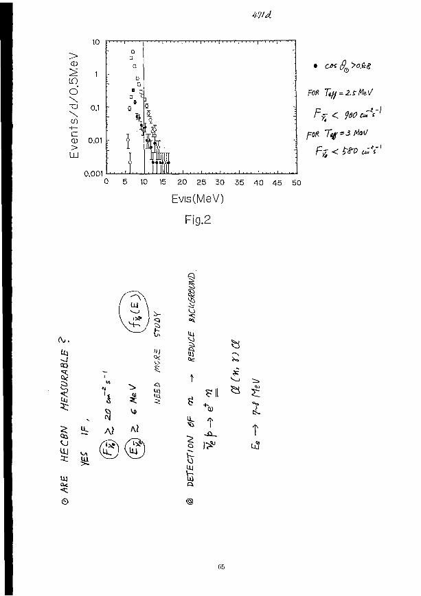
¥11 d.

10

> CD

d \ "O \ to c CD > LU

0.1

0.01

0.001

• D

i i i I i i i i 1

• • I . . . . i . . . . i . . . . i .

FOR Tuff = ZSrMe.V

F^ < <}$0 (£lf]

Fft < S8V ««"**"'

10 15 20 25 30 35 40 45 50

Evis(MeV)

Fig.2

<SJ.

! 3;

1 UJ a:

UJ

©

5 01

<3

1

Q

s is ft

Fll

T

1 ^

— N

T

6r>

5-K O f r O P )

- z -\ Eft. - [OMeV, F y = l O O c ' s

• ? n i 3 . « . - ' r - i - ; ; n i ' . , ' : / ; L . * , i ' - i ~>;|;?:£'Pfx4i*fiir*iT 100 IWS-Ui." »"-•»•? "> •» 7 J i : : « ; c r r , " ; i " ' | . ^ " - - - 7 i t * Ji Z- li V > * „ -

pi /e ~ J T ^ . Ql/

fc CBN

my * 3 f*'\ ~ lTv\5 J

= i f 0* MASSIVE M/\JO*J,NA

- //o(~) cm3

5. BEYoNb THE HILKy WAY

\JIRbO d. ' H V (Afc

d DETECTOR GALACTIC

CENTEX lOkpc lo*t VI R&D

U.OSTSR. HfHfi IO'U

J U )0

- = 3 - 1 0 -t Art

U -

CONCLUfl DAIS

i HOT MANY OBJECTS OBSERVABLE Iff ITU V

ESSENTIALLY Q -f- ShJ +• ATM

2. VEKY IhJTERSSTlua IF HI&H STATISTICS

OBSERVATIONS ARE HAl>£

3. IMPORTANT INFORMATION OAJ V- PROPERTIES

H-. LONCr-TERW MONITOR OF © -+ SW + fiTft

QUITE INTERESTING

S. NEED A FEYJ 600T> 2= LARGE -SCALE

DETECTORS, AN£> KEEP THEM

RVNN\NC* FOR VERY LONG- TIME.

CpiSAWlD)

G. VEXT TAR6ET PRD8f\8LY

"DAM-MATTER ASTRONOW^'.'

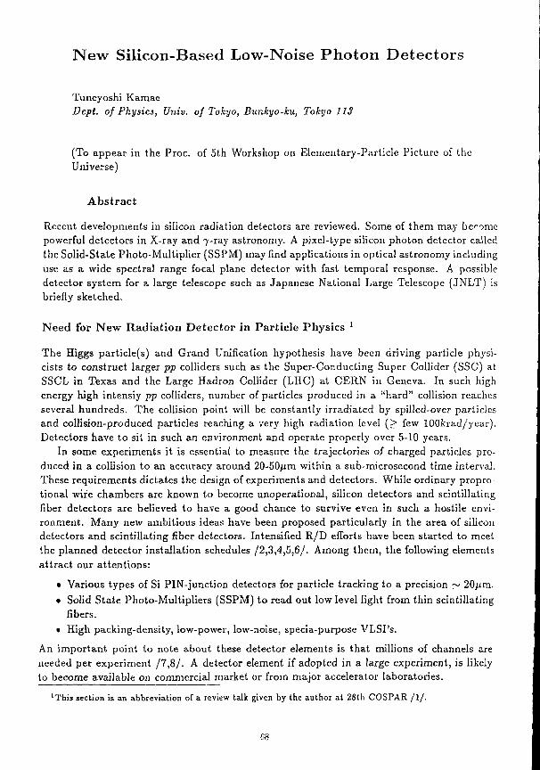
New Silicon-Based Low-Noise Photon Detectors

Tuneyoshi Kamae Dept. of Physics, Univ. of Tokyo, Bunkyo-ku, Tokyo 113

(To appear in the Proc. of 5th Workshop on Elementary-Particle Picture of the Universe)

Abstract

Recent developments in silicon radiation detectors are reviewed. Some of them may become powerful detectors in X-ray and 7-ray astronomy. A pixel-type silicon photon detector called the Solid-State Photo-Multiplier (SSPM) may find applications in optical astronomy including use as a wide spectral range focal plane detector with fast temporal response. A possible detector system for a large telescope such as Japanese National Large Telescope (JNLT) is briefly sketched.

N e e d for N e w Radiat ion Detec tor in Particle Phys i c s 1

The Higgs particle(s) and Grand Unification hypothesis have been driving particle physi­cists to construct larger pp colliders such as the Super-Conducting Super Collider (SSC) at SSCL in Texas and the Large Hadron Collider (LHC) at CERN in Geneva. In such high energy high intensiy pp colliders, number of particles produced in a "hard" collision reaches several hundreds. The colhsion point will be constantly irradiated by spilled-over particles and collision-produced particles reaching a very high radiation level (> few lOOkrad/year). Detectors have to sit in such an environment and operate properly over 5-10 years.

In some experiments it is essential to measure the trajectories of charged particles pro­duced in a collision to an accuracy around 20-50/xm within a sub-microsecond time interval. These requirements dictates the design of experiments and detectors. While ordinary propro-tional wire chambers are known to become unoperational, silicon detectors and scintillating fiber detectors are believed to have a good chance to survive even in such a hostile envi­ronment. Many new ambitious ideas have been proposed particularly in the area of silicon detectors and scintillating fiber detectors. Intensified R/D efforts have been started to meet the planned detector installation schedules /2,3,4,5,6/. Among them, the following elements attract our attentions:

t Various types of Si PIN-junction detectors for particle tracking to a precision ~ 20^m. • Solid State Photo-Multipliers (SSPM) to read out low level light from thin scintillating

fibers. • High packing-density, low-power, low-noise, specia-purpose VLSI's.

An important point to note about these detector elements is that millions of channels are needed per experiment / 7 , 8 / . A detector element if adopted in a large experiment, is likely to become available on commercial market or from major accelerator laboratories.

'This section is an abbreviation of a review talk given by the author at 28th COSPAR /!/ .

68

Silicon particle detectors now being developed can be classified into the following categories /9 ,10/ .

• Strip detectors: Large area PIN diode detectors with multi-strip structure (at 10-100/im pitch) for the p-electrode or for both electrodes (double-sided strip detectors).

• Drift detectors: PIN diode detectors with built-in field-shaping electrodes so that elec­trons drift a few cm to one element of a linearly segmented n-electrode array on one side substrate.

• Pixel detectors: PJN diode detectors with pixel-type electrodes (~ 100 x 100/xm2). Typically one signal processing circuitry per pixel on the same substrate or a bump-connected substrate. Included here is the PIN-CCD, which is a variant of the drift detector.

• Planar PIN detectors: Classical PIN diode detectors such as pholodiodes that have one pair of electrodes on a substrate.

Now these devices are fabricated mostly by the planar ion-implantation technology / l l / , the clean silicon processing technology used for VLSI's. Some manufacturers can produce devices with leakage current as low as l -2nA/cm 2 at room temperature /9,12/ .

Double-sided silicon strip detectors The Aleph group at CERN began the first large-scale use of double-sided Si strip detectors

(see Fig.l) in 1990. They were produced by MBB in Germany / 1 3 / . Hamamatsu / 1 4 / is also capable of producing similar detectors.

Double-sided strip detectors are typically 30-50mm square or ,'i0mmx80mm in area and 300-500/^m thick. The electronic noise is limited by the detector capacitance (about lOpF per strip) and the typical ENC(rms) is several lOOe. Both p and n-electrodes are linearly segmented at 10/xm to a few lOO^m intervals on the p+ surface and n + surface respectively. For hard X-rays, they offer a fine position resolution and energy resolution (< a few keV), and will allow fine imaging by combining with a coded mask or in a single/multiple Compton configuration / 1 5 / .

Drift detectors The carrier life of high purity silicon is very long: electrons in the conduction band can

"drift" over a few cm without appreciable loss. The electric field inside the substrate can be arranged so that holes drift to the nearest p electrode while electrons drift in the midplane to a small n electrode on the side of the substrate. By measuring the electron drift time, the position where the ionization took place can be located to ~ lOO/xm / 1 6 / (see Fig.2).

Since the first publication of the drift detector idea / 1 6 / several interesting variants have been proposed /10 ,5 / . The technology can be exploited in two ways: to reduce the detector capacitance (ie. energy resolution ~ a few lOOeV) and to obtain a high position resolution (~ 100/xm), unfortunately both by sacrificing the time resolution (> 10,us). The spiral drift detector (or the drift photodiode) shows potential to exceed the low noise planar detector (or the photodiode) in the energy resolution (ENC < 50e if cooled) / 1 7 / . They can be used as a low-noise large-area photodiode.

Pixel detectors NA32 at CERN was perhaps first to use CCD's as in a particle physics experiment / 1 8 / .

SLD at SLAC has installed CCD's around the electron-positron colliding region / 1 9 / . CCD's

69

have been used in X-ray astronomy by MIT-Lincoln Lab. / 20 / , \'l PI-A IT-iY] HH / 2 1 / , and GEC-EEV-Lcicestcr / 2 2 / . Among new ideas coming out of particle physics laboratories, the fully-depleted PIN-COD (MP1-A1T-MBB) interest us most.

The electrode arrangement of the fully-depleted CCD is similar to that of the drift de­tector. In this the CCD, electrons in the rnidplanc are forced to drift by multi-phase time-variation of voltage on the electrodes (sec Fig.3). This type has no pixel boundary (100% ac­tive compared with ~ 50% active for MOS-CCD's) and allows fast readout (< a few ms/frame compared with ~ 100ms for non-interlaced non-buffered MOS-CCD's). It will make a superb large-area X-ray detector because of its thick sensitive region (a few 100/xm campared with a few to 20/xm for MOS-CCD's). If its noise characteristics is further improved to ENC < 10-20c by cooling or other methods, it may find applications in optica] astronomy as an alternative to the state-of-the-art CCD's referenced in the next section.

Several European and US laboratories arc engaged in R/D works on the fast pixel device / 2 3 / . They include Inleruniversity Micro-Electronic Center in Belgium, Rutherford Appleton Lab. in England, CERN EP-Division, Lawrence Berkeley Lab. in USA. The detector part is the PIN diode array and the readout circuitry is either on a separate substrate (see Fig.4) or on the detector substrate. In either case, the detector typically has one readout circuit per pixel. Such a device may find applications in hard X-ray detection and photon detection particularly if fast (< fis) readout is required. Those working on the device arc hopeful of developing detectors whose noise figure are as low as the best MOS-CCD's referenced in the next section (< 10c).

Low noise planar detector Large area silicon PIN detectors (a few cm 2 , 0.5-2mm thick) are commercially available

as high resolution X-ray detectors and low-noise photodiodes / 1 2 / . Similar devices have been fabricated in a smaller scale as low-energy electron detectors / 24 / . They all can be used as a hard X-ray detector: the energy resolution can reach 150-500eV (fwhm) if cooled. Photodiodes can be used at room temperature with an energy resolution around a few keV.

Solid State Photo-Mult ipl ier

Need for SSPM in particle physics A typical scintillating fiber detector consists of 10 5 thin plastic fibers grouped into several

layers / 7 , 8 / . When a charged particle crosses a fiber, fewer than ten scintillation photons are emitted /6 ,25 / . Only few photons, however, reach the end of the fiber where a photon sensor is attached. Therefore the photon sensor must have a high quantum efficiency and must be able to detect one photo-electron signal. The frequency of beam collisions in the colliders dictate the detector to have a fast temporal response (<10ns). It must also be small and have a high packing density. The Solid State Photo-Multiplier (SSPM) described here is the only promising candidate to meet the above requirements.

History of the SSPM development works The development work can be traced back to the impurity band conduction infrared

detector (As-doped silicon to be specific) made by Rockwell International in early eighties / 26 / . Availability of such detectors seems to have been limited until mid-eighties because of their military value. According to reports by IRIS Special Group on Infrared Detectors, two Si:As detector arrays seem to have existed since mid-eighties: the Rockwell 10x50 a m y and the Hughes 20x64 array /26 / .

70

The detector operates on the following physical process. When As-doped n-type silicon is cooled to 6-7 K, conduction electrons become trapped in donor levels. Electrons in the donor level (B.E.=49m :V) can be exited by photons (A <28/xm) to the conduction band and drift to the N-electrode if biased appropriately.

In 1987, Petroff, Stapelbroek, and Kleinhans of Rockwell International Science C'*nter published a paper Jiat individual photon can be detected /27 / . They added an undoped blocking layer to the doped region and applied a moderate "acceleration" voltage (7-8V) between the two electrodes. The electric field concentrates in the thin (~4,uni) region at the end of the doped layer adjacent to the blocking layer. The electrons in the conduction band initiate avalanches by knocking electrons out of donar levels (see Fig.5). They observed isolated single photon pulses when the light intensity was low and multiple photon pulses when the light intensity was higher (see Fig.6).

Particle physicists picked up the SSPM idea and began R/D efforts to produce inexpensive photon sensors for scintillating fiber readout in 1989 / 2 8 / .

Present status and future prospect In the fall of 1990, the SSPM development group led by Atac received a few 4-channcl

devices from Rockwell. According to the group, a linear array with fiber adapters (see Fig.7) will be produced in 1991 /28 / .

There seems to be a few area where improvements arc needed for this device to be a photon (A =0.4-10/im) detector. The first is related to the dark current. The SSPM has reasonably low dark current (Fig.8). However it is noted in a publication that the long wavelength IR originating from surrounding materials needs be controlled by cooling the entire assembly to the Lq.N 2 temperature / 27 / . This may be solved if the light is guided to the device by optical fibers. The IR optical fiber blocks photons with wavelength longer than a sharply defined cutoff (see Fig.9). The noise characteristics may also be improved, though not experimentally proven, by changing the dopant to one with higher binding energy (eg., 13.E. of Bi is 69meV). The second concern is the spectral response and the quantum efficiency of the device (Fig.10). An ideal device would cover a wide spectral range at a high quantum efficiency. Measured response of SSPM is much better than that of phototubes or PIN photodiodes. We need, however, two detectors to cover the full accessible range of the Japanese National Large Telescope (JNLT) atop Maunakea (see Fig . l l ) : one front illuminated and the other edge illuminated. Since the response in the shorter wavelength is limited by the surface structure, one may expect improvements in the response function near future.

A sample design of the focal plane array One can take advantage of attractive characteristics the SSPM offers and make a powerful

general purpose focal plane array. Although this is only a conjecture at present, the following characteristics may well be within our reach.

• A matrix of IR fibers placed at the focal plane: Now good IR optical fibers are coming to be available /19/. The fiber matrix can be rearranged to fit various multi-object and multi-wavelength studies. The fiber diameter can be about 100/im for IR and 10/iin for visible Light. The area covering efficiency can be ~80%, higher than that of CCD's. Use of optical fibers are now common in optical astronomy / 3 0 / .

• The pixel size can be optimized to match the IR fibers used: The SSPM pixel dimension does not determine the spatial resolution.

71

• Many stacks of linear arrays to cover a large area: Any combination of various SSPM linear arrays and CCD's can be used simultaneously. For example, fibers from the central part are fed to front illuminated SSPM arrays, some selected fibers (the IR region) to odge illuminated SSPM arrays, and a few fibers to spectral analysis equipped with CCD's and linear SSPM arrays. Several large area CCD's may be a part of this focal plane array. One sample d<\sign of linear SSPM array is shown in Fig.7 (taken from /28 / ) .

• Noise count per pixel of ~ 1 0 _ l s _ 1 reachable: The test result shown in Fig.8 indicates that 1 count/s can be attained at ~ GK. One can hope for further reduction through R/D efforts as mentioned before.

• Time resolution better than ~ 100ns: Particle physicists have obtained 10ns resolution already. This feature will enable fine star tracking to compensate for smearing due to air turbulance / 3 1 / . Temporal analysis is important in various astronomical observations /32 / . In the proposed system, the time variation and correllation can be studied pixel by pixel and spectra] window by spectral window (see below).

• Each fiber channel can be wave analyzed into ~ 6 ?-•• c bands: Wavelength slicing technology developed for optical communication can be applied here as depicted in Fig.12. If needed each wondow can be anlalyzed further.

• Each pixel channel can be handled independently: By installing application specific electronic circuits for individual pixel channels or groups of pixel channels, one can carry out fully optimized multi-object studies /33,30/.

Comparison with low noise CCD's There are now two state-of-the-art CCD's for detection of low level light /34,35/. they are

both buried channel CCD's and capable of reducing noise to reach the photon statistics limit. In particular the one by Ford Aerospace / 3 4 / has a special feature (see the next section) that the readout circuit can be custom designed. One of such circuits reached the electronic noise figure (ENC) as low as 0.5e / 36 / . A larger number of pixels is possible in such CCD's than in SSPM's: perhaps typically 4-16M pixels compared with 10k pixels for SSPM's. The noise characteristics will be comparable.

The spectral response of these CCD's stops just above lfim. while it extends well beyond 10/j.m for an SSPM array. Because the two CCD's mentioned above are optimized to accu­mulation mode use, temporal resolution is in the order of lOmin. If an SSPM array is made, it will become a complimentary device to a more standard CCD array. The fully-depleted PIN-CCD will be regarded as a device between the MOS-CCD and the SSPM in its time response.

In the area coverage and the number of pixels, the buried channel MOS-CCD's and the PIN-CCD will be the choice. Regardless to the future development of SSPM's, these CCD's will remain to be the important device.

Other comments There are IR detectors known as Schottky-barrier detectors / 3 7 / . They have narrower

spectral response and lower quantum efficiency than SSPM's. Now a new family of opti­cal sensors using quantum-wells are being developed in fiber communication industry / 3 8 / . Their main use is digital communication and the spectral response does not extend beyond near IR at present. The quantum well devices are rapidly evolving now and need constant rcevaluation.

72

Low-Noise VLSI Ana log Elec t ronics

Analog VLSI's have been developed for the Si strip detectors used in collider experiments. They include Microplex (Mkll at SLAC) / 3 9 / , CAMEX (Aleph at CERN) /40 / , MX (Delphi at CERN) / 4 1 / , and SVX (CDF at FNAL) /42 / . These charge-sensitive preamplifiers are designed to sample the integrated charge just before and after the beam collision. With one correlated double-sampling, noise figures are typically ENC = 500 — 1000c (C'D — lOpF). One can design with the conventional RC feed-back and reach a better noise characteristics (ENC ~ 200 - 300e for CD ~ lOpF) if packing density is lowered from 128ch/chip to 8-16/chip. Circuits with a larger number of sampling have also been designed and known to lower the noise further.

The detector capacitance, the leakage current, and the 1 / / noise determine the electronic noise in the system / 4 3 / . To lower the noise, one has to shorten the path to the front-end circuitry (ie. reduce the total capacitance), to lower the ambient temperature (ie. reduce the leakage current), and to optimize the integration time as shown in Fig.13 / 4 3 / .

Analog VLSI's of different types have been designed for various applications in particle experiments / 4 4 / . The merits they bring are higher packing density, lower power consump­tion, higher reliability, and reduction in the total cost. Application-specific analog /LSl 's will gradually replace most hybrid circuits and PC-board circuits for the above reasons.

In the astronomical applications, use of analog VLSI's are particularly important in re­ducing the electronic noise. This is best demonstrated in the 4 mega-pixel CCD developed by Ford Aerospace / 3 4 / . The particular CCD allows customers to design the readout circuits on the chip. One interesting circuit design developed is the multiple-sampling scheme of the charge stored in the CCD-pixel named the "skipper" circuit / 45 / . The readout electronic noise has been reduced to a sub-electon level.

Conc lus ions

The author see sorn^ of the silicon-based photon detectors now being developed in the field of particle physics are directly applicable in optical astronomy as well as in X-ray astronomy. In the optical region, the Solid State Photo-Multipliers (SSPM), 1R optical fibers, and the PIN-CCD may find interesting applications. They together with the buried channel MOS-CCD's developed by US industries and US astronomers will make very attractive focal plane detectors for Japanese National Large Telescope.

A c k n o w l e d g e m e n t s

The author wish to thank Drs. M. Atac, S. Kobayashi, T. Kondo, S. Okarnura, L. B. Robin­son, W. Tanaka, H. Tsunemi, K. Yamamoto, and other colleagues in particle physics and astronomy for supplying him with information and answering enquiries. This report was pre­pared for 5th Workshop on Elementary-Particle Picture of the Universe but was not presented there. Through heartful encouragements and special arrangements by Drs. M. Fukugita and A. Suzuki, this came to be a part of the proceedings.

T.i

REFERENCES

1. T. Kamae, Invited paper presented at 2.8th COSPAR (The Hague, July 1990) to appear in Space .

2. Proc. of Summer Study on High Energy Physics in the 1990's, Snowmass (1988) 3. Proc. of 4th Pisa Meeting on Frontier Detectors for Frontier Physics, lsola d'Elba (J989):

Published as Nucl. Inslr. Meth., A289 (1990) 4. IEEE Nuclear Science Symposia, 1987, 1988, 1989. Published as IEEE Trans. Nucl. Sci.,

34(1), 35(1), 36(1), (1988) (1989). 5. Proc. of 5th European Symposium on Semiconductor Detectors, Munich (1989) published

as Nucl. Instr. Meth., A288 (1990). 6. Proc.. of Workshop on Scintillation Fiber Development for the SSC, eds. S. Reucroft and

R. Ruchti, Fermilab (1988). 7. L* Collaboration, Expression of Interest submitted to Superconducting Super Collider

Lab. (1990). 8. Solenoidal Detector Collaboration, Expression of Interest submitted to Superconducting

Super Collider Lab. (1990). 9. E. H. M. Heijne and Pierre Jarron, p.739 of / 2 / . See also articles in / 5 / .

10. P. Rehak and E. Gatti, Nucl. Instr. Meth., A289, 410 (1990). 11. J. Kemmer, Nucl. h-str. Meth., 169, 449 (1980). 12. S. Gunji et al., Nucl. Instr. Meth., A (in press). 13. P. Holl et al., IEEE Trans. Nucl. Sci., NS-3P(l), 25] (1989). 14. K. Yamamoto, Private communication (1989) 15. T. Kamae, R. Enomoto, and N. Hanada, Nucl. Instr. Meth., A260, 254 (1987).

T. Kamae, N. Hanada, and R. Enomoto, IEEE Trans. Nucl. Sci., NS-35(1), 352 (1988). 16. E. Gatti and P. Rehak, Nucl. Inslr. Meth., 225, 608 (1984). 17. P. Rehak et al., IEEE Trans. Nucl. Sci., NS-36(1) 203 (1989)

B. S. Avset et al., IEEE Trans. Nucl. Sci., NS-36(1) 295 (1989) 18. See description in C. J. S. Damerell, N-j.cl. Instr. Meth., A275, 484 (1989). 19. C. J. S. Damerell et al., Nucl. Instr. Meth., A288, 236 (1990). 20. Astro-D Proposal to ISAS (1986). 21. L. Striider et al., Nucl. Inslr. Meth., A288, 227 (1990).

L. Striider et al., IEEE Trans. Nucl. Sci., NS-35, 372 (1988). 22. D. H. Lumb, Nucl. Instr. Mcth., A288, 219 (1990). 23. Proc. of Workshop on Silicon Pixel Detectors, Leuven, (1988). Published as Nucl. Inslr.

Meth., A275 (1989). 24. K. Dpncshvar, R. G. Aitkcn and G. Singco, Rev. Sci. Inslr., 61, 1464 (1990). 25. F. Takasaki et al., Nucl. Instr. Meth., A260, 447 (1987); KEK Report, 89-183 (1990).

D. R. Wood et al., Nucl. Instr. Meth., A289, 331 (1990). C. Angelini et al., Nucl. Inslr. Meth., A289, 342 (1990).

26. M. D. Petroff and M. G. Stapelbroek, Many unpublished reports of IRIS Special Group on Infrared Detectors (1980-1985). A. M. Fowler and R. R. Joyce, Instrumentation in Astronomy VII, Proc. SPIE 1235 (Part 1) (1990) p.151.

74

27. M. D. Pctroff, M. G. Stapelbroek, and W. A. Kleihans, Appl. Phys. Lett. 51 (1987) 400. M. D. Pctroff and M. G. Stapelbroek, IEEE Trans, on Nuclear Science 30(1) (1989) 158.

28. M. D. Petroffand M. Atac, IEEE Trans. Nuclear Science 3G, JG3 (1989). M. Atac et al., Detector R/D Proposal to the SSCL (1989).

29. Infrared Fiber Optics, SPIE Tutorial Text (1989) 30. S. Bardcn (ed), Fiber Optics in Astronomy, ASP Conference Series (1988).

Donald Hamilton, Instrumentation in Astronomy VII, Proc. Sl'IE 1235 (Part 2) (1990) p.673. Ian R. Parry and Ian J. Lewis, Instrumentation in Astronomy VII, Proc. SPIE 1235 (Part 2) (1990) p.G81. Ian R. Parry and Esperanza Carrasco, Instrumentation in Astronomy VII, Proc. SPIE 1235 (Part 2) (1990) p.702. Peter Gray and Keith Taylor, Instrumentation in Astronomy VII, Proc. SPIE 1235 (Part 2) (1990) p.709.

31. M. Clampin et al., Charge-Coupled Devices and Solid State Optical Sensors, Proc. SPIE 1242 (1990) p.217.

32. J. L. A. Fordham et al., Instrumentation in Astronomy VII, Proc. SPIE 1235 (Part 2) (1990) p.636. C. R. Cox et al., Instrumentation in Astronomy VII, Proc. SPIE 1235 (Part 2) (1990) p.G57.

33. J. P. Brodic, ct al., Instrumentation in Astronomy VII, Proc. SPIE 1235 (Part 2) (1990) p.722. F. G. Watson, et al., Instrumentation in Astronomy VII, Proc. SPIE 1235 (Part 2) (1990) p.736.

34. It. A. Brcdthauer, New Methods in Microscopy and Low Light Imaging, Proc. SPIE 1161 (1989) p.Gl. J. C. Geary, ct al., Charge-Coupled Devices and Solid State Optical Sensors, Proc. SPIE 1242 (1990) p.38.

35. T. H. Lee, et al., Charge-Coupled Devices arid Solid State Optical Sensors, Proc. SPIE 1242 (1990) p.10.

3G. L. B. Robinson, ct al., Instrumentation in Astronomy VII, Proc. SPIE 1235 (Part 1) (1990) p.315. C. E. Chandler et al., Charge-Coupled Devices and Solid State Optical Sensors, Proc. SPIE 1242 (1990) p.238.

37. W. F. Kosonocky, Infrared Detectors and Focal Plane Arrays, Proc. SPIE 1308 (1990) p.2. J. Kurianski, et al., Infrared Detectors and Focal Plane Arrays, Proc. SPIE 1308 (1990) p.27.

38. F. Capasso et al., Appl. Phys. Lett. 48 (1986) 1294. 39. A. Litkc et al., Nucl. Instr. Meth., A265, 93 (1988) 40. II. Becker ct al., IEEE Trans. Nucl. Sci., NS-36(1), 24G (1989).

W. Buttler et al., Nucl. Inslr. Meth., A288, 140 (1990). 41. P. P. Allport, P. Seller, and M. Tyndal, Nucl. Instr. Mcth., A273, 630 (1988).

J. Stanton et al., IEEE Trans. Nucl. Sci., NS-3G, 522 (1989). 42. S. Klcinfelder, IEEE Trans Nucl. Sci., NS-35, 171 (1988)

43. V. Radeka, Ann. Rev. Nuci Part. Set., 38, 217 (1988) 44. H. H. Williams, IEEE Trans. Nucl. Sci., NS-36(1), 146 (1989). 45. J. Janessick, et al., Charge-Coupled Devices and Solid State Optical Sensors, Proc. SPIE

1242 (1990) p.223.

F i g u r e C a p t i o n s

1. Double-sided Si strip detector / 1 3 / : (a) Schematic showing the capacitive coupling used in picking off signals; (b) Cross-section of the n-side surface showing the n + electrodes, the p-type insulation strips, and the Al strips connected to the readout circuitry.

2. Schematic of the Si drift detector: Electrons drift along the potential minimum to the array of n-electrodes while holes are collected by the nearest p-electrodes. The time elapse between the electron and hole signals can be used in the position measurement / 1 6 / .

3. Schematic showing the operation of fully-depleted CCD: Electrons are trapped along the potential minimum in the mid-plane and shifted in the same manner as the ordinary frame-transfer CCD / 2 1 / .

4. Schematics of a fast Si pixel detector: The diode detector substrate and the readout chip are connected by indium bumps in this particular detector /3 ,23 / .

5. Basic physics process showing how the SSPM works / 2 7 / . 6. Electronic signals out of the first SSPM by produced by Rockwell / 2 7 / : (a) at low light

intensity all signals take the same waveform, the single photon signal; (b) at higher light intensity multi-photon signals appear.

7. A sample design of a linear SSPM array for a SSC experiment / 2 8 / . 8. Characteristics of the first SSPM produced by Rockwell / 2 7 / . 9. Transmission of light through a modern IR optical fiber / 2 9 / .

10. Spectral response of the SSPM made by Rockwell / 2 7 / . 11. Wavelength bands accessible to JNLT atop Maunakea (a), and the angular resolution

of JNLT (b). 12. A wavelength slicer used in optical fiber multiband communication. 13. Theoretical curves showing relations among the equivalent noise charge (ENC), the

measurement time (tm) and the detector capacitance (Co) /4&I'• Note that at room temperature the detector leakage current makes a large contribution to ENC forcing the solid curves to shoot up parallel to, and somewhere between, the dashed lines marked "Bose Current Noise" and "FET Leakage Current noise".

- 76 -

juration side

ohmic side

Fig.l Fig-2

DEEP N-1MPIANT n"-BULK

256 1

ssasn

Fig.4

Fig.3

-77

(a)

lb)

SS

" X

Fig.5

F I G . 1. (a) SSI'M layci configuration wi lh schematic lepresentalion ol' lhe goneian'on t i f bias current and iheell'ecls fol lowing absorption of a pholon. (b ) Electric field profile.

Time ((LS)

(a.)

Fig.6

SOLID STATE PHOTOMULTIPLIER

N

W'l CROBOND I NG PADS

OPTICAL FIBERS TO PREAMP

Fig.7

LIQUID He VAPOR CERAMIC SUPPORT LIQUID N, VAPOR

78

COUNT RATE

DENSITY

( s ' W | 10'

10*

G 7 8 9 10 TEMPERATURE (K)

(••>)

J = 0 .5 i<m

10'

10'

10'

(a) TEMPERATURE DEPENDENCE OF THE SSPM DARK-COUNT-RATE AND SATURATION-COUNT-RATE DENSITIES. (b) DIAS DEPENDENCE OF GAIN, M, AND QUANTUM EFFICIENCY

Fig.8

10 n l

KRS-5 10 3

102

10

10 -1

E

m •o 2 O

< io-2 £

< 10" 3

io-

0.5 1.0 2.0 3.0 5.0 10.0 20.0 30.0 50.0

WAVELENGTH^™)

Fig-9

79

QUANTUM EFFICIENCY (V.)

0.1 0.1

TYPICAL PARAMETERS NO AR COATING

BACK UV 1 VISIBLE I NEAR IR [SWIR(MWIR| LW1R | VlWtft

I ff I I r I ioL 1 10

WAVELENGTH frm)

Fig.lO

(a)

l/Alcn.-') I 0 °

r \ \

\ >

JNLTM8B««t\ r.-z,-CrC~

Hale_____—-

~^^~- " UKIRT NASA "

* < <snRi*> < a * n »

10,/ 30 « f i

0 2 -?^tr7\Mmv(nNHM£m. !tai 'pon+w7.5 m53iaK(JNLT)t HST. Mill{OAO)*> 1.88m, }= i viiaosaataraitK. tewasswi&wiK 2 &m-xmamnxiinmicx <>. Gammantmtmn

(b)

Fig. 11

-80-

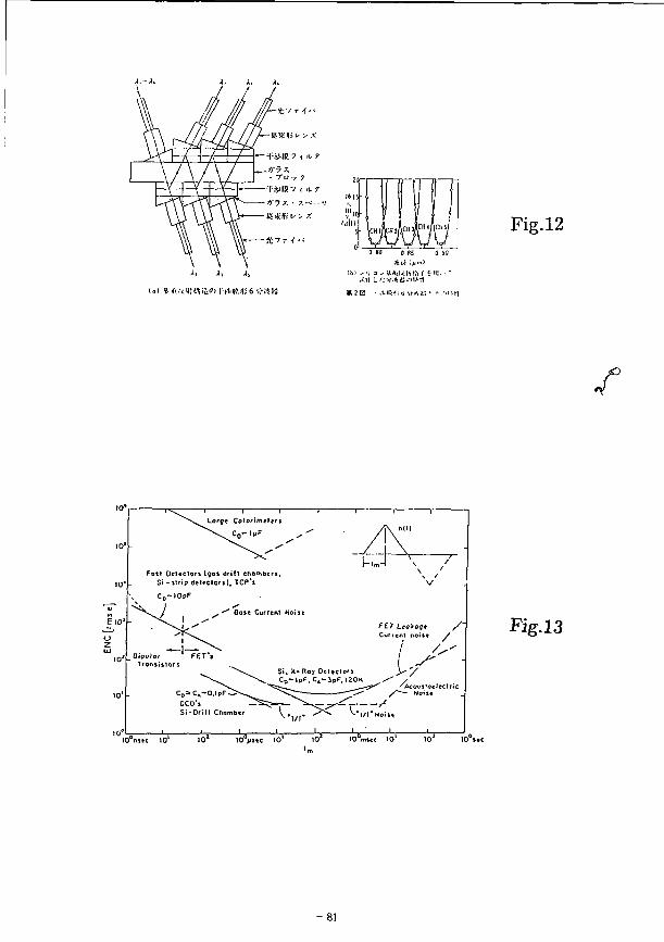
U) I .li.MtWilm I'llKfl; G ttiSS

Fig.12

* 2 H I .'UK!*; 6 ;}A-&

r

10'

10'

Lorgc Colorimttat

C Q - I P P

fo i t Oclecton (goi drift chomben. S i - it rip det tc ion) , TCP'i

Bo»e Current Noiit

1 0 » L Bipolar f ET ' j Tfoniislors

:,;:j\ 7

F£7 Leofcog* / ' C«rr«nt noi»« /

C 0 =»C*-0. lpF--> CCo'» Si-Dri l l Chamber

Si. X-Roy Detectors 3 " ' / ' C 0 - * lpF ,C A - 3pF , )20K ^ ^ /

i ^ ^ J -<?'*** 'Acou»lo«I«clric

Fig.13

IOVTC i c ? 1 0 * ioVtc 1? 1? ft« IO1 io* io°».c

- 8 1 -

Development of Analog VLSI for High Energy Physics Experiment*

HIROKAZU IKEDA

National Laboratory for High Energy Physics 1-1 Oho, Tsv.ku.ba, Ibaraki-ktn, 305 Japan

ABSTRACT

We have investigated large scale integrated circuit technologies to apply them for radiation detectors of high energy physics and related area. A special emphasis has been put on analog circuits which could be mounted directly on detectors. The research area covers a bipolar ASIC, a full custom bipolar circuit, and a full custom CMOS circuit. A computer aided design work is an indispensable part in this project.

1. Introduction

1.1. GENERAL REQUIREMENTS

The design concepts on the electronic system for high energy physics experi­ments are changing drastically. Traditional way was to put preampliiiers on the detector side, whose outputs were transmitted via a large bundle of cables to an electronics hut to be processed by data acquisition modules. The experiments at the SSC or the B-factory will meet a high repetition trigger rate and a large data size. The SSC experiments has additional issues about a radiation damage and an enormous number of readout channel of the order of 10 6. In order to over­come these hurdles, we have been investigating analog processing circuits with fast, high density, and low power VLSI technologies. The VLSIs have an analog processing capability as well as digital control functions to be directly mounted at detector front ends. These technologies are easy to spin-off to be applied for non-accelerator physics in the environment of a balloon borne experiment , and/or an underground experiment . An advanced collider experiment and a particle physics experiment without an accelerator happen to share common requirements and technologies about their data acquisition front end electronics.

* Presented at the Symposium on Elementary-Particle Picture of the Universe, Minami-izu Nov 19-21

82

1.2 . DEVEI.OPMEPTT OF DATA ACQUISITION SYSTEM

In order to meet experimental requirements, we have investigated advanced technologies to apply them for actual fields of high energy physics experiments and related area. The development area covers wide varieties of research topics. The major items are listed in Table. 1. Traditional area of electronics and/or data acquisition are confined in a fabrication of PCB based electronic modules. Now our design efforts go into a microscopic area, VLSI development, and also to a macroscopic area, a system-wide simulation based on the GPSS and the VHDL code. The efforts located in between the two are proliferated in terms of a computer farm, a high speed optical data link, and a backplane bus system for data acqusition modules. Familiar electronics modules of the NIM and the CAMAC standard have still application area. The most advanced backplane bus system invented in the nuclear science society is the FASTBUS standard131. The FASTBUS system has been used in the TRISTAN experiment and other collider experiments in the world. In order to meet a future experiment, we need to have a scope which goes beyond current technologies. The Scalable Coherent Interface project has started its activity to find a break-through in the area of the backplane bus system. The efforts about front end VLSI will not work without development efforts about the back end system. This paper reviews a present status of the VLSI development work. The other area of development efforts will be talked about by someone else at an appropriate chance.

Table 1. Development Area for Data Acquisition System

Simulation GPSS [ 4' /VHDL t 5 l t < s |

of electronic systems Computer farm ACP project and others High speed optical fiber link from 100 Mbps to 1 Gbps Backplane bus system FASTBUS/VME/VXI

FUTURE BUS/SCI1" Front end electronic module NIM/CAMAC/TKO Development of front-end VLSI Presented in this article

f Printed Circuit Board

83

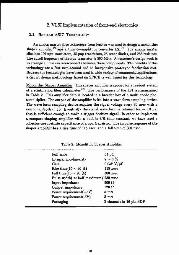
2. VLSI Implementation of front-end electronics

2 . 1 . B I P O L A R ASIC T E C H N O L O G Y

An analog master slice technology from Fujitsu was used to design a monolithic shaper amplifier and a time-to-amplitude converter LSI . The analog master slice has 120 npn transistors, 58 pnp transistors, 28 zener diodes, and 256 resistors. The cutoff frequency of the npn transistor is 500 MHz. A customer's design work is to arrange aluminum interconnects between these components. The benefits of this technology are a fast turn-around and an inexpensive prototype fabrication cost. Because the technologies have been used in wide variety of commercial applications, a circuit design methodology based on SPICE is well tuned for this technology.

Monolithic Shaper Amplifier This shaper amplifier is applied for a readout system of a scintillation-fiber calorimeter . The performance of the LSI is summarized in Table 2. This amplifier chip is located in a breeder box of a multi-anode pho-tomultiplier. The output of the amplifier is fed into a wave form sampling device. The wave form sampling device acquires the signal voltage every 80 nsec with a sampling depth of 16. Eventually the signal wave form is retained for ~ 1.3 fis; that is sufficient enough to make a trigger decision signal. In order to implement a compact shaping amplifier with a built-in CR time constant, we have used a collector-to-substrate capacitance of a npn transistor. The impulse response of the shaper amplifier has a rise time of 115 nsec, and a fall time of 300 nsec.

Table 2. Monolithic Shaper Amplifier

Full scale 64 P C Integral non-linearity 2 - 3 % Gain 0.03S V/pC Rise time(10 ~ 90 %) 115 nsec Fall time(10 ~ 90 %) 300 nsec Pulse width( at half maximum) 250 nsec Input impedance 500 il Output impedance 120 17 Power requirement (+5V) 5 mA Power requirement(-5V) 5 mA Packaging 2 channels in 16 pin SOP

- 84

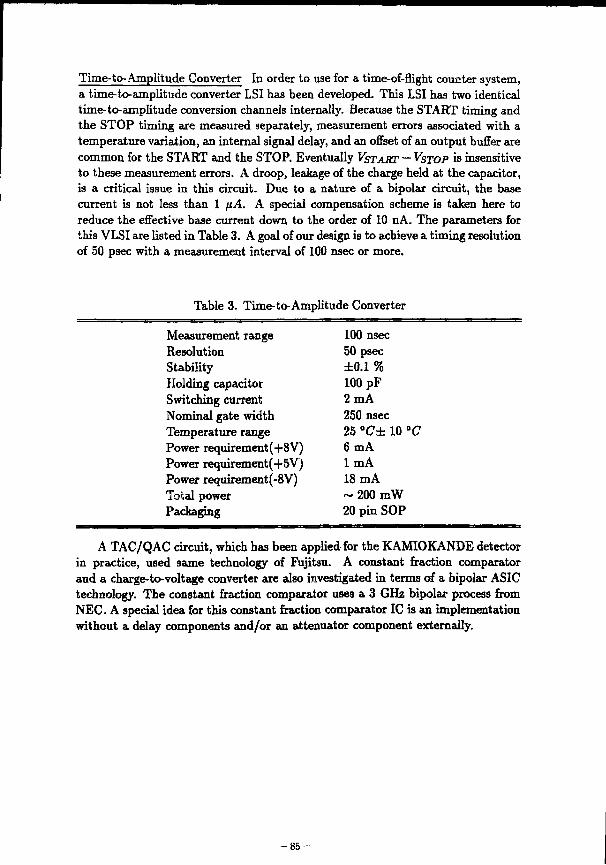
Time-to-Amplitude Converter In order to use for a time-of-flight counter system, a time-to-amplitude converter LSI has been developed. This LSI has two identical time-to-amplitude conversion channels internally. Because the START timing and the STOP timing are measured separately, measurement errors associated with a temperature variation, an internal signal delay, and an offset of an output buffer are common for the START and the STOP. Eventually VSTAST ~ VSTOP is insensitive to these measurement errors. A droop, leakage of the charge held at the capacitor, is a critical issue in this circuit. Due to a nature of a bipolar circuit, the base current is not less than 1 pA. A special compensation scheme is taken here to reduce the effective base current down to the order of 10 nA. The parameters for this VLSI are listed in Table 3. A goal of our design is to achieve a timing resolution of 50 psec with a measurement interval of 100 nsec or more.

Table 3. Time-to-Amplitude Converter

Measurement range 100 nsec Resolution 50 psec Stability ±0.1 % Holding capacitor 100 pF Switching current 2 mA Nominal gate width 250 nsec Temperature range 25 °C± 10 °C Power requirement (+8V) 6 mA Power requirement (+5V) 1mA Power requirement (-8V) 18 mA Total power ~200mW Packaging 20 pin SOP

A TAC/QAC circuit, which has been applied for the KAMIOKANDE detector in practice, used same technology of Fujitsu. A constant fraction comparator and a charge-to-voltage converter are also investigated in terms of a bipolar ASIC technology. The constant fraction comparator uses a 3 GHz bipolar process from NEC. A special idea for this constant fraction comparator IC is an implementation without a delay components and/or an attenuator component externally.

- 8 5 -

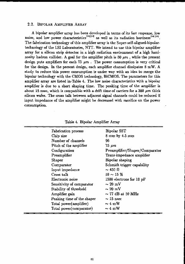
2.2. B I P O L A R A M P L I F I E R ARRAY

A bipolar amplifier array has been developed in terms of its fast response, low noise, and low power characteristics * as well as its radiation hardness . The fabrication technology of this amplifier array is the Super-self-aligned-bipolar-technology of the LSI Laboratories, NTT. We intend to use this bipolar amplifier array for a silicon strip detector in a high radiation environment of a high lumi­nosity hadron collider. A goal for the amplifier pitch is 50 fim , while the present design puts amplifiers for each 75 fim . The power consumption is very critical for the design. In the present design, each amplifier channel dissipates 8 mW. A study to reduce this power consumption is under way with an idea to merge the bipolar technology with the CMOS technology, BiCMOS. The parameters for this amplifier array are listed in'Table 4. The low noise characteristics with a bipolar amplifier is due to a short shaping time. The peaking time of the amplifier is about 15 nsec, which is compatible with a drift time of carriers for a 300 (im thick silicon wafer. The cross talk between adjacent signal channels could be reduced if input impedance of the amplifier might be decreased with sacrifice on the power consumption.

Table 4. Bipolar Amplifier Array

Fabrication process Chip size Number of channels Pitch of the amplifier Configuration Preamplifier Shaper Comparator Input impedance Cross talk Electronic noise Sensitivity of comparator Stability of threshold Amplifier gain Peaking time of the shaper Total power(amplifier) Total power(comparator)

Bipolar SST 8 mm by 4.5 mm 96 75 fim Preamplifier/Shaper/Comparator Trans-impedance amplifier Bipolar shaping Schmidt trigger capability ~ 4 5 0 f i 10 ~ 15 % 1500 electrons for 10 pF ~ 2 0 m V ~ 2 0 m V ~ 77 dB at 10 MHz ~ 15 nsec ~ 4 mW ~ 4 mW

86

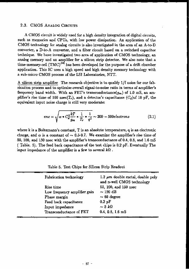
2.3. CMOS ANALOG CIRCUITS

A CMOS circuit is widely used for a high density integration of digital circuits, such as memories and CPUs, with low power dissipation. An application of the CMOS technology for analog circuits is also investigated in the area of an A-to-D converter, a D-to-A converter, and a filter circuit based on a switched capacitor technique. We have investigated two area of application of CMOS technology, an analog memory and an amplifier for a silicon strip detector. We also note that a time-memory-cell (TMC) " has been developed for the purpose of a drift chamber application. This IC uses a high speed and high density memory technology with a sub-micro CMOS process of the LSI Laboratories, NTT.

A silicon strip amplifier The research objective is to qualify 1/f noise for our fab­rication process and to optimise overall signal-to-noise ratio in terms of amplifier's frequency band width. With an FET's transconductance(^m) of 1.0 mS, an am­plifier's rise time of 100 nsec(Tr), and a detector's capacitance (C<j)of 10 pF, the equivalent input noise charge is still very moderate:

/ kT 1 1 enc = Wo * C\— * — * -=• ~ 300 - 500electr(ms (2.1)

Y 9m Tr q

where k is a Boltzmann's constant, T is an absolute temperature, q is an electronic charge, and a is a constant of ~ 0.5-0.7. We examine the amplifier's rise time of 50, 100, and 150 nsec with the amplifier's transconductance of 0.4, 0.8, and 1.6 mS ( Table. 5). The feed back capacitance of the test chips is 0.2 pF. Eventually The input impedance of the amplifier is a few to several kQ .

Table 5. Test Chips for Silicon Strip Readout

Fabrication technology 1.2 pm double metal, double poly and n-well CMOS technology

Rise time 50, 100, and 150 nsec Low frequency amplifier gain ~ 120 dB Phase margin ~ 60 degree Feed back capacitance 0.2 pF Input impedance ~ 5 kfi Transconductance of FET 0.4, 0.8, 1.6 mS

- 8 7 -

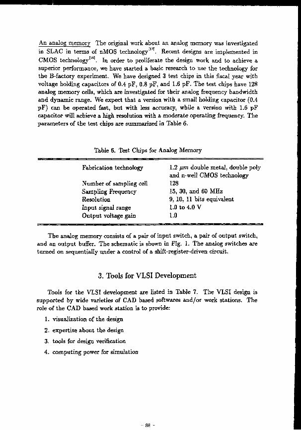
An analog memory The original work about an analog memory was investigated in SLAC in terms of nMOS technology' . Recent designs are implemented in CMOS technology . In order to proliferate the design work and to achieve a superior performance, we have started a basic research to use the technology for the B-factory experiment. We have designed 3 test chips in this fiscal year with voltage holding capacitors of 0.4 pF, 0.8 pF, and 1.6 pF. The test chips have 128 analog memory cells, which are investigated for their analog frequency bandwidth and dynamic range. We expect that a version with a small holding capacitor (0.4 pF) can be operated fast, but with less accuracy, while a version with 1.6 pF capacitor will achieve a high resolution with a moderate operating frequency. The parameters of the test chips are summarized in Table 6.

Table 6. Test Chips for Analog Memory

Fabrication technology 1.2 (im double metal, double poly and n-well CMOS technology

Number of sampling cell 128 Sampling Frequency 15, 30, and 60 MHz Resolution 9, 10, 11 bits equivalent Input signal range 1.0 to 4.0 V Output voltage gain 1.0

The analog memory consists of a pair of input switch, a pair of output switch, and an output buffer. The schematic is shown in Fig. 1. The analog switches are turned on sequentially under a control of a shift-register-driven circuit.

3. Tools for VLSI Development

Tools for the VLSI development are listed in Table 7. The VLSI design is supported by wide varieties of CAD based softwares and/or work stations. The role of the CAD based work station is to provide:

1. visualization of the design

2. expertise about the design 3. tools for design verification

4. computing power for simulation

The SPICE simulation and the mask layout software of CALMA axe very com­mon for the VLSI design. The net list used for the SPICE simulation can be used to verify the mask layout. Special SPICE parameters for a new device will be derived from the study with PISCES-II and/or SUPREM-3. The VHDL code provides a behavior model of a VLSI circuit. A complicated electronics system which consists of a large number of VLSIs can be simulated to determine specifications of VLSIs and to verify interface conditions between VLSIs. A silicon compiler system is an automatic layout generator, where we axe free from a tedious work of mask layout.

Table 7. Tools for VLSI Development

GPSS Simulation with QUEUE VHDL Behavior model of VLSI Verification of digital circuits Quicksim (Mentor Graphics)

Exert/Mads(European Silicon Structures) Digital Circuit Design NETED (Mentor Graphics) for PCB

SOLOl400(ES2) for Silicon compiler LSI design EDSIH(CALMA/VALID)

SX9000(SEIKO) Analog circuit design SPICE(UC,Berkeley) LSI device design PISCES-II(Stanford Univ.) LSI process design SUPREM-3, SUPREM-4 (Stanford Univ.)

4. Summary

A VLSI implementation of front end data acquisition circuits is in progress. The efforts open up new area of detector instrumentation, where highly integrated electronics axe directly mounted on the radiation detectors. In order to meet these high level designs of electronics, computer aided design work stations are brought to help our design efforts.

-89

ACKNOWLEDGEMENTS This work is partially supported by the US-Japan scientific collaboration pro­

gram and a grant-in-aid of Japanese ministry of education, science and culture. Directors of the physics department of KEK are appreciated for their encourage­ment to this work.

REFERENCES 1. S.Inaba, K.Anraku and M.Imori, "Low Power TAC&ADC for Balloon Borne

Experiments", KEK Preprint 89-139, Oct. 1989, IEEE Trans, on Nucl. Sci. NS-37 (1990) 412-416

2. T.Tanimori, H.Ikeda, M.Mori, K.Kihara, H.Kitagawa, and Y.Haren, "Design and Performance of Semi-Custom Analog IC Including Two TACs and Two Current Integrators for Super-KAMIOKANDE", IEEE Trans, on Nucl. Sci. NS-36 (1989) 1679-1684

3. IEEE Std 960-1989,"IEEE Standard FASTBUS Modular High-Speed Data Acquisition and Control System"

4. Y.Watase, and H.Ikeda, "A Simulation of Data Acquisition System for SSC Experiments", KEK Preprint 88-85, Nov 1988

5. IEEE Standard VHDL language Reference manual, IEEE Std 1076-1987, 1988

6. Y.Arai,"VHDL Simulation for the Straw Tube Readout", KEK Preprint 90-121, Oct 1990

7. R.Hance, "The ACP Branchbus and real Time Applications of the ACP Multiprocessor System", IEEE Trans, on Nucl. Sci. NS-34 (1987) 878-883

8. D. B. Gustavson, "IEEE P1595, a Scalable Coherent Interface for Giga-Byte/sec Multiprocessor Applications", IEEE Trans, on Nucl. Sci. NS-36 (1989) 811-812

9. H.Ikeda, M.Ikeda, S.Inaba, and F.Takasaki, "Monolithic Shaper Amplifier for Multi-Anode PMT Readout", Nucl. Instr. and Meth. A292 (1990) 439-444

10. M.Tanaka, H.Ikeda, M.Ikeda and S.Inaba," Development of Monolithic Time-to-Amplitude Converter for High Precision TOF Measurement", submitted to 1990 IEEE Nuclear Science Symposium, Oct 22-27, Arlington Virginia

11. H.Ikeda, M.Ikeda, S.Inaba, F.Takasaki, and M.Tanaka," Readout Electronics of Multi-Anode Photomultiplier Tubes for Scintillation Fiber calorimeter", Submitted to IEEE 1990 Nuclear Science Symposium, Oct 22-27, Arlington, Virginia, to be published in IEEE Trans, on Nucl. Sci.

90

12. H.Ikeda, N.Ujiie, and Y.Akazawa, "Monolithic Preamplifier with Bipolar SST for Silicon Strip Readout", IEEE Trans, on Nucl. Sci. NS-36 (1989) 502-531

13. H.Ikeda, N.Ujiie, K.Kawaguchi, and Y.Akazawa, "Evaluation of Bipolar Amplifier Chipset for Silicon Strip Readout", KEK-Preprint 90-47, June 1990. To be published in nucl. Instr. and Meth.

14. H.Ikeda and N.Ujiie, "Radiation Damage of Bipolar SST Due to Fast Neu­trons", Nucl. Instr. and Meth. A281 (1989) 508-511

15. H.Ikeda and N.Ujiie, "Radiation Damage of Bipolar SST Due to Gamma Ray of C o 6 0 " , Nucl. Instr. and Meth A290 (1990) 462-468

16. Y.Arai and T.Ohsugi, "TMC:A CMOS Time-to-Digital Converter LSI", IEEE Trans, on Nucl. Sci. NS-36 (1989) 528-531

17. J.T.Walker, Soo-Ik, S.Shapiro and R.S.Larsen,"The Stanford Analog Mem­ory Unit", IEEE Trans, on Nucl. Sci. NS-32 (1985) 616 •

18. S.Kleinfelder, "Development of a Switched Capacitor based Multi-channel Transient Waveform Recording Integrated Circuit", IEEE Trans, in Nucl. Sci. NS-35 (1988) 151-154

91

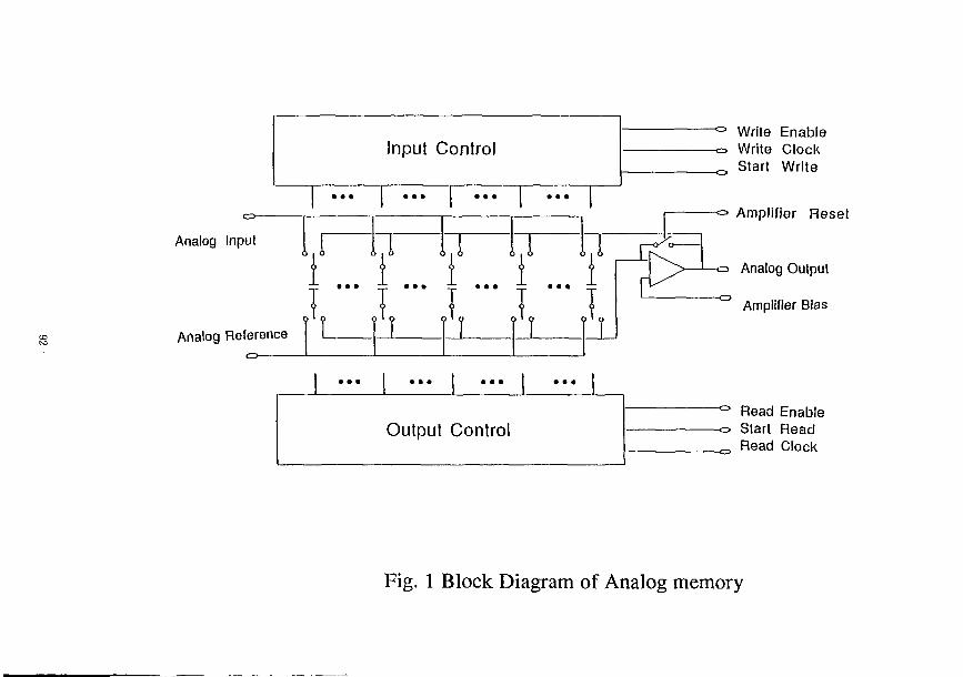
Input Control Input Control Input Control Input Control 0

• • • • • • • • • • • •

Analog Inpul

Analog Reference CD

, i n n n r r ^ i t i 1 1 I I T I T

> ' o O ' o o ' o o ' o o ' I U 1

Write Enable Write Clock Start Write

Amplifier Reset

-CD Analog Output

Amplifier Bias

0 Read Enable <=> Start Read

Read Clock

Fig. 1 Block Diagram of Analog memory

Development of Infrared Camera M. Ueno (National Astronomical Observatory)

(t-5l6PJ©(«ffitt(iSS/v(C|S^S^TI->fcA5. iiJ?JiftKJt^ft:£§©fcilJflJ*©£#:fc§<ttK*ffiSfi1J

SJ»iIia3ttClt^T^J-3TI,>6t)©©"»iR©'l-SS*i!!Mil>iIiE©SaS. SfcSRHHiWCfcHTttffi©* b * u - i / a :/lt.fc*SJ»©*i* 3 * f * ^ - ; L 5 i . mti^^WtX'gm^WittX^immififc'ft

STtfUil 2:£Sft!lJiB©liajEtt*[lI#rlI<£.--C* ofcfc8WCB#«C:foltSI»l£ • WAttlF-ffifc&taftTI.* ft:. %L*a)irn>-7X'ttl 9 8 8*f-«fc'3Hf?»Et*LS 1 PJWKJrOIHfcSftfcsStfHSl-f ^-^-fe>U— ©SSfctMKlfcH-SSSflHWcJKOIU/tTI.'fcaJ. 1 9 9 0*mfflftffllJ&*!fc%««l»lJfefMc'> C &*s •Ctfc. C©#UigSJ;tPtS i ^ 3 5 F*H$S£MS'4*-P*Jnt.>fcfe©-eS}t :i :ft5 1 2 x 5 1 2©-f jf-^-fe >!>--?*&. C<D®lliffili? * F ©fffiMSMC-f > F V :/£•? ?&PNMS&©/<> FI8ia» i&fflli-Cl.i^^fcfetCtfiO^USiBtltWlbTBlT-Wj^AS^ab©©. J/U a > L S I 7a-fe**/nt,»Tli'i! «%?TaJL4ft:«)*C^JiyfMb*s«a-P*»>!fi7-IBl©Kj-ffi • fittffl • WWtt«Cffihri,»<5. S / t lWMC b B#©t> •; =i >iN*tt©i*i*i*siSj&>-£'S j&feiwre&s.

&ae©fcmiBtt®£^:£6=«ff iWf 5cm©£ 'y^> i | l t ' > ; , C ( F / 4 ) fcffll'TtttttttW&fTfc •aT*si). 7^fny?*Mfi©#MSl««!fcW*'i '^ '> 'XIRI&OJIi&ftSMV- 'MIWJft££?7 ft -eft:. 36 tC$f f iC©#¥&£25cn iS&«- ; »-F>J t&.& ( F / 3 . 5 ) Kl«IKl,0-3*»>, £tvfc

flH,»T?s*©»i=iiR©fi:«i«u— ^-fMuctsafsiwiitcwiwt. miimofcftfflsffimfflmtft © i « * # * . - a * 5 .

M3 1 J / O F ' - M - ^ ' ( 7 r - ^ F = » > F T U ' < ; M i ^ * ^ L " 4 ^ © 0 . 4%-CAS. )

- 9 3 -

mi mz

*0l»<ft:«)Kgl2©J:5«:*a;T*Sa*©9M*S«)S-l i-5CtKJ:"7BWi-rs^*tS©*7 •kv hftmrnhmztxttm^itiitiUyX^tLtt. b^bmmmom^mis. • jmoxmm®. • si Mff i f t fc f f5f i«fcf t f t£©Sff iKJ:9f f i»*+5HC>h3 < WWiLisCb&XS&VA,X-btt. bfr L 2^7u*J1-»-fe>^-©§J*(C«J;>3fi!:'M!S©mfFT-3;tt:;&ia)fflT-tSJ;^lC«:0. zo>mm±%fr 6©»H9tteiBH , i -5>'- fX*/hS<1-act*SBIf f i tJa:*J*bft : . £fc. 2 * ; . fcJBSfc J; •)?;(* #><b©fi^-tSSfS4&S:*:*M l"<^*^]B$tC|| i) ir j-r5Ci^Brflgi*oft:fc«). *##>6©7fc£8!:

• ^ fc fc f f l -CSa. fcSKfc - jT^Sf . C©2^.KJ:»3-*J1-«lK»]tcfettS«aiRIFtt2*7C-f^-^•fe>-9—©g«tC«fc9*ISK|fiI±l,3Ebfc.

Munetaka Ueno

94

m%itftftU(»mfttfomm)nmtftiimp E 3. 3.

O E 3.

E 3 . eg

E a.

o H J 1 I I I I I | H 1 1 I I I I I

# « •

c NKQKff

^ y n ^ C C D

( 2^S-b>-9—= il«i*5i«<i5)

?V

I n S b 7 * h SM * - K

(0^7C"fe>-9—= " *T * i t S n W ' - - 7 7 K > ? )

InSb

JlgCdTe.

PtSi

^ -

c ft¥*<Cfc.£«#

(Tm I J MunetakaUeno

- 9 5 -

RSi IR CSD

Solid and

Liquid Nitrogen Dewar

Video Signal

/ideoAMP. Line Driver

Digitizer

Trigger" Signals

CCD Clock

DATA

Clock Pattern Generator STATUS

Telescope

Hard Disk

, Observation Room

Host Computer

t Bus

, Line

X68000

Frame Memories and Interface

Optical Fiber

Optical Fiber

To Sparc Workstation (Image Reduction)

PtSi Infrared Camera System Block Diagram

CCD Clocks to

CSD Dewar

Status Signal from

Interface unit (Optical Fiber) Block diagram of Clock Pa t te rn Generator

96

Video Signal

t Digitizer

High Speed 16 bits Analog-to-digital Convenor 3<

l.U I'll

Parallel to Serial Convenor

Trigger Signals from

Clock Pattern Generator

Data Transmitter

Block diagram of Digitizer unit

To X68000

Multi-bus Frame Memory

(1M Bytes SRAM)

Multi-bus Frame Memory

(1 MBytes SRAM)

Serial Data from

Digitizer (Optical Fiber)

Status Signal to

Clock Pattern Generator

(Optical Fiber)

Block diagram of Frame Memories and Interface uni t

97

5 1 2 X 5 1 2 P t S i mm'M (ft 6 0 K T®jft 5 Hi-Tt,> 6 )

Optical CCD

M. Sekiguchi

(National Astronomical Observatory)

&

S. Okamura

(Univ. of Tokyo)

».

r*

r

(5 8- I

ft

i

o s

fc-

P

1 1

^ ^

to

O - -SA ^Z.

X

0<4

- ^ ^g«< .<£* "v*" -iP" •*!*•

(to

- ^ - ^

j *

^ &

v - j L -

rv %

, * 4& Vr 0 *

o' r «* §

§

V v

o T

•s

99

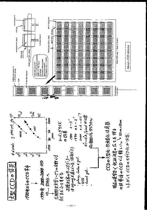
JUaB-i

8

If •8;

1

S i

* < - P

-K

Q

its

I

> * 1

T «

«li tie o *

%±

o & cm i

<X*

6

1 A&. ^ 7 * ' . *"<3

'•* 5S o 5

- ion

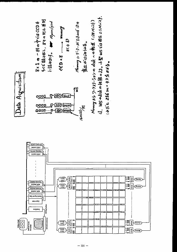
o

4 Q

'is X 5

* o i d

s ^

*2

'<

Qi

~ fit

<

A

ft »

* ^ • ^ s o

1 5 '.. •—* — — \*J f vi

— ampoui JJOUIJH

0 O

x*7 1 1 X K

sic IS

—*—»-

— i — * -m — • — • * -

- ioi

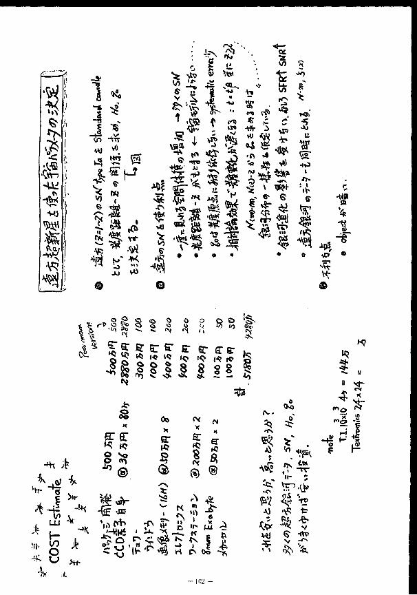
•H)

14^ • ^

. * -« i * 4 ^

to - # *u d

^ i f * ©

** *• * ? **

1?

1

? f t O (ho 3. -"> $

* V!.

8 * •a o 0

ST EC

•II SI

&srS" s" «• ffa- i„ 5 £ £ '* •* « * s IIISII! 1

^ 2

a* x

a: S ® ®

,4

fi ** * H * (J t

JO

i f ;

S -rtr» v -^ ^

"I-l

102 -

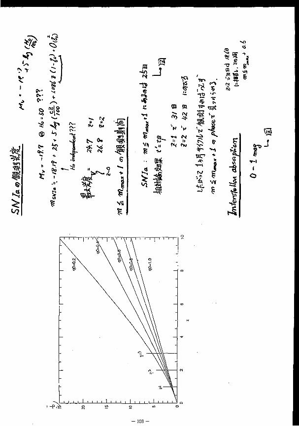
8?

I

•ssn

0"

8

ii

I

&

^ 5 5

^ J

II II •4S" * •

rN» fc» f -*K 5 » 7 5 ^» 0« W « * V! H? vn N «v

6 s

II O c5 * | ^

^

s-

1

•**

en »

II II

CO

5 .**

If V ^ J

I VK

NO

* * ! TO *» g *

(T> K B J-

•4

2 >

i o

J

1 ~P\ffi

- 1 0 3 -

*

2.

o V)

s.

f-*

«

^

^

*

N

x-

v l

I ^ •ft »• v. a

-*» -H ** v -2 ^

4*

tap *P

f

1? cs c

en

l_

« _ ^ *. *

J s \ A)

\t r «s.l ^ i

J$ti

^ 6 I i

ts Oo ^ Vo N <V(

3* -H) t-> •'? -^ <sr n ii

tN r*j

^ , n '£ -Ui O

. < • * , *n i j Jl

M 33 > j '6

^ VI <U \

4 -< - 1 ^

5 " w

^X <*•

•=7 q*

^

s x\

O •A

3

«»

45

s J 5

/V. A

^ ^

I\I

1

a

"> N

t

5 0 D

i >

- KM

_ «tr i it

4 ST C3

o

a?

OQr

1 c •*>

o o 1 CO

<* s: o

3 \ " \ ^^ vb —- -JT co CQ CQ

2 «H| x <"N f L *

o <N i <" L * «s **—'

c L *

II f f Jrvj toy

«sj>

3 | iii

PV-IK-

X

3

2 .2 y

1 us **—* C i 1 3 O

L J

1

f~ '

4 ^ « it»> «C3J1

J 1--»H< o

xh * i

f -•*" 1 *••» 1 r, * w>

i ' - l •hM

* rO

& « 1 *-* —. -H-4> ** V ii ^ u> 2 -e- -*>• r"; » . * f* v_/ "=> ^ l i i

.- 1 "X •~; to

V-I

4<r -i_'C CO ^ ~y

•s v ^ P i± "§£ V *

«%

@?

I 8 3

n

<

O

>N

-He

•(joe

vo trt. . c E V " J .

a > ^ JO Si

P£ c ^

^ ^ " | ft • f t

^

- 1 0 5 -

i

i s.

I •a;

s HJW

•2

£ W r{ t a . o i Q a- 5 . i-i « H U 21

S5 us A> IH -*-,=• o • f t -V Ui '—

2_ J m <• ,> a t H . o -v/i ,\

n ii

f /

->' Ul- **. ca tS

• x

X

I iK

• 2

C3 V* _> •ft Y9l

°T i i «=tf <S ©• s

_ I _ .•a -vis 1 • - -^ J € *?

• < K 3F *J \ •*>>

•"X V l IN

'-K t V* ^

^ S- « V->

» « * : #

4-s <* «J"N

Pi

5 4 &

8! BF LU. ^ »^ *a * v « « •

•5 4 a +-»

•5 4 i_ r

1 * 4 i i a

a rs

s . <u\» 0 @ ©

- 1 0 6 -

SP

I XN-*.

f

«

Hw4

1

a *

-7 W

.. *<

-J

o o H

> i IN Q O O

a

tft<

o

« J <

1

• ^ s J ' IK 6

$ \K

S '•ft iH

E -£-jift- a iw* JK *"• T >

( 'fr "o

Oo r1*

t M »

>•"»

S £

, <

IK

1 i I IK

,1

S <K

Ifij

J4

"3 3 s

(K p? -t.„

try cv».

I * \

*** ^

4 ^ ffiK

G 3 " ,

- 1 0 7 -

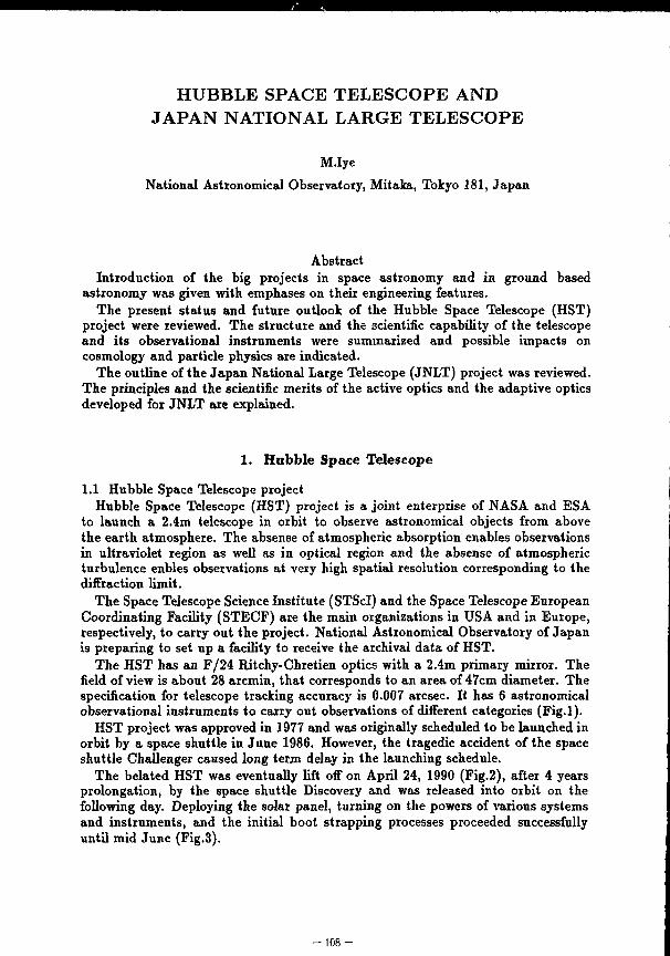
HUBBLE SPACE TELESCOPE AND JAPAN NATIONAL LARGE TELESCOPE

M.Iye

National Astronomical Observatory, Mitaka, Tokyo 181, Japan

Abstract Introduction of the big projects in space astronomy and in ground based

astronomy was given with emphases on their engineering features. The present status and future outlook of the Hubble Space Telescope (HST)

project were reviewed. The structure and the scientific capability of the telescope and its observational instruments were summarized and possible impacts on cosmology and particle physics are indicated.

The outline of the Japan National Large Telescope (JNLT) project was reviewed. The principles and the scientific merits of the active optics and the adaptive optics developed for JNLT are explained.

1. Hubble Space Telescope

1.1 Hubble Space Telescope project Hubble Space Telescope (HST) project is a joint enterprise of NASA and ESA

to launch a 2.4m telescope in orbit to observe astronomical objects from above the earth atmosphere. The absense of atmospheric absorption enables observations in ultraviolet region as well as in optical region and the absense of atmospheric turbulence enbles observations at very high spatial resolution corresponding to the diffraction limit.

The Space Telescope Science Institute (STScI) and the Space Telescope European Coordinating Facility (STECF) are the main organizations in USA and in Europe, respectively, to carry out the project. National Astronomical Observatory of Japan is preparing to set up a facility to receive the archival data of HST.

The HST has an F/24 Ritchy-Chretien optics with a 2.4m primary mirror. The field of view is about 28 arcmin, that corresponds to an area of 47cm diameter. The specification for telescope tracking accuracy is 0.007 arcsec. It has 6 astronomical observational instruments to carry out observations of different categories (Fig.l).

HST project was approved in 1977 and was originally scheduled to be launched in orbit by a space shuttle in June 1986. However, the tragedic accident of the space shuttle Challenger caused long term delay in the launching schedule.

The belated HST was eventually lift off on April 24, 1990 (Fig.2), after 4 years prolongation, by the space shuttle Discovery and was released into orbit on the following day. Deploying the solar panel, turning on the powers of various systems and instruments, and the initial boot strapping processes proceeded successfully until mid June (Fig.3).

- 1 0 8 -

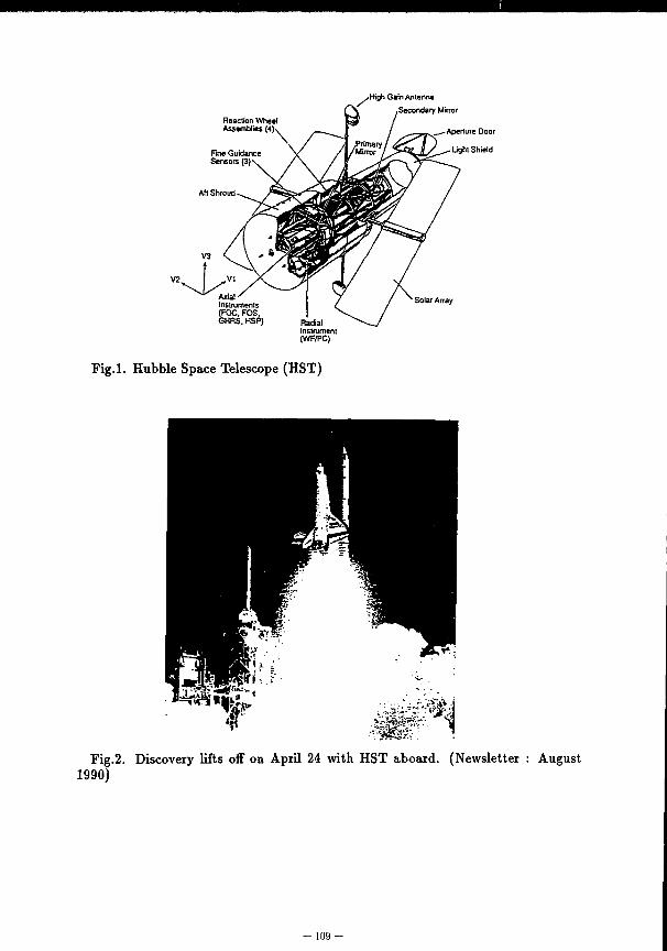
High Gain Antenna

Reaction Wheel Assemblies (A)-

Secondary Mirror

Aperture Door

Light Shield

Solar Array

Fig.l. Hubble Space Telescope (HST)

#m Fig.2. Discovery lifts off on April 24 with HST aboard. (Newsletter : August

1990)

109-

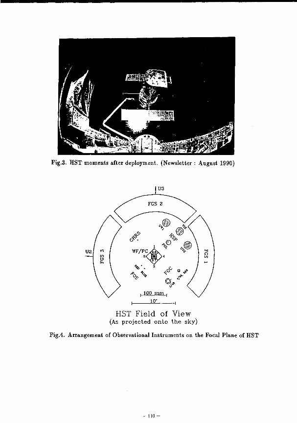
i-ifr-/^ \«&

Fig.3. HST moments after deployment. (Newsletter : August 1990)

HST Field of View (As p ro j ec t ed o n t o the sky)

Fig.4. Arrangement of Observational Instruments on the Focal Plane of HST

- 1 1 0 -

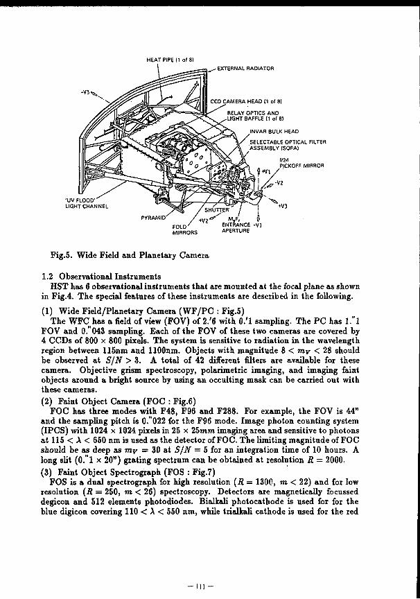
Fig.5. Wide Field and Planetary Camera

1.2 Observational Instruments HST has 6 observational instruments that are mounted at the focal plane as shown

in Fig.4. The special features of these instruments are described in the following. (1) Wide Field/Planetary Camera (WF/PC : Fig.5)

The WFC has a field of view (FOV) of 2.'6 with O.'l sampling. The PC has l."l FOV and 0. 043 sampling. Each of the FOV of these two cameras are covered by 4 CCDs of 800 x 800 pixels. The system is sensitive to radiation in the wavelength region between 115nm and llOOnm. Objects with magnitude 8 < my < 28 should be observed at S/N > 3. A total of 42 different filters are available for these camera. Objective grism spectroscopy, polarimetric imaging, and imaging faint objects around a bright source by using an occulting mask can be carried out with these cameras. (2) Faint Object Camera (FOC : Fig.6)

FOC has three modes with F48, F96 and F288. For example, the FOV is 44" and the sampling pitch is 0."022 for the F96 mode. Image photon counting system (IPCS) with 1024 x 1024 pixels in 25 x 25mm imaging area and sensitive to photons at 115 < A < 650 nm is used as the detector of FOC. The limiting magnitude of FOC should be as deep as my = 30 at S/N = 5 for an integration time of 10 hours. A long slit (O.'l x 20") grating spectrum can be obtained at resolution R = 2000. (3) Faint Object Spectrograph (FOS : Fig.7)

FOS is a dual spectrograph for high resolution (R = 1300, m < 22) and for low resolution (R = 250, m < 26) spectroscopy. Detectors are magnetically focussed degicon and 512 elements photodiodes. Bialkali photocathode is used for for the blue digicon covering 110 < A < 550 nm, while trialkali cathode is used for the red

- i l l -

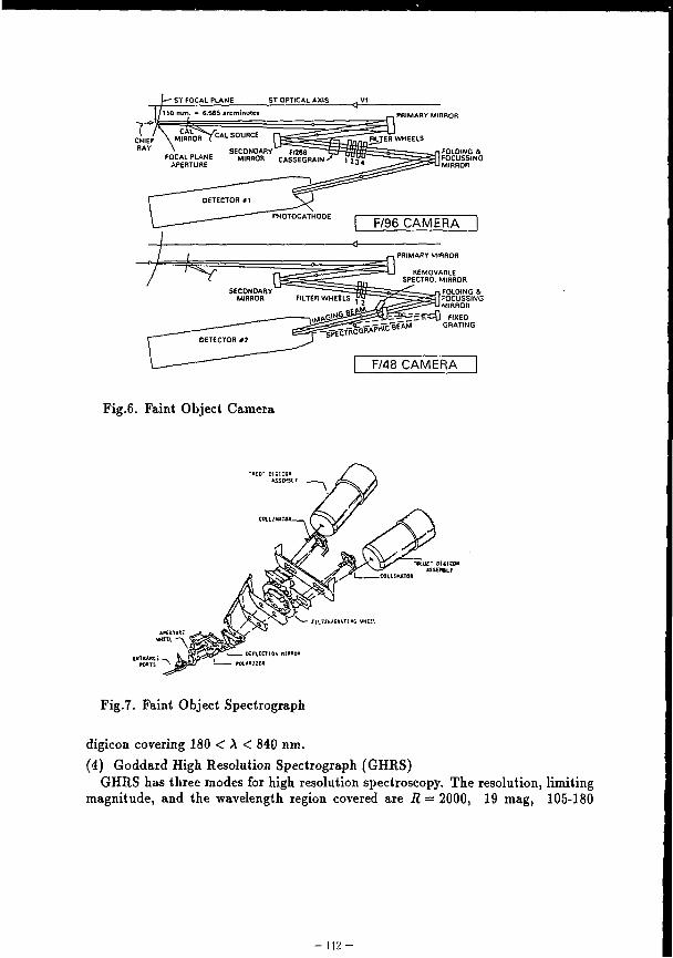
- ST FOCAL PLANE ST OPTICAL AXIS

Fig.6. Faint Object Camera

rH"rit/S«*T|NG WHi!V

. DEFUCTIOfc n!"OR - P«M12f<

Fig.7. Paint Object Spectrograph

digicon covering 180 < A < 840 nm. (4) Goddard High Resolution Spectrograph (GHRS)

GHRS has three modes for high resolution spectroscopy. The resolution, limiting magnitude, and the wavelength region covered are R — 2000, 19 mag, 105-180

- 1 1 2 -

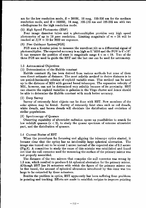
nm for the low resolution mode, R — 20000, 16 mag, 105-320 nm for the medium resolution mode, and R = 100000, 14 mag, 105-173 nm and 166-325 nm with two echellograms for the high resolution mode. (5) High Speed Photometer (HSP)

Four image dissector tubes and a photomultiplier provides very high speed photometry of up to 10 //sec resolution. Limiting magnitude of m = 24 will be reached at S/N = 10 for 2000 sec exposure. (6) Fine Guidance System(FGS)

FGS uses a Koester prism to measure the wavefront tilt as a differential signal of photomultiplier. The expected accuracy is as high as 0.'0016 and the FOV is 4' x 16'. It can measure the position of stars in magnitude range 4 < m < 18. Two of the three FGS are used to guide the HST and the last one can be used for astrometry.

1.3 Astronomical Objectives (1) Determination of the Hubble constant

Hubble constant Ho has been derived from various methods but none of them uses direct estimate of distance. The most reliable method to derive distance is to use period-luminosity relation of cepheid variable stars. This method can be used up to the distance of M31 with ground based telescopes. The expansion velocity of M31, however, can not be determined very reliably because of its proximity. HST can observe the cepheid variables in galaxies in the Virgo cluster and hence should be able to determine the Hubble constant with much better accuracy.

(2) Deep Survey Survey of extremely faint objects can be done with HST. New members of the

solar system may be found. Survey of extremely faint stars such as red dwarfs, white dwarfs, and brown dwarfs will elucidate the distribution and evolution of stellar populations. (3) Spectroscopy of Quasars

Observing capability of ultraviolet radiation opens up possibilities to search for low redshift quasars (z < 2), to study the quasar spectrum of extreme ultraviolet part, and the distribution of quasars.

1.4 Current Status of HST When the procedures for focussing and aligning the telescope optics started, it

became clear that the optics has an intolerably large spherical aberration. The image size turned out to be about 1 arcsec instead of the expected size of 0.1 arcsec (Fig.8). A committee to study the cause of this mistake was established and found out that the null corrector used for measuring the surface of the primary mirror was not properly assembled.

The distance of the two mirrors that comprise the null corrector was wrong by 1.3 mm, which resulted to produce 0.5A spherical aberration for the primary mirror. Although HST has 24 actuators with which the figure of the primary mirror can be fine tuned, the amount of spherical aberration introduced by this error was too large to be corrected by these actuators.

Besides the problem in optics, HST apparently has been suffering from problems in pointing and tracking. Efforts are made to establish recipies to improve pointing

- 1 1 3 -

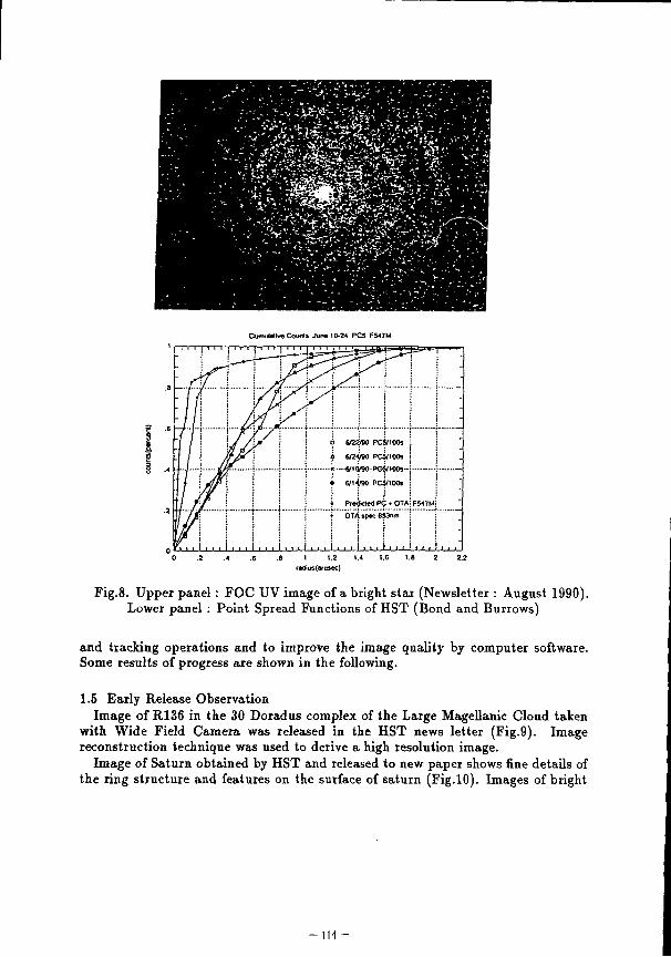
Fig.8. Upper panel : FOC UV image of a bright star (Newsletter : August 1990). Lower panel : Point Spread Functions of HST (Bond and Burrows)

and tracking operations and to improve the image quality by computer software. Some results of progress are shown in the following.

1.5 Early Release Observation Image of R136 in the 30 Doradus complex of the Large Magellanic Cloud taken

with Wide Field Camera was released in the HST news letter (Fig.9). Image reconstruction technique was used to derive a high resolution image.

Image of Saturn obtained by HST and released to new paper shows fine details of the ring structure and features on the surface of saturn (Fig.10). Images of bright

- I l l -

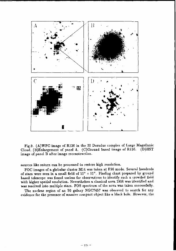
B . < • . • !

"ft*

•

* *wm ft:* s ft:* T

*>• &

D

• f • &.„• * , *• jr.

Fig.9. (A)WFC image of B.136 in the 30 Doradus complex of Large Magellanic Cloud. (B)Enlargement of panel A. (C)Ground based image of R136. (D)HST image of panel B after image reconstruction.

sources like saturn can be processed to restore high resolution. FOC images of a globular cluster M14 was taken at F96 mode. Several hundreds

of stars were seen in a small field of 11" x 11". Finding chart prepared by ground based telescope was found useless for observations to identify such a crowded field with higher spatial resolution. Nevertheless a classical nova 1938 was identified and was resolved into multiple stars. FOS spectrum of the nova was taken successfully.

The nuclear region of an SO galaxy NGC7457 was observed to search for any evidence for the presence of massive compact object like a black hole. However, the

- ur. -

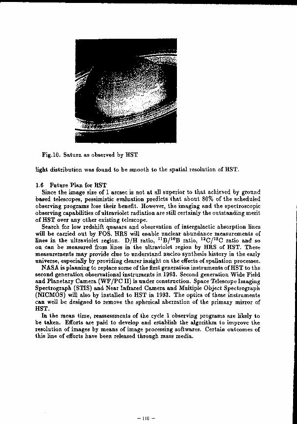
Fig.10. Saturn as observed by HST

light distribution was found to be smooth to the spatial resolution of HST.

1.6 Future Plan for HST Since the image size of 1 arcsec is not at all superior to that achieved by ground

based telescopes, pessimistic evaluation predicts that about 80% of the scheduled observing programs lose their benefit. However, the imaging and the spectroscopic observing capabilities of ultraviolet radiation are still certainly the outstanding merit of HST over any other existing telescope.

Search for low redshift quasars and observation of intergalactic absorption lines will be carried out by FOS. HRS will enable nuclear abundance measurements of lines in the ultraviolet region. D/H ratio, 1 1 B / 1 0 B ratio, 1 2 C / 1 3 C ratio and so on can be measured from lines in the ultraviolet region by HRS of HST. These measurements may provide clue to understand nucleo synthesis history in the early universe, especially by providing clearer insight on the effects of spallation processes.

NASA is planning to replace some of the first generation instruments of HST to the second generation observational instruments in 1993. Second generation Wide Field and Planetary Camera ( W F / P C II) is under construction. Space Telescope Imaging Spectrograph (STIS) and Near Infrared Camera and Multiple Object Spectrograph (NICMOS) will also by installed to HST in 1993. The optics of these instruments can well be designed to remove the spherical aberration of the primary mirror of HST.

In the mean time, reassessments of the cycle 1 observing programs are likely to be taken. Efforts are paid to develop and establish the algorithm to improve the resolution of images by means of image processing softwares. Certain outcomes of this line of efforts have been released through mass media.

- 116 -

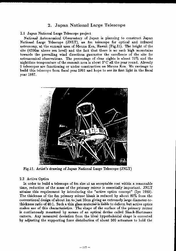
2. Japan National Large Telescope 2.1 Japan National Large Telescope project

National Astronomical Observatory of Japan is planning to construct Japan National Large Telescope (JNLT), an 8m telescope for optical and infrared astronomy, at the summit area of Mauna Kea, Hawaii (Fig.11). The height of the site (4200m above sea level) and the fact that there is no such high mountains towards the prevailing wind directions guarantee the excellence of the site for astronomical observations. The percentage of clear nights is about 70% and the nighttime temperature of the summit area is about 0°C all the year round. Already 9 telescopes are functioning or under construction on Mauna Kea. We envisage to build this telescope from fiscal year 1991 and hope to see its first light in the fiscal year 1987.

F ig . l l . Artist's drawing of Japan National Large Telescope (JNLT)

2.2 Active Optics In order to build a telescope of 8m size at an acceptable cost within a reasonable

time, reduction of the mass of the primary mirror is essentiaUy important. JNLT attains this requirement by introducing the "active optics concept" (lye 1989). The thickness of the 8m primary mirror blank is reduced by about 80% from the conventional design of about lm to just 20cm giving an extremely large diameter-to-thickness ratio of 40:1. Such a thin glass material is liable to deform but active optics makes use of this characteristics. The shape of the surface of the primary mirror is continuously measured by means of an optical devise called Shack-Hartmann camera. Any measured deviation from the ideal hyperboloidal shape is corrected by adjusting the supporting force distribution of about 300 actuators to hold the

- 1 1 7 -

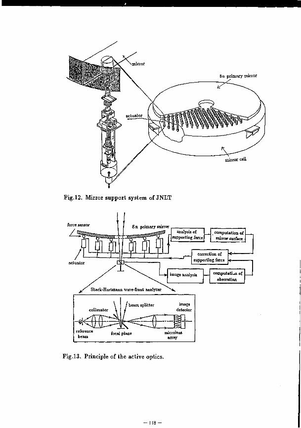
8 m primary mirror

mirror cell

Fig.12. Mirror support system of JNLT

analysii supporting

iis of ng force)

computation of mirror surface

correction of supporting force

image analysis computation of aberration

collimator

-«f reference beam

f beam splitter image detector

^ ^ focal plane mtcrolens

array

Fig.13. Principle of the active optics.

- 1 1 8 -

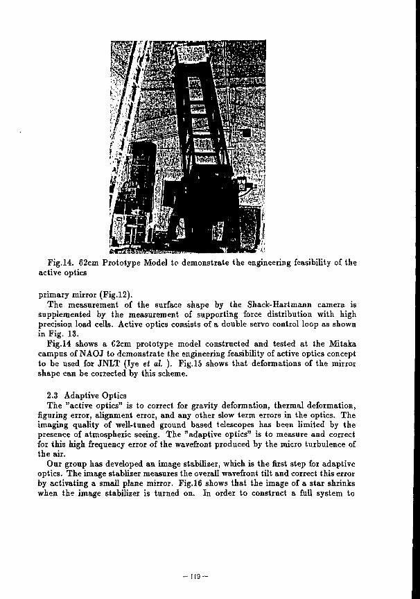
Fig.14. 62cm Prototype Model to demonstrate the engineering feasibility of the active optics

primary mirror (Fig.12). The measurement of the surface shape by the Shack-Hartmann camera is

supplemented by the measurement of supporting force distribution with high precision load cells. Active optics consists of a double servo control loop as shown in Fig. 13.

Fig.14 shows a 62cm prototype model constructed and tested at the Mitaka campus of NAOJ to demonstrate the engineering feasibility of active optics concept to be used for JNLT (lye et al. ). Fig.15 shows that deformations of the mirror shape can be corrected by this scheme.

2.3 Adaptive Optics The "active optics" is to correct for gravity deformation, thermal deformation,

figuring error, alignment error, and any other slow term errors in the optics. The imaging quality of well-tuned ground based telescopes has been limited by the presence of atmospheric seeing. The "adaptive optics" is to measure and correct for this high frequency error of the wavefront produced by the micro turbulence of the air.

Our group has developed an image stabilizer, which is the first step for adaptive optics. The image stablizer measures the overall wavefront tilt and correct this error by activating a small plane mirror. Fig. 16 shows that the image of a star shrinks when the image stabilizer is turned on. In order to construct a full system to

- 1 1 9 -

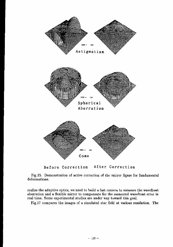
Fig.15. Demonstration of active correction of the mirror figure for fundamental deformations.

realize the adaptive optics, we need to build a fast camera to measure the wavefront aberration and a flexible mirror to compensate for the measured wavefront error in real time. Some experimental studies are under way toward this goal.

Fig.17 compares the images of a simulated star field at various resolution. The

- 1 2 ( 1 -

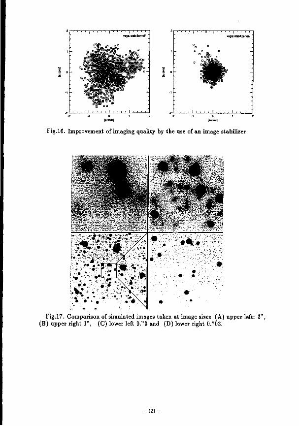
- l — i i i i — r — j — i i i i

vegt stabilizer off

[VCM3

i •

1 1 , 1 1 0 1 1 ' I ' • ' ' vtgtstibi&zcron

_ i — I — I — I I L .

[WT3K]

Fig.16. Improvement of imaging quality by the use of an image stabilizer

Fig.17. Comparison of simulated images taken at image sizes (A) upper left: 3", (B) upper right 1", (C) lower left 0."3 and (D) lower right 0."03.

- 121 -

impact of realizing higher resolution would be seen clearly. Observational astronomy has taken a big step in 1980s by the developments in solid state detectors. There would be further big steps in 1990s and in 2000s by the construction of large telescopes, and by the development of active / adaptive optics. The gain achieved by these developments can be assessed for a simple case where the photon statistics is the dominant source of noise. The gain factors are about 7 for the improvement of quantum efficiency by about factor 50, about 2 for enlargement of telescope aperture from 4m to 8m, and about 30 for improving the image size from 1" to 0.03" by adaptive optics. It should, therefore, be emphasized that the possible impact of the adaptive optics would be very large for astronomy.

References Wide Field and Planetary Camera Instrument Handbook, 1985 Faint Object Camera Instrument Handbook, 1985 Faint Object Spectrograph Instrument Handbook, 1985 STScI Newsletter, Aug., 1990, Vol.7, No.2 Bond,H and Burrows,C, 1990, NASA Bulletin, June 29. Kodaira,K. : 1989, Astrophys. Space Sci., 160, pp.137-144. Iye,M. : 1989, Asirophys. Space Set., 160, pp.149-157. Iye,M., Noguchi,T., Torii,Y., Mikami,Y., Yamashita.Y., Tanaka,W., Tabata,M., and

N.Itoh : 1990, in Advanced Technology Optical Telescopes iv, SPIE Proc, 1236, 929-939.

- 1 2 2 -

MEASUREMENT OF THE NEUTRON CAPTURE RATE OF LIGHT NUCLEI* Y. NAGAI

Department of Applied Physics, Tokyo Institute of Technology, Oh-okayama, Meguro-ku, Tokyo 152

ABSTRACT: Neutron capture rate of Li and C were measured to study

the production rate of intermediate-mass nuclei in primordial nucleosynthesis. The capture rates were obtained by using pulsed neutrons and detecting prompt 7 -rays from the captured states. The results favour the nucleosynthesis of intermediate-mass nuclei in the early universe.

.1. INTRODUCTION Following a phase transition from a quark-gluon plasma to the

hadronic phase both high-density proton-rich and low-density neutron-rich regions could be formed because of the different diffusion lengths of protons and neutrons in the primordial

1 *? plasma • . Consequently, intermodiatc-iiuiss nuclei could be produced sufficiently through a primordial rapid process in low-density neutron-rich regions '. It should be noted here that the standard big bang model predicts an extremely low production of intermediate-mass nuclei .

The main reaction sequence to synthesize the intermediate-mass nuclei is :

1H(n,Y)2H(n,Y)3H(d,n)4He(t,Y)7Li(n,Y)8Li 8Li(a,n) J- 1B(n,Y) 1 2B(e~) 1 2C(n,Y) 1 3C(n, Y) 1 4C etc.

- 123-

7 8 1 ? 1 "}

Thus, the Li(n,y) Li and C(n,y) C reactions are quite important for bridging the instability gap at mass 8 and to produce the intermediate-mass nuclei. 7 8 Moreover, the Li(n,y) Li reaction is important for evaluating the solar neutrino flux from B. This is because the neutrino flux is proportional to the 'Be(p,y) B reaction rate at low energies and the rate has been extrapolated by using the reaction rate measured at higher energies . In order to obtain

7 8 the parameters for the extrapolation the Li(n,y) Li reaction rate plays an important role. On the other hand, the C(n,7)^C reaction rate is also important for the slow process

in metal deficient stars. Because in such stars the competition of the neutron capture between iron and carbon should be considered for the nucleosynthesis of heavy elements.

Though the capture rates for the above two reactions at stellar energy play crucial roles, the values are still only approximately known and thus we have measured the rates at kT=30 keV by detecting the prompt r -rays from the reactions.

2. EXPERIMENTAL PROCEDURE The experiment was carried out by using pulsed neutrons,

produced by the 7Li(p,n)7Be reaction. A 1.5-ns bunched proton beam was provided by the 3.2-MV Pelletron Accelerator of the Research Laboratory for Nuclear Reactors at the Tokyo Institute of Technology. The energy of the proton beam was 1.898 MeV to produce 30 keV neutrons. The neutron energy spectrum was measured using a TOF method with a 6Li-glass scintillation detector and is shown in fig.l. A most probable energy of 30 keV

- 1 2 4 -

was obtained from the spectrum. A 7.6 cm^x 15.2 cm Nal(Tl) detector was used to detect the

7-rays. The detector was surrounded by an annular Nal(Tl) detector with the size of 25.4 cm <t> x 28 cm8. Heavy shield with lead, cadmium and borated paraffin was made to suppress the background events due to the thermal neutrons.

As two-dimensional data of TOF vs pulse height, r-ray events were stored in a minicomputer. The TOF spectrum taken with a Au sample is shown in fig.2 and digital gates were set to obtain the true 7 -ray spectrum as well as the background spectrum.

Samples of metallic Li and carbon disk were used and were positioned on the beam axis. The thickness of the samples were determined to make the correction factor for neutron multiple scattering and self-shielding small.

The Au sample was used to determine the absolute capture cross section of these samples, as the value of the Au has been

q determined accurately .

3. EXPERIMENTAL RESULT 7 o The background r-ray spectra from the Li(n,y) Li and

12 13 C(n,y) c reactions are shown in fig.3 and fig.4,respectively.

In t.licse spectra the 7-rays from the captured states to low-lying states can be seen clearly.

The cross sections were derived individually by using these 7-ray intensities from the captured states as 39.3+6.0 #b and 16.8 + 2.1 ub for the 7Li{n,y)8Li and 1 2 C ( n , 7 ) 1 3 C reactions,respectively. The errors are mostly due to the statistical ones of the 7-ray yields.

-125-

4.DISCUSSION AND CONCLUSION The present value of the capture cross section of the

7 R H(n,r) Li reaction is two-times larger than that recently

12 13 measured and the value of the C(n,y) C reaction is about five-times larger than that estimated from a thermal neutron capture cross section by using the 1/v law. The results favour the nucleosynthesis of intermediate-mass nuclei in inhomogeneous

12 13 big-bang models. The capture cross section of C(n,y) C also affects the discussion concerning the baryon number fluctuation amplitude and the average baryon density during the transition from the quark-gluon plasma to the hadronic phase, as the isotopic

T *3 i n

abundance ratio J-°C/ C relative to solar has been suggested to determine these important quantities, independent of the fraction of the closure density contributed by baryons . As for the calculation of the solar neutrino flux of 8B, the present value agrees with the value, which was used to obtain the parameter set

7 fi 7 8 to fit both capture rates of the Be(p,r) B and Li(n,y) Li reactions. Concerning the problem, however, more detailed studies should be done.

) This work has been carried out in collaboration with M.Igashira, H. Kitazawa, N. Mukai, K. Takeda, F. Uesawa, T. Ohsaki, T. Ando, T. Fukuda and S. Kubono

References: 1) J. Applegate, C. Hogan and R.J. Scherrer, Phys. Rev.

D35(1987)1151

- 126 -

2) N. Terasawa and K. Sato, Prog. Theor. Phys. 81(1989)254 3) J.II. Applegate, C. Hogan and R.J. Scherrer, Ap. J. 329(1988)592 4) T. Kajlno, G.J. Mathews and G.M. Fuller, Ap. J. 364(1990)7 5) A.M. Boesgaard and G. Stelgman, Ann. Rev. Astr. Ap.

23(1985)319 6) R.A. Malaney and W.A. Fowler, Ap. J. 333(1988)14 7) F.C. Barker and R.H. Spear, Ap J. 307(1986)847 8) M. Igashira, H. Kitazawa and N. Yamamuro, Nucl. Instr. Meth.

A245(1988)432 9) R.L. Macklin and H. Gibbons, Phys. Rev. 159(1967)1007

-127-

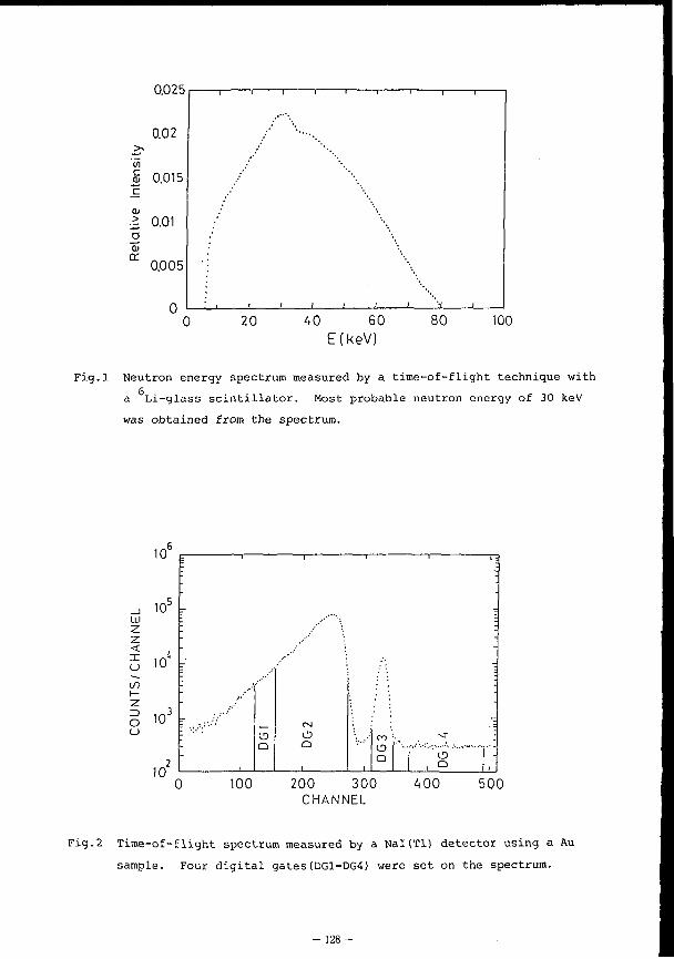
0.025

40 60 E(keV)

Fig.l Neutron energy spectrum measured by a time-of-flight technique with a Li-glass scintillator. Most probable neutron energy of 30 keV was obtained from the spectrum.

id 2 2 < X u Y-2 3 O u

10

1(f .

10

10

I

:

f :

1

190

1

o

1

1

1

1

.1

100 200 300 CHANNEL

A 00 500

Fig.2 Time-of-flight spectrum measured by a Nal(Tl) detector using a Au sample. Four digital gates(DG1-DG4) were set on the spectrum.

- 128-

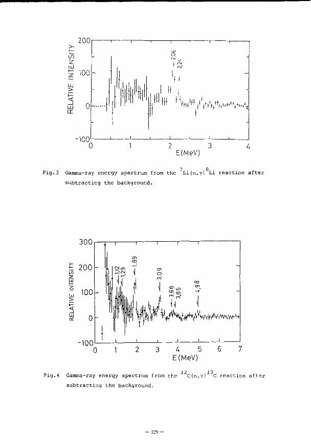
200

2 3 E(MeV)

Fig.3 Gamma-ray energy spectrum from the Li(n,y) Li reac t ion a f t e r sub t rac t ing the background.

UJ

UJ

> i— < UJ

300

200

100

0

-100

O l

o CO en

W|f VS^W^w^t

I L J L

0 1 2 3 4 5 6 7 E(MeV)

12 13 Fig.4 Gamma-ray energy spectrum from the C(n,y) C reaction after subtracting the background.

12!) •

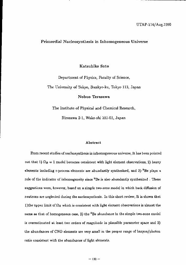
UTAP-114/Aug.l990

Primordial Nucleosynthesis in Inhomogeneous Universe

Katsuhiko Sato

Department of Physics, Faculty of Science,

The University of Tokyo, Bunkyo-ku, Tokyo 113, Japan

Nobuo Terasawa

The Institute of Physical and Chemical Research,

Hirosawa 2-1, Wako-shi 351-01, Japan

Abstract

From recent studies of nucleosynthesis in inhomogeneous universe, It has been pointed

out that 1) Q.B = 1 model becomes consistent with light element observations, 2) heavy

elements including r-process elements are abundantly synthesized, and 3) 9 Be plays a

role of the indicator of inhomogeneity since 9 Be is also abundantly synthesized . These

suggestions were, however, based on a simple two-zone model in which back diffusion of

neutrons are neglected during the nucleosynthesis. In this short review, It is shown that

l)the upper limit of QB which is consistent with light element observations is almost the

same as that of homogeneous case, 2) the 9 Be abundance in the simple two-zone model

is overestimated at least two orders of magnitude in plausible parameter space and 3)

the abundances of CNO elements are very small in the proper range of baryon/photon

ratio consistent with the abundances of light elements.

- 1 3 0 -

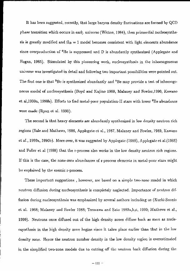
It has been suggested, recently, that large baryon density fluctuations are formed by QCD

phase transition which occurs in earl} universe (Witten, 1984), then primordial nucleosynthe­

sis is greatly modified and Q,B = 1 model becomes consistent with light elements abundance

since overproduction of 4 He is suppressed and D is abundantly synthesized (Applegate and

Hogan, 1985). Stimulated by this pioneering work, nucleosynthesis in the inhomogeneous

universe was investigated in detail and following two important possibilities were pointed out.

The first one is that 9 B e is synthesized abundantly and 9 Be may provide a test of inhomoge­

neous model of nucleosynthesis (Boyd and Kajino 1989, Malaney and Fowler,1990, Kawano

et al,1990a, 1990b). Efforts to find metal-poor population-II stars with lower 9 B e abundance

were made (Ryan et al. 1990).

The second is that heavy elements are abundantly synthesized in low density neutron rich

regions (Sale and Mathews, 1986, Applegate et al., 1987, Malaney and Fowler, 1989, Kawano

et al., 1990a, 1990b). More over, it was suggested by Applegate (1988), Applegate et al.(19SS)

and Fuller et al (1988) that the r-process also works in the low density neutron rich regions.

If this is the case, the none-zero abundances of r-process elements in metal-poor stars might

be explained by the cosmic r-process.

These important suggestions , however, are based on a simple two-zone model in which

neutron diffusion during nucleosynthesis is completely neglected. Importance of neutron dif­

fusion during nucleosynthesis was emphasized by several authors including us (Kurki-Suonio

et al. 1988; Malaney and Fowler 1988; Terasawa and Sato 1989a,b,c, 1990; Mathews et al.,

1990). Neutrons once diffused out of the high density zones diffuse back as soon as nucle­

osynthesis in the high density zone begins since it takes place earlier than that in the low

density zone. Hence the neutron number density in the low density region is overestimated

in the simplified two-zone models due to cutting off the neutron back diffusion during the

- 131 -

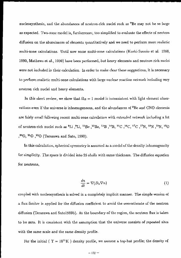
nucleosynthesis, and the abundances of neutron-rich nuclei such as 9 Be may not be so large

as expected. Two-zone model is, furthermore, too simplified to evaluate the effects of neutron

diffusion on the abundances of elements quantitatively and we need to perform more realistic

multi-zone calculations. Until now some multi-zone calculations (Kurki-Suonio et al. 1988,

1990, Mathews et al., 1990) have been performed, but heavy elements and neutron rich nuclei

were not included in their calculation. In order to make clear these suggestions, it is necessary

to perform realistic multi-zone calculations with large nuclear reaction network including very

neutron rich nuclei and heavy elements.

In this short review, we show that HB = 1 model is inconsistent with light element obser­

vations even if the universe is inhomogeneous, and the abundances of 9 Be and CNO elements

are fairly small following recent multi-zone calculation with extended network including a lot

of neutron-rich nuclei such as 8 Li , 9Li, u B e , 1 2 Be, 1 3 B , 1 4 B , 1 5 C , 1 6 C , 1 7 C , 1 7 N , , 8 N , 1 9 N, 1 9 0

, 2 0 O , 2 1 0 , 2 2 0 (Terasawa and Sato, 1990).

In this calculation, spherical symmetry is assumed as a model of the density inhomogeneity

for simplicity. The space is divided into 25 shells with same thickness. The diifusion equation

for neutrons,

"i = V(^Vn) (1)

coupled with nucleosynthesis is solved in a completely implicit manner. The simple version of

a flux-limiter is applied for the diffusion coefficient to avoid the overestimate of the neutron

diffusion (Terasawa and Satol989b). At the boundary of the region, the neutron flux is taken

to be zero. It is consistent with the assumption that the universe consists of repeated sites

with the same scale and the same density profile.

For the initial ( T = 1 0 n K ) density profile, we assume a top-hat profile; the density of

- 1 3 2 -

inner shells is R times higher than that of surrounding low-density shells. The parameter /„

refers to the volume fraction of the initial high-density shells in the whole region. Another

parameter d(T = lMeV) refers to the radius of the site in problem normalized by the size at

T= lMeV. We calculated in the ranges 10 5cm < d(T = lMeV) < 10 8cm, 1 < R < 1000, , 0 <

A < 0.5, and 4 x 10-w(ft = 0.014A"2 = 0.056Ajo

2) < ??o < 7 x 10~ 9(fi = 0 .25/r 2 = 1.0/tJo

2).

Reaction rates are updated according to Caughlan and Fowler (1988), Thielemann and

Wiescher (1990), and those relating to 9 Be are added and updated by the table given in

Malaney and Fowler (1990). The lifetime of neutrons is taken to be 887.6 sec (Mampe et al.

1989) and the number of neutrino species is 3.

Figure 1 displayt the time evolution of the local mass fractions of neutron in each shell

and the evolution of the ratio of local baryon density to the mean density for d(T = lMeV) =

10 5cm, R = 1000,/„ = 0.11, and rj0 = 4 x 1 0 - 1 ° . Neutrons begin to diffuse out of the inner

high-density shells into the surrounding space and spread over the low-density zone around

t = O.lsec. Since the density contrast among the high density shells and the low density shells

is very large in this case, the neutron fraction becomes completely dominant in the low density

shells and the baryon density in the outer low-density shells grows simultaneously. Thus the

ratio of the baryon density in the innermost shell to that in the outermost shell, which is 1,000

at first, finally reduces to 107. However, neutrons begin to diffuse back into the inner high-

density shells to keep the neutron density distribution uniform when nucleosynthesis starts

and the neutron density decreases in the high-density shells. It results in the decrease of

baryon density of the outer low-density shells. Due to this effect, the baryon density contrast,

which once reduces to 38 at t ~ lOOsec, increases again to ~ 100. This example clearly

shows that we cannot neglect the neutron diffusion, especially the back diffusion out of the

low-density region into the high-density region, during nucleosynthesis.

- 1 3 3 -

In Fig. 2, the average abundance of 7 Li/H, is shown on R — d plane for various values

of 7/0. As seen from this figure, models with rj0 > 5.6 x 10~ , o(ftB = 0.078Ag"0

2) is ruled out,

since there exist no regions which satisfy the observational limit 7 Li /H < 1 0 - 9 ' 6 (see the

review of Pagel in this volume). We searched regions where the constraint 7 Li /H < 1CT9 , 6 is

satisfied in very wide range parameter space d, Rand /„ , but no regions could not be found

for fig > 0.06k^Q. This conclusion is essentially consistent with Kurki-Suonio et al. (1990

),Terasawa and Sato (1989c) and Mathews et al. (1990).

9 Be is produced in the outer shells as shown in Figure 3 (d(T = lMeV) = 10 7cm, R =

1000, /„ = 0.11, and T/0 = 4 x 10 - 1 ° ) . In the high-density shells, 9 B e once produced is burnt

into heavier elements and its abundance turns out to be very small. The dependence of the

9 B e abundance on the scale of fluctuations is shown in Figure 4 as contour on the d — R

plane for j v — 0.11. The 9 Be abundance increases with increasing R and take the maximum

value around rf(T = lMeV) = 10 7cm. Though the /„ dependence of the 9 B e abundance is

different with i?, the 9 Be abundances takes the maximum value at /„ ~ 0.1 for large R. In the

calculated ranges of parameters, the highest value of the 9 B e abundance is 9 B e / H = 4 x 1 0 - 1 5

(d(T = lMeV) = 10 7cm, J? = 1000, /„ = 0.11) for i) 0 = 4 x 1 0 " 1 0 and 9 B e / H = 3 x lO" 1 5

(<i(T= lMeV) = 10 6 S cm,7? = 1000,/,, = 0.11) for TJ0 = 7 x 10~ 9. These values are two

orders smaller than those calculated in the simplified two-zone model. The reason for the

discrepancy between these results is the overestimate of the neutron diffusion in the latter

model. To confirm this point, we cut off neutron diffusion artificially when the neutron density

distribution became almost uniform and calculated the abundances of elements in the case of

rf(T = lMeV) = 10 s- 5cm, R = 1000, /„ = 0.11, and TJ0 = 4 x lO" 1 0 . The 9 B e abundance in

this case is 9 B e / H = 1.0 X 1 0 - 1 3 , which is as large as that obtained in the simplified two-zone

model and higher by orders of magnitude than that in the case that neutron diffusion is not

- 1 3 4 -

cut off with the same parameters; 9 Be/H = 8.3 X 10" 1 8 .

The recent observations of several population-II stars have placed the upper limit on the

primordial 9 Be abundance to log 9 Be /H = —13.7 (Ryan et al. 1990), which is two orders of

magnitude greater than the predicted abundance in the present work.

The constraints on the parameters from other light elements, D, 3 He, 4 He, and 7Li are

more stringent than those placed by the 9 B e abundance. The abundances of these elements, of

course, depend on the scale of density fluctuations and they reduce to the uniform abundances

in the limit of small scale. However, in the range of the fluctuation scale so long that the 9 Be

abundance is larger than the uniform abundance; <f(T = lMeV)>10 6 cm, the 7 Li abundance

increases monotonically with R and R is constrained to R<10 even when the very loose

bound on the primordial abundance of the 7 Li abundance; 7 Li /H < 1 x 1 0 - 9 , is taken. The

constraints placed by the upper bound on the sum of the D abundance and the 3 H e abundance

are also stringent: R should be smaller than ~ 50 in the range, d(T = lMeV)>10 6 cm. Hence,

the constraints from the light elements except for 9 Be, that is, D, 3 He, 4 He, and 7Li are still

more stringent and powerful to examine the inhomogeneous models of nucleosynthesis in the

present stage.

The total abundance of heavy elements (A > 7) is at most ~ 1 0 - 1 3 by mass fraction for

TJO = 4 x 10- 1 0 (f t = 0.014ft-2 = 0.056/i^o

2) and ~ lO" 1 1 for rj0 = 7 x 10~9(ft = 0.25/r 2 =

l.Oh^Q) which is dominated by n B and CNO elements produced in the inner high density

shells (Fig. 5). The abundances of CNO elements in the low-density neutron-rich shells are

at most X ( 1 2 C ) ~ 10~ 1 4 , J f ( M N ) ~ 10" 2 0 , and A ' ( 1 6 0) <C l O " 2 0 for i,„ = 4 x 10" 1 0 . For

ri0 = 7x 1 0 - 9 , X(12C) ~ 10" 1 1 , X(14N) ~ lO" 1 6 , and X(160) ~ l O " 1 7 . Thus the abundances

of CNO elements in the proper range of baryon/photon ratio, which is consistent with the

abundances of light elements, are too small to be the seeds of cosmological r-process. For the

- 1 3 5 -

large value of baryon/photon ratio as to close the universe only by baryons, the abundances

of these elements are significantly large. However, the fact that such high baryon density

models are inconsistent with the abundances of light elements should not be ignored.

This work was supported in part by the Grant-in-Aid for Scientific Research Fund from

the Ministry of Education, Science and Culture No. 01540308.

- 1 3 6 -

Cap t ions

Figure 1

Time evolution of the local mass fraction of neutron (top) and the time evolution of the

local baryon density(bottom) in the case that d(T = lMeV) = 10 5cm, 7? = 1000, /„ = 0.11,

and 770 = 4 x 10~ 1 0 . The local baryon density is denoted by the ratio to the average density.

Figure 2

The average abundance of 7 Li is shown on R — d plane for various values of 770, but for

/v = 0.11

Figure 3

The time evolution of the local 9 Be abundance (mass fraction) for d(T = lMeV) =

1 0 7 c m , i ? = 1000,/„ = 0.11, and 7/0 = 4 x lO" 1 0 .

Figure 4

The contour of the average abundances of 9 Be on the d — R plane for r/0 = 4 x 10 _ 1 0 ( top)

and 770 = 7 X 10 _ 9 (bot tom). Contour levels are log( 9Be/H).

Figure 5

The contour of the average abundances of heavy elements (A > 7) on the d — R plane for

?7o = 4 x 10 _ 1 °(top) and 770 = 7 X 10 -9(botf0111). Contour levels are \og(X{A{> 7)/M).

- 137 -

— ^ — — — w ^ — — — — — I — —

Reference

Applegate, J. H., Hogan, C. J., 1985, Phys. Rev., D31, 3037.

Applegate, J. H., Hogan, C. J., and Scherrer, R. J., 1988, Ap. J., 329, 572.

Applegate, J. H., 1988, Phys. Rep., 163, 141.

Boyd, R. N. and Kajino, T. 1989, Ap. J.(Letters), 336, L55.

Fuller, G. M., Mathews, G. J. and Alcock, C. R.,1988, Phys. Rev., D37, 1380.

Kawano, L. H. , Fowler, W. A. and Malaney, R. A. and, 1990, Ap. J., to be published.

Kawano. L. H., Fowler, W. A. , Kavanagh, R. W. and Malaney, R. A. 1990, Ap. J., to be

published.

Kurki-Suonio, H., Matzner, R. A., Centrella, J. M., Rothman, T. and Wilson, J. R., 1988,

Phys. Rev. D, 38, 1091.

Kurki-Suonio, H. and Matzner, R. A., 1989, Phys. Rev. D, 39, 1046.

Kurki-Suonio, H., Matzner, Olive, K. A. and Schramm, D. N., 1990, Ap. J., 353, 406.

Malaney, R. A. and Fowler, W. A. , 1.988, Ap. J., 333, 14.

Malaney, R. A. and Fowler, W. A. , 1990, Ap. J., to be published.

Mampe, W., Ageron, P., Bates, C , Pendlebury, J. M. and Steyerl, A., 1989, Phys. Rev.

Lett, 63, 593.

Mathews, G. J., Meyer, B. S.,Alcock, C. R. and Fuller, G. M.,1990, Ap. J., 358, 36.

- 1 3 8 -

Ryan, S. G., Bessell, M. S., Sutherland, R. S., Norris, J. E., 1990, Ap. J. {Letters), 348,

L57.

Sale, K. E. and Mathews,1986, Ap. J., 309, LI.

Terasawa, N. and Sato, K., 1989a, Prog. Theor. Phys. 81,254.

Terasawa, N. and Sato, K., 1989b, Phys. Rev. D, 39, 2893.

Terasawa, N. and Sato, K., 1989c, Prog. Theor. Phys. (Letters) 81,1085.

Terasawa, N. and Sato, K., 1990, Ap. J. Letters, to be published.

Thielemann, F. K. and Wiescher, M. Proceedings of Primordial Nucleosynthesis Symposium,

Chapel Hill, Noth Carolina, 1989 to be published.

Witten, E., 1984, Phys. Rev. D, 30, 272.

- 1 3 9 -

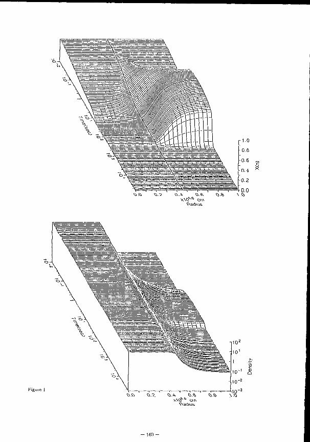
•yAO V Q TO

Figuie i

- l i t ) -

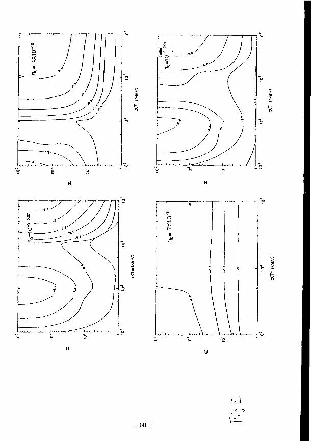
M s i

- ->.»

-' / y O T\ ~

-

O T\ ~

-

•

-. O 1

-

. • • • • , : — i •

/ -

V 1 • m

7X10

'

-

II «? 1

- 1

1 ' -

*1

\ 1 1 I \ .

141 -

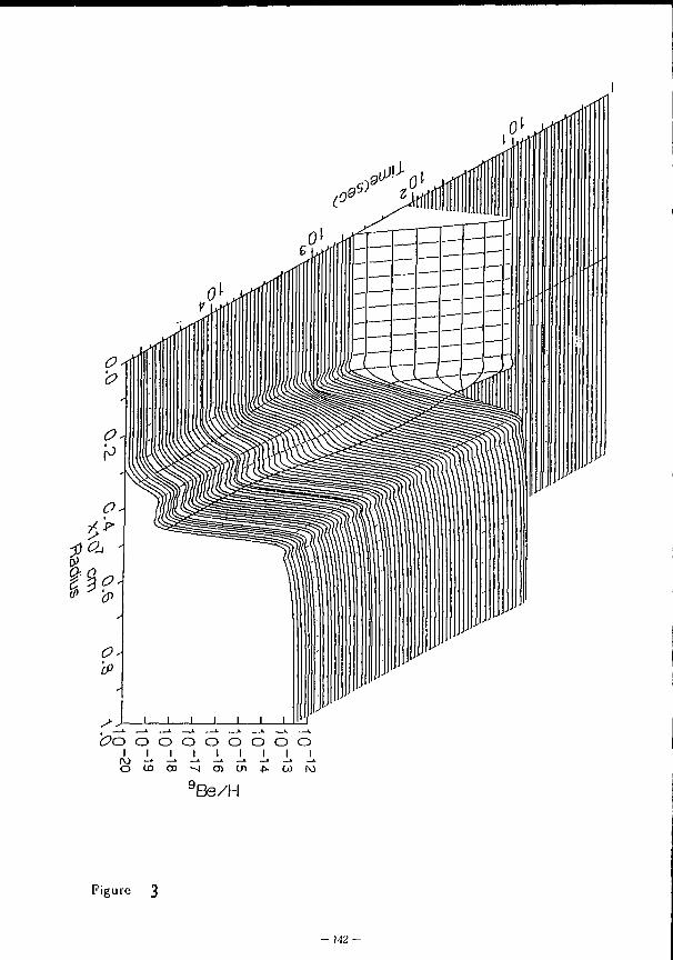
Oo o o o o o o o o I I I I I i I I I

f V ) - » - ' - ' - » - ' - * - » - « . o i o o i s o i o i j i u i y

9 Bs/H

Figure 3

- 142 •

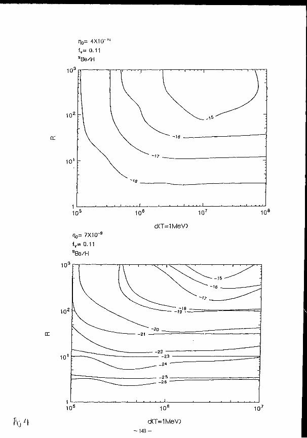
h l\

Ho= 4X10" I U

f v= 0.11 98e/H

10<

10 2 _

0C

10'

J ' • I i • i • • i • ,. | • i . . . . .

• \ - \ -

. ^^.^ -\ \ •

' \ \ -

; \ ^ *"• ~t? _ ; \ ^ *"• ~t? _

" : \ . .

'« •

•

i , i . .

10 s

H0= 7X10"9

f v = 0.11 9Be/H

10 ;

10'

DC

10"

10°

10 6 107

d<T=1MeV)

10°

I ' ] \' ' ' V \ \ >—s , - I I \ \ ^ \ ^ - - 1 5 — -

\ V \ \ . ~'6 ^ \ v \ ^ - » ? - ~ ~ - ~ ^ ^

k \ ^ ^ ~ ~ ~ — - I B _ _ k \ ^ • 19 —

N. " - 2 ) _ •-

- J ^ ^ - 2 2 • ' "

^ \ ^ ^ ^ \ ^ ^ _—• ~z* " -1 25 ,.

• ~ - - - - - ^ _ . - i b —

. . . 1 . . . i . . . .

. - i b —

. . . 1 . . . i . . . .

10"

d(T=1MeV) — 143 —

10'

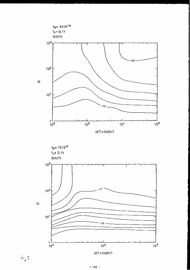
n0= 4xio-t v = 0.11 XCA>7)

a:

d(T=1MeV)

) • < • r

T)o=7X10-f v= 0.11 X(A>7)

10'

10*

cc

10'

10 s

• I ' , , , . , . , , . t .

. 1

. ...

J J — -^ ~~"\ -J J -

. • . •

-—

. •

— j ^ - * * * * ^ ^ — ~ ~

•

j ^ - * * * * ^ ^ — ~ ~ — - I 5 > .

j ^ - * * * * ^ ^ — ~ ~

1 . . . . 1 1 1 1 1 1 1

10 6

d(T=1MeV>

10'

- 1 4 4 -

NATURE OF THE QCD PHASE TRANSITION AT FINITE TEMPERATURES

M. Fukugita Yukawa Institute for Theoretical Physics, Kyoto University Kyoto 606, Japan

1. SU(3) pure gauge theory: first order. A first-order transition had been suggested by an analytical argument, and early

lattice simulations (1982-1988) showed that this is true. In 1988 an Italian collabo­ration (the APE group) then claimed that the transition is rather second order (see [1] for the status at that time). With a powerful technique of finite-size scaling, however, this possibility was excluded; it was also shown that the claim of the APE group was based on their misinterpretation (partly due to a bias in their simulation) of the phenomena that they observed (see ref.[2] for a review). 2. QCD with four light flavours: first order.

Analytic argument based on an effective theory (sigma model) predicts that it is first order. Early simulations also supported this[3]. More recently a finite-size scaling analysis with lattices varying from 4 4 to 12 3 x 4 confirmed a strong first-order transition[4]. Whether this survives a continuum limit (which is our world) is yet to be studied, however. 2. QCD with two light flavours: no phase transition.

This is close to our world, since a strange quark is much heavier than is to play a role for chiral symmetry. Analytic argument from a sigma model does not tell anything about the order. Earlier simulations indicated that the transition is first order[3]. Recent simulations cast doubt, however, on this point. When one increases the spatial extent of the lattice (towards thermodynamic limit) no signature was found that indicates a first-order transition[4,5]. A more decisive test is again finite size scaling; the combined use of the most recent Columbia result on 16 3 x 4 [5] with the Japanese calculation (6 — 12 3 x 4)[4] clearly excludes the possibility of a first-order transition (it cannot be of second order either by a general argument). It was also demonstrated that the earlier "evidence" for a first-order transition was misleading, a result of short runs on a small lattice; large fluctuations, which are probably related to the same collective effect which causes the discontinuous chiral transition in a large flavour number case, was misidentified with a two-state metastability signal which is taken to be evidence for a first-order transition[4j.

- M 5 -

It was also shown that the introduction of the strange quark with a mass > 50MeV indeed does not change the situation[5]. It should be noted that we expect a yet weaker transition in the continuum limit.

In conclusion the standard model of nucleosynthesis in the early Universe, which neglects the effect of small-scale inhomogeneities, does not need modification for effects of QCD-induced bubbles. We have no reason any more to expect quark-nugget like remnants from the QCD transition epoch either. The QCD transition is smooth and does not affect at all our understanding of the early Universe. See Ref.[7] for a short summary. The interested reader may be referred to the reviews Ref.[3 (1987); 1(1988); 2(1989); 6(1990)] for stories at the relevant time.

The final remark is that all of these statements are for a very high entropy environment, as in the early Universe, and do not apply to a transition in a cold high-density environment. Realistic calculations for this type of matter are not yet possible.

References 1. M. Fukugita, Proc. Lattice 88, Nucl. Phys. B (Proc. Suppl.) 9, 291 (1989) —

— review talk. 2. A. Ukawa, Proc. Lattice 89, Nucl. Phys. B (Proc. Suppl.) 17, 118 (1990) —

— review talk. 3. M. Fukugita, Proc. Lattice 87, Nucl. Phys. B (Proc. Suppl.) 4, 105 (1988) —

— review talk. 4. M. Fukugita, H. Mino, M. Okawa k A. Ukawa, Phys. Rev. Lett. 65, 816 (1990);

Phys. Rev. D42, 2936 (1990). 5. A. Vaccarino, Proc. Lattice 90, Nucl. Phys. B (Proc. Suppl.) 20, 263 (1991). 6. S. Gottlieb, Proc. Lattice 90, Nucl. Phys. B (Proc. Suppl.) 20, 247 (1991) —

— review talk. 7. M. Fukugita & C. J. Hogan, Nature 354, 17 (1991).

- 1 4 6 -

Paradigm Lost ? — Role of Theoretical Prejudices in Cosmology —

YASUSHI S U T O

Uji Research Center, Yuicawa Institute for Theoretical Physics Kyoto University, Uji 611, Japan

Here we may reign secure, and in my choice To reign is worth ambition, though in Hell: Better to reign in Hell, than serve in Heaven.

— J.Milton ; Paradise Lost -

A b s t r a c t

During the last decade, several wild ideas in particle physics have inspired theoretical studies in astrophysics and cosmology, which resulted in the new field, particle - astro­physics. Quite recently, however, new observational data have been revealing the surprising image of our universe; taken at the face value, they are not only embarrassing the theorists but may require a new paradigm in cosmology.

1. Introduct ion

The title of this workshop "Elementary-Particle Picture of the Universe" reflects the

rapid progress in cosmology, especially in 1980's when the various concepts in particle

physics proved to be powerful in exploring the physical conditions of the early universe.

In particular, the idea of the exponential expansion in the very early epoch, suggested

independently by A. Guth (1981) and by K. Sato (1981), inspired the subsequent progress

in theoretical cosmology. The idea, coined inflationary universe scenario by Guth (1981),

becomes one of the central dogmas or paradigms in the present cosmology.

Along with such ambitious attempts to understand the early universe, observational

data to characterize the structure of the universe have been accumulated in the last decade,

which include the CfA redshift surveys (Huchra et al. 1082; de Lapparent et al. 1986,

1988; Geller and Huchra 1989), the peculiar velocity field of galaxies (Dressier et al. 1987;

Burstein, Faber, and Dressier 1990; Dressier and Faber 1990a,b), the number counts of

faint galaxies (Tyson 1988), and the IRAS galaxy surveys (Efstathjou et al. 1990; Saunders

et al. 1991). Such unexpected and exciting observational results continuously challenge

the theoretical scenarios which are often too idealized and simplistic. Great Wall (Geller

- 1 4 7 -

and Huchra 1989) and Great Attractor (Dressier et al. 1987) were already sufficient to

embarrass the simple-minded theorists in cosmology, and the apparent periodicity in the

galaxy distribution (Broadhurst et al. 1990), if confirmed, would be a disaster for our

conventional picture of the evolution of the universe. Is the present-day cosmology in a

stage of paradigm lost ?

Before throwing away the present paradigm, mainly inspired by inflationary scenario,

it is instructive to briefly review the cherished belief of some theorists in cosmology.

2. Fundamental Parameters in Cosmology

There are a number of parameters to quantitatively describe our universe. Among

others, the following four quantities seem to me the most basic ingredients for our universe

to first order approximation,

(i) the expansion rate of the universe, or, the Hubble parameter :

1 da(t) F W = ^ )^T' ( 1 )

where a(t) is the cosmic scale factor,

(ii) the mean mass density of the universe />(t), or equivalently, the density parameter :

(iii) cosmological constant A, or equivalently,

3H(t)2 m = -ttv- (3)

(iv) the power spectrum P(k,t) = (\Sk\2) of cosmological density fluctuations, where k is

the comoving wavenumber.

Unfortunately we could observe at best the present values of the above quantities, i.e.,

Ho, fio> o> and Po(fc), respectively. Since there is no particular reason why we should

live in the cosmic age of t = to, it would impossible in general to theoretically predict the

values at t = to of such time-dependent quantities. Depressingly, it is also quite difficult

for cosmological observations to determine them to the desired accuracy. Therefore one

needs a kind of working hypothesis in order to go further, even if it is based on specific

theoretical prejudices.

- 1 4 8 -

3 . Theoret ical Prejudices

Progress of particle physics has been frequently guided by some aesthetic points of view. In fact, this methodology turned out to be amazingly successful in particle physics. Since this workshop is entitled "Elementary-Particle Picture of the Universe", it is reasonable to ask if the analogous reasoning works in cosmology.

Prejudice #1. Harrison-Zel'dovich spectrum

The density fluctuations which are responsible for the variety of cosmic structures are supposed to originate from the quantum fluctuations in the very early universe. Since we have no particular reason to introduce the characteristic scale in the fluctuation spectrum relevant to the astronomical consideration, it is conventionally assumed that the primordial spectrum Pj(fc) takes a single power-law form :

Pi(k) = Aikn. (4)

Still one has a freedom to choose the spectral index n, but n = 1 is commonly used (Ai is not regarded as a parameter in this context, since the amplitude of power-spectrum grows independently of k in linear regime. It will be normalized at the present epoch by means of the galaxy correlation function etc., with some reservation though). Harrison (1970) pointed out that eq.(4) with n = 1 provides the appropriate initial condition for the successful galaxy formation. Later, Zel'dovich (1972) considered the thermalization of the universe due to the gravitational bound objects in a non-standard model (cold universe scenario). He concluded that with n = 1, it is possible to produce the cosmic microwave background radiation. For these reasons, n = 1 spectrum is called the Harrison-Zel'dovich spectrum. It is remarkable that a decade later the inflationary model predicts the same spectrum with n = 1 from the first principle (for a review, see Blau and Guth 1987). In fact, this prejudice # 1 has been frequently employed in the subsequent studies of the formation of galaxy and large-scale structure (Davis efc aJ. 1985; Suto and Suginohara 1991; Suginohara and Suto 1991; but see also, Kofman and Linde 1987; Ostriker and Suto 1990; Suto, Gouda and Sugiyama 1990; Yokoyama and Suto 1991).

Prejudice #2. A = 0

The cosmological constant A has been regarded as a redundant free parameter in the standard Friedmann models, ever since Einstein accepted the idea of the expanding universe. Observationally, Ao ~ 1, which in turn implies that

A = 3A 0ff 2 < 3tf0

2 ~ 1.3 x 10~ 8 3 GeV 2 . (5)

- 1 4 9 -

On the other hand, the natural scale of A seems to be 121 orders of magnitude larger than

the above :

A ~ m j , ~ 1.5 x 10 3 8 GeV 2 , (6)

if one seeks its origin of in the Planck epoch. Therefore the relevant question to address is

not why a nonvanishing cosmological constant should exists, but why it is so small, if any,

in our universe. So far, no convincing answer to the question has been given (Weinberg

1989), and the usual, and sensible maybe, att i tude is to forget it by assuming A = 0.

Although this does not solve anything in effect, apparently it is a sensible way of doing,

thus our prejudice # 2 .

Prejudice #3. 9, = 1

As eq.(2) indicates, Q(t) depends on time, and its small deviation from unity grows

very rapidly. If our universe is dominated by pressureless matter, Q(t) = 1 is the only

time-independent solution (apart from the unphysical values of 0 and oo). Since it seems

likely that we live in a universe where 0.1 ,$ fio ~ lj it is tempting to interpret that QQ = 1,

hence il(t) = 1.

Prejudice #4. K = 0

Admittedly, it is too premature to adopt the two prejudice # 2 and # 3 . In fact, recent

observations seem to accumulate some indications in favor of the nonvanishing cosmological

constant (Tully 1988; Tyson 1988; Tonry, Ajhar, and Luppino 1989; Jacoby, Ciardullo, and

Ford 1990;Alcaino, Liller and Alvarado 1988; Deliyannis, Demarque, and Pinsonneault

1989; Fukugita et aJ. 1990). If one accepts A ^ 0, then the prejudices should be replaced

by # 4 . To explain this, rewrite the Einstein equation :

^ y + J f = ^ ( i ) a ( i ) ! + A o ( i ) ! m

as

n W + A W " 1 = ^)§(i)5' ( S )

where K is the scalar curvature. In general, the right-hand-side of eq.(8) is independent

of time only for K = 0. In this case, the two free parameters (H(<) and A(<)) are reduced

to one dgree of freedom. In fact, this is one of the strongest case for the spatially flat

universe. If we postulate that f i 0 and/or Ao be predicted by a theory, then K = 0 is a

requirement (we neglect the special case of a(t) oc t here). Of course such a postulate may

- 150 -

not be justified in general, but the inflationary scenario is an example of such theories; the

scenario is interesting in specifically explaining why K becomes vanishing small (exponetial

expansion). The point here is that no theory could not predict fto and/or A0 in K ^ 0

models unless it could predict at least to simultaneously.

Although the reasoning in favor of the flat universe here sounds very convincing to

me, I agree that it is simply a matter of taste.

4. Structure Formation in the Inflationary Paradigm wi th C D M

Although there are tens of particle-physics models leading to the inflationary universe

scenario, most of them predict n = 1 and K = 0 (but see Kofman and Linde 1987;

Yokoyama and Suto 1991; Sasaki and Yokoyama 1991). In the light of structure formation,

the inflationary scenario provides a very specific initial condition, n = 1 and K = 0,

together with the following prediction on the statistics of density fluctuations; the Fourier

transform of the density contrast:

6{k) = |5k|exp(i<Ak), (9)

has the random-Gaussian distribution function :

P r o b ( | 5 k | 2 , ^ k ) # k | 2 # k = ^ e x p ( " ^ ) d l * x | 2 ^ - (10)

This enables the detailed predictions of the resultant structure in the scenario. In

particular, extensive studies were focused on a universe dominated by cold dark matter

(CDM). Although CDM in an ft = 1 universe (prejudices # 1 ~ # 3 ) was once supposed to

be successful in explaining the present structure on small and large scales as well (Davis

et ai. 1985; Davis and Efstathioul988), several shortcomings have been pointed out recently

(Ostriker and Suto 1990; Efstathiou et ai. 1990; Saunders et aJ. 1991; Suto and Suginohara

1991). A fashionable recourse is to replace the prejudices # 2 and # 3 by # 4 . In fact,

CDM with fto ~ 0.2, Ao ~ 0.8 and h ~ 0.8 turned out to improve the agreement with the

observational data (Efstathiou, Sutherland and Maddox 1990; Martel 1991;Turner 1991;

Suginohara and Suto 1991). Although it is quite likely that this is just a swing of the fashion,

the theoretical prejudices clearly motivated the serious investigations of the cosmological

implications of CDM with nonvanishing A.

- 1 5 1 -

mmmmmmmmm

5. Conclusions

Now it is the time to go back to the issues of Great Wall (Geller and Huchra 1989),

Great Attractor (Dressier et al. 1987) and the apparent periodicity in the galaxy distri­

bution (Broadhurst et al. 1990). It is true that we have no theory to properly account

for either of them. Nevertheless it would be premature to rule out any theory owing to

that, taking account of the uncertainties in the observations. One thing certain is that

something is wrong; they may simply suggest that the CDM model is not a correct story,

or may begin to reveal that our current paradigm (prejudices # 1 and # 4 ) is dead wrong.

I prefer that the former is the case, but it might be simply because I feel comfortable to

live in the paradigm. It is definitely more exciting if we are in a stage of "paradigm lost".

It is also true that a paradigm is destined to be replaced by more convincing or more ap­

pealing ones in due course. Most probably, a new paradigm will be introduced by the wild

idea in particle physics, as the idea of phase transition in the early universe motivated the

inflationary scenario. Then it will open a new era for the "Elementary-Particle Picture of

the Universe". We will see, hopefully by the end of this century.

I gratefully acknowledge stimulating conversations on the paradigms in cosmology with

Katsuhiko Sato and Jun'ichi Yokoyama.

References

Alcaino, G., Liller, W., and Alvarado, F. 1988, Ap.J., 330, 569. Bardeen, J.M., Bond, J.R., Kaiser, N. and Szalay, A.S. 1986, Ap.J., 304, 15. Blau, S.K. and Guth, A.H. 1987, in 300 Years of Gravitation eds. S.W.Hawking and

W.Israel, ( Cambridge: Cambridge University Press), 521. Broadhurst, T.J., Ellis, U.S., Koo, D.C., and Szalay, A.S. 1990, Nature. 343, 726. Burstein, D., Faber, S.M., and Dressler,A. 1990, Ap.J., 354, 18. Davis, M. and Efstathiou, G. 1988, in the Proceedings of the Vatican Study Week

on Large-Scale Motions in the Universe (Princeton University Press: Princeton), edited by V.C.Rubin and G.V.Coynes, S.J., p.439.

Davis, M., Efstathiou, G., Frenk, C.S., and White, S.D.M. 1985, Ap. J. , 292, 371. de Lapparent, V., Geller, M.J., Huchra, J.P. 1986, Ap.J.(Letters), 302, LI. de Lapparent, V., Geller, M.J., Huchra, J.P. 1988, Ap.J., 332, 44. Deliyannis, C. P., Demarque, P., and Pinsonneault, M. H. 1989, Ap.J. (Letters), 347,

L73. Dressler,A., Faber, S.M., Burstein, D., Davies, R.L., Lynden-Bell, D., Terlevich, R.J.

and Wegner, G.1987, Ap.J.(Letters), 313, L37.

- 152 -

Dressier,A. and Faber, S.M. 1990a, Ap.J.(Letters), 354, L45. Dressler,A. and Faber, S.M. 1990b, Ap.J., 354, 13. Efstathiou.G., Sutherland, W.J., and Maddox, S.J. 1990, Nature., 348, 705. Efstathiou,G., Kaiser, N., Saunders, W., Lawrence, A., Rowan-Robinson,M., Ellis, R.S.,

and Frenk, C.S. 1990, M.N.R.A.S., 247, lOp. Fukugita, M., Takahara, F., Yamashita, K., and Yoshii, Y. 1990, Ap. J. (Letters), 361,

LI . Geller, M.J. and Huchra, J.P. 19S9, Science, 246, 897. Guth.A.H. 1981, Phys.Rev., D23 , 347. Harrison, E.R. 1970, Phys.Rev., D l , 2726. Huchra, J., Davis, M., Latham, D., and Tonry, J. 1982, Ap.J.SuppL, 52, 89. Jacoby, G. H., Ciardullo, R., and Ford, H. C. 1990, Ap.J., 356, 332. Kofman, L.A. and Linde, A.D. 1987, Nucl. Phys., B282, 555. Martel, H. 1991, Ap.J., 366, 353. Ostriker, J .P. and Suto, Y. 1990, Ap.J., 348 , 378. Peebles, P. J.E. 1980, The Large Scale Structure of the Universe (Princeton University

Press: Princeton). Sasaki, M. and Yokoyama, J. 1991, Phys.Rev.D, submitted. Sato, K. 1981, M.N.R.A.S., 195, 467. Saunders, W. et ai. 191*1, Nature, 349, 32. Suginohara, T. and Suto, Y. 1991, Publ.Astron.Soc.Japan.(Letters), in press. Suto, Y., Gouda, N., and Sugiyama, N. 1990, Ap.J.Suppl, 74, 665. Suto, Y. and Suginohara, T. 1991, Ap.J.(Letters), in press. Tonry, J. L., Ajhar, E. A., and Luppino, G. A. 1989, Ap.J. (Letters), 346, L57. Tully, R. B. 1988, Nature, 334, 209. Turner, M.S. 1991, in the Proceedings of the IUPAP conference on Primordial Nucle­

osynthesis and Evolution of the Early Universe (Kluwcr: Dordrecht), ed. K.Sato, in press.

Tyson, J.A. 1988, A. J. , 96, 1. Weinberg,S. 1989, Rev.Mod.Phys., 61 , 1. Yokoyama, J. and Suto, Y. 1991, Ap.J., submitted. Zel'dovich, Ya.B. 1972, M.N.R.A.S., 160, lp .

- 1 5 3 -

A Review of Atmospheric Neutrino Problem

T.Kajita Institute for Cosmic Ray Research, University of Tokyo, Tanashi, Tokyo 188, Japan

Abstract Experiments observing atmospheric neutrino interactions are reviewed. A new

result from IMB-3 is consistent with that of Kamiokande. Both of the 2 experi­ments observed smaller /i-like/e-like ratio than the expected value. Results from NUSEX and Frejus show that the above ratio is consistent with the expectation. One possibility which might explain the IMB-3/Kamiokande results might be neu­trino oscillations. Future prospect on the atmospheric neutrino problem is also discussed.

1.Introduction The atmospheric neutrinos arise from decay of the secondaries (7r, K and fi) pro­

duced by primary cosmic ray interactions in the atmosphere. In the energy range below lGeV, where all the secondaries decay, we roughly expect u^jv^.2, because a 7r-decay or K-decay produces Xv^ and \fi and this l/j. when it decays produces Iv^ and lf e . The i/p/ve ratio increases with increasing neutrino energy(E„), because the fraction of the muons does not decay before reaching the ground. The ^ / f e ratio integrated over full solid angle is calculated to be 2.1 at E„=lGeV by several calculations. Because of the long source-to-detector distance up to 13000km, accurate measurements of the atmospheric neutrinos provide useful information on the nature of neutrinos, such as neutrino oscillations^. In most part of this paper, when mention is made of neutrinos, I imply both neutrinos and anti-neutrinos.

In 1988, Kamiokande' 1 showed that the number of fully contained muon(/j)-like single-ring events(Np,), which were mostly due to interactions of atmospheric fM

in the detector, had a significant deficit compared with the MC prediction, while the number of electron(e)-like single-ring events(N e) was in good agreement with the ex­pected number. Defining R=(/t-like)/(e-Iike, with p e >100MeV/c), R(Data)/R(MC) was (85/93)/(144.0/88.5) = 0.56to;of(stat). Figure 1 shows, as an example, the momen­tum distribution of the single ring ^-like and e-like events from Ref.[2]. Those events are mostly (~95%) due to charged current (CC) J/M and ue interactions. One sees that the deficit of ^-like events relative to the MC prediction is quite significant, without any strong momentum dependence, while the momentum of e-like events are well ex­plained by the MC prediction. Some au thor s^ analyzed the data interns of neutrino oscillations.

Soon thereafter, it was pointed out!4) that the calculation of the atmospheric neutrino fluxes in Ref.[5], which were used in the analysis of Ref.[2], did not take into

- 154 -

account the effect of the polarization of cosmic ray muons in their decay. Since the neglect of the fi polarization underestimates the flux of i/e, the polarization effect account for a part of the small R ratio of the data. Following the suggestion, authors in Ref.[6] recalculated the atmospheric neutrino fluxes including this effect. It turned out that the change of the v^/v^ ratio by the polarization effect is less than 15% at E„<lGeV.

Experimentally, three large underground experiments, NUSEX, Frejus and 1MB, started detailed studies of the flavor composition of atmospheric neutrinos. Recently, IMB-3'') published a result on the atmospheric neutrinos, showing a smaller fi/e ratio than the theoretical prediction, in good agreement with the Kamiokande result. Now physicists have to be more serious to the results from atmospheric neutrinos. I describe in this paper on the status of atmospheric neutrino experiments.

2.Present s tatus By the time of this writing, there are several flux calculations! 6)! 9)! 1 0]! 1 1] all

of them agree each other quite well on the f^/fe ratio. Also, the four experiments (NUSEXt 1 2 ! , Frejus! 1 3], IMB-3! 7]! 8! and Kamiokande! 2!! 1 4!) finished/updated their anal­ysis based on the flux calculations in which the polarization effect is properly taken into account.

Figure 2 .shows the calculated vjv^ ratio as a function of the neutrino energy by several detailed calculations. Figure 3 shows the differential energy spectra of the atmospheric v^-Yv^ at the Kamioka site. One sees, from these figures, that the Ve.jv^ ratio agrees each other quite well, while there is a large uncertainty on the absolute flux value. The calculation dependence on the vjv,,. ratio at E„~lGeV is less than ± 3 % . Authors in Ref.[ll] systematically studied the dependence of the v^jv^ on the uncer­tainties of the various input parameters, and found that the ratio is quite stable against the changes. This is quite reasonable, since the vejvy, ratio is essentially determined by the decay kinematics of x and /*, the energy spectrum of primary cosmic rays, and dE /dx of the atmospheric \i. From these arguments, it is obvious that the experimental observation of the v^/v^ ratio, deviating from the above prediction, might be indication of new physics (or astrophysics).

Four large underground experiments, NUSEX, Frejus, IMB-3 and Kamiokande, which are of our concern here, started taking data in early 1980's. The initial motivation for these experiments was the search for nucleon decay. In the course of this search, significant number of atmospheric neutrino events {T,exp ~O(1000)) have been observed.

Table 1 summarizes the experiments. Two of them, NUSEX and Frejus, are tracking calorimeters which detect the tracks of charged particles. The other two are imaging water Cherenkov detectors. Also shown in the same table are the v^ju^ or fi/e separation efficiency. One sees that the quoted efficiencies are quite high, 90%~98%. In tracking calorimeters, the event pattern is recorded in a 2-dimensional view, and the fi/e separation can be done clearly. Figure 4 shows examples of (a) a ve and (b) a u,L

- 1 5 5 -

Table 1. Experiments studying atmospheric neutrinos.

NUSEX Frejus IMB-3 Kamiokande Fiducial mass 113t 550t 3300t 780~1040t Total exposure 0.74kt-yr 1.56 3.4 4.92 Number of cv. 50 ~I85 422 476 fi/e

identification good 95% for iv

85% for vc

-92% 98%

Event selection

>200MeV fully-

contained

>200MeV all ev.

100-1500MeV/c for e 300-1500MeV/c for fi

1-ring

100-1330 MeV/c for e 205-1500MeV/c for /x

1-ring

candidate event observed by the Frejus detector. An event due to a CC v^ interaction can be clearly recognized by a long straight track which is supposed to be due to a muon. An event due to a CC vt interaction, on the other hand, has an electromagnetic shower linked to the vertex point. In water Cherenkov detectors, the difference between a CC u€ interaction and a v^ interaction can be recognized by the characteristic shape of the Cherenkov ring. Figures 5(a) and 5(b) show a //- and an e-like candidate event, respectively. One sees a clear outer edge for the /x-hke event, while for the e-like event the edge is not clear due to the electromagnetic shower and multiple scattering of low energy electrons. In water Cherenkov detectors, multi-prong events are not used because of the potential difficulty in separating overlapping rings and of the ambiguity in selecting a lepton candidate in a muiti-prong event. In tracking calorimeters, multi-prong events are also used by a suitable criteria to select a lepton candidate. One should notice that the analysis of multi-prong events are easier in tracking calorimeters than in water Cherenkov detectors. There is another reason to use multi-track events in tracking calorimeters. In tracking calorimeters, protons recoiled by neutrino interactions are, in some cases, visible and these events are recognized as at least 2 prong events. On the other hand, recoiled protons are invisible in water Cherenkov detectors in most cases.

Table 2 summarizes the results from the four experiments. First, one sees that the total number of events detected by each experiment is in reasonable agreement with the expected number within the statistics and systematics. The uncertainty on the absolute number of events is expected to be about ±30%, coming mainly from uncertainty of the flux calculation which is (at least) ±20% at E„=lGeV and from that of the error on the cross section of low energy neutrino interactions, ~10%. Next, we see the ^ / ^ e

ratio and compare the experimental ratio with the MC prediction, R(Data)/R(MC). This has less ambiguities in the prediction, because the ambiguities in the total number of events cancels out. As already seen, the u^fve ratio is calculated quite accurately, their errors being less than ±5%. The cross section ratio between v^ and vK can be estimated accurately from the lepton universality of weak interactions. One sees that the R(Data) from NUSEX and Frejus is in good agreement with the expectation. There

- 1 5 6 -

Table 2. Atmospheric neutrino data from the 4 e x p e r i m e n t s .

Exp. Data i/MCW (/*/e)<iata e-like /i-like e-like /x-like (/*/eW

NUSEX• 18 32 20.5 36.8 0.99±g;i| ± small Frejus 57 108 70.6 125.8 i.o6ig:{?±o.n IMB-3 139 97 113.7 118.4 0.67±0.17(**» Kamiokande 159 151 164.9 260.6 0.60+g;g| ± 0.05 Combined 373 396 369.7 541.6 0.72igJS (stat)

(*) In estimating the event late, NUSEX, Ftejus and Kamiokande used the flux calculation of Ref.[6], while IMB-3 used that of Ref.[9]. (**) Statistical and systematic errors are combined' 1. If the systematic error is not included, then the result is 0.67±g;jj|.

is no problem as far as these data are concerned. On the other hand, the results from IMB-3 and Kamiokande show smaller /x/e ratio than the expected ratio.

Figure 6 shows the R(Data)/R(MC) as a function of the momentum. Figure 7 shows the zenith angle dependence of the R ratio. In these figures, I do not include systematic errors. One sees that the small R ratio from IMB-3 and Kamiokande do not show any strong momentum and zenith angle dependence.

In the case of the imaging water Cherenkov experiments one can check these results by comparing the fraction of fi-e decay associated events with the MC ex­pectation. This analysis does not involve the particle identification and hence con­stitute an independent check. The IMB-3 observed for single-ring totally contained events thai, the fraction of /j-e decay associated events, F<iata, was 0.36±0.03 while FMC of 0.42±0.01 was expected from the MC simulation. The Kamiokande observed for the same category of events that F(Data)=0.34±0.03 against F(MC) =0.46±0.01. These results are consistent with the small fi/e ratio described above; since the frac­tions, F(Data) and F(MC), are related to the above R(Data)/R(MC) by the relation R(Data) /R(MC) ~ (F(Data) / ( l -F(Data)) / (F(MC)/( l -F(MC)) , the corresponding val­ues of R(Data)/R(MC) for the entire momentum range are 0.77t%]l(stat.) for IMB-3 and 0.6l±0.Q7(stat.) for Kamiokande.

There is a simple question; are all the data statistically consistent each other? At the 6th column of Table 2, I summarized the momentum integrated R(Data)/R(MC); i.e., R(Data)/R(MC) of all the data. There seems to be large deviation of the central val­ues among the experiments, however the experimental errors are also large. Obviously, the NUSEX data do not support nor exclude the Kamiokande/IMB-3 results. The R ratio from Frejus is about 3<r statistically higher than those of Kamiokande and IMB-3. The inclusion of the systematic error reduces the significance of the disagreement. Also, the data from Frejus are slightly higher in momentum range than that of IMB-3 and Kamiokande. The trigger threshold of Frejus is about 400MeV for single-track events at

- 1 5 7 -

50% efficiency' ^ . Although the disagreement between Kamiokande/IMB-3 and Frejus might be rather large, I combine all the data from the four experiments and calculate the R(Data) /R(MC) ratio. The result is;

R(Data) R(MC)

= 0-72ig;gf (sfa<.) {NUSEX + Frejus + IMBZ + Kamiokande)

One sees that the statistical deviation of the above quantity from unity is quite significant, more than a 4<r effect. Systematic error is not shown, because it is not easy to estimate it in a result obtained by combining various experiments. Nevertheless, Kamiokande estimates that the systematic error is of the order of 9% of the central value. Therefore, the systematic errors might not be able to account for the discrepancy between the data and the MC prediction. From these arguments, one sees that the deviation of the above ratio from unity could be quite significant.

Since it is known that the theoretical calculation on the v^jv^. ratio is quite accu­rate and does not depend strongly on the ambiguities of the various input parameters, the discrepancy between the calculations and the experiments is very serious, and needs some explanations. So far, the only explanation proposed to explain the atmospheric neutrino result was neutrino oscillations. Analysis using the Kamiokande result was carried ou t'1 4l[21]. Figu re 8 shows the allowed regions of the neutrino oscillation pa­rameters from Kamiokande. Because of the large uncertainty in the normarization of the total number of the events, both i/«. <-> t/M and vM <-> uT oscillations are allowed. Also shown in the same figure is the excluded regions from a reactor experiment""' , an accel­erator experiment' ' and the Frejus experiment'*''!. The Frejus experiment calculated the excluded region of the neutrino oscillation parameters, because they did not observe any significant deviation from the theoretical prediction. I could not include the result from IMB-3, because they have not presented the analysis in terms of neutrino oscilla­tions. I expect the result from IMB-3 should be similar to that of Kamiokande, because the data from the two experiments are in good agreement. One sees that large parts of the allowed regions from Kamiokande ( A m 2 > 4 x l 0 - 3 and sin 22# >0.3 for v^ —* i/c

oscillations, and A m 2 > l x l 0 ~ 3 and sin 220 >0.45 for v)L —* vT oscillations ) are not excluded by the other experiments. Neutrino oscillations could be a viable solution to the atmospheric neutrino problem.

3.Future Prospect Results from Kamiokande and IMB-3 show that the atmospheric neutrino data

might be evidence for neutrino oscillations. Several more improvements of the data might strengthen the evidence. The followings are the lists of the future prospect. (3-1). The evidence for neutrino oscillations should be more strong if the distribution of /j-like/e-Iike events show some zenith angle dependence. The systematic uncertainty of the up-down uncertainty of the fife ratio should be much smaller, since all the de-

- 158 -

tectors are designed as up-down symmetric. The event distribution observed by current detectors show no strong zenith angle dependence, i.e., small /t/e ratio is independent of the zenith angle within the statistics. The current detectors are operated for typically 5 years, and one do not expect great improvements in statistics with the current detectors. One possible experiment to improve the statistics significantly is Super-Kamiokande'•'•"l. This is an experiment which have 22kton of the fiducial mass. The detector should ob­serve ~1400 single-ring atmospheric neutrino events in a year. Figure 9 shows the expected error bars on the zenith angle dependence after 5 years of its operation. There might be a chance of observing a up-down asymmetry of the R(Data)/R(MC).

Finally, the high statistics experiment with Super-Kamiokande might be able to distinguish between i/e <-»• v^ and v^ «-+ vT oscillations. This is possible, because in the case of i/e «-» v,, oscillations, both the //-like(Data)//i-like(MC) and the e-like(Data)/e-like(MC) should show a characteristic zenith angle dependence, while in the case of Vp «-+ vT oscillations only the /*-like(Data)///-like(MC) should show this dependence.

(3-2). So far the small (i/e ratio was observed only in water Cherenkov detectors. The results from iron-calorimeters show agreements with the prediction. Although the statistics from the calorimeter-type experiments is limited compared with that of water Cherenkov detectors, many people worry about this discrepancy. Since both Frejus and NUSEX have already stopped the data acquisition, one have to wait for new experiments to start taking data. Soudan-2' i"l is a fine grained tracking calorimeter with the capability of dE/dx measurement. The detector is scheduled to start full operation in late 1992, and is expected to observe ~600 atmospheric neutrino events in 5years of its operation. With the dE/dx measurement, the detector can distinguish muons from protons, further improving the fi/e separation compared with Frejus and NUSEX. This experiment might clarify the possible disagreement between (IMB-3 + Kamiokande) and (Frejus + NUSEX).

(3-3). One of the water Cherenkov detector, Kamiokande, is trying to reduce the sys­tematic error. In 1990, Kamiokande installed mirrors around each PMT, increasing the light correction by about 25% with negligible distortion of the event pattern by badly scattered light from the mirror. This improvement should slightly reduce the misidentification probability near the analysis threshold (205MeV/c for muons). Also the Kamiokande collaboration is trying to prove their analysis in two steps of beam test. In the first step, they are going use the beam of cosmic ray muons. Figure 10 shows the schematic of the test run. The level of the water in Kamiokande is changed from the upper end to the lower end of the fiducial volume slowly. During this time, the data acquisition is kept active. Then the observed stopping muons should be good simulators of fully contained /x-like events, because the muons start to radiate Cherenkov photons in the fiducial volume. The test run should be able to confirm that the observed small fi/e ratio is not due to wrong identification of //-like events to e-like events.

In the next step, they are going to construct a small version of Kamiokande and

- 1 5 9 -

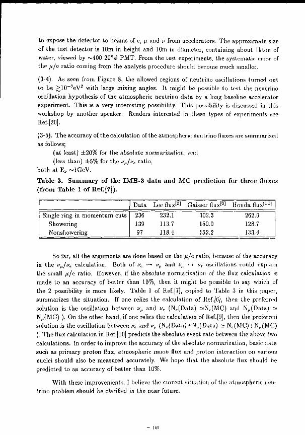
to expose the detector to beams of e, fi and v from accelerators. The approximate size of the test detector is 10m in height and 10m in diameter, containing about lkton of water, viewed by ~400 20'V PMT. From the test experiments, the systematic error of the fj./e ratio coming from the analysis procedure should become much smaller.

(3-4). As seen from Figure 8, the allowed regions of neutrino oscillations turned out to be >10~ 3 eV 2 with large mixing angles. It might be possible to test the neutrino oscillation hypothesis of the atmospheric neutrino data by a long baseline accelerator experiment. This is a very interesting possibility. This possibility is discussed in this workshop by another speaker. Readers interested in these types of experiments see Ref.[20].

(3-5). The accuracy of the calculation of the atmospheric neutrino fluxes arc summarized as follows;

(at least) ±20% for the absolute normarization, and (less than) ± 5 % for the v^jv^ ratio,

both at E„ ~ lGeV.

Table 3. Summary of the I M B - 3 data and M C prediction for three fluxes (from Table 1 of Ref.[7]).

Data Lee fluxM Gaisser fW yi Honda fluxl l ul

Single ring in momentum cuts 236 232.1 302.3 262.0 Showering 139 113.7 150.0 128.7 Nonshowering 97 118.4 152.2 133.4

So far, all the arguments are done based on the fi/c ratio, because of the accuracy in the v^/v^ calculation. Both of vc «-• v^ and v)t «-» vT oscillations could explain the small /z/e ratio. However, if the absolute normarizatioii of the flux calculation is made to an accuracy of better than 10%, then it might be possible to say which of the 2 possibility is more likely. Table 1 of Ref.[7], copied to Table 3 in this paper, summarizes the situation. If one relies the calculation of Ref.[G], then the preferred solution is the oscillation between v^ and vr (N,.(Data) ~N C (MC) and N„(Data) ~ NM(MC) ). On the other hand, if one relies the calculation of Ref.[9], then the preferred solution is the oscillation between i/e and i//t (N (.(Data)-(-N / i(Data) ~ N c(MC)+N,,(JvlC) ). The flux calculation in Ref.[10] predicts the absolute event rate between the above two calculations. In order to improve the accuracy of the absolute normarization, basic data such as primary proton flux, atmospheric muon flux and proton interaction on various nuclei should also be measured accurately. We hope that the absolute flux should be predicted to an accuracy of better than 10%.

With these improvements, I believe the current situation of the atmospheric neu­trino problem should be clarified in the near future.

- Kill

Finally, I mention on the solar neutrino data. The presently available data from the 3 7 C I ^ * and the Kamiokande-H e x p e r i m e n t s ^ both indicate that the observed solar neutrino flux is smaller than the theoretical prediction. At present, one of the most promising solution to the solar neutrino deficit is the neutrino oscillations in the solar interior (MSW mechanism^ 4 ' ) . If MSW mechanism is the solution of the solar neutrino problem, then i/e <-+ v^ oscillations are ruled out for the solution of the atmospheric neutrino problem. The only remaining possibility is liie v^ <-> vT oscillations. Thus, for the consistency check of the solar and atmospheric neutrino data, it is important to discriminate which of the two possibilities are the real solution of <he atmospheric neutrino problem.

4 . S u m m a r y The deficit of the atmospheric v^ relative to ue has been observed by Kamiokande

and IMB-3. The deficit is quite large, R(Data)/R(MC) are 0.60±g;g|±0.05 and 0.67±0.17 for Kamiokande and IMB-3, respectively. Neutrino oscillations between i/M and ue or between v^ and vT might be the solution of the problem. In the near future, we expect a better understanding of the problem with more information on this problem.

I would like to thank the Kamiokande collaborators and M.Honda for useful discussions.

References [1] J.Maki et al., Prog. Theor. Phys. 28. (1962) 870; B.Pontecorvo, Zh. Eksp. Theor.

Fis., 53 (1967) 1717; V.Gribov and B.Pontecorvo, Phys. Lett. B 28 (1969) 493.

[2] K.S.Hirata et al., Phys. Le+t. B 205 (1988) 416.

[3] J.G.Learned, S.Pakvasa and T.J.Weiler, Phys. Lett. B 207 (1988) 79; V.Barger and K.Whisnant, Phys. Lett. B 20fi (1988) 365; K.Hidaka, M.Honda and S.Midorikawa, Phys. Rev. Lett. M (1988) 1537.

[4] L.V.Volkova, Sov. J. Nucl. Phys. 3_1 (1980) 784; private communication.

[5] T.K.Gaisser, T.Stanev and G.Barr, Phys. Rev. D 3J (1988) 85.

[6] G.Barr, T.K.Gaisser and T.Stanev, Phys. Rev. D 3J (1989) 3532.

[7] D.Casper et al., Phys. Rev. Lett. 6fi (1991) 2561.

[8] D.W.Casper Doctor Thesis, University of Michigan (1990).

- 1 6 1 -

[9] H.Lee and Y.S.Koh, Nuovo Cimento, 105B (1990) 883.

[10] M.Honda et al., Phys. Lett. B 21£ (1990) 193.

[11] K.Kawasaki and S.Mizuta, Phys. Rev. D 43. (1991) 2900.

[12] M.Aglietta et al., Europhys. Lett. £ (1989) 611.

[13] Ch.Berger et al., Phys. Lett. B 227 (1989) 489; Ch.Berger et al., Phys. Lett. B 245 (1990) 305.

[14] K.S.Hirata et al., to be published.

[15] Ch.Berger et al., Nucl. Inst. Meth. A262 (1987) 463.

[16] K.Gabathuler et al., Phys. Lett. B I3_8_ (1984) 449.

[17] F.Dydak et al., Phys. Lett. B 1M (1984) 281.

[18] M.Koshiba, proceedings of Workshop on Grand Unified Theories and Cosmol­ogy, KEK, Japan, December 1983, P24; Y.Totsuka, Proceedings of the Seventh Workshop on Grand Unification / ICOBAN'86, April 1986, Toyama, Japan, P78; A.Suzuki, Proceedings of the Workshop on Elementary Particle Picture of the Uni­verse, KEK, Japan, February 1987, P136; T.Kajita, Proceedings of the third Work­shop on Elementary-Particle Picture of the Universe, Fuji-yoshida, Japan, October 1988, pl63, ICR-Report-185-89-2.

[19] D.S.Ayres (Soudan 2 collaboration), Proceedings of the Last Workshop on Grand Unification, North Carolina, USA, April 1989, p28.

[20] M.Koshiba, in these proceedings, and references therein.

[21] M.Takita, Doctor Thesis, University of Tokyo (February 1989), ICR-Report-186-89-3.

[22] R.Davis, Jr. et al., Phys. Rev. Lett. 20. (1968) 1205; K.Lande, talk at the 25"" Int'l Conference on High Energy Physics, Singapore, Aug. 1990.

[23] K.S.Hirata et al., Phys. Rev. Lett. £5. (1990) 1297; K.S.Hirata et al., Phys. Rev. Lett. £5. (1990) 1301; K.S.Hirata et al., Phys. Rev. Lett, 6J> (1991) 9. K.S.Hirata et al., submitted for publication in Phys. Rev. D.

[24] S.P.Mikheyev and A.Yu.Smirnov, Sov. J. Nucl. Phys. 42 (1985) 913; L.Wolfenstein, Phys. Rev. DH (1978) 2369, ibid. D2Q (1979) 2634.

- 1 6 2 -

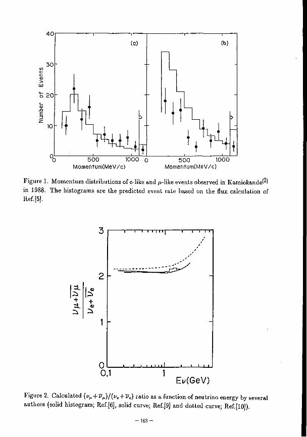
500 1000 o Momentum(MeV/c)

500 1000 Momentum(MeV/c)

Figure 1. Momentum distributions of e-like and fi-Yike events observed in Kamiokande^l in 1988. The histograms are the predicted event rate based on the flux calculation of Ref.[5].

Eu(GeV) Figure 2. Calculated (fM + f (,)/("« + "=) ratio as a function of neutrino energy by several authors (solid histogram; Ref.[6], solid curve; Ref.[9] and dotted curve; Ref.[10]).

- 1 6 3 -

^10< o i_ tn \ o a> tn \

CI

§10 2

X

LL

li + 3-101

S 1.2 D

* i.oh X

LL 0.8

0.6 0.1

"^—I 1 1 I I I I I I 1 1 |—TT (a)

\ ~L Gaisser

-\—I I I M l l | 1—h-f-B Honda (b)

Gaisser LBS

Gaisser

• 11 H I _i i i i i

Eu(GeV)

Figure 3. (a):Calcu)ated (*>„ + v^) energy spectra by several authors (solid histogram; Ref.[6], solid curve; Ref.[9] and dotted curve; Ref.[10]). (b): Absolute (u^ + 17,,) spectra calculated in Ref.[10] and Ref.[9] relative to that of Ref.[6].

- 1 6 4 -

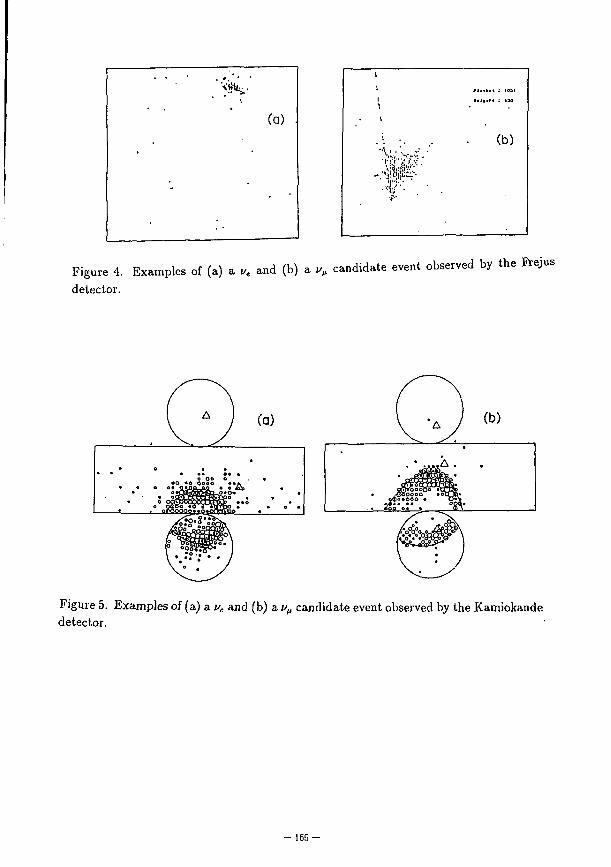
\ 1 • t n > * 1 130

' • \ 1 • *. *.' •'

(b)

•'•¥'• •$•'

Figure 4. Examples of (a) a „. and (b) a „„ candidate event observed by the Frejus

detector.

(a) (b)

Figure 5. Examples of (a) a vc and (b) a v^ candidate event observed by the Kamiokande detector.

- 1 6 5 -

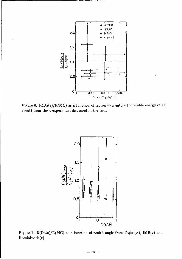
a.

. 1 x NUSEX

2.0 -a Frejus o IMB-3 . Kam-l+ll

1.5 i 5 1 1

<» 1 n a.

i 1 ^ ' i 1 ^ ' i 1

'- J., , ' 0.5 I ' •

1 .J

I r

500 1000 1500 P or E (M*V

Figure 6. R(Data)/R(MC) as a function of lepton momentum (or visible energy of an event) from the 4 experiment discussed in the text.

Figure 7. R(Data)/R(MC) as a function of zenith angle from Frejus(x), IMB(o) and Kamiokande(»).

- 1 6 6 -

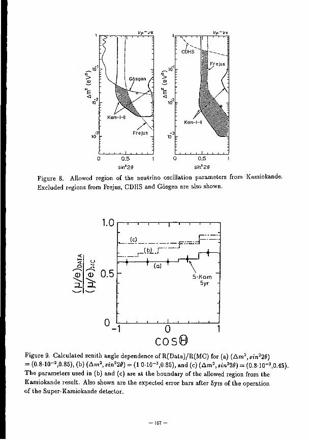
Un - ye 1 ' ' ' ' :

: :

Id1 -z

1 G6sgen A

*A / (: ,5' 'r W ^ ^

-3 10

^ Kam-l-ll ^ — *

• / \

Frejus

h , , , . i . . . , "

ff i - l /r

0 0.5 1 0 0.5 sin22e sln*2e

Figure 8. Allowed region of the neutrino oscillation parameters from Kamiokande. Excluded regions from Frejus, CDIIS and Gosgen are also shown.

1.0

A ID 0.5 2:

0

-I 1 1 r -i 1 1 r

_ M F = = = r -. . - J - t H ~ r "~\_T+

(a) \ 5-Kam

5yr

-1 0 cos8

Figure 9. Calculated zenith angle dependence of R(Data)/R(MC) for (a) (Am 2, sin226) = (0.8-10-2,0.85), (b) (Am 2, sin^B) = (1.0-10^,0.85), and (c) (Am 2 , S m 2 20) = (0.8-10-2,0.45). The parameters used in (b) and (c) are at the boundary of the allowed region from the Kamiokande result. Also shown are the expected error bars after 5yrs of the operation of the Super-Kamiokande detector.

- 1 6 7 -

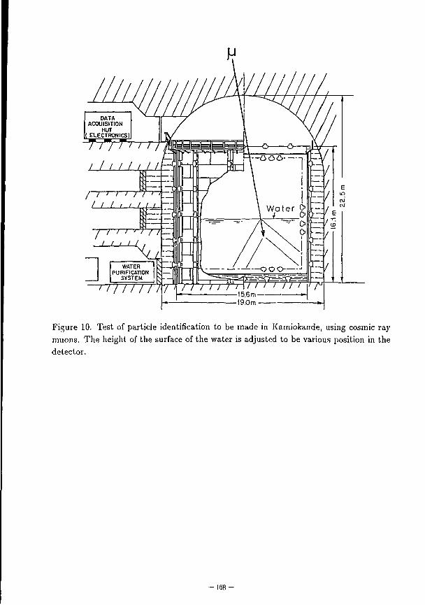
1111 /1 /

Figure 10. Test of particle identification to be made in Katniokande, using cosmic ray muons. The height of the surface of the water is adjusted to be various position in the detector.

- 168 -

Calculation of Atmospheric Neutrino Fluxes * S. Mizuta

Department of Physics, Tohoku University, Sendai 980, JAPAN

Abstract

The atmospheric neutrino fluxes at Kamioka site are calculated semi-analytically changing the value of some physical parameters in order to investigate how the resultant neutrino fluxes depend on them. Besides both the absolute value of the fluxes and the {ye -f ve)/{vp + &p) ratio agree with those of the previous calculation, it is found that the dependence of the (v e + v^liy^ + *v) ratio on such physical parameters is very weak.

1 Introduction

It is known that the atmospheric neutrinos are produced by the decay of mesons which

come from scatterings between the primary cosmic rays (mainly protons) and air nuclei;

/** -» e± + ve(Ve) + i>M(j/J. (1)

Naively we expect the (i/e + ue)l{u^ + P,,) ratio to be 0.5. However, it was reported by

Kamiokande Collaboration[2] that the ratio of electron-like to muon-like events in the

energy range between about 0.1 GeV and about 1 GeV is different from a theoretical

expectation value. The measured value of R0t,s, where

_ number of electron — like events number of muon — like events

is I.09±0.16. On the other hand, the expectation value RMOIU which is calculated by

a Monte Carlo simulation based on theoretical neutrino fluxes given by Gaisser el al.[i\

is 0.61. Therefore R0bs/RMont ' s l-78±0.27, which shows 2.9a discrepancy. Recently

new data of both R0bs and RMOUI which include the effect of muon polarization were

"This work is done with M. Kawasaki (Tohoku Univ.)[l].

- 169 -

reported[4,5]. According to these new data, R0b*l R-Mom is 1.63±0.22 and this still shows

2.9a discrepancy.

The observational data of other underground detectors (IMB[6], Frejus[7j, NUSEX[S])

agree with the expectation value based on the same theoretical neutrino fluxes[3,5]. How­

ever, they are also consistent with that of Kamiokande Collaboration, therefore the ob­

servational data of Kamiokande Collaboration is not excluded or confirmed by those of

other underground detectors yet.

Since this discrepancy between the observational data and the expectation value sug­

gests that there may exist new phenomena beyond the standard model, such as neutrino

oscillation[9], it is important to examine whether or not this discrepancy indeed exists by

re-calculating the neutrino fluxes at the earth's surface.

There are already some calculations of the neutrino fluxes[3,5,12,ll,10), but many of

them estimate the fluxes by a numerical experiment with Monte Carlo method. In a

numerical experiment, however, it is not clear what is the most essential among various

physical processes which determine the atmospheric neutrino fluxes. In this paper, there­

fore, we calculate them in a different way from those of the previous authors. We represent

them as semi-analytical form which contain several physical parameters and finally inte­

grate them numerically changing the value of these parameters. By this method, we can

investigate how the resultant neutrino fluxes depend on various physical processes much

more easily than by a numerical experiment. Thus we can study whether the discrep­

ancy of the [ve + P e)/(j/,, + i/p) ratio can decrease or not. (Note that Bugaev et al. also

calculated the atmospheric neutrino fluxes semi-analytically[Il], but they neglect muon

polarization (see section 2.7.))

As is seen later, it is concluded that the (ve + v^j^v^ + D^) ratio is almost universal,

which leads to confirm the discrepancy between the observational data and the expectation

value.

- 1 7 0 -

2 Calculation

The primary cosmic ray protons hit the air nuclei in the upper atmosphere and produce

many pions (and kaons). Some of pions are absorbed by air nuclei but mostly decay

into muons and muon-neutrinos. The produced muons lose their energy by ionizing the

air atoms and most of them decay into electrons (positron) and electron-neutrinos. We

express the atmospheric neutrino fluxes as semi-analytical form. For this end we make

several assumptions on the various physical process and the primary cosmic ray spectrum.

2.1 Pr imary protons

We assume the power-low momentum spectrum for the primary protons in high energy

region (oc pp~a ; a = 2.67 ). The power index a is determined from the observational

data[13]. However, the observed spectrum bends below about 3 GeV, because the solar

wind blows out low momentum protons. Furthermore, the geomagnetic field prevents low

momentum protons from reaching the earth's atmosphere. The cut-off momentum by the

earth's geomagnetic field is approximately represented by Stormer's formula[14] and we

take the higher value between 3 GeV and the geomagnetic cut-off as the actual cut-off

momentum.

Note that, in the calculation of Gaisser et a/.[3,5], the Stormer's formula is averaged

over the azimuthal angle and they use the averaged cut-off momentum, but it is not in

our case.

We partially take the effect of the secondary protons into account by assuming the flat

spectrum of the primary protons below the cut-off momentum. In order to investigate

the effect of secondary protons upon the resultant neutrino fluxes, we also calculate the

neutrino fluxes by neglecting the primary protons with momentum smaller than the cut­

off.

2.2 One-dimensional approximation

We take the one-dimensional approximation, i.e., we assume that the direction of neutrinos

is same as that of the primary protons. Some low momentum muons lose almost all of

- 171 -

their kinetic energy and stop before their decay. As a result the emitted neutrinos are

generated nearly isotropic, hence about half of them escape without reaching the earth's

surface. Therefore the neutrino flux of one-dimensional calculation might be about two

times larger than that of three-dimensional calculation at low momentum region. It is

shown by Lee and Bludman[10], however, for neutrinos with energy greater than 200

MeV, the result of one-dimensional calculation is in good agreement with that of three

dimensional one. Thus we can safely take the one-dimensional approximation.

2.3 Atmospheric density

The atmospheric density profile is assumed to be represented by a single exponential:

p{h) = p0 e x p ( - ^ - ) , (3)

where k is the altitude measured vertically from the earth's surface and h0 is the scale

parameter of the upper atmosphere (ko = 6.42 km). We determine p0 so that the column

density calculated by this formula corresponds to measured one and we get p0 — 1.61

kg /m 3 . It is reasonable to determine p0 in this way, because the energy loss of muons

depends only on the column density. An actual atmospheric density on the earth's surface

is a little smaller than po, but this difference has only negligible effect on the neutrino

fluxes.

2.4 Pion production

We assume that the pion production momentum spectrum is given by

dr„(x) _ (i - x)3

dx ~ xP ' [ >

where x is the fractional momentum of a pion in the laboratory system (x = pion momen­

tum /proton momentum). Here the normalization factor is set to one and it is discussed

later(see section 2.8). Since the value of p in eq.(4) is not well known (usually p = 1

is used), we calculate the muon fluxes and neutrino fluxes at the earth's surface with

different values of p, and investigate the dependence of the resultant muon and neutrino

fluxes on p.

- 172 -

2.5 Effect of K meson

We neglect K mesons which are produced by scatterings between the primary protons

and air nuclei. Experimentally the K/ir ratio in hadron interaction is known to be about

10% averaged over +,— charges[15]. Therefore the effect of K mesons upon the resultant

neutrino fluxes is thought to be small. In fact, we can estimate the effect of A' mesons

upon the resultant (i/ e + Ve)/(vn+ v^) ratio by calculating neutrino fluxes for the channel,

A ' ± —» ^ ± + j/ / 1 (t ' / i ) , fi* —» e ± + (/e(j'c) + ^ ( j ' ( x ) , and it is found that K mesons could reduce

the (ve + i/ e)/(i/^ + Up) ratio by at most 4% which would rather enlarge the discrepancy

between R0t,a and Riwont-

2.6 Muon energy loss

The muon energy loss by ionizing the earth's atmosphere is expressed by

dE»{h) - ^ - = ap(h), (5)

where £>(/») is the muon energy at the altitude h, a is the rate of ionization loss (—

2.06 MeV/g • c m - 2 ) and p(h) is the atmospheric density profile(see eq.(3)).

2.7 Muon polarization

We take into a.ccount the polarization of the muon from a pion decay[16]. It is well

known that / j - ( / z + ) from 7r"~(7r+) decay is completely polarized to helicity +(—) in the

pion rest frame. This muon polarization remains about 30% in the laboratory system,

and it increases the (i/e + P e )/(j/ ( J + v^) ratio in the high energy region, because i>e{ve)

from the decay of / i~(/i + ) which is polarized to helicity +(—) has higher energy compared

with the unpolarized case.

In this calculation, we average the decay distributions over the angle between the

momentum of decay neutrinos and the muon helicity in the laboratory system.

2.8 Normalization factor

Since, in this calculation, the effects of the secondary protons and the secondary pions

are taken into account only partially, the overall normalization factor of neutrino fluxes is

- 1 7 3 -

not determined theoretically. Therefore we choose it so that the calculated vertical muou

flux at the earth's surface at the energy of 11.4 GcV corresponds with the observational

one[17]. Note that the {ue + >/c)l{"^ + >'li) ratio is independent of this normalization factor.

3 Results

We calculate the atmospheric neutrino fluxes by the numerical integral program VE­

GAS. In order to check the results of this calculation, we calculate the vertical and

horizontal muon fluxes at the earth's surface and compare them with the observational

data[17](Fig.i). The shape of the calculated muon fluxes is in good agreement with the

observational data for the vertical flux and both the shape and the absolute value fit the

data for the horizontal one.

The calculated neutrino fluxes and the {vc + i>e)/(i/ ( l + )>,,) ratio at Kamioka site with

the standard value of p(= l)(see eq.(4)) are given in Fig.2 with the results of Barr t/ al.[r>]

for comparison. Although the absolute values of the calculated neutrino fluxes arc larger

than those of Barr et al. by about 50% at 0.1 GeV of neutrino energy, they are in good

agreement above 0.2 GeV, and the (ve + ue)/(i/ti + i>tl) ratio agrees within about 5% al. all

over the energy range for this calculation.

In Fig.2,we also show the (i/e + ^eJ/t'V + <v) ratio without muon polarization. As

mentioned before the {vc + i/e)/(f^ -f i>M) ratio with muon polarization is indeed larger

than that without muon polarization (see section 2.7).

We show in Fig.3 the results of calculation neglecting the primary protons below

the cut-off momentum(see section 2.1). Both the absolute value of the fluxes and the

(ue + ve)/(i/f, + F//t) ratio are in good agreement with those with the flat spectrum below

the cut-ofT (see Fig.2). Therefore the effect of the secondary protons upon the atmospheric

neutrino fluxes is negligible in this calculation.

Fig.4 shows the angular distributions where 0 is the zenith angle and y? is the azimuthal

angle measured anticlockwise from the magnetic south. Tlic upgoing neutrino fluxes are

larger than downgoing ones at low energy region, because the geomagnetic cut-off for

upgoing initial protons is effectively smaller than that for downgoing ones. The azimuthal

- 171 -

angle distribution of the downgoing neutrino (luxes is understood Iroin the similar reason,

i.e., for the same zenith angle 0, the smaller is sin -p, the smaller is the geomagnetic cut-oil

[14]. On the other hand, the azimuthal angle distribution of the upgoing neutrino lluxes

is complicated but it can be understood in the same way.

The (i/c + i/c)l{i>iL -\- u^) ratios of the vertically upgoing and vertically downgoing

neutrinos are smaller than those of horizontally coming ones at high energy region. This

is because some of the vertically coming muons with high energy reach the earth's surface

before they decay. Since the electron-neutrinos are produced from only anion decays, the

(ue + i>c)/(;/,i -f ;/,,) ratio of the vertically coming neutrinos becomes smaller than that of

the horizontally coming ones. The azimuthal angle distribution of the (uf + i>e)/(r'„ + uu)

ratio is almost isotropic within 10%.

Fig.5 show the calculated neutrino fluxes and the {t/c -f u, )/(i'„ -)- //,,) ratio with three

dilTerent values of ;;. As mentioned before, since the value of p in tin1 pion production

momentum spectrum (seeeq.(4)) is not well known, we calculate union fluxes and neutrino

fluxes with some dilTerent values of p. (The difference of the calculated union (luxes with

these values of p is found to be negligible.) For example, the magnitude of neutrino fluxes

with p = 1.5 is nearly fifteen times larger than that with p = — 1 at 0.1 GeV of neutrino

energy. This is because, for large p, pious from the scatterings between the initial protons

and air nuclei tend to be produced with low energy, as a result, low energy neutrinos

increase. On the other hand, the (;/e + (/ e)/(// ( I + u^) ratios for the different values of p are

in good agreement with each other within at most 10%.

In Fig.6, we show the resultant neutrino fluxes on other parameters. We calculate

the neutrino fluxes changing the scale parameter and the scattering cross section between

pions and air nuclei at low energy region within the range where the calculated muon

fluxes at the earth's surface do not change so much. For example, we take 8 km for

the scale parameter of atmosphere (the standard value is (i.42 km) and 2500 nib (or the

scattering cross section below 1 GeV of pion momentum (the standard value is 25 mb).

Although the absolute values of the resultant neutrino fluxes change about 10% ~ 20%.

the (i/e -f- ^e)/(^i + ^(i) ratios agree with those with the standard values within at most

- 175 -

4%(see Fig.2).

At last let us consider ueji/€ ratio. The source of ve(vc) is /; + (/t~) from 7r + (7r~) decay,

but in this calculation we do not distinguish between /i — (TT_ ) and / i + (7r + ) . Therefore the

i'ejvt ratio can not be determined in our scheme. Since, however, the source of vc{vc) is

/( +(/x~), the i>e/i'c ratio is expected to be roughly same as the /i~//j + ratio at the earth's

surface. The observational value of the / J~ / / . J + ratio is 0.77 ~ 0.83 at the miion energy

between 3 GeV and 10 TeV[18]. Although the energy range of these experimental data

is higher than that of muons which produce the neutrinos with energy between 0.1 GeV

and 1.5 GeV, the observational data shows no clear dependence of union energy. Hence

the f-i~ J/.i+ ratio, that is the velve ratio, is expected to be about 0.8 even at lower energy

region. Thus the f/e/ue ratio is estimated to be nearly one, therefore the ciiect of the

asymmetry between ve and i/e on the observed events of Kamiokande 11 is thought to be

small.

4 Conclusion

We calculate the atmospheric neutrino fluxes semi-analylicaJly. Jn summary, the resultant

neutrino fluxes agree with those of the previous works[3,5). In particular, the (ue -f

'•'<•)/('y(i + '-v) ratio is in good agreement.

Furthermore, we calculate them changing the value of some physical parameters as far

as unphysical region, in order to estimate the influence of these parameters upon the fluxes

and the (^P + i/ e)/(i',, + ///1) ratio. As a result, it is found that the (i/c + i ,

e)/( ' / , i + '',i) ratio is

almost independent of the value of p in the pion production momentum spectrum(eq.('l)),

the scale parameter of atmosphere(eq.(3)l and the scattering cross section between pious

and air nuclei at low energy region. Therefore we expect that the (i/e 4- ve)l{>',i + i'u) ratio

is almost independent of the way and the details of calculation and it is very difficult to

explain the data by Kamiokande Collaboration within the frame of the standard model.

In other words, if we take the observational data seriously, it suggests the existence of

new phenomena such as neutrino oscillation.

- 17(i -

5 Acknowledgements

We are grateful to T. Yanagida and M. Yoshimura for helpful discussions and to F. Takagi

for useful comments on hadron physics. The numerical computations were carried out on

the ACOS S-2000 at the Bubble Chamber Physics Laboratory of Tohoku University and on

the FACOM M7S0 at the Astronomical Data Analysis Center of National Astronomical

Observatory o[ Japan. This research was supported in part by the Japanese Grant in

Aid for Science Research Fund of the Ministry of Education. Science and Culture No.

02610213 and 02211201.

References

[1] M. Kawasaki and S. Mizuta, Phys. Rev. D (to be published)

[2] K.S. Hirata ct «/., Phys. lett. B205,416(19SS).

[3] T.K. Gaisser, T. Stanev and G. Barr, Phys. Rev. D38 .So I 1988).

[4] Y. Totsuka, in "Last Workshop on Grand Unification'. ed. P.11. Frampton. p3 (World

Scientific, 1989).

[5] G. Barr, T.K. Gaisser and T. Stanev. Phys. Rev. D39. 3532 (1989).

[6] W. Gajcwski, in Prok. 24th Inten. Conf. on High Energy Physics (Munich. 1988).

eds. R. Kotthaus and J.H. Kuhn (Springer. Berlin):

D. Casper it et al., preprint BU Preprint 90-23 (1990).

[7] Ch. Berger et ai, Phys. Lett. B227, 489 (1989).

[8] S. Ragazzi, in Proc. 24th on Recontre de Mpriond "Tests of Fundamental Laws in

Physics", eds. 0 . Fackler and J.T. Thanh Van,(Editions Frontiers. 1989).

[9] J.G. Learned, S. Pakvasa and T.J. Weiler, Phys. Lett. B207. 79 (1988):

K. Hidaka, M. Honda and S. Midorikawa, Phys. Rev. Lett. 61 . lo37 (1988):

V. Barger and K. Whisnant, Phys. Lett. B209, 365 (1988);

M. Takita, Pli.D. Tliesis, University of Tokyo (1989).

[10] II. Lee and S.A. Bludman, Phys. Rev. D37, 122 (1988).

[11] E.V. Bugaev and V.A. Naumov, Phys. Lett. B232, 391 (L9S9).

[12] M. Honda, K. Kasahara, K. Hidaka and S. Midorikawa, Phys. Lett. B248, 193 (1990).

[13] E.g. see, J.A. Simpson, Ann. Rev. Nucl. Part. Sci. 33. 323 (1983).

[14] C. Stonner, Astrophysics 1, 237 (1930);

U.J. Cooke, Phys. Rev. Lett. 51, 320 (1983).

[15] E.g. see, T. Eichtcn ct «/., Nuci. Phys. B44, 333 (1972).

[16] L.V. Volkova, in "Cosmic Gamma Rays, Neutrinos and Related Astrophysics", edited

by M.M. Shapiro and J.P. Wel'el (Kluvver Academic Publishers, Dordrecht 1988)

p.139;

S. Barr,T.K. Gaisser, P. Lipari and S. Tilav, Pliys. Lett. B214, 147(1988).

[17] O.C. Allkofer, K. Carstensen and W.D. Dau, Phys. Lett. B36, 425 (1971);

II. Jokisch et a/., Phys. Rev. D19, 136S (1979).

[18] Y. Muraki et al., Phys. Rev. D28, 40 (1983);

O.C. Allkofcr ct «/., Phys. Rev. Lett. 41, 832 (1978);

G.D. Badhwar, S.A. Stephens and R.L. Golden, Phys. Rev. D15, 820 (1977) and

references therein.

Figure Captions

Fig. l : Vertical(zenith angle is 0 deg) and horizontal(zcnith angle is 75 deg) muon fluxes

at the earth's surface(magnetic latitude A is 49.8°). Circles and crosses represent

the observational data[17] and the results of our calculation, respectively.

- 1 7 8 -

Fig.2 : Neutrino fluxes and the (i/e + ve)/(i/lt + i>,,) ratio at Kamioka site calculated with

p = l(see eq.(4)) (solid lines and a dashed line). The dashed line shows the result

neglecting the muon polarization. The histograms are results of Barr e.t «/.[3,5].

Fig.3 : Neutrino fluxes calculated with neglecting the primary protons with momentum

smaller than the cut-off.

Fig.4 : (a)The zenith angle distribution of neutrino fluxes and (t/c -f- /',)/(/',, + ''„) ratio

where cos 0 = 1 corresponds to vertically downgoing neutrinos. (b)The azimulhal

angle distribution for downgoing neutrinos. (c)Tho azimuthal angle distribution

for upgoing neutrinos. The azimuthal angle is measured anticlockwise from the

magnetic south. In figures of flux, the solid line and the dashed line corresponds

to muon-neutrino flux and electron-neutrino flux, respectively, and the energy of

neutrino is 0.1 GeV, 0.6 GeV, 1 GeV, 1.5 GeV from top to bottom, respectively. In

the figures of {vr -f- ve)l{vti + u)t) ratio, the solid line, dotted line, dashed line and

dotted dashed line corresponds to the neutrino energy of 0.1 GeV, 0.6 GeV, ] GeV.

1.5 GeV, respectively.

Fig.5 : Calculated neutrino fluxes and the [v€ + T/S)l{utl + />,,) ratio with some different

values of p(see eq.(4)), (a)p = — l,(b)p = 0.5,(c)p = 1.5.

Fig.6 : Calculated neutrino fluxes and the (;/e + vc)/(i',t -f '-',,) ratio with (n)hu — 8 km

which is the scale parameter of the atmospheric density profile (normal value is fi.42

km) and with (b)<r„ = 2500 mb which is the scattering cross section between pious

and air nuclei at low energy region (normal value is 25 mb).

- 179 -

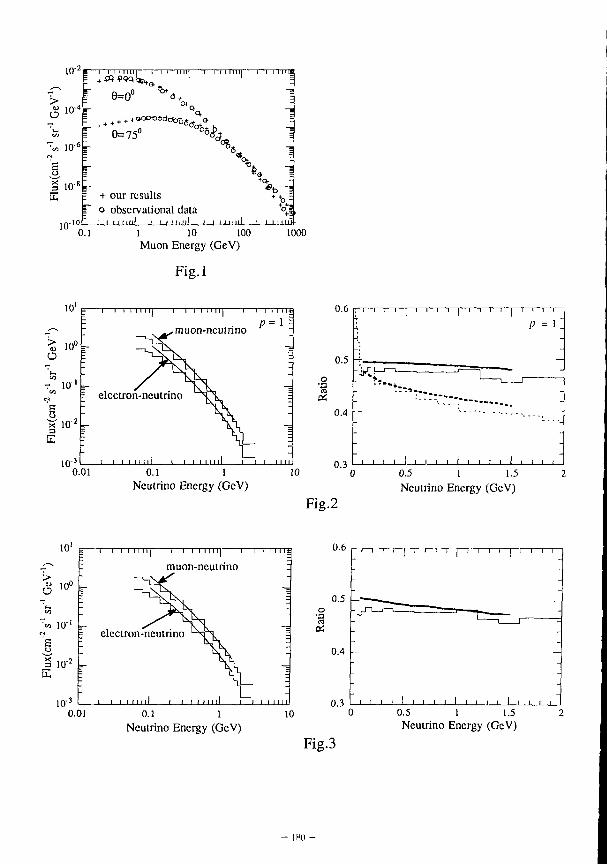
10"

> „ g 10"

e — i — i i i m i l 1—i i 111 IT] 1—i 11 m i '—i—i 11 ui

io-<

IO-1

10"

6=75° °*&

+ our results F o observational data

%. "9

I ' M ' m l i i i i m i l I I I I m i l I i i i i n 0.1 1 10 100 1000

Muon Energy (GeV)

Fig.l

10'

ft io° _ o : — u.

1 / 3 1 -7 10 *

VI

'a 3 o ~x 10' 2

3

E

10"

i i I 11 H I 1—i I i 11 i l l 1—i i I 11 m

muon-neutnno P = l

electron-neutrino

i i i 1111 i i i i i 1111 i i i i i 111

0.01 0.1 1 Neutrino Energy (GeV)

10

Fig.2

0.5 1 1.5 Neutrino Energy (GeV)

o

10'

10"

••» i o '

6 u ¥ IO-2 t-

10"J

T — I I i 11 h j 1—i i i I u i j 1—i i i i u g

muon-neutrino

electron-neutrino

i i i m l i i i i n m i i i i 111

0.6

0.5 •1

0.4

0.3

~i—I—i—i—I—i—i—r ~~i—r~ i—i—i—r

J 1 I I I I I I I I I I I _l I I I I I I o.oi o.i i

Neutrino Energy (GeV) 10 0 0.5 1 1.5 2

Neutrino Energy (GcV)

Fig.3

1 H U -

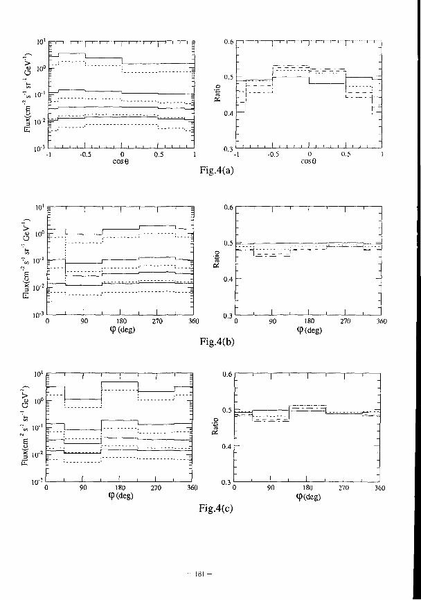
10* E ' ' ' ' [ ' ' ' ' 1 1 1 1 j J 1 1 J =

: ' * -—J 1

1 1 1 1 j J 1 1 J =

:

<u in"

1—

1 1 1 1 j J 1 1 J =

:

<u in"

1—

r _:= <u in"

1—

r

~v> 10 ' • N

"s f.: E ~v> 10 ' •

N

"s g io-2 ^ -= E

,n -3

n- -•

' 1 1 1 1 1 ! I 1 1

' - -2

1 1 1 1 1 1 1 1 1

0.6 I—r

0.5 o •a a Pi

-0.5 0 cose

0.5

0.4

0.3

-I—r-i—r-r-

1 -1

Fig.4(a)

-0.5 0 cos 6

0.5

f r

• i i i i i i i i i i i i i i i i i i_

10' ff

;> ."=> irr o

10"

10-"

10"

I ' I ' I ' I ' S

H i—p^-^

r ^ .! .T7!i

90 180 270 9(deg)

360

Fig.4(b)

180 9(deg)

10l

> o $ 10°

io-

io- z -

10"

i i!

1 ' 1 i = i

i!

- -\ i =

liji "" I

- i

"" I

- i -= U4 - - , i E

• ^ i

r.._. - T=

i I I i I i

90 180 270 <P(deg)

360

Fig.4(c)

90 180 270 *P(deg)

360

- 181 -

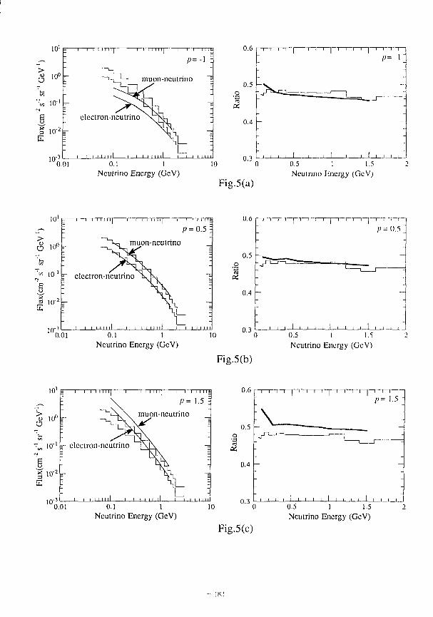
10'

10"'

0.6

tu

10"' 0.01 0.1 1

Nculrino Energy (GcV) Fig.5(a)

0.5 1 1.5 Neutrino Energy (GcV)

10'

rS I" 0

« io_

H o ">< 3. 10" t

10".

-i—r i 11 i i j 1—i i i 11 i i j 1—i i M 11

p=0.5z

muon-neutrino

electron-neutrino

' i ' n [ ]__ i i ' i i 1 1 1 i i

0.6

0.5

"0.01 0.1 1 Neutrino Energy (GcV)

10

0.4

0.3

i—i—I" 1—i ~r~

Fig.5(b)

—r~r -T—i -

P = 0.5;

0.5 1 1.5 Neutrino Energy (GcV)

10'

u 10° O

TTTTTT] i I TTTTTE

P=\.5 "L_\ \ muon-ncuirino

~,„ 10"' — electron-neutrino

* 10"2

10o.oT I I I I I I I I I I I ! I I I I I I I I

0.6

0.5

« 0.4

T—i—i—I—r~ i—i—i—I—r—i—r p= 1.5

0.1 1 Neutrino Energy (GcV)

10 0 3 I 1 I I I 1 I I I 1 I L

0.5 1 1.5 Neutrino Energy (GcV)

Fig.5(c)

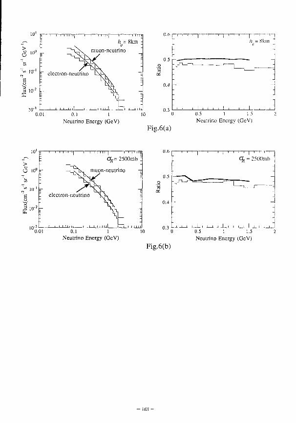
o

10'

10u

'<« 10'1

3 10 2

E

10';

electron-neutrino

0.01 0.1 1 Neutrino Energy (GeV)

0.6

0.5

0.4

0.3

/;.= skm ;]

J i I I I L

Fig.6(a)

_L 0.5 1 1.5 Neutrino Energy (GeV)

10'

o iol

10

S. W u.

" i — i — i i 1 1 r rrrrp -TTTTTT-

On= 2500mb 3

muon-neutnno

1 0o.oT

electron-neutrino

J I I I I m l | I I I M i l l I i I i I i n

0.6

0.5

Qi

0.1 1 Neutrino Energy (GeV)

10

0.4

0.3 I

n—i—;—i—r-1" i~

%= 2500mb

Fig.6(b)

0.5 1 1.5 Neutrino Energy (GcV)

- i s ; ? -

The Anomalous Atmospheric Neutrino Flux and the Possibility of Neutrino Oscillation

S. Midorikawa Institute for Nuclear Study, University of Tokyo, Tanashi, Tokyo 188, Japan

M. Honda® and K. Kasahara* Institute for Cosmic Ray Research, University of Tokyo, Tanashi, Tokyo 188, Japan

A b s t r a c t The data of atmospheric neutrino at the Kamiokande and liMB-3 are analyzed with the fluxes calculated by several authors. A translation formula, is introduced to compare dif­ferent experiments and/or different flux models. The three-neutrino oscillations explain both result consistently and if one neutrino-mass-squarcd difference is dominant, it, should be greater than the 1 x 1 0 - 4 eV 2 at 1 a level almost independent of a flux model.

A deficit of muon-like events from atmospheric neutrinos, similar to the one observed at Kamiokande 1 ' , has been reported recently by the 1MB group 2 ' , which uses the same water Cerenkov technique as that of Kamiokande. Analyses to explain the anomaly in terms of neutrino oscillations 3 ' have been marlo 4 , 5 ' . However, it was pointed out that the problem may lie in the calculation of neutrino fluxes, in particular in the neglect of miion polarization '. New calculations of the atmospheric neutrino have been made by several g r o u p s ' ' 8 , 9 , 1 0 ' 1 1 ' . Although these fluxes have a maximum difference of ~ ±30% \v magnitude, they agree within a few percent for the (i/c + Vc)/{vn + i',L) ratio and none of them can explain the deficit of muon-like events observed by the experiments.

Jn our analysis, we employ a similar method to the Frampton and Glashow 1 2 ' as following. We define

< eaffaFt, > = Y. f £c(Ea)frt{F,.,Ka)F^liP,nP)p(h)dEadEPdnvdht (1)

where £a(Ea) is the detection efficiency for an o-type charged lepton with energy Ea, <rrt

the differential cross section of !/„, F/j(El,A'll,) the incident vp flux with energy £',,, P.,, solid angle and p(l>) the neutrino production height distribution.

@ Talk wa.s given by him * Address after Apr. 1, 1991 Faculty of Engineering, Kanagawa University, Yokohama 221, Japan

- I R I -

Instead of the number Ne and A',, of the observed elect run and union events, we will use the ratio Ue = Ne/[/c < s^a^]^ >] and /. ;

; l = A',,/[/>• < f,.,"-., ./•',, >). w!i''iv K = (number of nucleons) x {lime). The ratios / ' r and ['^ in the presence of oscillal ions become

",-) > i'Jl

I 'r) >

i>.i)p{h).ii-:.,,ii-:,<i<i,.<ih

and

f z . <eH(TltFc> _ <s,.a,F, > ( | )

< C/iO-, , / ' ' , . > " < ? . f, /•',, >

Note that, (lux models, geomagnetic cutoffs, and the detection efficiencies are integral.•<{ in the value of / .

fn previous papers we studied the two typical cases: ''as*' I when- all neul) ino-ma.--squared differences are the same order and they are large enough and ca.se II where two neutrino masses are almost degenerate and the only one mass-squared difference dominates oscillations. The ca.se II is more interesting because ii may sohe nut only atmospheric neutrino problem by vacuum oscillations but also solve the solar neutrino problem by I lie MSW effect1'1'. Hence we examine case II in more detail. We parametrize the lepi,,n mixing matrix in the standard manner 5 ' 1 5 ' . In case II wheie only the largest mass-squared difference 8m~ = mjj — m\ ~ 7H3 — m~, contributes to three-iuut riuo oscillations, 1 he probabilities for oscillations with the neutrino energy /'.',, are

P{Ve -^Ve) = \ - 2clsl[\ - co^(~L)}

/ , K , - » ^ ) = l - 2 S ^ ( l - . s ? r ? ) [ l - a 1 s ( ^ / . ) ] 101

P(v, - J/,,) = 1s\s\cl\\ - cos(J^A)] - / - I ,

where c,- = cos!?,-, s,- = sin#;, and L is the distance from the neutrino source to the detec­tor. We can determine a point in the (&'<.,£/,,) plane from a set of oscillation parameters {^1,82,83,6m2) h_, substituting these into equation {'•)) and referring to equation {'2). \ \v define 5m2 dependent oscillation region for a given e?/r by tracing whole region of the other oscillation parameters.

ue = f<P{vr. - * > c ) > + < ;>(//„ -UIL =< P(uti — u„) > +f < P{ult ~

whore

< P(va — /A,) > =

x £ je^E^a^E,,. Eft)Fa(E,,n,.)r(u„ -

- I K f i -

All experiment determines the region in the (f>. {.',,) plane. We can evaluate the values of / , U, . ir

lt and i'e/U,, for various flux m .dels. We summarize in table 1 the results which are obtained from the Kamiokande data with 3.'13 kton y r u , ) and in table "2 those obtained from the 1MB data with 3.1 kton-yr"'. We combine the statistical and systematic errors of ~ 10% including the uncertainty in the neutrino cross section. In analyzing 1MB data, wo calculate A r

e and ;V(, from showering and non-showering events in single ring events using llavour-misidentification probabilities and mis-identification probability of neutral currents with charged currents in 1MB-3 I S ) . We obtain Ne = l .Tl.Si 1.7 and A',. = 89.3 ± 1.0. From these tables, we find that although the value of UC/U,L agrees within ±5% for different flux models, the values of Ur and U/L themselves differ by ~ ±30%.

We note that even a small difference of (he value / makes it difficult to compare {l'.-l',,) in different experiments and/or flux models directly. It is important to find a translation from one (Ue,Ult) plane with a value of / to another (i.')\ (/") piaue with another value / ( ) . In general, the translation is expressed in a complicated form and is not unique since the mapping from the oscillation parameter space to (Ur.,Ulk) plane is not. one to one. However, if we limit ourselves to the case II with large enough hm~, we get an analytic expression for the translation as follows, from </,../',, and < P(i'r —* 17) > for a given value of/ , we can evaluate < /'(;/,. — i',) >. < P(i', — ult) > and < /'(/ ',, — //,,) >. Substituting these values to equation (2) with / being replaced by / n , we obtain

t„ = c.„ + — c , . - - [ - T - o

where o = 1— < P(vc — i/T) >. We note that a has two solutions for a point in the ((".., f';j I plane. One solution which satisfies the condition that the line Ur = f corresponds to vjt «— vr oscillations is obtained perturvatively around the no oscillation point:

J - [^jfL(1 - Uu)(/ - Uc) for Ue < f

'> = L - 7 ^ 7 y F ( ^ - / ) [ ( l + / ) - ( ^ + ^ ) i for f<U,

(7)

Because the equation (7) is modified little for small 6m~ and (he other solution of a coincide at the boundary of the oscillation region, the translation (6) and (7) can be applied to the translation of fim- dependent oscillation region. This is true even in case I as an approximation.

The allowed regions which we obtain from tables 1 and 2 with the translation ((i) and (7) are represented in Fig. 1 (Kamiokande) and Fig.2 (IMB-3) respectively, where we chocse

/o, which we obtain from our fluxes for Kamiokande, to be O.'17-l. From these figures we find that the regions allowed by two experiments for each flux model agree well witli each oilier, although the coincidence is not so good as other pairs for Bugaev and Naumov's flux ( B N ) D \ We also plot the oscillation region boundary in the (?/,'.', ^ ) plane Tor case I when 8m^;>j]Q~2 eV 2 (i,j = 1..3), and for case II when the mass-squared differences are large enough (Aw 2 ,>10 - 2 cV 2 ) and 5m'1 = 1 x 10~'1 e \ ' - . for largo neutrino-mass-squared differences, the regions allowed by both experiments are within the range of being explained by three neutrino oscillations. For case J I, the same conclusion can be drawn for 6 m 2 ^ , 1 0 - 2 eV 2 , but for 5m'2 < 1 x l O - 4 eV 2 the allowed regions are almost outside (he oscillation region.

In summary, we have derived a translation formula, to be used when we eon.pare one experiment with another, and found that both Kamiokande and IMB-3 data can be interpreted in terms of three neutrino oscillations. If a. flux model is fixed, both experi­ments suggest, similar values of the oscillation parameter in spite of different experimental conditions. As an almost flux-model independent, result, we find that if one iieutrino-mass-squared difference (A?n2) dominates oseillal ions (case II), 5in~ should be greater than 1 x I(J~'1 eV"' at. the 1 a level in both the experiments.

Acknowledgments We are grateful to M.Takita for detailed information of Kamiokande experiment

and D.Casper for detailed information of I MB-3 experiment. We would like (o thank T.K.Gaisser and T.Stancv for useful comments and discussions on neutrino fluxes. We also thank II.Lee and V.A.Naumov for the information on their neutrino (lux calculations.

References 1. K.S.IIirata ct «/., Phys. Lett. B 205 -116 (1988). 2. D.Casper c.t <//., Boston University preprint. 90-2:} (1990). 3. Z.Maki, M.Nakagawa, and S.Sakata, Prog. Theor. Phys. 28, S70( I 9G2):Y.(;ribov and

B.Pontecorvo, Phys.Lctt. B 28, (1909). 4. J.G.Learned, S.Pakvasa, and T.J.Wciler, Phys Lett. B 207, 79 (JOSS): V.Berger and

K.Whisnant, Phys Lett. B 209, 365 (1988). 5. K.Hidaka, M.Honda and S.Midorikawa, Phys Hcv.LcU. 61 , 1537 (1988). G. L.V.Volkova, Yad, Fiz. 31 , 1 0 (1980) [Sov.,1. Nud. Phys. 3 1 , 781(1980)], and

private communication. 7. G.Barr, T.K.Gaisser and T.Stanev, Phys. Hev. 1) 39, 3532 (1989). an<l private

communications.

- 1 8 7 -

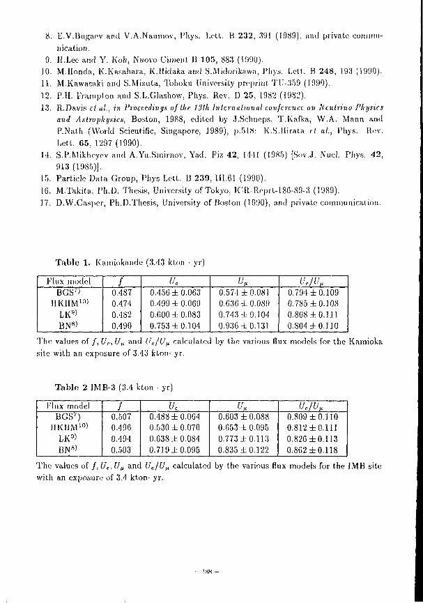
9. 10. 11. 12. 13.

14.

15. 1C. 17.

E.V.Bugaev and V.A.Nauniov, Phys. Lett. H 232, 391 (1989), and private commu­nication. H.Lee and Y. Koh, Nuovo Ciment B 105, 883 (1990). M.Honda, K.Kasahara, K.llidaka and S.Midorikawn, Phys. Lett. B 248, 193 (1990). M.Kawasaki and S.Mizula, Tohoku University preprint TU-359 (1990). P.H. Prampton and S.L.Glashow, Phys. Rev. D 25, 1982 (19S2). R.Davis ct ai, in Proceedings of the 13th Inlcrnational conference on Neutrino Physics and Astrophysics, Boston, 1988, edited by .l.Sclmeps, T.Kafka, W.A. Mann and P.Nath (World Scientific, Singapore, 1989), p.518: K.S.llirata el ai, Phy.s. Rev. Lett. 65, 1297 (1990). S.P.Mikheyev and A.Yu.Smirnov, Yad. Fiz 42, 1441 (1985) [Sov.J. Nucl. Phys. 42, 913 (1985)]. Particle Data Group, Phys Lett. B 239, III.C1 (1990). M.Takita, Ph.D. Thesis, University of Tokyo, ICR-Reprt-180-89-3 (1989). D.W.Casper, Pli.I).Thesis, University of Boston (1990), and private communication.

Tab ic 1. Kamiokande (3.43 kton • yr)

Flux model / uc u* Ur/Up BGS 7 ' 0.487 0.456 ± 0.063 0.574 ±0.081 0.794 ±0.109

HK1IM10> 0.474 0.499 ±0.069 0.636 ± 0.089 0.785 ±0.108 LK9' 0.482 0.600 ±0.083 0.743 ±0.104 0.808 ±0.111 BN8) 0.490 0.753 ±0.104 0.936 ±0.131 0.804 ±0.110

The values of / , {/<,, U^ and Ue/Un calculated by the various flux models for the Kamioka site with an exposure of 3.43 kton- yr.

Tab le 2 IMB-3 (3.4 kton • yr)

Flux model / uc u* Ue/U,, BGS7) 0.507 0.488 ± 0.004 0.603 ± 0.088 0.809 ±0.110

I1KHM10> 0.496 0.530 ±0.070 0.653 ± 0.095 0.812 ±0.111 LK9> 0.494 0.638 ±0.084 0.773 ±0.113 0.820 ±0.113 BN 8 ' 0.503 0.719 ±0.095 0.835 ±0.122 0.862 ±0.118

The values of / , Uf, Ufi and Uc/Ult calculated by the various flux models for the 1MB site with an exposure of 3.4 kton- yr.

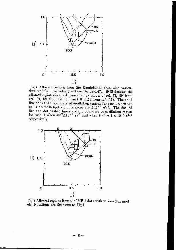
U u 0.5 -

Ue Fig.l Allowed regions from the Kamiokande data with various flux models. The value / is taken to be 0.474. BGS denotes the allowed region obtained from the flux model of ref. 8), BN from ref. 9), LK from ref. 10) and HKHM from ref. 11). The solid line shows the boundary of oscillation regions for case I when the neutrino-mass-squared differences are >,10 - 2 eV 2. The dashed line and dot-dashed line show the boundary of oscillation region for case II when 6m2,>10~2 eV 2 and when 6m2 = 1 x 10~4 eV2

respectively.

MS

Fig.2 Allowed regions from the IMB-3 data with various flux mod­els. Notations are the same as Fig.l.

- 1 8 9 -

Experimental Study of Atmospheric Electrons at Airplane Altitude*

R. Enomolo, J. Chiba, K. Ogawa, T. Sumiyoshi, F. Takasaki T. Kifune( a \ Y. MatsubaraW, and J. Nish imura^ c '

National Laboratory for High Energy Physio, Tsukuba 305, Japan (a'Institute for Cosmic Ray Research, Tanashi 305, Japan

^l Tokyo Institute of Technology, Meguro 152, Japan ( c)Institute for Space and Astronautical Science, Sagamihara 229, Japan

Abstract We have measured the atmospheric electron fluxes at airplane altitude. We loaded a lead-

glass-based electron telescope on a commercial cargo airplane. The experiment has been carried out using the air-route between Narita (Japan) and Sydney (Australia) and electron fluxes at various altitudes and latitudes have been measured. The thresholds of the electron energies were 1, 2, and 4 GeV. The results agreed with a simple estimation by one-dimensional shower theory. The atmospheric neutrino fluxes were evaluated with a simple assumption using these data, A comparison with Monte Carlo calculations was made.

1. Introduction

An airborne experiment to measure astronomical 7-ray has been carried out (VEGA Experiment). ' In the experiment, we measured the secondary elec­tron fluxes in the air cascade. Most of the events were those from atmospheric electrons initiated by primary hadrons. By measuring the atmospheric electrons precisely, we can determine the production rates of secondary neutral pions at various altitudes and latitudes systematically. The previous measurements were carried out using emulsion stacks and ion chambers J and systematic measure­ments have been awaited.

In recent days, information about hadron cascade in the atmosphere become important in order to estimate atmospheric neutrino fluxes. The underground experiments have reported discrepancies between the experimental vjt fluxes and

* Talk presented at 5-th Workshop on Elementary-Particle Picture of the Universe, lzu, Japan, 1990-Nov.

- 190-

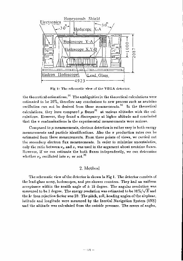
Electronics Honeycomb Shield

Fig 1: The schematic view of the VEGA clctpctor.

the theoretical estimations. The ambiguities in the theoretical calculations were estimated to be 20%, therefore any conclusions to new process such as neutrino oscillation can not be derived from these measurements. In the theoretical calculations, they have compared fi fluxes at various altitudes with the cal­culations. However, they found a discrepancy at higher altitude and concluded that the n contaminations in the experimental measurements were serious.

Compared to /t measurements, electron detection is rather easy in both energy measurements and particle identifications. Also the ir production rates can be estimated from these measurements. From these points of views, we carried out the secondary electron flux measurements. In order to minimize uncertainties, only the ratio between v,t and ue was used in the argument about neutrino fluxes. However, if we can estimate the both fluxes independently, we can determine whether vlt oscillated into vT or not.

2. Method

The schematic view of the detector is shown in Fig 1. The detector consists of the lead-glass array, hodoscopes, and pre-shower counters. They had an uniform acceptance within the zenith angle of ± 15 degree. The angular resolution was measured to be 1 degree. The energy resolution was estimated to be 10%/y/E and the lir iron rejection factor was 20. The pitch, roll, heading angles of the airplane, latitude and longitude were measured by the Inertial Navigation System (INS) and the altitude was calculated from the outside pressure. The errors of angles,

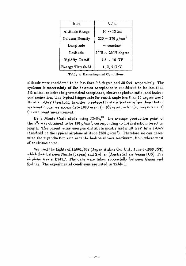
Item Value

Altitude Range 10 ~ 13 km

Column Density 220 ~ 270 g/cm2

Longitude ~ constant

Latitude 30°S ~ 20°N degree

Rigidity Cutoff 4.5 ~ 16 GV

Energy Threshold 1, 2, 4 GeV

Table 1: Experimental Conditions.

altitude were considered to be less than 0.5 degree and 50 feet, respectively. The systematic uncertainty of the detector acceptance is considered to be less than 5% which includes the geometrical acceptance, electron/photon ratio, and hadron contamination. The typical trigger rate for zenith angle less than 15 degree was 5 Hz at a 1-GeV threshold. In order to reduce the statistical error less than that of systematic one, we accumulate 1000 event (= 3% error, ~ 5 min. measurement) for one point measurement.

By a Monte Carlo study using EGS4, the average production point of the 7r°s was obtained to be 130 g/cm2, corresponding to 1.4 inelastic interaction length. The parent 7-ray energies distribute mostly under 10 GeV by a 1-GeV threshold at the typical airplane altitude (260 g/cm2). Therefore we can deter­mine the n production rate near the hadron shower maximum, from where most of neutrinos come.

We used the flights of JL661/662 (Japan Airline Co. Ltd., June-6-1989 JST) which flew between Narita (Japan) and Sydney (Australia) via Guam (US). The airplane was a B747F. The data were taken successfully between Guam and Sydney. The experimental conditions are listed in Table I.

- 192 -

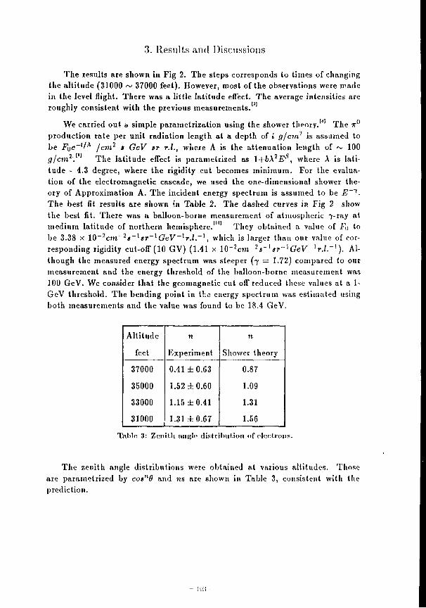
3. Results and Discussions

The results are shown in Fig 2. The steps corresponds to times of changing the altitude (31000 ~ 37000 feet). However, most of the observations were made in the level flight. There was a little latitude effect. The average intensities are roughly consistent with the previous measurements.

We carried out a simple parametrizalion using the shower thpory. The ir° production rate per unit radiation length at a depth of i g/cm? is assumed to be .F()e _ ( ' A / c m 2 * GeV sr r.l., where A is the attenuation length of ~ 100 g/cm2. The latitude effect is parametrized as 1+bX7E", where A is lati­tude - 4.3 degree, where the rigidity cut becomes minimum. For the evalua­tion of the electromagnetic cascade, we used the one-dimensional shower the­ory of Approximation A. The incident energy spectrum is assumed to be E~1. The best fit results are shown in Table 2. The dashed curves in Fig 2 show the best fit. There was a balloon-borne measurement of atmospheric 7-ray at medium latitude of northern hemisphere. They obtained a value of F{> to be 3.38 x 10~ 2 c77i - 2 «~ 1 «r~ 1 GeV~ 1 r .Z . - 1 , which is larger than our value of cor­responding rigidity cut-off (10 GV) (1.41 x l O ^ c m " 2 * " 1 sr~lGcV-lr.lr]). Al­though the measured energy spectrum was steeper (7 = 1.72) compared to out measurement and the energy threshold of the balloon-borne measurement was 100 GeV. We consider that the geomagnetic cut off reduced these values at a 1-GeV threshold. The bending point in the energy spectrum was estimated using both measurements and the value was found to be 18.4 GeV.

Altitude n 71

feet Experiment Shower theory

37000 0.41 ±0.63 0.87

35000 1.52 ±0.60 1.09

33000 1.15 ±0.41 1.31

31000 1.31 ±0.67 1.56

Table 3: Zenith angle distribution of electrons.

The zenith angle distributions were obtained at various altitudes. Those are parametrized by cosn0 and 71s ate shown in Table 3, consistent with the prediction.

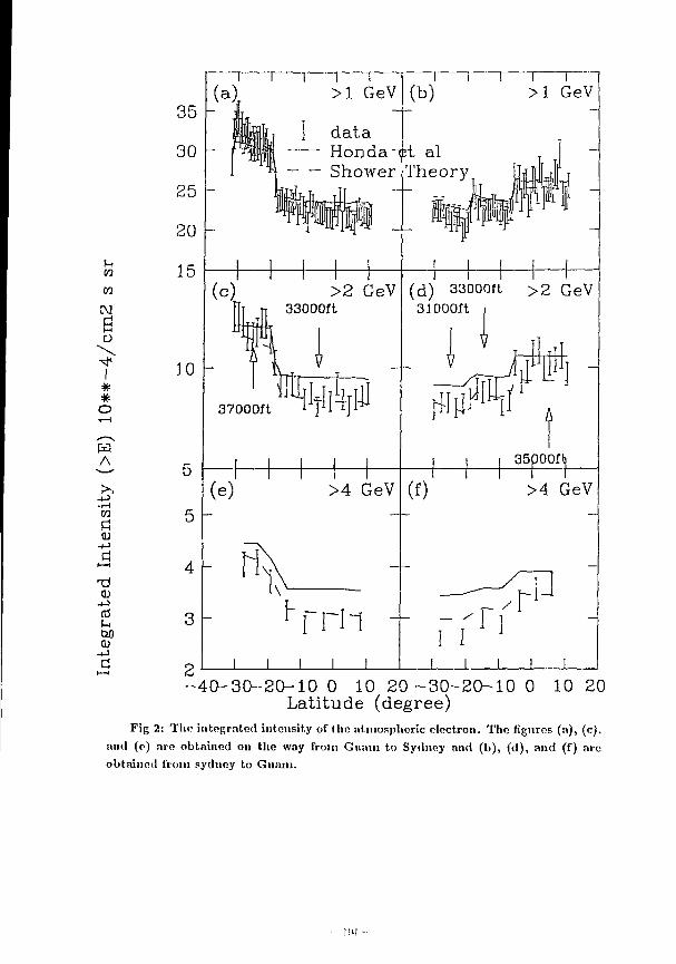
w w

C\2

B

I # # o A

-1-3 •r-i w

CD -i-J (0

CD

35

30

25

20

15

>1 GeV

I data — Honda - — Shower

(c)

10

5

5

4

3

>2 GeV TT 33000ft

37000ft

(e)

- n >4 GeV

S-PI rm J I I I L

00 "1 1 — >1 GeV

( d ) 33000ft > 2 GeV 31000ft

ftil*1/, iwP 35000f

(f)

pOOftj

> 4 GeV

J L - 4 0 - 3 0 - 2 0 - 1 0 0 10 2 0 - 3 0 - 2 0 - 1 0 0 10 20

La t i tude (degree) Fig 2: The integrated intensity of the atmospheric electron. The figures (a), (c).

and (e) are obtained on the way from Guam to Sydney and (b), (d), and (f) are obtained from Sydney to Guam.

KM -

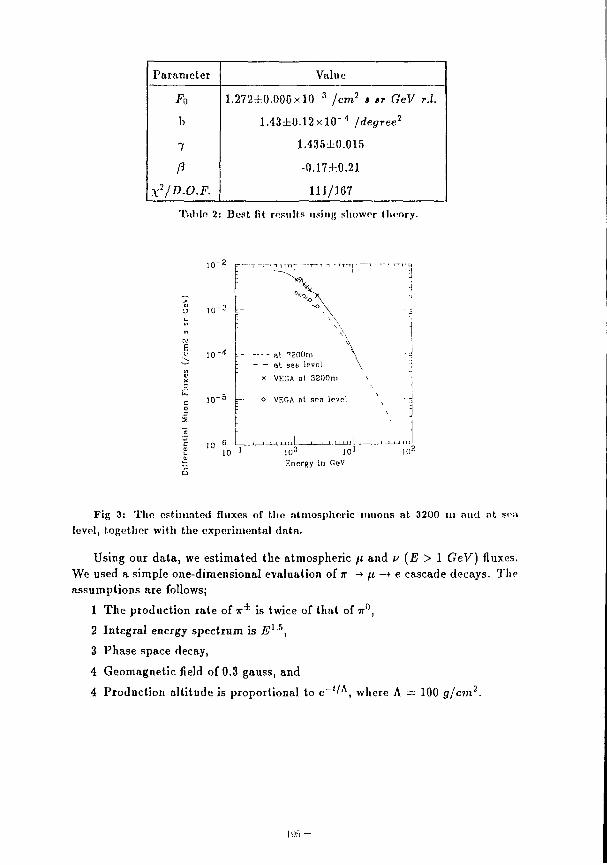
Parameter Value

^ 0 1.272±0.000xKr 3 /cm2 s »r GeV r.l.

b l.n±QA2xlO~A /degree2

7 1.435±0.015

P -0.17±0.21

X'/D.O.F. 111/167

Table 2: Best lit results using shower theory.

s\

- - - al ^200in • - a t sea level

x VEGA al 3200m

° VEGA nt sna level

10 u I 0 1

Energy in GeV

Fig 3: The est imated fluxes of the atmospheric unions at 3200 tn and at sea level, together with the exper imental da ta .

Using our data, we estimated the atmospheric // and v (E > 1 GeV) fluxes. We used a simple one-dimensional evaluation of TT -» fi —* e cascade decays. The assumptions are follows;

1 The production rate of TT* is twice of that of 7r°,

2 Integral energy spectrum is E l h ,

3 Phase space decay,

4 Geomagnetic field of 0.3 gauss, and

4 Production altitude is proportional to e _ l / , A , where A = 100 g/crn2.

- I!)<i

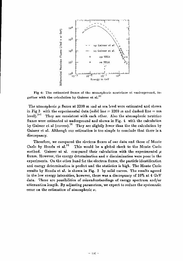
10" > <V O L.

w 1 0 3

CM

£

X

o S 10= 3 W

Z

1 10° -f ? -1 0 C 1 0 " 3 1 0 ~ z 10 ' 1 0 u

tj Energy in GeV

s

Fig 4: The estimated fluxes of the atmospheric neutrinos at underground, to­gether with the calculation by Gaisser et al. *

The atmospheric fi fluxes at 3200 m and at sea level were estimated and shown in Fig 3 with the experimental data (solid line = 3200 m and dashed line = sea level)."" They are consistent with each other. Also the atmospheric neutrino fluxes were estimated at underground and shown in Fig. 4 with the calculation by Gaisser et al (curves). They are slightly lower than the the calculation by Gaisser et al. Although our estimation is too simple to conclude that there is a discrepancy.

Therefore, we compared the electron fluxes of our data and those of Monte Carlo by Honda et al. This would be a global check to the Monte Carlo method. Gaisser at al. compared their calculation with the experimental fi fluxes. However, the energy determination and K discrimination were poor in the experiments. On the other hand for the electron fluxes, the particle identification and energy determination is perfect and the statistics is high. The Monte Carlo results by Honda et al. is shown in Fig. 2 by solid curves. The results agreed in the low energy intensities, however, there was a discrepancy of 10% at 4 GeV data. There are possibilities of misunderstandings of energy spectrum and/or attenuation length. By adjusting parameters, we expect to reduce the systematic error on the estimation of atmospheric v.

vfi Gaisscr et. el.

z>e Gaisser eL al.

ufi VEGA

i/e VEGA

- Hl(i —

4. Conclusion

We have carried out the systematic measurement of the atmospheric elec­trons at various energies, altitudes, and latitudes. The statistical error of our measurement is typically 3% and the systematic error was estimated to be less than 5%. The intensities agree with the simple calculation using one-dimensional shower theory. The estimations of (i and v fluxes have been carried out. The /i fluxes agreed with the previous measurements. Also a global test with the Monte Carlo calculation have been carried out and there was a disagreement at the higher energy data. By adjusting parameters in the Monte Carlo using our data, we expect to reduce the systematic error on the estimation of atmospheric v fluxes.

In addition, an airborne experiment for /i-measurement is urgently needed, because a direct estimation for i/-fluxes is possible. In this experiment, particle identification and precise momentum measurement are necessary.

ACKNOWLEDGED ENTS

We appreciate supports from Prof. H. Sugawara, Prof. K. Kikuchi, Prof. K. Takahashi, Prof. S. Iwata, Mr. Y. Ukita (KEK), Prof. J. Arafune (ICRIl), Dr. Y. Takahashi (NASA/Alabama), Prof. T. Kamae, Dr. T. Takahashi (Univ. of Tokyo) in proceeding this experiment. We deeply appreciate Dr. M. Honda (ICRR) for the offer of the Monte Carlo results. We thank Mr. T. Hakamada of Hamamatsu Photonics K. K. for cooperation. Finally we deeply appreciate Mr. N. Iizuka (Japan Air Line Co. Ltd.) for substantial help an:', cooperation.

- 107 -

KKFERKNCKS

1. R. Enomoto et al., Nucl. Instr. Meth., A295 (1990) 201-267; R. Enomoto et al., Phys. Rev. Lett., Vol. 64 (1990) 2603-2G06.

2. L. T. Baradzei et al., J. Phys. Soc. Japan. 17, Suppl. A-III, 433 (1961); J. Duthie et al., Nuovo Cim., 24, 122 (1962); L. T. Baradzei et al., Proc. Int. Conf. on Cosmic Rays at Jaipur, 5, 283 (19G3).

3. K. S. Hirata et al., Phys. Lett. B205 (1988) 410.; D. Casper et a)., BU-IIEP-90-23, submitted to Phys. Rev. Lett.

4. T. K. Gaisser et al., Pliys. Rev. Lett., 51 (1983) 223; T. K. Gaisser et al., Pltys. Rev. D38 (1988) 85; M. Honda et al., Phys. Lett. B248 (1990) 193.

5. M. Conversi, Phys. Rev. 79 (1950) 749.

6. J. Learned et al., Phys. Lett., B207 (1988) 79; V. Barger et al., Phys. Lett., B209 (1988) 3G5; K. Hidaka et al., Phys. Rev. Lett., Gl (1988) 1537.

7. W. R. Nelson et al., SLAC-Report-265 (1985), unpublished.

8. J. Nishimura, Hand Book der Physik, 46 (19G7) p. 1, Springer Verlng.

9. S. Hayakawa, "Cosmic Ray Physics", New York, Wiley (19C9).

10. J. Nishirnura et al., Astro. Phys. J., 238 (1980) 394.

11. J. Pine ci al., Nuovo Cim., 14 (1959) 118; F. Ashton et al., Nature, 185 (1969) 354; W. Pak el al., Phys. Rev., 121 (1961) 905; G. Brooke et al., Proc. Phys. Soc. (London), 83 (1904) 853.

E X P E R I M E N T A L RESULTS O B T A I N E D F R O M T H E A K E N O G I A N T A I R S H O W E R A R R A Y

Pre sen t ed by M. Tesliima

(AGASA collaboration) 1

A B S T R A C T The energy spectrum of the highest energy cosmic rays and the neutral emis­

sion from Cyg X-3 are studied using the data from Akeno ]km2 array, Akeno 20km2 array and AGASA (Akeno Giant Air Shower Array) of ]0tU-m2. The ob­served energy spectrum implies structures. It becomes sleeper above ID" ' 'el ' and becomes flatter again above 10 1 9eV. The exponents of spectra below lOi7*eV, between 10 1 7 8 eK and 1 0 1 9 0 e l / and above 10 1 9 0 el ' ' are 3.02 ± 0.02( \kvr anay), 3.24±0.18(l£m 2)/3.20±0.09(20fcm 2) and 2.<M±0.52 {20km2), respectively. These structures may be closely related to the origin of the highest energy cosmic rays. Using data from the 20km2 array, we found excess showers from the direction of Cyg X-3. This excess corresponds to a flux of (1.8 ± 0.7) x 10~ 1 7 cm~ 2 s~ ! above 5 x 10l7eV. The search for neutral emission from Cyg X-3 has been continued using AGASA data. At present, we do not obtain the independent confirmation of DC-excess in the new data. However we observed an event rate increase from the direction of Cyg X-3 in April of 1990.

'T.Hara 1 , K.IIashimoto3, N.Hayashida1, K.Honda2, M.Honda1, N.Ijioje3, F.Ishikawa1, F Kal-- moto\ K.Kamata 5, S.Kawaguclu8, N.Kawasumi3, T.Kifune1, Y-Matsubara*, K.Murakami7. M.Nagano1, S.Ogio1. Il.Oiiolta1, To.Saito1, M.Sakata8, I.Tsusliima2, M.Teshima1, T.Umezawa4, Y-Yamaiiiots" S.Yushida4. an.] H.Yoshii9

(l)Institute for Cosmic Ray Research, University of Tokyo, Tokyo 188, Japan (2)Faculty of Education, Yamanashi University, Koju 400, Japan (3)Department of Physics, Saitama University, Urawa 388, Japan (4)De.partmenl oj Physics, Tokyo Institute oj Technology, Ohokayama. Megxtro-ku, 7'oh.. 1$£, .'-.;pau (S)Nishina Memorial Foundation, Tokyo, Japan (6)Faculty oj General Education, Hirosaki University, Ilirosaki 036, Japan (l)Solar Terrestrial Environment Laboratory, Nagoya University, Nagoya 464-01, Japan (S)Department o] Physics, Konan University, Kohe 658, Japan (S) Faculty oj General Education, Ehime University, Matsuyama 190, Japan

- 199-

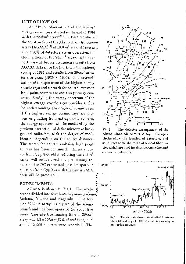
I N T R O D U C T I O N At Akeno, observations of the highest

energy cosmic rays started in the end of 1984 with Die "20Aw2 array"' 1). In 1987, we started the construction of the Akeno Giant Air Shower Array (AGASA) ( 2 ) of lOOfcm2 area. At present, about 90% of detectors are in operation, in­cluding those of the 20fcm2 array. In this re­port, we will discuss preliminary results from AG ASA data since the (northern hemisphere) spring of 1991 and results from 20km2 array for five years (1985 ~ 1990). The determi­nation of the spectrum of the highest energy cosmic rays and a search for neutral emission from point sources are our two primary con­cerns. Studying the energy spectrum of the highest energy cosmic rays provides a clue for understanding the origin of cosmic rays. If the highest energy cosmic rays are pro­tons originating from extragalactic sources, the energy spectrum will be modified by the protons interaction with the microwave back­ground radiation, with the degree of mod­ification depending on the source distance. The search for neutral emission from point sources has been continued. Excess show­ers from Cyg X-3, obtained using the 20km2

array, will be reviewed and preliminary re­sults on the DC-excess and possible sporadic emission from Cyg X-3 with the new AGASA data will be presented. a

Fig.l The detector arrangement of the Akcno (Jiant Air Shower Array. The open circles show the location of detectors, and solid lines show the route of optical fiber ca­bles which are used for data transmission and control of detectors.

100.00 -

E X P E R I M E N T S £ AGASA is shown in Fig.l. The whole o

area is divided into four branches named Akeno, Sudama, Takane and Nagasaka. The for­mer "20A:7?i2 array" is a part of the Akeno branch and has been operated for about five .3'cars. The effective running time of 20km2

array was 1.2 x 10 8sec (82% of real time) and about 12,000 showers were recorded. The

50 .00

Sudjms(Jul.30)

T>kmc(Jun.21)

Akcno(Fcb.7)

.00 50.00 100.00 150.00

mjd-47939 Fig.2 The daily air shoiver rale of AGASA between Feb. 1990 and August 1990. The rate is increasing as construction continues.

• 2 0 0 -

u c Q) D CT 10. 0)

. . , , , . 1 . i • • • • i • •

• E.p t i imt . i t

:' 1-1 Simulation

- r1' '1 ^ >. _ .twill '.

operation with the new data acquisition system (OS-9 system) started in February 1990 at the Akeno Branch, in May at Nagasaka, in June at Takane and in July at the Sudania branches successively. The daily air shower rate between Feb. 1990 and Aug. 1990 is shown in Fig.2. More than 14,000 showers were recorded above 10 1 7eK in the first six months operation. This is because the energy threshold of AGASA is lower than that of 20km2 array by a factor of 2 ~ 3. The effective exposure (SQT) for 10 1 8cV cosmic rays in the present analysis by AGASA is about one fourth of that of 20km2 array.

P E R F O R M A N C E O F A G A S A The densely equipped lkm2 array ( 3 ) is

located in the east corner of the 20km2 array. ^ We can estimate the accuracy of arrival di­rection and energy determination of AGASA by comparing the air shower parameters ob­tained by the 20hn2 array with those of the lkm2 array for ~ 10 I 8 eV showers with core locations inside the lkm2 array. o.oi

Fig.3 shows the distance distribution be­tween core locations determined by the 20km2

array and the lkm2 array. Since the error in the core determination for the 1km2 array is negligible compared with that of the 20km2

array, the average error of 50m is mainly due to the core determination error of the 20km2

array. The distribution agrees with the re­sult obtained from a Monte Carlo simulation, shown in the same figure. Fig.4 shows the space angle between arrival directions deter­mined by both arrays, and the distribution is consistent with the assumption that an­gular resolutions are ~ 3.0° in both arrays for cosmic rays of ~ 10 1 8eV. In this figure, the histogram show the expected distribution obtained by Monte Carlo simulation.

For showers observed by the 20km2 ar- o. oo ray, the observable 5(600), which is the lo­cal density at core distance 600m, is used to estimate the primary energy of cosmic rays. We carried out a Monte Carlo simulation to obtain the following relation between the pri-

0.00 1.00 2.00 3.00

Log (Core Separa t i on ) (m) Fig.3 The distribution of the distance between the coie determined by 20km' array and that of the U r n 1

array. The accuracy of the core determination for the 2 0 t m ' array is estimated to be ~ 50m for cosmic rays of I0 ' "e l ' .

30.00 -

>-o Si 20.00 -n a UJ re tt-

J " 1 1

10. 00 -

•

• Experiment

,—. Simulation

11 LJ^hiA^L-. 0 0 1 0 . 0 0 15 .00

OPENING ANGLE ( d e g r e e )

Kg.4 The distribution of the space angle between arrival directions determined by the 20km7 array and the lkm3 array. The accuracies of the arrival direction determination for both arrays is estimated to be ~ 3.0* for cosmic rays of ]0'"eV.

~ 2 0 ! -

mary energy and S(GOO) (Dai et al.W):

E2a = 2.0 x J0 1 75ty(G00) 1 0eK o

Here Sv{G00) is the local density for vertical « showers. The intrinsic fluctuation of Sv(600) <u for fixed primary energy cosmic rays is found "-to be 20% ~ 30% in the Monte Carlo simu­lation.

On the other hand, for the Ikm2 array data, the energy is estimated from the total number of electrons {Ne). Following conver­sion is used for the energy determination,

2?, = 3 . 9 x l O I 5 ( t f e / l 0 6 ) a 9 e K

10" 10' Log(E20/EI)

Fig.5 The ratio of energy determined by the 2Ufcm3

array to that of the l i m 3 array. The accuracy of energy determination by 20km* array is estimated to be lesr than 40%.

Fig.5 shows the ratio E20/Ei for showers with cores inside the Ikm2 array. The standard deviation of this distribution is ~ 40%. The accuracy of energy estimation in each array is found to be ~ 30% for cosmic rays of 10 1 8eV\

E N E R G Y S P E C T R U M Since the observable S(600) depends on not only primary energy but also zenith angle

(atmospheric depth), we must convert S(600) to the vertical density Sv(600). Experimen­tally, the attenuation length of S(600) in the atmosphere is well fitted to the exponential function with the decay constant of A = (500±30)<//cm 2 for 10 1 8eV air showers. Though the attenuation length may be weakly energy dependent (becomes larger with energy increment), our data does not show any significant dependence. Hence we use the con­stant value 500g/cm7 irrespective of energy. The vertical density at core distance 600m is obtained as follows:

Sf(600) = S(6Q0)exp{t - to/A),

to = 920g/cm2, A = 500g/cm2

Fig.G shows the acceptance of the 20km2 ar­ray which is estimated by Monte Carlo simu­lation. It is strongly energy dependent below i o , 8 e y .

The number of observed events above 10 1 7eV is about 1200 in the 5 years of the 20km2 array. The modal energy is 5 x l 0 i r e K . Until August 1990 the highest energy event

LOC(CO)

Fig.G The acceptance of the Akeno 20*m 1 array ob­tained by Monle Carlo simulation. The icnith angle is limited to S less than •15".

2CCQC0

o O

° O ° > n O ° °

O o O o

—«X,00 -20O1C0

X(m)

RUN=05044 EVE=0021 TIME=(86I023 , 142515)

HIT=23 S6Q0=2.23 Ne=10.08 Eo=19.73 XC=-1572.90 YC=-1137.4C| ZEN=31.53 AZM=129.18 RA=211.70 DEC=50.66 ER0=1.99 ERS=4.44

mniFPM

l l l t n l Ol i l r lb . l l

1J3) 2IXI ICO 4CD

core d i s t a n c e Log(R)

Fig.7 The highest energy event observed at Akeno to Aug. 1990. Upper left: the height of the bar represents the logarithm of observed electron density in each detector. Upper right: the height of the bar represents the arrival time delay of shower particles. We can see shower front and its curvature. Lower left: The diameter of the circle represents the logarithm of observed density in each detector. Lower right: The observed lateral distribution of electron density, and the fitted curve.

25. 50

2 5 . 0 0

- Akeno 20km2 array (Sep.1984-Feb.1989)

CO

LU

W 24. 50

bO o 24. 00

- i i 1 i -i 1 I r

* t t * * * N * | • • • t m t

23. 50. - I I I L. -1 I I I -

17.00 18.00 19.00 20.00

l og (p r ima ry energy)

Fig.8 The energy spectrum obtained by dividing the energy distribution by the accep­tance.

25. 50

£ p 25. 00 LU X

UJ 24. 50

u_ hO O

24. 00

23. 50

i i i i i i i • i i

HI

16.00 18.00 20.00

l og ( p r ima ry energy) Fig.9 The combined energy spectra observed by the Akeno 2Qkm2 and Ikm7 arrays. The closed circles and closed squares arc 20km7 array data and updated lkm2 array data, respectively. The open circles are the Ikm1 data already published' 4 '.

- 2(M

observed, shown in Fig.7, had an energy of 10 1 9 - 8 eV. By dividing the observed counts by the acceptance and the running time of 1.3 x 10 8s,

the differential energy spectrum is obtained, as shown in Fig.8. Error bars correspond to 90% confidence level. Though the statistics are not enough, the spectrum seems to show some structure, with bendings at ~ 10 ) 8eK and ~ 10 l s eK. The spectrum becomes steeper around W18eV and becomes flatter again above 1019eV. It should be noted that the obtained spectrum can also be fitted with a single power law between 10175eV ~ 10 1 9 5 eV. In Fig.9, energy spectra observed by the 20&?n2 array and the lkm2 array are plotted. The closed circles are 20km2 array data, the open circles are already published' 5 ' lkm2

data, and the closed squares are updated lkm2 array results based on 8 years of operation. There is a slight difference in the absolute flux around 10 1 8eV between 20km2 and lkm2

data. Tliis difference can be removed by changing the energy conversion factor by 20%. Since the systematic errors in the energy estimation are not calibrated, this difference is not important. It should be remarked that both data support the steepening at around 10 I 8 eK. Since in the case of the 20km2 array data, the acceptance is energy dependent, there remain some uncertainties in the interpretation of the bending. However, in the case of the lkm2 array (closed square data), the acceptance is constant over the whole energy range and is free from systematic errors, though the statistics are low. The energy spectra obtained by the 20km2 and the 1A??12 arrays between 10 1 7 8 eV and 10 1 9eV can be fitted by the power laws with exponents of 3.20 ± 0.09 and 3.24 ± 0.18, respectively. On the other hand, below 10 1 7 , 8 eV the energy spectrum can be fitted with an exponent of 3.02 ± 0.02. And above 10 1 9eK, it can be fitted with an exponent of 2.44 ± 0.52.

Statistically the existence of the bendings in the energy spectrum at 10 1 8eV and 10 1 9eV are not significant enough to be beyond doubt. However, if these structures are real, they may be closely related to the origin of the highest energy cosmic rays.

N E U T R A L E M I S S I O N F R O M C Y G N U S X-3 I . D a t a from t h e Akeno 2 0 k m 2 a r r a y ( 6 )

We have searched for point sources at EeV energies using data from the 20fc?n2 array from December 1984 to July 1989. In the present analysis, we used only the 3, 922 showers which had cores inside the array, zenith angles smaller than 45°, and primary energies above 5 x 10 i r eV.

In order to find DC excess peaks in the celestial sphere, we employed a similar method to that developed by the Fly's Eye g roup^ . The error function with a is applied to the direction of each shower, and the event fraction is calculated in each cell (1° x 1°) of the celestial sphere around the shower direction. Then, the fractions are summed for each cell in equatorial coordinates. The error in the determination of the arrival direction was taken to be 3 3 x sec8 for each shower, where 0 is the zenith angle.

In Fig. 10, the significance of the density excess is mapped for the whole celestial sphere. Among about 1000 independent areas (there are about 1000 cones of 3° half angle), there are two regions showing a deviation greater than 3CT. The most significant

- 2 0 5 -

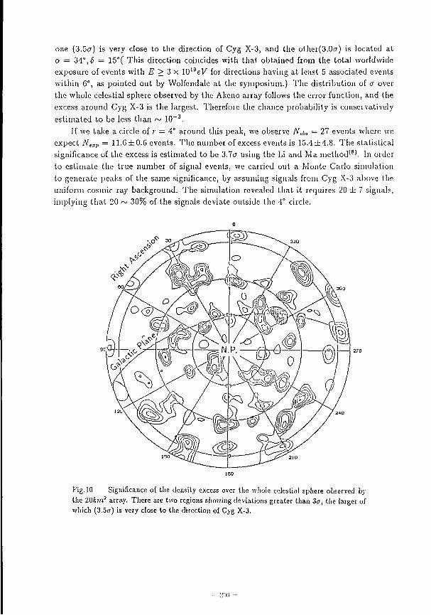
one (3.5a) is very close to the direction of Cyg X-3, and the other(3.0(j) is located at a = 34°, 6 = 15°( This direction coincides with that obtained from the total worldwide exposure of events with E > 3 x 10 1 9e V for directions having at least 5 associated events within 6°, as pointed out by Wolfendale at the symposium.) The distribution of a over the whole celestial sphere observed by the Akeno array follows the error function, and the excess around Cyg X-3 is the largest. Therefore the chance probability is conservatively estimated to be less than ~ 10~ 3.

If we take a circle of r = 4° around this peak, we observe N0i, = 27 events where we expect Ncxp = 1 l.C ± 0.6 events. The number of excess events is 15.4 ±4.8 . The statistical significance of the excess is estimated to be 3.7a using the Li and Ma method' 8 ' . In order to estimate the true number of signal events, we carried out a Monte Carlo simulation to generate peaks of the same significance, by assuming signals from Cyg X-3 above the uniform cosmic ray background. The simulation revealed that it requires 20 ± 7 signals, implying that 20 ~ 30% of the signals deviate outside the 4° circle.

ico

Fig. 10 Significance of the density excess over the whole celestial sphere observed by the 20Am3 array. There are two regions showing deviations greater than 3<7, the larger of which (3.5CT) is very close to the direction of Cyg X-3.

• - L'IKi -

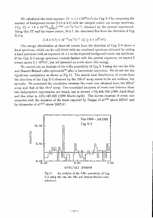
We calculated the total exposure ST = 1.1 x 1018c??i3s for Cyg X-3 by comparing the number of background events (11.G ± O.G) with the integral cosmic ray energy spectrum, f(> E) = 1.6 x 10" 1 6 ( j j j i f^7) - 2 , 0 8 cm"2s~2sr"1, obtained by the present experiment. Using this ST and the excess counts, 20 ± 7 , the associated flux from the direction of Cyg X-3 is

(1.8 ± 0.7) x 10" , 7C7? 1~ 2s~ 1 ( I i > 5 x 10 1 7eK).

The energy distribution of observed events from the direction of Cyg X-3 shows a hard spectrum, which can be well fitted with the combined spectrum obtained by adding a hard spectrum with an exponent of-1.1 to the expected backgound cosmic ray spectrum. If the Cyg X-3 energy spectrum extends further with the present exponent, we expect 5 events above 3 x 10 1 8eK, but we'observed no event above this energy.

We carried out an analysis of the 4.8hr periodicity of Cyg X-3 using the van der Klis and Bonnct-Bidaud cubic ephemeris ( 9 ) after a baryceutric correction. We do not see any significant modulation as shown in Fig.U. The arrival time distribution of events from the direction of the Cyg X-3 observed by the 20km2 array seems to be not uniform, but sporadic. We examined the correlation between the event rate obtained from the 20km array and that of the lkm2 array. Two correlated increases of event rate between these two independent experiments are found; one is around JD2,446, 550 (1986 April-May) and the other is J£>2,447, 620 (1989 March-April). The former increase of event rale coincides with the duration of the burst reported by Dingus et alS10) above 50TeV and by Alexeen ko et alSn) above 200TeV.

w +-» c o (J

10. 00

5.00

o. oc

fUlfl

Sep.1984- Jul.1989 Cyg X-3

n Hh=ft=F

00 0. 50 o r b i t a l phase

u:

1. 00

Fig.11 An analysis of the 4.81ir periodicity of Cyg X-3 using the van der Klis and Bonnet-Bidaud cubic ephemcris.

- 207 -

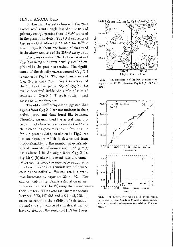
I I .New A G A S A D a t a Of the 14553 events observed, the 2822

events with zenith angle less than 45.0° and primary energy greater than 10 1 7eK are used in the present analysis. The total exposure of this new observation by AGASA for 10 1 8eV cosmic rays is about one fourth of that used in the above analysis of the 20fc?n2 array data.

First, we examined the DC excess about Cyg X-3 using the event density method ex­plained in the previous section. The signifi­cance of the density excess around Cyg X-3 is shown in Fig.12. The significance around Cyg X-3 is only 2.0a. We also examined the 4.8 hr orbital periodicity of Cyg X-3 for events observed inside the circle of r = 8° centered on Cyg X-3. There is no significant excess in phase diagram.

The old 20/cm2 array data suggested that signals from Cyg X-3 are not uniform in their arrival time, and show burst like features. Therefore we examined the arrival time dis­tribution of observed events inside the 8° cir­cle. Since the exposure is not uniform in time for the present data, as shown in Fig.2, we use an exposure which is determined from proportionality to the number of events ob­served from the ofT-source region 8° < 8 < 24° (where 8 is the angle from Cyg X-3). Fig. 13(a),(b) show the event rate and cumu­lative counts from the on-source region as a function of exposure (cumulative off source counts) respectively. We can see the event rale increases at exposure 20 ~ 30. The chance probability of such a deviation occur­ring is estimated to be 1% using the Kolmogorov-Snurnov test. This event rate increase occurs between JD2, 44T, 985 and JZ>2,448,005. In order to examine the validity of this analy­sis and the significance of this deviation, we have carried out the same test (KS lest) over

R i g h t A s c e n s i o n

Fig. 12 The significance of llic density excess al en­ergies above l O ' ^ K cenlciecJ on C jg X-3 (AGASA new data) .

£ 30. oo

. i • • ' ! ' • • • I • i • • |

- Feb.1990-Auj.1990 Cyg X.3

(*) i

/ / ^

-

•4., . , . . . . ( . . . 60. 00 J00. 00 150. 00 200. 00

exposure

- <i>)

T - — n i j 3 - ftrT -

0. 00 50. 00 100. 00 150. 00 200. 00

exposure

Fig. 13 (a) Cumulative counts and (bj event rales in the on source region (inside an 8* circle centered on Cyg X-3) as a function of exposure (cumulative off source counts).

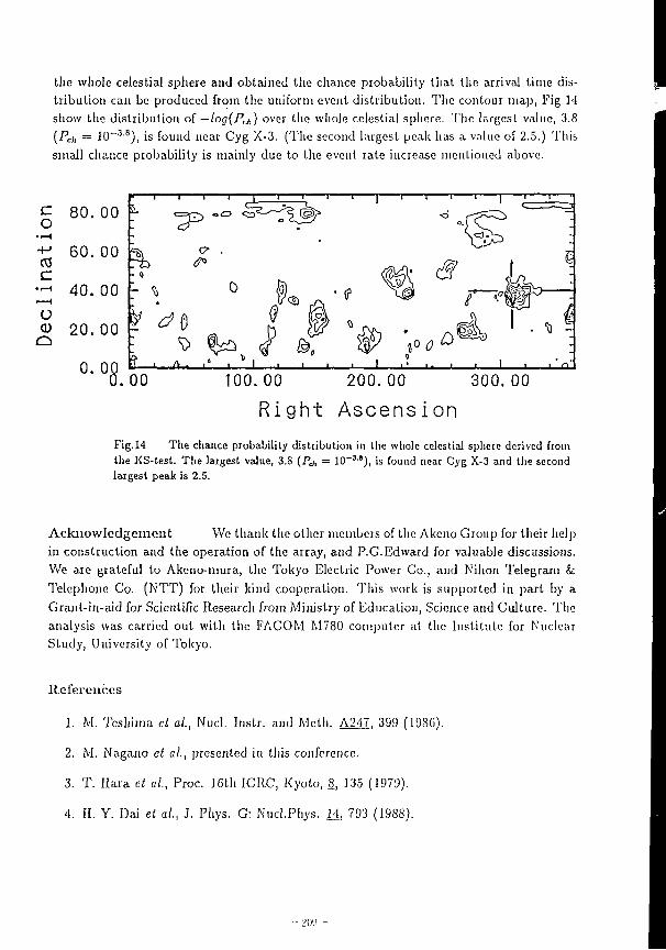
the whole celestial sphere and obtained the chance probability that the arrival time dis­tribution can be produced from the uniform event distribution. The contour map, Fig. 14 show the distribution of — log(Prj,) over the whole celestial sphere. The largest value, 3.8 (Pcll = 1 0 - 3 ' 8 ) , is found near Cyg X-3. (The second largest peak has a value of 2.5.) This small chance probability is mainly due to the event rate increase mentioned above.

f 1 1 ' i c 80. 00 ^ *=& - o «»•

•H 60. 00 c &

u <D 2 0 . 0 0 o

0. 0 8.

-i 1 r

O

<7*

40. 00 r *

L A • • '

00 1.00.00 200.00 300.00

R i g h t Ascens ion Fig.14 The chance probability distribution in the whole celestial sphere derived from the KS-test. The largest value, 3.8 (/>* = lO - " ) , is found near Cyg X-3 and the second largest peak is 2.5.

Acknowledgemen t We thank the other members of the Akeno Group for their help in construction and the operation of the array, and P.G.Edward for valuable discussions. We are grateful to Akeno-mura, the Tokyo Electric Power Co., and Nihon Telegram & Telephone Co. (NTT) for their kind cooperation. This work is supported in part by a Grant-in-aid for Scientific Researcli from Ministry of Education, Science and Culture. The analysis was carried out with the FACOM M780 computer at the Institute for Nuclear Study, University of Tokyo.

References

1. M. Tesliima et al., Nucl. Instr. and Mcth. A247, 399 (l'JSG).

2. M. Nagano et al., presented in this conference.

3. T. Hara et al., Proc. 16th 1CRC, Kyoto, 8, 135 (1979).

4. II. Y. Dai el al., J. Phys. G: Nucl.Phys. H, 793 (19S8).

5. M. Nagano et al, J. Phys. G: Nucl.Phys. 10, 1295 (1984)

6. M. Teshima et al, Phys. Rev. Lett. 64, 1628 (1990).

7. G. L. Cassiday et al., Phys. Rev. Lett. 62, 383 (1988).

8. T. P. Li and Y. Q. Ma, Astrophys. J. 272, 317 (1983).

9. M. van der Klis and J. M. Bonnet-Bidaud, Astron. Astrophys. 214, 203 (1989).

10. B. L. Dingus et al., Phys. Rev. Lett. 60, 1785 (19S8).

11. V. V. Alexeenko et al, Proc. 20th ICRC, Moscow I, 219 (1987).

Recent Status of CANGAROO Project

The CANGAROO Collaboration

presented by

T.Tanimori

Department of Physics, Tokyo Institute of Technolof/y, Tokyo 152, Japan

Abstract

Recently the existence of steady TeV gamma-ray emission from the drab Nebula has been confirmed by the Whipple group, and the effectiveness of the imaging technique for air Cherenkov obervation is shown in identifying gamma-ray signals against the cosmic ray background. The future stereoscopic observation with more than two telescopes is expected to further improve the sensitivity of the imaging technique. The d'ANGAKOO project, a collaboration between a number of Japanese institutions and the University of Adelaide, are employing both of the imaging technique and stereoscopic observation at Wooinera, Aust ralia. In particular, Japanese telescope, which consists of the telescope with good surface quality and the imaging camera, of the finest resolution, compared with the other 1'eY telescopes, is expected to provide the fineset iamgc of air showers. The main purpose of this paper is to describe the features of imaging camera and electronics of the Japanese telescope.

1. Introduction

The existence of astrophysical very high energy gamma-ray from a point-like source has been recently confirmed by the detection of TeV gamma-ray from drab Nebula with a tremen­dous significance of 25 ov 1 ' This detection by Whipple obsevatory has demonstrated the drastic usefulness of the imaging technique in air dherenkov fur the observation of very high energy gamma-ray. Until now, the observation of the nstrophysical energetic gamma-ray has been carried out with the satellite and ballon-bone, to detect many point sources. In the energy region of TeV gamma-ray, a number of claims have been done for the emission of

-211 ~

gamma-rays from X-ray binaries and pulscrs to encourage the models of the acceleration of cosmic rays in such sources.'2' However, these observations arc biased to detect pulsic .signals of known periodicity. The marginal statistical significance, together with the lack of evidence to detect excess of the events from the source, can not. deny the schepticisin on its credibility, and seems to be insufficinent to establish the very high energy gamma-ray astronomy.

On such a stalemate of the situation, the new technique of the imaging of air Cheronkov light provides us with both a good angular accuracy of a lew minutes of arc and good discrimination of the gamma-rays from the overwhelming background of hadronic shower events. The imaging technique will be capable of opening and establishing a new window of TcV gamma-ray astronomy.'3'

Now we are constructing the new TeV gamma-ray telescope with the high resolution imaging camera at. Woomera in Australia. In the southern hemisphere, (here exist a number of interesting potential sources, for example, Galactic center. X-ray pulscrs more than in the northern hemisphere. Table 1 compares the number of objects which may emit. TeV gamma-rays in both the northern and southern hemispheres.'''. Our telescope will be the first imaging telescope to observe these interesting point sources in the southern hemisphere.

This project is a collaboration with University of Adelaide which has a B1GRAT air Cherenkov Telescope at Woomera Australia.'''' We now have a plan of the stereoscopic obei-vation using Japanese telescope and BIGRAT for the simultanous observation of lite same opint sources. As well as an imaging technique, stereoscopic observation is expected to be very powerful for the improvement of both the pointing accuracy and the discrimination of gamma-ray induced showers.'6'

In 1991 March, Gamma Ray Observatory satellite (GftO) has been launched, which will add more data below 100 GeV to gamma-ray astronomy. The new qualified data of TcV gamma-ray will co-work with the satellite data to understand the mechanism of high energy phenomena taking place in peculiar astrophysic.nl objects.

2. CANGAROO Project

Cosmic rays initiate extensive air showers in the upper atmosphere, and air Cherenkov light emitted from the showers is detected by ground-based telescopes. The shape of the shower is extended with different shapes dependent on the species of initiating paricles, and, thus, the image of the Cherenkov light emitted from the showers is also expected to have this difference. By measuring the shower mage and analysing the shape of the image, it enables us to improve the angular resolution of the arrival direction of gamma-rays and the discrim­ination of the background of hadronic showers. Furthermore, the simultenious obervations with more than two telescopes for same showers, combined with the imaging techniqe, are cosidered to improve the above features drastically, which is called as "steroscopic" obser­vation. The deitails of the imaging technique for air Cherenkov light and the steroscopic observation are described in Ref.3,6,7.

The CANGAROO (Collaboration between Australia and Nippon lor a (lamina-Kay Ob­servatory in the Outback) project is to make sinmltanious ohsevatiuns of celestial iibjcct-using two imaging telescopes at Woomera, in which B1GRAT telescope made |>y l'ni\cisii\ of Adelaide, and New Japanese telescope(CANGAROO) brought from Japan will be uvd M'''•• Woomera is located at 500km north from Adelaide in South Australia, where «v get 11»• i• • good conditions for observations, year-round clear, dark sky, and a good stippuit <>! \\'ui>m<'ia town.

The Japanese New telescope has been transported from Dodaira Observaloiy in \V<>uiiieia January in 1991. The 3.8m diameter Dodaira telescope was originally used for lunar ranging, and has a comparatively very accurate surface with an image plane blur of about 0.()().!. Thi­ne w telescope was already improved to be driven by pulse-counting motcrs under a coiupul.'i controll with an accuracy of 0.01° in the wind speed up to 30km/hrJ ' ' l u ' figure 1 show* i In­accuracy of tracking of the new telescope. A number of test operations of (racking star> and the moon have been done in order to estimate the offset values of the direction.

B1GR.AT telescope has been in operation since November 198,S. and consists of l i i i c composite mirrors with a 4m diameter. Recently this telescope has been upgraded with replacement of the gamma camera to the imaging type.' 9 ' The new camera will consist nf 37 pixels, each a 13mm x 13mm square photoinultipliers, which correspond a 0.27" x 0.27" coverage and total field of view is about 2.5°. The camera will be sourrounded by a 2-inch PMTs, which arc expetcd to be used as a "guard ring" to reject hadronic showers.

2.1 Imaging Camera of CANGAROO

To lake full advantage of its accurate surface, an imaging camera is designed tu consist of very fine PMTs with 10mm x 10mm square Hamamatsu R2248. Initially, the camera contains about 250 PMTs, giving a total field of view of 2.4". At the second stage in future, the camera is planned to use a total of 450 PMTs with a field of view of about 4". The alignment of PMTs in the camera is shown in Fig.2. The camera consists of PMT modules. Each PMT module contains 8 PMTs, compact high voltage generator, bleeders, and butter ampliferes to drive 20m long twisted signal cables, and all parts are simply housed in a long box, to achieve simple handieness, as shown in Fig.3. 8 PMTs are to be closely packed with a dead-space between neighbouring PMTs of not greater than 2mm. Since the photocathode of each PMT covers an area of 8mm x 8mm, the total photocathode subtends 0.12°, still much larger than the image blur.

By mounting the II.V. generators in a PMT module, thin cables for low vlotagc supply arc-used avoiding a large number of H. V. cables, which makes an easier driving of the telescope due to the reduction of the total weight of the camera system. The use of buffer amplifiers enables us to use thin twisted pair cables in place of coaxial cables without the critical loss of PMT signals. Because of the use of both the buffer amplifiers in a PMT modules and the high gain amplifiers in CCM to be mentioned later, we can operate the PMTs with very low

- 2 1 3 -

gain of less than 106, so that the transit of a moderately bright star through the field of view of a PMT should not cause saturation.

Padding lamp in front of PMT has been usually used to reduce the effect of gain variation of a PMT caused by variable background illumination of star light. The padding lamp illuminates PMTs to keep the dc current of a PMT constant at the level of the brightest star passing through the field of view.' 1 1 ' However, the condition of PMTs always should be kept to be at the worst level, for example, average counting rate of PMTs in an obervation being usually more than JO MHz by padding lamp illuminating. For this reason, we decided not to use padding lamps. Instead of the padding lamp, CANGAROO has following features for the reduction of the systeinatics caused by the star light background;

(])a small sized photomultiplier is adopted. This response time is very fast, less than 5nesc, and expected to be free from the pile-tip problem caused by very high counting con­dition under star light. The field of view of each PMT is also decreased, which reduces the counting rale per one PMTs.

(2)PMTs is operated with very 1<" » gain. The result of the test ' the gain variation under the constant light background (about 2xI0 7photon/s) is SIK. .I in Fig/1. It presents that the operation with low gain can drastically reduce the effect, of gain decrea.se under the constan light background. We will operate PMTs with low gain of about \()b.

(3)A huge number of PMTs are simalutcniously are used with a. small field of view in each PMT, compared with other air Chcrenkov observations. Any systcmatics caused by one PMT is considered to be averaged or canceled by using a lot of PMTs.

('l)All the information from PMTs, both charge and timing of signals, counting rate, and dc current, arc recorded event by event, which makes it possible to reject accidental hits by star light using timing information, and to estimate the acunatc systematic* at the off-line analysis. Furthercmore the detailed timing information of the Cherenkov light, coming from showers (the liming resolution obtained from the combined system of CCM and a PMT modules for a single photon is estimated to be about 500 psec.) may provide us witli the new methods to reconstruct the direction of showers or to discriminate the gamma-ray induced showers from the hadron showers.

2.2 Data hadling of CANGAROO

The electronics to support the camera is housed in almost, one TKO (Tristan- KFK-Online system) module. This circuit is abbreviated as CCM (Cherenkov Circuit Module), which has been designed with experience gained from the development, and construction of the new Kamiokande electronics system.! 1 2' CCM has 16 inputs channels and contains the high gain a .plificrsfxlOO), current amplifiers, discriminators, TDC, ADC, scalers, dc current monitors, and summings of both (he number of bitted PMTs and pulse heights. These outputs of summed signals arc used for creating the master pulse for event triggering. The schematic diagram of CCM is drawn in Fig..r>. The Cherenkov observations, such as CANGAROO, do

- L ' ] . | -

not have a enough space for electronics, different from the laboratory experiments. In order to handle a lot of channels in such a circumstance, the multi-function electronics specified for the experiment, such a CCM, is very powerful to reduce both the number of components of the system and the time of the construction. All analog parts in CCM are packaged into two IC packages, by which it makes very easy to maintain the system.

The combination of the CANGAROO Camera and CCM system is very flexible for the requirement for any configuration of a camera and a triggering scheme of air Chercnkov observation, and also very transportable, which give a possibility to bring this system of high guranuarity camera and CCM of CANGAROO to other air Cherenkov telescopes. The prototype of CCM has been completed and tested to find that the required performance has been obtained. Now the 22 CCM modules arc in production, and will be shipped to Australia before November 1901. The data obtained by CCM modules are transfered to a memory module (MP) in CAMAC via CMAMC-TKO interface (CD). In CAMAC, there exist another modules, HV contoroller, interface of the controll system of the telescope, and interupt regsisters, etc. The CAMAC system is controlled by the M68020 on-board micro processor in VME system, in which real time operating system, OS9, is used.' 1 ! ' The OS9 has useful features for on-line systems, for example, real-time OS, muti-task, and can be loaded from the ROM memory in an on-board processor. The data of CANGAROO telescope are finally recoreded to 8mm tape recorder via SCSI interface in VME. Some of data are analized by CPU in VME simultaneously to check the peroformace of the system using the capability of multi-task in OS9. The schematc diagram of data flow is shown in Pig.G. The triggering scheme is under considerations. The data size of CANGAROO telescope is about O.Tk word per event, and the CANGAROO data-acquitision system is expected to handle about 100 triggers per scond.

The triggers is intended to be consisted of the number of hit ted PMTs within about 20nsc timing gate and requiring a large summing of pulse height in a few modules out of 32 PMT modules. In order to reject the accidental coincidence caused by the night sky background and a part of hadron induced showers at the trigger level, the second requirement for the trigger schehme has been recently shown to be very effective.'1' The expected trigger rate is about 20 Hz for 'he energy threshold of 0.5 TcV, where no selection for gamma-ray showers at the trigger level is considered.

The expected peroformance of the CANGAROO system is summarized in Table 2, in case of single observation of Japanese telescope.

Status of CANGAROO Project

Both the Australlian and Japanese side of the collaboration have been funded. The Japanese telescope has been transported and reassembled in the new telescope hut at. Woomera in early 1991. The Japanese tehelscope has been situated at about 100m to the cast of Bl-GRAT to optimize the stereotypic observations for both southern sources (Magellanic Cloud,

— 215 —

SN19S7a) and northern source (Crab Nebula). The adjustment of the contrail system of (lie Japanese telescope is being carried out at Woomera. New CCM modules and PMT modules for the 250 PMTs camera at the first stage are being produced in Japan. After the overall test of the combined system both CCMs and PMT modules in Japan, all the system of CAN-GAROO camera will be installed to the telescope in November 1991. We hope and endeavor to start the observation within this year.

Refernces

[1] G. Vacanti et al., JIarvaard Smithsonian for Astrophysics preprint No. 3200(Keb 1991), to appear in A p. J.

[2] T. C. Weeks, Phys. Rep. 1G0, 1 (1988) and references therein.

[3] A. M. Ilillas, in Proc. 19th Int. Cosmic Ray Con/". (La Jolla) 14A, 4-15 (1985).

[4] T. Kifunc, to appear in Proc. of Aslrophysicn.1 Aspects of the Most Energetic Cosmic RaysKoufu (1990).

[5] A. G. Gregory et al., in Proc. 21th Int. Cosmic Ray Con/". (Adelaide) 4, 228 (1990), and R. W. Clay ct al., Astr. Soc. Anst. 8, 41 (1989).

[6] A. M. Ilillas and J. R. Patterson, J. Phys. G: Nucl. Phys. 1G, 1271 (1990).

[7] S. Ogio Master Thesis,unpublished Tokyo Institute of Technology (1990).

[8] T. Kifune, in Proc. of Crimean Workshop on Very High Energy Gmrma-Rr.y Astronomy cds. A. A. Stcpanian, D. J. Fcgan and M. F. Cawley, p. 05 (1989).

[9] P. G. Edwards, to appear in Proc. of the Michigan Workshop Ann Arbor (1990)

[10] T. Hara, to appear in Proc. of Astrophysics! Aspects of the Most Energetic Cosmic Rays Koufu (1990), and T. Tanimori Nucl. Phys. (Proc. SuppL), 14A, 183 (1989).

[11] A. I. Gibson et al., in Proc. of the 17th Int. Cosmic Ray Conf. Paris, 8, p. 38 (1979)

[12] T.Tanimori et al., IEEE Trans, on Nucl. Sri., 36, -197 (I9S9).

[13] M. Nomachi, Internal Report of KEK-online group (1989).

L>]6 --

Table 1 List of observable objects which may emit TeV gamma-ray in the both northern hemisphere and southern hemisphere

1 Object Northern Hemisphere ( 5 > 10°)

1 intermediate (10° > 5 > -10°)

1 Southern Hemisphere (<5<-10°)

Candidate of Standard Candle

Crab Vela Pulsar/Nebula ? W28 ?

Diffuse 7 from GC ? Number of COSB Sources W X-ray Pulsars ^

9 8

3 4

13 18

Diffuse 7-rays Anti-Galactic Center Spiral arm - in

Galactic Center Spiral arm - out

Claimed Sources of 7-rays ^

~ 9 ~ 1 ~ 10

Extragalactic candidates ( 3) |

1 1

(1) Observations are still biased toward the solar-neighborhood, and more sources are expected to be found in the Sourthern hemisphere. (2) Number of observations is still comparatively small in the Sourthern hemi­sphere, and more sources are expected to be found in the Sourthern hemisphere. (3) Cen A (claimed by Grindley et al. in 1975 (4.5 a), and 3C237, a COSB source.

Table 2 Characteristics of Japanese telescope of CANGAROO

Mirror Material Aluminized duralmin Shape of Mirror Parabolic. Diameter and Area 3.8 m and 11.34 m2

Focal Length 3.8 m Pixel Size 3/8 inch x 3/8 inch (square)

0.15° x 0.15° Angular Resolution ~o.r Total Field of View ~ 3 ° Tracking Accuracy o.or Threshold Energy 0.5 TeV for 7-ray showers

1.5 TeV for proton showers Trigger Rate / ~ 15Hz Electronics Circuit Toshiba Modules containing ADC, TDC

and other monitoring functions such as anode current and single count in each phototube

CPU VME 68020 for supervising data recording PC9801 for driving telescope

Recording Device 8 mm video tape

2 1 7 -

0.03 5? 0.02 g> 0.01 B 0.00

-0.01 c o | -0.02 h •g -0.03

40

+ + + + + + , . 4-4J-

50 60 70 80

time (minutes)

Figure 1. Accuarcy of tracking of the Japanese telescope. The data are taken from test operation of tracking the Crab Purser. The Trackingis programmed not to pass and go beyond the object, resulting in the negative values of hte measured deviation, which appear as large as -0.01°.

' ' (I)

- - - - - - i f c L ± _ _ " . E •

- • - - P3C I - C 7 b " "

"t " • i T- -T

Figure 2. Arrangement of photomultipliers of the imaging camera. Inside the contour (1), 489 PMTs are contained, and correspond to a field of view of 4.0°. Inside (2) and (3), 269 and 129 PMTs are contained, and correpond to fields of view of 3.0° and 2.1° respectively.

- 2\H -

2.0X1 O'p.e./sec — i — i — i — i — i — i — r -HV = 1100 volt

% • f* P=S«K "Vw s

ejil*

~\—i—i—I—I—i—I—r HV = 900 volt

, 0'rn 4ta|»i. ,«t? t

7200 10*00 14400

time ( sec )

(a) (b)

Figure 3.Time variation of the gain of photomultipliers. The gain of photomultipliers is calibrated by Am source in Nal. Between time A and B, LED illuminated a photomultiplicrs as a background source with about 107 phton/sec. (a) shows the variation with the 1100 V supplied PMTs, and (b) shows that with 900 V supplied PMTs.

PMT sockets

HV Power Supply

3/8inch PMT Hamamatsu R2248

F igure 4. Side and front view of PMT module. The size of PMT module is about 2cm x 4cm x 30cm, and contains 8 photomutipliesd, bleeders for photomutipliers, buffer amplifiers, and a high voltage generator in this box.

_ + - ANAUCIIM

- > - DJC hOKITOK

- t i a n w M U O t ) * - ° * C

OM>-C

•in KTT t A.TT1W „ ,

=11

AMALOO

i- SS Ifck AHAUW1UMH

( M T X O MfA&M 1U1)

MArrEATWCCU-

—pOCmt* DBUt) >-TAC

_*-TJUCC£l. fATTEAH

jiucr U S ET

STAJtT

% TAC

$*c

<A 11 TAC TAC

Q * Q *

D.c MOHTTOK

r Certnkov Circuit Module (CCM) invma

F i g u r e 5 . Schematic diagram of CCM module VME-BUS

8mm tape

CAMAC

TKO

\

PMT signal

/ )PMT \ £ signal

F i g u r e 6. Schematic daiagram of the data acquisition system of CANGAROO

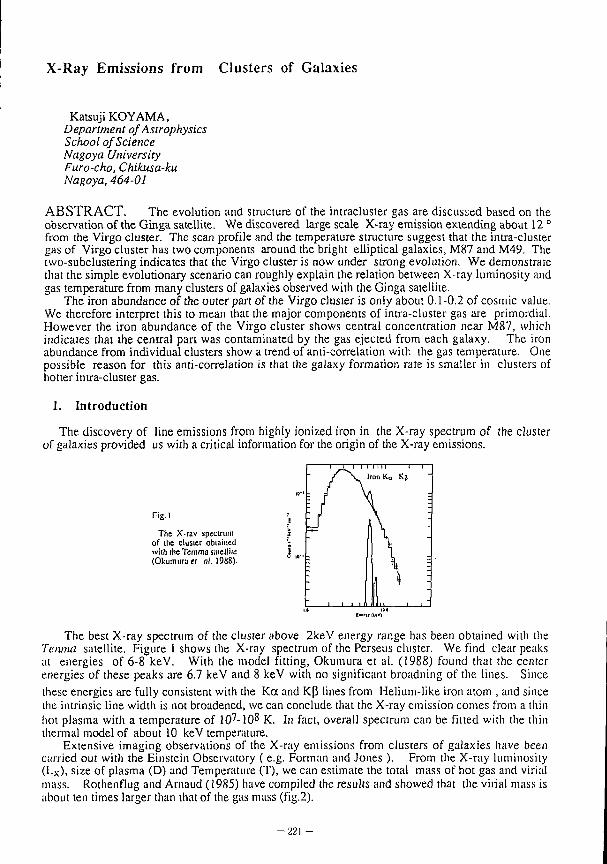
X-Ray Emissions from Clusters of Galaxies

Katsuji KOYAMA, Department of Astrophysics School of Science Nagoya University Furo-cho, Chikusa-ku Nagoya, 464-01

ABSTRACT. The evolution and structure of the intracluster gas are discussed based on the observation of the Ginga satellite. We discovered large scale X-ray emission extending about 12 ° from the Virgo cluster. The scan profile and the temperature structure suggest that the intra-cluster gas of Virgo cluster has two components around the bright elliptical galaxies, M87 and M49. The two-subclustering indicates that the Virgo cluster is now under strong evolution. We demonstrate that the simple evolutionary scenario can roughly explain the relation between X-ray luminosity and gas temperature from many clusters of galaxies observed with the Ginga satellite.

The iron abundance of the outer part of the Virgo cluster is only about 0.1-0.2 of cosmic value. We therefore interpret this to mean that the major components of intra-cluster gas are primordial. However the iron abundance of the Virgo cluster shows central concentration near M87, which indicates that the central part was contaminated by the gas ejected from each galaxy. The iron abundance from individual clusters show a trend of anti-correlation with the gas temperature. One possible reason for this anti-correlation is that the galaxy formation rate is smaller in clusters of hotter intra-cluster gas.

1. Introduction

The discovery of line emissions from highly ionized iron in the X-ray spectrum of the cluster of galaxies provided us with a critical information for the origin of the X-ray emissions.

n g . i

The X-rav specirum of [lie cluster obtained with the Temma s.'iielliic (Okumuraei al. 19SS).

I I IDS

The best X-ray spectrum of the cluster above 2keV energy range has been obtained with the Tenma satellite. Figure 1 shows the X-ray spectrum of the Perseus cluster. We find clear peaks at energies of 6-8 keV. With the model fitting, Okumura et al. (1988) found that the center energies of these peaks are 6.7 keV and 8 keV with no significant broadning of the lines. Since these energies are fully consistent with the Koc and Kp lines from Helium-like iron atom , and since the intrinsic line width is not broadened, we can conclude that the X-ray emission comes from a thin hot plasma with a temperature of 107-108 K. In fact, overall spectrum can be fitted with the thin thermal model of about 10 keV temperature.

Extensive imaging observations of the X-ray emissions from clusters of galaxies have been carried out with the Einstein Observatory ( e.g. Forman and Jones ). From the X-ray luminosity (L x), size of plasma (D) and Temperature (T), we can estimate the total mass of hot gas and virial mass. Rothenflug and Arnaud (1985) have compiled the results and showed that the virial mass is about ten times larger than that of the gas mass (fig.2).

J I L_l LiiJ I L_

- 2 2 1 -

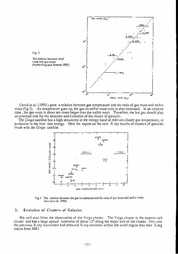
I:ig. 2

The relaiion between virial mass and gas mass. (Rothenflug and Arnaud 1985)

GAS MASS [M„)

_L_A_2»65

A 19< / / 'viRCO.

,-/ ' ' - raHc

VIRIAL MASS (M 0J

David el al. (1990 ) gave a relation between gas temperature and the ratio of gas mass and stellar mass (fig.3). As temperature goes up, the gas-to-stellar mass ratio is also increased. In an extreme case , the gas mass is about ten times larger than the stellar mass. Therefore, the hot gas should play an essential role for the structure and evolution of the cluster of galaxies.

The Ginga satellite has a high sensitivity in the energy band of relevant cluster gas temperature, in particular in the iron-line energy. Here we report on the new X-ray results of clusters of galaxies made with the Ginga satellite.

MKW3r O

A I 5 4 X

AWM4 QMKYfA

1«.7

GAS TEMPERATURE: Ucv)

Fig.3 The relation between the gas temperature and the ratio of gas mass and stellar mass. (David etal. 1990)

Evolution of Clusters of Galaxies

We will start from the observation of the Virgo cluster. The Virgo cluster is the nearest rich cluster and has a large optical extension of about 12° along the major axis of the cluster. Hovever the previous X-ray instrument had obtained X-ray emission within the small region less than 2 deg radius from M87.

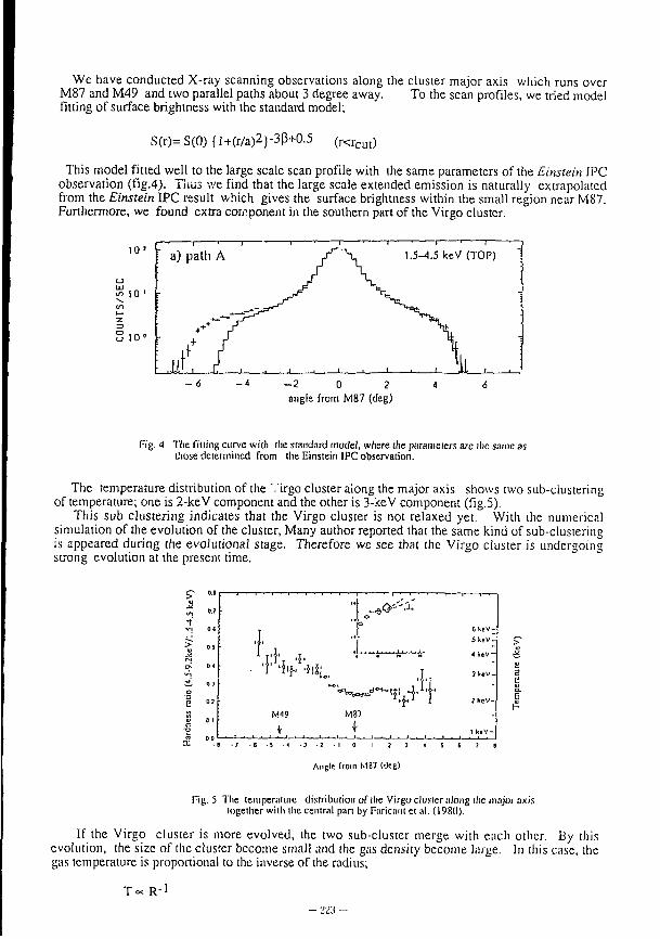
We have conducted X-ray scanning observations along the cluster major axis which runs over M87 and M49 and two parallel paths about 3 degree away. To the scan profiles, we tried model fating of surface brightness with the standard model;

S(r)= S(0) {l+(r/a)2)-3p+0.5 ( r < r c m )

This model fitted well to the large scale scan profile with the same parameters of the Einstein IPC observation (fig.4). Thus we find that the large scale extended emission is naturally extrapolated from the Einstein IPC result which gives the surface brightness within the small region near M87. Furthermore, we found extra component in the southern part of the Virgo cluster.

10 '

<r> 1 0 '

10'

- 2 0 2 angle from M87 (cleg)

Fig. 4 The filling curve with the standard model, where the parameters are the same as those determined from the Einstein IPC observation.

The temperature distribution of the Virgo cluster along the major axis shows two sub-clustering of temperature; one is 2-keV component and the other is 3-keV component (fig.5).

This sub clustering indicates that the Virgo cluster is not relaxed yet. With the numerical simulation of the evolution of the cluster, Many author reported that the same kind of sub-clustering is appeared during the evolutional stage. Therefore we see that the Virgo cluster is undergoing strong evolution at the present time.

rV\ 9 o -

.J. I

M<19 M87 fc.+ft

6 k e V -S k e V -

4 k e V ->

3 k e u - I - I ?keV-

Tern

Angle Ironi M87 (tlcg)

fig. 5 The temperature distribution of Ihc Virgo cluster along the major axis together with ihe central part by Faricant et al. (1980).

If the Virgo cluster is more evolved, the two sub-cluster merge with each other. By this evolution, the size of the cluster become small and the gas density become large. In this case, the gas temperature is proportional to the inverse of the radius;

T « R-l •m -

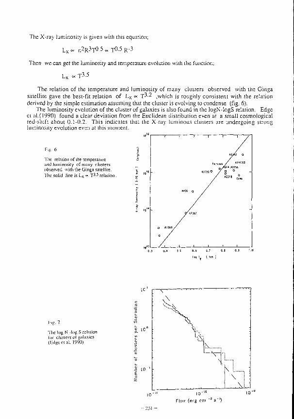
The X-ray luminosity is given with this equation;

L x « n2R3-r0.5 « TO-5 R-3

Then we can get the luminosity and temperature evolution with the function;

L X « T 3 . 5

The relation of the temperature and luminosity of many clusters observed with the Ginga satellite gave the best-fit relation of L x <* T^-2 ,which is roughly consistent with the relation derived by the simple estimation assuming that the cluster is evolving to condense (fig. 6).

The luminosity evolution of the cluster of galaxies is also found in the logN-logS relation. Edge et al.(I990) found a clear deviation from the Euclidean distribution even at a small cosmological red-shift about 0.1-0.2. This indicates that the X-ray luminous clusters are undergoing strong luminosity evolution even at this moment.

rig. 6

The relationof the temperature and luminosity of many clusters observed with the Ginga satellite. The solid line is I . x ~ T -5 relation .

l °9 r ( k«< )

n g . 7

The log N -log S relation fur (.lusters of galaxies (Huge ci al. 1990)

Flux (erg cm ~z s" 1)

1.0 I.I J. 1,6 I.S 1.0 |d.s

~i i i ^~i 1 r

1 I s I

- I 1 1 I I I i l l • '•• ' • • >.• i.» I . I i . i ,., i.o

Fig. 8 The relation between ihe gas temperature and iron line K a (upper panel) and Kp (lower panel) energy ( Hatsukade 1989).

3. Iron Line from Clusters of Galaxies

3-1 Iron distribution in the Virgo cluster

Since heavy elements such as iron are not primordial but originate in stars, the iron line is a powerful tool to study the origin of the intracltister gas. Figure 8 gives a relation between the gas temperature and iron line Kcc and Kp energies. The data fits well to these theoretical lines in which we assume the ionization equilibrium. Then, we can easily estimate iron abundance from the observed iron line intensity .

Koyama et al. (1991) obtained a distribution of iron abundance along the major axis of the Virgo cluster and found a clear peak near the cluster center at M87 ( fig,1? )•

sLl - I -7 - C - 3 - i . l 0 I I J

Angle from M87 ('leg)

Pig. 9 The distribution of iron abundance along the major axis of the Virgo cluster (Koyama ct al 1990)

They concluded that the iron abundance from the central region ( within 1° from M87) is about 0.5 cosmic value, while that at the outer region of the cluster (larger than 1° from M87) is 0 .1-0.2 cosmic value.

Since the iron abundance of the outer part of the Virgo cluster is only 0.1-0.2 of cosmic value, we can assume that the intracluster gas of Virgo should mainly originated from the primordial gas. The outer region of the Virgo cluster has not yet been contaminated by the gas ejected from each galaxy. By contrast, the central region of the cluster has been contaminated by a more efficient mass-loss from galaxies due to a denser galaxy distribution than the outer region of the cluster. Therefore the iron line distribution of the Virgo cluster gives us good example of tracing the hot gas evolution in the cluster. Another example was found in the recent study of the Perseus cluster bv Ponmanetal. (1990).

3-2 Iron Abundance and Gas Temperature

The Ginga field of view is too large to investigate the spatial structure other than the Virgo cluster. Therefore we will discuss the mean iron abundance and the gas temperature of the cluster of galaxies. Hatsukade (1989) summarized the iron abundance and the temperature from many clusters of galaxies. He found that the iron abundance is not constant but shows a decrease as the gas temperature increases (fig. io)

l-'ig. 10 The iron abundance and the temperature from many clusters of galaxies (Halsukailc 1989).

We will assume that the intracluster gas consists of two components: the primordial gas which includes no iron, and the gas ejected from the galaxy with the cosmic abundance. Then the iron abundance in the intracluster gas is a simple function of the tatio of the primordial gas and the ejected gas. From the observation, we found when the gas temperature is high, iron abundance is snail. If we simply assume that the temperature is proportional to the deptii of gravitational potential of the cluster. Then a cluster of deeper potential tend to have a smaller amount of ejected gas. This may be interpreted that the formation rate of the galaxy is small in a cluster of deep gravitational potential.

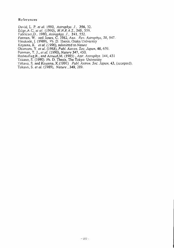
References

David, L. P. etal. 1990, Astrophys. J., 356, 32. Edge,A.C, etal. (1990), M.N.R.A.S., 245, 559. Fabricant.D.. 1980, Astrophys. J., 241,552. Forman, W. and Jones, C. 1982, Ann. Rev. Astrophys, 20, 547. Hatukade, I. (1989), Ph .D. Thesis, Osaka University Koyama, K. et al. (1990), submitted to Nature Okumura, Y. et al. (1988), Publ. Asiron. Soc. Japan, 40, 639. Ponman, T. J., etal. (1990), Nature 347, 450. RothenflugJR.., and Arnaud.M. (1985) , Astr. Astrophys. 144, 431 Takano, S. (1990). Ph. D. Thesis, The Tokyo University Takano, S. and Koyama, K.(1991) Publ. Astron. Soc. Japan, 43, (accepted). Takano, S. et al. (1989), Nature , 340, 289.

Stellar Neutr inos a n d Cosmic Rays

M.Koshiba Tokai University, Tokyo, Japan

Stellar Neutrinos The dream of observational neutrino astrophysics must have been

entertained by innumerable scientists but the far-sighted initiatives in 1950's of Markov in USSR and of Reines in USA no doubt played the in­strumental roles in realizing the situation we are now in. The observational neutrino astrophysics was born over the years 1987 to 1990. I think we can make this statement despite the existence of the pioneering work of Davis, R. Jr. over 20 years in the U.S. on the solar neutrinos which I personally admire greatly. The above statement is still Justified because: Both the arrival direction and the arrival time of the signal are indispens­able for an astronomy and: The energy spectrum of the signal in addition is essential for an astro­physics.

The Dav:3' experiment observed the accumulated, over several weeks, yield of 3 7 Ar from the inverse beta decay of 3 7 C1 for detecting the solar neutrinos and thus did not satisfy the above requirements'. This fact by no means reduces the importance of the experiment and in fact it has given birth to the so-called Solar Neutrino Problem (SNP); i.e. the ob­served neutrino flux being about 1 / 3 of the value expected from the Standard Solar Model2, (SSM).

On the other hand, the observation3 by Kamiokande-II, confirmed immediately by 1MB4, of the neutrino burst from the supernova SN1987A was done by means of the Cerenkov light of the positrons from the reac­tion, (antive+proton)->(positron+neutron), and thus it was realtime and spectral, though not directional, observation; (the first of the observed eleven events could be an elastic scattering of v e off electron giving the di­rectional information). The observation of the solar 8 B neutrinos by Kamiokande-II5 uses the Cerenkov light of the recoil electrons from the elastic scattering of these v e 's off electrons in the water and hence it is re­altime, directional and spectral observation. This is the reason why I make the statement that the observational neutrino astrophysics was born over the years 1987 to 1990.

Let us briefly look at the present situation. I do not touch upon the observation of the neutrino burst from SN1987A, which has already been widely discussed in the literature, see for instance the excellent re­view article by Bethe6 and begin with the solar neutrino.

Fig. 1 shows the directional signal of solar neutrinos as observed by Kamiokande-II, KAM-II for short hereafter.

- L'28 -

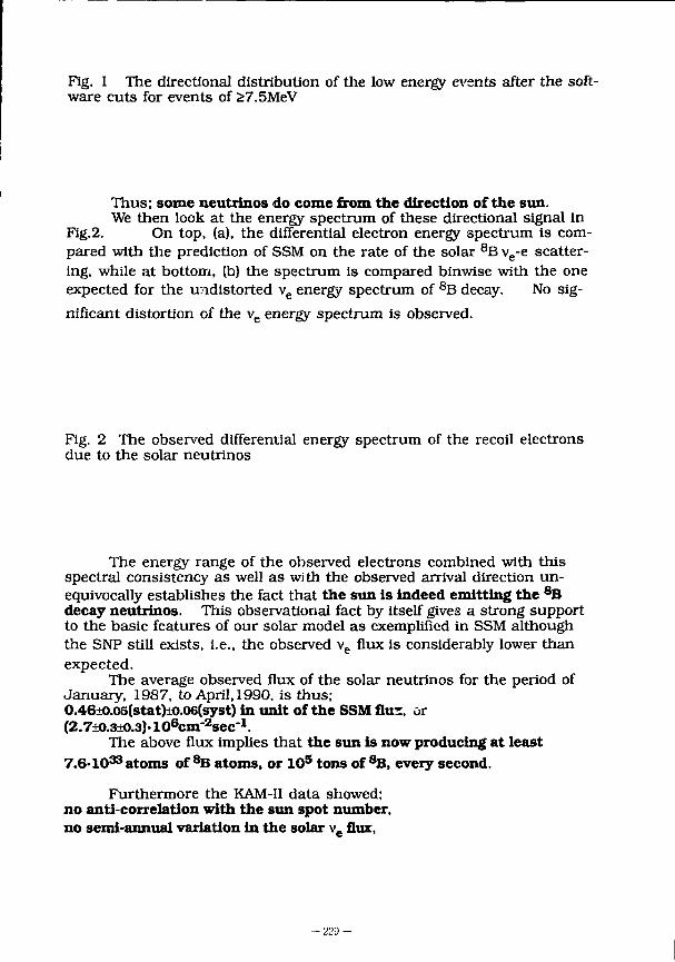
Fig. 1 The directional distribution of the low energy events after the soft­ware cuts for events of £7.5MeV

Thus; some neutrinos do come from the direction of the sun. We then look at the energy spectrum of these directional signal in

Fig.2. On top, (a), the differential electron energy spectrum is com­pared with the prediction of SSM on the rate of the solar 8 B ve-e scatter­ing, while at bottom, (b) the spectrum is compared binwise with the one expected for the undistorted v e energy spectrum of 8 B decay. No sig­nificant distortion of the v e energy spectrum is observed.

Fig. 2 The observed differential energy spectrum of the recoil electrons due to the solar neutrinos

The energy range of the observed electrons combined with this spectral consistency as well as with the observed arrival direction un­equivocally establishes the fact that the sun is indeed emitting the 8 B decay neutrinos. This observational fact by itself gives a strong support to the basic features of our solar model as exemplified in SSM although the SNP still exists, i.e., the observed v e flux is considerably lower than expected.

The average observed flux of the solar neutrinos for the period of January, 1987, to April, 1990, is thus; 0.46+O.05(stat)±o.06(syst) in unit of the SSM flu?, or (2.7±o.3±o.3)-106cm"2sec"1.

The above flux implies that the sun is now producing at least 7.6-10 3 3 atoms of 8 B atoms, or 1 0 s tons of S B, every second.

Furthermore the KAM-II data showed; no anti-correlation with the sun spot number, no semi-annual variation in the solar v e flux,

- 2 2 9 -

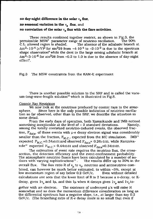
no day-night difference in the solar v e flux, no seasonal variation in the v e flux, and no correlation of the solar v e flux with the flare activities.

These results combined together restrict, as shown in Fig. 3, the permissible MSW7 parameter range of neutrino oscillation. The 90% C.L. allowed region is shaded. The absence of the adiabatic branch at Am 2 -10" 4 (eV) 2 for sin 220 from -4-10" 4 to -2-10" 2 is due to the spectrum shape observation8 while the dent in the large mixing adiabatic branch at Am 2~3-10" 6 for sin 228 from ~0.2 to 1.0 is due to the absence of day-night effect8.

Fig. 3 The MSW constraints from the KAM-II experiment

There is another possible solution to the SNP and is called the vacu­um-long-wave-length solution1 0 which is illustrated in Fig.8.

Cosmic Ray Neutrinos We now look at the neutrinos produced by cosmic rays in the atmo­

sphere. Since here is the only possible indication of neutrino oscilla­tion so far observed, other than in the SNP, we describe the situation in some detail.

From the early days of operation, both Kamiokande and 1MB noticed something inexplicable at the level of ~ 2 standard deviations. Namely, among the totally contained neutrino-induced events, the observed frac­tion, F d a t a , of those events with |i-e decay electron signal was considerably smaller than the fraction, F M c , expected from the MC simulation. 1MB" expected F M C =0.34±o.oland observed F d a t a = 0.26±0.03, while Kamioka­nde 1 2 expected F M c = 0.44±o.Oi and observed F d a t a=0.34+0.03.

The estimation of event rate requires the neutrino flux, the cross-section, the detection efficiency and the event-confinement probability. The atmospheric neutrino fluxes have been calculated by a number of au­thors with varying sophistications1 3 . The results differ up to 20% in the overall flux. The flux ratio R of v„ to ve, neutrino and antineutrino com­bined, can however be much better estimated, to within ~5%, except at low momentum region of say below 0.2 GeV/c. Even without detailed calculations one sees that the lower limit of R is 2 because a rc-decay, or It-decay, gives lv^ and l|i, and this In when it decays gives lv and lv e to­gether with an electron. The existence of undecayed \i's will raise R somewhat and so does the momentum difference consideration as long as the differential spectrum has a negative slope, i.e., at larger than say 0.2 GeV/c. (The branching ratio of K-e decay mode is so small that even if

- L':«i -

one assumes the equal production in number of 7t and K the reduction of R is less than 5%.) The relevant weak cross-sections are rather well understood except the nuclear effects especially near the threshold and here again taking the ratio of similar processes reduces the systematic un­certainties greatly. The detection efficiencies and the confinement probabilities have to be estimated for the experimental set-up under con­sideration. For an imaging water Cerenkov experiment they can be es­timated quite accurately, while for a fine grain calorimeter of layered structure one usually needs beam tests'" to determine these quantities.

The effect above of apparently missing v -events will be more acute­ly visible in the pseudo-elastic ^;harged-current events. Kamiokande 1 5

thus looked at the sample of single-ring totally-contained events, corre­sponding to 0.1 to 1.33 GeV for e and 0.2 to 1.5 GeV for n. in the 2.87 kton-year data. The data were analyzed with 98% efficient discrimina­tion between showering- and nonshowering-events, called e- and ^-events hereafter for short, respectively. In order to avoid the - 2 0 % uncer­tainty in the overall flux, the ratio R d a t a =(observed number of |a-events)/ (observed number of e-events) was compared with the ratio R M c =(M.C. expected number of n-events)/(M.C. expected number of e-events) and the result was; (we consider for the moment only the statistical fluctua­tion and the discussion on the systematic errors will be made later.) R ( n / e ) = R d a t a / R M C =(0.56+0.09-0.08), which is 0.56+0.32-0.20 at 3-a. So it was statistically more than 3-o below 1.00 of no anomaly.

Whether this is a real anomaly or not was questioned for instance by pointing out the necessity of taking into account the muon polarization ef­fects in the MC flux simulations 1 6 which soon turned out to be a less than 15% effect on the above ratio R(ji/e). The subsequent publications, however, of other underground experiments, NUSEX 1 7 and Fre jus 1 8 , both claiming that the ratio R(M/e) is consistent with unity, reduced the credi­bility of the anomaly considerably even though their statistics were not very high; 32ji-events/18e-events in NUSEX data of 0.74 kton-year and 108|i-events/57e-events in Frejus data of 1.56 kton-year. The NUSEX value of R(n/e) was 0.99+0.35-0.25, while that of Frejus was 1.06+0.19-0.16.

The Kami^kande collaboration has been working on updating the data and recently completed the analysis of atmospheric neutrino data of 4.92 kton-year, i.e., an additional 2.05 kton-year, with an improved version of M.C. simulation including the polarization effects. The additional in­dependent data fully confirmed the R(n7e) anomaly previously observed and, hence, we combine the two, new and old, sets of data. Based on a total of 151 ^-events, 0.2 to 1.5 GeV/c, and 159 e-events, 0.1 to 1.33 GeV/c, which are all single-ring totally-contained events, the momentum spectra of the e-events, upper diagram, and of the ^-events, lower dia­gram, are shown in Fig.4, where one notices an appreciable reduction of |i flux below 700 MeV while the higher momentum (i-events and the e-events in the entire momentum range behave as expected from the re­spective MC simulations.

- I'.XI -

Fig.4 The momentum spectra of e- and |i-events.

The momentum dependence of R(n/e) is shown in Fig.5. In the figure the open circles, with vertical bar of statistical ± 1 -a, show the val­ues of R(n/e) in the respective momentum bins, while the filled circles, with addition of the dotted vertical bars of ± 3-a statistical fluctuation and the vertical arrows of ± 1 -a systematic uncertainty, show the R(|i/e) values in the two momentum ranges of L, 0.3 to 0.7 GeV/c, and H, >0.7 GeV/c, and these latter data will be used in comparisons with the results of other experiments. The horizontal line at R(^i/e)=l signify the absence of anomaly.

Fig.5 The momentum dependence of R(n/e)

The overall R(n/e) turned out to be; (KAM-I-II) R(ji/e)=0.60+0.07-0.06; i.e., statistically more than 4-abelow unity.

In the meantime in September of 1990 the 1MB collaboration has submitted a paper for publication regarding this problem19. The 1MB de­tector was upgraded to IMB-3 in 1986 by changing the 5"<1> PMTs to the 8"<t> ones equipped with wave shifter plates thereby improving the photo-cathode coverage from 1.3% to about 7% level. This enabled them to make, with about 90% confidence, the differentiation between a shower­ing track and a non-showering track as was done in the Kamiokande ex­periment of 20% photocathode coverage. Among the totally contained events recorded during the 3.4 kton-year exposure, they observed 97 non-showering-events and 139 showering-events of single Cerenkov ring type in the range of Evis larger than 0.1 GeV and momentum smaller than

1.5 GeV/c. They compared the observed momentum distributions of the two types of events with the respective expectations based on a new 3-dimensional calculation of atmospheric neutrinos with polarization ef­fects 2 0 . Their conclusion was:

"When the statistical and systematic uncertainties are combined, our measured fraction of non-showering single-ring events is less than 2a below expectation. The fraction of events with muon decays, indepen­dent of the particle identification algorithm, exhibits a similar discrepan­cy. If this discrepancy represents a real deficit, the vast majority of miss­ing events would be v„-induced. However, the magnitude of the devia­tion is not sufficient to require neutrino oscillation to explain our data. The overall spectra and total number of interactions are in reasonable agreement with predictions. Furthermore, there is no correlation of deficit with energy or angle, as might be expected of an oscillation effect."

However, the inspection of their figures reveal a seemingly system­atic over (under) abundance of e- ((J.-) events compared to the respective MC simulation, although the deviations in each case remained less than ~2 o a s they concluded. The observed numbers of the two types of events and their respective MC expectations as given in their paper imply R((i/e)=0.67+0.09-0.08; i.e., an anomaly of ~ 3-0 statistical significance.

For a more detailed comparison we proceed along the following guidelines. 1): Compare first the two results of similar experiments, IMB-3 and KAM-I-II, on the totally contained single-ring events, which are mostly the pseudo-elastic charged-current interactions of v and v e . 2): Comparison between the data and the MC simulations are to be made in the form of R((i/e) above. This is not only because the anomaly, if it indeed exists, will manifest itself most directly in this ratio but also be­cause most of the systematic uncertainties like the nuclear effects, the de­tection efficiencies and the confinement probabilities will cancel substan­tially or at least they become amenable to easy trace. The momentum range for comparison is to be set in such a way that the detection efficien­cies are at least 50% for both \i- and e-events. This requirement sets the threshold momentum at 0.3 GeV/c for IMB-3 and at 0.2 GeV/c for KAM-I-II, while for Frejus it is 0.6 GeV in energy. Preferably the com­parison threshold should not be chosen too close to the reaction thresh­old where the nuclear effects can differ considerably for the two species. So in what follows we set the threshold at 0.3 GeV/c for both IMB-3 and KAM-I-II. Noting in Fig.4 that the deficit of v^-events is apparently sub­stantial below 0.7 GeV/c, we thus divide the momentum range into two; L of (0.3 to 0.7GeV/c) and H of (above 0.7 GeV/c). 3): The results of fine grain calorimeter type experiments, NUSEX and Frejus, will then be looked at to see if they indeed negate the combined conclusion of IMB-3 and KAM-I-II.

Reading off the IMB-3 data from the figures in ref. 19 we find; 69 | i /58e in L to be divided by their MC expectations of 84.5ji/43.4e for L,

and 28u/32e in H to be divided by the MC expectations of 33.9u/22.7e for H. Disregarding still the systematic uncertainties in the MC calculation, to be discussed shortly, the R(ji/e) of IMB-3 is thus; O.6I+0.12-0.10 in L and 0.59+O.17-O.14 in H. (IMB-3) On the other hand die updated KAM-I-II data give: 77u/75c in L to be di­vided by the MC expectations of 137.6u/72.9e for L, and 41u/29e in H to be divided by the MC expectations of 51.7u/27.5e for H. Thus the KAM-I-II value of R(u/e) is, as shown by the filled circles in Fig.5; 0.54+o.i(M).O8 in L and 0.75+o.2H>.i6 in H. (KAM-I-II)

The two sets of data are thus seen to be statistically consistent with each other and they both indicate the existence of anomaly.

We now discuss the systematic errors involved in these data. Among the various possible systematic errors, the most critical is the error in the u / e identification since it affects the numerator and the de­nominator of R d a t a in the opposite direction.

In the KAM-I1 experiment, R , j a l a suffers the error of 2 times 2% due to the identification error. The other error sources to R^atil are all small; < 1 % from the difference in the vertex fittings of u- and e-events, and < 1 % from the uncertainty in the absolute energy calibration. We have found all the theoretical uncertainties, except that in the v / v e flux ratio, almost cancel in R(|i/e) we are dealing here. Note in this connection that the difference in the threshold energies of v and v 0 is only l8MeV for producing the secondaiy of >300MeV/c. The errors in R M c are thus estimated as; <5% from the incident v„ A' e flux ratio, 4% from the statisti­cal fluctuation of M.C. events, 2% from the uncertainty in the ant iv e /v e flux ratio, <2% from the difference in the C-C interactions including the nu­clear effects, 2% from the uncertainty in the N-C interactions and - 1 % from the effect in event identification of y-rays emitted by the excited tar­get nucleus. Adding all these errors in quadrature we estimate the sys­tematic error of R(u/e) to be 8.8%.

1MB quotes the overall systematic uncertainty of 10% in the MC es­timation of the non-showering fraction and of 5% in the observed number of non-showering events. The break-down of these figures can be found in ref.10. Namely, the theoretical uncertainty in the v /v e flux ratio is quoted less than 5%, that in the fraction of v -induced quasi-clastic events about 2% (from the 10% variation of the axial vector mass in the nucleon form factor) and less than 5% (from the 20% variation in the Fermi mo­mentum of the oxygen nucleus), and that in the neutral-current cross-sec­tion 3.5%, all of which were linearly added to give the 10% uncertainty for the MC simulation. ( The linear addition of these errors seems to me too pessimistic but this was their choice.) In estimating the error in R(u/e) the 10% overall uncertainty in the non-showering fraction has to be doubled and so is the systematic error in the type-identification of data they quoted as ±5%. Adding these errors in quadrature we find 22% sys­tematic error in R(u/e) of IMB-3.

We first note that the two results are quite consistent with each other and that in the low momentum range of (0.3 to 0.7 GeV/c) the IMB-3 data gives ~2.3o anomaly and the KAM-I-II data gives ~3.5o anomaly. On the other hand in the higher momentum range of >0.7GeV it is consis­tent with no-anomaly, KAM-1-I1 within - l o a n d IMB-3 within ~2o. Since the two sets of data were obtained independently but with similar tech­nique we can combine, by the weighted mean, the two sets of data to ob­tain; 0.57+0.09-0.08 in L and 0.68+O.15-O.13 in H. (KAM-I-II plus IMB-3), where the total errors were computed by adding in quadrature the statis­

tical and systematic errors.

In the case of the imaging water Cerenkov experiment one can check these results by comparing the fraction of |i-e decay associated events with the MC expectation. This analysis does not involve the particle identification and hence constitute a completely independent check. The IMB-3 observed for single-ring totally contained events that the fraction of |i-e decay associated events, F d a t a , was 0.36±0.03 while F M c

of 0.42±0.0i was expected from the MC simulation. The KAM-I-II observed for the same category of events that F d a t a =0.34±0.03 against F M c

=0.46±0.0i. These results are quite consistent with the overall R(fi/e) anomalies described above; since the fractions, F d a t a and F M c , are related to the above R(|i/e) by R ( j i / e ) ~ ( F c l a t a / ( l - F d a l a ) ) / ( F M c / ( 1 - F M c )), the cor­responding values of R(ji/e) for the entire momentum range are 0.77+0.11-0.10 for IMB-3 and 0.61± 0.07 for KAM-I-II.

It is thus clear that the anomaly exists in the lower momentum range at ~ 4 o level, while in the higher momentum range it is at ~ 2 a level and should be regarded as not inconsistent with no-anomaly. This conclusion is supported by the fact that the KAM-I-II gives the additional data of R(^/e)=0.44+0.12-0.10 for the (0.2 to 0.3 GeV/c) momentum range below L and by the fact that in the momentum range higher than H, i.e., at >1.7 GeV/c, the zenith angle distribution 2 1 of 252 upward-going (i's ob­served by KAM-I-II is quite consistent with no oscillation.

The energy range satisfying the 50% detection efficiencies for both \i and e is 0.4 to 0.8 GeV in NUSEX and if we stick to the above guideline for comparison the event numbers become 13|j/4e to be divided by the M.C. generated 13 .0^ /6 . le . R((i/e) then is 1.53+1.26-0.65. These R(u/e) values are of course consistent with no anomaly, R(|i/e)=l, but it is also within 1.5a from the joint (IMB-3 and KAM-I.-II) result. For the data of Frejus, a s read off from the figures in ref. 18, we take the Evis threshold of 0.6 GeV in accordance with the guideline 2) above, there are 82 | i /36e in the data to be compared with 92.1u/51.2e from the M.C. simulation. R(n/e) of Frejus is thus 1.27+0.28-0.25 for Evis > 0.6 GeV, which is about 2.5 a above the combined fit R(u/e) value in H, > 0.7 GeV/c, of KAM-I-II and IMB-3. In the case of this type of experiment there is no independent

check of the results as was done with the fraction of p.-e decay associated events in the case of imaging water Cerenkov experiment. We note that in both of these experiments with parallel iron slabs the detectors were not calibrated for incidence angles >60° to the iron slab normal where the MC simulation becomes delicate and that these angular interval corre­sponds to one half of the total solid angle for isotropic incidence. We thus do not attempt to combine these results with those of the imaging water Cerenkov experiments.

Now that the deficit of v„ flux relative to that of v e seems estab­lished, at least in the momentum range below 0.7 GeV/c, the next prob­lem is of course to seek for a physical explanation. One of the promis­ing explanation of this observed anomaly may be sought in the neutrino os­cillation, in vacua and/or in matter. If it is indeed caused by the neutrino oscillation the KAM-I-II result gives the constraint on the oscillation pa­rameters as shown in Fig.6 for the cases of v„-*ve, left, and v -»vT., right. In the figure the crosses indicate the best fit parameters in the respective cases and the shaded regions give the 90%C.L. allowed regions. We, how­ever, do not consider the possibility of v ->veany further not only because it would conspire with the constraints from the solar neutrino data but also because of the reason to be explained later.

Fig.6 The neutrino oscillation parameters from R(n/e)

The best fit values of Am 2 and sin 229, for v„-»vT oscillation, are 0.8-10" 2(eV) 2 and 0.85, respectively. Only the shaded region in the fig­ure is not excluded at 90%C.L..

We should further check if the suggested oscillation parameters are con­sistent with the other pertinent data. Since ail the accelerator- and reactor-experiments did not reach Am 2 of 10"2(eV)2 or below, there is no conflict here. The neutrino oscillation may manifest itself in the zenith angle distribution of the observed atmospheric neutrino events re­flecting the difference in the path length or in the amount of earth matter. The zenith angle dependence as observed by KAM-I-II is shown in Fig.7 together with that of IMB-3, read off from Fig.4 of ref.19. Also shown are the respective expectations from MC simulation.

Fig.7 The zenith angle dependence of R(n/e)

The solid, dash-dot, and dash-dot-dot, lines correspond to the MC simu­lated variations for the parameter sets (Am2 in (eV)2, sin220)= (0.8-10"2, 0.85) the best-fit parameter set, (0.8-10"2, 0.45) and ( 1 1 0 3 , 0.85) both at the boundary of the allowed region, respectively, and one sees that the zenith angle distribution is consistent with the oscillation interpretation of the R(|i/e) anomaly as long as the oscillation parameters are in the shaded region of Fig. 6.

Combining all the existing constraints, i.e., from the atmospheric v^ /v e anomaly just described and from the solar neutrino deficit, on the pa­rameters of neutrino oscillation we have the result as shown in Fig.8.

Fig.8 The constraints on the neutrino oscillation parameters

One should note, however, that the indication here of neutrino os­cillation came from the so-called disappearance experiment as was the case in the solar neutrino problem.

The see-saw mechanism" , which is considered to be the natural explanation for the very small masses of neutrinos, introduces a heavy right-handed Majorana neutrino N R of mass M R and predicts;

m(v e)/(m(e")) 2= m(v ) / (m(fi") ) 2 = m(v T)/(m(r)) 2, for a generation indepen­dent MR, or more generally mlvJ/tmtDDP, with m(D) being the mass of the Dirac particle of the generation, is equal to a generation independent constant with p in the range of 1 to 2.

Dar and Nussinov23 made an analysis using u, c and t quarks (in­stead of e, n and x, above) but did not include the R(nVe) anomaly of the atmospheric neutrinos nor the absence of day-night effect of the solar neutrinos. They concluded that the recent results suggest m(vT)~10 eV, m(vj~10~ 3 eV and m(v e)~10"8 eV. The mass M R in this case corresponds to ~ 1 0 1 2 GeV. The theorists in general seem to favor small mixing pa­rameters for the neutrino oscillation as has been so witnessed in the quark sector. I personally do not see, however, why the lepton sector has to behave in the same way in this respect as the quark sector did. The value suggested for m(vT) is convenient for explaining the dark matter but so far there is no experimental indication for this value. We shall call this the theorist's guess T-guess. T-guess: m(vx)~10 eV, m(vR)~10" 3 eV and mfv^-lO" 8 eV In this connection an experiment in search of (v„-vx) oscillation with Am2 ~10 1~ 2-(eV) 2 and sin 220 down to a few times 10"4 is being prepared at CERN in collaboration with Nagoya University and others in Japan.

The allowed regions in Fig.8 seem however to indicate, assigning the largest Am 2 at 8-10" 3(eV) 2 as due to (m{vT) ) 2 , taking the charged lep-tons as the Dirac particles, and assuming p=2, that, within a factor of ~3, {(m(vT))2, (m(v u)) 2and (m(ve))2} in (eV)2 is; (1): {8'Kr 3, 1-10"7 and 5-10" 1 7 ) with large mixing of >0.45 for v ->vT and of >0.1 for v e -w . This cor­responds to taking MR=3.6-10 1 0GeV and places the (m(v ) ) 2 nicely at the lower end of MSW solution. If instead we used u, c and t as the Dirac par­ticles and assume the undetected t-quark mass of ~140 GeV, we obtain; (2): (8-10"3, ~2-10- 1 0 and -10" 2 0} with large mixing of >0.45. This corre­sponds to taking M R =6.910 1 3 GeV and places the (m(v ) ) 2 near the vacu­um long-wave-length oscillation value.

The author's guess, as an experimentalist, is more inclined, largely from the preliminary result of SAGE, toward (1) which we call E-guess. E-guess: m(vT)~0.09 eV, m(v^)~0.3aO-3eV and nUv^J-O.T-lO-8 eV all within a factor of -2 .

In either of the above cases the yield of 7 1 Ga experiment would be considerably reduced from the Solar Standard Model prediction of 132 SNU and this seems in accord with the recent preliminary report of SAGE experiment2 4. More specifically the above cases (1) and (2) predict for the 7 1 Ge yield of < 57 SNUs and > 65 SNUs, respectively, and the fu­ture results from SAGE and GALLEX experiments will decide the choice among the two possibilities. Furthermore we note that the above m(v T ) 2 value is within the reach of long-base-line, > 500 km, oscillation

- L'.'-W -

experiment of appearance type using the neutrino beam of high energy ac­celerators. This possibility should be seriously pursued by all means and in what follows we describe an example.

Near Future Possibility: the case of LENA25

Aims: The final goal of the experiment is to build a LENA of 1 Megatons fiducial mass at 500 to 1,000 km from the neutrino beam of high energy accelerator, CERN-SPS or FNAL-Main-Injector, in order to study; (1) the v -oscillation, in the form of appearance experiment, down to the hitherto unexplored Am 2 region around or below 10" 2 (eV) 2 , i.e., the region suggested by the R(|i/e) anomaly of the atmospheric neutrinos, (2) supplementary to (1), the atmospheric v interaction by the high statistics data: ca., 14,000 upward-moving |i's and 100,000 contained events annual­ly, (3) possible heavy relic particles accumulated in the sun, or in the earth core, with a factor of more than 1000 increase, compared to any ex­isting devices, in sensitivity, (4) high energy v-astronomy with a sensitive area of 35 ,000m 2 and with an angular resolution of 1 degree or better, and (5) very high energy primary y-ray point sources with excellent back­ground rejection of cosmic ray hadronic showers.

Detector: The proposed detector is an imaging water Cerenkov de­tector. In Fig.9 is shown the vertical cross section of LENA.

Fig.9 The vertical cross section of LENA

One of the differences from Kamiokande, for example, is in the surface density of photomultipliers, PMTs, 1 per 9 m 2 rather than 1 per l m 2 , and in the installation site, on surface rather than underground. In order to achieve a really large size detector at moderate cost, we consider a photo-cathode coverage s of 2.2% for LENA. This choice will degrade the ener­gy resolution but still retains the (0,-e discrimination capability which is crucial in order to study the v ->vT oscillation by appearance method. The vertex reconstruction accuracy is expected to be a o of 30 cm or bet­ter, due to the improvements already achieved on PMT design in its time jitter and in its single photoelectron detection capability. LENA will be surrounded by anti-counter modules, also of water Cerenkov type, on top and at sides. In high energy y-ray astronomy, these modules act as the total absorption energy-flow detectors, while the main detector act as ji-monitor covering the entire area.

Expected performances: Monte Carlo studies showed that the ac­curacy in direction is indeed better than 1 degree. For the energy

measurements , scaling from Kamiokande by the photocathode coverage, we expect to have the accuracies; 11% for lGeV electron or y, 8% for stopping n's, and 40% for charged 7c's of energy larger than 1 GeV. The discrimination between p. and e is based on the cascade shower de­velopment by the latter. The probability for erroneously assigning a |i-event as an electron event was shown by MC simulations to be 0 . 1 % or less for 60% acceptance of 1 Gev electrons.

Neutrino beam and event rates: For rate calculations, we assume 200 GeV proton energy and 1 0 2 0 protons to be delivered on target per year. The detector fiducial mass is 1 Megatons, placed at a distance of 730 km. Considered is a dichromatic v-beam from a secondary beam mo­mentum of 25 GeV/c with ±10% momentum bite and with a decay pipe of 400 m in length. The following table, based on 5,000 M.C. simulated events, shows the expected yearly rates and the possible signatures under the assumption of s in 2 29=0.85 and Am 2 > 0.005-(eV) 2, i.e., the parameter region suggested by the atmospheric neutrino anomaly.

-Table -Total v u CC events 17,200 Pseudo-elastic v CC events 8,600 Total v x CC events 5 ,200 Pseudo-elastic v x CC events 2 .600 Pseudo-elastic n e w decay events 4 6 0 Pseudo-elastic T->jiw decay events 4 6 0 "Single 7t° "events of 1 to 5 GeV, from v^ NC 190 "Single 7t° "events of 1 to 5 GeV. from v CC (slow n) 100 "Single y " events from "Single TC° "events < 25

Signal and backgrounds: The v energy spectrum has a peak at 11 GeV with FWHM of 1.5GeV.

If we observe some clean single |a events with more than 50% miss­ing energy, these will be good candidates for the (Pseudo-elastic T -» | IW decay events) in the table; because a deposit of more than 5.5 GeV energy to the hadronic system without detectable Cerenkov output, i.e., < 30 MeV electron equivalent, is extremely rare and can be neglected. By restrict­ing the event energy to >1 GeV the contribution, as background, of the NC single charged rc production, total of -1600 in number, is greatly reduced because a n of this energy has to traverse more than 5 times the nuclear mean free path in the water before it comes to the end of range and thus it can be easily recognized as not being a \i. The background due to this cause is estimated to be smaller than - 1 1 . The observation of (Pseudo-elastic T->)!W decay events) is thus rather straightforward.

The detection of (Pseudo-elastic n e w decay events) is more in­volved because in this case the apparent single K° -background resulting from both NC and CC interactions require special attention. When a 7t° is produced, charged pions will most likely to accompany for the energy

spectrum under consideration. (The only exception to this is due to co­herent TtO production in NC interaction at a level of <10" 3 of the total cross section.) The estimated numbers of 1 to 5 GeV single rc°-production, without any other charged particles above Cerenkov threshold, are given in the table separately for NC- and CC-interactions. These events con­tain 2 showers due to the 7t° ->2 y decay. The problem is thus whether or not we can experimentally recognize the "Single 7t° "events of 1 to 5 GeV", - 2 9 0 in number, as due to 2 showers rather than to 1 shower ex­pected for (Pseudo-elastic n e w decay events). For y-ray emission angles smaller than 60° in the 7t° rest system the laboratory opening angle of 2 y's is more than 4°for the energy range under consideration and in this case the event will be recognized as due to 2 y's by observing the az-imuthal photon distribution of the overlapping Cerenkov rings. This will reduce the number of background by a factor of 2. For the remain­ing, - 1 4 5 in number, the detailed studies of the longitudinal development of the shower will be needed in addition to identify them as due to 2 showers and not (Pseudo-elastic n e w decay events). The observation of (Pseudo-elastic n e w decay events) is thus at the S/N level of of larger than ~3 .

Cosmic ray background for LEN A-II is indeed severe amounting to a rate of 5 Mhz of top-module firing, 5 khz per module. This implies on the average, 0.75 top-module will fire even during the 150 nsec coinci­dence width of the beam neutrino events. However MC studies show that the experiment is tenable if the topological information of the hit PMT's is incorporated in the hardware trigger logic.

Detection of pure gamma-ray shower: The selection rely on the number of muons contained in the shower as well as on the lateral distri­bution of energy flow. MC-simulation of the LENA response to the electromagnetic and hadron showers shows the instrumental role in re­jecting the hadronic background played by the main detector as the muon-monitor covering the entire area.

Acknowledgement The content of this written version has been considerably improved

from that of the talk I gave. I am grateful to all my colleagues in the Kamiokande collaboration. Especially Kajita, T and Suzuki, A. have helped substancially in preparing this writing. The part pertaining to the atmospheric neutrino anomaly will be published soon as a joint paper of the Kamiokande collaboration.

j u

Davis, R.Jr. et al, Phys. Rev. Lett., 2 0 (1968) 1205. Davis, R.Jr., 13th Int. Conf. Neu. Phys. Astrop. (1988). Bahcall, J.N. and Ulrich, R.K., Rev. Mod. Phys., 60 (1988) 297. Hirata, K. et al, Phys. Rev. Lett., 5 8 (1987) 1490. Hirata, K.S. et al. Phys. Rev. , D38 (1988) 448 . Bionta, R.M. et al, Phys. Rev. Lett.. 5 8 (1987) 1494. Bratton, C.B. et al, Phys. Rev.. D37 (1988) 3361 Hirata, K.S. et al, Phys. Lett., B205 (1988) 416. Hirata, K.S. et al, Phys. Rev. Lett., 6 1 (1988) 2653 . Hirata, K.S. et al, Phys. Rev. Lett., 6 3 (1989) 16. Hirata. K.S. et al, Phys. Rev. Lett., 6 5 (1990) 1297. Hirata, K.S. et al, Phys. Rev. Lett., 6 5 (1990) 1301. Hirata, K.S. et al, Ap. J. , 3 5 9 (1990) 574. Hirata, K.S. et al, Phys. Rev. Lett.. 6 6 (1991) 9. Hirata, K.S. et al, to appear in Phys. Rev. D (1991). Bethe, H.A., Rev. Mod. Phys., 62 (1990) 8 0 1 . Wolfenstein, L., Phys. Rev., D17 (1978) 2369. Wblfenstein, L., Phys. Rev., D20 (1979) 2634. Mikheyev, S.P. and Smirnov, A.Yu., Nuovo Cimento, C9 (1986) 17. Rosen, S.P. and Gelb, J.M., Phys. Rev., D34 (1986) 969. Bethe, H.A., Phys. Rev. Lett., 6 3 (1989) 837. Hirata, K.S. et al, Phys. Rev. Lett., 6 5 (1990) 1301. Crivier, M. et al. Phys. Lett., B182 (1986) 89. Hirata, K.S. et al, Phys. Rev. Lett., 66 (1991) 9. Glashow.S.L. and Kraus, L.M., Phys. Lett., B190 (1987)199. Barger.V. et al., Phys. Rev. Lett., 65 (1990) 3084. Acker, A. et al., Univ.Hawaii preprint;UH-511-710-90. Aug.1990. Haines, T.J. et al, Phys. Rev. Let t . 57 (1986) 1986. Hirata, K.S. et al, Phys. Lett.. B205 (1988) 416. Gaisser, T.K. et al, Phys. Rev. Lett., 51 (1983) 223 . Lee, H and Bludman, S.A., Phys. Rev., D37 (1988)122. Lee, H. and Koh, Y., Chungnam National University Preprint CNU PHY-1989-T1 (rev. Aug. 1989). Barr, G. et al. Phys. Rev., D39 (1989) 3532. Bugaev, E.V. and Naumov, V.A., Phvs. Lett., B232 (1989) 3 9 1 . Honda. M. et al, Phys. Lett., B248 (1990) 193. Berger, Ch. et al, Saclay preprint, DPhPE 90-21. Hirata, K.S. r t al, Phys. Lett., B205 (1988) 416. Barr, G. et al. Phys. Rev.. D39 (1989) 3532. Aglietta, M. et al, Europhys. Lett., 8 (1989' 611 . Berger, Ch. et al, Phys. Lett, B227 (1989J 489. Berger. Ch. et al., Phys. Lett., B245 (1990) 305. Casper, D et al, submitted to Phys. Rev. Lett., Boston U. preprint 90-23 (1990). Casper, D.. PhD thesis, University of Michigan, (1990). Lee, H and Bludman, S.A., Phys. Rev., D37 (1988)122. Lee, H. and Koh, Y., Chungnam National University Preprint CNU PHY-1989-T1 (rev. Aug. 1989). Oyama, Y. et al. Phys. Rev., D39 (1989) 1481, and the updated data.

22 Gell-Mann, M. et al., in Supergravity (1979) 317, North-Holland. Yanagida, T., in Proc. Workshop on the Unified Theory and the Baryon Number in the Universe, ed., Sawada, O. and Sugimoto, A., KEK-79-18 (1979).

2 3 Dar, A. and Nussinov, S., to app. in Phys. Rev. Lett. (1990). See also; Harari, H. and Nir, Y., Nucl. Phys., B292 (1987) 251.

24 Gavrin, V.N. et al, in Proc. 25th. Int. Conf. H.E. Phys., Singapore. Gavrin, V.N. et al, to appear in Proc. XXVI Rencontre de Moriond, ed.Tran Thanh Van, J., (1991).

25 Sasaki, M. et al, in Proc. 2nd. Work Shop on Elementary Particle Picture of the Universe (1988) 181.

- -m -

Figure caption

Fig. 1 The directional distribution of the low energy events after the software cuts for events of S7.5MeV. 1,040 live days data.

Fig. 2 The observed differential energy spectrum of the recoil electrons due to the solar neutrinos.

Fig.3 The MSW constraints from the KAM-II experiment

Fig.4 The momentum spectra of e- and ^-events.

Fig.5 The momentum dependence of R(n/e)

Fig. 6 The neutrino oscillation parameters from R(|i/e)

Fig. 7 The zenith angle dependence of R(n/e)

Fig. 8 The constraints on the neutrino oscillation parameters

Fig.9 The vertical cross section of LENA

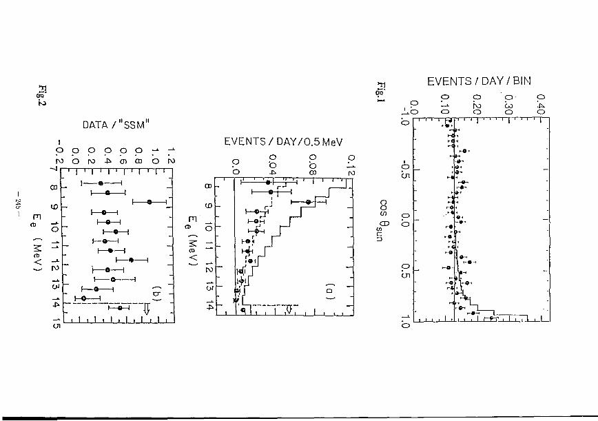
3i erg" t o

m ro

CD

<

DATA/" SSM"

i o o p o o o N O N * O) d ) O W

I ' I ' I ' I ' I I

EVENTS/DAY/0.5 MeV

31 cro'

E V E N T S / D A Y / B I N

o o in CD c/>

c 3

O k -> — j . t\3 CO •f^

J^b 0 0 0 0 O i 1 ' '£» 1 1 1 1 1 1 1 , 1 . , ' ' 1

- •-<»-•

>-< -1

•-* - (

•< -1 .

•"»-1 • -(,-, 0 ' — In •"•

•V" :£ -1 - 0

0 • -« •* 0 >-• -•-

• - « ! ' •-a • -

1 ! - • ' 0 . -O'

en h *~i

H M 1

1 1 , , 1 , - ^ 1

1 , 1 1 1 , , 1 , .-•- 1 1 , 1 ~*• 1 1 , , 1 , , , , 1 r f ^ . l i i 1 , 1 o

4^

O

Number of Events (IV)

- W W -P> Ul O)

o o o o o o o

en o o T)

CD < _ \ o o O

O

Number of Events (Ne)

^ M W | i o o o o o

31 cfo"

Am2 (eVE)

o o o o o o

C7W

"5 i

o Q

ID

+

< v

ro O ! ^ CD H i ^ <

° J Ul a 11 ol ?! I o

K

L

( 9 / W ) d

ID

d

© u o u

o 0X3

- •=• ~s = -r : : - - T U - - -- , z" i — - " I 1 v l . '•'

- 1 T*

'- - ] -^ 1 1 1 J

*i • 1

i i 1 . : : • . • : ,

•x _-b - - ' I ' , -< r — ' ^ '-."::. : - - • > ! - - - ' rn .-.. •:-: : .- :

___-h - ' ! 4— — * T

1 c : _" L ',\- .4 i— * T —— 1 -J2 >—* "TS " —— - ^ :

- I s .V. t ^ : - -- i , A fe -' -;-' cty-

-—_ 1 ' • - n <i* - - -.:. ' v_ j - . -

-" i - • H - - • : , ; p : - ~

- - 1 ~J ^F--- -= " - ~J ^F-- " • :

- i —^ . j j ' f~-J- —^ In - . ^1 - i * f~-J- .O .

^ ! f~-J-^2 Vfi - •

«3; 1 0 1 l ! -L

«3; 1 0 1 l ! -L

— - « : — — - « : — i

1 i 1 ^ — -1»

Jj&±2L : IT)

—:— eb £

247 •

Ue<-^Vfl

v^vx

> CD

E <

I0C

10"

10"

10"

r^T" T\ ; r I

I

\ Gosgen

"m r

Kamiokande

10 - 4

10 - 5 .1. ... I I L.

Kamiokande

• i i t -

10"

10 - 5

O 0.2 0.4 0.6 0.8 1 0 0.2 0.4 0.6 0.8

SIN220 SIN226 Fig.7

m -

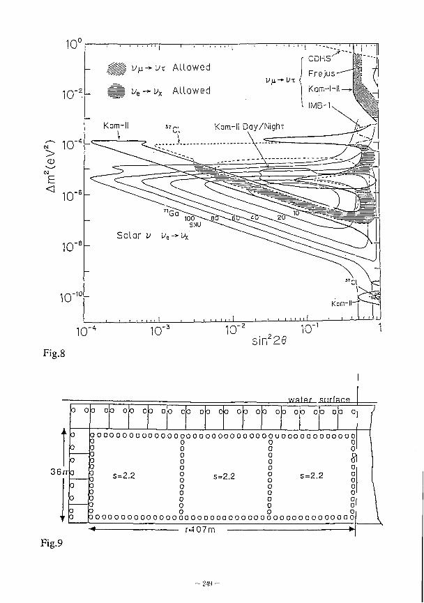
10c

CM 1(T4

> CD

> ' W

E < i r \ - 6

H H up+vx Allowed

§ H vs-*vx Allowed

sin220 Fig-8

36rro

watfir qnrfarifi o o o o o o

000000000000.0 00000000000000000000000000000

0 0

_L

0 0 0 00 0 0 00 0 0 0 0 0 3 0 o op o

J _

s=2.2 0

|0 0 3

0

0 0 0 0 0 0 0 0 0 0 0 0

s=2.2

0 0 0 0 0 0 0 0 0 0 0 0

s=2.2

0 0 0 ( 0 0 0 0 0 0 0 0 0 0 0 0 0 0 0 0 0 0 0 0 0 0 0 0 0 0 0 0 0 0 0 0 0 0 0 0 0 0 0 0 0 0

— • r 407m

Fig.9

- 249 -

Recent Progress in the Cosmic Dark Matter Problem

Hideo Kodama Department of Physics

College of Liberal Arts and Sciences Kyoto University

Yoshida, Kyoto 606, Japan

In this paper we review the present status of the dark matter problem. After summa­rizing the fundamental observational information on the abundance and the distribution of dark matter, we discuss the three fundamental aspects of the dark matter problem: a hierarchical nature of M/L, the total abundance, and the composition. In particular, taking account of the recent increase of observational information in favor of baryonic dark matter, we survey baryonic candidates of dark matter in details.

1 Dark Matter from M/L Ratios

1.1 Solar Neighborhood M/L ratio is defined as the ratio of the mass to the luminosity of a system and gives a measure how bright the constituent matter is. In actual observations, only luminosities in some narrow wavelength bands are measured. So, the value of M/L ratio of a given system depends on the photometric system adopted. In the present review V band luminosity is used as far as possible, and the values of M/L ratio are expressed in units of the solar value (M/LV)Q.

The standard of the M/L ratio for the baryonic matter is given by that obtained by observations of the matter in the solar neighborhood. The matter in the solar neighbor­hood consists of luminous stars, gas, dead stars, and dark stars and/or stellar objects. Though the contribution from the luminous stars is determined well by observations of stars inside about 50pc from the sun, it is very difficult to determine the abundance of dark stars and dead stars. Usually the abundance of dead stars which are mainly white dwarfs is estimated theoretically. No reliable estimate is possible for stars with magnitude My > 14(mass < 0.16MQ) and brown dwarfs with mass less than 0.0SM@ which do not burn hydrogen stably. Further there exists an uncertainty in the abundance of gas in the form of giant molecular clouds, though recent observations suggest that its contribution is not large. Because of these uncertainties the solar neighborhood M/L ratio is determined only up to a factor 2 at present"':

Mt/Lv = 1.4-2.8 (solar nbd). (1.1)

When one uses this value as the standard baryonic M/L value of galaxies, one should bear in mind that this value is obtained from observations of disk population. As is known

ZD NGC 2*03

s 2?

X"

*

s 2* \

"v.. 1 26

I ISO

I 100 / ' A ^ - \ SO

( ^ ^ 10 IS

R a d > u i ( k o c i

Figure 1: Examples of rotation curves

well, Our Galaxy as well as other spiral galaxies have two different populations of stars: population I (disk stars) and population II (halo and bulge stars). Due to the diffence in metalicity abundance and mean stellar mass, the stellar M/L value depends on the population. Actually the M/L for the halo stars in Our Galaxy is arround 5 which is more than twice the value for disk stars.' J

1.2 Dark matter in galaxies 1.2.1 M/L ratio

The most clear evidence of the existence of dark matter comes from observations of the rotations of spiral galaxies including Our Galaxy. In particular observations by 21 cm HI emission line have revealed that the rotation velocity stay almost constant far beyond the edges of optical disks for lots of spiral galaxies. This constant value is around 250km/s for most galaxies. Some typical examples are shown in Fig. l l 3 l In this figure the possible maximal contributions of the luminous matter to the rotation velocities determined from the luminosity densities are depicted for comparison(the maximal disk model).

The total M/L ratio inside regions of optical disk extents determined from Die mea­surements of rotation curves are^> J

{MILvW < 2ft0) s 14 (Our Galaxy), {MILV){R < R2$) = (6 - 14)/i (spirals : Sd •SO),

(1.2) (1.3)

where R0 s 8.6kpc is the distance of the sun from the Galactic Center, h is the Hubble constant in units of lOOkm/s/Mpc, and R2s is the radius where the surface brightness is equal to 25mg/arcsec2, which could be regarded as the extent of each optical disk. Note that the range of the values for spirals is due to the systematic dependence of the mean M/L on the Hubble type, lowest for Sd and hightest for SO, and the real dispersion from sample to sample is much larger than that range even within a fixed Hubble type.

- L'Bl

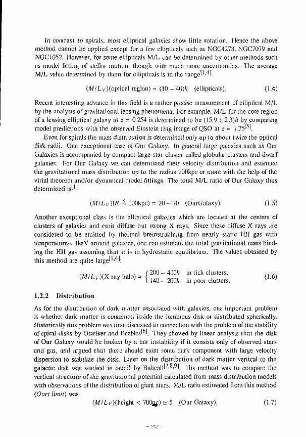
In contrast to spirals, most elliptical galaxies show little rotation. Hence the above method cannot be applied except for a few ellipticals such as NGC4278, NGC7079 and NGC1052. However, for some ellipticals M/L can be determined by other methods such as model fitting of stellar motion, though with much more uncertainties. The average M/L value determined by them for ellipticals is in the range' 1 ' 4 '

(MILv)(optical region) = (10-40)/i (ellipticals). (1.4)

Recent interesting advance in this field is a rather precise measurement of elliptical M/L by the analysis of gravitational lensing phenomena. For example, M/L for the core region of a lensing elliptical galaxy at z = 0.254 is determined to be (15.9 ± 2.3)/i by comparing model predictions with the observed Einstein ring image of QSO at z = 1.75151.

Even for spirals the mass distribution is determined only up to about twice the optical disk radii. One exceptional case is Our Galaxy. In general large galaxies such as Our Galaxies is accompanied by compact large star cluster called globular clusters and dwarf galaxies. For Our Galaxy we can determined their velocity distribution and estimate the gravitational mass distribution up to the radius lOOkpc or more with the help of the virial theorem and/or dynamical model fittings. The total M/L ratio of Our Galaxy thus determined is1'J

{M/Lv)(R ~ lOOkpc) = 2 0 - 7 0 (OurGalaxy). (1.5)

Another exceptional class is the elliptical galaxies which are located at the centers of clusters of galaxies and emit diffuse but strong X rays. Since these diffuse X rays .ire considered to be emitted by thermal bremstrahlung from nearly static HII gas with temperature^ IkeV around galaxies, one can estimate the total gravitational mass bind­ing the HII gas assuming that it is in hydrostatic equilibrium. The values obtained by this method are quite large' ' J :

. . . , , . . v . . . [200-400/t in rich clusters, ., ,. (MIL v)(X ray halo) = { ] 4 [ ) _ ^ J n ^ ^ ^ (1.6)

1.2.2 Distribution

As for the distribution of dark matter associated with galaxies, one important problem is whether dark matter is contained inside the luminous disk or distributed spherically. Historically this problem was first discussed in connection with the problem of the stability of spiral disks by Ostriker and Peebles' L They showed by linear analysis that the disk of Our Galaxy would be broken by a bar instability if it consists only of observed stars and gas, and argued that there should exist some dark component with large velocity dispersion to stabilize the disk. Later on the distribution of dark matter vertical to the galactic disk was studied in detail by Bahca

1)17,8,91 His method was to compare the

vertical structure of the gravitational potential calculated from mass distribution models with observations of the distribution of giant stars. M/L ratio estimated from this method (Oort limit) was

OW/Li/)(height < 700jjc) ~ 5 (Our Galaxy), (1.7)

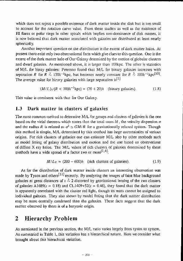
which does not reject a possible existence of dark matter inside the disk but is too small to account for the rotation curve value. From these studies as well as the existence of III flares or polar rings in other spirals which implies non-dominance of disk masses, it is now believed that dark matter associated with galaxies are distributed at least nearly spherically.

Another important question on the distribution is the extent of dark matter halos. At present there exist only two observational facts which give clues to this question. One is the extent of the dark matter halo of Our Galaxy detemined by the motion of globular clusters and dwarf galaxies. As mentioned above, it is larger than lOOkpc. The other is statistics of M/L for binay galaxies: Peterson found that M/L for binary galaxies increases with seperation R for R ~ 100/i_1kpc, but becomes nearly constant for/? ~ \QQh~]kpc"®\ The average value for binary galaxies with large separation is''J

{MIL)v{R < 100/r'kpc) = (70±20)/i (binary galaxies). (1.8)

This value is consistent with that for Our Galaxy.

1.3 Dark matter in clusters of galaxies The most common method to determine M/L for groups and clusters of galaxies is the one based on the virial theorem which states that the total mass M, the velocity dispersion a and the radius R is related as o 2 ~ GM/R for a gravitationally relaxed system. Though this method is simple, M/L determined by this method has large uncertainties of various origins. For rich clusters of galaxies one can estimate M/L also by other methods such as model fitting of galaxy distribution and motion and the one based on observations of diffuse X ray halos. The M/L values of rich clusters of galaxies determined by these methods have a wide spread of a factor two or more''' 4!:

MILv = (200-600)/; (rich clusters of galaxies). (1.9)

As for the distribution of dark matter inside clusters an interesting observation was made by Tyson and others' 1" recently. By analyzing the images of faint blue background galaxies at great distances of z ~ 2 distorted by gravitational lensing of the two clusters of galaxies A1689(z = 0.18) and CL1409+52(z = 0.46), they found that the dark matter is apparently correlated with the cluster red light, though its mass cannot be assigned to individual galaxies. They also shown by model fitting that the dark matter distribution may be more centrally condensed than the galaxies. These facts suggest that the dark matter observed by them is of a baryonic origin.

2 Hierarchy Problem

As mentioned in the previous section, the M/L ratio varies largely from systm to system. As summaried in Table 1, this variation has a hierarchical nature. Here we consider what brought about this hierachical variation.

- 253 -

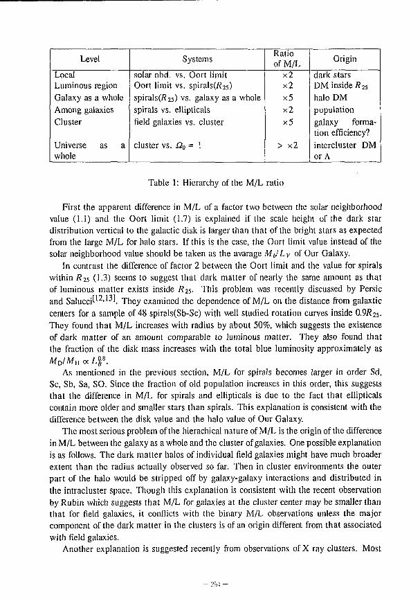
Level Systems Ratio of M/L Origin

Local solar nbd. vs. Oort limit x2 dark stars Luminous region Oort limit vs. spirals(/?25) x2 DM inside fl25 Galaxy as a whole spirals(/?25) vs. galaxy as a whole x5 halo DM Among galaxies spirals vs. ellipticals x2 population Cluster field galaxies vs. cluster x5 galaxy forma­

tion efficiency? Universe as a cluster vs. £20 = 1 > x2 intercluster DM whole or A

Table 1: Hierarchy of the M/L ratio

First the apparent difference in M/L of a factor two between the solar neighborhood value (1.1) and the Oort limit (1.7) is explained if the scale height of the dark star distribution vertical to the galactic disk is larger than that of the bright stars as expected from the large M/L for halo stars. If this is the case, the Oort limit value instead of the solar neighborhood value should be taken as the avarage MbILv of Our Galaxy.

In contrast the difference of factor 2 between the Oort limit and the value for spirals within /?25 (1.3) seems to suggest that dark matter of nearly the same amount as that of luminous matter exists inside R15. This problem was recently discussed by Persic and Saluccit12'1-^. They examined the dependence of M/L on the distance from galaxtic centers for a sample of 48 spirals(Sb-Sc) with well studied rotation curves inside 0.97?25• They found that M/L increases with radius by about 50%, which suggests the existence of dark matter of an amount comparable to luminous matter. They also found that the fraction of the disk mass increases with the total blue luminosity approximately as M D /M H ocL£ 8 .

As mentioned in the previous section, M/L for spirals becomes larger in order Sd, Sc, Sb, Sa, SO. Since the fraction of old population increases in this order, this suggests that the difference in M/L for spirals and ellipticals is due to the fact that ellipticals contain more older and smaller stars than spirals. This explanation is consistent with the difference between the disk value and the halo value of Our Galaxy.

The most serious problem of the hierachical nature of M/L is the origin of the difference in M/L between the galaxy as a whole and the cluster of galaxies. One possible explanation is as follows. The dark matter halos of individual field galaxies might have much broader extent than the radius actually observed so far. Then in cluster environments the outer part of the halo would be stripped off by galaxy-galaxy interactions and distributed in the intracluster space. Though this explanation is consistent with the recent observation by Rubin which suggests that M/L for galaxies at the cluster center may be smaller than that for field galaxies, it conflicts with the binary M/L observations unless the major component of the dark matter in the clusters is of an origin different from that associated with field galaxies.

Another explanation is suggested recently from observations of X ray clusters. Most

- 2M -

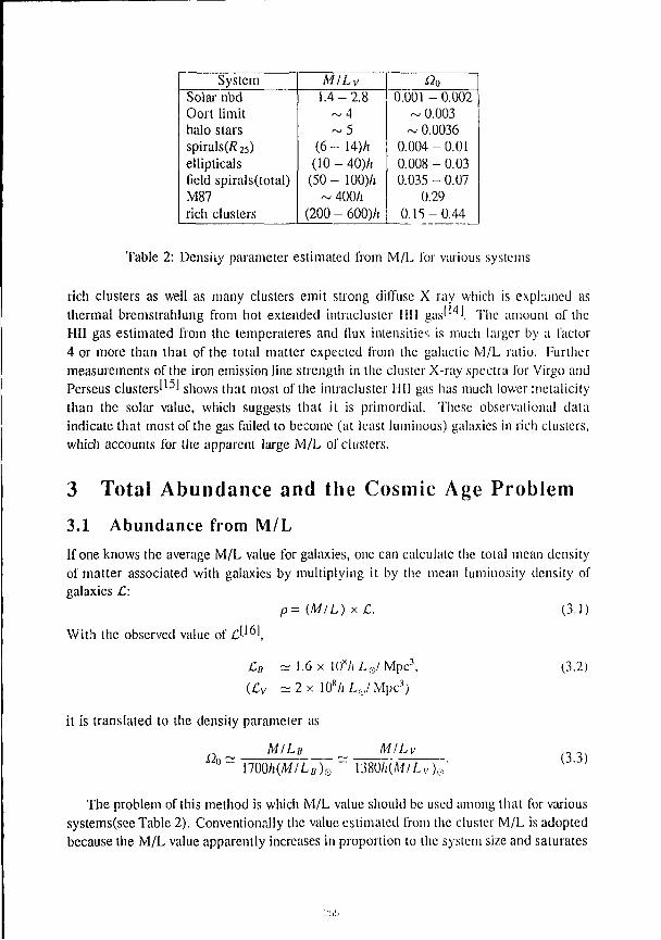
System MILv O0

Solar nbd 1.4-2.8 0.001 -0.002 Oort limit r^f 4 ~ 0.003 halo stars ~ 5 ~ 0.0036 spirals(/?25) (6 - 14)/i 0.004-0.01 ellipticals (10 - 40)/; 0.008 - 0.03 field spirals(total) ( 5 0 - 100)/i 0.035 - 0.07 M87 ~ 400/i 0.29 rich clusters (200 - 600)/i 0.15-0.44

Table 2: Density parameter estimated from M/L for various systems

rich clusters as well as many clusters emit strong diffuse X ray which is exphined as thermal bremstrahlung from hot extended intracluster 1111 gas'''*'. The amount of the HII gas estimated from the temperateres and flux intensities is much larger by a factor 4 or more than that of the total matter expected from the galactic M/L ratio. Further measurements of the iron emission line strength in the cluster X-ray spectra for Virgo and Perseus clusters^15! shows that most of the intracluster HII gas has much lower metalicity than the solar value, which suggests that it is primordial. These observational data indicate that most of the gas failed to become (at least luminous) galaxies in rich clusters, which accounts for the apparent large M/L of clusters.

3 Total Abundance and the Cosmic Age Problem 3.1 Abundance from M/L If one knows the average M/L value for galaxies, one can calculate the total mean density of matter associated with galaxies by multiplying it by the mean luminosity density of galaxies C:

p=(M/L)xC. (3.1)

With the observed value of £^ I 6J,

CD ~ 1.6 x Hfh L&/ Mpc3, (Cv - 2 x 10 8/i/. t,/Mpc 3)

(3.2)

it is translated to the density parameter as

MILB Go

M/Lx 17OO/i(M/Lfl)0 1380/i(Af//.v)s

(3.3)

The problem of this method is which M/L value should be used among that for various systems(see Table 2). Conventionally the value estimated from the cluster M/L is adopted because the M/L value apparently increases in proportion to the system size and saturates

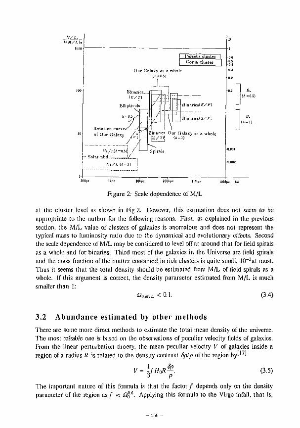
M/L, hlM/L)s a

- i

1

a - i

l'erseus cluster 1 -0.6 Coma cluster 1 -0.5

-0.4

Our Ga laxy as a who (A =-0.5)

1 c -0.3

0.2

100

Our Ga

-0.) 100 liinarics -0.)

{E/l

Elliptical? \

A =0.5 . - "

y Rotation curve.*/- L of Our Galaxy / a

/ " ,

)

3T

/.

; _.u. x BinaricsfE//')

Hii iaries(S// \

-0.) (ft =0.5

Cb (ft = l )

10

{E/l

Elliptical? \

A =0.5 . - "

y Rotation curve.*/- L of Our Galaxy / a

/ " ,

)

3T

3inarics \ Our Galaxy as a whole

(ft = l )

-0.) (ft =0.5

Cb (ft = l )

Mi//,(*=0.5)j / v . S o l a r nb< l :;-•;::•:•_—•/—.,

Mi/1. ( A = l ) !

)

3T

Spirals -0.004

-0.002

1-1( Ope lkpc 10 [JIC ]00kp c I Mpc lOMpc hit

Figure 2: Scale dependence of M/L

at the cluster level as shown in Fig.2. However, this estimation does not seem to be appropriate to the author for the following reasons. First, as explained in the previous section, the M/L value of clusters of galaxies is anomalous and does not represent the typical mass to luminosity ratio due to the dynamical and evolutionary effects. Second the scale dependence of M/L may be considered to level off at around that for field spirals as a whole and for binaries. Third most of the galaxies in the Universe are field spirals and the mass fraction of the matter contained in rich clusters is quite small, 10 - 3at most. Thus it seems that the total density should be estimated from M/L of field spirals as a whole. If this argument is correct, the density parameter estimated from M/L is much smaller than 1:

flb.w,L<0.1. (3.4)

3.2 Abundance estimated by other methods There are some more direct methods to estimate the total mean density of the universe. The most reliable one is based on the observations of peculiar velocity fields of galaxies. From the linear perturbation thoery, the mean peculiar velocity V of galaxies inside a region of a radius R is related to the density contrast Splp of the region by' 1 'J

V=^fH0RSA (3.5)

The important nature of this formula is that the factor/ depends only on the density parameter of the region a s / w /22 s. Applying this formula to the Virgo infall, that is,

the deviation of the receding velocity from the mean Hubble flow of Our Galaxy relative to the Virgo cluster center, one obtains'1 ^

0> = 0.05 - 0.34 (Virgo infall), (3.6)

provided that the galaxy number density is proportional to the true mass density. Another method which can determine the mean density on much larger scale is the

galaxy count. For example, by a recent detailed analysis of the dependence of the galaxy number on the apparent brightness^ v t is shown that the density parameter should be small,

O)«0 .1 (N-m relation), (3.7)

to account for the observational data. These results are consistent with the value obtained from M/L as well as the upper

bound on the intercluster HI abundance given by the Gunn-Peterson testl 2^, i2m < 1 x 10~uh~l, and suggests that most of the matter in the universe is localize around galaxies or intracluster space. However, this expectation is challanged by some recent observations. The most impressive one is the observations suggesting an existence of Great Atlractor^ J at distance ~ 45/r'Mpc from Our Galaxy. It is in a completely dark region and affects the galaxy velocity fields of a scale 100/j_1Mpc. Its mass is estimated to be more than the typical supercluster value 10 1 5 M o .

Another interesting observation is the finding of a diffuse synchrotron radion bridge in a dark region between the two clusters, Coma and A1367. Its extension is about 100/r'Mpc and the magnetic field stregth there is estimated to be as large as 0.3-0.6juG, which suggests an existence of high density HII gas there.

3.3 Cosmic Age Problem Since the cosmic age depends on the density parameter, it also gives a constraint on the total mean density of the universe. To be precise, the present cosmic age to is written as

t0= 100h-lf(nQ, X0)Gyr, (3.8)

where Xo = A/ (3/VQ) is the cosmological constant measured in units of the Hubble constant squared, and/ increases monotonically with decreasing £20 or increasing Ao- For example, / ( 0 ,0 )= l a n d / ( 1 , 0 ) = 2/3.

At present, there are several methods to estimate the cosmic age observationally, most of which give actually the age of Our Galaxy, hence the lower bound on the true cosmic age(See Table 3). The most established one is the method to determine the ages of globular clusters, which are regarded as the oldest population in Our Galaxy, by comparing observations and theoretical calculations of their HR diagram. The best estimate by this method is to = 17 ± 1.5Gry. Slightly shorter estimates have been obtained by the method of the nucleo-cosmochronology, which is based on the measurements of the abundance ratio of some unstable heavy nuclei with long life to some stable nuclei. In contrast to these, the method based on the observation of the white dwarf luminosity function yields a

Method Age Reference Globular cluster A M "£ 17 ± 1.5 Gyr [22] Nucleocosmochronology Th/Nd 15 - 20 Gyr [23]

Th/U/Pu 12.4-14.7Gyr 124] WD luminosity function 10.3 ±2.2 Gyr [25J z = 3.4 galaxy ~ 17 Gyr

Table 3: Lower bounds on the cosmic age

very short age of around lOGyr. Mowerver, this result does not seem to be reliable enough because it relies on the cooling theory of white dwarfs which is not well established and also because the observed sample is quite local. Finally we have one interesting estimate which is based on the observation of a high reds hi ft galaxy. From the fact that this galaxy has a well-evolved spectrum and the requirement that the age of the galaxy is younger than the cosmic age when the light was emitted from it, a lower bound on the present cosmic age of 17Gyr is obtained. To summarize these results, it seems that the present cosmic age is longer than 14Gyr at least.

In order to relate the density parameter to the comis age, one needs the values of the Hubble constant and the cosmological constat further. Unfortunately these parameters are quite uncertain. First the Hubble constant is observationally determined only up to a factor of two^j ;

0.4 ~ /i ~ 1.1 ( u ~ 2 x 10"km/s), (3.9)

though some people claim recently that a careful analysis of the data obained by various methods yields a higher value of 0.75 ~ h ~ 1 consistently^27'28!.

As for the cosmological constant the situation is worse. Of course it is certain that its value is of order H^2, but it does not restrict the cosmic age enough. This is because there exists a critical value of A0 of order H^2 for which the cosmic age becomes infinite. Thus we need a precise estimate of the cosmological constant if its value happens to be near the critical value. However, it is quite difficult because the cosmological constant is determined only by observations of the structure of the Universe on quite large scales which are plagued by various uncertainties.

Due to this difficulty and also for an aesthetic reason, it is often assumed that the cosmological constant vanishes. Under this assumption we can obtain a quite strong constraints on the other cosmological parameters from the cosmic age. In fact, as is seen from Fig.3, Q$ must be smaller than unity at least, and the Hubble constant h must be smaller than 0.7 irrespective of the value of n0. Hence the cosmological constant should take a postive value if the recent large estimate of h mentioned above is correct.

la Hi 1-1 la ltl R [Cyr]

Figure 3: Iso-cosmic-age contour in the i^-h plane

4 Possibility of Baryonic Dark Matter The most important question on the dark matter is what it is made of. Because of its darkness and dissipalionless nature, it is usually assumed to be made of nonbaryonic particles, and various candidates have been proposed. The most promising candidates are light neutrinos with a mass of 10 to 100 eV, invisible axions with a mass of 10~5

to 10~3 eV and SUSY particles with a mass larger than a low GeV. However, recent progress in direct detection experiments and observations of astronomical phenomena such as SN1987A are rejecting many heavy candidates and narrowering the allowed mass ranges of light candidates. To be pesimistic, it appears that the only possible nonbaryonic candidate left is tau neutrinos which are expected to have a mass of order lOeV if the solar neutrino problem is solved by the MSW mechanism and the neutrino mass is produced by the sce-saw mechanism in SO(10) type GUT models. However, if we take account of its influence on the large scale structure formation explained below, it is hard to believe that neutrinos are the dominant component of dark matter.

From these considerations, we reexamine here the possibility that the dark matter consists of baryons.

4.1 Cosmological constraints The most stringent constraint on the baryonic dark matter comes from the arguments on the primordial nucleosynthesis. Bt taking account of the recent strong observational upper bounds on the primordial abundance of 7Li and ''lie, the density parameter of baryonic matter is constrained as' '

0.011 ~ h212M ~ 0.02. (4.1)

Conventionally the total density parameter was believed to be greater than 0.1, prob­ably 0.2-0.4, on the basis of the M/L ratio for clusters of galaxies and the Virgo infall estimation. With such huge £20 the above constraint implies that baryons cannot explain the dark matter even for /; = 0.5. Of course the constraint can be loosened if one alters

the fundamental assumptions underlying the standard cosmological model. For example, if there exist strong density inhomogeneities at the epoch of nucleosynthesis, the upper bound on h2i2w may be as large as 0.2 as discussed by many authors(e.g. [30]). However, the most promissing mechanism to produce such large density inhomogeneities, the first-order quark-hadron phase transition, has been rejected by recent Monte Carlo simulations of the lattice QCD.

Thus it app- ars that the possibility of baryonic dark matter is simply denied by the primordial nucleosynthesis argument. However, this conclusion may be circumvented or made milder if one assumes that the total density parameter is smaller than 0.1 as suggested by the recent galaxy count observation as well as the arguments on the typical M/L of galaxies presented in the previous section. Further the above constraint may be changed in the future by increase of the observational information on the light element abundance and/or by reestimation of the primordial abundance.

Another strong constraint comes from the formation theories of the large scale struc­ture of the universe. At present there are three major formation scenarios' ' 3 J: the grav­itational instability scenario, the cosmic string scenario and the explosion scenario. In the first scenario the large scale structure is assumed to be formed simply through growth of tiny amplitude density fluctuations at the early universe by gravitational instabilities. In this scenario, the present inhomogeneities determine the amplitude of the fluctuations at the decoupling time, (5p/p) c i c c, which is strongly constrained by measurements of the anisotropies of the cosmic microwave backgiound radiation(CMB). For example, if one assumes that the cosmic matter consists mainly of baryon and radiation at the decou­pling time, (5p/p) d c c must be smaler than 2 x 10~4. However, since the density fluctuation amplitude grows in proportion to the cosmic scale factor after decoupling, this implies that the present density contrast should be smaller than 0.2, which is much smaller than the observed value. To be precise, the estimation changes depending on the nature of perturbations, adiabatic or isocurvature, the conclusion is the same.

Though this argument is strong, it is not strong enough to reject the possibility of baryonic dark matter since the nonbaryonic dark matter does not resolve the difficulty. Thus it may be said that the observations of the CMB and the large scale inhomogeneities at present reject the simple gravitational instability scenario.

In contrast to this scenario, the CMB anisotropy does not give a strong constraint on the second scenario which assumes that the structure is formed by accretion of matter onto cosmic strings. However, due to its intricate nature, this scenario cannot make clear quantalive predictions to be confronted with observations.

The final scenario which assumes that some seed objects present at the decoupling time explode to trigcr the subsequent formation and explosion of new objects leading to the large scale structure observed at present. Though this scenario is quite attractive, it is shown to require an absurd amount of explosion energy for the largest observed structure to be formed. It also conflicts with the observed CMB isotropy.

Thus the large scale structure formation theories are in a quite unsatisfactory situation, and cannot give clear information on the content of dark matter. In particular, baryons remain as a dark matter candidate. This conclusion is supported by a recent theoretical

I

L'tid -

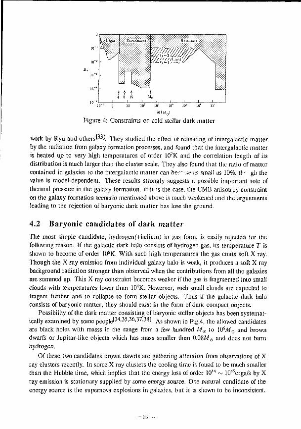
4 8 15 M c

10" 51 I I I L . I I I I 10"' 1 10 1 0 ! 10 1 10' 10' 10 6 10'

A f ( « 0 )

Figure 4: Constraints on cold stellar dark matter

work by Ryu and others^]. They studied the effect of reheating of intergalactic matter by the radiation from galaxy formation processes, and found that the intergalactic matter is heated up to very high temperatures of order 107K and the correlation length of its distribution is much larger than the cluster scale. They also found that the ratio of matter contained in galaxies to the intergalactic matter can bec---.;e as small as 10%, If"- gh the value is model-dependent. These results strongly suggests a possible important role of thermal pressure in the galaxy formation. If it is the case, the CMB anisotrpy constraint on the galaxy formation scenario mentioned above is much weakened and the arguements leading to the rejection of baryonic dark matter has lose the ground.

4.2 Baryonic candidates of dark matter The most simple candidate, hydrogen(+helium) in gas form, is easily rejected for the following reason. If the galactic dark halo consists of hydrogen gas, its temperature T is shown to become of order 106K. With such high temperatures the gas emits soft X ray. Though the X ray emission from individual galaxy halo is weak, it produces a soft X ray background radiation stronger than observed when the contributions from all the galaxies are summed up. This X ray constraint becomes weaker if the gas is fragmented into small clouds with temperatures lower than 104K. Howerver, such small clouds are expected to fragent further and to collapse to form stellar objects. Thus if the galactic dark halo consists of baryonic matter, they should exist in the form of dark compact objects.

Possibility of the dark matter consisting of baryonic stellar objects has been systemat­ically examined by some people^ 3 4 , 3 5 ' 3 " ' 3 7 ' 3 ^ . As shown in Fig.4, the allowed candidates are black holes with masss in the range from a few hundred MQ to 106A/o and brown dwarfs or Jupitar-like objects which has mass smaller than O.O8M0 and does not burn hydrogen.

Of these two candidates brown dawrfs are gathering attention from observations of X ray clusters recently. In some X ray clusters the cooling time is found to be much smaller than the Hubble time, which implies that the energy loss of order 1044 ~ 1045ergs/s by X ray emission is stationary supplied by some energy source. One natural candidate of the energy source is the supernova explosions in galaxies, but it is shown to be inconsistent.

- 261 -

Another source is the gravitational energy. In fact HII gas emitting X ray cannot be in the complete static equilibrium due to thermal instabilities associated with the bremstrahlung cooling. Hence the gas should stationarily infalling toward the cluster center or outflowing. Of these two possibilities, outflow is denied because it is expected to be supersonic and requires two large gas repleshment rate. Hence the HII gas is expected to be falling slowly releasing the gravitational energy. This infall is called the cooling flow^l.

If this cooling flow model is correct, the X ray luminosity is related to the mass accretion rale M as

Hence, in order to explain the observed luminosity, the accretion rate should be larger than 100M©/yr or more.

Where does this accreted mass go eventually? It is shown that it cannot exist in gas form. The possibility of its being absorbed into some central large black hole is also denied because it leads to loo large non-lhermal emission. The final possibility is stars. In fact there are some observational evidences which support active star formation at the centers of clusters. First dense optical emission filaments of extent 1 ~ lOOkpc with temparature lCK are observed at the central parts of some cooling flow clusters. The most specutacular one is the filamentary nebulosity around the NGC1275 at the center of the Perseus cluster. Further HI gas is detected in some central cD galaxies or cores of some clusters' 4^. These cold gases are considered to be produced by cooling from high temperature HII gas. Second some central cD galaxies have young stellar population with much larger fraction than other elliptical galaxies and have overall spectral type of A stars.

However, there is a mysterious aspect with the last possibility. In Our Galaxy newly born stats are massive in general and have spectral type of O and B. However, the observed fraction of O and B stars in the cD galaxies at the centers of the cooling flow clusters is much smaller than the value expected from the IMF in Our Galaxy and the mass accretion rate. This suggests that the IMF of star formation in the cooling flow is largely different from the local IMF such that low mass stars are preferentially formed. This is supported from the fact that the Jeans mass of the cooling flow gas is estimated to be smaller than 1/W,., due to the high pressure. Further the observation of the HI gas in cD galaxies mentioned above suggests that the gas is in the form of small clouds of masses ~ 10- 7 M o .

On the basis of these facts, sonic authors are proposing that most of the accreting mass goes into invisible brown dwarfs. It this is the case, there is a possibility that the most of the primordial gas might have been converted to dark brown dwarfs, which form the dark matter halo of galaxies now, by phenomena at galaxy formation silimar to the cooling flows observed presctly' ' '.

5 Summary Though observational and experimental information is slowly increasing recently, the mystery of dark matter is not getting cleared but is rather deepening. In particular, observational data supporting the baryonic dark matter is increasing in contrary to the conventional belief, while the upper bound on the dcnisty of baryons by the primordial nucleosynthesis argument is decreasing.

The only way of getting out of this frustrating situation is to make clear the content of the dark matter observationally or experimentally. Astrophysically the most important step toward this goal is to find a clear evidence for or against the possibility of baryonic dark matter. Presently conceivable observations of having such a chance are 1R surveys of the Great Attractor region and IR search of nearby brown dwarfs.

References [1J Fabcr, S. M. and Gallagher, J. S., Ann. Rev. Astron. Astrophys. 17, 135 (1979).

[2| Mihalas, D. and Binney, J., Galactic Astronomy (W.I I.Freeman and Company, 1981).

[3] Sancisi, R and van Albacla, V.S., in 1AU Symposium No.Ill (D.Reidel Publishing Company, 1987)page 69.

[4] Trimble, V., Ann. Rev. Astron. Aslrophys. 25, 425 (1987).

|5] Langston, G.I. et al„ Nature 344, 43 (1990).

[6] Ostrikcr, J.P. and Peebles, P.J.B., A^liophys. J. 186, 467 0973).

[7! Bahcall, N.A., Aslrophys. J. 276, 156 (1984).

[8j Bahcall, N.A., Astrophys. J. 276, 169 (1984).

[9] Bahcall, N.A., Astrophys. J. 287, 926 (1984).

[10] Peteson, S.D., Astrophys. J. 232, 20 (1979).

[11] Tyson, J.A., Valdes, F., and Wenk, R.A., Astrophys. J. 349, LI (1990).

[12] Persic, M. and Salucci, P., Astrophys. J. 355, 44 (1990).

[13] Persic, M. and Salucci, P., Astrophys. J. 356, 83 (1990).

[14] Sarazin, C.L., Rev. Mod. Phys. 58, 1 (1986).

[15J Ponman, T.J. et al., Nature 347, 450 (1990).

[16] Binggcli, B„ Sandage, A., and Tammann, G.A., Ann. Rev. Astron. Asirophys. 26, 509 (1988).

[17] Peebles, P.J.E., The Large-Scale Structure of the Universe (Princeton Univ. Press, 1980).

[18] Peebles, P. J. E., Nature 371, 27 (1986).

- :;i;:( ~

[19] Fukugita, M. et al., Astrophys. J. 361, LI (1990).

[20] Sargent, W. L. W., in lAU Symposium No.124 (D.Reidel Publishing Company, 1987)page 777.

[21] Dressier, A. and Faber, S.M., Astrophys. J. 354, 13-17 (1990).

[22] Alcaino, G., Astrophys. J. 330, 569 (1988).

[23] Lawler, E., Whaling, W., and Grevesse, N., Nature 346, 635 (1990).

[24] Cowan, J. J., Thielemann, F.-K., and Truran, J. W., Astrophys. J. 323, 543 (1987).

[25] Winget et al., Astrophys. J. Lett. 315, 77 (1987).

[26] Hodge, P.W., Ann. Rev. Astron. Astrophys. 19, 357 (1981).

[27] Fukugita, M. and Hogan, C.J., Nature , to be published (1990).

[28] Fukugita, M. and Hogan, C.J., Preprint YITP/K-882 , unpublished (1990).

[29] Krauss, L.M. and Romanelli, P., Astrophys. J. 358, 47 (1990).

[30] Mathews, G.J. et al., Astrophys. J. 358, 36 (1990).

[31] Peebles, P.J.E. and Silk, J., Nature 335, 601-606 (1988).

[32] Bond, J.R., in B. Campbell and F. Khanna, editors, Frontiers in Physics — From Colliders to Cosmology, Proceedings of the Lake Louise Winter Institute (World Scientific, Singapore, 1989)page .

[33] Ryu, D., Vishniac, E.T., and Chiang, W.-H., Astrophys. J. 354, 389 (1990).

[34] Carr, B.J., Bond, J.R., and Arnett, W.D., Astrophys. J. 277, 445 (1984).

[35] Hegyi, D.J. and Olive, K.A., Phys. Lett. B 126, 28 (1983).

[36] Hegyi, D.J. and Olive, K.A., Astrophys. J. 303, 56 (1986).

[37] Hegyi, D.J. and Olive, K.A., Astrophys. J. 346, 648 (1989).

[38] Ryu, D., Olive, K.A., and Silk, J., preprint UMN-TH-722/89 , unpublished (1989).

[39] Fabian, A.C., editor, Cooling Flows in Clusters of Galaxies (Kluwer, Dordrecht, 1988).

[40] McNamara, B.R., Bregman, J.N., and O'Connell, R.W., Astrophys. J. 360, 20 (1990).

[41] Ashman, K.M. and Carr, B.J., Mon. Not. R. astr. Soc. 234, 219 (1988).

[42] Ashman, K.M., Astrophys. J. 359, 15 (1990).

- 20<1 -

Supergravity and Supersymmetric Dark Matter

M. M. Nojiri

National Laboratory for High Energy Physics

Oho, Tsukuba-shi, Ibaraki-ken 305, Japan

1 INTRODUCTION

Although no evidence which conflicts with the Standard model was found in LEP

experiments, we have several reasons to believe the existence of new physics beyond

the standard model. One of the reasons is GUT(grand unification theory) which is very

attractive and would play a key role in future particle physics. To make the idea "natural"

the model needs supersymmetry at unification scale to remove the quadratic divergence

of the theory. Remarkably, the recent LEP experiment show nice unification of couplings

under RG of the minimal supersymmetric model. The "naturalness" condition requires

rich 'low energy' supexparticle spectrums below TeV scale.

Superparticles are thus one of the targets of particle searches in collider experiments.

But there is another possibility to find the existence of new physics. The evidence

may come from the astronomical observations. The unexpectedly large number density

of the universe, which might not be explained by Baryons, would be a signal of new

physics. Lee-Weinberg first pointed out that a unknown stable particle generally could

be a part of this mass density. On the other hand, the lightest superparticle which is

expected to be neutralino is stable if the model has multiplicatively conserved R-parity.

So supersymmetric standard model could give an explanations of the mass density. Even

if the case these mass density is Baryonic one, We could exclude a part of parameter

space of supersymmetric model where CI > 1, which might not be excluded by collider

experiments.

Anyway it is the subjects which have been considered from long time ago. One

may think there is nothing new, but it is not true. The supersymmetric standard model,

- 2 6 5 -

which is a rule of our game, had been treated very phenomenologically except the several

work, and the interesting predictions of the supersymmetric model, related to the origin

of supersyminetry breaking have not be taken care of so systematically.

The main point of my work is to consider supergravity, which bring the possibility of

spontaneous supersymmetry breaking to the theory, more seriously when we estimate the

mass density of LSP. We require the simple mass relation between squarks and sleptons

which is expected in the Minimal Supergravity Model. The relation is now important

because this could requires large mass deferences between squarks and sleptons when

gluino mass is heavy. It comes from the boundary conditions at the unification scale and

quite safe at least first two generations. The mass density of gaugino LSP led under the

relation is drastically different from most of previous works. Because, the annihilation

process of gaugino LSP, which is relevant to calculate the mass density of the universe,

is intermediated by the squarks and sleptons. Then the conclusion is that if LSP is

gaugino like, squark mass should be very close to gluino mass, otherwise the universe is

overdosed.

In section 2 3 and 4, I will review the dark matter, minimal supersymmetric model

and minimal supergravity model. In sec5, we will discuss the effect of mass relations

coming from supergravity model on mass density of relic neulralinos. First we restrict

our attention to the annihilation process XX —' If through squarks and sleptons. Higgs

boson contribution to the annihilation cross section of LSP which determine the mass

density of it could be sizeable on pole and considered at the sec6.

2 DARK MATTER

The present mass density of the Universe is often expressed as the form normalized

by the critical density of the Universe, ft = p/pc- Here pCTmcai is the critical density

of the Universe, and h is Ho = 100/& Km s e c _ 1 M p c - 1 ; #0 is present Hubble constant.

The important knowledge about the mass density comes from nucleosynthesis. The

discussions are fairly sophisticated now, and the upper bound of the portion of ft in

baryons now suggested to be ftj < 0.0]4/i - 2 . So it seems to be difficult to explain

- 266 -

observed number density of Universe, which is much larger than 0.1 by Baryon component

only. Of course the observed lower bound comes from the indirect observation such as a

motion of galaxies, there are always some uncertainty on these bounds itself.

There are several candidate of the mass density; light v, axions and the lightest

neutralino. But here we concentrated on the lightest neutralino, because the scenario

of SUSY-GUT is fascinating. Even if people do not believe the existence of the non-

baryonic dark matter, the cosmological constraints is still helpful for particle physicists.

The observed upper limits of U constraint the mass and annihilation cross section of these

candidates. For neutralinos, the condition will exclude some regions of parameter space.

Now we briefly review how stable particles which were created in the Early Universe

remains in the present Universe without annihilating each other.

Following to Lee and Weinberg, the evolution equation of the number density n of

particle \ is

^ = -3Hn - {<j\v\)(n2 - n\q).

Here H is a hubble constant at the tiiie and {cr|wj} is the pair annihilation cross section

of x- neq is the particle number densi'.y in thermal equilibrium. The first term in the

right hand side thus comes from the effect of the expansion of Universe and the second

term comes from the effect of the pair annihilation of x- At very high temperature where

T » mx, neq is of order 0(T3) and H is of 0(T2). Thus the last them dominates in

the equation and n is very close to ntq. Once T « mx, n become exponentially small

as T decrease and we can safely neglect n2 term effectively; this means particles cannot

interact enough to be in thermal equilibrium. The decoupling occurs roughly at the

temperature Tr where // is very close to the interaction ratios. The dependence of TV to

the cross section is only logarithmic; so, the mass density of the particle at decoupling

time and after is roughly in inverse proportion to the cross section at Tr.

- 267 -

3 SUPERSYMMETRY

Minimal supersymmetric standard model is a guide or a rule of the game for the

search of superparticles. The model has all particle contents of the SM and its super-

partner which have opposite fermion number. We need two Higgs doublets H\, #2with

opposite hypercharge for giving masses both up and down component of SU(2) doublets

and also for anomaly cancellation. The theory has multiplicatively conserved It-parity,

which means a superparticle should decay into a superparticle and the others, so the

lightest superparticle(LSP) should be stable. The LSP should be neutral, otherwise it

will easily found in cosmic rays. The candidates in the model is then sneutrinos (su­

per partner of neutrino) and the lightest neutralino which is a mixture of gaugino and

higgsino. Sneutrinos are excluded as dark matter by Ge-detector experiments; lightest

neutralino remains unexcluded by the experiments because it is a Majorana fermion.

If the action is exactly supersymmetric, a particle and its superpartner has same

mass. It is phenomenologically unacceptable, but fortunately we can break a Super-

symmetry by adding terms which doesn't cause quadratic divergence to the theory. The

other terms apparently conflict with the motivation of the theory. These soft breaking

term are classified as follows.

• gaugino mas terms M\BB + M?WW + M$gg\ B,W and g is a super partner of

gauge bosons.

• scalar mass terms m? J? + m??," ; masses of super partner of fermions, where

i runs left and right and all generations.

• 2 or 3-point scalar interactions which is proportional to super potential

All there parameters are free if we do not assume any conditions at the unification

scale Mx- the common choice of the particle physicist is,

= SMg^ = Q A l M M = ^p_ = 0 8 3 M > M = m Mp. _ 2.75M. 3gx gx g\

It comes from the condition at Mx', 9x i s a S ^ S 6 coupling at Mx and M is a common

- 26X -

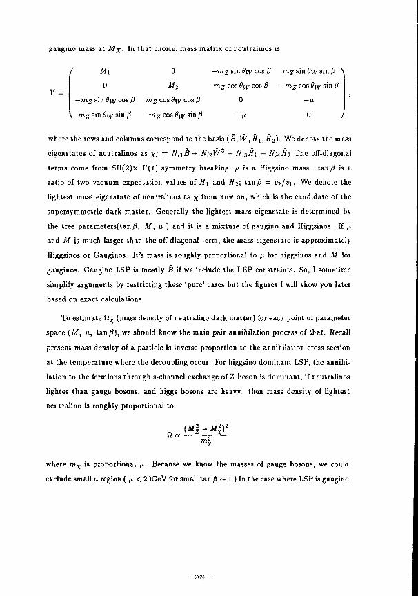
gaugino mass at Mx- In that choice, mass matrix of neutralinos is

/ M\ 0 — vn.2 sin 8yy cos /? mx sin Qyy sin /3 \

0 M2 m^ cos#w cos,8 — m^cos^y sin/?

—m^ sin^iy cos/9 m,2 cos (?jy cos /3 0 — /i

\ m^ sin Oy/ sin /3 — m^cos^y-sin/? —\i 0 /

where the rows and columns correspond to the basis (B, W,H\, Hi). We denote the mass

eigenstates of neutralinos as xi = N\\B + A r i2^ 3 + NiiHl + NnHn The off-diagonal

terms come from SU(2)x U(l) symmetry breaking, fi is a Higgsino mass, tan^ is a

ratio of two vacuum expectation values of i/j and Hi; tan/? = vijv\. We denote the

lightest mass eigenstate of neu'.ralinos as x from now on, which is the candidate of the

supersymmetric dark matter. Generally the lightest mass eigenstate is determined by

the tree parameters(tan/?, M, \i ) and it is a mixture of gaugino and Higgsinos. If fi

and M is much larger than the off-diagonal term, the mass eigenstate is approximately

Higgsinos or Gauginos. It's mass is roughly proportional to \x for higgsinos and M for

gauginos. Gaugino LSP is mostly B if we include the LEP constraints. So, I sometime

simplify arguments by restricting these 'pure' cases but the figures I will show you later

based on exact calculations.

To estimate Qx (mass density of neutralino dark matter) for each point of parameter

space (Af, /i, tan/?), we should know the main pair annihilation process of that. Recall

present mass density of a particle is inverse proportion to the annihilation cross section

at the temperature where the decoupling occur. For higgsino dominant LSP, the annihi­

lation to the fermions through s-channel exchange of Z-boson is dominant, if neutralinos

lighter than gauge bosons, and higgs bosons are heavy, then mass density of lightest

neutralino is roughly proportional to

(Ml - Ml)2

m\

where mx is proportional ft. Because we know the masses of gauge bosons, we could

exclude small /1 region ( n < 20GeV for small tan § ~ 1 ) In the case where LSP is gaugino

( This is a case where M « //) the main process is t-channel sfermion exchanges. The

mass density is thus roughly expressed by this formula,

n«i/(£<0>-« /.

so the process which includes lightest sfermion dominates;

0 oc / " ' * ' " ' .

where mx oc M. So, most analysis was done under the assumption all squarks and

slepton masses have equal mass.

At present, the only accelerator bound is that slepton mass is larger than 45GeV,

so it seems that we couldn't get any strong constraint to the gaugino mass in the phe-

nomenological treatment. But once we include the implication of the model, we get much

more from the cosmological constraints.

4 SUPERGRAVITY

Spontaneous supersymmetry breaking in the hidden sector is most promising idea to

introduce soft supersymmetry breaking to the theory. In the Minimal Supergraviy Model,

the hidden sector which couples to OUT sector only through gravity induce spontaneous

local supersymmety breaking to the theory. The coupling of the hidden sector to the our

sector is suppressed by ihe planck mass, so the soft susy breaking terms which appear in

our sector has small mass scale (ITeV) although the breaking scale of the hidden sector

is high (10 1 1 GeV). Because gravity couples all particle equivalently, we get the following

unification conditions at the unification scale Mx'-,

Mi = Mi = M3 = M

m-, = m^ = m

This is the boundary condition at the planck scale in the supergravity model, and we

have already come upon the first one. Notice the parameters of the model are greatly

reduced in this model compared to the phenomenological treatments. But it does not

mean that they have a common mass at the weak scale. Gluino and squarks have color

charge, so they get strong corrections which comes from SU(3) gauge interaction. The

other superparticles get relatively small correction due to SU(2)x U(l) gauge interaction.

This feature is independent on the low energy contents of the theory. The large differences

are due to the fact that the SU(3) coupling is much stronger than that of SU(2) x U(l)

Thus we get the following relation at weak scale in addition to the mass relation of

gauginos we got before;

m\ - m2 + (6.28 ~ 5.82)M 2 + (0.35 ~ -0A2)D

m? = m? + (0.52 ~ 0.15)A/ 2 + (0.5 ~ -0 .27) /?

where D — m^cos(2j8) < 0 and we have used sin 2 6w{mz) = 0.233. These relation

determined by renormalization group analysis, which make us possible to discuss the

relation between the parameters at GUT scale and weak scale. The equations are derived

by assuming that Yukawa coupling does not affects the R.G flow. Top yukawa coupling

plays important role in the stop mass RG equation, because top mass is extremely heavy

relative to the other quarks. Thus the relation do not hold stop masses. But this

exception is not harmful when neutralino is lighter than top mass. Also, because we

have two Higgs doublets in the model and bottom mass and top mass is determined by

the relation mj = Ajvi,mj = htvi, where v\ and V2 are the vacuum expectation values

of two Higgs doublets, bottom ynkawa and tau Yukawa also might not be negligible in

the whole RG flow. This means this relation might not holds for sbottm and stau, but

it is quite safe to assume the relation for these particles if tan/? = v^jv\ < 10.

- 271 --

5 COSMOLOGICAL DENSITY OF NEUTRALINO IN MINIMAL SUPERGRAVITY MODEL

We can see from those equations that squarks and gluino get large corrections from

the value at the planck scale; squarks and sleptons expected to have large mass differences

when gluino mass is large relative to m. This relation affects the estimation of the mass

density of gaugino LSP, or the mass density for the model where M is much smaller

than (i, because relations include gaugino mass. Actually, eliminating mo from these two

equations,

TOj= Jm2- - 5.9M2

This tells that if we fix squaik mass, m.- quickly decreases when m~ ~ m; or 6.7mx

(Because Y is mostly B whose mass is roughly M\. Let us consider the case where the

gaugino is lightest neutralino, or M << fi, and what will occur. The mass density of

neutralino is proportional to inverse cross section, and now

2 mi. erv <x — j -

rru

because we expect that m,- is much smaller than m;. Then in the region where M is

small relative to m, fi is very large because mx oc M (so mx is very small ). On the

other hand the region where trig ~ m^, slepton mass is very small and mx is large, so ft

is very close to zero.

Fig.l displays the allowed region and excluded region in (mq,nig oc Mi oc mx )

plain. We take fi = -600 GeV in the figure, which correspond to the gaugino LSP area,

but the plot is more or less same provided |^| > 300GeV, and mx < 80GeV You will see

that the mass density decrease very quickly around the region where rrig ~ nig-, the right

and left areas are excluded because m 2 < 0 and because ft » 1.

The result is completely different to the one under the assumption all squark and

slepton mass is equal and give the constraint rriq ~ rrtg. We could say the widely accepted

assumptions such as m« = m-. may give a misleading conclusions. We could rewrite the

conclusion in the mass parameter M and m. It tells that for the case where fi > > M m

should be smaller than M. on the other hand the region where /J < M generally gives

small mass density of x due to the strong Z pole effects; on the one hand the region is free

from cosmological constraint, on the other hand it does not give interesting cosmological

mass density.

6 HIGGS CONTRIBUTIONS IN THE SUPERGRAVITY MODEL AND DISCUSSIONS

Until now we have been working under the assumption that the annihilation into

fermions intermediated by squark and slepton are dominant. I would like to consider

when the assumption breaks.

The most dangerous cannels which break the assumption is the annihilation through

the S channel Higgs bosons. In the minimal supersymmetric standard model, we have two

charged Ifiggs bosons and two neutral scalar higgs bosons {h,ll) and one pseudoscalar

neutral Higgs boson(/t). Charged Higgs is always heavier than W boson. But the

lightest scalar higgs h is always lighter than Z. These Higgs couples to neutralino x

and the coupling is proportional to the product of its Higgsino fraction times gaugino

fraction of x- Thus the coupling is zero if x is pure gaugino, but generally not zero

due to the mixing of those. So it cannot be neglected if mx = m/,/2, m^/2,...., where

the pole effect is enormous. It should be noted that Z couples Higgsino fraction only.

So for gaugino dominant neutralino the effect of Higgs bosons are comparable to that

of Z, although the Higgs effects are suppressed by the masses of final state fermion.

Also the pseudoscalar higgs boson give very important contribution to the annihilation

process to the neutralinos. Because the neutralino are majorana particle, the S-wave

form 0 - + . The pseudoscalar higgs boson A then give very strong contribution to the

annihilation cross section on mass shell relative to scalar higgs bosons. The contribution

might be much stronger than that of Z-pole, because Z-pole appears in P wave which

is kinematically suppressed. Also h A final state could be CP odd so the process could

have very large contribution to av once if the process become kinematically allowed.

But before saying it is really a matter we should be careful about the mass of the

pseudoscalar Higgs boson; it is also constrained by the same boundary conditions at

- L'73 -

unification scale M%. The constraint to the mass of the pseudoscalar higgs boson m^

at Mx is

m\ = 2m2 + 2 / i (M x ) 2

m,A gets strong corrections coming from top Yukawa coupling, but if we can neglect

the bottom Yukawa, the following relation holds.

m2

P = ^ 2 - (cot 2 p - l ) + (m 2 + 0.52M2 + / / 2 ( m z ) f - ^ - j

This tells that m^ is much heavier than slepton mass or ,u; thus the process including

A never dominates in the total annihilation cross section of x So for the case where

tan/? < 10, we could say the annihilation process though m; dominates except the pole

of scalar h and Z boson.

Also I would like to mention here the recently found solutions (by M. Drees and

M.M.N.) where both bottom Yukawa and top Yukawa are large at the unification scale.

The solutions always give large tan/? > 14 ~ 15. In this case pseudoscalar is arbitrary

light due to the effect of bottom yukawa, and the stau mass also become very light

compared with the other slepton mass.

So the previous arguments I gave doesn't holds here, because the simple mass rela­

tions does not hold; Here the lightest sfeimion is stau and Q a m*fm'l

< is still valid, but

m,f ~ m do not holds. Mass density is determined by the annihilation though stau or A ,

whose masses should be determined by the more detailed analysis of the renormalzation

group equation.

Conclusion

If the lightest neutralinos is gaugino, lighter than W boson and providing tan 0 < 10,

we could say, squark and gluino should have almost equal masses, which is equivalent to

the slepton mass is light.

References

M.M. Nojiri, Phys. Lett 261B,76(1991)

- 2 7 4 -

M. Drees and M.M. Nojiri, KEK-TH-290, June 1991 and references there in.

- 275 -

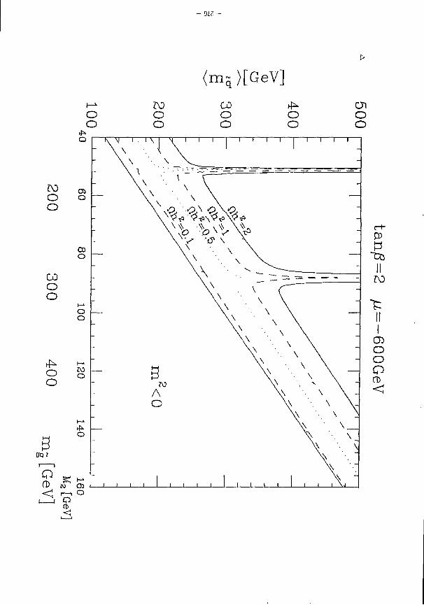
- 9 L Z -

(m~Q }[GeV]

The Birth and Early Evolution

of

Our Universe

K. Sato

(Univ. of Tokyo)

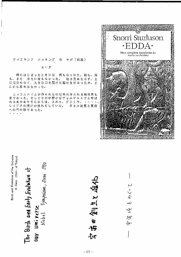
7 A -X v y Y : -< * y •. © t f j ( e a )

no it u * o k t g tut* ®t>tj;iftrz. ®i>, m * , S fc ft £ ^ ffi *J tt 4i -3 fc . l ! i I S f ; 5 r , ± K is 21) & < « * § tt n * ra <t fc a (t a # s -3 & *<> if £ 1;: & 5 * !i ft S -3 fe.

=. -j Z) fr J\ -( -L i< ft b h K. Olt 1& <D ft $ ti Z $&%• R <b a1 Tr S •= & . i b T f » t l C I » ' i * y * 5 7 t »f if ft5S*SvTi:*4ii> 7#<•?, yytvs • • • • , L- -f 7 5- © VRT JH 45 S ft fc' 0 T ^ tz. *" a )l \t % t ^ Jfi -\ © H © Ki Tr 6 -3. fc .

Snom Stmluson EDDA

5 £ 0

JS ° -»-> s i ­

Z .i 0 0 s S B "P tu

• «s 3 •s 5 "+• y-n r-^ A —•»

1 * £ * a *-*i 0

Bit

* L i t 0

v/"> "^ >-. Si V 1—»

<S > _ £ »

r£ '«: £ CO

3

V V =5

h- 0

-0

Hi

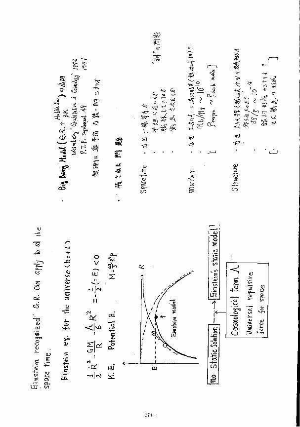
"iV

»* «-*--. —. 5 > k-<§ 1 • \

6" «3 *""» ~ f J

? °^ . r -*= <? <s o -\ a-3 1 * : *£•-+• 1

^ CO....S -*g

-S > &- <% m

s: ^~

J CO

\

c/0

-*0 -<Z 6~

3 ^

n? ? Q—,

i -

*0

•56:

^ • ' a • c-

4V- VA ° - u ^ V i

^ * S •?> ^ >J*

I S •

CO

CS

Cjj

o o

CO

• + -

t i l •

+ •I

00

0»

v if. II

I II

^ | M D I

t£rl I

<•» • Of

*£

o-

is:

1 ^ i \

•

< 1

( i f

f

" 3 CO

o

o

< 0) > •

CI

<a i -V J

o - o t f o <a CO w-> o i _

o O

O => M--

- 1'7H -

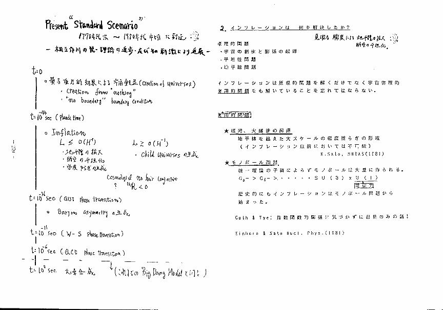
fteswt SWAcmi Scenario

• flu bowido-j" t f t w i ^ ci«W(fc»n.

t -10 sec ( fWddViO

• 0Vf O- fJMb

t : m sec CQui f^,c ttMKttD'fc')

, -H t | l O 5co C V - S tWlVwinftw)

i> io l sec * ^ £- ^ (Mif ta 1 ^ ft*3 H>^ 11--] t J

2. -f > ~7 U - -> B > ii W fe MR' Li fc » ?

- ¥ iB © £i] ife t HM 35 ffl J2 ilS

- ¥ IB 14 PI Z& • O ¥ IX P3 £9

0 7 b - j ' 3 > u i ! ! a i i i i ! ; a * f i < f c " i f 5 a < ¥ t f s a i i i i

• as ft. -kmm o&n ill! ¥ « * & A fc ± 3. T - A (D ffi ffi i£ * 8' © IK « ( -f > 7 u - if 3 > ia nii K *J v1 x u 7 . L fig)

K . S a L o , H H R A S ( 1 P 8 I )

•k * ; ,-li - ; i pn ,15 K - 11 S ffl ? .9 i: i 6 V -t- y ;K - * (i * fi i: If v> ft 3 . G „ - > G.< S U ( 3 ) x L) ( 1 )

in !t 15 u fc O 7 b - i ' a > li i ; * - ;v HI a *> £ te 4 o fc .

Cu th i Tye; |g » Bfl » flj He 3S r. R ri i i f t; ja tt ro ft m Wl

E i n h o r n J S a t o N u c l . P h y s . ( I D 8 1 )

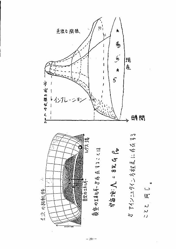
&ft* # * .

1=2

•is*

•Br

5 1

1^ * ?

ST

- 280 -

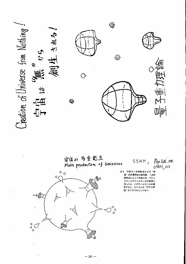
• r

e

. o

C3

$ ?

5

•K»

•DhT

o

§>

® 4®

Multi production, of (MiV««« SSKH fwj.Lft. M i

cnw^rt 05 ?S«1IS8EBI:J:5 •?

s ' «isaffl£«jaKa. i .£«> >.-—JH>9—A.-s—Jlftisai; firiho. C«)7—A.T—A»iSt S T i t , fc<?/,« ' ? t ' 6 ? S ' J ' T J o J ' i L f K i l '

-281

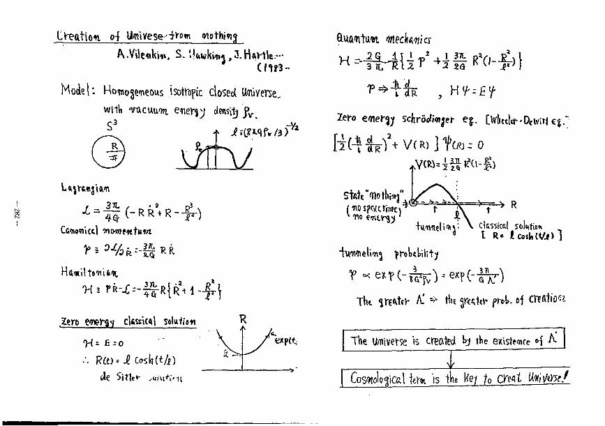
A.Vile«kii». S. H&w-ki'M,3.Hftrtl*.—

Model: Homogeneous isotrofic closed U<niverse„ wnli imcuu'm e<ne)r^ dmty j>v.

Cc«o4ii(cl we»ne«t««t

Hainlltooiitit

.Zero Cne^y cUttiCOJ Soluftati

••• R f t )« i Cos h(t/i)

€Xp(t

ftuaiituiii mechanics

Zero emerjy Scfcrocfioijer e j . CWtala-DtMif eg.

[ i(^%V(R)]too--o yo^if^u-Jb

* R Stole "Wtlifrj" (flospottltaci*

+u<nnel »««(• \ classical solution

"tuwheliiij troUlility

The Umivette is created fy the existence °{ A.

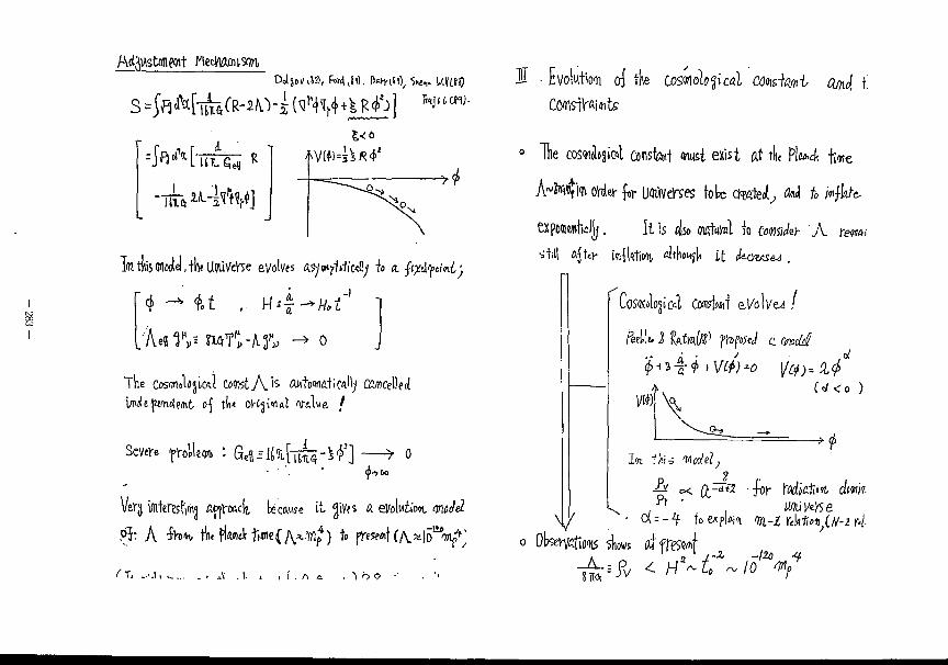
£^6

III tkis Onodd, "th* UQVJVcVe eVotas esj^Uk^) io a. fodpintj

"4 -* it , H4-W^"1

The CosnmJUjiwl CotetA'1* autoMfl.tiwl^ GJfflCellfJ

Sevtire ^lltfl, : G^iH%[^-i^] — > 0

Ve 3 imteftst'i^ ftffV«4 te cause i t $iVfS ft elfolwfciwi We?

Pi: A fro*v lMA««k1i»>e(y\vW*) t» fTeswif f / V ^ l A n ^

/ 'T , . - J , L\: . I. L i l . r t a ^ O P

1 • Evolution oj tile Coswioloflica! OJoisij/jit fl/^ t.

COtflsilrAimte

itfe 0 Hie cos&iotajkil constant ml exist ftt 4 Plw«cA f;

A ^ M OVdev y UluVcWes tote o m W , ^ /<> / 4 ' a ^

eXpOMfthclk , I t IS fllso 0W,W to CoW<?)- A cewfl/

CoS»lo§ifrl CowW eVoIve^ /

Pedlu 2 fomltf1 flroftftJ c cirvdi

W W U<0 )

~&> •*f>

V

1*1 ffi-i Wfrf.ll?

• o u - ^ foetpkii iiL-ZYtUt,oit(^-zr4-

»< ft.23*2 J-oy- tofto>«. dim

0 Obsevv«fioois tiovs a t f res^ f A . Slid

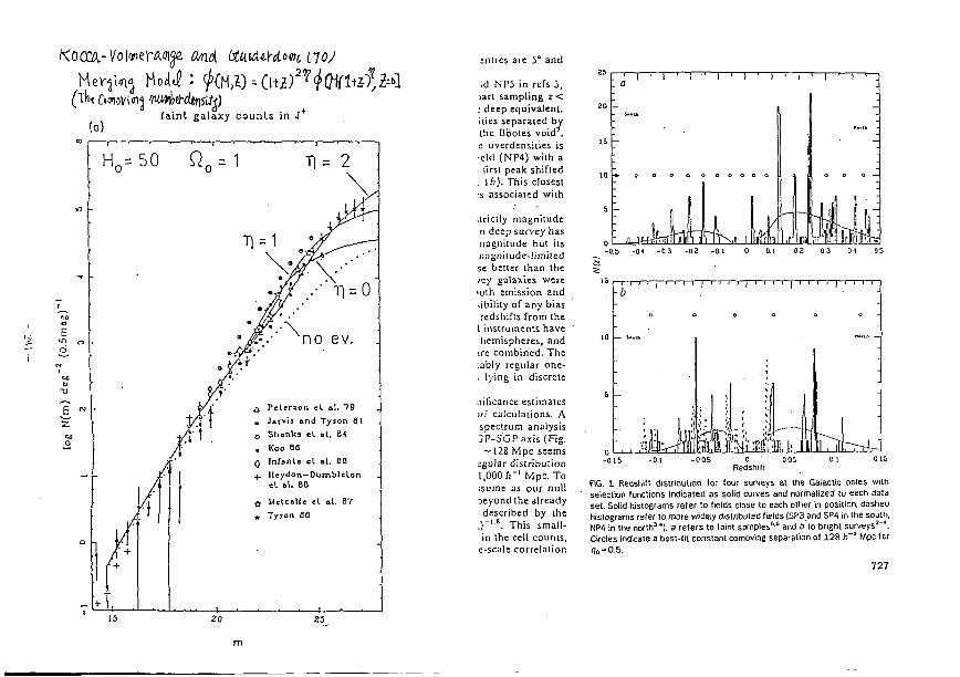
(ainl galaxy counts in J (a)

H o =50 fi0=1 Tl= 2

A Peterson cl al. 79 H Jarv'u and Tyson 81 o Shanks el et. 6-1 « Koo 66 0 Infanle el »I. 66 + Hcydon-Dumbleton

el al. 60 {, Melcalfe cl al. 87 * Tyjon HO

25

cnlres are 5" and

Id NP5 in refs 3, (art sampling z < : deep equivalent, ilies separated by the Dbotes void 7 , c overdensities is •eld (NP4) with a

lirst peak shifted . 16). This closest s associated with

.trictly magnitude n deep survey has nagnitude but its n.-igniiude-limited se better than the ^cy galaxies were 'Olh emission and iibility of any bias redshifts from the

1 instruments have hemispheres, and

ire combined. The :ably regular one-. lying in discrete

nificance estimates in' calculations. A spectrum analysis i P - S G P a x i s (Fig. — 128 Mpc seems

jgular distribution 1,000 ;."' Mpc. To ssume as our null beyond the already described by the

, ) - ' • ' . This small-in the cell counts,

e-scale correlation

-0.5 -04 - 0 3 - 0 2 -0.1 0 0.1 0 2 0.3 0 4 OS

- 015 Redshift

FIG. 1 Redshift distribution for four surveys at the Galactic poles with seleclion functions indicated as solid curves and normalized to each data set. Solid histograms refer to fields close to each other in position; dashed histograms refer to more widely distributed fields (SP3 and SP4 in the south, NP4 in the north 3 4), a refers to faint samples 5 6 and b lo bright surveys 3"'. Circles indicate a best-fit constant comoving separation of 128 h~l Mpc for q 0 = 0.5.

727

•o

at

1

^9*

^

2 * .3

2"*'* jar

-rf» •sg.

:JG c s

,?£•

t

s i

* •A

« J?

1 «

<

0/

^ *i

s J

•s ir • t—

' N 5 +•> w

£. :\

r

< 1 | f « |**« dL 'Mi o 1 ^

v> t* £ 1 ^ o •<r

& +c» <u t i ' ^

o: 3 I <

i -£ u

_§

Q

o o •I II

C(

• ^

2S 4 i

4

-£ 3

o

cif-

II E -

c? ^

O ' C

o T o

•e ^ t

t / \

4? oS

. J ,a

.•JB •ir +=>

-vr -

ft 'US

-e£<

- 2 8 5 -

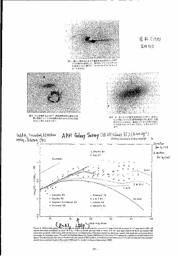
A:»jiiti n t l i r , - m i ' i i r * ' ' ) - ' <. - <. «•'/> .

^^i^^^PSi^-" 0 ] ^ - 7 _ i ; >?tt?l ESO-U5-C26"". B W i :

•WAa W,t*M,Eirt*»u APH G«1«W S«Wey OS UfffcUt Hl)tW>tyl) ov? i ^ , M i r * * < » G"'fl'^ 'ev0'""'<"t"'/ovv ' " ^ i/? 3r

1 , ... ,

- Shores 8 *

a Koo 81

Euclidean , 0 u a

• a + . 6.

0 0 ° 0

0

o

0

o

0

o

. . - - . . Tyson • • a

+ . 6.

0 0 ° 0

0

o

0

o

0

o

. . - - . . Tyson •

^ y * ^ "^ t^^..... C & R-V • - . .

&^^* * Y & p

/ * « Metcalfe e9 * Peterson 79

+ Shanks 89 o j & r si No evoJ

• Heydon-DumbletQn &9 • Infante 86 a Peterson 86

I . I .

0 Metcalfe 90

20*ini«

f 26

Frg\jr« counl: linear corrcc figure, mode!

2. Differeniial galaxy founts per s / W e degree pcf magnitude {i.e. count in 0.1 maj binjx 10, or counl in 0.5 mag binjx 1.98). All have been multiplied by dc*[-0.45(J>,- 16)] la provide an expanded ordinate. The thin mi thick solid lines Jhow our results with

and quadratic calibrations, with correction for incompleteness. The thick dotted line ihows our results will quadratic calibration before lion for incompleteness. The u*rrck dashed tine jho«*s (he Tyson {}988) hint CCD counts. The various data poinu are as indicated on the .The thin smooth line shows the no-evoluiion model of Ellis (1981 J, normalized lo our counts at b,~ 17, and we alja plot two evolution i (je;;e.il} from Yoihii A Peterson (1990) and CuiderdoniiRocca-Volmera7ise{t 990).

L>m; • -

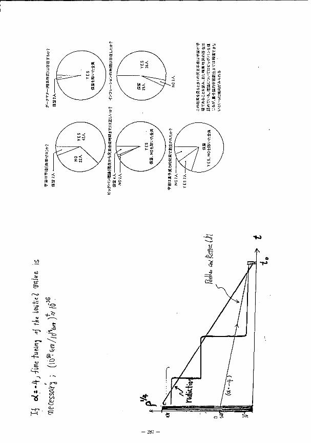
i2

i <o

& & 3

•I .

M

- 2 8 7 -

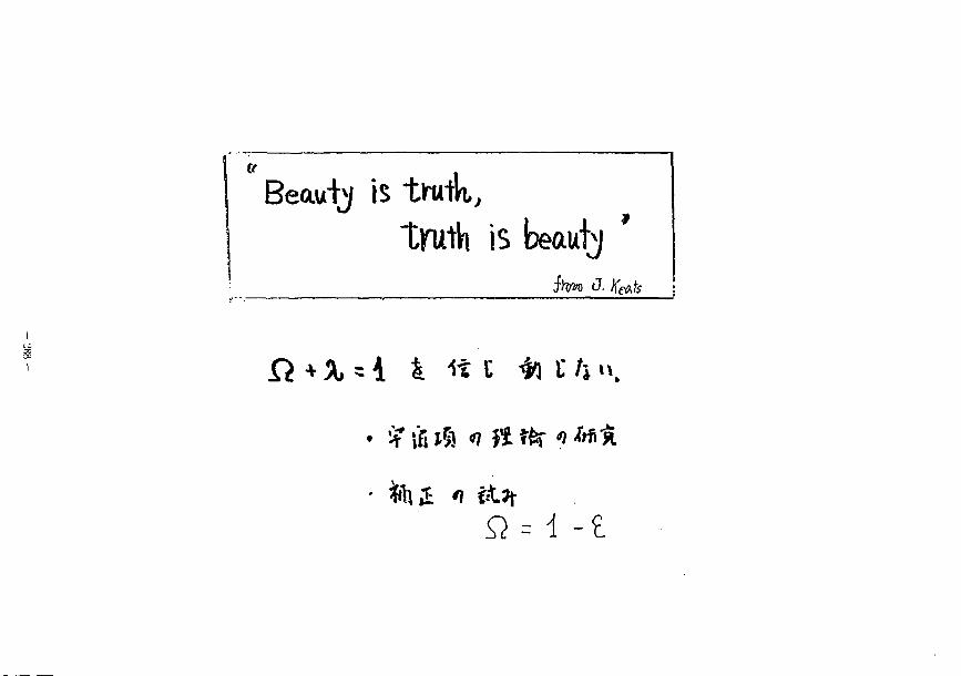
Or

Beauty IS tlrutk, truth is beauty *

j t w J- fo&fe

I}+A>=1 4 i t U * f / i n i

N E W U P P E R B O U N D O N E L E C T R O N A N T I - N E U T R I N O M A S S

H. KAWAKAMI, S. KATO, T. OHSHIMAt, S. SHIBATA, K. UKAI Institute for Nuclear Study, The University of Tokyo, Tanashi, Tokyo 188, Japan

N. MORIKAWA, N. NOGAWA Isotope Centre, The University of Tokyo, Bunkyo-ku, Tokyo 113, Japan

K. HAGAt* Department of Physics, Tohoku University, Sendai 980 Japan

T. NAGAFUCHI* Department of Applied Physics, Tokyo Institute of Technology, Meguro-ku, Tokyo 152, Japan

M. SHIGETA" The Graduate School of Science and Technology, Kobe University, Kobe 657, Japan

Y. FUKUSHIMA, T. TANIGUCHI National Laboratory for High Energy Physics (KEK), Tsukuba, Ibaraki 305, Japan

A new upper bound of m„ < 13 eV at 95% C.L. has been obtained on the electron anti-neutrino mass. This result is based on more than a tenfold improvement in data relative to our previous measurements of the /^-spectrum in 3H-decay, and is in conflict with a finite mass of 17< m„ <40 eV reported by an ITEP group.

- L J8!) -

t Present address : National Laboratory for High Energy Physics (KEK), Tsukuba, Ibaraki 305, Japan

tf Present address : Fuji Plioto Film Co, Fujinoiniya, Shizuoka 418, Japan | Present address : Toshiba Co, Tsurumi, Yokohama 230, Japan It Present address : Toshiba Co, Fuchu Works, Fuchu, Tokyo 183, Japan

A group from ITEP [1,2,3] has consistently reported a finite mass for the electron anti-neutrino (m„), and a value of 17< m„ <40 eV for their accumulated data indicated in their latest paper [3], Nevertheless, three other experiments [4,5,6,7] could not find evidence to support a finite mass. More experimental study with better mass sensitivity is required to finally settle this important problem, with major consequences on issues in particle physics and cosmology. From our two previous measurements of the /?-ray spectrum in 3H-decay, we obtained an upper limit on the mass of the electron anti-neutrino of 32eV [6] and 29eV [7]. Despite our good overall energy resolution of ~15eV, the mass sensitivity was limited by the statistical precision in these experiments : The accumulated signals in the 100 eV region below the 3 H end-point energy (E„) had 5,000 and 10,000 events in INS-87 [6] and INS-88 [7], respectively. To overcome this limitation, the radioactivity of the /^-source and the sensitive area of the /7-detector were enhanced this time, respectively, by a factor of 5 and 6 times relative to the previous runs. As a consequence, 150,000 events were accumulated, and a new upper bound on the m„ of < 13 eV was obtained, at a confidence level of 95%. In this note, we report our latest measurement (INS-90), carried out at the Institute for Nuclear Study (INS) of the University of Tokyo.

The experimental method is the same as in the previous measurements, which are described in detail in ref. [6,7]. A correct estimate of the overall response function (R/r) is essential for a reliable measurement of m„, and one of our unique advantages in this regard is that we use the same chemical compound for both the 3 H and the reference I 0 9 C d sources : The former is a tritium-labeled arachidic acid (C2oH 4 0 0 2 ) in the form of a natural Cd salt, and the latter is non-active arachidic acid in the form of a radioactive 1 0 9 C d salt. Because components of R/r, namely an optical response function (R o p<), an energy-loss effect (EL) and a backward-scattering effect (BS), are the same for both the /?-rays of the 3 H and of the 1 0 9 C d sources, the R;r can be extracted reliably and simply with small systematic uncer­tainties from the observed spectrum of the mono-energetic KL2L3 Auger electron in 1 0 9 Cd-decay, whose energy is close to E 0 . Botli sources are deposited on high-resistivity RU2O3 coated alumina plates (200mmx 60mm) in two mono-molecular layers of total thickness of 50A (0.6/xg/cm 2), using the Langmuir-Blodgett method [8]. Owing to this preparation method, the average thicknesses seen by the /?-rays

- L'9] -

from both the 3 H and I 0 9 C d atoms are the same regardless of different labeled po­sition of these atoms in the molecules. The activities built up on the plates are 40mCi and 200/iCi for the 3 H and the 1 0 9 C d sources, respectively. The distribution of radioactive emission is observed to be uniform and the same for both the 3 H and 1 0 9 C d sources over the whole plate surface, using a photometric method with a measurement accuracy of a few percent. Although the evaporation rate of the acid as Cd salt is known to be low in vacuum, the sources are cooled down to -35° in order to further suppress evaporation, which contributes to background for the /3-spectrum.

The P-rays were analyzed using the INS double focusing 7r\/2 iron-free spectrom­eter, whose schematic layout is shown in Fig.1(a). The central-orbit radius was 75cm, the relative stability of the main-coil current was 2 x l 0 - 5 , fluctuations in the external magnetic field were cancelled out to 0.05mG, and a vacuum of 5 x l 0 ~ 7 Torr was achieved. A position sensitive proportional chamber shown in Fig.1(b), used as a /9-detector [9], was placed in the focal plane. The chamber consisted of 7 cells, with wires oriented horizontally in the focal plane, each cell being 35mmx 10mm in transverse dimensions ; the position of the /?-ray was detected using charge di­vision. .Good position resolution was achieved by minimizing multiple-scattering effects of the /3-rays in the chamber window and gas, and through high enough gas-multiplication. Using a relatively thick window of aluminized polyestel film, and isobutane gas at nearly one atmosphere, the /?-rays stopped just after passing through the window. An extra layer of proportional chamber was used as a veto just behind the 7 cells for rejecting background, due mainly to cosmic rays. The re­sultant position resolution was a=500fj.m for 18keV /?-rays. Without using 0.5mm slits for position determination, as was the case in the previous measurements, the sensitive area of the /5-detector was effectively enlarged by a factor of 6.

The overall performance of the detector was carefully examined and compared with the previous systems. For compensation of optical aberration due to finite source size, a focusing electric potential was formed by applying voltages on the source plate and on an electrode box surrounding the source. Five narrow elec­trodes, each being 300jtm along vertical direction, were printed and spaced on the source plate every 50mm in the horizontal direction, with each supplied by in­dependently adjustable voltages. The distribution of the applied voltage had an

approximately parabolic form, at a bias voltage (VACC) of ~-1.5KV with stability of 0.2V. With an optimized focusing electric potential, Auger spectra were measured using slits of 0.5mm in front of the /^-detector, and an overall energy resolution of 15eV (FWHM) was observed, consistent with the previous measurement. In this experiment described below, the slits were removed and a resolution of 30eV (FWHM) was found, which was dominated mainly by the position resolution of the ^-detector. Curvature of the vertical focal line, arising from a third-order aberra­tion due to the large source size, was observed as a peak-shift of the Auger spectra among individual chamber cells, and agreed well with the effect expected on the basis of a numerical orbit analysis.

The 3 H /?-spectrum was measured with six different settings of VACC> keeping the magnetic field strength constant. Correcting for the acceleration voltage of VACC> the ^-energies at the center of the /^-detector for the settings were 17.97, 18.24, 18.52, 18.59, 18.69 and 18.79keV. Data were taken for times corresponding to these VACC values in the ratios of 3 : 9 : 50 : 2 : 2 : 2, with full scans of the 3 H /J-spectrum. The energy range at each setting was ~350eV, and the adjacent settings had overlap regions to check for smooth transition. The K L 2 L 3 Auger spectrum was also measured daily, at the third VACC setting, upon completion of the 3 H cycle, by interchanging the 3 H source for 1 0 9 C d . This Auger energy line (18511.7±1.3)eV, precisely determined using the well known energies of 1 6 9 T m M conversion spectra in 1 6 9 Yb-decay [10], was used to calibrate the absolute energy of the 3 H /^-spectrum, and its position and spectral shape were used to monitor the stability of the whole detection system. Moreover, the Auger spectrum provided the function Rx, as obtained by deconvoluting a natural line width (T) and a shake up/off effect (SUO) from the Auger spectrum :

RT = {Auger) ^T-^SUO-1 (1)

where the superscript -1 denotes the deconvolution procedure [11]. Dv.mg two months of measurement, no appreciable change was observed in the shape of the spectrum.

Besides the above energy measurements, it is vital to acquire precise information regarding dispersion, namely the relation between the detected position of the /?-ray and its energy, and variations in detection-efficiency over the sensitive area. Po­sition linearity of the detector is measured by noting the response at various slits settings, and in fact, good linearity was found between the positions of the slits

and the observed data within an accuracy of 0.1mm. By periodically measuring the Auger spectrum for different positions of the /3-detector, at 14 values of VACC (in 20V steps), we obtained a dispersion relation for energy vs. peak-position, that indicated a small second-order aberration consistent with the intrinsic properties of the spectrometer. The efficiency variation was examined by comparing the Auger peak-counts, obtained by fitting the spectrum to a smooth function around the peak, with expectations assuming constant efficiency over the fitting region. This comparison displayed a slight parabolic behavior of <2% increase in efficiency for the ends of each cell. The same behavior for the efficiency dependence was also obtained from the 3 H /3-spectrum, as measured without the focusing potential.

Background was studied by setting VACC values that corresponded to central /?-ray energies of 18.88, 18.98 and 19.38keV. A small energy dependent component was found, but its rate did not change during the experiment. By closing vacuum gate valves just downstream of the sources, or upstream of the detector, the origin of the background was determined not to be associated with the /^-sources.

A total of 150,000 events were accumulated in the 100 eV region below the E 0

value of the 3 H /?-spectrum ; this sample corresponds therefore to the same or higher statistics.as those from other recent experiments [3,4], Data from the first and last cells were not used because of their lower accumulated number of signal events and the data from the remaining five cells were analyzed separately. Background was discriminated from the signal by imposing a cut on the pulse-height distri­bution. Also, any event that fired the veto counter or several cells was rejected as a cosmic-ray. A small energy dependence of the transmission, long-term drift of the system, and dead time of the data acquisition system, were corrected in the data. The energy of the 3 H ^-spectrum was determined from a comparison with the K L 2 L 3 Auger line, and the dispersion was measured to be ~12.3 eV/mm. For the final analysis, the /?-spectra from the six different VACC settings of the individual 5 cells were binned in 5 eV interval.

The function R^ was also obtained from the measured KL^f^-spectrum with the help of Eq.(l) . The detailed procedure is described in ref. [6,7]. In the present analysis, the SUO spectrum used is based on a newly refined calculation described in ref. [12]. Two mechanisms of the Auger transition are considered, one is associated with a K-vacancy produced in the initial K-capture by , 0 9 C d , and the

31 -

other is associated with a K-vacancy produced by a K-conversion emission of the 1 0 9 A g metastable nuclear state. The SUO spectrum and the resultant function R? are shown in Fig.2. The EL component in the Rj- was measured previously under the same conditions as in this experiment to be 30% ; it consists of two almost equal contributions, one from the source substance itself, and the other from an adsorbed gas on the cooled source surface [7,13].

The m2, is deduced from a x 2 fit of the data to the following formula for each cell:

N'(E) = y(&E)ADJ[ F(E')PET{1 + a2(E„ - E')2}

X £,• Ui{E0 - Ei - E'){{E0 - Ei - E'f - m 2 } 1 ' 2

+ {BG0 + BGi(E0 - £')} ] RT{E,E')dE\ (2)

where

» j (A£)= l + C1AiJ + C2.(Ai!)2, (3)

AE = E - Ei. (4)

F(E) is the Fermi function and p, E and E^ are the momentum, kinetic energy and total energy of the /?-ray, respectively. E; is the final state excitation energy in the /?-decay, with transition probability w;. Just as in the previous experiments [1-7,14], an empirical shape correction factor a 2 >s required in fitting the data. An energy-dependent linear term BGi, in addition to a constant component BG 0 , for the background is included in the formula. Instead of using the value obtained from the Auger-spectrum, the energy-dependent efficiency T/ parametrized by £i and £2, as defined in Eq.(3), was introduced as another fitted variable. A superscript j refers to different sets of 3 H spectra, Ej is the central energy of the /^-detector at the j setting, and d and £2 are common to all 6 data sets. Free parameters consist of the normalization constant A 0 , E 0 1 oil, BG 0 and BGi, 0 and £ 2 ) and m 2 . There were typically 354 data points used in each cell within the energy range 17.88-18.95keV.

The spectrum of the final state (SFS) is most seriously affected by the nearest surroundings of the tritium atom [15,16], consequently our acid is expected to have a similar SFS to that calculated for valine acid by Kaplan et al. [15,16]. It is found, in fact, that the results calculated for our acid by Arafune et al. [17] are on the whole very close to those in ref. [15,16]. Since electron correlation effects

- 295 -

are not considered in the calculation by Arafune et al, the values of the Ey and Wj calculated by Kaplan et al. are assumed appropriate, and used as in our previous analyses in ref. [6,7).

Resultant parameters from the best fit are listed in Table 1, and the correspond­ing Kurie plot for the individual cells are shown in Fig.3. Fig.4(a,b) and (c), show the typical deviations of fitted curves from the experimental data, and the relation between x 2 and m 2 , respectively, for one of the cells. The resultant r/'s for individ­ual cells agree very well with the values deduced from the Auger-spectrum. Using 77's deduced from the Auger-spectrum, the fit with six parameters results in consis­tent values not only for m 2 but also the other parameters. The main function of a j is to supplement the imperfect evaluation of the small but long tail of R7-, so that it contributes dominantly in the lower energy region and is essentially insensitive to m2,. We examined the sensitivity to m 2 by varying the lowest energy data points up to 18.13keV in the fits, and we found that the resultant m 2 values agreed within statistical accuracy.

Systematic errors in KT arising from ambiguities in estimating T and SUO were evaluated by changing their amounts individually by ±10%. Their effect was to shift the .resultant m 2 by the amount of ±34 (eV) 2 . Uncertainty from the SFS is difficult to estimate, so that our result is inevitably model dependent. Arafune et al. [17] examined the dependence of the transition probabilities on the basis set by taking larger number of wave functions for representing the initial and final molecules than those by Kaplan et al [15,16], while the latter calculation emphasized importance of configuration mixing. By referring the result of ref. [17], the w,-'s of the ground and the excited states which had more than 1% of the probability were varied randomly by Au>,- = ± 1 % , as the systematic uncertainty ot the SFS used in the fit. In this process, the average energy of the SFS (A£*) and the ionization probability (ti;;o n) were fixed to be the original values obtained in ref. [15], namely 18.8 eV and 10.6%, respectively. The E ; o n representing the ionization energy by a single level was calculated by AE", w I < m and the average energy of only discrete levels, with the help of Eq.(35,36) of ref. [16]. It was found that resultant m 2 shifts at maximum by ±31 (eV) 2 relative to the m 2 for the best fit. The above two systematic uncertainties behaved the same on the m 2 and were added linearly to yield our systematic uncertainty as Am 2 (sys t . )=±65 (eV) 2 .

- 2!)(i -

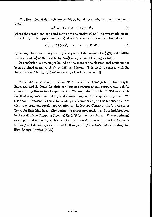
The five different data sets are combined by taking a weighted mean average to yield :

ml = -65 ± 85 ± 65 (eV)2 , (5)

where the second and the third terms are the statistical and the systematic errors, respectively. The upper limit on mj at a 95% confidence level is obtained as :

ml < 166 [eVf, or m„ < 13 eV , (6)

by taking into account only the physically acceptable region of mj >0, and shifting the resultant mj of the best fit by Am*(syst.) to yield the largest value.

In conclusion, a new upper bound on the mass of the electron anti-neutrino has been obtained as m„ < 13 eV at 95% confidence. This result disagrees with the finite mass of 17< m„ <40 eV reported by the ITEP group [3].

We would like to thank Professors T. Yamazaki, Y. Yamaguchi, T. Nomura, H. Sugawara and S. Ozaki for their continuous encouragement, support and helpful advice during this series of experiments. We are grateful to Mr. M. Takano for his excellent cooperation in building and maintaining our data-acquisition system. We also thank Professor T. Ferbel for reading and commenting on this manuscript. We wish to express our special appreciation to the Isotope Center at the University of Tokyo for their kind hospitality during the source preparation, and our indebtedness to the stafFof the Computer Room at the INS for their assistance. This experiment was supported in part by a Grant-in-Aid for Scientific Research from the Japanese Ministry of Education, Science and Culture, and by the National Laboratory for High Energy Physics (KEK).

- 2 9 7 -

References

[I] V.A.Lubimov et al, Phys. Lett. B 94 (1980) 266.

[2] S.Boris et al, Phys. Lett. B 159 (1985) 217.

[3] S.Boris et al, Phys. Rev. Lett. 58 (1987) 2019.

[4] M.Fritschi et al, Phys. Lett. B 173 (1986) 485.

[5] J.F.Wilkerson et al, Phys. Rev. Lett. 58 (1987) 2023.

[6] H.Kawakami et al, Phys. Lett. B 187 (1987) 198.

[7] H.Kawakami et al, J. Phys.Soc. Jpn. 57 (1988) 2873.

[8] K.B.Blodgett, J. Am. Chem. Soc. 56 (1935) 1007 ;

K.B.Blodgett and I.Langmuir, Phys. Rev. 51 (1939) 964.

[9] H.Kawakami et al, preprint INS-Rep.-758.

[10] H.Kawakami et al, Phys. Lett. A 121 (1987) 414. [II] T.J.Kennett, W.V.Prestwich and A.Robertson, Nucl. Instr. and Meth. 151

(1978) 285 ; ibid 293.

[12] M.Takizawa and K.Kubodera, Proc. XVI INS Int. Symp. on Neutrino Mass and Related Topics, Tokyo, 16-18 March, 1988, p349, ed. S.Kato and T.Ohshima.

[13] H.Kawakami et al, Nucl. Instr. & Methods, A 264 (1988) 511 ; Jpn. J. App. Phys. 28 (1989) 883.

[14] K.E.Bergkvist, Nucl. Phys. 39 B (1972) 317.

[15] I.G.Kaplan, V.N.Smutny and G.V.Smelov, Phys. Lett. 112 B (1982) 417 ; I.G.Kaplan, G.V.Smelov and V.N.Smutny, Phys. Lett. 161 B (1985) 389.

[16] I.G.Kaplan, V.N.Smutnyi and G.V.Smelov, Sov. Phys. JETP 57 (1983) 483.

[17] J.Arafune, N.Koga, K.Morokuma and T.Watanabe, J. Phys. Soc. Jpn. 55 (1986) 3806 ; ibid 3813 ; J.Arafune and T.Watanabe, Phys. Rev. C 34 (1986) 336.

- 2! 18 -

Table Captions

Table 1 : Parameters resulting from the x 2 fit to the data. The number of data-points in the 6th-cell is 294 instead of 354, because carbon coated quartz fiber with 30fim diameter as the high resistive anode wire peeled off locally and the corresponding data regions were removed from the fit. The second and the third terms of the final values of m* and E0 are statistical and systematic errors, respectively. The systematic error for E 0 arises from uncertainties in the energy calibration of the KL2L3 line and from the relative alignment between the 3 H and the I 0 9 C d sources.

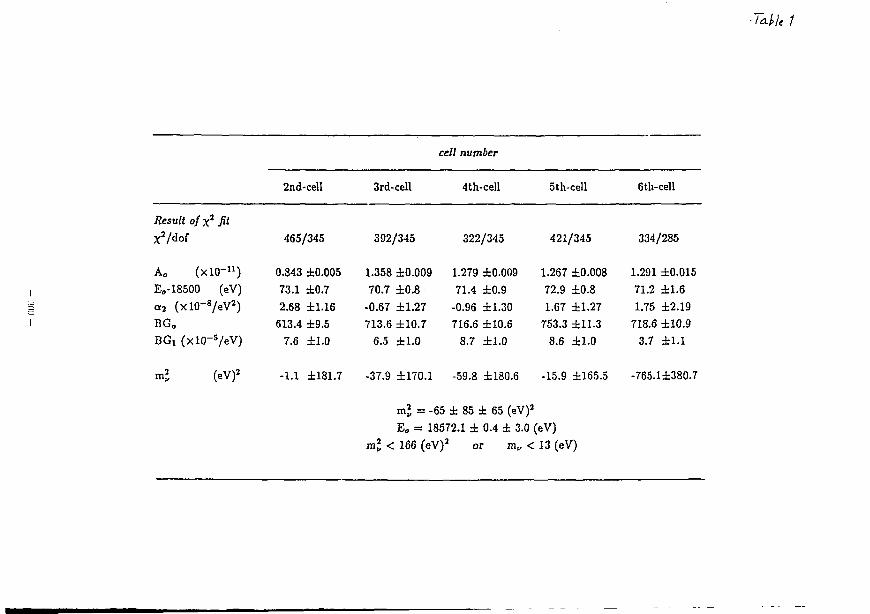
cell number

2nd-cell 3rd-cell 4th-cell 5th-cell 6th-cell

Result of x2 fit X 2/dof

A„ ( x l 0 " n ) E„-18500 (eV) a 2 (x lO- 8 /eV 2 ) BG„ BGi (x l0 - 5 / eV)

465/345

0.843 ±0.005 73.1 ±0.7 2.68 ±1.16

613.4 ±9.5 7.6 ±1.0

392/345

1.358 ±0.009 70.7 ±0.8

-0.67 ±1.27 713.6 ±10.7

6.5 ±1.0

322/345

1.279 ±0.009 71.4 ±0.9

-0.96 ±1.30 716.6 ±10.6

8.7 ±1.0

421/345

1.267 ±0.008 72.9 ±0.8 1.67 ±1.27

753.3 ±11.3 8.6 ±1.0

334/285

1.291 ±0.015 71.2 ±1.6 1.75 ±2.19

718.6 ±10.9 3.7 ±1.1

(eV)2 -1.1 ±181.7 -37.9 ±170.1 -59.8 ±180.6 -15.9 ±165.5 -765.1±380.7

ml = -65 ± 85 ± 65 (eV)2

E„ = 18572.1 ± 0.4 ± 3.0 (eV) ml < 166 (eV) 2 or m„ < 13 (eV)

F i g u r e C a p t i o n s

F i g . l : (a) Schematic layout of the top view of the INS /J-spectrometer. Intrinsic momentum resolution of the spectrometer is determined by the size of the discrimination baffle. Three Liq.N2 tanks are equipped to trap evapolated molecules and to improve achievable vacuum pressure, (b) Structure of the proportional chamber. The front layer consists of seven cells for detecting /3-rays, and the rear one is a regular multi-wire proportional chamber for vetoing cosmic rays.

Fig.2 : (a) shows the total response function R r for the 4th-cell, which is obtained from the measured KL2L3 spectrum via Eq.( l) . The small, but long tail at low energy extends up to -1000 eV. Total intensity is normalized to unity, (b) is the shake-up/off SUO spectrum convoluted with the natural Lorentzian line of width r=11.43 eV.

F ig .3 : Observed data and the best fit curves are shown for the energy region from 18.4 to 18.7 keV in the form of Kurie-plots. The detection efficiency 77 is corrected and overlapping data are summed up in the figure.

Fig.4 : Deviation of the fit from data divided by the error on each data point, and the relation between \ 7 y s - mj , are shown in the case of the 4th cell, (a) corresponds to the best fit case for all 8 free parameters including the m j , while (b) corresponds to 7 free parameters at a fixed m2

v of (30eV) 2 . (c) shows x 2

obtained as a function of m ' for the full fit to 7 free parameters, assuming the SFS for the 3 H nucleus, 3 H atom, and 3 I I compound as calculated by [15,16].

- 3 0 1 -

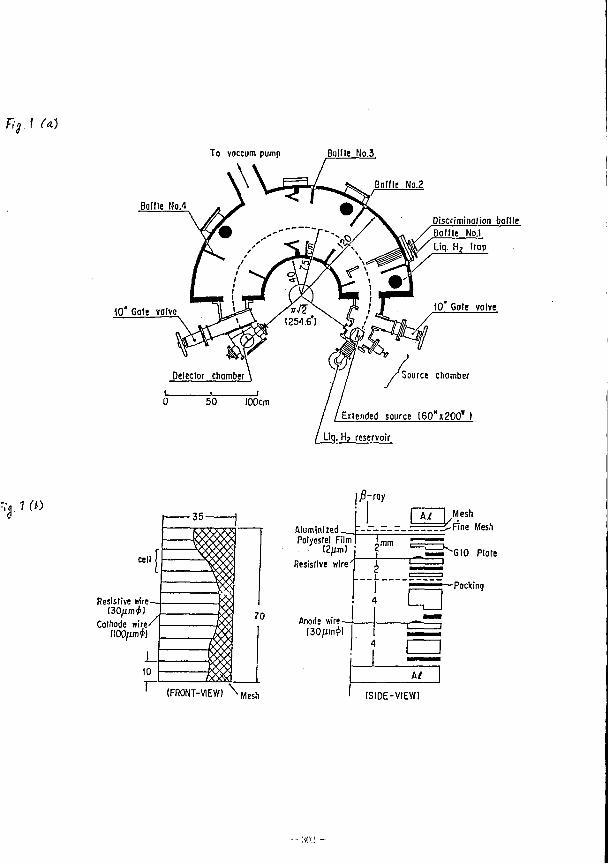
To voccum pump Boffle No.3

Baffle No.4

10 Gale valve

Boffle No.2

Discriminofion boffle Bo I fie No.l Liq. H z Irop

Source chamber

'Emended source ( S O ^ O O * )

Liq. H? reservoir

Resistive wire

Colhode wire' UOOfuni)

(FRONT-VIEW) ^Mesh

jfl-ray

Aluminlzed Polyestel Film

• (2/im)

Resistive wire'

Ai

Anode wire — [30/xm<£l

I I

Mesh / -

-Fine Mesh

"GIO Plate

a -Porting

"T I

A/

(SIDE-VIEW)

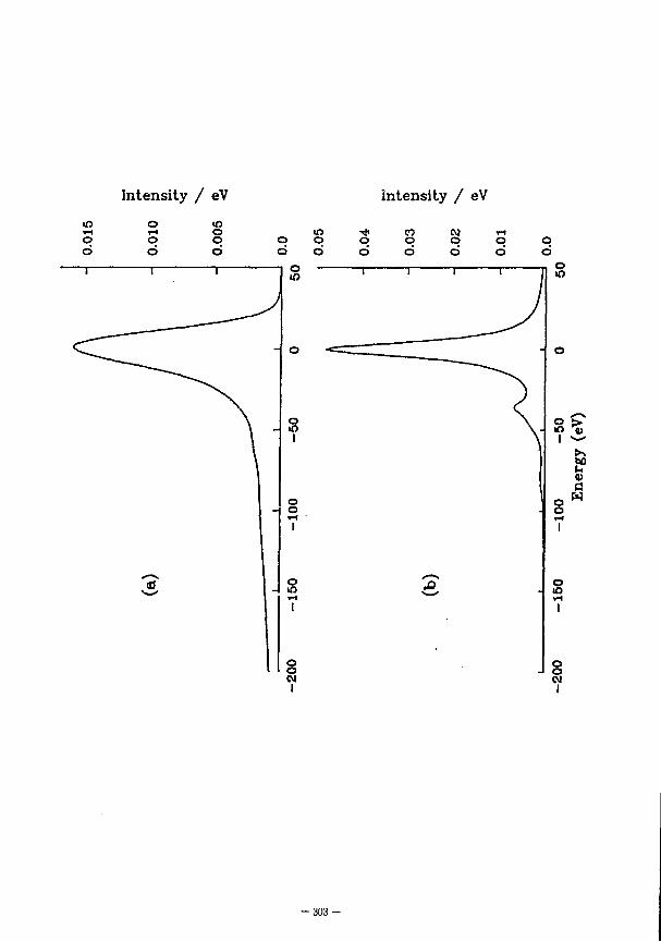
Intensity / eV intensity / eV

© 6

o © d

o o o d

o

o I

o o

o m

o o w I

•303-

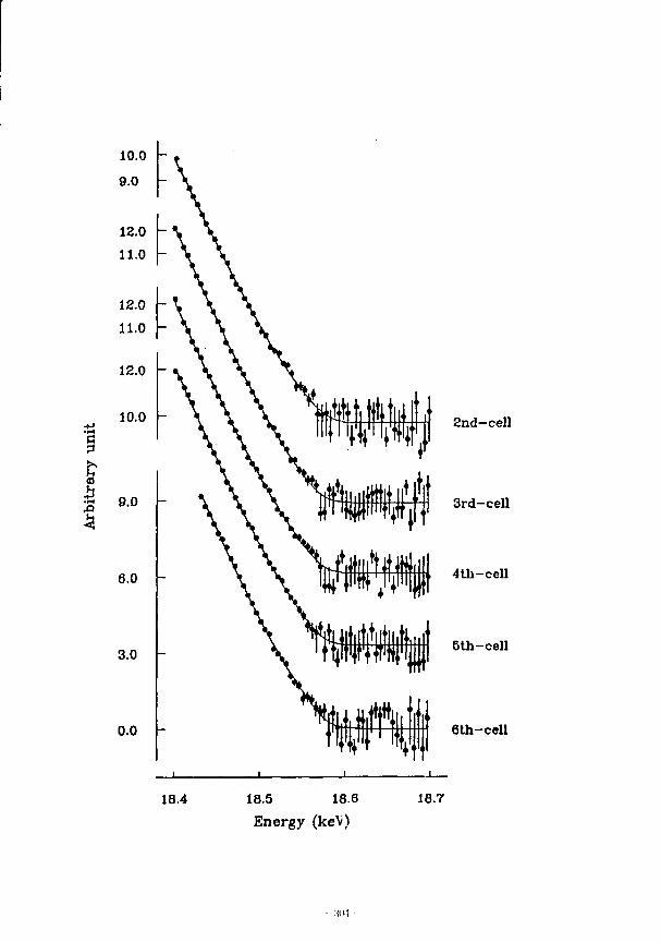
10.0

9.0

12.0 11.0

12.0 11.0

12.0

10.0

<a

5 9.0

6.0

3.0

0.0

2nd-cell

3rd-cell

4th-cell

5th-cell

6th-cell

18.4 18.5 18.6 Energy (keV)

18.7

- :«M -

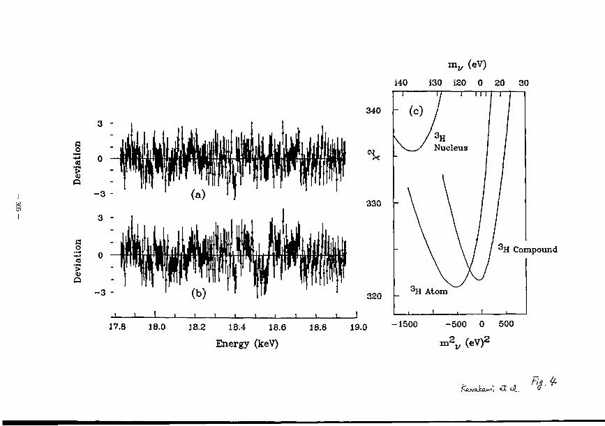
m„ (eV) i40 i30 i20 0 20 30

340

X

330

320

-i 1 1 1 1 i i_

3 H Atom

3 H Compound

J_

17.8 18.0 18.2 18.4 18.6

Energy (keV) 18.8 19.0 -1500 -500 0 500

2 („v\2 m V (eV)

fcLMahun", -tt ii_. 0 '

Liquid Xenon Ionization Drift Chamber for Detection of Neutrino-less Double Beta-decay of 1 3 6Xe

and Related research Programs

M.Miyajima, S.Sasaki and H.Tawara

Radiation Safety Control Center National Laboratory for High Energy Physics

Oho 1-1, Tsukuba, Ibaraki 305, Japan

1. Introduction Recently, there has been a growing interest in nuclear

double beta-decay, the process in which an atomic nucleus with Z protons and A mass number decays to another with Z+2 protons and the same mass number emitting two electrons with two neutrinos or with nothing. Especially, the neutrino-less double beta-decay is interested in testing the properties of electro-weak interaction such as lepton number violation, masses of neutrinos, and non­existence of right-handed weak current.

Liquid xenon is a promising material for radiation detec­tors. It has a small W-value(15.6 eV) for ionization processes due to conversion electrons of 1 Mev[1] and also a comparable W-value(16.4 eV) for scintillations due to alpha-particles of 5.3 MeV[2]. Xenon is a natural mixture of nine stable isotopes. 1 3 4Xe

and 1 J bXe are candidates for the double beta-decay. The isotopic abundance of 1 3 4Xe and 1 3 6Xe are 10.4 % and 8.9 %, respectively. The transition energies of those are 0.895 MeV and 2.479. The life time of 1 3 6Xe is then expected much shorter in both zero-neutrino and two-neutrino decays. The isotopic abundance of Xe is rather large in a natural mixture of isotopes like that of Ge(7.8 %) in the high resolution germanium gamma ray spectrome­

ter as a candidate of the double beta decays. Furthermore, Xe has advantages from a view point of competing gamma-ray back­grounds since the sum energy of emitted electrons in the decay oi the zero-neutrino mode is higher than that of Ge. Tnere is also some merit to use liquid xenon as a detector medium in the selec­tion of its shape and volume of detectors. There, however, are several disadvantages for using the liquid xenon such as the large sensitivity of ionization signals to existence of impurity atoms or molecules, the difficulty of tracking emitted elec­trons, and the requirement of cryostats for keeping the tempera­ture of liquid about -110°C.

We are at present developing a liquid xenon ionization drift chamber with a size of several liters as a proto-type in order to observe the neutrino-less double beta-decay of 1 3 6Xe. Further­more, a method for identifying a decayed nucleus is looking for to unambiguously observe the neutrino-less double beta-decay of

Xe. Also, basic experiments to detect daughter nuclei of 1 3 6Xe collected in liquid xenon are under progress by using a TOF mass spectrometer in which neutral barium atoms are selectively and resonantly ionized with laser beams[3],

- - :«)7 -

2. Liquid xenon ionization drift chamber A proto-type of self-triggerable liquid xenon ionization

drift chamber was constructed in order to detect the neutrino-less double beta-decay of 1 3 6Xe[4]. The chamber system is sche­matically shown in Fig.1. Two single gridded ionization chambers are arranged back to back with a cathode as a common high voltage electrode in a cylindrical chamber vessel with vacuum thermal shield. Four VUV sensitive photomultipliers(PMT) of 2" in diame­ter observe scintillations from the liquid xenon of an effective volume of each chamber. The size of all electrodes are 200 mm in diameter and the effective diameters of the collector and the grid are 160 mm. The distance between the cathode and the grid is 50 mm and that between the grid and the collector is 5 mm. Then, the total effective volume is about 2 liters.

The signals from the PMT make trigger signals and also serve to roughly estimate event locations. The liberated electrons by radiation in liquid xenon drift to the collector according to the applied electric field between the cathode and the grid and are collected to a collector without being trapped at the grid if the ratio of the applied electric field between the grid and the collector to that between the cathode and the grid exceeds the critical field ratio[5]. The number of liberated electrons is proportional to the sum of energies of emitted two electrons at a decay. The drift velocity of a swarm of liberated electrons is almost constant at the field above 3 kV/cm. Then, the drift time of a swarm is proportional to a distance from the grid to the

- 308 -

position where the ionization takes place(z-directi on). Also, each collector is divided in to nine segments to get the rough position of liberated electrons(x- and v-direction). The event is assured to lie in tl>e effective volume from the measured drift time and the segment. Furthermore, the segmentation serves to operate a chamber as nine independent ionization chambers. Then, the 18 independent ionization chambers make possible to apply coincidence measurements between each others. These are powerful to measure the zero-neutrino decay of 1 3 6Xe to the first excited state of °Ba and yet to eliminate backgrounds which can not be distinguished only from their ionization yields corresponding to the sum energies of two electrons. The rise time of signals from each segment serves to select localized electron swarms, of which the size depends on the ranges of two emitted electrons in liquid xenon, and also to separate successive independent electron swarms. This supplies a method of background reduction.

3. Electronics A charge sensitive preamplifier is connected to each segment

of the collectors, and also to each PMT. Signals from the pream­plifier connected to each segment are further amplified with a wideband linear amplifier to measure the rise time of the sig­nals, and with a narrowband low noise linear amplifier to measure the collected charges which correspond to the summed energy of emitted electrons. The output from the preamplifier connected to each PMT is also amplified with a linear amplifier with a shaping time constant of 0.5 usee. The schematic diagram of an electronic

-309-

system is shown in Fig.2. The signals from each PMT are fed into a master triggering circuit through a discriminator. The first input to the triggering circuit generates a master trigger signal which makes all TPC start, generates a gate pulse for the system controller and all ADC, and make a scaler reset and start to measure a period between two successive events. All the TPC are stopped by the discriminator signal which is slightly delayed at the front of TPC. All the data from ADC and the scaler are col­lected into a micro-computer and are stored in a magnetic tape mass storage. Time profiles of signals are schematically shown in Fig.3. The data is analyzed with an off-line computer.

The input equivalent noise charges of all the preamplifiers were almost about 500 electrons in full width at half maximum under the input capacitance of 100 pF with the shaping time constant of 10 usee in the linear amplifier.

4.Vacuum and low temperature operation The experimental apparatus is schematically shown in Fig.4.

This is composed of a chamber vessel filled with liquid xenon, the vacuum thermal shield of the vessel, two vacuum systems for the vessel and the thermal shield, a gas filling system with a purifier and an about 500 1 reservoir tank, and a three stages refrigerator system. The chamber vessel is evacuated with a turbo-molecular pump and the vacuum less than 1x10 torr is easily achievable, and the outside vessel for the thermal shield is evacuated less than 1x10 - 6 torr. Gaseous xenon in the reser­voir is sent to the vessel through a purifier and fills up the

- mo -

vessel at the pressure of about 1.5 kg/cm*1 after evacuation. Then, the operation of the refrigerator begins for cooling. The temperature of refrigerant is kept at about -112°C during conden­sation of gaseous xenon. It took about 12 hours to fill the vessel with the liquid xenon of 5 1 . After the vessel was filled up with the liquid xenon of 5 1, the temperature control of the liquid was attempted by cooling the gaseous xenon in the chamber vessel with controlling the refrigerant temperature from the refrigerator for more than a week. The temperature of the vessel turned out to be well controlled in this method.

The gaseous xenon is passed through a purifier filled with 10,000 pellets of barium-titanium getters kept at about 450°C and is condensed into the chamber vessel. This purification method was not enough to operate the ionization chamber properly. The system of continuous purification seems to be required to obtain highly purified liquid xenon.

5.Ionization and scintillation in liquid xenon In this apparatus, all the signals depend on the number of

liberated electrons and the number of scintillation photons pro duced by radiation. Since the W-value of liquid xenon is 15.6 eV described above, the electrons with the summed energy of 2.479 MeV emitted at a neutrino-less double beta-decay liberates 1.6x105 electrons in liquid xenon and also 1.1x105 electrons are liberated by electrons emitted at a decay to the first excited state. Those electron swarms move with an average velocity of

-311 -

3x105 cm/sec under the electric field of 5 kV/cm in liquid xenon[6]. The rise time of signals at the collector is in a range of 1.7 to 3.0 usee depending on the range of electrons, and the drift time of swarms is in a range of 1.7 to 17 usee depending on the emitted position of electrons. In the case of scintillation, an electron of 2.479 MeV produces 1.5x105 VUV photons, if the W-value due to energetic electrons is assumed to be equal to one due to alpha-particles(16.4 eV). However, there are two compo­nents in the scintillation of liquid xenon[7]. One is due to the deexcitation of excited xenon atoms and the other is due to the recombination between the liberated electrons and ionized xenons. In this apparatus the electric field always exists to collect electron swarms liberated by radiation. Then, the scintillation yields decrease to about 5x10 photons, 1/3 of the total yield[8]. The number of photons incident on the PMT(2" in diame­ter) is about 5000 from a scintillation at the nearest point in the effective volume, about 500 at the center and about 150 at the furthermost. The quantum efficiency of the PMT is expected to be about 10 % in liquid xenon temperature[2].

6.Estimation of backgrounds In this apparatus, the effective volume of liquid xenon is 2

1 and is divided into 18 independent volumes by the segmented collectors. The volume per each segment is 110 cm and is roughly equal to one of a 2"x 2" Nal(Tl) scintillator. The effective atomic number and the density of Nal(Tl) are also roughly equal to those of liquid xenon. Gamma ray backgrounds are estimated to

-31L'-

be about 2 cph/keV around 2.479 MeV and 85 cph/keV at around 1.660 MeV from the measured gamma-ray backgrounds with the Nal(Tl) without any shielding material in a room of a normal concrete building. If the energy resolution of 1 % is achieved in the liquid ionization chamber, the background rate is about 100 cph/segment at the energy of 2.479 MeV, and 3000 cph/segment at 1.66 MeV. However, the lead shield of about 10 cm readily reduces background gamma-rays by a factor of 10~ 2 or more. Further background reduction of 10~ 4 is required at around 2.479 MeV to see several decays of 1 3 6Xe with a half-life of about 10 2 3 y in a year. Also, the reduction factor is about 10 - 6 at around 1.66 MeV. However, there are large ambiguities in these estimations.

7. Remarks We are preparing apparatus for the detection of 3 Ba with a

radiochemical method, while constructing the above liquid xenon ionization drift chamber. The daughter nuclei are collected on an electrode immersed into the liquid xenon by applying the elec trie field between this and the outside electrode for an appro­priate period. Those collected daughter are selectively ionized with laser beams and are analyzed with a TOF mass spectrometer. This method is not capable to distinguish the decay modes of the zero-neutrino and the two-neutrino. However, it serves to unam­biguously identify the existence of the double beta decay. Fur­thermore, the extension of this method is applicable to detect a daughter when a candidate event of the decay of the zero-neutrino mode is detected in the real time measurement.

- :m -

References; [1] T.Takahashi et al., Phys. Rev. 12, 1771(1975). [2] M.Miyajima, S.Sasaki, and E.Shibamura,

To be published in Nucl. Instr. Meth. [3] M.Miyajima, T.Tawara, and S.Sasaki,

KEK Rep. 89-5, 12(1989). [4] M.Miyajima, Ionizing Radiation, 15, 45(1988). [5] O.Bunemann, T.E.Cranshaw, and J.A.Harvey,

Can. J. Res. 27,191(1949). [6] E.Shibamura et al., Nucl. Instr. Meth. 131, 249(1975). [7] K.Kubota et al., Phys. Rev. B21, 2632(1980). [8] S.Kubota et al., Phys. Rev. B17, 2762(1978).

-:<M -

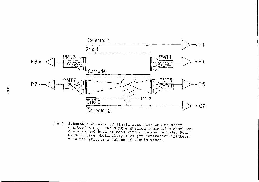
Collector

Grid 1 CI

PMT3 PMT1

Col lector 2

Fig.l Schematic drawing of liquid xenon ionization drift chamber(LXIDC). Two single gridded ionization chambers are arranged back to back with a common cathode. Four UV sensitive photomultipliers per ionization chambers view the effective volume of liquid xenon.

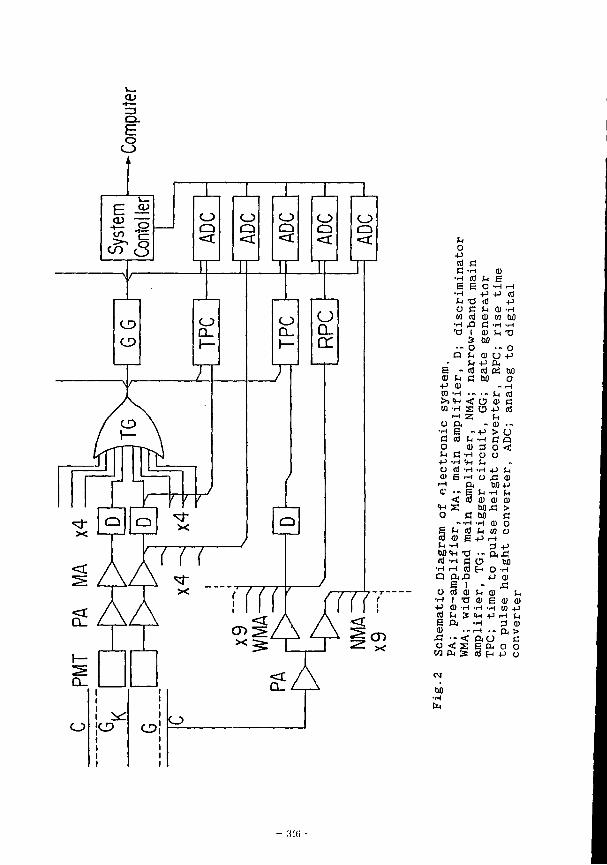
o p cd C a -H

•H cd e e •H

O C w cd

•H J3 T3 I

3 . - o

Q U u

E - cd <u (H c +J a) (0 'H . ->><H <

-» •z. O ft

E -cd f*

Q) o <d >H <u e H -t a a- •- E

< (0 o a

- • H

p p cd cd P (H d) - H CD 07 M C 'H -H

CD S H T 3

. - o Q) o P P a-cd Pi DO M O

cd c

a o p

e u <a awe M<>H -d

• H H «) a ft,a

E i o cd Qj

•H i -a P CD -H cd u $ E ft si - < o <: s OT PL, g

• - In O 0 O P u - <D . -p > o •H c a 3 o < CJ O L,

•H p L, O X) 0)

M P t-i -H U CD CD 0) W1.C > M C

•rl 1) O h ID <J

p .-( 3 p

• - ftJ3 O M H O -H

P 0) - J3

SH CD !H H E f f l d )

•H 'H 0] p *H P r-l U •H 3 d ) - • • - ft > ftO C E CL, O O cd H P o

- :m -

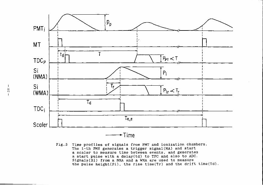
•Time

Fig.3 Time profiles of signals from PMT and ionization chambers. The i-th PMT generates a trigger signal(MA) and start a scaler to measure time between events, and generates a start pulse with a delay(td) to TPC and also to ADC. Signals(Si) from a NMA and a WMA are used to measure the pulse height(Pi), the rise time(Tr) and the drift time(Td)

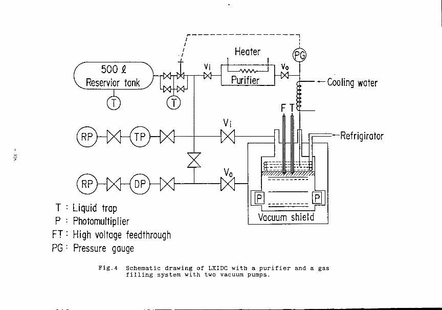
500 9. Reservior tank

(RP>H

(RPHxHgH><3 T : Liquid trap P : Photomultiplier

FT '• High voltage feedthrough PG : Pressure gauge

^Cooling water

^Refrigirator

Fig.4 Schematic drawing of LXIDC with a purifier filling system with two vacuum pumps.

and a gas

Detection of Galactic Axions

with

Rydberg Atoms

S. Matsuki

(RINP, Osaka Univ.)

Detection of Galactic Axious with Rydberg Atoms S. Malsuii (Osaka Univ.)

2 ) ULVUt fkXhJ:^ bj ^.XI'CMS •>^'1 RyJ.ie^ aL«s

^ / ' i f f tt(t>\Kui tv-a^uilo^ }yi0 mat. j\dl

Wj '".it. cf-^^,,^ /-/. C./-.<i.1.-

'v Si!>Md_c-rfeA. conversion of /)euiy',y\oS

S,*A> "y.-<J:ni.Q mass d:..-f{ ?•>•(.':'•'••• An*

^Ly.,<<M. MOAA

4^JL.=

£ • —-^-2. WUIUOA tfa-V -in&< <f-x<G-&\f-

$JU 1LO*J &™lb£^ %c<r-/*/o%l/ wrimrrm^ <0-J

.^ £ ^ - t £ - ^ — A M ! / ^ < v g ^

-ZW<!

] J f

flXify^-^Bfe^

T.u»A<rF&$: UySt-&T3^

: ^ ^ g p J M ^

&t--ma f f y V ' , /JQ-/7 1-= _ V —

'ar ~7o.tr

^atrs^j-rfen--ir** -fir

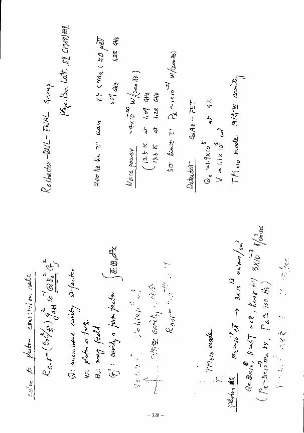
I I

) i -

O r -

4

£ Ci 5? -h- -^ 5 \- 5 * ? rtj

Bi

V • = * : 0 r4 "•? s<3- 0 r4 ' o

J.. o— # Ob

"iO-«: o S v!r Ob

"iO- •X

7 o i - ~ w

•X

7 1 o. N ri? 3

^ *

> <5>

3 crt c i ^ o i y / 6 =c a) •Ln

a t Q ~*5 et ^

<* ^ 4 I

O

0 >

4

51

- $

ii

r

* 4 vi ^

C3 £ 02 vjp

I!

#

.k"

f

r T

/) A

*>J T g

v

/;

V

i

- 320 •

-Wv—g t a un i a un

i •

D JL.

A n

.«- i j . H* f f O f O 8 <oC- szaz <f

CO .'s-

el el SS£» f.rt el 3£.~\ + 1 r=-**fK ^ >-.~^ e

"^1 l r >n "^1 — e ^ j i n

&S u &S 12 nu t M &S • J l l . I > CJ a.

p£.i± — C3

* ' — f e

o U U U o o a o o m LJ m n r-J CN '— ti

o o O <

E

f-V") H I D N T l • 3 2 )

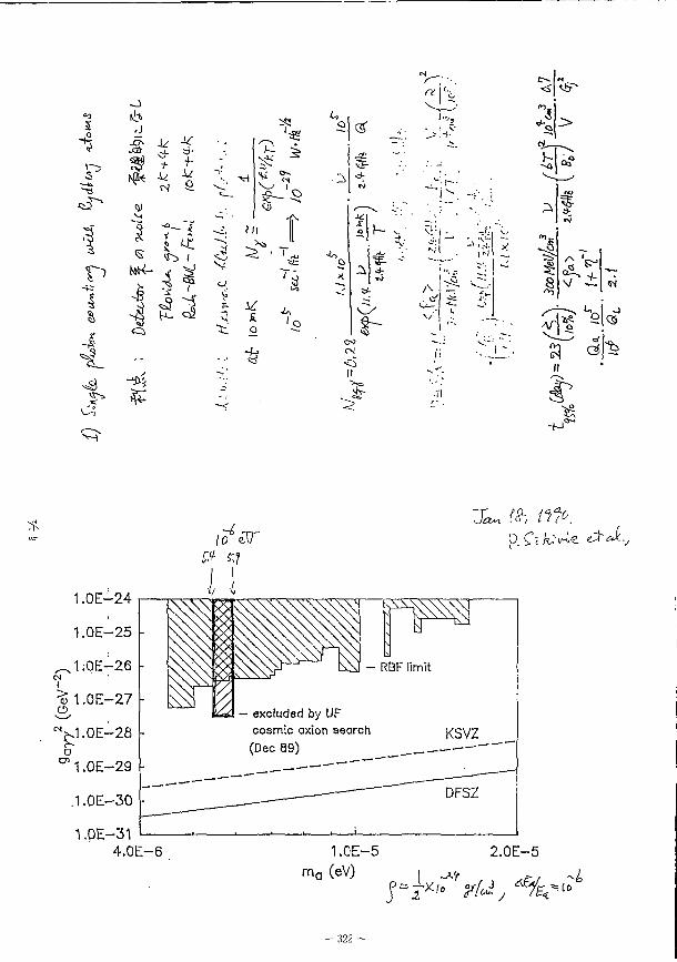
s

r>

o ^ #

$e

v.

f o

-I <2>

g3 <*

" t

is:

1?

u &

^

4 • 3

t *l ill o h -^ ^ u - > • 1 M • io ( "°

?c O ~A^-•— - *— • H: ' t f X. 1 w

-~. iA

X ^ O ' O ^

• *

[I

iK-

i—

v.- .. -J: j - •—* -\'^ w

t - ;

''- Z >S. . ^> A *"-—'

. cC ^ fr ^ - I. 0

\/ * • ..—

vS

>

Hi?

^

« J .

f ••5

— 3

£ + <w

II

^ - M

1.0E-24

1.0E-25

^ l ; 0 E - 2 6 CM

I ^ l.OE-27 o

£ D en

.1.0E-28

1 .OE-29 |-

.1 .OE-30

1.QE-31

/o^aV ^ q

x . /<?-, w .

TW^ RBF limit

- excluded by UF co3mic axion search (Dec 89)

KSVZ

DFSZ

4.0E-6 1.0E-5 2.0E-5 m a (eV) ( ^ .4

- 322 -

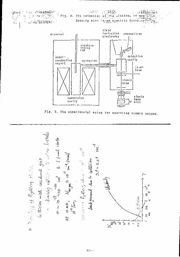
n**^

•*a«te&M*J ny<lbs:rc Mm- ; n.-nn' e i e c i r l c £ l eia.-.•«•*

!'!;. 2 . T h e ! : o t n n l l » i oi^'.hi

c r y o s L a I

s u p e r - . con d u c t Ins m a g n e t

s a p D h l r e tun i ng rod

wavegu i de

c o n v e r s I o n cavlly

field I o n i z a t i o n channel Iron c Icctrodes

L

de l e d Ion cavl ly

. . l a s e r beam

I a I O K i c i beam

f f T a tonic "^=3—i beam "3 o v e n

F i e . 3 . T h e e x p e r i m e n t a l s o l u p f o r s e a r c h i n g c o s m i c n x l o n s

J -J5

.)

• J

o

o

*>

< -8 -£

V V,

- m •

~3

—a

Q ^

a

>* 0

<r 5 a - . J ^ -* I i

c c

o e> \-i /;

1=s

r ^

V

2 fe ^ "* M TO 0

•^ i "

°* _ 'i

Q

7

UJ

as CM

I 'j > » UJ * «

3 U J

•a K <5)

LU \1

V ^

^

v=

» *

1

1

o o £ °o a V i f* 4J

4

* ~ ^

Oo

o 5*

Si

I!

"4

i) II

• J - .

- 32A -

+•

i ll

^

IA s

X

4 m ll

II II

I 5

ll S i a • W D •w

1 h~->

£

i s

„ J."

- M

5 <=x

\ •

a oJ

4

.a

o

<v

—a

fi

- 325

t e - i t ^ a

^

r u

n

S3 ' J

i f * :i3§£fc : t T

L - c

i _

H&s, Sf^i I :n

r>=rf -p -is

1

- 32fi -

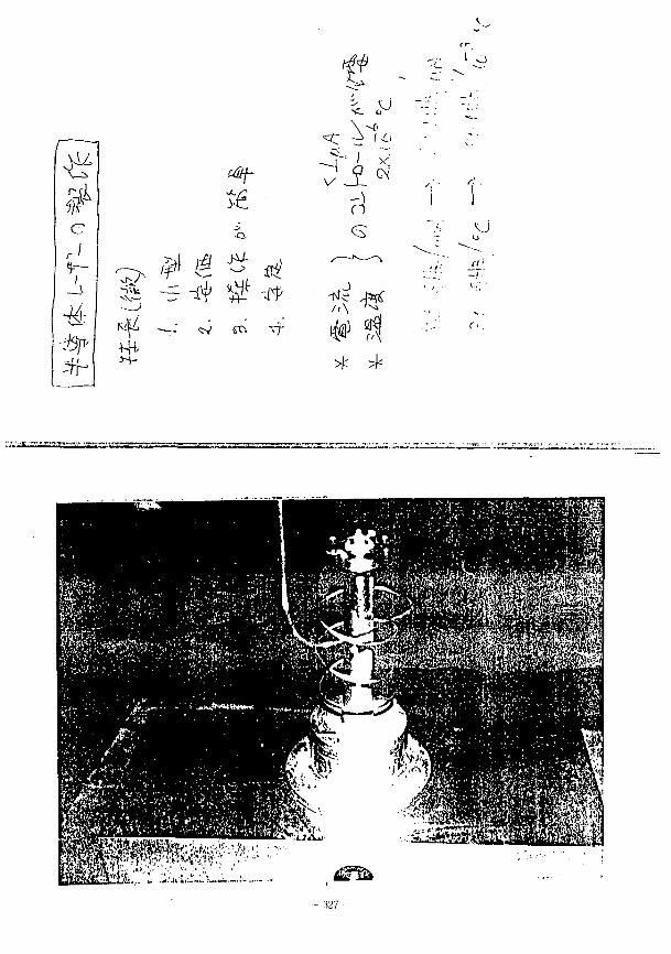
. ^ v ^

$ e ,-/ <)—

i ^7 __v ~>vvs. ^-V-

^ *|Z • -#J* Hi

~ M *+--rr

«8f-

<r

v

•<- ^

- J 3. X"'

(X

n <s

j U

# ?,t ^

-_;: <rv 6^ ^

—r.*

Vi^SSEEES

:#7

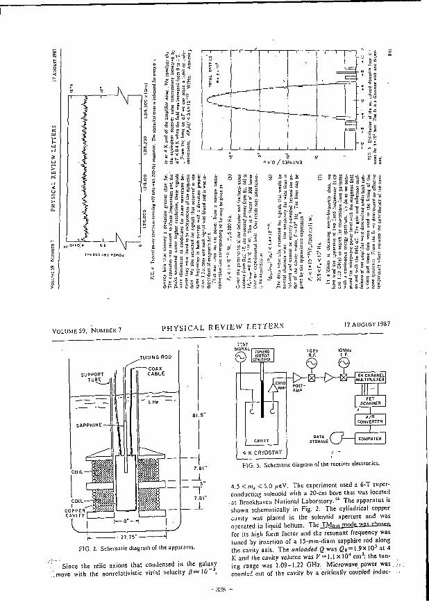
I I i i \ J

PO / S3IU1N3

ml miii im

(>H 002 /Wi ajMOd II Si , UMII

• - ' - 2 H ~ i

U t i 5 5 * - |

V O L U M E 59, N U M B E R 7 PHYSICAL REVIEW LETTERS 17 AUGUST 1987

.TU.'IING ROD

COPPER CAVITY

7 . 8 1 "

__1 .5"

"T 7.81"

— 27.75"-

FIG. 2. Schematic diagram of the apparatus.

Since the relic axions that condensed in the galaxy '.move with the nonrclativistic viml velocity / J«10" ,

r is r SIGNAL TUNING

MOTOH CONTROL

I GHz R.F.

hu

10 Mil; I.F.

3

4 K CRYOSTAT

64 CHANNEL MULTIPLEXED

POST-AMP

FET SCANNER

A/D CONVERTER

DATA STORAGE OH COMPUTER

FIG. 3. Schematic diagram of the receiver electronics.

4.5 < m a < 5.0 / ieV. The experiment used a 6-T super­conducting solenoid with a 20-cm bore that was located at Brookhaven National Labora to ry . M The apparatus is shown schematically in Fig. 2: The cylindrical copper c.ivily was placed in the solenoid aperture and was operated in l iquid helium. The T M 0 1 n modejvai-chaseq for its high form factor and the resonant frequency was tuned by insertion of a 15-mm-diarn sapphire rod along the cavity axis. The unloaded Q was 0 o = l .9x I O j at 4 K and the cavity volume was f / = l . l x l O ' 1 cm 3 ; the tun­ing range was 1.09-1.22 GHz. Microwave power was counlcd out of the cavity by a cr i t ical ly coupled induc-

- HL'8 -

» }

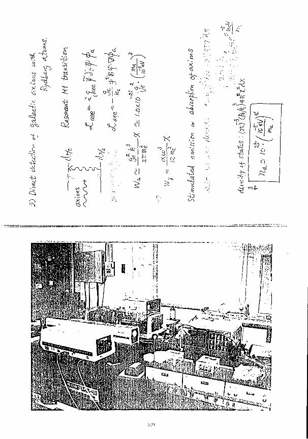
r. 4

1 CTCi

cS

I

§

-el

£

•IF i //

a)

^ ^

o

d K

-a; era

K

CO

3

9

3

x

w f c : \ r

•*"•> -s ' V-

V J r o ^s 'I? VW tf

fNJ s 5

£•) j ^

^ ? *

tf o -£. C-;

"*-. c'i \ <« >^ 1 <-o

> 1 r-^

- 5 = £ - •

- » «

:«>

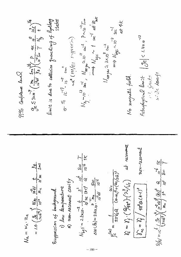
i

o

33

'a

^

1

>

1

m

' J <?

<•! f •*-* I

T g X

V

-!5

1 r s

4!

H J

^ 1

"•tf

o

^

5

2 1=

IP

5:

K

(S

•">

-+J

v ?o

Of

* L 5

^ -

ri II

Si" 2

<3

-f-

£

a^

- 330 •

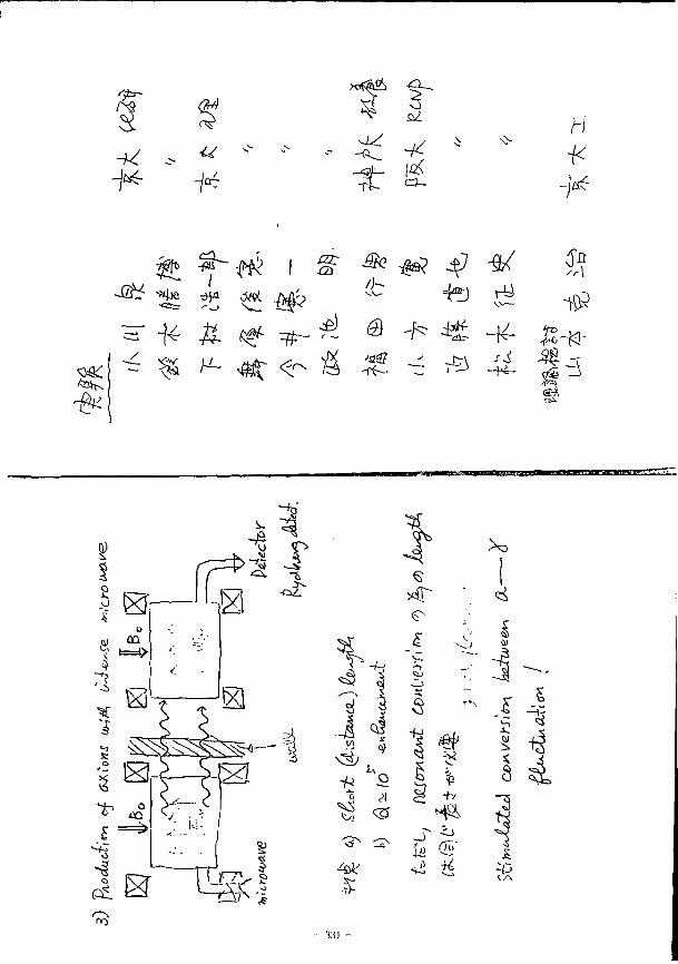
-Jfi£

0 ^

H" -K £ «£- ^ ^ ^ ^ ~ <#c < ^ ^

.£)

4^j i-y

0 ^ 4£ -^ 7 ^

w 1° v\

-:.* ^ ^

*

*1 el d

4& 5"-• 7 > -

3

XD

<4

Ml

A Cryogenic Detector using Superheated Superconducting Tin Granules

Takeo EBISU Department of Physics, Kobe University, Kobe 657, Japan

Tadashi WATANABE Department of Information Systems, Tokyo University of Information Sciences, Chiba 280-01, Japan

Abstract We first recapitulate briefly the results of our research on

properties of SSG: the transition time and the line shape of signals from a superheated to a normal state, energy and temperature dependence of the phase transition field, and the sensitivity in energy response. Next, we discuss the result of stability experiment on a prototype detector with a one-layer target which consists of 1000 tin granules of diameter 190//m.

3 Finally, we describe our cryogenic-detector system with the He-4 He dilution refrigerator.

§ 1. Introduction As is well-known, there is evidence for the existence of large

quantities of dark matter in the galactic halo. The observed velocities due to rotational motion in spiral galaxies imply a total mass in excess of a visible mass. Interest in detection of hypothetical dark-matter particles in cosmic rays led to studies on cryogenic detectors which are capable of catching feeble signals caused with a very small energy transfer. Some attempts were already performed to operate such novel type detectors at underground sites.

Cryogenic techniques range over bolometer, transition-edge thermometer, superconducting tunnel junctions, and superheated superconducting granules!SSG). In this paper, we first recapitulate briefly the results of our research on properties of SSG: the transition time and the line shape of signals from a superheated to a normal state, energy and temperature dependence of the phase transition field, and the sensitivity in energy response, which were all already reported in the series of proceedings of this Workshop ' and elsewhere. Next, we describe the stability experiment in which a prototype detector made of more than 1000 tin granules of diameter 190«m was operated at 2K in 650 hours. Finally, we present the He- He dilution refrigerator under construction, which will provide the environment of very low temperatures indispensable for attaining the energy sensitivity of the order of several electron volts.

§2. Some bai-ic properties A small spherical granule of type-I superconducting material

remains in a superheated or supercooled phase under respective applied fields. We first measured extensively the superheating field for specimens of diameter 80-300/um, and obtained the phase

4 ) diagram for temperature range of 2.0-3.7K. The supercooling field (H ) was found out to be insensitive to the size of sc specimens used, while the superheating one (H . ) depends on the size and the smoothness of the surface.

There can be two fundamental processes for a granule to make a phase transition from a superheated to a normal state. One is a magnetic nucleation process which is cause by imposition of an

- ;<:« -

additional field AH alone. This is expected to be applicable to

detection of magnetic monopoles. The other is the thermal

nucleation process which is due to a temperature rise AT in the

granule. If a small quantity of energy deposit heats the hit

granule sufficiently, a large change of magnetic susceptibility

is triggered off to be identified with a signal of an unknown

neutral particle inducing nuclear recoil through an elastic

scattering.

Then, we studied line shapes of the output signals for phase 5 } transitions in different fields. The flips of a granule are

read out through a pick-up coil which measures the flux change

due to the disappearance of the Meissner effect. Signals were

amplified by wide-band amplifiers and were recorded on a personal

computer by way of a digital storage scope.

We obtained signal pulses induced with incident a particles

having energies of l-2MeV in several fields lower than the

superheating field(H , ) as well as ones induced with a field

increasing beyond the strength of H , without the irradiation at

3K. The line shapes are not so sensitive to the incident

energies, but crucially depend on the field. The area under each

pulse line corresponds to an amount of magnetic flux penetrating

granules. The transition times range over 4-8#s for a specimen of

diameter 250>um. Line shapes for the smaller specimen of 150/um

remain unchanged, through the transition times lessen by 1-2/c/s.

Responses of a granule to energy deposit is expressed with the

phase-transition field H (T,E), which is the lowest field

necessary for the granule to change its phase receiving energy E

of incident a particles. To study the field H .(T,E), single

- :«i -

grains should be irradiated with a rays of well-defined collision

energies. We provided a space filled with the saturated vapor of

helium in which the distance between a specimen and a radioactive 241 source of Am is variable. Collision energies are calculated

taking account of the energy loss of ionization along the path in

the vapor. Temperatures of helium of liquid and vapor were

controlled with error of lmK at most over the range from 4.2 to

1.8K through a vapor-pressure regulator. We measured the phase-

transition field H at eight energies from 4.7MeV to lMeV

corresponding to eight distances for specimens of diameter 145,

165 and 250,um. 3 ' 5 ' 6 '

Several interesting results were derived from the analysis of

the field H . obtained. Response sensitivity d(AH)/dE of granules pt of a size increases with decreasing temperature with AH=H ,(T)-

H (T,E), as is shown in Table I for a granule of diameter 14t'/um.

The temperature dependence of the sensitivity and the specific

heat C of tin links each other in the sense that the products of

the two quantities are almost independent of temperatures. We

found out that a single grain changes its phase with an energy

deposit two orders of magnitude less than that is required for

the whole of grain to be heated uniformly. This implies that the

flippings are triggered off with a temperature rise in a quite

small volume, and that the effect of so called local heating

process plays a dominant role. The local region heated should not

be so deep inside, since a particles loss almost all their

energies near the granule surface. Similar phenomenon will not be

expected for a postulated dark-matter particle which kicks an

atomic nucleus located deep and/or shallow within a granule with

- 335 -

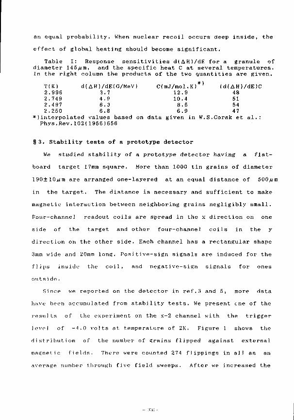
an equal probability. When nuclear recoil occurs deep inside, the

effect of global heating should become significant.

Table I: Response sensitivities d(AH)/dE for a granule of diameter 145yum, and the specific heat C at several temperatures. In the right column the products of the two quantities are given.

T(K) d(AH)/dE(G/MeV) C(mJ/mol.K )** (d(AH)/dE)C 2.996 3.7 12.9 48 2.749 4.9 10.4 51 2.497 6.3 8.5 54 2.250 6.8 6.9 47

*)interpolated values based on data given in W.S.Corak et al.: Phys.Rev.102(1956)656

§3. Stability tests of a prototype detector

We studied stability of a prototype detector having a flat-

board target 17mm square. More than 1000 tin grains of diameter

190±10/im are arranged one-layered at an equal distance of 500//m

in the target. The distance is necessary and sufficient to make

magnetic interaction between neighboring grains negligibly small.

Four-channel readout coils are spread in the x direction on one

side of the target and other four-channel coils in the y

direction on the other side. Each channel has a rectangular shape

3mm wide and 20mm long. Positive-sign signals are induced for the

flips inside the coil, and negative-sign signals for ones

outsi do.

Since we reported on the detector in ref.3 and 5, more data

have been accumulated from stability tests. We present cne of the

results of the experiment on the x-2 channel with the trigger

]c?vel of -4.0 volts at temperature of 2K. Figure 1 shows the

distribution of the number of grains flipped against external

magnetic fields. There were counted 274 flippings in all as an

average number through five field sweeps. After we increased the

-- :«; -

field again from zero up to 178.5G shown with a vertical line to

make one third of all the granules flip into the normal state,

the field was lowered by AH from 178.5G and was kept at the value

for many hours. The field strength is short by more than AH for

the granules remaining unflipped to be triggered through the

magnetic fic-iu alone. We can relate the gap of AH to energy AE

through the SSG sensitivity d(AH)/dE, which is estimated to be

3.8G/MeV at 2.OK for the granules of this size from the data of

irradiation experiments. Stability of the SSG detector was thus

examined as a function of threshold energy A E by varying the

field gap. Running tests were performed at 12 threshold energies

of A E from 0 up to 3MeV. Each observation time was about 50

hours, totaling up to 650 hours. The distribution of events is

shown against the threshold energy AE in Fig.2. It is seen that

there is no energy transfer more than 1.75MeV.

Four causes are considered for those events. Fluctuations in

applied fields and temperatures were at most 50keV and lOkeV in

energy, respectively, so that they only contribute to flippings

at the threshold energy AE=0. The third candidate is radioactive

impurity contained in the granules. The radioactivities in the

tin used were measured by T.Watanabe and K.Matsuoka using the

low-background gamma-ray detector system in Osaka university. The

contamination data of the sample were obtained as follows:

U-chain < 3.9pCi/kg(90%CL), Th-chain < 2.lpCi/kg(90%CL), 6 0 C o < 0.42pCi/kg(90%CL), 1 3 ?Cs= ( 0 . 4 ± 0 . 3 )pCi/kg( Iff ) and 40

K=(6.2±2. 7)pCi/kg(Iff ) . Then, the radioactivities from the U-40 chain and K are less than 4.4nBq and are equal to

7.0nBq( /? : 1 . 3MeV, y : 1 . 5MeV ) , respectively, for a 200//m-diam.

- SH7 -

granule. There remains about 180 granules unflipped for the

threshold energy A E of OMeV in Fig.l. Not more than 0.1-0.2

events are expected for a 50-hour run, whereas 12 events were

recorded at AE=0. Cosmic-ray muons may cause the flippings. An

average energy of 300keV is released by a single muon running

200,um in a grain. The standard flux of the secondary particle may

lead to one event per five hours in our experiments. Although

both the muon flux and the released energy seem apparently

consistent with the observational results, we should notice that

mechanism of energy loss of muons and a particles are different

each other. In the former case, energy is deposited along a

lengthy path and not locally at the surface so that the local

heating hypothesis may not be applicable.

§4. Toward Higher Sensitivity

The specific heat of metal becomes smaller for lower

temperatures so that the energy sensitivity of granules is

generally expected to become higher as is discussed in §2. 7 ) Drukier and Stodolsky have pointed out that Sn grains of

diameter ~2//m at the temperature of 50mK is sensitive to solar

neutrinos with E =420keV, depositing an average energy of leV.

They adopted an electronic heat capacity(—yT) of the normal state

in their calculation. But the contribution from electrons fades

away exponentially with decreasing temperature in the

superconducting state and that from phonons remains in the form 3 of aT , As a result, the heat capacity at 50mK should be three

orders of magnitude less than that used by the authors of ref.7.

Therefore, neutrinos of 420keV will be detected with tin grains

- 3HB -

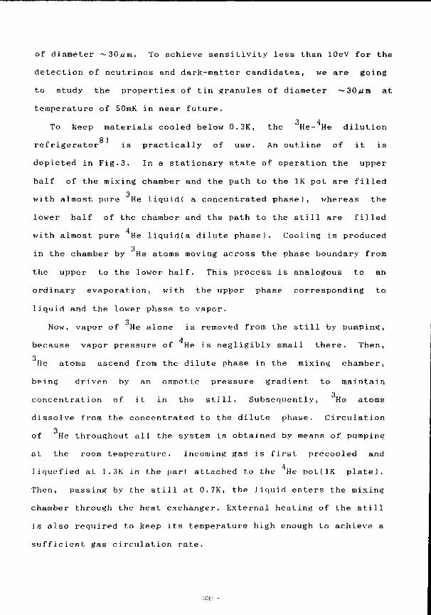
of diameter ~30 >um. To achieve sensitivity less than lOeV for the

detection of neutrinos and dark-matter candidates, we are going

to study the properties of tin granules of diameter ~30^m at

temperature of 50mK in near future. 3 4 To keep materials cooled below 0.3K, the He- He dilution

8 ) refrigerator is practically of use. An outline of it is

depicted in Fig.3. In a stationary state of operation the upper

half of the mixing chamber and the path to the IK pot are filled 3 with almost pure He liquid( a concentrated phase), whereas the

lower half of the chamber and the path to the still are filled 4 with almost pure He liquid(a dilute phase). Cooling is produced 3 in the chamber by He atoms moving across the phase boundary from

the upper to the lower half. This process is analogous to an

ordinary evaporation, with the upper phase corresponding to

liquid and the lower phase to vapor. 3 Now, vapor of He alone is removed from the still by pumping,

4 because vapor pressure of He is negligibly small there. Then, 3 He atoms ascend from the dilute phase in the mixing chamber,

being driven by an osmotic pressure gradient to maintain 3 concentration of it in the still. Subsequently, He atoms

dissolve from the concentrated to the dilute phase. Circulation 3 of He throughout all the system is obtained by means of pumping

at the room temperature. Incoming gas is first precooled and 4 liquefied at 1.3K in the part attached to the He pot(IK plate).

Then, passing by the still at 0.7K, the liquid enters the mixing

chamber through the heat exchanger. External heating of the still

is also required to keep its temperature high enough to achieve a

sufficient gas circulation rate.

Schematic of our cryogenic-detector system under construction 3 is shown in Fig.4. Circulating rate of He atoms is designed to

have a value of ~ 100^mole/sec. The dilution refrigerator will

have a cooling power of ~70microwatts at lOOmK and a sample of

several kilograms will be cooled down to 50mK. After completion

of the refrigerator, we will first study sensitivity of single

grains. Next, we will make a stability test of a detector having

a cylindrical target of diameter 10mm and height 20mm. The target

consists of tin granules of diameter ~30/um with a filling factor

of 10%. The total weight of the granules is lgram. Two SQUID

systems are connected to readout coils. An events of one grain

flipping will be distinguished from that multiple flipping due to

a cosmic muon. Then, we will try to take annual variation of

signals by running the detector for two weeks per month through

one year. We thank Dr.Takayuki Watanabe and Dr.Kenji Matsuoka for

measuring radioactivities in our sample tin. This work is supported in part by Grant-in-Aids for Scientific Research on Priority Areas from the Ministry of Education, Science and Culture, Japan, #63629508, #01629007 and #02211210.

References 1) A.Alessandrello et al.: "Low Temperature Detectors for

Neutrinos and Dark Matter III"(Editions Frontieres, I990)p.253 N,J.C.Spooner et al.: ibid.p.281 F.Boehm et al.: ibid.p.299 D.O.Caldwell et al.: Phys.Rev.Lett.65(1990)1305

2) T.Watanabe and T.Ebisu: Proc. of Elementary-Particle Picture of the Universe, KEK Report 88-1H, p.81

3) T.Ebisu and T.Watanabe: Proc. of the Fourth Workshop on Elementary-Particle Picture of the Universe, KEK Progress Report 90-1H, p.163

4) T.Ebisu and T.Watanabe: "Low Temperature Detectors for Neutrinos and Dark Matter Il"(Editions Frontieres, 1988)p.329

5) T.Ebisu, N.Nakagawa and T.Watanabe: "Low Temperature Detectors for Neutrinos and Dark Matter III"(Editions Frontieres, 1990)p.61

6) T.Ebisu, N.Nakagawa and T.Watanabe: J.Phys.Soc.Japan to appear

- :iio -

in April,1991 7) A.K.Drukier and Stodolsky: Phys. Rev. D30(1984)2295 8) 0.V.Lounasmaa: "Experimental Principles and Methods Below IK'

(Academic Press, 1974)Chap.3

Figure Captions

Fig.l:The measured distribution of the number of flips for magnetic field. We increased magnetic field again from zero up to 178.5G shown with a vertical line. In this stage one third of all the granules is already in the normal state. Then, external field was lowered by AH. Stability of the detector was observed as a function of energy by varying AH.

Fig. 2 .'Observed events are plotted against the threshold energy AE.

Fig.3: Fig.4:Schematic of our cryogenic-detector system

3 4 :Outline of the He- He dilution refrigerator.

15

a

I o 10 6 * a a.

! •

o z

Chanel X-2

Temp. 2.010 K

Trigger Level -4.0 Volt

Tolal Number 274

2MeV i )

1.3 1.4 1.5 1.6 1.7 Current of Magnet (Amp.) 1 Amp. = 120.6 Oe

F i g . l .

'MI

3 H e Pumping System -30OK i , „ . 1

He A H e Pumping

S t i l l ~0.7K

A H e - T / 0

3 H e

' / '

3 He 1

' / ' vy/r

Heat Exchanger

Mixing Chamber

' A H e - 6 . A % 3 H e

F i g . 3 .

10

c ai >

UJ

* E 3 2

I 1 2 3

Thresho ld Energy (MeV)

F i g . 2 .

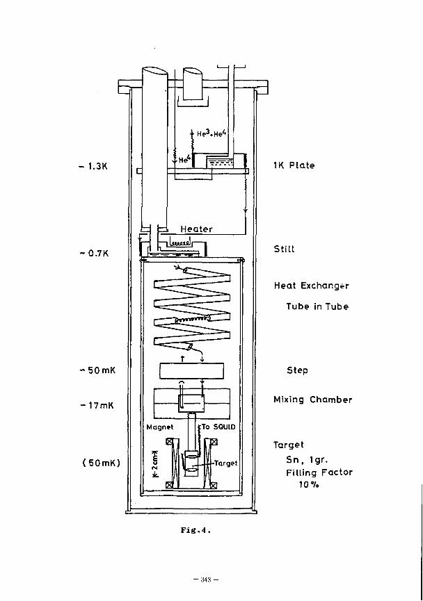
c r i Heater -i |—lUmmtli—|

1K Plate

Still

Heat Exchanger

Tube in Tube

Step

Mixing Chamber

Target S n , 1gr. Fi l l ing Factor

10°/.

F i g . 4 .

- 343 -

i-, lX7 Elementary Particle and Universe M. Yoshimura (Tohoku Univ.)

• ttv - 3

. T 0 = 1 .73 5" 1 o,°6 "K.

• H l U T FoR.

I

t'<t r, SI -r

PARK M A - 1 " ^

.$-Mwt>ARP 9A<J*& TH,

y-" V 3 v ^ * t * * •

7; v, v

5 U 5 Y

^

- ^

A-

\

e\

O--

-\W Jft

Mrt

o

V \

"2 0

ii •>

H

ill

? p VI

-> \-ui • <

& 0^

3

' N

3

* I — >

v \ I

•s- ai C * <3" Ui •5

a_ -?? Q \-ZC - ^

<;

0

$

v (T!

*5.

l i 2 X y < \

H

i- H

v-<•

- :»<-,

p-«

•2 o

<:

x 2

>-

V-

Mi «r o r o X

I o

0

\-5 o \-

ui

V

2:

IV

V-

ui

H ui oo

^ ^ ""\ VJ

<> v_-c<

Ui X <

Ui 2 J

:> v-<c 2

v-l

ui 3

-V

11

"3

z «. CI

w is tvi <JT o •N 2 X M V •s. *\ M « to

•s " --> o Or •<

-r V

to V 2 4

> III V V- -v a

< --* —'

_l *- M V <1 1 <o ^ •A Ti (i •b •J

< 3 « J

«

•u

-1 -6

<

o

H

0

t

3 a

>-

3 S-

0 -J 0 X

\

ro la f i

>n I ^ 1 v\ 3 r> Z >- V- I-

2 <

>

0"

u. 0

>-

2

••ft

1. is

<sr

O

- M(i -

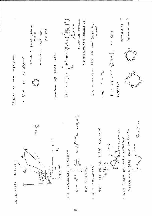
2

_1

5:

o

Vil

5:

> ,1

A

V

It 3 -

<: >

u. 0 2 c V

-<

•,l\ l->

VI a

4 us <; \-< Ui K >•

V- o X a .

V ~ V c/ V- V-0 c a

J 0

2 «; Ui

-J •a

fc-

to uj

•a:

0

-=!

V

0

<1 • i :

- < \ X

J

>-

<

4*

• ^ III

r

i

+>

>n

Q 0

0 V-

tl

a.

HI

•J

a

l-i.

Qj

I

<r t-v. 2 H

a o

:t-i7 -

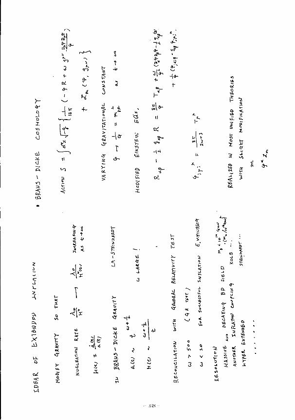
o _i o X VI Q O

Ml

ft

CO

/—x

% % «-i r->~^^

'N ^ 3 1 .

T 3

*• i 9^

-IS

*o

4-J

<

•A)

A-

II

-ier

T i 9 -

Ui

ui v-

(

*-

+•

1-

I a—

•0 I t 2 s a: H a. <

i . t * 5) «. iH u.

1- i 3

0"

Z 1 " t~

'-• * •f\

•>! 3 0 >-1* X c

u •3 -1 *< X

3—

<* 1 i

v9- < %

a •*: >

1 * " 0 I

A < 1 ui

-1 ~

2 1 > <: •5T a ;

0 »

i 1 < c a 1 3 us 5 tX

<s-v. r ~s J a J 2. V* u . CD ^ j

A V- I j - %£ V •ft 4 -

§ 0 4|*x ^ J ;

<r 5

I 0

<ii

3 + 3 1*

v 1 Ci

2 a >- -1 -- 3 -P 3 1 1 VA ^

X V- a: •jj i ; * • < X

. l i 5 •2

• «^<s p. V <? ^

3 0 0 rt

V-V. or < lA 2 . -N. ^ ^ V

Q 14 <c A \ i — 0 «S 2 >-Q >-VA­

0 V X O a 0 is

3 J i s < -t ST a

0 2 i

O a 0 is

\ l i

v4

- :IIH -

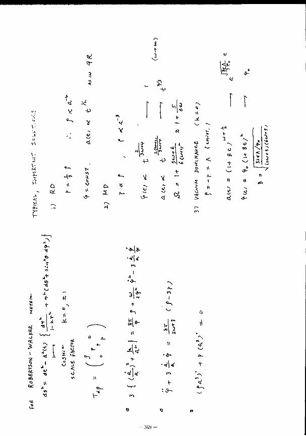
0"

J-

5

*! r J 3 f f V I V -P \«0 tl

i l «-, V + \- ^ V « £ - , , » iy , • V •V J

\-•i

« 1* Il I*

si Ui 0

5

<

•3

+

to •9-

< \-•i

« - N

V |V ^ 0

-5-

Q n v5-

II

c5 -•ar >

I u

li II

3 •3-

iv JO

o r \ a - *~N ^ r-

V-

'-9-19-

a/

<rf •3 CJ 1 >- A o/ V uv X tti a (I

tki

o

ii z

0

°~>

t °-|

•t-

*N

\~*

* » *

• 349 -

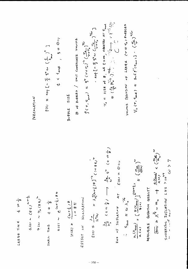
f <: j o o

3 3-

I v-/ X

0

1 •

u l

-1

CO

ft-

m J

2

V v V

i-

3

i

5

!* ilr"

O

7

*

V ^

I

vV

v4

4

-(«)

\-us cr

3

CO if

X

-J

X

+ 3

<U

CD

X

2 l)

0

-el t-3

< 3

- 1 *

-<\x

0 tl

t-

< 2

tf -< -3 U

i%

3

<i <

*l* ^ v^ A V

"if - ^ 3 i 0 <J « z

5 - «»

cr

2

cr 2

o

J -

- HSO •

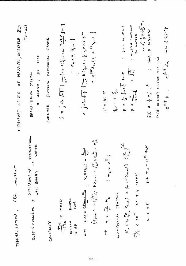
ft Ml

<*> «1 1

111 I-5* •"v; H " 1 5. • J c

-\ uj \ 1» i

v\ " 1 j

< "3 c X 0

• o

u. - i

o 5 ' V I ul

u. v\ »J C £ c O 1

T \

a >- < a- aL O to. C i .

1-T

Ul

-If

iS FT 5 ul 5 s « a 3 P h-

t-

£ u

•a.

T

.x

o <!r uu

< 3

t "2. c,

a o o us

CO

X.

r o

Ul

ui

a! ul

• i o

o

&

* ^

-r l i s *

4

1-

> 4

•s 1

i Ol

+i

\i rfo If

3\:

J

4 ]

4 J.

to

I

J

u ui

H? u

* * a

t f-

0

Y-

? 1 V £1-

A H^

r j

"1

i

\, tu fc >9-

4 a J

iV. <u

• * u It? ,~- "• lo -u ' I l l

ll n ••£ *£

^ O G -II

Co

w

3S

X»-< III

*

vV U-

.1

p v

^f *

4 «

a u ,1-

V -

\-

^

- 3 5 1 -

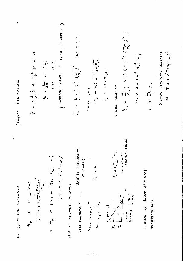
a

o

5.

1 -

«n

- ^

4*

o K '" V

V-% u *. tt a * <c

to HV-* i f

Ul

I

"I

5

i "J

V-

9-

t-

o •5 11

vl

ax 5 2

fl*

O i.

* *

a.

* > i)

01 ir1

ui

f."

>t

2

0

>• u 'N 5

k1

a a!

A_ ft

i X

0 X 0

ta­£

V\ a

•2 0 <y II £ rt III

*- i". V J U / •

< <£ < / • J -J ^

V NJ s 3 X J-

H c--J

a ^ . < # VI V

3 £

• <

y ul

Uj

5. I*, o a. u

v-

£

^ y §

0 ,1 « * >~

•* <L? fc X

4:

-Ac*

J.

ul "• DD w\

ul "• *? ul I*. X a # « 2 ?• .* >~ i v\ * 3 0 <£

0 V

0 Si

0 u J 3 -i=X. Z

- 3ffi -

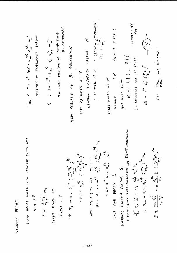
m „

2

"5

x \-

5 HI

Ul

UJ

j

<-o

a

5

h

>- * r

"« 3

1 "52 ft 0

a;

Hi

3 I 111 -1

ul

I \- § 'A

t » l < ad t-i-

0 a V->

b

Li­ < ft W X ^

o J

Y-

Ot :? < "C ">i £ \ _ _ _ j

V) VI

2=

2

^

'N

Ml

* 1

-1

ui

X

' 2, •o:

< V '

T

t-

>-

A t u

-J

ECk

-3

< 2

tf2

I la

I ^

^ -0

Itt - 71 <»i V 5 <t us V * &

t

2

1." •—

i

j

* % u Z "

1

ul

0 i-<

•/** 0

>-<:

T

>-<

y

X Vis 0

O

0 vl

y

X Ul "»> ) us, Ul &• t I? v-

t_ >-0 Ul

X T 5 V- X Ci < J

if » I 0

a" 2

•I

or

o MS

I VI

•2

o V

"5 0

< <

0 ui *-2

K

V-

ll

I - '

= • 1

Ol

- :ir>n -

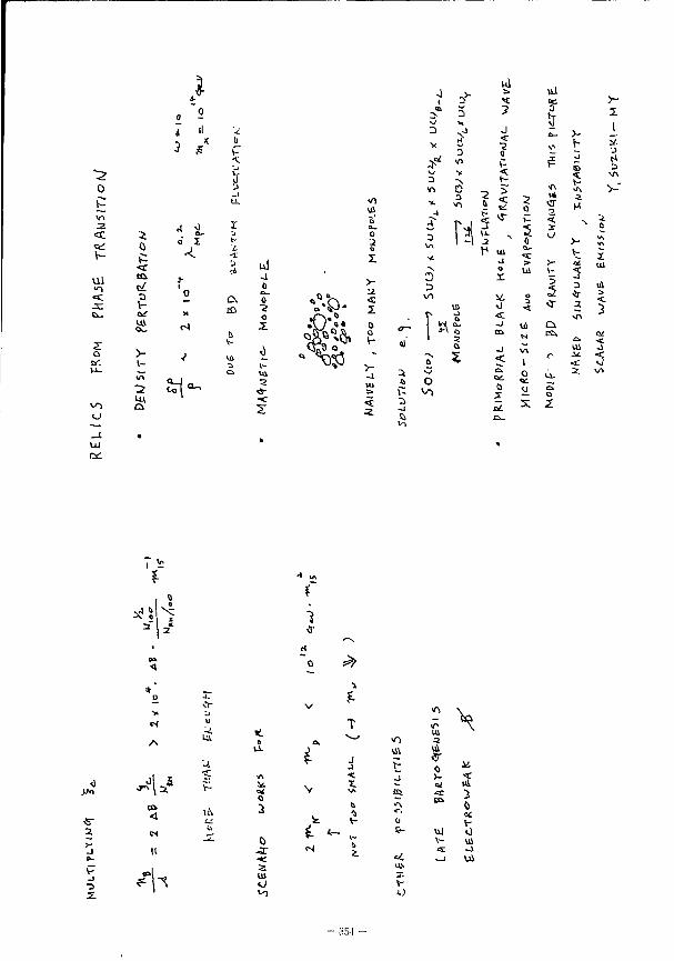
I ul ul

•2 0

Ul

o

o

<r

\-<*• ui

1-

£

o 2

4 i.

- i .

c-l

^

I

0 V

3 5 >-2.

1

(1 >J < •3

I

5. V- D 0 '_> *" v c # • J

3 V v V < ^ vn 0 D •N t- v-

U-

r ui

0 •J

j J" D

C a

"2

5

5> 2 0

0

< N

>-

ul 0 0 •2

5 X

\A St

p 0-> >- w

^ ul 0 0 •2

0 %- >-12

2 Ui

0 X it •0 <

5

«3-

5 3 * a

< 3 o .-o*« 0

0

a. - J Vi a »n

vii 3

<r

> •

•a w

«)' 0

c. 2 Ci

5 -J < 1

Ul at <. -1

5 Ci

<r

> •

•a w 3 & O

o 0 X

0 Li.

Q

X V*

^ 2 0 ^

X 2

Ul OS

*<» ^ •J

^

A

r u

V

T <o 3

\

•-1 w i j

>-i i

4

to <

3

V •< X

J >- <

2 W \V . ^- , &- \U 0

>- U ~^ 0 j r

N ui

&. • * : ci ~ j Ui IU V

-J *h V 2 : *h <o u

351

< ST X

•2

v» U.

tj 2

0

3

Ul

3

a

s 0

HI J

PQ

u a a 0

VU -J

?s

< Ul >

2.

H

Q •f

T.

H

0

2 * 4 . to

oi.

-<

2fr

-J

<

<. a o

s •3.

2.

- x,