arX

iv:0

902.

0941

v1 [

q-bi

o.B

M]

5 F

eb 2

009

Probing Noise in Gene Expression

and Protein Production

Sandro Azaele,1 Jayanth R. Banavar, 2 and Amos Maritan,3

1Department of Civil and Environmental Engineering, E-Quad,

Princeton University, Princeton, NJ 08544, USA.

2Department of Physics, The Pennsylvania State University,

104 Davey Laboratory, University Park, Pennsylvania 16802, USA.

3Dipartimento di Fisica “Galileo Galilei,” Universita di Padova,

CNISM-Unita di Padova and INFN, via Marzolo 8, I-35131, Padova, Italy.

We derive exact solutions of simplified models for the temporal

evolution of the protein concentration within a cell population ar-

bitrarily far from the stationary state. We show that monitoring

the dynamics can assist in modeling and understanding the nature

of the noise and its role in gene expression and protein production.

We introduce a new measure, the cell turnover distribution, which

can be used to probe the phase of transcription of DNA into mes-

senger RNA.

Advances in experimental techniques, that enable the direct observation

of gene expression in individual cells, have demonstrated the importance of

stochasticity in gene expression, the translation into proteins of the informa-

tion encoded within DNA.1–5 Such variability can lead to deleterious effects in

cell function and cause diseases.6 On the positive side, stochasticity in gene ex-

pression confers on cells the ability to be responsive to unexpected stresses and

may augment growth rates of bacterial cells compared to homogeneous pop-

ulations.7 Disentangling the various contributions to production fluctuations

is further complicated by the recent finding that different stochastic processes

1

yield the same response in the variance in protein abundance at stationarity.8

A population of isogenic cells growing under the same environmental conditions

can exhibit protein abundances that vary greatly from cell to cell. The sources

of variability have been identified at multiple levels,9–13 with transcription and

translation playing a major role under certain circumstances.14–16

The low concentration of reactants potentially has two important conse-

quences: the first is that fluctuations around the mean can be large; the sec-

ond is that the nature of the stochastic noise should be taken into account

in some detail because one may not simply invoke the central limit theorem17

which leads to the universal and ubiquitous Gaussian noise. Thus, two genes

expressed at the same average abundance can produce populations with dif-

ferent phenotypic noise strengths, defined as the ratio of the variance over

the mean value of the number of proteins.18 We show here that two distinct

models, one taking into account the detailed nature of the noise and the other

following from an application of the central limit theorem, yield exactly the

same stationary solution for the distribution of proteins in isogenic cells under

the same environmental conditions. The exact dynamical solution of these

two simplified models demonstrate the value of monitoring the dynamics for

understanding the nature of the noise in a cell.

We make the simplified assumption that the kinetics of gene expression can

be described approximately by four rate constants: k1 and k2 are the transcrip-

tion and translation rates, respectively and γ1 and γ2 are the degradation rates

for mRNA and proteins, respectively. It has been found experimentally that

proteins are produced in bursts5,18–20 with an exponential distribution of the

number of proteins produced in a given event. Following Paulsson et al.21 and

Friedman et al.,22 we will assume that transcription pulses are Poisson events

and that the probability distribution that in a single event I > 0 proteins

are produced, w(I), is approximated by w(I) = γ1

k2

e−

γ1

k2I, where k2/γ1 is the

translation efficiency, i.e. the mean number of proteins produced in a given

burst. Here we consider a simple model for the production of proteins without

memory and aging of molecules. Using the specific burst distribution given

above allows one to obtain the shape of the protein distribution even far from

stationarity. Under these assumptions, the stochastic equation that governs

the single-variable dynamics of gene expression, can be written as

x(t) = δ − γ2 x(t) + Λ(t). (1)

2

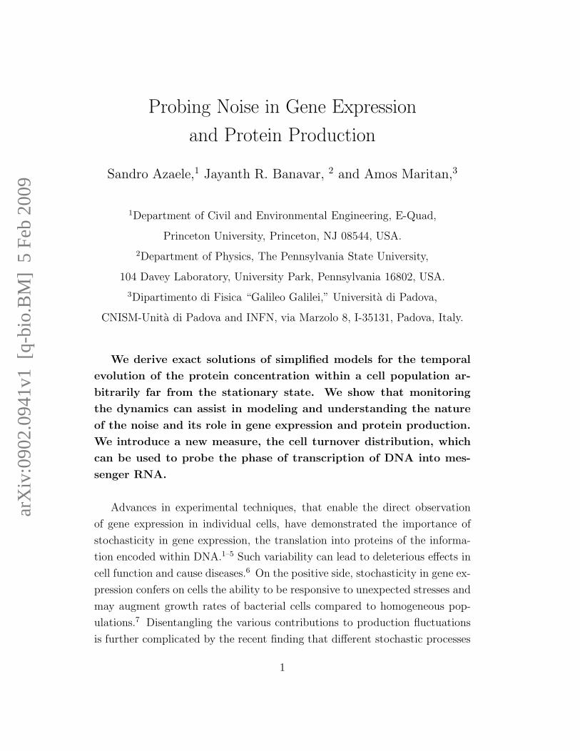
0 100 200 300 400 500 600 700number of proteins Hfluorescence unitsL

0

100

200

300

400

num

ber

ofce

lls

Figure 1: The stationary distribution of proteins in a prokaryotic cell popula-

tion taken from Ref.18 fitted to Eq. (3) with δ = 0 or δ/γ2 = 60.3 (dashed).

The best fit parameters are γ1/k2 = 0.038, k1/γ2 = 12.88 (χ2 ≃ 6100) and

γ1/k2 = 0.030, k1/γ2 = 8.33 (χ2 ≃ 8700), respectively. From the experimental

data it is hard to distinguish between the steady state distributions predicted

by Eq. (3) with δ = 0 and δ > 0.

This pseudo-equation describes the real-time stochastic evolution of gene

expression through a deterministic part and a stochastic term Λ(t), which

will be defined later on. Here x is a continuous variable that represents the

number of proteins within a cell. δ is a term added for generality which can

be incorporated in the average noise.

In order to understand the nature of the noise for the gene expression case,

let us consider the random variable, Ik, that is a measure of the number of

proteins in the kth transcription event, where k = 1, 2, . . . , n. A key quantity

of interest is∑n(t)

k=1 Ik ≡ Λ(t)∆t where n(t), the number of events in the time

interval (t, t + ∆t), is a random variable independent of both x and the Iks.

As in the experiment, let us postulate that: i) the Iks are independent and

identically distributed with exponential distribution; and ii) the probability

of n events occurring during the time interval ∆t is given by the Poisson

distribution qn(∆t) = (k1∆t)n exp(−k1∆t)/n!. The distribution of Λ(t) that

we use in Eq. (1) can be explicitly calculated23 and leads to the following

expression for the cumulants: 〈〈Λ(t1) · · ·Λ(tn)〉〉 = n!k1 (k2/γ1)n ∏n

i=2 δ(ti− t1)

for n ≥ 2 and 〈Λ(t)〉 = k1k2/γ1, independent of time. Because the cumulants

3

are delta functions, the noise is still white (events are uncorrelated if they occur

at different times); however the noise is no longer Gaussian because cumulants

with n greater than two are non-zero.

The master equation that describes this burst-like process is17

∂p(x, t)

∂t= − ∂

∂x[(δ − γ2 x)p(x, t)] +

+ k1

∫ x

0

w(x − y)p(y, t)dy − k1p(x, t) , (2)

where p(x, t) ≡ p(x, t|x0, 0) is the conditional probability that the protein

concentration has a value x at time t given that it has a value x0 at time 0;

and w(x) = γ1

k2

e−

γ1

k2x. The stationary solution of this model (with δ = 0) was

first obtained by Paulsson et al.21 and subsequently re-derived by Friedman

et al.22 For arbitrary δ > 0, we find the stationary solution is

ps(x) =

(

γ1

k2

)

k1

γ2 Θ(x − δ/γ2)

Γ(k1/γ2)

(

x − δ

γ2

)

k1

γ2−1

e−

γ1

k2(x− δ

γ2)

(3)

where Θ(x) is the step function equal to 1 when x > 0 and zero otherwise.

This distinctive feature is a sharp signature of the nature of the noise even in

the stationary solution but is present only when δ 6= 0. However, as shown

in the fit to the stationary solution in Fig. (1), the singularity, if it exists, is

easily masked by other noise effects leading to a rounding effect.

Although experiments on gene expression5,18 are consistent with a burst-

like protein production, steady-state distributions of protein abundances are

equally compatible with alternative explanations. In fact, because mRNA is

unstable compared to protein lifetime (γ1 ≫ γ2), one can assume that tran-

scripts give rise to a constant flux of proteins f and subsequently any protein

degrades at a constant rate γ2. Because of the great amount of available

molecules, one can apply the central limit theorem and suppose that the am-

plitude of fluctuations is simply proportional to√

x. Within this framework

there is no burst-like production, nevertheless the stationary solutions that

one obtains for a burst-like process, including that of the extended autoregula-

tion model,24,25 are also obtained in models with appropriately chosen random

multiplicative Gaussian noise.23 Within this scenario the stochastic evolution

of the protein concentration x(t) is governed by the equation

x(t) = f − γ2 x(t) +√

Dx(t)η(t), (4)

4

100 200 300 400 500 600 700x

0.001

0.002

0.003

0.004

pHx,tÈ0,0L t = 120 min

100 200 300 400 500 600 700x

0.001

0.002

0.003

0.004

pHx,tÈ0,0L t = 240 min

100 200 300 400 500 600 700x

0.0010.0020.0030.0040.0050.0060.007

pHx,tÈ0,0L t = 40 min

100 200 300 400 500 600 700x

0.0010.0020.0030.0040.005

pHx,tÈ0,0L t = 60 min

100 200 300 400 500 600 700x

0.0050.01

0.0150.02

0.0250.03

0.035

pHx,tÈ0,0L t = 5 min

100 200 300 400 500 600 700x

0.0020.0040.0060.0080.01

pHx,tÈ0,0L t = 20 min

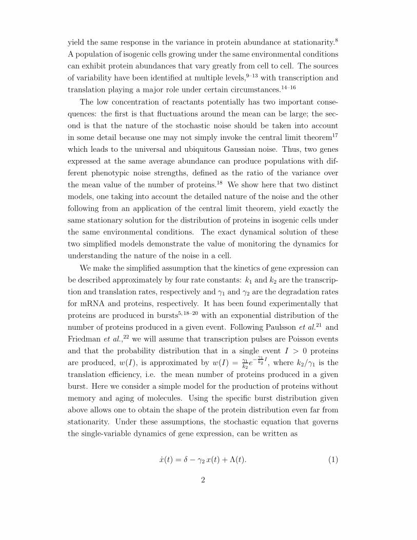
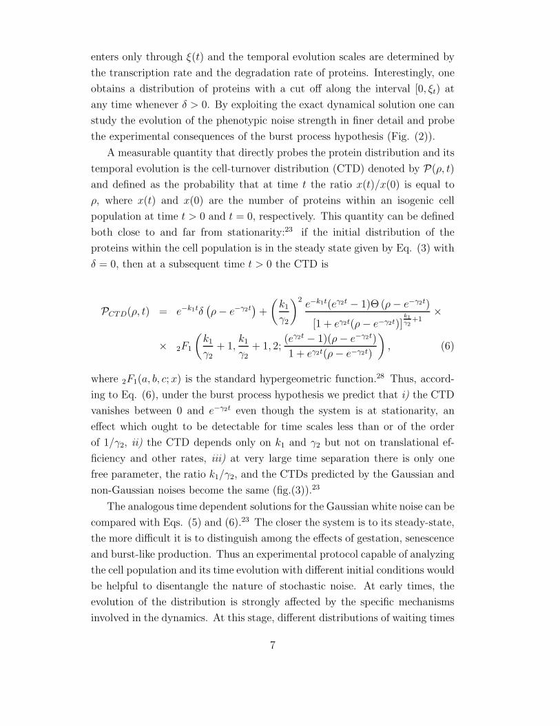
Figure 2: Protein distribution dynamics for different types of noise and with

the same initial conditions, i.e. x0 = 0 proteins at t = 0. The dashed curve

is for the multiplicative Gaussian noise, i.e. Eq. (4) with f ≡ k1k2/γ1 and

D ≡ γ2k2/γ1;23 whereas the other curve is for the non-Gaussian noise, i.e. for

Eq. (5). In both cases the parameters are δ = 0, γ2/D = γ1/k2 = 0.038,

f/D = k1/γ2 = 12.88 and we have set γ−12 = 40 min, γ−1

1 = 2 min.

where η(t) is a Gaussian white noise with autocorrelation 〈η(t)η(t′)〉 = 2δ(t−t′). Note that the same equation could be obtained on setting 〈Λ(t)〉 = f and

〈〈Λ(t)Λ(t′)〉〉 ≡ 〈Λ(t)Λ(t′)〉 − 〈Λ(t)〉〈Λ(t′)〉 = 2Dx(t)δ(t − t′) in Eq. (1) with

all higher order cumulants being identically zero. We point out that in ecology

Eq. (4) is useful for studying the evolution of tropical forests,26 where the

detailed nature of the stochastic noise is not important because of the rela-

tively large numbers of trees of a given species. In the field of finance, Eq. (4)

has been used to study the evolution of interest rates (the Cox-Ingersoll-Ross

model27), where analogous considerations on fluctuations can be made. On

defining f ≡ k1k2/γ1 and D ≡ γ2k2/γ1, Eq. (4) yields the same stationary

state as in Eq. (2) with δ = 0, i.e. Eq. (3). The mean number of proteins at

stationarity is k1k2/γ1γ2 and the phenotypic noise strength at stationarity is

5

k2/γ1, relations that are consistent with previous findings.18 In order to take

into account the effects of feedback in a system undergoing auto-regulation,

one can introduce the physically transparent modification f → Dc(x), where

c is a response function which can be modeled as having two distinct limiting

values at zero and at infinity with the latter being smaller than the former.

Even in this situation, we obtain the same stationary distribution with bista-

bility as Friedman et al.22 Despite this much more realistic analysis, the final

stationary protein distribution is experimentally indistinguishable from Eq.

(3) with δ = 0. Thus, a theoretical modeling of the stationary state of pro-

tein production provides little insight into the microscopic nature of the noise

that leads to stationarity. According to our approach, stochasticity in gene

expression ensues from the large number of available components which en-

tangle a lot of different mechanisms within a cell. Interestingly, this calls for

effective mechanisms which can dampen the deleterious effects of protein noise.

Such efficient noise-reducing mechanisms could be a combination of gestation

and senescence, because of their ability to prevent fluctuations rather than

correcting.8

These results raise the question whether the agreement between the sta-

tionary solutions of the theoretical models and experiments are in fact a direct

probe of the nature of the microscopic noise and whether the asymmetric sta-

tionary solutions derive from a careful consideration of the bursty nature of

the noise. In order to circumvent the indistinguishability of steady-states, one

can look into empirical protein abundances far from stationarity, for which we

provide analytical formulas. Thus we turn now to a study of the dynamics of

Eq. (2) which is a powerful probe of the noise effects. We have derived23 the

solution at arbitrary time,

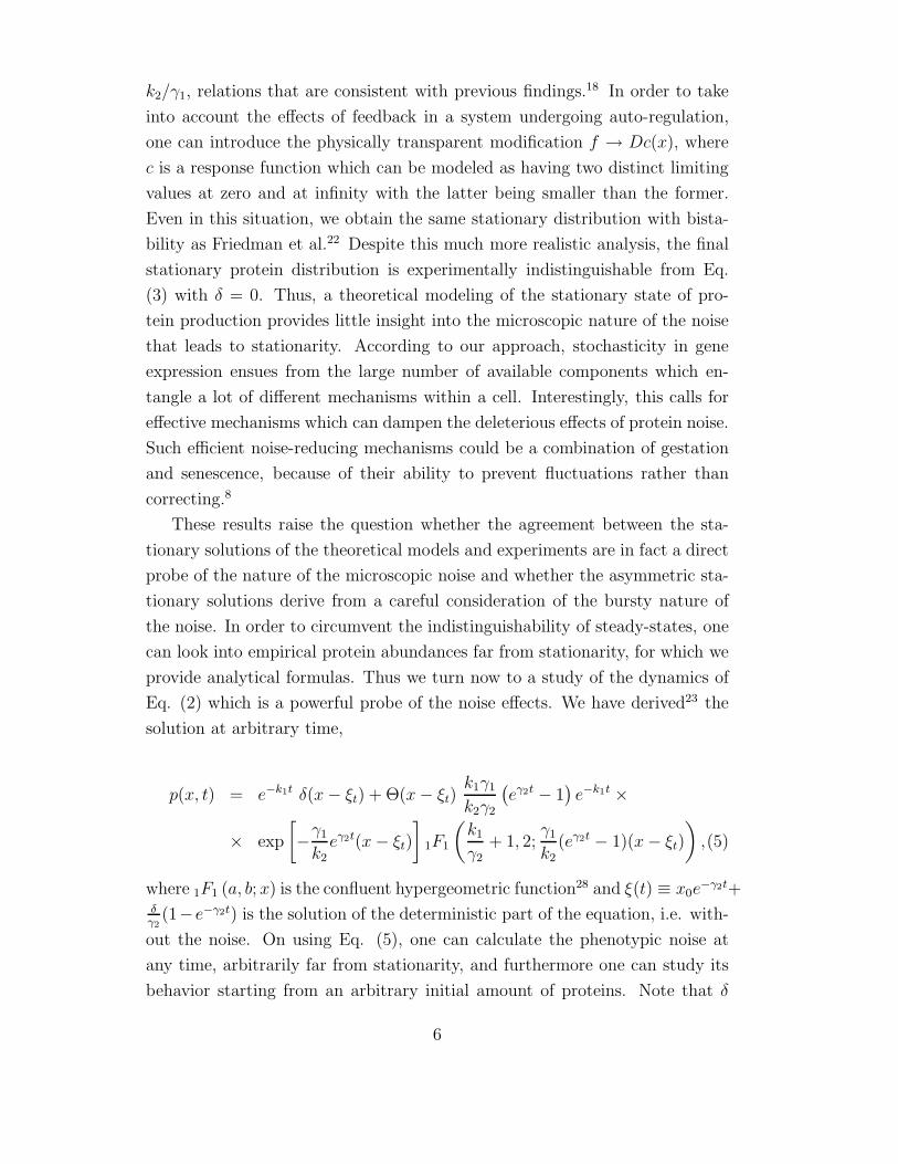
p(x, t) = e−k1t δ(x − ξt) + Θ(x − ξt)k1γ1

k2γ2

(

eγ2t − 1)

e−k1t ×

× exp

[

−γ1

k2eγ2t(x − ξt)

]

1F1

(

k1

γ2+ 1, 2;

γ1

k2(eγ2t − 1)(x − ξt)

)

,(5)

where 1F1 (a, b; x) is the confluent hypergeometric function28 and ξ(t) ≡ x0e−γ2t+

δγ2

(1−e−γ2t) is the solution of the deterministic part of the equation, i.e. with-

out the noise. On using Eq. (5), one can calculate the phenotypic noise at

any time, arbitrarily far from stationarity, and furthermore one can study its

behavior starting from an arbitrary initial amount of proteins. Note that δ

6

enters only through ξ(t) and the temporal evolution scales are determined by

the transcription rate and the degradation rate of proteins. Interestingly, one

obtains a distribution of proteins with a cut off along the interval [0, ξt) at

any time whenever δ > 0. By exploiting the exact dynamical solution one can

study the evolution of the phenotypic noise strength in finer detail and probe

the experimental consequences of the burst process hypothesis (Fig. (2)).

A measurable quantity that directly probes the protein distribution and its

temporal evolution is the cell-turnover distribution (CTD) denoted by P(ρ, t)

and defined as the probability that at time t the ratio x(t)/x(0) is equal to

ρ, where x(t) and x(0) are the number of proteins within an isogenic cell

population at time t > 0 and t = 0, respectively. This quantity can be defined

both close to and far from stationarity:23 if the initial distribution of the

proteins within the cell population is in the steady state given by Eq. (3) with

δ = 0, then at a subsequent time t > 0 the CTD is

PCTD(ρ, t) = e−k1tδ(

ρ − e−γ2t)

+

(

k1

γ2

)2e−k1t(eγ2t − 1)Θ (ρ − e−γ2t)

[1 + eγ2t(ρ − e−γ2t)]k1

γ2+1

×

× 2F1

(

k1

γ2

+ 1,k1

γ2

+ 1, 2;(eγ2t − 1)(ρ − e−γ2t)

1 + eγ2t(ρ − e−γ2t)

)

, (6)

where 2F1(a, b, c; x) is the standard hypergeometric function.28 Thus, accord-

ing to Eq. (6), under the burst process hypothesis we predict that i) the CTD

vanishes between 0 and e−γ2t even though the system is at stationarity, an

effect which ought to be detectable for time scales less than or of the order

of 1/γ2, ii) the CTD depends only on k1 and γ2 but not on translational ef-

ficiency and other rates, iii) at very large time separation there is only one

free parameter, the ratio k1/γ2, and the CTDs predicted by the Gaussian and

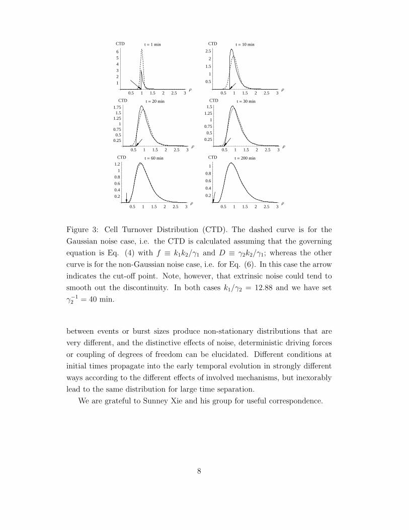
non-Gaussian noises become the same (fig.(3)).23

The analogous time dependent solutions for the Gaussian white noise can be

compared with Eqs. (5) and (6).23 The closer the system is to its steady-state,

the more difficult it is to distinguish among the effects of gestation, senescence

and burst-like production. Thus an experimental protocol capable of analyzing

the cell population and its time evolution with different initial conditions would

be helpful to disentangle the nature of stochastic noise. At early times, the

evolution of the distribution is strongly affected by the specific mechanisms

involved in the dynamics. At this stage, different distributions of waiting times

7

0.5 1 1.5 2 2.5 3Ρ

0.2

0.4

0.6

0.8

1

1.2

CTD t = 60 min

0.5 1 1.5 2 2.5 3Ρ

0.2

0.4

0.6

0.8

1

CTD t = 200 min

0.5 1 1.5 2 2.5 3Ρ

0.250.5

0.751

1.251.5

1.75

CTD t = 20 min

0.5 1 1.5 2 2.5 3Ρ

0.25

0.5

0.75

1

1.25

1.5

CTD t = 30 min

0.5 1 1.5 2 2.5 3Ρ

1

2

3

4

5

6

CTD t = 1 min

0.5 1 1.5 2 2.5 3Ρ

0.5

1

1.5

2

2.5

CTD t = 10 min

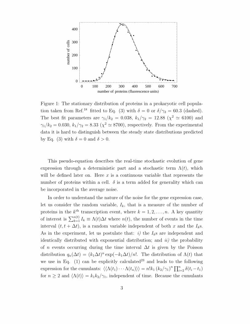
Figure 3: Cell Turnover Distribution (CTD). The dashed curve is for the

Gaussian noise case, i.e. the CTD is calculated assuming that the governing

equation is Eq. (4) with f ≡ k1k2/γ1 and D ≡ γ2k2/γ1; whereas the other

curve is for the non-Gaussian noise case, i.e. for Eq. (6). In this case the arrow

indicates the cut-off point. Note, however, that extrinsic noise could tend to

smooth out the discontinuity. In both cases k1/γ2 = 12.88 and we have set

γ−12 = 40 min.

between events or burst sizes produce non-stationary distributions that are

very different, and the distinctive effects of noise, deterministic driving forces

or coupling of degrees of freedom can be elucidated. Different conditions at

initial times propagate into the early temporal evolution in strongly different

ways according to the different effects of involved mechanisms, but inexorably

lead to the same distribution for large time separation.

We are grateful to Sunney Xie and his group for useful correspondence.

8

References

[1] Kaern, M. et al., Nature Genet. 6, 451-464 (2005).

[2] Raser, J. M. & O’Shea, E. K., Science 309, 2010-2013 (2005).

[3] Paulsson, J., Nature 427, 415-418 (2004).

[4] Golding, I., Paulsson, J., Zawilski S. M. & Cox, E. C., Cell 123, 1025-1036

(2005).

[5] Cai, L., Friedman, N. & Xie, X. S., Nature 440, 358-362 (2006).

[6] Magee, J. A., Abdulkadir, S. A. & Milbrandt, J., Cancer Cell 3, 273-283

(2003).

[7] Thattai, M. & van Oudenaarden, A., Genetics 167, 523-530 (2004).

[8] Pedraza, J. M. & Paulsson, J., Science 319, 339-343 (2008).

[9] Elowitz, M. B., Levine, A. J., Siggia, E. D. & Swain, P. S., Science 297,

1183-1186 (2002).

[10] Raser, J. M. & O’Shea, E. K., Science 304, 1811-1814 (2004).

[11] Becskei, A., Kaufmann, B. B. & van Oudenaarden, A., Nature Genet. 37,

937-944 (2005).

[12] Rosenfeld, N. et al., Science 307, 1962-1965 (2005).

[13] Pedraza, J. M. & van Oudenaarden, A., Science 307, 1965-1969 (2005).

[14] Newman, J. R. S. et al., Nature 441, 840-846 (2006).

[15] Bar-Even, A. et al., Nature Genet. 38, 636-643 (2006).

[16] McAdams, H. H. & Arkin, A., Proc. Natl Acad. Sci. USA 94, 814-819

(1997).

[17] van Kampen, N. G. Stochastic Processes in Physics and Chemistry (Else-

vier, 2004).

[18] Ozbudak, E. M., Thattai, M., Kurtser, I., Grossman, A. D. & van Oude-

naarden, A., Nature Genet. 31, 69-73 (2002).

9

[19] Thattai, M. & van Oudenaarden, A., Proc. Natl Acad. Sci. USA 98, 8614-

8619 (2001).

[20] Kierzek, A. M., Zaim, J. & Zielenkiewicz, P., J. Biol. Chem. 276, 8165-

8172 (2001).

[21] Paulsson, J. & Ehrenberg, M., Phys. Rev. Lett. 84, 5447-5450 (2000).

[22] Friedman, N., Cai, L. & Xie, X. S., Phys. Rev. Lett. 97, 168302 (2006).

[23] See Supplementary Information for further details.

[24] Becskei, A. & Serrano, L., Nature 405, 590-593 (2000).

[25] Isaacs, F. J., Hasty, J., Cantor, C. R. & Collins, J. J., Proc. Natl Acad.

Sci. USA 100, 7714-7719 (2003).

[26] Azaele, S., Pigolotti, S., Banavar, J. R. & Maritan, A., Nature 444, 926-

928 (2006).

[27] Cox, J., Ingersoll, J. & Ross, S., Econometrica 53, 385-407 (1985).

[28] Lebedev, N. N. Special Functions and their Applications (Dover, 1972).

10