POLICY RESEARCH WORKING PAPER

Rural Demand for Drought lnsurancem

A&Aur Gautam~~~~~~~~~~~~~~~~~~~~~.k'x4~~

Harold AkLff

'Me WoddW Bank

Poy P liar Depa me

Pove, and Hum %"a Divn !a E

November 1994~~~~~~~~~~~~~~~~~~~~~~~~~~~,.. ~

Pub

lic D

iscl

osur

e A

utho

rized

Pub

lic D

iscl

osur

e A

utho

rized

Pub

lic D

iscl

osur

e A

utho

rized

Pub

lic D

iscl

osur

e A

utho

rized

Pub

lic D

iscl

osur

e A

utho

rized

Pub

lic D

iscl

osur

e A

utho

rized

Pub

lic D

iscl

osur

e A

utho

rized

Pub

lic D

iscl

osur

e A

utho

rized

I POLICY RESEARCH WORKING PAPER 1383

Summary findings

Many agricultural regions in the developing world are The results indicate that agricultural householdssubject to severe droughts, which can have devastating exhibit significant risk-avoidance behavior, and thateffects on household incomes and consumption, even though they may use a range of risk managementespecially for the poor. To protect consumption, rural strategies, there still remains an unmet demand forhouseholds engage in many different risk management insurance against drought risks. The study did notstrategies - some mainly risk-reducing and some simply estimate the likely costs of supplying drought insurance,coping devices to protect consumption once income has but the latent demand in the study region is strongbeen lost. An important limitation of these traditional enough to more than cover Lhe breakeven rate ofrisk management strategies is their inability to insure approximately the pure risk coist (the probability ofagainst covariate risks. And they are costly. The absence drought) plus 5 percent administration costs.of formal credit and insurance institutions, which offer The findings confirm. the inadequacies of traditionalan efficient alternative by overcoming regional strategies of coping with droughts in poor rural areas.covariance problems and reducing the cost of risk Because of the catastrophic and simultaneous effects ofnminagement, amounts to a market failure. Past research droughts on all households over large areas, there ishas paid much more attention to the supply-side reasons limited scope for spreading risks effectively at the localfor this market failure than to the demand side question level. Either households must increase their savingsof whether there exist financial instruments that farmers significantly (a problem with low average incomes andwant and would be willing to pay for. an absence of safe and convenient savings instruments),

Gautam, Hazell, and Alderman use a dynamic or more effective risk management aids are needed thathousehold model to examine the efficiency of drought can overcome the covariation problem. Improvedmanagement strategies used by peasant households. An financial mark-ets (with both credit and savings facilities)attractive feature of the method is that it exploits actual could be helpful, particularly if they intermediate over aproduction (input-output) data and does not deal with the larger and more diverse economic base than the localusually unreliable data on household consumption and economy. Alternatively, formal drought insurance in theleisure activities. The model is applied to a two-year panel form of a drought (or rainfall) lottery might be feasible,of data on households from five villages in Tamil Nadu and the results suggest that it could be sold on a full-(South India). The sample is small, but the data are cost basis.special, as one of the two years was a severe drought year.

This paper- a product of the Agricutural Policies Division, Agriculture and Narural Resouces Department, in collaborationwith the Poverty and Human Resources Division, Policy Research Department-is part of a study funded by rhe Bank'sResearch Supporr Budget under research project "Management of Drought Risks in Rural Areas" (RPO 677-51). Copiesof this paper are available free from the World Bank, 1818 H Street NW, Washington DC, 20433. Please contact CicelySpooner, room N8-041, extension 32116 (44 pages). Novermber 1994.

Thc Policy Reerch Working Paper Series diseminates the fidings of work it progrss to encorge he exhang of ias aboutdeclopmentsssues.An objectie of the serials to ge the fuling outquickly, even if the presntations are less than flly polishe& Thepapers any the names of the authors and shoutd be used and edeaccordingfy. The findings, inrerprewtions, and condusionsare theautdhcrs' own and sbould not be attributed to the World Bank its Exeaive Board of Directors, or any of its maeber countries.

Produced by the Policy Research Dissemination Center

Rural Demand for Drought Insurancde

Madhur Gautam', Peter Hazell' and Harold Alderan 3

'The World Bank, Washington D.C.2lnternational Food Policy Research Institute, Washington D.C.3The World Bank, Washington D.C.

The views expressed in this paper are those of the authors and should not be attributed to the World Bank. Thisresearch is part of a World Bank Research Project, RPO 677-51 entitled "Management of Drought Risks in RuralAreas". The authors would like to thank Jock Anderson, Francesco Goletti, Ricbard Just, Martin Ravallion,Thomas Reardon and Takeshi Sakurai for valuable comments on earlier drafts of this paper.

Introduction

Many agricultural regions in the developing world are subject to severe droughts, which can have

devastating effects on household incomes and consumption, particularly for the poor. In order to protect

their consumption, rural households engage in a variety of risk management strategies (Walker and Jodha,

1986; Madon, 1991). Some of these are primarily risk-reducing in nature (e.g., income diversification,

intercropping, farm fragmentation and seasonal migration), while others are coping devices designed to

protect consumption once income losses have occurred (e.g., borrowing from local stores and money

lenders, drawing down food stocks, selling assets and participation in govenmment relief programs).

Alderman and Paxson (1992) present evidence on the ability of households to effectively pmtect

consumption against exogenous income shocks. One general conclusion is thathouseholds are collectively

unable to insure against covariate risks. This feature of drought damage - the simultaneous effect on most

households within a region - is an important limitation of many traditional risk nmamgement strategies.

During droughts, many households seek credit at the same time, leading to increases in local interest

rates. Similarly, local wages may be driven down by a surge of labor supply combined with a contraction

of demand. Farmers may also face a buyers' market for their assets in a drought year but a sellers'

market in a post-drought year making it difficult to replenish assets liquidated under stress (Jodha, 1975).

To overcome the covariability problem requires risk-sharing arrangements that cut across regicns that do

not experience droughts simultaneously. Few informal arrangements can accomplish this (with the

exception of seasonal migration and agricultural trader credit).

Another important limitation of traditional risk management strategies is their cost. For example,

diversification pursued as a risk management aid reduces average incomes; credit borrowed in drought

years must be repaid with interest; maintaining food stocks involves storage costs and losses; temporarily

liquidating assets is costly due to capital losses as noted above; and off-farm work may entail a cost in

terms of potential additional farm income foregone.

1

Formal credit and insurance institutions can pool risks across large and diversified portfolios and,

in principle, offer an efficient way of overcoming regional covariance problems and reducing the cost of

risk management. These institutions, however, are rarely weIl-developed in the developing world and

their absence amounts to a market failure. Research on the reasons for this market failure has paid much

more attention to supply-side problems (moral hazard, set-up costs, etc., cf. Hazell, Pomareda and

Valdds, 1986) that limit the spread of formal credit and insurance instruments than to the demand-side

questions of whether there are financial instruments that farmers want and would be willing to pay for

on a full-cost basis. If dhe latter can be demonstrated, then governments may have a key role to play in

either helping private banking and insurance institutions overcome supply-side constraints, or in offering

these services themselves.1

Tne primary objective in this paper is to develop a model to determine if there is any latent

demand for insurance by poor rural households against extreme outcomes such as droughts. If existing

risk-management strategies are inadequate in the sense that households exhibit an unmet demand for

insurance, potential Pareto gains may be possible should alternative income or consumption smoothing

mechanisms be identified. An alternative that this paper explores is a hypothetical drought insurance

scheme in the form of a drought (or rainfall) lottery described in Appendix A.

Defining welfare as the expected value of the sum of discounted lifetime utilities of consumption

and leisure, dynamic programming is used to set up an inter-temporally separable household model. The

dynamic equilibrium conditions are used to derive the benefits and costs associated with ex-ante household

decisions. These conditions help in deriving empirical relationships that allow consistent estimation of

key behavioral parameters. A distinctive feature of the approach used here is that the parameters needed

'The latter should not be confused with government programs that are essentially income transfers, e.g.,relief employment, food rations and subsidized crop isurance. While there is undoubtedly a need for some ofthese programs in many poor rural areas, the focus here is on facilitating the spread of risk-managementmstruments on purely economic grounds. Of course, successful instruments would also help reduce the need forwelfare assistance.

2

to assess the efficiency of existing risk-management strategies can be obtained without explicitly

specifying a utility function. The method yields a parsimonious empirical model, which requires detailed

data only on production activities; such data are often more accessible and reliable than consumption data.

The focus here is on the latent demand for drought insurance. This demand is likely to be

determined jointly by risk behavior and the ability of households to smooth welfare over states of nature.

No attempt is made to distinguish or identify 'pure risk attitudes, say by estimating the Arrow-Pratt risk

aversion coefficients (Binswanger, 1981; Antle, 1987). Instead, a model which explicitly accounts for

various risk-management mechanisms is used to empirically test for thejoint hypothesis of risk avoidance

and welfare smootiing.

The model is applied to a two-year panel from the IFRI.-TNAU2 household survey of five

villages in the North Arcot district of Tamil Nadu, India. Although the sample is small, the data are

appropriate to the question as the region suffered a severe drought in the first year of the survey, with

rainfall levels above the long-run average the following year. The estimates are used to derive implied

premia that sample households might be willing to pay for a hypothetical drought insurance scheme. The

empirical application is intended to be mainly demonstrative due to data limitations. The results obtained

here complement an application of a similar method to data from Burkina Faso (Sakurai, et al., 1994).

The plan of the paper is as follows: the next section describes the problem under study; the third

section briefly reviews the solution principle for a multiperiod consumption problem; the fourth section

develops a household model with drought risks; the fifth section derives efficiency conditions for the risk-

management strategies currently available to households; the sixth section is concerned with the empirical

application of the model with sub-sections that describe the data, present the econometric procedures and

discuss the results; and the final section summariz and concludes.

21FTRI is thme Itrntinal Food Policy Research Institute, Washington D.C., and TNAU is the Tamil NaduAgriculturd University, Tamil Nadu, india.

3

The Problem

To conceptualize the sequential decision making process for an agricultural household, each

production period (i.e., the agricultural year) is divided into tv ;- stages: stage I corresponds to the time

between planting and harvesting, and stage II corresponds to the time from harvesting to the start of the

next planting season. Each stage is different in tenns of its decision-making environment and the nature

of the problem faced by the household.

At the beginning of stage I, a household is endowed with a level of resources carried over as a

result of previous actions. Frequent occurrence of droughts makes future income, and hence future

welfare, of the household uncertain. It has to decide on how to allocate resources between current

consumption, (recautionary) savings, and production in order to attain a plan that maximizes its welfare.

These decisions are assumed to be made at the beginning of stage I and, hence, will be conditioned only

on information available at the beginning of stage L.

The resources available to the household include a fixed labor endowment, an initial level of fixed

capital, an initial level of savings, and initial disposable income. Fixed capital stock is combined with

variable inputs (abor and working capital) in stage I to produce agricultural income that is realized in

stage Ji. Ihe production outcome is subject to uncertain weather, makig the stage I decision-making

environment risky. In response to this uncertainty, the household resorts to risk-management stategies

in an attempt to maintain a desired balance between expected income and income risk.

Ihe ex ante (stage I) risk-management strategies include risk-reducing actions such as diversifying

investment of given resources (labor and capital) across farm and non-farm income sources, and within

farm income diversifying across crops, fields and technologies. This 'self-insurance,' however, is bought

at the cost of lower expected income. The 'premium' associated with, for example, risk-induced crop

diversification is the expected income foregone by not adopting a profit-maximizing cropping patten.

Other ex ante strategies include precautionary savings. These savings tie up scarce capital in a liquid

4

form at the cost of Iforegone production opportunties.

In stage II the outcome of stage I decisions is realized. With weather-related uncertainty resolved,

the decision-making environment at this stage is certain. For simplicity, shocks are modelled as binary

outcomes, namely 'non-drought' and 'drought': in the event of a non-drought year, anticipated income

is realized; in the event of a drought year, realized income suffers a downward shock. The household

responds to such shocks with risk-coping mechanisms such as obtaining temporary off-farm employment,

drawing down savings, and borrowing to smooth consumption.

It should be reiterated that stage II risk-coping actions are ex post in nature. While decisions in

this stage will be dependent on the outcome of stage I, they cannot influence that outcome per se.' The

primary role of various risk-oping devices is to cushion income shortfalls in the same way that savings

do. However, under the assumption of rational intertemporal behavior, the ability of households to

smooth consumption ecx post is expected to influence ex ante risk behavior. For example, if households

know that they can obtain moderately priced consumption credit in the event of a drought, they are

unlikely to pursue risk-reducing strategies in stage I that are more costly in terms of expected income.

In control parlance this forward-looking nature of decision making calls for a closed-loop

solution. Dynamic programming provides such solutions to multi-period problems, and Bellman's

Principle of Optimality (Bellman, 1957) ensures that decision rules obtained by this approach will be

optimal at each stage, irrespective of the realization of future outcomes. Thus, assuming that households

are aware of their options (i.e., risk-coping devices)', the efficiency of existing risk-management devices

can be used to determine their costs in smoothing welfare over stage II outcomes. This cost of self-

insurance can then be used to determine whether there is any demamd for more cost-efficient alternatives.

3Although, they will influence stage I decisions of thefollowing year.

'In case the household is unaware of its fxture options, the situation corsponds to an open-loop decisionframework. In such circumstances, what the household can or cannot do in the future is irrelevant for currentdecision maling, and the dynamic optimiztion model reduces to a static optimization modeL

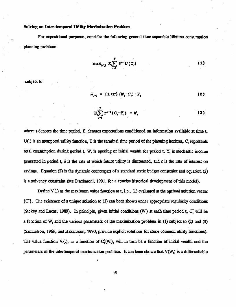
Solving an Inter-temporal Utility Maximization Problem

For expositional purposes, consider the following general tine-separable lifetime consumption

planing problem:

J

max(,, E,- &' U(CI)(1t-1

subject to

W'1= (l+r) (W,-C,) +Y, (2)

BIE r- l t ,-ytr)= W, (3)

where t denotes the time period, E, denotes expectations conditioned on inibrmation available at time t,

U(.) is an atemporal utility function, T is the terminal time period of the planning horizon, C, represents

total consumption during period t, Wf is opening or initial wealth for period t, Y, is stochastic income

generated in period t, 6 is the rate at which future utility is discounted, and r is the rate of interest on

savings. Equation (2) is the dynamic counterpart of a standard static budget constraint and equation (3)

is a solvency constraint (see Dardanoni, 1991, for a concise historical development of this model).

Define V,(.) as the maximum value function at t, i.e., (1) evaluated at the optimal solution vector

{C,. The existence of a unique solution to (1) can been shown under appropriate regularity conditions

(Stokey and Lucas, 1989). In principle, given initial conditions (W) at each time period t, C, will be

a function of W, and the various parameters of the maximization problem in (1) subject to (2) and (3)

(Samuelson, 1969, and Hakansson, 1970, provide explicit solutions for some common utility fimctions).

The value function V,(.), as a function of C(W), will in trn be a function of initial wealth and the

parameters of the intertemporal maximization problem. It can been shown that V(WJ is a differentiable

6

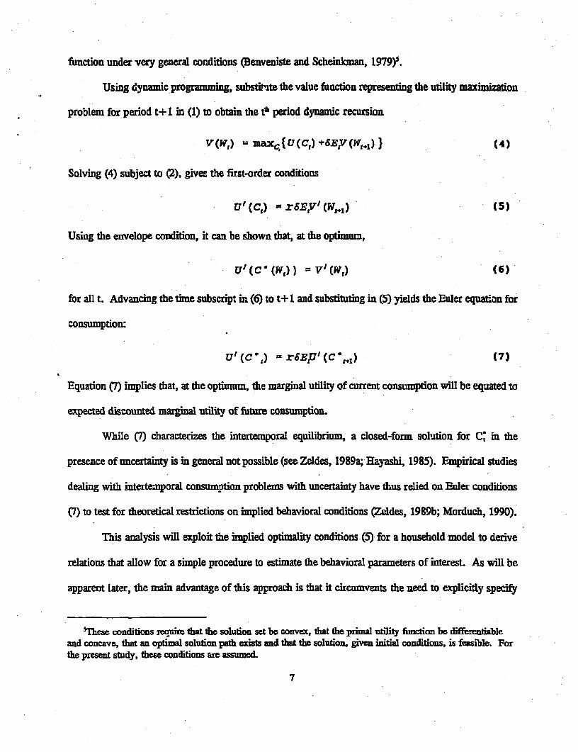
function under very general conditions (Benveniste and Scheinkann, 1979)5.

Using dynamic programming, substitute the value function representing the utility maximization

problem for period t+ 1 in (1) to obtain the t period dynamic recursion

V (W,) - max4,U(C,) EVy(W1 *t.)) (4)

Solving (4) subject to (2), gives the first-order conditions

u' (C,) e r6EV' (W[,1 ) (5)

Using the envelope condition, it can be shown that, at the optimum,

U' (c (W,) ) =V (W,) (6)

for all t. Advancing the time subscript in (6) to t+ I and substituting in (5) yields the Euler equation for

consumption:

U'(C 1P) = rJEr6 (CO, 1 ) (7)

Equation (7) implies that, at the optimum, the marginal utility of current consumption will be equated to

expected discounted marginal utility of future consumnption.

While (7) characterizes the intertemporal equilibrium, a closed-form solution for C; in the

presence of uncertainty is in geneaml not possible (see Zeldes, 1989a; Hayashi, 1985). Empirical studies

dealing with intertemporal consumption problems with unceraint have thus relied on Euler conditions

(7) to test for theoretical restrictions on implied behavioral conditions (Zeldes, 19B9b; Morduch, 1990).

This analysis will exploit the implied optimality conditions (5) for a household model to derive

relations that allow for a simple procedure to esfimate the behavioral parameters of interest. As will be

apparent later, the main advantage of this approach is that it circumvents the need to explicitly specify

5mese conditions require that the solution set be convex, that the primal utility fimction be differentiableand concave, that an optimal solution path exists and that the solution, given initial conditions, is feasible. Forthe present study, these conditions are assumed.

7

consumption preferences. The resulting relationships are parsimonious in data requirements and model

specification. In particular, the method will not require data on consumption or savings, which are often

unavailable or unreliable. Infbrxnation on actual production decisions is used to 'recover' preferences

revealed by households during their normal course of activity.

A Household Model

Before applying the dynamic model represented by (4), the time subscript 't' needs to be carefully

interpreted to avoid confusion about the relevant decision periods. Earlier, the agricultural year was

divided into two distinct sub-periods, stage I and stage H. These stages are the appropriate time periods

for this analysis. Hence the time subscript 't' represents one 'stage' of an agricultural year and 't+ 1'

the immediately following 'stage'. Further, since the model must hold for all time periods, notation can

be simplified by replacing t and t+ 1 by 1 and 2, respectively.

Next note that this analysis is limited to stage I decisions (and henceforth 1 refers to stage I).

Stage II decisions are ex post, made in response to realized outcomes. With uncertainty resolved, stage

H decisions are not appropriate to model ex ante behavioral response to weather-related risks. This is

not to imply that stage II decisions are not relevant to the current problem or that they are ignored in the

model. The fact that stage It decisions will be conditional on, and hence affected by, stage I decisions

is fully accounted for by the dynamic programming approach used to solve the household problem.

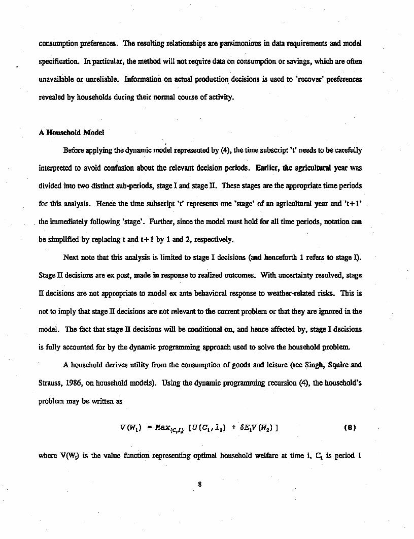
A household derives utility from the consumption of goods and leisure (see Singh, Squire and

Strauss, 1986, on household models). Using the dynamic programming recursion (4), the household's

problem may be written as

V(WI) = Kaxc.a [ U(Cl, 1 1 ) + 6E1V(W2) J I8)

where V(W.) is the value function representing optimal household welfare at time i, C1 is period 1

8

consumption of goods, 41 is period 1 leisure, El denotes expectation taken over the distribution of random

period 2 opening wealtfi, with subsCLipt 1 signifying that expectations are based only on information

available at the beginnming of period 1, and B is the rate at which the household discounts ftture welfare.

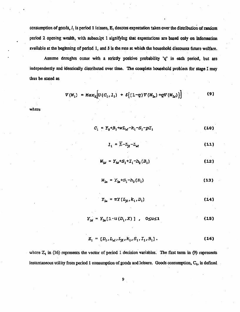
Assume droughts occur with a strictly positive probability 'q' in each period, but are

independendy and identically distributed over time. The complete household problem for stage I may

thus be stated as

V(W1 ) = MaXz[U (Cu,11) + (l-C)V(W2.) +9V(W2) (9)

where

C1 C Yo+B1 +wL0 1 -k 1 -SI-pX 1 (10)

1I = (Lfl 11)

W2d= Y2d+S, + 1 -h 2 (B1 ) (312)

=2 Y2,+Sl-h 2 (B1 ) (13)

Y2n= 7rYY(Zf,k 1 ,Dl) (14)

Y2d = Y2 ,jI-u(Dl,X) ], 0•u1L (15)

Z, = [DI,L.llLfvkl SIrIllBl]J (16)

where Z, in (16) represents the vector of period 1 decision variables. The first term in (9) represents

instantaneous utility from period 1 consumption of goods and leisure. Goods consumption, CL, is defined

9

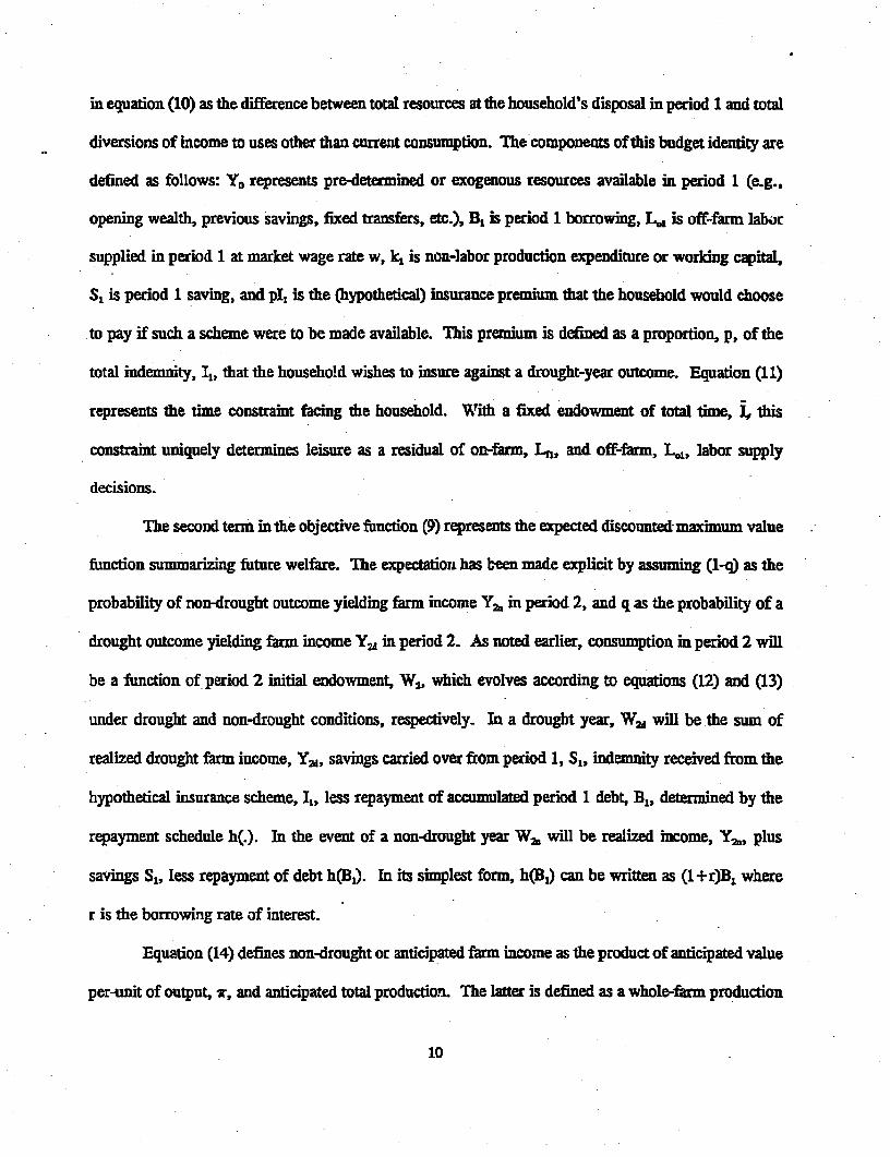
in equation (10) as the difference between total resources at the household's disposal in period 1 and total

diversions of income to uses other than current consumption. The componens. of this budget identity are

defined as follows: Y. represents pro-determined or exogenous resources available in period 1 (e.g..

opening wealth, previous savings, fixed transfers, etc.), B, is period 1 borrowing, Ld is off-farm labor

supplied in period 1 at market wage rate w, k1 is non-labor production expenditure or working capital,

S, is period 1 saving, and pl, is the (hypothetical) insurance premium that the household would choose

to pay if such a scheme were to be made available. This premium is defined as a proportion, p, of the

total indemnity, I,, that the household wishes to insure against a drought-year outcome. Equation (11)

represents the time constraint facing the household. Xrith a fixed endowment of total time, I this

constraint uniquely determines leisure as a residual of on-farm, Lfl, and off-farm, L.,, labor supply

decisions.

The second term in the objective fmnction (9) represents the expected discounted maximum value

function summarizing future welfare. The expectation has been made explicit by assuming (1-a as the

probability of non-drought outcome yielding fann income Y2, in period 2, and q as the probability of a

drought outcome yielding farm income Y2 in period 2. As noted earlier, consumption in period 2 will

be a function of period 2 initial endowment, W2, which evolves according to equations (12) and (13)

under drought and non-drought conditions, respectively. In a drought year, Wd will be the sum of

realized drought farm income, Y2a, savings carried over from period 1, SI, indemnity received from the

hypothetical insurance scheme, II, less repayment of accumulated period 1 debt, B,, determined by the

repayment schedule h(.). In the event of a non-drought year W2, will be realized income, Ya2, plus

savings S,, less repayment of debt h%B). In its simplest form, h(B1) can be written as (1+r)B1 where

r is the borrowing rate of interest.

Equation (14) defines non-drought or anticipated farm income as the product of anticipated value

per-unit of output, jr, and anticipated total production. The latter is defined as a whole-farm production

10

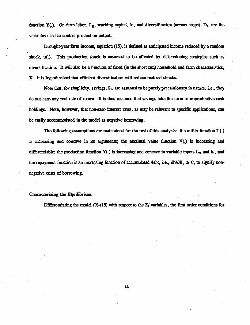
finction Y(.). On-farm labor, Li, working capital, k,, and diversification (across crops), D1, are the

variables used to control production output.

Drought-year farm income, equation (15), is defined as anticipated income reduced by a random

shock, u(.). This production shock is assumed to be affected by risk-reducing strategies such as

diversification. It will also be a fimction of fixed (in the short run) household and farm characteristics,

X. It is hypothesized that efficient diversification will reduce realized shocks.

Note that, for simplicity, savings, S1, are assumed to be purely precautionary in nature, i.e., they

do not earn any real rate of return. It is thus assumed that savings take the form of unproductive cash

holdings. Note, however, that non-zero interest rates, as may be relevant to specific applications, can

be easily accommodated in the model as negative borrowing.

The foilowing assumptions are maintained for the rest of this analysis: the utility function U(.)

is increasing and concave in its arguments; the maximal value function V(.) is increasing and

differentiable; the production function Y(.) is increasing and concave in variable inputs Ln and k,, and

the repayment fimction is an increasing function of accumulated debt, i.e., OhfIB1 Ž 0, to signify non-

negative costs of borrowing.

Characterizing the Equilibrium

Differentiating the model (9)-(15) with respect to the Zf variables, the first-order conditions for

11

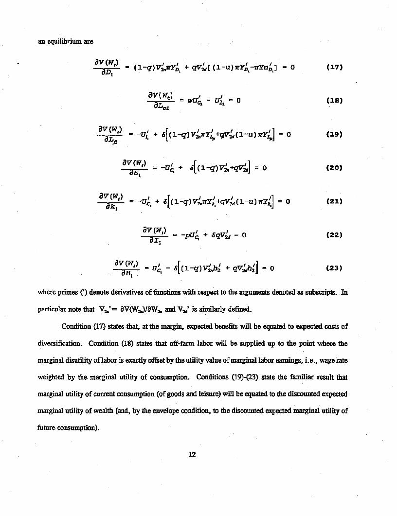
an equilibrium are

Ov (P4)= (1-q)V2.WrYn + qV2d (1-u) 7rY,rYu, ] = 0 (17)

aav(w) = (18)

8= +Ui +[(1q)V4Y4+gVLca-u)fr4 ] = 0 (19)

8v(FV,) I (20)I-. (a) -u + 6[(i-q)vt+qV2d] = o (20)

avV(W,+ [(3-q)V2'ry',+qV2d(l-u)ry'l = 0 (21)

p4 = 6qV2- =0 (22)

= DE,- 6[ CI-q)VL4 + qVLh'] = o (23)

where primes () denote derivatives of functions with respect to the arguments denoted as subscripts. In

particular note that V2;'= avW 2.JI8Wh and VY2 ' is similarly defined.

Condition (17) states that, at the margin, expected benefits will be equated to expected costs of

diversification. Condition (18) states that off-farm labor will be supplied up to the point where the

marginal disutility of labor is exactly offset by the utility value of marginal labor earnings, i.e., wage rate

weighted by the marginal utility of consumption. Conditions (19)0i23) state the familiar result that

marginal utility of current consumption (of goods and leisure) will be equated to the discounted expected

marginal utility of wealth (and, by the envelope condition, to the discounted expected marginal utiity of

future consumption).

12

Simple manipulation of the first-order conditions yields equilibrium relationships that provide

useful insights into the cost-efficiency of the risk-management strategies used by households. They also

suggest a framework that can be fruitfully used for empirical analysis.

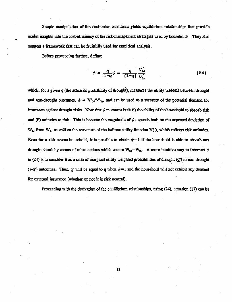
Before proceeding further, define:

i-q (1-g) w (24)

which, for a given q (the actuarial probability of drought), measures the utility tradeoff between drought

and non-drought outcomes, i = V'2|VN'21 , and can be used as a measure of the potential demand for

insurance against drought risks. Note that , measures both (i) the ability of the household to absorb risk

and (ii) attitudes to risk. This is because the magnitude of 4b depends both on the expected deviation of

W2d from W2, as welt as the curvature of the indirect utility function V(.), which reflects risk attitudes.

Even for a risk-averse household, it is possible to obtain ,1 if the household is able to absorb any

drought shock by means of other actions which ensure W2d=W2,. A more intuitive way to interpret +

in (724) is to consider it as a ratio of marginal utility weighted probabilities of drought (q) to non-drought

(I-qj outcomes. Thus, ql will be equal to q when 4= 1 and the household will not exhibit any demand

for external insurance (whether or not it is risk neutral).

Proceeding with the derivation of the equilibrium relationships, using (24), equation (17) can be

13

rewritten as

-7FYAE 1t@ ( 1-U )J] = ¢-07rYUL (25)

Using (18), equating (19) and (20) yields

w( 1+] = WY(,[1+0 (3-u)] (26)

Equating (20) and (21) yields

7rY(,[1+0(1-u)] = 14* (27)

Combining (21) and (22) gives

p1YI[1+*(-l-u) I = * (28)

Finally, using (21) and (23) gives

h1 (1+4) = 7rY(,t+ (1-u)J] (29)

In each equality (5)-(29), the left-hand side gives the marginal cost and the right-hand side the

marginal benefit associated with decision variables D1, Ln, S1, II and B1, respectively. Note that in

equilibrium the benefits and costs associated with each decision are evaluated in terms of their relative

effects on future utility; as a result the discount rate drops out in deriving (2){9).

Condition (25) states that diversification, D1, entails a cost by reducing anticipated production

(OYIaD, < 0) in both non-drought and drought years. These losses, weighted by 1 and 0 for the non-

drought and drought years, respectively, are offset by the marginal utility benefit accrued in drought

years in the form of a reduced income shock (auIaD < 0).

Condition (26) states that the expected marginal benefit of labor use in agricultral production

is equated at the margin with its opportunity cost, the 'effective marginal returns to off-farm labor, i.e.,

the market wage rate weighted by the expected marginal utility of wealth. This condition reiterates the

intuitive result that riskiness in agricultral production makes (certain) off-farm wage income more

14

attractive, leading to a reduction in the use of labor on farm.

According to condition (27), the marginal cost of savings is the value of output foregone by

diverting resources from production to liquid reserves. T.he marginal benefit is the weighted non-drought-

and drought-year utility value of marginal savings carried into the next period.

Condition (28) states that the marginal cost of the hypothetical insurance will be the production

foregone by diverting resources to pay fr the insurance premium. With p as the premium rate, output

will be reduced by p times the productivity of the marginal unit of capital diverted from production. The

benefit of insurance will be the drought-year utility derived from the marginal unit of indemnity received.

Insurance benefits and costs closely resemble those associated with savings; in fact, savings can

be interpreted as an indigenous insurance scheme. The relative cost efficiency is, however, a priori

ambiguous. Using (27) and (28), it is seen that insurance will be cost-efficient relative to savings only

if

1 -p) WY,, I+0 ( -u) I > 1 (30?

Ihe marginal cost associated with borrowing inperiod 1 is the reduction in weighted non-drought-

and drought-year marginal values of resources available to finance consumption in period 2. The

reduction in resources will, at the margin, depend on the slope of the repayment schedule, W'. The

margin; benefit of borrowing is the utlity value of the marginal productivity of capital used in

production. The intuition behind this equilibrium condition is that borrowing to finance current

consumption helps to keep an equivalent amount of capital in productive use, which at the margin

increases output at its current level of productivity. If borrowing is used to finance production, e.g.

buying !ertilizer, then the marginal benefit of borrowing in terms of the marginal productivity of capital

is more transparent

The efficiency of risk-management strategies to mitigate drought risk can be indicated using the

parameters in (25)-(29). To evaluate the efficiency of an insurance scheme of the type considered here,

15

note that (27) and (28) imply

p = 0_ (31)(1+0)

which is the premium rate at which a household will be indifferent between purchasing insurance and

holding liquid reserves. It is simple to verifr that while a household which has efficiently diversified its

risks, or is risk-neutral, will be indifferent between purchasing and not purchasing an actuarially fair

insurance', it will be willing to purchase drought insurance at a subsidized rate, i.e., at a premium rate

less than q. It is also straight-forward to confirm the intuitive result that more risk-averse households

will be willing to pay a larger insurance premium

8p q 1 >0 (32)

where the strict inequality follows from the assumption of a stricdy positive probability of drought in each

rime period, i.e, q > 0.

Empirical Application

The empirical approach adopted here follows from a literature which infers risk attitudes from

risk-avoidance behavior in agricultural production (Moscardi and de Janviy, 1977; Anile, 1987,1989).

We depart from such studies in that we directly use information on drought shocts experienced by

households in a structural model of farm income risk. In addition, we incorporate the use of non-farm

risk smoothing in household risk management strategies to test for the latent demand for drought

insurance.

"Sincev= V'iV' = 1 implis (from24)) that q = q1(1Iq), which in tun implies p q = q.

16

Data

The data used for the empirical application come from to the IFPRI-TNAU household survey

conducted over the period 1982-84 (see Hazell and Ramasamy, 1991, for a detailed description of the

data, the survey design and of the study region). Intially designed for one year (1982-83), the survey

was extended for an additional year (1983-84) after the first year turned out to be a severe drought year7.

A two-stage sampling approach was adopted: in the first stage 1 1 representative villages were

identified, and in the second stage a stratified random sample of households was drawn from these

villages. The first-year survey covered a total of 345 rural households- Due to resource constraints the

resurvey was planned to cover only 75 of the original households from 5 villages that were most affected

by the drought. Of this sub-sample, 36 were agricultural producers; complete panel informatiot,

however, is available only for 32 households. This is the sample used for the empirical analysis.

All survey villages lie in the North Arcot district in the northwest of Tamil Nadu state in southern

India. The region is densely populated (350 persons per square kilometer) and poor - both absolutely and

relative to other regions in Inlia - with an annual income equivalent of US$95/capita compared with the

national average of US$260/capita. The region is dominated by small, fanily farms averaging 1.2

hectares. Paddy and groundnut are the main crops, followed by millet, sorghum and pulses.

The district enjoys two monsoons: the southwest monsoon from June to September and the

northeast monsoon from October to December. The northeast monsoon is relatively more important,

providing about 60 percent of the total annual rainfall. In harmony with these rainfall patterns, the

agricultural year (June-May) is divided into three cropping seasons, namely samba, navarai and

sornavari. The samba (rainy season) crop is the main crop, sown in July-August and harvested in

December-January. The navarai crop coincides with the dry season and depends entirely on irrigation

7Annual rainfall for 1982-83 was 751 -m as compared to the average rainfall of 1032 mm over the perod1961-62 to 19B485. It has also be described as one of the 9 worst rainfill years since 1901 (Rodgers andSvendsen, 1991).

17

It stretches from December-January to May. The sornavaraL crop extends from June to September and

encompasses the light, southwest monsoon.

Almost all households in the retained sample have access to irrigation. The main sources of water

are tanks or small reservoirs (33 percent) and wells (60 percent). Access to irrigation allows almost

continuous cropping of the land throughout the year. Ironically, this dependence on irrigation accenuated

the effects of the 1982-83 drought While 1981-82 was a normal year, it was insufficient to recharge

groundwater reserves after the drought of 1980-81, making even the households that rely on irrigation

prone to drought. Thus the insurance offered by irrigation was limited in 1982-83.

Access to irrigation makes delineating seasons difficult because of overlapping crop cycles. While

it is possible to separate out the naarai crop from the rest becaue of the distinct gap in the planting

periods, it is difficult to separate the two rainy-season crops. Part of the problem also lies in the starting

and ending dates of the two survey periods. Considermg the short time between the planting dates of

sornavarai and samba crops, there is considerable overlapping in the crop cycles of the two crops. The

allocation of land for the two seasons is thus likely to be joindy determined.

For the present parposes, the two rainy season crops are treated as a single stage I crop and

referred to as the samba season for convenience. Stage 11 of the sequential household planning problem

thus includes the nayarai season and extends from January to May of the agricultural year. Total samba

production is thus estimated as the value of production from all land planted prior to the month of January

in each survey period. Total labor and capital inputs, and gross cropped area are also aggregated

accordingly for the purposes of production fimction estimation. Diversification is defied over area

allocated to different crops over the season. The agricultura production shock is calculated using the

value of total samba output for the two years.

It is probable that households respond to shocks in total income rather than to the prospect of

production shocks alone. Accordingly, an alternative estimate of drought shocks is used to estimate

1B

household behavioral response, based on total (farm and non-farm) income. Annualized household

income is used to proxy stage I total income for lack of a more appropriate estimates.

Econometric SpecUication

To specify the essential parameters for estimation it is sufficient to concentrate on equations (25),

(26) and (27). Equation (28) pertains to conditions of hypothetical insurance; as such a market did not

exist in the study area, it provides no insights to observed behavior and hence is treated here as an

analytical tool. Equation (29) requires knowledge of repayment schedules for households as well as data

on borrowing. Since such information is not available, equation (29) is dropped from the empirical

model.

To estfimate the remaining system, infbrmation is required on technology of agricultural

production, Y(.), and expectations of income shocks u(.) held at the beginning of stage I. The former

requires estimating a production function and the latter the estimation of a 'shock' equation. Given data

on a single pair of drought and non-drought years, a two-step estimation procedure is adopted that

optimizes the use of data. In the first step, a shock equation is estimated as a function of pre-determined

drought-year variables (i.e., initial endowments and fixed farm characteristics). Using the estimated

parameters, predicdons for shocks anticipated at the beginning of the non-drought year are obtained using

the non-drought-year values of pre-determined variables. In the second step, these predictions are used

along with production data for ihe non-drought year to estimate the rema ining parameters.

Assuming that non-drought year farm income is representative of the long run expected income,

drought shock is defined as

== - I-=i - u (33)

where rY, is income for a non-drought year and srYd is income for a drought year. Earlier, u(.) was

19

hypothesized to be a function of diversification. Since diversification is an endogenous choice variable,

reflecting anticipated shocks among other things, a simultaneous equation system is required to estimate

the strucural relationship between the two variables. Although such a relationship would be useful by

itself, it is not essendal for the purposes of this analysis. Accordingly, the shock equation is estimated

as a reduced form using available fixed and pre-determined variables. The main advantage of doing this

is that it avoids imposing structure on an instrumenting regression which makes predictions of expected

shocks more straightforward.

The last equality in (33) is used to esimate C, which represents drought year output as a ratio to

non-drought year output. We use the logarithm of the output ratio u' as the dependent variable. The

explanatory variables used for this regression include village dummies and opening stoccs (of variable

inputs and food commodities), fixed capital, family size, and farm characteristics as of the beginning of

the drought year. Using the estimated coefficients and the values of the respective variables at the

beginning of the non-drought year yields an estimate, Ing', from which the anticipated shock for the non-

drought year, A, is calculated as I-expon(nf.

The production function is specified with a Cobb-]Douglas functional form:

log(Y) = )jz,f+aIog(Ljz) +flog(kl) +Olog(1-D,) +v1og (A1 ) +e (34)

where Y is the value of anticipated (non-drought) output; Ln is total labor used on-farm; k, is working

capital input; A, is area cultivated; D1 represents diversification; Gi is a dummy variable for village i; z;,

a!, 6i, U and v are parameters, and e is a random error term. A Simpson index", defined over area

allocated to different crops, is used to measure on-farm diversification, D1.

Given production function (34), the behavioral relations of interest, i.e., equations (25), (26) and

'A Simpson index of diversification over xi, for all i, is defined as D(x)=(1 - E;,(x/xA7.

20

(27), can be rearranged to derive the following' estimable equations

logt = log(a) +log(1+i(1-,O) ) -log(l+ )±ca (35)

log[(] = log(fl)+log(l'+(l-,))-log(l+@)+wO (36)

log((Dl) = log(-y) +log(1+0i(l-) ) -log(q) +COD (37)

where u is the predicted shock, y=0/u' and WL, cok and wD are disturbances (with standard Gauss-

Markov assumptions) associated with (35), (36) and (37), respectively. The left-hand-side variables of

equations (35) and (36) are logaitms of the shares of labor and capital in total value of output,

respectively, and the left hand side of (37) is the logarithm of the diversification index. Given that the

production errors enter multiplicatively in (34), and that the hypothesized drought shock is also

multiplicative in (15), it is assumed tnat optimization, specification or data-related errors are likely to

affect conditions (25)-(27) multiplicatively rather than additively. Besides being more robust to

specification errors, this structure also simplifies estimation somewhat.

These three equations together with the production function (34) yield a simultaneous system.

Across-equation restrictions are necessary to identify all of the system parameters. Parameters a and f

are held as constants across the production function (34) and equations (35) and (36), respectively. The

risk coefficient, X, is similarly restricted to be identical across equations (35), (36) and (37). The

coefficient on the specialization variable, 0, is estimated unrestricted and is expected to be positive9.

'Note that diversification, D, is expected to have a negafive effect on output. However, takng logariths isnot possible for observations on households that do not diversify (i.e. have D=O). Hence, the variable includedin the specification is (1-D) which represents specialization. Accordingly, 0, the coefficient on log(Q-D), isexpected to be positive.

21

Parameter y in equation (37) is also esdmated freely. As derived from the first order conditions above,

=Y0 1 Iu4 It represents the ratio of the marginal effect of diversification on expected output to the

marginal effect of diversification on output shock. Since both effects are hypothesized to be negative,

y is expected to be positive.

Labor, capital and diversification are variables endogenous to the system (34)-(37) and hence

instrumental variable estimation is necessary for consistent estimation. A three-stage least squares

procedure, with appropriate cross-equation parametric restrictions, is used to obtain consistent and

efficient estimates (Judge, et al., 1985). Household and farm characteristics including demographic

variables and opening inventories are used as instruments. Labor and capital are normalized by area to

avoid collinearity in the production function. The estimated coefficient on the log of area, thus, provides

a direct test of constant returns to scale (l::v= 1).

Resudrs and Discussion

The sample used in this study is admittedly small but the detailed information under drought

conditions provides a rare opporunity to model the effects of drought on household incomes, maldng the

data particularly useful for this analysis. As mentioned earlier, the following empirical results are

intended to serve as an illustration. To corroborate the findings and to provide additional results, a

companion study (Sakurai, et al, 1994) uses panel data collected by the Interational Crops Research

Institute for the Semi-Arid Tropics (ICRISAM) on rural households from Burkdna Faso.

Simple statistics for the variables used in the estimations are given in Table 1. Regression results

for the output ratio, u , are giveen in Table 2. Note from (33) that a larger ratio implies a smaller drought

effect. In terms of explanatory power, the regression explains 58 percent of total variation. The lack

of significance of most coefficients, however, suggests the presence of collinearity. This is verified by

the regression results without vilage dummy variables, also reported in Table 2. Both qualitatively anu

22

quantitatively the results are consistent for the two specifications with the exception of a sign change in

one insignificant variable, while the significance level of three key variables improves markedly when

the village dummy variables are omitued. The RP, however, falls considerably. The formal test of

exclusion of the village dummy variables is significant at the 10% level'0. Since the primary concern

with this instrumenting regression is consistent prediction, the specification with village dummy variables

is used to predict anticipated drought shocks for estimating the main parameters of interest (in the second

step).

It should be noted that there are no clear theoretical priors for the asset variables. The dependent

variable is realized shock, and hence will be a function of both the choice behavior of the household

(e.g., the shock may increase with wealth indicating a large risk-bearing capacity of the wealthier

households) and the efficacy of measures adopted by the household (the shock is expected to decrease

with protective measures).

The results show that households owning a greater number of wells experience a smaller

production shock, as may be expected. The number of owned fragments also tends to reduce the shocc.

Fragmentation implies spatial diversification which is likely to be positively related to diversificaL in and

hence the expected positive effect on the drought-non-drought output ratio Ci.e., a negative effect on

production shock). Value of total land owned has a positive effect on the output ratio, i.e., a negative

effect on the shock, although, it is relatively insignificant. Opening stocks have a similar effiect. Larger

food stocks are positively correlated with diversification. This suggests that stocks induce households to

diversify their crop portfolio which in turn helps cushion the effects of drought on total production.

Households with larger fixed farm capital experienced a greater production shock as reflected by the large

and relatively significant negative effect on the output ratio. This is perhaps because a large proportion

"Mhe F statisc for the exclusion of the four village dummies is F(4,20)=2.41 which is significant at the8% level.

23

of fixed capital is in the form of irrigation equipment. While such equipment yields large returns in non-

drought years, the shock is also pronounced in drought years when such equipment is of little use. An

increase in the average distance of owned land (from the village) reduces the output ratio, i.e., it tends

to increase production shocks. 'This may reflect greater care being given to plots that are closer to home,

reducing the effects of drought. Finally, family size has an insignificant effect.

Table 3 presents results for the total income shock equation. Note that the dependent variable

for this regression is the ttal household income ratio in drought and non-drought years and that the

specification includes two additional variables, value of owned business capital and a dummy variable for

illiterate households.'1 Overall, the regression for total income shock performs better han the one for

production shock, with an R2 of 0.72. The number of owned wells again has a significantly positive

effect on the income ratio Ci.e., it reduces total income shock). Number of fragments owned has a

negative effect on the drought-non-drought income ratio or a positive effect on the income shock. This

reflects a scale effect the number of land fragments is positively correlated with total land owned. A

larger share of agriculture in total income and a greater ability to bear risks perhaps explains this effect.

The same is also suggested by the significantly negative effect of owned land value and opening stocks

on the income ratio, i.e., a positive effect on the income shock. Farm fixed capital, ceterisparibus, has

a positive effect on income ratio (negative effect on income shock). It should be noted that total income

includes income from the navarai (irrigated) crop grown in the latter half of the agricultural year. With

irrigation equipment included in farm fixed capital, this result is not surprising. An increase in the

distance of plots from the village tends to increase income shocks, as in the case of production shocks.

Family size, however, has a negative effect on the income ratio, or a positive effect on income shocks,

as does the value of owned business capital. These signs, although insignificant, probably reflect the

"t These two variables were omitted fiom the production shock equation because of tehir lack in explanatorypower.

24

widespread effects of drought on the local economy. With agriculture as the main activity in the study

area, a severe drought has a depressing effect on all activities via intersectoral linkages. This is also

reflected in the large and highly significant negative coefficient on the dummy for illiterate households

who are likely to rely more heavily on unskilled wage labor (Hazell, et al., 1991). Finally, one of the

village dummies is highly significant and consistent in sign with the village effects on production shocks,

while the others are insignificant. Thus there appears to be some regional variation in the effects of the

drought.

Turning now to the main parameters of interest, Tables 4 and 5 give the results for the model

represented by equations (34)-37) using predicted shocks for samba production and total income,

respectively. Using crop production data for the non-drought year 1983-84, Tables 4a and Sa present

results with dummy variables for four of the five villages in the production function specification (34),

while Tables 4b and 5b present results without the dummy variables. Given the small sample size, this

is done to check the robustness of behavioral and technology parameters against village-specific effects.

In the production funtcion, logariftms of variable inputs, labor and capital, and the crop

specialization index (i.e. 1-D) are treated as endogenous. The estimation results for the first-stage

instrumenting equations for these variables are presented in Appendix B, Tables B. 1-B.3. The results

of these regressions are not discussed since they are of not of immediate interest. As is evident, with R2s

of about 0.70, 0.85 and 0.57 for the three variables, respectively, the instruments appear to explain a

substantial proportion of observed variation. However, a limited number of observations combined with

moderate collinearity generates large standard errors making it difficult to establish the importance of

individual variables as identifying variables.

The production elasticity parameters for labor and capital are highly significant, and appear to

be robust to the production function specification with and without village dummy variables as well as

to production and income shock estimates. The coefficient on area is positive and insignificanty different

25

from I in all specifications.

The specialization index, although positiv: in all regressions, is sensitive to village dummy

variables in the production shock specification. The positive sign is as expected, suggesting that

specialization (diversification) increases (decreases) expected output. The estimate is significant in the

regression without village effects, but is insignificant in the regression with village effects. This suggests

that diversification is correlated with village-specific effects. The significance of the coefficient on the

specialization index in the two total income shock specifications follows a similar pattern, although in

magnitude the estimates are close to the production shock specification estimate without village dummy

variables.

The ratio of the marginal effect of diversification on expected production to its marginal effect

on production shock, 'y, is positive in all regressions as expected. It is also significantly less than one

in all cases, indicating that the 'benefif of diversification (i.e. the reduction in shock) is greater than its

'cost' (i.e., the reduction of output). This parameter, however, is also sensitive to village-specific effects

in the production shock specification.

Finally, the parameter of chief ixterest in this study, the risk coefficient, qY1 The estimate is

0.50 (significant at the 5% level) in the specification with village effects, and 0.25 (significant at ihe 10%

level) in the specification without village effects in the specifications using predicted samba production

shocks (rables 4a and 4b). The change in the magnitude of the coefficient suggests an omitted variables

bias in the specification without village fixed effects, considering that at least one village dummy is quite

significant (at the 6% level). The rest of the discussion is restricted to the specification with fixed effects.

In the specification using predicted total household income shocks in Tables 5a and 5b, the

"The reported is estmatd as a constant and interpreted as the smple mean. Alternative specificationswere tried maing 5 a linear f-tfio of household wealth as well as other household charactedstics such asfimily size, age of household head, dummy variable for illiterate households and owned business capital. Noneof the household charctenstics attaned sigmfiamce- A quadrtic specfication in initial wealth was also tnedwith similar results. Since these regressions do not add much to the discussion, ftey have not beea presented.

26

estimates of # are 0.39 and 0.34, respectively, with both significant at the 5% level. The insignificance

of village effects reflects the insensitivity of the coefficient to the two specifications. It should be noted

that despite the differences in the istrumenting equations for the two shock variables, the risk parameter

estimates using total income shocks are within one standard error of each other as well as of the estimate

using production shocks (with village effects), indicating that the # estimate is robust across the different

specifications. Since total household income is likely to be less sensitive to weather shoclk, one might

expect a lower estimate for the risk coefficient using the total income shock specification. As can be

seen, even though the difference is statistically insignificant, the estimates using total income shock are

quantitadvely smaller than the estimate using production shocks.

One way to interpret this coefficient, as nioted earlier, is as a ratio of the marginal-utility-weighted

probabilities of drought (q') to non-drought (Ii< outcomes. The 0 estimates of 0.50 and 0.39 imply

values of q" of about 0.33 and 0.28, respectively. These probabilities should be compared with the

actuarial probability of drought using historical data. As noted earlier, risk neutrality or complete

insurance against drought shocks Ci.e., for which W%=W%), imply q" will be equal to q, and households

will not exhibit any unmet demand for insurance. On the other hand, a q > q would indicate such a

demand.

Using annual rainfll data from 1961-2 to 1984-85, mean annual rainfal is estmated at 1031

mm with a standard deviation of 223 (Ramasmy et al., 1991). The definition of drought used is one

developed by the Indian Meteorologic (sc.) Department: a drought is t... a situation occurring in any

area in a year when annual rainfall is less than 75% of normal' (quoted from Rodgers and Svendsen,

1991). Using this definition, the probability of obseving a drought in any given year is 0.124 (or

12.4%). The utility weighted probability estimates of 0.33 and 0.28 are both substandally higher and

strongly suggest an unmet demand for insurance against drought shocks.

To put these numbers in perspective, consider the proportional risk premiums (PRP) associated

27

with each q'. A PRP is defined as the difference between actuarial expected income and utility-weighted

expectation income as a proportion of the actuarial expected income. Calculating utility-weighted

A~~~~~~~~~~~~

expectation as Yr={(l-qjY2+qY2,(1-u)) and actuarial expectation as Ye={(l-Y2,+qY2.(1-u)}, the

PRP can be simply calculated as 1-(Y 'N9, which reduces to {(qu(Ci(q4}. With the mean production

shock experienced by sample households of 0.74, and the mean total income shock of 0.61, the PRPs are

estimated at 0.17 and 0.13, respectively, for the corresponding q"s. This indicates the sample households

would be willing to pay 13-17% as the premium to purchase extemal insurance. Note that this 'premium'

is in excess of the pure risk-cost of 0.124 that a risk-neutral or a fully insured household would be

indifferent to for an actuarially fair insurance. Thus allowing for reasonable program costs (5-10%), such

an insurance may be commercially viable.

Binswanger and Sillers (1984) report mean proportional insurance premia using data from

Binswanger's experimenta study in southern India (Binswanger, 1981). These rangefromO.09-0.20 (for

'low' to 'high' payoff games where 'low' payoffs were Rs. 5 and high payoffs were Rs. 500). Similar

mangnitudes of risk premia (with a population mean relative risk premium of 0.14) have also been

reported by Ande (19fl for South Indian Rice producers using econometric risk attitude estimates. The

estimated risk premia from this study are quite comparable.

The results indicate that agricultural households in the sample exhibit significant risk-avoidance

behavior. This suggests there is a latent demand for better smoothing mechanisms. Subject to the caveats

of sample and fiuetional form specificity, based on the mean proportion of income that the households

are currently 'paying' as insurance against drought outcomes, it may be concluded that there is a potential

market in the study villages for additional (external) insurance against droughts at unsubsidized premium

rates. Since the premiums calculated here are at sample means, it is likely that there would be some

uptake if a scheme such as a drought or rainfall lottery were to be introduced.

The analysis in this paper is restricted to agricultural households. Given the predominance of

28

agriculture in rural economies, droughts are likely to have a significant effect on non-agricultural

activities as well. It is thus possible that non-agricultural households (e.g., agricultural wage earners and

local business operators) will also exhibit demand for insurance against droughts. Based on exogenous

variables such as rainfall levels, as opposed to endogenous variables such as production shortfalls, such

insurance can be readily made accessible to non-agricultural households as well.

In drawing policy conclusions,, it is important to keep two issues in mind. First, the definition

of the objective probability of drought. Note that the estimated risk-response coefficients do not depend

on the actual probability of drought; it is their interpretation in determining the demand for insurance,

i.e., the marginal premium the households vill be willing to pay, that requires, a precise definition of

drought. The results indicate that households will be indifferent to purchasing insurance at actuarially

fair premiuris for insurance based on objective drought probabilities of up to 33% and 28% (based on

estimates of production shocks and total income shocks, respectively).

Second, the non-drought year which is used to determine the latent demand for insurance followed

a drought year. It is possible that risk coping mechanisms of households were exhausted by the end -of

1982-83 (the drought year) and, hence, household behavior in 1983-84 (the subsequent non-drought year)

may reflect greater risk avoidance than may be observed in other circumstances. Thus, measured demand

may be an over-estmate of the long-run average demand for insurance. This is a generic issue with a

path-dependent historic event Nevertheless, the results are indicative of the inability of households to

absorb drought shocks when they do occur. Considering that droughts are a recurrent event, one may

argue that there is a real, perhaps fluctuating, demand for smoothing mechanisms against droughts

outcomes.

29

Summary

This paper develops a dynamic household model to examine the efficiency of existing drought

management strategies used by peasant households. An attractive feature of the method is that it exploits

actual production (input-output) data without having to deal with the usually unreliable data on household

consumption and leisure activities.

The model is applied to a two-year panel of data on households from five villages in the North

Arcot district of Tamil Nadu (South India). Although sample is small, the data are special in that one

of the two years for which data are available was a severe drought year. This provides an opportunity

to apply the model developed in this paper. Subject to the asmptions about the structure and fimctional

forms of the relationships used in this study, as well as the limitations imposed by the sample, the

conclusions must be viewed as indicative rather than definitive. The key parameters, nevertheless, are

estimated with sufficient precision and the implied risk premia are plausible in comparison with exsting

evidence based on experimental estimates of risk-aversion for households in similar circumstances.

The results indicate that agricultural households exhibit significant risk-avoidance behavior, and

that even though they may use a range of risk management strategies, there still remains an unmet

demand for insurance against drought risks. The study did not estimate the likely costs of supplying

drought insurance, but the latent demand in the study region is found to be strong enough to more than

cover the break-even rate of approximately the pure risk-cost (the probability of drought) plus 5 percent

administration costs.

The findings confm the inadequacies of traditional strategies of coping with drwghts in poor

nrual areas. Because of catastrophic and simultaneous effects of droughts on all households over large

areas, there is limittxd scope for spreading risks effectively at the local level. Either households must

increase their savngs significanly (a problem with low average incomes and an absence of safe and

convenient savings instuments), or more effectieve risk management aids are needed that can overcome

30

the covariation problem. Improved financial markets (with botli credit and savings facilities) could be

helpful, particularly if they intermediate over a larger and more diverse economic base than the local

economy. Alternatively, formal drought insurance in the form of a drought (or rainfall) lottery might

be feasible, and the results suggest that it could be sold on a full-cost basis. These conclusions support

a case for firther research on other areas and for using more reliable data to provide further evidence

on. the latent demand for insurance in poor rural areas.

31

References

Alderman, H. and C. Paxson. 1992. "Do the Poor Insure? A Synthesis of the Literature on Risk andConsumption in Developing Countries." Policy Research Working Paper #1008, The WorldBank, Washington D.C.

Anile, J. 1987. "Econometric Estimation of Producer's Risk Attitudes." Amercan Journal ofAgricultural Economics, 69(3):509-522.

Antle, J. 1989. "Nonstructural Risk Attitude Estimation." American Journal ofAgricultural Economics,71(3):774-784.

Bellman, R. 1957. Dynamic Programming. Princeton University Press.

Benveniste, L.M. tDd J.A. Scheinkman. 1979. 'On the Differentiability of the Value Function inDynamic Miodels of Eoonomics'. Econometrica. 47(3):727-732.

Binswanger, H.P. 1981. "Attitudes Towards Risk: Theoretical Implications of an Experiment in RuralIndia". Econonmc Joumnal. 91:S67-890.

Binswanger, HIP. and D.A. Sillers. 1983. 'Risk Aversion and Credit Constraints in Fanners' Decision-Making: A Reinterpretation". Journal of Development Studies. 21:5-21.

Dardanoni, V. 1991. 'Precautionary Savings under Income Uncertainty: A Cross-Sectional Analysis'.Applied Economics, 23:153-160.

Gudger, M. 1991. "Crop Insurance: Failure of the Public Sector and the Rise of the Private SectorAlternative". In D. Holden, P. Hazell and A. Pritchard (eds.): Risk in Agriculture: Proceedingsof the Terth Agriculture Sector Symposium. 1990, The World Bank, Washington, D.C.

Hakansson, N.H. 1970. 'Optimal Investment and Consumption Strategies Under Risk for a Class ofUtility Functions". Econometrica. 38(5):587-607.

Hayashi, F. 1985. "The Effect of Liquidity Constraints on Consumption: A Cross-Sectional Analysis".Quarterly Journal of Economics. 100:183-206.

Hazell, P.B.R. 1992. "The Appropriate Role of Agricultural Isurance in Developing Countries".Journd of International Development. 4(6):567-582.

Hazell, P., C. Pomerada and A. Valdds. 1986. Crop Insurance for Agricultural Development. JohnsHopkis University Press, Baltimore.

Hazell, P.B.R. and C.Ramasamy. 1991. The Green Revolution Reconsidered: The Impact of High-Yielding Rice Varieties in South India. John Hopkins University Press, Baltimore.

Hazell, P.B.R., C. Ramasamy, V. Rajagopalan, P.K. Aiyasamy and Neal Blevin. 1991. "EconomicChanges Among Village Households" in Hazell and Ramasamy (1991).

32

Jodha, N.S. (1975). "Famine and Famine Policies: Some Empirical Evidence". Econommc and PolM catWeeldy, 10:1609-23.

Judge, G.G., W.E. Griffiths, R.C. Hill, H. Lutkepohl aud T-C. Lee. 1985. Theoq and Practice ofEconometrics. John Wiley and Sons, New York.

Matlon, P. 1991. "Farmer Risk Management Strategies: The Case of West-African Semi-Arid Tropics" .In D. Holden, P. Hazell and A. Pritcbard (eds.): Risk in Agriculture: Proceedings of the TenthAgnculture Sector Symposium. 1990, The World Bank, Washington, D.C.

Moscardi, E. and A. de Janvry. 1977. "Attitudes Toward Risk Among Peasants: An EconometricApproach." Amercan Journal ofAgriculta Economics, 59(4):710-716.

Morduch, J. 1990. "Risk, Production and Saving: Theory and Evidence from nian Households". Dept.of Economics, Harvard University. Mimeo.

Ramasamy, C., P.B.R. Hazell, and P.K. Aiyasamy, 1991. "North Arcot and the Green Revolution" inHazell and Ramasamy (1991).

Rodgers, C. and Mark Svendsen. 1991. "Objective Assessment of Drought and Agricultural Impacts ofDrought in The Monsoonal Climate of South India". Mimeo. The International Food PolicyResearch Institute, Washington, D.C.

Samuelson, P.A. 1969 "Lifetime Portfolio Selection by Dynamic Stochastic Programming". The Reiewof Economics and Staisics. August: 239-246.

Singh, I., L. Squires and J. Strauss. 1986. Agricultural Household Models: Extensions. Applications andPlicy. Johns Hopkins University Press, Baltimore.

Stokey, N.L. and RE. Lucas. 1989. Recursive Methods in Economic Dvnamics. Harvard UniversityPress, Cambridge, Mass.

Sakurai, T.., M. Gautam, T. Reardon, P. Hazell and H. Alderman. 1994. "Potential Demand forDrought Insurance in Burina Faso." - .Mim., Agricultural Policies Division, Agriculture andNatural Resources Department, The World Bank, Washington, D.C.

Walker, T.S. and N.S. Jodha. 1986. "How Small Farms Adapt to Risk". In P. Hazell, C. Pomerada andA. Valdes (1986)

Zeldes, S. 1989a. Optimal Consumption with Stochastic Income: Deviations fiom CertaintyEquivalence". QuarterlyJowunu of Economics. 104(2):275-298.

Zeldes, S. 1989b. "Consumption and Liquidity Constraints; An Empirical Investigation". Jornas ofPolitical Economy. 97(2):305-347.

33

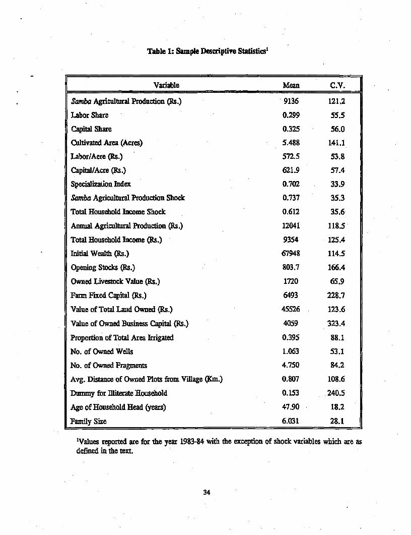
Table 1: Sanple Descriptive Statistics1

f Variable Mean C.V.

Samba Agricultural Production (Rs.) 9136 121.2

Labor Share 0.299 55.5

Capital Share 0.325 56.0

Cultivated Area (Acres) 5.488 141.1

Labor/Acre (Rs.) 572.5 53.8

Capital/Acre (Rs.) 621.9 57.4

Specialization Index 0.702 33.9

Samba Agricultural Production Shock 0.737 35.3

Total Household Income Shock 0.612 35.6

Annual Agculthral Production (Rs.) 12041 118.5

Total Household Income (Rs.) 9354 125.4

Initial Wealth (Rs.) 67948 114.5

Opening Stocks (Rs.) 803.7 166.4

Owned Livestock Value (Rs.) 1720 65.9

Farm Fixed Capital (Rs.) 6493 228.7

Value of Total Land Owned (Rs.) 45526 123.6

Value of Owned Business Capital (Rs.) 4059 323.4

Proportion of Total Area Irrigated 0.395 88.1

No. of Owned Wells 1.063 53.1

No. of Owned Fragments 4.750 84.2

Avg. Distance of Owned Plots from Village (Km.) 0.807 108.6

Dummy for Illiterate Household 0.153 240.5

Age of Household Head (years) 47.90 18.2

Family Size 6.031 28.1

'Values reported are for the year 1983-84 with the exception of shock variables which are asdefined in the text.

34

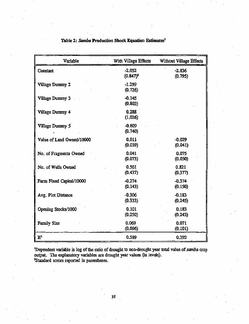
Table 2: Samba Production Shock Equation Estimates'

Variable With Village Effects Without Village Effects

Constant -2.052 -2.836(0.84Th (0.795)

Village Dummy 2 -1.299(0.726)

Village Dummy 3 -0.145(0.803)

Village Dummy 4 0.288(1.026)

Village Dummy 5 -0.809(0.740)

Value of Land Owned/10000 0.011 -0.029(0.039) (0.041)

No. of Fragments Owned 0.041 0.075(0.073) (0.050)

No. of Wells Owned 0.561 0.821(0.437) (0.377)

Farm Fixed Capital/10000 -0.274 -0.374(0.143) (0.150)

Avg. Plot Distance -0.306 -0.183(0.333) (0.245)

Opening Stocks/1000 0.101 0.183(0.250) (0.243)

Family Size 0.069 0.071(0.096) (0.101)

_2 0.589 0.392

'Dependent variable is log of the ratio of drought to non-drought year total value of samba cropoutput. The explanatory variables are drought year values (in levels).2Standard errors reported in parentheses-

35

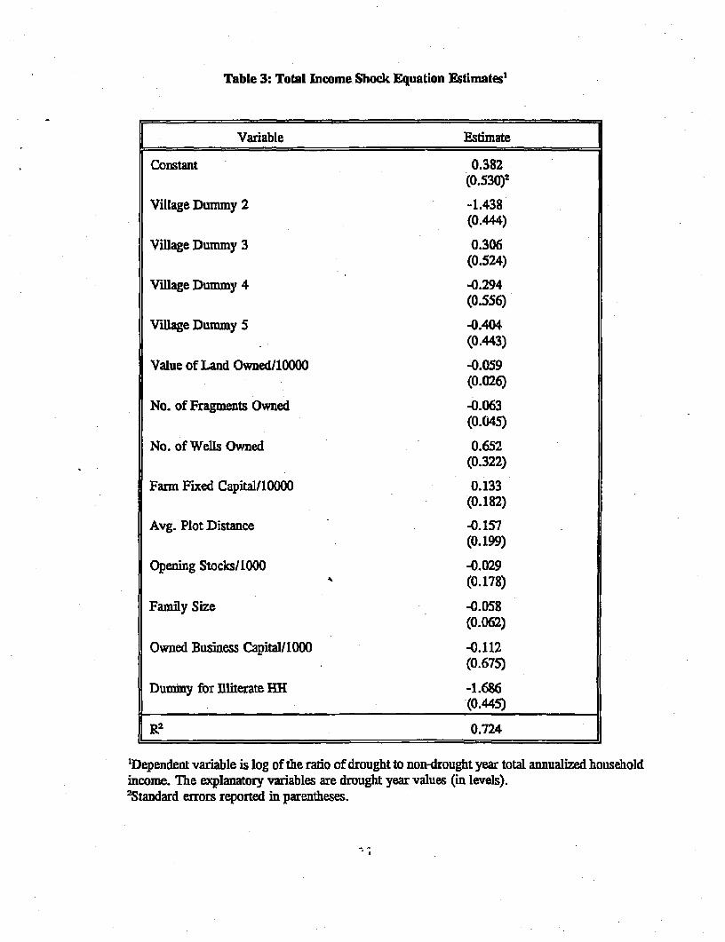
Table 3: Total Income Shock Equation Estimates'

Variable Estimate

Constant 0.382(0.530)2

Village Dummy 2 -1.438(0.444)

Village Dummy 3 0.306(0.524)

Yillage Dummy 4 -0.294(0.556)

Village Dummy 5 -0.404(0.443)

Value of Land Owned/10000 -0.059(0.026)

No. of Fragments Owned -0.063(0.045)

No. of Wells Owned 0.652(0.322)

Farm Fixed Capital/10000 0.133(0.182)

Avg. Plot Distance -0.157(0.199)

Opening Stocks/1000 -0.029(0.178)

Family Size -0.058(0.062)

Owned Business Capital/1000 -0.112(0.675)

Dummy for Illiterate RH -1.686(0.445)

R2 0.724

'Dependent variable is log of the ratio of drought to non-drought year total annualized householdincome. The explanatory variables are drought year values (in levels).2Standard errors reported in parentheses.

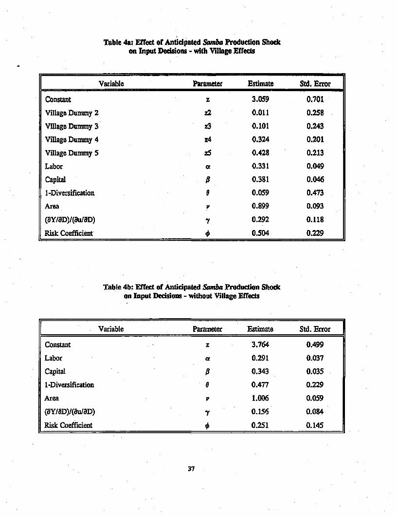
Table 4a: Effect or Anticipated Samba Production Shockon Input Decisions - with Village Effects

[ Variable Parameter Estimate Std. Error

Constant z 3.059 0.701

Village Dummy 2 z2 0.011 0.258

Village Dummy 3 z3 0.101 0.243

Village Dummy 4 z4 0.324 0.201

Village Dummy 5 z5 0.428 0.213

Labor 0.331 0.049

Capital 0.381 0.046

I-Diversification 0 0.059 0.473

Area v 0.899 0.093

(aYIOD)I/(8uID) y 0.292 0.118

Risk Coefficient 0.504 0.229

Table 4b: Effect of Anticipated Samba Production Shockon Input Decisions - without Village Effects

Variable Parameter Estimate Std. Error

Constant z 3.764 0.499

Labor 0.291 0.037

Capital 0.343 0.035

1-Diversification 0 0.477 0.229

Area 1.006 0.059

(aY18D)/(8uIBD) 0 0.156 0.084

Risk Coefficient 0.251 0.145

37

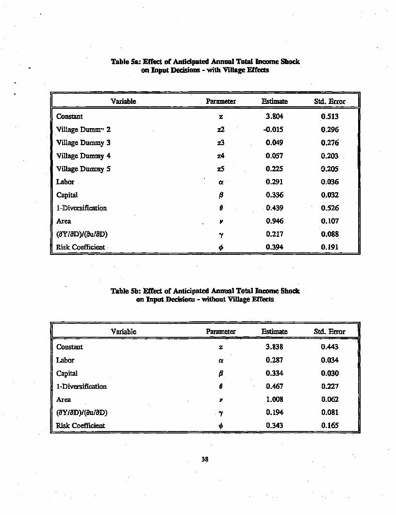
Table Sa: Effect of Antidpated Annual Total Income Shockon Input Decisions - with Village Effects

r Variable Parameter Estimate Std. Error

Constant z 3.804 0.513

Village Dumm-' 2 z2 -0.015 0.296

Village Dummy 3 z3 0.049 0.276

Village Dummy 4 z4 0.057 0.203

Village Dummy 5 zS 0.225 0.205

Labor a 0.291 0.036

Capital 0.336 0.032

1-Diversification 0 0.439 0.526

Area p 0.946 0.107

(aYIaD)I(auIaD) y 0.217 0.088

Risk Coefficient + 0.394 0.191

Table Sb: Effect of Anticipated Annual Total Income Shockon Input Decisions - without Village Effects

j Variable Parameter Estimate Std. Error

Constant z 3.838 0.443

Labor a 0.287 0.034

Capital U 0.334 0.030

1-Diversification 9 0.467 0.227

Area 1.008 0.062

(aYIaD)/(au/8D) 7 0.194 0.081[ Risk Coefficient 0.343 0.165

38

APPENDIX A

DROUGHT INSURANCE

Crop Isurance:

Several countries have publicly operated crop insurance programs that provide insurance againstdrought as one of many insured yield perils. But without exception, these programs have requiredmassive subsidies from govemment and they have not proved particularly effective in protecting farmincomes against droughts.

The basic reason why most publicly-operated crop insurance programs lose money is because theyinsure yields against a wide range of perils, many of which are subject to severe moral hazard andadverse selection problems. This problem is typically compounded by features of insitutitonal andprogram design that increase the insurer's risk exposure (e.g., the insurance portfolio is tied toagricultural credit programs, realistic deductibles are not equired, and indemnitites are valued on the basisof shortfalls from target yeilds rather than on actual crop damage); see Gudger (1991) and Hazell (1992)for recent reviews of public crop insurance.

Commercial crop insurance, which has to be financially viable to survive, is invariably limitedto very specific perils that satisfy four insurability conditions: Ci) the likelihood of the event must bereadily quantiable; Cii) the damage it causes must be easy to attribute and value; (iii) neither theoccurrence of the event nor the damage it causes should be affected by the insured's behavior (i.e.,absence of moral hazard); and (iv) the event should not occur so frequendy that farmers- canot realisticallyafford the required premiums.

Crop losses due to extreme droughts can be insurable when judged by these criteria, particularlyif the damage is total. In fact, private insurers do offer drought insurance in a number of countries,though because of the high administration costs incurred when insuring smal!-scale farmers, it is rarelyextended to other than large-scale, commercial fanners. Insurance of less extreme shortfalls in rainfallis more problematic, since losses are only partial and moral hazard and adverse selection problems canarise. For example, if the shortfall is due to poor rains after planting, the farmer can affect the amountof damage through fertilization, weeding and harvesting practices.

In order to harness drought insurance as a more general risk management aid for drought-proneregions, several objectives must be met.

First, the insurance must be readily accessible to all kinds of households; small and largefarmers, landless laborers, shopkeepers, agricultural merchants and processors, artisans, etc. This meansthat insurance contracts cannot be tied solely to crop or livestock production.

Second, the insurance must be affordable, particularly by poor people. This implies thatadministration costs must be kept very low; and that only drought events that occur with someinfrequency (say 1 or 2 in 10 years) can be reasonably insured.

Thlid, since drought damage within a region tends to be highly covariate, drought insurance willonly be fianncially viable if a mechanism exists to spread the risk beyond the insured region. In a large

39

country, this might be achieved by insuring many regions, particularly if these have low or evennegatively correlated rainfall pattems. But more generally, it is necessary to establish arrangements forreinsurance or contingent loans with the government or with private banking and insurance institutions.

New forms of drought insurance can be designed which meet thse objectives whilst satisfyingessential insurability conditions.

A New Approach to Drought Insurance

The drought insurance envisaged here would be weather-station specific, and al persons insuringagainst the rainfall at a specific station would pay the same premium and receive the same indemnity perdollar of insurance. Indemnities would be paid whever the station's cumulative rainfall for some specifiedperiod of the year (say an agricultural season) fell below an agreed 'drought' level (elel, 70 percent ofaverage). Premiums would be calculated on the basis of the probability of a drought occurring, on thesize of the indemnity to be paid, and on administration costs. For example, for a station faced with aone year in ten drought and an insurance administration cost of 10 percent, a $1.00 insurance ticketwould pay out approxinately $9.00 in the event of a drought (i.e., the expected premium collected overten years minus the 10 percent administration cost). The calculation is approximate because no allowancehas been made for expected interest earnings on accumulated premiums held by the insurere, or forreinsurance costs.

Drought insurance tickets could be marketed rather like lottery tickets, employing low-incomepeople to sell the tickets on a commission basis. Unlike standard insurance, however, all ticket holdersfor a given weather station would receive an indemnity in a drought year, but no indemnity would begiven in non-drought years. If the scheme is managed by a commercial bank, then the indemnitites couldbe issued through its local brance offices after suitable announcements in the lcoal press, radio and.television.

Since all participants would pay the same premium and receive the same indemnity, droughtinsurance avoids all moral hazard and adverse selection problems. Moreover, since the insurance is nottied to agricultural output, participation does not have to be restricted to farmers. In fact, many typesof rural households might find it attractive. Nor need the emergence of a secondary market bediscouraged, since this would enable cash-strappped individuals to obtain their expected prizes (albeit,at a discount) prior to the end of the monitored raifall period. Finally, since thei nrance does not requireany contract wirnig with individuals, or any field inspections or loss assessments, administration costscould be kept very low (perhaps at 2 to 3 percent of the ticket value).

There are at least three potential problems with the proposed insurance. First, its value as adrought-coping aid depends on whether catastrophic income outcomes for most households coincide withsevere droughts at nearby weather stations. This is more likely to be true the greater a region'sdependence on agriculture, but it also depends on the number and geographic dispersion of the weatherstations used in defining the insurance. NOte that since individual households would be free to purchasetickets for any insured weather station, they would have considerable scope to exploit less than perfectlycorrelated drought risks to tailor insurance portfolios to their individual income risks.

Second, there could be difficulties in measuring the cumlative rainfall over the specified periodif large numbers of local people have an interst in a low reading. Guarding the weather stations is

40

expensive, nor would it necessarioly be successful since the guards might acquire a financial interestthemselves. The problem might be reduced by narrowing the time period over which readings must betaken to key periods in growth of important Ical crops. Some recent work at ICRISAT, for example;suggests that the date of onset of the monsoon is an excellent indicator of the agricultural production valueof the ensuing monsoon. This could be a very insurable event. Another promising approach is to usesoil-moisture content readings as a proxy for rainfall deficiency, perhaps even defining drought in texmsof soild moistue contnet rather than in terms of cumulative rainfall. Soil moisture readings could berandomly sampled in much the same way that crop-cutting methods are used to estimate regional yields.

Third, the drought insurance proposed here faces an even more extreme covariability problemthan conventional drought insurance. This is because all the participants receive the same indemnity perdollar of ticket and at the same time. Under these conditions, an insurance for a single weather stationis almost equivalent to a group savings scheme in which households save in non-drought years and simplyreceive their money back in drought years. However, there are two important differences. First, in apure savings scheme, the amount of money available in a drought year is determined solely by thecumulated savings since the last drought. But with the insurance, the available funds depend on theexpected value of the total savings that can be accumulated between droughts; that is, the indemnitiesfrom the insurance do not depend on the order in which drought years occur. This feature of theinsurance can only work if the insurer either runds a number of weather station insurances that are lessthan perfectly correlated, or has access to reinsurance or contingency loan arrangements. Either approacheffectively expeands the reserves available to be tapped in drought years. SEcond, if the insurer isadequately diversified or reinsured, the amounts of liquid reserves that need to be carried can beconsiderably less than with a private savings shceme. This increases the scope for eaniing larger returnson the nonliquid share of toal reserves.

I the insurance is to succeed in helping the poor cope with droughts, it would be especiallyimportant to market the tickets to this clientele. To the extent that thfe poor are overdy more risk averse,then the insurance should be pardy self targeting. However, since poor people often might not be ableto afford the premium, subsidized tickets would enhance their auractiveness. Such subsidies might befunded by diverting some govenment funds from existing crop insurance or drought relief programs.

41

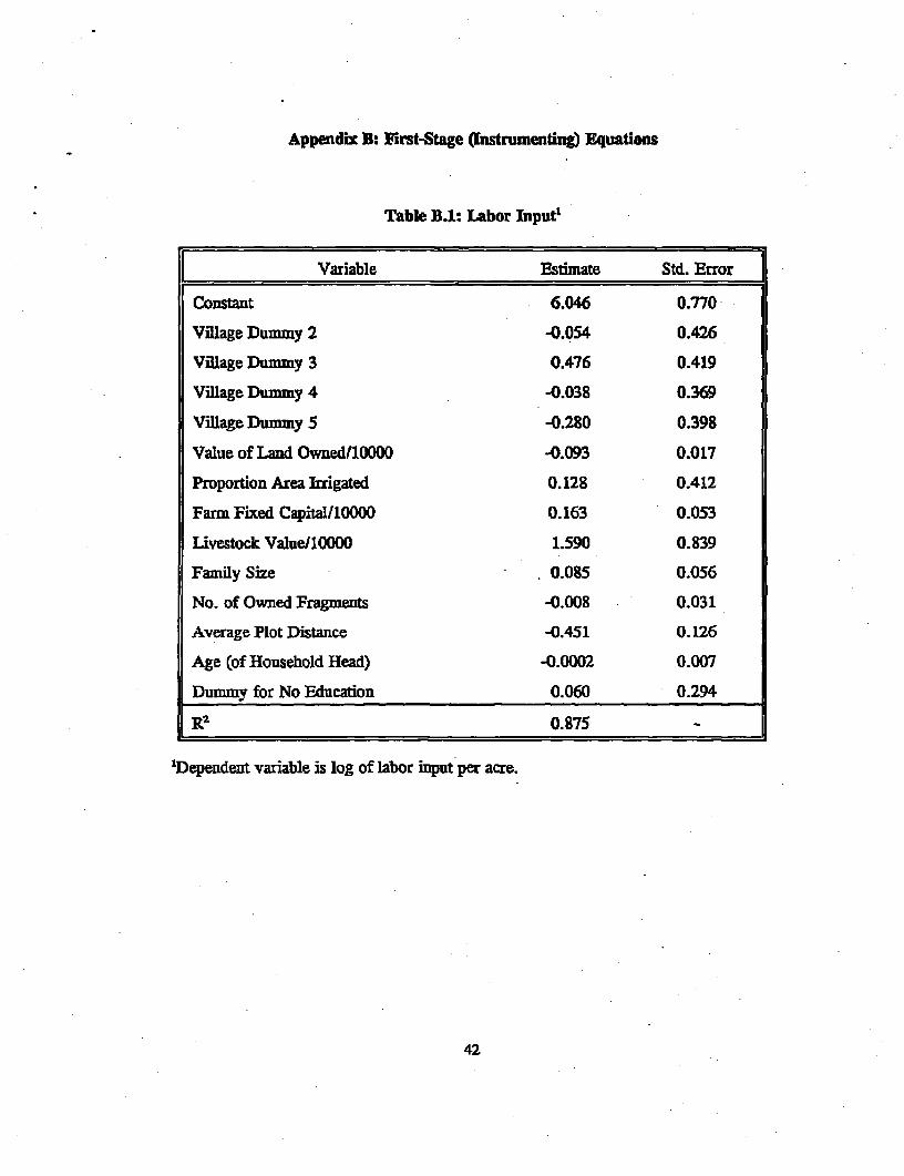
Appendix B: First-Stage (Instrumenting) Equations

Table B.1: Labor Input'

Variable Estimate Std. Error

Constant 6.046 0.770

Village Dummy 2 -0.054 0.426

Village Dummy 3 0.476 0.419

Village Dummy 4 -0.038 0.369

Village Dummy 5 -0.280 0.398

Value of Land Owned(10000 -0.093 0.017

Proportion Area Irrigated 0.128 0.412

Farm Fixed Capital/10000 0.163 0.053

Livestock Value/10000 1.590 0.839

Family Size 0.085 0.056

No. of Owned Fragments -0.008 0.031

Average Plot Distance -0.451 0.126

Age (of Household Head) -0.0002 0.007

Dummy for No Education 0.060 0.294

R2 0.B75 -

'Dependent variable is log of labor input per acre.

42

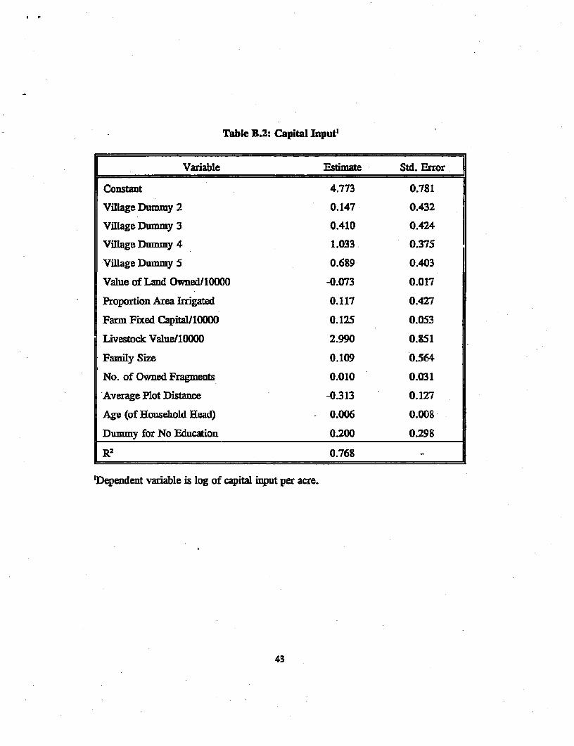
Table B.2: Capital Input'

Variable Estimate Std. Error

Constant 4.773 0.781

Village Dummy 2 0.147 0.432

Village Dummy 3 0.410 0.424

Village Dummy 4 1.033. 0.375

Village Dummy 5 0.689 0.403

Value of Land Owned/10000 -0.073 0.017

Proportion Area Irrigated 0.117 0.427

Farm Fixed Capital/10000 0.125 0.053

Livestock Value/10000 2.990 0.851

Family Size 0.109 0.564

No. of Owned Fragments 0.010 0.031

Average Plot Distance -0.313 0.127

Age (of Household Head) 0.006 0.008

Dummy forNo Education 0.200 0.298

R2 0.768 -

'Dependent variable is log of capital input per acre.

43

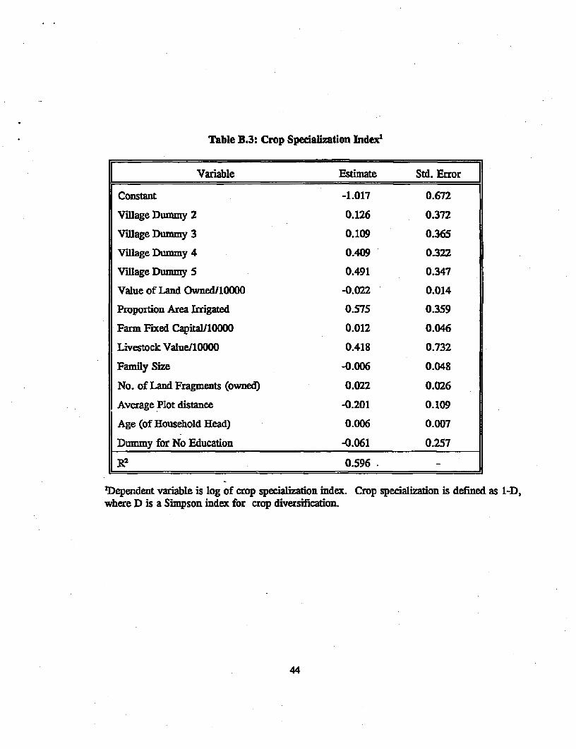
Table B.3: Crop Specialization Index1

Variable Estimate Std. Error

Constant -1.017 0.672

Village Dummy 2 0.126 0.372

Vilage Dummy 3 0.109 0.365

Village Dummy 4 0.409 0.322

Village Dummy 5 0.491 0.347

Value of Land Owned/10000 -0.022 0.014

Proportion Area Irrigated 0.575 0.359

Farm Fixed Capital/10000 0.012 0.046

Livestock ValuellO000 0.418 0.732

Family Size -0.006 0.048

No. of Land Fragments (owned) 0.022 0.026

Average Plot distance -0.201 0.109

Age (of Household Head) 0.006 0.007

Dummy for No Education -0.061 0.257

R2 0.596 -

'Dependent variable is log of crop specialition index. Crop specialization is defined as 1-D,where D is a Simpson index for crop diversification.

44

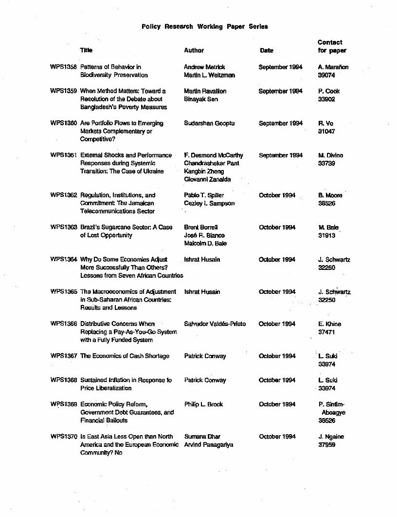
Policy Research Working Paper Series

ContactTitle Author Date for paper

WPS1358 Patterns of Behavior in Andrew Metrick September 1994 A. MaraionBiodiversity Preservation Martin L Weltzman 39074

WPS1 359 When Method Matters: Toward a Martin Ravallion September 1994 P. CookResolution of the Debate about Binayak Sen 33902Bangladesh's Poverty Measures

WPS1360 Are Portfolio Flows to Emerging Sudarshan Gooptu September 1994 R. VoMarkets Complementary or 31047Competitive?

WPS1361 Extemal Shocks and Performance F. Desmond McCarthy Septenber 1994 M. DivinoResponses during Systemic Chandrashekar Pant 33739Transition: The Case of Ukraine Kangbin Zheng

Giovanni Zanalda

WPS1362 Regulation, Institutions, and Pablo T. Spiller October 1994 B. MooreCommitment The Jamaican Cezley I. Sampson 38526Telecommunications Sector

WPS1363 Brazil's Sugarcane Sector A Case Brent Borrell October 1994 M. Baleof Lost Opportunity Jose R. Bianco 31913

Malcolm D. Bale

WPS1364 Why Do Some Economies Adjust Ishrat Husain October 1994 J. SchwartzMore Successfully Than Others? 32250Lessons from Seven African Countries

WPS1365 The Macroeconomics of Adjustment Ishrat Husain October 1994 J. Schwartzin Sub-Saharan African Countries: 32250Results and Lessons

WPS1366 Distributive Concems When Salvador Valdes-Prieto October 1994 E KhineReplacing a Pay-As-You-Go System 37471with a Fully Funded System

WPS1367 The Economics of Cash Shortage Patrick Conway October 1994 L. Suki33974

WPS1368 Sustained Inflation in Response to Patrick Conway October 1994 L SukiPrice Uberalization 33974

WPS1369 Economic Policy Reform, Philip L Brock October 1994 P. Sintim-Govemment Debt Guarantees, and AboagyeFinancial Bailouts 38526

WPS13S70 Is East Asia Less Open than North Sumana Dhar October 1994 J. NgaineAmerica and the European Economic Arvind Panagariya 37959Community? No

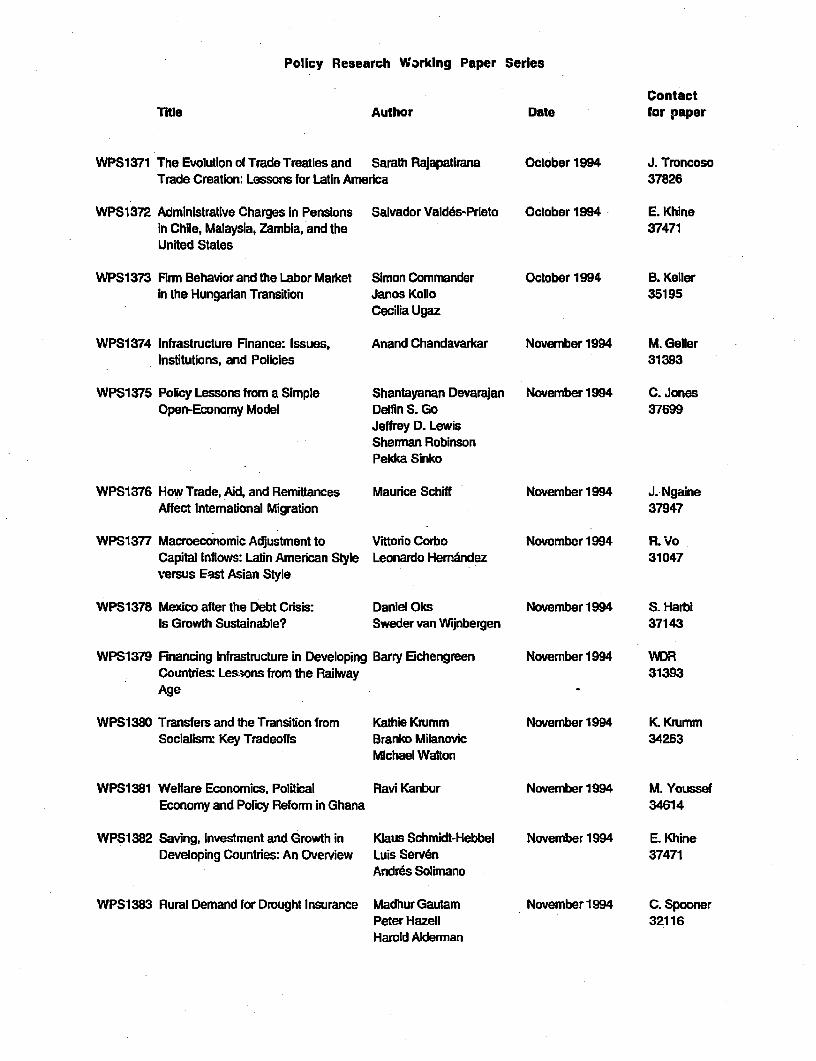
Policy Research Working Paper Series

ContactTitle Author Date for paper

WPS1371 The Evolution of Trade Treaties and Sarath Rajapatirana Oclober 1994 J. TroncosoTrade Creation: Lessons for Latin America 37826

WPS1372 Administrative Charges In Pensions Salvador Vald6s-Prleto Oclober 1994 E. Khinein Chile, Malaysia, Zambia, and the 37471United States

WPS1373 Fim Behavior and the Labor Market Simon Commander October 1994 B. KellerIn the Hungarian Transition Janos Kollo 35195

Cecilia Ugaz

WPS1374 Infrastructure Finance: Issues, Anand Chandavarkar November 1994 M. GellerInstitutions, and Poiicies 31393

WPS1375 Policy Lessons from a Simple Shantayanan Devarajan November 1994 C. JonesOpen-Economy Model Delfin S. Go 37699

Jeffrey D. LewisSherman RobinsonPekka Sinko

WPS1376 How Trade, Aid, and Remdtances Maurice Schiff November1994 J. NgaineAffect Intemational Migration 37947

WPS1377 Macroeconomic Adjustment to Vitorio Corbo November1994 R. VoCapital Inflows: Latin American Style Leonardo HerrAndez 31047versus East Asian Style

WPS1378 Mexico afler the Debt Crisis: Daniel Oks November1994 S. HarbiIs Growth Sustainable? Sweder van Wijnbergen 37143

WPS1379 Financing infrastructure in Developing Barry Eichengreen November1994 WDRCountries: Les ions from the Railway 31393Age

WPS1380 Transfers and the Transition from Kathie Krumm November 1994 KI KrummSocialism: Key Tradeoffs Branko Milanovic 34263

Michael Walton

WPS1381 Welfare Economics, Political RaviKanbur November1994 M. YoussefEconomy and Policy Reform in Ghana 34614

WPS1382 Saving, Investment and Growth in Klaus Schmidt-Hebbel November 1994 E. KhineDeveloping Gountries: An Overview Luis Serv6n 37471

Andres Solimano

WPS1383 Rural Demand for Drought Insurance MadhurGautam November1994 C. SpoonerPeter Hazell 32116Harold Alderman