Planning Ex

European Scientific Journal April 2013 edition vol.9, No.10 ISSN: 1857 – 7881 (Print) e - ISSN 1857- 7431

ECONOMIC DEVELOPMENT PLANNING MODELS: ATHEORETICAL AND ANALYTICAL EXPOSITION

Bashir Olayinka Kolawole

Department Of Economics, Lagos State University, Ojo, Lagos

State, Nigeria

Abstract This paper explores some planning models that have, in

one period or the other, been employed by both developed and

less developed countries to forge development of their

respective economies. Using theoretical basis of analysis, the

paper shows that while some models are weak in their

applicability, certain models like the Leontief Input-Output

model and the Linear programming model, however, are relevant

in efficacy to the development of economies via sectoral and

inter-industry interdependence, aggregate demand, and growth

in output.

Keywords: Economic planning, Econometric, Development, Market

mechanism, Growth

IntroductionIn the literature of economics, any economy whose

economic activity is not market-driven is often described to

be government-intervened. Such economy is usually referred to

as a centrally planned economy at least, in the traditional

176


parlance of the economic system. However, whether an economy

is market-driven or state-controlled, there is the rationale

for planning in such country in order to improve and

strengthen the market mechanism. According to Ghatak (1995),

since the product and the factor markets in less developed

countries (LDCs) are usually imperfect, market forces fail to

attain efficient allocation of resources. Hence, state

intervention in the form of planning is necessary to obtain an

efficient allocation of resources, as prices are wrong signals

to the decision makers. Although, markets have created

benefits over the long run, but only through trial and errors,

yet they leave behind many scars of failures with negative

externalities. As such, despite its apparent plausibility,

Kooros and McManis (1998) are of the opinion that markets by

themselves cannot provide an accelerated and well-coordinated

comprehensive economic plan, and therefore each country must

develop a blueprint for its own future economic well-being.

Such blueprints, however, would take the form of economic

models which are frequently used to construct economic

planning.

Ordinarily, economic models are useful in the setting out

of the objective and targets to be achieved, the constraints

which have to be overcome, and the interrelationships among

the different economic variables which would indicate the

general structure of the economy. In the light of such

exercise there is, therefore, a need for comprehensive

economic planning. By this, it means determining the country's

core competencies, resources, and long-term comparative

177


advantage, and formulating the country's priorities, and the

manner by which its objectives can be met. Since the outputs

of the market are determined by trail-and-error, and over a

long period of time, the development of such a comprehensive

blue print is extremely crucial. As large urban centers or

even a comprehensive university cannot be designed ex-post

facto, after the problems have emerged, nor can such problems

be mitigated through ad hoc trial-an-error, or the market

system, in which some economists have developed irrationally

infinite confidence, because markets are not coordinated. More

so, some markets are also manipulated by oligopolies (see

Kooros and Badeaux, 2007).

Thus, since economic models are frequently used to

construct economic planning and for the fact that such models

should have the dual characteristics of clarity and

consistency aside the property of being selective so that only

the behavior of the major variables is analyzed, and

quantitative (Streeten, 1966), this paper thus explores some

empirically tested aggregate and multi-sectoral planning

models in the developed and developing countries. The

objective of the paper is to examine the theoretical and

analytical bases surrounding each model and also determine the

efficacy of such models, as economic models provide systematic

and logical frameworks for economic planning in order to

obtain feasible and optimal solutions in the light of

available information.

The rest of the paper is structured with the concepts of

economic planning and development in the second section, and

178


theories and models of economic development plan in section

three. Section four gives empirical discussion, while the

conclusion is in the fifth section.

Concepts of Economic Planning and Development:Economic Planning

Economic planning, otherwise known as economic

development planning, has become one of the main instruments

of achieving a higher growth rate and better standard of

living in many less developed countries (LDCs). Planning in

different forms has also been accepted as an important policy

instrument to attain specific targets in most LDCs. It is

frequently advocated as an alternative to the market

mechanism, and the use of market prices, for the allocation of

resources in developing countries. As a holistic approach to

development in developing economies, it promotes the idea and

practice of matching development planning with economic

planning as the economy is regarded as the bedrock for a

nation’s development.

Essentially, economic visions and programs cannot be

realized without viewing developmental issues in a holistic

way which entails improvement in all human endeavors. In this

sense, development surpasses the economic criteria often

measured by economic growth indices and must be conceived of

as a multidimensional process involving changes in social

structures, destructive attitudes, ineffective national

institutions and plan for an increase in par capita output.

Thus, development planning presupposes a formally

predetermined rather than a sporadic action towards achieving

specific developmental results. In essence, economic planning

179


entails direction and control towards achieving set

objectives. Following this line of thought, Jhingan, (2005)

sees development planning as a deliberate control and

direction of the economy by a central authority for the

purpose of achieving definite targets and objectives within a

specified period of time. According to Ghatak (1995),

planning can be defined as a conscious effort on the part of

any government to follow a definite pattern of economic

development in order to promote rapid and fundamental change

in the economy and society.

Economic DevelopmentThe veritable concept of development is based on the fact

that economic, social, political and physical environment, all

combine to characterize the structure of the economy and the

entire social system, as well as the capabilities of the

people and their aspirations for better life. The UNDP Human

Development Report 2002 asserted that “politics is as

important to successful development as economics”. But the

concept of development goes even beyond economics and

politics. As Todaro and Smith (2003) put it: “Any realistic

analysis of development problems necessitates the

supplementation of strictly economic variables such as

incomes, prices, and savings rates, with equally relevant non-

economic institutional factors, including the nature of land

tenure arrangements; the influence of social and class

stratifications; the structure of credit, education, and

health systems; the organization and motivation of government

bureaucracies; the machinery of public administration; the

nature of popular attitudes toward work, leisure, and self-

180


improvement; and the values, roles, and attitudes of political

and economic elites.”

World Bank, in its 1991 World Development Report opined

that the challenge of development . . . is to improve the

quality of life. Especially in the world’s poor countries, a

better quality of life generally calls for higher incomes- but

it involves much more. It encompasses as ends in themselves

better education, higher standard of health and nutrition,

less poverty, a cleaner environment, more equality of

opportunity, greater individual freedom, and a richer cultural

life. Development, thus, must be conceived of as a

multidimensional process involving major changes in social

structures, popular attitudes and national institutions, as

well as the acceleration of economic growth, the reduction of

inequality, and the eradication of poverty.

In more relevance, development theories of modern days

revolve around questions about what variables or inputs

correlate or affect economic growth the most: elementary,

secondary, or higher education, government policy stability,

tariffs and subsidies, fair court systems, available

infrastructure, availability of medical care, prenatal care

and clean water, ease of entry and exit into trade, and

equality of income distribution (for example, as indicated by

the Gini coefficient), and how to advise governments about

macroeconomic policies, which include all policies that affect

the economy. For instance, education enables countries to

adapt the latest technology and creates an environment for new

innovations. According to Todaro and Smith (2003),

181


“Development, in its essence, must represent the whole gamut

of change by which an entire social system, tuned to the

diverse basic needs and desires of individuals and social

groups, within that system, moves away from a condition of

life widely perceived as unsatisfactory toward a situation or

condition of life regarded as materially and spiritually

better.” In other words, they imply that “. . . . development

is the sustained elevation of an entire society and social

system toward a ‘better’ or ‘more humane’ life”.

Irrespective of the specific components of better life,

Todaro and Smith (2003) yet hold the view that development in

all societies must have at least the following three

objectives:

To increase the availability and widen the distribution

of basic life-sustaining goods such as food, shelter,

health, and protection.

To raise levels of living, in addition to higher incomes,

the provision of more jobs, better education, and greater

attention to cultural and human values, which will serve

not only to enhance material well-being but also to

generate greater individual and national self-esteem.

To expand the range of economic and social choices

available to individuals and nations by freeing them from

servitude and dependence not only in relation to other

people and nation-states but also to the forces of

ignorance and human misery.

Economic development, as distinguished from economic

growth, results from an assessment of the economic development182


objectives with the available resources, core competencies,

and the infusion of greater productivity, technology and

innovation, as well as improvement in human capital,

resources, and access to large markets. Economic development

transforms a traditional dual-system society into a productive

framework in which everyone contributes and from which each

one receives benefits accordingly.

Also, economic development occurs when all segments of

the society benefit from the fruits of economic growth through

economic efficiency and equity. Economic efficiency will be

present with minimum negative externalities to the society,

including agency, transaction, secondary, and opportunity

costs.

Theories and Models of Economic Development Plan:In development planning, according to Thirlwall (1983),

there are four basic types of models that are typically used.

There are macro or aggregate models of the economy which may

either be of the simple Harrod-Domar, or of a more econometric

nature, consisting of a series of n equations in an unknown

variable which represents the basic structural relations in an

economy between, say, factor inputs and product output, saving

and income, imports and expenditure. There are also sectoral

models which isolate the major sectors of an economy and give

the structural relations within each, and perhaps specify the

interrelationships between sectors. Thirdly, there are inter-

industry models which show transactions and interrelationships

between producing sectors of an economy, normally in the form

of an input-output matrix. The fourth comprises of models and

183


techniques for project appraisal and the allocation of

resources between industries.

In similar but with slight categorization, most

development plans, according to Todaro and Smith (2011), have

traditionally been based initially on some more or less

formalized macroeconomic model which can be divided into two

basic categories as: the one in which aggregate growth models,

involving macroeconomic estimates of planned or required

changes in principal economic variables, and the other of

multisector input-output, social accounting and computable

general equilibrium (CGE) models which ascertain, among other

things, the production, resource, employment, and foreign-

exchange implications of a given set of final demand targets

within an internally consistent framework of inter-industry

product flows. These models are presented as follows.

The Harrod-Domar ModelsThe Harrod-Domar models of economic growth are based on

the experiences of advanced economies. These models are

primarily addressed to a developed capitalist economy and

intend to analyze the requirements of steady growth in such

economy. Based on the assumptions of a closed economy, initial

full employment equilibrium level of income, absence of

government intervention, among others, Harrod and Domar assign

a key role to invest in the process of economic growth. Though

they arrive at similar conclusions, the different details of

each of the models are discussed as follows.

The Domar ModelDomar (1946) builds his model by forging a link between

aggregate supply and aggregate demand through investment. He

184


did this as an answer to the question: “Since investment

generates income on the one hand and creates the productive

capacity on the other, at what rate should investment increase

in order to make the increase in income equal to the increase

in productive capacity, so that full employment is

maintained?” Beginning the analysis, Domar connotes the supply

side as ‘Increase in Production capacity’, using the following

identities:

I = annual rate of investment

S = annual productive capacity per dollar of newly

created capital. It represents the ratio of increase in real

income or output to an increase in capital or is the

reciprocal of the accelerator or the marginal capital-output

ratio.

Is = the productive capacity of I dollar invested per

year.

σ = the net potential social average productivity of

investment (=ΔY/I)

Iσ (as Iσ ˂ Is) = the total net potential increase in the

output of the economy and is known as the sigma effects. In

Domar’s word this “is the increase in output which the economy

can produce. It is the “supply side of our economy.”

The Demand side is ‘Required Increase in Aggregate

Demand’

ΔY = the annual increase in income

ΔI = the increase in investment

α(= ΔS/ΔY) = marginal propensity to save

185


Then the increase in income will be equal to the

multiplier (1/α) times the increase in investment. That is

ΔY = ΔI 1/α since (1/α ≡ 1/1-mpc)

(1)

thus,

ΔS = ΔI

(2)

At equilibrium, that is

AD = AS

(3)

and

ΔI = αIσ

(4)

implying that

ΔI 1/α = Iσ = ΔY

(5)

The above equation shows that in order to maintain full

employment, the growth rate of net autonomous investment (ΔI/I)

must be equal to ασ (the MPS times the productivity of

capital). This is the stage at which investment must grow to

assure the use of potential capacity in order to maintain a

steady growth rate of the economy at full employment.

The Harrod ModelHarrod (1939) holds the view that once the steady or

equilibrium growth rate is interrupted and the economy falls

into disequilibrium, cumulative forces tend to perpetuate this

divergence thereby leading to either secular deflation or

secular inflation. He, therefore, tries to show in his model

how steady growth rate may occur in the economy.

186


Harrod (1939) based his model upon three different rates

of growth: the actual growth rate (G); the warranted growth

rate (Gw); and the natural growth rate (Gn). The first

fundamental equation of the model takes root in the actual

growth rate as

GC = s

(6)

where G is the rate of growth of output in a given period

of time and can be expressed as ΔY/Y; C is the net addition to

capital and is defined as the ratio of investment to the

increase in income. That is I/ΔY. S is the average propensity

to save, S/Y.

Substituting the ratios into (6) gives

I = S

(7)

The equation for the warranted growth, Gw is given by

Harrod to be

GwCr = s

(8)

where Gw is the “warranted rate of growth” or the full

capacity rate of growth of income which will fully utilize a

growing stock of capital that will satisfy entrepreneurs with

the amount of investment actually made. It is, thus, the value

of ΔY/Y. Cr is the “capital requirements.” It denotes the

amount of capital needed to maintain the warranted rate of

growth. That is, the required capital-output ratio. (It is the

value of I/ΔY, or C). S is the average propensity to save, S/Y.

187


Essentially, equation (8) states that if the economy is

to advance at the steady rate of Gw that will fully utilize

its capacity, income must grow at the rate of S/Cr per year.

That is, Gw = s/Cr. If income grows at the warranted rate, the

capital stock of the economy will be fully utilized and

entrepreneurs will be willing to invest the amount of saving

generated at full potential income. According to Harrod, Gw

is, therefore a self-sustaining rate of growth and if the

economy continues to grow at this rate it will follow the

equilibrium path. The economy will be in disequilibrium when

Gw is not equal to G.

Incorporating the natural growth rate, Gn Harrod

specifies that

Gn.Cr = or =� s

(9)

where Gn is the natural rate of advancement the increase

of population and technological improvements allow. This rate

depends on the macro variables like population, technology,

natural resources and capital equipment. In other words, it is

the rate of increase in output at full employment as

determined by a growing population and the rate of technical

progress.

As such in this situation, for full employment

equilibrium growth, the below must hold as

Gn = Gw = G

(10)

As a caveat, Harrod stresses the fact that the relation

in equation (10) above is but a knife-edge balance. He

188


maintained that for once there is any divergence between

natural, warranted and actual rates of growth, conditions of

secular stagnation or secular inflation will be generated in

the economy.

In comparison, however, the Harrod and Domar models are

similar to an extent. Given the capital-output ratio, as long

as the average propensity to save is equal to the marginal

propensity to save, the quality of saving and investment

fulfills the conditions of equilibrium rate of growth. Also,

putting the models side by side, Harrod’s s is Domar’s α.

Harrod’s warranted rate of growth, Gw is Domar’s full

employment rate of growth, ασ. Thus, Harrod’s Gw = s/Cr ≡

Domar’s ασ.

By implication, therefore, in an economy, s has to be

moved up or down as the situation demands. The model's

assumption that labor and capital are used in fixed

proportions is untenable. Generally, labor can be substituted

for capital and the economy can move more smoothly towards a

path of steady growth. Also, the restrictive assumption of a

constant saving-income ratio cannot hold considering Kaldor

(1960) model that is based on the classical saving function

which implies that saving equals the ratio of profits to

national income. That is, S = P/Y.

The Fel‘dman ModelFel’dman (1928) presents his model on a theoretical basis

which is concerned with long term planning. The was built on

the assumptions that there is no government expenditure except

on consumption and investment, production is independent of

189


consumption, there is no lags in the growth process, capital

is the only limiting factor, among others.

Given the assumptions, Fel’dman (1928) follows the

Marxian division of the total output of an economy (W) into

category 1 and category 2. The former relates to capital goods

that are meant for both producer goods and consumer goods,

while the latter category relates to all consumer goods

including raw materials for them. The production of each

category is expressed as the sum of constant capital (C),

variable capital (wages), V, and surplus value S. It can be

represented as

W1 = C1 + V1 + S1

+ W2 = C2 + V2 + S2

W = C + V + S

(11)

The fraction of total investment allocated to category 1

is the key variable to the model as the rate of investment is

rigidly determined by the capital coefficient and the stock of

capital in the first category. Fel’dman (1928) employed the

following notations to demonstrate the two-sector model:

γ = the fraction of total investment allocated to

category 1;

I = the annual rate of net investment allocated to the

respective categories, so that I = I1 + I2;

t = the time, as measured in years;

V = the marginal capital coefficient for the whole

economy, as V1 and V2 represent marginal

capital coefficients of the respective category;

190


C = the annual rate of output of consumer goods;

Y = the annual net rate of output/income of the whole

economy;

α = the average propensity to consume;

α' = the marginal propensity to save;

t0, C0, and Y0 = the respective initial magnitudes of t, C,

and Y; and

I1 = γI = the annual rate of net investment allocated to

category 1.

Thus, since only I1 increases the capacity of category 1,

then it follows that

dIdt =

I1

V1 =

γIV1 [since I1 = γI]

(12)

In time t, total investment will grow at an exponential

rate

I = eγt /V1

(13)

In other words, total investment will grow at a constant

exponential rate of γ/V1.

Similarly, the annual rate of net investment allocated to

category 2 is given by I2 = (1−γ)I. And I2 being the source of

increased capacity in category 2,

dCdt =

I2

V2 =

(1−γ)V2

eγ /V1t [since I = eγ/V1t ]

(14)

The annual rate of output of consumer goods is given by

191


C = C0 + (1−γγ ) V1

V2 (eγ/V1t−1)

(15)

The elements which determine the national income and the

growth rate of the economy are given by

Y = I + C

(16)

By substituting the values of I and C in the above

equation, it gives

Y = eγ/V1t + C0 + (1−γγ ) V1

V2 (eγ/V1t−1)

(17)

Y = eγ/V1t – 1 + 1 + C0 + (1−γγ ) V1

V2 (eγ/V1t−1)

(18)

Y = (eγ/V1t – 1) + 1 + C0 + (1−γγ ) V1

V2 (eγ/V1t−1)

(19)

Y = [1 + C0 + (1−γγ ) V1

V2 + 1] (eγ/V1t−1)

(20)

Assuming that I0 = 1, the equation becomes

Y = I0 + C0 + ¿ V1

V2 + 1] (eγ/V1t−1)

(21)

Y = Y0 + ¿ V1

V2 + 1] (eγ/V1t−1) [Since Y0 = I0 + C0]

(22)

192


The fundamental equation shows that C and Y each

represent a sum of a constant and an exponential in t. Their

rates of growth will differ from γ/V1. The values of C and Y

will be greater than the value of I. With the passage of time,

the exponential eγ/V1t will dominate the scene and the rates of

growth of C and Y will gradually approach γ/V1. But this may

take quite a long time, unless of course it so happens that

C0 = (1−γ)γ

V1

V2

(23)

in which case the constants will vanish, and C and Y will

grow at the rate of γ/V1 from the very beginning.

By implication, if the purpose of economic development is

the maximization of investment or national income at a point

of time, or of their respective rates of growth, or of

integrals overtime, γ should be set as high as possible. Thisis always true for investment and nearly always for income,

the only exception being when V1 greatly exceeds V2 and even

then for a short period of time. A high γ does not imply,however, any reduction in consumption. With capital assets

assumed to be permanent, even γ=1 would merely freeze

consumption as its original level. If assets were subject to

wear and tear, consumption would be slowly reduced by failure

to replace them.

The Mahalanobis ModelMahalanobis, (1953 & 1955) developed a single-sector,

two-sector, and a four-sector model that fit into development

planning of the Indian economy. Initially making national

income and investment the variables in his single model,193


Mahalanobis (1953) further developed a two-sector model where

the entire net output of the economy was to be produced in the

investment goods sector and the consumer goods sector. The

model assumes an economy that is related to a closed economy;

non-shiftable capital equipment once installed in any of the

sector; a full capacity production in both the consumer and

capital goods sectors; determination of investment by the

supply of capital goods; and no changes in prices.

On the basis of the above assumptions, the economy is

divided into λk, that is, the proportion of net investment used

in the capital goods sector; and λc, the proportion of net

investment used in the consumer goods sector. Thus,

λc + λk = 1

(24)

Further, at any point of time (t), net investment (I) is

divided into λkIk, the part that increases the productive

capacity of the capital goods sector, and λcIc the part that

increases the productive capacity of the consumer goods

sector. In the form that

It = λcIt + λkIt

(25)

If taking β as the total productivity coefficient when βk

and βc are the capital-output ratio of the capital goods sector

and consumer goods sector, then it can be shown that

β = βkIk+βcIc

λk+λc

(26)

The income identity equation for the entire economy is

194


Yt = It + Ct

(27)

As national income changes, investment and consumption

also change. The change in investment depends upon previous

year’s investment (It−1) and so does consumption depends on

previous year’s consumption (Ct−1). Hence, the increase in

investment in period t, is

ΔIt = It – It-1

(28)

and increase in consumption is

ΔCt = Ct – Ct-1

(29)

Essentially, the increase in the two sectors is related

to the linking up of productive capacity of investment and the

output-capital ratio. Initially, the investment growth path is

determined by the productive capacity of investment in the

capital goods sector (λk Ik) and its output-capital ratio (βk),

such that

It – It-1 = λkβkIt-1

(30)

It = It-1 + λkβkIt-1

(31)

It = (1 + λkβk) It-1

(32)

Inserting different value for t (t= 1, 2, 3, . . .,) the

solutions to equation (32) become

I1 = (1 + λkβk) I0

(33)

195


I2 = (1 + λkβk) I1

(34)

I2 = (1 + λkβk) (1 + λkβk) I0

(35)

I2 = (1 + λkβk)2 I0

(36)

Similarly, by putting the value of t in equation (36), it gives

It = I0 (1 + λkβk)t

(37)

It – I0 = I0 (1 + λkβk)t – I0

(38)

It – I0 = I0 (1 + λkβk)t – 1

(39)

Also, by inserting the value of t (t= 1, 2, 3, . . .,) in the

consumption growth path, as

Ct – C0 = λcβcI0

(40)

C2 – C1 = λcβcI1

(41)

Ct – C0 = λcβc (I0 + I1 + I2 + . . . + It)

(42)

By substituting the values of I1, I2, . . ., It in

equation (39) and its related equations, it can be solved as

below

Ct – C0 = λcβc [I0 + (1 + λkβk)I0 + (1 + λkβk)2I0 + . . . + (1 + λkβk)t I0] (43)

Ct – C0 = λcβcI0 [1+ (1 + λkβk) + (1 + λkβk)2 + . . . + (1 + λkβk)t]

(44)

196


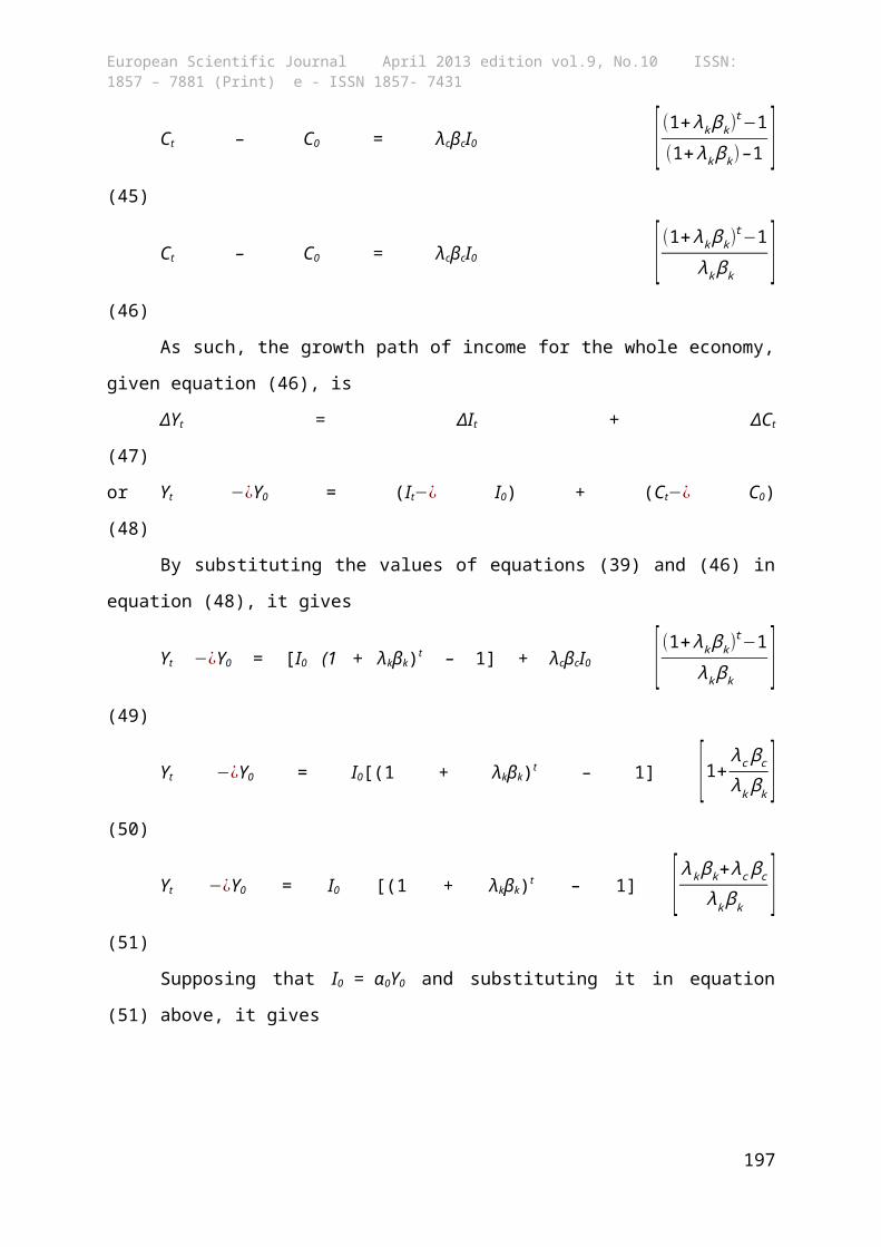
Ct – C0 = λcβcI0 [ (1+λkβk)t−1

(1+λkβk)–1 ](45)

Ct – C0 = λcβcI0 [ (1+λkβk)t−1

λkβk ](46)

As such, the growth path of income for the whole economy,

given equation (46), is

ΔYt = ΔIt + ΔCt

(47)

or Yt −¿Y0 = (It−¿ I0) + (Ct−¿ C0)

(48)

By substituting the values of equations (39) and (46) in

equation (48), it gives

Yt −¿Y0 = [I0 (1 + λkβk)t – 1] + λcβcI0 [ (1+λkβk)t−1

λkβk ](49)

Yt −¿Y0 = I0[(1 + λkβk)t – 1] [1+λcβcλkβk ]

(50)

Yt −¿Y0 = I0 [(1 + λkβk)t – 1] [λkβk+λcβcλkβk ]

(51)

Supposing that I0 = α0Y0 and substituting it in equation

(51) above, it gives

197


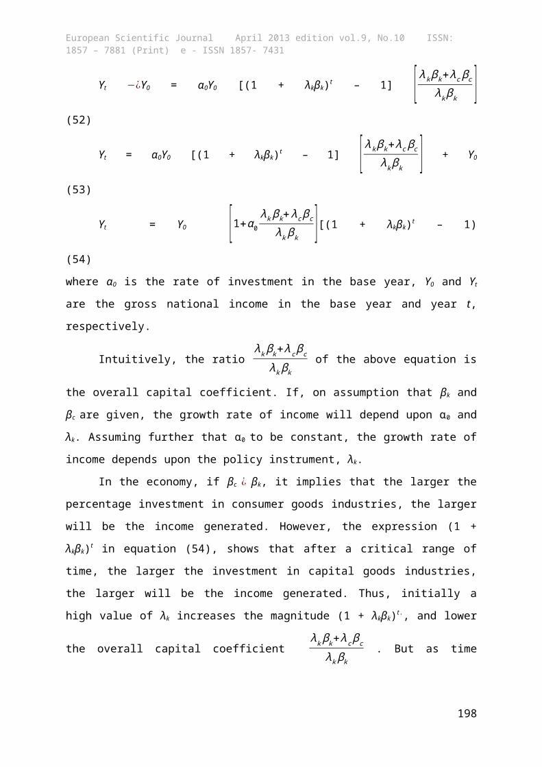
Yt −¿Y0 = α0Y0 [(1 + λkβk)t – 1] [λkβk+λcβcλkβk ]

(52)

Yt = α0Y0 [(1 + λkβk)t – 1] [λkβk+λcβcλkβk ] + Y0

(53)

Yt = Y0 [1+α0λkβk+λcβc

λkβk ][(1 + λkβk)t – 1)

(54)

where α0 is the rate of investment in the base year, Y0 and Yt

are the gross national income in the base year and year t,

respectively.

Intuitively, the ratio λkβk+λcβc

λkβk of the above equation is

the overall capital coefficient. If, on assumption that βk and

βc are given, the growth rate of income will depend upon α0 and

λk. Assuming further that α0 to be constant, the growth rate of

income depends upon the policy instrument, λk.

In the economy, if βc ¿ βk, it implies that the larger the

percentage investment in consumer goods industries, the larger

will be the income generated. However, the expression (1 +

λkβk)t in equation (54), shows that after a critical range of

time, the larger the investment in capital goods industries,

the larger will be the income generated. Thus, initially a

high value of λk increases the magnitude (1 + λkβk)t., and lower

the overall capital coefficient λkβk+λcβc

λkβk . But as time

198


passes, a higher value of λk would lead to higher growth rate

of income in the long run.

On the other hand, if βc = βk, then the reciprocal of the

overall capital coefficient, that is, λkβk

λkβk+λcβc = λk equals

marginal rate of saving. By extension, the important policy

implication of the model is that for a higher rate of

investment (λk), the marginal rate of saving must also be

higher. Thus, a higher rate of investment on capital goods in

the short run would make available a smaller volume of output

for consumption. But in the long run, it would lead to a

higher growth rate of consumption. See Jones (1975).

The Leontief Input-Output ModelThe input-output model or technique is used to analyze

inter-industry relationship in order to understand the

interdependencies and complexities of the economy and thus the

conditions for maintaining equilibrium between supply and

demand. According to Ghatak (1995), the technique usually

delineates the general equilibrium analysis and the empirical

side of the economic system of production of any country. It

is also known as “inter-industry analysis.”

As a finest variant of general equilibrium analysis,

Jhingan (2004) enumerates three main features of input-output

analysis to be: concentration on an economy which is in

equilibrium as it is not applicable to partial equilibrium

analysis; it does not concern itself with the demand analysis

as it deals exclusively with technical problems of production;

and it is based on empirical investigation. The assumptions

upon which the technique operates, according to Ghatak (1995),

199


are that no substitution takes place between the inputs to

produce a given unit of output and the input coefficient are constant –the linear input functions imply that the marginal input

coefficients are equal to the average; joint products are

ruled out, that is, each industry produces only on commodity

and each commodity is produced by only one industry; and

external economies are ruled out and production is subject to

the operation of constant returns to scale.

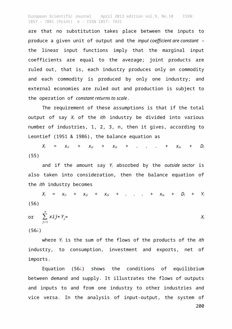
The requirement of these assumptions is that if the total

output of say Xi of the ith industry be divided into various

number of industries, 1, 2, 3, n, then it gives, according to

Leontief (1951 & 1986), the balance equation as

Xi = xi1 + xi2 + xi3 + . . . + xin + Di

(55)

and if the amount say Yi absorbed by the outside sector is

also taken into consideration, then the balance equation of

the ith industry becomes

Xi = xi1 + xi2 + xi3 + . . . + xin + Di + Yi

(56)

or ∑j=1

nxij+Yi= Xi

(56¿)

where Yi is the sum of the flows of the products of the ith

industry, to consumption, investment and exports, net of

imports.

Equation (56¿) shows the conditions of equilibrium

between demand and supply. It illustrates the flows of outputs

and inputs to and from one industry to other industries and

vice versa. In the analysis of input-output, the system of200


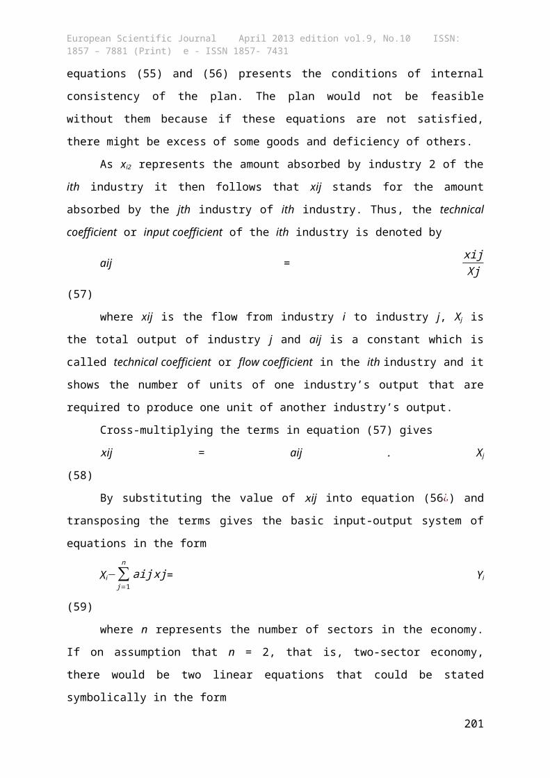
equations (55) and (56) presents the conditions of internal

consistency of the plan. The plan would not be feasible

without them because if these equations are not satisfied,

there might be excess of some goods and deficiency of others.

As xi2 represents the amount absorbed by industry 2 of the

ith industry it then follows that xij stands for the amount

absorbed by the jth industry of ith industry. Thus, the technical

coefficient or input coefficient of the ith industry is denoted by

aij = xijXj(57)

where xij is the flow from industry i to industry j, Xj is

the total output of industry j and aij is a constant which is

called technical coefficient or flow coefficient in the ith industry and it

shows the number of units of one industry’s output that are

required to produce one unit of another industry’s output.

Cross-multiplying the terms in equation (57) gives

xij = aij . Xj

(58)

By substituting the value of xij into equation (56¿) and

transposing the terms gives the basic input-output system of

equations in the form

Xi−∑j=1

naijxj= Yi

(59)

where n represents the number of sectors in the economy.

If on assumption that n = 2, that is, two-sector economy,

there would be two linear equations that could be stated

symbolically in the form

201


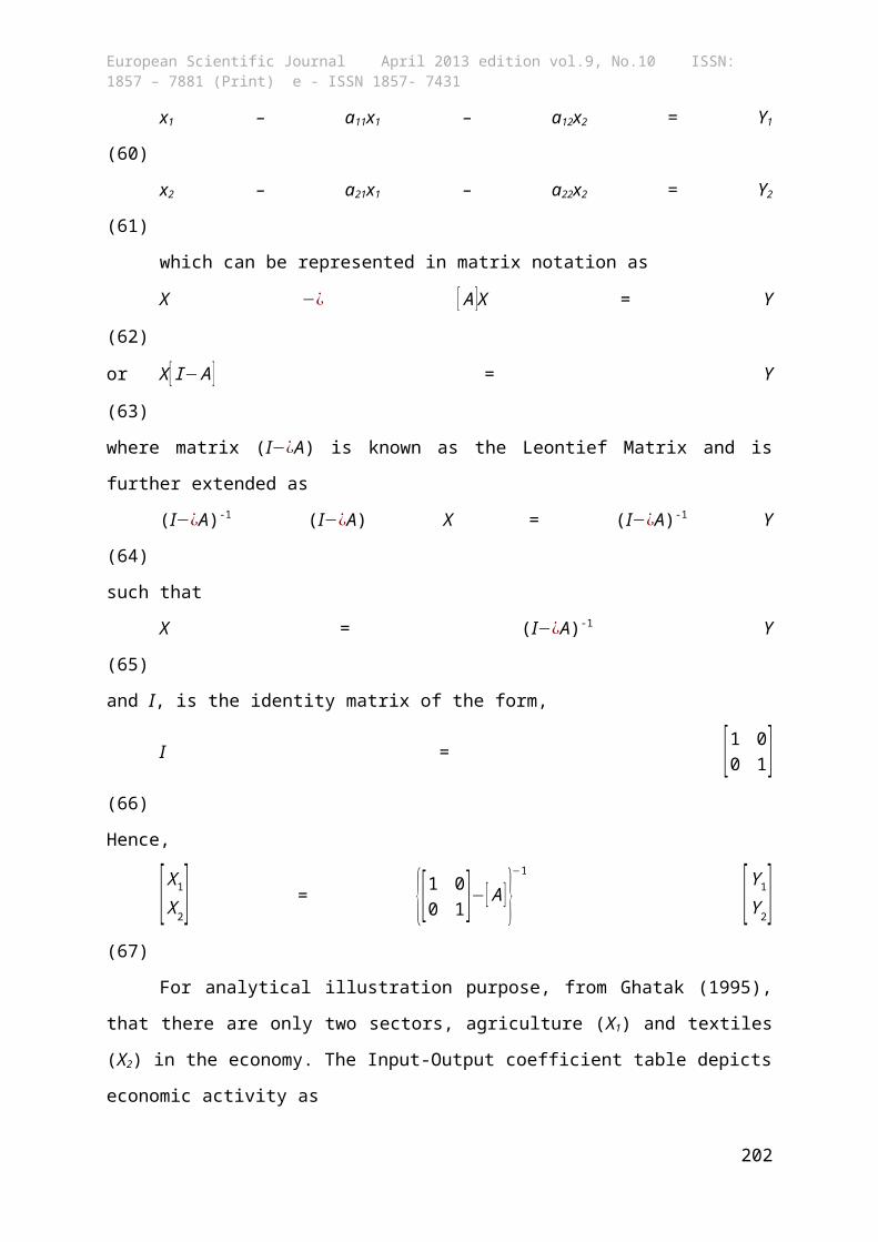
x1 – a11x1 – a12x2 = Y1

(60)

x2 – a21x1 – a22x2 = Y2

(61)

which can be represented in matrix notation as

X −¿ [A ]X = Y

(62)

or X[I−A ] = Y

(63)

where matrix (I−¿A) is known as the Leontief Matrix and is

further extended as

(I−¿A)-1 (I−¿A) X = (I−¿A)-1 Y

(64)

such that

X = (I−¿A)-1 Y

(65)

and I, is the identity matrix of the form,

I = [1 00 1]

(66)

Hence,

[X1

X2] = {[1 00 1]−[A ]}

−1

[Y1

Y2](67)

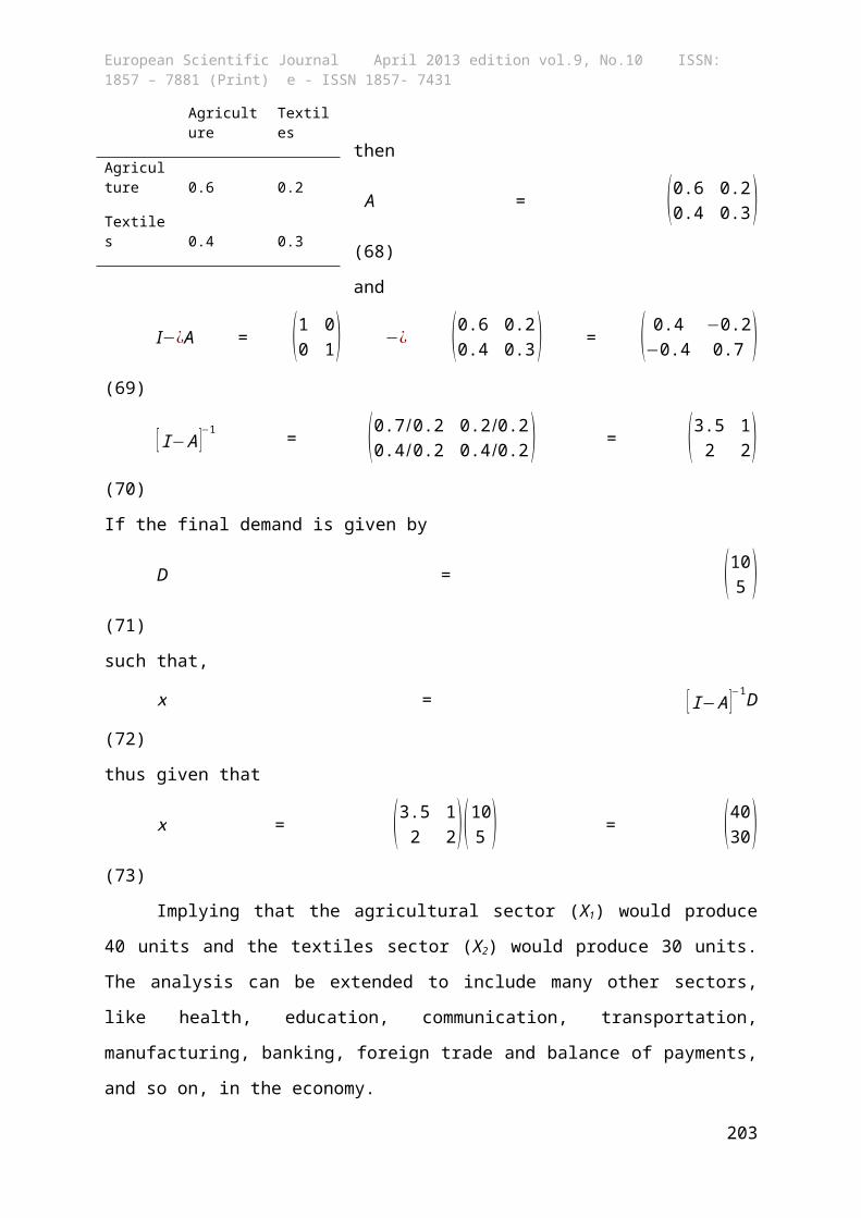
For analytical illustration purpose, from Ghatak (1995),

that there are only two sectors, agriculture (X1) and textiles

(X2) in the economy. The Input-Output coefficient table depicts

economic activity as

202


then

A = (0.6 0.20.4 0.3)

(68)

and

I−¿A = (1 00 1) −¿ (0.6 0.2

0.4 0.3) = ( 0.4 −0.2−0.4 0.7 )

(69)

[I−A ]−1 = (0.7/0.2 0.2/0.20.4/0.2 0.4/0.2) = (3.5 1

2 2)(70)

If the final demand is given by

D = (105 )(71)

such that,

x = [I−A ]−1D

(72)

thus given that

x = (3.5 12 2)(105 ) = (4030)

(73)

Implying that the agricultural sector (X1) would produce

40 units and the textiles sector (X2) would produce 30 units.

The analysis can be extended to include many other sectors,

like health, education, communication, transportation,

manufacturing, banking, foreign trade and balance of payments,

and so on, in the economy.

203

Agriculture

Textiles

Agriculture 0.6 0.2

Textiles 0.4 0.3


The above presentation, however, is an open static model

of Input-Output analysis. But in reality, most economic

variables are dynamic in nature as cause and effect, and

action and reaction do not occur immediately after one and

other: it takes some time for certain economic activities to

happen as a result of some causes or actions. Thus, according

to Sandee (1988), the analysis becomes dynamic when it is

closed by the linking of the investment part of the final bill

of goods to output. The dynamic input-output model extends the

concept of inter-sectoral balancing at a given point of time

to that of inter-sectoral balancing over time.

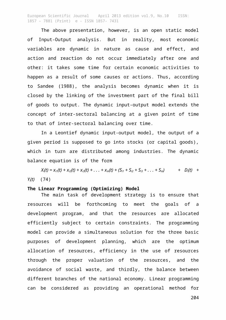
In a Leontief dynamic input-output model, the output of a

given period is supposed to go into stocks (or capital goods),

which in turn are distributed among industries. The dynamic

balance equation is of the form

Xi(t) = xi1(t) + xi2(t) + xi3(t) + . . . + xin(t) + (Si1 + Si2 + Si3 + . . . + Sin) + Di(t) +

Yi(t) (74)

The Linear Programming (Optimizing) ModelThe main task of development strategy is to ensure that

resources will be forthcoming to meet the goals of a

development program, and that the resources are allocated

efficiently subject to certain constraints. The programming

model can provide a simultaneous solution for the three basic

purposes of development planning, which are the optimum

allocation of resources, efficiency in the use of resources

through the proper valuation of the resources, and the

avoidance of social waste, and thirdly, the balance between

different branches of the national economy. Linear programming

can be considered as providing an operational method for

204


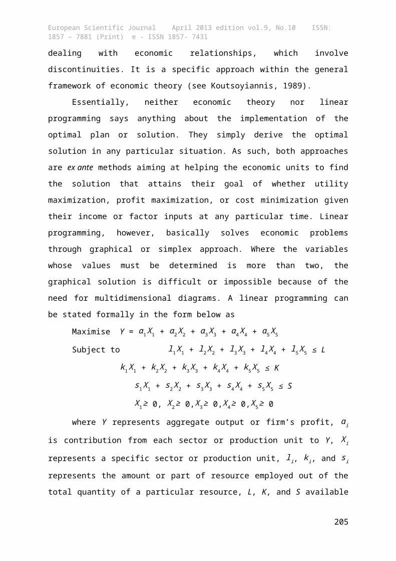
dealing with economic relationships, which involve

discontinuities. It is a specific approach within the general

framework of economic theory (see Koutsoyiannis, 1989).

Essentially, neither economic theory nor linear

programming says anything about the implementation of the

optimal plan or solution. They simply derive the optimal

solution in any particular situation. As such, both approaches

are ex ante methods aiming at helping the economic units to find

the solution that attains their goal of whether utility

maximization, profit maximization, or cost minimization given

their income or factor inputs at any particular time. Linear

programming, however, basically solves economic problems

through graphical or simplex approach. Where the variables

whose values must be determined is more than two, the

graphical solution is difficult or impossible because of the

need for multidimensional diagrams. A linear programming can

be stated formally in the form below as

Maximise Y = α1X1 + α2X2 + α3X3 + α4X4 + α5X5

Subject to l1X1 + l2X2 + l3X3 + l4X4 + l5X5 ≤ L

k1X1 + k2X2 + k3X3 + k4X4 + k5X5 ≤ K

s1X1 + s2X2 + s3X3 + s4X4 + s5X5 ≤ S

X1≥ 0, X2≥ 0,X3≥ 0,X4≥ 0,X5≥ 0

where Y represents aggregate output or firm’s profit, αi

is contribution from each sector or production unit to Y, Xi

represents a specific sector or production unit, li, ki, and si

represents the amount or part of resource employed out of the

total quantity of a particular resource, L, K, and S available

205


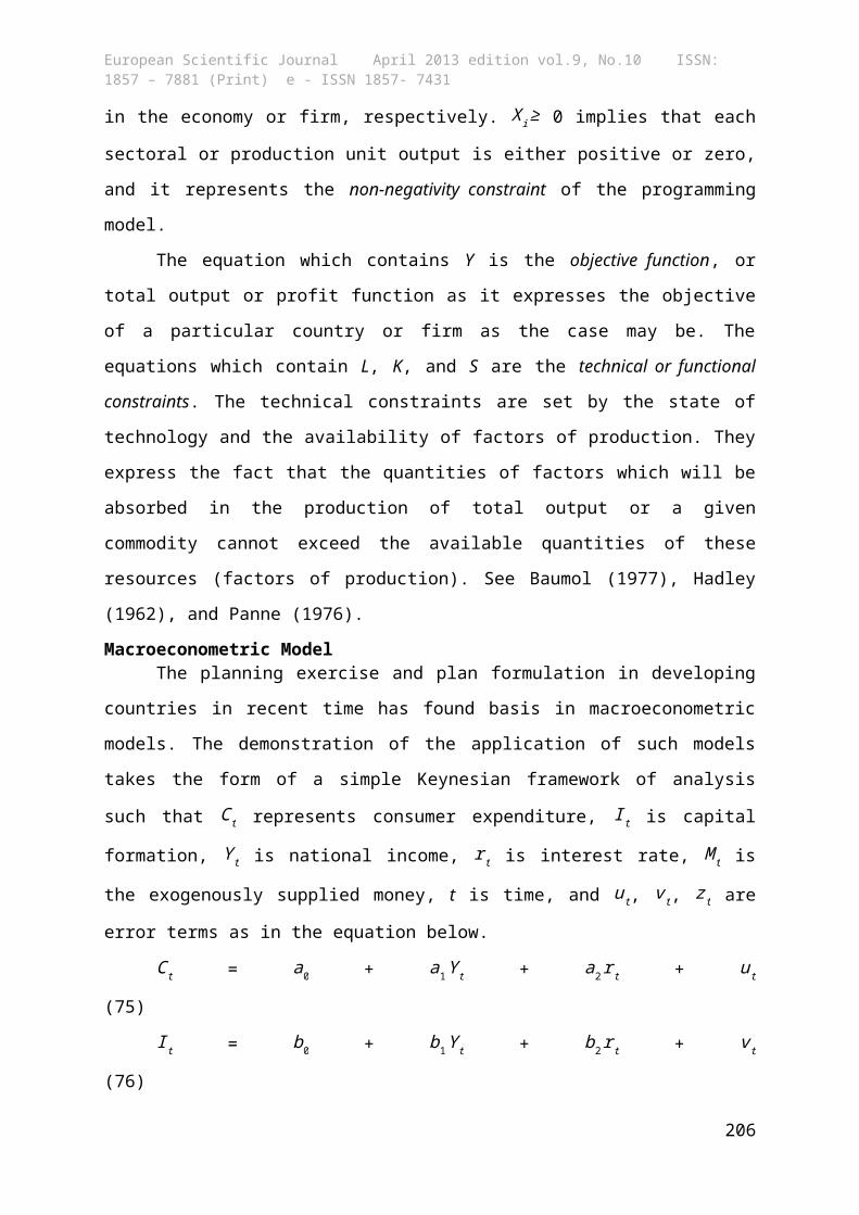
in the economy or firm, respectively. Xi≥ 0 implies that each

sectoral or production unit output is either positive or zero,

and it represents the non-negativity constraint of the programming

model.

The equation which contains Y is the objective function, or

total output or profit function as it expresses the objective

of a particular country or firm as the case may be. The

equations which contain L, K, and S are the technical or functional

constraints. The technical constraints are set by the state of

technology and the availability of factors of production. They

express the fact that the quantities of factors which will be

absorbed in the production of total output or a given

commodity cannot exceed the available quantities of these

resources (factors of production). See Baumol (1977), Hadley

(1962), and Panne (1976).

Macroeconometric ModelThe planning exercise and plan formulation in developing

countries in recent time has found basis in macroeconometric

models. The demonstration of the application of such models

takes the form of a simple Keynesian framework of analysis

such that Ct represents consumer expenditure, It is capital

formation, Yt is national income, rt is interest rate, Mt is

the exogenously supplied money, t is time, and ut, vt, zt are

error terms as in the equation below.

Ct = a0 + a1Yt + a2rt + ut

(75)

It = b0 + b1Yt + b2rt + vt

(76)

206


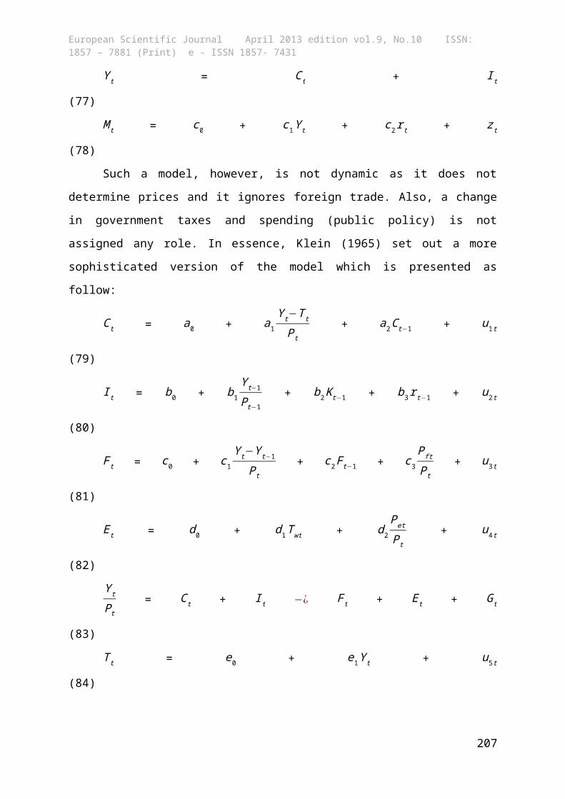
Yt = Ct + It

(77)

Mt = c0 + c1Yt + c2rt + zt

(78)

Such a model, however, is not dynamic as it does not

determine prices and it ignores foreign trade. Also, a change

in government taxes and spending (public policy) is not

assigned any role. In essence, Klein (1965) set out a more

sophisticated version of the model which is presented as

follow:

Ct = a0 + a1

Yt−Tt

Pt + a2Ct−1 + u1t

(79)

It = b0 + b1

Yt−1

Pt−1 + b2Kt−1 + b3rt−1 + u2t

(80)

Ft = c0 + c1

Yt−Yt−1

Pt + c2Ft−1 + c3

Pft

Pt + u3t

(81)

Et = d0 + d1Twt + d2

Pet

Pt + u4t

(82)

Yt

Pt = Ct + It −¿ Ft + Et + Gt

(83)

Tt = e0 + e1Yt + u5t

(84)

207


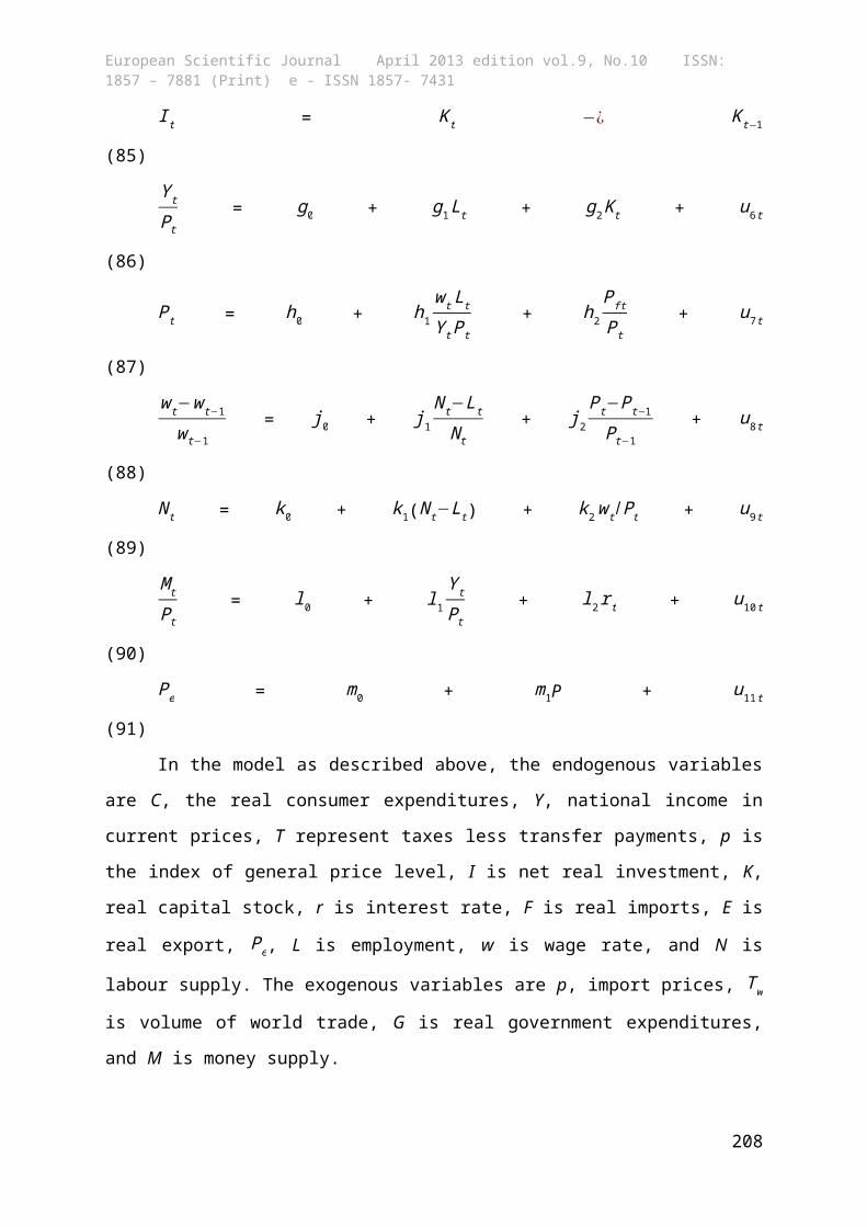
It = Kt −¿ Kt−1

(85)

Yt

Pt = g0 + g1Lt + g2Kt + u6t

(86)

Pt = h0 + h1

wtLtYtPt

+ h2

Pft

Pt + u7t

(87)

wt−wt−1

wt−1 = j0 + j1

Nt−Lt

Nt + j2

Pt−Pt−1

Pt−1 + u8t

(88)

Nt = k0 + k1(Nt−Lt) + k2wt/Pt + u9t

(89)

MtPt = l0 + l1

Yt

Pt + l2rt + u10t

(90)

Pe = m0 + m1P + u11t

(91)

In the model as described above, the endogenous variables

are C, the real consumer expenditures, Y, national income in

current prices, T represent taxes less transfer payments, p is

the index of general price level, I is net real investment, K,

real capital stock, r is interest rate, F is real imports, E is

real export, Pe, L is employment, w is wage rate, and N is

labour supply. The exogenous variables are p, import prices, Tw

is volume of world trade, G is real government expenditures,

and M is money supply.

208


Practically, however, the planner will have to determine

different types of the mentioned variables to render such a

model applicable to the special problems of LDCs. The actual

econometric techniques to be used will now depend upon initial

specifications of the equations and the subjective judgement

of the planner in the light of the actual state of

information. See Agarwala (1970), Chenery et al (1971), Ghosh

(1968), and Ghosh et al (1974).

Empirical DiscussionThe Harrod-Domar model has been applied as a basis to

develop more comprehensive plans for some less developed

countries. In its First Five Year Plan (1950-1 to 1955-6),

India employed the Harrod-Domar model to formulate her

national plan. The strategy of the plan was to rehabilitate

the Indian economy which had been hit hard by the Second World

War and the Partition. Thus, the emphasis was to create the

necessary economic and social overheads like power, transport,

public health, education and to develop agriculture in order

to build a solid foundation for industrialisation in the

subsequent plans. The Harrod-Domar model, however, failed as

the implementation informed the private sector control of the

development of local industries and minerals resulting in

about six percent public expenditure on them.

The Mahalanobis model which was adopted in India’s Second

Five Year Plan (1955-6 to 1960-1) as four sectors strategy has

shown that the value that was chosen for λk yielded

inefficient resource allocation as it lay within the

feasibility locus between an increase in employment and a rise

in output. In other words, reallocation of investment among209


the three sectors apart from the capital goods sector would

have resulted in higher output and employment. Also, the

model’s supposition that the supply of agricultural produce is

infinitely elastic is untenable as supply of agricultural

produce has failed to meet the increased demand for food and

raw materials ever since the beginning of the planning period.

The problem of capital accumulation that Fel’dman and

Mahalanobis models encountered has neither been solved

satisfactorily even by the Brahmananda and Vakil (1956) model

as the abundant labor alone is not enough to achieve a higher

level of capital accumulation. Thus, it is true that the

problem of employment creation in labor-surplus countries can

hardly be exaggerated, and such a problem has not really been

solved in the Mahalanobis model. Komiya (1959) also shows that

the value which Mahalanobis chose for λK yielded inefficient

resource allocation as it lay within the feasibility locus

between an increase in employment and a rise in output.

The input-output model of Leontief was adopted in the

Netherlands in 1948 through 1960, as well as in some other

developed and less developed countries. The theory basically

centers on the ratios between inputs and output, otherwise

called input coefficients. The model’s analysis of the

Netherlands case involves 35 sectors constituting the

industrial sectors, 7 primary sectors, and 6 final sectors.

Using the central input-output prediction experiment, the

prediction of the intermediate demand given final demand for

the predicted year and applying the input coefficients for the

base year as they are expressed in current value: The analysis

210


reveals that only 27 out of the 35 industries are considered

covering, on the average, 95 per cent of aggregate

intermediate demand. The prediction, according to Tilanus

(1989) is seen to defeat final demand blowup. However, the

superiority of input-output vanishes if the national accounts

data used for the blowup procedure are two or more years more

recent than the input-output table.

ConclusionThe use of an aggregate approach like the Harrod-Domar

model provides simplicity and clarity in its application.

Also, the model is complete in the sense that it covers the

entire economy as it is selective and fairly realistic.

Moreover, the model does not suffer from any internal

inconsistencies. However, such models is highly aggregated and

does not provide any idea about the internal relationships and

interdependencies between different sectors in the economy.

More importantly, the adoption of capital-output ratio is

constrained by the difficulty in estimating capital in LDCs

with the difference in regional capital-output ratios among

regions or states in one hand, and difference in the capital-

output ratios between the regions and the central government

on the other hand. Thus, it fails to provide any idea about

the consistency between different sectors. Even yet, the

disaggregation of the Harrod-Domar model into the Two-sector

model is not sufficient for development planning for LDCs as

experienced by Kenya.

In the linear programming model, prices are regarded as

the indicators of the marginal worth to the society. However,

in the LDCs, where the market is mostly imperfect, price will

211


usually be higher than the marginal cost. Also, the

relationships in the optimizing model are assumed to be linear

while many constraints in the LDCs are nonlinear functions of

the structural variables.

Availability of reliable data is always the bain of the

econometric model and such model also suffers from the

difficulties involved in misplaced aggregation and

illegitimate isolation. Thus, given the need for analyzing

many important sectors of the economy and their

interrelationships, with sectoral interdependence, to provide

greater consistency between aggregate supply and aggregate

demand, development planners have increasingly turned their

attention to the application of the input-output model.

References:

Agarwala, R. (1970). An Econometric Model of India: 1948-1961.

London: Frank, Cass

Baumol, W.J. (1977). Economic Theory and Operations Analysis.

4th Edition, London: Prentice Hall

Brahmananda, P.R. and C.N. Vakil (1956). Planning for an

Expanding Economy. Bombay: Vora

Domar, Evsey (1946). “Capital Expansion, Rate of Growth, and

Employment”, Econometrica, Vol. 14, pp. 137-47.

Fel’dman, G.A. (1928). On the Theory of National Income

Growth. The Planned Economy, (GOSPLAN)

Ghatak, S. (1995). Introduction to Development Economics.

Third edition. Routledge, London and New York.

212


Ghosh, A. (1968). Planning, Programming and Input-Output

Analysis. Cambridge: Cambridge University Press

Ghosh, A., D. Chakravarty, H. Sarkar (1974). Development

Planning in South-East Asia. Rotterdam: Rotterdam University

Press

Hadley, G. (1962). Linear Programming. Reading: Addison-Wesley

Harrod, R. (1939). “An Essay in Dynamic Theory”, Economic

Journal 49, pp.14-33.

Jhingan, M.L. (2005). The Economics of Development Planning.

New Delhi: Vrinda Publications Ltd.

Kaldor, N. (1960). Essays on Stability and Growth. Economic

Journal. Pp. 258-300.

Klein, L. (1965). ‘What kind of macro-econometric model for

developing economies.’ Indian Economic Journal 13 (3): 313-24.

Komiya, R. (1959). ‘A note on Professor Mahalanobis’ model of

Indian Economic Planning. Review of Economics and Statistics’ 41: 29-35

Kooros, S.K. and L.M. Badeaux (2007). Economic Development

Planning Models: A Comparative Assessment. International Research

Journal of Finance and Economics. pp. 120-139.

Kooros, Syrous K. and Bruce L. McManis (1998). “A Multi-

Attribute Optimization Model for Strategic Investment

Decision.” Canadian Journal of Administrative Sciences.

Koutsoyiannis, A. (1989). Modern Microeconomics. Second

Edition. ELBS Macmillan.

Leontief, W.W. (1951). The Structure of the American Economy

1919-39. 2nd edition, New York: Oxford University Press.

Leontief, W.W. (1986). Input-Output Economics. Oxford

University Press, New York.

213


Mahalanobis, P.C. (1953). “Some Observations on the Process of

Growth of National Income.” Sankhya (Indian Journal of Statistics). 14:

307-12.

Mahalanobis, P.C. (1955). The Approach of Operational Research

to Planning in India. Sankhya (The India Journal of Statistics). 16: 3-

13D.

Panne, van de C. (1976). Linear Programming and Related

Techniques. 2nd Edition, Amsterdam: North-Holland

Sandee, J. (1988). A Demonstration Planning Model for India

Sen, A. (1985). Commodities and Capabilities. North Holland:

Amsterdam

Sen, A. (1999). Development as Freedom. New York: Alfred Knopf

Streeten, Paul (1966). ‘Use and Abuse of Planning Models’, in

K. Martin and J. Knapp (eds) Teaching of Development Economics.

London: Frank Cass

Thirwal, A.P. (1983). Growth & Development with special

reference to Developing Economies. Third Edition. The

Macmillan Press

Tilanus, (1989).

Todaro, M. P. and S. C. Smith (2011). Economic Development.

Eleventh Edition, Addison-Wesley. Pearson.

Todaro, M. P. and S. C. Smith (2003). Economic Development.

Eighth Edition, Pearson.

214


215

Documents

Planning Ex