September 7, 2015

[ELECTROMAGNETIC FIELD THEORY - PHY321 - ASH. SEPT. 2015 RUH]

Page 1 of 20

Department of Physics - Al Imam Mohammed Ibn Saud Islamic University - KSA

PHY 321

ELECTROMAGNETIC FIELD THEORY

PART ONE

Compiled by

Prof. Dr. Ali S. Hennache

RUH- KSA , Sept. 2015

September 7, 2015

[ELECTROMAGNETIC FIELD THEORY - PHY321 - ASH. SEPT. 2015 RUH]

Page 2 of 20

Vector Analysis

1.1 Scalars and Vectors

There are many physical quantities in nature, and we can divide them up into two categories. The quantity is either a vector or a scalar. These two categories can be distinguished from one another by their distinct definitions:

Vectors are quantities that are fully described by both a magnitude ( numerical value) in a specific direction, and is used in mathematics, physics, and engineering. Vectors in physics are drawn as arrows. An arrow has both a magnitude (how long it is) and a direction (the direction in which it points). The starting point of a vector is known as the tail and the end point is known as the head . Vector can be added to other vectors according to vector algebra. The direction of a vector in one-dimensional motion is given simply by a plus (+) or minus (−) sign. A vector is frequently represented by a line segment with a definite direction, or graphically as an arrow, connecting an initial point A with a terminal point B, as shown in .

Scalars are quantities that are fully described by a magnitude (numerical

value) but no direction is needed.

Scientists refer to the two values as direction and magnitude(size).

Vector representation

A line of given length and pointing along a given direction, such as an arrow, is the typical representation of a vector. Typical notation to designate a vector is a boldfaced character, a character with and arrow on it, or a character with a line

under it (i.e., ). The magnitude of a vector is its length and is

normally denoted by or A.

September 7, 2015

[ELECTROMAGNETIC FIELD THEORY - PHY321 - ASH. SEPT. 2015 RUH]

Page 3 of 20

Examples of vector and scalar quantities:

o mass has only a value, no direction

o electric charge has only a value, no direction

o force has a value and a direction. You push or pull something with some strength (magnitude) in a particular direction o weight has a value and a direction. Your weight is proportional to your

mass (magnitude) and is always in the direction towards the centre of the earth.

Exercise 1:

Classify the following as vectors or scalars

1. length scalar 2. force vector 3. direction scalar 4. height scalar 5. time scalar 6. speed vector 7. temperature scalar 8. 12 km scalar 9. 1 m south vector 10. 2 m·s−1, 45° vector 11. 075°, 2 cm vector 12. 100 km·h−1, 0° vector

September 7, 2015

[ELECTROMAGNETIC FIELD THEORY - PHY321 - ASH. SEPT. 2015 RUH]

Page 4 of 20

1.2 Operations on vectors

We can define a number of operations on vectors geometrically without reference to any coordinate system. Here we define addition, subtraction , and multiplication (two different ways to multiply two vectors together: the dot product and the cross product ) by a scalar.

1.2.1 Addition of vectors

Given two vectors A and B, we form their sum A+B, as follows: We translate the vector B until its tail coincides with the head of A. (Recall such translation does not change a vector.) Then, the directed line segment from the tail of A to the head of B is the vector A+B.

Addition of vectors satisfies two important properties.

1. The commutative law which states the order of addition doesn't matter: A+B = C B+A = C The head-to-tail rule yields vector C for both A+B and B+A

This law is also called the parallelogram law, as illustrated in the below image. Two of the edges of the parallelogram define a+b, and the other pair of edges define B+A. But, both sums are equal to the same diagonal of the parallelogram.

September 7, 2015

[ELECTROMAGNETIC FIELD THEORY - PHY321 - ASH. SEPT. 2015 RUH]

Page 5 of 20

If you start from point P you end up at the same spot no matter which

displacement (A or B) you take first.

2. The associative law

The above diagram shows the result of adding (A+ B) + D = C + D. The result is the vector with length and direction the same as the diagonal of the figure. The bottom diagram shows the result of adding A + (B + D) = C +D. The result is the same . This is a demonstration of the associative property of vector addition:

which states that the sum of three vectors does not depend on which pair of vectors is added first:

A + (B + D) = (A+ B) + D

September 7, 2015

[ELECTROMAGNETIC FIELD THEORY - PHY321 - ASH. SEPT. 2015 RUH]

Page 6 of 20

The rule works in all dimensions. Mostly the geometric vectors of computer graphics are two dimensional and three dimensional (although, in general, higher dimensions are possible). The associative property means that sums of several vectors can be written like A + B + D without parentheses. 1.2.1.1 Representing points with column matrices

Points can be represented with column matrices. To do this, you first need to decide on a coordinate frame (sometimes called just frame. A coordinate frame consists of a distinguished point P0 (called the origin) and an axis for each dimension (often called X and Y). In 2D space there are two axes; in 3D space there are three axes (often called X, Y, and z).

Virtual world Virtual world with Virtual world with coordinate frame a different coordinate frame

- The left diagram shows a (rather simple) virtual world in 2D space. The points and vectors exist in the space independent of any coordinate frame. - The next diagram shows the same virtual world, this time with a coordinate frame consisting of a particular point P0 and two axes. In this coordinate frame, the point A is represented by the column matrix (2, 2). - The right diagram shows the same virtual world, but with a different coordinate frame. In the second coordinate frame, the point A is represented by the column matrix (2, 3) 1.2.1.2 Vector Addition represented by Column Matrix Addition

September 7, 2015

[ELECTROMAGNETIC FIELD THEORY - PHY321 - ASH. SEPT. 2015 RUH]

Page 7 of 20

If vectors are represented with column matrices, then vector addition is represented by addition of column matrices. For example:

A = ( 3, 2 ) B = ( -2, 1 )

A + B = C = ( 1, 3 ) The diagram shows the head-to-tail rule used to add A and B to get C. Adding the column matrices A and B yields the column matrix C. This matrix is the correct representation of the vector C.

1.2.1.3 Commutative law (different order, but same answer)

To draw the diagram follow the rules with b as the starting vector: 1- Draw the first vector b as an arrow with its tail at the origin. 2- Draw the second vector a as an arrow with its tail at the point of the first. 3- The sum is the arrow from the origin to the tip of the second vector. Since vector addition is commutative, the result must be the same.

September 7, 2015

[ELECTROMAGNETIC FIELD THEORY - PHY321 - ASH. SEPT. 2015 RUH]

Page 8 of 20

Example The vector operations we defined in the vector introduction are easy to express in terms of these coordinates. If a=(a1,a2) and b=(b1,b2), their sum is simply a+b=(a1+b1,a2+b2), as illustrated in the below figure. It is also easy to see that b−a=(b1−a1,b2−a2) and λa=(λa1,λa2) for any scalar λ.

1.2.2 Subtraction of vectors

Before we define subtraction, we define the vector −a, which is the opposite of a. The vector −a is the vector with the same magnitude as a but that is pointed in the opposite direction.

We define subtraction as addition with the opposite of a vector:

b−a = b+(−a)

September 7, 2015

[ELECTROMAGNETIC FIELD THEORY - PHY321 - ASH. SEPT. 2015 RUH]

Page 9 of 20

This is equivalent to turning vector a around in the applying the above rules for addition. Can you see how the vector x in the below figure is equal to b−a? Notice how this is the same as stating that a+x=b, just like with subtraction of scalar numbers.

1.2.3 Scalar multiplication

Given a vector a and a real number (scalar) λ, we can form the vector λa as

follows.

If λ is positive, then λa is the vector whose direction is the same as the direction

of a and whose length is λ times the length of a. In this case, multiplication

by λ simply stretches (if λ>1) or compresses (if 0<λ<1) the vector a.

If, on the other hand, λ is negative, then we have to take the opposite

of a before stretching or compressing it. In other words, the vector λa points in

the opposite direction of a, and the length of λa is |λ| times the length of a. No

matter the sign of λ, we observe that the magnitude of λa is |λ| times the

magnitude of a: ∥λa∥=|λ|∥a∥.

Scalar multiplications satisfies many of the same properties as the usual

multiplication.

1. s(a+b)= sa+sb (distributive law, form 1)

2. (s+t)a=sa+ta (distributive law, form 2)

3. 1a=a

4. (−1)a=−a

5. 0a=0

In the last formula, the zero on the left is the number 0, while the zero on the right is the vector 0, which is the unique vector whose length is zero.

September 7, 2015

[ELECTROMAGNETIC FIELD THEORY - PHY321 - ASH. SEPT. 2015 RUH]

Page 10 of 20

If a=λb for some scalar λ, then we say that the vectors a and b are parallel. If λ is negative, some people say that a and b are anti-parallel, but we will not use that language. We were able to describe vectors, vector addition, vector subtraction, and scalar multiplication without reference to any coordinate system. The advantage of such purely geometric reasoning is that our results hold generally, independent of any coordinate system in which the vectors live. However, sometimes it is useful to express vectors in terms of coordinates, such as cartesian , cylindrical or spherical coordinates).

1.2.4 The dot product

The dot product between two vectors is based on the projection of one vector onto another. Let's imagine we have two vectors a and b, and we want to calculate how much of a is pointing in the same direction as the vector b. We want a quantity that would be positive if the two vectors are pointing in similar directions, zero if they are perpendicular, and negative if the two vectors are pointing in nearly opposite directions. We will define the dot product between the vectors to capture these quantities. But first, notice that the question “how much of a is pointing in the same direction as the vector b” does not have anything to do with the magnitude (or length) of b; it is based only on its direction. (Recall that a vector has a magnitude and a direction.) The answer to this question should not depend on the magnitude of b, only its direction. To sidestep any confusion caused by the magnitude of b, let's scale the vector so that it has length one. In other words, let's replace b with the unit vector that points in the same direction as b. We'll call this vector u, which is defined by

u=b∥b∥

The dot product of a with unit vector u, denoted a⋅u, is defined to be the projection of a in the direction of u, or the amount that a is pointing in the same direction as unit vector u. Let's assume for a moment that a and u are pointing in

similar directions. Then, you can imagine a⋅u as the length of the shadow of a onto u if their tails were together and the sun was shining from a direction perpendicular to u. By forming a right triangle with a and this shadow, you can use geometry to calculate that

a⋅u= ∥a∥cosθ (1)

where θ is the angle between a and u.

September 7, 2015

[ELECTROMAGNETIC FIELD THEORY - PHY321 - ASH. SEPT. 2015 RUH]

Page 11 of 20

If a and u were perpendicular, there would be no shadow. That corresponds to

the case when cosθ =cosπ/2=0 and a⋅u=0. If the angle θ between a and u were larger than π/2, then the shadow wouldn't hit u. Since in this case cosθ<0, the

dot product a⋅u is also negative. You could think of −a⋅u (which is positive in this case) as being the length of the shadow of a on the vector −u, which points in the opposite direction of u.

But we need to get back to the dot product a⋅b, where b may have a magnitude different than one. This dot product a⋅b should depend on the magnitude of both

vectors, ∥a∥ and ∥b∥, and be symmetric in those vectors. Hence, we don't want to define a⋅b to be exactly the projection of a on b; we want it to reduce to this projection for the case when b is a unit vector. We can accomplish this very

easily: just plug the definition u=b∥b∥ into our dot product definition of equation (1). This leads to the definition that the dot product a⋅b, divided by the

magnitude ∥b∥ of b, is the projection of a onto b. a⋅b∥b∥=∥a∥cosθ.

Then, if we multiply by through by ∥b∥, we get a nice symmetric definition for the

dot product a⋅b.

a⋅b=∥a∥∥b∥cosθ. (2)

The picture of the geometric interpretation of a⋅b is almost identical to the above

picture for a⋅u. We just have to remember that we have to divide through

by ∥b∥ to get the projection of a onto b.

September 7, 2015

[ELECTROMAGNETIC FIELD THEORY - PHY321 - ASH. SEPT. 2015 RUH]

Page 12 of 20

In the following interactive applet, you can explore this geometric interpretation of the dot product, and observe how it depends on the vectors and the angle

between them. (The reported number shouldn't depend on the length of ∥b∥ since we divided by that magnitude.) The dot product as projection. The dot product of the vectors a (in blue) and b (in green), when divided by the magnitude of b, is the projection of a onto b. This projection is illustrated by the red line segment from the tail of b to the projection of the head of a on b. You can change the vectors a and b by dragging the points at their ends or dragging the vectors themselves. Notice how the dot product is positive for acute angles and negative for obtuse angles. The reported number

does not depend on ∥b∥ only because we've divided through by that magnitude.

1.2.5 The cross product

There are two ways to take the product of a pair of vectors. One of these methods of multiplication is the cross product, which is the subject of this part. The other multiplication is the dot product, which we discuss on latter

The cross product is defined only for three-dimensional vectors. If a and b are two three-dimensional vectors, then their cross product, written as a×b and pronounced “a cross b,” is another three-dimensional vector. We define this cross product vector a×b by the following three requirements: 1. a×b is a vector that is perpendicular to both a and b.

2. The magnitude (or length) of the vector a×b, written as ∥a×b∥, is the area of the parallelogram spanned by a and b (i.e. the parallelogram whose adjacent sides are the vectors a and b, as shown in below figure).

3. The direction of a×b is determined by the right-hand rule. (This means that if we curl the fingers of the right hand from a to b, then the thumb points in the direction of a×b.)

September 7, 2015

[ELECTROMAGNETIC FIELD THEORY - PHY321 - ASH. SEPT. 2015 RUH]

Page 13 of 20

The below figure illustrates how, using trigonometry, we can calculate that the area of the parallelogram spanned by a and b is

∥a∥ ∥b∥sinθ,

where θ is the angle between a and b. The figure shows the parallelogram as

having a base of length ∥b∥ and perpendicular height ∥a∥sinθ.

This formula shows that the magnitude of the cross product is largest when a and b are perpendicular. On the other hand, if a and b are parallel or if either vector is the zero vector, then the cross product is the zero vector. (It is a good thing that we get the zero vector in these cases so that the above definition still makes sense. If the vectors are parallel or one vector is the zero vector, then there is not a unique line perpendicular to both a and b. But since there is only one vector of zero length, the definition still uniquely determines the cross product.)

1.3 Components of vectors

Some physical quantities cannot be added in the simple way described for scalars.

September 7, 2015

[ELECTROMAGNETIC FIELD THEORY - PHY321 - ASH. SEPT. 2015 RUH]

Page 14 of 20

For example, if you were to walk 4 m in a northerly direction and then 3 m in an easterly direction, how far would you be from your starting point? The answer is clearly NOT 7 m! To find the answer, one could draw a scale diagram (1 cm = 1 m) such as is shown below:

One could also calculate the distance from the starting point using the theorem of Pythagoras, i.e.

It is also useful to know in which direction one has moved from the starting

point. This can also be measured from the diagram or calculated from simple

trigonometry:

1.4 Algebraic Properties of Vectors

Commutative (vector) A + B = B + A Associative (vector) (A+B) + C = a + (B +C) Additive identity There is a vector 0 such that (A+ 0) = A = (0 + A)

for all A Additive inverse For any A there is a vector -A such that A + (-A) = 0 Distributive (vector) r(A + B) = rA + rB Distributive (scalar) (r + s) A = rA + sA

September 7, 2015

[ELECTROMAGNETIC FIELD THEORY - PHY321 - ASH. SEPT. 2015 RUH]

Page 15 of 20

Associative (scalar) r(sA) = (rs)A Multiplicative identity For the real number 1, 1A= A for each A

1.5 Coordinate systems in space and transformation

1.5.1 Introduction

An orthogonal systems is one in which the coordinates are mutually perpendicular. A coordinate system consists of four basic elements: (1) Choice of origin (2) Choice of axes (3) Choice of positive direction for each axis (4) Choice of unit vectors for each axis A good understanding of coordinate systems can be very helpful in solving problems related to Maxwell’s Equations. The three most common coordinate systems are:

Rectangular (x, y, z),

Cylindrical (r, φ , z), and

Spherical ( r, θ , φ ).

1.5.2 Cartesian Coordinates ( x , y , z ) in Space

In Cartesian coordinates (or rectangular coordinates), a point P is referred to by three real numbers, indicating the positions of the perpendicular projections from the point to three fixed, perpendicular, graduated lines, called the axes. If the coordinates are denoted x, y, z, in that order, the axes are called the x-axis, y-axis and z-axis, and we write P=(x,y,z). Often the x-axis is imagined to be horizontal and pointing roughly toward the viewer (out of the page), the y-axis also horizontal and pointing more or less to the right, and the z-axis vertical, pointing up. The system is called right-handed if it can be rotated so the three axes are in this position. Figure below shows a right-handed system. The point x=0, y=0, z=0 is the origin, where the three axes intersect.

In rectangular coordinates a point P is specified by x, y, and z, where these values are all measured from the origin (see figure below). The ranges of the coordinate variables x, y and z are

September 7, 2015

[ELECTROMAGNETIC FIELD THEORY - PHY321 - ASH. SEPT. 2015 RUH]

Page 16 of 20

A vector A in Cartesian coordinates can be written as ( Ax, Ay, Az ) or Axax + Ayay + Azaz

In Cartesian coordinates, P=(4.2,3.4,2.2).

1.5.3 Circular cylindrical coordinates ( , , z ) in Space

To define cylindrical coordinates, we take an axis (usually called the z-axis) and a perpendicular plane, on which we choose a ray (the initial ray) originating at the intersection of the plane and the axis (the origin). The coordinates of a point P are: the polar coordinates (r, ) of the projection of P on the plane, and the coordinate z of the projection of P on the axis (figure below).

In cylindrical coordinates a point P is specified by r, φ , z, where φ is measured from the x axis (or x-z plane) (see figure below). The ranges of the variables are:

September 7, 2015

[ELECTROMAGNETIC FIELD THEORY - PHY321 - ASH. SEPT. 2015 RUH]

Page 17 of 20

Among the possible sets (r, ,z) of cylindrical coordinates for P are (10,30°,5) and (10,390°,5).

1.5.4 Spherical Coordinates in Space

To define spherical coordinates, we take an axis (the polar axis) and a perpendicular plane (the equatorial plane), on which we choose a ray (the initial ray) originating at the intersection of the plane and the axis (the origin O). The

coordinates of a point P are: the distance from P to the origin; the angle (zenith) between the line OP and the positive polar axis; and the angle (azimuth) between the initial ray and the projection of OP to the equatorial plane. See figure below. As in the case of polar and cylindrical coordinates, is only

defined up to multiples of 360°, and likewise . Usually is assigned a value

between 0 and 180°, but values of between 180° and 360° can also be used;

the triples ( , , ) and ( , 360°- , 180°+ ) represent the same point. Similarly,

one can extend to negative values; the triples ( , , ) and (- , 180°- , 180°+) represent the same point.

September 7, 2015

[ELECTROMAGNETIC FIELD THEORY - PHY321 - ASH. SEPT. 2015 RUH]

Page 18 of 20

A set of spherical coordinates for P is ( , , )=(10,60°,30°).

In spherical coordinates a point P is specified by r, θ , φ , where r is measured from the origin, θ is measured from the z axis, and φ is measured from the x axis (or x-z plane) (see figure at right). With z axis up, θ is sometimes called the zenith angle and φ the azimuth angle.

1.5.5 Relations between Cartesian, Cylindrical, and Spherical coordinates

Consider a Cartesian, a cylindrical, and a spherical coordinate system, related as shown in Figure below.

September 7, 2015

[ELECTROMAGNETIC FIELD THEORY - PHY321 - ASH. SEPT. 2015 RUH]

Page 19 of 20

Standard relations between Cartesian, cylindrical, and spherical coordinate systems.

The origin is the same for all three. The positive z-axes of the Cartesian and cylindrical systems coincide with the positive polar axis of the spherical system. The initial rays of the cylindrical and spherical systems coincide with the positive x-axis of the Cartesian system, and the rays =90° coincide with the positive y-axis.

Then the Cartesian coordinates (x,y,z), the cylindrical coordinates (r, ,z), and the

spherical coordinates ( , , ) of a point are related as follows:

Cartesian from cylindrical variable transformation and Cylindrical from

Cartesian variable transformation

September 7, 2015

[ELECTROMAGNETIC FIELD THEORY - PHY321 - ASH. SEPT. 2015 RUH]

Page 20 of 20

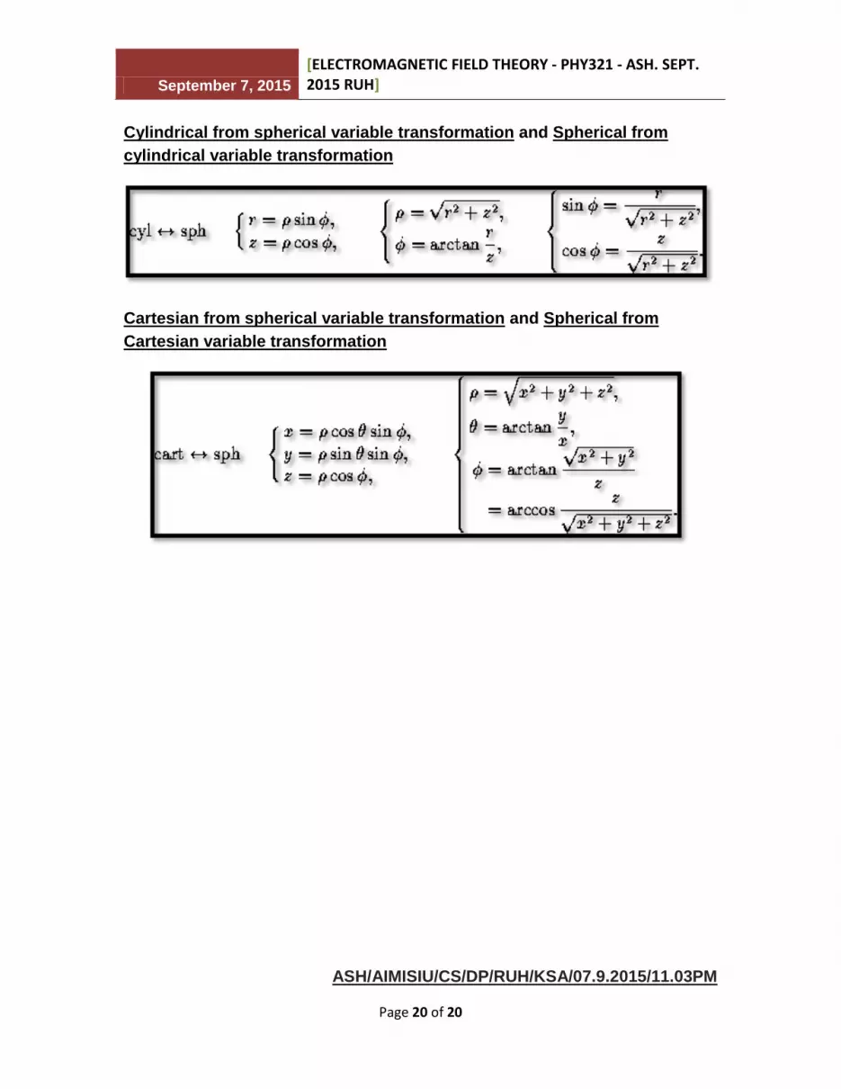
Cylindrical from spherical variable transformation and Spherical from

cylindrical variable transformation

Cartesian from spherical variable transformation and Spherical from

Cartesian variable transformation

ASH/AIMISIU/CS/DP/RUH/KSA/07.9.2015/11.03PM