Performance Enhancement for DigitalImplementations of Resonant Controllers

Alejandro G. Yepes, Francisco D. Freijedo, Pablo Fernandez-Comesana,Jano Malvar, Oscar Lopez and Jesus Doval-Gandoy

Department of Electronics Technology, University of Vigo,ETSEI, Campus Universitario de Vigo, 36200, Spain.

Email:agyepes,fdfrei,pablofercom,janomalvar,olopez,jdoval@uvigo.es

Abstract—Resonant control is one of the highest performancealternatives for ac current/voltage control. The implementationsbased on two integrators are a widely employed choice in orderto provide frequency adaptation to these regulators withoutsubstantial computational burden. However, the discretizationof these schemes causes a significant error both in the reso-nant frequency and in the phase lead provided by the delaycompensation. Therefore, perfect tracking is not assured, andstability is compromised at high frequencies or low samplingperiods. This paper contributes solutions for both problemswithout adding a significant resource consumption. Furthermore,the previously proposed approaches for calculating the leadingangle are analyzed, and a novel expression with superior perfor-mance is contributed. Experimental results obtained by meansof a laboratory prototype corroborate the theoretical analysisand the improvement achieved by the proposed discrete-timeimplementations.

Index Terms—Current control, digital control, power condi-tioning, pulsewidth-modulated power converters.

I. INTRODUCTION

Resonant controllers are capable of tracking sinusoidal ref-erences of arbitrary frequencies of both positive and negativesequences with zero steady-state error. An important saving ofcomputational burden and complexity is obtained because oftheir lack of multiple Park transformations [1]–[8].

The implementations of resonant controllers based on twointerconnected integrators are a widely employed optionmainly due to its simplicity for frequency adaptation [7]–[13]. However, the discretization of these schemes leads toa displacement of the poles. This fact results in a deviation ofthe frequency at which the infinite gain is located with respectto the expected resonant frequency, so a significant error mayappear in steady-state [11].

On the other hand, with large values of resonant frequencyor sampling period, the computational delay affects the systemperformance and may cause instability. Therefore, a delaycompensation scheme, which introduces a phase lead to cancelthe plant delay (phase lag), should be implemented [6], [7],[9]–[11], [14]–[16]. It has been proved in [11] that the existingproposals to add delay compensation to the implementations

This work was supported by the Spanish Ministry of Science and In-novation and the European Commission (FEDER) under project numberDPI2009-07004.

based on two integrators do not provide the expected phaselead (its target value) when they are implemented in digitaldevices. Furthermore, it is proved in this paper that to assumea target leading angle of two samples is quite inaccurate withrespect to the actual delay caused by the plant. The phase errordue to these two facts is accumulated in the implementationsbased on two integrators, so the phase margins are reducedand anomalous peaks appear in the closed-loop frequencyresponse.

Alternative implementations based on two integrators areproposed in this paper, which provide a higher performanceby means of more accurate resonant peak locations anddelay compensation, while maintaining the advantage on lowcomputational burden and good frequency adaptation of theoriginal schemes. This is achieved by means of a correctionof poles (associated with the resonant frequency), a correctionof zeros (related to delay compensation) and a simple linearexpression for the target leading angle that achieves a moreaccurate approximation of the actual phase lag caused by theplant.

Finally, experimental results obtained with a single-phaseshunt active power filter (APF) validate the theoretical analysisand the improvement achieved by the proposed discrete-timeimplementations.

II. IMPLEMENTATIONS OF RESONANT CONTROLLERSBASED ON TWO INTEGRATORS

A Proportional+Resonant (PR) controller can be imple-mented as shown in Fig. 1a [8], where ω1 is the fundamentalfrequency and h is the harmonic order to be tracked. It is acommon practice to employ this scheme due to the simplicityit permits when frequency adaptation is required [7]–[13].

Lascu et al proposed in [17] an alternative resonant reg-ulator, known as vector PI (VPI) controller, which may beimplemented as shown in Fig. 1b [11]. This controller can-cels coupling terms produced when the plant has the form1/(sL f +R f ), by adjusting the integral gain as KIh = KPhR f /L f[7], [11], [16], [17].

Finally, the scheme depicted in Fig. 1c performs the delaycompensation in PR controllers [9], where φ∗h is the targetleading angle at the resonant frequency hω1. The actualleading angle value, that is, the actual phase difference at

978-1-4244-5287-3/10/$26.00 ©2010 IEEE 2535

s1

s1

++

+-

outputinput KIh

KPh

X2 21h ω

(a) PR controller.

s1

X

s1

2 21h ω

++

+-

outputinputKIh

KPh

(b) VPI controller.

++-

+-

X

*cos( )hφ

X

X

outputinput

*1 sin( )hhω φ

KIh

KPh

2 21h ω

s1

s1

(c) PR + delay compensation.

Figure 1. Block diagrams of continuous resonant controllers based on two integrators.

frequencies close to hω1 with respect to a simple PR controller,is defined as φh. In the s-domain, φh = φ∗h.

It is also possible to add a delay compensation technique toVPI controllers, but at least three integrators would be requiredfor its implementation.

III. CORRECTION OF RESONANT POLES LOCATION

The direct and feedback integrators of Fig. 1a are usuallydiscretized with Forward and Backward Euler, respectively[11], [12], [18]. Other existing possibilities for discretizingboth integrators do not lead to better results [11]. Applying thisapproach to the three schemes of Fig. 1, the same denominatoris obtained for their equivalent transfer functions:

1−2z−1(1−h2ω

21T 2

s /2)+ z−2, (1)

with Ts = 1/ fs being the sampling period.On the other hand, an accurate resonant frequency would

be obtained by placing the poles at e− jhω1Ts and e jhω1Ts [11],which leads to a denominator of the form

1−2z−1 cos(hω1Ts)+ z−2. (2)

The denominator (1) differs from (2) in the fact that theterm cos(hω1Ts) appears as a second order Taylor series ap-proximation. Therefore, (1) provides infinite gain at a resonantfrequency different from the expected (hω1), so a significanterror may appear in steady-state when current references aretracked in closed-loop [11].

The on-line calculation of explicit cosine functions in (2)requires larger resources [11]. An alternative approach isproposed in the following. The second order Taylor series in(1) may be corrected to a higher order k if the input signalh2ω2

1 of Fig. 1 schemes [ω1 is estimated with, e.g., a phase-locked loop (PLL)] is corrected as

h2ω

21→ 2

k/2

∑n=1

(−1)n+1h2nω2n1 T 2n−2

s

(2n)!

=

k=4︷ ︸︸ ︷h2

ω21−h4 ω4

1T 2s

12+h6 ω6

1T 4s

360︸ ︷︷ ︸k=6

+...

(3)

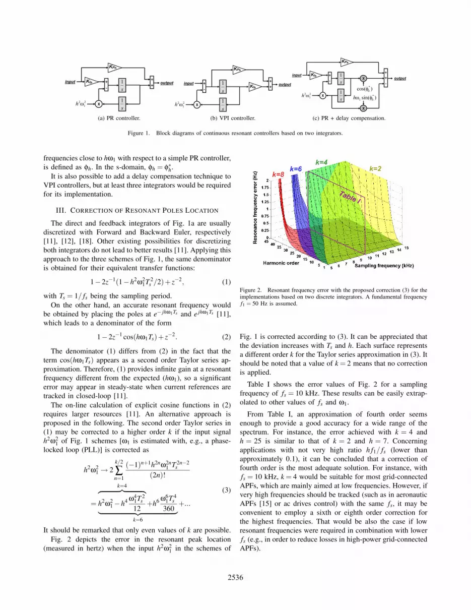
It should be remarked that only even values of k are possible.Fig. 2 depicts the error in the resonant peak location

(measured in hertz) when the input h2ω21 in the schemes of

Figure 2. Resonant frequency error with the proposed correction (3) for theimplementations based on two discrete integrators. A fundamental frequencyf1 = 50 Hz is assumed.

Fig. 1 is corrected according to (3). It can be appreciated thatthe deviation increases with Ts and h. Each surface representsa different order k for the Taylor series approximation in (3). Itshould be noted that a value of k = 2 means that no correctionis applied.

Table I shows the error values of Fig. 2 for a samplingfrequency of fs = 10 kHz. These results can be easily extrap-olated to other values of fs and ω1.

From Table I, an approximation of fourth order seemsenough to provide a good accuracy for a wide range of thespectrum. For instance, the error achieved with k = 4 andh = 25 is similar to that of k = 2 and h = 7. Concerningapplications with not very high ratio h f1/ fs (lower thanapproximately 0.1), it can be concluded that a correction offourth order is the most adequate solution. For instance, withfs = 10 kHz, k = 4 would be suitable for most grid-connectedAPFs, which are mainly aimed at low frequencies. However, ifvery high frequencies should be tracked (such as in aeronauticAPFs [15] or ac drives control) with the same fs, it may beconvenient to employ a sixth or eighth order correction forthe highest frequencies. That would be also the case if lowresonant frequencies were required in combination with lowerfs (e.g., in order to reduce losses in high-power grid-connectedAPFs).

2536

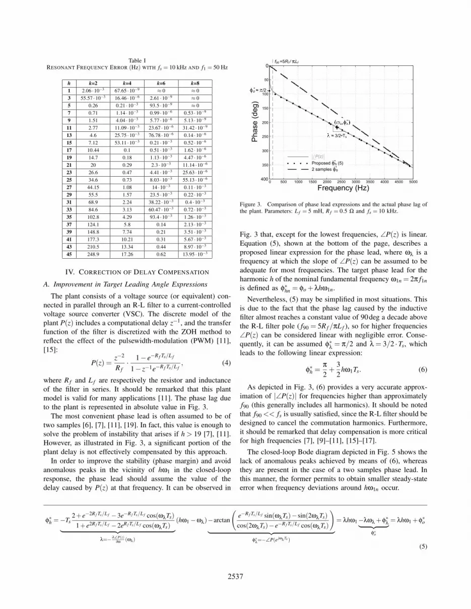
Table IRESONANT FREQUENCY ERROR (Hz) WITH fs = 10 kHz AND f1 = 50 Hz

h k=2 k=4 k=6 k=81 2.06 ·10−3 67.65 ·10−9 ≈ 0 ≈ 03 55.57 ·10−3 16.46 ·10−6 2.61 ·10−9 ≈ 05 0.26 0.21 ·10−3 93.5 ·10−9 ≈ 07 0.71 1.14 ·10−3 0.99 ·10−6 0.53 ·10−9

9 1.51 4.04 ·10−3 5.77 ·10−6 5.13 ·10−9

11 2.77 11.09 ·10−3 23.67 ·10−6 31.42 ·10−9

13 4.6 25.75 ·10−3 76.78 ·10−6 0.14 ·10−6

15 7.12 53.11 ·10−3 0.21 ·10−3 0.52 ·10−6

17 10.44 0.1 0.51 ·10−3 1.62 ·10−6

19 14.7 0.18 1.13 ·10−3 4.47 ·10−6

21 20 0.29 2.3 ·10−3 11.14 ·10−6

23 26.6 0.47 4.41 ·10−3 25.63 ·10−6

25 34.6 0.73 8.03 ·10−3 55.13 ·10−6

27 44.15 1.08 14 ·10−3 0.11 ·10−3

29 55.5 1.57 23.5 ·10−3 0.22 ·10−3

31 68.9 2.24 38.22 ·10−3 0.4 ·10−3

33 84.6 3.13 60.47 ·10−3 0.72 ·10−3

35 102.8 4.29 93.4 ·10−3 1.26 ·10−3

37 124.1 5.8 0.14 2.13 ·10−3

39 148.8 7.74 0.21 3.51 ·10−3

41 177.3 10.21 0.31 5.67 ·10−3

43 210.5 13.34 0.44 8.97 ·10−3

45 248.9 17.26 0.62 13.95 ·10−3

IV. CORRECTION OF DELAY COMPENSATION

A. Improvement in Target Leading Angle Expressions

The plant consists of a voltage source (or equivalent) con-nected in parallel through an R-L filter to a current-controlledvoltage source converter (VSC). The discrete model of theplant P(z) includes a computational delay z−1, and the transferfunction of the filter is discretized with the ZOH method toreflect the effect of the pulsewidth-modulation (PWM) [11],[15]:

P(z) =z−2

R f· 1− e−R f Ts/L f

1− z−1e−R f Ts/L f, (4)

where R f and L f are respectively the resistor and inductanceof the filter in series. It should be remarked that this plantmodel is valid for many applications [11]. The phase lag dueto the plant is represented in absolute value in Fig. 3.

The most convenient phase lead is often assumed to be oftwo samples [6], [7], [11], [19]. In fact, this value is enough tosolve the problem of instability that arises if h > 19 [7], [11].However, as illustrated in Fig. 3, a significant portion of theplant delay is not effectively compensated by this approach.

In order to improve the stability (phase margin) and avoidanomalous peaks in the vicinity of hω1 in the closed-loopresponse, the phase lead should assume the value of thedelay caused by P(z) at that frequency. It can be observed in

0 500 1000 1500 2000 2500 3000 3500 4000 4500 5000400

350

300

250

200

150

100

50

0

Frequency (Hz)

Phase (deg)

Proposed h (5)

2 samples h

P(z)

f90 =5Rf / Lf

*

*

≈ 3/2•Ts

o ≈ /2*

*

Figure 3. Comparison of phase lead expressions and the actual phase lag ofthe plant. Parameters: L f = 5 mH, R f = 0.5 Ω and fs = 10 kHz.

Fig. 3 that, except for the lowest frequencies, ∠P(z) is linear.Equation (5), shown at the bottom of the page, describes aproposed linear expression for the phase lead, where ωλ is afrequency at which the slope of ∠P(z) can be assumed to beadequate for most frequencies. The target phase lead for theharmonic h of the nominal fundamental frequency ω1n = 2π f1nis defined as φ∗hn = φo +λhω1n.

Nevertheless, (5) may be simplified in most situations. Thisis due to the fact that the phase lag caused by the inductivefilter almost reaches a constant value of 90deg a decade abovethe R-L filter pole ( f90 = 5R f /πL f ), so for higher frequencies∠P(z) can be considered linear with negligible error. Conse-quently, it can be assumed φ∗

λ= π/2 and λ = 3/2 ·Ts, which

leads to the following linear expression:

φ∗h =

π

2+

32

hω1Ts. (6)

As depicted in Fig. 3, (6) provides a very accurate approx-imation of |∠P(z)| for frequencies higher than approximatelyf90 (this generally includes all harmonics). It should be notedthat f90 << fs is usually satisfied, since the R-L filter should bedesigned to cancel the commutation harmonics. Furthermore,it should be remarked that delay compensation is more criticalfor high frequencies [7], [9]–[11], [15]–[17].

The closed-loop Bode diagram depicted in Fig. 5 shows thelack of anomalous peaks achieved by means of (6), whereasthey are present in the case of a two samples phase lead. Inthis manner, the former permits to obtain smaller steady-stateerror when frequency deviations around hω1n occur.

φ∗h =−Ts

2+ e−2R f Ts/L f −3e−R f Ts/L f cos(ωλTs)1+ e2R f Ts/L f −2eR f Ts/L f cos(ωλTs)︸ ︷︷ ︸

λ=− ∂∠P(z)∂ω

(ωλ)

(hω1−ωλ)−arctan

(e−R f Ts/L f sin(ωλTs)− sin(2ωλTs)cos(2ωλTs)− e−R f Ts/L f cos(ωλTs)

)︸ ︷︷ ︸

φ∗λ=−∠P(e jω

λTs )

= λhω1−λωλ +φ∗λ︸ ︷︷ ︸

φ∗o

= λhω1 +φ∗o

(5)

2537

11

sT

z−−

+

+

+

+

-

X

outputinput 1

11

sT z

z

−

−−

KPh*cos( )h

φ

X

X

*

1 sin( )h

hω φ

KIh

2

1ω+

+

4 2

1

12

sTω

h2

h4

(a) Before optimizing the delay compensation.

PREPRE--CALCULATED CONSTANTSCALCULATED CONSTANTS

11

sT

z−−

+

-

+

+

+

-

X

1∆ω

X outputinput 1

11

sT z

z

−

−−

KPh

-1

sT

+

-

ah

bh

ch

dh

+

+

2

1ω

+

+

4 2

1

12

sTω

h2

h4

*

*

*

*

(b) With optimized delay compensation.

Figure 4. Proposed discrete-time implementations of PR controllers including delay compensation.

0

0.5

1

1.5

2

2.5

3

1000 1200 1400 1600 1800 2000 2200-180

-135

-90

-45

0

45

90135180

Ph

as

e (

de

g)

Frequency (Hz)

Ma

gn

itu

de

(a

bs

)

Proposed h (5)

2 samples h

*

*

Figure 5. Closed-loop Bode diagrams using PR controllers with phaselead of two samples and according to (6), for h ∈ 21,23,25, ...,45.Notethe avoidance of closed-loop anomalous peaks provided by the proposedleading angle. Parameters: L f = 5 mH, R f = 0.5 Ω, fs = 10 kHz, KPT = 15and KIh = 2000 ∀h.

B. Correction of Phase Lead Provided by Schemes Based onTwo Integrators

The original delay compensation schemes fail to providethe expected phase lead in the z-domain (the actual φh doesnot coincide with its target φ∗h) [11]. An accurate phase leadφh = φ∗h in PR controllers can be achieved by moving the zerosas

GcdPRh

(z) = KPh +KIhz−1 cos(hω1Ts +φ∗h)− z−2 cos(φ∗h)

1−2z−1 cos(hω1Ts)+ z−2 . (7)

In fact, the proposals of Yuan et al in [6] for delay com-pensation are particular cases of (7). Fig. 1c can be modifiedto satisfy (7) by changing one of the inputs, hω1 sin(φ∗h), asdepicted in Fig. 4a.

C. Frequency Adaptation of Delay Compensation

The variation of the input frequency is less critical forthe delay compensation than for the resonant peak locations.Applying first order Taylor approximations, the block diagramof Fig. 4a leads to the scheme shown in Fig. 4b, where∆ω1 = ω1−ω1n.

Fig. 6 illustrates the difference between the actual andthe expected phase lead provided by the block diagram ofFig. 4b when φ∗hn is calculated according to (6). Two casesare considered: with and without frequency adaptation of theφ∗h for each resonant controller. In the latter, input ∆ω1 of

Fig. 4b is fixed to zero. The different curves correspond toodd harmonic orders up to h = 45. It can be appreciated inFig. 6a that if only small deviations from nominal frequencyare expected (such as in most grid-connected converters), noadaptation of the delay compensation is necessary, so theFig. 4b scheme can be simplified (ah and ch are not needed).However, for greater frequency fluctuations, it is recommendedto recalculate the leading phase accordingly (complete Fig.4b block diagram, i.e., input ∆ω1 6= 0), so that stability isimproved as shown in Fig. 6b.

V. EXPERIMENTAL RESULTS

The experimental setup is shown in Fig. 7, and Table II givesthe values of its main parameters. An APF application has beenchosen because it is very suitable for proving the controllersperformance when tracking different and variable frequencies,and results can be extrapolated to other applications [11].

From Fig. 7, the APF is a VSC made with four insulatedgate bipolar transistor (IGBTs), and connected to the point ofcommon coupling (PCC) through the interfacing inductanceL f . After measuring the influence of frequency on L f and itsequivalent series resistance R f with an inductance analyzer, ithas been concluded that it can be neglected. A programmableload (Hocherl & Hackl ZSAC426) and a programmable acsource (Chroma 61501) are connected in parallel to the APF.The control is implemented in a prototyping platform (dSpaceDS1104), which includes a Power PC MPC8240 (PPC) and aTexas Instruments TMS320F240 DSP. The most critical blockshave been implemented by S-Functions written in C language,as done in [11], [17].

The harmonic detection block in Fig. 7 identifies the har-monic currents iLh of the load current iL by detection andsubtraction of its fundamental component iL1 . The referencefundamental current i∗f1 to maintain Vdc is obtained by meansof a proportional+integral (PI) controller and the in-phasesignal θ1 from a PLL. The total current reference for the APFis calculated as iLh + i∗f1 . The PLL also estimates ω1 in orderto adapt the harmonic identification algorithm and the resonantcontrollers [11].

For this experiment, the load current is programmed as asquare wave (high harmonic content) with rise and fall timesof 39 µs, which leads to the spectrum shown in Fig. 8.

Fig. 9 shows the results obtained when the proposed cor-rection (3) is employed with different orders k for resonant

2538

0 10 20 30 40 50 60 70 80 90 100-70

-60

-50

-40

-30

-20

-10

0

10

20

30

Fundamental frequency (Hz)

Phase lead error (deg)

h

fh=45

h=43

h=41

0 10 20 30 40 50 60 70 80 90 100-250

-200

-150

-100

-50

0

50

100

150

200

Fundamental frequency (Hz)

Phase lead error (deg)

h

WITHOUT FREQUENCY ADAPTATION OF h WITH FREQUENCY ADAPTATION OF h

f

(a) Without frequency adaptation of φh (input ∆ω1 fixed tozero)

0 10 20 30 40 50 60 70 80 90 100-70

-60

-50

-40

-30

-20

-10

0

10

20

30

Fundamental frequency (Hz)

Phase lead error (deg)

h

fh=45

h=43

h=41

0 10 20 30 40 50 60 70 80 90 100-250

-200

-150

-100

-50

0

50

100

150

200

Fundamental frequency (Hz)

Phase lead error (deg)

h

WITHOUT FREQUENCY ADAPTATION OF h WITH FREQUENCY ADAPTATION OF h

f

(b) Including frequency adaptation of φh (input ∆ω1 6= 0)

Figure 6. Difference between the actual and the expected phase leadaccording to (6) provided by the block diagram proposed in Fig. 4b, forh ∈ 1,3,5, ...,45 and f1n = 50 Hz. Parameters: L f = 5 mH, R f = 0.5 Ω andfs = 10 kHz.

if1

VsrcPCCisrc

ifVSC

LfCV

dc

PWM

-

m

PLL

PI

+

+

Vdc

-

+

+if

if

iLh

HARMONIC

DETECTION

iL

iL

PPCPPC

603e603e

VPCC

Vdc

PROGRAMMABLE

AC LOAD

CURRENT

CONTROLLER

Lsrc

X

Rf

1ω

)θsin( 1ˆ

1ω

DSPDSP

dSPACEdSPACE DS1104DS1104

*

*

*

Figure 7. APF prototype circuit and control.

controllers tuned at odd harmonics up to h = 45.From Fig. 9, a great improvement is achieved by the

proposed correction (3) in terms of resonant frequency ac-curacy, providing much better harmonic cancellation than thatachieved by the original scheme (Figs. 9a and 9b). To increasek just from 2 to 4 permits to reduce the THD of isrc from

Table IIPOWER CIRCUIT VALUES

Parameter ValueV ∗dc 220 V

Vsrc (rms) 110 VC 3.3 mFL f 5 mHR f 0.5 Ω

Lsrc 50 µHfsw = fs 10 kHz

Figure 8. Spectrum of programmed load current iL. Scale: 10 dB/div and250 Hz/div. THD= 42.3%.

Table IIICURRENT CONTROL EXECUTION TIMES

k Time (µs)2 25.84 29.86 32.18 34.7

26.26% to 9.04%. From Figs. 9c and 9d, a correction of fourthorder is enough for frequencies up to approximately 1300 Hz;whereas k = 6 is more suitable for higher frequencies, asshown in Figs. 9e and 9f. On the other hand, k = 8 does notachieve a noticeable improvement over k = 6, as it can beappreciated in Figs. 9g and 9h. Moreover, Fig. 9 proves theeffectiveness of proposed expression (6) and Fig. 4b schemein assuring stability even for very high frequencies.

The average execution times of the current control withdifferent values of k are shown in Table III. The computation ofthe ω1 powers is also taken into account. Bearing in mind thatthere are 23 resonant controllers involved, it can be appreciatedthat the calculation time increase with small variations of kis not significant (specially if it is compared with the greatimprovement achieved regarding steady-state error). In anycase, it seems recommendable to employ k = 4 except for veryhigh h f1/ fs values, so almost perfect tracking is achieved andthe computational burden that would be required by higher(and not necessary) values of k is avoided.

The proposed implementation is also tested in presence ofa very demanding frequency transient: f1 ramp from 25 Hz to90 Hz in 800 ms. Obviously, so great deviations from nominalfrequency are not usual in grid-connected converters, and so

2539

(a) Steady-state currents with k = 2, i.e., proposedcorrection (3) not applied).

(b) Spectrum of isrc in Fig. 9a. THD= 26.16%.

(c) Steady-state currents with k = 4. (d) Spectrum of isrc in Fig. 9c. THD= 9.04%.

(e) Steady-state currents with k = 6. (f) Spectrum of isrc in Fig. 9e. THD= 5.67%.

(g) Steady-state currents with k = 8. (h) Spectrum of isrc in Fig. 9g. THD= 5.56%.

Figure 9. Steady state currents and spectra of source current isrc for different values of k, with f1 = f1n = 50 Hz. Ch2 is i f , Ch3 is isrc and Ch4 is iL. Scale:10 dB/div and 250 Hz/div in spectra; 1 A/div and 5 ms/div in current waveforms.

2540

many resonant controllers are usually not required either. Themain reason to test resonant controllers tuned at such highfrequencies and so large frequency variations is to serve asan useful test for applications in which both requirementsare common, such as aeronautic APFs, ac drives control ortorque ripple minimization in high speed permanent magnetdrives [11]. The objective is to confirm that, in those cases,the proposed Fig. 4b scheme and (6) avoid stability problemswith resonant controllers tuned at high frequencies and largefrequency variations.

Fig. 10a shows the response of the controller to the fre-quency transient. It can be observed that Fig. 4b proposedscheme and (6) provide stable operation within a very widerange of frequencies. Figs. 10b and 10c show the steady-state currents obtained with f1 = 25 Hz and f1 = 90 Hz( f1n = 50 Hz in both cases), respectively. In order to assurea good tracking of all frequencies, k = 8 has been chosen.It can be appreciated that at these frequencies the resonantcontrollers are also able to achieve a very high rejection ofthe harmonic components.

VI. CONCLUSIONS

In this work, novel implementations of resonant controllersare contributed. These proposals are proved to provide asignificant improvement over the previously existing schemesbased on two integrators in terms of accuracy in resonantfrequency (perfect tracking) and leading angle, while theirlow computational burden and good frequency adaptation aremaintained. Therefore, zero steady-state error and stabilityare assured even while tracking very high frequencies oremploying low sampling rates.

REFERENCES

[1] Y. Sato, T. Ishizuka, K. Nezu, and T. Kataoka, “A new control strategyfor voltage-type pwm rectifiers to realize zero steady-state control errorin input current,” IEEE Trans. Ind. Appl., vol. 34, no. 3, pp. 480 –486,may/jun 1998.

[2] D. N. Zmood, D. G. Holmes, and G. H. Bode, “Frequency-domainanalysis of three-phase linear current regulators,” IEEE Trans. Ind. Appl.,vol. 37, no. 2, pp. 601–610, Mar./Apr. 2001.

[3] Y.-S. Kwon, J.-H. Lee, S.-H. Moon, B.-K. Kwon, C.-H. Choi, and J.-K.Seok, “Standstill parameter identification of vector-controlled inductionmotors using the frequency characteristics of rotor bars,” IEEE Trans.Ind. Appl., vol. 45, no. 5, pp. 1610–1618, Sep./Oct. 2009.

[4] D. N. Zmood and D. G. Holmes, “Stationary frame current regulationof PWM inverters with zero steady-state error,” IEEE Trans. PowerElectron., vol. 18, no. 3, pp. 814–822, May 2003.

[5] P. Zhou, Y. He, and D. Sun, “Improved direct power control of a DFIG-based wind turbine during network unbalance,” IEEE Trans. PowerElectron., vol. 24, no. 11, pp. 2465–2474, Nov. 2009.

[6] X. Yuan, W. Merk, H. Stemmler, and J. Allmeling, “Stationary-framegeneralized integrators for current control ofactive power filters with zerosteady-state error for current harmonicsof concern under unbalanced anddistorted operating conditions,” IEEE Trans. Ind. Appl., vol. 38, no. 2,pp. 523–532, Mar./Apr. 2002.

[7] L. Limongi, R. Bojoi, G. Griva, and A. Tenconi, “Digital current-controlschemes,” IEEE Industrial Electronics Magazine, vol. 3, no. 1, pp. 20–31, Mar. 2009.

[8] S. Fukuda and T. Yoda, “A novel current-tracking method for activefilters based on asinusoidal internal model,” IEEE Trans. Ind. Appl.,vol. 37, no. 3, pp. 888–895, May/Jun. 2001.

(a) Response to f1 ramp from 25 Hz to 90 Hz in 800 ms, with f1n = 50 Hz.Time scale: 100 ms/div.

(b) Steady-state currents with f1 = 25 Hz andf1n = 50 Hz. Time scale: 10 ms/div.

(c) Steady-state currents with f1 = 90 Hz andf1n = 50 Hz. Time scale: 10 ms/div.

Figure 10. Test of frequency adaptation provided by Fig. 4b proposedscheme. Ch2 is f1, Ch3 is isrc and Ch4 is iL. Scale: 1 A/div in currentwaveforms and 50 Hz/div in f1.

[9] R. I. Bojoi, G. Griva, V. Bostan, M. Guerriero, F. Farina, and F. Pro-fumo, “Current control strategy for power conditioners using sinusoidalsignal integrators in synchronous reference frame,” IEEE Trans. PowerElectron., vol. 20, no. 6, pp. 1402–1412, Nov. 2005.

[10] R. Bojoi, L. Limongi, F. Profumo, D. Roiu, and A. Tenconi, “Analysisof current controllers for active power filters using selective harmoniccompensation schemes,” IEEJ Transactions on Electrical and ElectronicEngineering, vol. 4, no. 2, pp. 139–157, 2009.

2541

[11] A. G. Yepes, F. D. Freijedo, J. Doval-Gandoy, O. Lopez, J. Malvar,and P. Fernandez-Comesana, “Effects of discretization methods on theperformance of resonant controllers,” IEEE Trans. Power Electron.,vol. 25, no. 7, pp. 1692 –1712, july 2010.

[12] R. Teodorescu, F. Blaabjerg, U. Borup, and M. Liserre, “A new controlstructure for grid-connected LCL PV inverters with zero steady-state er-ror and selective harmonic compensation,” in Applied Power ElectronicsConference and Exposition, 2004. APEC ’04. Nineteenth Annual IEEE,vol. 1, 2004, pp. 580–586.

[13] R. Teodorescu, F. Blaabjerg, M. Liserre, and P. C. Loh, “Proportional-resonant controllers and filters for grid-connected voltage-source con-verters,” in Electric Power Applications, IEE Proceedings -, vol. 153,no. 5, Sep. 2006, pp. 750–762.

[14] D. G. Holmes, T. A. Lipo, B. McGrath, and W. Kong, “Optimizeddesign of stationary frame three phase ac current regulators,” IEEETrans. Power Electron., vol. 24, no. 11, pp. 2417–2426, Nov. 2009.

[15] R. P. Venturini, P. Mattavelli, P. Zanchetta, and M. Sumner, “Variablefrequency adaptive selective compensation for active power filters,” in4th IET Conference on Power Electronics, Machines and Drives, 2008.PEMD 2008., Apr. 2008, pp. 16–21.

[16] C. Lascu, L. Asiminoaei, I. Boldea, and F. Blaabjerg, “Frequencyresponse analysis of current controllers for selective harmonic compen-sation in active power filters,” IEEE Trans. Ind. Electron., vol. 56, no. 2,pp. 337–347, Feb. 2009.

[17] ——, “High performance current controller for selective harmoniccompensation in active power filters,” IEEE Trans. Power Electron.,vol. 22, no. 5, pp. 1826–1835, Sep. 2007.

[18] F. J. Rodriguez, E. Bueno, M. Aredes, L. G. B. Rolim, F. A. S. Neves,and M. C. Cavalcanti, “Discrete-time implementation of second ordergeneralized integrators for grid converters,” in Industrial Electronics,2008. IECON 2008. 34th Annual Conference of IEEE, Orlando, FL,Nov. 2008, pp. 176–181.

[19] D. Basic, V. S. Ramsden, and P. K. Muttik, “Harmonic filtering of high-power 12-pulse rectifier loads with aselective hybrid filter system,” IEEETrans. Ind. Electron., vol. 48, no. 6, pp. 1118–1127, Dec. 2001.

2542