Embed Size (px)
Citation preview
Three-term controller Ziegler-Nichols tuning rules Summary
Basics of Automation and Control I
Lecture 13: PID controllers
Paweł Malczyk
Division of Theory of Machines and RobotsInstitute of Aeronautics and Applied MechanicsFaculty of Power and Aeronautical Engineering
Warsaw University of Technology
© Paweł Malczyk. Basics of Automation and Control I Lecture 13: PID controllers 1 / 35
Three-term controller Ziegler-Nichols tuning rules Summary
Outline
1 Three-term controller
2 Ziegler-Nichols tuning rules
3 Summary
© Paweł Malczyk. Basics of Automation and Control I Lecture 13: PID controllers 2 / 35
Three-term controller Ziegler-Nichols tuning rules Summary
Three-term controller
1 Three-term controllerIntroductionBasic control functionsP controllerPI controllerPD controllerPID controller
2 Ziegler-Nichols tuning rules
3 Summary
© Paweł Malczyk. Basics of Automation and Control I Lecture 13: PID controllers 3 / 35
Three-term controller Ziegler-Nichols tuning rules Summary
Introduction
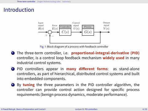
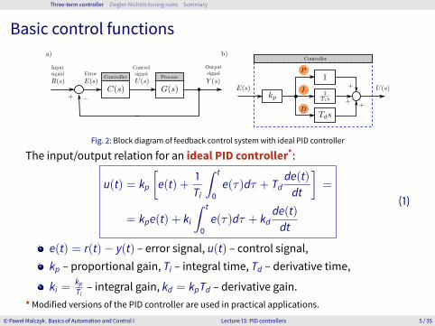
Fig. 1: Block diagram of a process with feedback controller
1 The three-term controller, i.e. proportional-integral-derivative (PID)controller, is a control loop feedback mechanism widely used in manyindustrial control systems.
2 PID controllers appear in many different forms: as stand-alonecontrollers, as part of hierarchical, distributed control systems and builtinto embedded components.
3 By tuning the three parameters in the PID controller algorithm, thecontroller can provide control action designed for specific processrequirements (benign process dynamics, moderate performance).
© Paweł Malczyk. Basics of Automation and Control I Lecture 13: PID controllers 4 / 35
Three-term controller Ziegler-Nichols tuning rules Summary
Basic control functions
Fig. 2: Block diagram of feedback control systemwith ideal PID controller
The input/output relation for an ideal PID controller*:
u(t) = kp[e(t) +
1Ti
∫ t
0e(τ)dτ + Td
de(t)dt
]=
= kpe(t) + ki∫ t
0e(τ)dτ + kd
de(t)dt
(1)
e(t) = r(t) − y(t) – error signal, u(t) – control signal,kp – proportional gain, Ti – integral time, Td – derivative time,
ki =kpTi– integral gain, kd = kpTd – derivative gain.
*Modified versions of the PID controller are used in practical applications.
© Paweł Malczyk. Basics of Automation and Control I Lecture 13: PID controllers 5 / 35
Three-term controller Ziegler-Nichols tuning rules Summary
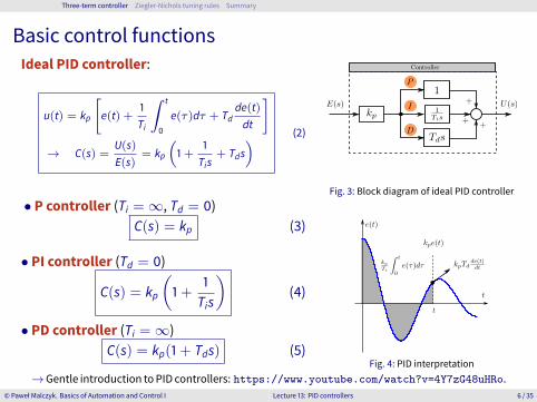
Basic control functionsIdeal PID controller:
u(t) = kp
[e(t) +
1Ti
∫ t
0
e(τ)dτ + Tdde(t)dt
]→ C(s) =
U(s)E(s)
= kp(1+
1Tis
+ Tds) (2)
Fig. 3: Block diagram of ideal PID controller• P controller (Ti = ∞, Td = 0)
C(s) = kp (3)
• PI controller (Td = 0)
C(s) = kp(1+
1Tis
)(4)
• PD controller (Ti = ∞)C(s) = kp(1+ Tds) (5)
Fig. 4: PID interpretation→Gentle introduction toPID controllers: https://www.youtube.com/watch?v=4Y7zG48uHRo.
© Paweł Malczyk. Basics of Automation and Control I Lecture 13: PID controllers 6 / 35
Three-term controller Ziegler-Nichols tuning rules Summary
Mechanical system
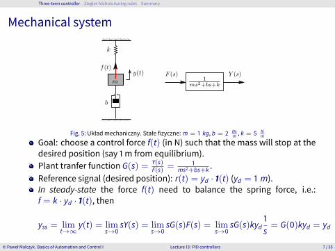
Fig. 5: Układmechaniczny. Stałe fizyczne: m = 1 kg, b = 2 Nsm , k = 5 N
m
Goal: choose a control force f(t) (in N) such that the mass will stop at thedesired position (say 1 m from equilibrium).Plant tranfer function G(s) = Y(s)
F(s) =1
ms2+bs+k .Reference signal (desired position): r(t) = yd · 1(t) (yd = 1 m).In steady-state the force f(t) need to balance the spring force, i.e.:f = k · yd · 1(t), then
yss = limt→∞
y(t) = lims→0
sY(s) = lims→0
sG(s)F(s) = lims→0
sG(s)kyd1s= G(0)kyd = yd
© Paweł Malczyk. Basics of Automation and Control I Lecture 13: PID controllers 7 / 35
Three-term controller Ziegler-Nichols tuning rules Summary
Mechanical systemwith disturbance
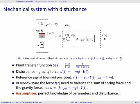
Fig. 6: Mechanical system. Physical constants: m = 1 kg, b = 2 Nsm , k = 5 N
m , and g = 10 ms2
Plant transfer function G(s) = Y(s)F(s) =
1ms2+bs+k .
Disturbance – gravity force: d(t) = −mg · 1(t).Reference signal (desired position): r(t) = yd · 1(t) (yd = 1 m).In steady-state the force f(t) need to balance the sum of spring force andthe gravity force, i.e.: u = (k · yd +mg) · 1(t).Assumption: perfect knowledge of parameters and disturbance...
© Paweł Malczyk. Basics of Automation and Control I Lecture 13: PID controllers 8 / 35
Three-term controller Ziegler-Nichols tuning rules Summary
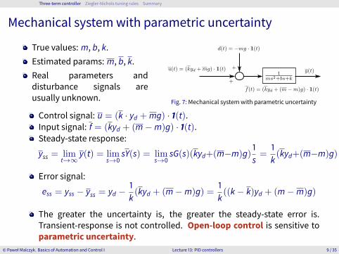
Mechanical systemwith parametric uncertainty
True values: m, b, k.Estimated params: m, b, k.Real parameters anddisturbance signals areusually unknown. Fig. 7: Mechanical systemwith parametric uncertainty
Control signal: u = (k · yd +mg) · 1(t).Input signal: f = (kyd + (m − m)g) · 1(t).Steady-state response:
yss = limt→∞
y(t) = lims→0
sY(s) = lims→0
sG(s)(kyd+(m−m)g)1s=
1k(kyd+(m−m)g)
Error signal:
ess = yss − yss = yd − 1k(kyd + (m − m)g) =
1k((k − k)yd + (m − m)g)
The greater the uncertainty is, the greater the steady-state error is.Transient-response is not controlled. Open-loop control is sensitive toparametric uncertainty.
© Paweł Malczyk. Basics of Automation and Control I Lecture 13: PID controllers 9 / 35
Three-term controller Ziegler-Nichols tuning rules Summary
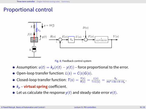
Proportional control
Fig. 8: Feedback control system
Assumption: u(t) = kp(r(t) − y(t)) – force proportional to the error.Open-loop transfer function: L(s) = C(s)G(s).
Closed-loop transfer function: T(s) = Y(s)R(s) =
L(s)1+L(s) =
kpms2+bs+k+kp
.
kp – virtual spring coefficient.Let us calculate the response y(t) and steady-state error e(t).
© Paweł Malczyk. Basics of Automation and Control I Lecture 13: PID controllers 10 / 35
Three-term controller Ziegler-Nichols tuning rules Summary
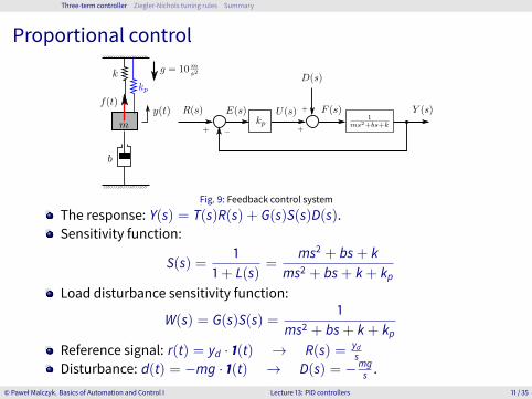
Proportional control
Fig. 9: Feedback control system
The response: Y(s) = T(s)R(s) + G(s)S(s)D(s).Sensitivity function:
S(s) =1
1+ L(s)=
ms2 + bs+ kms2 + bs+ k+ kp
Load disturbance sensitivity function:
W(s) = G(s)S(s) =1
ms2 + bs+ k+ kpReference signal: r(t) = yd · 1(t) → R(s) = yd
sDisturbance: d(t) = −mg · 1(t) → D(s) = −mg
s .© Paweł Malczyk. Basics of Automation and Control I Lecture 13: PID controllers 11 / 35
Three-term controller Ziegler-Nichols tuning rules Summary
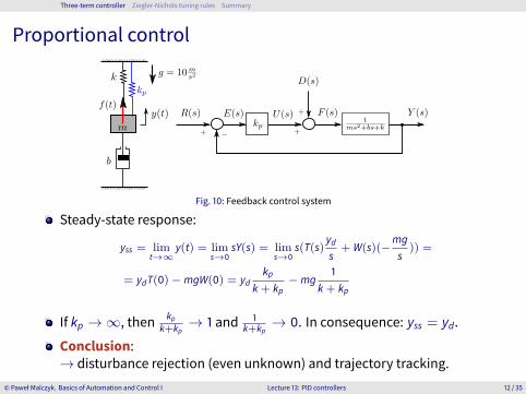
Proportional control
Fig. 10: Feedback control system
Steady-state response:
yss = limt→∞
y(t) = lims→0
sY(s) = lims→0
s(T(s)yds
+ W(s)(−mgs
)) =
= ydT(0) − mgW(0) = ydkp
k+ kp− mg
1k+ kp
If kp → ∞, then kpk+kp
→ 1 and 1k+kp
→ 0. In consequence: yss = yd.
Conclusion:→ disturbance rejection (even unknown) and trajectory tracking.
© Paweł Malczyk. Basics of Automation and Control I Lecture 13: PID controllers 12 / 35
Three-term controller Ziegler-Nichols tuning rules Summary
P controller
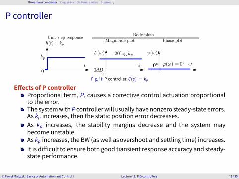
Fig. 11: P controller, C(s) = kp
Effects of P controllerProportional term, P, causes a corrective control actuation proportionalto the error.The systemwithP controllerwill usually havenonzero steady-state errors.As kp increases, then the static position error decreases.As kp increases, the stability margins decrease and the system maybecome unstable.As kp increases, the BW (as well as overshoot and settling time) increases.It is difficult to ensure both good transient response accuracy and steady-state performance.
© Paweł Malczyk. Basics of Automation and Control I Lecture 13: PID controllers 13 / 35
Three-term controller Ziegler-Nichols tuning rules Summary
P controller
0 1 2 3 4 5 6 7 8 9 10
t
0
0.2
0.4
0.6
0.8
1
1.2
1.4
y(t)
kp=15kp=20kp=25kp=30
r(t)
0 1 2 3 4 5 6 7 8 9 10
t
-15-10-505
1015202530
u(t)
kp=15kp=20kp=25kp=30
10-2 10-1 100 101 102
Frequency (rad/sec)
-60-50-40-30-20-10
010203040
Mag
nitu
de (
dB)
kp=30
10-2 10-1 100 101 102
Frequency (rad/sec)
-180
-150
-120
-90
-60
-30
0
Pha
se (
deg)
kp=30
GCLST
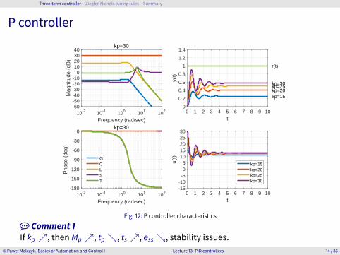
Fig. 12: P controller characteristics
Comment 1If kp ↗, thenMp ↗, tp ↘, ts ↗, ess ↘, stability issues.
© Paweł Malczyk. Basics of Automation and Control I Lecture 13: PID controllers 14 / 35
Three-term controller Ziegler-Nichols tuning rules Summary
P controller
10-2 10-1 100 101 102
Frequency (rad/sec)
-60
-50
-40
-30
-20
-10
0
10
20
30
40
Mag
nitu
de (
dB)
kp=30
GCLST
0 1 2 3 4 5 6 7 8 9 10
t
0
0.2
0.4
0.6
0.8
1
1.2
1.4
y(t)
kp=15
kp=20kp=25kp=30
r(t)
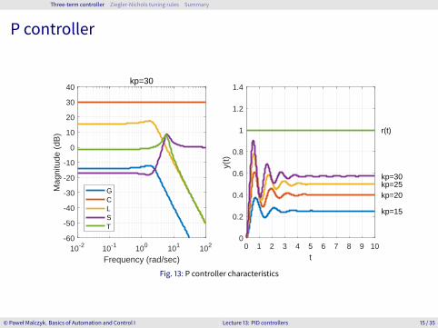
Fig. 13: P controller characteristics
© Paweł Malczyk. Basics of Automation and Control I Lecture 13: PID controllers 15 / 35
Three-term controller Ziegler-Nichols tuning rules Summary
PI controller
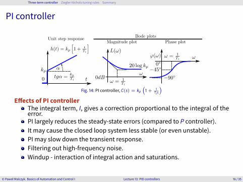
Fig. 14: PI controller, C(s) = kp(1 + 1
Tis
)Effects of PI controller
The integral term, I, gives a correction proportional to the integral of theerror.PI largely reduces the steady-state errors (compared to P controller).It may cause the closed loop system less stable (or even unstable).PI may slow down the transient response.Filtering out high-frequency noise.Windup - interaction of integral action and saturations.
© Paweł Malczyk. Basics of Automation and Control I Lecture 13: PID controllers 16 / 35
Three-term controller Ziegler-Nichols tuning rules Summary
PI controller
0 1 2 3 4 5 6 7 8 9 10
t
-0.6-0.4-0.2
00.20.40.60.8
11.21.41.6
y(t)
kp=30
Ti=1Ti=5Ti=10Ti=100
0 1 2 3 4 5 6 7 8 9 10
t
-20-15-10-505
1015202530
u(t)
kp=30
Ti=1Ti=5Ti=10Ti=100
10-2 10-1 100 101 102
Frequency (rad/sec)
-80
-60
-40
-20
0
20
40
60
80
Mag
nitu
de (
dB)
kp=30, Ti=1
G C L S T
10-2 10-1 100 101 102
Frequency (rad/sec)
-180
-150
-120
-90
-60
-30
0
Pha
se (
deg)
kp=30, Ti=1
GCLST
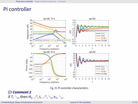
Fig. 15: PI controller characteristics
Comment 2If Ti ↘, thenMp ↗, ts ↗, ↘, ess ↘.
© Paweł Malczyk. Basics of Automation and Control I Lecture 13: PID controllers 17 / 35
Three-term controller Ziegler-Nichols tuning rules Summary
PI controller
10-2 10-1 100 101 102
Frequency (rad/sec)
-80
-60
-40
-20
0
20
40
60
80
Mag
nitu
de (
dB)
kp=30, Ti=1
GCLST
0 1 2 3 4 5 6 7 8 9 10
t
-0.6
-0.4
-0.2
0
0.2
0.4
0.6
0.8
1
1.2
1.4
1.6
y(t)
kp=30
Ti=1Ti=5Ti=10Ti=100
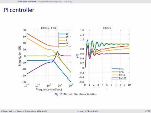
Fig. 16: PI controller characteristics
© Paweł Malczyk. Basics of Automation and Control I Lecture 13: PID controllers 18 / 35
Three-term controller Ziegler-Nichols tuning rules Summary
PD controller
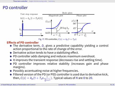
Fig. 17: PD controller, C(s) = kp(1 + Tds)
Effects of PD controllerThe derivative term, D, gives a predictive capability yielding a controlaction proportional to the rate of change of the error.Derivative action tends to have a stabilizing effect.PD controller adds damping and reduces maximum overshoot.It improves the transient response (decreases rise and settling time).PD controller improves relative stability (increases gain and phasemargins).Possibly accentuating noise at higher frequencies.Filtered version of the PD (or PID) controller is used due to derivative kick,then, C(s) = kp(1+ Tds 1
TdN s+1
). Typical values of N are 8 to 20.
© Paweł Malczyk. Basics of Automation and Control I Lecture 13: PID controllers 19 / 35
Three-term controller Ziegler-Nichols tuning rules Summary
PD controller
0 1 2 3 4 5 6 7 8 9 10
t
-0.6-0.4-0.2
00.20.40.60.8
11.21.4
y(t)
kp=30
Td=0Td=0.01Td=0.05Td=0.1
0 1 2 3 4 5 6 7 8 9 10
t
-15-10-505
1015202530
u(t)
kp=30
Td=0Td=0.01Td=0.05Td=0.1
10-2 10-1 100 101 102 103
Frequency (rad/sec)
-60
-40
-20
0
20
40
60
80
Mag
nitu
de (
dB)
kp=30, Td=0.1
G C L S T
10-2 10-1 100 101 102
Frequency (rad/sec)
-180-150-120
-90-60-30
0306090
120
Pha
se (
deg)
kp=30, Td=0.1
GCLST
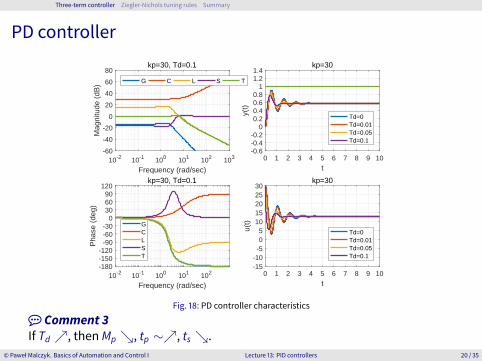
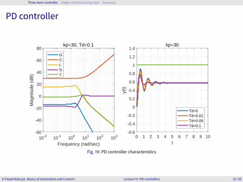
Fig. 18: PD controller characteristics
Comment 3If Td ↗, thenMp ↘, tp ∼↗, ts ↘.
© Paweł Malczyk. Basics of Automation and Control I Lecture 13: PID controllers 20 / 35
Three-term controller Ziegler-Nichols tuning rules Summary
PD controller
10-2 10-1 100 101 102 103
Frequency (rad/sec)
-60
-40
-20
0
20
40
60
80
Mag
nitu
de (
dB)
kp=30, Td=0.1
GCLST
0 1 2 3 4 5 6 7 8 9 10
t
-0.6
-0.4
-0.2
0
0.2
0.4
0.6
0.8
1
1.2
1.4
y(t)
kp=30
Td=0Td=0.01Td=0.05Td=0.1
Fig. 19: PD controller characteristics
© Paweł Malczyk. Basics of Automation and Control I Lecture 13: PID controllers 21 / 35
Three-term controller Ziegler-Nichols tuning rules Summary
PID controller
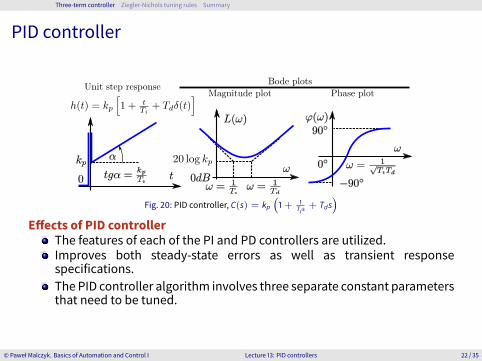
Fig. 20: PID controller, C(s) = kp(1 + 1
Tis+ Tds
)Effects of PID controller
The features of each of the PI and PD controllers are utilized.Improves both steady-state errors as well as transient responsespecifications.The PID controller algorithm involves three separate constant parametersthat need to be tuned.
© Paweł Malczyk. Basics of Automation and Control I Lecture 13: PID controllers 22 / 35
Three-term controller Ziegler-Nichols tuning rules Summary
PID controller
0 1 2 3 4 5 6 7 8 9 10
t
0
0.2
0.4
0.6
0.8
1
1.2
1.4
y(t)
kp=30, Td=0.1, Ti=1
y(t)r(t)
0 1 2 3 4 5 6 7 8 9 10
t
-10
0
10
20
30
40
50
u(t)
kp=30, Td=0.1, Ti=1
u(t)
10-3 10-2 10-1 100 101 102 103
Frequency (rad/sec)
-80
-60
-40
-20
0
20
40
60
80M
agni
tude
(dB
)kp=30, Td=0.1, Ti=1
G C L S T
10-3 10-2 10-1 100 101 102 103
Frequency (rad/sec)
-180-150-120
-90-60-30
0306090
120
Pha
se (
deg)
kp=30, Td=0.1, Ti=1
G C L S T
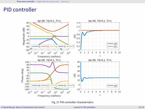
Fig. 21: PID controller characteristics
© Paweł Malczyk. Basics of Automation and Control I Lecture 13: PID controllers 23 / 35
Three-term controller Ziegler-Nichols tuning rules Summary
PID controller
10-3 10-2 10-1 100 101 102 103
Frequency (rad/sec)
-80
-60
-40
-20
0
20
40
60
80
Mag
nitu
de (
dB)
kp=30, Td=0.1, Ti=1
G C L S T
0 1 2 3 4 5 6 7 8 9 10
t
0
0.2
0.4
0.6
0.8
1
1.2
1.4
y(t)
kp=30, Td=0.1, Ti=1
y(t)r(t)
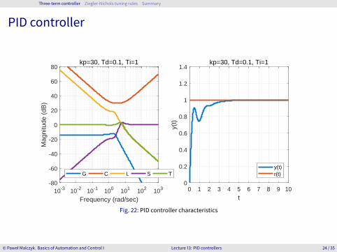
Fig. 22: PID controller characteristics
© Paweł Malczyk. Basics of Automation and Control I Lecture 13: PID controllers 24 / 35
Three-term controller Ziegler-Nichols tuning rules Summary
PID controllers
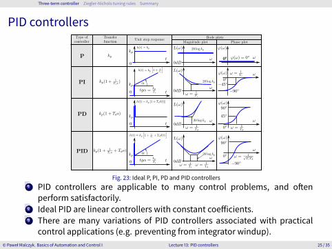
Fig. 23: Ideal P, PI, PD and PID controllers1 PID controllers are applicable to many control problems, and often
perform satisfactorily.2 Ideal PID are linear controllers with constant coefficients.3 There are many variations of PID controllers associated with practical
control applications (e.g. preventing from integrator windup).© Paweł Malczyk. Basics of Automation and Control I Lecture 13: PID controllers 25 / 35
Three-term controller Ziegler-Nichols tuning rules Summary
Ziegler-Nichols tuning rules
1 Three-term controller
2 Ziegler-Nichols tuning rulesIntroductionFirst methodSecondmethodCommentsExample
3 Summary
© Paweł Malczyk. Basics of Automation and Control I Lecture 13: PID controllers 26 / 35
Three-term controller Ziegler-Nichols tuning rules Summary
Introduction
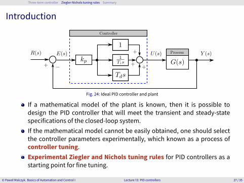
Fig. 24: Ideal PID controller and plant
If a mathematical model of the plant is known, then it is possible todesign the PID controller that will meet the transient and steady-statespecifications of the closed-loop system.If the mathematical model cannot be easily obtained, one should selectthe controller parameters experimentally, which known as a process ofcontroller tuning.Experimental Ziegler and Nichols tuning rules for PID controllers as astarting point for fine tuning.
© Paweł Malczyk. Basics of Automation and Control I Lecture 13: PID controllers 27 / 35
Three-term controller Ziegler-Nichols tuning rules Summary
First method
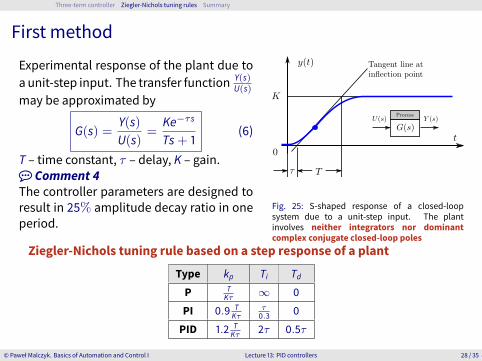
Experimental response of the plant due toa unit-step input. The transfer function Y(s)
U(s)may be approximated by
G(s) =Y(s)U(s)
=Ke−τs
Ts+ 1(6)
T – time constant, τ – delay, K – gain. Comment 4The controller parameters are designed toresult in 25% amplitude decay ratio in oneperiod.
Fig. 25: S-shaped response of a closed-loopsystem due to a unit-step input. The plantinvolves neither integrators nor dominantcomplex conjugate closed-loop poles
Ziegler-Nichols tuning rule based on a step response of a plant
Type kp Ti TdP T
Kτ ∞ 0
PI 0.9 TKτ
τ0.3 0
PID 1.2 TKτ 2τ 0.5τ
© Paweł Malczyk. Basics of Automation and Control I Lecture 13: PID controllers 28 / 35
Three-term controller Ziegler-Nichols tuning rules Summary
Secondmethod
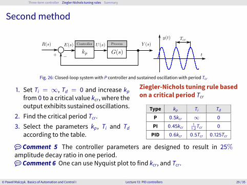
Fig. 26: Closed-loop systemwith P controller and sustained oscillation with period Tcr
1. Set Ti = ∞, Td = 0 and increase kpfrom0 to a critical value kcr, where theoutput exhibits sustained oscillations.
2. Find the critical period Tcr.3. Select the parameters kp, Ti and Td
according to the table.
Ziegler-Nichols tuning rule basedon a critical period Tcr
Type kp Ti TdP 0.5kcr ∞ 0
PI 0.45kcr 11.2Tcr 0
PID 0.6kcr 0.5Tcr 0.125Tcr
Comment 5 The controller parameters are designed to result in 25%amplitude decay ratio in one period. Comment 6 One can use Nyquist plot to find kcr, and Tcr.
© Paweł Malczyk. Basics of Automation and Control I Lecture 13: PID controllers 29 / 35
Three-term controller Ziegler-Nichols tuning rules Summary
Comments
1 Ziegler-Nichols tuning rules (and other tuning rules) have been widelyused in process control systems.
2 The plant dynamics may be known or may be not precisely known.3 Experience has shown that the Z-N rules provide acceptable closed-loop
response for many systems.4 The empirical PID tuning strategies are only starting points in the process
to obtain the right controller.5 Tuning method (by Astrom & Hagglund) based on relay feedback is
available.
© Paweł Malczyk. Basics of Automation and Control I Lecture 13: PID controllers 30 / 35
Three-term controller Ziegler-Nichols tuning rules Summary
Example
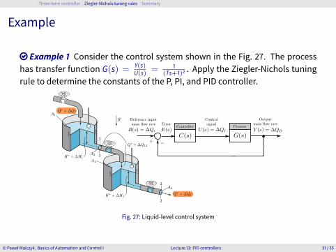
Example 1 Consider the control system shown in the Fig. 27. The processhas transfer function G(s) = Y(s)
U(s) = 1(Ts+1)2 . Apply the Ziegler-Nichols tuning
rule to determine the constants of the P, PI, and PID controller.
Fig. 27: Liquid-level control system
© Paweł Malczyk. Basics of Automation and Control I Lecture 13: PID controllers 31 / 35
Three-term controller Ziegler-Nichols tuning rules Summary
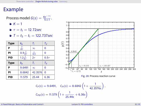
ExampleProcess model G(s) = Ke−τs
Ts+1 .K = 1τ = t1 = 12.72secT = t3 − t1 = 122.737sec
Type kp Ti TdP T
Kτ ∞ 0
PI 0.9 TKτ
τ0.3 0
PID 1.2 TKτ 2τ 0.5τ
Type kp Ti TdP 9.6491 ∞ 0
PI 8.6842 42.3576 0
PID 11.579 25.44 6.36
0 20 40 60 80 100 120 140 160 180 200 220 240 260 280 300−0.2
−0.1
0
0.1
0.2
0.3
0.4
0.5
0.6
0.7
0.8
0.9
1
1.1
1.2
Fig. 28: Process reaction curve
CP(s) = 9.6491, CPI(s) = 8.6842(1+
142.3576s
),
CPID(s) = 11.579(1+
125.44s
+ 6.36s)
© Paweł Malczyk. Basics of Automation and Control I Lecture 13: PID controllers 32 / 35
Three-term controller Ziegler-Nichols tuning rules Summary
Example
0 50 100 150 200 250 3000
0.20.40.60.81
1.21.41.61.8
PPIPID
0 50 100 150 200 250 300−6−4−202468101214161820
PPIPID
0 50 100 150 200 250 300−0.05
0
0.05
0.1
0.15
0.2PPIPID
0 50 100 150 200 250 3000
0.025
0.05
0.075
0.1PPIPID
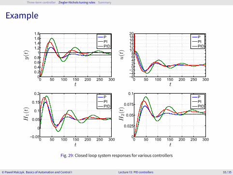
Fig. 29: Closed loop system responses for various controllers
© Paweł Malczyk. Basics of Automation and Control I Lecture 13: PID controllers 33 / 35
Three-term controller Ziegler-Nichols tuning rules Summary
Review questions
1 What is themain objective of introducing proportional control, integral control or derivativecontrol?
2 What is a P, PI, PD, PID controller? Write the input-output relation, unit-step response andBode plots.
3 Give the effects of P, PI, PD and PID controllers on the feedback control systemperformance.4 Formulate and comment on the twoZiegler-Nichols tuning rules for a PID controller. Discuss
the range of applicability of both methods.
© Paweł Malczyk. Basics of Automation and Control I Lecture 13: PID controllers 34 / 35
Three-term controller Ziegler-Nichols tuning rules Summary
Summary
1 Three-term controller
2 Ziegler-Nichols tuning rules
3 Summary
© Paweł Malczyk. Basics of Automation and Control I Lecture 13: PID controllers 35 / 35


