Embed Size (px)
Citation preview
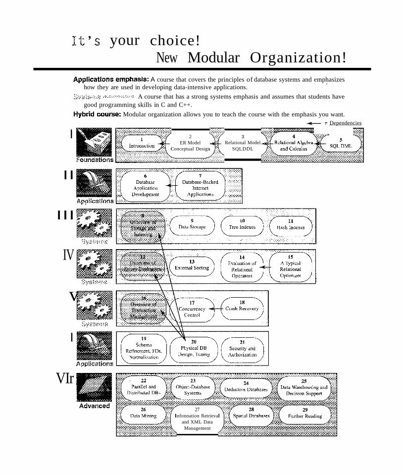
It's your choice!New Modular Organization!
3Relational Model
SQLDDL
27Infonnation Retrieval
and XML DataManagement
2ER Model
Conceptual Design
Appncatirms emphasis: A course that covers the principles of database systems and emphasizeshow they are used in developing data-intensive applications. .
f,;~tY'W';Yl~t';;:;,~7' A course that has a strong systems emphasis and assumes that students havegood programming skills in C and C++.
Hybrid course: Modular organization allows you to teach the course with the emphasis you want.......- := Dependencies
~~~
I
v
I
II
IV
VIr
III

j
j
j
j
j
j
j
j
j
j
j
j
j
j
j
j
j
j
j
j
j
j
j
j
j
j
j
j
j
j
DATABASE MANAGEMENTSYSTEMS

DATABASE MANAGEMENTSYSTEMS
Third Edition
Raghu RamakrishnanUniversity of Wisconsin
Madison, Wisconsin, USA
•Johannes Gehrke
Cornell University
Ithaca, New York, USA
Boston Burr Ridge, IL Dubuque, IA Madison, WI New York San Francisco St. LouisBangkok Bogota Caracas Kuala Lumpur Lisbon London Madrid Mexico CityMilan Montreal New Delhi Santiago Seoul Singapore Sydney Taipei Toronto

McGraw-Hill Higher Education tzA Lhvision of The McGraw-Hill Companies
DATABASE MANAGEMENT SYSTEMS, THIRD EDITIONInternational Edition 2003
Exclusive rights by McGraw-Hill Education (Asia), for manufacture and export. Thisbook cannot be re-exported from the country to which it is sold by McGraw-Hill. TheInternational Edition is not available in North America.
Published by McGraw-Hili, a business unit of The McGraw-Hili Companies, Inc., 1221Avenue of the Americas, New York, NY 10020. Copyright © 2003, 2000, 1998 by TheMcGraw-Hill Companies, Inc. All rights reserved. No part of this publication may bereproduced or distributed in any form or by any means, or stored in a database or retrievalsystem, without the prior written consent of The McGraw-Hill Companies, Inc.,including, but not limited to, in any network or other electronic storage or transmission,or broadcast for distance learning.Some ancillaries, including electronic and print components, may not be available tocustomers outside the United States.
10 09 08 07 06 05 04 0320 09 08 07 06 05 04CTF BJE
Library of Congress Cataloging-in-Publication DataRamakrishnan, Raghu
Database management systems / Raghu Ramakrishnan, Johannes Gehrke.~3rd ed.p. cm.
Includes index.ISBN 0-07-246563-8-ISBN 0-07-115110-9 (ISE)1. Database management. 1. Gehrke, Johannes. II. Title.
QA76.9.D3 R237 2003005.74--Dc21 2002075205
CIP
When ordering this title, use ISBN 0-07-123151-X
Printed in Singapore
www.mhhe.com

To Apu, Ketan, and Vivek with love
To Keiko and Elisa

1
1
1
1
1
1
1
1
1
1
1
1
1
1
1
1
1
1
1
1
1
1
1
1
1
1
1
1
1
1
1
1
1
1
1
1
1
PREFACE
Part I FOUNDATIONS
CONTENTS
XXIV
1
1
2
OVERVIEW OF DATABASE SYSTEMS1.1 Managing Data
1.2 A Historical Perspective
1.3 File Systems versus a DBMS
1.4 Advantages of a DBMS
1.5 Describing and Storing Data in a DBMS
1.5.1 The Relational Model
1.5.2 Levels of Abstraction in a DBMS
1.5.3 Data Independence
1.6 Queries in a DBMS
1.7 Transaction Management
1.7.1 Concurrent Execution of Transactions
1.7.2 Incomplete Transactions and System Crashes
1.7.3 Points to Note
1.8 Structure of a DBMS
1.9 People Who Work with Databases
1.10 Review Questions
INTRODUCTION TO DATABASE DESIGN2.1 Database Design and ER Diagrams
2.1.1 Beyond ER Design
2.2 Entities, Attributes, and Entity Sets
2.3 Relationships and Relationship Sets
2.4 Additional Features of the ER Model
2.4.1 Key Constraints
2.4.2 Participation Constraints
2.4.3 Weak Entities
2.4.4 Class Hierarchies
2.4.5 Aggregation
vii
34
6
8
9
10
11
12
15
16
17
17
18
19
19
21
22
2526
27
28
29
32
32
34
35
37
39
Vlll DATABASE "NIANAGEMENT SYSTEivlS
Preliminaries
Relational Algebra
4.2.1 Selection and Projection
4.2.2 Set Operations
3
4
2.5 Conceptual Design With the ER Model
2..5.1 Entity versus Attribute
2.5.2 Entity versus Relationship
2.5.3 Binary versus Ternary Relationships
2..5.4 Aggregation versus Ternary Relationships
2.6 Conceptual Design for Large Enterprises
2.7 The Unified Modeling Language
2.8 Case Study: The Internet Shop
2.8.1 Requirements Analysis
2.8.2 Conceptual Design
2.9 Review Questions
THE RELATIONAL MODEL3.1 Introduction to the Relational Model
3.1.1 Creating and Modifying Relations Using SQL
3.2 Integrity Constraints over Relations
3.2.1 Key Constraints
:3.2.2 Foreign Key Constraints
3.2.3 General Constraints
3.3 Enforcing Integrity Constraints
3.3.1 Transactions and Constraints
3.4 Querying Relational Data
3.5 Logical Database Design: ER to Relational
3.5.1 Entity Sets to Tables
3.5.2 Relationship Sets (without Constraints) to Tables
3.5.3 Translating Relationship Sets with Key Constraints
3.5.4 Translating Relationship Sets with Participation Constraints
3.5.5 Translating Weak Entity Sets
3.5.6 cn'anslating Class Hierarchies
3.5.7 Translating ER Diagrams with Aggregation
3.5.8 ER to Relational: Additional Examples
:3.6 Introduction to Views
3.6.1 Views, Data Independence, Security
3.6.2 Updates on Views
:3.7 Destroying/Altering Tables and Views
:3.8 Case Study: The Internet Store
:3.9 Review Questions
RELATIONAL ALGEBRA AND CALCULUS4.1
4.2
40
41
42
43
4546
4749
49
50
51
5759
62
63
6466
6869
72
73
74
75
76
787982
83
8485
868788
91
92
94
100101102
103
104
Contents lX~
4.2.3 Renaming 106
4.2.4 Joins 107
4.2.5 Division 109
4.2.6 1\'lore Examples of Algebra Queries 110
4.3 Relational Calculus 116
4.3.1 Tuple Relational Calculus 117
4.3.2 Domain Relational Calculus 122
4.4 Expressive Power of Algebra and Calculus 124
4.5 Review Questions 126
5 SQL: QUERIES, CONSTRAINTS, TRIGGERS 1305.1 Overview 131
5.1.1 Chapter Organization 132
.5.2 The Form of a Basic SQL Query 133
5.2.1 Examples of Basic SQL Queries 138
5.2.2 Expressions and Strings in the SELECT Command 139
5.3 UNION, INTERSECT, and EXCEPT 141
5.4 Nested Queries 144
5.4.1 Introduction to Nested Queries 145
5.4.2 Correlated Nested Queries 147
5.4.3 Set-Comparison Operators 148
5.4.4 More Examples of Nested Queries 149
5.5 Aggregate Operators 151
5.5.1 The GROUP BY and HAVING Clauses 154
5.5.2 More Examples of Aggregate Queries 158
5.6 Null Values 162
5.6.1 Comparisons Using Null Values 163
5.6.2 Logical Connectives AND, OR, and NOT 163
5.6.3 Impact 011 SQL Constructs 163
5.6.4 Outer Joins 164
5.6.5 Disallowing Null Values 165
5.7 Complex Integrity Constraints in SQL 165
5.7.1 Constraints over a Single Table 165
5.7.2 Domain Constraints and Distinct Types 166
5.7.3 Assertions: ICs over Several Tables 167
5.8 Triggers and Active Databases 168
5.8.1 Examples of Triggers in SQL 169
5.9 Designing Active Databases 171
5.9.1 Why Triggers Can Be Hard to Understand 171
5.9.2 Constraints versus Triggers 172
5.9.:3 Other Uses of Triggers 172
5.10 Review Questions 17:3
x DATABASE J\;1ANAGEMENT SYSTEMS
Part II APPLICATION DEVELOPMENT 183
6 DATABASE APPLICATION DEVELOPMENT 1856.1 Accessing Databases from Applications 187
6.1.1 Embedded SQL 187
6.1.2 Cursors 189
6.1.3 Dynamic SQL 194
6.2 An Introduction to JDBC 194
6.2.1 Architecture 196
6.3 JDBC Classes and Interfaces 197
6.3.1 JDBC Driver Management 197
6.3.2 Connections 198
6.3.3 Executing SQL Statements 200
6.3.4 ResultSets 201
6.3.5 Exceptions and Warnings 203
6.3.6 Examining Database Metadata 204
6.4 SQLJ 206
6.4.1 Writing SQLJ Code 207
6.5 Stored Procedures 209
6.5.1 Creating a Simple Stored Procedure 209
6.5.2 Calling Stored Procedures 210
6.5.3 SQL/PSM 212
6.6 Case Study: The Internet Book Shop 214
6.7 Review Questions 216
7 INTERNET APPLICATIONS 2207.1 Introduction 220
7.2 Internet Concepts 221
7.2.1 Uniform Resource Identifiers 221
7.2.2 The Hypertext Transfer Protocol (HTTP) 223
7.3 HTML Documents 226
7.4 XML Documents 227
7.4.1 Introduction to XML 228
7.4.2 XML DTDs 231
7.4.3 Domain-Specific DTDs 234
7.5 The Three-Tier Application Architecture 236
7.5.1 Single-Tier and Client-Server Architectures 236
7.5.2 Three-Tier Architectures 239
7.5.3 Advantages of the Three-Tier Architecture 241
7.6 The Presentation Layer 242
7.6.1 HTrvlL Forms 242
7.6.2 JavaScript 245
7.6.3 Style Sheets 247
Contents :»:i
7.7 The Middle Tier
7.7.1 CGI: The Common Gateway Interface
7.7.2 Application Servers
7.7.3 Servlets
7.7.4 JavaServer Pages
7.7.5 Maintaining State
7.8 Case Study: The Internet Book Shop
7.9 Review Questions
251
251
252
254
256
258
261
264
Part III STORAGE AND INDEXING 271
273274
275
277
277
278
279
280
282
283
284
285
287
288
289
290
291
292
292
295
299
299
Data on External Storage
File Organizations and Indexing
8.2.1 Clustered Indexes
8.2.2 Primary and Secondary Indexes
Index Data Structures
8.3.1 Hash-Based Indexing
8.3.2 Tree-Based Indexing
Comparison of File Organizations
8.4.1 Cost Model
8.4.2 Heap Files
8.4.3 Sorted Files
8.4.4 Clustered Files
8.4.5 Heap File with Unclustered Tree Index
8.4.6 Heap File With Unclustered Hash Index
8.4.7 Comparison of I/O Costs
Indexes and Performance Tuning
8..5.1 Impact of the Workload
8.5.2 Clustered Index Organization
8.5.3 Composite Search Keys
8.5.4 Index Specification in SQL:1999
Review Questions8.6
8.5
8.4
8.3
OVERVIEW OF STORAGE AND INDEXING8.1
8.2
8
9 STORING DATA: DISKS AND FILES9.1 The Memory Hierarchy
9.1.1 Magnetic Disks
9.1.2 Performance Implications of Disk Structure
9.2 Redundant Arrays of Independent Disks
9.2.1 Data Striping
9.2.2 Redundancy
9.2.3 Levels of Redundancy
9.2.4 Choice of RAID Levels
304305
306
308
309
310
311
312
316
Xll DATABASE ~/IANAGE1'vIENT SYSTEMS
9.3 Disk Space Management
9.3.1 Keeping Track of Free Blocks
9.3.2 Using as File Systems to il/ranage Disk Space
9.4 Buffer Manager
9.4.1 Buffer Replacement Policies
9.4.2 Buffer Management in DBMS versus OS
9.5 Files of Records
9.5.1 Implementing Heap Files
9.6 Page Formats
9.6.1 Fixed-Length Records
9.6.2 Variable-Length Records
9.7 Record Formats
9.7.1 Fixed-Length Records
9.7.2 Variable-Length Records
9.8 Review Questions
10 TREE-STRUCTURED INDEXING10.1 Intuition For Tree Indexes
10.2 Indexed Sequential Access Method (ISAM)
10.2.1 Overflow Pages, Locking Considerations
10.3 B+ Trees: A Dynamic Index Structure
10.3.1 Format of a Node
10.4 Search
10.5 Insert
10.6 Delete
10.7 Duplicates
10.8 B+ Trees in Practice
10.8.1 Key Compression
10.8.2 Bulk-Loading a B+ Tl'ee
10.8.3 The Order Concept
10.8.4 The Effect of Inserts and Deletes on Rids
10.9 Review Questions
11 HASH-BASED INDEXING11.1 Static Hashing
11.1.1 Notation and Conventions
11.2 Extendible HCkshing
11.3 Line~r Hashing
11.4 Extendible vs. Linear Ha"lhing
n.5 Review Questions
Part IV QUERY EVALUATION
:316
317
317
318
320
322
324
324
326
327
328
330
331
331
333
338339
341
344
344
346
347
348
352
356
358
358
360
363
364
364
370371
373
373
379
384
385
391
Contents
12 OVERVIEW OF QUERY EVALUATION12.1 The System Catalog
12.1.1 Information in the Catalog
12.2 Introduction to Operator Evaluation
12.2.1 Three Common Techniques
12.2.2 Access Paths
12.3 Algorithms for Relational Operations
12.3.1 Selection
12.3.2 Projection
12.3.3 Join
12.3.4 Other Operations
12.4 Introduction to Query Optimization
12.4.1 Query Evaluation Plans
12.4.2 Multi-operator Queries: Pipelined Evaluation
12.4.3 The Iterator Interface
12.5 Alternative Plans: A Motivating Example
12.5.1 Pushing Selections
12.5.2 Using Indexes
12.6 What a Typical Optimizer Does
12.6.1 Alternative Plans Considered
12.6.2 Estimating the Cost of a Plan
12.7 Review Questions
13 EXTERNAL SORTING13.1 When Does a DBMS Sort Data?
13.2 A Simple Two-Way Merge Sort
13.3 External Merge Sort
13.3.1 Minimizing the Number of Runs
13.4 Minimizing I/O Cost versus Number of I/Os
13.4.1 Blocked I/O
13.4.2 Double Buffering
13.5 Using B+ Trees for Sorting
13.5.1 Clustered Index
1:3.5.2 Unclustered Index
13.6 Review Questions
14 EVALUATING RELATIONAL OPERATORS14.1 The' Selection Operation
14.1.1 No Index, Unsorted Data
14.1.2 No Index, Sorted Data
14.1.:3 B+ Tree Index
14.1.4 Hash Index, Equality Selection
14.2 General Selection Conditions
393:394
:39.5
397
398
398
400401401
402404404
405
407408409409411
414
414
416
417
421422423
424
428
430430
432
4:33
433
434
436
439441
441
442442
444
444
XIV DATABASE ~11ANAGEMENTSYSTEMS
14.2.1 CNF and Index Matching
14.2.2 Evaluating Selections without Disjunction
14.2.3 Selections with Disjunction
14.3 The Projection Operation
14.3.1 Projection Based on Sorting
14.3.2 Projection Based on Hashing
14.3.3 Sorting Versus Hashing for Projections
14.3.4 Use of Indexes for Projections
14.4 The Join Operation
14.4.1 Nested Loops Join
14.4.2 Sort-Merge Join
14.4.3 Hash Join
14.4.4 General Join Conditions
14.5 The Set Operations
14.5.1 Sorting for Union and Difference
14.5.2 Hashing for Union and Difference
14.6 Aggregate Operations
14.6.1 Implementing Aggregation by Using an Index
14.7 The Impact of Buffering
14.8 Review Questions
445
445
446
447
448
449
451
452
452
454
458
463
467
468
469
469
469
471
471
472
15 A TYPICAL RELATIONAL QUERY OPTIMIZER 47815.1 Translating SQL Queries into Algebra 479
15.1.1 Decomposition of a Query into Blocks 479
15.1.2 A Query Block as a Relational Algebra Expression 481
15.2 Estimating the Cost of a Plan 482
15.2.1 Estimating Result Sizes 483
15.3 Relational Algebra Equivalences 488
15.3.1 Selections 488
15.3.2 Projections 488
15.3.3 Cross-Products and Joins 489
15.3.4 Selects, Projects, and Joins 490
15.3.5 Other Equivalences 491
15.4 Enumeration of Alternative Plans 492
15.4.1 Single-Relation Queries 492
15.4.2 Multiple-Relation Queries 496
IS.5 Nested Subqueries 504
15.6 The System R Optimizer 506
15.7 Other Approaches to Query Optimization S07
15.8 Review Questions 507
Part V TRANSACTION MANAGEMENT 517
Contents XfV
16 OVERVIEW OF TRANSACTION MANAGEMENT 51916.1 The ACID Properties 520
16.1.1 Consistency and Isolation 521
16.1.2 Atomicity and Durability 522
16.2 Transactions and Schedules 523
16.3 Concurrent Execution of Transactions 524
16.3.1 rvlotivation for Concurrent Execution 524
16.3.2 Serializability 525
16.3.3 Anomalies Due to Interleaved Execution 526
16.3.4 Schedules Involving Aborted Transactions 529
16.4 Lock-Based Concurrency Control 530
16.4.1 Strict Two-Phase Locking (Strict 2PL) 531
16.4.2 Deadlocks 533
16.5 Performance of Locking 533
16.6 Transaction Support in SQL 535
16.6.1 Creating and Terminating Transactions 535
16.6.2 What Should We Lock? 537
16.6.3 Transaction Characteristics in SQL 538
16.7 Introduction to Crash Recovery 540
16.7.1 Stealing Frames and Forcing Pages 541
16.7.2 Recovery-Related Steps during Normal Execution 542
16.7.3 Overview of ARIES 543
16.7.4 Atomicity: Implementing Rollback 543
16.8 Review Questions 544
17 CONCURRENCY CONTROL 54917.1 2PL, Serializability, and Recoverability 550
17.1.1 View Serializability 553
17.2 Introduction to Lock Management 553
17.2.1 Implementing Lock and Unlock Requests 554
17.3 Lock Conversions 555
17.4 Dealing With Deadlocks 556
17.4.1 Deadlock Prevention 558
17.5 Specialized Locking Techniques 559
17.5.1 Dynamic Databases and the Phantom Problem 560
17.5.2 Concurrency Control in B+ Trees 561
17.5.3 Multiple-Granularity Locking 564
17.6 ConClurency Control without Locking 566
17.6.1 Optimistic Concurrency Control 566
17.6.2 Timestamp-Based Concurrency Control 569
17.6.3 Multiversion Concurrency Control 572
17.7 Reviev Questions 57:3
XVI DATABASE rvlANAGEMENT SYSTEMS
18 CRASH RECOVERY18.1 Introduction to ARIES
18.2 The Log
18.3 Other Recovery-Related Structures
18.4 The Write-Ahead Log Protocol
18.5 Checkpointing
18.6 Recovering from a System Crash
18.6.1 Analysis Phase
18.6.2 Redo Phase
18.6.3 Undo Phase
18.7 Media Recovery
18.8 Other Approaches and Interaction with Concurrency Control
18.9 Review Questions
Part VI DATABASE DESIGN AND TUNING
579580
582
585
586
587
587
588
590
592
595
596
597
603
19 SCHEMA REFINEMENT AND NORMAL FORMS 60519.1 Introduction to Schema Refinement 606
19.1.1 Problems Caused by Redundancy 606
19.1.2 Decompositions 608
19.1.3 Problems Related to Decomposition 609
19.2 Functional Dependencies 611
19.3 Reasoning about FDs 612
19.3.1 Closure of a Set of FDs 612
19.3.2 Attribute Closure 614
19.4 Normal Forms 615
19.4.1 Boyce-Codd Normal Form 615
19.4.2 Third Normal Form 617
19.5 Properties of Decompositions 619
19.5.1 Lossless-Join Decomposition 619
19.5.2 Dependency-Preserving Decomposition 621
19.6 Normalization 622
19.6.1 Decomposition into BCNF 622
19.6.2 Decomposition into 3NF 625
19.7 Schema Refinement in Database Design 629
19.7.1 Constraints on an Entity Set 630
19.7.2 Constraints on a Relationship Set 630
19.7.3 Identifying Attributes of Entities 631
19.7.4 Identifying Entity Sets 6:33
19.8 Other Kinds of Dependencies 6:33
19.8.1 Multivalued Dependencies 6:34
19.8.2 Fourth Normal Form 6:36
19.8.:3 Join Dependencies (1:38
Contents XVll
19.8.4 Fifth Normal Form 6:38
19.8.5 Inclusion Dependencies 639
19.9 Case Study: The Internet Shop 640
19.10 Review Questions 642
20 PHYSICAL DATABASE DESIGN AND TUNING 64920.1 Introduction to Physical Database Design 650
20.1.1 Database Workloads 651
20.1.2 Physical Design and Tuning Decisions 652
20.1.3 Need for Database Tuning 653
20.2 Guidelines for Index Selection 653
20.3 Basic Examples of Index Selection 656
20.4 Clustering and Indexing 658
20.4.1 Co-clustering Two Relations 660
20.5 Indexes that Enable Index-Only Plans 662
20.6 Tools to Assist in Index Selection 663
20.6.1 Automatic Index Selection 663
20.6.2 How Do Index Tuning Wizards Work? 664
20.7 Overview of Database Tuning 667
20.7.1 Tuning Indexes 667
20.7.2 Tuning the Conceptual Schema 669
20.7.3 Tuning Queries and Views 670
20.8 Choices in Tuning the Conceptual Schema 671
20.8.1 Settling for a Weaker Normal Form 671
20.8.2 Denormalization 672
20.8.3 Choice of Decomposition 672
20.8.4 Vertical Partitioning of BCNF Relations 674
20.8.5 Horizontal Decomposition 674
20.9 Choices in Tuning Queries and Views 675
20.10 Impact of Concurrency 678
20.10.1 Reducing Lock Durations 678
20.10.2 Reducing Hot Spots 679
20.11 Case Study: The Internet Shop 680
20.11.11\ming the Datab~'ie 682
20.12 DBMS Benchmarking 682
20.12.1 Well-Known DBMS Benchmarks 683
20.12.2 Using a Benchmark 684
20.13 Review Questions 685
21 SECURITY AND AUTHORIZATION 69221.1 Introduction to Datab~"e Security 693
21.2 Access Control 694
21.3 Discretionary Access Control 695
xviii DATABASE ~/IANAGEMENTSYSTEMS
21.3.1 Grant and Revoke on Views and Integrity Constraints
21.4 Mandatory Access Control
21.4.1 Multilevel Relations and Polyinstantiation
21.4.2 Covert Channels, DoD Security Levels
21.5 Security for Internet Applications
21.5.1 Encryption
21.5.2 Certifying Servers: The SSL Protocol
21.5.3 Digital Signatures
21.6 Additional Issues Related to Security
21.6.1 Role of the Database Administrator
21.6.2 Security in Statistical Databases
21. 7 Design Case Study: The Internet Store
21.8 Review Questions
Part VII ADDITIONAL TOPICS
22 PARALLEL AND DISTRIBUTED DATABASES22.1 Introduction
22.2 Architectures for Parallel Databases
22.3 Parallel Query Evaluation
22.3.1 Data Partitioning
22.3.2 Parallelizing Sequential Operator Evaluation Code
22.4 Parallelizing Individual Operations
22.4.1 Bulk Loading and Scanning
22.4.2 Sorting
22.4.3 Joins
22.5 Parallel Query Optimization
22.6 Introduction to Distributed Databases
22.6.1 Types of Distributed Databases
22.7 Distributed DBMS Architectures
22.7.1 Client-Server Systems
22.7.2 Collaborating Server Systems
22.7.3 Midclleware Systems
22.8 Storing Data in a Distributed DBMS
22.8.1 Fragmentation
22.8.2 Replication
22.9 Distributed Catalog Management
22.9.1 Naming Objects
22.9.2 Catalog Structure
22.9.3 Distributed Data Independence
22.10 Distributed Query Processing
22.1.0.1 Nonjoin Queries in a Distributed DBMS
22.10.2 Joins in a Distributed DBMS
704
705707708
709709
712
713714
714715716718
723
725726727728730
730
731
731
732
732
735736
737
737738738
739739739741
741
741742
743743
744
745
Contents J6x
22.10.3 Cost-Based Query Optimization 749
22.11 Updating Distributed Data 750
22.11.1 Synchronous Replication 750
22.11.2 Asynchronous Replication 751
22.12 Distributed Transactions 755
22.13 Distributed Concurrency Control 755
22.13.1 Distributed Deadlock 756
22.14 Distributed Recovery 758
22.14.1 Normal Execution and Commit Protocols 758
22.14.2 Restart after a Failure 760
22.14.3 Two-Phase Commit Revisited 761
22.14.4 Three-Phase Commit 762
22.15 Review Questions 763
23 OBJECT-DATABASE SYSTEMS 77223.1 Motivating Example 774
23.1.1 New Data Types 775
23.1.2 Manipulating the New Data 777
23.2 Structured Data Types 779
23.2.1 Collection Types 780
23.3 Operations on Structured Data 781
23.3.1 Operations on Rows 781
23.3.2 Operations on Arrays 781
23.3.3 Operations on Other Collection Types 782
23.3.4 Queries Over Nested Collections 783
23.4 Encapsulation and ADTs 784
23.4.1 Defining Methods 785
23.5 Inheritance 787
23.5.1 Defining Types with Inheritance 787
23.5.2 Binding Methods 788
23.5.3 Collection Hierarchies 789
23.6 Objects, aIDs, and Reference Types 789
23.6.1 Notions of Equality 790
23.6.2 Dereferencing Reference Types 791
23.6.3 URLs and OIDs in SQL:1999 791
23.7 Database Design for an ORDBJ\'IS 792
23.7.1 Collection Types and ADTs 792
2~).7.2 Object Identity 795
23.7.3 Extending the ER Model 796
23.7.4 Using Nested Collections 798
2:3.8 ORDBMS Implementation Challenges 799
23.8.] Storage and Access Methods 799
23.8.2 Query Processing 801
DATABASE ~/IANAGEMENT SYSTEl\,fS
23.8.3 Query Optimization
23.9 OODBMS
23.9.1 The ODMG Data Model and ODL
23.9.2 OQL
23.10 Comparing RDBMS, OODBl'vlS, and ORDBMS
23.10.1 RDBMS versus ORDBMS
23.10.2 OODBMS versus ORDBMS: Similarities
23.10.3 OODBMS versus ORDBMS: Differences
23.11 Review Questions
80;3
805
805
807
809
809
809
810
811
24 DEDUCTIVE DATABASES 81724.1 Introduction to Recursive Queries 818
24.1.1 Datalog 819
24.2 Theoretical Foundations 822
24.2.1 Least Model Semantics 823
24.2.2 The Fixpoint Operator 824
24.2.3 Safe Datalog Programs 825
24.2.4 Least Model = Least Fixpoint 826
24.3 Recursive Queries with Negation 827
24.3.1 Stratification 828
24.4 From Datalog to SQL 831
24.5 Evaluating Recursive Queries 834
24.5.1 Fixpoint Evaluation without Repeated Inferences 835
24.5.2 Pushing Selections to Avoid Irrelevant Inferences 837
24.5.3 The Magic Sets Algorithm 838
24.6 Review Questions 841
25 DATA WAREHOUSING AND DECISION SUPPORT 84625.1 Introduction to Decision Support 848
25.2 OLAP: Multidimensional Data Model 849
25.2.1 Multidimensional Database Design 853
25.:3 Multidimensional Aggregation Queries 854
25.3.1 ROLLUP and CUBE in SQL:1999 856
25.4 Window Queries in SQL:1999 859
25.4.1 Framing a Window 861
25.4.2 New Aggregate Functions 862
25.5 Findipg Answers Quickly 862
25.5.1 Top N Queries 863
25.5.2 Online Aggregation 864
25.6 Implementation Techniques for OLAP 865
25.6.1 Bitmap Indexes 866
25.6.2 Join Indexes 868
25.6.3 File Organizations 869
Contents
25.7 Data 'Warehousing
25.7.1 Creating and Ivlaintaining a Warehouse
25.8 Views and Decision Support
25.8.1 Views, OLAP, and \Varehousing
25.8.2 Queries over Views
25.9 View Materialization
25.9.1 Issues in View Materialization
25.10 Maintaining Materialized Views
2.5.10.1 Incremental View Maintenance
25.10.2 Maintaining Warehouse Views
25.10.3 When Should We Synchronize Views?
25.11 Review Questions
870
871
872
872
873
873
874
876
876
879
881
882
26 DATA MINING 88926.1 Introduction to Data Mining 890
26.1.1 The Knowledge Discovery Process 891
26.2 Counting Co-occurrences 892
26.2.1 Frequent Itemsets 892
26.2.2 Iceberg Queries 895
26.3 Mining for Rules 897
26.3.1 Association Rules 897
26.3.2 An Algorithm for Finding Association Rules 898
26.3.3 Association Rules and ISA Hierarchies 899
26.3.4 Generalized Association Rules 900
26.3.5 Sequential Patterns 901
26.3.6 The Use of Association Rules for Prediction 902
26.3.7 Bayesian Networks 903
26.3.8 Classification and Regression Rules 904
26.4 Tree-Structured Rules 906
26.4.1 Decision Trees 907
26.4.2 An Algorithm to Build Decision Trees 908
26.5 Clustering 911
26.5.1 A Clustering Algorithm 912
26.6 Similarity Search over Sequences 913
26.6.1 An Algorithm to Find Similar Sequences 915
26.7 Incremental Mining and Data Streams 916
26.7.1 Incremental Maintenance of Frequent Itemsets 918
26.8 Additional Data Mining Tasks 920
26.9 Review Questions 920
27 INFORMATION RETRIEVAL AND XML DATA 92627.1 Colliding Worlds: Databa'3es, IR, and XML
27.1.1 DBMS versus IR Systems
927
928
xxii DATABASE l\1ANAGEMENT SYSTEMS
27.2 Introduction to Information Retrieval 929
27.2.1 Vector Space Model 930
27.2.2 TF jIDF Weighting of Terms 931
27.2.3 Ranking Document Similarity 932
27.2.4 :Measuring Success: Precision and Recall 934
27.3 Indexing for Text Search 934
27.3.1 Inverted Indexes 935
27.3.2 Signature Files 937
27.4 Web Search Engines 939
27.4.1 Search Engine Architecture 939
27.4.2 Using Link Information 940
27.5 Managing Text in a DBMS 944
27.5.1 Loosely Coupled Inverted Index 945
27.6 A Data Model for XML 945
27.6.1 Motivation for Loose Structure 945
27.6.2 A Graph Model 946
27.7 XQuery: Querying XML Data 948
27.7.1 Path Expressions 948
27.7.2 FLWR Expressions 949
27.7.3 Ordering of Elements 951
27.7.4 Grouping and Generation of Collection Values 951
27.8 Efficient Evaluation of XML Queries 952
27.8.1 Storing XML in RDBMS 952
27.8.2 Indexing XML Repositories 956
27.9 Review Questions 959
28 SPATIAL DATA MANAGEMENT 96828.1 Types of Spatial Data and Queries 969
28.2 Applications Involving Spatial Data 971
28.3 Introduction to Spatial Indexes 973
28.3.1 Overview of Proposed Index Structures 974
28.4 Indexing Based on Space-Filling Curves 975
28.4.1 Region Quad Trees and Z-Ordering: Region Data 976
28.4.2 Spatial Queries Using Z-Ordering 978
28.5 Grid Files 978
28..5.1 Adapting Grid Files to Handle Regions 981
28.6 R Trees: Point and Region Data 982
28.6~1 Queries 983
28.6.2 Insert and Delete Operations 984
28.6.3 Concurrency Control 986
28.6.4 Generalized Search Trees 987
28.7 Issues in High-Dimensional Indexing 988
28.8 Review Questions 988
Contents
29 FURTHER READING29.1 Advanced Tl"ansaction Processing
29.1.1 Transaction Processing Monitors
29.1.2 New Transaction Models
29.1.3 Real-Time DBlvISs
29.2 Data Integration
29.3 Mobile Databases
29.4 Main Memory Databases
29.5 Multimedia Databases
29.6 Geographic Information Systems
29.7 Temporal Databases
29.8 Biological Databases
29.9 Information Visualization
29.10 Summary
30 THE MINIBASE SOFTWARE30.1 What Is Available
30.2 Overview of Minibase Assignments
30.3 Acknowledgments
REFERENCES
AUTHOR INDEX
SUBJECT INDEX
xxm
992993
993
994
994
995
995
996
997
998
999
999
1000
1000
10021002
1003
1004
1005
1045
1054
PREFACE
The advantage of doing one's praising for oneself is that one can lay it on so thickand exactly in the right places.
--Samuel Butler
Database management systems are now an indispensable tool for managinginformation, and a course on the principles and practice of database systemsis now an integral part of computer science curricula. This book covers thefundamentals of modern database management systems, in particular relationaldatabase systems.
We have attempted to present the material in a clear, simple style. A quantitative approach is used throughout with many detailed examples. An extensiveset of exercises (for which solutions are available online to instructors) accompanies each chapter and reinforces students' ability to apply the concepts toreal problems.
The book can be used with the accompanying software and programming assignments in two distinct kinds of introductory courses:
1. Applications Emphasis: A course that covers the principles of databasesystems, and emphasizes how they are used in developing data-intensive applications. Two new chapters on application development (one on databasebacked applications, and one on Java and Internet application architectures) have been added to the third edition, and the entire book has beenextensively revised and reorganized to support such a course. A runningcase-study and extensive online materials (e.g., code for SQL queries andJava applications, online databases and solutions) make it easy to teach ahands-on application-centric course.
2. Systems Emphasis: A course that has a strong systems emphasis andassumes that students have good programming skills in C and C++. Inthis case the accompanying Minibase software can be llsed as the basisfor projects in which students are asked to implement various parts of arelational DBMS. Several central modules in the project software (e.g.,heap files, buffer manager, B+ trees, hash indexes, various join methods)
xxiv
PTeface XKV
are described in sufficient detail in the text to enable students to implementthem, given the (C++) class interfaces.
r..,1any instructors will no doubt teach a course that falls between these twoextremes. The restructuring in the third edition offers a very modular organization that facilitates such hybrid courses. The also book contains enoughmaterial to support advanced courses in a two-course sequence.
Organization of the Third Edition
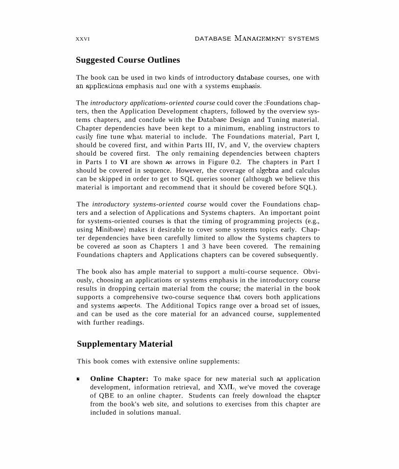
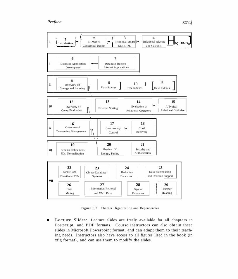
The book is organized into six main parts plus a collection of advanced topics, asshown in Figure 0.1. The Foundations chapters introduce database systems, the
(1) Foundations Both(2) Application Development Applications emphasis(3) Storage and Indexing Systems emphasis(4) Query Evaluation Systems emphasis(5) Transaction Management Systems emphasis(6) Database Design and Tuning Applications emphasis(7) Additional Topics Both
Figure 0.1 Organization of Parts in the Third Edition
ER model and the relational model. They explain how databases are createdand used, and cover the basics of database design and querying, including anin-depth treatment of SQL queries. While an instructor can omit some of thismaterial at their discretion (e.g., relational calculus, some sections on the ERmodel or SQL queries), this material is relevant to every student of databasesystems, and we recommend that it be covered in as much detail as possible.
Each of the remaining five main parts has either an application or a systemsempha.sis. Each of the three Systems parts has an overview chapter, designed toprovide a self-contained treatment, e.g., Chapter 8 is an overview of storage andindexing. The overview chapters can be used to provide stand-alone coverageof the topic, or as the first chapter in a more detailed treatment. Thus, in anapplication-oriented course, Chapter 8 might be the only material covered onfile organizations and indexing, whereas in a systems-oriented course it would besupplemented by a selection from Chapters 9 through 11. The Database Designand Tuning part contains a discussion of performance tuning and designing forsecure access. These application topics are best covered after giving studentsa good grasp of database system architecture, and are therefore placed later inthe chapter sequence.
XXVI
Suggested Course Outlines
DATABASE ~1ANAGEMENTSYSTEMS
The book can be used in two kinds of introductory database courses, one withan applications emphasis and one with a systems empha..':iis.
The introductory applications- oriented course could cover the :Foundations chapters, then the Application Development chapters, followed by the overview systems chapters, and conclude with the Database Design and Tuning material.Chapter dependencies have been kept to a minimum, enabling instructors toeasily fine tune what material to include. The Foundations material, Part I,should be covered first, and within Parts III, IV, and V, the overview chaptersshould be covered first. The only remaining dependencies between chaptersin Parts I to VI are shown as arrows in Figure 0.2. The chapters in Part Ishould be covered in sequence. However, the coverage of algebra and calculuscan be skipped in order to get to SQL queries sooner (although we believe thismaterial is important and recommend that it should be covered before SQL).
The introductory systems-oriented course would cover the Foundations chapters and a selection of Applications and Systems chapters. An important pointfor systems-oriented courses is that the timing of programming projects (e.g.,using Minibase) makes it desirable to cover some systems topics early. Chapter dependencies have been carefully limited to allow the Systems chapters tobe covered as soon as Chapters 1 and 3 have been covered. The remainingFoundations chapters and Applications chapters can be covered subsequently.
The book also has ample material to support a multi-course sequence. Obviously, choosing an applications or systems emphasis in the introductory courseresults in dropping certain material from the course; the material in the booksupports a comprehensive two-course sequence that covers both applicationsand systems a.spects. The Additional Topics range over a broad set of issues,and can be used as the core material for an advanced course, supplementedwith further readings.
Supplementary Material
This book comes with extensive online supplements:
.. Online Chapter: To make space for new material such a.'3 applicationdevelopment, information retrieval, and XML, we've moved the coverageof QBE to an online chapter. Students can freely download the chapterfrom the book's web site, and solutions to exercises from this chapter areincluded in solutions manual.
Preface xxvii;
( , ( ( 32 4 H 5 JI I 1~ !---i Relational Model Relational AlgebraI Introduction, : ERModel 1--1SQLDM~
"---~~~ . Conceptual Design l SQLDDL and Calculus
II
6Database Application ~
Development
7Database-Backed
Internet Applications
8 9 ] 10 ] [ 11 ]III Overview of
J\Storage and Indexing Data Storage Tree Indexes Hash Indexes
\
12 13 14 15IV Overview of Evaluation of I-- A Typical
Query Evaluation 1\ External SortingRelational Operators Relational Optimizer
\
16 17 18V Overview of Concurrency r-- Crash
Transaction Management 1\ Control Recovery
\ \
\19 20 21VI Schema Refinement, Physical DB Security and
FDs, Normalization Design, Tuning Authorization
22 23 24 25Parallel and Object-Database Deductive Data Warehousing
Distributed DBs Systems Databases and Decision Support
VII
C26 27 28 29Data Information Retrieval Spatial Further
Mining and XML Data Databases Reading
Figure 0.2 Chapter Organization and Dependencies
lIII Lecture Slides: Lecture slides are freely available for all chapters inPostscript, and PDF formats. Course instructors can also obtain theseslides in Microsoft Powerpoint format, and can adapt them to their teaching needs. Instructors also have access to all figures llsed in the book (inxfig format), and can use them to modify the slides.
xxviii DATABASE IVIANAGEMENT SVSTErvIS
• Solutions to Chapter Exercises: The book has an UnUS1H:l,lly extensiveset of in-depth exercises. Students can obtain solutioIls to odd-numberedchapter exercises and a set of lecture slides for each chapter through thevVeb in Postscript and Adobe PDF formats. Course instructors can obtainsolutions to all exercises.
• Software: The book comes with two kinds of software. First, we haveJ\!Iinibase, a small relational DBMS intended for use in systems-orientedcourses. Minibase comes with sample assignments and solutions, as described in Appendix 30. Access is restricted to course instructors. Second,we offer code for all SQL and Java application development exercises inthe book, together with scripts to create sample databases, and scripts forsetting up several commercial DBMSs. Students can only access solutioncode for odd-numbered exercises, whereas instructors have access to allsolutions.
• Instructor's Manual: The book comes with an online manual that offers instructors comments on the material in each chapter. It provides asummary of each chapter and identifies choices for material to emphasizeor omit. The manual also discusses the on-line supporting material forthat chapter and offers numerous suggestions for hands-on exercises andprojects. Finally, it includes samples of examination papers from coursestaught by the authors using the book. It is restricted to course instructors.
For More Information
The home page for this book is at URL:
http://www.cs.wisc.edu/-dbbook
It contains a list of the changes between the 2nd and 3rd editions, and a frequently updated link to all known erTOT8 in the book and its accompanyingsupplements. Instructors should visit this site periodically or register at thissite to be notified of important changes by email.
Acknowledgments
This book grew out of lecture notes for CS564, the introductory (senior/graduatelevel) database course at UvV-Madison. David De\Vitt developed this courseand the Minirel project, in which students wrote several well-chosen parts ofa relational DBMS. My thinking about this material was shaped by teachingCS564, and Minirel was the inspiration for Minibase, which is more comprehensive (e.g., it has a query optimizer and includes visualization software) but

Preface XXIX
tries to retain the spirit of MinireL lVEke Carey and I jointly designed much ofMinibase. My lecture notes (and in turn this book) were influenced by Mike'slecture notes and by Yannis Ioannidis's lecture slides.
Joe Hellerstein used the beta edition of the book at Berkeley and providedinvaluable feedback, assistance on slides, and hilarious quotes. vVriting thechapter on object-database systems with Joe was a lot of fun.
C. Mohan provided invaluable assistance, patiently answering a number of questions about implementation techniques used in various commercial systems, inparticular indexing, concurrency control, and recovery algorithms. Moshe Zloofanswered numerous questions about QBE semantics and commercial systemsbased on QBE. Ron Fagin, Krishna Kulkarni, Len Shapiro, Jim Melton, DennisShasha, and Dirk Van Gucht reviewed the book and provided detailed feedback,greatly improving the content and presentation. Michael Goldweber at BeloitCollege, Matthew Haines at Wyoming, Michael Kifer at SUNY StonyBrook,Jeff Naughton at Wisconsin, Praveen Seshadri at Cornell, and Stan Zdonik atBrown also used the beta edition in their database courses and offered feedbackand bug reports. In particular, Michael Kifer pointed out an error in the (old)algorithm for computing a minimal cover and suggested covering some SQLfeatures in Chapter 2 to improve modularity. Gio Wiederhold's bibliography,converted to Latex format by S. Sudarshan, and Michael Ley's online bibliography on databases and logic programming were a great help while compiling thechapter bibliographies. Shaun Flisakowski and Uri Shaft helped me frequentlyin my never-ending battles with Latex.
lowe a special thanks to the many, many students who have contributed tothe Minibase software. Emmanuel Ackaouy, Jim Pruyne, Lee Schumacher, andMichael Lee worked with me when I developed the first version of Minibase(much of which was subsequently discarded, but which influenced the nextversion). Emmanuel Ackaouy and Bryan So were my TAs when I taught CS564using this version and went well beyond the limits of a TAship in their effortsto refine the project. Paul Aoki struggled with a version of Minibase andoffered lots of useful eomments as a TA at Berkeley. An entire class of CS764students (our graduate database course) developed much of the current versionof Minibase in a large class project that was led and coordinated by Mike Careyand me. Amit Shukla and Michael Lee were my TAs when I first taught CS564using this vers~on of Minibase and developed the software further.
Several students worked with me on independent projects, over a long periodof time, to develop Minibase components. These include visualization packagesfor the buffer manager and B+ trees (Huseyin Bekta.'3, Harry Stavropoulos, andWeiqing Huang); a query optimizer and visualizer (Stephen Harris, Michael Lee,and Donko Donjerkovic); an ER diagram tool based on the Opossum schema
xxx DATABASE NIANAGEMENT SYSTEMS~
editor (Eben Haber); and a GUI-based tool for normalization (Andrew Prockand Andy Therber). In addition, Bill Kimmel worked to integrate and fix alarge body of code (storage manager, buffer manager, files and access methods,relational operators, and the query plan executor) produced by the CS764 classproject. Ranjani Ramamurty considerably extended Bill's work on cleaning upand integrating the various modules. Luke Blanshard, Uri Shaft, and ShaunFlisakowski worked on putting together the release version of the code anddeveloped test suites and exercises based on the Minibase software. KrishnaKunchithapadam tested the optimizer and developed part of the Minibase GUI.
Clearly, the Minibase software would not exist without the contributions of agreat many talented people. With this software available freely in the publicdomain, I hope that more instructors will be able to teach a systems-orienteddatabase course with a blend of implementation and experimentation to complement the lecture material.
I'd like to thank the many students who helped in developing and checkingthe solutions to the exercises and provided useful feedback on draft versions ofthe book. In alphabetical order: X. Bao, S. Biao, M. Chakrabarti, C. Chan,W. Chen, N. Cheung, D. Colwell, C. Fritz, V. Ganti, J. Gehrke, G. Glass, V.Gopalakrishnan, M. Higgins, T. Jasmin, M. Krishnaprasad, Y. Lin, C. Liu, M.Lusignan, H. Modi, S. Narayanan, D. Randolph, A. Ranganathan, J. Reminga,A. Therber, M. Thomas, Q. Wang, R. Wang, Z. Wang, and J. Yuan. ArcadyGrenadeI' , James Harrington, and Martin Reames at Wisconsin and Nina Tangat Berkeley provided especially detailed feedback.
Charlie Fischer, Avi Silberschatz, and Jeff Ullman gave me invaluable adviceon working with a publisher. My editors at McGraw-Hill, Betsy Jones and EricMunson, obtained extensive reviews and guided this book in its early stages.Emily Gray and Brad Kosirog were there whenever problems cropped up. AtWisconsin, Ginny Werner really helped me to stay on top of things.
Finally, this book was a thief of time, and in many ways it was harder on myfamily than on me. My sons expressed themselves forthrightly. From my (then)five-year-old, Ketan: "Dad, stop working on that silly book. You don't haveany time for me." Two-year-old Vivek: "You working boook? No no no comeplay basketball me!" All the seasons of their discontent were visited upon mywife, and Apu nonetheless cheerfully kept the family going in its usual chaotic,happy way all the many evenings and weekends I was wrapped up in this book.(Not to mention the days when I was wrapped up in being a faculty member!)As in all things, I can trace my parents' hand in much of this; my father,with his love of learning, and my mother, with her love of us, shaped me. Mybrother Kartik's contributions to this book consisted chiefly of phone calls inwhich he kept me from working, but if I don't acknowledge him, he's liable to
Preface
be annoyed. I'd like to thank my family for being there and giving meaning toeverything I do. (There! I knew I'd find a legitimate reason to thank Kartik.)
Acknowledgments for the Second Edition
Emily Gray and Betsy Jones at 1tfcGraw-Hill obtained extensive reviews andprovided guidance and support as we prepared the second edition. JonathanGoldstein helped with the bibliography for spatial databases. The followingreviewers provided valuable feedback on content and organization: Liming Caiat Ohio University, Costas Tsatsoulis at University of Kansas, Kwok-Bun Vueat University of Houston, Clear Lake, William Grosky at Wayne State University, Sang H. Son at University of Virginia, James M. Slack at Minnesota StateUniversity, Mankato, Herman Balsters at University of Twente, Netherlands,Karen C. Davis at University of Cincinnati, Joachim Hammer at University ofFlorida, Fred Petry at Tulane University, Gregory Speegle at Baylor University, Salih Yurttas at Texas A&M University, and David Chao at San FranciscoState University.
A number of people reported bugs in the first edition. In particular, we wishto thank the following: Joseph Albert at Portland State University, Han-yinChen at University of Wisconsin, Lois Delcambre at Oregon Graduate Institute,Maggie Eich at Southern Methodist University, Raj Gopalan at Curtin University of Technology, Davood Rafiei at University of Toronto, Michael Schrefl atUniversity of South Australia, Alex Thomasian at University of Connecticut,and Scott Vandenberg at Siena College.
A special thanks to the many people who answered a detailed survey about howcommercial systems support various features: At IBM, Mike Carey, Bruce Lindsay, C. Mohan, and James Teng; at Informix, M. Muralikrishna and MichaelUbell; at Microsoft, David Campbell, Goetz Graefe, and Peter Spiro; at Oracle,Hakan Jacobsson, Jonathan D. Klein, Muralidhar Krishnaprasad, and M. Ziauddin; and at Sybase, Marc Chanliau, Lucien Dimino, Sangeeta Doraiswamy,Hanuma Kodavalla, Roger MacNicol, and Tirumanjanam Rengarajan.
After reading about himself in the acknowledgment to the first edition, Ketan(now 8) had a simple question: "How come you didn't dedicate the book to us?Why mom?" K~tan, I took care of this inexplicable oversight. Vivek (now 5)was more concerned about the extent of his fame: "Daddy, is my name in evvycopy of your book? Do they have it in evvy compooter science department inthe world'?" Vivek, I hope so. Finally, this revision would not have made itwithout Apu's and Keiko's support.

xx.,xii DATABASE l\IANAGEl'vIENT SYSTEMS
Acknowledgments for the Third Edition
\rYe thank Raghav Kaushik for his contribution to the discussion of XML, andAlex Thomasian for his contribution to the coverage of concurrency control. Aspecial thanks to Jim JVlelton for giving us a pre-publication copy of his bookon object-oriented extensions in the SQL: 1999 standard, and catching severalbugs in a draft of this edition. Marti Hearst at Berkeley generously permittedus to adapt some of her slides on Information Retrieval, and Alon Levy andDan Sueiu were kind enough to let us adapt some of their lectures on X:NIL.Mike Carey offered input on Web services.
Emily Lupash at McGraw-Hill has been a source of constant support and encouragement. She coordinated extensive reviews from Ming Wang at EmbryRiddle Aeronautical University, Cheng Hsu at RPI, Paul Bergstein at Univ. ofMassachusetts, Archana Sathaye at SJSU, Bharat Bhargava at Purdue, JohnFendrich at Bradley, Ahmet Ugur at Central Michigan, Richard Osborne atUniv. of Colorado, Akira Kawaguchi at CCNY, Mark Last at Ben Gurion,Vassilis Tsotras at Univ. of California, and Ronald Eaglin at Univ. of CentralFlorida. It is a pleasure to acknowledge the thoughtful input we received fromthe reviewers, which greatly improved the design and content of this edition.Gloria Schiesl and Jade Moran dealt cheerfully and efficiently with last-minutesnafus, and, with Sherry Kane, made a very tight schedule possible. MichelleWhitaker iterated many times on the cover and end-sheet design.
On a personal note for Raghu, Ketan, following the canny example of thecamel that shared a tent, observed that "it is only fair" that Raghu dedicatethis edition solely to him and Vivek, since "mommy already had it dedicatedonly to her." Despite this blatant attempt to hog the limelight, enthusiasticallysupported by Vivek and viewed with the indulgent affection of a doting father,this book is also dedicated to Apu, for being there through it all.
For Johannes, this revision would not have made it without Keiko's supportand inspiration and the motivation from looking at Elisa's peacefully sleepingface.

PART I
FOUNDATIONS

1OVERVIEW OF
DATABASE SYSTEMS
-- What is a DBMS, in particular, a relational DBMS?
.. Why should we consider a DBMS to manage data?
.. How is application data represented in a DBMS?
-- How is data in a DBMS retrieved and manipulated?
.. How does a DBMS support concurrent access and protect data duringsystem failures?
.. What are the main components of a DBMS?
.. Who is involved with databases in real life?
.. Key concepts: database management, data independence, databasedesign, data model; relational databases and queries; schemas, levelsof abstraction; transactions, concurrency and locking, recovery andlogging; DBMS architecture; database administrator, application programmer, end user
Has everyone noticed that all the letters of the word database are typed withthe left hand? Now the layout of the QWEHTY typewriter keyboard was designed,among other things, to facilitate the even use of both hands. It follows, therefore,that writing about databases is not only unnatural, but a lot harder than it appears.
---Anonymous
The alIlount of information available to us is literally exploding, and the valueof data as an organizational asset is widely recognized. To get the most out oftheir large and complex datasets, users require tools that simplify the tasks of
3
4 CHAPTER If
The area of database management systenls is a microcosm of computer science in general. The issues addressed and the techniques used span a widespectrum, including languages, object-orientation and other progTammingparadigms, compilation, operating systems, concurrent programming, datastructures, algorithms, theory, parallel and distributed systems, user interfaces, expert systems and artificial intelligence, statistical techniques, anddynamic programming. \Ve cannot go into all these &<;jpects of databasemanagement in one book, but we hope to give the reader a sense of theexcitement in this rich and vibrant discipline.
managing the data and extracting useful information in a timely fashion. Otherwise, data can become a liability, with the cost of acquiring it and managingit far exceeding the value derived from it.
A database is a collection of data, typically describing the activities of one ormore related organizations. For example, a university database might containinformation about the following:
• Entities such as students, faculty, courses, and classrooms.
• Relationships between entities, such as students' enrollment in courses,faculty teaching courses, and the use of rooms for courses.
A database management system, or DBMS, is software designed to assistin maintaining and utilizing large collections of data. The need for such systems,as well as their use, is growing rapidly. The alternative to using a DBMS isto store the data in files and write application-specific code to manage it. Theuse of a DBMS has several important advantages, as we will see in Section 1.4.
1.1 MANAGING DATA
The goal of this book is to present an in-depth introduction to database management systems, with an empha.sis on how to design a database and 'li8C aDBMS effectively. Not surprisingly, many decisions about how to use a DBIvISfor a given application depend on what capabilities the DBMS supports efficiently. Therefore, to use a DBMS well, it is necessary to also understand howa DBMS work8.
Many kinds of database management systems are in use, but this book concentrates on relational database systems (RDBMSs), which are by far thedominant type of DB~'IS today. The following questions are addressed in thecorc chapters of this hook:
Overview of Databa8e SY8tem8 5
1. Database Design and Application Development: How can a userdescribe a real-world enterprise (e.g., a university) in terms of the datastored in a DBMS? \Vhat factors must be considered in deciding how toorganize the stored data? How can ,ve develop applications that rely upona DBMS? (Chapters 2, 3, 6, 7, 19, 20, and 21.)
2. Data Analysis: How can a user answer questions about the enterprise byposing queries over the data in the DBMS? (Chapters 4 and 5.)1
3. Concurrency and Robustness: How does a DBMS allow many users toaccess data concurrently, and how does it protect the data in the event ofsystem failures? (Chapters 16, 17, and 18.)
4. Efficiency and Scalability: How does a DBMS store large datasets andanswer questions against this data efficiently? (Chapters 8, 9, la, 11, 12,13, 14, and 15.)
Later chapters cover important and rapidly evolving topics, such as parallel anddistributed database management, data warehousing and complex queries fordecision support, data mining, databases and information retrieval, XML repositories, object databases, spatial data management, and rule-oriented DBMSextensions.
In the rest of this chapter, we introduce these issues. In Section 1.2, we begin with a brief history of the field and a discussion of the role of databasemanagement in modern information systems. We then identify the benefits ofstoring data in a DBMS instead of a file system in Section 1.3, and discussthe advantages of using a DBMS to manage data in Section 1.4. In Section1.5, we consider how information about an enterprise should be organized andstored in a DBMS. A user probably thinks about this information in high-levelterms that correspond to the entities in the organization and their relationships, whereas the DBMS ultimately stores data in the form of (rnany, many)bits. The gap between how users think of their data and how the data is ultimately stored is bridged through several levels of abstract1:on supported bythe DBMS. Intuitively, a user can begin by describing the data in fairly highlevel terms, then refine this description by considering additional storage andrepresentation details as needed.
In Section 1.6, we consider how users can retrieve data stored in a DBMS andthe need for techniques to efficiently compute answers to questions involvingsuch data. In Section 1.7, we provide an overview of how a DBMS supportsconcurrent access to data by several users and how it protects the data in theevent of system failures.
1 An online chapter on Query-by-Example (QBE) is also available.
6 CHAPTERrl
vVe then briefly describe the internal structure of a DBMS in Section 1.8, andmention various groups of people associated with the development and use ofa DBMS in Section 1.9.
1.2 A HISTORICAL PERSPECTIVE
From the earliest days of computers, storing and manipulating data have been amajor application focus. The first general-purpose DBMS, designed by CharlesBachman at General Electric in the early 1960s, was called the Integrated DataStore. It formed the basis for the network data model, which was standardizedby the Conference on Data Systems Languages (CODASYL) and strongly influenced database systems through the 1960s. Bachman was the first recipientof ACM's Turing Award (the computer science equivalent of a Nobel Prize) forwork in the database area; he received the award in 1973.
In the late 1960s, IBM developed the Information Management System (IMS)DBMS, used even today in many major installations. IMS formed the basis foran alternative data representation framework called the hierarchical data model.The SABRE system for making airline reservations was jointly developed byAmerican Airlines and IBM around the same time, and it allowed several peopleto access the same data through a computer network. Interestingly, today thesame SABRE system is used to power popular Web-based travel services suchas Travelocity.
In 1970, Edgar Codd, at IBM's San Jose Research Laboratory, proposed a newdata representation framework called the relational data model. This proved tobe a watershed in the development of database systems: It sparked the rapiddevelopment of several DBMSs based on the relational model, along with a richbody of theoretical results that placed the field on a firm foundation. Coddwon the 1981 Turing Award for his seminal work. Database systems maturedas an academic discipline, and the popularity of relational DBMSs changed thecommercial landscape. Their benefits were widely recognized, and the use ofDBMSs for managing corporate data became standard practice.
In the 1980s, the relational model consolidated its position as the dominantDBMS paradigm, and database systems continued to gain widespread use. TheSQL query language for relational databases, developed as part of IBM's System R project, is now the standard query language. SQL was standardizedin the late 1980s, and the current standard, SQL:1999, was adopted by theAmerican National Standards Institute (ANSI) and International Organizationfor Standardization (ISO). Arguably, the most widely used form of concurrentprogramming is the concurrent execution of database programs (called transactions). Users write programs a." if they are to be run by themselves, and
Overview of Database Systems 7
the responsibility for running them concurrently is given to the DBl\/IS. JamesGray won the 1999 Turing award for his contributions to database transactionmanagement.
In the late 1980s and the 1990s, advances were made in many areas of databasesystems. Considerable research was carried out into more powerful query languages and richer data models, with emphasis placed on supporting complexanalysis of data from all parts of an enterprise. Several vendors (e.g., IBM'sDB2, Oracle 8, Informix2 UDS) extended their systems with the ability to storenew data types such as images and text, and to ask more complex queries. Specialized systems have been developed by numerous vendors for creating datawarehouses, consolidating data from several databases, and for carrying outspecialized analysis.
An interesting phenomenon is the emergence of several enterprise resourceplanning (ERP) and management resource planning (MRP) packages,which add a substantial layer of application-oriented features on top of a DBMS.Widely used. packages include systems from Baan, Oracle, PeopleSoft, SAP,and Siebel. These packages identify a set of common tasks (e.g., inventorymanagement, human resources planning, financial analysis) encountered by alarge number of organizations and provide a general application layer to carryout these ta.'3ks. The data is stored in a relational DBMS and the applicationlayer can be customized to different companies, leading to lower overall costsfor the companies, compared to the cost of building the application layer fromscratch.
Most significant, perhaps, DBMSs have entered the Internet Age. While thefirst generation of websites stored their data exclusively in operating systemsfiles, the use of a DBMS to store data accessed through a Web browser isbecoming widespread. Queries are generated through Web-accessible formsand answers are formatted using a markup language such as HTML to beeasily displayed in a browser. All the database vendors are adding features totheir DBMS aimed at making it more suitable for deployment over the Internet.
Databclse management continues to gain importance as more and more data isbrought online and made ever more accessible through computer networking.Today the field is being driven by exciting visions such a'S multimedia databases,interactive video, streaming data, digital libraries, a host of scientific projectssuch as the human genome mapping effort and NASA's Earth Observation System project, and the desire of companies to consolidate their decision-makingprocesses and mine their data repositories for useful information about theirbusinesses. Commercially, database management systems represent one of the
2Informix was recently acquired by IBM.
8
largest and most vigorous market segments. Thus the study of database systems could prove to be richly rewarding in more ways than one!
1.3 FILE SYSTEMS VERSUS A DBMS
To understand the need for a DB:~,,1S, let us consider a motivating scenario: Acompany has a large collection (say, 500 GB3 ) of data on employees, departments, products, sales, and so on. This data is accessed concurrently by severalemployees. Questions about the data must be answered quickly, changes madeto the data by different users must be applied consistently, and access to certainparts of the data (e.g., salaries) must be restricted.
We can try to manage the data by storing it in operating system files. Thisapproach has many drawbacks, including the following:
• We probably do not have 500 GB of main memory to hold all the data.We must therefore store data in a storage device such as a disk or tape andbring relevant parts into main memory for processing as needed.
• Even if we have 500 GB of main memory, on computer systems with 32-bitaddressing, we cannot refer directly to more than about 4 GB of data. Wehave to program some method of identifying all data items.
• We have to write special programs to answer each question a user may wantto ask about the data. These programs are likely to be complex becauseof the large volume of data to be searched.
• We must protect the data from inconsistent changes made by different usersaccessing the data concurrently. If applications must address the details ofsuch concurrent access, this adds greatly to their complexity.
• We must ensure that data is restored to a consistent state if the systemcrac;hes while changes are being made.
• Operating systems provide only a password mechanism for security. This isnot sufficiently flexible to enforce security policies in which different usershave permission to access different subsets of the data.
A DBMS is a piece of software designed to make the preceding tasks easier. Bystoring data in.a DBNIS rather than as a collection of operating system files,we can use the DBMS's features to manage the data in a robust and efficientrnanner. As the volume of data and the number of users grow hundreds ofgigabytes of data and thousands of users are common in current corporatedatabases DBMS support becomes indispensable.------,- .
3 A kilobyte (KB) is 1024 bytes, a megabyte (MB) is 1024 KBs, a gigabyte (GB) is 1024 MBs, aterabyte ('1'B) is 1024 CBs, and a petabyte (PB) is 1024 terabytes.
Overv'iew of Database Systems
1.4 ADVANTAGES OF A DBMS
Using a DBMS to manage data h3..'3 many advantages:
9
II Data Independence: Application programs should not, ideally, be exposed to details of data representation and storage, The DBJVIS providesan abstract view of the data that hides such details.
II Efficient Data Access: A DBMS utilizes a variety of sophisticated techniques to store and retrieve data efficiently. This feature is especially impOl'tant if the data is stored on external storage devices.
II Data Integrity and Security: If data is always accessed through theDBMS, the DBMS can enforce integrity constraints. For example, beforeinserting salary information for an employee, the DBMS can check thatthe department budget is not exceeded. Also, it can enforce access contmlsthat govern what data is visible to different classes of users.
II Data Administration: When several users share the data, centralizingthe administration of data can offer sig11ificant improvements. Experiencedprofessionals who understand the nature of the data being managed, andhow different groups of users use it, can be responsible for organizing thedata representation to minimize redundancy and for fine-tuning the storageof the data to make retrieval efficient.
II Concurrent Access and Crash Recovery: A DBMS schedules concurrent accesses to the data in such a manner that users can think of the dataas being accessed by only one user at a time. Further, the DBMS protectsusers from the effects of system failures.
II Reduced Application Development Time: Clearly, the DBMS supports important functions that are common to many applications accessingdata in the DBMS. This, in conjunction with the high-level interface to thedata, facilitates quick application development. DBMS applications arealso likely to be more robust than similar stand-alone applications becausemany important tasks are handled by the DBMS (and do not have to bedebugged and tested in the application).
Given all these advantages, is there ever a reason not to use a DBMS? Sometimes, yes. A DBMS is a complex piece of software, optimized for certain kindsof workloads (e.g., answering complex queries or handling many concurrentrequests), and its performance may not be adequate for certain specialized applications. Examples include applications with tight real-time constraints orjust a few well-defined critical operations for which efficient custom code mustbe written. Another reason for not using a DBMS is that an application mayneed to manipulate the data in ways not supported by the query language. In
10 CHAPTER:l
such a situation, the abstract view of the datet presented by the DBlVIS doesnot match the application's needs and actually gets in the way. As an example, relational databa.'3es do not support flexible analysis of text data (althoughvendors are now extending their products in this direction).
If specialized performance or data manipulation requirements are central to anapplication, the application may choose not to use a DBMS, especially if theadded benefits of a DBMS (e.g., flexible querying, security, concurrent access,and crash recovery) are not required. In most situations calling for large-scaledata management, however, DBlVISs have become an indispensable tool.
1.5 DESCRIBING AND STORING DATA IN A DBMS
The user of a DBMS is ultimately concerned with some real-world enterprise,and the data to be stored describes various aspects of this enterprise. Forexample, there are students, faculty, and courses in a university, and the datain a university database describes these entities and their relationships.
A data model is a collection of high-level data description constructs that hidemany low-level storage details. A DBMS allows a user to define the data to bestored in terms of a data model. Most database management systems todayare based on the relational data model, which we focus on in this book.
While the data model of the DBMS hides many details, it is nonetheless closerto how the DBMS stores data than to how a user thinks about the underlyingenterprise. A semantic data model is a more abstract, high-level data modelthat makes it easier for a user to come up with a good initial description ofthe data in an enterprise. These models contain a wide variety of constructsthat help describe a real application scenario. A DBMS is not intended tosupport all these constructs directly; it is typically built around a data modelwith just a few bi:1Sic constructs, such as the relational model. A databa.sedesign in terms of a semantic model serves as a useful starting point and issubsequently translated into a database design in terms of the data model theDBMS actually supports.
A widely used semantic data model called the entity-relationship (ER) modelallows us to pictorially denote entities and the relationships among them. vVecover the ER model in Chapter 2.
Overview of Database Systc'lns 11J
An Example of Poor Design: The relational schema for Students illustrates a poor design choice; you should neVCT create a field such as age,whose value is constantly changing. A better choice would be DOB (fordate of birth); age can be computed from this. \Ve continue to use age inour examples, however, because it makes them easier to read.
1.5.1 The Relational Model
In this section we provide a brief introduction to the relational model. Thecentral data description construct in this model is a relation, which can bethought of as a set of records.
A description of data in terms of a data model is called a schema. In therelational model, the schema for a relation specifies its name, the name of eachfield (or attribute or column), and the type of each field. As an example,student information in a university database may be stored in a relation withthe following schema:
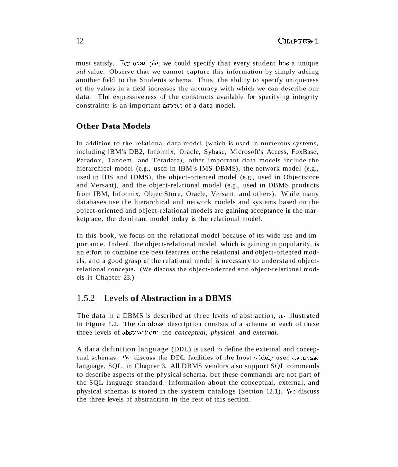
Students( sid: string, name: string, login: string,age: integer, gpa: real)
The preceding schema says that each record in the Students relation has fivefields, with field names and types as indicated. An example instance of theStudents relation appears in Figure 1.1.
I sid [ name IZogin
53666 Jones jones@cs 18 3.453688 Smith smith@ee 18 3.253650 Smith smith@math 19 3.853831 Madayan madayan(gmusic 11 1.853832 Guldu guldui:Qhnusic 12 2.0
Figure 1.1 An Instance of the Students Relation
Each row in the Students relation is a record that describes a student. Thedescription is rlOt completeo----for example, the student's height is not included--but is presumably adequate for the intended applications in the universitydatabase. Every row follows the schema of the Students relation. The schemacall therefore be regarded as a template for describing a student.
vVe can make the description of a collection of students more precise by specifying integrity constraints, which are conditions that the records in a relation
12 CHAPTER? 1
must satisfy. for example, we could specify that every student has a uniquesid value. Observe that we cannot capture this information by simply addinganother field to the Students schema. Thus, the ability to specify uniquenessof the values in a field increases the accuracy with which we can describe ourdata. The expressiveness of the constructs available for specifying integrityconstraints is an important ar;;pect of a data model.
Other Data Models
In addition to the relational data model (which is used in numerous systems,including IBM's DB2, Informix, Oracle, Sybase, Microsoft's Access, FoxBase,Paradox, Tandem, and Teradata), other important data models include thehierarchical model (e.g., used in IBM's IMS DBMS), the network model (e.g.,used in IDS and IDMS), the object-oriented model (e.g., used in Objectstoreand Versant), and the object-relational model (e.g., used in DBMS productsfrom IBM, Informix, ObjectStore, Oracle, Versant, and others). While manydatabases use the hierarchical and network models and systems based on theobject-oriented and object-relational models are gaining acceptance in the marketplace, the dominant model today is the relational model.
In this book, we focus on the relational model because of its wide use and importance. Indeed, the object-relational model, which is gaining in popularity, isan effort to combine the best features of the relational and object-oriented models, and a good grasp of the relational model is necessary to understand objectrelational concepts. (We discuss the object-oriented and object-relational models in Chapter 23.)
1.5.2 Levels of Abstraction in a DBMS
The data in a DBMS is described at three levels of abstraction, ar;; illustratedin Figure 1.2. The database description consists of a schema at each of thesethree levels of abstraction: the conceptual, physical, and external.
A data definition language (DDL) is used to define the external and coneeptual schemas. \;Ye discuss the DDL facilities of the Inost wid(~ly used databaselanguage, SQL, in Chapter 3. All DBMS vendors also support SQL commandsto describe aspects of the physical schema, but these commands are not part ofthe SQL language standard. Information about the conceptual, external, andphysical schemas is stored in the system catalogs (Section 12.1). vVe discussthe three levels of abstraction in the rest of this section.
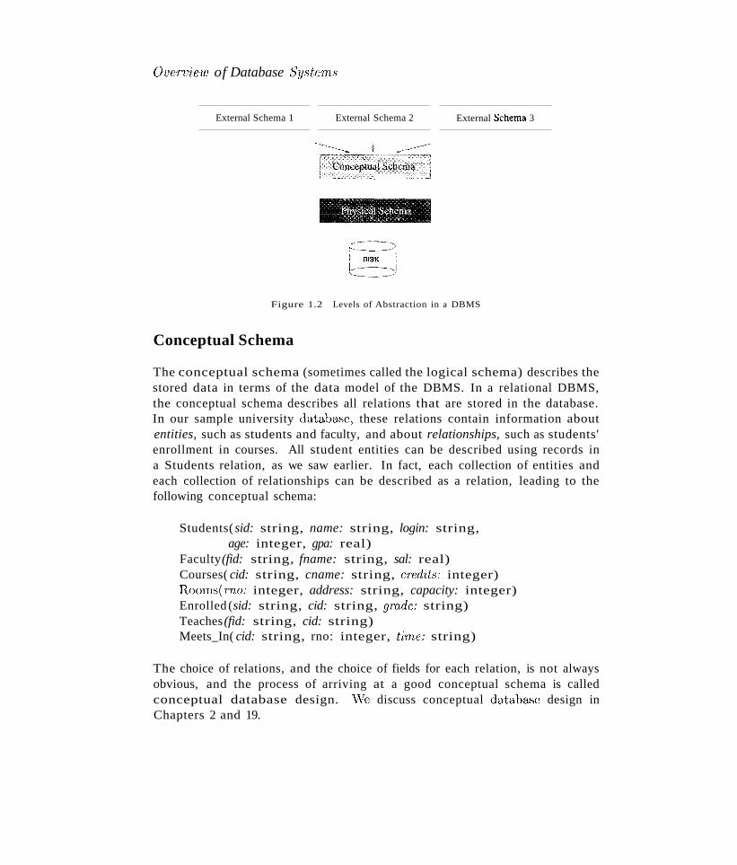
OucTlJ'iew of Database SyslcTns
External Schema 1 External Schema 2 External Schema 3
Figure 1.2 Levels of Abstraction in a DBMS
Conceptual Schema
The conceptual schema (sometimes called the logical schema) describes thestored data in terms of the data model of the DBMS. In a relational DBMS,the conceptual schema describes all relations that are stored in the database.In our sample university databa..'3e, these relations contain information aboutentities, such as students and faculty, and about relationships, such as students'enrollment in courses. All student entities can be described using records ina Students relation, as we saw earlier. In fact, each collection of entities andeach collection of relationships can be described as a relation, leading to thefollowing conceptual schema:
Students(sid: string, name: string, login: string,age: integer, gpa: real)
Faculty(fid: string, fname: string, sal: real)Courses( cid: string, cname: string, credits: integer)Rooms(nw: integer, address: string, capacity: integer)Enrolled (sid: string, cid: string, grade: string)Teaches(fid: string, cid: string)Meets_In( cid: string, rno: integer, ti'fne: string)
The choice of relations, and the choice of fields for each relation, is not alwaysobvious, and the process of arriving at a good conceptual schema is calledconceptual database design. vVe discuss conceptual databa..se design inChapters 2 and 19.
14
Physical Schema
CHAPTER»1
The physical schema specifies additional storage details. Essentially, thephysical schema summarizes how the relations described in the conceptualschema are actually stored on secondary storage devices such as disks andtapes.
We must decide what file organizations to use to store the relations and createauxiliary data structures, called indexes, to speed up data retrieval operations.A sample physical schema for the university database follows:
• Store all relations as unsorted files of records. (A file in a DBMS is eithera collection of records or a collection of pages, rather than a string ofcharacters as in an operating system.)
• Create indexes on the first column of the Students, Faculty, and Coursesrelations, the sal column of Faculty, and the capacity column of Rooms.
Decisions about the physical schema are based on an understanding of how thedata is typically accessed. The process of arriving at a good physical schemais called physical database design. We discuss physical database design inChapter 20.
External Schema
External schemas, which usually are also in terms of the data model ofthe DBMS, allow data access to be customized (and authorized) at the levelof individual users or groups of users. Any given database has exactly oneconceptual schema and one physical schema because it has just one set ofstored relations, but it may have several external schemas, each tailored to aparticular group of users. Each external schema consists of a collection of one ormore views and relations from the conceptual schema. A view is conceptuallya relation, but the records in a view are not stored in the DBMS. Rather, theyare computed using a definition for the view, in terms of relations stored in theDBMS. \iVe discuss views in more detail in Chapters 3 and 25.
The external schema design is guided by end user requirements. For exalnple,we might want to allow students to find out the names of faculty membersteaching courses as well as course enrollments. This can be done by definingthe following view:
Courseinfo( rid: string, fname: string, enTollment: integer)
A user can treat a view just like a relation and ask questions about the recordsin the view. Even though the records in the view are not stored explicitly,
Overview of Database Systems ).5
they are computed as needed. vVe did not include Courseinfo in the conceptualschema because we can compute Courseinfo from the relations in the conceptualschema, and to store it in addition would be redundant. Such redundancy, inaddition to the wasted space, could lead to inconsistencies. For example, atuple may be inserted into the Enrolled relation, indicating that a particularstudent has enrolled in some course, without incrementing the value in theenrollment field of the corresponding record of Courseinfo (if the latter also ispart of the conceptual schema and its tuples are stored in the DBMS).
L5.3 Data Independence
A very important advantage of using a DBMS is that it offers data independence. That is, application programs are insulated from changes in the waythe data is structured and stored. Data independence is achieved through useof the three levels of data abstraction; in particular, the conceptual schema andthe external schema provide distinct benefits in this area.
Relations in the external schema (view relations) are in principle generatedon demand from the relations corresponding to the conceptual schema.4 Ifthe underlying data is reorganized, that is, the conceptual schema is changed,the definition of a view relation can be modified so that the same relation iscomputed as before. For example, suppose that the Faculty relation in ouruniversity database is replaced by the following two relations:
Faculty_public (fid: string, fname: string, office: integer)Faculty_private (J£d: string, sal: real)
Intuitively, some confidential information about faculty has been placed in aseparate relation and information about offices has been added. The Courseinfoview relation can be redefined in terms of Faculty_public and Faculty_private,which together contain all the information in Faculty, so that a user who queriesCourseinfo will get the same answers as before.
Thus, users can be shielded from changes in the logical structure of the data, orchanges in the choice of relations to be stored. This property is called logicaldata independence.
In turn, the conceptual schema insulates users from changes in physical storagedetails. This property is referred to as physical data independence. Theconceptual schema hides details such as how the data is actually laid out ondisk, the file structure, and the choice of indexes. As long as the conceptual
4In practice, they could be precomputed and stored to speed up queries on view relations, but thecomputed view relations must be updated whenever the underlying relations are updated.
16 CHAPTE~ 1
schema remains the same, we can change these storage details without alteringapplications. (Of course, performance might be affected by such changes.)
1.6 QUERIES IN A DBMS
The ease \vith which information can be obtained from a database often determines its value to a user. In contrast to older database systems, relationaldatabase systems allow a rich class of questions to be posed easily; this featurehas contributed greatly to their popularity. Consider the sample universitydatabase in Section 1.5.2. Here are some questions a user might ask:
1. What is the name of the student with student ID 1234567
2. What is the average salary of professors who teach course CS5647
3. How many students are enrolled in CS5647
4. What fraction of students in CS564 received a grade better than B7
5. Is any student with a CPA less than 3.0 enrolled in CS5647
Such questions involving the data stored in a DBMS are called queries. ADBMS provides a specialized language, called the query language, in whichqueries can be posed. A very attractive feature of the relational model isthat it supports powerful query languages. Relational calculus is a formalquery language based on mathematical logic, and queries in this language havean intuitive, precise meaning. Relational algebra is another formal querylanguage, based on a collection of operators for manipulating relations, whichis equivalent in power to the calculus.
A DBMS takes great care to evaluate queries as efficiently as possible. vVediscuss query optimization and evaluation in Chapters 12, Vl, and 15. Ofcourse, the efficiency of query evaluation is determined to a large extent byhow the data is stored physically. Indexes can be used to speed up manyqueries----in fact, a good choice of indexes for the underlying relations can speedup each query in the preceding list. \Ve discuss data storage and indexing inChapters 8, 9, 10, and 11.
A DBMS enables users to create, modify, and query data through a datamanipulation language (DML). Thus, the query language is only one partof the Dl\ilL, which also provides constructs to insert, delete, and modify data,.vVe will discuss the DML features of SQL in Chapter 5. The DML and DDLare collectively referred to cl.s the data sublanguage when embedded withina host language (e.g., C or COBOL).
Overview of Database Systems
1.7 TRANSACTION MANAGEMENT
Consider a database that holds information about airline reservations. At anygiven instant, it is possible (and likely) that several travel agents are looking up information about available seats OIl various flights and making newseat reservations. When several users access (and possibly modify) a databaseconcurrently, the DBMS must order their requests carefully to avoid conflicts.For example, when one travel agent looks up Flight 100 on some given dayand finds an empty seat, another travel agent may simultaneously be makinga reservation for that seat, thereby making the information seen by the firstagent obsolete.
Another example of concurrent use is a bank's database. While one user'sapplication program is computing the total deposits, another application maytransfer money from an account that the first application has just 'seen' to anaccount that has not yet been seen, thereby causing the total to appear largerthan it should be. Clearly, such anomalies should not be allowed to occur.However, disallowing concurrent access can degrade performance.
Further, the DBMS must protect users from the effects of system failures byensuring that all data (and the status of active applications) is restored to aconsistent state when the system is restarted after a crash. For example, if atravel agent asks for a reservation to be made, and the DBMS responds sayingthat the reservation has been made, the reservation should not be lost if thesystem crashes. On the other hand, if the DBMS has not yet responded tothe request, but is making the necessary changes to the data when the crashoccurs, the partial changes should be undone when the system comes back up.
A transaction is anyone execution of a user program in a DBMS. (Executingthe same program several times will generate several transactions.) This is thebasic unit of change as seen by the DBMS: Partial transactions are not allowed,and the effect of a group of transactions is equivalent to some serial executionof all transactions. vVe briefly outline how these properties are guaranteed,deferring a detailed discussion to later chapters.
1.7.1 Concurrent Execution of Transactions
An important task of a DBMS is to schedule concurrent accesses to data sothat each user can safely ignore the fact that others are accessing the dataconcurrently. The importance of this ta.sk cannot be underestimated becausea database is typically shared by a large number of users, who submit theirrequests to the DBMS independently and simply cannot be expected to dealwith arbitrary changes being made concurrently by other users. A DBMS
18 CHAPTER a.
allows users to think of their programs &'3 if they were executing in isolation,one after the other in some order chosen by the DBJ\;:IS. For example, if aprogTam that deposits cash into an account is submitted to the DBMS at thesame time as another program that debits money from the same account, eitherof these programs could be run first by the DBMS, but their steps will not beinterleaved in such a way that they interfere with each other.
A locking protocol is a set of rules to be followed by each transaction (and enforced by the DBMS) to ensure that, even though actions of several transactionsmight be interleaved, the net effect is identical to executing all transactions insome serial order. A lock is a mechanism used to control access to databaseobjects. Two kinds of locks are commonly supported by a DBMS: sharedlocks on an object can be held by two different transactions at the same time,but an exclusive lock on an object ensures that no other transactions holdany lock on this object.
Suppose that the following locking protocol is followed: Every transaction begins by obtaining a shared lock on each data object that it needs to read and anexclusive lock on each data object that it needs to rnod~fy, then releases all itslocks after completing all actions. Consider two transactions T1 and T2 suchthat T1 wants to modify a data object and T2 wants to read the same object.Intuitively, if T1's request for an exclusive lock on the object is granted first,T2 cannot proceed until T1 relea..':les this lock, because T2's request for a sharedlock will not be granted by the DBMS until then. Thus, all of T1's actions willbe completed before any of T2's actions are initiated. We consider locking inmore detail in Chapters 16 and 17.
1.7.2 Incomplete Transactions and System Crashes
Transactions can be interrupted before running to completion for a va,riety ofreasons, e.g., a system crash. A DBMS must ensure that the changes made bysuch incomplete transactions are removed from the database. For example, ifthe DBMS is in the middle of transferring money from account A to accountB and has debited the first account but not yet credited the second when thecrash occurs, the money debited from account A must be restored when thesystem comes back up after the crash.
To do so, the DBMS maintains a log of all writes to the database. A crucialproperty of the log is that each write action must be recorded in the log (on disk)before the corresponding change is reflected in the database itself--otherwise, ifthe system crcLShes just after making the change in the datab(Lse but before thechange is recorded in the log, the DBIVIS would be unable to detect and undothis change. This property is called Write-Ahead Log, or WAL. To ensure
Overview of Database By.stems 19
this property, the DBMS must be able to selectively force a page in memory todisk.
The log is also used to ensure that the changes made by a successfully completed transaction are not lost due to a system crash, as explained in Chapter18. Bringing the database to a consistent state after a system crash can bea slow process, since the DBMS must ensure that the effects of all transactions that completed prior to the crash are restored, and that the effects ofincomplete transactions are undone. The time required to recover from a crashcan be reduced by periodically forcing some information to disk; this periodicoperation is called a checkpoint.
1.7.3 Points to Note
In summary, there are three points to remember with respect to DBMS supportfor concurrency control and recovery:
1. Every object that is read or written by a transaction is first locked in sharedor exclusive mode, respectively. Placing a lock on an object restricts itsavailability to other transactions and thereby affects performance.
2. For efficient log maintenance, the DBMS must be able to selectively forcea collection of pages in main memory to disk. Operating system supportfor this operation is not always satisfactory.
3. Periodic checkpointing can reduce the time needed to recover from a crash.Of course, this must be balanced against the fact that checkpointing toooften slows down normal execution.
1.8 STRUCTURE OF A DBMS
Figure 1.3 shows the structure (with some simplification) of a typical DBMSbased on the relational data model.
The DBMS accepts SQL comma,nels generated from a variety of user interfaces,produces query evaluation plans, executes these plans against the databc4'le, andreturns the answers. (This is a simplification: SQL commands can be embeddedin host-language application programs, e.g., Java or COBOL programs. vVeignore these issues to concentrate on the core DBl\ilS functionality.)
vVhen a user issues a query, the parsed query is presented to a query optimizer, which uses information about how the data is stored to produce anefficient execution plan for evaluating the query. An execution plan is a
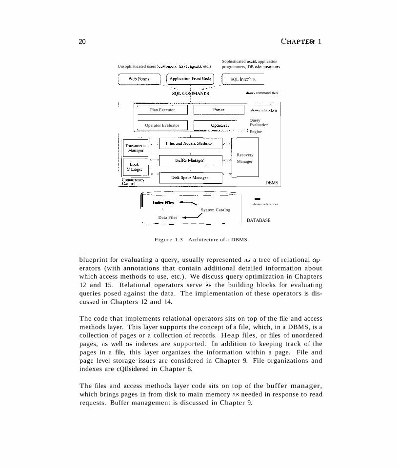
20 CHAPTER 1
Unsophisticated users (customers, travel agents, etc.)Sophisticated users. applicationprogrammers, DB administrators
DBMS
-shows references
DATABASE
Recovery
Manager
shov.':$ command now
SQL Interla<:e
\ System Catalog
Data Files .--/
Plan Executor
Operator Evaluator
[C-l Ind,"'I~---""
'----------,-~-~~-~ - --- ---,.--------.--
QueryEvaluation
L::::=======~=========::',J'Engine
Figure 1.3 Architecture of a DBMS
blueprint for evaluating a query, usually represented as a tree of relational operators (with annotations that contain additional detailed information aboutwhich access methods to use, etc.). We discuss query optimization in Chapters12 and 15. Relational operators serve as the building blocks for evaluatingqueries posed against the data. The implementation of these operators is discussed in Chapters 12 and 14.
The code that implements relational operators sits on top of the file and accessmethods layer. This layer supports the concept of a file, which, in a DBMS, is acollection of pages or a collection of records. Heap files, or files of unorderedpages, a:s well as indexes are supported. In addition to keeping track of thepages in a file, this layer organizes the information within a page. File andpage level storage issues are considered in Chapter 9. File organizations andindexes are cQIlsidered in Chapter 8.
The files and access methods layer code sits on top of the buffer manager,which brings pages in from disk to main memory ct." needed in response to readrequests. Buffer management is discussed in Chapter 9.
Ove1'Fie'll} of Database SY.'3te'171S 2).
The lowest layer of the DBMS software deals with management of space ondisk, where the data is stored. Higher layers allocate, deallocate, read, andwrite pages through (routines provided by) this layer, called the disk spacemanager. This layer is discussed in Chapter 9.
The DBMS supports concurrency and crash recovery by carefully schedulinguser requests and maintaining a log of all changes to the database. DBNIS components associated with concurrency control and recovery include the transaction manager, which ensures that transactions request and release locksaccording to a suitable locking protocol and schedules the execution transactions; the lock manager, which keeps track of requests for locks and grantslocks on database objects when they become available; and the recovery manager, which is responsible for maintaining a log and restoring the system to aconsistent state after a crash. The disk space manager, buffer manager, andfile and access method layers must interact with these components. We discussconcurrency control and recovery in detail in Chapter 16.
1.9 PEOPLE WHO WORK WITH DATABASES
Quite a variety of people are associated with the creation and use of databases.Obviously, there are database implementors, who build DBMS software,and end users who wish to store and use data in a DBMS. Dat,abase implementors work for vendors such as IBM or Oracle. End users come from a diverseand increasing number of fields. As data grows in complexity ant(volume, andis increasingly recognized as a major asset, the importance of maintaining itprofessionally in a DBMS is being widely accepted. Many end user.s simply useapplications written by database application programmers (see below) and sorequire little technical knowledge about DBMS software. Of course, sophisticated users who make more extensive use of a DBMS, such as writing their ownqueries, require a deeper understanding of its features.
In addition to end users and implementors, two other cla.'3ses of people areassociated with a DBMS: application programmer-s and database administrators.
Database application programmers develop packages that facilitate dataaccess for end users, who are usually not computer professionals, using thehost or data languages and software tools that DBMS vendors provide. (Suchtools include report writers, spreadsheets, statistical packages, and the like.)Application programs should ideally access data through the external schema.It is possible to write applications that access data at a lower level, but suchapplications would comprornise data independence.
22 CHAPTEI~ 1
A personal databa'3e is typically maintained by the individual who owns it anduses it. However, corporate or enterprise-wide databases are typically important enough and complex enough that the task of designing and maintaining thedatabase is entrusted to a professional, called the database administrator(DBA). The DBA is responsible for many critical tasks:
III Design of the Conceptual and Physical Schemas: The DBA is responsible for interacting with the users of the system to understand whatdata is to be stored in the DBMS and how it is likely to be used. Based onthis knowledge, the DBA must design the conceptual schema (decide whatrelations to store) and the physical schema (decide how to store them).The DBA may also design widely used portions of the external schema, although users probably augment this schema by creating additional views.
III Security and Authorization: The DBA is responsible for ensuring thatunauthorized data access is not permitted. In general, not everyone shouldbe able to access all the data. In a relational DBMS, users can be grantedpermission to access only certain views and relations. For example, although you might allow students to find out course enrollments and whoteaches a given course, you would not want students to see faculty salariesor each other's grade information. The DBA can enforce this policy bygiving students permission to read only the Courseinfo view.
III Data Availability and Recovery from Failures: The DBA must takesteps to ensure that if the system fails, users can continue to access as muchof the uncorrupted data as possible. The DBA must also work to restorethe data to a consistent state. The DB.I\!IS provides software support forthese functions, but the DBA is responsible for implementing proceduresto back up the data periodically and maintain logs of system activity (tofacilitate recovery from a crash).
l'il Database Tuning: Users' needs are likely to evolve with time. The DBAis responsible for modifying the database, in particular the conceptual andphysical schemas, to ensure adequate performance as requirements change.
1.10 REVIEW QUESTIONS
Answers to the review questions can be found in the listed sections.
III vVhat are the main benefits of using a DBMS to manage data in applications involving extensive data access? (Sections 1.1, 1.4)
III vVhen would you store data in a DBMS instead of in operating system filesand vice-versa? (Section 1.3)
Over-view of Database Systems 239
• What is a data model? \Vhat is the relational data model? What is dataindependence and how does a DBNIS support it? (Section 1.5)
• Explain the advantages of using a query language instead of custom programs to process data. (Section 1.6)
• What is a transaction? \Vhat guarantees does a DBMS offer with respectto transactions? (Section 1.7)
• What are locks in a DBMS, and why are they used? What is write-aheadlogging, and why is it used? What is checkpointing and why is it used?(Section 1.7)
• Identify the main components in a DBMS and briefly explain what theydo. (Section 1.8)
• Explain the different roles of database administrators, application programmers, and end users of a database. Who needs to know the most aboutdatabase systems? (Section 1.9)
EXERCISES
Exercise 1.1 Why would you choose a database system instead of simply storing data inoperating system files? When would it make sense not to use a database system?
Exercise 1.2 What is logical data independence and why is it important?
Exercise 1.3 Explain the difference between logical and physical data independence.
Exercise 1.4 Explain the difference between external, internal, and conceptual schemas.How are these different schema layers related to the concepts of logical and physical dataindependence?
Exercise 1.5 What are the responsibilities of a DBA? If we assume that the DBA is neverinterested in running his or her own queries, does the DBA still need to understand queryoptimization? Why?
Exercise 1.6 Scrooge McNugget wants to store information (names, addresses, descriptionsof embarrassing moments, etc.) about the many ducks on his payroll. Not surprisingly, thevolume of data compels him to buy a database system. To save money, he wants to buy onewith the fewest possible features, and he plans to run it as a stand-alone application on hisPC clone. Of course, Scrooge does not plan to share his list with anyone. Indicate which ofthe following DBMS features Scrooge should pay for; in each case, also indicate why Scroogeshould (or should not) pay for that feature in the system he buys.
1. A security facility.
2. Concurrency control.
3. Crash recovery.
4. A view mechanism.
24 CHAPTER 1
5. A query language.
Exercise 1.1 Which of the following plays an important role in representing informationabout the real world in a database'? Explain briefly.
1. The data definition language.
2. The data manipulation language.
3. The buffer manager.
4. The data model.
Exercise 1.8 Describe the structure of a DBMS. If your operating system is upgraded tosupport some new functions on as files (e.g., the ability to force some sequence of bytes todisk), which layer(s) of the DBMS would you have to rewrite to take advantage of these newfunctions?
Exercise 1.9 Answer the following questions:
1. What is a transaction?
2. Why does a DBMS interleave the actions of different transactions instead of executingtransactions one after the other?
3. What must a user guarantee with respect to a transaction and database consistency?What should a DBMS guarantee with respect to concurrent execution of several transactions and database consistency'?
4. Explain the strict two-phase locking protocol.
5. What is the WAL property, and why is it important?
PROJECT-BASED EXERCISES
Exercise 1.10 Use a Web browser to look at the HTML documentation for Minibase. Tryto get a feel for the overall architecture.
BIBLIOGRAPHIC NOTES
The evolution of database management systems is traced in [289]. The use of data modelsfor describing real-world data is discussed in [423], and [425] contains a taxonomy of datamodels. The three levels of abstraction were introduced in [186, 712]. The network datamodel is described in [186], and [775] discusses several commercial systems based on thismodel. [721] contains a good annotated collection of systems-oriented papers on databasemanagement.
Other texts covering database management systems include [204, 245, 305, 3;~9, 475, 574,689, 747, 762]. [204] provides a detailed discussion of the relational model from a conceptual standpoint and is notable for its extensive annotated bibliography. [574] presents aperformance-oriented perspective, with references to several commercial systems. [245] and[689] offer broad coverage of databa,se system concepts, including a discussion of the hierarchical and network data models. [339] emphasizes the connection between database querylanguages and logic programming. [762] emphasizes data models. Of these texts, [747] provides the most detailed discussion of theoretical issues. Texts devoted to theoretical aspectsinclude [3, 45, 501]. Handbook [744] includes a section on databases that contains introductorysurvey articles on a number of topics.
2INTRODUCTION TODATABASE DESIGN
.. What are the steps in designing a database?
.. Why is the ER model used to create an initial design?
.. What are the main concepts in the ER model?
.. What are guidelines for using the ER model effectively?
.. How does database design fit within the overall design framework forcomplex software within large enterprises?
.. What is UML and how is it related to the ER model?
.. Key concepts: database design, conceptual, logical, and physicaldesign; entity-relationship (ER) model, entity set, relationship set,attribute, instance, key; integrity constraints, one-to-many and manyto-many relationships, participation constraints; weak entities, classhierarchies, aggregation; UML, class diagrams, clataba,se diagrams,component diagrams.
The great successful men of the \vorld have used their imaginations. Theythink ahead and create their mental picture. and then go to work materializing thatpicture in all its details, filling in here, adding a little there, altering this bit andthat bit, but steadily building, steadily building.
Robert Collier
The (~ntitY-T'd(ltion8hip(ER) data 'model allows us to describe the data involvedin a real-world enterprise in terms of objects and their relationships and iswidely used to (levelop an initial databa.'3e design. It provides useful eonceptsthat allow us to move fronl an informal description of what users we:mt 1'rorn
25
26 CHAPTEij, 2
their database to a more detailed, precise description that can be implementedin a DBMS. In this chapter, we introduce the ER model and discuss how itsfeatures allow us to model a wide range of data faithfully.
\Ve begin with an overview of databa...')e design in Section 2.1 in order to motivateour discussion of the ER model. \Vithin the larger context of the overall designprocess, the ER model is used in a phase called conceptual database design.\Ve then introduce the ER model in Sections 2.2, 2.3, and 2.4. In Section 2.5,we discuss database design issues involving the ER model. We briefly discussconceptual database design for large enterprises in Section 2.6. In Section 2.7,we present an overview of UML, a design and modeling approach that is moregeneral in its scope than the ER model.
In Section 2.8, we introduce a case study that is used as a running examplethroughout the book. The case study is an end-to-end database design for anInternet shop. We illustrate the first two steps in database design (requirementsanalysis and conceptual design) in Section 2.8. In later chapters, we extend thiscase study to cover the remaining steps in the design process.
We note that many variations of ER diagrams are in use and no widely acceptedstandards prevail. The presentation in this chapter is representative of thefamily of ER models and includes a selection of the most popular features.
2.1 DATABASE DESIGN AND ER DIAGRAMS
We begin our discussion of database design by observing that this is typicallyjust one part, although a central part in data-intensive applications, of a largersoftware system design. Our primary focus is the design of the database, however, and we will not discuss other aspects of software design in any detail. Werevisit this point in Section 2.7.
The database design process can be divided into six steps. The ER model ismost relevant to the first three steps.
1. Requirements Analysis: The very first step in designing a databaseapplication is to understand what data is to be stored in the database,what applications must be built on top of it, and what operations aremost frequent and subject to performance requirements. In other words,we must find out what the users want from the database. This is usuallyan informal process that involves discussions with user groups, a studyof the current operating environment and how it is expected to change,analysis of any available documentation on existing applications that areexpected to be replaced or complemented by the database, and so OIl.
IntToduct'ion to Database Design 27.
Database Design Tools: Design tools are available from RDBwiS vendors as well as third-party vendors. For example! see the following link fordetails on design and analysis tools from Sybase:http://www.sybase.com/products/application_toolsThe following provides details on Oracle's tools:http://www.oracle.com/tools
Several methodologies have been proposed for organizing and presentingthe information gathered in this step, and some automated tools have beendeveloped to support this process.
2. Conceptual Database Design: The information gathered in the requirements analysis step is used to develop a high-level description of the datato be stored in the database, along with the constraints known to hold overthis data. This step is often carried out using the ER model and is discussed in the rest of this chapter. The ER model is one of several high-level,or semantic, data models used in database design. The goal is to createa simple description of the data that closely matches how users and developers think of the data (and the people and processes to be represented inthe data). This facilitates discussion among all the people involved in thedesign process, even those who have no technical background. At the sametime, the initial design must be sufficiently precise to enable a straightforward translation into a data model supported by a commercial databasesystem (which, in practice, means the relational model).
3. Logical Database Design: We must choose a DBMS to implementour databctse design, and convert the conceptual database design into adatabase schema in the data model of the chosen DBMS. We will consideronly relational DBMSs, and therefore, the task in the logical design stepis to convert an ER schema into a relational database schema. We discuss this step in detail in Chapter 3; the result is a conceptual schema,sometimes called the logical schema, in the relational data model.
2.1.1 Beyond ER Design
The ER diagram is just an approximate description of the data, constructedthrough a subjective evaluation of the information collected during requirements analysis. A more careful analysis can often refine the logical schemaobtained at the end of Step 3. Once we have a good logical schema, we mustconsider performance criteria and design the physical schema. Finally, we mustaddress security issues and ensure that users are able to access the data theyneed, but not data that we wish to hide from them. The remaining three stepsof clatabase design are briefly described next:
28 CHAPTER. 2
4. Schema Refinement: The fourth step ill databa')e design is to analyzethe collection of relations in our relational database schema to identify potential problems, and to refine it. In contrast to the requirements analysisand conceptual design steps, which are essentially subjective, schema refinement can be guided by some elegant and powerful theory. \Ve discussthe theory of normalizing relations-restructuring them to ensure somedesirable properties-in Chapter 19.
5. Physical Database Design: In this step, we consider typical expectedworkloads that our database must support and further refine the databasedesign to ensure that it meets desired performance criteria. This step maysimply involve building indexes on some tables and clustering some tables,or it may involve a substantial redesign of parts of the database schemaobtained from the earlier design steps. We discuss physical design anddatabase tuning in Chapter 20.
6. Application and Security Design: Any software project that involvesa DBMS must consider aspects of the application that go beyond thedatabase itself. Design methodologies like UML (Section 2.7) try to address the complete software design and development cycle. Briefly, we mustidentify the entities (e.g., users, user groups, departments) and processesinvolved in the application. We must describe the role of each entity in every process that is reflected in some application task, as part of a completeworkflow for that task. For each role, we must identify the parts of thedatabase that must be accessible and the parts of the database that mustnot be accessible, and we must take steps to ensure that these access rulesare enforced. A DBMS provides several mechanisms to assist in this step,and we discuss this in Chapter 21.
In the implementation phase, we must code each task in an application language (e.g., Java), using the DBlVIS to access data. We discuss applicationdevelopment in Chapters 6 and 7.
In general, our division of the design process into steps should be seen as aclassification of the kinds of steps involved in design. Realistically, althoughwe might begin with the six step process outlined here, a complete databasedesign will probably require a subsequent tuning phase in which all six kindsof design steps are interleaved and repeated until the design is satisfactory.
2.2 ENTITIES, ATTRIBUTES, AND ENTITY SETS
An entity is an object in the real world that is distinguishable frQm otherobjects. Examples include the following: the Green Dragonzord toy, the toydepartment, the manager of the toy department, the home address of the rnan-
Introd'lJ.ctioTt to Database De8'(qn
agel' of the toy department. It is often useful to identify a collection of similarentities. Such a collection is called an entity set. Note that entity sets neednot be disjoint; the collection of toy department employees and the collectionof appliance department employees may both contain employee John Doe (whohappens to work in both departments). \Ve could also define an entity set calledEmployees that contains both the toy and appliance department employee sets.
An entity is described using a set of attributes. All entities in a given entityset have the same attributes; this is what we mean by similar. (This statementis an oversimplification, as we will see when we discuss inheritance hierarchiesin Section 2.4.4, but it suffices for now and highlights the main idea.) Ourchoice of attributes reflects the level of detail at which we wish to representinformation about entities. For example, the Employees entity set could usename, social security number (ssn), and parking lot (lot) as attributes. In thiscase we will store the name, social security number, and lot number for eachemployee. However, we will not store, say, an employee's address (or gender orage).
For each attribute associated with an entity set, we must identify a domain ofpossible values. For example, the domain associated with the attribute nameof Employees might be the set of 20-character strings. 1 As another example, ifthe company rates employees on a scale of 1 to 10 and stores ratings in a fieldcalled mting, the associated domain consists of integers 1 through 10. FUrther,for each entity set, we choose a key. A key is a minimal set of attributes whosevalues uniquely identify an entity in the set. There could be more than onecandidate key; if so, we designate one of them as the primary key. For now weassume that each entity set contains at least one set of attributes that uniquelyidentifies an entity in the entity set; that is, the set of attributes contains a key.We revisit this point in Section 2.4.3.
The Employees entity set with attributes ssn, name, and lot is shown in Figure2.1. An entity set is represented by a rectangle, and an attribute is representedby an oval. Each attribute in the primary key is underlined. The domaininformation could be listed along with the attribute name, but we omit this tokeep the figures compact. The key is s.m.
2.3 REL~TIONSHIPS AND RELATIONSHIP SETS
A relationship is an association among two or more entities. For example, wemay have the relationship that Attishoo works in the pharmacy department.
iTo avoid confusion, we assume that attribute names do not repeat across entity sets. This is nota real limitation because we can always use the entity set name to resolve ambiguities if the sameattribute name is used in more than one entity set.
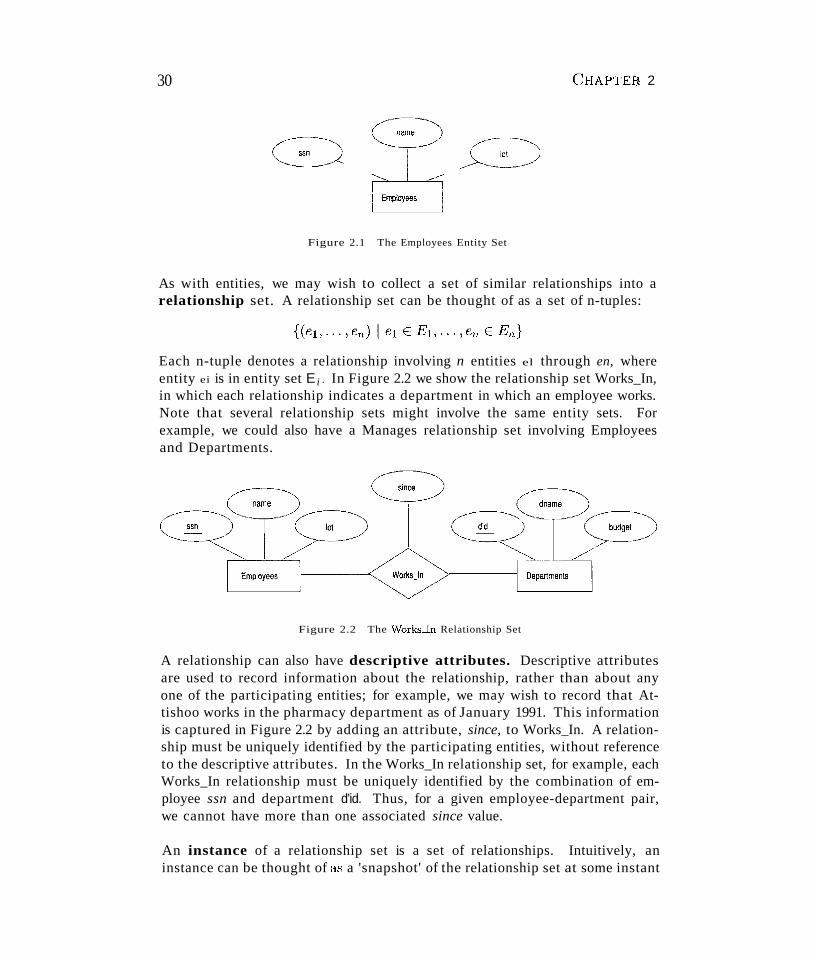
30 CHAPTER 2
Figure 2.1 The Employees Entity Set
As with entities, we may wish to collect a set of similar relationships into arelationship set. A relationship set can be thought of as a set of n-tuples:
Each n-tuple denotes a relationship involving n entities el through en, whereentity ei is in entity set E i . In Figure 2.2 we show the relationship set Works_In,in which each relationship indicates a department in which an employee works.Note that several relationship sets might involve the same entity sets. Forexample, we could also have a Manages relationship set involving Employeesand Departments.
Figure 2.2 The Works-ln Relationship Set
A relationship can also have descriptive attributes. Descriptive attributesare used to record information about the relationship, rather than about anyone of the participating entities; for example, we may wish to record that Attishoo works in the pharmacy department as of January 1991. This informationis captured in Figure 2.2 by adding an attribute, since, to Works_In. A relationship must be uniquely identified by the participating entities, without referenceto the descriptive attributes. In the Works_In relationship set, for example, eachWorks_In relationship must be uniquely identified by the combination of employee ssn and department d'id. Thus, for a given employee-department pair,we cannot have more than one associated since value.
An instance of a relationship set is a set of relationships. Intuitively, aninstance can be thought of &'3 a 'snapshot' of the relationship set at some instant
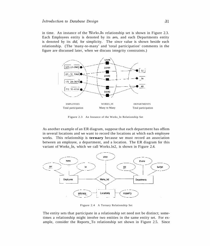
Introduction to Database Design ;31
in time. An instance of the vVorks.ln relationship set is shown in Figure 2.3.Each Employees entity is denoted by its ssn, and each Departments entityis denoted by its did, for simplicity. The since value is shown beside eachrelationship. (The 'many-te-many' and 'total participation' comments in thefigure are discussed later, when we discuss integrity constraints.)
~__I---\-~---r-~5J
---IIL---t----j-----W~
--.__---t-----\I-:::::~~
EMPLOYEES
Total participation
WORKS_IN
Many to Many
DEPARTMENTS
Total participation
Figure 2.3 An Instance of the Works_In Relationship Set
As another example of an ER diagram, suppose that each department has officesin several locations and we want to record the locations at which each employeeworks. This relationship is ternary because we must record an associationbetween an employee, a department, and a location. The ER diagram for thisvariant of Works_In, which we call Works.ln2, is shown in Figure 2.4.
Figure 2.4 A Ternary Relationship Set
The entity sets that participate in a relationship set need not be distinct; sometimes a relationship might involve two entities in the same entity set. For example, consider the Reports_To relationship set shown in Figure 2.5. Since
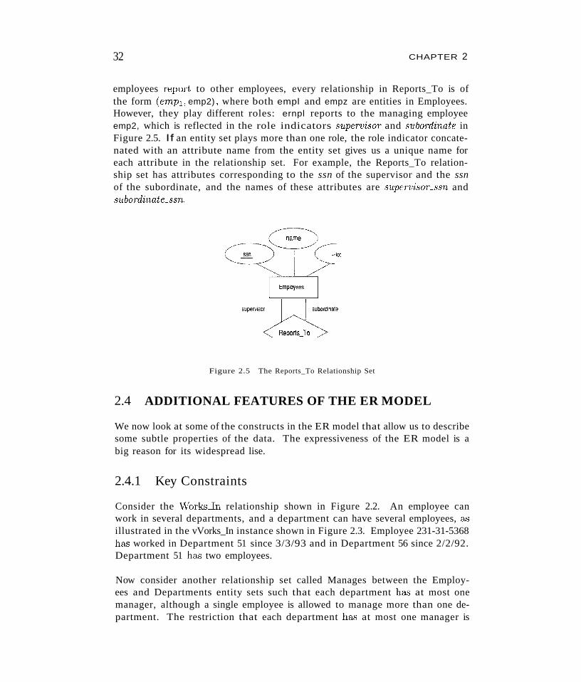
32 CHAPTER 2
employees report. to other employees, every relationship in Reports_To is ofthe form (emlJ1. emp2) , where both empl and empz are entities in Employees.However, they play different roles: ernpl reports to the managing employeeemp2, which is reflected in the role indicators supervisor and subordinate inFigure 2.5. If an entity set plays more than one role, the role indicator concatenated with an attribute name from the entity set gives us a unique name foreach attribute in the relationship set. For example, the Reports_To relationship set has attributes corresponding to the ssn of the supervisor and the ssnof the subordinate, and the names of these attributes are supcrvisoLssn andsubordinate-ssn.
Figure 2.5 The Reports_To Relationship Set
2.4 ADDITIONAL FEATURES OF THE ER MODEL
We now look at some of the constructs in the ER model that allow us to describesome subtle properties of the data. The expressiveness of the ER model is abig reason for its widespread lise.
2.4.1 Key Constraints
Consider the Works-.In relationship shown in Figure 2.2. An employee canwork in several departments, and a department can have several employees, &.,illustrated in the vVorks_In instance shown in Figure 2.3. Employee 231-31-5368h&., worked in Department 51 since 3/3/93 and in Department 56 since 2/2/92.Department 51 h&'3 two employees.
Now consider another relationship set called Manages between the Employees and Departments entity sets such that each department h&') at most onemanager, although a single employee is allowed to manage more than one department. The restriction that each department h&,> at most one manager is
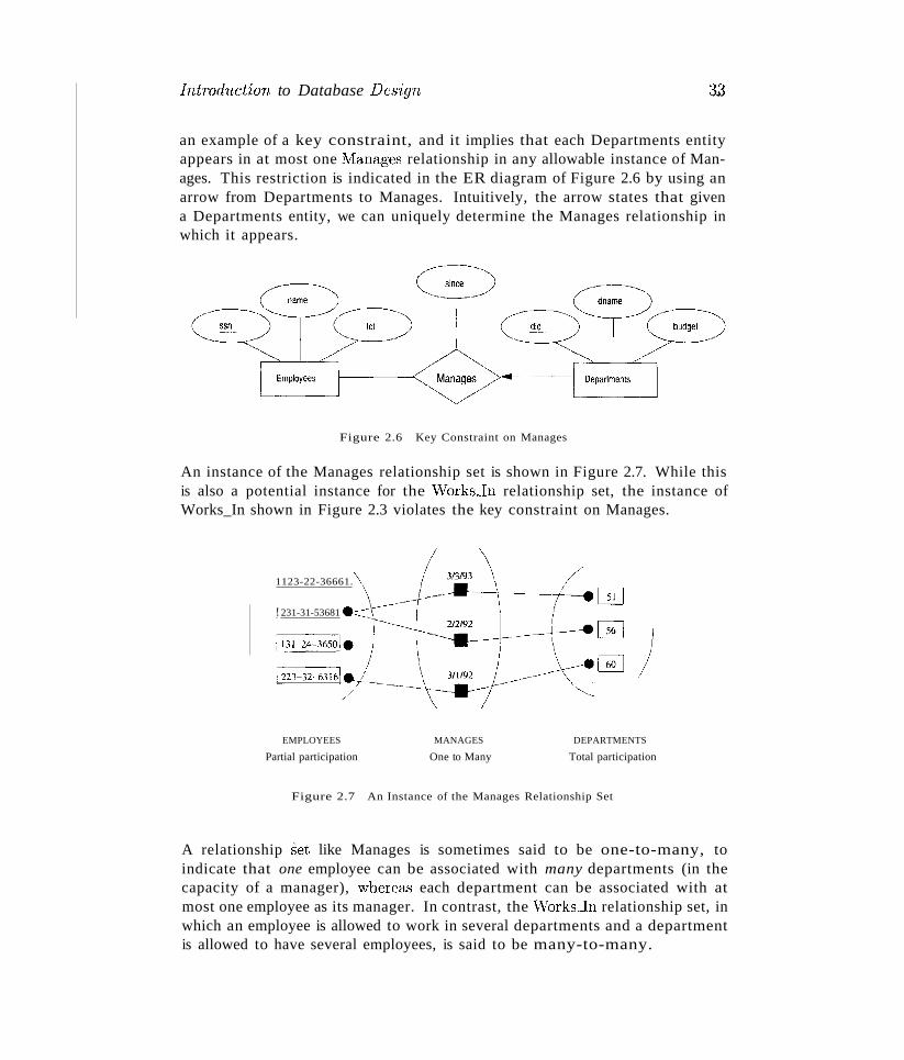
Introduction to Database Des'ign 33
an example of a key constraint, and it implies that each Departments entityappears in at most one 1Jlanages relationship in any allowable instance of Manages. This restriction is indicated in the ER diagram of Figure 2.6 by using anarrow from Departments to Manages. Intuitively, the arrow states that givena Departments entity, we can uniquely determine the Manages relationship inwhich it appears.
Figure 2.6 Key Constraint on Manages
An instance of the Manages relationship set is shown in Figure 2.7. While thisis also a potential instance for the WorksJn relationship set, the instance ofWorks_In shown in Figure 2.3 violates the key constraint on Manages.
1123-22-36661.
!231-31-53681
[223-32-6316\
--..----t-------;'-------a~
~
~
EMPLOYEES
Partial participation
MANAGES
One to Many
DEPARTMENTS
Total participation
Figure 2.7 An Instance of the Manages Relationship Set
A relationship set like Manages is sometimes said to be one-to-many, toindicate that one employee can be associated with many departments (in thecapacity of a manager), whereas each department can be associated with atmost one employee as its manager. In contrast, the \Vorks-.In relationship set, inwhich an employee is allowed to work in several departments and a departmentis allowed to have several employees, is said to be many-to-many.
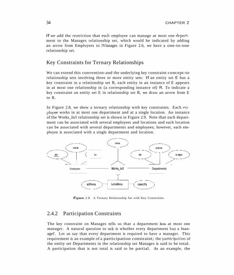
34 CHAPTER 2
If we add the restriction that each employee can manage at most one depl:1J'tment to the Manages relationship set, which would be indicated by addingan arrow from Employees to lVlanages in Figure 2.6, we have a one-to-onerelationship set.
Key Constraints for Ternary Relationships
We can extend this convention-and the underlying key constraint concept-torelationship sets involving three or more entity sets: If an entity set E has akey constraint in a relationship set R, each entity in an instance of E appearsin at most one relationship in (a corresponding instance of) R. To indicate akey constraint on entity set E in relationship set R, we draw an arrow from Eto R.
In Figure 2.8, we show a ternary relationship with key constraints. Each employ~e works in at most one department and at a single location. An instanceof the Works_In3 relationship set is shown in Figure 2.9. Note that each department can be associated with several employees and locations and each locationcan be associated with several departments and employees; however, each employee is associated with a single department and location.
lot
Employees WorksJn3 Departments
Figure 2.8 A Ternary Relationship Set with Key Constraints
2.4.2 Participation Constraints
The key constraint on Manages tells us that a department ha:s at most onemanager. A natural question to ask is whether every department ha.'3 a Inanagel'. Let us say that every department is required to have a manager. Thisrequirement is an example of a participation constraint; the particip::ltion ofthe entity set Departments in the relationship set Manages is said to be total.A participation that is not total is said to be partial. As an example, the
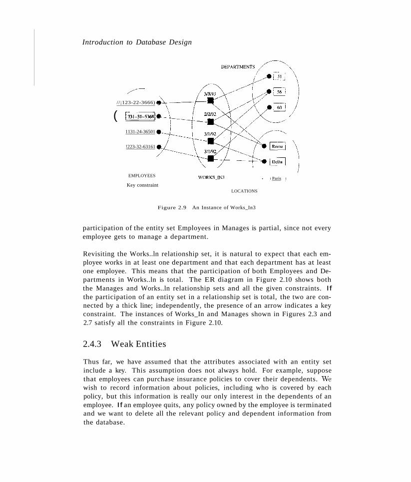
Introduction to Database Design
• I Paris IEMPLOYEES
!223-32-63161
/~~
//;123-22-3666) a..:~---~-r---'"
( ~~1131-24-36501
Key constraintLOCATIONS
Figure 2.9 An Instance of Works_In3
participation of the entity set Employees in Manages is partial, since not everyemployee gets to manage a department.
Revisiting the Works..ln relationship set, it is natural to expect that each employee works in at least one department and that each department has at leastone employee. This means that the participation of both Employees and Departments in Works..ln is total. The ER diagram in Figure 2.10 shows boththe Manages and Works..ln relationship sets and all the given constraints. Ifthe participation of an entity set in a relationship set is total, the two are connected by a thick line; independently, the presence of an arrow indicates a keyconstraint. The instances of Works_In and Manages shown in Figures 2.3 and2.7 satisfy all the constraints in Figure 2.10.
2.4.3 Weak Entities
Thus far, we have assumed that the attributes associated with an entity setinclude a key. This assumption does not always hold. For example, supposethat employees can purchase insurance policies to cover their dependents. "Vewish to record information about policies, including who is covered by eachpolicy, but this information is really our only interest in the dependents of anemployee. If an employee quits, any policy owned by the employee is terminatedand we want to delete all the relevant policy and dependent information fromthe database.
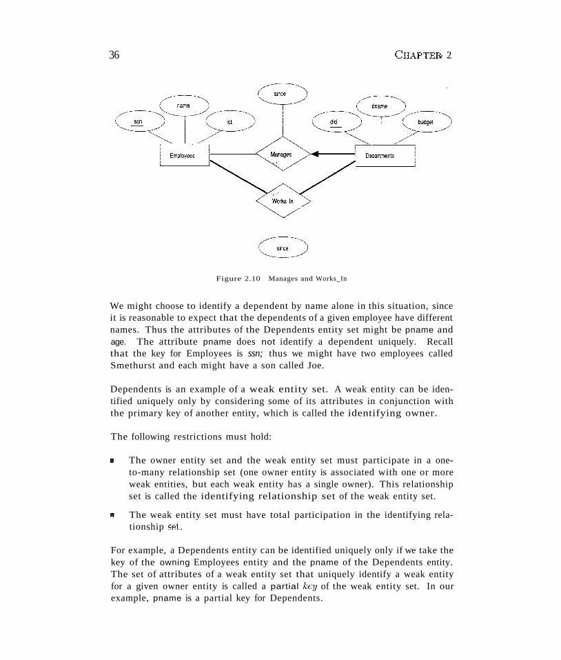
36 CHAPTETh 2
Figure 2.10 Manages and Works_In
We might choose to identify a dependent by name alone in this situation, sinceit is reasonable to expect that the dependents of a given employee have differentnames. Thus the attributes of the Dependents entity set might be pname andage. The attribute pname does not identify a dependent uniquely. Recallthat the key for Employees is ssn; thus we might have two employees calledSmethurst and each might have a son called Joe.
Dependents is an example of a weak entity set. A weak entity can be identified uniquely only by considering some of its attributes in conjunction withthe primary key of another entity, which is called the identifying owner.
The following restrictions must hold:
11'I The owner entity set and the weak entity set must participate in a oneto-many relationship set (one owner entity is associated with one or moreweak entities, but each weak entity has a single owner). This relationshipset is called the identifying relationship set of the weak entity set.
III The weak entity set must have total participation in the identifying relationship set.
For example, a Dependents entity can be identified uniquely only if we take thekey of the owning Employees entity and the pname of the Dependents entity.The set of attributes of a weak entity set that uniquely identify a weak entityfor a given owner entity is called a partial key of the weak entity set. In ourexample, pname is a partial key for Dependents.
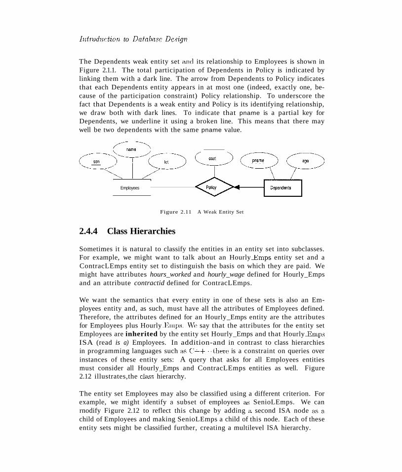
Introd'uction to Database Design
The Dependents weak entity set and its relationship to Employees is shown inFigure 2.1.1. The total participation of Dependents in Policy is indicated bylinking them with a dark line. The arrow from Dependents to Policy indicatesthat each Dependents entity appears in at most one (indeed, exactly one, because of the participation constraint) Policy relationship. To underscore thefact that Dependents is a weak entity and Policy is its identifying relationship,we draw both with dark lines. To indicate that pname is a partial key forDependents, we underline it using a broken line. This means that there maywell be two dependents with the same pname value.
Employees
Figure 2.11 A Weak Entity Set
2.4.4 Class Hierarchies
Sometimes it is natural to classify the entities in an entity set into subclasses.For example, we might want to talk about an Hourly-Emps entity set and aContracLEmps entity set to distinguish the basis on which they are paid. Wemight have attributes hours_worked and hourly_wage defined for Hourly_Empsand an attribute contractid defined for ContracLEmps.
We want the semantics that every entity in one of these sets is also an Employees entity and, as such, must have all the attributes of Employees defined.Therefore, the attributes defined for an Hourly_Emps entity are the attributesfor Employees plus Hourly~mps. \Ve say that the attributes for the entity setEmployees are inherited by the entity set Hourly_Emps and that Hourly-EmpsISA (read is a) Employees. In addition-and in contrast to class hierarchiesin programming languages such &'3 C++~~~there is a constraint on queries overinstances of these entity sets: A query that asks for all Employees entitiesmust consider all Hourly_Emps and ContracLEmps entities as well. Figure2.12 illustrates,the cl&ss hierarchy.
The entity set Employees may also be classified using a different criterion. Forexample, we might identify a subset of employees &'3 SenioLEmps. We canrnodify Figure 2.12 to reflect this change by adding a second ISA node &'3 achild of Employees and making SenioLEmps a child of this node. Each of theseentity sets might be classified further, creating a multilevel ISA hierarchy.
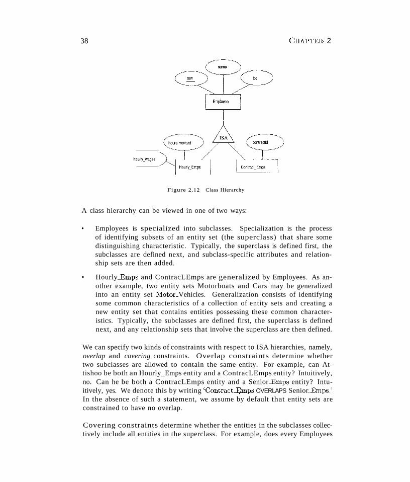
38 CHAPTEJl; 2
hourly-wages
Figure 2.12 Class Hierarchy
A class hierarchy can be viewed in one of two ways:
• Employees is specialized into subclasses. Specialization is the processof identifying subsets of an entity set (the superclass) that share somedistinguishing characteristic. Typically, the superclass is defined first, thesubclasses are defined next, and subclass-specific attributes and relationship sets are then added.
• Hourly-Emps and ContracLEmps are generalized by Employees. As another example, two entity sets Motorboats and Cars may be generalizedinto an entity set MotoLVehicles. Generalization consists of identifyingsome common characteristics of a collection of entity sets and creating anew entity set that contains entities possessing these common characteristics. Typically, the subclasses are defined first, the superclass is definednext, and any relationship sets that involve the superclass are then defined.
We can specify two kinds of constraints with respect to ISA hierarchies, namely,overlap and covering constraints. Overlap constraints determine whethertwo subclasses are allowed to contain the same entity. For example, can Attishoo be both an Hourly_Emps entity and a ContracLEmps entity? Intuitively,no. Can he be both a ContracLEmps entity and a Senior-Emps entity? Intuitively, yes. We denote this by writing 'ContracLE;mps OVERLAPS Senior-Emps.'In the absence of such a statement, we assume by default that entity sets areconstrained to have no overlap.
Covering constraints determine whether the entities in the subclasses collectively include all entities in the superclass. For example, does every Employees
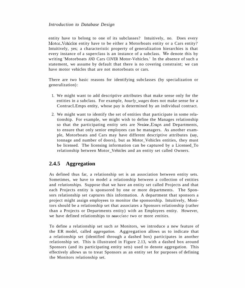
Introduction to Database Design
entity have to belong to one of its subclasses? Intuitively, no. Does every~'IotoLVehicles entity have to be either a Motorboats entity or a Cars entity?Intuitively, yes; a characteristic property of generalization hierarchies is thatevery instance of a superclass is an instance of a subclass. vVe denote this bywriting 'Motorboats AND Cars COVER Motor-Vehicles.' In the absence of such astatement, we assume by default that there is no covering constraint; we canhave motor vehicles that are not motorboats or cars.
There are two basic reasons for identifying subclasses (by specialization orgeneralization) :
1. We might want to add descriptive attributes that make sense only for theentities in a subclass. For example, hourly_wages does not make sense for aContracLEmps entity, whose pay is determined by an individual contract.
2. We might want to identify the set of entities that participate in some relationship. For example, we might wish to define the Manages relationshipso that the participating entity sets are Senior-Emps and Departments,to ensure that only senior employees can be managers. As another example, Motorboats and Cars may have different descriptive attributes (say,tonnage and number of doors), but as Motor_Vehicles entities, they mustbe licensed. The licensing information can be captured by a Licensed_Torelationship between Motor_Vehicles and an entity set called Owners.
2.4.5 Aggregation
As defined thus far, a relationship set is an association between entity sets.Sometimes, we have to model a relationship between a collection of entitiesand relationships. Suppose that we have an entity set called Projects and thateach Projects entity is sponsored by one or more departments. The Sponsors relationship set captures this information. A department that sponsors aproject might assign employees to monitor the sponsorship. Intuitively, Monitors should be a relationship set that associates a Sponsors relationship (ratherthan a Projects or Departments entity) with an Employees entity. However,we have defined relationships to &'3sociate two or more entities.
To define a relationship set such &'3 Monitors, we introduce a new feature ofthe ER model, called aggregation. Aggregation allows us to indicate thata relationship set (identified through a dashed box) participates in anotherrelationship set. This is illustrated in Figure 2.13, with a dashed box aroundSponsors (and its participating entity sets) used to denote aggregation. Thiseffectively allows us to treat Sponsors as an entity set for purposes of definingthe Monitors relationship set.
40 CHAPTER 2
Monitors /~
I ._. _. - - - - .- - - - - - - - - - ~ -~ - - - - - - - - - - - - - - - - - - ~ - - - - - - - -- - - - - - - ~ - - - - - - - - -- - -- -;
II
~:- I
DepartmentsSponsorsI
II
II
---------------------------------------- 1
I------~~~~~-------
Figure 2.13 Aggregation
When should we use aggregation? Intuitively, we use it when we need to express a relationship among relationships. But can we not express relationshipsinvolving other relationships without using aggregation? In our example, whynot make Sponsors a ternary relationship? The answer is that there are reallytwo distinct relationships, Sponsors and Monitors, each possibly with attributesof its own. For instance, the Monitors relationship has an attribute 1tntil thatrecords the date until when the employee is appointed as the sponsorship monitor. Compare this attribute with the attribute since of Sponsors, which is thedate when the sponsorship took effect. The use of aggregation versus a ternaryrelationship may also be guided by certain integrity constraints, as explainedin Section 2.5.4.
2.5 CONCEPTUAL DESIGN WITH THE ER MODEL
Developing an ER diagram presents several choices, including the following:
.. Should a concept be modeled as an entity or an attribute?
.. Should a concept be modeled &'3 an entity or a relationship?
II "Vhat arc the relationship sets and their participating entity sets? Shouldwe use binary or ternary relationships?
II Should we use aggregation?
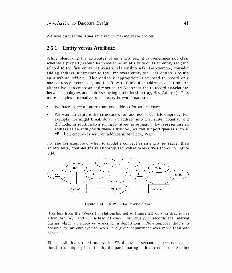
Introd'lLct'ion to Database Design
\Ve now discuss the issues involved in making these choices.
2.5.1 Entity versus Attribute
41
\Vhile identifying the attributes of an entity set, it is sometimes not clearwhether a property should be modeled as an attribute or as an entity set (andrelated to the first entity set using a relationship set). For example, consideradding address information to the Employees entity set. One option is to usean attribute address. This option is appropriate if we need to record onlyone address per employee, and it suffices to think of an address as a string. Analternative is to create an entity set called Addresses and to record associationsbetween employees and addresses using a relationship (say, Has_Address). Thismore complex alternative is necessary in two situations:
• We have to record more than one address for an employee.
• We want to capture the structure of an address in our ER diagram. Forexample, we might break down an address into city, state, country, andZip code, in addition to a string for street information. By representing anaddress as an entity with these attributes, we can support queries such as"Find all employees with an address in Madison, WI."
For another example of when to model a concept as an entity set rather thanan attribute, consider the relationship set (called WorksJ:n4) shown in Figure2.14.
Figure 2.14 The \Vorks_In4 Relationship Set
It differs from the \Vorks_In relationship set of Figure 2.2 only in that it hasattributes JTOtn and to, instead of since. Intuitively, it records the intervalduring which an employee works for a department. Now suppose that it ispossible for an employee to work in a given department over more than oneperiod.
This possibility is ruled out by the ER diagram's semantics, because a relationship is uniquely identified by the participating entities (recall from Section
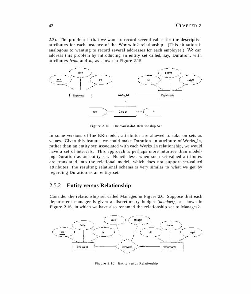
42 CHAPTER' 2
2.3). The problem is that we want to record several values for the descriptiveattributes for each instance of the vVorks-ln2 relationship. (This situation isanalogous to wanting to record several addresses for each employee.) vVe canaddress this problem by introducing an entity set called, say, Duration, withattributes from and to, as shown in Figure 2.15.
(~~-T:~~~)I Employees I WorksJn4 Departments
from to
Figure 2.15 The Works-ln4 Relationship Set
In some versions of the' ER model, attributes are allowed to take on sets asvalues. Given this feature, we could make Duration an attribute of Works_In,rather than an entity set; associated with each Works_In relationship, we wouldhave a set of intervals. This approach is perhaps more intuitive than modeling Duration as an entity set. Nonetheless, when such set-valued attributesare translated into the relational model, which does not support set-valuedattributes, the resulting relational schema is very similar to what we get byregarding Duration as an entity set.
2.5.2 Entity versus Relationship
Consider the relationship set called Manages in Figure 2.6. Suppose that eachdepartment manager is given a discretionary budget (dbudget) , as shown inFigure 2.16, in which we have also renamed the relationship set to Manages2.
Figure 2.16 Entity versus Relationship

Introduction to Database Design
Given a department, we know the manager, as well &'3 the manager's startingdate and budget for that department. This approach is natural if we t'l"ssumethat a manager receives a separate discretionary budget for each departmentthat he or she manages.
But what if the discretionary budget is a sum that covers all departmentsmanaged by that employee? In this case, each Manages2 relationship thatinvolves a given employee will have the same value in the db1Ldget field, leadingto redundant storage of the same information. Another problem with thisdesign is that it is misleading; it suggests that the budget is associated withthe relationship, when it is actually associated with the manager.
We can address these problems by introducing a new entity set called Managers(which can be placed below Employees in an ISA hierarchy, to show that everymanager is also an employee). The attributes since and dbudget now describea manager entity, as intended. As a variation, while every manager has abudget, each manager may have a different starting date (as manager) for eachdepartment. In this case dbudget is an attribute of Managers, but since is anattribute of the relationship set between managers and departments.
The imprecise nature of ER modeling can thus make it difficult to recognizeunderlying entities, and we might associate attributes with relationships ratherthan the appropriate entities. In general, such mistakes lead to redundantstorage of the same information and can cause many problems. We discussredundancy and its attendant problems in Chapter 19, and present a techniquecalled normalization to eliminate redundancies from tables.
2.5.3 Binary versus Ternary Relationships
Consider the ER diagram shown in Figure 2.17. It models a situation in whichan employee can own several policies, each policy can be owned by severalemployees, and each dependent can be covered by several policies.
Suppose that we have the following additional requirements:
III A policy cannot be owned jointly by two or more employees.
11II Every policy must be owned by some employee.
lIII Dependents is a weak entity set, and each dependent entity is uniquelyidentified by taking pname in conjunction with the policyid of a policyentity (which, intuitively, covers the given dependent).
The first requirement suggests that we impose a key constraint on Policies withrespect to Covers, but this constraint has the unintended side effect that a
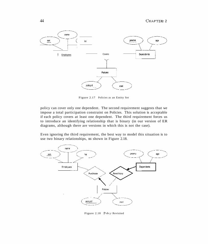
44
C~~C~T~~I
I Employees
lot
Covers
Figure 2.17 Policies as an Entity Set
CHAPTERf 2
policy can cover only one dependent. The second requirement suggests that weimpose a total participation constraint on Policies. This solution is acceptableif each policy covers at least one dependent. The third requirement forces usto introduce an identifying relationship that is binary (in our version of ERdiagrams, although there are versions in which this is not the case).
Even ignoring the third requirement, the best way to model this situation is touse two binary relationships, as shown in Figure 2.18.
Figure 2.18 Policy Revisited
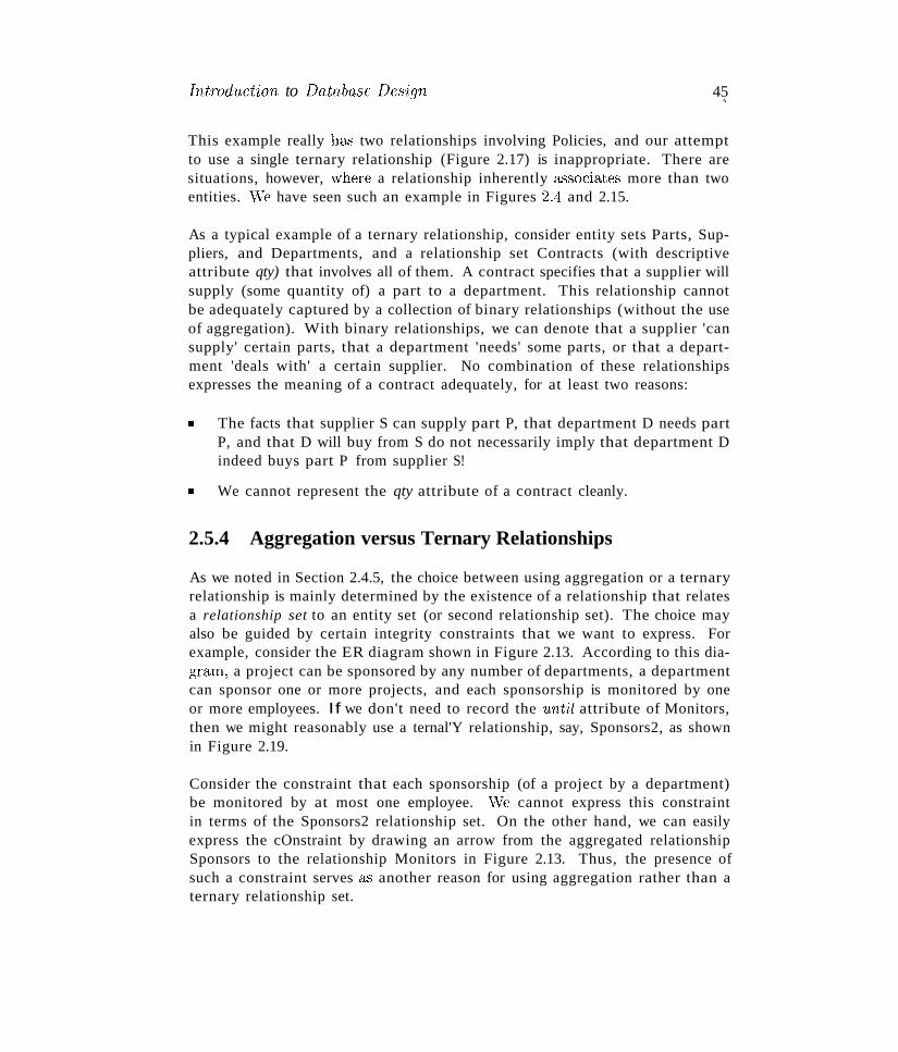
IntTod'U(~t"ion to Database Des'ign 45.This example really has two relationships involving Policies, and our attemptto use a single ternary relationship (Figure 2.17) is inappropriate. There aresituations, however, "vhere a relationship inherently a.'3sociates more than twoentities. vVe have seen such an example in Figures 2,4 and 2.15.
As a typical example of a ternary relationship, consider entity sets Parts, Suppliers, and Departments, and a relationship set Contracts (with descriptiveattribute qty) that involves all of them. A contract specifies that a supplier willsupply (some quantity of) a part to a department. This relationship cannotbe adequately captured by a collection of binary relationships (without the useof aggregation). With binary relationships, we can denote that a supplier 'cansupply' certain parts, that a department 'needs' some parts, or that a department 'deals with' a certain supplier. No combination of these relationshipsexpresses the meaning of a contract adequately, for at least two reasons:
• The facts that supplier S can supply part P, that department D needs partP, and that D will buy from S do not necessarily imply that department Dindeed buys part P from supplier S!
• We cannot represent the qty attribute of a contract cleanly.
2.5.4 Aggregation versus Ternary Relationships
As we noted in Section 2.4.5, the choice between using aggregation or a ternaryrelationship is mainly determined by the existence of a relationship that relatesa relationship set to an entity set (or second relationship set). The choice mayalso be guided by certain integrity constraints that we want to express. Forexample, consider the ER diagram shown in Figure 2.13. According to this diagram, a project can be sponsored by any number of departments, a departmentcan sponsor one or more projects, and each sponsorship is monitored by oneor more employees. If we don't need to record the unt-il attribute of Monitors,then we might reasonably use a ternal'Y relationship, say, Sponsors2, as shownin Figure 2.19.
Consider the constraint that each sponsorship (of a project by a department)be monitored by at most one employee. VVe cannot express this constraintin terms of the Sponsors2 relationship set. On the other hand, we can easilyexpress the cOnstraint by drawing an arrow from the aggregated relationshipSponsors to the relationship Monitors in Figure 2.13. Thus, the presence ofsuch a constraint serves &s another reason for using aggregation rather than aternary relationship set.
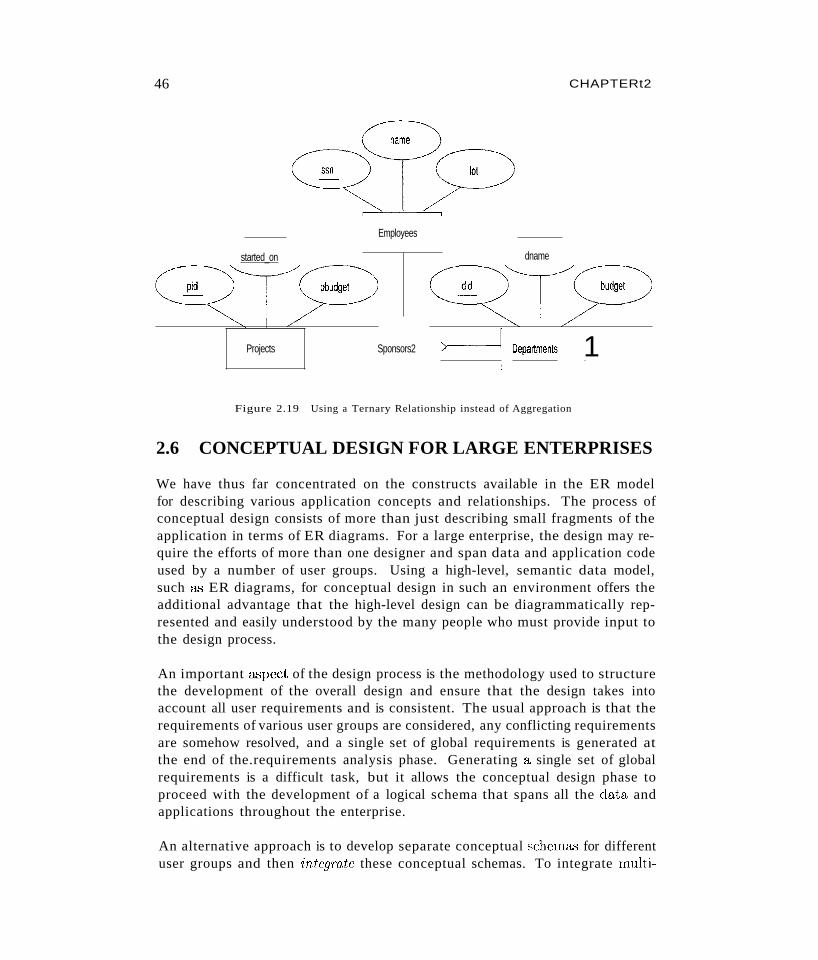
46 CHAPTERt2
Employees
started_on
G:(:PProjects Sponsors2
dname
G:(?>-------11 Department< 1
Figure 2.19 Using a Ternary Relationship instead of Aggregation
2.6 CONCEPTUAL DESIGN FOR LARGE ENTERPRISES
We have thus far concentrated on the constructs available in the ER modelfor describing various application concepts and relationships. The process ofconceptual design consists of more than just describing small fragments of theapplication in terms of ER diagrams. For a large enterprise, the design may require the efforts of more than one designer and span data and application codeused by a number of user groups. Using a high-level, semantic data model,such as ER diagrams, for conceptual design in such an environment offers theadditional advantage that the high-level design can be diagrammatically represented and easily understood by the many people who must provide input tothe design process.
An important aspect of the design process is the methodology used to structurethe development of the overall design and ensure that the design takes intoaccount all user requirements and is consistent. The usual approach is that therequirements of various user groups are considered, any conflicting requirementsare somehow resolved, and a single set of global requirements is generated atthe end of the.requirements analysis phase. Generating a single set of globalrequirements is a difficult task, but it allows the conceptual design phase toproceed with the development of a logical schema that spans all the data andapplications throughout the enterprise.
An alternative approach is to develop separate conceptual scherna.'-l for differentuser groups and then integTate these conceptual schemas. To integrate multi~
Intmduction to Database De.s'ign 47
pIe conceptual schemas, we must €'Btablish correspondences between entities,relationships, and attributes, and we must resolve numerous kinds of conflicts(e.g., naming conflicts, domain mismatches, differences in measurement units).This task is difficult in its own right. In some situations, schema integrationcannot be avoided; for example, when one organization merges with another,existing databases may have to be integrated. Schema integration is also increasing in importance as users demand access to heterogeneous data sources,often maintained by different organizations.
2.7 THE UNIFIED MODELING LANGUAGE
There are many approaches to end-to-end software system design, covering allthe steps from identifying the business requirements to the final specificationsfor a complete application, including workflow, user interfaces, and many aspects of software systems that go well beyond databases and the data stored inthem. In this section, we briefly discuss an approach that is becoming popular,called the unified modeling language (UML) approach.
UML, like the ER model, has the attractive feature that its constructs can bedrawn as diagrams. It encompasses a broader spectrum of the software designprocess than the ER model:
III Business Modeling: In this phase, the goal is to describe the businessprocesses involved in the software application being developed.
III System Modeling: The understanding of business processes is used toidentify the requirements for the software application. One part of therequirements is the database requirements.
III Conceptual Database Modeling: This step corresponds to the creationof the ER design for the database. For this purpose, UML provides manyconstructs that parallel the ER constructs.
III Physical Database Modeling: Ul\IL also provides pictorial representations for physical database design choices, such &'3 the creation of tablespaces and indexes. (\\1e discuss physical databa"se design in later chapters,but not the corresponding UML constructs.)
III Hardware System Modeling: UML diagrams can be used to describethe hardware configuration used for the application.
Th(~re are many kinds of diagrams in UML. Use case diagrams describe theactions performed by the system in response to user requests, and the peopleinvolved in these actions. These diagrams specify the external functionality<-hat the system is expected to support.
48 CHAPTER;2
Activity diagrams 8hmv the flow of actions in a business process. Statechartdiagrams describe dynamic interactions between system objects. These diagrams, used in busine.c;s and systern modeling, describe how the external functionality is to be implemented, consistent with the business rules and processesof the enterprise.
Class diagrams are similar to ER diagrams, although they are more generalin that they are intended to model application entities (intuitively, importantprogram components) and their logical relationships in addition to data entitiesand their relationships.
Both entity sets and relationship sets can be represented as classes in UML,together with key constraints, weak entities, and class hierarchies. The termrelationship is used slightly differently in UML, and UML's relationships arebinary. This sometimes leads to confusion over whether relationship sets inan ER diagram involving three or more entity sets can be directly representedin UML. The confusion disappears once we understand that all relationshipsets (in the ER sense) are represented as classes in UML; the binary UML'relationships' are essentially just the links shown in ER diagrams betweenentity sets and relationship sets.
Relationship sets with key constraints are usually omitted from UML diagrams,and the relationship is indicated by directly linking the entity sets involved.For example, consider Figure 2.6. A UML representation of this ER diagramwould have a class for Employees, a class for Departments, and the relationshipManages is shown by linking these two classes. The link can be labeled witha name and cardinality information to show that a department can have onlyone manager.
As we will see in Chapter 3, ER diagrams are translated into the relationalmodel by mapping each entity set into a table and each relationship set intoa table. FUrther, as we will see in Section 3.5.3, the table corresponding to aone-to-many relationship set is typically omitted by including some additionalinformation about the relationship in the table for one of the entity sets involved. Thus, UML class diagrams correspond closely to the tables created bymapping an ER diagram.
Indeed, every class in a U1I1L class diagram is mapped into a table in the corresponding U]\'1L database diagram. UML's database diagrams show howclasses are represented in the database and contain additional details aboutthe structure of the database such as integrity constraints and indexes. Links(UML's 'relationships') between UML classes lead to various integrity constraints between the corresponding tables. Many details specific to the relational model (e.g., views, fOTe'ign keys, null-allowed fields) and that reflect
Introduction to Dutaba8C Design 49
physical design choices (e.g., indexed fields) can be modeled ill UN[L databasediagrams.
UML's component diagrams describe storage aspects of the database, suchas tablespaces and database pa,titions) , as well as interfaces to applicationsthat access the database. Finally, deployment diagrams show the hardwareaspects of the system.
Our objective in this book is to concentrate on the data stored in a databaseand the related design issues. To this end, we deliberately take a simplifiedview of the other steps involved in software design and development. Beyondthe specific discussion of UlIIL, the material in this section is intended to placethe design issues that we cover within the context of the larger software designprocess. \Ve hope that this will assist readers interested in a more comprehensive discussion of software design to complement our discussion by referring toother material on their preferred approach to overall system design.
2.8 CASE STUDY: THE INTERNET SHOP
We now introduce an illustrative, 'cradle-to-grave' design case study that weuse as a running example throughout this book. DBDudes Inc., a well-knowndatabase consulting firm, has been called in to help Barns and Nobble (B&N)with its database design and implementation. B&N is a large bookstore specializing in books on horse racing, and it has decided to go online. DBDudes firstverifies that B&N is willing and able to pay its steep fees and then schedules alunch meeting--billed to B&N, naturally~to do requirements analysis.
2.8.1 Requirements Analysis
The owner of B&N, unlike many people who need a database, has thoughtextensively about what he wants and offers a concise summary:
"I would like my customers to be able to browse my catalog of books andplace orders over the Internet. Currently, I take orders over the phone. I havemostly corporate customers who call me and give me the ISBN number of abook and a quantity; they often pay by credit card. I then prepare a shipmentthat contains the books they ordered. If I don't have enough copies in stock,I order additional copies and delay the shipment until the new copies arrive;I want to ship a customer's entire order together. My catalog includes all thebooks I sell. For each book, the catalog contains its ISBN number, title, author,purcha.se price, sales price, and the year the book was published. Most of mysustomers are regulars, and I have records with their names and addresses.
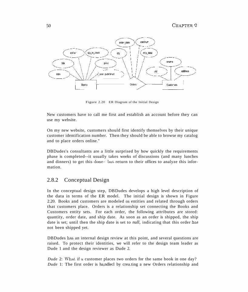
50
year-published
Orders
Figure 2.20 ER Diagram of the Initial Design
CHAPTER¢2
New customers have to call me first and establish an account before they canuse my website.
On my new website, customers should first identify themselves by their uniquecustomer identification number. Then they should be able to browse my catalogand to place orders online."
DBDudes's consultants are a little surprised by how quickly the requirementsphase is completed--it usually takes weeks of discussions (and many lunchesand dinners) to get this done~~but return to their offices to analyze this information.
2.8.2 Conceptual Design
In the conceptual design step, DBDudes develops a high level description ofthe data in terms of the ER model. The initial design is shown in Figure2.20. Books and customers are modeled as entities and related through ordersthat customers place. Orders is a relationship set connecting the Books andCustomers entity sets. For each order, the following attributes are stored:quantity, order date, and ship date. As soon as an order is shipped, the shipdate is set; until then the ship date is set to null, indicating that this order hasnot been shipped yet.
DBDudes has an internal design review at this point, and several questions areraised. To protect their identities, we will refer to the design team leader asDude 1 and the design reviewer as Dude 2.
Dude 2: \\That if a. customer places two orders for the same book in one day?Dude 1: The first order is ha,ndlecl by crea.ting a new Orders relationship and
Introduct'ion to Database Design 51,
the second order is handled by updating the value of the quantity attribute inthis relationship.Dude 2: \\That if a customer places two orders for different books in one day?Dude 1: No problem. Each instance of the Orders relationship set relates thecustomer to a different book.Dude 2: Ah, but what if a customer places two orders for the same book ondifferent days?Dude 1: \Ve can use the attribute order date of the orders relationship todistinguish the two orders.Dude 2: Oh no you can't. The attributes of Customers and Books must jointlycontain a key for Orders. So this design does not allow a customer to placeorders for the same book on different days.Dude 1: Yikes, you're right. Oh well, B&N probably won't care; we'll see.
DBDudes decides to proceed with the next phase, logical database design; werejoin them in Section 3.8.
2.9 REVIEW QUESTIONS
Answers to the review questions can be found in the listed sections.
• Name the main steps in database design. What is the goal of each step?In which step is the ER model mainly used? (Section 2.1)
• Define these terms: entity, entity set, attribute, key. (Section 2.2)
• Define these terms: relationship, relationship set, descriptive attributes.(Section 2.3)
• Define the following kinds of constraints, and give an example of each: keyconstraint, participation constraint. What is a weak entity? What are classhierarchies'? What is aggregation? Give an example scenario motivatingthe use of each of these ER model design constructs. (Section 2.4)
• What guidelines would you use for each of these choices when doing ERdesign: \Vhether to use an attribute or an entity set, an entity or a relationship set, a binary or ternary relationship, or aggregation. (Section 2.5)
III'l Why is designing a database for a large enterprise especially hard? (Section 2.6)
• What is UML? How does databa"se design fit into the overall design ofa data-intensive software system? How is UML related to ER diagrams?(Section 2.7)
52
EXERCISES
CHAPTERJ2
Exercise 2.1 Explain the following terms briefly: attribute, domain, entity, relationship,.entity set, relationship set, one-to-many relat'ionship, many-to-many 1'elationship. pan·tcipation constmint. overlap constraint, covering constraint, weak entity set,. aggregat'ion, and roleindicator.
Exercise 2.2 A university database contains information about professors (identified by social security number, or SSN) and courses (identified by courseid). Professors teach courses;each of the following situations concerns the Teaches relationship set. For each situation,draw an ER diagram that describes it (assuming no further constraints hold).
1. Professors can teach the same course in several semesters, and each offering must berecorded.
2. Professors can teach the same course in several semesters, and only the most recentsuch offering needs to be recorded. (Assume this condition applies in all subsequentquestions. )
3. Every professor must teach some course.
4. Every professor teaches exactly one course (no more, no less).
5. Every professor teaches exactly one course (no more, no less), and every course must betaught by some professor.
6. Now suppose that certain courses can be taught by a team of professors jointly, but itis possible that no one professor in a team can teach the course. Model this situation,introducing additional entity sets and relationship sets if necessary.
Exercise 2.3 Consider the following information about a university database:
II Professors have an SSN, a name, an age, a rank, and a research specialty.
II Projects have a project number, a sponsor name (e.g., NSF), a starting date, an endingdate, and a budget.
II Graduate students have an SSN, a name, an age, and a degree program (e.g., M.S. orPh.D.).
II Each project is managed by one professor (known as the project's principal investigator).
II Each project is worked on by one or more professors (known as the project's co-investigators).
III Professors can manage and/or work on multiple projects.
II Each project is worked on by one or more graduate students (known as the project'sresearch assistants).
II When graduate students >'lark on a project, a professor must supervise their work on theproject. Graduate students can work on multiple projects, in which case they will havea (potentially different) supervisor for each one.
II Departments have a department number, a department name, and a main office.
II Departments have a professor (known as the chairman) who runs the department.
II Professors work in one or more departments, and for each department that they workin, a time percentage is associated with their job.
II Graduate students have one major department in which they are working OIl their degree.
Introduction to Database Design ~3
III Each graduate student has another, more senior graduate student (known as a studentadvisor) who advises him or her OIl what courses to take.
Design and dra\v an ER diagram that captures the information about the university. Use onlythe basic ER model here; that is, entities, relationships, and attributes. Be sure to indicateany key and participation constraints.
Exercise 2.4 A company database needs to store information about employees (identifiedby ssn, with salary and phone as attributes), departments (identified by dna, with dname andbudget as attributes), and children of employees (with name and age as attributes). Employeeswork in departments; each department is managed by an employee; a child must be identifieduniquely by name when the parent (who is an employee; assume that only one parent worksfor the company) is known. We are not interested in information about a child once theparent leaves the company.
Draw an ER diagram that captures this information.
Exercise 2.5 Notown Records has decided to store information about musicians who performon its albums (as well as other company data) in a database. The company has wisely chosento hire you as a database designer (at your usual consulting fee of $2500jday).
III Each musician that records at Notown has an SSN, a name, an address, and a phonenumber. Poorly paid musicians often share the same address, and no address has morethan one phone.
III Each instrument used in songs recorded at Notown has a name (e.g., guitar, synthesizer,flute) and a musical key (e.g., C, B-flat, E-flat).
III Each album recorded on the Notown label has a title, a copyright date, a format (e.g.,CD or MC), and an album identifier.
III Each song recorded at Notown has a title and an author.
III Each musician may play several instruments, and a given instrument may be played byseveral musicians.
III Each album has a number of songs on it, but no song may appear on more than onealbum.
III Each song is performed by one or more musicians, and a musician may perform a numberof songs.
III Each album has exactly one musician who acts as its producer. A musician may produceseveral albums, of course.
Design' a conceptual schema for Notown and draw an ER diagram for your schema. Thepreceding information describes the situation that the Notown database must model. Be sureto indicate all key and cardinality constraints and any assumptions you make. Identify anyconstraints you are unable to capture in the ER diagram and briefly explain why you couldnot express them.
Exercise 2.6 Computer Sciences Department frequent fliers have been complaining to DaneCounty Airport officials about the poor organization at the airport. As a result, the officialsdecided that all information related to the airport should be organized using a DBMS, andyou have been hired to design the database. Your first task is to organize the informationabout all the airplanes stationed and maintainecl at the airport. The relevant information isas follows:
54 CHAPTER 12
• Every airplane has a registration number, and each airplane is of a specific model.
• The airport accommodates a number of airplane models, and each model is identified bya model number (e.g., DC-lO) and has a capacity and a weight.
• A number of technicians work at the airport. You need to store the name, SSN, address,phone number, and salary of each technician.
• Each technician is an expert on one or more plane model(s), and his or her expertise mayoverlap with that of other technicians. This information about technicians must also berecorded.
• Traffic controllers must have an annual medical examination. For each traffic controller,you must store the date of the most recent exam.
• All airport employees (including technicians) belong to a union. You must store theunion membership number of each employee. You can assume that each employee isuniquely identified by a social security number.
• The airport has a number of tests that are used periodically to ensure that airplanes arestill airworthy. Each test has a Federal Aviation Administration (FAA) test number, aname, and a maximum possible score.
• The FAA requires the airport to keep track of each time a given airplane is tested by agiven technician using a given test. For each testing event, the information needed is thedate, the number of hours the technician spent doing the test, and the score the airplanereceived on the test.
1. Draw an ER diagram for the airport database. Be sure to indicate the various attributesof each entity and relationship set; also specify the key and participation constraints foreach relationship set. Specify any necessary overlap and covering constraints a.s well (inEnglish).
2. The FAA passes a regulation that tests on a plane must be conducted by a technicianwho is an expert on that model. How would you express this constraint in the ERdiagram? If you cannot express it, explain briefly.
Exercise 2.7 The Prescriptions-R-X chain of pharmacies ha.s offered to give you a free lifetime supply of medicine if you design its database. Given the rising cost of health care, youagree. Here's the information that you gather:
11II Patients are identified by an SSN, and their names, addresses, and ages must be recorded.
11II Doctors are identified by an SSN. For each doctor, the name, specialty, and years ofexperience must be recorded.
III Each pharmaceutical company is identified by name and has a phone number.
III For each drug, the trade name and formula must be recorded. Each drug is sold bya given pharmaceutical company, and the trade name identifies a drug uniquely fromamong the pJ;oducts of that company. If a pharmaceutical company is deleted, you neednot keep track of its products any longer.
III Each pharmacy has a name, address, and phone number.
III Every patient has a primary physician. Every doctor has at least one patient.
• Each pharmacy sells several drugs and has a price for each. A drug could be sold atseveral pharmacies, and the price could vary from one pharmacy to another.
IntToduction to DatabaBe Design 55
• Doctors prescribe drugs for patients. A doctor could prescribe one or more drugs forseveral patients, and a patient could obtain prescriptions from several doctors. Eachprescription has a date and a quantity associated with it. You can assume that, if adoctor prescribes the same drug for the same patient more than once, only the last suchprescription needs to be stored.
• Pharmaceutical companies have long-term contracts with pharmacies. A pharmaceuticalcompany can contract with several pharmacies, and a pharmacy can contract with severalpharmaceutical companies. For each contract, you have to store a start date, an end date,and the text of the contract.
• Pharmacies appoint a supervisor for each contract. There must always be a supervisorfor each contract, but the contract supervisor can change over the lifetime of the contract.
1. Draw an ER diagram that captures the preceding information. Identify any constraintsnot captured by the ER diagram.
2. How would your design change if each drug must be sold at a fixed price by all pharmacies?
3. How would your design change if the design requirements change as follows: If a doctorprescribes the same drug for the same patient more than once, several such prescriptionsmay have to be stored.
Exercise 2.8 Although you always wanted to be an artist, you ended up being an expert ondatabases because you love to cook data and you somehow confused database with data baste.Your old love is still there, however, so you set up a database company, ArtBase, that builds aproduct for art galleries. The core of this product is a database with a schema that capturesall the information that galleries need to maintain. Galleries keep information about artists,their names (which are unique), birthplaces, age, and style of art. For each piece of artwork,the artist, the year it was made, its unique title, its type of art (e.g., painting, lithograph,sculpture, photograph), and its price must be stored. Pieces of artwork are also classified intogroups of various kinds, for example, portraits, still lifes, works by Picasso, or works of the19th century; a given piece may belong to more than one group. Each group is identified bya name (like those just given) that describes the group. Finally, galleries keep informationabout customers. For each customer, galleries keep that person's unique name, address, totalamount of dollars spent in the gallery (very important!), and the artists and groups of artthat the customer tends to like.
Draw the ER diagram for the database.
Exercise 2.9 Answer the following questions.
• Explain the following terms briefly: UML, use case diagrams, statechart diagrams, classdiagrams, database diagrams, component diagrams, and deployment diagrams.
• Explain the relationship between ER diagrams and UML.
BffiLIOGRAPHIC NOTES
Several books provide a good treatment of conceptual design; these include [63J (which alsocontains a survey of commercial database design tools) and [730J.
The ER model wa..<; proposed by Chen [172], and extensions have been proposed in a numberof subsequent papers. Generalization and aggregation were introduced in [693]. [390, 589]
56 CHAPTER ,;2
contain good surveys of semantic data models. Dynamic and temporal aspects of semanticdata models are discussed in [749].
[731] discusses a design methodology based on developing an ER diagram and then translatingit to the relational model. Markowitz considers referential integrity in the context of ER torelational mapping and discusses the support provided in some commercial systems (a..<; ofthat date) in [513, 514].
The entity-relationship conference proceedings contain numerous papers on conceptual design,with an emphasis on the ER model; for example, [698].
The OMG home page (www. omg. org) contains the specification for UML and related modelingstandards. Numerous good books discuss UML; for example [105, 278, 640] and there is ayearly conference dedicated to the advancement of UML, the International Conference on theUnified Modeling Language.
View integration is discussed in several papers, including [97, 139, 184, 244, 535, 551, 550,685, 697, 748]. [64] is a survey of several integration approaches.
3THE RELATIONAL MODEL
.... How is data represented in the relational model?
.... What integrity constraints can be expressed?
.... How can data be created and modified?
.... How can data be manipulated and queried?
.... How can we create, modify, and query tables using SQL?
.... How do we obtain a relational database design from an ER diagram?
.... What are views and why are they used?
.. Key concepts: relation, schema, instance, tuple, field, domain,degree, cardinality; SQL DDL, CREATE TABLE, INSERT, DELETE,UPDATE; integrity constraints, domain constraints, key constraints,PRIMARY KEY, UNIQUE, foreign key constraints, FOREIGN KEY; referential integrity maintenance, deferred and immediate constraints; relational queries; logical database design, translating ER diagrams torelations, expressing ER constraints using SQL; views, views and log:ical independence, security; creating views in SQL, updating views,querying views, dropping views
TABLE: An arrangement of words, numbers, or signs, or combinations of them,&s in parallel columns, to exhibit a set of facts or relations in a definite, compact,and comprehensive form; a synopsis or scheme.
-----vVebster's Dictionary of the English Language
Codd proposed the relational data model in 1970. At that time, most databa,,'Sesystems were based on one of two older data models (the hierarchical model
57
58 CHAPTER ~
SQL. Originally developed as the query language of the pioneeringSystem-R relational DBl\1S at IBIYl, structured query language (SQL)has become the most widely used language for creating, manipulating,and querying relational DBMSs. Since many vendors offer SQL products,there IS a need for a standard that defines \official SQL.' The existence ofa standard allows users to measure a given vendor's version of SQL forcompleteness. It also allows users to distinguish SQLfeatures specific toone product from those that are standard; an application that relies onnonstandard features is less portable.
The first SQL standard was developed in 1986 by the American NationalStandards Institute (ANSI) and was called SQL-86. There was a minorrevision in 1989 called SQL-89 and a major revision in 1992 called SQL92. The International Standards Organization (ISO) collaborated withANSI to develop SQL-92. Most commercial DBMSs currently support (thecore subset of) SQL-92 and are working to support the recently adoptedSQL:1999 version of the standard, a major extension of SQL-92. Ourcoverage of SQL is based on SQL:1999, but is applicable to SQL-92 aswell; features unique to SQL:1999 are explicitly noted.
and the network model); the relational model revolutionized the database fieldand largely supplanted these earlier models. Prototype relational databa.'3emanagement systems were developed in pioneering research projects at IBMand DC-Berkeley by the mid-197Gs, and several vendors were offering relationaldatabase products shortly thereafter. Today, the relational model is by farthe dominant data model and the foundation for the leading DBMS products,including IBM's DB2 family, Informix, Oracle, Sybase, Microsoft's Access andSQLServer, FoxBase, and Paradox. Relational database systems are ubiquitousin the marketplace and represent a multibillion dollar industry.
The relational model is very simple and elegant: a database is a collection ofone or more relations, where each relation is a table with rows and columns.This simple tabular representation enables even novice users to understand thecontents of a database, and it permits the use of simple, high-level languagesto query the data. The major advantages of the relational model over the olderdata models are its simple data representation and the ease with which evencomplex queries can be expressed.
\Vhile we concentrate on the underlying concepts, we also introduce the DataDefinition Language (DDL) features of SQL, the standard language forcreating, manipulating, and querying data in a relational DBMS. This allowsus to ground the discussion firmly in terms of real databa.se systems.
The Relational 1\1odd 59
vVe discuss the concept of a relation in Section ~t1 and show how to createrelations using the SQL language. An important component of a data model isthe set of constructs it provides for specifying conditions that must be satisfiedby the data. Such conditions, called 'integrity constraints (lGs), enable theDBIviS to reject operations that might corrupt the data. We present integrityconstraints in the relational model in Section 3.2, along with a discussion ofSQL support for les. \Ve discuss how a DBMS enforces integrity constraintsin Section 3.3.
In Section 3.4, we turn to the mechanism for accessing and retrieving datafrom the database, query languages, and introduce the querying features ofSQL, which we examine in greater detail in a later chapter.
We then discuss converting an ER diagram into a relational database schemain Section 3.5. We introduce views, or tables defined using queries, in Section3.6. Views can be used to define the external schema for a database and thusprovide the support for logical data independence in the relational model. InSection 3.7, we describe SQL commands to destroy and alter tables and views.
Finally, in Section 3.8 we extend our design case study, the Internet shop introduced in Section 2.8, by showing how the ER diagram for its conceptualschema can be mapped to the relational model, and how the use of views canhelp in this design.
3.1 INTRODUCTION TO THE RELATIONAL MODEL
The main construct for representing data in the relational model is a relation.A relation consists of a relation schema and a relation instance. Therelation instance is a table, and the relation schema describes the column headsfor the table. We first describe the relation schema and then the relationinstance. The schema specifies the relation's name, the name of each field (orcolumn, or attribute), and the domain of each field. A domain is referred toin a relation schema by the domain name and has a set of associated values.
\Ve use the example of student information in a university database from Chapter 1 to illustrate the parts of a relation schema:
Students(sid: string, name: string, login: string,age: integer, gpa: real)
This says, for instance, that the field named sid has a domain named string.The set of values associated with domain string is the set of all characterstrings.
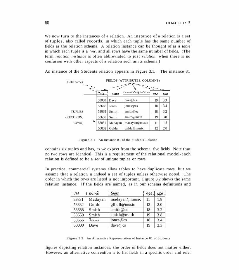
60 CHAPTER 3
We now turn to the instances of a relation. An instance of a relation is a setof tuples, also called records, in which each tuple has the same number offields as the relation schema. A relation instance can be thought of as a tablein which each tuple is a row, and all rows have the same number of fields. (Theterm relation instance is often abbreviated to just relation, when there is noconfusion with other aspects of a relation such as its schema.)
An instance of the Students relation appears in Figure 3.1. The instance 81
Field names
TUPLES
(RECORDS,
ROWS)
FIELDS (ATTRIBUTES, COLUMNS)
-~ name I---/o'-gz-'n--
50000 Dave dave@cs 19 3.3
53666 Jones jones@cs 18 3.4
53688 Smith smith@ee 18 3.2
53650 Smith smith@math 19 3.8"'\ 53831 Madayan madayan@music 11 1.8
53832 Guldu guldu@music 12 2.0
Figure 3.1 An Instance 81 of the Students Relation
contains six tuples and has, as we expect from the schema, five fields. Note thatno two rows are identical. This is a requirement of the relational model-eachrelation is defined to be a set of unique tuples or rows.
In practice, commercial systems allow tables to have duplicate rows, but weassume that a relation is indeed a set of tuples unless otherwise noted. Theorder in which the rows are listed is not important. Figure 3.2 shows the samerelation instance. If the fields are named, as in our schema definitions and
I s'id I name [.login
53831 Madayan madayan@music 11 1.853832 Guldu gllldll@music 12 2.053688 Smith smith@ee 18 3.253650 Smith smith@math 19 3.853666 JOI;es jones@cs 18 3.450000 Dave dave@cs 19 3.3
Figure 3.2 An Alternative Representation of Instance 81 of Students
figures depicting relation instances, the order of fields does not matter either.However, an alternative convention is to list fields in a specific order and refer
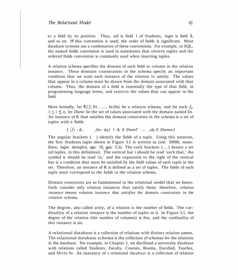
The Relat'ional lvfodel 61,
to a field by its position. Thus, s'id is field 1 of Students, login is field :~,
and so on. If this convention is used, the order of fields is significant. Mostdatabase systems use a combination of these conventions. For example, in SQL,the named fields convention is used in statements that retrieve tuples and theordered fields convention is commonly used when inserting tuples.
A relation schema specifies the domain of each field or column in the relationinstance. These domain constraints in the schema specify an importantcondition that we want each instance of the relation to satisfy: The valuesthat appear in a column must be drawn from the domain associated with thatcolumn. Thus, the domain of a field is essentially the type of that field, inprogramming language terms, and restricts the values that can appear in thefield.
More formally, let R(fI:Dl, ... , In:Dn) be a relation schema, and for each Ii,1 :::; i :::; n, let Dami be the set of values associated with the domain named Di.
.An instance of R that satisfies the domain constraints in the schema is a set oftuples with n fields:
{ (fI : d l , ,In: dn) I d l E Daml' ... ,dn E Damn}
The angular brackets ( ) identify the fields of a tuple. Using this notation,the first Students tuple shown in Figure 3.1 is written as (sid: 50000, name:Dave, login: dave@cs, age: 19, gpa: 3.3). The curly brackets {... } denote a set(of tuples, in this definition). The vertical bar I should be read 'such that,' thesymbol E should be read 'in,' and the expression to the right of the verticalbar is a condition that must be satisfied by the field values of each tuple in theset. Therefore, an instance of R is defined as a set of tuples. The fields of eachtuple must correspond to the fields in the relation schema.
Domain constraints are so fundamental in the relational model that we henceforth consider only relation instances that satisfy them; therefore, relationinstance means relation instance that satisfies the domain constraints in therelation schema.
The degree, also called arity, of a relation is the number of fields. The cardinality of a relation instance is the number of tuples in it. In Figure 3.1, thedegree of the relation (the number of columns) is five, and the cardinality ofthis instance is six.
A relational database is a collection of relations with distinct relation names.The relational database schema is the collection of schemas for the relationsin the database. 'For example, in Chapter 1, we discllssed a university databasewith relations called Students, Faculty, Courses, Rooms, Enrolled, Teaches,and Meets~In. An instance of a relational databa..'3e is a collection of relation
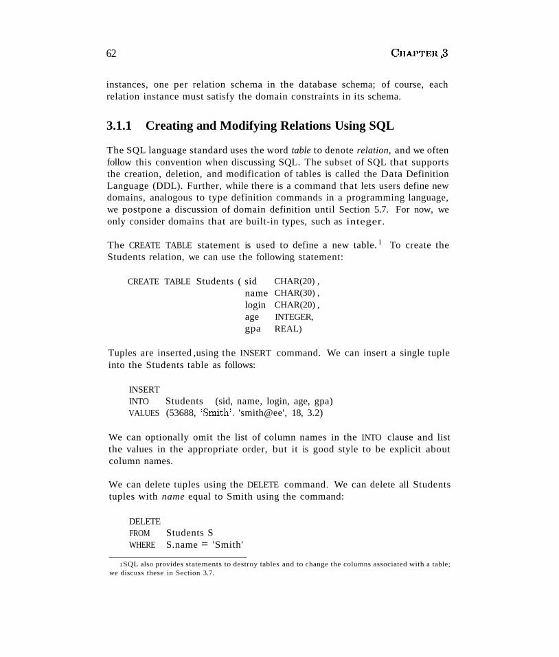
62 CHAPTER~3
instances, one per relation schema in the database schema; of course, eachrelation instance must satisfy the domain constraints in its schema.
3.1.1 Creating and Modifying Relations Using SQL
The SQL language standard uses the word table to denote relation, and we oftenfollow this convention when discussing SQL. The subset of SQL that supportsthe creation, deletion, and modification of tables is called the Data DefinitionLanguage (DDL). Further, while there is a command that lets users define newdomains, analogous to type definition commands in a programming language,we postpone a discussion of domain definition until Section 5.7. For now, weonly consider domains that are built-in types, such as integer.
The CREATE TABLE statement is used to define a new table. 1 To create theStudents relation, we can use the following statement:
CREATE TABLE Students ( sidnameloginagegpa
CHAR(20) ,CHAR(30) ,CHAR(20) ,INTEGER,REAL)
Tuples are inserted ,using the INSERT command. We can insert a single tupleinto the Students table as follows:
INSERTINTO Students (sid, name, login, age, gpa)VALUES (53688, 'Smith', 'smith@ee', 18, 3.2)
We can optionally omit the list of column names in the INTO clause and listthe values in the appropriate order, but it is good style to be explicit aboutcolumn names.
We can delete tuples using the DELETE command. We can delete all Studentstuples with name equal to Smith using the command:
DELETEFROMWHERE
Students SS.name = 'Smith'
1SQL also provides statements to destroy tables and to change the columns associated with a table;we discuss these in Section 3.7.
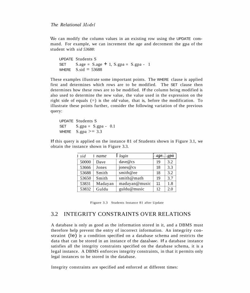
The Relational Pr10del
vVe can modify the column values in an existing row using the UPDATE command. For example, we can increment the age and decrement the gpa of thestudent with sid 53688:
UPDATE Students SSET S.age = S.age + 1, S.gpa = S.gpa - 1WHERE S.sid = 53688
These examples illustrate some important points. The WHERE clause is appliedfirst and determines which rows are to be modified. The SET clause thendetermines how these rows are to be modified. If the column being modified isalso used to determine the new value, the value used in the expression on theright side of equals (=) is the old value, that is, before the modification. Toillustrate these points further, consider the following variation of the previousquery:
UPDATE Students SSET S.gpa = S.gpa - 0.1WHERE S.gpa >= 3.3
If this query is applied on the instance 81 of Students shown in Figure 3.1, weobtain the instance shown in Figure 3.3.
I sid I name I login
50000 Dave dave@cs 19 3.253666 Jones jones@cs 18 3.353688 Smith smith@ee 18 3.253650 Smith smith@math 19 3.753831 Madayan madayan@music 11 1.853832 Guldu guldu@music 12 2.0
Figure 3.3 Students Instance 81 after Update
3.2 INTEGRITY CONSTRAINTS OVER RELATIONS
A database is only as good as the information stored in it, and a DBMS musttherefore help prevent the entry of incorrect information. An integrity constraint (Ie) is a condition specified on a database schema and restricts thedata that can be stored in an instance of the databa'3e. If a database instancesatisfies all the integrity constraints specified on the database schema, it is alegal instance. A DBMS enforces integrity constraints, in that it permits onlylegal instances to be stored in the database.
Integrity constraints are specified and enforced at different times:
64 CHAPTER 3
1. \\Then the DBA or end user defines a database schema, he or she specifiesthe rcs that must hold on any instance of this database.
2. "Vhen a database application is run, the DBMS checks for violations anddisallows changes to the data that violate the specified ICs. (In somesituations, rather than disallow the change, the DBMS might make somecompensating changes to the data to ensure that the database instancesatisfies all ICs. In any case, changes to the database are not allowed tocreate an instance that violates any IC.) It is important to specify exactlywhen integrity constraints are checked relative to the statement that causesthe change in the data and the transaction that it is part of. We discussthis aspect in Chapter 16, after presenting the transaction concept, whichwe introduced in Chapter 1, in more detail.
Many kinds of integrity constraints can be specified in the relational model.We have already seen one example of an integrity constraint in the domainconstraints associated with a relation schema (Section 3.1). In general, otherkinds of constraints can be specified as well; for example, no two studentshave the same sid value. In this section we discuss the integrity constraints,other than domain constraints, that a DBA or user can specify in the relationalmodel.
3.2.1 Key Constraints
Consider the Students relation and the constraint that no two students have thesame student id. This IC is an example of a key constraint. A key constraintis a statement that a certain minimal subset of the fields of a relation is aunique identifier for a tuple. A set of fields that uniquely identifies a tupleaccording to a key constraint is called a candidate key for the relation; weoften abbreviate this to just key. In the case of the Students relation, the (setof fields containing just the) sid field is a candidate key.
Let us take a closer look at the above definition of a (candidate) key. Thereare two parts to the definition: 2
1. Two distinct tuples in a legal instance (an instance that satisfies all Ies,including the key constraint) cannot have identical values in all the fieldsof a key.
2. No subset of the set of fields in a key is a unique identifier for a tuple.
2The term key is rather overworked. In the context of access methods, we speak of sear'ch keys.which are quite different.
The Relational ltdodel
The first part of the definition means that, in any legal instance, the values inthe key fields uniquely identify a tuple in the instance. \Vhen specifying a keyconstraint, the DBA or user must be sure that this constraint will not preventthem from storing a 'correct' set of tuples. (A similar comment applies to thespecification of other kinds of les as well.) The notion of •correctness' heredepends on the nature of the data being stored. For example, several studentsmay have the same name, although each student has a unique student id. Ifthe name field is declared to be a key, the DBMS will not allow the Studentsrelation to contain two tuples describing different students with the same name!
The second part of the definition means, for example, that the set of fields{sid, name} is not a key for Students, because this set properly contains thekey {sid}. The set {sid, name} is an example of a superkey, which is a set offields that contains a key.
Look again at the instance of the Students relation in Figure 3.1. Observe thattwo different rows always have different sid values; sid is a key and uniquelyidentifies a tuple. However, this does not hold for nonkey fields. For example,the relation contains two rows with Smith in the name field.
Note that every relation is guaranteed to have a key. Since a relation is a set oftuples, the set of all fields is always a superkey. If other constraints hold, somesubset of the fields may form a key, but if not, the set of all fields is a key.
A relation may have several candidate keys. For example, the login and agefields of the Students relation may, taken together, also identify students uniquely.That is, {login, age} is also a key. It may seem that login is a key, since notwo rows in the example instance have the same login value. However, the keymust identify tuples uniquely in all possible legal instances of the relation. Bystating that {login, age} is a key, the user is declaring that two students mayhave the same login or age, but not both.
Out of all the available candidate keys, a database designer can identify aprimary key. Intuitively, a tuple can be referred to from elsewhere in thedatabase by storing the values of its primary key fields. For example, we canrefer to a Students tuple by storing its sid value. As a consequence of referringto student tuples in this manner, tuples are frequently accessed by specifyingtheir sid value. In principle, we can use any key, not just the primary key,to refer to a tuple. However, using the primary key is preferable because itis what the DBMS expects this is the significance of designating a particularcandidate key as a primary key and optimizes for. For example, the DBMSmay create an index with the primary key fields 8..'3 the search key, to make theretrieval of a tuple given its primary key value efficient. The idea of referringto a tuple is developed further in the next section.
66
Specifying Key Constraints in SQL
CHAPTER,3
In SQL, we can declare that a subset of the columns of a table constitute a keyby using the UNIQUE constraint. At most one of these candidate keys can bedeclared to be a primary key, using the PRIMARY KEY constraint. (SQL doesnot require that such constraints be declared for a table.)
Let us revisit our example table definition and specify key information:
CREATE TABLE Students ( sid CHAR(20) ,name CHAR (30) ,login CHAR(20) ,age INTEGER,gpa REAL,UNIQUE (name, age),CONSTRAINT StudentsKey PRIMARY KEY (sid) )
This definition says that sid is the primary key and the combination of nameand age is also a key. The definition of the primary key also illustrates howwe can name a constraint by preceding it with CONSTRAINT constraint-name.If the constraint is violated, the constraint name is returned and can be usedto identify the error.
3.2.2 Foreign Key Constraints
Sometimes the information stored in a relation is linked to the informationstored in another relation. If one of the relations is modified, the other must bechecked, and perhaps modified, to keep the data consistent. An IC involvingboth relations must be specified if a DBMS is to make such checks. The mostcommon IC involving two relations is a foreign key constraint.
Suppose that, in addition to Students, we have a second relation:
Enrolled(studid: string, cid: string, gTade: string)
To ensure that only bona fide students can enroll in courses, any value thatappears in the studid field of an instance of the Enrolled relation should alsoappear in the sid field of some tuple in the Students relation. The st'udid fieldof Enrolled is called a foreign key and refers to Students. The foreign key int~l~referencil1grel~tio~~(Enrolled,inour. exalIlpl~)!nll~tl~latcht~le~)l:lirl~l~y~key:_:-- ()f -the JCferC11(;ed relation (Students); that jS,-jtIn~lstJUly(iU"lhe'-s<lnie-~l~~i;;~_
_.. ,'--" . ". ...•.. .... ........••..... ....-._--.... --~-----~-
of columns and cornpatible dCita types, altl1()u~h the column nanl(~S can bealffei'cii£.' - .---- '~'. _N~ ~_-~
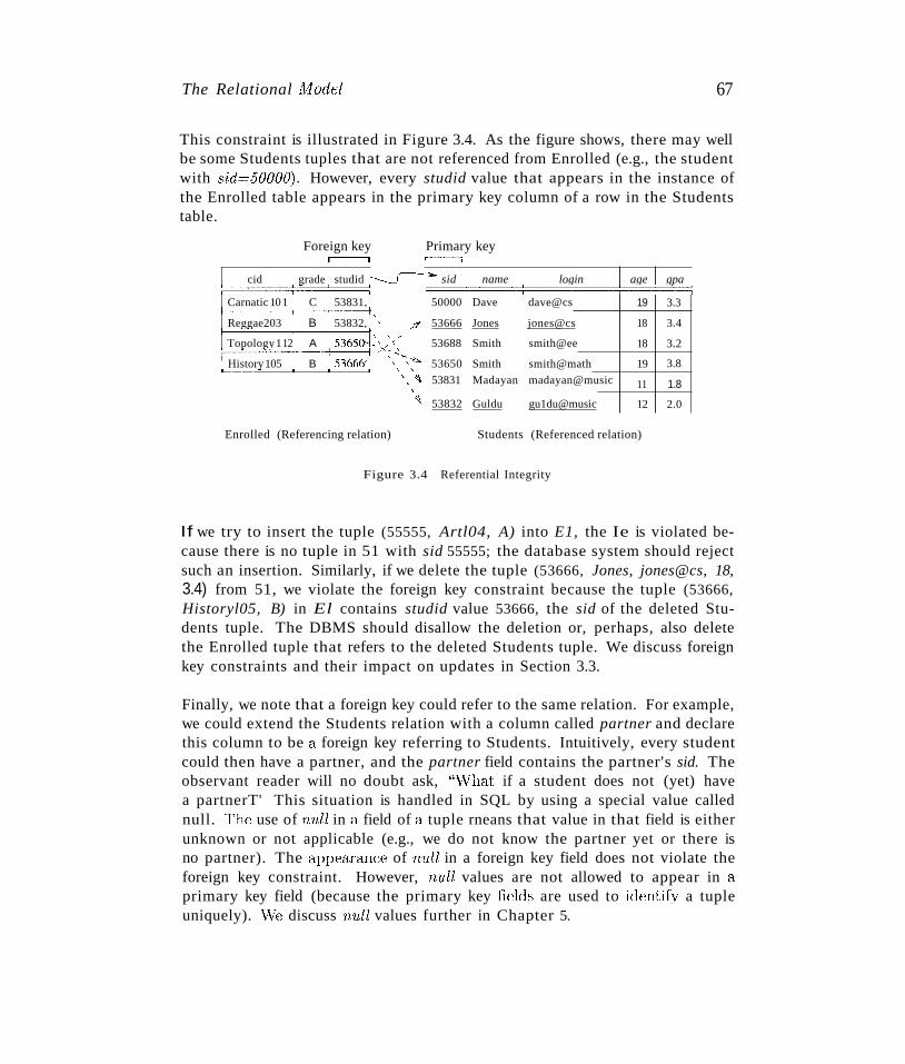
The Relational A10del 67
This constraint is illustrated in Figure 3.4. As the figure shows, there may wellbe some Students tuples that are not referenced from Enrolled (e.g., the studentwith sid=50000). However, every studid value that appears in the instance ofthe Enrolled table appears in the primary key column of a row in the Studentstable.
Foreign keyr---I
Primary key~
cid grade studid~ -- sid name login age gpa~===:====:==~ ~==i====*==========*====:::*~
Carnatic 101 C 53831, 50000 Dave dave@csI---~~~~~+-~--t
Reggae203 B 53832, '- ,-f 53666 Jones jones@csI---..::::::...~~~~+-~--t
Topology112 A 5365(}-~' ,\' 53688 Smith smith@ee1---~-=~~~+-~---1 ,'\- ,
History105 B 53666" \'"",~ 53650 Smith smith@math
~~-=--~-'----~...L-~-J \"'\ 53831 Madayan madayan@music
"'\ 53832 Guldu gu1du@music
19
18
18
19
11
12
3.3
3.4
3.2
3.8
1.8
2.0
Enrolled (Referencing relation) Students (Referenced relation)
Figure 3.4 Referential Integrity
If we try to insert the tuple (55555, Artl04, A) into E1, the Ie is violated because there is no tuple in 51 with sid 55555; the database system should rejectsuch an insertion. Similarly, if we delete the tuple (53666, Jones, jones@cs, 18,3.4) from 51, we violate the foreign key constraint because the tuple (53666,Historyl05, B) in El contains studid value 53666, the sid of the deleted Students tuple. The DBMS should disallow the deletion or, perhaps, also deletethe Enrolled tuple that refers to the deleted Students tuple. We discuss foreignkey constraints and their impact on updates in Section 3.3.
Finally, we note that a foreign key could refer to the same relation. For example,we could extend the Students relation with a column called partner and declarethis column to be a foreign key referring to Students. Intuitively, every studentcould then have a partner, and the partner field contains the partner's sid. Theobservant reader will no doubt ask, "y\That if a student does not (yet) havea partnerT' This situation is handled in SQL by using a special value callednull. The use of nun in a field of a tuple rneans that value in that field is eitherunknown or not applicable (e.g., we do not know the partner yet or there isno partner). The appearanC(~ of null in a foreign key field does not violate theforeign key constraint. However, null values are not allowed to appear in aprimary key field (because the primary key fields are used to identify a tupleuniquely). \Ve discuss null values further in Chapter 5.
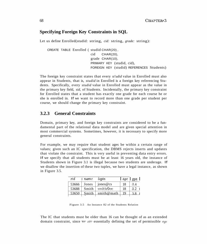
68
Specifying Foreign Key Constraints in SQL
CHAPTERp3
Let us define Enrolled(studid: string, cid: string, grade: string):
CREATE TABLE Enrolled ( studid CHAR(20) ,
cid CHAR(20),grade CHAR(10),
PRIMARY KEY (studid, cid),FOREIGN KEY (studid) REFERENCES Students)
The foreign key constraint states that every st'udid value in Enrolled must alsoappear in Students, that is, studid in Enrolled is a foreign key referencing Students. Specifically, every studid value in Enrolled must appear as the value inthe primary key field, sid, of Students. Incidentally, the primary key constraintfor Enrolled states that a student has exactly one grade for each course he orshe is enrolled in. If we want to record more than one grade per student percourse, we should change the primary key constraint.
3.2.3 General Constraints
Domain, primary key, and foreign key constraints are considered to be a fundamental part of the relational data model and are given special attention inmost commercial systems. Sometimes, however, it is necessary to specify moregeneral constraints.
For example, we may require that student ages be within a certain range ofvalues; given such an IC specification, the DBMS rejects inserts and updatesthat violate the constraint. This is very useful in preventing data entry errors.If we specify that all students must be at least 16 years old, the instance ofStudents shown in Figure 3.1 is illegal because two students are underage. Ifwe disallow the insertion of these two tuples, we have a legal instance, as shownin Figure 3.5.
s'id I na'me login I age I gpa I53666 Jones jones@cs 18 3.453688 Smith smithCQ)ee 18 ~).2 I53650 Smith smith@math 19 3.8 I
. -
Figure 3.5 An Instance 82 of the Students Relation
The IC that students must be older than 16 can be thought of as an extendeddomain constraint, since we are essentially defining the set of permissible age
The Relational lV/ode! 69
values more stringently than is possible by simply using a standard domainsuch :'1.S integer. In general, however, constraints that go well beyond domain,key, or foreign key constraints can be specified. For example, we could requirethat every student whose age is greater than 18 must have a gpa greater than3.
Current relational database systems support such general constraints in theform of table constraints and assertions. Table constraints are associated with asingle table and checked whenever that table is modified. In contrast, assertionsinvolve several tables and are checked whenever any of these tables is modified.Both table constraints and assertions can use the full power of SQL queries tospecify the desired restriction. We discuss SQL support for table constraintsand assertions in Section 5.7 because a full appreciation of their power requiresa good grasp of SQL's query capabilities.
3.3 ENFORCING INTEGRITY CONSTRAINTS
As we observed earlier, ICs are specified when a relation is created and enforcedwhen a relation is modified. The impact of domain, PRIMARY KEY, and UNIQUEconstraints is straightforward: If an insert, delete, or update command causesa violation, it is rejected. Every potential Ie violation is generally checked atthe end of each SQL statement execution, although it can be deferred until theend of the transaction executing the statement, as we will see in Section 3.3.1.
Consider the instance 51 of Students shown in Figure 3.1. The following insertion violates the primary key constraint because there is already a tuple withthe s'id 53688, and it will be rejected by the DBMS:
INSERTINTO Students (sid, name, login, age, gpa)VALUES (53688, 'Mike', 'mike@ee', 17,3.4)
The following insertion violates the constraint that the primary key cannotcontain null:
INSERTINTO Students (sid, name, login, age, gpa)VALUES (null, 'Mike', 'mike@ee', 17,3.4)
Of course, a similar problem arises whenever we try to insert a tuple with avalue in a field that is not in the domain associated with that field, that is,whenever we violate a domain constraint. Deletion does not cause a violationof clornain, primary key or unique constraints. However, an update can causeviolations, sirnilar to an insertion:
70
UPDATE Students SSET S.sid = 50000WHERE S.sid = 53688
CHAPTER, 3
This update violates the primary key constraint because there is already a tuplewith sid 50000.
The impact of foreign key constraints is more complex because SQL sometimestries to rectify a foreign key constraint violation instead of simply rejecting thechange. We discuss the referential integrity enforcement steps taken bythe DBMS in terms of our Enrolled and Students tables, with the foreign keyconstraint that Enrolled.sid is a reference to (the primary key of) Students.
In addition to the instance 81 of Students, consider the instance of Enrolledshown in Figure 3.4. Deletions of Enrolled tuples do not violate referentialintegrity, but insertions of Enrolled tuples could. The following insertion isillegal because there is no Students tuple with sid 51111:
INSERTINTO Enrolled (cid, grade, studid)VALUES ('Hindi101', 'B', 51111)
On the other hand, insertions of Students tuples do not violate referentialintegrity, and deletions of Students tuples could cause violations. Further,updates on either Enrolled or Students that change the studid (respectively,sid) value could potentially violate referential integrity.
SQL provides several alternative ways to handle foreign key violations. Wemust consider three basic questions:
1. What should we do if an Enrolled row is inserted, with a studid columnvalue that does not appear in any row of the Students table?
In this case, the INSERT command is simply rejected.
2. What should we do if a Students row is deleted?
The options are:
• Delete all Enrolled rows that refer to the deleted Students row.
• Disallow the deletion of the Students row if an Enrolled row refers toit.
• Set the studid column to the sid of some (existing) 'default' student,for every Enrolled row that refers to the deleted Students row.
The Relational l'lfodel 71
• For every Enrolled row that refers to it, set the studid column to null.In our example, this option conflicts with the fact that stud'id is partof the primary key of Enrolled and therefore cannot be set to mtll.Therefore, we are limited to the first three options in our example,although this fourth option (setting the foreign key to null) is availablein general.
3. What should we do if the primary key val'ue of a Students row is updated?
The options here are similar to the previous case.
SQL allows us to choose any of the four options on DELETE and UPDATE. Forexample, we can specify that when a Students row is deleted, all Enrolled rowsthat refer to it are to be deleted as well, but that when the sid column of aStudents row is modified, this update is to be rejected if an Enrolled row refersto the modified Students row:
CREATE TABLE Enrolled ( studid CHAR(20) ,
cid CHAR(20) ,
grade CHAR(10),
PRIMARY KEY (studid, dd),FOREIGN KEY (studid) REFERENCES Students
ON DELETE CASCADE
ON UPDATE NO ACTION)
The options are specified as part of the foreign key declaration. The defaultoption is NO ACTION, which means that the action (DELETE or UPDATE) is to berejected, Thus, the ON UPDATE clause in our example could be omitted, withthe same effect. The CASCADE keyword says that, if a Students row is deleted,all Enrolled rows that refer to it are to be deleted as well. If the UPDATE clausespecified CASCADE, and the sid column of a Students row is updated, this updateis also carried out in each Enrolled row that refers to the updated Students row.
If a Students row is deleted, we can switch the enrollment to a 'default' studentby using ON DELETE SET DEFAULT. The default student is specified 3.'3 part ofthe definition of the sid field in Enrolled; for example, sid CHAR(20) DEFAULT
'53666 '. Although the specification of a default value is appropriate in somesituations (e.g" a default parts supplier if a particular supplier goes out ofbusiness), it is really not appropriate to switch enrollments to a default student.The correct solution in this example is to also delete all enrollment tuples forthe deleted student (that is, CASCADE) or to reject the update.
SQL also allows the use of null as the default value by specifying ON DELETE
SET NULL.
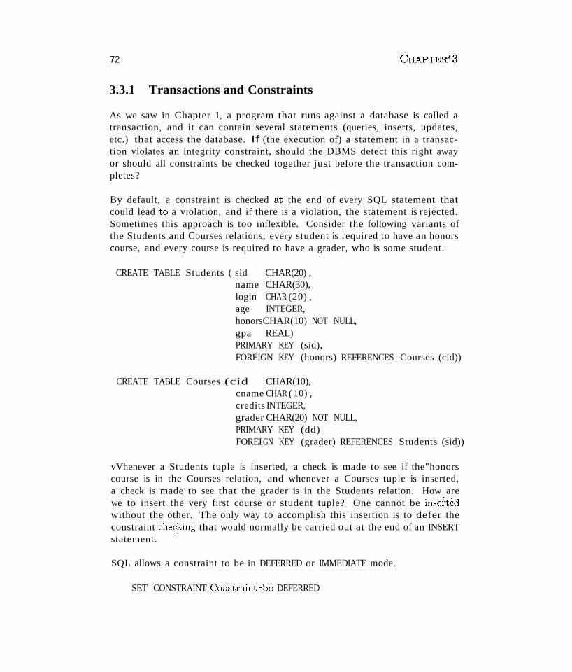
72 CHAPTERf 3
3.3.1 Transactions and Constraints
As we saw in Chapter 1, a program that runs against a database is called atransaction, and it can contain several statements (queries, inserts, updates,etc.) that access the database. If (the execution of) a statement in a transaction violates an integrity constraint, should the DBMS detect this right awayor should all constraints be checked together just before the transaction completes?
By default, a constraint is checked at the end of every SQL statement thatcould lead to a violation, and if there is a violation, the statement is rejected.Sometimes this approach is too inflexible. Consider the following variants ofthe Students and Courses relations; every student is required to have an honorscourse, and every course is required to have a grader, who is some student.
CREATE TABLE Students ( sid CHAR(20) ,name CHAR(30),login CHAR (20) ,age INTEGER,honorsCHAR(10) NOT NULL,gpa REAL)PRIMARY KEY (sid),FOREIGN KEY (honors) REFERENCES Courses (cid))
CREATE TABLE Courses (cid CHAR(10),cname CHAR ( 10) ,credits INTEGER,grader CHAR(20) NOT NULL,PRIMARY KEY (dd)FOREI GN KEY (grader) REFERENCES Students (sid))
vVhenever a Students tuple is inserted, a check is made to see if the"honorscourse is in the Courses relation, and whenever a Courses tuple is inserted,a check is made to see that the grader is in the Students relation. How arewe to insert the very first course or student tuple? One cannot be inseitedwithout the other. The only way to accomplish this insertion is to defer theconstraint che~king that would normally be carried out at the end of an INSERTstatement.
SQL allows a constraint to be in DEFERRED or IMMEDIATE mode.
SET CONSTRAINT ConstntintFoo DEFERRED
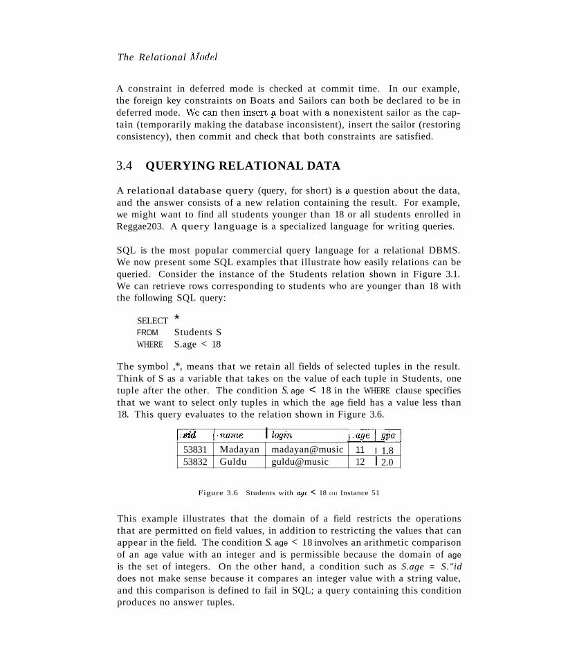
The Relational 1\11odel
A constraint in deferred mode is checked at commit time. In our example,the foreign key constraints on Boats and Sailors can both be declared to be indeferred mode. "VVe can then insert? boat with a nonexistent sailor as the captain (temporarily making the database inconsistent), insert the sailor (restoringconsistency), then commit and check that both constraints are satisfied.
3.4 QUERYING RELATIONAL DATA
A relational database query (query, for short) is a question about the data,and the answer consists of a new relation containing the result. For example,we might want to find all students younger than 18 or all students enrolled inReggae203. A query language is a specialized language for writing queries.
SQL is the most popular commercial query language for a relational DBMS.We now present some SQL examples that illustrate how easily relations can bequeried. Consider the instance of the Students relation shown in Figure 3.1.We can retrieve rows corresponding to students who are younger than 18 withthe following SQL query:
SELECT *FROM Students SWHERE S.age < 18
The symbol ,*, means that we retain all fields of selected tuples in the result.Think of S as a variable that takes on the value of each tuple in Students, onetuple after the other. The condition S. age < 18 in the WHERE clause specifiesthat we want to select only tuples in which the age field has a value less than18. This query evaluates to the relation shown in Figure 3.6.
I··sid j .. name I login
53831 Madayan madayan@music 11 I 1.853832 Guldu guldu@music 12 I 2.0
Figure 3.6 Students with age < 18 OIl Instance 51
This example illustrates that the domain of a field restricts the operationsthat are permitted on field values, in addition to restricting the values that canappear in the field. The condition S. age < 18 involves an arithmetic comparisonof an age value with an integer and is permissible because the domain of age
is the set of integers. On the other hand, a condition such as S.age = S."iddoes not make sense because it compares an integer value with a string value,and this comparison is defined to fail in SQL; a query containing this conditionproduces no answer tuples.
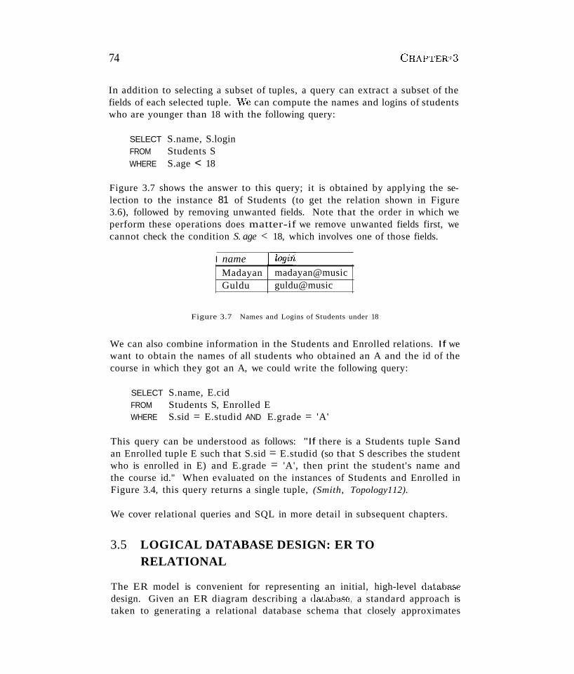
74 CHAPTERJ 3
In addition to selecting a subset of tuples, a query can extract a subset of thefields of each selected tuple. vVe can compute the names and logins of studentswho are younger than 18 with the following query:
SELECT S.name, S.loginFROM Students SWHERE S.age < 18
Figure 3.7 shows the answer to this query; it is obtained by applying the selection to the instance 81 of Students (to get the relation shown in Figure3.6), followed by removing unwanted fields. Note that the order in which weperform these operations does matter-if we remove unwanted fields first, wecannot check the condition S. age < 18, which involves one of those fields.
I nameMadayanGuldu
madayan@musicguldu@music
Figure 3.7 Names and Logins of Students under 18
We can also combine information in the Students and Enrolled relations. If wewant to obtain the names of all students who obtained an A and the id of thecourse in which they got an A, we could write the following query:
SELECT S.name, E.cidFROM Students S, Enrolled EWHERE S.sid = E.studid AND E.grade = 'A'
This query can be understood as follows: "If there is a Students tuple Sandan Enrolled tuple E such that S.sid = E.studid (so that S describes the studentwho is enrolled in E) and E.grade = 'A', then print the student's name andthe course id." When evaluated on the instances of Students and Enrolled inFigure 3.4, this query returns a single tuple, (Smith, Topology112).
We cover relational queries and SQL in more detail in subsequent chapters.
3.5 LOGICAL DATABASE DESIGN: ER TORELATIONAL
The ER model is convenient for representing an initial, high-level databi'lsedesign. Given an ER diagram describing a databa'3e, a standard approach istaken to generating a relational database schema that closely approximates
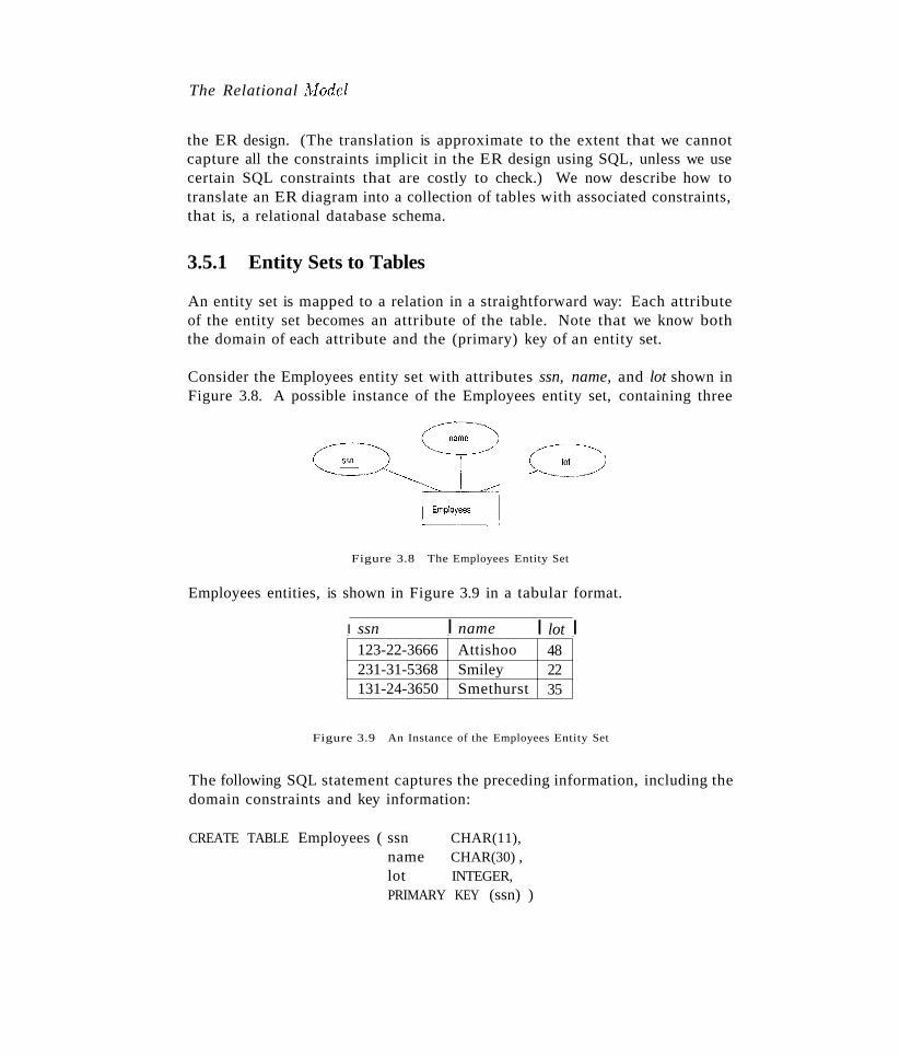
The Relational !'viodel
the ER design. (The translation is approximate to the extent that we cannotcapture all the constraints implicit in the ER design using SQL, unless we usecertain SQL constraints that are costly to check.) We now describe how totranslate an ER diagram into a collection of tables with associated constraints,that is, a relational database schema.
3.5.1 Entity Sets to Tables
An entity set is mapped to a relation in a straightforward way: Each attributeof the entity set becomes an attribute of the table. Note that we know boththe domain of each attribute and the (primary) key of an entity set.
Consider the Employees entity set with attributes ssn, name, and lot shown inFigure 3.8. A possible instance of the Employees entity set, containing three
Figure 3.8 The Employees Entity Set
Employees entities, is shown in Figure 3.9 in a tabular format.
I ssn I name I lot I123-22-3666 Attishoo 48231-31-5368 Smiley 22131-24-3650 Smethurst 35
Figure 3.9 An Instance of the Employees Entity Set
The following SQL statement captures the preceding information, including thedomain constraints and key information:
CREATE TABLE Employees ( ssn CHAR(11),name CHAR(30) ,lot INTEGER,PRIMARY KEY (ssn) )
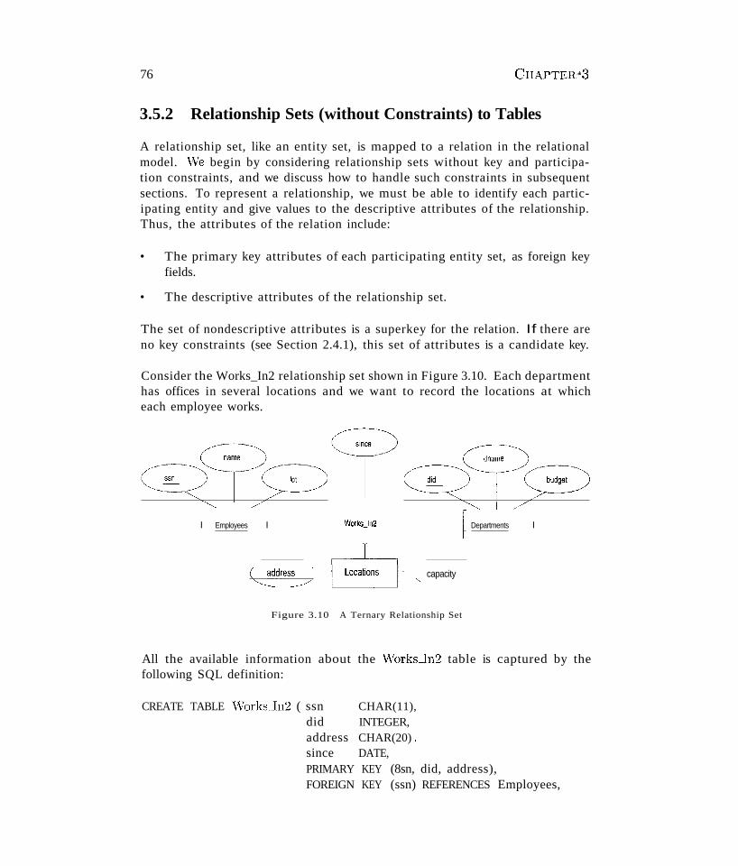
76 CHAPTER~3
3.5.2 Relationship Sets (without Constraints) to Tables
A relationship set, like an entity set, is mapped to a relation in the relationalmodel. Vve begin by considering relationship sets without key and participation constraints, and we discuss how to handle such constraints in subsequentsections. To represent a relationship, we must be able to identify each participating entity and give values to the descriptive attributes of the relationship.Thus, the attributes of the relation include:
• The primary key attributes of each participating entity set, as foreign keyfields.
• The descriptive attributes of the relationship set.
The set of nondescriptive attributes is a superkey for the relation. If there areno key constraints (see Section 2.4.1), this set of attributes is a candidate key.
Consider the Works_In2 relationship set shown in Figure 3.10. Each departmenthas offices in several locations and we want to record the locations at whicheach employee works.
C~~~T:~:~~Cf)(~~fT3~~I Employees I WorksJn2 r Departments I
~ddress~ capacity
Figure 3.10 A Ternary Relationship Set
All the available information about the Works-ln2 table is captured by thefollowing SQL definition:
CREATE TABLE \iVorks_In2 ( ssn CHAR(11),did INTEGER,address CHAR(20) ,since DATE,PRIMARY KEY (8sn, did, address),FOREIGN KEY (ssn) REFERENCES Employees,
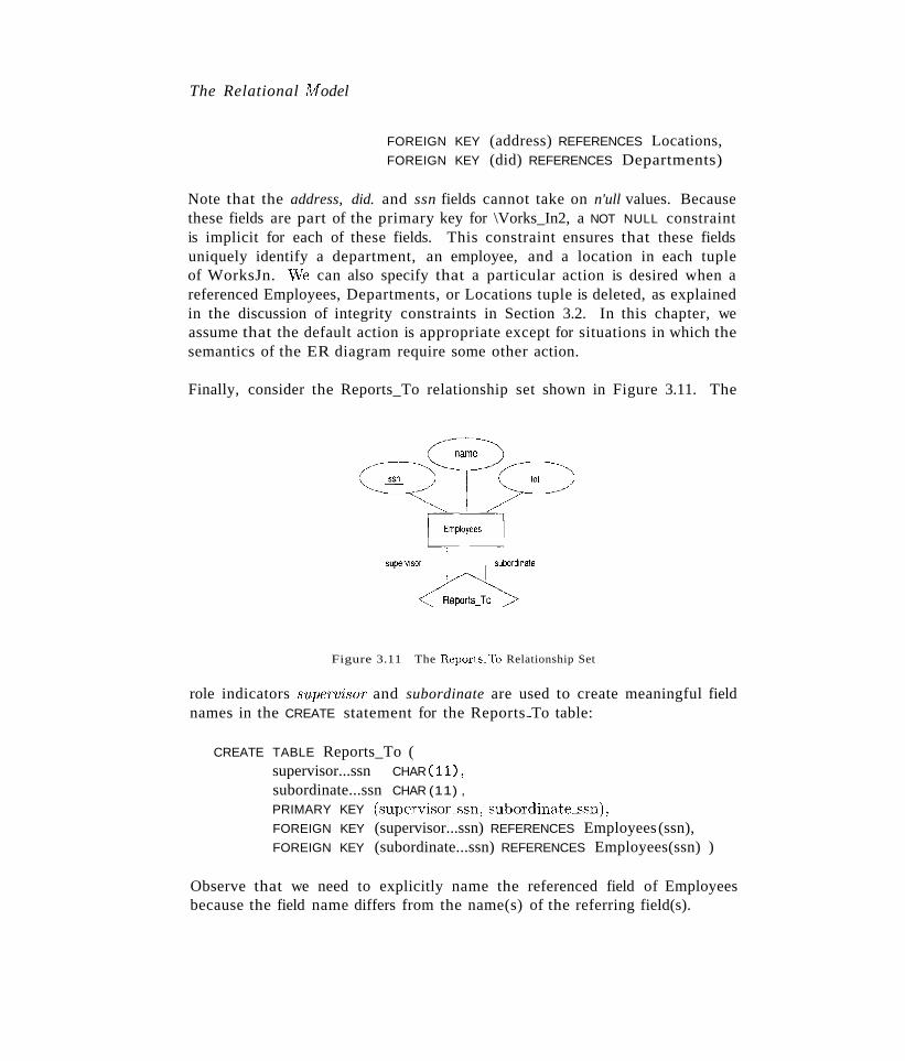
The Relational Iv!odel
FOREIGN KEY (address) REFERENCES Locations,FOREIGN KEY (did) REFERENCES Departments)
Note that the address, did. and ssn fields cannot take on n'ull values. Becausethese fields are part of the primary key for \Vorks_In2, a NOT NULL constraintis implicit for each of these fields. This constraint ensures that these fieldsuniquely identify a department, an employee, and a location in each tupleof WorksJn. vVe can also specify that a particular action is desired when areferenced Employees, Departments, or Locations tuple is deleted, as explainedin the discussion of integrity constraints in Section 3.2. In this chapter, weassume that the default action is appropriate except for situations in which thesemantics of the ER diagram require some other action.
Finally, consider the Reports_To relationship set shown in Figure 3.11. The
Figure 3.11 The Reports_To Relationship Set
role indicators supervisor and subordinate are used to create meaningful fieldnames in the CREATE statement for the Reports..To table:
CREATE TABLE Reports_To (supervisor...ssn CHAR (11),
subordinate...ssn CHAR (11) ,
PRIMARY KEY (supervisor~'3sn, subordinate_",,:>sn),FOREIGN KEY (supervisor...ssn) REFERENCES Employees(ssn),FOREIGN KEY (subordinate...ssn) REFERENCES Employees(ssn) )
Observe that we need to explicitly name the referenced field of Employeesbecause the field name differs from the name(s) of the referring field(s).
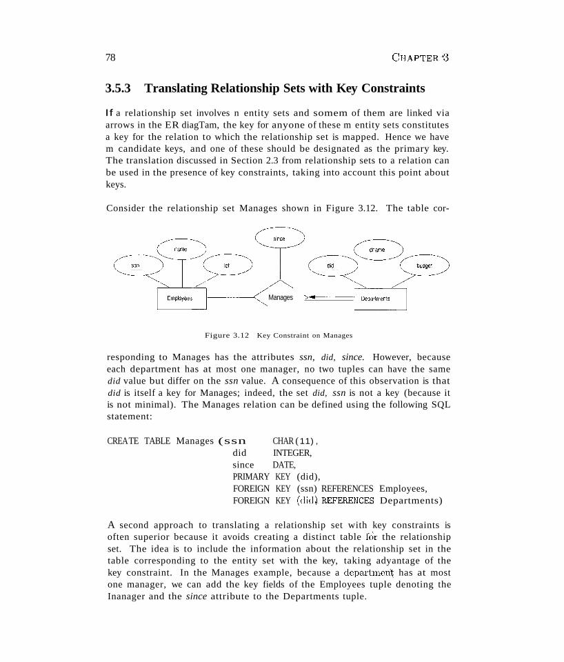
78 CHAPTER~3
3.5.3 Translating Relationship Sets with Key Constraints
If a relationship set involves n entity sets and somem of them are linked viaarrows in the ER diagTam, the key for anyone of these m entity sets constitutesa key for the relation to which the relationship set is mapped. Hence we havem candidate keys, and one of these should be designated as the primary key.The translation discussed in Section 2.3 from relationship sets to a relation canbe used in the presence of key constraints, taking into account this point aboutkeys.
Consider the relationship set Manages shown in Figure 3.12. The table cor-
Manages >4I"f--~~-
Figure 3.12 Key Constraint on Manages
responding to Manages has the attributes ssn, did, since. However, becauseeach department has at most one manager, no two tuples can have the samedid value but differ on the ssn value. A consequence of this observation is thatdid is itself a key for Manages; indeed, the set did, ssn is not a key (because itis not minimal). The Manages relation can be defined using the following SQLstatement:
CREATE TABLE Manages (ssn CHAR (11) ,did INTEGER,since DATE,PRIMARY KEY (did),FOREIGN KEY (ssn) REFERENCES Employees,FOREIGN KEY (did~REFERENCES Departments)
A second approach to translating a relationship set with key constraints isoften superior because it avoids creating a distinct table for the relationshipset. The idea is to include the information about the relationship set in thetable corresponding to the entity set with the key, taking adyantage of thekey constraint. In the Manages example, because a departmerl~ has at mostone manager, we can add the key fields of the Employees tuple denoting theInanager and the since attribute to the Departments tuple.
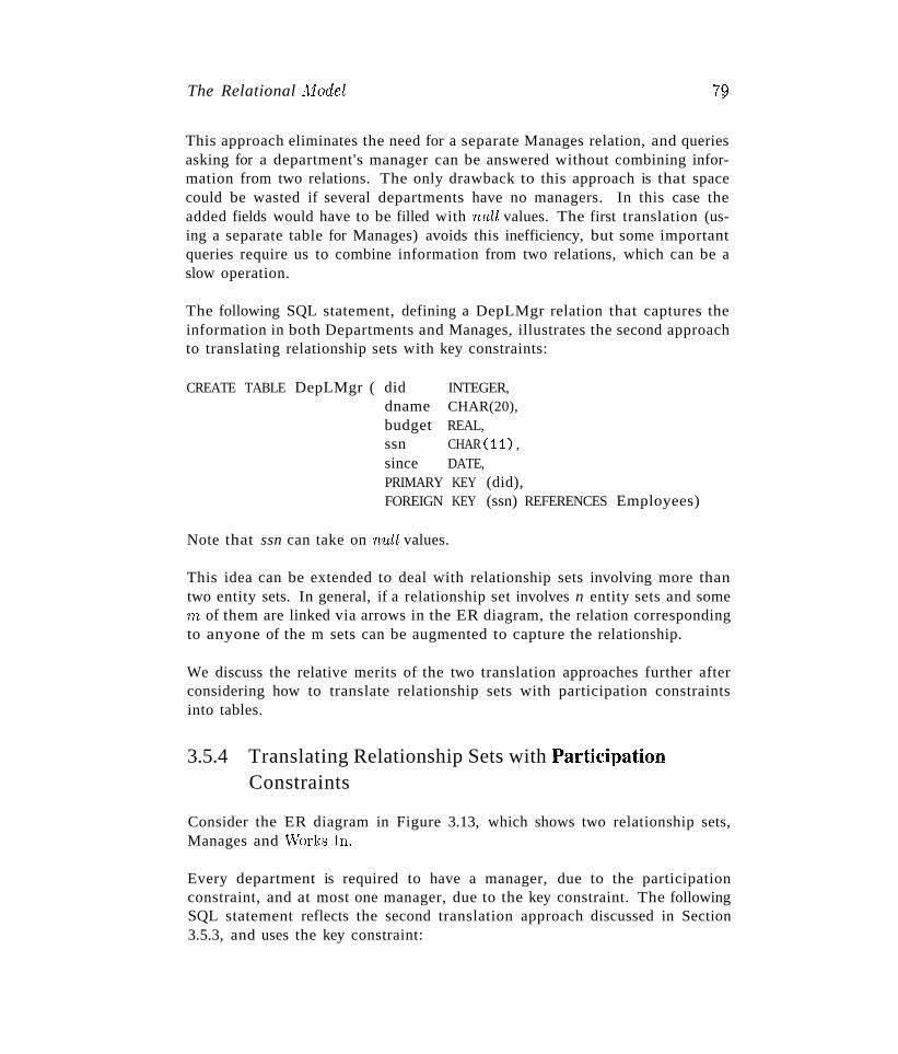
The Relational 1\1odel 7~
This approach eliminates the need for a separate Manages relation, and queriesasking for a department's manager can be answered without combining information from two relations. The only drawback to this approach is that spacecould be wasted if several departments have no managers. In this case theadded fields would have to be filled with null values. The first translation (using a separate table for Manages) avoids this inefficiency, but some importantqueries require us to combine information from two relations, which can be aslow operation.
The following SQL statement, defining a DepLMgr relation that captures theinformation in both Departments and Manages, illustrates the second approachto translating relationship sets with key constraints:
CREATE TABLE DepLMgr ( did INTEGER,dname CHAR(20),budget REAL,ssn CHAR (11) ,
since DATE,PRIMARY KEY (did),FOREIGN KEY (ssn) REFERENCES Employees)
Note that ssn can take on null values.
This idea can be extended to deal with relationship sets involving more thantwo entity sets. In general, if a relationship set involves n entity sets and someTn of them are linked via arrows in the ER diagram, the relation correspondingto anyone of the m sets can be augmented to capture the relationship.
We discuss the relative merits of the two translation approaches further afterconsidering how to translate relationship sets with participation constraintsinto tables.
3.5.4 Translating Relationship Sets with ParticipationConstraints
Consider the ER diagram in Figure 3.13, which shows two relationship sets,Manages and "Vorks_In.
Every department is required to have a manager, due to the participationconstraint, and at most one manager, due to the key constraint. The followingSQL statement reflects the second translation approach discussed in Section3.5.3, and uses the key constraint:
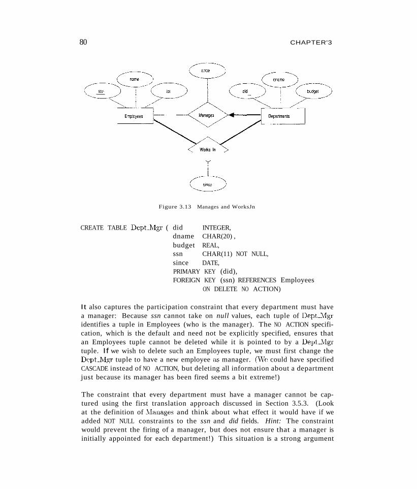
80 CHAPTER'3
Figure 3.13 Manages and WorksJn
CREATE TABLE DepLMgr ( did INTEGER,dname CHAR(20) ,budget REAL,ssn CHAR(11) NOT NULL,since DATE,PRIMARY KEY (did),FOREIGN KEY (ssn) REFERENCES Employees
ON DELETE NO ACTION)
It also captures the participation constraint that every department must havea manager: Because ssn cannot take on null values, each tuple of DepLMgridentifies a tuple in Employees (who is the manager). The NO ACTION specification, which is the default and need not be explicitly specified, ensures thatan Employees tuple cannot be deleted while it is pointed to by a Dept-Mgrtuple. If we wish to delete such an Employees tuple, we must first change theDepLMgr tuple to have a new employee &'3 manager. (vVe could have specifiedCASCADE instead of NO ACTION, but deleting all information about a departmentjust because its manager has been fired seems a bit extreme!)
The constraint that every department must have a manager cannot be captured using the first translation approach discussed in Section 3.5.3. (Lookat the definition of lVIanages and think about what effect it would have if weadded NOT NULL constraints to the ssn and did fields. Hint: The constraintwould prevent the firing of a manager, but does not ensure that a manager isinitially appointed for each department!) This situation is a strong argument
The Relational lvfodel 8~
in favor of using the second approach for one-to-many relationships such asManages, especially when the entity set with the key constraint also has a totalparticipation constraint.
Unfortunately, there are many participation constraints that we cannot captureusing SQL, short of using table constraints or assertions. Table constraints andassertions can be specified using the full power of the SQL query language(as discussed in Section 5.7) and are very expressive but also very expensive tocheck and enforce. For example, we cannot enforce the participation constraintson the \iVorks_In relation without using these general constraints. To see why,consider the Works-ln relation obtained by translating the ER diagram into·relations. It contains fields ssn and did, which are foreign keys referring toEmployees and Departments. To ensure total participation of Departments inWorks_In, we have to guarantee that every did value in Departments appearsin a tuple of Works_In. We could try to guarantee this condition by declaringthat did in Departments is a foreign key referring to Works_In, but this is nota valid foreign key constraint because did is not a candidate key for Works_In.
To ensure total participation of Departments in Works_In using SQL, we needan assertion. We have to guarantee that every did value in Departments appearsin a tuple of Works_In; further, this tuple of Works_In must also have non-nullvalues in the fields that are foreign keys referencing other entity sets involved inthe relationship (in this example, the ssn field). We can ensure the second partof this constraint by imposing the stronger requirement that ssn in Works-lncannot contain null values. (Ensuring that the participation of Employees inWorks_In is total is symmetric.)
Another constraint that requires assertions to express in SQL is the requirementthat each Employees entity (in the context of the Manages relationship set)must manage at least one department.
In fact, the Manages relationship set exemplifies most of the participation constraints that we can capture using key and foreign key constraints. Manages isa binary relationship set in which exactly one of the entity sets (Departments)has a key constraint, and the total participation constraint is expressed on thatentity set.
\Ve can also capture participation constraints using key and foreign key constraints in one other special situation: a relationship set in which all participating entity sets have key constraints and total participation. The best translationapproach in this case is to map all the entities &'3 well as the relationship intoa single table; the details are straightforward.
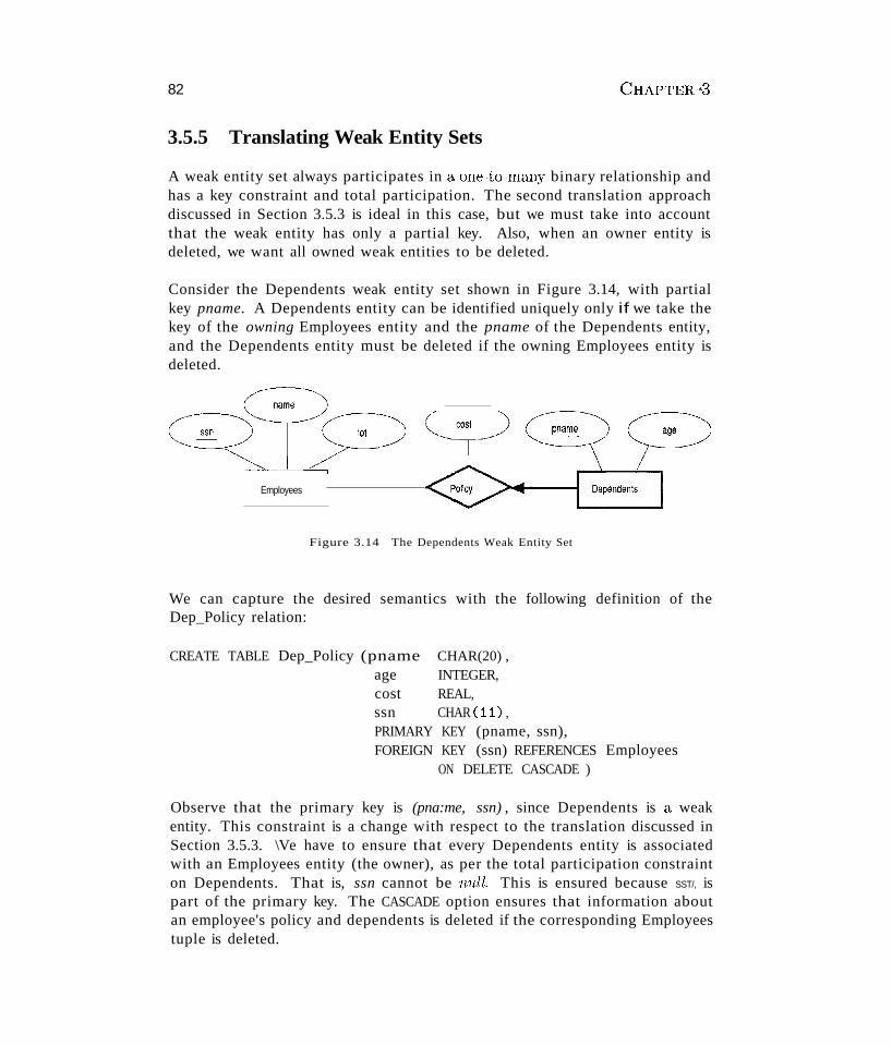
82 CHAPTER~3
3.5.5 Translating Weak Entity Sets
A weak entity set always participates in a one-to-many binary relationship andhas a key constraint and total participation. The second translation approachdiscussed in Section 3.5.3 is ideal in this case, but we must take into accountthat the weak entity has only a partial key. Also, when an owner entity isdeleted, we want all owned weak entities to be deleted.
Consider the Dependents weak entity set shown in Figure 3.14, with partialkey pname. A Dependents entity can be identified uniquely only if we take thekey of the owning Employees entity and the pname of the Dependents entity,and the Dependents entity must be deleted if the owning Employees entity isdeleted.
Employees
Figure 3.14 The Dependents Weak Entity Set
We can capture the desired semantics with the following definition of theDep_Policy relation:
CREATE TABLE Dep_Policy (pname CHAR(20) ,age INTEGER,cost REAL,ssn CHAR (11) ,
PRIMARY KEY (pname, ssn),FOREIGN KEY (ssn) REFERENCES Employees
ON DELETE CASCADE )
Observe that the primary key is (pna:me, ssn) , since Dependents is a weakentity. This constraint is a change with respect to the translation discussed inSection 3.5.3. \Ve have to ensure that every Dependents entity is associatedwith an Employees entity (the owner), as per the total participation constrainton Dependents. That is, ssn cannot be null. This is ensured because SST/, ispart of the primary key. The CASCADE option ensures that information aboutan employee's policy and dependents is deleted if the corresponding Employeestuple is deleted.
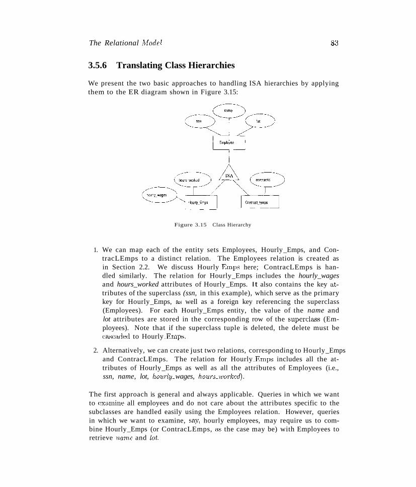
The Relational 1"1,,1oriel
3.5.6 Translating Class Hierarchies
83
We present the two basic approaches to handling ISA hierarchies by applyingthem to the ER diagram shown in Figure 3.15:
Figure 3.15 Class Hierarchy
1. We can map each of the entity sets Employees, Hourly_Emps, and ContracLEmps to a distinct relation. The Employees relation is created asin Section 2.2. We discuss Hourly~mps here; ContracLEmps is handled similarly. The relation for Hourly_Emps includes the hourly_wagesand hours_worked attributes of Hourly_Emps. It also contains the key attributes of the superclass (ssn, in this example), which serve as the primarykey for Hourly_Emps, a.', well as a foreign key referencing the superclass(Employees). For each Hourly_Emps entity, the value of the name andlot attributes are stored in the corresponding row of the supercla...,s (Employees). Note that if the superclass tuple is deleted, the delete must becascaded to Hourly~mps.
2. Alternatively, we can create just two relations, corresponding to Hourly_Empsand ContracLEmps. The relation for Hourly~mps includes all the attributes of Hourly_Emps as well as all the attributes of Employees (i.e.,ssn, name, lot, hO'l.1,rly_wages, hours_worked:).
The first approach is general and always applicable. Queries in which we wantto (~xamine all employees and do not care about the attributes specific to thesubclasses are handled easily using the Employees relation. However, queriesin which we want to examine, say, hourly employees, may require us to combine Hourly_Emps (or ContracLEmps, as the case may be) with Employees toretrieve name and lot.
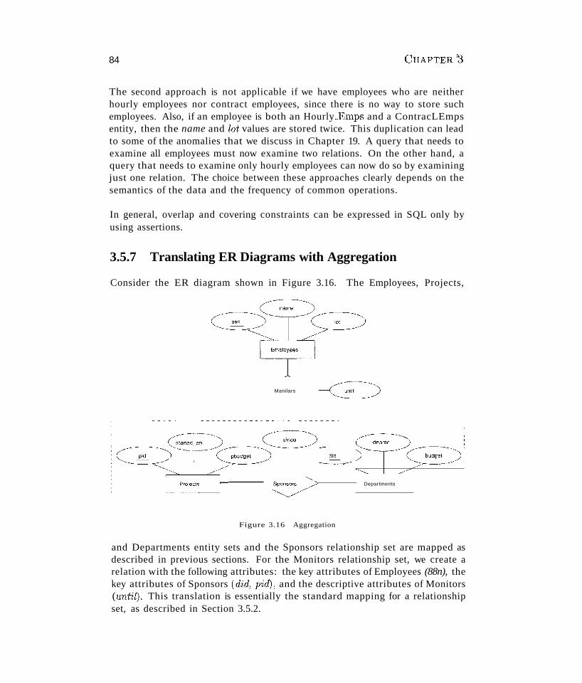
84 CHAPTER··~
The second approach is not applicable if we have employees who are neitherhourly employees nor contract employees, since there is no way to store suchemployees. Also, if an employee is both an Hourly-.Emps and a ContracLEmpsentity, then the name and lot: values are stored twice. This duplication can leadto some of the anomalies that we discuss in Chapter 19. A query that needs toexamine all employees must now examine two relations. On the other hand, aquery that needs to examine only hourly employees can now do so by examiningjust one relation. The choice between these approaches clearly depends on thesemantics of the data and the frequency of common operations.
In general, overlap and covering constraints can be expressed in SQL only byusing assertions.
3.5.7 Translating ER Diagrams with Aggregation
Consider the ER diagram shown in Figure 3.16. The Employees, Projects,
Manilars
Departments
I
_______did~ fT:C~'~~)
Figure 3.16 Aggregation
and Departments entity sets and the Sponsors relationship set are mapped asdescribed in previous sections. For the Monitors relationship set, we create arelation with the following attributes: the key attributes of Employees (88n), thekey attributes of Sponsors (d'id, p'id), and the descriptive attributes of Monitors('/.tnt:'il). This translation is essentially the standard mapping for a relationshipset, as described in Section 3.5.2.
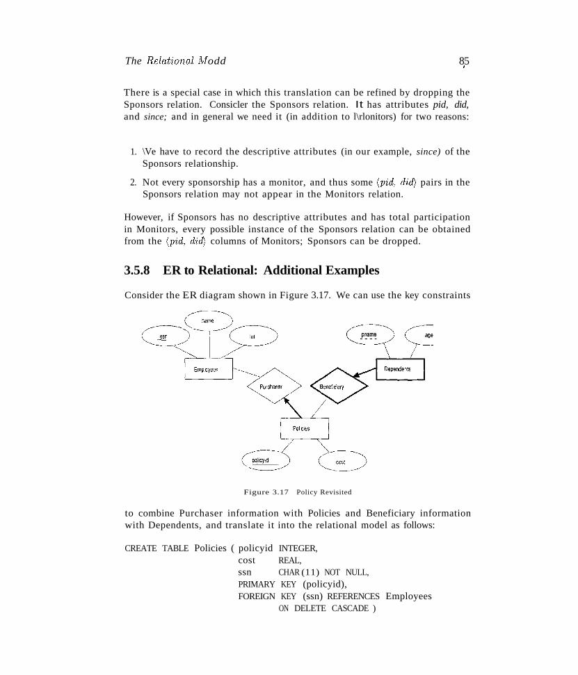
The Relational A!odd 85~
There is a special case in which this translation can be refined by dropping theSponsors relation. Consicler the Sponsors relation. It has attributes pid, did,and since; and in general we need it (in addition to l\rlonitors) for two reasons:
1. \Ve have to record the descriptive attributes (in our example, since) of theSponsors relationship.
2. Not every sponsorship has a monitor, and thus some (p'id, did) pairs in theSponsors relation may not appear in the Monitors relation.
However, if Sponsors has no descriptive attributes and has total participationin Monitors, every possible instance of the Sponsors relation can be obtainedfrom the (pid, did) columns of Monitors; Sponsors can be dropped.
3.5.8 ER to Relational: Additional Examples
Consider the ER diagram shown in Figure 3.17. We can use the key constraints
Figure 3.17 Policy Revisited
to combine Purchaser information with Policies and Beneficiary informationwith Dependents, and translate it into the relational model as follows:
CREATE TABLE Policies ( policyid INTEGER,cost REAL,ssn CHAR (11) NOT NULL,PRIMARY KEY (policyid),FOREIGN KEY (ssn) REFERENCES Employees
ON DELETE CASCADE )
86 CHAPTERB
CREATE TABLE Dependents (pname CHAR(20) ,age INTEGER,policyid INTEGER,PRIMARY KEY (pname, policyid),FOREIGN KEY (policyid) REFERENCES Policies
ON DELETE CASCADE)
Notice how the deletion of an employee leads to the deletion of all policiesowned by the employee and all dependents who are beneficiaries of those policies. Further, each dependent is required to have a covering policy-becausepolicyid is part of the primary key of Dependents, there is an implicit NOT NULLconstraint. This model accurately reflects the participation constraints in theER diagram and the intended actions when an employee entity is deleted.
In general, there could be a chain of identifying relationships for weak entitysets. For example, we assumed that policyid uniquely identifies a policy. Suppose that policyid distinguishes only the policies owned by a given employee;that is, policyid is only a partial key and Policies should be modeled as a weakentity set. This new assumption about policyid does not cause much to changein the preceding discussion. In fact, the only changes are that the primarykey of Policies becomes (policyid, ssn) , and as a consequence, the definition ofDependents changes-a field called ssn is added and becomes part of both theprimary key of Dependents and the foreign key referencing Policies:
CREATE TABLE Dependents (pname CHAR(20) ,ssn CHAR (11) ,
age INTEGER,policyid INTEGER NOT NULL,PRIMARY KEY (pname, policyid, ssn),FOREIGN KEY (policyid, ssn) REFERENCES Policies
ON DELETE CASCADE )
3.6 INTRODUCTION TO VIEWS
A view is a table whose rows are not explicitly stored in the database butare computed as needed from a view definition. Consider the Students andEnrolled relations. Suppose we are often interested in finding the names andstudent identifiers of students who got a grade of B in some course, togetherwith the course identifier. \Ne can define a view for this purpose. Using SQLnotation:
CREATE VIEW B-Students (name, sid, course)AS SELECT S.sname, S.sid, E.cid
The Relational 1I1odel
FROMWHERE
Students S, Enrolled ES.sid = E.studid AND E.grade = 'B'
87$
The view B-Students has three fields called name, sid, and course with thesame domains as the fields sname and sid in Students and cid in Enrolled.(If the optional arguments name, sid, and course are omitted from the CREATEVIEW statement, the column names sname, sid, and cid are inherited.)
This view can be used just like a base table, or explicitly stored table, indefining new queries or views. Given the instances of Enrolled and Studentsshown in Figure 3.4, B-Students contains the tuples shown in Figure 3.18.Conceptually, whenever B-Students is used in a query, the view definition isfirst evaluated to obtain the corresponding instance of B-Students, then the restof the query is evaluated treating B-Students like any other relation referredto in the query. (We discuss how queries on views are evaluated in practice inChapter 25.)
sid course
History105Reggae203
Figure 3.18 An Instance of the B-Students View
3.6.1 Views, Data Independence, Security
Consider the levels of abstraction we discussed in Section 1.5.2. The physicalschema for a relational database describes how the relations in the conceptualschema are stored, in terms of the file organizations and indexes used. Theconceptual schema is the collection of schemas of the relations stored in thedatabase. While some relations in the conceptual schema can also be exposed toapplications, that is, be part of the exte'mal schema of the database, additionalrelations in the external schema can be defined using the view mechanism.The view mechanism thus provides the support for logical data independencein the relational model. That is, it can be used to define relations in theexternal schema that mask changes in the conceptual schema of the databasefrom applications. For example, if the schema of a stored relation is changed,we can define a view with the old schema and applications that expect to seethe old schema can now use this view.
Views are also valuable in the context of security: We can define views thatgive a group of users access to just the information they are allowed to see. Forexample, we can define a view that allows students to see the other students'
88 CHAPTER B
name and age but not their gpa, and allows all students to access this view butnot the underlying Students table (see Chapter 21).
3.6.2 Updates on Views
The motivation behind the view mechanism is to tailor how users see the data.Users should not have to worry about the view versus base table distinction.This goal is indeed achieved in the case of queries on views; a view can be usedjust like any other relation in defining a query. However, it is natural to want tospecify updates on views as well. Here, unfortunately, the distinction betweena view and a ba.se table must be kept in mind.
The SQL-92 standard allows updates to be specified only on views that aredefined on a single base table using just selection and projection, with no use ofaggregate operations. 3 Such views are called updatable views. This definitionis oversimplified, but it captures the spirit of the restrictions. An update onsuch a restricted view can always be implemented by updating the underlyingbase table in an unambiguous way. Consider the following view:
CREATE VIEW GoodStudents (sid, gpa)AS SELECT S.sid, S.gpa
FROM Students SWHERE S.gpa> 3.0
We can implement a command to modify the gpa of a GoodStudents row bymodifying the corresponding row in Students. We can delete a GoodStudentsrow by deleting the corresponding row from Students. (In general, if the viewdid not include a key for the underlying table, several rows in the table could'correspond' to a single row in the view. This would be the case, for example,if we used S.sname instead of S.sid in the definition of GoodStudents. A command that affects a row in the view then affects all corresponding rows in theunderlying table.)
We can insert a GoodStudents row by inserting a row into Students, usingnull values in columns of Students that do not appear in GoodStudents (e.g.,sname, login). Note that primary key columns are not allowed to contain nullvalues. Therefore, if we attempt to insert rows through a view that does notcontain the primary key of the underlying table, the insertions will be rejected.For example, if GoodStudents contained snarne but not ,c;id, we could not insertrows into Students through insertions to GooclStudents.
3There is also the restriction that the DISTINCT operator cannot be used in updatable vi(;w definitions. By default, SQL does not eliminate duplicate copies of rows from the result of it query; theDISTINCT operator requires duplicate elimination. vVe discuss t.his point further in Chapt.er 5.
The Relational A10dd
----------------~-
Updatable Views in SQL:1999 The Hew SQL standard has expandedthe class of view definitions that are updatable~ taking primary . keyconstraints into account. In contra..')t· to SQL-92~ a· view definition thatcontains more than OIle table in the FROM clause may be updatable underthe new definition. Intuitively~ we can update afield of a. view if it isobtained from exactly one of the underlying tables, and the primary keyof that table is included in the fields of the view.
SQL:1999 distinguishes between views whose rows can be modified (updatable views) and views into which new rows can be inserted (insertableinto views): Views defined using the SQL constructs UNION, INTERSECT,and EXCEPT (which we discuss in Chapter 5) cannot be inserted into, evenif they are updatable. Intuitively, updatability ensures that an updatedtuple in the view can be traced to exactly one tuple in one of the tablesused to define the view. The updatability property, however, may still notenable us to decide into which table to insert a new tuple.
An important observation is that an INSERT or UPDATE may change the underlying base table so that the resulting (i.e., inserted or modified) row is notin the view! For example, if we try to insert a row (51234, 2.8) into the view,this row can be (padded with null values in the other fields of Students andthen) added to the underlying Students table, but it will not appear in theGoodStudents view because it does not satisfy the view condition gpa > 3.0.The SQL default action is to allow this insertion, but we can disallow it byadding the clause WITH CHECK OPTION to the definition of the view. In thiscase, only rows that will actually appear in the view are permissible insertions.
We caution the reader, that when a view is defined in terms of another view,the interaction between these view definitions with respect to updates and theCHECK OPTION clause can be complex; we not go into the details.
Need to Restrict View Updates
vVhile the SQL rules on updatable views are more stringent than necessary,there are some fundamental problems with updates specified on views and goodreason to limit the class of views that can be updated. Consider the Studentsrelation and a new relation called Clubs:
Clubs( cname: string, jyear: date, mnarne: string)
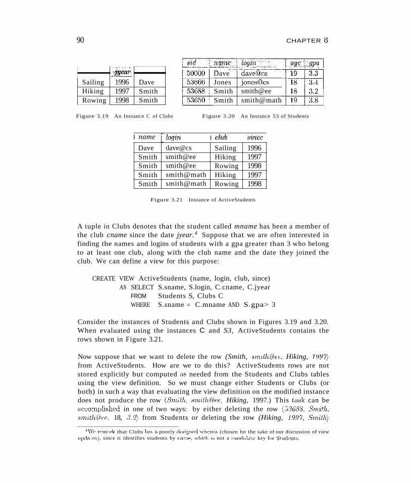
90
~Sailing 1996 DaveHiking 1997 SmithRowing 1998 Smith
DaveJonesSmithSmith
dave(gcsjones~~cs
smith@eesmith@math
CHAPTER 8
Figure 3.19 An Instance C of Clubs
I name ,. login
Figure 3.20 An Instance 53 of Students
I dub sinceDave dave@cs Sailing 1996Smith smith@ee Hiking 1997Smith smith@ee Rowing 1998Smith smith@math Hiking 1997Smith smith@math Rowing 1998
Figure 3.21 Instance of ActiveStudents
A tuple in Clubs denotes that the student called mname has been a member ofthe club cname since the date jyear. 4 Suppose that we are often interested infinding the names and logins of students with a gpa greater than 3 who belongto at least one club, along with the club name and the date they joined theclub. We can define a view for this purpose:
CREATE VIEW ActiveStudents (name, login, club, since)AS SELECT S.sname, S.login, C.cname, C.jyear
FROM Students S, Clubs CWHERE S.sname = C.mname AND S.gpa> 3
Consider the instances of Students and Clubs shown in Figures 3.19 and 3.20.When evaluated using the instances C and S3, ActiveStudents contains therows shown in Figure 3.21.
Now suppose that we want to delete the row (Smith, smith@ee, Hiking, 1997)from ActiveStudents. How are we to do this? ActiveStudents rows are notstored explicitly but computed as needed from the Students and Clubs tablesusing the view definition. So we must change either Students or Clubs (orboth) in such a way that evaluating the view definition on the modified instancedoes not produce the row (Snrith, 8Tnith@ec, Hiking, 1997.) This ta.sk can bectccomplished in one of two ways: by either deleting the row (53688.. Sm'ith,8Tn'ith(iJ)ee, 18, ,g.2) from Students or deleting the row (Hiking, 1.997, 8m/ith)
clvVe remark that Clubs has a poorly designed schema (chosen for the sake of our discussion of viewupdates), since it identifies students by name, which is not a candidate key for Students.
The Relational tv!odel 9J
from Clubs. But neither solution is satisfactory. Removing the Students rowhas the effect of also deleting the row (8m:ith, smith@ee, Rowing, 1998) from theview ActiveStudents. Removing the Clubs row h&'3 the effect of also deleting therow (Smith, smith@math, Hiking, 1991) from the view ActiveStudents. Neitherside effect is desirable. In fact, the only reasonable solution is to d'isallow suchupdates on views.
Views involving more than one base table can, in principle, be safely updated.The B-Students view we introduced at the beginning of this section is an example of such a view. Consider the instance of B-Students shown in Figure3.18 (with, of course, the corresponding instances of Students and Enrolled asin Figure 3.4). To insert a tuple, say (Dave, 50000, Reggae203) B-Students, wecan simply insert a tuple (Reggae203, B, 50000) into Enrolled since there is already a tuple for sid 50000 in Students. To insert (John, 55000, Reggae203), onthe other hand, we have to insert (Reggae203, B, 55000) into Enrolled and alsoinsert (55000, John, null, null, null) into Students. Observe how null valuesare used in fields of the inserted tuple whose value is not available. Fortunately,the view schema contains the primary key fields of both underlying base tables;otherwise, we would not be able to support insertions into this view. To deletea tuple from the view B-Students, we can simply delete the corresponding tuplefrom Enrolled.
Although this example illustrates that the SQL rules on updatable views areunnecessarily restrictive, it also brings out the complexity of handling viewupdates in the general case. For practical reasons, the SQL standard has chosento allow only updates on a very restricted class of views.
3.7 DESTROYING/ALTERING TABLES AND VIEWS
If we decide that we no longer need a base table and want to destroy it (i.e.,delete all the rows and remove the table definition information), we can usethe DROP TABLE command. For example, DROP TABLE Students RESTRICT destroys the Students table unless some view or integrity constraint refers toStudents; if so, the command fails. If the keyword RESTRICT is replaced byCASCADE, Students is dropped and any referencing views or integrity constraintsare (recursively) dropped as well; one of these t\VO keyvlOrds must always bespecified. A vipw can be dropped using the DROP VIEW command, which is justlike DROP TABLE.
ALTER TABLE modifies the structure of an existing table. To add a columncalled maiden-name to Students, for example, we would use the following command:
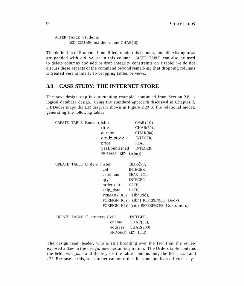
92
ALTER TABLE StudentsADD COLUMN maiden-name CHAR(10)
CUAPTER·.'3
The definition of Students is modified to add this column, and all existing rowsare padded with null values in this column. ALTER TABLE can also be usedto delete columns and add or drop integrity constraints on a table; we do notdiscuss these aspects of the command beyond remarking that dropping columnsis treated very similarly to dropping tables or views.
3.8 CASE STUDY: THE INTERNET STORE
The next design step in our running example, continued from Section 2.8, islogical database design. Using the standard approach discussed in Chapter 3,DBDudes maps the ER diagram shown in Figure 2.20 to the relational model,generating the following tables:
CREATE TABLE Books ( isbn CHAR ( 10) ,title CHAR(80) ,author CHAR(80),qty_in-stock INTEGER,price REAL,yeaLpublished INTEGER,PRIMARY KEY (isbn))
CREATE TABLE Orders ( isbn CHAR (10) ,ciel INTEGER,carelnum CHAR (16) ,qty INTEGER,order_date DATE,ship_date DATE,PRIMARY KEY (isbn,cid),FOREIGN KEY (isbn) REFERENCES Books,FOREIGN KEY (cid) REFERENCES Customers)
CREATE TABLE Customers ( cid INTEGER,cname CHAR(80),address CHAR(200),PRIMARY KEY (cid)
The design team leader, who is still brooding over the fact that the reviewexposed a flaw in the design, now has an inspiration. The Orders table containsthe field order_date and the key for the table contains only the fields isbn andc'id. Because of this, a customer cannot order the same book OIl different days,
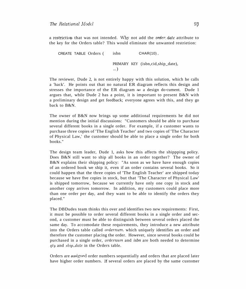
The Relat'ional l1;lodel 9~
a re.striction that was not intended. vVhy not add the order-date attribute tothe key for the Orders table? This would eliminate the unwanted restrietion:
CREATE TABLE Orders ( isbn CHAR(10) ,
PRIMARY KEY (isbn,cid,ship_date),... )
The reviewer, Dude 2, is not entirely happy with this solution, which he callsa 'hack'. He points out that no natural ER diagram reflects this design andstresses the importance of the ER diagram &<; a design do·cument. Dude 1argues that, while Dude 2 has a point, it is important to present B&N witha preliminary design and get feedback; everyone agrees with this, and they goback to B&N.
The owner of B&N now brings up some additional requirements he did notmention during the initial discussions: "Customers should be able to purchaseseveral different books in a single order. For example, if a customer wants topurchase three copies of 'The English Teacher' and two copies of 'The Characterof Physical Law,' the customer should be able to place a single order for bothbooks."
The design team leader, Dude 1, asks how this affects the shippping policy.Does B&N still want to ship all books in an order together? The owner ofB&N explains their shipping policy: "As soon as we have have enough copiesof an ordered book we ship it, even if an order contains several books. So itcould happen that the three copies of 'The English Teacher' are shipped todaybecause we have five copies in stock, but that 'The Character of Physical Law'is shipped tomorrow, because we currently have only one copy in stock andanother copy arrives tomorrow. In addition, my customers could place morethan one order per day, and they want to be able to identify the orders theyplaced."
The DBDudes team thinks this over and identifies two new requirements: First,it must be possible to order several different books in a single order and second, a customer must be able to distinguish between several orders placed thesame day. To accomodate these requirements, they introduce a new attributeinto the Orders table called ordernum, which uniquely identifies an order andtherefore the customer placing the order. However, since several books could bepurchased in a single order, onleTnum and isbn are both needed to determineqt.y and ship_dat.e in the Orders table.
Orders are assign(~d order numbers sequentially and orders that are placed laterhave higher order numbers. If several orders are placed by the same customer
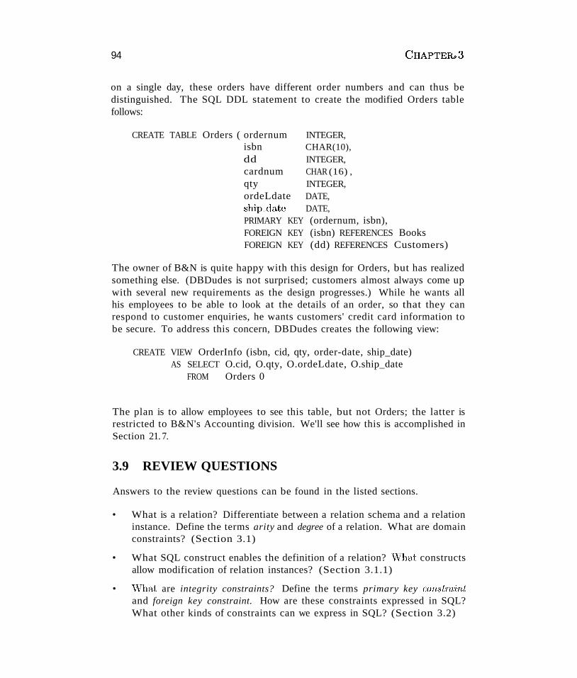
94 CHAPTER03
on a single day, these orders have different order numbers and can thus bedistinguished. The SQL DDL statement to create the modified Orders tablefollows:
CREATE TABLE Orders ( ordernum INTEGER,isbn CHAR(10),dd INTEGER,cardnum CHAR (16) ,qty INTEGER,ordeLdate DATE,ship~date DATE,PRIMARY KEY (ordernum, isbn),FOREIGN KEY (isbn) REFERENCES BooksFOREIGN KEY (dd) REFERENCES Customers)
The owner of B&N is quite happy with this design for Orders, but has realizedsomething else. (DBDudes is not surprised; customers almost always come upwith several new requirements as the design progresses.) While he wants allhis employees to be able to look at the details of an order, so that they canrespond to customer enquiries, he wants customers' credit card information tobe secure. To address this concern, DBDudes creates the following view:
CREATE VIEW OrderInfo (isbn, cid, qty, order-date, ship_date)AS SELECT O.cid, O.qty, O.ordeLdate, O.ship_date
FROM Orders 0
The plan is to allow employees to see this table, but not Orders; the latter isrestricted to B&N's Accounting division. We'll see how this is accomplished inSection 21. 7.
3.9 REVIEW QUESTIONS
Answers to the review questions can be found in the listed sections.
• What is a relation? Differentiate between a relation schema and a relationinstance. Define the terms arity and degree of a relation. What are domainconstraints? (Section 3.1)
• What SQL construct enables the definition of a relation? \Vhat constructsallow modification of relation instances? (Section 3.1.1)
• \Vhat are integrity constraints? Define the terms primary key constTa'intand foreign key constraint. How are these constraints expressed in SQL?What other kinds of constraints can we express in SQL? (Section 3.2)
The Relational Alodel 95
• \Vhat does the DBMS do when constraints are violated? What is referential 'integr-ity? \Vhat options does SQL give application programmers fordealing with violations of referential integrity? (Section 3.3)
• When are integrity constraints enforced by a DBMS? How can an application programmer control the time that constraint violations are checkedduring transaction execution? (Section 3.3.1)
• What is a relational database query? (Section 3.4)
• How can we translate an ER diagram into SQL statements to create tables? How are entity sets mapped into relations? How are relationshipsets mapped? How are constraints in the ER model, weak entity sets, classhierarchies, and aggregation handled? (Section 3.5)
• What is a view? How do views support logical data independence? Howare views used for security? How are queries on views evaluated? Whydoes SQL restrict the class of views that can be updated? (Section 3.6)
• What are the SQL constructs to modify the structure of tables and de-stray tables and views? Discuss what happens when we destroy a view.(Section 3.7)
EXERCISES
Exercise 3.1 Define the following terms: relation schema, relational database schema, domain, relation instance, relation cardinality, and relation degree.
Exercise 3.2 How many distinct tuples are in a relation instance with cardinality 22?
Exercise 3.3 Does the relational model, as seen by an SQL query writer, provide physicaland logical data independence? Explain.
Exercise 3.4 \\That is the difference between a candidate key and the primary key for a givenrelation? What is a superkey?
Exercise 3.5 Consider the instance of the Students relation shown in Figure 3.1.
1. Give an example of an attribute (or set of attributes) that you can deduce is not acandidate key, based on this instance being legaL
2. Is there any example of an attribute (or set of attributes) that you can deduce is acandidate key, based on this instance being legal?
Exercise 3.6 What is a foreign key constraint? Why are such constraints important? Whatis referential integrity?
Exercise 3.7 Consider the relations Students, Faculty, Courses, Rooms, Enrolled, Teaches,'Lnd Meets_In defined in Section 1.5.2.
96 CHAPTERr3
1. List all the foreign key constraints among these relations.
2. Give an example of a (plausible) constraint involving one or more of these relations thatis not a primary key or foreign key constraint.
Exercise 3.8 Answer each of the following questions briefly. The questions are b&'>ed OIl thefollowing relational schema:
Emp( eid: integer, ename: string, age: integer, sala1l1: real)Works (eid: integer, did: integer, peLtime: integer)Dept(did: integer, dname: string, budget: real, managerid: integer)
1. Give an example of a foreign key constraint that involves the Dept relation. What arethe options for enforcing this constraint when a user attempts to delete a Dept tuple?
2. Write the SQL statements required to create the preceding relations, including appropriate versions of all primary and foreign key integrity constraints.
3. Define the Dept relation in SQL so that every department is guaranteed to have amanager.
4. Write an SQL statement to add John Doe as an employee with eid = 101, age = 32 andsalary = 15,000.
5. Write an SQL statement to give every employee a 10 percent raise.
6. Write an SQL statement to delete the Toy department. Given the referential integrityconstraints you chose for this schema, explain what happens when this statement isexecuted.
Exercise 3.9 Consider the SQL query whose answer is shown in Figure 3.6.
1. Modify this query so that only the login column is included in the answer.
2. If the clause WHERE S.gpa >= 2 is added to the original query, what is the set of tuplesin the answer?
Exercise 3.10 Explain why the addition of NOT NULL constraints to the SQL definition ofthe Manages relation (in Section 3.5.3) would not enforce the constraint that each departmentmust have a manager. What, if anything, is achieved by requiring that the S8n field of Managesbe non-null?
Exercise 3.11 Suppose that we have a ternary relationship R between entity sets A, B,and C such that A has a key constraint and total participation and B has a key constraint;these are the only constraints. A has attributes al and a2, with al being the key; BandC are similar. R has no descriptive attributes. Write SQL statements that create tablescorresponding to this information so &s to capture as many of the constraints as possible. Ifyou cannot capt,).ue some constraint, explain why.
Exercise 3.12 Consider the scenario from Exercise 2.2, where you designed an ER diagramfor a university database. \Vrite SQL staternents to create the corresponding relations andcapture as many of the constraints as possible. If you cannot: capture some constraints, explainwhy.
Exercise 3.13 Consider the university database from Exercise 2.:3 and the ER diagram youdesigned. Write SQL statements to create the corresponding relations and capture &'> manyof the constraints as possible. If you cannot capture some constraints, explain why.
The RelatioTwl A10del 97t
Exercise 3.14 Consider the scenario from Exercise 2.4, where you designed an ER diagramfor a company databa,c;e. \~Trite SQL statements to create the corresponding relations andcapture as many of the constraints as possible. If you cannot capture some constraints,explain why.
Exercise 3.15 Consider the Notown database from Exercise 2.5. You have decided to recommend that Notown use a relational database system to store company data. Show theSQL statements for creating relations corresponding to the entity sets and relationship setsin your design. Identify any constraints in the ER diagram that you are unable to capture inthe SQL statements and briefly explain why you could not express them.
Exercise 3.16 Thanslate your ER diagram from Exercise 2.6 into a relational schema, andshow the SQL statements needed to create the relations, using only key and null constraints.If your translation cannot capture any constraints in the ER diagram, explain why.
In Exercise 2.6, you also modified the ER diagram to include the constraint that tests on aplane must be conducted by a technician who is an expert on that model. Can you modifythe SQL statements defining the relations obtained by mapping the ER diagram to check thisconstraint?
Exercise 3.17 Consider the ER diagram that you designed for the Prescriptions-R-X chain ofpharmacies in Exercise 2.7. Define relations corresponding to the entity sets and relationshipsets in your design using SQL.
Exercise 3.18 Write SQL statements to create the corresponding relations to the ER diagram you designed for Exercise 2.8. If your translation cannot capture any constraints in theER diagram, explain why.
Exercise 3.19 Briefly answer the following questions based on this schema:
Emp(e'id: integer, ename: string, age: integer, salary: real)Works (eid: integer, did: integer, peLtime: integer)Dept(did: integer, budget: real, managerid: integer)
1. Suppose you have a view SeniorEmp defined as follows:
CREATE VIEW SeniorEmp (sname, sage, salary)AS SELECT E.ename, Kage, E.salary
FROM Emp EWHERE Kage > 50
Explain what the system will do to process the following query:
SELECT S.snameFROM SeniorEmp SWHERE S.salary > 100,000
2. Give an example of a view on Emp that could be automatically updated by updatingEmp.
3. Give an example of a view on Emp that would be impossible to update (automatically)and explain why your example presents the update problem that it does.
Exercise 3.20 C::onsider the following schema:
98
Suppliers( sid: integer, sname: string, address: string)
Parts(pid: integer, pname: string, color: string)
Catalog(sid: integer, pid: integer, cost: real)
CHAPTER,. 3
The Catalog relation lists the prices charged for parts by Suppliers. Answer the followingquestions:
• Give an example of an updatable view involving one relation.
• Give an example of an updatable view involving two relations.
• Give an example of an insertable-into view that is updatable.
• Give an example of an insertable-into view that is not updatable.
PROJECT-BASED EXERCISES
Exercise 3.21 Create the relations Students, Faculty, Courses, Rooms, Enrolled, Teaches,and Meets_In in Minibase.
Exercise 3.22 Insert the tuples shown in Figures 3.1 and 3.4 into the relations Students andEnrolled. Create reasonable instances of the other relations.
Exercise 3.23 What integrity constraints are enforced by Minibase?
Exercise 3.24 Run the SQL queries presented in this chapter.
BIBLIOGRAPHIC NOTES
The relational model was proposed in a seminal paper by Codd [187]. Childs [176] and Kuhns[454] foreshadowed some of these developments. Gallaire and :WIinker's book [296] containsseveral papers on the use of logic in the context of relational databases. A system based on avariation of the relational model in which the entire database is regarded abstractly as a singlerelation, called the universal relation, is described in [746]. Extensions of the relational modelto incorporate null values, which indicate an unknown or missing field value, are discussed byseveral authors; for example, [329, 396, 622, 754, 790].
Pioneering projects include System R [40, 150] at IBM San Jose Research Laboratory (nowIBM Almaden Research Center), Ingres [717] at the University of California at Berkeley,PRTV [737] at the IBNI UK Scientific Center in Peterlee, and QBE [801] at IBM T. J.Watson Research Center.
A rich theory underpins the field of relational databases. Texts devoted to theoretical aspectsinclude those by··Atzeni and DeAntonellis [45]; Maier [501]; and Abiteboul, Hull, and Vianu[:3]. [415] is an excellent survey article.
Integrity constraints in relational databases have been discussed at length. [190] addressessemantic extensions to the relational model, and integrity, in particular referential integrity.U~60] discusses semantic integrity constraints. [2()~3] contains papers that address variousaspects of integrity constraints, including in particular a detailed discussion of referentialintegrity. A vast literature deals \vith enforcing integrity constraints. [51] compares the cost
The Relational AIodel 99.~
of enforcing integrity constraints via compile-time, run-time, and post-execution checks. [145]presents an SQL-based language for specifying integrity constraints and identifies conditionsunder which integrity rules specified in this language can be violated. [713] discusses thetechnique of integrity constraint checking by query modification. [180] discusses real-timeintegrity constraints. Other papers on checking integrity constraints in databases include[82, 122, 138,517]. [681] considers the approach of verifying the correctness of programs thataccess the database instead of run-time checks. Note that this list of references is far fTomcomplete; in fact, it does not include any of the many papers on checking recursively specifiedintegrity constraints. Some early papers in this widely studied area can be found in [296] and[295].
For references on SQL, see the bibliographic notes for Chapter 5. This book does not discussspecific products based on the relational model, but many fine books discuss each of the majorcommercial systems; for example, Chamberlin's book on DB2 [149], Date and McGoveran'sbook on Sybase [206], and Koch and Loney's book on Oracle [443].
Several papers consider the problem of translaping updates specified on views into updateson the underlying table [59, 208, 422, 468, 778]. [292] is a good survey on this topic. Seethe bibliographic notes for Chapter 25 for references to work querying views and maintainingmaterialized views.
[731] discusses a design methodology based on developing an ER diagram and then translatingto the relational model. Markowitz considers referential integrity in the context of ER torelational mapping and discusses the support provided in some commercial systems (as ofthat date) in [513, 514].

4RELATIONAL ALGEBRA
AND CALCULUS
.. What is the foundation for relational query languages like SQL? Whatis the difference between procedural and declarative languages?
... What is relational algebra, and why is it important?
... What are the basic algebra operators, and how are they combined towrite complex queries?
... What is relational calculus, and why is it important?
... What subset of mathematical logic is used in relational calculus, andhow is it used to write queries?
.. Key concepts: relational algebra, select, project, union, intersection,cross-product, join, division; tuple relational calculus, domain relational calculus, formulas, universal and existential quantifiers, boundand free variables
'--------------------
Stand finn in your refusal to remain conscious during algebra. In real life, Iassure you, there is no such thing as algebra.
~·-Fran Lebowitz, Social Studies
This chapter presents two formal query languages associated with the relationalmodel. Query 'languages are specialized languages for asking questions, orqueries, that involve the data in a database. After covering some preliminariesin Section 4.1, we discuss rdafional algebra in Section 4.2. Queries in relationalalgebra are composed using a collection of operators, and each query describesa step-by-step procedure for computing the desired answer; that is, queries are
100
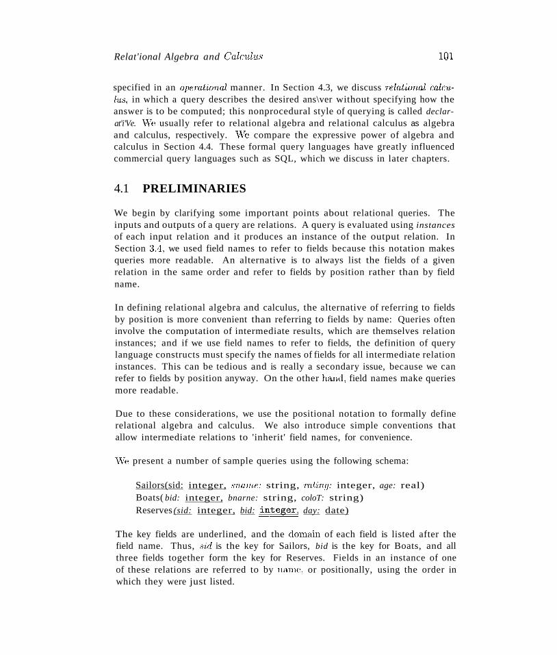
Relat'ional Algebra and Calcullls un
specified in an operationa.l manner. In Section 4.3, we discuss Tela.l'ional calculus, in which a query describes the desired ans\ver without specifying how theanswer is to be computed; this nonprocedural style of querying is called declarat'i'Ve. \Ve usually refer to relational algebra and relational calculus as algebraand calculus, respectively. vVe compare the expressive power of algebra andcalculus in Section 4.4. These formal query languages have greatly influencedcommercial query languages such as SQL, which we discuss in later chapters.
4.1 PRELIMINARIES
We begin by clarifying some important points about relational queries. Theinputs and outputs of a query are relations. A query is evaluated using instancesof each input relation and it produces an instance of the output relation. InSection 3.4, we used field names to refer to fields because this notation makesqueries more readable. An alternative is to always list the fields of a givenrelation in the same order and refer to fields by position rather than by fieldname.
In defining relational algebra and calculus, the alternative of referring to fieldsby position is more convenient than referring to fields by name: Queries ofteninvolve the computation of intermediate results, which are themselves relationinstances; and if we use field names to refer to fields, the definition of querylanguage constructs must specify the names of fields for all intermediate relationinstances. This can be tedious and is really a secondary issue, because we canrefer to fields by position anyway. On the other hand, field names make queriesmore readable.
Due to these considerations, we use the positional notation to formally definerelational algebra and calculus. We also introduce simple conventions thatallow intermediate relations to 'inherit' field names, for convenience.
vVe present a number of sample queries using the following schema:
Sailors(sid: integer, snarne: string, rating: integer, age: real)Boats( bid: integer, bnarne: string, coloT: string)Reserves (sid: integer, bid: _~_r:teger, day: date)
The key fields are underlined, and the doma,in of each field is listed after thefield name. Thus, .sid is the key for Sailors, bid is the key for Boats, and allthree fields together form the key for Reserves. Fields in an instance of oneof these relations are referred to by name, or positionally, using the order inwhich they were just listed.
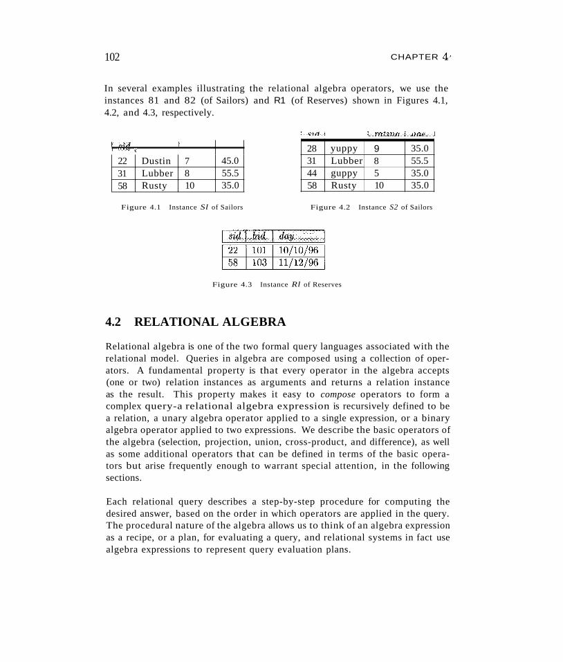
102 CHAPTER 4,
In several examples illustrating the relational algebra operators, we use theinstances 81 and 82 (of Sailors) and R1 (of Reserves) shown in Figures 4.1,4.2, and 4.3, respectively.
1",';-1 JI yv'l' 1
22 Dustin 7 45.031 Lubber 8 55.558 Rusty 10 35.0
Figure 4.1 Instance Sl of Sailors
t'Cc'Jdl l'l"n1mn1Jlnl:JlPj
28 yuppy 9 35.031 Lubber 8 55.544 guppy 5 35.058 Rusty 10 35.0
Figure 4.2 Instance S2 of Sailors
Figure 4.3 Instance Rl of Reserves
4.2 RELATIONAL ALGEBRA
Relational algebra is one of the two formal query languages associated with therelational model. Queries in algebra are composed using a collection of operators. A fundamental property is that every operator in the algebra accepts(one or two) relation instances as arguments and returns a relation instanceas the result. This property makes it easy to compose operators to form acomplex query-a relational algebra expression is recursively defined to bea relation, a unary algebra operator applied to a single expression, or a binaryalgebra operator applied to two expressions. We describe the basic operators ofthe algebra (selection, projection, union, cross-product, and difference), as wellas some additional operators that can be defined in terms of the basic operators but arise frequently enough to warrant special attention, in the followingsections.
Each relational query describes a step-by-step procedure for computing thedesired answer, based on the order in which operators are applied in the query.The procedural nature of the algebra allows us to think of an algebra expressionas a recipe, or a plan, for evaluating a query, and relational systems in fact usealgebra expressions to represent query evaluation plans.
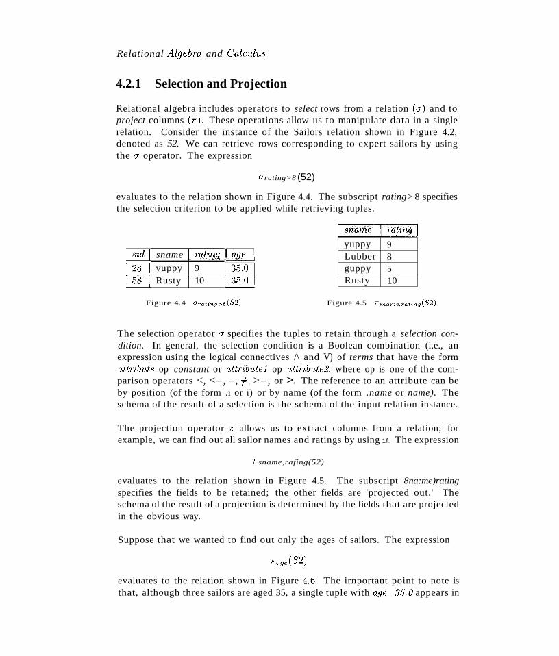
Relational AlgebTa and Calculus
4.2.1 Selection and Projection
Relational algebra includes operators to select rows from a relation (a) and toproject columns (7r). These operations allow us to manipulate data in a singlerelation. Consider the instance of the Sailors relation shown in Figure 4.2,denoted as 52. We can retrieve rows corresponding to expert sailors by usingthe a operator. The expression
arating>8 (52)
evaluates to the relation shown in Figure 4.4. The subscript rating> 8 specifiesthe selection criterion to be applied while retrieving tuples.
sname I rating Iyuppy 9Rusty 10
Figure 4.4 O"r(lting>s(S2)
yuppy 9Lubber 8guppy 5Rusty 10
Figure 4.5 7r,m(lT1lc,Tating(S2)
The selection operator a specifies the tuples to retain through a selection condition. In general, the selection condition is a Boolean combination (i.e., anexpression using the logical connectives /\ and V) of terms that have the formattribute op constant or attributel op attribute2, where op is one of the comparison operators <, <=, =, ,#, >=, or >. The reference to an attribute can beby position (of the form .i or i) or by name (of the form .name or name). Theschema of the result of a selection is the schema of the input relation instance.
The projection operator 7r allows us to extract columns from a relation; forexample, we can find out all sailor names and ratings by using 1f. The expression
7rsname,rafing(52)
evaluates to the relation shown in Figure 4.5. The subscript 8na:me)ratingspecifies the fields to be retained; the other fields are 'projected out.' Theschema of the result of a projection is determined by the fields that are projectedin the obvious way.
Suppose that we wanted to find out only the ages of sailors. The expression
evaluates to the relation shown in Figure /1.6. The irnportant point to note isthat, although three sailors are aged 35, a single tuple with age=:J5.0 appears in
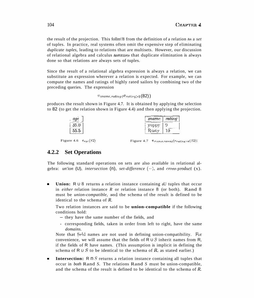
104 CHAPTER+!
the result of the projection. This follm\'8 from the definition of a relation as a setof tuples. In practice, real systems often omit the expensive step of eliminatingduplicate tuples, leading to relations that are multisets. However, our discussionof relational algebra and calculus a..-;sumes that duplicate elimination is alwaysdone so that relations are always sets of tuples.
Since the result of a relational algebra expression is always a relation, we cansubstitute an expression wherever a relation is expected. For example, we cancompute the names and ratings of highly rated sailors by combining two of thepreceding queries. The expression
7rsname,rating ( (Jrati.ng>8 (82) )
produces the result shown in Figure 4.7. It is obtained by applying the selectionto 82 (to get the relation shown in Figure 4.4) and then applying the projection.
I age ·.1
QBO~
Figure 4.6 1rage (82)
4.2.2 Set Operations
Figure 4.7 1rsname,rating(Urating>s(S2))
The following standard operations on sets are also available in relational algebra: un'ion (U), intersection (n), set-difference (-), and cmss-product (x).
II Union: R U 8 returns a relation instance containing aU tuples that occurin either relation instance R or relation instance 8 (or both). Rand 8must be union-compatible, and the schema of the result is defined to beidentical to the schema of R.
Two relation instances are said to be union-compatible if the followingconditions hold:~ they have the same number of the fields, and
- corresponding fields, taken in order from left to right, have the samedomains.
Note that ~eld names are not used in defining union-compatibility. forconvenience, we will assume that the fields of R U 5' inherit names from R,if the fields of R have names. (This assumption is implicit in defining theschema of R U 5' to be identical to the schema of R, as stated earlier.)
III Intersection: R n 5' returns a relation instance containing all tuples thatoccur in both Rand S. The relations Rand S must be union-compatible,and the schema of the result is defined to be identical to the schema of R.
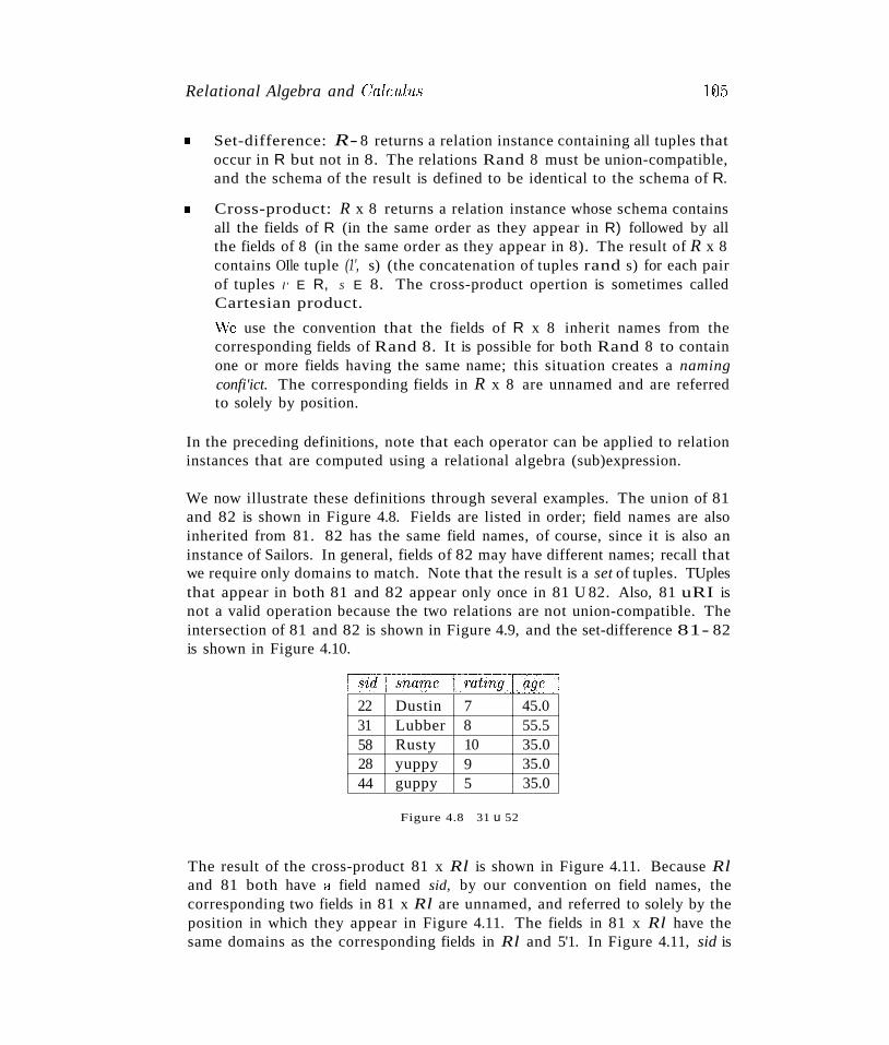
Relational Algebra and CalC'ul1L8 H15
• Set-difference: R- 8 returns a relation instance containing all tuples thatoccur in R but not in 8. The relations Rand 8 must be union-compatible,and the schema of the result is defined to be identical to the schema of R.
• Cross-product: R x 8 returns a relation instance whose schema containsall the fields of R (in the same order as they appear in R) followed by allthe fields of 8 (in the same order as they appear in 8). The result of R x 8contains OIle tuple (1', s) (the concatenation of tuples rand s) for each pairof tuples l' E R, S E 8. The cross-product opertion is sometimes calledCartesian product.
\\Te use the convention that the fields of R x 8 inherit names from thecorresponding fields of Rand 8. It is possible for both Rand 8 to containone or more fields having the same name; this situation creates a namingconfi'ict. The corresponding fields in R x 8 are unnamed and are referredto solely by position.
In the preceding definitions, note that each operator can be applied to relationinstances that are computed using a relational algebra (sub)expression.
We now illustrate these definitions through several examples. The union of 81and 82 is shown in Figure 4.8. Fields are listed in order; field names are alsoinherited from 81. 82 has the same field names, of course, since it is also aninstance of Sailors. In general, fields of 82 may have different names; recall thatwe require only domains to match. Note that the result is a set of tuples. TUplesthat appear in both 81 and 82 appear only once in 81 U 82. Also, 81 uRI isnot a valid operation because the two relations are not union-compatible. Theintersection of 81 and 82 is shown in Figure 4.9, and the set-difference 81- 82is shown in Figure 4.10.
22 Dustin 7 45.031 Lubber 8 55.558 Rusty 10 35.028 yuppy 9 35.044 guppy 5 35.0
Figure 4.8 31 u 52
The result of the cross-product 81 x Rl is shown in Figure 4.11. Because Rland 81 both have a field named sid, by our convention on field names, thecorresponding two fields in 81 x Rl are unnamed, and referred to solely by theposition in which they appear in Figure 4.11. The fields in 81 x Rl have thesame domains as the corresponding fields in Rl and 5'1. In Figure 4.11, sid is
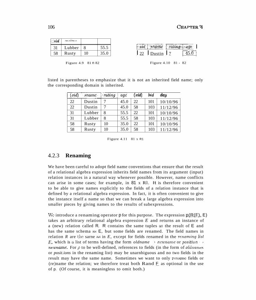
106
.. isifi """.h.~"
31 Lubber 8 55.558 Rusty 10 35.0
Figure 4.9 81 n 82
GHAPTER f4
li~·iiJB1ff/fj,me It,{4t~rf1l1f:4f1ei II 22 I Dustin I 7 [3fOJ
Figure 4.10 81 - 82
listed in parentheses to emphasize that it is not an inherited field name; onlythe corresponding domain is inherited.
(sid!) bid aay
22 Dustin 7 45.0 22 101 10/10/9622 Dustin 7 45.0 58 103 11/12/9631 Lubber 8 55.5 22 101 10/10/9631 Lubber 8 55.5 58 103 11/12/9658 Rusty 10 35.0 22 101 10/10/9658 Rusty 10 35.0 58 103 11/12/96
Figure 4.11 81 x R1
4.2.3 Renaming
We have been careful to adopt field name conventions that ensure that the resultof a relational algebra expression inherits field names from its argument (input)relation instances in a natural way whenever possible. However, name conflictscan arise in some cases; for example, in 81 x Rl. It is therefore convenientto be able to give names explicitly to the fields of a relation instance that isdefined by a relational algebra expression. In fact, it is often convenient to givethe instance itself a name so that we can break a large algebra expression intosmaller pieces by giving names to the results of subexpressions.
vVe introduce a renaming operator p for this purpose. The expression p(R(F), E)takes an arbitrary relational algebra expression E and returns an instance ofa (new) relation called R. R contains the same tuples as the result of E andhas the same schema as E, but some fields are renamed. The field names inrelation R are the sarne as in E, except for fields renamed in the Tenaming listF, which is a list of terms having the form oldname ~, newnarne or position ~rW1llTlJLrne. For p to be well-defined, references to fields (in the form of oldnarnesor posit.ions in the renaming list) may be unarnbiguous and no two fields in theresult may have the same name. Sometimes we want to only renarne fields or(re)name the relation; we therefore treat both Rand F as optional in the useof p. (Of course, it is meaningless to omit both.)
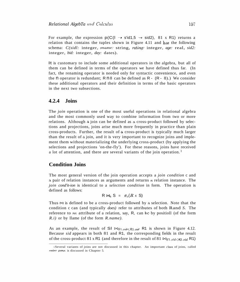
Relational AlgebTa and Calc"Uh18 107
For example, the expression p(C(l ----7 s'id1,5 ----7 sid2), 81 x R1) returns arelation that contains the tuples shown in Figure 4.11 and has the followingschema: C(sidl: integer, ,marrw: string, mt'ing: integer, age: real, sid2:integer, bid: integer, day: dates).
It is customary to include some additional operators in the algebra, but all ofthem can be defined in terms of the operators we have defined thus far. (Infact, the renaming operator is needed only for syntactic convenience, and eventhe n operator is redundant; R n 8 can be defined as R - (R - 8).) We considerthese additional operators and their definition in terms of the basic operatorsin the next two subsections.
4.2.4 Joins
The join operation is one of the most useful operations in relational algebraand the most commonly used way to combine information from two or morerelations. Although a join can be defined as a cross-product followed by selections and projections, joins arise much more frequently in practice than plaincross-products. Further, the result of a cross-product is typically much largerthan the result of a join, and it is very important to recognize joins and implement them without materializing the underlying cross-product (by applying theselections and projections 'on-the-fly'). For these reasons, joins have receiveda lot of attention, and there are several variants of the join operation. 1
Condition Joins
The most general version of the join operation accepts a join condition c anda pair of relation instances as arguments and returns a relation instance. Thejoin cond'it-ion is identical to a selection condition in form. The operation isdefined as follows:
R [:X)e S = O"e(R X S)
Thus [:X) is defined to be a cross-product followed by a selection. Note that thecondition c can (and typically does) refer to attributes of both Rand S. Thereference to an attribute of a relation, say, R, can be by positioll (of the formR.i) or by Ilame (of the form R.name).
As an example, the result of Sl [><JS1.8id<Rl.sid R1 is shown in Figure 4.12.Because sid appears in both 81 and R1, the corresponding fields in the resultof the cross-product 81 x R1 (and therefore in the result of 81 [:X)S1.sid<Rl.sid R1)
1 Several variants of joins are not discussed in this chapter. An important c.la..'iS of joins, called01lter joins, is discussed in Chapter 5.
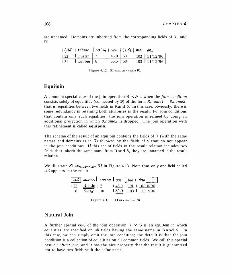
108 CHAPTER ..t1
are unnamed. Domains are inherited from the corresponding fields of 81 andRl.
I (sid) I snarne I rating I age I··· {si41:l bid da/lj
I 22 I Dustin 7 45.0 58 I 103 I 11/12/96I 31 I Lubber 8
.-55.5 58 I 103 I 11/12/96
Figure 4.12 51 NSl. s id<R1.sid R1
Equijoin
A common special case of the join operation R [>(] 8 is when the join conditionconsists solely of equalities (connected by 1\) of the form R.name1 = 8.name2,that is, equalities between two fields in Rand S. In this case, obviously, there issome redundancy in retaining both attributes in the result. For join conditionsthat contain only such equalities, the join operation is refined by doing anadditional projection in which 8.name2 is dropped. The join operation withthis refinement is called equijoin.
The schema of the result of an equijoin contains the fields of R (with the samenames and domains as in R) followed by the fields of 8 that do not appearin the join conditions. If this set of fields in the result relation includes twofields that inherit the same name from Rand 8, they are unnamed in the resultrelation.
We illustrate 81l:<JR.sid=5.sid Rl in Figure 4.13. Note that only one field calledsid appears in the result.
~ ,marne I rating I age I· bid·1 day =tJI 22 DustIn I 7 I 45.0 101 I 10/10/96 II 58 Rust}~ I 10 I ~5.0 103 I 11/12/96 I
Figure 4.13 81 MR ..,H1=S'."id HI
Natural Join
A further special ca.'3e of the join operation R [>(] S is an eqUlJom in whichequalities arc specified on all fields having the same name in Rand S. Inthis case, we can simply omit the join condition; the default is that the joincondition is a collection of equalities on all common fields. We call this specialcase a natumJ jo'in, and it has the nice property that the result is guaranteednot to have two fields with the saIne name.
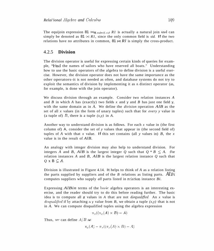
Relai'ional Algelrra and Calculus lQ9
The equijoin expression 81 D<m..sid=s.sid R1 is actually a natural join al1d cansimply be denoted as 81 [Xl R1, since the only common field is sid. If the tworelations have no attributes in common, 81 [Xl Rl is simply the cross-product.
4.2.5 Division
The division operator is useful for expressing certain kinds of queries for example, "Find the names of sailors who have reserved all boats." Understandinghow to use the basic operators of the algebra to define division is a useful exercise. However, the division operator does not have the same importance as theother operators-it is not needed as often, and database systems do not try toexploit the semantics of division by implementing it as a distinct operator (as,for example, is done with the join operator).
We discuss division through an example. Consider two relation instances Aand B in which A has (exactly) two fields x and y and B has just one field y,with the same domain as in A. We define the division operation AlB as theset of all x values (in the form of unary tuples) such that for every y value in(a tuple of) B, there is a tuple (x,y) in A.
Another way to understand division is as follows. For each x value in (the firstcolumn of) A, consider the set of y values that appear in (the second field of)tuples of A with that x value. If this set contains (all y values in) B, the xvalue is in the result of AlB.
An analogy with integer division may also help to understand division. Forintegers A and B, AlB is the largest integer Q such that Q * B ::::; A. :Forrelation instances A and B, AlB is the largest relation instance Q such thatQ x B S:::A.
Division is illustrated in Figure 4.14. It helps to think of A as a relation listingthe parts supplied by suppliers and of the B relations as listing parts. AIB'icomputes suppliers who supply all parts listed in rdation instance Bi.
Expressing AlBin terms of the ba...sic algebra operators is an interesting exercise, and the reader should try to do this before reading further. The basicidea is to compute all :r values in A that are not disqualified. An x value isdisqualified if lJy attaching a y value from B, we obtain a tuple (x,y) that is notin A. We can compute disqualified tuples using the algebra expression
Thus, we can define AlBa.....,
110
A I sno i pno I81 \ pI Isl p2
~._~~81 i p482 \ pI
~_P2-~83 ' p284 p2s4 p4
CHAPTER$4
Bl [P.!!~J AlBl ~;~J,....---,
~LEUI 82 I
B2 I pno ] 83
BE 0p4
~AlB2
B3 ~ BEB1J
84
p2~p4 AlB3
[ill
Figure 4.14 Examples Illustrating Division
To understand the division operation in full generality, we have to consider thecase when both x and yare replaced by a set of attributes. The generalization isstraightforward and left as an exercise for the reader. We discuss two additionalexamples illustrating division (Queries Q9 and Q10) later in this section.
4.2.6 More Examples of Algebra Queries
We now present several examples to illustrate how to write queries in relationalalgebra. We use the Sailors, Reserves, and Boats schema for all our examplesin this section. We use parentheses as needed to make our algebra expressionsunambiguous. Note that all the example queries in this chapter are givena unique query number. The query numbers are kept unique across both thischapter and the SQL query chapter (Chapter 5). This numbering makes it easyto identify a query when it is revisited in the context of relational calculus andSQL and to compare different ways of writing the same query. (All referencesto a query can be found in the subject index.)
In the rest of this chapter (and in Chapter 5), we illustrate queries using theinstances 83 of Sailors, R2 of Reserves, and B1 of Boats, shown in Figures4.15, 4.16, and 4.17, respectively.
(Q1) Find the names of sailors who have rcscT'ucd boat lOS.
This query can be written as follows:
".marne (((Jbid=1O:~Re.5erve8)[XJ 8ailoT.5)

Relational Algebra and Calcul1ls
~l »> ....."""'.+A.".,'" hAh
22 Dustin 7 45.029 Brutus 1 33.031 Lubber 8 55.532 Andy 8 25.558 Rusty 10 35.064 Horatio 7 35.071 Zorba 10 16.074 Horatio 9 35.085 Art 3 25.595 Bob 3 63.5
Figure 4.15 An Instance 83 of Sailors
111,
22 101 10/10/9822 102 10/10/9822 103 10/8/9822 104 10/7/9831 102 11/10/9831 103 11/6/9831 104 11/12/9864 101 9/5/9864 102 9/8/9874 103 9/8/98
Figure 4.16 An Instance R2 of Reserves
We first compute the set of tuples in Reserves with bid = 103 and then take thenatural join of this set with Sailors. This expression can be evaluated on instances of Reserves and Sailors. Evaluated on the instances R2 and S3, it yieldsa relation that contains just one field, called sname, and three tuples (Dustin),(Horatio), and (Lubber). (Observe that two sailors are called Horatio and onlyone of them has reserved a red boat.)
[~]bname I color· I101 Interlake blue102 Interlake red103 Clipper green104 Marine red
Figure 4.17 An Instance HI of Boats
We can break this query into smaller pieces llsing the renaming operator p:
p(Temp1, IJbir1=103 ReseTves)
p(Temp2, Temp11XJ Sailor's)
1Tsname(Temp2)
Notice that because we are only llsing p to give names to intermediate relations,the renaming list is optional and is omitted. TempI denotes an intermediaterelation that identifies reservations of boat 103. Temp2 is another intermediaterelation, and it denotes sailors who have mad(~ a reservation in the set Templ.The instances of these relations when evaluating this query on the instances R2and S3 are illustrated in Figures 4.18 and 4.19. Finally, we extract the snamecolumn from Temp2.
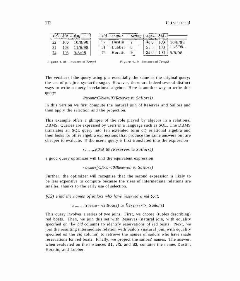
112
22 10~~ 10/8/9831 103 11/6/9874 103 9/8/98
Dustin31 Lubber 874 Horatio 9
CHAPTER;l
10/8/9811/6/98--
9/8/98
Figure 4.18 Instance of TempI Figure 4.19 Instance of Temp2
The version of the query using p is essentially the same as the original query;the use of p is just syntactic sugar. However, there are indeed several distinctways to write a query in relational algebra. Here is another way to write thisquery:
Jrsname(CJbid=103(Reserves IX! Sailors))
In this version we first compute the natural join of Reserves and Sailors andthen apply the selection and the projection.
This example offers a glimpse of the role played by algebra in a relationalDBMS. Queries are expressed by users in a language such as SQL. The DBMStranslates an SQL query into (an extended form of) relational algebra andthen looks for other algebra expressions that produce the same answers but arecheaper to evaluate. If the user's query is first translated into the expression
7fsname (CJbid=103 (Reserves IX! Sailors))
a good query optimizer will find the equivalent expression
7rsname ((CJb·id=103Reserves) IX! Sailors)
Further, the optimizer will recognize that the second expression is likely tobe less expensive to compute because the sizes of intermediate relations aresmaller, thanks to the early use of selection.
(Q2) Find the names of sailors who ha've reserved a red boat.
7f.marne ((CJcolor='red' Boats) IX! Reserves !><J S ailoI's)
This query involves a series of two joins. First, we choose (tuples describing)red boats. Then, we join this set with Reserves (natural join, with equalityspecified on thE) bid column) to identify reservations of red boats. Next, wejoin the resulting intermediate relation with Sailors (natural join, with equalityspecified on the sid column) to retrieve the names of sailors who have rnadereservations for red boats. Finally, we project the sailors' names. The answer,when evaluated on the instances B1, R2, and S3, contains the names Dustin,Horatio, and Lubber.
Relational Algebra and Calculus
An equivalent expression is:
B.3
The reader is invited to rewrite both of these queries by using p to make theintermediate relations explicit and compare the schema.<=; of the intermediaterelations. The second expression generates intermediate relations with fewerfields (and is therefore likely to result in intermediate relation instances withfewer tuples as well). A relational query optimizer would try to arrive at thesecond expression if it is given the first.
(Q3) Find the colors of boats reserved by Lubber.
Jrcolor((asname='Lubber,Sa'ilors) [XJ Reserves [XJ Boats)
This query is very similar to the query we used to compute sailors who reservedred boats. On instances Bl, R2, and S3, the query returns the colors greenand red.
(Q4) Find the names of sailors who have reserved at least one boat.
Jrsname(Sailors [XJ Reserves)
The join of Sailors and Reserves creates an intermediate relation in which tuplesconsist of a Sailors tuple 'attached to' a Reserves tuple. A Sailors tuple appearsin (some tuple of) this intermediate relation only if at least one Reserves tuplehas the same sid value, that is, the sailor has made some reservation. Theanswer, when evaluated on the instances Bl, R2 and S3, contains the threetuples (Dustin), (HoTatio) , and (LubbeT). Even though two sailors calledHoratio have reserved a boat, the answer contains only one copy of the tuple(HoTatio) , because the answer is a relation, that is, a set of tuples, with noduplicates.
At this point it is worth remarking on how frequently the natural join operationis used in our examples. This frequency is more than just a coincidence basedon the set of queries we have chosen to discuss; the natural join is a verynatural, widely used operation. In particular, natural join is frequently usedwhen joining two tables on a foreign key field. In Query Q4, for exalnple, thejoin equates the sid fields of Sailors and Reserves, and the sid field of Reservesis a foreign key that refers to the sid field of Sailors.
(Q5) Find the narnes of sailors who have reserved a Ted OT a gTeen boat.
p(Tempboats, (acoloT='rcd' Boats) U (acolor='green' Boats))
Jrsna·rne(Tempboats [XJ ReseTves [XJ Sailors)
114 CHAPTER $4
vVe identify the set of all boats that are either red or green (Tempboats, whichcontains boats \vith the bids 102, 103, and 104 on instances E1, R2, and S3).Then we join with Reserves to identify sid.., of sailors who have reserved OIle ofthese boats; this gives us sids 22, 31, 64, and 74 over our example instances.Finally, we join (an intermediate relation containing this set of sids) with Sailorsto find the names of Sailors with these sids. This gives us the names Dustin,Horatio, and Lubber on the instances E1, R2, and S3. Another equivalentdefinition is the following:
p(Tempboats, (acolor='red'Vcolor='green' Boats))7fsname(Tempboats [><] Reserves [><] Sailors)
Let us now consider a very similar query.
(Q6) Find the names of sailors who have reserved a red and a green boat. Itis tempting to try to do this by simply replacing U by n in the definition ofTempboats:
p(Tempboats2, (acolor='red,Eoats) n (O"color='green,Boats))
'7fsname(Tempboats2 [><] Reserves [><] Sailors)
However, this solution is incorrect-it instead tries to compute sailors who havereserved a boat that is both red and green. (Since bid is a key for Boats, a boatcan be only one color; this query will always return an empty answer set.) Thecorrect approach is to find sailors who have reserved a red boat, then sailorswho have reserved a green boat, and then take the intersection of these twosets:
p(Tempred, '7fsid ((acolor='red' Eoats) [><] Reserves))
p(Tempgreen, '7fsid((O"color='green,Boats) [><] Reserves))
'7f,marne((Ternpred n Tempgreen) [><] Sailors)
The two temporary relations compute the sids of sailors, and their intersectionidentifies sailors who have reserved both red and green boats. On instancesBI, R2, and 53, the sids of sailors who have reserved a red boat are 22, 31,and 64. The s'icLs of sailors who have reserved a green boat are 22, 31, and 74.Thus, sailors 22 and 31 have reserved both a red boat and a green boat; theirnames are Dustin and Lubber.
This formulation of Query Q6 can easily be adapted to find sailors \vho havereserved red or green boats (Query Q5); just replace n by U:
p(TempTed, '7fsid( (O"color=lrcd' Boats) [)<] Reserves))
p(Tempgreen, '7fsid( (O"color='green' Boats) [)<] Reserves))
'7fsTwme((Tempred U Tempgreen) [)<] Sailors)
Relatiorwl Algebra and Galcurus 115
In the formulations of Queries Q5 and Q6, the fact that sid (the field overwhich we compute union or intersection) is a key for Sailors is very important.Consider the following attempt to answer Query Q6:
p(Tempred, Jrsname((CJcolor='red,Boats) [><] Reserves [><] Sailors))
p(Tempgreen,Jrsname((CJcoloT='gTeenlBoats) [><] Reserves [><] Sailors))
Tempred n Tempgreen
This attempt is incorrect for a rather subtle reason. Two distinct sailors withthe same name, such as Horatio in our example instances, may have reservedred and green boats, respectively. In this case, the name Horatio (incorrectly)is included in the answer even though no one individual called Horatio hasreserved a red boat and a green boat. The cause of this error is that snameis used to identify sailors (while doing the intersection) in this version of thequery, but sname is not a key.
(Q7) Find the names of sailors who have reser-ved at least two boats.
p(Reser-vations, Jrsid,sname,bid (Sailor s [><] Reserves))
p(Reservationpairs(l ---'? sid1, 2 ---'? sname1, 3 ---'? bid1, 4 ---'? sid2,
5 ---'? sname2, 6 ---'? bid2), Reservations x Reservations)
Jrsname1 CJ(sidl=sid2)I\(bidl=1-bid2) Reservationpair-s
First, we compute tuples of the form (sid,sname, bid) , where sailor sid has madea reservation for boat bid; this set of tuples is the temporary relation Reservations. Next we find all pairs of Reservations tuples where the same sailor hasmade both reservations and the boats involved are distinct. Here is the centralidea: To show that a sailor has reserved two boats, we must find two Reservations tuples involving the same sailor but distinct boats. Over instances El,R2, and S3, each of the sailors with sids 22, 31, and 64 have reserved at leasttwo boats. Finally, we project the names of such sailors to obtain the answer,containing the names Dustin, Horatio, and Lubber.
Notice that we included sid in Reservations because it is the key field identifyingsailors, and we need it to check that two Reservations tuples involve the samesailor. As noted in the previous example, we cannot use sname for this purpose.
(Q8) Find the sids of sailors w'ith age over 20 who have not TeseTved a Ted boat.
Jrsid(CJage>20Sa'ilors) -
7rsid((CJco[oT='red,Boats) [><] Reserves [><] Sa'ilors)
This query illustrates the use of the set-difference operator. Again, we use thefact that sid is the key for Sailors. vVe first identify sailors aged over 20 (over
116
instances B1, R2, and S3, .'!'ids 22, 29, 31, 32, 58, 64, 74, 85, and 95) and thendiscard those who have reserved a red boat (sid.c; 22, 31, and 64), to obtain theanswer (sids 29, 32, 58, 74, 85, and 95). If we want to compute the names ofsuch sailors, \ve must first compute their sids (as shown earlier) and then joinwith Sailors and project the sname values.
(Q9) Find the names of sailors 'Who have rese'rved all boats.
The use of the word all (or every) is a good indication that the division operationmight be applicable:
p(Tempsids, (7l"sid,bidReserves) / (7l"bidBoats))
7l"sname(Tempsids N Sailors)
The intermediate relation Tempsids is defined using division and computes theset of sids of sailors who have reserved every boat (over instances Bl, R2, andS3, this is just sid 22). Note how we define the two relations that the divisionoperator (/) is applied to·-·--the first relation has the schema (sid,bid) and thesecond has the schema (b'id). Division then returns all sids such that there is atuple (sid,bid) in the first relation for each bid in the second. Joining Tempsidswith Sailors is necessary to associate names with the selected sids; for sailor22, the name is Dustin.
(Q 10) Find the names of sailors 'Who have reserved all boats called Interlake.
p(Tempsids, (7l".5'id,bidReserves) / (7l"bid( (Jbname='Interlake' Boats)))
7l"sname(Tempsids [Xl Sailors)
The only difference with respect to the previous query is that now we apply aselection to Boats, to ensure that we compute bids only of boats named Interlakein defining the second argument to the division operator. Over instances El,R2, and S3, Tempsids evaluates to sids 22 and 64, and the answer containstheir names, Dustin and Horatio.
403 RELATIONAL CALCULUS
Relational calculus is an alternative to relational algebra. In contra.':;t to thealgebra, which is procedural, the calculus is nonprocedural, or declarative, inthat it allows us to describe the set of answers without being explicit abouthow they should be computed. Relational calculus has had a big influence onthe design of commercial query languages such a,s SQL and, especially, Queryby-Example (QBE).
The variant of the calculus we present in detail is called the tuple relationalcalculus (TRC). Variables in TRC take on tuples as values. In another vari-
RelatiO'Tul,l Algebra and Calculus
ant, called the domain relational calculus (DRC), the variables range overfield values. TRC has had more of an influence on SQL, \vhile DRC has stronglyinfluenced QBE. vVe discuss DRC in Section 4.3.2.2
4$3.1 Tuple Relational Calculus
A tuple variable is a variable that takes on tuples of a particular relationschema as values. That is, every value assigned to a given tuple variable hasthe same number and type of fields. A tuple relational calculus query has theform { T I p(T) }, where T is a tuple variable and p(T) denotes a formula thatdescribes T; we will shortly define formulas and queries rigorously. The resultof this query is the set of all tuples t for which the formula p(T) evaluates totrue with T = t. The language for writing formulas p(T) is thus at the heart ofTRC and essentially a simple subset of first-order logic. As a simple example,consider the following query.
(Q11) Find all sailors with a rating above 7.
{S I S E Sailors 1\ S.rating > 7}
When this query is evaluated on an instance of the Sailors relation, the tuplevariable S is instantiated successively with each tuple, and the test S. rat'ing> 7is applied. The answer contains those instances of S that pass this test. Oninstance S3 of Sailors, the answer contains Sailors tuples with sid 31, 32, 58,71, and 74.
Syntax of TRC Queries
We now define these concepts formally, beginning with the notion of a formula.Let Rel be a relation name, Rand S be tuple variables, a be an attribute ofR, and b be an attribute of S. Let op denote an operator in the set {<, >, =, :S;, 2:, =I- }. An atomic formula is one of the following:
III R E Ref
lIII R.a op S.b
IIlI R.a op constant, or constant op R.a
A formula is recursively defined to be one of the following, where p and qare themselves formula.s and p(R) denotes a formula in which the variable Rappears:
.~-----------
2The material on DRC is referred to in the (online) chapter OIl QBE; with the exception of thischapter, the material on DRC and TRe can be omitted without loss of continuity.
118 CHAPTER .,4
• any atomic formula
• -'p, P /\ q, P V q, or p :::} q
• 3R(p(R)), where R is a tuple variable
• 'ifR(p(R)) , where R is a tuple variable
In the last two clauses, the quantifiers :3 and 'if are said to bind the variable R.A variable is said to be free in a formula or subformuia (a formula containedin a larger formula) if the (sub)formula does not contain an occurrence of aquantifier that binds it.3
We observe that every variable in a TRC formula appears in a subformulathat is atomic, and every relation schema specifies a domain for each field; thisobservation ensures that each variable in a TRC formula has a well-defineddomain from which values for the variable are drawn. That is, each variablehas a well-defined type, in the programming language sense. Informally, anatomic formula R E Rei gives R the type of tuples in ReI, and comparisonssuch as R.a op S.b and R.a op constant induce type restrictions on the fieldR.a. If a variable R does not appear in an atomic formula of the form R E Rei(Le., it appears only in atomic formulas that are comparisons), we follow theconvention that the type of R is a tuple whose fields include all (and only) fieldsof R that appear in the formula.
We do not define types of variables formally, but the type of a variable shouldbe clear in most cases, and the important point to note is that comparisons ofvalues having different types should always fail. (In discussions of relationalcalculus, the simplifying assumption is often made that there is a single domainof constants and this is the domain associated with each field of each relation.)
A TRC query is defined to be expression of the form {T I p(T)}, where T isthe only free variable in the formula p.
Semantics of TRC Queries
What does a TRC query mean? More precisely, what is the set of answer tuplesfor a given TRC query? The answer to a TRC query {T I p(T)}, as notedearlier, is the set of all tuples t for which the formula peT) evaluates to truewith variable T &'3signed the tuple value t:. To complete this definition, we muststate which assignments of tuple values to the free variables in a formula makethe formula evaluate to true.
3vVe make the assumption that each variable in a formula is either free or bound by exactly oneoccurrence of a quantifier, to avoid worrying about details such a.'l nested occurrences of quantifiersthat bind some, but not all, occurrences of variables.
Relational Algebra and Calcuhl8 119
A query is evaluated on a given instance of the database. Let each free variablein a formula F be bound to a tuple value. For the given assignment of tuplesto variables, with respect to the given database instance, F evaluates to (orsimply 'is') true if one of the following holds:
• F is an atomic formula R E Rel, and R is assigned a tuple in the instanceof relation Rel.
• F is a comparison R.a op S.b, R.a op constant, or constant op R.a, andthe tuples assigned to Rand S have field values R.a and S.b that make thecomparison true.
• F is of the form ---,p and p is not true, or of the form p 1\ q, and both p andq are true, or of the form p V q and one of them is true, or of the formp =} q and q is true whenever4 p is true.
• F is of the form 3R(p(R)), and there is some assignment of tuples to thefree variables in p(R), including the variable R,5 that makes the formulap(R) true.
• F is of the form VR(p(R)), and there is some assignment of tuples to thefree variables in p(R) that makes the formula p(R) true no matter whattuple is assigned to R.
Examples of TRC Queries
We now illustrate the calculus through several examples, using the instancesB1 of Boats, R2 of Reserves, and S3 of Sailors shown in Figures 4.15, 4.16,and 4.17. We use parentheses as needed to make our formulas unambiguous.Often, a formula p(R) includes a condition R E Rel, and the meaning of thephrases some tuple R and for all tuples R is intuitive. We use the notation3R E Rel(p(R)) for 3R(R E Rel 1\ p(R)). Similarly, we use the notationVR E Rel(p(R)) for VR(R E Rel =} p(R)).
(Q12) Find the names and ages of sailors with a rating above 7.
{P I 3S E Sailors(S.rating > 7 1\ Pname = S.sname 1\ Page = S.age)}
This query illustrates a useful convention: P is considered to be a tuple variablewith exactly two fields, which are called name and age, because these are theonly fields of P mentioned and P does not range over any of the relations inthe query; that is, there is no subformula of the form P E Relname. Theresult of this query is a relation with two fields, name and age. The atomic
4 WheneveT should be read more precisely as 'for all assignments of tuples to the free variables.'5Note that some of the free variables in p(R) (e.g., the variable R itself) IIlay be bound in P.
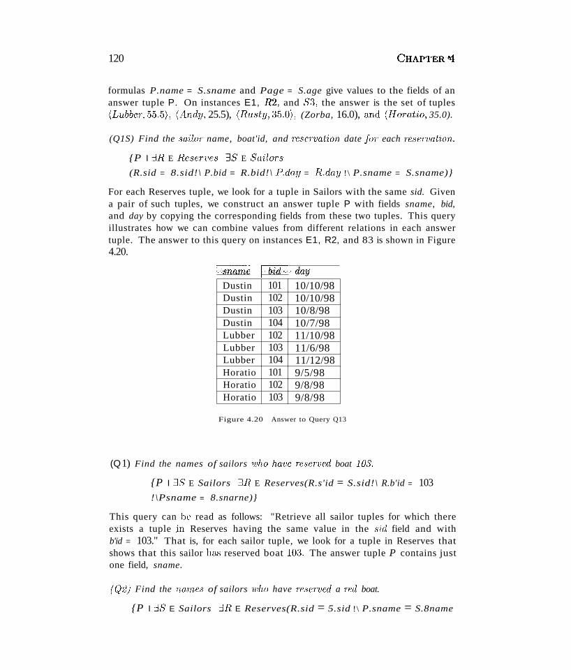
120 CHAPTER J4
formulas P.name = S.sname and Page = S.age give values to the fields of ananswer tuple P. On instances E1, R2, and S3, the answer is the set of tuples(Lubber,55.5), (Andy, 25.5), (Rusty, ~~5.0), (Zorba, 16.0), ::lnd (Horatio, 35.0).
(Q1S) Find the so;ilor name, boat'id, and reseT1}Q.tion date for each reservation.
{P I 3R E ReseT"ues 3S E Sailors
(R.sid = 8.sid!\ P.bid = R.bid!\ P.day = R.day !\ P.sname = S.sname)}
For each Reserves tuple, we look for a tuple in Sailors with the same sid. Givena pair of such tuples, we construct an answer tuple P with fields sname, bid,and day by copying the corresponding fields from these two tuples. This queryillustrates how we can combine values from different relations in each answertuple. The answer to this query on instances E1, R2, and 83 is shown in Figure4.20.
Isname ~ ..... day
Dustin 101 10/10/98Dustin 102 10/10/98Dustin 103 10/8/98Dustin 104 10/7/98Lubber 102 11/10/98Lubber 103 11/6/98Lubber 104 11/12/98Horatio 101 9/5/98Horatio 102 9/8/98Horatio 103 9/8/98
Figure 4.20 Answer to Query Q13
(Q1) Find the names of sailors who have reserved boat lOS.
{P I 35 E Sailors 3R E Reserves(R.s'id = S.sid!\ R.b'id = 103!\Psname = 8.snarne)}
This query can be read as follows: "Retrieve all sailor tuples for which thereexists a tuple ,in Reserves having the same value in the s,id field and withb'id = 103." That is, for each sailor tuple, we look for a tuple in Reserves thatshows that this sailor ha" reserved boat 10~~. The answer tuple P contains justone field, sname.
((22) Find the narnes of sailors who have reserved a n:.d boat.
{P I :38 E Sailors :3R E Reserves(R.sid = 5.sid !\ P.sname = S.8name
Relational Algebra (nul Calculus 121)
1\3B E Boats(B.llid = R.md 1\ B.color ='red'))}
This query can be read as follows: "Retrieve all sailor tuples S for whichthere exist tuples R in Reserves and B in Boats such that S.sid = R.sid,R.bid = B.b'id, and B.coior ='red'." Another way to write this query, whichcorresponds more closely to this reading, is as follows:
{P I 3S E SailoTs 3R E Reserves 3B E Boats
(Rsid = S.sid 1\ B.bid = R.bid 1\ B.color ='red' 1\ Psname = S.sname)}
(Q7) Find the names of sailors who have reserved at least two boats.
{P I 3S E Sailors 3Rl E Reserves 3R2 E Reserves
(S.sid = R1.sid 1\ R1.sid = R2.sid 1\ R1.bid =I- R2.bid
I\Psname = S.sname)}
Contrast this query with the algebra version and see how much simpler thecalculus version is. In part, this difference is due to the cumbersome renamingof fields in the algebra version, but the calculus version really is simpler.
(Q9) Find the narnes of sailors who have reserved all boats.
{P I 3S E Sailors VB E Boats
(3R E Reserves(S.sid = R.sid 1\ R.bid = B.bid 1\ Psname = S.sname))}
This query was expressed using the division operator in relational algebra. Notehow easily it is expressed in the calculus. The calculus query directly reflectshow we might express the query in English: "Find sailors S such that for allboats B there is a Reserves tuple showing that sailor S has reserved boat B."
(Q14) Find sailors who have reserved all red boats.
{S I S E Sailor's 1\ VB E Boats
(B.color ='red' :::} (3R E Reserves(S.sid = R.sid 1\ R.bid = B.bid)))}
This query can be read as follows: For each candidate (sailor), if a boat is red,the sailor must have reserved it. That is, for a candidate sailor, a boat beingred must imply that the sailor has reserved it. Observe that since we can returnan entire sailor tuple as the ans\ver instead of just the sailor's name, we avoidedintroducing a new free variable (e.g., the variable P in the previous example)to hold the answer values. On instances Bl. R2, and S3, the answer containsthe Sailors tuples with sids 22 and 31.
We can write this query without using implication, by observing that an expression of the form p :::} q is logically equivalent to -'p V q:
{S ! S E Sailors 1\ VB E Boats
122 CHAPTER .~
(B.coioT i-'Ted' V (3R E ReSeTVeS(S.sid = R..':tid/\ R.b'id = B.lJid)))}
This query should be read a.s follows: "Find sailors S such that, for all boats B,either the boat is not red or a Reserves tuple shows that sailor S has reservedboat B."
4.3.2 Domain Relational Calculus
A domain variable is a variable that ranges over the values in the domainof some attribute (e.g., the variable can be assigned an integer if it appearsin an attribute whose domain is the set of integers). A DRC query has theform {(XI,X2, ... ,Xn ) I P((XI,X2, ... ,Xn ))}, where each Xi is either a domainvariable or a constant and p( (Xl, X2, ... ,xn )) denotes a DRC formula whoseonly free variables are the variables among the Xi, 1 Sis n. The result of thisquery is the set of all tuples (Xl, X2, ... , x n ) for which the formula evaluates totrue.
A DRC formula is defined in a manner very similar to the definition of a TRCformula. The main difference is that the variables are now domain variables.Let op denote an operator in the set {<, >, =, S,~, i-} and let X and Y bedomain variables. An atomic formula in DRC is one of the following:
II (Xl, X2, ... , X n ) E Rel, where Rei is a relation with n attributes; eachXi, 1 SiS n is either a variable or a constant
II X op Y
II X op constant, or constant op X
A formula is recursively defined to be one of the following, where P and qare themselves formulas and p(X) denotes a formula in which the variable Xappears:
II any atomic formula
II --.p, P /\ q, P V q, or p =} q
II 3X(p(X)), where X is a domain variable
II \/X(p(X)), where X is a domain variable
The reader is invited to compare this definition with the definition of TRCforrnulch'3 and see how closely these two definitions correspond. \Ve will notdefine the semantics of DRC formula.s formally; this is left as an exercise forthe reader.
Relat'ional Algebra and Calculus
Examples of DRC Queries
vVe now illustrate DRC through several examples. The reader is invited tocompare these with the TRC versions.
(Q11) Find all sa'ilors with a rating above 7.
{(1, N, T, A) I (I, N, T, A) E Sa'ilors /\ T > 7}
This differs from the TRC version in giving each attribute a (variable) name.The condition (1, N, T, A) E Sailors ensures that the domain variables I, N,T, and A are restricted to be fields of the same tuple. In comparison with theTRC query, we can say T > 7 instead of S.rating > 7, but we must specify thetuple (I, N, T, A) in the result, rather than just S.
(Q1) Find the names of sailors who have reserved boat 103.
{(N) I 31, T, A( (1, N, T, A) E Sa'ilors
/\311', Br, D( (11', Br, D) E Reserves /\ 11' = I /\ Br = 103))}
Note that only the sname field is retained in the answer and that only Nis a free variable. We use the notation 3Ir,Br,D( ... ) as a shorthand for3Ir(3Br(?JD( .. .))). Very often, all the quantified variables appear in a single relation, as in this example. An even more compact notation in this caseis 3(11', Br, D) E Reserves. With this notation, which we use henceforth, thequery would be as follows:
{(N) I 31, T, A( (I, N, T, A) E Sailors
/\3(11', Br, D) E Reserves(Ir = I /\ Br = 103))}
The comparison with the corresponding TRC formula should now be straightforward. This query can also be written as follows; note the repetition ofvariable I and the use of the constant 103:
{(N) I 31, T, A( (1, N, T, A) E Sailors
/\3D( (1,103, D) E Reserves))}
(Q2) Find the names of sailors who have Teserved a red boat.
{(N) I 31, T, A( (1, N, T, A) E Sailors
/\3(1, Br, D) E ReseTves /\ 3(Br, BN,'Ted') E Boats)}
(Q7) Find the names of sailoT.'! who have TeseTved at least two boat.s.
{(N) I 31, T, A( (1, N, T, A) E Sailors /\
?JBrl, BT2, Dl, D2( (1, Brl, DI) E Reserves
/\(1, Br2, D2) E Reserves /\ Brl # Br2))}
124 CHAPTER ..fl
Note how the repeated use of variable I ensures that the same sailor has reservedboth the boats in question.
(Q9) Find the names of sailors who have Teserved all boat8.
{(N) I ~I, T, A( (I, N, T, A) E Sailors!\
VB, BN,C(-,((B, BN,C) E Boats) V
(::J(Ir, Br, D) E Reserves(I = IT!\ BT = B))))}
This query can be read as follows: "Find all values of N such that some tuple(I, N, T, A) in Sailors satisfies the following condition: For every (B, BN, C),either this is not a tuple in Boats or there is some tuple (IT, BT, D) in Reservesthat proves that Sailor I has reserved boat B." The V quantifier allows thedomain variables B, BN, and C to range over all values in their respectiveattribute domains, and the pattern '-,( (B, BN, C) E Boats )V' is necessary torestrict attention to those values that appear in tuples of Boats. This patternis common in DRC formulas, and the notation V(B, BN, C) E Boats can beused as a shortcut instead. This is similar to the notation introduced earlierfor 3. With this notation, the query would be written as follows:
{(N) I 31, T, A( (I, N, T, A) E Sa'iloTs !\ V(B, BN, C) E Boats
(3(1'1', BT, D) E ReseTves(I = IT!\ BT = B)))}
(Q14) Find sailoTs who have TeseTved all Ted boats.
{(I, N, T, A) I (I, N, T, A) E SailoTs!\ V(B, BN, C) E Boats
(C ='red' =? ?J(Ir, BT, D) E Reserves(I = IT!\ Br = B))}
Here, we find all sailors such that, for every red boat, there is a tuple in Reservesthat shows the sailor has reserved it.
4.4 EXPRESSIVE POWER OF ALGEBRA ANDCALCULUS
\Ve presented two formal query languages for the relational model. Are theyequivalent in power? Can every query that can be expressed in relationalalgebra also be expressed in relational calculus? The answer is yes, it can.Can every query that can be expressed in relational calculus also be expressedin relational algebra? Before we answer this question, we consider a majorproblem with the calculus as we presented it.
Consider the query {S I -,(S E Sailors)}. This query is syntactically correct.However, it asks for all tuples S such that S is not in (the given instance of)
Relational Algebra an,d Calculu8 125
Sailors. The set of such S tuples is obviously infinite, in the context of infinitedomains such as the set of all integers. This simple example illustrates anunsafe query. It is desirable to restrict relational calculus to disallow unsafequeries.
vVe now sketch how calculus queries are restricted to be safe. Consider a set Iof relation instances, with one instance per relation that appears in the queryQ. Let Dom(Q, 1) be the set of all constants that appear in these relationinstances I or in the formulation of the query Q itself. Since we allow onlyfinite instances I, Dom(Q, 1) is also finite.
For a calculus formula Q to be considered safe, at a minimum we want toensure that, for any given I, the set of answers for Q contains only values inDom(Q, 1). While this restriction is obviously required, it is not enough. Notonly do we want the set of answers to be composed of constants in Dom(Q, 1),we wish to compnte the set of answers by examining only tuples that containconstants in Dom(Q, 1)! This wish leads to a subtle point associated with theuse of quantifiers V and :::J: Given a TRC formula of the form :::JR(p(R)), we wantto find all values for variable R that make this formula true by checking onlytuples that contain constants in Dom(Q, 1). Similarly, given a TRC formula ofthe form VR(p(R)), we want to find any values for variable R that make thisformula false by checking only tuples that contain constants in Dom(Q, 1).
We therefore define a safe TRC formula Q to be a formula such that:
1. For any given I, the set of answers for Q contains only values that are inDom(Q, 1).
2. For each subexpression of the form :::JR(p(R)) in Q, if a tuple r (assignedto variable R) makes the formula true, then r contains only constants inDorn(Q,I).
3. For each subexpression of the form VR(p(R)) in Q, if a tuple r (assignedto variable R) contains a constant that is not in Dom(Q, 1), then r mustmake the formula true.
Note that this definition is not constructive, that is, it does not tell us hmv tocheck if a query is safe.
The query Q = {S I -.(S E Sailors)} is unsafe by this definition. Dom(Q,1)is the set of all values that appear in (an instance I of) Sailors. Consider theinstance Sl shown in Figure 4.1. The answer to this query obviously includesvalues that do not appear in Dorn(Q,81).
126 CHAPTERJ4
Returning to the question of expressiveness, we can show that every query thatcan be expressed using a safe relational calculus query can also be expressed asa relational algebra query. The expressive power of relational algebra is oftenused as a metric of how powerful a relational database query language is. Ifa query language can express all the queries that we can express in relationalalgebra, it is said to be relationally complete. A practical query language isexpected to be relationally complete; in addition, commercial query languagestypically support features that allow us to express some queries that cannot beexpressed in relational algebra.
4.5 REVIEW QUESTIONS
Answers to the review questions can be found in the listed sections.
• What is the input to a relational query? What is the result of evaluatinga query? (Section 4.1)
• Database systems use some variant of relational algebra to represent queryevaluation plans. Explain why algebra is suitable for this purpose. (Section 4.2)
• Describe the selection operator. What can you say about the cardinalityof the input and output tables for this operator? (That is, if the input hask tuples, what can you say about the output?) Describe the projectionoperator. What can you say about the cardinality of the input and outputtables for this operator? (Section 4.2.1)
• Describe the set operations of relational algebra, including union (U), intersection (n), set-difference (-), and cross-product (x). For each, whatcan you say about the cardinality of their input and output tables? (Section 4.2.2)
• Explain how the renaming operator is used. Is it required? That is, if thisoperator is not allowed, is there any query that can no longer be expressedin algebra? (Section 4.2.3)
• Define all the variations of the join operation. vVhy is the join operationgiven special attention? Cannot we express every join operation in termsof cross-product, selection, and projection? (Section 4.2.4)
• Define the division operation in terms of the ba--sic relational algebra operations. Describe a typical query that calls for division. Unlike join, thedivision operator is not given special treatment in database systems. Explain why. (Section 4.2.5)
Relational Algebnl and Calculus 1~7
• Relational calculus is said to be a declarati've language, in contrast to algebra, which is a procedural language. Explain the distinction. (Section 4.3)
• How does a relational calculus query 'describe' result tuples? Discuss thesubset of first-order predicate logic used in tuple relational calculus, withparticular attention to universal and existential quantifiers, bound and freevariables, and restrictions on the query formula. (Section 4.3.1).
• vVhat is the difference between tuple relational calculus and domain relational calculus? (Section 4.3.2).
• What is an unsafe calculus query? Why is it important to avoid suchqueries? (Section 4.4)
• Relational algebra and relational calculus are said to be equivalent in expressive power. Explain what this means, and how it is related to thenotion of relational completeness. (Section 4.4)
EXERCISES
Exercise 4.1 Explain the statement that relational algebra operators can be composed. Whyis the ability to compose operators important?
Exercise 4.2 Given two relations R1 and R2, where R1 contains N1 tuples, R2 contains N2tuples, and N2 > N1 > 0, give the minimum and maximum possible sizes (in tuples) for theresulting relation produced by each of the following relational algebra expressions. In eachcase, state any assumptions about the schemas for R1 and R2 needed to make the expressionmeaningful:
(1) R1 U R2, (2) R1 n R2, (3) R1 ~ R2, (4) R1 x R2, (5) (Ta=5(R1), (6) 7Ta(R1), and(7) R1/R2
Exercise 4.3 Consider the following schema:
Suppliers( sid: integer, sname: string, address: string)
Parts(pid: integer, pname: string, color: string)Catalog( sid: integer, pid: integer, cost: real)
The key fields are underlined, and the domain of each field is listed after the field name.Therefore sid is the key for Suppliers, pid is the key for Parts, and sid and pid together formthe key for Catalog. The Catalog relation lists the prices charged for parts by Suppliers. Writethe following queries in relational algebra, tuple relational calculus, and domain relationalcalculus:
1. Find the narnes of suppliers who supply some red part.
2. Find the sids of suppliers who supply some red or green part.
:3. Find the sids of suppliers who supply some red part or are at 221 Packer Ave.
4. Find the sids of suppliers who supply some rcd part and some green part.
128 CHAPTER 4:
5. Find the sids of suppliers who supply every part.
6. Find the sids of suppliers who supply every red part.
7. Find the sids of suppliers who supply every red or green part.
8. Find the sids of suppliers who supply every red part or supply every green part.
9. Find pairs of sids such that the supplier with the first sid charges more for some partthan the supplier with the second sid.
10. Find the pids of parts supplied by at least two different suppliers.
11. Find the pids of the most expensive parts supplied by suppliers named Yosemite Sham.
12. Find the pids of parts supplied by every supplier at less than $200. (If any supplier eitherdoes not supply the part or charges more than $200 for it, the part is not selected.)
Exercise 4.4 Consider the Supplier-Parts-Catalog schema from the previous question. Statewhat the following queries compute:
1. 1fsname('rrsid(CTcolor='red' Parts) !Xl (O'cost<lOoCatalog) !Xl Suppliers)
2. 1fsname (1f S id ((0'color='red' Parts) !Xl (O'cost< looCatalog) !Xl Suppliers))
3. (1fsname ((O'color'='red' Parts) [X] (crcost<looCatalog) !Xl Suppl'iers)) n
4. (1fsid((crcolor='red,Parts) !Xl (crcost<10oCatalog) [X] Suppliers)) n
(1fsid((CTcolor='green' Parts) [X] (crcost<lOoCatalog) !Xl Suppliers))
(1f.sid,sname (( CTCO!07'='green' Parts) !Xl (CTcost< lOoCatalog) [X] Suppliers)))
Exercise 4.5 Consider the following relations containing airline flight information:
Flights(fino: integer, from: string, to: string,
d·istance: integer, depaTts: time, arrives: time)Aircraft( aid: integer, aname: string, cTuisingrange: integer)
Certified( eid: integer, aid: integer)
Employees( eid: integer, ename: string, salary: integer)
Note that the Employees relation describes pilots and other kinds of employees cLS well; everypilot is certified for some aircraft (otherwise, he or she would not qualify as a pilot), and onlypilots are certified to fly.
Write the following queries in relational algebra, tuple relational calculus, and domain relational calculus. Note that some of these queries may not be expressible in relational algebra(and, therefore, also not expressible in tuple and domain relational calculus)! For such queries,informally explain why they cannot be expressed. (See the exercises at the end of Chapter 5for additional queries over the airline schenla.)
1. Finel the eids of pilots certified for some Boeing aircraft.
2. Find the names of pilots certified for some Boeing aircraft.
~). Find the aids of all aircraft that. can be used on non-stop flights from Bonn to Madras.

Relational Algebra and CalcuIu,s 129
4. Identi(y the flights that can be piloted by every pilot whose salary is more than $100,000.
5. Find the names of pilots who can operate planes with a range greater than 3,000 milesbut are not certified on any Boeing aircraft.
6. Find the eids of employees who make the highest salary.
7. Find the eids of employees who make the second highest salary.
8. Find the eids of employees who are certified for the largest number of aircraft.
9. Find the eids of employees who are certified for exactly three aircraft.
10. Find the total amount paid to employees as salaries.
11. Is there a sequence of flights from Madison to Timbuktu? Each flight in the sequence isrequired to depart from the city that is the destination of the previous flight; the firstflight must leave Madison, the last flight must reach Timbuktu, and there is no restrictionon the number of intermediate flights. Your query must determine whether a sequenceof flights from Madison to Timbuktu exists for any input Flights relation instance.
Exercise 4.6 What is relational completeness? If a query language is relationally complete,can you write any desired query in that language?
Exercise 4.7 What is an unsafe query? Give an example and explain why it is importantto disallow such queries.
BIBLIOGRAPHIC NOTES
Relational algebra was proposed by Codd in [187], and he showed the equivalence of relationalalgebra and TRC in [189]. Earlier, Kuhns [454] considered the use of logic to pose queries.LaCroix and Pirotte discussed DRC in [459]. Klug generalized the algebra and calculus toinclude aggregate operations in [439]. Extensions of the algebra and calculus to deal withaggregate functions are also discussed in [578]. Merrett proposed an extended relationalalgebra with quantifiers such as the number of that go beyond just universal and existentialquantification [530]. Such generalized quantifiers are discussed at length in [52].
5SQL: QUERIES,
CONSTRNNTS, TRIGGERS
.. What is included in the SQL language? What is SQL:1999?
.. How are queries expressed in SQL? How is the meaning of a queryspecified in the SQL standard?
,..- How does SQL build on and extend relational algebra and calculus?
l"- \Vhat is grouping? How is it used with aggregate operations?
... What are nested queries?
.. What are null values?
... How can we use queries in writing complex integrity constraints?
... What are triggers, and why are they useful? How are they related tointegrity constraints?
Itt Key concepts: SQL queries, connection to relational algebra andcalculus; features beyond algebra, DISTINCT clause and multiset semantics, grouping and aggregation; nested queries, correlation; setcomparison operators; null values, outer joins; integrity constraintsspecified using queries; triggers and active databases, event-conditionaction rules.
-------_.__._---_._------------_..__._---------------_ _ _----_.._ .._---
\Vhat men or gods are these? \\1hat Inaiclens loth?\Vhat mad pursuit? \1\7hat struggle to escape?\Vhat pipes and tilubrels? \Vhat wild ecstasy?
.... John Keats, Odc on (L Gr'ccian Urn
Structured Query Language (SQL) is the most widely used conunercial relational database language. It wa.", originally developed at IBlVI in the SEQUEL-
130
131
SQL Standards Conformance: SQL:1999 ha.,;; a collection of featurescalled Core SQL that a vendor must implement to claim conformance withthe SQL:1999 standard. It is estimated that all the major vendors cancomply with Core SQL with little effort. l\IIany of the remaining featuresare organized into packages.
For example, packages address each of the following (with relevant chaptersin parentheses): enhanced date and time, enhanced integrity management
I and active databases (this chapter), external language 'interfaces (Chapter
l:6), OLAP (Chapter 25), and object features (Chapter 23). The SQL/Ml\JI
standard complements SQL:1999 by defining additional packages that support data mining (Chapter 26), spatial data (Chapter 28) and text documents (Chapter 27). Support for XML data and queries is forthcoming.
XRM and System-R projects (1974-1977). Almost immediately, other vendorsintroduced DBMS products based on SQL, and it is now a de facto standard.SQL continues to evolve in response to changing needs in the database area.The current ANSI/ISO standard for SQL is called SQL:1999. While not allDBMS products support the full SQL:1999 standard yet, vendors are workingtoward this goal and most products already support the core features. TheSQL:1999 standard is very close to the previous standard, SQL-92, with respect to the features discussed in this chapter. Our presentation is consistentwith both SQL-92 and SQL:1999, and we explicitly note any aspects that differin the two versions of the standard.
5.1 OVERVIEW
The SQL language has several aspects to it.
.. The Data Manipulation Language (DML): This subset of SQL allowsusers to pose queries and to insert, delete, and modify rows. Queries arethe main focus of this chapter. We covered DML commands to insert,delete, and modify rows in Chapter 3.
.. The Data Definition Language (DDL): This subset of SQL supportsthe creation, deletion, and modification of definitions for tables and views.Integrity constraints can be defined on tables, either when the table iscreated or later. \Ve cocvered the DDL features of SQL in Chapter 3. Although the standard does not discuss indexes, commercial implementationsalso provide commands for creating and deleting indexes.
.. Triggers and Advanced Integrity Constraints: The new SQL:1999standard includes support for triggers, which are actions executed by the
132 CHAPTER 5
DBMS whenever changes to the databa..'3e meet conditions specified in thetrigger. vVe cover triggers in this chapter. SQL allows the use of queriesto specify complex integrity constraint specifications. vVe also discuss suchconstraints in this chapter.
• Embedded and Dynamic SQL: Embedded SQL features allow SQLcode to be called from a host language such as C or COBOL. DynamicSQL features allow a query to be constructed (and executed) at run-time.\Ve cover these features in Chapter 6.
• Client-Server Execution and Remote Database Access: These commands control how a client application program can connect to an SQLdatabase server, or access data from a database over a network. We coverthese commands in Chapter 7.
• Transaction Management: Various commands allow a user to explicitlycontrol aspects of how a tnmsaction is to be executed. We cover thesecommands in Chapter 21.
• Security: SQL provides mechanisms to control users' access to data objects such as tables and views. We cover these in Chapter 2l.
• Advanced features: The SQL:1999 standard includes object-orientedfeatures (Chapter 23), recursive queries (Chapter 24), decision supportqueries (Chapter 25), and also addresses emerging areas such as data mining (Chapter 26), spatial data (Chapter 28), and text and XML data management (Chapter 27).
5.1.1 Chapter Organization
The rest of this chapter is organized as follows. We present basic SQL queriesin Section 5.2 and introduce SQL's set operators in Section 5.3. We discussnested queries, in which a relation referred to in the query is itself definedwithin the query, in Section 5.4. vVe cover aggregate operators, which allow usto write SQL queries that are not expressible in relational algebra, in Section5.5. \Ve discuss null values, which are special values used to indicate unknownor nonexistent field values, in Section 5.6. We discuss complex integrity constraints that can be specified using the SQL DDL in Section 5.7, extending theSQL DDL discussion from Chapter 3; the new constraint specifications allowus to fully utilize the query language capabilities of SQL.
Finally, we discuss the concept of an active databa8e in Sections 5.8 and 5.9.An active database h&'3 a collection of triggers, which are specified by theDBA. A trigger describes actions to be taken when certain situations arise. TheDBMS lllonitors the database, detects these situations, and invokes the trigger.
SqL: QueT'ies. ConstTairLts, Triggf::T"s
The SQL:1999 standard requires support for triggers, and several relationalDB.rvIS products already support some form of triggers.
About the Examples
~Te will present a number of sample queries using the following table definitions:
Sailors( sid: integer, sname: string, rating: integer, age: real)Boats( bid: integer, bname: string, color: string)Reserves (sid: integer, bid: integer, day: date)
We give each query a unique number, continuing with the numbering schemeused in Chapter 4. The first new query in this chapter has number Q15. QueriesQ1 through Q14 were introduced in Chapter 4.1 We illustrate queries using theinstances 83 of Sailors, R2 of Reserves, and B1 of Boats introduced in Chapter4, which we reproduce in Figures 5.1, 5.2, and 5.3, respectively.
All the example tables and queries that appear in this chapter are availableonline on the book's webpage at
http://www.cs.wisc.edu/-dbbook
The online material includes instructions on how to set up Orade, IBM DB2,Microsoft SQL Server, and MySQL, and scripts for creating the example tablesand queries.
5.2 THE FORM OF A BASIC SQL QUERY
This section presents the syntax of a simple SQL query and explains its meaningthrough a conceptual Evaluation strategy. A conceptual evaluation strategy isa way to evaluate the query that is intended to be easy to understand ratherthan efficient. A DBMS would typically execute a query in a different and moreefficient way.
The basic form of an SQL query is &'3 follows:
SELECT [DISTINCT] select-listFROM from-listWHERE qualification
1 All references to a query can be found in the subject index for the book.

134
I sid I sname·1 rating I age I
CHAPTER 9
22 Dustin 7 45.029 Brutus 1 33.031 Lubber 8 55.532 Andy 8 25.558 Rusty 10 35.064 Horatio 7 35.071 Zorba 10 16.074 Horatio 9 35.085 Art 3 25.595 Bob 3 63.5
Figure 5.1 An Instance 53 of Sailors
22 101 10/10/9822 102 10/10/9822 103 10/8/9822 104 10/7/9831 102 11/10/9831 103 11/6/9831 104 11/12/9864 101 9/5/9864 102 9/8/9874 103 9/8/98
Figure 5.2 An Instance R2 of Reserves
~ bname I color ··1
101 Interlake blue102 Interlake red103 Clipper green104 Marine red
Figure 5.3 An Instance Bl of Boats
Every query must have a SELECT clause, which specifies columns to be retainedin the result, and a FROM clause, which specifies a cross-product of tables. Theoptional WHERE clause specifies selection conditions on the tables mentioned inthe FROM clause.
Such a query intuitively corresponds to a relational algebra expression involvingselections, projections, and cross-products. The close relationship between SQLand relational algebra is the basis for query optimization in a relational DBMS,as we will see in Chapters 12 and 15. Indeed, execution plans for SQL queriesare represented using a variation of relational algebra expressions (Section 15.1).
Let us consider a simple example.
(Q15) Find the' names and ages of all sailors.
SELECT DISTINCT S.sname, S.ageFROM Sailors S
The answer is a set of rows, each of which is a pair (sname, age). If two ormore sailors have the same name and age, the answer still contains just one pair
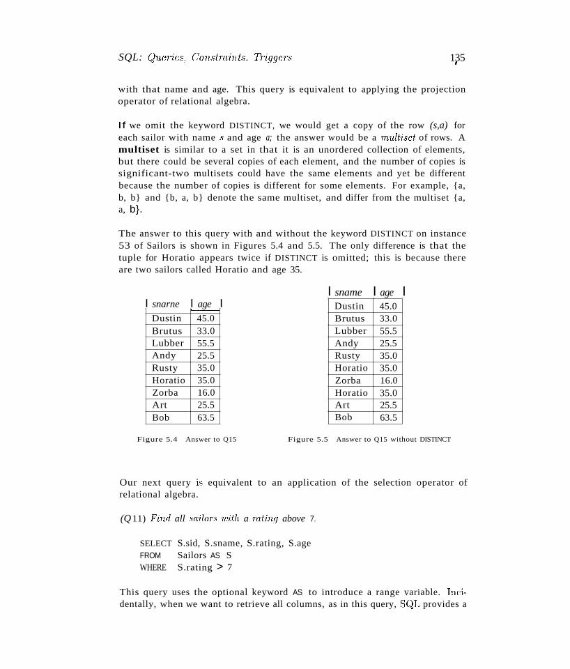
SQL: Q1Le7~ies. Con8tnrint8, TriggeT8 135~
with that name and age. This query is equivalent to applying the projectionoperator of relational algebra.
If we omit the keyword DISTINCT, we would get a copy of the row (s,a) foreach sailor with name s and age a; the answer would be a rnultiset of rows. Amultiset is similar to a set in that it is an unordered collection of elements,but there could be several copies of each element, and the number of copies issignificant-two multisets could have the same elements and yet be differentbecause the number of copies is different for some elements. For example, {a,b, b} and {b, a, b} denote the same multiset, and differ from the multiset {a,a, b}.
The answer to this query with and without the keyword DISTINCT on instance53 of Sailors is shown in Figures 5.4 and 5.5. The only difference is that thetuple for Horatio appears twice if DISTINCT is omitted; this is because thereare two sailors called Horatio and age 35.
Dustin 45.0Brutus 33.0Lubber 55.5Andy 25.5Rusty 35.0Horatio 35.0Zorba 16.0Horatio 35.0Art 25.5Bob 63.5
I sname I age I'-----"--
Dustin 45.0Brutus 33.0Lubber 55.5Andy 25.5Rusty 35.0Horatio 35.0Zorba 16.0Art 25.5Bob 63.5
I.snarne I age I
Figure 5.4 Answer to Q15 Figure 5.5 Answer to Q15 without DISTINCT
Our next query is equivalent to an application of the selection operator ofrelational algebra.
(Q 11) Find all sailors with a rating above 7.
SELECT S.sid, S.sname, S.rating, S.ageFROM Sailors AS SWHERE S.rating > 7
This query uses the optional keyword AS to introduce a range variable. Incidentally, when we want to retrieve all columns, as in this query, SQL provides a
136 CHAPTER fj
convenient shorthand: \eVe can simply write SELECT *. This notation is usefulfor interactive querying, but it is poor style for queries that are intended to bereused and maintained because the schema of the result is not clear from thequery itself; we have to refer to the schema of the underlying Sailors ta.ble.
As these two examples illustrate, the SELECT clause is actually used to do pmjection, whereas selections in the relational algebra sense are expressed usingthe WHERE clause! This mismatch between the naming of the selection and projection operators in relational algebra and the syntax of SQL is an unfortunatehistorical accident.
We now consider the syntax of a basic SQL query in more detail.
• The from-list in the FROM clause is a list of table names. A table namecan be followed by a range variable; a range variable is particularly usefulwhen the same table name appears more than once in the from-list.
• The select-list is a list of (expressions involving) column names of tablesnamed in the from-list. Column names can be prefixed by a range variable.
• The qualification in the WHERE clause is a boolean combination (i.e., anexpression using the logical connectives AND, OR, and NOT) of conditionsof the form expression op expression, where op is one of the comparisonoperators {<, <=, =, <>, >=, >}.2 An expression is a column name, aconstant, or an (arithmetic or string) expression.
• The DISTINCT keyword is optional. It indicates that the table computedas an answer to this query should not contain duplicates, that is, two copiesof the same row. The default is that duplicates are not eliminated.
Although the preceding rules describe (informally) the syntax of a basic SQLquery, they do not tell us the meaning of a query. The answer to a query isitself a relation which is a rnultisef of rows in SQL!--whose contents can beunderstood by considering the following conceptual evaluation strategy:
1. Cmnpute the cross-product of the tables in the from-list.
2. Delete rows in the cross-product that fail the qualification conditions.
3. Delete all columns that do not appear in the select-list.
4. If DISTINCT is specified, eliminate duplicate rows.
2ExpressiollS with NOT can always be replaced by equivalent expressions without NOT given the setof comparison operators just listed.
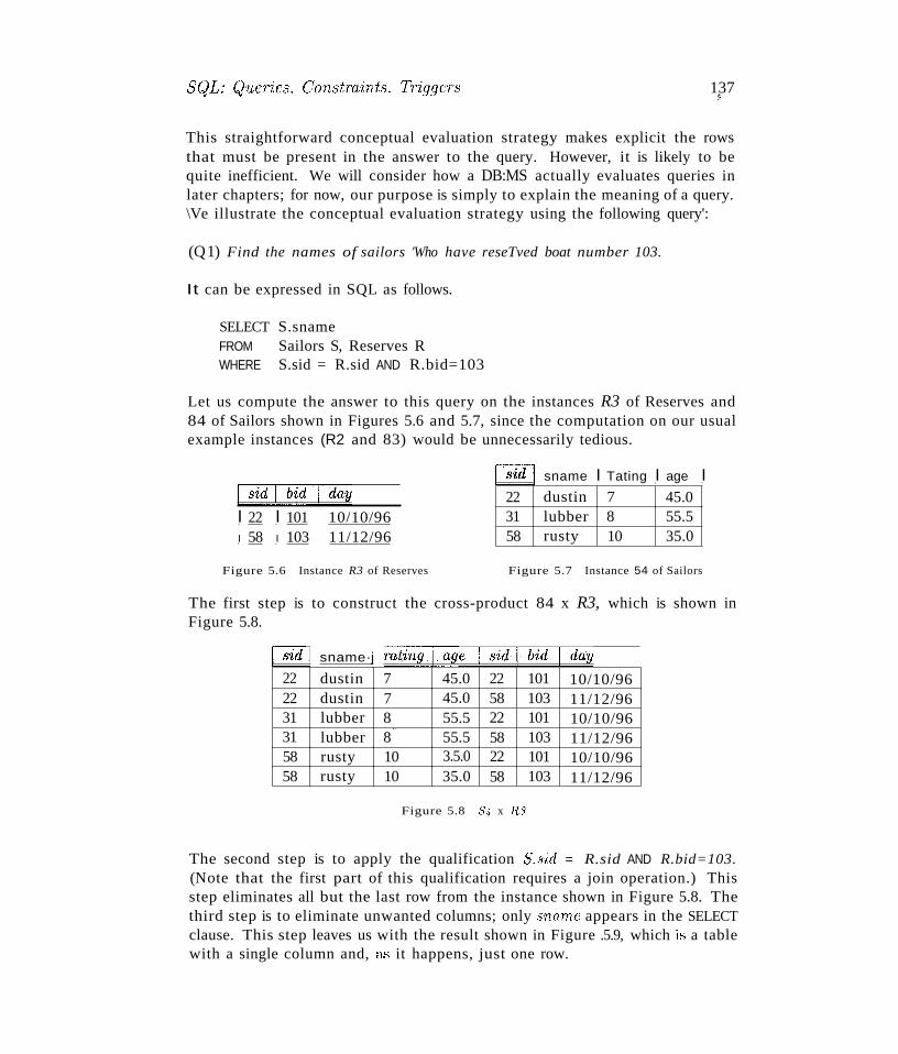
SCJL: Queries, ConstTaints, TriggeTs 137~
This straightforward conceptual evaluation strategy makes explicit the rowsthat must be present in the answer to the query. However, it is likely to bequite inefficient. We will consider how a DB:MS actually evaluates queries inlater chapters; for now, our purpose is simply to explain the meaning of a query.\Ve illustrate the conceptual evaluation strategy using the following query':
(Q1) Find the names of sailors 'Who have reseTved boat number 103.
It can be expressed in SQL as follows.
SELECT S.snameFROM Sailors S, Reserves RWHERE S.sid = R.sid AND R.bid=103
Let us compute the answer to this query on the instances R3 of Reserves and84 of Sailors shown in Figures 5.6 and 5.7, since the computation on our usualexample instances (R2 and 83) would be unnecessarily tedious.
~day
I 22 I 101 10/10/96I 58 I 103 11/12/96
Figure 5.6 Instance R3 of Reserves
~ sname I Tating I age I22 dustin 7 45.031 lubber 8 55.558 rusty 10 35.0
Figure 5.7 Instance 54 of Sailors
The first step is to construct the cross-product 84 x R3, which is shown inFigure 5.8.
~ sname·j Tating·I···age~day
22 dustin 7 45.0 22 101 10/10/9622 dustin 7 45.0 58 103 11/12/9631 lubber 8 55.5 22 101 10/10/9631 lubber 8
---55.5 58 103 11/12/96
58 rusty 10 3.5.0 22 101 10/10/9658 rusty 10 35.0 58 103 11/12/96
Figure 5.8 84 x RS
The second step is to apply the qualification S./rid = R.sid AND R.bid=103.(Note that the first part of this qualification requires a join operation.) Thisstep eliminates all but the last row from the instance shown in Figure 5.8. Thethird step is to eliminate unwanted columns; only sname appears in the SELECTclause. This step leaves us with the result shown in Figure .5.9, which is a tablewith a single column and, a.c; it happens, just one row.
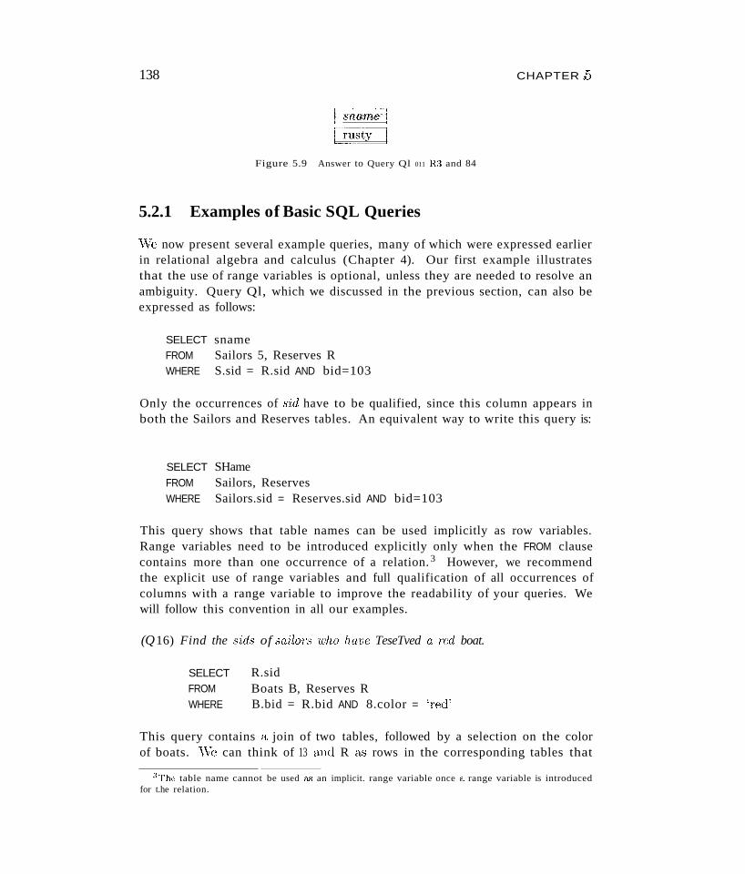
138
! sna'me!
[I1lStL]
Figure 5.9 Answer to Query Ql 011 R:l and 84
5.2.1 Examples of Basic SQL Queries
CHAPTER 15
vVe now present several example queries, many of which were expressed earlierin relational algebra and calculus (Chapter 4). Our first example illustratesthat the use of range variables is optional, unless they are needed to resolve anambiguity. Query Ql, which we discussed in the previous section, can also beexpressed as follows:
SELECT snameFROM Sailors 5, Reserves RWHERE S.sid = R.sid AND bid=103
Only the occurrences of sid have to be qualified, since this column appears inboth the Sailors and Reserves tables. An equivalent way to write this query is:
SELECT SHameFROM Sailors, ReservesWHERE Sailors.sid = Reserves.sid AND bid=103
This query shows that table names can be used implicitly as row variables.Range variables need to be introduced explicitly only when the FROM clausecontains more than one occurrence of a relation. 3 However, we recommendthe explicit use of range variables and full qualification of all occurrences ofcolumns with a range variable to improve the readability of your queries. Wewill follow this convention in all our examples.
(Q16) Find the sids of sa'iloTs who have TeseTved a Ted boat.
SELECTFROMWHERE
R.sidBoats B, Reserves RB.bid = R.bid AND 8.color = 'red'
This query contains a join of two tables, followed by a selection on the colorof boats. vVe can think of 13 and R &<; rows in the corresponding tables that
:~The table name cannot be used aii an implicit. range variable once a range variable is introducedfor t.he relation.
SQL: QUEeries, Constraints, Triggers
:prove' that a sailor with sid R.sid reserved a reel boat B.bid. On our exampleinstances R2 and 83 (Figures 5.1 and 5.2), the answer consists of the Bids 22,31, and 64. If we want the names of sailors in the result, we must also considerthe Sailors relation, since Reserves does not contain this information, as thenext example illustrates.
(Q2) Find the names of sailors 'Who have TeseTved a Ted boat.
SELECTFROMWHERE
S.snameSailors S, Reserves R, Boats 13S.sid = R.sid AND R.bid = 13.bid AND B.color = 'red'
This query contains a join of three tables followed by a selection on the colorof boats. The join with Sailors allows us to find the name of the sailor who,according to Reserves tuple R, has reserved a red boat described by tuple 13.
(QS) Find the coloTS of boats reseTved by LubbeT.
SELECT 13.colorFROM Sailors S, Reserves R, Boats 13WHERE S.sid = R.sid AND R.bid = B.bid AND S.sname = 'Lubber'
This query is very similar to the previous one. Note that in general there maybe more than one sailor called Lubber (since sname is not a key for Sailors);this query is still correct in that it will return the colors of boats reserved bysome Lubber, if there are several sailors called Lubber.
(Q4) Find the names of sa'iloTs who have Teserved at least one boat.
SELECT S.snameFROM Sailors S, Reserves RWHERE S.sid = R.sid
The join of Sailors and Reserves ensures that for each selected sname, thesailor has made some reservation. (If a sailor has not made a reservation, thesecond step in the conceptual evaluation strategy would eliminate all rows inthe cross-product that involve this sailor.)
5.2.2 Expressions and Strings in the SELECT Command
SQL supports a more general version of the select-list than just a list ofcolu1nn8. Each item in a select-list can be of the form e:l:pTcssion AS col'wnrLno:rne, where c:rprcs.sion is any arithmetic or string expression over column
140 CHAPTERf)
names (possibly prefixed by range variables) and constants, and colurnnswrneis a ne"v name for this column in the output of the query. It can also containaggregates such as smn and count, which we will discuss in Section 5.5. TheSQL standard also includes expressions over date and time values, which we willnot discuss. Although not part of the SQL standard, many implementationsalso support the use of built-in functions such as sqrt, sin, and rnod.
(Q17) Compute increments for the mtings of peTsons who have sailed two different boats on the same day.
SELECTFROMWHERE
S.sname, S.rating+1 AS ratingSailors S, Reserves R1, Reserves R2S.sid = R1.sid AND S.sid = R2.sidAND R1.day = R2.day AND R1.bid <> R2.bid
Also, each item in a qualification can be as general as expTession1 = expression2.
SELECT S1.sname AS name1, S2.sname AS name2FROM Sailors Sl, Sailors S2WHERE 2*S1.rating = S2.rating-1
For string comparisons, we can use the comparison operators (=, <, >, etc.)with the ordering of strings determined alphabetically as usual. If we needto sort strings by an order other than alphabetical (e.g., sort strings denotingmonth names in the calendar order January, February, March, etc.), SQL supports a general concept of a collation, or sort order, for a character set. Acollation allows the user to specify which characters are 'less than' which othersand provides great flexibility in string manipulation.
In addition, SQL provides support for pattern matching through the LIKE operator, along with the use of the wild-card symbols % (which stands for zeroor more arbitrary characters) and ~ (which stands for exactly one, arbitrary,character). Thus, '_AB%' denotes a pattern matching every string that contains at lea.'3t three characters, with the second and third characters being Aand B respectively. Note that unlike the other comparison operators, blankscan be significant for the LIKE operator (depending on the collation for theunderlying character set). Thus, 'Jeff' = 'Jeff' is true while 'Jeff'LIKE 'Jeff, is false. An example of the use of LIKE in a query is given below.
(Q18) Find the ages of sailors wh08e name begins and ends with B and has atleast three chamcters.
SELECT S.age
SQL: Q'Il,e'rie8, Constraints, TTiggeTs 141$
r---'-~~-~:~;- Expre~~~'~-:~'-'~:' '~Q'~'~""~,~flecting the incr~~~~~~~mpo~~:l~ceof II text data, SQL:1999 includes a more powerful version of theLIKE operator i
i called SIMILAR. This operator allows a rich set of regular expressions to be I
Iused as patterns while searching text. The regular expressions are similart~
I those sUPPo.rted by the Unix operating systenifor string searches, although'the syntax is a little different.
-- - . ••••._m. .-.-.-.-.-....•-- ..-----........ .-••••••••••••.•.•••••••....-- ..- ----.-- -----..-- ..- ------------ ---------- -.••..•.---•••••.••.•.•••••••••..•.•.••••••.••- ••••.....•- ••••.'.-""-'-.J'.
Relational Algebra and SQL: The set operations of SQL are available inrelational algebra. The main difference, of course, is that they are multisetoperations in SQL, since tables are multisets of tuples.
FROMWHERE
Sailors SS.sname LIKE 'B.%B'
The only such sailor is Bob, and his age is 63.5.
5.3 UNION, INTERSECT, AND EXCEPT
SQL provides three set-manipulation constructs that extend the basic queryform presented earlier. Since the answer to a query is a multiset of rows, it isnatural to consider the use of operations such as union, intersection, and difference. SQL supports these operations under the names UNION, INTERSECT, andEXCEPT. 4 SQL also provides other set operations: IN (to check if an elementis in a given set), op ANY, op ALL (to compare a value with the elements ina given set, using comparison operator op), and EXISTS (to check if a set isempty). IN and EXISTS can be prefixed by NOT, with the obvious modificationto their meaning. We cover UNION, INTERSECT, and EXCEPT in this section,and the other operations in Section 5.4.
Consider the following query:
(Q5) Find the names of sailors who have reserved a red 01' a green boat.
SELECTFROMWHERE
S.snameSailors S, Reserves R, Boats BS.sid = R.sid AND R.bid = B.bidAND (B.color = 'red' OR B.color = 'green')
.. _----4Note that although the SQL standard includes these operations, many systems currently support
only UNION. Also. many systems recognize the keyword MINUS for EXCEPT.
142 CHAPTERD
This query is easily expressed using the OR connective in the WHERE clause.Hovvever, the following query, which is identical except for the use of 'and'rather than 'or' in the English version, turns out to be much more difficult:
(Q6) Find the names of sailor's who have rescr'ved both a red and a green boat.
If we were to just replace the use of OR in the previous query by AND, in analogyto the English statements of the two queries, we would retrieve the names ofsailors who have reserved a boat that is both red and green. The integrityconstraint that bid is a key for Boats tells us that the same boat cannot havetwo colors, and so the variant of the previous query with AND in place of OR willalways return an empty answer set. A correct statement of Query Q6 usingAND is the following:
SELECTFROMWHERE
S.snameSailors S, Reserves RI, Boats BI, Reserves R2, Boats B2S.sid = Rl.sid AND R1.bid = Bl.bidAND S.sid = R2.sid AND R2.bid = B2.bidAND B1.color='red' AND B2.color = 'green'
We can think of RI and BI as rows that prove that sailor S.sid has reserved ared boat. R2 and B2 similarly prove that the same sailor has reserved a greenboat. S.sname is not included in the result unless five such rows S, RI, BI, R2,and B2 are found.
The previous query is difficult to understand (and also quite inefficient to execute, as it turns out). In particular, the similarity to the previous OR query(Query Q5) is completely lost. A better solution for these two queries is to useUNION and INTERSECT.
The OR query (Query Q5) can be rewritten as follows:
SELECT
FROMWHEREUNIONSELECTFROMWHERE
S.snameSailors S, Reserves R, Boats BS.sicl = R.sid AND R.bid = B.bid AND B.color = 'red'
S2.snameSailors S2, Boats B2, Reserves H2S2.sid = H2.sid AND R2.bid = B2.bicl AND B2.color = 'green'
This query sa,)'s that we want the union of the set of sailors who have reservedred boats and the set of sailors who have reserved green boats. In completesymmetry, the AND query (Query Q6) can be rewritten a.s follovvs:
SELECT S.snarne
SqL: Q'lleries7 Constraints, Triggers
FROM Sailors S, Reserves R, Boats BWHERE S.sid = R.sid AND R.bid = B.bid AND B.color = 'red'INTERSECTSELECT S2.snameFROM Sailors S2, Boats B2, Reserves R2WHERE S2.sid = R2.sid AND R2.bid = B2.bid AND B2.color = 'green'
143
This query actually contains a subtle bug-if there are two sailors such asHoratio in our example instances B1, R2, and 83, one of whom has reserved ared boat and the other has reserved a green boat, the name Horatio is returnedeven though no one individual called Horatio has reserved both a red and agreen boat. Thus, the query actually computes sailor names such that somesailor with this name has reserved a red boat and some sailor with the samename (perhaps a different sailor) has reserved a green boat.
As we observed in Chapter 4, the problem arises because we are using snameto identify sailors, and sname is not a key for Sailors! If we select sid instead ofsname in the previous query, we would compute the set of sids of sailors whohave reserved both red and green boats. (To compute the names of such sailorsrequires a nested query; we will return to this example in Section 5.4.4.)
Our next query illustrates the set-difference operation in SQL.
(Q 19) Find the sids of all sailor's who have reserved red boats but not greenboats.
SELECTFROMWHEREEXCEPTSELECTFROMWHERE
S.sidSailors S, Reserves R, Boats BS.sid = R.sid AND R.bid = B.bid AND B.color = 'red'
S2.sidSailors S2, Reserves R2, Boats B2S2.sid = R2.sid AND R2.bid = B2.bid AND B2.color = 'green'
Sailors 22, 64, and 31 have reserved red boats. Sailors 22, 74, and 31 havereserved green boats. Hence, the answer contains just the sid 64.
Indeed, since the Reserves relation contains sid information, there is no needto look at the Sailors relation, and we can use the following simpler query:
SELECTFROMWHEREEXCEPT
H.. sidBoats B, Reserves RR.bicl = B.bid AND B.color = 'red'
144
SELECT R2.sidFROM Boats B2, Reserves R2WHERE R2.bicl = B2.bid AND B2.color = :green'
CHAPTER~5
Observe that this query relies on referential integrity; that is, there are noreservations for nonexisting sailors. Note that UNION, INTERSECT, and EXCEPTcan be used on any two tables that are union-compatible, that is, have the samenumber of columns and the columns, taken in order, have the same types. Forexample, we can write the following query:
(Q20) Find all sids of sailors who have a rating of 10 or reserved boat 104.
SELECTFROMWHEREUNIONSELECTFROMWHERE
S.sidSailors SS.rating = 10
R.sidReserves RR.bid = 104
The first part of the union returns the sids 58 and 71. The second part returns22 and 31. The answer is, therefore, the set of sids 22, 31, 58, and 71. Afinal point to note about UNION, INTERSECT, and EXCEPT follows. In contrastto the default that duplicates are not eliminated unless DISTINCT is specifiedin the basic query form, the default for UNION queries is that duplicates areeliminated! To retain duplicates, UNION ALL must be used; if so, the numberof copies of a row in the result is always m + n, where m and n are the numbers of times that the row appears in the two parts of the union. Similarly,INTERSECT ALL retains cluplicates--the number of copies of a row in the resultis min(m, n )-~ancl EXCEPT ALL also retains duplicates~thenumber of copiesof a row in the result is m - n, where 'm corresponds to the first relation.
5.4 NESTED QUERIES
One of the most powerful features of SQL is nested queries. A nested queryis a query that has another query embedded within it; the embedded queryis called a suhquery. The embedded query can of course be a nested queryitself; thus queries that have very deeply nested structures are possible. Whenwriting a query, we sornetimes need to express a condition that refers to a tablethat must itself be computed. The query used to compute this subsidiary tableis a subquery and appears as part of the main query. A subquery typicallyappears within the WHERE clause of a query. Subqueries can sometimes appearin the FROM clause or the HAVING clause (which we present in Section 5.5).
SQL: QueT~ie8] Constraints] Triggers 145$
r-~'-'-'~ -.------- -~--- ,.,.._,---..-- , ,-, ,-_ , . ---------
I Relational Algebra and SQL: Nesting of queries is a feature that is notI available in relational algebra, but nested queries can be translated intoi algebra, as we will see in Chapter 15. Nesting in SQL is inspired more by, relational calculus than algebra. In conjunction with some of SQL's other
features, such as (multi)set operators and aggregation, nesting is a veryexpressive construct.
This section discusses only subqueries that appear in the WHERE clause. Thetreatment of subqueries appearing elsewhere is quite similar. Some examples ofsubqueries that appear in the FROM clause are discussed later in Section 5.5.1.
5.4.1 Introduction to Nested Queries
As an example, let us rewrite the following query, which we discussed earlier,using a nested subquery:
(Ql) Find the names of sailors who have reserved boat 103.
SELECTFROMWHERE
S.snameSailors SS.sid IN ( SELECT
FROMWHERE
R.sidReserves RR.bid = 103 )
The nested subquery computes the (multi)set of sids for sailors who have reserved boat 103 (the set contains 22,31, and 74 on instances R2 and 83), andthe top-level query retrieves the names of sailors whose sid is in this set. TheIN operator allows us to test whether a value is in a given set of elements; anSQL query is used to generate the set to be tested. Note that it is very easy tomodify this query to find all sailors who have not reserved boat 103-we canjust replace IN by NOT IN!
The best way to understand a nested query is to think of it in terms of a conceptual evaluation strategy. In our example, the strategy consists of examiningrows in Sailors and, for each such row, evaluating the subquery over Reserves.In general, the conceptual evaluation strategy that we presented for definingthe semantics of a query can be extended to cover nested queries as follows:Construct the cross-product of the tables in the FROM clause of the top-levelquery as hefore. For each row in the cross-product, while testing the qllalifica-
146
tion in the WHERE clause, (re)compute the subquery.5 Of course, the subquerymight itself contain another nested subquery, in which case we apply the sameidea one more time, leading to an evaluation strategy \vith several levels ofnested loops.
As an example of a multiply nested query, let us rewrite the following query.
(Q2) Find the names of sailors 'who ha'ue reserved a red boat.
SELECTFROMWHERE
S.snameSailors SS.sid IN ( SELECT R.sid
FROM Reserves RWHERE R. bid IN (SELECT B.bid
FROM Boats BWHERE B.color = 'red'
The innermost subquery finds the set of bids of red boats (102 and 104 oninstance E1). The subquery one level above finds the set of sids of sailors whohave reserved one of these boats. On instances E1, R2, and 83, this set of sidscontains 22, 31, and 64. The top-level query finds the names of sailors whosesid is in this set of sids; we get Dustin, Lubber, and Horatio.
To find the names of sailors who have not reserved a red boat, wc replace theoutermost occurrence of IN by NOT IN, as illustrated in the next query.
(Q21) Find the names of sailors who have not reserved a red boat.
SELECT S.snameFROM Sailors SWHERE S.sid NOT IN ( SELECT
FROMWHERE
R.sidReserves RR.bid IN ( SELECT B.bid
FROM Boats BWHERE B.color = 'red' )
This qucry computes the names of sailors whose sid is not in the set 22, 31,and 64.
In contrast to Query Q21, we can modify the previous query (the nested versionof Q2) by replacing the inner occurrence (rather than the outer occurence) of
5Since the inner subquery in our example does not depend on the 'current' row from the outerquery ill any way, you rnight wonder why we have to recompute the subquery for each outer row. Foran answer, see Section 5.4.2.
SQL: Queries, Con.,trf1'inis, Triggers
IN with NOT IN. This modified query would compute the naU1eS of sailors whohave reserved a boat that is not red, that is, if they have a reservation, it is notfor a red boat. Let us consider how. In the inner query, we check that R.bidis not either 102 or 104 (the bids of red boats). The outer query then finds thesids in Reserves tuples \vhere the bid is not 102 or 104. On instances E1, R2,and 53, the outer query computes the set of sids 22, 31, 64, and 74. Finally,we find the names of sailors whose sid is in this set.
\Ve can also modify the nested query Q2 by replacing both occurrences of INwith NOT IN. This variant finds the names of sailors who have not reserved aboat that is not red, that is, who have reserved only red boats (if they've reserved any boats at all). Proceeding as in the previous paragraph, on instancesE1, R2, and 53, the outer query computes the set of sids (in Sailors) otherthan 22, 31, 64, and 74. This is the set 29, 32, 58, 71, 85, and 95. We then findthe names of sailors whose sid is in this set.
5.4.2 Correlated Nested Queries
In the nested queries seen thus far, the inner subquery has been completelyindependent of the outer query. In general, the inner subquery could depend onthe row currently being examined in the outer query (in terms of our conceptualevaluation strategy). Let us rewrite the following query once more.
(Q1) Pind the names of sailors who have reserved boat nv,mber 103.
SELECTFROMWHERE
S.snameSailors SEXISTS ( SELECT *
FROM Reserves RWHERE R.bid = 103
AND R.sid = S.sid )
The EXISTS operator is another set comparison operator, such as IN. It allowsus to test whether a set is nonempty, an implicit comparison with the emptyset. Thus, for each Sailor row 5, we test whether the set of Reserves rowsR such that R.bid = 103 AND S.sid = R.sid is nonempty. If so, sailor 5 hasreserved boat t03, and we retrieve the name. '1'he subquery clearly dependson the current row Sand IIlUSt be re-evaluated for each row in Sailors. Theoccurrence of S in the subquery (in the form of the literal S.sid) is called acOTTelation, and such queries are called con-elated queries.
This query also illustrates the use of the special symbol * in situations whereall we want to do is to check that a qualifying row exists, and do Hot really
148 CHAPTER,.5
want to retrieve any columns from the row. This is one of the two uses of * inthe SELECT clause that is good programming style; the other is &':1 an argumentof the COUNT aggregate operation, which we describe shortly.
As a further example, by using NOT EXISTS instead of EXISTS, we can computethe names of sailors who have not reserved a red boat. Closely related toEXISTS is the UNIQUE predicate. \Vhen we apply UNIQUE to a subquery, theresulting condition returns true if no row appears twice in the answer to thesubquery, that is, there are no duplicates; in particular, it returns true if theanswer is empty. (And there is also a NOT UNI QUE version.)
5.4.3 Set-Comparison Operators
We have already seen the set-comparison operators EXISTS, IN, and UNIQUE,along with their negated versions. SQL also supports op ANY and op ALL, whereop is one of the arithmetic comparison operators {<, <=, =, <>, >=, >}. (SOMEis also available, but it is just a synonym for ANY.)
(Q22) Find sailors whose rating is better than some sailor called Horatio.
SELECT S.sidFROM Sailors SWHERE S.rating > ANY ( SELECT
FROMWHERE
S2.ratingSailors S2S2.sname = 'Horatio' )
If there are several sailors called Horatio, this query finds all sailors whose ratingis better than that of some sailor called Horatio. On instance 83, this computesthe sids 31, 32, 58, 71, and 74. \\That if there were no sailor called Horatio? Inthis case the comparison S.rating > ANY ... is defined to return false, and thequery returns an elnpty answer set. To understand comparisons involving ANY,it is useful to think of the comparison being carried out repeatedly. In thisexample, S. rating is successively compared with each rating value that is ananswer to the nested query. Intuitively, the subquery must return a row thatmakes the comparison true, in order for S. rat'ing > ANY ... to return true.
(Q23) Find sailors whose rating is better than every sailor' called Horat·to.
vVe can obtain all such queries with a simple modification to Query Q22: Justreplace ANY with ALL in the WHERE clause of the outer query. On instance 8~~,
we would get the sid", 58 and 71. If there were no sailor called Horatio, thecomparison S.rating > ALL ... is defined to return true! The query would thenreturn the names of all sailors. Again, it is useful to think of the comparison
SQL: C2uerie,s, ConstTain,ts, Triggers 149
being carried out repeatedly. Intuitively, the comparison must be true for everyreturned row for S. rating> ALL ... to return true.
As another illustration of ALL, consider the following query.
(Q24J Find the 8ailor's with the highest rating.
SELECT S.sidFROM Sailors SWHERE S.rating >= ALL ( SELECT S2.rating
FROM Sailors S2 )
The subquery computes the set of all rating values in Sailors. The outer WHEREcondition is satisfied only when S.rating is greater than or equal to each ofthese rating values, that is, when it is the largest rating value. In the instance53, the condition is satisfied only for rating 10, and the answer includes thesid." of sailors with this rating, Le., 58 and 71.
Note that IN and NOT IN are equivalent to = ANY and <> ALL, respectively.
5.4.4 More Examples of Nested Queries
Let us revisit a query that we considered earlier using the INTERSECT operator.
(Q6) Find the names of sailors who have reserved both a red and a green boat.
SELECTFROMWHERE
S.snameSailors S, Reserves R, Boats BS.sid = R.sid AND R.bid = B.bid AND B.color = 'red'AND S.sid IN ( SELECT S2.sid
FROM Sailors S2, Boats B2, Reserves R2WHERE S2.sid = R2.sid AND R2.bid = B2.bid
AND B2.color = 'green' )
This query can be understood as follows: "Find all sailors who have reserveda red boat and, further, have sids that are included in the set of sids of sailorswho have reserved a green boat." This formulation of the query illustrateshow queries involving INTERSECT can be rewritten using IN, which is useful toknow if your system does not support INTERSECT. Queries using EXCEPT canbe similarly rewritten by using NOT IN. To find the side:, of sailors who havereserved red boats but not green boats, we can simply replace the keyword INin the previous query by NOT IN.
150 CHAPTER"S
As it turns out, writing this query (Q6) using INTERSECT is more complicatedbecause we have to use sids to identify sailors (while intersecting) and have toreturn sailor names:
SELECT S.snameFROM Sailors SWHERE S.sid IN (( SELECT R.sid
FROM Boats B, Reserves RWHERE R.bid = B.bid AND B.color = 'red' )INTERSECT(SELECT R2.sidFROM Boats B2, Reserves R2WHERE R2.bid = B2.bid AND B2.color = 'green' ))
Our next example illustrates how the division operation in relational algebracan be expressed in SQL.
(Q9) Find the names of sailors who have TeseTved all boats.
SELECT S.snameFROM Sailors SWHERE NOT EXISTS (( SELECT B.bid
FROM Boats B )EXCEPT(SELECT R. bidFROM Reserves RWHERE R.sid = S.sid ))
Note that this query is correlated--for each sailor S, we check to see that theset of boats reserved by S includes every boat. An alternative way to do thisquery without using EXCEPT follows:
SELECT S.snameFROM Sailors SWHERE NOT EXISTS ( SELECT
FROMWHERE
B.bidBoats BNOT EXISTS ( SELECT R. bid
FROM Reserves RWHERE R.bid = B.bid
AND R.sid = S.sid ))
Intuitively, for each sailor we check that there is no boat that has not beenreserved by this sailor.
SQL: Q'ueT'ics. Constraint8, Triggers lQJ
SQL:1999 Aggregate Functions: The collection of aggregate functionsis greatly expanded in the new standard, including several statisticaltions such as standard deviation, covariance, and percentiles. However,new aggregate functions are in the SQLjOLAP package and may notsupported by all vendors.
5.5 AGGREGATE OPERATORS
In addition to simply retrieving data, we often want to perform some computation or summarization. As we noted earlier in this chapter, SQL allows theuse of arithmetic expressions. We now consider a powerful class of constructsfor computing aggregate values such as MIN and SUM. These features representa significant extension of relational algebra. SQL supports five aggregate operations, which can be applied on any column, say A, of a relation:
1. COUNT ([DISTINCT] A): The number of (unique) values in the A column.
2. SUM ([DISTINCT] A): The sum of all (unique) values in the A column.
3. AVG ([DISTINCT] A): The average of all (unique) values in the A column.
4. MAX (A): The maximum value in the A column.
5. MIN (A): The minimum value in the A column.
Note that it does not make sense to specify DISTINCT in conjunction with MINor MAX (although SQL does not preclude this).
(Q25) Find the average age of all sailors.
SELECT AVG (S.age)FROM Sailors S
On instance 53, the average age is 37.4. Of course, the WHERE clause can beused to restrict the sailors considered in computing the average age.
(Q26) Find the average age of sailors with a rating of 10.
SELECT AVG (S.age)FROM Sailors SWHERE S.rating = 10
There are two such sailors, and their average age is 25.5. MIN (or MAX) can beused instead of AVG in the above queries to find the age of the youngest (oldest)
1,..')0 ...
sailor. However) finding both the name and the age of the oldest sailor is moretricky, as the next query illustrates.
(Q,"21) Find the name and age of the oldest sailor.
Consider the following attempt to answer this query:
SELECT S.sname, MAX (S.age)FROM Sailors S
The intent is for this query to return not only the maximum age but also thename of the sailors having that age. However, this query is illegal in SQL-ifthe SELECT clause uses an aggregate operation, then it must use only aggregateoperations unless the query contains a GROUP BY clause! (The intuition behindthis restriction should become clear when we discuss the GROUP BY clause inSection 5.5.1.) Therefore, we cannot use MAX (S.age) as well as S.sname in theSELECT clause. We have to use a nested query to compute the desired answerto Q27:
SELECT
FROMWHERE
S.sname, S.ageSailors SS.age = ( SELECT MAX (S2.age)
FROM Sailors S2 )
Observe that we have used the result of an aggregate operation in the subqueryas an argument to a comparison operation. Strictly speaking, we are comparingan age value with the result of the subquery, which is a relation. However,because of the use of the aggregate operation, the subquery is guaranteed toreturn a single tuple with a single field, and SQL Gonverts such a relation to afield value for the sake of the comparison. The following equivalent query forQ27 is legal in the SQL standard but, unfortunately, is not supported in manysystems:
SELECT
FROMWHERE
S.sname, S.ageSailors S( SELECT MAX (S2.age)
FROM Sailors S2 ) = S.age
\Vc can count the number of sailors using COUNT. This exarnple illustrates theuse of * as an argument to COUNT, which is useful when \ve want to count allrows.
(Q28) Count the n:umbCT of sa:iloTs.
SELECT COUNT (*)
FROM Sailors S
vVe can think of * as shorthand for all the columns (in the cross-product of thefrom-list in the FROM clause). Contrast this query with the following query,which computes the number of distinct sailor names. (Remember that ,'mameis not a key!)
(Q29) Count the nmnber of d'i.fferent sailor names.
SELECT COUNT ( DISTINCT S.sname )FROM Sailors S
On instance 83, the answer to Q28 is 10, whereas the answer to Q29 is 9(because two sailors have the same name, Horatio). If DISTINCT is omitted,the answer to Q29 is 10, because the name Horatio is counted twice. If COUNTdoes not include DISTINCT, then COUNT (*) gives the same answer as COUNT (x) ,
where x is any set of attributes. In our example, without DISTINCT Q29 isequivalent to Q28. However, the use of COUNT (*) is better querying style,since it is immediately clear that all records contribute to the total count.
Aggregate operations offer an alternative to the ANY and ALL constructs. Forexample, consider the following query:
(Q30) Find the names of sailors who are older than the oldest sailor with arating of 10.
SELECTFROMWHERE
S.snameSailors SS.age > ( SELECT MAX ( S2.age )
FROM Sailors S2WHERE S2.rating = 10 )
On instance 83, the oldest sailor with rating 10 is sailor 58, whose age is ~j5.
The names of older sailors are Bob, Dustin, Horatio, and Lubber. Using ALL,this query could alternatively be written as follows:
SELECT S.snameFROM Sailors SWHERE S.age > ALL ( SELECT
FROMWHERE
S2.ageSailors S2S2.rating = 10 )
However, the ALL query is more error proncone could easily (and incorrectly!)use ANY instead of ALL, and retrieve sailors who are older than some sailor with
154 CHAPTEFt,~5
Relationa~ Algebra and SQL: ~~~~:egation is a fUIl~~~:·mental operati(~:l-'-lthat canIlot be expressed in relational algebra. Similarly, SQL'8 grouping Iconstruct cannot be expressed in algebra. I
L..- ._. .....__ . I
a rating of 10. The use of ANY intuitively corresponds to the use of MIN, insteadof MAX, in the previous query.
5.5.1 The GROUP BY and HAVING Clauses
Thus far, we have applied aggregate operations to all (qualifying) rows in arelation. Often we want to apply aggregate operations to each of a numberof groups of rows in a relation, where the number of groups depends on therelation instance (i.e., is not known in advance). For example, consider thefollowing query.
(Q31) Find the age of the youngest sailor for each rating level.
If we know that ratings are integers in the range 1 to la, we could write 10queries of the form:
SELECT MIN (S.age)FROM Sailors SWHERE S.rating = i
where i = 1,2, ... ,10. vVriting 10 such queries is tedious. More important,we may not know what rating levels exist in advance.
To write such queries, we need a major extension to the basic SQL queryform, namely, the GROUP BY clause. In fact, the extension also includes anoptional HAVING clause that can be used to specify qualificatioIls over groups(for example, we may be interested only in rating levels> 6. The general formof an SQL query with these extensions is:
SELECT [ DISTINCT] select-listFROM from-listWHERE 'qualificationGROUP BY grouping-listHAVING group-qualification
Using the GROUP BY clause, we can write Q:n a.s follows:
SELECT S.rating, MIN (S.age)
S(JL: queries. Constraints. Triggers
FROM Sailors SGROUP BY S.rating
Let us consider some important points concerning the new clauses:
II The select-list in the SELECT clause consists of (1) a list of column namesand (2) a list of terms having the form aggop ( column-name) AS newname. vVe already saw AS used to rename output columns. Columns thatare the result of aggregate operators do not already have a column name,and therefore giving the column a name with AS is especially useful.
Every column that appears in (1) must also appear in grouping-list. Thereason is that each row in the result of the query corresponds to one gmup,which is a collection of rows that agree on the values of columns in groupinglist. In general, if a column appears in list (1), but not in grouping-list,there can be multiple rows within a group that have different values in thiscolumn, and it is not clear what value should be assigned to this columnin an answer row.
We can sometimes use primary key information to verify that a columnhas a unique value in all rows within each group. For example, if thegrouping-list contains the primary key of a table in the from-list, everycolumn of that table has a unique value within each group. In SQL:1999,such columns are also allowed to appear in part (1) of the select-list.
II The expressions appearing in the group-qualification in the HAVING clausemust have a single value per group. The intuition is that the HAVING clausedetermines whether an answer row is to be generated for a given group.To satisfy this requirement in SQL-92, a column appearing in the groupqualification must appear a'3 the argument to an aggregation operator, orit must also appear in grouping-list. In SQL:1999, two new set functionshave been introduced that allow us to check whether every or any row in agroup satisfies a condition; this allows us to use conditions similar to thosein a WHERE clause.
III If GROUP BY is omitted, the entire table is regarded as a single group.
vVe explain the semantics of such a query through an example.
(QS2) Find the age of the youngest sa'ilor who is eligible to vote (i.e., is at least18 years old) for each rating level with at least h.uo such sailors.
SELECTFROMWHEREGROUP BYHAVING
S.rating, MIN (S.age) AS minageSailors SS.age >= 18S.ratingCOUNT (*) > 1
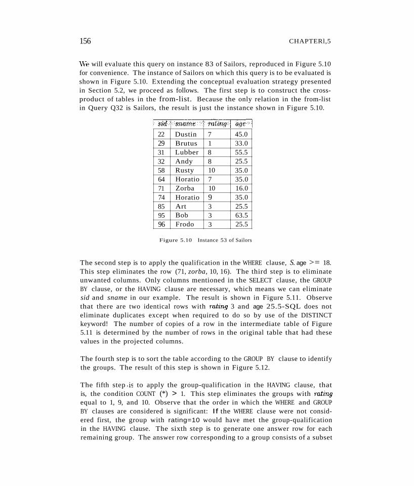
156 CHAPTERl,5
vVe will evaluate this query on instance 83 of Sailors, reproduced in Figure 5.10for convenience. The instance of Sailors on which this query is to be evaluated isshown in Figure 5.10. Extending the conceptual evaluation strategy presentedin Section 5.2, we proceed as follows. The first step is to construct the crossproduct of tables in the from-list. Because the only relation in the from-listin Query Q32 is Sailors, the result is just the instance shown in Figure 5.10.
22 Dustin 7 45.029 Brutus 1 33.031 Lubber 8 55.532 Andy 8 25.558 Rusty 10 35.064 Horatio 7 35.071 Zorba 10 16.074 Horatio 9 35.085 Art 3 25.595 Bob 3 63.596 Frodo 3 25.5
Figure 5.10 Instance 53 of Sailors
The second step is to apply the qualification in the WHERE clause, S. age >= 18.This step eliminates the row (71, zorba, 10, 16). The third step is to eliminateunwanted columns. Only columns mentioned in the SELECT clause, the GROUPBY clause, or the HAVING clause are necessary, which means we can eliminatesid and sname in our example. The result is shown in Figure 5.11. Observethat there are two identical rows with rating 3 and age 25.5-SQL does noteliminate duplicates except when required to do so by use of the DISTINCTkeyword! The number of copies of a row in the intermediate table of Figure5.11 is determined by the number of rows in the original table that had thesevalues in the projected columns.
The fourth step is to sort the table according to the GROUP BY clause to identifythe groups. The result of this step is shown in Figure 5.12.
The fifth step ,-is to apply the group-qualification in the HAVING clause, thatis, the condition COUNT (*) > 1. This step eliminates the groups with ratingequal to 1, 9, and 10. Observe that the order in which the WHERE and GROUPBY clauses are considered is significant: If the WHERE clause were not considered first, the group with rating=10 would have met the group-qualificationin the HAVING clause. The sixth step is to generate one answer row for eachremaining group. The answer row corresponding to a group consists of a subset
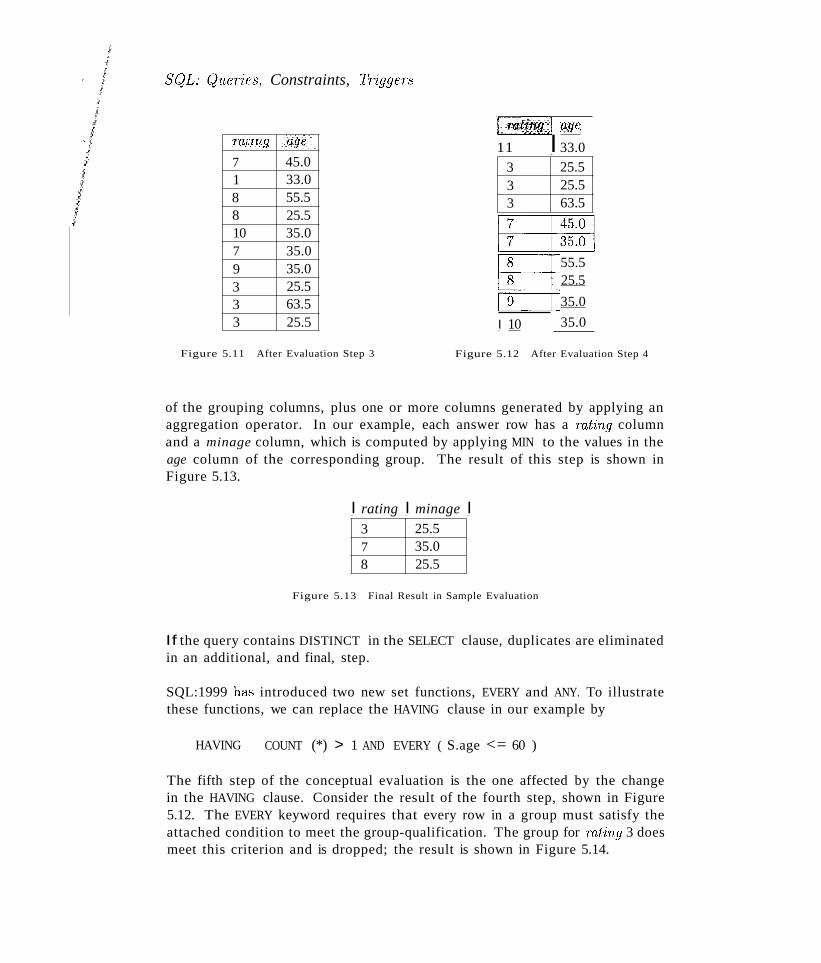
SqL: queries, Constraints, Triggers
3 25.53 25.53 63.5
55.525.5
35.0
35.0I 10
~~tl?l (J;fJ6;
11 I 33.0.f'(Lf'tTbf} iigge·····.. . ....
7 45.01 33.08 55.58 25.510 35.07 35.09 35.03 25.53 63.53 25.5
Figure 5.11 After Evaluation Step 3 Figure 5.12 After Evaluation Step 4
of the grouping columns, plus one or more columns generated by applying anaggregation operator. In our example, each answer row has a rating columnand a minage column, which is computed by applying MIN to the values in theage column of the corresponding group. The result of this step is shown inFigure 5.13.
I rating I minage I3 25.57 35.08 25.5
Figure 5.13 Final Result in Sample Evaluation
If the query contains DISTINCT in the SELECT clause, duplicates are eliminatedin an additional, and final, step.
SQL:1999 ha.s introduced two new set functions, EVERY and ANY. To illustratethese functions, we can replace the HAVING clause in our example by
HAVING COUNT (*) > 1 AND EVERY ( S.age <= 60 )
The fifth step of the conceptual evaluation is the one affected by the changein the HAVING clause. Consider the result of the fourth step, shown in Figure5.12. The EVERY keyword requires that every row in a group must satisfy theattached condition to meet the group-qualification. The group for rat'ing 3 doesmeet this criterion and is dropped; the result is shown in Figure 5.14.
158 CHAPTER. 5
SQL:1999 Extensions: Two new set functions, EVERY and ANY, havebeen added. vVhen they are used in the HAVING clause, the basic intuitionthat the clause specifies a condition to be satisfied by each group, taken asa whole, remains unchanged. However, the condition can now involve testson individual tuples in the group, whereas it previously relied exclusivelyon aggregate functions over the group of tuples.
It is worth contrasting the preceding query with the following query, in whichthe condition on age is in the WHERE clause instead of the HAVING clause:
SELECTFROMWHEREGROUP BYHAVING
S.rating, MIN (S.age) AS minageSailors SS.age >= 18 AND S.age <= 60S.ratingCOUNT (*) > 1
Now, the result after the third step of conceptual evaluation no longer containsthe row with age 63.5. Nonetheless, the group for rating 3 satisfies the conditionCOUNT (*) > 1, since it still has two rows, and meets the group-qualificationapplied in the fifth step. The final result for this query is shown in Figure 5.15.
3 25.57 45.08 55.5
I rating I minage I
55.5
rating I minage
~ 145
.0
Figure 5.14 Final Result of EVERY Query Figure 5.15 Result of Alternative Query
5.5.2 More Examples of Aggregate Queries
(Q33) FOT each red boat; find the number of reservations for this boat.
SELECT B.bid, COUNT (*) AS reservationcountFROM Boats B, Reserves RWHERE R.bid = B.bid AND B.color = 'red'GROUP BY B.bid
On instances B1 and R2, the answer to this query contains the two tuples (102,3) and (104, 2).
Observe that this version of the preceding query is illegal:
SCdL: (J'ueries, Constraints. IhggeT8
SELECT B.bicl, COUNT (*) AS reservationcountFROM Boats B, Reserves RWHERE R.bid = B.bidGROUP BY B.bidHAVING B.color = 'red'
lijj9
Even though the gToup-qualification B.coloT = 'Ted'is single-valued per group,since the grouping attribute bid is a key for Boats (and therefore determinescoloT) , SQL disallows this query.6 Only columns that appear in the GROUP BYclause can appear in the HAVING clause, unless they appear as arguments toan aggregate operator in the HAVING clause.
(Q34) Find the avemge age of sailoTs fOT each mting level that has at least twosailoTs.
SELECTFROMGROUP BYHAVING
S.rating, AVG (S.age) AS avgageSailors SS.ratingCOUNT (*) > 1
After identifying groups based on mting, we retain only groups with at leasttwo sailors. The answer to this query on instance 83 is shown in Figure 5.16.
I mting I avgage I3 44.57 40.08 40.510 25.5
Figure 5.16 Q34 Answer
I mting I avgage I3 45.57 40.08 40.510 35.0
Figure 5.17 Q35 Answer
I··rating I av.qage]
3 45.57 40.08 40.5
Figure 5.18 Q:36 Answer
The following alternative formulation of Query Q34 illustrates that the HAVINGclause can have a nested subquery, just like the WHERE clause. Note that wecan use S. mtiTLg inside the nested subquery in the HAVING clause because ithas a single value for the current group of sailors:
SELECTFROMGROUP BYHAVING
S.rating, AVG ( S.age ) AS avgageSailors SS.rating1 < ( SELECT COUNT (*)
FROM Sailors S2WHERE S.rating = S2.Hl,ting )
6This query can be ea..'iily rewritten to be legal in SQL: 1999 using EVERY in the HAVING clause.
160 CHAPTER .;5
(Q35) Find the average age of sailors 'Who aTe of voting age (i.e.~ at least 18year8 old) for each 'rating level that has at least two sailors.
SELECTFROMWHEREGROUP BYHAVING
S.rating, AVG ( S.age ) AS avgageSailors SS. age >= 18S.rating1 < ( SELECT COUNT (*)
FROM Sailors S2WHERE S.rating = S2.rating )
In this variant of Query Q34, we first remove tuples with age <= 18 and groupthe remaining tuples by rating. For each group, the subquery in the HAVINGclause computes the number of tuples in Sailors (without applying the selectionage <= 18) with the same rating value as the current group. If a group hasless than two sailors, it is discarded. For each remaining group, we outputthe average age. The answer to this query on instance 53 is shown in Figure5.17. Note that the answer is very similar to the answer for Q34, with the onlydifference being that for the group with rating 10, we now ignore the sailorwith age 16 while computing the average.
(Q36) Find the average age oj sailors who aTe of voting age (i.e., at least 18yeaTs old) JOT each rating level that has at least two such sailors.
SELECTFROMWHEREGROUP BYHAVING
S.rating, AVG ( S.age ) AS avgageSailors SS. age> 18S.rating1 < ( SELECT COUNT (*)
FROM Sailors S2WHERE S.rating = S2.rating AND S2.age >= 18 )
This formulation of the query reflects its similarity to Q35. The answer to Q36on instance 53 is shown in Figure 5.18. It differs from the answer to Q35 inthat there is no tuple for rating 10, since there is only one tuple with rating 10and age 2 18.
Query Q36 is actually very similar to Q32, as the following simpler formulationshows:
SELECTFROMWHEREGROUP BY
S.rating, AVGSailors SS. age> 18S.rating
( S.age ) AS avgage
SQL: QueTies, Constraints, Triggers
HAVING COUNT (*) > 1
This formulation of Q36 takes advantage of the fact that the WHERE clause isapplied before grouping is done; thus, only sailors with age> 18 are left whengrouping is done. It is instructive to consider yet another way of writing thisquery:
SELECTFROM
WHERE
Temp.rating, Temp.avgage( SELECT S.rating, AVG ( S.age ) AS
COUNT (*) AS ratingcountFROM Sailors SWHERE S. age> 18GROUP BY S.rating) AS Temp
Temp.ratingcount > 1
avgage,
This alternative brings out several interesting points. First, the FROM clausecan also contain a nested subquery according to the SQL standard. 7 Second,the HAVING clause is not needed at all. Any query with a HAVING clause canbe rewritten without one, but many queries are simpler to express with theHAVING clause. Finally, when a subquery appears in the FROM clause, usingthe AS keyword to give it a name is necessary (since otherwise we could notexpress, for instance, the condition Temp. ratingcount > 1).
(Q37) Find those ratings fOT which the average age of sailoTS is the m'inirnumover all ratings.
We use this query to illustrate that aggregate operations cannot be nested. Onemight consider writing it as follows:
SELECTFROMWHERE
S.ratingSailors SAVG (S.age) = ( SELECT MIN (AVG (S2.age))
FROM Sailors S2GROUP BY S2.rating )
A little thought shows that this query will not work even if the expression MIN(AVG (S2.age)), which is illegal, were allowed. In the nested query, Sailors ispartitioned int,o groups by rating, and the average age is computed for eachrating value. for each group, applying MIN to this average age value for thegroup will return the same value! A correct version of this query follows. Itessentially computes a temporary table containing the average age for eachrating value and then finds the rating(s) for which this average age is theminimum.
7Not all commercial database systems currently support nested queries in the FROM clause.
162 GHAPTER r5
r-_m .
I The Relational Model and SQL: Null values arc not part of the baskI relational model. Like SQL's treatment of tables as multisets of tuples,
~liS is a del~.~~~~r~ ...~~~..1~._t_h_e_l_)ru_s_,i_c_l_l1_o_d_e_1. ----'
SELECTFROM
WHERE
Temp.rating, Temp.avgage( SELECT S.rating, AVG (S.age) AS avgage,
FROM Sailors SGROUP BY S.rating) AS Temp
Temp.avgage = ( SELECT MIN (Temp.avgage) FROM Temp)
The answer to this query on instance 53 is (10, 25.5).
As an exercise, consider whether the following query computes the same answer.
SELECTFROM
GROUP BY
Temp.rating, MIN (Temp.avgage )( SELECT S.rating, AVG (S.age) AS
FROM Sailors SGROUP BY S.rating) AS Temp
Temp.rating
avgage,
5.6 NULL VALUES
Thus far, we have assumed that column values in a row are always known. Inpractice column values can be unknown. For example, when a sailor, say Dan,joins a yacht club, he may not yet have a rating assigned. Since the definitionfor the Sailors table has a rating column, what row should we insert for Dan?\\That is needed here is a special value that denotes unknown. Suppose the Sailortable definition was modified to include a rnaiden-name column. However, onlymarried women who take their husband's last name have a maiden name. Forwomen who do not take their husband's name and for men, the nw'idcn-nmnccolumn is inapphcable. Again, what value do we include in this column for therow representing Dan?
SQL provides H special column value called null to use in such situations. "Veuse null when the column value is either 'lJ,nknown or inapplicable. Using ourSailor table definition, we might enter the row (98. Dan, null, 39) to representDan. The presence of null values complicates rnany issues, and we consider theimpact of null values on SQL in this section.
SQL: Q'lteT'leS, ConstT'aJnt." Trigger's
5.6.1 Comparisons Using Null Values
Consider a comparison such as rat'in,g = 8. If this is applied to the row for Dan,is this condition true or false'? Since Dan's rating is unknown, it is reasonableto say that this comparison should evaluate to the value unknown. In fact, thisis the C::lse for the comparisons rating> 8 and rating < 8 &'3 well. Perhaps lessobviously, if we compare two null values using <, >, =, and so on, the result isalways unknown. For example, if we have null in two distinct rows of the sailorrelation, any comparison returns unknown.
SQL also provides a special comparison operator IS NULL to test whether acolumn value is null; for example, we can say rating IS NULL, which wouldevaluate to true on the row representing Dan. We can also say rat'ing IS NOTNULL, which would evaluate to false on the row for Dan.
5.6.2 Logical Connectives AND, OR, and NOT
Now, what about boolean expressions such as mting = 8 OR age < 40 andmting = 8 AND age < 40? Considering the row for Dan again, because age< 40, the first expression evaluates to true regardless of the value of rating, butwhat about the second? We can only say unknown.
But this example raises an important point~once we have null values, wemust define the logical operators AND, OR, and NOT using a three-val1LCd logic inwhich expressions evaluate to true, false, or unknown. We extend the usu1'11interpretations of AND, OR, and NOT to cover the case when one of the argumentsis unknown &., follows. The expression NOT unknown is defined to be unknown.OR of two arguments evaluates to true if either argument evaluates to true,and to unknown if one argument evaluates to false and the other evaluates tounknown. (If both arguments are false, of course, OR evaluates to false.) ANDof two arguments evaluates to false if either argument evaluates to false, andto unknown if one argument evaluates to unknown and the other evaluates totrue or unknown. (If both arguments are true, AND evaluates to true.)
5.6.3 Impact on SQL Constructs
Boolean expressions arise in many contexts in SQI", and the impact of nv,llvalues must be recognized. H)r example, the qualification in the WHERE clauseeliminates rows (in the cross-product of tables named in the FROM clause) forwhich the qualification does not evaluate to true. Therefore, in the presenceof null values, any row that evaluates to false or unknown is eliminated. Eliminating rows that evaluate to unknown h&') a subtle but signifieant impaet onqueries, especially nested queries involving EXISTS or UNIQUE.
164 CHAPTER~5
Another issue in the presence of 'null values is the definition of when two rowsin a relation instance are regarded a.'3 duplicates. The SQL definition is that tworows are duplicates if corresponding columns are either equal, or both containTrull. Contra..9t this definition with the fact that if we compare two null valuesusing =, the result is unknown! In the context of duplicates, this comparison isimplicitly treated as true, which is an anomaly.
As expected, the arithmetic operations +, -, *, and / all return Tmll if one oftheir arguments is null. However, nulls can cause some unexpected behaviorwith aggregate operations. COUNT(*) handles 'null values just like other values;that is, they get counted. All the other aggregate operations (COUNT, SUM, AVG,MIN, MAX, and variations using DISTINCT) simply discard null values--thus SUMcannot be understood as just the addition of all values in the (multi)set ofvalues that it is applied to; a preliminary step of discarding all null values mustalso be accounted for. As a special case, if one of these operators-other thanCOUNT-is applied to only null values, the result is again null.
5.6.4 Outer Joins
Some interesting variants of the join operation that rely on null values, calledouter joins, are supported in SQL. Consider the join of two tables, say SailorsMe Reserves. Tuples of Sailors that do not match some row in Reserves according to the join condition c do not appear in the result. In an outer join, onthe other hanel, Sailor rows without a matching Reserves row appear exactlyonce in the result, with the result columns inherited from Reserves assignednull values.
In fact, there are several variants of the outer join idea. In a left outer join,Sailor rows without a matching Reserves row appear in the result, but not viceversa. In a right outer join, Reserves rows without a matching Sailors rowappear in the result, but not vice versa. In a full outer join, both Sailorsand Reserves rows without a match appear in the result. (Of course, rows witha match always appear in the result, for all these variants, just like the usualjoins, sometimes called inner joins, presented in Chapter 4.)
SQL allows the desired type of join to be specified in the FROM clause. Forexample, the following query lists (sid, b'id) pairs corresponding to sailors andboats they ha~e reserved:
SELECT S.sid, R.bidFROM Sailors S NATURAL LEFT OUTER JOIN Reserves R
The NATURAL keyword specifies that the join condition is equality on all commonattributes (in this example, sid), and the WHERE clause is not required (unless
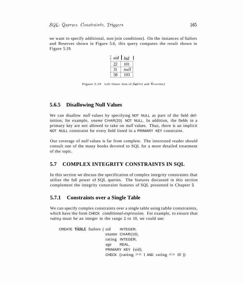
Hj5
we want to specify additional, non-join conditions). On the instances of Sailorsand Reserves shown in Figure 5.6, this query computes the result shown inFigure 5.19.
I sid I bid I22 10131 null58 103
Figure 5.19 Left Outer Join of Sailo7"1 and Rese1<Jesl
5.6.5 Disallowing Null Values
We can disallow null values by specifying NOT NULL as part of the field definition; for example, sname CHAR(20) NOT NULL. In addition, the fields in aprimary key are not allowed to take on null values. Thus, there is an implicitNOT NULL constraint for every field listed in a PRIMARY KEY constraint.
Our coverage of null values is far from complete. The interested reader shouldconsult one of the many books devoted to SQL for a more detailed treatmentof the topic.
5.7 COMPLEX INTEGRITY CONSTRAINTS IN SQL
In this section we discuss the specification of complex integrity constraints thatutilize the full power of SQL queries. The features discussed in this sectioncomplement the integrity constraint features of SQL presented in Chapter 3.
5.7.1 Constraints over a Single Table
We can specify complex constraints over a single table using table constraints,which have the form CHECK conditional-expression. For example, to ensure thatrating must be an integer in the range 1 to 10, we could use:
CREATE TABLE Sailors ( sid INTEGER,sname CHAR(10),
rating INTEGER,
age REAL,PRIMARY KEY (sid),CHECK (rating >= 1 AND rating <= 10 ))
166 CHAPTER*5
To enforce the constraint that Interlake boats cannot be reserved, we could use:
CREATE TABLE Reserves (sid INTEGER,bid INTEGER,day DATE,FOREIGN KEY (sid) REFERENCES SailorsFOREIGN KEY (bid) REFERENCES BoatsCONSTRAINT noInterlakeResCHECK ( 'Interlake' <>
( SELECT B.bnameFROM Boats BWHERE B.bid = Reserves.bid )))
When a row is inserted into Reserves or an existing row is modified, the conditional expression in the CHECK constraint is evaluated. If it evaluates to false,the command is rejected.
5.7.2 Domain Constraints and Distinct Types
A user can define a new domain using the CREATE DOMAIN statement, whichuses CHECK constraints.
CREATE DOMAIN ratingval INTEGER DEFAULT 1CHECK ( VALUE >= 1 AND VALUE <= 10 )
INTEGER is the underlying, or source, type for the domain ratingval, andevery ratingval value must be of this type. Values in ratingval are furtherrestricted by using a CHECK constraint; in defining this constraint, we use thekeyword VALUE to refer to a value in the domain. By using this facility, wecan constrain the values that belong to a domain using the full power of SQLqueries. Once a domain is defined, the name of the domain can be used torestrict column values in a table; we can use the following line in a schemadeclaration, for example:
rating ratingval
The optional DEFAULT keyword is used to associate a default value with a domain. If the domain ratingval is used for a column in some relation andno value is entered for this column in an inserted tuple, the default value 1associated with ratingval is used.
SQL's support for the concept of a domain is limited in an important respect.For example, we can define two domains called SailorId and BoatId, each
iii?
SQL:1999 Distinct Types: :Many systems, e.g., Informix UDS and IBMDB2, already support this feature. With its introduction, we expect thatthe support for domains will be deprecated, and eventually eliminated, infuture versions of the SqL standard. It is really just one part of a broadset of object-oriented features in SQL:1999, which we discuss in Chapter23.
using INTEGER as the underlying type. The intent is to force a comparison of aSailorId value with a BoatId value to always fail (since they are drawn fromdifferent domains); however, since they both have the same base type, INTEGER,the comparison will succeed in SqL. This problem is addressed through theintroduction of distinct types in SqL:1999:
CREATE TYPE ratingtype AS INTEGER
This statement defines a new distinct type called ratingtype, with INTEGERas its source type. Values of type ratingtype can be compared with eachother, but they cannot be compared with values of other types. In particular,ratingtype values are treated as being distinct from values of the source type,INTEGER--····we cannot compare them to integers or combine them with integers(e.g., add an integer to a ratingtype value). If we want to define operationson the new type, for example, an average function, we must do so explicitly;none of the existing operations on the source type carryover. We discuss howsuch functions can be defined in Section 23.4.1.
5.7.3 Assertions: ICs over Several Tables
Table constraints are associated with a single table, although the conditionalexpression in the CHECK clause can refer to other tables. Table constraintsare required to hold only if the a,ssociated table is nonempty. Thus, whena constraint involves two or more tables, the table constraint mechanism issometimes cumbersome and not quite what is desired. To cover such situations,SqL supports the creation of assertions, which are constraints not associatedwith anyone table.
As an example, suppose that we wish to enforce the constraint that the numberof boats plus the number of sailors should be less than 100. (This conditionIllight be required, say, to qualify as a 'smaIl' sailing club.) We could try thefollowing table constraint:
CREATE TABLE Sailors ( sid INTEGER,sname CHAR ( 10) ,
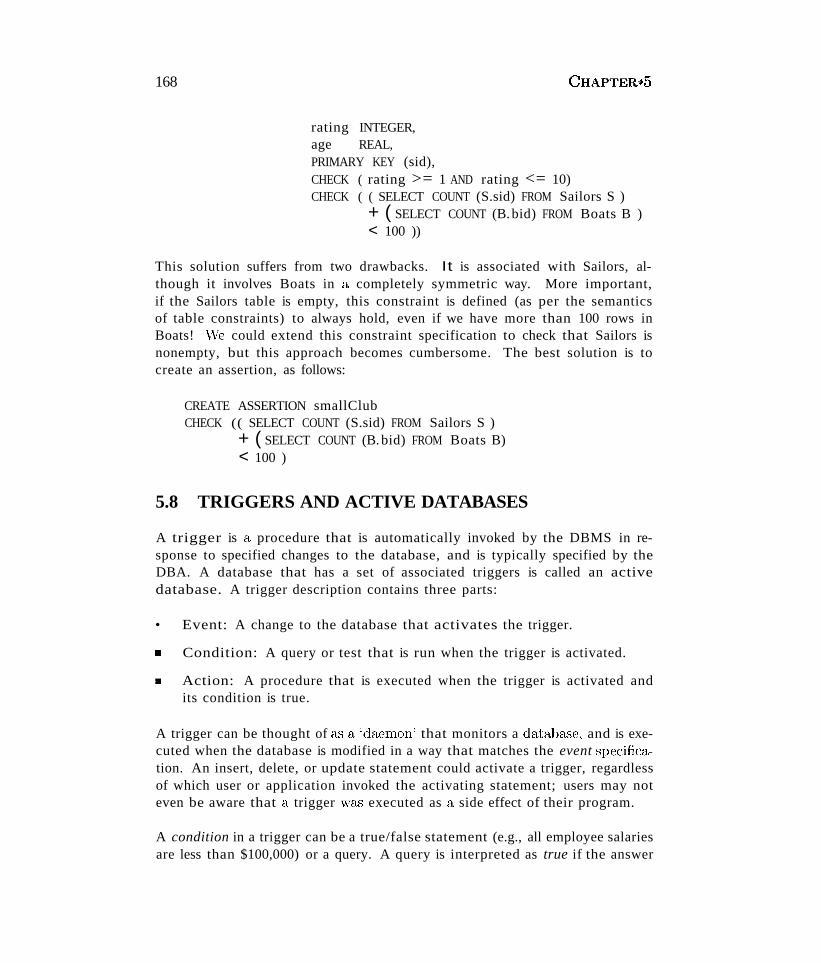
168 CHAPTER$5
rating INTEGER,age REAL,PRIMARY KEY (sid),CHECK ( rating >= 1 AND rating <= 10)CHECK ( ( SELECT COUNT (S.sid) FROM Sailors S )
+ ( SELECT COUNT (B. bid) FROM Boats B )< 100 ))
This solution suffers from two drawbacks. It is associated with Sailors, although it involves Boats in a completely symmetric way. More important,if the Sailors table is empty, this constraint is defined (as per the semanticsof table constraints) to always hold, even if we have more than 100 rows inBoats! vVe could extend this constraint specification to check that Sailors isnonempty, but this approach becomes cumbersome. The best solution is tocreate an assertion, as follows:
CREATE ASSERTION smallClubCHECK (( SELECT COUNT (S.sid) FROM Sailors S )
+ ( SELECT COUNT (B. bid) FROM Boats B)< 100 )
5.8 TRIGGERS AND ACTIVE DATABASES
A trigger is a procedure that is automatically invoked by the DBMS in response to specified changes to the database, and is typically specified by theDBA. A database that has a set of associated triggers is called an activedatabase. A trigger description contains three parts:
• Event: A change to the database that activates the trigger.
.. Condition: A query or test that is run when the trigger is activated.
.. Action: A procedure that is executed when the trigger is activated andits condition is true.
A trigger can be thought of as a 'daemon' that monitors a databa.se, and is executed when the database is modified in a way that matches the event specification. An insert, delete, or update statement could activate a trigger, regardlessof which user or application invoked the activating statement; users may noteven be aware that a trigger wa.'3 executed as a side effect of their program.
A condition in a trigger can be a true/false statement (e.g., all employee salariesare less than $100,000) or a query. A query is interpreted as true if the answer

SQL: Que'ries, Constrairds, TriggeTs It>9
set is nonempty and false if the query ha.') no answers. If the condition partevaluates to true, the action a.,sociated with the trigger is executed.
A trigger action can examine the answers to th(~ query in the condition partof the trigger, refer to old and new values of tuples modified by the statementactivating the trigger, execute Hew queries, and make changes to the database.In fact, an action can even execute a series of data-definition commands (e.g.,create new tables, change authorizations) and transaction-oriented commands(e.g., commit) or call host-language procedures.
An important issue is when the action part of a trigger executes in relation tothe statement that activated the trigger. For example, a statement that insertsrecords into the Students table may activate a trigger that is used to maintainstatistics on how many studen~s younger than 18 are inserted at a time by atypical insert statement. Depending on exactly what the trigger does, we maywant its action to execute before changes are made to the Students table orafterwards: A trigger that initializes a variable used to count the nurnber ofqualifying insertions should be executed before, and a trigger that executes onceper qualifying inserted record and increments the variable should be executedafter each record is inserted (because we may want to examine the values inthe new record to determine the action).
5.8.1 Examples of Triggers in SQL
The examples shown in Figure 5.20, written using Oracle Server syntax fordefining triggers, illustrate the basic concepts behind triggers. (The SQL:1999syntax for these triggers is similar; we will see an example using SQL:1999syntax shortly.) The trigger called iniLcount initializes a counter variable before every execution of an INSERT statement that adds tuples to the Studentsrelation. The trigger called incr_count increments the counter for each insertedtuple that satisfies the condition age < 18.
One of the example triggers in Figure 5.20 executes before the aetivating statement, and the other example executes after it. A trigger can also be scheduledto execute instead of the activating statement; or in deferred fashion, at theend of the transaction containing the activating statement; or in asynchronousfashion, as part of a separate transaction.
The example in Figure 5.20 illustrates another point about trigger execution:A user must be able to specify whether a trigger is to be executed once permodified record or once per activating statement. If the action depends on individual changed records, for example, we have to examine the age field of theinserted Students record to decide whether to increment the count, the trigger-
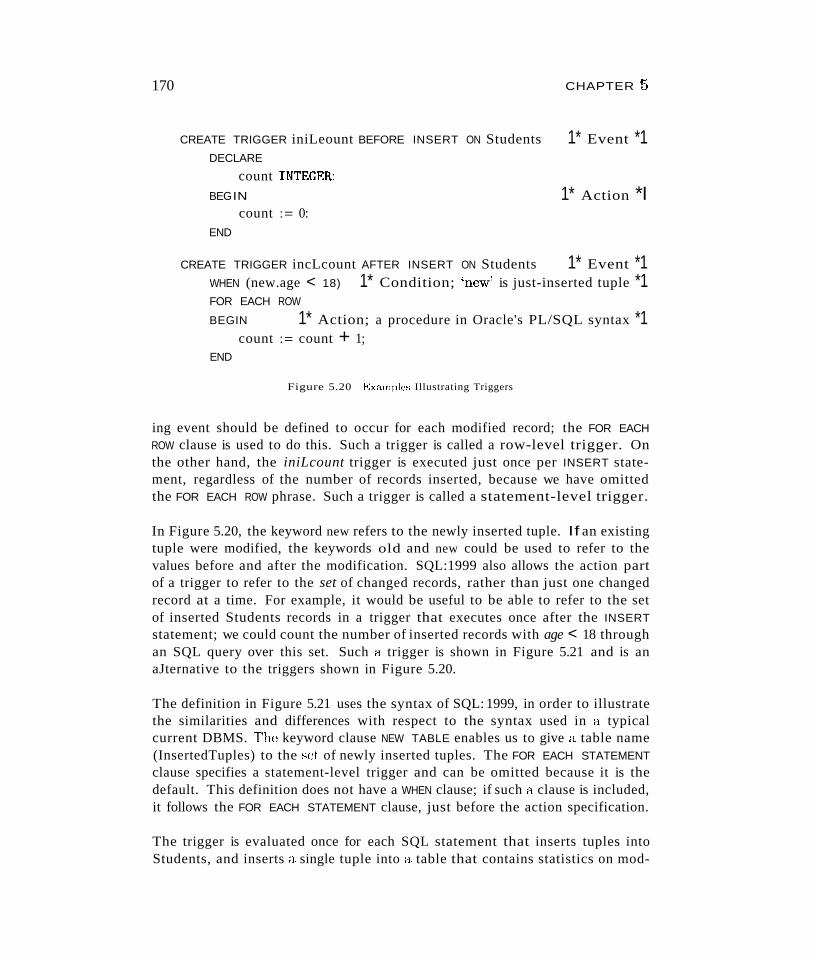
170 CHAPTER 5
CREATE TRIGGER iniLeount BEFORE INSERT ON Students 1* Event *1DECLARE
count INTEGER:
BEGIN 1* Action *Icount := 0:
END
CREATE TRIGGER incLcount AFTER INSERT ON Students 1* Event *1WHEN (new.age < 18) 1* Condition; 'new' is just-inserted tuple *1FOR EACH ROW
BEGIN 1* Action; a procedure in Oracle's PL/SQL syntax *1count := count + 1;
END
Figure 5.20 Examples Illustrating Triggers
ing event should be defined to occur for each modified record; the FOR EACH
ROW clause is used to do this. Such a trigger is called a row-level trigger. Onthe other hand, the iniLcount trigger is executed just once per INSERT statement, regardless of the number of records inserted, because we have omittedthe FOR EACH ROW phrase. Such a trigger is called a statement-level trigger.
In Figure 5.20, the keyword new refers to the newly inserted tuple. If an existingtuple were modified, the keywords old and new could be used to refer to thevalues before and after the modification. SQL:1999 also allows the action partof a trigger to refer to the set of changed records, rather than just one changedrecord at a time. For example, it would be useful to be able to refer to the setof inserted Students records in a trigger that executes once after the INSERT
statement; we could count the number of inserted records with age < 18 throughan SQL query over this set. Such a trigger is shown in Figure 5.21 and is anaJternative to the triggers shown in Figure 5.20.
The definition in Figure 5.21 uses the syntax of SQL: 1999, in order to illustratethe similarities and differences with respect to the syntax used in a typicalcurrent DBMS. The keyword clause NEW TABLE enables us to give a table name(InsertedTuples) to the set of newly inserted tuples. The FOR EACH STATEMENT
clause specifies a statement-level trigger and can be omitted because it is thedefault. This definition does not have a WHEN clause; if such a clause is included,it follows the FOR EACH STATEMENT clause, just before the action specification.
The trigger is evaluated once for each SQL statement that inserts tuples intoStudents, and inserts a single tuple into a table that contains statistics on mod-
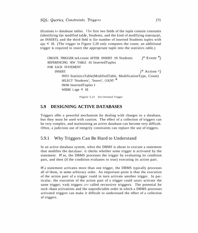
S(JL: (JneTie,s, Constraints, Triggers 171
ifications to database tables. The first two fields of the tuple contain constants(identifying the modified table, Students, and the kind of modifying statement,an INSERT), and the third field is the number of inserted Students tuples withage < 18. (The trigger in Figure 5.20 only computes the count; an additionaltrigger is required to insert the appropriate tuple into the statistics table.)
CREATE TRIGGER seLcount AFTER INSERT ON Students j* Event *jREFERENCING NEW TABLE AS InsertedTuplesFOR EACH STATEMENT
INSERT j* Action * jINTO StatisticsTable(ModifiedTable, ModificationType, Count)SELECT 'Students', 'Insert', COUNT *FROM InsertedTuples IWHERE 1.age < 18
Figure 5.21 Set-Oriented Trigger
5.9 DESIGNING ACTIVE DATABASES
Triggers offer a powerful mechanism for dealing with changes to a database,but they must be used with caution. The effect of a collection of triggers canbe very complex, and maintaining an active database can become very difficult.Often, a judicious use of integrity constraints can replace the use of triggers.
5.9.1 Why Triggers Can Be Hard to Understand
In an active database system, when the DBMS is about to execute a statementthat modifies the databa.se, it checks whether some trigger is activated by thestatement. If so, the DBMS processes the trigger by evaluating its conditionpart, and then (if the condition evaluates to true) executing its action part.
If a statement activates more than one trigger, the DBMS typically processesall of them, in senne arbitrary order. An important point is that the executionof the action part of a trigger could in turn activate another trigger. In particular, the execution of the action part of a trigger could a,gain activate thesarne trigger; such triggers "u'e called recursive triggers. The potential forsuch chain activations and the unpredictable order in which a DBMS processesactivated triggers can make it difficult to understand the effect of a collectionof triggers.
172 CHAPTER'5
5.9.2 Constraints versus Triggers
A common use of triggers is to maintain databa..'3e consistency, and in suchcases, we should always consider whether using an integrity constraint (e.g., aforeign key constraint) achieves the same goals. The meaning of a constraint isnot defined operationally, unlike the effect of a trigger. This property makes aconstraint easier to understand, and also gives the DBMS more opportunitiesto optimize execution. A constraint also prevents the data from being madeinconsistent by any kind of statement, whereas a trigger is activated by a specifickind of statement (INSERT, DELETE, or UPDATE). Again, this restriction makesa constraint easier to understand.
On the other hand, triggers allow us to maintain database integrity in moreflexible ways, as the following examples illustrate.
• Suppose that we have a table called Orders with fields iternid, quantity,custornerid, and unitprice. When a customer places an order, the firstthree field values are filled in by the user (in this example, a sales clerk).The fourth field's value can be obtained from a table called Items, but itis important to include it in the Orders table to have a complete record ofthe order, in case the price of the item is subsequently changed. We candefine a trigger to look up this value and include it in the fourth field ofa newly inserted record. In addition to reducing the number of fields thatthe clerk h&'3 to type in, this trigger eliminates the possibility of an entryerror leading to an inconsistent price in the Orders table.
• Continuing with this example, we may want to perform some additionalactions when an order is received. For example, if the purchase is beingcharged to a credit line issued by the company, we may want to checkwhether the total cost of the purch&'3e is within the current credit limit.We can use a trigger to do the check; indeed, we can even use a CHECKconstraint. Using a trigger, however, allows us to implement more sophisticated policies for dealing with purchases that exceed a credit limit. Forinstance, we may allow purchases that exceed the limit by no more than10% if the customer has dealt with the company for at least a year, andadd the customer to a table of candidates for credit limit increases.
5.9.3 Other Uses of Triggers
.l\'Iany potential uses of triggers go beyond integrity maintenance. Triggers canalert users to unusual events (&'3 reflected in updates to the databa..<;e). Forexample, we may want to check whether a customer placing an order h&s madeenough purchases in the past month to qualify for an additional discount; ifso, the sales clerk must be informed so that he (or she) can tell the customer
SQL: Q'UeT'Ze,S, CO'l/stmints, Tr'iggers
and possibly generate additional sales! \Ve can rela;y this information by usinga trigger that checks recent purcha.ses and prints a message if the customerqualifies for the discount.
Triggers can generate a log of events to support auditing and security checks.For example, each time a customer places an order, we can create a record withthe customer's ID and current credit limit and insert this record in a customerhistory table. Subsequent analysis of this table might suggest candidates foran increased credit limit (e.g., customers who have never failed to pay a bill ontime and who have come within 10% of their credit limit at least three timesin the last month).
As the examples in Section 5.8 illustrate, we can use triggers to gather statisticson table accesses and modifications. Some database systems even use triggersinternally as the basis for managing replicas of relations (Section 22.11.1). Ourlist of potential uses of triggers is not exhaustive; for example, triggers havealso been considered for workflow management and enforcing business rules.
5.10 REVIEW QUESTIONS
Answers to the review questions can be found in the listed sections.
• What are the parts of a basic SQL query? Are the input and result tablesof an SQL query sets or multisets? How can you obtain a set of tuples asthe result of a query? (Section 5.2)
• What are range variables in SQL? How can you give names to outputcolumns in a query that are defined by arithmetic or string expressions?What support does SQL offer for string pattern matching? (Section 5.2)
• What operations does SQL provide over (multi)sets of tuples, and howwould you use these in writing queries? (Section 5.3)
• vVhat are nested queries? What is correlation in nested queries? Howwould you use the operators IN, EXISTS, UNIQUE, ANY, and ALL in writingnested queries? Why are they useful? Illustrate your answer by showinghow to write the division operator in SQL. (Section 5.4)
• \Vhat aggregate operators does SQL support? (Section 5.5)
• \i\That is gmvping? Is there a counterpart in relational algebra? Explainthis feature, and discllss the interaction of the HAVING and WHERE clauses.Mention any restrictions that mllst be satisfied by the fields that appear inthe GROUP BY clause. (Section 5.5.1)
174 CHAPTER?5
• \Vhat are null values? Are they supported in the relational model, &'3
described in Chapter 3'1 Hc)\v do they affect the meaning of queries? Canprimary key fields of a table contain null values? (Section 5.6)
• vVhat types of SQL constraints can be specified using the query language?Can you express primary key constraints using one of these new kindsof constraints? If so, why does SQL provide for a separate primary keyconstraint syntax? (Section 5.7)
• What is a trigger, and what are its three parts? vVhat are the differencesbetween row-level and statement-level triggers? (Section 5.8)
• \Vhy can triggers be hard to understand? Explain the differences betweentriggers and integrity constraints, and describe when you would use triggers over integrity constrains and vice versa. What are triggers used for?(Section 5.9)
EXERCISES
Online material is available for all exercises in this chapter on the book's webpage at
http://www.cs.wisc.edu/-dbbOok
This includes scripts to create tables for each exercise for use with Oracle, IBM DB2, MicrosoftSQL Server, and MySQL.
Exercise 5.1 Consider the following relations:
Student(snum: integer, sname: string, major: string, level: string, age: integer)Class( name: string, meets_at: time, room: string, fid: integer)Enrolled(snum: integer, cname: string)Faculty (fid: integer, fnarne: string, deptid: integer)
The meaning of these relations is straightforward; for example, Enrolled has one record perstudent-class pair such that the student is enrolled in the class.
Write the following queries in SQL. No duplicates should be printed in any of the ans\vers.
1. Find the nari1es of all Juniors (level = JR) who are enrolled in a class taught by 1. Teach.
2. Find the age of the oldest student who is either a History major or enrolled in a coursetaught by I. Teach.
:3. Find the names of all classes that either meet in room R128 or have five or more studentsenrolled.
4. Find the Ilames of all students who are enrolled in two classes that meet at the sametime.
SCJL: Queries, ConstrainLsl Triggers 175t
5. Find the names of faculty members \vho teach in every room in which some class istaught.
6. Find the names of faculty members for \vhorn the combined enrollment of the coursesthat they teach is less than five.
7. Print the level and the average age of students for that level, for each level.
8. Print the level and the average age of students for that level, for all levels except JR.
9. For each faculty member that has taught classes only in room R128, print the facultymember's name and the total number of classes she or he has taught.
10. Find the names of students enrolled in the maximum number of classes.
11. Find the names of students not enrolled in any class.
12. For each age value that appears in Students, find the level value that appears most often.For example, if there are more FR level students aged 18 than SR, JR, or SO studentsaged 18, you should print the pair (18, FR).
Exercise 5.2 Consider the following schema:
Suppliers( sid: integer, sname: string, address: string)
Parts(pid: integer, pname: string, color: string)
Catalog( sid: integer, pid: integer, cost: real)
The Catalog relation lists the prices charged for parts by Suppliers. Write the followingqueries in SQL:
1. Find the pnames of parts for which there is some supplier.
2. Find the snames of suppliers who supply every part.
3. Find the snames of suppliers who supply every red part.
4. Find the pnamcs of parts supplied by Acme Widget Suppliers and no one else.
5. Find the sids of suppliers who charge more for some part than the average cost of thatpart (averaged over all the suppliers who supply that part).
6. For each part, find the sname of the supplier who charges the most for that part.
7. Find the sids of suppliers who supply only red parts.
8. Find the sids of suppliers who supply a red part anel a green part.
9. Find the sirl'i of suppliers who supply a red part or a green part.
10. For every supplier that only supplies green parts, print the name of the supplier and thetotal number of parts that she supplies.
11. For every supplier that supplies a green part and a reel part, print the name and priceof the most expensive part that she supplies.
Exercise 5.3 The following relations keep track of airline flight information:
Flights(.flno: integer, from: string, to: string, di8tance: integer,
rlepa7'i:s: time, a'T'l~ivcs: time, Tn~ice: integer)Aircraft( aid: integer, aname: string, cTllisingT'ange: integer)
Certified( eid: integer, aid: integer)
Employees( eid: integer I ename: string, salary: integer)
176 CHAPTE&5
Note that the Employees relation describes pilots and other kinds of employees as well; everypilot is certified for some aircraft, and only pilots are certified to fly. Write each of thefollO\ving queries in SQL. (Additional queries using the same schema are listed in the exereisesfoT' Chapter 4·)
1. Find the names of aircraft such that all pilots certified to operate them earn more than$80,000.
2. For each pilot who is certified for more than three aircraft, find the eid and the maximumcruisingmnge of the aircraft for which she or he is certified.
3. Find the names of pilots whose salary is less than the price of the cheapest route fromLos Angeles to Honolulu.
4. For all aircraft with cmisingmnge over 1000 miles, find the name of the aircraft and theaverage salary of all pilots certified for this aircraft.
5. Find the names of pilots certified for some Boeing aircraft.
6. Find the aids of all aircraft that can be used on routes from Los Angeles to Chicago.
7. Identify the routes that can be piloted by every pilot who makes more than $100,000.
8. Print the enames of pilots who can operate planes with cruisingmnge greater than 3000miles but are not certified on any Boeing aircraft.
9. A customer wants to travel from Madison to New York with no more than two changesof flight. List the choice of departure times from Madison if the customer wants to arrivein New York by 6 p.m.
10. Compute the difference between the average salary of a pilot and the average salary ofall employees (including pilots).
11. Print the name and salary of every nonpilot whose salary is more than the average salaryfor pilots.
12. Print the names of employees who are certified only on aircrafts with cruising rangelonger than 1000 miles.
13. Print the names of employees who are certified only on aircrafts with cruising rangelonger than 1000 miles, but on at least two such aircrafts.
14. Print the names of employees who are certified only on aircrafts with cruising rangelonger than 1000 miles and who are certified on some Boeing aircraft.
Exercise 5.4 Consider the following relational schema. An employee can work in more thanone department; the pcLtime field of the Works relation shows the percentage of time that agiven employee works in a given department.
Emp(eid: integer, ename: string, age: integer, salary: real)
Works(eid: integer, did: integer, pet_time: integer)
Dept(did.· integer, budget: real, managerid: integer)
Write the following queries in SQL:
1. Print the names and ages of each employee who works in both the Hardware departmentand the Software department.
2. For each department with more than 20 full-time-equivalent employees (i.e., where thepart~time and full-time employees add up to at least that many full-time employees),print the did together with the number of employees that work in that department.
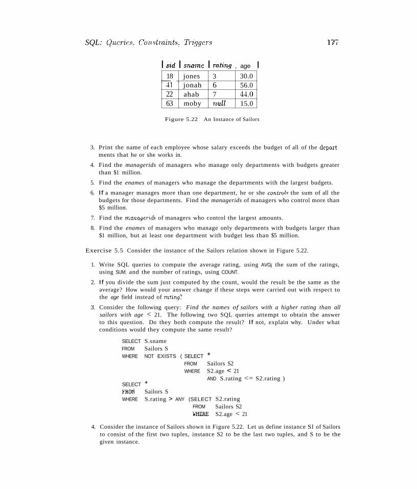
SQL: quehes, ConstTaint.s, Triggers 117
, ,
18 jones 3 30.0~- -
jonah 6 56.04122 ahab 7 44.063 moby 'mdl 15.0
I s'id I sname I mting , age I
Figure 5.22 An Instance of Sailors
3. Print the name of each employee whose salary exceeds the budget of all of the departments that he or she works in.
4. Find the managerids of managers who manage only departments with budgets greaterthan $1 million.
5. Find the enames of managers who manage the departments with the largest budgets.
6. If a manager manages more than one department, he or she controls the sum of all thebudgets for those departments. Find the managerids of managers who control more than$5 million.
7. Find the managerids of managers who control the largest amounts.
8. Find the enames of managers who manage only departments with budgets larger than$1 million, but at least one department with budget less than $5 million.
Exercise 5.5 Consider the instance of the Sailors relation shown in Figure 5.22.
1. Write SQL queries to compute the average rating, using AVGj the sum of the ratings,using SUM; and the number of ratings, using COUNT.
2. If you divide the sum just computed by the count, would the result be the same as theaverage? How would your answer change if these steps were carried out with respect tothe age field instead of mting?
~3. Consider the following query: Find the names of sailors with a higher rating than allsailors with age < 21. The following two SQL queries attempt to obtain the answerto this question. Do they both compute the result? If not, explain why. Under whatconditions would they compute the same result?
S2.ratingSailors S2S2.age < 21
SELECT *FROM Sailors SWHERE S.rating > ANY (SELECT
FROM\-/HERE
SELECT S.snameFROM Sailors SWHERE NOT EXISTS ( SELECT *
FROM Sailors S2WHERE S2.age < 21
AND S.rating <= S2.rating )
4. Consider the instance of Sailors shown in Figure 5.22. Let us define instance Sl of Sailorsto consist of the first two tuples, instance S2 to be the last two tuples, and S to be thegiven instance.
178 CHAPTER'5
Show the left outer join of S with itself, with the join condition being 8'id=sid.
(b) Show the right outer join of S ,vith itself, with the join condition being s'id=sid.
(c) Show the full outer join of S with itself, with the join condition being S'id=sid.
(d) Show the left outer join of Sl with S2, with the join condition being sid=sid.
(e) Show the right outer join of Sl with S2, with the join condition being sid=sid.
(f) Show the full outer join of 81 with S2, with the join condition being sid=sid.
Exercise 5.6 Answer the following questions:
1. Explain the term 'impedance mismatch in the context of embedding SQL commands in ahost language such as C.
2. How can the value of a host language variable be passed to an embedded SQL command?
3. Explain the WHENEVER command's use in error and exception handling.
4. Explain the need for cursors.
5. Give an example of a situation that calls for the use of embedded SQL; that is, interactiveuse of SQL commands is not enough, and some host lang;uage capabilities are needed.
6. Write a C program with embedded SQL commands to address your example in theprevious answer.
7. Write a C program with embedded SQL commands to find the standard deviation ofsailors' ages.
8. Extend the previous program to find all sailors whose age is within one standard deviationof the average age of all sailors.
9. Explain how you would write a C program to compute the transitive closure of a graph,represented as an 8QL relation Edges(jrom, to), using embedded SQL commands. (Youneed not write the program, just explain the main points to be dealt with.)
10. Explain the following terms with respect to cursors: 'tlpdatability, sens,itivity, and scmllability.
11. Define a cursor on the Sailors relation that is updatable, scrollable, and returns answerssorted by age. Which fields of Sailors can such a cursor not update? Why?
12. Give an example of a situation that calls for dynamic 8QL; that is, even embedded SQLis not sufficient.
Exercise 5.7 Consider the following relational schema and briefly answer the questions thatfollow:
Emp( eid: integer, cname: string, age: integer, salary: real)\Vorks( eid: integer, did: integer, pet-time: integer)Dept( did.' integer, budget: re~l, managerid: integer)
1. Define a table constraint on Emp that will ensure that ever)' employee makes at leELst$10,000.
2. Define a table constraint on Dept that will ensure that all managers have age> ;'W.
:3. Define an assertion on Dept that will ensure that all managers have age> 30. Comparethis assertion with the equivalent table constraint. Explain which is better.
SQL: (JwTies, Const7nint.s, Triggers 119
4. vVrite SQL statements to delete all information about employees whose salaries exceedthat of the manager of one or more departments that they work in. Be sure to ensurethat all the relevant integrity constraints are satisfied after your updates.
Exercise 5.8 Consider the following relations:
Student (sn'llrn: integer, sname: string, rnajor: string,
level: string, age: integer)Class(narne: string, rneets_at: time, roorn: string, fid: integer)
Enrolled (snurn: integer, cnarne: string)
Faculty (fid: integer, fnarne: string, deptid: integer)
The meaning of these relations is straightforward; for example, Enrolled has one record perstudent-class pair such that the student is enrolled in the class.
1. Write the SQL statements required to create these relations, including appropriate versions of all primary and foreign key integrity constraints.
2. Express each of the following integrity constraints in SQL unless it is implied by theprimary and foreign key constraint; if so, explain how it is implied. If the constraintcannot be expressed in SQL, say so. For each constraint, state what operations (inserts,deletes, and updates on specific relations) must be monitored to enforce the constraint.
(a) Every class has a minimum enrollment of 5 students and a maximum enrollmentof 30 students.
(b) At least one dass meets in each room.
(c) Every faculty member must teach at least two courses.
(d) Only faculty in the department with deptid=33 teach more than three courses.
(e) Every student must be enrolled in the course called lVlathlOl.
(f) The room in which the earliest scheduled class (i.e., the class with the smallestnucets_at value) meets should not be the same as the room in which the latestscheduled class meets.
(g) Two classes cannot meet in the same room at the same time.
(h) The department with the most faculty members must have fewer than twice thenumber of faculty members in the department with the fewest faculty members.
(i) No department can have more than 10 faculty members.
(j) A student cannot add more than two courses at a time (i.e., in a single update).
(k) The number of CS majors must be more than the number of Math majors.
(I) The number of distinct courses in which CS majors are enrolled is greater than thenumber of distinct courses in which Math majors are enrolled.
(rn) The total enrollment in courses taught by faculty in the department with deptid=SSis greater than the number of ivlath majors.
(n) There lIlUst be at least one CS major if there are any students whatsoever.
(0) Faculty members from different departments cannot teach in the same room.
Exercise 5.9 Discuss the strengths and weaknesses of the trigger mechanism. Contrasttriggers with other integrity constraints supported by SQL.

180
Exercise 5.10 Consider the following relational schema. An employee can work in morethan one department; the pel-time field of the \Vorks relation shows the percentage of timethat a given employee works in a given department.
Emp( eid: integer, ename: string, age: integer, salary: real)
\Vorks( eid: integer, did: integer, pcLtime: integer)
Dept( did: integer, budget: real, mana,gerid: integer)
\Vrite SQL-92 integrity constraints (domain, key, foreign key, or CHECK constraints; or asser··bons) or SQL:1999 triggers to ensure each of the following requirements, considered independently.
1. Employees must make a minimum salary of $1000.
2. Every manager must be also be an employee.
3. The total percentage of aU appointments for an employee must be under 100%.
4. A manager must always have a higher salary than any employee that he or she manages.
5. Whenever an employee is given a raise, the manager's salary must be increased to be atleast as much.
6. Whenever an employee is given a raise, the manager's salary must be increased to beat least as much. Further, whenever an employee is given a raise, the department'sbudget must be increased to be greater than the sum of salaries of aU employees in thedepartment.
PROJECT-BASED EXERCISE
Exercise 5.11 Identify the subset of SQL queries that are supported in Minibase.
BIBLIOGRAPHIC NOTES
The original version of SQL was developed as the query language for IBM's System R project,and its early development can be traced in [107, 151]. SQL has since become the mostwidely used relational query language, and its development is now subject to an internationalstandardization process.
A very readable and comprehensive treatment of SQL-92 is presented by Melton and Simonin [524], and the central features of SQL:1999 are covered in [525]. We refer readers to thesetwo books for an authoritative treatment of SQL. A short survey of the SQL:1999 standardis presented in [237]. Date offers an insightful critique of SQL in [202]. Although some ofthe problems have been addressed in SQL-92 and later revisions, others remain. A formalsemantics for a large subset ofSQL queries is presented in [560]. SQL:1999 is the current International Organization for Standardization (ISO) and American National Standards Institute(ANSI) standard. Melton is the editor of the ANSI and ISO SQL:1999 standard, documentANSI/ISO/IEe 9075-:1999. The corresponding ISO document is ISO/lEe 9075-:1999. Asuccessor, planned for 2003, builds on SQL:1999 SQL:200:3 is close to ratification (a.s of June20(2). Drafts of the SQL:200:3 deliberations are available at the following URL:
ftp://sqlstandards.org/SC32/
SqL: queries, COll./:!tTo/inLs, Triggers lSI
[774] contains a collection of papers that cover the active database field. [794J includes agood in-depth introduction to active rules, covering smnantics, applications and design issues.[251] discusses SQL extensions for specifying integrity constraint checks through triggers.[123] also discusses a procedural mechanism, called an alerter, for monitoring a database.[185] is a recent paper that suggests how triggers might be incorporated into SQL extensions.Influential active database prototypes include Ariel [366], HiPAC [516J, ODE [18], Postgres[722], RDL [690], and Sentinel [36]. [147] compares various architectures for active databasesystems.
[32] considers conditions under which a collection of active rules has the same behavior,independent of evaluation order. Semantics of active databases is also studied in [285] and[792]. Designing and managing complex rule systems is discussed in [60, 225]. [142] discussesrule management using Chimera, a data model and language for active database systems.

1
1
1
1
1
1
1
1
1
1
1
1
1
1
1
1
1
1
1
1
1
1
1
1
1
1
1
1
1
1

PART II
APPLICATION DEVELOPMENT

6DATABASE APPLICATION
DEVELOPMENT
.. How do application programs connect to a DBMS?
.. How can applications manipulate data retrieved from a DBMS?
.. How can applications modify data in a DBMS?
.. What are cursors?
.. What is JDBC and how is it used?
.. What is SQLJ and how is it used?
.. What are stored procedures?
.. Key concepts: Embedded SQL, Dynamic SQL, cursors; JDBC,connections, drivers, ResultSets, java.sql, SQLJ; stored procedures,SQL/PSM
Hf~ profits most who serves best.
------Ivlotto for Rotary International
In Chapter 5, we looked at a wide range of SQL query constructs, treating SQLas an independent language in its own right. A relational DBMS supports aninteuLctive SqL interface, and users can directly enter SQL commands. Thissimple approach is fine as long as the task at hand can be accomplished entirelywith SQL cormnands. In practice, we often encounter situations in which weneed the greater flexibility of a general-purpose programming language in addition to the data manipulation facilities provided by SQL. For example, we rnaywant to integrate a database application with a nice graphical user interface,or we may want to integrate with other existing applications.
185
186 CHAPTEFt 6J
Applications that rely on the DBMS to manage data run as separate processesthat connect to the DBlvIS to interact with it. Once a connection is established,SQL commands can be used to insert, delete, and modify data. SQL queries canbe used to retrieve desired data. but we need to bridge an important differencein how a database system sees data and how an application program in alanguage like Java or C sees data: The result of a database query is a set (ormultiset) or records, hut Java has no set or multiset data type. This mismatchis resolved through additional SQL constructs that allow applications to obtaina handle on a collection and iterate over the records one at a time.
vVe introduce Embedded SQL, Dynamic SQL, and cursors in Section 6.1. Embedded SQL allows us to access data using static SQL queries in applicationcode (Section 6.1.1); with Dynamic SQL, we can create the queries at run-time(Section 6.1.3). Cursors bridge the gap between set-valued query answers andprogramming languages that do not support set-values (Section 6.1.2).
The emergence of Java as a popular application development language, especially for Internet applications, has made accessing a DBMS from Java code aparticularly important topic. Section 6.2 covers JDBC, a prograruming interface that allows us to execute SQL queries from a Java program and use theresults in the Java program. JDBC provides greater portability than Embedded SQL or Dynamic SQL, and offers the ability to connect to several DBMSswithout recompiling the code. Section 6.4 covers SQLJ, which does the samefor static SQL queries, but is easier to program in than Java, with JDBC.
Often, it is useful to execute application code at the database server, rather thanjust retrieve data and execute application logic in a separate process. Section6.5 covers stored procedures, which enable application logic to be stored andexecuted at the databa"se server. We conclude the chapter by discussing ourB&N case study in Section 6.6.
'Vhile writing database applications, we must also keep in mind that typicallymany application programs run concurrently. The transaction concept, introduced in Chapter 1, is used to encapsulate the effects of an application onthe datahase. An application can select certain transaction properties throughSQL cormnands to control the degree to which it is exposed to the changes ofother concurrently running applications. \Ve touch on the transaction conceptat many points i,n this chapter, and, in particular, cover transaction-related ~hS
pects of JDBC. A full discussion of transaction properties and SQL's supportfor transactions is deferred until Chapter 16.
Examples that appear in this chapter are available online at
http://www.cs.wisc.edu/-dbbook
Database Application DeveloplTu:nt
6.1 ACCESSING DATABASES FROlVl APPLICATIONS
187
In this section, we cover how SQL commands can be executed from within aprogram in a host language such as C or Java. The use of SQL commandswithin a host language program is called Embedded SQL. Details of Embed~ded SQL also depend on the host language. Although similar capabilities aresupported for a variety of host languages, the syntax sometimes varies.
vVe first cover the basics of Embedded SQL with static SQL queries in Section6.1.1. We then introduce cursors in Section 6.1.2. vVe discuss Dynamic SQL,which allows us to construct SQL queries at runtime (and execute them) inSection 6.1.:3.
6.1.1 Embedded SQL
Conceptually, embedding SQL commands in a host language program is straightforward. SQL statements (i.e., not declarations) can be used wherever a statement in the host language is allowed (with a few restrictions). SQL statementsmust be clearly marked so that a preprocessor can deal with them before invoking the compiler for the host language. Also, any host language variablesused to pass arguments into an SQL command must be declared in SQL. Inparticular, some special host language variables must be declared in SQL (sothat, for example, any error conditions arising during SQL execution can becommunicated back to the main application program in the host language).
There are, however, two complications to bear in mind. First, the data typesrecognized by SQL may not be recognized by the host language and vice versa.This mismatch is typically addressed by casting data values appropriately before passing them to or frorn SQL commands. (SQL, like other programminglanguages, provides an operator to cast values of aIle type into values of another type.) The second complication h~s to do with SQL being set-oriented,and is addressed using cursors (see Section 6.1.2. Commands operate on andproduce tables, which are sets
In our discussion of Embedded SQL, w(~ assmne thi'Lt the host language is Cfor concretenc~ss. because minor differcnces exist in how SQL statements areembedded in differcnt host languages.
Declaring Variables and Exceptions
SQL statements can refer to variables defined in the host program. Such hostlanguage variables must be prefixed by a colon (:) in SQL statements and bedeclared between the commands EXEC SQL BEGIN DECLARE SECTION and EXEC
188 CHAPTER 6~
SQL END DECLARE SECTION. The declarations are similar to how they wouldlook in a C program and, as usual in C. are separated by semicolons. Forexample. we can declare variables c-sname, c_sid, c_mt'ing, and cage (with theinitial c used as a naming convention to emphasize that these are host languagevariables) as follows:
EXEC SQL BEGIN DECLARE SECTIONchar c_sname[20];long csid;short crating;float cage;EXEC SQL END DECLARE SECTION
The first question that arises is which SQL types correspond to the variousC types, since we have just declared a collection of C variables whose values are intended to be read (and possibly set) in an SQL run-time environment when an SQL statement that refers to them is executed. The SQL-92standard defines such a correspondence between the host language types andSQL types for a number of host languages. In our example, c_snamc has thetype CHARACTER(20) when referred to in an SQL statement, csid has the typeINTEGER, crating has the type SMALLINT, and cage has the type REAL.
\Ve also need some way for SQL to report what went wrong if an error conditionarises when executing an SQL statement. The SQL-92 standard recognizestwo special variables for reporting errors, SQLCODE and SQLSTATE. SQLCODE isthe older of the two and is defined to return some negative value when anerror condition arises, without specifying further just what error a particularnegative integer denotes. SQLSTATE, introduced in the SQL-92 standard for thefirst time, &':lsociates predefined values with several common error conditions,thereby introducing some uniformity to how errors are reported. One of thesetwo variables must be declared. The appropriate C type for SQLCODE is longand the appropriate C type for SQLSTATE is char [6J , that is, a character stringfive characters long. (Recall the null-terminator in C strings.) In this chapter,we assume that SQLSTATE is declared.
Embedding SQL Statements
All SQL staternents embedded within a host program must be clearly marked,with the details dependent on the host language; in C, SQL statements must beprefixed by EXEC SQL. An SQL statement can essentially appear in any placein the host language program where a host language statement can appear.
Database Application DC?lelopment 189
As a simple example, the following Embedded' SQL statement inserts a row,whose column values me based on the values of the host language variablescontained in it, into the Sailors relation:
EXEC SQLINSERT INTO Sailors VALUES (:c_sname, :csid, :crating, :cage);
Observe that a semicolon terminates the command, as per the convention forterminating statements in C.
The SQLSTATE variable should be checked for errors and exceptions after eachEmbedded SQL statement. SQL provides the WHENEVER command to simplifythis tedious task:
EXEC SQL WHENEVER [SQLERROR I NOT FOUND] [ CONTINUE I GOTO st'mt ]
The intent is that the value of SQLSTATE should be checked after each EmbeddedSQL statement is executed. If SQLERROR is specified and the value of SQLSTATEindicates an exception, control is transferred to stmt, which is presumably responsible for error and exception handling. Control is also transferred to stmtif NOT FOUND is specified and the value of SQLSTATE is 02000, which denotes NODATA.
6.1.2 Cursors
A major problem in embedding SQL statements in a host language like C isthat an impedance mismatch occurs because SQL operates on set" of records,whereas languages like C do not cleanly support a set-of-records abstraction.The solution is to essentially provide a mechanism that allows us to retrieverows one at a time from a relation.
This mechanism is called a cursor. vVe can declare a cursor on any relationor on any SQL query (because every query returns a set of rows). Once acurwr is declared, we can open it (which positions the cursor just before thefirst row); fetch the next row; move the cursor (to the next row, to the rowafter the next n, to the first row, or to the previous row, etc., by specifyingadditional parameters for the FETCH command); or close the cursor. Thus, acursor essentially allows us to retrieve the rows in a table by positioning thecursor at a particular row and reading its contents.
Basic Cursor Definition and Usage
r'11rsors enable us to examine, in the host language program, a collection ofJWS computed by an Embedded SQL statement:
190 CHAPTEl} 6
.. \Ve usually need to open a cursor if the embedded statement is a SELECT(i.e.) a query). However, we can avoid opening a cursor if the answercontains a single row, as we see shortly.
.. INSERT, DELETE, and UPDATE staternents typically require no cursor, although some variants of DELETE and UPDATE use a cursor.
As an example, we can find the name and age of a sailor, specified by assigninga value to the host variable c~sir1, declared earlier, as follows:
EXEC SQL SELECTINTOFROMWHERE
S.sname, S.age:c_sname, :c_ageSailors SS.sid = :c_sid;
The INTO clause allows us to assign the columns of the single answer row tothe host variables csname and c_age. Therefore, we do not need a cursor toembed this query in a host language program. But what about the followingquery, which computes the names and ages of all sailors with a rating greaterthan the current value of the host variable cminmting?
SELECT S.sname, S.ageFROM Sailors SWHERE S.rating > :c_minrating
This query returns a collection of rows, not just one row. 'When executedinteractively, the answers are printed on the screen. If we embed this query ina C program by prefixing the cOlnmand with EXEC SQL, how can the answersbe bound to host language variables? The INTO clause is inadequate becausewe must deal with several rows. The solution is to use a cursor:
DECLARE sinfo CURSOR FORSELECT S.sname, S.ageFROM Sailors SWHERE S.rating > :c_minrating;
This code can be included in a C program, and once it is executed, the cursor8ir~lo is defined. Subsequently, we can open the cursor:
OPEN sinfo:
The value of cminmting in the SQL query associated with the cursor is thevalue of this variable when we open the cursor. (The cursor declaration isprocessed at compile-time, and the OPEN command is executed at run-time.)
Database Applicat'ion Development 191,
A cursor can be thought of as 'pointing' to a row in the collection of answersto the query associated with it. vVhen a cursor is opened, it is positioned justbefore the first row. \Ve can use the FETCH command to read the first row ofcursor sinfo into host language variables:
FETCH sinfo INTO :csname, :cage;
When the FETCH statement is executed, the cursor is positioned to point atthe next row (which is the first row in the table when FETCH is executed forthe first time after opening the cursor) and the column values in the row arecopied into the corresponding host variables. By repeatedly executing thisFETCH statement (say, in a while-loop in the C program), we can read all therows computed by the query, one row at a time. Additional parameters to theFETCH command allow us to position a cursor in very flexible ways, but we donot discuss them.
How do we know when we have looked at all the rows associated with thecursor? By looking at the special variables SQLCODE or SQLSTATE, of course.SQLSTATE, for example, is set to the value 02000, which denotes NO DATA, toindicate that there are no more rows if the FETCH statement positions the cursorafter the last row.
When we are done with a cursor, we can close it:
CLOSE sinfo;
It can be opened again if needed, and the value of : cminrating in theSQL query associated with the cursor would be the value of the host variablecminrating at that time.
Properties of Cursors
The general form of a cursor declaration is:
DECLARE cursomame [INSENSITIVE] [SCROLL] CURSOR[WITH HOLD]FOR some query[ ORDER BY order-item-list ][ FOR READ ONLY I FOR UPDATE ]
A cursor can be declared to be a read-only cursor (FOR READ ONLY) or, ifit is a cursor on a base relation or an updatable view, to be an updatablecursor (FOR UPDATE). If it is IIpdatable, simple variants of the UPDATE and
192 CHAPTER 6il'
DELETE commands allow us to update or delete the row on which the cursoris positioned. For example, if sinfa is an updatable cursor and open, we canexecute the following statement:
UPDATE Sailors SSET S.rating = S.rating ~ 1WHERE CURRENT of sinfo;
This Embedded SQL statement modifies the rating value of the row currentlypointed to by cursor sinfa; similarly, we can delete this row by executing thenext statement:
DELETE Sailors SWHERE CURRENT of sinfo;
A cursor is updatable by default unless it is a scrollable or insensitive cursor(see below), in which case it is read-only by default.
If the keyword SCROLL is specified, the cursor is scrollable, which means thatvariants of the FETCH command can be used to position the cursor in veryflexible ways; otherwise, only the basic FETCH command, which retrieves thenext row, is allowed.
If the keyword INSENSITIVE is specified, the cursor behaves as if it is rangingover a private copy of the collection of answer rows. Otherwise, and by default,other actions of some transaction could modify these rows, creating unpredictable behavior. For example, while we are fetching rows using the sinfacursor, we might modify rating values in Sailor rows by concurrently executingthe command:
UPDATE Sailors SSET S.rating = S.rating -
Consider a Sailor row such that (1) it has not yet been fetched, and (2) itsoriginal rating value would have met the condition in the WHERE clause of thequery associated with sinfa, but the new rating value does not. Do we fetchsuch a Sailor row'? If INSENSITIVE is specified, the behavior is as if all answerswere computed,and stored when sinfo was opened; thus, the update commandhas no effect on the rows fetched by sinfa if it is executed after sinfo is opened.If INSENSITIVE is not specified, the behavior is implementation dependent inthis situation.
A holdable cursor is specified using the WITH HOLD clause, and is not closedwhen the transaction is conunitted. The motivation for this cornes from long
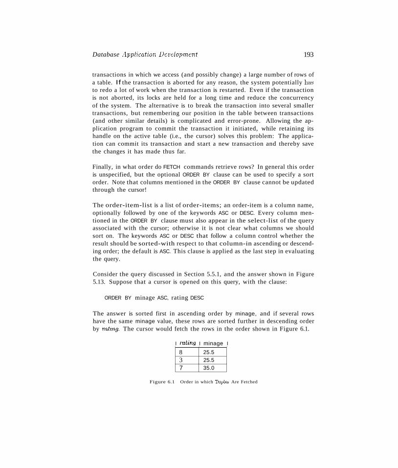
Database Apphcation Development 193
transactions in which we access (and possibly change) a large number of rows ofa table. If the transaction is aborted for any reason, the system potentially hasto redo a lot of work when the transaction is restarted. Even if the transactionis not aborted, its locks are held for a long time and reduce the concurrencyof the system. The alternative is to break the transaction into several smallertransactions, but remembering our position in the table between transactions(and other similar details) is complicated and error-prone. Allowing the application program to commit the transaction it initiated, while retaining itshandle on the active table (i.e., the cursor) solves this problem: The application can commit its transaction and start a new transaction and thereby savethe changes it has made thus far.
Finally, in what order do FETCH commands retrieve rows? In general this orderis unspecified, but the optional ORDER BY clause can be used to specify a sortorder. Note that columns mentioned in the ORDER BY clause cannot be updatedthrough the cursor!
The order-item-list is a list of order-items; an order-item is a column name,optionally followed by one of the keywords ASC or DESC. Every column mentioned in the ORDER BY clause must also appear in the select-list of the queryassociated with the cursor; otherwise it is not clear what columns we shouldsort on. The keywords ASC or DESC that follow a column control whether theresult should be sorted-with respect to that column-in ascending or descending order; the default is ASC. This clause is applied as the last step in evaluatingthe query.
Consider the query discussed in Section 5.5.1, and the answer shown in Figure5.13. Suppose that a cursor is opened on this query, with the clause:
ORDER BY minage ASC, rating DESC
The answer is sorted first in ascending order by minage, and if several rowshave the same minage value, these rows are sorted further in descending orderby rating. The cursor would fetch the rows in the order shown in Figure 6.1.
I rating I minage I
8 25.5
3 25.5
7 35.0
Figure 6.1 Order in which 'fuples Are Fetched
194 CHAPTER c6
6.1.3 Dynamic SQL
Consider an application such as a spreadsheet or a graphical front-end thatneeds to access data from a DBMS. Such an application must accept commandsfrom a user and, based on what the user needs, generate appropriate SQLstatements to retrieve the necessary data. In such situations, we may not beable to predict in advance just what SQL statements need to be executed, eventhough there is (presumably) some algorithm by which the application canconstruct the necessary SQL statements once a user's command is issued.
SQL provides some facilities to deal with such situations; these are referredto as Dynamic SQL. We illustrate the two main commands, PREPARE andEXECUTE, through a simple example:
char c_sqlstring[] = {"DELETE FROM Sailors WHERE rating>5"};EXEC SQL PREPARE readytogo FROM :csqlstring;EXEC SQL EXECUTE readytogo;
The first statement declares the C variable c_sqlstring and initializes its value tothe string representation of an SQL command. The second statement results inthis string being parsed and compiled as an SQL command, with the resultingexecutable bound to the SQL variable readytogo. (Since readytogo is an SQLvariable, just like a cursor name, it is not prefixed by a colon.) The thirdstatement executes the command.
Many situations require the use of Dynamic SQL. However, note that thepreparation of a Dynamic SQL command occurs at run-time and is run-timeoverhead. Interactive and Embedded SQL commands can be prepared onceat compile-time and then re-executecl as often as desired. Consequently youshould limit the use of Dynamic SQL to situations in which it is essential.
There are many more things to know about Dynamic SQL~~~how we can pa'3Sparameters from the host language program to the SQL statement being preparcel, for example--but we do not discuss it further.
6.2 AN INTRODUCTION TO JDBC
Embedded SQL enables the integration of SQL with a general-purpose programming language. As described in Section 6.1.1, a DBMS-specific preprocessor transforms the Embedded SQL statements into function calls in the hostlanguage. The details of this translation vary across DBMSs, and thereforeeven though the source code can be cOlnpiled to work with different DBMSs,the final executable works only with one specific DBMS.
Database Application Develop'Tnent 195,
ODBC and JDBC, short for Open DataBase Connectivity and Java DataBaseConnectivity, also enable the integration of SQL with a general-purpose programming language. Both ODBC and JDBC expose database capabilities ina standardized way to the application programmer through an applicationprogramming interface (API). In contrast to Embedded SQL, ODBC andJDBC allow a single executable to access different DBMSs 'Without recompilation. Thus, while Embedded SQL is DBMS-independent only at the sourcecode level, applications using ODBC or JDBC are DBMS-independent at thesource code level and at the level of the executable. In addition, using ODBCor JDBC, an application can access not just one DBMS but several differentones simultaneously.
ODBC and JDBC achieve portability at the level of the executable by introducing an extra level of indirection. All direct interaction with a specific DBMShappens through a DBMS-specific driver. A driver is a software programthat translates the ODBC or JDBC calls into DBMS-specific calls. Driversare loaded dynamically on demand since the DBMSs the application is goingto access are known only at run-time. Available drivers are registered with adriver manager.
One interesting point to note is that a driver does not necessarily need tointeract with a DBMS that understands SQL. It is sufficient that the drivertranslates the SQL commands from the application into equivalent commandsthat the DBMS understands. Therefore, in the remainder of this section, werefer to a data storage subsystem with which a driver interacts as a datasource.
An application that interacts with a data source through ODBC or JDBC selects a data source, dynamically loads the corresponding driver, and establishesa connection with the data source. There is no limit on the number of openconnections, and an application can have several open connections to differentdata sources. Each connection has transaction semantics; that is, changes fromone connection are visible to other connections only after the connection hascommitted its changes. While a connection is opcn, transactions are executedby submitting SQL statements, retrieving results, processing errors, and finallycommitting or rolling back. The application disconnects from the data sourceto terminate the interaction.
In the remainder of this chapter, we concentrate on JDBC.
196 CHAPTEij. 6
r--I JDBC Drivers: The most up-to-date source of .IDBC drivers is the Sun
JDBC Driver page athttp://industry.java.sun.com/products/jdbc/driversJDBC drivers are available for all major database sytems.
6.2.1 Architecture
The architecture of JDBC has four main components: the application, thedriver manager, several data source specific dr-iveTs, and the correspondingdata SOUTces.
The application initiates and terminates the connection with a data source.It sets transaction boundaries, submits SQL statements, and retrieves theresults-----all through a well-defined interface as specified by the JDBC API. Theprimary goal of the dr-iver manager is to load JDBC drivers and pass JDBCfunction calls from the application to the correct driver. The driver manageralso handles JDBC initialization and information calls from the applicationsand can log all function calls. In addition, the driver manager performs· somerudimentary error checking. The dr-iver establishes the connection with thedata source. In addition to submitting requests and returning request results,the driver translates data, error formats, and error codes from a form that isspecific to the data source into the JDBC standard. The data source processescommands from the driver and returns the results.
Depending on the relative location of the data source and the application,several architectural scenarios are possible. Drivers in JDBC are cla.ssified intofour types depending on the architectural relationship between the applicationand the data source:
III Type I Bridges: This type of driver translates JDBC function callsinto function calls of another API that is not native to the DBMS. Anexample is a JDBC-ODBC bridge; an application can use JDBC calls toaccess an ODBC compliant data source. The application loads only onedriver, the bridge. Bridges have the advantage that it is easy to piggyback the applica.tion onto an existing installation, and no new drivers haveto be installed. But using bridges hl:l.-'3 several drawbacks. The increasednumber of layers between data source and application affects performance.In addition, the user is limited to the functionality that the ODBC driversupports.
iii Type II Direct Thanslation to the Native API via N on-JavaDriver: This type of driver translates JDBC function calls directly intomethod invocations of the API of one specific data source. The driver is
Database Application Develop'll1,ent 197}
usually ,vritten using a combination of C++ and Java; it is dynamicallylinked and specific to the data source. This architecture performs significantly better than a JDBC-ODBC bridge. One disadvantage is that thedatabase driver that implements the API needs to be installed on eachcomputer that runs the application.
II Type III~~Network Bridges: The driver talks over a network to amiddleware server that translates the JDBC requests into DBMS-specificmethod invocations. In this case, the driver on the client site (Le., thenetwork bridge) is not DBMS-specific. The JDBC driver loaded by the ap~
plication can be quite small, as the only functionality it needs to implementis sending of SQL statements to the middleware server. The middlewareserver can then use a Type II JDBC driver to connect to the data source.
II Type IV-Direct Translation to the Native API via Java Driver:Instead of calling the DBMS API directly, the driver communicates withthe DBMS through Java sockets. In this case, the driver on the client side iswritten in Java, but it is DBMS-specific. It translates JDBC calls into thenative API of the database system. This solution does not require an intermediate layer, and since the implementation is all Java, its performanceis usually quite good.
6.3 JDBC CLASSES AND INTERFACES
JDBC is a collection of Java classes and interfaces that enables database accessfrom prograrl1s written in the Java language. It contains methods for connecting to a remote data source, executing SQL statements, examining setsof results from SQL statements, transaction management, and exception handling. The cla.sses and interfaces are part of the java. sql package. Thus, allcode fragments in the remainder of this section should include the statementimport java. sql . * at the beginning of the code; we omit this statement inthe remainder of this section. JDBC 2.0 also includes the j avax. sql package, the JDBC Optional Package. The package j avax. sql adds, amongother things, the capability of connection pooling and the Row-Set interface.\\Te discuss connection pooling in Section 6.3.2, and the ResultSet interface inSection 6.3.4.
\\Te now illustrate the individual steps that are required to submit a databa.sequery to a data source and to retrieve the results.
6.3.1 JDBC Driver Management
In .lDBe, data source drivers are managed by the Drivermanager class, whichmaintains a list of all currently loaded drivers. The Drivermanager cla.ss has
198 CHAPTEa 6
methods registerDriver, deregisterDriver, and getDrivers to enable dynamic addition and deletion of drivers.
The first step in connecting to a data source is to load the corresponding JDBCdriver. This is accomplished by using the Java mechanism for dynamicallyloading classes. The static method forName in the Class class returns the Javaclass as specified in the argument string and executes its static constructor.The static constructor of the dynamically loaded class loads an instance of theDriver class, and this Driver object registers itself with the DriverManagerclass.
The following Java example code explicitly loads a JDBC driver:
Class.forName("oracle/jdbc.driver.OracleDriver");
There are two other ways ofregistering a driver. We can include the driver with-Djdbc. drivers=oracle/jdbc. driver at the command line when we start theJava application. Alternatively, we can explicitly instantiate a driver, but thismethod is used only rarely, as the name of the driver has to be specified in theapplication code, and thus the application becomes sensitive to changes at thedriver level.
After registering the driver, we connect to the data source.
6.3.2 Connections
A session with a data source is started through creation of a Connection object;A connection identifies a logical session with a data source; multiple connectionswithin the same Java program can refer to different data sources or the samedata source. Connections are specified through a JDBC URL, a URL thatuses the jdbc protocol. Such a URL has the form
jdbc:<subprotocol>:<otherParameters>
The code example shown in Figure 6.2 establishes a connection to an Oracledatabase assuming that the strings userld and password are set to valid values.
In JDBC, connections can have different properties. For example, a connectioncan specify the granularity of transactions. If autocommit is set for a connection, then each SQL statement is considered to be its own transaction. Ifautocommit is off, then a series of statements that compose a transaction canbe committed using the commit 0 method of the Connection cla..<;s, or abortedusing the rollbackO method. The Connection cla.'ss has methods to set the
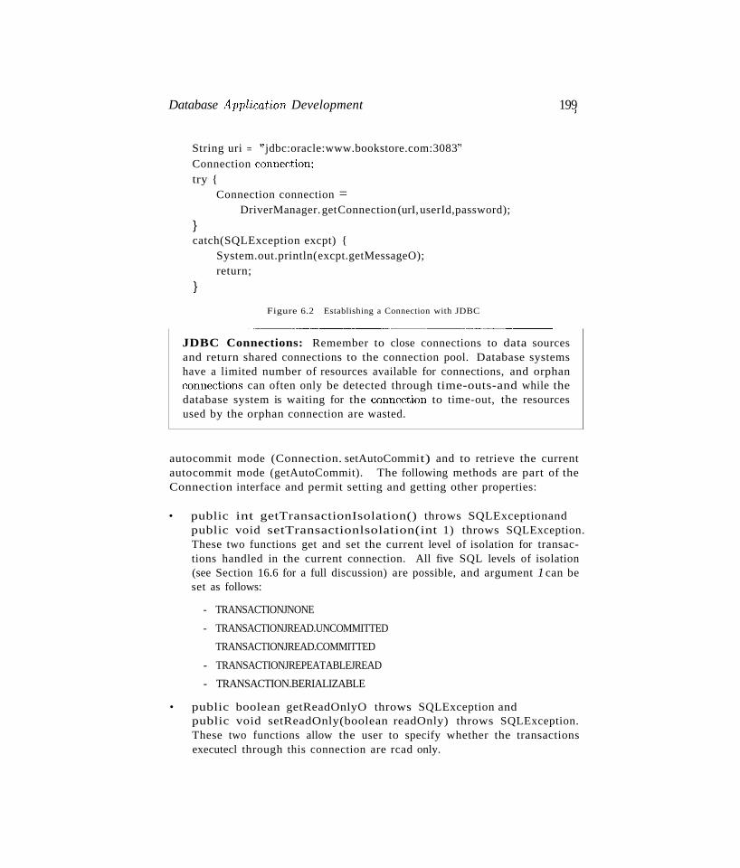
Database Appl'ication Development
String uri = .. jdbc:oracle:www.bookstore.com:3083..Connection connection;try {
Connection connection =DriverManager. getConnection (urI, userId,password);
}catch(SQLException excpt) {
System.out.println(excpt.getMessageO);return;
}
Figure 6.2 Establishing a Connection with JDBC
- ----~--._--_._---~,._-----~---_._-----,
199I
JDBC Connections: Remember to close connections to data sourcesand return shared connections to the connection pool. Database systemshave a limited number of resources available for connections, and orphanconnections can often only be detected through time-outs-and while thedatabase system is waiting for the connection to time-out, the resourcesused by the orphan connection are wasted.
autocommit mode (Connection. setAutoCommit) and to retrieve the currentautocommit mode (getAutoCommit). The following methods are part of theConnection interface and permit setting and getting other properties:
• public int getTransactionIsolation() throws SQLExceptionandpublic void setTransactionlsolation(int 1) throws SQLException.These two functions get and set the current level of isolation for transactions handled in the current connection. All five SQL levels of isolation(see Section 16.6 for a full discussion) are possible, and argument 1 can beset as follows:
- TRANSACTIONJNONE
- TRANSACTIONJREAD.UNCOMMITTED
- TRANSACTIONJREAD.COMMITTED
- TRANSACTIONJREPEATABLEJREAD
- TRANSACTION.BERIALIZABLE
• public boolean getReadOnlyO throws SQLException andpublic void setReadOnly(boolean readOnly) throws SQLException.These two functions allow the user to specify whether the transactionsexecutecl through this connection are rcad only.
200 CHAPTER ()
.. public boolean isClosed() throws SQLException.Checks whether the current connection has already been closed.
.. setAutoCommit and get AutoCommit.vVe already discussed these two functions.
Establishing a connection to a data source is a costly operation since it involves several steps, such as establishing a network connection to the datasource, authentication, and allocation of resources such as memory. In case anapplication establishes many different connections from different parties (suchas a Web server), connections are often pooled to avoid this overhead. A connection pool is a set of established connections to a data source. Whenever anew connection is needed, one of the connections from the pool is used, insteadof creating a new connection to the data source.
Connection pooling can be handled either by specialized code in the application,or the optional j avax. sql package, which provides functionality for connectionpooling and allows us to set different parameters, such as the capacity of thepool, and shrinkage and growth rates. Most application servers (see Section7.7.2) implement the j avax . sql package or a proprietary variant.
6.3.3 Executing SQL Statements
We now discuss how to create and execute SQL statements using JDBC. In theJDBC code examples in this section, we assume that we have a Connectionobject named con. JDBC supports three different ways of executing statements:Statement, PreparedStatement, and CallableStatement. The Statementclass is the base class for the other two statment classes. It allows us to querythe data source with any static or dynamically generated SQL query. We coverthe PreparedStatement class here and the CallableStatement class in Section6.5, when we discuss stored procedures.
The PreparedStatement cla,Cis dynamicaJly generates precompiled SQL statements that can be used several times; these SQL statements can have parameters, but their structure is fixed when the PreparedStatement object (representing the SQL statement) is created.
Consider the sample code using a PreparedStatment object shown in Figure6.3. The SQL query specifies the query string, but uses ''1' for the valuesof the parameters, which are set later using methods setString, setFloat,and setlnt. The ''1' placeholders can be used anywhere in SQL statementswhere they can be replaced with a value. Examples of places where they canappear include the WHERE clause (e.g., 'WHERE author=?'), or in SQL UPDATEand INSERT staternents, as in Figure 6.3. The method setString is one way
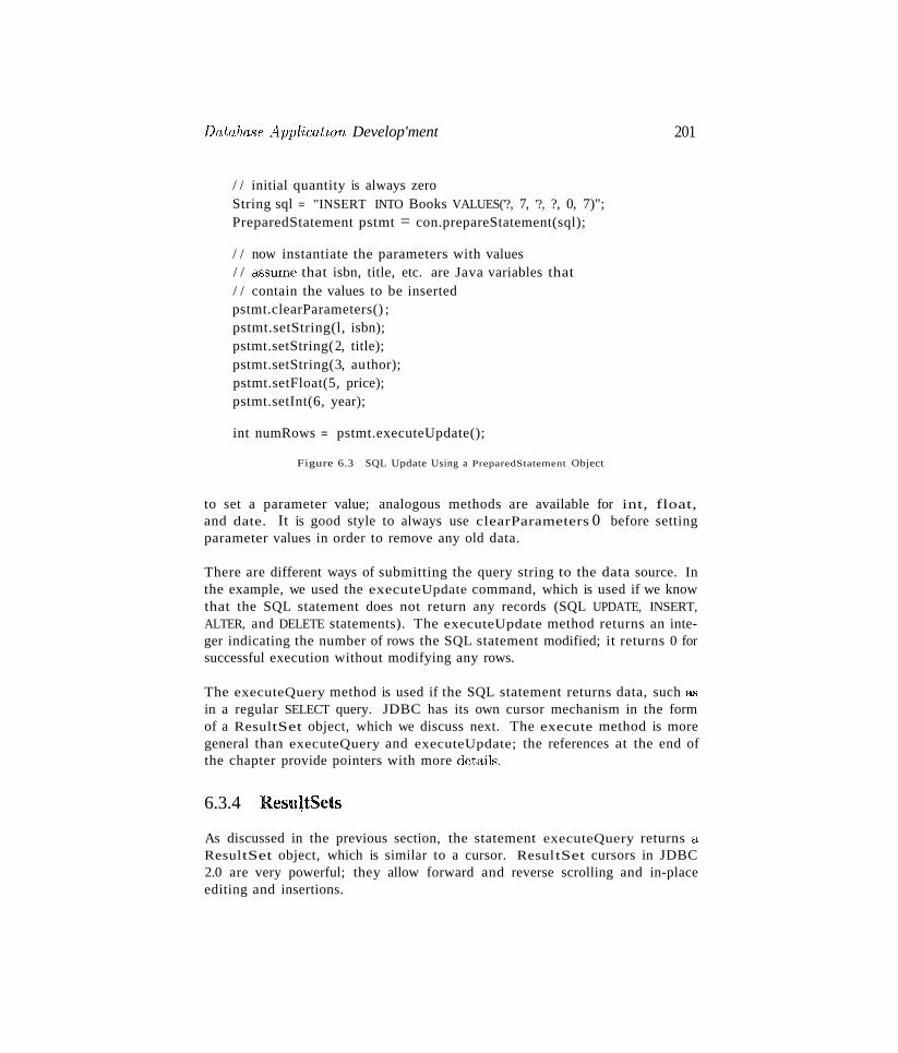
Database Application Develop'ment
/ / initial quantity is always zeroString sql = "INSERT INTO Books VALUES('?, 7, '?, ?, 0, 7)";PreparedStatement pstmt = con.prepareStatement(sql);
/ / now instantiate the parameters with values/ / a,ssume that isbn, title, etc. are Java variables that/ / contain the values to be insertedpstmt.clearParameters() ;pstmt.setString(l, isbn);pstmt.setString(2, title);pstmt.setString(3, author);pstmt.setFloat(5, price);pstmt.setInt(6, year);
int numRows = pstmt.executeUpdate();
Figure 6.3 SQL Update Using a PreparedStatement Object
201
to set a parameter value; analogous methods are available for int, float,and date. It is good style to always use clearParameters 0 before settingparameter values in order to remove any old data.
There are different ways of submitting the query string to the data source. Inthe example, we used the executeUpdate command, which is used if we knowthat the SQL statement does not return any records (SQL UPDATE, INSERT,ALTER, and DELETE statements). The executeUpdate method returns an integer indicating the number of rows the SQL statement modified; it returns 0 forsuccessful execution without modifying any rows.
The executeQuery method is used if the SQL statement returns data, such &"l
in a regular SELECT query. JDBC has its own cursor mechanism in the formof a ResultSet object, which we discuss next. The execute method is moregeneral than executeQuery and executeUpdate; the references at the end ofthe chapter provide pointers with more details.
6.3.4 Resul,tSets
As discussed in the previous section, the statement executeQuery returns a,ResultSet object, which is similar to a cursor. ResultSet cursors in JDBC2.0 are very powerful; they allow forward and reverse scrolling and in-placeediting and insertions.
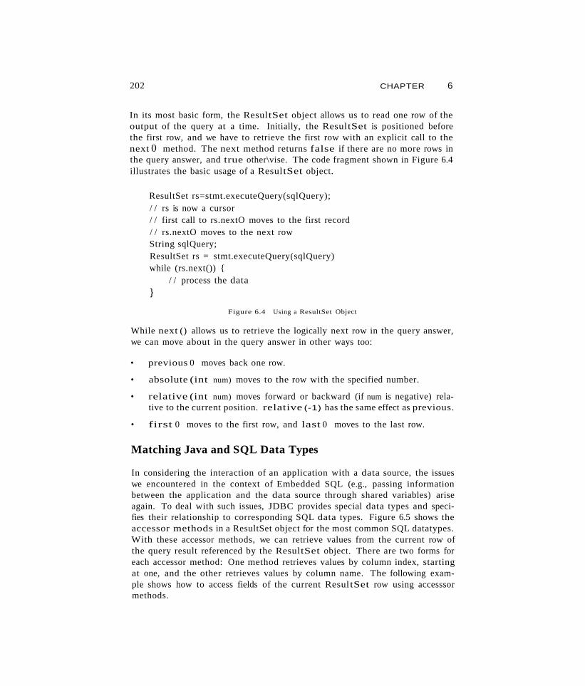
202 CHAPTER 6
In its most basic form, the ResultSet object allows us to read one row of theoutput of the query at a time. Initially, the ResultSet is positioned beforethe first row, and we have to retrieve the first row with an explicit call to thenext 0 method. The next method returns false if there are no more rows inthe query answer, and true other\vise. The code fragment shown in Figure 6.4illustrates the basic usage of a ResultSet object.
ResultSet rs=stmt.executeQuery(sqlQuery);/ / rs is now a cursor/ / first call to rs.nextO moves to the first record/ / rs.nextO moves to the next rowString sqlQuery;ResultSet rs = stmt.executeQuery(sqlQuery)while (rs.next()) {
/ / process the data}
Figure 6.4 Using a ResultSet Object
While next () allows us to retrieve the logically next row in the query answer,we can move about in the query answer in other ways too:
• previous 0 moves back one row.
• absolute (int num) moves to the row with the specified number.
• relative (int num) moves forward or backward (if num is negative) relative to the current position. relative (-1) has the same effect as previous.
• first 0 moves to the first row, and last 0 moves to the last row.
Matching Java and SQL Data Types
In considering the interaction of an application with a data source, the issueswe encountered in the context of Embedded SQL (e.g., passing informationbetween the application and the data source through shared variables) ariseagain. To deal with such issues, JDBC provides special data types and specifies their relationship to corresponding SQL data types. Figure 6.5 shows theaccessor methods in a ResultSet object for the most common SQL datatypes.With these accessor methods, we can retrieve values from the current row ofthe query result referenced by the ResultSet object. There are two forms foreach accessor method: One method retrieves values by column index, startingat one, and the other retrieves values by column name. The following example shows how to access fields of the current ResultSet row using accesssormethods.
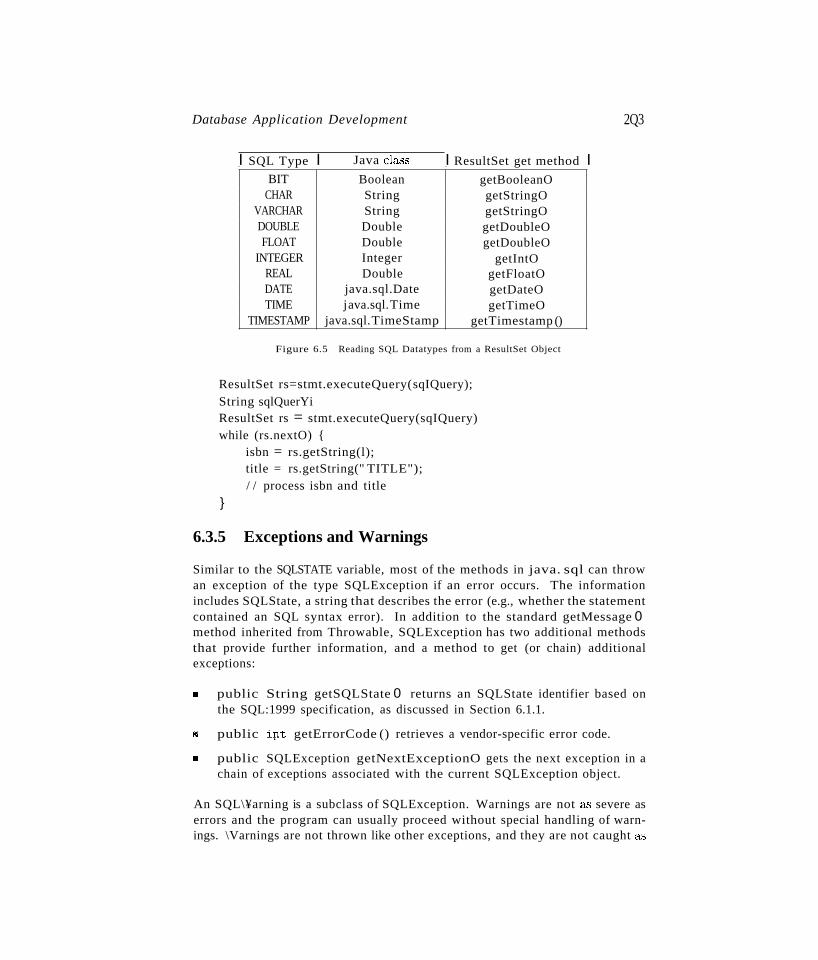
Database Application Development 2Q3
I SQL Type I Java cla.c;;s I ResultSet get method IBIT Boolean getBooleanO
CHAR String getStringOVARCHAR String getStringODOUBLE Double getDoubleOFLOAT Double getDoubleO
INTEGER Integer getIntOREAL Double getFloatODATE java.sql.Date getDateOTIME java.sql.Time getTimeO
TIMESTAMP java.sql.TimeStamp getTimestamp ()
Figure 6.5 Reading SQL Datatypes from a ResultSet Object
ResultSet rs=stmt.executeQuery(sqIQuery);String sqlQuerYiResultSet rs = stmt.executeQuery(sqIQuery)while (rs.nextO) {
isbn = rs.getString(l);title = rs.getString(" TITLE");/ / process isbn and title
}
6.3.5 Exceptions and Warnings
Similar to the SQLSTATE variable, most of the methods in java. sql can throwan exception of the type SQLException if an error occurs. The informationincludes SQLState, a string that describes the error (e.g., whether the statementcontained an SQL syntax error). In addition to the standard getMessage 0method inherited from Throwable, SQLException has two additional methodsthat provide further information, and a method to get (or chain) additionalexceptions:
III public String getSQLState 0 returns an SQLState identifier based onthe SQL:1999 specification, as discussed in Section 6.1.1.
.. public i:p.t getErrorCode () retrieves a vendor-specific error code.
III public SQLException getNextExceptionO gets the next exception in achain of exceptions associated with the current SQLException object.
An SQL\¥arning is a subclass of SQLException. Warnings are not H•.'3 severe aserrors and the program can usually proceed without special handling of warnings. \Varnings are not thrown like other exceptions, and they are not caught a.,
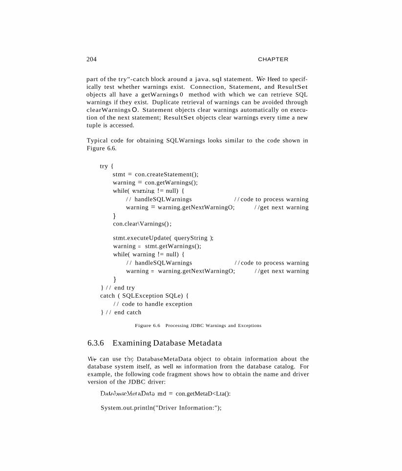
204 CHAPTER
part of the try"-catch block around a java. sql statement. VVe Heed to specifically test whether warnings exist. Connection, Statement, and ResultSetobjects all have a getWarnings 0 method with which we can retrieve SQLwarnings if they exist. Duplicate retrieval of warnings can be avoided throughclearWarnings O. Statement objects clear warnings automatically on execution of the next statement; ResultSet objects clear warnings every time a newtuple is accessed.
Typical code for obtaining SQLWarnings looks similar to the code shown inFigure 6.6.
try {stmt = con.createStatement();warning = con.getWarnings();while( warning != null) {
/ / handleSQLWarnings / / code to process warningwarning = warning.getNextWarningO; / /get next warning
}con.clear\Varnings() ;
stmt.executeUpdate( queryString );warning = stmt.getWarnings();while( warning != null) {
/ / handleSQLWarnings / / code to process warningwarning = warning.getNextWarningO; / /get next warning
}} / / end trycatch ( SQLException SQLe) {
/ / code to handle exception} / / end catch
Figure 6.6 Processing JDBC Warnings and Exceptions
6.3.6 Examining Database Metadata
\Ve can use tlw DatabaseMetaData object to obtain information about thedatabase system itself, as well as information frorn the database catalog. Forexample, the following code fragment shows how to obtain the name and driverversion of the JDBC driver:
Databa..seMetaData md = con.getMetaD<Lta():
System.out.println("Driver Information:");
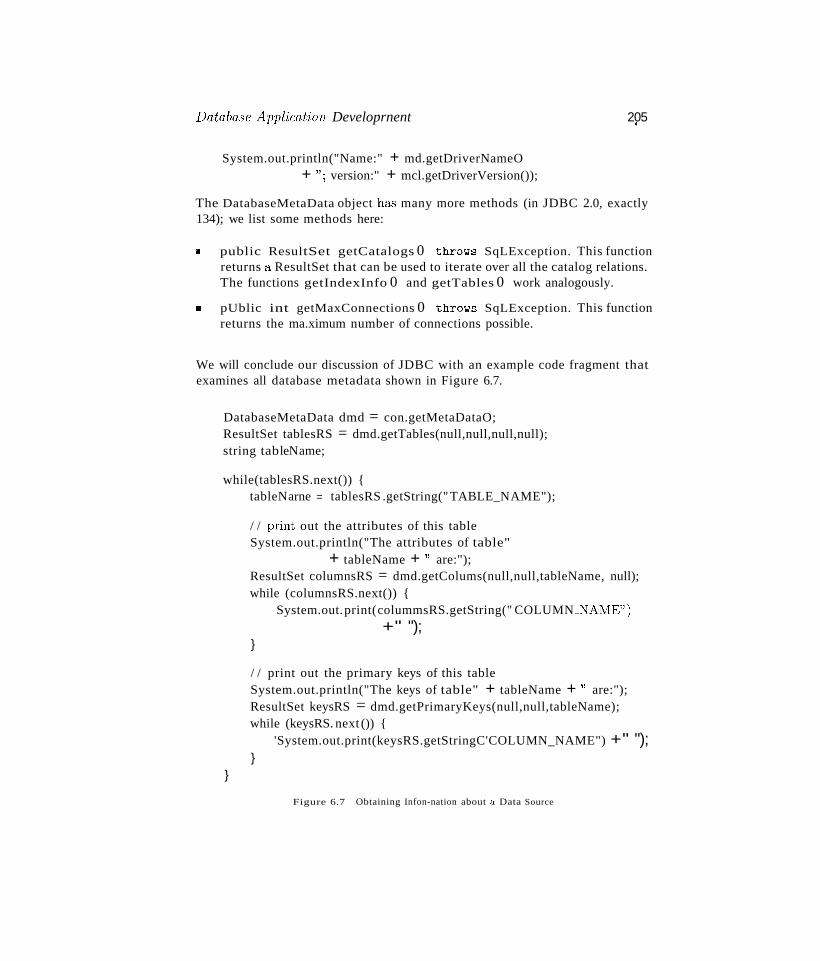
Database Appl'imtion Developrnent
System.out.println("Name:" + md.getDriverNameO+ "; version:" + mcl.getDriverVersion());
205~
The DatabaseMetaData object has many more methods (in JDBC 2.0, exactly134); we list some methods here:
• public ResultSet getCatalogs 0 throws SqLException. This functionreturns a ResultSet that can be used to iterate over all the catalog relations.The functions getIndexInfo 0 and getTables 0 work analogously.
• pUblic int getMaxConnections 0 throws SqLException. This functionreturns the ma.ximum number of connections possible.
We will conclude our discussion of JDBC with an example code fragment thatexamines all database metadata shown in Figure 6.7.
DatabaseMetaData dmd = con.getMetaDataO;ResultSet tablesRS = dmd.getTables(null,null,null,null);string tableName;
while(tablesRS.next()) {tableNarne = tablesRS .getString(" TABLE_NAME");
/ / print out the attributes of this tableSystem.out.println("The attributes of table"
+ tableName + " are:");ResultSet columnsRS = dmd.getColums(null,null,tableName, null);while (columnsRS.next()) {
System.out.print(colummsRS.getString(" COLUMN_NAME")+" ");
}
/ / print out the primary keys of this tableSystem.out.println("The keys of table" + tableName + " are:");ResultSet keysRS = dmd.getPrimaryKeys(null,null,tableName);while (keysRS. next ()) {
'System.out.print(keysRS.getStringC'COLUMN_NAME") +" ");}
}
Figure 6.7 Obtaining Infon-nation about it Data Source
206 CHAPTER.:6
6.4 SQLJ
SQLJ (short for 'SQL-Java') was developed by the SQLJ Group, a group ofdatabase vendors and Sun. SQLJ was developed to complement the dynamicway of creating queries in JDBC with a static model. It is therefore very closeto Embedded SQL. Unlike JDBC, having semi-static SQL queries allows thecompiler to perform SQL syntax checks, strong type checks of the compatibility of the host variables with the respective SQL attributes, and consistencyof the query with the database schema-tables, attributes, views, and storedprocedures--all at compilation time. For example, in both SQLJ and Embedded SQL, variables in the host language always are bound statically to thesame arguments, whereas in JDBC, we need separate statements to bind eachvariable to an argument and to retrieve the result. For example, the followingSQLJ statement binds host language variables title, price, and author to thereturn values of the cursor books.
#sql books = {SELECT title, price INTO :title, :priceFROM Books WHERE author = :author
};
In JDBC, we can dynamically decide which host language variables will holdthe query result. In the following example, we read the title of the book intovariable ftitle if the book was written by Feynman, and into variable otitleotherwise:
/ / assume we have a ResultSet cursor rsauthor = rs.getString(3);
if (author=="Feynman") {ftitle = rs.getString(2):
}else {
otitle = rs.getString(2);}
vVhen writing SQLJ applications, we just write regular Java code and embedSQL statements according to a set of rules. SQLJ applications are pre-processedthrough an SQLJ translation program that replaces the embedded SQLJ codewith calls to an SQLJ Java library. The modified program code can then becompiled by any Java compiler. Usually the SQLJ Java library makes calls toa JDBC driver, which handles the connection to the datab&'3e system.
Database Application Development 2Q7
An important philosophical difference exists between Embedded SQL and SQLJand JDBC. Since vendors provide their own proprietary versions of SQL, it isadvisable to write SQL queries according to the SQL-92 or SQL:1999 standard.However, when using Embedded SQL, it is tempting to use vendor-specific SQLconstructs that offer functionality beyond the SQL-92 or SQL:1999 standards.SQLJ and JDBC force adherence to the standards, and the resulting code ismuch more portable across different database systems.
In the remainder of this section, we give a short introduction to SQLJ.
6.4.1 Writing SQLJ Code
We will introduce SQLJ by means of examples. Let us start with an SQLJ codefragment that selects records from the Books table that match a given author.
String title; Float price; String atithor;#sql iterator Books (String title, Float price);Books books;
/ / the application sets the author/ / execute the query and open the cursor#sql books = {
SELECT title, price INTO :titIe, :priceFROM Books WHERE author = :author
};
/ / retrieve resultswhile (books.next()) {
System.out.println(books.titleO + ", " + books.price());}books.close() ;
The corresponding JDBC code fragment looks as follows (assuming we alsodeclared price, name, and author:
PrcparcdStatcment stmt = connection.prepareStatement(" SELECT title, price FROM Books WHERE author = ?");
/ / set the parameter in the query ancl execute itstmt.setString(1, author);ResultSet 1'8 = stmt.executeQuery();
/ / retrieve the resultswhile (rs.next()) {
208 CHAPTER
System.out.println(rs.getString(l) + ", " + rs.getFloat(2));}
6
Comparing the JDBC and SQLJ code, we see that the SQLJ code is mucheasier to read than the JDBC code. Thus, SQLJ reduces software developmentand maintenance costs.
Let us consider the individual components of the SQLJ code in more detail.All SQLJ statements have the special prefix #sql. In SQLJ, we retrieve theresults of SQL queries with iterator objects, which are basically cursors. Aniterator is an instance of an iterator class. Usage of an iterator in SQLJ goesthrough five steps:
• Declare the Iterator Class: In the preceding code, this happened throughthe statement#sql iterator Books (String title, Float price);This statement creates a new Java class that we can use to instantiateobjects.
• Instantiate an Iterator Object from the New Iterator Class: Weinstantiated our iterator in the statement Books books;.
• Initialize the Iterator Using a SQL Statement: In our example, thishappens through the statement #sql books ;;;;;; ....
• Iteratively, Read the Rows From the Iterator Object: This step isvery similar to reading rows through a ResultSet object in JDBC.
• Close the Iterator Object.
There are two types of iterator classes: named iterators and positional iterators.For named iterators, we specify both the variable type and the name of eachcolumn of the iterator. This allows us to retrieve individual columns by name asin our previous example where we could retrieve the title colunm from the Bookstable using the expression books. titIe (). For positional iterators, we needto specifY only the variable type for each column of the iterator. To accessthe individual columns of the iterator, we use a FETCH ... INTO eonstruct,similar to Embedded SQL. Both iterator types have the same performance;which iterator to use depends on the programmer's taste.
Let us revisit our example. \Ve can make the iterator a positional iteratorthrough the following statement:
#sql iterator Books (String, Float);
vVe then retrieve the individual rows from the iterator 3,.'3 follows:
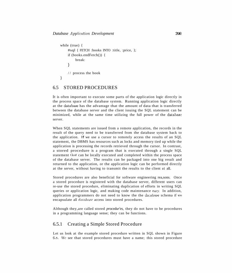
Database Application Development
while (true) {#sql { FETCH :books INTO :title, :price, };if (books.endFetch()) {
break:}
/ / process the book}
6.5 STORED PROCEDURES
200
It is often important to execute some parts of the application logic directly inthe process space of the database system. Running application logic directlyat the databa.se has the advantage that the amount of data that is transferredbetween the database server and the client issuing the SQL statement can beminimized, while at the same time utilizing the full power of the databa.seserver.
When SQL statements are issued from a remote application, the records in theresult of the query need to be transferred from the database system back tothe application. If we use a cursor to remotely access the results of an SQLstatement, the DBMS has resources such as locks and memory tied up while theapplication is processing the records retrieved through the cursor. In contrast,a stored procedure is a program that is executed through a single SQLstatement that can be locally executed and completed within the process spaceof the database server. The results can be packaged into one big result andreturned to the application, or the application logic can be performed directlyat the server, without having to transmit the results to the client at alL
Stored procedures are also beneficial for software engineering rea,sons. Oncea stored procedure is registered with the database server, different users canre-use the stored procedure, eliminating duplication of efforts in writing SQLqueries or application logic, and making code maintenance ea."lY. In addition,application programmers do not need to know the the databa.se schema if weencapsulate all databa.'3e access into stored procedures.
Although they,are called stored procedur'es, they do not have to be proceduresin a programming language sense; they can be functions.
6.5.1 Creating a Simple Stored Procedure
Let us look at the example stored procedure written in SQL shown in Figure(i.S. vVe see that stored procedures must have a name; this stored procedure
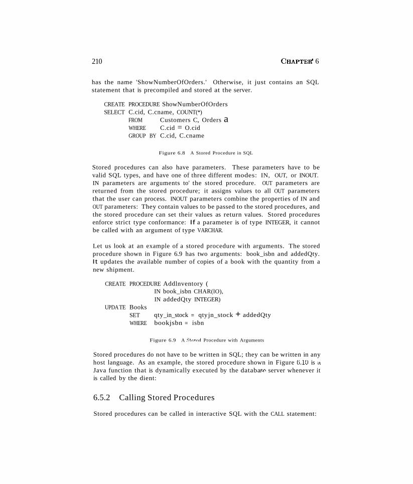
210 CHAPTER' 6
has the name 'ShowNumberOfOrders.' Otherwise, it just contains an SQLstatement that is precompiled and stored at the server.
CREATE PROCEDURE ShowNumberOfOrdersSELECT C.cid, C.cname, COUNT(*)
FROM Customers C, Orders aWHERE C.cid = O.cidGROUP BY C.cid, C.cname
Figure 6.8 A Stored Procedure in SQL
Stored procedures can also have parameters. These parameters have to bevalid SQL types, and have one of three different modes: IN, OUT, or INOUT.IN parameters are arguments to' the stored procedure. OUT parameters arereturned from the stored procedure; it assigns values to all OUT parametersthat the user can process. INOUT parameters combine the properties of IN andOUT parameters: They contain values to be passed to the stored procedures, andthe stored procedure can set their values as return values. Stored proceduresenforce strict type conformance: If a parameter is of type INTEGER, it cannotbe called with an argument of type VARCHAR.
Let us look at an example of a stored procedure with arguments. The storedprocedure shown in Figure 6.9 has two arguments: book_isbn and addedQty.It updates the available number of copies of a book with the quantity from anew shipment.
CREATE PROCEDURE Addlnventory (IN book_isbn CHAR(lO),IN addedQty INTEGER)
UPDATE BooksSETWHERE
qty_in_stock = qtyjn_stock + addedQtybookjsbn = isbn
Figure 6.9 A Stored Procedure with Arguments
Stored procedures do not have to be written in SQL; they can be written in anyhost language. As an example, the stored procedure shown in Figure 0.10 is aJava function that is dynamically executed by the databa..<;e server whenever itis called by the dient:
6.5.2 Calling Stored Procedures
Stored procedures can be called in interactive SQL with the CALL statement:
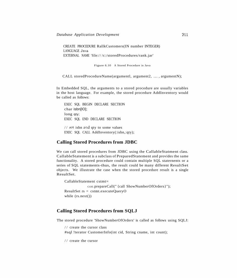
Database Application Development
CREATE PROCEDURE RallkCustomers(IN number INTEGER)LANGUAGE JavaEXTERNAL NAME 'file:/ / /c:/storedProcedures/rank.jar'
Figure 6.10 A Stored Procedure in Java
211
CALL storedProcedureName(argumentl, argument2, ... , argumentN);
In Embedded SQL, the arguments to a stored procedure are usually variablesin the host language. For example, the stored procedure AddInventory wouldbe called as follows:
EXEC SQL BEGIN DECLARE SECTIONchar isbn[lO];long qty;
EXEC SQL END DECLARE SECTION
/ / set isbn and qty to some valuesEXEC SQL CALL AddInventory(:isbn,:qty);
Calling Stored Procedures from JDBC
We can call stored procedures from JDBC using the CallableStatment class.CallableStatement is a subclass of PreparedStatement and provides the samefunctionality. A stored procedure could contain multiple SQL staternents or aseries of SQL statements-thus, the result could be many different ResultSetobjects. We illustrate the case when the stored procedure result is a singleResultSet.
CallableStatement cstmt=COIl. prepareCall(" {call ShowNumberOfOrders}");
ResultSet rs = cstmt.executeQueryOwhile (rs.next())
Calling Stored Procedures from SQLJ
The stored procedure 'ShowNumberOfOrders' is called as follows using SQLJ:
/ / create the cursor class#sql !terator CustomerInfo(int cid, String cname, int count);
/ / create the cursor
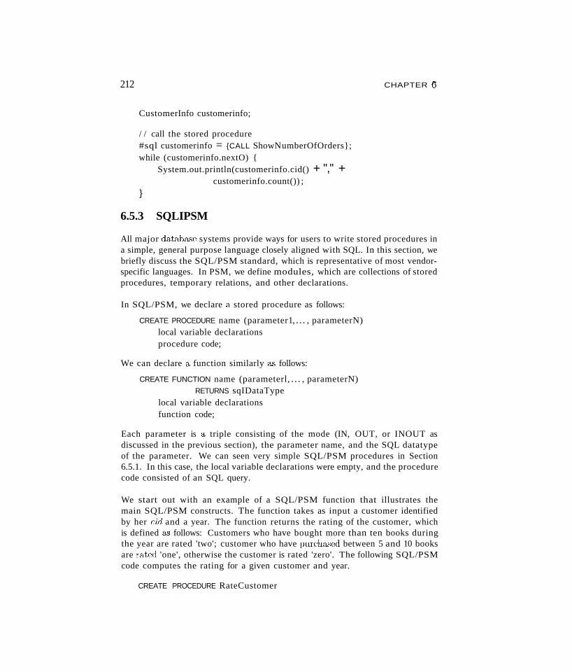
212
CustomerInfo customerinfo;
/ / call the stored procedure#sql customerinfo = {CALL ShowNumberOfOrders};while (customerinfo.nextO) {
System.out.println(customerinfo.cid() + "," +customerinfo.count()) ;
}
6.5.3 SQLIPSM
CHAPTER (5
All major databa...<;e systems provide ways for users to write stored procedures ina simple, general purpose language closely aligned with SQL. In this section, webriefly discuss the SQL/PSM standard, which is representative of most vendorspecific languages. In PSM, we define modules, which are collections of storedprocedures, temporary relations, and other declarations.
In SQL/PSM, we declare a stored procedure as follows:
CREATE PROCEDURE name (parameter1,... , parameterN)local variable declarationsprocedure code;
We can declare a function similarly as follows:
CREATE FUNCTION name (parameterl, ... , parameterN)RETURNS sqIDataType
local variable declarationsfunction code;
Each parameter is a triple consisting of the mode (IN, OUT, or INOUT asdiscussed in the previous section), the parameter name, and the SQL datatypeof the parameter. We can seen very simple SQL/PSM procedures in Section6.5.1. In this case, the local variable declarations were empty, and the procedurecode consisted of an SQL query.
We start out with an example of a SQL/PSM function that illustrates themain SQL/PSM constructs. The function takes as input a customer identifiedby her cid and a year. The function returns the rating of the customer, whichis defined a...'3 follows: Customers who have bought more than ten books duringthe year are rated 'two'; customer who have purcha...<;ed between 5 and 10 booksare rated 'one', otherwise the customer is rated 'zero'. The following SQL/PSMcode computes the rating for a given customer and year.
CREATE PROCEDURE RateCustomer
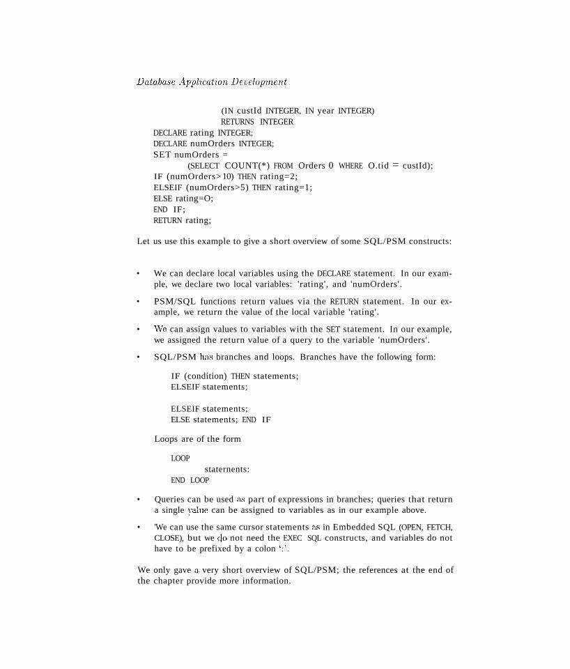
Database Appl'ication Development
(IN custId INTEGER, IN year INTEGER)RETURNS INTEGER
DECLARE rating INTEGER;DECLARE numOrders INTEGER;SET numOrders =
(SELECT COUNT(*) FROM Orders 0 WHERE O.tid = custId);IF (numOrders> 10) THEN rating=2;ELSEIF (numOrders>5) THEN rating=1;ELSE rating=O;END IF;RETURN rating;
Let us use this example to give a short overview of some SQL/PSM constructs:
• We can declare local variables using the DECLARE statement. In our example, we declare two local variables: 'rating', and 'numOrders'.
• PSM/SQL functions return values via the RETURN statement. In our example, we return the value of the local variable 'rating'.
• vVe can assign values to variables with the SET statement. In our example,we assigned the return value of a query to the variable 'numOrders'.
• SQL/PSM h&<; branches and loops. Branches have the following form:
IF (condition) THEN statements;ELSEIF statements;
ELSEIF statements;ELSE statements; END IF
Loops are of the form
LOOPstaternents:
END LOOP
• Queries can be used as part of expressions in branches; queries that returna single ;ralue can be assigned to variables as in our example above.
• 'We can use the same cursor statements &s in Embedded SQL (OPEN, FETCH,CLOSE), but we do not need the EXEC SQL constructs, and variables do nothave to be prefixed by a colon ':'.
We only gave a very short overview of SQL/PSM; the references at the end ofthe chapter provide more information.
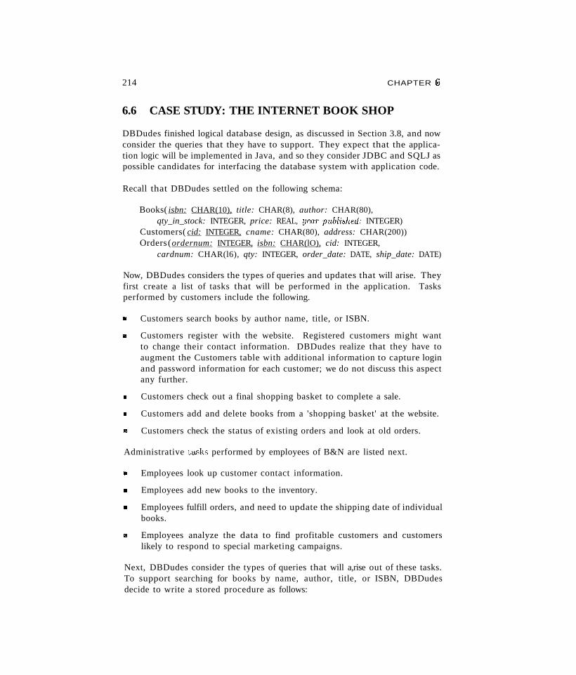
214 CHAPTER €i
6.6 CASE STUDY: THE INTERNET BOOK SHOP
DBDudes finished logical database design, as discussed in Section 3.8, and nowconsider the queries that they have to support. They expect that the application logic will be implemented in Java, and so they consider JDBC and SQLJ aspossible candidates for interfacing the database system with application code.
Recall that DBDudes settled on the following schema:
Books( isbn: CHAR(10), title: CHAR(8), author: CHAR(80),qty_in_stock: INTEGER, price: REAL, year_published: INTEGER)
Customers( cid: INTEGER, cname: CHAR(80), address: CHAR(200))Orders (ordernum: INTEGER, isbn: CHAR(lO), cid: INTEGER,
cardnum: CHAR(l6), qty: INTEGER, order_date: DATE, ship_date: DATE)
Now, DBDudes considers the types of queries and updates that will arise. Theyfirst create a list of tasks that will be performed in the application. Tasksperformed by customers include the following.
II Customers search books by author name, title, or ISBN.
.. Customers register with the website. Registered customers might wantto change their contact information. DBDudes realize that they have toaugment the Customers table with additional information to capture loginand password information for each customer; we do not discuss this aspectany further.
III Customers check out a final shopping basket to complete a sale.
III Customers add and delete books from a 'shopping basket' at the website.
.. Customers check the status of existing orders and look at old orders.
Administrative ta.'3ks performed by employees of B&N are listed next.
II Employees look up customer contact information.
III Employees add new books to the inventory.
.. Employees fulfill orders, and need to update the shipping date of individualbooks.
.. Employees analyze the data to find profitable customers and customerslikely to respond to special marketing campaigns.
Next, DBDudes consider the types of queries that will a,rise out of these tasks.To support searching for books by name, author, title, or ISBN, DBDudesdecide to write a stored procedure as follows:
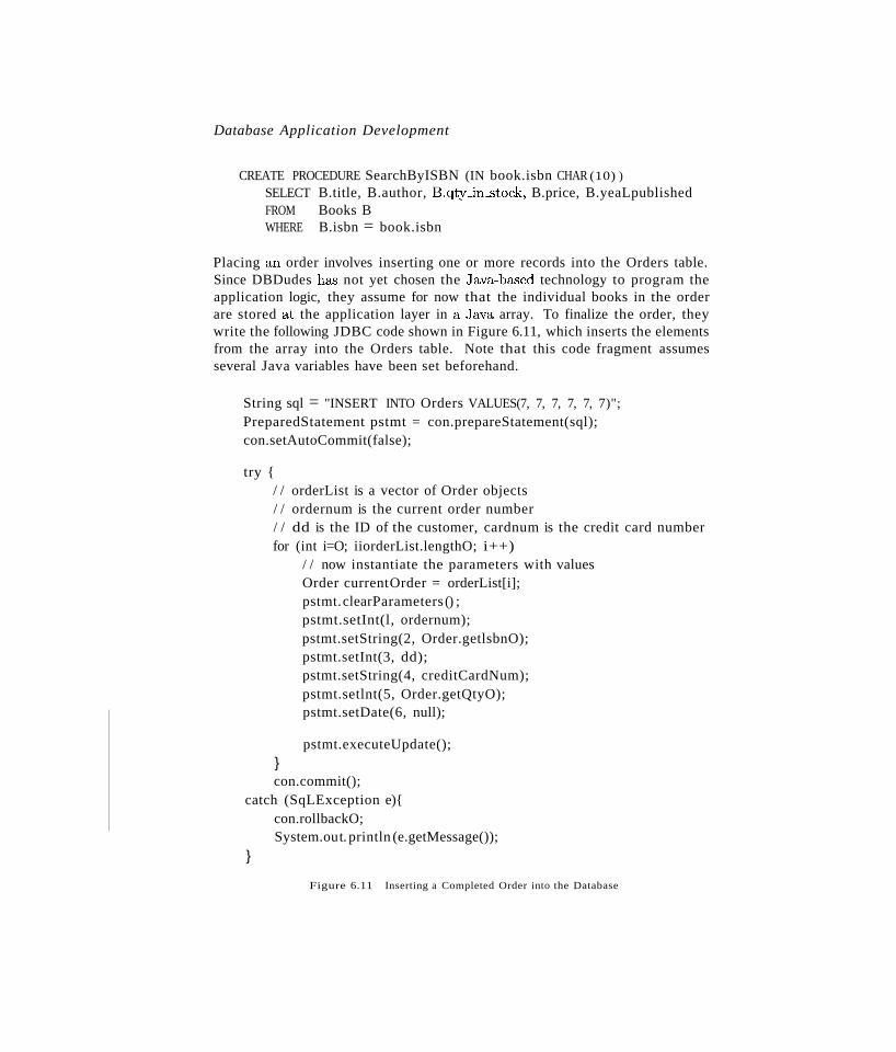
Database Application Development
CREATE PROCEDURE SearchByISBN (IN book.isbn CHAR (10) )SELECT B.title, B.author, B.qty_in~'3tock,B.price, B.yeaLpublishedFROM Books BWHERE B.isbn = book.isbn
Placing an order involves inserting one or more records into the Orders table.Since DBDudes has not yet chosen the Java-based technology to program theapplication logic, they assume for now that the individual books in the orderare stored at the application layer in a Java array. To finalize the order, theywrite the following JDBC code shown in Figure 6.11, which inserts the elementsfrom the array into the Orders table. Note that this code fragment assumesseveral Java variables have been set beforehand.
String sql = "INSERT INTO Orders VALUES(7, 7, 7, 7, 7, 7)";PreparedStatement pstmt = con.prepareStatement(sql);con.setAutoCommit(false);
try {/ / orderList is a vector of Order objects/ / ordernum is the current order number/ / dd is the ID of the customer, cardnum is the credit card numberfor (int i=O; iiorderList.lengthO; i++)
/ / now instantiate the parameters with valuesOrder currentOrder = orderList[i];pstmt.clearParameters () ;pstmt.setInt(l, ordernum);pstmt.setString(2, Order.getlsbnO);pstmt.setInt(3, dd);pstmt.setString(4, creditCardNum);pstmt.setlnt(5, Order.getQtyO);pstmt.setDate(6, null);
pstmt.executeUpdate();}con.commit();
catch (SqLException e){con.rollbackO;System.out. println (e.getMessage());
}
Figure 6.11 Inserting a Completed Order into the Database
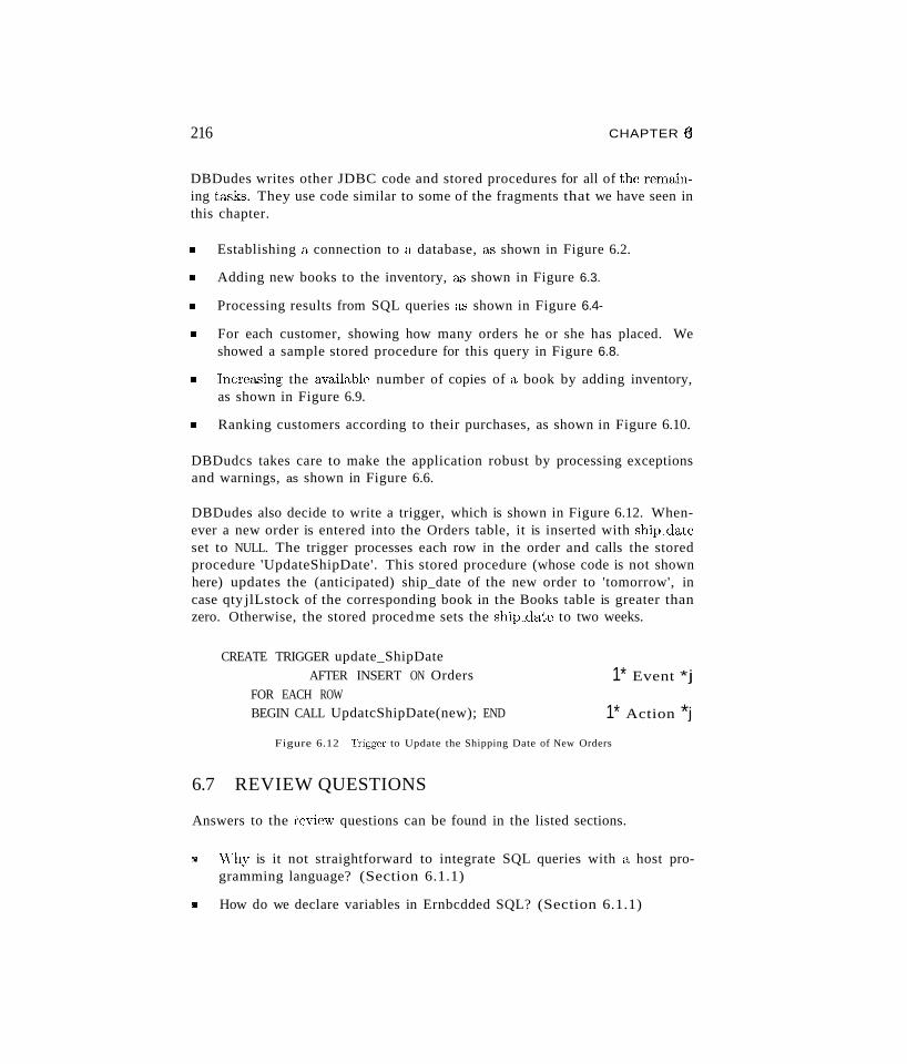
216 CHAPTER (}
DBDudes writes other JDBC code and stored procedures for all of the remaining tasks. They use code similar to some of the fragments that we have seen inthis chapter.
II Establishing a connection to a database, as shown in Figure 6.2.
II Adding new books to the inventory, a'3 shown in Figure 6.3.
II Processing results from SQL queries a'3 shown in Figure 6.4-
II For each customer, showing how many orders he or she has placed. Weshowed a sample stored procedure for this query in Figure 6.8.
II Increa'3ing the available number of copies of a book by adding inventory,as shown in Figure 6.9.
II Ranking customers according to their purchases, as shown in Figure 6.10.
DBDudcs takes care to make the application robust by processing exceptionsand warnings, as shown in Figure 6.6.
DBDudes also decide to write a trigger, which is shown in Figure 6.12. Whenever a new order is entered into the Orders table, it is inserted with ship~date
set to NULL. The trigger processes each row in the order and calls the storedprocedure 'UpdateShipDate'. This stored procedure (whose code is not shownhere) updates the (anticipated) ship_date of the new order to 'tomorrow', incase qty jlLstock of the corresponding book in the Books table is greater thanzero. Otherwise, the stored procedme sets the ship_date to two weeks.
CREATE TRIGGER update_ShipDateAFTER INSERT ON Orders
FOR EACH ROWBEGIN CALL UpdatcShipDate(new); END
1* Event *j
1* Action *j
Figure 6.12 Trigger to Update the Shipping Date of New Orders
6.7 REVIEW QUESTIONS
Answers to the i'eview questions can be found in the listed sections.
lYl vVhy is it not straightforward to integrate SQL queries with a host programming language? (Section 6.1.1)
IIii How do we declare variables in Ernbcdded SQL? (Section 6.1.1)
Database Applicat'ion Deuelop'Tnent 217'*
• How do we use SQL statements within a host langl.lage? How do we checkfor errors in statement execution? (Section 6.1.1)
• Explain the impedance mismatch between host languages and SQL, anddescribe how cursors address this. (Section 6.1.2)
• '\That properties can cursors have? (Section 6.1.2)
• What is Dynamic SQL and how is it different from Embedded SQL? (Section 6.1.3)
• What is JDBC and what are its advantages? (Section 6.2)
• What are the components of the JDBC architecture? Describe four different architectural alternatives for JDBC drivers. (Section 6.2.1)
• How do we load JDBC drivers in Java code? (Section 6.3.1)
• How do we manage connections to data sources? What properties canconnections have? (Section 6.3.2)
• What alternatives does JDBC provide for executing SQL DML and DDLstatements? (Section 6.3.3)
• How do we handle exceptions and warnings in JDBC? (Section 6.3.5)
• 'What functionality provides the DatabaseMetaDataclass? (Section 6.3.6)
• What is SQLJ and how is it different from JDBC? (Section 6.4)
• vVhy are stored procedures important? How do we declare stored procedures and how are they called from application code? (Section 6.5)
EXERCISES
Exercise 6.1 Briefly answer the following questions.
1. Explain the following terms: Cursor, Embedded SQL, JDBC, SQLJ, stored procedure.
2. What are the differences between JDBC and SQLJ? \Nhy do they both exist?
3. Explain the term stored procedure, and give examples why stored procedures are useful.
Exercise 6.2 Explain how the following steps are performed in JDBC:
1. Connect to a data source.
2. Start, commit, and abort transactions.
3. Call a stored procedure.
How are these steps performed in SQLJ?
218 CHAPTER (:)
Exercise 6.3 Compare exception handling and handling of warnings ill embedded SQL, dynamic SQL, .IDBC, and SQL.I.
Exercise 6.4 Answer the following questions.
1. Why do we need a precompiler to translate embedded SQL and SQL.J? Why do we notneed a precompiler for .IDBC?
2. SQL.J and embedded SQL use variables in the host language to pass parameters to SQLqueries, whereas .JDBC uses placeholders marked with a ''1'. Explain the difference, andwhy the different mechanisms are needed.
Exercise 6.5 A dynamic web site generates HTML pages from information stored in adatabase. Whenever a page is requested, is it dynamically assembled from static data anddata in a database, resulting in a database access. Connecting to the database is usuallya time~consuming process, since resources need to be allocated, and the user needs to beauthenticated. Therefore, connection pooling--setting up a pool of persistent databaseconnections and then reusing them for different requests can significantly improve the performance of database-backed websites. Since servlets can keep information beyond singlerequests, we can create a connection pool, and allocate resources from it to new requests.
Write a connection pool class that provides the following methods:
III Create the pool with a specified number of open connections to the database system.
11II Obtain an open connection from the pool.
III Release a connection to the pool.
III Destroy the pool and close all connections.
PROJECT-BASED EXERCISES
In the following exercises, you will create database-backed applications. In this chapter, youwill create the parts of the application that access the database. In the next chapter, youwill extend this code to other &'3pects of the application. Detailed information about theseexercises and material for more exercises can be found online at
http://www.cs.wisc.edu/-dbbook
Exercise 6.6 Recall the Notown Records database that you worked with in Exercise 2.5 andExercise 3.15. You have now been tasked with designing a website for Notown. It shouldprovide the following functionality:
III Usen; can sem'ch for records by name of the musician, title of the album, and Bame ofthe song.
11II Users can register with the site, and registered users ca.n log on to the site. Once loggedon, users should not have to log on again unless they are inactive for a long time.
III Users who have logged on to the site can add items to a shopping basket.
11II Users with items in their shopping basket can check out and ma.ke a purchase.
Database Apphcation De'velopment 219
NOtOWIl wants to use JDBC to access the datab&<;e, \¥rite .JDBC code that performs thenecessary data access and manipulation. You will integrate this code with application logicand presentation in the next chapter.
If Notown had chosen SQLJ instead of JDBC, how would your code change?
Exercise 6.7 Recall the database schema for Prescriptions-R-X that you created in Exer~
cise 2.7. The Prescriptions-R-X chain of pharmacies has now engaged you to design theirnew website. The website has two different classes of users: doctors and patients. Doctorsshould be able to enter new prescriptions for their patients and modify existing prescriptions.Patients should be able to declare themselves as patients of a doctor; they should be ableto check the status of their prescriptions online; and they should be able to purchase theprescriptions online so that the drugs can be shipped to their home address.
Follow the analogous steps from Exercise 6.6 to write JDBC code that performs the necessary data access and manipulation. You will integrate this code with application logic andpresentation in the next chapter.
Exercise 6.8 Recall the university database schema that you worked with in Exercise 5.l.The university has decided to move enrollment to an online system. The website has twodifferent classes of users: faculty and students. Faculty should be able to create new coursesand delete existing courses, and students should be able to enroll in existing courses.
Follow the analogous steps from Exercise 6.6 to write JDBC code that performs the necessary data access and manipulation. You will integrate this code with application logic andpresentation in the next chapter.
Exercise 6.9 Recall the airline reservation schema that you worked on in Exercise 5.3. Design an online airline reservation system. The reservation system will have two types of users:airline employees, and airline passengers. Airline employees can schedule new flights and cancel existing flights. Airline passengers can book existing flights from a given destination.
Follow the analogous steps from Exercise 6.6 to write JDBC code that performs the necessary data access and manipulation. You will integrate this code with application logic andpresentation in the next chapter.
BIBLIOGRAPHIC NOTES
Information on ODBC can be found on Microsoft's web page (www.microsoft.com/data/odbc),and information on JDBC can be found on tlw Java web page (j ava. sun. com/products/jdbc).There exist rnany books on ODBC, for example, Sanders' ODBC Developer's Guicle [652] andthe lvIicrosoft ODBC SDK [5:3;3]. Books on JDBC include works by Hamilton et al. [359],Reese [621], and White et a!. [773].
7INTERNET APPLICATIONS
It How do we name resources on the Internet?
It How do Web browsers and webservers communicate?
It How do we present documents on the Internet? How do we differentiate between formatting and content?
It What is a three-tier application architecture? How do we write threetiered applications?
It Why do we have application servers?
.. Key concepts: Uniform Resource Identifiers (URI), Uniform Re.source Locators (URL); Hypertext Transfer Protocol (HTTP), stateless protocol; Java; HTML; XML, XML DTD; three-tier architecture,client-server architecture; HTML forms; JavaScript; cascading stylesheets, XSL; application server; Common Gateway Interface (CGI);servlet; JavaServer Page (JSP); cookie
Wow! They've got the Internet on computers now!
--Homer Simpson, The Simpsons
7.1 INTROpUCTION
The proliferation of computer networks, including the Internet and corporate'intranets,' has enabled users to access a large number of data sources. Thisincreased access to databases is likely to have a great practical impact; dataand services can now be offered directly to customers in ways impossible until
220
Intc'T7wt Applications 221
recently. Examples of such electronic commerce rtpplications include purchasing books through a \Veb retailer such <1.'3 Amazon.com, engaging in onlineauctions at a site such as eBay, and exchanging bids and specifications forproducts between companies. The emergence of standards such as XrvIL fordescribing the content of documents is likely to further accelerate electroniccommerce and other online applications.
While the first generation of Internet sites were collections of HTML files, mostmajor sites today store a large part (if not all) of their data in database systems.They rely on DBMSs to provide fast, reliable responses to user requests receivedover the Internet. This is especially true of sites for electronic commerce andother business applications.
In this chapter, we present an overview of concepts that are central to Internetapplication development. We start out with a basic overview of how the Internetworks in Section 7.2. We introduce HTML and XML, two data formats that areused to present data on the Internet, in Sections 7.3 and 7.4. In Section 7.5, weintroduce three-tier architectures, a way of structuring Internet applicationsinto different layers that encapsulate different functionality. In Sections 7.6and 7.7, we describe the presentation layer and the middle layer in detail; theDBMS is the third layer. We conclude the chapter by discussing our B&N casestudy in Section 7.8.
Examples that appear in this chapter are available online at
http://www.cs.wisc.edu/-dbbook
7.2 INTERNET CONCEPTS
The Internet has emerged as a universal connector between globally distributedsoftware systems. To understand how it works, we begin by discussing two ba"licissues: how sites on the Internet are identified, and how programs at one sitecommunicate with other sites.
vVe first introduce Uniform Resource Identifiers, a naming schema for locatingresources on the Internet in Section 7.2.1. \Ve then talk about the most popularprotocol for accessing resources over the Vv"eh, the hypertext transfer protocol(HTTP) in Se(tion 7.2.2.
7.2.1 Uniform Resource Identifiers
Uniform Resource Identifiers (URIs), are strings that uniquely identifyresources 011 the Internet. A resource is any kind of information that can
222 CHAPTER 7;
j;istributed Applications and Service-Oriented Architectures:I ~he advent of XML, due to its loosely-coupled nature, has made· infor
mation exchange between different applications feasible to an extent previously unseen. By using XML for information exchange, applications can bewritten in different programming languages, run on different operating systems, and yet they can still share information with each other. There arealso standards for externally describing the intended content of an XMLfile or message, most notably the recently adopted W3C XML Schemasstandard.A promising concept that has arisen out of the XML revolution is the notionof a Web service. A Web service is an application that provides a welldefined service, packaged as a set of remotely callable procedures accessiblethrough the Internet. Web services have the potential to enable powerfulnew applications by composing existing Web services-all communicatingseamlessly thanks to the use of standardizedXML-based information exchange. Several technologies have been developed or are currently underdevelopment that facilitate design and implementation of distributed applications. SOAP is a W3C standard for XML-based invocation of remoteservices (think XML RPC) that allows distributed applications to communicate either synchronously or asynchronously via structured, typed XMLmessages. SOAP calls can ride on a variety of underlying transport layers,including HTTP (part of what is making SOAP so successful) and various reliable messaging layers. Related to the SOAP standard are W3C'sWeb Services Description Language (WSDL) for describing Webservice interfaces, and Universal Description, Dis.;;overy, and Integration (UDDI), a WSDL-based Web services registry standard (thinkyellow pages for Web services).SOAP-based Web services are the foundation for Microsoft's recently released .NET framework, their application development infrastructure andassociated run-time system for developing distributed applications, as wellas for the Web services offerings of major software vendors such as IBM,BEA, and others. Many large software application vendors (major companies like PeopleSoft and SAP) have announced plans to provide Web serviceinterfaces to their products and the data that they manage, and many arehoping that XML and Web services will finally provide the answer to thelong-standing problem of enterprise application integration. Web servicesare also being looked to as a natural foundation for the next generation ofbusiness process management (or workflow) systems.
Internet Applications 223
be identified by a URI, and examples include webpages, images, downloadablefiles, services that can be remotely invoked, mailboxes, and so on. The mostcommon kind of resource is a static file (such as a HTML document), but aresource may also be a dynamically-generated HTML file, a movie, the outputof a program, etc.
A URI has three parts:
• The (name of the) protocol used to access the resource.
• The host computer where the resource is located.
• The path name of the resource itself on the host computer.
Consider an example URI, such as http://www.bookstore.com/index .html.This URI can be interpreted as follows. Use the HTTP protocol (explained inthe next section) to retrieve the document index. html located at the computerwww.bookstore.com.This example URI is an instance of a Universal Resource Locator (URL) , a subset of the more general URI naming scheme;the distinction is not important for our purposes. As another example, thefollowing HTML fragment shows a URI that is an email address:
<a href=lImailto:[email protected] ll >Email the webmaster.</A>
7.2.2 The Hypertext Transfer Protocol (HTTP)
A communication protocol is a set of standards that defines the structureof messages between two communicating parties so that they can understandeach other's messages. The Hypertext Transfer Protocol (HTTP) is themost common communication protocol used over the Internet. It is a clientserver protocol in which a client (usually a Web browser) sends a request to anHTTP server, which sends a response back to the client. When a user requestsa webpage (e.g., clicks on a hyperlink), the browser sends HTTP requestmessages for the objects in the page to the server. The server receives therequests and responds with HTTP response messages, which include theobjects. It is important to recognize that HTTP is used to transmit all kindsof resources, not just files, but most resources on the Internet today are eitherstatic files or :(lIes output from server-side scripts.
A variant of the HTTP protocol called the Secure Sockets Layer (SSL)protocol uses encryption to exchange information securely between client andserver. We postpone a discussion of SSL to Section 21.5.2 and present the basicHTTP protocol in this chapter.
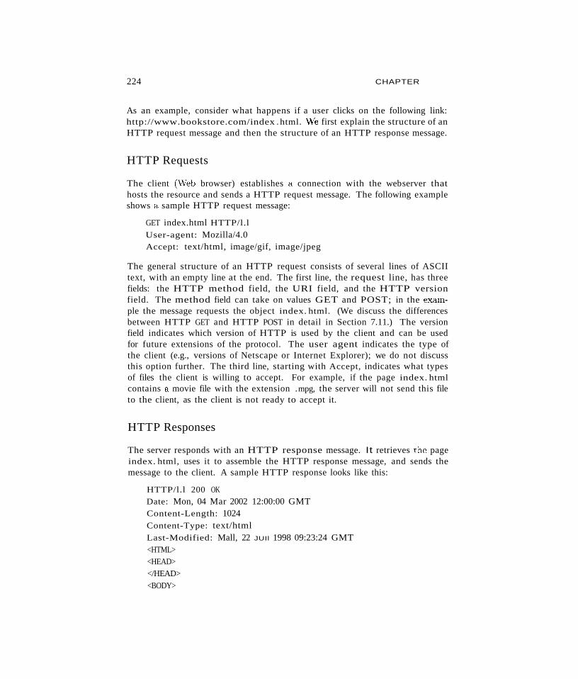
224 CHAPTER
As an example, consider what happens if a user clicks on the following link:http://www.bookstore.com/index . html. 'We first explain the structure of anHTTP request message and then the structure of an HTTP response message.
HTTP Requests
The client (\\Teb browser) establishes a connection with the webserver thathosts the resource and sends a HTTP request message. The following exampleshows a sample HTTP request message:
GET index.html HTTP/l.l
User-agent: Mozilla/4.0Accept: text/html, image/gif, image/jpeg
The general structure of an HTTP request consists of several lines of ASCIItext, with an empty line at the end. The first line, the request line, has threefields: the HTTP method field, the URI field, and the HTTP versionfield. The method field can take on values GET and POST; in the example the message requests the object index. html. (We discuss the differencesbetween HTTP GET and HTTP POST in detail in Section 7.11.) The versionfield indicates which version of HTTP is used by the client and can be usedfor future extensions of the protocol. The user agent indicates the type ofthe client (e.g., versions of Netscape or Internet Explorer); we do not discussthis option further. The third line, starting with Accept, indicates what typesof files the client is willing to accept. For example, if the page index. htmlcontains a movie file with the extension .mpg, the server will not send this fileto the client, as the client is not ready to accept it.
HTTP Responses
The server responds with an HTTP response message. It retrieves tht: pageindex. html, uses it to assemble the HTTP response message, and sends themessage to the client. A sample HTTP response looks like this:
HTTP/l.l 200 OKDate: Mon, 04 Mar 2002 12:00:00 GMTContent-Length: 1024Content-Type: text/htmlLast-Modified: Mall, 22 JUIl 1998 09:23:24 GMT<HTML><HEAD></HEAD>
<BODY>
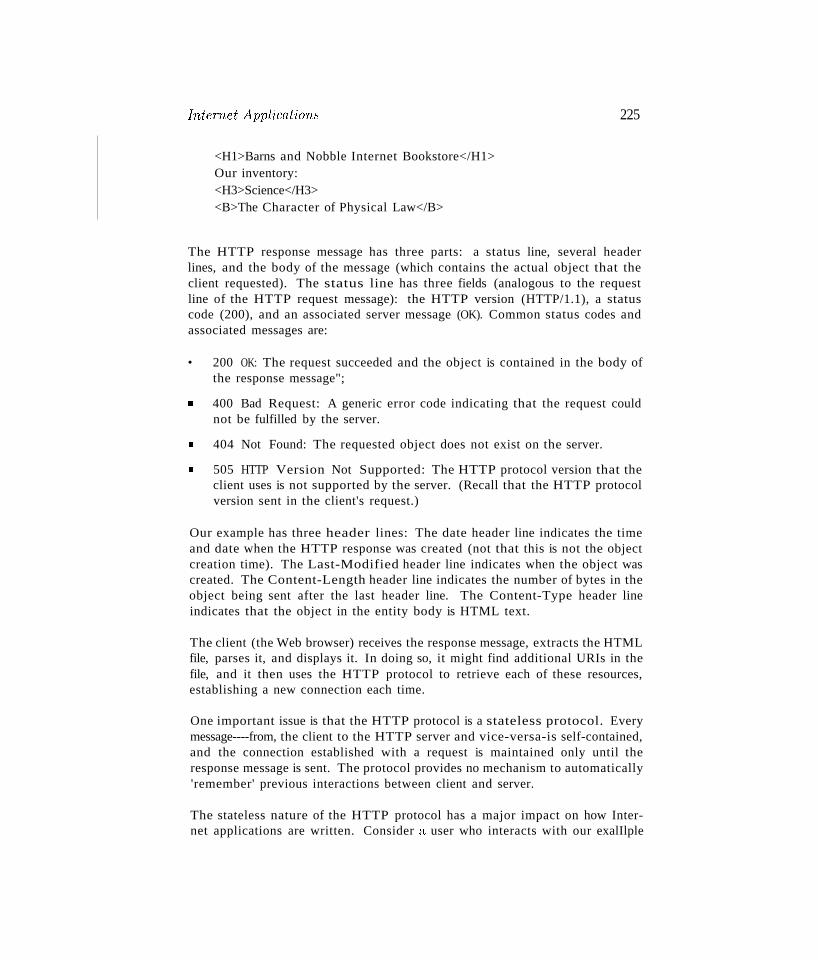
Internet Applications
<H1>Barns and Nobble Internet Bookstore</H1>Our inventory:<H3>Science</H3><B>The Character of Physical Law</B>
225
The HTTP response message has three parts: a status line, several headerlines, and the body of the message (which contains the actual object that theclient requested). The status line has three fields (analogous to the requestline of the HTTP request message): the HTTP version (HTTP/1.1), a statuscode (200), and an associated server message (OK). Common status codes andassociated messages are:
• 200 OK: The request succeeded and the object is contained in the body ofthe response message";
• 400 Bad Request: A generic error code indicating that the request couldnot be fulfilled by the server.
• 404 Not Found: The requested object does not exist on the server.
• 505 HTTP Version Not Supported: The HTTP protocol version that theclient uses is not supported by the server. (Recall that the HTTP protocolversion sent in the client's request.)
Our example has three header lines: The date header line indicates the timeand date when the HTTP response was created (not that this is not the objectcreation time). The Last-Modified header line indicates when the object wascreated. The Content-Length header line indicates the number of bytes in theobject being sent after the last header line. The Content-Type header lineindicates that the object in the entity body is HTML text.
The client (the Web browser) receives the response message, extracts the HTMLfile, parses it, and displays it. In doing so, it might find additional URIs in thefile, and it then uses the HTTP protocol to retrieve each of these resources,establishing a new connection each time.
One important issue is that the HTTP protocol is a stateless protocol. Everymessage----from, the client to the HTTP server and vice-versa-is self-contained,and the connection established with a request is maintained only until theresponse message is sent. The protocol provides no mechanism to automatically'remember' previous interactions between client and server.
The stateless nature of the HTTP protocol has a major impact on how Internet applications are written. Consider a user who interacts with our exalIlple
226 CHAPTER ,7
bookstore application. Assume that the bookstore permits users to log intothe site and then carry out several actions, such as ordering books or changingtheir address, without logging in again (until the login expires or the user logsout). How do we keep track of whether a user is logged in or not? Since HTTPis stateless, we cannot switch to a different state (say the 'logged in' state) atthe protocol level. Instead, for every request that the user (more precisely, hisor her Web browser) sends to the server, we must encode any state informationrequired by the application, such as the user's login status. Alternatively, theserver-side application code must maintain this state information and look itup on a per-request basis. This issue is explored further in Section 7.7.5.
Note that the statelessness of HTTP is a tradeoff between ease of implementation of the HTTP protocol and ease of application development. The designersof HTTP chose to keep the protocol itself simple, and deferred any functionalitybeyond the request of objects to application layers above the HTTP protocol.
7.3 HTML DOCUMENTS
In this section and the next, we focus on introducing HTML and XML. InSection 7.6, we consider how applications can use HTML and XML to createforms that capture user input, communicate with an HTTP server, and convertthe results produced by the data management layer into one of these formats.
HTML is a simple language used to describe a document. It is also called amarkup language because HTML works by augmenting regular text with'marks' that hold special meaning for a Web browser. Commands in the language, called tags, consist (usually) of a start tag and an end tag of theform <TAG> and </TAG>, respectively. For example, consider the HTML fragment shown in Figure 7.1. It describes a webpage that shows a list of books.The document is enclosed by the tags <HTML> and </HTML>, marking it as anHTML document. The remainder of the document-enclosed in <BODY> ...</BoDY>-contains information about three books. Data about each book isrepresented as an unordered list (UL) whose entries are marked with the LItag. HTML defines the set of valid tags as well 8.'3 the meaning of the tags. :Forexample, HTML specifies that the tag <TITLE> is a valid tag that denotes thetitle of the document. As another example, the tag <UL> always denotes anunordered list.
Audio, video, and even programs (written in Java, a highly portable language)can be included in HTML documents. vVhen a user retrieves such a documentusing a suitable browser, images in the document arc displayed, audio and videoclips are played, and embedded programs are executed at the uset's machine;the result is a rich multimedia presentation. The e8."ie with which HTML docu-
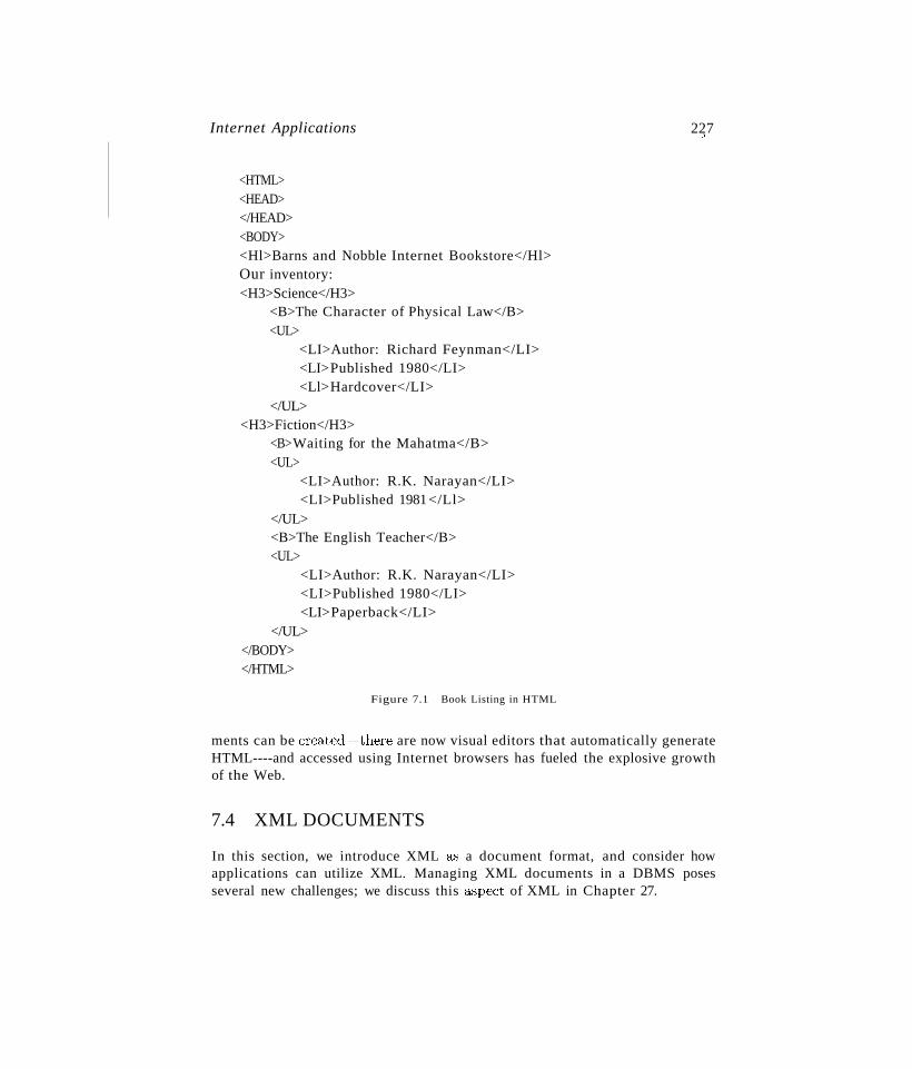
Internet Applications
<HTML><HEAD></HEAD><BODY><Hl>Barns and Nobble Internet Bookstore</Hl>Our inventory:<H3>Science</H3>
<B>The Character of Physical Law</B><UL>
<LI>Author: Richard Feynman</LI><LI>Published 1980</LI><Ll>Hardcover</LI>
</UL><H3>Fiction</H3>
<B>Waiting for the Mahatma</B><UL>
<LI>Author: R.K. Narayan</LI><LI>Published 1981</Ll>
</UL><B>The English Teacher</B><UL>
<LI>Author: R.K. Narayan</LI><LI>Published 1980</LI><LI>Paperback</LI>
</UL></BODY></HTML>
Figure 7.1 Book Listing in HTML
227»
ments can be created--there are now visual editors that automatically generateHTML----and accessed using Internet browsers has fueled the explosive growthof the Web.
7.4 XML DOCUMENTS
In this section, we introduce XML a.'3 a document format, and consider howapplications can utilize XML. Managing XML documents in a DBMS posesseveral new challenges; we discuss this a.'3pect of XML in Chapter 27.
228 CHAPTER l
vVhile HTl\.fL can be used to mark up documents for display purposes, it isnot adequate to describe the structure of the content for more general applications. For example, we can send the HTML document shown in Figure 7.1 toanother application that displays it, but the second application cannot distinguish the first names of authors from their last names. (The application cantry to recover such information by looking at the text inside the tags, but thisdefeats the purpose of using tags to describe document structure.) Therefore,HTML is unsuitable for the exchange of complex documents containing productspecifications or bids, for example.
Extensible Markup Language (XML) is a markup language developed toremedy the shortcomings of HTML. In contrast to a fixed set of tags whosemeaning is specified by the language (as in HTML), XML allows users to define new collections of tags that can be used to structure any type of data ordocument the user wishes to transmit. XML is an important bridge betweenthe document-oriented view of data implicit in HTML and the schema-orientedview of data that is central to a DBMS. It has the potential to make databasesystems more tightly integrated into Web applications than ever before.
XML emerged from the confluence of two technologies, SGML and HTML. TheStandard Generalized Markup Language (SGML) is a metalanguagethat allows the definition of data and document interchange languages such asHTML. The SGML standard was published in 1988, and many organizationsthat rnanage a large number of complex documents have adopted it. Due to itsgenerality, SGML is complex and requires sophisticated programs to harnessits full potential. XML was developed to have much of the power of SGMLwhile remaining relatively simple. Nonetheless, XML, like SGML, allows thedefinition of new document markup languages.
Although XML does not prevent a user from designing tags that encode thedisplay of the data in a Web browser, there is a style language for XML calledExtensible Style Language (XSL). XSL is a standard way of describinghow an XML docmnent that adheres to a certain vocabulary of tags should bedisplayed.
7.4.1 Introduction to XML
Vve use the smaJI XML docmnent shown in Figure 7.2 a,s an example.
11II Elements: Elements, also called tags, a.rc the primary building blocks ofan XML docmnent. The start of the content of an element ELM is markedwith <ELM>, which is called the start tag, and the end of the content endis marked with </ELM>, called the end tag. In our example document.
Internet Applicai'ions 229
The Design Goals ofXML: XML wa.."l developed'startingin 1996 by aworking group under guidance of the ';Yorld Wide Web Consortium (W3C)XML Special Interest Group. The design goals for XML included thefollowing:
1. XML should be compatible with SGML.
2. It should be easy to write programs that process XML documents.
3. The design of XML should be formal and concise.
the element BOOKLIST encloses all information in the sample document.The element BOOK demarcates all data associated with a single book.XML elements are case sensitive: the element BOOK is different fromBook. Elements must be properly nested. Start tags that appear insidethe content of other tags must have a corresponding end tag. For example,consider the following XML fragment:
<BOOK><AUTHOR>
<FIRSTNAME>Richard</FIRSTNAME><LASTNAME>Feynluan</LASTNAME>
</AUTHOR></BOOK>The element AUTHOR is completely nested inside the element BOOK, andboth the elements LASTNAME and FIRSTNAME are nested inside the elementAUTHOR.
.. Attributes: An element can have descriptive attributes that provide additional information about the element. The values of attributes are setinside the start tag of an element. For example, let ELM denote an elementwith the attribute att. We can set the value of att to value through thefollowing expression: <ELM att=" value II >. All attribute values must beenclosed in quotes. In Figure 7.2, the element BOOK has two attributes.The attribute GENRE indicates the genre of the book (science or fiction)and the attribute FORMAT indicates whether the book is a hardcover or apaperback.
III Entity References: Entities are shortcuts for portions of common text orthe content of external files, and we call the usage of an entity in the XMLdocument an entity reference. Wherever an entity reference appears inthe document, it is textually replaced by its content. Entity referencesstart with a '&' and end with a '; '. Five predefined entities in XML areplaceholders for chara.cters with special meaning in XML. For example, the
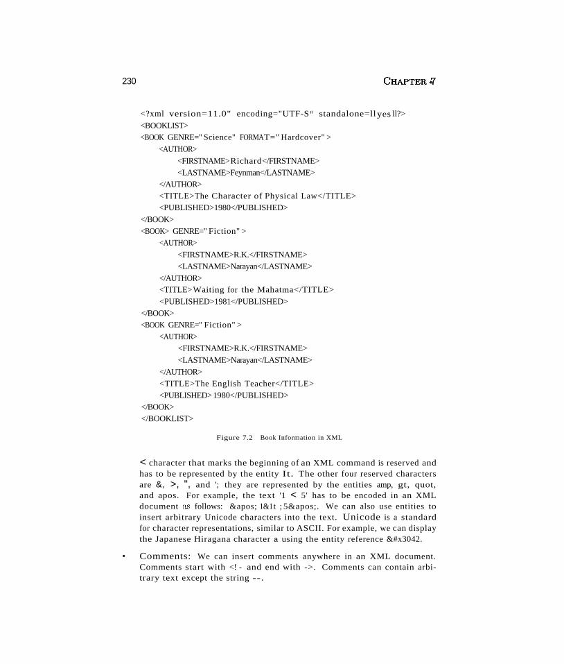
230 CHAPTER~7
<?xml version=11.0" encoding="UTF-S Il standalone=llyes ll?>
<BOOKLIST><BOOK GENRE=" Science" FORMAT=" Hardcover" >
<AUTHOR>
<FIRSTNAME>Richard</FIRSTNAME><LASTNAME>Feynman</LASTNAME>
</AUTHOR><TITLE>The Character of Physical Law</TITLE><PUBLISHED>1980</PUBLISHED>
</BOOK><BOOK> GENRE=" Fiction" >
<AUTHOR>
<FIRSTNAME>R.K.</FIRSTNAME><LASTNAME>Narayan</LASTNAME>
</AUTHOR><TITLE>Waiting for the Mahatma</TITLE>
<PUBLISHED>1981</PUBLISHED></BOOK><BOOK GENRE=" Fiction" >
<AUTHOR><FIRSTNAME>R.K.</FIRSTNAME>
<LASTNAME>Narayan</LASTNAME>
</AUTHOR><TITLE>The English Teacher</TITLE><PUBLISHED> 1980</PUBLISHED>
</BOOK></BOOKLIST>
Figure 7.2 Book Information in XML
< character that marks the beginning of an XML command is reserved andhas to be represented by the entity It. The other four reserved charactersare &, >, ", and '; they are represented by the entities amp, gt, quot,and apos. For example, the text '1 < 5' has to be encoded in an XMLdocument &'3 follows: ' 1&1t ; 5'. We can also use entities toinsert arbitrary Unicode characters into the text. Unicode is a standardfor character representations, similar to ASCII. For example, we can displaythe Japanese Hiragana character a using the entity reference あ.
• Comments: We can insert comments anywhere in an XML document.Comments start with <! - and end with ->. Comments can contain arbitrary text except the string --.
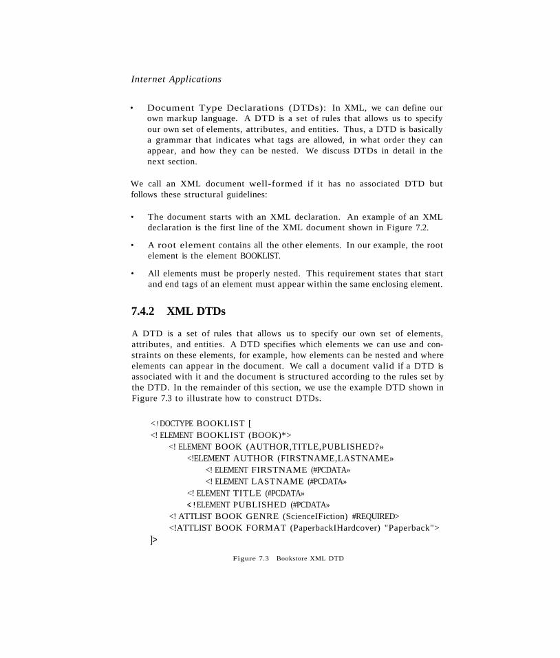
Internet Applications
• Document Type Declarations (DTDs): In XML, we can define ourown markup language. A DTD is a set of rules that allows us to specifyour own set of elements, attributes, and entities. Thus, a DTD is basicallya grammar that indicates what tags are allowed, in what order they canappear, and how they can be nested. We discuss DTDs in detail in thenext section.
We call an XML document well-formed if it has no associated DTD butfollows these structural guidelines:
• The document starts with an XML declaration. An example of an XMLdeclaration is the first line of the XML document shown in Figure 7.2.
• A root element contains all the other elements. In our example, the rootelement is the element BOOKLIST.
• All elements must be properly nested. This requirement states that startand end tags of an element must appear within the same enclosing element.
7.4.2 XML DTDs
A DTD is a set of rules that allows us to specify our own set of elements,attributes, and entities. A DTD specifies which elements we can use and constraints on these elements, for example, how elements can be nested and whereelements can appear in the document. We call a document valid if a DTD isassociated with it and the document is structured according to the rules set bythe DTD. In the remainder of this section, we use the example DTD shown inFigure 7.3 to illustrate how to construct DTDs.
< ! DOCTYPE BOOKLIST [<! ELEMENT BOOKLIST (BOOK)*>
<! ELEMENT BOOK (AUTHOR,TITLE,PUBLISHED?»<!ELEMENT AUTHOR (FIRSTNAME,LASTNAME»
<! ELEMENT FIRSTNAME (#PCDATA»<! ELEMENT LASTNAME (#PCDATA»
<! ELEMENT TITLE (#PCDATA»<! ELEMENT PUBLISHED (#PCDATA»
<! ATTLIST BOOK GENRE (ScienceIFiction) #REQUIRED><!ATTLIST BOOK FORMAT (PaperbackIHardcover) "Paperback">
]>
Figure 7.3 Bookstore XML DTD
232 CHAPTER .;{
A DTD is enclosed in <! DOCTYPE name [DTDdeclarationJ >, where name isthe name of the outermost enclosing tag, and DTDdeclaration is the text ofthe rules of the DTD. The DTD starts with the outermost element---the rootelenwnt--which is BOOKLIST in our example. Consider the next rule:
<!ELEMENT BOOKLIST (BOOK)*>
This rule tells us that the element BOOKLIST consists of zero or more BOOKelements. The * after BOOK indicates how many BOOK elements can appearinside the BOOKLIST element. A * denotes zero or more occurrences, a + denotesone or more occurrences, and a? denotes zero or one occurrence. For example,if we want to ensure that a BOOKLIST has at least one book, we could changethe rule as follows:
<!ELEMENT BOOKLIST (BOOK)+>
Let us look at the next rule:
<!ELEMENT BOOK (AUTHOR,TITLE,PUBLISHED?»
This rule states that a BOOK element contains a AUTHOR element, a TITLE element, and an optional PUBLISHED clement. Note the use of the? to indicatethat the information is optional by having zero or one occurrence of the element.Let us move ahead to the following rule:
< !ELEMENT LASTNAME (#PCDATA»
Until now we considered only elements that contained other elements. Thisrule states that LASTNAME is an element that does not contain other elements,but contains actual text. Elements that only contain other elements are saidto have element content, whereas elements that also contain #PCDATA are::laid to have mixed content. In general, an element type declaration has thefollowing structure:
< !ELEMENT (contentType»
Five possible content types are:
III Other elements.
II The special syrnbol #PCDATA, which indicates (parsed) character data.
II The special symbol EMPTY, which indicates that the element has no content.Elements that have no content are not required to have an end tag.
11II The special symbol ANY, which indicates that any content is permitted.This content should be avoided whenever possible ::lince it disables all checking of the document structure inside the element.
Internet Apphcat'ions 2~3
• A regular expression constructed from the preceding four choices. Aregular expression is one of the following:
- expL exp2, exp3: A list of regular expressions.
- exp*: An optional expression (zero or more occurrences).
- exp?: An optional expression (zero or one occurrences).
- exp+: A mandatory expression (one or more occurrences).
- expl I exp2: expl or exp2.
Attributes of elements are declared outside the element. For example, considerthe following attribute declaration from Figure 7.3:
<! ATTLIST BOOK GENRE (ScienceIFiction) #REQUIRED»
This XML DTD fragment specifies the attribute GENRE, which is an attributeof the element BOOK. The attribute can take two values: Science or Fiction.Each BOOK element must be described in its start tag by a GENRE attributesince the attribute is required as indicated by #REQUIRED. Let us look at thegeneral structure of a DTD attribute declaration:
<! ATTLIST elementName (attName attType default)+>
The keyword ATTLIST indicates the beginning of an attribute declaration. Thestring elementName is the name of the element with which the following attribute dcfinition is associated. What follows is the declaration of one or moreattributes. Each attribute has a name, as indicated by attName, and a type,as indicated by attType. XML defines several possible types for an attribute.We discuss only string types and enumerated types here. An attribute oftype string can take any string as a value. We can declare such an attribute bysetting its type field to CDATA. F'or example, we can declare a third attribute oftype string of the elernent BOOK a.s follows:
<!ATTLIST BOOK edition CDATA "1">
If an attribute has an enumerated type, we list all its possible values in theattribute declaration. In our example, the itttribute GENRE is an enumeratedattribute type; its possible attribute values are 'Science' and 'Fiction'.
The last part 'Of an attribute declaration is called its default specification.The DTD in Figure 7.:3 shows two different default specifications: #REQUIREDitnd the string 'Pitperback'. The default specification #REQUIRED indicates thatthe attribute is required and whenever its associated element itppears somewhere in the XML document ~t value for the attribute must be specified. Thedebult specification indicated by the string 'Paperback' indicates that the attribute is not required; whenever its a.')sociated element itppears without setting
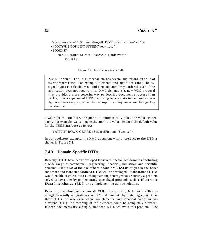
234
<?xml version=11.0" encoding=IUTF-8" standalone=" no "?>< ! DOCTYPE BOOKLIST SYSTEM" books.dtd" ><BOOKLIST>
<BOOK GENRE=" Science" FORMAT=" Hardcover" ><AUTHOR>
Figure 7.4 Book Information in XML
XML Schema: The DTD mechanism has several limitations, in spite ofits widespread use. For example, elements and attributes cannot be assigned types in a flexible way, and elements are always ordered, even if theapplication does not require this. XML Schema is a new W3C proposalthat provides a more powerful way to describe document structure thanDTDs; it is a superset of DTDs, allowing legacy data to be handled easily. An interesting aspect is that it supports uniqueness and foreign keyconstraints.
a value for the attribute, the attribute automatically takes the value 'Paperback'. For example, we can make the attribute value 'Science' the default valuefor the GENRE attribute as follows:
<! ATTLIST BOOK GENRE (ScienceIFiction) "Science" >
In our bookstore example, the XML document with a reference to the DTD isshown in Figure 7.4.
7.4.3 Domain-Specific DTDs
Recently, DTDs have been developed for several specialized domains-includinga wide range of commercial, engineering, financial, industrial, and scientificdomains----and a lot of the excitement about XML h3...<; its origins in the beliefthat more and more standardized DTDs will be developed. Standardized DTDswould enable seamless data exchange among heterogeneous sources, a problemsolved today either by implementing specialized protocols such as ElectronicData Interchange (EDI) or by implementing ad hoc solutions.
Even in an environment where all XML data is valid, it is not possible tostraightforwardly integrate several XML documents by matching elements intheir DTDs, because even when two elements have identical names in twodifferent DTDs, the meaning of the elements could be completely different.If both documents use a single, standard DTD, we avoid this problem. The
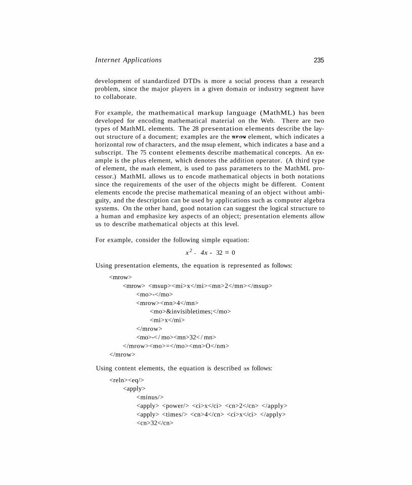
Internet Applications 235
development of standardized DTDs is more a social process than a researchproblem, since the major players in a given domain or industry segment haveto collaborate.
For example, the mathematical markup language (MathML) has beendeveloped for encoding mathematical material on the Web. There are twotypes of MathML elements. The 28 presentation elements describe the layout structure of a document; examples are the mrow element, which indicates ahorizontal row of characters, and the msup element, which indicates a base and asubscript. The 75 content elements describe mathematical concepts. An example is the plus element, which denotes the addition operator. (A third typeof element, the math element, is used to pass parameters to the MathML processor.) MathML allows us to encode mathematical objects in both notationssince the requirements of the user of the objects might be different. Contentelements encode the precise mathematical meaning of an object without ambiguity, and the description can be used by applications such as computer algebrasystems. On the other hand, good notation can suggest the logical structure toa human and emphasize key aspects of an object; presentation elements allowus to describe mathematical objects at this level.
For example, consider the following simple equation:
x 2- 4x - 32 = 0
Using presentation elements, the equation is represented as follows:
<mrow><mrow> <msup><mi>x</mi><mn>2</mn></msup>
<mo>-</mo><mrow><mn>4</mn>
<mo>&invisibletimes;</mo><mi>x</mi>
</mrow><mo>-</ mo><mn>32< / mn>
</mrow><mo>=</mo><mn>O</nm></mrow>
Using content elements, the equation is described as follows:
<reln><eq/><apply>
<minus/><apply> <power/> <ci>x</ci> <cn>2</cn> </apply><apply> <times/> <cn>4</cn> <ci>x</ci> </apply><cn>32</cn>
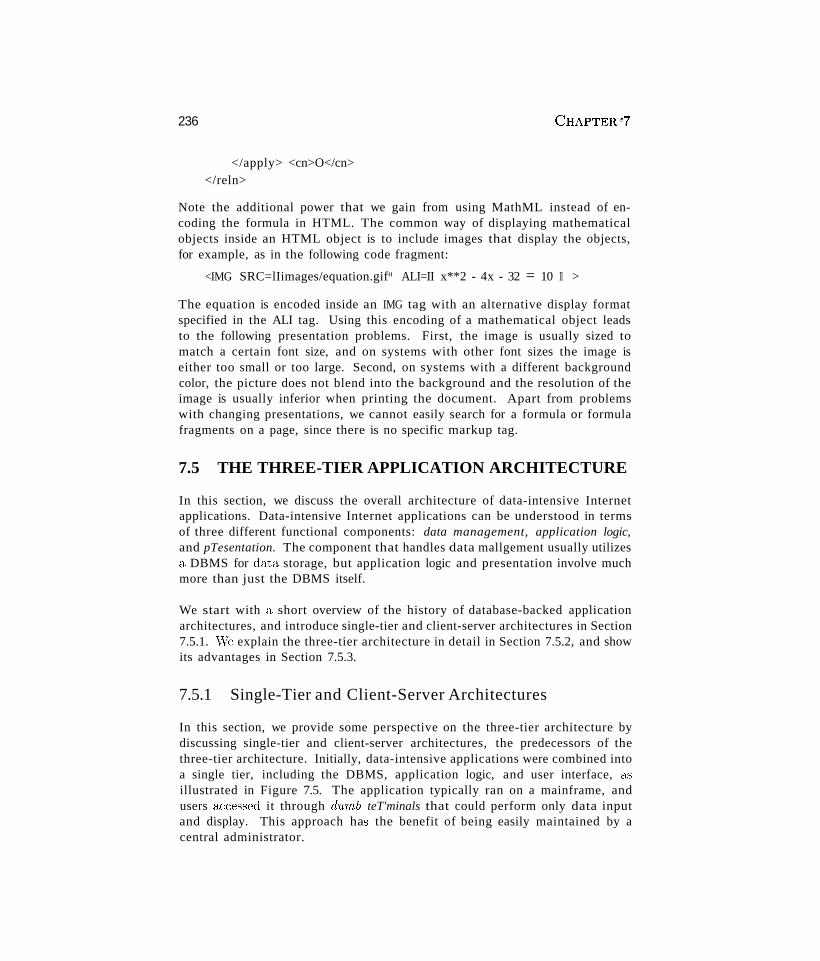
236
</apply> <cn>O</cn></reln>
CHAPTER J7
Note the additional power that we gain from using MathML instead of encoding the formula in HTML. The common way of displaying mathematicalobjects inside an HTML object is to include images that display the objects,for example, as in the following code fragment:
<IMG SRC=lIimages/equation.gifll ALI=II x**2 - 4x - 32 = 10 II >
The equation is encoded inside an IMG tag with an alternative display formatspecified in the ALI tag. Using this encoding of a mathematical object leadsto the following presentation problems. First, the image is usually sized tomatch a certain font size, and on systems with other font sizes the image iseither too small or too large. Second, on systems with a different backgroundcolor, the picture does not blend into the background and the resolution of theimage is usually inferior when printing the document. Apart from problemswith changing presentations, we cannot easily search for a formula or formulafragments on a page, since there is no specific markup tag.
7.5 THE THREE-TIER APPLICATION ARCHITECTURE
In this section, we discuss the overall architecture of data-intensive Internetapplications. Data-intensive Internet applications can be understood in termsof three different functional components: data management, application logic,and pTesentation. The component that handles data mallgement usually utilizesa DBMS for data storage, but application logic and presentation involve muchmore than just the DBMS itself.
We start with a short overview of the history of database-backed applicationarchitectures, and introduce single-tier and client-server architectures in Section7.5.1. \Ve explain the three-tier architecture in detail in Section 7.5.2, and showits advantages in Section 7.5.3.
7.5.1 Single-Tier and Client-Server Architectures
In this section, we provide some perspective on the three-tier architecture bydiscussing single-tier and client-server architectures, the predecessors of thethree-tier architecture. Initially, data-intensive applications were combined intoa single tier, including the DBMS, application logic, and user interface, a"illustrated in Figure 7.5. The application typically ran on a mainframe, andusers accessed it through dumb teT'minals that could perform only data inputand display. This approach ha..s the benefit of being easily maintained by acentral administrator.
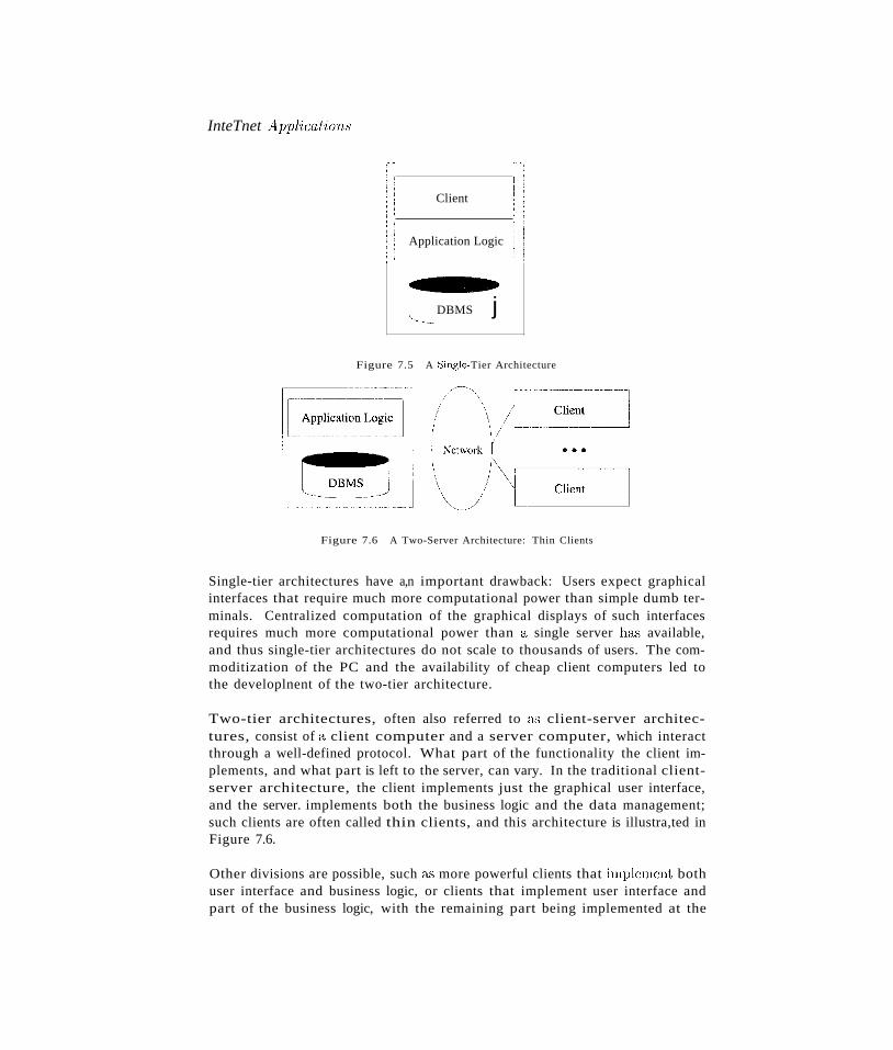
InteTnet Applications
Client
Application Logic
DBMS j
Figure 7.5 A Single-Tier Architecture
Figure 7.6 A Two-Server Architecture: Thin Clients
Single-tier architectures have a,n important drawback: Users expect graphicalinterfaces that require much more computational power than simple dumb terminals. Centralized computation of the graphical displays of such interfacesrequires much more computational power than a single server hclS available,and thus single-tier architectures do not scale to thousands of users. The commoditization of the PC and the availability of cheap client computers led tothe developlnent of the two-tier architecture.
Two-tier architectures, often also referred to a<; client-server architectures, consist of a client computer and a server computer, which interactthrough a well-defined protocol. What part of the functionality the client implements, and what part is left to the server, can vary. In the traditional clientserver architecture, the client implements just the graphical user interface,and the server. implements both the business logic and the data management;such clients are often called thin clients, and this architecture is illustra,ted inFigure 7.6.
Other divisions are possible, such as more powerful clients that hnplement bothuser interface and business logic, or clients that implement user interface andpart of the business logic, with the remaining part being implemented at the
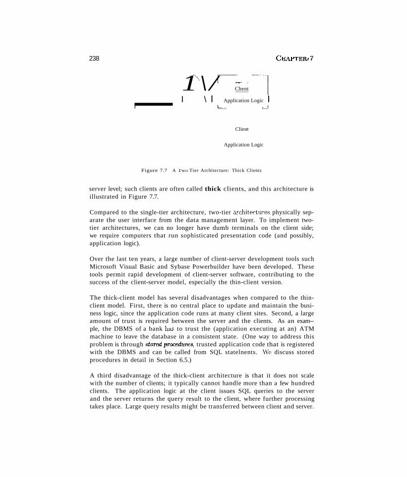
238
//~\ I--"-"-'---~-~I
1\/ Chent .. jI \ I Application Logic I
i i / ~. __-1
Client
Application Logic
Figure 7.7 A Two-Tier Architecture: Thick Clients
CHAPTERt7
server level; such clients are often called thick clients, and this architecture isillustrated in Figure 7.7.
Compared to the single-tier architecture, two-tier architectures physically separate the user interface from the data management layer. To implement twotier architectures, we can no longer have dumb terminals on the client side;we require computers that run sophisticated presentation code (and possibly,application logic).
Over the last ten years, a large number of client-server development tools suchMicrosoft Visual Basic and Sybase Powerbuilder have been developed. Thesetools permit rapid development of client-server software, contributing to thesuccess of the client-server model, especially the thin-client version.
The thick-client model has several disadvantages when compared to the thinclient model. First, there is no central place to update and maintain the business logic, since the application code runs at many client sites. Second, a largeamount of trust is required between the server and the clients. As an exam-pIe, the DBMS of a bank has to trust the (application executing at an) ATMmachine to leave the database in a consistent state. (One way to address thisproblem is through stored procedures, trusted application code that is registeredwith the DBMS and can be called from SQL statelnents. 'Ve discuss storedprocedures in detail in Section 6.5.)
A third disadvantage of the thick-client architecture is that it does not scalewith the number of clients; it typically cannot handle more than a few hundredclients. The application logic at the client issues SQL queries to the serverand the server returns the query result to the client, where further processingtakes place. Large query results might be transferred between client and server.
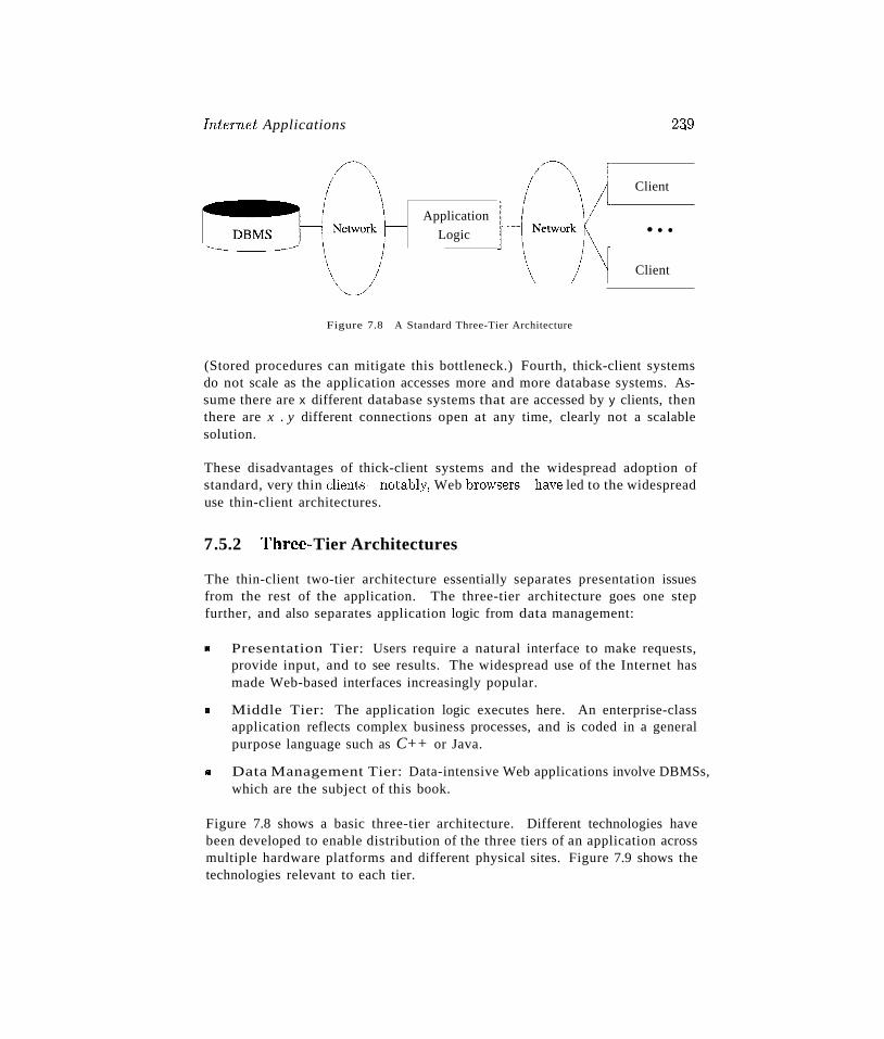
Inter-net Applications 2:19
Application
Logic
Client
• • •
Client
Figure 7.8 A Standard Three-Tier Architecture
(Stored procedures can mitigate this bottleneck.) Fourth, thick-client systemsdo not scale as the application accesses more and more database systems. Assume there are x different database systems that are accessed by y clients, thenthere are x . y different connections open at any time, clearly not a scalablesolution.
These disadvantages of thick-client systems and the widespread adoption ofstandard, very thin clients~notably,Web browsers~haveled to the widespreaduse thin-client architectures.
7.5.2 Three~Tier Architectures
The thin-client two-tier architecture essentially separates presentation issuesfrom the rest of the application. The three-tier architecture goes one stepfurther, and also separates application logic from data management:
III Presentation Tier: Users require a natural interface to make requests,provide input, and to see results. The widespread use of the Internet hasmade Web-based interfaces increasingly popular.
III Middle Tier: The application logic executes here. An enterprise-classapplication reflects complex business processes, and is coded in a generalpurpose language such as C++ or Java.
III Data Management Tier: Data-intensive Web applications involve DBMSs,which are the subject of this book.
Figure 7.8 shows a basic three-tier architecture. Different technologies havebeen developed to enable distribution of the three tiers of an application acrossmultiple hardware platforms and different physical sites. Figure 7.9 shows thetechnologies relevant to each tier.
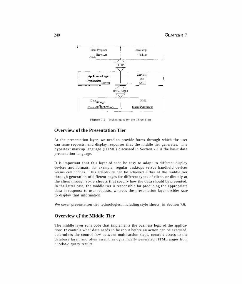
240
~i~-----",".~._,----~~---.~u·"r-----··'"
, Client Program I JavaScript
(Web Br_~=:~)__~_~_~~~~~__________ JHTIP
---:;;""io:~~I--" servle~~~----lJSP I
~PPlication Server) ~__.__.__ .....XSLT ~
JDBe. SQLJ
Data Storage---I----- XML -
(Database system)__ ___ Stored p:cedure~~__
Figure 7.9 Technologies for the Three Tiers
Overview of the Presentation Tier
CHAPTERi' 7
At the presentation layer, we need to provide forms through which the usercan issue requests, and display responses that the middle tier generates. Thehypertext markup language (HTML) discussed in Section 7.3 is the basic datapresentation language.
It is important that this layer of code be easy to adapt to different displaydevices and formats; for example, regular desktops versus handheld devicesversus cell phones. This adaptivity can be achieved either at the middle tierthrough generation of different pages for different types of client, or directly atthe client through style sheets that specify how the data should be presented.In the latter case, the middle tier is responsible for producing the appropriatedata in response to user requests, whereas the presentation layer decides howto display that information.
\Ve cover presentation tier technologies, including style sheets, in Section 7.6.
Overview of the Middle Tier
The middle layer runs code that implements the business logic of the application: It controls what data needs to be input before an action can be executed,determines the control flow between multi-action steps, controls access to thedatabase layer, and often assembles dynamically generated HTML pages fromdataba"se query results.
Internet Applications 24;1
The middle tier code is responsible for supporting all the different roles involvedin the application. For example, in an Internet shopping site implementation,we would like customers to be able to browse the catalog and make purchases,administrators to be able to inspect current inventory, and possibly data analysts to ask summary queries about purchase histories. Each of these roles canrequire support for several complex actions.
For example, consider the a customer who wants to buy an item (after browsingor searching the site to find it). Before a sale can happen, the customer hasto go through a series of steps: She has to add items to her shopping ba.sket,she has to provide her shipping address and credit card number (unless she hasan account at the site), and she has to finally confirm the sale with tax andshipping costs added. Controlling the flow among these steps and rememberingalready executed steps is done at the middle tier of the application. The datacarried along during this series of steps might involve database accesses, butusually it is not yet permanent (for example, a shopping basket is not storedin the database until the sale is confirmed).
We cover the middle tier in detail in Section 7.7.
7.5.3 Advantages of the Three-Tier Architecture
The three-tier architecture has the following advantages:
1/ Heterogeneous Systems: Applications can utilize the strengths of different platforms and different software components at the different tiers.It is easy to modify or replace the code at any tier without affecting theother tiers.
II Thin Clients: Clients only need enough computation power for the presentation layer. Typically, clients are Web browsers.
II Integrated Data Access: In many applications, the data must be accessed from several sources. This can be handled transparently at themiddle tier, where we can centrally manage connections to all databasesystems involved.
II Scalabilit,y to Many Clients: Each client is lightweight and all access tothe system is through the middle tier. The middle tier can share databaseconnections across clients, and if the middle tier becomes the bottle-neck,we can deploy several servers executing the middle tier code; clients canconnect to anyone of these servers, if the logic is designed appropriately.This is illustrated in Figure 7.10, which also shows how the middle tieraccesses multiple data sources. Of course, we rely upon the DBMS for each
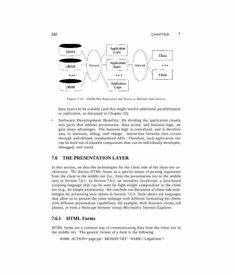
242 CHAPTER
Figure 7.10 Middle~Tier Replication and Access to Multiple Data Sources
7
data source to be scalable (and this might involve additional parallelizationor replication, as discussed in Chapter 22).
• Software Development Benefits: By dividing the application cleanlyinto parts that address presentation, data access, and business logic, wegain many advantages. The business logic is centralized, and is thereforeeasy to maintain, debug, and change. Interaction between tiers occursthrough well-defined, standardized APls. Therefore, each application tiercan be built out of reusable components that can be individually developed,debugged, and tested.
7.6 THE PRESENTATION LAYER
In this section, we describe technologies for the client side of the three-tier architecture. vVe discuss HTML forms as a special means of pa.ssing argumentsfrom the client to the middle tier (i.e., from the presentation tier to the middletier) in Section 7.6.1. In Section 7.6.2, we introduce JavaScript, a Java-basedscripting language that can be used for light-weight computation in the clienttier (e.g., for simple animations). We conclude our discussion of client-side technologies by presenting style sheets in Section 7.6.3. Style sheets are languagesthat allow us to present the same webpage with different formatting for clientswith different presentation capabilities; for example, Web browsers versus cellphones, or even a Netscape browser versus Microsoft's Internet Explorer.
7.6.1 HTML Forms
HTML forms are a common way of communicating data from the client tier tothe middle tier. The general format of a form is the following:
<FORM ACTION="page.jsp" METHOD="GET" NAME="LoginForm">
Internet Applications
</FORM>
246
A single HTML document can contain more than one form. Inside an HTMLform, we can have any HTML tags except another FORM element.
The FORM tag has three important attributes:
• ACTION: Specifies the URI of the page to which the form contents aresubmitted; if the ACTION attribute is absent, then the URI of the currentpage is used. In the sample above, the form input would be submited tothe page named page. j sp, which should provide logic for processing theinput from the form. (We will explain methods for reading form data atthe middle tier in Section 7.7.)
• METHOD: The HTTP/1.0 method used to submit the user input from thefilled-out form to the webserver. There are two choices, GET and POST; wepostpone their discussion to the next section.
• NAME: This attribute gives the form a name. Although not necessary,naming forms is good style. In Section 7.6.2, we discuss how to writeclient-side programs in JavaScript that refer to forms by name and performchecks on form fields.
Inside HTML forms, the INPUT, SELECT, and TEXTAREA tags are used to specifyuser input elements; a form can have many elements of each type. The simplestuser input element is an INPUT field, a standalone tag with no terminating tag.An example of an INPUT tag is the following:
<INPUT TYPE=ltext" NAME="title">
The INPUT tag has several attributes. The three most important ones are TYPE,NAME, and VALUE. The TYPE attribute determines the type of the input field. Ifthe TYPE attribute h&'3 value text, then the field is a text input field. If theTYPE attribute has value password, then the input field is a text field where theentered characters are displayed as stars on the screen. If the TYPE attributehas value reset, it is a simple button that resets all input fields within theform to their default values. If the TYPE attribute has value submit, then it isa button that sends the values of the different input fields in the form to theserver. Note that reset and submit input fields affect the entire form.
The NAME attribute of the INPUT tag specifies the symbolic name for this fieldand is used to identify the value of this input fi.eld when it is sent to the server.NAME has to be set for INPUT tags of all types except submit and reset. In thepreceding example, we specified title as the NAME of the input field.
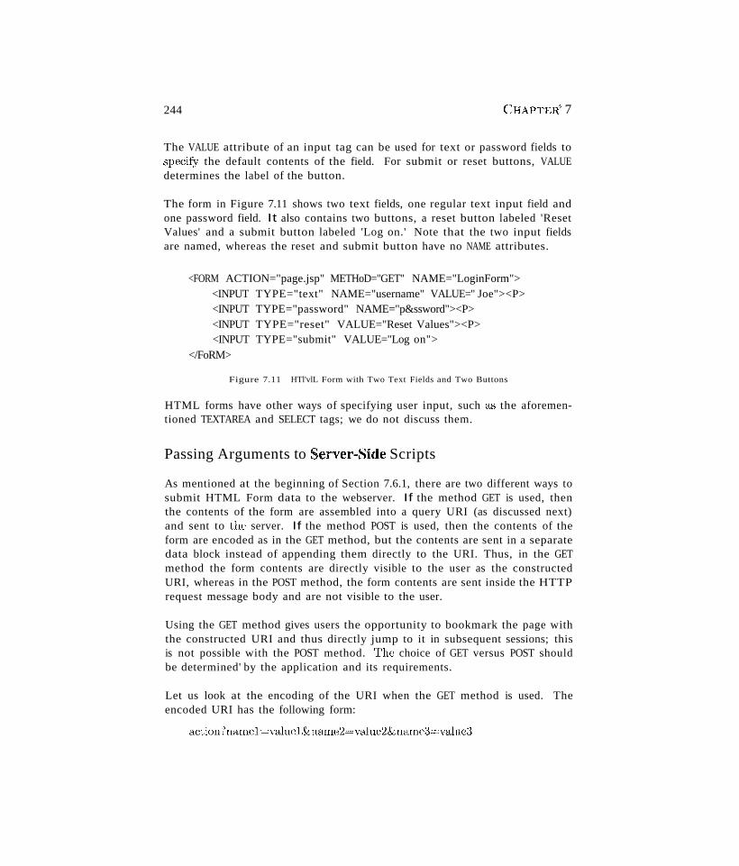
244 CHAPTER' 7
The VALUE attribute of an input tag can be used for text or password fields tospecify the default contents of the field. For submit or reset buttons, VALUEdetermines the label of the button.
The form in Figure 7.11 shows two text fields, one regular text input field andone password field. It also contains two buttons, a reset button labeled 'ResetValues' and a submit button labeled 'Log on.' Note that the two input fieldsare named, whereas the reset and submit button have no NAME attributes.
<FORM ACTION="page.jsp" METHoD="GET" NAME="LoginForm"><INPUT TYPE="text" NAME="username" VALUE=" Joe"><P><INPUT TYPE="password" NAME="p&ssword"><P><INPUT TYPE="reset" VALUE="Reset Values"><P><INPUT TYPE="submit" VALUE="Log on">
</FoRM>
Figure 7.11 HTl'vlL Form with Two Text Fields and Two Buttons
HTML forms have other ways of specifying user input, such as the aforementioned TEXTAREA and SELECT tags; we do not discuss them.
Passing Arguments to Server~Side Scripts
As mentioned at the beginning of Section 7.6.1, there are two different ways tosubmit HTML Form data to the webserver. If the method GET is used, thenthe contents of the form are assembled into a query URI (as discussed next)and sent to the server. If the method POST is used, then the contents of theform are encoded as in the GET method, but the contents are sent in a separatedata block instead of appending them directly to the URI. Thus, in the GETmethod the form contents are directly visible to the user as the constructedURI, whereas in the POST method, the form contents are sent inside the HTTPrequest message body and are not visible to the user.
Using the GET method gives users the opportunity to bookmark the page withthe constructed URI and thus directly jump to it in subsequent sessions; thisis not possible with the POST method. The choice of GET versus POST shouldbe determined' by the application and its requirements.
Let us look at the encoding of the URI when the GET method is used. Theencoded URI has the following form:
action?name1=vallle1&name2=value2&name;J=value3
Internet Applicat'icJns 245
The action is the URI specified in the ACTION attribute to the FORM tag, or thecurrent document URI if no ACTION attribute was specified. The 'name=value'pairs are the user inputs from the INPUT fields in the form. For form INPUTfields where the user did not input anything, the name is stil present with anempty value (name=). As a concrete example, consider the PCl,.'3sword submissionform at the end of the previous section. Assume that the user inputs 'JohnDoe' as username, and 'secret' as password. Then the request URI is:
page.jsp?username=J01111+Doe&password=secret
The user input from forms can contain general ASCII characters, such as thespace character, but URIs have to be single, consecutive strings with no spaces.Therefore, special characters such as spaces, '=', and other unprintable characters are encoded in a special way. To create a URI that has form fields encoded,we perform the following three steps:
1. Convert all special characters in the names and values to '%xyz,' where'xyz' is the ASCII value of the character in hexadecimal. Special charactersinclude =, &, %, +, and other unprintable characters. Note that we couldencode all characters by their ASCII value.
2. Convert all space characters to the '+' character.
3. Glue corresponding names and values from an individual HTML INPUT tagtogether with '=' and then paste name-value pairs from different HTMLINPUT tags together using'&' to create a request URI of the form:action?namel=value1&name2=value2&name3=value3
Note that in order to process the input elements from the HTML form atthe middle tier, we need the ACTION attribute of the FORM tag to point to apage, script, or program that will process the values of the form fields the userentered. We discuss ways of receiving values from form fields in Sections 7.7.1and 7.7.3.
7.6.2 JavaScript
JavaScript is a scripting language at the client tier with which we can addprograms to webpages that run directly at the client (Le., at the machine running the Web !)rowser). J avaScript is often used for the following types ofcomputation at the client:
III Browser Detection: J avaScript can be used to detect the browser typeand load a browser-specific page.
III Form Validation: JavaScript is used to perform simple consistency checkson form fields. For example, a JavaScript program might check whether a
246 CHAPTER~ 7
form input that asks for an email address contains the character '@,' or ifall required fields have been input by the user.
• Browser Control: This includes opening pages in customized windows;examples include the annoying pop-up advertisements that you see at manywebsites, which are programmed using JavaScript.
J avaScript is usually embedded into an HTML document with a special tag,the SCRIPT tag. The SCRIPT tag has the attribute LANGUAGE, which indicatesthe language in which the script is written. For JavaScript, we set the language attribute to JavaScript. Another attribute of the SCRIPT tag is theSRC attribute, which specifies an external file with JavaScript code that is automatically embedded into the HTML document. Usually JavaScript sourcecode files use a '.js' extension. The following fragment shows a JavaScript fileincluded in an HTML document:
<SCRIPT LANGUAGE=" JavaScript" SRC="validateForm.js"> </SCRIPT>
The SCRIPT tag can be placed inside HTML comments so that the JavaScriptcode is not displayed verbatim in Web browsers that do not recognize theSCRIPT tag. Here is another JavaScipt code example that creates a pop-upbox with a welcoming message. We enclose the JavaScipt code inside HTMLcomments for the reasons just mentioned.
<SCRIPT LANGUAGE=" JavaScript" ><I--
alert (" Welcome to our bookstore");//--></SCRIPT>
JavaScript provides two different commenting styles: single-line comments thatstart with the '//' character, and multi-line comments starting with '/*' andending with ,*/' characters.l
JavaScript has variables that can be numbers, boolean values (true or false),strings, and some other data types that we do not discuss. Global variables haveto be declared in advance of their usage with the keyword var, and they canbe used anywhere inside the HTML documents. Variables local to a JavaScriptfunction (explained next) need not be declared. Variables do not have a fixedtype, but implicitly have the type of the data to which they have been assigned.
1 Actually, '<! --' also marks the start of a single-line comment, which is why we did not haveto mark the HTML starting cormnent '<! --' in the preceding example using J avaScript commentnotation. In contrast, the HTML closing comment "-->" has to be commented out in JavaScript asit is interpreted otherwise.
Internet Applications 247,
JavaScript has the usual assignment operators (=, + =, etc.), the usual arithmetic operators (+, -, *, /, %), the usual comparison operators (==, ! =,>=, etc.), and the usual boolean operators (&& for logical AND, 11 for logicalOR, and! for negation). Strings can be concatenated using the '+' character. The type of an object determines the behavior of operators; for example1+1 is 2, since we are adding numbers, whereas "1"+"1" is "11," since weare concatenating strings. JavaScript contains the usual types of statements,such as assignments, conditional statements (if Ccondition) {statements;}else {statements; }), and loops (for-loop, do-while, and while-loop).
JavaScript allows us to create functions using the function keyword: functionf Cargl, arg2) {statements;}. We can call functions from JavaScript code,and functions can return values using the keyword return.
We conclude this introduction to JavaScript with a larger example of a JavaScriptfunction that tests whether the login and password fields of a HTML form arenot empty. Figure 7.12 shows the JavaScript function and the HTML form.The JavaScript code is a function called testLoginEmptyO that tests whethereither of the two input fields in the form named LoginForm is empty. In thefunction testLoginEmpty, we first use variable loginForm to refer to the formLoginForm using the implicitly defined variable document, which refers to thecurrent HTML page. (JavaScript has a library of objects that are implicitly defined.) We then check whether either of the strings loginForm. userif. valueor loginForm. password. value is empty.
The function testLoginEmpty is checked within a form event handler. Anevent handler is a function that is called if an event happens on an object ina webpage. The event handler we use is onSubmit, which is called if the submitbutton is pressed (or if the user presses return in a text field in the form). Ifthe event handler returns true, then the form contents are submitted to theserver, otherwise the form contents are not submitted to the server.
J avaScript has functionality that goes beyond the basics that we explained inthis section; the interested reader is referred to the bibliographic notes at theend of this chapter.
7.6.3 Style Sheets
Different clients have different displays, and we need correspondingly differentways of displaying the same information. For example, in the simplest ca.se,we might need to use different font sizes or colors that provide high-contra.ston a black-and-white screen. As a more sophisticated example, we might needto re-arrange objects on the page to accommodate small screens in personal
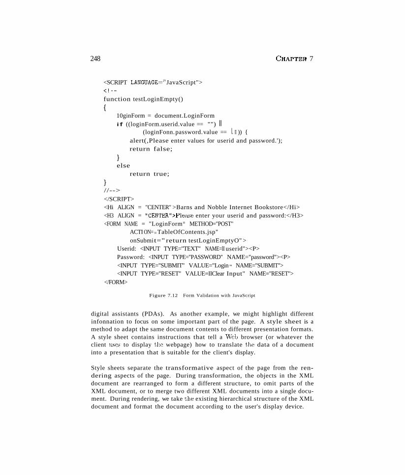
248 CHAPTER 7
<SCRIPT LANGUAGE==" JavaScript"><!--function testLoginEmpty(){
10ginForm = document.LoginFormif ((loginForm.userid.value == "") II
(loginFonn.password.value == I. II )) {alert(,Please enter values for userid and password.');return false;
}else
return true;
}//--></SCRIPT><Hi ALIGN = "CENTER" >Barns and Nobble Internet Bookstore</Hi><H3 ALIGN = "CENTER">Plec1Se enter your userid and password:</H3><FORM NAME = "LoginForm ll METHOD="POST"
ACTI ON= II TableOfContents.jsp"onSubmit=" return testLoginEmptyO" >
Userid: <INPUT TYPE="TEXT" NAME=lI userid"><P>Password: <INPUT TYPE="PASSWORD" NAME="password"><P><INPUT TYPE="SUBMIT" VALUE="Login " NAME="SUBMIT"><INPUT TYPE="RESET" VALUE=IIClear Input" NAME="RESET">
</FORM>
Figure 7.12 Form Validation with JavaScript
digital assistants (PDAs). As another example, we might highlight differentinfonnation to focus on some important part of the page. A style sheet is amethod to adapt the same document contents to different presentation formats.A style sheet contains instructions that tell a 'Veb browser (or whatever theclient uses to display the webpage) how to translate the data of a documentinto a presentation that is suitable for the client's display.
Style sheets separate the transformative aspect of the page from the rendering aspects of the page. During transformation, the objects in the XMLdocument are rearranged to form a different structure, to omit parts of theXML document, or to merge two different XML documents into a single document. During rendering, we take the existing hierarchical structure of the XMLdocument and format the document according to the user's display device.
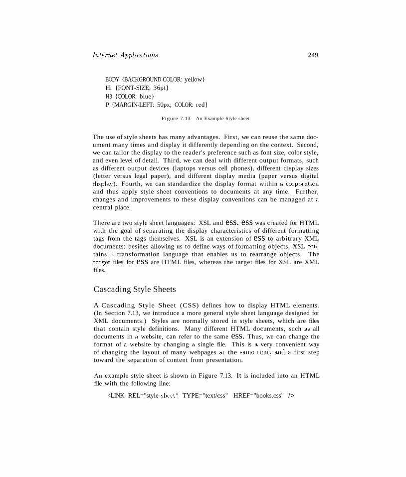
Inte17u'.t Apphcations
BODY {BACKGROUND-COLOR: yellow}Hi {FONT-SIZE: 36pt}H3 {COLOR: blue}P {MARGIN-LEFT: 50px; COLOR: red}
Figure 7.13 An Example Style sheet
249
The use of style sheets has many advantages. First, we can reuse the same document many times and display it differently depending on the context. Second,we can tailor the display to the reader's preference such as font size, color style,and even level of detail. Third, we can deal with different output formats, suchas different output devices (laptops versus cell phones), different display sizes(letter versus legal paper), and different display media (paper versus digitaldisplay). Fourth, we can standardize the display format within a corporationand thus apply style sheet conventions to documents at any time. Further,changes and improvements to these display conventions can be managed at acentral place.
There are two style sheet languages: XSL and ess. ess was created for HTMLwith the goal of separating the display characteristics of different formattingtags from the tags themselves. XSL is an extension of ess to arbitrary XMLdocurnents; besides allowing us to define ways of formatting objects, XSL contains a transformation language that enables us to rearrange objects. Thetarget files for ess are HTML files, whereas the target files for XSL are XMLfiles.
Cascading Style Sheets
A Cascading Style Sheet (CSS) defines how to display HTML elements.(In Section 7.13, we introduce a more general style sheet language designed forXML documents.) Styles are normally stored in style sheets, which are filesthat contain style definitions. Many different HTML documents, such as alldocuments in a website, can refer to the same ess. Thus, we can change theformat of a website by changing a single file. This is a very convenient wayof changing the layout of many webpages at the seune time, and a first steptoward the separation of content from presentation.
An example style sheet is shown in Figure 7.13. It is included into an HTMLfile with the following line:
<LINK REL="style sheet" TYPE="text/css" HREF="books.css" />
250 CHAPTERt7
Each line in a CSS sheet consists of three parts; a selector, a property, and avalue. They are syntactically arranged in the following way:
selector {property: value}
The selector is the element or tag whose format we are defining. The propertyindicates the tag's attribute whose value we want to set in the style sheet, andthe property is the actual value of the attribute. As an example, consider thefirst line of the example style sheet shown in Figure 7.13:
BODY {BACKGROUND-COLOR: yellow}
This line has the same effect as changing the HTML code to the following:
<BODY BACKGROUND-COLOR=" yellow" >.
The value should always be quoted, as it could consist of several words. Morethan one property for the same selector can be separated by semicolons asshown in the last line of the example in Figure 7.13:
P {MARGIN-LEFT: 50px; COLOR: red}
Cascading style sheets have an extensive syntax; the bibliographic notes at theend of the chapter point to books and online resources on CSSs.
XSL
XSL is a language for expressing style sheets. An XSL style sheet is, like CSS,a file that describes how to display an XML document of a given type. XSLshares the functionality of CSS and is compatible with it (although it uses adifferent syntax).
The capabilities of XSL vastly exceed the functionality of CSS. XSL containsthe XSL Transformation language, or XSLT, a language that allows 11S totransform the input XML document into a XML document with another structure. For example, with XSLT we can change the order of elements that we aredisplaying (e.g.; by sorting them), process elements more than once, suppresselements in one place and present them in another, and add generated text tothe presentation.
XSL also contains the XML Path Language (XPath), a language thatallows us to refer to parts of an XML document. We discuss XPath in Section
Inte1~net Applications 251
27. XSL also contains XSL Formatting Object, a way of formatting the outputof an XSL transformation.
7.7 THE MIDDLE TIER
In this section, we discuss technologies for the middle tier. The first generation of middle-tier applications were stand-alone programs written in ageneral-purpose programming language such as C, C++, and Perl. Programmers quickly realized that interaction with a stand-alone application was quitecostly; the overheads include starting the application every time it is invokedand switching processes between the webserver and the application. Therefore,such interactions do not scale to large numbers of concurrent users. This ledto the development of the application server, which provides the run-timeenvironment for several technologies that can be used to program middle-tierapplication components. Most of today's large-scale websites use an applicationserver to run application code at the middle tier.
Our coverage of technologies for the middle tier mirrors this evolution. Westart in Section 7.7.1 with the Common Gateway Interface, a protocol that isused to transmit arguments from HTML forms to application programs running at the middle tier. We introduce application servers in Section 7.7.2. Wethen describe technologies for writing application logic at the middle tier: Javaservlets (Section 7.7.3) and Java Server Pages (Section 7.7.4). Another important functionality is the maintenance of state in the middle tier component ofthe application as the client component goes through a series of steps to complete a transaction (for example, the purchase of a market basket of items orthe reservation of a flight). In Section 7.7.5, we discuss Cookies, one approachto maintaining state.
7.7.1 CGI: The Common Gateway Interface
The Common Gateway Interface connects HTML forms with application programs. It is a protocol that defines how arguments from forms are passed toprograms at the server side. We do not go into the details of the actual CGIprotocol since libraries enable application programs to get arguments from theHTML fonn; we shortly see an example in a CGI program. Programs thatcommunicate with the webserver via CGI are often called CGI scripts, sincemany such application programs were written in a scripting language such Ike.;
Perl.
As an example of a program that interfaces with an HTML form via CGI,consider the sample page shown in Figure 7.14. This webpage contains a formwhere a user can fill in the name of an author. If the user presses the 'Send
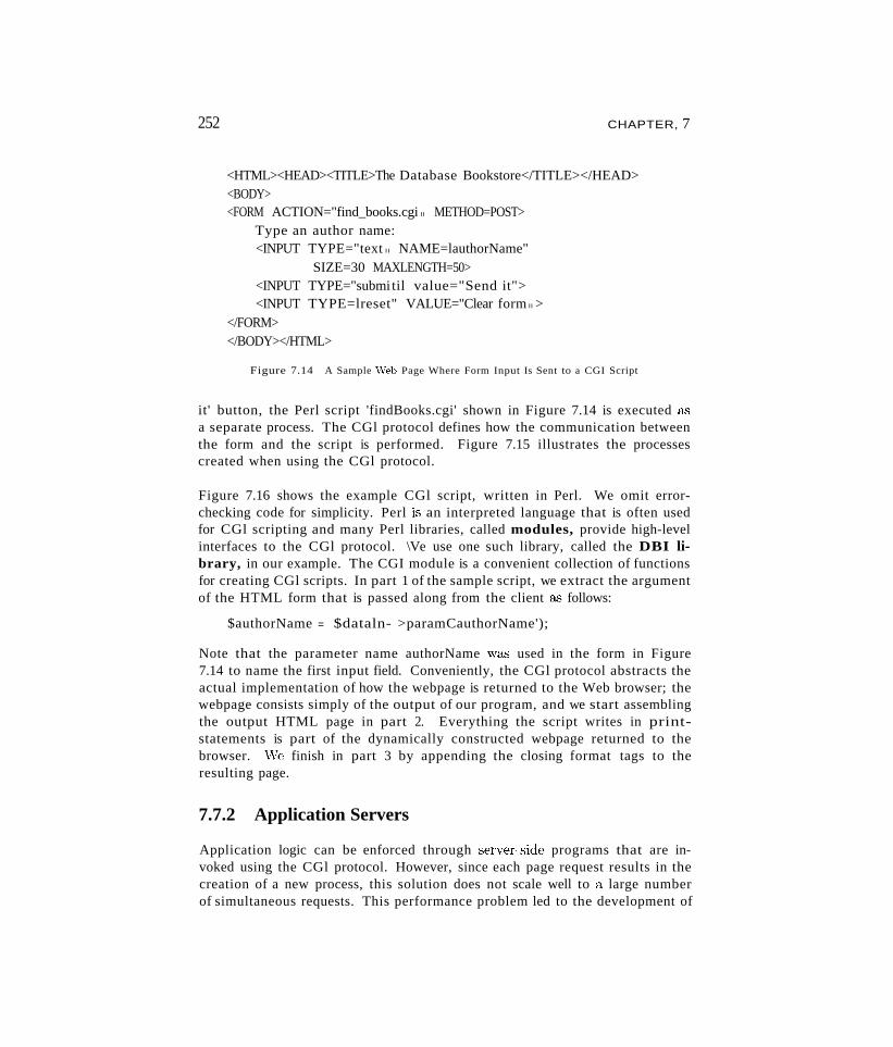
252 CHAPTER, 7
<HTML><HEAD><TITLE>The Database Bookstore</TITLE></HEAD><BODY><FORM ACTION="find_books.cgi II METHOD=POST>
Type an author name:<INPUT TYPE="text II NAME=lauthorName"
SIZE=30 MAXLENGTH=50><INPUT TYPE="submi til value="Send it"><INPUT TYPE=lreset" VALUE="Clear form II >
</FORM></BODY></HTML>
Figure 7.14 A Sample 'Neb Page Where Form Input Is Sent to a CGI Script
it' button, the Perl script 'findBooks.cgi' shown in Figure 7.14 is executed asa separate process. The CGl protocol defines how the communication betweenthe form and the script is performed. Figure 7.15 illustrates the processescreated when using the CGl protocol.
Figure 7.16 shows the example CGl script, written in Perl. We omit errorchecking code for simplicity. Perl is· an interpreted language that is often usedfor CGl scripting and many Perl libraries, called modules, provide high-levelinterfaces to the CGl protocol. \Ve use one such library, called the DBI library, in our example. The CGI module is a convenient collection of functionsfor creating CGl scripts. In part 1 of the sample script, we extract the argumentof the HTML form that is passed along from the client as follows:
$authorName = $dataln- >paramCauthorName');
Note that the parameter name authorName wa.s used in the form in Figure7.14 to name the first input field. Conveniently, the CGl protocol abstracts theactual implementation of how the webpage is returned to the Web browser; thewebpage consists simply of the output of our program, and we start assemblingthe output HTML page in part 2. Everything the script writes in printstatements is part of the dynamically constructed webpage returned to thebrowser. \Ve finish in part 3 by appending the closing format tags to theresulting page.
7.7.2 Application Servers
Application logic can be enforced through server-side programs that are invoked using the CGl protocol. However, since each page request results in thecreation of a new process, this solution does not scale well to a large numberof simultaneous requests. This performance problem led to the development of
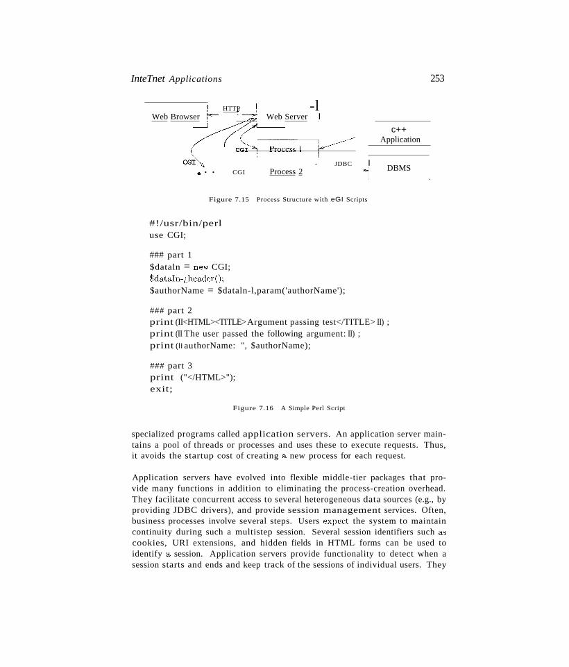
InteTnet Applications 253
DBMS
c++Application
I HTTP i -lWeb Browser r- ~ Web Server I
//(G( c~~-p-ro-c-'e-s-s-l--~
CGI~ - JDBC I• • • CGI Process 2 'I
L..-- ---'
Figure 7.15 Process Structure with eGI Scripts
#!/usr/bin/perluse CGI;
### part 1$dataln = new CGI;$dataln-l,headerO;$authorName = $dataln-l,param('authorName');
### part 2print (II<HTML><TITLE>Argument passing test</TITLE> II) ;print (II The user passed the following argument: II) ;print (lI authorName: ", $authorName);
### part 3print ("</HTML>");exit;
Figure 7.16 A Simple Perl Script
specialized programs called application servers. An application server maintains a pool of threads or processes and uses these to execute requests. Thus,it avoids the startup cost of creating a new process for each request.
Application servers have evolved into flexible middle-tier packages that provide many functions in addition to eliminating the process-creation overhead.They facilitate concurrent access to several heterogeneous data sources (e.g., byproviding JDBC drivers), and provide session management services. Often,business processes involve several steps. Users expect the system to maintaincontinuity during such a multistep session. Several session identifiers such ascookies, URI extensions, and hidden fields in HTML forms can be used toidentify a session. Application servers provide functionality to detect when asession starts and ends and keep track of the sessions of individual users. They
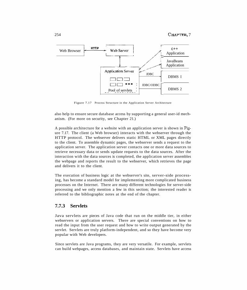
254
Web Browser
DODDO ••• :
I
Pool of servlets I--~-----~-~_ .....
JDBC
JDBC/ODBC
CHAPTER" 7
c++Application
JavaBeansApplication
DBMS I
DBMS 2
Figure 7.17 Process Structure in the Application Server Architecture
also help to ensure secure database access by supporting a general user-id mechanism. (For more on security, see Chapter 21.)
A possible architecture for a website with an application server is shown in Figure 7.17. The client (a Web browser) interacts with the webserver through theHTTP protocol. The webserver delivers static HTML or XML pages directlyto the client. To assemble dynamic pages, the webserver sends a request to theapplication server. The application server contacts one or more data sources toretrieve necessary data or sends update requests to the data sources. After theinteraction with the data sources is completed, the application server assemblesthe webpage and reports the result to the webserver, which retrieves the pageand delivers it to the client.
The execution of business logic at the webserver's site, server-side processing, has become a standard model for implementing more complicated businessprocesses on the Internet. There are many different technologies for server-sideprocessing and we only mention a few in this section; the interested reader isreferred to the bibliographic notes at the end of the chapter.
7.7.3 Servlets
Java servlets are pieces of Java code that run on the middle tier, in eitherwebservers or application servers. There are special conventions on how toread the input from the user request and how to write output generated by theservlet. Servlets are truly platform-independent, and so they have become verypopular with Web developers.
Since servlets are Java programs, they are very versatile. For example, servletscan build webpages, access databases, and maintain state. Servlets have access
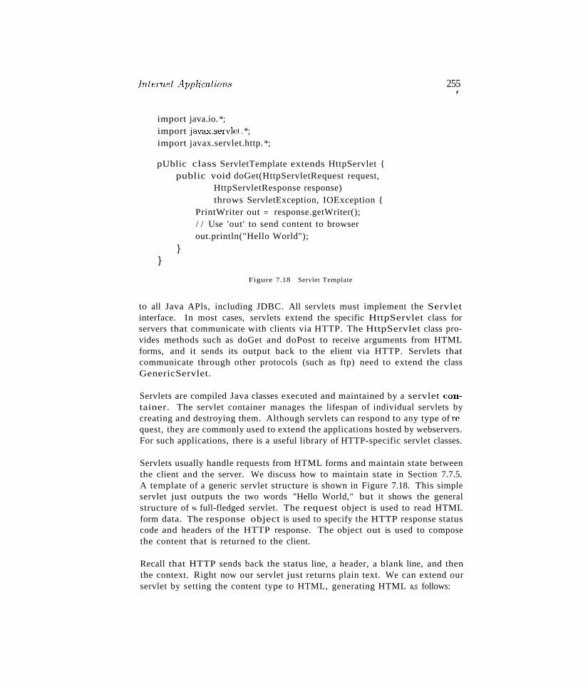
InteT1Iet AIJplications
import java.io.*;
import javCLx.servlet. *;import javax.servlet.http.*;
pUblic class ServletTemplate extends HttpServlet {public void doGet(HttpServletRequest request,
HttpServletResponse response)throws ServletException, IOException {
PrintWriter out = response.getWriter();/ / Use 'out' to send content to browserout.println("Hello World");
}}
Figure 7.18 Servlet Template
255@
to all Java APls, including JDBC. All servlets must implement the Servletinterface. In most cases, servlets extend the specific HttpServlet class forservers that communicate with clients via HTTP. The HttpServlet class provides methods such as doGet and doPost to receive arguments from HTMLforms, and it sends its output back to the elient via HTTP. Servlets thatcommunicate through other protocols (such as ftp) need to extend the classGenericServlet.
Servlets are compiled Java classes executed and maintained by a servlet container. The servlet container manages the lifespan of individual servlets bycreating and destroying them. Although servlets can respond to any type of request, they are commonly used to extend the applications hosted by webservers.For such applications, there is a useful library of HTTP-specific servlet classes.
Servlets usually handle requests from HTML forms and maintain state betweenthe client and the server. We discuss how to maintain state in Section 7.7.5.A template of a generic servlet structure is shown in Figure 7.18. This simpleservlet just outputs the two words "Hello World," but it shows the generalstructure of a full-fledged servlet. The request object is used to read HTMLform data. The response object is used to specify the HTTP response statuscode and headers of the HTTP response. The object out is used to composethe content that is returned to the client.
Recall that HTTP sends back the status line, a header, a blank line, and thenthe context. Right now our servlet just returns plain text. We can extend ourservlet by setting the content type to HTML, generating HTML a,s follows:
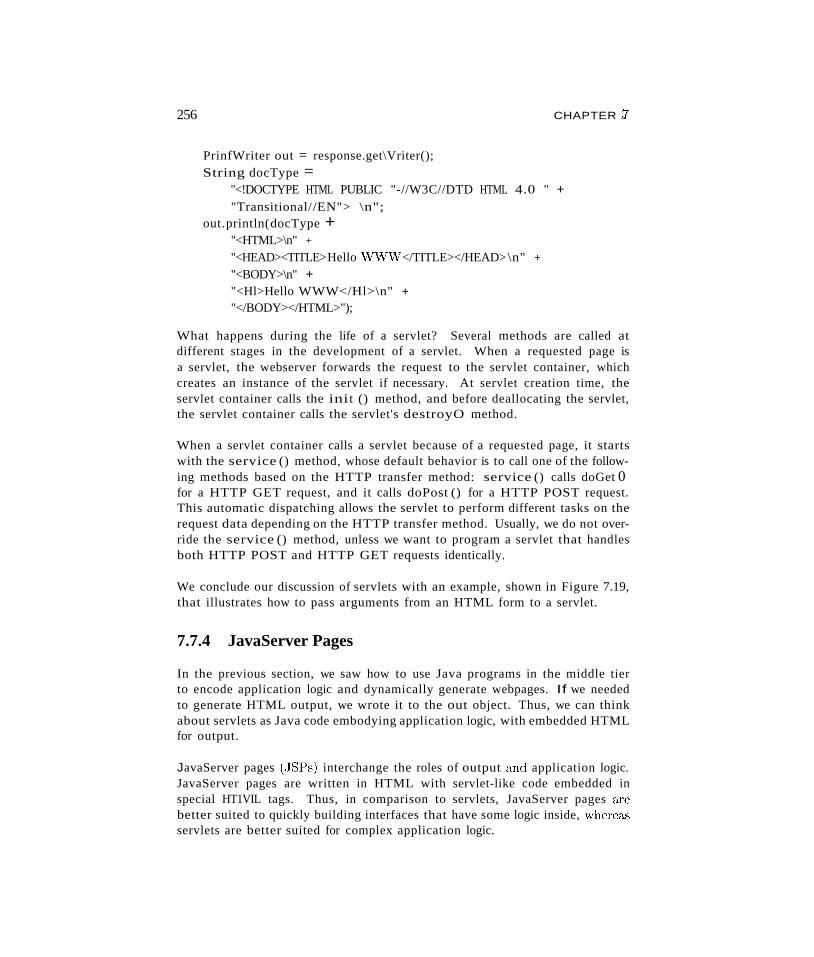
256 CHAPTER .7
PrinfWriter out = response.get\Vriter();String docType =
"<!DOCTYPE HTML PUBLIC "-//W3C//DTD HTML 4.0 " +"Transitional//EN"> \n";
out.println(docType +"<HTML>\n" +
"<HEAD><TITLE>Hello 'vVWW</TITLE></HEAD>\n" +
"<BODY>\n" +"<Hl>Hello WWW</Hl>\n" +"</BODY></HTML>");
What happens during the life of a servlet? Several methods are called atdifferent stages in the development of a servlet. When a requested page isa servlet, the webserver forwards the request to the servlet container, whichcreates an instance of the servlet if necessary. At servlet creation time, theservlet container calls the init () method, and before deallocating the servlet,the servlet container calls the servlet's destroyO method.
When a servlet container calls a servlet because of a requested page, it startswith the service () method, whose default behavior is to call one of the following methods based on the HTTP transfer method: service () calls doGet 0for a HTTP GET request, and it calls doPost () for a HTTP POST request.This automatic dispatching allows the servlet to perform different tasks on therequest data depending on the HTTP transfer method. Usually, we do not override the service () method, unless we want to program a servlet that handlesboth HTTP POST and HTTP GET requests identically.
We conclude our discussion of servlets with an example, shown in Figure 7.19,that illustrates how to pass arguments from an HTML form to a servlet.
7.7.4 JavaServer Pages
In the previous section, we saw how to use Java programs in the middle tierto encode application logic and dynamically generate webpages. If we neededto generate HTML output, we wrote it to the out object. Thus, we can thinkabout servlets as Java code embodying application logic, with embedded HTMLfor output.
JavaServer pages (.JSPs) interchange the roles of output amI application logic.JavaServer pages are written in HTML with servlet-like code embedded inspecial HT1VIL tags. Thus, in comparison to servlets, JavaServer pages arebetter suited to quickly building interfaces that have some logic inside, wherea..':iservlets are better suited for complex application logic.
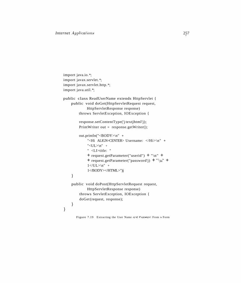
Internet Applications
import java.io. *;
import javax.servlet. *;
import javax.servlet.http.*;
import java.util.*;
public class ReadUserName extends HttpServlet {public void doGet(HttpServletRequest request,
HttpServletResponse response)throws ServletException, IOException {
response.setContentType('j textjhtml'j);
PrintWriter out = response.getWriter();
out.println("<BODY>\n" +
"<Hi ALIGN=CENTER> Username: </Hi>\n" +
"<UL>\n" +
" <LI>title: "+ request.getParameter("userid") + "\n" ++ request.getParameter("password'j) + "\n
j' +
1</UL>\n" +
1</BODY></HTML>")j
}
public void doPost(HttpServletRequest request,HttpServletResponse response)
throws ServletException, IOException {doGet (request, response);
}}
Figure 7.19 Extracting the User Name and Password From a Form
257J
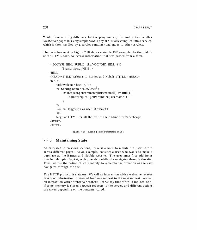
258 CHAPTER,7
~While there is a big difference for the programmer, the middle tier handlesJavaServer pages in a very simple way: They are usually compiled into a servlet,which is then handled by a servlet container analogous to other servlets.
The code fragment in Figure 7.20 shows a simple JSP example. In the middleof the HTML code, we access information that was passed from a form.
< !DOCTYPE HTML PUBLIC 11_//W3C/ /DTD HTML 4.0
Transitional//EN lI ><HTML><HEAD><TITLE>Welcome to Barnes and Nobble</TITLE></HEAD><BODY>
<Hl>Welcome back!</Hl><% String name="NewUser ll ;
if (request.getParameter(lIusernamell) != null) {name=request .getParameter (" username" );
}%>You are logged on as user <%=name%><P>Regular HTML for all the rest of the on-line store's webpage.
</BODY></HTML>
Figure 7.20 Reading Form Parameters in JSP
7.7.5 Maintaining State
As discussed in previous sections, there is a need to maintain a user's stateacross different pages. As an example, consider a user who wants to make apurchase at the Barnes and Nobble website. The user must first add itemsinto her shopping basket, which persists while she navigates through the site.Thus, we use the notion of state mainly to remember information as the usernavigates through the site.
The HTTP protocol is stateless. We call an interaction with a webserver stateless if no inforination is retained from one request to the next request. We callan interaction with a webserver stateful, or we say that state is maintained,if some memory is stored between requests to the server, and different actionsare taken depending on the contents stored.
Internet Applico,tiol/s 259!
In our example of Barnes and Nobble, we need to maintain the shopping basketof a user. Since state is not encapsulated in the HTTP protocol, it has to bemaintained either at the server or at the client. Since the HTTP protocolis stateless by design, let us review the advantages and disadvantages of thisdesign decision. First, a stateless protocol is easy to program and use, andit is great for applications that require just retrieval of static information. Inaddition, no extra memory is used to maintain state, and thus the protocolitself is very efficient. On the other hand, without some additional mechanismat the presentation tier and the middle tier, we have no record of previousrequests, and we cannot program shopping baskets or user logins.
Since we cannot maintain state in the HTTP protocol, where should we mtaintain state? There are basically two choices. We can maintain state in themiddle tier, by storing information in the local main memory of the application logic, or even in a database system. Alternatively, we can maintain stateon the client side by storing data in the form of a cookie. We discuss these twoways of maintaining state in the next two sections.
Maintaining State at the Middle Tier
At the middle tier, we have several choices as to where we maintain state.First, we could store the state at the bottom tier, in the database server. Thestate survives crashes of the system, but a database access is required to queryor update the state, a potential performance bottleneck. An alternative is tostore state in main memory at the middle tier. The drawbacks are that thisinformation is volatile and that it might take up a lot of main memory. Wecan also store state in local files at the middle tier, &s a compromise betweenthe first two approaches.
A rule of thumb is to use state maintenance at the middle tier or database tieronly for data that needs to persist over many different user sessions. Examplesof such data are past customer orders, click-stream data recording a user'smovement through the website, or other permanent choices that a user makes,such as decisions about personalized site layout, types of messages the user iswilling to receive, and so on. As these examples illustrate, state information isoften centered around users who interact with the website.
Maintaining State at the Presentation Tier: Cookies
Another possibility is to store state at the presentation tier and pass it to themiddle tier with every HTTP request. We essentially work around aroundthe statelessness of the HTTP protocol by sending additional information withevery request. Such information is called a cookie.
260 CHAPTE~ 7
/ / no 88L required/ / one month lifetime
A cookie is a collection of (name, val'Ue)~~pairs that can be manipulated atthe presentation and middle tiers. Cookies are ea..''!Y to use in Java servletsand J ava8erver Pages and provide a simple way to make non-essential datapersistent at the client. They survive several client sessions because they persistin the browser cache even after the browser is closed.
One disadvantage of cookies is that they are often perceived as as being invasive,and many users disable cookies in their Web browser; browsers allow users toprevent cookies from being saved on their machines. Another disadvantage isthat the data in a cookie is currently limited to 4KB, but for most applicationsthis is not a bad limit.
We can use cookies to store information such as the user's shopping basket, logininformation, and other non-permanent choices made in the current session.
Next, we discuss how cookies can be manipulated from servlets at the middletier.
The Servlet Cookie API
A cookie is stored. in a small text file at the client and. contains (name, val'l1e/pairs, where both name and value are strings. We create a new cookie throughthe Java Cookie class in the middle tier application code:
Cookie cookie = new Cookie( II username" ,"guest" );cookie.setDomain(" www.bookstore.com .. );cookie.set8ecure(false);cookie.setMaxAge(60*60*24*7*31);response.addCookie(cookie);
Let us look at each part of this code. First, we create a new Cookie object withthe specified (name, val'l1e)~~·pair. Then we set attributes of the cookie; we listsome of the most common attributes below:
III setDomain and getDomain: The domain specifies the website that willreceive the cookie. The default value for this attribute is the domain thatcreated the cookie.
II setSecure and getSecure: If this flag is true, then the cookie is sent onlyif we are llsing a secure version of the HTTP protocol, such <t,<; 88L.
III setMaxAge and getMaxAge: The MaxAge attribute determines the lifetimeof the cookie in seconds. If the value of MaxAge is less than or equal tozero, the cookie is deleted when the browser is closed.
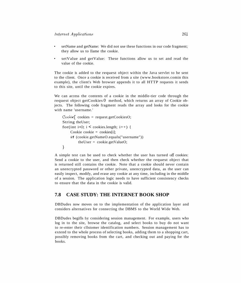
Inte7~net Applications 26~
• setName and getName: We did not use these functions in our code fragment;they allow us to Ilame the cookie.
• setValue and getValue: These functions allow us to set and read thevalue of the cookie.
The cookie is added to the request object within the Java servlet to be sentto the client. Once a cookie is received from a site (www.bookstore.comin thisexample), the client's Web browser appends it to all HTTP requests it sendsto this site, until the cookie expires.
We can access the contents of a cookie in the middle-tier code through therequest object getCookies 0 method, which returns an array of Cookie objects. The following code fragment reads the array and looks for the cookiewith name 'username.'
CookieD cookies = request.getCookiesO;String theUser;for(int i=O; i < cookies.length; i++) {
Cookie cookie = cookies[i];if (cookie.getNameO.equals("username"))
theUser = cookie.getValueO;}
A simple test can be used to check whether the user has turned oft' cookies:Send a cookie to the user, and then check whether the request object thatis returned still contains the cookie. Note that a cookie should never containan unencrypted password or other private, unencrypted data, as the user caneasily inspect, modify, and erase any cookie at any time, including in the middleof a session. The application logic needs to have sufficient consistency checksto ensure that the data in the cookie is valid.
7.8 CASE STUDY: THE INTERNET BOOK SHOP
DBDudes now moves on to the implementation of the application layer andconsiders alternatives for connecting the DBMS to the World Wide Web.
DBDudes begifls by considering session management. For example, users wholog in to the site, browse the catalog, and select books to buy do not wantto re-enter their cllstomer identification numbers. Session management has toextend to the whole process of selecting books, adding them to a shopping cart,possibly removing books from the cart, and checking out and paying for thebooks.
262 CHAPTERi 7
DBDudes then considers whether webpages for books should be static or dynamic. If there is a static webpage for each book, then we need an extradatabase field in the Books relation that points to the location of the file.Even though this enables special page designs for different books, it is a verylabor-intensive solution. DBDudes convinces B&N to dynamically assemblethe webpage for a book from a standard template instantiated with information about the book in the Books relation. Thus, DBDudes do not use staticHTML pages, such as the one shown in Figure 7.1, to display the inventory.
DBDudes considers the use of XML a'S a data exchange format between thedatabase server and the middle tier, or the middle tier and the client tier.Representation of the data in XML at the middle tier as shown in Figures 7.2and 7.3 would allow easier integration of other data sources in the future, butB&N decides that they do not anticipate a need for such integration, and soDBDudes decide not to use XML data exchange at this time.
DBDudes designs the application logic as follows. They think that there willbe four different webpages:
• index. j sp: The home page of Barns and Nobble. This is the main entrypoint for the shop. This page has search text fields and buttons that allowthe user to search by author name, ISBN, or title of the book. There isalso a link to the page that shows the shopping cart, cart. j sp.
• login. j sp: Allows registered users to log in. Here DBDudes use anHTML form similar to the one displayed in Figure 7.11. At the middletier, they use a code fragment similar to the piece shown in Figure 7.19and JavaServerPages as shown in Figure 7.20.
• search. j sp: Lists all books in the database that match the search condition specified by the user. The user can add listed items to the shoppingbasket; each book ha'3 a button next to it that adds it. (If the item isalready in the shopping basket, it increments the quantity by one.) Thereis also a counter that shows the total number of items currently in theshopping basket. (DBDucles makes a note that that a quantity of five for asingle item in the shopping basket should indicate a total purcha'3c quantityof five as well.) The search. j sp page also contains a button that directsthe user to cart. j sp.
III cart. j sp: Lists all the books currently in the shopping basket. The listing should include all items in the shopping basket with the product name,price, a text box for the quantity (which the user can use to change quantities of items), and a button to remove the item from the shopping basket.This page has three other buttons: one button to continue shopping (whichreturns the user to page index. j sp), a second button to update the shop-
Inter'net Applications
ping basket with the altered quantities from the text boxes, and a thirdbutton to place the order, which directs the user to the page confirm.jsp.
II coni irm. j sp: Lists the complete order so far and allows the user to enterhis or her contact information or customer ID. There are two buttons onthis page: one button to cancel the order and a second button to submitthe final order. The cancel button ernpties the shopping ba.'3ket and returnsthe user to the home page. The submit button updates the database withthe new order, empties the shopping basket, and returns the user to thehome page.
DBDudes also considers the use of JavaScript at the presentation tier to checkuser input before it is sent to the middle tier. For example, in the pagelogin. j sp, DBDudes is likely to write JavaScript code similar to that shownin Figure 7.12.
This leaves DBDudes with one final decision: how to connect applications tothe DBMS. They consider the two main alternatives presented in Section 7.7:CGI scripts versus using an application server infrastructure. If they use CGIscripts, they would have to encode session management logic-not an easy task.If they use an application server, they can make use of all the functionalitythat the application server provides. Therefore, they recommend that B&Nimplement server-side processing using an application server.
B&N accepts the decision to use an application server, but decides that nocode should be specific to any particular application server, since B&N doesnot want to lock itself into one vendor. DBDudes agrees proceeds to build thefollowing pieces:
III DBDudes designs top level pages that allow customers to navigate thewebsite as well as various search forms and result presentations.
II Assuming that DBDudes selects a Java-ba..sed application server, they haveto write Java servlets to process form-generated requests. Potentially, theycould reuse existing (possibly commercially available) JavaBeans. Theycan use JDBC a." a databa.':ie interface; exarnples of JDBC code can befound in Section 6.2. Instead of prograrnming servlets, they could resortto Java Server Pages and annotate pages with special .JSP markup tags.
II DBDudes select an application server that uses proprietary markup tags,but due to their arrangement with B&N, they are not allowed to use suchtags in their code.
For completeness, we remark that if DBDudes and B&N had agreed to use CGrscripts, DBDucles would have had the following ta.sks:
264 CHAPTER~ 7
II Create the top level HTML pages that allow users to navigate the site andvaTious forms that allow users to search the catalog by ISBN, author name,or title. An example page containing a search form is shown in Figure7.1. In addition to the input forms, DBDudes must develop appropriatepresentations for the results.
II Develop the logic to track a customer session. Relevant information must bestored either at the server side or in the customer's browser using cookies.
II Write the scripts that process user requests. For example, a customer canuse a form called 'Search books by title' to type in a title and search forbooks with that title. The CGI interface communicates with a script thatprocesses the request. An example of such a script written in Perl usingthe DBI library for data access is shown in Figure 7.16.
Our discussion thus far covers only the customer interface, the part of thewebsite that is exposed to B&N's customers. DBDudes also needs to addapplications that allow the employees and the shop owner to query and accessthe database and to generate summary reports of business activities.
Complete files for the case study can be found on the webpage for this book.
7.9 REVIEW QUESTIONS
Answers to the review questions can be found in the listed sections.
II What are URIs and URLs? (Section 7.2.1)
II How does the HTTP protocol work? What is a stateless protocol? (Section 7.2.2)
II Explain the main concepts of HTML. Why is it used only for data presentation and not data exchange? (Section 7.3)
II What are some shortc.ornings of HTML, and how does XML address them?(Section 7.4)
II What are the main components of an XML document? (Section 7.4.1)
II Why do we have XML DTDs? What is a well-formed XML document?What is a valid XML document? Give an example of an XML documentthat is valid but not well-formed, and vice versa. (Section 7.4.2)
II 'What is the role of domain-specific DTDs? (Section 7.4.3)
II \Vhat is a three-tier architecture? 'What advantages does it offer over singletier and two-tier architectures? Give a short overview of the functionalityat each of the three tiers. (Section 7.5)
Internet Apphcat-ions 2&5
• Explain hmv three-tier architectures address each of the following issuesof databa.<;e-backed Internet applications: heterogeneity, thin clients, dataintegration, scalability, software development. (Section 7.5.3)
• Write an HTML form. Describe all the components of an HTML form.(Section 7.6.1)
• What is the difference between the HTML GET and POST methods? Howdoes URI encoding of an HT~IL form work? (Section 7.11)
• What is JavaScript used for? Write a JavaScipt function that checkswhether an HTML form element contains a syntactically valid email address. (Section 7.6.2)
• What problem do style sheets address? What are the advantages of usingstyle sheets? (Section 7.6.3)
• What are Ca.5cading Style Sheets? Explain the components of Ca.<;cadingStyle Sheets. What is XSL and how it is different from CSS? (Sections7.6.3 and 7.13)
• What is CGl and what problem does it address? (Section 7.7.1)
• What are application servers and how are they different from webservers?(Section 7.7.2)
• What are servlets? How do servlets handle data from HTML forms? Explain what happens during the lifetime of a servlet. (Section 7.7.3)
• What is the difference between servlets and JSP? When should we useservlets and when should we use JSP? (Section 7.7.4)
• Why do we need to maintain state at the middle tier? What are cookies?How does a browser handle cookies? How can we access the data in cookiesfrom servlets? (Section 7.7.5)
EXERCISES
Exercise 7.1 Briefly answer the following questions:
1. Explain the following terms and describe what they are used for: HTML, URL, XML,Java, JSP, XSL, XSLT, servlet, cookie, HTTP, ess, DTD.
2. What is eGl? Why was eGI introduced? What are the disadvantages of an architectureusing eel scripts?
3. \Vhat is the difference between a webserver and an application server? What fUl1cionalitydo typical application servers provide?
4. When is an XML document well-formed? When is an XML document valid?
Exercise 7.2 Briefly answer the following questions about the HTTP protocol:
266 CHAPTER$ 7
1. \Nhat is a communication protocol?
2. "What is the structure of an HTTP request message? What is the structure of an HTTPresponse message? \Vhy do HTTP messages carry a version field?
3. vVhat is a stateless protocol? "Why was HTTP designed to be stateless?
4. Show the HTTP request message generated when you request the home page of thisbook (http://TNWW . cs. wisc. edur dbbook). Show the HTTP response message that theserver generates for that page.
Exercise 7.3 In this exercise, you are asked to write the functionality of a generic shoppingbasket; you will use this in several subsequent project exercises. Write a set of JSP pages thatdisplays a shopping basket of items and allows users to add, remove, and change the quantityof items. To do this, use a cookie storage scheme that stores the following information:
• The UserId of the user who owns the shopping basket.
• The number of products stored in the shopping basket.
I! A product id and a quantity for each product.
When manipulating cookies, remember to set the Expires property such that the cookie canpersist for a session or indefinitely. Experiment with cookies using JSP and make sure youknow how to retrieve, set values, and delete the cookie.
You need to create five JSP pages to make your prototype complete:
.. Index Page (index. j sp): This is the main entry point. It has a link that directs theuser to the Products page so they can start shopping.
I! Products Page (products. j sp): Shows a listing of all products in the database withtheir descriptions and prices. This is the main page where the user fills out the shoppingbasket. Each listed product should have a button next to it, which adds it to the shoppingbasket. (If the item is already in the shopping basket, it increments the quantity byone.) There should also be a counter to show the total number of items currently in theshopping basket. Note that if a user has a quantity of five of a single item in the shoppingbasket, the counter should indicate a total quantity of five. The page also contains abutton that directs the user to the Cart page.
I! Cart Page (cart. jsp): Shows a listing of all items in the shopping basket cookie. Thelisting for each item should include the product name, price, a text box for the quantity(the user can changc the quantity of items here), and a button to remove the item fromthe shopping basket. This page has three other buttons: one button to continue shopping(which returns the user to the Products page), a second button to update the cookiewith the altered quantities from the text boxes, and a third button to place or confirmthe order, which directs the user to the Confirm page.
I! Confirm Pl;tge (confirm. j sp) : List.s the final order. There are two but.tons on thispage. One button cancels t.he order and the other submits the completed order. Thecancel button just deletes the cookie and returns the lIser to the Index page. The submitbutton updates the database with the new order, delet.es the cookie, and returns the lIserto the Index page.
Exercise 7.4 In the previous exercise, replace the page products. jsp with the follmvingsearch page search. j sp. 'T'his page allows users to search products by name or description. There should be both a text box for the search text and radio buttons to allow the
Internet Applications 2@7
user to choose between search-by-name and search-by-description (as \vell as a submit button to retrieve the results), The page that handles search results should be modeled afterproducts.jsp (as described in the previous exercise) and be called products.jsp. It shouldretrieve all records where the search text is a substring of the name or description (as chosenby the user). To integrate this with the previous exercise, simply replace all the links toproducts. j sp with search. j sp.
Exercise 7.5 'Write a simple authentication mechanism (without using encrypted transfer ofpasswords, for simplicity). We say a user is authenticated if she has provided a valid usernamepassword combination to the system; otherwise, we say the user is not authenticated. Assumefor simplicity that you have a database schema that stores only a customer id and a password:
Passwords(cid: integer, username: string, password: string)
1. How and where are you going to track when a user is 'logged on' to the system?
2. Design a page that allows a registered user to log on to the system.
3. Design a page header that checks whether the user visiting this page is logged in.
Exercise 7.6 (Due to Jeff Derstadt) TechnoBooks.com is in the process of reorganizing itswebsite. A major issue is how to efficiently handle a large number of search results. In ahuman interaction study, it found that modem users typically like to view 20 search results ata time, and it would like to program this logic into the system. Queries that return batches ofsorted results are called top N queries. (See Section 25.5 for a discussion of database supportfor top N queries.) For example, results 1-20 are returned, then results 21~40, then 41-60,and so OIl. Different techniques are used for performing top N queries and TechnoBooks.comwould like you to implement two of them.
Infrastructure: Create a database with a table called Books and populate it with somebooks, using the format that follows. This gives you III books in your database with a titleof AAA, BBB, CCC, DDD, or EEE, but the keys are not sequential for books with the sametitle.
Books( bookid: INTEGER, title: CHAR(80), author: CHAR(80), price: REAL)
For i = 1 to 111 {Insert the tuple (i, "AAA", "AAA Author", 5.99)i=i+lInsert the tuple (i, "BBB", "BBB Author", 5.99)i = i + 1Insert the tuple (i, "CCC", "CCC Author", 5.99)i=i+1Insert the tuple (i, "DDD", "DDD Author", 5.99)1=i+lInsert the tuple (i, "EEE", "EEE Author", 5.99)
Placeholder Technique: The simplest approach to top N queries is to store a placeholderfor the first and last result tuples, and then perform the same query. When the new queryresults are returned, you can iterate to the placeholders and return the previous or next 20results.
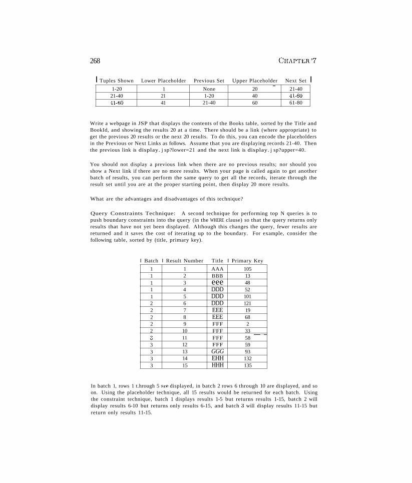
268
I Tuples Shown Lower Placeholder Previous Set Upper Placeholder Next Set I1-20 1 None 20 "- 21-40
21-40 21 1-20 40 41-6041-60 41 21-40 60 61-80
Write a webpage in JSP that displays the contents of the Books table, sorted by the Title andBookId, and showing the results 20 at a time. There should be a link (where appropriate) toget the previous 20 results or the next 20 results. To do this, you can encode the placeholdersin the Previous or Next Links as follows. Assume that you are displaying records 21-40. Thenthe previous link is display. j sp?lower=21 and the next link is display. j sp?upper=40.
You should not display a previous link when there are no previous results; nor should youshow a Next link if there are no more results. When your page is called again to get anotherbatch of results, you can perform the same query to get all the records, iterate through theresult set until you are at the proper starting point, then display 20 more results.
What are the advantages and disadvantages of this technique?
Query Constraints Technique: A second technique for performing top N queries is topush boundary constraints into the query (in the WHERE clause) so that the query returns onlyresults that have not yet been displayed. Although this changes the query, fewer results arereturned and it saves the cost of iterating up to the boundary. For example, consider thefollowing table, sorted by (title, primary key).
I Batch I Result Number Title I Primary Key
1 1 AAA 1051 2 BBB 131 3 eee 481 4 DDD 521 5 DDD 1012 6 DDD 1212 7 EEE 192 8 EEE 682 9 FFF 22 10 FFF 33
FFF."~
:~ 11 583 12 FFF 593 13 GGG 933 14 EHH 1323 15 HHH 135
In batch 1, rows 1 t.hrough 5 are displayed, in batch 2 rows 6 through 10 are displayed, and soon. Using the placeholder technique, all 15 results would be returned for each batch. Usingthe constraint technique, batch 1 displays results 1-5 but returns results 1-15, batch 2 willdisplay results 6-10 but returns only results 6-15, and batch :~ will display results 11-15 butreturn only results 11-15.
Internet Applications 299
The constraint can be pushed into the query because of the sorting of this table. Considerthe following query for batch 2 (displaying results 6-10):
EXEC SQL SELECT B.TitleFROM Books BWHERE (B.Title = 'DDD' AND B.BookId > 101) OR (B.Title > 'DDD')ORDER BY B.Title, B.Bookld
This query first selects all books with the title 'DDD,' but with a primary key that is greaterthan that of record 5 (record 5 has a primary key of 101). This returns record 6. Also, anybook that has a title after 'DDD' alphabetically is returned. You can then display the firstfive results.
The following information needs to be retained to have Previous and Next buttons that returnmore results:
• Previous: The title of the first record in the previous set, and the primary key of thefirst record in the previous set.
• Next: The title of the first record in the next set; the primary key of the first record inthe next set.
These four pieces of information can be encoded into the Previous and Next buttons as in theprevious part. Using your database table from the first part, write a JavaServer Page thatdisplays the book information 20 records at a time. The page should include Previous andNext buttons to show the previous or next record set if there is one. Use the constraint queryto get the Previous and Next record sets.
PROJECT~BASEDEXERCISES
In this chapter, you continue the exercises from the previous chapter and create the parts ofthe application that reside at the middle tier and at the presentation tier. More informationabout these exercises and material for more exercises can be found online at
http://~.cs.wisc.edu/-dbbook
Exercise 7.7 Recall the Notown Records website that you worked on in Exercise 6.6. Next,you are asked to develop the actual pages for the Notown Records website. Design the partof the website that involves the presentation tier and the middle tier, and integrate the codethat you wrote in Exercise 6.6 to access the database.
I. Describe in detail the set of webpages that users can access. Keep the following issuesin mind:
• All users start at a common page.
• For each action, what input does the user provide? How will the user provide it -byclicking on a link or through an HTML form?
• What sequence of steps does a user go through to purchase a record? Describe thehigh-level application flow by showing how each lIser action is handled.
270 CHAPTER .,7
2. vVrite the webpages in HTML without dynamic content.
3. vVrite a page that allows users to log on to the site. Use cookies to store the informationpermanently at the user's browser.
4. Augment the log-on page with JavaScript code that checks that the username consistsonly of the characters from a to z.
5. Augment the pages that allow users to store items in a shopping basket with a conditionthat checks whether the user has logged on to the site. If the user has not yet logged on,there should be no way to add items to the shopping cart. Implement this functionalityusing JSP by checking cookie information from the user.
6. Create the remaining pages to finish the website.
Exercise 7.8 Recall the online pharmacy project that you worked on in Exercise 6.7 inChapter 6. Follow the analogous steps from Exercise 7.7 to design the application logic andpresentation layer and finish the website.
Exercise 7.9 Recall the university database project that you worked on in Exercise 6.8 inChapter 6. Follow the analogous steps from Exercise 7.7 to design the application logic andpresentation layer and finish the website.
Exercise 7.10 Recall the airline reservation project that you worked on in Exercise 6.9 inChapter 6. Follow the analogous steps from Exercise 7.7 to design the application logic andpresentation layer and finish the website.
BIBLIOGRAPHIC NOTES
The latest version of the standards mentioned in this chapter can be found at the websiteof the World Wide Web Consortium (www. w3. org). It contains links to information aboutI-ITML, cascading style sheets, XIvIL, XSL, and much more. The book by Hall is a general introduction to Web progn1.111ming technologies [357]; a good starting point on the Webis www.Webdeve1oper.com. There are many introductory books on CGI progranuning, forexample [210, 198]. The JavaSoft (java. sun. com) home page is a good starting point forServlets, .JSP, and all other Java-related technologies. The book by Hunter [394] is a goodintroduction to Java Servlets. Microsoft supports Active Server Pages (ASP), a comparabletedmology to .lSI'. l'vIore information about ASP can be found on the Microsoft Developer'sNetwork horne page (msdn. microsoft. com).
There are excellent websites devoted to the advancement of XML, for example 1.l1-iTW. xm1. comand www.ibm.com/xm1. that also contain a plethora of links with information about the otherstandards. There are good introductory books on many diflerent aspects of XML, for exarnple[195, 158,597,474, :381, 320]. Information about UNICODE can be found on its home pagehttp://www.unicode.org.
Inforrnation about .lavaServer Pages ane! servlets can be found on the JavaSoft home page atjava. sun. com at java. sun. com/products/j sp and at java. sun. com/products/servlet.

PART III
STORAGE AND INDEXING

1
1
1
1
1
1
1
1
1
1
1
1
1
1
1
1
1
1
1
1
1
1
1
1
1
1
1
1
8OVERVIEW'OF STORAGE
AND INDEXING
.. How does a DBMS store and access persistent data?
.. Why is I/O cost so important for database operations?
.. How does a DBMS organize files of data records on disk to minimizeI/O costs?
... What is an index, and why is it used?
.. What is the relationship between a file of data records and any indexeson this file of records?
.. What are important properties of indexes?
.. How does a hash-based index work, and when is it most effective?
.. How does a tree-based index work, and when is it most effective?
... How can we use indexes to optimize performance for a given workload?
.. Key concepts: external storage, buffer manager, page I/O; file orga-nization, heap files, sorted files; indexes, data entries, search keys, clustered index, clustered file, primary index; index organization, hashbased and tree-based indexes; cost comparison, file organizations andcommon operations; performance tuning, workload, composite searchkeys, use of clustering,
____________________J
If you don't find it in the index, look very carefully through the entire catalog.
--Sears, Roebuck, and Co., Consumers' Guide, 1897
The ba.'3ic abstraction of data in a DBMS is a collection of records, or a file,and each file consists of one or more pages. The files and access methods
274 CHAPTER 8
software layer organizes data carefully to support fast access to desired subsetsof records. Understanding how records are organized is essential to using adatabase system effectively, and it is the main topic of this chapter.
A file organization is a method of arranging the records in a file when thefile is stored on disk. Each file organization makes certain operations efficientbut other operations expensive.
Consider a file of employee records, each containing age, name, and sal fields,which we use as a running example in this chapter. If we want to retrieveemployee records in order of increasing age, sorting the file by age is a good fileorganization, but the sort order is expensive to maintain if the file is frequentlymodified. Further, we are often interested in supporting more than one operation on a given collection of records. In our example, we may also want toretrieve all employees who make more than $5000. We have to scan the entirefile to find such employee records.
A technique called indexing can help when we have to access a collection ofrecords in multiple ways, in addition to efficiently supporting various kinds ofselection. Section 8.2 introduces indexing, an important aspect of file organization in a DBMS. We present an overview of index data structures in Section8.3; a more detailed discussion is included in Chapters 10 and 11.
We illustrate the importance of choosing an appropriate file organization inSection 8.4 through a simplified analysis of several alternative file organizations.The cost model used in this analysis, presented in Section 8.4.1, is used inlater chapters as welL In Section 8.5, we highlight some important choices tobe made in creating indexes. Choosing a good collection of indexes to buildis arguably the single most powerful tool a database administrator has forimproving performance.
8.1 DATA ON EXTERNAL STORAGE
A DBMS stores vast quantities of data, and the data must persist across program executions. Therefore, data is stored on external storage devices such asdisks and tapes, and fetched into main memory as needed for processing. Theunit of information read from or written to disk is a page. The size of a pageis a DBMS parameter, and typical values are 4KB or 8KB.
The cost of page I/O (input from disk to main Inemory and output from memory to disk) dominates the cost of typical database operations, and databa,'>esystems are carefully optimized to rninimize this cost. While the details of how
Storage and Indexing :175
files of records are physically stored on disk and how main memory is utilizedare covered in Chapter 9, the following points are important to keep in mind:
• Disks are the most important external storage devices. They allow us toretrieve any page at a (more or less) fixed cost per page. However, if weread several pages in the order that they are stored physically, the cost canbe much less than the cost of reading the same pages in a random order.
• Tapes are sequential access devices and force us to read data one page afterthe other. They are mostly used to archive data that is not needed on aregular basis.
• Each record in a file has a unique identifier called a record id, or rid forshort. An rid ha.'3 the property that we can identify the disk address of thepage containing the record by using the rid.
Data is read into memory for processing, and written to disk for persistentstorage, by a layer of software called the buffer manager. When the files andaccess methods layer (which we often refer to as just the file layer) needs toprocess a page, it asks the buffer manager to fetch the page, specifying thepage's rid. The buffer manager fetches the page from disk if it is not alreadyin memory.
Space on disk is managed by the disk space m,anager, according to the DBMSsoftware architecture described in Section 1.8. When the files and access methods layer needs additional space to hold new records in a file, it asks the diskspace manager to allocate an additional disk page for the file; it also informsthe disk space manager when it no longer needs one of its disk pages. The diskspace manager keeps track of the pages in use by the file layer; if a page is freedby the file layer, the space rnanager tracks this, and reuses the space if the filelayer requests a new page later on.
In the rest of this chapter, we focus on the files and access methods layer.
8.2 FILE ORGANIZATIONS AND INDEXING
The file of records is an important abstraction in a DBMS, and is implemented by the files and access methods layer of the code. A file can be created,destroyed, and have records inserted into and deleted from it. It also supportsscallS; a scan operation allows us to step through all the records in the file oneat a time. A relatioll is typically stored a.':l a file of records.
The file layer stores the records in a file in a collection of disk pages. It keepstrack of pages allocated to each file, and as records are inserted into and deletedfrom the file, it also tracks availa.ble space within pages allocated to the file.
276 CHAPTER 8
The simplest file structure is an unordered file, or heap file. Records in aheap file are stored in random order across the pages of the file. A heap fileorganization supports retrieval of all records, or retrieval of a particular recordspecified by its rid; the file manager must keep track of the pages allocated forthe file. ("Ve defer the details of how a heap file is implemented to Chapter 9.)
An index is a data structure that organizes data records on disk to optimizecertain kinds of retrieval operations. An index allows us to efficiently retrieveall records that satisfy search conditions on the search key fields of the index.We can also create additional indexes on a given collection of data records,each with a different search key, to speed up search operations that are notefficiently supported by the file organization used to store the data records.
Consider our example of employee records. We can store the records in a fileorganized as an index on employee age; this is an alternative to sorting the fileby age. Additionally, we can create an auxiliary index file based on salary, tospeed up queries involving salary. The first file contains employee records, andthe second contains records that allow us to locate employee records satisfyinga query on salary.
"Ve use the term data entry to refer to the records stored in an index file. Adata entry with search key value k, denoted as k*, contains enough informationto locate (one or more) data records with search key value k. We can efficientlysearch an index to find the desired data entries, and then use these to obtaindata records (if these are distinct from data entries).
There are three main alternatives for what to store as a data entry in an index:
1. A data entry h is an actual data record (with search key value k).
2. A data entry is a (k, rid) pair, where rid is the record id of a data recordwith search key value k.
3. A data entry is a (k. rid-list) pair, where rid-list is a list of record ids ofdata records with search key value k.
Of course, if the index is used to store actual data records, Alternative (1),each entry b is a data record with search key value k. We can think of such anindex &'3 a special file organization. Such an indexed file organization canbe used instead of, for exarnple, a sorted file or an unordered file of records.
Alternatives (2) and (3), which contain data entries that point to data records,are independent of the file organization that is used for the indexed file (i.e.,
Storage and Indexing 277.the file that contains the data records). Alternative (3) offers better space utilization than Alternative (2), but data entries are variable in length, dependingon the number of data records with a given search key value.
If we want to build more than one index on a collection of data records-forexample, we want to build indexes on both the age and the sal fields for a collection of employee records-~at most one of the indexes should use Alternative(1) because we should avoid storing data records multiple times.
8.2.1 Clustered Indexes
When a file is organized so that the ordering of data records is the same asor close to the ordering of data entries in some index, we say that the indexis clustered; otherwise, it clustered is an unclustered index. An index thatuses Alternative (1) is clustered, by definition. An index that uses Alternative(2) or (3) can be a clustered index only if the data records are sorted on thesearch key field. Otherwise, the order of the data records is random, definedpurely by their physical order, and there is no reasonable way to arrange thedata entries in the index in the same order.
In practice, files are rarely kept sorted since this is too expensive to maintainwhen the data is updated~ So, in practice, a clustered index is an index that usesAlternative (1), and indexes that use Alternatives (2) or (3) are unclustered.We sometimes refer to an index using Alternative (1) as a clustered file,because the data entries are actual data records, and the index is therefore afile of data records. (As observed earlier, searches and scans on an index returnonly its data entries, even if it contains additional information to organize thedata entries.)
The cost of using an index to answer a range search query can vary tremendously based on whether the index is clustered. If the index is clustered, i.e.,we are using the search key of a clustered file, the rids in qualifying data entriespoint to a contiguous collection of records, and we need to retrieve only a fewdata pages. If the index is unclustered, each qualifying data entry could containa rid that points to a distinct data page, leading to as many data page l/Os8.'3 the number of data entries that match the range selection, as illustrated inFigure 8.1. This point is discussed further in Chapter 13.
8.2.2 Primary and Secondary Indexes
An index on a set of fields that includes the primaTy key (see Chapter 3) iscalled a primary index; other indexes are called secondary indexes. (Theterms jJrimaTy inde.T and secondaTy index are sometimes used with a different

278
Index entries
(Direct search fordata enrries)
Data entries
Data
records
Figure 8.1 Uuelllst.ered Index Using Alt.ernat.ive (2)
CHAPTER .~
Index file
Data tile
meaning: An index that uses Alternative (1) is called a primary index, andone that uses Alternatives (2) or (3) is called a secondary index. We will beconsistent with the definitions presented earlier, but the reader should be awareof this lack of standard terminology in the literature.)
Two data entries are said to be duplicates if they have the same value for thesearch key field associated with the index. A primary index is guaranteed notto contain duplicates, but an index on other (collections of) fields can containduplicates. In general, a secondary index contains duplicates. If we knowtha.t no duplicates exist, that is, we know that the search key contains somecandidate key, we call the index a unique index.
An important issue is how data entries in an index are organized to supportefficient retrieval of data entries.vVe discuss this next.
8.3 INDEX DATA STRUCTURES
One way to organize data entries is to hash data entries on the sea.rch key.Another way to organize data entries is to build a tree-like data structure thatdirects a search for data entries. "Ve introduce these two basic approaches illthis section. \iV~e study tree-based indexing in more detail in Chapter 10 andha"sh-based indexing in Chapter 11.
We note that the choice of hash or tree indexing techniques can be combinedwith any of the three alternatives for data entries.
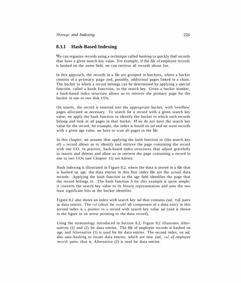
StoTage and Indexing
8.3.1 Hash-Based Indexing
2'49
Vie can organize records using a technique called hashing to quickly find recordsthat have a given search key value. For example, if the file of employee recordsis hashed on the name field, we can retrieve all records about Joe.
In this approach, the records in a file are grouped in buckets, where a bucketconsists of a primary page and, possibly, additional pages linked in a chain.The bucket to which a record belongs can be determined by applying a specialfunction, called a hash function, to the search key. Given a bucket number,a hash-based index structure allows us to retrieve the primary page for thebucket in one or two disk l/Os.
On inserts, the record is inserted into the appropriate bucket, with 'overflow'pages allocated as necessary. To search for a record with a given search keyvalue, we apply the hash function to identify the bucket to which such recordsbelong and look at all pages in that bucket. If we do not have the search keyvalue for the record, for example, the index is based on sal and we want recordswith a given age value, we have to scan all pages in the file.
In this chapter, we assume that applying the hash function to (the search keyof) a record allows us to identify and retrieve the page containing the recordwith one I/O. In practice, hash-based index structures that adjust gracefullyto inserts and deletes and allow us to retrieve the page containing a record inone to two l/Os (see Chapter 11) are known.
Hash indexing is illustrated in Figure 8.2, where the data is stored in a file thatis hashed on age; the data entries in this first index file are the actual datarecords. Applying the hash function to the age field identifies the page thatthe record belongs to. The hash function h for this example is quite simple;it converts the search key value to its binary representation and uses the twoleast significant bits as the bucket identifier.
Figure 8.2 also shows an index with search key sal that contains (sal, rid) pairsas data entries. The tid (short for record id) component of a data entry in thissecond index is a pointer to a record with search key value sal (and is shownin the figure as an arrow pointing to the data record).
Using the terminology introduced in Section 8.2, Figure 8.2 illustrates AlternativE"S (1) and (2) for data entries. The file of employee records is hashed onage, and Alternative (1) is used for for data entries. The second index, on sal,also uses hashing to locate data entries, which are now (sal, rid of employeerecoT'(~ pairs; that is, Alternative (2) is used for data entries.
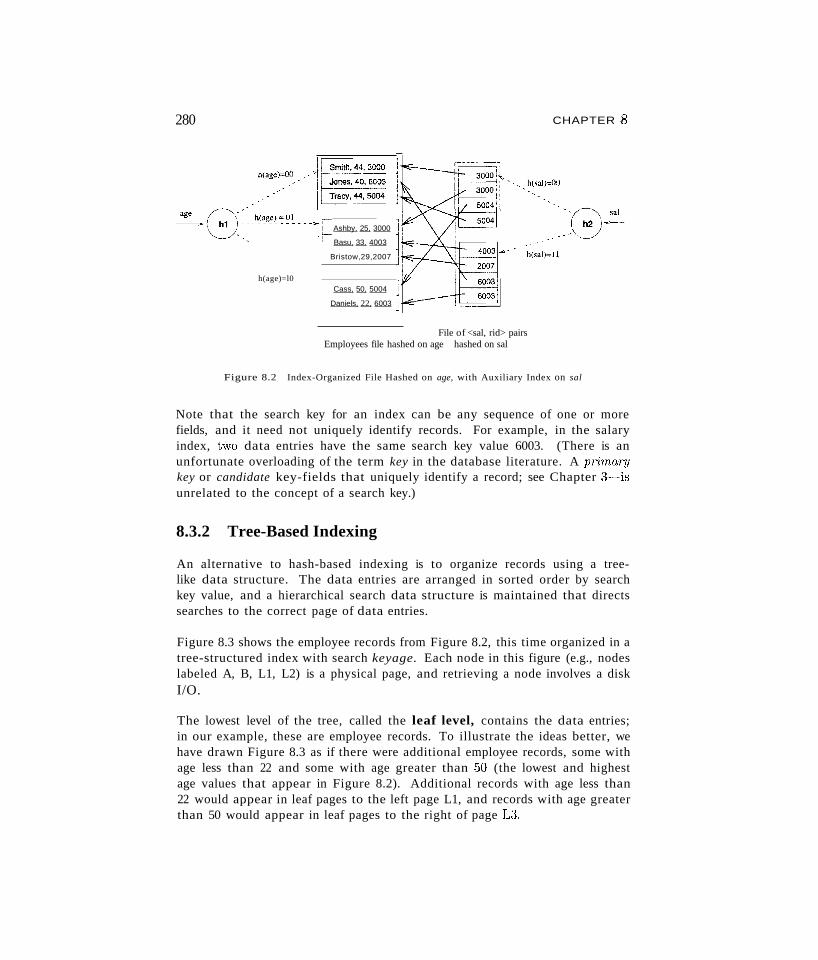
280 CHAPTER 8
Ashby. 25, 3000
Basu, 33, 4003
Bristow,29,2007
h(age)=l0Cass, 50, 5004
Daniels, 22, 6003
File of <sal, rid> pairsEmployees file hashed on age hashed on sal
Figure 8.2 Index-Organized File Hashed on age, with Auxiliary Index on sal
Note that the search key for an index can be any sequence of one or morefields, and it need not uniquely identify records. For example, in the salaryindex, two data entries have the same search key value 6003. (There is anunfortunate overloading of the term key in the database literature. A primarykey or candidate key-fields that uniquely identify a record; see Chapter 3~is
unrelated to the concept of a search key.)
8.3.2 Tree-Based Indexing
An alternative to hash-based indexing is to organize records using a treelike data structure. The data entries are arranged in sorted order by searchkey value, and a hierarchical search data structure is maintained that directssearches to the correct page of data entries.
Figure 8.3 shows the employee records from Figure 8.2, this time organized in atree-structured index with search keyage. Each node in this figure (e.g., nodeslabeled A, B, L1, L2) is a physical page, and retrieving a node involves a diskI/O.
The lowest level of the tree, called the leaf level, contains the data entries;in our example, these are employee records. To illustrate the ideas better, wehave drawn Figure 8.3 as if there were additional employee records, some withage less than 22 and some with age greater than EiO (the lowest and highestage values that appear in Figure 8.2). Additional records with age less than22 would appear in leaf pages to the left page L1, and records with age greaterthan 50 would appear in leaf pages to the right of page L~~.
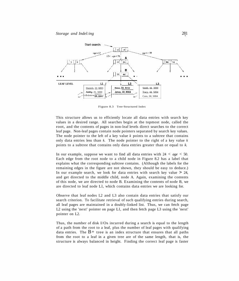
Storage and Indel:ing 281~
...LEAF LEVEL L1 /
Daniels. 22. 6003
/'"" Ashby, 25, 3000/ I--B-ris-to-w-,2-9,-2-00-7--Y
L3
Smith, 44, 3000
Tracy, 44, 5004
Cass, 50, 5004
...
Figure 8.3 Tree·Structured Index
This structure allows us to efficiently locate all data entries with search keyvalues in a desired range. All searches begin at the topmost node, called theroot, and the contents of pages in non-leaf levels direct searches to the correctleaf page. Non-leaf pages contain node pointers separated by search key values.The node pointer to the left of a key value k points to a subtree that containsonly data entries less than k. The node pointer to the right of a key value kpoints to a subtree that contains only data entries greater than or equal to k.
In our example, suppose we want to find all data entries with 24 < age < 50.Each edge from the root node to a child node in Figure 8.2 has a label thatexplains what the corresponding subtree contains. (Although the labels for theremaining edges in the figure are not shown, they should be easy to deduce.)In our example search, we look for data entries with search key value > 24,and get directed to the middle child, node A. Again, examining the contentsof this node, we are directed to node B. Examining the contents of node B, weare directed to leaf node Ll, which contains data entries we are looking for.
Observe that leaf nodes L2 and L3 also contain data entries that satisfy oursearch criterion. To facilitate retrieval of such qualifying entries during search,all leaf pages are maintained in a doubly-linked list. Thus, we can fetch pageL2 using the 'next' pointer on page Ll, and then fetch page L3 using the 'next'pointer on L2.
Thus, the number of disk I/Os incurred during a search is equal to the lengthof a path from the root to a leaf, plus the number of leaf pages with qualifyingdata entries. The B+ tree is an index structure that ensures that all pathsfrom the root to a leaf in a given tree are of the same length, that is, thestructure is always balanced in height. Finding the correct leaf page is faster
282 CHAPTER 8-1,
than binary search of the pages in a sorted file because each non~leaf node canaccommodate a very large number of node-pointers, and the height of the treeis rarely more than three or four in practice. The height of a balanced tree isthe length of a path from root to leaf; in Figure 8.3, the height is three. Thenumber of l/Os to retrieve a desired leaf page is four, including the root andthe leaf page. (In practice, the root is typically in the buffer pool because itis frequently accessed, and we really incur just three I/Os for a tree of heightthree.)
The average number of children for a non-leaf node is called the fan-out ofthe tree. If every non-leaf node has n children, a tree of height h has nh leafpages. In practice, nodes do not have the same number of children, but usingthe average value F for n, we still get a good approximation to the number ofleaf pages, F h . In practice, F is at least 100, which means a tree of height fourcontains 100 million leaf pages. Thus, we can search a file with 100 million leafpages and find the page we want using four l/Os; in contrast, binary search ofthe same file would take log21OO,000,000 (over 25) l/Os.
8.4 COMPARISON OF FILE ORGANIZATIONS
We now compare the costs of some simple operations for several basic fileorganizations on a collection of employee records. We assume that the files andindexes are organized according to the composite search key (age, sa~, and thatall selection operations are specified on these fields. The organizations that weconsider are the following:
• File of randomly ordered employee records, or heap file.
• File of employee records sorted on (age, sal).
• Clustered B+ tree file with search key (age, sal).
• Heap file with an unclustered B+ tree index on (age, sal).
• Heap file with an unclustered hash index on (age, sal).
Our goal is to emphasize the importance of the choice of an appropriate fileorganization, and the above list includes the main alternatives to consider inpractice. Obviously, we can keep the records unsorted or sort them. We canalso choose to build an index on the data file. Note that even if the data fileis sorted, an index whose search key differs from the sort order behaves like anindex on a heap file!
The operations we consider are these:
Storage and Indexing 283
• Scan: Fetch all records in the file. The pages in the file must be fetchedfrom disk into the buffer pool. There is also a CPU overhead per recordfor locating the record on the page (in the pool).
• Search with Equality Selection: Fetch all records that satisfy an equality selection; for example, "Find the employee record for the employee withage 23 and sal 50." Pages that contain qualifying records must be fetchedfrom disk, and qualifying records must be located within retrieved pages.
• Search with Range Selection: Fetch all records that satisfy a rangeselection; for example, "Find all employee records with age greater than35."
• Insert a Record: Insert a given record into the file. We must identify thepage in the file into which the new record must be inserted, fetch that pagefrom disk, modify it to include the new record, and then write back themodified page. Depending on the file organization, we may have to fetch,modify, and write back other pages as well.
• Delete a Record: Delete a record that is specified using its rid. We mustidentify the page that contains the record, fetch it from disk, modify it, andwrite it back. Depending on the file organization, we may have to fetch,modify, and write back other pages as well.
8.4.1 Cost Model
In our comparison of file organizations, and in later chapters, we use a simplecost model that allows us to estimate the cost (in terms of execution time) ofdifferent database operations. We use B to denote the number of data pageswhen records are packed onto pages with no wasted space, and R to denotethe number of records per page. The average time to read or write a diskpage is D, and the average time to process a record (e.g., to compare a fieldvalue to a selection constant) is C. In the ha.'3hed file organization, we use afunction, called a hash function, to map a record into a range of numbers; thetime required to apply the hash function to a record is H. For tree indexes, wewill use F to denote the fan-out, which typically is at lea.'3t 100 as mentionedin Section 8.3.2.
Typical values today are D = 15 milliseconds, C and H = 100 nanoseconds; wetherefore expect the cost of I/O to dominate. I/O is often (even typically) thedominant component of the cost of database operations, and so considering I/Ocosts gives us a good first approximation to the true costs. Further, CPU speedsare steadily rising, whereas disk speeds are not increasing at a similar pace. (Onthe other hand, as main memory sizes increase, a much larger fraction of theneeded pages are likely to fit in memory, leading to fewer I/O requests!) \Ve
284 CHAPTER,8
have chosen to concentrate on the I/O component of the cost model, and weassume the simple constant C for in-memory per-record processing cost. Bearthe follO\ving observations in mind:
.. Real systems must consider other aspects of cost, such as CPU costs (andnetwork transmission costs in a distributed database).
.. Even with our decision to focus on I/O costs, an accurate model would betoo complex for our purposes of conveying the essential ideas in a simpleway. We therefore use a simplistic model in which we just count the numberof pages read from or written to disk as a measure of I/O. \lVe ignore theimportant issue of blocked access in our analysis-typically, disk systemsallow us to read a block of contiguous pages in a single I/O request. Thecost is equal to the time required to seek the first page in the block andtransfer all pages in the block. Such blocked access can be much cheaperthan issuing one I/O request per page in the block, especially if theserequests do not follow consecutively, because we would have an additionalseek cost for each page in the block.
We discuss the implications of the cost model whenever our simplifying assumptions are likely to affect our conclusions in an important way.
8.4.2 Heap Files
Scan: The cost is B(D +RC) because we must retrieve each of B pages takingtime D per page, and for each page, process R records taking time C per record.
Search with Equality Selection: Suppose that we know in advance thatexactly one record matches the desired equality selection, that is, the selectionis specified on a candidate key. On average, we must scan half the file, assumingthat the record exists and the distribution of values in the search field is uniform.For each retrieved data page, we must check all records on the page to see ifit is the desired record. The cost is O.5B(D + RC). If no record satisfies theselection, however, we must scan the entire file to verify this.
If the selection is not on a candidate key field (e.g., "Find employees aged 18"),we always have to scan the entire file because records with age = 18 could bedispersed all over the file, and we have no idea how many such records exist.
Search with Range Selection: The entire file must be scanned becausequalifying records could appear anywhere in the file, and we do not know howmany qualifying records exist. The cost is B(D + RC).
Storage and Inde:r'ing 285f
Insert: \Ve assume that records are always inserted at the end of the file. \¥emust fetch the last page in the file, add the record, and write the page back.The cost is 2D + C.
Delete: We must find the record, remove the record from the page, and writethe modified page back. vVe assume that no attempt is made to compact thefile to reclaim the free space created by deletions, for simplicity. 1 The cost isthe cost of searching plus C + D.
We assume that the record to be deleted is specified using the record id. Sincethe page id can easily be obtained from the record id, we can directly read inthe page. The cost of searching is therefore D.
If the record to be deleted is specified using an equality or range conditionon some fields, the cost of searching is given in our discussion of equality andrange selections. The cost of deletion is also affected by the number of qualifyingrecords, since all pages containing such records must be modified.
8.4.3 Sorted Files
Scan: The cost is B(D +RC) because all pages must be examined. Note thatthis case is no better or worse than the case of unordered files. However, theorder in which records are retrieved corresponds to the sort order, that is, allrecords in age order, and for a given age, by sal order.
Search with Equality Selection: We assume that the equality selectionmatches the sort order (age, sal). In other words, we assume that a selectioncondition is specified on at leclst the first field in the composite key (e.g., age =30). If not (e.g., selection sal = t50 or department = "Toy"), the sort orderdoes not help us and the cost is identical to that for a heap file.
We can locate the first page containing the desired record or records, shouldany qualifying records exist, with a binary search in log2B steps. (This analysisassumes that the pages in the sorted file are stored sequentially, and we canretrieve the ith page on the file directly in one disk I/O.) Each step requiresa disk I/O and two cornparisons. Once the page is known, the first qualifyingrecord can again be located by a binary search of the page at a cost of Clog2R.The cost is Dlo92B +Clog2R, which is a significant improvement over searchingheap files.
] In practice, a directory or other data structure is used to keep track of free space, and records areinserted into the first available free slot, as discussed in Chapter 9. This increases the cost of insertionand deletion a little, but not enough to affect our comparison.
286 CHAPTER~8
If several records qualify (e.g., "Find all employees aged 18"), they are guaranteed to be adjacent to each other due to the sorting on age, and so thecost of retrieving all such records is the cost of locating the first such record(Dlog2B+Clog2R) plus the cost ofreading all the qualifying records in sequential order. Typically, all qualifying records fit on a single page. If no recordsqualify, this is established by the search for the first qualifying record, whichfinds the page that would have contained a qualifying record, had one existed,and searches that page.
Search with Range Selection: Again assuming that the range selectionmatches the composite key, the first record that satisfies the selection is locatedas for search with equality. Subsequently, data pages are sequentially retrieveduntil a record is found that does not satisfy the range selection; this is similarto an equality search with many qualifying records.
The cost is the cost of search plus the cost of retrieving the set of records thatsatisfy the search. The cost of the search includes the cost of fetching the firstpage containing qualifying, or matching, records. For small range selections,all qualifying records appear on this page. For larger range selections, we haveto fetch additional pages containing matching records.
Insert: To insert a record while preserving the sort order, we must first findthe correct position in the file, add the record, and then fetch and rewrite allsubsequent pages (because all the old records are shifted by one slot, assumingthat the file has no empty slots). On average, we can &'3sume that the insertedrecord belongs in the middle of the file. Therefore, we must read the latter halfof the file and then write it back after adding the new record. The cost is thatof searching to find the position of the new record plus 2 . (O.5B(D + RC)),that is, search cost plus B(D + RC).
Delete: We must search for the record, remove the record from the page, andwrite the modified page back. We must also read and write all subsequentpages because all records that follow the deleted record must be moved up tocornpact the free space. 2 The cost is the same as for an insert, that is, searchcost plus B(D + RC). Given the rid of the record to delete, we can fetch thepage containing the record directly.
If records to be deleted are specified by an equality or range condition, the costof deletion depends on the number of qualifying records. If the condition isspecified on the sort field, qualifying records are guaranteed to be contiguous,and the first qualifying record can be located using binary search.
2Unlike a heap file. there is no inexpensive way to manage free space, so we account for the costof compacting it file when il record is deleted.
il
Storage and Indexing
8.4.4 Clustered Files
In a clustered file, extensive empirical study has shown that pages are usuallyat about 67 percent occupancy. Thus, the Humber of physical data pages isabout 1.5B, and we use this observation in the following analysis.
Scan: The cost of a scan is 1.5B(D + RC) because all data pages must beexamined; this is similar to sorted files, with the obvious adjustment for theincreased number of data pages. Note that our cost metric does not capturepotential differences in cost due to sequential I/O. We would expect sorted filesto be superior in this regard, although a clustered file using ISAM (rather thanB+ trees) would be close.
Search with Equality Selection: We assume that the equality selectionmatches the search key (age, sal). We can locate the first page containingthe desired record or records, should any qualifying records exist, in logF1.5Bsteps, that is, by fetching all pages from the root to the appropriate leaf. Inpractice, the root page is likely to be in the buffer pool and we save an I/O,but we ignore this in our simplified analysis. Each step requires a disk I/Oand two comparisons. Once the page is known, the first qualifying record canagain be located by a binary search of the page at a cost of Clog2R. The costis DlogF1.5B +Clog2 R, which is a significant improvement over searching evensorted files.
If several records qualify (e.g., "Find all employees aged 18"), they are guaranteed to be adjacent to each other due to the sorting on age, and so thecost of retrieving all such records is the cost of locating the first such record(Dlogp1.5B + Clog2R) plus the cost of reading all the qualifying records insequential order.
Search with Range Selection: Again assuming that the range selectionmatches the composite key, the first record that satisfies the selection is locateda..'3 it is for search with equality. Subsequently, data pages are sequentiallyretrieved (using the next and previous links at the leaf level) until a record isfound that does not satisfy the range selection; this is similar to an equalitysearch with many qualifying records.
Insert: To insert a record, we must first find the correct leaf page in the index,reading every page from root to leaf. Then, we must add the llew record. Mostof the time, the leaf page has sufficient space for the new record, and all weneed to do is to write out the modified leaf page. Occasionally, the leaf is fulland we need to retrieve and modify other pages, but this is sufficiently rare
288 CHAPTER :8
that we can ignore it in this simplified analysis. The cost is therefore the costof search plus one write, DlogF L5B + Clog2R + D.
Delete: \;Ye must search for the record, remove the record from the page,and write the modified page back. The discussion and cost analysis for insertapplies here as well.
8.4.5 Heap File with Unclustered Tree Index
The number of leaf pages in an index depends on the size of a data entry.We assume that each data entry in the index is a tenth the size of an employee data record, which is typical. The number of leaf pages in the index iso.1(L5B) = O.15B, if we take into account the 67 percent occupancy of indexpages. Similarly, the number of data entries on a page 10(0.67R) = 6.7R,taking into account the relative size and occupancy.
Scan: Consider Figure 8.1, which illustrates an unclustered index. To do a fullscan of the file of employee records, we can scan the leaf level of the index andfor each data entry, fetch the corresponding data record from the underlyingfile, obtaining data records in the sort order (age, sal).
We can read all data entries at a cost of O.15B(D + 6.7RC) l/Os. Now comesthe expensive part: We have to fetch the employee record for each data entryin the index. The cost of fetching the employee records is one I/O per record,since the index is unclustered and each data entry on a leaf page of the indexcould point to a different page in the employee file. The cost of this step isB R(D + C), which is prohibitively high. If we want the employee recordsin sorted order, we would be better off ignoring the index and scanning theemployee file directly, and then sorting it. A simple rule of thumb is that a filecan be sorted by a two-Pl1SS algorithm in which each pass requires reading andwriting the entire file. Thus, the I/O cost of sorting a file with B pages is 4B,which is much less than the cost of using an unclustered index.
Search with Equality Selection: \lVe assume that the equalit.y selectionmatches the sort order (age, sal). \Ve can locate the first page containing thedesired data entry or entries, should any qualifying entries exist, in lagrO.15Bsteps, that is, by fetching all pages from the root to the appropriate leaf. Eachstep requires a disk I/O and two comparisons. Once the page is known, thefirst qua1ifying data entry can again be located by a binary search of the pageat a cost of Clog2 G. 7R. The first qualifying data record can be fetched fronlthe employee file with another I/O. The cost is DlogpO.15B + Clag26.7R + D,which is a significant improvement over searching sorted files.
Storage and Inde:rzng 289.~
If several records qualify (e.g., "Find all employees aged ISn), they are not
guaranteed to be adjacent to each other. The cost of retrieving all such recordsis the cost oflocating the first qualifying data entry (Dlo9pO.15B +Clo926.7R)plus one I/O per qualifying record. The cost of using an unclustered index istherefore very dependent on the number of qualifying records.
Search with Range Selection: Again assuming that the range selectionmatches the composite key, the first record that satisfies the selection is locatedas it is for search with equality. Subsequently, data entries are sequentiallyretrieved (using the next and previous links at the leaf level of the index)until a data entry is found that does not satisfy the range selection. For eachqualifying data entry, we incur one I/O to fetch the corresponding employeerecords. The cost can quickly become prohibitive as the number of records thatsatisfy the range selection increases. As a rule of thumb, if 10 percent of datarecords satisfy the selection condition, we are better off retrieving all employeerecords, sorting them, and then retaining those that satisfy the selection.
Insert: "Ve must first insert the record in the employee heap file, at a cost of2D + C. In addition, we must insert the corresponding data entry in the index.Finding the right leaf page costs Dl09pO.15B + Cl0926.7R, and writing it outafter adding the new data entry costs another D.
Delete: We need to locate the data record in the employee file and the dataentry in the index, and this search step costs Dl09FO.15B + Cl0926.7R + D.Now, we need to write out the modified pages in the index and the data file,at a cost of 2D.
8.4.6 Heap File With Unclustered Hash Index
As for unclustered tree indexes, we a.'3sume that each data entry is one tenththe size of a data record. vVe consider only static hashing in our analysis, andfor simplicity we a.'3sume that there are no overflow chains.a
In a static ha.shed file, pages are kept at about SO percent occupancy (to leavespace for future insertions and minimize overflows as the file expands). This isachieved by adding a new page to a bucket when each existing page is SO percentfull, when records are initially loaded into a hashed file structure. The numberof pages required to store data entries is therefore 1.2.5 times the number ofpages when the entries are densely packed, that is, 1.25(0.10B) = O.125B.The number of data entries that fit on a page is 1O(O.80R) = 8R, taking intoaccount the relative size and occupancy.
:JThe dynamic variants of hashing are less susceptible to the problem of overflow chains, and havea slight.ly higher average cost per search, but are otherwise similar to the static version.
290 CHAPTER 8
Scan: As for an unclustered tree index, all data entries can be retrieved inexpensively, at a cost of O.125B(D + 8RC) I/Os. However, for each entry, weincur the additional cost of one I/O to fetch the corresponding data record; thecost of this step is BR(D + C). This is prohibitively expensive, and further,results are unordered. So no one ever scans a hash index.
Search with Equality Selection: This operation is supported very efficientlyfor matching selections, that is, equality conditions are specified for each fieldin the composite search key (age, sal). The cost of identifying the page thatcontains qualifying data entries is H. Assuming that this bucket consists ofjust one page (i.e., no overflow pages), retrieving it costs D. If we assume thatwe find the data entry after scanning half the records on the page, the cost ofscanning the page is O.5(8R)C = 4RC. Finally, we have to fetch the datarecord from the employee file, which is another D. The total cost is thereforeH + 2D + 4RC, which is even lower than the cost for a tree index.
If several records qualify, they are not guaranteed to be adjacent to each other.The cost of retrieving all such records is the cost of locating the first qualifyingdata entry (H +D +4RC) plus one I/O per qualifying record. The cost of usingan unclustered index therefore depends heavily on the number of qualifyingrecords.
Search with Range Selection: The hash structure offers no help, and theentire heap file of employee records must be scanned at a cost of B(D + RC).
Insert: We must first insert the record in the employee heap file, at a costof 2D + C. In addition, the appropriate page in the index must be located,modified to insert a new data entry, and then written back. The additionalcost is H + 2D + C.
Delete: We need to locate the data record in the employee file and the dataentry in the index; this search step costs H + 2D + 4RC. Now, we need towrite out the modified pages in the index and the data file, at a cost of 2D.
8.4.7 Comparison of I/O Costs
Figure 8.4 compares I/O costs for the various file organizations that we discussed. A heap file has good storage efficiency and supports fast scanning andinsertion of records. However, it is slow for searches and deletions.
A sorted file also offers good storage efficiency. but insertion and ddetion ofrecords is slow. Searches are fa.ster than in heap files. It is worth noting that,in a real DBMS, a file is almost never kept fully sorted.
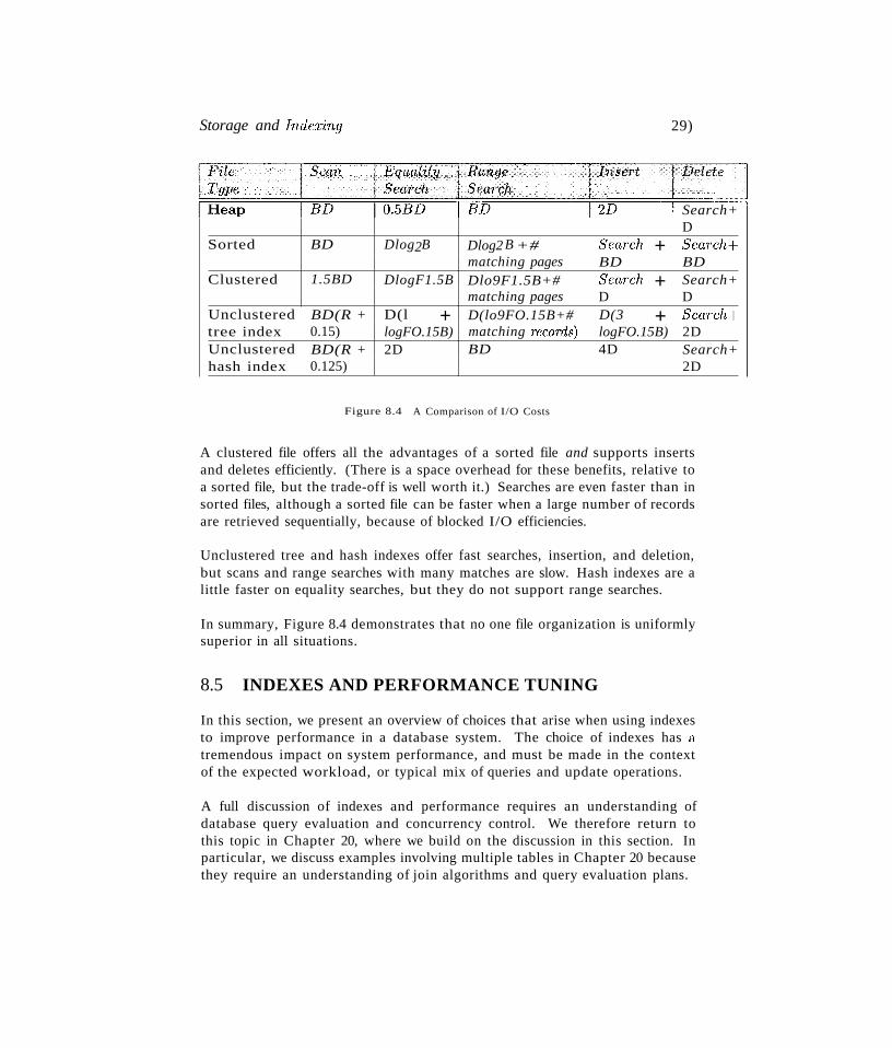
Storage and Inde:r'lng 29)
Search+D
Sorted BD Dlog2B Dlog2 B +# Sear-ch + Sear-ch+matching pages BD BD
Clustered 1.5BD DlogF1.5B Dlo9F1.5B+# Sear-ch + Search+matching pages D D
Unclustered BD(R + D(l + D(lo9FO.15B+# D(3 + Sear-ch+tree index 0.15) logFO.15B) matching recor-ds) logFO.15B) 2DUnclustered BD(R + 2D BD 4D Search+hash index 0.125) 2D
Figure 8.4 A Comparison of I/O Costs
A clustered file offers all the advantages of a sorted file and supports insertsand deletes efficiently. (There is a space overhead for these benefits, relative toa sorted file, but the trade-off is well worth it.) Searches are even faster than insorted files, although a sorted file can be faster when a large number of recordsare retrieved sequentially, because of blocked I/O efficiencies.
Unclustered tree and hash indexes offer fast searches, insertion, and deletion,but scans and range searches with many matches are slow. Hash indexes are alittle faster on equality searches, but they do not support range searches.
In summary, Figure 8.4 demonstrates that no one file organization is uniformlysuperior in all situations.
8.5 INDEXES AND PERFORMANCE TUNING
In this section, we present an overview of choices that arise when using indexesto improve performance in a database system. The choice of indexes has atremendous impact on system performance, and must be made in the contextof the expected workload, or typical mix of queries and update operations.
A full discussion of indexes and performance requires an understanding ofdatabase query evaluation and concurrency control. We therefore return tothis topic in Chapter 20, where we build on the discussion in this section. Inparticular, we discuss examples involving multiple tables in Chapter 20 becausethey require an understanding of join algorithms and query evaluation plans.
292 CHAPTER. 8
8.5.1 Impact of the Workload
The first thing to consider is the expected workload and the common operations. Different file organizations and indexes, a:"l we have seen, support differentoperations well.
In generaL an index supports efficient retrieval of data entries that satisfy agiven selection condition. Recall from the previous section that there are twoimportant kinds of selections: equality selection and range selection. Hashbased indexing techniques are optimized only for equality selections and fa.repoorly on range selections. where they are typically worse than scanning theentire file of records. Tree-based indexing techniques support both kinds ofselection conditions efficiently, explaining their widespread use.
Both tree and hash indexes can support inserts, deletes, and updates quiteefficiently. Tree-based indexes, in particular, offer a superior alternative tomaintaining fully sorted files of records. In contrast to simply maintaining thedata entries in a sorted file, our discussion of (B+ tree) tree-structured indexesin Section 8.3.2 highlights two important advantages over sorted files:
1. vVo can handle inserts and deletes of data entries efficiently.
2. Finding the correct leaf page when searching for a record by search keyvalue is much faster than binary search of the pages in a sorted file.
The one relative disadvantage is that the pages in a sorted file can be allocatedin physical order on disk, making it much faster to retrieve several pages insequential order. Of course. inserts and deletes on a sorted file are extremelyexpensive. A variant of B+ trees, called Indexed Sequential Access Method(ISAM), offers the benefit of sequential allocation of leaf pages, plus the benefitof fast searches. Inserts and deletes are not handled as well a'3 in B+ trees, butare rnuch better than in a sorted file. \Ve will study tree-structured indexingin detail in Cha,pter 10.
8.5.2 Clustered Index Organization
As we smv in Section 8.2.1. a clustered index is really a file organization forthe underlying data records. Data records can be la.rge, and we should avoidreplicating them; so there can be at most one clustered index on a given collection of records. On the other hanel. we UU1 build several uncIustered indexeson a data file. Suppose that employee records are sorted by age, or stored in aclustered file with search keyage. If. in addition. we have an index on the salfield, the latter nlUst be an llnclllstered index. \:Ve can also build an uncIusteredindex on. say, depaThnent, if there is such a field.
Stomge and Inde:rin,g 29,3
Clustered indexes, while less expensive to maintain than a fully sorted file, arenonetJleless expensive to maintain. When a new record h&'3 to be inserted intoa full leaf page, a new leaf page must be allocated and sorne existing recordshave to be moved to the new page. If records are identified by a combination ofpage id and slot, &'5 is typically the case in current database systems, all placesin the datab&"ie that point to a moved record (typically, entries in other indexesfor the same collection of records) must also be updated to point to the newlocation. Locating all such places and making these additional updates caninvolve several disk I/Os. Clustering must be used sparingly and only whenjustified by frequent queries that benefit from clustering. In particular, thereis no good reason to build a clustered file using hashing, since range queriescannot be answered using h&c;h-indexcs.
In dealing with the limitation that at most one index can be clustered, it isoften useful to consider whether the information in an index's search key issufficient to answer the query. If so, modern database systems are intelligentenough to avoid fetching the actual data records. For example, if we havean index on age, and we want to compute the average age of employees, theDBMS can do this by simply examining the data entries in the index. This is anexample of an index-only evaluation. In an index-only evaluation of a querywe need not access the data records in the files that contain the relations in thequery; we can evaluate the query completely through indexes on the files. Animportant benefit of index-only evaluation is that it works equally efficientlywith only unclustered indexes, as only the data entries of the index are used inthe queries. Thus, unclustered indexes can be used to speed up certain queriesif we recognize that the DBMS will exploit index-only evaluation.
Design Examples Illustrating Clustered Indexes
To illustrate the use of a clustered index 011 a range query, consider the followingexample:
SELECTFROMWHERE
E.dnoEmployees EE.age > 40
If we have a H+ tree index on age, we can use it to retrieve only tuples thatsatisfy the selection E. age> 40. \iVhether such an index is worthwhile dependsfirst of all on the selectivity of the condition. vVhat fraction of the employees areolder than 40'1 If virtually everyone is older than 40 1 we gain little by using anindex 011 age; a sequential scan of the relation would do almost as well. However,suppose that only 10 percent of the employees are older than 40. Now, is anindex useful? The answer depends on whether the index is clustered. If the
294 CHAPTER~ 8
index is unclustered, we could have one page I/O per qualifying employee, andthis could be more expensive than a sequential scan, even if only 10 percentof the employees qualify! On the other hand, a clustered B+ tree index onage requires only 10 percent of the l/Os for a sequential scan (ignoring the fewl/Os needed to traverse from the root to the first retrieved leaf page and thel/Os for the relevant index leaf pages).
As another example, consider the following refinement of the previous query:
SELECTFROMWHEREGROUP BY
Kdno, COUNT(*)Employees EE.age> 10E.dno
If a B+ tree index is available on age, we could retrieve tuples using it, sortthe retrieved tuples on dna, and so answer the query. However, this may notbe a good plan if virtually all employees are more than 10 years old. This planis especially bad if the index is not clustered.
Let us consider whether an index on dna might suit our purposes better. Wecould use the index to retrieve all tuples, grouped by dna, and for each dnacount the number of tuples with age> 10. (This strategy can be used withboth hash and B+ tree indexes; we only require the tuples to be grouped, notnecessarily sorted, by dna.) Again, the efficiency depends crucially on whetherthe index is clustered. If it is, this plan is likely to be the best if the conditionon age is not very selective. (Even if we have a clustered index on age, if thecondition on age is not selective, the cost of sorting qualifying tuples on dna islikely to be high.) If the index is not clustered, we could perform one page I/Oper tuple in Employees, and this plan would be terrible. Indeed, if the indexis not clustered, the optimizer will choose the straightforward plan based onsorting on dna. Therefore, this query suggests that we build a clustered indexon dna if the condition on age is not very selective. If the condition is veryselective, we should consider building an index (not necessarily clustered) onage instead.
Clustering is also important for an index on a search key that does not includea candidate key, that is, an index in which several data entries can have thesame key value. To illustrate this point, we present the following query:
SELECT E.dnoFROM Employees EWHERE E.hobby='Stamps'
Stomge and Indexing
If many people collect stamps, retrieving tuples through an unclustered indexon hobby can be very inefficient. It may be cheaper to simply scan the relationto retrieve all tuples and to apply the selection on-the-fly to the retrieved tuples.Therefore, if such a query is important, we should consider making the indexon hobby a clustered index. On the other hand, if we assume that eid is a keyfor Employees, and replace the condition E.hobby= 'Stamps' by E. eid=552, weknow that at most one Employees tuple will satisfy this selection condition. Inthis case, there is no advantage to making the index clustered.
The next query shows how aggregate operations can influence the choice ofindexes:
SELECT E.dno, COUNT(*)FROM Employees EGROUP BY E.dno
A straightforward plan for this query is to sort Employees on dno to computethe count of employees for each dno. However, if an index-hash or B+ tree--on dno is available, we can answer this query by scanning only the index. Foreach dno value, we simply count the number of data entries in the index withthis value for the search key. Note that it does not matter whether the indexis clustered because we never retrieve tuples of Employees.
8.5.3 Composite Search Keys
The search key for an index can contain several fields; such keys are calledcomposite search keys or concatenated keys. As an example, consider acollection of employee records, with fields name, age, and sal, stored in sortedorder by name. Figure 8.5 illustrates the difference between a composite indexwith key (age, sa0, a composite index with key (sal, age), an index with keyage, and an index with key sal. All indexes shown in the figure use Alternative(2) for data entries.
If the search key is composite, an equality query is one in which each field inthe search key is bound to a constant. For example, we can ask to retrieve alldata entries with age = 20 and sal = 10. The hashed file organization supportsonly equality queries, since a ha"ih function identifies the bucket containingdesired records only if a value is specified for each field in the search key.
With respect to a composite key index, in a range query not all fields in thesearch key are bound to constants. For example, we can ask to retrieve all dataentries with age :=0:: 20; this query implies that any value is acceptable for thesal field. As another example of a range query, we can ask to retrieve all dataentries with age < 30 and sal> 40.
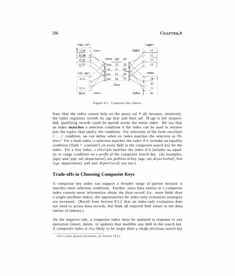
296 CHAPTEI48
~I
80
75
name age sal
"~-_.-
bob 12 10
cal 11 80-
joe 12 20----
sue 13 75
Data
Index
75,13
80,11
10,12
<age, sal>,~..._---!
I 11,80 ,,! Index
R;:IO ~ __:~i1 12,20 ~_.1
U~:~,<sal, age> ../
Figure 8.5 Composite Key Indexes
Nate that the index cannot help on the query sal > 40, because, intuitively,the index organizes records by age first and then sal. If age is left unspecified, qualifying records could be spread across the entire index. We say thatan index matches a selection condition if the index can be used to retrievejust the tuples that satisf:y the condition. For selections of the form condition1\ ... 1\ condition, we can define when an index matches the selection as 1'0110ws:4 For a hash index, a selection matches the index if it includes an equalitycondition ('field = constant') on every field in the composite search key for theindex. For a tree index, a selection matches the index if it includes an equality or range condition on a prefi.T of the composite search key. (As examples,(age) and (age, sal, department) are prefixes of key (age, sal, depa7'tment) , but(age, department) and (sal, department) are not.)
Trade-offs in Choosing Composite Keys
A composite key index can support a broader range of queries because itmatches more selection conditions. Further, since data entries in a compositeindex contain more information about the data record (i.e., more fields thana single-attribute index), the opportunities for index-only evaluation strategiesare increased. (Recall from Section 8.5.2 that an index-only evaluation doesnot need to access data records, but finds all required field values in the dataentries of indexes.)
On the negative side, a composite index must be updated in response to anyoperation (insert, delete, or update) that modifies any field in the search key.A composite index is Hlso likely to be larger than a singk'-attribute search key
4 For a more general discussion, see Section 14.2.)
StoTage and Inde.Ting
index because the size of entries is larger. For a composite B+ tree index, thisalso means a potential increase in the number of levels, although key COlnpression can be used to alleviate this problem (see Section 10.8.1).
Design Examples of Composite Keys
Consider the following query, which returns all employees with 20 < age < 30and 3000 < sal < 5000:
SELECTFROMWHERE
E.eidEmployees EE.age BETWEEN 20 AND 30AND E.sal BETWEEN 3000 AND 5000
A composite index on (age, sal) could help if the conditions in the WHERE clauseare fairly selective. Obviously, a hash index will not help; a B+ tree (or ISAM)index is required. It is also clear that a clustered index is likely to be superiorto an unclustered index. For this query, in which the conditions on age and salare equally selective, a composite, clustered B+ tree index on (age, sal) is aseffective as a composite, clustered B+ tree index on (sal, age). However, theorder of search key attributes can sometimes make a big difference, as the nextquery illustrates:
SELECTFROMWHERE
E.eidEmployees EE.age = 25AND E.sal BETWEEN 3000 AND 5000
In this query a composite, clustered B+ tree index on (age, sal) will give goodperformance because records are sorted by age first and then (if two recordshave the same age value) by sal. Thus, all records with age = 25 are clusteredtogether. On the other hand, a composite, clustered B+ tree index on (sal, age)will not perform as well. In this case, records are sorted by sal first, and therefore two records with the same age value (in particular, with age = 25) may bequite far apart. In effect, this index allows us to use the range selection on sal,but not the equality selection on age, to retrieve tuples. (Good performanceon both variants of the query can be achieved using a single spatial index. \:Yediscuss spatial indexes in Chapter 28.)
Composite indexes are also useful in dealing with many aggregate queries. Consider:
SELECT AVG (E.sal)
298
FROMWHERE
Employees EE.age = 25AND Ksal BETWEEN 3000 AND 5000
CHAPTERt 8
A composite B+ tree index on (age, sal) allows us to answer the query withan index-only scan. A composite B+ tree index on (sal, age) also allows usto answer the query with an index-only scan, although more index entries areretrieved in this case than with an index on (age, sal).
Here is a variation of an earlier example:
SELECTFROMWHEREGROUP BY
Kdno, COUNT(*)Employees EE.sal=lO,OOOKdno
An index on dna alone does not allow us to evaluate this query with an indexonly scan, because we need to look at the sal field of each tuple to verify thatsal = 10, 000. However, we can use an index-only plan if we have a compositeB+ tree index on (sal, dna) or (dna, sal). In an index with key (sal, dno) , alldata entries with sal = 10,000 are arranged contiguously (whether or not theindex is clustered). Further, these entries are sorted by dna, making it easy toobtain a count for each dna group. Note that we need to retrieve only dataentries with sal = 10, 000.
It is worth observing that this strategy does not work if the WHERE clause ismodified to use sal> 10, 000. Although it suffices to retrieve only index dataentries-that is, an index-only strategy still applies-these entries must nowbe sorted by dna to identify the groups (because, for example, two entries withthe same dna but different sal values may not be contiguous). An index withkey (dna, sal) is better for this query: Data entries with a given dna value arestored together, and each such group of entries is itself sorted by sal. For eachdna group, we can eliminate the entries with sal not greater than 10,000 andcount the rest. (Using this index is less efficient than an index-only scan withkey (sal, dna) for the query with sal = 10, 000, because we must read all dataentries. Thus, the choice between these indexes is influenced by which query ismore common.)
As another eXEunple, suppose we want to find the minimum sal for each dna:
SELECT Kdno, MIN(E.sal)FROM Employees EGROUP BY E.dno
Stomge and Indexing 2~9
An index on dna alone does not allow us to evaluate this query with an indexonly scan. However, we can use an index-only plan if we have a composite B+tree index on (dna, sal). Note that all data entries in the index with a givendna value are stored together (whether or not the index is clustered). :B\lrther,this group of entries is itself sorted by 8al. An index on (sal, dna) enables usto avoid retrieving data records, but the index data entries must be sorted ondno.
8.5.4 Index Specification in SQL: 1999
A natural question to ask at this point is how we can create indexes usingSQL. The SQL:1999 standard does not include any statement for creating ordropping index structures. In fact, th.e standard does not even require SQLimplementations to support indexes! In practice, of course, every commercialrelational DBMS supports one or more kinds of indexes. The following command to create a B+ tree index-we discuss B+ tree indexes in Chapter 10----·-isillustrative:
CREATE INDEX IndAgeRating ON StudentsWITH STRUCTURE = BTREE,
KEY = (age, gpa)
This specifies that a B+ tree index is to be created on the Students table usingthe concatenation of the age and gpa columns as the key. Thus, key values arepairs of the form (age, gpa) , and there is a distinct entry for each such pair.Once created, the index is automatically maintained by the DBMS adding orremoving data entries in response to inserts or deletes of records on the Studentsrelation.
8.6 REVIEW QUESTIONS
Answers to the review questions can be found in the listed sections.
III 'Where does a DBMS store persistent data? How does it bring data intomain memory for processing? What DBMS component reads and writesdata from main memory, and what is the unit of I/O? (Section 8.1)
• 'What is a file organization? vVhat is an index? What is the relationshipbetween files and indexes? Can we have several indexes on a single fileof records? Can an index itself store data records (i.e., act as a file)?(Section 8.2)
III What is the 8earch key for an index? What is a data entry in an index?(Section 8.2)
300 CHAPTER S
• vVhat is a clustered index? vVhat is a prinwry index? How many clusteredindexes can you build on a file? How many unclustered indexes can youbuild? (Section 8.2.1)
• Hmv is data organized in a hash-ba'lcd index? \Vhen would you use ahash-based index? (Section 8.3.1)
• How is data organized in a tree-based index? vVhen would you use a treebased index? (Section 8.3.2)
• Consider the following operations: scans, equality and 'range selections,inserts, and deletes, and the following file organizations: heap files, sortedfiles, clustered files, heap files with an unclustered tree index on the searchkey, and heap files with an unclusteTed hash index. Which file organizationis best suited for each operation? (Section 8.4)
• What are the main contributors to the cost of database operations? Discussa simple cost model that reflects this. (Section 8.4.1)
• How does the expected workload influence physical database design decisiems such as what indexes to build? vVhy is the choice of indexes a centralaspect of physical database design? (Section 8.5)
• What issues are considered in using clustered indexes? What is an indcl;only evaluation method? \\That is its primary advantage? (Section 8.5.2)
• What is a composite 8earch key? What are the pros and cons of compositesearch keys? (Section 8.5.3)
• What SQL commands support index creation? (Section 8.5.4)
EXERCISES
Exercise 8.1 Answer the following questions about data on external storage in a DBMS:
1. \Vhy does a DBMS store data on external storage?
2. Why are I/O costs important in a DBMS?
3. \Vhat is a record id? Given a record's id, how many I/Os are needed to fetch it intomain memory?
4. \Vhat is the role of the buffer manager in a DBMS? What is the role of the disk spacemanager? How do these layers interact with the file and access methods layer?
Exercise 8.2 Answer the following questions about files and indexes:
1. What operations arc supported by the file of records abstraction?
2. \Vhat is an index on a file of records? \Nhat is a search key for an index? Why do weneed indexes?
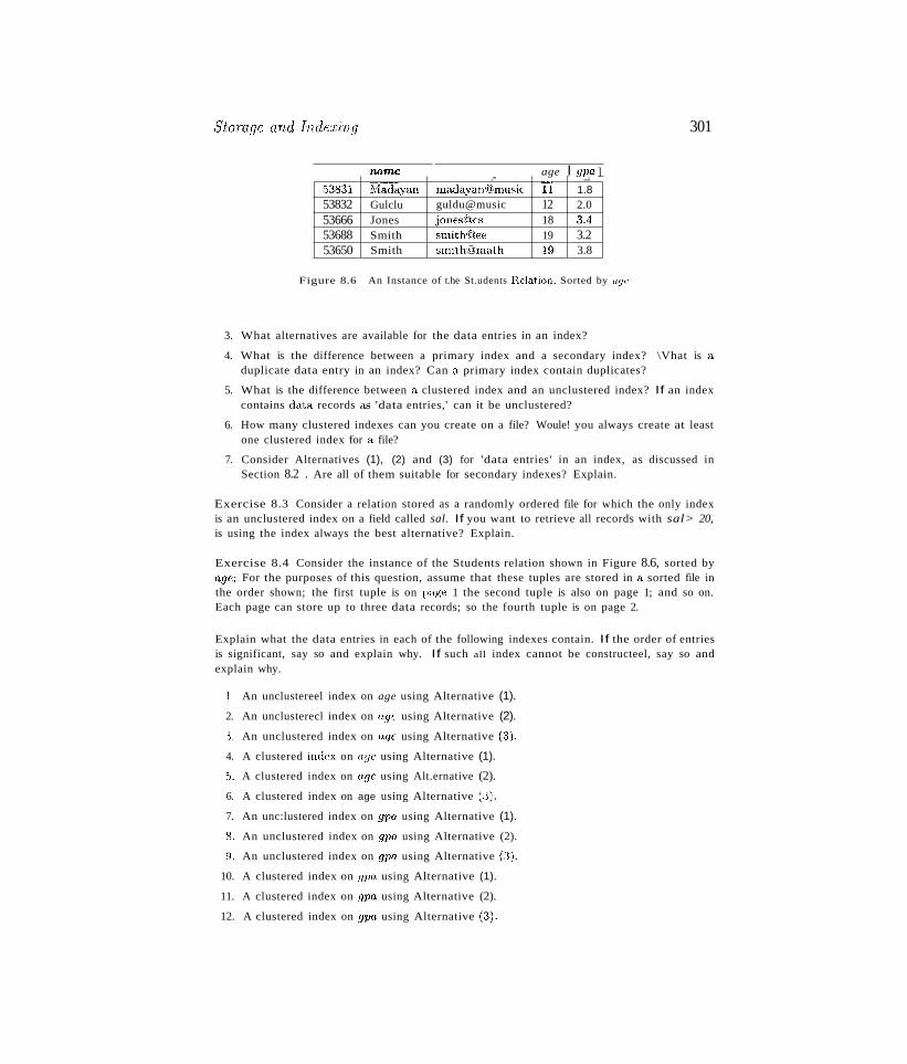
Storage and Inde:ring 301
age I gpo, ]narnc.- _.
5:3831 r\ladayan rnadayan(Q:!music h 1.853832 Gulclu guldu@music 12 2.053666 Jones jones(Q;cs 18 3.453688 Smith smith(@ee 19 3.253650 Smith srnithtg]math 19 3.8
Figure 8.6 An Instance of t.he St.udents Relation. Sorted by age
3. What alternatives are available for the data entries in an index?
4. What is the difference between a primary index and a secondary index? \Vhat is aduplicate data entry in an index? Can a primary index contain duplicates?
5. What is the difference between a clustered index and an unclustered index? If an indexcontains data records as 'data entries,' can it be unclustered?
6. How many clustered indexes can you create on a file? Woule! you always create at leastone clustered index for a file?
7. Consider Alternatives (1), (2) and (3) for 'data entries' in an index, as discussed inSection 8.2 . Are all of them suitable for secondary indexes? Explain.
Exercise 8.3 Consider a relation stored as a randomly ordered file for which the only indexis an unclustered index on a field called sal. If you want to retrieve all records with sal> 20,is using the index always the best alternative? Explain.
Exercise 8.4 Consider the instance of the Students relation shown in Figure 8.6, sorted byage: For the purposes of this question, assume that these tuples are stored in a sorted file inthe order shown; the first tuple is on page 1 the second tuple is also on page 1; and so on.Each page can store up to three data records; so the fourth tuple is on page 2.
Explain what the data entries in each of the following indexes contain. If the order of entriesis significant, say so and explain why. If such all index cannot be constructeel, say so andexplain why.
1. An unclustereel index on age using Alternative (1).
2. An unclusterecl index on age using Alternative (2).
3. An unclustered index on age using Alternative (:3).
4. A clustered index on age using Alternative (1).
5. A clustered index on age using Alt.ernative (2).
6. A clustered index on age using Alternative (:3).
7. An unc:lustered index on gpo using Alternative (1).
8. An unclustered index on gpa using Alternative (2).
9. An unclustered index on gpa using Alternative (3).
10. A clustered index on gpa using Alternative (1).
11. A clustered index on gpa using Alternative (2).
12. A clustered index on gpa using Alternative (:3).
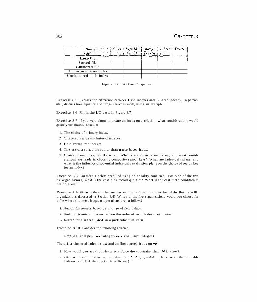
302 CHAPTERf8
Sorted fileClustered file
Unclustered tree indexUnclustered hash index
Figure 8.7 I/O Cost Comparison
Exercise 8.5 Explain the difference between Hash indexes and B+-tree indexes. In particular, discuss how equality and range searches work, using an example.
Exercise 8.6 Fill in the I/O costs in Figure 8.7.
Exercise 8.7 If you were about to create an index on a relation, what considerations wouldguide your choice? Discuss:
1. The choice of primary index.
2. Clustered versus unclustered indexes.
3. Hash versus tree indexes.
4. The use of a sorted file rather than a tree-based index.
5, Choice of search key for the index. What is a composite search key, and what considerations are made in choosing composite search keys? What are index-only plans, andwhat is the influence of potential index-only evaluation plans on the choice of search keyfor an index?
Exercise 8.8 Consider a delete specified using an equality condition. For each of the fivefile organizations, what is the cost if no record qualifies? What is the cost if the condition isnot on a key?
Exercise 8.9 What main conclusions can you draw from the discussion of the five basic fileorganizations discussed in Section 8.4? Which of the five organizations would you choose fora file where the most frequent operations are a<; follows?
1. Search for records based on a range of field values.
2. Perform inserts and scans, where the order of records docs not matter.
3. Search for a record based on a particular field value.
Exercise 8.10 Consider the following relation:
Emp( eid: integer, sal: integer l age: real, did: integer)
There is a clustered index on cid and an llnclustered index on age.
1. How would you use the indexes to enforce the constraint that eid is a key?
2. Give an example of an update that is definitely speeded 1lJi because of the availableindexes. (English description is sufficient.)
Storage and Inde.7:ing 303~
3. Give an example of an update that is definitely slowed down because of the indexes.(English description is sufficient.)
4. Can you give an example of an update that is neither speeded up nor slowed down bythe indexes?
Exercise 8.11 Consider the following relations:
Emp( eid: integer, ename: varchar, sal: integer, age: integer, did: integer)Dept(did: integer, budget: integer, floor: integer, mgr_eid: integer)
Salaries range from $10,000 to $100,000, ages vary from 20 to 80, each department has aboutfive employees on average, there are 10 floors, and budgets vary from $10,000 to $1 million.You can assume uniform distributions of values.
For each of the following queries, which of the listed index choices would you choose to speedup the query? If your database system does not consider index-only plans (i.e., data recordsare always retrieved even if enough information is available in the index entry), how wouldyour answer change? Explain briefly.
1. Query: Print ename, age, and sal for all employees.
(a) Clustered hash index on (ename, age, sal) fields of Emp.
(b) Unclustered hash index on (ename, age, sal) fields of Emp.
(c) Clustered B+ tree index on (ename, age, sal) fields of Emp.
(d) Unclustered hash index on (eid, did) fields of Emp.
(e) No index.
2. Query: Find the dids of departments that are on the 10th floor and have a budget of lessthan $15,000.
(a) Clustered hash index on the floor field of Dept.
(b) Unclustered hash index on the floor' field of Dept.
(c) Clustered B+ tree index on (floor, budget) fields of Dept.
(d) Clustered B+ tree index on the budget: field of Dept.
(e) No index.
PROJECT-BASED EXERCISES
Exercise 8.12 Answer the following questions:
1. What indexing techniques are supported in Minibase?
2. \;v'hat alternatives for data entries are supported'?
:3. Are clustered indexes supported?
BIBLIOGRAPHIC NOTES
Several books discuss file organization in detail [29, :312, 442, 531, 648, 695, 775].
Bibliographic: notes for hash-indexes and B+-trees are included in Chapters 10 and 11.
9STORING DATA:
DISKS AND FILES
.. What are the different kinds of memory in a computer system?
.. What are the physical characteristics of disks and tapes, and how dothey affect the design of database systems?
... What are RAID storage systems, and what are their advantages?
.. How does a DBMS keep track of space on disks? How does a DBMSaccess and modify data on disks? What is the significance of pages asa unit of storage and transfer?
,.. How does a DBMS create and maintain files of records? How arerecords arranged on pages, and how are pages organized within a file?
.. Key concepts: memory hierarchy, persistent storage, random versussequential devices; physical disk architecture, disk characteristics, seektime, rotational delay, transfer time; RAID, striping, mirroring, RAIDlevels; disk space manager; buffer manager, buffer pool, replacementpolicy, prefetching, forcing; file implementation, page organization,record organization
A memory is what is left when :iomething happens and does not cornpletelyunhappen.
. Edward DeBono
This chapter initiates a study of the internals of an RDBivIS. In terms of theDBj\JS architecture presented in Section 1.8, it covers the disk space manager,
304
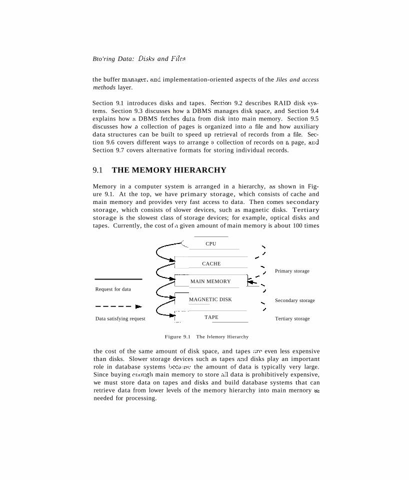
Bto'ring Data: Disks and Files
the buffer manager, and implementation-oriented aspects of the Jiles and accessmethods layer.
Section 9.1 introduces disks and tapes. Section 9.2 describes RAID disk systems. Section 9.3 discusses how a DBMS manages disk space, and Section 9.4explains how a DBMS fetches data from disk into main memory. Section 9.5discusses how a collection of pages is organized into a file and how auxiliarydata structures can be built to speed up retrieval of records from a file. Section 9.6 covers different ways to arrange a collection of records on a page, andSection 9.7 covers alternative formats for storing individual records.
9.1 THE MEMORY HIERARCHY
Memory in a computer system is arranged in a hierarchy, a'S shown in Figure 9.1. At the top, we have primary storage, which consists of cache andmain memory and provides very fast access to data. Then comes secondarystorage, which consists of slower devices, such as magnetic disks. Tertiarystorage is the slowest class of storage devices; for example, optical disks andtapes. Currently, the cost of a given amount of main memory is about 100 times
Request for data
----- .....Data satisfying request
CPU
",/.,CACHE ....
,/ Primary storage
MAIN MEMORY f.: ....,/
MAGNETIC DISK Secondary storage....,/
TAPE Tertiary storage
Figure 9.1 The Ivlemory Hierarchy
the cost of the same amount of disk space, and tapes are even less expensivethan disks. Slower storage devices such as tapes and disks play an importantrole in database systems because the amount of data is typically very large.Since buying e110ugh main memory to store all data is prohibitively expensive,we must store data on tapes and disks and build database systems that canretrieve data from lower levels of the memory hierarchy into main mernory asneeded for processing.
306
There are reasons other than cost for storing data on secondary and tertiaJ:ystorage. On systems with 32-bit addressing, only 232 bytes can be directly referenced in main memory; the number of data objects may exceed this number!Further, data must be maintained across program executions. This requiresstorage devices that retain information when the computer is restarted (aftera shutdown or a crash); we call such storage nonvolatile. Primary storage isusually volatile (although it is possible to make it nonvolatile by adding a battery backup feature), whereas secondary and tertiary storage are nonvolatile.
Tapes are relatively inexpensive and can store very large amounts of data. Theyare a good choice for archival storage, that is, when we need to maintain datafor a long period but do not expect to access it very often. A Quantum DLT4000 drive is a typical tape device; it stores 20 GB of data and can store abouttwice as much by compressing the data. It records data on 128 tape tracks,which can be thought of as a linear sequence of adjacent bytes, and supportsa sustained transfer rate of 1.5 MB/sec with uncompressed data (typically 3.0MB/sec with compressed data). A single DLT 4000 tape drive can be used toaccess up to seven tapes in a stacked configuration, for a maximum compresseddata capacity of about 280 GB.
The main drawback of tapes is that they are sequential access devices. We mustessentially step through all the data in order and cannot directly access a givenlocation on tape. For example, to access the last byte on a tape, we would haveto wind through the entire tape first. This makes tapes unsuitable for storingoperational data, or data that is frequently accessed. Tapes are mostly used toback up operational data periodically.
9.1.1 Magnetic Disks
Magnetic disks support direct access to a desired location and are widely usedfor database applications. A DBMS provides seamless access to data on disk;applications need not worry about whether data is in main memory or disk.To understand how disks work, eonsider Figure 9.2, which shows the structureof a disk in simplified form.
Data is stored on disk in units called disk blocks. A disk block is a contiguoussequence of bytes and is the unit in which data is written to a disk and readfrom a disk. Bloc:ks are arranged in concentric rings called tracks, on one ormore platters. Tracks can be recorded on one or both surfaces of a platter;we refer to platters as single-sided or double-sided, accordingly. The set of alltracks with the SaIne diameter is called a cylinder, because the space occupiedby these tracks is shaped like a cylinder; a cylinder contains one track perplatter surface. Each track is divided into arcs, called sectors, whose size is a
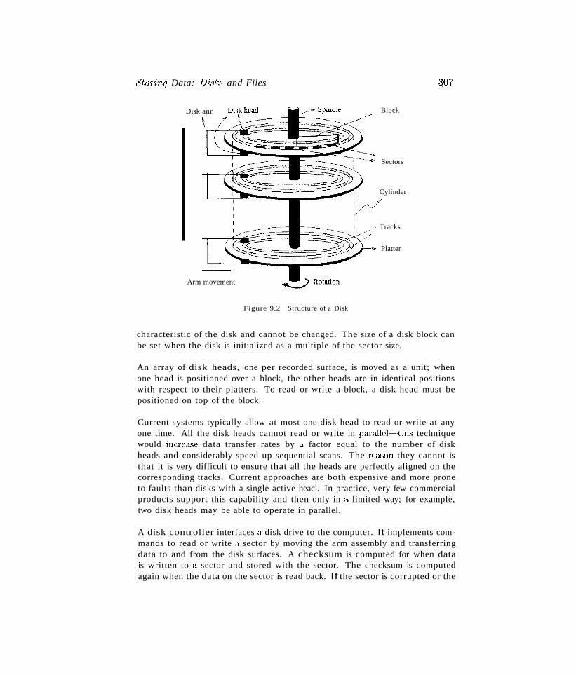
Storing Data: Disks and Files
Disk ann
Arm movement
Figure 9.2 Structure of a Disk
____ Block
Sectors
Cylinder
- Tracks
,.. Platter
~07
characteristic of the disk and cannot be changed. The size of a disk block canbe set when the disk is initialized as a multiple of the sector size.
An array of disk heads, one per recorded surface, is moved as a unit; whenone head is positioned over a block, the other heads are in identical positionswith respect to their platters. To read or write a block, a disk head must bepositioned on top of the block.
Current systems typically allow at most one disk head to read or write at anyone time. All the disk heads cannot read or write in parallel~-this techniquewould increa.se data transfer rates by a factor equal to the number of diskheads and considerably speed up sequential scans. The rea.son they cannot isthat it is very difficult to ensure that all the heads are perfectly aligned on thecorresponding tracks. Current approaches are both expensive and more proneto faults than disks with a single active heacl. In practice, very few commercialproducts support this capability and then only in a limited way; for example,two disk heads may be able to operate in parallel.
A disk controller interfaces a disk drive to the computer. It implements commands to read or write a sector by moving the arm assembly and transferringdata to and from the disk surfaces. A checksum is computed for when datais written to a sector and stored with the sector. The checksum is computedagain when the data on the sector is read back. If the sector is corrupted or the
308 CHAPTER 9
An Example of a Current Disk: The IBM Deskstar 14G~~~Th~lIBM Deskstar 14GPX is a 3.5 inch§.J4.4 GB hfl,rd disk with an averageseek time of 9.1 miUisecoudsTmsec) and an average rotational delay of4.17 msec. However, the time to seek from one track to the nexUs just 2.2msec, the maximum seek time is 15.5 :rnsec. The disk has five double-sidedplatters that spin at 7200 rotations per minute. Ea,ch platter holds 3.35 GBof data, with a density of 2.6 gigabit per square inch. The data transferrate is about 13 MB per secmld. To put these numbers in perspective,observe that a disk access takes about 10 msecs, whereas accessing a mainmemory location typically takes less than 60 nanoseconds!
read is faulty for some reason, it is very unlikely that the checksum computedwhen the sector is read matches the checksum computed when the sector waswritten. The controller computes checksums, and if it detects an error, it triesto read the sector again. (Of course, it signals a failure if the sector is corruptedand read fails repeatedly.)
~While direct access to any desired location in main memory takes approximately the same time, determining the time to access a location on disk ismore complicated. The time to access a disk block has several components.Seek time is the time taken to move the disk heads to the track on whicha desired block is located. As the size of a platter decreases, seek times alsodecrease, since we have to move a disk head a shorter distance. Typical platterdiameters are 3.5 inches and 5.25 inches. Rotational delay is the waitingtime for the desired block to rotate under the disk head; it is the time requiredfor half a rotation all average and is usually less than seek time. Transfertime is the time to actually read or write the data in the block once the headis positioned, that is, the time for the disk to rotate over the block.
9.1.2 Performance Implications of Disk Structure1. Data must be in mernory for the DBMS to operate on it.
2. The unit for data transfer between disk and main memory is a block; if asingle item on a block is needed, the entire block is transferred. Readingor writing a disk block is called an I/O (for input/output) operation.
3. The time to read or write a block varies, depending on the location of thedata:
access time = seek time + rotational delay + tmn8feT time
These observations imply that the time taken for database operations is affectedsignificantly by how data is stored OIl disks. The time for moving blocks to
Storing Data: D'isks and Files 309
or from disk usually dOlninates the time taken for database operations. Tominimize this time, it is necessary to locate data records strategically on diskbecause of the geometry and mechanics of disks. In essence, if two records arefrequently used together, we should place them close together. The 'closest'that two records can be on a disk is to be on the same block. In decrea<;ingorder of closeness, they could be on the same track, the same cylinder, or anadjacent cylinder.
Two records on the same block are obviously as close together as possible,because they are read or written as part of the same block. As the platterspins, other blocks on the track being read or written rotate under the activehead. In current disk designs, all the data on a track can be read or writtenin one revolution. After a track is read or written, another disk head becomesactive, and another track in the same cylinder is read or written. This processcontinues until all tracks in the current cylinder are read or written, and thenthe arm assembly moves (in or out) to an adjacent cylinder. Thus, we have anatural notion of 'closeness' for blocks, which we can extend to a notion of nextand previous blocks.
Exploiting this notion of next by arranging records so they are read or writtensequentially is very important in reducing the time spent in disk l/Os. Sequential access minimizes seek time and rotational delay and is much faster thanrandom access. (This observation is reinforced and elaborated in Exercises 9.5and 9.6, and the reader is urged to work through them.)
9.2 REDUNDANT ARRAYS OF INDEPENDENT DISKS
Disks are potential bottlenecks for system performance and storage system rfc'liability. Even though disk performance ha,s been improving continuously, microprocessor performance ha.'s advanced much more rapidly. The performanceof microprocessors has improved at about 50 percent or more per year, butdisk access times have improved at a rate of about 10 percent per year anddisk transfer rates at a rate of about 20 percent per year. In addition, sincedisks contain mechanical elements, they have much higher failure rates thanelectronic parts of a computer system. If a disk fails, all the data stored on itis lost.
A disk array is an arrangement of several disks, organized to increase performance and improve reliability of the resulting storage system. Performanceis increased through data striping. Data striping distributes data over severaldisks to give the impression of having a single large, very fa'3t disk. Reliability is improved through redundancy. Instead of having a single copy of thedata, redundant information is maintained. The redundant information is carc-
310 CHAPTER. Q
fully organized so that, in C&'3e of a disk failure, it can be used to reconstructthe contents of the failed disk. Disk arrays that implement a combination ofdata striping and redundancy are called redundant arrays of independentdisks, or in short, RAID.! Several RAID organizations, referred to as RAIDlevels, have been proposed. Each RAID level represents a different trade-offbetween reliability and performance.
In the remainder of this section, we first discuss data striping and redundancyand then introduce the RAID levels that have become industry standards.
9.2.1 Data Striping
A disk array gives the user the abstraction of having a single, very large disk.If the user issues an I/O request, we first identify the set of physical disk blocksthat store the data requested. These disk blocks may reside on a single disk inthe array or may be distributed over several disks in the array. Then the setof blocks is retrieved from the disk(s) involved. Thus, how we distribute thedata over the disks in the array influences how many disks are involved whenan I/O request is processed.
In data striping, the data is segmented into equal-size partitions distributedover multiple disks. The size of the partition is called the striping unit. Thepartitions are usually distributed using a round-robin algorithm: If the diskarray consists of D disks, then partition i is written onto disk i mod D.
As an example, consider a striping unit of one bit. Since any D successive databits are spread over all D data disks in the array, all I/O requests involve andisks in the array. Since the smallest unit of transfer from a disk is a block,each I/O request involves transfer of at least D blocks. Since we can read the Dblocks from the D disks in parallel, the transfer rate of each request is D timesthe transfer rate of a single disk; each request uses the aggregated bandwidthof all disks in the array. But the disk access time of the array is ba.'3ically theaccess time of a single disk, since all disk heads have to move for" all requests.Therefore, for a disk array with a striping unit of a single bit, the number ofrequests per time unit that the array can process and the average response timefor each individual request are similar to that of a single disk.
As another exarhple, consider a striping unit of a disk block. In this case, I/Orequests of the size of a disk block are processed by one disk in the array. Ifrnany I/O requests of the size of a disk block are made, and the requested
1 Historically, the J in RAID stood for inexpensive, as a large number of small disks was much moreeconornical than a single very large disk. Today, such very large disks are not even manufactured .. ··asign of the impact of RAID.
Storing Data: Disks and Piles
Redundancy Schemes: Alternatives to the parity scheme includeschemes based on Hamming codes and Reed-Solomon codes. In addition to recovery from single disk failures, Hamming codes can identifywhich disk failed. Reed-Solomon codes can recover from up to two simultaneous disk failures. A detailed discussion of these schemes is beyondthe scope of our discussion here; the bibliography provides pointers for theinterested reader.
blocks reside on different disks, we can process all requests in parallel and thusreduce the average response time of an I/O request. Since we distributed thestriping partitions round-robin, large requests of the size of many contiguousblocks involve all disks. We can process the request by all disks in parallel andthus increase the transfer rate to the aggregated bandwidth of all D disks.
9.2.2 Redundancy
While having more disks increases storage system performance, it also lowers overall storage system reliability. Assume that the mean-time-to-failure(MTTF), of a single disk is 50, 000 hours (about 5.7 years). Then, the MTTFof an array of 100 disks is only 50, 000/100 = 500 hours or about 21 days,assuming that failures occur independently and the failure probability of a diskdoes not change over time. (Actually, disks have a higher failure probabilityearly and late in their lifetimes. Early failures are often due to undetectedmanufacturing defects; late failures occur since the disk wears out. Failures donot occur independently either: consider a fire in the building, an earthquake,or purchase of a set of disks that come from a 'bad' manufacturing batch.)
Reliability of a disk array can be increased by storing redundant information.If a disk fails, the redundant information is used to reconstruct the data on thefailed disk. Redundancy can immensely increase the MTTF of a disk array.When incorporating redundancy into a disk array design, we have to make twochoices. First, we have to decide where to store the redundant information. Wecan either store the redundant information on a small number of check disksor distribute the redundant information uniformly over all disks.
The second choice we have to make is how to compute the redundant information. Most disk arrays store parity information: In the parity scheme, anextra check disk contains information that can be used to recover from failureof anyone disk in the array. Assume that we have a disk array with D disksand consider the first bit on each data disk. Suppose that i of the D data bitsare 1. The first bit on the check disk is set to 1 if i is odd; otherwise, it is set to
312 CHAPTER 9
O. This bit on the check disk is called the parity of the data bits. The checkdisk contains parity information for each set of corresponding D data bits.
To recover the value of the first bit of a failed disk we first count the numberof bits that are 1 on the D - 1 nonfailed disks; let this number be j. If j is oddand the parity bit is 1, or if j is even and the parity bit is 0, then the valueof the bit on the failed disk must have been O. Otherwise, the value of the biton the failed disk must have been 1. Thus, with parity we can recover fromfailure of anyone disk. Reconstruction of the lost information involves readingall data disks and the check disk.
For example, with an additional 10 disks with redundant information, theMTTF of our example storage system with 100 data disks can be increasedto more than 250 years! "What is more important, a large MTTF implies asmall failure probability during the actual usage time of the storage system,which is usually much smaller than the reported lifetime or the MTTF. (Whoactually uses lO-year-old disks?)
In a RAID system, the disk array is partitioned into reliability groups, wherea reliability group consists of a set of data disks and a set of check disks. Acommon 7'cdundancy scheme (see box) is applied to each group. The numberof check disks depends on the RAID level chosen. In the remainder of thissection, we assume for ease of explanation that there is only one reliabilitygroup. The reader should keep in mind that actual RAID implementationsconsist of several reliability groups, and the number of groups plays a role inthe overall reliability of the resulting storage system.
9.2.3 Levels of Redundancy
Throughout the discussion of the different RAID levels, we consider sampledata that would just fit on four disks. That is, with no RAID technology ourstorage system would consist of exactly four data disks. Depending on theRAID level chosen, the number of additional disb varies from zero to four.
Level 0: Nonredundant
A RAID Level 0 system uses data striping to incre,clse the maximum bandwidthavailable. No redundant information is maintained. \\ThUe being the solutionwith the lowest cost, reliability is a problem, since the MTTF decreases linearlywith the number of disk drives in the array. RAID Level 0 has the best writeperformance of all RAID levels, because absence of redundant information implies that no redundant information needs to be updated! Interestingly, RAIDLevel 0 docs not have the best read perfonnancc of all RAID levels, since sys-
StoTing Data: Disks (1'lul Piles 313,
tems with redundancy have a choice of scheduling disk accesses, as explainedin the next section.
In our example, the RAID Level a solution consists of only four data disks.Independent of the number of data disks, the effective space utilization for aRAID Level a system is always 100 percent.
Levell: Mirrored
A RAID Level 1 system is the most expensive solution. Instead of havingone copy of the data, two identical copies of the data on two different disks arelnaintained. This type of redundancy is often called mirroring. Every write ofa disk block involves a write on both disks. These writes may not be performedsimultaneously, since a global system failure (e.g., due to a power outage) couldoccur while writing the blocks and then leave both copies in an inconsistentstate. Therefore, we always write a block on one disk first and then write theother copy on the mirror disk. Since two copies of each block exist on differentdisks, we can distribute reads between the two disks and allow parallel readsof different disk blocks that conceptually reside on the same disk. A read of ablock can be scheduled to the disk that h&'3 the smaller expected access time.RAID Level 1 does not stripe the data over different disks, so the transfer ratefor a single request is comparable to the transfer rate of a single disk.
In our example, we need four data and four check disks with mirrored data fora RAID Levell implementation. The effective space utilization is 50 percent,independent of the number of data disks.
Level 0+1: Striping and Mirroring
RAID Level 0+ l---sometimes also referred to H..S RA ID Level 10- -combinesstriping and mirroring. As in RAID Level L read requests of the size of a diskblock can be scheduled both to a disk and its mirror image. In addition, readrequests of the size of several contiguous blocks benefit froIl1 the aggregatedbandwidth of all disks. Thc cost for writes is analogous to RAID LevelL
As in RAID Levell, our exa.Inple with four data disks requires four check disksand the effective space utilization is always 50 percent.
Level 2: Error-Correcting Codes
In RAID Level 2, the striping unit is a single bit. The redundancy scheme usedis Hamming code. In our example with four data disks, only three check disks
314 CHAPTER 9
are needed. In general, the number of check disks grows logarithmically withthe number of data disks.
Striping at the bit level has the implication that in a disk array with D datadisks, the smallest unit of transfer for a read is a set of D blocks. Therefore,Level 2 is good for workloads with many large requests, since for each request,the aggregated bandwidth of all data disks is used. But RAID Level 2 is badfor small requests of the size of an individual block for the same reason. (Seethe example in Section 9.2.1.) A write of a block involves reading D blocksinto main memory, modifying D + C blocks, and writing D + C blocks todisk, where C is the number of check disks. This sequence of steps is called aread-modify-write cycle.
For a RAID Level 2 implementation with four data disks, three check disksare needed. In our example, the effective space utilization is about 57 percent.The effective space utilization increases with the number of data disks. Forexample, in a setup with 10 data disks, four check disks are needed and theeffective space utilization is 71 percent. In a setup with 25 data disks, fivecheck disks are required and the effective space utilization grows to 83 percent.
Level 3: Bit~Interieaved Parity
While the redundancy schema used in RAID Level 2 improves in terms of costover RAID Level 1, it keeps more redundant information than is necessary.Hamming code, as used in RAID Level 2, has the advantage of being able toidentify which disk has failed. But disk controllers can easily detect whichdisk has failed. Therefore, the check disks do not need to contain informationto identify the failed disk. Information to recover the lost data is sufficient.Instead of using several disks to store Hamming code, RAID Level 3 has asingle check disk with parity information. Thus, the reliability overhead forRAID Level 3 is a single disk, the lowest overhead possible.
The performance characteristics of RAID Levels 2 and 3 are very similar. RAIDLevel 3 can also process only one I/O at a time, the minimum transfer unit isD blocks, and a write requires a read-modify-write cycle.
Level 4: Block~Interleaved Parity
RAID Level 4 hEk"i a striping unit of a disk block, instead of a single bit as inRAID Level 3. Block-level striping has the advantage that read requests ofthe size of a disk block can be sen;ed entirely by the disk where the requestedblock resides. Large read requests of several disk blocks can still utilize theaggregated bandwidth of the D disks.
Sto'ring Data: D'isks and Files 315
The \vrite of a single block still requires a read-modify-write cycle, but onlyone data disk and the check disk are involved. The parity on the check diskcan be updated without reading all D disk blocks, because the new parity canbe obtained by noticing the differences between the old data block and the newdata block and then applying the difference to the parity block on the checkdisk:
NewParity = (OldData XOR NewData) XOR OldParity
The read-modify-write cycle involves reading of the old data block and the oldparity block, modifying the two blocks, and writing them back to disk, resultingin four disk accesses per write. Since the check disk is involved in each write,it can easily become the bottleneck.
RAID Level 3 and 4 configurations with four data disks require just a singlecheck disk. In our example, the effective space utilization is 80 percent. Theeffective space utilization increases with the number of data disks, since alwaysonly one check disk is necessary.
Level 5: Block-Interleaved Distributed Parity
RAID Level 5 improves on Level 4 by distributing the parity blocks uniformlyover all disks, instead of storing them on a single check disk. This distributionhas two advantages. First, several write requests could be processed in parallel,since the bottleneck of a unique check disk has been eliminated. Second, readrequests have a higher level of parallelism. Since the data is distributed overall disks, read requests involve all disks, whereas in systems with a dedicatedcheck disk the check disk never participates in reads.
A RAID Level 5 system has the best performance of all RAID levels withredundancy for small and large read ancllarge write requests. Small writes stillrequire a read-modify-write cycle and are thus less efficient than in RAID Level1.
In our example, the corresponding RAID Level 5 system has five disks overalland thus the effective spa,ce utilization is the same as in RAID Levels 3 and 4.
Level 6: P+Q Redundancy
The motivation for RAID Level 6 is the observation that recovery from failureof a single disk is not sufficient in very large disk arrays. First, in large diskarrays, a second disk lllight fail before replacement of an already failed disk
316 CHAPTER~ 9
could take place. In addition, the probability of a disk failure during recoveryof a failed disk is not negligible.
A RAID Level 6 system uses Reed-Solomon codes to be able to recover fromup to two simultaneous disk failures. RAID Level 6 requires (conceptually)two check disks, but it also uniformly distributes redundant information at theblock level as in RAID Level 5. Thus. the performance characteristics for smalland large read requests and for large write requests are analogous to RAIDLevel 5. For small writes, the read-modify-write procedure involves six insteadof four disks as compared to RAID Level 5, since two blocks with redundantinformation need to be updated.
For a RAID Level 6 system with storage capacity equal to four data disks, sixdisks are required. In our example, the effective space utilization is 66 percent.
9.2.4 Choice of RAID Levels
If data loss is not an issue, RAID Level 0 improves overall system performanceat the lowest cost. RAID Level 0+ 1 is superior to RAID Level 1. The mainapplication areas for RAID Level 0+1 systems are small storage subsystemswhere the cost of mirroring is moderate. Sometimes, RAID Level 0+1 is usedfor applications that have a high percentage of writes in their workload, sinceRAID Level 0+1 provides the best write performance. RAID Levels 2 and4 are always inferior to RAID Levels 3 and 5, respectively. RAID Level 3 isappropriate for workloads consisting mainly of large transfer requests of severalcontiguous blocks. The performance of a RAID Level 3 system is bad forworkloads with many small requests of a single disk block. RAID Level 5 is agood general-purpose solution. It provides high performance for large as wellas small requests. RAID Level 6 is appropriate if a higher level of reliability isrequired.
9.3 DISK SPACE MANAGEMENTI
The lowest level of software in the DB.lVIS architecture discussed in Section 1.8,called the disk space manager, manages space on disk. Abstractly, the diskspace manager supports the concept of a page as a unit of data and providescOlmnands to allocate or deallocate a page and read or write a page. The sizeof a page is chosen to be the size of a disk block and pages are stored as diskblocks so that reading or writing a page can be done in one disk I/O.
It is often useful to allocate a sequence of pages (lS a contiguous sequence ofblocks to hold data frequently accessed in sequential order. This capabilityis essential for exploiting the advantages of sequentially accessing disk blocks,
StoTing Data: Disks and Files 317
which we discussed earlier in this chapter. Such a capability, if desired, mustbe provided by the disk space manager to highcr-levellayers of the DBMS.
The disk space manager hides details of the underlying hardware (and possiblythe operating system) and allows higher levels of the software to think of thedata cLS a collection of pages.
9.3.1 Keeping Track of Free Blocks
A database grows and shrinks <1.<; records are inserted and deleted over time.The disk space manager keeps track of which disk blocks are in usc, in additionto keeping track of which pages are on which disk blocks. Although it is likelythat blocks are initially allocated sequentially on disk, subsequent allocationsand deallocations could in general create 'holes.'
One way to keep track of block usage is to maintain a. list of free blocks. Asblocks are deallocated (by the higher-level software that requests and uses theseblocks), we can add them to the free list for future use. A pointer to the firstblock on the free block list is stored in a known location on disk.
A second way is to maintain a bitmap with one bit for each disk block, whichindicates whether a block is in use or not. A bitmap also allows very fastidentification and allocation of contiguous areas on disk. This is difficult toaccomplish with a linked list approach.
9.3.2 Using OS File Systems to Manage Disk Space
Operating systems also manage space on disk. Typically, an operating systemsupports the abstraction of a file as a sequence of bytes. The as managesspace on the disk and translates requests, such as "Read byte i of file f," intocorresponding low-level instructions: "Read block m of track t of cylinder cof disk d." A database disk space manager could he built using OS files. J:;'orexample, the entire database could reside in one or more as files for whicha number of blocks are allocated (by the aS) and initialized. The disk spacemanager is then responsible for managing the space in these OS files.
Many database systems do not rely on the as file system and instead do theirown disk management, either from scratch or by extending as facilities. Thereasons are practical <1.<; well eLe; technical One practical reason is that a DB~1S
vendor who \vishes to support several as platfonns cannot assume featuresspecific to any OS, for porta.bilit,'rr, and would therefore try to make the DBMScode as self-contained as possible. A technical reason is that on a :32-bit systern,the la.rgest file size is 4 GD, whereas a DBMS may want to access a single file
318 CHAPTER 9
larger than that. A related problem is that typical as files cannot span diskdevices, which is often desirable or even necessary in a DBMS. Additionaltechnical reasons why a DBMS does not rely on the as file system are outlinedin Section 9.4.2.
9.4 BUFFER MANAGER
To understand the role of the buffer manager, consider a simple example. Suppose that the database contains 1 million pages, but only 1000 pages of mainmemory are available for holding data. Consider a query that requires a scanof the entire file. Because all the data cannot be brought into main memory atone time, the DBMS must bring pages into main memory as they are neededand, in the process, decide what existing page in main memory to replace tomake space for the new page. The policy used to decide which page to replaceis called the replacement policy.
In terms of the DBMS architecture presented in Section 1.8, the buffer manager is the software layer responsible for bringing pages from disk to mainmemory as needed. The buffer manager manages the available main memoryby partitioning it into a collection of pages, which we collectively refer to as thebuffer pool. The main memory pages in the buffer pool are called frames;it is convenient to think of them as slots that can hold a page (which usuallyresides on disk or other secondary storage media).
Higher levels of the DBMS code can be written without worrying about whetherdata pages are in memory or not; they ask the buffer manager for the page,and it is brought into a frame in the buffer pool if it is not already there.Of course, the higher-level code that requests a page must also release thepage when it is no longer needed, by informing the buffer manager, so thatthe frame containing the page can be reused. The higher-level code must alsoinform the buffer manager if it modifies the requested page; the buffer managerthen makes sure that the change is propagated to the copy of the page on disk.Buffer management is illustrated in Figure 9.3.
In addition to the buffer pool itself, the buffer manager maintains some bookkeeping information and two variables for each frame in the pool: pirLcountand dirty. The number of times that the page currently in a given frame hasbeen requested but not released-the number of current users of the page--isrecorded in the pin_count variable for that frame. The Boolean variable dirtyindicates whether the page ha.<; been modified since it was brought into thebuffer pool from disk.
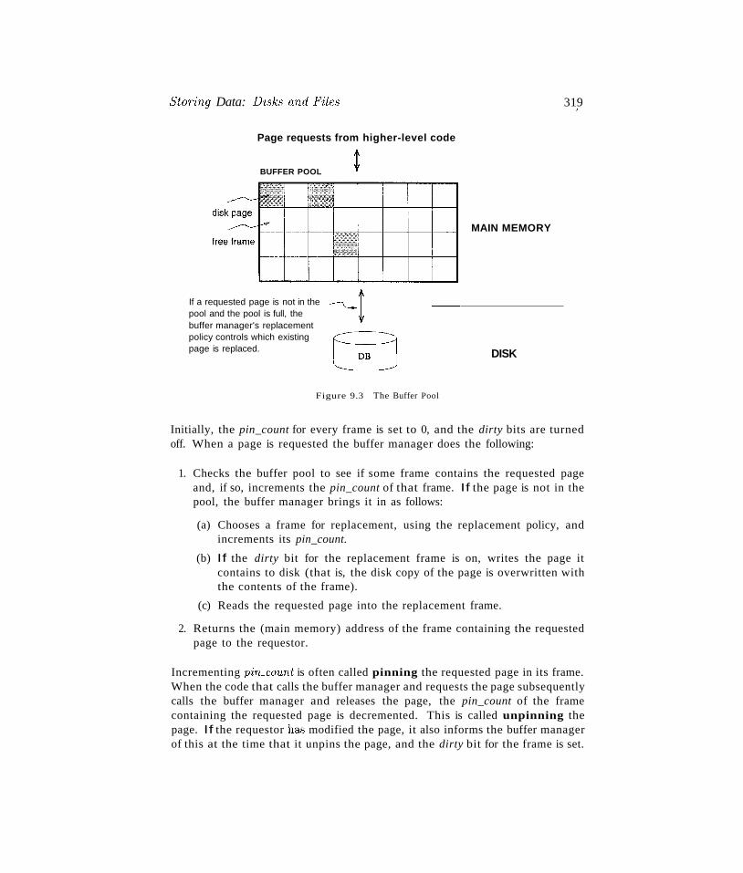
Sio'ring Data: D'isks and Files
Page requests from higher-level code
BUFFER POOL
If a requested page is not in thepool and the pool is full, thebuffer manager's replacementpolicy controls which existingpage is replaced.
Figure 9.3 The Buffer Pool
MAIN MEMORY
DISK
319,
Initially, the pin_count for every frame is set to 0, and the dirty bits are turnedoff. When a page is requested the buffer manager does the following:
1. Checks the buffer pool to see if some frame contains the requested pageand, if so, increments the pin_count of that frame. If the page is not in thepool, the buffer manager brings it in as follows:
(a) Chooses a frame for replacement, using the replacement policy, andincrements its pin_count.
(b) If the dirty bit for the replacement frame is on, writes the page itcontains to disk (that is, the disk copy of the page is overwritten withthe contents of the frame).
(c) Reads the requested page into the replacement frame.
2. Returns the (main memory) address of the frame containing the requestedpage to the requestor.
Incrementing pirLco'llnt is often called pinning the requested page in its frame.When the code that calls the buffer manager and requests the page subsequentlycalls the buffer manager and releases the page, the pin_count of the framecontaining the requested page is decremented. This is called unpinning thepage. If the requestor has modified the page, it also informs the buffer managerof this at the time that it unpins the page, and the dirty bit for the frame is set.
320 CHAPTER ,,9
The buffer manager will not read another page into a frame until its pi'll-count
becomes 0, that is, until all requestors of the page have unpilln~d it.
If a requested page is not in the buffer pool and a free frame is not availablein the buffer pool, a frame with pirl-count 0 is chosen for replacement. If thereare many such frames, a frame is chosen according to the buffer manager'sreplacement policy. vVe discuss various replacement policies in Section 9.4.1.
\-\Then a page is eventually chosen for replacement, if the dir'ty bit is not set,it means that the page h1-:1..<; not been modified since being brought into mainmemory. Hence, there is no need to write the page back to disk; the copyon disk is identical to the copy in the frame, and the frame can simply beoverwritten by the newly requested page. Otherwise, the modifications to thepage must be propagated to the copy on disk. (The crash recovery protocolmay impose further restrictions, as we saw in Section 1.7. For example, in theWrite-Ahead Log (WAL) protocol, special log records are used to describe thechanges made to a page. The log records pertaining to the page to be replacedmay well be in the buffer; if so, the protocol requires that they be written todisk before the page is written to disk.)
If no page in the buffer pool has pin_count 0 and a page that is not in the poolis requested, the buffer manager must wait until some page is released beforeresponding to the page request. In practice, the transaction requesting the pagemay simply be aborted in this situation! So pages should be released-by thecode that calls the buffer manager to request the page- as soon as possible.
A good question to ask at this point is, "What if a page is requested by severaldifferent transactions?" That is, what if the page is requested by programsexecuting independently on behalf of different users? Such programs couldmake conflicting changes to the page. The locking protocol (enforced by higherlevel DBMS code, in particular the transaction manager) ensures that eachtransaction obtains a shared or exclusive lock before requesting a page to reador rnodify. Two different transactions cannot hold an exclusive lock on thesame page at the same time; this is how conflicting changes are prevented. Thebuffer rnanager simply ~1..'3surnes tha.t the appropriate lock has been obtainedbefore a page is requested.
9.4.1 Buffer Replacement Policies
The policy used to choose an unpinned page for replacement can affect the timetaken for database operations considerably. Of the man,Y alternative policies,each is suitable in different situations.
Sto7~ing Data: Disks and Files 321
The best-known replacement policy is least recently used (LRU). This canbe implemented in the buffer manager using a queue of pointers to frames withpin_count O. A frame is added to the end of the queue when it becomes acandidate for replacement (that is, when the p'irLco'unt goes to 0). The pagechosen for replacement is the one in the frame at the head of the queue.
A variant of LRU, called clock replacement, has similar behavior but lessoverhead. The idea is to choose a page for replacement using a current variablethat takes on values 1 through N, where N is the number of buffer frames, incircular order. Vie can think of the frames being arranged in a circle, like aclock's face, and current as a clock hand moving across the face. To approximateLRU behavior, each frame also has an associated referenced bit, which is turnedon when the page p'in~count goes to O.
The current frame is considered for replacement. If the frame is not chosen forreplacement, current is incremented and the next frame is considered; this process is repeated until some frame is chosen. If the current frame has pin_countgreater than 0, then it is not a candidate for replacement and current is incremented. If the current frame has the referenced bit turned on, the clockalgorithm turns the referenced bit off and increments cm'rent-this way, a recently referenced page is less likely to be replaced. If the current frame hasp'irLcount 0 and its referenced bit is off, then the page in it is chosen for replacement. If all frames are pinned in some sweep of the clock hand (that is,the value of current is incremented until it repeats), this means that no pagein the buffer pool is a replacement candidate.
The LRU and clock policies are not always the best replacement strategies for adatabase system, particularly if many user requests require sequential scans ofthe data. Consider the following illustrative situation. Suppose the buffer poolh<4'3 10 frames, and the file to be scanned has 10 or fewer pages. Assuming,for simplicity, that there are no competing requests for pages, only the firstscan of the file does any I/O. Page requests in subsequent scans always find thedesired page in the buffer pool. On the other hand, suppose that the file to bescanned has 11 pages (which is one more than the number of available pagesin the buffer pool). Using LRU, every scan of the file will result in readingevery page of the file! In this situation, called sequential flooding, LRU isthe worst possible replacement strategy.
Other replacement policies include first in first out (FIFO) and most recently used (MRU), which also entail overhead similar to LRU, and random,arnong others. The details of these policies should be evident from their namesand the preceding discussion of LRU and clock.
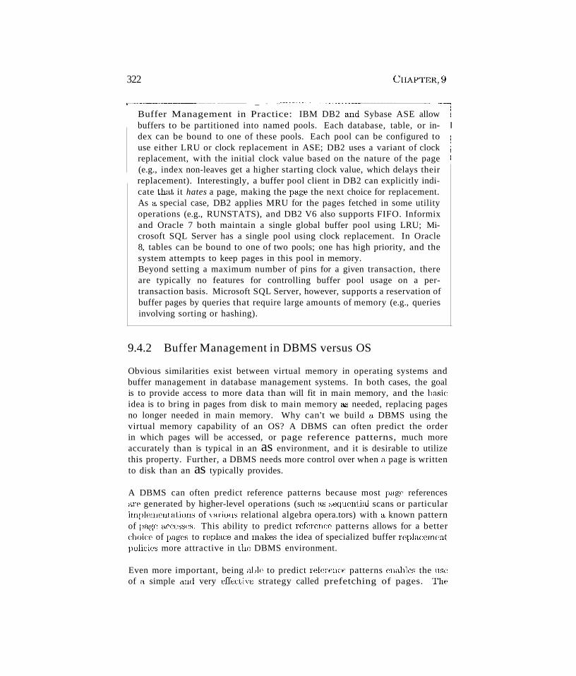
322
,---------------- _ _.._._-_..----~~-------------··-~~l
Buffer Management in Practice: IBM DB2 and Sybase ASE allow !buffers to be partitioned into named pools. Each database, table, or in- Idex can be bound to one of these pools. Each pool can be configured to Iuse either LRU or clock replacement in ASE; DB2 uses a variant of clock !replacement, with the initial clock value based on the nature of the page !(e.g., index non-leaves get a higher starting clock value, which delays theirreplacement). Interestingly, a buffer pool client in DB2 can explicitly indicate that it hates a page, making the page the next choice for replacement.As a special case, DB2 applies MRU for the pages fetched in some utilityoperations (e.g., RUNSTATS), and DB2 V6 also supports FIFO. Informixand Oracle 7 both maintain a single global buffer pool using LRU; Microsoft SQL Server has a single pool using clock replacement. In Oracle8, tables can be bound to one of two pools; one has high priority, and thesystem attempts to keep pages in this pool in memory.Beyond setting a maximum number of pins for a given transaction, thereare typically no features for controlling buffer pool usage on a pertransaction basis. Microsoft SQL Server, however, supports a reservation ofbuffer pages by queries that require large amounts of memory (e.g., queriesinvolving sorting or hashing).
9.4.2 Buffer Management in DBMS versus OS
Obvious similarities exist between virtual memory in operating systems andbuffer management in database management systems. In both cases, the goalis to provide access to more data than will fit in main memory, and the basicidea is to bring in pages from disk to main memory a.<.; needed, replacing pagesno longer needed in main memory. Why can't we build a DBMS using thevirtual memory capability of an OS? A DBMS can often predict the orderin which pages will be accessed, or page reference patterns, much moreaccurately than is typical in an as environment, and it is desirable to utilizethis property. Further, a DBMS needs more control over when a page is writtento disk than an as typically provides.
A DBMS can often predict reference patterns because most page referencesare generated by higher-level operations (such as sequential scans or particularimplementations of various relational algebra opera.tors) with a. known patternof page accesses. This ability to predict reference patterns allows for a betterchoice of pages to replace and makes the idea of specialized buffer replacmnentpolicies more attractive in the DBMS environment.
Even more important, being able to predict reference patterns enables the uscof a simple and very effective strategy called prefetching of pages. The
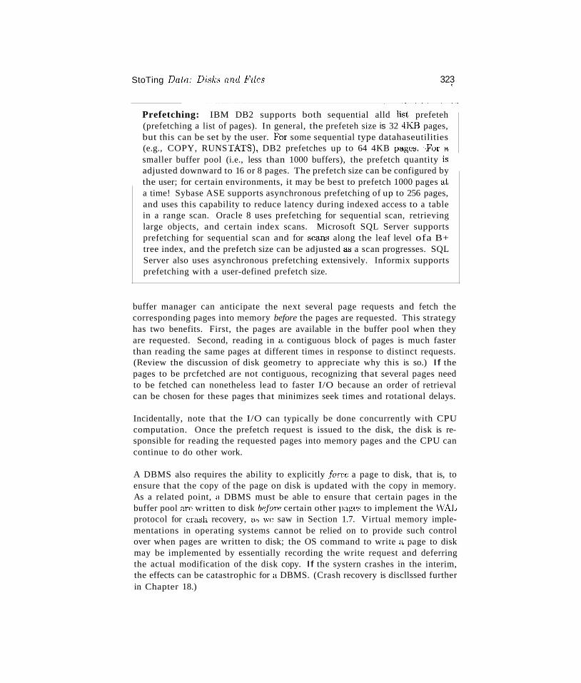
StoTing Data: Disks and Files 3231
~" ~--~--"------------------------~
Prefetching: IBM DB2 supports both sequential alld list prefeteh(prefetching a list of pages). In general, the prefeteh size is 32 4KB· pages,but this can be set by the user. £tor some sequential type datahaseutilities(e.g., COPY, RUNSTATS), DB2 prefetches up to 64 4KB pages,·!'cJr asmaller buffer pool (i.e., less than 1000 buffers), the prefetch quantity isadjusted downward to 16 or 8 pages. The prefetch size can be configured bythe user; for certain environments, it may be best to prefetch 1000 pages ata time! Sybase ASE supports asynchronous prefetching of up to 256 pages,and uses this capability to reduce latency during indexed access to a tablein a range scan. Oracle 8 uses prefetching for sequential scan, retrievinglarge objects, and certain index scans. Microsoft SQL Server supportsprefetching for sequential scan and for scarlS along the leaf level ofa B+tree index, and the prefetch size can be adjusted a<; a scan progresses. SQLServer also uses asynchronous prefetching extensively. Informix supportsprefetching with a user-defined prefetch size.
buffer manager can anticipate the next several page requests and fetch thecorresponding pages into memory before the pages are requested. This strategyhas two benefits. First, the pages are available in the buffer pool when theyare requested. Second, reading in a contiguous block of pages is much fasterthan reading the same pages at different times in response to distinct requests.(Review the discussion of disk geometry to appreciate why this is so.) If thepages to be prcfetched are not contiguous, recognizing that several pages needto be fetched can nonetheless lead to faster I/O because an order of retrievalcan be chosen for these pages that minimizes seek times and rotational delays.
Incidentally, note that the I/O can typically be done concurrently with CPUcomputation. Once the prefetch request is issued to the disk, the disk is responsible for reading the requested pages into memory pages and the CPU cancontinue to do other work.
A DBMS also requires the ability to explicitly force a page to disk, that is, toensure that the copy of the page on disk is updated with the copy in memory.As a related point, a DBMS must be able to ensure that certain pages in thebuffer pool are written to disk before certain other pages to implement the ';VALprotocol for cra,<;h recovery, as we saw in Section 1.7. Virtual memory implementations in operating systems cannot be relied on to provide such controlover when pages are written to disk; the OS command to write a page to diskmay be implemented by essentially recording the write request and deferringthe actual modification of the disk copy. If the systern crashes in the interim,the effects can be catastrophic for a DBMS. (Crash recovery is discllssed furtherin Chapter 18.)
324 CHAPTER~9
Indexes as Files: In Chapter 8, we presented indexes as a way of 6rga11i~~--··w·ling data records for efficient search. From an implementation standpoint, I
Ii
indexes are just another kind of file, containing records that dil'ect trafficon requests for data records. For example, a tree index is a collection ofrecords organized into one page per node in the tree. It is convenient toactually think of a tree index as two files, because it contains two kindsof records: (1) a file of index entries, which are records with fields for theindex's search key, and fields pointing to a child node, and (2) a file of dataentries, whose structure depends on the choice of data entry alternative.
9.5 FILES OF RECORDS
We now turn our attention from the way pages are stored on disk and broughtinto main memory to the way pages are used to store records and organizedinto logical collections or files. Higher levels of the DBMS code treat a page aseffectively being a collection of records, ignoring the representation and storagedetails. In fact, the concept of a collection of records is not limited to thecontents of a single page; a file can span several pages. In this section, weconsider how a collection of pages can be organized as a file. We discuss howthe space on a page can be organized to store a collection of records in Sections9.6 and 9.7.
9.5.1 Implementing Heap Files
The data in the pages of a heap file is not ordered in any way, and the onlyguarantee is that one can retrieve all records in the file by repeated requestsfor the next record. Every record in the file has a unique rid, and every pagein a file is of the same size.
Supported operations on a heap file include CTeatc and destmy files, 'insert arecord, delete a record with a given rid, get a record with a given rid, and scanall records in the file. To get or delete a record with a given rid, note that wemust be able to find the id of the page containing the record, given the id ofthe record.
vVe must keep track of the pages in each heap file to support scans, and we mustkeep track of pages that contain free space to implement insertion efficiently.\Ve discuss two alternative ways to rnaintain this information. In each of thesealternatives, pages must hold two pointers (which are page ids) for file-levelbookkeeping in addition to the data.
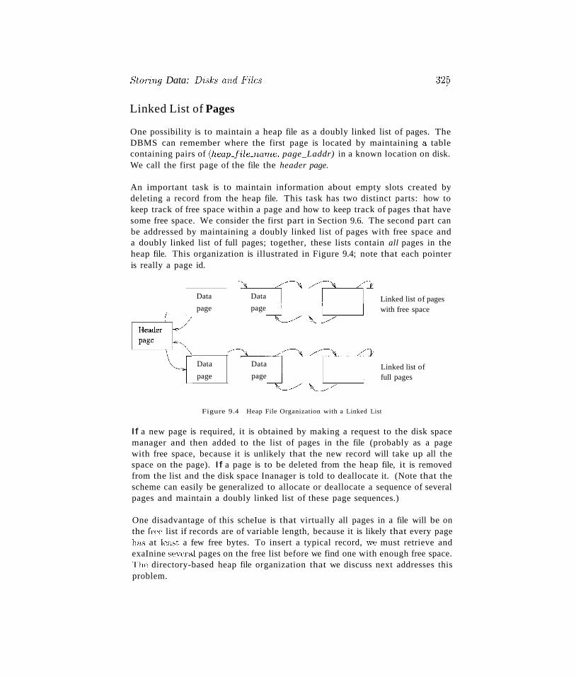
Storing Data: Disks aTul File,s 32~
Linked List of Pages
One possibility is to maintain a heap file as a doubly linked list of pages. TheDBMS can remember where the first page is located by maintaining a tablecontaining pairs of (heap_file_name, page_Laddr) in a known location on disk.We call the first page of the file the header page.
An important task is to maintain information about empty slots created bydeleting a record from the heap file. This task has two distinct parts: how tokeep track of free space within a page and how to keep track of pages that havesome free space. We consider the first part in Section 9.6. The second part canbe addressed by maintaining a doubly linked list of pages with free space anda doubly linked list of full pages; together, these lists contain all pages in theheap file. This organization is illustrated in Figure 9.4; note that each pointeris really a page id.
Data
page
Data
page
Linked list offull pages
Linked list of pageswith free space
page
Data
Data
page
Figure 9.4 Heap File Organization with a Linked List
If a new page is required, it is obtained by making a request to the disk spacemanager and then added to the list of pages in the file (probably as a pagewith free space, because it is unlikely that the new record will take up all thespace on the page). If a page is to be deleted from the heap file, it is removedfrom the list and the disk space Inanager is told to deallocate it. (Note that thescheme can easily be generalized to allocate or deallocate a sequence of severalpages and maintain a doubly linked list of these page sequences.)
One disadvantage of this scheIue is that virtually all pages in a file will be onthe free list if records are of variable length, because it is likely that every pageha",,, at least a few free bytes. To insert a typical record, we must retrieve andexaInine several pages on the free list before we find one with enough free space.The directory-based heap file organization that we discuss next addresses thisproblem.
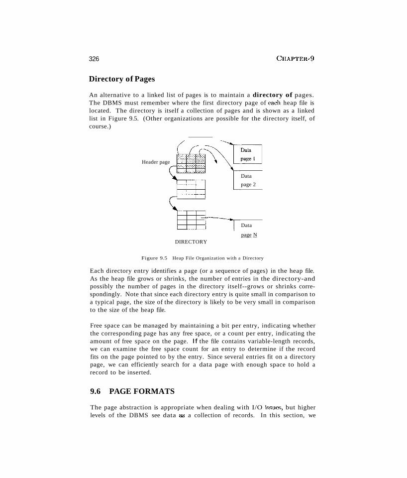
326
Directory of Pages
CHAPTER,g
An alternative to a linked list of pages is to maintain a directory of pages.The DBMS must remember where the first directory page of each heap file islocated. The directory is itself a collection of pages and is shown as a linkedlist in Figure 9.5. (Other organizations are possible for the directory itself, ofcourse.)
Header page
Data
page 2
Data
page NDIRECTORY
Figure 9.5 Heap File Organization with a Directory
Each directory entry identifies a page (or a sequence of pages) in the heap file.As the heap file grows or shrinks, the number of entries in the directory-andpossibly the number of pages in the directory itself--grows or shrinks correspondingly. Note that since each directory entry is quite small in comparison toa typical page, the size of the directory is likely to be very small in comparisonto the size of the heap file.
Free space can be managed by maintaining a bit per entry, indicating whetherthe corresponding page has any free space, or a count per entry, indicating theamount of free space on the page. If the file contains variable-length records,we can examine the free space count for an entry to determine if the recordfits on the page pointed to by the entry. Since several entries fit on a directorypage, we can efficiently search for a data page with enough space to hold arecord to be inserted.
9.6 PAGE FORMATS
The page abstraction is appropriate when dealing with I/O issue-s, but higherlevels of the DBMS see data a..<; a collection of records. In this section, we
StoTing Data: D'i.5ks and Files 327.Rids in COInmercial Systems: IBM DB2 l Informix, Microsoft SQLServer l Oracle 8, and Sybase ASE all implement record ids as a page idand slot number. Syba..c;e ASE uses the following page organization, whichis typical: Pages contain a header followed by the rows and a slot array.The header contains the page identity, its allocation state, page free spacestate, and a timestamp. The slot array is simply a mapping of slot numberto page offset.Oracle 8 and SQL Server use logical record ids rather than page id and slotnumber in one special case: If a table has a clustered index, then records inthe table are identified using the key value for the clustered index. This hasthe advantage that secondary indexes need not be reorganized if recordsare moved ac~oss pages.
consider how a collection of records can be arranged on a page. We can thinkof a page as a collection of slots, each of which contains a record. A record isidentified by using the pair (page id, slot number); this is the record id (rid).(We remark that an alternative way to identify records is to assign each recorda unique integer as its rid and maintain a table that lists the page and slot ofthe corresponding record for each rid. Due to the overhead of maintaining thistable, the approach of using (page id, slot number) as an rid is more common.)
We now consider some alternative approaches to managing slots on a page.The main considerations are how these approaches support operations such assearching, inserting, or deleting records on a page.
9.6.1 Fixed-Length Records
If all records on the page are guaranteed to be of the same length, record slotsarc uniform and can be arranged consecutively within a page. At any instant,some slots are occupied by records and others are unoccupied. When a recordis inserted into the page, we must locate an empty slot and place the recordthere. The main issues are how we keep track of empty slots and how we locateall records on a page. The alternatives hinge on how we handle the deletion ofa record.
The first alternative is to store records in the first N slots (where N is thenumber of records on the page); whenever a record is deleted, we move the lastrecord on the page into the vacated slot. This format allows us to locate theith record on a page by a simple offset calculation, and all empty slots appeartogether at the end of the page. However, this approach docs not work if there
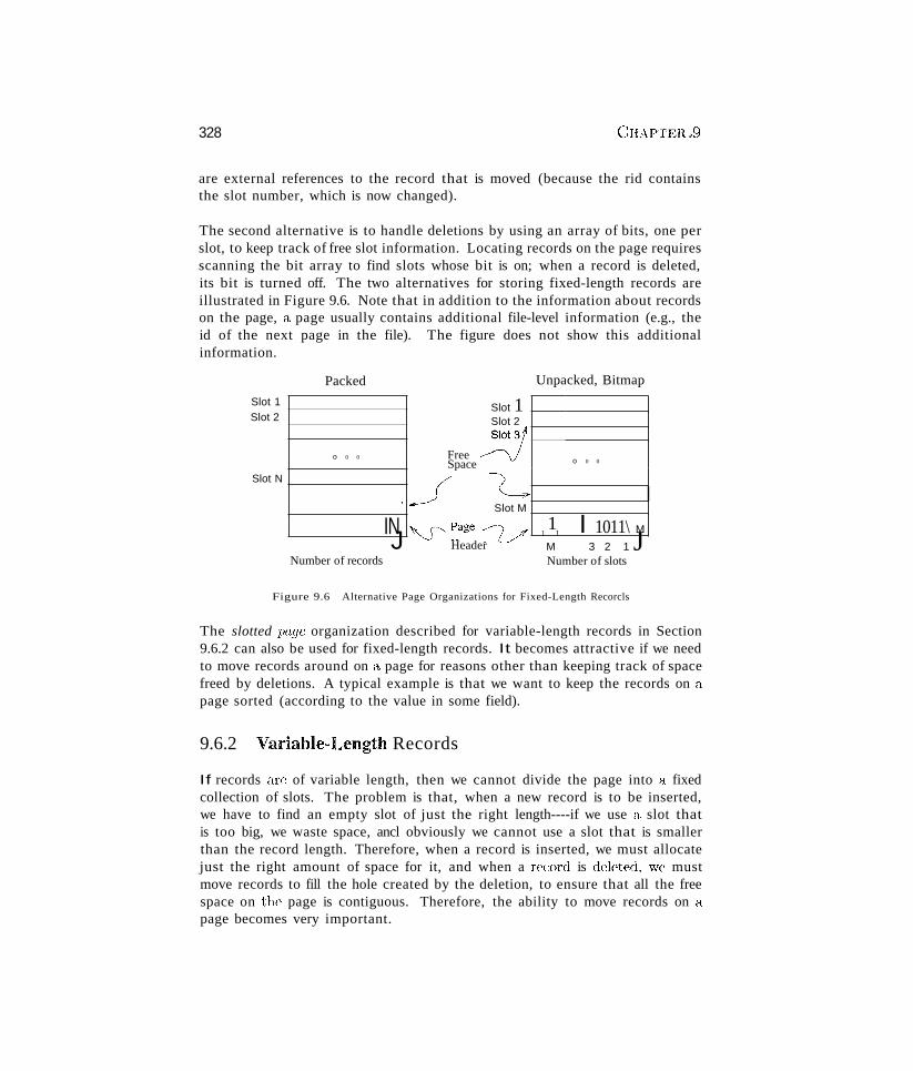
328 CHAPTER.9
are external references to the record that is moved (because the rid containsthe slot number, which is now changed).
The second alternative is to handle deletions by using an array of bits, one perslot, to keep track of free slot information. Locating records on the page requiresscanning the bit array to find slots whose bit is on; when a record is deleted,its bit is turned off. The two alternatives for storing fixed-length records areillustrated in Figure 9.6. Note that in addition to the information about recordson the page, a page usually contains additional file-level information (e.g., theid of the next page in the file). The figure does not show this additionalinformation.
Packed Unpacked, Bitmap
M 3 2 1 JNumber of slots
Slot 1Slot 2Slot 3
o 0 0
~Slot M
11
I I 1011\ M
Free~Space
J'-S"Page~
J HeaderNumber of records
o 0 0
...
IN
Slot N
Slot 1Slot 2
Figure 9.6 Alternative Page Organizations for Fixed-Length Recorcls
The slotted page organization described for variable-length records in Section9.6.2 can also be used for fixed-length records. It becomes attractive if we needto move records around on a page for reasons other than keeping track of spacefreed by deletions. A typical example is that we want to keep the records on apage sorted (according to the value in some field).
9.6.2 Variable-Length Records
If records are of variable length, then we cannot divide the page into a fixedcollection of slots. The problem is that, when a new record is to be inserted,we have to find an empty slot of just the right length----if we use a slot thatis too big, we waste space, ancl obviously we cannot use a slot that is smallerthan the record length. Therefore, when a record is inserted, we must allocatejust the right amount of space for it, and when a record is deleted, we mustmove records to fill the hole created by the deletion, to ensure that all the freespace on the page is contiguous. Therefore, the ability to move records on apage becomes very important.
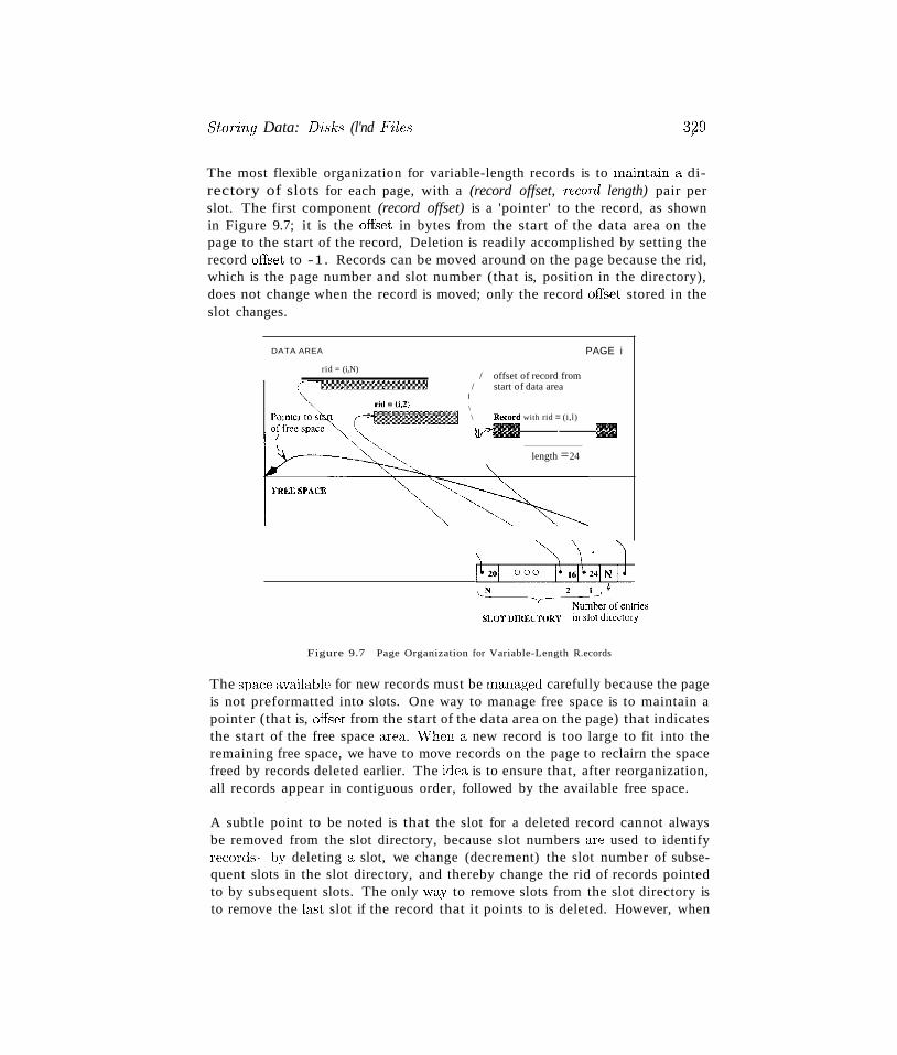
St011ng Data: Disks (l'nd Files 3#29
The most flexible organization for variable-length records is to maintain a directory of slots for each page, with a (record offset, recOT'd length) pair perslot. The first component (record offset) is a 'pointer' to the record, as shownin Figure 9.7; it is the ofl'set in bytes from the start of the data area on thepage to the start of the record, Deletion is readily accomplished by setting therecord ofl'set to -1. Records can be moved around on the page because the rid,which is the page number and slot number (that is, position in the directory),does not change when the record is moved; only the record ofl'set stored in theslot changes.
DATA AREA
rid = (i,N)
PAGE i
/ offset of record from/ start of data area
I
\\ Record with rid = (i,l)\~__II
length =24
Figure 9.7 Page Organization for Variable-Length R.ecords
The space available for new records must be managed carefully because the pageis not preformatted into slots. One way to manage free space is to maintain apointer (that is, ofl'set from the start of the data area on the page) that indicatesthe start of the free space area. vVhen a new record is too large to fit into theremaining free space, we have to move records on the page to reclairn the spacefreed by records deleted earlier. The idea is to ensure that, after reorganization,all records appear in contiguous order, followed by the available free space.
A subtle point to be noted is that the slot for a deleted record cannot alwaysbe removed from the slot directory, because slot numbers are used to identifyrecords-by deleting a slot, we change (decrement) the slot number of subsequent slots in the slot directory, and thereby change the rid of records pointedto by subsequent slots. The only way to remove slots from the slot directory isto remove the last slot if the record that it points to is deleted. However, when
330 CHAPTER .9
a record is inserted, the slot directory should be scanned for an element thatcurrently does not point to any record, and this slot should be used for the newrecord. A new slot is added to the slot directory only if all existing slots pointto records. If inserts are much more common than deletes (as is typically thecase), the number of entries in the slot directory is likely to be very close tothe actual number of records on the page.
This organization is also useful for fixed-length records if we need to movethem around frequently; for example, when we want to maintain them in somesorted order. Indeed, when all records are the same length, instead of storingthis common length information in the slot for each record, we can store it oncein the system catalog.
In some special situations (e.g., the internal pages of a B+ tree, which wediscuss in Chapter 10), we lIlay not care about changing the rid of a record. Inthis case, the slot directory can be compacted after every record deletion; thisstrategy guarantees that the number of entries in the slot directory is the sameas the number of records on the page. If we do not care about modifying rids,we can also sort records on a page in an efficient manner by simply moving slotentries rather than actual records, which are likely to be much larger than slotentries.
A simple variation on the slotted organization is to maintain only record offsetsin the slots. for variable-length records, the length is then stored with therecord (say, in the first bytes). This variation makes the slot directory structurefor pages with fixed-length records the salIle a..s for pages with variab1e~length
records.
9.7 RECORD FORMATS
In this section, we discuss how to organize fields within a record. While choosinga way to organize the fields of a record, we must take into account whether thefields of the record are of fixed or variable length and consider the cost of variousoperations on the record, including retrieval and modification of fields.
Before discussing record fonnats, we note that in addition to storing individualrecords, inforlI1(~tion conllnon to all records of a given record type (such a.'3 thenumber of fields and field types) is stored in the system catalog, which canbe thought of as a description of the contents of a database, maintained by theDBMS (Section 12.1). This avoids repeated storage of the same informationwith each record of a given type.
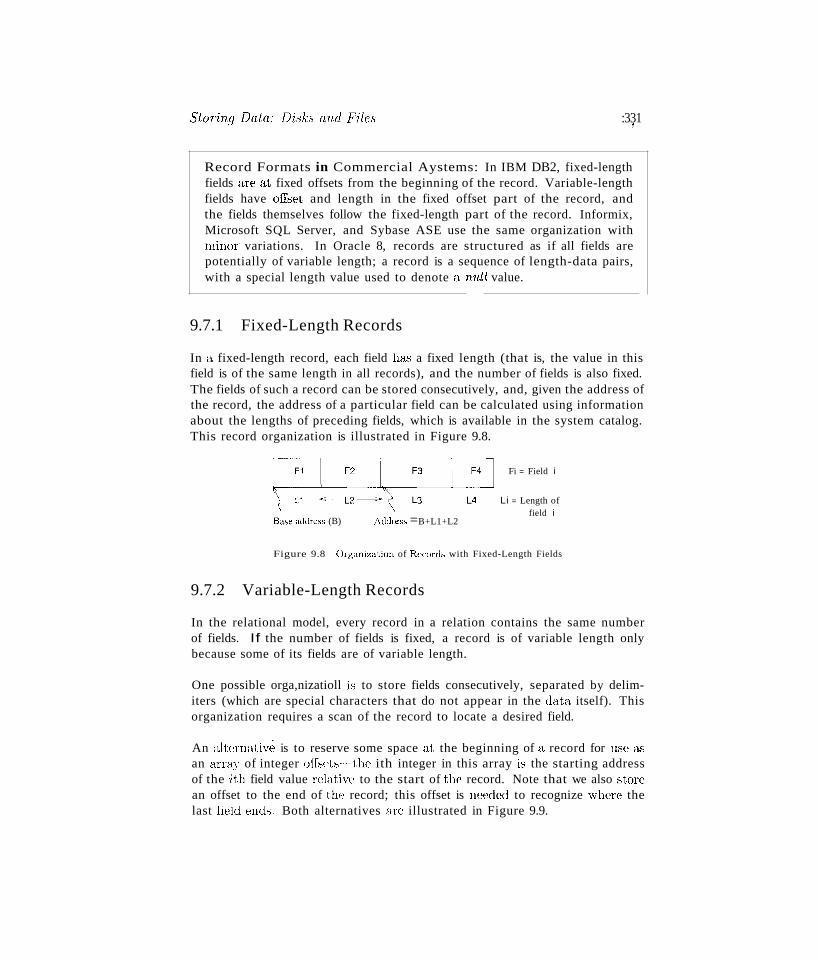
StoTing Data: Disks and Files :331,
Record Formats in Commercial Aystems: In IBM DB2, fixed-lengthfields are at fixed offsets from the beginning of the record. Variable-lengthfields have ofIset and length in the fixed offset part of the record, andthe fields themselves follow the fixed-length part of the record. Informix,Microsoft SQL Server, and Sybase ASE use the same organization withminor variations. In Oracle 8, records are structured as if all fields arepotentially of variable length; a record is a sequence of length-data pairs,with a special length value used to denote a null value.
9.7.1 Fixed-Length Records
In a fixed-length record, each field h&<; a fixed length (that is, the value in thisfield is of the same length in all records), and the number of fields is also fixed.The fields of such a record can be stored consecutively, and, given the address ofthe record, the address of a particular field can be calculated using informationabout the lengths of preceding fields, which is available in the system catalog.This record organization is illustrated in Figure 9.8.
Base address (B) Address =B+L1+L2
Fi = Field i
Li = Length offield i
Figure 9.8 Organi'lation of Records with Fixed-Length Fields
9.7.2 Variable-Length Records
In the relational model, every record in a relation contains the same numberof fields. If the number of fields is fixed, a record is of variable length onlybecause some of its fields are of variable length.
One possible orga,nizatioll is to store fields consecutively, separated by delimiters (which are special characters that do not appear in the data itself). Thisorganization requires a scan of the record to locate a desired field.
An alternative is to reserve some space at the beginning of a record for use 1:LS
an array of integer offsets-the ith integer in this array is the starting addressof the ith field value relative to the start of the record. Note that we also storean offset to the end of the record; this offset is needed to recognize where thelast held ends. Both alternatives are illustrated in Figure 9.9.
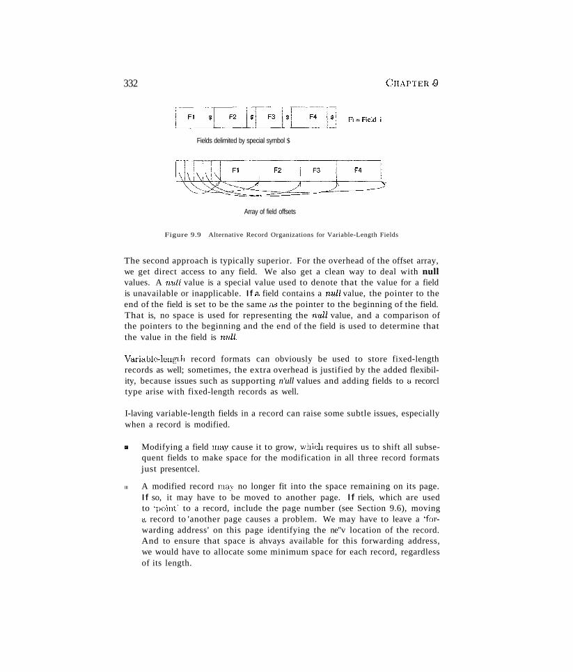
332 CHAPTERr9
Fields delimited by special symbol $
Array of field offsets
Figure 9.9 Alternative Record Organizations for Variable-Length Fields
The second approach is typically superior. For the overhead of the offset array,we get direct access to any field. We also get a clean way to deal with nullvalues. A mdl value is a special value used to denote that the value for a fieldis unavailable or inapplicable. If a field contains a null value, the pointer to theend of the field is set to be the same as the pointer to the beginning of the field.That is, no space is used for representing the null value, and a comparison ofthe pointers to the beginning and the end of the field is used to determine thatthe value in the field is null.
Variable~length record formats can obviously be used to store fixed-lengthrecords as well; sometimes, the extra overhead is justified by the added flexibility, because issues such as supporting n'ull values and adding fields to a recorcltype arise with fixed-length records as well.
I-laving variable-length fields in a record can raise some subtle issues, especiallywhen a record is modified.
III Modifying a field may cause it to grow, whieh requires us to shift all subsequent fields to make space for the modification in all three record formatsjust presentcel.
III A modified record may no longer fit into the space remaining on its page.If so, it may have to be moved to another page. If riels, which are usedto 'point' to a record, include the page number (see Section 9.6), movinga record to 'another page causes a problem. We may have to leave a 'forwarding address' on this page identifying the ne"v location of the record.And to ensure that space is ahvays available for this forwarding address,we would have to allocate some minimum space for each record, regardlessof its length.
Storing Data: Disks and Files
Large Records in Real Systems: In Sybc1se ASE, a record can be atmost 1962 bytes. This limit is set by the 2KB log page size, since recordsare not allowed to be larger than a page. The exceptions to this rule. an~BLOBs and CLOBs, which consist of 1:1 set of bidirectionally linked pages.IBlvl DB2 and Microsoft SqL Server also do not allow records to spanpages, although large objects are allowed to span pages and are handledseparately from other data types. In DB2, record size is limited only bythe page size; in SQL Server, a record can be at most 8KB, excludingLOBs. Informix and Oracle 8 allow records to span pages. Informix allowsrecords to be at most 32KB, while Oracle has no maximum record size;large records are organized as a singly directed list.
III A record may grow so large that it no longer fits on anyone page. We haveto deal with this condition by breaking a record into smaller records. Thesmaller records could be chained together-part of each smaller record isa pointer to the next record in the chain---to enable retrieval of the entireoriginal record.
9.8 REVIEW QUESTIONS
Answers to the review questions can be found in the listed sections.
III Explain the term memory hierarchy. What are the differences betweenprimary, secondary, and tertiary storage? Give examples of each. Whichof these is volatile, and which are pCf'sistenf? Why is persistent storagemore important for a DBMS than, say, a program that generates primenumbers? (Section 9.1)
III Why are disks used so widely in a DBMS? What are their advantagesover main memory and tapes? ':Vhat are their relative disadvantages?(Section 9.1.1)
III What is a disk block or page? How are blocks arranged in a disk? Howdoes this affect the time to access a block? Discuss seek tiTne, rotationaldday, and transfer time. (Section 9.1.1)
III Explain how careful placement of pages on the disk to exploit the geometryof a disk can minimize the seek time and rotational delay when pages areread sequentially. (Section 9.1.2)
III Explain what a RAID systenl is and how it improves performance andreliability. Discuss str-iping and its impact on performance and nxlundancyand its irnpact on reliability. vVhat are the trade-offs between reliability
334 CHAPTER.£)
and performance in the different RAID organizations called RAID levels'?(Section 9.2)
.. Wnat is the role of the DBMS d'isk space manager'? vVhy do databasesystems not rely on the operating system instead? (Section 9.3)
.. Why does every page request in a DBMS go through the buffer manager?What is the buffer poor? '\That is the difference between a frame in a bufferpool, a page in a file, and a block on a disk? (Section 9.4)
.. What information does the buffer manager maintain for each page in thebuffer pool? ·What information is maintained for each frame? What isthe significance of p'in_count and the d'irty flag for a page? Under whatconditions can a page in the pool be replaced? Under what conditionsmust a replaced page be written back to disk? (Section 9.4)
.. Why does the buffer manager have to replace pages in the buffer pool?How is a page chosen for replacement? vVhat is sequent'ial flood'ing, andwhat replacement policy causes it? (Section 9.4.1)
.. A DBMS buffer manager can often predict the access pattern for disk pages.How does it utilize this ability to minimize I/O costs? Discuss prefetch'ing. \iVhat is forc'ing, and why is it required to support the write-aheadlog protocol in a DBMS? In light of these points, explain why databasesystems reimplement many services provided by operating systems. (Section 9.4.2)
.. Why is the abstraction of a file of records important? How is the softwarein a DBMS layered to take advantage of this? (Section 9.5)
.. What is a heap file? How are pages organized in a heap file? Discuss listversus directory organizations. (Section 9.5.1)
III Describe how records are arranged on a page. \i\That is a slot, and howare slots used to identify records? How do slots ena.ble us to move recordson a page withont altering the record's identifier? ·What arc the differences in page organizations for fixed-length and variable-length records?(Section 9.6)
iii ·What are the differences in how fields are arranged within fixed-length andvariable-length records? For variable-length records, explain how the arrayof offsets organization provides direct access to a specific field and supportsnull values. (Section 9.7)
Storing Data: Disks and Files
EXERCISES
Exercise 9.1 \-Vhat is the most important difference behveen a disk and a tape?
Exercise 9.2 Explain the terms seek time, mtat'ional delay, and transfer t'ime.
33:)
Exercise 9.3 Both disks and main memory support direct access to any desired location(page). On average, main memory accesses are faster, of course. \\That is the other importantdifference (from the perspective of the time required to access a desired page)?
Exercise 9.4 If you have a large file that is frequently scanned sequentially, explain how youwould store the pages in the file on a disk.
Exercise 9.5 Consider a disk with a sector size of 512 bytes, 2000 tracks per surface, 50sectors per track, five double-sided platters, and average seek time of 10 msec.
1. What is the capacity of a track in bytes? What is the capacity of each surface? What isthe capacity of the disk?
2. How many cylinders does the disk have?
:~. Give examples of valid block sizes. Is 256 bytes a valid block size? 2048? 51,200?
4. If the disk platters rotate at 5400 rpm (revolutions per minute), what is the maximumrotational delay?
5. If one track of data can be transferred per revolution, what is the transfer rate?
Exercise 9.6 Consider again the disk specifications from Exercise 9.5 and suppose that ablock size of 1024 bytes is chosen. Suppose that a file containing 100,000 records of 100 byteseach is to be stored on such a disk and that no record is allowed to span two blocks.
L How many records fit onto a block?
2. How many blocks are required to store the entire file? If the file is arranged sequentiallyon disk, how lllallY surfaces are needed?
:3. How many records of 100 bytes each can be stored using this disk?
4. If pages are stored sequentially on disk, with page 1 on block 1 of track 1, what page isstored on block 1 of track 1 on the next disk surface? How would your answer change ifthe disk were capable of reading and writing from all heads in parallel?
5. VVhat titne is required to read a file containing 100,000 records of 100 bytes each sequentially? Again, how \vould your answer change if the disk were capable of reading/writingfrom all heads in parallel (and the data was arranged optimally)?
6. \\That is the time required to read a file containing 100,000 records of 100 bytes each in arandom order? To read a record, the block containing the recOl'd has to be fetched fromdisk. Assume that each block request incurs the average seek time and rotational delay.
Exercise 9.7 Explain what. the buffer manager JIms! do to process a read request for a page.\Vhat happens if the requested page is in the pool but not pinned?
Exercise 9.8 When does a buffer manager write a page to disk?
Exercise 9.9 What. does it mean to say that a page is p'inned in the buffer pool? Who isresponsible for pinning pages? \Vho is responsible for unpinning pages?
CHAPTERJ9
Exercise 9.10 'When a page in the bulTer pool is modified, how does the DBMS ensure thatthis change is propagated to disk? (Explain the role of the buffer manager as well as themodifier of the page.)
Exercise 9.11 \Vhat happens if a page is requested when all pages in the buffer pool aredirty?
Exercise 9.12 \Vhat is sequential flooding of the buffer pool?
Exercise 9.13 Name an important capability of a DBIVIS buffer manager that is not supported by a typical operating system's buffer manager.
Exercise 9.14 Explain the term prefetching. \Vhy is it important?
Exercise 9.15 Modern disks often have their own main memory caches, typically about1 MB, and use this to prefetch pages. The rationale for this technique is the empiricalobservation that, if a disk page is requested by some (not necessarily database!) application,80% of the time the next page is requested as well. So the disk gambles by reading ahead.
1. Give a nontechnical reason that a DBMS may not want to rely on prefetching controlledby the disk.
2. Explain the impact on the disk's cache of several queries running concurrently, eachscanning a different file.
3. Is this problem addressed by the DBMS buffer manager prefetching pages? Explain.
4. Modern disks support segmented caches, with about four to six segments, each of whichis used to cache pages from a different file. Does this technique help, with respect tothe preceding problem? Given this technique, does it matter whether the DBMS buffermanager also does prefetching?
Exercise 9.16 Describe two possible record formats. What are the trade-offs between them?
Exercise 9.17 Describe two possible page formats. What are the trade-offs between them?
Exercise 9.18 Consider the page format for variable-length records that uses a slot directory.
1. One approach to managing the slot directory is to use a maximum size (i.e., a maximumnumber of slots) and allocate the directory array when the page is created. Discuss thepros and cons of this approach with respect to the approach discussed in the text.
2. Suggest a modification to this page format that would allow us to sort records (accordingto the value in some field) without moving records and without changing the record ids.
Exercise 9.19 Consider the two internal organizations for heap files (using lists of pages anda directory of pages) discussed in the text.
1. Describe them briefly and explain the trade-offs. \Vhich organization would you chooseif records are variable in length?
2. Can you suggest a single page format to implement both internal file organizations'?
Exercise 9.20 Consider a list-based organizat.ion of the pages in a heap file in which twolists are maintained: a list of all pages in the file and a list of all pages with free space. Incontrast, the list-based organizatioll discussed in the text maintains a list of full pages and alist of pages with free space.

Storing Data: Disks and Files 3&7
1. VVhat are the trade-offs, if any'? Is one of them clearly superior?
2. For each of these organizations, describe a suitable page format.
Exercise 9.21 Modern disk drives store more sectors on the outer tracks than the innertracks. Since the rotation speed is constant, the sequential data transfer rate is also higher onthe outer tracks. The seek time and rotational delay are unchanged. Given this information,explain good strategies for placing files with the following kinds of access patterns:
1. rrequent, random accesses to a small file (e.g., catalog relations).
2. Sequential scans of a large file (e.g., selection from a relation with no index).
3. Random accesses to a large file via an index (e.g., selection from a relation via the index).
4. Sequential scans of a small file.
Exercise 9.22 Why do frames in the buffer pool have a pin count instead of a pin flag?
PROJECT-BASED EXERCISES
Exercise 9.23 Study the public interfaces for the disk space manager, the buffer manager,and the heap file layer in Minibase.
1. Are heap files with variable-length records supported?
2. What page format is used in Minibase heap files?
3. What happens if you insert a record whose length is greater than the page size?
4. How is free space handled in Minibase?
BIBLIOGRAPHIC NOTES
Salzberg [648] and Wiederhold [776] discuss secondary storage devices and file organizationsin detail.
RAID wa.s originally proposed by Patterson, Gibson, and Katz [587]. The article by Chenet al. provides an excellent survey of RAID [171] . Books about RAID include Gibson'sdissertation [.317] and the publications from the RAID Advisory Board [605].
The design and implementation of storage managers is discussed in [65, 1:33, 219, 477, 718].With the exception of [219], these systems emphasize el:tensibili.ty, anel the papers containmuch of interest from that stanelpoint as well. Other papers that cover storage managementissues in the context of significant implemented prototype systems are [480] and [588]. TheDali storage Inanager, which is optimized for main memory databases, is described in [406].Three techniques for ilnplementing long fields are compared in [96]. The impact of processorcache misses 011 DBMS performallce ha.'i received attention lately, as complex queries havebecome increasingly CPU-intensive. [:33] studies this issue, and shows that performance can besignificantly improved by using a new arrangement of records within a page, in which recordson a page are stored in a column~oriented format (all field values for the first attribute followedby values for the second attribute, etc.).
Stonebraker discusses operating systems issues in the context of databases in [715]. Severalbuffer management policies for databa.se systems are compared in [181]. Buffer managementis also studied in [119, 169, 2G1, 2:35].

10TREE-STRUCTURED
INDEXING
... What is the intuition behind tree-structured indexes? Why are theygood for range selections?
... How does an ISAM index handle search, insert, and delete?
i"- How does a B+ tree index handle search, insert, and delete?
... What is the impact of duplicate key values on index implementation'?
... What is key compression, and why is it important?
... What is bulk-loading, and why is it important?
... What happens to record identifiers when dynamic indexes are updated? How does this affect clustered indexes?
Itt Key concepts: ISAM, static indexes, overflow pages, locking issues;B+ trees, dynamic indexes, balance, sequence sets, node format; B+tree insert operation, node splits, delete operation, merge versus redistribution, minimum occupancy; duplicates, overflow pages, includingrids in search keys; key compression; bulk-loading; effects of splits onrids in clustered indexes.
One that would have the fruit must climb the tree.
I'homas Fuller
VVe now consider two index data structures, called ISAM and B+ trees, b<:h':ledon tree organizations. These structures provide efficient support for rangesearches, including sorted file scans as a special c<h'3e. Unlike sorted files, these
Tree-StTuctuTed Indel:ing
index structures support efficient insertion and deletion. They also providesupport for equality selections, although they are not &'3 efficient in this case ashash-b::l.'3ed indexes, which are discussed in Chapter 11.
An ISAJVI1 tree is a static index structure that is effective when the file isnot frequently updated, but it is unsuitable for files that grow and shrink alot. \Ve discuss ISAM in Section 10.2. The B+ tree is a dynamic structurethat adjusts to changes in the file gracefully. It is the most widely used indexstructure because it adjusts well to changes and supports both equality andrange queries. We introduce B+ trees in Section 10.3. We cover B+ trees indetail in the remaining sections. Section 10.3.1 describes the format of a treenode. Section lOA considers how to search for records by using a B+ treeindex. Section 10.5 presents the algorithm for inserting records into a B+ tree,and Section 10.6 presents the deletion algorithm. Section 10.7 discusses howduplicates are handled. \Ve conclude with a discussion of some practical issuesconcerning B+ trees in Section 10.8.
Notation: In the ISAM and B+ tree structures, leaf pages contain data entries,according to the terminology introduced in Chapter 8. For convenience, wedenote a data entry with search key value k as k*. Non-leaf pages conta.ininde:c entries of the form (search key 'Value., page id) and are used to direct thesea.rch for a desired data entry (which is stored in some leaf). We often simplyuse entr'Y where the context makes the nature of the entry (index or data) clear.
10.1 INTUITION FOR TREE INDEXES
Consider a file of Students recorcls sorted by gpa. To answer a range selectionsuch as "Find all students with a gpa higher than 3.0," we must identify thefirst such student by doing a binary search of the file and then scan the filefrom that point on. If the file is large, the initial binary search can be quiteexpensive, since cost is proportional to the number of pages fetched; can weimprove upon this method'?
OIle idea is to create a second file with OIle record per page in the original(data) file, of the form (first key on page, pointer to page), again sortecl by thekey attribute (which is gpa in our example). The format of a page in the secondinde:c file is illustrated in Figure 10.1.
We refer to pairs of the form (key, pointer) ~l.S indc:J: entries or just entries \'\'henthe context is dear. Note that each index page contains OIle pointer more than
I ISAM stands for Indexed Sequential Access Method.
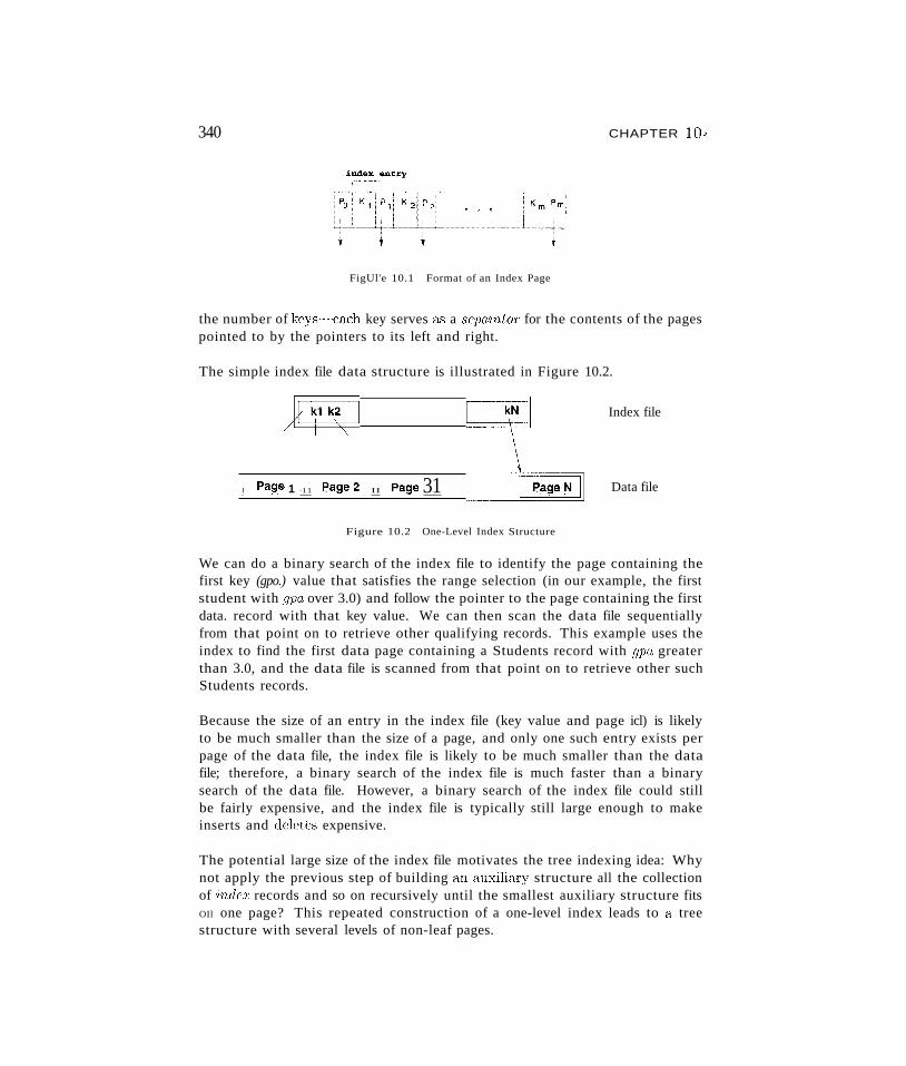
340
index entryr·.. ········
FigUl'e 10.1 Format of an Index Page
CHAPTER 10,
the number of keys---each key serves as a separator- for the contents of the pagespointed to by the pointers to its left and right.
The simple index file data structure is illustrated in Figure 10.2.
I PafJe 1 ·11 Page 2.· II Page 31
Index file
Data file
Figure 10.2 One-Level Index Structure
We can do a binary search of the index file to identify the page containing thefirst key (gpo.) value that satisfies the range selection (in our example, the firststudent with gpo. over 3.0) and follow the pointer to the page containing the firstdata. record with that key value. We can then scan the data file sequentiallyfrom that point on to retrieve other qualifying records. This example uses theindex to find the first data page containing a Students record with gpo. greaterthan 3.0, and the data file is scanned from that point on to retrieve other suchStudents records.
Because the size of an entry in the index file (key value and page icl) is likelyto be much smaller than the size of a page, and only one such entry exists perpage of the data file, the index file is likely to be much smaller than the datafile; therefore, a binary search of the index file is much faster than a binarysearch of the data file. However, a binary search of the index file could stillbe fairly expensive, and the index file is typically still large enough to makeinserts and clelett~s expensive.
The potential large size of the index file motivates the tree indexing idea: Whynot apply the previous step of building an auxiliar:v structure all the collectionof inde:l: records and so on recursively until the smallest auxiliary structure fitsOIl one page? This repeated construction of a one-level index leads to a treestructure with several levels of non-leaf pages.
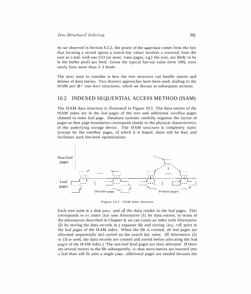
Trce-Stn.lduTed Inde:ring 341J
As we observed in Section 8.3.2, the power of the approach comes from the factthat locating a record (given a search key value) involves a traversal from theroot to a leaf, with one I/O (at most; SCHne pages, e.g.) the root, are likely to bein the buffer pool) per level. Given the typical fan-out value (over 100), treesrarely have more than 3-4 levels.
The next issue to consider is how the tree structure can handle inserts anddeletes of data entries. Two distinct approaches have been used, leading to theISAM and B+ tree data structures, which we discuss in subsequent sections.
10.2 INDEXED SEQUENTIAL ACCESS METHOD (ISAM)
The ISAM data structure is illustrated in Figure 10.3. The data entries of theISAM index are in the leaf pages of the tree and additional overflow pageschained to some leaf page. Database systems carefully organize the layout ofpages so that page boundaries correspond closely to the physical characteristicsof the underlying storage device. The ISAM structure is completely static(except for the overflow pages, of which it is hoped, there will be few) andfacilitates such low-level optimizations.
Non-leafpages
Leafpages
OverjlowP{~c::::J1 ~ ~Primary pages
Figure 10.3 ISAM Index Structure
Each tree node is a disk page, and all the data resides in the leaf pages. Thiscorresponds to an index that uses Alternative (1) for data entries, in terms ofthe alternatives described in Chapter 8; we can create an index with Alternative(2) by storing t.he data records in a separate file and storing (key, rid) pairs inthe leaf pages of the ISAM index. When the file is created, all leaf pages areallocated sequentially and sorted on the search key value. (If Alternative (2)or (3) is used, the data records are created and sorted before allocating the leafpages of the ISAM index.) The non-leaf level pages are then allocated. If thereare several inserts to the file subsequently, so that more entries are inserted intoa leaf than will fit onto a single page, additional pages are needed because the
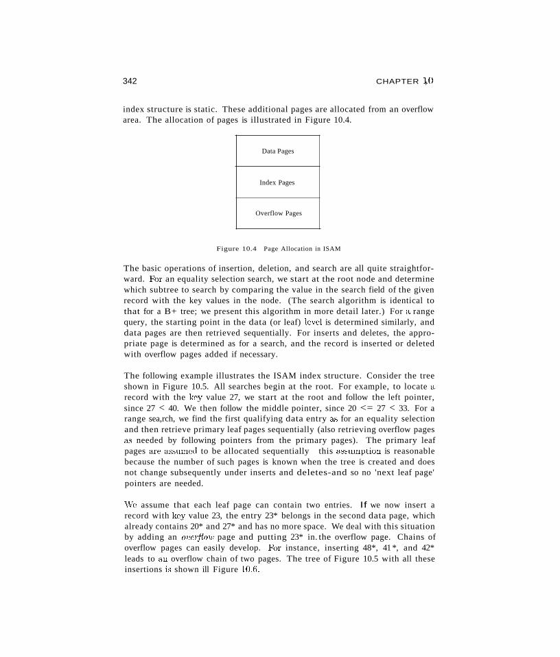
342 CHAPTER lO
index structure is static. These additional pages are allocated from an overflowarea. The allocation of pages is illustrated in Figure 10.4.
Data Pages
Index Pages
Overflow Pages
Figure 10.4 Page Allocation in ISAM
The basic operations of insertion, deletion, and search are all quite straightforward. J;"'or an equality selection search, we start at the root node and determinewhich subtree to search by comparing the value in the search field of the givenrecord with the key values in the node. (The search algorithm is identical tothat for a B+ tree; we present this algorithm in more detail later.) For a rangequery, the starting point in the data (or leaf) level is determined similarly, anddata pages are then retrieved sequentially. For inserts and deletes, the appropriate page is determined as for a search, and the record is inserted or deletedwith overflow pages added if necessary.
The following example illustrates the ISAM index structure. Consider the treeshown in Figure 10.5. All searches begin at the root. For example, to locate arecord with the key value 27, we start at the root and follow the left pointer,since 27 < 40. We then follow the middle pointer, since 20 <= 27 < 33. For arange sea,rch, we find the first qualifying data entry as for an equality selectionand then retrieve primary leaf pages sequentially (also retrieving overflow pagesas needed by following pointers from the primary pages). The primary leafpages are cL..ssumed to be allocated sequentially this a..ssumption is reasonablebecause the number of such pages is known when the tree is created and doesnot change subsequently under inserts and deletes-and so no 'next leaf page'pointers are needed.
vVe assume that each leaf page can contain two entries. If we now insert arecord with key value 23, the entry 23* belongs in the second data page, whichalready contains 20* and 27* and has no more space. We deal with this situationby adding an overflow page and putting 23* in. the overflow page. Chains ofoverflow pages can easily develop. F'or instance, inserting 48*, 41 *, and 42*leads to an overflow chain of two pages. The tree of Figure 10.5 with all theseinsertions is shown ill Figure 10.6.
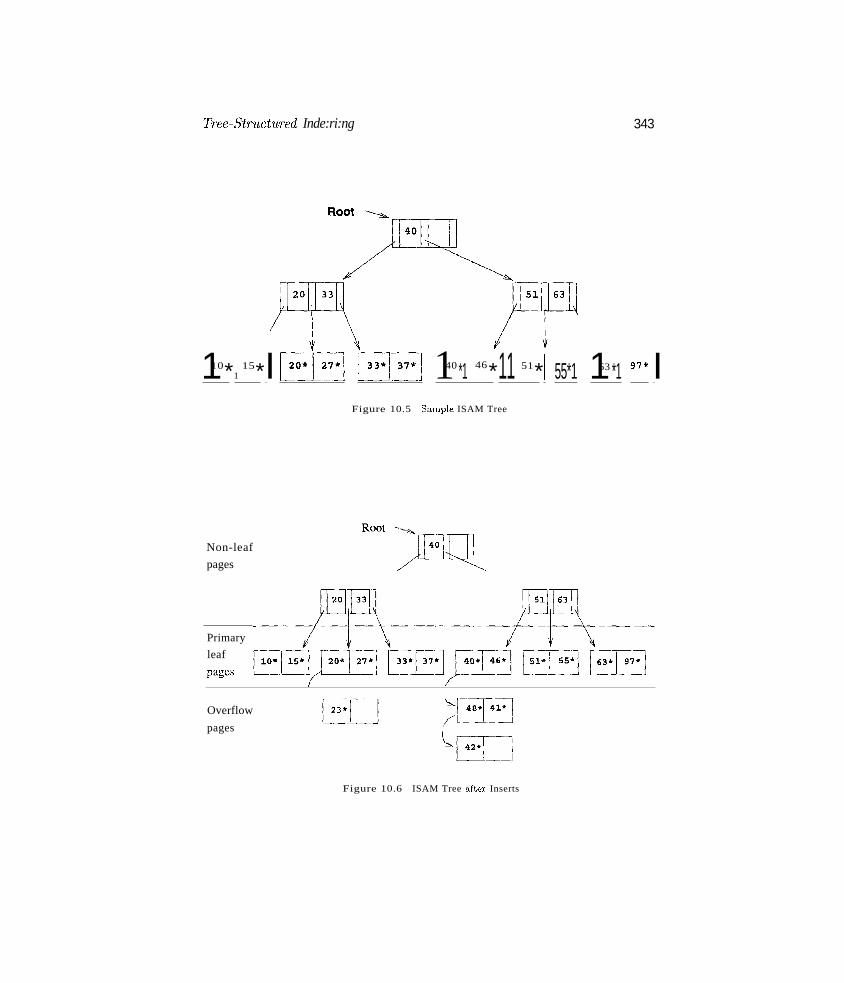
Tree~StrLLctuTed Inde:ri:ng 343
110*115*IEEl B3 140 *1 46*11 51*l 55*1 163 *1 97* I
Figure 10.5 Sa.mple ISAM Tree
Non-leaf
pages
Primary
leaf
pages
Overflow
pages
Figure 10.6 ISAM Tree a.fter Inserts
344 CHAPTER Ii)
The deletion of an entry h is handled by simply removing the entry. If thisentry is on an overflow page and the overflow page becomes empty, the page canbe removed. If the entry is on a primary page and deletion makes the primarypage empty, the simplest approach is to simply leave the empty primary page~s it is; it serves as a placeholder for future insertions (and possibly lloll-emptyoverflow pages, because we do not move records from the overflow pages to theprimary page when deletions on the primary page create space). Thus, thenumber of primary leaf pages is fixed at file creation time.
10.2.1 Overflow Pages, Locking Considerations
Note that, once the ISAM file is created, inserts and deletes affect only thecontents of leaf pages. A consequence of this design is that long overflow chainscould develop if a number of inserts are made to the same leaf. These chainscan significantly affect the time to retrieve a record because the overflow chainhas to be searched as well when the search gets to this leaf. (Although data inthe overflow chain can be kept sorted, it usually is not, to make inserts fast.) Toalleviate this problem, the tree is initially created so that about 20 percent ofeach page is free. However, once the free space is filled in with inserted records,unless space is freed again through deletes, overflow chains can be eliminatedonly by a complete reorganization of the file.
The fact that only leaf pages are modified also has an important advantage withrespect to concurrent access. When a page is accessed, it is typically 'locked'by the requestor to ensure that it is not concurrently modified by other usersof the page. To modify a page, it must be locked in 'exclusive' mode, which ispermitted only when no one else holds a lock on the page. Locking can leadto queues of users (transactions, to be more precise) waiting to get access to apage. Queues can be a significant performance bottleneck, especially for heavilyaccessed pages near the root of an index structure. In the ISAM structure,since we know that index-level pages are never modified, we can safely omitthe locking step. Not locking index-level pages is an important advantage ofISAM over a dynamic structure like a B+ tree. If the data distribution andsize are relatively static, which means overflow chains are rare, ISAM might bepreferable to B+ trees due to this advantage.
10.3 B+ TREES: A DYNAMIC INDEX STRUCTURE
A static structure such as the ISAI\il index suffers from the problem that longoverflow chains can develop a"s the file grows, leading to poor performance. Thisproblem motivated the development of more flexible, dynamic structures thatadjust gracefully to inserts and deletes. The B+ tree search structure, whichis widely llsed, is a balanced tree in which the internal nodes direct the search
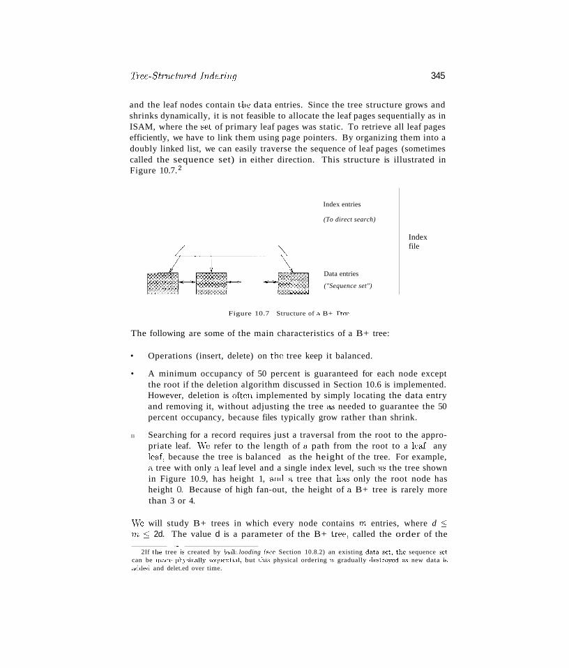
Tree~StT7lChtTed IndeTing 345
and the leaf nodes contain the data entries. Since the tree structure grows andshrinks dynamically, it is not feasible to allocate the leaf pages sequentially as inISAM, where the set of primary leaf pages was static. To retrieve all leaf pagesefficiently, we have to link them using page pointers. By organizing them into adoubly linked list, we can easily traverse the sequence of leaf pages (sometimescalled the sequence set) in either direction. This structure is illustrated inFigure 10.7.2
Index entries
(To direct search)
Indexfile
Data entries
("Sequence set")
Figure 10.7 Structure of a B+ 'n'ee
The following are some of the main characteristics of a B+ tree:
• Operations (insert, delete) on the tree keep it balanced.
• A minimum occupancy of 50 percent is guaranteed for each node exceptthe root if the deletion algorithm discussed in Section 10.6 is implemented.However, deletion is often implemented by simply locating the data entryand removing it, without adjusting the tree &'3 needed to guarantee the 50percent occupancy, because files typically grow rather than shrink.
l1li Searching for a record requires just a traversal from the root to the appropriate leaf. Vie refer to the length of a path from the root to a leaf anyleaf, because the tree is balanced as the height of the tree. For example,a tree with only a leaf level and a single index level, such as the tree shownin Figure 10.9, has height 1, and a tree that h&'3 only the root node hasheight O. Because of high fan-out, the height of a B+ tree is rarely morethan 3 or 4.
\Ve will study B+ trees in which every node contains Tn entries, where d :::;nJ, :::; 2d. The value d is a parameter of the B+ tree, called the order of the
.._-2If the tree is created by IYll.lk.. looding (see Section 10.8.2) an existing data set, the sequence set.
can be nHlde physically sequential, but this physical ordering is gradually destroyed as new data isadded and delet.ed over time.
346 CHAPTER \0
tree, and is a measure of the capacity of a tree node. The root node is theonly exception to this requirement on the number of entries; for the root, it issimply required that 1 ::; m ::; 2d.
If a file of records is updated frequently and sorted access is important, maintaining a B+ tree index with data records stored as data entries is almostalways superior to maintaining a sorted file. For the space overhead of storingthe index entries, we obtain all the advantages of a sorted file plus efficient insertion and deletion algorithms. B+ trees typically maintain 67 percent spaceoccupancy. B+ trees are usually also preferable to ISAM indexing because inserts are handled gracefully without overflow chains. However, if the datasetsize and distribution remain fairly static, overflow chains may not be a majorproblem. In this case, two factors favor ISAM: the leaf pages are allocated insequence (making scans over a large range more efficient than in a B+ tree, inwhich pages are likely to get out of sequence on disk over time, even if they werein sequence after bulk-loading), and the locking overhead ofISAM is lower thanthat for B+ trees. As a general rule, however, B+ trees are likely to performbetter than ISAM.
10.3.1 Format of a Node
The format of a node is the same as for ISAM and is shown in Figure 10.1.Non-leaf nodes with m 'index entr'ies contain m+ 1 pointers to children. PointerPi points to a subtree in which all key va.lues K are such that Ki ::; K < K i +1.
As special ca"Jes, Po points to a tree in which all key values are less than Kl'and Pm points to a tree in which all key values are greater than or equal toK m . For leaf nodes, entries arc denoted a"J k*, as usual. Just as in ISAM, leafnodes (and only leaf nodes!) contain data entries. In the common ca.'se thatAlternative (2) or (:3) is used, leaf entries are (K,I(K) ) pairs, just like non-leafentries. Regardless of the alternative chosen for leaf entries, the leaf pages arechained together in a doubly linked list. Thus, the leaves form a sequence,which can be used to answer range queries efficiently.
The reader should carefully consider how such a node organization can beachieved using the record formats presented in Section 9.7; after all, each keypointer pair can be thought of as a record. If the field being indexed is offixed length, these index entries will be of fixed length; otherwise, we havevariable-length records. In either case the B+ tree can itself be viewed as a fileof records. If the leaf pages do not contain the actual data records, then the13+ tree is indeed a file of records that is distinct from the file that contains thedata. If the leaf pages contain data. records, then a file contains the 13+ tree a...swell as the data.
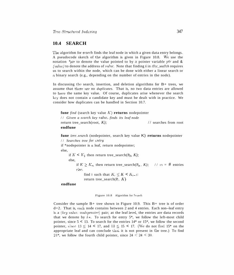
TTee-St'r~uct'uTed Jude.ring
10.4 SEARCH
347
The algorithm for sean:h finds the leaf node in which a given data entry belongs.A pseudocode sketch of the algorithm is given in Figure 10.8. "\Te use thenotation *ptT to denote the value pointed to by a pointer variable ptT and &(value) to denote the address of val'nc. Note that finding i in tTcc_seaTch requiresus to search within the node, which can be done with either a linear search ora binary search (e.g., depending on the number of entries in the node).
In discussing the search, insertion, and deletion algorithms for B+ trees, weassume that there are no duplicates. That is, no two data entries are allowedto have the same key value. Of course, duplicates arise whenever the searchkey does not contain a candidate key and must be dealt with in practice. Weconsider how duplicates can be handled in Section 10.7.
fune find (search key value K) returns nodepointer/ / Given a seaTch key value, finds its leaf node
return tree_search(root, K); / / searches from rootendfune
fune tTee-seaTch (nodepointer, search key value K) returns nodepointer/ / Searches tree for entry
if *nodepointer is a leaf, return nodepointer;else,
if K < K 1 then return tree_search(Po, K);else,
if K 2: K m then return tree_search(Pm , K); / / 171 = # entrieselse,
find i such that K i :::; K < Ki+ 1 ;
return tree_search(Pi , K)endfune
Figure 10.8 Algorithm for Search
Consider the sample B+ tree shown in Figure 10.9. This B+ tree is of orderd=2. That is, each node contains between 2 and 4 entries. Each non--leaf entryis a (key valuc.' nodepointcT) pair; at the leaf level, the entries are data recordsthat we denote by k*. To search for entry 5*, we follow the left-most childpointer, since 5 < 13. To search for the entries 14* or 15*, we follow the secondpointer, since 1:3 :::; 14 < 17, and 1:3 :::; 15 < 17. (vVe do not find 15* on theappropriate leaf and can conclude that it is not present in the tree.) To find24 *, we follow the fourth child pointer, since 24 :::; 24 < :30.
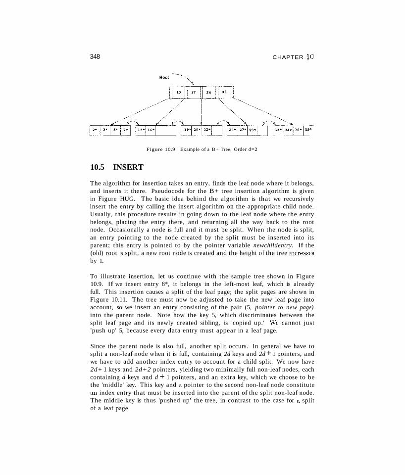
348 CHAPTER 10
Figure 10.9 Example of a B+ Tree, Order d=2
10.5 INSERT
The algorithm for insertion takes an entry, finds the leaf node where it belongs,and inserts it there. Pseudocode for the B+ tree insertion algorithm is givenin Figure HUG. The basic idea behind the algorithm is that we recursivelyinsert the entry by calling the insert algorithm on the appropriate child node.Usually, this procedure results in going down to the leaf node where the entrybelongs, placing the entry there, and returning all the way back to the rootnode. Occasionally a node is full and it must be split. When the node is split,an entry pointing to the node created by the split must be inserted into itsparent; this entry is pointed to by the pointer variable newchildentry. If the(old) root is split, a new root node is created and the height of the tree increa..<;esby 1.
To illustrate insertion, let us continue with the sample tree shown in Figure10.9. If we insert entry 8*, it belongs in the left-most leaf, which is alreadyfull. This insertion causes a split of the leaf page; the split pages are shown inFigure 10.11. The tree must now be adjusted to take the new leaf page intoaccount, so we insert an entry consisting of the pair (5, pointer to new page)into the parent node. Note how the key 5, which discriminates between thesplit leaf page and its newly created sibling, is 'copied up.' \\Te cannot just'push up' 5, because every data entry must appear in a leaf page.
Since the parent node is also full, another split occurs. In general we have tosplit a non-leaf node when it is full, containing 2d keys and 2d + 1 pointers, andwe have to add another index entry to account for a child split. We now have2d+ 1 keys and 2d+2 pointers, yielding two minimally full non-leaf nodes, eachcontaining d keys and d + 1 pointers, and an extra key, which we choose to bethe 'middle' key. This key and a pointer to the second non-leaf node constitutean index entry that must be inserted into the parent of the split non-leaf node.The middle key is thus 'pushed up' the tree, in contrast to the case for a splitof a leaf page.
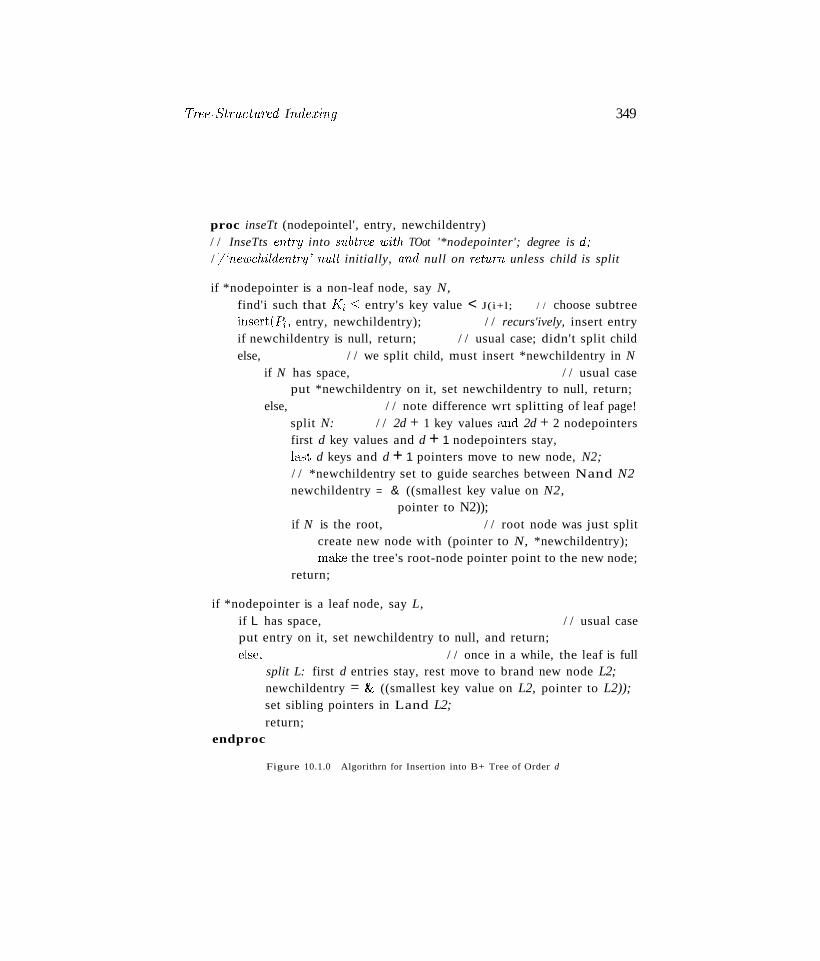
Tree~Structured Inde.1:ing 349
proc inseTt (nodepointel', entry, newchildentry)/ / InseTts entry into subtree with TOot '*nodepointer'; degree is d;/ /'newchildentTy' null initially, and null on retUTn unless child is split
if *nodepointer is a non-leaf node, say N,find'i such that J(i S entry's key value < J(i+l; / / choose subtreeinsert(.R;, entry, newchildentry); / / recurs'ively, insert entryif newchildentry is null, return; / / usual case; didn't split childelse, / / we split child, must insert *newchildentry in N
if N has space, / / usual caseput *newchildentry on it, set newchildentry to null, return;
else, / / note difference wrt splitting of leaf page!split N: / / 2d + 1 key values and 2d + 2 nodepointersfirst d key values and d + 1 nodepointers stay,last d keys and d + 1 pointers move to new node, N2;/ / *newchildentry set to guide searches between Nand N2newchildentry = & ((smallest key value on N2,
pointer to N2));if N is the root, / / root node was just split
create new node with (pointer to N, *newchildentry);make the tree's root-node pointer point to the new node;
return;
if *nodepointer is a leaf node, say L,if L has space, / / usual caseput entry on it, set newchildentry to null, and return;else, / / once in a while, the leaf is full
split L: first d entries stay, rest move to brand new node L2;newchildentry = & ((smallest key value on L2, pointer to L2));set sibling pointers in Land L2;return;
endproc
Figure 10.1.0 Algorithrn for Insertion into B+ Tree of Order d
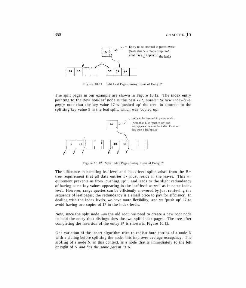
350 CHAPTER jO
/
,_ - - Entry to be inserted in parent 11(.)de.[i]1 <<-- -- (Note that 5 is 'copied up' and
_-....... "---\ ,ontin.", to ,ppcM;n the lenf.)
EEf-rJ-~rFigure 10.11 Split Leaf Pages during Insert of Entry 8*
The split pages in our example are shown in Figure 10.12. The index entrypointing to the new non-leaf node is the pair (17, pointer to new index-levelpage); note that the key value 17 is 'pushed up' the tree, in contrast to thesplitting key value 5 in the leaf split, which was 'copied up.'
/
Entry to be inserted in parent node.
~7 ..£~_ :' - - (Note that 17 is 'pushed up' and
and appears once In the index. ContrastthIS with a leaf spILt.)
)EffJD HPJFigure 10.12 Split Index Pages during Insert of Entry 8*
The difference in handling leaf-level and index-level splits arises from the B+tree requirement that all data entries h must reside in the leaves. This requirement prevents us from 'pushing up' 5 and leads to the slight redundancyof having some key values appearing in the leaf level as well as in some indexleveL However, range queries can be efficiently answered by just retrieving thesequence of leaf pages; the redundancy is a small price to pay for efficiency. Indealing with the index levels, we have more flexibility, and we 'push up' 17 toavoid having two copies of 17 in the index levels.
Now, since the split node was the old root, we need to create a new root nodeto hold the entry that distinguishes the two split index pages. The tree aftercompleting the insertion of the entry 8* is shown in Figure 10.13.
One variation of the insert algorithm tries to redistribute entries of a node Nwith a sibling before splitting the node; this improves average occupancy. Thesibling of a node N, in this context, is a node that is immediately to the leftor right of N and has the same pare'nt as N.
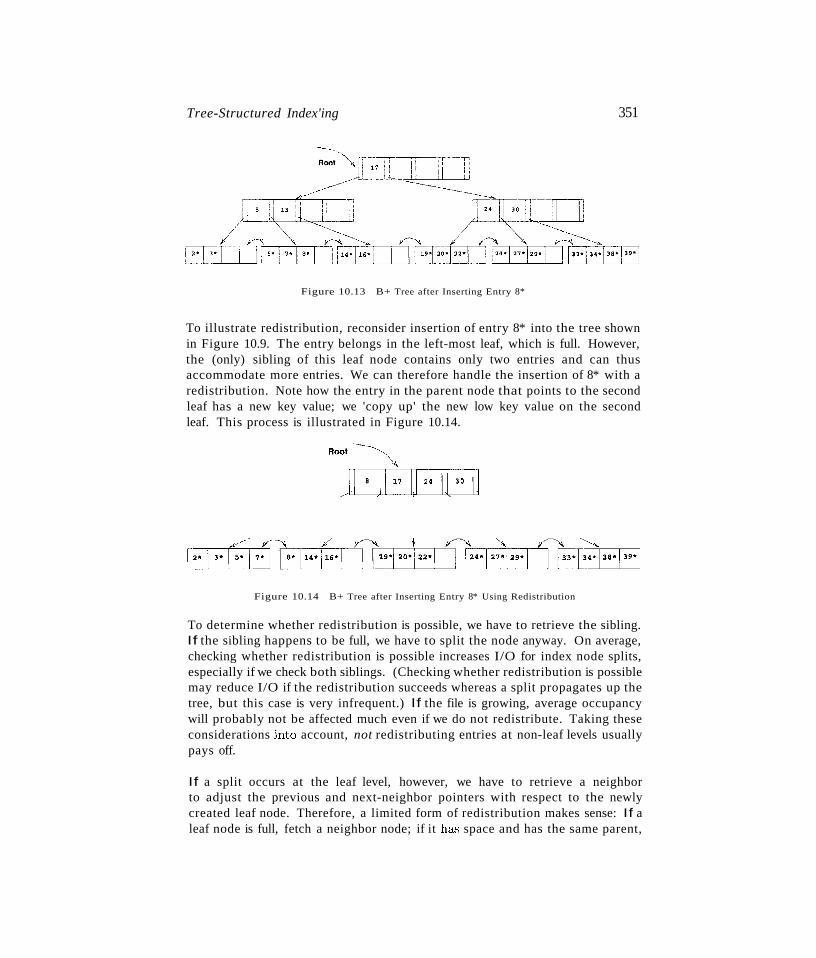
Tree-Structured Index'ing 351
Figure 10.13 B+ Tree after Inserting Entry 8*
To illustrate redistribution, reconsider insertion of entry 8* into the tree shownin Figure 10.9. The entry belongs in the left-most leaf, which is full. However,the (only) sibling of this leaf node contains only two entries and can thusaccommodate more entries. We can therefore handle the insertion of 8* with aredistribution. Note how the entry in the parent node that points to the secondleaf has a new key value; we 'copy up' the new low key value on the secondleaf. This process is illustrated in Figure 10.14.
Figure 10.14 B+ Tree after Inserting Entry 8* Using Redistribution
To determine whether redistribution is possible, we have to retrieve the sibling.If the sibling happens to be full, we have to split the node anyway. On average,checking whether redistribution is possible increases I/O for index node splits,especially if we check both siblings. (Checking whether redistribution is possiblemay reduce I/O if the redistribution succeeds whereas a split propagates up thetree, but this case is very infrequent.) If the file is growing, average occupancywill probably not be affected much even if we do not redistribute. Taking theseconsiderations ,into account, not redistributing entries at non-leaf levels usuallypays off.
If a split occurs at the leaf level, however, we have to retrieve a neighborto adjust the previous and next-neighbor pointers with respect to the newlycreated leaf node. Therefore, a limited form of redistribution makes sense: If aleaf node is full, fetch a neighbor node; if it ha.'3 space and has the same parent,
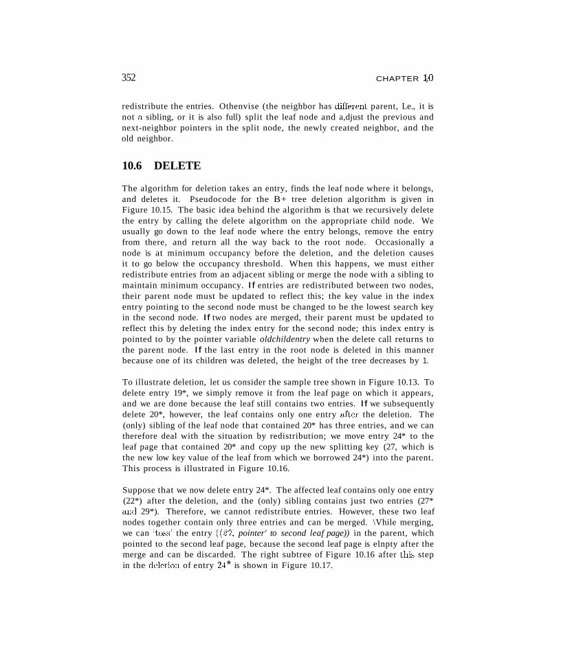
352 CHAPTER :40
redistribute the entries. Othenvise (the neighbor has diflerent parent, Le., it isnot a sibling, or it is also full) split the leaf node and a,djust the previous andnext-neighbor pointers in the split node, the newly created neighbor, and theold neighbor.
10.6 DELETE
The algorithm for deletion takes an entry, finds the leaf node where it belongs,and deletes it. Pseudocode for the B+ tree deletion algorithm is given inFigure 10.15. The basic idea behind the algorithm is that we recursively deletethe entry by calling the delete algorithm on the appropriate child node. Weusually go down to the leaf node where the entry belongs, remove the entryfrom there, and return all the way back to the root node. Occasionally anode is at minimum occupancy before the deletion, and the deletion causesit to go below the occupancy threshold. When this happens, we must eitherredistribute entries from an adjacent sibling or merge the node with a sibling tomaintain minimum occupancy. If entries are redistributed between two nodes,their parent node must be updated to reflect this; the key value in the indexentry pointing to the second node must be changed to be the lowest search keyin the second node. If two nodes are merged, their parent must be updated toreflect this by deleting the index entry for the second node; this index entry ispointed to by the pointer variable oldchildentry when the delete call returns tothe parent node. If the last entry in the root node is deleted in this mannerbecause one of its children was deleted, the height of the tree decreases by 1.
To illustrate deletion, let us consider the sample tree shown in Figure 10.13. Todelete entry 19*, we simply remove it from the leaf page on which it appears,and we are done because the leaf still contains two entries. If we subsequentlydelete 20*, however, the leaf contains only one entry after the deletion. The(only) sibling of the leaf node that contained 20* has three entries, and we cantherefore deal with the situation by redistribution; we move entry 24* to theleaf page that contained 20* and copy up the new splitting key (27, which isthe new low key value of the leaf from which we borrowed 24*) into the parent.This process is illustrated in Figure 10.16.
Suppose that we now delete entry 24*. The affected leaf contains only one entry(22*) after the deletion, and the (only) sibling contains just two entries (27*and 29*). Therefore, we cannot redistribute entries. However, these two leafnodes together contain only three entries and can be merged. \Vhile merging,we can 'tos::;' the entry ((27, pointer' to second leaf page)) in the parent, whichpointed to the second leaf page, because the second leaf page is elnpty after themerge and can be discarded. The right subtree of Figure 10.16 after thi::; stepin the deletion of entry 2!1* is shown in Figure 10.17.
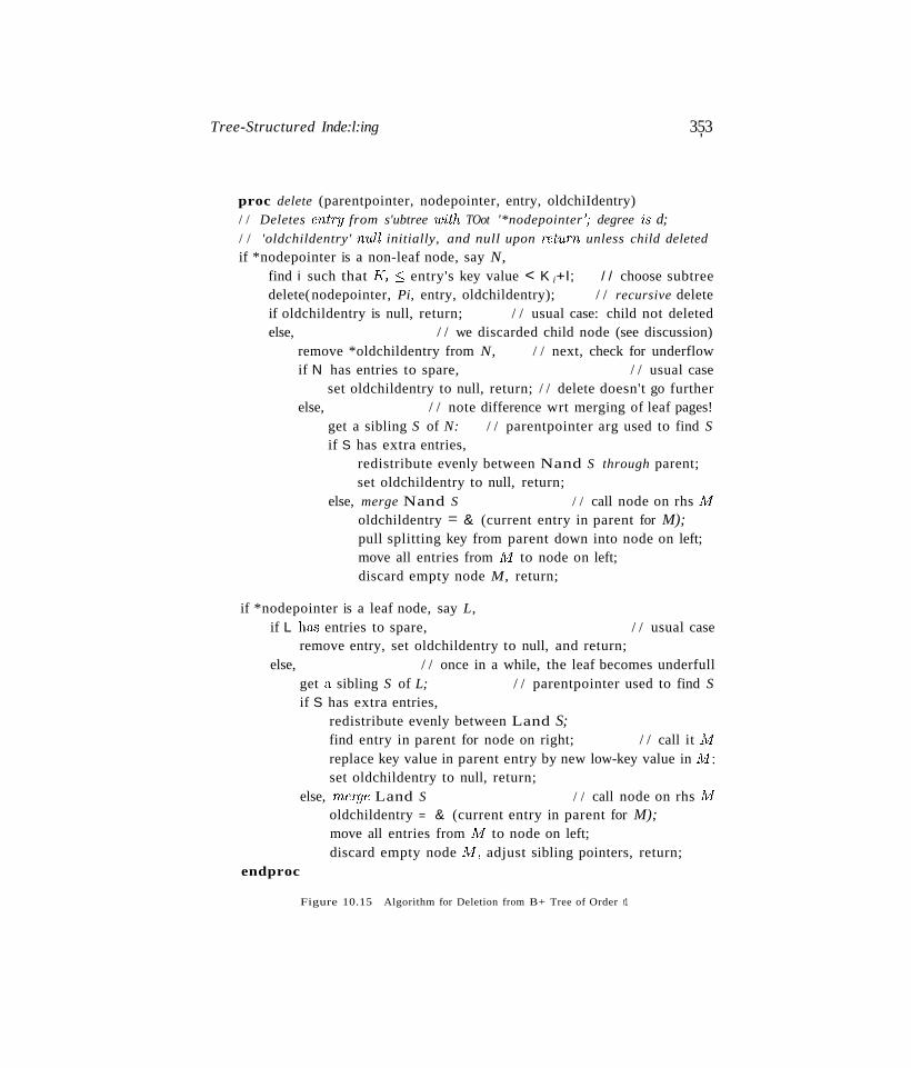
Tree-Structured Inde:l:ing 353,
proc delete (parentpointer, nodepointer, entry, oldchiIdentry)/ / Deletes entry from s'ubtree w'ith TOot '*nodepointer '; degree is d;/ / 'oldchildentry' null initially, and null upon ret1lrn unless child deleted
if *nodepointer is a non-leaf node, say N,find i such that K i ::; entry's key value < K i+l; / / choose subtreedelete(nodepointer, Pi, entry, oldchildentry); / / recursive deleteif oldchildentry is null, return; / / usual case: child not deletedelse, / / we discarded child node (see discussion)
remove *oldchildentry from N, / / next, check for underflowif N has entries to spare, / / usual case
set oldchildentry to null, return; / / delete doesn't go furtherelse, / / note difference wrt merging of leaf pages!
get a sibling S of N: / / parentpointer arg used to find Sif S has extra entries,
redistribute evenly between Nand S through parent;set oldchildentry to null, return;
else, merge Nand S / / call node on rhs 111oldchildentry = & (current entry in parent for M);pull splitting key from parent down into node on left;move all entries from 1\11 to node on left;discard empty node M, return;
if *nodepointer is a leaf node, say L,if L h&<; entries to spare, / / usual case
remove entry, set oldchildentry to null, and return;else, / / once in a while, the leaf becomes underfull
get a sibling S of L; / / parentpointer used to find Sif S has extra entries,
redistribute evenly between Land S;find entry in parent for node on right; / / call it A;Jreplace key value in parent entry by new low-key value in 1\11;
set oldchildentry to null, return;else, merge Land S / / call node on rhs 1\11
oldchildentry = & (current entry in parent for M);move all entries from 1\11 to node on left;discard empty node AI, adjust sibling pointers, return;
endproc
Figure 10.15 Algorithm for Deletion from B+ Tree of Order r1
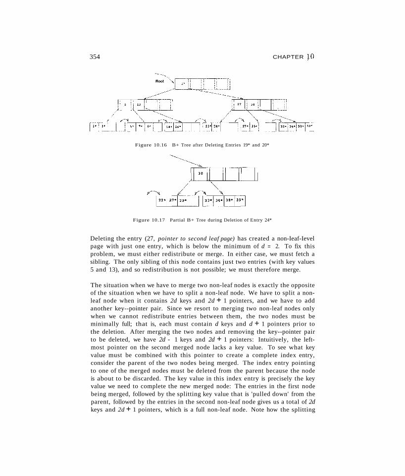
354 CHAPTER 1-0
Figure 10.16 B+ Tree after Deleting Entries 19* and 20*
Figure 10.17 Partial B+ Tree during Deletion of Entry 24*
Deleting the entry (27, pointer to second leaf page) has created a non-Ieaf-Ievelpage with just one entry, which is below the minimum of d = 2. To fix thisproblem, we must either redistribute or merge. In either case, we must fetch asibling. The only sibling of this node contains just two entries (with key values5 and 13), and so redistribution is not possible; we must therefore merge.
The situation when we have to merge two non-leaf nodes is exactly the oppositeof the situation when we have to split a non-leaf node. We have to split a nonleaf node when it contains 2d keys and 2d + 1 pointers, and we have to addanother key--pointer pair. Since we resort to merging two non-leaf nodes onlywhen we cannot redistribute entries between them, the two nodes must beminimally full; that is, each must contain d keys and d + 1 pointers prior tothe deletion. After merging the two nodes and removing the key--pointer pairto be deleted, we have 2d - 1 keys and 2d + 1 pointers: Intuitively, the leftmost pointer on the second merged node lacks a key value. To see what keyvalue must be combined with this pointer to create a complete index entry,consider the parent of the two nodes being merged. The index entry pointingto one of the merged nodes must be deleted from the parent because the nodeis about to be discarded. The key value in this index entry is precisely the keyvalue we need to complete the new merged node: The entries in the first nodebeing merged, followed by the splitting key value that is 'pulled down' from theparent, followed by the entries in the second non-leaf node gives us a total of 2dkeys and 2d + 1 pointers, which is a full non-leaf node. Note how the splitting
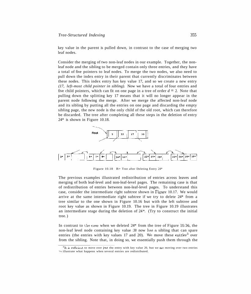
Tree-Structured Indexing 355
key value in the parent is pulled down, in contrast to the case of merging twoleaf nodes.
Consider the merging of two non-leaf nodes in our example. Together, the nonleaf node and the sibling to be merged contain only three entries, and they havea total of five pointers to leaf nodes. To merge the two nodes, we also need topull down the index entry in their parent that currently discriminates betweenthese nodes. This index entry has key value 17, and so we create a new entry(17, left-most child pointer in sibling). Now we have a total of four entries andfive child pointers, which can fit on one page in a tree of order d = 2. Note thatpulling down the splitting key 17 means that it will no longer appear in theparent node following the merge. After we merge the affected non-leaf nodeand its sibling by putting all the entries on one page and discarding the emptysibling page, the new node is the only child of the old root, which can thereforebe discarded. The tree after completing all these steps in the deletion of entry24* is shown in Figure 10.18.
Figure 10.18 B+ Tree after Deleting Entry 24*
The previous examples illustrated redistribution of entries across leaves andmerging of both leaf-level and non-leaf-level pages. The remaining case is thatof redistribution of entries between non-leaf-level pages. To understand thiscase, consider the intermediate right subtree shown in Figure 10.17. We wouldarrive at the same intermediate right subtree if we try to delete 24* from atree similar to the one shown in Figure 10.16 but with the left subtree androot key value as shown in Figure 10.19. The tree in Figure 10.19 illustratesan intermediate stage during the deletion of 24*. (Try to construct the initialtree. )
In contrast to the caf.;e when we deleted 24* from the tree of Figure HUG, thenon-leaf level node containing key value :30 now ha..s a sibling that can spareentries (the entries with key values 17 and 20). vVe move these entries3 overfrom the sibling. Note that, in doing so, we essentially push them through the
:11t is sufficient to move over just the entry with key value 20, hut we are moving over two entries°0 illustrate what happens when several entries are redistributed.
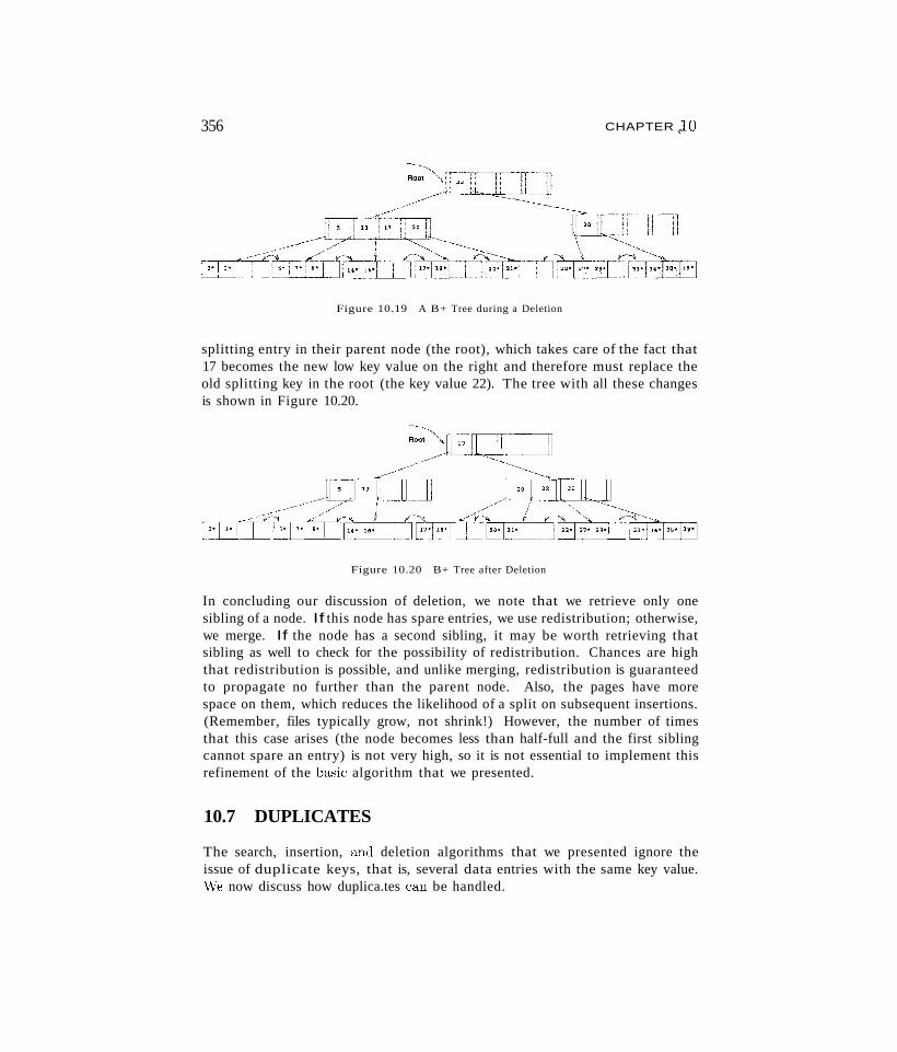
356 CHAPTER ;'0
Figure 10.19 A B+ Tree during a Deletion
splitting entry in their parent node (the root), which takes care of the fact that17 becomes the new low key value on the right and therefore must replace theold splitting key in the root (the key value 22). The tree with all these changesis shown in Figure 10.20.
Figure 10.20 B+ Tree after Deletion
In concluding our discussion of deletion, we note that we retrieve only onesibling of a node. If this node has spare entries, we use redistribution; otherwise,we merge. If the node has a second sibling, it may be worth retrieving thatsibling as well to check for the possibility of redistribution. Chances are highthat redistribution is possible, and unlike merging, redistribution is guaranteedto propagate no further than the parent node. Also, the pages have morespace on them, which reduces the likelihood of a split on subsequent insertions.(Remember, files typically grow, not shrink!) However, the number of timesthat this case arises (the node becomes less than half-full and the first siblingcannot spare an entry) is not very high, so it is not essential to implement thisrefinement of the bct.'3ic algorithm that we presented.
10.7 DUPLICATES
The search, insertion, and deletion algorithms that we presented ignore theissue of duplicate keys, that is, several data entries with the same key value.vVe now discuss how duplica.tes can be handled.
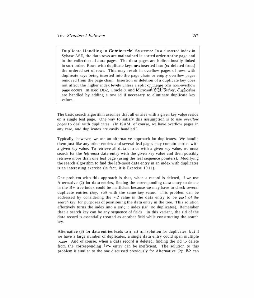
Tree-StT'llct'uTed Inde:ring 35~
Duplicate Handling in COlllmercial Systems: In a clustered index inSybase ASE, the data rows are maintained in sorted order onthe page andin the eollection of data pages. The data pages are bidireetionally linkedin sort order. Rows with duplicate keys are inserted into (or deleted from}the ordered set of rows. This may result in overflow pages of rows withduplieate keys being inserted into the page chain or empty overflow pagesremoved from the page chain. Insertion or deletion of a duplicate key doesnot affect the higher index level'> unless a split or. lIlergy ofa .non.-overflowpage occurs. In IBM DB2, Oracle 8, and Miero§oft'SQL'Server; dupliclltesare handled by adding a row id if necessary to eliminate duplicate keyvalues.
.
The basic search algorithm assumes that all entries with a given key value resideon a single leaf page. One way to satisfy this assumption is to use overflowpages to deal with duplicates. (In ISAM, of course, we have overflow pages inany case, and duplicates are easily handled.)
Typically, however, we use an alternative approach for duplicates. We handlethem just like any other entries and several leaf pages may contain entries witha given key value. To retrieve all data entries with a given key value, we mustsearch for the left-most data entry with the given key value and then possiblyretrieve more than one leaf page (using the leaf sequence pointers). Modifyingthe search algorithm to find the left-most data entry in an index with duplicatesis an interesting exercise (in fact, it is Exercise 10.11).
One problem with this approach is that, when a record is deleted, if we useAlternative (2) for data entries, finding the corresponding data entry to deletein the B+ tree index could be inefficient because we may have to check severalduplicate entries (key, rid) with the same key value. This problem can beaddressed by considering the rid value in the data entry to be part of thesearch key, for purposes of positioning the data entry in the tree. This solutioneffectively turns the index into a uniq71,e index (i.e" no duplicates), Rememberthat a search key can be any sequence of fields in this variant, the rid of thedata record is essentially treated as another field while constructing the searchkey.
Alternative (3) f'or data entries leads to a natural solution for duplicates, but ifwe have a large number of duplicates, a single data entry could span multiplepages. And of course, when a data record is deleted, finding the rid to deletefrom the corresponding data entry can be inefficient, The solution to thisproblem is similar to the one discussed previously for Alternative (2): vVe can
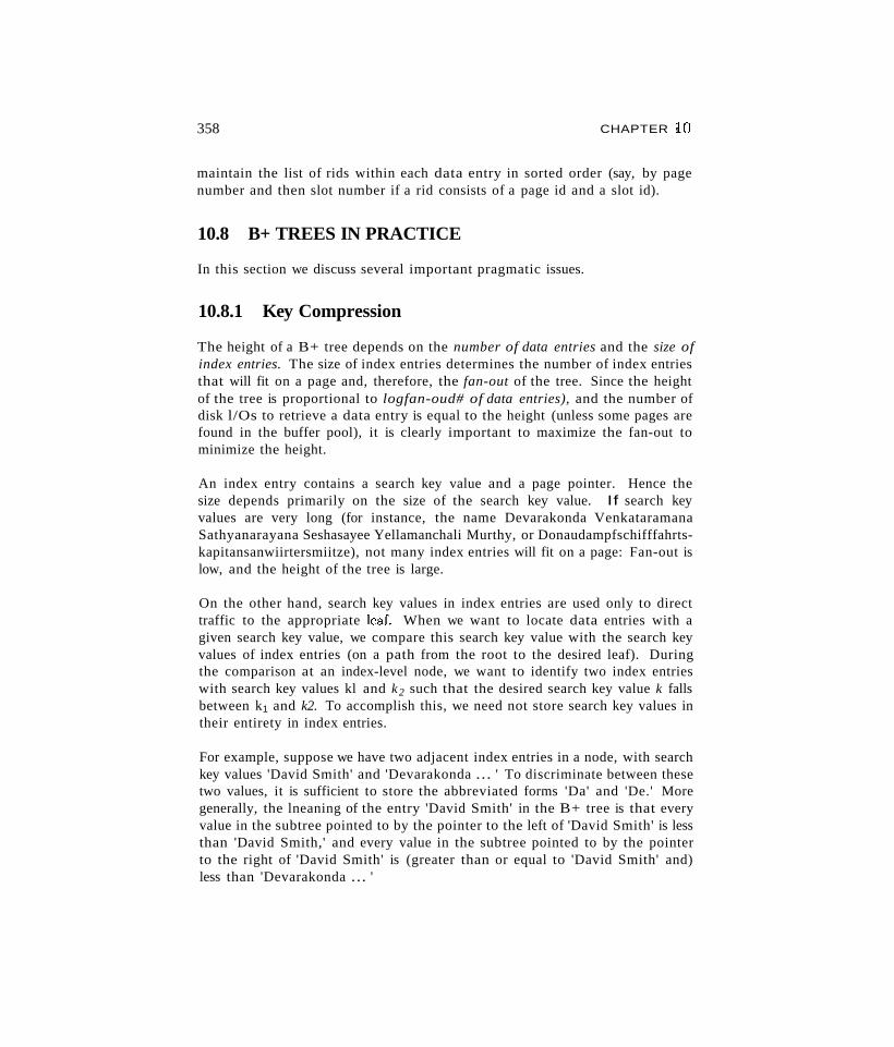
358 CHAPTER 10
maintain the list of rids within each data entry in sorted order (say, by pagenumber and then slot number if a rid consists of a page id and a slot id).
10.8 B+ TREES IN PRACTICE
In this section we discuss several important pragmatic issues.
10.8.1 Key Compression
The height of a B+ tree depends on the number of data entries and the size ofindex entries. The size of index entries determines the number of index entriesthat will fit on a page and, therefore, the fan-out of the tree. Since the heightof the tree is proportional to logfan-oud# of data entries), and the number ofdisk l/Os to retrieve a data entry is equal to the height (unless some pages arefound in the buffer pool), it is clearly important to maximize the fan-out tominimize the height.
An index entry contains a search key value and a page pointer. Hence thesize depends primarily on the size of the search key value. If search keyvalues are very long (for instance, the name Devarakonda VenkataramanaSathyanarayana Seshasayee Yellamanchali Murthy, or Donaudampfschifffahrtskapitansanwiirtersmiitze), not many index entries will fit on a page: Fan-out islow, and the height of the tree is large.
On the other hand, search key values in index entries are used only to directtraffic to the appropriate leaf. When we want to locate data entries with agiven search key value, we compare this search key value with the search keyvalues of index entries (on a path from the root to the desired leaf). Duringthe comparison at an index-level node, we want to identify two index entrieswith search key values kl and k2 such that the desired search key value k fallsbetween k1 and k2. To accomplish this, we need not store search key values intheir entirety in index entries.
For example, suppose we have two adjacent index entries in a node, with searchkey values 'David Smith' and 'Devarakonda ... ' To discriminate between thesetwo values, it is sufficient to store the abbreviated forms 'Da' and 'De.' Moregenerally, the lneaning of the entry 'David Smith' in the B+ tree is that everyvalue in the subtree pointed to by the pointer to the left of 'David Smith' is lessthan 'David Smith,' and every value in the subtree pointed to by the pointerto the right of 'David Smith' is (greater than or equal to 'David Smith' and)less than 'Devarakonda ... '
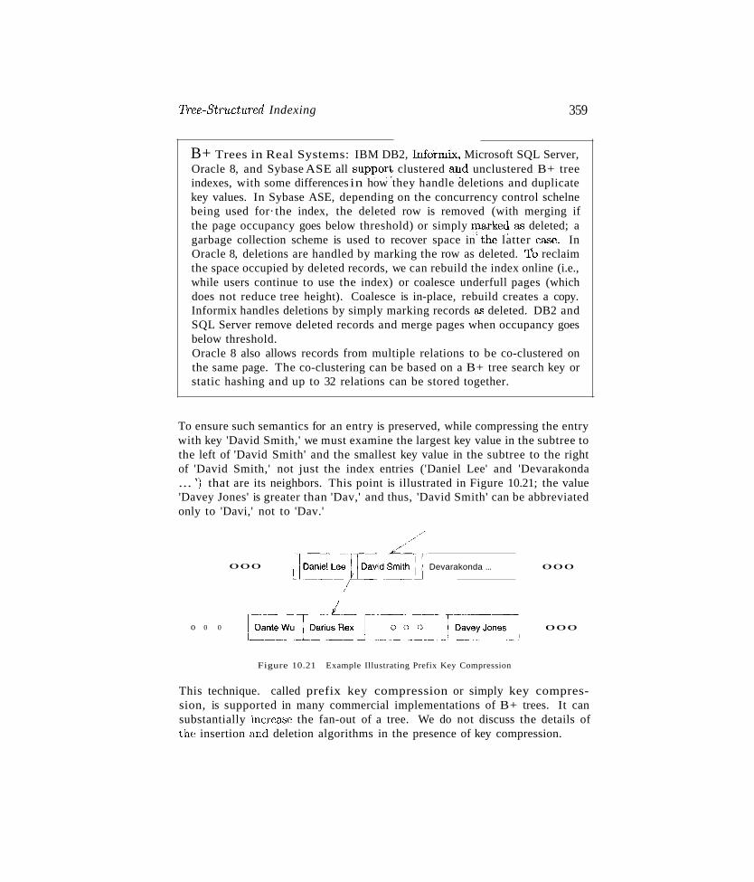
Tree-Struct'ured Indexing 359
B+ Trees in Real Systems: IBM DB2, Infol:mLx, Microsoft SQL Server,Oracle 8, and Sybase ASE all support clustered ~d unclustered B+ treeindexes, with some differences in how they handle deletions and duplicatekey values. In Sybase ASE, depending on the concurrency control schelnebeing used for· the index, the deleted row is removed (with merging ifthe page occupancy goes below threshold) or simply 111arkedas deleted; agarbage collection scheme is used to recover space .. in th~ latter case, InOracle 8, deletions are handled by marking the row as deleted. 1'0 reclaimthe space occupied by deleted records, we can rebuild the index online (i.e.,while users continue to use the index) or coalesce underfull pages (whichdoes not reduce tree height). Coalesce is in-place, rebuild creates a copy.Informix handles deletions by simply marking records as deleted. DB2 andSQL Server remove deleted records and merge pages when occupancy goesbelow threshold.Oracle 8 also allows records from multiple relations to be co-clustered onthe same page. The co-clustering can be based on a B+ tree search key orstatic hashing and up to 32 relations can be stored together.
To ensure such semantics for an entry is preserved, while compressing the entrywith key 'David Smith,' we must examine the largest key value in the subtree tothe left of 'David Smith' and the smallest key value in the subtree to the rightof 'David Smith,' not just the index entries ('Daniel Lee' and 'Devarakonda... ') that are its neighbors. This point is illustrated in Figure 10.21; the value'Davey Jones' is greater than 'Dav,' and thus, 'David Smith' can be abbreviatedonly to 'Davi,' not to 'Dav.'
000 Devarakonda ... 000
o 0 0
Figure 10.21 Example Illustrating Prefix Key Compression
000
This technique. called prefix key compression or simply key compression, is supported in many commercial implementations of B+ trees. It cansubstantially increCL')e the fan-out of a tree. We do not discuss the details ofthe insertion and deletion algorithms in the presence of key compression.
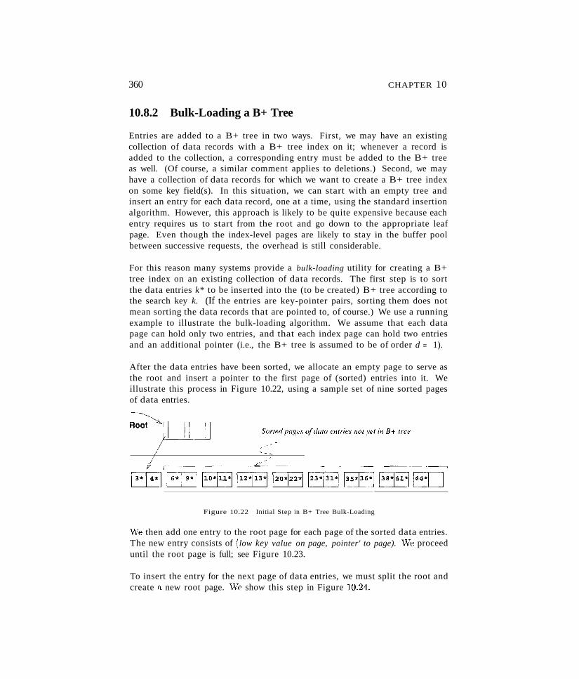
360 CHAPTER 10
10.8.2 Bulk-Loading a B+ Tree
Entries are added to a B+ tree in two ways. First, we may have an existingcollection of data records with a B+ tree index on it; whenever a record isadded to the collection, a corresponding entry must be added to the B+ treeas well. (Of course, a similar comment applies to deletions.) Second, we mayhave a collection of data records for which we want to create a B+ tree indexon some key field(s). In this situation, we can start with an empty tree andinsert an entry for each data record, one at a time, using the standard insertionalgorithm. However, this approach is likely to be quite expensive because eachentry requires us to start from the root and go down to the appropriate leafpage. Even though the index-level pages are likely to stay in the buffer poolbetween successive requests, the overhead is still considerable.
For this reason many systems provide a bulk-loading utility for creating a B+tree index on an existing collection of data records. The first step is to sortthe data entries k* to be inserted into the (to be created) B+ tree according tothe search key k. (If the entries are key-pointer pairs, sorting them does notmean sorting the data records that are pointed to, of course.) We use a runningexample to illustrate the bulk-loading algorithm. We assume that each datapage can hold only two entries, and that each index page can hold two entriesand an additional pointer (i.e., the B+ tree is assumed to be of order d = 1).
After the data entries have been sorted, we allocate an empty page to serve asthe root and insert a pointer to the first page of (sorted) entries into it. Weillustrate this process in Figure 10.22, using a sample set of nine sorted pagesof data entries.
~!--==_~~~~"",L:-=o-s_c_,:_.te_d_p~a~g_e_s_()f_(_la_t_a_e_nt_rie_s~n~ot_Y_"_il_l_B_+_t_re_e~~_----,ffi EEJ 110*~~ 112j~ 1
20*[221
Figure 10.22 Initial Step in B+ Tree Bulk-Loading
vVe then add one entry to the root page for each page of the sorted data entries.The new entry consists of \ low key value on page, pointer' to page). vVe proceeduntil the root page is full; see Figure 10.23.
To insert the entry for the next page of data entries, we must split the root andcreate a new root page. vVe show this step in Figure 10.2/1.
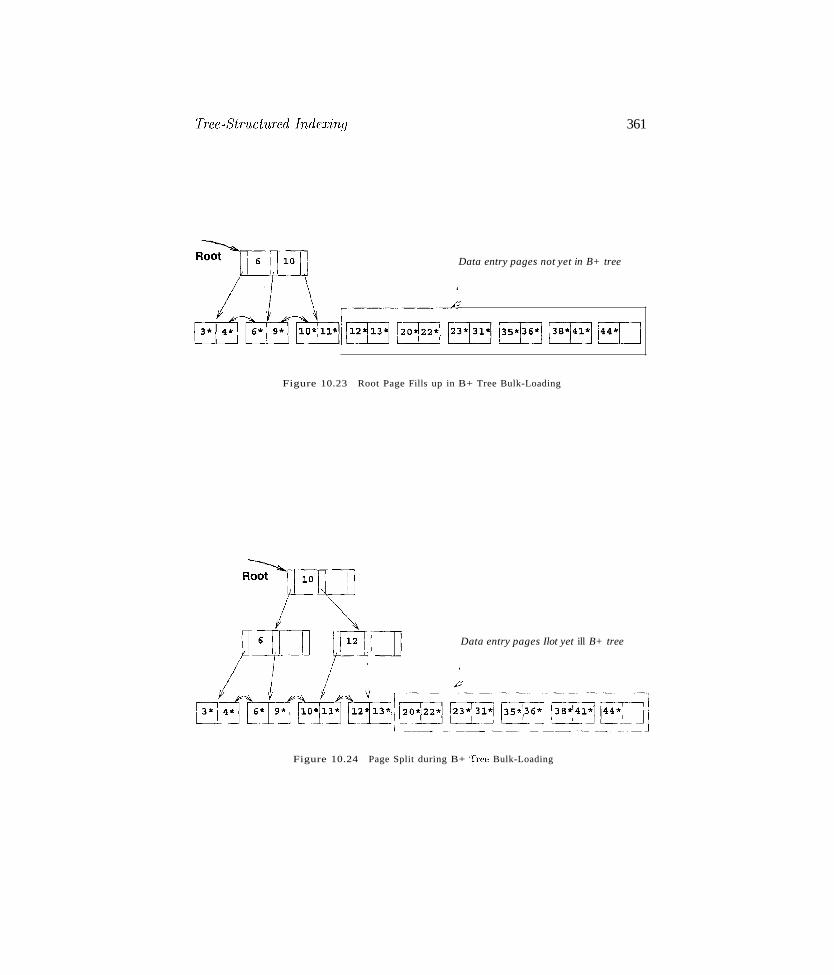
Tr'ee-8iruci'ured Index'ing
Data entry pages not yet in B+ tree
Figure 10.23 Root Page Fills up in B+ Tree Bulk-Loading
Data entry pages Ilot yet ill B+ tree
Figure 10.24 Page Split during B+ 'fi'ee Bulk-Loading
361
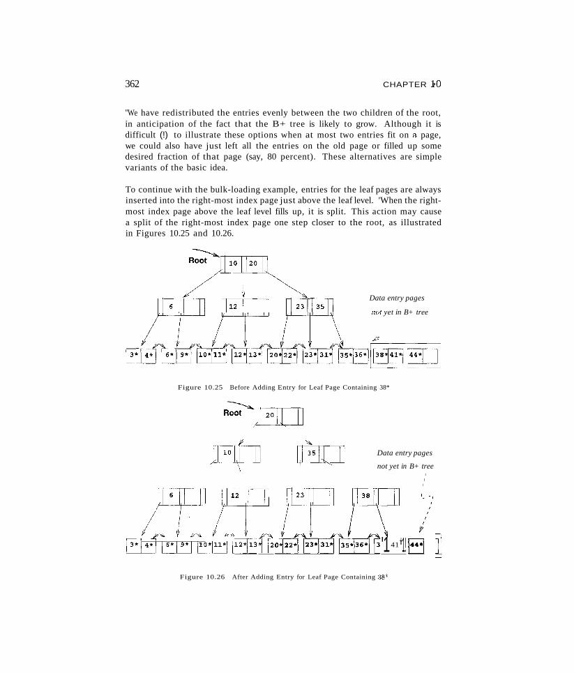
362 CHAPTER :FO
"We have redistributed the entries evenly between the two children of the root,in anticipation of the fact that the B+ tree is likely to grow. Although it isdifficult (!) to illustrate these options when at most two entries fit on a page,we could also have just left all the entries on the old page or filled up somedesired fraction of that page (say, 80 percent). These alternatives are simplevariants of the basic idea.
To continue with the bulk-loading example, entries for the leaf pages are alwaysinserted into the right-most index page just above the leaf level. 'When the rightmost index page above the leaf level fills up, it is split. This action may causea split of the right-most index page one step closer to the root, as illustratedin Figures 10.25 and 10.26.
Data entry pages
not yet in B+ tree
Figure 10.25 Before Adding Entry for Leaf Page Containing 38*
Data entry pages
not yet in B+ treeI
II
ITIf IT, fT ?'r---.----'i
12113{j2 '122:J123*EJ ~5*136*~ '141 *1! f'*1 ]Figure 10.26 After Adding Entry for Leaf Page Containing :38*
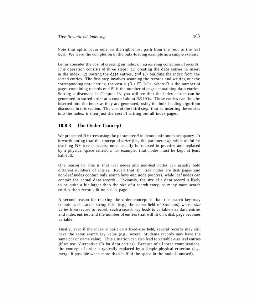
Tiee-Structured Inde:ring 36,3
Note that splits occur only on the right-most path from the root to the leaflevel. \Ve leave the completion of the bulk-loading example as a simple exercise.
Let us consider the cost of creating an index on an existing collection of records.This operation consists of three steps: (1) creating the data entries to insertin the index, (2) sorting the data entries, and (3) building the index from thesorted entries. The first step involves scanning the records and writing out thecorresponding data entries; the cost is (R + E) I/Os, where R is the number ofpages containing records and E is the number of pages containing data entries.Sorting is discussed in Chapter 13; you will see that the index entries can begenerated in sorted order at a cost of about 3E I/Os. These entries can then beinserted into the index as they are generated, using the bulk-loading algorithmdiscussed in this section. The cost of the third step, that is, inserting the entriesinto the index, is then just the cost of writing out all index pages.
10.8.3 The Order Concept
We presented B+ trees using the parameter d to denote minimum occupancy. Itis worth noting that the concept of order (i.e., the parameter d), while useful forteaching B+ tree concepts, must usually be relaxed in practice and replacedby a physical space criterion; for example, that nodes must be kept at lea..c;thalf-full.
One reason for this is that leaf nodes and non-leaf nodes can usually holddifferent numbers of entries. Recall that B+ tree nodes are disk pages andnon-leaf nodes contain only search keys and node pointers, while leaf nodes cancontain the actual data records. Obviously, the size of a data record is likelyto be quite a bit larger than the size of a search entry, so many more searchentries than records fit on a disk page.
A second reason for relaxing the order concept is that the search key maycontain a character string field (e.g., the name field of Students) whose sizevaries from record to record; such a search key leads to variable-size data entriesand index entries, and the number of entries that will fit on a disk page becomesvariable.
Finally, even i{ the index is built on a fixed-size field, several records may stillhave the same search key value (e.g., several Students records may have thesame gpa or name value). This situation can also lead to variable-size leaf entries(if we use Alternative (3) for data entries). Because of all these complications,the concept of order is typically replaced by a simple physical criterion (e.g.,merge if possible when more than half of the space in the node is unused).
364 CHAPTER 1()
10.8.4 The Effect of Inserts and Deletes on Rids
If the leaf pages contain data records-that is, the B+ tree is a clustered indexthen operations such as splits, merges, and redistributions can change rids.Recall that a typical representation for a rid is some combination of (physical)page number and slot number. This scheme allows us to move records withina page if an appropriate page format is chosen but not across pages, as is thecase with operations such as splits. So unless rids are chosen to be independentof page numbers, an operation such as split or merge in a clustered B+ treemay require compensating updates to other indexes on the same data.
A similar comment holds for any dynamic clustered index, regardless of whetherit is tree-based or hash-based. Of course, the problem does not arise withnonclustered indexes, because only index entries are moved around.
10.9 REVIEW QUESTIONS
Answers to the review questions can be found in the listed sections.
• Why are tree-structured indexes good for searches, especially range selections? (Section 10.1)
• Describe how search, insert, and delete operations work in ISAM indexes.Discuss the need for overflow pages, and their potential impact on performance. What kinds of update workloads are ISAM indexes most vulnerableto, and what kinds of workloads do they handle well? (Section 10.2)
• Only leaf pages are affected in updates in ISAM indexes. Discuss theimplications for locking and concurrent access. Compare ISAM and B+trees in this regard. (Section 10.2.1)
• What are the main differences between ISAM and B+ tree indexes? (Section 10.3)
• What is the order of a B+ tree? Describe the format of nodes in a B+tree. Why are nodes at the leaf level linked? (Section 10.3)
• How rnany nodes must be examined for equality search in a B+ tree? Howmany for a range selection? Compare this with ISAM. (Section 10.4)
• Describe the B+ tree insertion algorithm, and explain how it eliminatesoverflow pages. Under what conditions can an insert increase the height ofthe tree? (Section 10.5)
• During deletion, a node might go below the minimum occupancy threshold.How is this handled? Under what conditions could a deletion decrease theheight of the tree? (Section 10.6)
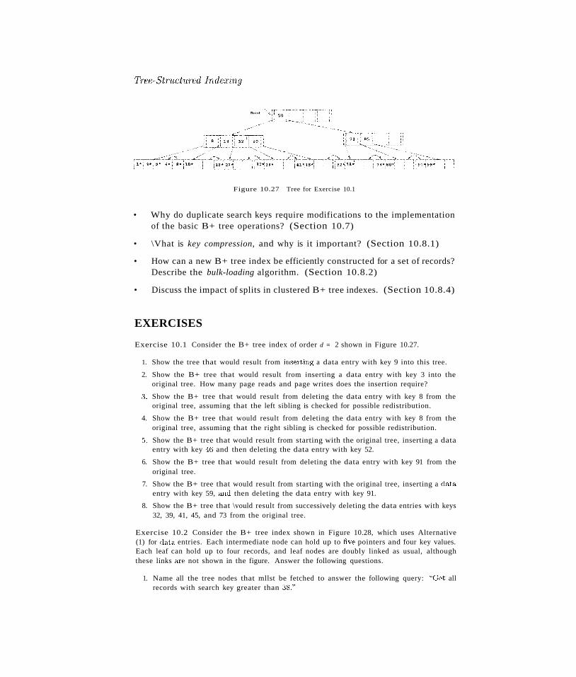
Tree-Str"l.tct1lTcd Indccing
Figure 10.27 Tree for Exercise 10.1
• Why do duplicate search keys require modifications to the implementationof the basic B+ tree operations? (Section 10.7)
• \Vhat is key compression, and why is it important? (Section 10.8.1)
• How can a new B+ tree index be efficiently constructed for a set of records?Describe the bulk-loading algorithm. (Section 10.8.2)
• Discuss the impact of splits in clustered B+ tree indexes. (Section 10.8.4)
EXERCISES
Exercise 10.1 Consider the B+ tree index of order d = 2 shown in Figure 10.27.
1. Show the tree that would result from inserting a data entry with key 9 into this tree.
2. Show the B+ tree that would result from inserting a data entry with key 3 into theoriginal tree. How many page reads and page writes does the insertion require?
:3. Show the B+ tree that would result from deleting the data entry with key 8 from theoriginal tree, assuming that the left sibling is checked for possible redistribution.
4. Show the B+ tree that would result from deleting the data entry with key 8 from theoriginal tree, assuming that the right sibling is checked for possible redistribution.
5. Show the B+ tree that would result from starting with the original tree, inserting a dataentry with key 46 and then deleting the data entry with key 52.
6. Show the B+ tree that would result from deleting the data entry with key 91 from theoriginal tree.
7. Show the B+ tree that would result from starting with the original tree, inserting a dataentry with key 59, and then deleting the data entry with key 91.
8. Show the B+ tree that \vould result from successively deleting the data entries with keys32, 39, 41, 45, and 73 from the original tree.
Exercise 10.2 Consider the B+ tree index shown in Figure 10.28, which uses Alternative(1) for data entries. Each intermediate node can hold up to five pointers and four key values.Each leaf can hold up to four records, and leaf nodes are doubly linked as usual, althoughthese links are not shown in the figure. Answer the following questions.
1. Name all the tree nodes that mllst be fetched to answer the following query: "Get allrecords with search key greater than :38."
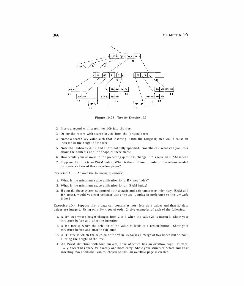
366 CHAPTER 10
L3 L6
Figure 10.28 Tree for Exercise 10.2
2. Insert a record with search key 109 into the tree.
3. Delete the record with search key 81 from the (original) tree.
4. Name a search key value such that inserting it into the (original) tree would cause anincrease in the height of the tree.
5. Note that subtrees A, B, and C are not fully specified. Nonetheless, what can you inferabout the contents and the shape of these trees?
6. How would your answers to the preceding questions change if this were an ISAM index?
7. Suppose that this is an ISAM index. What is the minimum number of insertions neededto create a chain of three overflow pages?
Exercise 10.3 Answer the following questions:
1. What is the minimum space utilization for a B+ tree index?
2. What is the minimum space utilization for an ISAM index?
3. If your database system supported both a static and a dynamic tree index (say, ISAM andB+ trees), would you ever consider using the static index in preference to the dynamicindex?
Exercise 10.4 Suppose that a page can contain at most four data values and that aU datavalues are integers. Using only B+ trees of order 2, give examples of each of the following:
1. A B+ tree whose height changes from 2 to 3 when the value 25 is inserted. Show yourstructure before and after the insertion.
2. A B+ tree in which the deletion of the value 25 leads to a redistribution. Show yourstructure before and aft.er the deletion.
3. A B+ tree in which t.he delet.ion of the value 25 causes a merge of two nodes but without.altering the height of the tree.
4. An ISAM structure with four buckets, none of which has an overflow page. Further,every bucket has space for exactly one more entry. Show your structure before and aft.erinserting t.wo additional values, chosen so that. an overflow page is created.
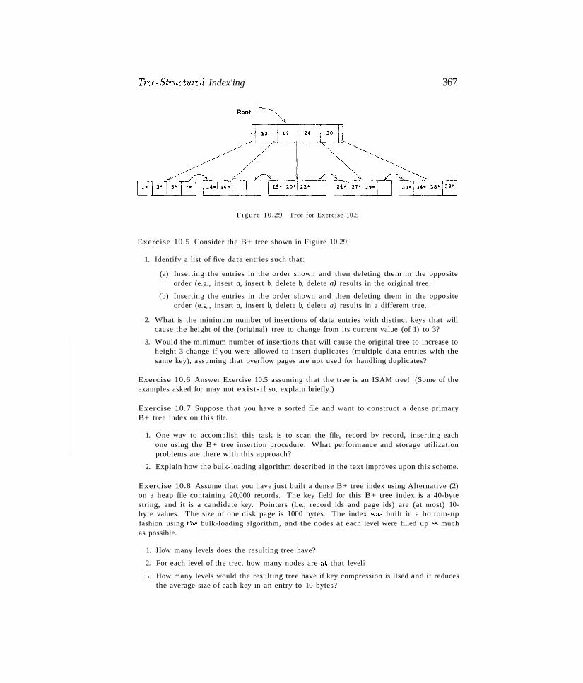
Tree-Structured Index'ing 367
Figure 10.29 Tree for Exercise 10.5
Exercise 10.5 Consider the B+ tree shown in Figure 10.29.
1. Identify a list of five data entries such that:
(a) Inserting the entries in the order shown and then deleting them in the oppositeorder (e.g., insert a, insert b, delete b, delete a) results in the original tree.
(b) Inserting the entries in the order shown and then deleting them in the oppositeorder (e.g., insert a, insert b, delete b, delete a) results in a different tree.
2. What is the minimum number of insertions of data entries with distinct keys that willcause the height of the (original) tree to change from its current value (of 1) to 3?
3. Would the minimum number of insertions that will cause the original tree to increase toheight 3 change if you were allowed to insert duplicates (multiple data entries with thesame key), assuming that overflow pages are not used for handling duplicates?
Exercise 10.6 Answer Exercise 10.5 assuming that the tree is an ISAM tree! (Some of theexamples asked for may not exist-if so, explain briefly.)
Exercise 10.7 Suppose that you have a sorted file and want to construct a dense primaryB+ tree index on this file.
1. One way to accomplish this task is to scan the file, record by record, inserting eachone using the B+ tree insertion procedure. What performance and storage utilizationproblems are there with this approach?
2. Explain how the bulk-loading algorithm described in the text improves upon this scheme.
Exercise 10.8 Assume that you have just built a dense B+ tree index using Alternative (2)on a heap file containing 20,000 records. The key field for this B+ tree index is a 40-bytestring, and it is a candidate key. Pointers (Le., record ids and page ids) are (at most) 10byte values. The size of one disk page is 1000 bytes. The index wa9 built in a bottom-upfashion using the bulk-loading algorithm, and the nodes at each level were filled up a..9 muchas possible.
1. Ho\v many levels does the resulting tree have?
2. For each level of the trec, how many nodes are at that level?
3. How many levels would the resulting tree have if key compression is llsed and it reducesthe average size of each key in an entry to 10 bytes?
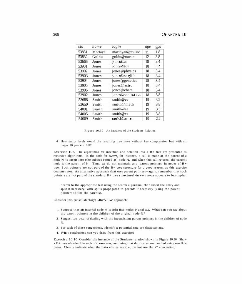
368
sid name login age gpa
CHAPTER to
53831 Maclayall maclayan@music 11 1.853832 Guldu guldu@music 12 3.853666 Jones jones(gcs 18 3.453901 Jones jones({'!Jtoy 18 3A53902 Jones jones@physics 18 3.453903 Jones jones(Q)english 18 3.453904 Jones jones(ggenetics 18 3.453905 Jones jones@astro 18 3.453906 Jones jones@chem 18 3.453902 Jones jones(Qlsanitation 18 3.853688 Smith smith@ee 19 3.253650 Smith smith@math 19 3.854001 Smith smith@ee 19 3.554005 Smith smith@cs 19 3.854009 Smith smith@a.'3tro 19 2.2
Figure 10.30 An Instance of the Students Relation
4. How many levels would the resulting tree have without key compression but with allpages 70 percent full?
Exercise 10.9 The algorithms for insertion and deletion into a B+ tree are presented asrecursive algorithms. In the code for inseTt, for instance, a call is made at the parent of anode N to insert into (the subtree rooted at) node N, and when this call returns, the currentnode is the parent of N. Thus, we do not maintain any 'parent pointers' in nodes of B+tree. Such pointers are not part of the B+ tree structure for a good reason, as this exercisedemonstrates. An alternative approach that uses parent pointers--again, remember that suchpointers are not part of the standard B+ tree structure!-in each node appears to be simpler:
Search to the appropriate leaf using the search algorithm; then insert the entry andsplit if necessary, with splits propagated to parents if necessary (using the parentpointers to find the parents).
Consider this (unsatisfactory) <dternative approach:
I. Suppose that an internal node N is split into nodes Nand N2. What can you say aboutthe parent pointers in the children of the original node N?
2. Suggest two \\rays of dealing with the inconsistent parent pointers in the children of nodeN.
3. For each of these suggestions, identify a potential (major) disadvantage.
4. \Vhat conclusions can you draw from this exercise?
Exercise 10.10 Consider the instance of the Students relation shown in Figure 10.30. Showa B+ tree of order 2 in each of these cases, assuming that duplicates are handled using overflowpages. Clearly indicate what the data entries are (i.e., do not use the k* convention).

Tree-StIlJ,ct7.1red Indexing 369
1. A B+ tree index on age using Alternative (1) for data entries.
2. A dense B+ tree index on gpa using Alternative (2) for data entries. For this question,assume that these tuples are stored in a sorted file in the order shown in the figure: Thefirst tuple is in page 1, slot 1; the second tuple is in page 1, slot 2; and so on. Each pagecan store up to three data records. You can use (page-id, slot) to identify a tuple.
Exercise 10.11 Suppose that duplicates are handled using the approach without overflowpages discussed in Section 10.7. Describe an algorithm to search for the left-most occurrenceof a data entry with search key value K.
Exercise 10.12 Answer Exercise 10.10 assuming that duplicates are handled without usingoverflow pages, using the alternative approach suggested in Section 9.7.
PROJECT-BASED EXERCISES
Exercise 10.13 Compare the public interfaces for heap files, B+ tree indexes, and linearhashed indexes. What are the similarities and differences? Explain why these similarities anddifferences exist.
Exercise 10.14 This exercise involves using Minibase to explore the earlier (non-project)exercises further.
1. Create the trees shown in earlier exercises and visualize them using the B+ tree visualizerin Minibase.
2. Verify your answers to exercises that require insertion and deletion of data entries bydoing the insertions and deletions in Minibase and looking at the resulting trees usingthe visualizer.
Exercise 10.15 (Note to instructors: Additional details must be pT'Ovided if this cxer'Cise isassigned; see Appendix 30.) Implement B+ trees on top of the lower-level code in Minibase.
BIBLIOGRAPHIC NOTES
The original version of the B+ tree was presented by Bayer and McCreight [69]. The B+tree is described in [442] and [194]. B tree indexes for skewed data distributions are studiedin [260]. The VSAM indexing structure is described in [764]. Various tree structures forsupporting range queries are surveyed in [79]. An early paper on multiattribute search keysis [498].
References for concurrent access to B+ trees are in the bibliography for Chapter 17.
11HASH-BASED INDEXING
... What is the intuition behind hash-structured indexes? Why are theyespecially good for equality searches but useless for range selections?
... What is Extendible Hashing? How does it handle search, insert, anddelete?
... What is Linear Hashing? How does it handle search, insert, anddelete?
... What are the similarities and differences between Extendible and Linear Hashing?
Itt Key concepts: hash function, bucket, primary and overflow pages,static versus dynamic hash indexes; Extendible Hashing, directory ofbuckets, splitting a bucket, global and local depth, directory doubling,collisions and overflow pages; Linear Hashing, rounds ofsplitting, family of hash functions, overflow pages, choice of bucket to split and timeto split; relationship between Extendible Hashing's directory and Linear Hashing's family of hash functiolis, need for overflow pages in bothschemes in practice, use of a directory for Linear Hashing.
L.~~_~__Not chaos-like, together crushed and bruised,
But, as the wo~ld harmoniously confused:Where order in variety we see.
___ J
Alexander Pope, Windsor Forest
In this chapter we consider file organizations that are excellent for equalityselections. The basic idea is to use a hashing function, which maps values
370
Hash-Based Indexing 371
in a search field into a range of b'ucket numbers to find the page on which adesired data entry belongs. \Ve use a simple scheme called Static Hashing tointroduce the idea. This scheme, like ISAM, suffers from the problem of longoverflow chains, which can affect performance. Two solutions to the problemare presented. The Extendible Hashing scheme uses a directory to supportinserts and deletes efficiently with no overflow pages. The Linear Hashingscheme uses a clever policy for creating new buckets and supports inserts anddeletes efficiently without the use of a directory. Although overflow pages areused, the length of overflow chains is rarely more than two.
Hash-based indexing techniques cannot support range searches, unfortunately.n'ee-based indexing techniques, discussed in Chapter 10, can support rangesearches efficiently and are almost as good as ha...,h-based indexing for equalityselections. Thus, many commercial systems choose to support only tree-basedindexes. Nonetheless, hashing techniques prove to be very useful in implementing relational operations such as joins, as we will see in Chapter 14. Inparticular, the Index Nested Loops join method generates many equality selection queries, and the difference in cost between a hash-based index and atree-based index can become significant in this context.
The rest of this chapter is organized as follows. Section 11.1 presents StaticHashing. Like ISAM, its drawback is that performance degrades as the datagrows and shrinks. We discuss a dynamic hashing technique, called ExtendibleHashing, in Section 11.2 and another dynamic technique, called Linear Hashing,in Section 11.3. vVe compare Extendible and Linear Hashing in Section 11.4.
11.1 STATIC HASHING
The Static Hashing scheme is illustrated in Figure 11.1. The pages containingthe data can be viewed as a collection of buckets, with one primary pageand possibly additional overflow pages per bucket. A file consists of bucketsa through N - 1, with one primary page per bucket initially. Buckets containdata entTies, which can be any of the three alternatives discussed in Chapter8.
To search for a data entry, we apply a hash function h to identify the bucketto which it belongs and then search this bucket. To speed the search of abucket, we can maintain data entries in sorted order by search key value; inthis chapter, we do not sort entries, and the order of entries within a buckethas no significance. To insert a data entry, we use the hash function to identifythe correct bucket and then put the data entry there. If there is no space forthis data entry, we allocate a new overflow page, put the data entry on thispage, and add the page to the overflow chain of the bucket. To delete a data
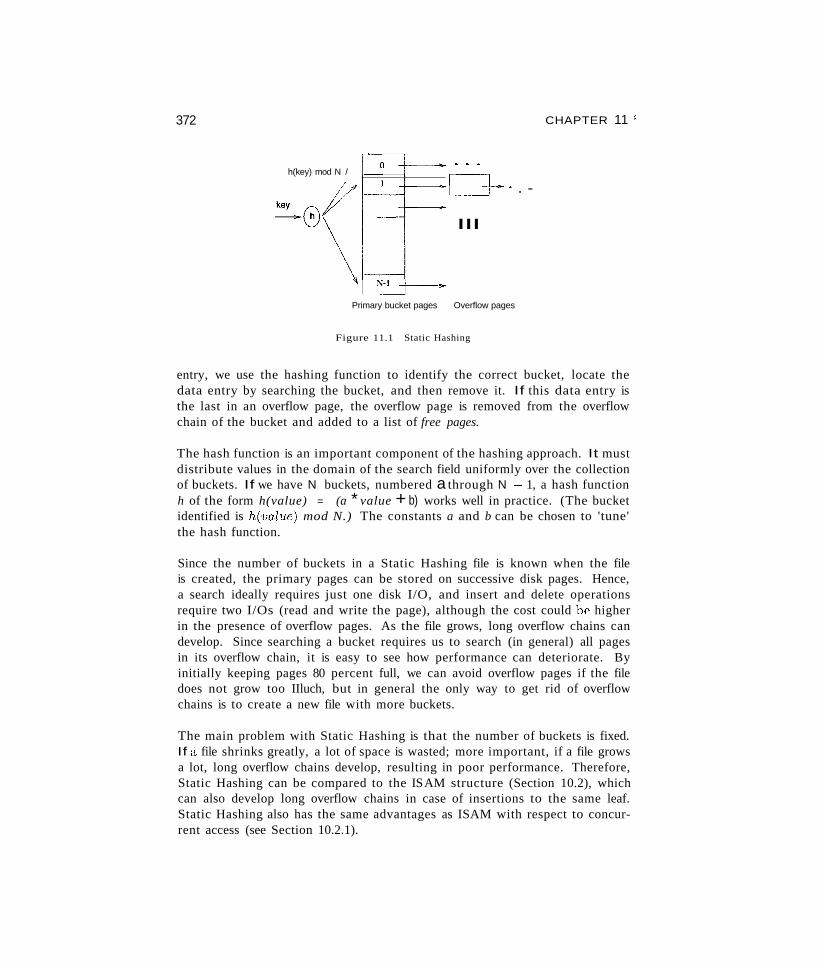
372
h(key) mod N / ~-~-§=l~// __ ~L~--.-J~· . -
~G\---I ...,INd-Primary bucket pages Overflow pages
Figure 11.1 Static Hashing
CHAPTER 11 $
entry, we use the hashing function to identify the correct bucket, locate thedata entry by searching the bucket, and then remove it. If this data entry isthe last in an overflow page, the overflow page is removed from the overflowchain of the bucket and added to a list of free pages.
The hash function is an important component of the hashing approach. It mustdistribute values in the domain of the search field uniformly over the collectionof buckets. If we have N buckets, numbered a through N ~ 1, a hash functionh of the form h(value) = (a * value + b) works well in practice. (The bucketidentified is h(value) mod N.) The constants a and b can be chosen to 'tune'the hash function.
Since the number of buckets in a Static Hashing file is known when the fileis created, the primary pages can be stored on successive disk pages. Hence,a search ideally requires just one disk I/O, and insert and delete operationsrequire two I/Os (read and write the page), although the cost could be higherin the presence of overflow pages. As the file grows, long overflow chains candevelop. Since searching a bucket requires us to search (in general) all pagesin its overflow chain, it is easy to see how performance can deteriorate. Byinitially keeping pages 80 percent full, we can avoid overflow pages if the filedoes not grow too IIluch, but in general the only way to get rid of overflowchains is to create a new file with more buckets.
The main problem with Static Hashing is that the number of buckets is fixed.If a file shrinks greatly, a lot of space is wasted; more important, if a file growsa lot, long overflow chains develop, resulting in poor performance. Therefore,Static Hashing can be compared to the ISAM structure (Section 10.2), whichcan also develop long overflow chains in case of insertions to the same leaf.Static Hashing also has the same advantages as ISAM with respect to concurrent access (see Section 10.2.1).
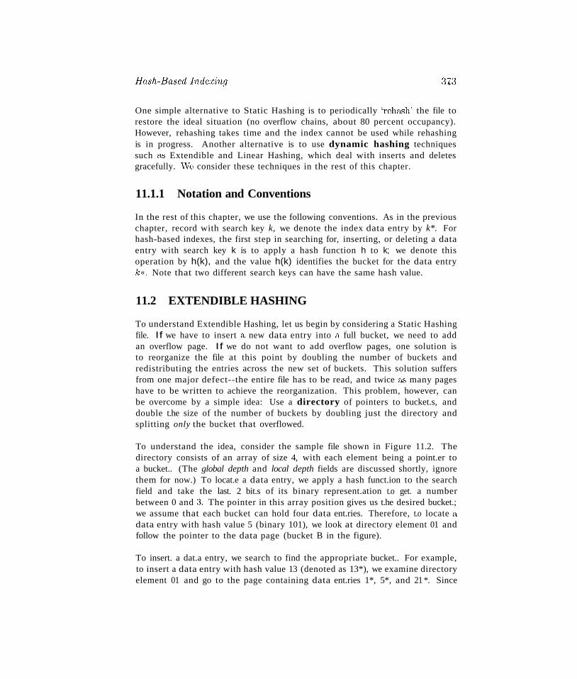
Hash-Based Inrle:ring 373
One simple alternative to Static Hashing is to periodically 'rehash' the file torestore the ideal situation (no overflow chains, about 80 percent occupancy).However, rehashing takes time and the index cannot be used while rehashingis in progress. Another alternative is to use dynamic hashing techniquessuch as Extendible and Linear Hashing, which deal with inserts and deletesgracefully. vVe consider these techniques in the rest of this chapter.
11.1.1 Notation and Conventions
In the rest of this chapter, we use the following conventions. As in the previouschapter, record with search key k, we denote the index data entry by k*. Forhash-based indexes, the first step in searching for, inserting, or deleting a dataentry with search key k is to apply a hash function h to k; we denote thisoperation by h(k), and the value h(k) identifies the bucket for the data entryh. Note that two different search keys can have the same hash value.
11.2 EXTENDIBLE HASHING
To understand Extendible Hashing, let us begin by considering a Static Hashingfile. If we have to insert a new data entry into a full bucket, we need to addan overflow page. If we do not want to add overflow pages, one solution isto reorganize the file at this point by doubling the number of buckets andredistributing the entries across the new set of buckets. This solution suffersfrom one major defect--the entire file has to be read, and twice (h') many pageshave to be written to achieve the reorganization. This problem, however, canbe overcome by a simple idea: Use a directory of pointers to bucket.s, anddouble t.he size of the number of buckets by doubling just the directory andsplitting only the bucket that overflowed.
To understand the idea, consider the sample file shown in Figure 11.2. Thedirectory consists of an array of size 4, with each element being a point.er toa bucket.. (The global depth and local depth fields are discussed shortly, ignorethem for now.) To locat.e a data entry, we apply a hash funct.ion to the searchfield and take the last. 2 bit.s of its binary represent.ation t.o get. a numberbetween 0 and ~~. The pointer in this array position gives us t.he desired bucket.;we assume that each bucket can hold four data ent.ries. Therefore, t.o locate adata entry with hash value 5 (binary 101), we look at directory element 01 andfollow the pointer to the data page (bucket B in the figure).
To insert. a dat.a entry, we search to find the appropriate bucket.. For example,to insert a data entry with hash value 13 (denoted as 13*), we examine directoryelement 01 and go to the page containing data ent.ries 1*, 5*, and 21 *. Since
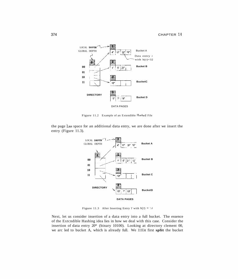
374 CHAPTER 11
BucketC
Bucket B
Bucket A1f L~--L----i----4.,J.--'~ Data entry r
with h(r)=32
00
01
10
11
LOCAL DEPTH~GLOBAL DEPTH
DIRECTORYBucket D
DATA PAGES
Figure 11.2 Example of an Extendible Ha.~hed File
the page has space for an additional data entry, we are done after we insert theentry (Figure 11.3).
LOCAL DEPTH~GLOBAL DEPTH
00
01
10
11
DIRECTORY
Bucket A
Bucket B
Bucket C
BucketD
DATA PAGES
Figure 11.3 After Inserting Entry T with h(T) = 1:3
Next, let us consider insertion of a data entry into a full bucket. The essenceof the Extcndible Hashing idea lies in how we deal with this case. Consider theinsertion of data entry 20* (binary 10100). Looking at directory clement 00,we arc led to bucket A, which is already full. We 111Ust first split the bucket
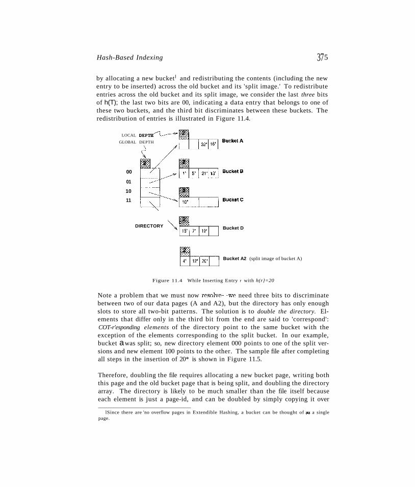
Hash-Based Indexing 375
by allocating a new bucket l and redistributing the contents (including the newentry to be inserted) across the old bucket and its 'split image.' To redistributeentries across the old bucket and its split image, we consider the last three bitsof h(T); the last two bits are 00, indicating a data entry that belongs to one ofthese two buckets, and the third bit discriminates between these buckets. Theredistribution of entries is illustrated in Figure 11.4.
LOCAL DEPTH~:>
GLOBAL DEPTH
00
01
10
11
DIRECTORY Bucket D
Bucket A2 (split image of bucket A)
Figure 11.4 While Inserting Entry r with h(r}=20
Note a problem that we must now resolve""" ""we need three bits to discriminatebetween two of our data pages (A and A2), but the directory has only enoughslots to store all two-bit patterns. The solution is to double the directory. Elements that differ only in the third bit from the end are said to 'correspond':COT-r'esponding elements of the directory point to the same bucket with theexception of the elements corresponding to the split bucket. In our example,bucket awas split; so, new directory element 000 points to one of the split versions and new element 100 points to the other. The sample file after completingall steps in the insertion of 20* is shown in Figure 11.5.
Therefore, doubling the file requires allocating a new bucket page, writing boththis page and the old bucket page that is being split, and doubling the directoryarray. The directory is likely to be much smaller than the file itself becauseeach element is just a page-id, and can be doubled by simply copying it over
lSince there are 'no overflow pages in Extendible Hashing, a bucket can be thought of a.~ a singlepage.
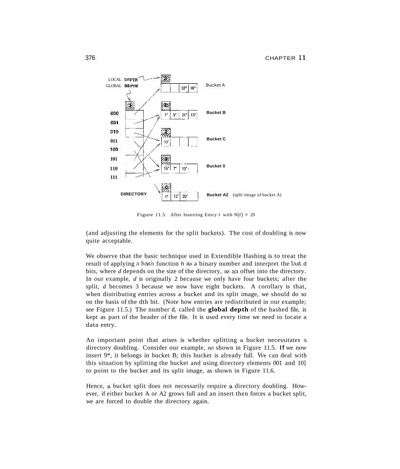
376
LOCAL DEPTH~GLOBAL DEPTH
000
001
010
011
100
101
110
111
CHAPTER 11
Bucket A
Bucket B
Bucket C
Bucket 0
DIRECTORY Bucket A2 (split image of bucket A)
Figure 11.5 After Inserting Entry r with h(r) = 20
(and adjusting the elements for the split buckets). The cost of doubling is nowquite acceptable.
We observe that the basic technique used in Extendible Hashing is to treat theresult of applying a hash function h a" a binary number and interpret the last dbits, where d depends on the size of the directory, as an offset into the directory.In our example, d is originally 2 because we only have four buckets; after thesplit, d becomes 3 because we now have eight buckets. A corollary is that,when distributing entries across a bucket and its split image, we should do soon the basis of the dth bit. (Note how entries are redistributed in our example;see Figure 11.5.) The number d, called the global depth of the hashed file, iskept as part of the header of the file. It is used every time we need to locate adata entry.
An important point that arises is whether splitting a bucket necessitates adirectory doubling. Consider our example, as shown in Figure 11.5. If we nowinsert 9*, it belongs in bucket B; this bucket is already full. \Ve can deal withthis situation by splitting the bucket and using directory elements 001 and 10]to point to the bucket and its split image, as shown in Figure 11.6.
Hence, a bucket split does not necessarily require a directory doubling. However, if either bucket A or A2 grows full and an insert then forces a bucket split,we are forced to double the directory again.
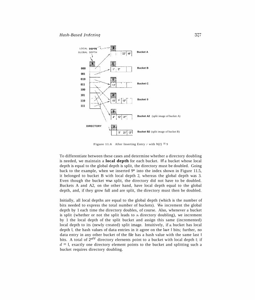
Hash-Based Inde:ring
LOCAL DEPTH---L..-->
GLOBAL DEPTH
000
001
010
011
100
101
110
111
DIRECTORY
Bucket A
Bucket B
Bucket C
Bucket 0
Bucket A2 (split image of bucket A)
Bucket B2 (split image of bucket B)
377
Figure 11.6 After Inserting Entry l' with h(r) = 9
To differentiate between these cases and determine whether a directory doublingis needed, we maintain a local depth for each bucket. If a bucket whose localdepth is equal to the global depth is split, the directory must be doubled. Goingback to the example, when we inserted 9* into the index shown in Figure 11.5,it belonged to bucket B with local depth 2, whereas the global depth was 3.Even though the bucket was split, the directory did not have to be doubled.Buckets A and A2, on the other hand, have local depth equal to the globaldepth, and, if they grow full and are split, the directory must then be doubled.
Initially, all local depths are equal to the global depth (which is the number ofbits needed to express the total number of buckets). vVe increment the globaldepth by 1 each time the directory doubles, of course. Also, whenever a bucketis split (whether or not the split leads to a directory doubling), we incrementby 1 the local depth of the split bucket and assign this same (incremented)local depth to its (newly created) split image. Intuitively, if a bucket has localdepth l, the hash values of data entries in it agree on the la.st l bits; further, nodata entry in any other bucket of the file has a hash value with the same last Ibits. A total of 2dl directory elernents point to a bucket with local depth I; ifd = l, exactly one directory element points to the bucket and splitting such abucket requires directory doubling.
378 CHAPTER hI
A final point to note is that we can also use the first d bits (the most significantbits) instead of the last d (least s'ignificant bits), but in practice the last d bitsare used. The reason is that a directory can then be doubled simply by copyingit.
In summary, a data entry can be located by computing its hash value, takingthe last d bits, and looking in the bucket pointed to by this directory element.For inserts, the data entry is placed in the bucket to which it belongs and thebucket is split if necessary to make space. A bucket split leads to an increase inthe local depth and, if the local depth becomes greater than the global depthas a result, to a directory doubling (and an increase in the global depth) aswell.
For deletes, the data entry is located and removed. If the delete leaves thebucket empty, it can be merged with its split image, although this step isoften omitted in practice. Merging buckets decreases the local depth. If eachdirectory element points to the same bucket as its split image (i.e., 0 and 2d - 1
point to the same bucket, namely, A; 1 and 2d- 1 + 1 point to the same bucket,
namely, B, which mayor may not be identical to A; etc.), we can halve thedirectory and reduce the global depth, although this step is not necessary forcorrectness.
The insertion examples can be worked out backwards as examples of deletion.(Start with the structure shown after an insertion and delete the inserted element. In each case the original structure should be the result.)
If the directory fits in memory, an equality selection can be answered in asingle disk access, as for Static Hashing (in the absence of overflow pages), butotherwise, two disk I/Os are needed. As a typical example, a 100MB file with100 bytes per data entry and a page size of 4KB contains 1 million data entriesand only about 25,000 elements in the directory. (Each page/bucket containsroughly 40 data entries, and we have one directory element per bucket.) Thus,although equality selections can be twice as slow as for Static Hashing files,chances are high that the directory will fit in memory and performance is thesame as for Static Ha.<;hing files.
On the other hand, the directory grows in spurts and can become large forskewed data distTibutions (where our assumption that data pages contain roughlyequal numbers of data entries is not valid). In the context of hashed files, in askewed data distribution the distribution of hash values of seaTch field values(rather than the distribution of search field values themselves) is skewed (very'bursty' or nonuniform). Even if the distribution of search values is skewed, thechoice of a good hashing function typically yields a fairly uniform distributionof lw"sh va.lues; skew is therefore not a problem in practice.
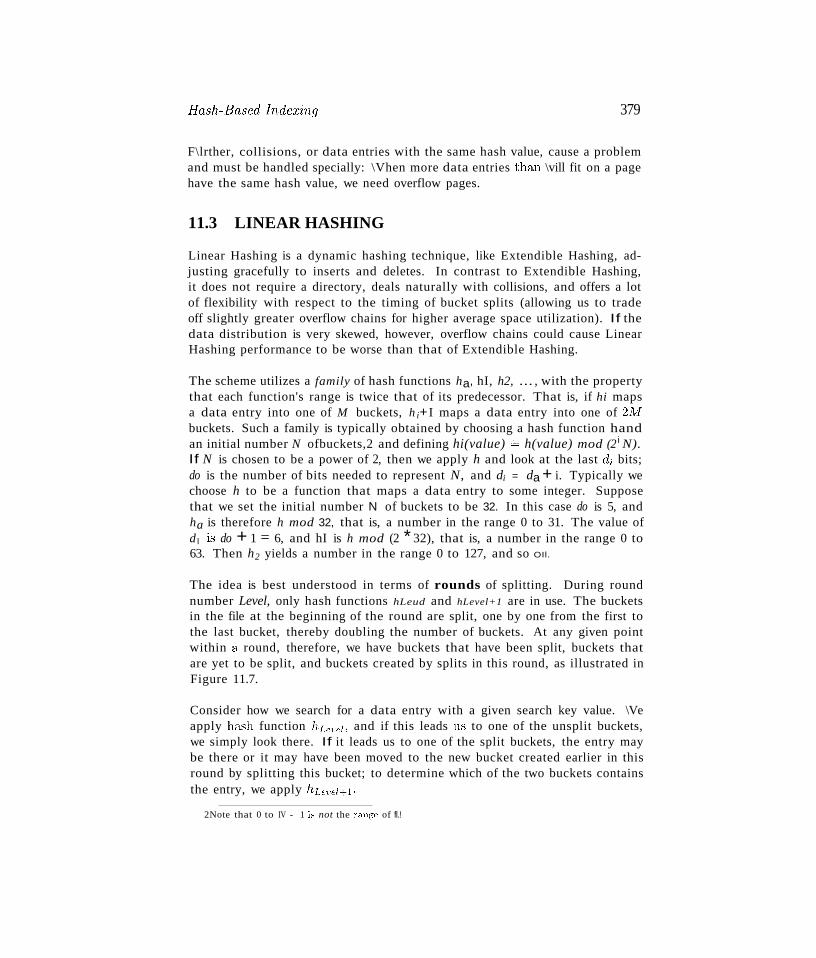
Hash~Based Inde:cing 379
F\lrther, collisions, or data entries with the same hash value, cause a problemand must be handled specially: \Vhen more data entries th311 \vill fit on a pagehave the same hash value, we need overflow pages.
11.3 LINEAR HASHING
Linear Hashing is a dynamic hashing technique, like Extendible Hashing, adjusting gracefully to inserts and deletes. In contrast to Extendible Hashing,it does not require a directory, deals naturally with collisions, and offers a lotof flexibility with respect to the timing of bucket splits (allowing us to tradeoff slightly greater overflow chains for higher average space utilization). If thedata distribution is very skewed, however, overflow chains could cause LinearHashing performance to be worse than that of Extendible Hashing.
The scheme utilizes a family of hash functions ha, hI, h2, ... , with the propertythat each function's range is twice that of its predecessor. That is, if hi mapsa data entry into one of M buckets, h i+ I maps a data entry into one of 2lv!buckets. Such a family is typically obtained by choosing a hash function handan initial number N ofbuckets,2 and defining hi(value) "'= h(value) mod (2 i N).If N is chosen to be a power of 2, then we apply h and look at the last di bits;do is the number of bits needed to represent N, and di = da + i. Typically wechoose h to be a function that maps a data entry to some integer. Supposethat we set the initial number N of buckets to be 32. In this case do is 5, andha is therefore h mod 32, that is, a number in the range 0 to 31. The value ofd l is do + 1 = 6, and hI is h mod (2 * 32), that is, a number in the range 0 to63. Then h2 yields a number in the range 0 to 127, and so OIl.
The idea is best understood in terms of rounds of splitting. During roundnumber Level, only hash functions hLeud and hLevel+1 are in use. The bucketsin the file at the beginning of the round are split, one by one from the first tothe last bucket, thereby doubling the number of buckets. At any given pointwithin a round, therefore, we have buckets that have been split, buckets thatare yet to be split, and buckets created by splits in this round, as illustrated inFigure 11.7.
Consider how we search for a data entry with a given search key value. \Veapply ha..:sh function h Level , and if this leads us to one of the unsplit buckets,we simply look there. If it leads us to one of the split buckets, the entry maybe there or it may have been moved to the new bucket created earlier in thisround by splitting this bucket; to determine which of the two buckets containsthe entry, we apply hLevel+I'
2Note that 0 to IV - 1 is not the range of fl.!
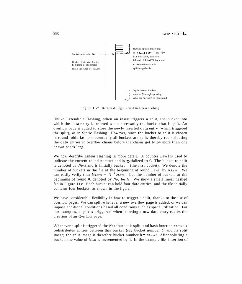
380
Bucket to be split Next
Buckets that existed at thebeginning of this round:
this is the range of h Level
- 1
r
II-<-
CHAPTER \1
Buckets split in this round:
If h Le~'el ( search key mil,e
is in this range, must use
h Level+1 (search key vallie
to decide if entry is in
split image bucket.
'split image' buckets:
created (tlrrough splitting
of other buckets) in this round
Figure 11. 7 Buckets during a Round in Linear Hashing
Unlike Extendible Hashing, when an insert triggers a split, the bucket intowhich the data entry is inserted is not necessarily the bucket that is split. Anoverflow page is added to store the newly inserted data entry (which triggeredthe split), as in Static Hashing. However, since the bucket to split is chosenin round-robin fashion, eventually all buckets are split, thereby redistributingthe data entries in overflow chains before the chains get to be more than oneor two pages long.
We now describe Linear Hashing in more detail. A counter Level is used toindicate the current round number and is initialized to O. The bucket to splitis denoted by Next and is initially bucket °(the first bucket). We denote thenumber of buckets in the file at the beginning of round Level by N Level. Wecan easily verify that N Level = N * 2Level. Let the number of buckets at thebeginning of round 0, denoted by No, be N. We show a small linear hashedfile in Figure 11.8. Each bucket can hold four data entries, and the file initiallycontains four buckets, as shown in the figure.
We have considerable flexibility in how to trigger a split, thanks to the use ofoverflow pages. We can split whenever a new overflow page is added, or we canimpose additional conditions based all conditions such as space utilization. Forour examples, a split is 'triggered' when inserting a new data entry causes thecreation of an Qverftow page.
\Vhenever a split is triggered the Next bucket is split, and hash function hLevel+l
redistributes entries between this bucket (say bucket number b) and its splitimage; the split image is therefore bucket number b + NLeve/. After splitting abucket, the value of Next is incremented by 1. In the example file, insertion of
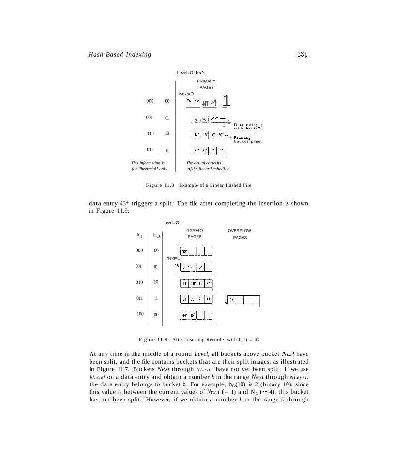
Hash-Based Indexing 38J
Level=O. N=4
PRIMARY
PAGES
000 00
Next=O
"'1 32'1 44'1 36'1 1001
010
01
10
I 9" 1 2S" i S'f~~_ Data entry r
with h{r)mS
~4: 18" 10" 30" .
, PrJ.mary_ bucket page
11011
~This information is The actual contelJtsfor illustratiolJ only of the linear hashedjile
Figure 11.8 Example of a Linear Hashed File
data entry 43* triggers a split. The file after completing the insertion is shownin Figure 11.9.
Level=O
PRIMARY OVERFLOWh 1 h O PAGES PAGES
000 00
~Next=1 -
001 01"'~
010 10
~011 11
100 00
Figure 11.9 After Inserting Record T with h(T) = 43
At any time in .the middle of a round Level, all buckets above bucket Ne:rt havebeen split, and the file contains buckets that are their split images, as illustratedin Figure 11.7. Buckets Next through NLevcl have not yet been split. If we usehLevel on a data entry and obtain a number b in the range Next through NLevel,
the data entry belongs to bucket b. For example, ho(18) is 2 (binary 10); sincethis value is between the current values of Ne:r:t (= 1) and N 1 (=,-:': 4), this buckethas not been split. However, if we obtain a number b in the range 0 through
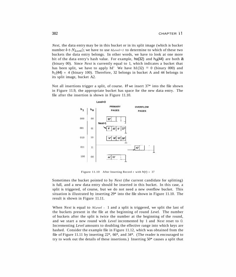
382 CHAPTER 11
Next, the data entry may be in this bucket or in its split image (which is bucketnumber b+NLevet}; we have to use hLevel+1 to determine to which of these twobuckets the data entry belongs. In other words, we have to look at one morebit of the data entry's hash value. For example, ho(32) and ho(44) are both a(binary 00). Since Next is currently equal to 1, which indicates a bucket thathas been split, we have to apply hI' We have hI (32) = 0 (binary 000) andh1(44) = 4 (binary 100). Therefore, 32 belongs in bucket A and 44 belongs inits split image, bucket A2.
Not all insertions trigger a split, of course. If we insert 37* into the file shownin Figure 11.9, the appropriate bucket has space for the new data entry. Thefile after the insertion is shown in Figure 11.10.
Level=O
PRIMARY OVERFLOWh1 ho PAGES PAGES
000 00
~Next=1 -
001 01 ~~
010 10
~011 11
100 00 EEITlFigure 11.10 After Inserting Record r with h(r) = 37
Sometimes the bucket pointed to by Next (the current candidate for splitting)is full, and a new data entry should be inserted in this bucket. In this case, asplit is triggered, of course, but we do not need a new overflow bucket. Thissituation is illustrated by inserting 29* into the file shown in Figure 11.10. Theresult is shown in Figure 11.11.
When Next is equal to NLevel - 1 and a split is triggered, we split the last ofthe buckets present in the file at the beginning of round Level. The numberof buckets after the split is twice the number at the beginning of the round,and we start a new round with Level incremented by 1 and Next reset to O.Incrementing Level amounts to doubling the effective range into which keys arehashed. Consider the example file in Figure 11.12, which was obtained from thefile of Figure 11.11 by inserting 22*, 66*, and 34*. (The reader is encouraged totry to work out the details of these insertions.) Inserting 50* causes a split that
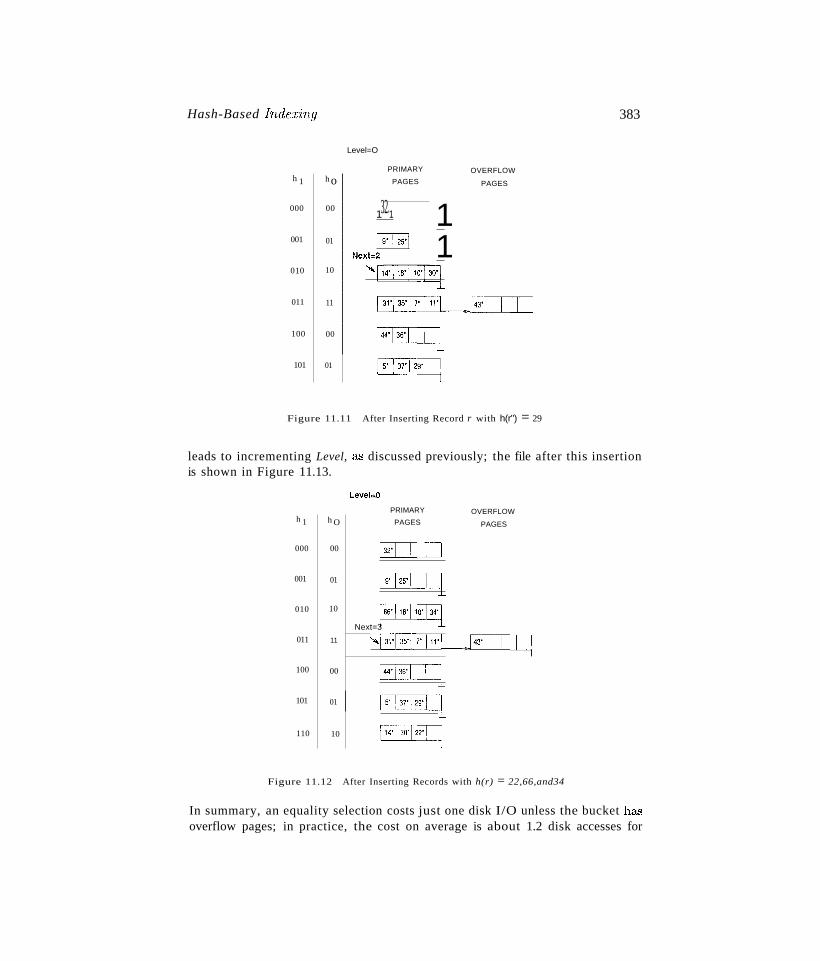
Hash-Based l'ndex'ing
Level=O
PRIMARY OVERFLOWh 1 h o PAGES PAGES
000 00132'1 1
001 01 025'\ 1Next",2
010 10"'114'\18'110'13°1
011 11~EITQ
100 00 E8Il101 01
~
Figure 11.11 After Inserting Record r with h(r") = 29
383
leads to incrementing Level, as discussed previously; the file after this insertionis shown in Figure 11.13.
Level=O
PRIMARYh 1 h O PAGES
000 00 ~C[l
001 01 ~[J=l
010 10
~Next=3
011 11 ~17'll1'1
100 00 ~J.:~lI{
101 01 EL~1i?I=]~
110 10 ~~
OVERFLOW
PAGES
Figure 11.12 After Inserting Records with h(r) = 22,66,and34
In summary, an equality selection costs just one disk I/O unless the bucket hasoverflow pages; in practice, the cost on average is about 1.2 disk accesses for
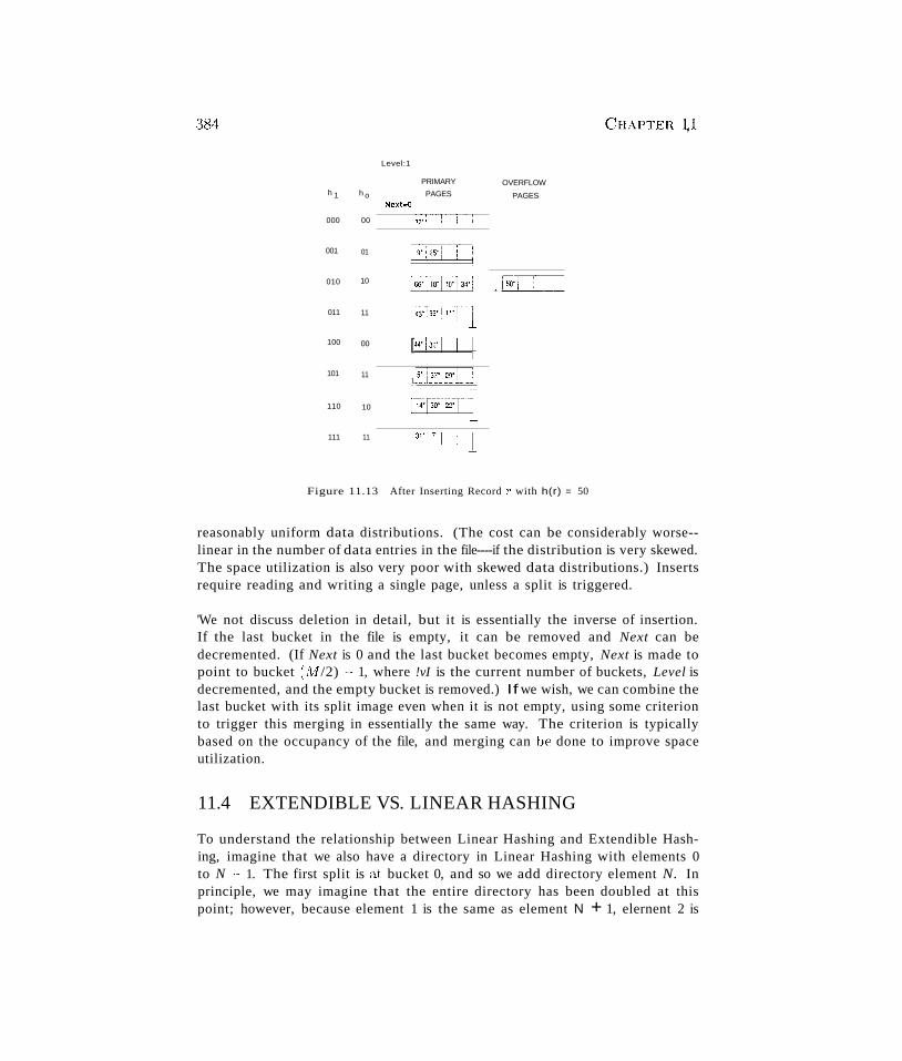
384
Level:1
PRIMARY OVERFLOWh 1 h o PAGES PAGES
Next=O
000 00
001 01 Ld~I~]~
010 10 ~~8]2or;~! .~l~j
011 11 ~5J11I-1'---=--L_~_ i
100 00 [44'!3sTT-l101 11
1..~13~J2::L~l
110 10 r-i4I30:@I1111 11
Figure 11.13 After Inserting Record r with h(r) = 50
reasonably uniform data distributions. (The cost can be considerably worse-linear in the number of data entries in the file----if the distribution is very skewed.The space utilization is also very poor with skewed data distributions.) Insertsrequire reading and writing a single page, unless a split is triggered.
'We not discuss deletion in detail, but it is essentially the inverse of insertion.If the last bucket in the file is empty, it can be removed and Next can bedecremented. (If Next is 0 and the last bucket becomes empty, Next is made topoint to bucket (AI /2) ~ 1, where !vI is the current number of buckets, Level isdecremented, and the empty bucket is removed.) If we wish, we can combine thelast bucket with its split image even when it is not empty, using some criterionto trigger this merging in essentially the same way. The criterion is typicallybased on the occupancy of the file, and merging can be done to improve spaceutilization.
11.4 EXTENDIBLE VS. LINEAR HASHING
To understand the relationship between Linear Hashing and Extendible Hashing, imagine that we also have a directory in Linear Hashing with elements 0to N - 1. The first split is at bucket 0, and so we add directory element N. Inprinciple, we may imagine that the entire directory has been doubled at thispoint; however, because element 1 is the same as element N + 1, elernent 2 is
Hash~Based Indexing 385!
the same a.'3 element N + 2, and so on, we can avoid the actual copying forthe rest of the directory. The second split occurs at bucket 1; now directoryelement N + 1 becomes significant and is added. At the end of the round, allthe original N buckets are split, and the directory is doubled in size (becauseall elements point to distinct buckets).
\Ve observe that the choice of hashing functions is actually very similar towhat goes on in Extendible Hashing---in effect, moving from hi to hi+1 inLinear Hashing corresponds to doubling the directory in Extendible Hashing.Both operations double the effective range into which key values are hashed;but whereas the directory is doubled in a single step of Extendible Hashing,moving from hi to hi+l, along with a corresponding doubling in the numberof buckets, occurs gradually over the course of a round in Linear Ha.'3hing.The new idea behind Linear Ha.'3hing is that a directory can be avoided by aclever choice of the bucket to split. On the other hand, by always splitting theappropriate bucket, Extendible Hashing may lead to a reduced number of splitsand higher bucket occupancy.
The directory analogy is useful for understanding the ideas behind Extendibleand Linear Hashing. However, the directory structure can be avoided for LinearHashing (but not for Extendible Hashing) by allocating primary bucket pagesconsecutively, which would allow us to locate the page for bucket i by a simpleoffset calculation. For uniform distributions, this implementation of LinearHashing has a lower average cost for equality selections (because the directorylevel is eliminated). For skewed distributions, this implementation could resultin any empty or nearly empty buckets, each of which is allocated at least onepage, leading to poor performance relative to Extendible Hashing, which islikely to have higher bucket occupancy.
A different implementation of Linear Hashing, in which a directory is actuallymaintained, offers the flexibility of not allocating one page per bucket; nulldirectory elements can be used as in Extendible Hashing. However, this implementation introduces the overhead of a directory level and could prove costlyfor large, uniformly distributed files. (Also, although this implementation alleviates the potential problem of low bucket occupancy by not allocating pagesfor empty buckets, it is not a complete solution because we can still have manypages with very few entries.)
11.5 REVIEW QUESTIONS
Answers to the review questions can be found in the listed sections.
386 CHAPTER).l
• How does a hash-ba..sed index handle an equality query? Discuss the use ofthe hash function in identifying a bucket to search. Given a bucket number,explain how the record is located on disk.
• Explain how insert and delete operations are handled in a static hash index.Discuss how overflow pages are used, and their impact on performance.How many disk l/Os does an equality search require, in the absence ofoverflow chains? What kinds of workload does a static hash index handlewell, and when it is especially poor? (Section 11.1)
• How does Extendible Hashing use a directory of buckets? How does Extendible Hashing handle an equality query? How does it handle insert anddelete operations? Discuss the global depth of the index and local depth ofa bucket in your answer. Under what conditions can the directory can getlarge? (Section 11.2)
• What are collisions? Why do we need overflow pages to handle them?(Section 11.2)
• How does Linear Hashing avoid a directory? Discuss the round-robin splitting of buckets. Explain how the split bucket is chosen, and what triggersa split. Explain the role of the family of hash functions, and the role ofthe Level and Next counters. When does a round of splitting end? (Section 11.3)
• Discuss the relationship between Extendible and Linear Hashing. What aretheir relative merits? Consider space utilization for skewed distributions,the use of overflow pages to handle collisions in Extendible Hashing, andthe use of a directory in Linear Hashing. (Section 11.4)
EXERCISES
Exercise 11.1 Consider the Extendible Hashing index shown in Figure 1l.14. Answer thefollowing questions about this index:
1. What can you say about the last entry that was inserted into the index?
2. What can you say about the last entry that was inserted into the index if you know thatthere have been no deletions from this index so far?
3. Suppose you are told that there have been no deletions from this index so far. What canyou say about the last entry whose insertion into the index caused a split?
4. Show the index after inserting an entry with hash value 68.
5. Show the original index after inserting entries with ha.sh values 17 and 69.
6. Show the original index after deleting the entry with hash value 21. (Assume that thefull deletion algorithm is used.)
7. Show the original index after deleting the entry with ha,,;h value 10. Is a merge triggeredby this deletion? If not, explain why. (Assume that the full deletion algorithm is used.)
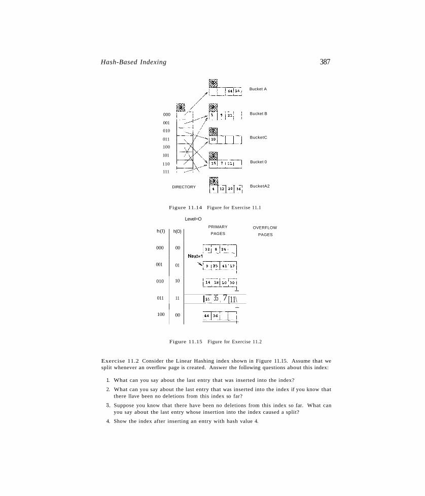
Hash-Based Indexing 387
000
001
010
011
100
101
110
111
DIRECTORY
Bucket A
Bucket B
BucketC
Bucket 0
BucketA2
Figure 11.14 Figure for Exercise 11.1
Level=O
PRIMARY OVERFLOWh(l) h(O) PAGES PAGES
000 00
~Next=l -
001 01"~
010 10
~011 11 I~ 35
17 [11\
1-
100 00 EFrqFigure 11.15 Figure for Exercise 11.2
Exercise 11.2 Consider the Linear Hashing index shown in Figure 11.15. Assume that wesplit whenever an overflow page is created. Answer the following questions about this index:
1. What can you say about the last entry that was inserted into the index?
2. What can you say about the last entry that was inserted into the index if you know thatthere llave been no deletions from this index so far?
:t Suppose you know that there have been no deletions from this index so far. What canyou say about the last entry whose insertion into the index caused a split?
4. Show the index after inserting an entry with hash value 4.
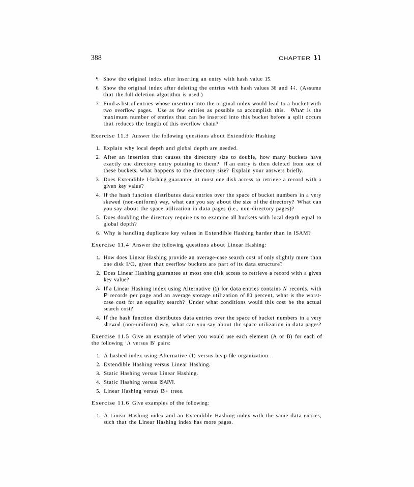
388 CHAPTER 11
5, Show the original index after inserting an entry with hash value 15.
6. Show the original index after deleting the entries with hash values 36 and 44. (Assumethat the full deletion algorithm is used.)
7. Find a list of entries whose insertion into the original index would lead to a bucket withtwo overflow pages. Use as few entries as possible t.o accomplish this. "Vhat is themaximum number of entries that can be inserted into this bucket before a split occursthat reduces the length of this overflow chain?
Exercise 11.3 Answer the following questions about Extendible Hashing:
1. Explain why local depth and global depth are needed.
2. After an insertion that causes the directory size to double, how many buckets haveexactly one directory entry pointing to them? If an entry is then deleted from one ofthese buckets, what happens to the directory size? Explain your answers briefly.
3. Does Extendible I-lashing guarantee at most one disk access to retrieve a record with agiven key value?
4. If the hash function distributes data entries over the space of bucket numbers in a veryskewed (non-uniform) way, what can you say about the size of the directory? What canyou say about the space utilization in data pages (i.e., non-directory pages)?
5. Does doubling the directory require us to examine all buckets with local depth equal toglobal depth?
6. Why is handling duplicate key values in Extendible Hashing harder than in ISAM?
Exercise 11.4 Answer the following questions about Linear Hashing:
1. How does Linear Hashing provide an average-case search cost of only slightly more thanone disk I/O, given that overflow buckets are part of its data structure?
2. Does Linear Hashing guarantee at most one disk access to retrieve a record with a givenkey value?
3. If a Linear Hashing index using Alternative (1) for data entries contains N records, withP records per page and an average storage utilization of 80 percent, what is the worstcase cost for an equality search? Under what conditions would this cost be the actualsearch cost?
4. If the hash function distributes data entries over the space of bucket numbers in a veryskew(,d (non-uniform) way, what can you say about thc space utilization in data pages?
Exercise 11.5 Give an example of when you would use each element (A or B) for each ofthe following 'A versus B' pairs:
1. A hashed index using Alternative (1) versus heap file organization.
2. Extendible Hashing versus Linear Hashing.
3. Static Hashing versus Linear Hashing.
4. Static Hashing versus ISAIVI.
5. Linear Hashing versus B+ trees.
Exercise 11.6 Give examples of the following:
1. A Linear Hashing index and an Extendible Hashing index with the same data entries,such that the Linear Hashing index has more pages.
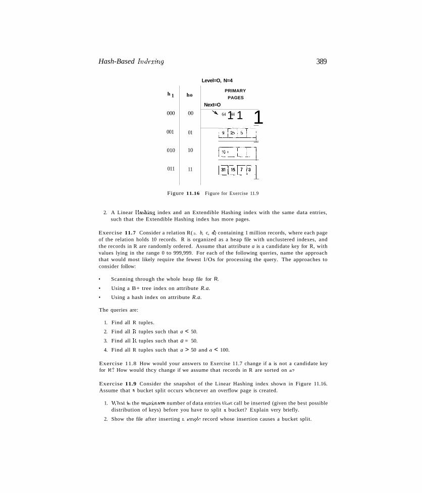
Hash-Based Indf1;ing
Level=O, N=4
h 1 hoPRIMARY
PAGES
Next=O
000 00 "I 64 144 1 1001 01 liliEI~010 10 GIQ011 11
~Figure 11.16 Figure for Exercise 11.9
389
2. A Linear H&shing index and an Extendible Hashing index with the same data entries,such that the Extendible Hashing index has more pages.
Exercise 11.7 Consider a relation R( [L, b, c, rf) containing 1 million records, where each pageof the relation holds 10 records. R is organized as a heap file with unclustered indexes, andthe records in R are randomly ordered. Assume that attribute a is a candidate key for R, withvalues lying in the range 0 to 999,999. For each of the following queries, name the approachthat would most likely require the fewest l/Os for processing the query. The approaches toconsider follow:
• Scanning through the whole heap file for R.
• Using a B+ tree index on attribute R.a.
• Using a hash index on attribute R.a.
The queries are:
1. Find all R tuples.
2. Find all R tuples such that a < 50.
3. Find all R tuples such that a = 50.
4. Find all R tuples such that a > 50 and a < 100.
Exercise 11.8 How would your answers to Exercise 11.7 change if a is not a candidate keyfor R? How would thcy change if we assume that records in R are sorted on a?
Exercise 11.9 Consider the snapshot of the Linear Hashing index shown in Figure 11.16.Assume that a bucket split occurs whcnever an overflow page is created.
1. vVhat is the mll1:imwn number of data entries that call be inserted (given the best possibledistribution of keys) before you have to split a bucket? Explain very briefly.
2. Show the file after inserting a singlc record whose insertion causes a bucket split.

390 CHAPTER 11
3. (a) What is the minimum number of record insertions that will cause a split of all fourbuckets? Explain very briefly.
(b) What is the value of Next after making these insertions?
(c) What can you say about the number of pages in the fourth bucket shown after thisseries of record insertions?
Exercise 11.10 Consider the data entries in the Linear Hashing index for Exercise 11.9.
1. Show an Extendible Hashing index with the same data entries.
2. Answer the questions in Exercise 11.9 with respect to this index.
Exercise 11.11 In answering the following questions, assume that the full deletion algorithmis used. Assume that merging is done when a bucket becomes empty.
1. Give an example of Extendible Hashing where deleting an entry reduces global depth.
2. Give an example of Linear Hashing in which deleting an entry decrements Next but leavesLevel unchanged. Show the file before and after the deletion.
3. Give an example of Linear Hashing in which deleting an entry decrements Level. Showthe file before and after the deletion.
4. Give an example of Extendible Hashing and a list of entries el, e2, e3 such that insertingthe entries in order leads to three splits and deleting them in the reverse order yields theoriginal index. If such an example does not exist, explain.
5. Give an example of a Linear Hashing index and a list of entries el, e2, e3 such thatinserting the entries in order leads to three splits and deleting them in the reverse orderyields the original index. If such an example does not exist, explain.
PROJECT-BASED EXERCISES
Exercise 11.12 (Note to inst1'7u:toTS: Additional details must be provided if this question isassigned. See Appendi:c 30.) Implement Linear Hashing or Extendible Hashing in Minibase.
BIBLIOGRAPHIC NOTES
Hashing is discussed in detail in [442]. Extendible Hashing is proposed in [256]. Litwinproposed Linear Hashing in [483]. A generalization of Linear Hashing for distributed envi~
ronments is described in [487]. There has been extensive research into hash-based indexingtechniques. Larson describes two variations of Linear Hashing in [469] and [470]. Ramakrishna presents an analysis of hashing techniques in [607]. Hash functions that do not producebucket overflows are studied in [608]. Order-preserving hashing techniques are discussed in[484] and [308] . Partitioned-hashing, in which each field is hashed to obtain some bits ofthe bucket address, extends hashing for the case of queries in which equality conditions arespecified only for some of the key fields. This approach was proposed by Rivest [628] and isdiscussed in [747]; a further development is described in [616].

PARTN
QUERY EVALUATION

12OVERVIEW OF QUERY
EVALUATION
.... What descriptive information does a DBMS store in its catalog?
.... What alternatives are considered for retrieving rows from a table?
.... ~Why does a DBMS implement several algorithms for each algebraoperation? What factors affect the relative performance of differentalgorithms?
.... What are query evaluation plans and how are they represented?
.... Why is it important to find a good evaluation plan for a query? Howis this done in a relational DBMS?
.. Key concepts: catalog, system statistics; fundamental techniques,indexing, iteration, and partitioning; access paths, matching indexesand selection conditions; selection operator, indexes versus scans, impact of clustering; projection operator, duplicate elimination; join operator, index nested-loops join, sort-merge join; query evaluation plan;materialization vs. pipelinining; iterator interface; query optimization, algebra equivalences, plan enumeration; cost estimation
This very remarkable man, commends a most practical plan:You can do what you want, if you don't think you can't,So c1on't think you can't if you can.
~~~--~Charles Inge
In this chapter, we present an overview of how queries are evaluated in a relational DBMS. Vve begin with a discussion of how a DBMS describes the data
393
394 CHAPTER 12
that it manages, including tables and indexes, in Section 12.1. This descriptivedata, or metadata, stored in special tables called the system catalogs, isused to find the best way to evaluate a query.
SQL queries are translated into an extended form of relational algebra, andquery evaluation plans are represented as trees of relational operators, alongwith labels that identify the algorithm to use at each node. Thus, relational operators serve as building blocks for evaluating queries, and the implementationof these operators is carefully optimized for good performance. We introduceoperator evaluation in Section 12.2 and describe evaluation algorithms for various operators in Section 12.3.
In general, queries are composed of several operators, and the algorithms forindividual operators can be combined in many ways to evaluate a query. Theprocess of finding a good evaluation plan is called query optimization. We introduce query optimization in Section 12.4. The basic task in query optimization,which is to consider several alternative evaluation plans for a query, is motivated through examples in Section 12.5. In Section 12.6, we describe the spaceof plans considered by a typical relational optimizer.
The ideas are presented in sufficient detail to allow readers to understandhow current database systems evaluate typical queries. This chapter providesthe necessary background in query evaluation for the discussion of physicaldatabase design and tuning in Chapter 20. Relational operator implementation and query optimization are discussed further in Chapters 13, 14, and 15;this in-depth coverage describes how current systems are implemented.
We consider a number of example queries using the following schema:
Sailors(sid: integer, .mame: string, rating: integer, age: real)Reserves(sid: integer, bid: integer, day: dates, marne: string)
We aSSUlne that each tuple of Reserves is 40 bytes long, that a page can hold100 Reserves tuples, and that we have 1000 pages of such tuples. Similarly,we assume that each tuple of Sailors is 50 bytes long, that a page can hold 80Sailors tuples, and that we have 500 pages of such tuples.
12.1 THE SYSTEM CATALOG
\Ve can store a table using one of several alternative file structures, and we cancreate one or more indexes -each stored as a file 011 every tal)le. Conversely,in a relational DBMS, every file contains either the tuples in a table or the
Overview of Query Evaluation 395
entries in an index. The collection of filE'-s corresponding to users' tables andindexes represents the data in the databa.<;e.
A relational DBMS maintains information about every table and index that itcontains. The descriptive information is itself stored in a collection of specialtables called the catalog tables. An example of a catalog table is shownin Figure 12.1. The catalog tables are also called the data dictionary, thesystem catalog, or simply the catalog.
12.1.1 Information in the Catalog
Let us consider what is stored in the system catalog. At a minimum, we "havesystem-wide information, such as the size of the buffer pool and the page size,and the following information about individual tables, indexes, and views:
• For each table:
- Its table name, the file name (or some identifier), and the file structure(e.g., heap file) of the file in which it is stored.
- The attribute name and type of each of its attributes.
- The index name of each index on the table.
- The integrity constmints (e.g., primary key and foreign key constraints)on the table.
• For each index:
- The inde:I: name and the structure (e.g., B+ tree) of the index.
- The search key attributes.
• For each view:
- Its view name and definition.
In addition, statistics about tables and indexes are stored in the system catalogsand updated periodically (not every time the underlying tables are modified).The following information is commonly stored:
• Cardinality: The number of tuples NTaplcs(R) for each table R.
• Size: The number of pages NPages(R) for each table R.
• Index Cardinality: The number of distinct key values NKeys(I) for eachindex I.
• Index Size: The nUluber of pages INPages(I) for each index I. (For a B+tree index I, we take INPagcs to be the number of leaf pages.)
396 CHAPTER 12
• Index Height: The number of nonleaf levels IHe'ight(I) for each tree indexI.
• Index Range: The minimum present key value ILow(I) and the maximumpresent key value INigh(I) for each index I.
vVe assume that the database architecture presented in Chapter 1 is used..Further, we assume that each file of records is implemented as a separate file ofpages. Other file organizations are possible, of course. For example, a page filecan contain pages that store records from more than one record file. If such afile organization is used, additional statistics must be maintained, such as thefraction of pages in a file that contain records from a given collection of records.
The catalogs also contain information about users, such as accounting information and authorization information (e.g., Joe User can modify the Reservestable but only read the Sailors table).
How Catalogs are Stored
An elegant aspect of a relational DBMS is that the system catalog is itselfa collection of tables. For example, we might store information about theattributes of tables in a catalog table called Attribute_Cat:
Attribute_Cat( attLnatne: string, reLname: string,type: string, position: integer)
Suppose that the database contains the two tables that we introduced at thebegining of this chapter:
Sailors(sid: integer, sname: string, rating: integer, age: real)Reserves(sid: integer, bid: integer, day: dates, mame: string)
Figure 12.1 shows the tuples in the Attribute_Cat table that describe the at-tributes of these two tables. Note that in addition to the tuples describingSailors and Reserves, other tuples (the first four listed) describe the four attributes of the Attribute_Cat table itself[ These other tuples illustrate an important Point: the catalog tables describe all the tables in the database, including the catalog tables themselves. When information about a table is needed,it is obtained from the system catalog. Of course, at the implementation level,whenever the DBMS needs to find the schema of a catalog table, the codethat retrieves this information must be handled specially. (Otherwise, the codeha",> to retrieve this information from the catalog tables without, presumably,knowing the schema of the catalog tables.)
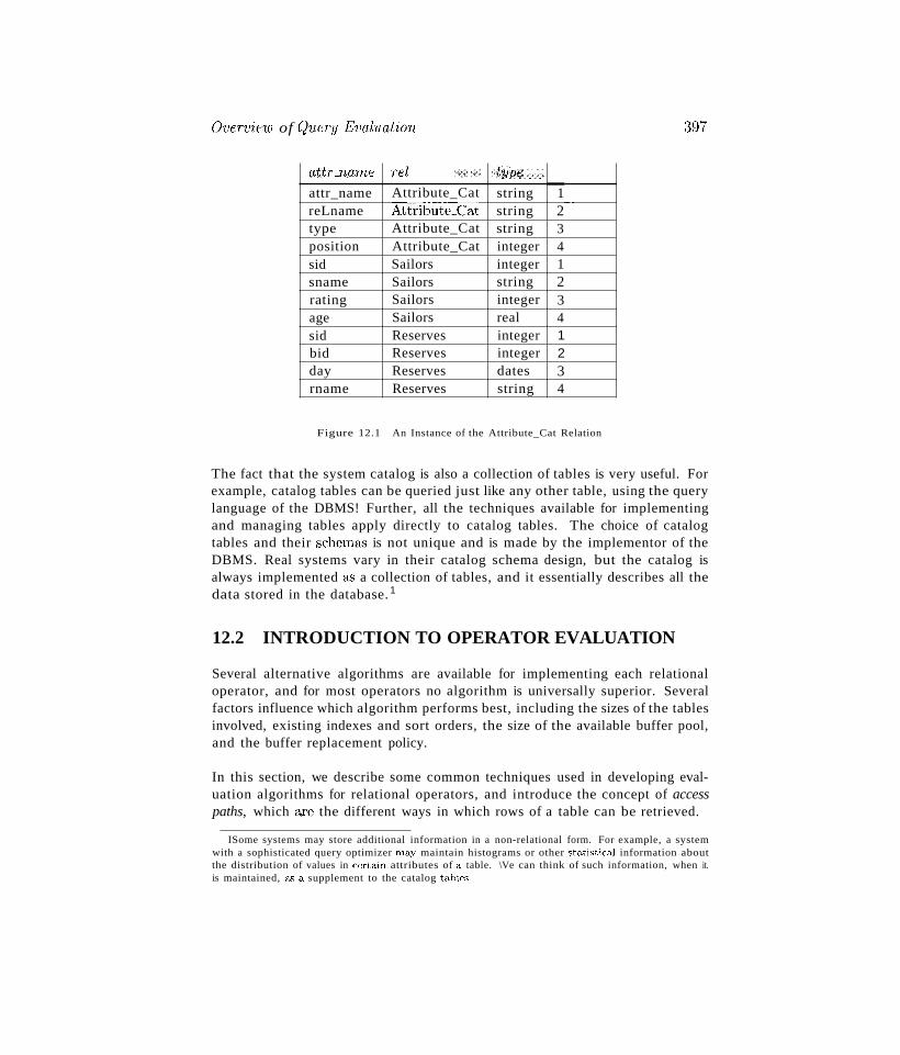
Overview of Q'lLC'l~1j E1Jaluotion
attT_narne rei ·.>./ ...·.i .·>ttJTJe:<>attr_name Attribute_Cat string 1reLname Attribute_Cat string 2
-_.-
type Attribute_Cat string 3position Attribute_Cat integer 4sid Sailors integer 1sname Sailors string 2rating Sailors integer 3age Sailors real 4sid Reserves integer 1bid Reserves integer 2day Reserves dates 3rname Reserves string 4
Figure 12.1 An Instance of the Attribute_Cat Relation
~397
The fact that the system catalog is also a collection of tables is very useful. Forexample, catalog tables can be queried just like any other table, using the querylanguage of the DBMS! Further, all the techniques available for implementingand managing tables apply directly to catalog tables. The choice of catalogtables and their schema..., is not unique and is made by the implementor of theDBMS. Real systems vary in their catalog schema design, but the catalog isalways implemented as a collection of tables, and it essentially describes all thedata stored in the database. 1
12.2 INTRODUCTION TO OPERATOR EVALUATION
Several alternative algorithms are available for implementing each relationaloperator, and for most operators no algorithm is universally superior. Severalfactors influence which algorithm performs best, including the sizes of the tablesinvolved, existing indexes and sort orders, the size of the available buffer pool,and the buffer replacement policy.
In this section, we describe some common techniques used in developing evaluation algorithms for relational operators, and introduce the concept of accesspaths, which are the different ways in which rows of a table can be retrieved.
ISome systems may store additional information in a non-relational form. For example, a systemwith a sophisticated query optimizer may maintain histograms or other statistical information aboutthe distribution of values in certain attributes of a table. \Ve can think of such information, when it.is maintained, as a supplement to the catalog tables.
398 CHAPTER 12
12.2.1 Three Common Techniques
The algorithms for various relational operators actually have a lot in common.A few simple techniques are used to develop algorithms for each operator:
III Indexing: If a selection or join condition is specified, use an index toexamine just the tuples that satisfy the condition.
III Iteration: Examine all tuples in an input table, one after the other. Ifwe need only a few fields from each tuple and there is an index whose keycontains all these fields, instead of examining data tuples, we can scan allindex data entries. (Scanning all data entries sequentially makes no useof the index's ha.8h- or tree-based search structure; in a tree index, forexample, we would simply examine all leaf pages in sequence.)
III Partitioning: By partitioning tuples on a sort key, we can often decompose an operation into a less expensive collection of operations on partitions. Sorting and hashing are two commonly used partitioning techniques.
We discuss the role of indexing in Section 12.2.2. The iteration and partitioningtechniques are seen in Section 12.3.
12.2.2 Access Paths
An access path is a way of retrieving tuples from a table and consists ofeither (1) a file scan or (2) an index plus a matching selection condition. Everyrelational operator accepts one or more tables as input, and the access methodsused to retrieve tuples contribute significantly to the cost of the operator.
Consider a simple selection that is a conjunction of conditions of the formattT op 'ualue, where op is one of the comparison operators <, ::;, =, =f., ~,
or >. Such selections are said to be in conjunctive normal form (CNF),and each condition is called a conjunct.2 Intuitively, an index matches aselection condition if the index can be used to retrieve just the tuples thatsatis(y the condition.
III A hash index matches a CNF selection if there is a term of the formattribute=1wJue in the selection for each attribute in the index's search key.
III A tree index matches a CNF selection if there is a term of the formattTibute op value for each attribute in a prefLr of the index's search key.((eL; and (a,b; are prefixes of key (a,b,e), but (a,e) and (b,e) are not.)
2We consider more complex selection conditions in Section 14.2.
Overview of Que7'.I! Evaluation 399
Note that op can be any comparison; it is not n:Btricted to he equality asit is for matching selections on a h&"h index.
An index can match some subset of the conjuncts in a selection condition (inCNP), even though it does not match the entire condition. \Ve refer to theconjuncts that the index matches as the primary conjuncts in the selection.
The following examples illustrate access paths.
• If we have a hash index H on the search key Cmarne, bid,sirf) , we canuse the index to retrieve just the Sailors tuples that satisfy the conditionrnarne='Joe'l\ bid=5 1\ sid=3. The index matches the entire condition77wme= 'Joe' 1\ bid=5 1\ sid= 3. On the other hand, if the selection condition is rname= 'Joe' 1\ bid=5, or some condition on date, this index doesnot match. That is, it cannot be used to retrieve just the tuples that satisfythese conditions.
In contrast, if the index were a B+ tree, it would match both rname= 'Joe'1\ bid=51\ 8id=3 and mame='Joe' 1\ bid=5. However, it would not matchbid=5 1\ sid=8 (since tuples are sorted primarily by rnarne).
• If we have an index (hash or tree) on the search key (bid,sid'; and the selection condition 'rname= 'Joe' 1\ bid=5 1\ sid=3, we can use the index toretrieve tuples that satisfy bid=51\ sid=3; these are the primary conjuncts.The fraction of tuples that satisfy these conjuncts (and whether the indexis clustered) determines the number of pages that are retrieved. The additional condition on Tna7ne must then be applied to each retrieved tupleand will eliminate some of the retrieved tuples from the result.
1iI If we have an index on the search key (bid, si(~ and we also have a B+ treeindex on day, the selection condition day < 8/9/2002 1\ bid=5 1\ sid=3offers us a choice. Both indexes match (part of) the selection condition,and we can use either to retrieve Reserves tuples. \Vhichever index we use,the conjuncts in the selection condition that are not matched by the index(e.g., bid=51\ sid=3 if we use the B+ tree index on day) must be checkedfor each retrieved tuple.
Selectivity of Access Paths
The selectivity of an access path is the number of pages retrieved (index pagesplus data pages) if we usc this access path to retrieve all desired tuples. If atable contains an index that matches a given selection, there are at lea.st twoaccess paths: the index and a scan of the data file. Sometimes, of course, wecan scan the index itself (rather than scanning the data file or using the indexto probe the file), giving us a third ,'lccess path.
400 CHAPTER l2
The most selective access path is the one that retrieves the fewest pages;using the most selective access path minimizes the cost of data retrieval. Theselectivity of an l:lCCeSS path depends on the primary conjuncts in the selectioncondition (with respect to the index involved). Each conjunct acts as a filteron the table. The fraction of tuples in the table that satisfy a given conjunct iscalled the reduction factor. 'When there are several primary conjuncts, thefraction of tuples that satisfy all of them can be approximated by the productof their reduction factors; this effectively treats them as independent filters,and while they may not actually be independent, the approximation is widelyused in practice.
Supose we have a hash index H on Sailors with search key (rname,bid,sid:), andwe are given the selection condition rname='Joe' 1\ bid=5 1\ sid=3. We canuse the index to retrieve tuples that satisfy all three conjuncts. The catalogcontains the number of distinct key values, N K eys(H), in the hash index, aswell as the number of pages, N Pages, in the Sailors table. The fraction ofpages satisfying the primary conjuncts is Npages(Sailors) . NI<e;s(H)'
If the index has search key (bid,sid:) , the primary conjuncts are bid=51\ sid=3.If we know the number of distinct values in the bid column, we can estimatethe reduction factor for the first conjunct. This information is available inthe catalog if there is an index with bid as the search key; if not, optimizerstypically use a default value such as 1/10. Multiplying the reduction factorsfor bid=5 and sid=3 gives us (under the simplifying independence assumption)the fraction of tuples retrieved; if the index is clustered, this is also the fractionof pages retrieved. If the index is not clustered, each retrieved tuple could beon a different page. (Review Section 8.4 at this time.)
vVe estimate the reduction factor for a range condition such a.s day> 8/9/2002by assuming that values in the column cLre uniformly distributed. If there is aB t T 'th k d tl d t' ft' High(T) ~ value+ ree WI ey ay, 1e re uc IOn ac or IS H' ! (T) L· (T)'tg 1. - AJW
12.3 ALGORITHMS FOR RELATIONAL OPERATIONS
vVe now briefly discuss evaluation algorithms for the main relational operators.~'hile the important idea.s are introduced here, a more in-depth treatment isdeferred to Chapter 14. As in Chapter 8, we consider only I/O costs andmea.'mre I/O costs in terms of the number of page I/Os. In this chapter, weuse detailed examples to illustrate how to compute the cost of an algorithm.Although we do not present rigorous cost formulas in this chapter, the readershould be able to apply the underlying icleas to do cost calculations on othersimilar examples.
Overview of Query Evaluation
12.3.1 Selection
40)
The selection operation is a simple retrieval of tuples from a table, and itsimplementation is essentially covered in our discussion of access paths. Tosummarize, given a selection of the form erRattr op value(R), if there is no indexon R.attr, we have to scan R.
If one or more indexes on R match the selection, we can use the index to retrieve matching tuples, and apply any remaining selection conditions to furtherrestrict the result set. As an example, consider a selection of the form rname< 'C%' on the Reserves table. Assuming that names are uniformly distributedwith respect to the initial letter, for simplicity, we estimate that roughly 10%of Reserves tuples are in the result. This is a total of 10,000 tuples, or 100pages. If we have a clustered B+ tree index on the rname field of Reserves, wecan retrieve the qualifying tuples with 100 l/Os (plus a few l/Os to traversefrom the root to the appropriate leaf page to start the scan). However, if theindex is unclustered , we could have up to 10,000 l/Os in the worst case, sinceeach tuple could cause us to read a page.
As a rule of thumb, it is probably cheaper to simply scan the entire table(instead of using an unclustered index) if over 5% of the tuples are to beretrieved.
Sec Section 14.1 for more details on implementation of selections.
12.3.2 Projection
The projection operation requires us to drop certain fields of the input, whichis easy to do. The expensive aspect of the operation is to ensure that noduplicates appear in the result. For example, if we only want the sid and bidfields from Reserves, we could have duplicates if a sailor has reserved a givenboat on several days.
If duplicates need not be eliminated (e.g., the DISTINCT keyword is not included in the SELECT clause), projection consists of simply retrieving a subsetof fields from each tuple of the input table. This can be accomplished by simpleiteration on either the table or an index whose key contains all necessary fields.(Note that we do not care whether the index is clustered, since the values wewant are in the data entries of the index itself!)
If we have to eliminate duplicates, we typically have to use partitioning. Suppose we want to obtain (sid, bid') by projecting from Reserves. \Ve can partitionby (1) scanning H.eserves to obtain (sid, b'id'; pairs and (2) sorting these pairs
402 CHAPTER 12
using (s'id, bid) as the sort key. ""Ve can then scan the sorted pairs and easilydiscard duplicates, which are now adjacent.
Sorting large disk-resident datasets is a very important operation in databasesystems, and is discussed in Chapter 13. Sorting a table typically requires twoor three passes, each of which reads and writes the entire table.
The projection operation can be optimized by combining the initial scan ofReserves with the scan in the first pass of sorting. Similarly, the scanningof sorted pairs can be combined with the last pass of sorting. With such anoptimized implemention, projection with duplicate elimination requires (1) afirst pass in which the entire table is scanned, and only pairs (s'id, bid) arewritten out, and (2) a final pass in which all pairs are scanned, but only onecopy of each pair is written out. In addition, there might be an intermediatepass in which all pairs are read from and written to disk.
The availability of appropriate indexes can lead to less expensive plans thansorting for duplicate elimination. If we have an index whose search key containsall the fields retained by the projection, we can sort the data entries in theindex, rather than the data records themselves. If all the retained attributesappear in a prefix of the search key for a clustered index, we can do evenbetter; we can simply retrieve data entries using the index, and duplicates areeasily detected since they are adjacent. These plans are further examples of~'index-only evaluation strategies, which we discussed in Section 8.5.2.
See Section 14.3 for more details on implementation of projections.
12.3.3 Join
Joins are expensive operations and very common. Therefore, they have beenwidely studied, and systems typically support several algorithms to carry outjoins.
Consider the join of Reserves and Sailors, with the join conclition Reserves.sid =Sa'ilors.sid. Suppose that one of the tables, say Sailors, has an index on thesid column. ""Ve can scan Reserves and, for each tuple, use the index to pTObeSailors for matGhing tuples. This approach is called index nested loops join.
Suppose that we have a ha.'3h-based index using Alternative (2) on the sidattribute of Sailors and that it takes about 1.2 1/0s on average:J to retrievethe appropriate page of the index. Since s'id is a key for Sailors, we have at
:IThis is a typical cost for hash-based indexes.
Ovenl'iew of Query E1.1aluat'ion 403
most one matching tuple, Indeed, sid in Reserves is a foreign key referringto Sailors, and therefore we have exactly one matching Sailors tuple for eachReserves tuple, Let us consider the cost of scanning Reserves and using theindex to retrieve the matching Sailors tuple for each Reserves tuple, The cost ofscanning Reserves is 1000. There are 100 * 1000 tuples in Reserves. For each ofthese tuples, retrieving the index page containing the rid of the matching Sailorstuple costs 1.2 I/Os (on average); in addition, we have to retrieve the Sailorspage containing the qualifying tuple, Therefore, we have 100,000 * (1 + 1.2)I/Os to retrieve matching Sailors tuples. The total cost is 221,000 I/Os. 4
If we do not have an index that matches the join condition on either table, wecannot use index nested loops, In this case, we can sort both tables on the joincolumn, and then scan them to find matches. This is called sort-merge join..Assuming that we can sort Reserves in two passes, and Sailors in two passesas well, let us consider the cost of sort-merge join. Consider the join of thetables Reserves and Sailors. Because we read and write Reserves in each pass,the sorting cost is 2 * 2 * 1000 = 4000 I/Os. Similarly, we can sort Sailors at acost of 2 *2 *500 = 2000 I/Os. In addition, the second phase of the sort-mergejoin algorithm requires an additional scan of both tables. Thus the total costis 4000 + 2000 + 1000 + 500 = 7500 I/Os.
Observe that the cost of sort-merge join, which does not require a pre-existingindex, is lower than the cost of index nested loops join, In addition, the resultof the sort-merge join is sorted on the join column(s). Other join algorithmsthat do not rely on an existing index and are often cheaper than index nestedloops join are also known (block nested loops and hash joins; see Chapter 14).Given this, why consider index nested loops at all?
Index nested loops has the nice property that it is incremental. The cost of ourexample join is incremental in the number of Reserves tuples that we process.Therefore, if some additional selection in the query allows us to consider onlya small subset of Reserves tuples, we can avoid computing the join of Reservesand Sailors in its entirety. For instance, suppose that we only want the resultof the join for boat 101, and there are very few such reservations. for eachsuch Reserves tuple, we probe Sailors, and we are clone. If we use sort-mergejoin, on the other hand, we have to scan the entire Sailors table at least once,and the cost of this step alone is likely to be much higher than the entire costof index nested loops join.
Observe that the choice of index nested loops join is based on considering thequery as a whole, including the extra selection all Reserves, rather than just-~~~~-~---~---
4 As an exercise, the reader should write formulas for the cost estimates in this example in termsof the properties e.g.• NPages-of the tables and indexes involved.
404 CHAPTER i2
the join operation by itself. This leads us to our next topic, query optimization,which is the process of finding a good plan for an entire query.
See Section 14.4 for more details.
12.3.4 Other Operations
A SQL query contains group-by and aggregation in addition to the basic relational operations. Different query blocks can be combined with union, setdifference, and set-intersection.
The expensive aspect of set operations such as union and intersection is duplicate elimination, just like for projection. The approach used to implementprojection is easily adapted for these operations a..s well. See Section 14.5 formore details.
Group-by is typically implemented through sorting. Sometimes, the input tablehas a tree index with a search key that matches the grouping attributes. In thiscase, we can retrieve tuples using the index in the appropriate order withoutan explicit sorting step. Aggregate operations are carried out using temporarycounters in main memory as tuples are retrieved. See Section 14.6 for moredetails.
12.4 INTRODUCTION TO QUERY OPTIMIZATION
Query optimization is one of the most important tasks of a relational DBMS.One of the strengths of relational query languages is the wide variety of ways inwhich a user can express and thus the system can evaluate a query. Althoughthis flexibility makes it easy to write queries, good performance relies greatlyon the quality of the query optimizer···a given query can be evaluated in manyways, and the difference in cost between the best and worst plans may beseveral orders of magnitude. Realistically, we cannot exped to always find thebest plan, but we expect to consistently find a plan that is quite good.
A more detailed view of the query optimization and execution layer in theDBMS architecture from Section 1.8 is shown in Figure 12.2. Queries areparsed and then presented to a query optimizer, which is responsible foridentifying an efficient execution plan. The optimizer generates alternativeplans and chooses the plan wit.h the least estimated cost.
The space of plans considered by a typical relational query optimizer can beunderstood by recognizing that a query is essentially treated as a a - Ii- CXJ
algebra c;r;prc88'lon, with the remaining operations (if any, in a given query)
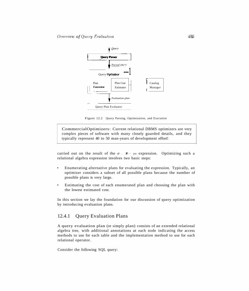
Overview of Qucry EvaJuat'lon 4115
• QUet}'
I'--"'---'-'~'-"'-'--'-
I Query ParserI~__._.•.•_~~ __tParsed query
Evaluation plan
---1r
Plan Cost I Catalog
EstimatorI
Manager
Query Optimizer
Plan
Query Plan Evaluator
Figure 12.2 Query Parsing, Optimization, and Execution
CommercialOptimizers: Current relational DBMS optimizers are verycomplex pieces of software with many closely guarded details, and theytypically represent 40 to 50 man-years of development effort!
carried out on the result of the (J" - 7f- [Xl expression. Optimizing such arelational algebra expression involves two basic steps:
• Enumerating alternative plans for evaluating the expression. Typically, anoptimizer considers a subset of all possible plans because the number ofpossible plans is very large.
• Estimating the cost of each enumerated plan and choosing the plan withthe lowest estimated cost.
In this section we lay the foundation for our discussion of query optimizationby introducing evaluation plans.
12.4.1 Query Evaluation Plans
A query evaluation plan (or simply plan) consists of an extended relationalalgebra tree, with additional annotations at each node indicating the accessmethods to use for each table and the implementation method to use for eachrelational operator.
Consider the following SQL query:
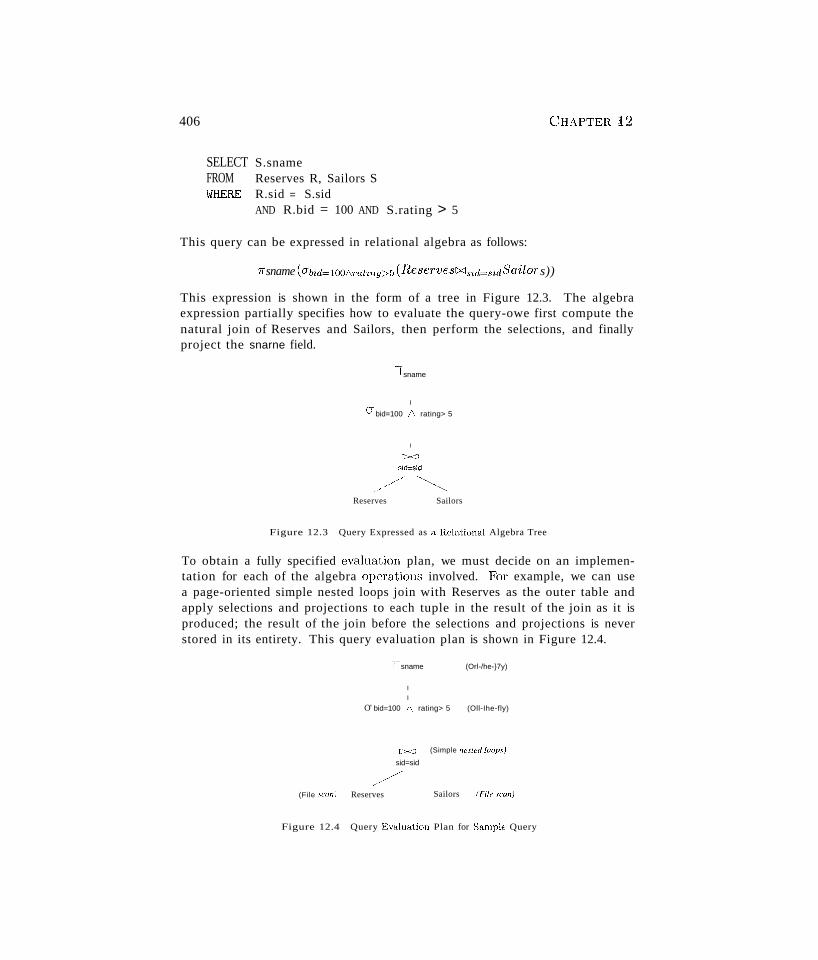
406
SELECTFROMWHERE
S.snameReserves R, Sailors SR.sid = S.sidAND R.bid = 100 AND S.rating > 5
CHAPTERi2
This query can be expressed in relational algebra as follows:
7fsname (O'bid=100/\mting>5 (ReservesMsid=sidSailor s))
This expression is shown in the form of a tree in Figure 12.3. The algebraexpression partially specifies how to evaluate the query-owe first compute thenatural join of Reserves and Sailors, then perform the selections, and finallyproject the snarne field.
ITsname
I
0- bid=100 A rating> 5
I
Reserves Sailors
Figure 12.3 Query Expressed as a Relational Algebra Tree
To obtain a fully specified evaluation plan, we must decide on an implementation for each of the algebra operations involved. }or example, we can usea page-oriented simple nested loops join with Reserves as the outer table andapply selections and projections to each tuple in the result of the join as it isproduced; the result of the join before the selections and projections is neverstored in its entirety. This query evaluation plan is shown in Figure 12.4.
ITsname (Orl-/he-}7y)
I
I
O' bid=100 A rating> 5 (Oll-Ihe-fly)
[><.::J (Simple IIcslcd loops)
sid=sid
//~/
(File SCOII) Reserves Sailors (File ,,'um)
Figure 12.4 Query Evaluation Plan for Sample Query
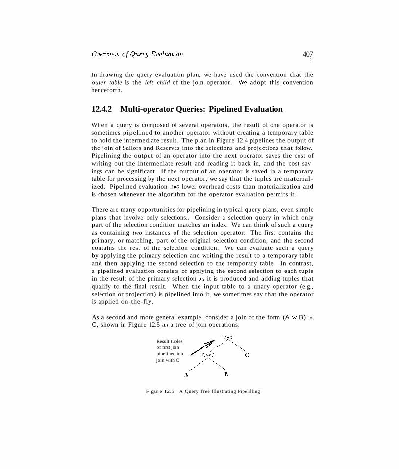
Overview of Query Eval'uation 407J
In drawing the query evaluation plan, we have used the convention that theouter table is the left child of the join operator. vVe adopt this conventionhenceforth.
12.4.2 Multi-operator Queries: Pipelined Evaluation
When a query is composed of several operators, the result of one operator issometimes pipelined to another operator without creating a temporary tableto hold the intermediate result. The plan in Figure 12.4 pipelines the output ofthe join of Sailors and Reserves into the selections and projections that follow.Pipelining the output of an operator into the next operator saves the cost ofwriting out the intermediate result and reading it back in, and the cost savings can be significant. If the output of an operator is saved in a temporarytable for processing by the next operator, we say that the tuples are materialized. Pipelined evaluation has lower overhead costs than materialization andis chosen whenever the algorithm for the operator evaluation permits it.
There are many opportunities for pipelining in typical query plans, even simpleplans that involve only selections.. Consider a selection query in which onlypart of the selection condition matches an index. We can think of such a queryas containing two instances of the selection operator: The first contains theprimary, or matching, part of the original selection condition, and the secondcontains the rest of the selection condition. We can evaluate such a queryby applying the primary selection and writing the result to a temporary tableand then applying the second selection to the temporary table. In contrast,a pipelined evaluation consists of applying the second selection to each tuplein the result of the primary selection as it is produced and adding tuples thatqualify to the final result. When the input table to a unary operator (e.g.,selection or projection) is pipelined into it, we sometimes say that the operatoris applied on-the-fly.
As a second and more general example, consider a join of the form (A CXJ B) 1><1
C, shown in Figure 12.5 &'3 a tree of join operations.
Result tuplesof first joinpipelined intojoin with C
Figure 12.5 A Query Tree Illustrating Pipelilling

408 CHAPTER ~2
Both joins can be evaluated in pipelined fa.<;hion using some version of a nestedloops join. Conceptually, the evaluation is initiated from the root, and the nodejoining A and B produces tuples as and when they are requested by its parentnode. 'When the root node gets a page of tuples from its left child (the outertable), all the matching inner tuples are retrieved (using either an index or ascan) and joined with matching outer tuples; the current page of outer tuplesis then discarded. A request is then made to the left child for the next pageof tuples, and the process is repeated. Pipelined evaluation is thus a controlstrategy governing the rate at which different joins in the plan proceed. It hasthe great virtue of not writing the result of intermediate joins to a temporaryfile because the results are produced, consumed, and discarded one page at atime.
12.4.3 The Iterator Interface
A query evaluation plan is a tree of relational operators and is executed bycalling the operators in some (possibly interleaved) order. Each operator hasone or more inputs and an output, which are also nodes in the plan, and tuplesmust be pa.<;sed between operators according to the plan's tree structure.
To simplify the code responsible for coordinating the execution of a plan, therelational operators that form the nodes of a plan tree (which is to be evaluatedusing pipelining) typically support a uniform iterator interface, hiding theinternal implementation details of each operator. The iterator interface foran operator includes the functions open, geLnext, and close. The openfunction initializes the state of the iterator by allocating buffers for its inputsand output, and is also used to pa.."s in arguments such ac; selection conditionsthat modify the behavior of the operator. The code for the get-next functioncalls the get-next function on each input node and calls operator-specific codeto process the input tuples. The output tuples generated by the processingare placed in the output buffer of the operator, and the state of the iterator isupdated to keep track of how much input hac; been consumed. \i\1hen all outputtuples have been produced through repeated calls to get-ne:rt, the close functionis called (by the code that initiated execution of this operator) to deallocatestate information.
The iterator interface supports pipelining of results naturally: the decision topipeline or mat(~rialize input tuples is encapsulated in the operator-specific codethat processes input tuples. If the algorithm implemented for the operatorallows input tuples to be processed completely when they are received, inputtuples are not Inaterialized and the evaluation is pipelined. If the algorithmexamines the same input tuples several times, they are materialized. This
Ov(;;'rvieu,) of query Eval'uaiion 409~
decision, like other details of the operator's implementation, is hidden by theiterator interface for the operator.
The iterator interface is also used to encapsulate access methods such as B+trees and hash-ba."ied indexes. Externally, access methods can be viewed simplyas operators that produce a stream of output tuples. In this case, the openfunction can be used to pass the selection conditions that match the accesspath.
12.5 ALTERNATIVE PLANS: A MOTIVATING EXAMPLE
Consider the example query from Section 12.4. Let us consider the cost ofevaluating the plan shown in Figure 12.4. We ignore the cost of writing outthe final result since this is common to all algorithms, and does not affecttheir relative costs. The cost of the join is 1000 + 1000 * 500 = 501,000 pagel/Os. The selections and the projection are done on-the-fly and do not incuradditional l/Os. The total cost of this plan is therefore 501,000 page l/Os.This plan is admittedly naive; however, it is possible to be even more naive bytreating the join as a cross-product followed by a selection.
vVe now consider several alternative plans for evaluating this query. Each alternative improves on the original plan in a different way and introduces someoptimization idea.<; that are examined in more detail in the rest of this chapter.
12.5.1 Pushing Selections
A join is a relatively expensive operation, and a good heuristic is to reducethe sizes of the tables to be joined as much as possible. One approach is toapply selections early; if a selection operator appears after a join operator, it isworth examining whether the selection can be 'pushed' ahead of the join. Asan example, the selection bid=1()(} involves only the attributes of Reserves andcan be applied to Reserves befoTe the join. Similarly, the selection mting> 5involves only attributes of Sailors and can be applied to Sailors before the join.Let us suppose that the selections are performed using a simple file scan, thatthe result of each selection is written to a temporary table on disk, and thatthe temporary tables are then joined using a sort-merge join. The resultingquery evaluation plan is shown in Figure 12.6.
Let us assume that five buffer pages are available and estimate the cost ofthis query evaluation plan. (It is likely that more buffer pages are availablein practice. vVe chose a small number simply for illustration in this example.)The cost of applying bid=100 to Reserves is the cost of scanning Reserves(1000 pages) plus the cost of writing the result to a temporary table, say Tl.
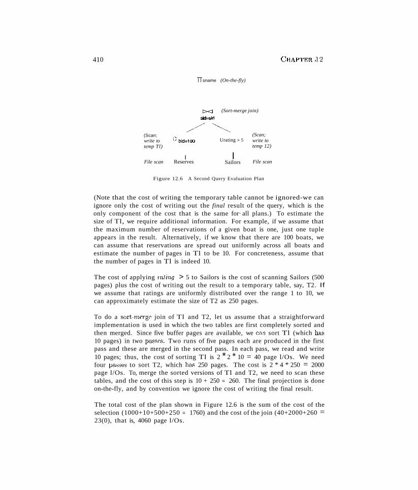
410
TTsname (On-the-fly)
C><J (Sort-merge join)
sid=sid
(Scan;U bid=100 Urating > 5
(Scan;write to write totemp Tl)
I Itemp 12)
File scan Reserves Sailors File scan
Figure 12.6 A Second Query Evaluation Plan
CHAPTER J2
(Note that the cost of writing the temporary table cannot be ignored-we canignore only the cost of writing out the final result of the query, which is theonly component of the cost that is the same for· all plans.) To estimate thesize of Tl, we require additional information. For example, if we assume thatthe maximum number of reservations of a given boat is one, just one tupleappears in the result. Alternatively, if we know that there are 100 boats, wecan assume that reservations are spread out uniformly across all boats andestimate the number of pages in Tl to be 10. For concreteness, assume thatthe number of pages in Tl is indeed 10.
The cost of applying rating > 5 to Sailors is the cost of scanning Sailors (500pages) plus the cost of writing out the result to a temporary table, say, T2. Ifwe assume that ratings are uniformly distributed over the range 1 to 10, wecan approximately estimate the size of T2 as 250 pages.
To do a sort-merge join of Tl and T2, let us assume that a straightforwardimplementation is used in which the two tables are first completely sorted andthen merged. Since five buffer pages are available, we C8Jl sort Tl (which ha..s10 pages) in two pa..'3ses. Two runs of five pages each are produced in the firstpass and these are merged in the second pass. In each pass, we read and write10 pages; thus, the cost of sorting Tl is 2 * 2 * 10 = 40 page l/Os. We needfour pa..'3ses to sort T2, which ha..s 250 pages. The cost is 2 * 4 * 250 = 2000page l/Os. To, merge the sorted versions of Tl and T2, we need to scan thesetables, and the cost of this step is 10 + 250 = 260. The final projection is doneon-the-fly, and by convention we ignore the cost of writing the final result.
The total cost of the plan shown in Figure 12.6 is the sum of the cost of theselection (1000+10+500+250 = 1760) and the cost of the join (40+2000+260 =23(0), that is, 4060 page l/Os.
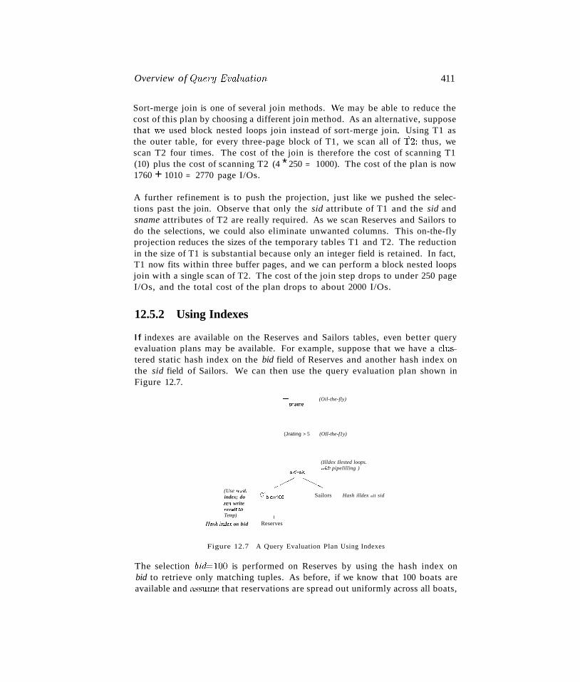
Overview of query Evaluation 411
Sort-merge join is one of several join methods. \Ve may be able to reduce thecost of this plan by choosing a different join method. As an alternative, supposethat \ve used block nested loops join instead of sort-merge join.. Using T1 asthe outer table, for every three-page block of T1, we scan all of T2; thus, wescan T2 four times. The cost of the join is therefore the cost of scanning T1(10) plus the cost of scanning T2 (4 * 250 = 1000). The cost of the plan is now1760 + 1010 = 2770 page I/Os.
A further refinement is to push the projection, just like we pushed the selections past the join. Observe that only the sid attribute of T1 and the sid andsname attributes of T2 are really required. As we scan Reserves and Sailors todo the selections, we could also eliminate unwanted columns. This on-the-flyprojection reduces the sizes of the temporary tables T1 and T2. The reductionin the size of T1 is substantial because only an integer field is retained. In fact,T1 now fits within three buffer pages, and we can perform a block nested loopsjoin with a single scan of T2. The cost of the join step drops to under 250 pageI/Os, and the total cost of the plan drops to about 2000 I/Os.
12.5.2 Using Indexes
If indexes are available on the Reserves and Sailors tables, even better queryevaluation plans may be available. For example, suppose that we have a clustered static hash index on the bid field of Reserves and another hash index onthe sid field of Sailors. We can then use the query evaluation plan shown inFigure 12.7.
(Use hashindex; donot writeresult 10
Temp)
Hash index on bid
ITsname
(Jrating > 5
sid=sid
IReserves
(Oil-the-fly)
(OIl-the-f1y)
(Illdex Ilested loops.with pipelilling )
Sailors Hash illdex all sid
Figure 12.7 A Query Evaluation Plan Using Indexes
The selection bid.=100 is performed on Reserves by using the hash index onbid to retrieve only matching tuples. As before, if we know that 100 boats areavailable and assume that reservations are spread out uniformly across all boats,
412 CHAPTER 12
\ve can estimate the number of selected tuples to be 100, 000/100 = lOOO. Sincethe index on b'id is clustered, these 1000 tuples appear consecutively within thesame bucket; therefore, the cost is 10 page l/Os.
:For each selected tuple, we retrieve matching Sailors tuples using the hash indexon the sid field; selected Reserves tuples are not materialized and the join ispipelined. For each tuple in the result of the join, we perform the selectionmting>5 and the projection of sname on-the-fly. There are several importantpoints to note here:
1. Since the result of the selection on Reserves is not materialized, the optimization of projecting out fields that are not needed subsequently is unnecessary (and is not used in the plan shown in Figure 12.7).
2. The join field sid is a key for Sailors. Therefore, at most one Sailors tuplematches a given Reserves tuple. The cost of retrieving this matching tupledepends on whether the directory of the hash index on the sid column ofSailors fits in memory and on the presence of overflow pages (if any). However, the cost does not depend on whether this index is clustered becausethere is at most one matching Sailors tuple and requests for Sailors tuplesare made in random order by sid (because Reserves tuples are retrieved bybid and are therefore considered in random order by sid). For a hash index,1.2 page l/Os (on average) is a good estimate of the cost for retrieving adata entry. Assuming that the sid hash index on Sailors uses Alternative(1) for data entries, 1.2 l/Os is the cost to retrieve a matching Sailors tuple (and if one of the other two alternatives is used, the cost would be 2,2l/Os).
3. vVe have chosen not to push the selection mt'ing>5 ahead of the join, andthere is an important reason for this decision. If we performed the selectionbefore the join, the selection would involve scanning Sailors, assuming thatno index is available on the mt'ing field of Sailors. Further, whether ornot such an index is available, once we apply such a selection, we haveno index on the sid field of the result of the selection (unless we chooseto build such an index solely for the sake of the subsequent join). Thus,pushing selections ahead of joins is a good heuristic, but not always thebest strategy. Typically, as in this example, the existence of useful indexesis the reason a selection is not pushed. (Otherwise, selections are pushed.)
Let us estimate the cost of the plan shown in Figure 12.7. The selection ofReserves tuples costs 10 l/Os, as we saw earlier. There are 1000 such tuples,and for each, the cost of finding the matching Sailors tuple is 1.2 l/Os, onaverage. The cost of this step (the join) is therefore 1200 l/Os. All remainingselections and projections are performed on~the-fly. The total cost of the planis 1210 l/Os.
Overview of quer7! Evaluation 413
As noted earlier, this plan does not utilize clustering of the Sailors index. Theplan can be further refined if the index on the sid field of Sailors is clustered.Suppose we materialize the result of performing the selection bid=100 on Reserves and sort this temporary table. This table contains 10 pages. Selectingthe tuples costs 10 page l/Os (as before), writing out the result to a temporarytable costs another 10 l/Os, and with five buffer pages, sorting this temporarycosts 2 * 2 * 10 = 40 l/Os. (The cost of this step is reduced if we push theprojection on sid. The sid column of materialized Reserves tuples requires onlythree pages and can be sorted in memory with five buffer pages.) The selectedReserves tuples can now be retrieved in order by 8'id.
If a sailor has reserved the same boat many times, all corresponding Reservestuples are now retrieved consecutively; the matching Sailors tuple will be foundin the bufFer pool on all but the first request for it. This improved plan alsodemonstrates that pipelining is not always the best strategy.
The combination of pushing selections and using indexes illustrated by thisplan is very powerful. If the selected tuples from the outer table join with asingle inner tuple, the join operation may become trivial, and the performancegains with respect to the naive plan in Figure 12.6 are even more dramatic.The following variant of our example query illustrates this situation:
SELECTFROMWHERE
S.snameReserves R, Sailors SRsid = S.sidAND R.bid = 100 AND S.rating > GAND Rday = '8/9/2002'
A slight variant of the plan shown in Figure 12.7, designed to answer this query,is shown in Figure 12.8. The selection day='8/9/2002' is applied on-the-fly tothe result of the selection bid=100 on the Reserves table.
Suppose that bid and day form a key for Reserves. (Note that this assumptiondiffers from the schema presented earlier in this chapter.) Let us estimate thecost of the plan shown in Figure 12.8. The selection bid=100 costs 10 pagel/Os, as before, and the additional selection day='8j.9/2002' is applied on-thefly, eliminating all but (at most) one Reserves tuple. There is at most onernatching Sailors tuple, and this is retrieved in 1.2 l/Os (an average value).The selection on rrding and the projection on sname are then applied on-thefly at no additional cost. The total cost of the plan in Figure 12.8 is thus about11 I/Os. In contrast, if we modify the naive plan in Figure 12.6 to performthe additional selection on day together with the selection bid=100, the costremains at 501,000 l/Os.
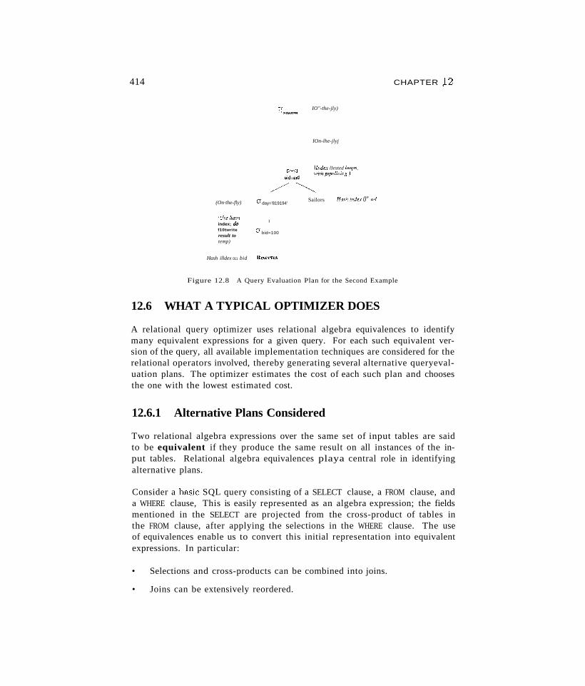
414
TT sname
1><1
IO"-the-jly)
IOn-lhe-jlyj
IIlIde.' lIested [oops,wilhl'il'eli"i"g)
CHAPTER J2
(On·the-fly)
(Use hashindex; dof10twrite
result totemp)
aday='819194'
I
a bid=100
Sailors Hash i"dex 0" sid
Hash illdex 011 bid Reserves
Figure 12.8 A Query Evaluation Plan for the Second Example
12.6 WHAT A TYPICAL OPTIMIZER DOES
A relational query optimizer uses relational algebra equivalences to identifymany equivalent expressions for a given query. For each such equivalent version of the query, all available implementation techniques are considered for therelational operators involved, thereby generating several alternative queryevaluation plans. The optimizer estimates the cost of each such plan and choosesthe one with the lowest estimated cost.
12.6.1 Alternative Plans Considered
Two relational algebra expressions over the same set of input tables are saidto be equivalent if they produce the same result on all instances of the input tables. Relational algebra equivalences playa central role in identifyingalternative plans.
Consider a basic SQL query consisting of a SELECT clause, a FROM clause, anda WHERE clause, This is easily represented as an algebra expression; the fieldsmentioned in the SELECT are projected from the cross-product of tables inthe FROM clause, after applying the selections in the WHERE clause. The useof equivalences enable us to convert this initial representation into equivalentexpressions. In particular:
• Selections and cross-products can be combined into joins.
• Joins can be extensively reordered.
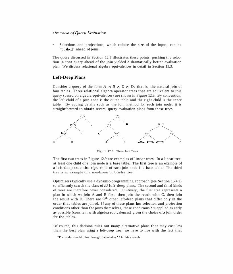
Overview of quer7J Evalnation
• Selections and projections, which reduce the size of the input, can be"pushed" ahead of joins.
The query discussed in Section 12.5 illustrates these points; pushing the selection in that query ahead of the join yielded a dramatically better evaluationplan. \Ve discuss relational algebra equivalences in detail in Section 15.3.
Left-Deep Plans
Consider a query of the form A [Xl B [Xl C [Xl D; that is, the natural join offour tables. Three relational algebra operator trees that are equivalent to thisquery (based on algebra equivalences) are shown in Figure 12.9. By convention,the left child of a join node is the outer table and the right child is the innertable. By adding details such as the join method for each join node, it isstraightforward to obtain several query evaluation plans from these trees.
C><J
/~C><J D
/~C><J c
/~A B
C><J
/~I><J I><J
/~ /~ABC D
Figure 12.9 Three Join Trees
The first two trees in Figure 12.9 are examples of linear trees. In a linear tree,at least one child of a join node is a base table. The first tree is an example ofa left-deep tree-the right child of each join node is a base table. The thirdtree is an example of a non-linear or bushy tree.
Optimizers typically use a dynamic-programming approach (see Section 15.4.2)to efficiently search the class of aU left-deep plans. The second and third kindsof trees are therefore never considered. Intuitively, the first tree represents aplan in which we join A and B first, then join the result with C, then jointhe result with D. There are 2~35 other left-deep plans that differ only in theorder that tables are joined. If any of these plans has selection and projectionconditions other than the joins themselves, these conditions are applied as earlyas possible (consitent with algebra equivalences) given the choice of a join orderfor the tables.
Of course, this decision rules out many alternative plans that may cost lessthan the best plan using a left-deep tree; we have to live with the fact that
"The reader should think through the number 2:3 in this example.
416 CHAPTER ,12
the optimizer will never find such plans. There are two main reasons for thisdecision to concentrate on left-deep plans, or plans ba.<;ed on left-deep trees:
1. As the number of joins increases, the number of alternative plans increa..:.;esrapidly and it becomes necessary to prune the space of alternat.ive plans.
2. Left-deep trees allow us to generate all fully pipelined plans; that is,plans in which all joins are evaluated using pipelining. (Inner tables mustalways be materialized because we must examine the entire inner table foreach tuple of the outer table. So, a plan in which an inner table is theresult of a join forces us to materialize the result of that join.)
12.6.2 Estimating the Cost of a Plan
The cost of a plan is the sum of costs for the operators it contains. The costof individual relational operators in the plan is estimated using information,obtained from the system catalog, about properties (e.g., size, sort order) oftheir input tables. We illustrated how to estimate the cost of single-operatorplans in Sections 12.2 and 12.3, and how to estimate the cost of multi-operatorplans in Section 12.5.
If we focus on the metric of I/O costs, the cost of a plan can be broken downinto three parts: (1) reading the input tables (possibly rnultiple times in thecase of some join and sorting algorithms), (2) writing intermediate tables, and(possibly) (3) sorting the final result (if the query specifies duplicate eliminationor an output order). The third part is common to all plans (unless one of theplans happens to produce output in the required order), and, in the commoncase that a fully-pipelined plan is chosen, no intermediate tables are written.
Thus, the cost for a fully-pipelined plan is dominated by part (1). This costdepends greatly on the access paths used to read input tables; of course, accesspaths that are used repeatedly to retrieve matching tuples in a join algorithmare especially important.
For plans that are not fully pipelined, the cost of rnaterializing temporary tablescan be significant. The cost of materializing an intermediate result dependson its size, and the size also infiuences the cost of the operator for which thetemporary is hn input table. The number of tuples in the result of a selection isestimated by multiplying the input size by the reduction factor for the selectionconditions. The number of tuples in the result of a projection is the same asthe input, a.ssuming that duplicates are not eliminated; of course, each resulttuple is smaller since it contains fewer fields.
Overview of q1lery Eval'llat'ion 417
The result size for a join can be estimated by multiplying the maximum resultsize, which is the product of the input table sizes, by the reduction factor of thejoin condition. The reduction factor for join condition columni = column2 canbe approximated by the formula ~(NJ{eY,~(~1),NKeys(I2)) if there are indexes11 and 12 on columni and colwnn2, respectively. This formula assumes thateach key value in the smaller index, say 11, has a matching value in the otherindex. Given a value for columni, we assume that each of the NKeys(I2)values for column2 is equally likely. Thus, the number of tuples that have thesame value in column2 as a given value in columni is N K e~s(I2) .
12.7 REVIEW QUESTIONS
Answers to the review questions can be found in the listed sections.
II What is metadata? What metadata is stored in the system catalog? Describe the information stored per relation, and per index. (Section 12.1)
II The catalog is itself stored as a collection of relations. Explain why. (Section 12.1)
II What three techniques are commonly used in algorithms to evaluate relational operators? (Section 12.2)
II What is an access path? When does an index match a search condition?(Section 12.2.2)
II What are the main approaches to evaluating selections? Discuss the use ofindexes, in particular. (Section 12.3.1)
II What are the main approaches to evaluating projections? What makesprojections potentially expensive? (Section 12.3.2)
II What are the main approaches to evaluating joins? Why are joins expensive? (Section 12.3.3)
II What is the goal of query optimization? Is it to find the best plan? (Section 12.4)
II How does a DBMS represent a relational query evaluation plan? (Section 12.4.1)
II What is pipelined evaluation? What is its benefit? (Section 12.4.2)
II Describe the iterator interface for operators and access methods. 'What isits purpose? (Section 12.4.3)
418 CHAPTER 12
• Discuss why the difference in cost between alternative plans for a query CI:Ul
be very large. Give specific examples to illustrate the impact of pushingselections, the choice of join methods, and the availability of appropriateindexes. (Section 12.5)
• What is the role of relational algebra equivalences in query optimization?(Section 12.6)
• What is the space of plans considered by a typical relational query optimizer? Justify the choice of this space of plans. (Section 12.6.1)
• How is the cost of a plan estimated? What is the role of the system catalog?What is the selectivity of an access path, and how does it influence the costof a plan? Why is it important to be able to estimate the size of the resultof a plan? (Section 12.6.2)
EXERCISES
Exercise 12.1 Briefly answer the following questions:
1. Describe three techniques commonly used when developing algorithms for relational operators. Explain how these techniques can be used to design algorithms for the selection,projection, and join operators.
2. What is an access path? When does an index match an access path? What is a primar1Jconj1Lnct, and why is it important?
3. What information is stored in the system catalogs?
4. What are the benefits of making the system catalogs be relations?
5. What is the goal of query optimization? Why is optimization important?
6. Describe pipelining and its advantages.
7. Give an example query and plan in which pipelining cannot be used.
8. Describe the itemto1' interface and explain its advantages.
9. What role do statistics gathered from the database play in query optimization?
10. What were the important design decisions made in the System R optimizer?
11. Why do query optimizers consider only left-deep join trees? Give an example of a queryand a plan that would not be considered because of this restriction.
Exercise 12.2 Consider a relation R( a,b,e,.d,e) containing 5,000,000 records, where each datapage of the relation holds 10 records. R is organized as a sorted file with secondary indexes.Assume that R.a is a candidate key for R, with values lying in the range 0 to 4,999,999, andthat R is stored in R.o, order. For each of the following relational algebra queries, state whichof the following three approaches is most likely to be the cheapest:
• Access the sorted file for R directly.
• Use a (clustered) B+ tree index on attribute R.o,.
• Usc a linear hashed index on attribute R.a..
Overview of Query Evaluation
1. (7a<50,000(R)
2. (T a=50,OOO (R)
3. (Ta>50,000Ao<50,OlO (R)
4. (Ta;>'50,000 (R)
419
Exercise 12.3 For each of the following SQL queries, for each relation involved, list theattributes that must be examined to compute the answer. All queries refer to the followingrelations:
Emp(eid: integer, did: integer, sal: integer, hobby: char(20))
Dept(did: integer, dname: char(20), floor: integer, budget: real)
1. SELECT * FROM Emp
2. SELECT * FROM Emp, Dept
3, SELECT * FROM Emp E, Dept D WHERE E.did = D.did
4. SELECT E.eid, D,dname FROM Emp E, Dept D WHERE E.did = D.did
Exercise 12.4 Consider the following schema with the Sailors relation:
Sailors(sid: integer, sname: string, rating: integer, age: real)
For each of the following indexes, list whether the index matches the given selection conditions.If there is a match, list the primary conjuncts.
1. A B+-tree index on the search key ( Sailors.sid ).
(a) (7Sailors.sid<50,OOO (Sailor s)
(b) (7Sailor.uid=f,o,ooo(Sailors)
2. A hash index on the search key ( Sailors.sid ).
(a) O'Sailo'·s.sid<50,OOO (Sailors)
(b) (7Sailon.S1d=5o,ooo(Sailors)
3. A B+-tree index on the search key ( Sailors.sid, Sailors.age ).
(a) O'Sallors.8icl<50,OOOASai.loT's.ag,,=21 (Sailors)
(b) O'Sailor.5.si.d=.SO,OOOASallors.age>21 (Sailors)
(c) (7Sai/oTS.sid=5o,ooo(Sailors)
(d) 0'!3ai/o·rs.ag('=21(Sailors)
4. A ha.'lh-tree hidex on the search key ( Sailors.sid, Sailors. age ).
(a) O'S"Il",·s.sid=50,OOOASo.ilors.ag,,=21 (Sailors)
(b) O'S",i/01·s ..,i.d=50,O(JOAS,,·i!or.,.age>21 (Sailors)
(c) O's'd{ors,,"d=5o,ooo(Sailors)
(d) O'S'''/01's.<l.()''=21 (Sa'ilors)
Exercise 12.5 Consider again the schema with the Sailors relation:

420
Sailors(sid: integer, sname: string, mUng: integer, age: real)
CHAPTERfi12
Assume that each tuple of Sailors is 50 bytes long, that a page can hold 80 Sailors tuples, andthat we have 500 pages of such tuples. For each of the following selection conditions, estimatethe number of pages retrieved, given the catalog information in the question.
1. Assume that we have a B+-tree index 7' on the search key ( Sailors.sid ), and assumethat IHeight(T) = 4, INPages(T) = 50, Low(7') = 1, and High(T) = 100,000.
(a) aSailors.'id<5o,ooo(S'a'ilors)
(b) aSailorssid=50,OOO(Sa'ilors)
2. Assume that we have a hash index 7' on the search key ( Sailors.sid ), and assume thatIHeight(7') = 2, INPages(7') = 50, Low(7') = 1, and High(T) = 100,000.
(a) aSa'lor's.sid<50,OOo(Sailors)
(b) aSailor·s.sid=5o,ooo(5ailors)
Exercise 12.6 Consider the two join methods described in Section 12.3.3. Assume that wejoin two relations Rand 5, and that the systems catalog contains appropriate statistics aboutRand S. Write formulas for the cost estimates of the index nested loops join and sort-mergejoin using the appropriate variables from the systems catalog in Section 12.1. For index nestedloops join, consider both a B+ tree index and a hash index. (For the hash index, you canassume that you can retrieve the index page containing the rid of the matching tuple with1.2 l/Os on average.)
Note.' Additional exercises on the material covered in this chapter can be found in the exercisesfor Chapters 14 and 15.
BIBLIOGRAPHIC NOTES
See the bibliograpic notes for Chapters 14 and 15.
13EXTERNAL SORTING
... Why is sorting important in a DBMS?
... Why is sorting data on disk different from sorting in-memory data?
... How does external merge-sort work?
... How do techniques like blockecl I/O and overlapped I/O affect thedesign of external sorting algorithms?
... When can we use a B+ tree to retrieve records in sorted order?
.. Key concepts: motivation, bulk-loading, duplicate elimination, sortmerge joins; external merge sort, sorted runs, merging runs; replacement sorting, increasing run length; I/O cost versus number of I/Os,blocked I/Os, double buffering; B+ trees for sorting, impact of clustering.
Good order is the foundation of all things.
Edmund Burke
In this chapter, we consider a widely used and relatively expensive operation,sorting records according to a search key. vVe begin by considering the lnanyuses of sorting In a database system in Section 13.1. \;Ye introduce the idea ofexternal sorting by considering a very simple algorithm in Section 1:3.2; usingrepeated passes over the data, even very large datasets can be sorted with asmall amount of rnemory. This algol'ithrn is generalized to develop a realisticexternal sorting algorithrn in Section 1:3.3. Three important refinements are
421
422 CHAPTER 1~~
discussed. The first, discussed in Section 13.3.1, enables us to reduce the number of passes. The next two refinements, covered in Section 13.4, require usto consider a more detailed model of I/O costs than the number of page I/Os.Section 13.4.1 discusses the effect of blocked I/O, that is, reading and writingseveral pages at a time; and Section 13.4.2 considers how to use a techniquecalled double buffering to minimize the time spent waiting for an I/O operationto complete. Section 13.5 discusses the use of B+ trees for sorting.
With the exception of Section 13.4, we consider only I/O costs, which we approximate by counting the number of pages read or written, as per the costmodel discussed in Chapter 8. Our goal is to use a simple cost model to conveythe main ideas, rather than to provide a detailed analysis.
13.1 WHEN DOES A DBMS SORT DATA?
Sorting a collection of records on some (search) key is a very useful operation.The key can be a single attribute or an ordered list of attributes, of course.Sorting is required in a variety of situations, including the following importantones:
II Users may' want answers in some order; for example, by increa.."iing age(Section 5.2).
II Sorting records is the first step in bulk loading a tree index (Section 10.8.2).
II Sorting is useful for eliminating duplicate copies in a collection of records(Section 14.3).
External Sorting
• A widely used algorithm for performing a very important relational algebraoperation, called jo'in, requires a sorting step (Section 14.4.2).
Although main memory sizes are growing rapidly the ubiquity of databasesystems has lead to increasingly larger datasets as well. '\Then the data tobe sorted is too large to fit into available main memory, we need an externalsorting algorithm. Such algorithms seek to minimize the cost of disk accesses.
13.2 A SIMPLE TWO-WAY MERGE SORT
We begin by presenting a simple algorithm to illustrate the idea behind externalsorting. This algorithm utilizes only three pages of main memory, and it ispresented only for pedagogical purposes. In practice, many more pages ofmemory are available, and we want our sorting algorithm to use the additionalmemory effectively; such an algorithm is presented in Section 13.3. Whensorting a file, several sorted subfiles are typically generated in intermediatesteps. In this chapter, we refer to each sorted subfile as a run.
Even if the entire file does not fit into the available main memory, we can sortit by breaking it into smaller subfiles, sorting these subfiles, and then mergingthem using a minimal amount of main memory at any given time. In the firstpass, the pages in the file are read in one at a time. After a page is read in,the records on it are sorted and the sorted page (a sorted run one page long) iswritten out. Quicksort or any other in-memory sorting technique can be usedto sort the records on a page. In subsequent passes, pairs of runs from theoutput of the previous pass are read in and merged to produce runs that aretwice as long. This algorithm is shown in Figure 13.1.
If the number of pages in the input file is 2k , for some k, then:
Pass 0 produces 2k sorted runs of one page each,Pass 1 produces 2k~1 sortecl runs of two pages each,Pass 2 produces 2k - 2 sortecl runs of four pages each,and so on, untilPass k produces one sorted run of 2k: pages.
In each pass, we read every page in the file, process it, and write it out.Therefore we have two disk I/Os per page, per pass. The number of passesis flog2Nl -+- 1, where N is the number of pages in the file. The overall cost is2N( ilog2Nl + 1) l/Os.
The algorithm is illustrated on all example input file containing seven pagesin Figure 13.2. The sort takes four passes, and in each pass, we read and
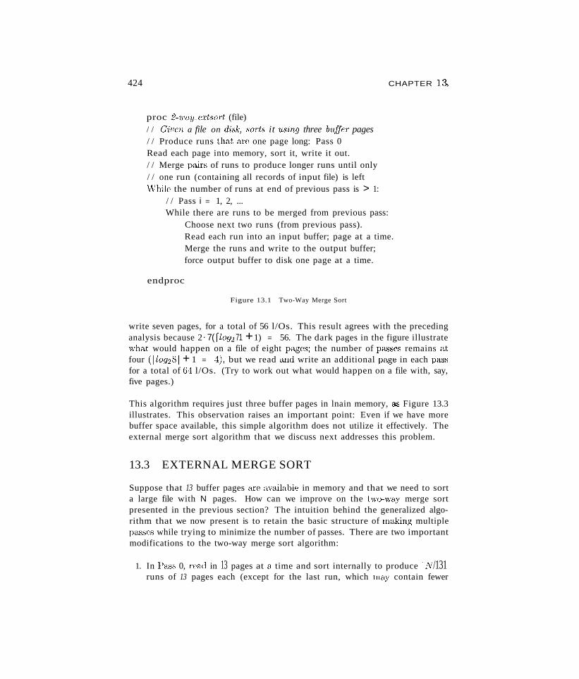
424 CHAPTER l~
proc 2-'ulay_cxtsort (file)/ / Oiven a file on disk) sorts it 'using three buffeT' pages/ / Produce runs that are one page long: Pass 0Read each page into memory, sort it, write it out./ / Merge pairs of runs to produce longer runs until only/ / one run (containing all records of input file) is left\Vhile the number of runs at end of previous pass is > 1:
/ / Pass i = 1, 2, ...While there are runs to be merged from previous pass:
Choose next two runs (from previous pass).Read each run into an input buffer; page at a time.Merge the runs and write to the output buffer;force output buffer to disk one page at a time.
endproc
Figure 13.1 Two-Way Merge Sort
write seven pages, for a total of 56 l/Os. This result agrees with the precedinganalysis because 2· 7( llo92 71 +1) = 56. The dark pages in the figure illustratewhat would happen on a file of eight pages; the number of passes remains atfour (llo9281 + 1 = 4), but we read and write an additional page in each passfor a total of 64 l/Os. (Try to work out what would happen on a file with, say,five pages.)
This algorithm requires just three buffer pages in lnain memory, Cl"S Figure 13.3illustrates. This observation raises an important point: Even if we have morebuffer space available, this simple algorithm does not utilize it effectively. Theexternal merge sort algorithm that we discuss next addresses this problem.
13.3 EXTERNAL MERGE SORT
Suppose that 13 buffer pages are available in memory and that we need to sorta large file with N pages. How can we improve on the t\vo-way merge sortpresented in the previous section? The intuition behind the generalized algorithm that we now present is to retain the basic structure of making multiplepasses while trying to minimize the number of passes. There are two importantmodifications to the two-way merge sort algorithm:
1. In Pass 0, read in 13 pages at a time and sort internally to produce IN/131runs of 13 pages each (except for the last run, which lnay contain fewer
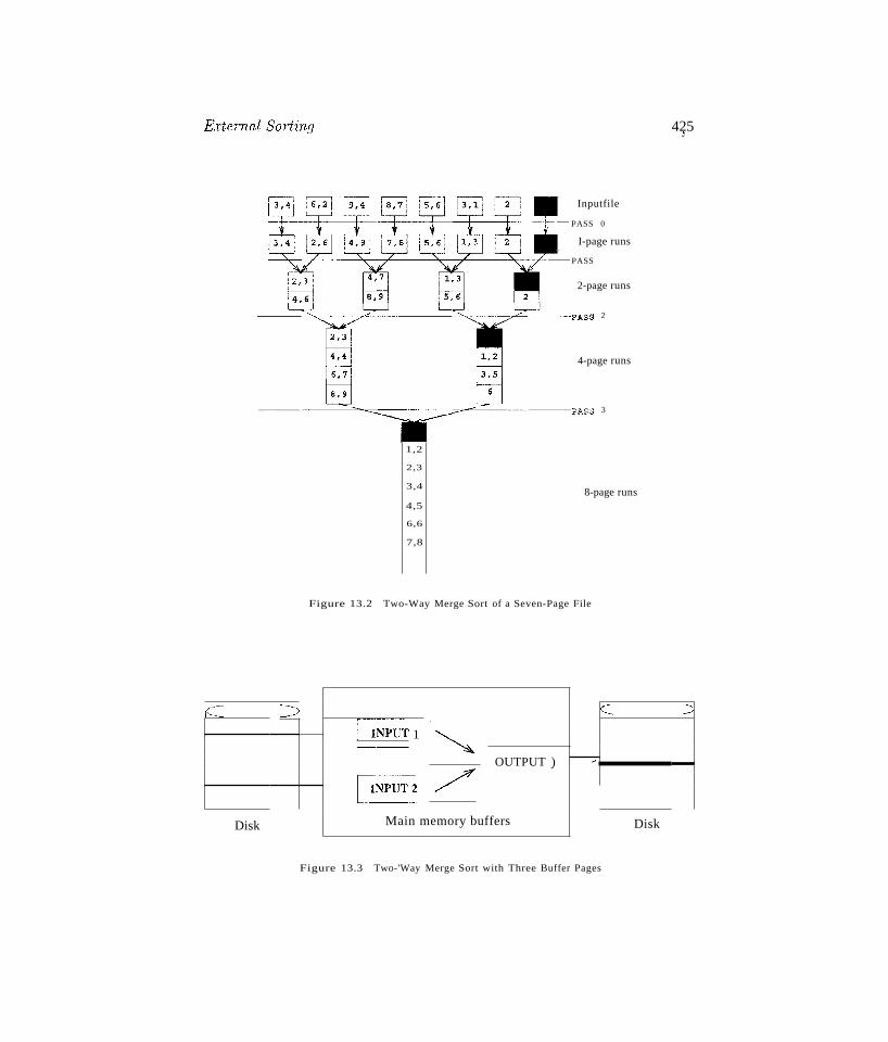
RTtemal Sorting
IInputfile
PASS 0
I-page runs
~-, PASS
2-page runs
-----C~--~,.._L----------"'>....,__---__O>"L.---~PASS2
4-page runs
---------""'----=::-------=-~-------PASS3
1,2
2,3
425;~
3,4
4,5
6,6
7,8
8-page runs
Figure 13.2 Two-Way Merge Sort of a Seven-Page File
c ~ r:=:- -------[iNPUT 1
I~IOUTPUT ) ..
[!NPUT2 1/Disk Main memory buffers Disk
Figure 13.3 Two-'Way Merge Sort with Three Buffer Pages
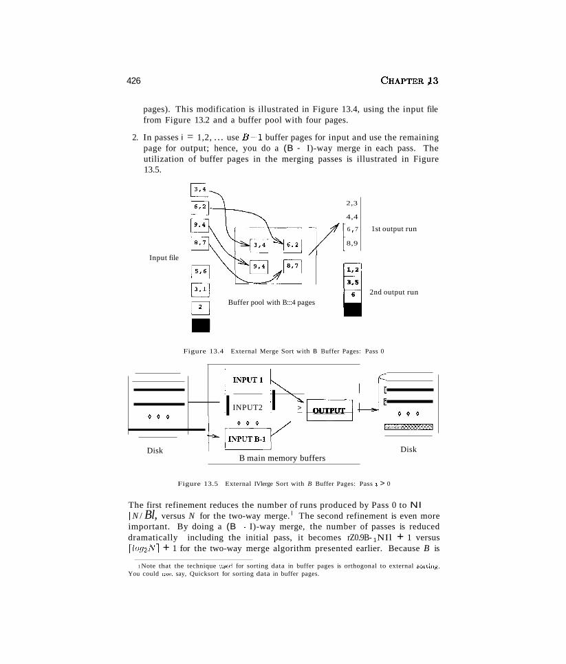
426 CHAPTER~3
pages). This modification is illustrated in Figure 13.4, using the input filefrom Figure 13.2 and a buffer pool with four pages.
2. In passes i = 1,2, ... use B-1 buffer pages for input and use the remainingpage for output; hence, you do a (B - I)-way merge in each pass. Theutilization of buffer pages in the merging passes is illustrated in Figure13.5.
2,3
8,9
2nd output run
4,4
6 , 7 1st output run
!'2
3,5
6Buffer pool with B:::4 pages
Input file
Figure 13.4 External Merge Sort with B Buffer Pages: Pass 0
¢ ¢ ¢
Disk
! ~UTl ~I INPUT2 I > I~IOUTPUT
B main memory buffers
¢ ¢ ¢
Disk
Figure 13.5 External IVlerge Sort with B Buffer Pages: Pass 'i > 0
The first refinement reduces the number of runs produced by Pass 0 to NIrN / Bl, versus N for the two-way merge. l The second refinement is even moreimportant. By doing a (B ~ I)-way merge, the number of passes is reduceddramatically including the initial pass, it becomes rZ0.9B- 1NIl + 1 versus[loY2Nl + 1 for the two-way merge algorithm presented earlier. Because B is
1 Note that the technique used for sorting data in buffer pages is orthogonal to external sorting.You could use, say, Quicksort for sorting data in buffer pages.
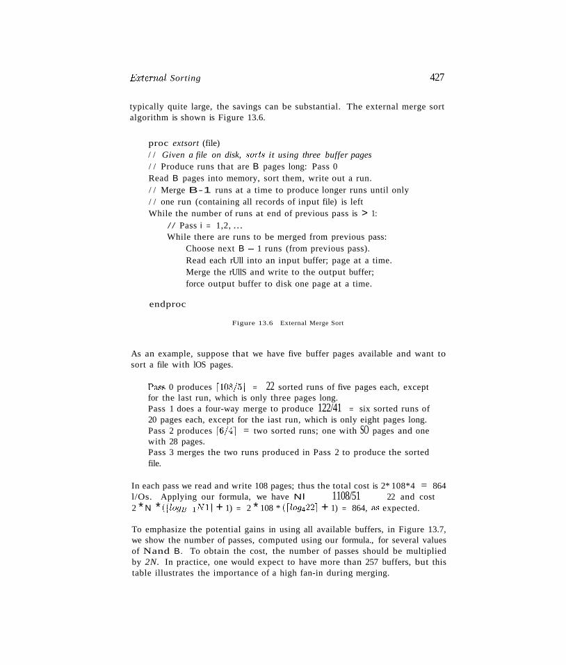
External Sorting 427
typically quite large, the savings can be substantial. The external merge sortalgorithm is shown is Figure 13.6.
proc extsort (file)/ / Given a file on disk, sorts it using three buffer pages/ / Produce runs that are B pages long: Pass 0Read B pages into memory, sort them, write out a run./ / Merge B-1 runs at a time to produce longer runs until only/ / one run (containing all records of input file) is leftWhile the number of runs at end of previous pass is > 1:
// Pass i = 1,2, ...While there are runs to be merged from previous pass:
Choose next B ~ 1 runs (from previous pass).Read each rUll into an input buffer; page at a time.Merge the rUllS and write to the output buffer;force output buffer to disk one page at a time.
endproc
Figure 13.6 External Merge Sort
As an example, suppose that we have five buffer pages available and want tosort a file with lOS pages.
Pac'Ss 0 produces POS/51 = 22 sorted runs of five pages each, exceptfor the last run, which is only three pages long.Pass 1 does a four-way merge to produce 122/41 = six sorted runs of20 pages each, except for the iast run, which is only eight pages long.Pass 2 produces 16/41 = two sorted runs; one with SO pages and onewith 28 pages.Pass 3 merges the two runs produced in Pass 2 to produce the sortedfile.
In each pass we read and write 108 pages; thus the total cost is 2* 108*4 = 864l/Os. Applying our formula, we have Nl 1108/51 22 and cost2 * N * (llogB~lNll + 1) = 2 * 108 * (llog4221 + 1) = 864, &'3 expected.
To emphasize the potential gains in using all available buffers, in Figure 13.7,we show the number of passes, computed using our formula., for several valuesof Nand B. To obtain the cost, the number of passes should be multipliedby 2N. In practice, one would expect to have more than 257 buffers, but thistable illustrates the importance of a high fan-in during merging.
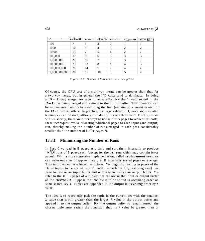
428 CHAPTER +3
" .... ..;:;.-,., .... B+F ••9i.n .,,.. n ..
·.·\~.:tt.:· •••• &Q'i" ••ilJ. J]2'i'i'u ·.£">;;;0;;;,[1 LJTfif",a
100 7 4 3 2 1 11000 10 5 4 3 2 210,000 13 7 5 4 2 2100,000 17 9 6 5 3 31,000,000 20 10 7 5 3 310,000,000 23 12 8 6 4 3100,000,000 26 14 9 7 4 41,000,000,000 30 15 10 8 5 4
Figure 13.7 Number of Passes of External Merge Sort
Of course, the CPU cost of a multiway merge can be greater than that fora two-way merge, but in general the I/O costs tend to dominate. In doinga (B - I)-way merge, we have to repeatedly pick the 'lowest' record in theB-1 runs being merged and write it to the output buffer. This operation canbe implemented simply by examining the first (remaining) element in each ofthe B-1 input buffers. In practice, for large values of B, more sophisticatedtechniques can be used, although we do not discuss them here. Further, as wewill see shortly, there are other ways to utilize buffer pages to reduce I/0 costs;these techniques involve allocating additional pages to each input (and output)run, thereby making the number of runs me,rged in each pass considerablysmaller than the number of buffer pages B.
13.3.1 Minimizing the Number of Runs
In Pass 0 we read in B pages at a time and sort them internally to produceIN/Bl runs of B pages each (except for the la..'3t run, which may contain fewerpages). With a more aggressive implementation, called replacement sort, wecan write out runs of approximately 2 . B internally sorted pages on average.This improvement is achieved as follows. We begin by reading in pages of thefile of tuples to be sorted, say R, until the buffer is full, reserving (say) onepage for use a..'3 an input buffer and one page for use a.s an output buffer. vVerefer to the B ~ 2 pages of R tuples that are not in the input or output bufferas the CUT'TCnt set. Suppose that the file is to be sorted in ascending order onsome search key k. Tuples are appended to the output in ctscending order by kvalue.
The idea is to repeatedly pick the tuple in the current set with the smallestk value that is still greater than the largest k value in the output buffer andappend it to the output buffer. l:<cx the output buffer to remain sorted, thechosen tuple must satisfy the condition that its k value be greater than or
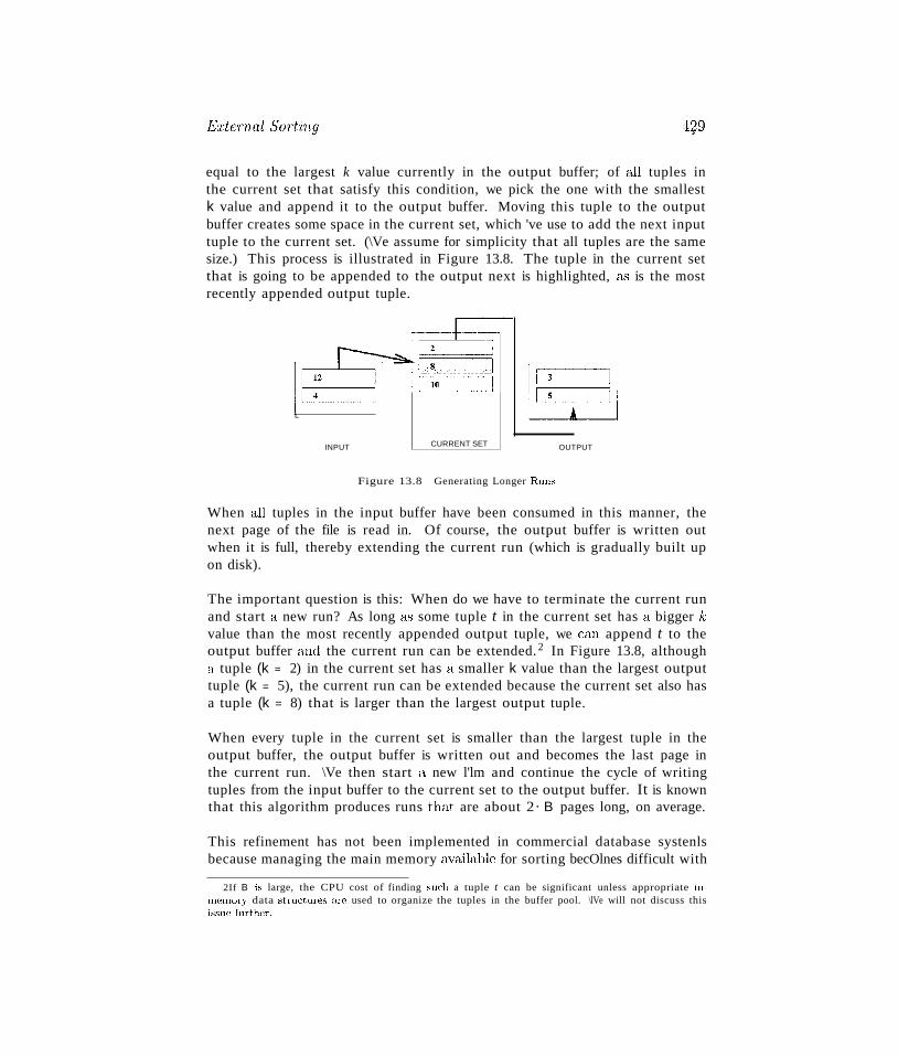
El:teT'nal Sorting 4f9
equal to the largest k value currently in the output buffer; of all tuples inthe current set that satisfy this condition, we pick the one with the smallestk value and append it to the output buffer. Moving this tuple to the outputbuffer creates some space in the current set, which 've use to add the next inputtuple to the current set. (\Ve assume for simplicity that all tuples are the samesize.) This process is illustrated in Figure 13.8. The tuple in the current setthat is going to be appended to the output next is highlighted, as is the mostrecently appended output tuple.
11±-L .. .• .... ..
INPUT CURRENT SET
~L~_II
OUTPUT
Figure 13.8 Generating Longer Runs
When all tuples in the input buffer have been consumed in this manner, thenext page of the file is read in. Of course, the output buffer is written outwhen it is full, thereby extending the current run (which is gradually built upon disk).
The important question is this: When do we have to terminate the current runand start a new run? As long as some tuple t in the current set has a bigger k:value than the most recently appended output tuple, we can append t to theoutput buffer and the current run can be extended.2 In Figure 13.8, althougha tuple (k = 2) in the current set has a smaller k value than the largest outputtuple (k = 5), the current run can be extended because the current set also hasa tuple (k = 8) that is larger than the largest output tuple.
When every tuple in the current set is smaller than the largest tuple in theoutput buffer, the output buffer is written out and becomes the last page inthe current run. \Ve then start a new l'lm and continue the cycle of writingtuples from the input buffer to the current set to the output buffer. It is knownthat this algorithm produces runs that are about 2· B pages long, on average.
This refinement has not been implemented in commercial database systenlsbecause managing the main memory ava.ilable for sorting becOlnes difficult with
2If B is large, the CPU cost of finding such a tuple t can be significant unless appropriate in·memory data structures are used to organize the tuples in the buffer pool. \lVe will not discuss thisissue further.
430 CHAPTER 13
replacement sort, especially in the presence of variable length records. Recentwork on this issue, however, shows promise and it could lead to the use ofreplacement sort in commercial systems.
13.4 MINIMIZING I/O COST VERSUS NUMBER OF I/OS
We have thus far used the number of page 1/Os as a cost metric. This metric isonly an approximation of true I/O costs because it ignores the effect of blockedI/O--issuing a single request to read (or write) several consecutive pages canbe much cheaper than reading (or writing) the same number of pages throughindependent I/O requests, as discussed in Chapter 8. This difference turns outto have some very important consequences for our external sorting algorithm.
Further, the time taken to perform I/O is only part of the time taken by thealgorithm; we must consider CPU costs as well. Even if the time taken to doI/O accounts for most of the total time, the time taken for processing records isnontrivial and definitely worth reducing. In particular, we can use a techniquecalled double buffeTing to keep the CPU busy while an I/O operation is inprogress.
In this section, we consider how the external sorting algorithm can be refinedusing blocked I/O and double buffering. The motivation for these optimizations requires us to look beyond the number of I/Os as a cost metric. Theseoptimizations can also be applied to other I/O intensive operations such asjoins, which we study in Chapter 14.
13.4.1 Blocked I/O
If the number of page I/Os is taken to be the cost metric, the goal is clearly tominimize the number of passes in the sorting algorithm because each page inthe file is read and written in each pa..ss. It therefore makes sense to maximizethe fan-in during merging by allocating just one buffer pool page per run (whichis to be merged) and one buffer page for the output of the merge. Thus, wecan merge B-1 runs, where B is the number of pages in the buffer pool. If wetake into account the effect of blocked access, which reduces the average costto read or write a .single page, we are led to consider whether it might be betterto read and write in units of more than one page.
Suppose we decide to read and write in units, which we call buffer blocks,of b pages. We must now set aside one buffer block per input run and onebufler block for the output of the merge, which means that we can merge atmost l B;)-b J runs in each pass. }-<or example, if we have 10 buffer pages, wecan either merge nine runs at a time with one-page input and output buffer
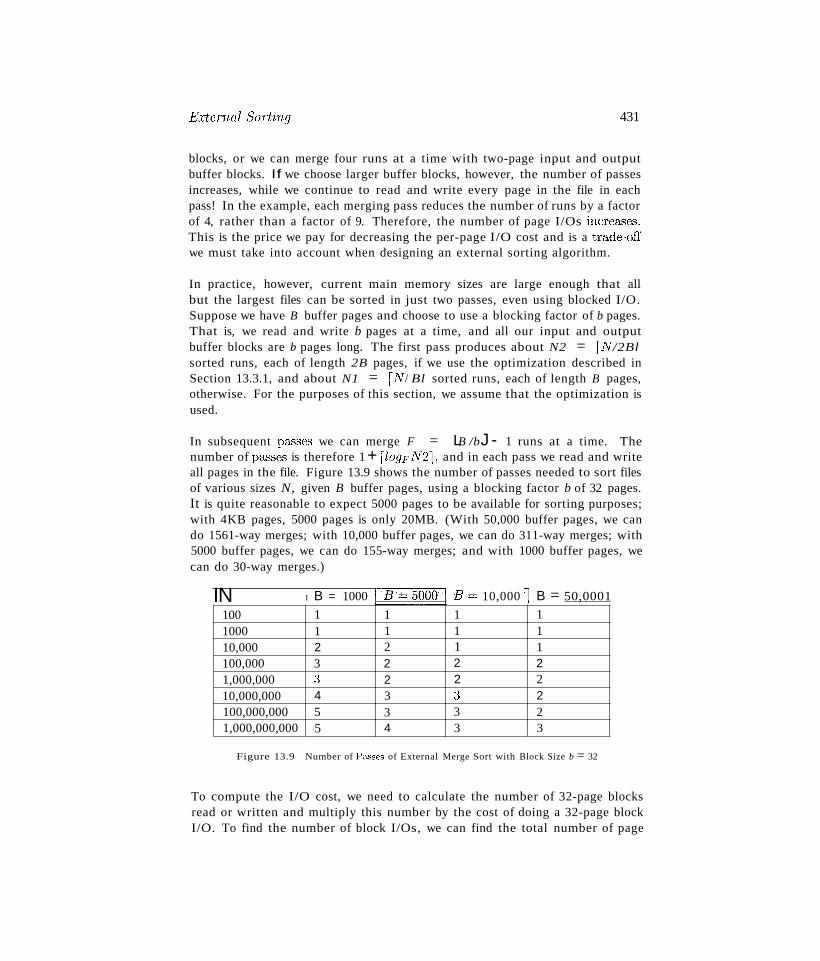
Krtcrnal SoTting 431
blocks, or we can merge four runs at a time with two-page input and outputbuffer blocks. If we choose larger buffer blocks, however, the number of passesincreases, while we continue to read and write every page in the file in eachpass! In the example, each merging pass reduces the number of runs by a factorof 4, rather than a factor of 9. Therefore, the number of page I/Os increa.'3es.This is the price we pay for decreasing the per-page I/O cost and is a trade-offwe must take into account when designing an external sorting algorithm.
In practice, however, current main memory sizes are large enough that allbut the largest files can be sorted in just two passes, even using blocked I/O.Suppose we have B buffer pages and choose to use a blocking factor of b pages.That is, we read and write b pages at a time, and all our input and outputbuffer blocks are b pages long. The first pass produces about N2 = IN/2Blsorted runs, each of length 2B pages, if we use the optimization described inSection 13.3.1, and about N1 = IN/ Bl sorted runs, each of length B pages,otherwise. For the purposes of this section, we assume that the optimization isused.
In subsequent pa.'3ses we can merge F = LB /bJ - 1 runs at a time. Thenumber of pa.'3ses is therefore 1 + lZo9pN21, and in each pass we read and writeall pages in the file. Figure 13.9 shows the number of passes needed to sort filesof various sizes N, given B buffer pages, using a blocking factor b of 32 pages.It is quite reasonable to expect 5000 pages to be available for sorting purposes;with 4KB pages, 5000 pages is only 20MB. (With 50,000 buffer pages, we cando 1561-way merges; with 10,000 buffer pages, we can do 311-way merges; with5000 buffer pages, we can do 155-way merges; and with 1000 buffer pages, wecan do 30-way merges.)
IN I B = 1000 1.8=50001 E± 10,000 >1 B = 50,0001
100 1 1 1 11000 1 1 1 110,000 2 2 1 1100,000 3 2 2 21,000,000 ~) 2 2 210,000,000 4 3 ~3 2100,000,000 5 3 3 21,000,000,000 5 4 3 3
Figure 13.9 Number of Passes of External Merge Sort with Block Size b = 32
To compute the I/O cost, we need to calculate the number of 32-page blocksread or written and multiply this number by the cost of doing a 32-page blockI/O. To find the number of block I/Os, we can find the total number of page
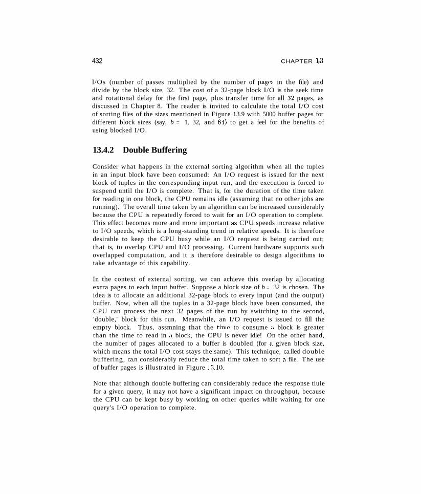
432 CHAPTER 13
l/Os (number of passes rnultiplied by the number of pages in the file) anddivide by the block size, 32. The cost of a 32-page block I/O is the seek timeand rotational delay for the first page, plus transfer time for all ~~2 pages, asdiscussed in Chapter 8. The reader is invited to calculate the total I/O costof sorting files of the sizes mentioned in Figure 13.9 with 5000 buffer pages fordifferent block sizes (say, b = 1, 32, and 64) to get a feel for the benefits ofusing blocked I/O.
13.4.2 Double Buffering
Consider what happens in the external sorting algorithm when all the tuplesin an input block have been consumed: An I/O request is issued for the nextblock of tuples in the corresponding input run, and the execution is forced tosuspend until the I/O is complete. That is, for the duration of the time takenfor reading in one block, the CPU remains idle (assuming that no other jobs arerunning). The overall time taken by an algorithm can be increased considerablybecause the CPU is repeatedly forced to wait for an I/O operation to complete.This effect becomes more and more important as CPU speeds increase relativeto I/O speeds, which is a long-standing trend in relative speeds. It is thereforedesirable to keep the CPU busy while an I/O request is being carried out;that is, to overlap CPU and I/O processing. Current hardware supports suchoverlapped computation, and it is therefore desirable to design algorithms totake advantage of this capability.
In the context of external sorting, we can achieve this overlap by allocatingextra pages to each input buffer. Suppose a block size of b = 32 is chosen. Theidea is to allocate an additional 32-page block to every input (and the output)buffer. Now, when all the tuples in a 32-page block have been consumed, theCPU can process the next 32 pages of the run by switching to the second,'double,' block for this run. Meanwhile, an I/O request is issued to fill theempty block. Thus, assmning that the tirne to consume a block is greaterthan the time to read in a block, the CPU is never idle! On the other hand,the number of pages allocated to a buffer is doubled (for a given block size,which means the total I/O cost stays the same). This technique, ca.lled doublebuffering, ca.n considerably reduce the total time taken to sort a file. The useof buffer pages is illustrated in Figure 1:3.10.
Note that although double buffering can considerably reduce the response tiulefor a given query, it may not have a significant impact on throughput, becausethe CPU can be kept busy by working on other queries while waiting for onequery's I/O operation to complete.
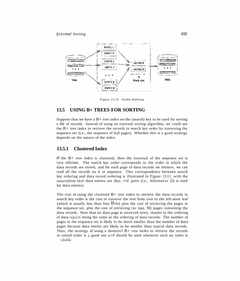
E:rteTnal Sorting
Figure 13.10 Double Buffering
13.5 USING B+ TREES FOR SORTING
433
Suppose that we have a B+ tree index on the (search) key to be used for sortinga file of records. Instead of using an external sorting algorithm, we could usethe B+ tree index to retrieve the records in search key order by traversing thesequence set (i.e., the sequence of leaf pages). Whether this is a good strategydepends on the nature of the index.
13.5.1 Clustered Index
If the B+ tree index is clustered, then the traversal of the sequence set isvery efficient. The search key order corresponds to the order in which thedata records are stored, and for each page of data records we retrieve, we canread all the records on it in sequence. This correspondence between searchkey ordering and data record ordering is illustrated in Figure 13.11, with thea.ssumption that data entries are (key, ric!; pairs (i.e., Alternative (2) is usedfor data entries).
The cost of using the clustered B+ tree index to retrieve the data records insearch key order is the cost to traverse the tree from root to the left-most leaf(which is usually less than four IIOs) plus the cost of retrieving the pages inthe sequence set, plus the cost of retrieving the (say, N) pages containing thedata records. Note that no data page is retrieved twice, thanks to the orderingof data entries being the same 1:18 the ordering of data records. The number ofpages in the sequence set is likely to be much smaller than the number of datapages because data entries are likely to be smaller than typical data records.Thus, the strategy of using a dusterecl B+ tree inclex to retrieve the recordsin sorted order is a good one and should be used whenever such an index is
'::lilable.
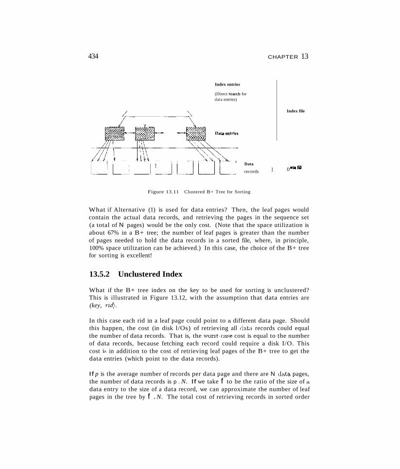
434
Index entries
(Direct search fordata entries)
CHAPTER 13
Data
records
Index file
] D... ""
Figure 13.11 Clustered B+ Tree for Sorting
What if Alternative (1) is used for data entries? Then, the leaf pages wouldcontain the actual data records, and retrieving the pages in the sequence set(a total of N pages) would be the only cost. (Note that the space utilization isabout 67% in a B+ tree; the number of leaf pages is greater than the numberof pages needed to hold the data records in a sorted file, where, in principle,100% space utilization can be achieved.) In this case, the choice of the B+ treefor sorting is excellent!
13.5.2 Unclustered Index
What if the B+ tree index on the key to be used for sorting is unclustered?This is illustrated in Figure 13.12, with the assumption that data entries are(key, rid).
In this case each rid in a leaf page could point to a different data page. Shouldthis happen, the cost (in disk l/Os) of retrieving all data records could equalthe number of data records. That is, the worst~case cost is equal to the numberof data records, because fetching each record could require a disk I/O. Thiscost is in addition to the cost of retrieving leaf pages of the B+ tree to get thedata entries (which point to the data records).
If p is the average number of records per data page and there are N data pages,the number of data records is p . N. If we take f to be the ratio of the size of adata entry to the size of a data record, we can approximate the number of leafpages in the tree by f . N. The total cost of retrieving records in sorted order

E:c:temal So-rt'ing 435
/Index entries
(Direct search fordata entries)
Index file
Data
recordsJD.....,
Figure 13.12 Unclustered B+ Tree for Sorting
using an unclustered B+ tree is therefore (J + p) . N. Since f is usually 0.1 orsmaller and p is typically much larger than 10, p . N is a good approximation.
In practice, the cost may be somewhat less because some rids in a leaf pagelead to the same data page, and further, some pages are found in the bufferpool, thereby avoiding an I/O. Nonetheless, the usefulness of an unclusteredB+ tree index for sorted retrieval highly depends on the extent to which theorder of data entries corresponds and-·~this is just a matter of chance-to thephysical ordering of data records.
We illustrate the cost of sorting a file of records using external sorting and unclustered B+ tree indexes in Figure 13.13. The costs shown for the unclusteredindex are worst-case numbers, based on the approximate formula p . N. Forcomparison, note that the cost for a clustered index is approximately equal toN, the number of pages of data records.
I Sorting I p=l Ip= 10 r p= foo100 200 100 1000 10,0001000 2000 1000 10,000 100,00010,000 40,000 10,000 100,000 1,000,000100,000 600,000 100,000 1,000,000 10,000,0001,000,000 8,000,000 1,000,000 10,000,000 100,000,00010,000,000 80,000,000 10,000,000 100,000,000 1,000,000,000
Figure 13.13 Cost of External Sorting (13 = 1000, b = :32) versus Unclustered Index
436 CHAPTER 13
Keep in mind that p is likely to be doser to 100 and B is likely to be higherthan 1,000 in practice. The ratio of the cost of sorting versus the cost of usingan unclustered index is likely to be even 10\ver than indicated by Figure 13.13because the I/O for sorting is in 32-page buffer blocks, whereas the I/O for theundustered indexes is one page at a time. The value of p is determined by thepage size and the size of a data record; for p to be 10, with 4KB pages, theaverage data record size must be about 400 bytes. In practice, p is likely to begreater than 10.
For even modest file sizes, therefore, sorting by using an unclustered index isclearly inferior to external sorting. Indeed, even if we want to retrieve onlyabout 10--20% of the data records, for example, in response to a range querysuch as "Find all sailors whose rating is greater than 7," sorting the file mayprove to be more efficient than using an unclustered index!
13.6 REVIEW QUESTIONS
Answers to the review questions can be found in the listed sections.
II What database operations utilize sorting? (Section 13.1)
II Describe how the two-way merge sort algorithm can sort a file of arbitrarylength using only three main-memory pages at any time. Explain whata run is and how runs are created and merged. Discuss the cost of thealgorithm in terms of the number of passes and the I/O cost per pass.(Section 13.2)
II How does the general external merge SOT,t algorithm improve upon the twoway merge sort? Discuss the length of initial runs, and how memory isutilized in subsequent merging passes. Discuss the cost of the algorithm interms of the number of pa.'3ses and the I/O cost per pa.ss. (Section 13.3)
II Discuss the use of r'cplacement sort to increase the average length of initialruns and thereby reduce the number of runs to be merged. How does thisaffect the cost of external sorting? (Section 13.3.1)
III \\That is blocked I/O? Why is it cheaper to read a sequence of pages usingblocked I/O than to read them through several independent requests? Howdoes the use of blocking affect the external sorting algorithm, and how doesit change the cost formula'? (Section 13.4.1)
.. What is double buffering? \\That is the motivation for using it? (Section 13.4.2)
II If we want to sort a file and there is a B-1- tree with the same search key, wehave the option of retrieving records in order through the index. Compa.re
E:r:tcmal SOTt'ing 437
the cost of this approach to retrieving the records in random order and thensorting them. Consider both clustered and unclustered B+ trees. ~What
conclusions can you draw from your comparison? (Section 13.5)
EXERCISES
Exercise 13.1 Suppose you have a file with 10,000 pages and you have three buffer pages.Answer the following questions for each of these scenarios, assuming that our most generalexternal sorting algorithm is used:
(a) A file with 10,000 pages and three available buffer pages.
(b) A file with 20,000 pages and five available buffer pages.
(c) A file with 2,000,000 pages and 17 available buffer pages.
1. How many runs will you produce in the first pass?
2. How many passes will it take to sort the file completely?
3. What is the total I/O cost of sorting the file?
4. How many buffer pages do you need to sort the file completely in just two passes?
Exercise 13.2 Answer Exercise 13.1 assuming that a two-way external sort is used.
Exercise 13.3 Suppose that you just finished inserting several records into a heap file andnow want to sort those records. Assume that the DBMS uses external sort and makes efficientuse of the available buffer space when it sorts a file. Here is some potentially useful informationabout the newly loaded file and the DBMS software available to operate on it:
The number of records in the file is 4500. The sort key for the file is 4 bytes long.You can assume that rids are 8 bytes long and page ids are 4 bytes long. Eachrecord is a total of 48 bytes long. The page size is 512 bytes. Each page has 12bytes of control information on it. Four buffer pages are available.
1. How many sorted subfiles will there be after the initial pass of the sort, and how longwill each subtile be?
2. How many passes (including the initial pass just considered) are required to sort thisfile?
:3. What is the total I/O cost for sorting this file?
4. What is the largest file, in terms of the number of records, you can sort with just fourbuffer pages in two passes? How would your answer change if you had 257 buffer pages?
5. Suppose that you have a B+ tree index with the search key being the same as the desiredsort key. Find the cost of USiIlg the index to retrieve the records in sorted order for eachof the following cases:
lllI The index uses Alternative (1) for data entries.
lllI The index uses Alternative (2) and is unclustered. (You can compute the worst-casecost in this case.)
438
•
CHAPTER 1\3
How would the costs of using the index change if the file is the largest that youcan sort in two passes of external sort with 257 buffer pages? Give your answer forboth clustered and unclustered indexes.
Exercise 13.4 Consider a disk with an average seek time of lOms, average rotational delayof 5ms, and a transfer time of 1ms for a 41< page. Assume that the cost of reading/writinga page is the sum of these values (i.e., 16ms) unless a sequence of pages is read/written. Inthis case, the cost is the average seek time plus the average rotational delay (to find the firstpage in the sequence) plus 1ms per page (to transfer data). You are given 320 buffer pagesand asked to sort a file with 10,000,000 pages.
1. Why is it a bad idea to use the 320 pages to support virtual memory, that is, to 'new'10,000,000 41< bytes of memory, and to use an in-memory sorting algorithm such asQuicksort?
2. Assume that you begin by creating sorted runs of 320 pages each in the first pass.Evaluate the cost of the following approaches for the subsequent merging passes:
(a) Do 31g-way merges.
(b) Create 256 'input' buffers of 1 page each, create an 'output' buffer of 64 pages, anddo 256-way merges.
(c) Create 16 'input' buffers of 16 pages each, create an 'output' buffer of 64 pages,and do 16-way merges.
(d) Create eight 'input' buffers of 32 pages each, create an 'output' buffer of 64 pages,and do eight-way merges.
(e) Create four 'input' buffers of 64 pages each, create an 'output' buffer of 64 pages,and do four-way merges.
Exercise 13.5 Consider the refinement to the external sort algorithm that produces runs oflength 2B on average, where B is the number of buffer pages. This refinement was describedin Section 11.2.1 under the assumption that all records are the same size. Explain why thisassumption is required and extend the idea to cover the case of variable-length records.
PROJECT-BASED EXERCISES
Exercise 13.6 (Note to i,nstnu:t01'S: Add~t'ional deta'ils must be pmvided if this exercise isassigned; see Appendi:r: SO.) Implement external sorting in Minibase.
BIBLIOGRAPHIC NOTES
Knuth's text [442] is the classic reference for sorting algorithms. I\Jemory management forreplacement sort is discussed in [471]. A number of papers discuss parallel external sortingalgorithms, including [66, 71, 223,494, 566, 647].
14EVALUATING RELATIONAL
OPERATORS
... What are the alternative algorithms for selection? Which alternatives are best under different conditions? How are complex selectionconditions handled?
... How can we eliminate duplicates in projection? How do sorting andhashing approaches -compare?
... What are the alternative join evaluation algorithms? Which alternatives are best under different conditions?
... How are the set operations (union, inter;section, set-difference, crossproduct) implemented?
... How are aggregate operations and grouping handled?
... How does the size of the buffer pool and the buffer replacement policyaffect algorithms for evaluating relational operators?
.. Key concepts: selections, CNF; projections, sorting versus hashing; joins, block nested loops, index nested loops, sort-merge, hash;union, set-difference, duplicate elimination; aggregate operations, running information, partitioning into groups, using indexes; buffer management, concurrent execution, repeated access patterns
Now, 'here, you see, it takes all the running you can do, to keep in the sameplace. If you want to get somewhere else, you must run at least twice 3..<; fast asthat!
-----Lewis Carroll, Throngh the Looking Glass
439
440 CHAPTER 14
In this chapter, we consider the implementation of individual relational operators in sufficient detail to understand how DBMSs are implemented. Thediscussion builds on the foundation laid in Chapter 12. vVe present implementation alternatives for the selection operator in Sections 14.1 and 14.2. It isinstructive to see the variety of alternatives and the wide variation in per'formanee of these alternatives, for even such a simple operator. In Section 14.:3,we consider the other unary operator in relational algebra, projection.
\iVe then discuss the implementation of binary operators, beginning with joinsin Section 14.4. Joins are among the most expensive operators in a relationaldatabase system, and their implementation has a big impact on performance.After discussing the join operator, we consider implementation of the binaryoperators cross-product, intersection, union, and set-difference in Section 14.5.We discuss the implementation of grouping and aggregate operators, which areextensions of relational algebra, in Section 14.6. We conclude with a discussionof how buffer management affects operator evaluation costs in Section 14.7.
The discussion of each operator is largely independent of the discussion of otheroperators. Several alternative implementation techniques are presented for eachoperator; the reader who wishes to cover this material ill less depth can skipsome of these alternatives without loss of continuity.
Preliminaries: Examples and Cost Calculations
We present a number of example queries using the same schema as in Chapter12:
Sailors(sid: integer, sname: string, rating: integer, age: real)ReservesC'iid: ~_nteger, bid: integer, day: dates, rname: string)
This schema is a variant of the one that we used in Chapter 5; we added astring field rname to Reserves. Intuitively, this field is the name of the personwho made the reservation (and may be different from the name of the sailor .sidfor whom the reservation wa." made; a reservation may be made by a personwho is not a sailor on behalf of a sailor). The addition of this field gives usmore flexibility in choosing illustrative examples. We assume that each tupleof Reserves is 40 bytes lOllg, that a page can hold 100 Reserves tuples, alldthat we have 1000 pages of such tuples. Similarly, we assume that each tupleof Sailors is 50 bytes long, that a page can hold 80 Sailors tuples, and that wehave 500 pages of such tuples.
Two points must be kept in Inind to understancl our discussion of costs:
Eval1wting Relational Operator" 441
• As discussed in Chapter 8, we consider only I/O costs and measure I/Ocost in terms of the number of page l/Os. vVe also use big-O notation toexpress the complexity of an algorithm in terms of an input parameter mIdassume that the reader is familiar with this notation. For example, thecost of a file scan is O(Jlv1), where Ai is the size of the file.
• vVe discuss several alternate algorithms for each operation. Since eachalternative incurs the same cost in writing out the result, should this benecessary, we uniformly ignore this cost in comparing alternatives.
14.1 THE SELECTION OPERATION
In this section, we describe various algorithms to evaluate the selection operator. To motivate the discussion, consider the selection query shown in Figure14.1, which has the selection condition rno:me='Joe'.
SELECT *FROM Reserves RWHERE R.rname='Joe'
Figure 14.1 Simple Selection Query
We can evaluate this query by scanning the entire relation, checking the condition on each tuple, and adding the tuple to the result if the condition is satisfied.The cost of this approach is 1000 l/Os, since Reserves contains 1000 pages. Ifonly a few tuples have rnarne= 'Joe', this approach is expensive because it doesnot utilize the selection to reduce the number of tuples retrieved in any way.How can we improve on this approach? The key is to utilize information in theselection condition and use an index if a suitable index is available. For example, a B+ tree index on 'marne could be used to answer this query considerablyfaster, but an index on bid would not be useful.
In the rest of this section. we consider various situations with respect to the fileorganization used for the relation and the availability of indexes and discussappropriate algorithms for the selection operation. We discuss only simpleselection operations of the form eJR.attr op lw!ue(R) until Section 14.2, wherewe consider general selections. In terms of the general techniques listed inSection 12.2~ the algorithms for selection use either iteration or indexing.
14.1.1 No Index, Unsorted Data
Given a selection of the form eJRattT op value (R), if there is no index on R. attT
and R is not sorted on R. aUT, we have to scan the entire relation. Therefore,
442 CHAPTER 14,
the most selective access path is a file scan. For each tuple, we must test thecondition R.attr op vaz'ue and add the tuple to the result if the condition issatisfied.
14.1.2 No Index, Sorted Data
Given a selection of the form O'R.attr op value(R), if there is no index on R.attr,but R is physically sorted on R.attr, we can utilize the sort order by doinga binary search to locate the first tuple that satisfies the selection condition.Further, we can then retrieve all tuples that satisfy the selection conditionby starting at this location and scanning R until the selection condition isno longer satisfied. The access method in this case is a sorted-file scan withselection condition O'R.attr op value(R).
For example, suppose that the selection condition is R.aUr! > 5, and that R issorted on attr1 in ascending order. After a binary search to locate the positionin R corresponding to 5, we simply scan all remaining records.
The cost of the binary search is O(l092M). In addition, we have the cost of thescan to retrieve qualifying tuples. The cost of the scan depends on the numberof such tuples and can vary from zero to M. In our selection from Reserves(Figure 14.1), the cost of the binary search is [0921000 ~ 10 I/Os.
In practice, it is unlikely that a relation will be kept sorted if the DBMS supports Alternative (1) for index data entries; that is, allows data records to bestored as index data entries. If the ordering of data records is important, abetter way to maintain it is through a B+ tree index that uses Alternative (1).
14.1.3 B+ Tree Index
If a clustereel B+ tree index is available on R.attr, the best strategy for selectionconditions O'R.attr op value(R) in which op is not equality is to use the index.This strategy is also a good access path for equality selections, although a hashindex on R.attr would be a little better. If the B+ tree index is not clustered,the cost of using the index depends on the number of tuples that satisfy theselection, as discussed later.
We can use the index as follows: We search the tree to find the first indexentry that points to a qualifying tuple of R. Then we scan the leaf pages of theindex to retrieve all entries in which the key value satisfies the selection condition. For each of these entries, we retrieve the corresponding tuple of R. (forconcreteness in this discussion, we a.<;sume that data entries use Alternatives(2) or (3); if Alternative (1) is used, the data entry contains the actual tuple
Evaluating Relational OpemtoTs 443
and there is no additional cost~beyond the cost of retrieving data entries-cforretrieving tuples.)
The cost of identifying the starting leaf page for the scan is typically two orthree I/Os. The cost of scanning the leaf level page for qualifying data entriesdepends on the number of such entries. The cost of retrieving qualifying tuplesfrom R depends on two factors:
• The number of qualifying tuples.
• Whether the index is clustered. (Clustered and unclustered B+ tree indexesare illustrated in Figures 13.11 and 13.12. The figures should give thereader a feel for the impact of clustering, regardless of the type of indexinvolved.)
If the index is clustered, the cost of retrieving qualifying tuples is probablyjust one page I/O (since it is likely that all such tuples are contained in asingle page). If the index is not clustered, each index entry could point to aqualifying tuple on a different page, and the cost of retrieving qualifying tuplesin a straightforward way could be one page I/O per qualifying tuple (unless weget lucky with buffering). We can significantly reduce the number of I/Os toretrieve qualifying tuples from R by first sorting the rids (in the index's dataentries) by their page-id component. This sort ensures that, when we bring ina page of R, all qualifying tuples on this page are retrieved one after the other.The cost of retrieving qualifying tuples is now the number of pages of R thatcontain qualifying tuples.
Consider a selection of the form rnarne < 'C%' on the Reserves relation. Assuming that names are uniformly distributed with respect to the initial letter,for simplicity, we estimate that roughly 10% of Reserves tuples are in the result.This is a total of 10,000 tuples, or 100 pages. If we have a clustered B+ treeindex on the marne field of Reserves, we can retrieve the qualifying tuples with100 I/Os (plus a few I/Os to traverse from the root to the appropriate leaf pageto start the scan). However, if the index is unclustered, we could have up to10,000 I/Os in the worst case, since each tuple could cause us to read a page. Ifwe sort the rids of Reserves tuples by the page number and then retrieve pagesof Reserves, we avoid retrieving the same page multiple times; nonetheless, thetuples to be retrieved are likely to be scattered across many more than 100pages. Therefc)re, the use of an unclusterecl index for a range selection couldbe expensive; it might be cheaper to simply scan the entire relation (which islOOn pages in our example).
444 CHAPTER 14
14.1.4 Hash Index, Equality Selection
If a hash index is available on R.attr and op is equality, the best way to implement the selection CTR.attr opualue(R) is obviously to use the index to retrievequalifying tuples.
The cost includes a few (typically one or two) l/Os to retrieve the appropriatebucket page in the index, plus the cost of retrieving qualifying tuples fromR. The cost of retrieving qualifying tuples from R depends on the number ofsuch tuples and on whether the index is clustered. Since op is equality, thereis exactly one qualifying tuple if R.attr is a (candidate) key for the relation.Otherwise, we could have several tuples with the same value in this attribute.
Consider the selection in Figure 14.1. Suppose that there is an unclusteredhash index on the marne attribute, that we have 10 buffer pages, and that100 reservations were made by people named Joe. The cost of retrieving theindex page containing the rids of such reservations is one or two l/Os. The costof retrieving the 100 Reserves tuples can vary between 1 and 100, dependingon how these records are distributed across pages of Reserves and the orderin which we retrieve these records. If these 100 records are contained in, say,some five pages of Reserves, we have just five additional l/Os if we sort therids by their page component. Otherwise, it is possible that we bring in one ofthese five pages, then look at some of the other pages, and find that the firstpage has been paged out when we need it again. (Remember that several usersand DBMS operations share the buffer pool.) This situation could cause us toretrieve the same page several times.
14.2 GENERAL SELECTION CONDITIONS
In our discussion of the selection operation thus far, we have considered selection conditions of the form CT R.attr op vall1e (R). In general, a selection conditionis a Boolean combination (Le., an expression using the logical connectives 1\
and V) of terms that have the form attribute op constant or attributel opattrilmte2. For example, if the WHERE clause in the query shown in Figure 14.1contained the condition R.rnarne='Joe' AND R.bid=r, the equivalent algebraexpression would be CTR.rname='Joe'l\R.bid=r(R).
In Section 14.2.1, we provide a more rigorous definition of CNF, which weintroduced in Section 12.2.2. We consider algorithms for applying selectionconditions without disjunction in Section 14.2.2 and then discuss conditionswith disjunction in Section 14.2.3.
Evaluating Relaf'ional OpemtoT8
14.2.1 CNF and Index Matching
445
To process a selection operation with a general selection condition, we firstexpress the condition in conjunctive normal form (CNF), that is, &9 acollection of conjunets that are connected through the use of the 1\ operator.Each conjunct consists of one or more terms (of the form described previously)connected by V. 1 Conjuncts that contain V are said to be disjunctive or tocontain disjunction.
As an example, suppose that we have a selection on Reserves with the condition(day < 8/9/02 1\ r-rwme = 'Joe ') V bid=5 V sid=3. ",re can rewrite this inconjunctive normal form as (day < 8/9/02 V bid=5 V s'id=3) 1\ (marne ='Joe'V bid=5 V sid=3).
Vve discussed when an index matches a CNF selection in Section 12.2.2 and introduced selectivity of access paths. The reader is urged to review that mate~ial
now.
14.2.2 Evaluating Selections without Disjunction
When the selection does not contain disjunction, that is, it is a conjunction ofterms, we have two evaluation options to consider:
11II \iVe can retrieve tuples using a file scan or a single index that matchessome conjuncts (and which we estimate to be the most selective accesspath) and apply all nonprimary conjuncts in the selection to each retrievedtuple. This approach is very similar to how we use indexes for simpleselection conditions, and we do not discuss it further. (We emphasize thatthe number of tuples retrieved depends on the selectivity of the primaryconjuncts in the selection, and the remaining conjuncts only reduce thecardinality of the result of the selection.)
II We can try to utilize several indexes. vVe examine this approach in the restof this section.
If several indexes containing data entries with rids (i.e., Alternatives (2) or (3))match conjuncts in the selection, we can use these indexes to compute sets ofrids of candidate tuples. "1e can then intersect these sets of rids, typically byfirst sorting them, then retrieving those records whose rids are in the intersection. If additional conjuncts are present in the selection, we can apply theseconjuncts to discard some of the candidate tuples from the result.
1 Every selection conditioll Olfl be expressed in CNF. V·/e refer the reader to any standard text onmathematical logic for the details.
446 CHAPTER 14~
I--~-""""""""""""""""""""'-"-"'- •••••- ••~~~.. - .•........•...•..• _ .... ---_.•--S-.-, .....·····T·-:-.·I---__._---········.············.·.-..··.···--"'---T-
I Intersecting rid Sets: Oracle 8 uses several techniques to do rid set intersection for selections with .AND. One is to ANDbitIl1aps.Another is todo a hash join of.indexes. For example, gi,,811 sal <5/\ If'ice > 30 andindexes on sal and price, we can join the indexes on the ri(1 column1 considering only entries that satisfy the given selection conditions. MicrosoftSQL Server imPlements rid set intersection through index joins. IBN!.~p2implements intersection of rid sets using Bloom filters (\I,'hjch are disy~§§~d
in Section 22.10.2). Sybase ASE does not do rid set intersection for ANDselections; Sybase ASIQ does it using bitmap operations. Informix alsodoes rid set intersection.
As an example, given the condition day < 8/9/02 A bid=5 A sid=,'J, we canretrieve the rids of records that meet the condition day < 8/9/02 by using aB+ tree index on day, retrieve the rids of records that meet the condition sid=,'Jby using a hash index on sid, and intersect these two sets of rids. (If we sortthese sets by the page id component to do the intersection, a side benefit isthat the rids in the intersection are obtained in sorted order by the pages thatcontain the corresponding tuples, which ensures that we do not fetch the samepage twice while retrieving tuples using their rids.) We can now retrieve thenecessary pages of Reserves to retrieve tuples and check bid=5 to obtain tuplesthat meet the condition day < 8/9/02 A bid=5/\ sid=,'J.
14.2.3 Selections with Disjunction
Now let us consider that one of the conjuncts in the selection condition is adisjunction of terms. If even one of these terms requires a file scan becausesuitable indexes or sort orders are unavailable, testing this conjunct by itself(I.e., without taking advantage of other conjuncts) requires a file scan. Forexample, suppose that the only available indexes are a hash index on marneand a hash index on sid, and that the selection condition contains just the(disjunctive) conjunct (day < 8/9/02 V rnarne='Joe'). We can retrieve tuplessatisfying the condition marne= 'Joe' by using the index on rnarne. However,day < 8/9/02 requires a file scan. So we might as well do a file scan andcheck the condition marne= 'Joe' for each retrieved tuple. Therefore, the mostselective access path in this example is a file scan.
On the other hand, if the selection condition is (day < 8/9/02 V mame='Joe')A sid=,'J, the index on sid matches the conjunct sid=S. We can use this indexto find qualifying tuples and apply day < 8/9/02 V marne='Joe' to just thesetuples. The best access path in this example is the index on sid with theprimary conjunct sid=S.
Evaluating Relational Operators
Disjunctions: Microsoft SQL Server considers the use of unions andbitmaps for dealing with disjunctive conditions. Oracle.8 considers fourways to handle disjunctive conditions: (1) Convert the query into a unionof queries without OR. (2) If the cOllditions involve the same attribute, suchas sal < 5 V sal > 30, use a nested query with an IN list and an index onthe attribute to retrieve tuples matching a valUe in the list. (3) Use bitmapoperations, e.g., evaluate sal <5 V sal> 30 by generating bitmaps for thevalues 5. and 30 and OR the bitmaps to find the tuples that satisfy one ofthe conditions. (We discuss bitmaps in Chapter 25.) (4) Simply apply thedisjunctive condition as a filter on the set of retrieved tuples. Syba.'3e ASEconsiders the use of unions for dealing with disjunctive queries and SybaseASIQ uses bitmap operations.
Finally, if every term in a disjunction has a matching index, we can retrievecandidate tuples using the indexes and then take the union. For example, if theselection condition is the conjunct (day < 8/9/02 V rname='Joe') and we haveB+ tree indexes on day and rname, we can retrieve all tuples such that day <8/9/02 using the index on day, retrieve all tuples such that rname= 'Joe' usingthe index on rname, and then take the union of the retrieved tuples. If all thematching indexes use Alternative (2) or (3) for data entries, a better approachis to take the union of rids and sort them before retrieving the qualifying datarecords. Thus, in the example, we can find rids of tuples such that day <8/9/02 using the index on day, find rids of tuples such that rname= 'Joe' usingthe index on rname, take the union of these sets of rids and sort them by pagenumber, and then retrieve the actual tuples from Reserves. This strategy canbe thought of as a (complex) access path that matches the selection condition(day < 8/9/02 V rname='Joe').
Most current systems do not handle selection conditions with disjunction efficiently and concentrate on optimizing selections without disjunction.
14.3 THE PROJECTION OPERATION
Consider the query shown in Figure 14.2. The optimizer translates this queryinto the relational algebra expression 7rsid,bidReserves. In general the projectionoperator is of the form 7rattTl,attr2, ... ,attrm (R). To implement projection, we have
SELECT DISTINCT R.sid, R.bidFROM Reserves R
Figure 14.2 Simple Projection Query

448
to do the following:
CHAPTER l4
1. Remove unwanted attributes (i.e., those not specified in the projection).
2. Eliminate any duplicate tuples produced.
The second step is the difficult one. There are two basic algorithms, one basedon sorting and one based on hashing. In terms of the general techniques listed inSection 12.2, both algorithms are instances of partitioning. While the techniqueof using an index to identify a subset of useful tuples is not applicable forprojection, the sorting or hashing algorithms can be applied to data entriesin an index, instead of to data records, under certain conditions described inSection 14.3.4.
14.3.1 Projection Based on Sorting
The algorithm based on sorting has the following steps (at least conceptually):
1. Scan R and produce a set of tuples that contain only the desired attributes.
2. Sort this set of tuples using the combination of all its attributes as the keyfor sorting.
3. Scan the sorted result, comparing adjacent tuples, and discard duplicates.
If we use temporary relations at each step, the first step costs IvI l/Os to scanR, where 111 is the number of pages of R, and T l/Os to write the temporaryrelation, where T is the number of pages of the temporary; T is a (J'v1). (Theexact value of T depends on the number of fields retained and the sizes of thesefields.) The second step costs O(TlogT) (which is also 0(MlogA1), of course).The final step costs T. The total cost is O(II;flogIvI). The first and third stepsare straightforward and relatively inexpensive. (As noted in the chapter onsorting, the cost of sorting grows linearly with data..<;et size in practice, giventypical data"iet sizes and main memory sizes.)
Consider the projection on Reserves shown in Figure 14.2. \iVe can scall Reserves at a cos,t of 1000 I/Os. If we assume that each tuple in the temporaryrelation created in the first step is 10 bytes long, the cost of writing this temporary relation is 250 l/Os. Suppose we have 20 buffer pages. \Ve um sort thetemporary relation in two pa"ises at a cost of 2 . 2 . 250 = 1000 l/Os. The scanrequired in the third step costs an additional 250 I/Os. The total cost is 2500l/Os.
Evaluat'ing Relational Operator's 449
This approach can be improved on by modifying the sorting algorithm to doprojection with duplicate elimination. Recall the structure of the external sorting algorithm presented in Chapter 13. The very first pass (Pass 0) involvesa scan of the records that are to be sorted to produce the initial set of (internally) sorted runs. Subsequently, one or more passes merge runs. Twoimportant modifications to the sorting algorithm adapt it for projection:
• 'We can project out unwanted attributes during the first pass (Pass 0) ofsorting. If B buffer pages are available, we can read in B pages of Randwrite out (T/!vI) . B internally sorted pages of the temporary relation. Infact, with a more aggressive implementation, we can write out approximately 2 . B internally sorted pages of the temporary relation on average.(The idea is similar to the refinement of external sorting discussed in Section 13.3.1.)
• We can eliminate duplicates during the merging passes. In fact, this modification reduces the cost of the merging passes since fewer tuples are writtenout in each pa.'3S. (Most of the duplicates are eliminated in the very firstmerging pass.)
Let us consider our example again. In the first pass we scan Reserves, at a costof 1000 I/Os and write out 250 pages. With 20 buffer pages, the 250 pagesare written out as seven internally sorted runs, each (except the last) about 40pages long. In the second pass we read the runs, at a cost of 250 I/Os, andmerge them. The total cost is 1,500 I/Os, which is much lower than the costof the first approach used to implement projection.
14.3.2 Projection Based on Hashing
If we have a fairly large number (say, B) of buffer pages relative to the numberof pages of R, a hash-based approach is worth considering. There are twophases: partitioning and duplicate elimination.
In the partitioning phase, we have one input buffer page and B-1 output bufferpages. The relation R is read into the input buffer page, one page at a time.The input page is processed a.'3 follows: For each tuple, we project out theunwanted attributes and then apply a hash function h to the combination ofall remaining.attributes. The function h is chosen so that tuples are distributeduniformly to one of B-1 partitions; there is one output page per partition.After the projection the tuple is written to the output buffer page that it ishashed to by h.
At the end of the partitioning phase, we have B-1 partitions, each of whichcontains a collection of tuples that share a common hash value (computed by
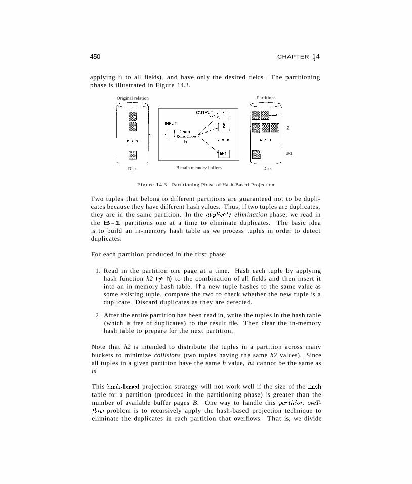
450 CHAPTER 14,
applying h to all fields), and have only the desired fields. The partitioningphase is illustrated in Figure 14.3.
Original relation
Disk B main memory buffers
Partitions
Disk
2
B-1
Figure 14.3 Partitioning Phase of Hash-Based Projection
Two tuples that belong to different partitions are guaranteed not to be duplicates because they have different hash values. Thus, if two tuples are duplicates,they are in the same partition. In the duplicate elimination phase, we read inthe B-1 partitions one at a time to eliminate duplicates. The basic ideais to build an in-memory hash table as we process tuples in order to detectduplicates.
For each partition produced in the first phase:
1. Read in the partition one page at a time. Hash each tuple by applyinghash function h2 (1= h) to the combination of all fields and then insert itinto an in-memory hash table. If a new tuple hashes to the same value assome existing tuple, compare the two to check whether the new tuple is aduplicate. Discard duplicates as they are detected.
2. After the entire partition has been read in, write the tuples in the hash table(which is free of duplicates) to the result file. Then clear the in-memoryhash table to prepare for the next partition.
Note that h2 is intended to distribute the tuples in a partition across manybuckets to minimize collisions (two tuples having the same h2 values). Sinceall tuples in a given partition have the same h value, h2 cannot be the same ash!
This ha.'3h-based projection strategy will not work well if the size of the ha.'3htable for a partition (produced in the partitioning phase) is greater than thenumber of available buffer pages B. One way to handle this paTtit'ion oveTflow problem is to recursively apply the hash-based projection technique toeliminate the duplicates in each partition that overflows. That is, we divide
Evaluating Relational Operators 451
an overflowing partition into subpartitions, then read each subpartition intomemory to eliminate duplicates.
If we assume that h distributes the tuples with perfect uniformity and that thenumber of pages of tuples after the projection (but before duplicate elimination)is T, each partition contains B~l pages. (Note that the number of partitionsis B-1 because one of the buffer pages is used to read in the relation duringthe partitioning phase.) The size of a partition is therefore B~l' and the size
of a hash table for a partition is B~l . f; where f is a fudge factor used tocapture the (small) increase in size between the partition and a hash table forthe partition. The number of buffer pages B must be greater than the partitionsize B~l . f to avoid partition overflow. This observation implies that we requireapproximately B > j"J-:r buffer pages.
Now let us consider the cost of hash-based projection. In the partitioningphase, we read R, at a cost of M I/Os. We also write out the projected tuples,a total of T pages, where T is some fraction of M, depending on the fields thatare projected out. The cost of this phase is therefore M +T l/Os; the cost ofhashing is a CPU cost, and we do not take it into account. In the duplicateelimination phase, we have to read in every partition. The total number ofpages in all partitions is T. We also write out the in-memory hash table foreach partition after duplicate elimination; this hash table is part of the resultof the projection, and we ignore the cost of writing out result tuples, as usual.Thus, the total cost of both phases is M + 2T. In our projection on Reserves(Figure 14.2), this cost is 1000 + 2 . 250 = 1500 l/Os.
14.3.3 Sorting Versus Hashing for Projections
The sorting-based approach is superior to hashing if we have many duplicatesor if the distribution of (hash) values is very nonuniform. In this case, somepartitions could be much larger than average, and a hash table for such a partition would not fit in memory during the duplicate elimination phase. Also,a useful side effect of using the sorting-based approach is that the result issorted. Further, since external sorting is required for a variety of reasons, mostdatabase systems have a sorting utility, which can be used to implement projection relatively easily. For these rea..-;ons, sorting is the standard approachfor projection. And perhaps due to a simplistic use of the sorting utility, unwanted attribute removal and duplicate elimination are separate steps in manysystems (i.e., the basic sorting algorithm is often used without the refinementswe outlined).
We observe that, if we have B > IT buffer pages, where T is the size ofthe projected relation before duplicate elimination, both approaches have the
452
I--~--~"-
CHAPTER 1~
Projection in Commercial Systems: InfotmLxuses hashing. IBMDB2,Oracle 8, and Sybase ASE use sorting. Microsoft SQL Server and SybaseASIQ implement both hash-based and sort-based algorithms.
same I/O cost. Sorting takes two passes. In the first pass, we read AI pagesof the original relation and write out T pages. In the second pa<;s, we readthe T pages and output the result of the projection. Using hashing, in thepartitioning pha<;e, we read M pages and write T pages' worth of partitions.In the second phase, we read T pages and output the result of the projection.Thus, considerations such as CPU costs, desirability of sorted order in theresult, and skew in the distribution of values drive the choice of projectionmethod.
14.3.4 Use of Indexes for Projections
Neither the hashing nor the sorting approach utilizes any existing indexes.An existing index is useful if the key includes all the attributes we wish toretain in the projection. In this case, we can simply retrieve the key valuesfrom the index-without ever accessing the actual relation-and apply ourprojection techniques to this (much smaller) set of pages. This technique,called an index-only scan, and wa<; discussed in Sections 8.5.2 and 12.3.2. Ifwe have an ordered (i.e., a tree) index whose search key includes the wantedattributes as a prefix, we can do even better: Just retrieve the data entriesin order, discarding unwanted fields, and compare adjacent entries to checkfor duplicates. The index-only scan technique is discussed further in Section15.4.1.
14.4 THE JOIN OPERATION
Consider the following query:
SELECT *FROM Reserves R, Sailors SWHERE R.sid = S.sid
This query can be expressed in relational algebra using the join operation:R [Xl S. The join operation, one of the most useful operations in relationalalgebra, is the primary means of combining information from two or morerelations.
Evaluating Relational OpemtoTs 453
,------------------_._.__._.._._ ..__ __ _ _ _-_._----_._._--_ _-----------,
Joins in Commercial Systems: Syba..<;eASE suppodsindex nested loopand sort-merge join. Sybase ASIQ supports page-oriented nested loop, index nested loop, simple hash, and sort-merge join, in addition to join indexes (which we discuss in Chapter 25). Ol'acle8stippoitspage-orientednested loops join, sort-merge join, and a variant of hybrid hash join. IBMDB2 supports block nested loop, sort-merge, and hybrid hash join. Microsoft SQL Server supports block nested loops, index' nested loops, 80rtmerge, hash join, and a technique called ha.sh team.s. Informix supportsblock nested loops, index nested loops, and hybrid hash join.
Although a join can be defined as a cross-product followed by selections and projections, joins arise much more frequently in practice than plain cross-products.Further, the result of a cross-product is typically much larger than the result ofa join, so it is very important to recognize joins and implement them withoutmaterializing the underlying cross-product. Joins have therefore received a lotof attention.
We now consider several alternative techniques for implementing joins. Webegin by discussing two algorithms (simple nested loops and block nested loops)that essentially enumerate all tuples in the cross-product and discard tuplesthat do not meet the join conditions. These algorithms are instances of thesimple iteration technique mentioned in Section 12.2.
The remaining join algorithms avoid enumerating the cross-product. Theyare instances of the indexing and partitioning techniques mentioned in Section12.2. Intuitively, if the join condition consists of equalities, tuples in the tworelations can be thought of &'3 belonging to partitions, such that only tuples inthe same partition can join with each other; the tuples in a partition containthe same values in the join columns. Index nested loops join scans one of therelations and, for each tuple in it, uses an index on the (join columns of the)second relation to locate tuples in the same partition. Thus, only a subset ofthe second relation is compared with a given tuple of the first relation, and theentire cross-product is not enumerated. The last two algorithms (sort-mergejoin and hash join) also take advantage of join conditions to partition tuples inthe relations to be joined and compare only tuples in the same partition whilecomputing the join, but they do not rely on a pre-existing index. Instead, theyeither sort or hash the relations to be joined to achieve the partitioning.
We discuss the join of two relations Rand S, with the join condition R i = Sj,using positional notation. (If we have more complex join conditions, the basicidea behind each algorithm remains essentially the same. \Ve discuss the detailsin Section 14.4.4.) vVe assmne AI pages in R with PI? tuples per page and N
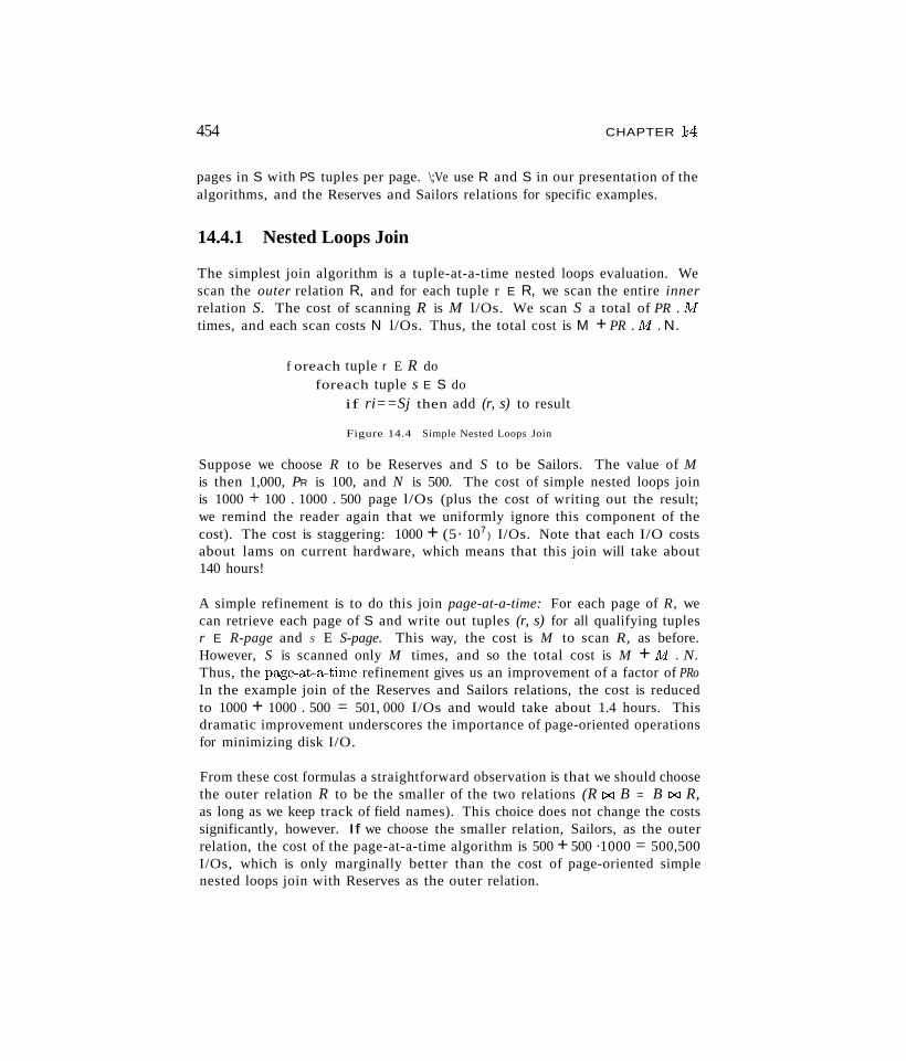
454 CHAPTER 14
pages in S with PS tuples per page. \;Ve use R and S in our presentation of thealgorithms, and the Reserves and Sailors relations for specific examples.
14.4.1 Nested Loops Join
The simplest join algorithm is a tuple-at-a-time nested loops evaluation. Wescan the outer relation R, and for each tuple r E R, we scan the entire innerrelation S. The cost of scanning R is M l/Os. We scan S a total of PR . Iv!times, and each scan costs N l/Os. Thus, the total cost is M + PR . Iv! . N.
f oreach tuple r E R doforeach tuple s E S do
if ri==Sj then add (r, s) to result
Figure 14.4 Simple Nested Loops Join
Suppose we choose R to be Reserves and S to be Sailors. The value of Mis then 1,000, PR is 100, and N is 500. The cost of simple nested loops joinis 1000 + 100 . 1000 . 500 page l/Os (plus the cost of writing out the result;we remind the reader again that we uniformly ignore this component of thecost). The cost is staggering: 1000 + (5· 107
) I/Os. Note that each I/O costsabout lams on current hardware, which means that this join will take about140 hours!
A simple refinement is to do this join page-at-a-time: For each page of R, wecan retrieve each page of S and write out tuples (r, s) for all qualifying tuplesr E R-page and S E S-page. This way, the cost is M to scan R, as before.However, S is scanned only M times, and so the total cost is M + Iv! . N.Thus, the page-at-a-time refinement gives us an improvement of a factor of PRoIn the example join of the Reserves and Sailors relations, the cost is reducedto 1000 + 1000 . 500 = 501, 000 I/Os and would take about 1.4 hours. Thisdramatic improvement underscores the importance of page-oriented operationsfor minimizing disk I/O.
From these cost formulas a straightforward observation is that we should choosethe outer relation R to be the smaller of the two relations (R [XJ B = B [XJ R,as long as we keep track of field names). This choice does not change the costssignificantly, however. If we choose the smaller relation, Sailors, as the outerrelation, the cost of the page-at-a-time algorithm is 500 + 500 ·1000 = 500,500I/Os, which is only marginally better than the cost of page-oriented simplenested loops join with Reserves as the outer relation.
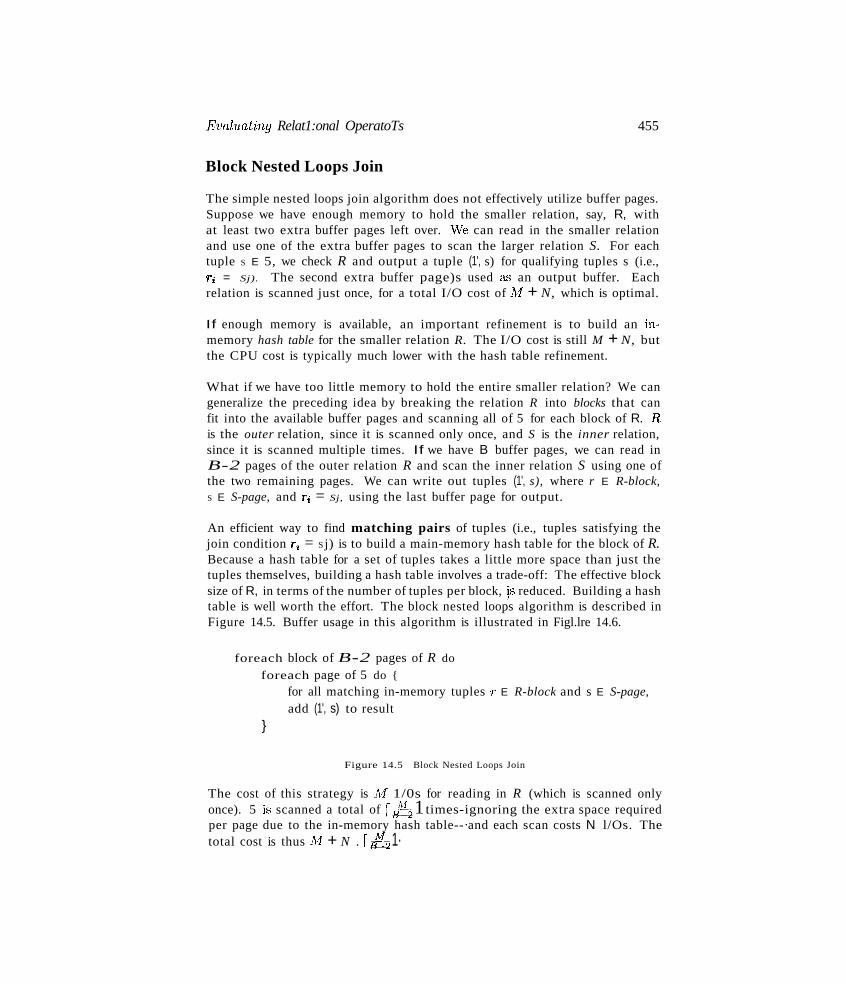
EvahLating Relat1:onal OperatoTs
Block Nested Loops Join
455
The simple nested loops join algorithm does not effectively utilize buffer pages.Suppose we have enough memory to hold the smaller relation, say, R, withat least two extra buffer pages left over. \Ve can read in the smaller relationand use one of the extra buffer pages to scan the larger relation S. For eachtuple S E 5, we check R and output a tuple (1', s) for qualifying tuples s (i.e.,ri = Sj). The second extra buffer page)s used as an output buffer. Eachrelation is scanned just once, for a total I/O cost of 1\1 + N, which is optimal.
If enough memory is available, an important refinement is to build an inmemory hash table for the smaller relation R. The I/O cost is still M + N, butthe CPU cost is typically much lower with the hash table refinement.
What if we have too little memory to hold the entire smaller relation? We cangeneralize the preceding idea by breaking the relation R into blocks that canfit into the available buffer pages and scanning all of 5 for each block of R. Ris the outer relation, since it is scanned only once, and S is the inner relation,since it is scanned multiple times. If we have B buffer pages, we can read inB-2 pages of the outer relation R and scan the inner relation S using one ofthe two remaining pages. We can write out tuples (1', s), where r E R-block,S E S-page, and ri = Sj, using the last buffer page for output.
An efficient way to find matching pairs of tuples (i.e., tuples satisfying thejoin condition ri = Sj) is to build a main-memory hash table for the block of R.Because a hash table for a set of tuples takes a little more space than just thetuples themselves, building a hash table involves a trade-off: The effective blocksize of R, in terms of the number of tuples per block, ~s reduced. Building a hashtable is well worth the effort. The block nested loops algorithm is described inFigure 14.5. Buffer usage in this algorithm is illustrated in Figl.lre 14.6.
foreach block of B-2 pages of R do
foreach page of 5 do {
for all matching in-memory tuples T E R-block and s E S-page,add (1', s) to result
}
Figure 14.5 Block Nested Loops Join
The cost of this strategy is !vI 1/0s for reading in R (which is scanned onlyonce). 5 is scanned a total of r:~21times-ignoring the extra space requiredper page due to the in-memory hash table--·and each scan costs N l/Os. Thetotal cost is thus I\1J + N . rrf!2 1·
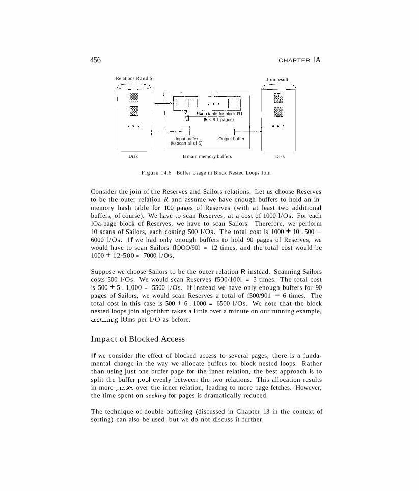
456 CHAPTER lA
Join result
~- =:::>
~ ~ ~
r=... ."
···-+iQD ~~-~~I l,-~Sh table for block R I
J (k < B-1 pages)
f-------j-,=O D~Input buffer Output buffer
(to scan all of S)
~ ~ ~
Relations Rand S
r==--~:)'
I
Disk B main memory buffers Disk
Figure 14.6 Buffer Usage in Block Nested Loops Join
Consider the join of the Reserves and Sailors relations. Let us choose Reservesto be the outer relation R and assume we have enough buffers to hold an inmemory hash table for 100 pages of Reserves (with at least two additionalbuffers, of course). We have to scan Reserves, at a cost of 1000 l/Os. For eachlOa-page block of Reserves, we have to scan Sailors. Therefore, we perform10 scans of Sailors, each costing 500 l/Os. The total cost is 1000 + 10 . 500 =6000 l/Os. If we had only enough buffers to hold 90 pages of Reserves, wewould have to scan Sailors flOOO/90l = 12 times, and the total cost would be1000 + 12·500 = 7000 l/Os,
Suppose we choose Sailors to be the outer relation R instead. Scanning Sailorscosts 500 l/Os. We would scan Reserves f500/100l = 5 times. The total costis 500 + 5 . 1,000 = 5500 l/Os. If instead we have only enough buffers for 90pages of Sailors, we would scan Reserves a total of f500/901 = 6 times. Thetotal cost in this case is 500 + 6 . 1000 = 6500 l/Os. We note that the blocknested loops join algorithm takes a little over a minute on our running example,a.ssuming lOms per I/O as before.
Impact of Blocked Access
If we consider the effect of blocked access to several pages, there is a fundamental change in the way we allocate buffers for block nested loops. Ratherthan using just one buffer page for the inner relation, the best approach is tosplit the buffer pool evenly between the two relations. This allocation resultsin more pa.sses over the inner relation, leading to more page fetches. However,the time spent on seeking for pages is dramatically reduced.
The technique of double buffering (discussed in Chapter 13 in the context ofsorting) can also be used, but we do not discuss it further.
Evaluating Relational Operators
Index Nested Loops Join
4.57
If there is an index on one of the relations on the join attribute(s), we can takeadvantage of the index by making the indexed relation be the inner relation.Suppose we have a suitable index on S; Figure 14.7 describes the index nestedloops join algorithm.
foreach tuple r E R do
foreach tuple s E S where ri == Sj
add (1', s) to result
Figure 14.7 Index Nested Loops Join
For each tuple T E R, we use the index to retrieve matching tuples of S.Intuitively, we compare r only with tuples of S that are in the same partition,in that they have the same value in the join column. Unlike the other nestedloops join algorithms, therefore, the index nested loops join algorithm does notenumerate the cross-product of Rand S. The cost of scanning R is M, asbefore. The cost of retrieving matching S tuples depends on the kind of indexand the number of matching tuples; for each R tuple, the cost is a..s follows:
1. If the index on S is a B+ tree index, the cost to find the appropriate leafis typically 2---4 l/Os. If the index is a hash index, the cost to find theappropriate bucket is 1-2 1/Os.
2. Once we find the appropriate leaf or bucket, the cost of retrieving matchingS tuples depends on whether the index is clustered. If it is, the cost perouter tuple r E R is typically just one more I/O. If it is not clustered, thecost could be one I/O per matching S-tuple (since each of these could beon a different page in the worst case).
As an example, suppose that we have a hash-based index using Alternative (2)on the sid attribute of Sailors and that it takes about 1.2 l/Os on average2
to retrieve the appropriate page of the index. Since sid is a key for Sailors,we have at most one matching tuple. Indeed, .sid in Reserves is a foreign keyreferring to Sailors, and therefore we have exactly one matching Sailors tuplefor each Reserves tuple. Let us consider the cost of scanning Reserves andusing the index to retrieve the matching Sailors tuple for each Reserves tuple.The cost of scanning Reserves is 1000. There are 100 . 1000 tuples in Reserves.For each of these tuples, retrieving the index page containing the rid of thematching Sailors tuple costs 1.2 l/Os (on average); in addition, we have toretrieve the Sailors page containing the qualifying tuple. Therefore, we have
2This is a typical cost for hash-ba.~ed indexes,
458 CHAPTER l~
100,000 ·(1 + 1.2) l/Os to retrieve matching Sailors tuples. The total cost is221,000 l/Os.
As another example, suppose that we have a hash-based index using Alternative(2) on the sid attribute of Reserves. Now we can scan Sailors (500 l/Os),and for each tuple, use the index to retrieve matching Reserves tuples. Wehave a total of 80 . 500 Sailors tuples, and each tuple could match with eitherzero or more Reserves tuples; a sailor may have no reservations or several.For each Sailors tuple, we can retrieve the index page containing the rids ofmatching Reserves tuples (assuming that we have at most one such index page,which is a reasonable guess) in 1.2 l/Os on average. The total cost thus far is500 + 40,000 . 1.2 = 48,500 l/Os.
In addition, we have the cost of retrieving matching Reserves tuples. Since wehave 100,000 reservations for 40,000 Sailors, assuming a uniform distributionwe can estimate that each Sailors tuple matches with 2.5 Reserves tuples onaverage. If the index on Reserves is clustered, and these matching tuples aretypically on the same page of Reserves for a given sailor, the cost of retrievingthem is just one I/O per Sailor tuple, which adds up to 40,000 extra l/Os.If the index is not clustered, each matching Reserves tuple may well be ona different page, leading to a total of 2.5 . 40,000 l/Os for retrieving qualifying tuples. Therefore, the total cost can vary from 48,500+40,000=88,500 to48,500+100,000=148,500 l/Os. Assuming 10ms per I/O, this would take about15 to 25 minutes.
So, even with an unclustered index, if the number of matching inner tuples foreach outer tuple is small (on average), the cost of the index nested loops joinalgorithm is likely to be much less than the cost of a simple nested loops join.
14.4.2 Sort-Merge Join
The basic idea behind the sort-merge join algorithm is to SOTt both relationson the join attribute and then look for qualifying tuples T E Rand s E Sby essentially TneTging the two relations. The sorting step groups all tupleswith the same value in the join column and thus makes it easy to identifypartitions, or groups of tuples with the same value, in the join column. Weexploit this partitioning by comparing the R tuples in a partition with only theS tuples in the same partition (rather than with all S tuples), thereby avoidingenumeration of the cross-product of Rand S. (This partition-ba.<-;ed approachworks only for equality join conditions.)
The external sorting algorithm discussed in Chapter 13 can be used to do thesorting, and of course, if a relation is already sorted on the join attribute, we
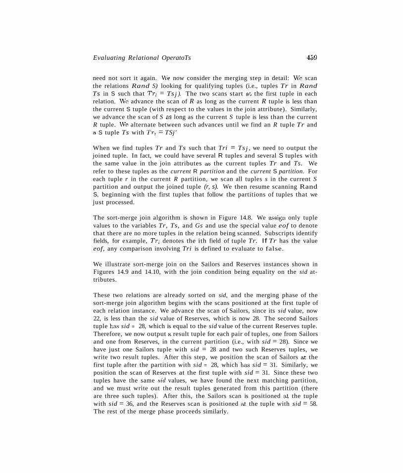
Evaluating Relational OperatoTs 4~9
need not sort it again. vVe now consider the merging step in detail: vVe scanthe relations Rand S) looking for qualifying tuples (i.e., tuples Tr in RandTs in S such that Tri = Ts j ). The two scans start at the first tuple in eachrelation. vVe advance the scan of R as long as the current R tuple is less thanthe current S tuple (with respect to the values in the join attribute). Similarly,we advance the scan of S as long as the current S tuple is less than the currentR tuple. \Ve alternate between such advances until we find an R tuple Tr anda S tuple Ts with Tri = TSj'
When we find tuples Tr and Ts such that Tri = Ts j , we need to output thejoined tuple. In fact, we could have several R tuples and several S tuples withthe same value in the join attributes as the current tuples Tr and Ts. Werefer to these tuples as the current R partition and the current S partition. Foreach tuple r in the current R partition, we scan all tuples s in the current Spartition and output the joined tuple (r, s). We then resume scanning RandS, beginning with the first tuples that follow the partitions of tuples that wejust processed.
The sort-merge join algorithm is shown in Figure 14.8. We assign only tuplevalues to the variables Tr, Ts, and Gs and use the special value eof to denotethat there are no more tuples in the relation being scanned. Subscripts identifyfields, for example, Tri denotes the ith field of tuple Tr. If Tr has the valueeof, any comparison involving Tri is defined to evaluate to false.
We illustrate sort-merge join on the Sailors and Reserves instances shown inFigures 14.9 and 14.10, with the join condition being equality on the sid attributes.
These two relations are already sorted on sid, and the merging phase of thesort-merge join algorithm begins with the scans positioned at the first tuple ofeach relation instance. We advance the scan of Sailors, since its sid value, now22, is less than the sid value of Reserves, which is now 28. The second Sailorstuple h&<; sid = 28, which is equal to the sid value of the current Reserves tuple.Therefore, we now output a result tuple for each pair of tuples, one from Sailorsand one from Reserves, in the current partition (i.e., with sid = 28). Since wehave just one Sailors tuple with sid = 28 and two such Reserves tuples, wewrite two result tuples. After this step, we position the scan of Sailors at thefirst tuple after the partition with sid = 28, which ha.<; sid = 31. Similarly, weposition the scan of Reserves at the first tuple with sid = 31. Since these twotuples have the same sid values, we have found the next matching partition,and we must write out the result tuples generated from this partition (thereare three such tuples). After this, the Sailors scan is positioned at the tuplewith sid = 36, and the Reserves scan is positioned at the tuple with sid = 58.The rest of the merge phase proceeds similarly.
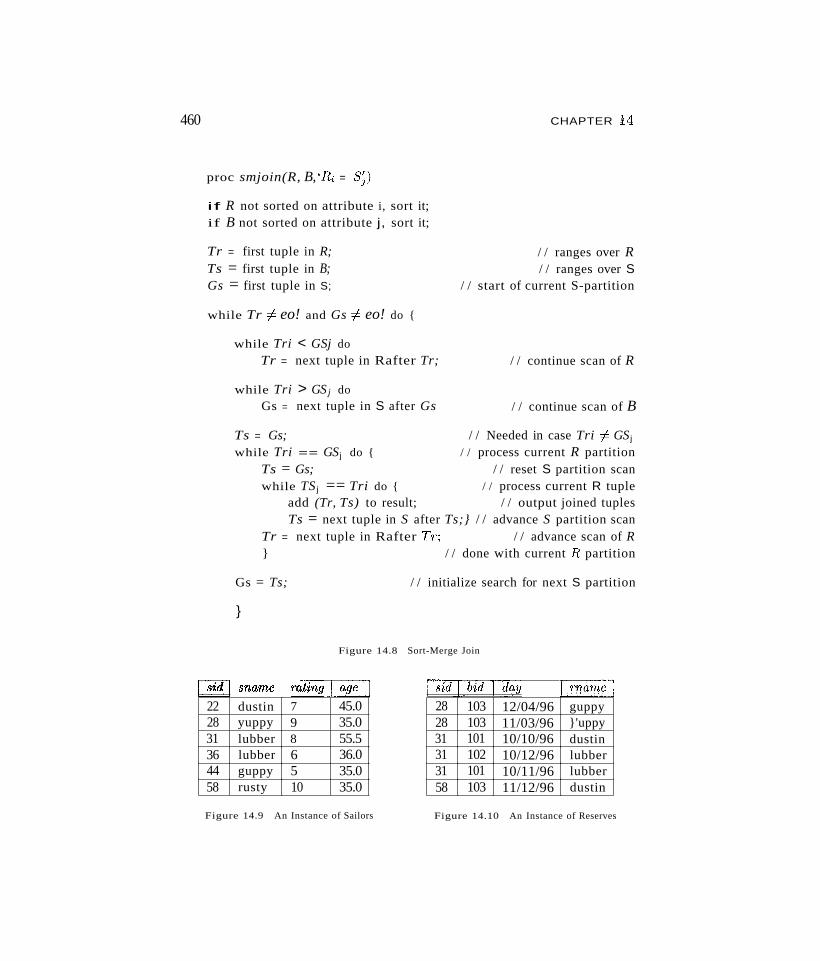
460 CHAPTER 14
proc smjoin(R, B, 'Hi = By)
if R not sorted on attribute i, sort it;if B not sorted on attribute j, sort it;
Tr = first tuple in R;Ts = first tuple in B;Gs = first tuple in S;
while Tr i= eo! and Gs -I=- eo! do {
while Tri < GSj do
Tr = next tuple in Rafter Tr;
while Tri > GSj do
Gs = next tuple in S after Gs
/ / ranges over R/ / ranges over S
/ / start of current S-partition
/ / continue scan of R
/ / continue scan of B
Ts = Gs; / / Needed in case Tri i= GS j
while Tri == GS j do { / / process current R partitionTs = Gs; / / reset S partition scanwhile TS j == Tri do { / / process current R tuple
add (Tr, Ts) to result; / / output joined tuplesTs = next tuple in S after Ts;} / / advance S partition scan
Tr = next tuple in Rafter Tr; / / advance scan of R} / / done with current R partition
Gs = Ts;
}
/ / initialize search for next S partition
Figure 14.8 Sort-Merge Join
~ snarrw mUng~ ~day
22 dustin 7 45.028 yuppy 9 35.031 lubber 8 55.536 lubber 6 36.044 guppy 5 35.058 rusty 10 35.0
Figure 14.9 An Instance of Sailors
28 103 12/04/96 guppy28 103 11/03/96 }'uppy31 101 10/10/96 dustin31 102 10/12/96 lubber31 101 10/11/96 lubber58 103 11/12/96 dustin
Figure 14.10 An Instance of Reserves
Evaluating Relational Operators ·161~
In general, we have to scan a partition of tuples in the second relation as oftenas the number of tuples in the corresponding partition in the first relation.The first relation in the example, Sailors, ha.', just one tuple in each partition.(This is not happenstance but a consequence of the fact that sid is a key~~~
this example is a key-foreign key join.) In contra."t, suppose that the joincondition is changed to be sname=7'name. Now, both relations contain morethan one tuple in the partition with sname=mame='lubber'. The tuples withrname= 'lubber' in Reserves have to be scanned for each Sailors tuple withsname='lubber'.
Cost of Sort~Merge Join
The cost of sorting R is O(/vlloglv1) ancl the cost of sorting S is O(NlogN).The cost of the merging phase is /vI + N if no S partition is scanned multipletimes (or the necessary pages are found in the buffer after the first pass). Thisapproach is especially attractive if at least one relation is already sorted on thejoin attribute or has a clustered index on the join attribute.
Consider the join of the relations Reserves and Sailors. Assuming that we have100 buffer pages (roughly the same number that we assumed were availablein our discussion of block nested loops join), we can sort Reserves in just twopasses. The first pass produces 10 internally sorted runs of 100 pages each.The second pass merges these 10 runs to produce the sorted relation. Becausewe read and write Reserves in each pass, the sorting cost is 2·2 . 1000 = 4000l/Os. Similarly, we can sort Sailors in two passes, at a cost of 2 . 2 . 500 = 2000l/Os. In addition, the seconcl phase of the sort-merge join algorithm requiresan additional scan of both relations. Thus the total cost is 4000 + 2000 +1000 + 500 = 7500 l/Os, which is similar to the cost of the block nested loopsalgorithm.
Suppose that we have only 35 buffer pages. \Ve can still sort both Reserves andSailors in two passes, and the cost of the sort-merge join algorithm remains at7500 l/Os. However, the cost of the block nested loops join algorithm is morethan 15,000 l/Os. On the other hand, if we have ~300 buffer pages, the costof the sort~merge join remains at 7500 I/Os, whereas the cost of the blocknested loops join drops to 2500 l/Os. (We leave it to the reader to verify thesenumbers. )
\Ve note that multiple scans of a partition of the second relation are potentiallyexpensive. In our example, if the number of Reserves tuples in a repeatedlyscanned partition is small (say, just a few pages), the likelihood of finding theentire partitiOli in the buffer pool on repeated scans is very high, and the I/Ocost remains essentially the same as for a single scan. However, if many pages
462 CHAPTER 14
of Reserves tuples are in a given partition, the first page of such a partitionmay no longer be in the buffer pool when we request it a second time (afterfirst scanning all pages in the partition; remember that each page is unpinneda'3 the scan moves past it). In this ca.se, the I/O cost could be as high as thenumber of pages in the Reserves partition times the number of tuples in thecorresponding Sailors partition!
In the worst-case scenario, the merging phase could require us to read thecomplete second relation for each tuple in the first relation, and the number ofl/Os is O(M . N) l/Os! (This scenario occurs when all tuples in both relationscontain the same value in the join attribute; it is extremely unlikely.)
In practice, the I/O cost of the merge phase is typically just a single scan ofeach relation. A single scan can be guaranteed if at least one of the relationsinvolved has no duplicates in the join attribute; this is the case, fortunately,for key~foreign key joins, which are very common.
A Refinement
We assumed that the two relations are sorted first and then merged in a distinctpass. It is possible to improve the sort-merge join algorithm by combining themerging phase of sorting with the merging phase of the join. First, we producesorted runs of size B for both Rand 5. If B > VI, where L is the size of thelarger relation, the number of runs per relation is less than VI. Suppose thatthe number of buffers available for the merging pha.<;e is at lea'3t 2 VI; thatis, more than the total number of runs for Rand 5. We allocate one bufferpage for each run of R and one for each run of 5. We then merge the runs ofR (to generate the sorted version of R), merge the runs of 5, and merge theresulting Rand 5 streams a'3 they are generated; we apply the join conditionas we merge the Rand S streams and discard tuples in the cross--product thatdo not meet the join condition.
Unfortunately, this idea increa<;es the number of buffers required to 2JI. However, by using the technique discussed in Section 13.3.1 we can produce sortedruns of size approximately 2· B for both Rand 5. Consequently, we have fewerthan VI/2 runs of each relation, given the assumption that B > VI. Thus,the total number of runs is less than VI, that is, less than B, and we cancombine the merging pha.ses with no need for additional buffers.
This approach allows us to perform a sort-merge join at the cost of reading andwriting Rand S in the first pa.ss and reading Rand 5 in the second pass. Thetotal cost is thus ~1 . (At + N). In our example, the cost goes down from 7500to 4500 l/Os.
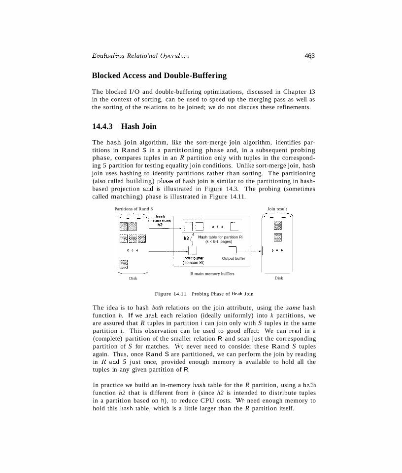
Evaluating Relatio'nal Operators 463}
Blocked Access and Double-Buffering
The blocked I/O and double-buffering optimizations, discussed in Chapter 13in the context of sorting, can be used to speed up the merging pass as well asthe sorting of the relations to be joined; we do not discuss these refinements.
14.4.3 Hash Join
The hash join algorithm, like the sort-merge join algorithm, identifies partitions in Rand S in a partitioning phase and, in a subsequent probingphase, compares tuples in an R partition only with tuples in the corresponding 5 partition for testing equality join conditions. Unlike sort-merge join, hashjoin uses hashing to identify partitions rather than sorting. The partitioning(also called building) pha.."Je of hash join is similar to the partitioning in hashbased projection and is illustrated in Figure 14.3. The probing (sometimescalled matching) phase is illustrated in Figure 14.11.
Disk
o 0 0
Output buffer
Hash table for partition Ri(k < B-1 pages)
B main memory bulTersDisk
Partitions of Rand S Join result
~
Figure 14.11 Probing Phase of Hash Join
The idea is to hash both relations on the join attribute, using the same hashfunction h. If we ha..'3h each relation (ideally uniformly) into k partitions, weare assured that R tuples in partition i can join only with S tuples in the samepartition i. This observation can be used to good effect: We can read in a(complete) partition of the smaller relation R and scan just the correspondingpartition of S for matches. \iVe never need to consider these Rand S tuplesagain. Thus, once Rand S are partitioned, we can perform the join by readingin Rand 5 just once, provided enough memory is available to hold all thetuples in any given partition of R.
In practice we build an in-memory hash table for the R partition, using a ha..'3hfunction h2 that is different from h (since h2 is intended to distribute tuplesin a partition based on h), to reduce CPU costs. \Ne need enough memory tohold this hash table, which is a little larger than the R partition itself.
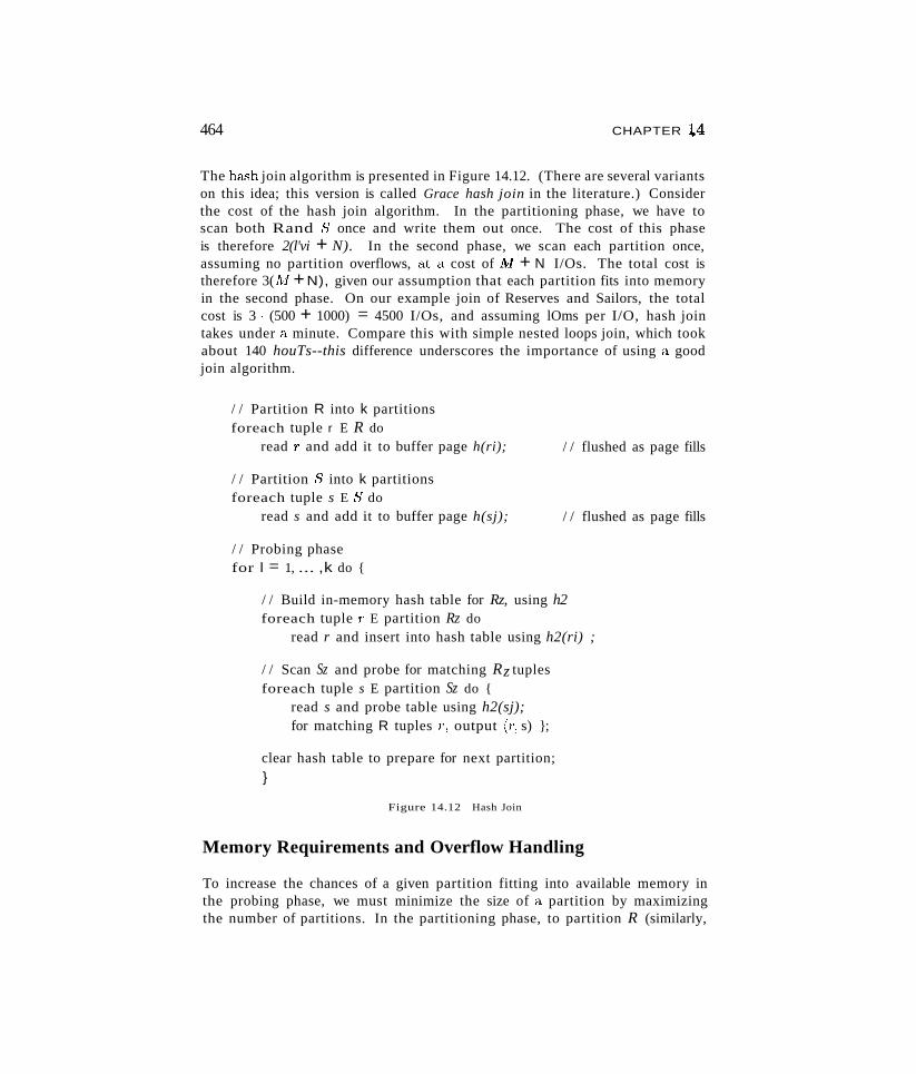
464 CHAPTER ~4
The hash join algorithm is presented in Figure 14.12. (There are several variantson this idea; this version is called Grace hash join in the literature.) Considerthe cost of the hash join algorithm. In the partitioning phase, we have toscan both Rand S once and write them out once. The cost of this phaseis therefore 2(l'vi + N). In the second phase, we scan each partition once,assuming no partition overflows, at a cost of .M + N I/Os. The total cost istherefore 3(AI + N), given our assumption that each partition fits into memoryin the second phase. On our example join of Reserves and Sailors, the totalcost is 3 . (500 + 1000) = 4500 I/Os, and assuming lOms per I/O, hash jointakes under a minute. Compare this with simple nested loops join, which tookabout 140 houTs--this difference underscores the importance of using a goodjoin algorithm.
/ / Partition R into k partitionsforeach tuple r E R do
read T and add it to buffer page h(ri);
/ / Partition S into k partitionsforeach tuple s E S do
read s and add it to buffer page h(sj);
/ / Probing phasefor I = 1, ... ,k do {
/ / flushed as page fills
/ / flushed as page fills
/ / Build in-memory hash table for Rz, using h2foreach tuple T E partition Rz do
read r and insert into hash table using h2(ri) ;
/ / Scan Sz and probe for matching Rz tuplesforeach tuple s E partition Sz do {
read s and probe table using h2(sj);for matching R tuples T, output (7', s) };
clear hash table to prepare for next partition;}
Figure 14.12 Hash Join
Memory Requirements and Overflow Handling
To increase the chances of a given partition fitting into available memory inthe probing phase, we must minimize the size of a partition by maximizingthe number of partitions. In the partitioning phase, to partition R (similarly,
Evaluating Relational Opera tOTS 465
8) into k partitions, we need at least k output buffers and one input buffer.Therefore, given B buffer pages, the maximum number of partitions is k =
B - 1. Assuming that partitions are equal in size, this means that the size ofeach R partition is t!l (a'3 usual, Ai is the number of pages of R). The numberof pages in the (in-memory) hash table built during the probing phase for apartition is thus ~'~'i, where f is a fudge factor used to capture the (small)increase in size between the partition and a hash table for the partition.
During the probing phase, in addition to the hash table for the R partition,we require a buffer page for scanning the 8 partition and an output buffer.Therefore, we require B > -k'~~ + 2. We need approximately B > J f . AI forthe hash join algorithm to perform well.
Since the partitions of R are likely to be close in size but not identical, thelargest partition is somewhat larger than t!l' and the number of buffer pages
required is a little more than B > J f . AI. There is also the risk that, if thehash function h does not partition R uniformly, the hash table for one or moreR partitions may not fit in memory during the probing phase. This situationcan significantly degrade performance.
As we observed in the context of hash-based projection, one way to handle thispartition overflow problem is to recursively apply the hash join technique to thejoin of the overflowing R partition with the corresponding 8 partition. Thatis, we first divide the Rand 8 partitions into subpartitions. Then, we join thesubpartitions pairwise. All subpartitions of R probably fit into memory; if not,we apply the hash join technique recursively.
Utilizing Extra Memory: Hybrid Hash Join
The minimum amount of memory required for ha.'3h join is B > Jf . AI. Ifmore memory is available, a variant of ha.'3h join called hybrid hash joinoHers better performance. Suppose that B > f· (lYI/k) , for some integer k.This means that, if we divide R into k partitions of size AI/k, an in-memoryhash table can be built for each partition. To partition R (similarly, 5) into kpartitions, we need k output buHers and one input buHer: that is, k + 1 pages.This leaves us with B - (k + 1) extra pages during the partitioning pha.<;e.
Suppose that B - (k + 1) > f . (1'.,1/k). That is, we have enough extra memoryduring the partitioning phase to hold an in-memory hash table for a partitionof R. The idea behind hybrid hash join is to build an in-memory ha.<;h tablefor the first partition of R during the partitioning pha.se, which means thatwe do not write this partition to disk. Similarly, while partitioning 8, ratherthan write out the tuples in the first partition of 5, we can directly probe the
466 CHAPTER }4
in-memory table for the first R partition and write out the results. At the endof the partitioning phase, we have completed the join of the first partitions ofRand S, in addition to partitioning the two relations; in the probing phase,we join the remaining partitions as in hash join.
The savings realized through hybrid hash join is that we avoid writing the firstpartitions of Rand S to disk during the partitioning phase and reading themin again during the probing phase. Consider our example, with 500 pages inthe smaller relation Rand 1000 pages in S. 3 If we have B = 300 pages, we caneasily build an in-memory hash table for the first R partition while partitioningR into two partitions. During the partitioning phase of R, we scan R and writeout one partition; the cost is 500 + 250 if we assume that the partitions are ofequal size. We then scan S and write out one partition; the cost is 1000 + 500.In the probing phase, we scan the second partition of R and of S; the cost is250 + 500. The total cost is 750 + 1500 + 750 = 3000. In contrast, the cost ofhash join is 4500.
If we have enough memory to hold an in-memory hash table for all of R, thesavings are even greater. For example, if B > f . N + 2, that is, k = 1, we canbuild an in-memory hash table for all of R. This llleans that we read R onlyonce, to build this hash table, and read S once, to probe the R hash table. Thecost is 500 + 1000 = 1500.
Hash Join Versus Block Nested Loops Join
While presenting the block nested loops join algorithm, we briefly discussedthe idea of building an in-memory hash table for the inner relation. We nowcompare this (more CPU-efficient) version of block nested loops join with hybridhash join.
If a hash table for the entire smaller relation fits in memory, the two algorithmsare identical. If both relations are large relative to the available buffer size, werequire several passes over one of the relations in block nested loops join; hashjoin is a more effective application of hashing techniques in this case. The I/Osaved in this case by using the hash join algorithm in comparison to a blocknested loops join is illustrated in Figure 14.13. In the latter, we read in all ofS for each block of R; the I/O cost corresponds to the whole rectangle. In thehash join algorithm, for each block of R, we read only the corresponding blockof S; the I/0 cost corresponds to the shaded areas in the figure. This differencein I/O due to scans of S is highlighted in the figure.
3It is unfortunate, that in our running example, the smaller relation, which we denoted by thevariable R in our discussion of hash join, is in fact the Sailors relation, which is more naturallydenoted by 8!
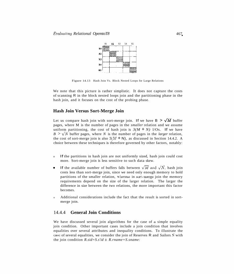
Eval1tat'ing Relational OpemtoT8
81 82 S3 54 S5
Figure 14.13 Hash Join Vs. Block Nested Loops for Large Relations
467.
We note that this picture is rather simplistic. It does not capture the costsof scanning R in the block nested loops join and the partitioning phase in thehash join, and it focuses on the cost of the probing phase ..
Hash Join Versus Sort-Merge Join
Let us compare hash join with sort-merge join. If we have B > VM bufferpages, where M is the number of pages in the smaller relation and we assumeuniform partitioning, the cost of hash join is 3(M + N) l/Os. If we haveB > VN buffer pages, where N is the number of pages in the larger relation,the cost of sort-merge join is also 3(NI + N), as discussed in Section 14.4.2. Achoice between these techniques is therefore governed by other factors, notably:
II If the partitions in hash join are not uniformly sized, hash join could costmore. Sort-merge join is less sensitive to such data skew.
II If the available number of buffers falls between -1M andVN, hash joincosts less than sort-merge join, since we need only enough memory to holdpartitions of the smaller relation, wherea'3 in sort-merge join the memoryrequirements depend on the size of the larger relation. The larger thedifference in size between the two relations, the more important this factorbecomes.
II Additional considerations include the fact that the result is sorted in sortmerge join.
14.4.4 General Join Conditions
We have discussed several join algorithms for the case of a simple equalityjoin condition. Other important cases include a join condition that involvesequalities over several attributes and inequality conditions. To illustrate theca.'3C of several equalities, we consider the join of Reserves R and Sailors 8 withthe join condition R.sid=S.s'id 1\ R.rname=S.sname:
468 CHAPTER 1.4
• For index nested loops join, we can build an index on Reserves on thecombination of fields (R.sid, R.rname) and treat Reserves as the innerrelation. vVe can also use an existing index on this combination of fields,or on R.s'id, or on R.marne. (Similar remarks hold for the choice of Sailorsas the inner relation, of course.)
• For sort-merge join, we sort Reserves on the combination of fields (sid,marne) and Sailors on the combination of fields (sid, snarne). Similarly,for hash join, we partition on these combinations of fields.
• The other join algorithms we discussed are essentially unaffected.
If we have an {nequality comparison, for example, a join of Reserves RandSailors 5 with the join condition R.rnarne < S.sname:
• We require a B+ tree index for index nested loops join.
• Hash join and sort-merge join are not applicable.
• The other join algorithms we discussed are essentially unaffected.
Of course, regardless of the algorithm, the number of qualifying tuples in aninequality join is likely to be much higher than in an equality join.
We conclude our presentation of joins with the observation that no one joinalgorithm is uniformly superior to the others. The choice of a good algorithmdepends on the sizes of the relations being joined, available access methods,and the size of the buffer pool. This choice can have a considerable impact onperformance because the difference between a good and a bad algorithm for agiven join can be enormous.
14.5 THE SET OPERATIONS
We now briefly consider the implementation of the set operations R n 5, R x S,R u 5, and R - S. From an implementation standpoint, intersection and cr08Sproduct can be seen as special cases of join (with equality on all fields &'S thejoin condition for intersection, and with no join condition for cross-product).Therefore, we will not discuss them further.
The main point to acldress in the implementation of union is the eliminationof duplicates. Set-difference can also be implemented using a variation of thetechniques for duplicate elimination. (Union and difference queries on a single relation can be thought of as a selection query with a complex selectioncondition. The techniques discussecl in Section 14.2 are applicable for suchqueries.)
Eval'uating Relational Operators 469~
There are two implementation algorithms for union and set-difference, againbased 011 sorting and hashing. Both algorithms are instances of the partitioningtechnique mentioned ill Section 12.2.
14.5.1 Sorting for Union and Difference
To implement R uS:
1. Sort R using the combination of all fields; similarly, sort S.
2. Scan the sorted Rand S in parallel and merge them, eliminating duplicates.
As a refinement, we can produce sorted runs of Rand S and merge theseruns in parallel. (This refinement is similar to the one discussed in detail forprojection.) The implementation of R- S is similar. During the merging pass,we write only tuples of R to the result, after checking that they do not appearin S.
14.5.2 Hashing for Union and Difference
To implement R U S:
1. Partition Rand S using a hash function h.
2. Process each partition I as follows:
• Build an in-memory hash table (using hash function h2 i= h) for SI.
• Scan RI. For each tuple, probe the hash table for SI. If the tuple is inthe ha.,,>h table, discard it; otherwise, add it to the table.
• Write out the ha.'3h table and then dear it to prepare for the nextpartition.
To implement R - S, we proceed similarly. The difference is in the processingof a partition. After building an in-memory ha.,,>h table for SI, we scan Rz. Foreach Rz tuple, we probe the hcl.,')h table; if the tuple is not in the table, we writeit to the result.
14.6 AGGREGATE OPERATIONS
The SQL query shown in Figure 14.14 involves an aggregate opemtion, AVG.The other aggregate operations supported in SQL-92 are MIN, MAX, SUM, andCOUNT.
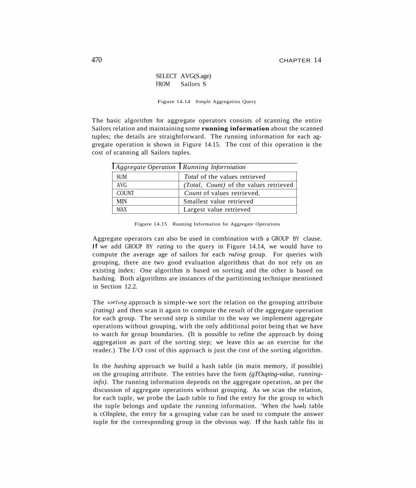
470
SELECT AVG(S.age)FROM Sailors S
Figure 14.14 Simple Aggregation Query
CHAPTER 14
The basic algorithm for aggregate operators consists of scanning the entireSailors relation and maintaining some running information about the scannedtuples; the details are straightforward. The running information for each aggregate operation is shown in Figure 14.15. The cost of this operation is thecost of scanning all Sailors tuples.
I Aggregate Operation I Running Inforrniation
SUM Total of the values retrievedAVG (Total, Count) of the values retrievedCOUNT Count of values retrieved.MIN Smallest value retrievedMAX Largest value retrieved
Figure 14.15 Running Information for Aggregate Operations
Aggregate operators can also be used in combination with a GROUP BY clause.If we add GROUP BY rating to the query in Figure 14.14, we would have tocompute the average age of sailors for each rating group. For queries withgrouping, there are two good evaluation algorithms that do not rely on anexisting index: One algorithm is based on sorting and the other is based onhashing. Both algorithms are instances of the partitioning technique mentionedin Section 12.2.
The sorting approach is simple-we sort the relation on the grouping attribute(rating) and then scan it again to compute the result of the aggregate operationfor each group. The second step is similar to the way we implement aggregateoperations without grouping, with the only additional point being that we haveto watch for group boundaries. (It is possible to refine the approach by doingaggregation as part of the sorting step; we leave this as an exercise for thereader.) The I/O cost of this approach is just the cost of the sorting algorithm.
In the hashing approach we build a hash table (in main memory, if possible)on the grouping attribute. The entries have the form (gTOuping-value, runninginfo). The running information depends on the aggregate operation, as per thediscussion of aggregate operations without grouping. As we scan the relation,for each tuple, we probe the hash table to find the entry for the group to whichthe tuple belongs and update the running information. 'When the h&'3h tableis cOlnplete, the entry for a grouping value can be used to compute the answertuple for the corresponding group in the obvious way. If the hash table fits in
Evaluating Relational OpemtoTs 471
memory, which is likely because each entry is quite small and there is only oneentry per grouping value, the cost of the hashing approach is O(.iV1), where 1V!is the size of the relation.
If the relation is so large that the hash table does not fit in memory, we canpartition the relation using a hash function h on gTOuping-value. Since all tupleswith a given grouping value are in the same partition, we can then process eachpartition independently by building an in-memory hash table for the tuples init.
14.6.1 Implementing Aggregation by Using an Index
The technique of using an index to select a subset of useful tuples is not applicable for aggregation. However, under certain conditions, we can evaluateaggregate operations efficiently by using the data entries in an index instead ofthe data records:
• If the search key for the index includes all the attributes needed for theaggregation query, we can apply the techniques described earlier in thissection to the set of data entries in the index, rather than to the collectionof data records and thereby avoid fetching data records.
• If the GROUP BY clause attribute list forms a prefix of the index searchkey and the index is a tree index, we can retrieve data entries (and datarecords, if necessary) in the order required for the grouping operation andthereby avoid a sorting step.
A given index may support one or both of these techniques; both are examplesof index-only plans. We discuss the use of indexes for queries with grouping andaggregation in the context of queries that also include selections and projectionsin Section 15.4.1.
14.7 THE IMPACT OF BUFFERING
In implementations of relational operators, effective use of the buffer pool isvery important, and we explicitly considered the size of the buffer pool in determining algorithm parameters for several of the algorithms discussed. Thereare three main points to note:
1. If several operations execute concurrently, they share the buffer pool. Thiseffectively reduces the number of buffer pages available for each operation.
2. If tuples are accessed using an index, especially an unclustered index, thelikelihood of finding a page in the buffer pool if it is requested multiple
472 CHAPTER 14
times depends (in a rather unpredictable way, unfortunately) on the size ofthe buffer pool and the replacement policy. Further, if tuples are accessedusing an unclustered index, each tuple retrieved is likely to require us tobring in a new page; therefore, the buffer pool fills up quickly, leading to ahigh level of paging activity.
3. If an operation has a pattern of repeated page accesses, we can increa..<;ethe likelihood of finding a page in memory by a good choice of replacementpolicy or by reseTving a sufficient number of buffers for the operation (if thebuffer manager provides this capability). Several examples of such patternsof repeated access follow:
• Consider a simple nested loops join. :For each tuple of the outer relation, we repeatedly scan all pages in the inner relation. If we haveenough buffer pages to hold the entire inner relation, the replacementpolicy is irrelevant. Otherwise, the replacement policy becomes critical. With LRU, we will never find a page when it is requested, becauseit is paged out. This is the sequential flooding problem discussed inSection 9.4.1. With MRU, we obtain the best buffer utilization~the
first B-2 pages of the inner relation always remain in the buffer pool.(B is the number of buffer pages; we use one page for scanning theouter relation4 and always replace the la..'3t page used for scanning theinner relation.)
• In a block nested loops join, for each block of the outer relation, wescan the entire inner relation. However, since only one unpinned pageis available for the scan of the inner rel~tion, the replacement policymakes no difference.
11III In an index nested loops join, for each tuple of the outer relation, weuse the index to find matching inner tuples. If several tuples of theouter relation have the same value in the join attribute, there is arepeated pattern of access on the inner relation; we can maximize therepetition by sorting the outer relation on the join attributes.
14.8 REVIEW QUESTIONS
Answers to the review questions can be found in the listed sections.
IIIIJ Consider a simple selection query of the form (JR.attr op 1)aluAR). Whatare the alternative access paths in each of these cases: (i) there is noindex and the file is not sorted, (ii) there is no index but the file is sorted.(Section 14.1)
4Think about the sequence of pins and unpins used to achieve this.
Evalllat'ing Relational Operators 473
• If a B+ tree index matches the selection condition, how does clusteringaffect the cost? Discuss this in terms of the selectivity of the condition.(Section 14.1)
• Describe conjunctive normal form for general selections. Define the termsconjunct and disfunct. Under what conditions does a general selectioncondition match an index? (Section 14.2)
• Describe the various implementation options for general selections. (Section 14.2)
• Discuss the use of sorting versus hashing to eliminate duplicates duringprojection. (Section 14.3)
• When can an index be used to implement projections, without retrievingactual data records? ~Then does the index additionally allow us to eliminate duplicates without sorting or hashing? (Section 14.3)
• Consider the join of relations Rand 5. Describe simple nested loops joinand block nested loops join. What are the similarities and differences? Howdoes the latter reduce I/O costs? Discuss how you would utilize buffers inblock nested loops. (Section 14.4.1)
• Describe index nested loops join. How does it differ from block nested loopsjoin? (Section 14.4.1)
• Describe sort-merge join of Rand 5. What join conditions are supported?What optimizations are possible beyond sorting both Rand 5 on the joinattributes and then doing a merge of the two? In particular, discuss howsteps in sorting can be combined with the merge P&<;s. (Section 14.4.2)
• What is the idea behind hash join? What is the additional optimization inhybrid hash join? (Section 14.4.3)
• Discuss how the choice of join algorithm depends on the number of bufferpages available, the sizes of Rand 5, and the indexes available. Be specific in your discussion and refer to cost formulas for the I/O cost of eae:halgorithm. (Sections 14.12 Section 14.13)
• How are general join conditions handled? (Section 14.4.4)
• \Vhy are the set operations R n 5 and R x S special cases of joins? What isthe similarity between the set operations Ru 5 and R - 5? (Section 14.5)
• Discuss the use of sorting versus hashing in implementing Ru 5 and R - S.Compare this with the ilnplementation of projection. (Section 14.5)
• Discuss the use of running injomwtion in implementing aggregate operations. Discuss the use of sorting versus hashing for dealing with grouping.(Section 14.6)
474 CHAPTER l4
• Under what conditions can we use an index to implement aggregate operations without retrieving data records? Under what conditions do indexesallow us to avoid sorting or ha.~hing? (Section 14.6)
• Using the cost formulas for the various relational operator evaluation algorithms, discuss which operators are most sensitive to the number of available buffer pool pages. How is this number influenced by the number ofoperators being evaluated concurrently? (Section 14.7)
• Explain how the choice of a good buffer pool replacement policy can influence overall performance. Identify the patterns of access in typical relational operator evaluation and how they influence the choice of replacementpolicy. (Section 14.7)
EXERCISES
Exercise 14.1 Briefly answer the following questions:
1. Consider the three basic techniques, iteration, indexing, and partitioning, and the relational algebra operators selection, projection, and join. For each technique-operator pair,describe an algorithm based on the technique for evaluating the operator.
2. Define the term most selective access path for a query.
3. Describe conjunctive normal form, and explain why it is important in the context ofrelational query evaluation.
4. When does a general selection condition match an index? What is a primary term in aselection condition with respect to a given index?
5. How does hybrid hash join improve on the basic hash join algorithm?
6. Discuss the pros and cons of hash join, sort-merge join, and block nested loops join.
7. If the join condition is not equality, can you use sort-merge join? Can you use hash join?Can you use index nested loops join? Can you use block nested loops join?
8. Describe how to evaluate a grouping query with aggregation operator MAX using a sortingbased approach.
9. Suppose that you are building a DBMS and want to add a new aggregate operator calledSECOND LARGEST, which is a variation of the MAX operator. Describe how you wouldimplement it.
10. Give an example of how buffer replacement policies can affect the performance of a joinalgorithm.
Exercise 14.2 Consider a relation R( a, b, c, d, e) containing 5,000,000 records, where each datapage of the relation holds 10 records. R is organized as a sorted file with secondary indexes.Assume that R.a is a candidate key for R, with values lying in the range 0 to 4,999,999, andthat R is stored in R.a order. For each of the following relational algebra queries, state whichof the following approaches (or combination thereof) is most likely to be the cheapest:
• Access the sorted file for R directly.
Evaluating Relational Operators
• Use a clustered B+ tree index on attribute R.a.
• Use a linear hashed index on attribute R.a.
• Use a clustered B+ tree index on attributes (R.a, R.b).
• Use a linear hashed index on attributes (R.a, R.b).
• Use an unclustered B+ tree index on attribute R.b.
1. O"u<50,OOOAb<50,ooo(R)
2. 0"u=50,OOOAb<50,OOO (R)
3. O"u>50,OOOAb=50,ooo(R)
4. 0"u=50,OOOi\a=50,OlO (R)
5. O"a#50,OOOi\b=50,Ooo(R)
6. 0"a<50,OOOvb=50,OOO (R)
Exercise 14.3 Consider processing the following SQL projection query:
SELECT DISTINCT E.title, E.ename FROM Executives E
You are given the following information:
Executives has attributes ename, title, dname, and address; all are string fields ofthe same length.The ename attribute is a candidate key.The relation contains 10,000 pages,There are 10 buffer pages.
475
Consider the optimized version of the sorting-based projection algorithm: The initial sortingpass reads the input relation and creates sorted runs of tuples containing only attributes enameand title. Subsequent merging passes eliminate duplicates while merging the initial runs toobtain a single sorted result (as opposed to doing a separate pass to eliminate duplicates froma sorted result containing duplicates).
1. How many sorted runs are produced in the first pass? What is the average length ofthese runs? (Assume that memory is utilized well and any available optimization toincrease run size is used.) What is the I/O cost of this sorting pass?
2. How many additional merge passes are required to compute the final result of the projection query? What is the I/O cost of these additional passes?
3. (a) Suppose that a clustered B+ tree index on tWe is available. Is this index likely tooffer a cheaper alternative to sorting? Would your answer change if the index wereunclustered? Would your answer change if the index were a hash index?
(b) Suppose that a clustered B+ tree index on ename is available. Is this index likelyto offer a cheaper alternative to sorting? Would your answer change if the indexwere unclustered? Would your answer change if the index were a hash index?
(c) Suppose that a clustered B+ tree index on (ename, title) is available. Is this indexlikely to offer a cheaper alternative to sorting? Would your answer change if theindex were unclustered? Would your answer change if the index were a hash index?
4. Suppose that the query is as follows:
SELECT E.title, E.ename FROM Executives E
476 CHAPTER ~4
That is, you are not required to do duplicate elimination. How would your answers tothe previous questions change?
Exercise 14.4 Consider the join RiXJR.a=SbS, given the following information about therelations to be joined. The cost metric is the number of page l/Os unless otherwise noted,and the cost of writing out the result should be uniformly ignored.
Relation R contains 10,000 tuples and has 10 tuples per page.Relation S contains 2000 tuples and also has 10 tuples per page.Attribute b of relation S is the primary key for S.Both relations are stored as simple heap files.Neither relation has any indexes built on it.52 buffer pages are available.
1. What is the cost of joining Rand S using a page-oriented simple nested loops join? Whatis the minimum number of buffer pages required for this cost to remain unchanged?
2. What is the cost of joining Rand S using a block nested loops join? What is the minimumnumber of buffer pages required for this cost to remain unchanged?
3. What is the cost of joining Rand S using a sort-merge join? What is the minimumnumber of buffer pages required for this cost to remain unchanged?
4. What is the cost of joining Rand S using a hash join? What is the minimum number ofbuffer pages required for this cost to remain unchanged?
5. What would be the lowest possible I/O cost for joining Rand S using any join algorithm,and how much buffer space would be needed to achieve this cost? Explain briefly.
6. How many tuples does the join of R. and S produce, at most, and how many pages arerequired to store the result of the join back on disk?
7. Would your answers to any of the previous questions in this exercise change if you weretold that R.a is a foreign key that refers to S.b?
Exercise 14.5 Consider the join of R. and S described in Exercise 14.1.
1. With 52 buffer pages, if unclustered B+ indexes existed on R.a and S.b, would eitherprovide a cheaper alternative for performing the join (using an index nested loops join)than a block nested loops join? Explain.
(a) Would your answer change if only five buffer pages were available?
(b) vVould your answer change if S contained only 10 tuples instead of 2000 tuples?
2. vVith 52 buffer pages, if clustered B+ indexes existed on R.a and S.b, would either providea cheaper alternative for performing the join (using the index nested loops algorithm)than a block nested loops join? Explain.
(a) Would your answer change if only five buffer pages were available?
(b) Would your answer change if S contained only 10 tuples instead of 2000 tuples?
3. If only 15 buffers were available, what would be the cost of a sort-merge join? Whatwould be the cost of a hash join?
4. If the size of S were increased to also be 10,000 tuples, but only 15 buffer pages wereavailable, what would be the cost of a sort-merge join? What would be the cost of ahash join?
Evaluating Relational Operators 477
5. If the size of S \vere increased to also be 10,000 tuples, and 52 buffer pages were available,what would be the cost of sort-merge join? \Vhat would be the cost of hash join?
Exercise 14.6 Answer each of the questions~ifsome question is inapplicable, explain why-in Exercise 14.1 again but using the following information about Rand S:
Relation R contains 200,000 tuples and has 20 tuples per page.Relation S contains 4,000,000 tuples and also ha." 20 tuples per page.Attribute a of relation R is the primary key for R.Each tuple of R joins with exactly 20 tuples of S.1,002 buffer pages are available.
Exercise 14.7 We described variations of the join operation called olLter joinB in Section 5.6.4. One approach to implementing an outer join operation is to first evaluate the corresponding(inner) join and then add additional tuples padded with null values to the result in accordancewith the semantics of the given outer join operator.. However, this requires us to comparethe result of the inner join with the input relations to determine the additional tuples to beadded. The cost of this comparison can be avoided by modifying the join algorithm to addthese extra tuples to the result while input tuples are processed during the join. Consider thefollowing join algorithms: block nested loops join, index nested loops join, sort-merge join, andhash join. Describe how you would modify each of these algorithms to compute the followingoperations on the Sailors and Reserves tables discussed in this chapter:
1. Sailors NATURAL LEFT OUTER JOIN Reserves
2. Sailors NATURAL RIGHT OUTER JOIN Reserves
3. Sailors NATURAL FULL OUTER JOIN Reserves
PROJECT-BASED EXERCISES
Exercise 14.8 (Note to instructors: Additional details m71st be provided if this exen:ise isassigned; see AppendiJ: SO.) Implement the various join algorithms described in this chapterin Minibase. (As additional exercises, you Inay want to implement selected algorithms for theother operators as well.)
BIBLIOGRAPHIC NOTES
The implementation techniques used for relational operators in System R are discussed in[101]. The implementation techniques used in PRTV, which utilized relational algebra transformations and a form of multiple-query optimization, are discussed in [358]. The techniquesused for aggregate operations in Ingres are described in [246]. [324] is an excellent survey ofalgorithms for implementing relational operators and is recommended for further reading.
Hash-based techniques are investigated (and compared with sort-based techniques) in [1 10],[222], [:325], and [677]. Duplicate elimination is discussed in [99]. [277] discusses secondarystorage access patterns arising in join implementations. Parallel algorithms for implementingrelational operations are discussed in [99, 168,220.224,2:3:3, 293,534].
15A TYPICAL RELATIONAL
QUERY OPTIMIZER
.. How are SQL queries translated into relational algebra? As a consequence, what class of relation algebra queries does a query optimizerconcentrate on?
.. What information is stored in the system catalog of a DBMS and howis it used in query optimization?
.. How does an optimizer estimate the cost of a query evaluation plan?
.. How does an optimizer generate alternative plans for a query? Whatis the space of plans considered? What is the role of relational algebraequivalences in generating plans?
.. How are nested SQL queries optimized?
.. Key concepts: SQL to algebra, query block; system catalog, datadictionary, metadata, system statistics, relational representation ofcatalogs; cost estimation, size estimation, reduction factors; histograms, equiwidth, equidepth, compressed; algebra equivalences,pushing selections, join ordering; plan space, single-relation plans,multi-relation left-deep plans; enumerating plans, dynamic programming approach, alternative approaches
Life is what happens while you're busy making other plam.
-John Lennon
In this chapter, we present a typical relational query optimizer in detail. Webegin by discussing how SQL queries are converted into units called blocks
478
A Typical Q'uery Optirn:izeT 479
i
~
and how blocks are translated into (extended) relational algebra expressions(Section 15.1). The central task of an optimizer is to find a good plan forevaluating such expressions. Optimizing a relational algebra expression involvestwo basic steps:
• Enumerating alternative plans for evaluating the expression. Typically, anoptimizer considers a subset of all possible plans because the number ofpossible plans is very large.
• Estimating the cost of each enumerated plan and choosing the plan withthe lowest estimated cost.
We discuss how to use system statistics to estimate the properties of the resultof a relational operation, in particular result sizes, in Section 15.2. After discussing how to estimate the cost of a given plan, we describe the space of plansconsidered by a typical relational query optimizer in Sections 15.3 and 15.4.We discuss how nested SQL queries are handled in Section 15.5. We brieflydiscuss some of the influential choices made in the System R query optimizerin Section 15.6. We conclude with a short discussion of other approaches toquery optimization in Section 15.7.
We consider a number of example queries using the following schema:
Sailors(sid: integer, sname: string, rating: integer, age: real)Boats( bid: integer, bname: string, color: string)Reserves(sid: integer, bid: integer, day: dates, mame: string)
As in Chapter 14, we assume that each tuple of Reserves is 40 bytes long, that apage can hold 100 Reserves tuples, and that we have 1000 pages of such tuples.Similarly, we assume that each tuple of Sailors is 50 bytes long, that a pagecan hold 80 Sailors tuples, and that we have 500 pages of such tuples.
15.1 TRANSLATING SQL QUERIES INTO ALGEBRA
SQL queries are optimized by decomposing them into a collection of smallerunits, called blocks. A typical relational query optimizer concentrates on op~
timizing a single block at a time. In this section, we describe how a queryis decomposed into blocks and how the optimization of a single block can beunderstood in tenus of plans composed of relational algebra operators.
15.1.1 Decomposition of a Query into Blocks
vVhen a user submits an SQL query, the query is parsed into a collection ofquery blocks and then passed on to the query optimizer. A query block
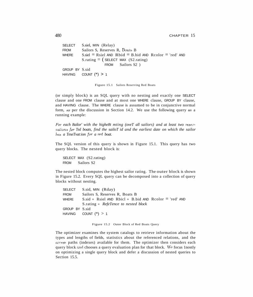
480
SELECTFROMWHERE
CHAPTER 15
S.siel, MIN (Relay)Sailors S, Reserves R, Boats BS.siel = Rsiel AND Rbid = B.bid AND Rcolor = 'red' ANDS.rating = ( SELECT MAX (S2.rating)
FROM Sailors S2 )GROUP BY S.sidHAVING COUNT (*) > 1
Figure 15.1 Sailors Reserving Red Boats
(or simply block) is an SQL query with no nesting and exactly one SELECTclause and one FROM clause and at most one WHERE clause, GROUP BY clause,and HAVING clause. The WHERE clause is assumed to be in conjunctive normalform, as per the discussion in Section 14.2. We use the following query 8.'3 arunning example:
FaT each 8ailor' with the highe8t mting (oveT all sailors) and at least two Teservat'lons faT Ted boats, find the sailoT id and the earliest date on which the sailorIULS a TeseTvat:ion faT a Ted boat.
The SQL version of this query is shown in Figure 15.1. This query has twoquery blocks. The nested block is:
SELECT MAX (S2.rating)FROM Sailors S2
The nested block computes the highest sailor rating. The outer block is shownin Figure 15.2. Every SQL query can be decomposed into a collection of queryblocks without nesting.
SELECT
FROMWHERE
GROUP BYHAVING
S.sid, MIN (Rday)Sailors S, Reserves R, Boats BS.sid = Rsiel AND Rbicl = B.bid ANDS.rating = RefeTence to nested blockS.sidCOUNT (*) > 1
Rcolor = 'red' AND
Figure 15.2 Outer Block of Red Boats Query
The optimizer examines the system catalogs to retrieve information about thetypes and lengths of fields, statistics about the referenced relations, and theaccess paths (indexes) available for them. The optimizer then considers eachquery block and chooses a query evaluation plan for that block. \Ve focus 1nostlyon optimizing a single query block and defer a discussion of nested queries toSection 15.5.
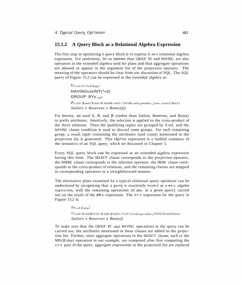
A Typical Query Opt'imizer
15.1.2 A Query Block as a Relational Algebra Expression
481
The first step in optimizing a query block is to express it as a relational algebraexpression. For uniformity, let us a.<;sume that GROUP BY and HAVING are alsooperators in the extended algebra used for plans and that aggregate operationsare allowed to appear in the argument list of the projection operator. Themeaning of the operators should be clear from our discussion of SQL. The SQLquery of Figure 15.2 can be expressed in the extended algebra as:
1rS. s id,M I N(R.day) (
HAVINGcoUNT(*»2(GROUP BYs. sid (
0"S. sid= R.sidAR. bid= B .bidAB.coloT='Ted' AS.Tating=valuc_Irom_nested_block (
Sailors x Reserves x Boats))))
For brevity, we used S, R, and B (rather than Sailors, Reserves, and Boats)to prefix attributes. Intuitively, the selection is applied to the cross-product ofthe three relations. Then the qualifying tuples are grouped by S.sid, and theHAVING clause condition is used to discard some groups. For each remaininggroup, a result tuple containing the attributes (and count) mentioned in theprojection list is generated. This algebra expression is a faithful summary ofthe semantics of an SQL query, which we discussed in Chapter 5.
Every SQL query block can be expressed as an extended algebra expressionhaving this form. The SELECT clause corresponds to the projection operator,the WHERE clause corresponds to the selection operator, the FROM clause corresponds to the cross-product of relations, and the remaining clauses are mappedto corresponding operators in a straightforward manner.
The alternative plans examined by a typical relational query optimizer can beunderstood by recognizing that a query is essentially tT'cated as a 0"1r x algebme;cpression, with the remaining operations (if any, in a given query) carriedout on the result of the 0'1r x expression. The enr x expression for the query inFigure 15.2 is:
1rS. sid,R.day(
a S.sid=R.sidAR.b'id= B .bidAB.coloT='n:d' AS'.1'atlTl.g=value_fTO/lLTlcste(Lblock (
Sailors x Reserves x Boats))
To make sure that the GROUP BY and HAVING operations in the query can becarried out, the attributes mentioned in these clauses are added to the projection list. Further, since aggregate operations in the SELECT cla.use, such a.s theMIN (R.day) operation in our example, are computed after first computing theCJ1r x part of the query, aggregate expressions in the projectioll list are replaced
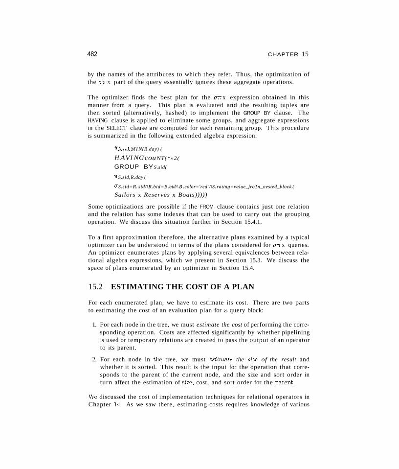
482 CHAPTER 15
by the names of the attributes to which they refer. Thus, the optimization ofthe a1r x part of the query essentially ignores these aggregate operations.
The optimizer finds the best plan for the a1r x expression obtained in thismanner from a query. This plan is evaluated and the resulting tuples arethen sorted (alternatively, hashed) to implement the GROUP BY clause. TheHAVING clause is applied to eliminate some groups, and aggregate expressionsin the SELECT clause are computed for each remaining group. This procedureis summarized in the following extended algebra expression:
1rS. s id,MI N(R.day) (
H AVI NGcouNT(*»2(
GROUP BYS.sid(
1rS.sid,R.day (
a S.sid=R. sid/\R.bid=B.bid/\ B .color='red' /\S. rating=value_fro1n_nested_block (
Sailors x Reserves x Boats)))))
Some optimizations are possible if the FROM clause contains just one relationand the relation has some indexes that can be used to carry out the groupingoperation. We discuss this situation further in Section 15.4.1.
To a first approximation therefore, the alternative plans examined by a typicaloptimizer can be understood in terms of the plans considered for a1r x queries.An optimizer enumerates plans by applying several equivalences between relational algebra expressions, which we present in Section 15.3. We discuss thespace of plans enumerated by an optimizer in Section 15.4.
15.2 ESTIMATING THE COST OF A PLAN
For each enumerated plan, we have to estimate its cost. There are two partsto estimating the cost of an evaluation plan for a query block:
1. For each node in the tree, we must estimate the cost of performing the corresponding operation. Costs are affected significantly by whether pipeliningis used or temporary relations are created to pass the output of an operatorto its parent.
2. For each node in the tree, we must estimate the size of the result andwhether it is sorted. This result is the input for the operation that corresponds to the parent of the current node, and the size and sort order inturn affect the estimation of size, cost, and sort order for the panmt.
"\Te discussed the cost of implementation techniques for relational operators inChapter 14. As we saw there, estimating costs requires knowledge of various
A Typical Q71.er'1I OptimizeT 483
parameters of the input relations, such as the number of pages and availableindexes. Such statistics are maintained in the DBMS's system catalogs. In thissection, we describe the statistics maintained by a typical DBMS and discusshow result sizes are estimated. As in Chapter 14, we use the number of pagel/Os as the metric of cost and ignore issues such as blocked access, for the sakeof simplicity.
The estimates used by a DBMS for result sizes and costs are at best approximations to actual sizes and costs. It is unrealistic to expect an optimizer tofind the very best plan; it is more important to avoid the worst plans and finda good plan.
15.2.1 Estimating Result Sizes
We now discuss how a typical optimizer estimates the size of the result computed by an operator on given inputs. Size estimation plays an important rolein cost estimation as well because the output of one operator can be the inputto another operator, and the cost of an operator depends on the size of itsinputs.
Consider a query block of the form:
SELECT attTibute listFROM Telation listWHERE teTml 1\ teTm2 1\ .. . 1\ teTmn
The maximum number of tuples in the result of this query (without duplicateelimination) is the product of the cardinalities of the relations in the FROMclause. Every term in the WHERE clause, however, eliminates some of these potential result tuples. We can model the effect of the WHERE clause on the resultsize by associating a reduction factor with each term, which is the ratio of the(expected) result size to the input size considering only the selection representedby the term. The actual size of the result can be estimated as the maximum sizetimes the product of the reduction factors for the terms in the WHERE clause.Of course, this estimate reflects the unrealistic but simplifying a.ssurnptionthat the conditions tested by each term are statistically independent.
\Ve now consider how reduction factors can be computed for different kinds ofterms in the WHERE clause by using the statistics available in the catalogs:
III column = value: For a term of this form. the reduction factor can beapproximated by Nf{ C~1js(I) if there is H11 ind~x I on column for the relationin question. This formula assumes uniform distribution of tuples among the
484
•
•
•
CHAPTER \5
index key values; this uniform distribution assumption is frequently madein arriving at cost estimates in a typical relational query optimizer. If thereis no index on col'umn, the System R optimizer arbitrarily assumes that thereduction factor is rlJ. Of course, it is possible to maintain statistics suchas the number of distinct values present for any attribute whether or notthere is an index on that attribute. If such statistics are maintained, wecan do better than the arbitrary choice of It.columni = column2: In this case the reduction factor can be approximatedby MAX (NKeys(~1),NKeys(I2)) if there are indexes Il and 12 on colmnnl andcolumn2, respectively. This formula assumes that each key value in thesmaller index, say, Il, has a matching value in the other index. Givena value for columnl, we assume that each of the N J(eys(I2) values forcol'U'mn2 is equally likely. Therefore, the number of tuples that have thesame value in column2 as a given value in columni is N K ets(I2)' If onlyone of the two columns has an index I, we take the reduction factor tobe NKe~1Js(I); if neither column has an index, we approximate it by the
ubiquitous rlJ. These formulas are used whether or not the two columnsappear in the same relation.
, l I o' TI . ) 1 . f 't' . d b High (I) - valueCO umn > va,ue. 1e Iec uctlOn ac or IS apprOXImate y High(I) ~ Low(I)
if there is an index 1 on column. If the column is not of an arithmetic typeor there is no index, a fraction less than half is arbitrarily chosen. Similarformulas for the reduction factor can be derived for other range selections.
column IN (list of values): The reduction factor is taken to be the reductionfactor for column = value multiplied by the number of items in the list.However, it is allowed to be at most half, reflecting the heuristic belief thateach selection eliminates at least half the candidate tuples.
These estimates for reduction factors are at best approximations that rely on <l..'3
sumptions such as uniform distribution of values and independent distributionof values in different columns. In recent years more sophisticated techniquesba"sed on storing more detailed statistics (e.g., histograms of the values in acolumn, which we consider later in this section) have been proposed and arefinding their way into commercial systems.
Reduction factors can also be approximated for terms of the form column IN
suhquery (ratio of the estimated size of the subquery result to the numberof distinct values in column in the outer relation); NOT condition (I-reductionfactor for condition); valuei< column< value2; the disjunction of two conditions;and so on, but \ve will not discuss such reduction factors.
To summarize, regardless of the plan chosen, we can estimate the size of thefinal result by taking the product of the sizes of the relations in the FROM clause
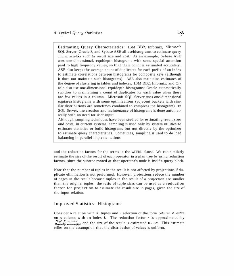
A T:yp'lcal query Opt'irnizer 485$
Estimating Query Characteristics: IBM DB2~ Informix, NlicrosoftSQL Server, Oracle 8, and Sybase ASE all usehistograms to estimate querycharacteristics such as result size and cost. As an example, Sybase ASEuses one-dimensional, equidepth histograms with some special attentionpaid to high frequency values, so that their count is estimated accurately.ASE also keeps the average count of duplicates for each prefix of an indexto estimate correlations between histograms for composite keys (althoughit does not maintain such histograms). ASE also maintains estimates ofthe degree of clustering in tables and indexes. IBM DB2, Informix, and Oracle also use one-dimensional equidepth histograms; Oracle automaticallyswitches to maintaining a count of duplicates for each value when thereare few values in a column. Microsoft SQL Server uses one-dimensionalequiarea histograms with some optimizations (adjacent buckets with similar distributions are sometimes combined to compress the histogram). InSQL Server, the creation and maintenance of histograms is done automatically with no need for user input.Although sampling techniques have been studied for estimating result sizesand costs, in current systems, sampling is used only by system utilities toestimate statistics or build histograms but not directly by the optimizerto estimate query characteristics. Sometimes, sampling is used to do loadbalancing in parallel implementations.
and the reduction factors for the terms in the WHERE clause. We can similarlyestimate the size of the result of each operator in a plan tree by using reductionfactors, since the subtree rooted at that operator's node is itself a query block.
Note that the number of tuples in the result is not affected by projections if duplicate elimination is not performed. However, projections reduce the numberof pages in the result because tuples in the result of a projection are smallerthan the original tuples; the ratio of tuple sizes can be used as a reductionfactor for projection to estimate the result size in pages, given the size ofthe input relation.
Improved Statistics: Histograms
Consider a relation with N tuples and a selection of the form colu:rnn > valueon a column with ,,),II index I. The reduction factor T is approximated by
I~:.~·~I~W_~ I:~:;)l(;), and the size of the result is estimated a"s TN. This estimaterelies on the assumption that the distribution of values is uniform.
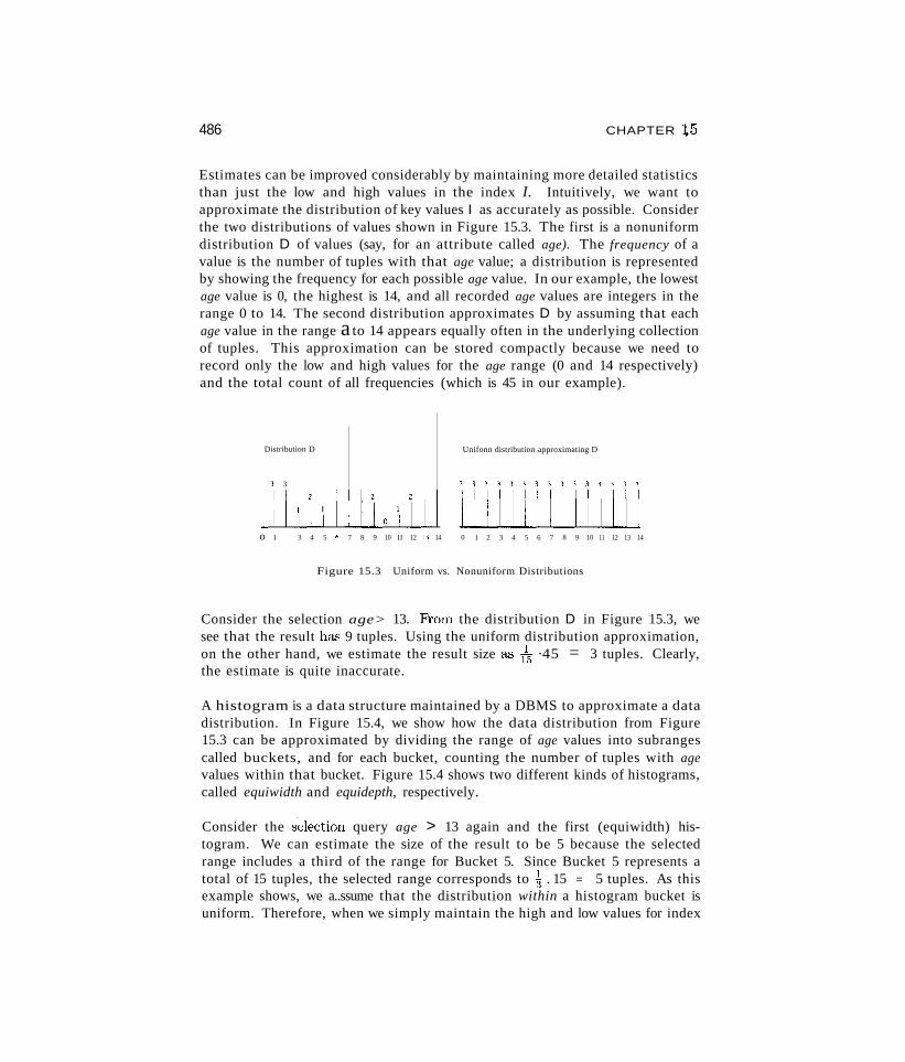
486 CHAPTER ~5
Estimates can be improved considerably by maintaining more detailed statisticsthan just the low and high values in the index I. Intuitively, we want toapproximate the distribution of key values I as accurately as possible. Considerthe two distributions of values shown in Figure 15.3. The first is a nonuniformdistribution D of values (say, for an attribute called age). The frequency of avalue is the number of tuples with that age value; a distribution is representedby showing the frequency for each possible age value. In our example, the lowestage value is 0, the highest is 14, and all recorded age values are integers in therange 0 to 14. The second distribution approximates D by assuming that eachage value in the range a to 14 appears equally often in the underlying collectionof tuples. This approximation can be stored compactly because we need torecord only the low and high values for the age range (0 and 14 respectively)and the total count of all frequencies (which is 45 in our example).
Distribution D
3 3
Unifonn distribution approximating D
333333333333333
o I 3 4 5 6 7 8 9 10 II 12 13 14 0 1 2 3 4 5 6 7 8 9 10 11 12 13 14
Figure 15.3 Uniform vs. Nonuniform Distributions
Consider the selection age> 13. Fl'om the distribution D in Figure 15.3, wesee that the result has 9 tuples. Using the uniform distribution approximation,on the other hand, we estimate the result size as fs ·45 = 3 tuples. Clearly,the estimate is quite inaccurate.
A histogram is a data structure maintained by a DBMS to approximate a datadistribution. In Figure 15.4, we show how the data distribution from Figure15.3 can be approximated by dividing the range of age values into subrangescalled buckets, and for each bucket, counting the number of tuples with agevalues within that bucket. Figure 15.4 shows two different kinds of histograms,called equiwidth and equidepth, respectively.
Consider the s~lection query age > 13 again and the first (equiwidth) histogram. We can estimate the size of the result to be 5 because the selectedrange includes a third of the range for Bucket 5. Since Bucket 5 represents atotal of 15 tuples, the selected range corresponds to ~ . 15 = 5 tuples. As thisexample shows, we a..ssume that the distribution within a histogram bucket isuniform. Therefore, when we simply maintain the high and low values for index
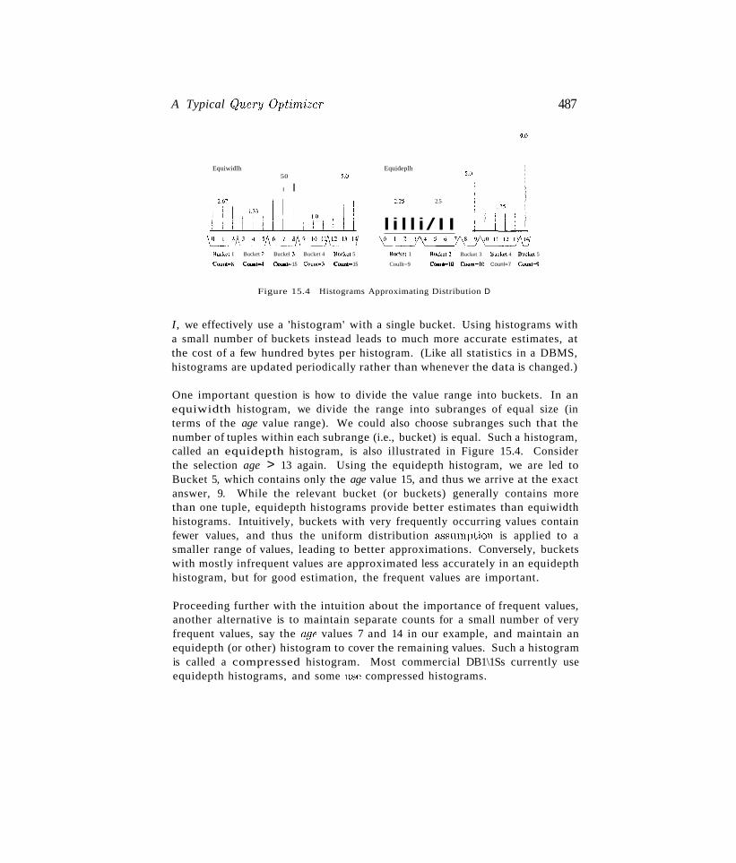
A Typical Query Optimizer
9.0
487
Equiwidlh50
I I5.0
Equideplh
2.25 2.5
lilli/II
5.0
Buckel I Bucket 2 Buckel 3 Bucket 4 Buckel 5
Count;::):\ C()unt~ Count::::: 15 COllnC;:::) Counl-::::: 15
Bucket 1
Coullt=9
Bucket 2 Bucket 3 Bucket 4 Bucket 5
Counl:::::10 Count-",IO Counl=7 Counl'"l9
Figure 15.4 Histograms Approximating Distribution D
I, we effectively use a 'histogram' with a single bucket. Using histograms witha small number of buckets instead leads to much more accurate estimates, atthe cost of a few hundred bytes per histogram. (Like all statistics in a DBMS,histograms are updated periodically rather than whenever the data is changed.)
One important question is how to divide the value range into buckets. In anequiwidth histogram, we divide the range into subranges of equal size (interms of the age value range). We could also choose subranges such that thenumber of tuples within each subrange (i.e., bucket) is equal. Such a histogram,called an equidepth histogram, is also illustrated in Figure 15.4. Considerthe selection age > 13 again. Using the equidepth histogram, we are led toBucket 5, which contains only the age value 15, and thus we arrive at the exactanswer, 9. While the relevant bucket (or buckets) generally contains morethan one tuple, equidepth histograms provide better estimates than equiwidthhistograms. Intuitively, buckets with very frequently occurring values containfewer values, and thus the uniform distribution &'isumption is applied to asmaller range of values, leading to better approximations. Conversely, bucketswith mostly infrequent values are approximated less accurately in an equidepthhistogram, but for good estimation, the frequent values are important.
Proceeding further with the intuition about the importance of frequent values,another alternative is to maintain separate counts for a small number of veryfrequent values, say the age values 7 and 14 in our example, and maintain anequidepth (or other) histogram to cover the remaining values. Such a histogramis called a compressed histogram. Most commercial DB1\1Ss currently useequidepth histograms, and some use compressed histograms.
488 CHAPTER ~5
15.3 RELATIONAL ALGEBRA EQUIVALENCES
In this section, we present several equivalences among relational algebra expressions; and in Section 15.4, we discuss the space of alternative plans consideredby a optimizer.
Our discussion of equivalences is aimed at explaining the role that such equivalences play in a System R style optimizer. In essence, a basic SQL query blockcan be thought of as an algebra expression consisting of the cross-product ofall relations in the FROM clause, the selections in the WHERE clause, and theprojections in the SELECT clause. The optimizer can choose to evaluate anyequivalent expression and still obtain the same result. Algebra equivalencesallow us to convert cross-products to joins, choose different join orders, andpush selections and projections ahead of joins. For simplicity, we assume thatnaming conflicts never arise and we need not consider the renaming operatorp.
15.3.1 Selections
Two important equivalences involve the selection operation. The first one involves cascading of selections:
Going from the right side to the left, this equivalence allows us to combine several selections into one selection. Intuitively, we can test whether a tuple meetseach of the conditions C1 ... Cn. at the same time. In the other direction, thisequivalence allows us to take a selection condition involving several conjunctsand replace it with several smaller selection operations. Replacing a selectionwith several smaller selections turns out to be very useful in combination withother equivalences, especially commutation of selections with joins or crossproducts, which we discuss shortly. Intuitively, such a replacement is useful incases where only part of a complex selection condition can be pushed.
The second equivalence states that selections are commutative:
In other words,' we can test the conditions C1 and C2 in either order.
15.3.2 Projections
The rule for cascading projections says that successively elilninating columnsfrom a relation is equivalent to sirnply eliminating all but the columns retained
A Typical qu.ery OptimizeT
by the final projection:
489
Each ai is a set of attributes of relation R, and ai ~ aHl for i = 1 ... n 1. This equivalence is useful in conjunction with other equivalences such ascommutation of projections with joins.
15.3.3 Cross-Products and Joins
Two important equivalences involving cross-products and joins. ~re presentthem in terms of natural joins for simplicity, but they hold for general joins aswell.
First, assuming that fields are identified by name rather than position, theseoperations are commutative:
Rx8
RN8
8xR
This property is very important. It allows us to choose which relation is to bethe inner and which the outer in a join of two relations.
The second equivalence states that joins and cross-products are associative:
R x (8 x T)
RN (8NT)
(R x 8) x T
(R N 8) NT
Thus we can either join Rand 8 first and then join T to the result, or join 8and T first and then join R to the result. The intuition behind associativityof cross-products is that, regardless of the order in which the three relationsare considered, the final result contains the same columns. Join associativity isbased on the same intuition, with the additional observation that the selectionsspecifying the join conditions can be cascaded. Thus the same rows appear inthe final result, regardless of the order in which the relations are joined.
Together with commutativity, associativity essentially says that we can chooseto join any p<l:ir of these relations, then join the result with the third relation,and always obtain the same final result. For example, let us verify that
R N (8 N T) ~ (T,C><] R) N 8
From commutativity, we have:
RN (8NT) RN (TN 8)
490
From associativity, we have:
RM (TM S)
Using commutativity again, we have:
(R fxJ T) M S
CHAPTER .15
In other words, when joining several relations, we are free to join the relationsin any order we choose. This order-independence is fundamental to how a queryoptimizer generates alternative query evaluation plans.
15.3.4 Selects, Projects, and Joins
Some important equivalences involve two or more operators.
We can commute a selection with a projection if the selection operation involves only attributes retained by the projection:
Every attribute mentioned in the selection condition c must be included in theset of attributes a.
We can combine a selection with a cross-product to form a join, as per thedefinition of join:
We can commute a selection with a cross-product or a join if the selectioncondition involves only attributes of one of the arguments to the cross-productor join:
oAR x S)
ac(R fxJ S)
ac(R) x S
ac(R) fxJ S
The attributes mentioned in c must appear only in R and not in S. Similarequivalences hold if c involves only attributes of S and not R, of course.
In general, a selection a c on R x S can be replaced by a ca<;cade of selectionsac], aC2 , and aC;J such that Cl involves attributes of both Rand S, C2 involvesonly attributes of R, and C;:l involves only attributes of S:
Using the ca...<;cading rule for selections, this expression is equivalent to
A Typical Query Optimizer 491:;.
Using the rule for commuting selections and cross-products, this expression isequivalent to
CTC1 (CTC2 (R) x CTC3 (S))
Thus we can push part of the selection condition c ahead of the cross-product.This observation also holds for selections in combination with joins. of course.
\Ve can commute a projection with a cross-product:
where al is the subset of attributes in a that appear in R, and a2 is the subsetof attributes in a that appear in S. We can also commute a projection witha join if the join condition involves only attributes retained by the projection:
where al is the subset of attributes in a that appear in R, and a2 is the subsetof attributes in a that appear in S. Further, every attribute mentioned in thejoin condition c must appear in a.
Intuitively, we need to retain only those attributes of Rand S that are eithermentioned in the join condition c or included in the set of attributes a retainedby the projection. Clearly, if a includes all attributes mentioned in c, theprevious commutation rules hold. If a does not include all attributes mentionedin C, we can generalize the commutation rules by first projecting out attributesthat are not mentioned in c or a, performing the join, and then projecting outall attributes that are not in a:
Now, (Ll is the subset of attributes of R that appear in either a or c, and a2 isthe subset of attributes of S that appear in either a or c.
We can in fact derive the more general commutation rule by using the rule forcascading projections and the simple commutation rule, and we leave this a.san exercise for the reader.
15.3.5 Oth,er Equivalences
Additional equivalences hold when we consider operations such as set-difference,union, and intersection. Union and intersection are associative and commutative. Selections and projections can be commuted with each of the set operations (set-difference, union, and intersection). \Ve do not discuss these equivalences further.
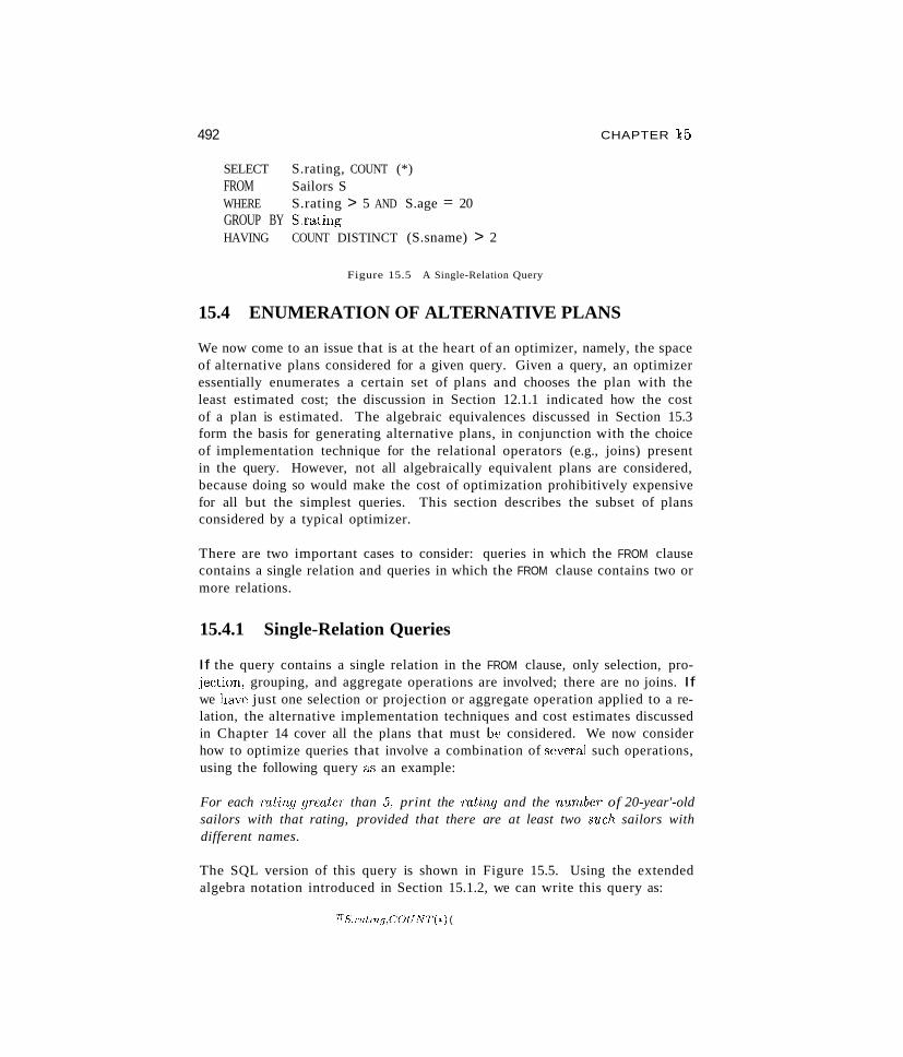
492
SELECTFROMWHEREGROUP BYHAVING
S.rating, COUNT (*)Sailors SS.rating > 5 AND S.age = 20S.ratingCOUNT DISTINCT (S.sname) > 2
Figure 15.5 A Single-Relation Query
CHAPTER 15
15.4 ENUMERATION OF ALTERNATIVE PLANS
We now come to an issue that is at the heart of an optimizer, namely, the spaceof alternative plans considered for a given query. Given a query, an optimizeressentially enumerates a certain set of plans and chooses the plan with theleast estimated cost; the discussion in Section 12.1.1 indicated how the costof a plan is estimated. The algebraic equivalences discussed in Section 15.3form the basis for generating alternative plans, in conjunction with the choiceof implementation technique for the relational operators (e.g., joins) presentin the query. However, not all algebraically equivalent plans are considered,because doing so would make the cost of optimization prohibitively expensivefor all but the simplest queries. This section describes the subset of plansconsidered by a typical optimizer.
There are two important cases to consider: queries in which the FROM clausecontains a single relation and queries in which the FROM clause contains two ormore relations.
15.4.1 Single-Relation Queries
If the query contains a single relation in the FROM clause, only selection, projection, grouping, and aggregate operations are involved; there are no joins. Ifwe have just one selection or projection or aggregate operation applied to a relation, the alternative implementation techniques and cost estimates discussedin Chapter 14 cover all the plans that must be considered. We now considerhow to optimize queries that involve a combination of several such operations,using the following query as an example:
For each rating greater than 5, print the rating and the nurnber' of 20-year'-oldsailors with that rating, provided that there are at least two such sailors withdifferent names.
The SQL version of this query is shown in Figure 15.5. Using the extendedalgebra notation introduced in Section 15.1.2, we can write this query as:
7fS. m ling,C'OUNT(*) (
A T,ypical QueI7/ Optim'izcr
H AVINGCOUNTDISTINCT(8.snume»2(
GROUP BYS.rating(
7iS.rating .5'.sname (
(lS.raling>5AS.age=20 (
Sailors)))))
493
Notice that S.sname is added to the projection list, even though it is not in theSELECT clause, because it is required to test the HAVING clause condition.
We are now ready to discuss the plans that an optimizer would consider. Themain decision to be made is which access path to use in retrieving Sailorstuples. If we considered only the selections, we would simply choose the mostselective access path, based on which available indexes match the conditions inthe WHERE clause (as per the definition in Section 14.2.1). Given the additionaloperators in this query, we must also take into account the cost of subsequentsorting steps and consider whether these operations can be performed withoutsorting by exploiting some index. We first discuss the plans generated whenthere are no suitable indexes and then examine plans that utilize some index.
Plans without Indexes
The basic approach in the absence of a suitable index is to scan the Sailorsrelation and apply the selection and projection (without duplicate elimination)operations to each retrieved tuple, as indicated by the following algebra expression:
7iS.1'ating,S.8'l!ame (
(lS.Ta[ing>5AS.age=20 (
Sailors))
The resulting tuplE~s are then sorted according to the GROUP BY clause (in theexample query, on mting) , and one answer tuple is generated for each group thatmeets the condition in the HAVING clause. The computation of the aggregatefunctions in the SELECT and HAVING clauses is done for each group, using oneof the techniques described in Section 14.6.
The cost of this approach consists of the costs of each of these steps:
1. Perfonning a file scan to retrieve tuples and apply the selections and pro-·jections.
2. 'Writing out tuples after the selections and projectiolls.
3. Sorting these tuples to implement the GROUP BY clause.
494 CHAPTER t5
Note that the HAVING clause does not cause additional I/O. The aggregatecomputations can be done on-the-fiy (with respect to I/O) as we generate thetuples in each group at the end of the sorting step for the GROUP BY clause.
In the example query the cost includes the cost of a file scan on Sailors plusthe cost of writing out (S. rating, S.sname) pairs plus the cost of sorting as perthe GROUP BY clause. The cost of the file scan is NPages(Sailors), which is 500I/Os, and the cost of writing out (S. rating, S.sname) pairs is NPages(Sailors)times the ratio of the size of such a pair to the size of a Sailors tuple times thereduction factors of the two selection conditiolls. In our example, the resulttuple size ratio is about 0.8, the mting selection has a reduction factor of 0.5,and we use the default factor of 0.1 for the age selection. Therefore, the costof this step is 20 l/Os. The cost of sorting this intermediate relation (whichwe call Temp) can be estimated as 3*NPages(Temp), which is 60 I/Os, if weassume that enough pages are available in the buffer pool to sort it in twopasses. (Relational optimizers often a.'3sume that a relation can be sorted intwo passes, to simplify the estimation of sorting costs. If this assumption is notmet at run-time, the actual cost of sorting may be higher than the estimate.)The total cost of the example query is therefore 500 + 20 + 60 = 580 l/Os.
Plans Utilizing an Index
Indexes can be utilized in several ways and can lead to plans that are significantly faster than any plan that does not utilize indexes:
1. Single-Index Access Path: If several indexes match the selection conditions in the WHERE clause, each matching index offers an alternative accesspath. An optimizer can choose the access path that it estimates will resultin retrieving the fewest pages, apply any projections and nonprimary selection terms (i.e., parts of the selection condition that do not match theindex), and proceed to compute the grouping and aggregation operations(by sorting on the GROUP BY attributes).
2. Multiple-Index Access Path: If several indexes using Alternatives (2)or (3) for data entries match the selection condition, each such index canbe used to retrieve a set of rids. vVe can intersect these sets of rids, thensort the result by page id (a."lsuming that the rid representation includesthe page id) and retrieve tuples that satisfy the primary selection terms ofall the matching indexes. Any projections and nonprimary selection termscan then be applied, followed by gTC)l1ping and aggregation operations.
3. Sorted Index Access Path: If the list of grouping attributes is a prefixof a trec index, the index can be used to retrieve tuples in the order requiredby the GROUP BY clause. All selection conditions can be applied on each
A Typical Qu,ery Optimizer
retrieved tuple, unwanted fields can be removed, and aggregate operationscomputed for each gTOUp. This strategy works well for clustered indexes.
4. Index-Only Access Path: If all the attributes mentioned in the query(in the SELECT, WHERE, GROUP BY, or HAVING clauses) are included in thesearch key for some dense index on the relation in the FROM clause, anindex-only scan can be used to compute answers. Because the dataentries in the index contain all the attributes of a tuple needed for thisquery and there is one index entry per tuple, we never neep to retrieveactual tuples from the relation. Using just the data entries from the index,we can carry out the following steps as needed in a given query: Applyselection conditions, remove unwanted attributes, sort the result to achievegrouping, and compute aggregate functions within each group. This indexonly approach works even if the index does not match the selections in theWHERE clause. If the index matches the selection, we need examine onlya subset of the index entries; otherwise, we must scan all index entries.In either case, we can avoid retrieving actual data records; therefore, thecost of this strategy does not depend on whether the index is clustered. Inaddition, if the index is a tree index and the list of attributes in the GROUPBY clause forms a prefix of the index key, we can retrieve data entries inthe order needed for the GROUP BY clause and thereby avoid sorting!
We now illustrate each of these four cases, using the query shown in Figure15.5 as a running example. We assume that the following indexes, all usingAlternative (2) for data entries, are available: a B+ tree index on rating, ahash index on age, and a B+ tree index on (rating. sname, age). For brevity,we do not present detailed cost calculations, but the reader should be able tocalculate the cost of each plan. The steps in these plans are scans (a file scan,a scan retrieving tuples by using an index, or a scan of only index entries),sorting, and writing temporary relations; and we have already discussed howto estimate the costs of these operations.
As an example of the first C<1se, we could choose to retrieve Sailors tuples suchthat S. age=20 using the hash index on age. The cost of this step is the costof retrieving the index entries plus the cost of retrieving the correspondingSailors tuples, which depends on whether the index is clustered. vVe can thenapply the condition S.mting > 5 to each retrieved tuple; project out fields notmentioned in ~he SELECT, GROUP BY, and HAVING clauses; and write the resultto a temporary relation. In the example, only the rating and sname fields needto be retained. The temporary relation is then sorted on the rating field toidentify the groups, and some groups are eliminated by applying the HAVINGconclitioIl.
496 CHAPTER 15. ...._._- -- -~--l
Utilizing Indexes: All of the main RDBMSs recognize the importanceof index-only plans and look for such plans whenever possible. In IBMDD2, when creating an index a user can specify ia set of 'include' "alumnsthat are to be kept in the index but are not part of the index key. Thisallows a richer set of index-only queries to be handled, because columnsfrequently a.ccessed are included in the index even if they are ;notpart ofthe key. In Microsoft SQL Server, an interesting class of index-only plansis considered: Consider a query that selects attributes sal and~age from atable, given an index on sal and another index on age. SQL Server usesthe indexes by joining the entries on the rid of data records to identify(sal, age) pairs that appear in the table.
As an example of the second case, we can retrieve rids of tuples satisfyingmting>5 using the index on rating, retrieve rids of tuples satisfying age=20 using the index on age, sort the retrieved rids by page number, and then retrievethe corresponding Sailors tuples. We can retain just the rating and name fieldsand write the result to a temporary relation, which we can sort on mting toimplement the GROUP BY clause. (A good optimizer might pipeline the projected tuples to the sort operator without creating a temporary relation.) TheHAVING clause is handled as before.
As an example of the third case, we can retrieve Sailors tuples in which S. mting> 5, ordered by rating, using the B+ tree index on rating. We can computethe aggregate functions in the HAVING and SELECT clauses on-the-fly becausetuples are retrieved in rating order.
As an example of the fourth case, we can retrieve data entT'ies from the (mting,sname, age) index in which mting > 5. These entries are sorted by rating (andthen by snarne CLnJ age, although this additional ordering is not relevant forthis query). vVe can choose entries with age=20 and compute the aggregatefunctions in the HAVING and SELECT clauses on-the-fly because the data entriesare retrieved in rating order. In this case, in contrast to the previous case, wedo not retrieve any Sailors tuples. This property of not retrieving data recordsmakes the index-only strategy especially valuable with unclusterecl indexes.
15.4.2 Multiple-Relation Queries
Query blocks that contain two or more relations in the FROM clause require joins(or cross-products). Finding a good plan for such queries is very importantbecause these queries can be quite expensive. Regardless of the plan chosen,the size of the final result can be estimated by taking the product of the sizes
A Typical Q'lLeTy OptimizeT 497
of the relations in the FROM clause and the reduction factors for the terms inthe WHERE clause. But, depending on the order in which relations are joined,intermediate relations of widely varying sizes can be created, leading to planswith very different costs.
Enumeration of Left-Deep Plans
As we saw in Chapter 12, current relational systems, following the lead of theSystem R optimizer, only consider left-deep plans. \;Ye now discuss how thisdass of plans is efficiently searched using dynamic programming.
Consider a query block of the form:
SELECT attribute listFROM relation listWHERE teT1nl 1\ term2 1\ ... 1\ ter1nn
A System R style query optimizer enumerates all left-deep plans, with selectionsand projections considered (but not necessarily applied!) as early as possible.The enumeration of plans can be understood &'3 a multiple-pass algorithm inwhich we proceed as follows:
Pass 1: We enumerate all single-relation plans (over some relation in theFROM clause). Intuitively, each single-relation plan is a partial left-deep planfor evaluating the query in which the given relation is the first (in the linearjoin order for the left-deep plan of which it is a part). When consideringplans involving a relation A, we identify those selection terms in the WHEREclause that mention only attributes of A. These are the selections that canbe performed when first accessing A, before any joins that involve A. We alsoidentify those attributes of A not mentioned in the SELECT clause or in termsin the WHERE clause involving attributes of other relations. These attributescan be projected out when first accessing A, before any joins that involve A.We choose the best access method for A to carry out these selections andprojections, &'3 per the discussion in Section 15.4.1.
For each relation, if we find plans that produce tuples in different orders, weretain the cheapest plan for each such ordering of tuples. An ordering of tuplescould prove useful at a subsequent step, say, for a sort-merge join or implementing a GROUP BY or ORDER BY clause. Hence, for a single relation, we mayretain a file scan (&'3 the cheapest overall plan for fetching all tuples) and a B+tree index (I:LS the cheapest plan for fetching all tuples in the search key order).
Pass 2: We generate all two-relation plans by considering each single-relationplan retained after Pass 1 &'3 the outer relation and (successively) every other
498 CHAPTER Jf5
relation as the inner relation. Suppose that A is the outer relation and Bthe inner relation for a particular two-relation plan. We examine the list ofselections in the WHERE clause and identify:
1. Selections that involve only attributes of B and can be applied before thejoin.
2. Selections that define the join (i.e., are conditions involving attributes ofboth A and B and no other relation).
3. Selections that involve attributes of other relations and can be applied onlyafter the join.
The first two groups of selections can be considered while choosing an accesspath for the inner relation B. We also identify the attributes of B that do notappear in the SELECT clause or in any selection conditions in the second orthird group and can therefore be projected out before the join.
Note that our identification of attributes that can be projected out before thejoin and selections that can be applied before the join is based on the relationalalgebra equivalences discussed earlier. In particular, we rely on the equivalencesthat allow us to push selections and projections ahead of joins. As we will see,whether we actually perform these selections and projections ahead of a givenjoin depends on cost considerations. The only selections that are really appliedbefor"e the join are those that match the chosen access paths for A and B. Theremaining selections and projections are done on-the-fly as part of the join.
An important point to note is that tuples generated by the outer plan are assumed to be pipelined into the join. That is, we avoid having the outer planwrite its result to a file that is subsequently read by the join (to obtain outertuples). For SOlne join methods, the join operator rnight require materializingthe outer tuples. For example, a hash join would partition the incoming tuples,and a sort-merge join would sort them if they are not already in the appropriate sort order. Nested loops joins, however, can use outer tuples H,"i they aregenerated and avoid materializing them. Similarly, sort-merge joins can useouter tuples as they are generated if they are generated in the sorted orderrequired for the join. We include the cost of materializing the outer relation,should this be necessary, in the cost of the join. The adjustments to the joincosts discussed in Chapter 14 to reflect the use of pipelining or materializationof the outer are straightforward.
For each single-relation plan for A retained after Pa."iS 1, for each join methodthat we consider, we must determine the best access lnethod to llse for B. Theaccess method chosen for B retrieves, in general, a subset of the tuples in B,possibly with some fields eliminated, as discllssed later. Consider relation B.
A T:lJpical qlleT~1J Optim'iztT 4~9
\Ve have a collection of selections (some of which are the join conditions) andprojections on a single relation, and the choice of the best access method ismade a<; per the discussion in Section 15.4.1. The only additional considerationis that the join method might require tuples to be retrieved in some order. Forexample, in a sort-merge join, we want the inner tuples in sorted order on thejoin column(s). If a given access method does not retrieve inner tuples in thisorder, we must add the cost of an additional sorting step to the cost of theaccess method.
Pass 3: We generate all three-relation plans. We proceed as in Pass 2, exceptthat we now consider plans retained after Pass 2 as outer relations, instead ofplans retained after Pass 1.
Additional Passes: This process is repeated with additional passes until weproduce plans that contain all the relations in the query. We now have thecheapest overall plan for the query as well as the cheapest plan for producingthe answers in some interesting order.
If a multiple-relation query contains a GROUP BY clause and aggregate functionssuch as MIN, MAX, and SUM in the SELECT clause, these are dealt with at thevery end. If the query block includes a GROUP BY clause, a set of tuples iscomputed based on the rest of the query, as described above, and this set issorted as per the GROUP BY clause. Of course, if there is a plan according towhich the set of tuples is produced in the desired order, the cost of this planis compared with the cost of the cheapest plan (a<;smning that the two aredifferent) plus the sorting cost. Given the sorted set of tuples, partitions areidentified and any aggregate functions in the SELECT clause are applied on aper-partition basis, as per the discussion in Chapter 14.
Examples of Multiple-Relation Query Optimization
Consider the query tree shown in Figure 12.~~. Figure 15.6 shows the samequery, taking into account how selections and projections are considered early.
In looking at this figure, it is worth ernphc1...sizing that the selections shown onthe leaves are not necessarily done in a distinct step that precedes the .ioin~H
rather, (:1...<; we have seen, they are considered as potential matching predicateswhen considerIng the available access paths on the relations.
Suppose that we have the following indexes, all unclustered and using Alternative (2) for data entries: a B+ tree index on the rating field of Sailors, ahash index on the sid field of Sailors, and a B+ tree index on the bid field of
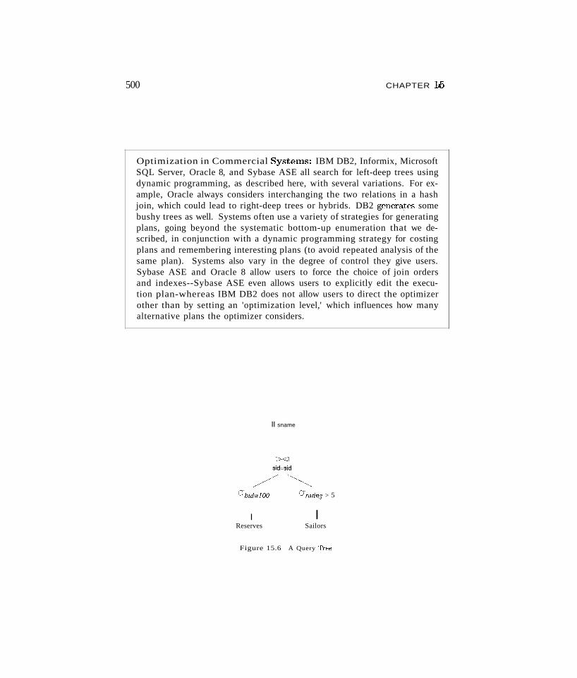
500 CHAPTER 10
Optimization in Commercial Syst~ms: IBM DB2, Informix, MicrosoftSQL Server, Oracle 8, and Sybase ASE all search for left-deep trees usingdynamic programming, as described here, with several variations. For example, Oracle always considers interchanging the two relations in a hashjoin, which could lead to right-deep trees or hybrids. DB2 gene'rates somebushy trees as well. Systems often use a variety of strategies for generatingplans, going beyond the systematic bottom-up enumeration that we described, in conjunction with a dynamic programming strategy for costingplans and remembering interesting plans (to avoid repeated analysis of thesame plan). Systems also vary in the degree of control they give users.Sybase ASE and Oracle 8 allow users to force the choice of join ordersand indexes--Sybase ASE even allows users to explicitly edit the execution plan-whereas IBM DB2 does not allow users to direct the optimizerother than by setting an 'optimization level,' which influences how manyalternative plans the optimizer considers.
II sname
IReserves
Urating > 5
ISailors
Figure 15.6 A Query Tree
A Typical Qv,cry Optinl'izcr 5Q1
Reserves. In addition, we a'Ssume that we can do a sequential scan of bothReserves and Sailors. Let us consider how the optimizer proceeds.
In Pch<;S 1, we consider three access methods for Sailors (B+ tree, hash index,and sequential scan), taking into account the selection IJrating>5' This selectionmatches the B+ tree on rating and therefore reduces the cost for retrievingtuples that satisfy this selection. The cost of retrieving tuples using the hashindex and the sequential scan is likely to be much higher than the cost of usingthe B+ tree. So the plan retained for Sailors is access via the B+ tree index, andit retrieves tuples in sorted order by rating. Similarly, we consider two accessmethods for Reserves taking into account the selection IJbid=100. This selectionmatches the B+ tree index on Reserves, and the cost of retrieving matchingtuples via this index is likely to be much lower than the cost of retrieving tuplesusing a sequential scan; access through the B+ tree index is therefore the onlyplan retained for Reserves after Pass 1.
In Pass 2, we consider taking the (relation computed by the) plan for Reservesand joining it (as the outer) with Sailors. In doing so, we recognize that now,we need only Sailors tuples that satisfy crrating>5 and IJsid=value, where valueis some value from an outer tuple. The selection IJsid=value matches the hashindex on the sid field of Sailors, and the selection crrating>5 matches the B+tree index on the rating field. Since the equality selection has a much lowerreduction factor, the hash index is likely to be the cheaper access method.In addition to the preceding consideration of alternative access methods, weconsider alternative join methods. All available join methods are considered.For example, consider a sort-merge join. The inputs must be sorted by sid;since neither input is sorted by sid or has an access method that can returntuples in this order, the cost of the sort-merge join in this case must includethe cost of storing the two inputs in tempora.ry relations and sorting them. Asort-merge join provides results in sorted order by sid, but this is not a usefulordering in this example because the projection 7fsname is applied (on-the-fly)to the result of the join, thereby eliminating the sid field from the answer.Therefore, the plan using sort-merge join is retained after Pch<;S 2 only if it isthe least expensive plan involving Reserves and Sailors.
Similarly, we also consider taking the plan for Sailors retained after Pass 1 andjoining it (as the outer relation) with Reserves. Now we recognize that we needonly Reserves tuples that satisfy IJhid=100 and IJsid=val'lU~' where value is somevalue from an outer tuple. Again, we consider all available join methods.
vVe finally retain the cheapest plan overall.
As another example, illustrating the ca<;e when more than two relations arejoined, consider the following query:
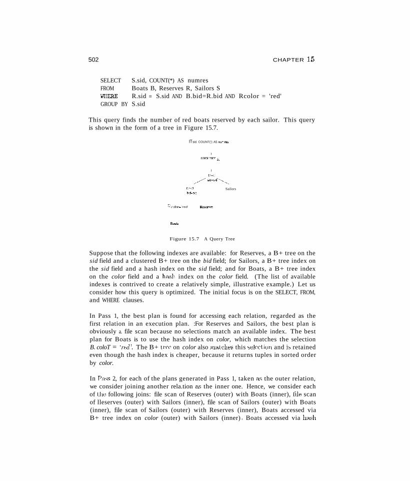
502 CHAPTER 15
SELECT S.sid, COUNT(*) AS numresFROM Boats B, Reserves R, Sailors SWHERE R.sid = S.sid AND B.bid=R.bid AND Rcolor = 'red'GROUP BY S.sid
This query finds the number of red boats reserved by each sailor. This queryis shown in the form of a tree in Figure 15.7.
ITsid. COUNT(') AS numras
I
GROUPB)' ~id
I
"'<I Sailorsbid~bld
(Jcolor';:::. 'red' Reserves
Boats
Figure 15.7 A Query Tree
Suppose that the following indexes are available: for Reserves, a B+ tree on thesid field and a clustered B+ tree on the bid field; for Sailors, a B+ tree index onthe sid field and a hash index on the sid field; and for Boats, a B+ tree indexon the color field and a ha'3h index on the color field. (The list of availableindexes is contrived to create a relatively simple, illustrative example.) Let usconsider how this query is optimized. The initial focus is on the SELECT, FROM,and WHERE clauses.
In Pass 1, the best plan is found for accessing each relation, regarded as thefirst relation in an execution plan. :For Reserves and Sailors, the best plan isobviously a. file scan because no selections match an available index. The bestplan for Boats is to use the hash index on color, which matches the selectionB. coloT = 'T'(~d '. The B+ tree on color also matches this selection and is retainedeven though the hash index is cheaper, because it returns tuples in sorted orderby color.
In Pass 2, for each of the plans generated in Pass 1, taken as the outer relation,we consider joining another rela.tion a'3 the inner one. Hence, we consider eachof the following joins: file scan of Reserves (outer) with Boats (inner), file scanof lleserves (outer) with Sailors (inner), file scan of Sailors (outer) with Boats(inner), file scan of Sailors (outer) with Reserves (inner), Boats accessed viaB+ tree index on color (outer) with Sailors (inner) 1 Boats accessed via ha'3h
A T.ypical q'lleT~1J Opt'im'izer S(}3
index on color (outer) with Sailors (inner), Boats accessed via B+ tree indexon color (outer) with Reserves (inner), and Boats accessed via hash index oncolor (outer) with RE'.3erves (inner).
For each such pair, we consider every join method, and for each join method,we consider every available access path for the inner relation. For each pairof relations, we retain the cheapest of the plans considered for every sortedorder in which the tuples are generated. For example, with Boats accessedvia the hash index on coloT as the outer relation, an index nested loops joinaccessing Reserves via the B+ tree index on bid is likely to be a good plan;observe that there is no ha."h index on this field of Reserves. Another plan forjoining Reserves and Boats is to access Boats using the hash index on coloT,access Reserves using the B+ tree on bid, and use a sort-merge join; this plan,in contrast to the previous one, generates tuples in sorted order by bid. Itis retained even if the previous plan is cheaper, unless an even cheaper planproduces the tuples in sorted order by bid. However, the previous plan, whichproduces tuples in no particular order, would not be retained if this plan ischeaper.
A good heuristic is to avoid considering cross-products if possible. If we applythis heuristic, we would not consider the following 'joins' in Pass 2 of thisexample: file scan of Sailors (outer) with Boats (inner), Boats accessed via B+tree index on color (outer) with Sailors (inner), and Boats accessed via hashindex on color (outer) with Sailors (inner).
In Pass 3, for each plan retained in Pass 2, taken as the outer relation, weconsider how to join the remaining relation as the inner one. An example of aplan generated at this step is the following: Access Boats via the hash indexon coloT, access Reserves via the B+ tree index on bid, and join them usinga sort-merge join, then take the result of this join as the outer and join withSailors using a sort-merge join, accessing Sailors via the B+ tree index on thesid field. Note that, since the result of the first join is produced in sorted orderby bid, wherea." the second join requires its inputs to be sorted by s'id, the resultof the first join must be sorted by sid before being used in the second join. Thetuples in the result of the second join are generated in sorted order by sid.
The GROUP BY clause is considered after all joins, and it requires sorting onthe sid field. For each plan retained in Pass 3, if the result is not sorted onsid, we add the cost of sorting on the sid field. The sample plan generated inPass 3 produces tuples in sid order; therefore, it may be the cheapest plan forthe query even if a cheaper plan joins all three relations but does not producetuples in sid order.
504 CHAPTER 15
15.5 NESTED SUBQUERIES
The unit of optimization in a typical system is a query block, and nested queriesare dealt with using some form of nested loops evaluation. Consider the following nested query in SQL: Find the names of sailors with the highest rating:
SELECTFROMWHERE
S.snameSailors SS.rating = ( SELECT MAX (S2.rating)
FROM Sailors S2 )
In this simple query, the nested subquery can be evaluated just once, yieldinga single value. This value is incorporated into the top-level query as if it hadbeen part of the original statement of the query. For example, if the highestrated sailor has a rating of 8, the WHERE clause is effectively modified to WHERES. rating = 8.
However, the subquery sometimes returns a relation, or more precisely, a tablein the SQL sense (i.e., possibly with duplicate rows). Consider the followingquery: Find the names of sailors who have Teserved boat number 103:
SELECTFROMWHERE
S.snameSailors SS.sid IN ( SELECT
FROMWHERE
RsidReserves RRbid = 103 )
Again, the nested subquery can be evaluated just once, yielding a collectionof sids. For each tuple of Sailors, we must now check whether the sid valueis in the computed collection of sids; this check entails a join of Sailors andthe computed collection of sids, and in principle we have the full range of joinmethods to choose from. For example, if there is an index on the sid fieldof Sailors, an index nested loops join with the computed collection of sid", asthe outer relation and Sailors as the inner one might be the most efficient joinmethod. However, in many systems, the query optimizer is not smart enoughto find this strategy a common approach is to always do a nested loops joinin which the inner relation is the collection of sid" computed from the subquery(and this colle(~tion may not be indexed).
The motivation for this approach is that it is a simple variant of the techniqueused to deal with condated ([neTics such as the following version of the previousquery:
SELECT S.snallle
A TYVical Q'lteTy Optim'izer 5()5
FROM~lHERE
Sailors SEXISTS ( SELECT *
FROM Reserves RWHERE R. bid = 103
AND S.sid = R.sid )
This query is correlated-"the tuple variable S from the top-level query appearsin the nested subquery. Therefore, we cannot evaluate the subquery just once.In this case the typical evaluation strategy is to evaluate the nested subqueryfor each tuple of Sailors.
An important point to note about nested queries is that a typical optimizeris likely to do a poor job, because of the limited approach to nested queryoptimization. This is highlighted next:
• In a nested query with correlation, the join method is effectively indexnested loops, with the inner relation typically a subquery (and thereforepotentially expensive to compute). This approach creates two distinctproblems. First, the nested subquery is evaluated once per outer tuple;if the same value appears in the correlation field (S.sid in our example) ofseveral outer tuples, the same subquery is evaluated many times. The second problem is that the approach to nested subqueries is not set-oriented.In effect, a join is seen as a scan of the outer relation with a selection onthe inner subquery for each outer tuple. This precludes consideration ofalternative join methods, such as a sort-merge join or a hash join, thatcould lead to superior plans.
• Even if index nested loops is the appropriate join method, nested queryevaluation may be inefficient. For example, if there is an index on the sidfield of Reserves, a good strategy might be to do an index nested loops joinwith Sailors as the outer relation and Reserves &'3 the inner relation andapply the selection on bid on-the-fly. However, this option is not consideredwhen optimizing the version of the query that uses IN, because the nestedsubquery is fully evaluated as a first step; that is, Reserves tuples thatmeet the bid selection are retrieved first.
• Opportunities for finding a good evaluation plan may also be missed because of the implicit ordering imposed by the nesting. For example, if thereis an index. on the sid field of Sailors, an index nested loops join with Reserves a,s the outer relation and Sailors as the inner one might be the mostefficient plan for our example correla,ted query. However, this join orderingis never considered by an optimizer.
A nested query often has an equivalent query without nesting, and a correlatedquery often he1.<; an equivalent query without correlation. vVe already saw cor-
506 CHAPTER ~5
Nested Queries: IBM DB2, Informix, Microsoft SQL Server, Orade 8,and Sybase ASE all use some version of correlated evaluation to handlenested queries, which are an important part qf tbe TPC-D benchmark;IBM and Informix support a version in which the results of subqueries arestored in a 'memo' table and the same subquery is not executed multipletimes. All these RDBMSs consider decqrrelation and "flattening" of nestedqueries as an option. Microsoft SQL Server, Oracle 8 and IBM DB2 alsouse rewriting techniques, e.g., Magic Sets (see Chapter 24) or variants, inconjunction with decorrelation.
related and uncorrelated versions of the example nested query. There is alsoan equivalent query without nesting:
SELECT S.snameFROM Sailors S, Reserves RWHERE S.sid = R.sid AND R.bid=103
A typical SQL optimizer is likely to find a much better evaluation strategy if it isgiven the unnested or 'decOlTelated' version of the example query than if it weregiven either of the nested versions of the query. Many current optimizers cannotrecognize the equivalence of these queries and transform one of the nestedversions to the nonnested form. This is, unfortunately, up to the educated user.From an efficiency standpoint, users are advised to consider such alternativeformulations of a query.
We conclude our discussion of nested queries by observing that there could beseveral levels of nesting. In general, the approach we sketched is extended byevaluating such queries from the innermost to the outermost levels, in order, inthe absence of correlation. A correlated subquery must be evaluated for eachcandidate tuple of the higher-level (sub)query that refers to it. The basic ideais therefore similar to the case of one-level nested queries; we omit the details.
15.6 THE SYSTEM R OPTIMIZER
Current relational query optimizers have been greatly influenced by choicesmade in the qesign of IBM's System R query optimizer. Important designchoices in the System R optimizer include:
1. The use of statistics about the databa'3e instance to estiInate the cost of aquery evaluation plan.
2. A decision to consider only plans with binary joins in which the innerrelation is a base relation (i.e., not a telnporary relation). This heuristic
A Typical Que7'y Optimizer' 507
reduces the (potentially very large) number of alternative plans that mustbe considered.
3. A decision to focus optimization on the class of SQL queries without nestingand treat nested queries in a relatively ad hoc way.
4. A decision not to perform duplicate elimination for projections (except asa final step in the query evaluation when required by a DISTINCT clause).
5. A model of cost that accounted for CPU costs as well as I/O costs.
Our discussion of optimization reflects these design choices, except for the lastpoint in the preceding list, which we ignore to retain our simple cost modelbased on the number of page l/Os.
15.7 OTHER APPROACHES TO QUERY OPTIMIZATION
We have described query optimization based on an exhaustive search of a largespace of plans for a given query. The space of all possible plans grows rapidlywith the size of the query expression, in particular with respect to the numberof joins, because join-order optimization is a central issue. Therefore, heuristicsare used to limit the space of plans considered by an optimizer. A widely usedheuristic is that only left-deep plans are considered, which works well for mostqueries. However, once the number of joins becomes greater than about 15,the cost of optimization using this exhaustive approach becomes prohibitivelyhigh, even if we consider only left-deep plans.
Such complex queries are becoming important in decision-support environments, and other approaches to query optimization have been proposed. Theseinclude rule-based optimizers, which use a set of rules to guide the generation of candidate plans, and randomized plan generation, which usesprobabilistic algorithms such as simulated annealing to explore a large space ofplans quickly, with a reasonable likelihood of finding a good plan.
Current research in this area also involves techniques for estimating the sizeof intermediate relations more accurately; parametric query optimization,which seeks to find good plans for a given query for each of several differentconditions that might be encountered at run-time; and multiple-query optimization, in which the optimizer takes concurrent execution of several queriesinto account.
15.8 REVIEW QUESTIONS
Answers to the review questions can be found in the listed sections.
508 CHAPTER 15,
• \Vhat is an SQL qlleTJJ block? \Vhy is it important in the context of queryoptimization? (Section 15.1)
• Describe how a query block is translated into extended relational algebra.Describe and motivate the extensions to relational algebra. VVhy are a'Tr xexpressions the focus of an optimizer? (Section 15.1)
• \Vhat are the two parts to estimating the cost of a query plan? (Section 15.2)
• How is the result size estimated for a (nrx expression? Describe the use ofreduction factors, and explain how they are calculated for different kindsof selections? (Section 15.2.1)
• ~What are histograms? How do they help in cost estimation? Explainthe differences between the different kinds of histograms, with particularattention to the role of frequent data values. (Section 15.2.1)
• VVhen are two relational algebra expressions considered equivalent? How isequivalence used in query optimization? What algebra equivalences thatjustify the common optimizations of pushing selections ahead of joins andre-ordering join expressions? (Section 15.3)
• Describe left-deep plans and explain why optimizers typically consider onlysuch plans. (Section 15.4)
• What plans are considered for (sub)queries with a single relation? Ofthese, which plans are retained in the dynamic programming approach toenumerating left-deep plans? Discuss access methods and output orderin your answer. In particular, explain index-only plans and why they areattractive. (Section 15.4)
• Explain how query plans are generated for queries with multiple relations.Discuss the space and time complexity of the dynamic programming approach, and how the plan generation process incorporates heuristics likepushing selections and join ordering. How are index-only plans for multiplerelation queries identified? How are pipelining opportunities identified?(Section 15.4)
• How are nested subqueries optimized and evaluated? Discuss correlatedqueries and the additional optimization challenges they present. \Vhy areplans produced for nested queries typically of poor quality? VVhat is thelesson for application programmers? (Section 15.5)
• Discuss some of the influential design choices made in the System R optimizer. (Section 15.6)
• Briefly survey optimization techniques that go beyond the dynamic programming framework discussed in this chapter. (Section 15.7)
A Typical Q'ueTy Ophm'izeT
EXERCISES
Exercise 15.1 Briefly answer the following questions:
5q9
1. In the context of query optimization, what is an SQL query block?
2. Define the term redw:t'i.on factor.
3. Describe a situation in which projection should precede selection in processing a projectselect query, and describe a situation where the opposite processing order is better.(Assume that duplicate elimination for projection is done via sorting.)
4. If there are unclustered (secondary) B+ tree indexes on both R.a and S.b, the joinR [Xla=bS could be processed by doing a sort-merge type of join-without doing anysorting-by using these indexes.
(a) Would this be a good idea if Rand S each has only one tuple per page or would itbe better to ignore the indexes and sort Rand S? Explain.
(b) What if Rand S each have many tuples per page? Again, explain.
5. Explain the role of interesting orders in the System R optimizer.
Exercise 15.2 Consider a relation with this schema:
Ernployees(eid: integer, ename: string, sal: integer, title: string, age: integer)
Suppose that the following indexes, all using Alternative (2) for data entries, exist: a hashindex on eid, a B+ tree index on sal, a hash index on age, and a clustered B+ tree indexon (age, sal). Each Employees record is 100 bytes long, and you can assume that each indexdata entry is 20 bytes long. The Employees relation contains 10,000 pages.
1. Consider each of the following selection conditions and, assuming that the reductionfactor (RF) for each term that matches an index is 0.1, compute the cost of the mostselective access path for retrieving all Employees tuples that satisfy the condition:
(a) sol> 100
(b) age. = 25
(c) age> 20
(d) eid = 1, 000
(e) sal> 200 1\ age> 30
(f) sal> 2001\ age = 20
(g) sal> 2001\ title ='CFO'
(h) sal> 200 II age> 301\ hUe ='CFO'
2. Suppose that, for each of the preceding selection conditions, you want to retrieve theaverage salary of qualifying tuples. For each selection condition, describe the least expensive evalwltion method and state its cost.
:3. Suppose that, for each of the preceding selection conditions, you want to compute the av-erage salary for each age group. For each selection condition, describe the least expensiveevaluation method and state its cost.
4. Suppose that, for each of the preceding selection conditions, you want to compute theaverage age for each sa/level (Le.) group by sal). For each selection condition, describethe least expensive evaluation method and state its cost.
510 CHAPTER ~5
5. For each of the following selection conditions, describe the best evaluation method:
(a) sal> 200 V age = 20
(b) sal> 200 V title ='CFO'
(c) title ='CFO' 1\ ename ='Joe'
Exercise 15.3 For each of the following SQL queries, for each relation involved, list theattributes that must be examined to compute the answer. All queries refer to the followingrelations:
Emp(eid: integer, did: integer, sal: integer, hobby: char(20))
Dept( did: integer, dname: char(20), floor: integer, budget: real)
1. SELECT COUNT(*) FROM Emp E, Dept D WHERE E.did = D.did
2. SELECT MAX(E.sal) FROM Emp E, Dept D WHERE E.did = D.did
3. SELECT MAX(E.sal) FROM Emp E, Dept D WHERE E.did = D.did AND D.floor = 5
4. SELECT E.did, COUNT(*) FROM Emp E, Dept D WHERE E.did = D.did GROUP BY D.did
5. SELECT D.floor, AVG(D.budget) FROM Dept D GROUP BY D.tloor HAVING COUNT(*) > 2
6. SELECT D.tloor, AVG(D.budget) FROM Dept D GROUP BY D.floor ORDER BY D.floor
Exercise 15.4 You are given the following information:
Executives has attributes ename, title, dname, and address; all are string fields ofthe same length.The ename attribute is a candidate key.The relation contains 10,000 pages.There are 10 buffer pages.
1. Consider the following query:
SELECT E.title, E.ename FROM Executives E WHERE E.title='CFO'
Assume that only 10% of Executives tuples meet the selection condition.
(a) Suppose that a clustered B+ tree index on title is (the only index) available. Whatis the cost of the best plan? (In this and subsequent questions, be sure to describethe plan you have in mind.)
(b) Suppose that an unclustered B+ tree index on title is (the only index) available.What is the cost of the best plan?
(c) Suppose that a clustered B+ tree index on enarne is (the only index) available.What is the cost of the best plan?
(d) Suppo$e that a clustered B+ tree index on address is (the only index) available.What is the cost of the best pian?
(e) Suppose that a clustered B+ tree index on (ename, title) is (the only index) available. What is the cost of the best plan?
2. Suppose that the query is as follows:
SELECT E.ename FROM Executives E WHERE E.title='CFO' AND E.dname='Toy'
A T..7Jpical Query Opl'irnizer 51J
Assume that only 10% of Executives tuples IIleet the condition E.title =' C FO', only10% meet E.dname ='Toy', and that only 5% meet both conditions.
(a) Suppose that a clustered B+ tree index on title is (the only index) available. Whatis the cost of the best plan?
(b) Suppose that a clustered B+ tree index on dname is (the only index) available.What is the cost of the best plan?
(c) Suppose that a clustered B+ tree index on (title, dname) is (the only index) available. What is the cost of the best plan?
(d) Suppose that a clustered B+ tree index on (title, ename) is (the only index) available. What is the cost of the best plan?
(e) Suppose that a clustered B+ tree index on (dname, title, ename) is( the only index)available. What is the cost of the best plan?
(f) Suppose that a clustered B+ tree index on (ename, title, dname) is (the only index)available. What is the cost of the best plan?
3. Suppose that the query is as follows:
SELECT E.title, COUNT(*) FROM Executives E GROUP BY E.title
(a) Suppose that a clustered B+ tree index on title is (the only index) available. Whatis the cost of the best plan?
(b) Suppose that an unclustered B+ tree index on t'ltle is (the only index) available.What is the cost of the best plan?
(c) Suppose that a clustered B+ tree index on ename is (the only index) available.What is the cost of the best plan?
(d) Suppose that a clustered B+ tree index on (ename, title) is (the only index) available. What is the cost of the best plan?
(e) Suppose that a clustered B+ tree index on (title, ename) is (the only index) available. What is the cost of the best plan?
4. Suppose that the query is as follows:
SELECT E.title, COUNT(*) FROM Executives EWHERE E.dname > 'W%' GROUP BY E.title
Assume that only 10% of Executives tuples meet the selection condition.
(a) Suppose that a clustered B+ tree index on title is (the only index) available. Whatis the cost of the best plan? If an additional index (on any search key you want) isavailable, would it help produce a better plan?
(b) Suppose that an unclustered B+ tree index OIl title is (the only index) available.What is the cost of the best plan?
(c) Suppose. that a clustered B+ tree index on dname is (the only index) available.What is the cost of the best plan? If an additional index (on any search key youwant) is available, would it help to produce a better plan'?
(d) Suppose that a clustered B+ tree index on (dname, title) is (the only index) available. What is the cost of the best plan?
(e) Suppose that a clustered B+ tree index on (title,dname) is (the only index) available. What is the cost of the best plan?
,512 CHAPTER ~5
Exercise 15.5 Consider the query 7rA.B,C,D(R CXlA=CS). Suppose that the projection routineis based on sorting and is smart enough to eliminate all but the desired attributes during theinitial pass of the sort and also to toss out duplicate tuples on-the-fly while sorting, thuseliminating two potential extra pa.'ises. Finally, assume that you know the following:
R is 10 pages long, and R tuples are aoo bytes long.S is 100 pages long, and S tuples are 500 bytes long.C is a key for S, and A is a key for R.The page size is 1024 bytes.Each S tuple joins with exactly one R tuple.The combined size of attributes A, B, G, and D is 450 bytes.A and B are in R and have a combined size of 200 bytes; C and D are in S.
L '''''hat is the cost of writing out the final result? (As usual, you should ignore this costin answering subsequent questions.)
2. Suppose that three buffer pages are available, and the only join method that is implemented is simple (page-oriented) nested loops.
(a) Compute the cost of doing the projection followed by the join.
(b) Compute the cost of doing the join followed by the projection.
(c) Compute the cost of doing the join first and then the projection on-the-fly.
(d) Would your answers change if 11 buffer pages were available?
Exercise 15.6 Briefly answer the following questions:
L Explain the role of relational algebra equivalences in the System R optimizer.
2. Consider a relational algebra expression of the form Uc(-lq (R X S)). Suppose that theequivalent expression with selections and projections pushed as much as possible, takinginto accollnt only relational algebra equivalences, is in one of the following forms. Ineach case give an illustrative example of the selection conditions and the projection Iitits(c, I, el, 11, etc.).
(a) Equivalent mm:imally pushed form: rrl1(u,dR) X S),
(b) Equivalent mal:imally pushed form: rrll(ucl(R) x U c2(S)).
(c) Equivalent maximally Tn/shed f07'771: CT e (rrll (n12 (R) x 8)).
(d) Equivalent maximally pushed fONT!: Uc1 (rrll (u,drrdR)) x 8)).
(e) Equivalent ma:rimally pushed fO'l'17L' Ucl (nil (rr12 (CTC 2(R)) x S)).
(f) Equi~}(tlent rnaximally pushed fOT1n: 71"1 (0'" 1(71"1l (71"12 (Uc2(R)) x 8))).
Exercise 15.7 Consider the following relational schema and SQL query. The schema captureti information about employees, departments, and company finances (organized on a perdepartment basis).
Emp(eid: integer, did: integer, sal: integer, hobby: char(20))
Dept(did: integer, dn07ne: char(20), floor: integer, phone: char(10))
Finance( did: integer, budget: real, sales: real, e:r:penses: real)
Consider t.he following query:
A Typical Q'llcry Opi'irnizer 51:?
SELECTFRONWHERE
D.dname, F.budgetEmp E, Dept D, Finance FE.did=D.did AND D.did=F.did AND D.floor=lAND E.sal ~ 59000 AND E.hobby = 'yodeling'
1. Identify a relational algebra tree (or a relational algebra expression if you prefer) thatreflects the order of operations a decent query optimizer would choose.
2. List the join orders (i.e., orders in which pairs of relations can be joined to compute thequery result) that a relational query optimizer will consider. (Assume that the optimizerfollows the heuristic of never considering plans that require the computation of crossproducts.) Briefly explain how you arrived at your list.
3. Suppose that the following aclditional information is available: lJnclustered B+ treeindexes exist on Ernp.did, Ernp.sal, Dept.floor, Dept. did, and Finance. did. The system'sstatistics indicate that employee salaries range from 10,000 to 60,000, employees enjoy200 different hobbies, and the company owns two floors in the building. There area total of 50,000 employees and 5,000 departments (each with corresponding financialinformation) in the database. The DBMS used by the company has just one join methodavailable, index nested loops.
(a) For each of the query's base relations (Emp, Dept, and Finance) estimate thenumber of tuples that would be initially selected from that relation if all of thenon-join predicates on that relation were applied to it before any join processingbegins.
(b) Given your answer to the preceding question, which of the join orders consideredby the optimizer has the lowest estimated cost?
Exercise 15.8 Consider the following relational schema and SQL query:
Suppliers(sid: integer, snarne: char(20), city: char(20»)Supply( sid: integer, pid: integer)Parts(pid: integer, pnarne: char (20), price: real)
SELECTFROMWHERE
S.sname, P.pnameSuppliers S, Parts P, Supply YS.sid = Y.sid AND Y.pid = P.pid ANDS.city = 'Madison' AND P.price :s: 1,000
1. What information abollt these relations does the query optimizer need to select a goodquery execution plan for the given query?
2. How many different join orders, assuming that cross-products are disallowed, does aSystem R. style query optimizer consider whcn deciding how to process the given query?List each of thcse join orders.
3. \\-That indexes' might be of help in processing this query? Explain briefly.
4. How does adding DISTINCT to the SELECT clause affect the plans produced?
5. How does adding ORDER BY sname to the query affect the plans produced?
G. How does adding GROUP BY .marne to the query affect the plans produced?
Exercise 15.9 Consider the following scenario:
514
Emp( eid: integer, sal: integer, age: real, did: integer)Dept( did: integer, pTOJid: integer, budget: real, status: char (10))
Proj(Tlf"ojid: integer, code: integer, report: varchar)
CHAPTER 15
Assume that each Emp record is 20 bytes long, each Dept record is 40 bytes long, and eachProj record is 2000 bytes long on average. There are 20,000 tuples in Emp, 5000 tuples inDept (note that did is not a key), and 1000 tuples in Proj. Each department, identified bydid, has 10 projects on average. The file system supports 4000 byte pages, and 12 bufferpages are available. All following questions are based on this information. You can assumeuniform distribution of values. State any additional assumptions. The cost metric to use isthe number of page 1/005. Ignore the cost of writing out the final result.
1. Consider the following two queries: "Find all employees with age = 30" and "Find allprojects with code = 20," Assume that the number of qualifying tuples is the samein each case. If you are building indexes on the selected attributes to speed up thesequeries, for which query is a clustered index (in comparison to an unclustered index) moreimportant?
2. Consider the following query: "Find all employees with age> 30." Assume that there isan unclustered index on age. Let the number of qualifying tuples be N. For what valuesof N is a sequential scan cheaper than using the index?
3. Consider the following query:
SELECT *FROM Emp E, Dept DWHERE E.did=D.did
(a) Suppose that there is a clustered hash index on did on Emp. List all the plans thatare considered and identify the plan with the lowest estimated cost.
(b) Assume that both relations are sorted on the join column. Lis.t all the plans thatare considered and show the plan with the lowest estimated cost.
(c) Suppose that there is a clustered B+ tree index on did on Emp and Dept is sortedon did. List all the plans that are considered and identify the plan with the lowestestimated cost.
4. Consider the following query:
SELECTFROMWHEREGROUP BY
D.dicl, COUNT(*)Dept D, Proj PD.projid=P.projidD.clid
(a) Suppose that no indexes are available. Show the plan with the lowest estimatedcost.
(b) If there is a hash index OIl P.projid what is the plan with lowest estimated cost?
(c:) If there is a hash index on D.pmjid what is the plan with lowest estimated cost?
(d) If there is a hash index on D-JiTojid and P.projid what is the plan with lowestestimated cost?
(e) Suppose that there is a clustered B+ tree index on D.did and a hash index onP.]Jmjid. Show the plan with the lowest estimated cost.
(f) Suppose that there is a clustered B+ tree index on D.did, a lUh<:h index OIl D.]JT'O)id,and a hash index on P.pmjid. Show the plan with the lowest estimated cost.
A Typical Q'UeT~lJ Opti'rnizcT 51i)
(g) Suppose that there is a clustered B+ tree index on (D. did, D.pmjidj and a ha..,hindex on P.pmjid. Show the plan with the lowest estimated cost.
(h) Suppose that there is a clustered B+ tree index on (D.pmjid, D.did> and a h&<;hindex on P.pmjid. Show the plan with the lowest estimated cost.
5. Consider the following query:
SELECTFROMWHEREGROUP BY
D.did, COUNT(*)Dept D, Proj PD.projid=P.projid AND D.budget>99000D.did
Assume that department budgets are uniformly distributed in the range 0 to 100,000.
(a) Show the plan with lowest estimated cost if no indexes are available.
(b) If there is a hash index on P.pmjid show the plan with lowest estimated cost.
(c) If there is a hash index on D. budget show the plan with lowest estimated cost.
(d) If there is a hash index on D.pmjid and D.budget show the plan with lowest esti~
mated cost.
(e) Suppose that there is a clustered B+ tree index on (D.did,D.budget) and a hashindex on P.projid. Show the plan with the lowest estimated cost.
(f) Suppose there is a clustered B+ tree index on D.did, a hash index on D.b1ldget,and a hash index on P.projid. Show the plan with the lowest estimated cost.
(g) Suppose there is a clustered B+ tree index on (D. did, D.budgct, D.projid> and ahash index on P.pmjid. Show the plan with the lowest estimated cost.
(h) Suppose there is a clustered B+ tree index on (D. did, D.projid, D.budget) and ahash index on P.pmjid. Show the plan with the lowest estimated cost.
6. Consider the following query:
SELECTFROMWHERE
E.eid, D.did, P.projidEmp E, Dept D, Proj PE.sal=50,000 AND D.budget>20,000E.did=D.did AND D.projid=P.projid
Assume that employee salaries are uniformly distributed in the range 10,009 to 110,008and that project budgets are uniformly distributed in the range 10,000 to 30,000. Thereis a clustered index on sal for Emp, a clustered index on did for Dept, and a clusteredindex on pmjid for Proj.
(a) List all the one-relation, two--relation, and three~relation subplans considered inoptimizing this query.
(b) Show the plan with the lowest estimated cost for this query.
(c) If the index on Proj wel'(" unclustered, would the cost of the preceding plan changesubstant:ially? What if the index on Emp or on Dept were unclllstered?

516
BIBLIOGRAPHIC NOTES
CHAPTER 15
Query optimization is critical in a relational DBMS, and it has therefore been extensivEllystudied. 'Ve concentrate in this chapter on the approach taken in System R, as describedin [668], although our discussion incorporates subsequent refinements to the approach. [78,1]describes query optimization in Ingres. Good surveys can be found in [41OJ and [399J. [434]contains several articles on query processing and optimization.
From a theoretical standpoint, [155] shows that determining whether two conjunctive q'ueT'ies(queries involving only selections, projections, and cross-products) are equivalent is an NPcomplete problem; if relations are mv,ltisets, rather than sets of tuples, it is not known whetherthe problem is decidable, although it is IT:zP hard. The equivalence problem is shown to bedecidable for queries involving selections, projections, cross-products, and unions in [643];surprisingly, this problem is undecidable if relations are multisets [404]. Equivalence of conjunctive queries in the presence of integrity constraints is studied in [30], and equivalence ofconjunctive queries with inequality selections is studied in [440].
An important problem in query optimization is estimating the size of the result of a queryexpression. Approaches based on sampling are explored in [352, 353, 384, 481, 569]. Theuse of detailed statistics, in the form of histograms, to estimate size is studied in [405, 558,598]. Unless care is exercised, errors in size estimation can quickly propagate and make costestimates worthless for expressions with several operators, This problem is examined in [400].[512] surveys several techniques for estimating result sizes and correlations between values inrelations. There are a number of other papers in this area; for example, [26, 170, 594, 725],and our list is far from complete,
Semantic qnery optimization is based on transformations that preserve equivalence only whencertain integrity constraints hold. The idea was introduced in [437] and developed further in[148,682, 688].
In recent years, there has been increasing interest in complex queries for decision supportapplications. Optimization of nested SQL queries is discussed in [298, 426, /130, 557, 760].The use of the Magic Sets technique for optimizing SQL queries is studied in [55:3, 554, 555,670, 67:3]. Rule-based query optimizers are studiecl in [287, 326, 490, 539, 596]. Finding it
good join order for queries with it large number of joins is studied in [401, 402, 453, 726].Optimization of multiple queries for simultaneous execution is considerecl in [585, 633, 669].Determining query plans at run-time is discussed in [327, 403]. Re-optimization of runningqueries based on statistics gathered during query execution is considered by Kabra and DeWitt[413]. Probabilistic optimization of queries is proposed in [183, 229].

PART V
TRANSACTION MANAGEMENT

1
1
1
1
1
1
1
1
1
1
1
1
1
1
1
1
1
1
1
1
1
1
1
1
1
1
1
1
1
1
1
1
1
1
1
1
1
1
1
1
1
1
1
1
1
1
1
1
1
1
1
1
1
1
1

16OVERVIEW OF TRANSACTION
MANAGEMENT
... What four properties of transactions does a DBMS guarantee?
... Why does a DBMS interleave transactions?
... What is the correctness criterion for interleaved execution?
... What kinds of anomalies can interleaving transactions cause?
... How does a DBMS use locks to ensure correct interleavings?
... What is the impact of locking on performance?
... What SQL commands allow programmers to select transaction characteristics and reduce locking overhead?
... How does a DBMS guarantee transaction atomicity and recovery fromsystem crashes?
.. Key concepts: ACID properties, atomicity, consistency, isolation,durability; schedules, serializability, recoverability, avoiding cascadingaborts; anomalies, dirty reads, unrepeatable reads, lost updates; locking protocols, exclusive and shared locks, Strict Two-Phase Locking;locking performance, thrashing, hot spots; SQL transaction characteristics, savepoints, rollbacks, phantoms, access mode, isolation level;transaction manager, recovery manager, log, system crash, media failure; stealing frames, forcing pages; recovery phases, analysis, redo andundo.
---~~--_....~------_._~---._._._..•_----_....
I always say, keep a diary and someday it'11 keep you.
·fvlae West
519
520 CHAPTER 16,
In this chapter, we cover the concept of a lm'nsacl£on, 'iNhich is the founda~
tion for concurrent execution and recovery from system failure in a DBMS. Atransaction is defined as anyone e;recut£on of a user program in a DBMS anddiffers from an execution of a program outside the DBMS (e.g., a C programexecuting on Unix) in important ways. (Executing the same program severaltimes generates several transactions.)
For performance reasons, a DBJ'vlS lul.'> to interleave the actions of several transactions. (vVe motivate interleaving of transactions in detail in Section 16.3.1.)However, to give users a simple way to understand the effect of running theirprograms, the interleaving is done carefully to ensure that the result of a concurrent execution of transactions is nonetheless equivalent (in its effect on thedatabase) to some serial, or one-at-a-time, execution of the same set of transactions, How the DBMS handles concurrent executions is an important a"spect oftransaction management and the subject of concurrency control. A closely r&lated issue is how the DBMS handles partial transactions, or transactions thatare interrupted before they run to normal completion, The DBMS ensures thatthe changes made by such partial transactions are not seen by other transactions. How this is achieved is the subject of crash r'ecovery. In this chapter,we provide a broad introduction to concurrency control and crash recovery ina. DBMS, The details are developed further in the next two chapters.
In Section 16.1, we discuss four fundamental properties of database transactionsand how the DBMS ensures these properties. In Section 16.2, we present an abstract way of describing an interleaved execution of several transactions, calleda schedule. In Section 16,3, we discuss various problems that can arise due tointerleaved execution, \Ve introduce lock-based concurrency control, the mostwidely used approach, in Section 16.4. We discuss performance issues associated with lock-ba'ied concurrency control in Section 16.5. vVe consider lockingand transaction properties in the context of SQL in Section 16.6, Finally, inSection 16.7, we present an overview of how a clatabase system recovers fromcrashes and what steps are taken during normal execution to support crashrecovery.
16.1 THE ACID PROPERTIES
vVe introduced the concept of database trans;:Lctions in Section 1.7, To recapitulate briefly, a transaction is an execution of a user program, seen by theDBMS as a series of read and write operations.
A DBJ\iIS must ensure four important properties of transactions to maintaindata in the face of concurrent a.ccess and system failures:
Overview of Transaction Alanagernent 521
1. Users should be able to regard the execution of each transaction as atomic:Either all actions are carried out or none are. Users should not have toworry about the effect of incomplete transactions (say, when a system crashoccurs).
2. Each transaction, run by itself with no concurrent execution of other transactions, lnust preserve the consistency of the datab&c;e. The DBMS assumes that consistency holds for each transaction. Ensuring this propertyof a transaction is the responsibility of the user.
3. Users should be able to understand a transaction without considering theeffect of other concurrently executing transactions, even if the DBMS interleaves the actions of several transactions for performance reasons. Thisproperty is sometimes referred to &'3 isolation: Transactions are isolated,or protected, from the effects of concurrently scheduling other transactions.
4. Once the DBMS informs the user that a transaction has been successfullycompleted, its effects should persist even if the system crashes before allits changes are reflected on disk. This property is called durability.
The acronym ACID is sometimes used to refer to these four properties of transactions: atomicity, consistency, isolation and durability. We now consider howeach of these properties is ensured in a DBMS.
16.1.1 Consistency and Isolation
Users are responsible for ensuring transaction consistency. That is, the userwho submits a transaction must ensure that, when run to completion by itselfagainst a 'consistent' database instance, the transaction will leave the databa.,sein a 'consistent' state. For example, the user may (naturally) have the consistency criterion that fund transfers between bank accounts should not changethe total amount of money in the accounts. To transfer money from one account to another, a transaction must debit one account, temporarily leaving thedatabase inconsistent in a global sense, even though the new account balancemay satisfy any integrity constraints with respect to the range of acceptableaccount balances. The user's notion of a consistent database is preserved whenthe second account is credited with the transferred amount. If a faulty transfer program always credits the second account with one dollar less than thealllount debited frOlll the first account, the DBMS cannot be expected to detect inconsistencies due to such errors in the user program's logic.
The isolation property is ensured by guaranteeing that, even though actionsof several transactions rnight be interleaved, the net effect is identical to executing all transactions one after the other in sorne serial order. (vVe discuss
522 CHAPTER 16~
hm'll the DBMS implements this guarantee in Section 16.4.) For example, iftwo transactions T1 and T2 are executed concurrently, the net effect is guaranteed to be equivalent to executing (all of) T1 followed by executing T2 orexecuting T2 followed by executing Tl. (The DBIvIS provides no guaranteesabout which of these orders is effectively chosen.) If each transaction maps aconsistent database instance to another consistent database instance, executing several transactions one after the other (on a consistent initial databaseinstance) results in a consistent final database instance.
Database consistency is the property that every transaction sees a consistentdatabase instance. Database consistency follows from transaction atomicity,isolation, and transaction consistency. Next, we discuss how atomicity anddurability are guaranteed in a DBMS.
16.1.2 Atomicity and Durability
Transactions can be incomplete for three kinds of reasons. First, a transactioncan be aborted, or terminated unsuccessfully, by the DBMS because someanomaly arises during execution. If a transaction is aborted by the DBMS forSOlne internal reason, it is automatically restarted and executed anew. Second,the system may crash (e.g., because the power supply is interrupted) while oneor more transactions are in progress. Third, a transaction may encounter anunexpected situation (for example, read an unexpected data value or be unableto access some disk) and decide to abort (i.e., terminate itself).
Of course, since users think of transactions &<; being atomic, a transaction thatis interrupted in the middle may leave the database in an inconsistent state.Therefore, a DBMS must find a way to remove the effects of partial transactionsfrom the database. That is, it must ensure transaction atomicity: Either all of atransaction's actions are carried out or none are. A DBMS ensures transactionatomicity by vindoing the actions of incomplete transactions. This means thatusers can ignore incomplete transactions in thinking about how the database ismodified by transactions over time. To be able to do this, the DBMS maintainsa record, called the log. of all writes to the database. The log is also used toensure durability: If the system crashes before the changes made by a completedtransaction are written to disk, the log is used to remember and restore thesechanges when th~ systenl restarts.
The DBMS component that ensures atomicity and durability, called the r'ec;ovcry rnanagcr', is discussed further in Section 16.7.
Overview of Transaction, A1anagement
16.2 TRANSACTIONS AND SCHEDULES
A transaction is seen by the DBMS a'l a series, or list, of actions. The actionsthat can be executed by a transaction include reads and writes of databaseobjects. To keep our notation simple, we a'Jsume that an object 0 is alwaysread into a program variable that is also named O. 'Ne can therefore denotethe action of a transaction T reading an object 0 as RT(O); similarly, we candenote writing as HTT(O). When the transaction T is clear from the context,we omit the subscript.
In addition to reading and writing, each transaction must specify as its finalaction either commit (i.e., complete successfully) or abort (i.e., terminateand undo all the actions carried out thus far). AbortT denotes the action of Taborting, and CommitT denotes T committing.
We make two important assumptions:
1. Transactions interact with each other only via databa'Je read and writeoperations; for example, they are not allowed to exchange messages.
2. A database is a fiJ;ed collection of independent objects. When objects areadded to or deleted from a database or there are relationships betweendatabase objects that we want to exploit for performance, some additionalissues arise.
If the first assumption is violated, the DBMS has no way to detect or preventinconsistencies cause by such external interactions between transactions, and itis upto the writer of the application to ensure that the program is well-behaved.We relax the second assumption in Section 16.6.2.
A schedule is a list of actions (reading, writing, aborting, or committing)from a set of transactions, and the order in which two actions of a transactionT appear in a schedule must be the same as the order in which they appear in T.Intuitively, a schedule represents an actual or potential execution sequence. Forexample, the schedule in Figure 16.1 shows an execution order for actions of twotransactions T1 and T2. \eVe move forward in time as we go down from one rowto the next. \Ve emphasize that a schedule describes the actions of transactionsas seen by the DBMS. In addition to these actions, a transaction rnay carry outother actions, such as reading or writing from operating system files, evaluatingarithmetic expressions, and so on; however, we a:ssume that these actions donot affect other transactions; that is, the effect of a transaction on anothertransaction can be understood solely in terms of the cornmon database objectsthat they read and write.
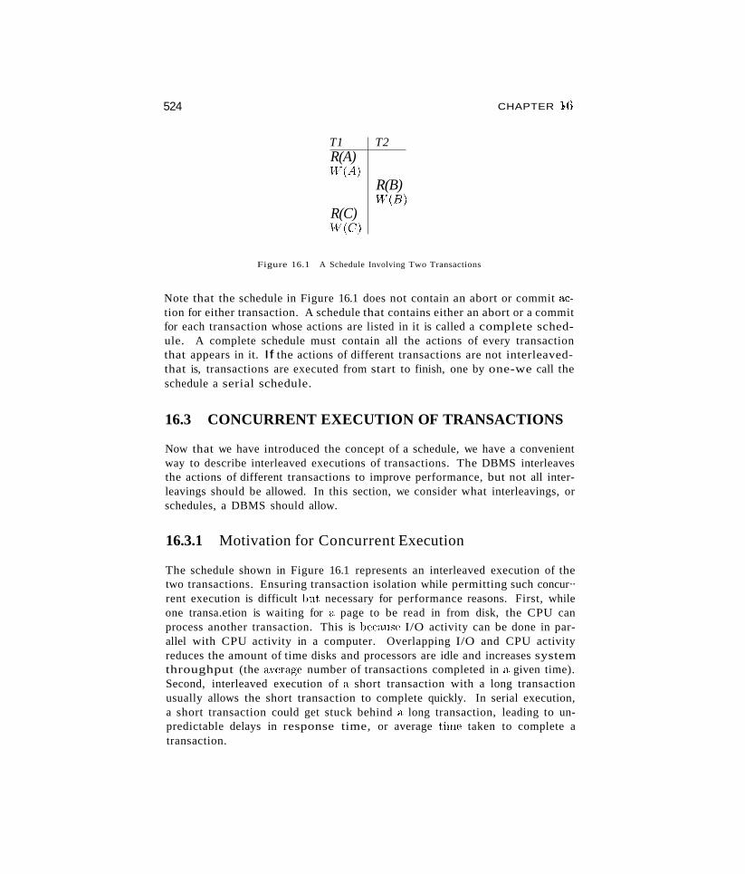
524
T1 T2R(A)Hl(A)
R(B)IV(B)
R(C)W"(C)
Figure 16.1 A Schedule Involving Two Transactions
CHAPTER 16
Note that the schedule in Figure 16.1 does not contain an abort or commit action for either transaction. A schedule that contains either an abort or a commitfor each transaction whose actions are listed in it is called a complete schedule. A complete schedule must contain all the actions of every transactionthat appears in it. If the actions of different transactions are not interleavedthat is, transactions are executed from start to finish, one by one-we call theschedule a serial schedule.
16.3 CONCURRENT EXECUTION OF TRANSACTIONS
Now that we have introduced the concept of a schedule, we have a convenientway to describe interleaved executions of transactions. The DBMS interleavesthe actions of different transactions to improve performance, but not all interleavings should be allowed. In this section, we consider what interleavings, orschedules, a DBMS should allow.
16.3.1 Motivation for Concurrent Execution
The schedule shown in Figure 16.1 represents an interleaved execution of thetwo transactions. Ensuring transaction isolation while permitting such concur··rent execution is difficult lnlt necessary for performance reasons. First, whileone transa.etion is waiting for a page to be read in from disk, the CPU canprocess another transaction. This is because I/O activity can be done in parallel with CPU activity in a computer. Overlapping I/O and CPU activityreduces the amount of time disks and processors are idle and increases systemthroughput (the average number of transactions completed in a given time).Second, interleaved execution of a short transaction with a long transactionusually allows the short transaction to complete quickly. In serial execution,a short transaction could get stuck behind a long transaction, leading to unpredictable delays in response time, or average time taken to complete atransaction.
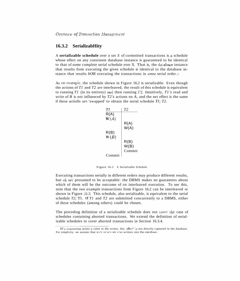
01)eruiew of Transaction A!anagf'rnent
16.3.2 SerializabHity
A serializable schedule over a set S of cormnitted transactions is a schedulewhose effect on any consistent database instance is guaranteed to be identicalto that of some complete serial schedule over S. That is, the databa..<;e instancethat results from executing the given schedule is identical to the database instance that results frOlIl executing the transactions in some serial order. 1
As an example, the schedule shown in Figure 16.2 is serializable. Even thoughthe actions of T1 and T2 are interleaved, the result of this schedule is equivalentto running T1 (in its entirety) and then running T2. Intuitively, T1 's read andwrite of B is not influenced by T2's actions on A, and the net effect is the sameif these actiolls are 'swapped' to obtain the serial schedule Tl; T2.
Tl T2R(A)vV(A)
R(A)W(A)
R(B)vV(B)
R(B)W(B)Commit
Commit
Figure 16.2 A Serializable Schedule
Executing transactions serially in different orders may produce different results,but all are presumed to be acceptable: the DBMS makes no guarantees ahoutwhich of them will be the outcome of an interleaved execution. To see this,note that the two example transactions from Figure 16.2 can be interleaved a.sshown in Figure 16.:3. This schedule, also serializable, is equivalent to the serialschedule T2; Tl. If T1 and T2 are submitted concurrently to a DBMS, eitherof these schedules (among others) could be chosen.
The preceding definition of a serializable schedule does not cover the case ofschedules containing aborted transactions. We extend the definition of serializable schedules to cover aborted transactions in Section 16.3.4.
llf a transaction prints a value to the screen, this 'effed' is not directly captured in the database.For simplicity, we assume that such values are abo written into the database.
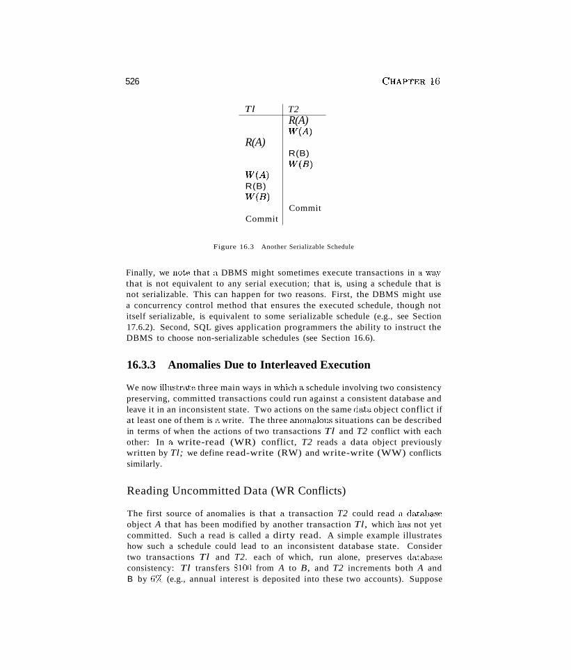
526
Tl T2R(A)vV(A)
R(A)R(B)vV(B)
vV(A)R(B)vV(B)
CommitCommit
Figure 16.3 Another Serializable Schedule
CHAPTER 16
Finally, we note that a DBMS might sometimes execute transactions in a waythat is not equivalent to any serial execution; that is, using a schedule that isnot serializable. This can happen for two reasons. First, the DBMS might usea concurrency control method that ensures the executed schedule, though notitself serializable, is equivalent to some serializable schedule (e.g., see Section17.6.2). Second, SQL gives application programmers the ability to instruct theDBMS to choose non-serializable schedules (see Section 16.6).
16.3.3 Anomalies Due to Interleaved Execution
We now illustrate three main ways in which a schedule involving two consistencypreserving, committed transactions could run against a consistent database andleave it in an inconsistent state. Two actions on the same data object conflict ifat least one of them is a write. The three anomcllous situations can be describedin terms of when the actions of two transactions Tl and T2 conflict with eachother: In a write-read (WR) conflict, T2 reads a data object previouslywritten by Tl; we define read-write (RW) and write-write (WW) conflictssimilarly.
Reading Uncommitted Data (WR Conflicts)
The first source of anomalies is that a transaction T2 could read a databaseobject A that has been modified by another transaction Tl, which ha"i not yetcommitted. Such a read is called a dirty read. A simple example illustrateshow such a schedule could lead to an inconsistent database state. Considertwo transactions Tl and T2. each of which, run alone, preserves datal)a"ieconsistency: Tl transfers 8100 from A to B, and T2 increments both A andB by G% (e.g., annual interest is deposited into these two accounts). Suppose
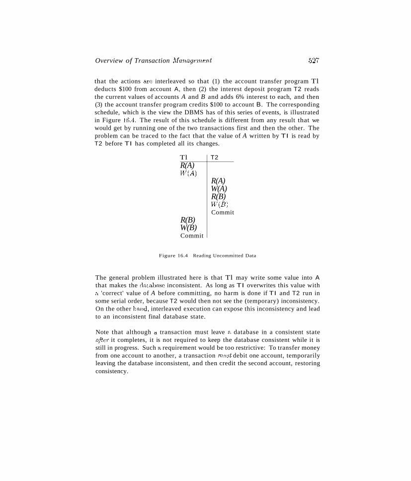
Overview of Transaction A1anagement 527
that the actions are interleaved so that (1) the account transfer program Tldeducts $100 from account A, then (2) the interest deposit program T2 readsthe current values of accounts A and B and adds 6% interest to each, and then(3) the account transfer program credits $100 to account B. The correspondingschedule, which is the view the DBMS has of this series of events, is illustratedin Figure 16.4. The result of this schedule is different from any result that wewould get by running one of the two transactions first and then the other. Theproblem can be traced to the fact that the value of A written by TI is read byT2 before TI has completed all its changes.
Tl T2R(A)vV(A)
R(A)W(A)R(B)liV(B)Commit
R(B)W(B)Commit
Figure 16.4 Reading Uncommitted Data
The general problem illustrated here is that Tl may write some value into Athat makes the databa..':le inconsistent. As long as TI overwrites this value witha 'correct' value of A before committing, no harm is done if TI and T2 run insome serial order, because T2 would then not see the (temporary) inconsistency.On the other hetnel, interleaved execution can expose this inconsistency and leadto an inconsistent final database state.
Note that although a transaction must leave a database in a consistent stateafter it completes, it is not required to keep the database consistent while it isstill in progress. Such a requirement would be too restrictive: To transfer moneyfrom one account to another, a transaction rn1l8t debit one account, temporarilyleaving the database inconsistent, and then credit the second account, restoringconsistency.
528
Unrepeatable Reads (RW Conflicts)
CHAPTERd.6
The second way in which anomalous behavior could result is that a transactionT2 could change the value of an object A that has been read by 1:1, transactionTl, while Tl is still in progress.
IfTl tries to read the value of A again, it will get a different result, even thoughit has not modified A in the meantime. This situation could not arise in a serialexecution of two transactions; it is called an unrepeatable read.
To see why this can cause problems, consider the following example. Supposethat A is the number of available copies for a book. A transaction that placesan order first reads A, checks that it is greater tha,n 0, and then decrements it.Transaction Tl reads A and sees the value 1. Transaction T2 also reads A andsees the value 1, decrements A to 0 and commits. Transaction Tl then tries todecrement A and gets an error (if there is an integrity constraint that preventsA from becoming negative).
This situation can never arise in a serial execution of Tl and T2; the secondtransaction would read A and see 0 and therefore not proceed with the order(and so would not attempt to decrement A).
Overwriting Uncommitted Data (WW Conflicts)
The third source of anomalous behavior is that a transaction T2 could overwritethe value of an object A, which has already been modified by a transaction Tl,while Tl is still in progress. Even if T2 does not read the value of A writtenby Tl, a potential problem exists as the following example illustrates.
Suppose that Harry and Larry are two employees, and their salaries must bekept equal. Transaction Tl sets their salaries to $2000 and transaction T2 setstheir salaries to $1000. If we execute these in the serial order Tl followed byT2, both receive the salary $1000: the serial order T2 followed by Tl gives eachthe salary $2000. Either of these is acceptable from a consistency standpoint(although Harry and Larry may prefer a higher salary!). Note that neithertransaction reads a salary value before writing it----such a write is called ablind write, t:or obvious rea.sons.
Now, consider the following interleaving of the actions of 1'1 and T2: T2 setsHarry's salary to $1000, Tl sets Larry's salary to $2000, T2 sets La.rry's salaryto $1000 and commits, and finally Tl sets Harry's salary to $2000 and connnits.The result is not identical to the result of either of the two possible serial
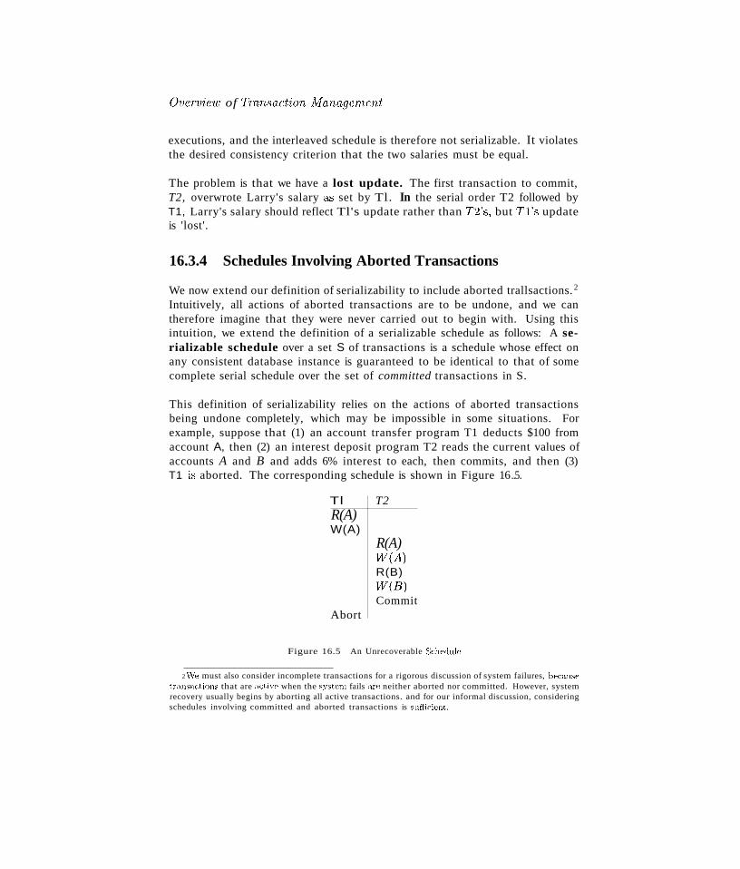
OuenJiew of Transaction ~Management
executions, and the interleaved schedule is therefore not serializable. It violatesthe desired consistency criterion that the two salaries must be equal.
The problem is that we have a lost update. The first transaction to commit,T2, overwrote Larry's salary as set by Tl. In the serial order T2 followed byT1, Larry's salary should reflect Tl's update rather than T2's, but Tl's updateis 'lost'.
16.3.4 Schedules Involving Aborted Transactions
We now extend our definition of serializability to include aborted trallsactions. 2
Intuitively, all actions of aborted transactions are to be undone, and we cantherefore imagine that they were never carried out to begin with. Using thisintuition, we extend the definition of a serializable schedule as follows: A serializable schedule over a set S of transactions is a schedule whose effect onany consistent database instance is guaranteed to be identical to that of somecomplete serial schedule over the set of committed transactions in S.
This definition of serializability relies on the actions of aborted transactionsbeing undone completely, which may be impossible in some situations. Forexample, suppose that (1) an account transfer program T1 deducts $100 fromaccount A, then (2) an interest deposit program T2 reads the current values ofaccounts A and B and adds 6% interest to each, then commits, and then (3)T1 is aborted. The corresponding schedule is shown in Figure 16..5.
Tl T2R(A)W(A)
R(A)vV(A)R(B)Hl(B)Commit
Abort
Figure 16.5 An Unrecoverable Schedule
2 Vie must also consider incomplete transactions for a rigorous discussion of system failures, becausetransactions that are active when the system fails are neither aborted nor committed. However, systemrecovery usually begins by aborting all active transactions. and for our informal discussion, consideringschedules involving committed and aborted transactions is sufficient.
530 CHAPTER$16
Now, T2 has read a value for A that should never have been there. (Recallthat aborted transactions' effects are not supposed to be visible to other transactions.) If T2 had not yet committed, we could deal with the situation bycascading the abort of TI and also aborting T2; this process recursively abortsany transaction that read data written by T2, and so on. But T2 has alreadycommitted, and so we cannot undo its actions. \Ve say that such a scheduleis unrecoverable. In a recoverable schedule, transactions commit only after(and if!) all transactions whose changes they read commit. If transactions readonly the changes of committed transactions, not only is the schedule recoverable, but also aborting a transaction can be accomplished without cascadingthe abort to other transactions. Such a schedule is said to avoid cascadingaborts.
There is another potential problem in undoing the actions of a transaction.Suppose that a transaction T2 overwrites the value of an object A that has beenmodified by a transaction TI, while TI is still in progress, and Tl subsequentlyaborts. All of Tl's changes to database objects are undone by restoring thevalue of any object that it modified to the value of the object before Tl'schanges. (We look at the details of how a transaction abort is handled inChapter 18.) When Tl is aborted and its changes are undone in this manner,T2's changes are lost as well, even if T2 decides to commit. So, for example, ifA originally had the value 5, then WetS changed by T1 to 6, and by T2 to 7, ifT1 now aborts, the value of A becomes 5 again. Even if T2 commits, its changeto A is inadvertently lost. A concurrency control technique called Strict 2PL,introduced in Section 16.4, can prevent this problem (as discussed in Section17.1) .
16.4 LOCK-BASED CONCURRENCY CONTROL
A DBMS must be able to ensure that only serializable, recoverable schedulesare allowed and that no actions of committed transactions are lost while undoing aborted transactions. A DBl'vlS typically uses a locking protocol to achievethis. A lock is a small bookkeeping object CL.ssociated with a database object.A locking protocol is a set of rules to be followed by each transaction (and enforced by the DBlVIS) to ensure that, even though actions of several transactionsmight be interleaved, the net effect is identical to executing all transactions insOlne serial or~ler. Different locking protocols use different types of locks, suchas shared locks or exclusive locks, as we see next, when we discuss the Strict2PL protocol.
Ove-nJiew of Transaction jvlanagement
16.4.1 Strict Two-Phase Locking (Strict 2PL)
531
The most widely used locking protocol, called Strict Two-Phase Locking, orStrict 2PL, has two rules. The first rule is
1. If a transaction T wants to read (respectively, rnodify) an object, itfirst requests a shared (respectively, exclusive) lock on the object.
Of course, a transaction that has an exclusive lock can also read the object;an additional shared lock is not required. A transaction that requests a lock issuspended until the DBMS is able to grant it the requested lock. The DBMSkeeps track of the locks it has granted and ensures that if a transaction holdsan exclusive lock on an object, no other transaction holds a shared or exclusivelock on the same object. The second rule in Strict 2PL is
2. All locks held by a transaction are relea.'3ed when the transaction iscompleted.
Requests to acquire and release locks can be automatically inserted into transactions by the DBMS; users need not worry about these details. eWe discusshow application programmers can select properties of transactions and controllocking overhead in Section 16.6.3.)
In effect, the locking protocol allows only 'safe' interleavings of transactions.If two transactions access completely independent parts of the database, theyconcurrently obtain the locks they need and proceed merrily on their ways. Onthe other band, if two transactions access the same object, and one wants tomodify it, their actions are effectively ordered serially·all actions of one ofthese transactions (the one that gets the lock on the common object first) arecompleted before (this lock is released and) the other transaction can proceed.
We denote the action of a transaction T requesting a shared (respectively, exclusive) lock on object 0 as 5T(0) (respectively, XT(O)) and omit the subscriptdenoting the tn1l1saction when it is clear from the context. As an example,consider the schedule shown in Figure 16.4. This interleaving could result in astate that cannot result from any serial execution of the three transactions. Forinstance, T1 could change A from 10 to 20, then T2 (which reads the value 20for A) could change B from 100 to 200, and then T1 would read the value 200for B. If run serially, either Tl or T2 would execute first, and read the values10 for A and 100 for B: Clearly, the interleaved execution is not equivalent toeither serial execution.
If the Strict 2PL protocol is used, such interleaving is disallowed. Let us seewhy. Assuming that the transactions proceed <tt the same relative speed as
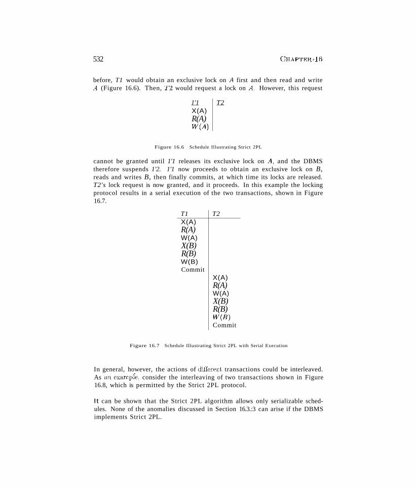
532 CHAPTER*16
before, T1 would obtain an exclusive lock on A first and then read and writeA (Figure 16.6). Then, 1'2 would request a lock on A. However, this request
1'1 T2X(A)R(A)lV(A)
Figure 16.6 Schedule Illustrating Strict 2PL
cannot be granted until 1'1 releases its exclusive lock on A, and the DBMStherefore suspends 1'2. 1'1 now proceeds to obtain an exclusive lock on B,reads and writes B, then finally commits, at which time its locks are released.T2's lock request is now granted, and it proceeds. In this example the lockingprotocol results in a serial execution of the two transactions, shown in Figure16.7.
T1 T2X(A)R(A)W(A)X(B)R(B)W(B)Commit
X(A)R(A)W(A)X(B)R(B)H'(B)Commit
Figure 16.7 Schedule Illustrating Strict 2PL with Serial Execution
In general, however, the actions of different transactions could be interleaved.As an example, consider the interleaving of two transactions shown in Figure16.8, which is permitted by the Strict 2PL protocol.
It can be shown that the Strict 2PL algorithm allows only serializable schedules. None of the anomalies discussed in Section 16.3.:3 can arise if the DBMSimplements Strict 2PL.
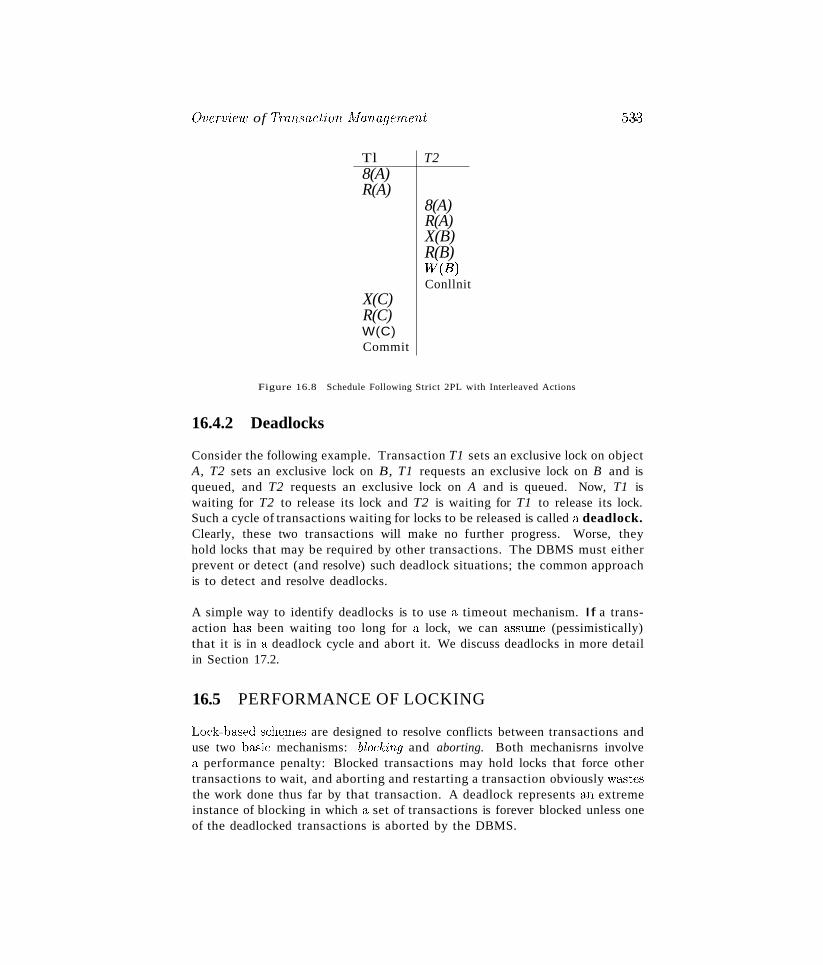
Ovenriew of Tran,.'wdion Alanagement
Tl T28(A)R(A)
8(A)R(A)X(B)R(B)vV(B)Conllnit
X(C)R(C)W(C)Commit
Figure 16.8 Schedule Following Strict 2PL with Interleaved Actions
16.4.2 Deadlocks
533
Consider the following example. Transaction T1 sets an exclusive lock on objectA, T2 sets an exclusive lock on B, T1 requests an exclusive lock on B and isqueued, and T2 requests an exclusive lock on A and is queued. Now, T1 iswaiting for T2 to release its lock and T2 is waiting for T1 to release its lock.Such a cycle of transactions waiting for locks to be released is called a deadlock.Clearly, these two transactions will make no further progress. Worse, theyhold locks that may be required by other transactions. The DBMS must eitherprevent or detect (and resolve) such deadlock situations; the common approachis to detect and resolve deadlocks.
A simple way to identify deadlocks is to use a timeout mechanism. If a transaction has been waiting too long for a lock, we can a'3sume (pessimistically)that it is in a deadlock cycle and abort it. We discuss deadlocks in more detailin Section 17.2.
16.5 PERFORMANCE OF LOCKING
Lock-b"l.'sed schqmes are designed to resolve conflicts between transactions anduse two ba'3ic mechanisms: blocking and aborting. Both mechanisrns involvea performance penalty: Blocked transactions may hold locks that force othertransactions to wait, and aborting and restarting a transaction obviously wa..'3testhe work done thus far by that transaction. A deadlock represents an extremeinstance of blocking in which a set of transactions is forever blocked unless oneof the deadlocked transactions is aborted by the DBMS.
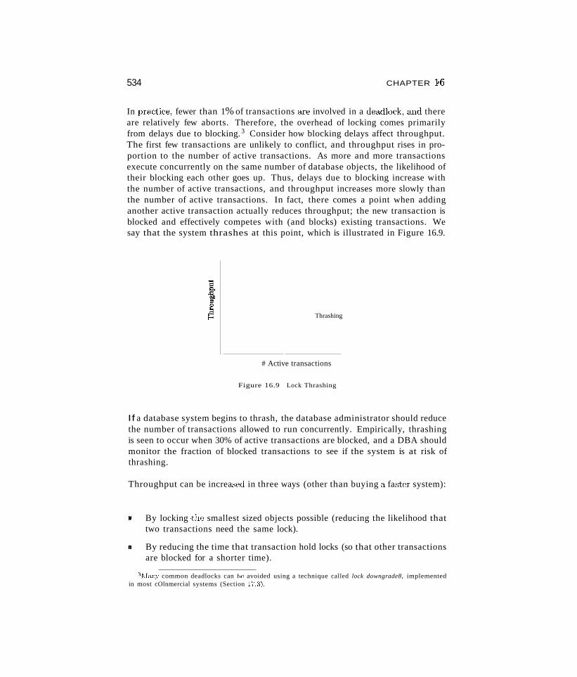
534 CHAPTER :F6
In practice, fewer than 1% of transactions are involved in a deadlock, (uId thereare relatively few aborts. Therefore, the overhead of locking comes primarilyfrom delays due to blocking.3 Consider how blocking delays affect throughput.The first few transactions are unlikely to conflict, and throughput rises in proportion to the number of active transactions. As more and more transactionsexecute concurrently on the same number of database objects, the likelihood oftheir blocking each other goes up. Thus, delays due to blocking increase withthe number of active transactions, and throughput increases more slowly thanthe number of active transactions. In fact, there comes a point when addinganother active transaction actually reduces throughput; the new transaction isblocked and effectively competes with (and blocks) existing transactions. Wesay that the system thrashes at this point, which is illustrated in Figure 16.9.
Thrashing
# Active transactions
Figure 16.9 Lock Thrashing
If a database system begins to thrash, the database administrator should reducethe number of transactions allowed to run concurrently. Empirically, thrashingis seen to occur when 30% of active transactions are blocked, and a DBA shouldmonitor the fraction of blocked transactions to see if the system is at risk ofthrashing.
Throughput can be increa..c;ed in three ways (other than buying a fa..'3ter system):
IIll By locking the smallest sized objects possible (reducing the likelihood thattwo transactions need the same lock).
.. By reducing the time that transaction hold locks (so that other transactionsare blocked for a shorter time).
3Ivlany common deadlocks can be avoided using a technique called lock downgrade8, implementedin most cOlnmercial systems (Section 17.3).

Overview of TmnsCLction lHanagement 535
• By reducing hot spots. A hot spot is a databa.ge object that is frequentlyaccessed and modified, and causes a lot of blocking delays. Hot spots cansignificantly affect performance.
The granularity of locking is largely determined by the databa..<;;e system's implementation of locking, and application programmers and the DBA have littlecontrol over it. We discuss how to improve performance by minimizing theduration locks are held and using techniques to deal with hot spots in Section20.10.
16.6 TRANSACTION SUPPORT IN SQL
We have thus far studied transactions and transaction management using anabstract model of a transaction as a sequence of read, write, and abort/commitactions. We now consider what support SQL provides for users to specifytransaction-level behavior.
16.6.1 Creating and Terminating Transactions
A transaction is automatically started when a user executes a statement thataccesses either the database or the catalogs, such as a SELECT query, an UPDATEcommand, or a CREATE TABLE statement.4
Once a transaction is started, other statements can be executed as part of thistransaction until the transaction is terminated by either a COMMIT commandor a ROLLBACK (the SQL keyword for abort) command.
In SQL:1999, two new features are provided to support applications that involvelong-running transactions, or that must run several transactions one after theother. To understand these extensions, recall that all the actions of a giventransaction are executed in order, regardless of how the actions of differenttransactions are interleaved. We can think of each transaction as a sequence ofsteps.
The first feature, called a savepoint, allows us to identify a point in a transaction and selectively roll back operations carried out after this point. Thisis especially useful if the transaction carries out what-if kinds of operations,and wishes to undo or keep the changes based on the results. This can beaccomplished by defining savepoints.
4Some SQL statements·..·····e.g., the CONNECT statement, which connects an application program to adatabase server do not require the creation of a transaction.
536 CHAPTEH 16
r-·······~~~~ .---.----- ---- """'-<··---------1
I SQL:1999 Nested Transactions: The concept of atn,msactioll as an I
I,
atomic sequence of actions has been extended in SQL:1999 thrQugh the i• introduction of the savepo'int feature. This allows parts of a transaction to
be selectively rolled back. The introduction of savepoints represents thefirst SQL support for the concept of nested transactions, which havebeen extensively studied in the research community. The idea is that a Itransaction can have several nested subtransactions, each of which can I
be selectively rolled back. Savepoints snpport a simple form of one-level i
nesting.'--------------, .. " , -
In a long-running transaction, we may want to define a series of savepoints.The savepoint command allows us to give each savepoint a name:
SAVEPDINT (savepoint name)
A subsequent rollback command can specify the savepoint to roll back to
ROLLBACK TO SAVEPDINT (savepoint name)
If we define three savepoints A, B, and C in that order, and then rollback toA, all operations since A are undone, including the creation of savepoints Band C. Indeed, the savepoint A is itself undone when we roll hack to it, andwe must re-establish it (through another savepoint conunand) if we wish to beable to roll back to it again. From a locking standpoint, locks obtained aftersavepoint A can be released when we roll back to A.
It is instructive to compare the use of savepoints with the alternative of executing a series of transactions (i.e., treat all operations in between two consecutivesavepoints as a new transaction). The savepoint mechanism offers two advantages. First, we can roll back over several savepoints. In the alternativeapproach, we can roll back only the most recent transaction, which is equivalent to rolling back to the most recent savepoint, Second, the overhead ofinitiating several transactions is avoided.
Even with the use of savepoints, certain applications might require us to runseveral transactions one after the other. To minimize the overhead in suchsituations, SQL:1999 introduces another feature, called chained transactions,\Ve can cornmit or roll back a transaction and immediately initiate anothertransaction, This is done by using the optional keywords AND CHAIN in theCOMMIT and ROLLBACK statements.
Overview of Transaction AIanagement
16.6.2 What Should We Lock?
537
Until now, we have discussed transactions and concurrency control in tenus ofan abstract model in which a database contains a fixed collection of objects, andeach transaction is a series of read and write operations on individual objects.An important question to consider in the context of SQL is what the DBMSshould treat as an object when setting locks for a given SQL statement (that ispart of a transaction).
Consider the following query:
SELECT S.rating, MIN (S.age)FROM Sailors SWHERE S.rating = 8
Suppose that this query runs as part of transaction T1 and an SQL statementthat modifies the age of a given sailor, say Joe, with rating=8 runs a-s part oftransaction T2. What 'objects' should the DBMS lock when executing thesetransactions? Intuitively, we must detect a conflict between these transactions.
The DBMS could set a shared lock on the entire Sailors table for T1 and setan exclusive lock on Sailors for T2, which would ensure that the two transactions are executed in a serializable manner. However, this approach yields lowconcurrency, and we can do better by locking smaller objects, reflecting whateach transaction actually accesses. Thus, the DBMS could set a shared lockon every row with mting=8 for transaction T1 and set an exclusive lock onjust the row for the modified tuple for transaction T2. Now, other read-onlytransactions that do not involve nding=8 rows can proceed without waiting forT1 or T2.
As this example illustrates, the DBMS can lock objects at different granularities: \~re can lock entire tables or set row-level locks. The latter approach istaken in current systems because it offers much better performance. In practice,while row-level locking is generally better, the choice of locking granularity iscomplicated. For example, a transaction that examines several rows and modifies those tha1 satisfy some condition might be best served by setting sharedlocks on the entire table and setting exclusive locks on those rows it wants tolllodify. vVe diseuss this issue further in Section 17.5.3.
A second point to note is that SQL statements conceptually access a collectionof rows described by a .selection predicate. In the prf~cedingexample, transactionT1 accesses all rows with mting=8. vVe suggested that this could be dealt withby setting shared locks on all rows in Sailors that had rating=8. Unfortunately,this is a little too silnplistic. To sec why, consider an SQL statelnent that inserts
538 CHAPTER 1.6
a new sailor with mting=8 and runs as transaction T3. (Observe that thisexample violates our assumption of a fixed number of objects in the database,but we must obviously deal with such situations in practice.)
Suppose that the DBJ\iIS sets shared locks on every existing Sailors row withmting=8 for Tl. This does not prevent transaction T3 from creating a brandnew row with mting=8 and setting an exclusive lock on this row. If this new rowhas a smaller age value than existing rows, Tl returns an answer that dependson when it executed relative to T2. However, our locking scheme imposes norelative order on these two transactions.
This phenomenon is called the phantom problem: A transaction retrievesa collection of objects (in SQL terms, a collection of tuples) twice and seesdifferent results, even though it does not modify any of these tuples itself. Toprevent phantoms, the DBMS must conceptually lock all possible rows withmting=8 on behalf of Tl. One way to do this is to lock the entire table, atthe cost of low concurrency. It is possible to take advantage of indexes to dobetter, as we will see in Section 17.5.1, but in general preventing phantoms canhave a significant impact on concurrency.
It may well be that the application invoking T1 can accept the potential inaccuracy due to phantoms. If so, the approach of setting shared locks on existingtuples for Tl is adequate, and offers better performance. SQL allows a programmer to make this choice---and other similar choices'--explicitly, as we seenext.
16.6.3 Transaction Characteristics in SQL
In order to give programmers control over the locking overhead incurred bytheir transactions, SQL allows them to specify three characteristics of a transaction: access mode, diagnostics size, and isolation level. The diagnosticssize determines the number of error conditions that can be recorded; we willnot discuss this feature further.
If the access mode is READ ONLY, the transaction is not allowed to modifythe databclse. Thus, INSERT, DELETE, UPDATE, and CREATE comlnands cannotbe executed. If we have to execute one of these commands, the access modeshould be set to READ WRITE. 1<or transactions with READ ONLY access mode.only shared locks need to be obtained, thereby increasing concurrency.
The isolation level controls the extent to which a given transaction is exposed to the actions of other transactions executing concurrently. By choosingone of four possible isolation level settings, a user can obtain greater concur-
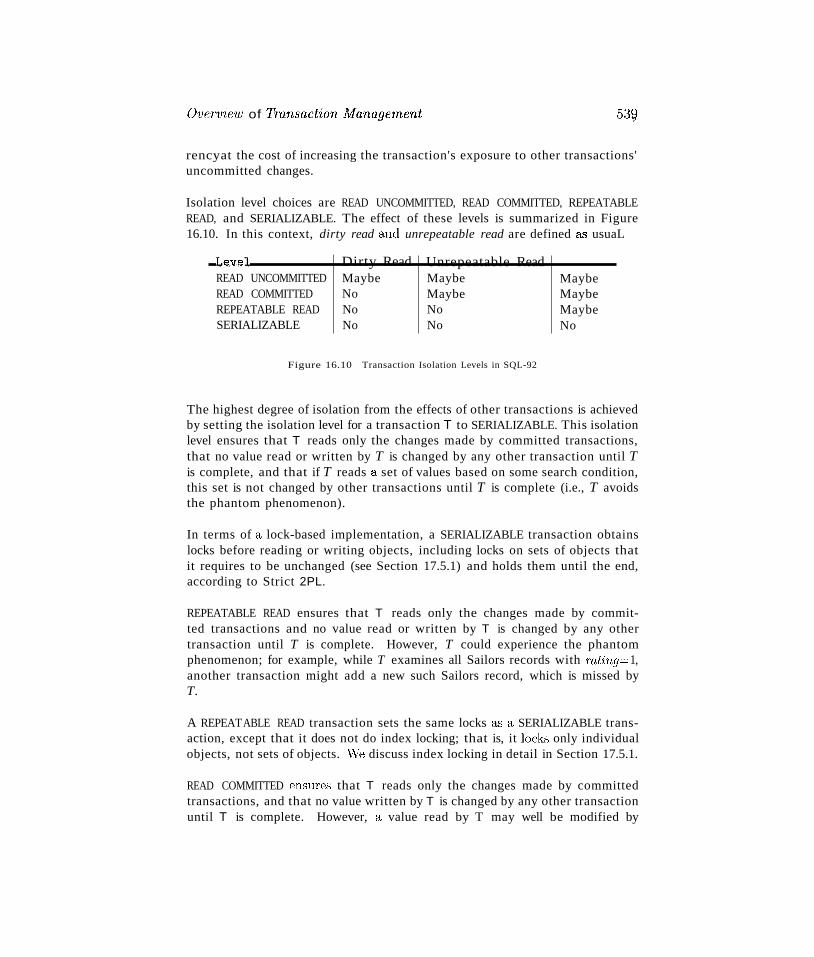
Ovenrie11J of Tnmsaction l"tfanagernent 53Q
rencyat the cost of increasing the transaction's exposure to other transactions'uncommitted changes.
Isolation level choices are READ UNCOMMITTED, READ COMMITTED, REPEATABLEREAD, and SERIALIZABLE. The effect of these levels is summarized in Figure16.10. In this context, dirty read and unrepeatable read are defined as usuaL
LevelREAD UNCOMMITTEDREAD COMMITTEDREPEATABLE READSERIALIZABLE
Dirty ReadMaybeNoNoNo
Unrepeatable ReadMaybeMaybeNoNo
MaybeMaybeMaybeNo
Figure 16.10 Transaction Isolation Levels in SQL-92
The highest degree of isolation from the effects of other transactions is achievedby setting the isolation level for a transaction T to SERIALIZABLE. This isolationlevel ensures that T reads only the changes made by committed transactions,that no value read or written by T is changed by any other transaction until Tis complete, and that if T reads a set of values based on some search condition,this set is not changed by other transactions until T is complete (i.e., T avoidsthe phantom phenomenon).
In terms of a lock-based implementation, a SERIALIZABLE transaction obtainslocks before reading or writing objects, including locks on sets of objects thatit requires to be unchanged (see Section 17.5.1) and holds them until the end,according to Strict 2PL.
REPEATABLE READ ensures that T reads only the changes made by committed transactions and no value read or written by T is changed by any othertransaction until T is complete. However, T could experience the phantomphenomenon; for example, while T examines all Sailors records with rating= 1,another transaction might add a new such Sailors record, which is missed byT.
A REPEATABLE READ transaction sets the same locks a'S a SERIALIZABLE transaction, except that it does not do index locking; that is, it locks only individualobjects, not sets of objects. vVe discuss index locking in detail in Section 17.5.1.
READ COMMITTED ensures that T reads only the changes made by committedtransactions, and that no value written by T is changed by any other transactionuntil T is complete. However, a value read by T may well be modified by
540 CHAPTER 1!6
another transaction while T is still in progress, and T is exposed to the phantomproblem.
A READ COMMITTED transaction obtains exclusive locks before writing objectsand holds these locks until the end. It also obtains shared locks before reading objects, but these locks are released immediately; their only effect is toguarantee that the transaction that last modified the object is complete. (Thisguarantee relies on the fact that every SQL transaction obtains exclusive locksbefore writing objects and holds exclusive locks until the end.)
A READ UNCOMMITTED transaction T can read changes made to an object by anongoing transaction; obviously, the object can be changed further while T is inprogress, and T is also vulnerable to the phantom problem.
A READ UNCOMMITTED transaction does not obtain shared locks before readingobjects. This mode represents the greatest exposure to uncommitted changesof other transactions; so much so that SQL prohibits such a transaction frommaking any changes itself-a READ UNCOMMITTED transaction is required to havean access mode of READ ONLY. Since such a transaction obtains no locks forreading objects and it is not allowed to write objects (and therefore neverrequests exclusive locks), it never makes any lock requests.
The SERIALIZABLE isolation level is generally the safest and is recommended formost transactions. Some transactions, however, can run with a lower isolationlevel, and the smaller number of locks requested can contribute to improved system performance. For example, a statistical query that finds the average sailorage can be run at the READ COMMITTED level or even the READ UNCOMMITTEDlevel, because a few incorrect or missing values do not significantly affect theresult if the number of sailors is large.
The isolation level and access mode can be set using the SET TRANSACTION com~
mand. For example, the following command declares the current transactionto be SERIALIZABLE and READ ONLY:
SET TRANSACTION ISOLATION LEVEL SERIALIZABLE READ ONLY
When a transaction is started, the default is SERIALIZABLE and READ WRITE.
16.7 INTRODUCTION TO CRASH RECOVERY
The recovery manager of a DBMS is responsible for ensuring transactionatomicity and durability. It ensures atomicity by undoing the actions of transactions that do not commit, and durability by making sure that all actions of
Overview of 7'ransaction lvlanagernent 541
committed transactions survive systenl crashes, (e.g., a core dump caused bya bus error) and media failures (e.g., a disk is corrupted).
\\Then a DB]\,IS is restarted after crashes. the recovery manager is given controland must bring the databa.'le to a consistent state. The recovery manager isalso responsible for undoing the actions of an aborted transaction. To see whatit takes to implement a recovery manager, it is necessary to understand whathappens during normal execution.
The transaction manager of a DBMS controls the execution of transactions.Before reading and writing objects during normal execution, locks must be acquired (and released at some later time) according to a chosen locking protocol. 5
For simplicity of exposition, we make the following assumption:
Atomic Writes: Writing a page to disk is an atomic action.
This implies that the system does not crash while a write is in progress and isunrealistic. In practice, disk writes do not have this property, and steps mustbe taken during restart after a crash (Section 18.6) to verify that the mostrecent write to a given page was completed successfully, and to deal with theconsequences if not.
16.7.1 Stealing Frames and Forcing Pages
\Vith respect to writing objects, two additional questions arise:
1. Can the changes made to an object 0 in the buffer pool by a transaction Tbe written to disk before T commits? Such writes are executed when another transaction wants to bring in a page and the buffer manager choosesto replace the frame containing 0; of course, this page must have beenunpinned by T. If such writes are allowed, we say that a steal approachis used. (Informally, the second transaction 'steals' a frame from T.)
2. \\"hen a transaction cOl1units, must we ensure that all the changes it hasmade to objects in the buffer pool are immediately forced to disk? If so.we say that a force approach is used.
From the standpoint of implementing a recovery manager, it is simplest to usea buffer manager with a no-steaL force approach. If a no-steal approach is used,we do not have to undo the changes of an aborted transaction (because thesedumges have not been written to disk) l and if a force approach is used, we do
S A concurrency control technique that does not involve locking could be used instead, but wea.ssul1lc t hat locking is llsed.
542 CHAPTER.16
not have to redo the changes of a committed transaction if there is a subsequentcrash (because all these changes are guaranteed to have been written to diskat commit time).
However, these policies have important drawbacks. The no-steal approach assumes that all pages modified by ongoing transactions can be accommodatedin the buffer pool, and in the presence of large transactions (typically run inbatch mode, e.g., payroll processing), this assumption is unrealistic. The forceapproach results in excessive page I/O costs. If a highly used page is updatedin succession by 20 transactions, it would be written to disk 20 times. With ano-force approach, on the other hand, the in-memory copy of the page wouldbe successively modified and written to disk just once, reflecting the effectsof all 20 updates, when the page is eventually replaced in the buffer pool (inaccordance with the buffer manager's page replacement policy).
For these reasons, most systems use a steal, no-force approach. Thus, if aframe is dirty and chosen for replacement, the page it contains is written todisk even if the modifying transaction is still active (steal); in addition, pages inthe buffer pool that are modified by a transaction are not forced to disk whenthe transaction commits (no-force).
16.7.2 Recovery-Related Steps during Normal Execution
The recovery manager of a DBMS maintains some information during normalexecution of transactions to enable it to perform its task in the event of afailure. In particular, a log of all modifications to the database is saved onstable storage, which is guaranteed6 to survive crashes and media failures.Stable storage is implemented by maintaining multiple copies of information(perhaps in different locations) on nonvolatile storage devices such as disks ortapes.
As discussed earlier in Section 16.7, it is important to ensure that the logentries describing a change to the database are written to stable storage beforethe change is made; otherwise, the system might crash just after the change,leaving us without a record of the change. (Recall that this is the Write-AheadLog, or WAL, property.)
The log enables the recovery manager to undo the actions of aborted andincomplete transactions and redo the actions of committed transactions. Forexample, a transaction that committed before the crash may have made updates
(jNothing in life is really guaranteed except death and taxes. However, we can reduce the chanceof log failure to be vanishingly small by taking steps such as duplexing the log and storing the copiesin different secure locations.
Overview of Transaction A1anagement 5il3
Tuning the Recovery Subsystem: DBMS performance can be greatlyaffected by the overhead imposed by the recoverysubsystem. A DBA cantake several steps to tune this subsystem1 such at> correctly sizing the logand how it is managed on disk l controlling the rate at which buffer pagesare forced to disk, choosing a good frequency for checkpointing, and soforth.
to a copy (of a database object) in the buffer pool, and this change may not havebeen written to disk before the crash, because of a no-force approach. Suchchanges must be identified using the log and written to disk. Further, changesof transactions that did not commit prior to the crash might have been writtento disk because of a steal approach. Such changes must be identified using thelog and then undone.
The amount of work involved during recovery is proportional to the changesmade by committed transactions that have not been written to disk at the timeof the crash. To reduce the time to recover from a crash, the DBMS periodically forces buffer pages to disk during normal execution using a backgroundprocess (while making sure that any log entries that describe changes thesepages are written to disk first, i.e., following the WAL protocol). A processcalled checkpointing, which saves information about active transactions anddirty buffer pool pages, also helps reduce the time taken to recover from acrash. Checkpoints are discussed in Section 18.5.
16.7.3 Overview of ARIES
ARIES is a recovery algorithm that is designed to work with a steal, no-forceapproach. When the recovery manager is invoked after a crash, restart proceedsin three pha.'Ses. In the Analysis phase, it identifies dirty pages in the bufferpool (i.e., changes that have not been written to disk) and active transactionsat the time of the cra.'Sh. In the Redo pha.'Se, it repeats all actions, startingfrom an appropriate point in the log, and restores the databa.'Se state to what itwa.'S at the time of the crash. Finally, in the Undo phase, it undoes the actionsof transactions that did not commit, so that the database reflects only theactions of committed transactions. The ARIES algorithm is discussed furtherin Chapter 18.,
16.7.4 Atomicity: Implementing Rollback
It is important to recognize that the recovery subsystem is also responsible forexecuting the ROLLBACK command, which aborts a single transaction. Indeed,
544 CHAPTER 1,6
the logic (and code) involved in undoing a single transaction is identical to thatused during the Undo phase in recovering from a system crash. All log recordsfor a given transctction are organized in a linked list and can be efficientlyaccessed in reverse order to facilitate transaction rollback.
16.8 REVIEW QUESTIONS
Answers to the review questions can be found in the listed sections.
III What are the ACID properties? Define atomicity, consistency, isolation,and durability and illustrate them through examples, (Section 16.1)
III Define the terms transaction, schedule, complete schedule, and seTial schedule. (Section 16.2)
III Why does a DBMS interleave concurrent transactions? (Section 16.3)
III When do two actions on the same data object conflict? Define the anomalies that can be caused by conflicting actions (dirty reads, unrepeatablereads, lost updates). (Section 16.3)
III What is a serializable schedule? What is a Tecoverable schedule? Whatis a schedule that avoids cascading abor'ts? What is a strict schedule?(Section 16.3)
III What is a locking pmtocol:? Describe the Strict Two-Phase Locking (StTict2PL) protocol. What can you say about the schedules allowed by thisprotocol? (Section 16.4)
III What overheads are associated with lock-based concurrency control? Discuss blocking and abo7,ting overheads specifically and explain which is moreimportant in practiee. (Section 16.5)
III What is thrashing? What should a DBA do if the system thrashes? (Section 16.5)
III How can throughput be increased? (Section 16.5)
III How are transactions created and terminated in SQL? What are savepoints? What are chained transactions? Explain why savepoints andchained tninsactions are useful. (Section 16.6)
III What are the considerations in determining the locking granularity whenexecuting SQL statements? \Nhat is the phantom problem? \\That irnpactdoes it have on performance? (Section 16.6.2)
Overview of Transaction !vIanagement
• vVhat transaction characteristics can a programmer control in SQL? Discuss the different access modes and isolat'ion levels in particular. vVhatissues should be considered in selecting an access mode and an isolationlevel for a transaction? (Section 16.6.3)
• Describe how different isolation levels are implemented in terms of the locksthat are set. 'What can you say about the corresponding locking overheads?(Section 16.6.3)
• vVhat functionality does the recovery manager of a DBMS provide? Whatdoes the transaction manager do? (Section 16.7)
• Describe the steal and force policies in the context of a buffer manager.What policies are used in practice and how does this affect recovery? (Section 16.7.1)
• What recovery-related steps are taken during normal execution? Whatcan a DBA control to reduce the time to recover from a crash? (Section 16.7.2)
• How is the log used in transaction rollback and crash recovery? (Sections 16.7.2, 16.7.3, and 16.7.4)
EXERCISES
Exercise 16.1 Give brief answers to the following questions:
1. What is a transaction? In what ways is it different from an ordinary program (in alanguage such as C)?
2. Define these terms: atomicity, consistency, isolation, durability, schedule, blind write,dirty read, unrepeatable read, serializable schedule, recoverable schedule, avoidsvcascadingaborts schedule.
3. Describe Strict 2PL.
4. What is the phantom problem? Can it occur in a database where the set of databaseobjects is fixed and only the values of objects can be changed?
Exercise 16.2 Consider the following actions taken by transaction 1'1 on database objectsX and Y:
R(X), W(X),R(Y), W(Y)
1. Give an example of another transaction 1'2 that, if run concurrently to transaction l'without some form of concurrency control, could interfere with 1'1.
2. Explain how the use of Strict 2PL would prevent interference between the two transactions.
:1. Strict 2PL is lIsed in many database systems. Give two reasons for its popularity.
546 CHAPTER l6
Exercise 16.3 Consider a database with objects X and Y and assume that there are twotransactions Tl and T2. Transaction T1 reads objects X and Y and then writes object X.Transaction T2 reads objects X and Y and then writes objects X and Y.
1. Give an example schedule with actions of transactions T1 and T2 on objects X and Ythat results in a write-read conflict.
2. Give an example schedule with actions of transactions T1 and T2 on objects X and Ythat results in a read-write conflict.
3. Give an example schedule with actions of transactions T1 and T2 on objects X and Ythat results in a write-write conflict.
4. For each of the three schedules, show that Strict 2PL disallows the schedule.
Exercise 16.4 We call a transaction that only reads database object a read-only transaction, otherwise the transaction is called a read-write transaction. Give brief answers to thefollowing questions:
1. What is lock thrashing and when does it occur?
2. What happens to the database system throughput if the number of read-write transactions is increased?
3. What happens to the datbase system throughput if the number of read-only transactionsis increased?
4. Describe three ways of tuning your system to increase transaction throughput.
Exercise 16.5 Suppose that a DBMS recognizes increment, which increments an integervalued object by 1, and decrement as actions, in addition to reads and writes. A transactionthat increments an object need not know the value of the object; increment and decrementare versions of blind writes. In addition to shared and exclusive locks, two special locks aresupported: An object must be locked in I mode before incrementing it and locked in D modebefore decrementing it. An I lock is compatible with another I or D lock on the same object,but not with 5 and X locks.
1. Illustrate how the use of I and D locks can increase concurrency. (Show a scheduleallowed by Strict 2PL that only uses 5 and X locks. Explain how the use of I and Dlocks can allow more actions to be interleaved, while continuing to follow Strict 2PL.)
2. Informally explain how Strict 2PL guarantees serializability even in the presence of Iand D locks. (Identify which pairs of actions conflict, in the sense that their relativeorder can affect the result, and show that the use of 5, X, I, and D locks accordingto Strict 2PL orders all conflicting pairs of actions to be the same as the order in someserial schedule.)
Exercise 16.6 Answer the following questions: SQL supports four isolation-levels and t.woaccess-modes, for a total of eight combinations of isolation-level and access-mode. Eachcombination impiicitly defines a class of transactions; the following questions refer to theseeight classes:
1. Consider the four SQL isolation levels. Describe which of the plHmomena can occur ateach of these isolation levels: dirty read, unrepeatable read, phantom problem.
2. For each of the four isolation levels, give examples of transactions that could be runsafely at that level.
:.3. Why does the access mode of a transaction matter?
Overview of Transaction Manage'm,ent
Exercise 16.7 Consider the university enrollment database schema:
547
Student(snurn: integer, snarne: string, majoT: string, level: string, age: integer)Class( name: string, meets_at: time, Toom: string, fid"' integer)Enrolled(snum: integer, cname: string)Faculty(fid: integer, fname: string, deptid: integer)
The meaning of these relations is straightforward; for example, Enrolled has one record perstudent-class pair such that the student is enrolled in the class.
For each of the following transactions, state the SQL isolation level you would use and explainwhy you chose it.
1. Enroll a student identified by her snum into the class named 'Introduction to DatabaseSystems'.
2. Change enrollment for a student identified by her snum from one class to another class,
3. Assign a new faculty member identified by his fid to the class with the least number ofstudents.
4. For each class, show the number of students enrolled in the class.
Exercise 16.8 Consider the following schema:
Suppliers(sid: integer, sname: string, addTess: string)Parts(pid: integer, pname: string, coloT: string)Catalog(sid: integer, pid: integer, cost: real)
The Catalog relation lists the prices charged for parts by Suppliers.
For each of the following transactions, state the SQL isolation level that you would use andexplain why you chose it.
1. A transaction that adds a new part to a supplier's catalog.
2. A transaction that increases the price that a supplier charges for a part.
3. A transaction that determines the total number of items for a given supplier.
4. A transaction that shows, for each part, the supplier that supplies the part at the lowestprice.
Exercise 16.9 Consider a database with the following schema:
Suppliers(sid: integer, sname: string, addTess: string)Parts(pid: integer, pname: string, coloT: string)Catalog( sid: integer, pid: integer, cost: real)
The Catalog relation lists the prices charged for parts by Suppliers.
Consider three transactions 1'1,1'2, and 1'3; 1'1 always h8.o.'3 SQL isolation level SERIALIZABLE.
We first run 1'1 concurrently with 1'2 and then we run 1'1 concurrently with 1'2 but we changethe isolation level of 1'2 as specified below. Give a database instance and SQL statements for1'1 and 1'2 such that result of running 1'2 with the first SQL isolation level is different fromrunning 1'2 with the second SQL isolation level. Also specify the common schedule of 1'1 and1'2 and explain why the results are different.
548
1. SERIALIZABLE versus REPEATABLE READ.
2. REPEATABLE READ versus READ COHMITTED.
3. READ COMHITTED versus READ UNCOMHITTED.
BIBLIOGRAPHIC NOTES
CHAPTER 16
The transaction concept and some of its limitations are discussed in [332J. A formal transaction model that generalizes several earlier transaction models is proposed in [182].
Two-phase locking was introduced in [252], a fundamental paper that also discusses the concepts of transactions, phantoms, and predicate locks. Formal treatments of serializabilityappear in [92, 581].
Excellent in-depth presentations of transaction processing can be found in [90] and [770]. [338]is a classic, encyclopedic treatment of the subject.

17CONCURRENCY CONTROL
.. How does Strict 2PL ensure serializability and recoverability?
.. How are locks implemented in a DBMS?
.. What are lock conversions and why are they important?
.. How does a DBMS resolve deadlocks?
.. How do current systerns deal with the phantom problerrl?
.. Why are specialized locking techniques used on tree indexes?
.. How does multiple-granularity locking work?
.. What is Optimistic concurrency control?
.. What is Timestarrlp-Ba..')ed concurrency control?
.. What is Multiversion concurrency control?
.. Key concepts: Two-phase locking (2PL), serializability, recoverability, precedence graph, strict schedule, view equivalence, view serializable, lock nlanager, lock table, transaction table, latch, convoy,lock upgrade, deadlock, waits-for graph, conservative 2PL, index locking, predicate locking, multiple-granularity locking, lock escalation,SQL isolation level, phantom problerrl, optirnistic concurrency control, Thornas Write Rule, recoverability
Pooh was sitting in his house one day, counting his pots of honey,when there carne a knock on the door."!'''ourteen,'' said Pooh. "Corne in. Fourteen. Or 'wa.c:; it fifteen? Bother.T'hat's rnuddled rnc."
549
550 CHAPTER 17
'~Hallo, Pooh/' said Rabbit. "Halla, R,abbit. Fourteen, wasn't it?""What was?" "lVly pots of honey what I was counting.""Fourteen, that's right.""Are you sure?""No," said Rabbit. "Does it matter?"
"--",,---A.A. Milne, The House at Pooh Comer
In this chapter, we look at concurrency control in more detail. We begin bylooking at locking protocols and how they guarantee various irnportant properties of schedules in Section 17.1. Section 17.2 is an introduction to how lockingprotocols are implemented in a DBMS. Section 17.3 discusses the issue of lockconversions, and Section 17.4 covers deadlock handling. Section 17.5 discussesthree specialized locking protocols---for locking sets of objects identified by somepredicate, for locking nodes in tree-structured indexes, and for locking collections of related objects. Section 17.6 examines some alternatives to the lockingapproach.
17.1 2PL, SERIALIZABILITY, AND RECOVERABILITY
In this section, we consider how locking protocols guarantee some importantproperties of schedules; namely, serializability and recoverability. Two schedules are said to be conflict equivalent if they involve the (sarne set of) actionsof the same transactions and they order every pair of conflicting actions of twocommitted transactions in the sanle way.
As we saw in Section 16.3.3, two actions conflict if they operate on the samedata object and at least one of them is a write. The outcome of a scheduledepends only on the order of conflicting operations; we can interchange anypair of nonconflicting operations without altering the effect of the schedule onthe database. If two schedules are conflict equivalent, it is easy to see thatthey have the same effect on a database. Indeed, because they order all pairsof conflicting operations in the same way, we can obtain one of thern frornthe other by repeatedly swapping pairs of nonconflicting actions, that is, byswapping pairs of actions whose relative order does not alter the outcome.
A schedule is conflict serializable if it is conflict equivalent to some serialschedule. Every conflict serializable schedule is serializable, if we assurne thatthe set of items in the databa"se does not grow or shrink; that is, values canbe nlodified but items are not added or deleted. We lllake this assurnption fornow and consider its consequences in Section 17.5.1. However, sonle serializable schedules are not conflict serializable, as illustrated in Figure 17.1. Thisschedule is equivalent to executing the transactions serially in the order TI, ~r2,
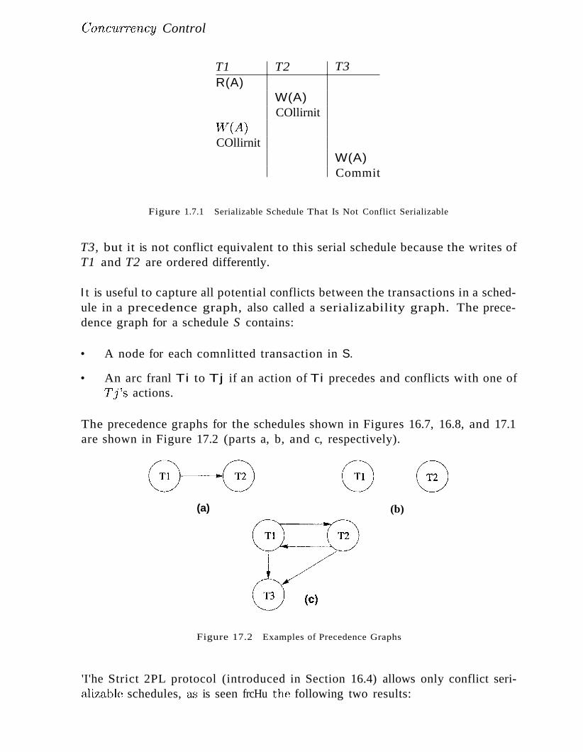
COnC'lLrrency Control
T1 T2 T3R(A)
W(A)COllirnit
VV(A)COllirnit
W(A)Commit
Figure 1.7.1 Serializable Schedule That Is Not Conflict Serializable
T3, but it is not conflict equivalent to this serial schedule because the writes ofT1 and T2 are ordered differently.
I t is useful to capture all potential conflicts between the transactions in a schedule in a precedence graph, also called a serializability graph. The precedence graph for a schedule S contains:
• A node for each comnlitted transaction in S.
• An arc franl Ti to Tj if an action of Ti precedes and conflicts with one ofTj's actions.
The precedence graphs for the schedules shown in Figures 16.7, 16.8, and 17.1are shown in Figure 17.2 (parts a, b, and c, respectively).
(a) (b)
Figure 17.2 Examples of Precedence Graphs
'I'he Strict 2PL protocol (introduced in Section 16.4) allows only conflict serializable schedules, as is seen frcHu the following two results:
.... -2~)b . CHAPTER Iv
1. A schedule S' is conflict serializable if and only if its precedence graph isacyclic. (An equivalent serial schedule in this C'k'3e is given by any topological sort over fhe precedence graph.)
2. Strict 2PL ensures t.hat the precedence graph for any schedule that it a11o\vsis acyclic.
A widely studied variant of Strict 2PL, called Two-Phase Locking (2PL),relaxes the second rule of Strict 2PL to allow transactions to release locks beforethe end, that is, before the comnlit or abort action. For 2PL, the second ruleis replaced by the following rule:
(2PL) (2) A transaction cannot request additional locks once it releases any lock.
Thus, every transaction h3.-" a 'growing' phase in which it acquires locks, followed by a 'shrinking' phase in which it releases locks.
It can be shown that even nonstrict 2PL ensures acyclicity of the precedencegraph and therefore allows only conflict serializable schedules. Intuitively, anequivalent serial order of transactions is given by the order in which transactionsenter their shrinking phase: If T2 reads or writes an object written by Tl, TlIllUSt have released its lock on the object before 7 12 requested a lock on thisobject. ~rhus, Tl precedes T2. (A sirnilar argulnent shows that Tl precedesT2 if 7'2 writes an object previously read by Tl. A forIllal proof of the claimwould have to show that there is no cycle of transactions that 'precede' eachother by this argurnent.)
A schedule is said to be strict if a value written by a transaction T is notread or overwritten by other transactions until T either aborts or eOlnrnits.Strict schedules are recoverable, do not require cascading aborts, and actions ofaborted transactions can be undone by restoring the original values of lnodifiedobjects. (See the last exaInple in Section 16.::~.4.) Strict 2PL irnproves on2PL by guaranteeing that every allowed schedule is strict in addition to beingconflict serializable. The reason is that when a transaction 'T writes an objectunder Strict 2PL, it holds the (exclusive) lock until it conunits or aborts. Thus,no other transaction can see or rnodify this object until T is cornplete.
]'he reader is invited to revisit the exarnples in Section 16.:~.3 to see how thecorresponding schedules are disallowed by Strict 2PL and 2PL. Sirnilarly, itwould be instructive to \vork out how the schedules for the exarnples in Section16.~3.4 are disallc)\ved by Strict 2PL but not by 2PL.
17.1.1 View Serializability
Conflict serializability is sufficient but not necessary for serializability. A 1n01'egeneral sufficient condition is vievv serializability. Two schedules 81 and 82 overthe saIne set of transactions"------any transaction that appears in either 81 or 82rnust also appear in the other-----------are view equivalent under these conditions:
1. If fTi reads the initial value of object A in 81, it Blust also read the initialvalue of A in 82.
2. If Ti reads a value of A written by Tj in 81, it IIlUst also read the value ofA written by Tj in 82.
3. For each data object A, the transaction (if any) that perforlns the finalwrite on A in 81 must also perform the final write on A in 82.
A schedule is view serializable if it is view equivalent to SaIne serial schedule.Every conflict serializable schedule is view serializable, although the converseis not true. ~or example, the schedule shown in Figure 17.1 is view serializable,although it is not conflict serializable. Incidentally, note that this exalnplecontains blind writes. This is not a coincidence; it can be shown that any viewserializable schedule that is not conflict serializable contains a blind write.
As we saw in Section 17.1, efficient locking protocols allow us to ensure thatonly conflict serializable schedules are allowed. Enforcing or testing vie\v serializability turns out to be lIluch lnore expensive, and the concept therefore haslittle practical use, although it increases our understanding of serializability.
17.2 INTRODUCTION TO LOCK MANAGEMENT
The part of the I)Bl\1S that keeps track of the locks issued to transactions iscalled the lock manager. The lock lnanager rnaintains a lock table, whichis a ha"sh table with the data object identifier (4S the key. The DBNIS alsoInaintains a descriptive entry for each transaction in a transaction table,and alIlong other things, the entry contains a pointer to a list of locks held b:ythe transaction. This list is checked before requesting a lock, to ensure that atransaction does not request the saIne lock twice.
A lock table entry for an object-u--which can be a page, a record, and soon, depending on the DBMS---contains the following inforrnation: the nurnberof transactions currently holding a. lock on the object (this can be rnore thanone if the object is locked in shared rnode), the nature of the lock (shared orexclusive), and a pointer to (1, queue of lock requests.
554 CHAPTER 17
17.2.1 Implementing Lock and Unlock Requests
According to the Strict 2PL protocol, before a transaction T reads or writes adatabase object 0, it must obtain a shared or exclusive lock on 0 and Inusthold on to the lock until it commits or aborts. When a transaction needs alock on an object, it issues a lock request to the lock manager:
1. If a shared lock is requested, the queue of requests is ernpty, and the objectis not currently locked in exclusive mode, the lock manager grants the lockand updates the lock table entry for the object (indicating that the objectis locked in shared mode, and incrernenting the number of transactionsholding a lock by one).
2. If an exclusive lock is requested and no transaction currently holds a lockon the object (which also implies the queue of requests is empty), the lockrnanager grants the lock and updates the lock table entry.
3. Otherwise, the requested lock cannot be immediately granted, and thelock request is added to the queue of lock requests for this object. Thetransaction requesting the lock is suspended.
When a transaction aborts or comrnits, it releases all its locks. When a lockon an object is released, the lock manager updates the lock table entry for theobject and exarnines the lock request at the head of the queue for this object.If this request can now be granted, the transaction that made the request iswoken up and given the lock. Indeed, if several requests for a shared lock on theobject are at the front of the queue, all of these requests can now be grantedtogether.
Note that if TI has a shared lock on 0 and 1'2 requests an exclusive lock,T2's request is queued. Now, if T3 requests a shared lock, its request entersthe queue behind that of T2, even though the requested lock is cornpatiblewith the lock held by TI. This rule ensures that T2 does not starve, that is,wait indefinitely while a stream of other transactions acquire shared locks andthereby prevent T2 frorn getting the exclusive lock for which it is waiting.
Atomicity of Locking and Unlocking
The irnplernentation of lock and l1nlock cornrnands rnust ensure that these areatomic operations. To ensure atornicity of these operations when several instances of the lock rnanager code can exccute concurrently, access to the locktable has to be guarded by an operating systern synchronization rnechanisrnsuch a..s a sernaphore.
Co'nc'UT'rency (}onlToI 5~5
To understand why, suppose that a transaction requests an exclusive lock.The lock manager checks and finds that no other transaction holds a lock onthe object and therefore decides to grant the request. But, in the 11leantirne,another transaction rnight have requested and received a conflicting lock. Toprevent this, the entire sequence of actions .in a lock request call (checkingto see if the request can be granted, updating the lock table, etc.) must beirnplernented as an atornic operation.
Other Issues: Latches, Convoys
In addition to locks, which are held over a long duration, a DBMS also supportsshort-duration latches. Setting a latch before reading or writing a page ensuresthat the physical read or write operation is atomic; otherwise, two read/writeoperations rnight conflict if the objects being locked do not correspond to diskpages (the units of I/O). Latches are unset immediately after the physical reador write operation is cOlnpleted.
We concentrated thus far on how the DBMS schedules transactions based ontheir requests for locks. This interleaving interacts with the operating system'sscheduling of processes' access to the CPU and can lead to a situation calleda convoy, where most of the CPU cycles are spent on process switching. Theproblem is that a transaction T holding a heavily used lock may be suspendedby the operating system. UntH T is resurned, every other transaction thatneeds this lock is queued. Such queues, called convoys, can quickly becomevery long; a convoy, once forrned, tends to be stable. Convoys are one of thedrawbacks of building a DB~lS on top of a general-purpose operating systemwith preeruptive scheduling.
17.3 LOCK CONVERSIONS
A transaction rnay need to acquire an exclusive lock on an object for which italready holds a shared lock. For exarnple, a SQL update statenlent could resultin shared locks being set on each row in a table. If a row satisfies the condition(in the WHERE clause) for being updated, an exclusive lock must be obtainedfor that row.
Such a lock upgrade request lnust be handled specially by granting the exclusive lock illunediately if no other transaction holds a shared lock on the objectand inserting the request at the front of the queue other\vise. The rationalefor favoring the transaction thus is that it already 1101ds a shared lock on theobject and queuing it behind. another tretnsaction that wants an exclusive lockon thf~ SeHne object causes both a deadlock. UnfortunatelY,while favoring lockupgrades helps, it does not prevent deadlocks caused by two conflicting upgrade
556 CHAPTER 17
requests. For exalnplc, if two transactions that hold a shared lock on an objectboth request an upgrade to an exclusive lock, this leads to a deadlock.
A better approach is to avoid the need for lock upgrades altogether by obtainingexclusive locks initially, and downgrading to a shared lock once it is clear thatthis is sufficient. In our exalnple of an SQL update statelnent, rows in a tableare locked in exclusive rnode first. If a row does not satisfy the condition forbeing updated, the lock on the row is dnwngraded to a shared lock. Does thedovvngrade approach violate the 2PL requirernent? On the surface, it does,because downgrading reduces the locking privileges held by a transaction, andthe transaction Illay go on to acquire other locks. However, this is a special case,because the transaction did nothing but read the object that it downgraded,even though it conservatively obtained an exclusive lock. We can safely expandour definition of 2PL from Section 17.1 to allow lock downgrades in the growingphase, provided that the transaction has not lnodified the object.
The downgrade approach reduces concurrency by obtaining write locks in somecases where they are not required. On the whole, however, it irnproves throughput by reducing deadlocks. This approach is therefore widely used in currentcommercial systems. Concurrency can be increased by introducing a new kindof lock, called an update lock, that is cornpatible with shared locks but notother update and exclusive locks. By setting an update lock initially, ratherthan exclusive locks, we prevent conflicts with other read operations. Once weare sure we need not update the object, we can downgrade to a shared lock. Ifwe need to update the object, we rnust first upgrade to an exclusive lock. Thisupgrade does not lead to a deadlock because no other transaction can have anupgrade or exclusive lock on the object.
17.4 DEALING WITH DEADLOCKS
Deadlocks tend to be rare and typically involve very few transactions. In practice, therefore, databa.'3c systerns periodically check for deadlocks. 'Vhen atransaction Ti is suspended because a lock that it requests cannot be granted,it rnust wa,it until all transactions Tj that currently hold conflicting locks relea,'3e thcrn. The lock rnanager rnaintains a structure called a waits-for graphto detect deadlock cycles. The nodes corr(~spond to active transactions, andthere is an arc frolnTi to 'Tj if (and only if)Ti is \vaiting for 1) to release alode The lock rnanagcr adds edges to this graph when it queues lock requestsand rernoves edges \vhcn it gra,nts lock requests.
Consider the schedule shown in F'igure 17.:3, The last step, sho\vn belovv theline, creates a cycle in the \vaits-for graph. Figure 17.4 shovvs the ·waits-forgraph before and after this step.
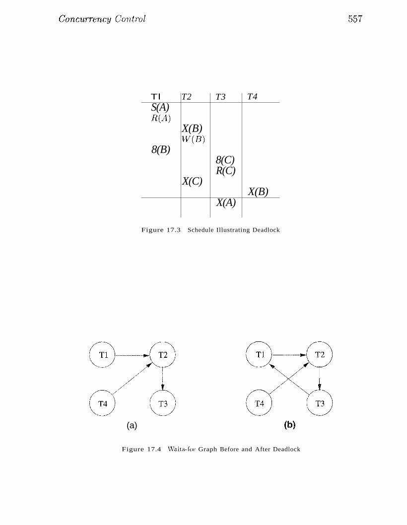
COnC1tTTency C'ontTol
Tl T2 T3 T4S(A)Jl(A)
X(B)vV(B)
8(B)8(C)R(C)
X(C)X(B)
X(A)
Figure 17.3 Schedule Illustrating Deadlock
597
(a)
Figure 17.4 \\!aits-for Graph Before and After Deadlock
558 CHAPTER lw7
Observe that the \vaits-for graph describes all active transactions, some of whicheventually abort. If there is an edge froIn Ti to T'j in the 'N~aits-for graph, andboth Ti and Tj eventually commit, there is an edge in the opposite direction (froIn l'j to Ti) in the precedence graph (which involves only cOlluuittedtransactions) .
The waits-for graph is periodically checked for cycles, which indicate deadlock.A deadlock is resolved by aborting a transaction that is on a cycle and releasingits locks; this action allows SOlne of the waiting transactions to proceed. Thechoice of which transaction to abort can be made using several criteria: theone with the fewest locks, the one that has done the least work, the one that isfarthest from completion, and so all. FUrther, a transaction might have beenrepeatedly restarted; if so, it should eventually be favored during deadlockdetection and allowed to complete.
A silnple alternative to maintaining a waits-for graph is to identify deadlocksthrough a timeout mechanism: If a transaction has been waiting too long fora lock, we assume (pessiruistically) that it is in a deadlock cycle and abort it.
17.4.1 Deadlock Prevention
Elnpirical results indicate that deadlocks are relatively infrequent, and detectionbased schemes work well in practice. However, if there is a high level of contention for locks and therefore an increased likelihood of deadlocks, preventionbased schelnes could perform better. We can prevent deadlocks by giving eachtransaction a priority and ensuring that lower-priority transactions are notallowed to wait for higher-priority transactions (or vice versa). One way toassign priorities is to give each transaction a timestamp when it starts up.The lower the timestamp, the higher is the transaction's priority; that is, theoldest transaction has the highest priority.
If a transaction Ti requests a lock and transaction Tj holds a conflicting lock,the lock lnanager can use one of the following two policies:
II Wait-die: If Ti has higher priority, it is allowed to wait; otherwise, it isaborted.
II Wound-wait: If Ti has higher priority, abort 7); otherwise, l"1i waits.
In the \vait-die scherne, lower-priority transactions can never wait for higherpriority transactions. In the wound-wait scherne, higher-priority transactionsnever wait for lower-priority transactions. In either ease, no deadlock cyc.ledevelops.
Concurrency Control 539
A subtle point is that we nlust also ensure that no transaction is perenniallyaborted because it never has a sufficiently high priority. (Note that, in bothschernes, the higher-priority transaction is never aborted.) When a transaction is aborted and restarted, it should be given the same timestamp it hadoriginally. Reissuing timestarnps in this way ensures that each transactionwill eventually becorne the oldest transaction, and therefore the one with thehighest priority, and will get all the locks it requires.
The wait-die scheme is nonpreemptive; only a transaction requesting a lock canbe aborted. As a transaction grows older (and its priority increases), it tendsto wait for more and rnore younger transactions. A younger transaction thatconflicts with an older transaction may be repeatedly aborted (a disadvantagewith respect to wound-wait), but on the other hand, a transaction that hasall the locks it needs is never aborted for deadlock reasons (an advantage withrespect to wound-wait, which is preemptive).
A variant of 2PL, called Conservative 2PL, can also prevent deadlocks. Under Conservative 2PL, a transaction obtains all the locks it will ever need whenit begins, or blocks waiting for these locks to become available. This schemeensures that there will be no deadlocks, and, perhaps lllore important, that atransaction that already holds some locks will not block waiting for other locks.If lock contention is heavy, Conservative 2PL can reduce the time that locksare held on average, because transactions that hold locks are never blocked.The trade-off is that a transaction acquires locks earlier, and if lock contentionis low, locks are held longer under Conservative 2PL. From a practical perspective, it is hard to know exactly what locks are needed ahead of time, andthis approach leads to setting more locks than necessary. It also has higheroverhead for setting locks because a transaction has to release all locks and tryto obtain thern all over if it fails to obtain even one lock that it needs. Thisapproach is therefore not used in practice.
17.5 SPECIAI-JIZED LOCKING TECHNIQUES
Thus far we have treated a database as a fixed collection of independent dataobjects in our presentation of locking protocols. We now relax each of theserestrictions and discuss the consequences.
If the collection of databa.se objects is not fixed, but can grow and shrinkthrough the insertion and deletion of objects, we must deal with a subtle cOlnplication known a'3 the phantom, problem, which was illustrated in Section 16.6.2.We discuss this problern in Section 17.5.1.
560 CHAPTER 17
Although treating a database H",S an independent collection of objects is adequate for a discussion of serializability and recoverability, luuch better perfc)l'rnance can sOlnetilnes be obtained using protocols that recognize and exploitthe relationships between objects. vVe discuss two such C<l"ses, nalnely, lockingin tree-structured indexes (Section 17.5.2) and locking a collection of objectswith contairnnent relationships between the1n (Section 17.5.3).
17.5.1 Dynamic Databases and the Phantom Problem
Consider the following exarnple: rrransaction Tl scans the Sailors relation tofind the oldest sailor for each of the rating levels 1 and 2. First, Tl identifiesand locks all pages (assurning that page-level locks are set) containing sailorsvvith rating 1 and then finds the age of the oldest sailor, which is, say, 71.Next, transaction T2 inserts a new sailor with rating 1 and age 96. Observethat this new Sailors record can be inserted onto a page that does not containother sailors with rating 1; thus, an exclusive lock on this page does not conflictwith any of the locks held by Tl. T2 also locks the page containing the oldestsailor with rating 2 and deletes this sailor (whose age is, say, 80). T2 thencomrnits and releases its locks. Finally, transaction T1 identifies and lockspages containing (all remaining) sailors with rating 2 and finds the age of theoldest such sailor, which is, say, 63.
The result of the interleaved execution is that ages 71 and 63 are printed inresponse to the query. If T1 had run first, then T2, we would have gotten theages 71 and 80; if T2 had run first, then T1, we would have gotten the ages96 and 63. Thus, the result of the interleaved execution is not identical to anyserial exection of Tl and 1'2, even though both transactions follow Strict 2PLand cOlnmit. The problem is that T1 assurnes that the pages it has lockedinclude all pages containing Sailors records with rating 1, and this assurnptionis violated when rT2 inserts a new such sailor on a different page.
'rhe Haw is not in the Strict 2PL protocol. R,ather, it is in T1 's irnplicit assurnption that it has locked the set of all Sailors n~cordswith rating value 1.T1 's sernantics requires it to identify all such records, but locking pages thatcontain such records at a given tirne does not prevent new "phantorn" recordsfrorn being added on other pages. ]"'1 has th~refore not locked the set of desiredSailors records,
Strict 2PL guarantees conflict serializability; indeed, there are no cycles in theprecedence graph for this exarnple because conflicts are defined with respectto objects (in this excunple, pages) read/written by the traJlsactions. However,because the set of objects that shrndd have been locked by Tl was altered bythe actions ofT2, the olltcorne of the schedule differed frolll the outcorne of any
CfoncuTTency Control 561
serial execution. 1~his exalllple brings out an irnportant point about conflictserializability: If new itenls are added to the databa'ie, conflict serializabilitydoes not guarantee serializability.
.i\ closer look at how a transaction identifies pages containing Sailors recordsvvith rating 1 suggests hovv the problenl can be handled:
• If there is no index and all pages in the file rnust be scanned, T1 IUUStsomeho\v ensurf~ that no new pages are added to the file, in addition tolocking all existing pages.
• If there is an index on the rating field, T1 can obtain a lock on the indexpage~again, assurning that physical locking is done at the page level-thatcontains a data entry with rating= 1. If there are no such data entries, thatis, no records with this rating value, the page that would contain a dataentry for rating=l is locked to prevent such a record from being inserted.Any transaction that tries to insert a record with rating=-l into the Sailorsrelation 11lUSt insert a data entry pointing to the new record into this indexpage and is blocked until T1 releases its locks. This technique is calledindex locking.
Both techniques effectively give T1 a lock on the set of Sailors records with rating=l: Each existing record with rating=l is protected frolll changes by othertransactions, and additionally, new records with rating=l cannot be inserted.
An independent issue is how transaction 7'1 can efficiently identify and lockthe index page containing rating=1. We discuss this issue for the case of treestructured indexes in Section 17.5.2.
\Ve note that index locking is a special ca..se of a luore general concept calledpredicate locking. In our exalnple, the lock on the index page irnplieitlylocked all Sailors records that satisfy the logical predicate rating= 1. 1V101'egenerally, we cn]} support irnplicit locking of all records that rnatch an arbitra,rypredicate. General predicate locking is expensive to irnplenlent and thereforenot cOllullonly used.
17.5.2 Concurrency Control in B+ Trees
A straightforward approach to concurrency control for B+ trees and ISA~iI
indexes is to ignore the index structure, treat each page as a data object, anduse senne version of 2PL. This siInplistic locking strategy vvould lead to very highlock contention in the higher levels of the tree~ because every tree search beginsat the root and proceeds along sorne path to a leaf node. Fortunately, InnchInore efficient locking protocols that exploit the hierarchical structure of a tree
562 CHAPTER J7
index are known to reduce the locking overhead while ensuring seriaIizabilityand recoverability.We discuss sorne of these approaches briefly, concentratingon the search and insert operations.
Two observations provide the necessary insight:
1. The higher levels of the tree only direct searches. All the 'real' data isin the leaf levels (in the forrnat of one of the three alternatives for dataentries).
2. For inserts, a node must be locked (in exclusive rnode, of course) only if asplit can propagate up to it frorn the modified leaf.
Searches should obtain shared locks on nodes, starting at the root and proceeding along a path to the desired leaf. The first observation suggests that alock on a node can be released as soon as a lock on a child node is obtained,because searches never go back up the tree.
A conservative locking strategy for inserts would be to obtain exclusive locks onall nodes as we go down from the root to the leaf node to be modified, becausesplits can propagate all the way from a leaf to the root. However, once we lockthe child of a node, the lock on the node is required only in the event that asplit propagates back to it. In particular, if the child of this node (on the pathto the modified leaf) is not full when it is locked, any split that propagates upto the child can be resolved at the child, and does not propagate further to thecurrent node. Therefore, when we lock a child node, we can release the lock onthe parent if the child is not full. The locks held thus by an insert force anyother transaction following the sarne path to wait at the earliest point (i.e., thenode nearest the root) that rnight be affected by the insert. The technique oflocking a child node and (if possible) releasing the lock on the parent is calledlock-coupling, or crabbing (think of how a crab walks, and cornpare it tohow we proceed down a tree, alternately releasing a lock on a parent and settinga lock on a child).
We illustrate B-t- tree locking using the tree in Figure 17.5. To search for dataentry 38*, a transaction T'i rnust obtain an S lock on node A, read the contentsand deterrnine that it needs to examine node B, obtain an S lock on node Band release the lock on A, then obtain an S lock on node C1 and relea.'3e thelock on B, then obtain an S lock on nodeD and release the lock on ().
Ti always rnaintains a lock all one node in the path, to force new transactionsthat want to read or nlodify nodes on the sarne path to wait until the currenttransaction is done. If transaction 7) wants to delete 38*, for exarnple, it rnustalso traverse the path fro111 the root to node D and is forced to wait until 1 1i
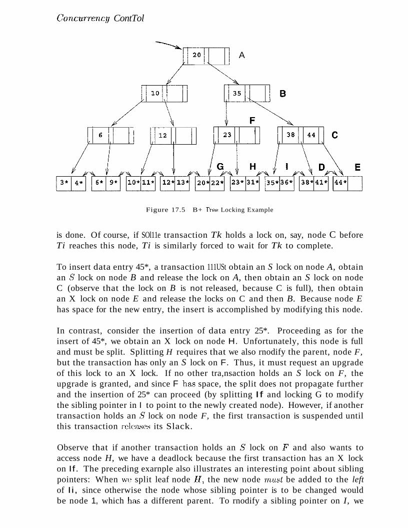
CO'TLc1trrency ContTol
A
Figure 17.5 B+ 'Thee Locking Example
is done. Of course, if SOl11e transaction Tk holds a lock on, say, node C beforeTi reaches this node, Ti is similarly forced to wait for Tk to complete.
To insert data entry 45*, a transaction 111USt obtain an S lock on node A, obtainan 8 lock on node B and release the lock on A, then obtain an S lock on nodeC (observe that the lock on B is not released, because C is full), then obtainan X lock on node E and release the locks on C and then B. Because node Ehas space for the new entry, the insert is accomplished by modifying this node.
In contrast, consider the insertion of data entry 25*. Proceeding as for theinsert of 45*, we obtain an X lock on node H. Unfortunately, this node is fulland must be split. Splitting H requires that we also rnodify the parent, node F,but the transaction ha..., only an S lock on F. Thus, it must request an upgradeof this lock to an X lock. If no other tra,nsaction holds an S lock on F, theupgrade is granted, and since F has space, the split does not propagate furtherand the insertion of 25* can proceed (by splitting If and locking G to modifythe sibling pointer in I to point to the newly created node). However, if anothertransaction holds an 8 lock on node F, the first transaction is suspended untilthis transaction relea.ses its Slack.
Observe that if another transaction holds an 8 lock on }' and also wants toaccess node H, we have a deadlock because the first transaction has an X lockon If. The preceding exarnple also illustrates an interesting point about siblingpointers: When \ve split leaf node If, the new node rn'Ust be added to the leftof Ii, since otherwise the node whose sibling pointer is to be changed wouldbe node 1, which ha"-,, a different parent. To rnodify a sibling pointer on I, we
564 C~HAPTER 1t{
'would have to lock its parent, node C: (and possibly ancestors of C:, in order tolock en.Except for the locks on int(~rrnediatenodes that we indicated could be releasedearly, senne variant of 2PL HUlst be used to govern when locks can be released,to ensure serializability and recoverability.
T'his approach irllproves considerably on the naive use of 2PL, but several exclusive locks are still set unnecessarily and, although they are quickly released,affect perfon.nance substantially. One way to iInprove perforlllance is for insertsto obtain shared locks instead of exclusive locks, except for the leaf, which islocked in exclusive 11lode. In the vast rnajority of cases, a split is not requiredand this approach works very well. If the leaf is full, however, we Blust upgradefrom shared locks to exclusive locks for all nodes to which the split propagates.Note that such lock upgrade requests can also lead to deadlocks.
The tree locking idea'3 that we describe illustrate the potential for efficientlocking protocols in this very important special case, but they are not thecurrent state of the art. The interested reader should pursue the leads in thebibliography.
17.5.3 Multiple-Granularity Locking
Another specialized locking strategy, called multiple-granularity locking,allows us to efficiently set locks on objects that contain other objects.
For instance, a database contains several files, a file is a collection of pages,and a page is a collection of records. A transaction that expects to access rnostof the pages in a file should probably set a lock on the entire file, rather thanlocking individual pages (or reeords) when it needs thern. Doing so reducesthe locking overhead considerably. On the other hand, other tra,nsactions thatrequire access to parts of the file....·....·-even parts not needed by this transaction··-·..·are blocked. If a transaction accesses relatively few pages of the file, it is betterto lock only those pages. Sirnilarly, if a transaction accesses several records ona page, it should lock the entire page, and if it accesses just a few records, itshould lock just those records.
The question to be addressed is h(nv a lock rnanager can efficiently ensure thata page, for exaruple, is not locked by a transaction while another transactionholds a conflicting lock on the file containing the page (a.nd therefore, irnplicitly,on the page).
ConC7lTTency COintTol 5jj5
The idea is to exploit the hierarchical nature of the 'contains~ relationship. Adat.abase contains a set of files, each file contains a set of pages, and each pagecontains a set of records. This contairunent hierarchy can be thought of asa tree of objects, \vhere each node contains all its children. (The approachcan easily be extended to cover hierarchies that are not trees, but we do notdiscuss this extension.) A lock on a node locks that node and, irnplicitly, all itsdescendants. (Note that this interpretation of a lock is very different fron1 B+tree locking, where locking a node does not lock any descendants ilnplicitly.)
In addition to shared (8) and exclusive (XO) locks, rnultiple-granularity lockingprotocols also use two new kinds of locks, called intention shared (18) andintention exclusive (IX) locks. 18 locks conflict only with X locks. IXlocks conflict with 8 and X locks. To lock a node in S (respectively, X) luode,a transaction must first lock all its ancestors in 18 (respectively, 1X) rllode.Thus, if a transaction locks a node in 8 rIlode, no other transaction can havelocked any ancestor in X rnode; siInilarly, if a transaction locks a node in Xmode, no other transaction can have locked any ancestor in 8 or X mode. Thisensures that no other transaction holds a lock on an ancestor that conflictswith the requested 8 or X lock on the node.
A common situation is that a transaction needs to read an entire file and modifya few of the records in it; that is, it needs an 8 lock on the file and an 1X lockso that it can subsequently lock sorne of the contained objects in X mode. Itis useful to define a new kind of lock, called an 81X lock, that is logicallyequivalent to holding an 8 lock and an I X lock. A transaction can obtain asingle 81X lock (which conflicts with any lock that conflicts with either S orI X) instead of an 8 lock and an I X lock.
A subtle point is that locks rnust be relea..sed in leaf-to-root order for this protocol to work correctly. Tb see this, consider what happens when a transaction Tilocks all nodes on a path frolH the root (corresponding to the entire database)to the node corresponding to sorne page p in 18 rnode, locks p in 8 rHode, andthen relea..ses the lock on the root node. Another transaction T j could nowobtain an X lock on the root. This lock iInplicitly gives Tj an .£Y lock on pagep, which conflicts with the 8 lock currently held by Ti.
lIIultiple-granularity locking lllust be used with 2PL to ensure serializability.The 2PL protocol dictates when locks can be rele(ksed. At that tirne, locks obtained using rIlultiple-granularity locking can be released and IIlUSt be relcclsedin leaf-to-root order.
Finally, there is the question of hO\\I to decide what granularity of locking isappropriate for a given transaction. One approach is to begin by obtaining finegranularity locks (e.g., at the record level) and, after the transaction requests
566 CHAPTER 107
-~",,_._ ..-_ _._.._.._.._ _--_.--_._._..-- _ _-~." _ _._-_ _........ .. _-_._-~.,,"
Lock Granularity: SOfie database systeIlls allow programmers to override the default mechanisllt for choosing a lock granularity. For exalnple,Microsoft SQL Server allows users to select page locking instead of tablelocking, using the keyword PAGLOCK. IBrvf'sDB2 UDB allows for explicittable-level locking.
a certain nUlnber of locks at that granularity, to start obtaining locks at thenext higher granularity (e.g., at the page level). This procedure is called lockescalation.
17.6 CONCURRENCY CONTROL WITHOUT LOCKING
Locking is the most widely used approach to concurrency control in a DBMS,but it is not the only one. We now consider some alternative approaches.
17.6.1 Optimistic Concurrency Control
Locking protocols take a pessimistic approach to conflicts between transactionsand use either transaction abort or blocking to resolve conflicts. In a systenlwith relatively light contention for data objects, the overhead of obtaining locksand following a locking protocol must nonetheless be paid.
In optimistic concurrency control, the basic premise is that most transactionsdo not conflict with other transactions, and the idea is to be as permissiveas possible in allowing transactions to execute. Transactions proceed in threephases:
1. Read: The transaction executes, reading values froIn the database andwriting to a private workspace.
2. Validation: If the transaction decides that it wants to c0l111uit, the DBIvISchecks whether the transaction could possibly have conflicted with anyother concurrently executing transaction. If there is a possible conflict, thetransaction is aborted; its private workspace is cleared and it is restarted.
:3. Write: If validation deterrnines that there are no possible confliets, thechanges to data objects 111ade by the transaction in its private workspaceare copied into the databa.se.
If, indeed, there are few confiicts, and validation can be done efficiently, thisapproach should lead to better' performance than locking. If there are rnany
Concurrency Control 567
conflicts, the cost of repeatedly restarting transactions (thereby wasting the,york they've done) hurts perfornlance significantly.
Each transaction Ti is assigned a thnestamp TS(T'i) at the beginning of itsvalidation pha.':ie, and the validation criterion checks whether the tiITlestalnpordering of transactions is an equivalent serial order. For every pair of transactions Ti and Tj such that TS(l"1i) < TS(Tj), one of the following validationconditions ITIUSt hold:
1. Ti completes (all three phases) before Tj begins.
2. Ti completes before Tj starts its Write phase, and Ti does not write anydatabase object read by Tj.
3. Ti completes its Read phase before Tj completes its Read phase, and Tidoes not write any database object that is either read or written by T j.
To validate T j, we must check to see that one of these conditions holds withrespect to each comlnitted transaction Ti such that TS(Ti) < TS(Tj). Eachof these conditions ensures that Tj's modifications are not visible to Ti.
Further, the first condition allows Tj to see some of Ti's changes, but clearly,they execute completely in serial order with respect to each other. The secondcondition allows Tj to read objects while Ti is still modifying objects, but thereis no conflict because Tj does not read any object rnodified by T'i. AlthoughTj might overwrite some objects written by Ti, all of Ti's writes precede all ofTj's writes. The third condition allows Ti and Tj to write objects at the sametime and thus have even IT10re overlap in time than the second condition, butthe sets of objects written by the two transactions cannot overlap. Thus, noRW, WR, or WW conflicts are possible if any of these three conditions is met.
Checking these validation criteria requires us to maintain lists of objects readand written by each transaction. Further, while one transaction is being validated, no other transaction can be allowed to commit; otherwise, the validationof the first transaction might miss conflicts with respect to the newly committed transaction. The Write phase of a validated transaction rnust also becompleted (so that its effects are visible outside its private workspace) beforeother transactions can be validated.
A synchronization rnechanisrn such as a critical section can be used to ensurethat at most one transaction is in its (colllbined) Validation/Write phases atany tirne. (When a process is executing a critical section in its code, thesystern suspends all other processes.) Obviously, it is irnportant to keep thesepha~es ~lS short H.S possible in order to rniniruize the irnpact on concurrency. Ifcopies of rnodified objects have to be copied frorn the private workspace, this
568 CHAPTER 17
can rnake the \Vrite phase long. An alternative approach (which carries thepenalty of poor physical locality of objects, such as B·+· tree leaf pages, thatrnust be clustered) is to use a level of indirection. In this schernc, every objectis accessed via a logical pointer, and in the \Vrite phase, we sirnply switch thelogical pointer to point to the version of the object in the private workspace,instead of copying the 0 bject.
Clearly, it is not the ca.sc that optiInistic concurrency control has no overheads;rather, the locking overheads of lock-based approaches are replaced with theoverheads of recording read-lists and write-lists for transactions, checking forconflicts, and copying changes frorn the private workspace. Sirnilarly, the irnplicit cost of blocking in a lock-based approach is replaced by the implicit costof the work wasted by restarted transactions.
Improved Conflict Resolution1
Optirnistic Concurrency Control using the three validation conditions describedearlier is often overly conservative and unnecessarily aborts and restarts transactions. In particular, according to the validation conditions, T'i cannot writeany object read by Tj. IIowever, since the validation is airned at ensuring thatTi logically executes before Tj, there is no harm if Ti writes all data itemsrequired by Tj before 7) reads theIn.
The problerIl arises because we have no way to tell when Ti wrote the object(relative to Tj's reading it) at the tirne we validate Tj, since all we have is thelist of objects written by T'i and the list read by T j. Such false conflicts can bealleviated by a finer-grain resolution of data conflicts, using rnechanisrI1s verysinlilar to locking.
The basic idea is that each transaction in the R,cacl pha.se tells the DBMS aboutiteIIls it is reading, and ·when a transaction Ti is cornrnitted (and its writes areaccepted), the DBMS checks whether any of the iterns written by Ti are beingread by any (yet to be validated) transaction T j. If so, we kno\v thatTj 'svalidation rnust eventually fail. vVe can either allow T,i to discover this whenit is validated (the die policy) or kill it and restart it innnediately (the killpolicy).
rfhe details are c1.,) follo\vs. Before reading a data iterrl, (1, transaction Tentersan access entry in a h::lSh table. The access entry contains the transact'ionid, a data object id, and a rn..odified flag (initially set to false), and entries arehashed on the data object id. A terl1porary exclusive lock is obtained on the
1 "\Ve thank Alexander Thoma..sian for writing this section.
(}O'lLCU1"rency Cfontrol 569$
hash bucket containing the entry, and the lock is held \vhile the read data iteIIlis copied frolll the datab<:lSe bufIer into the private 'workspace of the transactioll.
During validation of ~T the hash buckets of all data objects accessed by Tare again locked (in exclusive 11lode) to check if T has encountered any dataconflicts. ~r has encountered a conflict if the rnodified flag is set to true in oneof its access entries. (This &')SUIIles that the 'die' policy is being used; if the'kill' policy is used, 'T is restarted when the flag is set to true.)
If T is successfully validated, we lock the hash bucket of each object lnodifiedby T, retrieve all access entries for this object, set the rnodified flag to true,and release the lock on the bucket. If the 'kill' policy is used, the transactionsthat entered these access entries are restarted. We then cornplete~r's Writephase.
It seems that the 'kill' policy is always better than the 'die' policy, because itreduces the overall response time and wasted processing. However, executingT to the end has the advantage that all of the data items required for itsexecution are prefetched into the database buffe~r, and restarted executions ofT will not require disk I/O for reads. This assumes that the database bufferis large enough that prefetched pages are not replaced, and, 1nore irnportant,that access invariance prevails; that is, successive executions of T requirethe same data for execution. When T is restarted its execution tirne is nluchshorter than before because no disk I/O is required, and thus its chances ofvalidation are higher. (Of course, if a transaction has already completed itsRead phase once, subsequent conflicts should be handled using the 'kill' policybecause all its data objects are already in the buffer pool.)
17.6.2 Timestamp-Based Concurrency Control
In lock-ba'3ed concurrency control, conflicting actions of different transactionsare ordered by the order in which locks are obtained, and the lock protocol extends this ordering on actions to transactions, thereby ensuring serializability.In optirrlistic concurrency control, a tiInestanlp ordering is irnposed on transactions and validation checks that all conflicting actions occurred in the saIneorder.
Tinlcstarnps can also be used in another \vay: Each transaction can be assigneda tirnestanlp at startup, and we can ensure, at execution tirne, that if actiona'i of transaction T'i conflicts \vith action aj of transaction Tj, a'i occurs beforeaj if'1'8(T'i) < TS(Tj). If an action violates this ordering, the transaction isaborted and restarted.
570 CHAPTER 17
To irnplernent this concurrency control schellH~l every database object 0 is givena read tirnestampRTS (0) and a write timestamp v~lTS (0). If transactionT wants to read object 0, and TS(T) < ~VTS(O), the order of this readwith respect to the most recent write on 0 would violate the timestamp orderbetween this transaction and the writer. Therefore, T is aborted and restartedwith a new, larger timestarnp. If TS(T) > WTS(O), Treads 0, and l~TS(O)
is set to the larger of RTS(O) and TS(T). (Note that a physical change--thechange to RTS(O)-is written to disk and recorded in the log for recoverypurposes, even on reads. This write operation is a significant overhead.)
Observe that if T is restarted with the same timestamp, it is guaranteed to beaborted again, due to the saIne conflict. Contrast this behavior with the use oftimestamps in 2PL for deadlock prevention, where transactions are restartedwith the same timestarnp as before to avoid repeated restarts. This shows thatthe two uses of timestamps are quite different and should not be confused.
Next, consider what happens when transaction T wants to write object 0:
1. If TS(T) < RTS(O), the write action conflicts with the most recent readaction of 0, and T is therefore aborted and restarted.
2. If TS(T) < WTS(O), a naive approach would be to abort T becauseits write action conflicts with the most recent write of 0 and is out oftimestamp order. However, we can safely ignore such writes and continue.Ignoring outdated writes is called the Thomas Write Rule.
3. Otherwise, T writes 0 and WTS(O) is set to TS(T).
The Thomas Write Rule
We now consider the justification for the TholIlas Write Rule. If TS(T) <WTS(O), the current write action has, in effect, been made obsolete by thernost recent write of 0, which follows the current write according to the tirnestalnp ordering. We can think of T's write action as if it had occurred irnrnediately before the rnost recent write of 0 and was never read by anyone.
If the Thoma') vVrite Rule is not used, that is, T is aborted in case (2), thetirnestamp protocol, like 2PL, allows only conflict serializable schedules. If theTho1l1aS '\Trite R,ule is used, S(Hne schedules are perrnitted that are not conflictserializable, fl.'3 illustrated by the schedule in Figure 17.6.2 Because T2's \vritefollows Tl's read and precedes Tl's write of the sanle object, this schedule isnot conflict serializable.
21n the other direction, 2PL pennits some schedules that are not allowed by the timestamp algorithm with the Thomas Write Rule; see Exercise 17.7.
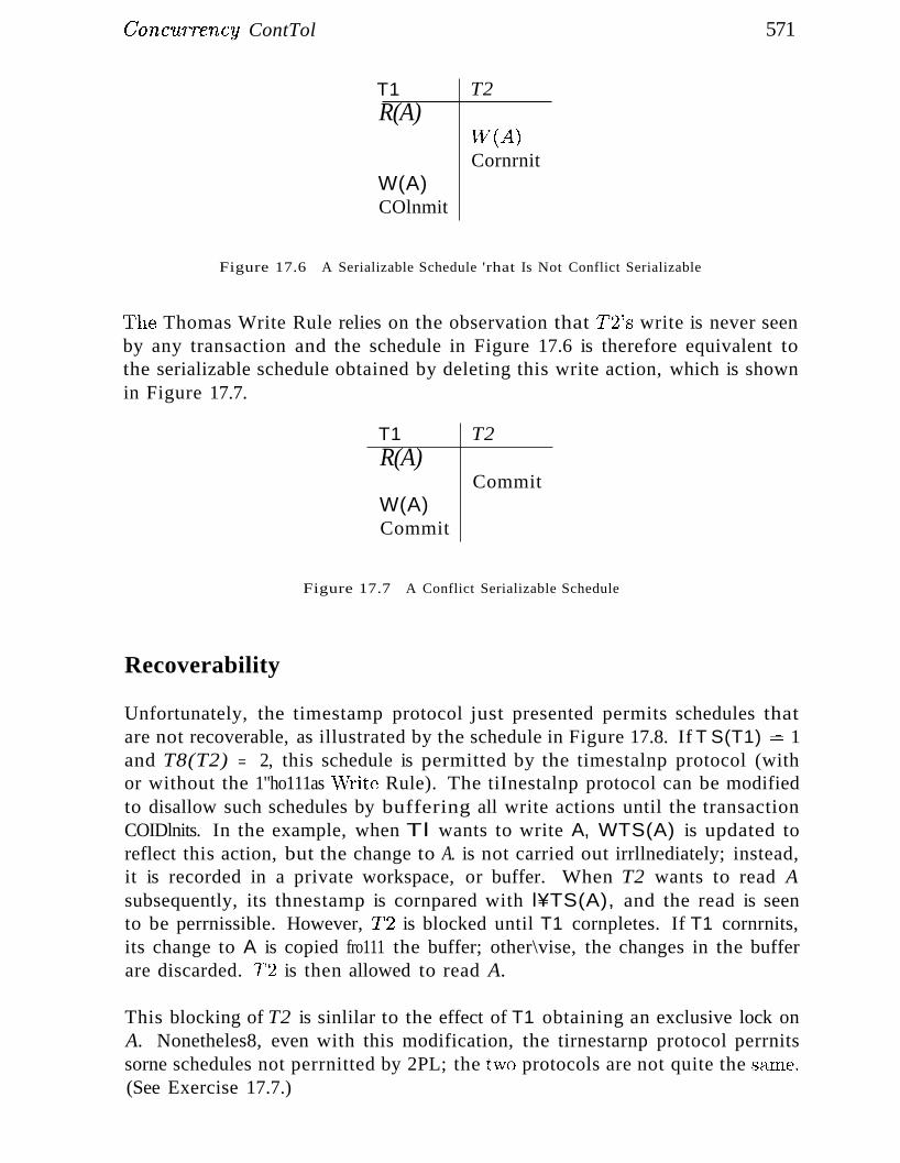
COnC'llr'Tency ContTol
T1R(A)
W(A)COlnmit
T2
l{T(A)Cornrnit
571
Figure 17.6 A Serializable Schedule 'rhat Is Not Conflict Serializable
l'he Thomas Write Rule relies on the observation that T2's write is never seenby any transaction and the schedule in Figure 17.6 is therefore equivalent tothe serializable schedule obtained by deleting this write action, which is shownin Figure 17.7.
T1 T2R(A)
CommitW(A)Commit
Figure 17.7 A Conflict Serializable Schedule
Recoverability
Unfortunately, the timestamp protocol just presented permits schedules thatare not recoverable, as illustrated by the schedule in Figure 17.8. If T S(T1) :::::: 1and T8(T2) = 2, this schedule is permitted by the timestalnp protocol (withor without the 1"ho111as \\Trite Rule). The tiInestalnp protocol can be modifiedto disallow such schedules by buffering all write actions until the transactionCOIDlnits. In the example, when Tl wants to write A, WTS(A) is updated toreflect this action, but the change to A. is not carried out irrllnediately; instead,it is recorded in a private workspace, or buffer. When T2 wants to read Asubsequently, its thnestamp is cornpared with l¥TS(A), and the read is seento be perrnissible. However, ~r2 is blocked until T1 cornpletes. If T1 cornrnits,its change to A is copied fro111 the buffer; other\vise, the changes in the bufferare discarded. ~r2 is then allowed to read A.
This blocking of T2 is sinlilar to the effect of T1 obtaining an exclusive lock onA. Nonetheles8, even with this modification, the tirnestarnp protocol perrnitssorne schedules not perrnitted by 2PL; the two protocols are not quite the senne.(See Exercise 17.7.)
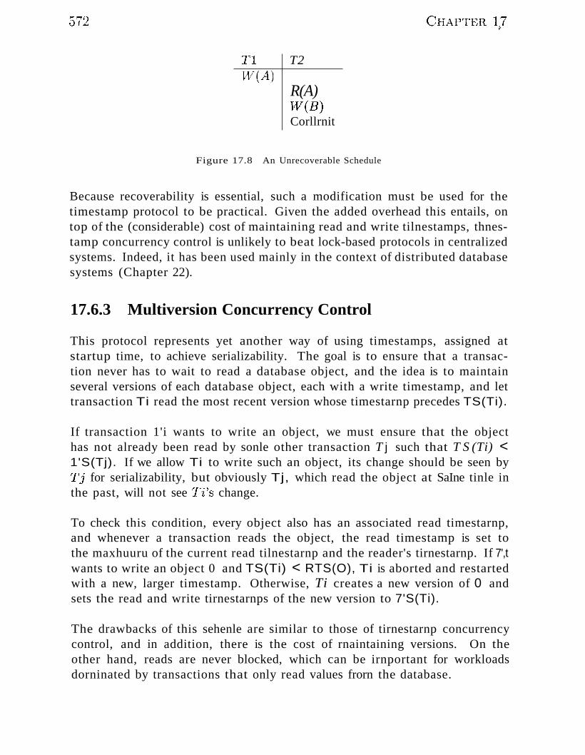
1"1 T2
R(A)l~T(B)
Corllrnit
Figure 17.8 An Unrecoverable Schedule
Because recoverability is essential, such a modification must be used for thetimestamp protocol to be practical. Given the added overhead this entails, ontop of the (considerable) cost of maintaining read and write tilnestamps, thnestamp concurrency control is unlikely to beat lock-based protocols in centralizedsystems. Indeed, it has been used mainly in the context of distributed databasesystems (Chapter 22).
17.6.3 Multiversion Concurrency Control
This protocol represents yet another way of using timestamps, assigned atstartup time, to achieve serializability. The goal is to ensure that a transaction never has to wait to read a database object, and the idea is to maintainseveral versions of each database object, each with a write timestamp, and lettransaction Ti read the most recent version whose timestarnp precedes TS(Ti).
If transaction 1'i wants to write an object, we must ensure that the objecthas not already been read by sonle other transaction T j such that T S (Ti) <1'S(Tj). If we allow Ti to write such an object, its change should be seen byTj for serializability, but obviously Tj, which read the object at SaIne tinle inthe past, will not see ~r'i's change.
To check this condition, every object also has an associated read timestarnp,and whenever a transaction reads the object, the read timestamp is set tothe maxhuuru of the current read tilnestarnp and the reader's tirnestarnp. If 7',twants to write an object 0 and TS(Ti) < RTS(O), Ti is aborted and restartedwith a new, larger timestamp. Otherwise, Ti creates a new version of 0 andsets the read and write tirnestarnps of the new version to 7'S(Ti).
The drawbacks of this sehenle are similar to those of tirnestarnp concurrencycontrol, and in addition, there is the cost of rnaintaining versions. On theother hand, reads are never blocked, which can be irnportant for workloadsdorninated by transactions that only read values frorn the database.
C:onC7LTr'ency C}ontTol r.::""3,';j(
I-;~t Do Real-;~ms Do? ~~~-~~;, Informix, Microsoft-~~~ Server, and Sybase ABE use Strict 2PL or variants (if a transaction reI quests a lower than SERIALIZABLE SQL isolation level; see Section 16.6).
IVlicrosoft SQL Server also supports rnodifieation timestamps so that atransaction can run ""vithout setting locks and validate itself (do-it-yourselfOptirnisticConC1:1rrency Control!). Oracle 8 uses a lllultiversion concurrency control scherne in ""vhich readers never wait; in fact, readers neverget locks and detect conflicts by checking if a block changed since theyread it. All these systerlls support rnultiple-granu1arity locking, with support for table, page, and row level locks. All deal with deadlocks usingwaits-for graphs. Sybase ASIQ supports only table-level locks and abortsa transaction if a lock request fails-·--updates (and therefore conflicts) arerare in a data warehouse, and this simple scheme suffices.
________. .",".1
17.7 REVIEW QUESTIONS
Answers to the review questions can be found in the listed sections.
• When are two schedules conflict equivalent? What is a conflict serializableschedule? What is a strict schedule? (Section 17.1)
• What is a precedence graph or serializability graph? Ilow is it related to conflict serializability? How is it related to two-phase locking? (Section 17.1)
• What does the lock manager do? Describe the lock table and transactiontable data structures and their role in lock management. (Section 17.2)
II Discuss the relative nH.~rits of lock upgrades and lock downgrades. (Section 17.3)
lIlI Describe and cornpare deadlock detection a,nd deadlock prevention schernes.\Vhy are detection schernes rnore cornrnonly used? (Section 17.4)
II If the collection of database objects is not fixed, but can gro\v and shrinkthrough insertion and deletion of objects, we lnust deal with a subtle corllplication known as the phantorn problern. Describe this problern and theindex locking approach to solving the probleln. (Section 17.5.1)
II In tree index structures, locking higher levels of the tree can becorne a perforrnanee bottleneck. Explain why. I)escribe specialized locking techniquesthat address the problenl, and explain why they work correctly despite notlJeing two-phase. (Section 17.5.2)
II AI71lt'iple-granldaT'ity locki'ng enables us to set locks on objects that containother objects, thus iInplicitly locking all contained objects. \Vhy is thisapproach irnportant and how does it work? (Section 17.5.3)
574 CHAPTER \7
• In optirrtistic conClLrrency control, no locks are set and transactions readand rnodify data objects in a private workspace. How are conflicts betweentransactions detected and resolved in this approach? (Section 17.6.1)
• In tirnestamp- based concurrency control, transactions are assigned a timestarnp at startup; how is it used to ensure serializability? How does theThomas Write Rule improve concurrency? (Section 17.6.2)
• Explain why tinlestamp-based concurrency control allows schedules thatare not recoverable. Describe how it can be modified through buffering todisallow such schedules. (Section 17.6.2)
• Describe multiversion concurrency control. What are its benefits and disadvantages in comparison to locking? (Section 17.6.3)
EXERCISES
Exercise 17.1 Answer the following questions:
1. Describe how a typical lock manager is implemented. Why must lock and unlock beatomic operations? What is the difference between a lock and a latch? What are convoysand how should a lock manager handle them?
2. Compare lock downgrades with upgrades. Explain why downgrades violate 2PL butare nonetheless acceptable. Discuss the use of update locks in conjunction with lockdowngrades.
3. Contrast the timestamps assigned to restarted transactions when tinwstanlps are usedfor deadlock prevention versus when timestamps are used for concurrency control.
4. State and justify the Thomas Write Rule.
5. Show that, if two schedules are conflict equivalent, then they are view equivalent.
6. Give an example of a serializable schedule that is not strict.
7. Give an example of a strict schedule that is not serialiable.
8. ~1otivate and describe the use of locks for improved conflict resolution in OptinlisticConcurrency Control.
Exercise 17.2 Consider the following cla..'3ses of schedules: ser'ializable l confiict-serializable,1..J'iew-ser'ializable, recoverable, avoids-cascading-aborts, and strict. For each of the followingschedules, state which of the preceding cla.'3ses it belongs to. If you cannot decide whether aschedule belongs in a certain class ba.'3ed on the listed actions, explain briefly.
The actions are listed in the order they are scheduled and prefixed with the transaction name.If a commit or abort is not shown, the schedule is incomplete; assurne that abort or cornrnitlllust follow all the listed actions.
1. Tl:R(X), T2:R(X), Tl:W(X), T2:\iV(X)
2. Tl:W(X), T2:R(Y), Tl:R(Y), T2:R(X)
C}oncurrency Contr'Ol
3. Tl:R(X), T2:R(Y), T~3:\V(X), T2:R(X), Tl:R(Y)
4. Tl:R(X), T1:R(Y), T1:W(X), T2:R(Y), T:3:\¥CY), Tl:W(X), T2:R(Y)
5. Tl:R(X), T2:W(X), Tl:W(X), T2:Abort, Tl:Cmnmit
6. Tl:R(X), T2:W(X), Tl:\V(X), T2:Comrnit, Tl:Comm.it
7. T1:W(X), T2:R(X), 1'l:W(X), 1'2:Abort, T.1:COllllllit
8. Tl:W(X), T2:R(X), Tl:W(X), T2:Conunit, Tl:Col1unit
9. Tl:W(X), T2:R(X), Tl:W(X), T2:Commit, Tl:Abort
10. 1'2: R(X), 1'3:W(X), T3:Cmnrnit, Tl:W(Y), Tl:Commit, T2:R(Y),T2:W(Z), T2:Colllmit
11. Tl:R(X), T2:W(X), T2:Cornrnit, Tl:W(X), Tl:Colllmit, T:3:R(X), T3:Collnnit
12. Tl:R(X), T2:W(X), Tl:W(X), T3:R(X), Tl:Comlllit, T2:Corn111it, 1'3:Comlnit
575
Exercise 17.3 Consider the following concurrency control protocols: 2PL, Strict 2PL, Conservative 2PL, Optimistic, Tilnestamp without the Thomas Write Rule, 1'ilnestamp with theThomas Write Rule, and Multiversion. l'or each of the schedules in Exercise 17.2, state whichof these protocols allows it, that is, allows the actions to occur in exactly the order shown.
For the timestamp-based protocols, assurne that the timestamp for transaction Ti is i andthat a version of the protocol that ensures recoverability is used. Further, if the ThomasWrite Rule is used, show the equivalent serial schedule.
Exercise 17.4 Consider the following sequences of actions, listed in the order they are submitted to the DBMS:
• Sequence 81: Tl:R(X), T2:W(X), T2:W(Y), T3:W(Y), Tl:W(Y),Tl:Commit, T2:Commit, T3:Commit
• Sequence 82: Tl:R(X), T2:W(Y), T2:W(X), T3:W(Y), Tl:W(Y),Tl:C0111mit, T2:Commit, T3:Commit
!<or each sequence and for each of the following concurrency control rnechanislns, describehow the concurrency control mechanislll handles the sequence.
Assurne that the tirnestarnp of transaction Ti is 'i. Fbr lock-based concurrency control rnechaniS111S, add lock and unlock requests to the previous sequence of actions as per the lockingprotocol. The DB"NIS processes actions in the order shown. If a transaction is blocked, a%Ulnethat all its actions are queued until it is reslllned; the I)B11S continues with the next action(according to the listed sequence) of an unblocked transaction.
1. Strict 2PL with tiluestamps used for deadlock prevention.
2. Strict 2PL with deadlock detection. (Show the waits-for graph in C(l.se of deadlock.)
~3. Conservative (and Strict, i.e., with locks held until end-of-transaction) 2PL.
4. Optimistic concurrency control.
5. Tiruestarup concurrency control with buffering of reads and writes (to ensure recoverability) and the Tholnas Write Rule.
6. rvluitiversioll concurrency control.
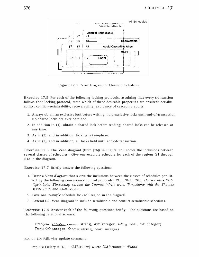
576 CIIAPTER 1J
All Schedules•• _. " ••~._~ ._",_. • •••_.__._•••_. __~",_.~••••••••~~••~.~ ~~••••• u ••••~••••~ ........
View Serializable '1
(.,~ ~_~_u.uu ••• u ••_ ••••••••••••••••••••••••• \ i
(---~~~t~~-t ~rft~l ~riaJ~ I-R~:able1
I r-~ ~:t~ll:;--~--:;~i~~~rt11
Ll=='==--t~---~-=k-t-+~LLJ~---_._---~--~ ..~...~_..__.._....._._.._-_......._._-_.._--</
Figure 17.9 Venn Dia,gram for Classes of Schedules
Exercise 17.5 For each of the following locking protocols, assulning that every transactionfollows that locking protocol, state which of these desirable properties are ensured: serializability, conflict-·serializability, recoverability, avoidance of cascading aborts.
1. Always obtain an exclusive lock before writing; hold exclusive locks until end-of-transaction.No shared locks are ever obtained.
2. In addition to (1), obtain a shared lock before reading; shared locks can be released atany time.
3. As in (2), and in addition, locking is two-phase.
4. As in (2), and in addition, all locks held until end-of-transaction.
Exercise 17.6 The Venn diagranl (frorn [76]) in Figure 17.9 shows the inclusions betweenseveral classes of schedules. Give one exaulple schedule for each of the regions Sl throughS12 in the diagrarn.
Exercise 17.7 Briefly answer the following questions:
1. Draw a Venn diagnnll that ShO\V8 the inclusions between the classes of schedules perulittccl by the following concurrency control protocols: 2PL, 8tr'ict 2PL, Conscr1.Jauve 2PL,Optirni.stic, Timestamp without the Thorna8~Vr'ite Rule, Tirne8tam.p with the ThonHt8Write R1J,lc~ and Ah.tlt'll,)(:T.'Fion.
2. Give one ex<:'unple schedule for each region in the diagrarIl.
:3. Extend the Venn diagranl to include serializable and conflict-serializable schedules.
Exercise 17.8 Answer each of the follmving questions briefly. The questions are based onthe following relational schern.a:
Ernp( C'id: integer) cnarne: string, age: integer, salary: real, did: integer)
Dept(~~~~~_~_~:.~.~::,drunne: string, flooT: integer)
(mel on the fc)llowing update cornrnand:
replace (salary = 1.1 *F]\{P.salary) where .KtvlP.enarne = 'Santa'
C:onC1LTTeTLCY C\Jn(:Tol 5r-.'.....",{
1. Give an exaruple of a query that would conflict with this comrnand (in a concurrencycontrol sense) if both were run at the s::.une tim.e. Explain what could go wroIlg~ and howlocking tuples would solve the probleIll.
2. Give an exarnple of a query or a cOHlInand that would conflict with this cOIl1ruand, suchthat the conflict could not be resolved by just locking individual tuples or pages butrequires index locking.
~). Explain what index locking is and how it resolves the preceding conflict.
Exercise 17.9 SQL supports four isolation-levels and two access-rllodes, for a total of eightcornbinations of isolation-level and access-rnode. Each corubinatioll inlplicitly defines a classof transactions; the follO\ving questions refer to these eight classes:
1. For each of the eight classes, describe a locking protocol that allows only transactions inthis class. Does the locking protocol for a given class make any assurnptiolls about thelocking protocols used for other classes? Explain briefly.
2. Consider a schedule generated by the execution of several SQL transactions. Is it guaranteed to be conflict-serializable? to be serializable'? to be recoverable?
3. Consider a schedule generated by the execution of several SQL transactions, each ofwhich has READ ONLY access-mode. Is it guaranteed to be conflict-serializable? to beserializable? to be recoverable?
4. Consider a schedule generated by the execution of several SQL transactions, each ofwhich has SERIALIZABLE isolation-level. Is it guaranteed to be conflict-serializable? tobe serializable? to be recoverable?
5. Can you think of a tinlCstarup-based concurrency control scheme that can support theeight classes of SQL transactions?
Exercise 17.10 Consider the tree shown In Figure 19.5. Describe the steps involved inexecuting each of the following operations according to the tree-index concurrency controlalgorithm discussed in Section 19.3.2, in terms of the order in which nodes are locked, unlocked, read, and written. Be specific about the kind of lock obtained and answer each partindependently of the others, always starting with the tree shown in Figure 19.5.
1. Search for data entry 40*.
2. Search for all data entries k* with k ~ 40.
3. Insert data entry 62*.
4. Insert data entry 40*.
5. Insert data entries 62* and 75*.
Exercise 17.11 Consider a database organized in tenns of the following hierarachy of objects: The database itself is an object (D), and it contains two files (Fl (lud F'2), each ofwhich contains 1QOO p<.Lges (PI . .. PlOOO ancl Pl()()l ... P2000, respectively). Each page contains 100 records, and records aTe identified as p : i, where]J is the page identifier and i is theslot of the record on that page.
I'vlultiple-granularity locking is used, with 5', .i\{) 15',#1 X and S'IX locks, and datah<Lse-level,file-level, page-level ;111<1 record-level locking. For each ()f the foll()\ving operations, indicaJ;ethe sequence of lock requests that 1nust be generated by a transctction that wants to carryout (just) these operations:
578
1. Read record P1200 : 5.
(~HAPTER 1;:7
2. Reacl recorclsP1200 : 98 through P1205 : 2.
ii. Read aU (records on all) pages in file }'l.
4. 'Read pages P500 through P520.
5. Read pages PIO through P980.
6. Read all pages in PI and (ba..ged on the values read) rnodify 10 pages.
7. Delete record P1200 : 98. (This is a blind write.)
8. Delete the first record frorn each page. (Again~ these are blind writes.)
9. Delete all records.
Exercise 17.12 Suppose that we have only two types of transactions, Tl and T2. Transactions preserve database consistency when run individually. We have defined several integrityconstnLiTtts such that the DBNIS never executes any SQL statenwnt that brings the databaseinto an inconsistent state. Assunle that the DBlVIS does not perform any concurrency control.Give an exarllple schedule of two transactions Tl and T2 that satisfies all these conditions,yet produces a database instance that is not the result of any serial execution of 7'1 and T2.
BIBLIOGRAPHIC NOTES
Concurrent access to B trees is considered in several papers, including [70,456,472,505,678].Concurrency control techniques for Linear Hashing are presented in [240] and [543]. Multiplegranularity locking is introduced in [3:36] and studied further in [127, 449].
A concurrency control method that works with the ARIES recovery rnethod is presented in[545]. Another paper that considers concurrency control issues in the context of recovery is[492]. AlgorithrIls for building indexes without stopping the DBMS are presented in [548] and[9]. 1'he performance of B tree concurrency control algorithnls is studied in [704]. Perfornlance of various concurrency control algorithms is discussed in [16, 729, 735]. A good surveyof concurrency control rnethods and their perfornlance is [734]. [455] is a comprehensivecollection of papers on this topic.
TilYwstarIlp-based multiversion concurrency control is studied in [6201. IvIultiversion concur-rency control algoritllIIls are studied forrnally in [87J. Lock-based rnultiversion techniquesare considered in [460]. Optirnistic concurrency control is introduced in [457]. The use ofaccess invariance to irnprove conflict resolution in high-contention environrnents is discussedin [281] and [280]. 1'rallsacti0I1 rnanagenwnt issues for real-tirne databa..'5e systerns are discussed in [1, 15, :368, :382, :386, 448]. There is a large body of theoretical results on data.ba.seconcurrency control; [582, 89] offer thorough textbook presentations of this rnaterial.

18CRASH RECOVERY
(,... What steps are taken in the ARIES method to recover fronl a DBl\1Scrash?
... How is the log rnaintained during nonnal operation?
.. How is the log used to recover frorn a crash?
(",.. What infonnation in addition to the log is used during recovery?
"'What is a checkpoint and why is it used?
... W'hat happens if repeated crashes occur during recovery?
... How is media failure handled?
... How does the recovery algorithnl interact with concurrency control?
.. Key concepts: steps in recovery, analysis, redo, undo; ARIES,repeating history; log, LSN, forcing pages, WAL; types of logrecords, update, cornrnit, abort, end, cOlnpensation; transaction ta-·ble, lastLSN; dirty page table, recLSN; checkpoint, fuzzy checkpointing, rnao;;;ter log record; rnedia recovery; interaction with concurrencycontrol; shadow paging
Hurnpty Durnpty sat on a \vall.lIurnpty Durnpty h(1,(1 a great fall.A.ll the King's horses and all the King's tnenCould not put lIllrnpty together again.
-~~~()ld nursery rhyrne
579
580 C~HAPTER 18p
The recovery manager of aDB~/[S is responsible for ensuring tvvo irnportantproperties of transactions: Atornicity and durability. It ensures ato'Tn:icity byundoing the actions of transactions that do not conlIllit and durab'il'ity by rnaking sure that all actions of conunitted transactions survive system crashes(e.g., a core durnp caused by a bus error) and Inedia failures (e.g., a disk iscorrupted).
1"'he recovery rnanager is one of the hardest cOlllponents of a DBlViS to designand inlplernent. It rnust deal 'with a wide va,riety of database states becauseit is called on during systenl failures. In this chapter, "\Ive present the ARIESrecovery algorithnl, which is conceptually sinlple, works well with a wide rangeof concurrency control rnechanisrns, and is being used in an incre&sing numberof database syterns.
We begin with an introduction to ARIES in Section 18.1. We discuss thelog, which a central data structure in recovery, in Section 18.2, and otherrecovery-related data structures in Section 18.3. We complete our coverageof recovery-related activity during normal processing by presenting the WriteAhead Logging protocol in Section 18.4, and checkpointing in Section 18.5.
We discuss recovery frorn a crash in Section 18.6. Aborting (or rolling back)a single transaction is a special case of Undo, discussed in Section 18.6.3. Wediscuss media failures in Section 18.7, and conclude in Section 18.8 with adiscussion of the interaction of concurrency control and recovery and other approaches to recovery. In this chapter, we consider recovery only in a centralizedDBMS; recovery in a distributed DBMS is discussed in Chapter 22.
18.1 INTRODUCTION TO ARIES
ARIES is a recovery algorithrn designed to work with a steal, no-force approach. When the recovery rnanager is invoked after a, craBh: restart proceedsin thn~e phases:
1. Analysis: Identifies dirty pages in the buffer pool (i.e., changes that havenot been written to disk) and active transactions at the tiITle of the crash.
2. Redo: H,epeats all actions, starting frOID an appropriate point in the log,and restores the database state to what it was at the tirne of the e1'a8h.
~). lJndo: lJndoes the actions of transactions that did not cOllunit, so tlU:l,tthe databa,se reflects only the actions of cornrnitted transactions.
Consider the sirnple execution history illustrated in Figure 18.1. '\\7hen thesysteIIl is restarted, the A,nalysis phase identifies 'Tl H.nd ~r:3 as transactions
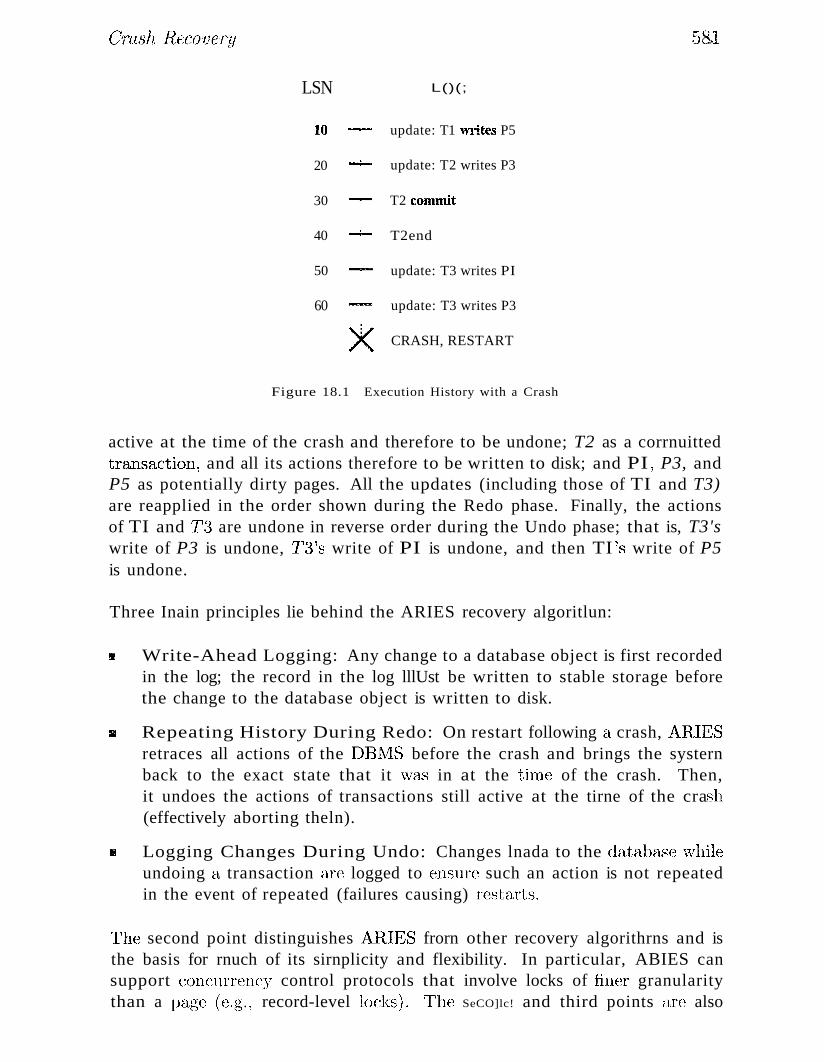
CrYlBh Recovery
LSN L()(;
10 - update: T1 writes P5
20 --- update: T2 writes P3
30 - T2 comnlit
40 --- T2end
50 - update: T3 writes PI
60 - update: T3 writes P3
X CRASH, RESTART
Figure 18.1 Execution History with a Crash
h&l,.'a
active at the time of the crash and therefore to be undone; T2 as a corrnuittedtransaction~ and all its actions therefore to be written to disk; and PI ~ P3, andP5 as potentially dirty pages. All the updates (including those of TI and T3)are reapplied in the order shown during the Redo phase. Finally, the actionsof TI and T;-3 are undone in reverse order during the Undo phase; that is, T3'swrite of P3 is undone, 7"3's write of PI is undone, and then TI ~s write of P5is undone.
Three Inain principles lie behind the ARIES recovery algoritlun:
!II Write-Ahead Logging: Any change to a database object is first recordedin the log; the record in the log lllUst be written to stable storage beforethe change to the database object is written to disk.
!II Repeating History During Redo: On restart following a crash, ,AllIESretraces all actions of the DBlVlS before the crash and brings the systernback to the exact state that it wa,s in at the tilne of the crash. Then,it undoes the actions of transactions still active at the tirne of the cra..sh(effectively aborting theln).
11II Logging Changes During Undo: Changes lnada to the databa.se '.vhileundoing a transaction are logged to ensure such an action is not repeatedin the event of repeated (failures causing) restarts.
The second point distinguishes AllIES frorn other recovery algorithrns and isthe basis for rnuch of its sirnplicity and flexibility. In particular, ABIES cansupport conCUlTcnc:Jl control protocols that involve locks of finer granularitythan a page (e.g., record-level loc:ks). T1he SeCO]lc! and third points are also
582 CIIAPTER 18
---.....,.------_._...._..._._._-_._._---
Crash Recovery: IB~1 DB2, Inforrnix, Iv1icrosoft SQL Server, Oracle 8,and Sybase l\SE all use a WAL seherue for recovery. IBIvI DB2 uses ARIES,
I!IiI
and the others use seherues that are actually quite sinlilar to ARIES (e.g., Iall changes are re-applied, not just the changes made by transactions that Iare 'winners') although there are several variations.
------- ~ .. - ...................._. . ---- ~
important in dealing with operations where redoing and undoing the operation are not exact inverses of each other. We discuss the interaction betweenconcurrency control and crash recovery in Section 18.8, where we also discussother approaches to recovery briefly.
18.2 THELOG
The log, SOlnetirnes called the trail or journal, is a history of actions executedby the DBMS. Physically, the log is a file of records stored in stable storage,which is assumed to survive crashes; this durability can be achieved by maintaining two or more copies of the log on different disks (perhaps in differentlocations), so that the chance of all copies of the log being sinlultaneously lostis negligibly small.
The most recent portion of the log, called the log tail, is kept in nlain Inemoryand is periodically forced to stable storage. This way, log records and datarecords are written to disk at the same granularity (pages or sets of pages).
Every log record is given a unique id called the log sequence number(LSN). As with any record id, we can fetch a log record with one disk accessgiven the LSN. Further, LSNs should be assigned in ruonotonically increasingorder; this property is required for the ARIES recovery algorithrn. If the log isa sequential file, in principle growing indefinitely, the LSN can sirllply be theaddress of the first byte of the log record'!
For recovery purposes, every page in the databa':lc contains the LSN of the rnostrecent log record that describes a change to this page. This LSN is called thepageLSN.
A log record is\vritten for each of the following actions:--_._--_.._...._._---------
1 In practice, various techniques are used to identify portions of the log that are 'too old' to beneeded again to bound the amount of stable storage used for the log. Given such a bound, the log maybe implemented a...<; a 'circular' file, in which case the I..ISN may be the log record id plus a "UYm,p-count.
583
• Updating a Page: After rTlodifying the page, an 'npdate type record (dt:~
scribed later in this section) is appended to the log tail. Tlhe pageLSN ofthe page is then set to the LSN of the update log record. (The page Blustbe pinned in the buffer pool while these actions are carried out.)
III Conl1nit: vVhen a transaction decides to conunit, it force-writes a conk'{nit type log record containing the transaction id. That is, the log recordis appended to the log, and the log tail is written to stable storage, up toand including the cOllunit record.2 The transaction is considered to havecOIlnnitted at the instant that its cOlnmit log record is written to stablestorage. (Solne additional steps rnust be taken, e.g., reilloving the transaction's entry in the transaction table; these follow the 'writing of the cOlInnitlog record.)
• Abort: When a transaction is aborted, an abort type log record containingthe transaction id is appended to the log, and Undo is initiated for thistransaction (Section 18.fL3).
• End: As noted above, when a transaction is aborted or comrnitted, someadditional actions rnust be taken beyond writing the abort or COlllIllit logrecord. After all these additional steps are c()lnpleted, an end type logrecord containing the transaction id is appended to the log.
III Undoing an update: When a transaction is rolled back (because thetransaction is aborted, or during recovery frorn a crash), its updates areundone. When the action described by an update log record is undone, acornpensation log Teconl, or CLR, is written.
Ev(~ry log record has certain fields: prevLSN, transID, and type. The set ofall log records for a given transaction is rnaintained as a linked list going backin tirne, using thE~ prevLSN field; this list HUlst be updated whenever a logrecord is added. The transII) field is the id of the transaction generating thelog record, and the type field obviously indicates the type of the log record.
Additional fields depend on the type of the log record. vVe already rnentionedthe additional contents of the various log record types, with the exception ofthe update EtIId cornpensa>tion log r(~cord types, \\Thieh we describe next.
Update Log Records
The fields in an update log record are illustrated in Figure 18.2. frhe pageIDfield is the page iel of the Inodified page; the length in bytes and the offset of the
'2 Note that this step requires the buffer manager to be able to selectively force pages to stabl(~
storage.
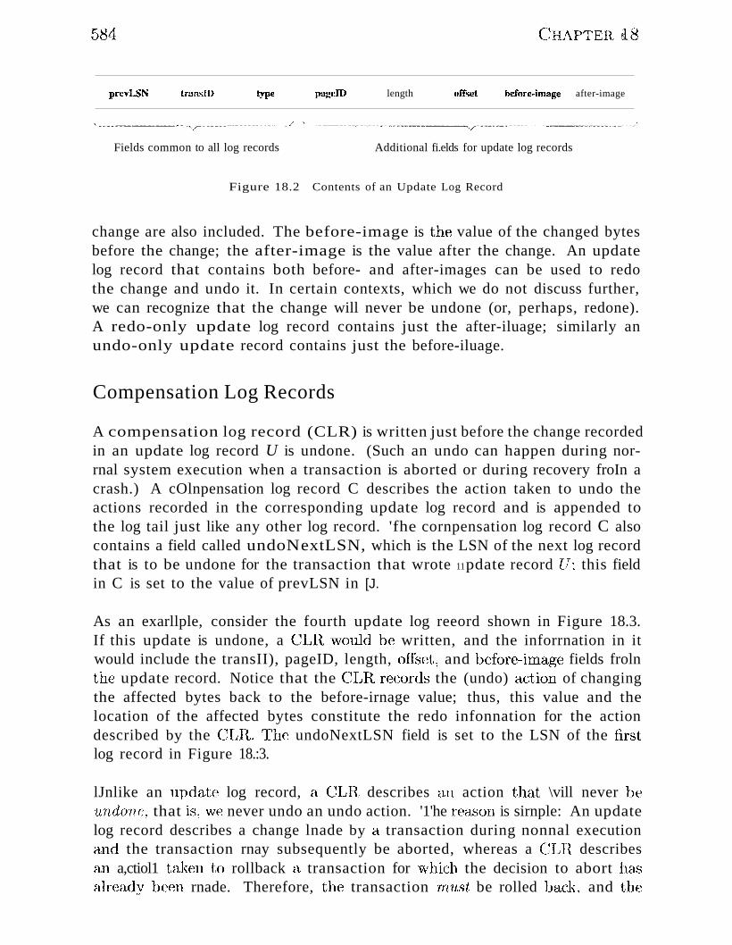
584
prevLloiN traa".iID type pageIJ.) length offset
C~HAPTERfl8
before~image after-image
Fields common to all log records Additional fi.elds for update log records
Figure 18.2 Contents of an Update Log Record
change are also included. The before-image is the value of the changed bytesbefore the change; the after-image is the value after the change. An updatelog record that contains both before- and after-images can be used to redothe change and undo it. In certain contexts, which we do not discuss further,we can recognize that the change will never be undone (or, perhaps, redone).A redo-only update log record contains just the after-iluage; similarly anundo-only update record contains just the before-iluage.
Compensation Log Records
A compensation log record (CLR) is written just before the change recordedin an update log record U is undone. (Such an undo can happen during norrnal system execution when a transaction is aborted or during recovery froIn acrash.) A cOlnpensation log record C describes the action taken to undo theactions recorded in the corresponding update log record and is appended tothe log tail just like any other log record. 'fhe cornpensation log record C alsocontains a field called undoNextLSN, which is the LSN of the next log recordthat is to be undone for the transaction that wrote 11pdate record lJ; this fieldin C is set to the value of prevLSN in [J.
As an exarllple, consider the fourth update log reeord shown in Figure 18.3.If this update is undone, a CLIl \vould be written, and the inforrnation in itwould include the transII), pageID, length, offset, and before-iInage fields frolnthe update record. Notice that the CLH, records the (undo) action of changingthe affected bytes back to the before-irnage value; thus, this value and thelocation of the affected bytes constitute the redo infonnation for the actiondescribed by the CLH,. r-Ihe undoNextLSN field is set to the LSN of the firstlog record in Figure 18.:3.
lJnlike an update log record, a CLIl describes an action that \vill never betlndone, that is, \ve never undo an undo action. '1'he rea,son is sirnple: An updatelog record describes a change lnade by a transaction during nonnal executionand the transaction rnay subsequently be aborted, whereas a (:LH, describeselll a,ctiol1 tak.en to rollback a transaction for \vllich the decision to abort hasalrea.lJy been rnade. Therefore, the transaction rnust be rolled back, and the
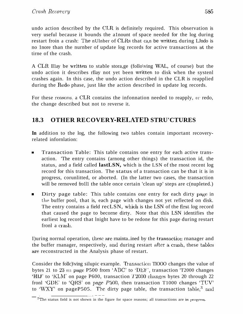
C:Tash Recover~lj 585
undo action described by the CLIl is definitely required. This observation isvery useful because it bounds the a1nount of space needed for the log duringrestart froin a crash: 1'he nUlnber of CLHs that ca,n be vvritten during LJndo isno 1nore than the nurnber of update log records for active transactions at thetirne of the crash.
A CLR. II1ay be 'written to stable stora,ge (follo\ving \iVAL, of course) but theundo action it describes rIlay not yet been vvrittcn to disk when the systenlcrashes again. In this case, the undo action described in the CLR is reappliedduring the Itedo phase, just like the action described in update log records.
For these re&'3ons, a CLIl contains the infonnation needed to reapply, 01' redo,the change described but not to reverse it.
18.3 OTHER RECOVERY..REI.JATED STRU'CTURES
In addition to the log, the following two tables contain important recoveryrelated infornlation:
II Transaction Table: This table contains one entry for each active transaction. 'The entry contains (arnong other things) the transaction id, thestatus, and a field called lastLSN, which is the LSN of the rnost recent logrecord for this transaction. The status of a transaction can be that it is inprogress, corunlitted, or aborted. (In the latter two cases, the transactionwill be rernoved fro1l1 the table once certain 'clean up' steps are c(nupleted.)
II Dirty page table: This table contains one entry for each dirty page inthE:~ buffer pool, that is, each page with changes not yet reflected on disk.The entry contains a field recLSN, vvhich is tlH~ LSN of the first log recordthat caused the page to becorne dirty. Note that this LSN identifies theearliest log record that lnight have to be redone for this page during restartfronl a cr<:1,sh.
I)uring norrnal operation, these cLre rnainta..ined by the transa,ction rnanager andthe buffer rnanager, respectively, and during restart after a crash, these ta,blesare reconstructed in the Analysis phase of restart.
Consider the follc)\ving silupic exarnple. 11:ansaction TIOOO changes the value ofbytes 21 to 2:3 011 page P500 frorn 'ABC' to '!)EF', transaction 'T2000 changes'lII.r to 'I<IJ\;1' on page P600, transaction 1~2000 changes bytes 20 through 22fronl 'C;rJE' to 'QRS' on page ])50(\ then transaction T1000 changes 'TlTV'to '-\,VXY' on pageP505. I'he dirty page table, the transaction table':~ ;:lnd_ _ ---------_.__.__.__.---
3The status field is not shown in the figure for space reasons; all transactions are in progress.
586 (~HAPTERil8
pageID recLSN
P500length offset hefore-image after-image
P600
P505
DIRTY PAGE
TRANSACTION TABLE
prcyl..-.."iN transID type pagelD
'1'1000 update P500
'1'2000 update P600
'1'2000 update PSOO
TlOOO update P505
LOG
3
3
2\ ABC DEF
4\ HU KLM
20 CiDE QRS
2\ TUV
Figure 18.3 Instance of Log and Ttansaction Table
the log at this instant are shown in Figure 18.3. ()bserve that the log is showngrowing froni top to bottorn; older records are at the top. Although the recordsfor each transaction are linked using the prevLSN field, the log as a whole alsohas a sequential order that is iInportant---for exarnple, T2000's change to pageP500 follows TIOOO's change to page P500, and in the event of a crash, thesechanges nUlst be redone in the sanle order.
18.4 THE WRITE-AHEAD LOG PROTOCOI.J
Before writing a page to disk, every update log record that describes a changeto this page rnust be forced to stable storage. This is accornplished by forcingall log records up to and including the one with LSN equal to the pageLSN tostable storage before \vriting the page to disk.
The irnportance of the "TAl" protocol carulot be overerl1phasized- --\VAL is thefundarnentaJ rule that ensures that a record of every change to the databaseis available while atternpting to recover froni a cra"sh. If a.· transaction rnade (l.
change and corIllnitted j the no-force approa,(:h Incans that SOlne of these changesrnay not have been vvrittcn to disk at the tirne of a sulJsequent cTcu,h. \\Tithout arecord of these changes, there would be no wa.y to erlsurc that the changes of acornl11.itted transaction survive crashes. Note that the definition of a cortun'ittedtTnn.sacf'ion is effectivel,Y 'a transa,ction all of whose log records j including aconunit record j have l)een \vritten to stcl,ble storage'.
\Vhen a txctnsc.tction is cornrnitted, the log U.til is forced to stabl(~ storage, evenif a no-force appro;J,ch is being used. It is '.1l1orth contrasting this operation withthe a,ctions taken under a forc(~ approach: If a., force approach is used, all thepages rIlodified by the transaction, rather than a portion of the log that includesall its records, IHllS!, be forced to disk Vl1herl the transaction conllIlits. The set of
(}rash Reco'LJery 5£7
all changed pages is typically 11luch larger than the log tajl because the size ofan update log record is close to (tvvice) the size of the changed bytes, ·which islikely to be Inuch s1na11er than the page size. Further, the log is 1naintained as asequential file, and all \\Trites to the log are sequential "\Trites. Consequently, thecost of forcing the log tail is luuch sIllaller than the cost of \vri ting aJl changedpages to disk.
18.5 CHECKPOINTIN(;
A checkpoint is like a snapshot of the DB:NlS state, and by taking checkpointsperiodically, as we will see, the DBl\1S can reduce the alnount of work to bedone during restart in the event of a subsequent crc1..sh.
Checkpointing in ARIES has three steps. First, a begin_checkpoint record iswritten to indicate when the checkpoint starts. Second, an end __checkpointrecord is constructed, including in it the current contents of the transactiontable and the dirty page table, and appended to the log. The third step iscarried out after the end_checkpoint record is written to stable storage: Aspecial master record containing the LSN of the begirLcheckpoint log record iswritten to a known place on stable storage. 'Vhile the end__checkpoint recordis being constructed, the DBMS continues executing transactions and writingother log records; the only guarantee we have is that the transaction table anddirty page table are accurate as of the ti'lY~e of the begirLcheckpoint record.
This kind of checkpoint, called a fuzzy checkpoint, is inexpensive because itdoes not require quiescing the SystCIll or writing out pages in the buffer pool(unlike senne other forlns of checkpointing). On the other hand, the effectivenessof this checkpointing technique is lirnited by the earliest recLSN of pages in thed.irty pages table, because during restart we Inust redo changes starting frointhe log record \vhose LSN is equal to this recI.lSN. l-Iaving a background processthat periodically writes dirty pages to disk helps to lirnit this probleln.
vVhen the SystCIIl cornes back up after a crash, the restart process begins bylocating the rnost recent checkpoint record. For uniforlnity, the systeIll al\v::tysbegins no1'n1al execution by takirlg a checkpoint, in \vhich. the transaction tableand dirty page table are both Clnpty.
18.6 RECOV~:RIN'G FROM A sysrr~=M CRASH
\Vhen the systenl is restarted after a crash, the recovery Iuana,ger proceeds inthree phases, as shown in Figure 18.4.

588
UNDO
REDO
LO(;
ANALYSIS
j
Oldest log rttord,\ of traa"actious
active at era<;l.
Smallest rec.LSNB in dirty page table
at end of Analysis
c ['-'lost recent checkpoint
CRASH (end of log)
C~HAPTEIl Its
Figure 18.4 Three l'lhases of Restart in ARIES
The Analysis phase begins by examInIng the rnost recent begin_checkpointrecord, whose LSN is denoted C in Figure 18.4, and proceeds forward in thelog until the last log record. '1'he Redo phase follows Analysis and redoes allchanges to any page that Illight have been dirty at the tir11e of the crash; this setof pages and the starting point for Redo (the srnallest recLSN of any dirty page)are deterrnined during Analysis. 'The Undo phase follows Redo and undoes thechanges of all transactions active at the tirne of the crash; again, this set oftransactions is identified during the Analysis phase. Note that Redo reapplieschanges in the order in which they were originally carried out; Undo reverseschanges in the opposite order, reversing the lllost recent change first.
Observe that the relative order of the three points A, B, and C in the log rnaydiffer frolIl that shown in Figure 18.4. The three phases of restart are describedin rnore detail in the following sections.
18.6.1 Analysis Phase
l'he Analysis phase perfonns three tc1...,ks:
1. It detennines the point in the log at \vhich to start the Redo pass.
2. It deterrnines ((1, conservative superset of the) pages in the buffer pool that\Ver8' clirty at the tirne of the crash.
:3. It identifies'iransEtctions that \\rere active at the tirne of the crash and rnustbe undone.
Analysis 'begins by exEtrnining the rnost recent begirLcheckpoint log record andinitializing the dirty page table and transaction table to the copies of thosestructures in the next end-e.:heckpoint record. ~rhus, t11ese tables are initializedto the set of dirty pages and active transcl,c:tions at the tilne of the checkpoint.
C:'1'ash Reco'Ve'T~lJ 5~9
(If additional log records are between the begiILcheckpoint and encLcheckpointrecords, the tables HIUst be adjusted to reflect the inforluation in these records~
but \ve cnnit the details of this step. See Exercise 18.9.) A.naJysis then scansthe log in the for\vard direction until it reaches the end of the log:
III If an end log record for a transaction T is encountered,T is reIlloved fronlthe transaction table because it is no longer active.
III If a log record other than an end record for a transaction T is encountered,an entry for T is added to the transaction table if it is not already there.Further, the entry for T is rnodified:
1. The lastLSN field is set to the LSN of this log record.
2. If the log record is a cOllnnit record, the status is set to C, otherwiseit is set to U (indicating that it is to be undone).
III If a redoable log record affecting page P is encountered, and P is not inthe dirty page table, an entry is inserted into this table with page id P andrecLSN equal to the LSN of this redoable log record. This LSN identifiesthe oldest change affecting page P that may not have been written to disk.
At the end of the Analysis phase, the transaction table contains an accuratelist of all transactions that were active at the tilue of the crash·-···_·--this is theset of transactions with status U. The dirty page table includes all pages thatwere dirty at the tirne of the crash but rnay also contain SOIne pages that werewritten to disk. If an end_write log record were written at the cornpletion ofea,ch write operation, the dirty page table constructed during Analysis couldbe lnade rnore accurate, but in AHJES, the additional cost of writing eneLwritelog records is not considered to be worth the gain.
As an exa.rnple, consider the execution illustrated in Figure 18.~3. Let us extendthis execution by assurning that ]'2000 COlIllnits, then TIOnO rnodifies anotherpage, say, .P700, and appends an update record to the log tail, and then thesystern cra"shes (before this update log record is written to stable storage).
The dirty page table and the transaction table, held in rnernory, are lost in thecra..sh. The rnost recent checkpoint \Vah') taken at the beginning of the execution,\vith an ernpty tran.saction table and dirty page table; it is not shown in Figure18.;3. After excunining this log record, \vhich \ve assurne is just before thefirst log record shown in the figure, Analysis initializes the two tables to l>eernpty. Scanning forv:.rard in the log, T'1000 is added to the transaction table;in additiol1,P500 is ad(h~d to the dirty page ta,blc\vith recLSN equal to theLSN of the first sho\vn log record. Sirnilarly, T2C)OO is added to the transactiontable andPGOO is added to the dirty page table. There is no change based onthe third log record, and the fourth record n:~sults in the addition of P505 to
590 CHAPTER,18
the dirty page table. The eOllnnit record forT2000 (not in the figure) is no\vencountered, and T2000 is relIloved fro111 the transaction table.
The Analysis pha~e is now eornplete, and it is recognized that the only activetransaction at the tilne of the crash is TIOOO, \vith lastLSN equal to the LSNof the fourth record in Figure 18.3. rrhe dirty page table reconstructed in theAnalysis pha.cse is identical to that shown in the figure. The update log recordfor the change to P700 is lost in the crash and not seen during the Analysispa.'3s. Thanks to the WAL protocol, however, all is well······--the correspondingchange to page P700 cannot have been written to disk either!
SaIne of the updates rnay have been written to disk; for concreteness, let usaSSUIne that the change to P600 (and only this update) was written to diskbefore the crash. ThereforeP600 is not dirty, yet it is included in the dirtypage table. rIhe pageLSN on page P600, however, reflects the write because itis now equal to the LSN of the second update log record shown in Figure 18.3.
18.6.2 Redo Phase
During the Redo phase, ARIES reapplies the updates of all transactions, COill
rnitted or otherwise. Further, if a transaction was aborted before the crashand its updates were undone, as indicated by CLRs, the actions described inthe CLRs are also reapplied. This repeating history paradigm distinguishesARIES from other proposed vVAL-based recovery algoritlnIls and causes thedatabase to be brought to the sarne state it was in at the time of the crash.
rrhe R,edo phase begins with the log record that has the srnallest recLSN of allpages in the dirty page table constructed by the Analysis pass because this logrecord identifies the oldest update that rnay not have been written to disk priorto the crash. Starting frorn this log record, R,edo scans forward until the endof the log. For each redoable log record (update or CLR) encountered, Rx~do
checks whether the logged action HUlst be redone. The action rnust be redoneunless one of the follo\ving conditions holds:
IIIIl The affected page is not in the dirty page table.
II rrhe affected page is in the dirty page table, but the recLSN for the entryis gTcatcT tlU),'t1 the LSN of the log record being checked.
II 1'he pageLSN (stored on the page, which rnust be retrieved to check thiscondition) is gTea!;cr than OT equal to the LSN of the log record beingchecked.
rrh(~ first condition obviously 1118a11S that all changes to this page have been\vritten to disk. Because the recLSN is the first update to this pa.,ge that lnay
Crush lleco1Jery 591
not have been written to disk, the second condition rneans that the updatebeing checked ,"va.s indeed propagated to disk. The third condition, \vhieh ischecked la.",st because it requires us to retrieve the page, also ensures that theupdate being checked was ·written to disk, because either this update or a laterupdate to the page wcL.'3 written. (R,ecall our a.ssurnption that a write to a pageis atomic; this assurnption is irnportant here!)
If the logged action lllust be redone:
1. The logged action is reapplied.
2. The pageLSN on the page is set to the LSN of the redone log record. Noadditional log record is written at this tiIne.
Let us continue with the exarnple discussed in Section 18.6.1. FrorIl the dirtypage table, the smallest recLSN is seen to be the LSN of the first log recordshown in Figure 18.3. Clearly, the changes recorded by earlier log records(there happen to be none in this example) have been written to disk. Now,Redo fetches the affected page, P500, and compares the LSN of this log recordwith the pageLSN on the page and, because we assurned that this page was notwritten to disk before the crash, finds that the pagE~LSN is less. The updateis therefore reapplied; bytes 21 through 23 are changed to 'DEF', and thepageLSN is set to the LSN of this update log record.
Redo then exarnines the second log record. Again, the affected page, P600, isfetched and the pageLSN is cornpared to the LSN of the update log record. Inthis case, because we assurned thatP600 was written to disk before the crash,they are equal, and the update does not have to be redone.
The rernaining log records are processed sirnilarly, bringing the systern backto the exact state it was in at the tirue of the cra,5h. Note that the first hvoconditions indicating that a redo is unnecessary never hold in this exaruple.Intuitively, they corne into play when the dirty page table contains a very oldrecLSN, going back to before the rJlost recent checkpoint. In this case, as Iledoscans forwa.rd frorn the log record with this LSN, it encounters log records forpages that were written to disk prior to the checkpoint and therefore not inthe dirty page table in the checkpoint. Sorne of these pages Inay be dirtiedagain after the checkpoint; nonetheless, the updates to these pages prior to thecheckpoint need not be redone. Although the third condition alone is sufficientto recognize that these updates need not be redone, it requires us to fetchthe affected page. 'The first t\VO conditions allc)\v us to recognize this situation\vithout fetching the page. (The reader is encouraged to construct exaulplesth,lt illustrate the use of each of these conditions; see Exercise 18.8.)
592
.At the end of the Iledo phase, end type records are written for an transactionswith status C, which are rCllloved '£1'01n the transaction table.
18.6.3 Undo Phase
The 1Jndo phase, unlike the other two pha..')cs, scans backward fronl the endof the log. The goal of this phase is to undo the actions of all transactionsactive at the tilne of the cra..sh, that is, to effectively abort the1n. This set oftransactions is identified in the transaction table constructed by the AIlalysisphase.
The Undo Algorithm
Undo begins with the transaction table constructed by the .Analysis phase,which identifies all transactions active at the tiIne of the crash, and includes theLSN of the 1110st recent log record (the lastLSN field) for each such transaction.Such transactions are called loser transactions. All actions of losers IllUst beundone, and further, these actions rnust be undone in the reverse of the orderin which they appear in the log.
Consider the set of lastLSN values for all loser transactions. Let us call this setToUndo. Undo repeatedly chooses the largest (Le., rnost recent) LSN value inthis set and processes it, until rro1Jndo is ernpty. To process a log record:
1. If it is a CLR and the undoNextLSN value is not null, the undoNextLSNvalue is added to the set ToUndo; if the undoNextLSN is null, an endrecord is written for the transaction because it is cornpletely undone, andthe CLR, is discarded.
2. If it is an. update record, a CLR, is written and the corresponding a,ction isundone, as described in Section 18.2, and the prevLSN value in the updatelog record is added to the set ToUndo.
\i\lhen the set rroUndo is ernpty, the lJndo phas(~ is cornplete. I{estart is no\vcornplete, and the systenl can proceed 'with nonnal operations.
Let us continue with the scenario discussed in Sections 18.6.1 and 18.6.2. Theonlv active tratlsaction at the tiTne of the cra,sh\vas detennined to be TI000.
~J . ,'- - . , . .. ., '-' - ., . " . - ••
:F'rorn the transaction table, vve get the LSN of its Inost recent log record, \vhichis the fourth update log record in Figure 18.3. '1'he npdn..te is undone, and aCL11 is \vritten\vith undoNextLSN equal to the LSN of the first log record inthe figure. T'he next record to be undone for transaction i"TI000 is the first logrecord in the figure. After this is undone, a CLR a,nel an end log record for711000 <trewritten, <tnd the IJndo phase is cornplete.
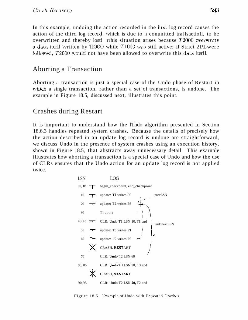
CT'ash ReC()7.]CT'!i 59,3
In this exarnple, undoing the action recorded in the first log record causes theaction of the third log recor~l, \vhich is due to a conunitted traJlsaetioIl, to beoverwritten and thereby lost! rrhis situation arises because 1"'2000 overvvrotea data itcrIl \vritten by TIOOO while 1''1000 W(l..'3 still active; if Strict 2PLwerefollo\ved, 1'2000 \vould not have been allowed to overwrite this data iterH.
Aborting a Transaction
Aborting a. transaction is just a special case of the Undo phase of Restart in\vhich a single transaction, rather than a set of transactions, is undone. Theexarnple in Figure 18.5, discussed next, illustrates this point.
Crashes during Restart
It is important to understand how the lTndo algorithrn presented in Section18.6.3 handles repeated systern crashes. Because the details of precisely howthe action described in an update log record is undone are straightforward,we discuss Undo in the presence of systern crashes using an execution history,shown in Figure 18.5, that abstracts away unnecessary detail. This exarnpleillustrates how aborting a transaction is a special case of Undo and how the useof CLRs ensures that the Undo action for an update log record is not appliedtwice.
LSN LOG
00, os -;- begin_checkpoint, end_checkpoint
10 -r update: Tl writes P5 prevLSN
20 -F- update: T2 writes P3
30 Tl abort .- \
I40,45 -F- CLR: Undo T1 LSN 10, T1 tnd
undonextLSN
50 -..,...... update: T3 writes PI iIj!I
60 -...... update: 1'2 writes P5 ....../
>< CRASH, RESTART
70 CLR: l1ndo '1'2 LSN 60
so, 85 CLR: Undo '1'3 LSN 50, '1'3 end
>< CRASH, RR~TART
90,95 CLR: lJndo T2 LSN 20, T2 end
Figure 18.5 ExC'uTlple of Undo with Repeatt!d C~rashes
594 (;IIAPTEH. J8
'rhe log shcnvs the order in \vhich theDB~IS executed various actions; note thatthe LSNs are in ascending order ~ and that eal~h log record for a transaction ha..'3a prevLSN' field that points to the previous log record for that transaction. \~Te
have not shown 'n/ull prevLSNs, that is, SOIne special '\lailleused in the prevLSNfield of the first log record for a, transaction to indicate tha,t there is no previouslog record. vVe also cOlnpacted the figure by occasionally displaying hvo logrecords (separated by a cOIlllna) on a single line.
Log record (with LSN) 30 indicates that Tl aborts. All actions of this transaction should be undone in reverse order, and the only action of ~r1, describedby the update log record 10, is indeed undone as indicated by CLR, 40.
After the first crash, Analysis identifies F)l (with recLSN 50), P~3 (with recLSN20), and P5 (with recLSN 10) as dirty pages. Log record 45 shows that Tl is acornpleted transaction; hence, the transaction table identifies T2 (with lastLSN60) andT3 (with lastLSN' 50) as active at the tirne of the crash. '1'he Redoplu:1...se begins with log record 10, which is the rninirnurn recLSN in the dirtypage table, and reapplies all actions (for the update and CLR, records), as perthe Redo algorithIl1 presented in Section 18.6.2.
The r1'olJndo set consists of LSNs 60, for 1'12, and 50, for T~3. The lJndo phasenow begins by processing the log record with LSN 60 because 60 is the largestLSN in the ToUndo set. The update is undone, and a CLR, (with LSN 70)is written to the log. ~rhis CLIl has llndoNextLSN equal to 20, which is theprevLSN value in log record 60; 20 is the next action to be undone for 112. Nowthe largest rernaining LSN in the rroundo set is 50. The \vritE~ correspondingto log record 50 is now undone, and a CLH, describing the change is 'written.rrhis eLH, has LSN 80, and its undoNextLSN field is null because 50 is theonly log record for transaction T3. Therefore T~3 is cOITlpletely undone, and anend record is written. Log records 70, 80, and 85 aTe written to stable storagebefore the systern crct.shes a second tirHe; ho\vever, the changes described bythese records ITlay not have been written, to disk..
\\lhen the systern is resta.rted after the S8C011(1 cra,,')}L Analysis deterrnines thatthe only active transactioIl at the tirne of the crash \\1[1.'3 'T2; in addition, the dirtypa,ge table is identicaJ to \\That it \VEtS during the previous restart. Log records10 througll 85 are processed Etgain during Itedo. (If sorne of the changes rnadeduring the prcv"ious H,edo were vvritten to disk, the pageLSN's on the affectedpages are used to detect this situation and avoid writing these pages again.)T'he lJndo phase considers the onlyLSN in the TolJndo set, 70, and processes it}))" adding tIle llndoNextLSN value (20) to the 1'olJndo set. Next, log record 20is processed l)y llndoing~r2's "\Trite of page }J:.3, a.nd a. CIJl, is VvTitten (LSN 90).Because 20 is the first of 7'2's log records and therefore, the laAst of its records
to be undone~~the undoNextLSN field in this CLR IS ntlll, an end record IS
written for T2, al1d the TolJndo set is no\v E:~rnpty.
llecovery is no\v cornplete, and norrnal execution can resurne vvith the ·writingof a checkpoint record.
This exarnple illustrated repeated crashes during the lJndo phage. Ii()l' cornpleteness, let us consider vvhat happens if the s)'stern cra,'3hes ·while R,estart isin the Analysis or Iledo pha.se. If a crash occurs during the Analysis phase, allthe work done in this phase is lost, and on restart the Analysis phase startsafresh vvith the sa11le inforrnation as before. If a cr&'3h occurs during the Redophase, the only effect that survives the cra...9h is that sorne of the changes rnadeduring Redo 11U1Y have been written to disk prior to the crash. R,estart startsagain with the Analysis phase and then the Redo phase, and sorne update logrecords that were redone the first tirne around will not be redone a second tirnebecause the pageLSN is now equal to the update record's LSN (although thepages have to be fetched again to detect this).
We can take checkpoints during llestart to rninirnize repeated work in the eventof a crash, but we do not discuss this point.
18.7 MEDIA RECOVERY
Media recovery is based on periodically rnaking a copy of the database. Because copying a large database object such as a file CeHl take a long tirHe, andthe I)BMS rnust be allowed to continue vvith its operations in the Ineantirne,creating a copy is handled in a rnanner sirnilar to taking a fuzzy checkpoint.
\\Then a databa.se object such as a file or a page is corrupted, the copy of thatobject is brought up-to-date by using the log to identify and reapply the changesof cornnlitted transactions and undo the changes of uncoI1unitted transactions(as of the tirne of the rnedia recovery operation).
The begilLchecl<.point LSN of the rnost recent cOlllplete checkpoint is recordedalong \vith the copy ()f the database object to luinirnize the vvork in reapplyingchaxlges of cornrnitt(~d transactions. Let us COlnpare the sl11<:.111est recLSN ofa dirty page in the corresponding encLcheckpoint record \vith the I;SN of thebegirLcheckpoint record and call the slua.ller of these tvvo LSNs I. \Ve observethat the actions recorded in all log records with LSNs less thaD I Inust beref1ectE~(l in the copy. Thus: 0111y log records \vithLSNs greater than I need bereapplied to the copy.
/""()6D... C~HAPTg,R 18
Finally, the updates of transactions that are incornplete at the tiIl1e of Inediarecovery or that \vere aborted after the fuzzy copy \va" corllpleted need to beundone to ensure that the page reflects only the actions of conunitted transactions. The set of such transactions can be identified (1...'3 in the Analysis pass,and we ornit the details.
18.8 OTHER APPROACHES AND INTERACTION WITHCONCURRENCY CONTROL
Like ARIES, the Inost popular alternative recovery algoritlllns also rnaintain alog of databa.'3e actions according to the \VAL protocol. A InajaI' distinctionbetween ARIES and these variants is that the Redo phase in ARIES repeatshistory, that is, redoes the actions of all transactions, not just the non-losers.Other algorithms redo only the non-losers, and the Redo phase follows theUndo phase, in which the actions of losers are rolled back.
Thanks to the repeating history paradigm and the use of CLRs, ARIES supports fine-granularity locks (record-level locks) and logging of logical operationsrather than just byte-level rnodifications. For exalllple, consider a transactionT that inserts a data entry 15* into a B+ tree index. Between the tirne thisinsert is done and the time that T is eventually aborted, other transactions Inayalso insert and delete entries frorn the tree. If record-level locks are set ratherthan page-level locks, the entry 15* I11ay be on a different physical page whenT aborts fr0111 the one that T inserted it into. In this case, the undo operationfor the insert of 15* lllUSt be recorded in logical tenns because the physical(byte-level) actions involved in undoing this operation are not the inverse ofthe physical actions involved in inserting the entry.
I.Jogging logical operations yields considerably higher concurrency, although theuse of fine-granularity locks can lead to increased locking activity (because rnorelocks 1nust be set). Hence: there is a trade-off between different \VAL-b<.k"ledrecovery schclnes. vVe chose to cover ARIES because it has several attractiveproperties, in pa.rticular, its sirnplicity and its ability to support fine-granularitylocks and logging of logical operations.
One of the earliest recovery algorithrns, llsed in the Syster11 R, prototype atIBI\'1, takes a v(~ry different approach. 'There is no logging and, of course,no \VAL protocol. Instead, the database is treated as a collection of pagesand accessed thTough a page table, which IIHtpS page ids to disk addresses.\Vhen a transaction Inakes changes to <'1 data pagel it actually Inakes a copyof the page, called the shadow of the page, a,nel changes the shadow page.The transaction copies the appropriate part of the page table and chan,ges theentry for the changed page to point to the shadov,r, so that it can see the
changes; ho\vever ~ other transactions continue to see the original page table,and therefore the original page, until this transaction COll1lnits. Aborting atransaction is sirnple: .Just discard its shadcnv versions of the page table andthe data pages. Cornrnitting a transaction involves rnaking its version of thepage table public and discarding the original data pages that are supersededby shado\v pages.
This schelue suffers frorn a nUlnber of problerlls. First, data becornes highlyfragrnented clue to the replacernent of pages by shado"v versions, "vhich rIlay belocated far fr01n the original page. This phenornenon reduces data clusteringand rnakes good garbage collection irnperative. Second, the sche1ne does notyield a sufficiently high degree of concurrency. rrhird, there is a, substantialstorage overhead due to the use of shadow pages. ~burth, the process abortinga transaction can itself run into deadlocks, and this situation rllust be speciallyhandled because the sernantics of aborting an abort transaction gets rnurky.
For these reasons, even in Systern R, shadow paging was eventually supersededby \VAL-based recovery techniques.
18.9 REVIEW QUESTIONS
Answers to the review questions can be found in the listed sections.
.. What are the advantages of the ARIES recovery algoritluu? (Section 18.1)
II Describe the three steps in crash recovery in ARIES? What is the goal ofthe Analysis phase? The redo phase? The undo phase? (Section 18.1)
II \lVhat is the LSN of a log record? (Section 18.2)
II \Vhat are the different types of log records <:l,,11d when are they written?(Section 18.2)
ifill "Vhat inforrnation is rnaintained in the transaction table and the dirty pagetable? (Section 18.3)
ifill vVhat is\Vrite-Ah(~ad Logging? \Vhat is forced to disk at the tirne a transaction COIlllnits? (Section 18.4)
• \~That is a fuzzy checkpoint? \Vhy is it useful? "\That is a rnaBter log record?(Section 18.5)
III In \vhich direction does the .A.nalysis phase of recovery scan the log? At\vhich point in the log does it begin and end the scan? (Section 18.6.1)
II Descril)c \vhat infonnation is gathered in the Analysis pha,se and ho\v.(Section 18.6.1)

598 CHAPTER IS
• In \vhich direction does the Redo phase of recovery process the log? Atwhich point in the log does it begin and end? (Section 18.6.2)
• What is a redoable log record? Under what conditions is the logged action redone? \Vhat steps are carried out when a logged action is redone?(Section 18.6.2)
• In which direction does the Undo phase of recovery process the log? Atwhich point in the log does it begin and end? (Section 18.6.3)
• What are loser transactions? How are they processed in the Undo phaseand in what order? (Section 18.6.3)
• Explain what happens if there are crashes during the Undo phase of recovery. What is the role of CLR.s? What if there are ~rashes during theAnalysis and Redo phases? (Section 18.6.3)
II How does a DBlV1S recover from 111edia failure without reading the completelog? (Section 18.7)
• Record-level logging increases concurrency. What are the potential problems, and how does ARIES address them? (Section 18.8)
II What is shadow paging? (Section 18.8)
EXERCISES
Exercise 18.1 Briefly answer the following questions:
1. How does the recovery rnanager ensure atornicity of transactions? How does it ensuredurability?
2. What is the difference between stable storage and disk?
:3. What is the difference between a systenl crash and a uledi"l failure?
4. Explain the vVAL protocol.
t). Describe the steal and no-force policies.
Exercise 18.2 Briefly answer the follO\ving questions:
1. v\That are the properties required of LSNs?
2. \\That arc the fields in an update log record? Explain the use of each field.
:3. VVhat are redoal)le log records?
4. vVha.t are the differences between update log records and CLRs?
Exercise 18.3 Briefly answer the following questions:
1. \Vhat are the roles of the Analysis, Iledo1 and Undo phases in AHlES?
2. (;onsider the execution shown in Figure 18.6.
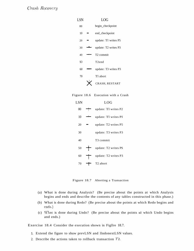
LSN LOG
00 begin__checkpoint
10 - end_cbeckpoint
20 - update: Tl writes P5
30 --- update: T2 writes P3
40 .....-.- T2 commit
SO T2end
60 .....-.- update: T3 writes P3
70 Tl abort
>< CRASH, RESTART
Figure 18.6 Execution with a Crash
LSN LOG
00 -r- update: Tl writes P2
10 -l- update: Tl writes PI
20 - update: T2 writes P5
30 update: T3 writes P3
40 T3 commit
50 1- update: T2 writes PS
60 i update: T2 writes P3
70 -r- T2 abort
Figure 18.7 Aborting a Transaction
(a) What is done during Analysis? (Be precise about the points at which Analysisbegins and ends and describe the contents of any tables constructed in this phase.)
(b) What is done during Redo? (Be precise about the points at which Redo begins andends.},
(c) 'VVhat is done during Undo? (Be precise about the points H.t which Undo beginsand ends.)
Exercise 18.4 Consider the execution shown in Figllre 18.7.
1. Extend the figure to shuw prevLSN and llndonextLSN values.
2. Describe the actions taken to rollback transaction 7"'2.

600 C~HAPTER 1B
LSN LOG
00 - begin_checkpoint
10 end_checkpoint
20 7 update: 1'1 write..~ PI
30 --- update: 1'2 writesP2
40 --- update: 1'3 writes P3
50 - 1'2 commit
60 --- update: 1'3 writes P2
70 ......0- 1'2 end
80 - update: 1'1 writes P5
90 -!- 1'3 abort
>< CRASH,RESTART
Figure 18.8 Execution with Multiple Cra...,hes
3. Show the log after T2 is rolled back, including all prevLSN and undonextLSN values inlog records.
Exercise 18.5 Consider the execution shown in Figure 18.8. In addition, the systerll crashesduring recovery after writing two log records to stable storage and again after writing anothertwo log records.
1. What is the value of the LSN stored in the master log record?
2. What is done during Analysis?
3. What is done during Redo?
4. \Vhat is done during Undo?
,5. Show the log when recovery is complete, including all non-null prevLSN and unclonextLSNvalues in log records.
Exercise 18.6 Briefly answer the following questions:
1. How is checkpointing done in ARIES?
2. Checkpointing can also be done as follows: Quiesce the systerll so that only checkpointingactivity can be in progress, write out copies of all dirty pages, and include the dirty pagetable and trallsaction table in the checkpoint record. \\lhat are the pros and cons of thisapproach versus the checkpointiug a,pproach of ARIES?
:3. \Vhat happens if a second begiILcheckpoint record is encountered during the Analysisph<-1..13e?
4. C;an a second en(Lcheckpoint record be encountered during the AnaJysis phase?
5. \iVh,Y is the use of CLRs irnportant for the use of undo actions that are not the physicalinverse of the original update?

Figure 18.9
LSN LOG
00 -'- begin_checkpoint
10 -!- update: Tl writes PI
20 + '1'1 commit
30 -+ update: T2 writes P2
40 T '1'1 end
50 - '1'2 abort
60 -r update: '1'3 write'ii P3
70 end_checkpoint
80 -- '1'3 commit
>< CRASH, RESTART
Log Records between Checkpoint Records
601f;
6. Give an example that illustrates how the paradigm of repeating history and the use ofCLRs allow ARIES to support locks of finer granularity than a page.
Exercise 18.7 Briefly answer the following questions:
1. If the system fails repeatedly during recovery, what is the rrlaximum nunlber of logrecords that can be written (as a function of the number of update and other log recordswritten before the crash) before restart cOInpletes successfully?
2. What is the oldest log record we need to retain?
3. If a bounded amount of stable storage is used for the log, how can we always ensureenough stable storage to hold all log records written during restart?
Exercise 18.8 Consider the three conditions under which a redo is unnecessary (Section20.2.2).
1. \Vhy is it cheaper to test the first two conditions?
2. Describe an execution that illustrates the use of the first condition.
;3. Describe an execution that illustrates the use of the second condition.
Exercise 18.9 The description in Section 18.6.1 of the Analysis pha,se rnade the sirnplifyingassulTlptioll that no log records appeared between the begill-checkpoint and end_checkpointrecords for the Inost recent cOlnplete checkpoint. The following questions explore how suchrecords should be handled.
1. Explain why log records could be written between the begiIl-checkpoint and eneLcheckpointrecords.
2. Describe how the Analysis phase could be Inodified to handle such records.
;3. Consider the execution sho\vn in l~"igure 18.9. Show the contents of the encLcheckpointrecord.
4. Illustrate your rnodified Analysis pha.se on the execution shown in Figure 18.9.
602
Exercise 18.10 Ans\ver the following questions briefly:
C~HAPTER IB
1. Explain how 1nedin recovery is handled in ARIES.
2. \Vhat are the pros (I,nd cons of using fuzzy durnps for nledia recovery?
~1. \Vhat are the sirYlilarities and differencf~s between checkpoints and fuzzy chunps?
4. Contrast ARIES with other vVAL-based recovery schernes.
5. Contrast AHlES with shadcrw-page-bcLsed recovery.
BIBLIOGRAPHIC NOTES
Our discussion of the ARIES recovery algorithm is based on [544]. [282] is a survey articlethat contains a very readable, short description of ARIES. [541, 545] also discuss ARIES.Fine,·granularity locking increases concurrency but at the cost of 11101'e locking activity; [542]suggests a technique based on LSNs for alleviating this problerYl. [458] presents a for111alverification of ARIES.
[355] is an excellent survey that provides a broader treatrnent of recovery algoritlulls than ourcoverage, in which we chose to concentrate on one particular algorithrn. [17] considers perforrnance of concurrency control and recovery algorithrIls, taking into account their interactions.The irnpact of recovery on concurrency control is also discussed in [769]. [625] contains aperforrnance analysis of various recovery techniques. [236] cornpares recovery techniques formain rnerllory database systeulS, which are optirnized for the case that 11l0st of the active dataset fits in rnain H1ernory.
[478] presents a description of a recovery algorithm based on write-ahead logging in which'loser' transactions cHe first undone and then (only) transactions that corl1nlitted before thecrash are redone. Shadow paging is described in [493, 337]. A scherne that uses a cOlnbinationof shadow paging and in-place updating is described in [624].
PART VI
DATABASE DESIGN AND TUNING


19SCHEMA REFINEMENT AND
NORMAL FORMS
WI" What problems are caused by redundantly storing information?
.. What are functional dependencies?
.. What are nornlal forms and what is their purpose?
... What are the benefits of BCNF and 8NF?
... What are the considerations in decolllposing relations into appropriatenormal forms?
.. Where does normalization fit in the process of database design?
... Are luore general dependencies useful in database design?
.. Key concepts: redundancy, insert, delete, and update anomalies;functional dependency, Armstrong's Axioms; dependency closure, attribute closure; normal fonns, BCNF, 8NF; decOlnpositions, losslessjoin, dependency-preservation; multivalued dependencies, join dependencies, inclusion dependencies, 4NF, 5NF
It is a nlelancholy truth that even great IneIl have their poor relations.
Charles Dickens
Conceptual database design gives us a set of relation 8chen1&') and integrityconstraints (ICs) that can be regarded a,s a good starting point for the finaldat(1)ase design. T'his initial design IHust be refined by taking the lCg intoaccount rnore fully than is possiblc\vith just the Ell rnodel constructs aIId alsoby considering perforrnance criteria and typical workloads. In this chapter,we c!iscllss how lCs can be used to refine the conceptual schenul produced by
G05

606 (]HAprrER 19
translating anER, 1Hodel design into a collection of relations. \Vorkload andperforrnance considerations are discussed in Chapter 20.
\Ve concentrate on an irnportant class of constraints called flLnct'ional dependencies. Other kinds of les, for exarnple, m/ultival'll,ed dependencies and joindependencies, also provide useful inforrnation. They can sOIuetilnes reveal redundancies that cannot be detected using functional dependencies alone. Wediscuss these other constraints briefly.
This chapter is organized as follows. Section 19.1 is an overview of the schenlarefineInent approach discussed in this chapter. We introduce functional dependencies in Section 19.2. In Section 19.3, we show how to reason with functionaldependency information to infer additional dependencies from a given set ofdependencies. We introduce norlnal forIns for relations in Section 19.4; thenormal form satisfied by a relation is a measure of the redundancy in the relation. A relation with redundancy can be refined by decomposing it, or replacingit with smaller relations that contain the saIne information but without redundancy. We discuss deco1npositions and desirable properties of decompositionsin Section 19.5, and we show how relations can be decomposed into smallerrelations in desirable normal forms in Section 19.6.
In Section 19.7, we present several examples that illustrate how relationalschemas obtained by translating an ER model design can nonetheless sufferfroln redundancy, and we discuss how to refine such schemas to eliminate theproblems. In Section 19.8, we describe other kinds of dependencies for databa..sedesign. We conclude with a discussion of nornlalization for our case study, theInternet shop, in Section 19.9.
19.1 INTRODUCTION TO SCHEMA REFINEMENT
We now present an overview of the probleIns that schenla refinement is intendedto address and a refinernent approach based on decolnpositions. Iledundantstorage of inforrnation is the root cause of these problerns. Although decoInposition can elirninate redundancy, it can lead to problclns of its o\vn and shouldbe used with caution.
19.1.1 Pro~lems Caused by Redundancy
Storing the SeHne inforrnation redundantly, that is, in l110re than one place\vithin a database, can lead to several problcll1S:
II Redundant Storage: SOU1C iuforInation is stored repeatedly.
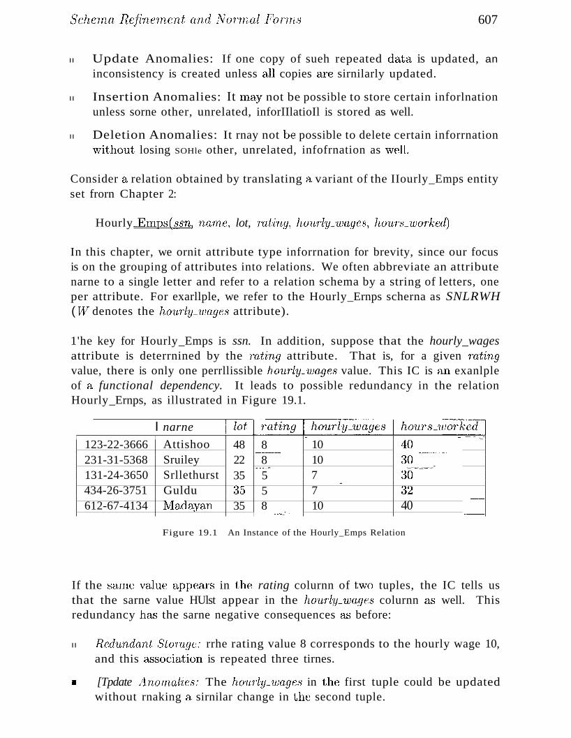
607
II Update Anomalies: If one copy of sueh repeated data is updated, aninconsistency is created unless all copies cu'c sirnilarly updated.
II Insertion Anomalies: It IIU1Y not be possible to store certain inforlnationunless sorne other, unrelated, inforIIlatioIl is stored as well.
II Deletion Anomalies: It rnay not be possible to delete certain inforrnationvvithout losing SOHle other, unrelated, infofrnation as v'lell.
Consider a relation obtained by translating a variant of the IIourly_Emps entityset frorn Chapter 2:
Hourly_Ernps(:2,sn, na'lne, lot, rating, hOllrly_wages, hOllr.'LwoTked)
In this chapter, we ornit attribute type inforrnation for brevity, since our focusis on the grouping of attributes into relations. We often abbreviate an attributenarne to a single letter and refer to a relation schema by a string of letters, oneper attribute. For exarllple, we refer to the Hourly_Ernps scherna as SNLRWH( ~V denotes the hov,rly_wages attribute).
1'he key for Hourly_Emps is ssn. In addition, suppose that the hourly_wagesattribute is deterrnined by the Tating attribute. That is, for a given 7'CLtingvalue, there is only one perrllissible houTly_wages value. This IC is an exanlpleof a functional dependency. It leads to possible redundancy in the relationHourly_Ernps, as illustrated in Figure 19.1.
I narne., ._ ....._..
-, --- - ._-
123-22-3666 Attishoo 48 8 10 40._.n_··_··~·~···~· ~.."""".'.'.""<-",,'-"""'.'
231-31-5368 Sruiley 22 8 10 ~30....'~.".li ..."'•. .__....~ .._..._.._..-
131-24-3650 Srllethurst 35 5 7 ~30-
434-26-3751 Guldu :35 5 7 ~)2---
612-67-4134 :NIadayan 35 8 10 40._........._- . .-
Figure 19.1 An Instance of the Hourly_Emps Relation
If the saIne value appears in the rating colurnn of tv'lo tuples, the IC tells usthat the sarne value HUlst appear in the hourly_wages colurnn c1.'3 well. Thisredundancy has the sarne negative consequences a..s before:
II Redtlndant StoTage: rrhe rating value 8 corresponds to the hourly wage 10,and this (L.':lsociation is repeated three tirnes.
II [Tpdate AnoTno1ic,,: The hO'lLTlY_'l1HLgcs in the first tuple could be updatedwithout rnaking a sirnilar change in the second tuple.
608 CHAPT'ER 19t
• InseT"lion Ano'mal'ie,';: VVe cannot insert a tuple for an crnployee unless \veknow the hourly wage for the ernployee's rating value.
• Delet'ion finon-LaUe..,: If \ve delete all tuples vvith a given rating value (e.g.,we delete the tuples for Snlcthurst and Guldu) \ve lose the &t;sociationbet:\veen that Tat'ing value and its houTly_wage value.
Ideally, vve \vant scherna.s that do not pennit redundancy, but at the very leastwe want to be able to identify schernas that do allow redundancy. Even if wechoose to accept a scherna vvith sorne of these drawbacks, perhaps owing toperforlnance considerations, we want to rnake an infonned decision.
Null Values
It is worth considering whether the use of null values can address some of theseproblems. As we will see in the context of our exarnple, they cannot provide acomplete solution, but they can provide sorne help. In this chapter, we do notdiscuss the use of null values beyond this one exarnple.
Consider the example Hourly_Elnps relation. Clearly, null values cannot helpeliminate redundant storage or update anomalies. It appears that they canaddress insertion and deletion anomalies. For instance, to deal with the insertion anolnaly exarnple, we can insert an elTIplayee tuple with null values in thehourly wage field. However, null values cannot address all insertion anornalies.For exarnple, we cannot record the hourly wage for a rating unless there isan ernployee with that rating, because we cannot store a null value in the ssnfield, which is a prirnary key field. Sinlilarly, to deal with the deletion anomalyexarnple, we rnight consider storing a tuple with null values in all fields exceptTat'ing and hourly_wages if the last tuple with a given rating would otherwisebe deleted. However, this solution does not work because it requires the 8871,
value to be null, and prirnary key fields cannot be null. Thus, rl/ull values donot provide a general solution to the problerns of reclundancy, even though theycan help in sorne cases.
19.1.2 Decompositions
Intuitively, redundancy arises \vhen a relational schcrna forces an associationbet\veen attributes that is not natural. Functional dependencies (and, for thatrnatter, other Ies) can 'be used to identify such situations and suggest re£1nernents to the scheruEL The essential idea is that rnany problerns arising fr0111 redundancy carl be addressed by replacing a relation 'with a collection of'srnaller'relations.
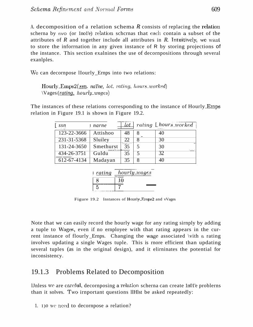
ScheTna Refine'Tnent and NOTlnal ]?o'T'rns 609
A. decomposition of a relation schema It consists of replacing the relationscherna by t\VO (or 1no1'e) relation schcrnas that each contain a subset of theattributes of R and together include all attributes in R. Intuitively, \eve \evantto store the inforrnation in any given instance of R by storing projections ofthe instance. This section exalnines the use of decornpositions through severalexanlples.
vVe can decornpose lIourly_Ernps into two relations:
Ifourly_Ernps2C~.:~n~naTne, lot, 'rating, hOUr\'Lwo'rked)\Vages (rating, hourly_wages)
The instances of these relations corresponding to the instance of Hourly_E1npsrelation in Figure 19.1 is shown in Figure 19.2.
'--['-ioT] 'rating [ hours_lLJorked-n
]I narne.. ._- .....""....,,,..........
123-22-3666 Attishoo 48 8 40-
231-31-5368 Sluiley 22 8 30-_..._...... _...
131-24-3650 Smethurst 35 5 30...-.,...-.....-..."' ...." ...... ,...._- ..._._...
434-26-3751 Guldu 35 5 32-_...~._--_ ...
612-67-4134 Madayan 35 8 40
[ ssn
I rating l!!ourly~'u)ages
Fl_~_no _Figure 19.2 Instances of Hourly...Emps2 and vVages
Note that we can easily record the hourly wage for any rating sirnply by addinga tuple to \;Vages, even if no ernployee with that rating appears in the current instance of flourly_Ernps. Changing the wage associated \vith a ratinginvolves updating a single Wages tuple. This is rnore efficient than updatingseveral tuples (as in the original design), and it elirninates the potential forinconsistency.
19.1.3 Problems Related to Decomposition
lJnless \ve are careful~ decornposing a relation scherna can create 1n01'e problernsthan it solves. rrvVO irnportant questions llHlst be asked repeatedly:
1. 1)0 vve need to decornpose a relation?
610
2. \\That problerns (if any) does a given deeornposition cause?
CHAPTER 19
To help \vith the first question, several norrrtal j'O'rnl,8 have been proposed forrelations. If a relation scherna is ill one of these nOfrual 1'orrns, we knovv thatcertain kinds of problerlls cannot arise. Considering the norrnal forrn of a givenrelation scherna can help us to decide \vhether or not to decornpose it further. Ifvve decide that a relation scherna 111USt be decornposed further, vve rnust choosea particular dec()lnposition (I.e., a particular collection of slnaller relations toreplace the given relation).
With respect to the second question, two properties of decornpositions areof particular inter(~st. The lossless-join property enables us to recover anyinstance of the decornposed relation froln corresponding instances of the s111allerrelations. The dependency-preservation property enables us to enforce anyconstraint on the original relation by sinlply enforcing SaIne contraints on eachof the srnaller relations. That is, we need not perform joins of the slllallerrelations to check whether a constraint on the original relation is violated.
From a performance standpoint, queries over the original relation may requireus to join the decomposed relations. If such queries are common, the perforrnance penalty of decomposing the relation may not be acceptable. In thiscase, we may choose to live with some of the problems of redundancy and notdecompose the relation. It is important to be aware of the potential problernscaused by such residual redundancy in the design and to take steps to avoidthern (e.g., by adding SaIne checks to application code). In sonle situations,decomposition could actually improve performance. This happens, for example, if lnost queries and updates exanline only one of the decornposed relations,which is srnaller than the original relation. vVe do not discuss the irnpact ofdecompositions on query perforInance in this chapter; this issue is covered inSection 20.8.
()ur goal in this chapter is to explain S0111e powerful concepts and design guidelines b&'3ed on the theory of functional dependencies. A good datab&'3e designershould have a firm grasp of nor1nal fonns and \vhat problerns they (do or donot) alleviate, the technique of decornposition, and potential problerns vvithdecornpositions. For exaInple, a designer often asks questions such &'3 these: Isa relation in a given nonnal forIn? Is a decornposition clependency-preserving?Our objective is to explain when to raise these questions and the significanceof the answers.
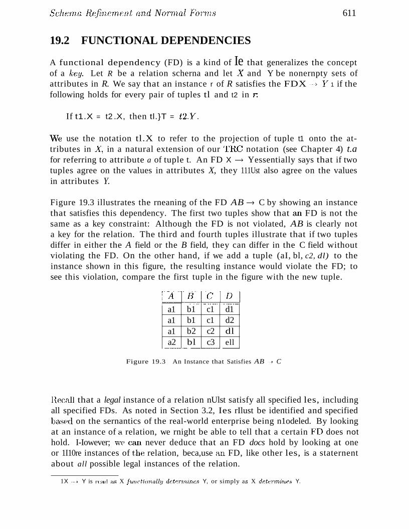
Scherna Refine'rnent and NornuIl }'OT'lnS
19.2 FUNCTIONAL DEPENDENCIES
611
A functional dependency (FD) is a kind of Ie that generalizes the conceptof a key. Let R be a relation scherna and let ..¥" and Y be nonernpty sets ofattributes in R. We say that an instance r of R satisfies the FDX ~ }i 1 if thefollowing holds for every pair of tuples tl and t2 in r-.
If t1.X = t2 ..X, then tl.}T = t2.Y'".
w(~ use the notation tl.X to refer to the projection of tuple t1 onto the attributes in .<\'", in a natural extension of our TIlC notation (see Chapter 4) t.afor referring to attribute a of tuple t. An FD X ----7 Yessentially says that if twotuples agree on the values in attributes X, they 111Ust also agree on the valuesin attributes Y.
Figure 19.3 illustrates the rneaning of the FD AB ----7 C by showing an instancethat satisfies this dependency. The first two tuples show that an FD is not thesame as a key constraint: Although the FD is not violated, AB is clearly nota key for the relation. The third and fourth tuples illustrate that if two tuplesdiffer in either the A field or the B field, they can differ in the C field withoutviolating the FD. On the other hand, if we add a tuple (aI, bl, c2, dl) to theinstance shown in this figure, the resulting instance would violate the FD; tosee this violation, compare the first tuple in the figure with the new tuple.
-- ...-......................... ..."""......................"N
a1 b1 c1 d1a1 b1 c1 d2a1 b2 c2 dla2 bl c3 ell
..............."" ...............,."'" ' ........ n ....' ...................-.---- -"-
Figure 19.3 An Instance that Satisfies AB -Jo C
Ilecall that a legal instance of a relation nUlst satisfy all specified les, includingall specified FDs. As noted in Section 3.2, Ies rIlust be identified and specifiedba...sed on the sernantics of the real-world enterprise being n1odeled. By lookingat an instance of a relation, we rnight be able to tell that a certain FD does nothold. I-Iowever; we C<-:l.Tl never deduce that an FD docs hold by looking at oneor 1I10re instances of the relation, beca,use an FD, like other les, is a staternentabout all possible legal instances of the relation.
1X _._, Y is re,lel aAS X fu'nctionally deteTrninc8 Y, or simply a..s X determ'ines Y.
612 C~HAP'TgR 19
.A prirnary key constraint is a special ease of an .1"1). The attributes in the keyplay the role of X, and the set of all attributes in the relation plays the role ofY. Note, ho\vever, that the definition of an FD does not require that the set ..Y"be 111iniInal; the additionalrninimality condition Illust be Inet for -'~ to be a key.If ..~ ----+Y holds, \vhere Y" is the set of all attributes, and there is SCHne (strictlycontajned) subset llof .iJ( such that 1/ ----+ },~ holds, then ..X" is a 81LIJerkey.
In the rest of this chapter, ·we see several exarIlples of FDs that are not keyconstraints.
19.3 REASONING ABOUT FDS
Given a set of FDs over a relation scheula .R, typically several additional FDshold over R whenever all of the given FDs hold. As an exalnple, consider:
WorkersC~~n, naTne, lot, did, since)
We know that ssn ----+ did holds, since ssn is the key, and FD did ----+ lot is givento hold. Therefore, in any legal instance of Workers, if two tuples have thesame ssn value, they Blust have the sarne did value (frolH the first FD), andbecause they have the sarrle did value, they must also have the saIne lot value(1'1'0111 the second FD). Therefore, the FD ssn ----+ lot also holds on Workers.
We say that an FD f is implied by a given set F of FDs if f holds on everyrelation instance that satisfies all dependencies in F; that is, f holds wheneverall FDs in F hold. Note that it is not sufficient for f to hold on SaIne instancethat satisfies all dependencies in F; rather, f rnust hold on every instance thatsatisfies all dependencies in P'.
19.3.1 Closure of a Set of FDs
The set of all .FDs irnplied by a given set F of FDs is called the closllre ofJi-', denoted as .F'+. An irnportant question is how we can infer, or cornpute,the closure of a given set ]? of FDs. ~rhe answer is sirnple and elegant. Thefolhwving three rules, called Armstrong's Axioms, can be applied repeatedlyto infer all FI)s irnplied by a set ]? of FDs. \lVe use ..,""Y, and Z to denote sctsof attributes over a relation scherna It:
\I Reflexivity: If X ~ }T, then X ----+ Y.
\I Augn1.entation: If )( -'tY, then ..YZ ---t }TZ for any Z.
11II Transitivity: If)( ----+Y (urd Y
Sche-rna Rejinenu:nt and lVoT'lnall?oTTns 61~
Theorem 1 AT1nstrong'8 A:riorns are sound J in that they gene1ute only 1t'Dsin F"+- 'when apT)l'ied to a set, F of j?D8. They are also completeJ in that repeateda]Jplicat'ion afthese T"ules 1JJill generate all FDs in the ClOS'U7"'e .Fl+.
The soundness of Arrnstrong's Axiorns is straightfor\vard to prove. Cornpleteness is harder to show; see Exercise 19.17.
It is convenient to use SOlne additional rules while rea..soning about P+:
• Union: If X ~ Yand X ~ Z, then X ~ YZ.
• Decomposition: If X -+ YZ, then X ~ y' and X -7 Z.
These additional rules are not essential; their soundness can be proved usingArmstrong's AxiolllS.
To illustrate the use of these inference rules for FDs, consider a relation scheluaABC with FDs A ····-*B and B -7 C. In a trivial FD, the right side containsonly attributes that also appear on the left side; such dependencies always holddue to reflexivity. Using reflexivity, we can generate all trivial dependencies,which are of the form:
X ~ Y, where Y ~ X, X ~ ABC, and Y ~ ABC.
FrOHl transitivity we get A -+ C. Fronl auglnentation we get the nontrivialdependencies:
AC--->- BGY, AB -7 AC', AB -7 C13.
As another exalnple, we use a rnore elaborate version of Contracts:
Contracts (!:..9ntractid, supplierid, pro,jectid, dept'id, partid, qty, val'ue)
\Ve denote the schenla for Contracts a..s CSJDPQ V. The rneaning of a tuple isthat the contract with contractid C is an agreelnent that supplier S (sv,pplierid)'will supply Q iterns of part? (par-tid) to project J (pTo,ject'id) associated withdepartrnent D (deptid); the value tl of this contract is equal to value.
The following res are known to hold:
1. 1'he contract id Gl is a key: C -+ CSJDP(J V.
2. A project purclHlses a given part using a single contract: .II) --+ C1•
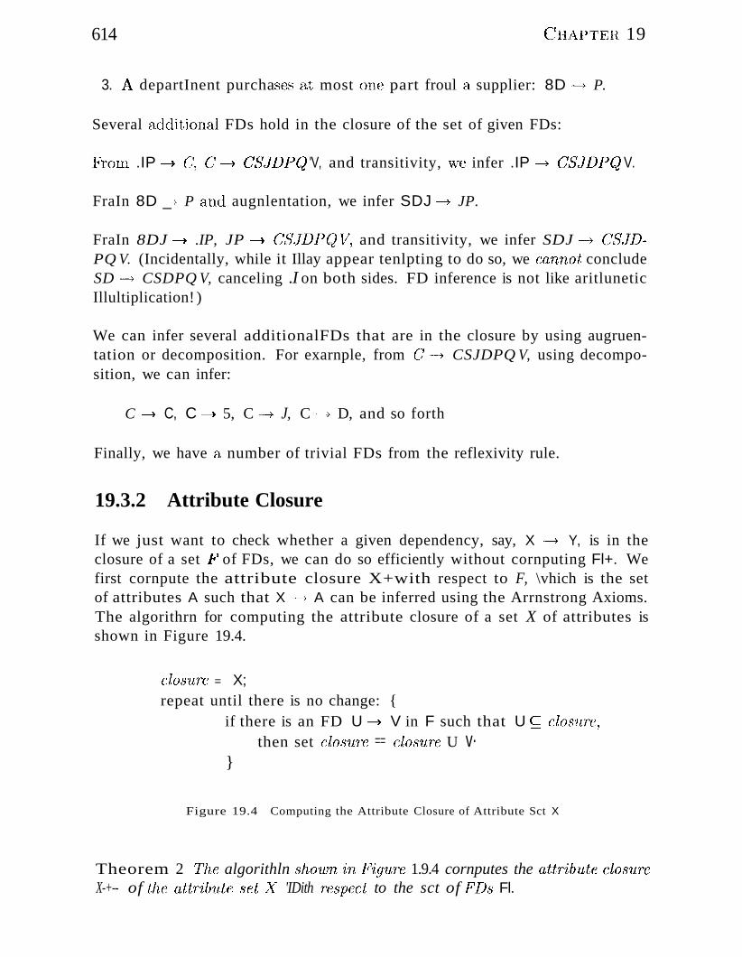
614 (JHAPTER 19
3. .A. departInent purcha..'3es a.t most one part froul a supplier: 8D ---+ P.
Several a.dditional FDs hold in the closure of the set of given FDs:
E'rorIl .IP -} C\ G'1 -+ C!SJD.PCJ 'V, and transitivity, ""VB infer .IP -_..+ CJSJDPCJ V.
FraIn 8D _...-7 P and augnlentation, we infer SDJ -7 JP.
FraIn 8DJ -7 .IP, JP -7 CSJDPQ~r, and transitivity, we infer SDJ ---+ CSJDPQ V. (Incidentally, while it Illay appear tenlpting to do so, we cannot concludeSD -7 CSDPQ V, canceling .I on both sides. FD inference is not like aritluneticIllultiplication! )
We can infer several additionalFDs that are in the closure by using augruentation or decomposition. For exarnple, from C----+ CSJDPQ V, using decomposition, we can infer:
C -7 C, C -7 5, C -7 J, C -} D, and so forth
Finally, we have a number of trivial FDs from the reflexivity rule.
19.3.2 Attribute Closure
If we just want to check whether a given dependency, say, X ---+ Y, is in theclosure of a set ~F' of FDs, we can do so efficiently without cornputing Fl+. Wefirst cornpute the attribute closure X+with respect to F, \vhich is the setof attributes A such that X -7 A can be inferred using the Arrnstrong Axioms.The algorithrn for computing the attribute closure of a set X of attributes isshown in Figure 19.4.
closure = X;repeat until there is no change: {
if there is an FD U -} V in F such that U ~ closllre,
then set clo,sure == closure U v·}
Figure 19.4 Computing the Attribute Closure of Attribute Sct X
Theorem 2 The algorithln .shown inF'iguTc 1.9.4 cornputes the attr'ibv,te closureX-+-- of the attribute set ~Y 'IDith respect to the sct of }"1Ds Fl.
Scherna RejiTtCrnerd and NOTlnal ForTns 615$
The proof of this theorern is considered in Exercise 19.15. This algoriUuIl canbe rl10dified to find keys by starting with set .i\"" containing a, single attribute andstopping as soon cl,.o;;; ClOS'UTC contains all attributes in the relation scherna. Byvarying the starting attribute and the order in \vhich the algorithrIl considersFDs, \ve can obtain all candidate keys.
19.4 NORMAL FORMS
Given a relation sche111a, we need to decide whether it is a good design or weneed to decornpose it into srnaller relations. Such a decision llUlst be guidedby an understanding of what problenls, if any, arise froln the current schelna.To provide such guidance, several normal forms have been proposed. If arelation schelna is in one of these norrnal forIns, we know that certain kinds ofproblerlls cannot arise.
The nonnal forrns ba...'Sed on FDs are fir-st nor-rnal forrn (1 Nfj, second nor-malforrn (2NJ?) , thi'td norrnalfor-rn (3NF) , and Boyce-Codd nor-rnal for-rn (BCN]?).These fonns have increasingly restrictive requirernents: Every relation in BCNFis also in 3NF, every relation in 3NF is also in 2NF, and every relation in 2NF isin INF. A relation is in first normal fortH if every field contains only atornicvalues, that is, no lists or sets. This requirerllent is iInplicit in our definitionof the relational rnode!. Although SOHle of the newer database systerlls arerelaxing this requirernent, in this chapter we aSSUlne that it always holds. 2NFis Inainly of historical interest. 3NF and BCNF are irnportant frolH a databasedesign standpoint.
While studying norrnal fonns, it is irnportant to appreciate the role played byFDs. Consider a relation scherna I? with f1ttributes ABC:. In the absence of anyICs, any set of ternary tuples is a legal instance and there is no potential forredundancy. ()n the other hand, suppose that \ve have the FI) A --,'> 13. Now ifseveral tuples have the sarne A value, they rnust also have tllC sarneB value.This potential redundanc:y can be predicted using the FD il1fonnation. If 11101'8
detailed 1Cs are specified, \ve rnay be able to detect rnore subtle redundanciesas \vell.
\Ve prilnarily discuss redundancy revealed l)y PI) inforrnation. In Section 19.8,\ve discuss 11lore sophisticated 1Cs ca1led rnuUivalued dependencies and joindependencies and norrnal forrns based on theIn.
19.4.1 Boyce...Codd Normal Form
Let I? be a relation scherna, 1? be the set ofF'I)s given to hold over R, .iX" be a.. - .
subset of the attributes ofR, and A be (\,.11 attribute of I? l~ is in Boyce-Codd
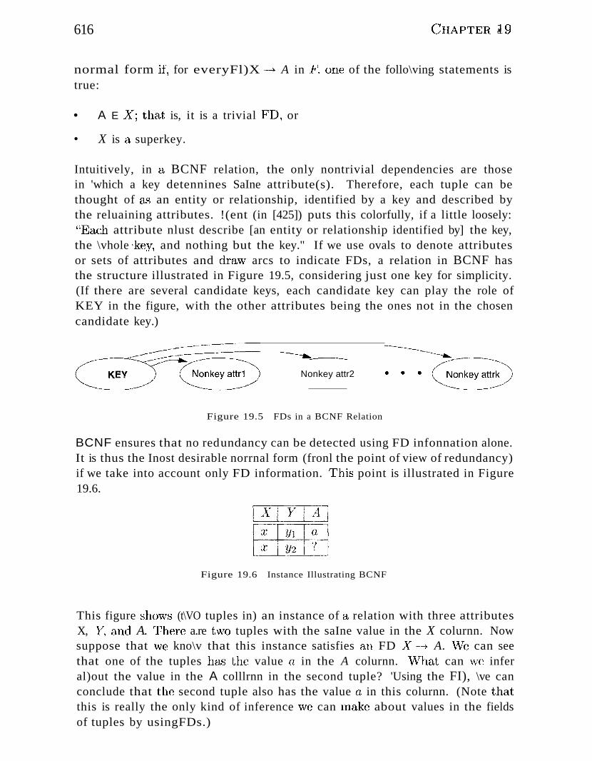
616 (~HAPTERtg
normal form if, for everyFl)X -+ A in F, one of the follo\ving statements istrue:
• A E .<Y; that is, it is a trivial FD, or
• X is a superkey.
Intuitively, in a BCNF relation, the only nontrivial dependencies are thosein 'which a key detennines SaIne attribute(s). Therefore, each tuple can bethought of C1....':l an entity or relationship, identified by a key and described bythe reluaining attributes. !(ent (in [425]) puts this colorfully, if a little loosely:"Each attribute nlust describe [an entity or relationship identified by] the key,the \vhole 'key, and nothing but the key." If we use ovals to denote attributesor sets of attributes and dravv arcs to indicate FDs, a relation in BCNF hasthe structure illustrated in Figure 19.5, considering just one key for simplicity.(If there are several candidate keys, each candidate key can play the role ofKEY in the figure, with the other attributes being the ones not in the chosencandidate key.)
--...-::-----Nonkey attr2
Figure 19.5 FDs in a BCNF Relation
BCNF ensures that no redundancy can be detected using FD infonnation alone.It is thus the Inost desirable norrnal form (fronl the point of view of redundancy)if we take into account only FD information. 1'his point is illustrated in Figure19.6.
Figure 19.6 Instance Illustrating BCNF
This figure shc)\vs (t\VO tuples in) an instance of a relation with three attributesX, }T, an.d A. r:Chere a.re t"vo tuples with the saIne value in the X colurnn. Nowsuppose that \ve kno\v that this instance satisfies an FD -,y._-+ A. ~re can seethat one of the tuples heLl) the value a in the A colurnn. \\lhat can \ve inferal)out the value in the A colllrnn in the second tuple? 'Using the FI), \ve canconclude that the second tuple also has the value a in this colurnn. (Note thatthis is really the only kind of inference \ve can Ina,ke about values in the fieldsof tuples by usingFDs.)
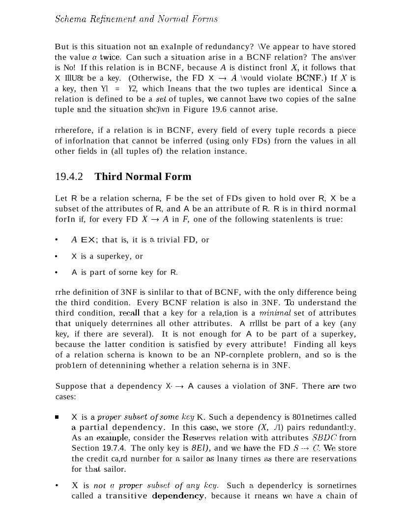
Schc'lna Refinenu:;nt and N(J'r'rnal F'orrns
But is this situation not an exaInple of redundancy? \Ve appear to have storedthe value a t\viee. Can such a situation arise in a BCNF relation? The ans\veris No! If this relation is in BCNF, because A is distinct fronl ..x:-, it follows thatX IllU8t be a key. (Otherwise, the FD X -+ A \vould violate BC:NF.) If .IY isa key, then Yl = Y2, which Ineans that the two tuples are identical Since arelation is defined to be a 8et of tuples, \\re cannot have two copies of the saInetuple and the situation shc)\vn in Figure 19.6 cannot arise.
rrherefore, if a relation is in BCNF, every field of every tuple records a pieceof inforlnation that cannot be inferred (using only FDs) frorn the values in allother fields in (all tuples of) the relation instance.
19.4.2 Third Normal Form
Let R be a relation scherna, F be the set of FDs given to hold over R, X be asubset of the attributes of R, and A be an attribute of R. R is in third normalforIn if, for every FD X -+ A in F, one of the following statenlents is true:
• A EX; that is, it is a trivial FD, or
• X is a superkey, or
• A is part of sorne key for R.
rrhe definition of 3NF is sinlilar to that of BCNF, with the only difference beingthe third condition. Every BCNF relation is also in 3NF. To understand thethird condition, recall that a key for a rela,tion is a rninirnal set of attributesthat uniquely deterrnines all other attributes. A rrlllst be part of a key (anykey, if there are several). It is not enough for A to be part of a superkey,because the latter condition is satisfied by every attribute! Finding all keysof a relation scherna is known to be an NP-cornplete problern, and so is theprob1ern of detennining whether a relation seherna is in 3NF.
Suppose that a dependency X· -+ A causes a violation of 3NF. There are twocases:
• X is a proper 8'l.lb8Ct of 80'(ne key K. Such a dependency is 801netirnes calleda partial dependency. In this Cc1se, we store (X, ./1) pairs redundantl:y.As an eXEtlnple, consider the Ileserves relation \vith attributes SBIJC1 frornSection 19.7.4. The only key is 8El), and \ve have the FD 8 -_.+ C/. vVe storethe credit ca,rd nurnber for a sailor as lnany tirnes <:1.'3 there are reservationsfor that sailor.
• X is not a pTOpCT snb8ct of any key. Such a dependerlcy is sornetirnescalled a transitive dependency, because it rneans \ve have a chain of
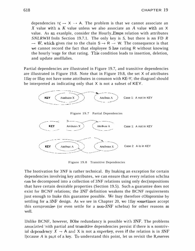
618 CHAPTER 19
dependencies !( ---+ X ---+ A. The problem is that we cannot associate anX value \vith a K value unless we also associate an A value vvith an Xvalue. As an exanlple, consider the Hourly-Enlps relation with attributesSNLRWH froIn Section 19.7.1. The only key is S, but there is an FD R---+ 1,V, \vhieh gives rise to the chain S ---+ R -~-" W. The consequence is that\ve cannot record the fact that elnployee S has rating R without knowingthe hourly \vage for that rating. 'This condition leads to insertion, deletion,and update anoIllalies.
Partial dependencies are illustrated in Figure 19.7, and transitive dependenciesare illustrated in Figure 19.8. Note that in Figure 19.8, the set X of attributes11lay or Illay not have some attributes in conunon with KE-Y; the diagranl shouldbe interpreted as indicating only that X is not a subset of KEY.
Case 1: A not in KEY
Figure 19.7 Partial Dependencies
Case 1: A not in KEY
Case 2: A is in KEY
Figure 19.8 Transitive Dependencies
The Inotivation for 3NF is rather technical. By Inaking an exception for certaindependencies involving key attributes, we can ensure that every relation schclnacan be decornposed into a collection of 3NF relations using only dec(nnpositionsthat have certain desirable properties (Section 19.5). Such a guarantee does notexist for BCNF relations; the :3NF definition weakens the BCNF requirernentsjust enough to Inake this guarantee possible. \Ve Inay therefore cOlnprornise bysettling for a :3NF design. As we see in Chapter 20, we 11lay sOllletilnes acceptthis cornpr()Jni~e (or even settle for a non-:3NF scheIna) for other reasons aswell.
lJnlike BCNF, however, BOlne redundancy is possible "Vvith :~NF. The problernsclssoci<:tted \vith partial and transitiv(~ dependencies persist if there is a nontrivial dep(~ndencyX --~., A and X is not a sup(~rkey, even if the relation is in :3NFl)ccause A is pa,rt of a key. Th understand this point, let us revisit the R,eserves
Scherna Refinelnent fLTUi J.N'oT1nal Forrns 619
relation with attributes SEDe a,nd the FD S ~ ['1, \vhich states that a sailoruses a unique credit card to pay for reservations. S is not a key, clnd C is notpart of a key. (In fact, the only key is SED.) Hence, this relation is not in 3NF;(S, CJ pairs are stored redundantly. IIowever, if we also know that credit cardsuniquely identify the o\vner, vve have the FD C --? 5, which rneans that GEJDis also a key for Reserves. Therefore, the dependency S -7 C does not violate3NF, and R,eserves is in 3NF. Nonetheless, in all tuples containing the saIne 5value, the saIne (8, CJ pair is redulJ.dantly recorded.
For cOlllpleteness, we reluark that the definition of second norrnal form isessentially that partial dependencies are not allowed. Thus, if a relation is in3NF (which precludes both partial and transitive dependencies), it is also in2NF.
19.5 PROPERTIES OF DECOMPOSITIONS
DecoIllposition is a tool that allows us to eliminate redundancy. As noted inSection 19.1.3, however, it is iInportant to check that a decoInposition does notintroduce new problellls. In particular, we should check whether a decomposition allows us to recover the original relation, and whether it allows us to checkintegrity constraints efficiently. vVe discuss these properties next.
19.5.1 Lossless-Join Decomposition
Let R be a relation schelna and let F be H, set of FDs over R. A decolnpositionof R into two schernas with attribute sets X andY is said to be a lossless-joindecomposition with respect to F if, for every instance T of R that satisfiesthe dependencies in }?, 1Tx('r) N 1T}-(r) = T. In other words, \ve can recoverthe original relation 1'rorn the deconlposed relations.
This definition can easily be extended to cover a decornposition of Ii into Inorethan two relations. It is ea."sy to see that T ~ 1fx(r) [XJ 1TyC,.,) ahvays holds.III general, though, the other direction does not hold. If sve take projectionsof a relation and recornbine theln using natural joirl,\Ve typically obta.in SOlne
tuples that 'were 1.'1.ot in the original relation. This situation is illustrated inFigure 19.9.
By replacing the instance T shown in Figure 19.9 "Vvith the instances 1f8P(r) and1T PI) (r), '\ve lose sorne inforInation. In particular, suppose that the tuples in 't
d(-~note relationships.vVe can no longer tell that the relationships (81, PI, d:3)
and (8:3,])1, d:d do not hold. rrhe decoluposition of schelna SPD into S.P andPI) is therefore loss,Y if the instance '( shown in the figure is legal, that is, if this
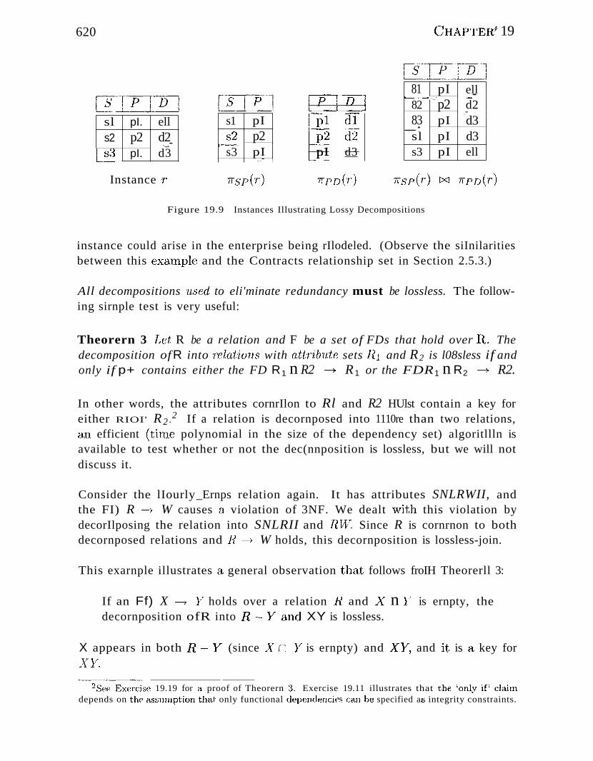
620 C;HAPTERt 19
81 pI ellf---- ._- _..-
82 p2 d2..-
83 pI d3_.sl pI d3s3 pI ell
[P--·-I~
§.'~ ~~pI d3
1rI:JD(r)
s1 pIs9 p2'....
f---..
s3 pI...-
Instance T
.....,.,.... .._.
sl pI. ells2 p2 d2
.._..-
L~.9. pI. d3
Figure 19.9 Instances Illustrating Lossy Decompositions
instance could arise in the enterprise being rIlodeled. (Observe the siInilaritiesbetween this eX~Llnple and the Contracts relationship set in Section 2.5.3.)
All decompositions used to eli'minate redundancy must be lossless. The following sirnple test is very useful:
Theorern 3 Let R be a relation and F be a set of FDs that hold over Il. Thedecomposition ofR into relations with attribute sets III and R2 is l08sless if andonly if p+ contains either the FD R1 n R2 ---+ R 1 or the FDR1 n R2 ---'f R2.
In other words, the attributes cornrIlon to Rl and R2 HUlst contain a key foreither RIOI' R 2 .2 If a relation is decornposed into 1110re than two relations,an efficient (tiTne polynomial in the size of the dependency set) algoritllln isavailable to test whether or not the dec(nnposition is lossless, but we will notdiscuss it.
Consider the lIourly_Ernps relation again. It has attributes SNLRWII, andthe FI) R ~ W causes a violation of 3NF. We dealt ¥lith this violation bydecorIlposing the relation into SNLRII and IlvV. Since R is cornrnon to bothdecornposed relations and Ii ---+ W holds, this decornposition is lossless-join.
This exarnple illustrates a general observation that follows froIH Theorerll 3:
If an Ff) X ---+ }T holds over a relation ii and ~y n }T is ernpty, thedecornposition ofR into .R - y~ and XY is lossless.
X appears in both It --~~. y' (since ~¥ (I }7 is ernpty) and .IYY, and it is a key for){}T.
2See Exercise 19.19 for a proof of Theorern :3. Exercise 19.11 illustrates that the 'only if l claimdepends on the IL')slIInption that only functional dependencies can be specified a..s integrity constraints.
ScheTna Rejinc'fnent and lVorrnal FOT1ns 6~1
Another hnportant observation, '\vhieh we state without pr()of~ hal;) to do \vithrepeated decolnpositiollS. Suppose that a relation Ii is decornposed into Rl andR2 through a IOBsless-join decolupositiol1, and tlUtt Rl is decolnposed intoRl.1and R12 through another lossless-join decolnposition. Then, the decolnpositionof R into R.lI, R.12, and .R2 is lossless-join; by joining ftll and R12, \ve canrecover R.1, and by then joining Rl and R2, we can recover flo
19.5.2 Dependency-Preserving Decomposition
Consider the Contracts relation with attributes C8JDPCJVfronl Section 19.3.l.The given FDs are C -+ C8JDPQV, JP "'-7 C1
, and SD -+ P. Because SD is nota key the dependency SD ".,-1- P causes a violation of BCNF.
We can decolnpose Contracts into two relations with schelnas CSJDQ V andSDP to address this violation; the decolnposition is lossless-join. There isone subtle problelll, however. We can enforce the integrity constraint JP -} Ceasily when a tuple is inserted into Contracts by ensuring that no existing tuplehas the same JP values (as the inserted tuple) but different C values. Oncewe decompose Contracts into CSJDQ V and SDP, enforcing this constraintrequires an expensive join of the two relations whenever a tuple is inserted intoCSJDQ V. We say that this decornposition is not dependency-preserving.
Intuitively, a dependency-preserving decornposition allows us to enforce all FDsby exarnining a single relation instance on each insertion or rnodification of a tuple. (Note that deletions cannot cause violation of FDs.) To define dependencypreserving decornpositions precisely, we have to introduce the concept of a projection of FDs.
Let R be a relation schenla that is decolnposed into two schernaswith attributesets X' and }/, and let F be a set of FDs over Il. T'he projection of F on X isthe set of FDs in the closure l i'+ (not just .F !) that involve only attributes in X.\Ve denote the projection of I? on attributes .iYa,s Fx . .Note that a dependencyU -_...+ V in F+ is in l~~x; only if all the cLttributes in [/ and V are in .iY.
The decornposition of relation scherna Il with FI)s }' into schcrnas with attributesets ..:¥ and }/ is dependency-preserving if CF'x U F\·)+ == I?+, That is, if wetake the dependencies in };'( and Fv and cornpute the closure of their un.ion, vveget back all dependencies in the closure of F. rrherefore, \ve need to enforce onl,ythe dependencies in Ji'){ and F}r: allFDs in }'+ are then sure to be satisfied. ~ro
enforce }~':( ,\V8 need to exarnine only relation )( (on in.serts to that relation).To enforce F'y,·, \Ale need to exarnine only rela,tion Y·.
622
To appreciate the need to consider the (:Iosure Fl+- while COIUpllting the projection of f?, suppose that a relation R \vith attributes ABG1 is clecornposed intorelations\vith attributes AB and Be:. The set ~F of FDs overR includes A -+
B, B ---+ C, and G1 -+ A. Of these, A ----+ B is in 1~~1B and B -+ C) is in }'"'lBC.
But is this decoIIlposition dependency-preserving? \~lhat about C ---+ A? Thisdependency is not irnplied by the dependencies listed (thus far) for [<'AB and}13c·
The closure of 1~1 contains all dependencies in }' plus A -+ C, B -+ A, and C ~---+ B.Consequently, f:1B also contains B -+ A, and .FBc contains C -+ B. Therefore,FAB U F}3c; contains A -+ B, B -+ C, Ii -+ A, and C -,. B. The closure of thed(~pendenciesin f:1.B and }'BC now includes C -). A (which follows frorn C _.....+ B,B·--+ A, and transitivity). l'hus, the deccHnposition preserves the dependencyC-+ A.
A direct application of the definition gives us a straightforward algoritlun fortesting whether a deconlposition is dependency-preserving. (This algorithrnis exponential in the size of the dependency set. A polynomial algorithnl isavailable; see Exercise 19.9.)
We began this sectiol1with an exanlple of a lossless-join deC0111position that wasnot dependency-preserving. Other decorupositions are dependency-preserving,but not lossless. A silnple exalnple consists of a relation ABC' with FD A~---+ Bthat is decornposed into AB and BG.
19.6 NORMAI-iIZATION
Having covered the concepts needed to understand the role of HortHa} fonnsand decolnpositions in databa"se design, we now consider algoritlnIls for converting relations to BCNF or :3NF. If a relation schelna, is not in BCNF, itis possible to obtain a lossless-join deccunpositioll into a collection of BCNFrelation sCherl1chs. Unfortunately, there lllay be no dependenc,y-preserving de-·cOlnposition into a collection of BCN.F relation schernas. l-Ic}\vever, there isahvays (l, dependency-preserving, lossless-join decoruposition into a collectionof ~3NF relation schernas.
19.6.1 Decomposition into BCNF
vVo now present an <llgorithIl1 for decornposing a relation scherna Ii with a setof FI)sF into a collection of BCNF relation schernas:
Scherna ,RefinClnent and IVoTTnal l?orrns 623
1. Suppose that R is not in BCNF. Let .IX' C It, A be ::1, single attribute in R,and X --7 A be an FD that causes a violation of BCNF. DecornposeR intoR - il and XA.
2. If either Ii - ",4 or ..YA is not in BCN.F, decornpose thern further by arecursive application of this algorithrn.
If ..- ",4 denotes the set of attributes other than A in Il, and ./YA denotes theunion of attributes in -"Yand A. Since X ----+ A violates BCNF, it is not a trivialdependency; further, A is a single attribute. Therefore, A is not in X; thatis, ..;\ n A is ernpty. Therefore, each dec()lnposition carried out in Step 1. islossless-join.
The set of dependencies associated vvith R .- A and XA is the projection of Fonto their attributes. If one of the new relations is not in BCNF, w'e decornposeit further in Step 2. Since a decornposition results in relations with strictlyfewer attributes, this process terrninates, leaving us with a collection of relationschernas that are all in BCNF. Further, joining instances of the (two or 1nore)relations obtained through this algorithrn yields precisely the correspondinginstance of the original relation (i.e., the decorllposition into a collection ofrelations each of which in BCNF is a lossless-join dec()lnposition).
Consider the Contracts relation with attributes C3JDPQ V and key C. We aregiven FDs JP ---7 C and 3D -+ P. By using the dependency 3D -+ P to guide thedecornposition, we get the two schernas 3DP and C5JDQV. 51)P is in BCNF.Suppose that we also have the constraint that each project deals with a singlesupplier: .I _.+ 5. This rneans tlutt the sche1na CSJDQ V is not in BeN}? So wedeccnnpose it further into J3 and C.IDC2 V. C --+ JDQ V holds over CJDQ V; theonly other FI)s that hold are those obtained frorll this PI) by augrnentation, andtherefore all FDs conte-tin a key in the left side. Thus, each of the schernas ST)P,.IS, and C:.I1J(J V is in BCNF~ and this collection of schcrnas also represents alossless-join decornposition of ()SJD(J V.
The st(~PS in this deC(nllposition process can be visualized as a tree, as sho\vnin Figure 19.10. rrhe root is the original relation CSJIJPQ \/, and the leaves arethe BCNl~~ relations that result frorn the deccHnposition aJgorithrn: 3D?, .IS,and CSDC2 V. Intuitively, ea.ch internal node is replaced by its children throughEt single decOruI}osition step guided by the FD shown just belo\v the node.
Redundancy in BCNF Revisited
T'he decolnposition of (}SJDQ V iuto ,S])}), J5'1, and C'JI)(J \l is not dependencypreserving. Intuitively, dependency Jp ..._...~ (} carlllot be enforced without a, join.()ne \vay to deal \vith this situation is to add a relation \vith attributes G1J}). In
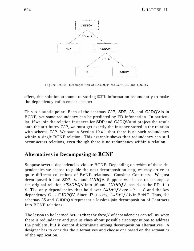
624 C~HAPTER 19
Figure 19.10 Decomposition of CSJDQV into SDP, JS, and CJDQ V
effect, this solution arnounts to storing SOITle information redundantly to rnakethe dependency enforcement cheaper.
This is a subtle point: Each of the schemas CJP, SDP, JS, and CJDQV is inBCNF, yet some redundancy can be predicted by FD infonnation. In particular, if we join the relation instances for SDP and CJDQVand project the resultonto the attributes CJP, we rnust get exactly the instance stored in the relationwith scherna CJP. We saw in Section 19.4.1 that there is no such redundancywithin a single BCNF relation. This exarnple shows that redundancy can stilloccur across relations, even though there is no redundancy within a relation.
Alternatives in Decomposing to BCN~-'
Suppose several dependencies violate BCNF. Depending on ·which of these dependencies we choose to guide the next decornposition step, we rnay arrive atquite different collections of BeNF relations. Consider Contracts. \Ve justdecornposed it into SDP, is, and CJDCj V. Suppose we choose to decornposethe original relation (}SJDPC2 V into JS and CJIJPCj V, based on the FD .I -+
S. The only dependencies that hold over (}JIJPQ V Etre .IP ----7 C and the keydependency C~ C.IDPQV. Since iP is a key, C:J.DPC2Vis in BeNF. Thus, theschernas JS and CJDPQ V represent a lossless-join decornposition of Contractsinto BCNF relations.
The lesson to be learned here is that the theor,Y of dependencies can tell us ·whenthere is redundancy and give us clues about possible clecornpositions to addressthe problern, but it cannot discrirninate arnong decornposition alternatives. Adesigner has to consider the alternatives and choose one based on the scrnanticsof the application.
*625
BCNF and Dependency-Preservation
Soruethnes, there siIuply is no decomposition into BCNF that is dependencypreserving. .i\s an exaruple, consider the relation schelna SBD, in which a tupledenotes that sailor S ha.s reserved boat ,8 OIl date [J. If we have the 11"'Ds 8B~ D (a sailor can reserve a given boat for at nlost one day) and D -+ B (onany given day at rllost one boat can be reserved), SBn is not in BCNF becauseD is not a key. If we try to dec(nnpose it, however, we cannot preserve thedependency BB "-7 D.
19.6.2 Decomposition into 3NF
Clearly, the approach \ve outlined for 10ssless-joiIl decornpositioIl into BCNFalso gives us a lossless-join decomposition into 3NF. (Typically, we can stopa little earlier if we are satisfied with a collection of 3NF relations.) But thisapproach does not ensure dependency-preservation.
A siInple rllodification, however, yields a deco111position into 3NF relations thatis lossless-join and dependency-preserving. Before we describe this modification, we need to introduce the concept of a lninirnal cover for a set of FDs.
Minimal Cover for a Set of FDs
A minimal cover for a set F of FDs is a set G of FDs such that:
1. Every dependency in G is of the forIn ..¥ ---+ A, where A is a single attribute.
2. The closure F+ is equal to the closure (;+.
:3. If we obtain a set II of dependencies frorn G by deleting one or 1110re dependencies or by deleting attributes frorn a dependency in G, then p+' i= II+.
Intuitively, a rninirnal cover for a set }-' of FDs is an equivalent set of dependencies that is 'minirnal in two respects: (1) Every dependency is as slIlall as
possible; tha,t; iS 1 each attribute on the left side is necessary and the right sideis a single attribute. (2) Every dependency in it is required for the closure tobe equal to j?-+',.
As an exarnplc, let J? be the set of dependencies:
1 B 1BCID E' E'j-' ("'I 1'" T;' lIlA (-'11)}'--' E-'G'1it ..-+ ',j -- ----+ .../, .f ...._--t >T, -~r --+ ,. 1 ~Ul( ./. f ----+ .../.J.
First 1 let us rewrite it ()DF -_...+ BG so that every right side is a single attribute:
626
ACDF-tEand ACDF-t G,
CHAPTERt9
Next consider ACDF -+ G, This dependency is irnplied by the following FDs:
A -7 B, ABC'D -7 E, and EF -7 G,
Therefore, \ve can delete it, Sirnilarly, we can delete A CDF -7 1:7, Next consider ABCD -7 E, Since A -7 B holds, we can replace it with ACD _..._~ E, (Atthis point, the reader should verify that each rernaining FD is rninilnal andrequired,) Thus, a rninilnal cover for F is the set:
A -7 B, ACD -7 E, EF ---7 Ci, and EF --+ H,
The preceding exarnple illustrates a general algorithrn for obtaining a rninimalcover of a set }i' of FDs:
1. Put the FDs in a Standard Form: Obtain a collection G of equivalentFDs with a single attribute on the right side (using the decornpositionaxiolIl),
2. Minimize the Left Side of Each FD: For each FD in G, check eachattribute in the left side to see if it can be deleted while preserving equivalence to F+,
3. Delete Redundant FDs: Check each reluaining FD in G to see if it canbe deleted while preserving equivalence to .F+,
Note that the order in which we consider FDs while applying these steps couldproduce different rninilnal covers; there could be severa'! rninirnal covers for agiven set of FDs,
lV101'8 irnportant, it is necessary to rniniInize the left sides of F'Ds befoTc checkingfor redundant FI)s, If these two steps are reversed, the final set of FI)s couldstill contain senne redundant FDs (i,e., not be a rninirnal cover), as the followingexarnple illustrates, LetF be the set of dependencies, each of ""vhich is alreadyin the standard fornl:
.A13CTJ -t E',E " ~~ D, A ----;. 13, and A C ----;. I),
Observe that none of these FDs is redundant; if \ve checked for redundantFDsfirst, \ve ""vould get the saIne set of FI)s I?, The left side of il13CIJ }; can ben~l)hiced by A Ct\vhile preserving equivalence to 1~"1+, and ,ve \vould stop here if\ve checked for reclunda.ntF'Ds in I? before rnillilnizing the left sides. HO\V8Ver,
the set of FDs ""ve 11(lVe is not a Inininlal cover:
Sche17~a Ilefinerncnt and NOTrnal j?OT'lnS
ACt .......:;. E,E _..-+ D,A --t B, and AG1 -+ D.
~127
FrOlIl transitivity, the first two FDs irnply the la.",'3t FD, ,v-hich can therefore bedeleted while preserving equivalence to 1~1+. The irnportant point to note isthat A C---+ D becc)lnes redundant only after we replace ABeD -)- E with A C-)- E. If "ve Ininirnize left sides of FDs first and then cheek for redundantFDs,,ve are left "vith the first three FDs in the preeeding list,whieh is indeed aIninirna1 cover for F.
Dependency-Preserving Decomposition into 3NJ.1-'
Returning to the problenl of obtaining a lossless-join, dependency-preservingdecornposition into 3NF relations, let R be a relation with a set [/' of FDs thatis a minirnal cover, and let R1 , R2 , ... , Rn be a lossless-join decolnpositionof R. For 1 < i < n, suppose that each Ri is in 3NF and let Fi denote theprojection of F onto the attributes of Ri . Do the following:
• Identify the set N of dependencies in F that is not preserved, that is, notincluded in the closure of the union of Fis.
• :F'or each FD X ---t A in N, create a relation schelna XA and add it to thedecomposition of R.
Obviously, every dependency in F is preserved if we replace R by the R'iS plusthe schernas of the forn1 XA added in this step. The Ris are given to be in3NF. We can show that each of the schelnas XA is in 3NF as follows: Since X----7' A is in the lninirnal cover F, Y ---+ A does not hold for any Y that is a strictsubset of X. Therefore, X is (1, key for XA. :F\llrther, if any other dependencieshold over XA, the right side can involve only attributes in X' because A is asingle attribute (because X -~ A is an FD in a rninhnal cover). Since X is akey for ..:YA, none of these additional dependencies causes a violation of ~3NF
(although they rnight cause a violation of BCNF).
As an optilYlization, if the set N contains several FI)swith the saIne leftside, say, X -~~.-t ..41 , X -t A2 , , ..X- ..+ /In , we can replace thern \vith(.I., single equivalent FD X -t AI ..I4·n . Therefore, \ve produce one relationscherna ..X' ..14 1 ... /In , instead of several schernas XA 1 , .... ~X'"An, \vhich is generally preferable.
(~onsider the Contracts relation vvith attrilnltes C:SJDPQV etnel FI)s JP -j> C:,81)--4 P. and J ....-» S. If \ve decolnpose (}SJIJPe) V into SDIJ and C}SJl) (JV,then 8DP is in BCNF, but C\'1J1) (2 V is not ev(~n in :3NI;'. So \ve dec.olupose itfurther into JS and C1JDe2 V. rrhe relation schcrnas 19IJ.P, .I8, Etnel C7JDQVarein ~3NF (in fact, in BCNF) 1 and the decoInposition is lossless-join. lIowever,
628 (;HAPTElt 19
the dependency JP ---:,. C' is not preserved. This problerIl can be addressed byadding a relation schenut e'Jp to the decornposition.
3NF Synthesis
vVe assurned that the design process starts with an Ell diagraII1, and that ouruse of FDs is prilnarily to guide decisions about decolnposition. The algorithill for obtaining a lossless-join, dependency-preserving decornpositiol1 waspresented in the previous section fro111 this perspective--------a lossless-join decoruposition into 3NF is straightforward, and the algorithrn addresses dependencypreservation by adding extra relation schcrnas.
An alternative approach, called synthesis, is to take all the attributes over theoriginal relation R and a rnininlal cover F for the FDs that hold over it andadd a relation scherna XA to the decomposition of R for each FD X -----+ A in F.
The resulting collection of relation schernas is in 3NF and preserves all FDs.If it is not a lossless-join decomposition of R, we can Dlake it so by adding arelation schenla that contains just those attributes that appear in sorne key.This algorithrn gives us a lossless-join, dependency-preserving decornpositioninto 3NF and has polynornial corIlplexity-----polynornial algorithms are availablefor coruputing rninirnal covers, and a key can be found in polync)Inial tirHe(even though finding all keys is known to be NP-cornplete). The existenceof a polynornial algorithnl for obtaining a lossless-join, dependency-preservingdecornposition into 3NF is surprising when we consider that testing whether agiven schenu:l, is in ~~NF is NP-cornplete.
As a.n exarnple, consider a relation AB G1 with FI)s F:::::::: {A -----+ B, C -----+ B}. ~rhe
first step yields the relation scheluas AB and BG. T'his is not a lossless-joindeC0l11position of AilC; AB nBC is B, and neither B -----+ A nor IJ -, C: is in /?+.If we add a, scherna A C:, \ve have the lossless-join property <:I"," well. Althoughthe collectic)ll of relations AB,BC, and A C is a depenclency-preserving, losslessjoin decornposition of ABC, we obtained it through a process of synthesis,rather tllan through a process of repeated decornposition. \\Te note that thedecoIIIposition produced by the synthesis approa,ch heavily dependends on therninirnal cover used.
As another exarnple of the synthesis approach, consider the Contracts relationwith attributes (}SJDP(JVand the follovving FI)s:
C C\').IIJ.P(J V, .IP -----+ C, 8D --+P, aDd J -7 s.
This set of FI)s is not a rninirnal cover, and so \ve IllUSt find OI18. \Ve firstreplace G -.-7 (}S'IJ[J.P(J V v'lith tllcF'I)s:
5~che'Tna Refincrnent and j\forlnal FC)'t'rns
C' -+ 5, Cf -" J, (: _.+ IJ, C' _...+ .P, C --+ Q~ and () -+ \1.
1 1he FD C --+ P is irnplied by C1-to S, C _.......;. D, and SD -_··+P~ so we can delete
it. ~rhe FD C-r ~ S is irnplied byC -;. J and J _..u} S; so \ve ean delete it. Thisleaves us with a rninirnal cover:
C _.-+ ,I, C _.-7 1), C·--:,. Q, C -;. V, JP --...;. C, 3D ---;. P, and J ~.._+ S.
lJsing the algorithrll for ensuring dependency-preservation, we obtain the relational scherna CJ, CD, CQ. CV, GlJP, SDP, and JB. We can irnprove thisschenla by cornbining relations for which C is the key into CDJP(J V. In addition, we have SDP and ,IS in our decorllposition. Since one of these relations(CDJPQ V) is a superkey, \ve are done.
Conlparing this decomposition with that obtained earlier in this section, wefind they are quite close, with the only difference being that one of them hasCDJPQV instead of CJP and CJDQV. In general, however, there could besignificant differences.
19.7 SCHEMA REFINEMENT IN DATABASE DESIGN
We have seen how normalization can elilninate redundancy and discussed several approaches to nonnalizing a relation. We now consider how these ideasare applied in practice.
Database designers typically use a conceptual design rnethodology, such as ERdesign, to arrive at an initial databa,,"3e design. Given this, the approach ofrepeated decorllpositions to rectify instances of redundancy is likely to be thernost natural use of PI)s and nonnalization techniques.
In this section, \ve Inotivate the need for a schcrna refinernent step follovvingEll design. It is natural to aBk whether \ve even need to decornpose relationsproduced by translating an Eli diagranl. Should a good ER design not lead to acollection of relations free of redundancy prob.lerns? Unfortunately, Fjll designis a c()!nplex, subjective process, and certain constraints are not expressiblein tenns of Ell diagraJns. 1'he exaruples in this section are intendecl to illustrate \vhy decornposition of relations produced through Ell design rnight benecessary.
6:30 C~lIAPTgR 19
19.7.1 Constraints on an Entity Set
Consider the Hourly_ElllPS relation again. rrhe constraint that attribute 8/)'n isa key can be expressed a..s an FI):
{ssn} ---} {SS11, naTne, lot, l>ai'ing, ho'U,'rIY_J.oages, hOUTS_'U)orke.d}
:For brevity, we \vrite this FD &'3 S ---} 8NLR~VII, using a single letter to denoteeach attribute and ornitting the set braces, but the reader should rernernberthat both sides of an FD contain sets of attributes. In addition, the constraintthat the hourl:y~wages attribute is deterruined by the rating attribute is an FD:R .,. W.
As \ve saw in Section 19.1.1, this FI) led to redundant storage of rating wageassociations. It cannot be expressed in, teTrns of the ER rr~odel. Only FDsthat deteTrr~ine all attTilndes of a relation (i. e., key constraints) can be expTessed in the ER rnodel. rrherefore, we could not detect it when we consideredHourly_EIIlPS as an entity set during ER IIlodeling.
We could argue that the problenl with the original design was an artifact of apoor ER design, which could have been avoided by introducing an entity setcalled Wag(~_Table (with attributes rating and houTly_wages) and a relationshipset lIas_Wages associating IIourly_.ErIlps and vVagc_Table. The point, however,is that we could easily arrive at the original design given the subjective nature ofEll rnodeling. Having forInal techniques to identify the problenl with this designand guide us to a, better design is very useful. 1'he value of such techniquescannot be underestirnated when designing large schernas····-schcrnas with rnorethan a hundred tables are not unCOIllIHon.
19.7..2 Constraints on a Relationship Set
1"'he previous exarnple illustrated how FDs can help to refine the subjectivedecisions Blade during ER. design, but one could argue that the best possibleER, eliagrarn \vould have led to the sc:Hne final set of relations. ()ur next exarnpleshovvs ho\v Ff) inforrnation ca.ll lead to a. set of relations unlikely to be arrivedat sol(~ly through ER. design.
\Ve revisit an exanlple frOTH Chapt<~r 2. Suppose that \ve have entity sets Parts,Suppli(~rs, and I)epartrnents, as \vell as a relationship set Contracts that involvesall of theIn. \lVe n~fer to th(~ scherna for Contra(:ts as C7C2}>S'1IJ. A contra,ct \vithcontract id () specifies that <1, supplier 8 \vill supply sorne ql.Hlntity (2 of a partP to a departrnent J). (\,Ve have adderl the contract ieI field C' tC) tIle versiorl ofthe C~ontracts relation discussed in Chapter 2.)
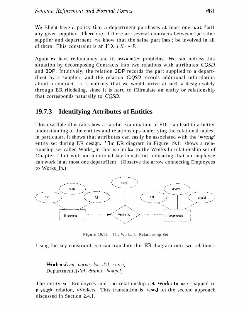
SchCTna Refinernc'n.t anr11VoT7nalFoTrn8 6431
vVe Blight have a policy that a departrnent purchases at Inost one paJt fror11any given supplier. 'Therefore, if there are several contracts between the saInesupplier and departrnent, \ve know that the saIne part Inus!; be involved in allof thcrn. This constraint is cUI FD, DS·--.+ P.
Again "ve have redundancy and its a",c;sociated problclns. \Ve can address thissituation by decornposing Contracts into two relations with attributes CQSDand 3DP. Intuitively, the relation 3DP records the part supplied to a departrllent by a supplier, and the relation C:QSD records additional infornlationabout a contract. It is unlikely that we would arrive at such a design solelythrough ER rIlodeling, sinee it is hard to fOfrnulate an entity or relationshipthat corresponds naturally to CQSD.
19.7.3 Identifying Attributes of Entities
This exarIlple illustrates how a careful examination of FDs can lead to a betterunderstanding of the entities and relationships underlying the relational tables;in particular, it shows that attributes can easily be associated with the 'wrong'entity set during ER design. 'I'he ER diagrarn in Figure 19.11 shows a relationship set called Works_In that is silnilar to the Works.ln relationship set ofChapter 2 but with an additional key constraint indicating that an employeecan work in at rnost one departrIlent. (Observe the arrow connecting Employeesto Works_In.)
Figure 19.11. The Works._In Relationship Set
Using the key constraint, \ve can translate this Ell diagrarn into two relations:
\VorkersC58n, narne, lot, d'id, since)Departrnents( did, dna1nc, budget)
The entity set Ernployees and the relationship set\iVorks~n are rnapped toa sil.lgle relation, vVorkers. This translation is ba".'Scd on the second approachdiscussed in Section 2.4.1.
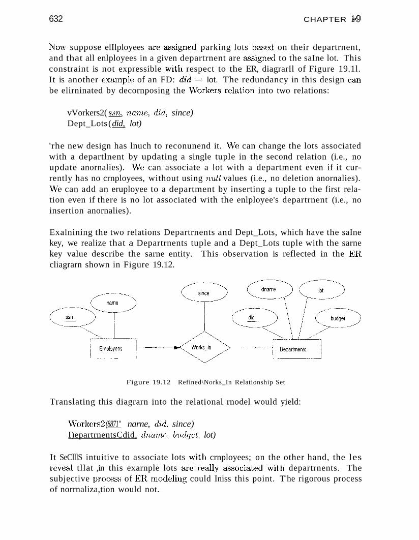
632 CHAPTER »9
No\v suppose elIlployees are a,,'3signed parking lots ba.rged on their departrnent,and that all enlployees in a given departrnent are ~'h'3signed to the saIne lot. Thisconstraint is not expressible vvith respect to the ER, diagrarIl of Figure 19.1l.It is another exarnple of an FD: did --: lot. The redundancy in this design canbe elirninated by decornposing the Vlorkers rela.tion into two relations:
vVorkers2( 8sn, narne, did, since)Dept_Lots (did, lot)
'rhe new design has lnuch to reconunend it. VVe can change the lots associatedwith a departlnent by updating a single tuple in the second relation (i.e., noupdate anornalies). \Ve can associate a lot with a department even if it currently has no crnployees, without using null values (i.e., no deletion anornalies).\Ve can add an eruployee to a department by inserting a tuple to the first relation even if there is no lot associated with the enlployee's departrnent (i.e., noinsertion anornalies).
Exalnining the two relations Departrnents and Dept_Lots, which have the saInekey, we realize that a Departrnents tuple and a Dept_Lots tuple with the sarnekey value describe the sarne entity. This observation is reflected in the ER,cliagrarn shown in Figure 19.12.
Figure 19.12 Refined\Norks_In Relationship Set
Translating this diagrarn into the relational rnodel would yield:
\iVorkers2 (8871" narne, did, since)I)epartrnentsCdid, dnarne, budget, lot)
It SeClllS intuitive to associate lots ,vith crnployees; on the other hand, the lesreveal tllat ,in this exarnple lots are rea.1ly a"ssociated ,\lith departrnents. Thesubjective pr()c(~ss of EIlrnodeling could Iniss this point. T'he rigorous processof norrnaliza,tion would not.
SchC'lna Ilejinernc'rd (uul IVOTTTUll Forrns
19.7.4 Identifying Entity Sets
Consider a variant of the lleserves scherna used in earlier chapters. Let Reserves contain attributes S, B, and D :::1.'3 before, indicating that sailor S hasa reservation for boat B on day D. In addition, let there be an attribute G"1denoting the credit card to which the reservation is charged. vVe use this exarnple to illustrate how FD illfonnation can be used to refine an ER design. Inparticular, \ve discuss how FD inforluation can help decide whether a conceptshould be rnodeled as an entity or as an attribute.
Suppose every sailor uses a unique credit card for reservations. This constra,intis expressed by the FD S -7- C. This constraint indicates that, in relation Reserves, we store the credit card rnllnber for a sailor as often as we have reservations for that sailor, and we have redundancy and potential update anolnalies.A solution is to deconlpose Reserves into two relations with attributes SBDand SC. Intuitively, one holds inforrnation about reservations, and the otherholds infonnation about credit cards.
It is instructive to think about an ER design that would lead to these relations. One approach is to introduce an entity set called Credit_Cards, with thesale attribute cardno, and a relationship set Has_Card associating Sailors andCredit_Cards. By noting that each credit card belongs to a single sailor, we canInap Has_Card and Credit_Cards to a single relation with attributes SC. Wewould probably not rnodel credit card nUlnbers as entities if our Inain interestin card nurnbers is to indicate how a reservation is to be paid for; it suffices touse an attribute to rnodel card nUlnbers in this situation.
A second approach is to rnake cardno an attribute of Sailors. But this approachis not very natural-" ..··(1 sailor lllay have several cards, and we are not interestedin all of theln. Our interest is in the one card that is used to pay for reservations,which is best lnodeled as an attribute of the relationship Iteserves.
A helpful way to think about the design problern in this exarnple is tlHlt wefirst lnake carrino an attribute of H,eserves and then refine the resulting tablesby taking into account the 1"1) inforrnation. C\Vhether \VC refine the design byadding cardno to the table obtained froTIl S<dlors or by creating a new table\vith attributes S'f(} is (1, separate issue.)
19.8 OTHER KINDS O~., D~:PENDENCIES
FI)s are probal)l.y the rn08t conunon and irnportant kind of (~onstraiIlt fr0 III
the point of vie"\! of database design. TIowever, there axe several other kindsof dependencies. In particular, there is a 'Vvell-developccl theory for database
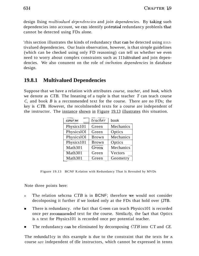
634 (;HAPTER 19
design llsing rrLultival'ued dependenc'ics and join dependencies. By taking suehdependencies into account, we C,Ul identify potential redundancy problenls thatcannot be detected using FDs alone.
'rhis section illustrates the kinds of redundancy that can be detected using II1Ul
tivalued dependencies. Our Inain observation, however, is that sirnple guidelines(which can be checked using only FD reasoning) can tell us whether we evenneed to worry about complex constraints such as 111ultivalued and join dependencies. We also conunent on the role of inclusion dependencies in databasedesign.
19.8.1 Multivalued Dependencies
Suppose that we have a relation with attributes course, teacher, and book, whichwe denote as CTB. The Ineaning of a tuple is that teacher T can teach courseC, and book B is a reccnnmended text for the course. There are no FDs; thekey is CTB. However, the recolnlnended texts for a course are independent ofthe instructor. The instance shown in Figure 19.13 illustrates this situation.
~ofurse .~ teache2J book
Green..-
Physics101 MechanicsPhysicslOl Green OpticsPhysicslOl Brown MechanicsPhysics101 Brown Optics
Green Mechanics._..
Math301..
Math301 Green Vectors--
Math301 Green GeometryL..--._..._ ........
Figure 19.13 BCNF R.elation with Redundancy That Is Revealed by MVDs
Note three points here:
II 1'he relation sehcrna CTB is in BCNF; therefore we would not considerdecolnposing it further if we looked only at the FDs that hold over (JTB.
II There is redundancy. rrhe fact that G·reen can teach Physics101 is recordedonce per reeonunendecl text for the course. Sirnila.rly, the fact that Opticsis a text for Physics101 is recorded once per potential teacher.
.. T'he redundancy can be elirninated by decornposing C1fTB into CT and CE.
The redundaJ1cy in this exarnple is due to the constraint that the texts for acourse are independent of tIle instructors, which cannot be expressed in tenns
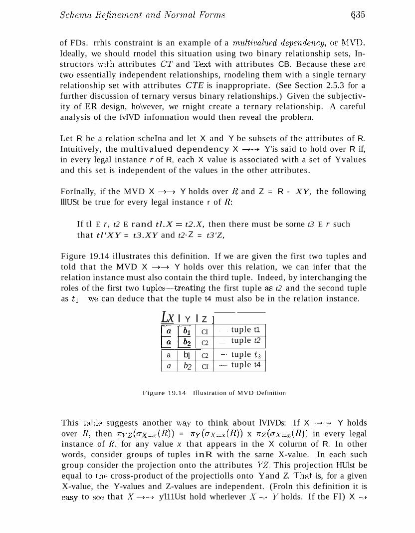
Scherna liefine'lnent an.d iVoT1nal FO'T"rns G35
of FDs. rrhis constraint is an example of a rn'll,ltival'ued dependency, or~1VD.Ideally, we should rnodel this situation using two binary relationship sets, Instructors \vith attributes G1T and l'ext with attributes CB. Because these aretwo essentially independent relationships, rnodeling them with a single ternaryrelationship set with attributes CTE is inappropriate. (See Section 2.5.3 for afurther discussion of ternary versus binary relationships.) Given the subjectivity of ER design, ho\vever, we rnight create a ternary relationship. A carefulanalysis of the fvIVD infonnation would then reveal the problern.
Let R be a relation scheIna and let X and Y be subsets of the attributes of R.Intuitively, the multivalued dependency X --+--+ Y'is said to hold over R if,in every legal instance r of R, each X value is associated with a set of Yvaluesand this set is independent of the values in the other attributes.
ForInally, if the MVD X -+-+ Y holds over l~ and Z = R - XY, the followinglllUSt be true for every legal instance r of Fl:
If tl E r, t2 E rand tl.X == t2.X, then there must be sorne t3 E r suchthat tl'XY = t3.XY and t2· Z = t3'Z,
Figure 19.14 illustrates this definition. If we are given the first two tuples andtold that the MVD X ,-+---+ Y holds over this relation, we can infer that therelation instance must also contain the third tuple. Indeed, by interchanging theroles of the first two tuples~treating the first tuple &'3 t2 and the second tupleas tl----we can deduce that the tuple t4 must also be in the relation instance.
Lx I Y I Z ]
t: B~CI ___'n tuple t1
C2 ____.n_ tuple t2--'-"-
a bl C2 .--- tuple t:~
a b2 CI -........... tuple t4
Figure 19.14 Illustration of MVD Definition
This table suggests another \vay to think about lVIVDs: If X ----7-+ Y holdsover Ii, then 1fyz(ax=:r(R)) = 1fy(ax=:r(R)) x 1fz(ax:::::.:x(Ii)) in every legalinstance of R,' for any value x that appears in the X colurnn of R. In otherwords, consider groups of tuples inR with the sarne X-value. In each suchgroup consider the projection onto the attributes lTZ. This projection HUlst beequal to the cross-product of the projectiolls onto Yand Z. That is, for a givenX-value, the Y-values and Z-values are independent. (Froln this definition it iseaAsy to sec that ~Y ----7-----;0 y'l11Ust hold wherlever ..!Y --..~ }T holds. If the FI) X _...;.
636
Y holds, there is exactly one Y:'value for a given X-value, and the conditions inthe ~!IVD definition hold trivially. ~rhe converse does not hold, a.s Figure 19.14illustrates. )
Returning to our G't1"'B exaIllple, the constraint that course texts are independent of instructors can be expressed as G1 ---+---+ T. In terlllS of the definition oflVIVDs, this constraint can be read as follo\vs:
If (there is a tuple showing that) () is taught by teacher T,and (there is a tuple showing that) G has book B as text,then (there is a tuple showing that) G is taught by T and has text B.
Given a set of FDs and :NIVDs, in general, we can infer that several additionalFDs and :NIVDs hold. A sound and complete set of inference rules consists ofthe three ArIllstrong AxioIllS plus five additional rules. Three of the additionalrules involve only :NIVDs:
• MVD Complementation: If X ---+~ Y, then X ~---+ II ~ XY.
• MVD .Augmentation: If X ---+~ Yand W:2 Z, then WX --+--t YZ.
• MVD Transitivity: If X --7-> Yand Y -+--+ Z, then X --+--+ (Z - Y).
As an exanlple of the use of these rules, since we have () --+---+ T over GTB,MVD complelnentation allows us to infer that C -7-+ OTB ~ CT as well, thatIS, C ---+---+ B. The remaining two rules relate FDs and MVDs:
• Replication: If X --+ Y, then X --+--+ Y.
• Coalescence: If ~y --+---+ Yand there is a W such that W n Y- is elnpty,W ---+ Z, and Y:2 Z, then X -7 z.
()bserve that replication states that every FD is also an l\1VT).
19.8.2 Fourth Normal Form
Fourth Horrnal fonn is a direct generalization of BeNF. Let R be a relationscherna, X and Y be nonernpty subsets of the attributes of R, and F' be a setof dependencies that includes both FDs and lVIVDs. R is said to be in fourthnormal form (4NF), if, for every l\1.VI) -'X',.>----'t }i that holds over R, one ofthe following staternents is true:
• y" ~ ~y or XIT
:::::::: .R, or
• X is a superkey.
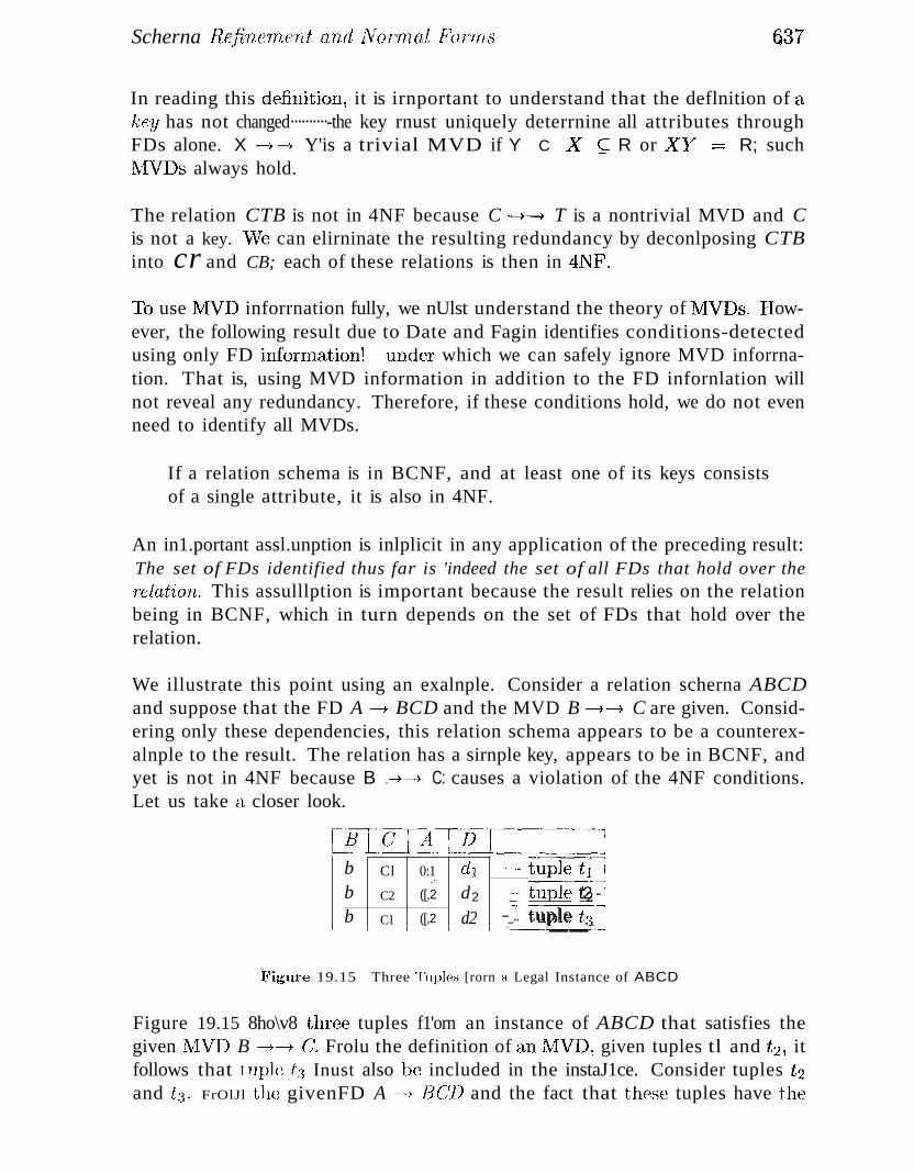
Scherna Ilefinernent and iVorrnal Fen'IlLs 637
In reading this definition, it is irnportant to understand that the deflnition of akey has not changed··········-the key rnust uniquely deterrnine all attributes throughFDs alone. X ---+-; Y'is a trivial MVD if Y C .LX" ~ R or .LX"Y· :::: R; suchwIVDs always hold.
The relation CTB is not in 4NF because C ~-> T is a nontrivial MVD and Cis not a key. vVe can elirninate the resulting redundancy by deconlposing CTBinto cr and CB; each of these relations is then in 4NF.
rfo use 1t1VD inforrnation fully, we nUlst understand the theory of :NIVDs. IIowever, the following result due to Date and Fagin identifies conditions-detectedusing only FD infornlation!~-underwhich we can safely ignore MVD inforrnation. That is, using MVD information in addition to the FD infornlation willnot reveal any redundancy. Therefore, if these conditions hold, we do not evenneed to identify all MVDs.
If a relation schema is in BCNF, and at least one of its keys consistsof a single attribute, it is also in 4NF.
An in1.portant assl.unption is inlplicit in any application of the preceding result:The set of FDs identified thus far is 'indeed the set of all FDs that hold over the'('elation. This assulllption is important because the result relies on the relationbeing in BCNF, which in turn depends on the set of FDs that hold over therelation.
We illustrate this point using an exalnple. Consider a relation scherna ABCDand suppose that the FD A -+ BCD and the MVD B -+-+ C are given. Considering only these dependencies, this relation schema appears to be a counterexalnple to the result. The relation has a sirnple key, appears to be in BCNF, andyet is not in 4NF because B ..~-+ C: causes a violation of the 4NF conditions.Let us take a closer look.
b Cl 0:1 ell --- tUP!ti§-'
-~ tUI?-ie t2 -b C2 ([,2 d2
b Cl ([,2 d2 --_... tuple t:3_..__ ...__..-
:Figure 19.15 Three Tuples [rorn a Legal Instance of ABCD
Figure 19.15 8ho\v8 three tuples f1'orn an instance of ABCD that satisfies thegiven lVIVI) B --+-+ Cr
, Frolu the definition of an lVIVD, given tuples tl and "t2: itfollows that tuple t:3 Inust also be included in the instaJ1ce. Consider tuples "t2and 1:3. FrOlJl the givenFD A -,B(/1) and the fact that these tuples have the
638 (;HAPTER L9
same A-value~ we GaIl deduce that Cl = C2. Therefore, ,ve see that the FD B ---+
C rnust hold overilBCD \V"henever the FI) A ~ BCD and theNIVI) B··_·-7~ (:hold. If B -·-4 () holds~ the relation ABeD is not in BeNF (unless additionalFDs lllake B a key)!
Thus, the apparent counterexalnple is really not a counterexalllple···········-rather,it illustrates the iInportance of correctly identifying all FDs that hold over arelation. In this exarnple, A -» BCI) is not the only FD; the FD B -+ Calso holds but ·wa..s not identified initially. Given a set of FDs and IvIVI)s, theinference rules can be used to infer additional FDs (and l\1VDs); to apply theDate-Fagin result without first using the l\1VD inference rules, we IUUSt becertain that we have identified all the FDs.
In summary, the Date-Fagin result offers a convenient way to check that arelation is in 4NF (without reasoning about l\1VDs) if we are confident thatwe have identified all FDs. At this point, the reader is invited to go over theexamples we have discussed in this chapter and see if there is a relation that isnot in 4NF.
19.8.3 Join Dependencies
A join dependency is a further generalization of MVDs. A join dependency(JD) [><J {R1 , ... , R'71,} is said to hold over a relation R if R1, ... , Rn is alossless-join decolnposition of R.
An MVD X ~~ Yover a relation R can be expressed as the join dependency[)<J {XV, X(R,--Y)} ..As an excunple, in the GTB relation, the MVD C ~-+ Tcan be expressed as the join dependency [)<J {Crr, CB}.
U·nlike FDs and l'v1VDs, there is no set of sound and cornplete inference rulesfor .IDs.
19.8.4 Fifth Normal Form
A relation schcrna R is said to be in fifth normal form (5NF) if, for every.II) [XJ {.R 1. , ••• , Tin} that holds over Il, one of the follo"ving statcrnents istrue:
• Il i == R, for scnne i, or
• The .lD is irnplied by the set of those FDs over Il in ·which the left side isa key for R.
&39
'The second condition deserves S(Hne explanation, since \ve have not presentedinference rules for FDs and .00Ds taken together. Intuitively, \ve rnust be able tosho\v that the decolnposition of R into {R l , ... ) R'TI} is lossless-join wheneverthe key dependencies (FDs in which the left side is a key for R) hold. JI)t><J {.R I , .. , , Rn } is a trivial JD if R j = R for SaIne i; such a .JD alwaysholds.
~rhe following result, also due to Date and Fagin, identifies conditions-H' ·again,detected llsing only FD inforlnation---under -which we can safely ignore JDinforlnation:
If a relation schenla is in 3NF and each of its keys consists of a singleattribute, it is also in 5NF.
The conditions identified in this result are sufficient for a relation to be in 5NFbut not necessary. rrhe result can be very useful in practice because it allcnvsus to conclude that a relation is in 5NF 'Without ever 'identifying the!'v1VDs andJDs that 'may hold oveT the relation.
19.8.5 Inclusion Dependencies
lVIVDs and JDs can be used to guide database design, as we have seen, althoughthey are less COllUllon than FDs and harder to recognize and rea..')on about. Incontrast, inclusion dependencies are very intuitive and quite cornrnon. IIowever,thE~y typically have little influence on database design (beyond the ER designstage).
Infonnally, an inclusion dependency is a statcrnent of the fOlTH that S0111e
cohunns of (1, relation are contained in other cohunns (usually of a second relation). A foreign key constraint is an exarnple of an inclusion dependency;the referring colurnn(s) in one relation rnust be contain.ecl in the prirnary keycohnnn(s) of the referenced relation. As another exarnple, if!? and S are tv\to
relations obtained 1)y translating t\VO entity sets that every R entity is alsoan 8 erltity, vve \vollid have an inclusion dependency; projecting If on its keyattributes yields a relation conta,ined in the relation obtained by projecting 8on its key attributes.
The rnain point to bear in rnind is that \ve should not split groups of attributesthat participate in aJl inclusion dependency. For exarnple, if ,ve have an inclusion dep(~ndenc'y Al~ ~ Of), \vhile decornposing the relation scherna containingA 13, \\le should ensure that at lea"st one of the scherna.g obtained in the deccnnposition contains botJ1 A and f3. ()ther\vise,v.re cannot check the inclusionclependency .1113 ~ C:/) ·without reconstructing the relation containing A 13.
640 (;If.APTER W
Ivlost inelu.sioIl dependencies in practice are kelJ-based~ that is, involve only keys.Foreign key constraints are a good exalnple of key-ba.'3ed inclusion dependencies.~A.n E~I{ diagralIl that involves ISA hierarchies (see Section 2.4.4) also leads tokey-based inclusion dependencies. If all inclusion dependencies are key-ba,sed,\ve rarely have to ''lorry about splitting attribute gTOUps that participate ininclusion dependencies, since decornpositions usually do not split the priInarykey. N'ote, ho\vever, that going fn:)111 3NF to BCNF ahvays involves splittingSOlne key (ideally not the prirnary key!), since the dependency guiding the splitis of the fornl ..x -7 ..4 where A is part of a key.
19.9 CASE STUDY: THE INTERN'ET SHOP
R,ecall froIn Section 3.8 that DBDudes settled on the following scherna:
Books(i~~~n: CHAR(10), title: CHAR(8) , author: CHAR(80) ,qty_iTL.stock: INTEGER, price: REAL, year_published: INTEGER)
Custolllers( cid: INTEGER, cnaTne: CHAR(80) , address: CHAR(200))
Orders (orde.rnum,: INTEGER, .....~sbn: CHAR(.10), cid: INTEGER,cardnu'm: CHAR(16), qty: INTEGER, ordeT_date: DATE, ship.... date: DATE)
DBDudes analyzes the set of relations for possible redundancy. The Booksrelation has only one key, (isbn), and no other functional dependencies holdover the table. Thus, Books is in BCNF. The Custorners relation also has onlyone key, (cid), and no other functional depedencies hold over the table. T'hus,Custorners is also in BCNF.
DBI)udes has already identified the pair (o7'(lerTl,'urr~7 isbn) as the key for theOrders table. In addition, since each order is placed by one custorner on onespecific date with one specific credit card nurnber, the following three functionaldependencies hold:
ordcrnuTn -_......j. cid, ordernuTrl,-+ order_date, and oTderTru,Tn -7 co:rdrHlTn
The experts at DBDudes conclude that Orders is not even in 3NF. (Can yousee \vh.y?) They decide to clecornpose ()rders into the follc)\ving t\VO relations:
()rders(Q!..:clcT71'u:rn, c1.:d, order_date, caTdnurtl, a.nd()rderlists( ordernurn,i8b..!.~, qty, 8hip~date)
The resulting t\VO relation,s~ ()rders and ()rderlists, are both in BCNF', and thedecornposition is lossless-join since oTcle'rn,'ll'rn is a key for (the new) ()rders. Ther(-~ader is invited to check that this decolnposition is also dependency-preserving.l?or cornpleteness, ,ve give th,e S(~L DIJL for the ()rders and Orderlists relationsbelow:
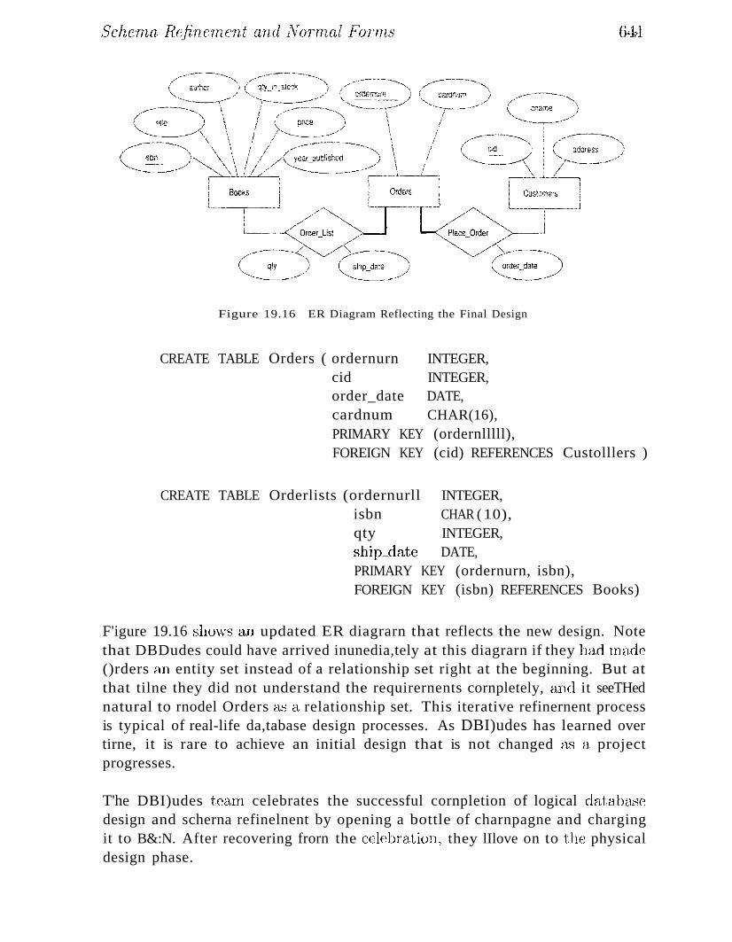
641
Figure 19.16 ER Diagram Reflecting the Final Design
CREATE TABLE Orders ( ordernurn INTEGER,cid INTEGER,order_date DATE,cardnum CHAR(16),PRIMARY KEY (ordernlllll),FOREIGN KEY (cid) REFERENCES Custolllers )
CREATE TABLE Orderlists (ordernurll INTEGER,isbn CHAR ( 10),qty INTEGER,ship~date DATE,PRIMARY KEY (ordernurn, isbn),FOREIGN KEY (isbn) REFERENCES Books)
F'igure 19.16 shc)\\TS an updated ER diagrarn that reflects the new design. Notethat DBDudes could have arrived inunedia,tely at this diagrarn if they ha"d llla.de()rders an entity set instead of a relationship set right at the beginning. But atthat tilne they did not understand the requirernents cornpletely, and it seeTHednatural to rnodel Orders a.I) a relationship set. This iterative refinernent processis typical of real-life da,tabase design processes. As DBI)udes has learned overtirne, it is rare to achieve an initial design that is not changed as a projectprogresses.
T'he DBI)udes tea,lll celebrates the successful cornpletion of logical dataJn1,.'3cdesign and scherna refinelnent by opening a bottle of charnpagne and chargingit to B&:N. After recovering frorn the celebration~ they lIlove on to the physicaldesign phase.
642 CHAPTER 19
19.10 REVIEW QUESTIONS
Answers to the review' questions can be found in the listed sections.
• Illustrate redundancy and the problerns that it ca.n cause. Give excunplesof insert, delete, and npdate anoInalies. Can 'fudl values help address theseproblerlls? Are they a cOlnplete solution? (Section 19.1.1)
• "VVhat is a decoTnpositio'n and how does it address redundancy? Whatproblerlls Inay be caused by the use of decolupositions? (Sections 19.1.2and 19.1.3)
• Define junctional dependencies. How are pr'lnLary keys related to FDs?(Section 19.2)
• V\Then is an PD j implied by a set F of FDs? Define Armstrong's Axioms,and explain the statement that "they are a sound and cornplete set of rulesfor FD inference." (Section 19.3)
• What is the dependency closure F+ of a set F of FDs? What is the attribute closure X+ of a set of attributes X with respect to a set of FDs F?(Section 19.3)
• Define INF, 2NF, 3NF, and BCNF. What is the nlotivation for putting arelation in BCNF? What is the motivation for 3NF? (Section 19.4)
• When is the decomposition of a relation schenla R into two relation schemasX and Y said to be a lossless-join decomposition? Why is this propertyso irnportant? Give a necessary and sufficient condition to test whether adecc)1nposition is lossless-join. (Section 19.5.1)
• When is a decornposition said to be depc'ndency-preserving? \Vhy is thisproperty useful? (Section 19.5.2)
• Describe how we can obtain a. lossless-join decornposition of a relation intoBCNI"""'. Give an exanlple to show that there rnay not be a dependencyprest~rvingdecornposition into BCNF. Illustrate how a given relation couldbe decornposed in different ways to arrive at several alternative decornpositions, and discuss the irnplications for clatabc~"e design. (Section 19.6.1)
IlIll (jive an cx.:arnple that illustrates how a collection of relations ill BCNFcould have redundancy even though each relation, by itself, is free fronlredundancy. (Section 19.6.1)
• What is a. Tninirnal cover for a set of I:(I)s? Describe an algorithrn forcornputing the rninirnaJ cover of B.. S(~t of FI)s, and illustrate it with anexarnple. (Section 19.6.2)
Sche77~a Refincrnent and N oT'Tnal FOTin8 64:3
• Describe hovv the algorithl11 for lossless-join decolnposition into BCNF canbe adapted to obtain a lossless-join, dependency-preserving decornpositioninto 3NF. Describe the alternative synthesis approach to obtaining sucha decorllposition into 3NF. Illustrate both approaches using an exarnple.(Section 19.6.2)
• Discuss how scherna refinernent through dependency analysis and norrnalization can iInprove scheIna.-') obtained through ER, design. (Section 19.7)
• Define 'Tn'l1,ltival'Ued dependencies, .Join dependencies, and inclusion dependencies. Discuss the use of such dependencies for database design. Define4NF and 5NF, and explain how they prevent certain kinds of redundancythat BCNF does not eliminate. Describe tests for 4NF and 5NF that useonly FDs. What key assumption is involved in these tests? (Section 19.8)
EXERCISES
Exercise 19.1 Briefly answer the following questions:
1. Define the term functional dependency.
2. Why are some functional dependencies called trivial?
3. Give a set. of FDs for the relation schema R(A,B, C,Dj with prilnary key AB under whichR is in 1NF but not in 2NF.
4. Give a set of FDs for the relation schelna R(A,B, C,Dj with prilnary key AB under whichR is in 2NF but not in 3NF.
5. Consider the relation schelna R(A,B, OJ, which has the FD B ~ C. If A is a candidatekey for R, is it possible for R to be in BCNF? If so, under what conditions? If not,explain why not.
6. Suppose we have a relation schema R (A, B, OJ representing a relationship between twoentity sets with keys A and 13, respectively, and suppose that R has (aIIlong others) theFDs A ..._+ Band 13 -ot A. Explain what such a pair of dependencies means (i.e., whatthey irnply about the relationship that the relation nlOdels).
Exercise 19.2 Consider a relation R with five attributes ABCDE. You are given the follc)\vingdependencies: A --t B, Be ~ B, and BD ~ A.
1. List all keys for R.
2. Is R in :3NF?
3. Is R in BCNF?
Exercise 19.3 Consider the relation shown in Figure 19.17.
1. l... ist all the functional dependencies that this relation instance satisfies.
2. ASSUIlIe that the value of attribute Z of the la..<:;t record in the relation is cluLuged frorH23 to Z2. Now list all the functional dependencies that this relation instance satisfies.
Exercise 19.4 Assurne that you are given a. relation with attributes A BCD.
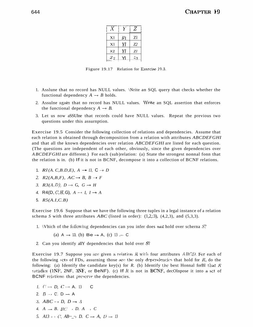
644
Xl Yl Zl
Xl Yl Z2
X2 Yl Zl
~r2 Yl Z~~'--.
Figure 19.17 Relation for Exercise 19.:3.
CJHAPTER }g
1. Asslune that no record has NULL values. \Nrite an SQL query that checks whether thefunctional dependency A ---,)0 B holds.
2. Assulne again that no record has NULL values. \tVrite an SQL assertion that enforcesthe functional dependency A -+ B.
3. Let us now aSSUlne that records could have NULL values. Repeat the previous twoquestions under this assurnption.
Exercise 19.5 Consider the following collection of relations and dependencies. Assume thateach relation is obtained through decomposition from a relation with attributes ABCDEFGHIand that all the known dependencies over relation ABCDEFGHI are listed for each question.(The questions are independent of each other, obviously, since the given dependencies overA BCDEFGHI are different.) For each (sub)relation: (a) State the strongest nonnal fonn thatthe relation is in. (b) If it is not in BCNF, decompose it into a collection of BCNF relations.
1. Rl (A. C,B.D,E), A -+ 13, C -+ D
2. R2(A,B,F), AC -+ B, B -+ F
3. R3(A~DJ.. D "".of G, G -+ H
4. R4(D, C,H, G), A -~·t I, I -+ A
5. R5(A.I,C.B)
Exercise 19.6 Suppose that we have the following three tuples in a legal instance of a relationschema S with three attributes ABC (listed in order): (1,2,:3), (4,2,3), and (5,3,3).
1. \Vhich of the follc)\\ring dependencies can you infer does 'lUJl hold over scherna S?
(a) A -+ 13, (b) Be ---'1 A, (c) 13 ..._-, C
2. Can you identify allY dependencies that hold over 5''?
Exercise 19.7 Suppose you are given a rebltion R \vith four attributes AB()D.F'or each ofthe following sets of FDs, assurning those are the only dependencies that hold for R, do thefollowing: (a) Identify the candidate key(s) for R. (b) Identify the best Honnal forBl thatRsatisfies (lNF, 2NF, :JNF, or BeNF). (c) If Ii is not in BCNl~\ decOlnpose it into a set ofBCNF relations that preserve the dependencies.
1. C:-······ D, C----+ A. 13 C
2. FJ '-~-f C'. D --> A
:3. ABC -~f D, D --> A
4. A -+ B. B(} ,. D. A ~. C
5. A13 _....... C, AB···_··.• D. C -+ A, D·_·-+ 13
Scherna llefincl1H;nt (nul IVorrnal 1:"~oTn18 645
Exercise 19.8 Consider the attribute set Ii = ABCDEGH (Lud theFD set F= {A.B·--+ C:,AC --+ B: AD ---4 E, B -----+ D, Be --+ 11, B -!- G}.
1. For each of the following attribute sets, do the following: Cornpute the set of depen-dencies that hold over the set and write down a rninirnal cover. (ii) Narne the strongestnonnal [onn that is not violated by the relation containing these attributes. (iii) DeCOlnpose it into a. collection of BCNF relations if it is IH)t in BeNF'.
(a) ABC, (b) ABCD, (c) ABCEG, (d) DC:BGII, (e) ACEH
2. vVhich of the following decOIllpositions of R = ABCDEG, with the saIne set of dependencies F', is (a) dependency-preserving? (b) lossless-join?
(a) {AB, BC, ABDE. EG }
(b) {ABC, ACDE, ADG }
Exercise 19.9 Let R be decOIllposed into R 1 , R2 , ... , Rn . Let F be a set of FDs on R.
1. Define what it rlleans for F to be pre8erved in the set of decOlllposed relations.
2. Describe a polynomial-tirne algorithm to test dependency-preservation.
3. Projecting the FDs stated over a set of attributes X onto a subset of attributes Y requiresthat we consider the closure of the FDs. Give an exarnple where considering the closureis irnportant in testing dependency-preservation, that is, considering just the given FDsgives incorrect results.
Exercise 19.10 Suppose you are given a relation R(A,B, C,D). For each of the followingsets of FDs, assuming they are the only dependencies that hold for R, do the following: (a)Identify the candidate key(s) for R. (b) State whether or not the proposed decOlnposition ofR into smaller relations is a good decolllposition and briefly explain why or why not.
1. B --+ C, D --+ A; decornpose into BC and AD.
2. AB -+ C, C -~~ A, C ,--)- D; decompose into A CD and Be.
~~. A -!- BC, C -+ AD; decornpose into ABC and AD.
4. A -!- B, B C, C '-1 D; decornpose into AB and A CD.
5. A --+ B, B -+ C, C -!- D; decOInpose into AB, AD and CD.
Exercise 19.11 Consider a relation R that has three a"ttributes ABC. It is decornposed intorelations R 1 with attributes AB and R2 with attributes Be.
1. St<lte the definition of a lossless-join decOlnposition with respect to this exarnple. Answerthis question concisely by \-vriting a relational algebra equation involving R, R 1 , and H2.
2. Suppose that B --+--+ C. Is the decorHposition of R into .R! and R2 lossless-join? Reconcileyour (l.,nswer with the observation that neither of the FDs HI nR2 ----'> R I nor R I n R2 --+ .H..2hold, in light <;)f the siInple test offering a necessary and sufficient condition for losslessjoin decmnposition into two relations in Section 15.6.1.
:3. If you are given the follc}\\ring justa.nees of R 1 a,nd 112, what can you say about theinstance of R from which these were obtained? Answer this question by listing tuplesthat are definitely ill R and tuples that a.re possibly· in R.
Instance of RJ. = {(5,l), (6,l)}Instance of R2 :::::: {(l,8), (1,9)}
Can you say that attribute B definitely is or 'is not. a key for R?

646 CHAPTER 19
Exercise 19.12 Suppose that we have the following four tuples in a relation 5' with threeattributes ABC: (1,2,:3), (4,2,:3), (5,3,:3), (5,::~A). \Vhich of the following functional (-+) andrIlultivalued (-+--» dependencies can you infer does not hold over relation S?
1. A -+ 13
2. A _....-} ..._,,-} B
3. Be --,} A
4. BG -+_..~> A
5. 8 -+ C
6. B ~'---'o C
Exercise 19.13 Consider a relation R with five attributes A BCDE'.
1. For each of the following instances of R, state whether it violates (a) theFD Be ",,"-, Dand (b) the J\fVD Be _..-t--+ D:
(a) { } (i.e., mnpty relation)
(b) {(0,,2,3,4,5), (2,a,3,5,5)}
(c) {(o,,2,3,4,5), (2,0,,3,5,5), (o,,2,3,4,6)}
(d) {(a,2)~,4,5), (2,0,,3,4,5), (o,,2,3,6,5)}
(e) {(0,,2,3,4,5), (2,0,,3,7,5), (a,2,3,4,6)}
(f) {(o,,2,3,4,5), (2,0,,3,4,5), (0,,2,3,6,5), (o,,2,3,6,6)}
(g) {(a,2,~3,4,5), (0,,2,:3,6,5), (0,,2,3,6,6), (o,,2,3,4,6)}
2. If each instance for R listed above is legal, what can you say about the FD A -+ B?
Exercise 19.14 JDs are lllotivated by the fact that sornetilnes a relation that cannot bedecoruposed into two sinaller relations in a lossless-join rnanner can be so deC0111pOsed intothree or rnore relations. An exa,rnple is a relation with attributes 8upplier, part, clnd J}Toject,
denoted SPJ, with no FDs or l'vlVDs. The JD [Xl {SP, P J, J S} holds.
Frorn the JD, the set of relation scheines SP, PJ, and JS is a IORsless-join decornposition ofSPJ. Construct an instance of HPJ to illustrate that no two of these schernes suffice.
Exercise 19.15 Answer the following questions
1. Prove that the algorithrn shown in Figure 19.4 correctly cornputes the ::l.ttribute closureof the input attribute set X.
2. Describe a linear-tirne (in the size of the set of FI)s, where the size of each FD is thenurnber of attributes involved) algoritlun for finding the attribute closure of a set ofattributes with respect to a set of FDs. Prove that your algoritlun correctly COInputesthe attribute closure of the input attrilnlte set.
Exercise 19.16 Let us say that an 'Fl) )( -_.,} Y is si'mple if Y is a single attribute.
1. Replace the FD AB........, CD l.Jy the srnallest equivalent collection of sirnple FDs.
2. Prove that everyFD X _...crY" in (.'L set of FDs F Cetn be replaced by a set of sirnple F'Dssuch that p+ is equal to the closure of the new set of FDs.
Scherria RejineTnent and NOT'nial 1?oT7ns 641
Exercise 19.17 Prove that Arrnstrong's i-\xiorns are sound and cOluplete for FD inference.rT'hat is, sh()\v that repeated application of thesf; ttxiOlllS on a set F ofF'Ds produces eX(lctlythe dependencies in P+.
Exercise 19.18 Consider a relation R with attributes A BCDE. aLet the following FDs begiven: A ~ BC, Be ----'!" E, and E ~ DA. Siluilarly, let S be a relation with attributes ABC1DEand let the follo\ving FDs be given: A-+ BC, B -+ IE, and E ----'!" DA. (Only the seconddependency differs frolll those that hold over R.) You do not know whether or which other(join) dependencies hold.
1. Is R in BCNF?
2. Is R in ,1NF?
3. Is R in 5NF?
4. Is Sin BeNF?
5. Is Sin 4NF?
6. Is Sin 5NF'?
Exercise 19.19 Let R be a relation schelna with a set F of FDs. Prove that the decOIllposition of R into HI and R2 is lossless-join if and only if p+ contains HI n R 2 ----'!" R 1 orR 1 n R2 ----'!" R 2 .
Exercise 19.20 Consider a scheme R with FDs F that is decOlnposed into schelnes witha..ttributes X and Y. Show that this is dependency-preserving if F' ~ (}~x U py)+.
Exercise 19.21 Prove that the optiInizatioll of the algorithrn for lossless··-join, dependencypreserving decornposition into ~)NF relations (Section 19.6.2) is correct.
Exercise 19.22 Prove that the 3NF synthesis algoritlull produces a lossless-join decOlnposition of the relation containing all the original attributes.
Exercise 19.23 Prove that an ]\IlVn .X -+-+ Y over a rehltion R can be expressed a,,') thejoin dependency [Xl {-,YY, X(R - Y)}.
Exercise 19.24 Prove that, if R has only one key, it is in BCNF if and only if it is in ~3NF.
Exercise 19.25 Prove that, if R is in 3NF and every key is shnple, then R is in HeNF.
Exercise 19.26 Prove these staternents:
1. If a relation scherne is in BCNF and at lea.st one of its l\.eys consists of }1 single attrilmte,it is also in 4NF.
2. If a relation scherne is in :3NF and each key has a single attribute, it is also in 5NF'.
Exercise 19.27 Give <ill algorithrn for testing whether a relation scheme is in BCNF. ]'he:.llgorithrn should l)e polynorniaJ in the size of the set of given FDs. ('rhe size is the surn overall FI)s of the nurnber of attributes that a,ppear in theFJ).) Is there ::t polyuOlnial algorithrnfor testing whether a relation scheme is in :~NF?
Exercise 19.28 Give ('UI algorithm for testing \vhether a relation scherne is in BCjNF'. 'I'hf~
aJgorithrn should be polynomial in the size of the set of given FI)s. CI'he 'size' is the SUln overall FI)s of the nurnber of attributes that appear in theFD.) Is there a polynomial algorithrnfor testing whether a relation scherne is in :~NF?
Exercise 19.29 1)rove that the algorithm for decomposing a re1cltion scherna with a set ofFI)s into a collection of BC~NS relation schenlas as describerl in Section 19.G.l is correct (i.e.,it produces a collection of BCNF relations, and is lossless-join) and terrninates.
648
BIBLIOGRAPHIC NOTES
(;I'IAPTER 19
Textbook presentations of dependency theory and its use in database design include [3, 45,501) 509, '747J. Good survey articles on the topic include [755,415].
FDs \vere introduced in [187], along with the concept of ::3NF, and aximlls for inferring FDswere presented in P38]. BCNF was introduced in [188]. The concept of a legal relation instanceand dependency satisfaction are studied fonnaUy in [828] .FDs were generalized to scrnanticdata Illodels in [768].
Finding a key is shown to be NP-COlnplete in [497]. Lossless-join decOlnpositions were studiedin [28, 502, 627]. Dependency-preserving decorIlpositions were studied in [74]. [81] introducedrninirnal covers. DecOlnposition into :3NF is studied by 1.81, 98] and decOlnposition into BCNFis addressed in [742]. [412] shows tha,t testing whether a relation is in ~1NF is NP-cOlnplete.[253] introduced 4NF and discussed decoillposition into 4NF. Fagin introduced other nonnalforIlls in [254J (project-join nonnal fonn) and [255] (doHluin-key nonnal forIll). In contrast tothe extensive study of vertical decOlnpositions, there has been relatively little formal investigation of horizontal decompositions. [209] investigates horizontal decoillpositiolls.
IvIVDs were discovered independently by Delobel [211] ,Fagin [253], and Zaniolo [789]. AxiOlllSfor FDs and MVDs were presented in [73}. [593] shows that there is no axiornatization forJDs, although [662] provides an axioHlatization for a more general class of dependencies. Thesufficient conditions for 4NF and 5NF in tenns of FDs that were discussed in Section 19.8 arefrom [205]. An approach to database design that uses dependency inforrnation to constructsarnple relation instances is described in [508, 509].
20PHYSICAL DATABASEDESIGN AND TUNING
--What is physical database design?
.. What is a query workload?
... How do we choose indexes? What tools are available?
.. What is co-clustering and how is it used?
.. What are the choices in tuning a database?
.. How do we tune queries and view?
.. What is the impact of concurrency on perforrnance?
.. How can we reduce lock contention and hotspots?
.. "'That are popular database benchnlarks and how are they used?
... Key concepts: Physical database design, database tuning, workload,co-clustering, index tuning, tuning wizard, index configuration, hotspot, lock contention, database benchmark, transactions per second
Advice to a client who cornplained al)out rain leaking through the roof onto thedining Utble: "J\!!ove the table."
............ Architect Frank IJoyd \"lright
The perfonnance of a 1)131:18 on cornrnonly &':lked queries and typical updateoperations is the ultirnate Ineasure of a database desigIl. A I}BA can irnproveperforrnance by identifying perforrnance bottlenecks and adjusting sorne DBIVlSpararneters (e.g., the size of the buffer pool or the frequency of checkpointing)or adding hanhvare to elirninate such bottlenecks. rIhe first step in achieving
Gi19
650 CHAPTER 20
good perforlnancc, however, is to Inake good databa.se design choices, which isthe focus of this chapter.
After we design the conceptual and exte'rnal scherna..'3, that is, create a collectionof relations and views along 'with a set of integrity constraints, we .Il1ust addresspe1'forlna11c8 goals through physical database design, in which we design thephysical sche111a. As user requirernents evolve, it is usually necessary to tune,or adjust, all &"3pects of a database design for good perforrnance.
This chapter is organized as follows. We give an overview of physical databasedesign and tuning in Section 20.1. The 1nost irnportant physical design decisions concern the choice of indexes. We present guidelines for deciding whichindexes to create in Section 20.2. These guidelines are illustrated through several exalnples and developed further in Sections 20.3. In Section 20.4, vve lookclosely at the irnportant issue of clustering; we discuss how to choose clusteredindexes and whether to store tuples fron1 different relations near each other (anoption supported by sorne DBMSs). In Section 20.5, we empha.."3ize how wellchosen indexes can enable some queries to be answered without ever looking atthe actual data records. Section 20.6 discusses tools that can help the DBA toautornatically select indexes.
In Section 20.7, we survey the lnain issues of database tuning. In additionto tuning indexes, we 111ay have to tune the conceptual schema as well asfrequently used query and view definitions. We discuss how to refine the conceptual schelna in Section 20.8 and how to refine queries and view definitionsin Section 20.9. We briefly discuss the perforrnance irnpact of concurrent accessin Section 20.10. We illustrate tuning on our Internet shop exarnple in Section20.11. \Ye conclude the chapter with a short discussion of DBMS benchrnarks inSection 20.12; benchrnarks help evaluate the perfOI'lnanCe of alternative DBl\1Sproducts.
20.1 INTRODUCTION TO PHYSICAI.J DATABASEDESIGN
Like all other a.spects of elataba.se design, physical design rnust b(~ guided bythe nature of the data, a,nd its intencled use. In particular, it is irnportant tonnderstand the typical workload th<:tt the database lI1Ust support; tlH~ vvorklc)adconsists of a rnix of queries a.nel updates. 1Jsers (:tlso have certain requirenl(~nts
about ho\v fast cert;:lin queries or llpdat(~s 11111st run or ho\v rnan.y tran.sactionsrnust be processed per second. rrhe \vorkload (l<~scription and users' perforIn(U1C(~ reqllirernents are the ba"sis on \vhich a nurnber of decisions have to bernade during pl1ysical datab':lse design.
Physical Dat;abase Design, an,cl l1zJ,ni'ltg 651
r-..····_·_,,·,_·.._~ .._···_··_-."_.~ _-_.-.-.._-_._ _-~"" __ _~ _.._ _..~ --·_ lI Identifying Perfornlance Bottlenecks: All cornrrlercial systeuls proI vide a suite of tools for rnonitoring a wide range of systeIll paralneters.
'I' These tOOlS. ' used properlY" C,Ul help identify perfOfIna.nc.e bO.ttlenecks andsuggest aspects of the databc1..'Se design and application code that need to
I be tuned for perforlnance. For exarnple 1 •"ve can ask the DBMS to rnonitorI the execution of the database for a certain period of tinle and report oni the nurnber of clustered scans, open cursors, lock requests, checkpoints,
buffer scans, average wait titne for locks, and many such statistics thatgive detailed insight into a snapshot of the live system. In Oracle, a reportcontaining this inforlnation can be generated by running a script calledUTLBSTAT. SQL to initiate monitoring and a script UTLBSTAT. SQL to terminate rnonitoring. The system catalog contains details about the sizes oftables, the distribution of values in index keys, and the like. The plan generated by the DBMS for a given query can be viewed in a graphical displaythat shows the estimated cost for each plan operator. While the detailsare specific to each vendor, all InajaI' DBlIIS products on the market today
~rovide a sUi~e of such tools. __~..
To create a, good physical database design and tune the systenl for performance in response to evolving user requirelnents, a designer HUlst understandthe workings of a DBMS, especially the indexing and query processing techniques supported by the DBMS. If the database is expected to be accessedconcurrently by rnany users, or is a d'istr'ibuted database, the task beeorneslnore cornplicated and other features of a, DBl\1S CaIne into play. 'iVe discussthe ilnpact of concurrency on database design in Section 20.10 and distributeddatabases in Chapter 22.
20..1..1 Database Workloads
The key to good physical design is DTriving at an accurate description of theexpectedworkloa.d. A workload description includes the follCJ\ving:
1. A list of queries (with their frequency, as <'1 rc:ttio of all queries / npdcltes).
2, A list of updates and their frequencies.
:3.Perfonnanc(~ goals for each type of query and update.
For each quer.y in the \vorklo;:vL vve HUlst identify
1\1II \Vhich relations (11'e accessecl.
1\1II \Vhich attributes are n:~tained (in the SELECT clru.lse).

652 CHAPTER 20
• \Vhich attributes have selection Of join conditions expressed on thern (inthe WHERE clause) (UH:! hovv selective these conditions are likely to be.
SiInilarly, for each update in the \vorkloacl, \ve Blust identify
• vVhich attributes have selection or join conditions expressed on therll (inthe WHERE clause) and ho\v selective these conditions are likely to be.
B The type of update (INSERT, DELETE, or UPDATE) and the updated relation.
• For UPDATE cOHnuands, the fields that are rnodified by the update.
R.ellleluber that queries and updates typically have parameters, for exarnple, adebit or credit operation involves a particular account nUlnber. rrhe values ofthese paralneters deterlnine selectivity of selection and join conditions.
Updates have a query cornponent that is used to find the target tuples. ThiscOlllponent can benefit froIn a good physical design and the presence of indexes.On the other hand, updates typically require additional work to ITlaintain indexes on the attributes that they 111odify. Thus, while queries can only benefitfroill the presence of an index, an index rnay either speed up or slow downa given update. Designers should keep this trade-off in rnind when creatingindexes.
20.1.2 Physical Design and Tuning Decisions
Irnportant decisions rnade during physical datab&'3e design and database tuninginclude the follovving:
1. Choice of indexes to create:
II \Vhich relations to index and which field or cornbination of fields tochoose as index search keys.
II For each index, should it be clustered or ul1clustered?
2. Tuning the conceptual 8chenLa:
l1li Alternative 'fuJTYnalized 8cherna/): \Ve usually have rnore than one wayto dec()1npose a schclua into a desired IlOl'Inal fOITn (BCNF or 3NF).A choice can be rnade on the basis of perforrnance criteria,.
II Den,OT7Tl.alizat'io'n: \Ve Inight\vant to reconsider scherna decolnposibons ca.rried Ollt for norrnalization. during the conceptual schern.a design process to irnprove the perforrnance of queries that involve attributes fr0111 several pn:~viously decornposed relations.
II l/crvtical part'itioning: LJnder certain circurnstances we rnight 'want tofurther decornpose relations to ilnprove the perfornlance of queriesthat involve only a fevv attributes.
II ViC'U1S: \Ve luight 'want to add sorne vie\vs to nlask the changes in theconceptual scherna fr0111 users.
3. Query and tTansact'ioTl, t'UJLing: Frequently executed queries and transactions ulight be re\\rritten to run fc1..ster.
In paTallel or distributed databases, \vhichwe discuss in Chapter 22, there areadditional choices to consider, such (laS whether to partition a relation acrossdifferent sites or whether to store copies of a relation a,t rnultiple sites.
20.1.3 Need for Database Thning
Accurate, detailed workload infonnation 111Cly be hard to corne by while doingthe initial design of the systen1. Consequently, tuning a database after it hasbeen designed and deployed is ilnportant---we HlllSt refine the initial design inthe light of actual usage patterns to obtain the best possible perfonnance.
The distinction bet\veen database design and database tuning is soruewhatarbitrary. We could consider the design process to be over once an initialconceptual sche1na is designed and a set of indexing and clustering decisionsis nlade. Any subsequent changes to the conceptual scherna or the indexes,say, would then be regarded as tuning. Alternatively, we could consider sornerefinernent of the conceptual scheula (and physical design decisions afl'ected bythis refinernent) to be part of the physical design process.
vVh,ere we draw the line between design and tuning is not very irnpoItant, andwe sirnply discuss the issues of in(lE:~x selection and databa..'3c tuning withoutregard to when the tuning is carrier} out.
20.2 (;UIDEI.JINES FOR INDEX SELECTION
In considering \vhich indexes to create; we begin \\rith the list of queries (including queries tha,t a.ppear as paTt of update operations). ()bviously, only relationsaccessed by sorTle qu(~ry need to be considered as candidates for indexing, andthe choice of attributes to index is guided by the conditions that appear in theWHERE clauses of the queries in the \vorkload. 1'he presence of suitable indexescan significa.,ntly irnprove the evaluation plan for (1, query, EtS\Ve saw in Chapters8 and 12.
654 (;HAPTER20
()ne approach to index selection is to consider the Ulost irnportant queries inturn, and, for each, deterrnine \vhich plan the optiInizer \vould choose giventhe indexes c:urrently on our list of (to be crc(;tted) indexes. Then\ve consider\vhetherwe can aTrive at a substantially better plan by a,clding 1110re indexes; ifso. these additional indexes are candidates for inclusion in our list of indexes.In general, range retrievals benefit froIn a 13'-f- tree index, and exact-IHatch.. ,-
retrievals benefit frorn a hash index. Clustering benefits range queries, and itbenefits exact-rnatch queries if several data entries contain the saIne key value.
Before adding an index to the list, hovvever, \ve lnust consider the irnpact ofhaving this index on the upda,tes in our workload. As \ve noted earlier, althoughan index can speed up the query cornponent of an update, all indexes on anupdated attribute---{)n any attribute, in the case of inserts Cl.,nd deleteslnustbe updated whenever the value of the attribute is changed. Therefore, weJ.nust sOlnetirnes consider the trade-off of slo\ving sorne update operations inthe workload in order to speed up sorne queries.
Clearly, choosing a good set of indexes for a given workload requires an understanding of the available indexing techniques, and of the workings of thequery optiruizer. The following guidelines for index selection sunnnarize ourdiscussion:
Whether to Index (Guideline 1): The obviollS points are often the lnostirnportant. Do not build an index unless sorne query including the querycOlnponents of updates benefits frolu it. Whenever possible, choose indexesthat speed up rIlore than one query.
Choice of Search Key (Guideline 2): Attributes rnentioned HI a, WHEREclause <),re ca,ndidates for indexing.
11I'I An exact-rnatch selection condition suggests that \ve consider an irldex ont}le selected attributes, ideally, <:-}, hash index.
II j\ range selection condition suggests that we consider a 13+- tree (Of ISA1/1)index on the selected attrilnltes. j\ B+ tree index is 11S1U111y preferaJ)le toan ISA1/1 index. A.n ISA:NI irlclex rnay l)e vvorth considering if the relation isinfrequently updated, but we assurne that a B-t--- tree index is (lhvays chosenover an lSft.\i\,1 index, for sirnplicity.
Multi-Attribute Search :Keys (Guideline 3): Indexes\vith Inllitipl(~-attributc
sea,rch keys slH)uld l)e considered in the follc)\ving two situ<ltion.s:
ill j\ WHERE clause includes conditinns 011 Inore t.han on(~ attribute of a relation.
&--.")'"')I ,_
III They ellilble index-only evaluation strategies (i.e., accessing the relation canbe avoided) for irnportCtnt queries. (This situation Gould lead to attributesbeing in the sCc:lrch key even if they do not appear in WHERE clauses.)
vVhen creating indexes on search keys wit.h rnultiple attributes, if range queriesaxe expected, be careful to order the attributes in the search key to Ina.tch thequenes.
Whether to Cluster (Guideline 4): At lllost one index on a given relationcan be clustered, and clustering affects perfonnance greatly; so the choice ofclustered index is iInportant.
II As a rule of tlnunb, range queries are likely to benefit the 1110St froIll clustering. If several ra,nge queries are posed on a relation, involving differentsets of attributes, consider the selectivity of the queries and their relativefrequency in the workload when deciding which index should be clustered.
II If an index enables an index-only evaluation strategy for the query it isintended to speed up, the index need not be clustered. (Clustering Inattersonly when the index is used to retrieve tuples fr(nll the underlying relation.)
Ifash versus Tree Index (Guideline 5): A B-·t- tree index is usually preferable because it supports range queries as well as equality queries. A hash indexis better in the following situations:
IIi1 The index is intended to support index nested loops join; the indexedrelation is the inner relation, and the search key includes the join colurllns.In this case, the slight ilnproveIllent of a hash index over a B·+ tree forequality self~ctions is rnagnified, because an equality selection is generatedfor each tuple in the outer relation..
II rrllcre is a very iInportant equality query, and no range queries, involvingthe sea.rch key attributes.
Balancing the C~ost of Index Maintenance (Guideline 6): After drawingup a ~\vishlist' of indexes to create, consider the irnpact of each index on theupdates in tl1cvvorkload.
• If Inaintainlng an index sl()\vs do\vn frc~quent update operations, considerdropping the index.
II I{eep ill rnind, hOvv(~ver, thaJ adding an index Illay 'well speed up a givenupdate operation. For exanlplc, <111 index on enlployec~ IDs could speed upth(~ operaJion of increa,'3ing the salary of a given ernployee (specified b:y ID).
20.3
CHAPTER.20
BASIC EXAMPLES OF INDEX SELECTION
The follawing examples illustrate hen¥ to choose indexes during databa..sc design,continuing the discussion froln Chctpter 8, \vherewe focused on index selectionfor single-table queries. The schernas used in the exarnples are not described indetail; in general, they contain the attributes nalned in the queries. Additionalinforlnation is presented "when necessary.
Let us begin with a silnple query:
SELECT E.enaIne 1 D .rugI'FROM Enlployees E, DepartInents DWHERE D.dncune='Toy' AND E.dno=D.dno
The relations rnentioned in the, query are Enlployees and Departnlents, andboth conditions in the WHERE clause involve equalities. Our guidelines suggestthat we should build hash indexes on the attributes involved. It seeIns clearthat we should build a hash index on the dnaTne attribute of DepartInents. Butconsider the equality E. dno=D. dno. Should we build an index (hash, of coursf~)
on the dno attribute of Departrnents or Ernployees (or both)? Intuitively, wewant to retrieve Departments tuples using the index on dnarne because fewtuples are likely to satisfy the equality selection .D. dnaTne= 'Toy '.1 For eachqualifying Departrnents tuple, we then find lnatching EInployees tuples by usingan index on the dno attribute of Ernployees. So, we should build an index on thedno field of En1ployees. (Note that nothing is gained by building an additionalindex on the dno field of Departrnents because Departnlents tuples are retrievedusing the dna:rne index.)
Our choice of indexes was guided by the query evaluation plan we \vantedto utilize. This consideration of a, potential evaluation pla.n is connnon whilernaking physical design decisions. U·nderstanding query optirnization is veryuseful for physical design. "VVe show the desired plal1 for this query in Figure20.1.
As a variant of this query, suppose that the WHERE clause is rnodified to beWHERE J). dnarne= 'Toy ~ AND E'.dno=D. dno AND E'1. 0,oge=25. Let us consider alternative evaluation plans. ()ne good plan is to retrieve Departrnents tuplesthat satisfy the selection on dnarne and retrieve rnatching Ernployees tuples byusing an index on the dno field; the selection on age is then applied on-the-fly.TIc)\vever, unlike the previous variant of this Cjllcry, vve do not really need tohave an index on the dna field of Ernployees if \ve have an index. on age. In this
------_...... _._--lThis is only a heuristic. If dnarne is not the key, and we have no statistics to verify this cla.inl. it
is possible that several tuples satisfy this condition.
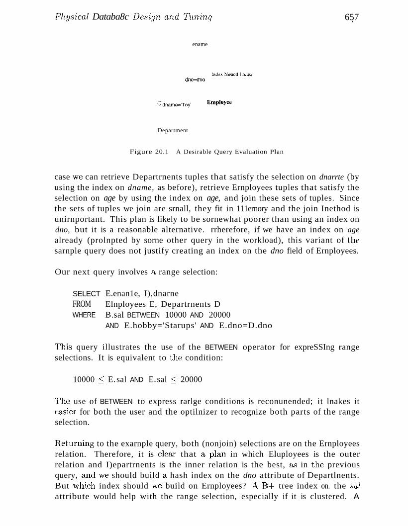
Physical Databa8c De,sign and Tuning
ename
Index Nested Loopsdno:::dno
657It
Odname::::'Toy'
Department
Employee
Figure 20.1 A Desirable Query Evaluation Plan
case we can retrieve Departrnents tuples that satisfy the selection on dnarrte (byusing the index on dname, as before), retrieve Ernployees tuples that satisfy theselection on age by using the index on age, and join these sets of tuples. Sincethe sets of tuples we join are srnall, they fit in 111ernory and the join Inethod isunirnportant. This plan is likely to be sornewhat poorer than using an index ondno, but it is a reasonable alternative. rrherefore, if we have an index on agealready (prolnpted by sorne other query in the workload), this variant of thesarnple query does not justify creating an index on the dno field of Ernployees.
Our next query involves a range selection:
SELECTFROMWHERE
E.enan1e, I),dnarneElnployees E, Departrnents DB.sal BETWEEN 10000 AND 20000AND E.hobby='Starups' AND E.dno=D.dno
T'his query illustrates the use of the BETWEEN operator for expreSSIng rangeselections. It is equivalent to the condition:
10000 ::; E.sal AND E.sal :S 20000
l~he use of BETWEEN to express rarlge conditions is reconunended; it lnakes itcc1.5ier for both the user and the optilnizer to recognize both parts of the rangeselection.
lleturning to the exarnple query, both (nonjoin) selections are on the Ernployeesrelation. Therefore, it is clear that a plan in which Eluployees is the outerrelation and I)epartrnents is the inner relation is the best, as in the previousquery, and\ve should build a hash index on the dno attribute of Departlnents.But vvhich index should vve build on Ernployees? 1\. 13+ tree index on. the salattribute would help with the range selection, especially if it is clustered. A
658 CHAPTER 20
hash index on the hobby attribute \\Tould help ·with the equality selection. Ifone of these indexes is available, we could retrieve Ernployees tuples using thisindex, retrieve rnatching Departruents tuples using the index on dno~ aJld applyall rernaining selections and projections on-the-fly. If both indexes are available,the optirnizer would choose the rno1'e selective index for the given query; that is,it \vollld consider \vhich selection (the range condition on salary or the equalityon hobby) ha",,; fe\ver qualifying tuples. In general, which index is rnore selectivedepends on the data. If there are very few people with salaries in the givenrange and rnany people collect starnps, the B-t- tree index is best. Otherwise,the hash index on hobby is best.
If the query constants are known (H,," in our exarnple) ~ the selectivities can beestiInated if statistics on the data are available. Otherwise, as a rule of thurnb,an equality selection is likely to be rnore selective, and a rea.sonable decisionwould be to create a hash index on hobby. Sornethnes, the query constantsare not knowIl",,··----we rnight obtain a query by expanding a query on a view atrUIl-tirrle, or we rnight have a query in Dynalnic SQL, which allows constantsto be specified as wild-card variables (e.g., %X) and instantiated at run-tinle(see Sections 6.1.3 and 6.2). In this case, if the query is very important, welllight choose to create a B+ tree index on sal and a hash index on hobby andleave the choice to be rnade by the optirnizer at run-tirrle.
20.4 CLUSrrERING AND INDEXING
Clustered indexes can be especially iInportant while accessing the inner relationin an index nested loops join. To understand the relationship between clusteredhldexes and joins, let us revisit our first exarnple:
SELECT E.enanle, D.rngrFROM I;~Inployees E, I)epartrnentsDWHERE I).dnalne=uroy~ AND Ii~.clno:=I).dno
\Ve concluded that a good evaluation plan is to use an index on dna:rne to retrieve DepartlnE:~nts tuples satisfying the condition on dnarne and to find. rnatching Ernployees tuples using an index on dna. Should these indexes be clustenxl?G·iven our asslunption that the nUlnl.H~r of tuples satisfying 1). dnarne:= 'Toy' islikely to be srnall, \ve should build an unclustered index on dnanu~. ()n theother IH:ind, Ernployees is the inner relation in an index nested loops join anddna is not El candidate key. 'fhis situation is a strong Etrgulnent that the indexon the dno field of Ernployees 8ho111(1 be clustered. In fact~ bec;:Luse the joinconsists of repeatedly posing equ.ality selections CH1 the dnofield of the innerrelation, this type of quer,Y is a stronger justification for rnaking tIle index ondno clustered than (1, sirnple sc~lecti(}n query such as the previous selection on
Physical Database Design and 7;l.lning 659
hobby. (Of courso, factors such as selectivities and frequency of queries have tobe taken into account a",swell.)
'rhe follc)\ving oxaluplc, very sirnilar to the previous one, illustrates ho\v clustered indexes can be used for sort-rnerge joins:
SELECT E.enarne,D.rngrFROM Ernployees E, DepartlTlents DWHERE E.hobby='Starnps' AND E.dno=D.dno
This query differs froIll the previous query in that the condition E. hobby-= 'Starnps i
replaces D. dnarne== 'Toy'. Based on the t1.'3sl.unption that there are few ernployees in the Toy departrnent, we chose indexes that would facilitate an indexednested loops join with DepartlTlents as the outer relation. Now, let us supposethat rllany ernployees collect stamps. In this case, a block nested loops or sortrnerge join Blight be rnore efficient. A sort-rnerge join can take advantage of aclustered B+ tree index on the dno attribute in Departrnents to retrieve tuplesand thereby avoid sorting Departrnents. Note that an unelustered index is notuseful----since all tuples are retrieved, performing one I/O per tuple is likely tobe prohibitively expensive. If there is no index on the dno field of Ernployees,we could retrieve Ernployees tuples (possibly using an index on hobby, especiallyif the index is clustered), apply the selection E. hobby= 'Starnps ' Oll-the-fly, andsort the qualifying tuples on dno.
As our discllssion has indicated, when we retrieve tuples using an index, theirnpact of clustering depends on the rnunber of retrieved tuples, that is, thenuruber of tuples that satisf\r the selection conditions that rnatch the index.An unclustered index is just a.s good as (1, clustered index for a selection thatretrieves a single tuple (e.g., an equality selection on a candidate key). As thellurnber of retrieved tuples increases, the unclustered index quickly becoHlcsrnore expensive than e'ven a sequential scan of the entire relation. Althoughthe sequential scan retrieves all tuples, each page is retrieved exactly onc(·~,
wherea,s a page rIlay be retrieved as often as the rnunber of tuples it containsif an unclustered index is usee!' If blocked l/C) is perforrned (as is COl1nnon),the relative advantage of sequential scan versus an llnclustered index increasesfurther. (Blocked T/C) also speeds up access using a clustered index, of c(nus(~.)
\Ve illustrate the relationship bet\veen the nUlnb(~r of r(~trieved tuples, vicv.redas a percentage of the total nurnber of tuples in the rehttioIl, a,nd the cost ofvarious access rnethods in .Figure 20.2. vVe assurne that the query is a selectionon a single relation, for sirnplicity. (Note that this figure reflects the C()st ofwriting out the result: other\vise~ the line for seqnential scan weHlld be flat.)
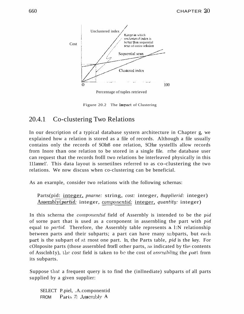
660 CHAPTER 20
Cost
Unclustered indexRange in whichuncl'Ustered index isbetter than sequentialscan of entire relation
oPercentage of tuples retrieved
Figure 20.2 The Impa.ct of Clustering
20.4.1 Co-clustering Two Relations
100
In our description of a typical database systern architecture in Chapter g, weexplained how a relation is stored as a file of records. Although a file usuallycontains only the records of SOIn8 one relation, SCHue systeIlls allow recordsfrorn Inore than one relation to be stored in a single file. rrhe database usercan request that the records froIll two relations be interleaved physically in this111anne1'. This data layout is sornetiInes referred to as co-clustering the tworelations. We now discuss when co-clustering can be beneficial.
As an exarnple, consider two relations with the following schernas:
Parts(pid: integer, pnarne: string, cost: integer, 8upplierid: integer)Asserllbly"(part'id: integer, cOT!.!,ponent~d: integer, quantity: integer)
In this scherna the cO'nl,ponentid field of Assernbly is intended to be the pidof sorne part that is used as a cornponent in assernbling the part with pidequal to partido Therefore, the Assernbly table represents a l:N relationshipbetween parts and their subparts; a part can have rnany S11 bparts, but eachpart is the subpart of at rnost one part. In, the Parts table, pid is the key. ForcOlnposite parts (those assernbled frorIl other parts, a.s indicated by the contentsof Assclnb1y), the cost field is taken to be the cost of a.sselubling the part frornits subparts.
Suppose tha.t a frequent query is to find the (inllnediate) subparts of all partssupplied by a given supplier:
SELECT P.piel, .A.componentidFROM Pql't'c' 'J") AS''''(.'·\I'Xll'')I't" A. (L" 11:::1 .. , \,S ..' ",r "
Physical Database Design atut Tuning
WHERE P.piel = A.partid AND P.supplierid = 'Acrne'
6ljl
A good evaluation plan is to apply the selection condition on Parts a,nel thenretrieve rnatching Asselnbly tuples throngh an index on the partid field. Ideally,the index on part'id should be clustered. rrhis plan is rea,,'30rHlbly good. :However,if such selections are COHU110n and we \.vant to optirnize thorn further, ,ve canco-cZ'usteT' the tvvo tables. In this approach, we store records of the two tablestogether, \vith each Parts record P follc)\ved by all the Assernbly records ./1 suchthat P.pid = A.partid. This approach improves on storing the two relationsseparately and having a, clustered index on paTtid because it does not need anindex lookup to find the A.ssernbly records that rnatch a given Parts record.Thus, for each selection query, we save a few (typically two or three) indexpage l/Os.
If we are interested in finding the imrnediate subparts of all parts (i.e., thepreceding query with no selection on supplierid) , creating a clustered index onpaTtid and doing an index nested loops join with Assembly as the inner relationoffers good perfonnance. An even better strategy is to create a clustered indexon the paTtid field of Assernbly and the pid field of Parts, then do a sort-rnergejoin, using the indexes to retrieve tuples in sorted order. This strategy iscomparable to doing the join using a co-clustered organization, which involvesjust one scan of the set of tuples (of Parts and Asselnbly, which are storedtogether in interleaved fashion).
The real benefit of co-clustering is illustrated by the following query:
SELECT P.pid,A.componentidFROM Parts P, Assernbly AWHERE P.pid = A.partid AND P.cost=10
Suppose that rnany parts have cost = 10. This query essentially a,rnonnts toa collection of queries in which we are given a Parts record and want to findrnatching Assernbly records. If we have an index on the cost field of Parts, wecan retrieve qualifying Parts tuples. I~'or each such tuple, we haNe to use theindex on Assernbly to locate records with the given pid. rrhe index access forA.ssernbly is avoided if we have a co-clustered organization. (()f courS8, vve stillrequire all index on the cost attribute of Parts tuples.)
Such an optirnization is especiftlly irnportant if we ,vant to traverse severallevels of the part-subpart hierarchy..For excunplc, a COnll110Il query is to findthe totaJ cost of a part, vvhich requires us to rep(~atedly carry out joins ofPa,rts (lIlel Asscrnbly. Incidentally~ if '\:V(~ do not know the nurnber of levels inthe hierarchy ill adVallCf\ the nUlnber of joins varies and the query cannot be(~xpressed in S(~L. The query can be ansvvered by ernbedcling an S(~L staterneIlt
662 (;IIAPTER 20
for the join insicie an iterative host language prograrll. fluw to express the queryis orthogonal to our lnain point here, which is that co-clustering is especiallybeneficial \vhen the join in question is carried out very frequently (either becauseit arises repeatedly in an ilnportant query such as finding total cost, or becausethe join query itself is asked frequently).
To sUIlunarize co-clustering:
III It can speed up joins, in pa,rticular key· foreign key joins corresponding tol:N relationships.
III A sequential scan of either relation becornes slower. (In our exalnple, sinceseveral Assenlbly tuples are stored in bet\veen consecutive Parts tuples, ascan of alll:>arts tuples becornes slower than if Parts tuples \vere stored separately. SiInilarly, a sequential scan of all Assernbly tuples is also slower.)
Ii All inserts, deletes, and updates that alter record lengths becorne slower,thanks to the overheads involved in ruaintaining the clustering. (We donot discuss the irnplernentation issues involved in co-clustering.)
20.5 INDEXES THAT ENABLE INDEX--ONLY PLANS
This section considers a nU111ber of queries for which we can find efficient plansthat avoid retrieving tuples froln one of the referenced relations; instead, theseplans scan an associated index (which is likely to be lnuch srnaller). An indexthat is used (only) for index-only scans does not have to be clustered becausetuples fronl the indexed relation are not retrieved.
This query retrieves the lnanagers of depal'truents with at least one ernployee:
SELECTD.rugrFROM Departrnents I) ~ F~rnployees EWHERE I).dno=E.dno
()bserve that no attributes of Ernployees are retahlcd. If ¥lC have an index onthe dno field of Ernployees: tl1e optirnization of doirlg an index nested loops joinusing an index-onl:y searl for the inner relation is applicable. C;iven this variantof the quer:y, the correct d(-~cision is to build an uncIustered index on tll(~ dnafield of Elfll>loyees, rather thaIl a clustered index.
rrhe next query takes this idea a step further:
SELECT ]) .rngr ,E.eidFROM ])epartrnents I), Ernployees EWHERE D.dno=E.dno
&63
If \ve have an index on the lino field of :Elnployees~weGan use it to retrieveEU.lployees tuples during the join (\vith Departrnents a",~ the alIter relation),but unless the index is clustered, this approach is not be efficient. ()n theother hand, suppose that vve have a B+- tree index on (dna, e'id).Now all theinforrnation \ve need about an Ernployee,s tuple is contained in the data entryfor this tuple in the index. We can use the index to find the first data entry\vith a given elno; all data entries 'with the SeHne dno are stored together in theindex. (Note that a ha'3h index on the cOlnposite key (dna, eid) cannot be usedto locate an entry with just a given dno!) \\Te can therefore evaluate this queryusing an index nested loops join with Departlnents as the outer relation andan index-only scan of the inner relation.
20.6 TOOLS TO ASSIST IN INDEX SELEC"fION
The rUllnber of possible indexes to consider building is potentially very large:For each relation, we can potentially consider all possible subsets of attributesas an index key; we have to decide on the ordering of the attributes in the index;and we also have to decide which indexes should be clustered and which unclustered. Many large applications---for exalnple enterprise resource planningsysterns~--··createtens of thousands of different relations, and rnanual tuning ofsuch a large schelna is a daunting endeavor.
The difficulty and irnportance of the index selection tc'ksk rnotivated the development of tools that help database adrninistrators select appropriate indexesfor a given workload. The first generation of such index tuning wizards, orindex advisors, were separate tools outside the database engine; they suggested indexes to build, given a workload of SQL queries. rfhe rnain drawbackof these systerns was that they had to replicate the database query optirnizer'scost rnodel in the tuning tool to rnake sure that the optilnizer would choose thesanlC query evaluation plans as the design tool. Since query optirnizers cha,ngefroIn release to release of a conunercial databa.se systern, considerable effort wasneeded to keep the tuning tool and the database optirnizer synchronized. Thernost recent g(~neration of tuning tools are integrated \vith the database engineand use the database query optiluizer to estirnate th(~ cost of a workload givena set of indexes, cl,voiding duplication of the query optirnizer's cost rnodel intoan external tool.
20.6.1 Automatic Index Selection
\{Ve call a set of indexes for a given database scherna. an index configuration.\Ve aSSlune that a, query workload is a set of queries over a databc'kse scherna'INhere each query has a frequency of occurrence assigned t.o it. (jiven a databaseschelna and a, workload, the cost of an index configuration is the expected
664 CHAPTEI{ 2JJ
cost of running the queries in the 'workload given the index configurationtaking the different frequencies of queries in the workloa-d into account. (jivena database schclna and a query workload, we can no\v define the problel11 ofautomatic index selection as finding an index configuration \vith nlinirnalcost. A.s in query optinlization, in practice our goaJ is to find a good indexconfiguration rather than the true optirnal configuration.
\Vhy is autollultic index selection a hard problern? Let us calculate the nUlnberof different indexes \vith c attributes, assurning that the table hc),sn attributes.For the first attribute in the index, there are n choices, for the second attributen ~ 1, and thus for a, c attribute index, there are overall n· (n -1) ... (n -'- c+ 1) =
(, ~! )' different indexes possible. The total nurnber of different indexes with upn c.to c attributes is
c ,
2: _!!-_.. "'i=l (n - 1,).
For a table with 10 attributes, there are 10 different one-attribute indexes, 90different two-attribute indexes, and 30240 different five-attribute indexes. Fora cornplex workload involving hundreds of tables, the nurnber of possible indexconfigurations is clearly very large.
The efficiency of autornatic index selection tools can be separated into twocomponents: (1) the nurnber of candidate index configurations considered, and(2) the nurnber of optimizer calls necessary to evaluate the cost for a configuration. Note that reducing the search space of candidate indexes is analogous torestricting the search space of the query optiInizer to left-deep plans. In lnanycases, the optirnal plan is not left-deep, but alllong all left-deep plans there isusually a plan whose cost is close to the optirnal plan.
We can easily reduce the tiIne taken for autornatic index selection by reducingthe nUlnber of candidate index configurations , but the srnaller the space ofindex. configurations considered, the farther away the final index configuration is[1'0111 the optirnal index configllration. rrherefore, different index tuning \vizardsprune the search space differently, for exarnple, by considering onl:y one- or twoattribute indexes.
20.6.2 How Do Index Thning Wizards Work?
All index tuning \vizards s(~arch a, set of candidate indexes for an index configuration '''lith lowest cost. 1hols differ in the spa.ce of candidate index configurations they consider aJld how they search this space. \Ve describe onerepresentative algoritlun; existing tools iInplernent 'variants of this algorithrn,hut their irnplernentations have the sanIe basic structun~.
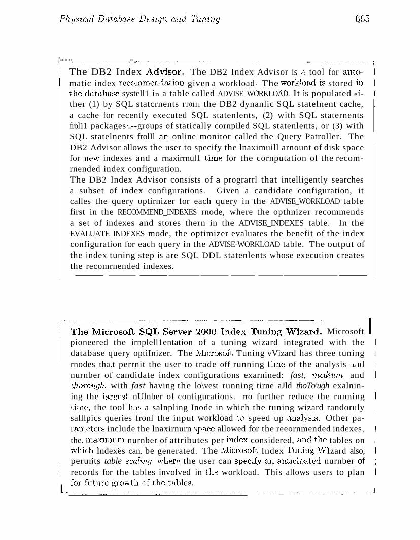
Physical Databa,se Design and 11_ln'ing G65
r-·······..-··---...----·····..·.··....··.-~-·· .."..--·-_............ .. ... .....~.--------lI The DB2 Index Advisor. The DB2 Index Advisor is a tool for auto- II matic index recon1nl~ndationgiven a workload.. The workl?adis stored i~ I
the databa~~e systell1 In a table called ADVISE_WORKLOAD. It IS populated e1- Ither (1) by SQL statcrnents 1'1'0111 the DB2 dynanlic SQL statelnent cache, .a cache for recently executed SQL statenlents, (2) with SQL staternentsfrol11 packages·....--groups of statically cornpiled SQL statenlents, or (3) withSQL statelnents frolIl an online monitor called the Query Patroller. TheDB2 Advisor allows the user to specify the lnaximuill arnount of disk spacefor ne\v indexes and a rnaxirrnul1 tiTne for the cornputation of the recomrnended index configuration.The DB2 Index Advisor consists of a prograrrl that intelligently searchesa subset of index configurations. Given a candidate configuration, itcalles the query optirnizer for each query in the ADVISE_WORKLOAD tablefirst in the RECOMMEND_INDEXES rnode, where the opthnizer recommendsa set of indexes and stores thern in the ADVISE_INDEXES table. In theEVALUATE_INDEXES mode, the optimizer evaluates the benefit of the indexconfiguration for each query in the ADVISE-WORKLOAD table. The output ofthe index tuning step is are SQL DDL statenlents whose execution createsthe recomrnended indexes.
Ghe M~crosoft-~Q~~~~er-;~OO ~~x ;:nin;-Wiz~d. Microsoft l, pioneered the irnplell1entation of a tuning wizard integrated with the I
database query optiInizer. The l\1icrosoft Tuning vVizard has three tuning I
rnodes tha.t perrnit the user to trade off running tiIne of the analysis and !
nurnber of candidate index configurations exarnined: fast, rned-itlm, and IthOTOUgh, with fast having the lo\vest running tirne aJld thoTo'ugh exalnining the h1rgest nUlnber of configurations. rro further reduce the running ItiIne, the tool has a salnpling Inode in which the tuning wizard randoruly :1'
salllpics queries fronl the input workload to speed up analysis. Other panuneters include the lnaxirnurn space allowed for the reeornmended indexes, !the. rn~x.iInu~n nurnber of attributes per i~ldex considered, a~d th:. tables on Ii
\Vl11C}~ Indexes can. be generated. The ~llcroso~'~' Index ~u.lung \\1 Izard also, Iperunts table scall,ng, \vhere the user can specIfy an antIcIpated nurnber of ;
i records for the tables involved in the workload. This allows users to plan I
I.._f~:t~~_~~~th_of::~_~~abl~~:__.____. ~" "" _ __".._" _.__~,._ __"..__.._ __ .J
666 CHAPTER 20
Before we describe the index tuning algoriUlIn, let us consider the problell1 ofestiInating the cost of a configuration. Note that it is not fea...sible to actually create the set of indexes in a candidate configuration and then optirnizethe query workload given the physical index configuration. Creation of even asingle candidate configuration with several indexes lIlight take hours for largedatabases and put considerable load on the database systerIl itself. Since wevvant to exauline a large nUlnber of possible candidate configurations, this approach is not feasible.
Therefore index tuning algorithrIls usually .sim,ulate the effect of indexes ina candidate configuration (unless such indexes already exist). Such what-ifindexes look to the query optilIlizer like any other index and are taken intoaccount when calculating the cost of the workload for a given configuration,but the creation of what-if indexes does not incur the overhead of actual indexcreation. Commercial databa..'3e systelIls that support index tuning wizardsusing the database query optirnizer have been extended with a module thatpermits the creation and deletion of what-if indexes with the necessary statisticsabout the indexes (that are used when estirnating the cost of a query plan).
We now describe a representative index tuning algorithm. The algorithm proceeds in two steps, candidate index selection and cor~figuration enumeration. Inthe first step, we select a set of candidate indexes to consider during the secondstep as building blocks for index configurations. Let us discuss these two stepsin Inore detail.
Candidate Index Selection
We saw in the previous section that it is iInpossible to consider every possibleindex, due to the huge nUluber of candidate indexes available for larger databa.'3cschernas. ()ne heuristic to prune the large space of possible indexes is to firsttune each query in the workload independently and then select the union ofthe indexes selected in this first step as input to the second step.
:F'or a query, let us introduce the notion of an indexable attribute, which is anattribute whose appearance in an index could change the cost of the query. Anindexable attribute is an attribute on \vhich the WHERE-part of the query h(4'3a condition (e.g., an equality predicate) or the attribute appears in a GROUP BYor ORDER BY clause of the SC~L query. An admissible index for a query is anindex that contains only indexable attributes in the query.
JIo\v do we select candidate indexes for an individual query? ()ne approach isa ba.sic ellurnenttion of all indexes with up to k attributes. \Ve start \ivith aUindexable attributes as single attribute candidate ind(~xes, then add all corn-
[>hysical Database ]Jc8ign and T11ning
binations of two indexable attributes &'3 candidate indexes, and repeat thisprocedure until a user-defined size threshold k. 'This procedure is obviouslyvery expensive a., we add overall n +n· (n - 1) + ... +n· (n - 1) ... (n·- k + 1)candidate indexes, but it guarantees that the best index with up to k attributesis aIl10ng the candidate indexes. The references at the end of this chapter COIl
tain pointers to faster (but less exhaustive) heuristieal search algorithrns.
Enumerating Index Configurations
In the second phase, we use the candidate indexes to enUInerate index configurations. As in the first phase, we can exhaustively enurnerate all indexconfigurations up to size k, this time cornbining candidate indexes. As in theprevious phase, more sophisticated search strategies are possible that cut downthe number of configurations considered while still generating a final configuration of high quality (i.e., low execution cost for the final workload).
20.7 OVERVIEW OF DATABASE TUNING
After the initial phase of databa.se design, actual use of the database providesa valuable source of detailed information that can be used to refine the initialdesign. Many of the original a.ssulnptions about the expected workload can bereplaced by observed usage patterns; in general, some of the initial workloadspecification is validated, and some of it turns out to be wrong. Initial guessesabout the size of data can be replaced with actual statistics frorn the systern catalogs (although this inforrnation keeps changing as the systern evolves).Carefulrnonitoring of queries can reveal unexpected problerlls; for eXaJnple, theoptirnizer lllay not be using SOIne indexes &'3 intended to produce good plans.
Continued database tuning is irnportant to get the best possible perforrnance.In this section, we introduce three kinds of tuning: tun'ing 'inde1;(~8J tun'ing theconceptual scherna, and tuning queT'ies. OUf discussion of index selection alsoapplies to index tuning decisions. Conceptual schcrna and query tuning arediscussed further in Sections 20.8 and 20.9.
20.7.1 Thning Indexes
The initial choice of indexes rnay be refined for one of several reasons. 'fhesirnplest reeL-son is that the observed \vorkload reveals that scnne queries andupdates considered irnportant in the initial\vorkload specification are not veryfrequent. 1'he observed \vorkload rnay a1so identi~y SCHne ne\v queries and updates that aTe inlportant.The initial choice of indexes has to be revievved inlight of this new inforrnation. Scnne of the original in,dexes rnay be dropped and
668 CHAPTER 20
new ones added. The rea.solling involved is siInilar to that used in the initialdesign.
It Inay also be discovered that the optimizer in a given systenl is not findingsome of the plans that it vvc1"s expected to. For exaluple, consider the followingquery, which \ve discussed earlier:
SELECT D.IngrFROM Ernployees E, Departulents DWHERE D.dname=='Toy' AND E.dno=D.dno
A good plan here would be to use an index on dnarne to retrieve Departnlentstuples with dnarne= 'Toy' and to use an index on the dno field of Employees asthe inner relation, using an index-only scan. Anticipating that the optirnizerwould find such a plan, we rnight have created an unclustered index on the dnofield of Ernployees.
Now suppose queries of this fonn take an unexpectedly long time to execute. Wecan ask to see the plan produced by the optiInizer. (Most commercial systerIlsprovide a simple cOillrnand to do this.) If the plan indicates that an index-onlyscan is not being used, but that Employees tuples are being retrieved, we haveto rethink our initial choice of index, given this revelation about our system's(unfortunate) lhnitations. An alternative to consider here would be to drop theunclustered index on the dno field of EUlployees and replace it with a clusteredindex.
SOUle other COllllnon lirnitations of optiInizers are that they do not handleselections involving string expressions, arithrnetic, or null values effectively.We discuss these points further when we consider query tuning in Section 20.9.
In addition to re-exarnining our choice of indexes, it pays to periodically reorganize S(Hne indexes. For example, a static index, such <he.:; an ISAl\Il index~ Illayhave developed long overflow chains. Dropping the index and rebuilding it ..···_·-iffeasible, given the interrupted access to the indexed relation----··can substantiallyirnprove access tiTHes through this index. Even for a dynarnic structure suchas a 13+ tree, if the implernentation does not rnerge pages on deletes, spaceoccupancy can decrea"se considerably in SaIne situations. This in turn rnakesthe size of the index (in pages) larger than necessary, and could increase theheight and therefore the access tilne. Ilebuilding the index should be considered.Extensive updates to a clustered index rnight also lead to overflow pagesbeing allocated, thereby decreasing the degree of clustering. Again, rehuildingthe index Inay be vvorthwhile.
Physical [Jatubasc Design (l,'ndTnnin,g 669@
l?inally, note that the query optinlizer relies on statistics rnaintained in theSystCIll catalogs. These statistics are updated only "til/hen a special utility progranl is run; be sure to run the utility frequently enough to keep the statisticsreasonably current.
20.7.2 Thning the Conceptual Schema
In the course of datab&'Se design, \ve rnay realize that our current choice ofrelation SChelllaS does not enable us rneet our perforrnance objectives for thegiven vvorkload with any (feasible) set of physical design choices. If so, \ve11lay have to redesign our conceptual scherna (and re-exarnine physical designdecisions affected by the changes we rnake).
We rnay realize that a redesign is necessary during the initial design process orlater, after the systern has been in use for a while. Once a database has beendesigned and populated with tuples, changing the conceptual scherna requiresa significant effort in tenrlS of rnapping the contents of the relations affected.Nonetheless, it rnay be necessary to revise the conceptual scherna in light ofexperience with the systern. (Such changes to the schema of an operationalsysterll are sometirnes referred to as schema evolution.) \lVe now considerthe issues involved in conceptual scherna (re)design frorn the point of vie\v ofperforrnance.
rrhe rnain point to understand is that OUT choice of concepb.lal 8cherna shouldbe gv-ided by a cons'ideration of the querflc8 and 'updates in our 'workload" inaddition to the issues of redundancy that rllotivate nonnalization (which wediscussed in Chapter 19). Several options rnust be considered while tuning theconceptual scherna:
IlIII \Ve lIlay decide to settle for a :3NF design instead of a BCN'F design.
III If there are two ways to decornpose a given schelna into 3NF or BCNF\ ourchoice should be guided by the workload.
III Sornetilnes we rnight decide to further decornpose a relation that is already. BC1 NF'-'rn :./1 .
III In other situations, we rnight denorrnalizc. rrhat is~ \ve rnight choose toreplace a cOllection of relations obtained by a dec(nnposition frorn a largerrelation ,vith the original (larger) relation, even though it suffers frorn 80rneredundancy problerl1s. Alternatively, we rnight choose to H.del sorne fieldsto certain relations to speed up SCHne irnportant queries, even if this leadsto a redundant storctge of 80rne infonnation (anei, consequently, a schernathat is in neither :3NF nor BCNF).
670 C~IIAPTER 20
II This discussion of nonnalization has concentrated on the technique of deCO'f17JJo8'ition, 'which arnounts to vertical partitioning of a relation. Anothertechnique to consider is horizontal ],Jartit'ion/ing of a relation, 'which \vouldlead to having two relations v'lith identical schernas. Note that we are nottalking about physically partitioning the tuples of a single relation; rather,\ve \vant to create two distinct relations (possibly \vith different constraintsand indexes on each).
Incidentally, when \ve redesign the conceptual scherna, especially if we are tuning an existing database sche1na, it is \vorth considering whether V'le shouldcreate vic\vs to rnask these changes fronl users for WhOlll the original schcrlla is]nore natural. \\le discuss the choices involved in tuning the conceptual schernain Section 20.8.
20.7.3 Thning Queries and Views
If we notice that a query is running rnuch slower than we expected~ we have toexarnine the query carefully to find the problern. SaIne rewriting of the query,perhaps in conjunction with SCHne index tuning, can often fix the problern. Sirnilar tuning rnay be called for if queries on SaIne view run slower than expected.We do not discuss view tuning separately; just think of queries on views asqueries in their own right (after all, queries on views are expanded to accountfor the view definition before being optirnized) and consider hcnv to tune thern.
vVhen tuning a query, the first thing to verify is that the systern uses the planyou expect it to use. Perhaps the systelll is not finding the best plan for avariety of rcclsons. Sorne COIllrllon situations not handled efficiently by rnanyoptinlizers follow:
.. A selection condition involving null values.
l1li Selection conditions involving aritlunetic or string expressions or conclitions using the OR connective. For exarnple, if we have a conclitionE. age= 2*]). age in the WHERE clause, the optirnizer rnay correctly utilize anavailable index onE. age but fail to utilize an availclble index on 1). age.R,eplacing the condition by 1;;. age/2 = 1). age \vould reverse the situation.
IIi1I Inability to recognize a sophisticated plan such as an index-only scan foran aggregation query involving a GROUP BY clause. ()f course, virtually nooptirnizer looks for plans outside the plan space described in Chapters 12and 15, such cL.snonleft-deep join trees. So a good urHl(~rstandingof ·whatan optirnizer typically does is irnportant. In addition, the rnore a:ware youare of a given systeur's strengths arrd lirnitations, the better off Y01J arc.
Physical IJataba.se Dcs'ign and 'Tun'ing 611
If the optirnizer is not SIl1art enough to find the best pla.n (using access Inethodsand evaluation straJegies supported by the DB.wIS), SOHle systern.s allo\v usersto guide the choice of a plan by providing hints to the opthnizer; for exalnplc,users rnight be able to force the use of a particular index or choose the joinorder and join rnethod. A user who wishes to guide optirnization in this Inannershould have a thorough understanding of both optirnizatioll and the capabilitiesof the given DBNIS. We discuss query tuning further in Section 20.9.
20.8 CHOICES IN TUNING THE CONCEPTUALSCHEMA
We novv illustrate the choices involved in tuning the conceptual scheIua throughseveral exarnples using the following schelnas:
Contracts( cid: i~.~eger, s'Upplierid: integer, projectid: integer,deptid: integer, partid: integer, qty: integer, value: real)
Departments (did: integer, budget: real, annualreport: varchar)Parts(pid: integer, cost: integer)Projects(jid: integer, rngr: char(20))
_.- -Suppliers (sid: _..~.:nteger, address: char(50))
For brevity, we often use the cornrnon convention of denoting attributes bya single character and denoting relation schernas by a sequence of characters.Consider the scherna for the relation Contracts, whic.h we denote as CSJDPQV,with each letter denoting an attribute. The Ineaning of a tuple in this relationis that the contract with cid C is an agreernent that supplier S (with sid equalto supplierid) will supply (~ iterns of part P (with pid equal to partid) to projectJ (with j'id equal to projectid) a.'3sociated with departrnent D (with deptid equalto did), and that the value V of this contract is equal to value. 2
There are two known integrity constraints with respect to Contracts. A projectpurdHk')cs a given part using a single contract; thus, there cannnot be twodistinct contracts in which the saIne project buys the saIne part. This constraintis represented using th.e FI) .II) ----;. (.1. Also, a departrnent purchases at rnostone part frolll any given supplier. This constraint is represented llsing the I?D8D ----;. I). In addition, of course, the contract ID C is a key. l"1he rneaningof the other relations should be obvious, and we do not describe thcrn furtherbecause we focus on the Contra.cts rela.tion.
2If this schema seems cornplicated, note that real-life situations often call for considerably morecornplex schema.,,':>!
672 CHAPTER 4()
20.8.1 Settling for a Weaker Normal Form
Consider the Contracts relation. Should we deconlpose it into sHlaller relations?Let us see what norrnal fann it is in. '1'he candidate keys for this relation are Cand .1P. (C is given to be a key~ and tIP functionally deterrnines C.) The onlynonkey dependency is 3D -+ P, and P is a pri'rne attribute because it is partof candidate key JP. rrhus, the relation is not in BC:NF···because there is anonkey dependency-..·..·....but it is in 3NF.
By using the dependency 8 D -tP to guide the decornposition, we get thet"vo sclH~rnas SDP and CSJDQV. This decornposition is lossless~ but it is notdependency-preserving. lfo\vever, by adding the relation schelne CJP, we obtain a lossiess-join, dependency-preserving decoruposition into BCNF. Usingthe guideline that such a decorllposition into BCNF is good, we might decideto replace Contracts by three relations with schernas CJP, SDP, and CSJDQV.
However, suppose that the following query is very frequently asked: Find thenurnber of copies Q of part P ordered in contract C. 'rhis query requires a join ofthe decornposed relations CJP and CSJDQV (or SDP and CSJDQV), wherea..'3it can be answered directly using the relation Contracts. The added cost forthis query could persuade us to settle for a 3NF design and not decomposeContracts further.
20.8.2 Denormalization
The rea.'3ons rTIotivating us to settle for t1 weaker norrnal forIn lIlcl;Y lead us totake an even rnore extrerne step: deliberately introduce SOlllC redundancy. Asan exarnple, consider the Contracts relation, 'which is in 3NF. Now, supposethat a frequent query is to check that the value of a contract is less thanthe budget of the contracting departruent. \Ve lllight decide to add a budgetfield B to Contracts. Since did is a key for Departrnents , \ve now have thedependency D -+ B in Contracts, \vhich InCt1IlS Contracts is not in 3NF anyr11orc. Nonethelf~ss, vVf~ rnight choose to stay vvith this design if the rnotivatingquery is sufficiently irnportant. Such a decision is clearly subjective and CaInesat the cost of significant redundancy.
20.8.3 Choice of Decomposition
Consider the Contracts relation again. Several choices are possible for dealingwith the redundancy in this relation:
IIiI \Ve can leave C\)ntracts as it is ::uld accept the rcchu1dancyr associaJed \\"ithits being in :3N:F ratller than .BCNF.
Ph:lp"ical Database Desiign and ~r1tning 673if
• \Ve Inight decide that we want to avoid the anolIlalies resulting froIn this redundancy by deeornposing Contracts into BC;NF using one of the followingruethods:
·0__ \Ve have a lossless-join decornposition into Partlnfovvith attributesSDP and Contractlnfo \vith attributes CSJDQ\l. As noted previously,this decornposition is not dependency-preserving, and to rnake it so\vould require us to add a third relation CJP: \vhose sale purpose is toallow us to cheek the dependency J P -+ C.
- \Ve could choose to replace Contracts by just Partlnfo and ContractInfo even though this decornposition is not dependency-preserving.
R,eplacing Contracts by just Partlnfo and Contractlnfo does not prevent usfrorll enforcing the constraint JP -+ C; it only makes this n10re expensive. Wecould create an assertion in SQL-92 to check this constraint:
CREATE ASSERTION checkDepCHECK ( NOT EXISTS
(SELECT *FROM Partlnfo PI, Contractlnfo ClWHERE PI. supplierid==CI. suppl'ierid
AND PI. deptid==CI. deptidGROUP BY C1.projectid, PI. partidHAVING COUNT (cid) > 1 ) )
This assertion is expensive to evaluate because it involves a join followed by asort (to do the grouping). In cornparison, the systerll can check that JP is aprirnary key for table CJP by rnaintaining an index on J P. This difference inintf~grity-checking cost is the rl1otivation for dependency-preservation. On theother hand, if updates are infrequent, this incrcclE;ed cost IIlay be acceptable;therefore, we rnight choose not to rnaintain the table C.JP (and quite likely, anindex all i~;).
As another exarnple illustrating decornposition choices, consider the Contractsrelation again, Etud suppose that we also have the integrity constraint that adepartrnent uses a given supplier for at rnost one of its projects: SPCJ --7 V.Proceeding (1"S before, we have a lossless-join decornposition of Contracts intoSDP and CSJDQV. Alternatively:\ve could begin by using the dependency8 PQ ----+ V to guide our decornpositioIl: and replace Contracts with SPQV andCS.JI)P(~. vVe can then dec(Hnpose CSJI)P(~, guided by 51D -+ P, to obtainSDP and CS.JD(~.
\Ve now have two alternative lossless-join decornpositions of Contracts intoBC:N}"\ neither of which is dependency-preserving. 'fhe first alternative is to
674 (~HAPTER 20&
replace Contra~~ts\viththe relations SDP and CS.JDC~V.The second alternativeis to replace it \vith SPQV, SDP, and (]SJD(~. The addition of CJP HU1kes thesecond deC0111positioll (but not the first) dependency-preserving. Again, thecost of lnaintaining the three relations CJP, SP(~V, and CSJD(~ (versus justCSJDQV) Illay lead us to choose the first alternative. In this ca..se, enforcingthe given FDs becornes Inore expensive. vVe Illight consider Ilot enforcing thern,but we then risk a violation of the integrity of our data.
20.8.4 Vertical Partitioning of BCNF Relations
Suppose that we have decided to decornpose Contracts into SDP and CSJDQV.These scheruas are in BCNF, and there is no reason to decornpose thern furtherfrom a nonl1alization standpoint. However, suppose that the following queriesare very frequent:
• Find the contracts held by supplier S.
• Find the contracts placed by departrnent D.
These queries rnight lead us to decompose CSJDQV into CS, CD, and CJQV.The decornposition is lossless, of course, and the two il11portant queries can beanswered by exarnining 111uch slualler relations. Another reason to consider sucha dec()l11position is concurrency control hot spots. If these queries are COIllIllon,and the rnost COIlunon updates involve changing the quantity of products (andthe value) involved in contracts, the decoulposition inlproves perforrnance byreducing lock contention. Exclusive locks are now set rnostly on the CJ(~V
table, and reads on CS and CD do not conflict with these locks.
Whenever we decornpose a relation, we have to consider which queries thedecolnposition rnight adverse~y affect, especially if the only rnotivation for thedecoInposition is iUlproved perforrnance. "For exaruplc, if another illlportantquery is to find the total value of contracts held by a supplier, it would involvea join of the decornposed relations CS and C.J(~V. In this situation, we rnightdecide against the decolnposition.
20.8.5 Horizontal Decomposition
Thus far, we have essentially considered how to replace a relation v'lith a collection of vertical decorupositions. Sornetilnes, it is \vorth considering whethf~r
to repla.ce a relation with t\VO relations that have the sa.Dle attributes as theoriginal relation, ea..eh containin.g a subsf'.t of thf~ tuples in tb.e original. Intuitively, this technique is useful \vhen different subsets of tuples are queried invery distinct ways.
675l'
For exanlple, different rules lnay govern large contracts, \vhich are defined a~"
contracts with values greater than 10,000. (Perhaps, such contra<cts have to beawarded through a bidding process.) This constraint could lead to a nUlnberof queries in which Contracts tuples are selected using a condition of the forIII
value > 10, 000. On8 way to approach this situation is to build a clusteredB+ tree index OIl the value field of Contracts. Alternatively, we could replaceContracts with t\VO relations called LargeContracts and SrnallContracts, withthe obvious 11leaning. If this query is the only lllotivation for the index, horizontal decornposition offers all the benefits of the index without the overhead ofindex maintenance. This alternative is especially attractive if other irnportantqueries on Contracts also require clustered indexes (on fields other than val'ue).
If we replace Contracts by two relations LargeContracts and SrnallContracts,we could r1l8sk this change by defining a view called Contracts:
CREATE VIEW Contracts(cid, supplierid, projectid, deptid, partid, qty, value)AS ((SELECT *
FROM LargeContracts)UNION(SELECT *FROM SmallContracts))
However, any query that deals solely with LargeContracts should be expresseddirectly on LargeContracts and not on the view. Expressing the query on theview Contracts with the selection condition value> 10, 000 is equivalent toexpressing the query on LargeContracts but less efficient. This point is quitegeneral: Although we can rllth"k changes to the conceptual scherlla by addingview definitions, users concerned about perforrnance have to be aware of thechange.
As another exanlple, if Contracts had an additional field yeaT and queries typically dealt with the contracts in sorne one year, we rnight choose to pa,rtitionContracts by year. ()f course, queries that involved contracts fron1 rnore thanone year rnight require us to pose queries against each of the decolllposed relations.
20.9 CHOICES IN TUNING QUERIES AND VIEWS
T'he first step in tuning a query is to understand the plan used by the I)B1-18to evaluate the query. 8ysten1s usually provide sorne facility for identifyingthe plan used to evaluate a query. ()nce\ve understand the plan selected bythe systelIl, we can consider how to irnprove perfornu:Ulce. "\Ve can consider adifferent choice of ilHlexes or perhaps co-clustering two relations for join queries,
676 C~HAPTER 20
guided by our understanding of the old plan and a better phtn that we wanttheDBlVIS to use. The detaHs are sinlilar to the initial design process.
One point'worth rnaking is that before creating ne"v indexes we should consider\vhether rewriting the query achieves acceptable results with existing indexes.For example, consider the foll()\ving query with an OR connective:
SELECT E.dnoFROM Ernployees EWHERE E.hobby='Stalnps' OR E.age==10
If \ve have indexes on both hobby and age, we can use these indexes to retrievethe necessary tuples, but an optiInizer ruight fail to recognize this opportunity.The optinlizer rnight view the conditions in the WHERE clause &1;) a whole &'3
not rnatching either index, do a sequential scan of Ernployees, and apply theselections on-the-fly. Suppose we rewrite the query ElS the union of two queries,one with the clause WHEREE.hobby= 'Starnps" and the other with the clauseWHERE E.agc==10. Now each query is answered efficiently with the aid of theindexes on hobby and age.
We should also consider rewriting the query to avoid sorne expensive operations.for exalnple, including DISTINCT in the SELECT clause leads to duplicate elirnination, which can be costly. rrhus, we should ornit DISTINCT whenever possible. For exalnple, for a query on a single relation, we can ornit DISTINCTwhenever either of the following conditions holds:
II We do not care about the presence of duplicates.
II rrhe attributes lllentioned in the SELECT clause include a candidate key forthe relation.
SOlnetirnes a query \vith GROUP BY and HAVING can be replaced by a querywithout these clauses, thereby eliminating c1 sort operation. For ext1rnplc, COIl
sider:
SELECTFROMGROUP BYHAVING
MIN (E.age)Ernployees EE.dnoE' ..}. " '1 ()'>;.( no=:::, , ~
This quer:y is equivalent to
SELECTFROMWHERE
MIN (E. age)Erl1ployees EE.dno=102
PhU,'.fical Database ]Jesign and 1'lf,n'ing 677t
Cornplex queries are often \vritten in steps, using a ternporary relation. \\lecan usually re\vrite such queries without the tClnporary relation to rnake thcrnrun faster. Consider the following query for cornputi.ng the average salary ofdepartrnents rnanaged by Robinson:
SELECTINTOFROMWHERE
*TernpErnployeesE, Depa:rtruents DE.dno==D.dno AND D.rngrnanle='Robinson'
SELECT T.dno, AVG (T.sal)FROM T'clnp TGROUP BY T.dno
This query can be rewritten a.s
SELECTFROMWHEREGROUP BY
E.dno, AVG (E.sal)Elnployees E, Departlnents DE.dno==D.dno AND D.rngrnarne=='llobinson'E.dno
The rewritten query does not 111aterialize the interrnediate relation ,Ternp and istherefore likely to be faster. In fact, the optimizer may even find a very efficientindex-only plan that never retrieves Ernployees tuples if there is a cornpositeB+· tree index on (d'no, sal). This exanlple illustrates a general observation: ByTewriting queries to avoid 'Unnecessary temporaries, we not only avoid creatingthe ternporary relations, we also open up rnore opt'im,ization possibilit'ies for theoptim,izer to el;plore.
In SCHne situations, ho\vever, if the optirnizer is unable to find a good plan for acornplex query (typically a nested query with correlation), it rnay be worthwhileto re\vrite the query using tenlporary relations to guide the optirnizer towarda good plan.
In fact, nested queries are a conunon source of inefficiency because luany optirnizers deal poorly with theIn, as discussed in Section 15.5.v'Vllenever possible,it is better to l:e\vrite a nested query \vithout nesting and a correlated querywithout correlation. As already notfxl, a good reforrIlulation of the query rnayrequire us to introduce ne\v, ternporary relations, and techniques to do so systenlatically (ideally, to be done by the optirnizer) have been \videly studied.()ften tllough, it is possible to re\vrite nested queries ,vithout nesting or the useof ternpora,ry relations, a"s illustrated in Section 15.5.
678 CHAPTER $20
20.10 IMPACT OF CONCURRENCY
In a system with IIlaIlY concurrent users, several additional points IllUSt beconsidered. Transactions obtain locks on the pages they a,ccess, and othertransactions Ina)' be blocked waiting for locks on objects they wish to access.
vVe observed in Section 1().5 that blocking delays 111ust be IniniInized for goodperforrnance and identified two specific ways to reduce blocking:
II R,educing the tilne that transactions hold locks.
II R,edllcing hot spots.
We now discuss techniques for achieving these goals.
20.10.1 Reducing Lock Durations
Delay Lock Requests: Tune transactions by writing to local prograrn variables and deferring changes to the database until the end of the transaction.This delays the acquisition of the corresponding locks and reduces the time thelocks are held.
Make Transactions Faster: The sooner a transaction c01npletes, the soonerits locks are released. We have already discussed several ways to speed upqueries and updates (e.g., tUllillg indexes, rewriting queries). In addition, acareful partitioning of the tuples in a relation and its &'3sociated indexes acrossa collection of disks can significantly irnprove concurrent access. :B-'or exarnple,if we have the relation on one disk and an index on another, accesses to theindex can proceed without interfering with accesses to the relation, at lea""t atthe level of disk reads.
Replace Long Transactions by Short Ones: SometiInes, just too ruuchwork is done within a transaction, and it takes a long tirne and holds locks along tirne. Consider rewriting the transaction as two or Inore sInall(-~r transactions; holdable cursors (see Section 6.1.2) can be helpful in doing this. Theadvantage is that each new transaction cornpletes quicker and releases lockssooner. ~rhe disadvantage is that the original list of operations is no longer executed atolni(~ally, and the application code Illust deal with situations in whichone or rnore of the new transactions fail.
Build a Warehouse: CC)lnplex queries can hold shared locks for a long tirne.()ften, howev('~r, these queries involve statistical analysis of business trends andit is a,cceptable to run theln on a copy of the da.ta that is a little out of date. rrhisled to the popularity of data ?LJaTeho1LBCS, which are databa.'3cs that cornplcnlcnt
}Jhys'ical Database Design and Tnn'ing 61~
the operational datab&"c by rnaintaining a copy of data USE:xl in cornplex queries(Chapter 25). H~unning these queries against the \varehouse relieves the burdenof long-running queries froln the operational datal:H1.'3c.
Consider a Lower Isolation Level: In rnany situations, such as queries generating aggregate infonnation or statistical sununaries, we can use a lo\ver SQLisolation level such as REPEATABLE READ or READ COMMITTED (Section 16.6).
Lo\ver isolation levels incur lower locking overheads, a,nel the application progrannner rllust nUlke good design trade-offs.
20.10.2 Reducing Hot Spots
Delay Operations on Hot Spots: We already discussed the value of delayinglock requests. Obviously, this is especially irnportant for requests involvingfrequently used objects.
Optimize Access Patterns: The patteTn of updates to a relation can also besignificant. For exanlple, if tuples are inserted into the Ernployees relation ineid order and we have a B+ tree index on eid, each insert goes to the last leafpage of the B+ tree. This leads to hot spots along the path froIn the root to therightrnost leaf page. Such considerations nlay lead us to choose a hash indexover a B+- tree index or to index on a different field. Note that this pattern ofaccess leads to poor perforrnance for ISAM indexes as well, since the last leafpage beCOlIles a hot spot. rrhis is not a problcln for hash indexes because thehashing process randornizes the bucket into which a record is inserted.
Partition Operations on Hot Spots: Consider a data entry transactionthat appends new records to a file (e.g., inserts into a table stored as a heapfile). Instead of appending records one-per-transaction and obtaining a lockon the hhst page for each record, we can replace the transaction by severalother transactions, each of which writes records to a local file and periodicallyappends a batch of records to the rnain file. While we do rnore work overall,this reduces the lock contention on the last page of the original file.
_As a further illustration of partitioning, suppose "\ve track the nU111ber of re(~ords
inserted in a counter. Instead of updating this counter once per record, the preceding approad,l results in updating several counters and periodically updatingthe HULin counter. rrhis idea can IJe aclapt(~d to rnany uses of counters, \vithvarying degrees of effort. For exaInple, consider a counter that tracks the Ilurnber of reservations, with the rule that a nc\v reservation is allowed onl~y if thecounter is belo"v a, rnaxiullun value. vVe can replace this by three counters, each\vith one-third the origina11naxirIlurn threshold, and three transactions that usethese counters rather than the original. \\le obtain greater concurrency, but
680 (;HAPTERQO
have to deal with the cc1..58 where one of the counters is at the 111axirnum valuebut SOHle other counter can still be incrcrnented. 1~hus, the price of greaterconcurrency is increased cornplexity in the logic of the application code.
Choice of Index: If a relation is updated frequently, B+ tree indexes canbecolne a concurrency control bottleneck, because all accesses through the indexHUlst go through the root. Thus, the root and index pages just below it canbec()lne hot spots. If the DBMS uses specialized locking protocols for treeindexes, and in particular, sets finc-granularity locks, this problenl is greatlyalleviated. l\Ilany current systeuls use such techniques.
Nonetheless, this consideration lllay lead us to choose an ISA~1 index in SOllIesituations. Because the index levels of an ISAM index are static, \ve need notobtain locks on these pages; only the leaf pages need to be locked. An ISAl\!lindex rnay be preferable to a B·+ tree index, for exalllple, if frequent updatesoccur but we expect the relative distribution of records and the nUlnber (andsize) of records with a given range of search key values to stay approxirnatelythe saIne. In this case the ISAM index offers a lower locking overhead (andreduced contention for locks), and the distribution of records is such that fewoverflow pages are created.
I-Iashed indexes do not create such a concurrency bottleneck, unless the datadistribution is very skewed and lnany data itenlS are concentrated in a fewbuckets. In this ca..'SC, the directory entries for these buckets can beccnne a hotspot.
20.11 CASE STUDY: THE INTERNET SHOP
Revisiting our running case study, I)BDudes considers the expected workloadfor the B(~N 1)00kstore. rrhe owner of the bookstore expects rnost of his CllS
torners to search for books by ISBN nUluber before placing an order. Placingan order involves inserting one record into the ()rders table and inserting oneor lllore records into the Orderlists relation. If a sufficient nurnber of books isavaihtble, a, shiprnent is prepared and a value for the ship.Jlale in the Orderlistsrelation is set. In addition, the available quantities of books in stock changesall the tirne, since orders are placed that; decrease the quantity available andnew books arrive frorn suppliers and increase the quantity available.
The DBDudes tearn begins by considering searches for books by ISBN'. Sinceisbn, is a key~ (l,n equality query on isbn returns at rnost one record. rrhereforc,to speed up queries frolll Cllstolllers who look for books "with a given ISBN,I)BIJudes decides to build an unclustered hash index on L"bn.
]:>hysical jJatabase IJesign, and Tuning 681
Next, it considers updates to book quantities. Tb update the qtll_iTLstock valuefor a book, we IllUSt first search for the book by ISBN; the index on 'isbn speedsthis up. Since the qty_irLstock value for a book is updated quite frequently,DBDudes also considers partitioning the Books relation vertically into the fo11c)\ving two relations:
Books(~ty(isbn, qty)BookH,(~st( 'isbn, title, author" price, yeQ.T_IHlblished)
Unfortunately, this vertical partitioning slows do\vn another very popular query:Equality search on ISBN to retrieve all infonnation about a book no\v requiresa join between BooksQty and BooksH,est. So DBDudes decides not to verticallypartition Books.
DBDudcs thinks it is likely that custonlers "vill also want to search for books bytitle and by author, and decides to add unclustered hash indexes on title andauthor-these indexes are inexpensive to rnaintain because the set of books israrely changed even though the quantity in stock for a book changes often.
Next, DBDudes considers the Custorners relation. A custorner is first identified by the unique custorner identifaction nurnber. So the rnost COlnrnon querieson Custorners are equality queries involving the custolner identification nurnber, and DBDudes decid(~s to build a clustered ha..'3h index on cid to achievemaxirnum speed for this query.
l\!Ioving on to the Orders relation, DBDudes sees that it is involved in twoqueries: insertion of new orders and retrieval of existing orders. Both queriesinvolve the ordcrrl/urn attribute as search key and so DBDudes decides to huildan index on it. What type of index should this be~""·"a 13+ tree or a hash index?Since order nurnbers are assigned sequentially and correspond to the order date,sorting by onleT"n'lun effectively sorts by order date as well. So DBDudes decidesto build a clustered B-t- tree index OIl onlernurn. A.lthough the operationalrequirernents rncntioned until no\v favor neither a 13+ tree nor a hash index,B&N\vill probably want to rnonitor daily a,ctivities and the clustered 13+ treeis a better choice for such range queries. ()f course, this 1118ans that retrievingall orders for a given custorner could be expensive for custolllers with InallYorders, since clustering by o'(ylerntlTn precludes clustering by other attributes,SllCh as cicio
l'he ()rderlists rela,tion involves lnostly insertions, vvith an occfLsionaJ update ofa shiprnent date or a query to list all cOlnponents of a given order. If Orderlistsis kept sorted on oT'dcrnvxn, all insertions are appends at the end of the relationand thus verJr efficient. A clustered 13+ tree index on oT'dernuTn rnaintains thissort order and also speeds up retrieval of aU iterns for a given order. lc) update
682 CHAPTER~O
a shiprnent date, we need to search for a tuple by oT(le1~rrnmj and isbn. Theindex on ordeT'n'Urn helps here as well. Although an index on (ardern:u,rn, 'isbn)would be better for this purpose, insertions would not be as efficient a..,,\vithan index on just oTdeT7rurn; DBDudes therefore decides to index ()rderlists onjust oTCiern7lrn.
20.11.1 Tuning the Database
Several rnonths after the launch of the B&N site, DBDudes is called in and toldthat custorner enquiries about pending orders are being processed very slowly.B&N has becorne very successful, and the Orders and Orderlists tables havegrown huge.
l'hinking further about the design, DBDudes realizes that there are two types oforders: completed orders, for which all books have already shipped, and partiallyco'mpleted order'S, for which sorne books are yet to be shipped. l\Ilost custorIlerrequests to look up an order involve partially corIlpleted orders, which are asInall fraction of all orders. DBDudes therefore decides to horizontally partitionboth the Orders table and the Orderlists table by ordernu'Tn. This results infour new relations: NewOrders, OldOrders, NewOrderlists, and OldOrderlists.
An order and its cornponents are always in exactly one pair of relations····· ..·--andwe can deterrIline which pair, old or new, by a sinlple check on ordernurn-----"andqueries involving that order can always be evaluated using only the relevantrelations. SCHIle queries are now slower, such as those asking for all of a custoruer's orders, since they require us to search two sets of relations. lIowever,these queries are infrequent and their perforrnance is acceptable.
20.12 DBMS BENCHMARKING
~rhus far, we considered ho\v to irnprove the design of a database to obtain better perforrnance. 1\S the database grows, however; the underlying IJB1tlS rnayno longer be able to provide adequate perforrnance, even with the best possible design, and \ve have to consider upgrading our systcrn, typically by buyingfaster harchva,re and additional rnernory. We IIlay also consider rnigrating ourdatabase to (1, new DBIVIS.
\\Then evaluating IJBl'vlS products, perforrnal1ce is an iUlportant consideration.ADBIVIS is a cornplex piece of sofb,va,rc, and different vendors rnay targettheir systerns to\vard cliff'erent 1I1Etrket segrnents by putting rnore effort intooptirnizirlg certa,in parts of the systern or choosing different systern designs.For exc:unple, sorne systcrIls are designed to run cornplex queries efficiently,while others are designed to run Inany sirnple transactions per second. \iVithin
Physical Database Des'ign and Tlln'ing 683
each category of systcrIls, there are lnany cornpeting products. To assist usersin choosing a DBi'vIS that is 'well suited to their needs, several performancebenchmarks have been developed. These include benchrnarks for Inea.'Hlringthe perforlnance of a certain class of applications (e.g., the TPC benclnnarks)and benchrnarks for rnecl,.c:;uring how well a DBIVlS perfOrII1S various operations(e.g., the \Visconsin benchrnark).
Benchnuuks should be portable, easy to understand, and scale naturally tolarger problenl instances. 'rhey should II1eaSUre peak performance (e.g., transactions per second, or ips) &s well as pTice/perforrnance ratios (e.g., $/tps) fortypical workloads in a given application donlain. The Transaction ProcessingCouncil (TPC) was created to define benchlnarks for transaction processingand database systerns. Other well-known benchlnarks have been proposed byacadelnic researchers and industry organizations. Benchrnarks that are proprietary to a given vendor are not very useful for cornparing different systerns(although they rnay be useful in deterrnining how well a given systern wouldhandle a particular workload).
20.12.1 Well-Known DBMS Benchmarks
Online 'Transaction Processing Benchmarks: The TPC-A and TPC-Bbenchrnarks constitute the standard definitions of the ips and $/ tps measures.TPC-A rneasures the perfonnance and price of a computer network in additionto the DBMS, whereas thE~ TPC-B benclnnark considers the DBMS by itself.These bencln11arks involve a sirnple transaction that updates three data records,frolIl three different tables, and appends a record to a fourth table. A 11urnberof details (e.g., transaction arrival distribution, interconnect rnethod, systernproperties) are rigorously specified, ensuring that results for different systenlscan be rneaningfully cOI11pared. The T'PC-C benchrna,rk is a l110re cornplexsuite of transactional ta.,,'3ks than TPC-A and TPC-B. It rnodels a waxehousethat tracks iterns supplied to custorners and involves five types of transrtctions.Each TPC-C transaction is rnuch rIlore expensive than a 1'PC-A or TPC-Btransaction, a,nel TPC-C exercises a rnuch ,videI' range of systern capabilities,such as use of secondary indexes and transaction aborts. It ha,,'3 Inore or lesscOlnpletely replaced 'I'PC-A and rrpC-B as the standard transaction processingbencillnark.
Query Benchmarks: '1'he \Visconsin l)cnchrnark is \videly used for 1neasnring the perforrnance of sirnple relational queries. ]'he Set (~ueI'Y benclunarkHleasures the perforrnance of Et suite of rJlore cornplex queries, and the .AS:{A.Pl)enchrnark rneaBures the perfonnance of (1, Inixed ~Torkloa,d of transactions 1 relatiol1(l] queries, (lnd utility fUllctions. 'The rrpC-I) benchn.lark is a suite ofcornplex S(~I.J queries intended to be representative of the (Incision-support ap-
684 CHAPTER 20
plication dCHuain. 'fhe ()LAP (]ouneil also developed a benehlnark for cornplexdecision-support queries, including sor11e queries that cannot be expressed easily in SQL; this is intended to rnea..'3ure systerIls for online a'nalyt'ic ]JTocessing
(OLAP),\vhieh we discuss in (~hapter 25, rather than traditional S(~L systerns. The Sequoia 2000 benchrnark is designed to cornpare DBNIS support forgeographic inforrnation systerns.
Object-Database Benchmarks: 'The 001 and 007 benclunarks rneasurethe perforrnance of object-oriented database systelns. 'rhe Bucky benclunarkrneasures the perforrnance of object-relational database systcrns. (We discussobject-database systelns in Chapter 23.)
20.12.2 Using a Benchmark
Benchrnarks should be used with a good understanding of what they are designed to rnea8ure and the application environrnent in \vhich a DBMS is to beused. \Vhen you use benchrnarks to guide your choice of a DBMS, keep thefollowing guidelines in rnind:
II How Meaningful is a Given Benchmark? Benchrnarks that try todistill perforrnance into a single nunlber can be overly sirnplistic. A DBMSis a cOlnplex piece of software used in a variety of applications. A goodbenchlnark should have a suite of tasks that are carefully chosen to cover aparticular application dornain and test DBJ\lIS features irnportant for thatd01nain.
II How Well Does a Benchrnark Reflect Your Workload? Consideryour expected workload and corupare it with the benchrnark. C;ive 11101'8\veight to the perfonnance of those l)enchrnark tasks (i.e., queries and updates) that are siInilar to irnportant tasks in your workload. Also considerhow benclunark nurnbers are rnect..sured. For exarnple, elapsed tirne for individual queries rnight be rnisleading if considered in a rnultiuser setting:A systern rnay have higher elapsed tirr18s because of slo\ver l/C). On a 1nultiuser workloa,d, given sufficient disks for parallel l/C), such a systern lnightolltperfofrn <1 SY8t8111 'with a leJ\ver elapsed tirne.
II Create Your Own Benchmark: Vendors often tweak their systernsin ad hoc ways to obtctin good nurnbers on irnportant benchrnctrks. frocounter this, create your own benc1unark by rnodi(ying standard benchrnarks slightly or by replacing the ta,'3k8 in f), standard benchrnark \vithsiInilar tct..sl<:s frarn your workload.
Phys'ical Database Design and T1un i'ng
20.13 REVIEW QUESTIONS
AllS\VerS to the revie\v questions can be found in the listed sections.
685
II vVhat aTe the cornponents of a \vorkload description? (Section 20.1.1)
II \Vhat decisions need to be rnade during physical design? (Section 20.1.2)
II Describe six high-level guidelines for index selection. (Section 20.2)
II \\Then should \ve create clustered indexes? (Section 20.4)
.. What is co-clustering, and when should vve use it? (Section 20.4.1)
II vVhat is an index-only plan, and how do we create indexes for index-onlyplans? (Section 20.5)
II \rVhy is automatic index tuning a hard problern? Give an exarnple. (Section 20.6.1)
II Give an exarnple of one algorithrn for autonlatic index tuning. (Section20.6.2)
II Why is database tuning irnportant? (Section 20.7)
II How do we tune indexes, the conceptual scheula, and queries and views?(Sections 20.7.1 to 20.7.3)
II What are our choices in tuning the conceptual scherna? What are the following techniques and when should \ve apply thern: settling for a weakernorrnal forrn, denorrnalization, and horizontal and vertiacal decornpositions. (Section 20.8)
11 vVhat choices do \ve have in tuning queries and vie\vs? (Section 20.9)
II \Vhat is the irnpact of locking 011 databa..se perforluance? I-Iow can wereduce lock contention and hot spots? (Section 20.10)
II1II \Vhy dO\~le have standaTdized database benclllnarks, and \vhat conunonInetrics are used to evaluate datalH:t..'Se systelns? Can ;you describe a fewpopular database benchrnarks? (Section 20.12)
EXERCISES
Exercise 20.1 Consider the following BCNF schcrna for a portion of a sirnple corporatedatabase (type infonnation is not relevant to this question and is ornitted):
Ernp (e'iq, enarne, addl', sal, age, yT8, deptid)Dept (did, dnarru~; flooT, [nalget)

686
Suppose you know that the following queries are the six rIlC>"'it COUUIlcm queries in the \vorkloadfor this corporation and that all six are roughly equivalent in frequency and inlportance:
II List the irC IHUn(~, and address of eUlployees in a user-specified age range.
II List the id, naUIe, and address of crnployees vv'ho work in the departHwnt \vith a llser-specified departInent narne.
II List the id and address of elnployees with a user-specified eluployeenanle.
II List the overall average salary for ernployees.
II List the average salary for eInployees of each age; that is, for each age in the datal)(1se,list the age and the corresponding average salary.
II List all the departrnent infonnation, ordered by departrnent floor nurnbers.
1. Given this infonnation, and assuIning that these queries are lnore iluportant than anyupdates, design a physical scherna for the corporate database that will give good perforrnance for the expected workload. In particular, decide which attributes will be indexedand whether each index will be a clustered index or an unclustered index. Assuuw that13+ tree indexes are the only index type supported by the DBMS and that both singleand nnrltiple-attribute keys are pernlitted. Specify yOllr physical design by identifyingthe attributes you recornnlCnd indexing on via clustered or unclustered 13+ trees.
2. Redesign the physical schelna assuIning that the set of iInportant queries is changed tobe the following:
III List the id and address of enlployees with a user-specified ernployee narne.
II List the overall rnaxinHun salary for eruployees.
III List the average salary for ernployees by departnlent; that is, for each deptid value,list the rlcpt'id value and the average salary of ernployees in that departrnent.
.. List the Slun of the budgets of all departrnents by floor; that is, for each floor, listthe floor and the sum.
II AssuIne that this workload is to be tuned with an autornatic index tuning wizard.Outline the rnain steps in the execution of the index tuning algorithrn and the setof candidate configurations that would be considered.
Exercise 20.2 Consider the follo\ving BCNF' relational scherna for a portion of a universit.ydatabase (type infonnation is not relevant to this question and is ornitted):
Prof(ssno, pnamc, office, age, 8ex:, specialt:y. dept-did)Dept (did, drw:rnc, budget, T//wlLTTI,ajoT8, cha'lT...ssno)
Suppose you kno\v that the folknving queries (I,rc the five rnost connnon queries in the workloa,dfor this university and that all five an~ roughly equivalent in frequency ::lud iInportance:
-List the n<un~~s, <lges, and offices of pn)fessors of (1 usc~r-specified sex (rnale or fernale)who have a llser"specified resean:h specialty (e.g., TeC'lLT8i'ue qtLer7J fJTOco3.'ring). Assurnethat the university hEtS a diverse set of faculty rnernbers, rnaking it very unCOlnmon forInore than a fe\\! professors to have the sarne r(~search specialty.
IIIi List all tite departrnent information for departrnents ''lith professors in a. user-specified<lge range.
Il List the <lepartlnent i<l, dep<lrtrnent BaIne, and chaiq)erscmnarne for depcutrnents ,viti!a user-specified nurnber of majors.

Physical Databa,se De.,'rign and T!zlTLing
.. IJist the lowest budget for a departInent in the university.
.. List all the infornultion about professors \vho are departlnent chairpersons.
f>&7
'These queries occur runch 1nore frequently than updates, so you should build whatever indexes you need to speed up these queries. Ho\\'ever, you should not build any unnecessaryindexes, as updates will occur (and would be slowed down by unnecessary indexes). (jiventhis information, design a physical schc1na for the university database that will give good perfonnance for the expected workload. In particular, decide which attributes should be indexedand 'whether each index should be a clustered index or an unclustered index. Assulne thatboth B·+ trees and hashed indexes are supported by the DBlVIS and that both single- andlImltiple-attribute index search keys are perrnitted.
1. Specify your physical design by identifying the attributes you recomlnend indexing on,indicating whether each index should be clustered or unclustered and whether it shouldbe a B+ tree or a hashed index.
2. Assurne that this workload is to be tuned with an autornatic index tuning wizard. Outlinethe rnain steps in the algorithrn and the set of candidate configurations considered.
3. Redesign the physical schema, assurning that the set of irnportant queries is changed tobe the following:
III List the nUlnber of different specialties covered by professors in each department,by department.
III ,Find the departrnent with the fewest rnajors.
II Find the youngest professor who is a department chairperson.
Exercise 20.3 Consider the following BCNF relational schmna for a portion of a cornpanydatabase (type inforrnation is not relevant to this question and is OInitted):
Project (pno, p'l'o}_narne. pro}_bascdept, ]YT'o}_'mgT, topic, budget):rvianagerC!.Itl..d, rngT."narne, rngr... dept, salary, age, sex:)
Note that each project is based in sorne cleprtrtrnent, each manager is e1Ylployed in somedepartIllEmt, and the lTu.tnager of a project need not be e1nployed in the sarne departrnent(in which the project is ba'Sed). Suppose you know that the following queries are the fivemost COHUllon queries in the workload for this university and aJl five are roughly equivalentin frequency and i1"nportance:
II1II List the IH1IlIeS, ages, and salaries of lnanagers of a user-specified sex (rnale or feluale)working in a given department. You can assurne that, while there are rnany deparhnents,each departInent contains very fe\v project IlHlnagers.
iIIIIl ljst the narnes of (ill projects with lnanagers whose ages are m a user-specified range(e.g., younger than :30).
Iii!l List the na"rnes of all departrnents such that a rnanager III this deparhnent manages aproject based in this department.
m I..list the nan1C of the project \'vith the l()\vest budget.
I11III List the narrIeS (Jf all managers in the SaITIC department as a given project.
rI'hese queries occur nIllch Inore frequently than updates, so you should build \vhatever indexes you need to speed up these queries. 110weve1', you should not build any unnecessaT.Yinclexes, <.lS updates \'lill occur (a"nd \vould be slmved down by urmccessary indexes). Given

688
this infonnatioll, design a physicaJ schelna for the conlpany database that win give good performance for the expected \vorkload. In particular l clc'Ci<le which attributes should be indexedand whether each index should be a clustered index or an unclustered index. Assuille thatboth B+ trees and hashed indexes are supported by the DBrvlS, and that both single- andIlluitiple-attribute index keys are perruitted.
1. Specify your physical design by identifying the attributes you recOlIlrIlend indexing on,indicating whether each index should be clustered or unclustered and \vhether it shouldbe a B+ tree or a hashed index.
2. Assunle that this workload is to be tuned with an autornatic index tuning wizard. Outlinethe lnain steps in the algorithrn and the set of candidate configurations considered.
3. Redesign the physical schenu't assulning the set of ilnportant queries is changed to be thefollowing:
• Find the total of the budgets for projects luanaged by each rnanager; that is, listp'roj_rngr and the total of the budgets of projects luanaged by that manager, forall values of proj _mgT.
• Find the total of the budgets for projects managed by each rnanager but only formanagers who are in a user-specified age range.
• Find the number of male rnanagers.
• Find the average age of rnanagers.
Exercise 20.4 The Globetrotters Club is organized into chapters. The president of a chaptercan never serve as the president of any other chapter, and each chapter gives its presidentsonle salary. Chapters keep moving to new locations, and a new president is elected when(and only when) a chapter rnoves. This data is stored in a relation G(C,S,L,P), where theattributes are chapters (C), salaries (S), locations (L), and presidents (P). Queries of thefollowing fornl are frequently asked, and you mU8t be able to answer thern without cOluputinga join: "Who was the president of chapter X when it was in location Y?"
1. List the FDs that are given to hold over G.
2. What are the candidate keys for relation G?
a. What Honnal fornl is the scherna Gin?
4. Design a good database scherna for the club. (Rernernber that your design 'mnst satisfythe stated query requirenlent!)
5. \\7hat nonnal fonn is your good scherna in? Give an exarnple of a query that is likely torun slc)\ver on this schema than on the relation G.
6. Is there a lossless-join, dependency-preserving deCOlTlposition of G into BeNF?
7. Is there ever <:::t good reason to accept sornething less than :3NF' \vhen designing a schemafor ct relaJional da..tabase? Use this ex~unple, if necessary adding further constraints, toillustrate your answer.
Exercise 20.5 Consider the following BCNF relation, which lists the ids, types (e.g., nutsor bolts), and costs of various parts, along with the mllnber available or in stock:
Parts (pid, pname, cost, n'll.1YLC/.'l)(L'il)
You are told that the following t\\'o queries are extrelnely irnportant:
III Find the total nunlber available by part type, for all types. CI'hat is, the surn of thenunL(l,'vail value of all nuts, the sum of the nunLuvau value of all bolts, and so forth)
III List the ]yids of parts with the highest cost.
1. Describe the physical design that you would choose for this relation. That is, what kindof a file structure would you choose for the set of Parts records, and what indexes wouldyou create?
2. Suppose your custorners subsequently cmnplain that performance is still not satisfactory(given the indexes and file organization you chose for the Parts relation in response to theprevious question). Since you cannot afford to buy new hardware or software, you haveto consider a schenla redesign. Explain how you would try to obtain better perfonnanceby describing the scherna for the relation(s) that you would use and your choice of fileorganizations and indexes on these relations.
3. How would your answers to the two questions change, if at all, if your systeIl1 did notsupport indexes with multiple-attribute search keys?
Exercise 20.6 Consider the following BCNF relations, which describe ernployees and thedepartments they work in:
Ernp (eid, sal, did)Dept. (d'id, location, budget)
You are told that the following queries are extrernely important:
II Find the location where a user-specified enlployee works.
II Check whether the budget of a department is greater than the salary of each ernployeein that departrnent.
1. Describe the physical design you would choose for this relation. That is, what kind of afile structure would you choose for these relations, and what indexes would you create?
2. Suppose that your custollwrs subsequently cOIuplain that perforrnance is still not satisfactory (given the indexes and file organization that you chose for the relations inresponse to the previous question). Since you cannot afford to buy ne\\' hardware orsoftware, you have to consider a schelna redesign. Explain how you would try to obtainbetter perfonnance by describing the scherna for the relation(s) that you would use andyour choice of file organizations and indexes on these rehltions.
~3. Suppose that your databa.:;e systern IU1S very ineff1cient irnplenlentations of index structures. \Vhat kind of a design would you try in this case?
Exercise 20.7 Consider the following BCNF relations, which describe departrnents in H,
company and ernployees:
Dept (did, dn.arne, location" managerid)Enlp( cid_, sal)
'You arE' told that the follovving queries are extrernely iruportant:
IlIII List the names and ids of rnanagel's for each department in a user-specified location., inalphabetical order by departuwl1t narne.
III Find the aventge salary of ernployees who rnanage departments in a user-specified location.You can ,kssurne that no one rnanages nlOre than one depa,rtrnent.

690 C:;HAPTER ~O
1. Describe the file structures and indexes that you would choose.
2. You subsequently realize that updates to these relations are frequent. Because indexesincur a high overhead, can you think of a way to irnprove perforrnance on these querieswithout using indexes?
Exercise 20.8 For each of the following queries, identify one possible reason why an optiInizer Illight not find a good plan. RevvTite the query so that a good plan is likely to befound. Any available indexes or known constraints are listed before each query; assurne thatthe relation schelnas are consistent with the attributes referred to in the query.
1. An index is available on the age attribute:
SELECT E.dnoFROM Elnployee EWHERE E.age=20 OR E.age=10
2. A B+ tree index is available on the age attribute:
SELECT E.dnoFROM Employee EWHERE E.age<20 AND E.age>10
3. An index is available on the age attribute:
SELECT E.eInoFROM Enlployee EWHERE 2*E.age<20
4. No index is available:
SELECT DISTINCT *FROM Enlployee E
5. No index is available:
SELECTFROMGROUP BYHAVING
AVG (B.sal)Elnployee EE.dnoE.dno=22
6. The sid in Reserves is a foreign key that refers to Sailors:
SELECTFROMWHERE
S.sidSailors S, Reserves HS.sid=R.sid
Exercise 20.9 Consider two 'ways to COlupute the HaIneS of elnployees who earn rnore than$100,000 and whose age is equal to their rnan~tger)s age. First, a nested query:
SELECTFROMWHERE
F~l.en(Hne
EnlpEIEl.sal > 100 AND El.age = ( SELECT
FROMWHERE
E2.(lgeErnp E2 , Dept D2E1.dname = D2.dnaJ.neAND D2.mgr = E2.enarne )
Second, a query that uses a view definition:
})hysical Dai:abaseDesign and Tun;ing t~91
SELECTFROM
WHERE
CREATE
£1.enarneErnp El, ~igrAge AEl.dnarue = A.dnarne AND E1.sal > 100 AND E1.age = A.age
VIEW :WIgrAge (dnan1e, age)AS SELECT D .dnanw, E.a,ge
FROM Errlp E, Dept DWHERE ~D.nlgr = E.erli:une
1. Describe a situation in which the first query is likely to outperforrn the second query.
2. Describe a situation in which the second query is likely to outperfonn the first query.
3. Can you construct an equivalent query that is likely to beat both these queries whenevery ernployee who earns rnore than $100,000 is either ~35 or 40 years old? Explainbriefly.
BIBLIOGRAPHIC NOTES
[658] is an early discussion of physical database design. [659] discusses the performanceimplications of normalization and observes that denormalization may improve perforrnancefor certain queries. The ideas underlying a physical design tool frorn IBl'vf are described in[272]. The Nlicrosoft AutoAdrnin tool that perfonns automatic index selection according toa query workload is described in several papers [163, 164]. The DB2 Advisor is describedin [750]. Other approaches to physical database design are described in [146, 639]. [679]considers transaction tuning, which we discussed only briefly. The issue is how an applicationshould be structured into a collection of transactions to rnaxirnize perfonnance.
The following books on database design cover physical design issues in detail; they are reCOIllrnended for further reading. [274] is largely independent of specific products, although rnaByexcunples are based on DB2 and Teradata systerl1S. [779] deals prirnarily with DB2. Shashaand Bonnet give an in-depth, readable introduction to database tuning [104].
[;334] contains several papers on benchrnarking database systerns and has accompanying soft-·ware. It includes articles on the AS:3AP, Set Query, 'I'PC-A, 'rpC-B, Wisconsin, and 001bendunarks written by the original developers. The Bucky benchrnark is described in [132],the 007 benchrnark is described in [l:H] , and the T'pe-D benchrnark is described in [7:39].The Sequoia 2000 bendunark is described in [720].
21SECURITY AND
AUTHORIZATION
.. What are the rnain security considerations in designing a databaseapplication?
.. What IIlechanisms does a DBNIS provide to control a user's access todata?
.. What is discretionary access control and how is it supported in SQL?
.. What are the weaknesses of discretionary access control? How arethese addressed in lnandatory access control?
.. What are covert channels and how do they cornpromise lnandatoryaccess control?
.. What lTIUst the DBA do to ensure security?
.. What is the added security threat when a database is accessed rernotely?
.. What is the role of encryption in ensuring secure access? How is itused for certifying servers and creating digital sig11atures?
.. Key concepts: security, integrity, availability; discretionary accesscontrol, privileges, GRANT, REVOKE; rna.ndatory access control, objects,subjects, security classes, rnultilevel tables, polyinstantiation; covertchannels, DoD security levels; statistical databases, inferring secureinformation; authentication for reIllote access, securing servers, digitalsignatures; encyption, public-key encryption. -
I know that's a secret, for it's whispered everywhere.
.. .... ·· ..·vVilliam Congreve
692
SeC1LTity and .A~uthoT'iz'ation
The data stored in a DBNIS is often vital to the business interests of the organization and is regarded &1.) a corporate a,,'Sset. In addition to protecting theintrinsic value of the data, corporations rnust consider O\vays to ensure privacyand control access to data that must not be revealed to certain groups of usersfor various re&'3ons.
In this chapter, \ve discuss the concepts underlying access control and security in a DB:N.IS. After introducing database security issues in Section 21.1,weconsider two distinct approaches, called d'iscTetionar~lj and rnandatory, to specifying and lTlanaging access controls. An access control Inechanism is a wayto control the data accessible by a given user . After introducing access controlsin Section 21.2, we cover discretionary access control,which is supported inS(~L, in Section 21.3.vVe briefly cover n1andatory access control, which is notsupported in SQL, in Section 21.4.
In Section 21.6, we discuss SOIne additional aspects of database security, suchas security in a statistical database and the role of the database adrninistrator.We then consider SOlne of the unique challenges in supporting secure access toa DBMS over the Internet, which is a central problern in e-COlllInerce and otherInternet database applications, in Section 21.5. We conclude this chapter witha discussion of security aspects of the Barns and Nobble case study in Section21.7.
21.1 INTRODUCTION TO DATABASE SECURITY
There are three rnain objectives \vhen designing a secure database application:
1. Secrecy: InfoI'rnation should not be disclosed to unauthorized users. EoI'exarnple, a student should not be allowed to exarnine other students' grades.
2. Integrity: ()nly authorized users should be allowed to Hlodify data. ForeXHxnplc, students 1Ilay be allowed to see their grades, yet not allowed(obviously) to rnodify thern.
:3. Availability: Authorized users should not be denied access. For excunplc,an instructor who wishes to change a grade should be allowed to do so.
T'() achieve these objectives, a clear and consistent security policy should bedeveloped to describe \vhat security Ine::1SU1'eS rnust be enforced. In particular,we rnu8t detennine what part of the data is to be protected and which usersget access to \vhich portions of the data. Next, the security mechanisrns ofthe underlying I)B:JVIS and operating systenl, as \veU as externaJ rnechanisHls,
694 CHAPTER 21
such as securing access to buildings, Illust be utilized to enforce the policy. \VecrIlphasize that security rneasures IIlust l)e taken at several levels.
Security leaks in the OS or network connections can cirCUlnvent databa.se security rnechanisrns. For exarnple, such leaks could allow an intruder to log on asthe database acbninistrator, 'with all the attendant I)BlVIS access rights. Hurnanfactors are another source of security leaks. :For exarnple, a user IHay choose apa.ss\v()l·d that is easy to guess, or a user who is authorized to see sensitive datarnay luisuse it. Such errors account for a large percentage of security breaches.\Ve do not discuss these aspects of security despite their irllportance becausethey are not specific to data,base rnanagerllent systelIls; our IIlain focus is ondataba..se access control rllechanisrns to support a security policy.
We observe that vie\vs are a valuable tool in enforcing security policies. Theview rnechanisrll can be used to create a 'window' 011 a collection of data that isappropriate for SOllIe group of users. 'Views allow us to liUlit access to sensitivedata by providing access to a restricted version (defined through a view) of thatdata, rather than to the data itself.
We use the following SCll(~InHS in our exaurples:
Sailors( s'id: integer, snarne: string, rating: integer, age: real)Boats( bid: integ~r, bnarne: string, color: string)Rl~serv~;s(sid: ,,~nteger, bid: _...integer, d~y): dates)
Increasingly, as database systcrlls becorne the backbone of e-COlluncrce applications requests originate over the Internet. This rnakes it irnportant to beable to authenticate a user to the databa..se systern. A.fter all, enforcing asecurity policy that allows user Sarn to read a table and Ehner to write thetable is not of l11uch use if S~un can rnasquerade a"s Ebner. COllversely, we Inus!;be able to assure users that they a,re COIluIlunicating \vith a legitilnate systern(e.g., the real Arnazoll.col11 server, and not a spurious application intended tosteal sensitive inforrnation such as c), credit card nurl11>cr). vVhile the detailsof authentication are outside the scope of our coverage, we discuss the roleof authentication (uId the l)Hsic ide;:ls involved in Section 21.5, after coveringdatabase access control rnechanisrIls.
21.2 ACCESS CONTROL
i\ database for an enterprise contains a great deal of inforrnation and usuallyhas sever(.tl groups of users. 1\IJost users need to access onl,y a sruall pa;rt of thedatabase to carry out their ta",:,ks. J\l1owing users unrestricted access to all the
SecuT'it:lJ ctnd, ,4ldlun~ization 6'() I'".. Qt
data can be undesirable, and a !)Bl\IlS should provide rnechanisHls to controlaccess to data.
A DBMS offers two rnain approaches to access control. Discretionary accesscontrol is ba,,"ed on the concept of access rights, or privileges, and rnechanisrllS for giving users such privileges. A privilege allows a user to access Bornedata object in a certain IIlHnIler (e.g., to read or 11lOdify). A user ,vho createsa databa,se object such as a table or a vie\v autornatically gets all applicableprivileges on that object. The D.BMS subsequently keeps track of how theseprivileges are granted to other users, and possibly revoked, and ensures that atall tirnes only users with the necessary privileges can access all object. S(~L supports discretionary access control through the GRANT and REVOKE conunands.The GRANT cOllnnand gives privileges to users, and the REVOKE cornrnand takesaway privileges. We discuss discretionary access control in Section 21.3.
Discretionary access control rnechanisrns, while generally effective, have certainweaknesses. In particular, a devious unauthorized user can trick an authorizeduser into disclosing sensitive data. Mandatory access control is based onsystemwide policies that cannot be changed by individual users. In this approach each databal.'3e object is assigned a security class, each user is assignedclearance for a security cla..ss, and rules are irnposed on reading and writing ofdatabase objects by users. The DBMS deterrnines whether a given user canread or write a given object based on certain rules that involve the securitylevel of the object and the clearance of the user. These rules seek to ensurethat sensitive data can never be 'passed on' to a user without the necessaryclearance. 'rhe SQL standard does not include any support for rnandatoryaccess control. 'We discuss rnandatory access control in Section 21.4.
21.3 DISCRETIONARY ACCESS CONTROL
SQL supports discretionary access control through the GRANT and REVOKE cornrnands. The GRANT cornrnand gives users privileges to base tables and views.'rhe syntax of this corllrllctnd is H.'I.'3 follows:
GRANT privileges ON object TO users [WITH GRANT OPTION]
For our purpo~esobject is either a base table or a vie\-v. SClL recognizes certainother kinds of objects, but we do not discuss thcrn. Several privileges can bespecified, including these:
III SELECT: The right to access (read) all colurnns of the table specified as theobject, including colurnns added later through ALTER TABLE cornrnands.
696 CHAPTER 2l
• INSERT( colurnn-na'Tne): The right to insert rowsvvith (non-nuU or nondefault) values in the naTned cohnnn of the table rHuncd as object. Ifthis right is to be gra,nted with respect to all cohunns, including coluulnsthat rnight be added later, \ve can sirnply usc INSERT. 1~he privilegesUPDATE( col't/,'rnn-narne) and UPDATE are sirnilar.
III DELETE: 1'hc right to delete rows frorn the table narned i:1..S object.
• REFERENCES(col'Urnn-namJe): The right to define foreign keys (in other tables) that refer to the specified cohnnn of the table object. REFERENCESwithout a colurnn naUIe specified denotes this right with respect to allcolurnns, including any that are added later.
If a user has a privilege with the grant option, he or she can P<:1..')S it to anotheruser (with or without the grant option) by using the GRANT conunand. A userwho creates a base table autolnatically has all applicable privileges on it, alongwith the right to grant these privileges to other users. A user who creates aview has precisely those privileges on the view that he or she has on everyone
of the views or base tables used to define the view. The user creating the viewInust have the SELECT privilege on each underlying table, of course, and so isalways granted the SELECT privilege on the view. The creator of the view hasthe SELECT privilege with the grant option only if hE~ or she has the SELECTprivilege with the grant option on every underlying table. In addition, if theview is updatable and the user holds INSERT, DELETE, or UPDATE privileges(with or without the grant option) on the (single) underlying table, the userautornatically gets the same privileges on the view.
()nly the owner of a scherna can execute the data definition statcrnents CREATE,ALTER, and DROP on that schcrna. The right to execute these staternents cannotbe granted or revoked.
In conjullction with the GRANT and REVOKE cOl1llnands, views are an irnportantcornponent of the security rnechanisrns provided by Et relational J)B~1S. Bydefining vie\vs on the base tables, \ve can present needed inforrnation to a user"while hiding other inforrnation that the user should not be given access to. Forexalnple, consider the following view definition:
CREATE VIEW }\ctiveSajlors (naJIle, age, day)AS SELECT S.snarne, S.age, R"day
FROM Sailors S, H,eserves }{WHERE S.sid =: Il.sid AND S.rating > 6
A user who can access ActiveSailors 1)11t not Sailors or R,eserves kno\vs thenennes of sailors who have reservations but cannot find out the bids of boatsreserved by a given sailor.
Sec1tTity an:rl Authorization 697
Role-Ba.'icd Authorization in SQL: Privileges are assigned to users(authorization 11)s, to be precise) in S(~L-92. In the real world, privilegesarE~ often LiSsociatedwith a user's job or Tole within the organizat;ion.. :NlanyDBMSs have long supported the concept of a role and allowed privilegesto be assigned to roles. I{,oles can then he granted to users and otherroles. (Of courses, privileges can also be granted directly to users.) l'heSQL:1999 standard includes support for roles. R.,oles eanbe created anddestroyed using the CREATE ROLE and DROP ROLE eornrnands. Users canbe granted roles (optionally, \vith the ability to P&'3S the role on to others).The standard GRANT and REVOKE connnands can assign privileges to (andrevoke from) roles or authorization IDs.What is the benefit of including a feature that Inany systerns already support? 'T'his ensures that, over tiIne, all vendors who comply with the standard support this feature. 'rhus, users can use the feature without worryingabout portability of their application across DBMSs.
Privileges are assigned in SQL to authorization IDs, which can denote a single user or a group of users; a user lllUSt specify an authorization ID and, inInany systerns, a corresponding password before the DBMS accepts any C0111
rnancls from hirn or her. So, technically, Joe, l'vlichael, and so on are authorization IDs rather than user nan1es in the following exalllpies.
Suppose that user Joe has created the tables Boats, Reserves, and Sailors.Senne exarnples of the GRANT cOllunand that Joe can now execute fo11o\v:
GRANT INSERT, DELETE ON Reserves TO Yuppy WITH GRANT OPTION
GRANT SELECT ON Reserves TO NlichaelGRANT SELECT ON Sailors TO Michael WITH GRANT OPTION
GRANT UPDATE (rating) ON Sailors TO LeahGRANT REFERENCES (bid) ON Boats TO Bill
Yuppy CaJl insert or delete Ileserves rO\V8 and authorize SOlneone else to do thesarne. I\1ichael can execute SELECT queries on Sailors and H,eserves, and 118 canpass this privilege to others for Sailors but not for R,eserves. \Vith the SELECT
privilege, 1-tichael can create a view that accesses the Sailors and Ileservestables (for exarnple, the ActiveSailors vic\v), but he cannot grant SELECT onActiveSailors to others.
()rl the other hand, suppose that Iv1ichael cn~ates the foUo\ving vie\v:
CREATE VIEWYoungSailors (sicl, age, rating)AS SELECT S.sicl, S.age, S.rating
698
FROMWHERE
Sailors SS.age < 18
CHAPTER 21
The only underlying table is Sailors, for which Michael has SELECT with thegrant option. He therefore h&'3 SELECT with the grant option on YoungSailorsand can pass on the SELECT privilege on YoungSailors to Eric and Guppy:
GRANT SELECT ON YoungSailors TO Eric, Guppy
Eric and Guppy can now execute SELECT queries on the view YoungSailorsnote, however, that Eric and Guppy do not have the right to execute SELECTqueries directly on the underlying Sailors table.
Michael can also define constraints based on the inforrnation in the Sailors andReserves tables. For exarnple, Michael can define the following table, whichhas an associated table constraint:
CREATE TABLE Sneaky (lnaxrating INTEGER,CHECK (maxrating >=
( SELECT MAX (S.rating)FROM Sailors S )))
By repeatedly inserting rows with gradually increasing rnaxrating values intothe Sneaky table until an insertion finally succeeds, lVIichael can find out thehighest rating value in the Sailors table. This exarnple illustrates why SQLrequires the creator of a table constraint that refers to Sailors to possess theSELECT privilege on Sailors.
Returning to the privileges granted by Joe, Leah can update only the ratingcolulnn of Sailors rows. She can execute the following cornmand, which sets allratings to 8:
UPDATE Sailors SSET S.rating = 8
IIuwever, she cannot execute the seune cOllunand if the SET clause is changedto be SET S. age = 25, because she is not allowed to update the age field. Arnoro subtle point is illustrated by the following cOIrllnand, which decrelnentsthe rating of all 'sailors:
UPDATE Sailors SSET S.ratillg = S.rating-l
Leah cannot execute this cOlInnand because it requires the SELECT privilege 011
the IS. Tabng colurnn anei Leah does not have this privilege.
/3ecurit:1J and .A'lLthoT"izat'ion 699
Bill can refer to the lxid colurnn of Boats as a foreign key in another table. Forexalnple~ Bill can create the Reserves table through the following cOlnnland:
CREATE TABLE R"eserves (sid INTEGER,
bid INTEGER,
day DATE,
PRIMARY KEY (bid, day),FOREIGN KEY (sid) REFERENCES Sailors ),FOREIGN KEY (bid) REFERENCES Boats)
If Bill did not have the REFERENCES privilege on the bid coh1111n of Boats, hewould not be able to execute this CREATE staternent because the FOREIGN KEY
clause requires this privilege. (A sirnilar point holds with respect to the foreignkey reference to Sailors.)
Specifying just the INSERT privilege (sirnilarly, REFERENCES and other privileges) in a GRANT conlmand is not the sarne as specifying SELECT( colurnn-name)for each column currently in the table. Consider the following command overthe Sailors table, which has cohllnns sid, snarne, rating, and age:
GRANT INSERT ON Sailors TO J\!Iichael
Suppose that this conunand is executed and then a colurnn is added to theSailors table (by executing an ALTER TABLE cOlIllnand). Note that Michaelhas the INSERT privilege with respect to the newly added colurnn. If we hadexecuted the following GRANT cornrnand, instead of the previous one, Michaelwould not have the INSERT privilege on the new cohllnn:
GRANT INSERT ON Sailors(sid), Sailors(sna1ne) , Sailors(rating),Sailors( age), TO J\!Iichael
There is a cornplernentary corl1rnand to GRANT that allov.ls the \vithdra:wal ofprivileges. The syntax of the REVOKE cOllunand is as follows:
REVOKE [GRANT OPTION FOR ] privilegesON object FROM users {RESTRICT I CASCADE }
The cOIlnnand CH,n be used to revoke either a privilege or just the grant optionon a privilege (by using the optional GRANT OPTION FOR clause). One of thetwo a..lternatives, RESTRICT or CASCADE, HUlst be specified; we see 'what thischoice IneaI1S shortly.
The intuition behind the GRANT cOlnnlHJHl is clear: rrhe creator of a ba",se tableor a vh~\v is given all the ctppropriate privileges \vith respect to it and is alh)\ved
700
to pass these privileges~··-·-includingthe right to pass along a privilege,,~,to otherusers. The REVOKE comuland is, as expected, intended to achieve the reverse:A user who ha",:; granted a privilege to another user rnay change his or her lnincIand \vant to withdraw the gra,nted privilege. 11 he intuition behind exactly 'whateffect <::1, REVOKE cornrnand has is conlplicated by the fact that a user Inay begranted the sarne privilege rnultiple tilnes, possibly by different users.
\Vhen a user executes a REVOKE cornmand with the CASCADE keyword, the effectis to \vithdraw the IHuned privileges or grant option froIn all users \vho currentlyhold tlH~se privileges solely through a GRANT cOllunand that "va,,') previouslyexecuted by the sallIe user who is now executing the REVOKE cOl1nnand. Ifthese users received the privileges with the grant option and passed it along,those recipients in turn lose their privileges as a consequence of the REVOKEcOIurnand, unless they received these privileges through an additional GRANTcomIuand.
We illustrate the REVOKE cOllllnand through several examples. First, considerwhat happens after the following sequence of eornmands, where Joe is thecreator of Sailors.
GRANT SELECT ON Sailors TO Art WITH GRANT OPTIONGRANT SELECT ON Sailors TO Bob WITH GRANT OPTIONREVOKE SELECT ON Sailors FROM Art CASCADE
(crecuted by Joe)(executed by Art)(executed by Joe)
Art loses the SELECT privilege on Sailors, of course. Then Bob, who receivedthis privilege from Art, and only Art, also loses this privilege. Bob's privilegeis said to be abandoned when the privilege froIn which it was derived (Art'sSELECT privilege with grant option, in this exarnple) is revoked. vVhen theCASCADE keyword is specified, all abandoned privileges are also revoked (possibly causing privileges held by other users to becOlne abandoned and therebyrevoked recursively). If the RESTRICT keyword is specified in the REVOKE corllmctnd, the cornrnand is rejected if revoking the privileges just frorn the usersspecified in the cOIllluand vvould result in other privileges becorning abandoned.
Consider the following sequence, as another exarnple:
GRANT SELECT ON Sailors TO Art WITH GRANT OPTIONGRANT SELE"cT ON Sailors TO Bob WITH GRANT OPTIONGRANT SELECT ON Sailors TO Bob WITH GRANT OPTIONREVOKE SELECT ON Sailors FROM Art CASCADE
(e:recuted by Joe)(e:tecuted by Joe)(e.Tfc'uted by Art)(e~cecuted by Joe)
.ilS before, Art loses the SELECT privilege on Sailors. But vvhat about Bob?Bob received this privilege fronl Art, but he (:llso received it: independently
8ec'u'rity and ..4nthoTization 701
(coincidentally, directly fro111 Joe). So Bob retains this privilege. Consider athird eXa,lllple:
GRANT SELECT ON Sailors TO Art WITH GRANT OPTIONGRANT SELECT ON Sailors TO Axt WITH GRANT OPTIONREVOKE SELECT ON Sailors FROM Art CASCADE
(executed by Joe)(executed by Joe)(e:l;ecuted by Joe)
Since Joe granted the privilege to Art twice and only revoked it once, doesArt get to keep the privilege? As per the SQL standard, no. Even if Joeabsentmindedly granted the saIne privilege to Art several tirnes, he can revokeit with a single REVOKE cOIlunand.
It is possible to revoke just the grant option on a, privilege:
GRANT SELECT ON Sailors TO Art WITH GRANT OPTION (executed by Joe)REVOKE GRANT OPTION FOR SELECT ON Sailors
FROM Art CASCADE (executed by Joe)
This cOlnmand would leave Art with the SELECT privilege on Sailors, but Artno longer has the grant option on this privilege and therefore cannot pass it onto other users.
These exarnples bring out the intuition behind the REVOKE cOillllland, andthey highlight the cOlllplex interaction between GRANT and REVOKE cOlnnlands.When a GRANT is executed, a privilege descriptor is added to a table of suchdescriptors Inaintained by the DElVIS. The privilege descriptor specifies the ~ol
lowing: the grantor of the privilege, the gTarrtee who receives the privilege, thegr-anted privilege (including the narne of the object involved), and whether thegrant option is included. When a user creates a table or view and 'autornatically' gets certain privileges~ a privilege descriptor with system, a.'S the grantoris entered into this table.
rrhe effect of a series of GRANT cornrnands can be described in terrns of anauthorization graph in which the nodes are users ......-technically~ they are authorization IDs·..·--and the arcs indicate .how privileges are passed. There is anarc fron1 (the node for) user 1. to user 2 if user 1. executed a GRANT cOIIunandgiving a privilege to user 2; the arc is labeled \vith the descriptor for the GRANTcOIlllnand. A GEANT cOIlnnand has no effect if the saIne privileges ha.ve alreadybeen granted to the SeHne grantee by th.e sarne grantor. The following sequenceof COnllllcUlds illustrates the sernantics of GRANT and REVOKE connnands whenthere is a cycle in the authorization graph:
GRANT SELECT ON Sailors TO .Art WITH GRANT OPTIONGRANT SELECT ON Sa.ilors TO Bob WITH GRANT OPTION
(e:r:e.c'U,ted by Joe)(e;1;(~c'lded by Art)
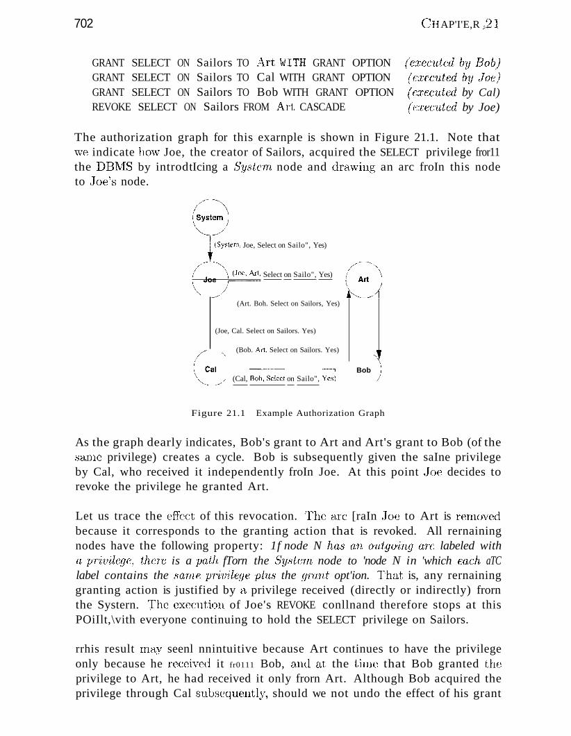
702
GRANT SELECT ON Sailors TO Axt WITH GRANT OPTIONGRANT SELECT ON Sailors TO Cal WITH GRANT OPTIONGRANT SELECT ON Sailors TO Bob WITH GRANT OPTIONREVOKE SELECT ON Sailors FROM i-\rt CASCADE
ellAP'I'E,R $21
(e:ceC1tted bllBob)(e:r:ec1lted bl/ Joe)(cJ;eclded by Cal)(executed by Joe)
The authorization graph for this exarnple is shown in Figure 21.1. Note thatvve indicate hovv Joe, the creator of Sailors, acquired the SELECT privilege fror11the DBlVIS by introdtIcing a 8ystern node and dravving an arc froIn this nodeto Joe's node.
~:~~/
jystem, Joe, Select on Sailo", Yes)
(JO~rt, Select on Sailo", Yes)
_../
(Art. Boh. Select on Sailors, Yes)
(Joe, Cal. Select on Sailors. Yes)
/" (Bob. Art, Select on Sailors. Yes)
0:/ (Cal, Bo;;:-;elecl on Sailo", ~) Bob
Figure 21.1 Example Authorization Graph
As the graph dearly indicates, Bob's grant to Art and Art's grant to Bob (of thescl.lne privilege) creates a cycle. Bob is subsequently given the saIne privilegeby Cal, who received it independently froIn Joe. At this point Joe decides torevoke the privilege he granted Art.
Let us trace the effect of this revocation. 1'he arc [raIn Joe to Art is renlov(,~d
because it corresponds to the granting action that is revoked. All rernainingnodes have the following property: 1f node N has an otdgo'ing aTe labeled witha pT'iv'ilege, there is a path fTorn the Systern node to 'node N in 'which each aTClabel contains the sante privilege phiS the grant opt'ion. That is, any rernaininggranting action is justified by a privilege received (directly or indirectly) frornthe Systern. The execution of Joe's REVOKE conllnand therefore stops at thisPOiIlt,\vith everyone continuing to hold the SELECT privilege on Sailors.
rrhis result rn~.ty seenl nnintuitive because Art continues to have the privilegeonly because he received it fr0111 Bob, and at the tiIne that Bob granted theprivilege to Art, he had received it only frorn Art. Although Bob acquired theprivilege through Cal subsequentl~y, should we not undo the effect of his grant
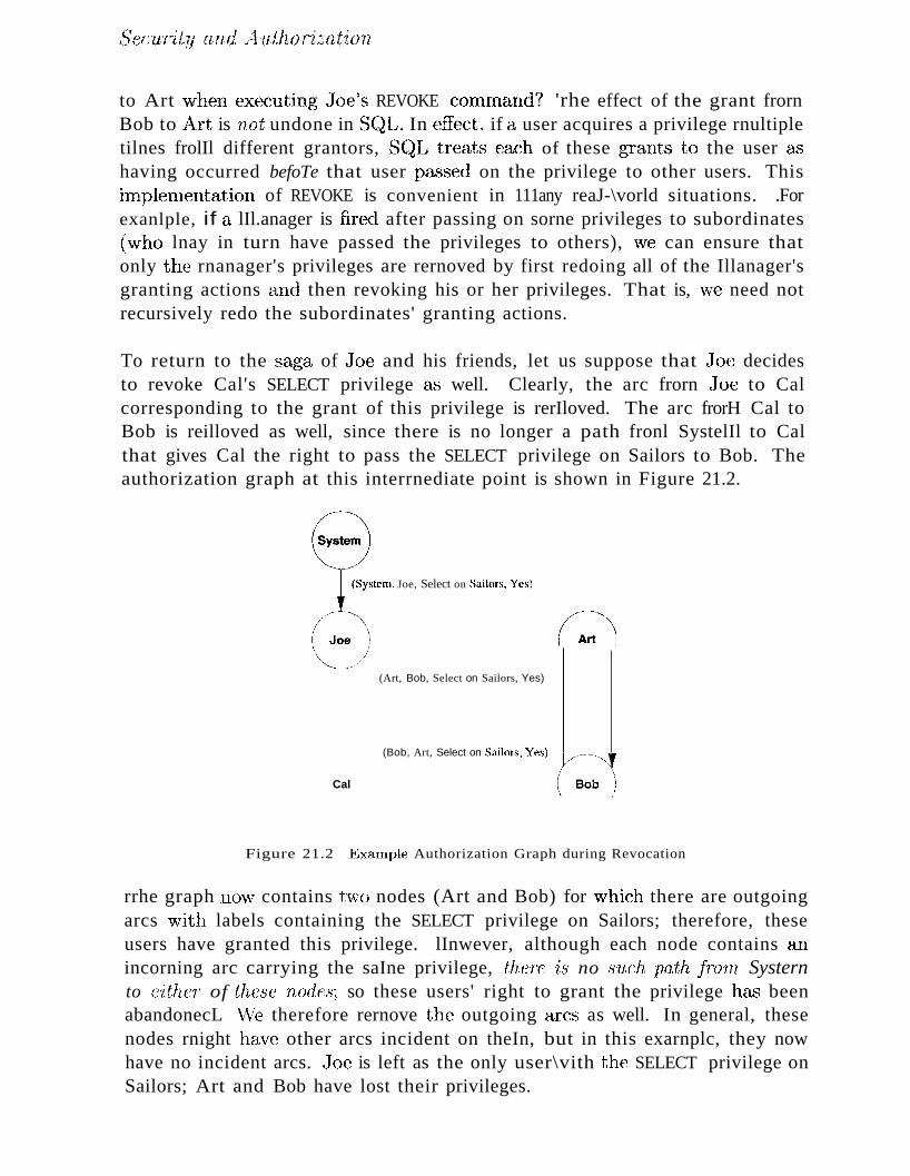
to Art vvhen executing Joe's REVOKE cOlInlland? 'rhe effect of the grant frorn"-" '"
Bob to ,Art is 'not undone in SCJL. In effecL if a user acquires a privilege rnultipletilnes frolIl different grantors, S(~L treats each of these grants to the user <he;
having occurred befoTe that user pa"c;sed on the privilege to other users. ThisiInplcrnentation of REVOKE is convenient in 111any reaJ-\vorld situations. .Forexanlple, if a lIl.anager is fired after passing on sorne privileges to subordinates(vvho lnay in turn have passed the privileges to others), vve can ensure thatonly the rnanager's privileges are rernoved by first redoing all of the Illanager'sgranting actions and then revoking his or her privileges. That is, Vle need notrecursively redo the subordinates' granting actions.
To return to the saga of Joe and his friends, let us suppose that Joe decidesto revoke Cal's SELECT privilege a.., well. Clearly, the arc frorn Joe to Calcorresponding to the grant of this privilege is rerIloved. The arc frorH Cal toBob is reilloved as well, since there is no longer a path fronl SystelIl to Calthat gives Cal the right to pass the SELECT privilege on Sailors to Bob. Theauthorization graph at this interrnediate point is shown in Figure 21.2.
E=01-(SY<tem, Joe, Select on Sailoe<, Ye<)
(o~) (~"''--'-''~'/
(Art, Bob, Select on Sailors, Yes)
(Bob, Art, Select on Sailors, Yes)
Cal
Figure 21.2 Example Authorization Graph during Revocation
rrhe graph 110Vv' contains t~lO nodes (Art and Bob) for vvhieh there are outgoingarcs \vith labels containing the SELECT privilege on Sailors; therefore, theseusers have granted this privilege. lInwever, although each node contains a,nincorning arc carrying the saIne privilege, then:; is no .such path jnnn Systernto either of these nodes; so these users' right to grant the privilege lUh'S beenabandonecL "\\le therefore rernove the outgoing arcs as well. In general, thesenodes rnight have other arcs incident on theIn, but in this exarnplc, they nowhave no incident arcs. Joe is left as the only user\vith the SELECT privilege onSailors; Art and Bob have lost their privileges.
704 CHAPTER 2J
21.3.1 (;rant and Revoke on Views and Integrity Constraints
1"'!he privileges held by the creator of a vie\\! (\vitll respect to the vie\v) changeover tiIne cbS he or she gains or loses privileges on the underlying tables. If thecreator loses a privilege held 'with the grant option, users vvho "vere given thatprivilege on the view lose it as \vell. 'There are SOlHO subtle &-spects to the GRANTand REVOKE conunands vvhen they involve vicV\1s or integrity constraints. \;Yeconsider senne exarnples that highlight the folloV\Ting irnportant points:
1. A view Inay be dropped because a SELECT privilege is revoked froIn theuser who created the vie\~r.
2. If the creator of a vie"v gains additional privileges on the underlying tables,he or she autornatically gains additional privileges on the view.
3. The distinction between the REFERENCES and SELECT privileges is irnportanto
Suppose that Joe created Sailors and gave Michael the SELECT privilege on itwith the grant option, and J\!Iichael then created the view YoungSailors andgave Eric the SELECT privilege on ·youngSailors. Eric now defines a view calledFiIl(~YoungSailors:
CREATE VIEW FineYoungSailors (naIne, age, rating)AS SELECT S.snarne, S.age, S.rating
FROM YoungSailors SWHERE S.rating > 6
\Vhat hc1.1>pens if .Joe revokes the SELECT privilege on Sailors froln l\1icha,el?lV1ichael no longer has the authority to execute the query used to define YoungSa,ilors because the definition refers to Sailors. rrherefore, the vieV\! YoungSailorsis dropped (Le., destroyed). In turn, Fine'{oungSailors is dropped as \vell. Bothview definitions axe rernoved fr0111 the systcln catalogs; even if (1, rerIlorseful Joedecides to give ba,ckthe SELECT privilege on Sailors to l\;1ichael, the vicV\Ts aregone a11d rnust be created afresh if they are required.
On a Inore happy note, suppose tllat everything proceeds as just described untilEric defines I~'\ineYoungSailors; tJleu, instead of revoking the SELECT privilegeon Sailors frorll I\:lichael, .Joe decides to also give l\'Echctel the INSERT privilege011 Sailors. l\!Iichael's privileges on th(~ vievv YoungS(tilors are upgraded to \vhathe \vould 11<'lVe if he \-vere to create the vie\v no'll!. lI(~ therefore acquires theINSERT privilege on 'YourlgSailors as VilCd1. (Note that this vie"v is updatal)le.)\~nlat ab(nltEri(~? IIis privileg(~s axe Un(Jlfu1g(:~d.
\Vh(~ther ()l' ll.ot .lVIicllael 11::18 tlle INSERT privilege 011 \roungSailors with thegra11t ()ption clel)encls 011 \vhether or not .Joe gives hirn the INSERT I)rivilege OIl
70~
Sailors \vith the grant option. 'Ib understand this situation, consider Eric again.If lVIiehael has the INSERT privilege on YoungSailors with the grant option, hecan pass this privilege to Eric. Eric could then insert rovvs into the Sailors tablebecause inserts on YC}llngSailors are effected by rnodifying the underlying basetable, Sailors. Clearly, vve do not \vant l\:1ichael to be able to authorize Eric tornake such changes unless :I\JIichael has the INSERT privilege on Sailors with thegrant option.
rrhe REFERENCES privilege is very different froIll the SELECT privilege, kk" thefollowing exarIlple illustrates. Suppose that Joe is the creator of Boats..He canauthorize another user, say, Freel, to create H,eserves with a foreign key thatrefers to the bid colurnn of Boats by giving ~'red the REFERENCES privilege withrespect to this colulnn. ()n the other hand, if Fred has the SELECT privilege onthe bid colurnn of Boats but not the REFERENCES privilege, Fred cannot createR.eserves with a foreign key that refers to Boats. If Fred creates R,eserves witha foreign key colunlll that refers to bid in Boats and later loses the REFERENCESprivilege on the bid colurnn of boats, the foreign key constraint in Reserves isdropped; however, the R,eserves table is not dropped.
To understand why the SQL standard chose to introduce the REFERENCES privilege rather than to siInply allow the SELECT privilege to be used in this situation, consider what happens if the definition of Iteserves specified the NOACTION option with the foreign key------.-Joe, the owner of Boats, Inay be prevented from deleting a row fronl Boats because a row in Reserves refers to thisBoats row. Giving Fred, the creator of Reserves, the right to constrain updateson Boats in this rnanner goes beyond. siInply allowing hinl to read the valuesin Boats, vvhich is all that the SELECT privilege authorizes.
21.4 MANDATORY ACCESS CONTROL
Discretionary access coutrollnechanislns, while generally effective, have certain\veaknesses. In particular they are susceptible to Trojan h07'se schelnes wherebya devious unauthorized user can trick an authorized user into disclosing sensitive data. For exalnple, suppose that student rrricky Dick \Va.nt8 to break intothe grade tables of instructor ]).'ustin Justin. IJick does the following:
IIIlI lIe creates a nc\v table called lVlineAlIlVIine and gives INSERT privilegeson this tahle to .Justin (who is blissfully una\vare of aJl this attention, ofcourse).
lI! lIe rllodifies the code of SOllIe I}BlVIS application that J llstin uses often todo (L couple of additional things: first, read the (jrades tel-ble, Ctlld next,\vrite the result into IVIineAl1~'1ine.
706 CHAPTER ~1
Then he sits back and waits for the grades to be copied into :NfineAllNlinc andlater undoes the Illodifications to the application to ensure that Justin doesnot sOlnehow find out later that he has been cheated. Thus, despite the DB~1S
enforcing all discretionary access controls··.,.-·--only Justin's authorized code ,vasallowed to access Grades....·..··....sensitive data is disclosed to an intruder. 1:'he factthat Dick could surreptitiously modify Justin's code is outside the scope of theDB1/IS's access control rnechanisrn.
NIandatory access control meehanisrns are airned at addressing such loopholes indiscretionary access control. 1"he popular rllodel for mandatory access control,called the Bell-LaPadula Illodel, is described in tenllS of objects (e.g., tables,views, rows, columns), subjects (e.g., users, prograrlls), security classes, andclearances. Each databa..'3e object is a..'3signed a security class, and each subjectis assigned clearance for a security class; we denote the class of an object orsubject A as class(A). The security classes in a systerll are organized accordingto a partial order, with a most secure class and a least secure class. forsirnplicity, we assume that there are four classes: top secTet (T8) , secret (8),confidential (C), and unclassified (U). In this system, T8> S > C> U, whereA > B rneans that class A data is more sensitive than class B data.
The Bell-LaPadula model imposes two restrictions on all reads and writes ofdatabase objects:
1. Simple Security Property: Subject S is allowed to read object 0 onlyif class(8) > class (()). For exarllple, a user with TS clearance can read atable with C clearance, but a user with C clearance is not allowed to reada table with TS classification.
2. *-Property: Subject S is allowed to write object 0 only if class(S) <class(O). For exarllple, a user with S clearance can write only objects withS or TS classification.
If discretionary a,ccess controls are also specified, these rules represent additionaJ restrictions. Therefore, to read or write a databa.'3e object, a user lllUsthave the necessary privileges (obtained via GRANT cornrnands) and the securityclasses of the user and the object rnust satis(y the preceding restrictions. Letus consider how such a Inandator~y control rnech.an.isrn lui.ght h.ave foiled 1'rickyI)ick. rfhe Grades table could be classified aB S, .Justin could be given clearancefor S, and 'Il'icky Di.ck could be given a lower clearance (Cf
). Dick can createobjects of only C! or lc)\ver classification; so the table l\!IineAl1ivline can have atInos1, the classification (}. \Vhen the application prograrIl running on behalf of..Justin (and therefore\vith clearance S) tries to copy (irades into 1\1ineAllIVline,it is not allowed to do so because clas,s(1\llineAlllvfrin,e) < class(applicat'ion), a.nelthe *-Property is violated.
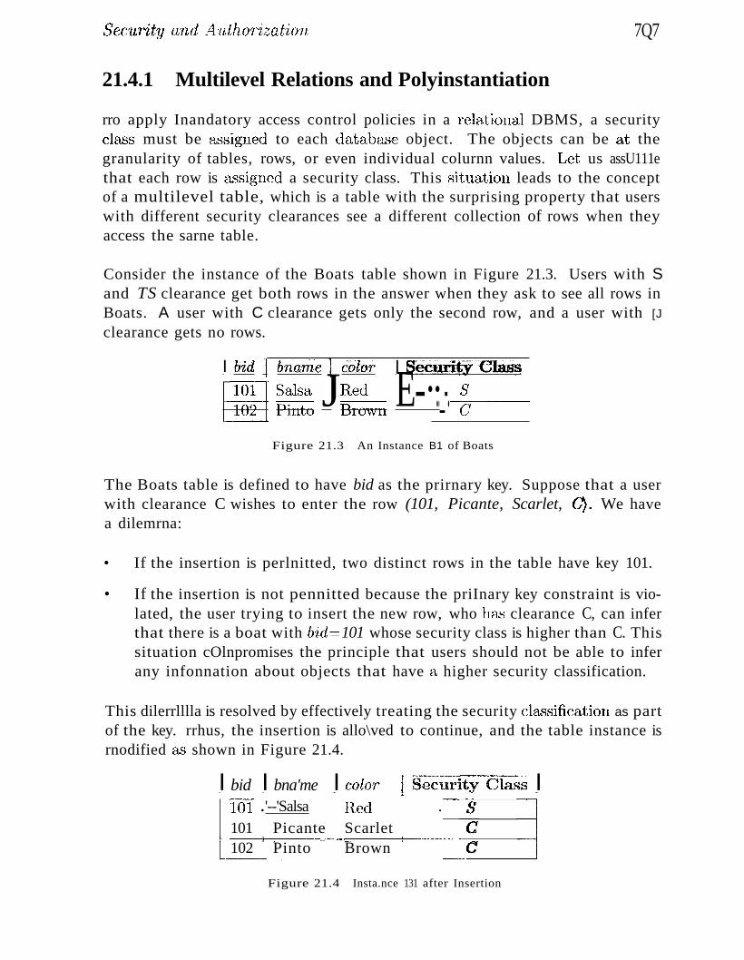
SeC'UT'ity and Authorization
21.4.1 Multilevel Relations and Polyinstantiation
7Q7
rro apply Inandatory access control policies in a relational DBMS, a securityclf:1SS must be ac;sig11ed to each databa...sc object. The objects can be at thegranularity of tables, rows, or even individual colurnn values. Let us assU111ethat each row is a9signed a security class. This situation leads to the conceptof a multilevel table, which is a table with the surprising property that userswith different security clearances see a different collection of rows when theyaccess the sarne table.
Consider the instance of the Boats table shown in Figure 21.3. Users with Sand TS clearance get both rows in the answer when they ask to see all rows inBoats. A user with C clearance gets only the second row, and a user with [J
clearance gets no rows.
I .bid ., bname J color I SeclJ,:citYClass.
[~ ~~~:: J~;:wn E-··..._-.-S-=-C---
Figure 21.3 An Instance B1 of Boats
The Boats table is defined to have bid as the prirnary key. Suppose that a userwith clearance C wishes to enter the row (101, Picante, Scarlet, 0). We havea dilemrna:
• If the insertion is perlnitted, two distinct rows in the table have key 101.
• If the insertion is not pennitted because the priInary key constraint is violated, the user trying to insert the new row, who ha...') clearance C, can inferthat there is a boat with {rid== 101 whose security class is higher than C. Thissituation cOlnpromises the principle that users should not be able to inferany infonnation about objects that have a higher security classification.
This dilerrlllla is resolved by effectively treating the security cla..ssification as partof the key. rrhus, the insertion is allo\ved to continue, and the table instance isrnodified as shown in Figure 21.4.
I bid I bna'me I color I Security-'Class Il(:i'T .'--'Salsa fled .--,§101 Picante Scarlet C
1---------+------....-- .___._----+-------102 Pinto Brown C
---_.... . _---
Figure 21.4 Insta.nce 131 after Insertion
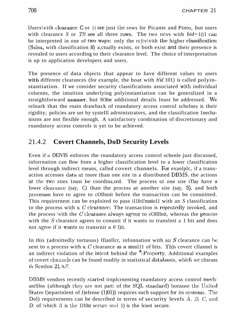
708 CHAPTER 21
lJsers\vith clearance C or [1 see just the rows for Picante and Pinto, but userswith clearance S or 1'8 see all three nnvs. The two ro\vs with bid=1()1 canbe interpreted in one of t'wo\vays: only the rc)\v\vith the higher cla..~sification
(Salsa, with classification 8) a,ctually exists, or both exist and their presence isrevealed to users according to their clearance level. The choice of interpretationis up to application developers and users.
The presence of data objects that appear to have different values to users¥lith different clearances (for exarnple, the boat with b'id 101) is called polyinstantiation. If we consider security classifications associated \~lith individualcolurnns, the intuition underlying polyinstantiation can be generalized in astraightforward rnanner~ but SOIne additional details Inust be addressed. \I\lerelnark that the rnain drawback of rnandatory access control schelnes is theirrigidity; policies are set by systeIll adrninistrators, and the classification 1nechanisrns are not flexible enough. A satisfactory cornbination of discretionary andrnandatory access controls is yet to be achieved.
21.4.2 Covert Channels, DoD Security Levels
Even if a DElVIS enforces the rnandatory access control schenle just discussed,inforrnation can flow frorn a higher classification level to a lower classificationlevel through indirect rneans, called covert channels. For exanlplc, if a transaction accesses data at rnore than one site in a distributed DBI\1S, the actionsat the tvvo sites 1nust be coordina,ted. The process at one site rTlay have alower cleara.nce (say, C) than the process at another site (say, S), and bothproceSSE~S have to agree to cOllnnit before the transaction can be conunitted.This requirernent can be exploited to pass i11fo1'rnatio11 with an S classificationto the process with a () clearance: The transaction is repeatedly invoked, andthe process \vith the C: clearance always agrees to cOlIllnit, whereas the prOCf~SS
with the 8 clearance agrees to conunit if it wants to translnit a 1 bit and doesnot agree if it ~rants to transrnit a 0 l)it.
In this (adrnittedly tortuous) lIlanllcr, infonnation with an ,9 clearance can b(~
sent to a process with a C: clearance as a strea111 of bits. 1~his covert cllannel isan indirect violation of the int(~nt behind the *-Propert.y. Additional exarnplesof covert channels can be found readilv in statistical dataJ)t:lses, vvhich vve cliscuss
,j
." S' . ')! 6'" 2"In k cetlon .... ,. ". '.
DBrv1S vendors recently started irnplcrnenting rnandatory access control rnechaniSlns (although they aTe not part: of the S(~L stanc!<trcl) because the lJ nit(:~(l
States l)epartnlent of J)efense (1)01)) requires such support for its systelns.TlH~
Dol) requirernents can be described in terrns of security levels ./1 ~ ,13, CI, E1JJd
D. of \vhich ./1 is the 1J10st secure and 1) is the lC<l,st secure.
SeC'llTity and ..4ntluJ1"ization 709
Current SysteIlls:ColnuilereiaIR,DBIvISs areavt\ilable that support discretionary controls at the C21evel andrnandat.ory controls at theBJ level.If3:NI DB2, Inforruix, ivIierosoft SQL Server, Oracle 8, and Sybase ASE ansupport SQL's features for discretionary clccess controL In gel1eral, theydo not support lnandatory a.ccess control; Ora,cle offers a versio:n of theirproduct with support for rnandatory access control.
Level C requires support for discretionary access control. It is divided intosublevels Cl and C:2; C2 also requires SOll1C degree of accountability throughprocedures such 3,.':3 login verification and audit trails. Level B requires support for lnandatory access control. It is subdivided into levels Bl, B2, andB3. Level 132 additionally requires the identification and clirnination of covertchannels. Level B3 additionally requires 11laintenance of audit trails and thedesignation of a security administrator (usually, but not necessarily, theDBA). Level A, the most secure level, requires a n1athernatical proof that thesecurity rnechanisrn enforces the security policy!
21.5 SECURITY FOR INTERNET APPLICATIONS
When a DBMS is accessed frorn a secure location, we can rely upon a shnplepassword rnechanisrn for authenticating users. IIowever, suppose our friendSarn wants to place an order for a hook over the Internet. rrhis presents sorneunique challenges: Saln is not even a known user (unless he is a repeat custonler). Fron1 Alnazon's point of view, we have an individual asking for a bookand offering to pay with a credit card registered to Saln, but is this individualreally Sarn? f'rcnn Sarn's point of view, he sees a fornl asking for credit cardinforrnation, but is this indeed a legitirnate part of Arnazon's site, and not arogue application designed to trick hi1l1 into revealing his credit card nurnber?
Tlhis exarnple illustrates the need for a rnore sophisticated approach to authentication than a sirnple pass"Vvord rnechanisrn. Encryption techniques provideth(-,~ foun,dation for rnodern authentica,tion.
21.5.1 Encryption
The basic ide(\' b(~hind encryption is to apply an encryption algorithrn to thedata, using a user-specified or IJBA-SI)Ccified encryption key. The output ofthe algorithrn is the en.cryptexl version of th(~ data. There is aJso a, decryption algorithrrL ·which ta,kes the encryptc"d data and (:1, decryption key asinput and then returns the original data.\Vithont the corn:~ct decryption key~
the decryption aJgori tll111produces gibl)crish. rrhe (~llcrypti(nl and clecryption
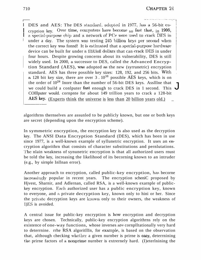
710 ()HAPTER 2~1
r-'-'" ---------·--·--·----·----·-..··-··1
I DES and AES: The DES standard,. adopted in 1977, has a 56-bit en- !
I cryption key. Over thne1 COII:tputers have become so ra",t that, in 19991 'I!!.
I (1, special-purpose chip and a network ofPCs were used to cra{:kDl~S in! under a day. The systern W~l.'3 testing 245biHion keys per second w,hen
the correct key "va,." fonnd! It is estirnated that a special~pu.rpose hE:trdwaredevice can be built for under a 1l1iUioIl dollars that can crack DES in underfour hours. Despite growing concerns about its vulnerability, DES is stillwidely used. In 2000, a successor to DES, called the Advanced Encryption Standard (AES), W&'3 adopted as the new (syrrunetric) encryptionstandard. AES has three possible key sizes: 128, 192, and 256 bits. \\lith II
a 128 bit key size, there are over 3 . 1038 possible AES keys, which is onthe order of 1024 Inore than the number of 56-bit DES keys. Asslllne thatwe could build a conlputer fa.'3t enough to crack DES in 1 second. This JCOIllputer would. cornpnte for about 149 trillion years to crack a 128-bit
~.=:..~~ (Experts think the universe is less than 20 billion years old.) _
algorithrns thernselves are assunled to be publicly known, but one or both keysare secret (depending upon the encryption scheme).
In symmetric encryption, the encryption key is also used as the decryptionkey. The ANSI Data Encryption Standard (DES), which has been in usesince 1977, is a well-known exarnple of syllunetric encryption. It uses an encryption algorithrn that consists of character substitutions and pernlutations.rrhe nlain weakness of synunetric encryption is that all authorized users rnustbe told the key, increasing the likelihood of its becorning known to an intruder(e.g., by sirnple Inllnan error).
Another approach to encryption, called public-key encryption, ha.l;) becorneincrea.'3ingly popular in recent years. The encryption scheniC proposed byHjvest, Sharnir, and Adlernan, called RSA, is a well-known exarnple of publickey encryption. Each authorized user has a public encryption key, knownto everyone, and a private decryption key, known only to hini or her. Sincethe priv<lte decryption keys are kno\llln only to their owners, the weakness of1)ES is avoided.
A central issue for public-key encryption is ho\v encryption and decryptionkeys are chosen. Technically, public-key encryption algorithrns rely on theexistence of one-way functions, whose inverses are cornplltationally very hardto deterrnine. rrhe I1SA algoritllIn, for exaJnple, is based on the observationthat, although checking vvhether a given nurnber is prirne is easy, deterrniningthe prirne factors of a nonpriIne nurnber is extrernely hard. (I)eterlnining the
Sec'lL'f'ity and ",4'llthoT'izat'ion 71J
Why RSA Works: The essential point of the scherne is that it is easy tocompute d given e, 1>, and q, but ve'r.lJ hard to cornpute d given just e andL. In turn, this difficulty depends OIl the fact that it is hard to deterlninethe priIne factors of L, ",r11ich happen to be p and q. A cavcat:Factoringis widely believed to be hard, but there is no proof that this is so. Noris there a proof that factoring is the only way to crack I\SA; that is, toCU11111 d frolll e and L.
prirne factors of a nurnber with over 100 digits can take years of CPlJ tirne onthe fastest available COIllputers today.)
We now sketch the idea behind the R,SA algorithrn, ~lssurning that the data. tobe encrypted is an integer I. To choose an encryption key and a decryptionkey for a given user, we first choose a very large integer L, larger than thelargest integer we will ever need to encode. 1 We then select a nUl1lber e as theencryption key and cornpute the decryption key d based on e and L; how thisis done is central to the approach, as we see shortly. Both Land e are l1ladepublic and used by the encryption algorithrn. However, d is kept secret and isnecessary for decryption.
II The encryption function is 8
II The decryption function is 1
Ie mod L.
Sd mod L.
vVe choose L to be the product of t,vlO large (e.g., 1024-bit), distinct prirnenurnbers, 11 * q. 1"he encryption key e is a randornly chosen nlunber between1 and L that is relatively prirne to (p "~- 1) * (q - 1). The decryption key d iscornputed such that d *e = 1 mod ((p - 1) * (q - 1)). Ciiven these choices, resultsin nurnber theory can be used to prove that the decryption function recoversthe original ruessage frorll its encrypted version.
A very irnportant property of the encryption and decryption algoritluns is thatthe roles of the encryption and decryption keys can be reversed:
decrypt( el, (encrypt(c, I))) = I == decTypt(c, (cru:rypt( el, I)))
Since In.any protocols rely on this property, \ve henceforth sirnply refer to public aTld private keys (since both keys CHJ1 be used for encryption as \'lell asdecryption) .
LA message th':lt is to be encrypted is decomposed into blocks such t.hat each block can be treated'L.S an integer less tha.n L.
..,.., ')t .. ,,-, (;HAPTER 2*1
\Vhilewe introduced encryption in the context of authenticatioll, \VC note thatit is a fundaIIlental tool for enforcing seeurity.ADBNIS can use encrlJ1Jt'lon toprotect inforrnation in situations where the norrnal security rnechanisrns of theDBlVIS are not adequate. For exarnple, an intruder rnay steal tapes containingSOUIC data or tap a conunu.nieation line. By storing and transrnitting data inan encrypted forIn, the DBNlS ensures that such stolen data is not intelligibleto the intruder.
21.5.2 Certifying Servers: The SSL Protocol
Suppose \ve associate a public key and a decryption key "vith Alnazon. Anyone, say, user Sa,rl1, can send Alnazon an order by encrypting the order usingArnazon's public key. ()nly Arnazon can decrypt this secret order because thedecryption algorithrn requires Arnazon's private key, known only to Arnazon.
This hinges on 8arn's ability to reliably find out Arnazon's public key. A number of cornpanies serve as certification authorities, e.g., Verisign. Arnazongenerates a public encryption key eA (and a private decryption key) and sendsthe public key to Verisign. Verisign then issues a certificate to Arnazon thatcontains the following inforrnation:
(VeTi8ig'r'l" Arnazoin, htl;P8://w'U)w. arnazon. corn, eA )
The certificate is encrypted using Verisign 's own (pTivate key, which is knownto (i.e., stored in) Internet Explorer, Netscape Navigator, and other browsers.
vVhen 8an1 carnes to the Anulzon site and wants to place an order, his browser,running the SSL protocol, 2 asks the server for the Verisign certificate. Thebro\vser then validates the certificate by decrypting it (using ·Verisign's publickey) and checking that the result is a certificate with the HaIne Verisign, andthat theURL it contains is that of the server it is talking to. (Note that anatternpt to forge a certificate \vill fail because certificates are encrypted usingVerisign 's private key, Vilhieh is knc)\vn only to Verisign.) Next, the brovvsergenerates (1, randc)ln session key, encrypt it using Arnazon's public key (\vhiehit obtained frorn the validated certificate anel therefore trusts), and sends it tothe 1\rn(lzon server.
Frorn this point on, the Arnazon server and the browser can use th.c sessionkey (which both know and are confident tliat only they know) and a /3Y'fnrnetricencrypticHl protc)collike AES or IJES to exchangc~ securely encrypted rnessages:l\Jlessages are encrypted by the sender anel decrypted by the receiver using thesa,HIe session key. rrhe encrypted Inessages travel over the Internet and rnay be
._-_ _--_.._.-----:2 A browser uses the SSL protocol if the tclrget lJHl..i begins with https.
8eC'lJ,1"ity and .AnthoT'ization 113
intercepted, but they cannot be decrypted without the session key. It is usefulto consider \vhy \ve need a session key; after all, the bro\vser could sirnply haveencrypted 8a1n's original request using Arnazon '8 public key and sent it securelyto the Arnazon server. The reason is that, without the session key, the Arnazonserver has no "'lay to securely send infonnation back to the bro\vser. A furtheradvantage of session keys is that syrnrnetric encryption is cOlnputationally nluchfaster than public key encryption. The session key is discarded at the end ofthe session.
Thus, 8aIn can be assured that only Alnazon can see the inforrnation he typesinto the fonn shown to hirn by the AIuazon server and the inforrnation sentback to hiln in responses froIn the server. However, at this point, r\rnazonhas no assurance that the user running the browser is actually Sanl, and notSOlneone who has stolen Sarn's credit card. l-'ypically, rnerchants accept thissituation, which also arises when a custoIner places an order over the phone.
If we want to be sure of the user's identity, this can be accoIuplished by additionally requiring the user to login. In our exarnple, 8arn 11lUSt first establishan account with Alnazon and select a password. (Stun's identity is originallyestablished by calling hiln back on the phone to verify the account inforrnationor by sending elnail to an elnail address; in the latter case, all we establish isthat the owner of the account is the individual with the given clnail address.)Whenever he visits the site and Anlazon needs to verify his identity, AInazonredirects hinl to a login fo1'1n after' using SSL to establish a session key. 'rhepaE;sword typed in is transrnitted securely by encrypting it with the session key.
()ne rcrnaining drawback in this approach is that Arnazon now kno\vs Sarn'scredit card nlunber, and he rnust trust Alnazon not to rnisuse it. The SecureElectronic Transaction protocol addresses this lirnitation. Every custolnerrnust nnw obtain a certificate, with his or her own private and public keys,and every transaction involves the Alnazon server, the cust(nner's browser, andthe server of a trusted third party, such as Visa for credit card transactions.r:Che basic idea is that the bro"vser encodes non-credit caTd inforrnation usingAInazon's public key and the credit ca.rd infonnation using Visa's public key andsends these to the AJnazon servc:~r, which for"vards the credit card inforrnation(which it cannot decrypt) to the Visa server. If theVisct server a,pproves theinforrnation, the transa,ction goes through.
21.5.3 Digital Signatures
Suppose tllat ,Elnlcr, who works for ArnazoIl, a,nd Betsy, \vho \\forks for IVlcCjnlwlIill,need to COlllll1Unicate \vith each other about inventory. Public key encryption can be used t() create digital signatures for rnessages. rrhat is, rnessages
714 CHAPTER 2l
can be encoded in such a way that, if ElIneI' gets a Inessage supposedly fr(nTIBetsy, he can verify that it is fronl Betsy (in addition to being able to decryptthe rnessage) and, further, prove that it is froIn Betsy at McGraw-lIill, even ifthe ll1cssage is sent froIn a IIotrnail account when Betsy is traveling. Sirnilarly,Betsy can authenticate the originator of Inessages froln Ellner.
If Ellner encrypts Inessages for Betsy using her public key, and vice-versa,they can exchange inforrnation securely but cannot authenticate the sender.Sorueone who wishes to irnpersonate Betsy could use her public key to send arnessage to EIrner, pretending to be Betsy.
A clever use of the encryption sche111e, however, allows Ellner to verify whetherthe rnessage was indeed sent by Betsy. Betsy encrypts the rnessage using herprivate key and then encrypts the result using Elrner's public key. When Ellnerreceives such a 111essage, he first decrypts it using his private key and thendecrypts the result using Betsy's public key. rrhis step yields the original unencrypted rnessage. FllrtherInore, Ehner can be certain that the rnessage wascomposed and encrypted by Betsy because a forger could not have known herprivate key, and without it the final result would have been nonsensical, ratherthan a legible 111essage. 1~\lIther, because even E~lrner does not know Betsy'sprivate key, Betsy cannot clairn that Ehner forged the ruessage.
If authenticating the sender is the objective and hiding the rnessage is not important, we can reduce the cost of encryption by using a message signature.A signature is obtained by applying a one-way function (e.g., a hashing schelne)to the rnessagc and is considerably sInaHer. \Ve encode the signature as in thebasic digital signature approach, and send the encoded signature together withthe full, unencoded 111cssage. rrhe recipient can verify the sender of the signature as just described, and validate the I11essage itself by applying the onc-\vayfunction and cOlnparing the result with the signature.
21.6 ADDITIONAL ISSUES REI.JATED TO SECURITY
Security is a, l)road topic, and our coverage is necessarily lirnited. 'rhis sectionbriefly touches on sorne additional irnportant issues.
21.6.1 Role of the Database Administrator
rrhe database (l,chninistrator (IJBA) plays an irnportant role in enfol'c:ing thesecurity-related aspects of i:1 dataJ>ase design. In conjunction with the o\vnersof the data, the I)BA aJso COlltributes to developing a security policy. The I)BAhas a sp(~cial i:1,ccount, \vhich we call the systenl account~ (l,nd is responsible
SeC1l7·o;zty and .A'ntho'rizaL·ion
for the overall security of the systeru. In particular ~ the DBA. deals with thefollo\ving:
1. Creating New Accounts: Each new user or group of users Blust beassigned an authorization ID and a paA'3s\vord. Note that application prograIns that access the database have the saIne authorization ID as the userexecuting the prograill.
2. Mandatory Control Issues: If the DB~'fS supports rnandatory control·-···S0111e custornized systeIns for applications \vith very high security requirernents (for exarllple, rnilitary data) provide such support~-theDBA lllUstassign security classes to each database object and a..'3sign security clearances to each authorization ID in accordance with the chosen security polICY·
The DBA is also responsible for rnaintaining the audit trail, which is essentially the log of updates with the authorization ID (of the user executing thetransaction) added to each log entry. This log is just a Ininor extension ofthe log mechanislll used to recover from crashes. Additionally, the DBA lllaychoose to rnaintain a log of all actions, including reads, perfornled by a user.Analyzing such histories of how the DBMS was accessed can help prevent security violations by identifying suspicious patterns before an intruder finallysucceeds in breaking in, or it can help track down an intruder after a violationh&" been detected.
21.6.2 Security in Statistical Databases
A statistical database contains specific inforrnation on individuals or eventsbut is intended to perlnit only statistical queries. For exarnple, if \ve rnailltaineda statistical database of inforrna,tion about sailors, we would allow statisticalqueries about average ratings, rnaxirnurn age, and so on, but not queries aboutindividua.l sailors. Security in such dataJxtses poses nevv probleurs because it ispossible to infer protected inforrnation (such Cl"S (1, sailor's rating) frorn ans\versto perrnitted statistical queries. Such inference opportunities represent covertchannels that can cornprornise the security policy of the database.
Suppose that sailor Sn(~aky Pete Vlants to kncrw the rating of .A.clrniral Ho1'ntooter ~ the c~st~elned chairrnarl of the sailing clu1), and happens to kno\v thcltIIorntooter is the olclest sailor in the (Jub. Pete repeat(~dly (18ks queries of thc~
forln "'IIow' InClny sailors aTe there whose age is greater than ..x,:?" for vaxiousva.1ues of ..\'", until the (UIS\Ver is 1. (}bviously, this sa,iIor is lIorntooter, th(~
oldest sailor. Notethat each of these queries is (J, valicl statistical query andis perrnitt(~d. Let the value of ..x at this POillt be, say, fi5. ~Pete no\v asks the(lller:y, "'vVhat is tll(·~ nraxirnurn rating of all sailors \vhose age is greater than
716 (:HAPTER ·121
65'1" f\gain~ this query is pennitted because it is a statistical query. However,the ans\ver to this query reveals J101'ntooter's rating to Pete, and the securitypolicy of the databa.se is violated.
One approach to preventing such violations is to require that each query rnustinvolve at 1e(1.'3t S01ne lnininuull nUluber, say,N, of l'()\VS. vVith a rea.sonablechoice of N, Pete \vould not be able to isolate the inforrnation about 1101'ntooter,because the query about the rna.xinUUll rating would fail. rrhis restriction,hc)\vever, is easy to overCOIne. By repeatedly (1.'3king queries of the forIII , '"Howruany sailors are there vvhose age is greater than ..Y?" until the systenl rejectsone such query, Pete identifies a set ofN sailors, including Florntooter. Let thevalue of ~Y at this point be 55. Novv, Pete can ask tvvo queries:
III "vVhat is the SlUll of the ratings of all sailors whose age is greater than557" Since N sailors have age greater than 55, this query is perrnitted.
• "What is the SUIll of the ratings of all sailors, other than l1orntooter, whoseage is greater than 55, and sailor Pete?" Since the set of sailors whose ratings are added up now includes Pete instead of Horntooter, but is otherwisethe sallle, the rnunber of sailors involved is still N, and this query is alsopennitted.
171'oln the answers to these two queries, say, Al and A2 , Pete, who knows hisrating, can easily calculate Horntooter's rating as Al ~ A2 + .Pete'8 rating.
Pete succeeded because he WcU3 able to ask two queries that involved Illany ofthe sarne sailors. 'The nurnber of rows exalnined in corllrnon by two queriesis called their intersection. If a liInit \vere to be pla,ced on the alIlount ofintersection perrnitted bet\veen anyt-wo queries issued by the Si::une user, Petecould be foiled. Actually, a truly fiendish (and patient) user can generally findout inforruation about specific individuals even if the systcrn phtces a, rniniruurnnUlnber of ro\vs bound (N) and a rnaxirnurn intersection bound (1\1) on queries,hut the n1.11n])er of qlleries required to do this gro\vs in proportion to N fA!. "Vecan try to additionally lirnit the total nUlnbe1' of queries that a user is allowedto aslc but t\VO users could still conspire to breach security. By Il1aintaininga log of all activity (including rectcl-on1y ac(,~esses), such query patterns can becletected, icleally before a security violation occurs. This discussion should rnakeit cleaT~ however, that security in statistical databases is difficult to enforce.
21.7 DESIGN CASf: STUDY: THE INTERNET STORE
\Ve return to our case study and our friends at DBI)udes to consider securityissues. 'There are three groups of users: custolners, ernl>loyees, a.nd the ovvnerof the l>ook shop. (()f course, there is also the datal)ase adrninistrator ~ who
SeC'lIT'ity aTidA'ldhorizaJion 717
luts universal access to all data and is responsible for regular operation of tlledatabase systcrTl.)
<:.,' ,
The ()\vner of the store has full privileges on all tables. Custorners can query theBooks table and place orders online, but they should not have access to othercustonH=~rs' records nor to other c11storne1'8' orders.DBDudes restricts accessin t\VO ·ways. First, it designs a silnple 'VVeb page with several fonus sirnilar tothe page shc}\vn in Figure 7.1 in Chapter 7. rrhis allo\vs custo1ners to subrnita s111all collection of valid requests without giving tho1n the ability to directlyaccess the underlying DB1JfS through an SQL interface. Second, I)B.Dudes usesthe security features of the .DB1\·IS to li111it access to sensitive data.
rIhe \vebpage allows custorners to query the Books relation by ISBN nU111bcr,narne of the author, and title of a boolc The webpage also has two buttons.The first button retrieves a list of all of the custolIler's orders that are notcompletely fulfilled yet. l'he second button displays a list of all cornpletedorders for that custorner. Note that custolllers cannot specify actual SQLqueries through the Web but only fill in SCHne pararneters in a forn1 to instantiatean autonlatically generated S(~L query. All queries generated through fonllinput have a WHERE clause that includes the cid attribute value of the currentcusto1ner, and evaluation of the queries generated by the two buttons requiresknowledge of the custolller identification nUlnber. Since all users have to logon to the website before browsing the catalog, the business logic (discussedin Section 7.7) lllust 1naintain state inforrnation about a custoDler (i.e., theCllstorner identification nUlnber) during the custorner's visit to the website.
~rhe second step is to configurEl, the database to lirnit access according to eachuser group's need to know. DBI)udes creates a special customer account thathas the following privileges:
SELECT ON Books, New()rders, ()ldOrders, NewOrderlists, OldOrderlistsINSERT ON New()rders, ()Ic:H)rders, New()rderlists, ()ld()rderlists
Ernployees should be able to acid ncvv books to the catalog, upda,te the quantityof (L book in stock, revise custorner orders if rlecessary, and update all custornerinforrnation e:ccept the credit card 'inforInation.. In fa,ct, ernployees should noteven be able to see a custorner's credit card nurnber. 1]lcreforc,DBDuclescreates the foUcnving vic\v:
CREATE VIEW C\lstornerlnfo (cid,cnarnc,address)AS SELECT (~.cid, C.cnaJTlE\ C.(l.cldress
FROMCllstolners C
I)BI)udes gives the employee account the follc)\ving privileges:
718 (~HAP'TER ~l
SELECT ON Cllstolnerlnfo~ Books~
Ne\vOrders, ()Id()rders~Ne\v(}rclerlists~ Old()rderlistsINSERT ON Cllstornerlnfo, Books,
Nc\vOrders, 01dC)rders, Ne\vOrderlists~ ()ldOrderlistsUPDATE ON CustolnerInfo, Books,
New()rders, OldOrders, Nevv()rderlists, Old()rderlistsDELETE ON Books, NewOrders, Old()rders~ NewOrderlists, ()ldOrderlists
Observe that ernployees can rnodify Custornerlnfo and even insert tuples intoit. This is possible because they have the necessary privileges, and further, theview is updatable and insertable-into. \Vhile it seerns rea.sonable that elllployeescan update a custorner's address, it does sceln odd that they call insert a t1lpleinto Cllstornerlnfo E~ven though they cannot see related infonna.tion about thecustorner (i.e., credit card nurnber) in the Cllstorners tahle. The reason forthis is that the store wants to be able to take orders 1'1'0111 first-tirne custornersover the phone without asking for credit card inforrnation over the phone.Ernployees can insert into Custornerlnfo, effectively creating a new Custoillersrecord without credit card inforluation, and custorners can subsequently providethe credit card nurnber through a Web interface. (Obviously, the order is notshipped until they do this.)
In addition, there are security issues when the user first logs on to the websiteusing the cllstolner identification nUlnber. Sending the nUlnber unencryptedover the Internet is a security hazard, and a secure protocol such as SSL shouldbe used.
Cornpanies such a.s CyberCash and DigiCash offer electronic conunerce payrIlcnt solutions, even inclu.ding electronic cash. Discussion of hoy\! to incorporatesuch techniques into the website are outside the scope of this book.
21.8 REVIEW QUESTIONS
..l\.nS\~lerS to the revic\v questions can be founel in the listed sections.
91! \\That (J..re tIle 1n,ain objectives in designing a secure datal)ase application?Explain the te1'rns ,seCT'CCY, 'integrity, availalrddy, and (lldhcn,tication. (Section 21.1)
IS Explain tlH~ tenns 8ccur'ity policy ,'UHl 8cc'u'l'ily TrlcchaILisnl arid ho\v tllCyare related. (Section 21.1)
l1li \\That is th(~ Blain iele;,1. behind disc'rct'ion,aT,1j acces.' con!;T'Ol? vVhat is theidea behind Trl.,(1,'ruiaf,oT;ij access con,troT? vVhat are the relativ(~ rnerits ofthes(~ tv·/C) approaches? (Section 21.2)
II Describe the privileges recognized in S(~L? In particular, describe SELECT,INSERT, UPDATE, DELETE, and REFERENCES. For each privilege, indicate\vho acquires it autornatical1y on a given table. (Section 2103)
II I-Io\v are the O\VIH~rS of privileges identified? In particular, discuss atLtho
rizlrt;ion ID8 and '{"ole8. (Section 21.3)
I'l \\That is an authorizat'ion graph? Explain S(~L's GRANT and REVOKE eOl11
IIHHlds in terrns of their effect on this graph. In particular, discuss \vhathappens when users pass on privileges that they receive frorn sorneone else.(Section 2103)
II Discuss the difference between having a privilege on a table and on a vie\vdefined over the table. In particular, how can a user have a privilege(say, SELECT) over a view 'without also having it on all underlying tables?\'Tho 11111st have appropriate privileges on all underlying tables of the view?(Section 21.3.1)
111 vVhat are objects, subjects, 8eCl.Ir'ity classes, and cleaTances in rnandatoryaccess control? IJiscuss the Bell-LaPadula restrictions in tenns of these concepts. Specifically, define the sirnple seC1LTity pr'Operty and the *-pToperty.(Section 21.4)
II What is a Trojan horse attack and how can it cOlnprornise discretionaryaccess control? Explain how lnandatory a,ccess control protects againstTrojan horse attacks. (Section 21.4)
Jl1II What do the tenns rnult'ilevf;l table and polyinstantiation rnean? Explaintheir rela.tionship, a,nd ho\,r they arise in the context of lnandatory accesscontrol. (Section 21.4.1)
Iii \'That are covert ChJlrrnels and how can they arise v\Then both discretionaryand luandatory access controls are in plcl,ce? (Section 2104;.2)
II Discuss the I)oD security levels for database systclns. (Section 21.4.2)
IiIil Explain why (t sirnple pEtssword rnechanisrn is insufficient for authentication of users "\vho <.lccess a databa.."c renJotely, say, over the Internet. (Section 21.5)
Illll \Vhat is the differellC(~ between sy'tnrnctTic a,lld public-key en,(~r'ypti()n? C.;iveex:.unples of 1Nell-kncJWll encryption algoritluns of both ki.lldso v\lhat is thernain \veakilcss of synunetric encryption and ho'Vv is this addressed in publick(~:y encryption? (Section 21.5.1)
II 1)i8c118s the choice of encrYIltion and decryption keys in public-key en.cryption cHId how they are llsed to c~ncrypt and decrypt dattL Explain the roleof ()'nC-'luay !u.'ncti(Jr/,.'i. vVhat H.ssurance do\ve h.ave that the H,SA SC;heln(~
(:;:'1,nno1, be cornprornised? (Section 21.5.1)
720 C~HAPTER 21
II \:\That are cert'ificat'ion attthorities and \vhy are they nE~eded? Explain ho\vcert'ificates are issued to sites and validated by H, bro\vser using the SSLTJrotocol: discuss the role of the session key. (Section 21.5.2)
II If a user connects to a site using the SSL protocol, explain \vhy there is stilla need to login the USCI'. Explain the use of SSL to protect pass\vords andother sensitive infonnation being exchal1ged. vVhat is the secure electTolu:Ctransaction pTOtoCO[? vVhat is the added value over SSL? (Section 21.5.2)
II A d'i.qital /:rignat'UTe facilitates secure exchange of rnessages. Explain whatit is and how it goes beyond sirnply encrypting rnessages. Discuss the useof rnessage signat'UTes to reduce the cost of encryption. (Section 21.5.3)
II \:Vhat is the role of the databa"se achninistrator with respect to security?(Section 21.6.1)
II Discuss the additional security loopholes introduced in statistical databases.(Section 21.6.2)
EXERCISES
Exercise 21.1 Briefly answer the following questions:
1. Explain the intuition behind the two rules in the Bell-LaPadulamodel for rnandatoryaccess control.
2. Give an exarnple of how covert channels can be used to defeat the Bell-LaPadula rnodel.
;3. Give an exarnple of polyinstantiation.
4. Describe a scenario in whichrnandatory access controls prevent a breach of security thatcannot be prevented through discretionary controls.
5. Describe a scen:'Lrio in which discretionary access controls are required to enforce a seCllrity policy that cannot be tmforced using onlymancl<ttory controls.
6. If a DBNIS already supports discretionary and Jnandatory access controls, is there a needfor encryption '?
7. Explain the need for each of the following lirnits in a statistical database systern:
(a) A maxirnurn on the munber of (pl(~ries a user ca.Jl PoS(~.
(b) A rninirnUln on the munber of tuples involved in ans\vering a query.
(c) A maximurn on the intersection of t\vo queries (Le.) on the number of tuples thatboth queries exarnine).
8. Explain the use of an audit trail, ''lith special reference to a statistical database system.
9. \,Vllat is the role of the DBA \vith respect to security?
10. Describe AES and its relationship to DES.
11. \?\'hat is public-key encryption? How does it differ frorn the encryption approach takenin the Data Encryption Standard (DES)~ and in \vhat ways is it better than DES?
SeCllTity and ""4'uthorizat'ion 721
12. Explain hmv a company offering services on the Internet could use encryption-basedtechniques to lllake its order-entry process secure. Discuss the role of DES, A.ES, SSL,SET, and digital signatures. Search the \tVeb to find out IllOre about related techniquessuch as electronic cash.
Exercise 21.2 You are the DBA for the VeryFine Toy Cornpany and create a relation calledEmployees with fields enam,e, dept, and Sala1~1j. For authorization reasons, you also defineviews EmployeeNallIes (with ena:rne as the only attribute) and DeptInfo with fields dept andavgsalary. The latter lists the average salary for each departrnent.
1. Show the view definition statements for EnlployeeNames and Deptlnfo.
2. What privileges should be granted to a user who needs to know only average departn1entsalaries for the Toy and CS departments?
3. You want to authorize your secretary to fire people (you will probably tell hill1 whorn tofire, but you want to be able to delegate this task), to check on who is an elllployee, andto check on average department salaries. What privileges should you grant?
4. Continuing with the preceding scenario, you do not want your secretary to be able tolook at the salaries of individuals. Does your answer to the previous question ensure this?Be specific: Can your secret~ry possibly find out salaries of some individuals (dependingon the actual set of tuples)", or can your secretary always find out the salary of anyindividual he wants to?
5. You want to give your secretary the authority to allow other people to read the EUlployeeNames view. Show the appropriate conI111and.
6. Your secretary defines two new views using the EnIployeeNarnes view. The first is calledAtoRNames and simply selects names that begin with a letter in the range A to R. Thesecond is called HowManyNan1es and counts the number of narnes. You are so pleasedwith this achievement that you decide to give your secretary the right to insert tuples intothe EnlployeeNan1es view. Show the appropriate cOllunand and describe 'what privilegesyour secretary has after this cornrnand is executed.
7. Your secretary allows Todd to read the Erl1ployeeNarnes relation and later quits. Youthen revoke the secretary's privileges. \Vhat happens to Todd's privileges?
8. Give an exarnple of a view update on the preceding schelna that cannot be illlplernenteclthrough updates to Erl1ployees.
9. You decide to go on an extended vacation, and to rnake sure that ernergencies can behandled, you want to authorize your boss Joe to read and modify the Ernplo~yees relationand the ErIlployeeNalnes relation (and Joe lllust be able to (leleg(:lte authority, of course,since he is too far up the managernent hierarchy to ttctually do any \vork). Show theappropriate SQL staternents. Can Joe read the Deptlnfo view?
10. After returning frorn your (wonderful) vacation, you see a note from Joe, indicating thathe authorized his secretary fvlike to rea,d the Ernployees relation. You \vant to revokef\like's SELECT privilege on Ernployees, but you do not \vant to revoke the rights yougave to Joe, even teruporarily. Can you do this in SQL?
11. Later you realize that Joe has been quite busy. He has defined a view called AllNarnesusing the view ErnployeeN(lIneS, defined another relation caJled StaffNarnes that he ha..saccess to (but you cannot access), and given his secretary f\1ike the right to read fromthe AllNanH:~s vicw.l\like has passed this right on to his friend Susan. You d(~cide that,even at the cost of annoying .Joe 1)y revoking Borne of his privileges, you sirnply haveto takf~ away TvIike (\,nd Susarl's rights to see your data.\VhaJ, REVOKE staternent \vouldyou execute? 'VVhat rights does Joe have on Ernployees after this staternent is executed?\Vha..t views are dropped as a consequence?

22PARALLEL AND
DISTRIBUTED DATABASES
... What is the rnotivation for parallel and distributed DBMSs?
... What are the alternative architectures for parallel database systellls?
... How are pipelining and data partitioning used to gain parallelism?
... How are dataflow concepts used to parallelize existingsequential code?
... What are alternative architectures for distributed DBMSs?
... How is data distributed across sites?
... How can we evaluate and optimize queries over distributed data?
... What are the nlerits of synchronous vs. asynchronous replication?
... How are transactions Inanaged in a distributed environment?
.. Key concepts: parallel DBNIS architectures; perfonnance, speedup and scale-up; pipelined versus data-partitioned parallelism, blocking; partitioning strategies; dataflow operators; distributed DB11Sarchitectures; heterogeneous systernsj gateway protocols; data distribution, distributed catalogs; sernijoins, data shipping; synchronousversus asynchronous replication; distributed transactions, lock nlanagcrnent, deadlock detection, two-phase ccnnlnit, Presurned Abort
No rnan IS an island, f~ntire of itself; every Tnan IS a pIece of thecontirlcnt, a part of the rnain.
········...JohnDonne
725
C~HAPTER 2~
In this chapter "ve look at the issues of p:u-allelislll arid data, distribution in aIJBlvIS. VVe begin by introducing parallel and distributed database systcrIls inSection 22.1. In Section 22.2~ we discuss aJternative hardwa,re configurations fora parallel DBI\lIS. In Section 22.:3,\ve introduce the concept of data partitioningand consider its influence on parallel query evaluation. In Section 22.4, we sho\vho\v data partitioning can be used to parallelize several relational operations.In Section 22.5, \ve conclude our treatrnent of parallel query processing with adiscussion of parallel query optirnization.
'The rest of the chapter is devoted to distributed databases. vVe present anovervievv of distributed databases in Section 22.6. \Ve discuss sorne alternative architectures for a distributed DBMS in Section 22.7 and describe optionsfor distributing data in Section 22.8. vVe describe distributed catalog rnanagernent in Section 22.9, then in Section 22.10, we discuss query optirnizationand evaluation for distributed databases. In Section 22.11, we discuss updatingdistributed data, and fina.lly, in Sections 22.12 to 22.14 we describe distributedtransaction ruanagernent.
22.1 IN"TRODUCTION
vVe have thus far considered centralized database rnanageruent systerns in whichall the data is luaintained at a single site and &ssluned that the processing ofindividual transactions is essentially sequential. One of the most irnportanttrends in data.bases is the increased use of parallel evaluation techniques anddata, distribution.
A parallel database system seeks to irnprove perforruance through parallelization of various operations, such as loading data, building indexes, andevaluating queries. Although data, IIH1Y be stored in a distributed fa"shion insuch a systcrn, the distribution is governed. solely by perfon.nance considerations.
In a distributed database systenl, data, is physically stored across severalsites, and ea,ch site is typically rnanaged by a 1)13lV18 capable of running il1
dependent of the 01:11e1' sites. rrhe location of data itenlS and the degree ofautonorny of iJldividual sites have a significctllt irnpa,ct on aJl aspects of thes)'stern, including c111ery optirnization and processing, concurrency control, andrecovery. In contnLst to parallel datal)ases, the distribution of data is governedby factors such cL'3 locaJ ownership and iIlcreasccl a,vailability, in addition toperforlnance issu(~s.
\Vhile paraJlelisrrl is 1110tivated l)y perforlnculc~c~ consideratiolls, sev(,~ra] distinctissues rnotivate data, clistriblltioIl:
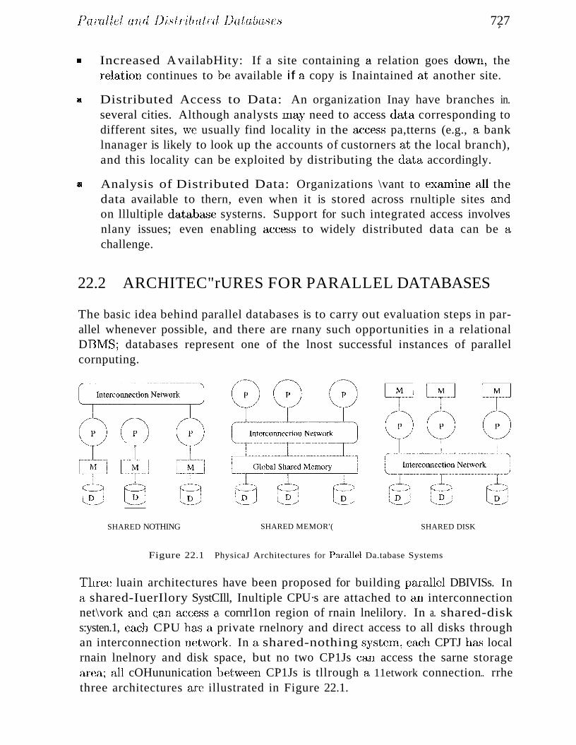
Par-alZel and Dist'rilnl,ted IJatabascs 727~
lIB Increased A vailabHity: If a site containing a relation goes dovvn, therelation continues to be available if a copy is Inaintained at another site.
M Distributed Access to Data: An organization Inay have branches in.several cities. Although analysts rnay need to access data corresponding todifferent sites, 1NC usually find locality in the access pa,tterns (e.g., a banklnanager is likely to look up the accounts of custorners at the local branch),and this locality can be exploited by distributing the data accordingly.
II Analysis of Distributed Data: Organizations \vant to exa"rnine all thedata available to thern, even when it is stored across rnultiple sites andon lllultiple databc6'3c systerns. Support for such integrated access involvesnlany issues; even enabling access to widely distributed data can be achallenge.
22.2 ARCHITEC"rURES FOR PARALLEL DATABASES
The basic idea behind parallel databases is to carry out evaluation steps in parallel whenever possible, and there are rnany such opportunities in a relationalDBJ\lIS; databases represent one of the lnost successful instances of parallelcornputing.
~ciJ
SHARED NOTHING SHARED MEMOR'( SHARED DISK
Figure 22.1 PhysicaJ Architectures for Parallel Da.tabase Systems
l~hree luain architectures have been proposed for building para.11el DBIVISs. Ina shared-IuerIlory SystCIll, Inultiple CPU·s are attached to an interconnectionnet\vork [Lnd c;an [l,ccess (1, cornrl1on region of rnain lnelilory. In a. shared-disks:ysten.1, c(l,ch CPU has a private rnelnory and direct access to all disks throughan interconnection nehvork. In a, shared-nothing systerl1: eac:h CPTJ haB localrnain lnelnory and disk space, but no two CP1Js can access the sarne storagearea; all cOHununication betvveen CP1Js is tllrough a 11etwork connection.. rrhethree architectures are illustrated in Figure 22.1.
728 (~HAPTER 22;
IThe shared-rnernory architecture is closer to a conventional rnachine, and Illanyconunercial database systerns have been ported to shared lnernory platfornlS\vith relative ea",":ic. C~oInrnunication overhead is low ~ because lnain rncIIlory canbe used for this purpose, and operating systern services can be leveraged toutilize the additional CPl:Js. Although this approach is attractive for achievingrnoderate paranelisln·····~··a few tens of CPlJS can be exploited in this fashion~
Inernory contention bec01nes a bottleneck as the nurnber of CPUs increases.rfhe shared-disk architecture faces a sirnilar problcrn because large a1110nnts ofdata are shipped through the interconnection network.
The basic problern with the shared-111Crrlory and shared-disk architectures is interference: As Inore CPUs are added, existing CPUs are slowed dovvn becauseof the increased contention for mClllory accesses and network bandwidth. It hasbeen noted that even an average 1 percent slowdown per additional CPU 1nea11Sthat the rnaxirnum speed-up is a factor of 37, and adding additional CPlJs actually slows down the systern; a systenl with 1000 CPUs is only 4 percent aseffective as a single- CP U systern! This observation has rllotivated the developrnent of the shared-nothing architecture, which is now widely considered to bethe best architecture for large parallel database systems.
rrhe shared-nothing architecture requires rnore extensive n~organization of theDBNIS code, but it has been shown to provide linear speed-up, in that thetilne taken for operations decreases in proportion to the increase in the nUlnberof CPlJs and disks, and linear scale-up, in that perforrnance is sustained ifthe nurnber of CPUs and disks are increased in proportion to the arnount ofdata. Consequently, ever-rnore-powerful parallel database systcrns can be builtby taking advantage of rapidly irnproving perforrllance for single-CPU systelnsand connecting as rnany CPUs as desired.
Speed-up and scale-up are illustrated in Figure 22.2. 'The speed-up curves showhow, for a fixed database size, Inore transactions can be executed l)cr secondby adding CPUs. 1118 scale-up curves shovv hovv adding Inorc resources (in theforln of CPlJs) enables us to process larger problerns. rrhe first scale-up graphIncasures the nurnber of transactions executed per second as the clatabase size isiucTec'lsed and th(~ nurnber of CPlJs is correspondingly inCr(~(lsed. Arl alternative\ivay to Ineasure scale-up is to consider the tirne Utken per transaction (kS r1101'eCPTJs aTe added to process an increasing nurnber of transactions per second;the goal here is to sustain the response tirne per transaction.
22.3 PARAI~l~EL QUERY EVALUATION'
In this s(~ction, vve (liscusspH,rallel evaluation of a relational query in a I).lHvlS\\'ith (1, slutred-nothing architccture.\Vhile it is I)Ossibl(\, to consicler para11el
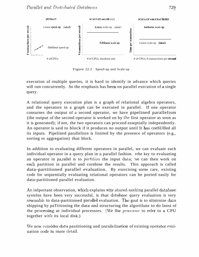
PaTallel and [}i.stTibuted Databa8es 729$
SPEED-UP
Linear speed-up (ideal)
Sublinear speed-up
# ofCPUs
SCALE-UP with DB SIZE
Linear scale-up (ideal)
Sllblint~ar scale-up
# of CPUs, database size
SCALI':-I]P with # KACTSiSEC
Sublinear scale-up
Linear scale-up (ideal)
# of CPUs, # transactions per second
Figure 22.2 Speed-up and Scale-up
execution of rnultiple queries, it is hard to identify in advance which querieswill run concurrently. So the ernphasis has been on parallel execution of a singlequery.
A relational query execution plan is a graph of relational algebra operators,and the operators in a graph can be executed in parallel. If one operatorconsurnes the output of a second operator, we have pipelined parallelism(the output of the second operator is worked on by the first operator as soon asit is generated); if not, the two operators can proceed esseptially independently.An operator is said to block if it produces no output until 'it has conSUllled allits inputs. Pipelined parallelisrn is lirnited by the presence of operators (e.g.,sorting or aggregation) that block.
In addition to evaluating different operators in parallel, we can evaluate eachindividual operator in a query plan in a parallel fashion. rrhe key to evaluatingan operator in pa,rallel is to partition the input data; \ve can then work oneach partition in parallel and cornbine the results. This approach is calleddata-partitioned parallel evaluation. By exercising sorne care, existingcode for sequentially evaluating relational operators can be ported easily fordata-partitioned parallel evaluation.
All inlportant observation, '\vhich explains vvhy shaxed-nothing parallel databa",;csystelns have been very successful, is that database query evaluation is veryaxncll<tble to data-partitioned parallel evaluation. The goal is to nlinirnize elata,shipping b:y paTtitioning the data ,lnd structuring the algoritluns to do lnost ofthe proc(\'ssing at individual processors. (\\le lIse PTOCCS80T to refer to a. CPUtogether vvrith its local disk.)
\Ve nOVil (~onsid(~r elata paxtitioning and pa.rallelization of existing operator evaJuation cod(\' ill rnore detail.
730 CHAPTER 22
22.3.1 Data Partitioning
Partitioning a large data..'Sct horizontally across several disks enables us to exploit the I/O banchvidth of the disks by reading and writing theln in parallel.rrhere are several \vays to horizontally partition a relation.vVe can assign tuplesto processors in a round-robin fashion, \ve can use hashing, or we can a..'Ssigntuples to processors by ranges of field values. If there are n processors, the 'ithtuple is assigned to processor 'i rnodn in round-robin partitioning. Recallthat round-robin partitioning is used in RAID storage systelTIS (see Section 9.2).In hash partitioning, a hash function is applied to (selected fields of) a tupleto deternline its processor. In range partitioning, tuples are sorted (conceptually), and n ranges are chosen for the sort key values so that each rangecontains roughly the SalTIe nurnber of tuples; tuples in range i are assigned toprocessor i.
Round-robin partitioning is suitable for efficiently evaluating queries that access the entire relation. If only a subset of the tuples (e.g., those that satisfythe selection condition age = 20) is required, hash partitioning and range partitioning are better than round-robin partitioning because they enable us toaccess only those disks that contain rnatching tuples. (Of course, this statement assumes that the tuples are partitioned on the attributes in the selectioncondition; if age = 20 is specified, the tuples must be partitioned on age.) Ifrange selections such as 15 < age < 25 are specified, range partitioning is superic)!' to ha.'3h partitioning because qualifying tuples are likely to be clusteredtogether on a few processors. On the other hand, range partitioning can leadto data skew; that is, partitions with widely varying numbers of tuples acrosspartitions or disks. Skew causes processors dealing with large partitions tobecorne perfonnance bottlenecks. Hash partitioning has the additional virtuethat it keeps data evenly distributed even if the data grows and shrinks overtirne.
To reduce ske\v in range partitioning, the luain question is how to choose theranges by which tuples are distributed. ()ne effective approach is to take sarnpIes fronl each processor, collect and sort all sarnples, and divide the sorted setof samples into equally sized subsets. If tuples are to be partitioned on age,the age ranges of the sarnpled subsets of tuples can be used as the ba,,5is forredistributing the entire relation.
22.3.2 Parallelizing Sequential Operator Evaluation Code
An elegant soflvvare architectnre for parallel I)BlVISs enables us to readily parallelize existing code for sequentially evaluating a relational oI>crator. 1"hebasic idea is to use parallel da.ta strearrlS. Strea,rIls (frorn different disks or
]JaTallel arul DistTilntted Databases 731
the output of other operators) are Inerged cl..S needed to provide the inputsfor a relational operator, and the output of an operator is split a.5 needed toparallelize subsequent processing.
A. parallel evaluation plan consists of a dataflow network of relational, luerge,and split operators. 1'he rnerge and split operators should be able to bufferSOlne data and should be able to halt the operators producing their input data.11hey can then regulate the speed of the execution according to the executionspeed of the operator that conSUlues their output.
As we will see, obtaining good parallel versions of algorithllls for sequentialoperator evaluation requires careful consideration; there is no luagic formulafor taking sequential code and producing a parallel version. Good use of splitand 111erge in a dataflow software architecture, however, can greatly reduce theeffort of implementing parallel query evaluation algorithms, as we illustrate inSection 22.4.3.
22.4 PARALLELIZING INDIVIDUAL OPERATIONS
This section shows how various operations can be implemented in parallel ina shared-nothing architecture. We assurne that each relation is horizontallypartitioned across several disks, although this partitioning mayor may not beappropriate for a given query. The evaluation of a query must take the initialpartitioning criteria into account and repartition if necessary.
22.4.1 Bulk Loading and Scanning
vVe begin with two siluple operations: scanning a relation and loading a relation.Pages can be read in parallel while scanning a relation, and the retrieved tuplescan then be lnerged, if the relation is partitioned across several disks. Moregenerally, the idea also c:lpplies when retrieving all tuples that Incet a selectioncondition. If ha'Shing or range partitioning is used, selection queries can beanswered by going to just those processors that contain relevant tuples.
A sirnilar observation holds for bulk loading. Further, if a relation ha.." associated indexes, any sorting of data entries required for building the indexesduring bulk loc:;tding can also be done in parallel (see later).
732 (;HAPTER 2;2
22.4.2 Sorting
A sirnple idea is to let each CPTJ sort the part of the relation that is on its localdisk and then rnerge these sorted sets of tuples. r:rhe degree of parallelisHl islikely to be lirnited by the rnerging phase.
A better idea is to first redistribute all tuples in the relation using range partitioning. For exarnple, if we want to sort a collection of ernploy-ee tuples bysalary~ salary values range froIH 10 to 210, and we have 20 processors, we couldsend all tuples with salary values in the range 10 to 20 to the first processor,all in the range 21 to 30 to the second processor, and so on. (Prior to the redistribution, while tuples are distributed across the processors, \ve cannot assurnethat they are distributed according to sa1ary ranges.)
Each processor then sorts the tuples &'3signed to it, using sorne sequential sortingalgorithrn. For exaluple, a processor can collect tuples until its lllemory is full,then sort these tuples and write out a run, until all incolning tuples have beenwritten to such sorted runs on the local disk. rrhese runs can then be rnergedto create the sorted version of the set of tuples assigned to this processor. Theentire sorted relation can be retrieved by visiting the processors in an ordercorresponding to the ranges assigned to thenl and sirnply scanning the tuples.
The basic challenge in parallel sorting is to do the range partitioning so thateach processor receives roughly the Si::Ulle runnber of tuples; otherwise, a processor that receives a disproportionately large nurnber of tuples to sort becornes abottleneck and lirnits the scalability of the parallel sort. ()ne good approach torange partitioning is to obtain a sarnple of the entire relation by taking sarnplesat each processor that initially contains part of the relation. The (relativelysrnall) saruple is sorted and used to identify ranges with equal nUlllbers of tuples. This set of range values, called a splitting vector, is then distributed toall processors and used to range partition the entire relation.
A particularly irnportant application of parallel sorting is sorting the data entries in tree-structured indexes. Sorting data entries can significantly speed upthe process of bulk-loading an index.
22.4.3 Joins
In this section, \ve consider ho\v the join operation can be parallelized.\Vepresent the basic idea behind the parallelization and illustrate the use of thernerge and split operators described in Section 22.:3.2. vVe focus on parallelhash join, \vhich is \videly useel, and "briefly outlin(~ how sort-rnerge join ca,n
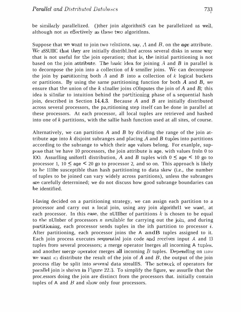
jJ(Jrallel ftnd [J"stT"ibuted Databases 73310
be sirnilarly parallelized. ()ther join algorithniS can be parallelized (lA'S \veIl,although not as effectively'" as thes(~t\vo algoritlnns.
Suppose that 'we \vant to join two relations. say, 1-1 and 13, on the age attribute.vVe aSSUIllC that they are initially distribl.lted across several disks in senne \vaythat is not useful for the join operation; that is, the initial partitioning is notbased on the join a.ttribute. '1'he l)ctsic idea. for joining A and B in parallel isto decornpose the join into a collection of k srnnller joins. vVe can decornposethe join by partitioning both /1 and B into a collection of k logical bucketsor partitions. By using the sarne partitioning function for both j! and B, \veensure that the union of the k s1naller joins cOlnputes the join of A and B; thisidea is si1nilar to intuition behind the pa..rtitioning phase of a sequential hashjoin, described in Section 14.4.3. Because A and B are initially distributedacross several processors, the pa,rtitioning step itself can be done in parallel atthese processors. At each processor, all local tuples are retrieved and hashedinto one of k partitions, with the salIie hash function used at all sites, of course.
Alternatively, we can partition A and B by dividing the range of the join attribute age into k disjoint subranges and placing .A and B tuples into partitionsaccording to the subrange to which their age values belong. For exanlple, supPOs(~ that \ve have 10 processors, the join attribute is age, with values froln 0 toIOO. Assurlling uniforrl1 distribution, A and B tuples with 0 < age < 10 go toprocessor 1, 10 < age < 20 go to processor 2, and so on. This approach is likelyto be 1110re susceptible than hash partitioning to data skew (i.e., the numberof tuples to be joined can vary widely across partitions), unless the subrangesare carefully deterrnined; we do not discuss how good subrange boundaries canbe identified.
I-Iaving decided on a partitioning strategy, we can assign each partition to aprocessor and carry out a local join, using any join algorithrl1 we want: ateach processor. In this case, the nUIIlber of partitions k: is chosen to be equalto the nUlnber of processors n availabl(~ for carrying out the join~ and duringp;:utitioning, each processor sends tuples in the ith partition to processor ,l.After partitioning, each processor joins the A andB tuples assigned to it.Each join process executes s(~quential join code a.Jld recfdves input ..4. and 13tuples froro several processors; a rnerge operator lnerges all incorning A tuples,and another rnerge operator rnerges all incorning 13 tuples. Depending on 110\V
\vc\vant tC) distribute the result of the join of ./1 and [3, the output of the joinprocess rl1ay be split into several data strealIlS. rI'he net\vork of operators forparallel join is sho\vn in Figur(~ 22.:3. To sirnplify the figure, \ve assurlle that theproc.essors doing the join are distinct frorn the processors that. initially containtuples of A and [3 and sho\v only four processors.
734
i
C~HAprrER 42
Figure 22.3 Dataflow Network of Operators for Parallel Join
If range partitioning is used, this algorithrn leads to a parallel version of a sortmerge join, with the advantage that the output is available in sorted order. Ifhash partitioning is used, we obtain a parallel version of a hash join.
Improved Parallel Hash Join
A hash-based refinernent of the approach offers iJuproved perforruanee. rrheruain observation is that, if A and B are very large and the nurnber of partitionsk is chosen to be equal to the nurnber of processors n, the size of each partition111ay still be large, leading to a high cost for each local join at the n processors.
An alternative is to execute the srnaller joins Ai !Xl Hi, for i = 1 ... k, oneafter the other, but\vith each join executed in parallel using all processors.This approa,ch allows us to utilize the total available ruain rueruory at all 'nprocessors in eEl.ch join Ai !Xl 13i and is described in rnore detail as follcJ\vs:
1. At each site, apply a hash function hI to partition the A and B tuplesat this site into partitions i = 1 ... k. Let A be the srnaller rela,tion. 1'henurnber of paJtitions k is chosen such that each partition of ..4 fits into theaggregate or cornbined rnernory of all n processors.
2. For 'i = 1 ... k, process the join of the ith partitions of A and B. Tocornpute .A.'i [Xl 13i , do the follcnving at every site:(a.) i\pply a second hash function 12,2 to all Ai tuples .to detennine \vhere
they should be joined and send tuple f; to site h2(t).
(b) As A.;. tuples El.rrive to be joined, add thcln to an in-rnernory hash. tabh~.
7B5
(c) After all~4i tuples have been distributed, apply h2 to Hi tuples todeterrnine \\There they should be joined and send tuple t to site h2(t).
(d) ..As B'i tuples HJTive to be joined, probe the in-rnernory table of ..4i
tuples and output result tuples.
The lIse of the second hash function h2 ensures that tuples (L1'e (rIlore or less)uniforrnly distributed across all n processors participating in the join. Thisapproach greatly reduces the cost for each of the srnaller joins and thereforereduces the overall join cost. ()bserve that all available processors are fullyutilized, even though the srnaller joins are carried out one after the other.
The reader is invited to adapt the nehvork of operators shown in Figure 22.3to reflect the iInproved parallel join algorithrn.
22.5 PARALLEL QUERY OPTIMIZATION
In addition to pa.rallelizing individual operations, we can obviously execute different operations in a query in parallel and execute rnultiple queries in parallel.Optirnizing a single query for parallel execution has received rnore attention;systerus typically optirnize queries without regard to other queries that mightbe executing at the scuue tilne.
rrwo kinds of interoperatioll parallelisrn can be exploited within a query:
II The result of one operator can be pip(·~lined into another. For exalnple,consider a left-deep plan in which all the joins use index nested loops. Theresult of the first (Le., the bottollunost) join is the outer relation tuplesfor the next join node. As tuples are produced by the first join, they canbe used to probe the inner relation in the second join. T'he result of thesecond join can sirnilarly be pipelined into the next join, and so 011.
I!III wi ultiple independent operations ca,rl be executed concurrently. For exarnpIe, consider a (bush~y) plan in vilhich relations A and I3 are joined, relations(7 and D are joined, and the results of these two joins are finally joined.(;learly, the join of Jl and 13 can be executed conculTcntly with the join ofC: anci D.
A.n optirnizer that seeks to parallelize query evaluation ha.s to consider severalissues, and we Ol11~y outline the rnain points. The cost of executing individualoperations in paraJlel (e.g., pcLrallel sorting) obviollsly differs frorn executingthern s(~quentjally, and tIle optirnizer should estirnate operation costs accordingly.
736 (;HAPTER;22
Next, the plan that returns answers quickest Inay not be the plan \vith thelea,,'3t cost. For ex,unple, the cost of A. [)<J B plus the cost of C rxJ D plus thecost of joining their results rnay be rnore than the cost of the cheapest left-deepplan. I-Iowever, the titne taken is the titne for the 1nore expensive of ..4 t><l Band () [)<J 1) plus the titne to join their results. Tlhis tirHe lnay be less thanthe tirne taken by the cheapest left-deep plan. This observation suggests thata parallelizing optirnizer should not restrict itself to left-deep trees and shouldalso consider bVJshy trees, which significantly enlarge the space of plans to beconsidered.
Finally, a nurnber of pararneters, such as available buffer space and the nUl1.1bel' of free processors, are known only at run-tirne. rrhis comnlent holds in arnultiuser environrnent even if only sequential plans are considered; a rnultiuserenvironrnent is a sirnple instance of interquery parallelisrn.
22.6 INTRODUCTION TO DISTRIBUTED DATABASES
As we observed earlier, data in a distributed database systern is stored acrossseveral sites, and each site is typically rnanaged by a DBMS that can run independent of the other sites. The classical view of a distributed database systernis that the systcrn should rnake the irnpact of data distribution transparent.In particular, the following properties are considered desirable:
III Distributed Data Independence: lJsers should be able to ask querieswithout specifying where the referenced relations, or copies or fragrnentsof the relations, are located. This principle is a natural extension of physical and logical data independence; vve discuss it in Section 22.8. Further,queries that span rnultiple sites should be optirnized systcrnatically in acos1,-based rnanner, taking into account COllllnunication costs and differences in local cornpntation costs. vVe discuss distributed query optirnizaLion in Section 22.10.
II Distributed 'Iransaction Atolnicity: lJsers should be able to 1,\r1'itetransactions that access and update data at several sites just as they vvould1,\rrite transEl,ctions over purely local data. In pa,rticular, the effects of (1.
1:rans(1.cti011 across sites should continue to be atornic; that is, all changespersist if the tranS<lction cOllnuits and none persist if it aborts. \Ve discussthis distributed transaction processing in Sections 22.11, 22.1:~, and 22.14.
AJthough rnost people would agree that these properties are in general clesira,blc~, in certain situ::ttions, such as when sites are conlH~cted by ct 810-w longdistance network, these properti(~s are not efficiently achievable. Indef\'d, it has1 :",Y' ····0· ··\·i t·l··'·1·· . r1" ,\' ,·,·t·:"S·' ':.1 )"1)1··11r "'1··,t"·l t·)·l 1"1' :,)":.) .. ,. ,:..·t···,s·" ....\ t)CC11 d.l buce ,Vl." V\. lcn ~I ,C, eU C' g <. )d, .. J <. IS ..1 1)11.C<', i lcse pIOpCl ,IC" ell C no ,even dcsiral)l(~. l]le argurnerlt essentiaJly is that the adrninistrative overheacl
[)arnllel aTLdDistribtlted Database,s 7~37t
of supporting a systern vvith distributed data independence and transactionatornicitY'....·..···in effect 1 coordinating all activities across all sites to support theview of the whole as a unified collection of data--is prohibitive, over and aboveI)B:NlS perfo1'rnanc8 considerations.
}(eep these rerna"rks about distributed databases in rnind a.'3 ,ve cover the topicin rno1'e detail in the rest of this chapter. There is no real consensus on \vhat thedesign objectives of distributed databases should be, and the field is evolvingin response to users 1 needs.
22.6.1 Types of Distributed Databases
If data is distributed but all servers run the sarne DBMS software,. we have ahomogeneous distributed database system. If different sites run underthe control of different DB:NISs, essentially autonorllously, and are connectedsOlllehow to enable access to data from rnultiple sites, we have a heterogeneous distributed database system, also referred to as a multidatabasesystem.
The key to building heterogeneous systelTIS is to have well-accepted standardsfor gateway protocols. A gateway protocol is an API that exposes DBl\1Sfunctionality to external applications. Examples include ODBC and JDBC (seeSection 6.2). By accessing database servers through gateway protocols, theirdifferences (in capability, data fonnat, etc.) are rnasked, and the differencesbetween the different servers in a distributed system are bridged to a largedegree.
C;ateways are not a panacea, however. They add a layer of processing that canbe expensive, and they do not cornpletely rllcL."k the differences arllong servers.For eXfunplc, a server Illay not be capable of providing the services required fordistributed transaction rnanagernent (see Sections 22.13 and 22.14), and evenif it is capable, standardizing gateway protocols all the \vay down to this levelof interaction poses challenges that have not yet been resolved satisfactorily.
Distributed data rnanagcrnent, in the final analysis, cornes at (1 significant costin terulS of perforrna"ncc, software cOlllplexity, and adrninistration difficulty.rrhis observation is especially true of heterogeneous SystCIllS.
22.7 DISTRIBUTED DBMS ARCHITECTURES
Three alternative approctches are uSf~d to separat,e functionality across differentDBIV'IS-related processes; tllese alternative distributed ])131VI8 axchitectures ar(~
ca,lled ()Zient-S'eTvcT, C/ollaborat'ing SeTver, and ]\;JiddZe'wo/t'(~.
738 CHAPTER t2
22.7.1 Client-Server Systems
A Client-Server systelIl has one or rno1'e client processes and one or rnoreserver processes, and a client process can send a query to anyone server process.Clients are responsible for user-interface issues, and servers rnanage data andexecute transactions. Thus, a client process could run on a personal cornputerand send queries to a server running on a 11lainframe.
This architecture has becorne very popular for several reasons. First, it is relatively sinlple to irnplernent due to its clean separation of functionality andbecause the server is centralized. Second, expensive server rnachines are notunderutilized by dealing with lllundane user-interactions, which are now relegated to inexpensive client machines. Third, users can run a graphical userinterface that they are familiar with, rather than the (possibly unfalniliar andunfriendly) user interface on the server.
While writing Client-Server applications, it is inlportant to remember theboundary between the client and the server and keep the communication between therll as set-oriented as possible. In particular, opening a cursor andfetching tuples one at a time generates many rnessages and should be avoided.(Even if we fetch several tuples and cache them at the client, rnessages 11lUStbe exchanged when the cursor is advanced to ensure that the current row islocked.) Techniques to exploit client-side caching to reduce comlnunicationoverhead have been studied extensively, although we do not discuss them further.
22.7.2 Collaborating Server Systems
The (;lient-Server architecture does not allow a single query to span rnultipleservers because the client process would have to be capable of breaking sucha query into appropriate subqueries to be executed at different sites and thenpiecing together the answers to the subqueries. The client process vvould therefore be quite cOlnplex, and its capabilities would begin to overlap with theserver; distinguishing between clients and servers becornes harder. EliIninatingthis distinction leads us to an alternative to the Client-Server architecture: aCollaborating Server systenl. \Ve can lUl,ve a collection of datab::lse servers,each capable of running tra,nsactions against local data, which cooperativelyexecute transactions spanning rnultiple servers.
'\Vhen a server receives a, query that requires access to data at other servers, itgenerates appropriate subqu(~ries to be executed by oth(~r servers and puts theresults together to COIllpute HJlSvVers to the original query. Ideally, the decorn-
Parallel and Dist'rib1lted IJatabases 739
position of the query should be done using cost-based optinlization, taking intoaccount the cost of network COlnnlunication as \vell a.s local processing costs.
22.7.3 Middleware Systems
The Middle\\Tare architecture is designed to allow a single query to span rnultiple servers, without requiring all database servers to be capable of rnanagingsuch nlulti-site execution strategies. It is especially attractive when trying tointegrate several legacy systerns, whose basic capabilities cannot be extended.
The idea is that we need just one database server capable of rnanaging queriesand transactions spanning nlultiple servers; the renlaining servers need to handle only local queries and transactions. We can think of this special server asa layer of software that coordinates the execution of queries and transactionsacross one or more independent database servers; such software is often calledmiddleware. The middleware layer is capable of executing joins and otherrelational operations on data obtained froln the other servers but, typically,does not itself maintain any data.
22.8 STORING DATA IN A DISTRIBUTED DBMS
In a distributed DBMS, relations are stored across several sites. Accessing arelation stored at a renlote site incurs message-passing costs and, to reducethis overhead, a single relation lnay be partitioned or fragrnented across severalsites, with fragrnents stored at the sites where they are most often accessed orreplicated at each site where the relation is in high demand.
22.8.1 Fragmentation
Fragrnentation consists of breaking a relation into srnaller relations or fragrnents and storing the fragrnents (instead of the relation itself), possibly atdifferent sites. In horizontal fragmentation, each fragrnent consists of a,subset of TOWS of the original relation. In vertical fragluentation, each fra.grllent consists of a subset of col'Urnns of the original relation. IIorizontal andverticaJ fragrnents are illustrated in Figllre 22.4.
Typically, the tuples that belong to a given horizontal fragrnent are identifiedby a selection query; for exarnple, crnployee tuples Blight be organized intofragrnents b~y city, \vith all enlployees in (1, given city assigned to the sanie fragrnent. rThe horizontal fragrnent shown in Figure 22.4 corresponds to Chicago." , storing fragrncnts in the data,l)E\..se site at the corresponding city, \ve a,chieve
.:ality of referencc',Chicago data is 1n08t likely to be updated (tnel queried
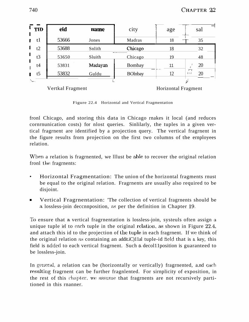
740 (;HAPTEll 42
r - !~-
---ITID eid Dame city i age sal
I II tl 53666 Jones Madras ! 18 I 35
I t2 53688 Snlith Chicago 18 32I
~....~.......................
t3 53650 Sluith Chicago 19 48I . ,.
t4 53831 Madayan Bombay 11 .I 20I J......... -- r-,·_····_-
I t5 53832 Guldu BOlnbay 12 ! I J 20..,................_-
"'.._.. / fVertkal Fragment Horizontal Fragment
Figure 22.4 Horizontal and Vertical Fragmentation
fronl Chicago, and storing this data in Chicago rnakes it local (and reducescornrnunication costs) for nlost queries. Sinlilarly, the tuples in a given vertical fragrnent are identified by a projection query. The vertical fragrnent inthe figure results frorn projection on the first two columns of the ernployeesrelation.
\;Vhen a relation is fragrnented, we lllust be able to recover the original relationfronl the fragrnents:
• Horizontal Fragmentation: The union of the horizontal fragments rnustbe equal to the original relation. Fragrnents are usually also required to bedisjoint.
III Vertical Fragrnentation: 'The collection of vertical fragrnents should bea lossless-join deccnnposition, ~lS per the definition in Chapter 19.
1'0 ensure that (1, vertical fragrnentation is lossless-join, systeuls often assign aunique tuple ieI to each tuple in the original relation~ as shown in Figure 22.4,and attach this id to the projection of the tuple in each fragrnent. If we think ofthe original relation a.s containing an addit.iC)11al tuple-id field that is a. key, thisfield is added to each vertical fragrnent. Such ~L decol11position is guaranteed tobe lossless-join.
In generaJ~ a relation can be (horizontally or vertically) fragrnented, a.nd eachr(~sulting fragrnent can be further fragnlented. For sirnplicity of exposition, inthe rest of this chapter, ,ve (LSSllnH~ that fragrnents are not recursively partitioned in this rnanner.
Parallel and IJistT'ilndcd Databases
22.8.2 Replication
741
Replication Incaus that "we store several copies of a relation or relation fragrnent. An entire relation can be repliccltecl at one or rnore sites. Sirnila,rly, oneor 1110re fragrncnts of a relation can be replicated at other sites. For exarnple, ifa relationR is fragrnented into 1?1,R2, and R:3, there nlight be just one copyof Ill, vvhereas R2 is replicated at two other sites and li,~>' is replica.,t:ed at allsites.
The rnotivation for replication is twofold:
• Increased Availability of Data: If a site that contains a replica goesdown, we can find the sarne data at other sites. Sirnilarly, if local copies ofrerllote relations are available, we are less vulnerable to failure of COllnnunication links.
• Faster Query Evaluation: Queries can execute faster by using a localcopy of a relation instead of going to a rernote site.
The two kinds of replication, called synchronous and asynchronous replication,differ prirnarily in how replicas are kept current when the relation is rnodified(see Section 22.11).
22.9 DISTRIBUTED CATALOG MANAGEMENT
Keeping track of data distributed across several sites can get cornplicated. \tVernust keep track of how relations are fragrnented and replicated------that is; howrelation fragrnents are distributed across several sites and ,vhere copies of fragrnents are st()red~"-----in addition to the lIsuaJ seherna, authorization, and statistical inforrnation.
22.9.1 Naming Objects
If a relation is fragruented and replicated, we rnust be able to uniquely identif\reach replica of ea,ch fragnlent. Cjenerating such unique narnes requires sornecare. If \ve use a global narne-server to a.ssign globally unique narnes, locala,utonornJl is cornprornised; we 'want (users at) each site to be able to <h'3signnarnes to local objects \vithout reference to nanH:~S systernwide.
The usual solution. to the naTning problenl is to use narnes consisting of severalfields. 1;'01' excunplc, we could hELve:
742 CHAPTER ~2
III A local TULTnC field, 'which is the HaIIle assigned locally at the site\vhere therelation is crea,ted. T\vo objects at different sites could have the saIne localnarne, but t\yO objects at a given site cannot have the saIne local narne.
III A biTth s'lt:e field, vvhich identifies the site where the relation \v~1..s crectted,and where il1fofrnation is ruaintained about all fragruents and replicas ofthe rela.tion.
These two fields identify a relation uniquely; we call the cornbination a globalrelation nanle. To identify a replica (of a relation or a relation fragnlent) ,wetake the global relation narne and add a 'tcplica-'id field; we call the cornbinationa global replica narrle.
22.9.2 Catalog Structure
A centralized systern catalog can be used but is vulnerable to failure of the sitecontaining the catalog. An alternative is to rnaintain a copy of a global systemcatalog,which describes all the data at every site. Although this approachis not vulnerable to a single-site failure, it comprornises site autonorny, justlike the first solution, because every change to a local catalog rnust now bebroadcast to all sites.
A better approach, which preserves local autonoruy and is not vulnerable to asingle-site failure, was developed in the It* distributed database project, whichwa..'S a successor to the Systerl1 R, project at IBlV!. Each site ruaintains a localcatalog that describes all copies of data stored at that site. In addition, thecatalog at the birth site for a relation is responsible for keeping track of wherereplicas of the relation (in general, of fragnlents of the relation) are stored. Inparticular, a precise description of each replica's contents""""''''a list of colurl1nsfor a vertical fragrnent or a selection condition for a horizontal fragruentisstored in the birth site catalog. \Vhenever a new replica is created or a replicais rnoved across sites, the inforrnation in the birth site catalog for the relationHUlst be updated.
To locate a relation, the catalog; at its birth site lnust be looked up. rrhise.atalog inforrnation can be ca.,ched at other sites for quicker access, but thecached inforrnation Inay becolue out of date if, for cxarnple, a fragrnent isrnoved. \rYe vvould discover that the locally cached inforrnation is out of datewhen \ve use it to access the relation, and at that point, we rll11st update thecache b.y looking up th(~ catalog at the birth site of the relation. (The birth siteof a relation is recorded in each local cache that describes the relation, and thebirth site never changes, even if the relation is rnoved.)
Parallel and Dis!;r'ibll!;ed Database8
22.9.3 Distributed Data Independence
743
Distributed data independence lueans thc.tt users should be able to \vrite queries\vithout regard to ho\v a relation is fragrnented or replicated; it is the responsibility of the DB:NIS to cornpute the relation a~s needed (by locating suitablecopies of fragrnents, joining the vertical fragrnents, and taking the union ofhorizontal fragn1cnts).
In particular, this property irnplies that users should not have to specify thefull nalne for the data objects accessed while evaluating a query. Let us see ho\vusers can be enabled to access relations without considering how the relationsare distributed. The local narne of a relation in the systeln catalog (Section22.9.1) is really a c01l1bination of a 'User narne and a user-defined relation narne.'Users can give whatever names they wish to their relations, without regard tothe relations created by other users. When a user writes a prograrn or SQLstatelnent that refers to a relation, he or she sirnply uses the relation narne.The DBMS adds the user narne to the relation narne to get a local narne, thenadds the user's site-id as the (default) birth site to obtain a global relationnarne. By looking up the global relation narne-- -in the local catalog if it iscached there or in the catalog at the birth site-·the I)Bl\;IS can locate replicasof the relation.
A user Il1ay want to create objects at several sites or refer to relations createdby other users. To do this, a user can create a, synonym for a global relationnarne' llsing an SQL-style cOl1unand (although such a corl1rnand is not currentlypart of the SQL:1999 standard) and subsequently refer to the relation usingthe synonyrn. For each user known at a site, the DBl\lS rna.intains a table ofsynonynls as part of the systern catalog at that site and uses this table to findthe global relation narne. Note that a user's prograrl1 runs unchanged even ifreplicas of the relation are rlloved, because th(~ global relation narne IS neverchanged until the relation itself is destroyed.
lJsers rnay \vant to run queries agctinst specific replicas, especially if asynchronous replication is used. To support this, the synonyrn Inechanisrn canbe adapted to also allo\v users to create synon.yrl1S for global replica, 11aJ.IH~S.
22.10 DISTRIBUTED QUERY PROCESSING
\Ve first discuss the issues involved in evaluating relational algebra operationsin a distrilnlted datal)ase through exalnples and then outline distributed queryoptiInization. Consider the following t\VO n·~lations:
744 (;lIAPTEH 22
Sailors(s'id: integer, snanu?: string, rating: integer, age: real)
Reserves (sid: int~~ger 1 l)'i(~.:: ~ntege:~, day: ~~te,rnalne: string)
r\S in C:hapter 14, assurne that each tuple of R.eserves is 40 bytes long, tha.t aIH'lge can hold 100 Reserves tuples, and that ¥lC have 1000 pages of such tuples.Sirnilarly, assurne that each tuple of Sailors is 50 bytes long, that a page canhold 80 Sailors tuples, and that \ve hrrve 500 pages of such tuples.
1'0 estiInate the cost of an evaluation strategy, in addition to counting thenurnber of page IjC)s, \ve Blust count the nurnher of pages sent frorH one siteto another because corllrIlunication costs are a significant cornponent of overallcost in a distributed database. \Ve rnust also change our cost rnodel to countthe cost of shipping the result tuples to the site where the query is posed frOInthe site where the result is assernbled! In this chapter, we denote the tilnetaken to read one page from disk (or to write one page to disk) as 1;el and thetiIne taken to ship one page (from any site to another site) as 1;s.
22.10.1 Nonjoin Queries in a Distributed DBMS
Even sirnple operations such as scanning a relation, selection, and projectionare affected by fragrnenta.tion and replication. Consider the following query:
SELECT S.ageFROM Sailors SWHERE S.rating > ;3 AND S.rating < 7
Suppose that the Sailors relation is horizontally fragruented, with all tupleshaving a rating less tha,n 5 at Shanghai and all tuples having a rating greaterthan 5 at rrokyo.
TheDBl\/IS nn.lst answer this query by evaluating it at both sites and takingthe union of the ans\vers. If the SELECT clause contained AVG (S. age), COln
bining the aJ1S\VerS could not be done by sirnply taking the union···-····the DBlV1Srnust cornpute the SUIn and count of age values at the two sites and use thisinfonna,tion to cornpute the average age of all sailors.
If the WHERE clause contained just the condition 5'. rating > 6, on the otherha,ud, the I)BI\/IS should recognize thEtt this query could be ansvvered by just
. .. t r[" kexecutIng It a j ,.n yo.
As ::ulother exarnple, suppose that the Sailors relation, were vertically frag11lented, \vith the 8'id and rai'ing fields at Sha.nghai a,nd the 8naUlC and agefields at rrokyo. No field is stored at both sites. 1]lis vertical fragrnentcttion
Parnllel and DistTilnded [)atllbases .... ,4.-( &l:~)
would therefore be a lossy decornposition, except that a field containing theid of the corresponding Sailors tuple is included by the DB~fS in both fraglnents! N'o\v, the I)BrvIS has to reconstruct the Sailors relation by joining thet\VO fraglnents on the COHllllon tuple-id field and execute the query over thisreconstructed relation.
Finally, suppose that the entire Sailors relation \vere stored at both Shanghaiand ~rokyo. \lVe could answer any of the previous queries by executing it ateither Sha,nghai or Tokyo. vVhere should the query be executed? This dependson the cost of shipping the answer to the query site (which rnay be Shanghai,Tokyo, or SOllIe other site) as well as the cost of executing the query at Shanghaiand at Tokyo...._·..··the local processing costs lnay differ depending on vvhat indexesare available on Sailors at the two sites, for exaluple.
22.10.2 Joins in a Distributed DBMS
Joins of relations at different sites can be very (~xpensive, and we now considerthe evaluation options that IIlUst be considered in a distributed environrnent.Suppose that the Sailors relation were stored at London, and the Ileservesrelation were stored at Paris. We consider the cost of various strategies forcOlnputing Sailor'S [X] Reserves.
Fetch As Needed
We could do a page-oriented nested loops join in Loudon with Sailors as theouter, and for each Sailors page, fetch all Reserves JH:tges frorn Paris. If wecache the fetched Ileserves pages in London until the join is cornpk~te, pagesare fetched only once, but aSSU111e that H,eservcs pages are not cached, just tosee how bad things can get. (The situation can get rnuch worse if vve use atuple-oriented nested loops join!)
rrhe cost is 500id to scan Sailors plus, for each Sailors page, the cost of seallningand shipping all of H,eserves, vvhich is 1000(td + ts). 1'he total cost is therefore500td + 500,OOO(td + is).
In additicHl, if the query was not sllbrnittccl at the London site, \rye rnust addthe cost of shipping the result to the query site; this cost depends on th(~ sizeof the result. Because sid is a key for Sailors, the nurnber of tuples in the resultis 100,000 (the rnunber ()f tuples in Ilcserv(~s) and each tuple is 40 + 50 = 90bytes long; thus 4000/DO = 44 result tuples fit on a page~ and the result sizeis 100,OOO/44=227~~ pages. rrhe cost of shipping the answer to another site, ifnecessary, is 227:3 t,,,. In tIle rest of this section, we assurne that the query is
746 CHAPTER 22
posed at the site where the result is computed; if not, the cost of shipping theresult to the query site Blust be added to the cost.
In this exarnple, observe that, if the query site is not London or Paris, thecost of shipping the result is greater than the cost of shipping both Sailorsand Ileserves to the query site! Therefore, it would be cheaper to ship bothrelations to the query site and COlllpute the join there.
Alternatively, we could do an index nested loops join in London, fetching allInatching Reserves tuples for each Sailors tuple. Suppose we have an uncIustered hash index on the sid colurnn of Ileserves. Because there aTe 100,000Ileserves tuples and 40,000 Sailors tuples, each sailor has on average 2.5 reservations. The cost of finding the 2.5 Ileservations tuples that lllatch a givenSailors tuple is (1.2 + 2.5)td' assluning 1.2 l/Os to locate the appropriatebucket in the index. The total cost is the cost of scanning Sailors plus thecost of finding and fetching nlatching Reserves tuples for each Sailors tuple,500td + 40, 000(3.7td + 2.5t s )'
Both algorithIns fetch required Reserves tuples from a remote site as needed.Clearly, this is not a good idea; the cost of shipping tuples dominates the totalcost even for a fast network.
Ship to One Site
\Ve can ship Sailors from London to Paris and carry out the join there, shipReserves to London and carry out the join there, or ship both to the site \\Therethe query was posed and cornpute the join there. Note again that the querycould have been posed in London, Paris, or perhaps a third site, say, Tirnbuktu!
11he cost of scanning and shipping Sailors, saving it at Paris, then doing thejoin at Paris is 500(2td + ts ) + 4500td, assurning that the version of the sortrnerge join described in Section Itt.l0 is used and we have an adequate nurnberof buffer pages. In the rest of this section we aSSUInc that sort-Inerge join isthe join rnethod used when both relations are at the saIne site.
The cost of shipping Ileserves <lJld doing the join at London is 1000(2t(1 -+- t,c;) +4500td·
Senlijoins andBloomjoins
Consider the strategy of shipping Ileserves to Londo.l1 and cornputing the joinat London. SOln(~ tuples in (the current inst;-l,llCe of)H,cserves do not join ¥lithan.y tuple in (the current instaJ1Ce of) Sailors. If Vie could sorneho\v identify
Parallel and DistT'ib'tded Databases 747
Reserves tuples that are guaranteed not to join ~Nith any Sailors tuples, wecould avoid shipping thern.
T,,·vo techniques, Se1n'ijo'ln and Bloo1r~ioin, have been proposed for reducingthe number of lleserves tuples to be shipped. The first technique is calledSemijoin. The idea is to proceed in three steps:
1. At London, cornpute the projection of Sailors onto the join colurnns (inthis case just the sid field) and ship this projection to Paris.
2. At Paris, cornpute the natural join of the projection received frorn thefirst site with the R,eserves relation. l'he result of this join is called thereduction of R,eserves with respect to Sailors. Clearly, only those Reserves tuples in the reduction will join with tuples in the Sailors relation.Therefore, ship the reduction of Reserves to London, rather than the entireReserves relation.
3. At London, cornpute the join of the reduction of R,eserves with Sailors.
Let us compute the cost of using this technique for our example join query.Suppose we have a straightforward irnplernentation of projection based on firstscanning Sailors and creating a telnporary relation with tuples that have onlyan sid field, then sorting the temporary and scanning the sorted ternporary toeliminate duplicates. If we assurne that the size of the sid field is 10 bytes,the cost of projection is 500"td for scanning Sailors, plus 100td for creatingthe ternporary, plus 400ld for sorting it (in two passes), plus IOOtc! for the finalscan, plus 100ld for writing the result into another tcrnporary relation; a total of1200f;d. (Because sid is a key, no duplicates need be elirninated; if the optiInizeris good enough to recognize this, the cost of projection is just (500 + 100)td.)
The cost of cornputing the projection and shipping it to Paris is therefore1200ld + 100l,';. The cost of c(nnputing the reduction of R.eserv8s is ~~ . (100 .+10(0) == ~330(}t(j, assurning that sort-rnerge join is used. crhe cost does notreflect that the projection of Sailors is already sorted; the cost \vould deerca.,seslightly if the refined sort-Inerge join exploited this.)
\Vhat is the size of the reduction? If every sailor holds at lC<L5t one reservation,the reduction includes every tuple of R,eserves! The effort invested in shippingthe projection and reducing lleserves is a total waste. Indeed, because of thisobserva.ticHl, \iVC note that Sernijoin is especially useful in conjunction \vith aselectiol1 on one of the relations.F()r exarnplc , if W(~ \vant to cornpute the joinof Sailors tuples with a ral'ing greater than 8 \vith the lleserves rela.tion, thesize of the projection on 8'id fen' tuples that satisfy the selection \vould be just20 percent of tIle original projection, that is, 20 pages.
748 C~HAprrEIl ~2
Let us nuw continue the exarnple join, 'with the assurnption that \ve have theadditional selection on 'r'(rt'ing. (The cost of cornputing the projection of Sailorsgoes de)\vn a bit, the cost of shipping it goes do\\rn to 20ts , and the cost of thereduction of F{,eser\fPS also goes de)\vn a little, but \ve ignore these reductions forsirnplicity.) \Ve assurne that; only 20 percent of the R,eserves tuples are includedin the reduction, thanks to the selection. lIencc 1 the reduction contains 200pages, and the cost of shipping it is 200ts .
Finally, at London, the reduction of I{eserves is joined with Sailors, at a costof ~3· (200 + 500) = 21100td. Observe that there are over 6500 page I/Os versusabout 200 pages shipped, using this join technique. In contrast, to ship R,eservesto London and do the join there costs IOOOi s plus 4500td. \Vith a high-speed.network, the cost of Sernijoin Illay be n10re than the cost of shipping Reservesin its entirety, even though the shipping cost, itself is rnueh less (200t s versusIOOOts )·
The second technique, called Bloomjoin, is quite sirnilar. The luain differenceis that a bit-vector is shipped in the first step, instead of the projection ofSailors. A bit-vector of (SOIlIC chosen) size k is cOlnputed by hashing each tupleof Sailors into the range 0 to k - I and setting bit i to I if seHne tuple hashes toi, and 0 otherwise. In the second step, the reduction of Reserves is cOlnputedby hashing each tuple of lleserves (using the sid field) into the range 0 to k --1,using the sanle hash function used to construct the bit-vector and discardingtuples whose hash value i corresponds to a 0 bit. Because no Sailors tupleshash to such an i, no Sailors tuple can join with any R,eserves tuple that is notin the reduction.
111e costs of shipping a bit-vector and reducing R,eserves using the vector areless than the corresponding costs in Sernijoin. ()n the other hand, the size ofthe reduction of Iteserves is likely to be larger than in Sernijoin; so, the costsof shipping the reduction and joining it 'with Sailors are likely to be higher.
Let us estirnate the cost of this approach. rrhe cost of cornputing the bitvector is essentially the cost of scanning Sailors, \vhich is 500td. rrhe cost ofsending the bit-vector depends on the size \ve choose for the bit-vector, 'whichis certainly sInaJler than the size of the projection; vve take this cost to be 201: 8 ,
for concreteness. The cost of reducing Reserves is just the cost of scanningH,eserves, lOOOl'd. T'he size of the reduction of R<eserves is likely to be aboutthe saIne Eh'3 or a little larger than the size of the reduction in tIle Scrnijoinclpproach; instea,d of 200, \ve will take tllis size to be 220 pages. (\Ve aSSUInethat the selection on Sailors is included, to pennit a direct cOInparison \vith thecost of Scrnijoin.) 'I'he cost of shipping the reduction is therefore 220ts ' 1'hecost of the final join at London is :3 . (500 + 220) == 2160td.
J)arallel and IJiBtTib'lded [)tdabases 749
rrhus, in cornparison to Sernijoin! the shipping cost of this approach is aboutthe SaIl1t\ although it could be higher if the bit-vector vvere not as selective(1.'; the projection of Sailors in tenns of reducing Reserves. 'Typically, though,the reduction of lleserves is no l110re than 10 to 20 percent larger than thesize of the reduction in SClnijoin. In exchange for this slightly higher shippingcost, Bloornjoin achieves a significantly lower processing cost: less than :370Cltdversus rnore than 6500td for SClnijoin. Indeed, Bloornjoin has a lo\ver I/C)cost and a lower shipping cost than the strategy of shipping all of R,eserves toLondon! These nurnbers inclicatewhy Bloollljoin is an attractive distributedjoin rnethod; but the sensitivity of the rnethod to the effectiveness of bit-vectorhashing (in reducing Reserves) should be kept in rnind.
22.10.3 Cost-Based Query Optimization
\Ve have seen how data distribution can affect the inlplernentation of individualoperations, such as selection, projection, aggregation, and join. In general, ofcourse, a query involves several operations, and optirnizing queries in a distributed database poses the following additional challenges:
• CornrIlunication costs lllUSt be considered. If we have several copies of arelation, we HlllSt also decide which copy to use.
• If individual sites are run under the control of difl'erent DBl\JlSs, the autonolny of each site HUlst be respected while doing global query planning.
(~uery optiInization proceeds essentially as in a centralized DBMS, as describedin Chapter 12, with inforrnation about relations at rernote sites obtained fron1the systeln catalogs. ()f course, there are nlore alternative lllethods to considerfor each operation (e.g., consider the new options for distributed joins), andthe cost rnetric ruust account for cornrnunication costs as \vell, but the overallplanning process is essentially unchanged if we take the cost rnetric to be thetotal cost of all operations. (If \ve consider response tilne, the fact that certainsubqueries can be carried out in pclrallel at different sites \vould require us tochange the optirnizer ,1,8 per the discussion in Section 22.5.)
In the overall plan, local rnanipulatiol1 of relations at the site where they arestored (to corllpute an interrnediate relation to be shipped elsewhere) is encapsulated into a :sugge8ted local plarl. The overall plan includes several such localplans, \vhichwe can think of as subqueries executing at different sites. \:Vhilegenerating the global plan, the suggested local plans provide recilistic cost estirnates for the cornputatioll of the interrnediate rehltions; the suggested localplans are constructed by the optirnizer rnainly to provide these local cost estiIuates. A site is free to ignore the local plan suggested to it if it is able to finda cheaper plan by llsing InorE~ current infonnation in the local catalogs. l'hus,
750 C~HAPT'ER 22
site autoncllny is respected in the optirnizaJion and evaluation of distributedquenes.
22.11 UPDATING DISTRIBUTED DATA
The classical view of a distributed DB:tvIS is that it should behave just like acentralized DBNIS froul the point of vievv of a user; issues arising froln distribution of data should be transparent to the user, although, of course, they rnu8tbe addressed at the irnplernentation level.
vVith respect to queries, this vievv of a distributed DBIVIS Ineans that usersshould be able to ask queries \vithout worrying about how and "\vhere relationsare stored; we have already seen the irnplications of this requirernent on queryevaluation.
vVith respect to updates, this view rneans that transactions should continueto be atornic actions, regardless of data fragrnentation and replication. Inparticular, all copies of a rnodified relation must be updated before the rnodifying transaction cornn1its. We refer to replication with this sernantics as synchronous replication; before an update transaction cOHllnits, it synchronizesall copies of rnodified data.
An altE:~rnativeapproach to replication, called asynchronous replication, hascorne to be widely usee1 in eornrnercial distributed DBlVISs. Copies of a rnodifiedrelation are updated only periodically in this approach, and a transaction thatreads different copies of the sarne relation rnay see different values. T'hus,asynchronous replication cornprolnises distributed data independence, but itcan be iInplernented 1110re efficiently than synchronous replication.
22.11.1 Synchronous Replication
There are two 1)3sic techniques for ensuring that transactions see the senne vaJueregardless of\vhich copy of an object they access. In the first technique, calledvoting, a tnulsaction Inust \vrite H" lnajority of copies to rnodify a,ll ol)ject <:lJld
read at lea"st enough copies to rnake sure that one of the copies is current. Forexanlple, if there <-:tre 10 copies and 7 copies are \vritten by update transactions,then at least /.1 copies rnust be read. Eac:h copy has a version nurnber, andthe copy \vith the highest version rllunber is current. This technique is not attra,ctive in rnost situations because reading aJl ol)ject reqllires reading rnultiplecopies; in rnost applications, objects are read rnuch 1n01'e frequently than thc~y
are updated, and f'~fficientperfonnanceon recvls is very irnportant.
I)aT'fLllel and IJistT'ib'ILted !Jai:abascs 751
In the second technique, called read-any write-all, to read an object, a traJ1Saction can read anyone copy, but to \vTite an object, it Inust \vrite all copies.R,eads are fast, especially if we have a local copy, but 'writes are slo\ver, relativeto the first technique. 1"'his technique is attractive vvhen reads are rnuch rnorefrequent than vvrites, and it is usually adopted for irnplernenting synchronousreplication.
22.11.2 Asynchronous Replication
Synchronous replication COines at a significant cost. Before an update transaction can corn1'nit, it rnust obtain exclusive locks on all copies···c1.SSUlning that theread-any write-all technique is used· ···of rnodified data. The transaction Inayhave to send lock requests to rernote sites and \vait for the locks to be granted,and during this potentially long period, it continues to hold all its other locks.If sites or connnunication links fail, the transaction cannot cOInrnit until all thesites at which it has rnodified data recover and are reachable. Finally, even iflocks are obtained readily and there are no failures, connnitting a transactionrequires several additional rnessages to be sent as part of a cOTnrn'it protocol(Section 22.14.1).
For these reasons, synchronous replication is undesirable or even unachievablein 111any situations. Asynchronous replication is gaining in popularity, eventhough it allows different copies of the saIne object to have different values forshort periods of tinlC. This situation violates the principle of distributed dataindependence; users 11Ulst be aware of which copy they are accessing, recognizethat copies are brought up-to-date only periodically, and live with this reducedlevel of data consistency. Nonetheless, this seeIns to be a practical C0l11pr0l11isethat is acceptable in rnany situations.
Primary Site versus Peer-to-Peer Replication
A.synchronous replication C01nes in t\VO flavors. In primary site asynchronousreplication, one copy of a relation is designated the primary or luaster COP)T.
H.eplicas of the entire relation or fragrnents of the relation C(lJl be created atother sites; these a,re secondary copies, and unlike tIle priInary copy, they cannot be updated . .l\.. conUIlon InecllallislIl for setting up prhnary and secondary!copies is that Osers first register or publish the relation at th(-~ priruaxy siteaXlcl subs(~quently subscribe to a fragrnent of a registered relation fron1 another(secondary) site.
In peer-to-peer as)rnchronous replication~ 111()re than one copy (although perhaps rIot (11) can be designated as updatable, that is, a 1'naste1' copy. In additionto propagating changes, a conflict resolution strat(~gy Inusi'; be used to deal
752 C~HAP'TER ~2
with conflicting CIH:ulges Inade at different sites. For exarnplc, .Joe's age rnaybe changed to ~i5 at one site and to 38 at another. \Vhich value is ·correct'?:NIany luore subtle kinds of conflicts can arise in peer-to-peer replication, and ingeneral peer-to-peer replication leads to ad hoc conflict resolution. Senne special situations in \vhich peer-to-peer replication does not lead to conflicts arisequite ()ften~ and in such situations peer-to-peer replication is best utilized. Forexalnple:
• Each 1naster is allo\ved to update only a fragrnent (typically a horizontalfrag1nent) of the relation, and any two fragrnents updatable by different!llasters are disjoint. For excunple, it rIlay be that salaries of Gerrnan erllployees are updated only in Frankfurt, and salaries of Indian ernployees areupdated only in 1\1adras, even though the entire relation is stored at bothFrankfurt and Madras.
• Updating rights are held by only one rnaster at a tillIe. For example, onesite is designated a backup to another site. Changes at the Iuaster siteare propagated to other sites and updates are not allowed at other sites(including the backup). But, if the Iuaster site fails, the backup site takesover and updatt~s are now perrnitted at (only) the backup site.
\Ve will not discuss peer-to-peer replication further.
Implementing Primary Site Asynchronous Replication
The Inain issue in irnpler11enting prilnary site replication is deterrnining howchanges to the prirnary copy are propagated to the secondary copies. Changesare usually propagated in two steps, called CalJtl1:re and Apply. Changes rnadeby cOHnnitted transactions to the prirnary copy are s()Jnehow identified duringthe Capture step and subsequently propagated to secondary copies during theApply step.
In contrast to synchronous replication~ a transacti.on that rnodifies a replicatedrelation directly locks and changes only the prirnary copy. It is typically C0111rnitted long before the Apply step is carried out. Systcrnsvary considerablyin their ilnplernentation of these steps. \Ve present an overvic\v of senne of thealternatives.
Capture
rrlle Capture step is ilnplerIlented using one of two approaches. In log-basedCaptU1'(,\ the log luainta,inecl for recovery purposes is used to generate a recordof updates. B(lsicall~Yj \vhen the log tail is written to stable storage, all log
records that affect replicated relations c1re also -written to a separate changedata table (eDT). Since the transaction that generated the update log recordluay still he active when the record is\vritten to the CDrT, it may subsequentlyabort. lJpdate log records written by transactions that subsequently abort1l1USt l)e rcrnoved fror11 the eDT to obtain a strearll of updates due (only) toconlln,itted transactions. This streanl can be obtained as part of the Capturestep or subsequently in the Apply step if conunit log records are added tothe eDT; for concreteness, vve aSSUlne that the cornruitted update strealll isobtained a.~ part of the Capture step and that the CDT sent to the Apply stepcontains only update log records of corl1ruitted transactions.
In procedural Capture, a procedure autornatically invoked by the DBlVlS oran application progra,lIl initiates the Capture process, which consists typicallyof taking a snapshot of the prirnary copy. A snapshot is just a copy of therelation as it existed at sorne instant in tirne. (A procedure that is autoluaticallyinvoked by the DENIS, such as the one that initiates Capture, is called a trigger.vVe covered triggers in Chapter 5.)
Log-based Capture has a s111aller overhead than procedural Capture and, because it is driven by changes to the data, results in a slua11er delay between thetirne the prirnary copy is changed and the ti111e that the change is propagatedto the secondary copies. (Of course, this delay also depends on ho\v the Applystep is implelnented.) In particular, only changes are propagated, and relatedchanges (e.g., updates to two tables with a referential integrity constraint between thern) are propagated together. The disadvantage is that ilnpleluentinglog-based Capture requires a detailed understanding of the structure of the log,which is quite systern specific. Therefore, a· vendor cannot easily iInplernenta log-based Capture rnechanisrn that ,viII capture clulnges rnade to data. inanother vendor's DB1\1S.
Apply
fI'he Apply step takes the changes collected by the Capture step, vvhich arein the CDT table or a snapshot, and propagates 1,h81n to the secondary copies.This c:an be done b:y having the prirnary site continuously send the CDT orperiodically requesting (the latest portion of) the crrr or a, snctpshot frorHthe prirnary site. Typically, each secondary site runs a copy of the J\pplyprocess and 'pulls ' the changes in the eDT fronl the prirnary site using periodicrequests. The interval l)(~t\veen such requests can be controlled by a tilner ora user ~s appliccl,tion prograrl1. ()nce the changes are avail(1)le at the secondarysite, they can be applied directly to the replica.
754 CHAPTER 12
In sorne systerns, the replica Heed not be just a frag1Ilent of the original relation~it can be a view defined using SQL, and the replication rnechanisrn is sufficientlysophisticated to 11laintain such a view at a reillote site incrementally (by reevaluating only the part of the vie\v affected by changes recorded in the CI)T).
Log-ba..f.3ed Capture in conjunction with continuous Apply rninirnizes the delayin propagating changes. It is the best cor11bination in situations where theprimary and secondary copies are both used as part of an operational DBlVISand replicas must be as closely synchronized with the prinlary copy as possible. Log-based Capture with continuous Apply is essentially a less expensivesubstitute for synchronous replication. Procedural Capture and applicationdriven Apply offer the 11l0St flexibility in processing source data and changesbefore altering the replica; this flexibility is often useful in data warehousingapplications where the ability to 'clean' and filter the retrieved data is 1110reimportant than the currency of the replica.
Data Warehousing: An Example of Replication
Cornplex decision support queries that look at data from Illultiple sites are becoming very inlportant. The paradigrn of executing queries that span r11ultiplesites is sirnply inadequate for perfornlance reasons. One way to provide suchcomplex query support over data froln rllultiple sources is to create a copy ofall the data at SaIne one location and use the copy rather than going to the individual sources. Such a copied collection of data is called a data warehouse.Specialized systelIls for building, rnaintaining, and querying data warehouseshave becolne irnportant tools in the rnarketplace.
Data vvarehouses can be seen as one instance of asynchronous replication, in'which copies are updated relatively infrequently. '\Vhen we talk of replication, \ve typically rIlCal1 copies Inaintained under the control of a single DBlVIS,\vhereaswith data \varehousing, the original data rnay be on different sofhvareplatforrns (including databa",'Sc systerns and as file systerIls) and even l)clong todifferent organizations. This distinction, 110\VeVer, is likely to becoine blurreda.'3 vendors adopt luore 'open' strategies to replication. For exarnple, sorneproducts already support the IJlaintenance of replicas of relations stored in onevendor's DB~·1S in al10ther vendor's I)BlVIS.
vVe 110te that data warehousing involves rnore than just replication. vVe discussother aspects of data warehousing in Chapter 2.5.
Parallel aTLd Dii8b~ib1LtedDataba8e8
22.12 DISTRIBUTED TRANSACTIONS
7~5
In a distributed DBlvIS, a given transaction is subrnitted at SOIne one site, butit can access data at other sites &') well. In this chapter we refer to the activityof a transaction at a given site as a subtransaction. VVhen a transactionis subrnitted at S0111e site, the transaction rnanager at that site breaks it upinto a collection of one or rnoro subtransactions that execute at different sites,subrnits theln to transaction rnanagers at the other sites, and coordinates theiractivity.
\\1e now consider ~lSpects of concurrency control and recovery that require additional attention because of data distribution. As we saw in Chapter 16, thereare many concurrency control protocols; in this chapter, for concreteness, weassurne that Strict 2PL 'with deadlock detection is used. We discuss the following issues in subsequent sections:
• Distributed Concurrency Control: How can locks for objects storedacross several sites be managed? How can deadlocks be detected in adistributed database?
• Distributed Recovery: Transaction atomicity lllUSt be ensured-·---when atransaction commits, all its actions, across all the sites at which it executes,rnust persist. Si111ilarly, when a transaction aborts, none of its actions mustbe allowed to persist.
22.13 DIS"fRIBUTED CONCURRENCY CONTROL
In Section 22.11.1, we described t\VO techniques for irnplernenting synchronousreplication, and in Section 22.11.2, "vo discussed various techniques for irllplernenting asynchronous replication. rrhe choice of technique deterrnines whichobjects are to be locked. When locks are obtained and released is deterrninedby the concurrency control protocol.vVe now consider how lock and unlockrequests are irnplcrnented in a distributed envirorllnent.
Lock rnanagernent can be distributed across sites in rnanyways:
II Centraliz,ed: A single site is in charge of handling lock and unlock requestsfor all objects.
!IIIl Priulary Copy: ()ne copy of each object is designated the prirnclry copy..i\.ll requests to lock or unlock a copy of this object are handled by the lockrnanager at the site \vhere the prirnary copy is stored, regardless of wherethe copy itself is stored.
75G (;HAPTER 22
II Fully Distributed: R,equests to lock or unlock a copy of an object storedat a site are handled by the lock lnanager at the site "where the copy isstored.
The centralized schelne is vulnerable to failure of the single site that controlslocking. The prirnary copy scherne avoids this problern, but in general, readinga,n object requires cornrnunicatiollwith t\VO sites: the site vvhere the prirnarycopy resides and the site "where the copy to be read resides. This problernis avoided in the fully distributed 8che1nc, because locking is done at the sitewhere the copy to be read resides. However, \vhile writing, locks rnust be setat all sites where copies are rnoclified in the fully distributed schclne, whereaslocks need be set only at one site in the other two schernes.
Clearly, the fully distributed locking scherne is the 1110st attractive schelne ifreads are much more frequent than writes, as is usually the case.
22.13.1 Distributed Deadlock
One issue that requires special attention when using either priluary copy or fullydistributed locking is deadlock detection. (Of course, a deadlock preventionscherne can be used instead, but we focus on deadlock detection, which is widelyused.) As in a centralized DBMS, deadlocks rnust be detected and resolved (byaborting sorne deadlocked transaction).
Each site rnaintains a local waits-for graph, and a cycle in a local graph indicatesa, deadlock. lIowever, then~ can be a deadlock even if no local graph containsa cycle. For exarnple, suppose that two sites, A and B, both contain copiesof objects 01 and 02, and that the read-any write-all technique is used. I~l,
which wants to read ()1 and write 02, obtains an S lock on 01 and an X lockon 02 at Site A, then requests an ..X lock on 02 at Site B. T2, which \vantsto read 02 and write 01, rneanwhilc, obtains an S lock on 02 and an ..x lockon 01 at Site B, then requests an X lock on ()1 at Site A..A.s I~'igure 22.5illustrates, 7~2 is waiting for Tl aJ, Site A. and Tl is waiting for T2 at Site 13;thus, \ve have a deadlock, \vhich neither site can detect based solely on its localwaits-for graph.
To detect such deadlocks, a distributed deadlock detection algoritlun rnustbe used. \Ve descTil)e three such algoritluns.
The first algorithrn,\vhich is centralized, consists of periodically sending all 10cal waits-for graphs to one site that is responsible for global deadlock detection.At this site, the globaJ \va-its-for graph is generated by cOlubinin.g all the localgraphs; the set of nodes is the union of nodes in the local graphs, and there is
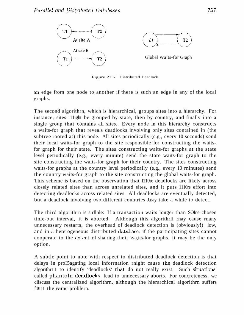
]JaTallel and Di8trilnded Databases 7fJ7
Global Waits-for Graph
Figure 22.5 Distributed Deadlock
an edge frorn one node to another if there is such an edge in any of the localgraphs.
The second algorithrn, which is hierarchical, groups sites into a hierarchy. Forinstance, sites r11ight be grouped by state, then by country, and finally into asingle group that contains all sites. Every node in this hierarchy constructsa waits-for graph that reveals deadlocks involving only sites contained in (thesubtree rooted at) this node. All sites periodically (e.g., every 10 seconds) sendtheir local waits-for graph to the site responsible for constructing the waitsfor graph for their state. The sites constructing waits-for graphs at the statelevel periodically (e.g., every minute) send the state waits-for graph to thesite constructing the waits-for graph for their country. The sites constructingwaits-for graphs at the country level periodically (e.g., every 10 rninutes) sendthe country waits-for graph to the site constructing the global waits-for graph.This scheme is based on the observation that l110re deadlocks are likely acrossclosely related sites than across unrelated sites, and it puts 1110re effort intodetecting deadlocks across related sites. All deadlocks are eventually detected,but a deadlock involving two different countries J.nay take a while to detect.
The third algorithrn is sirllple: If a transaction waits longer than SOIne chosentinle-out interval, it is aborted. Although this algorithrll rnay cause rnanyunnecessary restarts, the overhead of deadlock detection is (obviously!) low,and in a heterogeneous distributed database, if the participating sites cannotcooperate to the extent of sha,ring their \va,its-for graphs, it rnay be the onlyoption.
A subtle point to note with respect to distributed deadlock detection is thatdelays in proI5agating local inforrnation rnight cause the deadlock detectionalgorithr11 to identify 'deadlocks' that do not really exist. Such situations~
called phantoln deadlocks~ lead to unnecessary aborts. For concreteness, wecliscuss the centralized algorithrn, although the hierarchical algorithrn suffersfr0111 the Se1Ine problern.
758 (;HAPI'ER 2'2
Consider a rnodificatioll of the previous exarnple. As before, the two transactions \vait for each other, generating the local \vaits-for graphs shown in Figure22.5, and the local vvaits-for graphs are sent to the global deadlock-detectionsite. IIo\vever, 7'2 is now aborted for 1'ea..,;on8 other than deadlock. (For exarnple, T2 rnay also be executing at a third site, 'where it reads an unexpecteddata value and decides to abort.) .At this point, the local waits-for graphs havechanged so that there is no cycle in the 'true' global \vaits-for graph. l-Io\vever,the constructed globaJ waits-for graph \vill contain a cycle, and 7'1 Inay well bepicked as the victirn!
22.14 DISTRIBUTED RECOVERY
Recovery in a distributed DBJVIS is rnore cornplicated than In a centralizedDBMS for the following reasons:
l1li New kinds of failure can arise: failure of COlnnlunication links and failureof a remote site at which a subtransaction is executing.
l1li Either all subtransactions of a giv(~n transaction Iuust ccnnlnit or none HUlstconlnlit, and this property IIlust be guaranteed despite any cOIllbination ofsite and link failures. T'his guarantee is achieved using a commit protocol.
As in a centralized DBMS, certain actions are carried out as part of norrnalexecution to provide the necessary infonnation to recover fro111 failures. A log isrnaintained at each site, and in addition to the kinds of inforrnation rnaintainedin a centralized DB11S, actions taken as part of the cOlInnit protocol are alsologged. The Inost widely used conunit protocol is called TUJO-Phase Cornmit(2PC). A variant caned 21J C with Prcsurncd Abort, which we discuss next, hc'k'3been adopted as an industry standard.
In this section, we first describe the steps taken during nonnal execution, concentrating on the cOHnnit protocol, and tJlen discuss recovery fron1 failures.
22.14.1 Normal Execution and Commit I>rotocols
I)uring Donnal execution, each site rnaintains a log, and the actions of a subtransaction are ~.ogged at the site \vhere it executes. The regular logging activitydescribed in Chapter 18 is carried out and, in addition, a eornnlit protocol isfollc)\ved to ensure that all subtra,nsa.ctions of a given transaction either cOIrnnitor H,bort uniforrnly. 1'he transacticHl rnanager at the site vvhcl'e the transaction()riginat(~cl is called the coordinator for the transaction; transaction Inanagersat sites \vh(~l'e its subtraJ1Sactiol1S execute are ca.11(~d subordinates (\vith respect to the coordinatioll of this transaction).
Parallel and DistTilnlted ]Jatabases 7~9
\Ve no\v describe the Two-:Pha'5e Cornmit (2PC) protocol~ in tenns of thernessa,ges exchanged and the lc)g records vlritten. \Vhen the user decides tocornrnit a transactioll~ the conunit cOIrunand is sent to the coordinator for thetransaction. This initiates the 2PC; protocol:
1. The coordinator sends a prepare rnessage to each subordinate.
2. \'Then a subordinate receives a prepare rnessage~ it decides \vhether to abortor cornrnit its subtransaction. It force-writes an abort or prepare logrecord, and then sends a. no or yes rnessage to the coordinator. Note thata prepare log record is not used in a centralized DB.l\;lS; it is unique to thedistributed cornrnit protocol.
3. If the coordinator receives yes lnessages fr0 III all subordinates, it forcewrites a cornmit log record and then sends a cornrnit rnessage to all subordinates. If it receives even one no rnessage or receives no response fronlSOHle subordinate for a specified titne-out interval, it force-writes an abortlog record, and then sends an abort Inessage to all subordinates. 1
4. vVhen a subordinate receives an abort Inessage, it force-writes an abort logrecord, sends an ack Inessage to the coordinator, and aborts the subtransaction. When a subordinate receives a cornrnit rnessage, it force-writes acOl1nnit log record, sends an ack rnessage to the coordinator, and corrunitsthe subtransaction.
5. After the coordinator has received ack rnessages frorn all subordinates, itwrites an end log record for the transaction.
1:'he narne T'llJO- ]J}ULSC (7ornTnit reflects the fact that two rounds of rnessagesare exchanged: first a voting phase, then a tennination pha..se, both initiatedby the coordinator. ffhe basic principle is that any of the transaction tnanagel'S involved (including the coordinator) can unilaterally a,bort a transaction,\vhereas therernust be unanirnity to conuuit a transaction, vVhen a rnessageis serlt in 2PC, it signals a decision by the sender. To ensure that this decisionsurvives a crash at the sender's site, the log r(~cord describing the decision isahvays forced to stable storage before the rnessage is sent.
;\ transaction is ofIicially cornrnitted at the tirne the coordiIlator '8 cOllnnit logrecord reaches stable storage. Subsequent failures cannot affect the outcorne ofthe transaction; it is irrevocaJ)ly corrunitted. Log records\vritten to record theconnnit protocol actions contain the type of the record, tlH~ tn.lllsaction iel, andthe identity of the coordiu;:ltor. i\ coordinator's conunit or abort log recordalso contains the identities of the subordinates.
1As a,n optilnization J the coordinator need not send abort meSS;:lges {;o subordinates who voted no,
760 (';IIAPTER, ~2
22.14.2 Restart after a Failure
vVhen a site COUles back up after a erao.sh, \ve invoke a recovery process thatreads the log and processes all transactions executing the conunit protocol atthe tirne of the cnlsh. The transaction rnanager at this site could have been thecoordinator for SOUle of these transactions and a subordinate for others. We dothe follo¥ling in the recovery process:
• If vve have a cornInit or abort log record for transaction T, its status is clear;we redo or undo 1"\ respectively. If this site is the coordinator, which canbe deterrnined froru tl1(~ cOlTllnit or abort log record, we rnust periodicallyresend·-,·-because there rnay be other link or site failures in the system~~~"-a
com/n7,it or abort rnessage to each subordinate until we receive an ack. Afterwe have received acks frorn all subordinates, we write an end log record forT.
• If we have a prepare log record for T but no conunit or abort log record,this site is a subordinate, and the coordinator can be detennined froInthe prepare record. We rllust repeatedly contact the coordinator site todetermine the status of T. Once the coordinator responds with eithercOlurnit or abort, we write a corresponding log record, redo or undo thetransaction, and then write an end log record for T.
• If we have no prepare, cOllunit, or abort log record for transaction T,T certainly could not have voted to connuit before the crash; so we canunilaterally abort and undo T and vvrite an end log record. In this case,we have no way to detennine whether the current site is the coordinatoror a subordinate for 1'1. flowever, if this site is the coordinator, it rnighthave sent a prepare rnessage prior to the crEL.'3h, and if so, other sites rnayhave voted yes. If such a subordinate site contacts the recovery process atthe current site, we now know that the current site is the coordinator forT, and given that there is no cOllnnit or abort log record, the response tothe subordinate should be to abort 7 1
•
()bserve that, if the coordinator site for a transaction I' fails, subordinates whovoted yes cannot decide \vhether to conunit or abort ~r until the coordinatorsite recovers; \ve say that l' is blocked. In principle, the active subordinatesites could cOl1nnunicate arnong thelIlselves, and if at lccL.'3t one of thelIl containsan abort or coinrnit log record for T, its status becornes globally known. 1"0conununicate arnong thernselves, all subordinates nlust be told the identity ofth(~ other subordinates at the titne th(~y are sent the ]Jrcpa:re Inessage. llowever,2PC is still vlllnerable to coordinator failure durirlg recovery because even if allsubordinates voted yes, the coordinator (-who also ha,s a vote!) rnay have decided to aJ)ort rr, and this decision cannot be detennined until the coordinatorsi1,e recovers.
Parallel a1ul [Jistrilnded Database8 791
\Ve covered how a site recovers fro111 a crash, but\vhat should a site that isinvolved in the cOIIunit protocol do if a site that it is cornrl1unicating with fails?If the current site is the coordinator, it should shnply abort the transaction.If the current site is a sllbordina,te~ and it has not yet responded to the coordinator's prepaT(; lnessage, it can (and should) abort the transaction. If it is asubordinate and has voted yes, then it cannot unilaterally abort the transaction, and it cannot cOIUlnit either; it is blocked. It lnust periodically contactthe coordinator until it receives a reply.
Failures of COffilnunication links are seen by active sites as failure of other sitesthat they are comnlunicating with, and therefore the solutions just outlinedapply to this case as \-vell.
22.14.3 Two-Phase Commit Revisited
Now that we examined how a site recovers frolll a failure, and saw the interaction between the 2PC protocol and the recovery process, it is instructive toconsider how 2PC can be refined further. In doing so, we arrive at a more efficient version of 2PC, but equally irnportant perhaps, we understand the roleof the various steps of 2PC ruore clearly. Consider three basic observations:
1. l'he ack rnessages in 2PC an~ used to detennine when a coordinator (orthe recovery process at a coordinator site following a crash) can 'forget'about a transaction T. lJntil the coordinator knows that all subordinatesare aware of the cornrnit or abort decision for T, it IIlust keep inforrnationabout T in the transaction table.
2. If the coordinator site fails aJter sending out ]J'repoxe rnessages but beforewriting a cornrnit or abort log record, when it cornes back up, it 1Uts noinf'orruatiol1 abollt the transaction's connnit status prior to the crash. IInv.lever, it is still free to abort the transaction unilaterally (beca,use it has not\vrittcn a conunit record, it can still cast a no vote itself). If another siteinquires about the status of the transaction, the recovery process, as we
have seen, responds \vith an abort rnessage. Therefore, in the absence ofinforrnation, a transaction is pres'luned to h..ave aborted.
:3. If a subtnlnsaction does no llIHlates, it has no changes to either redo orundo: in other vvords. its cornrnit or abort status is irrelevant.
'l'he first tvvo ol)servations suggest several refinernents:
m \Vhen a coordirlCltor (tborts a tnl,nsa,cticHl T', it can undo ~r and rerl10ve itfronl the transaction table irnrrlediately. After all \ rernoving ~r frorn thetable results in a 'no inforrnatioI1' state with respect to T, and the default
762 CHAPTER 62
response (to an enquiry about T) in this state, \vhich is abort, is the correctresponse for an aborted transaction.
• By the same token, if a subordinate receives an abort Inessagc, it need notsend an ack lnessage. rrhe coordinator is not waiting to hear frorn subordinates after sending an abor't 111essage! If, for SOlne rea...")on, a subordinatethat receives a prepflrc message (and voted yes) does not receive an abortor cornm,it Inessage for a specified tirne-out interval, it contacts the coordinator again. If the coordinator decided to abort, there Inay no longer bean entry in the transaction table for this transaction, but the subordinatereceives the default abort nlessage, whicll is the correct response.
• Because the coordinator is not waiting to hear froul subordinates afterdeciding to abort a transaction, the names of subordinates need not berecorded in the abort log record for the coordinator.
• All abort log records (for the coordinator as well as subordinates) cansimply be appended to the log tail, instead of doing a force-write. Afterall, if they are not written to stable storage before a crash, the defaultdecision is to abort the transaction.
The third basic observation suggests SOlne additional refinements:
• If a subtransaction does no updates (which can be easily detected by keeping a count of update log records), the subordinate can respond to a prepare111essage from the coordinator with a r'eader message, instead of yes or no.The subordinate writes no log records in this case.
• vVhen a coordinator receives a reader lnessage, it treats the Inessage as a yesvote, but with the optiInization that it does not send any lnore messagesto the subordinate, because the subordinate's cornlnit or abort status isirrelevant.
• If all subtransactions, including the sllbtransaction at the coordinator site~
send a reader luessagc, we do not need the second phase of the conunit protocol. Indeed, \\'e can sirnply rernove the transaction frolH the transactiontable: \vithout \vriting any log records at any site for this transaction.
1lH~ T'wo-Phasc Cornrnit protocol with the refinernents discussed in this sectionis called Two-Phase Commit with Presurned Abort.
22.14.4 Three...Phase Commit
A cornlnitprotocol caIled Three-Phase Conlrnit (3PC) can avoid blockingeven if the coordinator sit(~ fails during recovery. T'he basic idea is that, \vhen
Parallel and Distrilnded Databases 763
the coordinator sends out prel)arc rnessages and receives yes votes £1'0111 all subordinates, it sends all sites a pTccomrrl-it message, rather than a cornrnit rnessage.\\Then a sufficient l1Ulllber..··....··....more than the lIlaxinlulll nUlnber of failures thatnlust be handled········of acks have been received, the coordinator force-writes acornrn·it log record and sends a cornmit lnessage to all subordinates. In 3PC,the coordinator effectively postpones the decision to cornrnit until it is surethat enough sites know about the decision to corn111it; if the coordinator subsequently fails, these sites can C0l11111Unicate with each other and detect thatthe transaction rnust be corllrnitted-conversely, aborted, if none of thern hasreceived a precomrnit rnessage-'-without waiting for the coordinator to recover.
rrhe 3PC protocol ilnposes a significant additional cost during normal executionand requires that COlnrIlunication link failures do not lead to a network partition(wherein sorne sites cannot reach some other sites through any path) to ensurefreedo111 fronl blocking. For these reasons, it is not used in practice.
22.15 REVIEW QUESTIONS
Answers to the review questions can be found in the listed sections.
• Discuss the different rnotivations behind parallel and distributed databases.(Section 22.1)
• Describe the three lllain architectures for parallel DBMSs. Explain whythe shared-memory and shaT'(~d-disk approaches suffer frOlll interference.What can you say about the speed-up and scale-up of the shared-nothingarchitecture? (Section 22.2)
• Describe and differentiate pipelined parallelism and data-partitioned parallelism. (Section 22.3)
• Discuss the following techniques for partitioning data: round-Tobin, hash,and range. (Section 22.3.1)
II Explain how existing code can be parallelized by introducing split andrnerrJC operators. (Section 22.3.2)
11II Discuss huw cadI of the following operators can be parallized using datapartitionipg: scanning, sorting, joiTL. Cornparc the use of sorting versushashing for partitioning. (Section 22.4)
11III vVhat do \ve need to consider in optilllizing queries for parallel execution?Discuss interoperation parallelislll, left-dcc~p trees versus bushy trees, and(~ost estirnation. (Section 22.5)
-("4I '):'
•
..
..
..
..
..
..
•
..
..
•
•
CIIAPTER 2~
Define the tenns disiribtded data itbde1JendeTU~eand distribttted transactionatryrnicitll. .ATe these concepts sllpported in current eornrnercial systerns?\Vhy not? \\That is the difference bet\veen hornogeneoclls and heteTogeneOtlsdistributed databa",'3es? (Section 22.6)
Describe the three lllain architectures for distributed DB~'lSs. (Section 22.7)
1\ relation can be distributed by jraglnent'ing it or rcplicat'ing it acrossseveral sites. Explain these concepts and ho\v they differ. Also, distinguishbetween }un'1;zontal and vertical fragrnentation. (Section 22.8)
If a relation is fraglnented and replicated, each partition needs a globallyunique nalne called the Tclat'ion narnc. Explain how such global naInesare created and the Inotivation behind the described approach to narning.(Section 22.9.1)
Explain how rnetadata about such distributed data is rnaintained in a distr'ibuted catalog. (Section 22.9.2)
Describe a nauling scherne that supports distributed data independence.(Section 22.9.3)
When processing queries in a distributed DBlVlS, the location of partitionsof the relation needs to be taken into account. Discuss the alternativeswhen joining two two relations that reside on different sites. In particular,explain and describe the rnotivation behind the Sernijoin and Bloornjointechniques. (Section 22.10.2)
What issues rnust be considered in optirnizing queries over distributed data,in addition to where the data is located? (Section 22.10.3)
\\7hat is the difference bet\veen synchronous asynchronous replication? Whyhas asynchronous replication gained in popularity? (Section 22.11)
Describe the 'ooting and Tead-a'ny 'l1J'rite-all approaches to synchronous replication. (Section 22.11.1)
Surnruarize the peer-lo-peer and ]JTinul,Ty site approaches to asynchronollsrepliccLtion. (Section 22.11.2)
In prirnary site replication, changes to the prirnary copy Inust be propagated to secondary copies. vVhat is done in the Caph.lT'c and Apply steps?Describe log-based and proceri'ttrnl approaches to Capture and cornparetheln. VVhat are the variations in scheduling the Apply step? Illustrate theuse of asynchronolls replication in a data vi.larehouse. (Section 22.11.2)
\Vhat is a 8'ubtrans(u.:t'io'n? (Section 22.12)
jJo,rallel and D'i.stributed Database8 765it
II \'That are the choices for rnanaglng locks in a distributed DBrvIS? (Section 22.13)
Ii Discuss deadlock detection in a distributed datab<:1Se. Contr&')t the ce1lLrnl'ized, hierarchical, and tirne-o'ut approaches. (Section 22.13.1)
III \\Thy is recovery in a distributed l.)BlVIS rIlore cornplicated tha.n III a centralized systern? (Section 22.14)
III \\That is a connnit protocol and \vhy is it required in a distributed database?Describe and C01npa.1"e T'wo-fJhasc a11d Three-Phase Cornn1it. \Vhat isblocking, and how does the Three-Pha,,')e protocol prevent it? vVhy is itnonetheless not used in practice? (Section 22.14)
EXERCISES
Exercise 22.1 Give brief answers to the following questions:
1. What are the siruilarities and differences between parallel and distributed database rnan-·agement systerns?
2. Would you expect to see a parallel database built using a wide-area network? \Vouldyou expect to see a distributed database built using a wide-area network? Explain.
3. Define the terms 8cale--'Up and speed-up.
4. Why is a shared-nothing architecture attractive for parallel database systerns?
5. The idea of building specialized hardware to run parallel database applications receivedconsiderable a+ t.ion but has fallen out of favor. Cornrnent on this trend.
6. \\That are th, (Lntages of a distributed D131\1[8 over a centralized DBNIS?
7. Briefly descr nnd cornpare the Client-Server and Collaborating Servers architectures.
tting Servers architecture, \vhen a transaction is subrnitted to the DBIVIS,how its activities at various sites are coordinated. In particular, describe
.saction managers at the different sites, the concept of 8ubtransacf:ions,_cept of d'i.5tributed tTan.saction atO'lnicity.
8. In the Colla l
briefly dew'the role (l
and the,
Exercise 22.2 Give brief a,nswers to the follmving questions:
1. I)efine the tenus fragrnentat'ion and rcpl'icah 0 T/" in tenns of where data is stored.
2. \\'11(1' is the difference behveen synclrrorwu8 and a,synchTo'TWU8 replication?
a.Define the tern1 distrilndcd data independence. \Vha.t does this Inean'with respect toquer:ying ane! updating data in the presence of data fragrnentation and n::plication?
4. C:onsieh:~r the 'uot:ing BJ1d n::ad-anywriic-all techniques for irnplementing synchronousreplication.\\rhat are their respectiv(~ l>ros and cons?
5. C;ive an c)Verview of henv asynchronous replication can 1)(' irnplernented. In particular:explain the tenns Cap t un:' and Apply.
6. \VIHtt is the difference between log-based and procedural irnplernentatiOlls of capture?
7. \VllY is giving database objcc:ts unique names rnore cennplicated in a distributed DB~IS?

766 CHAP'TER 42
8. Describe a catalog organization that pennits any replica (of an entire relation or a fragrnent) to be given a unique nam,e and provides the nanling infrastructure required forensuring distributed data independence.
9. If infonuation fi'Olll renlote catalogs is cached at other sites, what happens if the cachedinfoflllation becOInes outdated? How can this condition be detected and resolved?
Exercise 22.3 Consider a parallel DB,lVIS in \vhich each relation is stored by horizontallypartitioning its tuples across all disks:
Ernployees(eid: integer, did: integer, .sal.' real)
Departlnents(~'id: integer, Tngrid: integer, budget: integer)
The rngT"id field of DepartInents is the e'id of the manager. Each relation contains 20-bytetuples, and the sal and budget fields both contain unifonnly distributed values in the rangeo to 1 rnillion. The Enlployees relation contains 100,000 pages, the Departrnents relationcontains 5,000 pages, and each processor has 100 buffer pages of 4,000 bytes each. The cost ofone page I/O is tel, and the cost of shipping one page is t s ; tuples are shipped in units of onepage by waiting for a page to be filled before sending a rnessage frmn processor 'i to processorj. 'There are no indexes, and all joins that are local to a processor are carried out usinga sort-rnerge join. Assurne that the relations are initially partitioned using a round-robinalgorithlll and that there are 10 processors.
For each of the following queries, describe the evaluation plan briefly and give its cost in tennsof tel and t s . You should cornpute the total cost across all sites as well as the 'elapsed time'cost (i.e., if several operations are carried out concurrently, the tirne taken is the rnaxilnurnover these operations).
1. Find the highest paid ernployee.
2. Find the highest paid employee in the departrnent with d'id 55.
3. Find the highest paid ernployee over all departnHmts with lJ'ndget less than 100,000.
4. Find the highest paid enlployee over all departlnents with budget less than ~300,000.
5. Find the a;verage salary over all departnrents with budget less than ~300,OOO.
6. Find the salaries of all rnanagers.
7. Find the salaries of all rnanagers who rn::mage a departrnent with a budget less than300,000 and eaTll rnore than 100,000.
8. Print the eids of all elnployees, ordered by increasing salaries. Each processor is connectedto a separate printer, and the answer can appear as severaJ sorted lists, cadI printer] bya different processor, as long as we can ol)tain a fully sorted list by concatenating theprinted lists (in sorne order).
Exercise 22.4 Consider the saIne scenario as in Exercise 22.:3, except 1.h;':1t the relations areoriginally partitioned using range partitionirlg on the sal and fnulget fields.
Exercise 22.5 Repeat Exercises 22.~) and 22.4 \vith (i) 1 processor, ,1nd (ii) lelO processors.
Exercise 22.6 COllsicler the Ernployees (-uHIDepartments relations descril)cd in Ex.(~rcise
22.~3. rIhey are now stored in a distributed DBl\!lS with all of Eluployees stored at Naples<'lnd all of Departlnents stored at Berlin. There arc no indexes on these relations. 'rhe cost ofvarious operations is as describecl in Exercise 22.:3. Consider the query:
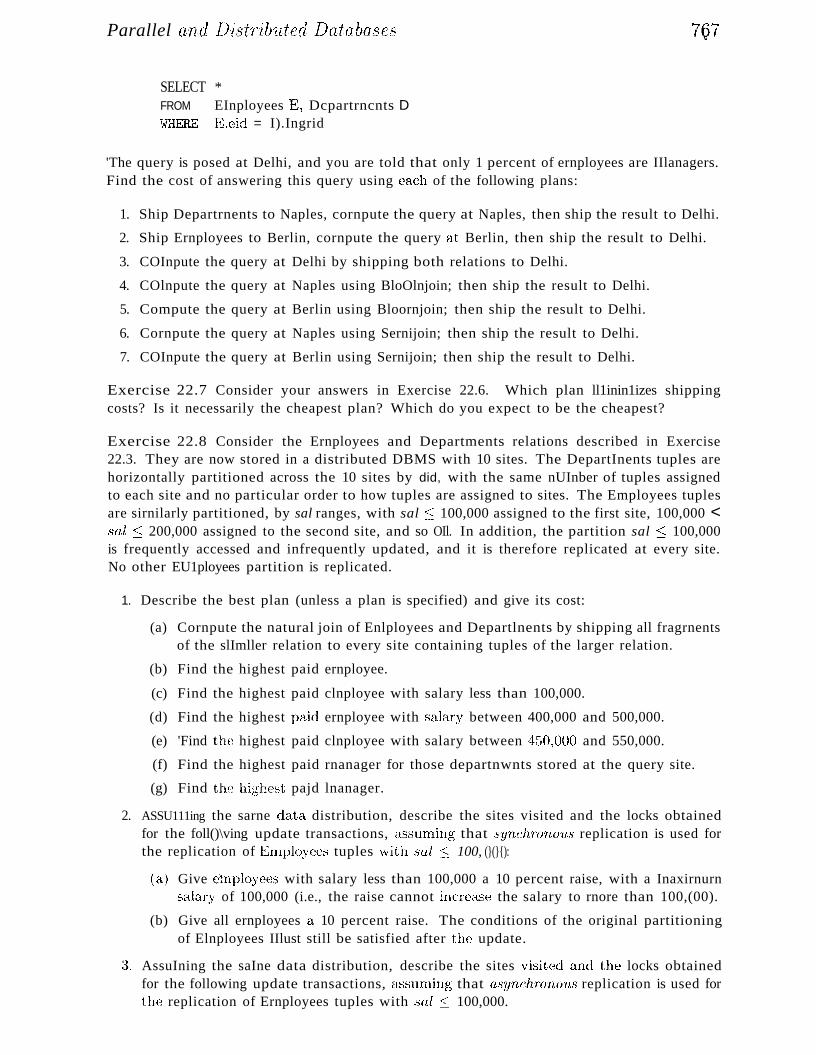
Parallel and Di8trib1Lted Databases
SELECT *FROM EInployees E) Dcpartrncnts DWHEREE.eid = I).Ingrid
7t)7
'The query is posed at Delhi, and you are told that only 1 percent of ernployees are IIlanagers.Find the cost of answering this query using each of the following plans:
1. Ship Departrnents to Naples, cornpute the query at Naples, then ship the result to Delhi.
2. Ship Ernployees to Berlin, cornpute the query at Berlin, then ship the result to Delhi.
3. COInpute the query at Delhi by shipping both relations to Delhi.
4. COlnpute the query at Naples using BloOlnjoin; then ship the result to Delhi.
5. Compute the query at Berlin using Bloornjoin; then ship the result to Delhi.
6. Cornpute the query at Naples using Sernijoin; then ship the result to Delhi.
7. COInpute the query at Berlin using Sernijoin; then ship the result to Delhi.
Exercise 22.7 Consider your answers in Exercise 22.6. Which plan ll1inin1izes shippingcosts? Is it necessarily the cheapest plan? Which do you expect to be the cheapest?
Exercise 22.8 Consider the Ernployees and Departments relations described in Exercise22.3. They are now stored in a distributed DBMS with 10 sites. The DepartInents tuples arehorizontally partitioned across the 10 sites by did, with the same nUInber of tuples assignedto each site and no particular order to how tuples are assigned to sites. The Employees tuplesare sirnilarly partitioned, by sal ranges, with sal S; 100,000 assigned to the first site, 100,000 <seLL::; 200,000 assigned to the second site, and so OIl. In addition, the partition sal :S 100,000is frequently accessed and infrequently updated, and it is therefore replicated at every site.No other EU1ployees partition is replicated.
1. Describe the best plan (unless a plan is specified) and give its cost:
(a) Cornpute the natural join of Enlployees and Departlnents by shipping all fragrnentsof the slImller relation to every site containing tuples of the larger relation.
(b) Find the highest paid ernployee.
(c) Find the highest paid clnployee with salary less than 100,000.
(d) Find the highest rn1id ernployee with sala,1'y between 400,000 and 500,000.
(e) 'Find the highest paid clnployee with salary between 4fjO,OOO and 550,000.
(f) Find the highest paid rnanager for those departnwnts stored at the query site.
(g) Find the highest pajd lnanager.
2. ASSU111ing the sarne (taUl distribution, describe the sites visited and the locks obtainedfor the foll()\ving update transactions, a",:;surnillg that 8ynchTono'u8 replication is used forthe replication of Ernployees tuples \vith sal ::s 100, (}(}{):
(a) Give einployees with salary less than 100,000 a 10 percent raise, with a InaxirnurnsaJary of 100,000 (i.e., the raise cannot incre;:lse the salary to rnore than 100,(00).
(b) Give all ernployees <1 10 percent raise. The conditions of the original partitioningof Elnployees IIlust still be satisfied after the update.
a. AssuIning the saIne data distribution, describe the sites visited and the locks obtainedfor the following update transactions, a..ssurning that rL8ynchTOn01./.,8 replication is used forthe replication of Ernployees tuples with sal :S 100,000.
768 CHAPTER:22
For all ernployees \vith salary less than lOOlOOO give them 11 10 percent raisc l \vitha rnaxirmun salary of 100/)00.
Give an ernployees a 10 percent raise. After the update is conlpleted~ the conditionsof the original partitioning of Eluployecs rnust still be satisfied.
Exercise 22.9 Consider the EInployees cUll:1 .DepartInents tahles frOluExercise 22.:3. You arc;;1 DBA and you need to decide ho\v to distribute these t\VO tables across t\VO sites, IVlanila andNairobi. Your D131\:18 supports only unclustered 13+ tree indexes. You have a choice betweensynchronous and asynchronous replication. 1"'01' each of the following scenarios, describe hmN
you would distribute thenl and what indexes you would build at each site. If you feel thatyou have insufficient inforrna.tion to 1nake a decision, explain briefly.
1. Half the departInents are located in IVlanila (l,lld the other half aTe in Nairobi. Departrnentinformation, including that for ernployees in the depart1nent, is changed only at the sitewhere the departrnent is located, but such changes are quite frequent. (Although thelocation of a depart1nent is not included in the Departrnents schclna, this inforrnationcan be obtained frorn another table.)
2. Half the departrnents are located in 1Vlanila and the other half are in Nairobi. Departrnentinformation, including that for errlployees in the departrnent, is changed only at the sitewhere the departrnent is located, but such changes are infrequent. F'inding the averagesalary for each departrnent is a frequently asked query.
~3. Half the departlnents are located in Ivlanila and the other half are in Nairobi. Ernployeestuples are frequently changed (only) at the site where the corresponding departrrlent is located, but the Depart1nents relation is aJulOst never changed. Finding a given ernployee'srnanager is a frequently asked query.
4. Half the e1nployees work in l'vlanila and the other half \vork in Nairobi. E1nployees tuplesare frequently changed (only) at the site where they work.
Exercise 22.10 Suppose that the Ernployees relation is stored in l\1adison and the tupleswith sal ~ 1.00,000 are replicated at Ne\v York. Consider the following three options for lockrnanagernent: all locks Huulaged at a s'inglf.~ site, say, 1VIilwaukee; prvirnaTy copy with l'vladisonbeing the primary for Ernployees; and fully di8tTilnded. For each of the lock rnanagernentoptions, explain what locks are set (and at which site) for the following queries. Also statefrorn which site the page is reac1.
1. A query at Austin wants to read a page of Erllployees tuples \vith sal s: 50,()OO.
2. A qttery at I\lfadison wants to read a page of E1nployees tuples \vith sal s: 50,000.
3. A query at Ne\v ',/'ork wants to re;:ld a page of Enlployees tuples "vith sal:::; 50,000.
Exercise 22.11 Briefly answer the follcnving questions:
1. C\Hnpare the relative rnerits of centralized and hierarchic;:tl deadlock detection in a distril)lIted I)BI\/IS.
2. \iVhat is a pha:ntorn de(ullock? Give an exarnple.
:3. (.;iv(~ an example of a distributed D131\-'18 \vith three sites such that no hvo loc;::d \vaits-forgraphs reveal a deadlock, :vet there is a global deadlock.
4. C;onsider the following rnoclification to ;:I, local waits-for gn1ph: Add a neVil node '1:':1:1, andfor ever.v trans;:lc:tion 7:/ that is waiting for a lock at ;:ulOther sib~, add the edge 'Ii 7~';I:t.
A.lso ;:lch.l HJl edge T~':d --+ Ti if a tr;::lHSi:lction executing at another site is waiting for T i
to release ;:1 lock at this site.
J)arallel and DislI'ib'ulc:d Dato,ba8C8 7tiqf
If there is ,1 cycle in the 11lodiHed local WEtits-for gra.ph that does not involve 7:~xt ~
what call you conclude? If every cycle involves T~~:rt., what can you conclude?
Suppose that every site is assigned a unique integer \Vhenever the lOC!:l}
waits-for graph suggests that there Blight be a global deadlock, send the local waitsfor graph to the site with tIle next higher site""id.At that site, combine the receivedgraph "vith the local \vaits-fc)[ grap,h. If this cornbined graph does not indictl.t:e adeadlock, ship it on to the next site, awl so on, until either a cleadlock is detectedor we are back at the site that originated this round of deadlock detection. Is thisscheuw guaranteed to find a global deadlock if one exists?
Exercise 22.12 Tirnestarnp-based concurrency control schernes can be used in a distributedDBivIS, but we rllust be able to generate globally unique, rllonotonicaJly increasing tirnestarnpswithout a bias in favor of anyone site. One approach is to a,...':\sign timestrunps at a single site.Another is to use the local clock tiTne and to append the site-iei. A third scherne is to use acounter at each site. COIllpare these three approaches.
Exercise 22.13 Consieler the rIlultiple-granlllarity locking protocol described in Chapter 18.In a distributed DB?vIS, the site containing the root object in the hierarchy can becmne a,
bottleneck. You hire a database consultant who tells you to rnodify your protocol to allowonly intention locks OIl the root and irnplicitly grant all possible intention locks to everytransaction.
1. Explain why this rnodification \vorks correctly, in that transactions continue to be ableto set locks on desired parts of the hierarchy.
2. Explain how it reduces the demand on the root.
3. Why is this idea not included as part of the standard rllultiple-granularity locking protocolfor a centralized DBTvlS?
Exercise 22.14 Briefly answer the following questions:
1. Explain the need for a cornmit protocol in a distributeclDIJf'vIS.
2. Describe 2PC. Be sure to explain the need for force-writes.
;3. vVhy are nch: HlCssages required in 2PC?
4. vVhat are the differences between 2PC; and 2PC with PresulTled Abort?
5. Give an exarnple execution sequence such that 2PC cHId 2PC 'with Presurned Abort:generate an identical sequence of actions.
6. Give ('UI exarIlple execution sequence such that 2PC; and 2PC,; with PresuIl1ed Abortgenerate different sequences of actions.
7. \Vhat is the intuition behirHI :3PC? \:Vhat are its fH'08 and cons relative to 2PC?
8. Suppose th.<1t a site gets no response frorn iJ.nother site for <'1 long tiITle. C;an the first sitetell whether .the connecting link has failed or the other site has failed? How is such afailure handled?
9. Suppose that the coordinator inclucles a list of aU subordinates in the In'f'-]UJ,'T'C Inessage. Ifthc~ coordinator fails aJter sending out either an abcrd or COTT1Jnit rnessage, call you suggesta\va,Y for active sites to terrninate this tra.nsaction without wajting f<)I' the coordinatorto recover? Assurnf~ that sonle but not all of the abort or cornrt1:it rnessages frOln thecocn'clinator are lost.
770 C~HAPTER 2&2
III Suppose that 2PC with PresuIl1ed Abort is used as the cOInmit protocol. Explain howthe systmll recovers froIn failure and deals with a particular transaction T in each of thefollowing cases:
(a) A subordinate site for T fails before receiving a prepare rnessage.
(b) A subordinate site for T fails after receiving a pTcparc rnessage but before rnakinga decision.
(c) A subordinate site for T fails after receiving a prepare lnessage and force-writingan abort log record but before responding to the pl'eparernessage.
(d) A subordinate site for T fails after receiving a prepare message and force-writing aprepare log record but before responding to the prepare lnessage.
(e) A subordinate site for T fails after receiving a prepare rnessage, force-writing anabort log record, and sending a no vote.
(f) The coordinator site for T fails before sending a prepare lnessage.
(g) The coordinator site for T fails after sending a prepare lllCssage but before collectingall votes.
(h) The coordinator site for T fails after writing an abort log record but before sendingany further rnessages to its subordinates.
(i) The coordinator site for T fails after writing a comrnit log record but before sendingany further rnessages to its subordinates.
(j) The coordinator site for T fails after writing an end log record. Is it possible for therecovery process to receive an inquiry about the status of T frolll a subordinate?
Exercise 22.15 Consider a heterogeneous distributed DBMS.
1. Define the terms multidatabase system and gateway.
2. Describe how queries that span multiple sites are executed in a rnultidatabase systern.Explain the role of the gateway with respect to catalog interfaces, query optirnizatiOll,and query execution.
3. Describe how transactions that update data at rnultiple sites are executed in a lllultidatabase systern. Explain the role of the gateway with respect to lock rnanagernent,distributed deadlock detection, Two-Phase COllnnit, and recovery.
4. SChell1aS at different sites in a llnI1tidatabase systern are probably designed independently.T'his situation can lead to semantic heterogeneity; that is, units of rneasure rnay differacross sites (e.g., inches versus centirneters), relatiolls containing essentially the SaIne
kind of infonnation (e.g., eIllployee salaries and ages) rnay have slightly different schernas,and so on. vVhat ilnpact does this heterogeneity have on the end user? In particular,COllunent on the concept of distributed data, independence in such a systcrIl.
BIBLIOGRAPHIC NOTES
\Vork on parallel algorithrns for sorting and various relational operations is discussed in thebibliographies for Chapters 1:3 and 14. Our discussion of parallel joins follows [220], and ourdiscussion of parallel sorting follows [22~3]. De\Vitt and C,ray make the case that for futurehigh perfornuHlce database systeuls, parallelisnl will be the key [221]. Scheduling ill parallelclata,b;:lse systenls is discusserl in [522). [49G] contains ,1 good collection of papers on queryprocessing in ptlrallel daUthase systems.
})aTallel and Distributed Databases 771t
Textbook discussions of distributed databa..C)€s include [78, 144, 580]. Good survey articles include [85], which focuses OIl concurrency control; [637], which is about distributed databasesin general; and [785], which concentrates on distributed query processing. Two InajaI' projectsin the area were 8DD-1 [636] and R* [777]. Fragmentation in distributed databases is considered in [157, 207]. Replication is considered in [11, 14, 137,239,238, 388, ~385, :~35, 552, 600].For good overviews of current trends in asynchronous replicatioll, see [234, 709, 772]. Paperson view maintenance mentioned in the bibliographic notes of Chapter 21 are also relevantin this context. Olston considers techniques for trading of performance versus precision in areplicated environment [571, 572, 573].
Query processing in the 8DD-1 distributed database is described in [88]. One of the notableaspects of 8DD-1 query processing was the extensive use of 8emijoins. Theoretical studiesof Semijoins are presented in [83, 86, 414]. Query processing in R* is described in [667].The R* query optimizer is validated in [500]; much of our discussion of distributed queryprocessing is drawn from the results reported in this paper. Query processing in DistributedIngres is described in [247]. Optimization of queries for parallel execution is discussed in[297,323,383]. Franklin, Jonsson, and Kossman discuss the trade-offs between query shipping,the more traditional approach in relational databases, and data shipping, which consists ofshipping data to the client for processing and is widely used in object-oriented systerns [284].A good recent survey of distributed query processing techniques can be found in [450].
Concurrency control in the 8DD-1 distributed database is described in [91]. Transaction management in R* is described in [547]. Concurrency control in Distributed Ingres is described in[714]. [740] provides an introduction to distributed transaction rrlanagement and various notions of distributed data independence. Optimizations for read-only transactions are discussedin [306]. Multiversion concurrency control algorithrlls based on timestamps were proposed in[620]. Tirrlestamp-ba.;;ed concurrency control is discussed in [84, 356]. Concurrency controlalgorithms based on voting are discussed in [303, 318, 408, 452, 732]. The rotating prirnarycopy scheme is described in [538]. Optimistic concurrency control in distributed databases isdiscussed in [660], and adaptive concurrency control is discussed in [488].
Two-Phase Commit was introduced in [466, 331]. 2PC with Presumed Abort is described in[546], along with an alternative called 2PC with Presum.ed Cornmit. A variation of PresumedCornrrlit is proposed in [465]. Three-Phase COlnrrlit is described in [692]. The deadlockdetection algorithnls in R * are described in [567]. Many papers discuss deadlocks, for exaInple,[156, 243, 526, 632]. [441] is a survey of several algoritluns in this area. Distributed clocksynchronization is discussed by [464]. [3~33] argues that distributed clata independence is notalways a good idea, clue to processing and adlninistrative overheads. The ARIES algorithrl1is applicable for distributed recovery, but the details of how rnessages should be handled arenot discussecl in [544]. The approach taken to recovery in SDD-1 is described in [4~3]. [114]also addresses distributed recovery. [444] is a survey article that discusses concurrency controland recovery in distributed systerIls. [95) contains several articles on these topics.
IVlultidatabase systerns are discussed in [10, IV3, 230, 2:31, 242,476, 485, 519, 520, 599, 641,765, 797]; sec [112, 486, 684] for surveys.
23OBJECT-DATABASE
SYSTEMS
.. What are object-databa,,~'3e systerlls and what new features do theysupport?
.. vVhat kinds of applications do they benefit?
(.. \Vhat kinds of data types can users de.fine?
(.. "Vhat are abstract data types and their benefits?
.. \\That is type inheritance and why is it useful?
.. What is the irnpact of introducing object ids in a database?
... How can we utilize the new features in database design?
i"'" What are the new implelncntation challenges?
.. \Vhat difFerentiates object-relational and object-oriented DBIvISs?
... Key concepts: user-defined data types, structured types, collectiontypes; data abstraction, rnethocls, encapsulation; inheritance, earlyand late binding of rnethods, collection hierarchies; object identity,reference types, shallow and deep equality
with Joseph M. HeHerstein[!n,'l'ucT'sily of C:fal!~foTT1,'iaBcTkeley
--YOll knovv Iny Inethods, \~l(ttson. A.pply theIn.
Arthur Conan ])oyle, The A1CTl1.0'iT8 of She'dock 1lolro,c;8
772
()bject- Database Systc1Tl'/3 77~3
H.{-~lational datalx:hse systeros support a sruaU, fixed collection of data types(e.g., integers, dates, strings),\vhich h&9 proven adequate for trcLClitional application dOHHlins such as adruinistrative data processing. In tHany applic<ltiondornains, hO'wever, rnuch 1nore eornplex kinds of data Blust be handled. I"rypi_cally this cornplex data has been stored in OS file systerns or specialized datastructures, rather than in a DB.tvIS.Exanlples of dornains vvith cOJ.uplex datainclude cornputer-aided design and rnodeling (CA.D/CAlvf.), rnultilnedia repositories, and docurnent Hl8.Jlagernent.
As the arnount of data grows, the luany features offered by a DBIvISfor exarIlpIe, reduced application developnlent tilne, concurrency control and recovery,indexing support, and query capabilities·······becorue increasingly attractive and,ultirnately, necessary. To support such applications, a DBNIS HUlst supportcornplex data types. ()bject-oriented concepts strongly influenced efforts toenhance database support for cornplex data and led to the developrnent ofobject-database systelus, \vhich we discuss in this chapter.
Object-database systerlls have developed along two distinct paths:
II Object-Oriented Database Systems: Object-oriented database systerns are proposed as an alternative to relational systerlls and are ainledat application dornains where cODlplex objects playa centra,} role. 1'heapproach is heavily influenced by object-oriented prograrllrlling languagesand can be understood as an atternpt to add DBMS functionality to aprograunning language environrnent. The ()bject Database :M:anagenlcntGroup (()DMG) has developed a standard Object Data Model (ODM)and Object Query Language (OQL), which are the equivalent of theS(~I..I standard for relational database systerns.
l1li Object-Relational ])atabase Systenls: ()bject-relational database s.ysterns ca,n be thought of as an atternpt to extend relational databa...sc systerns"lith the functionality necessary to support a broader class of applicationsand, in nlEUl~Y '\THY-S, provide a bridge between the relational and objectoriented paTadiguls. 1'he SC~I.I:1999 standard extends S(~L to incorporatesupport for the ol)ject-relationaJ rnode1 of data.
\Ve use clcronyuls for relational, object-oriented, and object-relational datrtbasernanagernent systerns (RDBMS, OODBMS, ORJDBMS). In this chapter,vve focus 011 ()HI)B~ilSs and ernphasize ho\v they can be vie\ved CbS a developrnent of HJ)B1\18s, rather than CbS an entjrely different paradigrn, as exernplifiedl)y the evolution of SCJL: 1999.
vVe concentrate on developing the fUlldarnental concepts rather than presc~nt
ing S(~L:1999; sorn(~ of the features \ve discuss axe not inc.luded in SC}L:1999.
774 CjHAPTER 2a t
Nonetheless, \;\le have chosen to ernpha",<:;ize concepts relevant to SQL: 1999 andits likely future extensions. vVe also try to be consistent with SCJL:1999 fornotation, although we occasionally diverge slightly for clarity. It is hnportantto recognize that the rnain concepts discussed are COIlllTIOn to both ()llDBJ\;ISsand ()()DBNISs; we discuss how they are supported in the ODLjOQL standardproposed for ()ODB)\t[Ss in Section 23.9.
RDB1\JIS vendors, including IBIVI, Inforrnix, and ()racle, are adding OIl-DBMSfunctionality (to varying degrees) in their products, and it is inlportant torecognize how the existing body of knowledge about the design and inlplernentation of relational databa'3es can be leveraged to deal with the OrtDBMSextensions. It is also ilnportant to understand the challenges and opportunitiesthese extensions present to database users, designers, and irnplernentors.
In this chapter, Sections 23.1 through 23.6 introduce object-oriented concepts.The concepts discussed in these sections are COlunlon to both OODBMSs andORDBJVISs. We begin by presenting an example in Section 23.1 that illustrateswhy extensions to the relational rnodel are needed to cope with some newapplication dornains. 'This is used as a running exarnple throughout the chapter.We discuss the use of type constructors to support user-defined structured datatypes in Section 23.2. We consider what operations are supported on these newtypes of data in Section 23.3. Next, we discuss data encapsulation and abstractdata types in Section 23.4. We cover inheritance and related issues, such asrnethod binding and collection hierarchies, in Section 23.5. We then considerobjects and object identity in Section 2~3.6.
vVe consider how to take advantage of the new object-oriented concepts to doOI{DBMS database design in Section 23.7. In Section 23.8, we discuss SOHleof the new irnplernentation challenges posed by object-relational systerns. Wediscuss ()I)L and OQL, the standards for OODBMSs, in Section 23.9, and thenpresent a brief cornparison of ()R,DBMSs and OC)DBwISs in Section 2;t10.
23.1 MOTIVATING EXAMPLE
As a specific exarnple of the need for object-relational systcrlls, we focus on anew business data processing probler.n that is both harder and (in our view)rnorc entertaining than the dollars and cents bookkeeping of previous decades.Today, cornpanies in industries such as entertainruent are in the business ofselling bits; their basic corporate assets are not tangible products, but rathersoftwa.1'c artifacts such as video (l,nd audio.
\Ve consider the fictional Dinky Entertaiurnent Corupa,ny, a laxgc IIollywoodconglornerate whose rllctin (\'ssets are a collection of cartoon characters, espe-
()b.ject-IJatabasc Systern8 775j}
cially the cuddly and internationally beloved IIerbert the \VarIll. Dinky ha..sseveral IIerbert the \Vornlfihns, rnany of which are shown in theaters aroundthe world at any given tiTne. Dinky also rnakes a good deal of rnoney licensingHerbert's irnage, voice, and video footage for various purposes: action figures,video gaInes, product endOrSelllents, and so on. I)inky's database is used tolnanage the sales and leasing records for the various IIerbert-related products,&l) well a..s the video and audio data that rnake up IIerbert's lllany filIns.
23.1.1 New Data Types
The basic problern confronting Dinky's database designers is that they needsupport for considerably richer data types than is available in a relationalDBMS:
II User-defined data types: Dinky's assets include Herbert's iIllage, voice,and video footage, and these rnust be stored in the database. To handlethese new types, we need to be able to represent richer structure. (See Section 23.2.) Further, we need special functions to rnanipulate these objects.Jior example, we may want to write functions that produce a cOlnpressedversion of an irnage or a lower-resolution image. By hiding the details of thedata structure through the functions that capture the behavior, we achievedata abstract'ion, leading to cleaner code design. (See Section 23.4.)
.. Inheritance: As the nurnber of data types grows, it is irnportant to takeadvantage of the cornrnonality between different types. :For exarnple, bothcOInpressed irnages and lower-resolution irnages are, at SOlne level, justilnages. It is therefore desirable to inherit some features of iluage objects \vhile defining (and later Inanipulating) cOInpressed irnage objectsand lower-resolution irnage objects. (See Section 2~j.5.)
!Ill Object Identity: Given that seHne of the new data types contain verylarge instances (e.g., videos), it is iInportant not to store copies of objects;instead, we IllUSt store Tejerence8, or po'inleTs, to such objects. In turn,this underscores the need for giving objects a unique object identity, vvhichcan be used to refer or 'point' to theln frorn elsewhere in the data. (SeeSection 2:3.6.)
Flow lnight \ve address these issues in an IlI)BNIS? \Ve could store ilnages,videos, and so on Ch') BLC)Bs in current relational syst(~lns. A binary largeobject (BLOB) is just a long 8trea1n of bytes, and the DBNIS's supportconsists of storing and retrieving BLC)Bs in such a rnanner that a user does nothave to worry about the size of the BLC)B; a 13LC}B can span several pages,unlike a tnulitional attribute. All further processing of the BLC)B has to bedone by the user's clpplication progranl, in the host languclge in \vhich the
776 (;lIAPTER ~3
The SQL/MM Standard: SQL/Nl:Nl is an eillerging standard that buildsupon SQL:1999's new data types to define extensions of SQL:1999 thatfacilitate handling of coruplex InultiInedia data types. SQL/lv!NI is a rnultipart standard. Part 1, SClL/rvUvfFl'arne\vork, identifies the SQL;1999concepts that are the foundation for SQLj1VllVI extensions. Each of therelnaining parts addresses a specific type of ccnnplex data: Full Text,Spatial, Still Image, and Data Mining. SQL/lVllVi anticipates thatthese l1e\v coruplex types can be used in colurnns of tables ck') field values.
. . ..
1".....
Large Objects: SQL:1999 includes a new data type called LARGE OBJECTor LOB, with two variaJ1ts called BLOB (binary large object) and CLOB (character large object). This standardizes the large object support found inlnany current relational DBMSs. LOBs cannot be included in priruarykeys, GROUP BY, or ORDER BY clauses. rrhey can be cornpared llsing equa.lity, inequality, and substring operations. A LOB has a locator that isessentially a unique id and allows LOBs to be rnanipulated without exten-. .
sIve copYIng.L()Bs are typically stored separately froIn the data records in whose fieldsthey appear. 1BlY1 DB2, InforInix, Microsoft SQL Server, Oracle 8, andSybase ASE all support LOBs.
SQL code is ernbedded. This solution is not efficient because we are forced toretrieve all BLOBs in a collection even if rnost of the111 could be filtt~red outof the ansvver by applying user-defined functions (within the I)B1118). It is notsatisfactory frorn a data consistency standpoint either, because the selnanticsof the data now depends heaNily on the host la,nguage application code andcannot be enforced by the I)BlVfS.
As for structured types and inheritance, there is siInply no support in therelational Dlodel. VVe are forced to Ina.p data 'with such cOlnplex structureinto a collection of flat tables. (vVe saw exarnples of such rnappings "vhen \vediscussed the tnlJlS1ation frorH Ell diagrarns vvith illheritance to relations inC:hapter 2.)
rrhis application clearly requires features not available in the relational Inode1.As an illustration of these features, Figure 2:3.1 presents S(~L:1999 :DDL staternents for a l)Ortion of Dinky's ()HJ)I31VIS sehelna used in subsequent excunples.Al though the 1)})L is very sirnilar to that of a traditional relational systeru,SOln(~ irnportant distinctions highlight thene\v data rnodeling capabilities of,Ul ()JII)B1VlS. J\ quick glance at the l)DL staternents is sufficient for now; westudy thenl in detail in the next section, after presenting S0111e of the basic
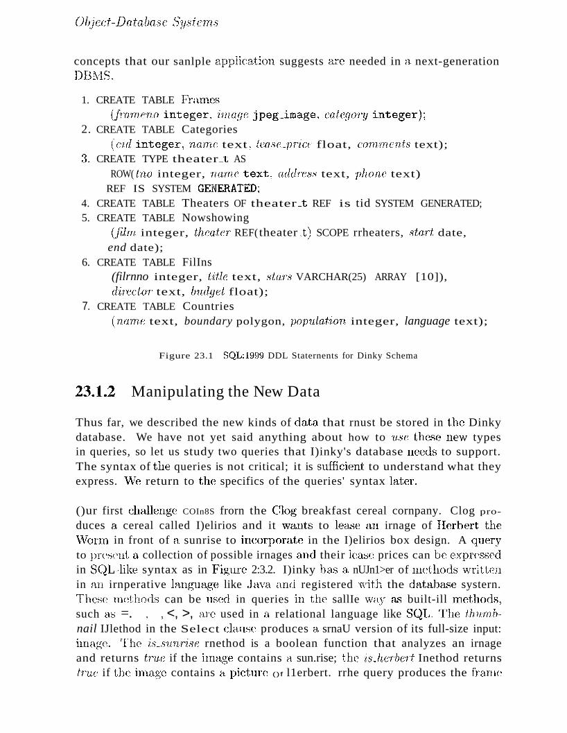
()b.ject-1Jatabase 8ystenM)
concepts that our sanlple application suggests are needed in a next-generationl)BrvlS.
1. CREATE TABLE FralnC\'3(}rarneno integer, 'iTrulge jpeg_image, categoT'Y integer)~
2. CREATE TABLE Categories(c'id integer, narne text 1 If:aSL.pricc float, c01n:rncnts text);
:3. CREATE TYPE theater_t AS
ROW( tno integer, n,arne text, address text, phone text)REF IS SYSTEM GENERATED;
4. CREATE TABLE Theaters OF theater_t REF is tid SYSTEM GENERATED;5. CREATE TABLE Nowshowing
(jilnL integer, theater REF(theater ..,t) SCOPE rrheaters, start date,
end date);6. CREATE TABLE FilIns
(filrnno integer, l/if;le text, staTs VARCHAR(25) ARRAY [10]),director text, budget float);
7. CREATE TABLE Countries(narnc text, boundary polygon, population integer, language text);
Figure 23.1 SQL:1999 DDL Staternents for Dinky Schema
23.1.2 Manipulating the New Data
Thus far, we described the new kinds of data that rnust be stored in the Dinkydatabase. We have not yet said anything about how to use these nevv typesin queries, so let us study two queries that I)inky's database needs to support.The syntax of th(~ queries is not critical; it is sufficient to understand what theyexpress. v\le return to the specifics of the queries' syntax later.
()ur first challenge COIn8S frorn the C~log breakfast cereal cornpany. Clog pro
duces a cereal called I)elirios and it vvants to lease an irnage of IIerbert thE:~
\\TorIn in front of a sunrise to incorporate in the I)elirios box design. A queryto present (1, collection of possible irnages (uld their le<ls8 prices can be ex.pressedin SC~L-like syntax as in I4'iglln~ 2:3.2. I)inky has a nUJn1>er of rnethodsvvrittenin an irnperative language like .J nva a,nd registered \vith the datal)Clse systern.These lIH~thods can be used in queries in the sallIe way as built-ill Hletllods,such as =. ,--~, <, >, are used in a relational language like S(~L. 1'he thwrnbnail IJlethod in the Select clausf~ produces a srnaU version of its full-size input:bnnge. rrhe i:L8'il'nri.se rnethod is a boolean function that analyzes an irnageand returns tr'ue if the inHtge contains a sun.rise; the is_h(Tbcrt Inethod returnsh"u.c if the irnag(~ contains a picture ()f l1erbert. rrhe query produces the frarl1c
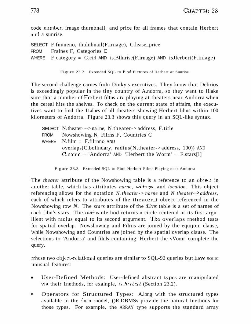
778 (jHAPTER 23
code nUlnber~ irnage thurnbnail, and price for all frames that contain Herbertand a sunrise.
SELECT F.fnuneno, thulnbnail(F.irnage), C.lease_priceFROM Fralnes F, Categories CWHERE F.category = C.cid AND is.Bllnrise(F.irnage) AND isJlerbert(F.inlage)
Figure 23.2 Extended SQL to Find Pictures of Herbert at Sunrise
The second challenge carnes froIn Dinky's executives. They know that Deliriosis exceedingly popular in the tiny country of A.ndorra, so they want to lIlakesure that a number of Herbert filIns are playing at theaters near Andorra whenthe cereal hits the shelves. To check on the current state of affairs, the executives want to find the 11aInes of all theaters showing Herbert fihns within 100kilorneters of Andorra. Figure 23.3 shows this query in an SQL-like syntax.
SELECTFROMWHERE
N. theater··--> na1ne, N. theater-> address, F. titleNowshowing N, Filrns F, Countries CN.film = F.filrnno ANDoverlaps(C.bollndary, radius(N.theater-> address, 100)) ANDC.narne::::: 'Andorra' AND 'Herbert the Worm' = F.stars[l]
Figure 23.3 Extended SQL to Find Herbert Films Playing near Andorra
The theater attribute of the Nowshowing table is a reference to an object inanother table, which has attributes narne, addr'(~88, and location. This objectreferencing allows for the notation N. theater-> narne and N. theater..···> address,each of which refers to attributes of the theater_t object referenced in theNowshowing row N. The stars attribute of the tUrns table is a set of narnes ofeach [ibn 's stars. The r'O,(1'i'u,8 nlethod returns a circle centered at its first argulllent with radius equal to its second argurnent. ~rhe overlaps rnethod testsfor spatial overlap. Nowshowing and Filrns are joined by the equijoin clause,\vhile Nowshowing and Countries are joined by the spatial overlap clause. Theselections to 'Andorra' and fiInls containing 'Herbert the vVorrn' cornplete thequery.
rrhcse two object-relational queries are sirnilar to SQL-92 queries but heLve SOlllC
unusual features:
l1li User-Defined Methods: User-defined abstract types are rnanipulatedvia their 1nethods, for exalnple, i.'Lhcrbert (Section 23.2).
II Operators for Structured Types: A.long with the structured typesavailable in the deLta rnodel, ()R,DBMSs provide the natural Inethods forthose types. For exarnple, the ARRAY type supports the standard array
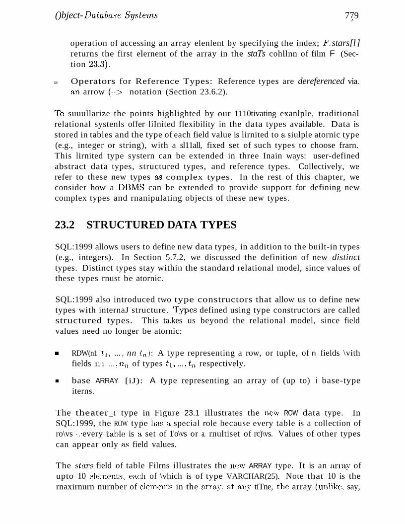
()bject- Database SYStC1718 779Ii>
operation of accessing an array elenlent by specifying the index; I?~ stars[l]returns the first elernent of the array in the staTs cohllnn of film F (Section 23.:3).
11III Operators for Reference Types: Reference types are dereferenced via.an arrow (---» notation (Section 23.6.2).
Ib suuullarize the points highlighted by our 1110tivating exanlple, traditionalrelational systenls offer liInited flexibility in the data types available. Data isstored in tables and the type of each field value is lirnited to a siulple atornic type(e.g., integer or string), with a sl11all, fixed set of such types to choose frarn.This lirnited type systern can be extended in three Inain ways: user-definedabstract data types, structured types, and reference types. Collectively, werefer to these new types &'S complex types. In the rest of this chapter, weconsider how a DBl\!IS can be extended to provide support for defining newcomplex types and rnanipulating objects of these new types.
23.2 STRUCTURED DATA TYPES
SQL:1999 allows users to define new data types, in addition to the built-in types(e.g., integers). In Section 5.7.2, we discussed the definition of new distincttypes. Distinct types stay within the standard relational model, since values ofthese types rnust be atornic.
SQL:1999 also introduced two type constructors that allow us to define newtypes with internaJ structure. ~rypes defined using type constructors are calledstructured types. This ta.kes us beyond the relational model, since fieldvalues need no longer be atornic:
11III RDW(n1 Il, ... , nn t,n): A type representing a row, or tuple, of n fields \vithfields 11,1, ... , Tl'n of types Ll, ... ,"tn respectively.
II base ARRAY [iJ): A type representing an array of (up to) i base-typeiterns.
The theater_t type in Figure 23.1 illustrates the IH~\V ROW data type. InSQL:1999, the ROW type hetS ()., special role because every table is a collection ofro\vs ...·..·every table is a set of 1'o\vs or a. rnultiset of rc)\vs. Values of other typescan appear only a..s field values.
The staT/., field of table Filrns illustrates the ne,v ARRAY type. It is an array ofupto 10 elernents, ea.ch of \vhich is of type VARCHAR(25). Note that 10 is thernaxirnurn nurnber of el(~rnents in the array; a.t <lny tiTne, the array (unlik(~, say,
780 (-~ .. ;- . ?').JHAP fER ~)
SQL:1999 Structured Data Types: Several conunercial systenls~ including IBw! DB2, Infonnix tTDS, and Oracle 9i support the ROWand ARRAYconstructors. rrhe listof, bagof, and setof type constructors are :not included in S(~L:1999. Nonetheless, cOIlunereiaJ systerIls support sorne ofthese constructors to varying degrees. ()racle supports nested relationsand arrays, but does not support fully cornposing these constructors. InfOI'rnix supports the setof, hagof, and Ustof constructors and allows thernto be cornposed. Support in this area varies \videly across vendors.
in C) can contain fewer elenlcnts. Since SQL:1999 does not support rnultidiInensional arrays, vector rnight ha,ve been a rnore accura,te narne for the arrayconstructor.
The power of tyP(~ constructors cornes froIn the fact that they can be cornposed.The following row type conta,ins a field that is an array of at Inost 10 strings:
ROW(filrnno: integer, staT's: VARCHAR(25) ARRAY [10])
The row type in SC~L:1999 is quite general; its fields can be of any SQL:1999data type. Unfortunately, the arra.y type is restricted; elernents of an arraycannot be arrays thcrnselves. Therefore, the following definition is illegal:
(integer ARRAY [5]) ARRAY [10]
23.2.1 Collection Types
S(~L: 1999 supports only the ROW a,nel ARRAY type constructors. Other COUUllontype constructors include
III listof(base): A. type representing <:1, sequence of base-t~ype itcrllS.
Ii setof (base): .l\ type rer)l'(~senting a set of base-type HeIns. Sets cannotcontain duplicate elen1cn1,8.
II bagof(base): j\ type representin.g a, bag or rnv,ltisct of base-type iterns.
Types llsing listof, ARRAY, bagof, or setof as the outennost type constructora.re sornetirnes referred to a,s collection types or bulk data types.
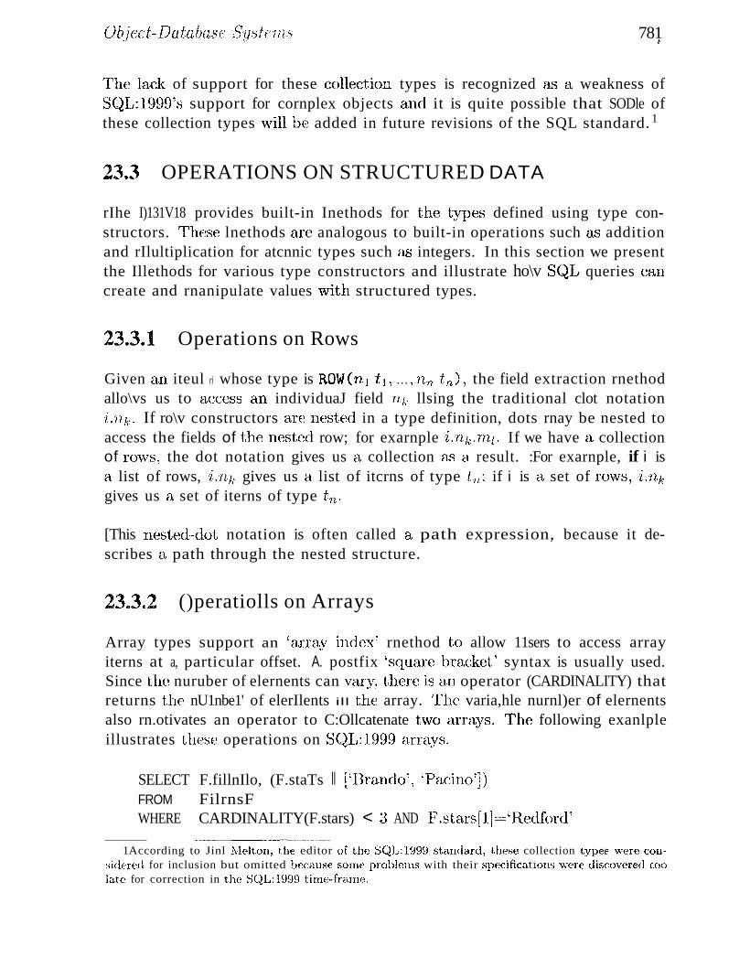
()b)ect- Databa,se Sy,steIns 781t
~rhe lack of support for these collection types is recognized as a weakness ofSQL:1999's support for cornplex objects and it is quite possible that SODle ofthese collection types "'lill be added in future revisions of the SQL standard. 1
23.3 OPERATIONS ON STRUCTURED DATA
rIhe I)131V18 provides built-in Inethods for the types defined using type constructors. These lnethods are analogous to built-in operations such as additionand rIlultiplication for atcnnic types such as integers. In this section we presentthe Illethods for various type constructors and illustrate ho\v SC~L queries cancreate and rnanipulate values \vith structured types.
23.3.1 Operations on Rows
Given an iteul ri whose type is ROW(n1t1 , ... , TL n t n ), the field extraction rnethodallo\vs us to ~l,ccess an individuaJ field nk llsing the traditional clot notation'i.nk. If ro\v constructors are nested in a type definition, dots rnay be nested toaccess the fields of the nestE"d row; for exarnple i.'fLk.n1/. If we have a collectionof rows, the dot notation gives us a collection as a result. :For exarnple, if i isa list of rows, i.nk gives us a list of itcrns of type tTl; if i is a set of rows, i.nk
gives us a set of iterns of type tn.
[This rH~ste(l-dot notation is often called a path expression, because it describes a path through the nested structure.
23.3.2 ()peratiolls on Arrays
Array types support an 'alT<lY index' rnethod to allow 11sers to access arrayiterns at a, particular offset. A. postfix 'square bracket' syntax is usually used.Since the nuruber of elernents can v<try, there is an operator (CARDINALITY) thatreturns the nU1nbe1' of elerIlents ill tl1E~ array. '1'he varia,hle nurnl)er of elernentsalso rn.otivates an operator to C:Ollcatenate t\VO arrays. rrh(~ following exanlpleillustrates these operations on S(~L:1999 arr(\ys.
SELECT F.fillnIlo, (F.staTs II ['Brando', 'Pacino'])FROM FilrnsFWHERE CARDINALITY(F.stars) < :3 AND F.stars[l]::::::'Iledford'
1According to Jinl tvlelton, the editor of the SQL:19DD standard, these collection types 'l}/ere considered for inclusion but omitted because sorne problt·mls with their specifications were discovered toolate for correction in the SQL: 1999 timc-fr;lrne.
782 CHAPTER 33
For each fibn with Redford ctS the first star2 and fe"wer than three stars, theresult of the query contains the fihn'8 array of stars concatenated \vith thearray containing the two elcrnents 'Brando' and 'Pacino'. Observe ho\\r a valueof type array (containing Brando and Pacino) is constructed through the useof square brackets in the SELECT clause.
23.3.3 Operations on Other Collection Types
Although only arrays are supported in SQL:1999, future versions of SQL areexpected to support other collection types, and we consider what operations areappropriate over these types of data. provide such operations. Our discussionis illustrative and not Ineant to be cOlnprehensive. For exarnple, one couldadditionally allow aggregate operators count, surn, avg, rna.T, and rnin to beapplied to any object of a collection type with an appropriate base type (e.g.,INTEGER). ()ne could also support operators for type conversions. For exaInple,one could provide operators to convert a rnultiset object to a set object byelirninating duplicates.
Sets and Multisets
Set objects can be cornpared using the traditional set methods c,~, =,:2, ~.An iteln of type setof (faa) can be cornpared with an iteln of type faa usingthe E rnethod, as illustrated in Figure 23.3, which contains the cornparison'.fferbert the W O'T"rn' E F. stars. T\vo set objects (having elernents of the saInetype) can be cornbined to forIlI a new object using the u, n, and --- operators.
Each of the Inethods for sets can be defined for Inultisets, taking the nUlnber ofcopies of elernents into account. The U operation silnply adds up the nurnberof copies of an elernent, the n operation counts the lesser nU1nbel' of tirnes agiven elernent appears in the two input rnultisets, Etuel _. subtracts the nurnberof ti1nes a given e1ernent appears in the second lnultiset frorn the nUlnber oftinles it appears in the first Inultiset. For exarnplc, using rnultiset scrnanticsU ({ 1 2 2· 2} {2 2 ')} ') --' {I ') 2 2 2 2 ,-)}. r1 ({"1 2 ') '2 '} {') ') ')} ') - {2 2}' , . I ", " , . , ,t) ..- , ....."",d, I ., ,..... , , ..... ,..... ,t.J --'.' ,d,11C
({1,2,2,2L {2,2,~3}) == {1,2}.
Lists
l'raditiona.l list operations include head, \vhich returns the first ele1nent; tail,vvhich returns the list obtained by rCIIloving the first elernent; prepend, which--_._ .
2Note that the first e1crnent in an SQL arra.y has index vaJue 1 (not 0, <:lAoS in sorne IanguH,ges).

()b.iect-Database 8ysterns
takes an elcrnent and inserts it (1.S the first elernent in a list; and append, whichappends one list to another.
23.3.4 Queries Over Nested Collections
\Ve no\v present SOHle exar11ples to illustrate ho\v relcltions that contain nestedcollections can be queried, using SQL syntax. In particular, extensions of therelational rnodel with nested sets and rnultisets have been \videly studied and\ve focus on these collection types.
\Ve consider a variant of the FihIIS relation from Figure 23.1 in this section,with the staTs field defined as a setof (VARCHAR [25] ), rather than an array.Each tuple describes a filrn, uniquely identified by filrnno, and contains a set(of stars in the filrn) a..'3 a field value.
Our first exarnple illustrates how we can apply an aggregate operator to such anested set. It identifies filrns with r11or8 than two stars by counting the nurnberof stars; the CARDINALITY operator is applied once per FilnIs tuple. ~~
SELECT F.filmnoFROM Filrns FWHERE CARDINALITY(F.stars) > 2
Our second query illustrates an operation called unnesting. Consider theinstance of Filrns shown in Figure 23.4; we have olnitted the direcloT and budgetfields (included in the Filnls schenHl in Figure 23.1) for simplicity. A flat versionof the saIne inforrna.tion is shown in Figure 23.5; for each filrn and star in the£ibn, we have a tuple in Filrns_flat.
--r-----·-·.._--.--:..- - - ;]star's . . .
~~ ,-
98 Casablanca {Bogart, Bergluan}54 EaTth vVorrns Are Juicy {Herbert, vVanda}
['··---··--···--······---·-1--·-·--·---·-------fil'mno title
Figure 23.4 A Nested Relation, Films
1"11e follc)\ving quer,r generates the instance of Fihns~flat frcnn Fihns:
SELECT F Jilrnno, F. title, S AS starFROM FilrnsF,F.stars AS S
3SQL: 1999 does not support set or rnultiset values, as we noted earlier. If it did) it would be naturalto allow the CARDINALITY operator to be applied to a set-vaJuc to count the nUluber of elernents; wehave used the operator in this spirit.
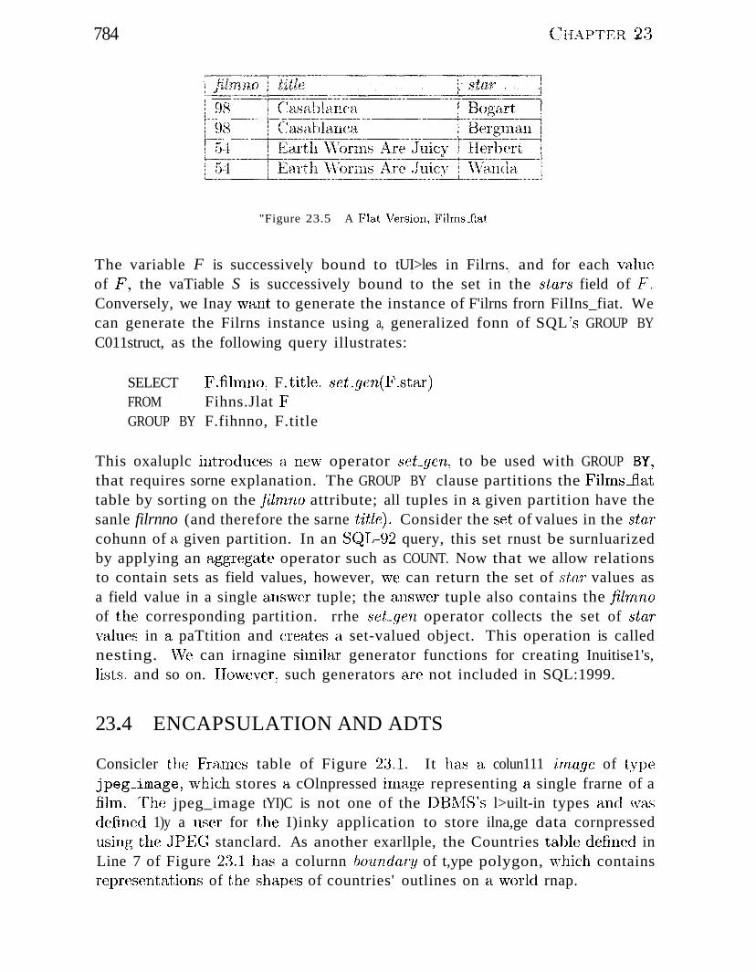
784
"Figure 23.5 A Plat Version,Films~fla,t
The variable F is successively bound to tUI>les in Filrns. and for each valuev . J
of I?, the vaTiable S is successively bound to the set in the staTs field of .F'.Conversely, we Inay "vant to generate the instance of F'ilrns frorn FilIns_fiat. Wecan generate the Filrns instance using a, generalized fonn of SQL '8 GROUP BYC011struct, as the following query illustrates:
SELECT F.fihnno, F. title, seLgen(F.star)FROM Fihns.Jlat FGROUP BY F.fihnno, F.title
This oxaluplc introducE~s (1, ne'w operator seLgen, to be used with GROUP BY,that requires sorne explanation. The GROUP BY clause partitions the FihnsJlattable by sorting on the .filTn:no attribute; all tuples in a given partition have thesanle filrnno (and therefore the sarne title). Consider the set of values in the starcohunn of (1, given partition. In an SC~L-92 query, this set rnust be surnluarizedby applying an aggregate operator such as COUNT. Now that we allow relationsto contain sets as field values, however, \ve can return the set of staT values asa field value in a single anSWE~r tuple; the ans\ver tuple also contains the fihnnoof the corresponding partition. rrhe set-gen operator collects the set of starvalues in a paTtition and creates a set-valued object. This operation is callednesting. vVe can irnagine shnihtr generator functions for creating Inuitise1's,lists. and so on. IIo\vever, such generators are not included in SQL:1999.
23..4 ENCAPSULATION AND ADTS
Consicler the Fnunes table of Figure 2:3.1. It lUls a colun111 ,zrnage of typejpeg~image, vlhich stores a, cOlnpressed iUHlge representing a single frarne of afihn.I'he jpeg_image tYI)C is not one of the DBlVIS's l>uilt-in types and \VEtS
d(~fined 1)y a user for the I)inky application to store ilna,ge data cornpressedllsingth(~ JPEC; stanclard. As another exarllple, the Countries table defined inLine 7 of Figure 2:3.1 h;:lS a colurnn boundaT'Y of t,ype polygon, \v111ch containsr(~presentationsof the shapes of countries' outlines on a vvorld rnap.
()b,ject:- Database Syst:en18
.Allowing users to define arbitrary nc\v data types is a key feature of ()RDBf\,1Ss.'1"he DBrvlS alh:)\vs users to store and retrieve objects of type jpeg_image, justlike an object of any other type, such as integer. No\v atornic data typesusually need to have t~ype-specific operations defined by the user 'who createsthern. For exanlple~ one rnight define operations on an irnage data type sucha"s compress, rotate, shrink, and crop. rrhe ccnnbination of an atolIlic datatype and its associated rnethods is called an abstract data type, or ,A,DT.Traditional S(~L COlnes with built-in ..l\DTs, such as integers (-with the a",ssociated arithnletic rnethods) or strings (with the equality~ cornparison, and LIKElllethods). Object-relational systerns include these ADT's and also allow usersto define their o\vn ADTs.
The label abstract is applied to these data types because the database systerIldoes not need to InlOW how anAD1~'s data is stored nor ho\v the ADT's rnethods work. It rnerely needs to know \vhat rnethods are availa,ble and the inputand output types for the rnethods. I-Eding ADT internals is called encapsulation.4 Note that even in a. relational systern, atolnic types such as integershave associated rnethods that encapsulate the1n. In the case of integers, thestandard Inethods for the ADT are the usual aritlunetic operators and COll1
parators. To evaluate the addition operator on integers, the database systenlneed not understand the laws of addition it l11erely needs to know how toinvoke the addition operator's code and what type of data to expect in return.
In an object-relational systenl, the Silllplification due to encapsulation is criticalbecause it hides any substantive distinctions between data types and allows anOR,DB1VIS to be iInplernented \vithout anticipating the types and rnethods thatusers Inight want to add. For exarnple, (l,dding integers and overlaying irnagescan be treated unifonnly by the systern, vvith the only significant distinctionsbeing that different code is invoked for the t\VO operations and differently typedobjects are expected to be returned froIll that code.
23.4.1 Defining Methods
rro register a rH~\V rnethod for a user-defined data type, users rnust \vrite thecode for the nlcthod and then infor1n the datalHlse systcrI1 about the Inethod.'rhe cod.e to be \i\rritten depends on the languages supported by the DBlVISand, possibly, the operating systerH in question. For eXC1ruple, the OHI)Bl\;ISInay handle J a\ta, co(h,~ in the Linux operating systern. In this case, the lnet,hodcode nlu,st be \vritten iII Java and cOlnpiled into a .Java bytecode file stored in.a Linux file s~vsteln. 'Then an SC~L-st~yle luethod registration eOllunand is givento the ()I:ll)Bl\/lS so that it recognizes the nc~\v rnethod:
4SOlue OIlIJBivISs actually refer to Aryl's as opaque types beca,use they are enci::tpsula.ted a,ndhence one cannot see their details.
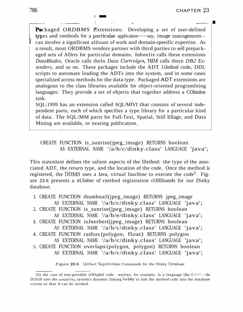
786 CHAPTER ~:3
r:-'"- _._-"".,.- -._ - ,-~ -- -----.Packaged ORDBMS Extensions: Developing a set of user-defined
. types and rnethods for a particular application·······-say, iInage management·,·,·,,·I can involve a significant aIIlount of work and dornain-speeific expertise. As
a result, most ORDBMS vendors partner with third parties to sell prepack-aged sets of ADrrs for particular domains. Inforn1ix calls these extensionsDataBlades, Oracle calls theln Data Cartridges, IBNI calls thern DB2 Extenders, and so on. These packages include the ADT 11lethod code, DDLscripts to automate loading the ADTs into the system, and in some casesspecialized access methods for the data type. Packaged ADT extensions areanalogous to the class libraries available for object-oriented programIninglanguages: They provide a set of objects that together address a COlnnlontask.SQL:1999 has an extension called SQL/MIVI that consists of several independent parts, each of which specifies a type library for a particular kindof data. The SQL/MM parts for Full-Text, Spatial, Still Iillage, and DataMining are available, or nearing publication.
CREATE FUNCTION is_sunrise(jpeg_image) RETURNS booleanAS EXTERNAL NAME '/a/b/c/dinky.class' LANGUAGE 'java';
This statenlent defines the salient aspects of the lllethod: the type of the associated ADT, the return type, and the location of the code. Once the method isregistered, the DBNIS uses a Java, virtual lnachine to execute the code5 . Figure 23.6 presents a nUlnber of rnethod registration cOllllnands for our Dinkydatabase.
1. CREATE FUNCTION thumbnail(jpeg_image) RETURNS jpeg_imageAS EXTERNAL NAME '/a/b/c/dinky.class' LANGUAGE 'java';
2. CREATE FUNCTION is_sunrise(jpeg_image) RETURNS booleanAS EXTERNAL NAME '/a/b/e/dinky.class' LANGUAGE 'java';
3. CREATE FUNCTION isJnerbert(jpeg_image) RETURNS booleanAS EXTERNAL NAME '/a/b/c/dinky.class' LANGUAGE 'java';
4. CREATE FUNCTION radius (polygon, float) RETURNS polygonAS EXTERNAL NAME '/a/b/c/dinky.class' LANGUAGE 'java';
5. CREATE FUNCTION overlaps (polygon, polygon) RETURNS booleanAS EXTERNAL NAME '/a/b/c/dinky.class' LANGUAGE 'java';
Figure 2:1.6 IVlethod H.,egistration Conunands for the Dinky Da.taha..se
._--_.51n the case of non-portable cOIl1piled code written, for example, in a, language like C++" .....···the
D131v18 uses the operating; system's dynamic linking facility to link the method code into the databa..sesystem so that it can be invoked.
()bject- Database Systerns 787~
rrype definition statelnents for the user-defined atornic data types in the Dinkyscherna are given in Figure 23.7.
1. CREATE ABSTRACT DATA TYPE jpeg_image('inte'rnallength = VARIABLE, input = jpeg~n, output = jpeg_out);
2. CREATE ABSTRACT DATA TYPE polygon(internallength = VARIABLE, input = polyjn, 01LtP'Ut == poly_out);
Figure 23.7 Atomic Type Declaration Commands for Dinky Database
23.5 INHERITANCE
We considered the concept of inheritance in the context of the ER, model inChapter 2 and discussed how ER diagrarns with inheritance 'were translatedinto tables. In object-database systems, unlike relational systerns, inheritanceis supported directly and allows type definitions to be reused and refined veryeasily. It can be very helpful when modeling similar but slightly different classesof objects. In object-database systerns, inheritance can be used in two ways: forreusing and refining types and for creating hierarchies of collections of sirnilarbut not identical objects.
23.5.1 Defining Types with Inheritance
In the Dinky database, we rnodel rnovie theaters with the type theater .._t.Dinky also wants their database to represent a new rnarketing technique in thetheater business: the theater-cafe, which serves pizza and other rneals whilescreening movies. rrheater-cafes require additional inforrnation to be represented in the database. In particular, a theater-cafe is just like a theater, buthas an additional attribute representing the theater's IIlenu. Inheritance allowsus to capture this 'specialization' explicitly in the database design with thefollowiIlg DDL staternent:
CREATE TYPE theatercafe_t UNDER theater_t (rn,enu text);
This staternent creates a new type, theatercaf e_t, which has the sarne attributes and rnethods <:l.S theater_t, plus one Etdditional attribute rnenu of typetext. lVlethocl,s defined on theater_..t apply to objeets of type theatercafe_t,but not viee versa. vVe sa~y that theatercaf e_t inherits the attributes andrnethods of theater_t.
Note that the illherita,nce rnechanisrll is not rnerely a rnacro to shorten CREATEstaternents. It creates an explicit relationship in the databa..se between th(~
subtype (theatercafe_t) and the supertype (theater_t ):An object of the
788 CJHA.prrElt 23
s'ublypc is also considered to be an object of the B'Upert:lJpe. This treatlnentIneans that an.y operations thi:tt apply to the supertype (nlcthods as \ven asquery operators, such as projection or join) also apply to the subtype. 1:'his isgenerall.y· expressed in the follo\ving principle:
The Substitution Principle: C~iven a supertype A. and a subtypeJj, it is always possible to substitute an object of type B into a legalexpression vvritten for objects of type A, without producing type errors.
This principle enables easy code reuse because queries and Inethodswritten forthe supert)rpe can be applied to the subtype vlithout I1lodification.
Note that inheritance can also be used for atc)luic types, in addition to ro\vtypes. Given a supertype image_t with rnethods title(), nurnber._of_colors(),and d'isplay(), we can define a subtype thumbnail_image_t for slllall irnagesthat inherits the rnethods of image_to
23.5.2 Binding Methods
In defining a subtype, it is sornetiInes useful to replace a rnethod for the Sll
pertype with a new version that operates differently on the subtype. Considerthe image_t type and the subtype jpeg_image_t frorH the Dinky database.lJnfortunately, the display() rnethod for standard .iInages does not work forJPEG irnages, which are specially cOlnpressed. Therefore, in creating typejpeg_image_t, we write a special display() rnethod for JPEG iruages and register it with the database systern using the CREATE FUNCTION cOIIuuand:
CREATE FUNCTION di8play(jpeg~image) RETURNS jpeg_imageAS EXTERNAL NAME '/a/b/c/jpeg.class' LANGUAGE 'java.';
Ilegistering a ne\v rnethod \vith the sarne HeHne as an aIel rnethod is calledoverloading the luethod narne.
Because of over1oading~ the systern Inust understand 'which rnethod is intendedin a, particular expression. For exarnple, when the systern needs to invoke thedisplay () rnethod on an object of type j peg ....image _t, it uses the specializeddisplay rnethocL 'VIlcn it needs to invoke display on an object of type image __tthat is not otherwise subtyped, it invokes the standard display Inethod. Theprocess of d(~ciding which rnethod to invoke is called binding the rnethod totJIC ol)ject. In certa.in situations, this binding CHJl be done \vhen (tIl expn~ssiorl ispaTsed (early binding), but in other cct.~es the 1n08t specific type of HJl objectC(1,nnot be known until rl.ln-tinle, so the rnethod cannot be l)ound until then(late binding) . Late birlding fa,cilties acId flexibility but can rnake it harder
()bject- Dat;aba8c8y8terIL8 7~9
for the user to rea)f:;on about the Inethods that get invoked for a given queryexpreSSIon.
23.5.3 Collection Hierarchies
Type inheritance was invented for object-oriented progranuning languages, andour discussion of inheritance up to this point differs little £roln the discussionone Inight find in a book on an object-oriented language such as C++ or Java.
I-I()\vever, because database systerns provide query languages over tabular datasets, the lnechanisnls fronl progrannning languages are enhanced in objectdatabases to deal with tables and queries as well. In particular, in objeetrelational systelIls, we can define a table containing objects of a particulartype, such &'-; the Theaters table in the Dinky sehenla. Given a new subtype,such as theatercafe_t, we would like to create another table Theater_cafes tostore the inforrnation about theater cafes. But, when writing a query over theTheaters table, it is sornetirnes desirable to ar;;k the saIne query over the rrheater_cafes table; after all, if we project out the additional C01UlllI1S, an instanceof the Theater_cafes table can be regarded as an instance of the Theaters table.
R,ather than requiring the user to specify a separate query for each such table,we can infonn the systern that a new table of the subtype is to be treated as
part of a table of the supertype, with respect to queries over the latter table.In our exalnple, we can say
CREATE TABLE Thea,ter_Cafes OF TYPE theatercafe ....t UNDER Theaters;
This staternent tells the systern that qu(~ries over the Theaters table shouldactually be run over all tuples in both the rrheaters and rrheater_Cafes tables. Insuch cases, if the subtype definition involves rnethod overloading, late-bindingis used to ensure that the appropriate rnethods are called for each tuple.
In general, t11.e UNDER chl11se can be used to genera,te an arbitrary tree of tables, called (1, collection hierarchy. (~ueries over a particular tal)le T in thehierarchy are run over all tuples in rr and its descendants. Sornetirnes, a userrnaywant the query to nUl ollly on rr and not on the descencl<tnts; additiona1syntax, for exaInple, the key\vord ONLY, can be used in the query's FROM clauseto fl,chieve this effect.
23~6 OBJJ1:Cl-'S, OIDS, AND REFERENCE TYPES
In object-elatabase systerns, data objects can be given an object identifier(aid), \vhich is sotne value that is unique in the database across tirne. The
790 CHAP1'ER 243
r---- - ~-················ -_ -.-................ - ------..... . -----... II OIDs: IBNl DB2, Inforul..ix lJDS, and Oracle 9i support REF types. IL--._. .__._..__.. .----_~ __ __ _ __ .
DBl\iIS is responsible for generating aids and ensuring that an oid identifies anobject uniquely over its entire lifetillle. In SOHle systenls, all tuples stored inany table are objects and autornatically assigned unique oids; in other systenls,a user can specify the tables for 'which the tuples are to be c1ssigned aids. Often,there are also facilities for generating oids for larger structures (e.g., tables) aswell as slnaller structures (e.g., instances of data values such as a copy of theinteger 5 or a .TPEG ilnage).
An object's aid can be used to refer to it from elsewhere in the data. An oidhas a type similar to the type of a pointer in a progralnll1ing language.
In SQL:1999 every tuple in a table can be given an aid by defining the tablein ternlS of a structured type and declaring that a REF type is associated withit, a,'3 in the definition of the Theaters table in Line 4 of Figure 23.1. Contrastthis with the definition of the Countries table in Line 7; Countries tuples donot have associated aids. (SQL:1999 also assigns 'oids' to large objects: Thisis the locator for the object.)
REF types have values that are unique identifiers or aids. SQL: 1999 requiresthat a given REF type must be associated with a specific table. For exalnple,Line 5 of Figure 23.1 defines a cohllnn theater of type REF(theater_t). TheSCOPE clause specifies that iterns in this colurnn are references to rows in therrheaters table, which is defined in Line 4.
23.6.1 Notions of Equality
The distinction between reference types and reference-free structured typesraises another issue: the definition of equality. Two objects having the saInetype are defined to be deep equal if and only if
1. The objects <1,1'e of atolnic type and have the saIne value.
2. The objects are of reference type and the deep eq'l.lals operator is true forthe two reforenced objects.
;3. rrhe objects are of structured type and the deep eqtlal.s operator is true forall the corresponding subparts of the two objects.
Two objects that have the SaJllC reference type are defined to be shallow equalif both refer to the saIne object (i.e., both references use the saUle aid). T'he
()b.ject-Database Systen18 791
definition of shallow equality can be extended to objects of arbitrary type bytaking the definition of deep equality and replacing deep eq1J,als by shallo'w elj'uals
in parts (2) and (~~).
As an exarnple, consider the cornplex objects ROW (538, tS9, 6-3-97, 8-7-97)and ROW(538, i33, 6-3-97, 8-7-97), whose type is the type of rows in the tableNowshowing (Line 5 of Figure 23.1). 1'hese t\VO objects are not shallow equalbecause they differ in the second attribute value. Nonetheless, they rnightbe deep equal, if, for instance, the oids t89 and t33 refer to objects of typetheater_t that have the saIne value; for exarnple, tuple (54, ':Nlajestic', '115King', '2556698').
While two deep equal objects Inay not be shallow equal, a._" the exarnple illustrates, two shallow equal objects are always deep equal, of course. 'The defaultchoice of deep versus shallow equality for reference types is different acrosssystenls, although typically we are given syntax to specify either semantics.
23.6.2 Dereferencing Reference Types
An item of reference type REF (basetype) is not the sarne as the basetype itenlto which it points. To access the referenced basetype itenl, a built-in deref ()rnethod is provided along with the REF type constructor. For example, givena tuple from the Nowshowing table, one can access the name field of the referenced theater_t object with the syntax Nowshowing.deref (theater). narne.Since references to tuple types are comInon, SQL:1999 uses a Java-style arrowoperator, which cOD.lbines a postfix version of the dereference operator with atuple-type dot operator. The narne of the referenced theater can be access(~d
with the equivalent syntax Nowshowing.theater-> narne, as in Figure 23.3.
At this point we have covered all the basic type extensions used in the Dinkyscherna in Figure 23.1. The reader is invited to revisit the scherna and exarninethe structure and content of each table and how the new features are used inthe various sarnple queries.
23.6.3 URLs and DIDs in SQL:1999
It is instructive to note the differences between Internet lJRIJs Etnel the oidsin object systerns. First, oids uniquely identify a single object over all tirne(at least, until the object is deleted, when the oid is undefined), vvherea,s the'\Veb resource pointed at by an lJHJ-J can change over tirue. Second, oids aresirnply identifiers and carry no physical infonnation about the objects theyidentify this rnakes it possible to change the storage location of an objectwithout rnodifying pointers to the object. In contra,st, lJH.I.ls include net\'lork
792 (jHAprI'ER 2*3
addresses and often file-syst;enl narnes (;1,,-:;; \veU, lIle<.:tning that if the resourceidentified by the {JIlL has to Inove to another file or network a,ddress. then alllinks to that resource are either incorrect or r(~quire a ~forwardiIlg' rnechanisH1.rrhird, oids are aut(Hnatically generated by the I)B1\;18 for each object, \vhereaslJIlLs are user-generated. Since users generate lJR,Ls, they often ernbed scrnantic inforlllation into the {JR.L via rnachine, directory, or file names; thiscan becoine confusing if the object's properties change over tilne.
For lJIlLs, deletions can be troublesorne: T'his leads to the notorious '404Page Not Found' error. For oids, SQL:1999 allows us to say REFERENCES ARECHECKED as part of the SCOPE clause and choose one of several actiol1swhen areferenced object is deleted. This is a direct extension of referential integritythat covers oids.
23$7 DATABASE DESIGN FOR AN ORDBMS
The rich variety of data types in an OH,DBTv1S offers a database designer Inanyopportunities for a rnore natural or lllore efficient design. In this section we illustrate the differences between IlDBl\!lS and ()RI)BMS database design throughseveral exarnples.
23.7.1 Collection Types and ADTs
()ur first exarnple involves several space probes, each of which continuouslyrecords a video. A single video strearll is associated with each probe, and whilethis strearn \Vck'3 conected over a certail1 tiule period, vve assurne that it is nowa cOlllplete object associated Vilith the probe. During the tirne period overwhich the video \vas collected, the probe's locatiol1\vas periodieaJly recorded(such infonnation (;an ea.-.sily be pigg~y-backedonto the header portion of a videostreanl conforrning to the TvIPEC; sta,ndard). 1'he inforrnation associated \vitha probe has three parts: (1) a probe ID that identifies a probe uniquely, (2) avideo s/;'r'carn, and 03) a location 8cqucn.ce of (t;inLe 1 location) pairs. \iVhat kindof a database scherna should we use to store this infonnation?
An RDBMS Database Design
In H,11 HIJBlVJ:S, \ve rnust store each video strcanl as a BIJ)13 Etnd each locationsequellce as tuples in a tabh.~. A possible HJ.JBIVJ.S data,b~J,,'3e design follo\vs:
Probes(.E~.~~~_ integer, UTnc~:~..._~imestamp, lat:: !:_~ ..~.~_,__!!:)ng: re~.!,carnCTa: string, 'v'ideo: BLOB)
()bject-lJatabase Syslelf);8 -n, ':3{ ;;~
There is a single table caned Probes and it lu1.'3 severa,} rows for each probe. Eachof these rovvs has the saIne pid, carneT(J" and1rideo values, but different t'irne,tat, and lcntg values. (vVe have used latitude and longitude to denote location.)The key for this table can be represented as a functional dependency: IJTLN-:. CY ll , '~lhere N stands for longitude. There is another dependency: p--;. (;V~
'rhis relation is therefore not in BCNT;"; indeed, it is not even in :INF. vVe ca:ndecolupose Probes to obtain a BCNF scherna:
ProbeS_bLoc(pid: integer, lirne: timestamp, tat: real, long: real)Probes_Video(p'id: integer, carn,era:"-;'t'i='ing, 'v'ideo: BLOB)
This design is about the best we can achieve in an RDBl'v1S.Ho\vever, it suffersfrorn several dn1\vbacks.
First, representing videos aA.'3 BLOBs lI1eanS that we have to write applicationcode in an external language to lnanipulate a video object in the database.Consider this query: "For probe 10, display the video recorded between 1:10P.M. and 1:15 P.M. on lVlay 10 1996." We lnust retrieve the entire video objectassociated ''lith probe 10, recorded over several hours, to display a segrnentrecorded over five rninutes.
Next, the fact that each probe has an associated sequence of location readingsis obscured, and the sequence inforrnatiol1 associated with a probe is dispersedacross several tuples. A third drawback is that vve are forced to separate thevideo infonnation froTn the sequence inforrnation for a probe. rrhese lirnitationsare exposed by queries that require us to consider all the infonnation associatedv'lith each probe; for excunple, ;'Fhr each probe, print the earliest tirne at whichit recorded, and the CEtrnen.l type." T'his query 110v'l involves a join of Probes.".Locand Probes_Video on the p'id field.
An ORDBMS Database Design
;\n ()HJ)BlVIS supports a lnuch better solution. FirsL \ve can store the videoas an A.DT object and \vrite rnethods that c':1I)ture a.ny special rna,nipulation\ve \vish to perforrr1. Second, 1)eCflT1Se \ve aTe allovved to store structured typessuch as lists,\ve (:a,n stc)re tIl(:; loca,tion sequerlce for (1. probe in a single tuple,along\vith thE: video infonnation. '['his layout elirnina,t;c;s the need for joins incIlH;ries that involve both the sequence ancl video inforrnation. An ()HI)BNISdesign for our exarrlpl(~ consists of ,1 single relation called Probes_i\llInfo:
Probes ... AIUnfo(pid: integer, loc8eq: location...seq, Ca'fTl·e'ra: string;'video: mpeg_.stream)
794 CHAPTER 2~
This definition involves t,vo new" types, location...seq and mpeg_stream. Thempeg_stream type is defined as an ADT, with a Inethod display() that takesa start tiIne and an end tirne and displays the portion of the video recordedduring that interval. This rnethod can be irnplernented efficiently by looking atthe total recording duration and the total length of the video and interpolatingto extract the segnlcnt recorded during the interval specified in the query.
Our first query in extended SQL using this display lnethod follows. We nowretrieve only the required segment of the video rather than the entire video.
SELECT display(P.video, 1:10 Po M0 May 10 1996, 1:15 Po M0 May 10 1996)FROM Probes-.Alllnfo PWHERE Popid = 10
Now consider the location_seq type. We could define it as a list type,containing a list of ROW type objects:
CREATE TYPE location_seq listof(row (time: timestamp, lat: real, long: real))
Consider the locseq field in a row for a given probe. This field contains a listof rows, each of which has three fields. If the ORDBMS implements collectiontypes in their full generality, we should be able to extract the time colurnnfrom this list to obtain a list of timestamp values and apply the MIN aggregateoperator to this list to find the earliest tiIne at which the given probe recorded.Such support for collection types would enable us to express our second querythus:
SELECTFROM
P.piel, MIN(P.locseq.tirne)Probes._AllInfo P
Current ()ItDBI\1Ss are not &'3 general and clean a..s this exalnple query suggests.For instance, the systern rnay not recognize that projecting the tirne colurnnfrorn a list of rows gives us a list of tirnestarnp values; or the systcru rnay allovvus to apply an aggregate operator only to a table and not to a nested list value.
Continuing "'lith our exa.rnple, we lnay want to do specialized operations onour location sequences that go beyond the standard aggregate operators. Forinstance, we rnay want to define a lnethod that takes a tirne interval and COIIl-
, .'putes the distaIlce traveled by the probe during this interval. The code for thisrnethod rnust understaJnd details of a probe's trajectory and geospatial coordinate systenls. FbI' these reasons, \ve rnight choose to define location_seq asan ADT\.
Object-Database Systerns 79~
Clearly, an (ideal) ORDBIvIS gives us IIlaIlY useful design options that are notavailable in an RDBMS.
23.7.2 Object Identity
\Ve now discuss S0l11e of the consequences of using reference types or aids. Theuse of aids is especially significant when the size of the object is large, eitherbecause it is a structured data type or because it is a big object such &s animage.
Although reference types and structured types seem sirnilar, they are actuallyquite different. For example, consider a structured type my_theater tuple (inainteger, name text, address text, phone text) and the reference type theaterref (theater_t) of Figure 23.1. rrhere are irnportant differences in the way thatdatabase updates affect these two types:
• Deletion: Objects with references can be affected by the deletion of objects that they reference, while reference-free structured objects are notaffected by deletion of other objects. For exaluple, if the Theaters tablewere dropped from the database, an object of type theater might changevalue to null, because the theater_t object it refers to has been deleted,while a similar object of type my_theater would not change value.
• Update: Objects of reference types change value if the referenced objectis updated. Objects of reference-free structured types change value only ifupdated directly.
• Sharing versus Copying: An identified object can be referenced byllluitiple reference-type iterIls, so that each update to the object is reflectedin IYlany places. ~ro get a sirnilar effect in reference-free types requiresupdating all 'copies' of an object.
There are also irnportant storage distinctions between reference types and nonreference types, \vhich rnight affect perfoI'rnance:
III Storage Overhead: Storing copies of a large value in rnultiple structuredtype objects IYlay use lnnch rno1'e space than stori.ng the value once andreferring to' it elsewhere through reference type objects. This additionalstorage requirelnent can affect both disk usage and buffer lnanagcrncnt (ifIIlal1Y copies are accessed at once).
III Clustering: The subparts of a structured object are typically stored together on disk. Objects with references rna,Y point to other objects that a,1'e
far a:way on the disk, and the disk ann Inay require significant rnOVClnent
-oct ,10 (~;HApcrER ~3
OIDs and Referential Integrity: In SQL:1999, aU the oids that appear in a cohunn of a relation are required to reference the srtrne targetrf~lation. This ~scoping' ulakes it possil)]e to check oid refere:nces for "1'e£e1'entiaJ. integrity' just like foreign key references are ehecked.vVhile currentOI{DB1JlS products supporting oids do not support such checks, it: is likelythat they will in future releases. This will nlake it rnnch safer to use aids.
to asserrlble the object and its references together. Structured objects canthus be l'nor8 efficient than reference types if they are typically accessed intheir entirety.
Many of these issues also arise in traditional prograunuing languages such as Cor Pascal, which distinguish between the notions of referring to objects by valueand by refer-ence. In database design, the choice between using a structuredtype or a reference type typically includes consideration of the storage costs,clustering issues, and the effect of updates.
Object Identity versus Foreign Keys
lJsing an oid to refer to an object is silnila,r to using a foreign key to referto a tuple in another relation but not quite the seune: An oid can point toan object of theater_t that is stored any'whcr-c in the database, even in afield, whereas a foreign key reference is constrained to point to an object in a,particular referenced relation. This restriction rnakes it possible for the DBlV1Sto provide lnuch greater support for refer(~ntial integrity than for arbitra,ry aidpointers. In general, if an object is deleted while there an~ still oid-pointersto it, the best the DBl\IIS can do is to recognize the situation by rnaintajninga reference count. (Even this lirnited support becornes irnpossible if oids canbe copied freely.) Thereforc 1 the responsibility for avoiding dangling n~ferences
rests largely \'lith the user if oids are llsed to refer to objects. This burdensoIllcresponsibility suggests that vVE~ should use oids \vith great ca.ution and useforeign keys instead \vhenever possible.
23.7.3 Extending the ER Model
The Ell rnodel, cLS described in Chapter 2, is not adequate for ()ItDB1\tlS design.\Ve have to use an extendedEH, rnodel that supports structured attributes(i.e., sets, lists, arra,Ys a,s attribute values) I distinguishes \vhethc~r entities haveol)ject ids, and allc)\vs us to Inodel entities \vhose attributes include rnethods.\Ve illustrate these connnents using an extended Ell diagrarn to describe the
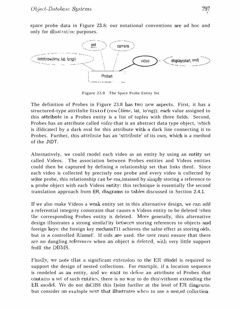
()b,icct- Database Sy"teTn,'3 797li
space probe data in Figure 2:.3.8; our notational conventions are ad hoc andonly for illustr;::ttivc purposes.
~ -(,~isPlay(start! end) ,._--:)---'_-'-_.~,..__.....~ ....-----, ..-"._.......~......--
Figure 23.8 The Space Probe Entity Set
The definition of Probes in Figure 23.8 has t\VO rH~\V &,;pects. First, it has astructured-type attrilnlte listof (row (ti'lnc, lat, lo'ng)); each value assigned tothis attribute in a Probes entity is a list of tuples with three fields. Second,Probes has an attribute called video that is an abstract data type object, \vhichis iIldicatecl by a dark oval for this attribute \vith a dark line connecting it toProbes. Further, this ctttribute has an 'attribute' of its own, \vhich is a rnethodof the J\DT.
Alternatively, we could rnodel each video as an entity by using an t~ntity setcalled Videos. The association between Probes entities and Videos entitiescould then be captured by defining a relationship set that links thenl. Sinceeach video is collected by precisely one probe and every video is collected byse)lne probe, this relationship can be rna,intained by siInply storing a reference toa probe object with each Videos entity; this technique is essentially the secondtranslation approach frorn ER, diagnuns to tables discussed in Section 2.4.1.
If we also rnake Videos a \iVeak entity set in this alternative design, we can adda referential integrity constraint that causes a Videos entity to be deleted \vhenthe corresponding Probes entity is deleted. 1\/101'8 generally, this alternativedesign illustrates a strong sirnila1'ity bet\veen storing references to objects andforeign keys; the foreign key rnechanisT11 achieves the saIne effect as storing oids~
but in (1, controlled lUanneI'. If oids are used. the user rnusi ensure that thereare no dangling references when an object is deleted, \iVith very little supportfroIll the DBlvlS.
Finally~we nofe tllat a significant extension. to the Ell rHodel is required tosupport the design of nested collections. For exa.rnple~ if a location sequenceis rnodeled (J",'3 an entity, and \ve \vant to clefine an attribute of Probes thatcontftins a set of such entities, there is no "vay to do this\vithont extending theEll rrlodeL\Vc do not disC1ISS this I)oint furtller at the level of Ell diagraIlls,but consider an exaJnple 11E~xt that illustrat(~swhen to use a nest,ed (~ollection.
798 C~HAPTER~3
23.7.4 Using Nested Collections
Nested collections offer great rnodeling power but also raise difficult designdecisions. Consider the following \vay to rnodel location sequences (other infonnation about probes is ornitted here to sirnplify the discussion):
Probesl(pid: integer, locseq: location_seq)
rrhis is a good choice if the irnportant queries in the workload require us to lookat the location sequence for a particular probe, as in the query "For each probe,print the earliest tirne at which it recorded and the caluera type." On the otherhand, consider a. query that requires us to look at all location sequences: "Findthe earliest tiIne at which a recording exists for laf;=5, long=90." This querycan be answered 1110re efficiently if the following scherna is used:
Probes2(pi(~: integ~r, tim~:_.timestamp, tat: real, long: real)
The choice of scherna Blust therefore be guided by the expected workload (asalways). As another example, consider the following scherna:
Can_TeachI (cid: integer, teacheTs: setof (ssn: string), sal: integer)
If tuples in this table are to be interpreted as "Course cid can be taught by anyof the teachers in the teacheTs field, at a cost sal." then we have the option ofusing the following schenla. instead:
CarLTeach2( cid: integer, teachCT_8sn: st~_~~.~, sal: integer)
A choice between these two alternatives can be Inade based on hovv we expectto query this table. On the other hand, suppose that tuples in CalL.Teachlare to be interpreted as "Course cid can be taught by the tearnteacheT8, ata cornbined cost of sal." CarLTeach2 is no longer a viable alternative. If we,vanted to flatten CarLleachl, ~we would have to use (1, separate table to encodetearns:
Can_TCcl,ch2 (.~:'~i..~~.:'..._...~.12~.~ ..~!!!_~_,_ ..!~~~(J;rrL 'id: 0 i ~, ,,(l, l: int eger)1'earns( tid: oid, .'iBn: string)
As these exarnples illustrate, nested collections are appropriate in certain situations, but this fea,ture can ea,,'3ily be rnisused; nested collections should thereforebe used ·with care.
()b.ject- Database Systerns
23.8 ORDBMS IMPLEMENTATION CHALLENGES
7fJ9#
The enhanced functionality of OIlDBIvlSs raises several irnp1ernentation challenges. SOlne of these are 'well understood and solutions have been irnp1enlentedin products; others are subjects of current research. In this section \ve exarninea few of the key challenges that arise in irnplernenting an efficient, fully functional OIlDBlvfS. l\:lany rnore issues are involved than those discussed here; the
I.- ,
interested reader is encouraged to revisit the previous chapters in this book andconsider whether the irnplernentation techniques described there apply naturally to ORDBJ\JISs or not.
23.8.1 Storage and Access Methods
Since object-relational databases store new types of data, ORDBMS implernentors need to revisit some of the storage and indexing issues discussed inearlier chapters. In particular, the system lllust efficiently store ADT objectsand structured objects and provide efficient indexed access to both.
Storing Large ADT and Structured Type Objects
Large ADT objects and structured objects cornplicate the layout of data ondisk. This problern is well understood and has been solved in essentially allORDBMSs and OODBMSs. We present Sallie of the main issues here.
User-defined ADTs can be quite la,rge. In particular, they can be bigger thana single disk page. Large ADTs, like BLOBs, require special storage, typicallyin a different location on disk frorn the tuples that contain them. Disk-basedpointers are rnaintained frorn the tuples to the objects they contain.
Structured objects can also be large, but unlike ADrr objects, they often vary insize during the lifetirne of a database. For exarnple, consider the stars attributeof the film,s table in l~igure 23.1. A.s the years pEt.'3S, SOlne of the 'bit actors' inan old rnovie rnay becorne farnous. 6 YVhen a bit actor hecornes farnous, Dinkyrnight want to advertise his or her presence in the earlier filrns. This involvesan insertion into the stars attribute of an individual tuple in filrns. Becausethese bulk attributes can grow arbitrarily, flexible disk layout rnechanisrns arerequired.
GA famous example is Marilyn IVlonroe, who had a bit part in the Bette Davis da..ssic All About.E'/Jc.
800 CHAPTER 23
i\n additional COlllplication arises \'lith array types. 'fraditionally, array elelnents are ston-xl sequentially on disk in a ro\'l-by-ro\v fashion; for exarnple
1Io\v8ver, queries rnay often request suba.rrays that are not stored contiguouslyon disk (e.g., .i411 , ,;121, ... ,Arn1). Such requests can result in a very high I/Ocost for retrieving the subarray. rro reduce the nurnber of l/Os required, arraysare often broken into contiguous chunks, vvhich are then stored in senne orderon disk. Although each chunk is sorne contiguous region of the array, chunksneed not be rovv-by-ro\v or colurnn-by-colurllll. For exalnple, a chunk of size 4111ight be All, A12 , A21 , /122 , 'which is a square region if we think of the arrayas being arranged row-by-row in two dimensions.
Indexing New Types
One ilnportant reason for users to place their data in a database is to allowfor efficient access via indexes. Unfortunately, the standard RDB11S indexstructures support only equality conditions (B+ trees and hash indexes) andrange conditions (B+ trees). An irnportant issue for OR,DB1\IISs is to provideefficient indexes for AD'I' rnethods and operators on structured objects.
Many specialized index structures have been proposed by researchers for particular applications such as cartography, genorne research, 11lultirnedia repositories, \Veb search, and so on. An OR,DBlVIS cornpany Cctnnot possibly inlplernentevery index that has been invented. Instead, the set of index structures in an()R,DBlVfS should be user-extensible. Extensibility would allow an expert incartography, for exanlple, to not only register an AD1' for points on a rnap(i.e., latitude··longitude pairs) but also irnplernent an index structure that supports natural rnap queries (e.g., the R,-tree, \vhich lnatches cOllclitions such as"Find rne all theaters within 100 Iniles of Andorra"). (See Chapter 28 for 1110reon Il-trees and other spatial indexes.)
One vvay to rnake the set. of index structures extensible is to publish ;:1,11 acccs.s nu~thod 'interface that lets users irnplcrnent an index structure o'llts'ide theDEl\;IS. 'I'he index and data can be stored in a file systeIll and the DEl\;IS sirnplyissues the open, ne:l.:f, and Cl08(:~ iterator requests to the user's external indexcode. Such functionality rnakes it possible for a user to connect a I)Bl\1S toa\Neb search engine, for exauII>le. A rnain dravvback of this approach is thatdata in an external index is lI0t protected l)y tIle ])B1V1S'8 support for concurrency and rec:over:y. 1\n alterrlativf~ is for the ()llI)B1ilS to provide a generic'tenlphtte' irHlex structure that is sufficientl:y general to encornpass rnost indexstructures that usersrn.ight irlvent. Bec<luse snell a structure is il11plc~Jnented
within theDBrvIS, it can support high concurrency and recovery. The G1C't'1,(:T-
Object- Database8ystenLS 801
alized SleaTch Tree (GiS'r) is suell a structure. It is a ternplate index structureba.':'ed on B+ trees, \vhich aJlo\vs IllOSt of the tree index structures invented sofar to be irnplernented'with only a few lines of user-definedAD'T' code.
23.8.2 Query Processing
.A..DTs and structured types call for l1e\v functionality in processing queriesin ()RDI-3I\!ISs. rrhey also change a nurnber of a..ssuruptions that affect theefficiency of queries. In this section we look at two functionality issues (u8erdefined aggregates and security) and two efficiency issues (rnethod caching andpointer swizzling).
User-Defined Aggregation Functions
Since users are allowed to define new rnethods for their ADTs, it is not unreasonable to expect thern to want to define new aggregation fUllctions for theirADTs as well. For example, the usual SQL aggregates····---CDUNT, SUM, MIN,MAX, AVG--are not particularly appropriate for the image type in the Dinkyschema.
Most ORDBMSs allow users to register new aggregation functions \vith thesystern. To register an aggregation function, a user lnust iruplenlent threernethods~ which we call 'initiaIize, iterate, and terrninate. The in'it'ial'ize rnethodinitializes the internal state for the aggregation. The iterate rnethod updatesthat state for every tuple seen~ "vhile the terrninate rnethod C0111putes the aggregation result based on the final state and then cleans up. As an exarnple,consider an aggregation function to cornpute the second-highest value in a, field.1'he init'ialize call would allocate storage for the top two values~ the 'iterate callwould corupare the current tuple's value with the top two and update the toptwo as necessary, and theterrn'inate call \vould delete the storage for the toptwo values~ returning a copy of the second-highest value.
Method Security
AIYTs give users the pO\\'8r to a,(1d code to the DBl'vlS; this power can beabused. A buggy or rnalicious ADT rnethod can bring do\vn the databaseserver or eveil corrupt the databcL'Sc. The DBNIS lnust have rnechanisrns toprevent buggy or rnalicious user code frcHn causing probleIlls. It 1nay rnakesense to overricle these rnechanislIls for efficiency in production environrnentswith vendor-supplied rnethods. I-Io\vever, it is irnportant for the rnechanisrns toexist, if only to support delJugging of J\DT rnethocls; othervvise rnethod \vriters
802 CHAPTER ~3
\vould have to \vrite bug-free code before registering their rnethods with theDBMS--not a very forgiving progralIuning environlnent.
()ne rnechanisrn to prevent problerns is to have the user rnethods be intc11Jretedrather than cornp'iled. The DBIv1S can check that the rnethod is well behavedeither by restricting the power of the interpreted language or by ensuring thateach step taken by a rnethod is safe before executing it. Typical interpreted la.nguages for this purpose include Java and the procedural portions of SQL:1999.
An alternative rnechanislll is to allow user methods to be cOlnpiled frorn ageneral-purpose progranuning langllage~ such as C++, but to run those rnethods in a different address space than the DBMS. In this case, the DBMS sendsexplicit interprocess cOl1uIlunications (IPCs) to the user rnethod~ which sendsIPCs back in return. This approach prevents bugs in the user methods (e.g.,stray pointers) frorn corrupting the state of the DBNIS or database and preventsrnalicious methods frorn reading or Inodifying the DBMS state or database aswell. Note that the user writing the method need not know that the DBMS isrunning the method in a separate process: The user code can be linked with a'wrapper' that turns method invocations and return values into IPCs.
Method Caching
User-defined ADT methods can be very expensive to execute and can accountfor the bulk of the time spent in processing a query. During query processing,it may 11lake sense to cache the results of methods, in case they are invokedlllultiple times with the same arglunent. Within the scope of a single query,one can avoid calling a Inethod twice on duplicate values in a colurnn by eithersorting the table on that colullln or using a ha,..'3h-ba'3ed scherne ruuch like thatused for aggregation (see Section 14.6). An alternative is to rnaintain a cacheof rnethod inputs and rnatching outputs as a table in the database. Then, tofind the value of a rnethod on particular inputs, we essentially join the inputtuples with the cache table. rrhese two approaches can also be cornbined.
Pointer Swizzling
In sorne applications, objects are retrieved into rnernory and accessed frequentlythrough their oids; dereferencin.g rnust be irnplcrnented very efficiently. 801nesysterns rnaintain a ta,hle of oids of objects that are (currently) in InenlOI'.Y.\Vhen an object () is In'ought into nlCnlOl'jr, they check each oid c~ontained
in 0 and replace oids of in-rrH~rnory objects by in-rncrl10ry point(~rs to thoseobjects. 1'his techrlique, caJled pointer swizzling, nUl-kes referenc(~s to inrnernory objects ver~y .fast. rfhe dO\7vnsicle is tlHtt vvhen an object is paged out,
()b.iect- Database 8ys/;clns
2389 OODBMS
805t
In the introduction of this chapter, \ve defined an O()DB:NlS as a progranlIninglanguage ''lith support for persistent objects.vVhile this definition reflects theorigins of OODB~1Ss accurately, and to a certain extent the irnplernentationfocus of OODBl\'1Ss, the fact that OODBl\!ISs support collecl:'ion, type" (seeSection 2:3.2.1) rnakes it possible to provide a query language over collections.Indeed, a standard has been developed by the Object Database l\'lanagernentGroup and is called Object Query Language.
OQL is sirnilar to SQL, with a SELECT----FROM--HWHERE---style syntax (even GROUPBY, HAVING, and ORDER BY are supported) and rnany of the proposed SC~L:1999
extensions. Notably, OQL supports structured types, including sets, bags,arrays, and lists. 1~he OQL treatrnent of collections is rnore uniforlll thanSQL: 1999 in that it does not give special treatrnent to collections of rows;for exalnple, ()QL allows the aggregate operation COUNT to be applied to alist to C0111pute the length of the list. O(~L also supports reference types,path expressions,ADrrs and inheritance, type extents, and SQL-style nestedqueries. 1'here is also a standard Data Definition Language for OODB1\1Ss(Object Data Language, or ODL) that is sirnilar to the DDL subset ofSQL but supports the additional features found in OODBMSs, such as ADTdefinitions.
23.9.1 The ODMG· Data Model and ODL
'The ODl\iIG data rnodel is the basis for an OODBl\iIS, just like the relationaldata 1nodel is the basis for an IlDB1\1S. A database contains a collection of objects, which are sirnilar to entities in the Ell rnode!. Every object ha.s a uniqueaid, and a database contains collections of objects with Silllilar properties; sucha collection is called a class.
The properties of a class arc specified using ()l)L and are of three kinds: attributes, relationships, and rnethod8. _Attributes have an atolnic type or astructured t~ype. ODl.l supports the set, bag, list, array, and struct t,ypeconstructors; these are just setof, bagof, listof, ARRAY, and ROW in the terrninology of Section 2:3.2.1.
R,elationships have a type that is either a reference to an object or a collectionof such references. A relationship captures ho'v an object is related to oneor r1101'e obj(~cts of the 8e1111(' class or of ;.1 different clctss. j\ relationship inthe ()IJIvIG- rnodel is really just (1 bincl,ry relationship in the sense of theEI{Inodel. A rela.tionship has ~l corresponding inverse relationship; intuitively,it is the relationship 'in the other clirection.' For exarnple, if a Inovie is being
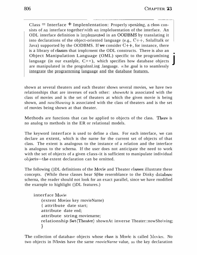
806 (jHAPTER 23
Class == Interface + Implenlentation: Properly speaking, a cla...,s consists of an interface together\vith an irnpleluentation of the interface. AnODL interface definition is irnpleInel~ted in an OODBlYIS by translating itinto declarations of the object-oriented language (e.g., C·+"+, Snlalltalk orJava) supported by the OODBMS. If V\Te consider C++, for instance, thereis a library of cl<:1Sses that irnplcrnent the ODL constructs. There is also anObject Manipulation Language (OML) specific to the programlninglanguage (in our exanlple, C++), which specifies how database objects jare manipulated in the progralnnl.ing .language. rr.he .goal is to seamlesslyintegrate the prograrnrning language and the database features.
shown at several theaters and each theater shows several rnovies, we have tworelationships that are inverses of each other: shownAt is associated with theclass of movies and is the set of theaters at which the given movie is beingshown, and nowShowing is associated with the class of theaters and is the setof rnovies being shown at that theater.
Methods are functions that can be applied to objects of the class. l~here isno analog to methods in the ER or relational models.
The keyword interface is used to define a class. For each interface, we candeclare an extent, which is the narne for the current set of objects of thatclass. The extent is analogous to the instance of a relation and the interfaceis analogous to the scherna. If the user does not anticipate the need to workwith the set of objects of a given class-it is sufficient to manipulate individualobjects--···the extent declaration can be ornitted.
The following ()DL definitions of the lViovie and Theater cla,,'3ses illustrate theseconcepts. (While these classes bear S(Hne resernblance to the Dinky databa",scscherna, the reader should not look for an exact parallel, since we have rnodifiedthe exarnple to highlight ()DL features.)
interface Iv/lovie(extent IVlovies key rnovieNarne){ attribute date start;attribute date end;attribute string rnovienarne;relationship Set('fheater) shownAt inverse Theater::nowSho\ving;}
1~he collection of databa...'3c objects whose cla"ss is lVlovie is called lVIovies. Notwo objects in lVIovies have the sarne rnovieNarne value, as the key declaration
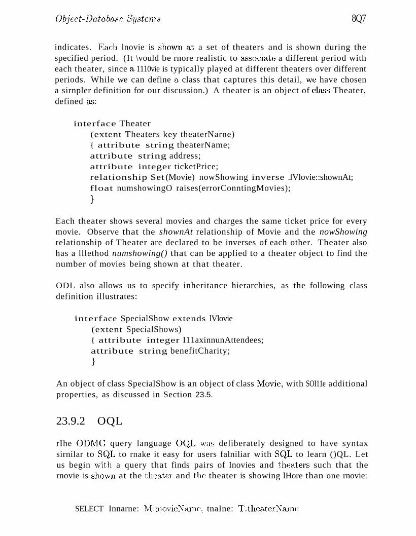
()bject-.Database Systelns 8Q7
indicates. Each lnovie is shov,rn at a set of theaters and is shown during thespecified period. (It \vould be rnore realistic to c'h'Ssoeiate a different period witheach theater, since a 1110vie is typically played at different theaters over differentperiods. While we can define a class that captures this detail, \ve have chosena sirnpler definition for our discussion.) A theater is an object of cla.o;;;s Theater,defined a.s:
interface Theater(extent Theaters key theaterNarne){ attribute string theaterName;attribute string address;attribute integer ticketPrice;relationship Set (Movie) nowShowing inverse .lVlovie::shownAt;float numshowingO raises(errorConntingMovies);}
Each theater shows several movies and charges the same ticket price for everymovie. Observe that the shownAt relationship of Movie and the nowShowingrelationship of Theater are declared to be inverses of each other. Theater alsohas a lllethod numshowing() that can be applied to a theater object to find thenumber of movies being shown at that theater.
ODL also allows us to specify inheritance hierarchies, as the following classdefinition illustrates:
interface SpecialShow extends lVlovie(extent SpecialShows){ attribute integer I11axinnunAttendees;attribute string benefitCharity;}
An object of class SpecialShow is an object of class l\1ovie, with SOI11e additionalproperties, as discussed in Section 23.5.
23.9.2 OQL
rIhe ODlV1G query language O(~L was deliberately designed to have syntaxsirnilar to S(~L to rnake it easy for users falniliar with S(~L to learn ()QL. Letus begin 'with a query that finds pairs of Inovies and theaters such that thernovie is sho\vn at the theater and the theater is showing lHore than one rnovie:
SELECT Innarne: lVLrnovieNarn(\ tnaIne: I'.theaterNarne
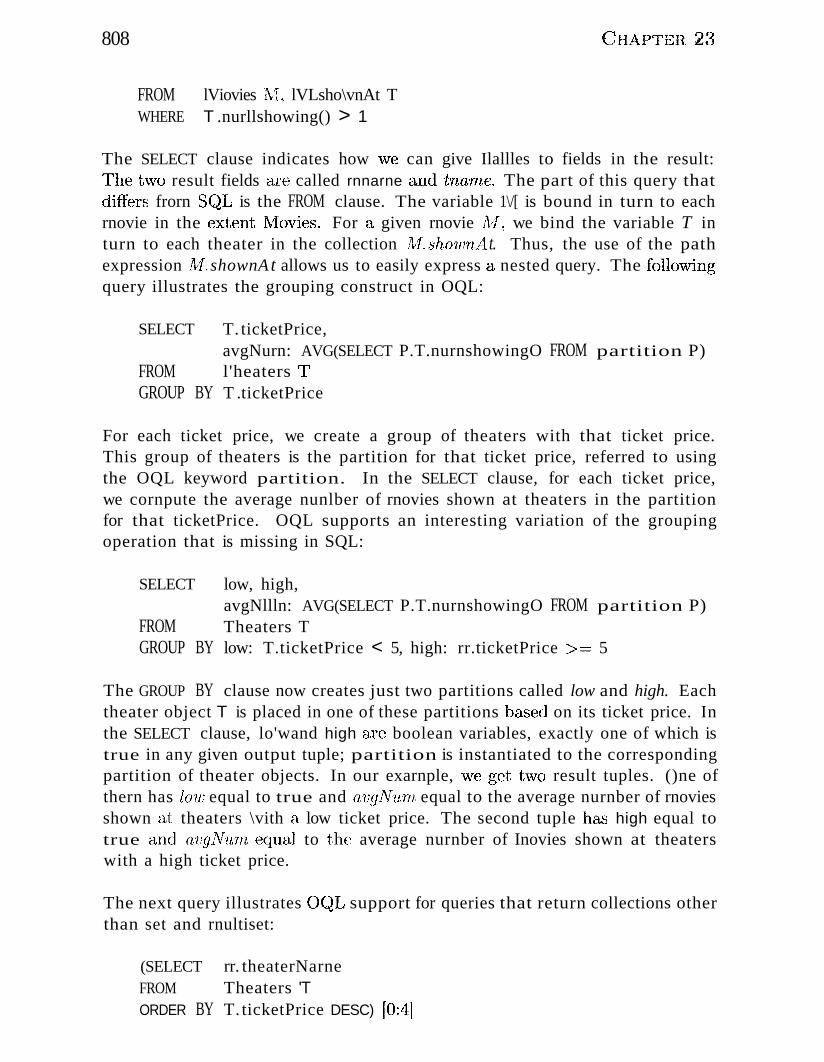
808
FROMWHERE
lViovies lV1, lVLsho\vnAt TT .nurllshowing() > 1
(~IIAPTER ~:3
The SELECT clause indicates how \ve can give Ilallles to fields in the result:The t\VO result fields are called rnnarne and tnarr~e. The part of this query thatdiffers frorn S(~L is the FROM clause. The variable 1\/[ is bound in turn to eachrnovie in the extent l\lovies. For a given rnovie Ai, we bind the variable T inturn to each theater in the collection lv1. shownA t. Thus, the use of the pathexpression lvi. shownAt allows us to easily express a nested query. The follo'Vvingquery illustrates the grouping construct in OQL:
SELECT
FROMGROUP BY
T. ticketPrice,avgNurn: AVG(SELECT P.T.nurnshowingO FROM partition P)l'heaters l'T .ticketPrice
For each ticket price, we create a group of theaters with that ticket price.This group of theaters is the partition for that ticket price, referred to usingthe OQL keyword partition. In the SELECT clause, for each ticket price,we cornpute the average nunlber of rnovies shown at theaters in the partitionfor that ticketPrice. OQL supports an interesting variation of the groupingoperation that is missing in SQL:
SELECT
FROMGROUP BY
low, high,avgNllln: AVG(SELECT P.T.nurnshowingO FROM partition P)Theaters Tlow: T.ticketPrice < 5, high: rr.ticketPrice >::::: 5
The GROUP BY clause now creates just two partitions called low and high. Eachtheater object T is placed in one of these partitions bEksed on its ticket price. Inthe SELECT clause, lo'wand high are boolean variables, exactly one of which istrue in any given output tuple; partition is instantiated to the correspondingpartition of theater objects. In our exarnple, 'Vve get t\VO result tuples. ()ne ofthern has lOll) equal to true and avgNuTn equal to the average nurnber of rnoviesshown at theaters \vith a low ticket price. The second tuple hEks high equal totrue a"nd avgNuTn equal to the average nurnber of Inovies shown at theaterswith a high ticket price.
The next query illustrates ()(~L support for queries that return collections otherthan set and rnultiset:
(SELECT rr. theaterNarneFROM Theaters 'TORDER BY T. ticketPrice DESC) [0:4]
()bject-.lJatabasc SYS'tCTflS 8U9
The ORDER BY clause nU1,kes the result a list of theater naInes ordered by ticketprice. l'"1he clcrnents of a list can be referred to by position, starting \vithposition O. Therefore, the expression [0:4] extracts a list containing the naInesof the five theaters \vith the highest ticket prices.
OC~L also supports DISTINCT, HAVING, explicit nesting of subqueries, vie'\.\T definitions, and other SQL features.
23.10 COMPARING RDBMS, OODBMS, AND ORDBMS
Now that we have covered the lnain object-oriented DBMS extensions, it istirne to consider the two lnain variants of object-datab&'Ses, OODBlVlSs andORDBJVISs, and cornpare thern with RDBMSs. Although we presented the concepts underlying object-databases, we still need to define the tenns OODBMSand OR,DBMS.
An ORDBMS is a relational DBl\1S with the extensions discussed in thischapter. (Not all ORDBMS systerlls support all the extensions in the general forrn that we have discussed theIn, but our concern in this section is theparadigrll itself rather than specific systenls.) An OODBMS is a progranlrning language with a type systern tha..t supports the ft~atures discussed in thischapter and allows any data object to be persistent; that is, to survive acrossdifferent prograrn ex(~cutions.Many current systerns conform to neither definition entirely but are lIluch closer to one or the other and can be classifiedaccordingly.
23.10.1 RDBMS versus ORDBMS
COlllparing anllDBlvlS with an OI{DBMS is straightforward. An R,DBl\1S doesnot support the extensions discussed in this chapter. rrhe resulting sirnplicityof the data rnodel rnakes it easier to optirnize queries for eHicient execution~
for exanlple. A relational systern is also easier to use because there are fe-weI'features to Illa,ster. ()n the other hand, it is less versatile than an ()HJ)BiviS.
23.10.2 OODBMS versus ORDBMS: Similarities
OODB1VlSs and ()HI)BJVISs both support user-defined ADTs, structured types,ol)ject identity and reference types, and inheritance. Both support a cpler,)llanguage for rnanipulating collection types. ()RDBlVlSs support an extendedfonn of S(~L, and 001)131\118s support C)I}L/O(~L. The sirnilarities are by norneans accidental ()llDBl\1Ss consciously try to add ()()DBlVfS features to anRI)B1\118 , and ()()DB~'1Ss in turn have developed query languages based on
810 CHAPTER 2~3
relational query languages. Both OODBIvISs and OR,DBIvlSs provide DBNISfunctionality such as concurrency control and recoverv.
ii, to,- ~$
23.10.3 OODBMS versus ORDBMS: Differences
The fundaulental difference is really a philosophy that is carried all the waythrough: OODBMSs try to add DBIvlS functionality to a progranllning language, wherca'3 ORDBIvlSs try to add richer data types to a relational DBlVIS.Although the two kinds of object-databases are converging in terrns of functionality, this difference in their underlying philosophy (and for most systeIns,their irnplementation approach) has iInportant consequences in terIllS of theissues emphasized in the design of these DBJVISs and the efficiency with whichvarious features are supported, as the following comparison indicates:
II OODBMSs airn to achieve seamless integration with a programrning language such as C++, Java, or Smalltalk. Such integration is not an important goal for an ORDBMS. SQL:1999, like SQL-92, allows us to embedSQL commands in a host language, but the interface is very evident to theSQL programer. (SQL:1999 also provides extended prograrnming languageconstructs of its own, as we saw in Chapter 6.)
II An OODBMS is aimed at applications where an object-centric viewpointis appropriate; that is, typical user sessions consist of retrieving a fewobjects and working on theHl for long periods, with related objects (e.g.,objects referenced by the original objects) fetched occasionally. Objectsrnay be extrelnely large and rnay have to be fetched in pieces; therefore,attention Inust be paid to buffering parts of objects. It is expected thatrnost applications can cache the objects they require in rnemory, once theobjects are retrieved froIn disk. rrherefore, considerable attention is paid tornaking references to ill-lnernory objects efficient. Tl'ansactions are likely tobe of very long duration and holding locks until the end of a transaction Inaylead to poor perfonnance; therefore, alternatives to Two-Phase LockingHUlst be used.
An OR,DBlVfS is optirnized for c1pplications in which large data collectionsare the focus, even though objects rnay have rich structure and be fairlylarge. It is expected that applications will retrieve data frorn disk extensively and optirnizing disk access is still the rnain concern for efficientexecution. Tl'a,nsactions are assurned to be relatively short and traditionalR.DB1VIS techniques are typically used for concurrency control and recovery.
iii T'he query facilities of ()(lL are not supported efficiently in rnost O()DBlVfSs,\vhereas the query facilities are the centerpiece of an ()HI)Bl\1S. To scnneextent, this situation is the result of different concentrations of effort inthe cleveloprnent of these systerns. '1'0 a sigrlificant (~xtenti it is also a
Object-Database SY8terns 81).
consequence of the systerlls' being optirnized. for very different kinds ofapplications.
23.11 REVIEW QUESTIONS
Ansvvers to the review questions can be found in the listed sections.
.. Consider the extended Dinky exarnple frorn Section 23.1. Explain howit lllotivates the need for each of the following object-database features:'User-defined struct'Ured types, abstract data types (AD Ts), inheritance, andobject identity. (Section 23.1)
.. What are structured data types? What are collection types, in particular?Discuss the extent to which these concepts are supported in SQL:1999.What irnportant type constructors are lllissing? What are the limitationson the ROWand ARRAY constructors? (Section 23.2)
.. What kinds of operations should be provided for each of the structureddata types? To what extent is such support included in SQL:1999? (Section 23.3)
.. What is an abstract data type? How are nlethods of an abstract data typedefined in an external programnling language? (Section 23.4)
.. Explain inheritance and how new types (called subtypes) extend existingtypes (called supertypes). What are rnethod overloading and late b'inding?What is a collect'ion hieruTchy? Contrast this with inheritance in prograrnIning languages. (Section 23.5)
I!II I-Iow is an object identifier (aid) different froln a record id in a relationalDElVIS? How is it different froIn a URI./? \iVhat is a reference type? Define deep and shallow equalit,y and illustrate thern through an exarnple.(Section 23.6)
II 'The rnultitude of data types in an (}H.DBlVIS allcnvs us to design a rnore natural and efficient databa"se schcrna but introduces S(Hne nev.,r design choices.I)iscuss OHJ)BJ\.{S database design issues and illustrate your discussion using an exalnple application. (Section 23.7)
11III Irnplernenting an ()11I)B1rfS brings new challenges. The systcrll rnust storelarge ADTs and structured types that rnight be very large. Efficient andextensible index rnechanisrns lIlUSt be provided. Exarnples of nc\v functionality include 'u,8cr-def£ned aggregation ./1lnct'ions (we can define nc\vaggrega,tion, functions for our AI)Ts) and rnethod security (the systcrIlhas to prevent user-defined rnethods fronl cornprornising the security ofthe ,DB~'IS). ExarIlples of nc\v techniques to increase perfonnance include
812 Cl:IAPTER ~3
1nethod cachi'llg and pointeT 871J'izzling. 'The optirnizer must know aboutthe l1e\v functionality and use it appropriately. Illustrate each of thesechallenges through an exarnple. (Section 23.8)
II Cornp<u'e OODBIvISs Vvith ()R,DB~1Ss. In particular, cornpare OQL andSQL:1999 and discuss the underlying data rnode!. (Sections 23.9 and23.10)
EXERCISES
Exercise 23.1 Briefly answer the following questions:
1. What are the new kinds of data types supported in object-database systcrIls? Give anexarnple of each and discuss how the exanlple situation would be handled if only anRDBl'v1S were available.
2. What rIlust a user do to define a new ADT?
3. Allowing users to define rIlethods can lead to efficiency gains. Give an exarnple.
4. \\That is late binding of nlCthods? Give an exarnple of inheritance that illustrates theneed for dynamic binding.
5. What are collection hierarchies? Give an exalIlple that illustrates how collection hierar-chies facilitate querying.
6. Discuss how a DBNIS exploits encapsulation in ilnplernenting support for ADTs.
7. Give an exarnple illustrating the nesting and unnesting operations.
8. Describe two objects that are deep equal but not shallow equal or explain why this isnot possible.
9. Describe two objects that are shallow equal but not deep equal or explain why this isnot possible.
10. COlnpare RDBNISs with ORDBlVISs. Describe an application scenario for which youwould choose anRDB11S and explain why. Silnilarly, describe an application scenariofor which you would choose an ORDBl\t1S and explain why.
Exercise 23.2 Consider the Dinky schclna shown in Figure 23.1 and all related lncthoclsdefined in the chapter. \\Trite the following queries in SQI... :1999:
1. How luany filrns were shm,vn at theater tno = 5 between January 1 and February 1 of2002'1
2. \Vhat is the lowest budget for a filnl with at leaBt t\vo stars?
:3. Consider theaters (It which a fihu directed by Steven Spielberg started showing on January 1, 2002. For each such theater, print the narnes of all countries within a 100-ruileradius. (You can use the o'ucrlap and nulius rnethods illustrated in Figure 2:3.2.)
Exercise 23.3 In a cornpany database, you need to store inforrnation about clnployees, departrnents, and children of erIlployees. For each ernployec, identified by ssn, you rnust recordyears (the number of years that the ernployee h(;1." worked for the cornpany), phone, and photoinforrnation. There are two subclasses of ernployees: contract and regular. Salary is coruputed by invoking a rnethod that takes year8 as a pararneter; this rnethod ha.s a different

()b:ject- Database SY8te'tns 813~
irnplernentation for each subclass. Further, for each regular enlployee, you Il1USt record theIHune and age of every child. l'he rnost conunon queries involving children are sirnilar to"Find the average a.ge of 1301/5 children" and:'Print the narnes of all of Bob's children."
A photo is a large inmge object and call be stored in one of several irnage fonnats (e.g.,gif, jpeg). You want to define a display rnethod for iUlage objects; display IIlust be defineddifferently for each irnage fonnat. 'For each departlllcnt, identified by dno, you rnust recorddnmne, budget, and WOTkET8 infonnation. Hf(wkc'T'8 is the set of crllployees who work in agiven departrnent. Typical querie.s involving workers include, "Find the average salary of allworkers (across all departrnents)."
1. Using extended SQL, design an ORDBIVIS scherna for the cornpany databa"se. Show alltype definitions, including rnethod definitions.
2. If you have to store this infonnation in an RDBl\'1S, what is the best possible design?
3. Cornpare the ORDBrvIS and RDBIVIS designs.
4. If you are told that a COlllInon request is to display the irnages of all employees in a givendepartruent, how would you use this inforulation for physical database design?
5. If you are told that an ernployee's ilnage rnust be displayed whenever any informationabout the employee is retrieved, would this affect your scherna design?
6. If you are told that a COU1Inon query is to find all erTlployees who look sirnilar to a givenimage and given code that lets you create an index over all irnages to support retrievalof sinlilar iuulges, what would you do to utilize this code in an OR.DBMS?
Exercise 23.4 ORDBMSs need to support efficient access over collection hierarchies. Consider the collection hierarchy of Theaters and Theater-cafes presented in the Dinky exanlple.In your role as a DBMS illlplernentor (not a DBA), you rnust evaluate three storage alternatives for these tuples:
II All tuples for all kinds of theaters are stored together all disk in an arbitrary order.
II All tuples for all kinds of theaters are stored together on disk, with the tuples that arefrOIIl TheateLcafes stored directly after the last of the non-cafe tuples.
III T'uples froIll Theater_cafes are stored separately froIll the rest of the (non-cafe) theatertuples.
1. F'or each storage option, describe a rnechanisrn for distinguishing plain theater tuplesfrorn Theater_cafe tuples.
2. For each storage option, describe hmv to handle the insertion of a new non-cafe tuple.
~i. \\Thich storage option is 1110St efficient for queries over all theaters? Over just r1'heateLcafes? In terrns of the nurnber of 1/Os, how rnuch rnore efficient is the best techniquefor each type of query cornpared to the other two techniques?
Exercise 23.5 Different ORDBl\!ISs use different techniques for building indexes to evaluatequeries over collection hierarchies. For our Dink:y' exarnple, to index theaters by name thereare two COIIlIIlon options:
III Build one 13+ tree index over Theaters.narne and another 13+ tree index over '1'he··ater_caJes. narne.
II Build one B+ tree index over the union of I'heaters. Twrne and Theater __cafes. nayne.
814 CHAPTER 243
1. Describe how to effic.iently evaluate the following query using each indexing option (thisquery is over aU kinds of theater tuples):
SELECT * FROM Theaters T WHERE T.narne= 'tvlajestic'
Give an estiInate of the nurnber of l/Os required in the two different scenarios, assurningthere are 1 rnillion standard theaters and 1000 theater-cafes. \V"hich option is Inoreefficient?
2. Perforrn the saIlIe analysis over the following query:
SELECT * FROM Theater-cafes 'I' WHERE T.nalne = '1vIajestic'
3. For clustered indexes, does the choice of indexing technique interact with the choice ofstorage options? For unclustered indexes?
Exercise 23.6 Consider the following query:
SELECT thurnbnail(Lirnage)FROM lInages I
Given that the 1. image colurnn 111ay contain duplicate values, describe how to use hashing toavoid conlputing the thum,bnail function rnore than once per distinct value in processing thisquery.
Exercise 23.7 You are given a two-dimensional, n x n array of objects. Assume that youcan fit 100 objects on a disk page. Describe a way to layout (chunk) the array onto pages sothat retrievals of square m x m subregions of the array are efficient. (Different queries requestsubregions of different sizes, i.e., different m values, and your arrangement of the array ontopages should provide good perforrnance, on average, for all such queries.)
Exercise 23.8 An ORDBJ\;IS optiruizer is given a single-table query with n expensive selection conditions, (Tn ( ... ((71 (T))). For each condition (7i, the optirnizer can estinlate the cost C\
of evaluating the condition on a tuple and the reduction factor of the condition Ti. Assurnethat there are t tuples in T.
1. How many tuples appear in the output of this query?
2. Assurning that the query is evaluated a,s shown (without reordering selections), whatis the total cost of the query? Be sure to include the cost of scanning the table andapplying the selections.
:3. In Section 2~3.8.2, it was asserted that the optiruizer should reorder selections so thatthey are applied to the table ill order of increasing rank, where ranki = (Ti ~... 1)/Ci.
Prove that this assertion is optirual. 'TIHlt is, 8ho\'/ that no other ordering could result ina query of lower cost. (Hint: It may be ea...-.,iest to consider the speciaJ ca.se where n = 2first and generalize from there.)
Exercise 23.9 ORDBIVlSs support references as a data type. It is often clailnecl that usingreferences instead of ke)lforeign key relationships will give rnuch higher perfonnance for joins.'T'his Cllwstion asks you to explore this issue.
III Consider the follmving SQL: 1999 DDL \vhich only uses straight relational constructs:
CREATE TABLE R(rkey integer, r'data text);CREATE TABLE S(skey integer, rfkey integer);
()~ject-DatabasE Syste'rns
Assurne that we have the following straightforward join query:
SELECT S.skey, H..relataFRO?-1 S, RWHERE S.rfkey = R.rkey
II Now consider the following SQL:1999 ORDBIvIS schelna:
CREATE TYPE r_t AS ROW(1'key integer, rdata text);CREATE TABLE R OF r _t REF is SYSTEM GENERATED;CREATE TABLE S (skey integer, r REF (r_t) SCOPE R);
Assurne we have the following query:
SELECT S.skey, S.r.rkeyFROM S
81~
What algorithrll would you suggest to evaluate the pointer join in the ORDBMS scherna?How do you think it will perform versus a relational join on the previous scherna?
Exercise 23.1.0 Ivlany object-relational systerns support set-valued attributes using somevariant of the setof constructor. For eXaInple, assurning we have a type person_t, we couldhave created the table Filrns in the Dinky Schema in Figure 23.1 as follows:
CREATE TABLE Films(filrnno integer, title text, star's setof Person);
1. Describe two ways of irnpleIIlenting set-valued attributes. One way requires variablelength records, even if the set elements are all fixed-length.
2. Discuss the irnpact of the two strategies on optimizing queries with set-valued attributes.
3. Suppose you would like to create an index on the column stars in order to look up filrnsby the narne of the star that has starred in the filIIl. For both irnplenlentation strategies,discuss alternative index structures that could help speed up this query.
4. What types of statistics should the query optirnizer rnaintain for set-valued attributes?How do we obtain these statistics'?
BIBLIOGRAPHIC NOTES
A nurnber of the object-oriented features described here are based in part on fairly old idea")in the prograrnrning langui:tges cornrnunity. [42] provides a good overview of these ideas ina database context. Stonebraker's book [719J describes the vision of OHDB:NISs ernbodiedby his company's early product, Illustra (now a product of Inforrnix). Current connnercialDBJ\lSs ,vith object-relational support include Infonnix Universc.l! Server, U3I"v'l D13/2 CS V2,and UniSQL. An new version of Oracle is scheduled to include OHJ)BrvlS features a,,'3 well.
IvL:rny of the idc..ls in current object-relational systerlls carne out of i:l, few prototypes built inthe 19808, especially POS'I'(jRES [72:3], Starburst (::351], and 02 [218].
The iclea of an object-oriented dataJ)c1".se wa.s first articulated in [197], \vhich described theGernStone prototype system. Other prototypes includeDASDBS [G57], EXODlTS [1:30], nus[27:,3], Ol:>jectStore [4G:3], ODE, [18] ORION [4::'32), SHOH.,E [1291, and 'rl-IOH [482]. 02 isactually an early exarnple of a, systenl that ,vas beginning to rnerge the thcrnes of ORDBrvISs
816 (;HAPTER ·~3
and OODBivISs ~it could fit in this list as well. [41] lists a collectioll of features that aTe
generally considered to belong in an 00DB1\18. Current cornrnercially available OODBIVISsinclude GelllStone, Itasca, 02, Objectivity, ObjectStore, Ontos, Poet, and Versant. [4:31Jcornpares OODBIvISs and RDBivISs.
Database support for ADTs was first explored in the INGRES and POSTGRES projectsat U.C. Berkeley. rrhe basic ideas are described in [716]' including Inechanisllls for queryprocessing and optilnization with ADTs as well as extensible indexing. Support for ADTs\vas also investigated in the Dannstadt database systern, [480]. Using the POSTGRES indexextensibility correctly required intiInate knowledge of DBTvIS-internal transaction ruechanisllls.Generalized search trees were proposed to solve this problern; they are described in (376], withconcurrency and ARIES-based recovery details presented in [L147]. [672] proposes that userslnust be allowed to define operators over ADT objects and properties of these operators thatcan be utilized for query optiInization, rather than just a collection of lnethods.
Array chunking is described in (653]. Techniques for luethod caching and optimizing querieswith expensive lnethods are presented in [37:3, 165]. Client-side data caching in a client-server00D131\I1S is studied in [283]. Clustering of objects on disk is studied in [741]. Work onnested relations was an early precursor of recent research on complex objects in OOD13rvlSsand ORD13IvISs. One of the first nested relation proposals is (504]. rvlVDs play an inlportantrole in reasoning about reduncancy in nested relations; see, for exalnple, [579]. Storagestructures for nested relations were studied in (215].
Fonnal rnodels and query languages for object-oriented databases have been widely studied;papers include [4, 56, 75, 125, 391, 392, 428, 578, 724]. [427] proposes SQL extensions forquerying object-oriented databases. An early and elegant extension of SQL with path expressions and inheritance was developed in GElY! [791]. There has been ITluch interest in cornbiningdeductive and object-oriented features. Papers in this area include (44, 288, ,195, 556, 706, 793].See [3] for a thorough textbook discussion of fonnal aspects of object-orientation and querylanguages.
[4~i2~, 4~)5, 721, 796] include papers on D13l'vISs that \vould now be tenned object-relationala"ndjor object-oriented. [794] contains a detailed overview of scherna and database evolutionin object-oriented database systenls. A thorough presentation of SQL: 1999 can be found in[525), and advanced features, including the object extensions, are covered in [523]. A shortsurvey of new SQL:1999 features can be found in [2:37]. The incorporation of several SQL:1999features into I131v1 D132 is described in [128J. OQL is described in [141]. It is based to a largeextent on the 02 query language, which is described, together with other a..'3pects of 02, inthe collection of papers [55].
24DEDUCTIVE DATABASES
.. What is the nlotivation for extending SQL with recursive queries?
.. What important properties must recursive programs satisfy to bepractical?
.. What are least lnodels and least fixpoints and how do they provide atheoretical foundation for recursive queries?
.. What cOlnplications are introduced by negation and aggregate operations? How are they addressed?
.. What are the challenges in efficient evaluation of recursive queries?
.. Key concepts: Datalog, deductive databases, recursion, rules, infeI'ences, safety, range-restriction; least model, declarative semantics; least fixpoint, operational semantics, fixpoint operator; negation,stratified program.s; aggregate operators, rnultiset generation, grouping; efficient evaluation, avoiding repeated inferences, Seminaive fixpoint evaluation; pushing query selections, lVlagic Sets rewriting
For 'Is' and 'Is-Not' though with Rule and Line,And 'lJp-and-l)own' by Logic I define,Of all that one should care to fathorn, IvVa.s never deep in anything but-------\Vine.
.. -Rubaiyat of ()rnar !(hayyarn, Translated by Edward Fitzgerald
llelational database rnanagernent systenls have been enonnously successful forC),chninistrative da,ta processing. In recent years, ho-wever, as people have tried to
817
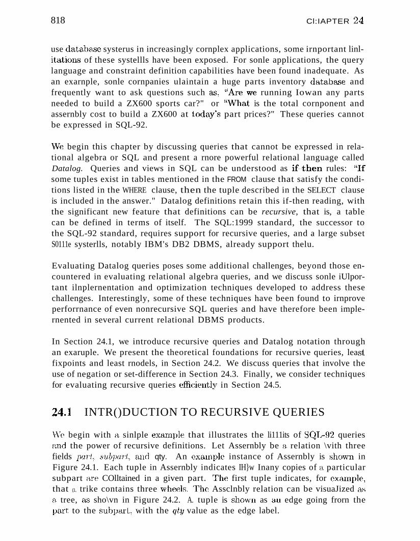
818 Cl:IAPTER 24
use database systerus in increasingly cornplex applications, some irnportant linlitations of these systellls have been exposed. For sonle applications, the querylanguage and constraint definition capabilities have been found inadequate. Asan exarnple, sonle cornpanies ulaintain a huge parts inventory database andfrequently want to ask questions such as, "Are 'we running Iowan any partsneeded to build a ZX600 sports car?" or "What is the total cornponent andassernbly cost to build a ZX600 at today's part prices?" These queries cannotbe expressed in SQL-92.
vVe begin this chapter by discussing queries that cannot be expressed in relational algebra or SQL and present a rnore powerful relational language calledDatalog. Queries and views in SQL can be understood as if~then rules: "Ifsome tuples exist in tables mentioned in the FROM clause that satisfy the conditions listed in the WHERE clause, then the tuple described in the SELECT clauseis included in the answer." Datalog definitions retain this if-then reading, withthe significant new feature that definitions can be recursive, that is, a tablecan be defined in terms of itself. The SQL:1999 standard, the successor tothe SQL-92 standard, requires support for recursive queries, and a large subsetS0111e systerlls, notably IBM's DB2 DBMS, already support thelu.
Evaluating Datalog queries poses some additional challenges, beyond those encountered in evaluating relational algebra queries, and we discuss sonle iUlportant ilnplernentation and optimization techniques developed to address thesechallenges. Interestingly, some of these techniques have been found to irnproveperforrnance of even nonrecursive SQL queries and have therefore been implernented in several current relational DBMS products.
In Section 24.1, we introduce recursive queries and Datalog notation throughan exaruple. We present the theoretical foundations for recursive queries, lea..'Stfixpoints and least rnodels, in Section 24.2. We discuss queries that involve theuse of negation or set-difference in Section 24.3. Finally, we consider techniquesfor evaluating recursive queries efficientl~y in Section 24.5.
24.1 INTR()DUCTION TO RECURSIVE QUERIES
\i\re begin with a sinlple exaJnple that illustrates the li111its of S(~L-92 queriescUld the power of recursive definitions. Let Assernbly be a relation \vith threefields part, 8 'ubpart, and qty. An excunple instance of Assernbly is shc)\vn inFigure 24.1. Each tuple in Assernbly indicates IH}w Inany copies of a particularsubpart are COlltained in a given part. The first tuple indicates, for exarnple,that (1, trike contains three "wheels. '}'he Assclnbly relation can be visuaJized a,sa tree, as sho\vn in Figure 24.2. A. tuple is shovvn as an edge going frorn thepart to the subpaJ"t, with the qty value as the edge label.
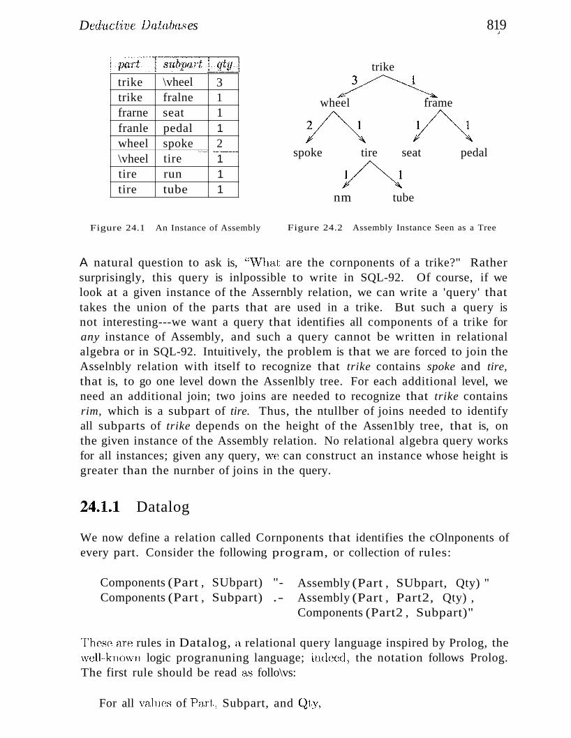
Ded'Uct'iveDatabases 819J;
pedaltire seat
~tubenm
trike
~#- •wheel frame
A Aspoke
trike \vheel 3trike fralne 1frarne seat 1franle pedal 1wheel spoke 2
._..__. .__.._--\vheel tire 1tire run 1tire tube 1
Figure 24.1 An Instance of Assembly Figure 24.2 Assembly Instance Seen as a Tree
A natural question to ask is, "What are the cornponents of a trike?" Rathersurprisingly, this query is inlpossible to write in SQL-92. Of course, if welook at a given instance of the Assernbly relation, we can write a 'query' thattakes the union of the parts that are used in a trike. But such a query isnot interesting---we want a query that identifies all components of a trike forany instance of Assembly, and such a query cannot be written in relationalalgebra or in SQL-92. Intuitively, the problem is that we are forced to join theAsselnbly relation with itself to recognize that trike contains spoke and tire,that is, to go one level down the Assenlbly tree. For each additional level, weneed an additional join; two joins are needed to recognize that trike containsrim, which is a subpart of tire. Thus, the ntullber of joins needed to identifyall subparts of trike depends on the height of the Assen1bly tree, that is, onthe given instance of the Assembly relation. No relational algebra query worksfor all instances; given any query, we can construct an instance whose height isgreater than the nurnber of joins in the query.
24.1.1 Datalog
We now define a relation called Cornponents that identifies the cOlnponents ofevery part. Consider the following program, or collection of rules:
Components (Part , SUbpart) "Components (Part , Subpart) .-
Assembly (Part , SUbpart, Qty) "Assembly (Part , Part2, Qty) ,Components (Part2 , Subpart)"
These axe rules in Datalog, a relational query language inspired by Prolog, the\vell-known logic progranuning language; indeed, the notation follows Prolog.The first rule should be read as follo\vs:
For all values of Part, Subpart, and (~ty,
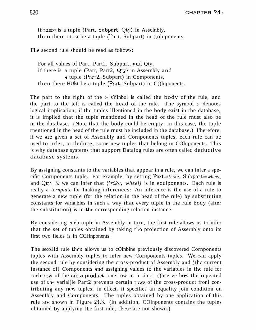
820 CHAPTER 24 $
if there is a tuple (Part, Subpart, (~ty) in Assclnbly,then there IJlUSt be a tuple (Part, Subpart) in (;olnponents.
rThe second rule should be read as follovols:
For all values of Part, Part2, Subpart, a.nd Qty,if there is a tuple (Part, Part2, Qty) in Assernbly and
a tuple (Part2, Subpart) in Components,then there HUlst be a, tuple (Part, Subpart) in C()lnponents.
The part to the right of the :- sYlnbol is called the body of the rule, andthe part to the left is called the head of the rule. The syrnbol :- denoteslogical irnplication; if the tuples lIlentioned in the body exist in the database,it is irnplied that the tuple rnentioned in the head of the rule rnust also bein the database. (Note that the body could be ernpty; in this case, the tuplernentioned in the head of the rule rnust be included in the database.) 1'herefore,if we are given a set of Assenlbly and Cornponents tuples, each rule can beused to infer, or deduce, sorne new tuples that belong in COlnponents. Thisis why database systerns that support Datalog rules are often called deductivedatabase systems.
By assigning constants to the variables that appear in a rule, we can infer a specific Coruponents tuple. For example, by setting Part:::::: trike, Subpart::::::wheel,and Qty=S, we can infer that (tTike, wheel) is in eoulponents. Each rule isreally a ternplate for Inaking inferences: An inference is the use of a rule togenerate a new tuple (for the relation in the head of the rule) by substitutingconstants for varia,bles in such a way that every tuple in the rule body (afterthe substitution) is in the corresponding relation instance.
By considering each tuple in Asselnbly in turn, the first rule allows us to inferthat the set of tuples obtained by taking the projection of Assernbly onto itsfirst two fields is in CCHnponents.
The seco11d rule then allo\vs us to cOlnbine previously discovered Cornponentstuples with Assernbly tuples to infer new Cornponents tuples. \Ve can applythe second rule by considering the cross-product of Assernbly and (the currentinstance of) Cornponents and assigning values to the variables in the rule foreach rO¥l of the cl'oss-product, one row at a titne. ()bserve ho\v the repeateduse of the varial)le Part2 prevents certain ro\vs of the cross-product fronl contributing any ne\v tuples; in effect, it specifies an equality join condition onAssenIbly and Cornpouents. The tuples obtained by one application of thisrule are shown in Figure 24.:t (In addition, COlnponents contains the tuplesobtained l)y applying the first rule; these are not shown.)
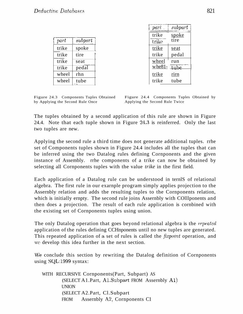
Derluct~iveDatabase8
trike spokef----
trike tire ;_.__.
trike seat..__......_.._-
trike pedalwheel rhnwheel tube
'''_"n
Figure 24.3 Components Tuples Obtainedby Applying the Second Rule Once
821
trike spoke·~·t"l~n{e···-·-· tire
trike seattrike pedalwheel runwhe81- '''Tllb-e---ltrike rirntrike tube
Figure 24.4 Components Tuples Obtained byApplying the Second Rule Twice
The tuples obtained by a second application of this rule are shown in Figure24.4. Note that each tuple shown in Figure 24.~~ is reinferred. Only the lasttwo tuples are new.
Applying the second rule a third time does not generate additional tuples. rrheset of Components tuples shown in Figure 24.4 includes all the tuples that canbe inferred using the two Datalog rules defining Cornponents and the giveninstance of Assembly. rrhe components of a trike can now be obtained byselecting all Cornponents tuples with the value trike in the first field.
Each application of a Datalog rule can be understood in ternlS of relationalalgebra. The first rule in our exarnple program simply applies projection to theAssernbly relation and adds the resulting tuples to the Cornponents relation,which is initially ernpty. The second rule joins Assernbly with COlllponents andthen does a projection. The result of each rule application is cornbined withthe existing set of Cornponents tuples using union.
The only Datalog operation that goes beyond relational algebra is the repeatedapplication of the rules defining CCHnponents until no new tuples are generated.This repeated application of a set of rules is called the jiJ.:point operation, and\ve develop this idea further in the next section.
vVe conclude this section by rewriting the Datalog definition of Cornponentsusing S(~L:1999 syntax:
WITH RECURSIVE Cornponents(Part, Subpart) AS(SELECT A1.Part, AJ.Subpart FROM Assernbly .,A.I)UNION(SELECT A2.Part, Cl.SubpartFROM Assernbly A2; Cornponents C1
822 C~HAPTER 24
WHERE A2.Subpart = Cl.PaTt)
SELECT * FROM COlllponents C2
The WITH clause introduces a relation that is part of a query definition; thisrelation is shnilar to a view, but the scope of a relation introduced using WITHis local to the query definition. The RECURSIVE key\vord signals that the table(in our exarnple, Cornponents) is recursively defined. The structure of thedefinition closely parallels the Datalog rules. Incidentally, if we wanted to findthe cornponents of a particular part, for exanlple, tTikc, we can sirnply replacethe last line ¥lith the following:
SELECT * FROM Cornponents C2WHERE C2.Part = 'trike'
24.2 THEORETICAL FOUNDATIONS
We classify the relations in a Datalog prograln as either output relations or input relations. Output relations are defined by rules (e.g., COluponents), andinput relations have a set of tuples explicitly listed (e.g., Assembly). Giveninstances of the input relations, we Inust compute instances for the output relations. The meaning of a Datalog prograrIl is usually defined in two differentways, both of which essentially describe the relation instances for the outputrelations. Technically, a query is a selection over one of the output relations(e.g., all Components tuples C with C. paTt = tTike). However, the lueaning ofa query is clear once we understand how relation instances are associated withthe output relations in a Datalog progranl.
rrhe first approach to defining the sernantics of a Datalog progralll, called theleast '{nodel sC'lnantics, gives users a way to understand the prograrn withoutthinking about how the prograrn is to be executed. That is, the sernanties isdeclarative, like the sernantics of relational calculus, and not o]JfTo,tional likerelational algebra sClnantics. This is irnportant becC111se recursive rules lnake itdifficult to understand a· prograIll in tcrrns of an evaluation strategy.
The second approach, called the least fi~rpoint 8crnantic8, gives a conceptu<tlevaluation strategy to COlnpute the desired relation insta..nces. This serves a..'3the basis for recursive query evaluation in a I)Brv:rS. 1I10re efficient evaluationstrategies are used in an actual iInplernentation, but their correctness is sho\vI1by dernonstntting their equivalence to the lea"st fixpoint approach. rrhe fixpointsClnantics is thus operational and. plays a. role analogous to that of relationalalgebra sernalltics for nonrecursive queries.
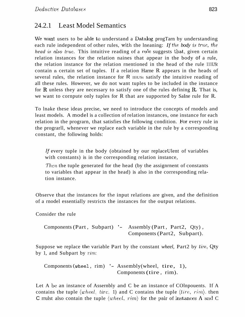
Deductive Databases
24.2.1 Least Model Semantics
823
vVe \¥ant users to be able to understand a Datalog progTarn by understandingeach rule independent of other rules, vvith the lneaning: If the body 'istT'ue, thehead is alsotT'ue. This intuitive reading of a rule suggests that, given certainrelation instances for the relation naines that appear in the body of a rule,the relation instance for the relation rnentioned in the head of the rule 111UStcontain a certain set of tuples. If a relation Harne R.. appears in the heads ofseveral rules, the relation instance for R IIlUSt satisfy the intuitive reading ofall these rules. However, we do not want tuples to be included in the instancefor R, unless they are necessary to satisfy one of the rules defining R,. That is,we want to cornpute only tuples for R that are supported by SaIne rule for R.
To lnake these ideas precise, we need to introduce the concepts of rnodels andleast models. A model is a collection of relation instances, one instance for eachrelation in the prograrn, that satisfies the following condition. For every rule inthe prograrll, whenever we replace each variable in the rule by a correspondingconstant, the following holds:
fr every tuple in the body (obtained by our replaceUlent of variableswith constants) is in the corresponding relation instance,
I 1hen the tuple generated for the head (by the assignrnent of constantsto variables that appear in the head) is also in the corresponding relation instance.
Observe that the instances for thE~ input relations are given, and the definitionof a rnodel essentially restricts the instances for the output relations.
Consider the rule
Components (Part , Subpart) '- Assembly (Part , Part2, Qty) ,Components (Part2, Subpart).
Suppose we replace the variable Part by the constant wheel, Part2 by 'tin:, (~ty
by 1, and Subpart by rirn:
Components (wheel , rim) '- Assembly(wheel, tire, 1),Components (tire , rim).
Let A be an instance of Assernbly and C be an instance of COlnpouents. If Acontains the tuple (udu~el, Lire, 1) and C contains the tuple (UTe, Tim,), thenC rrulst also contain the tuple ('wheel, rirn) for the pajr of instancc~s A. and C
824 CHAPTER 211
to be a rnodel. ()f course, the instances A and (; rnust satisfy the inclusionrequirenlent just illustrated for every assignruent of constants to the variablesin the rule: If the tuples in the rule body are in.A. and C, the tuple in the headInus1; be in C.
As an exarnple, the instances of Asscrnbly shown in Figure 24.1 and Cornponents shovvn in F'igure 24.4 together fornl a rnodel for the Conlponcnts prograll1.
C;iven the instance of Assernbly shown in Figure 24.1, there is no justificationfor including the tuple (spok~e, pedal) to the COlnponents instance. Indeed,if we add this tuple to the cornponents instance in Figure 24.4, '-'Te no longerhave a lllodel for our program, a.s the following instance of the recursive rulederllonstrates, since (wheel, pedal) is not in the Cornponents instance:
Components (wheel , pedal) :- Assembly(wheel, spoke, 2),Components(spoke, pedal).
However, by also adding the tuple (wheel, pedal) to the Cornponents instance,we obtain another rnodel of the Components prograrll. Intuitively, this is unsatisfactory since there is no justification for adding the tuple (spoke, pedal)in the first place, given the tuples in the Assembly instance and the rules inthe prograln.
We address this problern by using the concept of a least rllodel. A least modelof a prograrn is a rnodel M such that for every other model M2 of the sarneprogranl, for each relation Il in the progranl~ the instance for R in ]\II is containedin the instance of R in 1\12. The 1nodel forIned by the instances of Assernblyand COlnponents shown in Figures 24.1 and 24.4 is the least rHodel for theCC)lnponents progralll vvith the given Assernbly instance.
241&2,,2 The Fixpoint Operator
A fixpoint of a function f is a value v such that the function applied to thevalue returns the saIIle value, that is, f(v) = 'U. Consider a function appliedto a set of values that also returns a set of values. For eXH,rnple, we carl definedouble to l)e a function tllat Illuitiplies every elenlcnt of the input set by twoand d(YlJ,blc+ tobe double U idenhty. T'hus, d()'ublc( {1,2,5} ) == {2,4,lO}, anddouble+( {1,2,5} ) ::::::: {1,2,4.,5,lO}.The set of all even integers which happensto be an infinite set-is a fixpoint of the function double-+. Another fixpointof the function dO'lLble-f- is the set of all integers. l'he first fixpoint (the set ofall (~ven integers) is .';'(nailer than the second fixpoint (the set of all integers)because it is contained in the latter.
Ded'uct'lvC Database,s 825
The least fixpoint of a function is the fixpoint that is slnaller than every otherfixpoint of that function. In general, it is not glHlranteed that a function hasa loa.",t fixpoint. For exaIl1ple, there lnay be t'\¥o fixpoints, neither of \vhich is81na11er than the other. (Does double have a least fixpoint? What is it?)
No\V let us turn to functions over sets of tuples, in particular, functions definedusing relational algebra expressions. The Cornponents relation can be definedby an equation of the fonn
C!orrLponents = Jrl,5 (Assernbly [)<J2=1 Cornponents) U 7Tl,2 (Assernbly)
1'his equation has the forn1
Cornponents = f(Cornponents,Assembly)
where the function f is defined using a relational aJgebra expression. For agiven instance of the input relation Assernbly, this can be sirnplified to
C7ornponents = f(C f o1nponents)
The least fixpoint of f is an instance of Cornponents that satisfies this equation. Clearly the projection of the first two fields of the tuples in the giveninstance of the input relation Assernbly rnust be included in the (instance thatis the) least fixpoint of Cornponents. In addition, any tuple obtained by joiningComponents with Assernbly and projecting the appropriate fields IllUst also bein Components.
A little thought shows that the instance of Components that is the least fixpointof f can be ccnnputed using repeated applications of the Datalog rules sho\vnin the previous section. Indeed, applying the two Datalog rules is id(~ntical toevaluating the relational expression used in defining COlnponcnts. If an application generates Cornponents tuples that are not in the current instance of theCornponents relation, the current instance cannot be the fixpoint. Therefore,we add the new tuples to Cornponents <tnd evalu<.tte the relational expression(equivalently, the two Datalog rules) again. T'his process is repeated until every tuple generated is already in the current instance of Cornponents. \\Thenapplying the rules to i,he currerlt set of tuples does not produce any rl(~\V tuples,\ve have reached a fixpoint. If CC)lnponents is initialized to the erupty set oftuples. intuitively vve infer only tuples that (1,1'e necessary b:y the definition of afixpoint, and the fixpoint cornputed is the least fixpoint.
24.2.3 Safe Datalog Programs
(~onsider the follovving p1'ograrn:
ComplexYarts (Part) : - Assembly(Part, Subpart, Qty) , Qty > 2.
826 CHAPTER 21
According to this rule, a cOlnplex part is defined to be any part that ha" Inorethan t\VO copies of anyone subpart. :1:01' each part lnentioned in the AsselnblyrelatioIl, \ve can cac.;ily check \vhether it is a cOll1plex part. In contrast, considerthe following prograrn:
PriceYarts (Part, Price) '-Assembly (Part , Subpart, Qty) , Qty> 2.
This variation seeks to associate a price with each cornplex part. IIowever, thevariable Price does not appear in the body of the rule. This Ineans that aninfinite number of tuples must be included in any model of this progralll. Tosee this, suppose we replace the variable Part by the constant trike, SubPart bywheel, and Qty by 3. This gives us a version of the rule with the only remainingvariable being Price:
PriceYarts(trike,Price) :- Assembly (trike , wheel, 3), 3 > 2.
Now, any assignment of a constant to Price gives us a tuple to be included inthe output relation Price__.Parts. For example, replacing Price by 100 gives usthe tuple Price_Parts(trike,lOO). If the least Inodel of a progralIl is not finite,for even one instance of its input relations, then we say the program is unsafe.
Database systems disallow unsafe programs by requiring that every variablein the head of a rule also appear in the body. Such progralns are said tobe range-restricted, and every range-restricted Datalog prograln has a finiteleast model if the input relation instances are finite. In the rest of this chapter,we &'3SUllle that prograrns are range-restricted.
24.2.4 Least Model =Least Fixpoint
Does a Datalog prograln always have a least rnodel? ()r is it possible thatthere are two rnodels, neither of which is contained in the other'? Sirnilarly,does every Datalog progranl have a least fixpoint? VvThat is the relationshipbetween the least rnodel and the least fixpoint of <t Datalog prograln?
As we noted earlier, not every function has a lea"st fixpoint. Fortunately, everyfunction defined in tenns of relational algebra expressions tl1at do not containset-difference is ,guaranteed to have a least fixpoint, and the least fixpoint canbe cornputed by repeatedly evaluating the functic)ll. l'his tells us that everyl)atalog prograrn has a le~t.st fixpoint and that it can l)e cOlnputed by repeatedlyapplyi11g the rules of th(~ l)rogranl on the given instances of the input relations.
F\u·ther, every I)atcl.log progr(un is glla.r<lnteed to have a least rnodel <lud theleast rnodel is equal to the least fixpoint of the I>l'ograln. These results (whose
Deducti've Databases 827
proofs we do not discuss) provide the bclSis for Datalog query processing. 'Userscan understand a progTarn in terms of 'If the body is true, the head is also true,'thanks to the least l1lodel sClnantics. rrhe DBNIS can COlllpute the answer byrepeatedly applying the prograrn rules, thanks to the least fixpoint sernanticsand the fact that the least nlodel and the least fixpoint are identical.
24.3 RECURSIVE QUERIES WITH NEGATION
Unfortunately, once set-difference is allo\ved in the body of a rule, there r11aybe no least rnodel or least fixpoint for a program. Consider the following rules:
Big(Part):- Assembly (Part , Subpart, Qty) , Qty> 2,NOT Small (Part) .
Small (Part) :- Assembly (Part , Subpart, Qty) , NOT Big(Part).
These two rules can be thought of as an attenlpt to divide parts (those thatare mentioned in the first colulnn of the Asselubly table) into two classes, Bigand Small. The first rule defines Big to be the set of parts that use at leastthree copies of some subpart and are not classified as small parts. The secondrule defines Small as the set of parts not classified as big parts.
If we apply these rules to the instance of Assembly shown in Figure 24.1, trike isthe only part that uses at least three copies of senne subpart. Should the tuple(trike) be in Big or SUlall? If we apply the first rule and then the second rule,this tuple is in Big. To apply the first rule, we consider the tuples in Asselubly,choose those with Qty > 2 (which is just (trike)), discard those in the currentinstance of Srnal1 (both Big and Small are initially elnpty), and add the tuplesthat are left to Big. 1'herefore, an application of the first rule adds (trike) toBig. Proceeding siInilarly, \ve can see that if the second rule is applied beforethe first, (tTike) is added to Srnall instead of Big.
rrhis prognun has hvo fixpoints, neither of 'which is srnaller than the other, asshown in Figure 24.5. (rhe first fixpoint 11&\) a Big tuple that does not appear inthe second fixpoint; therefore, it is not sInaBer than the second fixpoint. 1'hesecond fixpoint ha,s a 81na11 tuple that does not appear in the first fixpoint;therefor(\ it is D.ot sr11a11e1' than the first fixpoint. The order ill \vhich \ve
apply the rul(~s detennines \vhich fixpoint is cOlnputed; this situation is veryunsatisfactory.\Ve want users to be able to understand their queries vvithoutthinking (1)out exactly" ho\v the evaJuation proceeds.
]'he root of the problerH is the use of NOT. \Vhen \ve apply the first rule, senneirlferences (1re disallc:)\~red because of the presence of tuples in 8rna11. PcLrts
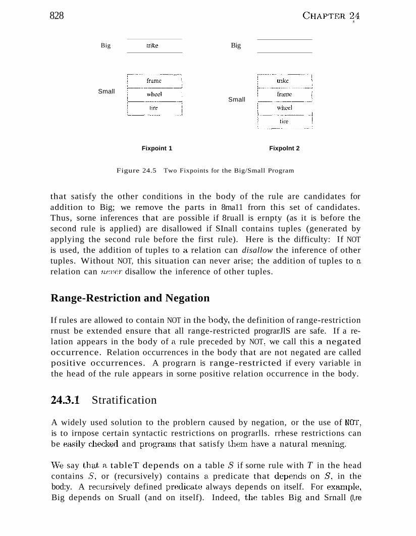
828
Big
Small
trike
Fixpoint 1
Big
Small
C;HAPTER 24"
Fixpolnt 2
Figure 24.5 Two Fixpoints for the Big/Small Program
that satisfy the other conditions in the body of the rule are candidates foraddition to Big; we remove the parts in 8rna11 frorn this set of candidates.Thus, sorne inferences that are possible if 8ruall is ernpty (as it is before thesecond rule is applied) are disallowed if SInall contains tuples (generated byapplying the second rule before the first rule). Here is the difficulty: If NOTis used, the addition of tuples to a relation can disallow the inference of othertuples. Without NOT, this situation can never arise; the addition of tuples to arelation can never disallow the inference of other tuples.
Range-Restriction and Negation
If rules are allowed to contain NOT in the bodYl the definition of range-restrictionrnust be extended ensure that all range-restricted prograrJlS are safe. If a relation appears in the body of a, rule preceded by NOT 1 we call this a negatedoccurrence. Relation occurrences in the body that are not negated are calledpositive occurrences. A prograrn is range-restricted if every variable inthe head of the rule appears in sorne positive relation occurrence in the body.
24.3.1 Stratification
A widely used solution to the problern caused by negation, or the use of NOT,is to irnpose certain syntactic restrictions on prograrlls. rrhese restrictions canbe ea~sily checkecl and progrcuns that satisfy thern have a natural lneaning.
\Ve say that a tableT depends on a table 8 if sorne rule with T in the headcontains 5", or (recursively) contains a predicate that depends on 8 ~ in thebod:y. A recursively defined predicate always depends on itself. For exarnple,Big depends on Sruall (and on itself). Indeed, the tables Big and Srnall (l,re
Dedv"ct'l'tle Databa,scs 8' ')9,_04:.1
nlutually recursive, that is, the definition of 'Big depends on SrnaU and viceversa. ,"Ve say that a table 'T depends negatively on a tal)le 8 if SCHne rule\vith 'T in the head contains NOT S, or (recursively) contains a predicate thatdepends negatively on S, in the body.
Suppose \ve classify the tables in a prograrll into strata or layers as follows.The tables that do not depend on any other tables aTe in straturll O. In ourBig/S1nall exarnple, ASSCIIlbly is the only table in stratu1Il O. Next, \ve identifytables in straturll 1; these are tables that depend only on tables in stratuln 0or straturn 1 and depend negatively only on tables in straturn O. Higher strataare sirnilarly defined: '}'he tables in straturni are those that do not belong tolOVvTer strata, depend only on tables in stratuIll i O[ lower strata, and dependnegatively only on tables in lo\;ver strata. A stratified program is one whosetables can be classified into strata according to the above algoritlull.
rrhe Big/Sruall progralIl is not stratified. Since Big and Snlall depend on eachother, they 1nust be in the sarne straturn. Ho\vever, they depend negativelyon each other, violating the requirc1Ilent that a table can depend negativelyonly on tables in lower strata. Consider the following variant of the Big/Srnallprogra1Il, in which the first rule has been rnodified:
Big2(Part) :- Assembly (Part , Subpart, Qty) , Qty> 2.Smal12(Part) :- Assembly (Part , Subpart, Qty) , NOT Big2(Part).
This prograrn is stratified. Slnall2 depends on Big2 but Big2 does not dependon 8111a1l2. Assernbly is in stratu111 0, Big is in straturn 1, and Srna1l2 is instraturn 2.
A stratified prograrn is evaluated stratu1n-by-straturn, starting with stratunlO. 'To evaluate a straturn, we cornpllte the fixpoint of all rules defining tablesin this straturn. "Fhen evaluating a straturn, any occurrence of NOT involvesa table frorH a lower straturn, \\'hich has therefore been corupletely evaluatedby no\\'. The tuples in the negated table still disallow sorne inferences, but theeffect is cornpletely deterrninistic, given the straturn-by-straturn evaJuation. Inthe c~xa.Inple, Big2 is C01uput8(1 before 81na1l2 because it is in ('t loviler straturIlthan 8rna112: (triA,~e) is added to Big2. Next, 'when we cornpute 81na112, \verecognize that (trike) is not in 8rna112 l)ecause it is already in Big2.
Incidentally, note that the stratified Big/Srnall progranl is not even recursive. If\ve repla,ce ..Assernbl.y b)l" Cornponents, \ve obtain a recursive, stratified prograrn:}\,sscrnbly is in straturn 0, Cornponents is in stratlull 1, Big2 is also in straturn1~ and 81na112 is in straturn 2.
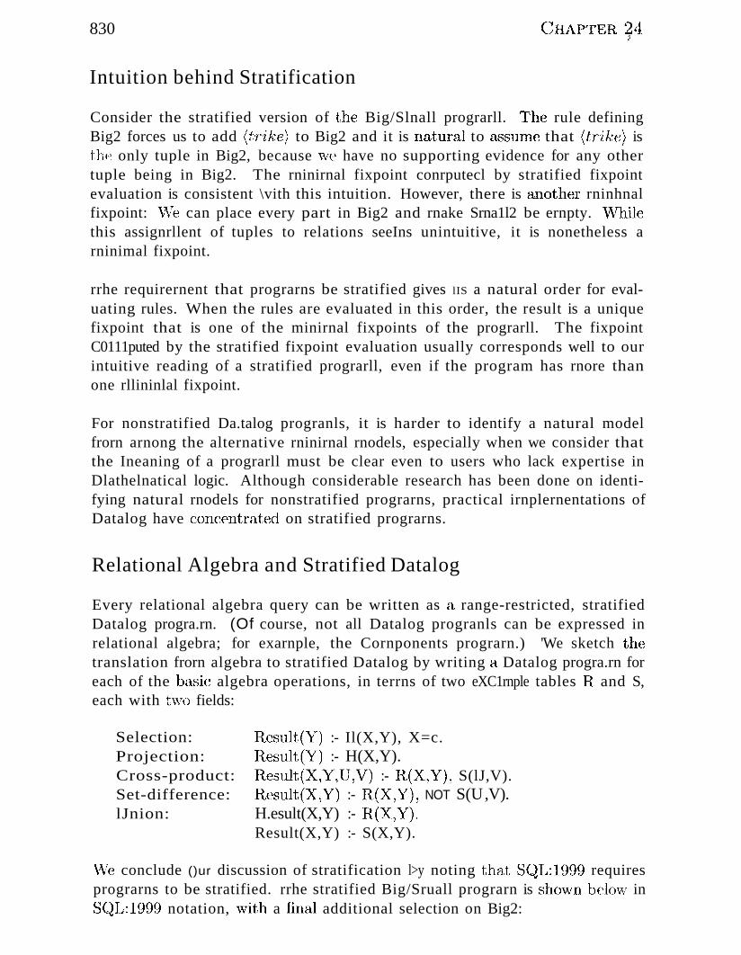
830
Intuition behind Stratification
(;IIAPTgR 24®
Consider the stratified version of the Big/Slnall prograrll. The rule definingBig2 forces us to add (l:T'ike) to Big2 and it is natural to a"C;;SUlne that (tirike) isthe only tuple in Big2, because \ve have no supporting evidence for any othertuple being in Big2. The rninirnal fixpoint conrputecl by stratified fixpointevaluation is consistent \vith this intuition. However, there is another rninhnalfixpoint: \Ve can place every part in Big2 and rnake Srna1l2 be ernpty. \\Thilethis assignrllent of tuples to relations seeIns unintuitive, it is nonetheless arninimal fixpoint.
rrhe requirernent that prograrns be stratified gives lIS a natural order for evaluating rules. When the rules are evaluated in this order, the result is a uniquefixpoint that is one of the minirnal fixpoints of the prograrll. The fixpointC0111puted by the stratified fixpoint evaluation usually corresponds well to ourintuitive reading of a stratified prograrll, even if the program has rnore thanone rllininlal fixpoint.
For nonstratified Da.talog progranls, it is harder to identify a natural modelfrorn arnong the alternative rninirnal rnodels, especially when we consider thatthe Ineaning of a prograrll must be clear even to users who lack expertise inDlathelnatical logic. Although considerable research has been done on identifying natural rnodels for nonstratified prograrns, practical irnplernentations ofDatalog have concentratt~d on stratified prograrns.
Relational Algebra and Stratified Datalog
Every relational algebra query can be written as a range-restricted, stratifiedDatalog progra.rn. (Of course, not all Datalog progranls can be expressed inrelational algebra; for exarnple, the Cornponents prograrn.) 'We sketch thetranslation frorn algebra to stratified Datalog by writing a Datalog progra.rn foreach of the b::l..sic algebra operations, in terrns of two eXC1rnple tables R, and S,each with t¥lO fields:
Selection:Projection:Cross-product:Set-difference:lJnion:
Ilesult(Y) :- Il(X,Y), X=c.Itesult(Y) :- H(X,Y).Ilesult(X:,Y,lJ,V) :- Il(X,YL S(lJ,V).11esult(X,Y) :- Il(X,yT), NOT S(U,V).H.esult(X,Y) :- R,(X,Y).Result(X,Y) :- S(X,Y).
\Ve conclude ()ur discussion of stratification l>y noting that S(~L:1999 requiresprograrns to be stratified. rrhe stratified Big/Sruall prograrn is shovvn belovl inSCJL: 1999 notation, vvith a final additional selection on Big2:
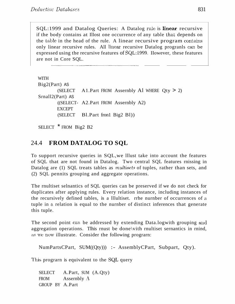
Ded'uct'ive Databases 831
SQL:1999 and Datalog Queries: A Datalog rule is linear recursiveif the body contains at Illost one occurrence of any table that depends onthe table in the head of the rule. A linear recursive program containsonly linear recursive rules. All linear recursive Datalog progranls can beexpressed using the recursive features of SC~L:1999. IIowever, these featuresare not in Core SQL.
WITHBig2(Part) AS
(SELECT A1.Part FROM Assernbly Al WHERE Qty > 2)Srnall2(Part) AS
((SELECT- A2.Part FROM Assernbly A2)EXCEPT(SELECT Bl.Part fron1 Big2 Bl))
SELECT * FROM Big2 B2
24.4 FROM DATALOG TO SQL
To support recursive queries in SQL,we lllust take into account the featuresof SQL that are not found in Datalog. Two central SQL features rnissing inDatalog are (1) SQL treats tables as Tntlltisets of tuples, rather than sets, and(2) SQL pennits grouping and aggregate operations.
The rnultiset selnantics of SQL queries can be preserved if we do not check forduplicates after applying rules. Every relation instance, including instances ofthe recursively defined tables, is a lllultiset. rrhe nurnber of occurrences of atuple in a relation is equal to the nurnber of distinct inferences that generatethis tuple.
The second point can be addressed by extending Data.logwith grouping andaggregation operations. Tlhis rnust be done\vith rnultiset sernantics in rnind,as \ve no\v illustrate. Consider the following prograrn:
NumPartsCPart, SUM((Qty))) :- AssemblyCPart, Subpart, Qty).
'fhis prograrn is equivalent to the SC~L query
SELECT A.Part, SUM (A.Qty)FROM Assernbly r'\GROUP BY A.Part
832 (JHAPTER 24
The angular brackets (... ) notation \va"s introduced in the LDL deductive systeln~ one of the pioneering deductive database prototypes developed at IVICCin the late 19808. VVe use it to dell0te TlH1ULsct geneTat'ion~ or the creation ofrnultiset-values. In principle, the rule definil1gNurnParts is evaluated by firstcreating the telnporary relation ShO\Vll in Figure 24.(3. \Ve create the ternporaryrelation by sorting on the part attribute (which appears on the left side of therule, along with the (...) terrn) and collecting the I11ultiset of qtU values foreach po,Tt value. vVe then apply the SUM aggregate to each lllultiset-value in thesecond colu111n to obtain the ans\ver ~ \vhich is sho\vn in Figure 24.7.
-.......""""""""........
trike 4f--._.,_.•
fran1e 2---
wheel 3tire 2_..
l part [SUM ( (qty) 'Itrike {3,l}
1--.
frarne {l,l}~•..__.
wheel {2,l}...._.__.
tire -'{1,l}'~_.""-',"-"-
I part I (qty) I
Figure 24.6 Temporary Relation Figure 24.7 The Tuples in NumParts
The telnporary relation shown in Figure 24.6 need not be nlC1terialized to cornpute NurnParts; for exalllplc, SUM can be applied on-the-fly or Assenlbly cansirnply be sorted and aggregated as described in Section 14.6.
The use of grouping and aggregation, like negation, causes cOlnplicatiol1s whenapplied to a partially cOlnputed relation. rrhe difficulty is overcorne by adopting the sarne solution used for n(~gation, stratification. Consider the followingprograrn: 1
TotParts(Part, Subpart, SUM«(Qty))) :- BOM(Part, Subpart, Qty).BOM(Part, Subpart, Qty) :- Assembly (Part , Subpart, Qty).BOM(Part, Subpart, Qty) :- Assembly(Part, Part2, Qty2) ,
BOM(Part2, Subpart, Qty3) , Qty=Qty2*Qty3.
The idea is to count the l111rnber of copies of Subpart for each Part. By ~1ggre
gating over B()l\II rather than Assernbly, we count subparts at any level in thehierarchy instead of just irnrnediate subparts. This prograrn is a version of avvell-known problcrl1 called Bill-of-1Vlo,terials and variants of it are probably thelnost \vide1)" used recursive queries in practice.
'rhe irnportant point to note in this exarnple is that we Inust vvait until therelation BC)]VI has been cornpletely evaluated l)(·Jore \ve apply the rrotParts~"ule. ()thervvis8, \ve obta.in incornplete counts. T1his situation is analogous totheprobler11 we faced 'with negation; we have to (~valuate the negated rel[\,tion
1The reader should write this in SQL: 1999 syntax, as a sirnple exercise.
Ded'ltctive Databases 833i\
~~:1999Cycle D~~:tion:-~~e Da;~~~~ qU;~~~-thatd~~ot l~::ith-l111etie operations have finite answers and the fixpoint evaluation is guaran- !teed to halt. Unfortunately, recursive SQL queries Ina)' have infinite answersets and query eva1ua,tion rnay not halt. l'here are tvvo independent rea,..
I sons for this: (1) the use of aritlnnetie operations to generate data valuesI that are not stored in input tables of a query, and (2) rTIultiset scrnantics1
1
"'1 for rule applications; intuitively, problems arise from cycles in the data., (To see this, consider the Cornponents prograrn on the Assenlbly instanceI shown in Figure 24.1 plus the tuple (tube, 'wheel, 1).) SQL: 1999 providesI_special constructs to check for such cycles. _~
cornpletely before applying a rule that involves the use of NOT. If a prograrn isstratified with respect to uses of (... ) as well as NOT, stratified fixpoillt evaluation gives us 111eaningful results.
There are two further aspects to this exarnple. First, we rnust understand thecardinality of each tuple in BOlVI, based on the rnultiset sernantics for ruleapplication. Second, we rnust understand the cardinality of the multiset of Qtyvalues for each (Part, Subpart) group in TotParts.
I part .._[ subpart] ···qtyl0---- .
frarue_..._.
trike 1... ._~
-·'"'trike seat 1fra.rne seat 1frame pedal 2
.~.~...
seat cover 1~-".... _........ ".'"-
Figure 24.8 Another Instance of Assembly
trike
y~,,-wheel frame
A Aspoke tire seat pedal
~nm tube
Figure 24.9 Assembly Instance Seen a,..s a Graph
\Ve illustrate these t\VO points using the instance of Assernbly shown in Figures24.8 and 24.9. f\pplying the first BONI rule, we add (one copy of) every tuple inAssernbly to BOl\J1. Applying the second BOIVI rule, \ve ctdd the follo\ving fourtuples to B()l\JI: (trike, scat, 1), (trike, pedal, 2) \ (trike, coveT, 1), and (frarne,coveT, 1). ()bserve that the tuple (trike, seat, 1) \vas (11r(~ady in BOl\/f becauseit \vas generated by ctpplying the first rule; therefore, rnultiset sernantics forrule application gives us two copies of this tuple. Applying the second BC)IVIrule on the new tuples, we generate the tuple (b'ike, cover, 1) (using the tuple(fran~e, cover, 1) for BaNI in t.he body of the rule): this is our second copy ofthe tuple. i\pplying the second rule again on this tupl(~ does not generate any
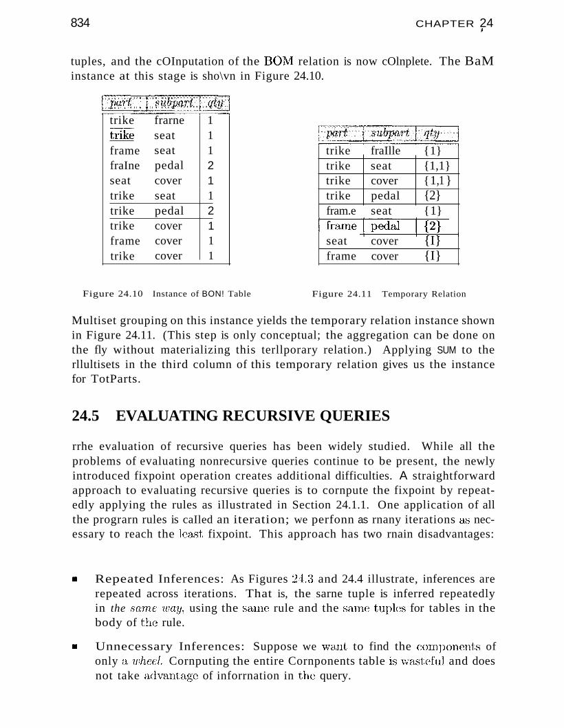
834 CHAPTER 24,
tuples, and the cOInputation of the BO:NI relation is now cOlnplete. The BaMinstance at this stage is sho\vn in Figure 24.10.
trike frarne 1trike seat 1frame seat 1fraIne pedal 2seat cover 1trike seat 1trike pedal 2trike cover 1frame cover 1trike cover 1
Figure 24.10 Instance of BON! Table
trike fraIlle {1}trike seat {1,1}trike cover {1,1}trike pedal {2}fram.e seat {1}
f---fr-aI-n-e-l--p-e-d-a-1--+-·T2T···_·-+-----+-~:;,-----l
seat cover {I}frame cover {I}
Figure 24.11 Temporary Relation
Multiset grouping on this instance yields the temporary relation instance shownin Figure 24.11. (This step is only conceptual; the aggregation can be done onthe fly without materializing this terllporary relation.) Applying SUM to therllultisets in the third column of this temporary relation gives us the instancefor TotParts.
24.5 EVALUATING RECURSIVE QUERIES
rrhe evaluation of recursive queries has been widely studied. While all theproblems of evaluating nonrecursive queries continue to be present, the newlyintroduced fixpoint operation creates additional difficulties. A straightforwardapproach to evaluating recursive queries is to cornpute the fixpoint by repeatedly applying the rules as illustrated in Section 24.1.1. One application of allthe prograrn rules is caIled an iteration; we perfonn as rnany iterations as necessary to reach the le&'3t fixpoint. This approach has two rnain disadvantages:
II Repeated Inferences: As Figures 24:.:3 and 24.4 illustrate, inferences arerepeated across iterations. That is, the sarne tuple is inferred repeatedlyin the ",arne way, using the ScHne rule and the seune tuples for tables in thebody of the rule.
11II Unnecessary Inferences: Suppose we want to find the cornponents ofonly a wheel. Cornputing the entire Cornponents table is \ve:lsteful and doesnot take advantage of inforrnation in the query.
Deductive Databases 835$
In this section, we discuss how each of these difficulties can be overcorne. \Veconsider only Datalog progralns without negation.
24.5.1 Fixpoint Evaluation without Repeated Inferences
COlnputing the fixpoint by repeatedly applying all rules is called Naive fixpoint evaluation. Naive evaluation is guaranteed to cornpute the least fixpoint, but every application of a rule repeats all inferences lllade by earlierapplications of this rule. We illustrate this point using the following rule:
Components (Part , Subpart) :- Assembly (Part , Part2, Qty) ,Components (Part2, Subpart).
When this rule is applied for the first time, after applying the first rule definingComponents, the Components table contains the projection of Assembly onthe first two fields. Using these Components tuples in the body of the rule, wegenerate the tuples shown in Figure 24.3. For example, the tuple (wheel, rim)is generated through the following inference:
Components (wheel , rim) :- Assembly(wheel, tire, 1),Components (tire, rim).
When this rule is applied a second tilne, the Components table contains thetuples shown in Figure 24.3 in addition to the tuples that it contained beforethe first application. Using the Components tuples shown in Figure 24.3 leadsto new inferences; for example,
Components(trike, rim) :- Assembly(trike, wheel, 3),Components (wheel, rim).
However, every inference carried out in the first application of this rule is alsorepeated in the second application of the rule, since all the Assernbly andCornponents tuples used in the first rule application are considered again. Forexarnple, the inference of (wheel, TiTr~) shown above is repeated in the secondapplication of this rule.
1~he solution to this repetition of inferences consists of rernelnbering whichinferences were carried out in earlier rule applications and not carrying thelnout again. vVe can 'relnclnber' previously executed inferences efficiently bysirnply keeping track of which COlnponents tuples were generated for the firsttiIne in the rnost recent applica.,tion of the recursive rule. Suppose \ve keeptrack by introducing (1, new relation called delta._Clornponcnts and storing justthe newly generated Cornponents tuples in it. Now, we can use only tlH~ tuples
(~HAPTER ~4
in deUeL G1(nnponents in the next application of the recursive rule; any inferenceusing other COIuponents tuples should have been carried out in earlier ruleEtpplications.
This refincrllcnt of fixpoint evaluation is called Seminaive fixpoint evaluation.Let us trace Serninaive fixpoint evaluation on our exarllple prognllTI. Thefirst application of the recursive rule produces the Cornponents tuples shown inFigure 24.3, just like Naive fixpoint evaluation, and these tuples are placed indelta_ C:on~ponents. In the second application, however, only delta_ C;()'{nponentstuples are considered, which rneans that only the following inferences are carriedout in the second application of the recursive rule:
Components (trike , rim) :- Assembly(trike, wheel, 3),delta_Components(wheel, rim).
Components (trike , tube) :-Assembly(trike, wheel, 3),delta_Components(wheel, tube).
Next, the bookkeeping relation delta_Cornponents is updated to contain justthese two Cornponents tuples. In the third application of the recursive rule, onlythese two delta_ Cornponents tuples are considered and therefore no additionalinferences can be nlade. The fixpoint of Cornponents has been reached.
To irnplernent Serninaive fixpoint evaluation for general Datalog prograrns, weapply all the recursive rules in a prograrll together in an iteration. Iterativeapplication of all recursive rules is repeated until no new tuples are generated inSOHle iteration. 10 surnrnarize how Serninaive fixpoint evaluation is carried out,there are two irnportant differences with respect to Naive fixpoint evaluation:
iIII WTe rnaintain a delta version of every recursive predicate to keep track of thetuples generated for this predicate in the Inost recent iteration; for excunple,delta_ Cornponents for COHlponents. rrhe delta versions are updated at theend of each iteration.
II 1'he original prograrn rules are re\vritten to ensure that every inference usesat least one delta tuple; that is, one tuple that\vas not kno\vn before theprevious iteration. This property guarantees that the inference could nothave been caxriccl out in earlier iterations.
\JVe do lI0t discuss details of Serninaive fixpoint evaluation (such fiB the a.lgoritlun for rc\vriting progranl rules to ensure the use of a delta tuple in eachinference) .
Ded'uctive Databases
24.5.2 Pushing Selections to Avoid Irrelevant Inferences
837
Consider a nonrecursive vievv definition. If \ve \vant only those tuples in theviC\\T that satisfy an additional selection condition, the selection can be aJldedto the plan as a final operation, and the relational algebra transforlnationsfor conunuting selections with other relational operators all<)\v us to 'push'the selection ahead of rnore expensive operations such as cross-products (;l,ndjoins. In effect, \ve restrict the cornputation by utilizing selections in the queryspecification. 1'he problerIl is rnore cOlnplicated for recursively defined queries.
\Ve use the following progranl as an exarnple in this section:
8ameLevel(81 , 82)
8ameLevel(81 , 82)
Assembly(P1, 81, Q1),Assembly(Pl, 82, Q2),Assembly(Pl, 81, Qi),8ameLevel(Pl, P2), Assembly(P2, 82, Q2).
Consider the tree representation of Assernbly tuples illustrated in Figure 24.2.1"here is a tuple (81,82) in SarneLevel if there is a path froln 81 to 82 thatgoes up a certain nUlnber of edges in the tree and then CaInes down the saInenurnber of edges.
Suppose we want to find all SalneLevel tuples with the fIrst fIeld equal tospoke. Since SalneLevel tuples can be used to COlupute other SarneLevel tuples,we cannot just cornpute those tuples with spoke in the first field. For exa.rnple,the tuple (1uheel, frarne) in SarneLevel allows us to infer a SarneLevel tuplewith spoke in the first field:
8ameLevel(spoke, seat) '- Assembly(wheel, spoke, 2),8ameLevel (wheel , frame),Assembly(frame, seat, i),
Intuitively, we have to conlpute all SarneLevel tllpleswhose first field conta,insa. value on the path froln .spoke to the root in Figure 24.2. Each such tuple hasthe potentia1 to contribute to (lnS\Vers for the given query. On the other hand,cornputing the entire SarneLevel table is wasteful; for exarnple, the SalneLeveltuple (l'ir'e, 8(:'0,1:) cannot be used to infer (lIly (1118\Ver to the given query (or,indeed, to infer any tuple that can in turn be used to infer an ans\ver tuple).\iVe define (1, new table, \vhich \ve call l\1agic_SaIneLevel, such that each t11plein this table identifies a value Tn for \vhich"ve have to cornpute all SarneLeveltuples with Tn in the first colulun to ansvver the given query:
Magic_SameLevel (Pi) : - Magic_.SameLevel (81), Assembly(P1, 81, Ql).Magic ...8ameLevel (spoke) '-
838 (;IIAPTER 44
Consider the tuples in lVlagic_SanleLevel. Obviously we have (spoke). lJsing this lVlagic_SalneLevel tuple and the Assernbly tuple ('LV heel , spoke, 2), wecan infer that the tuple (wheel) is in J\1agic_SarneLevel. lJsing this tuple aJldthe Assernbly tuple (tT'ike, 'wheel, a), \ve can infer that the tuple (tT'ike) is inNlagic_SarneLevel. Thus, J\tIagic_SarneLevel contains each node that is on thepath frorn spoke to the root in Figure 24.2. The Magic_SarneLcvel table can bellsed as a filter to restrict the computation:
5ameLevel(51 , 52) :- Magic_5ameLevel(51) ,Assembly(P1, 51, Q1), Assembly(P2, 52, Q2).
5ameLevel(51 , 52) :- Magic,._5ameLevel(51) , Assembly(Pl, 51, Ql),5ameLevel(Pl, P2), Assembly(P2, 52, Q2).
These rules together with the rules defining rvlagic_SarneLevel give us a progranl for cornputing all SanleLevel tuples with spoke in the first column. Noticethat the new progranl depends on the query constant spoke only in the second rule defining lVlagic_SameLevel. Therefore, the program for cornputing allSameLevel tuples with seat in the first column, for instance, is identical exceptthat the second Magic_SarneLevel rule is
Magic_5ameLevel(seat) :- .
~rhe nurnber of inferences rnade llsing the Magic program can be far fewer thanthe nurnber of inferences nlade using the original progranl, depending on justhow rnuch the selection in the query restricts the cornputation.
24.5.3 The Magic Sets Algorithm
We illustrated the intuition behind the Magic Sets algorithrn on the SarneLevelprograrn, which contains just one output relation and one recursive rule.
The intuition behind the rewriting is that the rows in the Magic tables correspond to the subqueries whose answers are relevant to the original query.By evaluating the rewritten prograrn instead of the original prograrn, \ve canrestrict cornputation by intuitively pushing the selection condition in the queryinto the recursion.
rIhe algorithrn, however, ca..Il be applied to any Datalog prograrn. T'he input tothe algorithrn consists of the prograrn and a query pattern, which is a relationwe want to query plus the fields for which a query will provide constants. Theoutput of the algorithrn is a rewritten prograrn.
The l\1a,gic Sets prognun rewriting algorithrn can be surnrnarized a..'3 follows:
]Jeductive IJatabases 8~9
1. Generate the Adorned Prograln: In this step~ the progranl is re\vrittento l1lake the pattern of queries and subqueries explicit.
2. Add Magic Filters: IVlodify each rule in the Adorned Prograrn by addinga IVlagic condition to the body that acts a'S a filter on the set of tuplesgenerated by this rule.
~~. Define the Magic Tables: We create nc\v rules to define the l\tlagictables. Intuitively, froIll each occurrence of a table R in the body of anAdorned PrograIu rule, we obtain a rule defining the table ~1.agi(>_I{.
vVhen a query is p()sed~ we add the corresponding Iv1agic tuple to the rewritten prograrl1 and evaluate the least fixpoint of the prograrIl (using Serninaiveevaluation).
We rernark that the Magic Sets algorithrll has turned out to be quite effectivefor cornputing correlated nested SQL queries, even if there is no recursion~ andis used for this purpose in rnany cornrnercial DBlVISs, even systenls that do notcurrently support recursive queries.
We now describe the three steps in the Magic Sets algorithrIl using the SarneLevelprogram as a running exalllple.
Adorned Program
We consider the query pattern 8 ameLevelbf . Thus, given a value c~ we wantto cornpute all rows in 8arneLevel in which c appears in the first eolurnn. \Vegenerate the Adorned Prograrn pad frorn the given prograrn P by repeatedlygenerating adorned versions of rules in [J for every reachable query pattern,with the given query pattern as the only reachable pattern to begin with;additional reachable patterns are identified during the course of generating theA,dorned Prograrll as described next.
Consider a rule in? whose head contains the sarne table as sorne reachablepattern. rrhe adorned version of the rule depends on the order in \vhichweconsider the predicates in the body of the rule. l'b sirnplify our discussion, ,veassurne that this is ahvays left-to-right. I~-'irst~ we replace the head of the rule,vith the rnatching query pattern. After this step, the recursive SarneLevel rulelooks like this:
8arncLeveZbf (S1, 82) : - Assembly(P1, 81, Q1),8ameLevel(P1, P2), Assembly(P2, 82, Q2).
Next, we proceed left-to-right in the l)ody of the rul(~ until 'we encounter thefirst recursive predicate. .A.11 cohullns that contain a consUl,ut or a variable that
840 (;HAPTER ~4
appears to the left are rnarked b (for bound) and the rest are rnar,ked f (for free)in the query pattern for this occurrence of the predicate. vVe add this patternto the set of reachal)le patterns and Inodify the rule accordingly:
SaTrLeLevelbf (Sl,82) :- Assembly(Pl, 81, Ql),
SarneLeveZbf (Pi, P2), Assembly CP2, 82, Q2).
If there are additional occurrences of recursive predicates in the body of therecursive rule, we continue (adding the query patterns to the reachable set andrllodifying the rule). (()f course, in linear recursive progralns, there is at illOStone occurrence of a recursive predicate in a rule body.)
\Ve repeat this until we have generated the adorned version of every rule in Pfor every reachable query pattern that contains the same table as the head ofthe rule. The result is the Adorned Program pad, which, in our example, is
SameLeveZbf C81, 82) : - AssemblyCP1, 81, Ql),AssemblyCP1, 82, Q2).
SameLeveZbf (81, 82) : - AssemblyCP1, 81, Q1),SameLeveZbf CP1, P2), Assembly CP2, 82, Q2).
In our exarnple, there is only one reachable query pattern. In general, therecan be several. 2
Adding Magic Filters
Every rule in the Adorned Prograrn is rllodified by adding a 'nlagic filter' predicate to obtain the rewritten prograrn:
Sarne-Levelbf (81, 82) : - 1\dag'ic~k9arneLeveZbf (81) ,Assembly(Pl, 81, Q1), Assembly(P2, 82, Q2).
SarneLeveZbf (S1, S2) : - J\;lag'ic...,San1eLevelbf CS1),Assembly(Pl, 81, Ql), 8arneLevelbf (P1, P2),Assembly(P2, 82, Q2).
The filter predicate is (:l, copy of the head of the rule, 'with 'IVlagic' a..s a prefixfor the table nhrne and the variables in colllrnns corresponding to free deleted,as illllstrc:ited in these two rules.
2 As an exarnple: consider a variant of the SameLevel program in which the variables PI and 1"'J2are interchanged in the body of the recursive rule (Exercise 24.5)
De(l1u:tive ]Jatabascs
Defining Magic Filter Tables
841
Consider the Adorned Prograrl1 after every rule has been rnodified a,,') described.FrorH each occurrence 0 of a recursive predicate in the body of a rule in thisrIlodified prograrl1, ,ve generate a rule that defines a .NIagic predicate. T'healgorithrl1 for generating this rule is as fo11o\:vs: (1) Delete everything to theright of occurrence () in the body of the rllodified rule. (2) i\dd the prefix'1I1agic' and delete the free colulnns of (). (~)) Move 0, "with these changes, intothe head of the rule.
FroIn th~~ recursive rule in our example, after steps (1) and (2) we get:
Sam,eLevelbf (81, 82) : - ]vIagic_SarneLevelbf (S1) ,
Assembly(P1, 81, Q1), AIag'ic_SameLevelbf (P1) .
After step (3), we get:
Magic.,_SameLevel bf (P1) : - A1ag'ic_Sam,eLevelbf (S1) ,Assembly(Pl, 81, Q1).
The query itself generates a row in the corresponding Magic table, for exarnple,l\Iagic.._SarneLevelbf (seat).
24.6 REVIEW QUESTIONS
Answers to the review questions can be found in the listed sections.
III Describe Datalog prograrIlS. lJse an exarnple Datalog prograrn to explainwhy it is not possible to write recursive rules in SQL-92. (Section 24.1)
l1li Define the terrns rnodel and least '(node!. vVhat can you say about leastrnodels for Datalog prograrns? \\Thy is this approach to defining the rneaning of a Datalog prograrll called declarative? (Section 24.2.1)
III Define the tenns .fi:rpoint and least ji:Epoint. \iVhat can you say about 1e&5tfixpoints for IJatalog prograrlls? vVhy is this approach to defining therneaning o{ a Datalog prograrIl said to be operational? (Section 24.2.2)
l1li \Vhat is a safe prograrn? \\lllY is this property irIlportant? \\That is rangerestriction and how does it ensure safety'? (Section 24.2.3)
l1li \Vhat is the connection between lccl.':lt lnodels and lea..st fixpoints for I)atalogprograrIls? (Section 24.2.4)

842 CHAPTER 24
• Explain ~why prograIIls with negation rnay not have a lea.'3t model or leastfixpoint. Extend the definition of Tange-Testriction to prograrns with negation. (Section 24.3)
• vVhat is a stratified prograIn? lIow does stratification address the problelnof identifying a desired fixpoint? Show how every relational algebra querycan be \vritten as a stratified Datalog prograrIl. (Section 24.3.1)
• Two ilnportant aspects of SQL, rnultiset table8 and aggr'egation 'with grouping, are rnissing in Datalog. Hovv can we extend Datalog to support thesefeatures? Discuss the interaction of these two new features and the needfor stratification of aggregation. (Section 24.4)
• Define the terms infeTence and iteration. What are the two main challengesin efficient evaluation of recursive Datalog programs? (Section 24.5)
• Describe Sem,inaive fixpoint evaluation and explain how it avoids repeatedinferences. (Section 24.5.1)
• Describe the Magic Sets program transformation and explain how it avoidsunnecessary inferences. (Sections 24.5.2 and 24.5.3)
EXERCISES
Exercise 24.1 Consider the Flights relation:
Flights(fino: _~~teger, from: string, to: string, distance: integer,departs: time, arrives: time)
Write the following queries in Datalog and SQL:1999 syntax:
1. Find the fino of all flights that depart from Madison.
2. Find the .flrw of all flights that leave Chicago after Flight 101 arrives in Chicago and nolater than 1 hour after.
:3. Find the fino of all flights that do not depart from NIadison.
4. Find aJI cities reachable frOlll l\iladison through a series of one or 1I10re connecting flights.
5. Find all cities reachable from IVladison through a chain of one or rnore connecting flights,with no 1I1Ore than 1 hour spent on any connection. (That is, every connecting flightmust depart < within an hour of the arrival of the previous flight in the chain.)
6. Find the shortest tilne to fly frOl11 ~IIadison to i\dadras, using a chain of one or 1noreconnecting flights.
7. Find the Jlno of all flights that do not depart [1'0111 ~!Iadison or a city that is reacha.blefrolIlrvladison through a chain of flights.
Exercise 24.2 Consider the definition of Cornponents in Section 24.1.1. Suppose that thesecond rule is replaced by
Deduct'ive Database.s
Components (Part, Subpart) : -Components (Part, Part2),Components (Part2 , Subpart).
U-:I;v
1. If the rnodified prograIn is evaluated on the ASS€lnbly relation in Figure 24.1~ how Inanyiterations does Naive fix point evaluation take and what COlllponents facts are generatedin each iteration?
2. Extend the given instance of Asselllbly so that Naive fixpoint iteration takes two rnoreiterations.
3. 'i\lrite this prograrn in SQL:1999 syntax, using the WITH clause.
4. vVrite a progranl in Datalog syntax to find the part with the Inost distinct subparts; ifseveral parts have the saIne Inaxinlllm number of subparts, your query should return allthese parts.
5. How would your answer to the previous part be changed if you also wanted to list thenumber of subparts for the part with the Inost distinct subparts?
6. Rewrite your answers to the previous two parts in SQL:1999 syntax.
7. Suppose that you want to find the part with the rnost subparts, taking into accountthe quantity of each subpart used in a part, how would you rllodify the COlnponentsprogram? (Hint: To write such a query you reason about the nuruber of inferences ofa fact. For this, you have to rely on SQL's nlaintaining as many copies of each fact asthe nurnber of inferences of that fact and take into account the properties of Seulinaiveevaluation. )
Exercise 24.3 Consider the definition of Components in Exercise 24.2. Suppose that therecursive rule is rewritten as follows for Seminaive fixpoint evaluation:
Components (Part , Subpart) :- deLta__Components(Part, Part2, Qty) ,
deLta_Components (Part2 , Subpart).
1. At the end of an iteration, what steps Illust be taken to update delta_Cornponents tocontain just the new tuples generated in this iteration? Can you suggest an index onCornponents that Inight help to lIHlke this faster?
2. Even if the delta relation is correctly updated, fixpoint evaluation using the precedingrule does not always produce all answers. Show an instance of Assembly that illustratesthe probleru.
3. Can you suggest a way to rewrite the recursive rule in tenns of delt(LC;Olnponents sothat Scrninaive fixpoint evaluation ahvays produces all answers and no inferences arerepeated across iterations?
4. Show how your version of the rewritten prograrn perfonns on the exa,rnple instaJICe ofAssernbly that you used to illustnlte the problern with the gi"ven rewriting of the recursiverule.
Exercise 24.4 Consider the definition of SarneLevel In Section 24.5.2 and the Assernblyinstance shown in Figure 24.1.
1. Re\vrite the recursive rule for Selninaivf~ fixpoint evaluation and shc)\,v ho\v Serninaiveevaluation proceeds.
2. Consider the rules defining the relation Nlagic, \vith spoke as the query constant. ForSernil1aive evaluation of the 'Nlagic' version of the SarneLevel prognllu, all tuples in Ivlagicare cornputed first. Show how 8erninaive evaluation of the I\rlagic relation proceeds.
844 CJHAPTER 24
~3. After the fvI;:lgic relation is cmnputed, it can be treated Cl"S a fixed database relation, justlike AsseInbly, in the Senlinaive fixpoint evaluation of the rules defining SarneLeveI inthe 'IVIagic' version of the prograrn. Rewrite the recursive rule for Selninaive evaluationand show how Scrninaive evaluation of these rules proceeds.
Exercise 24.5 Consider the definition of SanleLevel in Section 24.5.2 and a query in whichthe first argulnent is bound. Suppose that the recursive rule is rc\vritten as folIovls, leadingto rnultiple binding patterns in the adorned prognnn:
8ameLevel(81 , S2) :- Assembly(Pl, 81, Ql),Assembly(P1, 82, Q2).
8ameLevel(81 , S2) :- Assembly(Pl, S1, Ql),SameLevel(P2, P1), Assembly(P2, S2, Q2).
1. Show the adorned progranl.
2. Show the J\1agic program.
3. Show the Magic program after applying Seminaive rewriting.
4. Construct an example instance of Assenlbly such that the evaluating the optirnized prograrn generates less than 1% of the facts generated by evaluating the original prograrn(and finally selecting the query result).
Exercise 24.6 Again, consider the definition of SameLevel in Section 24.5.2 and a query inwhich the first argurnent is bound. Suppose that the recursive rule is rewritten as follows:
SameLevel(Sl, 82) :- Assembly(Pl, 81, Ql),Assembly(Pl, S2, Q2).
SameLevel(Sl, 82) :- Assembly(P1, S1, Ql),SameLevel(P1, Rl), SameLevel(Rl, P2), Assembly(P2, S2, Q2).
1. Show the adorned program.
2. Show the l\!Iagic prograln.
~3. Show the rv1agic prograul after applying Serninaive rewriting.
4. Construct an exarnple instance of Asselnbly such that the evaluating the optimized progranl generates less than 1% of the facts generated by evaluating the original progranl(and finally selecting the query result).
BIBLIOGRAPHIC NOTES
'1'he use of logic as a query language is discussed in several papers [296, 5~:W], "which arose outof influential workshops. (jood textbook discussions of deductive databases can be found in[747, :-3, 14:-"3, 794, '50~3]. [614] is a recent survey article that provides an overview and coversthe rnajor prototypes in the area, including LI)L [177], Glue-Nail! [214, 549] EKS-Vl [758],Aditi [615], Coral [612], LOLA [804], and XSB [644].
l'he fixpoint sernantics of logic programs (and deductive databases a..., a special case) is presented in [751], which also shows equivalenc(~ of the fixpoint seInantics to a lea.st-rnodd seIrul,ntics. The use of stratification to give a natural sernantics to prograrns with negation \va..sdeveloped independently in [:37, 154, 559,752].
Deduct'i'ue Databases 845
Efficient evaluation of deductive database queries has been widely studied, and [58J is asurvey and cOlnparison of several early techniques; [611] is a more recent survey_ Serninaivefixpoint evaluation wa.." independently proposed several tiInes; a good treatuwut appears in[54]. r1'he Ivlagic Sets technique is proposed in [57] and generalized to cover all deductivedatabase queries without negation in [77]. 'The Alexander rnethod [G~nJ was independentlydeveloped and is equivalent to a variant of l'vIagic Sets called Supplernentary Atagic Sets in [77].[553] shows how lVIagic Sets offers significant perfonnance benefits even for nonrecursive SQLqueries. [ti73] describes a version of l'vlagic Sets designed for SQL queries with correlation, andits irnplernentation in the Starbufst systern (which led to its iInplenlentation in IBNI's DB2DBNIS). [670] discusses ho\v lVlagic Sets can be incorporated into a Systenl R style cost-basedoptimization framework. The ~lagic Sets technique is extended to prograIIls with stratifiednegation in [53, 76] _ [121] cOlnpares tvlagic Sets with top-do\vn evaluation strategies derivedfroIn Prolog.
[642] develops a prograrn rewriting technique related to lVlagic Sets called lVlagic Counting.Other related methods that are not based on progranl rewriting but rather on fun- tirne controlstrategies for evaluation include [226, 429, 756, 757]. The ideas in 1.226] have been developedfurther to design an abstract rnachine for logic prograll1 evaluation using tabling in [609, 727];this is the basis for the XSB systell1 [644].
25DATA WAREHOUSING AND
DECISION SUPPORT
.. Why are traditional DBIvISs inadequate for decision support?
.. What is the multidimensional data nlOdel and what kinds of analysisdoes it facilitate?
.. What SQL:1999 features support rnultidiInensional queries?
.. How does SQL:1999 support analysis of sequences and trends?
.. How are DBMSs being optimized to deliver early answers for interactive analysis?
.. What kinds of index and file organizations do OLAP systerlls require?
.. VVhat is data warehousing and why is it irnportant for decision support?
.. Why have rnaterialized views becorne iInportant?
.. How can we efficiently Inaintain rnaterialized views?
.. Key concepts: OLAP, rnultirnensional rnodel, dinlellsions, nleasures;roll-up, drill-clown, pivoting, cross-tabulation, CUBE; WINDOW queries,[rallleS, order; top N queries, online aggregation; bitllli:tp indexes, joinindexes; data warehouses, extract, refresh, purge; rnaterialized views,incrernental rnaintenancc, rnaintaining warehouse views
Notlling is lnore difficult, and therefore rnore precious, than to be(1)1<" to decide.
. NCtI)oleon Bonaparte
846
[)ata ~;VaTeho1L8ing and Decis'io'n Support i47
Dcl.tabase luanagclncnt systerIls are widely used by organizations for rnaintaining data that docurnents their everyday operations. In applications that updatesuch operational data7 transactions typically rnake srna11 changes (for exalnple,adding a reservation or depositing a check) and a large nU111ber of transactionsH1USt be reliably and efficiently processed. Such online transaction processing (OLTP) applications have driven the gruwth of the DBlVIS industry in thepast three decades and "vill doubtless continue to be irnportant. DB1VISs havetraditionally been optirnized extensively to perforn1 vvell in such applications.
H,ecently, ho\vever, organizations have incrc&':lingly crnphasized applications inwhich current and historical data is coruprehensively analyzed and explored,identifying useful trends and creating sununaries of the data, in order to supporthigh-level decision rnaking. Such applications are referred to clS decision support. ~1ainstrearn relational DBlVlS vendors have recognized the irnportanceof this rnarket segment and are adding features to their products to support it.In particular, SQL has been extended with new constructs and novel indexingand query optirl1ization techniques are being added to support cornplex queries.
The use of views has gained rapidly in popularity because of their utility inapplications involving cornplex data analysis. While queries on views can beanswered by evaluating the view definition when the query is subrnitted, precornputing the view definition can rnake queries run Inuch faster. Carryingthe r11otivation for preconlputed views one step further, organizations can consolidate inforrnation from seven:tl databases into a data warehouse by copyingtables fror11 rnany sources into one location or rnaterializing a view defined overtables fr01n several sources. Data '\varehousing has becorne widespread, andIl1any specialized products are no\v available to create and rnanage warehousesof data frorH 1l1ultiple databases.
vVe begin this chapter with an overview of decision support in Section 25.1.\Ve introduce the rnultirnensional rnodel of data in Section 25.2 and considerdatabase design issues in 25.2.1. vVe discuss the rich cla..ss of queries that itnaturally supports in Section 25.;3. \Ve discuss how new SQL:1999 constructsallc)vl us tel express rnultidilnensional queries in 25.3.1. In Section 25.4, vvediscuss S(~L:1999 extensions that support queries over relations tLS orderedcollections .\\'"8 consider hOVl to optirnize for fa,st generation of initial ansvversin Sectioll 25.5. 1'11C rnany query language extensions required in the ()LA.Penvirolllnentprornpted the developrnent of llC\V irnplcrncntation techniques; wediscuss these in Section 25.6. In Section 25.7, \ve exarnirl(~ the issues involvedin creating and rnaintaining a data \varehouse. FraIn a technical sta,ndpoint, akey issue is how to Ilutintain \vctrehouse inforrnation (replicated tables or views)·when the llnderl.ying source infonnation changes. After covering tlH~ iUlportcl,ntrole played byvic\vs in OLAP and \vaxehousing irl Section 25.8, we considerIIuLintenance of rnaterialized vievvs in Sections 25.9 and 25.10.
848 C;lIAPTER 25
25.1 INTRODUCTION TO DECISION SUPPORT
()rganizational decisioll rnaking requires a cOlnprehensive vievv of all aspects ofan enterprise, so 111any organizations created consolidated data warehousesthat contain data drawn frcHn several databa..,;es ll1atntained by different business units together vvith historical and SUlnlna,ry inforInation.
The trend toward data warehousing is c0I11plelnented by an increa.sed ernphasison po"Vverful analysis tools. lVlany characteristics of decision support queriesmake traditional SQL systenls inadequate:
• 11 he WHERE clause often contains rnany AND and OR conditions. As we sawin Section 14.2.3, OR conditions, in particular, are poorly handled in rnanyrelational DBJV1Ss.
• Applications require extensive use of statistical functions, such as standarddeviation, that are not supported in SQL-92. Therefore, SQL queries rnustfrequently be ernbedded in a host language progrcun.
• Many queries involve conditions over time or require aggregating over timeperiods. SQL-92 provides poor support for such time-series analysis.
• Users often need to pose several related queries. Since there is no convenient way to express these cOlnnlonly occurring families of queries, usershave to write thern as a collection of independent queries, \vhich can betedious. Further, the DBlVIS has no way to recognize and exploit optimization opportunities arising froln executing nlany related queries together.
Three broad classes of analysis tools are available. First, SOIne systerIls supporta elc-1SS of stylized queries that typically involve group-by and aggregation operators and provide excellent support for cOlnplex boolean conditions, statisticalfunctions, and features for tilne-series analysis. Applications dominated bysuch queries are called online analytic processing (OLAP). 'These systernssupport a querying style in which the data is best thought of &9 a rnultidilnensional array and are influenced by end-user tools, such as spreadsheets, inaddition to database query languages.
Second, sorne DBwISs support traditional S(~L-style queries but are designedto also support OLAP queries efficiently. Such systenls can be regarded (1",,,
relational DB1'v1Ss optirnized for decision support applications. 'Nlany vendors ofrelational DBIVISs are currently enhancing their products in this direction and,over tilne, the distinction bet\veen specialized OLAP systerns and relationalDBIVISs enhEtnced to support ()LAP queries is likely to dirninish.
The third class of analysis tools is rllotivated by the desire to find interestingor unexpected trends and patterns in large data sets rather than the conlplex
Data 1-1l a:reho'U/3'ing and Decision Support ~49
___ •__• __••••••_._ ••__ • __••__• ._._.__ri·_ri •
SQL:1999 and OLAP: In this chapter, ,,'Ie discuss a nUInber of featuresintroduced in SQL:1999 to support OLAP. In order not to delay publication of the SQL: 1999 standard, these features \vere actually added to thestandard through an amendment called SQL/OLAP.
query characteristics just listed. In exploratory data analysis, although ananalyst can recognize an :interesting pattern' "vhen shown such a pattern, it isvery difficult to fannulate a query that captures the essence of an interestingpattern. For exalnple, an analyst looking at credit-card usage histories Illaywant to detect unusual activity indicating Inisuse of a lost or stolen card. Acatalog lllerchant lnay want to look at custolner records to identify pro111isingcustoiners for a new proillotion; this identification would depend on inccnIlelevel, buying patterns, delllonstrated interest areas, and so all. The alllountof data in Inany applications is too large to perrnit rnanual analysis or eventraditional statistical analysis, and the goal of data mining is to supportexploratory analysis over very large data sets. We discuss data rnining furtherin Chapter 26.
Clearly, evaluating OLAP or data rnining queries over globally distributed datais likely to be excruciatingly slow. Further, for such cOlnplex analysis, oftenstatistical in nature, it is not essential that the IllOSt current version of the databe used. The natural solution is to create a centralized repository of all thedata; that is, a data warehouse. Thus, the availability of a warehouse facilitatesthe application of ()LAP and data rnining tools and, conversely, the desire toapply such analysis tools is a strong 1Ilotivation for building a data warehouse.
25.2 OLAP: MULTIDIMENSIONAL DATA MODEL
aLAI' applications are dOlninated by ad hoc, cOlnplex queries. In SQL terllls,these are queries that involve group-by and aggregation operators. l'he natural\vay to think about typical ()LAP queries, ho\vever, is in tenns of a rnultidilnensinnal data rllodel. In this section, \ve present the rnultidirnensional data Illodeland corupare it with a relational representation of data. In subsequent sections, we describe ()LAP queries in. terrns of the rllultidirnensional data rnodeland consider .. scnne ne,v irnplernentation techniques designed to support suchqueries.
In the rnultidirnensional data rnodel, the focus is on a collection of nurnericmeasures. Each Inea..sure depends on a set of dirnensions. vVe use a runningexarnple based on sales data.. The rncc'tsure attribute in our exarnple is sales.The dirnensions are Product, Location, and Tirne. (jiven a product, a location;
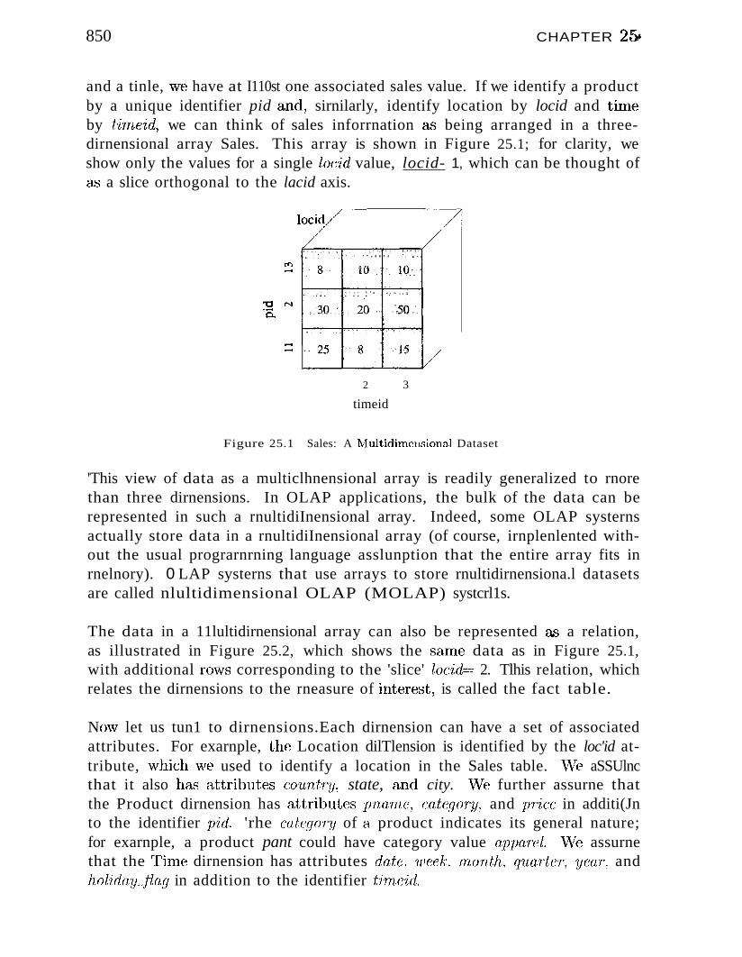
850 CHAPTER 25&
and a tinle, 'ATe have at I110st one associated sales value. If we identify a productby a unique identifier pid and, sirnilarly, identify location by locid and tiIneby tirrLeid, we can think of sales inforrnation Ct.') being arranged in a threedirnensional array Sales. This array is shown in Figure 25.1; for clarity, weshow only the values for a single loeid value, locid- 1, which can be thought ofas a slice orthogonal to the lacid axis.
rr.......
"0 N.....0..
............
locid/'/~-"'-/
2
timeid
3
Figure 25.1 Sales: A rvlulticlimensional Dataset
'This view of data as a multiclhnensional array is readily generalized to rnorethan three dirnensions. In OLAP applications, the bulk of the data can berepresented in such a rnultidiInensional array. Indeed, some OLAP systernsactually store data in a rnultidiInensional array (of course, irnplenlented without the usual prograrnrning language asslunption that the entire array fits inrnelnory). 0 LAP systerns that use arrays to store rnultidirnensiona.l datasetsare called nlultidimensional OLAP (MOLAP) systcrl1s.
The data in a 11lultidirnensional array can also be represented c1As a relation,as illustrated in Figure 25.2, which shows the SeHne data as in Figure 25.1,with additional rovvs corresponding to the 'slice' locid==- 2. Tlhis relation, whichrelates the dirnensions to the rneasure of inten~st, is called the fact table.
NO\~l let us tun1 to dirnensions.Each dirnension can have a set of associatedattributes. For exarnple, the Location dilTlension is identified by the loc'id attribute, \vhich \ve used to identify a location in the Sales table. "'Fe aSSUlncthat it also has ~),ttributes cau'ntry, state, and city. \Ve further assurne thatthe Product dirnension has ctttributes pnanu:, category, and pTice in additi(Jnto the identifier pid. 'rhe catcgoTy of a product indicates its general nature;for exarnple, a product pant could have category value appaTcl. \Ve assurnethat the rI'inlc dirnension has attributes date, 71JCek, Tnonth, quar-fcT, ycaT, andholiday.)lag in addition to the identifier tirneid.
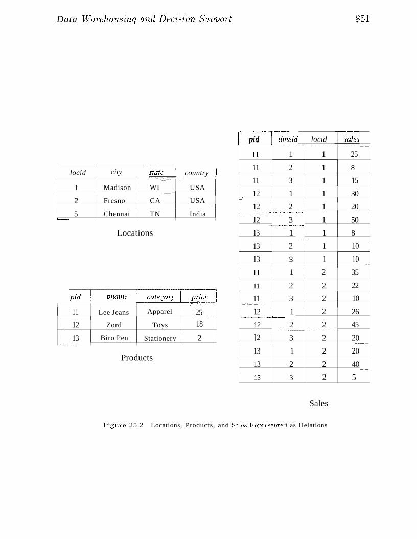
Data Warcho11sing and Dec-is'ion 8'lLppOTt 251
locid [\'ales-_.... ""........."'......,m""_. ... --
II 1 1 25
11 2 1 8
11 3 1 15
12 1 1 30_.12 2 1 20
r--------"... ,,~·.'"""" ....nfflfn,'V<+..._ ...................• ....
12 3 1 50.................""'.........".~".«"...."'.-.,
13 1 1 8-.-f-.
13 2 1 10
13 3 1 10--
II 1 2 35
11 2 2 22
11 3 2 10.__.,_._---
12 1 2 26.......,..........,.........._....._._..__.f-----
12 2 2 45. _._.._...................... ------_.._._-
]2 3 2 20..._----.......
13 1 2 20
13 2 2 40--
13 3 2 5
[-------·-I--=~~~:-·
pid L.!..!!!!eid
sta~ country I
Products
Locations
citylocid
- .. - --=..- - .
11 Lee Jeans Apparel 25.._._...
12 Zord Toys 18~,~--
13 Biro Pen Stationery 2.."""'''"'.........''"'.........,..~
.• ..............- ..._-_......... ... -
1 Madison WI USA._-
2 Fresno CA USA--
5 Chennai TN India'-----
Sales
Figure 25.2 Locations, Products, and Sales H.eprf~sent:ed as Helations
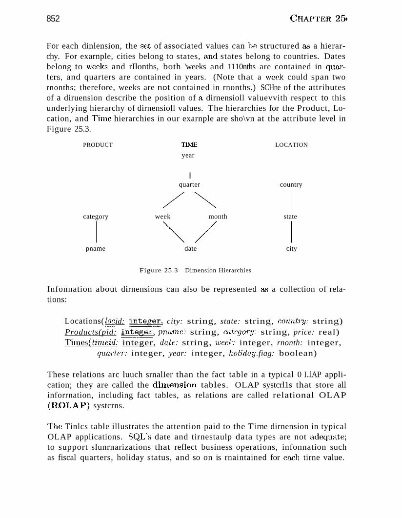
852 ('1. . . 2r:::jHAPTER aft
For each dinlension, the set of associated values can be structured a" a hierarchy. For exarnple, cities belong to states, and states belong to countries. Datesbelong to weeks and rIlonths, both 'weeks and 1110nths are contained in quaTtel's, and quarters are contained in years. (Note that a vveek could span twornonths; therefore, weeks are not contained in rnonths.) SCHne of the attributesof a diruension describe the position of a dirnensioll valuevvith respect to thisunderlying hierarchy of dirnensioll values. The hierarchies for the Product, Location, and ~rirne hierarchies in our exarnple are sho\vn at the attribute level inFigure 25.3.
PRODUCT
category
pname
TIl\tIE
year
Iquarter
week month
~/date
Figure 25.3 Dimension Hierarchies
LOCATION
country
state
city
Infonnation about dirnensions can also be represented &s a collection of relations:
Locations( lo~..id: intege:!:> city: string, state: string, country: string)Products(pid: int.~..~er, pnam,e: string, category: string, price: real)Tirnes(t'irnei~: integer, date: string, week: integer, rnonth: integer,
quarter: integer, year: integer, holiday~.. fiag: boolean)
These relations arc luuch srnalIer than the fact table in a typical 0 I..lAP application; they are called the diInension tables. OLAP systcrl1s that store allinforrnation, including fact tables, as relations are called relational OLAP(ROI.JAP) systcrns.
1'he Tinlcs table illustrates the attention paid to the T'irne dirnension in typicalOLAP applications. SC~L's date and tirnestaulp data types are not adequctte;to support slunrnarizations that reflect business operations, infonnation suchas fiscal quarters, holiday status, and so on is rnaintained for ea,ch tirne value.
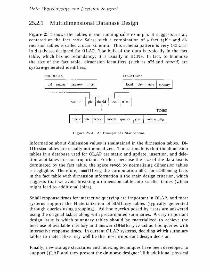
Data WarehOtlSing and DecL5'ion ~(hL1JPOTt
25.2.1 Multidimensional Database Design
Figure 25.4 shows the tables in our running sales exarnple. It suggests a star,centered at the fact table Sales; such a cornbination of a fact table and dirncnsion tables is called a star schema. This schelna pattern is very COIIUIlonin databc"kses designed for 0 LAP. IThe bulk of the data is typically in the facttable, which ha..'3 no redundancy; it is usually in BCNF. In fact, to Ininimizethe size of the fact table, dirnension identifiers (such as p'id and t'irneid) aresystcrn-generated identifiers.
PRODUCTS LOCATIONS
SALES
Figure 25.4 An Example of a Star Schema
holiday_flag
Inforrnation about dinlension values is rnaintained in the dirnension tables. Di111ension tables are usually not nonnalized. The rationale is that the dimensiontables in a database used for OL,AP are static and update, insertion, and deletion anoillalies are not irnportant. Further, because the size of the database isdorninated by the fact table, the space saVE-xi by norrnalizing dilnension tablesis negligible. Therefore, rnini111izing the cornputation tilllC for cOlllbining factsin the fact table with dirnension inforrnation is the rnain design criterion, whichsuggests that we avoid breaking a dirnension table into srnaller tables (whichrnight lead to additional joins).
Snlall response tirnes for interactive querying are irnportant in OLAP, and rnostsysterns support the Hlaterialization of SUrl1Inary tables (typically generatedthrough queries using grouping). Ad hoc queri(~s posed by users are answeredusing the original ta,bles along with precornputed surnrnaries. A very irnportantdesign issue is which sunnnary tables should be rnaterialized to achieve thebest use of available rnerllory and answer cOHnI1only a.sked ad hoc queries withinteractive response tirnes. In current OLAP systerns, deciding "vhich surnnlarytables to rnaterialize rnay \vell be the Inost irnportant design decision.
Finally, new storage structures and indexing techniques have been developed tosupport ()LAP and they present the database designer \'lith additional physical
854 CHAPTER 2[)f
design choices. \Vc cover BOIHe of these hnplclnentatiol1 techniques in Section')!:"" t'.... d.t>.
25.3 MULTIDIMENSIONAL AGGREGATION QUERIES
Now that \ve have seen the rnulticliInensiol1alluoclel of data, let us consider howsuch data can be queried and rnanipulatecl. The operations supported by thisInodel are strongly influenced by end user tools such as spreadsheets. The goalis to give end users v.rho are not SQL experts an intuitive and po\verful interfacefor cornnlon business-oriented analysis tasks. Users are expected to pose ad hocqueries directly, without relying on database application prograrrnners.
In this section, we asslllne that the user is working with a multidirnensionaldataset and that each operation returns either a different presentation or asunllnary; the underlying dataset is always available for the user to 1nanipulate,regardless of the level of detail at which it is currently viewed. In Section 25.3.1,we discuss how SQL:1999 provides constructs to express the kinds of queriespresented in this section over tabular, relational data.
A very C01111non operation is aggregating a rneasure over one or 1nore dimensions. The following queries are typical:
.. Find the total sales.
II Find total sales for each city.
II Find total sales for each state.
'These queries can be expressed as S(~L queries over the fact and dirnensiontables. When we aggregate a rnea.'3ure OIl one or rnore di1nensions, the aggregated 1118'1.SUre depends on fewer diInensioIls than the original Ineasure. Forexanlple, when we cornpute the total sales by city, the aggregated rneasure istotal sales and it depends only on the Location di1nension,whereas the originalsales rneasure depended on the Locatioll,Tirne, a,nd Product dirnensions.
Another use of aggregation is to SU1Ilrnarize at different levels of a dirnensionhierarchy. If \ve are given total sales per city, we can aggregate 011 the Locationdinlension to obtain sales per state. This operation is called roll-up in theOLAI' literature. 1 1he inverse of roll-up is drill-down: Given total sales bystate, \ve can Etsk for a 1Ilore detailed presentation by drilling down on Location.\\"T k f' I I· . t I I ·t £ I tIt t (·tl I( .' ..:1 'f '-', - ,- 1 1"" .' " '"'j ," ~'i .,~ . - r "J ".'''' -". ,.,~ ~, i' ::}"1 . .,. '.,. 0. '. ..,. I{ ",~ .".1 .)'" - :~. -", I." " :.\ ,.,...., " :.\-~C Cdn <1S01 t;d. LS J) (,1tJ 01 .J US, SeL CS J) C1 Y 01 d, t;C CC iCC S ,<:1,c WI, 1 set cspresented on a per-state basis for the rernaining states, riS before). We canalso drill dowll on a diluension other than Location. For exarnple, \ve can ask
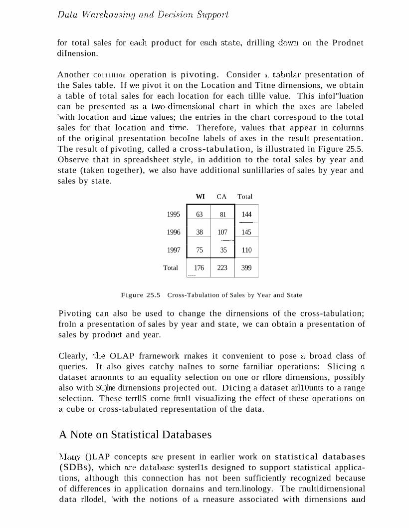
jJata WaTeho1.M3'ing and Decision SUppO'Tt
for total sales for each product for each state, drilling do\vn OIl the ProdnetdiInension.
Another C0111ll10n operation is pivoting. Consider a, tabulax presentation ofthe Sales table. If Vle pivot it on the Location and Titne dirnensions, we obtaina table of total sales for each location for each tillle value. This infoI"luationcan be presented <:1..'; a tvvo-dirnensional chart in which the axes are labeled'with location and titne values; the entries in the chart correspond to the totalsales for that location and tirnt~. Therefore, values that appear in colurnnsof the original presentation becoIne labels of axes in the result presentation.The result of pivoting, called a cross-tabulation, is illustrated in Figure 25.5.Observe that in spreadsheet style, in addition to the total sales by year andstate (taken together), we also have additional sunlillaries of sales by year andsales by state.
WI CA Total
1995
1996
1997
Total
63 81 144~,-,._-
38 107 145.~.~.~_ ..._.
75 35 110
176 223 399----
Figure 25.5 Cross-Tabulation of Sales by Year and State
Pivoting can also be used to change the dirnensions of the cross-tabulation;froIn a presentation of sales by year and state, we can obtain a presentation ofsales by produet and year.
Clearly, the OLAP frarnework rnakes it convenient to pose a broad class ofqueries. It also gives catchy naInes to sorne farniliar operations: Slicing adataset arnonnts to an equality selection on one or rIlore dirnensions, possiblyalso with SC)lne dirnensions projected out. Dicing a dataset arl10unts to a rangeselection. These terrllS corne frcnl1 visuaJizing the effect of these operations ona cube or cross-tabulated representation of the data.
A Note on Statistical Databases
lVlany ()LAP concepts c],re present in earlier work on statistical databases(SDBs), which are databaBe systerl1s designed to support statistical applications, although this connection has not been sufficiently recognized becauseof differences in application dornains and tern.linology. The rnultidirnensionaldata rllodel, 'with the notions of a rneasure associated with dirnensions (lond
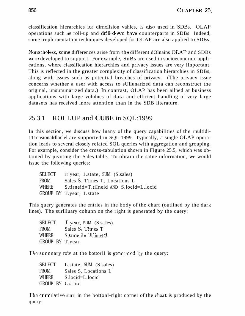
856 ('1 . 2r..:JHAPTER ··0$
classification hierarchies for dirncIlsion vahles, is also used in SDBs. OLAPoperations such as roll-up and drill-dovlJl have counterparts in SDBs. Indeed,sorne irnplcrnentation techniques developed for OLAP are also applied to SDBs.
Nonetheless~ senne differences arise frorn the different dOlnains ()L.LLlP and SDBs\vere developed to support. For exarnple, SnBs are used in socioeconornic applications, where classification hierarchies and privacy issues are very ilnportant.This is reflected in the greater cornplexity of classification hierarchies in SDBs,along with issues such as potential breaches of privacy. (The privacy issueconcerns whether a user with access to sUllunarized data can reconstruct theoriginal, unsununarized data.) In contrast, OLAP has been ailned at businessapplications with large volulnes of data and efficient handling of very largedatasets has received lnore attention than in the SDB literature.
25.3.1 ROLLUP and CUBE in SQL:1999
In this section, we discuss how lnany of the query capabilities of the rnultidi111ensionalrlloclel are supported in SQL:1999. Typically, a single OLAP operation leads to several closely related SQL queries with aggregation and grouping.For exarnple, consider the cross-tabulation shown in Figure 25.5, which was obtained by pivoting the Sales table. To obtain the saIne inforrnation, we wouldissue the following queries:
SELECTFROMWHEREGROUP BY
rr.year, 1.state, SUM (S.sales)Sales S, T'irnes T, Locations LS.tirneid=T.tiIneid AND S.locid=L.locidT.year, 1.state
This query generates the entries in the body of the chart (outlined by the darklines). The surllluary cohunn on the right is generated by the query:
SELECTFROMWHEREGROUP BY
]".year, SUM (S.saJes)Sales S1 ,]~ilncs TS · ·1 T' ·1'" .tuneu = .tunclCT.year
l'hc~ sunnnary ro\v at the bottorl1 is generated l)y the query:
SELECTFROMWHEREGROUP BY
L.state, SUM (S.sales)Sales S, Locations LS.locid=L.lociclI".state
l'he C>UI11111ative SUITl in the bottonl-right corner of the ch;:ut is produced by thequery:
857$
SELECTFROMWHERE
SUM (S.sales)Sales S ~ Locations LS.loc:id=L.locid
The exarnple cross-tabulation can be thought of as roll-up on the entire dataset(Le., treating everything as one big group), on the Location dirnension, on therrirne dirnensioIl, and on the Location and Tinle dinlensions together. Eachroll-up corresponds to a single SQL query with grouping. In general, given arneEtSUre with k a..ssociated dirnensions, we can roll up on any subset of these kdiInensions; so \ve have a total of 2k such SQL queries.
Through high-level operations such as pivoting, users can generate lTlany ofthese 2k~ SQL queries. R,ecognizing the cornrnonalities between these queriesenables r110re efficient, coordinated COlTlputation of the set of queries.
SQL: 1999 extends the GROUP BY construct to provide better support for roll-upand cross-tabulation queries. The GROUP BY clause with the CUBE keyword isequivalent to a collection of GROUP BY statenlents, with one GROUP BY statenlE~nt for each subset of the k dirnensions.
Consider the following query:
SELECTFROMWHEREGROUP BY
rr.year, L.state, SUM (S.sales)Sales S, Tirnes T, Locations LS.tirneid=T'.tirneid AND S.1ocid=L.locidCUBE (T.year, L.state)
The result of this query, shown in Figure 25.6, is just a tabular representationof the cross-tabulation in Figure 25.5.
SQL: 1999 also provides variants of GROUP BY that enable cornputatioll of subsets of the cross-tabulation cornputed using GROUP BY CUBE. For exarnple, \VC
call replace the grouping clause in the previous query \ivith
GROUP BY ROLLUP Cr.y(~ar, L.state)
In contrast to GROUP BY CUBE, Vile aggregate by an pairs of year ltnd state valuesetnel by each ~year, and. cornpute an overall SlIHl for the entire dataset (the la.strCNl in Figure 25.6), but \VC do not aggregate for 8(1,ch state value. 1'11e resultis identical to that sho\vn inF'igure 25.6, except that the rows with 'nl1,ll ill theT. ycru' COhUIlll and non-nvJl valuc~s in tlH~ L.,'itatc colurnn are not cornputed.
CUBE pid, locid, tirneid BY SUM Sales
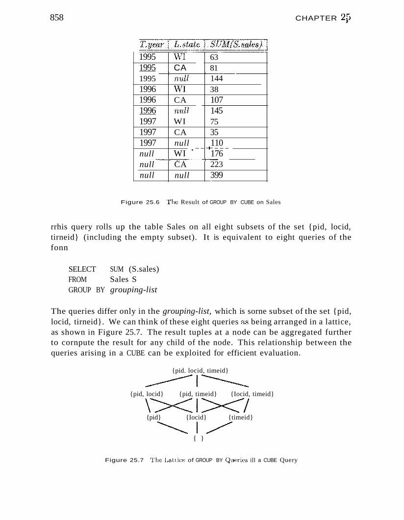
858 CHAPTER 2fJ
1995 6381144
CAnull
1995-r--------t---,
19951996 \V1 381996 CA 10719961997
1H,dlWI
14575
1997 CA 35110176223
null,--+---
WICA
null--+--~---t---
null
1997
null null 399
Figure 25.6 The Result of GROUP BY CUBE on Sales
rrhis query rolls up the table Sales on all eight subsets of the set {pid, locid,tirneid} (including the empty subset). It is equivalent to eight queries of thefonn
SELECT SUM (S.sales)FROM Sales SGROUP BY grouping-list
The queries differ only in the grouping-list, which is sorne subset of the set {pid,locid, tirneid}. We can think of these eight queries a'3 being arranged in a lattice,as shown in Figure 25.7. The result tuples at a node can be aggregated furtherto cornpute the result for any child of the node. This relationship between thequeries arising in a CUBE can be exploited for efficient evaluation.
{pid. locid, timeid}
~I~{pid, locid} {pid, timeid} {Iocid, timeid}
\><1><1{pid} {Iocid} {timeid}
~I~{ }
Figure 25.7 'l'he Lattice of GROUP BY Queries ill a CUBE Query
Data vf,!aTc}UJ1U3ing and Decision SllPP07't
25.4 WINDOW QUERIES IN SQL:1999
859
The tiIne dirnension is very important in decision support and queries involvingtrend analysis have traditionally been difficult to express in SQL. To addressthis, SQL: 1999 introduced a fundamental extension called a query window.Examples of queries that can be written using this extension, but are eitherdifficult or iInpossible to write in SQL without it, include
1. Find total sales by rnonth.
2. Find total sales by rnonth for each city.
3. Find the percentage change in the total monthly sales for each product.
4. Find the top five products ranked by total sales.
5. Find the trailing n day moving average of sales. (fbI' each day, we mustcompute the average daily sales over the preceding n days.)
6. Find the top five products ranked by cumulative sales, for every monthover the past year.
7. Rank all products by total sales over the past year, and, for each product,print the difference in total sales relative to the product ranked behind it.
The first two queries can be expressed as SQL queries using GROUP BY over thefact and dinlension tables. The next two queries can be expressed too, but arequite complicated in SQL-92. The fifth query cannot be expressed in SQL-92if n is to be a pararneter of the query. The last query cannot be expressed inSQL-92.
In this section, we discuss the features of SQL: 1999 that allow us to express allthese queries and, obviously, a rich class of sirnilar queries.
The rnain extension is the WINDOW clause, which intuitively identifies an ordered'window' of rows 'around' each tuple in a table. Tihis allows us to apply a richcollection of aggregate functions to the windovv of a row and extend the rowwith the results. F'or exarnple, we can associate the average sales over the past3 days with every Sales tuple (each of which records 1 day~s sales). This givesus a 3-day Illoving average of sales.
\Vhile there is sorne sirnilarity to the GROUP BY and CUBE clauses, there areilnportant differences as vvell. For exarnple, like the WINDOW operator, GROUPBY all()\~ls us to create partitions of rows and flT)ply aggregate functions such asSUM to the rows in a pa.,rtition. lIo\vever, unlike WINDOW, there is a single outputrow per pa.rtition, rather than one output row for each ro\v, and E~ach partitionis an unorder(~d collection of 1'O\\7's.
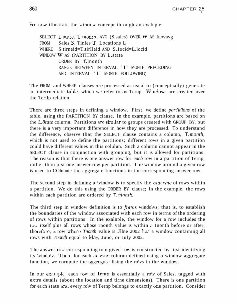
860
\Ve now illustrate the "window concept through an exalnple:
CHAPTER 25t
SELECT L.state, rr.IIlonth , AVG (S.sales) OVER "vV AS InovavgFROM Sales S, Tinles rr, Locations LWHERE S.tirneid=T.tirIleid AND S.1ocid=L.locidWINDOW VV~ AS (PARTITION BY L.state
ORDER BY 'f.lnonthRANGE BETWEEN INTERVAL '1' MONTH PRECEDINGAND INTERVAL '1' MONTH FOLLOWING)
The FROM and WHERE clauses are processed as usual to (conceptually) generatean interrnediate table, which we refer to a.'3 Ternp. vVindows are created overthe TeHIp relation.
There are three steps in defining a window. First 1 we define part'it'ions of thetable, using the PARTITION BY clause. In the exarnple, partitions are based onthe L.8tate colurnn. Partitions are sitnilar to groups created with GROUP BY, butthere is a very important difference in how they are processed. To understandthe difference, observe that the SELECT clause contains a column, T. month,which is not used to define the partitions; different rows in a given partitioncould have different values in this colulun. Such a colurnn cannot appear in theSELECT clause in conjunction with grouping, but it is allowed for partitions.'The reason is that there is one answer row for each row in a partition of Ternp,rather than just one answer row per partition. The window around a given rowis used to COlnpute the aggregate functions in the corresponding answer row.
The second step in defining a \vindow is to specify the ordeTir~g of rows withina partition. We do this using the ORDER BY clause; in the exarnple, the rowswithin each partition are ordered by T. 'Tnonth.
The third step in window definition is to !Ta'Tne windo\vs; that is, to establishthe boundaries of the window associated with each row in terrns of the orderingof rows within partitions. In the exalnple, the window for a row includes thero\v itself plus all rows whose rnonth value is within a Inonth before or after;therefore~ a row \,those Tnonth value is .Jllne 2002 has a window containing allrows with Tnonth equal to !\Ilay, June, or July 2002.
1'he answer ro\v corresponding to a given 1'0\\,' is constructed by first identifyingits \vindo\v. Then~ for each ansvver colurun defined using a window aggregatefunction, we cornpute the a,ggregate llsing the ro\vs in the V\Tindo\v.
In our exarnple~ each ro\v of l"elnp is essentially a ro\v of Sales, tagged withextra details (about the location and tirne dirnensions). There is one partitionfor ea.ch state (tnd every ro\v of Ternp belongs to exactly one partition. Consider
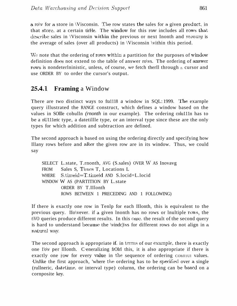
861
a ro\v for a store in \Visconsin. ~rhe row states the sales for a given product, inthat store~ at a certain tirHe. The \'lindc)\1\;' for this ro\.\! includes all ro\vs thatdescribe sales in \Visconsin vvithin the previous or next Inonth and 1novavg isthe average of sales (over all products) in \Visconsin \vithin this period.
\\To note that the ordering of ro\vs 'ivithin a partition for the purposes of windoVvTdefinition does not extend to the table of answer ro\vs. The ordering of ansvverro\vs is nondeterlninistic, unless, of course, \ve fetch therIl through (1, cursor anduse ORDER BY to order the cursor's output.
25.4.1 Framing a Window
There are two distinct ways to fra1118 a window in SQL: 1999. l'he exarnplequery illustrated the RANGE construct, which defines a window based on thevalues in SOllle cohulln (rnonth in our exarnple). The ordering colu111n has tobe a nU111eric type, a datetillle type, or an interval type since these are the onlytypes for which addition and subtraction are defined.
The second approach is based on using the ordering directly and specifying howIllany rows before and after the given row are in its window. Thus, we couldsay
SELECT L.state, T.rnonth, AVG (S.sales) OVER \V AS InovavgFROM Sales S, Tilll(~S T, Locations LWHERE S.tirneid=T'.tinlE~id AND S.locid=L.locidWINDOW W AS (PARTITION BY L.state
ORDER BY T.IIlonthROWS BETWEEN 1 PRECEDING AND 1 FOLLOWING)
If there is exactly one row in Tenlp for each IIlonth, this is equivalent to theprevious query. IIo\vever ~ if c\, given lnonth has no rows or lnultiple l"(nvs, thet\VO queries produce different results. In this case, the result of the second queryis hard to understand because the \vindc)\vs for different rows do not align in a,Ilfttllralway.
The second approach is appropriate if, in tcnns of our exarnple~ there is exactlyone 1'o\v per lllonth. C·eneralizing frOIrI this, it is also appropriate if there isexactly one i·o\v for every vahle in the sequence of ordering COhll1Ul values.·UnJike the first approach, 'where the ordering has to be specified over a single(rullneric, datetinl€-\ or interval type) colurnn, the ordering can be based on acornposite key.
862 (;HAPTER 25
\rYe can also define \vindows that include all rcnvs that are before B, given row(UNBOUNDED PRECEDING) or all r0\VS after a given row (UNBOUNDED FOLLOWING)'within the row~s partition.
25.4.2 New Aggregate Functions
\:Vhile the standard aggregate functions that apply to rnultisets of values (e.g.,SUM, AVG) can be used in conjunction \vith Willdo\ving, there is a lleed for anew class of functions that operate on a !'ist of values.
The RANK function returns the position of a row within its partition. If apartition ha..'3 15 rows, the first rovv (according to the ordering of rows in thewindow definition over this partition) ha.s rank 1 and the last row has rank 15.The rank of intermediate rows depends on whether there are multiple (or no)rows for a given value of the order.ing colurnn.
Consider our running example. If the first row in the Wisconsin partition hasthe lllonth January 2002, and the second and third rows both have the rnonthFebruary 2002, then their ranks are 1, 2, and 2, respectively. If the next rowhas rllonth March 2002 its rank is 4.
In contrast, the DENSE_.RANK function generates ranks without gaps. In ourexalnple, the four rows are given ranks 1, 2, 2, and 3. The only change is inthe fourth row, whose rank is now 3 rather than 4.
The PERCENT...RANK function gives a lneasure of the relative position of a rowwithin a partition. It is defined as (RANK-1) divided by the Innnber of rowsin the partition. CUME-DIST is sirnilar but based on actual position within theordered partition rather than rank.
25.5 FINDING ANSWERS QUICKLY
A recent trend, fueled in part by the popularity of the Internet, is an ernphasis011 queries for which a user vvants only the first fevill, or the 'best' few, ansvversquickly. \Vhcn users pose queries to a search engine such as AltaVista, theyrarely look beyond the first or second page of results. If they do not findwhat they are looking for, they refine their query and resubrnit it. '.rhe sennephen()lneuon occurs in decision support applications and scnne DBl\;1S products(e.g., DB2) already support extended SQL con.structs to specify sueh queries. Arelated trend is that, for cornplex queries, users would like to ~ee an approxirnat(~
answer quickly and then have it 1Je continually refined, rather than \vait untilthe exact ansvver is availablc~. \Ve now discuss these 1,""0 trends l)riefly.
Data WaTcho'u8'ing and Decis'io71 S'UPJ)OTt
25.5.1 Top N Queries
&63
An analyst often wants to identify the top-selling handful of products, for exalnple. \Ve can sort by sales for each product and return answers in this order.If \ve have a Inillion products and the analyst is interested only in the top 10,this straightforward evaluation strategy is clearly \vasteful. It is desirable forusers to be able to explicitly indicate how rnany answers they want, rnakingit possible for the DB1VlS to optirnize execution. l-'he follo\ving exarnple queryasks for the top 10 products ordered by sales in a given location and tiIne:
SELECT P.pid, P.pnarne, S.salesFROM Sales S, Products PWHERE S.pid=P.pid AND S.locid==l AND S.tiIneid=3ORDER BY S.sales DESCOPTIMIZE FOR 10 ROWS
The OPTIMIZE FOR N ROWS construct is not in SQL-92 (or even SQL:1999), butit is supported in IBM's DB2 product, and other products (e.g., Oracle 9i) havesirnilar constructs. In the absence of a cue such as OPTIMIZE FOR 10 ROWS, theDBMS computes sales for all products and returns thenl in descending orderby sales. The application can close the result cursor (i.e., tenninate the queryexecution) after consulning 10 rows, but considerable effort has already beenexpended in cornputing sales for all products and sorting them.
Now let us consider how a DBMS can use the OPTIMIZE FOR cue to execute thequery efficiently. The key is to sOlnehow cornpute sales only for products thatare likely to be in the top 10 by sales. Suppose that we know the distributionof sales values because we rnaintain a histogran1 on the sales cohuun of theSales relation. We can then choose a value of sales, say, c, such that only10 products have a larger sales value. For those Sales tuples that rneet thiscondition, we can apply the location and tirne conditions as well and sort theresult ..Evaluating the following query is equivalent to this approach:
SELECTFROMWHEREORDER BY
P.pid, P.pnarne, S.salesSales S, Products PS.pid=P.picl AND S.locid=1 ANDS.sales DESC
S.tirneid::::::~3 AND S.sales > c
This approach is, of course, ruuch faster than the alternative of cornputing allproduct sales and sorting thern, but there are SOIne in1portant problerns toresolve:
1. flow do 'we choose the sales cntoff value c? EIistograrns and other systelnstatistics can be used for this rn1rI)()SC, but this can be a tricky issue. For
864 C;HAPTER 25@
one thing~ the statistics rnaintained by a DBtv.IS are only approxirnate.For another, even if \ve choose the cutoff to reflect the top 10 sales valuesaccurately, other conditions in the query Inay elirninate SOHle of the selectedtuples, leaving us with fewer than 10 tuples in the result.
2. ~'Vhat 'if we have 'fnon~ than 10 t'll]Jlesin the 'result? Since the choice ofthe cutoff c is approxirnate, \'Ie could get 1nore than the desired nurnberof tuples in the result. rrhis is easily handled by returning just the top10 to the user. \Ve still save considerably with respect to the approachof cornputing sales for all products, thanks to the conservative pruning ofirrelevant sales infonnation, using the cutoff c.
3. What 'if we have fewer' than 10 tuples in the. resv,lt? Even if \ve choose thesales cutoff c conservatively, we could still cOlnpute fe\ver than 10 resulttuples. In this case, we can re-execute the query with a srnaller cutofF valueC2 or sirnply re-execute the original query \vith no cutoff.
The effectiveness of the approach depends on how well we can estirnate thecutoff and, in particular, on rninimizing the nurnber of tiules we obtain fewerthan the desired nurnber of result tuples.
25.5.2 Online Aggregation
Consider the following query, which asks for the average sales arIlount by state:
SELECTFROMWHEREGROUP BY
L.state, AVG (S.sales)Sales S, Locations LS.locid=L.locidL.state
This can be an expensive query if Sales and Locations are large relations. \Vecannot a.chieve fast response tirnes with the traditional approach of cornputingthe anwer in its entirety when the query is presented. One alternative, as wehave seen, is to use precornputation. Another alternative is to cornpute theans\ver to the query when the query is presented l)ut return an approxirnateansvver to the user as soon as possible. A.s the cornputation progresses, theans\ver quality ,is continually refined. This approach is called online aggregation. It is very attra,ctive for queries involving aggregation, beca,use efficienttechniques for cornputing and refining approxirnate ans\\rers are available.
Chllinf: aggregation is illustrated in Figure 25.8: For CeLeb statc" ""the groupingcriterion for our exarnple query . the current value for average sales is displayed,together with a confidence interval 11he entry for Alaska tells us that the
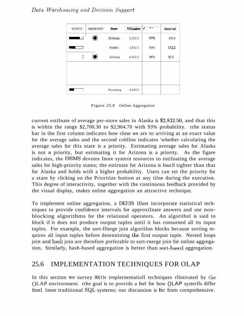
Data YlaTcho'lLs'ing and Decis'ion, 8'UPIJOTt:
STAfUS PRJORrrU£ Stare ,VGtsmtSJ r -. lnt.enal
_:::~Jf.Iii~\
\~) Alabama 5,232.5 97% 103.4
-=~==] Alaska 2,832.5 93% 132.2
J~.-~'
Arizona 6,432.5 98% 52.3\~)
Wyoming 4,243.5
Figure 25.8 Online Aggregation
current estiInate of average per-store sales in Alaska is $2,8~32.50, and that thisis within the range $2,700.30 to $2,964.70 with 93% probability. rrhe statusbar in the first column indicates how close we are to arriving at an exact valuefor the average sales and the second cohllnn indicates 'whether calculating theaverage sales for this state is a priority. Estimating average sales for Alaskais not a priority, but estimating it for Arizona is a priority. As the figureindicates, the DBlVIS devotes Inore systern resources to estiInating the averagesales for high-priority states; the estirnate for Arizona is Inucll tighter than thatfor Alaska and holds with a higher probability. Users can set the priority fora state by clicking on the Prioritize button at any tilne during the execution.This degree of interactivity, together with the continuous feedback provided bythe visual display, rnakes online aggregation an attractive technique.
To irnplernent online aggregation, a DEl\!IS lIlust incorporate statistical techniques to provide confidence intervals for approxiInate answers and use nonblocking algorithms for the relational operators. An algorithnl is said toblock if it does not produce output tuples until it has consurned all its inputtuples. For exarnple, the sort-Illerge join algoritlun blocks because sorting requires all input tuples before detennining the first output tuple. Nested loopsjoin and hash join are therefore preferable to sort-rnerge join for online aggregation. Sirnilarly, hash-based aggregation is better than sort-based aggregation.
25.6 IMPLEMENTATION TECHNIQUES FOR OLAP
In this section we survey 80r11e irnplernentatioll techniques rllotivated by the()LAP envirornnent. rrhe goal is to provide a feel for how ()LAP systerIls differfron1 1nore traditional S(~L systerns; our discussion is faT frorn cornprehensive.
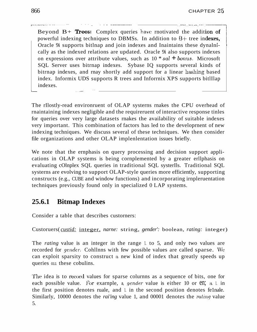
866 CHAPTER 2q
r------.-----.-- --- - - - _ _ _ __ __.._._.-_.,._-_._--•• - ••--.....- •• " •• " ....m".. '.....- ••••-.---....----:.l
Beyond B+ Tl~ees: Complex queries have rnotivated the addition ofpowerful indexing techniques to DBMSs. In addition to I3:+ tree indexes,Oracle 9i supports bitlnap and join indexes and Inaintains these dynalni- i
cally as the indexed relations are updated. Oracle 9i also supports indexeson expressions over attribute values, such as 10 * sal + bonus. MicrosoftSQL Server uses bitrnap indexes. Sybase IQ supports several kinds ofbitrnap indexes, and rnay shortly add support for a linear h&'3hing basedindex. Informix UDS supports R trees and Inforrnix XPS supports bitlIlapindexes.
l--- ~__. ..
The rIlostly-read environruent of OLAP systerns rnakes the CPU overhead ofrnaintaining indexes negligible and the requireruent of interactive response tinlesfor queries over very large datasets rnakes the availability of suitable indexesvery important. This combination of factors has led to the developrnent of newindexing techniques. We discuss several of these techniques. We then considerfile organizations and other OLAP implenlentation issues briefly.
We note that the ernphasis on query processing and decision support applications in OLAP systems is being cornplemented by a greater erllphasis onevaluating cOlnplex SQL queries in traditional SQL systerIls. Traditional SQLsysterns are evolving to support OLAP-style queries more efficiently, supportingconstructs (e.g., CUBE and window functions) and incorporating irnpleruentationtechniques previously found only in specialized 0 LAP systems.
25.6.1 Bitmap Indexes
Consider a table that describes custorners:
Custoruers( custid: integer, narne: string, gender': boolean, rating: integer)
The rating value is an integer in the range 1. to 5, and only two values arerecorded for gender. Cohllnns with few possible values are called sparse. vVecan exploit sparsity to construct a new kind of index that greatly speeds upqueries 011 these cobulins.
Th(~ idea is to r.i'ecord values for sparse colurnns as a sequence of bits, one foreach possible value. FbI' exarnple, a, gender value is either 10 or en; a 1. inthe first position denotes ruale, and 1. in the second position denotes fe1nale.Similarly, 10000 denotes the rai'ing value 1, and 00001 denotes the rating value5.
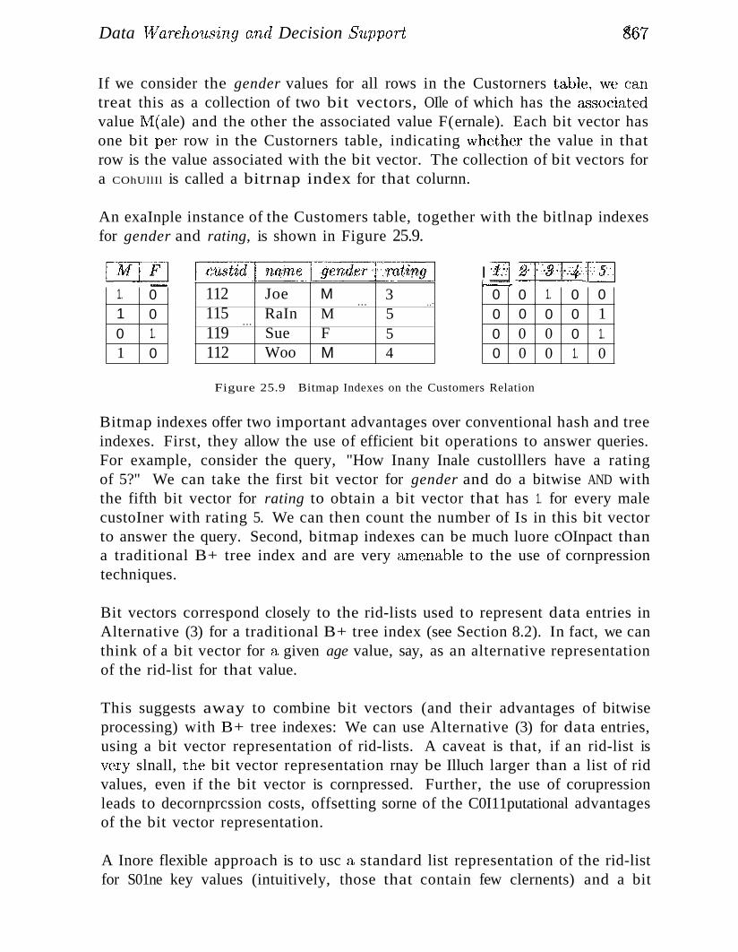
Data Wareho,lt,Crtng and Decision SUPPO'lt gf)7
If we consider the gender values for all rows in the Custorners table, vve cantreat this as a collection of two bit vectors, OIle of which has the a.,')sociatedvalue ~/I(ale) and the other the associated value F(ernale). Each bit vector hasone bit per row in the Custorners table, indicating vvhether the value in thatrow is the value associated with the bit vector. The collection of bit vectors fora COhUllIl is called a bitrnap index for that colurnn.
An exaInple instance of the Customers table, together with the bitlnap indexesfor gender and rating, is shown in Figure 25.9.
.----"
0 0 1. 0 00 0 0 0 10 0 0 0 1.0 0 0 1. 0
I ·;11 ..•1J··.·.].·.···.·.·.·.···ld·······I··········;4·····.....[!J112 Joe M 3
... ,,-
115 RaIn M 5...
119 Sue F 5112 Woo M 4
.:::.:=1. 01 00 1.1 0
!M!Fj
Figure 25.9 Bitmap Indexes on the Customers Relation
Bitmap indexes offer two important advantages over conventional hash and treeindexes. First, they allow the use of efficient bit operations to answer queries.For example, consider the query, "How Inany Inale custolllers have a ratingof 5?" We can take the first bit vector for gender and do a bitwise AND withthe fifth bit vector for rating to obtain a bit vector that has 1. for every malecustoIner with rating 5. We can then count the number of Is in this bit vectorto answer the query. Second, bitmap indexes can be much luore cOInpact thana traditional B+ tree index and are very cunenable to the use of cornpressiontechniques.
Bit vectors correspond closely to the rid-lists used to represent data entries inAlternative (3) for a traditional B+ tree index (see Section 8.2). In fact, we canthink of a bit vector for a given age value, say, as an alternative representationof the rid-list for that value.
This suggests away to combine bit vectors (and their advantages of bitwiseprocessing) with B+ tree indexes: We can use Alternative (3) for data entries,using a bit vector representation of rid-lists. A caveat is that, if an rid-list isvery slnall, the bit vector representation rnay be Illuch larger than a list of ridvalues, even if the bit vector is cornpressed. Further, the use of corupressionleads to decornprcssion costs, offsetting sorne of the C0I11putational advantagesof the bit vector representation.
A Inore flexible approach is to usc a standard list representation of the rid-listfor S01ne key values (intuitively, those that contain few clernents) and a bit
868 CHAPTER 2~
vector representation for other key values (those that contain rnany elenlents,and therefore lend themselves to a cOInpact bit vector representation).
This hybrid approach, 'which can easily be adapted to work \\lith hash indexesa,,~ well as B+ tree indexes, haa.') both advantages and disadvantages relative toa standard list of rids approach:
1. It can be applied even to cohllnns that are not sparse; that is, in ,vhich areTnany possible values can appear. The index levels (or the hashing scheIue)allow us to quickly find the 'list' of rids, in a standard list or bit vectorrepresentation, for a given key value.
2. Overall, the index is Tnore cornpact because we can use a bit vector representation for long rid lists. \Ve also have the benefits of f&'3t bit vectorprocessIng.
3. On the other hand, the bit vector representation of an rid list relies ona Inapping fron1 a position in the vector to an rid. (This is true of anybit vector representation, not just the hybrid approach.) If the set ofrows is static, and we do not worry about inserts and deletes of rows, itis straightforward to ensure this by assigning contiguous rids for rows ina table. If inserts and deletes Inust be supported, additional steps arerequired. For exanlple, we can continue to assign rids contiguously on aper-table basis and sirnply keep track of which rids correspond to deletedrows. Bit vectors can now be longer than the current nUlnber of rows, andperiodic reorganization is required to cOlllpact the 'holes' in the assignrnentof rids.
25.6.2 Join Indexes
Cornputing joins with sIllall response tirnes is extrernely hard for very largerelations. One approach to this problern is to create an index designed to speedup specific join queries. Suppose that the Custorners table is to be joined ~with
(1, table called Purchases (recording purchases Inacle by custorners) on the c,ltsUdfield.vVe can create a collection of (c, p) pairs, where p is the rid of a Purchasesrecord that joins \vith a Custc)lners recol'c! with cusUd c.
This idea can be generalized to support joins over ruore than t\VO relations. \Vediscuss the special case of a star scherna., in \vhich the fact table is likely tobe joined with several dirnension tables. Consider a join query that joins facttable F vvith dilnension tables D1 and D2 and includes selection conditions oncohunn [:1 of tal)le 1)1 Etnd colurnn (:12 of table D2. \Ve store a tuple ('tl' ('2, r)irl the join index if T1 is the rid of a tuple in table 1)1 with value ('1 in cohunnC1
1 , '1'2 is the rid of a tuple in table D2 ,vith value C2 in colllrnn (:12 , and T is therid of a tllple in the fact ta,ble F, (uHl tJlcsethree tUl)les join with each other.
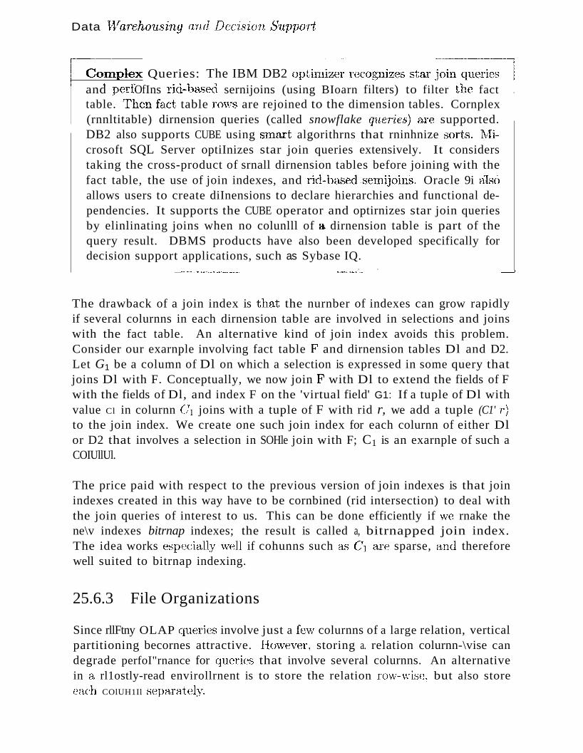
Data Vvareh07l8"ing arul DeC"lS'lCyn S'llppOTt
~:~p~ex Queries: The IBM DB2 o;;:izer recognizes star join~:::land perfOfIns rid-b&ged sernijoins (using BIoarn filters) to filter the fact III
table. 1'hen fact table rO\V8 are rejoined to the dimension tables. Cornplex .(rnnltitable) dirnension queries (called snowflake qucrvlcs) are supported.DB2 also supports CUBE using SlnclJ't algorithrns that rninhnize sorts.~1i
crosoft SQL Server optiInizes star join queries extensively. It considerstaking the cross-product of srnall dirnension tables before joining with thefact table, the use of join indexes, and rid-basedserniJoins. Oracle 9i alsoallows users to create diInensions to declare hierarchies and functional dependencies. It supports the CUBE operator and optirnizes star join queriesby elinlinating joins when no colunlll of a dirnension table is part of thequery result. DBMS products have also been developed specifically fordecision support applications, such as Sybase IQ.
_~__~ •__<,., ••_"•." .•_ ••••• • ---.J
The drawback of a join index is that the nurnber of indexes can grow rapidlyif several colurnns in each dirnension table are involved in selections and joinswith the fact table. An alternative kind of join index avoids this problem.Consider our exarnple involving fact table F and dirnension tables Dl and D2.Let G1 be a column of Dl on which a selection is expressed in some query thatjoins Dl with F. Conceptually, we now join F with Dl to extend the fields of Fwith the fields of Dl, and index F on the 'virtual field' G1: If a tuple of Dl withvalue Cl in colurnn C\ joins with a tuple of F with rid r, we add a tuple (C1' r)to the join index. We create one such join index for each colurnn of either Dlor D2 that involves a selection in SOHle join with F; C1 is an exarnple of such aCOIUllUl.
The price paid with respect to the previous version of join indexes is that joinindexes created in this way have to be cornbined (rid intersection) to deal withthe join queries of interest to us. This can be done efficiently if \ve rnake thene\v indexes bitrnap indexes; the result is called a, bitrnapped join index.The idea works especiaJly W(~ll if cohunns such a"s Cil are sparse, and thereforewell suited to bitrnap indexing.
25.6.3 File Organizations
Since rllFtny OLAP queries involve just a fev\! colurnns of a large relation, verticalpartitioning becornes attractive. IIcrwever, storing a. relation colurnn-\vise candegrade perfoI"rnance for queries that involve several colurnns. An alternativein a, rl1ostly-read envirollrnent is to store the relation rOvv-vvise, but also storeeach COlUH1Il separatel:y.
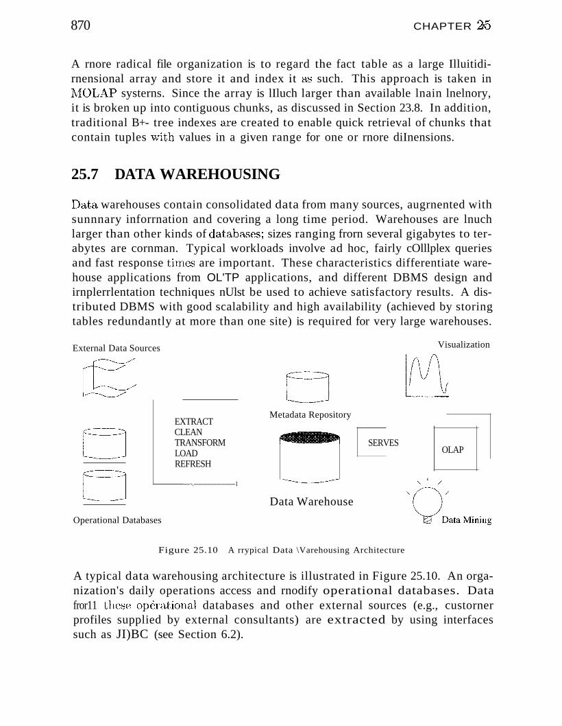
870 CHAPTER 26
A rnore radical file organization is to regard the fact table as a large Illuitidirnensional array and store it and index it as such. This approach is taken inNI0LAP systerns. Since the array is lIluch larger than available lnain lnelnory,it is broken up into contiguous chunks, as discussed in Section 23.8. In addition,traditional B+- tree indexes axe created to enable quick retrieval of chunks thatcontain tuples "'lith values in a given range for one or rnore diInensions.
25.7 DATA WAREHOUSING
Data warehouses contain consolidated data from many sources, augrnented withsunnnary inforrnation and covering a long time period. Warehouses are lnuchlarger than other kinds of databases; sizes ranging frorn several gigabytes to terabytes are cornman. Typical workloads involve ad hoc, fairly cOlllplex queriesand fast response tilnes are important. These characteristics differentiate warehouse applications from OL'TP applications, and different DBMS design andirnplerrlentation techniques nUlst be used to achieve satisfactory results. A distributed DBMS with good scalability and high availability (achieved by storingtables redundantly at more than one site) is required for very large warehouses.
External Data Sources
FJr=J
Operational Databases
EXTRACTCLEANTRANSFORMLOADREFRESH
----·-.--------------------------1
Metadata Repository
---_.-------Data Warehouse
SERVES
Visualization
OLAP
Figure 25.10 A rrypical Data \Varehousing Architecture
A typical data warehousing architecture is illustrated in Figure 25.10. An organization's daily operations access and rnodify operational databases. Datafror11 these oIlfSrational databases and other external sources (e.g., custornerprofiles supplied by external consultants) are extracted by using interfacessuch as JI)BC (see Section 6.2).
Data ~JVaTeh(nl8'ing and Decision 8UPP01 Tt
25.7.1 Creating and Maintaining a Warehouse
871
l\!Iany challenges rnust be Inet in creating and Inaintaining a large data warehouse.A good datab&'3e scherua nlust be designed to hold an integrated collection of data copied froIn diverse sources. For exarnple, a cornpany warehousernight include the inventory and personnel departrnents' databa.'3es, togetherwith sales databases rnaintained by offices in different countries. Since thesource databases are often created and rnaintained by different groups, thereare a nUlnber of selnantic Inisrnatches across these databases, such as differentcurrency units, different narnes for the saIne attribute, and differences in howtables are nornlalized or structured; these differences Inust be reconciled whendata is brought into the warehouse. After the warehouse schenla is designed,the warehouse must be populated, and over tirne, it Inust be kept consistentwith the source databases.
Data is extracted from operational databases and external sources, cleanedto Inininlize errors and fill in Inissing information when possible, and transformed to reconcile semantic Inismatches. Transforlning data is typically accOlnplished by defining a relational view over the tables in the data sources(the operational databases and other external sources). Loading data consistsof ruaterializing such views and storing therll in the warehouse. Unlike a standard view in a relational DBMS, therefore, the view is stored in a database(the warehouse) that is different frorn the database(s) containing the tables itis defined over.
The cleaned and transfonned data is finally loaded into the warehouse. Additional preprocessing such &'3 sorting and generation of surnrnary infornuttionis carried out at this stage. Data is partitioned and indexes are built for efficiency. Due to the large vohllue of elata, loading is a slow process. Loading aterabyte of data sequentially can take 'Y"eeks, and loading even a gigabyte cantake hours. Parallelisul is therefore iInportant for loading warehouses.
AJter data is loaded into a warehouse, additional rneasures rnust be taken toensure that the data in the vvarehouse is periodically refreshed to reflectupdates to the data sources and periodically purge old data (perhaps ontoarchival rnedia). Observe the connection between the problern of refreshingwarehouse tables and a,synchronously rnaintaining replica.." of tables in a distributed DBMS. Maintaining replicas of source relations is an essential part ofwarehousing, and this application clornain is an iInportant factor in the popularity of a.synchronous replication (Section 22.11.2), even though asynchronousreplication violates the principle of distributed data independence. The problern of refreshing warehouse tables (\vhich are rnaterialized views over tables in
872
the source databEkses) has also rene\ved interest in inerernental Illaintenance ofrna.terialized vic\vs. ("VVe discuss rnaterialized vie\\Ts in Section 25.8.)
An irnportant tC4sk in Inainta,ining a warehouse is keeping track of the datacurrently stored in it; this bookkeeping is done by storing infofrnation aboutthe \varehouse data in the systenl catalogs. rrhe systerIl catalogs associated 'witha \varehouse are very large and often stored and 111anaged in a separate databasecalled a metadata repository. The size and cornplexity of the catalogs is inpart due to the size and cOlnplexity of the warehouse itself and in part becausea lot of adrninistrative inforrnation rnust be Inaintained. For excunple, we HlllStkeep track of the source of each warehouse table and when it was last refreshed,in addition to describing its fields.
1'he value of a warehO"use is ultin1ately in the analysis it enables. The data in awarehouse is typically accessed and analyzed using a variety of tools, includingOLAP query engines, data. mining algorithrns, inforrnation visualization tools,statistical packages, and report generators.
25.8 VIEWS AND DECISION SUPPORT
Views are widely used in decision support applications. Different groups ofanalysts within an organization are typically concerned with different aspectsof the business, and it is convenient to define views that give each group insightinto the business details that concern it. Once a view is defined, we can writequeries or new view definitions that use it, as we saw in Section 3.6; in thisrespect a view is just like a base table. Evaluating queries posed against viewsis very ilnportant for decision support applications. In this section, we considerhow such queries can be evaluated efficiently after placing views within thecontext of decision support applications.
25.8.1 Views, OLAP, and Warehousing
Views are closely related to OLAP and data warehousing.
OLAP queries are typically aggregate queries. Analysts want fa.st answers tothese queries over very large datasets, and it is natural to consider precoluputingvievvs (see SectiorlS 25.9 and 25.10). In particular, the CUBE operator~ 'discussedin Section 25.3""'gives rise to several aggregate queries that are closely related.The relationships that exist betvveen the Inany aggregate queries that arise frolna single CUBE operation can be exploited to develop very effective precornputation strategies. The idea is to choose a subset of the aggregate queries forInaterialization in such a. vvay that typical CUBE queries can be quickly answeredby using the Inaterialized views arld doing S(Hne additional cornplltation. The
Data HlaTcho'zMring a'nd Deci,sion 5'UPPOTt ~73
choice of views to 111ateria1ize is influenced by ho\v lllany queries they can potentially speed up and by the aillount of space required to store the Inaterializedview (since we have to \vork with a given alnount of storage space).
A data \varehouse is just a collection of &csynchrollously replicated tables andperiodically synchronized views. A Wareh(HIS(~ is characterized by its size, thenuruber of tables involved, and the fact that IllOSt of the underlying tablesare froln external, independently lnaintained databases. Nonetheless, the fundaluental probleln in warehouse lnaintenance is asynchronous rnaintenance ofreplicated tables and materialized views (see Section 25.10).
25.8.2 Queries over Views
Consider the following view, RegionalSales, which cornputes sales of productsby category and state:
CREATE VIEW RegionalSales (category, sales, state)AS SELECT P.category, S.sales, L.state
FROM Products P, Sales S, Locations LWHERE P.pid = S.pid AND S.locid = L.locid
The following query computes the total sales for each category by state:
SELECT H,. category, It.state, SUM (R.sales)FROM RegionalSales H,GROUP BY R.category, R,.state
\\1hile the SQL standard does not specify how to evaluate queries on views, itis useful to think in ternlS of a process called query modification. rrhe idea isto replace the occurrence of RegionalSales in the query by the view definition.The result on this query is
SELECTFROM
GROUP BY
H,.category, R.state, SUM (R.sales)( SELECT P.category, S.sales, L.stateFROM Products P, Sales S, Locations LWHERE P.piel = S.pid AND S.locid == L.locid ) AS R,R,.category, H,.state
25.9 VIEW MATERIALIZATION
vVe can ansvver a query on a view by using the query rnodification techniquejust described. Often, however, queries against cornplex view definitions Illust
874 CHAPTER 25
be answered very fast because users engaged in decision support activities require interactive response tirIles. Even with sophisticated optilnization andevaluation techniques, there is a lirnit to how fa.."t we can answer such queries.Also, if the underlying tables are in a rernote database, the query rIlodification approach rnay not even be feasible because of issues like connectivity andavailability.
An alternative to query rnodification is to precornpute the view definition andstore the result. When a query is posed on the view, the (unrllodified) query isexecuted directly on the precornputed result. This approach, called view materialization, is likely to be rnuch fa,;ter than the query modification approachbecause the complex view need not be evaluated when the query is computed.Materialized views can be used during query processing in the sarne way a'Sregular relations; for exarnple, we can create indexes on nlaterialized views tofurther speed up query processing. The drawback, of course, is that we mustmaintain the consistency of the precomputed (or m,aterialized) view wheneverthe underlying tables are updated.
25.9.1 Issues in View Materialization
Three questions must be considered with regard to view nlaterialization:
1. What views should we rnaterialize and what indexes should we build onthe rnaterialized views?
2. Given a query on a view and a set of materialized views, can we exploitthe rnaterialized views to answer the query?
3. I-Iow should we synchronize rnaterialized views with changes to the underlying tables? The choice of synchronization technique depends on severalfactors, such a.c; whether the underlying tables are in a rernote database.We discuss this issue in Section 25.10.
'rhe answers to the first two questions are related. 'fhe choice of vievvs tornaterialize and index is governed by the expected workload, and the discussionof indexing in Chapter 20 is relevant to this question ac; well. The choice ofviews to rnaterialize is rnore cornplex than just choosing indexes on a set ofdatabase tables, however, because the range of alternative views to rnaterializeis wider. The goaJ is to rnaterialize a srnaU, carefully chosen set of views thatcan be utilized to quickly answer rnost of the irnportant queries. COIlversely,once vve have chosen a set of views to rnaterialize, we have to consider how theycan be used to ansvver a, given query.
Consider the RJ~gi()nalSales view. It involves a JOIn of Sales, Products, andLocations and is likely to be expensive to cornpute. On the other hand, if it
[Jata ~VaTehol1Bin,g (uLd Decis'ioTL S~Ll)poTt ~75
is rnaterialized and stored with a clustered B+ tree index on the search key(category, state, sales), we Gall ans\ver the exarnple query by an index-onlysearl.
Given the rnaterialized view and this index, we can also answer queries of thefollo\ving forrn efficiently:
SELECTFROMWHEREGROUP BY
R.state, SUM (R.sales)RegionalSales RILcategory == 'Laptop'R.state
To answer such a query, we can use the index on the Inaterialized view to locatethe first index leaf entry with category == 'Laptop' and then scan the leaf leveluntil we come to the first entry ¥lith category not equal to Laptop.
The given index is less effective on the following query, for which we are forcedto scan the entire leaf level:
SELECTFROMWHEREGROUP BY
R,.state, SUM (R.sales)R,egionalSales RR.state == 'Wisconsin'R.category
This exanlple indicates how the choice of views to materialize and the indexesto create are affected by the expected workload. ~rhis point is illustrated furtherby our next exarnple.
Consider the following two queries:
SELECTFROMWHEREGROUP BY
SELECTFROMWHEREGROUP BY
P.category, SUM (S.sales)Products P, Sales SP.pic! == S.pic!P.category
L.state, SUM (S.sales)I . I S 1 S...JocatIons ,,;, . a es ~
.L .locid = S.locidL.state
'These two queries require us to join the SaJes table (which is likely to be verylarge) with another table and aggregate the result. IIO'w can vve use rnaterialization to speed up these queries? The straightforward approach is to precornpute
876 ( "'1 . 2·~jHAPTER ~)p
each of the joins involved (Products with Sales and Locations with Sales) or topreconlpute each query in its entirety. An alternative approach is to define thefollowing view:
CREATE VIEW rrotalSaJes (pid, locid, total)AS SELECT S.pid, S.locid, SUM (S.sales)
FROM Sales SGROUP BY S.pid, S.locid
The view TotalSales can be rnaterialized and used instead of Sales in our twoexalnple queries:
SELECTFROMWHEREGROUP BY
SELECTFROMWHEREGROUP BY
P.category, SUM (T.total)Products P, TotalSales TP.pid = T.pidP.category
L.state, SUM (T.total)Locations L, TotalSales TL.locid = rr .locidL.state
25.10 MAINTAINING MATERIALIZED VIEWS
A materialized view is said to be refreshed when we rnake it consistent withchanges to its underlying tables. rrhe process of refreshing a view to keep itconsistent with changes to the underlying table is often referred to as viewmaintenance. Two questions to consider are
1. flow do vie refresh a view' when an underlying table is nlodified? Two issuesof particular interest are how to Inaintain vie\vs incTcrnentally, that is,without recornputing frolI! scratch when there is a change to an underlyingtable; and how to rnaintain vie\vs in a distributed environrnent such as adata vvarehouse.
2. vVhcn should \ve refresh a view in response to a change to an underlyingtable?
25.10.1 Incremental View Maintenance
A straightforward approach to refreshing a vie\v is to sirnply reeolnpute theview \.vhen an underlying table is rnodified. This rnay, in fact, be a reasonable strateKY in sorne ca."es. For exarnple, if the underlying tables are in a
Data HIaTehc)7I8'ing and Decision Support r;877
rernote databa..'3c, the view can be periodically recornputed and sent to the datawarehouse \vhere "the vie\v is Hlaterialized. This ha.'3 the advantage that theunderlying tables need not be replicated at the vvarehouse.
\Vhenever possible, however, algorithrns for refreshing a view should be incremental, in that the cost is proportional to the extent of the change rather thanthe cost of recornputing the vie\\r fr(Hn scratch.
To understand the intuition behind incrernental view rnaintenance algorithnls,observe that a given row in the rnaterialized view can appear several thnes,depending on how often it was derived. (R.ecall that duplicates are not elirninated fro111 the result of an SQL query unless the DISTINCT clause is used. Inthis section, we discuss rnultiset sernantics, even when relational algebra notation is used.) The rHain idea behind incremental rnaintenance algorithrIls is toefficiently compute changes to the rows of the view, either new rows or changesto the count associated with a row; if the count of a row becornes 0, the row isdeleted frorH the view.
We present an incrernental 11Ulintenance algorithnl for views defined using projection, binary join, and aggregation; we cover these operations because theyillustrate the rHain ideas. The approach can be extended to other operationssuch as selection, un.ion, intersection, and (rnultiset) difference, as well as expressions containing several operators. The key idea is still to rnaintain thenurnber of derivations for each view row, but the details of how to efficientlyconlpute the changes in view rows and associated counts differ.
Projection Views
Consider a view V defined in tenns of a projection on a tableR; that is,y"" = n(R). Every row v in V has an associated count, corresponding to thenurnber of tirnes it can be derived, \vhich is the nurnber of rows in R that yield '1)
when the projection is applied. Suppose we 1nodifyR by inserting a collectionof rows Il i and deleting a collection of existing 1'o\vs R d .1 vVe cornpute n(l1."'i)and add it to \l. If the rnultisetrr(R.i ) contains a row T \vith count c and rdoes not appear in 11 , \ve add it to V"with count c. If T is in V, we add c toits count. vVe also cornpute n(Rd) and subtract it fronl 1/. ()bserve that if r
appe~:trs in neRd) \\rith count c, it 111USt also appear in y"" with a higher count;2we subtract c frOTH r's count in V".__'''. "n__
1'These collections can be multisets of rows. \'/e can treat a ro\v rnodification a.s an insert follO\'1edby 1:1 delete, for sirnplici ty.
2 As a simple exercise, consider why this rnust be so.
878 (~HAPTER 26
As an exanlple, consider the view Jrsales(Sales) and the instance of Sales shownin Figure 25.2. _Each ro\v in the vie\v has a single cohunn; the (n)\vwith) value25 appears vvith count 1, and the value 10 appears vvith count 3. If \lve deleteone of the rows in Sales \vith sales 10, the count of the (l'()\V \vith) value 10 inthe vie"v becornes 2. If \ve insert a new row into Sales with sales 99, the vie"'!no\v has a row with value 99.
An hnportant point is that \ve have to rnaintain the counts associated vvith rowseven if the view definition uses the DISTINCT clause, rneaning that duplicatesare elilninated frorn the view. Consider the saIne view with set selnantics~
the DISTINCT clause is used in the SQL view definition··------and suppose that wedelete one of the rows in Sales with sales 10. Does the view now contain arow with value 10'1 To deterrIline that the answer is yes, we need to maintainthe rOw counts, even though each row (with a nonzero count) is displayed onlyonce in the Inaterialized view.
Join Views
Next, consider a view V defined as a join of two tables, R [X] S. Suppose wemodify R by inserting a collection of rows R'i and deleting a collection of rowsRd. We cornpute Ri [X] S and add the result to V. We also C0111pute Rd r><J Sand subtract the result fror11 V. Observe that if r appears in Rd [X] S withcount C, it rnust also appear in V with a higher count>J
Views with Aggregation
Consider a view V defined over R using GROUP BY on colUllln G and an aggregate operation on colu1nn A. Each row v in the vi(~w surnrnarizes a groupof tuples in R and is of the fonn (g, 8'u,'rrLrnary) , where 9 is the value of thegrouping colulnn G and the sununary inforInation depends on the aggregateoperation. To lnaintain such a view incrernentally, in general, we have to keepa lnore detailed surrllnary than just the inforrnation included in the view. Ifthe aggregate operation is COUNT, we need to Inaintain only a count c for eachrovv v in the vieVvT. If a ro\v r is inserted intoR, and there is no I'o,v v in "\;7
with 'v.G = T.G, we add <1 new row (r.G, 1). If there is a ro,v 'I) \vith v.C} = r.G,we incrernent its count. If a row r is deleted fro111 R, \ve decrcrnent the countfor the row v "vith v.Ci = T.C}; v can be deleted if its count becornes 0, becausethen the last row in this group ha.'3 been deleted frorn .R.
If the aggregate operation is SUM, we have to lllaintain a SUIll :3 and also a countc. If a row T is inserted into If, and there is no renv '1) in ~! "lith v.C; = T.C:,--_..- ...- .....
:{ As another simple exercise, consider why this mllst be so.
Data WaTchou8 ilng and Decis'io11 8UPPOTt i79
we add a new row ('r.C, a, 1). If there is a, row (T.G, 8, c), we replace it by(r.Ci, /3 +" a, C -t 1). If a rO\1ll T is deleted frolll Il, \ve replace the row (r.G, S, c)with {T.G,8 - a, C - 1); 1) can be deleted if its count becornes O. Observe thatwithout the count, \-ve do not know when to delete 'u, since the Slun for a groupcould be 0 even if the group contains SCHne rows.
If the aggregate operation is AVG, \ve have to lllaintain a Slun s, a count c,and the average for each row in the vie\v. The SlUll and count are rnaintainedincrernentally as already described, and the average is corllputed as s / c.
The aggregate operations MIN and MAX are potentially expensive to rnaintain.Consider MIN. For each group in R, we rnaintain (g, rn, c), where rn is theIninilnurn value for colUllln A in the group g, and c is the count of the nUlllberof rows l' in R with T.G == 9 and r.A == m. If a row l' is inserted into Randr.G == g, if r.A is greater than the miniriulill m for group g, we can ignore r. Ifr.A is equal to the 111iniInurll m for r's group, we replace the summary row forthe group with (g, m, c+ 1). If r.A is less than the minirllum m for r's group, wereplace the SUlnrnary for the group with (g, T.A, 1). If a row r is deleted frornRand T.A is equal to the minimurIl rrt for T'S group, then we HUlst decrernentthe count for the group. If the count is greater than 0, we sinlply replace thesurnmary for the group with (g, rn, c-_· 1). However, if the count becomes 0, thisIneans the last row with the recorded rninimum A value has been deleted fromR and we have to retrieve the sInallest A value among the relnaining rows inR with- group value r.G-and this might require retrieval of all rows in 11, withgroup value T.G.
25.10.2 Maintaining Warehouse Views
The views rnaterialized in a data warehouse can be based on source tablesin rernote databases. rIhe asynchronous replication techniques discussed inSection 22.11.2 allow us to connnunicate changes at the source to the warehouse,but refreshing vie\vs incrernentally in a distributed setting presents sorne uniquechallenges. To illustrate this, we consider a sirnpleview that identifies suppliersof Toys.
CREATE VIEW ToySuppliers (sid)AS SELECT S.sid
FROM Suppliers S, Products PWHERE S.pid == P.piel AND P.category == 'Tbys'
Suppliers is a new table introduced for this exarnple; let us &ssurne that ithEkS just two fields, sid aIld pid, indicating that supplier s'id supplies part pill.rrb.c location of th(~ tables Proclucts and Suppliers and the vie\v ToySuppliers
880
influences hovv we IIlaintain the vh~\v. Suppose that all three are rnaintainedat a single site. vVe can Inaintain the view increlnentally using the techniquesdiscussed in Section 25.10.1. If a replica of the vie\v is created at another site,we can 1l1onitor changes to the Inaterialized vie\v and apply thcIn at the secondsite using the a..synchronous replication techniques froIn Section 22.11.2.
But, what if Products and Suppliers are at one site and the view is Inaterialized(only) at a second site? To rnotivate this scenario, "we observe that, if the firstsite is used for operational data and the second site supports cornplex analysis,the two sites lnay well be adrninistered by different groups. The option oflnaterializing ToySuppliers (a view of interest to the second group) at the firstsite (run by a different group) is not attractive and may not even be possible; theadnlinistrators of the first site may not ,vant to deal with someone else's views,and the a(hninistrators of the second site n1ay not want to coordinate withsonleone else whenever they Inodify view definitions. As another motivationfor rnaterializing views at a different location froIn source tables, observe thatProducts and Suppliers may be at two different sites. Even if ·we rnaterializeToySuppliers at one of these sites, one of the two source tables is reillote.
Now that we have presented Inotivation for rnaintaining rroySuppliers at a location (say, Warehouse) different froIn the one (say, Source) that contains Products and Suppliers, let us consider the difficulties posed by data distribution.Suppose that a new Products record (with category == 'Toys') is inserted. Wecould try to rnaintain the view incren1entally as follows:
1. The Warehouse site sends this update to the Source site.
2. 1'0 refresh the view, we need to check the Suppliers table to find suppliers of the itern, and so the v\larehouse site asks the Source site for thisinforrnation.
3. The Source site returns the set of suppliers for the sold iteln, and thevVarehouse site incrernentally refreshes the view.
This works when there are no additional changes at the Source site in betweensteps (1) and (3). If there are changes, ho\vever, the Inaterializecl view canbecorne incorrect reflecting a state that can never arise except for anornaliesintroduced by the preceding, naive, increInental refresh algorithrn. To see this,suppose that Pr,oducts is enlpty and Suppliers contains just the row \81, 5)initially, and consider the following sequence of events:
1. Product pid = 5 is inserted \vith category = 'Toys'; Source notifies\Varehouse.
2. Warehouse asks Source for suppliers of product pid = 5. (The only suchsupplier at this instant is 81.)
jJata HIarehO'lt8'ing and Decisi(Y!L S7.qJ].J01'l" 881
3. The row (82,5) is inserted into Suppliers; Source notifies \Varehouse.
4. To decide whether 82 should be added to the vie\v, vve need to kno\v thecategory of product pid = 5, and \Varehouse asks Source. (ltVarehouse hasnot received an anS7.lJer to its previous quest1:on.)
5. Source now processes the first query frorn \tVarehouse, finds two suppliersfor part 5, and returns this inforrnation to Warehouse.
6. \tVarehouse gets the answer to its first question: suppliers 81 and 82, andadds these to the view, each with count 1.
7. Source processes the second query frorn \Varehouse and responds with theinforll1ation that part 5 is a toy.
8. Warehouse gets the answer to its second question and accordingly increHlents the count for supplier 82 in the view.
9. Product pid == 5 is now deleted; Source notifies Warehouse.
10. Since the deleted part is a toy, Warehouse decrements the counts of nlatching view tuples; 81 has count 0 and is relnoved, but s2 has count 1 and isretained.
Clearly, 82 should not rernain in the view after part 5 is deleted. This exampleillustrates the added subtleties of incremental view rnaintenance in a distributedenvironment, and this is a topic of ongoing research.
25.10.3 When Should We Synchronize Views?
A view maintenance policy is a decision about when a view is refreshed,independent of whether the refresh is incrernental or not. A view can be refreshed within the sallIe transaction that updates the underlying tables. Thisis called immediate view Iuaintenance. The update transaction is slowedby the refresh step, and the irupact of refresh increc1.'3es with the nurnber ofmaterialized views that depend on the updated table.
Alternatively, we can defer refreshing the vie\v. Updates are captured in a logand applied subsequently to the rnaterialized vic\vs. There are several deferredview maintenance policies:
1. Lazy: The rnaterialized vie\v\l is refreshed at the tilne a query is evaluatedusing V, if V is not already consistent vvith its underlying base tables. Thisapproach sl()\vs down queries rather than updates, in contra-st to iHnnediatevic",-! rnaintenance.
882 CHAPTER 2&
I~iews for De-cision Su;ort: ;-BMS ven~rs are e:hancing ;ieir m~~I relational products to support decision support querip.s. IBM DB2 sup..I ports materialized views with transaction-consistent or user-invoked main-I tenance. l\1icrosoft SQL Server supports partition views, \vhich areI unions of (ruany) horizontal partitions of a table. These aJ'e airned atI a warehollsing envirOllrnent where each partition could be, for exalnple, a
rnonthly update. Queries on partition vie\vs are opthnized so that only relevant partitions are accessed. Oracle 9i supports 111aterialized views withtransaction-consistent, user-invoked, or tilne-scheduled nlaintenance.
L_.~ _
2. Periodic: The lllaterialized view is refreshed periodically, say, once a day.The discussion of the Capture and Apply steps in asynchronous replication(see Section 22.11.2) should be reviewed at this point, since it is very relevant to periodic view lllaintenance. In fact, many vendors are extendingtheir asynchronous replication features to support lllaterialized views. Materialized views that are refreshed periodically are also called snapshots.
3. Forced: rrhe rnaterialized view is refreshed after a certain nurnber ofchanges have been made to the underlying tables.
In periodic and forced view nlaintenance, queries rllay see an instance of theIIlaterialized view that is not consistent with the current state of the underlyingtables. That is, the queries would see a different set of rows if the view definitionwas recornputed. This is the price paid for fast updates and queries, and thetrade-off is sirnilar to the trade-off rnade in using asynchronous replication.
25.11 REVIEW QUESTIONS
Answers to the review questions can be found in the listed sections.
II vVhat are decision support applications? :Oiscuss the relationship of co'rnple:r:8(2L q'lteries, OLA.P, data rnining, and data 1uarehousing. (Section 25.1)
IIiI Describe the rnultidirnensional data luodel. Explain the distinction betweenrneasurcs and dirnensions and between fact tables and din~en8ion tables.\\That is a sip:r 8chenz,a? (Sections 25.2 and 25.2.1)
II Cornrnon OLAP operations have received special naInes: roll-up, drilldeY/on" pivohng7 slicing, and dicing. Describe each of these operations andillustrate thern using exarnples. (Section 25.3)
II I)escribe the SCJL:1999 ROLLUP and CUBE features and their relationship tothe ()LAP operations. (Section 25.3.1)
Data WaTehousing and Decision Support 883
• Describe the SQL:1999 WINDOW feature, in particular, frarning and orderingof windows. How does it support queries over ordered data? Give exarnplesof queries that are hard to express without this feature. (Section 25.4)
• New query paradigrns include top N q'ue-ries and online aggTegation. Explain the nlotivation behind these concepts and illustrate then1 throughexaruples. (Section 25 .. 5)
• Index structures that are especially suitable for OLAP systen1s includebitrnap indexes and join indexes. Describe these structures. How arebitrnap indexes related to B+ trees? (Section 25 .. 6)
III Information about daily operations of an organization is stored in opeTational databases. Why is a data waTeho'i.LSe used to store data frolH operational databases? What issues arise in data warehousing? Discuss dataextTaction, cleaning, transjoTrnation, and loading. Discuss the challenges inefficiently TejTeshing and pUTging data. (Section 25 .. 7)
III Why are views irnportant in decision support environments? How are viewsrelated to data warehousing and OLAP? Explain the queTy mod~fication
technique for answering queries over views and discuss why this is notadequate in decision support environrnents. (Section 25 ..8)
III What are the rnain issues to consider in maintaining materialized views?Discuss how to select views to materialize and how to use rnaterializedviews to answer a query. (Section 25.9)
• How can views be rnaintained incTernentally? Discuss all the relationalalgebra operators and aggregation. (Section 25 .. 10.1)
• Use an exarnple to illustrate the added cornplications for incrernental viewmaintenance introduced by data distribution. (Section 25.10.2)
III Discuss the choice of an appropriate rnaintenance policy for when to refresha view. (Section 25.10.3)
EXERCISES
Exercise 25.1 Briefly answer the following questions:
1. How do warehousing, OLAP, and data rnining cornplernent each other?
2. vVhat is the relationship between datawan~housingand data replication? Which fornl ofreplication (synchronous or a.csynchronous) is better suited for data w(trehOllsing? \Vhy?
:J. \\That is the role of the rnetadata repository in a data warehouse'? How does it differfrorn a catalog in (1 relational IJB:NIS?
4. \Vhat considenttions are involved in designing a data warehouse'?

884 CHAPTER 251'
5. Once a warehouse is designed and loaded 1 how is it kept current with respect to changesto the source databases?
fl. One of the advantages of a waxehouse is that we can use it to track how the contents ofa relation change over titue; in contrast 1 we have only the current snapshot of a relationin a regular DBJ'vfS. Discuss how you would maintain the history of a relation R, takinginto account that 'old' infonnation lllust sOlnehow be purged to rnake space for Hewinfonnatioll.
7. Describe dilnensions and rneasures in the multidirnensional data model.
8. What is a fact table, and why is it so irnportant frOIn a performance standpoint?
9. Vvhat is the fundarnental difference between ~fOLAP and ROLAP systems?
10. \Vhat is a star scheIna? Is it typicaU:y in BCNF? Why or why not?
11. How is data rnining different from OLAP?
Exercise 25.2 Consider the instance of the Sales relation shown in Figure 25.2.
1. Show the result of pivoting the relation on pid and tirneid.
2. Write a collection of SQL queries to obtain the same result as in the previous part.
3. Show the result of pivoting the relation on pid and lacid.
Exercise 25.3 Consider the cross-tabulation of the Sales relation shown in Figure 25.5.
1. Show the result of roll-up on lacid (i.e., state).
2. Write a collection of SQL queries to obtain the same result as in the previous part.
3. Show the result of roll-up on lacid followed by drill-down on pid.
4. Write a collection of SQL queries to obtain the same result as In the previous part,starting with the cross-tabulation shown in Figure 25.5.
Exercise 25.4 Briefly answer the following questions:
1. What is the difIerences between the WINDOW clause and the GROUP BY clause'?
2. Give an example query that cannot be expressed in SQL without the WINDOW clause butthat can be expressed with the WINDOW clause.
:3. What is the fTCLrne of a window in SQL: 19997
4. Consider the fonowing simple GROUP BY query.
SELECTFROMWHEREGROUP BY
T.year, SUM (S.sales)Sales 5, Tilnes TS.tilneid='T.timeidT.year
Can you write this query in SQL:1999 without using a GROUP BY cIa.use? (Hint: Use theSQL:1999 WINDOW clause.)
Exercise 25.5 Consider the Locations, Products, and Sales relations shown in Figure 25.2.\iVrite the following queries in SQL:1999 llsing the WINDOW clause whenever you need it.
1. Find the percentage change in the total IJ10nthly sales for each location.
2. Find the percentage chc.tnge in the total quarterly sales for each product.

Data Warehousing and l]eci8ion 8'UPPOTt 885
3.FLnd the average daily sales over the preceding ;30 days for each product.
4. For each week, find the maximulu uloving average of sales over the preceding four \veeks.
5. Find the top three locations ranked by total sales.
6.F'ind the top three locations ranked by curnulative sales, for every month over the pastyear.
7. Rank all locations by total sales over the past year, and for each location print thedifference in total sales relative to the location behind it.
Exercise 25.6 Consider the CustOIuers relation and the bitmap indexes shown in Figure25.9.
1. For the same data, if the underlying set of rating values is assuIued to range froIlI 1 to10, show how the bitnlap indexes would change.
2. How would you use the bitIllap indexes to answer the following queries? If the bitmapindexes are not useful, explain why.
(a) How many customers with a rating less than 3 are male?
(b) What percentage of custoIners are male?
(c) How rnany customers are there?
(d) How many custonlers are named Woo?
(e) Find the rating value with the greatest number of custoIl1erS and also find the nUIllbel' of custorners with that rating value; if several rating values have the maxirnurnnumber of custoIllers, list the requested infonuation for all of theIn. (AssuIne thatvery few rating values have the same nUluber of customers.)
Exercise 25.7 In addition to the Customers table of Figure 25.9 with bitrnap indexes ongender' and 'rating, assurne that you have a table called Prospects, with fields ruting andprospectid. This table is used to identify potential customers.
1. Suppose that you also have a bitrnap index on the rating field of Prospects. Discusswhether or not the bitnlap indexes would help in corllputing the join of Custorners andProspects on rating.
2. Suppose you have no bitrnap index on the rating field of Prospects. Discuss whether ornot the bitrnap indexes on CustOIuers would help in conlputing the join of Custornersand Prospects on nLting.
~1. Describe the use of a join index to support the join of these two relations with the joincondition c'Ust'id=prospectid.
Exercise 25.8 Consider the instances of the Locations, Products, and Sales relations shownin Figure 25.2.
1. Consider the basic join indexes d€~scribed in Section 25.6.2. Suppose you want to optiInizefor the following two kinds of queries: Query 1 finds sa.les in a given city, and Query 2finds sa.les in a given state. Show the indexes you would create on the excunple instancesshown in Figure 25.2.
2. Consider the bitIIulpped join indexes described in Section 25.6.2. Suppose you want tooptirnize for the following two kinds of queries: Query 1 finds sales in a given city, andQuery 2 finds sales in a given state. Show the indexes that you would create on theexanlple instances shown in Figure 25.2.
886 CHAPTER 25II
~3. Consider the basic join indexes described in Section 25.6.2. Suppose you want to optiInizefor these two kinds of queries: Query 1 finds sales in a given city for a given productI1alne~ and Query 2 finds sales in a given state for a given product category. Show theindexes that you would create on the exarl1ple instances shown in Figure 25.2.
4. Consider the bitmapped join indexes described in Section 25.6.2. Suppose you want tooptirnize for these two kincls of queries: Query 1 finds sales in a given city for a givenproduct narne, and Query 2 finds sales in a given state for a given product category.Show the indexes that you would create on the example instances shown in Figure 25.2.
Exercise 25.9 Consicler the view NurnReservations defined as:
CREATE VIEW NumReservations (sid, snarnc, nUlures)AS SELECT S.sid, S.snarne, COUNT (*)
FROM Sailors S, Reserves RWHERE S.sid = R.sidGROUP BY 8.sid, S.sname
1. How is the following query, which is intended to find the highest number of reservationsnlade by smne one sailor, rewritten using query modification?
SELECT
FROM
MAX (N .numres)NurnReservations N
2. Consider the alternatives of cornputing on deluand and view materialization for thepreceding query. Discuss the pros and cons of materialization.
3. Discuss the pros and cons of materialization for the following query:
SELECT N.snarlle, MAX (N.numres)FROM NumReservations NGROUP BY N.sname
Exercise 25.10 Consider the Locations, Products, and Sales relations in Figure 25.2.
1. To decide whether to rnaterialize a view, what factors do we need to consider?
2. Assurne that we have defined the following lnaterialized view:
SELECT
FROMWHERE
L.state~ S.salesLocations I-i, Sales S8.locid=L.locid
(a) Describe what auxiliary infornlatioll the algorithnl for incrernental view rnaintenance frorn Section 25.10.1 maintains and how this data helps in lnainta.ining theview incrernentally.
(b) Discuss the pros and cons of ruaterializing this view.
:3. Consider the rnaterialized view in the previous question. Assume that the relationsLocations and Sales are stored at OIle site, but the view is rnaterialized on a second site.Why would we"ever want to luaintain the view at a second site? Give a concrete exarnplewhere the view could become inconsistent.
4. ASSUITW that we have defined the following rnaterialized view:
SELECT
FROMWHERE
GROUP BY
T.year, I..state, SUM (S.sales)Sales 8, 'rirnes '1', Locations LS. tirneid=T. tilneid AND S.locid=L.locidrr.year, L.state
[)ata WaTeho1.l.s'ing and DeC'lsion SUppOTt
(a) Describe what auxiliary infoflnation the algorithnl for incrernental view rnaintenance frOIn Section 25.10.1 luaintains, and how this data helps in rnaintaining theview increluentaJly.
(b) Discuss the pros and cons of 11laterializing this view.
BIBLIOGRAPHIC NOTES
A good survey of data warehousing and OLAP is presented in [161], which is the source ofFigure 25.10. [686] provides an overview of OLAP and statistical database research, showingthe strong parallels between concepts and research in these two areas. The book by Kirnball[436], one of the pioneers in warehousing, and the collection of papers in [(2) offer a good practical introduction to the area. The term OLAP was popularized by Codd's paper [191]. For arecent discussion of the performance of algorithms utilizing bitmap and other nontraditionalindex structures, see [575].
Stonebraker discusses how queries on views can be converted to queries on the underlyingtables through query modification [713]. Hanson cmnpares the perfornlance of query modification versus immediate and deferred view maintenance [365]. Srivastava and Roterll presentan analytical model of materialized view maintenance algorithnls [707]. A number of papersdiscuss how rnaterialized views can be incrementally maintained as the underlying relationsare changed. Research into this area has become very active recently, in part because of theinterest in data warehouses, which can be thought of as collections of views over relations fromvarious sources. An excellent overview of the state of the art can be found in [348], whichcontains a number of influential papers together with additional rnaterial that provides context and background. The following partial list should provide pointers for further reading:[100, 192, 193, 349, 369, 570, 601, 635, 664, 705, 800].
Gray et al. introduced the CUBE operator [~~35], and optirnization of CUBE queries and efficientmaintenance of the result of a CUBE query have been addressed in several papers, including[12, 94, 216, 367, 380, 451, 634, 6~38, 687, 799]. Related algorithrns for processing querieswith aggregates and grouping are presented in [160, 166]. Rao, Badia, and Van Gucht addressthe irnplelnentation of queries involving generalized quantifiers such as a rnajor'ity of [618].Srivastava, Tan, and LUIIl describe an access ruethod to support processing of aggregatequeries [708]. Shannlugasundaranl et al. discuss how to ruaintain cornpressed cubes forapproxirnate answering of aggregate queries in [675].
SQL: 1999's support for OLAP, including CUBE and WINDOW constructs, is described in [52:'3].The windowing extensions ::tre very sirnilar to SQL extension for querying sequence data,called SRQL, proposed in [610]. Sequence queries have received a lot of attention recently.Extending relational systeills, \vhich deal with sets of records, to deal with sequences of recordsis investigated in [473, 665, 671].
There has been recent interest in one-pass query evaluation algorithnls and database rnanagernent for data streaIns. A recent survey of data rnanagernent for data streams and algorithrnsfor data stream processing can be fonnd in [49J. Exarnples include quantile and order-statisticscOlnputation [340, 50G], estirnating frequency rnornents and join sizes [;34, :'35], estirnatingcorrelated aggregates [:310], rllultidirnensionaJ regression analysis [17J], etnd cornputing onedirnensional (i.e., single-attribute) histograrns and Haar wavelet clecmnpositioI1s [:U9, :345].
Other work includes techniques for incrementally IllElintaining equi-depth histograms [:31:3]and Baal' wavelets [515], rnaintaining sarnples and siluplc statistics over sliding \vindows [201],

888 CHAP'I'ER 25$
as well as general~ high-level architectures for stremll databa.,ge systenlS [50}. Zdonik et al. describe the architecture of a database systern for Hl0nit;oring data streaU1S [795J. A languageinfrastructure for developing data streaIll applications is described by Cortes 8t al. [199].
Carey and Kossrnann discuss how to evaluate queries for which only the first few answers aredesired [1:3.5, 1:36]. Donjerkovic and Ralnakrishnan consider how a probabilistic approach toquery optiInization call be applied to this probleul [229]. [120] compares several strategiesfor evaluating Top N queries. Hellerstein et al. discuss how to return approxiInate answersto aggregate queries and to refine thern 'online.' [47, :374]. This work ha..9 been extended toonline cOlnputation of joins [354], online reordering [617] and to adaptive query processing[48].
There has been recent interest in approximate query answering, where a small synopsis datastructure is used to give fast approxiruate query answers with provable perforrnance guarantees[7, 8, 61, 159, 167, 314, 759].
26DATA MINING
.. What is data mining?
.. What is lliarket basket analysis? What algorithms are efficient forcounting co-occurrences?
i"- What is the a priori property and why is it important?
.. What is a Bayesian network?
.. What is a cla..'Ssification rule? What is a regression rule?
... What is a decision tree? How are decision trees constructed?
... What is clustering? What is a salllple clustering algorithln?
... What is a similarity search over sequences? How is it implmuented?
.. How can data mining models be constructed increluentally?
.. What are the new mining challenges presented by data strealllS?
.. Key concepts: data nlining, KDD process; market basket analysis,co-occurrence counting, a..'Ssociation rule, generalized association rule;decision tree, cla..'Ssification tree; clustering; sequence similarity search;incrernental model llIaintenallce, data streanls, block evolution
1i he secret of success is to know sornething nobody else knows.
·-·Aristotle Onassis
Data luining consists of finding interesting trends or patterns in large data,setsto guicle decisions about future activities. There is a genera] expectation that
889
890 CHAPTER 26
data ruining tools should be able to identify these patterns in the data \vithminirnal user input. The patterns identified by such tools can give a dataanalyst useful and unexpected insight that can be Illore carefully investigatedsubsequently, perhaps using other decision support tools. In this chapter, wediscuss several widely studied data luining tasks. COllunercial tools are available for each of these tasks frorll major vendors, and the area is rapidly gTowingin ilnportance as these tools gain acceptance in the user cornrnunity.
We start in Section 26.1 by giving a short introduction to data mining. InSection 26.2, we discuss the irnportant task of counting co-occurring items. InSection 26.3, we discuss how this ta"k arises in data mining algorithms thatdiscover rules froln the data. In Section 26.4, we discuss patterns that representrules in the forln of a tree. In Section 26.5, we introduce a different data rniningtask, called clustering, and describe how to find clusters in large datasets. InSection 26.6, we describe how to perform siInilarity search over sequences. Wediscuss the challenges in rnining evolving data and data streams in Section 26.7.We conclude with a short overview of other data mining tasks in Section 26.8.
26.1 INTRODUCTION TO DATA MINING
Data nlining is related to the subarea of statistics called exploratory data analysis, which has siruilar goals and relies on statisticalrueasures. It is also closelyrelated to the subareas of artificial intelligence called knowledge discovery andrnachine learning. The important distinguishing characteristic of data rniningis that the volume of data is very large; although ideas froln these related areasof study are applicable to data nlining problems, scalability with respect to datasize is an important new criterion. An algorithm is scalable if the runningtirne grows (linearly) in proportion to the dataset size, holding the availablesystenl resources (e.g., arnount of rnain rnemory and CPU processing speed)constant. Old algorithms must be adapted or new algorithnls developed toensure scalability when discovering patterns fn)In data.
Finding useful trends in datasets is a rather loose definition of data 111ining: In acertain sense, all database queries can be thought of as doing just this. Indeed,we have a continuurn of ana.lysis and exploration tools with SQL queries at oneend, OLAP queries in the rniddle, and data ruining techniques at the other end.SQL queries are, constructed! using relational algebra (with sorne extensions),OLAP provides higher-level querying idiorlls ba"sed on the rnultidirnensionaldata rn.odel, and data rnining provides the rnost abstract analysis operations.vVe can think of different data rnining tasks a,,') cornplex 'queries' specified ata high level, with a few panuneters that are user-defina.ble, and for whichspecialized algorithrns are ilnplernented.
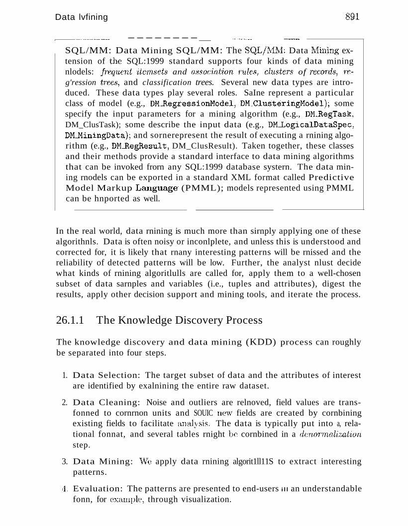
Data lvfining
--------_ __------
891
SQL/MM: Data Mining SQL/MM: The SQLfMtvi: Data IViining extension of the SQL:1999 standard supports four kinds of data miningnlodels: frequent itenLsets and associat'ion 'rules, clusters of records, reg'ression tn~es, and classification trees. Several new data types are introduced. These data types play several roles. SaIne represent a particularclass of model (e.g., DM~egressibnMod.el,D}JLClusteringModel); somespecify the input parameters for a mining algorithm (e.g., DM-RegTask,DM_ClusTask); some describe the input data (e.g., DM..LogicalDataSpec,DM-MiningData); and sornerepresent the result of executing a rnining algorithm (e.g., DM....RegResult, DM_ClusResult). Taken together, these classesand their methods provide a standard interface to data mining algorithmsthat can be invoked frorn any SQL:1999 database systern. The data mining rnodels can be exported in a standard XML format called PredictiveModel Markup Language (PMML); models represented using PMMLcan be hnported as well.
In the real world, data rnining is much more than sirnply applying one of thesealgorithnls. Data is often noisy or inconlplete, and unless this is understood andcorrected for, it is likely that rnany interesting patterns will be rnissed and thereliability of detected patterns will be low. Further, the analyst nlust decidewhat kinds of rnining algoritlulls are called for, apply them to a well-chosensubset of data sarnples and variables (i.e., tuples and attributes), digest theresults, apply other decision support and mining tools, and iterate the process.
26.1.1 The Knowledge Discovery Process
The knowledge discovery and data mining (KDD) process can roughlybe separated into four steps.
1. Data Selection: The target subset of data and the attributes of interestare identified by exalnining the entire raw dataset.
2. Data Cleaning: Noise and outliers are relnoved, field values are transfonned to cornrnon units and SOUIC l1C\V fields are created by cornbiningexisting fields to facilitate a,nalysis. The data is typically put into a, relational fonnat, and several tables rnight be cornbined in a denoTTnal'izationstep.
3. Data Mining: \Ve apply data rnining algorit1ll11S to extract interestingpatterns.
4. Evaluation: The patterns are presented to end-users ill an understandablefonn, for ex<unple, through visualization.
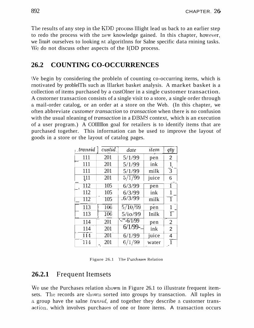
892 CHAPTER. 2&
1"he results of any step in the I<:DD proce:ss lllight lead us back to an earlier stepto redo the process with the ne\v knowledge gained. In this chapter, however,we lilnit ourselves to looking at algoritlnns for SaIne specific data rnining tasks.\¥e do not discuss other aspects of the I(DD process.
26.2 COUNTING CO-OCCURRENCES
\Ve begin by considering the probleln of counting co-occurring iterns, which isrnotivated by problelTIs such as lllarket basket analysis. A market basket is acollection of items purchased by a custOlner in a single customer transaction.A cnstorner transaction consists of a single visit to a store, a single order througha mail-order catalog, or an order at a store on the Web. (In this chapter, weoften abbreviate customer transaction to transaction when there is no confusionwith the usual nleaning of transaction in a DBlVlS context, which is an executionof a user program.) A COIIlIllon goal for retailers is to identify items that arepurchased together. This inforrnation can be used to improve the layout ofgoods in a store or the layout of catalog pages.
I .·transid ·1 c1tstidl date item .. ··l.qtyl5/1/99
.•111 201 pen 2
1'-'
5/1/99 ink111 201 15/1/99 milk
-'-111 201 3111 201 5/1l9'9 juice 6_ .••.
-"-
112 105 6/3/99 pen 1-_•.6/3/99112 105 ink 1
" "., ..._-112 105 ....6/3/99 milk 1-_ ....
r t~~5/10'/99
.- ..113 pen 1113 5/io/99 Inilk
..._-1
.....'·-"'-6/1/99 ....-
114 201 pen 2. ...._.. 6/1/99-.....114 201 ink 2
f--_.._- ...
114 201 6/1/99 juice 4,......-...__.
6/1/99---
114 201 water 1. "- ... ....-
Figure 26.1 'I'he Purcha'3es Relation
26.2.1 Frequent Itemsets
'vVe use the Purchases relation shovvn in Figure 26.1 to illustrate frequent itemsets. rrhe records are shoVi.rn sorted into groups by transaction. All tuples ina group have the saIne tr-ansid, and together they describe a custorner transaction, which involves purcha..ses of one or Inore iterns. A transaction occurs
Data lvlin'ing 893
on a given date, and the nanle of each purcha..lSed itenl is recorded, along \viththe purella,sed quantity. ()bserve that there is redundancy in Purchases: It canbe decolnposed by storing tTansid"c"lJ,8l'i,d~~date triples in a separate table anddropping c'lud'id and date froln Purchases; this nlay be ho\v the data is actuallystored. Hc)\vever, it is convenient to consider the Purcha..ses relation, as shov.rnin Figure 26.1, to corupute frequent iternsets. Creating such "denonnalized'tables for ease of data rnining is cOIIllllonly done in the data cleaning step ofthe I(DD process.
By ex<:unining the set of transaction groups in Purcha,..~es, we can rnake observations of the fornl: "In 751() of the transactions a pen and ink are purchasedtogether." rrhis stateulent describes the transactions in the database. Extrapolation to future transactions should be done with caution, as discussed inSection 26.3.6. Let us begin by introducing the terminology of rnarket basketanalysis. An itemset is a set of itelTIS. The support of an itelnset is the fraction of transactions in the database that contain all the iterus in the iterllset.In our exaIupl.e, the itelllset {pen, ink} has 75% support in Purchases. We cantherefore conclude that pens and ink are frequently purchased together. If weconsider the itelllset {milk, juice}, its support is only 25%; milk and juice arenot purchased together frequently.
Usually the nUlnber of sets of itenlS frequently purchased together is relativelysInall, especially as the size of the itenlsets increases. We are interested inall iterllsets whose support is higher than a user-specified minimUIl1 supportcalled m,insnp; we call such itemsets frequent itemsets. For exarnple, if theIIlinirl1Unl support is set to 70%, then the frequent iterllsets in our exampleare {pen}, {ink}, {nlilk}, {pen, ink}, and {pen, 111ilk}. Note that we arealso interested in iternsets that contain only a single iteru since they identifyfrequently purchased iterl1s.
\Ve show an algorithrn for identifying frequent iterllsets in Figure 26.2. Thisalgorithrn relies on a sirnple yet fundarnentaJ property of frequent iterIlsets:
The a Priori Property: Every subset of a frequent iterllset is also afrequent itelnset.
'fhe algorithnl proceeds iteratively, first identifying frequent iterIlsets 'with justone itcrll. In Bach subsequent iteration, frequent iterl1sets identified in theprevious iteration are extended with another itern to generate larger candidateitcrnsets. By considering only iterllsets obtained by enlarging frequent iternsets,we greatly reduce the nurnber of candidate frequent itcrllsets; this optirnizationis crucial for efficient execution. ~rhe a priori property guarantees that thisoptilnizatic)ll is correct; that is, \ve do not Iniss any frequent iterllsets. A singlescan of all trans(l,(tions (the Pllrchas(~s relation in our exarnple) suffices to
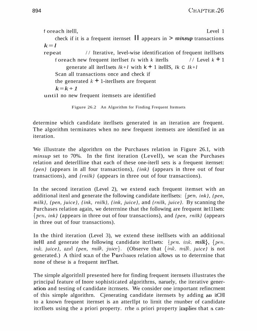
894
f oreach itelll, Level 1check if it is a frequent iternset II appears in > 'rnins'l1,p transactions
k=lrepeat / / Iterative, level-wise identification of frequent itelllsets
f oreach new frequent iterllset I k with k iterlls / / Level k + 1generate all iterl1sets lk+l with k + 1 itelllS, lk C Ik+l
Scan all transactions once and check ifthe generated k + 1-iterIlsets are frequentk=k+1
until no new frequent itemsets are identified
Figure 26.2 An Algorithm for Finding Frequent Itemsets
determine which candidate iterllsets generated in an iteration are frequent.The algorithm terminates when no new frequent itemsets are identified in aniteration.
'We illustrate the algorithrn on the Purchases relation in Figure 26.1, withminsup set to 70%. In the first iteration (Levell), we scan the Purchasesrelation and deterllline that each of these one-iterll sets is a frequent iternset:{pen} (appears in all four transactions), {ink} (appears in three out of fourtransactions), and {rnilk} (appears in three out of four transactions).
In the second iteration (Level 2), we extend each frequent itemset with anadditional itenl and generate the following candidate iterIlsets: {pen, ink}, {pen,milk}, {pen, juice}, {ink, rnilk}, {ink, juice}, and {rnilk, juice}. By scanning thePurchases relation again, we deterrnine that the following are frequent ite111sets:{pen, ink} (appears in three out of four transactions), and {pen, rnilk} (appearsin three out of four transactions).
In the third iteration (Level 3), we extend these itelllsets with an additionaliteHl and generate the following candidate itcrl1sets: {pen, ink, nl/ilk} , {pen,ink, juice}, and {pen, rnilk, fuice}. (Observe that fink, rnilk, juice} is notgenerated.) A third sca.n of the Pllrchc1E,es relation aJlows us to deterrnine thatnone of these is a frequent iterTlset.
The sirnple algoritlnll presented here for finding frequent iternsets illustrates theprincipal feature of Inore sophisticated algorithrns, naruely, the iterative generation and testing of candidate itcrnsets. vVe consider one irnportant refincrnentof this sirnple algorithrn. Cjenerating candidate iternsets by adding an itCHlto a known frequent iternset is an atterIlpt to lirnit the rnunber of candidateitcrIlsets using the a priori property. rrhe a priori property ~rnplies that a can-
Data lvJining 89p
dida,te iternset can be frequent only if all its subsets are frequent. Thus, we canreduce the nUlnber of candidate iternsets further··..··--a priari, or before scanningthe PurchEhses databaBe··........_·by checking whether all subsets of a newly generatedcandidate itcIIlset are frequent. Only if all subsets of a candidate iternset arefrequent do we cOlnpute its support in the subsequent databa'3c scan. COlnpared to the sirnple algoritlun, this refined algoritlull generates fewer candidateitenlsets at each level and thus reduces the arnount of conlputation perfonnedduring the database scan of Purchases.
Consider the refined algorithrn on the PurchclSes table in Figure 26.1 withrn:inStlp= 70%. In the first iteration (Level 1), we deterrnine the frequent itemsets of size one: {pen}, {ink}, and {ntilk}. In the second iteration (Level 2),only the following candidate itemsets rernain when scanning the Purchases table: {pen, ink}, {pen, 'm-ilk} , and {ink, rnilk}. Since {juice} is not frequent, theiterllsets {pen, juice}, {ink, juice}, and {rnilk, juice} cannot be frequent as welland we can elirninate those iterIlsets a priori, that is, without considering therllduring the subsequent scan of the Purchases relation. In the third iteration(Level 3), no further candidate itemsets are generated. The iternset {pen, ink,m,ilk} cannot be frequent since its subset {ink, milk} is not frequent. Thus, theirnproved version of the algorithrll does not need a third scan of Purchases.
26.2.2 Iceberg Queries
We introduce iceberg queries through an exaillple. Consider again the Purchases relation shown in Figure 26.1. Assurne that we want to find pairs ofcustorners and iterns such that the custorner has purchased the item rllore thanfive thnes. We can express this query in SQL as follows:
SELECTFROMGROUP BYHAVING
P.custid, P.itern, SUM
Purch~h"es PP.custid, P.iternSUM (P.qty) > 5
(P.qty)
rrhink about how this query would be evaluated by a relational DBMS. Conceptually, for each (c'usLid, 'itcrn) pair, we need to check whether the surn of theqty field is greater than 5. One approach is to rnake a scan over the Purchasesrelation and rnaintain running surns for each (c'Ustid, itern) pair. T'his is a feasible execution ,strategy a.s long as the nurnber of pairs is sruaU enough to fitinto lIlain rncIIlory. If the nurnber of pairs is larger than rnain Inernory, lnorcexpensive query evaluation plans,\vhich involve either sorting or hashing, haveto be used.
The query has an irnporta"nt property not exploited by the preceding executionstrategy: Even though the Purcha..'3cs relation is potentially very large and the
896 (;HAP'TER26
nurnber of (cltstid, 'itern) groups CaJl be huge, the Cyutput of the query is likely tobe relatively sInall because of the condition in the HAVING clause. ()nly groupswhere the custorner ha..9 pnrchaEied the itCHl Inure than five tiInes appear in theoutput. fihr exarllple, there are nine groups in the query over the Purcha.'3esrelation ShOVlll in Figure 26.1, although the output contains only three records.The nurnber of groups is very large, but the answer to the query---·-the tip ofthe iceberg------is usually very sInan. Therefore, ,ve call such a query an icebergquery. In general, given a relational scherna H. with attributes A.1. A 2, ... "Ak, and B and an aggrega,tion function aggr, an iceberg query has the follo\vingstructure:
SELECTFROMGROUP BYHAVING
R.Al, Il.A2, ... , R,.Ak, aggr(R.B)H,elation H,R,.AI, ... , R.Akaggr(ILB) >= constant
Traditional query plans for this query that use sorting or hashing first cornputethe value of the aggregation function for all groups and then elirninate groupsthat do not satisfy the condition in the HAVING clause.
Cornparing the query with the probleur of finding frequent itenlsets discussed inthe previous section, there is a striking sirnilarity. Consider again the Purchasesrelation shown in Figure 26.1 and the iceberg query froIn the beginning of thissection. We are interested in (custid, itern) pairs that have SUM (P.qty) > 5.lJsing a variation of the a priori property, we can argue that we only have toconsider values of the c'Ust'id field where the custorner has purchased at leastfive it-eurs. We can generate such iterns through the following query:
SELECTFROMGROUP BYHAVING
P.cllstidPurchases PP.cllstidSUM (P.qty) > 5
Sirnilarly, we can restrict the candidate values for theitern field through thefollowing query:
SELECTFROMGROUP BYHAVING
P.iternPurchases PP.iteulSUM (P.qty) > 5
If \ve restrict th(~ corrlputation of the original ic(~berg query to (C'a8t'id~ 'itern)groups \vhe1'e the field values aTe in the output of the previous t\VO queries,vve elirninate a large nUlllber of (c''lJ,stid1 'ite1n) pElirs a priori. So, a possible
897
evaluation strategy is to first COlnpute candidate values for the C'tlstid and 'itcTnfields, and use eornbinations of only these values in the evaluation of the originaliceberg query. '~!e first generate candidate field values for individual fields anduse only those values that survive the a priori pruning step as expressed inthe t,vo previous queries. 'Thus, the iceberg query is arnenable to the salIlebottorn-up evaluation strategy used to find frequent iternsets. In particular, \vecan use the a priori property a.'s follovls: vVe keep a counter for a group only ifeach individual cOlnponent of the group satisfies the condition expressed in theHAVING clause. The perfonnance irnprovernents of this alternative evaluationstrategy over traditional query plans can be very significant in practice.
Even though the botto111-UP query processing strategy elinlinates lnany groupsa priori, the nlunber of (c1lstid, itern) pairs can still be very large in practice;even larger than Inain lllernory. Efficient strategies that use sall1pling and llloresophisticated hashing techniques have been developed; the bibliographic notesat the end of the chapter providt~ pointers to the relevant literature.
26.3 MINING FOR RUI~ES
Many algorithrIls have been proposed for discovering various fonns of rules thatsuccinctly describe the data. We now look at some widely discussed fonns ofrules and algorithnls for discovering thenl.
26.3.1 Association Rules
We use the Purcha.ses relation shown in Figure 26.1 to illustrate ck'3sociationrules. By eXcl1nining the set of transactions in Purchc1..ses, we can identify rulesof the forrn:
{pen} =? {ink}
This rule should be read as follows: "If a pen is pUfcha.sed in a transaction, it islikely that in}( is also be purchased in that transaction.'~ It is a staternent thatdescribes the transactions in the databa.se; extrapolation to future tranSctctionsshould be done \vith caution, ChS discussed in Section 26.~3.6. More generally,an association rule has the forIn LJIS::::} RHS, where both LIIS andRJIS'are sets of iterns. The interpretation of such a, rule is that if every itern inLIIS is purchased in a transaction, then it is likely that the iterIlS in IlllS arepurcha",sed as well.
rThere are hvo irnportEtnt rnecl,sures for (1,n association rule:
IIIl Support: The support for a set of iterns is the percentage of transa,ctionsthat contain all these iterIls. rl~he support for a rule LIIS =} J~llS is the
898 C]HAPTER b6
support for the set of itenlS LHS Rf!S. For exalnple, consider the rule{pen} =:> {ink}. The support of this rule is the support of the itenlset {pen,ink}, which is 75%.
• Confidence: Consider transactions that contain all iterIls in LHS. Theconfidence for a rule LlIS =? RHS is the percentage of such transactionsthat also contain all iterIls in RHS. More precisely, let S1lp(LHS) be thepercentage of transactions that contain LllS and let s'up(LliS U RHS) bethe percentage of transactions that contain both LllS and RHS. rrhen theconfidence of the rule LHS => RHS is sup(LHSU RIIS) / sup(LHS). Theconfidence of a rule is an indication of the strength of the rule. As anexalnple, consider again the rule {pen} =? {ink}. The confidence of thisrule is 75%; 75% of the transactions that contain the itenlset {pen} alsocontain the iternset {ink}.
26.3.2 An Algorithm for Finding Association Rules
A user can ask for all association rules that have a specified minimum support(minsvp) and mininlum confidence (rninconf) , and various algorithrns havebeen developed for finding such rules efficiently. These algorithms proceedin two steps. In the first step, all frequent itemsets with the user-specifiedminimum support are computed. In the second step, rules are generated usingthe frequent itemsets as input. We discussed an algorithm for finding frequentiternsets in Section 26.2; we concentrate here on the rule generation part.
Once frequent iteulsets are identified, the generation of all possible candidaterules with the user-specified minirnum support is straightforward. Consider afrequent iternset X with support sx identified in the first step of the algorithrn.To generate a rule fronl X, we divide X into two iternsets, LHS and RJIS. Theconfidence of the rule LllS =} RHS is Sx / SLlIS, the ratio of the support of Xand the support of LHS. Frorn the a priori property, we know that the supportof LllS is larger than rninsup, and thus we have C0111puted the support of L1ISduring the first step of the algoritlnn. \rYe can cornpute the confidence valuesfor the candidate rule by calculating the ratio support(X)/support(LlIS) andthen check how the ratio cornpares to 'Tnincon!
In general, the expensive step of the algorithnl is the cornputation of the frequent itenlsets, and lnany different algorithrns have been developed to perfonnthis step efficiently. R,ule generation .... given that all frequent itcrl1sets havebeen identified·.....·..····is straightforward.
In the rest of this section, we discuss SOlne generalizations of the problern.
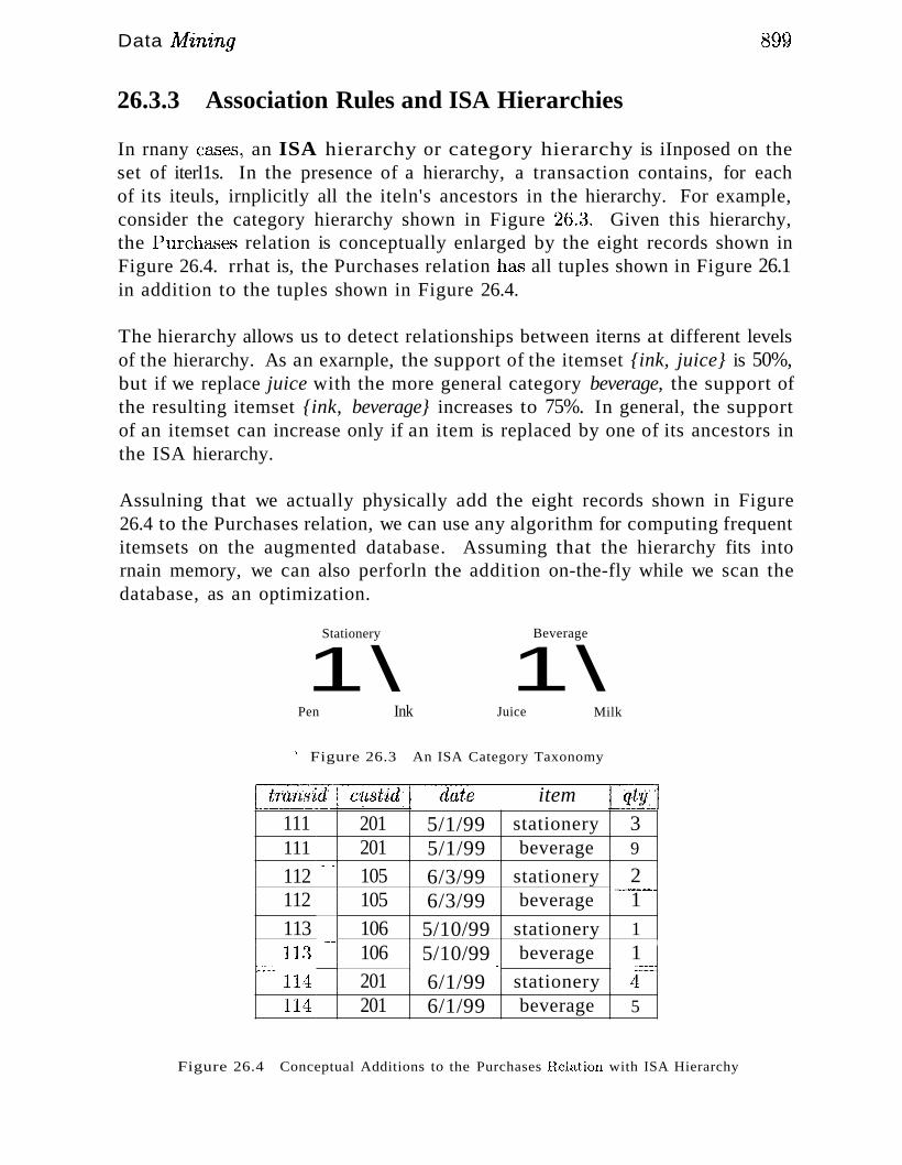
Data !vfin>ing
26.3.3 Association Rules and ISA Hierarchies
89Q
In rnany ca.'3es, an ISA hierarchy or category hierarchy is iInposed on theset of iterl1s. In the presence of a hierarchy, a transaction contains, for eachof its iteuls, irnplicitly all the iteln's ancestors in the hierarchy. For example,consider the category hierarchy shown in Figure 26.3. Given this hierarchy,the Purcha.,es relation is conceptually enlarged by the eight records shown inFigure 26.4. rrhat is, the Purchases relation has all tuples shown in Figure 26.1in addition to the tuples shown in Figure 26.4.
The hierarchy allows us to detect relationships between iterns at different levelsof the hierarchy. As an exarnple, the support of the itemset {ink, juice} is 50%,but if we replace juice with the more general category beverage, the support ofthe resulting itemset {ink, beverage} increases to 75%. In general, the supportof an itemset can increase only if an item is replaced by one of its ancestors inthe ISA hierarchy.
Assulning that we actually physically add the eight records shown in Figure26.4 to the Purchases relation, we can use any algorithm for computing frequentitemsets on the augmented database. Assuming that the hierarchy fits intornain memory, we can also perforln the addition on-the-fly while we scan thedatabase, as an optimization.
Stationery
1\Beverage
1\Pen Ink Juice Milk
, Figure 26.3 An ISA Category Taxonomy
item111 201 5/1/99 stationery 3111 201 5/1/99 beverage 9
- .6/3/99112 105 stationery 26/3/99
..._..-.-112 105 beverage 1113 106 5/10/99 stationery 1
----5/10/99 beverage11~3 106 1
':::;::--"- - ..._._----114 201 6/1/99 stationery 11114 201 6/1/99 beverage 5
Figure 26.4 Conceptual Additions to the Purchases Relation with ISA Hierarchy
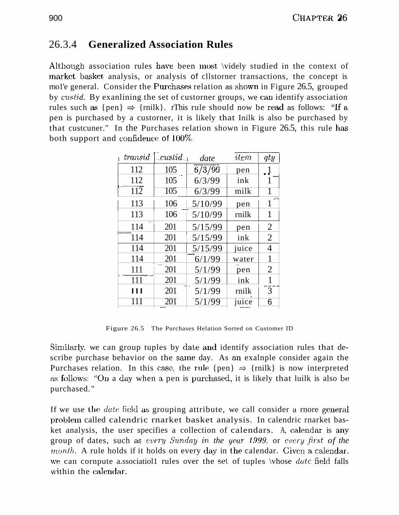
900 C~HAPTER 26
26.3.4 Generalized Association Rules
Although association rules have been rnost \videly studied in the context ofrnarket basket analysis, or analysis of cllstorner transactions, the concept isrno1'e general. Consider the Purcha.ges relation as sh()\vn in Figure 26.5, groupedby c'Ust'id. By exanlining the set of custorner groups, we can identify associationrules such as {pen} ::::} {rnilk}. rThis rule should now be read as follows: "If apen is purchased by a custorner, it is likely that Inilk is also be purchased bythat custcuner." In the Purchases relation shown in Figure 26.5, this rule ha.sboth support and c()nfidE~nce of 1000/(-).
I transid. I···. c'Ustid .. .1 date112 105 '6'73/99 pen 1
..•6/3/99 "-112 105 ink 1
f------------
112 105 6/3/99 milk 15/10/99
.....:::..
113 106 pen 1.........
5/10/99 rnilk113 106 1_....
5/15/99114 201 pen 2-" 5/15/99 ink114 201 2
114 201 5/15/99 juice 4_..
114 201 6/1/99 water 1- ...._...
5/1/99,.,~.....
111 201 pen 2~-._._.
5/1/99111 201 ink 1- _. ----
III 201 5/1/99 rnilk 3-
111 201 5/1/99 juice 6._-- .......................
Figure 26.5 The Purchases Helation Sorted on Customer ID
SiInilctrly, we can group tuples by date and identify association rules that describe purchase behavior on the SeHne day. As an exalnple consider again thePurchases relation. In this case, the rule {pen} =} {rnilk} is now interpretedas follc)\vs: "On a da.y when a pen is purclut.sed, it is likely that luilk is also bepurchased."
If we use the date field ct.s grouping attribute, we call consider a rnore genenllprolJlern called calendric rnarket basket analysis. In calendric rnarket basket analysis, the user specifies a collection of calendars. A, calendar is anygroup of dates, such as every l..9v,rulay 'iTt the yeaT 1.999, or eucTy fiT8t of the'fnonth. A rule holds if it holds on every day in the calendar. Civen a calendar.we can cornpute a.ssociatiol1 rules over the set of tuples \vhose date field falls\vithin the c:alendar.
90,1
By specifying interesting calendars, 'we can identify rules that rnight not haveenough support and confidence \vith respect to the entire datahase but haveenough support and confidence on the subset of tuples that fall \vithin thecalendar. On the other hand, even though a rule rnight have enough supportand confidence \vith respect to the c0l11plete database, it Inight grtin its supportonly £'1'0111 tuples that fall within a calendar. In this case, the support of therule over the tuples within the calendar is significantly higher than its supportwith respect to the entire database.
As an exarnple, consider the Purchases relation with the calendar every first ofthe m,onth. \Vithin this calendar, the association rule pen:::;. ju:ice has supportand confidence of 100%, \vhere&'3 over the entire Purcha.ses relation, this ruleonly has 50% support. On the other hand, within the calendar, the rule pen=> m,ilk; has support of confidence of 50%, wherca'3 over the entire Purch&'3esrelation it has support and confidence of 75%.
More general specifications of the conditions that rIlust be true within a groupfor a rule to hold (for that group) have also been proposed. We rnight want tosay that all items in the LHS have to be purchased in a quantity of less thantwo itelTIS, and all itenls in the RHS rnust be purchased in a quantity of morethan three.
lJsing different choices for the grouping attribute and sophisticated conditionsas in the preceding exarnples, we can identify rules Inore cornplex than thebasic association rules discussed earlier. These Inore cornplex rules, nonetheless,retain the essential structure of an association rule as a condition over a groupof tuples, with support and confidence rneasures defined c1..'3 usual.
26.3.5 Sequential Patterns
Consider the Purchases relation sho\vn in Figure 26.1. Each group of tuples,having the sarne c'l18tid value, can be thought of clS a sequence of trans~tctions
ordered by date. rrhis allo¥ls us to identify frequently arising buying patternsover tirne.
vVe begin b,Y introducing the concept of a sequence of itel11sets. Each transaction is represeqted by a set of tuples, and by looking at the values in the iterncolurnn, \ve get a set of iterns purchased in that transaction. 1'here£o1'e, thesequence of transactions associated \vith a cllstorner corresponds naturally toa sequence of itelnsets rnlrchELsed by the custorner. For exalnplc, the sequenceof purc!HL'3CS for cllstorner 201 is ({pen, ink, 'tn-ilk, juice}, {pen, 'iT/jIG, In'ice}).
902 CHAPTER 2t6
A subsequence of a sequence of iternsets is obtained by deleting one or 11101'eitcrnsets, and is also a sequence of itenlsets. We say that a sequence (aI, ... , arn )
is contained in another sequence S if S has a subsequence (b t , ... ,bIn) such thata'i C bi , for 1 < 'i < rn. Thus, the sequence {{pen,}, {ink, rnilk} , {pen" ju'ice}) iscontained in ({pen, link}, {shir·t} , {ju'ice, ink, m,ilk} , {juice, pen, rn'ilk}) . Notethat the order of itenlS within ectCh iterllset does not rnatter. However, theorder of iterllsets does lllatter: the sequence ({pen}, {ink, rn'ilk} , {pen, flL'ice})is not contained in ({pen, 'ink}, {shirt}, {juice, pen, rnilk} , {juice, nLilk, 'ink}).
The support for a sequence S of iternsets is the percentage of custorner sequences of which 8 is a subsequence. The problenl of identifying sequentialpatterns is to find all sequences that have a user-specified rllinimurll support.A sequence (aI, a2, a3, ... ,am) with minimurn support tells us that custornersoften purchase the itelns in set al in a transaction, then in sonle subsequenttransaction buy the itcrlls in set a2, then the items in set a3 in a later transaction, and so on.
Like association rules, sequential patterns are staternents about groups of tuplesin the current database. Cornputationally, algorithms for finding frequentlyoccurring sequential patterns resernble algorithrns for finding frequent itemsets.Longer and longer sequences with the required rninirnum support are identifiediteratively in a nlanner very similar to the iterative identification of frequentiternsets.
26.3.6 The Use of Association Rules for Prediction
Association rules are widely used for prediction, but it is inlportant to recognize that such predictive use is not justified without additional analysis ordornain knowledge. Association rules describe existing data accurately but canbe rnisle::1ding when used naively for prediction. For exaruple, consider the rule
{pen} => {ink}
The confidence a"ssociated with this rule is the conditional probability of an inkpurchase given a pen purcha...se over the given database; that is, it is a descriptiverueasure. We rnight use this rule to guide future sales prornotions. For exalllple,\ve rnight offer a discount on pens to increase the sales of pens and, therefore,aIso increase sales of ink.
Flowever, such a prorllotion ct.'3SU1l1CS that pen purchases are good indicatorsof ink purchases in future custC)Iuer transactions (in addition to transactionsin the current database). This a..ssurnption is justified if there is a cav,8al hnkbetween pen purchases and ink purcha.,scs; that is, if buying pens causes thebuyer to also buy ink. Ifowever,we can infer a,,')sociation rules\vith high support
Data w!'ining 903
and confidence in SOlnc situations \\There there is no causal link between L118and RIIS. For exarnple, suppose that pens are ahvays purchased together withpencils, perhaps because of customers' tendency to order writing instrulllentstogether. vVe would then infer the rule
{pencil} =? {ink}
with the saBle support and confidence as the rule
{pen} :::} {ink}
However, there is no causal link between pencils and ink. If we prornote pencils,a custolner who purchases several pencils due to the pronlotion has no rea..sonto buy Inore ink. Therefore, a sales prolnotion that discounted pencils in orderto increase the sales of ink would fail.
In practice, one would expect that, by exallllnlng a large database of pasttransactions (collected over a long tirne and a variety of circumstances) andrestricting attention to rules that occur often (i.e., that have high support),we rninirnize inferring lnisleading rules. However, we should bear in rnind thatnlisleading, noncausal rules lnight still be generated. Therefore, we shouldtreat the generated rules as possibly, rather than conclusively, identifying causalrelationships. Although association rules do not indicate causal relationshipsbetween the LHS and RHS, we elllphasize that they provide a useful startingpoint for identifying such relationships, using eithE~r further analysis or a dornainexpert's judgrnent; this is the reason for their popularity.
26.3.7 Bayesian Networks
Finding causal relationships is a challenging task, as we saw in Section 2G.3.6.In general, if certain events are highly correlated, there are rnany possibleexplanations. f""'cH' exalnple, suppose that pens, pencils, and ink are purchasedtogether frequently. It rnight be that the purchase of one of these itelIlS (e.g.,ink) depends causally on the purchase of another itern (e.g., pen). ()r it Blightbe that the purchase of one of these iterns (~.g., pen) is strongly correlated withthe purchase of another (e.g., pencil) because of sorne underlying phenornenon(e.g., users' tendency to think about \vriting instrulnents together) that causallyinfluences both purchcL.':'cs. IIc)\v can we identify the true causal relationshipsthat hold between these events in the real world?
One approach is to consider each possible cOlnbination of causal relationshipsarnong the varial)les or events of interest to us and evaluate the likelihood ofeach cornbination on the basis of the data el,vail::l,ble to us. If we think of ceLehcornbination of causal relationships as a rnodel of the real world underlying the
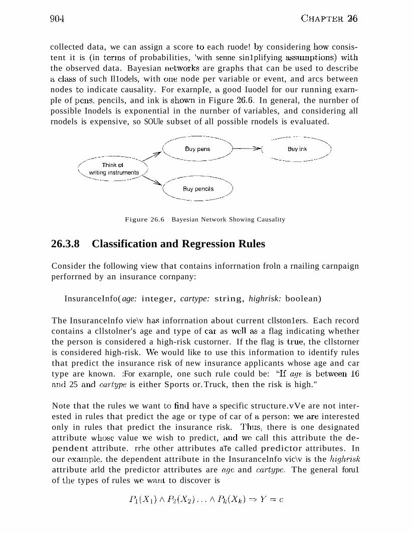
904 CHAPTER ~6
collected data, we can assign a score to' each ruode! by considering ho\v consistent it is (in tenns of probabilities, 'with senne sin1plifying assuInptions)\viththe observed data. Bayesian nebNorks are graphs that can be used to describea ChlSS of such Il1odels, with one node per variable or event, and arcs betweennodes to indicate causality. For exarnpIe, a good Iuodel for our running exarnpIe of pens, pencils, and ink is sho\vn in Figure 26.6. In general, the nurnber ofpossible Inodels is exponential in the nurnber of variables, and considering allrnodels is expensive, so SOUle subset of all possible rnodels is evaluated.
Figure 26.6 Bayesian Network Showing Causality
26.3.8 Classification and Regression Rules
Consider the following view that contains inforrnation froln a rnailing carnpaignperforrned by an insurance cornpany:
InsuranceInfo( age: integer, cartype: string, highrisk: boolean)
The Insurancelnfo vie\v ha..." inforrnation about current cllston1ers. Each recordcontains a cllstolner's age and type of ear as ,veIl as a flag indicating whetherthe person is considered a high-risk custorner. If the flag is true, the cllstorneris considered high-risk. vVe would like to use this information to identify rulesthat predict the insurance risk of new insurance applicants whose age and cartype are known. :For exarnple, one such rule could be: "If age is bet\veen IGand 25 a.n.d caTtypc is either Sports or.Truck, then the risk is high."
Note that the rules we want t.o find have a specific structure.vVe are not interested in rules that predict the age or type of car of a person: "\ve are interestedonly in rules that predict the insurance risk. T'hus, there is one designatedattribute vvhose value we wish to predict, and\ve call this attribute the dependent attribute. rrhe other attributes aTe called predictor attributes. Inour exarnple, the dependent attribute in the Insurancelnfo vic\v is the highriskattribute arld the predictor attributes are age and cartype. The general foru1of the types of rules \ve \Vcl,nt to discover is
Data i\{ining 90~
The predictor attributes Xl, ... ,")(k are used to predict the value of the dependent attribute}"". Both sides of a rule can be interpreted as conditions on fieldsof a tuple. The Pi (Xi) are predicates that involve attribute ..gi. The fornl ofthe predicate depends on the type of the predictor attribute. \rVe distinguishtwo types of attributes: numerical and categoricaL For numerical attributes,we can perfOrIn nurnerieal cornputations, such EL'3 cornputing the average of t\VOvalues; whereas for categorical attributes, the only allowed operation is testing "\vhether two values are equal. In the InsuranceInfo view, age is a nUlllericalattribute whereas cartype and highrisk are categorical attributes. Returning tothe forrn of the predicates, if Xi, is a nUlllerical attribute, its predicate Pi, isof the forln l'i < Xi < hi; if ..)(i is a categorical attribute, Pi is of the forIllX'i E {Vl, ... ,Vj}.
If the dependent attribute is categorical, we call such rules classification rules.If the dependent attribute is nurnerical, we call such rules regression rules.
For exarnple, consider again our exaInple rule: "If age is between 16 and 25and caTtype is either Sports or Truck, then highr-i8k is true." Since highrisk is acategorical attribute, this rule is a classification rule. We can express this rulefonnally as follows:
(16 < age < 25) /\ (car-type E {Sports, Truck}) ===? highri8k = true
We can define support and confidence for classification and regression rules, asfor association rules:
III Support: ffhe support for a condition C is the percentage of tuples thatsatisfy C. The support for a rule G'11===? C:2 is the support for the conditionCI/\ C2.
III Confidence: Consider those tuples that satisfy condition (71. The confidence for a rule Cl =} G'12 is the percentage of such tuples that also satisfycondition (;2.
As a further generalization, consider 1,118 right-hand side of a classification orregression rule: y~ =. c..Each rule predicts a v,lJue of Y- for a given tuple basedon the vaJues of predictor attributes Xl, ... ,Xk. \Ve can consider rules of thefonn
where f is sonlC function. VVe do not discuss such rules further.
Classification H,1l<1 regression rules differ fr0111 clssociation rules by consideringcontinuous and categorical fields, rather than only one field that is set-valued.Identifying such rules efficiently presents a ne\v set of challenges; vve do not
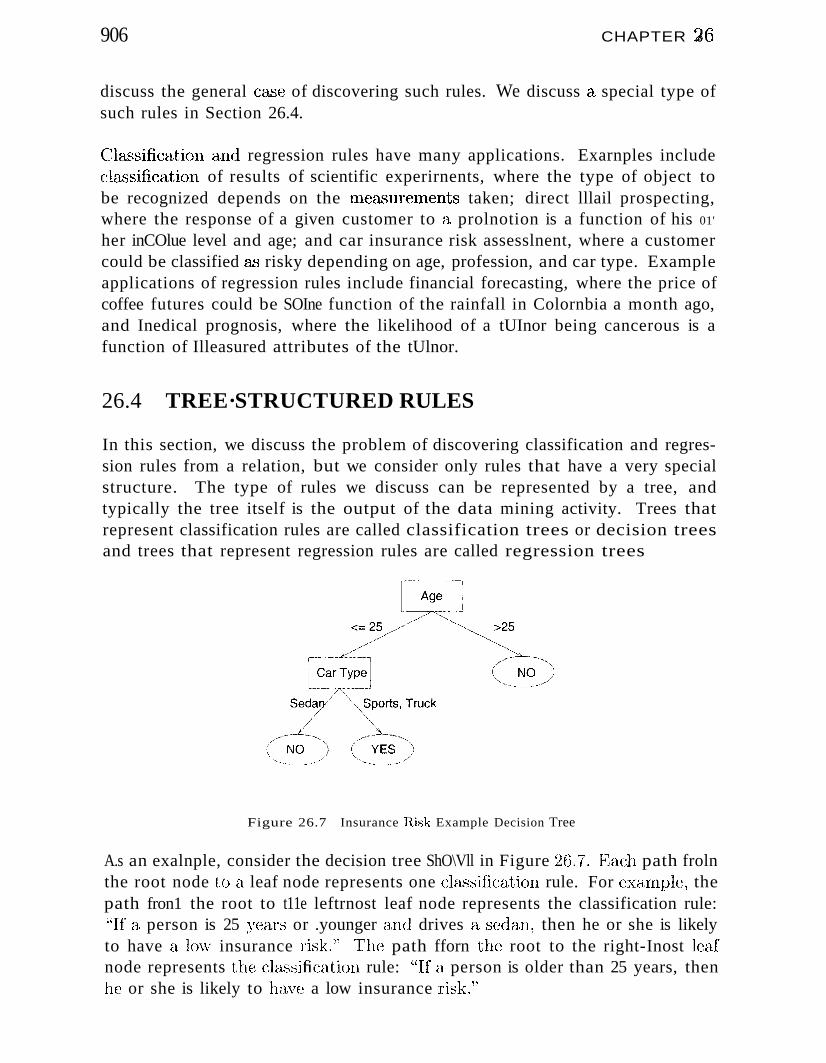
906 CHAPTER 26
discuss the general case of discovering such rules. We discuss a special type ofsuch rules in Section 26.4.
Cla.-ssification and regression rules have many applications. Exarnples includeela'3sification of results of scientific experirnents, where the type of object tobe recognized depends on the InCa'3Urernents taken; direct lllail prospecting,where the response of a given customer to a prolnotion is a function of his 01'
her inCOlue level and age; and car insurance risk assesslnent, where a customercould be classified as risky depending on age, profession, and car type. Exampleapplications of regression rules include financial forecasting, where the price ofcoffee futures could be SOIne function of the rainfall in Colornbia a month ago,and Inedical prognosis, where the likelihood of a tUInor being cancerous is afunction of Illeasured attributes of the tUlnor.
26.4 TREE·STRUCTURED RULES
In this section, we discuss the problem of discovering classification and regression rules from a relation, but we consider only rules that have a very specialstructure. The type of rules we discuss can be represented by a tree, andtypically the tree itself is the output of the data mining activity. Trees thatrepresent classification rules are called classification trees or decision treesand trees that represent regression rules are called regression trees
Figure 26.7 Insurance lUsk Example Decision Tree
A.s an exalnple, consider the decision tree ShO\Vll in Figure 2G.7. Each path frolnthe root node ti) a leaf node represents one claBsification rule. For exa,rnplc, thepath fron1 the root to t11e leftrnost leaf node represents the classification rule:"If a person is 25 y(~a,rs or .younger and drives a sedan, then he or she is likelyto have a lo\v insurance risk." ~rhe path fforn the root to the right-Inost leafnode represents tlle cla,,':)sification rule: "If a person is older than 25 years, thenhe or she is likely to have a low insurance risk."
Data JvIin'ing 907
Tree-structured rules are very popular since they are easy to interpret. E<l.'3e ofunderstanding is very hllportant because the result of any data rninillg activityneeds to be cOlllprehensible by nonspecialists. In addition, studies have shownthat, despite Ihnitations in structure, trCt'-structured rules are very accurate.There exist efficient algorithrl1s to construct tree-structured rules fronl largedatabases. vVe discuss a sample algorithrIl for decision tree construction in therernainder of this section.
26.4.1 Decision Trees
A decision tree is a graphical representation of a collection of classificationrules. Given a data record, the tree directs the record frOIn the root to aleaf. Each internal node of the tree is labeled with a predictor attribute. Thisattribute is often called a splitting attribute, because the data is 'split' basedon conditions over this attribute. The outgoing edges of an internal node arelabeled with predicates that involve the splitting attribute of the node; everydata record entering the node must satisfy the predicate labeling exactly oneoutgoing edge. T'he cornbined information about the splitting attribute andthe predicates on the outgoing edges is called the splitting criterion of thenode. A node with no outgoing edges is called a leaf node. Each leaf node ofthe tree is labeled with a value of the dependent attribute. We consider onlybinary trees where internal nodes have two outgoing edges, although trees ofhigher degree are possible.
Consider the decision tree shown in Figure 26.7. The splitting attribute of theroot node is age, the splitting attribute of the left child of the root node iscar-type. The predicate on the left outgoing edge of the root node is age :s; 25,the predicate on the right outgoing edge is age> 25.
"'e can no\v aBsociate a classification rule with each leaf node in the tree as
follows. Consider the path frorH the root of the tree to the leaf node..Each edgeon that path is labeled with a predicate. 'The conjunction of all these predicatesrnakes up the left-hand side of the rule. rrhe value of the dependent attributeat the leaf node rnakesup the right-ha,nd side of the rule. Thus, the deeisiontree represents a, collection of claA~sification rules, OIle for ea..ch leaf node.
A decision tree ,is usuaJly constructed in t\VO pha"ses. In phase onc, the growthphase, an overly large tree is constructed. ]~his tree represents the recordsin the input database very cLccurately; for exaluple, the tree rnight containleaf nodes for inclividual records frorn the input dataJ:>Hse. Tn phase t\VO, thepruning phase, the final size of the tree is deterrnined. ]~he rules representedby the tn~e constructed in p}laS(~ one a,rc usuall:y overspecialized. By reducingthe size of the tree, we generate a srnaller nUlnber of lllore general rules that
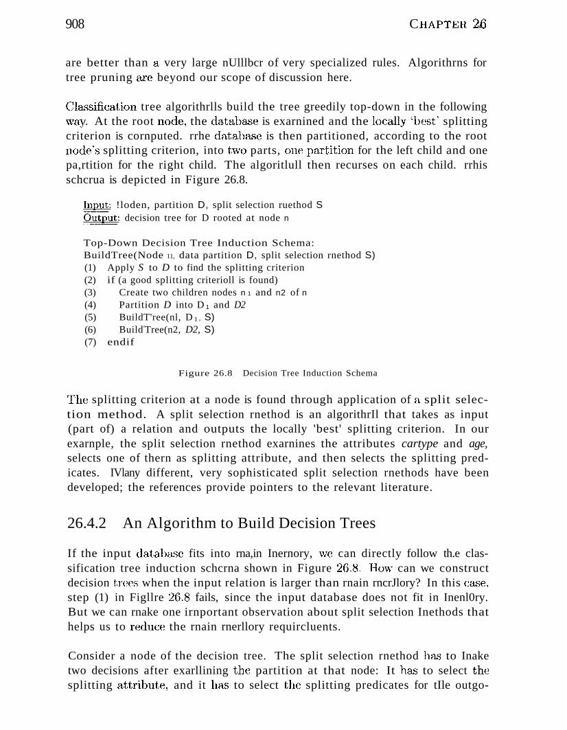
908 C ""'. ')6lIAPTI~J.R .....
are better than a very large nUlllbcr of very specialized rules. Algorithrns fortree pruning are beyond our scope of discussion here.
Classification tree algorithrlls build the tree greedily top-down in the following\vay. At the root node~ the database is exarnined and the locally'best' splittingcriterion is cornputed. rrhe database is then partitioned, according to the rootnode's splitting criterion, into t"W{) parts, one paTtition for the left child and onepa,rtition for the right child. The algoritlull then recurses on each child. rrhisschcrua is depicted in Figure 26.8.
Inr.ut: !loden, partition D, split selection ruethod S.Qutput: decision tree for D rooted at node n
Top-Down Decision Tree Induction Schema:BuildTree(Node 11, data partition D, split selection rnethod S)(1) Apply S to D to find the splitting criterion(2) if (a good splitting criterioll is found)(3) Create two children nodes n 1 and n2 of n
(4) Partition D into D 1 and D2(5) BuildT'ree(nl, D 1 , S)(6) Build rTree(n2, D2, S)(7) endif
Figure 26.8 Decision Tree Induction Schema
T'he splitting criterion at a node is found through application of a split selection method. A split selection rnethod is an algorithrIl that takes as input(part of) a relation and outputs the locally 'best' splitting criterion. In ourexarnple, the split selection rnethod exarnines the attributes cartype and age,selects one of thern as splitting attribute, and then selects the splitting predicates. IVlany different, very sophisticated split selection rnethods have beendeveloped; the references provide pointers to the relevant literature.
26.4.2 An Algorithm to Build Decision Trees
If the input database fits into rna,in Inernory, ~Te can directly follow th.e classification tree induction schcrna shown in Figure 26.8. flovv can we constructdecision trees when the input relation is larger than rnain rncrJlory? In this ca.se,step (1) in Figllre 26.8 fails, since the input database does not fit in Inenl0ry.But we can rnake one irnportant observation about split selection Inethods thathelps us to reduce the rnain rnerllory requircluents.
Consider a node of the decision tree. The split selection rnethod ha.s to Inaketwo decisions after exarllining the partition at that node: It ha.'3 to select thesplitting attribute: and it ha,s to select th(~ splitting predicates for tIle outgo-
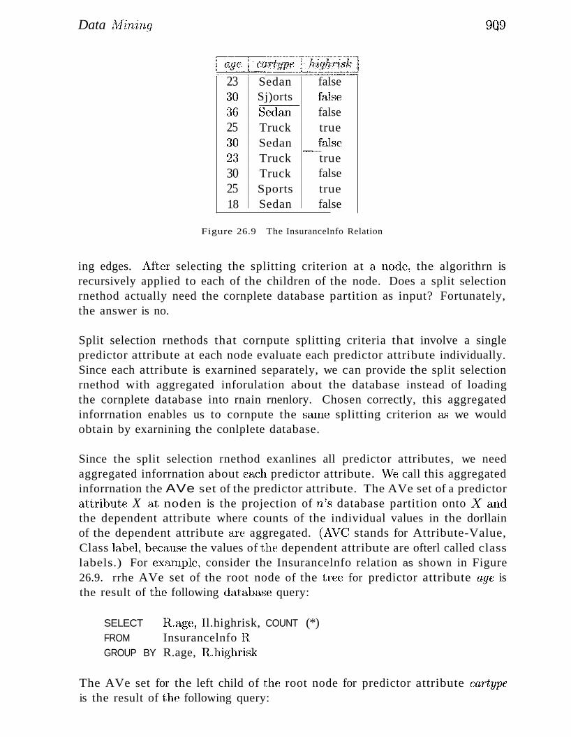
Data AfiTJ,ing
23 Sedan false~iO Sj)orts false~36 Sccran--- false25 Truck true~lO Sedan false
........." ..........
2~~ Truck true30 Truck false25 Sports true18 Sedan false
Figure 26.9 The Insurancelnfo Relation
9Q9
ing edges. After selecting the splitting criterion at a node, the algorithrn isrecursively applied to each of the children of the node. Does a split selectionrnethod actually need the cornplete database partition as input? Fortunately,the answer is no.
Split selection rnethods that cornpute splitting criteria that involve a singlepredictor attribute at each node evaluate each predictor attribute individually.Since each attribute is exarnined separately, we can provide the split selectionrnethod with aggregated inforulation about the database instead of loadingthe cornplete database into rnain rnenlory. Chosen correctly, this aggregatedinforrnation enables us to cornpute the senne splitting criterion as we wouldobtain by exarnining the conlplete database.
Since the split selection rnethod exanlines all predictor attributes, we needaggregated inforrnation about ceLeh predictor attribute. vVe call this aggregatedinforrnation the AVe set of the predictor attribute. The AVe set of a predictorattribute X <tt noden is the projection of 'n's database partition onto ..:X" andthe dependent attribute where counts of the individual values in the dorllainof the dependent attribute are aggregated. (AVe; stands for Attribute-Value,Class label, because the values of the dependent attribute are ofterl called classlabels.) For exarnple, consider the Insurancelnfo relation as shown in Figure26.9. rrhe AVe set of the root node of the tree for predictor attribute age isthe result of the following databEtse query:
SELECT FLage, Il.highrisk, COUNT (*)FROM Insurancelnfo IlGROUP BY R.age, H,.highrisk
The AVe set for the left child of t1H'~ root node for predictor attribute car-typeis the result of the following query:
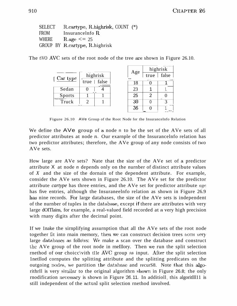
910
SELECTFROMWHEREGROUP BY
Itcartype, H,.highrisk, COUNTInsurancelnfo R,R.-age <= 25ILcartype, H..highrisk
(*)
CHAPTER~6
The t\VO .A.VC sets of the root node of the tree are shown in Figure 26.10.
[ Ca~~ype... ,
highrisk'--
falsetrue""'•..~
Sedan 0 4- -
Sports 1 1f---..._..
Truck 2 1- .-
"'-"'-
Agehighrisk
true false-- _. ... _.-
18 0 123
""-
1 1.25 2 0
..-
~30 () 3......-
36 0 1......"'.. --"'-
Figure 26.10 AVe Group of the Root Node for the InsuranceInfo Relation
We define the AVe group of a node n to be the set of the AVe sets of allpredictor attributes at node TL Our exarnple of the Insurancelnfo relation hastwo predictor attributes; therefore, the AVe group of any node consists of twoAVe sets.
How large are AVe sets? Nate that the size of the AVe set of a predictorattribute X at node n depends only on the nurnber of distinct attribute valuesof X and the size of the dornain of the dependent attribute. For exarnple,consider the AVe sets shown in Figure 26.10. The AVe set for the predictorattribute cartype has three entries, and the AVe set for predictor attribute agehas five entries, although the Insuraneelnfo relation as shown in Figure 26.9has nine records. For large databases, the size of the AVe sets is independentof the nurnber of tuples in the databa.'3e, except if there are attributes with verylarge dOITlains, for exarnple, a real-valued field recorded at a very high precisionwith rnany digits after the decirnal point.
If we 1nake the sirnplifying assurnption that all the AVe sets of the root nodetogether £it into rnain rnernory, then \ve can construct decision trees frOTH verylarge clataba,,~es as follo\vs: \Ve rnake a scan over the database and constructthe AVe group of the root node in rneIllory. Then \ve run the split selectionrnethod of our choicc\vith t11e i\Ve group as input. .AJ'ter the split selection1netllod cornputes the splitting attribute and the splitting predicates on theoutgoing 1H)des 1 \ve partition the databa,se and recurS8. Note that this algorithrIl is very sirnihu' to the original algorithrn shovvn in Figure 26.8; the onlyrnodification necessa.r;y is shown in Figure 2(L 11. In additioll 1 this algoritlll11 isstill independent of the aetuaJ split selection rnethod involved.
Data JvlirLing
Input: node n, partition D, split selection 111ethod S2..~~_~;EI:!.~: decision tree for D rooted at node 11
Top-Down Decision Tree Induction Schenla:BuHdTree(Node n, data partition D, split selection method S)(la) Ivlake a scan over D and construct the AVe group of n in-nlCIIlory(1b) Apply S to the AVe group to find the splitting criterion
Figure 26.11 Cla...'>sification rn-ee Induction Refinement with AVe Groups
26.5 CLUSTERING
911
In this section we discuss the clustering problem. The goal is to partitiona set of records into groups such that records within a group are shnilar toeach other and records that belong to two different groups are dissimilar. Eachsuch group is called a cluster and each record belongs to exactly one cluster. 1
Sirnilarity between records is Ineasured cOlnputationally by a distance function. A distance function takes two input records and returns a value that isa measure of their silnilarity. Different applications have different notions ofsimilarity, and no one rneasure works for all domains.
As an exarnple, consider the scherna of the Custol11erlnfo view:
CustornerInfo( age: int, salary: real)
We can plot the records in the view on a two-dil11ensional plane as shown inFiguf(~ 26.12. The two coordinates of a record are the values of the record'ssalaTyand age fields. \Ve can visually identify three clusters: yToung cllstornerswh.o have low salaries, young cllstorners with high salaries, and older cnstornerswith high salaries.
{Jsnally, the output of a clustering algorithrll consists of a, summarized representation of each cluster. The type of sUIrllnarized representation dependsstrongly on the type and shape of clusters the algoritlull cornputes. For exarnple, a.'3S111ne that we have spherical clusters as in the exalllple shuwn inFigure 26.12. vVe can surnrnarize each cluster by its centeT (often also calledthe rnea'n) and its Tndi'l1,t), which are defined as follo\vs. C;iven a collection ofrecords '/'1, ... '17"11' their center C: and radius .R are defined fL.'3 follows:
. n I -·-..... n 'f'
('1 1 '" ..1 I:::> IL-i=l (r'i - C)" == - .L..t. Ti, aI1C .1 = '\ .....-....--.....:.--.---.---
n . . V n(=1
1There are clustering algorithrns that allow overlapping clusters, \vhere a record could belong toseveral clusters.
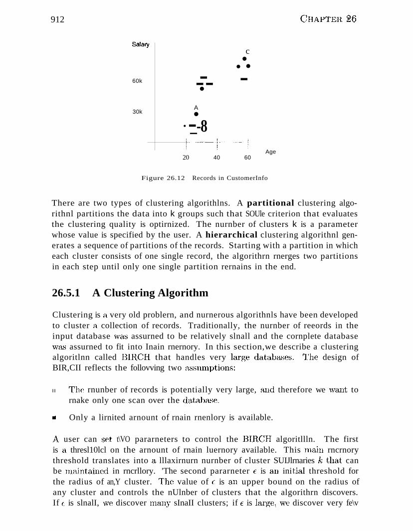
912
Salary
60k
30k
---•A
•-· _-8
20 40
c•• •-
60Age
(JIIAPTgR ·~6
Figure 26.12 Records in CustomerInfo
There are two types of clustering algorithlns. A partitional clustering algorithnl partitions the data into k groups such that SOUle criterion that evaluatesthe clustering quality is optirnized. The nurnber of clusters k is a parameterwhose value is specified by the user. A hierarchical clustering algorithnl generates a sequence of partitions of the records. Starting with a partition in whicheach cluster consists of one single record, the algorithrn rnerges two partitionsin each step until only one single partition rernains in the end.
26.5.1 A Clustering Algorithm
Clustering is a very old problern, and nurnerous algorithnls have been developedto cluster a collection of records. Traditionally, the nurnber of reeords in theinput database \vas assurned to be relatively slnall and the cornplete databasewa.s assurned to fit into Inain rnernory. In this section,we describe a clusteringalgoritlnn called BIllCII that handles very la.rge datab~1.ses. rrhe design ofBIR,CII reflects the follovving two a",ssurnptions:
II 1'he rnunber of records is potentially very large, and therefore we \\Tant tornake only one scan over the da.ta,b(~se.
II Only a lirnited arnount of rnain rnenlory is available.
j\ user can set t\VO pararneters to control the BIRfJII algoritllln. The firstis a thresl10lcl on the arnount of rnain luernory available. This HUlin rncrnorythreshold translates into a lllaxirnurn nurnber of cluster SUIJlrnaries k that canbe lIutintained in rncrllory. 'The second pararneter f is EUI ini tied threshold forthe radius of an,Y cluster. 1]H~ value of E is an upper bound on the radius ofany cluster and controls the nUlnber of clusters that the algorithrn discovers.If (' is slnalI, \eve discover TnaDy sInaII clusters; if E is large; we discover very fe\v
91~
clusters, each of which is relatively large. \Ve say that a cluster is compact ifits radius is s1na11e1' than t.
BIF.{,CH always lTlaintains k~ or fc\ver cluster sU1nrnaries (C/i ~ R~i) in rnain Hlcnl0ry,"vhere C:i is the center of cluster 'i and lii is the radius of cluster ,i. The a1gorithrnahvays rnaintains cornpact clusters; that is, the radius of each cluster is lessthan E. If this invariant cannot be rnaintained with the given arIlount of rnainlnerno1'y, E is increased t=ts described next.
The algoritlnl1 reads records frorn the database sequentially and processes the1l1as follows:
1. Cornpute the distance betVileen record T' and each of the existing clustercenters. Let i be the cluster index such that the distance between randC i is the srnallest.
2. Cornpute the value of the new radius R~ of the ith cluster under the assumption that r is inserted into it. If R~ < E, then the ith cluster rernainscornpact, and we assign T to the ith cluster by updating its center andsetting its radius to R~. If R:z, > E, then the ith cluster would no longer becOlnpact if we insert r into it. Therefore, we start a new cluster containingonly the record T.
The second step presents a problern if we already have the rnaxinnun nurnberof cluster sUIInnaries, k. If we now read a record that requires us to create anew cluster, we lack the rnain rne1nory required to hold its surnrnary. In thiscase, we increase the radius threshold E-----using SOHle heuristic to detenninethe increase--- in order to rner:qe existing clusters: An increase of c has twoconsequences. First, existing clusters can accorl1rnodate rnore records, sincetheir rnaxirnurn radius has increased. Second, it Blight be possible to rnergeexisting clusters such that the resulting cluster is still cornpact. rrhus, anincrease in ( usually reduces the l1ulIlber of existing clusters.
The cornplete BlItCH algorithrl1 uses a balanced in-rnernory tree, which is sirnilar to a B-·t- tree in structure, to quickly identify the closest cluster center fora neV\r record. A description of this data structure is beyond the scope of ourdiscussion.
26.6 SIMILARITY SEARCH OVER S~=QUENCES
A lot of inforrnation stored in datal)ases consists of sequences. In this section,w(~ introduce the problern of siInilarity search over a collection of sequences.Our query Inode} is very sirnple: vVe assurne that the user specifies a querysequence andvvants to retrieve all data sequences that are silnilar to the
914 (]H.APTER 26
Commercial Data Mining Systems: There area number of dataruining products on the rnarket tod~y, such as SASEnterprise Nliner,SPSS Clenlcntine, CART froIn Salford SystenlS, Ariegaputer PolyAnaJyst,ANGOSS I<nowledgeStudio. We highlight t\VO that have strong databaseties.
IBM's Intelligent Miner offers a wide ra,ngeof algorithlns, includingassociation rules, regression, cla.'3sification, and clustering. The enlpha'3isof Intelligent Miner is on scalability-·~·theproduct contains versions of allalgorithllls for parallel cOlnputers and is tightly integrated with IBM'sDB2 database systenl. DB2's object-relational capabilities can be used todefine the data Inining classes of SQL/MM. Of course, other data 111iningvendors can use these capabilities to add their own data mining modelsand algorithms to DB2.
Microsoft's SQL Server 2000 has a component called the Analysis Serverthat lnakes it possible to create, apply, and lnanage data mining modelswithin the DBMS. (SQL Server's OLAP capabilities are also packaged inthe Analysis Server component.) The basic approach taken is to representa mining rrlodel as a table; clustering and decision tree models arecurrently supported. The table conceptually has one row for each possiblecombination of input (predictor) attribute values. The model is createdusing a staternent analogous to SQL's CREATE TABLE that describes theinput on which the model is to be trained and the algorithrn to use inconstructing the model. An interesting feature is that the input tablecan be defined, using a specialized view rnechanisnl, to be a nested table.For exalnple,we can define an input table with one row per custolner,where one of the fields is a nested table that describes the eustolner'spurchases. The SQL/Ml\;1 extensions for data ruining do not provide thiscapability because SQL: 1999 does not currently support nested tables(Section 23.2.1). Several properties of attributes, such f}",C; whether theyare discrete or continuous, can also be specified.
.J.~ rnodel is trained by inserting rows into it, using the INSERT cornlnand.I t is applied to a llC\V dataset to lnake predictions using a new kind ofjoin called PREDICTION JOIN; in principle, each input tuple is nlatched !with the corxesponding tuple in the rnining lllodel to detennine the value Iof the predicted attribute. Thus, end users can create, train,and apply I,.
decision trees and clustering using extended SQL. 'There are aJso cornrnandsi
to browse rnodels. Unfortnnately, users cannot add new rnodels or new i
algorithrlns for models, a capability that is supported in the SQL/MlVI Iproposa. I
L._ __..~ _ _.__ ~__~ _ __~_ _ _ _ __''.._ .1
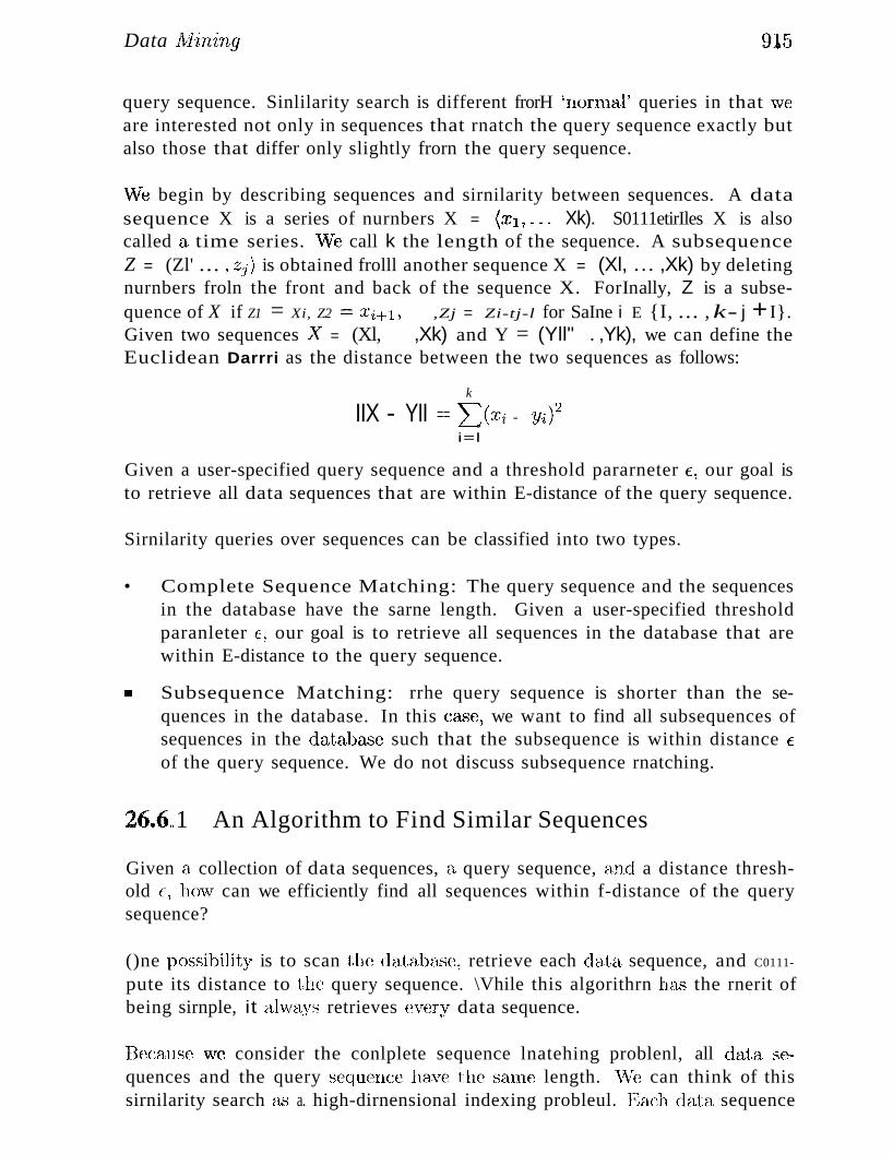
Data l\ifining 915
query sequence. Sinlilarity search is different frorH 'llornlal' queries in that \veare interested not only in sequences that rnatch the query sequence exactly butalso those that differ only slightly frorn the query sequence.
We begin by describing sequences and sirnilarity between sequences. A datasequence X is a series of nurnbers X = (;1~1,"" Xk). S0111etirIles X is alsocalled a time series. \lVe call k the length of the sequence. A subsequenceZ = (Zl' ... ,Zj) is obtained frolll another sequence X = (Xl, ... ,Xk) by deletingnurnbers froln the front and back of the sequence X. ForInally, Z is a subse-quence of X if Z1 = Xi, Z2 == Xi+l, ,Zj = Zi-tj-l for SaIne i E {I, ... , k- j + I}.Given two sequences .iY = (Xl, ,Xk) and Y = (Yll" . ,Yk), we can define theEuclidean Darrri as the distance between the two sequences as follows:
k
IIX - YII == L(Xi - Yi)2
i=l
Given a user-specified query sequence and a threshold pararneter E, our goal isto retrieve all data sequences that are within E-distance of the query sequence.
Sirnilarity queries over sequences can be classified into two types.
• Complete Sequence Matching: The query sequence and the sequencesin the database have the sarne length. Given a user-specified thresholdparanleter E, our goal is to retrieve all sequences in the database that arewithin E-distance to the query sequence.
II Subsequence Matching: rrhe query sequence is shorter than the sequences in the database. In this case, we want to find all subsequences ofsequences in the databc1.Se such that the subsequence is within distance E
of the query sequence. We do not discuss subsequence rnatching.
26.6..1 An Algorithm to Find Similar Sequences
Given a collection of data sequences, a query sequence, and a distance threshold f, henv can we efficiently find all sequences within f-distance of the querysequence?
()ne p()ssibilit~y is to scan the databa.se, retrieve each data sequence, and C0111
pute its distance to the query sequence. \Vhile this algorithrn has the rnerit ofbeing sirnple, it ahvays retrieves every data sequence.
Because \V(~ consider the conlplete sequence lnatehing problenl, all data sequences and the query sequ(~nce have tllC seune length. \Ve can think of thissirnilarity search (1.,"1 a. high-dirnensional indexing probleul. Each data, sequence
916 CHAPTER 2ti
and the query sequence can be represented as a point in a k-dirnensionaJ space.Therefore, if we insert all data sequences into a Illuitidirnensional index, we canretrieve data sequences that exactly ll1atch the query sequence by qllerying theindex. But since 'we \vant to retrieve not only dat~l sequences that Inatch thequery exactly but also all sequences within (-distance of the query sequence, \vedo not use a point query as defined by the query sequence. Instead, we querythe index 'with a hyper-rectangle that has side-length 2E and the query sequenceas center, and \ve retrieve all sequences that fall within this hyper-rectangle.\Ve then discard sequences that are actually further than c away froln the querysequence.
ITsing the index allows us to greatly reduce the nurnber of sequences we consider and decreases the thne to evaluate the sirnilarity query significantly. Thebibliographic notes at the end of the chapter provide pointers to further irnprovernents.
26.7 INCREMENTAL MINING· AND DATA STREAMS
Real-life data is not static, but is constantly evolving through additions ordeletions of records. In sorne applications, such as network Inonitoring, dataarrives in such high-speed strearns that it is infeasible to store the data foroffline analysis. We describe both evolving and strearning data in terlns ofa framework called block evolution. In block evolution, the input datasetto the data mining process is not static but periodically updated with a newblock of tuples, for exarnple, every day at rnidnight or in a continuous strealn.A block is a set of tuples added siInultaneously to the database. For largeblocks, this Inodel captures comrnon practice in rnany of today's data warehouseinstallations, where updates from operational databases are batched togetherand perforrned in a block update. For srnall blocks of data-~····-at the extrerne,each block consists of a single record····-····-this rnodel captures strealning data.
In the block evolution rnodel, the datab~"kqe consists of a (conceptually infinite)sequence of data blocks D 1 , [J2 , . .. that arrive at tilnes I, 2, ... ,\Vhe1'8 eachblock D i consists of a set of records. 2 \¥e call 'i the block identifier of block 13i .
~rherefore, at a,ny titHe t 1 the database consists of a finite sequence of blocks ofdata (Dl 1 ••• ,I)t;) that arrived at tirnes {I, 2, ... ,t}. The databc1se at tilne t,\vhic.h we denot.e by 1)[1, t], is the union of the databa",se at tiIne t - 1 and theblock that arrives at tirue t, Dl .
For evolving data, t\VO classes of problerns are of particular interest: rnodelInaintenance and change detection. rIhe goal of 1110del maintenance is to---"-"
2In general, a block specifies records to change or delete, in addition to n~cords to insert. \Ve onlyconsider inserts.
.Data A1in'ing 9~7
rnaintain a data rnining ulodcl under insertion and deletions of blocks of data.To incrernentally cornpute the data mining rnodel at tirne t,\vhich \ve denote byl\:I(D[l, t)), we HUlst consider only Af(D[l, t -- 1]) and .Dt ; \ve cannot considerthe data that arrived prior to tiIne t. Further, a data analyst rllight specifytirne-dependent subsets of D [1, t], such as a window of interest (e.g., all the dataseen thus far or last week's data). 1\I10re general selections are also possible,for exarnple, all weekend data over the P<:k~t year. Given such selections, weHlllst incrernentally CCHupute the rnodel on the appropriate subset of .D[l, t] byconsidering only [Jt and the model on the appropriate subset of 1)[1, t - 1].'Alrnost' incrernental algoritlulls that occasionally exarnine older data rnightbe acceptable in warehouse applications, where incrementality is lTIotivated byefficiency considerations and older data is available to us if necessary. Thisoption is not available for high-speed data strearns, where older data may notbe available at all.
The goal of change detection is to quantify the difference, in terrns of theirdata characteristics, between two sets of data and determine whether the changeis rneaningful (i.e., statistically significant). In particular, we rnust quantifythe difference between the rllodels of the data as it existed at sonle tiIne tland the evolved version at a subsequent ·tirne t2; that is, we Blust quantify thedifference between 1\1(D[I, tl]) and 1\1(D[1, t2]). We can also measure changeswith respect to selected subsets of data. Several natural variants of the problemexist; for exarnple, the difference between M(D[l, t - 1]) and 1\1(Dt ) indicateswhether the latest block differs substantially frorn previously existing data. Inthe rest of this chapter, we focus on rnodel rnaintenance and do not discusschange detection.
Incrernental rnodel rnaintenance has received rnuch attention. Since the qualityof the data rllining rnodel is of utrnost irnportance, incrernental rnodel rnaintena,nce a1gorithrns have concentrated on cornputing exactly the sarne Inode1HAS cOlnputed by running the basic rnodel construction algoritlul1 on the unionof old and new data. ()ne \videly used scalability technique is localization ofchanges due to new blocks. For exarnple, for density-based clustering algoritluns, the insertion of a ne"v record affects only clusters in the neighborhoodof the record, and thus efficient algorithrlls can localize the change to a fe\vclusters and avoid reccHnputing all clusters. As another exarllple, in decisiontree construction, \ve rnight be able to shovv that the split criterion at a, node ofthe tree changes only within acceptably srnall confidence intervals vvhen recordsare inserted, if we a..ssurne tha,t the underlying distribution of training recordsis static.
()nc-pclSS rnodel construction over data strearllS ha,,"~ received particular attention, since data arrives and rnust be processed continuously in several ernerging application dCHnains. For exarnple, network installations of la,rge TelecOll1
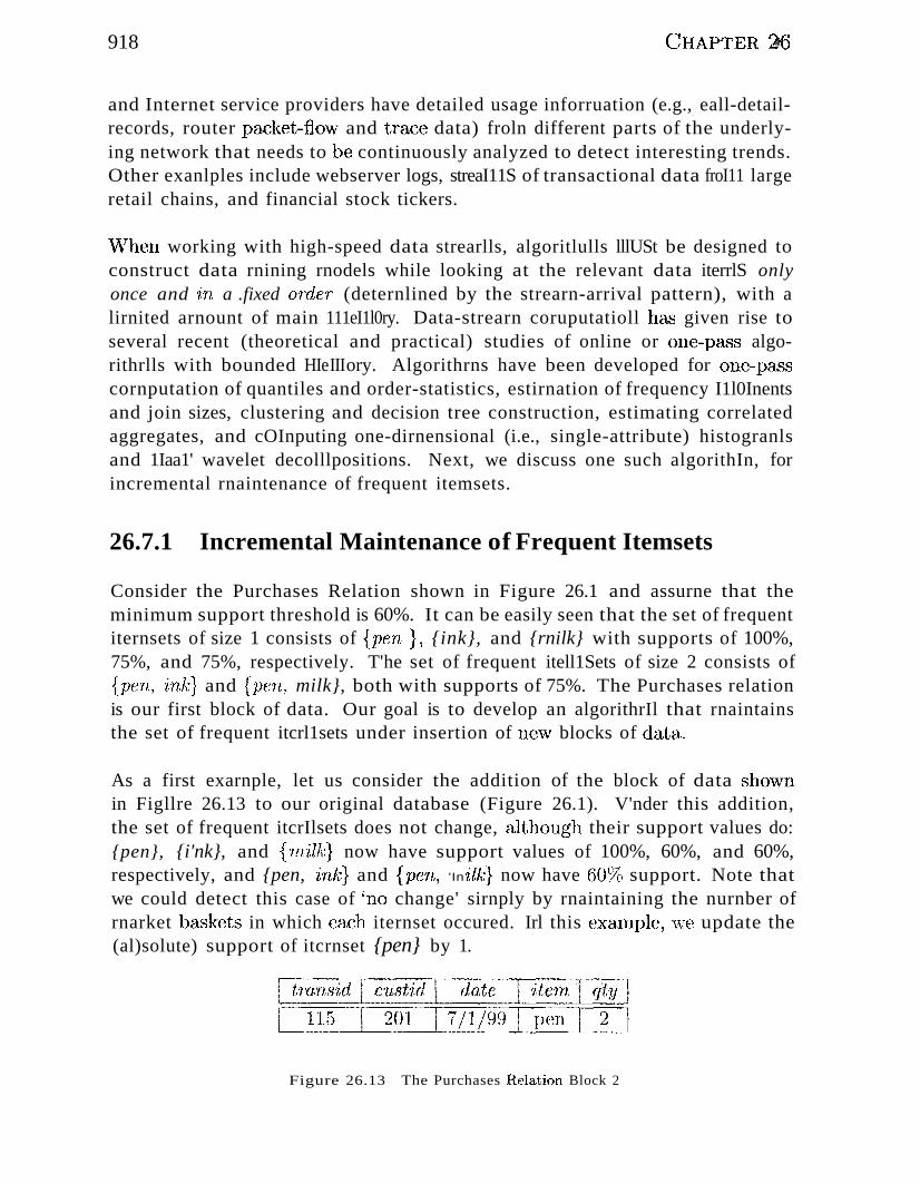
918 ()HAPTER ~
and Internet service providers have detailed usage inforruation (e.g., eall-detailrecords, router p<:1Cket-flovv and trace data) froln different parts of the underlying network that needs to be continuously analyzed to detect interesting trends.Other exanlples include webserver logs, streaI11S of transactional data froI11 largeretail chains, and financial stock tickers.
\\Then working with high-speed data strearlls, algoritlulls lllUSt be designed toconstruct data rnining rnodels while looking at the relevant data iterrlS onlyonce and in a .fixed order (deternlined by the strearn-arrival pattern), with alirnited arnount of main 111eI1l0ry. Data-strearn coruputatioll has given rise toseveral recent (theoretical and practical) studies of online or one-pass algorithrlls with bounded HIeIIIory. Algorithrns have been developed for one-passcornputation of quantiles and order-statistics, estirnation of frequency I1l0Inentsand join sizes, clustering and decision tree construction, estimating correlatedaggregates, and cOInputing one-dirnensional (i.e., single-attribute) histogranlsand 1Iaa1' wavelet decolllpositions. Next, we discuss one such algorithIn, forincremental rnaintenance of frequent itemsets.
26.7.1 Incremental Maintenance of Frequent Itemsets
Consider the Purchases Relation shown in Figure 26.1 and assurne that theminimum support threshold is 60%. It can be easily seen that the set of frequentiternsets of size 1 consists of {pen }, {ink}, and {rnilk} with supports of 100%,75%, and 75%, respectively. T'he set of frequent itell1Sets of size 2 consists of{pen, ink:} and {pen, milk}, both with supports of 75%. The Purchases relationis our first block of data. Our goal is to develop an algorithrIl that rnaintainsthe set of frequent itcrl1sets under insertion of nevv blocks of data.
As a first exarnple, let us consider the addition of the block of data shovvnin Figllre 26.13 to our original database (Figure 26.1). V'nder this addition,the set of frequent itcrIlsets does not change, although their support values do:{pen}, {i'nk}, and {Tn'ilk} now have support values of 100%, 60%, and 60%,respectively, and {pen, ink} and {pen, 'In'ilk} now have 609() support. Note thatwe could detect this case of 'rlO change' sirnply by rnaintaining the nurnber ofrnarket b::1.,>kets in which (~ach iternset occured. Irl this exaInple, vve update the(al)solute) support of itcrnset {pen} by 1.
Figure 26.13 The Purchases Relation Block 2
Data 1\1ining
115 201115 201
7/1/99 \vater7/1/99 lllilk
11
919
Figure 26.14 The Purchases Relation Block 2a
In general, the set of frequent itemsets Illay change. As an exalnple, considerthe addition of the block shown in Figure 26.14 to the original datab&'3e shownin Figure 26.1. vVe see a transaction containing the itern water, but we donot know the support of the iterllset {water}, since water was not above theInininUlm support in our original database. A sirnple solution in this case is tornake an additional scan over the original database and cornpute the support ofthe itenlset {water}. But can we do better? Another innnediate solution is tokeep counters for all possible iterllsets, but the nUlnber of all possible itemsetsis exponential in the nurnber of iterns-·-and most of these counters would be 0anyway. Can we design an intelligent strategy that tells us which counters toruaintain?
We introduce the notion of the negative border of a set of iternsets to helpdecide which counters to keep. The negative border of a set of frequent itemsetsconsists of all iterllsets X such that X itself is not frequent, but all subsets ofX are frequent. For example, in the case of the database shown in Figure 26.1,the following iternsets rnake up the negative border: {juice}, {water}, and {ink,milk}. Now we can design a more efficient algorithm for maintaining frequentiternsets by keeping counters for all currently frequent iternsets and all iterllsetscurrently in the negative border. ()nly if an iternset in the negative borderbecomes frequent do we need to read the original data..set again, to find thesupport for new candidate itemsets that Blight be frequent.
We illustrate this point through the following t\VO exarnples. If we add Block2a shown in Figure 26.14 to the original database shown in Figure 26.1, weincrease the support of the frequent iterllset {Tn'ilk} by one, and we increase thesupport of the iternset {water}, which is in the negative border, by one as well.But since no iternset in the negative border beearne frequent, we do not haveto re-scan the original database.
In eontrast, cbnsider the addition of Block 2b shown in Figure 26.15 to theoriginal database shown in Figure 26.1. In this CCl"se, the iternset {juice}, whichwas originally in the negative border, becornes frequent with a support of 60%.rrhis rneans that now the following itcrnsets of size two enter the negativeborder: {juice, pen}, {juice, ink}, and {juice, Tnilk}. (vVe know that {juice,'Water} cannot be frequent since the iteulset {water} is not freqlient.)
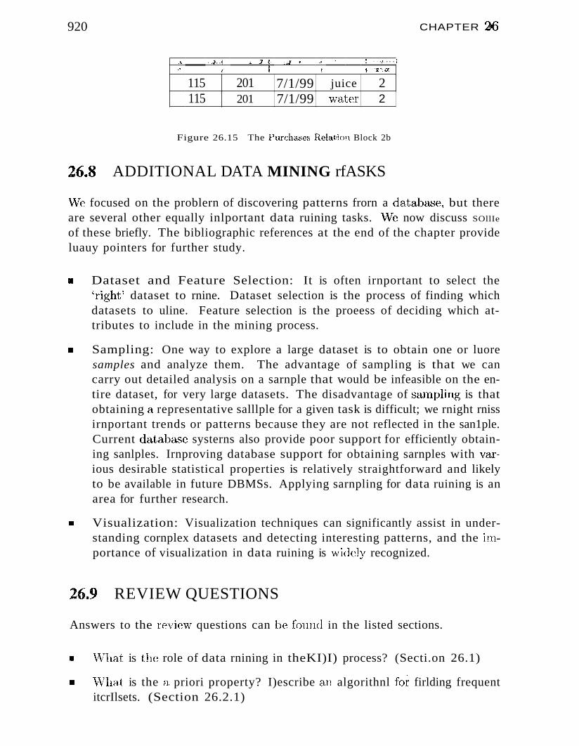
920
of . jJ 1- J:L :"J.. ~ 1 " ..... 1 .....•...... !..,.
[ 1 f LX'{7
115 201 7/1/99 juice 2115 201 7/1/99 water 2
Figure 26.15 The Purcha.."es Rt~lation Block 2b
26.8 ADDITIONAL DATA MINING rfASKS
CHAPTER 2t6
vVe focused on the problern of discovering patterns frorn a databa,sc, but thereare several other equally inlportant data ruining tasks. vVe now discuss SOllIe
of these briefly. The bibliographic references at the end of the chapter provideluauy pointers for further study.
.. Dataset and Feature Selection: It is often irnportant to select the'right' dataset to rnine. Dataset selection is the process of finding whichdatasets to uline. Feature selection is the proeess of deciding which attributes to include in the mining process.
II Sampling: One way to explore a large dataset is to obtain one or luoresamples and analyze them. The advantage of sampling is that we cancarry out detailed analysis on a sarnple that would be infeasible on the entire dataset, for very large datasets. The disadvantage of scunpling is thatobtaining a representative salllple for a given task is difficult; we rnight rnissirnportant trends or patterns because they are not reflected in the san1ple.Current databa..'Se systerns also provide poor support for efficiently obtaining sanlples. Irnproving database support for obtaining sarnples with various desirable statistical properties is relatively straightforward and likelyto be available in future DBMSs. Applying sarnpling for data ruining is anarea for further research.
II Visualization: Visualization techniques can significantly assist in understanding cornplex datasets and detecting interesting patterns, and the ilnportance of visualization in data ruining is \videly recognized.
26.9 REVIEW QUESTIONS
Answers to the revie\v questions can be fuunel in the listed sections.
IIlI vVl1at is the role of data rnining in theKI)I) process? (Secti.on 26.1)
II \Vhat is the a priori property? I)escribe an algorithnl for' firlding frequentitcrIlsets. (Section 26.2.1)
Data i\~lir'l,in.9 921
III IInw are iceberg queries related to frequent iterIlsets? (Section 26.2.2)
• (jive the definition of an associat'ian rule. '\Vhat is the difference betv'leensupport and confidence of a rule? (Setion 26.3.1)
III Can you explain extensions of association rules to ISA hierarchies? "Vhatother extensions of association rules are you farniliar v'lith? (Sections26.3.3 and 26.3.4)
III "Vhat is a sequential pattern? How can we cornpute sequential patterns?(Section 26.3.5)
II Can we use association rules for prediction? (Section 26.3.6)
III What is the difference bet\'leen Bayesian Networks and association rules?(Section 26.3.7)
.. Can you give exanlples of classification and regression rules? How is support and confidence for such rules defined? (Section 26.3.8)
.. vVhat are the cOlnponents of a decision tree? I{ow are decision trees constructed? (Sections 26.4.1 and 26.4.2)
II What is a cluster? What inforrnation do we usually output for a cluster?(Section 26.5)
.. How can we define the distance between two sequences? Describe an algorithnl to find all sequences similar to a query sequence. (Section 26.6)
• Describe the block evolution Inodel and define the problclllS of increlnentalrnodel maintenance and change detection. \Vhat is the added challenge inrnining data strearns? (Section 26.7)
11II Describe an incrernental algorithnl for conlpllting frequent iternsets. (Section 26.7.1)
III Give exarnples of other tasks related to data rnining. (Section 26.8)
EXERCISES
Exercise 26.1 Briefly ans\ver the following questions:
1. Define 8uppor>t, and confidence for (111 association 1"ule.
2. Expla.in why association rules cannot be used directly for prediction, \vithout furtheranal.'1lsis or clornain knowledge.
:3. \\7ha1; axe the differences between a88oc'iat:ion 'rlde8, classification rules, (;1,11(1 regression
'r'lLles?
4. \Vhat is the difference bet\veen cla88ijic(JJio'Tl and cZ.u8tcrin,g?
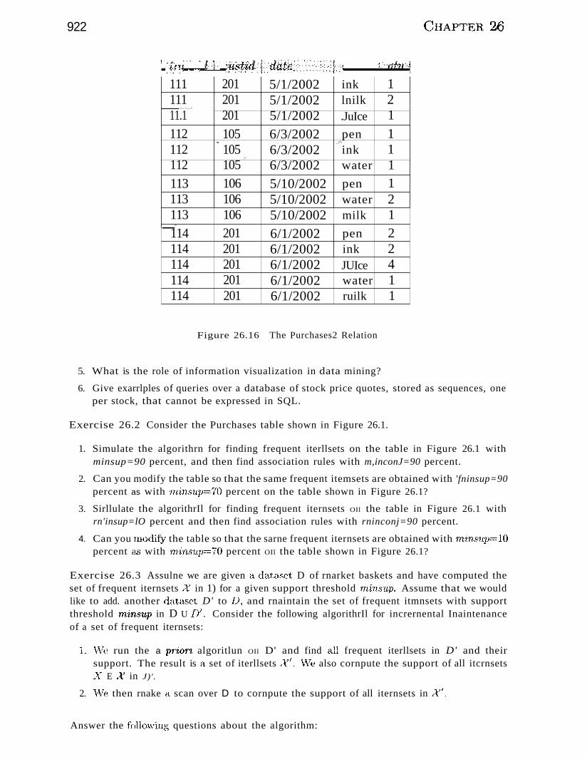
922
i........ ............. .'. ·"'.li ..............<Jri(j~t~iiiili ·,..······i.···f"ll:it i ····tii.{':f.c, .~ ",. it ·il.. .i ..1i\I
111 201 5/1/2002 ink 1111 201 5/1/2002 lnilk 2
1---..._ .._...
11.1 201 5/1/2002 .JuIce 1112 105 6/3/2002 pen 1
-6/3/2002
_.-.
112 105 ink 1.-
112 105 6/3/2002 water 1113 106 5/10/2002 pen 1113 106 5/10/2002 water 2113 106 5/10/2002 milk 1_...
6/1/2002114 201 pen 2114 201 6/1/2002 ink 2114 201 6/1/2002 JUIce 4114 201 6/1/2002 water 1114 201 6/1/2002 ruilk 1
Figure 26.16 The Purchases2 Relation
C~H:APTER 26
5. What is the role of information visualization in data mining?
6. Give exarrlples of queries over a database of stock price quotes, stored as sequences, oneper stock, that cannot be expressed in SQL.
Exercise 26.2 Consider the Purchases table shown in Figure 26.1.
1. Simulate the algorithrn for finding frequent iterllsets on the table in Figure 26.1 withminsup=90 percent, and then find association rules with m,inconJ=90 percent.
2. Can you modify the table so that the same frequent itemsets are obtained with 'fninsup=90percent as with 11Linsup=70 percent on the table shown in Figure 26.1?
3. Sirllulate the algorithrIl for finding frequent iternsets OIl the table in Figure 26.1 withrn'insup=lO percent and then find association rules with rninconj=90 percent.
4. Can you rnodi~y the table so that the sarne frequent iternsets are obtained with rnin-'i1lp=10percent as with minsvp=70 percent OIl the table shown in Figure 26.1?
Exercise 26.3 Assulne we are given a, data:set D of rnarket baskets and have computed theset of frequent iternsets X in 1) for a given support threshold rnin,B'up. Assume that we wouldlike to add. another data'Set D' to D, and rnaintain the set of frequent itmnsets with supportthreshold 'fn'in8up in D U IJ'. Consider the following algorithrIl for incrernental Inaintenanceof a set of frequent iternsets:
l.vVe run the a p'T-ioT'i algoritlun OIl D' and find all frequent iterllsets in D' and theirsupport. The result is a set of iterllsets .Y'. \Ve also cornpute the support of all itcrnsets-,y E "Y in J)'.
2. \Ve then rnake a scan over D to cornpute the support of all iternsets in .y'.
Answer the follo:\ving questions about the algorithm:
Data lvf-in'ing 923
• The last step of the algorithm is rnissing; that is, what should the algorithm output'?
• Is this algorithm lllore efficient than the algorithm described in Secti0n 26.7.1'1
Exercise 26.4 Consider the Purchases2 table shown in Figure 26.16.
• List all iterllsets in the negative border of the dataset.
• List all frequent itelnsets for a support threshold of 50%.
• Give an exaruple of a database in which the addition of this database does not changethe negative border.
• Give an exarnple of a database in which the addition of this database would change thenegative border.
Exercise 26.5 Consider the Purchases table shown in Figure 26.1. Find all (generalized)association rules that indicate the likelihood of items being purchased on the same date bythe same customer, with minsup set to 10% and minconj set to 70%.
Exercise 26.6 Let us develop a new algorithm for the computation of all large itemsets.Assume that we are given a relation D siInilar to the Purchases table shown in Figure 26.1.We partition the table horizontally into k parts D 1 , ... , D k .
1. Show that, if itemset X is frequent in D, then it is frequent in at least one of the k parts.
2. Use this observation to develop an algorithm that cornputes all frequent itemsets in twoscans over .D. (Hint: In the first scan, compute the locally frequent itemsets for eachpart Di , i E {I, ... , k}.)
3. Illustrate your algorithm using the Purchases table shown in Figure 26.1. The firstpartition consists of the two transactions with transid 111 and 112, the second partitionconsists of the two transactions with transid 113 and 114. Assulne that the minimumsupport is 70 percent.
Exercise 26.7 Consider the Purchases table shown in Figure 26.1. Find all sequential patterns with minsup set to 60%. (The text only sketches the algorithm for discovering sequentialpatterns, so use brute force or read one of the references for a complete algorithm.)
Exercise 26.8 Consider the SubscriberInfo Relation shown in Figure 26.17. It containsinformation about the marketing cmnpaign of the DB Aficionado magazine. The first twocolurnns show the age and salary of a potential customer and the subscription colurnn showswhether the person subscribes to the rnagazine. \Ve want to use this data to construct adecision tree that helps predict whether a person will subscribe to the 11lagazine.
1. Construct the AVC-group of the root node of the tree.
2. Assume that the spliting predicate at the root nod€~ is age S; 50. Construct the AVCgroups of the two children nodes of the root node.
Exercise 26.9 Assurne you are given the following set of six records: (7,55), (21, 202),(25,220), (12,7:3), (8,61), and (22,249).
1. Assurning that all six records belong to a single cluster, cornpute its center and radius.
2. Assurne that the first three records belong to one cluster and the second three recordsbelong to a different cluster. COlnpute the center and radius of the two clusters.
3. \Vhich of the two clusterings is 'better' in your opinion and why?
Exercise 26.10 Asslune you are given the three sequences (1, :3, 4), (2, :3, 2), (:3,3, 7). COlnpute the Euclidian Bonn between all pairs of sequences.
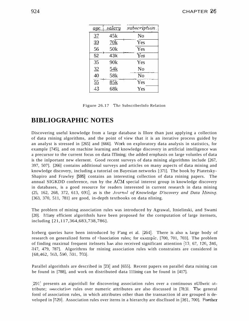
924 CHAPTER 26
age·······I···'s-illatry Amb8·C!r1pti{j~'t-··1- .....-
37 45k No-_:---!---~ .....,,----1
~39 70k Yes__------1
56 50k Yesf---------...t------j---------j
52 43k "Yes35 90k Yes32 54k No
-------_.-40 58k No----+-----::---t----=-::,------55 85k Yes43 68k Yes
Figure 26.17 The SubscriberInfo Relation
BIBLIOGRAPHIC NOTES
Discovering useful knowledge from a large database is lllore than just applying a collectionof data rnining algorithms, and the point of view that it is an iterative process guided byan analyst is stressed in [265] and [666]. \'Fork on exploratory data analysis in statistics, forexample [745], and on rnachine learning and knowledge discovery in artificial intelligence wasa precursor to the current focus on data lTlining; the added ernphasis on large volunles of datais the inlportant new elernent. Good recent surveys of data mining algorithms include [267,397, 507]. [266] contains additional surveys and articles on many aspects of data mining andknowledge discovery, including a tutorial on Bayesian networks [:371]. The book by PiatetskyShapiro and Frawley [595] contains an interesting collection of data rnining papers. Theannual SIGKDD conference, run by the AClVI special interest group in knowledge discoveryin databases, is a good resource for readers interested in current research in data mining(25, 162, 268, 372, 613, 691]' as is the ]o'urnal of Knowledge D'iscovery and Data Alining.[363, 370, 511, 781] are good, in-depth textbooks on data nlining.
The problern of mining association rules was introduced by Agrawal, Itnielinski, and Swami[20]. l\!1any efficient algorithnls have been proposed for the cornputation of large iternsets,including [21,117,364,683,738,786].
Iceberg queries have been introduced by F'ang et al. [264]. There is also a large body ofresearch on generalized forrns of <lssociation rules; for ex<:unple, [700, 701, 703]. The problemof finding rnaxirnal frequent itelnsets ha'3 also received significant attention [13, 67, 12G, ;H6,~~47, 479, 787]. Algorithrns for rnining association rules with constraints are considered in[68,462, 56;'{, 590, 591, 70:3].
Parallel algorithnls are described in [2:3] and [655]. Recent papers on parallel data ruining canbe found in [788], and work on distributed data 111ining can be found in [417].
[291] presents an aigoritlull for discovering association rules over a continuous nUllwric attribute; association rules over numeric attributes are also discussed in [78:3J. 1'he generalfornl of association rules, in which attributes other than the transaction id are grouped is developed in [529]. Association rules over iterns in a hierarchy are discllssed in [:361, 700]. F'llrther
J)ata A1in'i'TLg ()nr.:, L,··i
extensions and generalization of a,,'3sociation rules are proposed in [67, 115, 56~3]. Integrationof rnining for frequent itcrHsets into datalxLse systcrns has been addressed in [654, 74a]. 'rheproblern of Inining sequential patterns is discussed in [24}, and further algorithrIls for rniningsequential patterns can be found in [510, 702].
General introductions to classification and regression rules can be found in [~362, 5a2]. Theclassic reference for decision and regression tree construction is the CART book by Breilnan,Friccl!nau, Olsheu, and Stone [111]. A lnachine learning perspective of decision tree construction is given by Quinlan [603]. Recently, several scalable algorithnls for decision treeconstruction have been developed [309, 311, 521, 619, 674J.
'rhe clustering problern has been studied for decades in several disciplines. Sample textbooksinclude [232, 407, 418]. Scalable clustering algorithuls include CLARANS [562], DBSCAN[249, 250], BIRCH [798], and CURE [344]. Bradley, Fayyad, and Reina address the problemof scaling the K-lVIeans clustering algorithm to large databases [108, 109]. The problern offinding clusters in subsets of the fields is addressed in [19]. Ganti et al. exauline the problerllof clustering data in arbitrary rnetric spaces [302]. Algorithrlls for clustering caterogical datainclude STIRR [315J and CACTUS [301]. [651] is a clustering algorithm for spatial data.
Finding siulilar sequences from a large database of sequences is discussed in [22, 262, 446,606,680].
Work on incrernental rnaintenance of association rules is considered in [174, 175, 736]. Esteret al. describe how to nlaintain clusters incrernentally [248], and Hidber describes how tornaintain large iteulsets incrernentally [378]. There has also been recent work on rnining datastrearns, such as the construction of decision trees over data streams [228, 309, 39~)] andclustering data streanlS [343,568]. A general framework for ruining evolving data is presentedin [299]. A framework for measuring change in data characteristics is proposed in [300J.
INFORMATION RETRIEVALANDXMLDATA
... How are DBNISs evolving in response to the growing aIllounts of textdata?
... What is the vector space rnodel and how doe's it suppo~ text search?
... How are text collections indexed?
... Cornpared to IR systenls, what is new in Web search?
... How is XNIL data different from plain text and relational tables?
... What are the main features of XQuery?
... What are the irnplementation challenges posed by XML data?
.. Key concepts: information retrieval, boolean and ranked queries;relevance, precision, recall; vector space model, TF/IDF terrn weighting, document similarity; inverted index, signature file; Web crawler,hubs and authorities, Pigeon Rank of a webpage; sernistructured datalllodel, XML; XQuery, path expressions, FLWR queries; XML storageand indexing
27
'with Raghav KaushikUniveTsity of Wi8consin---Aladison
A Tne'rne:r is a device in vvhieh an individual stores all his books,records, and cornrnunications, and which is rnechanized so that it rnaybe consulted with exceeding speed and flexibility.
--'Vannevar Bush, As We !vlay Think, 1.945
926
IR and XlvlL Data 9~7
The field of inforlnation retrieval (IR) has studied the problenl of sea,rchingcollections of text docurnents since the 19508 and developed largely independently of database systenls. The proliferation of text docunlents on the Weblllade docurnent search an everyday operation for 1110st people and led to renewed research on the topic.
The database field's desire to expand the kinds of data that can be managed ina DB~IS is well-established and reflected in developments like object-relationalextensions (Chapter 23). Documents on the Web represent one of the rnostrapidly growing sources of data, and the challenge of rnanaging such documentsin a DBMS has naturally become a focal point for database research.
The Web, therefore, brought the two fields of database rnanagement systenlsand information retrieval closer together than ever before, and, as we will see,XML sits squarely in the middle ground between thenl. We introduce IR systems as well as a data model and query language for XML data and discussthe relationship with (object- )relational database systerns.
In this chapter, we present an overview of information retrieval, Web search,and the emerging XML data model and query language standards. We beginin Section 27.1 with a discussion of how these text-oriented trends fit withinthe context of current object-relational database systeIns. We introduce inforrnation retrieval concepts in Section 27.2 and discuss specialized indexingtechniques for text in Section 27.3. We discuss Web search engines in Section27.4. In Section 27.5, we briefly outline current trends in extending databasesystems to support text data and identify SOllle of the irnportant issues involved. In Section 27.6, we present the XML data lllodel, building on the XMLconcepts introduced in Chapter 7. We describe the XQuery language in Section27.7. In Section 27.8, we consider efficient evaluation of XQuery queries.
27.1 COLLIDING WORLDS: DATABASES, IR, AND XML
'The \i\Teb is the rnost widely used doculnent collection today, and search on thevVeb differs froIn traditional IR-style docurnent retrieval in iluportant ways.First, there is great ernphclsis on scalability to very large document collections.IR systerns typically dealt with tens of thousands of documents, wherea.'3 thevVeb contains l)illions of pages.
Second, the vVeb has significantly changed how docurnent collections are createdand used. Traditionally, III systerlls were aiIned at professionals like librariansand legal researchers, who were trained in using sophisticated retrieval engines.Docurnents were carefully prepared, and docllrnents in a given collection weretypically on related topics. On thevVeb, docurnents are created by an infinite
928 CHAPT8R 27
variety of individuals for equally lllClny purposes, and reflect this diversity insize and content. Searches aTe carried out by ordinary people with no trainingin using retrieval software.
The ernergence of Xl\/lL has added a third interesting diInensioI1 to text search:Every cloClunent can no\v be rnarked up to reflect additional infol'lnation ofinterest, such as authorship, source, and even details about the intrinsic content.This he),s changed the nature of a '"docurnent" froIn free text to textual objects\vith a..')sociated fields containing metadata (data about data) or descriptiveinfonnation. Links to other docurnents are a particularly irnportant kind oflnetadata, and they can have great value in searching docurnent collections onthe vVeb.
The Web also changed the notion of what constitutes a docunlent. Documentson the Web may be multinledia objects such as irnages or video clips, withtext appearing only in descriptive tags. We must be able to Inanage suchheterogeneous data collections and support searches over thern.
Database rnanagernent systenls traditionally dealt with simple tabular data. Inrecent years, object-relational database systerns (ORDBMSs) were designed tosupport complex data types. Images, videos, and textual objects have beenexplicitly rnentioned as exaruples of the data types ORDBMSs are intended tosupport. Nonetheless, current database systerns have a long way to go beforethey can support such cOlnplex data types satisfactorily. In the context of textand XML data, challenges include efficient support for searches over textualcontent and support for searches that exploit the loose structure of XNIL data.
27.1.1 DBMS versus IR Systems
I)atabc1.se and IR, systcrns have the COllllnon objective of supporting searchesover collections of data. However, rnany irnportant differences have influencedtheir developrnent.
11II Searches versus Queries: IR, systerns are designed to support a specialized class of qlH~ries that \ve also call searches. Searches are specified internlS of a. fo",T search terms, and the underlying data is usually a collection of unstructured text docurnents. III addition, an irnportant feature ofTH, searches is that search resultsrnay be ranked, or ordered, in tcrrns ofhovv '\vell' the search results rnatch the search tenns. In contra.'3t, databa"scsysterns support a very general class of queries, and the underlying data isrigidly structured. Unlike III systerns~ database systerns have traditionallyreturnedunranked sets of results. (Even the recent S(~L/()L,AP extensionsthat support earl:y results and searches over ordered data (secl, Chapter 25)
IR and )(ivlL ]Jata 929
do not order results in terlTIS of how ""veIl they rnatch the query. Relationalqueries are pTeC'i8e in that a ro\v is either in the answer or it is not ; thereis no notion of 'how vvell a row rnatches~ the query.) In other ""rords, arelational query only assigns two raJlks to a row, indicating 'whether therow is in the ans\ver or not.
• Updates and Tr'ansactions: IR systelns are optirnized for a read-Illostlyworkload and do not support the notion of a transaction. In traditionalIR systerlls, ne\v docurnents are added to the doculnent collection frorHtirne to titne, and index structures that speed up searches are periodicallyrebuilt or updated. Therefore, docllrnents that are highly relevant for asearch rnight exist in the IR systeln, but not be retrievable yet because ofoutdated index structures. In contrast, databa...'3e systerns are designed tohandle a wide range of workloads, including update-intensive transactionprocessing workloads.
These differences in design objectives have led, not surprisingly, to very different research elnphases and system designs. Ilesearch in IR studied rankingfunctions extensively. For example, arllong other topics, research in IR investigated how to incorporate feedback frOITl a user's behavior to modify a rankingfunction and how to apply linguistic processing techniques to improve searches.Database research concentrated on query processing, concurrency control andrecovery, and other topics, as covered in this book.
The differences between a DB1\tIS and an III systenl from a design and irnplementation standpoint should become clear as we introduce IR systerlls in thenext few sections.
27.2 INTRODUCTION TO INFORMATION RETRIEVAL
There are two COrllr110n types of searches, or queries, over text collections:boolean queries and ranked queries. In a boolean query~ the user spE~ci
fies an expression constructed using terlllS and boolean operators (And, Or,Not). For exalnple,
database And (lvlicT08ojt Or IBM)
This query a..sks for all docurnents that contain the terrn database and in addition, either PvficT080jt or IBN!.
In a ranked query the user specifies one or rnore terrlls, a,rlcl the result of thequery is a list of docurllents ranked by their relevance to the query. Intuitively,docurnents at the top of the result list are expected to 'rnatch' the search
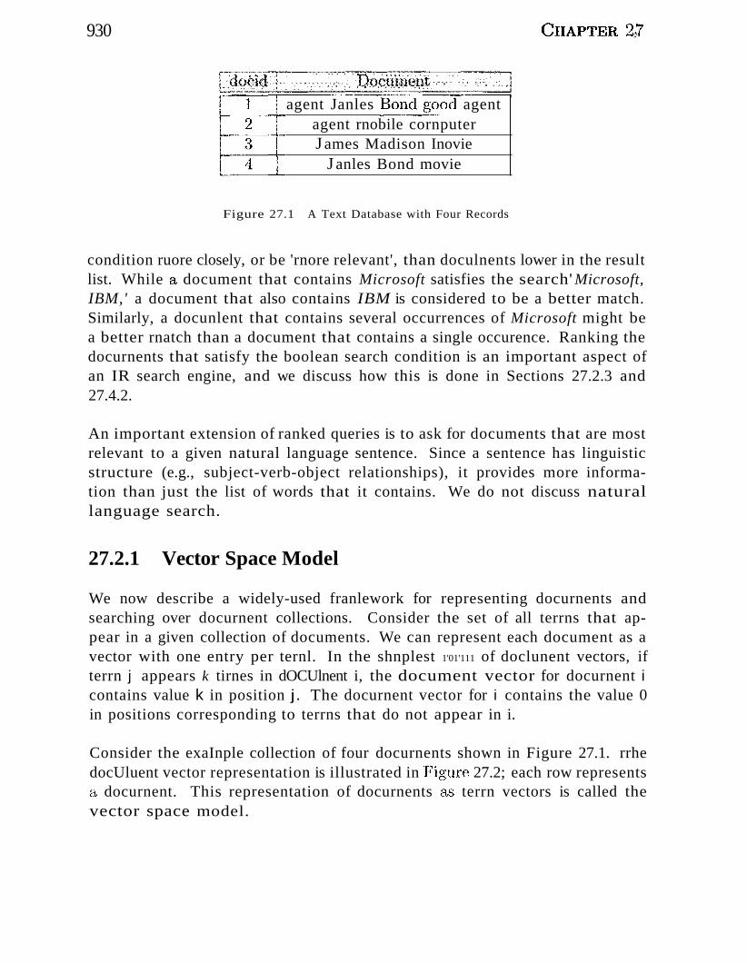
930
agent Janles agentagent rnobile cornputerJ ames Madison Inovie
J anles Bond movie
Figure 27.1 A Text Database with Four Records
CHAPTER 2$7
condition ruore closely, or be 'rnore relevant', than doculnents lower in the resultlist. While a document that contains Microsoft satisfies the search' Microsoft,IBM,' a document that also contains IBM is considered to be a better match.Similarly, a docunlent that contains several occurrences of Microsoft might bea better rnatch than a document that contains a single occurence. Ranking thedocurnents that satisfy the boolean search condition is an important aspect ofan IR search engine, and we discuss how this is done in Sections 27.2.3 and27.4.2.
An important extension of ranked queries is to ask for documents that are mostrelevant to a given natural language sentence. Since a sentence has linguisticstructure (e.g., subject-verb-object relationships), it provides more information than just the list of words that it contains. We do not discuss naturallanguage search.
27.2.1 Vector Space Model
We now describe a widely-used franlework for representing docurnents andsearching over docurnent collections. Consider the set of all terrns that appear in a given collection of documents. We can represent each document as avector with one entry per ternl. In the shnplest 1'01'111 of doclunent vectors, ifterrn j appears k tirnes in dOCUlnent i, the document vector for docurnent icontains value k in position j. The docurnent vector for i contains the value 0in positions corresponding to terrns that do not appear in i.
Consider the exaInple collection of four docurnents shown in Figure 27.1. rrhedocUluent vector representation is illustrated in Figurf~ 27.2; each row representsa docurnent. This representation of docurnents a,,'3 terrn vectors is called thevector space model.
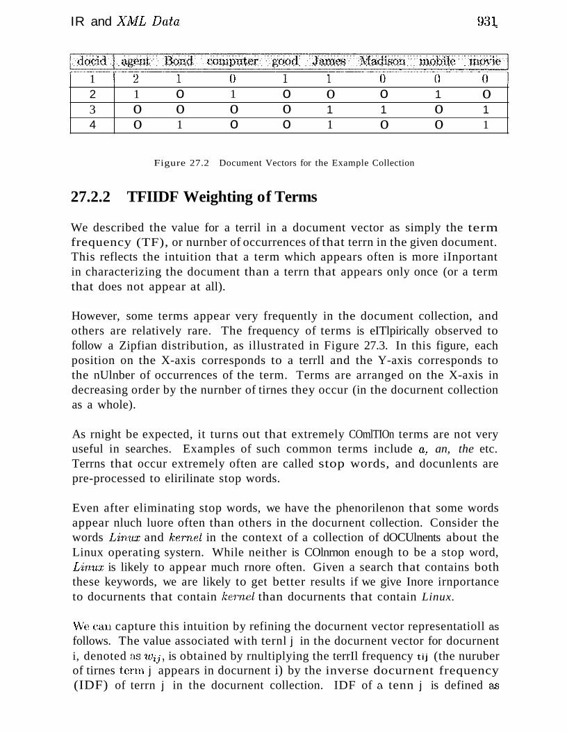
IR and XNfL Data
1
93L
234
1oo
oo1
1oo
ooo
o11
o1o
1oo
o11
Figure 27.2 Document Vectors for the Example Collection
27.2.2 TFIIDF Weighting of Terms
We described the value for a terril in a document vector as simply the termfrequency (TF), or nurnber of occurrences of that terrn in the given document.This reflects the intuition that a term which appears often is more iInportantin characterizing the document than a terrn that appears only once (or a termthat does not appear at all).
However, some terms appear very frequently in the document collection, andothers are relatively rare. The frequency of terms is eITlpirically observed tofollow a Zipfian distribution, as illustrated in Figure 27.3. In this figure, eachposition on the X-axis corresponds to a terrll and the Y-axis corresponds tothe nUlnber of occurrences of the term. Terms are arranged on the X-axis indecreasing order by the nurnber of tirnes they occur (in the docurnent collectionas a whole).
As rnight be expected, it turns out that extremely COmlTIOn terms are not veryuseful in searches. Examples of such common terms include a, an, the etc.Terrns that occur extremely often are called stop words, and docunlents arepre-processed to elirilinate stop words.
Even after eliminating stop words, we have the phenorilenon that some wordsappear nluch luore often than others in the docurnent collection. Consider thewords Lirnl;E and kernel in the context of a collection of dOCUlnents about theLinux operating systern. While neither is COlnrnon enough to be a stop word,Linux is likely to appear much rnore often. Given a search that contains boththese keywords, we are likely to get better results if we give Inore irnportanceto docurnents that contain kernel than docurnents that contain Linux.
vVe ca.'!} capture this intuition by refining the docurnent vector representatioll as
follows. The value associated with ternl j in the docurnent vector for docurnenti, denoted a.." 'Wij, is obtained by rnultiplying the terrIl frequency tij (the nuruberof tirnes tenn j appears in docurnent i) by the inverse docurnent frequency(IDF) of terrn j in the docurnent collection. IDF of a tenn j is defined aAS
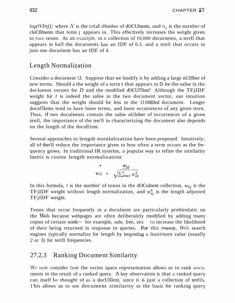
932 CHAPTER 27
log(lVInj); where 1'1 is the total rHnnber of dOCUlnents, and nj is the nurnber ofcloClllnents that tenn j appears in. This effectively increases the weight givento rare tenns. As an exarnple, in a collection of 10,000 docurnents, a terrIl thatappears in half the docurnents has an IDF of 0.3, and a tenll that occurs injust one docurnent has an IDF of 4.
Length Normalization
Consider a docurnent !J. Suppose that we lnodify it by adding a large nUlllber ofnew terrns. Should a the weight of a terrn t that appears in D be the saIne in thedoclunent vectors for D and the rnodified dOCUlTlent? Although the TFjIDFweight for t is indeed the saIne in the two document vector, our intuitionsuggests that the weight should be less in the 1110dified document. Longerdocul'llents tend to have lnore terms, and lnore occurrences of any given terrn.Thus, if two doculnents contain the saIne nUlnber of occurrences of a giventenll, the importance of the ten'll in characterizing the document also dependson the length of the docull1ent.
Several approaches to length nornlalization have been proposed. Intuitively,all of ther'll reduce the irnportance given to how often a term occurs as the frequency grows. In traditional IR systelns, a popular way to refine the sirnilarityInetric is cosine length normalization:
* tvij
Wij = l'£~=l 11I[
In this formula, t is the nurnbei' of tenns in the dOCulnent collection, 'Wij is theTFjIDF weight without length norrnalization, and tvij is the length adjustedTFjlDF weight.
Tenns that occur frequently in a doculnent are particularly problenlatic onthe "Veb because webpages are often deliberately rnodified by adding rnanycopies of certain words···· for exarnple, sale, free, sex to increase the likelihoodof their being returned in response to queries. l:'or this reason, \:Veb searchengines typically norrnalize for length by ilnposing a lnaxirnurn value (usually2 or 3) for terrIl frequencies.
27.2.3 Ranking Document Similarity
\Ve no\v consider ho\\-' the vector space representation allows us to rank dOCll
rnents in the result of a ranked query. A key observation is that a ranked querycan itself be thought of EL'S a docUlllent, since it is just a collection of terrl1s.1'his allows us to use document similarity as the ba",sis for ranking query
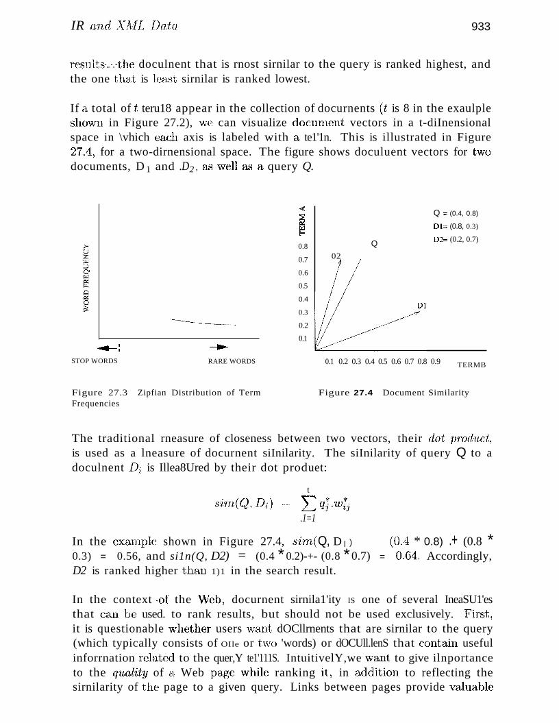
IR and Xi\:fL Data 933
results".... -..,-the doculnent that is rnost sirnilar to the query is ranked highest, andthe one that is least sirnilar is ranked lowest.
If a total of t teru18 appear in the collection of docurnents (t is 8 in the exaulplesho\~ln in Figure 27.2), \\"e can visualize docunH:~nt vectors in a t-diInensionalspace in \vhich each axis is labeled with a te1'1n. This is illustrated in Figure27.4, for a two-dirnensional space. The figure shows doculuent vectors for t\VOdocuments, D 1 and .D2 , &'3 \vell (;1",'3 a query Q.
0.1 0.2 0.3 0.4 0.5 0.6 0.7 0.8 0.9 TERMB
Q :;:: (0.4, 0.8)
01:;:: (0.8, 0.3)
D2:;:: (0.2, 0.7)Q
02
~
:EffiE-
0.8
0.7
0.6
0.5
0.4
0.3
0.2
0.1-......RARE WORDS
....-:STOP WORDS
Figure 27.3 Zipfian Distribution of TermFrequencies
Figure 27.4 Document Similarity
The traditional rneasure of closeness between two vectors, their dot prodlJ,ct,is used as a lneasure of docurnent siInilarity. The siInilarity of query Q to adoculnent IJi is Illea8Ured by their dot produet:
t
sim,(Q,Di ) ---... , LQj·7LJ7j.1=1
In the excunple shown in Figure 27.4, si'nt(Q, D l ) (0.4 * 0.8) .+ (0.8 *0.3) = 0.56, and si1n(Q, D2) = (0.4 * 0.2)-+- (0.8 *0.7) = 0,64. Accordingly,D2 is ranked higher than 1)1 in the search result.
In the context ,of the VVeb, docurnent sirnila1'ity IS one of several IneaSU1'esthat can be used. to rank results, but should not be used exclusively. First,it is questionable vvheth,er users want dOCllrnents that are sirnilar to the query(which typically consists of OIle or tvvo 'words) or dOCUll.lenS that contajn usefulinforrnation n~lated to the quer,Y te1'111S. IntuitivelY,we "vant to give ilnportanceto the Q'uality of a Web page \vhile ranking it, in addition to reflecting thesirnilarity of tlH.~ page to a given query. Links between pages provide valuable
934 C~HAPTER '2.7
additional inforrnation that can be used to obtain high-quality results. Wediscuss this issue in Section 27.4.2.
27.2.4 Measuring Success: Precision and Recall
Two criteria are cornnlonly used to evaluate information retrieval systerlls. Precision is the percentage of retrieved documents that are relevant to the query.Recall is the percentage of relevant docurnents in the database that are retrieved in response to a query.
Retrieving all documents in response to a query trivially guarantees perfectrecall, but results in very poor precision. The challenge is to achieve goodrecall together with high precision.
In the context of search over the Web, the size of the underlying collection ison the order of billions of docuruents. Given this, it is questionable whetherthe traditional measure of recall is very useful. Since users typically don't lookbeyond the first screen of results, the quality of a Web search engine is largelydeterlnined by the results shown on the first page. The following adapteddefinitions of precision and recall rnight be more appropriate for Web searchengInes:
• Web Search Precision: The percentage of results on the first page thatare relevant to the query.
• Web Search Recall: rrhe fraction N / M, expressed as a percentage, whereM is the nUluber of results displayed on the front page, and of the M ruostrelevant documents, N is the number displayed on the front page.
27.3 INDEXING FOR TEXT SEARCH
In this section, we introduce two indexing techniques that support the evaluation of boolean and ranked queries. 'The 'inverted index structure discussedin Section 27.3.1 is widely used due to its sirnplicity and good perforlnance.Its rnain disadvantage is that it imposes a significant space overhead: The sizecan be up to 300 percent the size of the original file. The signature file indexdiscussed in Section 27.::3.2 has a sInall space overhead and offers a quick filterthat elirninates rnost nonqualifying docurnents. However, does not scale as wellto larger dataha..')c sizes because the index has to be sequentially scanned.
Before a doeuruent is indexed, it is typically pre-processed to elirninate stopwords. Since the size of the indexes is very sensitive to the nurnber of tern1Sin the docurnent collection, elirninating stop words can greatly reduce index
IR and ..'KML Data
size. IR, systcrns also do certain other kinds of pre-processing. :For instance,they apply stelnming to reduce related terrns to a ca,nonical forrn. This stepalso reduces the nUluber of terrn8 to be indexed, but equally irnportantly, itallows us to retrieve documents that lnay not contain the exact query terrIl butcontain S(Hne variant. As an exarnple, the terrns T1ln, T'lLnning, and T'unncr allstern to 'run. The terrIl run is indexed, and every occurrence of a variant of thisterm is treated as an occurrence of run. A query that specifies rtLnneT findsdocurnents that contain any word that stenlS to T'UTt.
27.3.1 Inverted Indexes
An inverted index is a data structure that enables fast retrieval of all documents that contain a query terr11. For each ternl, the index rnaintains a list(called the inverted list) of entries describing occurrences of the tenn, withone entry per docurnent that contains the ternl.
Consider the inverted index for our running example shown in Figure 27.5. Theterm 'Jarnes' has an inverted list with one entry each for documents 1, 3, and4; the term 'agent' has entries for docurnents 1 and 2.
The entry for document d in the inverted list for terrn t contains details aboutthe occurrences of term t in document d. In Figure 27.5, this informationconsists of a list of locations within the document that contain term t. Thus,the entry for document 1 in the inverted list for terrn 'agent' lists the locations1 and 5, since 'agent' is the first and fifth word of docurnent 1. In general,we can store additional information about each occurrence (e.g., in an HTMLdocurnent, is the occurrence in the 1'ITLE tag?) in the inverted list. We canalso store the length of the docurnent if this is used for length norlnalization(see below).
The collection of inverted lists is called the postings file. Inverted lists can bevery large for large doeurnent collections. In fact, Web search engines typicallystore each inverted list on a separate page, and Inost lists span rnultiple pages(and if so, are rnaintained &'S a linked list of pages). In order to quickly findthe inverted list for a, query terrn, all possible query terrns are organized in asecond index structure such as a B+ tree or a. hash index.
The second index, called the lexicon, is Inuch srnaller than the postings filesince it only contains one entry per terrn, and further, only contains entries forthe set of terl11S that aTe retained after elirninating stop words, and applyingstenlluing rules. An entry consists of the terlIl, SOH1C surnrnary inforrnationabout its inverted list, and the address (on disk) of the inverted list. In Figure27.5, the SllIl1lnary inforrnation consists of the lllllllber of entries in the inverted
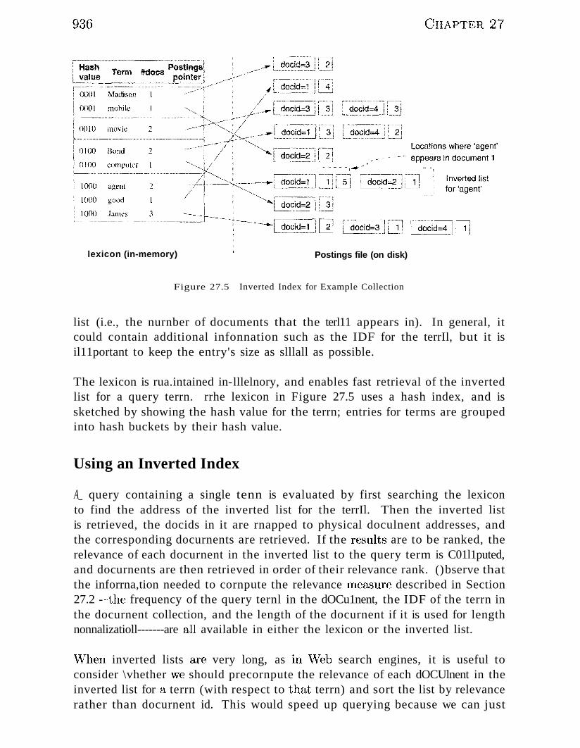
93G
lexicon (in-memory) Postings file (on disk)
CHAPTER 27
Figure 27.5 Inverted Index for Example Collection
list (i.e., the nurnber of documents that the terl11 appears in). In general, itcould contain additional infonnation such as the IDF for the terrIl, but it isil11portant to keep the entry's size as slllall as possible.
The lexicon is rua.intained in-lllelnory, and enables fast retrieval of the invertedlist for a query terrn. rrhe lexicon in Figure 27.5 uses a hash index, and issketched by showing the hash value for the terrn; entries for terms are groupedinto hash buckets by their hash value.
Using an Inverted Index
A_ query containing a single tenn is evaluated by first searching the lexiconto find the address of the inverted list for the terrIl. Then the inverted listis retrieved, the docids in it are rnapped to physical doculnent addresses, andthe corresponding docurnents are retrieved. If the results are to be ranked, therelevance of each docurnent in the inverted list to the query term is C01l1puted,and docurnents are then retrieved in order of their relevance rank. ()bserve thatthe inforrna,tion needed to cornpute the relevance 1neEU3ure described in Section27.2 - -the frequency of the query ternl in the dOCu1nent, the IDF of the terrn inthe docurnent collection, and the length of the docurnent if it is used for lengthnonnalizatioll-------are all available in either the lexicon or the inverted list.
\"lhen inverted lists are very long, as in\Veb search engines, it is useful toconsider \vhether we should precornpute the relevance of each dOCUlnent in theinverted list for a terrn (with respect to that terrn) and sort the list by relevancerather than docurnent id. This would speed up querying because we can just
IR and .i'yAtfL Data 937
look at a prefix of the inverted list, since users rarely look at 11101'0 than thefirst fc\v results. II(ywever 1 Ina.intaining lists in sorted order by relevance canbe expensive. (Sorting by dOcUll1cnt id is convenient because nevv dOCUlnentsare assigned increasing ids, and we can therefore sirnply <1ppend entries for newdOCUlnents at the end of the inverted list. Further, if the sirnilarity function ischanged, \ve do not have to rebuild the index.)
A query with a conjunction of several terrns is evaluated by retrieving theinverted lists of the query terrns one at a tiTne and intersecting theln. In orderto rninirnize 111en10r,}T usage, the inverted lists should be retrieved in order ofincreasing length. A query with a disjunction of several terrns is evaluated byruerging all relevant inverted lists.
Consider the exaruple inverted index shown in Figure 27.5. To evaluate thequery 'JaUles', we probe the lexicon to find the address of the inverted list for'Ja1nes', fetch it from disk and then retrieve docurIlent 1. To evaluate the query,Jarnes' AND 'Bond', we first retrieve the inverted list for the tenn 'Bond' andintersect it with the inverted list for the terrn 'Janles.' Crhe inverted list ofthe terrn 'Bond' has length two, whereas the inverted list of the terrIl 'Jarnes'has length three.) rrhe result of the intersection of the list (1,4) with the list(1, ~~, 4) is the list (1,4) and doculuents 1 and 4 are therefore retrieved. 'faevaluate the query '.lalnes' OR 'Bond,' we retrieve the two inverted lists in anyorder and merge the results.
for ranked queries with lnultiple tenns, we 1nust fetch the inverted lists forall terrl1s, COlllpute the relevance of every doclunent that appears in one ofthese lists with respect to the given collection of query terrns, and then sortthe docurnent ids by their relevance before fetching the docluuents in relevancerank order. Again, if the inverted lists are sorted by the relevance rnea,sure,we can support ranked queries by typically processing only sluall prefixes ofthe the inverted lists. (()bserve that the relevance of a docuIllent with respectto the query is easily cornputed froIn its relevance with respect to each queryterm.)
27.3.2 Signature Files
A signature fi,le is another index structure for text data.JH-:kse systerns thatsupports efficient evaluation of boolean queries. A signature file contains anindex record for each docurnent in the database. This index record is calledthe signature of the dOClunent. F~ach signature has a fixed size of b bits; b iscalled the signature width. rrhe bits that are set depend on the words thatappear in the docllrnent. vVe rnap words to bits by applying a hash functionto ea,ch vvord in the docurnent and we set the bits that appear in the result of
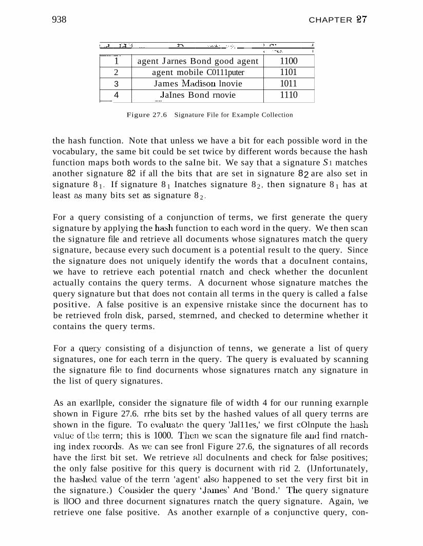
938 CHAPTER ~7
1...1 !lI ,.", 'l''''' ,.~,,± ".. '....:",.:'.;.. "" ""L£1' A
I .....""".,, !,,---_ ..
1 agent J arnes Bond good agent 11002 agent mobile C0111puter 11013 James 1rfadison lnovie 10114 JaInes Bond rnovie 1110_ ... ---
Figure 27.6 Signature File for Example Collection
the hash function. Note that unless we have a bit for each possible word in thevocabulary, the same bit could be set twice by different words because the hashfunction maps both words to the saIne bit. We say that a signature S 1 matchesanother signature 82 if all the bits that are set in signature 82 are also set insignature 8 1 . If signature 8 1 Inatches signature 8 2 , then signature 8 1 has atleast as many bits set as signature 8 2 .
For a query consisting of a conjunction of terms, we first generate the querysignature by applying the hash function to each word in the query. We then scanthe signature file and retrieve all documents whose signatures match the querysignature, because every such document is a potential result to the query. Sincethe signature does not uniquely identify the words that a docuInent contains,we have to retrieve each potential rnatch and check whether the docunlentactually contains the query terms. A docurnent whose signature matches thequery signature but that does not contain all terms in the query is called a falsepositive. A false positive is an expensive rnistake since the docurnent has tobe retrieved froln disk, parsed, stemrned, and checked to determine whether itcontains the query terms.
For a qUf~ry consisting of a disjunction of tenns, we generate a list of querysignatures, one for each terrn in the query. The query is evaluated by scanningthe signature file to find docurnents whose signatures rnatch any signature inthe list of query signatures.
As an exarllple, consider the signature file of width 4 for our running exarnpleshown in Figure 27.6. rrhe bits set by the hashed values of all query terrns areshown in the figure. To evaluat(~ the query 'Jal11es,' we first cOlnpute the hashvalue of the terrn; this is 1000. 'fhen we scan the signature file a11(1 find rnatching index recol~ds. As \lve can see fronl Figure 27.6, the signatures of all recordshave the first bit set. We retrieve all doculnents and check for false positives;the only false positive for this query is docurnent with rid 2. (lJnfortunately,the ha..shed value of the terrn 'agent' also happened to set the very first bit inthe signature.) C~onsider the query \Jarnes' And 'Bond.' ~rhe query signatureis llOO and three docurnent signatures rnatch the query signature. Again, \ve
retrieve one false positive. As another exarnple of a conjunctive query, con-
IR andXJvfL Data 939
sider the query 'rnovie' And ':Nladison.' The query signature is 0011, and onlyone doclunent signature lnatches the query signature.N0 false positives areretrieved.
Note that for each query we have to scan the cOlllplete signature file, and thereare a" 11lany records in the signature file as there are documents in the database.To reduce the anlount of data that has to be retrieved for each query, we canvertically partition a signature file into a set of bit slices, and we call such anindex a bit-sliced signature file. The length of each bit slice is still equal tothe number of doculllents in the database, but for a query with q bits set inthe query signature we need only to retrieve q bit slices. The reader is invitedto construct a bit-sliced signature file and to evaluate the exarnple queries inthis paragraph using the bit slices.
27.4 WEB SEARCH ENGINES
Web search engines rIlust contend with extreruely large nurubers of doculllents,and have to be highly scalable. Docurnents are also linked to each other, andthis link infonnation turns out to be very valuable in finding pages relevantto a given search. These factors have caused search engines to differ frorntraditional IR systerns in irnportant ways. Nonetheless, they rely on sorne forn1of inverted indexes as the basic indexing mechanism. In this section, we discussWeb search engines, using Google as a typical example.
27.481 Search Engine Architecture
'Veb search engines crawl the web to collect docurnents to index. 'Ihe crawlingalgorithrn is sirrlple, but crawler software can be cornplex because of the detailsof connecting to millions of sites, minimizing network latencies, parallelizingthe crawling, dealing with tirneouts and other connection failures, ensuringthat crawled sites are not unduly stressed by thE~ cra\vler, and other practicalconcerns.
The search algorithrn used by a crawler is a graph traversal. Starting at acollection of pages with rnany links (e.g. ,Yahoo directory pages), all links oncra\vled pages a,re follo\\red to identify ne\v pages. This step is iterated, keepingtrack of which pages have been visited in order to avoid re-visiting thenl.
The collection of pages retrieved through crawling can be enonnous, on theorder of billions of pages. Indexing thern is a very expensive ta"sk. Fortunately,tlle ta",sk is highly parallelizable: Each docurnent is independently arlalyzedto create inverted lists for the terrns that appear in the docurnent. T'heseper-doCUlnent lists are then sorted b~y terrn and luerged to crcclte cornplete per-
940 CHAPTER '47
terrn inverted lists that span all dOCllrnents. Ternl statistics such as IDF canbe cornputed during the lnerge phase.
Supporting searc~hes over such vast indexes is another luanulloth undertaking.Fortunately, again, the task is readily parallelized using a cluster of inexpensiveInachines: \Ve can deal with the anlount of data by partitioning the index acrossseveral rnachines. Each Inachine contains the inverted index for those termsthat are Inapped to that luachine (e.g., by hashing the tenn). Queries 111ayhave to be sent to luultiple Inachines if the terrl1S they contain are handled bydifferent rnachines, but given thatvVeb queries rarely contain rnore than twoterrns, this is not a serious probleln in practice.
We rnust also deal \vith a huge volume of queries; Google supports over 150lllillion searches each day, and the nUlnber is growing. This is acc(nnplishedby replicating the data across several machines. vVe already described how thedata is partitioned across Inachines. For each partition, we now a..ssign severalnlachines, each of which contains an exact copy of the data for that partition.Queries on this partition can be handled by any rnachine in the partition.Queries can be distributed across rnachines on the basis of load, by hashing onIP addresses, etc. Replication also addresses the problern of high-availability,since the failure of a Inachine only increases the load on the remaining rnachinesin the partition, and if partitions contain several rnachines the ilnpact is sIuall.Failures can be rnade transparent to users by routing queries to other Inachinesthrough the load balancer.
27.4.2 Using Link Information
webpages are created by a variety of users for a variety of purposes, and theircontent does not always lend itself to effective retrieval. The rnost relevantpages for a search rnay not contain the search terrns at all and are thereforenot returned by a boolean keyvvord search! For exarnple, consider the queryternl 'Web browser.' A boolea,11 text query using the tenns does not return therelevant pages of Netscape Corporation or }\trierosoft, because these pages donot contain the terrn 'Web browser' at all. Sirnilarly, the horne page of 'Yahoodoes not contain the terrn 'search engine.' The problenl is that relevant sitesdo not necessarily describe their contents in a ¥,ray that is llseful for booleantext queries.
Until no\v, ¥,re only considered infonnation 'within a single \vebpage to estirnateits relevance to a query. But webpages are connected through h:yperlinks, andit is quite likely that there is a \VebpEtge containing the terrn 'search engine'that has a link to Yahoo's horne page. Can we use the inforrnation hidden insuch links'?
III aTul X1vIL Data ~41
Building on research in the sociology literature, an interesting analogy betweenlinks and bibliographic citations suggests a \vay to exploit link infoI'Ination: Justas influential authors and pubications are cited often, good 'Vvebpages are likelyto be often linked to. It is useful to distinguish between two types of pages,authorities and hubs. An authority is a page that is very relevant to a certaintopic and that is recognized by other pages as authoritative on the subject.These other pages, called hubs, usually have a significant nUll1ber of hyperlinksto authorities, although they tlH~nlselves are not very well known and do notnecessarily carry a lot of content relevant to the given query. Hub pages couldbe cOlnpilatiol1s of resources about a topic on a site for professionals, lists ofreco111mended sites for the hobbies of an individual user, or even a part of thebookIllarks of an individual user that are relevant to one of the user's interests;their Blain property is that they have IHany outgoing links to relevant pages.Good hub pages are often not well known and there may be few links pointingto a good hub. In contrast, good authorities are 'endorsed' by rnany good hubsand thus have many links froln good hub pages.
This symbiotic relationship between hubs and authorities is the basis for theHITS algoritlun, a link-based search algorithm that discovers high-quality pagesthat are relevant to a user's query terrns. The HITS algorithIll rnodels \iVeb as adirected graph. Each webpage represents a node in the graph, and a hyperlinkfroIn page A to page B is represented as an edge between the two correspondingnodes.
Assulne that we are given a user query with several terIns. The algorithIllproceeds in two steps. In the first step, the sarnpling step, we collect a set ofpages called the base set. The ba..se set 11lOSt likely includes very relevant pagesto the user's query, but the base set can still be quite large. In the second step,the itera"tion step, we find good authorities and good hubs arnong the pages inthe ba.."c set.
The salnpling step retrieves a set of webpages that contain the query terrns,using sorne traditional technique. For exarnple, 'we can evaluate the query et.e;
a boolean key-word search and retrieve all webpages that contain the queryterrns. vVe call the resulting set of pages the root set. 1'he root set Inight notcontain all relevant pages because senne <\'uthoritative pages rnight not includethe user query \vords. But \ve expect that at lea."t SOlne of the pages in the rootset contain hyperlinks to the rnost relevant authoritative pages or that SCHneauthoritative pages link to pages in the root set. rrhis rnotivates our notion ofa link page. \¥e call a page a link page if it ha.." a hyperlink to sorne page inthe root set or if a page in the root set has a hyperlink to it. In order not toIniss potentially relevant pa,ges, \ve auglnent the root set by all link pages andvve call the resulting set of pages the base set. rrhus~ the base set includes all
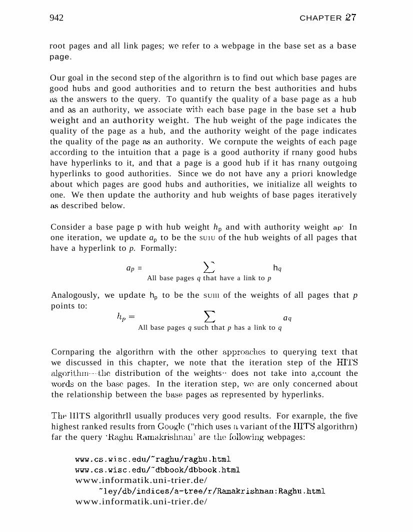
942 CHAPTER i2.7
root pages and all link pages; \ve refer to a webpage in the base set as a basepage.
Our goal in the second step of the algorithrn is to find out which base pages aregood hubs and good authorities and to return the best authorities and hubsa,." the answers to the query. To quantify the quality of a base page as a huband as an authority, we associate vvith each base page in the base set a hubweight and an authority weight. The hub weight of the page indicates thequality of the page as a hub, and the authority weight of the page indicatesthe quality of the page as an authority. We cornpute the weights of each pageaccording to the intuition that a page is a good authority if rnany good hubshave hyperlinks to it, and that a page is a good hub if it has rnany outgoinghyperlinks to good authorities. Since we do not have any a priori knowledgeabout which pages are good hubs and authorities, we initialize all weights toone. We then update the authority and hub weights of base pages iterativelyas described below.
Consider a base page p with hub weight hp and with authority weight ap' Inone iteration, we update ap to be the SU1U of the hub weights of all pages thathave a hyperlink to p. Formally:
ap = L hq
All base pages q that have a link to p
Analogously, we update hp to be the SUlll of the weights of all pages that ppoints to:
hp == L aq
All base pages q such that p has a link to q
Cornparing the algorithrn with the other approctches to querying text thatwe discussed in this chapter, we note that the iteration step of the lIlT'Salgorithln-·m·the distribution of the weights·· does not take into a,ccount the'Vvards on the ba,,'3c pages. In the iteration step, \ve are only concerned aboutthe relationship between the base pages as represented by hyperlinks.
l'he lIlTS algorithrIl usually produces very good results. For exarnple, the fivehighest ranked results frorn (ioogle ("rhich uses a variant of the lIIT'S algorithrn)far the query '.R,aghuH.arnakrishnan' are the follo'Vving webpages:
www.cs.wisc.edu/~raghu/raghu.html
www.cs.wisc.edu/~dbbook/dbbook.html
www.informatik.uni-trier.de/~ley/db/indices/a-tree/r/Ramakrishnan:Raghu.html
www.informatik.uni-trier.de/
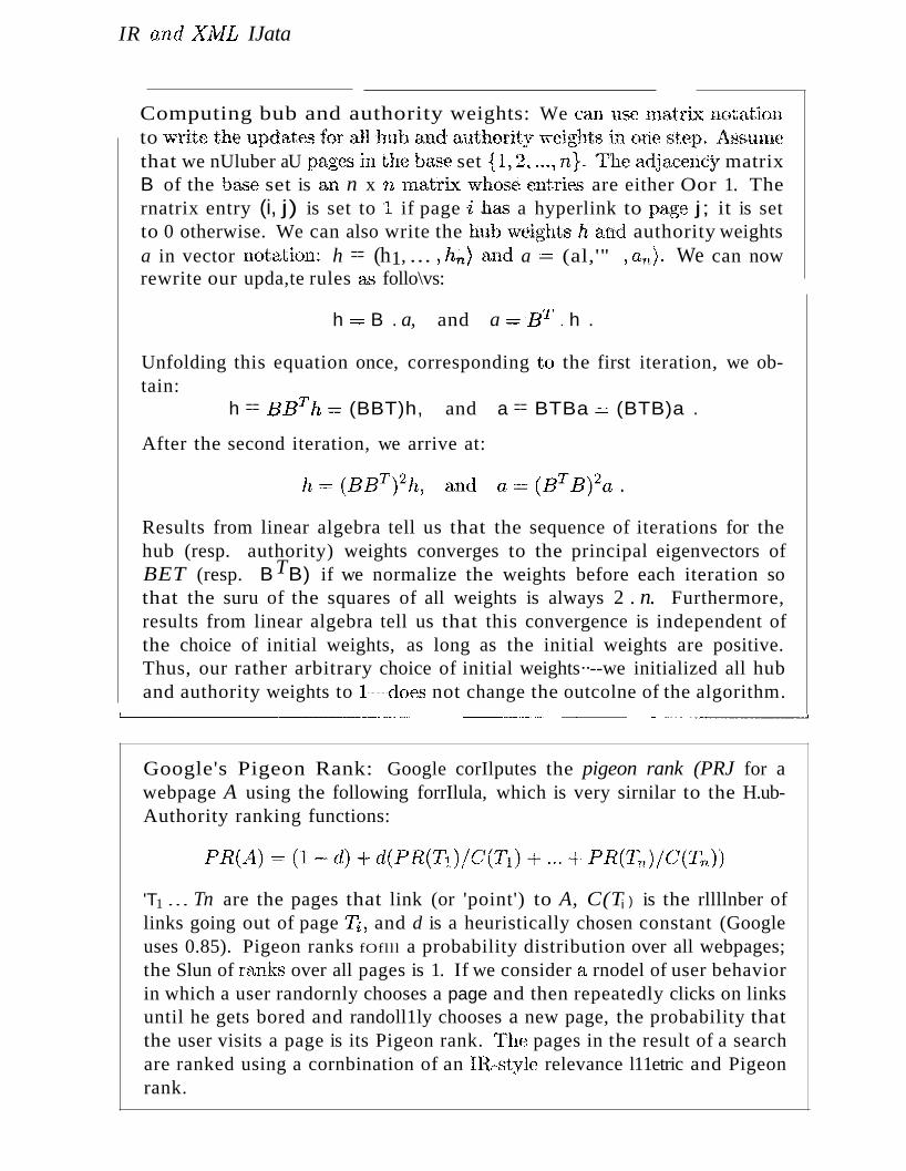
IR and XlvlL IJata
Computing bub and authority weights: We can use luatrix notationto write the updates for allhllband cLuthotity weights in orle step. Assumethat we nUluber aU pages in the base set {I, 2, "'1 n}.The·adjaeCIJ.CY matrixB of the ba.se set is an n x n matrix whose entries are either Oor 1. Thernatrix entry (i, j) is set to 1 if page 'ihas a hyperlink to page j; it is setto 0 otherwise. We can also write the hub weightshand authority weightsa in vector notat.ion: h == (h1, ... ,hn ) and a == (al,'" ,an)' We can nowrewrite our upda,te rules as follo\vs:
h :::;: B . a, and a =::BT . h .
Unfolding this equation once, corresponding to the first iteration, we obtain:
h == BBTh:::;: (BBT)h, and a == BTBa == (BTB)a .
After the second iteration, we arrive at:
Results from linear algebra tell us that the sequence of iterations for thehub (resp. authority) weights converges to the principal eigenvectors ofBET (resp. B TB) if we normalize the weights before each iteration sothat the suru of the squares of all weights is always 2 . n. Furthermore,results from linear algebra tell us that this convergence is independent ofthe choice of initial weights, as long as the initial weights are positive.Thus, our rather arbitrary choice of initial weights··--we initialized all huband authority weights to l-·u·-~does not change the outcolne of the algorithm.
._---~--_ _ _--------------'
Google's Pigeon Rank: Google corIlputes the pigeon rank (PRJ for awebpage A using the following forrIlula, which is very sirnilar to the H.ubAuthority ranking functions:
'T1 ... Tn are the pages that link (or 'point') to A, C(Ti ) is the rllllnber oflinks going out of page T i , and d is a heuristically chosen constant (Googleuses 0.85). Pigeon ranks fOflll a probability distribution over all webpages;the Slun of ranks over all pages is 1. If we consider a rnodel of user behaviorin which a user randornly chooses a page and then repeatedly clicks on linksuntil he gets bored and randoll1ly chooses a new page, the probability thatthe user visits a page is its Pigeon rank. 1]le pages in the result of a searchare ranked using a cornbination of an lIt-style relevance l11etric and Pigeonrank.
944 CHAPTER ;27
..........__ -_ _--~ _~ _..__ _~ ..~,----_ ~_ .._-_._ __._ _-_ _-_ _ _._-,
SQL/M:rvl: Full Text 'Fun text.' is described as data that can be searched,unlike simple charac~ter strings, and a ne\v data type called FullText isintroduced to support it. The Inethods associated 'with this type supportsearching for individual \vords, phrases, words that 'sound like' a queryterlll, etc. Three 11lethods are of particular interest. CONTAINS checks if aFullText object contains a specified search terln (word or phrase). RANKreturns the relevance rank of a FullText object with respect to a specifiedsearch terln. (I-Iow the rank is defined is left to the hnplementation.) IS
IABOUT detennines whether the FullText object is sufficiently related to I
I the specified search term. (The behavior of IS ABOUT is also left to the Ii iInplelllentation.) ,
LRelational DB1'ISs fnnn IBIvI, Microsoft, and Oracle all support text fields'~jalthough they do not currently conforrll to the SQL/JV1NI standard.--~.. -"~ '" - - - -
-ley/db/indices/a-tree/s/Seshadri:Praveen.htmlwww.acm.org/awards/fellows_citations_n-z/ramakrishnan.htmI
The first result is Rarnakrishnan's horne page; the second is the horne page forthis book; the third is the page listing his publications in the popular DBLPbibliography; and the fourth (initially puzzling) result is the list of publicationsfor a forrner student of his.
27.5 MANAGING TEXT IN A DBMS
In preceding sections, we saw how large text collections are indexed and queriedin JR, systerns and vVeb search engines. We now consider the additional challenges raised by integrating text data into databa",se systerns.
The basic approach being pursued by the SQI.I standards cornrnunity is to treattext docllrnents a..'S a ne\v data type, FullText, that can appear as the value of afield in a table. If \ve define a table w'ith a single cohunn of type FullText, eachrow in the table corresponds to a docurnent in a dOClllnent collection. IVlethodsof Fulll'ext can be llsed in the WHERE clause of SQL queries to retrieve rowscontaining text objects that Inatch an IR-style search criterion. The relevancerank of a FullText object can be explicitly retrieved using the RANK rnethod,fUld this can be llsed to sort results by relevance.
Several points ruust be kept in rnind as '\Te consider this approach:
Ii This is an extrernely general (l,pproach, a,nel the perforlnance of a SC~L systern that supports such an extension is likely to be inferior to a specializedIII SystCIIl.
IR and J){lVfL Data 945
• The rnodel of data does not ad.equately reflect docurnents with additionalrnetadata. If "\ve store docurnents in a table with a FullText colurnn anduse additional cohl1nns to store rnetadata--for exarnple, author, title, SUIllInary, rating, popularitY---~'relevancerneasures that cornbine nletadata 'withIR, similarity rnea..'3ures 11lUSt be expressed using lle\V user-defined rnethods, because the RANK rnethod only has access to the F\lllText object, andnot the rnetadata. The ernergence of XML docurnents, which have nonuniforrn, partial rlletadata, further cornplicates nlatters.
• The handling of updates is unclear. As we have seen, IR indexes are corllplex, and expensive to 111aintain. Requiring a systern to update the indexesbefore the updating transaction cOl1ullits can irnpose a severe perfonnancepenalty.
27.5.1 Loosely Coupled Inverted Index
The irrlplenlcntation approach used in current relational DBMSs that supporttext fields is to have a separate text-search engine that is loosely coupled to theDBMS. The engine periodically updates the indexes, but provides no transactional guarantees. Thus, a transaction could insert (a row containing) a textobject and cornrnit, and a subsequent transaction that issues a. Inatching searchmight not retrieve the (row containing the) object.
27.6 A DATA MODEL FOR XML
.Aswe saw in Section 7.4.1, XML provides a way to rnark up a docurnentwith rneaningful tags that irnpart SaIne partial structure to the docurnent.Se'fnistrtLctured data rnodels, which we introduce in this section, capture rnuchof the structure in X~fL doculnents, while abstracting away Inany deta.ils. 1
Sernistructured data Inodels have the potential to serve as a forInal foundationfor XlVIL and enable us to rigorously define the sernantics of queries over XlVIL,which we disc-uBs in Section 27.7.
27.6.1 Motivation for Loose Structure
Consider a set of doculnents on the Web that contain hyperlinks to other docUHlents. These docurnents, although not eornpletely unstructurecl~ cannot bernodeled naturally in the relational data rnodel because the pattern of hyperlinks is not regular across docurnents. In fa,ct, every HTl\1L docurnent ha.s
1.An iruportant aspect of XIvII..; tha.t is not captured is the ordering of elements. A more completedata model called XData ha...,,; been proposed by the \;V:3C committee that is developing XivtL standards,but we do not discuss it here.
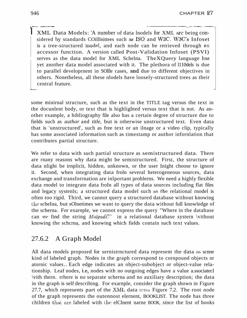
946 CHAPTER 27
r-"~---""'-" -...---.-----.---..........---..-----....
I XML Data Models: 'A number of data lnodels for XML are being considered by standards COilllnittees such as ISO and W3C.vV3C's Infosetis a tree-structured ll10del, and each node can be retrieved through anaccessor function. A version called Post-Validation Infoset (PSVI)serves as the data model for XML Schelna. TheXQuery language hasyet another data model associated with it. The plethora of l110dels is dueto parallel developrnent in SOllle cases, and due to different objectives inothers. Nonetheless, all these nlodels have loosely-structured trees as theircentral feature.
L-- . . , , .-1
some minirnal structure, such as the text in the TITLE tag versus the text inthe docunlent body, or text that is highlighted versus text that is not. As another example, a bibliography file also has a certain degree of structure due tofields such as author and title, but is otherwise unstructured text. Even datathat is 'unstructured', such as free text or an ilnage or a video clip, typicallyhas some associated information such as timestamp or author infornlation thatcontributes partial structure.
We refer to data with such partial structure as semistructured data. Thereare rnany reasons why data might be semistructured. First, the structure ofdata nlight be irnplicit, hidden, unknown, or the user Inight choose to ignoreit. Second, when integrating data froln several heterogeneous sources, dataexchange and transforrnation are inlportant problerns. We need a highly flexibledata rnodel to integrate data froIn all types of data sources including flat filesand legacy systenls; a structured data model such a",s the relational rnodel isoften too rigid. Third, we cannot query a structured database without knowingthe scheIna, but sOlnetimes we want to query the data without full knowledge ofthe scherna. For exarnple, we cannot express the query "Where in the databasecan ,ve find the string Malgv.d'i?" in a relational database systern \vithoutknowing the schcrna, and knowing which fields contain such text values.
27.6.2 A Graph Model
All data rnodels proposed for sernistrnctured data represent the data as scnnekind of labeled graph. Nodes in the graph correspond to cornpound objects oratornic values.. Each edge indicates an object-subobject or object-value relationship. Leaf nodes, Le; nodes with no outgoing edges have a value a.ssociatecl\vith thern. rrhere is no separate scherna and no auxiliary description; the datain the graph is self describing. For exarnple, consider the graph shown in Figure27.7, which represents part of the XlVIL data f1'01n Figure 7.2. The root nodeof the graph represents the outennost elernent, BOOKLIST. The node has threechildren that are labeled with the elClnent narne BOOK, since the list of books
IR and )(lvfL Data
Richard Feynman
('-;-~'\ BOOKUST
,"~""'~\."-_/'~';::'':;::::::::::::_,,-~---,,", -"--..,-...~ ....~
-"'-._--....................-
Waitinglor the
Mahatma
R.K. Narayan
Figure 27.7 The Semistructured Data :NIodel
"',/'\
( 13 ; PUBLISHED\ !r
1981
9»17
consists of three individual books. The numbers within the nodes indicate theobject identifier associated with the corresponding object.
We now describe one of the proposed data models for semistructured data,called the object exchange model (OEM). Each object is described by aquadruple consisting of a label, a type, the value of the object, and all. objectidentifier which is a unique identifier for the object. Since each object has alabel that can be thought of as a column nallle in the relational model, and eachobject has a type that can be thought of as the column type in the relationalrnodel, the object exchange Illodel is self-describing. Labels in OEM should be&'3 infol'rnative as possible, since they serve two purposes they can be used toidentify an object as well as to convey the meaning of an object. For example,we can represent the last HaIne of an author as follows:
(lastName, string, "Feynman")
More cOInplex objects are decornposed hierarchically into srnaller objects. Forexalllple, a,n author naIne can contain a first narne and a last narne. rrhis objectis described as follows:
(authorName, set, {fiT stnarnel, lastnaTnel})fiTsi:nantel is (firstName, string, "Richard")lastnarnef is (lastName, string, "Feynman")
As another exarnple, an object representing a set of books is described a"s follows:
(bookList, set, {book1 , book2 , book;3} )book} is (book, set, {(L'U,thOTl, title}, p'u,blishcd1})
948 CHAPTER 2*7
'-~-- .._......•.._._-_.-._._-- ---'" _.-_.__._ __..__ _.__ _..~
SQL and XML: XQuery is a standard proposed by the vVorld-vVide Web 1
Consortiurn (W3C). In parallel, standards con:unittees developing the SQL Istandards have been working on a successor to SQL:1999 that supportsX~fL. 1"'he part that relates to X:NIL is tentatively called SQL/XML anddetails can be found at http: / / sqlx . arg.
. _ ..__ ._._~._.._ _ __ __l
bo()k~2 is (book, set, {attthor2, t-itle2, ]Jubl'ished2 })
book3 is (book, set, {aui:hoT:3, t'itle3,Published3})authoT3 is (author, set, {!'lrstnarnJe3, lastna'Tne3})t'itle3 is (title, string, liThe English Teacher")pttbl'ished3 is (published, integer, 1980)
27.7 XQU'ERY: QUERYING XML DATA
Given that XlvII.. doculnents are encoded in a way that reflects (a considerable amount of) structure, we have the opportunity to use a high-level language that exploits this structure to conveniently retrieve data fro111 withinsuch documents. Such a language would also allow us to easily translate XMLdata between different DTDs, as we lllUSt when integrating data from multiplesources. At the tirne of writing of this book, XQuery is the W3C standardquery language for XML data. In this section, we give a brief overview ofXQuery.
27.7.1 Path Expressions
Consider the XlvII.. dOCUlnent shown in Figure 7.2. The following exarnple queryreturns the last nanles of all authors, assullling that our XML docurnent residesat the location www.ourbookstore.com/books . xml.
FOR$1 IN doc(www.ourbookstore.com/books.xml)//AUTHOR/LASTNAME
RETURN <RESULT> $1 </RESULT>
This exarnple illustrates sonle of the basic constructs of X(~uery. The FORclause in XQuer:y is roughly analogous to the FROM clause in SC:~L. The RETURNclause is sirnilar to the SELECT clause. \Ve return to the general fornl of queriesshortly, after introducing an irnportant concept called a path expression.
'1'he expression
doc(www.ourbookstore.com/books.xml)//AUTHOR/LASTNAME
IR and ./YA1L ]Jata 949j)
XPath and Other XML Query Languages: Path expressions inXQuery are derived frorn XPath, an earlier Xl\:IL query facility. Path expressions in XPath can be qualified ,vith selection conditions, and can utilize several built-in functions (e.g., counting the nurnber of nodes rnatchedby the expression). l\tlany of XQuery's features areborro\vecl {roIn earlierlanguages, including XML-QL and Quilt.
r'~'~~~""""""~""'"
!
IIII
in the FOR clause is an exarnple of a path expression. It specifies a pathinvolving three entities: the docurnent itself, the AUTHOR elernents and theLASTNAME elernents.
The path relationship is expressed through separators / and / /. The separator / / specifies that the AUTHOR elernent can be nested anywhere withinthe document whereas the separator / constrains the LASTNAME elernent to benested immediately under (in terms of the graph structure of the docurnent)the AUTHOR element. Evaluating a path expression returns a set of elernentsthat rnatch the expression. The variable l in the example query is bound inturn to each LASTNAME elernent returned by evaluating the path expression.(To distinguish variable naInes fronl normal text, variable narnes in XQueryare prefixed with a dollar sign $.)
The RETURN clause constructs the query result-·--which is also an XML docurnent-···_·by bracketing each value to which the variable l is bound with the tag RESULT.
If the exanlple query is applied to the sarnple data shown in Figure 7.2, theresult would be the following X:NIL docurnent:
<RESULT><LASTNAME>Feynman </LASTNAME></RESULT>
<RESULT><LASTNAME>Narayan </LASTNAME></RESULT>
We use the docurnent in Figure 7.2 as our input in the rest of this chapter.
27.7.2 FLWR Expressions
The ba~sic fornl of an X(~uery consists of a FLWR expression, where theletters denote the FOR, LET, WHERE and RETURN clauses. The FOR etHel LET
clauses bind variables to values through path expressions. These values arequalified by the WHERE clause, and the result .XlVIL fragrnent is constructed bythe RETURN clause.
rrhe difference between a FOR and LET clause is that while FOR binds a variableto each elernent specified by the path expression, LET binds a variable to thewhole collection of elernents. T'hus, if we change our exarnple query to:
950 CHAPTER 2;;
LET$IINdoc(www.ourbookstore.com/books.xm1)//AUTHOR/LASTNAME
RETURN <RESULT> $1 </RESULT>
then the result of the query beconles:
<RESULT><LASTNAME>Feynman</LASTNAME><LASTNAME>Narayan</LASTNAME>
</RESULT>
Selection conditions are expressed using the WHERE clause. Also, the output ofa query is not lirnited to a single elernent. These points are illustrated by thefollowing query, which finds the first and last names of all authors who wrotea book that was published in 1980:
FOR $b IN doc(www.ourbookstore.com/books.xm1)/BOOKLIST/BOOKWHERE $b/PUBLISHED='19S0'RETURN
<RESULT> $b/AUTHOR/FIRSTNAME, $b/AUTHOR/LASTNAME </RESULT>
The result of the above query is the following XML docurnent:
<RESULT><FIRSTNAME>Richard </FIRSTNAME><LASTNAME>Feynman </LASTNAME>
</RESULT><RESULT>
<FIRSTNAME>R.K. </FIRSTNAME><LASTNAME>Narayan </LASTNAME></RESULT>
For the specific DTI) in this exalnple, where a BOOK elernent hac; only oneAUTHOR, the above query can be written by using a different path expression inthe FOR clause, as follows.
FOR $a INdoc(www.ourbookstore.com/books.xml)
/BOOKLIST/BOOK[PUBLISHED='19S0']/AUTHORRETURN <RESULT> $a/FIRSTNAME, $a/LASTNAME </RESULT>
rrhe path expression in this query is an instance of a branching path expression. The variable l is now bound to every AUTHOR elernent that rnatchesthe path doc/BOOKLIST/BOOK/AUTHOR where the intennediate BOOK elClnent isconstrained to have a PUBLISHED elernent nested inunediatelv within it with
./
the value 1980.
IR and ){NfL IJata
27.7.3 Ordering of Elements
951
XML data consists of ordered doculnents and so the query language IllUSt returndata in SOUle order. The selnantics of X(~uery is that a path expression returnsresults sorted in document order. Thus, variables in the FOR clause are boundin doculnent order. If however, we desire a different order, we can explicitlyorder the output as shown in the follo\ving query, which returns TITLE elernentssorted lexicographically.
FOR$b IN doc(www.ourbookstore.com/books.xml)/BOOKLIST/BOOK
RETURN <BOOKTITLES> $b/TITLE </BOOKTITLES>SORT BY TITLE
27.7.4 Grouping and Generation of Collection Values
Our next example illustrates grouping in XQuery, which allows us to generatea new collection value for each group. (Contrast this with grouping in SQL,which only allows us to generate an aggregate value (e.g., SUM) per group.)Suppose that for each year we want to find the last narnes of authors whowrote a book published in that year. We group by year of publication andgenerate a list of la.."t names for each year:
FOR $p IN DISTINCTdoc(www.ourbookstore.com/books.xml)/BOOKLIST/BOOK/PUBLISHEDRETURN<RESULT>
$p,FOR $a IN DISTINCT /BOOKLIST/BOOK[PUBLISHED=$pJ/AUTHOR
RETURN $a</RESULT>
The keyword ,DI8TINC}T elirninates duplicates fronl the collection returned bya, path expression. Using the XML docurnent in Figure 7.2 as input, the abovequery produces the following result:
<RESULT>: <PUBLISHED>1980</PUBLISHED><LASTNAME>Feynman</LASTNAME><LASTNAME>Narayan</LASTNAME>
</RESULT><RESULT> <PUBLISHED>1981</PUBLISHED>
<LASTNAME>Narayan</LASTNAME></RESULT>
952 CHAPTER 2¥"f
27.8 EFFICIENT EVALUATION OF XML QUERIES
X.Query operates on XKJIL data and produces XTvIL data as output. In order tobe able to evaluate queries efficiently, we need to address the follo\ving issues.
• Storage: \Ve can use an existing storage systerIl like a relational or objectoriented systerll or design a new storage forInat for X1tIL doclunents. Thereare several ways to use a relational systenl to store XML. One of thern isto store the X1VIL data as Character Large Objects (CLOBs). (CLOBSwere discussed in Chapter 23.) In this case, hc)\vever, we cannot exploitthe query processing infrastructure provided by the relational systerrl andwould instead have to process XQuery outside the database systenl. Inorder to circumvent this problenl, we need to identify a scherna accordingto which the XML data can be stored. rr'hese points are discussed inSection 27.8.1.
• Indexing: Path expressions add a lot of richness to XQuery and yieldlllany new access patterns over the data. If we use a relational system forstoring XML data, then we are constrained to use only relational indexeslike the B-n·ee. However, if we use a native storage engine, then we havethe option of building novel index structures for path expressions, some ofwhich are discussed in Section 27.8.2.
• Query Optimization: Optirnization of queries in XQuery is an openproblern. The work so far in this area can be divided into three parts. 'rhefirst is developing an algebra for XQuery, analogous to relational algebra.The second research direction is providing statistics for path expressionqueries. Finally, SOlne work has addressed sirnplification of queries by exploiting constraints on the data. Since query optirnization for X.Query isstill at a prelirninary stage, we do not cover it in this chapter.
Another issue to be considered while designing a ne\v storage systeul for X1.1Ldata is the verbosity of repeated tags. As we see in Section 27.8.1) using arelational storage systelu addresses this problern since tag narnes are not storedrepeatedly. If on the other hand, we \vant to build a native storage systcrn, thenthe rnanner in which the X.~lL data is cornpressed becornes significant. Severalcornpression. algorithrHs aTe known that achieve cOlnpression ratios close torelational storage, 1n1t \ve do not discuss ther11 here.
27.8.1 Storing XML in RDBMS
()n(~ nEttural candidate for storing X1JIL data is a relational dataJKlse systern.The ruain issues involved in storing XJ\;IL data in a relational systelTI are:
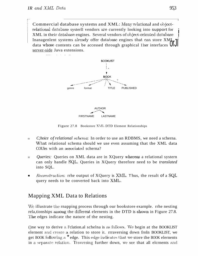
IR and XlvIL Data 953},)
Commercial database systems and XML: wiany relational and objeetrelational database systerll vendors are currently looking into support forXML in their database engines. Several vendors of object-oriented database
!
iI!
Inanagenlent systems already offer database engines that can store XML i
data 'whose contents can be accessed through graphical 11ser interfaces orJIserver-side Java extensions.
+++-,~~-~,.~."-_.~..~ ~ _ _ _._ _._~._._-_.
genre format TITLE PUBLISHED
AUTHOR
~~FIRSTNAME LASTNAME
Figure 27.8 Bookstore X:NIL DTD Element Relationships
II C;hoice of relational scherr~a: In order to use an RDBMS, we need a scherna.vVhat relational schema should we use even assuming that the XML dataCOUles with an &'Ssociated scherna?
II Queries: Queries on XML data are in XQuery wherea" a relational systerncan only handle S(~L. Queries in XQuery therefore need to be translatedinto SQL.
III Ilecon8tructioT~: rrhe output of XQuery is X~1L. T1hus, the result of a S(~L
query needs to be converted back into XNIL.
Mapping XML Data to Relations
\lVe illustrate the rnapping process through our bookstore exarnple. rrhe nestingrela,tionships alIlong the different elernents in the DTD is sho\vn in Figure 27.8.rrhe edges indicate the nature of the nesting.
()ne way to derive a l'clation.al schelna is as follovvs. \Ve begin at the BOOKLISTelernent anel create (1 relation to store it. rrraversing down froIn BOOKLIST, weget BOOK foIlc)\ving (l. * edge. This edge indic.ates that \~le store the BOOK elernentsin a separate reJation. l'r;:l,versing further down, we see that all elcrnents and
954 CHAPTER 27
attributes nested \vithin BOOK occur at 1I10St once. Hence, we can store thenlin the saIne relation a.." BOOK. The resulting relational schelIla Relschernal isshown below.
BOOKLIST( id: integer)BOOK (booklistid: integer, author_firstna'me: string,
author_lastnarne: string, title: string,published: string, genre: string, format: string)
BOOK. booklistid connects BOOK to BOoKLIST. Since a DTD has only one basetype, string, the only base type used in the above schelna is string. Theconstraints expressed through the DTD are expressed in the relational schema.For instance, since every BOOK must have a TITLE child, we Illust constrain thetitle column to be non-null.
Alternatively, if the DrrD is changed to allow BOOK to have more than oneAUTHOR child, then the AUTHOR elements cannot be stored in the sallie relationas BOOK. This change yields the following relational schema Relschema2.
BOOKLIST( id: integer)BOOK (id: integer, booklistid: integer,
title: string, published: string, genre: string, for1nat: string)AUTHoR( bookid: integer, firstname: string, lastname: string)
The column AUTHOR. bookid connects AUTHOR to BOOK.
Query Processing
Consider the following example query again:
FOR
$b IN doc(www.ourbookstore.com/books.xml)/BOOKLIST/BooK
WHERE $b/PUBLISHED='1980'
RETURN
<RESULT> $b/AUTHOR/FIRSTNAME, $b/AUTHOR/LASTNAME </RESULT>
If the nlapping between the XML data and relational tables is known, thenwe can construct a SQL query that returns all colunlIls that are needed toreconstruct the result XlvIL docuIIlent for this query. (JonditioIlS enforced bythe path expressions and the WHERE clause are translated into equivalent conditions in the S(~L query. VVe obtain the following equivalent SQL query if weuse llel,C3chernal El...'3 our relational scherna.
SELECT BOOK. author.J: irstname, BOOK. author~astname
SELECTFROMWHERE
IR and XML Data
FROM BOOK, BOOKLISTWHERE BOOKLIST.id = BOOK.booklistid
AND BOOK.published='1980'
The results thus returned by the relational query processor are then tagged,outside the relational systern, as specified by the RETURN clause. This is theresult of the reconstruct'ion phase.
In order to understand this better, consider what happens if we allow a BOOKto have 111ultiple AUTHOR children. Assume that we use Rel8chema2 as ourrelational schema. Processing the FOR and WHERE clauses tells us that it isnecessary to join relations BOOKLIST and BOOK with a selection on the BOOKrelation corresponding to the year condition in the above query. Since theRETURN clause needs information about AUTHOR elements, we need to furtherjoin the BOOK relation with the AUTHOR relation and project the jir8tnameand lastname columns in the latter. Finally, since each binding of the variable$b in the above query produces one RESULT element, and since each BOOK isnow allowed to have more than one AUTHOR, we need to project the id columnof the BOOK relation. Based on these observations, we obtain the followingequivalent SQL query:
BOOK.id, AUTHOR. firstname , AUTHOR.lastnameBOOK, BOOKLIST, AUTHORBOOKLIST.id = BOOK.booklistid AND
BOOK.id = AUTHOR.bookid AND BOOK.published='1980'GROUP BY BOOK.id
T'he result is grouped by BOOK.id. The tagger outside the database systemnow receives results clustered by the BOOK element and can tag the resultingtuples on the fly.
Publishing Relational Data as XML
Since XlV1L has elnerged as the standard data exchange forrnat for businessapplications, it is necessary to publish existing business data as XML. NJostoperational business data is stored in relational systerns. Consequently, 111echanisrns have be~~n proposed to publish such data as XlV1L docul11ents. Theseinvolve a language for specifying henv to tag and structure relational data andan irnplernentation to carry out the conversion. This 111apping is in SCHne sensethe reverse of the Xl\1:L-to-relationaJ rnapping used to store XlVIL data. 'Theconversion process Inirnics the reconstruction pha..'3c when \ve execute XQueryusing a relational systern. The published Xl\1L data can be thought of <:1...') an.X.lVIT..; vic¥l of relational data. This view can be queried using X(~uery. One
956 CHAPTER 27
lnethod of executing XCluery on such vie'ws is to translate thCIIl into SQL andthCIl construct the XrvlL result.
27.8.2 Indexing XML Repositories
Path expressions are at the heart of all proposed XIVIL query languages, inparticular XQuery. A natural question that arises is how to index X:NIL datato support path expression evaluation. The ainl of this section is to give aflavor of the indexing techniques proposed for this probleul. vVe consider theOENI rnodel of senlistructured data, 'where the data is self-describing and thereis no separate scherna.
Using a B+ Tree to Index Values
Consider the following XQuery exaluple, which we discussed earlier on thebookstore XML data in Figure 7.2. The OEM representation of this data isshown in Figure 27.7.
FOR$b IN doc(www.ourbookstore.com/books.xml)/BOOKLIST/BOOK
WHERE $b/PUBLISHED='1980'RETURN
<RESULT> $b/AUTHOR/FIRSTNAME, $b/AUTHOR/LASTNAME </RESULT>
This query specifies joins alIlong the objects with labels BOOKLIST, BOOK,AUTHOR, FIRSTNAME, LASTNAME and PUBLISHED \vith a selection condition onPUBLISHED objects.
Let us suppose that \ve are evaluating this query in the absence of any indexesfor path expressions. I-Io\vever, we do have a value index such as a B-T'ree thatenables us to find the ids of all objects with label PUBLISHED and value 1980.There are several \vays of executing this query under these a'3surnptions.
For instance, \ve could begin at the docurncnt root and traverse down the datagraph through the BOOKLIST object to the BOOK objects. By further traversingthe data graph downwards, for each BOOK object we can check whether it satisfies the valuc'predicate (PUBLISHED=~1980'). Finally, for those BOOK objectsthat satisfy the predicate, we can find the relevant FIRSTNAME and LASTNAMEobjects. This approach corresponds to a top-down evaluation of the query.
Alternatively, \ve could begin by using the value index to find all PUBLISHEDol)jects that satisfy PUBLISHED='1980'. If the data graph can be traversed inthe reverse directiono·that is, given an object, \ve can find its parent-~~thenwe
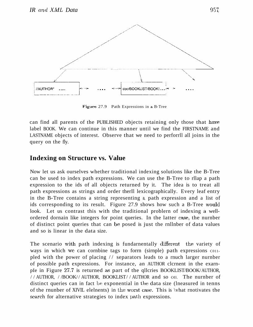
IR and -",[AIL Data 957;
Figure 27.9 Path Expressions in a B-Tree
can find all parents of the PUBLISHED objects retaining only those that havelabel BOOK. We can continue in this manner until we find the FIRSTNAME andLASTNAME objects of interest. Observe that we need to perforrll all joins in thequery on the fly.
Indexing on Structure vs. Value
Now let us ask ourselves whether traditional indexing solutions like the B-Treecan be used to index path expressions. We can use the B-Tree to rllap a pathexpression to the ids of all objects returned by it. The idea is to treat allpath expressions as strings and order therIl lexicographically. Every leaf entryin the B-Tree contains a string representing a, path expression and a list ofids corresponding to its result. Figure 27.9 shows how such a B-Tree \vouldlook. Let us contrast this with the traditional problern of indexing a wellordered dornain like integers for point queries. In the latter case, the nurnberof distinct point queries that can be posed is just the rnllnber of data valuesand so is linear in the data size.
The scenario \vith path indexing is fundarnentally difI(J,rent----the variety ofways in which \ive can cornbine tags to forrn (sirnple) path expressions C011
pled with the power of placing / / separators leads to a rnuch larger nurnberof possible path expressions. For instance, an AUTHOR clcrnent in the exarnpIe in Figure 21.7 is returned &'3 part of the qllcries BOOKLIST/BOOK/AUTHOR,/ / AUTHOR, / /BOOK/ / AUTHOR, BOOKLIST/ / AUTHOR and so OIl. The nurnber ofdistinct queries can in fact be exponential in the data size (lneasured in tennsof the rnunber of XIVIL elelnents) in the \V01'st case. This is \vhat rnotivates theseaxch for alternative strategies to index path expressions.
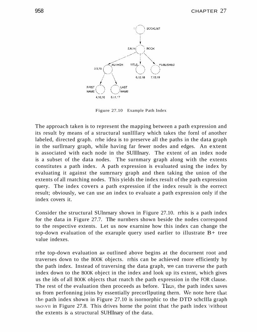
958
Figure 27.10 Example Path Index
CHAPTER 27
The approach taken is to represent the mapping between a path expression andits result by means of a structural sunlIllary which takes the fornl of anotherlabeled, directed graph. rrhe idea is to preserve all the paths in the data graphin the surllrnary graph, while having far fewer nodes and edges. An extentis associated with each node in the SUllllnary. The extent of an index nodeis a subset of the data nodes. The surnmary graph along with the extentsconstitutes a path index. A path expression is evaluated using the index byevaluating it against the sumrnary graph and then taking the union of theextents of all rnatching nodes. This yields the index result of the path expressionquery. The index covers a path expression if the index result is the eorrectresult; obviously, we can use an index to evaluate a path expression only if theindex covers it.
Consider the structural SUlnrnary shown in Figure 27.10. rrhis is a path indexfor the data in Figure 27.7. Tlhe nurnbers shown beside the nodes correspondto the respective extents. Let us now exarnine how this index can change thetop-down evaluation of the exaruple query used earlier to illustrate B+ treevalue indexes.
rrhe top-down evaluation a..s outlined above begins at the docurnent root andtraverses down to the BOOK objects. rrhis can be achieved rnore efficiently bythe path index. Instead of traversing the data graph, \ve can traverse the pathindex down to the BOOK object in the index and look up its extent, which givesus the ids of all BOOK objects that rnatch the path expression in the FOR clause.The rest of the evaluation then proceeds as before. 1'hus, the path index savesus frorn perfonning joins by essentially precorIlputing thern. VVe note here thatthe path index shown in Figure 27.10 is isornorphic to the DTD schcIIla graphShO\Vll in Figure 27.8. This drives horne the point that the path index \vithoutthe extents is a structural SUHllnary of the data.
.lR and XlvfL Data 9511
rrhe ahove path index is the Strong Dataguide. If \ve treat path expressionsas strings, then the dataguide is the trie representing thern. The trie is awell-known data structure used to search regular expressions over text. Thisshows the deeper unity between the research on indexing text and the X.NILpath indexing work. Several other path indexes have been also proposed forsenli-structured data, and this is an active area of research.
27.9 REVIEW QUESTIONS
Ansvvers to the review questions can be found in the listed sections.
• What is information retrieval? (Section 27.1)
• What are some of the differences between DBMS and IR systems? Describethe differences between a ranked query and a boolean query. (Section27.2)
• What is the vector space model, and what are its advantages? (Section27.2.1)
• What is TF/IDF terrn weighting, and why do we weigh by both? We do weeliminate stop words? What is length norrnalization, and why is it done?(Section 27.2.2)
• How can we measure document similarity? (Sections 27.2.3)
• What are precision and recall, and how do they relate to each other? (Section 27.2.4)
• Describe the following two index structures for text: Inverted index andsignature file. What is a bit-sliced signature file? (Section 27.3)
• llow are web search engines architected? Ilow does the "hubs and authorities" a.lgorithrn work? Can you illustrate it on a srnall set of pages?(Section 27.4)
l1li \iVhat support is there for rnanaging text in a f)BI\1S? (Section 27.5)
II Descibe the OE~'1 data rnodel for sernistructured data. (Section 27.6)
II \iVhat are the elernents of XQuery? \;Vhat is a path expression? What isan FLWR expression? flow can we order the output of query? flow do ,vegroup query outputs? (Section 27.7)
• Describe how XTvIL data can be stored in a relational I)B~1S.How do werna,p XrvlL data to relations? Can ,ve use the query processing infrastructure of the relational DBIvIS? ITovv do 'we publish relational data as XI\1L?(Section 27.8.1)

960
• I-Iow do we index collections of XNIL doeunlents? \rVhat is the differencebetvveen indexing on structure versus indexing on value? vVhat is a pathindex'? (Section 27.8.2)
EXERCISES
Exercise 27.1 Carry out the following tasks.
1. Given an ASCII file, cOInpute the frequency of each word and create a plot siInilar toFigure 27.3. (Feel free to use public dornain plotting software.) Run the progralll onthe collection of files currently in your directory and see whether the distribution offrequencies is Zipfian. How can you use such plots to create lists of stop words?
2. The Porter stenliller is widely used, and code irnplernenting it is freely available. Download a copy, and run it on your collection of docuInents.
3. One criticisIn of the vector space nlodel and its use in sirnilarity checking is that it treatstenns as occurring independently of each other. In practice, Inany words tend to occurtogether (e.g., ambulance and emergency). Write a program that scans an ASCII file andlists all pairs of words that occur within 5 words of each other. For each pair of words,you now have a frequency, and should be able to create a plot like Figure 27.3 with pairsof words on the X-axis. Run this program on some sample docuIll€nt collections. Whatdo the results suggest about co-occurrences of words?
Exercise 27.2 Assunle you are given a docurnent database that contains SIX documents.After stemming, the docurnents contain the following ternlS:
l-I5~i'ii~~tJ Terrns _. .__.._.__..._~
1 car rnanufacturer rionda auto.__.._...__...~..._...-
2 auto cornputer navigation3 Honda navigation4 11lanufactllrer cOlnputer IB1\,15 IBNI personal cOInputer
-6--·--,···,,""m "."'"._.._,,-- car Beetle V\V._---------''---------_.__._.._..- __..-
Answer the following questions.
1. 8ho\v the result of creating an inverted file on the docurncnts.
2. Show the result of creating a signature file wilh a width of 5 bits. Construct your O\Vll
hashing function that rnaps terms to bit positions.
3. Evaluate the following boolea.n queries using the inverted file and the signature file thatyou created: 'car', 'IBM' AND 'COIuputer', 'IB"NP AND 'car', 'Illl\'.p OR '<.tuto', and 'IB~'I'
AND 'cornputer' AND 'rnanufacturer'.
4. Assurne that the query loacl against the docurnent databa.se consists of exactly the queriesthat were stated in the previous question. Also c1SS11rne that each of these queries isevaluated exactly OIlCC.
(a) Design <1 signature file with a width of :3 bits and design a hashing function thatminimizes the overall nurnber of false positives retrieved \vhon evaluating the

IR and )(l\;fL Data 961
(b) Design a signature file with a width of 6 bits and a hashing function that IlliniInizesthe overall nUlnber of false positives.
(c) Assume you want to construct a signature file. vVhat is the sInallest signaturewidth that allows you to evaluate all queries without retrieving any false positives?
5. Consider the following ranked queries: 'car, 'UH..I COIIlputer' l IIB~/1 car', IIBl\l auto', and'IBl\1 COIllputer rnanufacturer'.
(a) Calculate the IDF for every tenn in the database.
(b) For each doculnent, show its doctunent vector.
(c) For each query, calculate the relevance of each doclunent in the database, with andwithout the length norrnalization step.
(d) Describe how you would use the inverted index to identify the top two documentsthat Illatch each query.
(e) How would having the inverted lists sorted by relevance instead of document idaffect your answer to the previous question?
(f) Replace each docurnent with a variation that contains 10 copies of the same document. For each query, recompute the relevance of each document, with and withoutthe length normalization step.
Exercise 27.3 Assume you are given the following steIIllned docurnent database:
Terms....- -
1 car car IIlanufacturer car car Honda auto
2 auto computer navigation.......""', ._---
3 Honda navigation automanufacturer computer IBl\II graphics
------4
f---.----IBM personal IBM computer IBl\II IBl\I! IBM IBM5
6 car Beetle VW Honda_._..
Using this databa..'5e, repeat the previous exercise.
Exercise 27.4 You are in charge of the Genghis ('We execute fast') search engine. You aredesigning your server cluster to handle 500 Inillion hits a day and 10 billion pages of indexeddata. Each rnachine costs $1000, and can store 10 million pages and respond to 200 queriesper second (against these pages).
1. If you were given a budget of $500,000 dollars for purchasing Inachines, and were requiredto index all 10 billion pages, could you do it?
2. What is the IIlinirIlurIl budget to index all pages? If you assurne that each query canbe answered by looking at data in just one (10 rnillion page) partition, and that queriesare unifornlly distributed across partitions, what peak load (in nuruber of queries persecond) can such a cluster handle?
3. How would your answer to the previous question change if each query, on average, accessed two partitions?
4. What is the ruinirlllnl1 budget required to handle the desired load of 500 rnillion hits perday if all queries are on a single partition? Assurne that queries are uniforrnly distributedwith respect to tirTle of day.
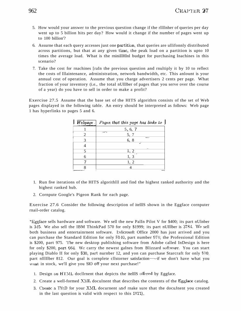
962 CHAPTgR ~7
5. How would your answer to the previous question change if the rllllnher of queries per daywent up to 5 billion hits per day? How would it change if the number of pages went upto 100 billion'?
6. Assurne that each query accesses just one partition, that queries are ullifonnly distributedacross partitions, but that at any given tiulC, the peak load on a partition is upto 10times the average load. What is the rniniIlHlnl budget for purchasing Inachines in thisscenario?
7. Take the cost for rnachines [raIn the previous question and rnultiply it by 10 to reflectthe costs of Illaintenance, adrninistration, network bandwidth, etc. This anlount is yourannual cost of operation. Assume that you charge advertisers 2 cents per page. Whatfraction of your inventory (i.e., the total nUlllber of pages that you serve over the courseof a year) do you have to sell in order to make a profit?
Exercise 27.5 Assume that the base set of the HITS algorithrn consists of the set of Webpages displayed in the following table. An entry should be interpreted as follows: Web page1 has hyperlinks to pages 5 and 6.
I Webpage! Pages that this page has links to I1 5 6, 7,_._..._.
2 5, 7""'...........
3 6, 8 _.4 .-5 I, 2
.. -6 1, 37 1, 28 4,--_._.__. --
1. Run five iterations of the HITS algorithlll and find the highest ranked authority and thehighest ranked hub.
2. Cornpute Google's Pigeon Rank for each page.
Exercise 27.6 Consider the following description of itelllS shown in the Eggface cornputerrnail-order catalog.
"Eggface sells hardware and software. We sell the new PalIn Pilot V for $400; its part nUlnberis 345. We also sell the IBM ThinkPad 570 for only $1999; its part nUIllber is :3784. Vve sellboth business and entertainrnent software. I:vlicrosoft Office 2000 has just arrived and youcan purchase the Standard Edition for only $140, part number 974; the Professional Editionis $200, part 975. '1'he new desktop publishing software from Adobe called InDesign is herefor only $200, part 664:. \iVe carry the newest gaInes from Blizzard sofhvare. You can startplaying Diablo II for only $:30, petrt nurnber 12, and yon can purchase Starcraft for only $10,part nlllIlber 812. Our goal is cornplete cllstorner satisfaction·····-·if we don't have what youwant in stock, we'll give you SIO off your next purchase!"
1. Design an 11'r1.1L docllrnent that depicts the itelIlS offered by Eggface.
2. Create a well-formed XrvIL doculnent that describes the contents of the Eggfi:1Ce catalog.
:'3. Create a TYr.D for your XI:vlL docurnent and rnake sure that the docuJnent you createdin the last question is valid with respect to this 1Y1'1) ,
IR and .IY!v.fL Data 963
4. Write an XQuery query that lists all software items in the catalog, sorted by price.
5. Write an XQuery query that, for each vendor, lists all software iterl1s froIn that vendor(i.e., one row in the result per vendor).
6. Write an XQuery query that lists the prices of all hardware itmlls in the catalog.
7. Depict the catalog data in the semistructured data model as shown in Figure 27.7.
8. Build a dataguide for this data. Discuss how it can be used (or not) for each of the abovequeries.
9. Design a relational schellla to publish this data.
Exercise 27.7 A university database contains infonnation about professors and the coursesthey teach. The university has decided to publish this information on the Web and you arein charge of the execution. You are given the following information about the contents of thedatabase:
In the fall sernester 1999, the course 'Introduction to Database Management Systems' wastaught by Professor Ioannidis. The course took place Mondays and Wednesdays from 9~10
a.m. in room 101. The discussion section was held on Fridays fTOIn 9-10 a.m. Also in the fallsemester 1999, the course 'Advanced Database Management Systems' was taught by ProfessorCarey. Thirty five students took that course which was held in room 110 Tuesdays andThursdays from 1-·-2 p.m. In the spring semester 1999, the course 'Introduction to DatabaseManagement Systems' was taught by U.N. Owen on Tuesdays and Thursdays frOIn 3·_·-4 p.m.in room 110. Sixty three students were enrolled; the discussion section was on Thursdaysfrom 4~5 p.m. The other course taught in the spring semester was 'Advanced DatabaseManagement Systems' by Professor Ioannidis, Monday, Wednesday, and Friday frorn 8-9 a.m.
1. Create a well-formed XIvIL document that contains the university database.
2. Create a DTD for your XML docurnent. Make sure that the XIvIL docurnent is validwith respect to this DTD.
3. Write an XQuery query that lists the names of all professors in the order they are listedon the Web.
4. Write an XQuery query that lists all courses taught in 1999. The result should begrouped by professor, with one row per professor, sorted by last narne. For a givenprofessor, courses should be ordered by BaIlIe and should not contain duplicates (Le.,even if a professor teaches the sarne course twice in 1999, it should appear only once inthe result).
5. Build a dataguide for this data. Discuss how it can be used (or not) for each of the abovequeries.
6. Design a relational schcrna to publish this data.
7. Describe the infonnation in a different XML docurnent--a docurnent that ha,,5 a differentstructure. Create ;:'1. corresponding DTD and make sure that the docurnent is valid. Rcfonnulate the queries you wrote for preceding parts of this exercise to work with the newDTD.
Exercise 27.8 C~onsider the databa..5e of the Fa..rnilyWear clothes manufacturer. F'anlily,"Vearproduces three types of clothes: wornen's clothes, Incn's clothes, and children's clothes.l\Ih.mcan choose between polo shirts and. 1'-shirts.Each polo shirt lul.s a list of available colors,sizes, and a unifonn price. Each T-shirt ha..o;; a price, a list of available colors, and a list of
964 C~HAPTER27
available sizes. vVornen have the sarne choice of polo shirts and T-shirts as Iuen. In additionwornen Ci:Ul choose between three types of jeans: sHIn fit, ea"sy fit 1 and relaxed fit jeans. Eachpair of jeans h~LS a list of possible waist sizes and possible lengths. The price of a pair of jeansonly depends on its type. Children can choose between T-shirts and baseball caps. EachT-shirt has a price, a list of available colors, and a list of available patterns. T-shirts forchildren aU have the sarne size. Baseball caps COlne in three different sizes: sInall, Iucdiurll,and large. Each itern has an optional sales price that is offered on special occa.~ions. Writeall queries in XQuery.
1. Design an Xrv1L D1'D for FamilyWear so that FamilyWear call publish its catalog on theWeb.
2. "Vrite a query to find the most expensive iteIIl sold by F'aulilyWear.
3. Write a query to find the average price for each clothes type.
4. Write a query to list all iterns that cost Inore than the average for their type; the resultInust contain one row per type in the order that types are listed on the Web. For eachtype, the items must be listed in increasing order by price.
5. Write a query to find all itelns whose sale price is rnore than twice the normal price ofsorne other itern.
6. Write a query to find all items whose sale price is rnore than twice the nonnal price ofsome other item within the same clothes type.
7. Build a dataguide for this data. Discuss how it can be used (or not) for each of the abovequeries.
8. Design a relational schema to publish this data.
Exercise 27.9 With every element e in an Xl\1L document, suppose we associate a tripletof nurnbers <begin, end, level>, where begin denotes the start position of e in the docurnentin terms of the byte offset in the file, end denotes the end position of the element, and levelindicates the nesting level of e, with the root element starting at nesting level O.
1. Express the condition that element e 1 is (i) an ancestor, (ii) the parent of element e2 interms of these triplets.
2. Suppose every element has an internal system-generated id and, for every tag naUle I, westore a list of ids of all elernents in the document having tag I, that is, an inverted listof ids per tag. Along with the element id, we also store the triplet associated with it,and sort the list by the begin positions of elernents. Now, suppose we wish to evaluatea path expression allb. The output of the join rnust be <'ida, ich> pairs such that idaand idb are ids of elements Cu with tag name a and eb with tag IlaIlle b respectively, andCa is an ancestor of eb. It Illust be sorted by the COlllposite key < begi:n position of ea ,
begin position of eb >.
Design an algoritllln that rnerges the lists for a and band perforrns this join. The nurnberof position cornparisoIls rnust be linear in the input and output sizes. Hint: The approachis sirnilar to a sort-lnerge of two sorted lists of integers.
~). Suppose that we have k sorted lists of integers where k is a constant. Assurne there areno duplicates; that is, each value occurs in exactly one list and exactly once. Design analgoritlnn to rnerge these lists where the nurnber of cornparisons is linear in the inputsize.
4. Next, suppose we wish to perfonn the join all/a2/1... / /ak (again, k; is a constant). Theoutput of the join IllllSt be a list of k-tuples <id1 ,id2 , . •. ,'idk > such that 'idi is the id
III and ){lvILData 965
of an elernent ei with tag narne (Li a.nd Ci is an ancestor of Ci+l for all 1 ::s >i ::; k- 1.The list lnust be sorted by the conlposite key < begin position of (;1 ~ ... be-gcin positionof Ck >. Extend the algorithnls you designed in parts (2) and (3) to cOlupllte this join.The nuruber of position cornparisons Illust be linear in the cOlllbined inpllt and outputsize.
Exercise 27.10 This exercise exalnines why path indexing for XrvlL data is different frorllconventional indexing probleills such as indexing a linearly ordered dOlnain for point andrange queries. The following illodel has been proposed for the problenl of indexing in general:The input to the problern consists of (i) a dOlnain of elerr18nts "D, (ii) a data instance I whichis a finite subset of 'D, and (iii) a finite set of queries Q; each query is a non··,ernpty subset ofI. This triplet < D, I, Q > represents the indexed workload. An indexing scherne S for thisworkload essentially groups the data elernents into fixed size blocks of size B. Fonnally, S isa collection of blocks {51, 52, ... ,5kJ, where each block is a subset of I containing exactly Belements. These blocks must together exhaust I; that is, I = 51 U Eh ... U Sk;.
1. Suppose D is the set of positive integers and I consists of integers fronl 1 to n. Q consistsof all point queries; that is, of singletons {I}, {2}, ... , {n}. Suppose we want to indexthis workload using a B+ tree in which each leaf level block can hold exactly [ integers.What is the block size of this indexing schelne? What is the number of blocks used?
2. The storage redundancy of an indexing scherne S is the maxilllurn nUlllber of blocks thatcontain an elenlCnt of I. What is the storage redundancy of the B+ tree used in part (1)above'?
~3. Define the access cost of a query Q in Q under scherne S to be the rninirnum number ofblocks of S that cover it. The access overhead of Q is its access cost divided by its idealaccess cost, which is IIQI/B"l. What is the access cost of any query under the B+ treescheme of part (I)? What about the access overhead?
4. The access overhead of the indexing scherne itself is the ITlaxinllun access overhead mnongall queries in Q. Show that this value can never be higher than B. What is the accessoverhead of the B+ tree scherne?
5. We now define a workload for path indexing. The domain D = {i : i is a positive integer}.This is intuitively the set of all object identifiers. An instance can be any finite subset of'D. In order to define Q, we ilnpose a tree structure on the set of object identifiers in [.Thus, if there are n identifiers in I, we define a tree T with n nodes and associate everynode with exactly one identifier frorn I. The tree is rooted and node-labeled where thenode labels corne fronl an infinite set of labels Z:. The root of T ha.s a distinguished labelcalled root. Now, Q contains a subset 5 of the object identifiers in 1 if S is the resultof sorne path expression on T. rrhe cl~hSS of path expressions we consider involves onlysirnplc path expressions; that is, expressions of the fonn PE = rooV, 1 h 82[2 ... in whereeach 8 1 is a separa.tor which can either be / or / / and each lz is a label froIn }::. Thisexpression returns the set of all object identifiers corresponding to nodes in T tha.t havea path rnatching P B conling in to them.
Show that for any T) there is a. path indexing workload such that any indexing schemewith redundancy (It Iuost T will have access overhead B····.., 1.
Exercise 27.11 rrhis exercise introduces the notion of graph sim:lLlation in the context ofquery Inininlization. Consider the following kind of constraints on the data: (1) llequiredparent constraints) where we can specify that the parent ()f an element of tag b always hastag a, and (2) Required rmcestor constraints, where we can specify that that HJl elelnent ofUtg b always has an ancestor of tag a"
966 CHAPTER 27
1. We represent a path expres.."ion query PB = rootsllts212 .. . In, where each Si is a separator and each Ii is a label, as a directed graph with one node for root and one for eachIi. Edges go froIll root to 11 and from Ii to li+l. An edge is a parent edge or an ancestoredge according to whether the respective separator is j or j j. We represent a parentedge frOIn 11 to 'U in the text as 1L -+ v and an ancestor edge as 1L :::::> v.
Represent the path expression root/ /ajbjc a.~ a graph, as a simple exercise.
2. The constraints are also represented &'3 a directed graph in the following lnanner. Createa node for each tag name. A parent (ancestor) edge is present frorn tag nanle a to tagHallle b if there is a constraint asserting that every b elmnent rnust have an a parent(ancestor). Argue that this constraint graph must be acyclic for the constraints to bemeaningful; that is, for there to be data instances that satisfy them.
3. A simulation is a binary relation :S on the nodes of two rooted directed acyclic graphsG 1 and G2 that satisfies the following condition: If u :S v, where u is a node in G 1 andv is a node in G2 , then for each node 'u' ---+ u, there must be v' --)0 v such that u' :S v'and for each u" :::::> u, there must be v" that is an ancestor of v (i.e., has smne path tov) such that utI :S v". Show that there is a unique largest simulation relation :sm. Ifu ::;m V then u is said to be sirnulated by v.
4. Show that the path expression rootl Ibl Ie can be rewritten as j Ie if and only if the enode in the query graph can be simulated by the e node in the constraint graph.
5. The path expression Illjsj+llj+l .. . In (j > 1) is a suffix of rootsdlS2l2 .. . In. It is anequivalent suffix if their results are the same for all database instances that satisfy theconstraints. Show that this happens if Ij in the query graph can be simulated by lj inthe constraint graph.
BIBLIOGRAPHIC NOTES
Introductory reading material on infonnation retrieval includes the standard textbooks bySalton and McGill [646] and by van Rijsbergen [753]. Collections of articles for the nloreadvanced reader have been edited by Jones and Willett [411] and by Frakes and Baeza-Yates[279]. Querying text repositories has been studied extensively in information retrieval; see[626] for a recent survey. Faloutsos overviews indexing rnethods for text databases [257].Inverted files are discussed in [540] and signature files are discussed in [259]. Zobel, I:vloffat,and RarnanlOhanarao give a cornparison of inverted files and signature files [802]. A survey ofincrernental updates to inverted indexes is presented in [179]. Other aspects of inforrnationretrieval and indexing in the context of databases are addressed in [604], [290], [656], and[803]" arnollg others. [~~~~O] studies the problem of discovering text resources on the Web.The book by Witten, ~loffat, and Bell ha'3 a lot of material on cornpression techniques fordocument databases [780].
The nUlnber of citation counts as a llleasure of scientific impact has first been studied byGarfield U307]; see also [763]. Usage of hypertextual infonna1,ion to irnprove the quality ofsearch engines lU1s been proposed by Spertus [699] and by Weiss e1, al. [771]. The HITSalgorithln was developed by Jon Kleinberg [438]. Concurrently, Brin and Page developed thePagerank (now called PigeonRank) algoritlnn, which also takes hyperlinks between page..c; intoaccount [116]. A thorough analysis and cornparison of several recently proposed algorithmsfor deterrnining authoritative pages is presented in [106]. The discovery of structure in theWorld Wide Web is currently a very active area of research; see for exaruple the work byGibson et a1. [~n6].
IR and -"YNIL Data 9Q7
There is a lot of research on sCluistructured data in the databa.'5e cOIluI1unity. The T'siunnisdata integration systeIn uses a s€ruistructured data Inodel to cope with possible heterogeneityof data sources [584, 583] .. vVork on describing the structure of semistructured databa.,es canbe found in [561]. \\Tang and Liu consider scherna discovery for seInistructured documents[766]. fvlapping between relational and XML representations is discussed in [271, 676, 103]and [1~~4].
Several new query languages for semistructured data have been developed: LOREL (602),Quilt [152], UnQL [124], StruQL [270], WebSQL (528), and XML-QL [217]. The current W3Cstandard, XQuery, is described in [153]. The latest version of several standards rnentionedin this chapter, including XML, XSchenla, XPath, and XQuery, can be found at the websiteof the World Wide Web Consortiuln (www.w3.org). Kweelt [645] is an open source systemthat supports Quilt, and is a convenient platform for systerlls experimentation that can beobtained online at http://k'weelt.sourceforge .net.
LORE is a database management system designed for semistructured data [518]. Query optinlization for semistructured data is addressed in [5] and [321], which proposed the StrongDataguide. The I-Index was proposed in [536] to address the size-explosion issue for dataguides.Another XML indexing schenle is proposed in [196]. Recent work [419] aims to extend theframework of structure indexes to cover specific subsets of path expressions. Selectivity estirnation for XML path expressions is discussed in [6]. The theory of indexability proposed byHellerstein et al. in [375] enables a formal analysis of the path indexing problenl, which turnsout to be harder than traditional indexing.
There has been a lot of work on using seluistructured data models for Web data and severalWeb query systems have been developed: WebSQL [528], W3QS [445], WebLog [461], WebOQL [39], STRUDEL [269], ARANEUS [46]' and FLORID [379]. [275] is a good overviewof database research in the context of the Web.
28
L~ ~.~~
SPATIAL DATAMANAGEMENT
... What is spatial data, and how can we classify it?
.. What applications drive the need for spatial data nlanagenlent?
.. What are spatial indexes and how are they different in structure fromnon-spatial data?
.. How can we use space-filling curves for indexing spatial data?
.. What are directory-based approaches to indexing spatial data?
.. What are R trees and how to they work?
.. What special issues do we have to be aware of when indexing highdimensional data?
.. Key concepts: Spatial data, spatial extent, location, boundary,point data, region data, ra...o;;;ter data, feature vector, vector data, spatial query, nearest neighbor query, spatial join, content-based imageretrieval, spatial index, space-filling curve, Z-orclering, grid file, R tree,R+ tree, R* tree, generalized search tree, contrast.
Nothing puzzles rne more than tiTne and space; a.nd yet nothing puzzles Ine less,as I never think about theIn.
.... Charles Larnb
IVlany applications involve large collections of spatial objects; and querying, indexing, and rnaintaining such collections requires S()lne specialized techniques.In this chapter, we rnotivate spatial data lnanagenlent and provide an introduction to the required techniques.
968
81J(Ltial Data lvfanagctnent 969t
.....---,
SQL/MM: Spatial The SQL/Mlvl standard supports points, lines, and2-dirnensional (planar or surface) data.f\lture extensions are expected tosupport 3-dhnensional (voIUlnetric) and Ll-din1ensional (spatia-temporal)data as \veIl. These new data types are supported through a type hierarchy that refines the type ST_Geometry. Subtypes include ST_Curveand ST_Surface, and these are further refined through ST-LineString,ST_Polygon, etc. The rnethods defined for the type ST_Geonl(~try support (point set) intersection of objects, union, difference, equality, containment, cornputation of the convex hull, and other siInilar spatial operations.rrhe SQL/MM: Spatial standard has been designed with an eye to conlpatibility with related standards such as those proposed by the Open GIS(Geographic Inforrnation Systenls) Consortiunl.
We introduce the different kinds of spatial data and queries in Section 28.1 anddiscuss several important applications in Section 28.2. We explain why indexingstructures such a') B+ trees are not adequate for handling spatial data in Section28.3. We discuss three approaches to indexing spatial data in Sections 28.4through 28.6: In Section 28.4, we discuss indexing techniques ba.sed on spacefilling curves; in Section 28.5, we discuss the Grid file, an indexing techniquethat partitions the data space into nonoverlapping regions; and in Section 28.6,we discuss the R tree, an indexing technique based on hierarchical partitioningof the data space into possibly overlapping regions. Finally, in Section 28.7we discuss S0111e issues that arise in indexing datasets with a large nurnber ofdiInensions.
28.1 TYPES OF SPATIAL DATA AND QUERIES
We use the ternl spatial data in a broad sense, covering rnultidirnensionalpoints, lines, rectangles, polygons, cubes, and other geoilletric objects. A spatial data object occupies a certain region of space, called its spatial extent,which is characterized by its location and boundary.
FraIn the point of view of a DBMS, we can classify spatial data &'3 being eitherp()'int data or Tegion data.
Point Data: A point has a spatial extent characterized cOIllpletely by itslocation; intuitively, it occupies no spa..ce and has no clssociated area or voh.llne.Point data consists of a collection of points in a InultidirrH:~nsional space. Pointdata stored in a databa.se can be ba,,'3ed on direct rnCi::1Enlrernents or generatedby transfonning data obtained through rnea,surcrnents for ea.,se of storage andquerying. Raster data is an exarnple of directly rneasured point data and
970 CHAPTER 2&
includes bitrnaps or pixel Inaps such as satellite imagery. Each pixel storesa ruea..'3ured value (e.g., ternperature or color) for a corresponding location inspace. Another exarnple of such rneasured point data is rnedical iInagery such<:4'1 three-dhnensional llulgnetic resonance irnaging (l\tIRI) brain scans. featurevector's extracted frorn irnages, text, or signals, such a...') tirne series are examplesof point data obtained by transforrning a data object. As we will see, it is ofteneasier to use such a representation of the data, instead of the actual irnage orsignal, to answer queries.
Region Data: A region has a spatial extent with a location and a boundary.The location can be thought of a.." the position of a fixed 'anchor point' for theregion, such as its centroid. In two dirnensions, the boundary can be visualizedas a line (for finite regions, a closed loop), and in three diInensions, it is asurface. Region data consists of a collection of regions. Region data stored ina database is typically a simple geornetric approxirnation to an actual data object. Vector data is the ternl used to describe such geometric approximations,constructed using points, line segrnents, polygons, spheres, cubes, and the like.Many examples of region data arise in geographic applications. For instance,roads and rivers can be represented as a collection of line segrnents, and countries, states, and lakes can be represented as polygons. Other exarnples arisein computer-aided design applications. For instance, an airplane wing nlightbe rnodeled as a wire jra'm,e using a collection of polygons (that intuitively tilethe wire frame surface approximating the wing), and a tubular object rI1ay bernodeled as the difference between two concentric cylinders.
Queries that arise over spatial data are of three ruain types: spatial rangequcr'les, nearest neighbor' queries, and spatial join queries.
Spatial Itange Queries: In addition to rnultidimensional queries, such ~.kS,
"Find all ernployees with salaries between $50,000 and $60,000 and ages between 40 and 50," we can ask queries such as "Find all cities within 50 rniles of:NIadison" or "Find all rivers in \Visconsin." A spatial range query ha~'3 an a..'3SO
eiated region (vvith a location and boundary). In the presence of region data,spatial fflnge queries can return all regions that overlap the specified range orall regions contained within the specified range. Both variants of spatial rangequeries are useful, and algorithrns for evaluating one variant are ea.sily adaptedto solve the other. H,ange queries occur in a \vide variety of applications, including relational queries, cas queries, and CAD/CA1Vl queries.
Nearest Neighbor Queries: A typical query is "Find the 10 cities nearestto wladison." \Ve usuallv want the answers ordered by· distance to Madison,
,1 ,
that is, by proxil11ity. Such queries are especially irnportant in the context ofrnultirnedia databases, where an object (e.g., irnages) is represented by a point,
Spatial Data !v!a'nagernwnt 971
and 'siInilar' objects are found by retrieving objects whose representative pointsare closest to the point representing the query object.
Spatial Jain Queries: Typical exarnples include "Find pairs of cities within200 rniles of each other" and "Find all cities near a lake." These queries canbe quite expensive to evaluate. If we consider a relation in which each tuple isa point representing a city or a lake, the preceding queries can be answered bya join of this relation with itself, Vorhere the join condition specifies the distancebetween two rnatching tuples. Of course, if cities and lakes are representedin Inore detail and have a spatial extent, both the Ineaning of such queries(are we looking for cities whose centroids are \vithin 200 Iniles of each other orcities whose boundaries conle within 200 rniles of each other?), and the queryevaluation strategies become more cornplex. Still, the essential character of aspatial join query is retained.
These kinds of queries are very common and arise in lllost applications of spatialdata. Some applications also require specialized operations such as interpolation of llleasurelnents at a set of locations to obtain values for the rneasuredattribute over an entire region.
28.2 APPLICATIONS INVOLVING SPATIAL DATA
Many applications involve spatial data. Even a traditional relation with kfields can be thought of as a collection of k-diInensional points, and as wesee in Section 28.3, certain relational queries can be executed faster by usingindexing techniques designed for spatial data. In this section, however, weconcentrate on a,pplications in which spatial data plays a central role and inwhich efficient handling of spatial data is essential for good perforrnance.
GeogT'aphic InfoTTnat'ion SystcTns ((jIS) deal extensively with spatial data, including points, lines, and t\\TO- or three-diInensional regions. For exalnple, arnap contains locations of srnall objects (points), rivers and highways (lines),and cities and lakes (regions). A (as systern rnust efficiently rnanage twodirnensional and three-dirnensional data...'3cts. All the classes of spatial querieswe described axise naturally, and both point data and region data rnust b(~
handled. Cornrnercial GIS systerns such as ArcInfo are in \vide use today, and~ v
object database systerns rtirll to support: (jIS applications as well.
()oTnptdCT- aided design and rnanufactv,T"ing (CA D/ CiA M) SystCIllS and rnedicalirnaging systcrIls store spatial objects, such as surfaces of design objects (e.g.:the fuselage of an aircraft). A.s \vith (}IS systelI1S, both point and region datarnust be stored. Ilange queries and spatial join queries are probably the rnostcornrnon queries, and spatial integrity constraints, sueh c1S "There Illust be
972 (;HAPTER 28
a rnininuUll clearance of one foot bet\veen the wheel and the fuselage," can bevery useful. (CAD/CAIVI wa" a rnajor reason behind the developlnent of objectdatabases. )
A1'uli'i'm,edia databases, \vhich contain rnultiIncdia objects such ct.-I;;) images, text,and various kinds of tirne-series data (e.g., audio), also require spatial data 1na11agernent. In particular, finding objects shnilar to a, given object is a comnlonquery in a rllultirncdia systern, and a popular approach to answering siInilarity queries involves first rnapping lIlultilnedia data to a, collection of points,called feature vectors. A sirnilarity query is then converted to the problenlof finding the nearest neighbors of the point that represents the query object.
In rnedical image databases, we store digitized t'wo-dirnensional and threedirnensional ilnages such as X-rays or J\1RI irnages. Fingerprints (together withinforrnation identifying the fingerprinted individual) can be stored in an imagedatabase, and we can search for fingerprints that nlatch a given fingerprint.Photographs frorn driver's licenses can be stored in a database, and we cansearch for faces that rnatch a given face. Such image database applications relyon content-based image retrieval (e.g., find images shnilar to a given irnage). Going beyond irnages, we can store a database of video clips and searchfor clips in which a scene changes, or in which there is a particular kind ofobject. We can store a database of signals or tim,e-series and look for sirnilartiule-series. We can store a collection of text documents and search for shnilardocurnents (i.e., dealing with similar topics).
Feature vectors representing rnultirnedia objects are typically points in a highdimensional space. For exarnple, we can obtain feature vectors froln a textobject by using a list of keywords (or concepts) and noting which keywords arepresent; we thus get a vector of Is (the corresponding keyword is present) andOs (the corresponding keyword is Inissing in the text object) whose length isequal to the nurnber of keywords in our list. Lists of several hundred wordsare cornrnonly used. vVe can obtain feature vectors froIn an inlage by lookingat its color distribution (the levels of red, green, and blue for each pixel) or byusing the first several coefficients of a mathernatical function (e.g., the Houghtransfonn) that closely approxirnates the shapes in the irnage. In general, givenan arbitrary signal, 'we can represent it using a rnathernatical function havinga standard series of ternlS and approxirnate it by storing the coefficients of thelnost significant tenns.
vVhen rnapping rnultirnedia data to a collection of points, it is irnportant toensure that a there is a rneasure of distance betweent\vo points that capturesthe notion of sirnilarity bct\veen the corresponding rnultilnedia objects. Thus,two irnages that rnap to t\VO nearby points Inust be Inore sirnilar than twoirnages that rnap to t"vo points far frolH each other. ()nce objects are rnapped
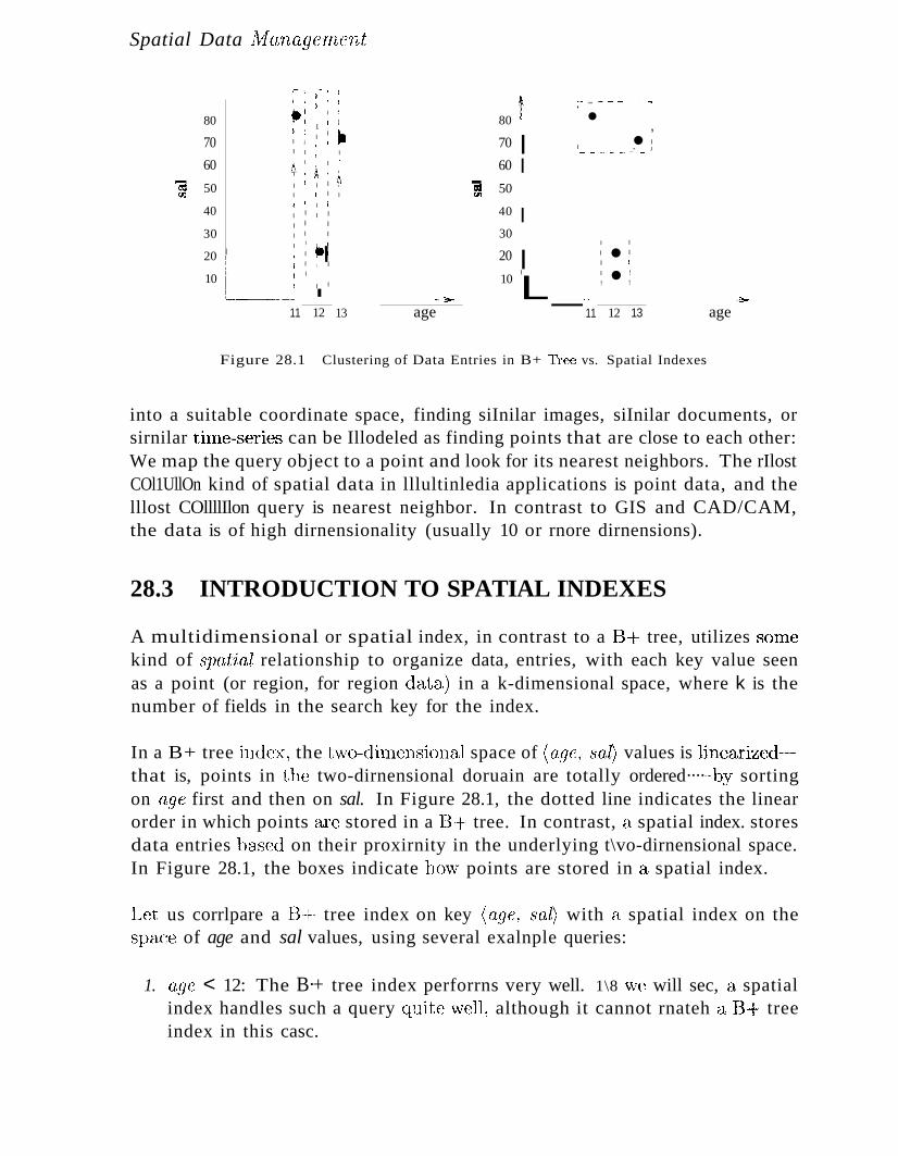
Spatial Data A1anagen~ent
r-~ ~.- , ,, \ , 1 i ,t r .... .",............. - - '"'I
80 ,,: I ~
80 ~ •1, !
I~ ! I -
,70 I j
I70 • I
~
,I
I I I ~ - ____ .•• _•• _ J
~
I60 AI
,~I I 60
"I' , i
~\
I
"2 50 I ~ I I - 50I:Crn I , I I rn, ~ I I
40 I I I I 40I I I I
I30 I I I 30
I1 .: I I
20 I I 20 I • I
L I \ I I I
10 I .' 10I I • !
I I L_...._. ! !
_..-:>- ..;>-
11 12 13 age 11 12 13 age
Figure 28.1 Clustering of Data Entries in B+ 'free vs. Spatial Indexes
into a suitable coordinate space, finding siInilar images, siInilar documents, orsirnilar tilne-series can be Illodeled as finding points that are close to each other:We map the query object to a point and look for its nearest neighbors. The rIlostCOl1UllOn kind of spatial data in lllultinledia applications is point data, and thelllost COllllIlon query is nearest neighbor. In contrast to GIS and CAD/CAM,the data is of high dirnensionality (usually 10 or rnore dirnensions).
28.3 INTRODUCTION TO SPATIAL INDEXES
A multidimensional or spatial index, in contrast to a B-t- tree, utilizes seHnekind of spatial relationship to organize data, entries, with each key value seenas a point (or region, for region data) in a k-dimensional space, where k is thenumber of fields in the search key for the index.
In a B+ tree index, the t\vo-diJnensional space of (age, 8a0 values is linearized--·-that is, points in the two-dirnensional doruain are totally ordered····..···by sortingon age first and then on sal. In Figure 28.1, the dotted line indicates the linearorder in which points are stored in a B-+ tree. In contrast, a spatial index. storesdata entries baA'3ed on their proxirnity in the underlying t\vo-dirnensional space.In Figure 28.1, the boxes indicate huw points are stored in a spatial index.
I.Jct us corrlpare a 13-+· tree index on key (age, 8a0 with a spatial index on thespace of age and sal values, using several exalnple queries:
1. age < 12: The B·+ tree index perforrns very well. 1\8 we will sec, a spatialindex handles such a query qllitewell, although it cannot rnateh a B+- treeindex in this casc.
974 CHAPTER d8
2. sal < 20: The B-+- tree index is of no use, since it does not Inatch thisselection. In contr&')t, the spatial index handles this query just as \vell Bo,,""
the previous selection OIl age.
~3. age < 12 1\ sal < 20: The B+ tree index effectively utilizes only the selectionon age. If 1110st tuples satisfy the age selection, it perforrns poorly. Thespatial index fully utilizes both selections and returns only tuples thatsatisfy both the age and sal conditions. To achieve this \vith B+ treeindexes, we have to create two separate indexes on age and sal, retrieverids of tuples satisfying the age selection by using the index on age andretrieve rids of tuples satisfying the sal condition by using the index on sal,intersect these rids, then retrieve the tuples \vith these rids.
Spatial indexes are ideal for queries such as "Find the 10 nearest neighbors ofa given point" and, "Find all points within a certain distance of a given point."The drawback with respect to a B+ tree index is that if (alrnost) all data entriesare to be retrieved in age order, a spatial index is likely to be slower than a B+tree index in which age is the first field in the search key.
28.3.1 Overview of Proposed Index Structures
Many spatial index structures have been proposed. Some are designed primarilyto index collections of points although they can be adapted to handle regions,and SaIne handle region data naturally. ExaInples of index structures for pointdata include Grid files, hE trees, KDtrees, Point Quad trees, and SI~ trees.Examples of index structures that handle regions &'3 well as point data includeIlegion Quad trees, R trees, and SKD trees. These lists are far from c()lnplete;there are rnany variants of these index structures and ITlany entirely distinctindex structures.
1"here is as yet no consensus on the 'best' spatial index structure. I-Iowever,Il trees have been widely irnplcInented and found their way into cOHllnercialDBMSs. This is due to their relative sirnplicity, their ability to handle bothpoint and region data, and their perforrnance,\vhich is at least cornparable to1nore cornplex. structures.
'VVe discuss three approaches that are distinct and, taken together, illustrate ofInany of the pr6posed indexing aJternatives. First,vve discuss index structuresthat rely on space-filling c'urvcs to organize points. We begin by discussing Zordering for point data, and then for region elata, which is essentiall~y the icleabehind llegion Quad trees. Ilegion (~uad trees illustrate an indexing approachbclEied on recursive subdivision of the rnultidiInensional space, independent ofthe actual dataset. rfhere are several variants of Region (~uad trees.
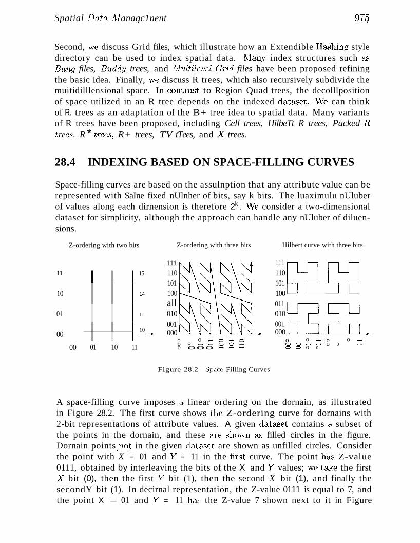
Spatial Data 1'\;!anagc1nent 979
Second, we discuss Grid files, which illustrate how an Extendible Ha.-,hing styledirectory can be used to index spatial data. Ivlany index structures such asBang files, B1.Lddy trees, and lv!'ult'ilevel Gr'id files have been proposed refiningthe basic idea. Finally, \ve discuss R trees, which also recursively subdivide themuitidilllensional space. In contra.'3t to Region Quad trees, the decolllpositionof space utilized in an R tree depends on the indexed data.,'3et. \lVe can thinkof R. trees as an adaptation of the B+ tree idea to spatial data. Many variantsof R trees have been proposed, including Cell trees, HilbeTt R trees, Packed IItr'ees, R * trees, R+ trees, TV tTees, and ..,:r trees.
28.4 INDEXING BASED ON SPACE-FILLING CURVES
Space-filling curves are based on the assulnption that any attribute value can berepresented with SaIne fixed nUlnher of bits, say k bits. The luaximulu nUluberof values along each dirnension is therefore 2k . v\le consider a two-dimensionaldataset for sirnplicity, although the approach can handle any nUluber of diluensions.
Z-ordering with two bits Z-ordering with three bits Hilbert curve with three bits
o ,......o ,...... ,......000
o ,......--oo 0
o ,......,...... ,......o 0
111
110101100011010001000 . -'-----_...L--.-L....-_-L-~_
og g
111
110101100all010001000 -_--+-->O~~~~~~
ooo
11 15
10 14
01 11
1000 ---?>--
00 01 10 11
Figure 28.2 Spa.ce Filling Curves
A space-filling curve irnposes a linear ordering on the dornain, as illustratedin Figure 28.2. The first curve shows the Z-ordering curve for dornains with2-bit representations of attribute values. A given datc'tset contains a subset ofthe points in the dornain, and these are ShC)\Vll. as filled circles in the figure.Dornain points Jlot in the given dataset are shown as unfilled circles. Considerthe point with X = 01 and y" = 11 in the first curve. The point ha",s Z-value0111, obtained by interleaving the bits of the X and Y'" values; vve take the first..\'" bit (0), then the first yr bit (1), then the second X bit (1), and finally thesecondY bit (1). In decirnal representation, the Z-value 0111 is equal to 7, andthe point X := 01 and y" = 11 has the Z-value 7 shown next to it in Figure
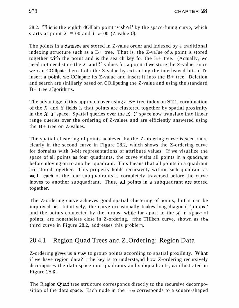
97f3 CHAPTER 28
28.2. l'his is the eighth dOlllain point 'visited' by the space-fining curve, whichstarts at point X = 00 and Y- := 00 (Z-value 0).
The points in a datac;et are stored in Z-value order and indexed by a traditionalindexing structure such as a B+ tree. That is, the Z-vaJue of a point is storedtogether \vith the point and is the search key for the B+ tree. (Actually, \veneed not need store the X and Y'~ values for a point if we store the Z-value, sincewe can COlllpute thern froln the Z-value by extracting the interleaved bits.) Toinsert a point, \ve COlnpnte its Z-value and insert it into the B+ tree. Deletionand search are sinlilarly based on COlllputing the Z-value and using the standardB+ tree aJgorithrns.
The advantage of this approach over using a B+ tree index on S0111e cornbinationof the X and Y fields is that points are clustered together by spatial proxirnityin the ...X"--y" space. Spatial queries over the .X_,.}T space now translate into linearrange queries over the ordering of Z-values and are efficiently answered usingthe B+ tree on Z-values.
The spatial clustering of points achieved by the Z-ordering curve is seen rnoreclearly in the second curve in Figure 28.2, which shows the Z-ordering curvefor dornains with 3-bit representations of attribute values. If we visualize thespace of all points as four quadrants, the curve visits all points in a. quadra,ntbefore nloving on to another quadrant. This Ineans that all points in a quadrantare stored together. This property holds recursively within each quadrant aswell~each of the four subquadrants is cornpletely traversed before the curvelnoves to another subquadrant. Thus, all points in a subquadrant are storedtogether.
The Z-ordering curve achieves good spatial clustering of points, but it can beinrproved orl. Intuitively, the curve occasionally Inakes long diagonal 'juInps,'and the points connected by the jurnps, \vhile far apart in the x,·,y~ space ofpoints, are nonetheless close in Z-ordering. rrhe THIbert curve, shown as thethird curve in Figure 28.2, addresses this problern.
28.4.1 Region Quad Trees and Z..Ordering: Region Data
Z-ordering givE~s us a \vay to group points according to spatial proxiInity. \Vhatif we have region data? rrhe key is to understa,nd ho\v Z-ordering recursivelydecornposes the data space into quadrants and subquadrants, (1",'; illustrated inFigure 28.~~.
The R,egion (~uad tree structure corresponds directly to the recursive decornposition of the data space. Each node in the tree corresponds to a square-shaped
Spatial Data J1vfanagenu:nt
11
10
01
00
Figure 28.3 Z-Ordering and Region Quad Trees
region of the data space. As special cases, the root corresponds to the entiredata space, and S0111e leaf nodes correspond to exactly one point. Each internal node has four children, corresponding to the four quadrants into whichthe space corresponding to the node is partitioned: 00 identifies the bottomleft quadrant, 01 identifies the top left quadrant, 10 identifies the bottorn rightquadrant, and 11 identifies the top right quadrant.
In Figure 28.3, consider the children of the root. All points in the quadrantcorresponding to the 00 child have Z-values that begin with 00, all points inthe quadrant corresponding to the 01 child have Z-values that begin with 01,and so on. In fact, the Z-value of a point can be obtained by traversing thepath froIn the root to the leaf node for the point and concatenating all the edgelabels.
Consider the region represented by the rounded rectangle in Figure 28.3. Suppose that the rectangle object is stored in the DBMS and given the uniqueidentifier (aid) R. R includes all points in the 01 quadrant of the root as wellas the points with Z-values 1 and 3,which are in the 00 quadrant of the root.In the figure, the nodes for points 1 and 3 and the 01 quadrant of the root areshown 'with dark boundaries. Together, the dark nodes represent the rectangleR. ffhe three records (0001, R), (OOll, R), and (01, R) can be used to store thisinfonnation. The first field of each record is a Z-valuc; the records a,re clustered and indexed on this colurun using a B+ tree. Thus, a B+ tree is used toirnplcInent a H,(~gion Quad tree, just &'3 it was used to irnplernent Z-ordering.
Note that a region object can usually be stored using fewer records if it issufficient to represent it at a coarser level of detail. For exarl1ple, rectangle Rcan be represented using t\VO records (00, R) and (01, R). This approxirnates Rby using the bottorn-Ieft and top-left qua.drants of the root.
978 CHAPTER 28
1~he Region Quad tree idea can be generalized beyond two dilncnsions. In kdirnensions, at each node we partition the space into 2k subregions; for k == 2,\ve partition the space into four equal parts (quadrants). vVe will not discussthe details.
28.4.2 Spatial Queries Using Z-Ordering
Range queries can be handled by translating the query into a collection ofregions, each represented by a Z-value. (vVe saw how to do this in our discussionof region data and R,egion Quad trees.) We then search the B+ tree to findrnatching data iterns.
Nearest neighbor queries can also be handled, although they are a little trickierbecause distance in the Z-value space does not always correspond well to distance in the original X - Y coordinate space (recall the diagonal jumps in theZ-order curve). The basic idea is to first compute the Z-value of the query andfind the data point with the closest Z-value by using the B+ tree. Then, tornake sure we are not overlooking any points that are closer in the X-Y space,we cornpute the actual distance r between the query point and the retrieveddata point and issue a range query centered at the query point and with radiusr. We check all retrieved points and return the one closest to the query point.
Spatial joins can be handled by extending the approach to range queries.
28.5 GRID FILES
In contrast to the Z-ordering approach, which partitions the data space independent of anyone dataset, the Grid file partitions the data space in a waythat reflects the data distribution in a given dataset. rrhe Inethocl is designedto guarantee that any point q'U,CTy (a query that retrieves the illfonnation associated with the quer:y point) can be ansvvered in, at rnost, two disk a,ccesses.
Grid files rely upon a grid directory to identify the data, page containing adesired point. rrhe grid directory is sirnilar to the directory used in ExtendibleIIashing (see Chapter 11).vVhen seaTching for a point,we first find the C01'1'esponcling entry in the grid directory. The grid directory entry, like the directoryentry in Extendible flashing, identifies the page on which the desired point isstored, if the point is in the database. To understand the Cjrid file structure,\ve need to understand ho\v to find the grid directory entry for a giverl point.
\Ve describe the (jrid file structure for two-dirnensional data. IThe rnethodcan be generalized to any nurnber of dilnensions, but \ve restrict ourselves tothe t\vo-diInensional C(1.'3e for sirnplicity. The C;ricl file partitions sl>(1ce into
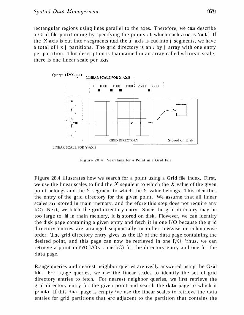
Spatial Data A1anagernent 979
rectangular regions using lines parallel to the axes. Therefore, we can describea Grid file partitioning by specifying the points at which each &,xis is 'cut.' Ifthe ,X axis is cut into 'i segrnents and the y" axis is cut into j segments, we havea total of i x j partitions. The grid directory is an 'i by j array with one entryper partition. This description is Inaintained in an array called a linear scale;there is one linear scale per CLxis.
LI,~~:~~ ~~~~~ ~~~,~-.~?'!S__: ...: I I
I 0 1000 1500 1700 ~ 2500 3500 :: . .. .1 _
Query: (1800,~ut)
I
I
I
I1 F" - •••••~ ~ -
I I I
I I a II I I
I I • II I I
I I f I
I I • II I I
I I k :-~-~.~~--+,I PI
I •
: zIL , I
---_ , ~._~~_.--_.-
,--+-~- ...,.,.. -+---1
GRID DIRECTORY Stored on Disk
LINEAR SCALE FOR Y-AXIS
Figure 28.4 Searching for a Point in a Grid File
Figure 28.4 illustrates how we search for a point using a Grid file index. First,we use the linear scales to find the ..,X- segulent to which the .LY value of the givenpoint belongs and the Y segrnent to which the y" value belongs. This identifiesthe entry of the grid directory for the given point. We assurne that all linearscales are stored in rnain rnernory, and therefore this step does not require anyl/C). Next, we fetch the grid directory entry. Since the grid directory rnay betoo large to .fit in rnain rnenlory, it is stored on disk. Flowever, we can identifythe disk page containing a given entry and fetch it in one I/O because the griddirectory entries are arra,nged sequentially in either row\vise or cohuunwiseorder. The grid directory entry gives us the ID of the data page containing thedesired point, and this page can now be retrieved in one l/C). 'rhus, we canretrieve a point in t\VO l/Os . one l/C) for the directory entry and one for thedata page.
R.ange queries and nearest neighbor queries are e&l;)ily answered using the Cjridfile.B-br rttnge queries, we use the linear scaJes to identify the set of griddirectory entries to fetch. For nearest neighbor queries, we first retrieve thegrid directory entry for the given point and search the data page to which itPOit1tS. If this data page is crnpty,\ve use the linear scales to retrieve the dataentries for grid partitions that are adjacent to the partition that contains the
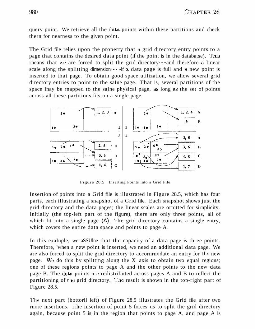
980 C~HAPTER 28
query point. We retrieve all the data points within these partitions and checkthern for nearness to the given point.
The Grid file relies upon the property that a grid directory entry points to apage that contains the desired data point (if the point is in the databa,se). T'hisrneans that \ve are forced to split the grid directory·····and therefore a linearscale along the splitting dirnension··-·-··-if a data page is full and a new point isinserted to that page. To obtain good space utilization, we allow several griddirectory entries to point to the saIne page. That is, several partitions of thespace Inay be rnapped to the saIne physical page, a.s long as the set of pointsacross all these partitions fits on a single page.
3 4
A
B
c
2
Figure 28.5 Inserting Points into a Grid File
Insertion of points into a Grid file is illustrated in Figure 28.5, which has fourparts, each illustrating a snapshot of a Grid file. Each snapshot shows just thegrid directory and the data pages; the linear scales are ornitted for sirnplicity.Initially (the top-left part of the figure), there are only three points, all ofwhich fit into a single page (A). 'rhe grid directory contains a single entry,which covers the entire data space and points to page A.
In this exaInple, we aSSUlne that the capacity of a data page is three points.Therefore, 'when a 11e\V point is inserted, we need an additional data page. Weare also forced to split the grid directory to accornrnodate an entry for the newpage. \¥e do this by splitting along the X axis to obtain two equal regions;one of these regions points to page A and the other points to the new datapage B. The data points are redistributed across pages A and B to reflect theparti tioning of the grid directory. 1'he result is shown in the top-right part ofFigure 28.5.
The next part (bottorll left) of Figure 28.5 illustrates the Grid file after twornore insertions. rrhe insertion of point 5 forces us to split the grid directoryagain, because point 5 is in the region that points to page A, and page A is
Spatial IJata Nfanagc'rnent 981
already full. Since we split along the ...X" axis in the previous split, \ve now splitalong the 1/" axis, and redistribute the points in page A acrex..,s page A and aIle\V data page, C. (Choosing the a.xis to split in a round-robin fashion is one ofseveral possible splitting policies.) ()bserve that splitting the region that pointsto page A also caiuses a split of the region that points to page B, leading to t\VO
regions pointing to page B. Inserting point 6 next is straightforward because itis in a region that points to page 13, and page B h<:1...1;) space for the new point.
Next, consider the bottonl right part of the figure. It shows the exarnple fileafter the insertion of two additional points, 7 and 8. The insertion of point 7fills page C, and the subsequent insertion of point 8 causes another split. ThistiIne, we split along the ~X axis and redistribute the points in page C acrossC and the new data page, D. Observe how the grid directory is partitionedthe most in those parts of the data space that contain the rnost points-··-thepartitioning is sensitive to data distribution, like the partitioning in ExtendibleHashing, and handles skewed distributions well.
Finally, consider the potential insertion of points 9 and 10, which are shownas light circles to indicate that the result of these insertions is not reflected inthe data pages. Inserting point 9 fills page B, and subsequently inserting point10 requires a new data page. However, the grid directory does not have to besplit further~ points 6 and 9 can be in page B, points 3 and 10 can go to a newpage E, and the second grid directory entry that points to page B can be resetto point to page E.
Deletion of points from a Grid file is cOITlplicated. When a data page falls belowSaIne occupancy threshold, such as, less than half-full, it luust be rnerged withscnue other data page to rnaintain good space utilization. We do not go intothe details beyond noting that, to siInplify deletion, a conve:£'ity requirernent isplaced on the set of grid directory entries that point to a single data page: Theregion defined by this set of grid directory erd'ries rnust be conve:r.
28.5.1 Adapting Grid Files to Handle Regions
There are two basic approaches to handling region data in a Grid file, neither of which is satisfactory. First, vve can represent a region by a point in ahigher-dirnens~onal space. E'or exarnple, a box in tvvo diInensions can be represented as a four-dirnensional point by storing t\VO diagonal corner points of thebox. This approach does not support nearest neighbor and spatial join queries,since distances in the original space are not reflected in the distances betweenpoints in the higher-dirnensional space. f'urther, this approach increases thedirnensionality of the stored data, which leads to various problcrns (see Section28.7).
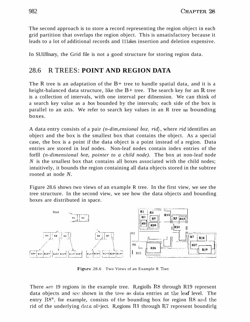
982 CHAPTER 28
The second approach is to store a record representing the region object in eachgrid partition that overlaps the region object. This is unsatisfactory because itleads to a lot of additional records and 111akes insertion and deletion expensive.
In SUIJllnary, the Grid file is not a good structure for storing region data.
28.6 R TREES: POINT AND REGION DATA
The R tree is an adaptation of the B+ tree to handle spatial data, and it is aheight-balanced data structure, like the B+ tree. The search key for an Il treeis a collection of intervals, with one interval per diInension. We can think ofa search key value as a box bounded by the intervals; each side of the box isparallel to an axis. We refer to search key values in an R tree a'S boundingboxes.
A data entry consists of a pair (n-dim,ensional box, riel), where rid identifies anobject and the box is the smallest box that contains the object. As a specialcase, the box is a point if the data object is a point instead of a region. Dataentries are stored in leaf nodes. Non-leaf nodes contain index entries of theforIll (n-dimensional box, pointer to a child node). The box at non-leaf nodeN is the srnallest box that contains all boxes associated with the child nodes;intuitively, it bounds the region containing all data objects stored in the subtreerooted at node N.
Figure 28.6 shows two views of an example R tree. In the first view, we see thetree structure. In the second view, we see how the data objects and boundingboxes are distributed in space.
Root
1~1~- ~~':~~l~~~~j I§4 III
R2 ---1 Itt:::-:::·:::~::::::::::::::::::::::::::·:::·::::-:::::=:~;-I
---------- --,-- --~---,.- ......,;J.. :::::::::=:::==j'jR6 L. _I R15 1,·-----'
Figure 28.6 Two Views of an Example R Tree
There are 19 regions in the exarnple tree. R,egiolls RB through R19 representdata objects and are shown in the tree (1..'3 data entries at the leaf level. Theentry R.8*, for exarnple, consists of the bounding box for region Its and therid of the underlying data ol>ject. R,egions III through 117 represent boundirlg
81)(ltial Data Nfanagenl,cnt
boxes for internal nodes in the tree. Region Rl, for exanlple, is the boundingbox for the space containing the left subtree, which includes data objects RB,R9, RIO, Rll, R12, R13, and R14.
The bounding boxes for two children of a given node can overlap; for ex,unplc,the boxes for the children of the root node, Rl and R2, overlap. rrhis 111eansthat rnore than one leaf node could accornrnodate a given data object whilesatisfying all bounding box constraints. However, every data object is storedin exactly one leaf node, even if its bounding box falls within the regions corresponding to two or Illore higher-level nodes. For exarnple, consider the dataobject represented by R9. It is contained within both R3 and R4 and could beplaced in either the first or the second leaf node (going from left to right in thetree). We have chosen to insert it into the left-rnost leaf node; it is not insertedanywhere else in the tree. (We discuss the criteria used to Blake such choicesin Section 28.6.2.)
28.6.1 Queries
To search for a point, we cornpute its bounding box B, which is just the point,and start at the root of the tree. We test the bounding box for each child ofthe root to see if it overlaps the query box B, and if so, we search the subtreerooted at the child. If more than one child of the root has a bounding boxthat overlaps B, we lTIUSt search all the corresponding subtrees. This is anirnportant difference with respect to B+ trees: The seaTch faT even a singlepoint can lead us down several paths in the tree. When we get to the leaf level,we check to see if the node contains the desired point. It is possible that ·wedo not visit any leaf node------this happens when the query point is in a regionnot covered by any of the boxes associated with leaf nodes. If the search doesnot visit any leaf pages, we know that the query point is not in the indexeddataset.
Searches for region objects and range queries are handled sirnilarly by COluputing a bounding box for the desired region and proceeding as in the search foran object. For a range query, when we get to the leaf level we ITlllst retrieveall region objects that belong there and test "vhether they overlap (or are contained in, depending on the query) the given range. The reason for this testis that, even if the bounding box for an object overlaps the query region, theobject itself rnay not!
As an exalnple, suppose we want to find all objects that overlap our queryregion, and the query region happens to be the box representing object R8.We start at the root and find that the query box overlaps RJ but not R2.l"herefore, we search the left subtree but not the right subtree. We then find
984 (;HAPTER 28
that the query box overlaps R,3 but not RA or ItS. So we seal"eh the le:ft-rnostleaf and find object RB. As another exarnple, suppose that the query regioncoincides \vith Il9 rather than RB. A.gain, the query box overlaps RJ but notR,2 and so we search (only) the left subtree. Now we find that the query boxoverlaps both R3 and R,4 but not H,5. 'Vo therefore search the children pointedto by the entries for R3 and HA.
As a refinernent to the basic search strategy, we can approxirnate the queryregion by a convex region defined by a collection of linear constraints, ratherthan a bounding box, and test this convex region for overlap with the boundingboxes of internal nodes a'S we search down the tree. The benefit is that a convexregion is a tighter approxirnation than a box, and therefore we can sometirnesdetect that there is no overlap although the intersection of hounding boxes isnonernpty. 'rhe cost is that the overlap test is Inore expensive, but this is apure CPU cost and negligible in cOillparison to the potential I/O savings.
Nate that using convex regions to approximate the regions associated withnodes in the Il tree would also reduce the likelihood of false overlaps-----thebounding regions overlap, but the data object does not overlap the queryregion-··-but the cost of storing convex region descriptions is rlluch higher thanthe cost of storing bounding box descriptions.
1'0 search for the nearest neighbors of a given point, we proceed as in a searchfor the point itself. We retrieve all points in the leaves that we exarnine a.spart of this search and return the point closest to the query point. If we donot visit any leaves, then we replace the query point by a srnall box centeredat the query point and repeat the search. If we still do not visit any leaves, weincrease the size of the box and search again, continuing in this fashion untilwe visit a leaf node. 'Ve then consider all points retrieved froIll leaf nodes inthis iteration of the search and return the point closest to the query point.
28.6.2 Insert and Delete Operations
To insert a data object with rid T, we cornpute the bounding box B for theobject and insert the pair (B, r) into the tree. We start at the root node andtraverse a single path frorH the root to a leaf (in contrast to searching, where"vo could traverse several such paths). At each level, 'we choose the child node\V~hose bounding box needs the least enla.rgcruent (in tenns of the increase in itsarea) to cover the box [3. If several chilclren have bounding boxes that cover 13(or that require the sarriC enlargcrnent in order to cover 13), frorn these children,·we choose the one with the slnallest bounding box.
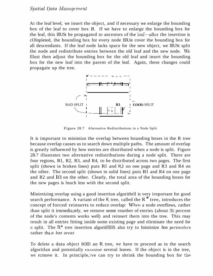
Spatial I)ata !v{anageTnent
At the leaf level, we insert the object, and if necessary we enlarge the boundingbox of the leaf to cover box B. If we have to enlarge the bounding box forthe leaf, this IllUSt be propagated to ancestors of the leaf-after the insertion iscOlnpleted, the bounding box for every node IIlUst cover the bounding box forall descendants. If the leaf node lacks space for the new object, we IllUSt splitthe node and redistribute entries between the old leaf and the new node. \lVelllust then adjust the bounding box for the old leaf and insert the boundingbox for the new leaf into the parent of the leaf. Again, these changes couldpropagate up the tree.
r----- - - - --I I
I~~~~~~=tt::::::11I II I
,r-~ I/ I I
BAD SPLIT I R3 I ~DOOD SPLIT
~--++--t-r----;---+--+~I
Figure 28.7 Alternative Redistributions in a Node Split
It is important to minimize the overlap between bounding boxes in the R treebecause overlap causes us to search down multiple paths. The amount of overlapis greatly influenced by how entries are distributed when a node is split. Figure28.7 illustrates two alternative redistributions during a node split. There arefour regions, Rl, R2, R3, and R4, to be distributed across two pages. The firstsplit (shown in broken lines) puts Rl and R,2 on one page and R3 and R4 onthe other. The second split (shown in solid lines) puts Rl and R4 on one pageand R2 and R,3 on the other. Clearly, the total area of the bounding boxes forthe new pages is lnuch less with the second split.
Minirnizing overlap using a good insertion algorithrll is very irnportant for goodsearch perforrnance. A variant of the R, tree, called the R * tree, introduces theconcept of forced reinserts to reduce overlap: vVhen a node overflows, ratherthan split it irnrnedia,tely, we rernove senne rnunber of entries (about ~30 percentof the node's contents works well) and reinsert thern into the tree. This rnayresult in all entries fitting inside sorne existing page and elirninate the need fora split. The ~,* tree insertion algoritlllIlS also try to Ininirnize box peTirneteT8rather tha.n bo:r areas.
To delete a data object frOID an H, tree, vve have to proceed as in the searchalgoritlun and potentially ex(unine several leaves. If the object is in the tree,"ve rcrnove it. In principle,\ve can try to shrink the bounding box for the
986 CHAPTER 28
leaf containing the object and the bounding boxes for all ancestor nodes. Inpractice, deletion is often irnplernented by sirnply rernoving the object.
Another variant, called the R+ tree, avoids overlap by inserting an object intolllultiple leaves if necessary. Consider the insertion of an object with boundingbox B at a node lV. If box B overlaps the boxes associated with more thanone child of N, the object is inserted into the subtree associated with eachsuch child. For the purposes of insertion into child C with bounding box Be,the object's bounding box is considered to be the overlap of Band Be. 1 Theadvantage of the more cornplex insertion strategy is that searches can nowproceed along a single path froln the root to a leaf.
28.6.3 Concurrency Control
l'he cost of implernenting concurrency control algorithms is often overlooked indiscussions of spatial index structures. l'his is justifiable in environments wherethe data is rarely updated and queries are predominant. In general, however,this cost can greatly influence the choice of index structure.
We presented a simple concurrency control algorithm for B+ trees in Section17.5.2: Searches proceed from root to a leaf obtaining shared locks on nodes;a node is unlocked as soon as a child is locked. Inserts proceed from root to aleaf obtaining exclusive locks; a node is unlocked after a child is locked if thechild is not full. This algorithrn can be adapted to R trees by lllodifying theinsert algorithm to release a lock on a node only if the locked child has spaceand its region contains the region for the inserted entry (thus ensuring that theregion modifications do not propagate to the node being unlocked).
We presented an index locking technique for B+· trees in Section 17.5.1, whichlocks a range of values and prevents new entries in this range frorn being insertedinto the tree. This technique is used to avoid the phantorn problern. Now letus consider how to adapt the index locking approach to R trees. The ba..."ic ideais to lock the index page that contains or would contain entries with key valuesin the locked range. In R, trees, overlap between regions associated with thechildren of a node could force us to lock several (non-leaf) nodes on differentpaths frorn the root to SOH1C leaf. Additional cornplica..tions a.rise fronl having todeal with changes "in pi:lIticular, enlargernents due to insertions ....·in the regionsof locked nodes. vVithout going into further detail, it should be clear that indexlocking to avoid phant0l11 insertions in H. trees is both harder and less efficientthan in 13+ trees. Further, idea",') such ae:; forced reinsertion in It* trees and----_ _--
1 Insertion into an R+ tree involves additional details. For example, if box B is not contained in thecollection of boxes associat(~d with the children of N whose boxes 13 overlaps, one of the childnm mustluwe its box enlarged so that 13 is contajned in the collection of boxes associ<lf;ed with thf~ children.
Spatial Data !vIanage7Tu~nt 98}
rIlultiple insertions of an object in R+ trees nlake index locking prohibitivelyexpenSIve.
28.6.4 Generalized Search Trees
The B+ tree and R tree index structures are sirnilar in 111any respects: Bothare height-balanced, in which searches start at the root of the tree and proceedtoward the leaves; each node covers a portion of the underlying data space, andthe children of a node cover a subregion of the region associated with the node.There are irnportant differences of course-for exa111ple, the space is linearizedin the B+ tree representation but not in the R tree·~··~~but the cornrnon featureslead to striking siruilarities in the algorithms for insertion, deletion, search, andeven concurrency control.
The generalized search tree (GiST) abstracts the essential features of treeindex structures and provides 'template' algorithms for insertion, deletion, andsearching. The idea is that an ORDBMS can support these template algorithnlsand thereby make it easy for an advanced database user to implement specificindex structures, such as R trees or variants, without nlaking changes to anysystem code. The effort involved in writing the extension 1nethods is l11uch lessthan that involved in ilIlplementing a new indexing 111ethod frolIl scratch, andthe performance of the GiST te111plate algorithms is cornparable to specializedcode. (For concurrency control, 1110re efficient approaches are applicable ifwe exploit the properties that distinguish B+ trees from R trees. However,B+ trees are irnplernented directly in most cOllllIlercial DBMSs, and the GiSTapproach is intended to support 1nore conlplex tree indexes.)
rrhe ternplate algorithlIls call on a set of extension methods specific to a particular index structure, and these 111USt be supplied by the irnplernentor. Forexarnple, the search te1nplate searches all children of a node whose region isconsistent with the query. In a B-t- tree the region a.ssociated with a node isa range of key values~ and in an R tree, the region is spatial. The check tosee whether a region is consistent with the query region is specific to the indexstructure and is an exarnple of an extension rnethod. As another exa.rnple of anextension rnethod, consider ho\;y to choose the child of an Il tree node to inserta new entry into. This choice can be rnade based on \vhich candidate child'sregion needs expanded the least; an extension rnethod is required to calculatethe required expansions for candidate children and choose the child into Vlhichto insert the entry.
988 (;HAPTER 28
28.7 ISSUES IN HIGH-DIMENSIONAL INDEXING
The spatial indexing techniques just discussed ''lark quite \vell for t\VO- andthree-dirnensional dat&"ets, which are encountered in Illany applications of spatial data. In SCHne applications, such as content-based ilnage retrieval or textindexing, however, the nurIlber of dirnensions can be large (tens of dirnensionsare not unCOtnlnon). Indexing such high-dirnensional data presents unique challenges, and ne\'l techniques are required. For exanlple, sequential scan becomessuperior to R, trees even when searching for a single point for datasets with1nore than about a dozen dirnensions.
IIigh-dirnensional datasets are typically collections of points, not regions, andnearest neighbor queries are the rnost cotnrIlon kind of queries. Searching forthe nearest neighbor of a query point is rneaningful when the distance frotn thequery point to its nearest neighbor is less than the distance to other points.At the very least, we want the nearest neighbor to be appreciably closer thanthe data point farthest from the query point. High-dimensional data poses apotential problem: For a wide range of data distributions, as dimensionality dincreases, the distance (frolll any given query point) to the nearest neighborgrows closer and closer to the distance to the farthest data point! Searchingfor nearest neighbors is not lneaningful in such situations.
In many applications, high-dirnensional data may not suffer frorn these problenls and may be amenable to indexing. However, it is advisable to check highdimensional datasets to rnake sure that nearest neighbor queries are meaningful.Let us call the ratio of the distance (frorn a query point) to the nearest neighbor to the distance to the farthest point the contrast in the dataset. We canmeasure the contra.'3t of a dataset by generating a number of sarnple queries,measuring distances to the nearest and farthest points for each of these sarIlplequeries and cornputing the ratios of these distances, and taking the averageof the 111easured ratios. In applications that call for the nearest neighbor, weshould first ensure that datasets have good contrast by ernpirical tests of thedata.
28.8 REVIEW QUESTIONS
Answers to th~ review questions can be found in the listed sections.
• vVhat are the characteristics of spatial data? vVhat is a spatial extent?What are the differences between spatial range queries, nearest neighborqueries, and spatial join queries? (Section 28.1)
Spatial Data 1\1an,age'lnent 989$
IJII Nalne several applications that deal ,,"ith spatial data and specify theirrequircrnents on a database systeln. \Vhat is a feature vector and ho\v is itused? (Section 28.2)
III vVhat is a IIlulti-dirnensional index'? \\That is a spatial index? \tVhat arethe differences bet\vccn a spatial index and a B+ tree? (Section 28.3)
IlIl \iVhat is a space-filling curve, and hovv can it be used to design a spatialindex? Describe a spatial index structure ba"oscd on space-filling curves.(Section 28.4)
II What data structures are lnaintained for the Grid file index? How doinsertion and deletion in a Grid file work? For what types of queries anddata are Grid files especially suitable and why? (Section 28.5)
II What is an R tree? "Vhat is the structure of data entries in R trees?How can we lninimize the overlap between bounding boxes when splittingnodes? lIow does concurrency control in a R tree work? Describe a genericteulplate for tree-structured indexes. (Section 28.6)
• Why is indexing high-dilnensional data very difficult? What is the ilnpactof the dirrlensionality on nearest neighbor queries? What is the contrast ofa dataset? (Section 28.7)
EXERCISES
Exercise 28.1 Answer the following questions briefly:
1. How is point spatial data different frolll nonspatial data?
2. How is point data different fronl region data?
~). Describe three cornrnon kinds of spatial queries.
4. Why are nearest neighbor queries irnportant in rnultin1edia applications?
5. How is a 13+ tree index different froIll a spatial index? vVhen would you use a 13+ treeindex over a spatial index for point data? vVhen would you use a spatial index over a13+ tree index for point data?
6. vVhat is the relationship between Z-ordering and Region Quad trees?
7. Compare Z-ordering and H.ilbert curves as techniques to cluster spatial data.
Exercise 28.2 Consider Figure 28.3, \vhich illustrates Z-ordering and Region Quad trees.Answer the following questions.
1. Consider the region cOInposed of the points with these Z-values: 4, 5, 6, and 7. lVlark thenodes that represent this region in the Region Quad tree shown in Figure 28.:3. (Expandthe tree if necessary.)
2. llepeat the preceding exercise for the region cornposed of the points with Z-vaJues 1 and~~ .

990 CHAPTER 28
3. Repeat it for the region composed of the points with Z-values 1 and 2.
4. Repeat it for the region cOll1posed of the points with Z-values 0 and 1.
5. Repeat it for the region coruposed of the points with Z-values 3 and 12.
6. Repeat it for the region cmnposed of the points with Z-values 12 and 15.
7. Repeat it for the region COITlposed of the points with Z-values 1, 3, 9, and 11.
8. Repeat it for the region COITlposed of the points with Z-values 3, 6, 9, and 12.
9. Repeat it for the region COITlposed of the points with Z-values 9, 11, 12, and 14.
10. Repeat it for the region cornposed of the points with Z-values 8, 9, 10, and 11.
Exercise 28.3 This exercise also refers to Figure 28.3.
1. Consider the region represented by the 01 child of the root in the Region Quad treeshown in Figure 28.3. What are the Z-values of points in this region?
2. Repeat the preceding exercise for the region represented by the 10 child of the root andthe 01 child of the 00 child of the root.
3. List the Z-values of four adjacent data points distributed across the four children of theroot in the Region Quad tree.
4. Consider the alternative approaches of indexing a two-dimensional point dataset using aB+ tree index: (i) on the composite search key (X, Y), (ii) on the Z-ordering computedover the X and Y values. Assuming that X and Y values can be represented using twobits each, show an example dataset and query illustrating each of these cases:
(a) The alternative of indexing on the COITlposite query is faster.
(b) The alternative of indexing on the Z-value is faster.
Exercise 28.4 Consider the Grid file instance with three points 1, 2, and 3 shown in thefirst part of Figure 28.5.
1. Show the Grid file after inserting each of these points, in the order they are listed: (), 9,10, 7, 8, 4, and 5.
2. Assume that deletions are handled by sirnply rernoving the deleted points, with no atterl1pt to merge empty or underfull pages. Can you suggest a siruple concurrency controlscheme for Grid files?
3. Discuss the use of Grid files to handle region data.
Exercise 28.5 Answer each of the following questions independently with respect to the Rtree shown in Figure 28.6. (That is, don't consider the insertions corresponding to otherquestions when answering a given question.)
1. Show the bounding box of a new object that can be inserted into R4 but not into n:3.2. Show the bounding box of a new object that is contained in both Rl and R6 but is
inserted into R6.
3. Show the bounding box of a new object that is contained in both Rl and R6 and isinserted into Rl. In which leaf node is this object placed?
4. Show the bounding box of a new object that could be inserted into either R4 or R5 butis placed in R5 based on the principle of least expansion of the bounding box area.
8pat'ial Data l\lanagernent 991
5. Given an exarIlple of an object such that searching for the object takes us to both theRl and R2 subtrees.
6. Give an eXCllnple query that takes us to nodes Ra and R5. (Explain if there is no suchquery.)
7. Give an exanlple query that takes us to nodes R3 and R4 but not to R5. (Explain ifthere is no such query.)
8. Give an eXaInple query that takes us to nodes Ra and R5 but not to R4. (Explain ifthere is no such query.)
BIBLIOGRAPHIC NOTES
Several multidimensional indexing techniques have been proposed. These include Bang files[286], Grid files [565], hB trees [491]' KDB trees [630], Pyrarnid trees [80] Quad trees[649],R trees [350], R* trees [72], R+ trees, the TV tree, and the VA file [767]. [322] discusseshow to search R trees for regions defined by linear constraints. Several variations of these,and several other distinct techniques, have also been proposed; Samet's text [650] deals withmany of them. A good recent survey is [294].
The use of Hilbert curves for linearizing multidimensional data is proposed in [263]. [118] is anearly paper discussing spatial joins. Hellerstein, Naughton, and Pfeffer propose a generalizedtree index that can be specialized to obtain many of the specific tree indexes mentionedearlier [376]. Concurrency control and recovery issues for this generalized index are discussedin [447]. Hellerstein, Koutsoupias, and Papadinlitriou discuss the complexity of indexingschemes [377], in particular range queries, and Beyer et a1. discuss the problerlls arising withhigh dimensionality [93]. Faloutsos provides a good overview of how to search multirnediadatabases by content [258]. A recent trend is towards spatiotemporal applications, such astracking rnoving objects [782].
29FURTHER REi\DING
.. What is next?
.. Key concepts: TP monitors, real-tirne transactions; data integration; mobile data; main meInory databa.~es; multimedia databases;GIS; tenlporal databases; Bioinformatics; infonnation visualization
This is not the end. It is not even the beginning of the end. But it is, perhaps,the end of the beginning.
······-·Winston Churchill
In this book, we concentrated on relational databa.'3e systerus and discussedseveral fundaruental issues in detail. However, our coverage of the databasearea, and indeed even the relational database H,rea, is far from exhaustive. Inthis chapter, we look briefly at several topics vve did not cover, with the goal ofgiving the reader SOUle perspective and indicating directions for further study.
vVe begin with a discussion of advanced transaction processing concepts inSection 29.1. vVe discuss integrated access to data frOUl rnultiple databases inSection 29.2 and touch on Inobile applications that connect to databases in Section 29.3. \Ve consider the irnpact of increasingly larger rnain Inenlory sizes inSection 29.4. \Ve discuss rnultirnedia databctses in Section 29.5, geographic inforrnation systerns in Section 29.G, tcrnporaJ data in Section 29.7, and sequencedata in Section 29.8. \Ve conclude with a look at inforrnation visualization inS ·,t· . ')0 C)k. ec ,Ion ....J •• '.
992
FUTthcr- Read'ing 99a
T'he applications covered in this chapter push the lirnits of currently availabledatabase technology and drive the developrnent of new techniques. As even ourbrief coverage indicates, Innch \vork lies ahead for the database field!
29.1 ADVANCED TRANSACTION PROCESSING
The concept of a transaction has wide applicability for a variety of distributedcOlnputing tasks, such as airline reservations, inventory rnanagernent, and electronic COlnnlerce.
29.1.1 Transaction Processing Monitors
Cornplex applications are often built on top of several resource managers,such as database managernent systenls, operating systerns, user interfaces, andmessaging software. A transaction processing (TP) monitor glues togetherthe services of several resource managers and provides application programmersa uniform interface for developing transactions with the ACID properties. Inaddition to providing a uniform interface to the services of difl'erent resourceillanagers, a TP rnonitor also routes transactions to the appropriate resourcernanagers. Finally, a TP monitor ensures that an application behaves as atransaction by implernenting concurrency control, logging, and recovery functions and by exploiting the transaction processing capabilities of the underlyingresource rnanagers.
TP rnonitors are used in environments where applications require advancedfeatures, such as access to rnultiple resource lllanagers, sophisticated requestrouting (also called workflow management); assigning priorities to transactions and doing priority-based load-balancing across servers, and so on. ADBlVIS provides lllany of the functions supported by a TP monitor in additionto processing queries and database updates efficiently. A DBMS is appropriate for environrnents where the wealth of transaction rnanagernent capabilitiesprovided by a TP rnonitor is not necessary and, in particular, \vhere very highscalability (with respect to transaction processing activity) and interoperabilityare not essential.
The transaction processing capabilities of database systerlls are irnproving continually. For eKarnple, rnany vendors offer distributed DBMS products today inwhich a transaction can execute across several resource rnanagers, each of whichis a DBMS. Currently, all the DBlVISs Inust be frorn the saIne vendor; however,as transaction-oriented services frorn different vendors becom.e rnore standardized, distributed, heterogeneous DBlV'ISs should becorne available. Eventually,perhaps, the functions of current rrp rnonitors will also be available in rnany
994
DBIV1Ss; for now, 'I'P rnonitors provide essential infrastructure for high-endtransaction processing ellviroIllnents.
29.1.2 New Transaction Models
Consider an application such as cornputer-aided design, in which users retrievelarge design objects froIn a database and interactively analyze and 1110dify thenl.Each transaction takes a long tiIne---Ininutes or even hours, whereas the TPCbench1nark transactions take under a millisecond-----and holding locks this longaffects perfonnance. F\uther, if a crash occurs, undoing an active transactioncOlllpletely is unsatisfactory, since considerable user effort may be lost. Ideally,we want to restore 1nost of the actions of an active transaction and reSluneexecution. Finally, if several users are concurrently developing a design, theynlay want to see changes being rnade by others without waiting until the endof the transaction that changes the data.
To address the needs of long-duration activities, several refinements of thetransaction concept have been proposed. The basic idea is to treat each transaction as a collection of related subtransactions. Subtransactions can acquirelocks, and the changes made by a subtransaction become visible to other transactions after the subtransaction ends (and before the nlain transaction of whichit is a part commits). In multilevel transactions, locks held by a subtransaction are released when the subtransaction ends. In nested transactions,locks held by a subtransaction are assigned to the parent (sub)transaction whenthe subtransaction ends. These refinements to the transaction concept have asignificant effect on concurrency control and recovery algorithnls.
29.1.3 Real-Time DBMSs
SOllIe transactions 1nust be executed within a user-specified deadline. A harddeadline Ineans the value of the transaction is zero after the deadline. Forexa1nple, in a DBMS designed to record bets on horse races, a transactionplacing a bet is worthless once the race begins. Such a transaction shouldnot be executed; the bet should not be placed. A soft deadline rIlcal1S thevalue of the transaction decrccl..'3cs after the deadline, eventually going to zero.:For exarnple, in a DB1rlS designed to rnonitor S(Hne activity (e.g., a c01nplexreactor), a transaction that looks up the current reading of a sensor rnust beexecuted within a sl10rt tiIne, sa.y, one second. The longer it takes to executethe tra.nsaction, the less useful the reading becorn.es. In a real-tirne DBl\1S, thegoal is to 1naxirnize the value of executed transactions, and the DBlVIS 111Ustprioritize transactions, taking their deadlines into account.
[further Ileading
29.2 DATA INTEGRATION
995$
As datab&ses proliferate, users want to access data fronl rnore than one source.For exaulple, if several travel agents rnarket their travel packages through theWeb, custorners would like to cornpare packages from different agents. A rnoretraditional exaruple is that large organizations typically have several databases,created (and rnaintained) by different divisions, such as Sales, Production, andPurchasing. \i\Thile these databases contain much common inforrnation, determining the exact relationship between tables in different databases can be acomplicated problem. For example, prices in one database might be in dollars per dozen items, while prices in another database might be in dollars peritelll. The developruent of XML DTDs (see Section 7.4.3) offers the pronlisethat such sernantic rnisrnatches can be avoided if all parties conforrll to a singlestandard DTD. However, there are many legacy databases and rllost dornainsstill do not have agreed-upon DTDs; the problem of selllantic rnismatches willbe encountered frequently for the foreseeable future.
Semantic mismatches can be resolved and hidden fronl users by defining relational views over the tables from the two databases. Defining a collection ofviews to give a group of users a uniform presentation of relevant data frornrnultiple databases is called semantic integration. Creating views that masksernantic mismatches in a natural manner is a difficult task and has been widelystudied. In practice, the task is rllade harder because the scheruas of existingdatabases are often poorly documented; hence, it is difficult to even understandthe meaning of rows in existing tables, let alone define unifying views acrossseveral tables frorll different databases.
If the underlying databases are rnanaged using difl"erent DBlVISs, as is oftenthe case, SaIne kind of 'middleware' rnust be used to evaluate queries over theintegrating views, retrieving data at query execution tirne by using protocolssuch as Open Database Connectivity (ODBC) to give each underlying databa..'3ca uniforrn interface, as discussed in Chapter 6. Alternatively, the integratingviews can be nlaterialized and stored in a data warehouse, as discussed inChapter 25. Queries can then be executed over the warehoused data withoutaccessing the source DBlVISs at run-tirne.
29.3 MOBILE DATABASES
The availability of portable coruputers and wireless eorrnnunications has createda nevv breed of nornadic database users. At one level, these users are sirnplyaccessing a databa.>se through a network, which is silnilar to distributed DBMSs.At another level, the network a:s well as data and user characteristics now haveseveral novel properties, Wllich affect b<l..sic assurnptioI1S in rnany cornponents
996 (;HAPTER 49
of a DB~fS~ including the query engine~ transaction rnanager, and recoveryInanager:
• 1Isers are connected through a \vireless link whose band,vidth is 10 timesless than Ethernet and 100 tiIIles less than ATM networks. COIIul1unicationcosts are therefore significantly higher in proportion to I/O and CPU costs.
11 Users' locations constantly change, and Inobile corllputers have a liInitedbattery life. 'Therefore, the true cOllullunication costs reflect connectiontiIne and battery usage in addition to bytes transferred and change constantly depending on location. Data is frequently replicated to lninirnizethe cost of accessing it from different locations.
• As a user moves around, data could be accessed froIn multiple databaseservers within a single transaction. The likelihood of losing connectionsis also lnnch greater than in a traditional network. Centralized transaction rnanagenlent may therefore be irnpractical, especially if sorne data isresident at the mobile computers. We may in fact have to give up onACID transactions and develop alternative notions of consistency for userprograms.
29.4 MAIN MEMORY DATABASES
The price of rnain llleInory is now low enough that we can buy enough mainrnernory to hold the entire database for many applications; with 64-bit addressing, rnodern CPUs also have very large address spaces. Sorne commercialsysterns now have several gigabytes of rrlain IneInory. This shift proInpts a reexarnination of scnne basic DBMS design decisions, since disk accesses no longerdorninate processing tilue for a Inemory-resident database:
• lVlain nlerllory does not survive systelll crashes, and so we still have toiluplernent logging and recovery to ensure transaction atolnicity and durability. Log records rnust be written to stable storage at conlluit tirne, andthis process could becorne a bottleneck. To rninirnize this problern, ratherthan comnlit each transaction ,1S it conlpletes, we can collect cOlupletedtransactions and cornlnit theIu in batches; this is called group commit.Recovery algorithrns can also be optirnized, since pages rarely have to bevvrritten out to rrlake roorn for other pages.
• The irnplerrlentation of in-lnelnory operations has to be optinlized carefully,since disk accesses are no longer the lirniting factor for perforrnance.
• A ne,v criterion llUlst be considered while optirnizing queries, the alllountof space required to execute a plan. It is iInportant to rninirnize the space
FUTther llearling 991
overhead because exceeding available physical Incrnory would lead to swapping pages to disk (through the operating systcrIl '8 virtual rncillory ruechanisIIls), greatly slo\ving do\vn execution.
• Page-oriented data structures becolue less iInportant (since pages are 110
longer the unit of data retrieval), and clustering is not ilnportant (sincethe cost of accessing any region of IIlain rneIIlory is uniforrn).
29.5 MULTIMEDIA DATABASES
In an object-relational DB~1S, users can define ADTs \vith appropriate rnethods, which is an irnprovement over an RDBI\1S. Nonetheless, supporting justADTs falls short of what is required to deal with very large collections ofmultimedia objects, including audio, irnages, free text, text nlarked up inHTML or variants, sequence data, and videos. Illustrative applications includeNASA's EGS project, which aims to create a repository of satellite irnagery;the JIUlnan Genorne project, which is creating databases of genetic inforrnationsuch as GenBank; and NSF/DARPA's Digital Libraries project, which aiIns toput entire libraries into database systems and make thelll accessible throughcOlnputer networks. Industrial applications, such as collaborative developnlentof engineering designs, also require multimedia database rnanagernent and arebeing addressed by several vendors.
We outline some applications and challenges in this area:
• Content-Based Retrieval: Users 111Ust be able to specify selection conclitions based on the contents of rllultilnedia objects. For exanlplc, users lllaysearch for inlages using queries such as "Find all irnages that are sirnilar tothis image" and "Find all inlages that contain at lea"t three airplanes." Asinulges are inserted into the database, the DBMS lllUSt analyze thern andautomatically eJ:tract features that help answer such content-based queries.1~his inforrnation can then be used to search for inlages that satisfy a givenquery, ae;,; discussed in Chapter 28. As another exarnple, users would like tosearch for docurnents of interest using infonnation retrieval techniques andkeyword searches. Vendors are rnoving toward incorporating such techniques into DBMS products. It is still not clear how these dOlnain-specificretrieval and search techniques can be corubined effectively \vith traditionalDBIvIS quei-ies. R,csearch into abstract data types and ()R,DBMS queryprocessing has provided a starting point, but lnore work is needed.
II Managing Repositories of Large Objects: Traditionally, DBlVISs haveconcentrated on tables that contain a large nurnber of tuples, each of \vhichis relatively srnaii. ()nce Illultilnedia objects such as irnages, sound clips,and videos are stored in a database, individual objects of very large size
998 CHAPTER 39
have to be handled efficiently. For example, compression techniques lllUSt
be carefully integrated into the DBIvlS environrnent. As another exarnple,distributed DBMSs HUlst develop techniques to efficiently retrieve suchobjects. Retrieval of r11ultir11edia objects in a distributed systern has beenaddressed in liInited contexts, such as client-server systerns, but in generalreulains a difficult probleul.
• Video-On-Denland: lVlany cornpanies want to provide video-on-denlandservices that enable users to dial into a server and request a particularvideo. The video Inust then be delivered to the user's COI11puter in real time,reliably and inexpensively. Ideally, users nlust be able to perform farniliarVCR functions such as fast-forward and reverse. Fronl a database perspective, the server has to contend with specialized real-time constraints; videodelivery rates must be synchronized at the server and at the client, takinginto account the characteristics of the communication network.
29.6 GEOGRAPHIC INFORMATION SYSTEMS
Geographic Information Systems (GIS) contain spatial information aboutcities, states, countries, streets, highways, lakes, rivers, and other geographicalfeatures and support applications to combine such spatial information withnon-spatial data. As discussed in Chapter 28, spatial data is stored in eitherraster or vector formats. In addition, there is often a terTIporal dirnension, a'S
when we measure rainfall at several locations over time. An important issuewith spatial datasets is how to integrate data froIn rnultiple sources, since eachsource rnay record data using a different coordinate system to identify locations.
Now let us consider how spatial data in a GIS is analyzed. Spatial information is lllost naturally thought of as being overlaid on maps. rTypical queriesinclude "What cities lie on 1-94 between Madison and Chicago?" and "Whatis the shortest route from Madison to St. Louis?" These kinds of queries canbe addressed using the techniques discussed in Chapter 28. An emerging application is in-vehicle navigation aids. With Global Positioning Systcrn (CPS)technology, a car's location can be pinpointed, and by accessing a databa.se oflocal rnaps, a driver can receive directions froIn his or her current location to adesired destination; this application also involves rnobile databa..'3e access!
In addition, many applications involve interpolating rneasurernents at certainlocations across an entire region to obtain a rnodel and cornbining overlappingrnodels. For exarnple, if \-ve have rneasured rainfall at certain locations, we canuse the Triangulated Irregular Network (TIN) approach to triangulatethe region, with the loeations at which we have measurcrnents being the vertices of the triangles. Then, we use sorne forrn of interpolation to estirnate
}tuTther Reading 999
the rainfall at points within triangles. Interpolation, triangulation, Il1ap overlays, visualization of spatial data, and rnany other dornain-specific operationsare supported in GIS products such a,,'3ESRI Systerlls' ARC-Info. l'he1'efore,\vhile spatial query processing techniques as discussed in Chapter 28 are anirnportant part of a GIS product, considerable additional functionality rnust beincorporated as well. How best to extend 0 ltDB1.1S systenls with this additional functionality is an irnportant problenl yet to be resolved. Agreeing onstandards for data representation forrnats and coordinate systeuls is anotherlTIajor challenge facing the field.
29.7 TEMPORAL DATABASES
Consider the following query: "Find the longest interval in which the sameperson managed two different departlTIents." Many issues are associated withrepresenting telnporal data and supporting such queries. We need to be able todistinguish the times during which sOlnething is true in the real world (validtime) from the times it is true in the database (transaction time). Theperiod during which a given person rnanaged a departrnent can be indicated bytwo fields from and to, and queries must reason about time intervals. further,temporal queries require the DBMS to be aware of the anolTIalies associatedwith calendars (such as leap years).
29.8 BIOLOGICAL DATABASES
Biolnfornlatics is an emerging field at the intersection of Biology and COHlputerScience. FraIn a database standpoint, the rapidly growing data in this area h~LS
(at lea..'3t) two interesting characteristics. First, a lot of loosely str'UchLTcd datais widely exchanged, leading to interest in integration of such data. This ha",,,rnotivated SOlne of the research in the area of XML repositories.
The second interesting feature is sequence data. DNA sequences are beinggenerated at a rapid pace by the biological cOllnnunity. The field of biologicalinforrnation rnanagernent and analysis ha"s becorne very popular in recent years,called bioinformatics. Biological data, such as DNA sequence data, characterized by cornplex structure and nurnerous relationships arnong data elernents,rllany overlapping and incoruplete or erroneous data fragrnents (because experiInentally collected data froIll several groups, often working on related problelIls,is stored in the databa"ses), a need to frequently change the databa..se 8chcrnaitself as ne¥l kinds of relationships in the data are discovered, and the need tornaintain several versions of data for archival and reference.
IOOO CHAPTER ~g
29.9 INFORMATION VISUALIZATION
As coruputors becoule faster and rnain rnornory cheaper, it beconies increa...~ingly feasible to create visual presentations of data, rather than just text-b&'3edreports. Data visualization rnakes it easier for users to understand the inforInation in large cornplex data..'3ets. The challenge here is to lTlake it easy forusers to develop visual presentations of their data and interactively query suchpresentations. Although a nurnber of data visualization tools are available,efficient visualization of large datasets presents Inany challenges.
The need for visualization is especially irnportant in the context of decisionsupport; when confronted with large quantities of high-dhnensional data andvarious kinds of data sUffirnaries produced by using analysis tools such as SQL,OLAP, and data ll1ining algorithrns, the inforrnation can be overwhehning.Visualizing the data, together with the generated sumrnaries, can be a powerfulway to sift through this infonnation and spot interesting trends or patterns.The hurnan eye, after all, is very good at finding patterns. A good frameworkfor data mining lTIUst combine analytic tools to process data and bring outlatent anolllalies or trends with a visualization environment in which a usercan notice these patterns and interactively drill down to the original data forfurther analysis.
29.10 SUMMARY
'rhe database area continues to grow vigorously, in terrns of both technologyand applications. The fundarnental rea...,on for this growth is that the amountof inforrnation storE~d and processed using computers is growing rapidly. Regardless of the nature of the data and the intended applications, users needdatabase rnanagernent systems and their services (concurrent access, crash recovery, ea...,y and efficient querying, etc.) a'3 the vohllue of data increases. Asthe range of applications is broadened, however, SOIlIC shortcornings of currentDBMSs becoIne serious lilTlitations. These problerus are being actively studiedin the database research cornrnunity.
'The coverage in this book provides an introduction, but is not intended to coverall aspects of datab<:"k'3e systerns. Anlple rnaterial is available for further study,as this chapter Hlustrates, and we hope that the reader is rnotivated to pursuethe leads in the bibliography. Bon voyage!
FU7theT Recui'ing
BffiLIOGRAPHIC NOTES
1001
[338] contains a conlprehensive treatnlent of all &<spects of transaction processing. See [241Jfor several papers that describe new transaction models for nontraditional applications suchas CAD/CATv1. [1,577,696,711,761] are SaIne of the Inany papers on real-tirne databases.
Detenllining which entities are the same across different databases is a difficult probleIn;it is an example of a semantic lllisrnatch. Resolving such nlismatches h3.." been addressedin rIlany papers, including [424, 476, 641, 663]. [389] is an overview of theoretical work inthis area. Also see the bibliographic notes for Chapter 22 for references to related work onrnultidatabases, and see the notes for Chapter 2 for references to work on view integration.
[304] is an early paper on main mernory databa..ses. [102, 406] describe the Dali rnain rllerllorystorage manager. [421] surveys visualization idioms designed for large databases, and [342]discusses visualization for data mining.
Visualization systerns for databases include DataSpace [592], DEVise [489], IVEE [27], theMineset suite from SGI, Tioga [31], and VisDB [420]. In addition, a number of general toolsare available for data visualization.
Querying text repositories has been studied extensively in information retrieval; see [626] fora recent survey. This topic has generated considerable interest in the database cOITnnunityrecently because of the widespread use of the Web, which contains many text sources. Inparticular, HTML dOCUITlents have sonle structure if we interpret links as edges in a graph.Such documents are examples of selllistructured data; see [2] for a good overview. Recentpapers on queries over the Web include [2, 445, 527, 564].
See [576] for a survey of multimedia issues in database management. There has been muchrecent interest in database issues in a mobile computing environment; for example, [387,398].See [395] for a collection of articles on this subject. [728] contains several articles that coverall aspects of telnporal databases. The use of constraints in databases has been activelyinvestigated in recent years; [416] is a good overview. Geographic Infonnation SysteIT1S havealso been studied extensively; [586] describes the Paradise systern, which is notable for itsscalability.
'The book [794] contains detailed discussions of ternporal databases (including the TSQL2language, which is influencing the SQL standard), spatial and nnIltimedia databases, anduncertainty in databa.ses.
30THE MINIBASE SOFTWARE
Practice is the best of all instructors.
-Publius Syrus, 42 B.C.
Minibase is a small relational DBMS, together with a suite of visualizationtools, that has been developed for use with this book. While the book rnakesno direct reference to the software and can be used independently, Minibaseoffers instructors an opportunity to design a variety of hands-on &'3signments,with or without programming. To see an online description of the software,visit this URL:
http://www.cs.wisc.edu/-dbbook/minibase.html
The software is available freely through ftp. By registering themselves as usersat the UR,L for the book, instructors can receive prompt notification of anyInajor bug reports and fixes. Sarnple project assignments, which elaborate onSOIne of the briefly sketched ideas in the project- based exercises at the end ofchapters, can be seen at
http://www.cs.wisc.edu/-dbbook/minihwk.html
Instructors should consider making sillall lllodifications to each ::t..ssignlnentto discourage undesin1ble 'code reuse' by students; assignrnent handouts forrnatted using Latex are available by ftp. Instructors can also obtain solutions to these assiglunents by contacting the authors (raghu@cs. wise. edu,j ohannes@cs. cornell. edu).
30.1 WHAT IS AVAILABLE
NIiniba.se is intcllded to snpplCIllent the use of a cornrnercial DBlVfS such as()racle or Sybase in course projects, not to replace theIn. \Vhile a cornlnerciaJDBl\r1.S is ideal for SC:~L assignrnents, it does not help students understand hovvthe DBNIS w'orks. IVlinibase is intended to address the latter issue; the subsetof S(~L that it supports is intentionally kept 8rnall, and students should alsobe asked to use a connnercialDBIVlS for writing SQL queries and prograrns.
1002
The N!inibase Soft'wo/re 1003t
:NIinibase is provided on an as-is basis with no \varrantics or restrictions foreducational or personal use. It includes the fol1o\ving:
• Code for a sl11al1 single-user relational DB1VIS, including a parser and queryoptirnizer for a subset of SQL, and cOlnponents designed to be (re)writtenby students as project assignrnents: heap files, buffer 1nanager, B+ trees,Borting, and jo'ins.
30.2 OVERVIEW OF MINIBASE ASSIGNMENTS
Several assignrnents involving the use of l\!linibase are described here. Each ofthese has been tested in a course already, but the details of how l\!linibase isset up might vary at your school, so you 111ay have to rnodify the a..'3Sigluncntsaccordingly. If you plan to use these assignrnents, you are advised to downloadand try thern at your site well in advance of handing thern to students. Wehave done our best to test and docurnent these assignrnents and the Minibasesoftware, but bugs undoubtedly persist. Please report bugs at this URL:
http://www.cs.wisc.edu/-dbbook/minibase.comments.html
We hope users will contribute bug fixes, additional project assignments, andextensions to Minibase. These will be rnade publicly available through theMinibase site, together with pointers to the authors.
In several assignrnents, students are asked to rewrite a cornponent of Minibase.The book provides the necessary background for all these assignrnents, andthe cl-'3signrnent handout provides additional systern-Ievel details. The onlineI-rrML docurnentation provides an overvic\v of the softv.rare, in particular thecorllponent interfaces, and can be downloaded and installed at each school thatuses Minibcl-'3e. ~rhe projects that follow should be assigned after covering therelevctnt rnaterial fro1ll the indicated chapter:
II Buffer Manager (Chapter 9): Students c\,re given code for the layerthat rnanag(~s space on disk and supports the concept of pages \vith pageids. ~rhey are a"sked to i1nplelnent a buffer lnanager that brings requestedpages into Inelnory if they an.'. not already there. ()ne variation of thisassignrnent could use differerlt repla,ceruent policies. Students are asked toaSSlllne a single-user enVir0l11nent, vvith no concurrency control or recovery1nanagclnent.
11III HF Page (Chapter 9): Students rllust\vrite code that rnanages recordson a page using (1, slot-directory pa,ge forrnat to keep track of the records.Possible variants include fixed-length versus variable-length records andother vvays to keep track of records on a pagf'..
1004 CHAPTER 30
• Heap Files (Chapter 9): {,Ising the HF page and buffer manager code,stludents are asked to inlplernent a layer that supports the abstraction offiles of unordered pages, that is, heap files.
• B+ Trees (Chapter 10): This is one of the lnore cornplex assignrnents.Students have to implernent a page class that Inaintains records in sortedorder vvithin a page and iUlplernent the B+ tree index structure to iInpose asort order across several leaf-level pages. Indexes store (key, record-pointer)pairs in leaf pages, and data records are stored separately (in heap files).Shnilar assignments can easily be created for Linear Hashing or ExtendibleIIa.'1hing index structures.
• External sorting (Chapter 13): Building on the buffer manager andheap file layers, students are asked to irnplelnent external 111erge-sort. Theenlphasis is on rninimizing I/O rather than on the in-melnory sort used tocreate sorted runs.
• Sort-Merge Join (Chapter 14): Building upon the code for externalsorting, students are asked to implelnent the sort-merge join algorithm.This assignment can be easily lnodified to create assignments that involveother join algorithms.
• Index Nested-Loop Join (Chapter 14): rrhis assignrnent is silnilar tothe sort-merge join assignruent, but relies on B+ tree (or other indexing)code, instead of sorting code.
30.3 ACKNOWLEDGMENTS
The Minibase software was inpired by Minirel, a sInall relational DBMS developed by David DeWitt for instructional use. l\rlinibase wa'S developed by alarge nUlllber of dedicated students over a long tilne, and the design was guidedby Mike Carey and R. Ralnakrishnan. See the online docurnentation for moreon rvlinibase's history.
REFERENCES
[1] R. Abbott and ,H. Garcia-Nlolina. Scheduling real-titne transactions: A perfonnanceevaluation. ACNf Transactions on Database SY8te7ns: 17(3), 1992.
[2] S. Abiteboul. Querying serni-structured data. In Intl. Conf. on Database Theory, 1997.
[~3] S. Abiteboul, R. Hull, and V. Vianu. Fo'U'ndations of Databases. Addison-vVesley, 1995.
[4] S. Abiteboul and P. Kanellakis. Object identity as a query language prirnitive. In Proc.ACM SIGAI0D Conf. on the NIanagerrtent of Data, 1989.
[5] S. Abiteboul and V. Vianu. Regular path queries with constraints. In Proc. ACM Symp.on Principles of Database Systems, 1997.
[6] A. Aboulnaga, A. R. Almneldeen, and J. F. Naughton. Estimating the selectivity ofXML path expressions for Internet scale applications. In Proceedings of VLDB, 2001.
[7] S. Acharya, P. B. Gibbons, V. Poosala, and S. Ramaswamy. The Aqua approxinu\tequery answering system. In Proc. AClvI SIGMOD Conf. on the Managem,ent of Data,pages 574-576. ACl\!I Press, 1999.
[8] S. Acharya, P. B. Gibbons, V. Poosala, and S. Ramaswamy. Join synopses for approxirnate query answering. In Proc. ACM SIGNJOD Conf. on the ]l,1anagernent of Data,pages 275~286. ACM Press, 1999.
[9] K. Achyutuni, E. Omiecinski, and S. Navathe. Two techniques for on-line index rnodification in shared nothing parallel databases. In Proc. ACM SIGMOD Conf. on theJvIanagement of Data, 1996.
[10] S. Adali, K. Candan, Y. Papakonstantinou, and V. Subrahrnanian. Query caching andoptirnization in distributed rnediator systems. In Pr·oc. ACM SIGlvIOD Conf. on theNIanagernent of Data, 1996.
[11] .Nt E. Adiba. Derived relations: A unified rnechanisHl for views, snapshots and distributed data. In Proc. Intl. Conf. on Very La·rge Databases, 1981.
[12] S. Agarwal: R. Agrawal, P. Deshpande, A. Gupta, J. Naughton, R. Rmnakrishnan, andS. Sarawagi. On the cornputation of InultidinlCnsionaJ aggregates. In Proc. Intl. Conf.on Very Large Databases, 1996.
[la] R. C. Agarwal, C. C. Aggarwal, and V. V. V. Prasad. A tree projection algorithrnfor generation of frequent itern sets. ]()'unl,al of Parallel and Distributed Cornputing,G1 U~) :~~50··-"371: 2001.
[14]D. Agntwal and A. El Abbadi. The generalized tree quorurn protocol: An efficientapproach for rnanaging replicated data. ACA1 Trn'nsactions on Database Systems, 17(4),1992.
[15] D. Agrawal, A. El Abbadi, and R. Jeffers. Using delayed cornlnitrnent in locking protocols for real-tirne databases. In Proc. AC/1;1 8IGA.fOD Conf. on the Nlanagerncnt ofData, 19H2.
1005
1006 DATABASE NIANAGElYfENT SYSTEIVIS
[16] R. Agrawal, LvI. Carey, and 1\/t Livny. Concurrency control pcrfornlance-ulOdeling:Alternatives and ilnplications. In Prof. AClvf SIG/dOD Conf. (rn the Ilfanagement ofData, 1985.
[17] R. Agrawal and D. De\iVitt. Integrated concurrency control and recovery HlcchaniSII1s: Design and perforrnance evaluation. AC.A1 T'ransaciions on Database SystenlS,10(4) :529---564, 1985.
[18] R.. Agra\val and N. Gehani. ODE (Object Database and Envirolllnent): The languageand the data rnode!. In Proc. ACA1 SIGA10D ConI on the A:lanage'l7tent of Data, 1989.
[19] R. Agrawal, J. E. Gehrke, D. Gunopulos, and P. Raghavan. Autoillatic subspace clustering of high dirnensional data for data rnining. In Proc. ACl\!I SIGJvIOD ConlonIVIanagement of Data, 1998.
[20] R. Agrawal, T. Imielinski, and A. Swanli. Database rnining: A performance perspective.IEEE Transactions on Knowledge and Data Engi'neering, 5(6):914--925, December 1993.
[21] R. Agrawal, H. NIannila, R. Srikant, H. Toivonen, and A. I. Verkamo. Fast discovery ofassociation rules. In U. M. Fayyad, G. Piatetsky-Shapiro, P. Srnyth, and R. UthurusanlY,editors, Advances in Knowledge Discovery and Data Mining, chapter 12, pages 307-328.AAAI/NIIT Press, 1996.
[22] R. Agrawal, G. Psaila, E. Wimmers, and M. Zaot. Querying shapes of histories. InPTOC. Inti. Conf. on Very Large Databases, 1995.
[23] R. Agrawal and J. Shafer. Parallel mining of association rules. IEEE Transactions onKnowledge and Data Engineering, 8(6):962-969, 1996.
[24] R. Agrawal and R. Srikant. Mining sequential patterns. In Proc. IEEE Inti. Conj. onData Engineering, 1995.
[25] R. Agrawal, P. Stolorz, and G. Piatetsky-Shapiro, editors. Proc. Intl. Conf. on Knowl-edge Discovery and Data Mining. AAAI Press, 1998.
[26] R. Ahad, K. BapaRao, and D. McLeod. On estimating the cardinality of the projectionof a database relation. ACiVf TTansactions on Database Systerns, 14(1):28~-40, 1989.
[27] C. Ahlberg and E. Wistr·and. IVEE: An information visualization exploration environHlCnt. In Intl. Sy'mp. on InjoTrnation V'isualization, 1995.
[28] A. Aho, C. Beeri, and J. Ulhnan. The theory of joins in relational databases. ACAfTransactions on Database System,s, 4(~3):297--314, 1979.
[29] A. Aho, J. Hopcroft, and J. Ulhnan. The Design and Analysis of ComputeT Algorithrns.Addison-Wesley, 1983.
P30] A. Aha, Y. Sagiv, and J. Ulhnan. Equivalences aIllong relational expressions. SIAA1J01LTnal of Cornput'l.ng, 8(2):218--246, 1979.
[31] A. Aiken, .1. Chen, IvI. Stonebraker, and A. VVoodruff. rr'ioga-2: A direct rnanipulationdatabase visualization envirOIunent. In PT()c. IEEE Intl. ConI on Data Eng'ineeT'ing,1996.
[:32] A. Aiken, .J. Widorn, and .J. Hellerstein. Static analysis techniques for predicting thebehavior of active database rules. ACl\11Jransactions on Database Systems, 20(1):3-41,1995.
[:3:3] A. AilanHlki, IO). De\Vitt,lVI. Hill, and NI. Skounakis. \\leaving relations for cacheperfonnance. In PTOC. Intl. Conj. on -VeT~1J Lwge Data Bases, 2001.
[:34] N. Alon, P. 13. Gibbons,Y. rVlatias, and IV!. Szegedy. ]'racking join a,nd self-join sizes inlirnited storage. In Proc. A CAf 8yrnp08iurn on Pri.nC'iples of Database Syste'ln8,Philadcplphia, Pennsylvania, 1999.
RE~FERENC!E8 1007~
[35] N. AloIl, Y. iYfatias, and Nt Szegedy. The space cmllplexity of approxilnating thefrequency mornents. In Proc. of the ACAf 81rrnp. on Theory of Computing, pages 20.-29,1996.
[36J E. An\vl.-lr, L.J\1augis, and U. Chakravarthy. A new perspective OIl rule support forobject-oriented databa..-;es. In Proc. A C/I;f SIGAfOD Conf. on the A1arwgernent of Data,1993.
[37] K. Apt, H. Blair, and A. \iValker. Tm,vards a theory of declarative knowledge. InJ. 1IIinker, editor, PO'undations of Deductive Databases and Logic Prog'rarnm.ing. J\1organKaufInann, 1988.
[38] W. Arrnstrong. Dependency structures of database relationships. In Proc. IFIPCongress, 1974.
[39] G. Arocena and A. O. Iv1endelzon. WebOQL: restructuring doculnents, databases andwebs. In Proc. Inti. Conf. on Data Engineering, 1988.
[40] Iv!. Astrahan, rv1. Blasgen, D. Chaluberlin, K. Eswaran, J. Gray, P. Griffiths, W. King,R. Lorie, P. McJones, J. 1I1ehl, G. Putzolu, 1. Traiger, B. Wade, and V. Watson. SystenlR: a relational approach to database Inanageluent. A CM Transactions on DatabaseSysterns, 1(2) :97~~137, 1976.
[41 J :tvI. Atkinson, P. Bailey, K. Chishohn, P. Cockshott, and R. Morrison. An approach topersistent programming. In Readings in Object-Oriented Databases. eds. S.B. Zdonikand D. 1\lIaier, Morgan Kaufmann, 1990.
[42] :tvI. Atkinson and P. Buneman. Types and persistence in database programming languages. ACJvI Cornputing Sur'Veys, 19(2):105-"-190, 1987.
[43] R. Attar, P. Bernstein, and N. Goodman. Site initialization, recovery, and back-up in adistributed database systern. IEEE Transactions on Software Engineering, 10(6):645--650, 1983.
[44] P. Atzeni, L. Cabibbo, and G. Mecca. Isalog: A declarative language for complexobjects with hierarchies. In P'roc. IEEE Intl. ConI on Data Engineering, 1993.
[45] P. Atzeni and V. De Antonellis. Relational Database Theory. Benjarnill-Culnmings,1993.
[46] P. Atzeni, G. 1Vlecca, and P. .lVlerialdo. To weave the web. In P'roc. Intl. Conf. VeryLaTye Data Bases, 1997.
[47] H.. Avnur, .1. Hellerstein, B. Lo, C. Olston, B. Rarnan, V. Ranlan, T. Roth, and K. Wylie.Control: Continuous output and navigation technology with refinernent online In Proc.ACA1 SIGNIOD Conf. on the fvlanagement of Data, 1998.
[48] R. Avnur and .J. ~t Hellcrstcin. Eddies: Continuously adaptive query processing. Inp.roc. A CAl 8IGA10D ConI on the fvfanagernent of Data, pages 261·.. 272. AC1Vl, 2000.
[49J B. Babcock, S. Babu, I'vl. Datal', R. l\Jlotwani, and J. Widom. 1Vlodels and issues in datastreanl systerns. In Proc. A CM Syrnp. on on Principles of Database Systems, 2002.
[50J S. Bahu and J. \Vidoln. Continous queries over data strealIlS. AC1\;[ SIGA10D Record,:30(3): 109-·120, 2001.
[51] D. Badal and G. Popek. Cost and perfonnance analysis of senHlntic integrit,Y validationruethods. In Proc. ACA1 SIGJl.10D Conf. OTt the !I/[anagernent of Data, 1979.
(52] A. Badia, D. Van Gucht, and Iv!. Gyssens. Querying with generalized quantifiers. InApplicabons of LOg'lC Databases. cd. R. Ranutkrishnan, Killwer Acadelnic, 1995.
[5:3] 1. Balbin, G. Port, K. RanUll110hanarao, and K. .Nleenakshi. Efficient bottorn-up COInputation of queries on stratified dcl.tabc\...;;;es . .fo'UTT/,al of Logic PTograrnrn'in!ll 11 (:3) :295·<~44,1991.
1008 DATABASE lVIANAGEIVIENT SYSTElVl;;
[54] 1. Balbin and K. Rarnarllohanarao. A generalization of the differential approach torecursive query e'laluation. Journal of Loqic Progrmnm,ing, 4(3):259"-262, 1987.
[55} _F. Bancilhon, C. Delobel, and P. Kanellakis. Building an Ob.iect-Oriented DatabaseSystem. Morgan Kaufnlann, 1991.
[56] F. Bancilhon clnd S. Khoshafian. A calculus for corIlplex objects. Jml'rnal of C01npnterand System Sciences, :38(2):~~26--"""340, HJ89.
[57] .F. BancilhoIl, D. l\1aier, Y. Sagiv, and J. Ullnlan. IVIagic sets and other strange waysto inlplement logic progranlS. In A ()Al Sy·mp. on Principles of Database Systerns, 1986.
[58] F. Bancilhon and H. Rarnakrishnan. An anlateur's introduction to recursive queryprocessing strategies. In Proc. A CAl SIG1\,I0D Conf. on the .ft.,1anage'f1~ent of Data,1986.
[59] F. Bancilhon and N. Spyratos. Update senlantics of relational views. A CM Transactionson Database Systems, 6(4):557--575, 1981.
[60] E. Baralis, S. Ceri, and S. Paraboschi. lVlodularization techniques for active rules design.ACAI Transactions on Database Syste'ms, 21(1):1-29, 1996.
[61] D. Barbara, W. DUNlouchel, C. Faloutsos, P. J. Haas, J. 1\1. Hellerstein, Y. E. Ioannidis,H. V. Jagadish, T. Johnson, R. T. Ng, V. Poosala, K. A. Ross, and K. C. Sevcik. TheNew Jersey data reduction report. Data Engineering Bulletin, 20(4):3-45, 1997.
[62] R. Barquin and H. Edelstein. Planning and Designing the Data Warehouse. PrenticeHall, 1997.
[63] C. Batini, S. Ceri, and S. Navathe. Database Design: An Entity Relationship Approach.Benjarnin/Cummings Publishers, 1992.
[64] C. Batini, IvI. Lenzerini, and S. Navathe. A comparative analysis of ruethodologies fordatabase schema integration. A ONI Computing Surveys, 18(4) :323-364, 1986.
[65] D. Batory, J. Barnett, J. Garza, K. Smith, K. Tsukuda, B. Twichell, and T. Wise.GENESIS: An extensible database 11lanageruent system. In S. Zdonik and D. Maier,editors, Readings in Object-Oriented Databases. Ivlorgan Kaufrnann, 1990.
[66] B. Baugsto and J. Greipslancl. Parallel sorting rnethods for large data volunH~s on ahypercube database cornputer. In Proc. Intl. vVorkshop on Database JvIachines, 1989.
[67] R. J. Bayardo. Efficiently ruining long patterns frorn databases. In Proc. A CAl SICA10DInt!. Con]. on JvIanagernent of Data, pages 85-93. AClVl Press, 1998.
[68] R. J. Bayardo, R. Agrawal, and D. Gunopulos. Constraint-based rule ruining in large,dense databases. Data AIining and Knowledge Discovery, 4(2/3):217···240, 2000.
[69] R. Bayer and E. ~/IcCreight. Organization and rnaintenance of large ordered indexes.Acta InfoT'TrW tica, 1(3):173-189, 1972.
[70J R. Bayer and IVI. Schkolnick. Concurrency of operations on B-trees. Acta lnforrnal;ica,9(.1): 1--21, 1977.
[71] IV1. Beck, D. Bitton, and \\T. \Nilkinson. Sorting large files on a backend rTIultiprocessor.IEEE 7'ransdct'ions on C'omp'uters, 37(7) :769--778, 1988.
[72] N. Becknlann, H.-P. Kriegel, R. Schneider, and B. Seeger. The R* tree: An efficientand robust access ruethod for points and rectangles. In Proc. ACAI SIGAI0D Conf. onthe Afanagernent of Data, 1990.
[7~3] C. Beeri, R. Fagin, and .J. Howard. A complete axiOluatization of functional and rnultivalued dependencies in database relations. In Proc. A01\4 SIG/vIOD Con]. on the1\1anagernent of Data, 1977.
REFEREIVCES lOQ9
[74] C. Beeri and P..Honeylnall. Preserving functional dependencies. SIA1H Journal ofComputing, lO(:3):G4T·-656, 1982.
[75] C. Beeri and T. ivIilo. A model for active object-oriented database. In Proc. Intl. Conf.on llery Large Databases, 1991.
[76} C. Beeri, S. Naqvi , R. Rmnakrishnan, O. Shmueli, and S. Tsur. Sets and negation ina logic database language (LDLI ). In ACNf Symp. on Prirtciples of Database Systems,1987.
[77] C. Beeri and R. RaIllakrishnan. On the power of rnagic. In AC1\1 Syrnp. on Principlesof Database Sy8terns, 1987.
[78] D. Bell and J. GriIDson. Dist1'ib1lted Database Systems. AddisoIl-\\lesley, 1992.
[79] J. Bentley and J. ~'riedman. Data structures for range searching. A CAl Cornputing8'urveys, 13(3) :397-·409, 1979.
[80] S. Berchtold, C. Bohm, and H.-P. Kriegel. The pyramid-tree: breaking the curse ofdimensionality. In ACM SIG1\10D Conf. on the l\lanagement of Data, 1998.
[81] P. Bernstein. Synthesizing third normal form relations from functional dependencies.A CM Transactions on Database Systerns, 1(4) :277-298, 1976.
[82] P. Bernstein, B. Blaustein, and E. Clarke. Fast maintenance of sernantic integrityassertions using redundant aggregate data. In Proc. Intl. Conf. on Very Large Databases,1980.
[83] P. Bernstein and D. Chiu. Using senli-joins to solve relational queries. Journal of theACM, 28(1):25-40, 1981.
[84] P. Bernstein and N. Goodman. Tirnestamp-based algorithms for concurrency control indistributed database systems. In Proc. Intl. Conf. on Very Large Databases, 1980.
[85] P. Bernstein and N. Goodman. Concurrency control in distributed database systems.AClVf Computing S1Lrveys, 13(2):185-222, 1981.
[86] P. Bernstein and N. Goodlnan. Power of natural semijoins. SIAM Journal of Corrtput'ing,10(4) :751-~771, 1981.
[87] P. Bernstein and N. Goodulan. Multiversion concurrency control-Theory and algorithms. A ClVI Transactions on Database Systerns, 8(4) :465-483, 1983.
[88] P. Bernstein, N. Goodnlan, E. Wong, C. Reeve, and J. Rothnie. Query processing in asystern for distributed databases (SDD-1 ). A C1\1 11ransactions on Database Systerns,6(4):602··~~625, 1981.
[89] P. Bernstein, V. Hadzilacos, and N. Goodlnan. Conc'u,rrency Cont'rol and Recovery inDatabase System,s. Addison-vVesley, 1987.
[90] P. Bernstein and E. Newcomer. Pr"inciples of Transaction Processing. rvlorgan Kaufmann, 1997.
[91] P. Bernstein, D. Shiprnan, and J. Rothnie. Concurrency control in a SystCIll for distributed databa..'5es (SDD-l). ACAITransactions on Database Systerns, 5(1):18-51,1980.
[92] P. Bernstein, D. Shiprnan, and \V. Wong. Forrnal aspects of serializability in databaseconcurrency control. IEEE 7r'CLnsactions on Software Engineering, 5(;3):203-··-21G, 1979.
[9~3] K. Beyer, J. Goldstein, R. RaInakrishnan, and U. Shaft. \\Then is nearest neighborrneaningful? In IEEE International Conference on Database Theory, 1999.
[94] K. Beyer and R. Rarnakrishnan. BottOlIl-UP cornputatioll of sparse and iceberg cubesIn Proc. ACA1 SIGlVfOD ()onf. on the Alanagernent of Data, 1999.
1010 DATABASE lVIANAGEMENT SYSTEJ\iS
[95] B. Bhargava, editor. Concurrency Control and Reliability in DiBt1~ibuted Systc'ms. VanNostrand Reinhold, 1987.
[96] A. Biliris. The perfornutnce of three database storage structures for r.nanaging largeobjects. In Proc. A CAf SIGAfOf) Conf. on the AianagC'Tnent of Data, 1992.
[97] J. Biskup and B. Convent. A fonnal view integration method. In Proc. ACA1 SIClvIODConf. on the l\1anagem,ent of Data, 1986.
[98] J. Biskup, U. Dayal, and P. Bernstein. Synthesizing independent database schenlas. InProc. ACi\1 SICA,iOD Conf. on the A'ianage7nent of Data, 1979.
[99J D. Bitton and D. DevVitt. Duplicate record elimination in large data files. ACA1Transactions on Database System.s, 8(2):255-265, 1983.
[100] J. Blakeley, P.-A. Larson, andF'. TOInpa. Efficiently updating lllaterialized views. InProc. AC1V[ SIGN/OD Conf. un the llfanagem,ent of Data, 1986.
[101] Iv1. Blasgen and K. Eswaran. On the evaluation of queries in a database systenl. Technical report, IBM FJ (R.J1745), San Jose, 1975.
[102] P. Bohannon, D. Leinbaugh, R. Rastogi, S. Seshadri, A. Silberschatz, and S. Sudarshan.Logical and physical versioning in main memory databases. In Proc. Intl. Conf. on VeryLarge Databases, 1997.
(103] P. Bohannon, J. Freire, P. Roy, and J. Siuleon. From XML schema to relations: Acost-based approach to XML storage. In Proceedings of ICDE, 2002.
[104] P. Bonnet and D. E. Shasha. Database Tuning: Pr'lnciples, Experirnents, and Troubleshooting Techniq1Les. J\lIorgan Kaufrnann Publishers, 2002.
[105] G. Booch, 1. Jacobson, and J. Rurnbaugh. The Unified Model'lng Language User Guide.Addison-Wesley, 1998.
[106] A. Borodin, G. Roberts, J. Rosenthal, and P. Tsaparas. Finding authorities and hubsfrorn link structures on Roberts G.O. the world wide web. In World Wide Web Conference, pages 415~429, 2001.
[107] R. Boyce and D. Chamberlin. SEQUEL: A structured English query language. In PTOC.
ACM SIGAIOD Conf. on the lvfanagement of Data, 1974.
[108] P. S. Bradley and U. 1\1. Fayyad. Refining initial points for K-1\1eans clustering. In Pr'oc.Intl. Conlon IHachine Learning, pages 91--'-99. :NIorgan Kaufnlann, San :Francisco, CA,1998.
[109] P. S. Bradley, U.N!. Fayyad, and C. Reina. Scaling clustering algorithnls to largedataba.ses. In Pr·oc. Intl. Conlon Knowledge D'lscoveTy and Datafvhning, 1998.
[lID] K. Bratbergscngen. I-lashing rnethods and relational algebra operations. In Pr·oc. Intl.ConI on Very Lca:qe Databases, 1984.
[111] L. Brcilnan, J. II. Friechnan, It A. Olshen, and C~. J. Stone. Classificat'ion CLnd Reg'rcssionTrees. Wadsworth, Belrnont. CA, 1984.
[112] Y. Breitbart, H. Garcia-l\/Iolina, and A. Silberschatz. Overvic\v of llluitidataba,c.;e transaction rnanagernent. In p.roc. Ina. C'onf. on 1/ery Large Databases, 1992.
[11~3] Y. Breitbeut, A. Silberschatz, and G. Thornpson. Reliable transaction rllanagcrllent ina llmltidatabase systerll. In Proc. A()A:[ SIGA/[OD Conf. on the l\
1011\1
[115] S. Brin, R. wlotwani, and C. Silverstein. Beyond Inarket baskets: Generalizing a"c;,..;;ociation rules to correlations. In Proc. ACJVl SIGlvfOD Conf. on the lvfanagement of Data,1997.
[116] S. Brin and L. Page. The anatorny of a large-scale hypertextual web search engine. InProceediT/,gs of 7th ItFodd Wide Web Conference, 1998.
(117) S. Brin, R. rvlotwani, J. D. lHlrnan, and S. Tsur. Dynaruic itertlset counting and inlplication rules for rnarket ba"c;ket data. In Proc. ACiV[ SlGlvl0D lntl. Conf. on A'[anagementof Data, pages 255···264. ACIVI Press, 1997.
[118] T. Brinkhofl', H.-P. Kriegel, and R. Schneider. Cornparison of approximations of cOlllplexobjects used for approximation-ba..'3ed query processing in spatial database systerIls. InProc. IEEE IntZ. Conf. on Data Engineering, 1993.
[119] K. Brown, M. Carey, and ~L Livny. Goal-oriented bufl'er rnanagement revisited. InProc. ACj\;f SIC.NI0D Conf. on the NJanagernent of Data, 1996.
[120] N. Bruno, S. Chaudhuri, and L. Gravano. Top-k selection queries over relationaldatabases: ~fapping strategies and performance evaluation. A C1v! Transactions onDatabase System,s, To appear, 2002.
[121] F. Bry. Towards an efficient evaluation of general queries: Quantifier and disjunctionprocessing revisited. In Proc. AC}.;1 SIC1vl0D Conf. on the Management of Data, 1989.
[122] F. Bry and R. Manthey. Checking consistency of database constraints: A logical basis.In Proc. Intl. Conf. on Very Large Databases, 1986.
[12~~] P. Bunernan and E. Clemons. Efficiently rnonitoring relational databases. A CNf Transactions on Database Systerns, 4(3), 1979.
[124] P. Bunernan, S. Davidson, G. Hillebrand, and D. Suciu. A query language and optimization techniques for unstructured data. In Proc. ACM SIG.1I.10D Conf. on Managementof Data, 1996.
[125] P. Buneman, S. Naqvi, V. Tannen, and L. Wong. Principles of prograrnrning withcomplex objects and collection types. Theoretical Compl1ter Science, 149(1) ::3-48, 1995.
[126] D. Burdick, l\!I. Calirnlim, and J. E. Gehrke. lVlafia: A rnaxirnal frequent itemset algaritlull for transactional databases. In Proc. Intl. Conf. on Data Engineerving (JCDE).IEEE Cornputer Society, 2001.
[127] l\!I. Carey. Granularity hierarchies in concurrency control. In A CA1 ..9yrnp. on Principlesof Database Systern8, 198~3.
[128] .LvI. Carey, D. Charnberlin, S. Narayanan, B. Vance, D. Doole, S. Rielau, R. Swagerrnan,and N. lVlattos. 0-0, what's happening to DB2? In Prnc. ACAf SICAI0D Conf. on theA/anagernent of Data, 1999.
[129] ~/I. Carey, D. DeWitt, Nt Franklin, N. HaIl,N1. ~lcAuliffe, .1. Naughton, D. Schuh,JVI. SOlOlIlOIl, C. 'rau, O. Tsatalos, S. White, and tvI. Zwilling. Shoring up persistentapplications. In Plue. AC)Af SIGAI0D Can]. on the l'vlanagernent of Data, 1994.
[1~30)rvL Carey, D. De\Vitt, G. Graefe, D. Haight, .1. Richardson, D. Schuh, E. Shekita, andS. Vandenberg. The EXODUS Extensible DBtv1S project: An overvimv. In S. Zdonikand D. l\!:Iaier, editors, Readings 'in Ob,jed-Oriented Databases. l\Iorgan K.aufrnann, 1990.
[1~n) 1\'1. Carey, IJ. De\Vitt, and .1. Naughton. The 007 benchrnark. InP.roc. ACiV! SICA/ODConj. on, the fl.Ianagernent of Data, 199;~.
[132)~J. Carey, D. DevVitt, J. Na,ughton, ~L Asgarian, J. Gehrke, andD. Shah. The BUGK\{object-rehltional benchlnark. In Proc. A CA.1 S'IGAIOD Conj. on the A[anagernent ofData, 1997.
1012 DATABASE NIANAGElVIENT SVSTEN\S
[1:33] Ivi. Carey, D. DeWitt, J. Richardson, and E. Shekita. Object and file rnanageInent inthe Exodus extensible database system. In Pr'Oc. IntI. Conf. on Very Lar:qe Databases,1986.
[1;34] M. Carey, D. Florescu, Z. Ives, Y. Lu, J. Shanmugasundaraul, E. Shekita, and S. Sub.f<:llnanian. XPF;RANTO: publishing object-relational data as XNIL. In Pr'oceedings ofthe Third InteT7wt'ional lIVOTkshop on the Web and Databases, Nlay 2000.
[1:35] rvi. Carey and D. Kosslllan. On saying "Enough Already!" in SQL In Proc. ACA1SIGlvlOD Conf. on the lvlanagernent of Data, 1997.
[136] M. Carey and D. Kossrnan. Reducing the braking distance of an SQL query engine InPTOC. Intl. Conf. on "{ler1j Large Databases, 1998.
[137] 11. Carey and M. LivllY. Conflict detection tradeoffs for replicated data. A CA1 Transactions on Database Systerns, 16(4), 1991.
[138] M. Casanova, L. Tuchennan, and A. F\utado. Enforcing inclusion dependencies andreferential integrity. In Proc. Intl. Conf. on "{lery Large Databases, 1988.
[139] M. Casanova and M. Vidal. Towards a sound view integration lnethodology. In A C1\1.Symp. on Principles of Database Systems, 1983.
[140] S. Castano, M. Fugini, G. Martella, and P. Samarati. Database Security. AddisonWesley, 1995.
[141] R. Cattell. The Object Database Standard: ODMG-93 (Release 1.1). Morgan Kaufmann,1994.
[142] S. Ceri, P. Fraternali, S. Paraboschi, and L. Tanca. Active rule lnanagement in Chimera.In J. Widom and S. Ceri, editors, Active Database Systems. Morgan Kaufmann, 1996.
[143] S. Ceri, G. Gottlob, and L. Tanca. Logic Programming and Databases. Springer Verlag,1990.
[144] S. Ceri and G. Pelagatti. Distributed Database Design: Principles and Systems.McGraw-Hill, 1984.
[145] S. Ceri and J. Widom. Deriving production rules for constraint maintenance. In Proc.Intl. Conf. on "{leTy Large Databases, 1990.
[146] F. Cesarini, M. Missikoff, and G. Soda. An expert systeln approach for database application tuning. Data and Knowledge Engineering, 8:35"'55, 1992.
[147] U. Chakravarthy. Architectures and rnonitoring techniques for active databases: Anevaluation. Data and Knowledge Engineering, 16(1):1'-26, 1995.
[1.48] U. Chakravarthy, .1. Grant, and J. Minker. Logic-based approach to semantic queryoptimization. ACAI Tran8actions on Database Systern8, 15(2):162····207, 1990.
[149] I). Charnberlill. Using the New DB2. Morgan Kaufrnann, 1996.
[150] D. Chaluberlin, M. Astrahan, M. Blasgen, J. Gray, W. King, B. Lindsay, R. Lode,.1. Ivlehl, T. Price, P. Selinger, 1V1. Schkolnick, D. Slutz, I. Traiger, B. Wade, and R. Yost.A history and evaluation of System R Comm7J:nication.s of the ACM, 24(10):m32""'646,1981.
[151] D. Charnberlin,tv1. Astrahan, K. Eswaran, P. Griffiths, R. Lorie, .J.f\.1ehl, P. Reisner,and B. Wade. Sequel 2: a unified approach to data definition, manipulation, and control.IB1v1 Journal of ReseaT(;h and Developrnent, 20(6):560"""575, 1976.
[152] D. Charnberlin, D. Florescu, a,nd .1. Robie. Quilt: an XIvIL query language for heterogeneous data sources. In P1YJceeclings of WebDB, Dalla.,s, 'TX, May 2000.
1013t
[153] D. ChaInberlin! D. Florescu, J. Robie, .1. Sinwoll, and ivI. Stefanescu. XQuery: A querylanguage for XivIL. World \VideWeb ConsortiUJIl, http://www . w3. org!TR!xquery, Feb2000.
[154] A. Chandra and D.Harel. Structure and complexity of relational queries. J. CornputeTand SY.5tern Sciences, 25:99--128, 1982.
[155] A. Chandra and P. Ivlerlin. Optinlal ilnplernentation of conjunctive queries in relationaldatabases. In Proc. ACiVl SIGACT Syrnp. on Theo'ry of Co'mp'uting, 1977.
[156] ]\;1. Chandy, L. Haas, and J. 1/Iisra. Distributed deadlock detection. A CA,l Trunsact'ionson Co'mputer SY.5tel1~S, 1(3): 144--156, 198~~.
[157] C. Chang and D. Leu. Ivlulti-key sorting as a file organization schenle when queries arenot equally likely. In Proc. Intl. Syrnp. on Database Systems for Advanced Applications,1989.
[158] D. Chang and D. Harkey. Client/ server data access with Java and ...YML. John Wileyand Sons, 1998.
[159] M. Charikar, S. Chaudhuri, R. Motwani, and V. R. Narasayya. Towards estimationerror guarantees for distinct values. In Proc. A CAf Symposium on Principles of DatabaseSystems, pages 268~279. ACM, 2000.
[160] D. Chatziantoniou and K. Ross. Groupwise processing of relational queries. In Proc.Inti. ConI on Very Large Databases, 1997.
[161] S. Chaudhuri and U. Dayal. An overview of data warehousing and OLAP technology.SIGMOD RecoTd, 26(1):65-74, 1997.
[162] S. Chaudhuri and D. Madigan, editors. Proc. ACM SIGKDD Inti. ConfeTence on Knowledge Discovery and Data lvIining. ACIvI Press, 1999.
[163] S. Chaudhuri and V. Narasayya. An efficient cost-driven index selection tool for Microsoft SQL Server. In Proc. Inti. Conf. on Very Large Databases, 1997.
[164] S. Chaudhuri and V. R. Narasayya. Autoadrnin 'what-if' index analysis utility. In Pr'Oc.ACM SIGMOD Inti. Conf. on lvIanagernent of Data, 1998.
[165] S. Chaudhuri and K. Shirrl. Optimization of queries with user-defined predicates. InPr'Oc. Intl. Conf. on Very Large Databases, 1996.
[166] S. Chaudhuri and K. Shirn. Optimization queries with aggregate views. In Intl. Conf.on Extending Database Technology, 1996.
[167] S. Chaudhuri, G. Das, and V. R. Narasayya. A robust, optirrlization-hased approachfor approximate answering of aggregate queries. In Proc. AC]t;J SIG1v/OD Conf. on theManagement of Data, 2001.
[168] J. Cheiney, P. Faudenlay, R. J'vfichel, and J. Thevenin. A reliable parallel backend usingrnultiattribute clustering and select-join operator. In Proc. Intl. Conf. on Very Lm:qeDatabases, 1986.
[169] C. Chen and N.Roussopoulos. Adaptive databa~e buffer rnanagernent using queryfeedback. In Proc. Inti. Conj. on Very Lar:qe Databases, 199;3.
[170J C. Chen and N. Roussopoulos. Adaptive selectivity estimation using query feedback.In Proc. ACM SIGMOD Conf. on the Manage1nent of Data, 1994.
[171] P. M. Chen, E. K. Lee, G. A. Gibson, R. H. Katz, andD. A. Patterson. RAID: Highperforrnance, reliable secondary storage. AClvI Computing SuT7H':-YS, 26(2):14,5·....185, June1994.
[172} P. P. Chen. The entity-relationship rnodel-········toward a unified view of data. ACM Transactions on Database System,s, 1(1):9--36, 1976.
1014 I)ATABASE NIANAGENIENT SVSTEiVlS
[173] Y. Chen, G. Dong, J. Han, B. vv. Wah, and J.vVang. 1Vlulti-dinlcnsional regressionanalysis of tinIe-series data strearllS. In Pro£:. Intl. ConI on Very Larye Datn Bases,2002.
[174] D. \V. Cheung, .1. Han, V. T'. Ng, and C. Y. Wong. ~i[aintenanceof discovered associationrules in large databases: An incrernental updating technique. In P1Y)c. InL Conf. DataEngineer"ing, 1996.
[175] D. VV. Cheung, V. T. Ng, and B. W. Tarn ?viaintenance of discovered knowledge: Acase in rnlllti-level association rules. In Proc. Inti. Conf. on Knowledge Discover:lI andData A1in:ing. AAAI Press, 1996.
[176] D. Childs. Feasibility of a set theoretical data structure-~"Ageneral structure based ona reconstructed definition of relation. Proc. Tri-annual IFIP Conference, 1968.
[177] D. Chimenti, R. Garnboa, R. Krishnarnurthy, S. Naqvi, S. Tsur, and C. Zaniolo. The lellsystem prototype. IEEE Tra'nsactions on Knowledge and Data Engineering, 2(1):76"-90,1990.
[178] F. Chin and G. Ozsoyoglu. Statistical database design. AClv/ TTansactions on DatabaseSysterns, 6(1):113--139, 1981.
[179] T.-C. Chiueh and L. Huang. Efficient real-time index updates in text retrieval systems.
[180] J. ChOillicki. Real-time integrity constraints. In ACM Symp. on Principles of DatabaseSyste'ms, 1992.
[181] H.-T. Chou and D. DeWitt. An evaluation of buffer rnanagelnent strategies for relationaldatabase systerns. In Proc. Intl. Conf. on VeTy Large Databases, 1985.
[182] P. Chrysanthis and K. Ramarnritharn. Acta: A framework for specifying and reasoning about transaction structure and behavior. In Proc. ACM SIGN/OD Conf. on thelvlanagement of Data, 1990.
[183] F. Chu, .J. Halpern, and P. Seshadri. Least expected cost query optinlization: Anexercise in utility A CM Symp. on Principles of Database System,s, 1999.
[184] F. Civelek, A. Dogac, and S. Spaccapietra. An expert systern approach to view definitionand integration. In Pr'oc. Entity-Relationship ConfeTence, 1988.
[185] R.. Cochrane, H. Pirahesh, and N. Mattos. Integrating triggers and declarative constraints in SQL database systems. In Pr'Oc. Intl. Conf. on Very Large Databases, 1996.
[186] CODASYL. Report of the CODASYL Data Base Task Group. ACM, 1971.
[187]E. Codd. A relational lllodel of data for large shared data banks. Cornmunications ofthe A C-"'f, 1~~(6) :377--<387, 1970.
[188] E. Codd. Further norrnalization of the data base relational rnodeL In R. Rustin, editor,Data Base Systetn8. Prentice Hall, 1972.
[189J E. Codd. Relational cOlnpleteness of data base sub-languages. Inll. Rustin, editor,Data Base System,s. Prentice Hall, 1972.
[190] E. Codd. Extending the database relational lnodel to capture rnore IllCC1ning. AClv[Trnnsactions on Database 8ystcrns, 4(4):~{97""'4:34, 19n).
[191] E. Codd. Twelve rules for on-line analytic processing. CornputC'rwoTld, April 1~3 1995.
[192] L. Colby, T. Griffin, L. Libkin, 1. Nhunick, anei H. 'Trickey. Algorith.IllS for deferred viewrnaintenance. In Prnc. AC?I.! SIGAfOD ConI on the A1anagernent of Data, 1996.
[19:3] L. Colby, A. Kawaguchi, D.Lieuwen, 1. l\'l111nick, i:tnd K. 11.oss. Supporting nnIltipleview rnaintenance policies: Concepts, algorithnls, and performance analysis. In Fmc.A CAl 8IGA10D ()onj. on the A1anagernent of Data, 1997.
REFEREIVC}ES 1015
[194} D. COIner. The ubiquitous B-tree. ACA1 C. SU7"l.Jeys, 11(2):121··1:37, 1979.
[195] D. Connolly, editor. XlvfL Priru:iples, Tools and Techniques. O'Reilly & Associates,Sebastopol, USA, 1997.
[196J B. Cooper, N. Sample, :tVl. J. Franklin, G. R. Hjalta':ion, and :Nt Shadmon. A fast indexfor senlistructured data. In Proceedings of VLDB, 2001.
[197J D. Copeland and D. I\1aier. Making SMALLTALK a database systerll. In Proc. ACJi1SIGA10D Conf. on the lvfanagerment of Data, 1984.
[198] G. Cornell and K. Abdali. CGI Prograrnm'ing With Java. PrenticeHall, 1998.
[199} C. Cortes, K. Fisher, D. Pregibon, and A. Rogers. Hancock: a language for extractingsignatures fronl data strearllS. In Proc. ACM SIGKDD Inti. Conference on KnowledgeDiscovery and Data A1ining, pages 9~-17. AAAI Press, 2000.
[200] J. Daenlen and V. RijrrleIl. The Design of Rijndael: AES -The Advanced EncryptionStandard (Information Security and CryptogTaphy). Springer Verlag, 2002.
[201] M. Datal', A. Gionis, P. Indyk, and R.. Motwani. Maintaining stream statistics oversliding windows. In PTOC. of the Annual ACM-SIAJvf Symp. on Discrete Algorithms,2002.
[202] C. Date. A critique of the SQL database language. ACid SIGM·OD Record, 14(3):8-54,1984.
[203] C. Date. Relational Database: Selected Writings. Addison-Wesley, 1986.
[204] C. Date. An Introduction to Database Systems. Addison-Wesley, 7 edition, 1999.
[205] C. Date and R. Fagin. SiIIlpie conditiolls for guaranteeing higher norrnal forms Inrelational databases. ACAI Transactions on Database Systerns, 17(3), 1992.
[206] C. Date and D. :NIcGoveran. A Guide to Sybase and SQL Server. Addison-Wesley, 1993.
[207] U. Dayal and P. Bernstein. On the updatability of relational views. In Proc. Intl. Conf.on Very Large Databases, 1978.
[208] U. Dayal and P. Bernstein. On the correct translation of update operations on relationalviews. A CAf Transactions on Database Systems, 7(3), 1982.
[209] P. DeBra and J. Paredaens. Horizontal decompositions for handling exceptions to FDs.In H. Gallaire, .1. Minkel', and J.-M. Nicola..'5, editors, Advances in Database Theory,.PlenurIl Press, 1981.
[210] J. Deep and P. Holfelder. Developing CGI applications with PerL Wiley, 1996.
[211] C. Delobel. Norrrialization and hierarchial dependencies in the relational data model.ACAI TTansactions on Database Systerns, ~~(~3):201-222, 1978.
[212] D. Denning. Secure statistical databa'5es with randOlIl sC1nlple queries. ACA1 TTansactions on Database Systems, 5(~3):291-'--315, 1980.
[21~3] D. E. Denning. Cryptogrnphy and Data 8ec'UT'ity. AddisOI1-Wesley, 1982.
[214] M. Derr, S. Nlorishita, and G. Phipps. The glue-nail deductive database systern: Design,implernentation, and evaluation. VLDB Journal, 3(2):123-..-160, 1994.
[215] A. Deshpailde. An iruplelnentation for nested relational databases. l'echnical report,PhD thesis, Indiana University, 1989.
[216] P. I)eshpande, K. RaInasaIny, A. Shukla, and J. F. Naughton. Caching rIlultidirnensionalqueries using chunks. In Proc. ACiV! SIGA10D Ina. Conf. on A1anagernent of Data, 1998.
[217] A. Deutsch, :tvt Fernandez, D. Florescu, A. Levy, and D. Sueiu. XI\1L-QL: A query language for XJ\tlL. WorldWide Web Consortium, http://WTilTN .w3 .org/TR/NOTE-xml-ql,Aug 1998.
1016 I)ATABASE lVIANAGEMENT SYSTEfvlS
(218] O. e. a. Deux. The story of 02. IEEE 7'rft1lSact<ions on Knowlen,ge and Data BnfliTtecring,2(1), 1990.
[219] D. DeVvitt, II.-T. Chou, Fe Katz, and A. Klug. Design and inlplenlcntation of theWisconsin Storage Systern. Software Practice a'nd Experience, 15(10):943--962, 1985.
[220] D. De\Vitt, H. Gerber, G. Graefe,.lVL Heytens, K. Kumar, and NI. i\1uralikrishna.Ganuua-····-··A high perforrnance dataflow databa..o;;;e Inachine. In Pr'Oc. Intl. Conf. on VeryLa'l~qe Datllbases, 1.986.
[221] D. DeWitt and J. Gray. Parallel database systenls: The future of high-perfornlancedatabase systerIls. Cornm:unications of the ACA1, 35(6):85-98, 1992.
[222] D. DeWitt, R. Katz, F. Olken, L. Shapiro, M. Stonebraker, and D. vVood. Inlplelnentation techniques for rnain menlory databases. In Proc. AC1l1 8IG1'vfOD Conf. on theAIanagement of Dat.a, 1984.
(223] D. DeWitt, J. Naughton, and D. Schneider. Parallel sorting on a shared-nothing architecture using probabilistic splitting. In Proc. Conf. on Parnllel and Distributed Inforrnation Systerns, 1991.
[224] D. DeWitt, J. Naughton, D. Schneider, and S. Seshadri. Practical skew handling inparallel joins. In Proc. Inti. Conf. on Very Large Databases, 1992.
[225] O. Diaz, N. Paton, and P. Gray. Rule rnanagenlent in object-oriented databases: Auniform approach. In Proc. Ina. Conf. on Very Larye Databases, 1991.
[226] S. Dietrich. Extension tables: Merno relations in logic programming. In Proc. Intl.8yrrtp. on Logic Programming, 1987.
[227] W. Diffie and M. E. Hellman. New directions in cryptography. IEEE lrnnsactions onInformation Theory, 22(6):644~654, 1976.
[228] P. Domingos and G. Hulten. Mining high-speed data strearns. In Pr'Oc. ACM 8IGI(DDInti. ConfeTence on }(nowledge Discovery and Data lVlining. AAAI Press, 2000.
[229] D. Donjerkovic and R. Ramakrishnan. Probabilistic optiInization of top N queries InPTOC. Inti. Conf. on Very Large Databases, 1999.
[230] W. Du and A. Eltnagarrnid. Quasi-serializability: A correctness criterion for globalconcurrency control in interbase. In Proc. Intl. Conf. on Very La'rye Databases, 1989.
(231] \V. Du, R. Krishnarnurthy, and M.-C. Shan. Query optiruization in a heterogeneousDBlVIS. In PTOC. Int!. ConI on VeTy LaTge Database8, 1992.
[232] R. C. Dubes and A. .Jain. Clustering f\1ethodologies in ExplonLtory Data Analysi.s,Advances 'in C01npnters. Acadelnic Press, New York, 1980.
[233] N. Duppe!. Parallel SQL on TANDE1\1 's NonStop SQL. IEEE COA1PCON, 1989.
[2:34] H..Edelstein. The challenge of replication, Parts 1 and 2. DBAfS: Database and ClientServer Solutions, 1995.
[235J \V.Effelsberg and T. Haerder. Principles of database buffer rnanagement. AC1\l[ Transactions on, Database Systems, ~)(4) :560--595, 1984.
[236] 1\/[' H. Eich. A classification and cOlTlparison of rnain lTlCrnory database recovery techniques. In PrOf:. IEEE IntZ. Conf. on Data Engineering, 1987.
(2~37J A. Eisenberg and J. TYlelton. SQL:1999 , forrnerly kno\vn as SQL:3 ACNf SIG.A10DRecord, 28(1):1:31·-1~38, 1999.
[238] A. El Abbadi. Adaptive protocols for rnanaging replicated distributed databases. InIEBB 8yrnp. 011 Parnllel and Distributed Proccs"in,g, 1991.
REFERE1VCE", 1017,$
[239] A. EI Abbadi, D. Skeen, and F. Cristiano An efficient, fault-tolerant protocol for replicated data managenlent. In ACk[ Syn"tp. on Principles of DatabaBc Systems, 1985.
[240J C. Ellis. Concurrency in Linear Hashing. A Clv[ Trnnsuct'lons all, Database Sllsterns,12(2):195·····217, 1987.
[241] A. Ehnagarrnid. Database Trunsaction J.vfodels faT Ad'uanced Applications. l\ilorganKaufIllann, 1992.
[242] A. Elrnagannid, J. ,Hng, \V. Kinl, O. Bukhres, and A. Zhang. Global cOllunitabilityin liluitidatabase systerns. IEEE Transactions on j(rwwledge and Data Bngirteering,8(5):816824, 1996.
[243] A. Elrnagarrnid, A. Sheth, and N1. Liu. Deadlock detection algorithms in distributeddatabase systenls. In Proc. .IEEE Intl. Conf. on Data Engineering, 1986.
[244] R. Elmasri and S. Navathe. Object integration in database design. In Proc. IEEE Intl.Conf. on Data Engineer'ing, 1984.
[245] R. Ehnasri and S. Navathe. Fundamentals of Database Systems. Benjamin-Curnrnings,3 edition, 2000.
[246] R. Epstein. Techniques for processing of aggregates in relational database systeIlls.Technical report, DC-Berkeley, Electronics Research Laboratory, M798, 1979.
[247] R. Epstein, M. Stonebraker, and E. Wong. Distributed query processing in a relationaldata base system. In Proc. AC!vI SICAI0D Conf. on the !vlanagement of Data, 1978.
[248] M. Ester, H.-P. Kriegel, J. Sander, M. Wimmer, and X. Xu. Incremental clustering formining in a data warehousing environment. In Proc. Intl. Conf. On Very Large DataBases, 1998.
[249] M. Ester, H.-P. Kriegel, J. Sander, and X. Xu. A density-based algorithm for discovering clusters in large spatial databases with noise. In Proc. Intl. ConI. on KnowledgeDiscovery in Databases and Data Jl;/ining, 1995.
[250] J\1. Ester, H.-P. Kriegel, and X. Xu. A database interface for clustering in large spatialdatabases. In Proc. Intl. ConI. on Knowledge Discovery in Databases and Data Mining,1995.
[251] K. Eswaran and D. Chamberlin. Functional specification of a subsysteIll for data baseintegrity. In Proc. Intl. ConI. on Very Lar:qe Databases, 1975.
[252] K. Eswaran, .J. Gray, R. Lorie, and 1. Thaiger. The notions of consistency and predicatelocks in a data base systern. CornrnunicatJons of the AC!v[, 19(11):624~-6~3~3, 1976.
[253]
[254]
[256]
[257]
[258]
[259]
R.Fagin. ~1ultivalued dependencies a.nd a new nornml fonn for relational databases.AC]v[ Trnnsact'ions on Database Systerns, 2(~3):262·278, 1977.
R. Fagin. Normal fonns and relational database operators. In Proc. A C.l\.:f SlCAI0DConf. on the Jvlanagernent of Data, 1979.
R. Fagin. A nonnal form for relational databclses that is ba...'3ed on dornains and keys.A C.J\,f Trnnsactions on Database Systerns, 6(;3) :~)87-~415, 198!.
R. Fagin, .1. Nievergelt, N. Pippenger, and H. Strong. Extendible Hashing--·a fast accessrnethod for dynarnic files. A Cit! Transactions on Database Systems, 4(3), 1979.
C. Faloutsos. Access rnethods for text. ACl\l Cmn]Juting Survey", 17(1):49~"74, 1985.
C. Faloutsos. 8eaTC~hing l\Iultirnedia Databases by Content Kluwer Acadernic, 1996.
C. I.i'aloutsos and S. Christodoulakis. Signature files: An access rnethod for docurnentsand its analytical perforrnance evaluation. A CAl T1'anBact'ions on Oifice Inforrnal'ionSystems, 2(4):267288, 1984.
1018 DA.'I'ABASE NIANAGEivIENT SYSTEI\1S
[260] C. Faloutsos and H. Jagadish. On B-Tree indices for skewed distributions. In Proc. Inti.Conf. on Very Large Databa..ges, 1992.
[261J C. Faloutsos, R. Ng,and T. Sellis. Predictive load control for flexible buffer allocation.In Proc. Intl. Conf. on \fery Larye Databases, 1991.
[262J C. Faloutsos, M. Ranganathan, and Y. ivfanolopoulos. Fa.."t subsequence lnatching intitne-series databases. In Proc. ACA1 SIGAfOD Conj. on the A1anagement of Data,1994.
[263] C. Faloutsos and S. Rasenlan. Fractals for secondary key retrieval. In A C1\I1 Symp. onPr~inciples of Database 8yste'ms, 1989.
[264] M. Fang, N. ShivakuIIlar, H. Garcia-Molina, R. Motwani, and J. D. Ullrnan. Cornputingiceberg queries efficiently. In Proc. Intl. ConlOn Very Large Data Bases, 1998.
[265] U. Fayyad, G. Piatetsky-Shapiro, and P. Srnyth. The KDD process for extracting usefulknowledge from volumes of data. Co'rnmunications of the ACJvI, 39(11):27--34, 1996.
[266] U. Fayyad, G. Piatetsky-Shapiro, P. Smyth, and R. Uthurusamy, editors. Advances inKnowledge Discovery and Data Mining. MIT Press, 1996.
[267] U. Fayyad and E. Simoudis. Data mining and knowledge discovery: T'utorial notes. InInti. Joint Conf. on Artificial Intelligence, 1997.
[268] U. M. Fayyad and R. Uthurusamy, editors. Proc. Intl. ConI 'on Knowledge Discoveryand Data Mining. AAAI Press, 1995.
[269] M. Fernandez, D. Florescu, J. Kang, A. Y. Levy, and D. Suciu. STRUDEL: A Web sitemanagement system. In Proc. ACM SIGMOD Conf. on Management of Data, 1997.
[270] M. Fernandez, D. Florescu, A. Y. Levy, and D. Suciu. A query language for a Web -sitemanagement system. SIGMOD Record (ACM Special Interest Group on Managementof Data), 26(3):4-11, 1997.
[271] ]\II. Fernandez, D. Suciu, and W. Tan. SilkRoute: trading between relations and XML.In Proceedings of the WWW9, 2000.
[272] S. Finkelstein, M. Schkolnick, and P. Tiberio. Physical database design for relationaldatabases. IBM Research Review RJ5034 , 1986.
[273] D. Fishrnan, D. Beech, H. Cate, E. Chow, T. Connors, J. Davis, N. Derrett, C. Hoch,W. Kent, P. Lyngbaek, B. Nlahbod, M..-A. Neirnat, T. Ryan, and M.-C. Shan. Iris: anobject-oriented database rnanagernent system ACM Transactions on Office Infor"mationSysterns, 5(1):48--69, 1987.
[274J C. Flerning and B. von Halle. IIandbook of Relational Database Desig'n. Addison-Wesley,1989.
[275] D. Florescu, A. Y. Levy, and A. O. IVlendelzon. Database techniques for the WorldWide Web: A survey. SIGlvl0D Record (ACM Special Interest Group on lYfanagement.of Data), 27(a):59··74, 1998.
[276] vV. Ford and :LvI. S. Balun. Sec7.lre ElectnJrt'ic Cornrnerrx: Building the Infrastructure forDigital 8-ignaturcs and Bnc'ryption (2nd Edition). Prentice Hall, 2000.
[277] F. F'otouhi ahd S. Prarnanik. OptirnaJ secondary storage access sequence for perfonningrelational join. IEEE 7'ransactions on j{nowledge and Data Engineering, 1(:3):J18··';328,l!)89.
[278J :LvI. I''owler and K. Scott. [fAIL D'lstilled: Applying the S't(J/ndaTd Object. A1.odeli'11,g Language. Addison-\Nesley, 1999.
[279] \N. B. Frakes and R. Baeza-Yates, editors. Inforrnation Retrieval: J)al;a 8tructuTes andAlgorithms. PrenticeHall, 1992.
REFERENCES 1019
[280J P. Franaszek, J. Robinson, and A. Thornasian. Concurrency control for high contentionenvironrnents. ACArf Transactions on Database Systems, 17(2), 1992.
[281] P. Franazsek, J. Robinson, and A. Thornasian. Access invariance and its use in highcontention enviroIlrnents. In Proc. IEEE Intel'nat'ional Conference on Data Eng'ineering,1990.
[282] NI. Franklin. Concurrency control and recovery. In Handbook of COmp'l.lter Science,A.B. Tucker (ed.)) eRe Press, 1996.
[283] IV1. :FrankliIl, N1. Carey, and IV1. Livny. Local disk caching for client-server databasesysterlls. In Prnc. Intl. Conj. on Very Large Databases, 1993.
[284] IV1. Franklin, B. Jonsson, and D. Kosslnan. Perfonnance tradeoffs for client-server queryprocessing. In Proc. AC]l.l SIGMOD Conj. on the Managernent of Data, 1996.
[285] P. Fraternali and L. Tanca. A structured approach for the definition of the semanticsof active databases. AeM TrYlnsactions on Database Systems, 20(4) :414---471, 1995.
[286] M. W. Freeston. The BANG file: A new kind of Grid File. In Proc. ACM SIGMODConj. on the JvIanagement of Data, 1987.
[287] .1. Freytag. A rule-based view of query optimization. In Proc. ACJvI SIGJvIOD Conj. onthe Managernent of Data, 1987.
[288] O. Friesen, A. Lefebvre, and L. Vieille. VALIDITY: Applications of a DOOD system.In IntZ. Can/. on Extending Database Technology, 1996.
[289] J. Fry and E. Sibley. Evolution of data-base management systems. ACM ComputingSurveys, 8(1):7-42, 1976.
[290] N. Fuhr. A decision-theoretic approach to database selection in networked ir. AClvITransactions on Database Systems, 17(3), 1999.
[291] T. Fukuda, Y. Morimoto, S. Morishita, and T. Tokuyama. Mining optinlized associationrules for numeric attributes. In A CJvI Syrnp. on .Principles of Database Systems, 1996.
[292] A. F\utado and M. Casanova. Updating relational views. In Query Processing inDatabase Systems. eds. W. Kiln, D.S. Reiner and D.S. Batory, Springer-Verlag, 1985.
[293] S. Fushin1i, M. Kitsuregawa, and H. Tanaka. An overview of the systems softwareof a parallel relational database machine: Grace. In Proc. Intl. Conf. on Very LargeDatabases, 1986.
[294] V. Gaede and O. Guenther. Multidinlensional access rnethods. C01nputing Surveys,30(2):170---231, 1998.
[295] H. Gallaire, J. IV1inker, and .1.-11. Nicolas (eds.). Advances in Database TheoT1.J) Vols. 1and 2. Plenum Press, 1984.
[296] H. Gallaire and J. l\!Iinker (cds.). Logic and Data Bases. Plcnurn Press, 1978.
[297] S. Ganguly, \tv. Hasan, and R. Krishnarnurthy. Query optirnizatioll for parallel execution. In PTOC. A CAl SIGAfOD Conj. on the A1anagement of Data, 1992.
[298J R. Ganski and H. \i\long. Optirnization of nested SQL qUf~ries revisited. In PTOC. AOAISIGAI0D C7onj. on the Alanagement of Data, 1987.
[299) V. Ganti, .1. Gehrke, and R. Rmnakrishnan. DenlOu: rnining and rnonitoring evolvingdata. IEEE Trnnsaclions on KnO'llJledgc and Data Enginee1"ing, 1;·:~(1), 2001.
[:300] V. Ganti, J. Gehrke, R. H.arn::lkrishnan, and \tV.-Y. Loh. Focus: a franH~\Vork for rneasuring changes in data characteristics. In Pr'Oc. A Of'll SyrnposiurT1 on,Principlcs of Databa.seBysterns, 1999.
1020 DATABASE J\'IANAGElVIENT SYSTEN!S
(301] V. Ganti, J. E. Gehrke, and R. RaIuakrishnan. Cactus·-clustering categorical data usingsununaries. In PruG. A CAl IntI. Conf. on Knowledge Discovery in Databases, 1999.
[302] V. Ganti, R. Rarnakrishnan, .T. E. Gehrke, A. Powell, and J. French. Clustering largedatasets in arbitrary lnetric spaces. In Froe. IEEE IntI. Conf. Data Engineering, 1999.
[~30a] H. Garcia-IvIolina and D. Barbara. How to assign votes in a distributed systenl. Jou17~al
of the ACAJ, 32(4), 1985.
[~304J H. Garcia-J\Iolina, R. Lipton, and J. Valdes. A 11lassive Inemory systern machine. IEEETran8action.s on Compute'rs, C33(4)::391'-'-399, 1984.
[305] H. Garcia-rvIolina, J. Ullman, and J. Widom. Database SY8tem,s: The CO'mplete BookPrentice Hall, 2001.
[306] H. Garcia-:Nlolina and G. Wiederhold. Read-only transactions in a distributed database.ACM Transactions on Database Syste'ms, 7(2):209~234, 1982.
[307J E. Garfield. Citation analysis as a tool in journal evaluation. Science, 178(4060):471479, 1972.
[308] A. Garg and C. Gotlieb. Order preserving key transformations. A CM Transaction8 onDatabase Systems, 11(2):213--234, 1986.
[309] J. E. Gehrke, V. Ganti, R. Ramakrishnan, and W.-Y. Loh. Boat: Optimistic decisiontree construction. In Proc. ACNI SIGNIOD Conj. on Managnwnt of Data, 1999.
[310] J. E. Gehrke, F. Korn, and D. Srivastava. On computing correlated aggregates overcontinual data streams. In Proc. ACNI SIGil/lOD Conj. on the l\1anagement of Data,2001.
[311] J. E. Gehrke, R. RaInakrishnan, and V. Ganti. Rainforest: A framework for fast decisiontree construction of large datasets. In Proc. Intl. Conf. on Very Large Databases, 1998.
[312] S. P. Ghosh. Data Base Organization for Data Manage'rnent (2nd ed.). Academic Press,1986.
[313] P. B. Gibbons, Y. l\1atias, and V. Poosala. Fast increlnental rnaintenance of approximatehistogran1s. In Proe. of the Conf. on Very Large Databases, 1997.
[314] P. B. Gibbons and Y. Matias. New sarnpling-based summary statistics for irnprovingapproximate query answers. In Proc. ACM SIGNIOD Conf. on the Nlanagement ofData, pages 331-342. ACM Press, 1998.
[~n5] D. Gibson, J. N1. Kleinberg, and P. Raghavan. Clustering categorical data: An approachbased on dynamical systems. In Proc. Int!. Conj. Very LaTge Data Bases, 1998.
[316] D. Gibson, J. :N1. Kleinberg, and P. Raghavan. Inferring web comrnunities fronl linktopology. In Proc. A C/vI Conj. on Hypertext, 1998.
[317J G. A. Gibson. Redundant Disk Arrays: Reliable: Parallel Secondary Storage. An ACl\1Distinguished Dissertation 1991. :NUT Press, 1992.
[318] D. Gifford. vVeighted voting for replicated data. In ACAtf Syrnp. on Operating SystemsPrinciples, 1979.
[319] A. C. Gilbert, Y. Kotidis~ S. Muthukrishnan, and N1. J. Strauss. Surfing wavelets 011
streams: One-pass sumrnaries for approximate aggregate queries. In Proc. of the Conf.on Very Large Databases, 2001..
[320] C. F. Goldfarb and P. Prescod. The )(ML Handbook. PrenticeHall, 1998.
[321] R. Goldnlan and .1. vVidorIl. DataGuides: enabling query forrnulation and optiInizationin semistructured databases. In .Proc. Intl. Conf. on Very Large Data Bases, pa,ges436--445, H~97.
1021
[322] J. Goldstein l R. Ramakrishnan, U. Shaft, and J.-B. Yu. Processing queries by linearconstraints. In Proc. A CAl Syrnposiurn on Pl'ineiples of Database Sy8telns, 1997.
(32:3] G. Graefe. Encapsulation of parallelisln in the Volcano query processing systeul. InProc. ACAtf 8IGA-fOD Con]. on the Jvfanagernent of Data, 1990.
(324] G. Graefe. Query evaluation techniques for large databases. AGA£ Cornp'uti>ng Surveysl25(2), 1993.
[325] G. Graefe l R. Bunker, and S. Cooper. Ha."h joins and hash tealns ill lnicrosoft SQLServer: In Proc. Inti. Conlon Very Lar:qe Databases, 1998.
[:326] G. Graefe and D. De\iVitt. The Exodus optirnizer generator. In Proc. ACi\,1 SIGAlODConf. on the 1vfanagernent of Data, 1987.
[327] G. Graefe and K. ¥lard. Dynanlic query optimization plans. In Proc. A CAl SIG1vfODConf. on the Alanagement of Data, 1989.
[328] M. Graham, A. :Nlendelzon, and M. Vardi. Notions of dependency satisfaction. Journalof the ACiVf, 33(1):105-129, 1986.
[329] G. Grahne. The PToblem of lncornplete Inform,ation in Relational Databases. SpringerVerlag, 1991.
[~~~~O] L. Gravano, H. Garcia-lVlolina, and A. Tornasic. Gloss: text-source discovery over theinternet. A CAf Transactions on Database Systerns, 24(2), 1999.
[331] J. Gray. Notes on data base operating systems. In Operating Systems: An AdvancedCourse. eds. Bayer, Grahanl, and Seegmuller, Springer-Verlag, 1978.
[332] J. Gray. The transaction concept: Virtues and lilnitations. In PT'oc. Intl. Conf. on VeryLaTge Databases, 1981.
[333] J. Gray. Transparency in its place~thecase against transparent access to geographicallydistributed data. Tandem ComputeT's: TR-8.9-1, 1989.
[334] .J. Gray. The Bench'markHandbook: foT' Database and Transaction Processing System,s.1\1organ Kaufmann, 1991.
[3:3.5] .J. Gray, A. Bosworth, A. Layrnan, and H. Pirahesh. Data cube: A relational aggregationoperator generalizing group-by, cross-tab and sub-totals. In Proc. IEEE Intl. COrtf. onData Engineering, 1996.
[:3:36] J. Gray, R. Lorie, G. Putzolu, and 1. Traiger. Granularity of locks and degrees ofconsistency in a shared data base. In Proc. of IFf? Working Conf. on 1I,lodelling ofData Base lvfanagement 8ysterns, 1977.
[:3:37] ..J. Gray, P. McJones, ]\:1. Blasgen, B. Lindsay, R. Lorie, G. Putzolu, T. Price, and1. Traiger. The recovery manager of the Systern R database Inanager. A CA1 C;ornp'llf'ingS'vrvcys, 13(2):223"'242, 1981.
[3:38] J. Gray and A. Reuter. TTansaction Processing: Concepts and Techniq11es. rv10rganKaufmann, 1992.
[339] P. Gray. Logic. Algebral and Databases. John \\liley, 1984.
[:3,10] 1\-1. Greenwald and S. Khanna. Space-efficient online cornputation of quantile SUlIlluaries.In Proc. AC1\1 SlGJt10D Conf. on A1anagement of Data, 2001.
[:341] P. Griffiths and B. "Vade. An authorization rnechanisrn for a relational databC:kse system./leAf rlhlnsactions on Database 8yslerns, 1(:3):242---255, 1976.
[:342J G. Grinsteill. VisualizaJion and data rnining. In Inti. Con]. on Knowledge Disco'uery inDatabases, 1996.
1022 DATABASE rvlANAGEfvlENT SYSTE¥S
[343] S. Guha, N. lVlishra, R. lVIotwani, and L. O'CaHaghan. Clustering data streanlS. InProc. of the Annlwl SYlnp. on Foundations of Cornputer Seience, 2000.
[~~44] S. Guha, R. Rastogi, and K. Shilll. Cure: an efficient clustering algorithrn for largedataba.,,;;es. In Proc. AClvl SIGlvfOD Conf. on A1anagernent of Data, 1998.
[345] S. Guha, N. Kondas, and K. Shirn. Data streams and histogralns. In Proc. of the ACA:fSymp. on Theory of Computing, 2001.
[346] D. Gunopulos, H. l\1annila, R. Khardon, and H. Toivonen. Data rnining, hypergraphtransversals, and rnachine learning. In Proc. A C}v[ Syrnposium on Principles of DatabaseSystem,s, pages 209-216, 1997.
[347] D. Gunopulos, H. Nlannila, and S. Saluja. Discovering all most specific sentences byrandomized algorithms. In Proc. of the Inti. Conf. on Database Theory, voluille 1186 ofLecture Notes in Co'mputer Science, pages 215-229. Springer, 1997.
[348] A. Gupta and 1. Munlick. Materialized Views: Techniques] Implementations] and Applications MIT Press, 1999.
[349] A. Gupta, I. Munlick, and V. Subrahmanian. Maintaining views incrementally. In Proc.ACNI SIG1vfOD Conf. on the lvIanagement of Data, 1993.
[350] A. Guttman. R-trees: a dynarnic index structure for spatial searching. In Proc. ACMSIGMOD Conf. on the lvfanagernent of Data, 1984.
[351] L. Haas, W. Chang, G. Lohman, J. McPherson, P. Wilrns, G. Lapis, B. Lindsay, H. Pirahesh, M. Carey, and E. Shekita. Starburst mid-flight: As the dust clears. IEEETransactions on Knowledge and Data Engineering, 2(1), 1990.
[352] P. Haas, J. Naughton, S. Seshadri, and L. Stokes. Sanlpling-based estimation of thenumber of distinct values of an attribute. In Proc. Intl. Conf. on Very Large Databases,1995.
[353] P. Haas and A. Swarni. Sampling-based selectivity estinlation for joins using augmentedfrequent value statistics. In Prne. IEEE Intl. Conf. on Data Engineering, 1995.
[354] P. J. Haas and .J. M. Hellerstein. Ripple joins for online aggregation. In Proc. A ClvISIGMOD Conf. on the A:fanagement of Data, pages 287-298. ACM Press, 1999.
[355] T. Haerder and A. Reuter. Principles of transaction oriented database recovery-ataxonorny. ACM Cornputing Surveys, 15(4), 1982.
[356) U. Halici and A. Dogac. Concurrency control in distributed databases through tirneintervals and short-term locks. IEEE Transaction8 on SoftwaTe Engineering, 15(8):994-100~3, 1989.
[;357] N1. HalL COTe Web Prograrnrning: IfTML ] Java, CGI J €.1 Javasc'lipt. Prentice-Hall,1997.
[358) P. Hall. Optirnization of a sinlple expression in a relational data base systern. IBMJournal of Research and Develop'ment, 20(3):244--257, 1976.
[;359] G. Harnilton, R. G. Cattell, and 1:1. Fisher. JDBC Database Accc.ss With Java: ATutorial and Annotated Refe-rence. Java Series. Addison-Wesley, 1997.
[360] IVI. Harnrner and D. lIIcLeod. Semantic integrity in a relational data ba,se system. InProc. Intl. Conf. on Very Large Databases, 1975.
[~~61] J. Han and Y. Fu. IJiscovery of rnultiple-Ievel association rules frorn large databases.In Pr'Oc. Intl. Conf. on Ver'Y Lar:qe Databases, 1995.
[:362] D. Hanel. Constr"uction and Asscssrnent of Classification Rules. John \,\liley & SOilS,
Chichester, England, 1997.
t
lO~3
[:36:3] J. Han and ivi. Kamber. Data lvlining: Cancellt" and Techn'iques. iv1.organ KauflnannPublishers, 2000.
[364] J, Han, J. Pei, and Y. Yin. wIining frequent patterns without candidate generation. InProc. ACAri 8IGlvfOD Inti, Conf. on lvfanagernent of Data, pages 1~12, 2000.
[;365] E. Hanson. A perfonnanee analysis of vie-\v lllaterialization strategies. In Proc. A CAf8IOA10D Conf. on the A1anagement of Data, 1987.
[366] E. Hanson. Rule condition testing and action execution in Ariel. In Proc. ACAf SIGA10DConf. on the Afanagernent of Data, 1992.
[367] V. Harinarayan, i\. Rajaralnan , and J. Ulhnan. Implelnenting data cubes efficiently. InProc. ACAf SIGltfOD Conf. art the Management of Data, 1996.
[368] J. Haritsa, 1V1. Carey, and 11. Livny. On being optilnistic about real-tilne constraints.In A CA'1 Syrnp. onp,,'inciples of Database Systems, 1990.
[369] J. Harrison and S. Dietrich. Nlaintenance of rnaterialized views in deductive databases:An update propagation approach. In Proc. Workshop on Deductive Databases, 1992.
[370] T. Ha..stie, R.. Tibshirani, and J. H. Friednlan. The Elements of Statistical Learning:Data Mining, Inference, and Prediction. Springer Verlag, 2001.
[371] D. Heckennan. Bayesian networks for knowledge discovery. In Advances in KnowledgeDiscovery and Data Mining. eds. U.M. Fayyad, G. Piatetsky-Shapiro, P. SInyth, and R..UthurusaIny, MIT Press, 1996.
[372] D. Heckerman, H. Mannila, D. Pregibon, and R, Uthurusamy, editors. Proc . .Intl. Conf.on Knowledge Disc07Jery and Data A1ining. AAAI Press, 1997.
[373] J. Hellerstein. Optimization and execution techniques for queries with expensive methods. Ph,D. thesis, University of Wisconsin-Aladison, 1995.
[374] J. Hellerstein, P. Haas, and H. Wang. Online aggregation In Proc. ACM SIGNIODConf. on the Nlanagernent of Data, 1997.
[~375] J. Hellerstein, E. Koutsoupias, and C. Papadirnitriou. On the analysis of indexingschemes. In Proceed'ings of the A CN! Syrnposi7.lm, on Principles of Database Systems,pages 249~256. AClVI Press, 1997.
[376] .1. Hellerstein, .1. Naughton, and A. Pfeffer. Generalized search trees for database systems. In Prnc. Inti. Conf. on Very Lar:qe Databases, 1995.
[377] J .N1. Hellerstein, E. Koutsoupias, and C. H. Papadirrlitriotl. On the analysis of indexingschclnes. In PTOC. A CAf Symposium, on Principles of Database SysterrLs, pages 249····256,1997.
[:378] C. Hidber Online association rule rnining. In Proc. A CAf SIGNfOD ()onf. on, theAfanagernent of Data, pages 145····-156, 1999.
[:379] R. H.imnlcrocder, G. Lausen, B. Ludaescher, and C. Schlepphorst. On a declarativesernantics for Web queries. Lect-ure Notes 'in Computer Science, 1341:386··...;398, 1997.
U~80] C.-'1'. Ho, R. Agrawal, N. rvIegiddo, and R. Srikant. Range queries in OLAP data cubes.In Proc. A CAl SIGN/OJ) Conf. on the A1anagernent of Data, 1997.
[:381J S. Holzner. Xl'l/[L Cornplete. ?v1c Craw-Hill, 1998.
[:382] I). Hong, T. Johnson, and U. Chakravarthy. Real-tirne transaction scheduling: A costconscious approach. In Pr'Oc. ACAf SIGAfOD Conf. on the Alanagcment of Data, 1993.
[383J \V. Hong and Iv1. Stonebraker. Optirnization of parallel query execution plans in XPRS.In Proc. Intl. Conf. on Parallel and Distributed Injo-rmation 8ystem,8, 1991.
1024 DATABASE IviANAGEMENT SYSTEMS
[:384} \¥.-C. HOll and G. Ozsoyoglu. Statistical estimators for aggregate relational algebraqueries. AG1Vf Transactions on Database Systems, 16(4), 1991.
[385] H. Hsiao and D. DeWitt. A performance study of three high availability data replicationstrategies. In Pr-oe. Inti. Conf. o'n Parallel and D'istributed Info'rmation Systerrts, 1991.
[386J J. Huang, J. Stankovic, K. RamaIllrithaIll, and D. Towsley. Experimental evaluation ofreal- tirne optiInistic concurrency control SChell1es. In Proc. Intl. Conf. on Very La'rgeDatabases, 1991.
[387} Y. Huang, A. Sistla, and O. vVolfson. Data replication for rrlObile cOlnputers. In Proc.AC.L\>f SIGA10D Conj. on the .A1anagement of Data, 1994.
[388] Y. Huang and O. Wolfson. A cOlnpetitive dynarnic data replication algorithm. In Proc.IEEE CS IEEE Inti. Conf. on Data Engineering, 1993.
[389] R. Hull. Managing semantic heterogeneity in databases: A theoretical perspective. InACM Symp. on Principles of Database Syste'ms, 1997.
[390] R. Hull and R. King. Semantic database modeling: Survey, applications, and researchissues. A CM Cornputing Surveys, 19(19) :201-260, 1987.
[391J R. Hull and J. Suo Algebraic and calculus query languages for recursively typed complexobjects. Journal of Computer and System Sciences, 47(1):121-156, 1993.
[392] R. Hull and M. Yoshikawa. ILOG: Declarative creation and rnanipulation of objectidentifiers. In Proc. Inti. Conf. on Very Large Databases, 1990.
[393] G. Hulten, L. Spencer, and P. Domingos. Mining tillIe-changing data strearns. In Proc.AClvI SIGKDD Intl. Conference on Knowledge Discovery and Data l\!Jining, pages 97106. AAAI Press, 2001.
[394] J. Hunter. Java Servlet Programming. O'Reilly Associates, Inc., 1998.
[395] T. Imielinski and H. Korth (eds.). Mobile Computing. Kluwer Acadeluic, 1996.
[396] T. Imielinski and W. Lipski. Incomplete information in relational databases. Journalof the AClvI, 31(4):761-791, 1984.
[~{97] T. Imielinski and H. Mannila. A database perspective on knowledge discovery. Communications of the ACM, 38(11):58-64, 1996.
[398J T. Imielinski, S. Viswanathan, and B. Badrinath. Energy efficient indexing on air. InProc. ACM SIGJv!OD Conf. on the Management of Data, 1994.
[399] Y. Ioannidis. Query optimization. In Handbook of Comp'uteT Science. ed. A.B. Tucker,CRC Press, 1996.
[400] Y. Ioannidis and S. Christodoulakis. Optirnal histograms for liIlliting worst-case errorpropagation in the size of join results. ACM Transactions on Databw,e Systems, 1993.
[401] Y. Ioannidis and Y. Kang. Randornized algorithms for optimizing large join queries. InProc. ACA1 SIGlvl0D Conf. on the Jvfanagement of Data, 1990.
[402] Y. Ioannidis and Y. Kang. I.left-deep vs. bushy trees: An analysis of strategy spacesand its irnplications for query optirnization. In PTOC. A CAf SIG1VfOD Conf. on thejVfanagemerd of Data, 1991.
[403] Y. Ioannidis, R. Ng, K. Shirn, and T. Sellis. Parall1etric query processing. In Pn)c. Ina.Conf. on Very Large Databases, 1992.
[404] Y. Ioannidis and R. Rarnakrishnan. Containment of conjunctive queries: Beyond relations (l"S sets. ACA1 TransactioTl,s on Database Sy8terns, 20(3):288--324, 1995.
[405J Y. E. Ioannidis. Universality of serial histograrns. In Proc. Intl. Conf. on Ve'ry LargeDatabase8, 199:3.
REF"1ERENGES 1025~
[406] H. .Jagadish, D. Lieuwen, R. Rastogi, A. Silberschatz, and S. Sudarshan. Dali: Ahigh perfonnance Inain-rnClnory storage rnanager. In Proc. Inti. Conf. on Very La'rgeDatabases, 1994.
[407] A. K. Jain and R. C. Dubes. Algor'ithrns for Clllster'ing Data. PrenticeHall, 1988.
[408] S. Jajodia and D. Mutchler. Dynamic voting algorithllls for rnaintaining the consistencyof a replicated database. ACA,1 Transact'ions on Database Systerns, 15(2):23{}-280, 1990.
(409) S. Jajodia and R. Sandhu. Polyinstantiation integrity in multilevel relations. In Proc.IEEE Syrnp. on Security and PT'ivacy, 1990.
[410] NI. Jarke and J. Koch. Query optimization in database systerns. ACA1 CornputingSUT'veys, 16(2):111-152, 1984.
[411] K. S. Jones and P. Willett, editors. Readings in Information RetT'ieval. IvIultimediaInfonnation and Systems. Morgan Kaufmann Publishers, 1997.
[412] J . .lou and P. Fischer. The complexity of recognizing 3NF schemes. Inforrnation Processing Letters, 14(4):187---190, 1983.
[413] N. Kabra and D. J. DeWitt. Efficient mid-query re-optirnization of sub-optimal queryexecution plans. In Proc. ACM SIGMOD Intl. Conf. on lvIanagement of Data, 1998.
[414] Y. Kambayashi, M. Yoshikawa, and S. Yajirna. Query processing for distributeddatabases using generalized semi-joins. In Proc. ACM SIGMOD Conf. on the lvlanagement of Data, 1982.
[415] P. Kanellakis. Elements of relational database theory. In Handbook of TheoreticalComputer Science. ed. J. Van Leeuwen, Elsevier, 1991.
[416] P. Kanellakis. Constraint programming and database languages: A tutorial. In A CMSymp. on Principles of Database Systems, 1995.
[417] H. Kargupta and P. Chan, editors. Advances in Distributed and Parallel KnowledgeDiscovery. MIT Press, 2000.
[418] L. Kaufman and P. Rousseeuw. Finding Groups in Data: An Introduction to ClusterAnalysis. John Wiley and Sons, 1990.
[419] R. Kaushik, P. Bohannon, J. F. Naughton, and H. F. Korth. Covering indexes forbranching path expression queries. In Proceedings of SIG!v[OD, 2002.
[420] D. Keirn and H.-P. Kriegel. VisDB: a system for visualizing large databases. In PTOC.
ACM SIGMOD Conf. on the Management of Data, 1995.
[421] D. Keirn and H.-P. Kriegel. Visualization techniques for mining large databases: Acomparison. IEEE Transactions on Knowledge and Data Engineering, 8(6):923-----938,1996.
[422) A. Keller. Algorithrns for translating view updates to database updates for views involving selections, projections, and joins. A CAf Syrnp. on Principles of Database Syste'ms,1985.
[423] \V. Kent. Data and Reality, Basic Ass'LLTnptions in Data Processing Reconsidered. NorthHolland, 1978.
[424] W. Kent, R. Ahrned, J. Albert, IVI. Ketabchi, and fv1.-C. Shan. Object identification inrnulti-database systerns. In IFIP Intl. Conf. on Data S'ernantics, 1992.
[425] L. Kerschberg, A. Klug, and D. Tsichritzis. A taxonorny of data rnodels. In SysternsfaT Lm:qe Data Bases. eds. P.C. Lockernann and E.J. Neuhold, North-Holland, 1977.
[426] VV'. Kiessling. On senlantic reefs and efficient processing of correlation queries withaggregates. In Pr-oc. Intl. Conf. on Very Lar:ge Databases, 1985.
1026 I)ATABASE JVIANAGE?v1ENT SYSTEtvi~
[427J Ivi. Kifer, \V. Kiln, and Y. Sagiv. Querying object-oriented databases. In Proc. ACAJSIOlviODCon,j. on the lvfanagerncnt of Data, 1992.
[428J1V1:. Kifer, G. Lausen, and J. \tVu. Logical foundations of object-oriented and fraIne-basedlanguages. .lou'rnal of the AOA4, 42(4):741-····843, 1995.
[429J :tv1. Kifer and E. Lozinskii. Sygraf: lrnpleuwIlting logic prograrns in a database style.IEEE Transactions on Software Bngineering, 14(7):922-935, 1988.
[4:30] W. Kirn. On optimizing an SQL -like nested query. AONf Transactions on DatabaseSystents, 7(3), 1982.
[431] \V. Kirn. Object-oriented database systerIls: Prornise, reality, and future. In Proc. Intl.ConI on Ve1'y Large Database8, H)9~3.
[432] V\l. Kim, J. Garza, N. Ballou, and D. Woelk. Architecture of the ORION next-gcnerationdatabasc systeln. IEEE Transactions on Knowledge and Data Engineering, 2(1):109·'"124, 1990.
[433] W. Kiln and F. Lochovsky (eds.). Object-Oriented Concepts, Databa8es, and Applicat'ions. Addison-Wesley, 1989.
[434] W. Kim, D. Reiner, and D. Batory (eds.). Quer1.J Processing in Database Systems.Springer Verlag, 1984.
[435] W. Kirn (ed.). A10dern Database Systerns. ACM Press and Addison-Wesley, 1995.
[436] R. Kimball. The Data WarehO'lL8e Toolkit. John Wiley and Sons, 1996.
[437] J. King. Quist: A system for semantic query optilnization in relational databases. InPTOC. Inti. Conf. on Very Large Databases, 1981.
[438] J. M. Kleinberg. Authoritative sources in a hyperlinked environrnent. In Proc. AClV!-SIAlV! Syrnp. on Discrete AlgoTithrns, 1998.
[439] A. Klug. Equivalence of relational algebra and relational calculus query languageshaving aggregate fUIlctions. Jov,1twl of the AClV[, 29(3):699-717, 1982.
[440] A. Klug. On conjunctive queries containing inequalities. JouTnal of the ACA1, 35(1):146--160, 1988.
[441] E. Knapp. Deadlock detection in distributed databa.ses. ACA1' C01npu,t'ing Sur''Vcys,19(4) :30:l<{28, 1987.
[442] D. Knuth. The Art of Cornpv,{cr Pr-ograrnrning, Vol.3--..-"-Sorting and Sear-ching. AddisonWesley, 1973.
[443] G. Koch and K. Loney. Or-acle: The Cornplete Reference. Oracle Press, OsbornelVlcGraw-Hill, 1995.
[444] \tV. Kohler. A survey of techniques for synchronization and recovery in decentralizedcornputer systerns. AC1\lf ()ornputing S1Lr~lJeys, 1:3(2):149..--184, 1981.
[445] D. Konopnicki and O. Shmueli. W:3QS: A systern for WW\V querying. In Proc. IEEEIntl. Conf. on Data Bng'ine(:T'ing, 1997.
[446] F. Korn, H. Jagadish, and C. Faloutsos. I~fficiently supporting ad hoc queries in largedatasets of tirne sequences. In PTOC. AeA1 SIGllifOD Conf. on A1anagernent of Data,1997.
[4471 lYt Kornacker, C. fvlohan, etnd J. Hellerstein. Concurrency and recovery in generalizedsearch trees. In Proc. ACM SIGJI.;10D Conf. on the !'v1anagenwnt of Data, 1997.
[448] II. Korth, N. Soparkar, and A. Silberschatz. Triggered real-tilne databa.."es with consistency constraints. In PTOC. 1ntL Conf. on Very Large IJatabase8, 1990.
REJ?ERE1VCES lCl;27
[449] H. F. Korth. Deadlock freedoIIl using edge locks. ACAJ Trunsact'ions on Database8:t/stem,s, 7(4) :6;32--..652, 1982.
[450J I). Kosslnann. The state of the art in distributed query processing. ACAtf CornputingBuT'veys, :32(4) :422-~·4G9, 2000.
[451] Y. Kotidis and N. Roussopoulos. An alternative storage organization for ROLAP aggregate views based on cubetrees. In Proc. A (;.Nf SIGAI0D Inti. Conf. on Alanagernentof Data, 1998.
[452J N. Krishnakulllar and A. Bernstein. High throughput escrow algorithrns for replicateddatabases. In Proc. Intl. Conf. on Very Large Databases, 1992.
[45~1] R. Krishnarllurthy, H. Boral, and C. Zaniolo. Optilnization of nonrecursive queries. InProc. Inti. Conf. on Very Large Databases, 1986.
[454] J. Kuhns. Logical aspects of question answering by cOlnputer. Technical report, RandCorporation, R?\1-5428-Pr., 1967.
[455] V. Kumar. Perjorrnance of COnC'/1,Trency ContTol lv1echanisrns in Centralized DatabaseSysterns. PrenticeHall, 1996.
[456] H. Kung and P. Lehillan. Concurrent lnanipulation of binary search trees. AClv1 Transactions on Database Systems, 5(3):354-382, 1980.
[457] H. Kung and J. Robinson. On optimistic rnethods for concurrency control. PTOC. Inti.Conf. on Very Large Databases, 1979.
[458] D. Kuo. Model and verification of a data manager based on ARIES. In Inti. Conf. onDatabase Theory, 1992.
[459] M. LaCroix and A. Pirotte. Domain oriented relational languages. In PTOC. Inil. Conf.on Very Large Databases, 1977.
[460] M.-Y. Lai and W. Wilkinson. Distributed transaction management in Jasmin. In Proc.Intl. Conf. on VeTy Large Databases, 1984.
[461] L. Lakshmanan, F. Sadri, and 1. N. Subramanian. A declarative query language forquerying and restructuring the web. In Pr"Oc. Inti. Conf. on Re8eaTch Issues ,in DataEngineeTing, 1996.
[462] L. V. S. Lakshrnanan, Rayrnond '1'. Ng, J. Han, and A. Pang. Optirnization of con-strained frequent set queries with 2-variable constraints. In Prvc. AC!vl SIGA10D Inti.Conf. on Afanagernent of Data, pages 157-168. ACM Press, 1999.
[46~i] C. Larn, G. Landis, J. Orenstein, and D. Weinreb. The Objectstore database systern.Corn'l7'LuTt'ications of the AC1vf, 34(10), 1991.
[464] L.Laruport. TiIHe, clocks and the ordering of events in a distributed system. Cornrnu'nications of the A CAl, 21(7):558---565, 1978.
[465] B. l..larnpson and D. Lornet. A new presurned comnlit optirnization for two phase cOHauit.In Proc. Intl. Conf. on -Very Large Databases, 199:3.
[466] B. Larnpson and H. Sturgis. Crash recovery in a distributed data storage systen1.Technical teport, Xerox PARC, 197fi.
[467] C. Landwehr. Fonnal rnodels of cornputer security. A CAl Cornputing 5'uT'ueys, 13(:3):247278, 1981.
[468] R. Langerak. View updates in relational databases with an independent scheIne. A (7/1;17hrnsactions on Dat;abase Systems, 15(1):40-66, 1990.
[469] P.-A. Larson. Linear hashing with overflow-handling by linear probing. !lelv! 7''rnnsactions on Database Systems, 10(1) :75---89, 1985.
1028 DATABASE JVIANAGEMENT SYSTEIVPS
[470] P.-A. Larson. Linear hashing with separators~~-A dyuarnic hashing scheIlle achievingone-access retrieval. AC!t:f Transact'ions on Database Systerns, 13(3):~366·-388, 1988.
[471) P.-A. Larson and G. Graefe. lVlernory 1vlanageluent During Run Generation in ExternalSorting. In Pror:. ACAI SIGAIOD Conf. on N!anagernent of Data, 1998.
[472J P. LehIuan and S. Yao. Efficient locking for concurrent operations on b trees. A CN!Transactions on Database Systerns, 6(4):65(}--·670, 1981.
[473} T. Leung and R. lVIuntz. Tenlporal query processing and optilllization in rllultiprocessordatabase machines. In Proc. Intl. Conf. on 'Very Large Databases, 1992.
[474] Ivt Leventhal, D. Lewis, and ~1. J:.'uchs. Designing XlvIL Internet applications. TheCharles F. Goldfarb series on open infornlation managelnent. PrenticeHall, 1998.
[475] P. Lewis, A. Bernstein, and 1\l1. Kifer. Databases and 1ransaction Processing. Addison\Vesley, 200l.
[476] E.-P. Lim and J. Srivastava. Query optirnization and processing in federated databasesystenls. In Proc. Intl. Conf. on Intelligent Knowledge N[anagement, 1993.
[477] B. Lindsay, J. McPherson, and H. Pirahesh. A data InanageIllent extension architecture.In PTOC. AC]v[ SIGMOD Conf. on the Management of Data, 1987.
[478] B. Lindsay, P. Selinger, C. Galtieri, J. Gray, R. Lorie, G. Putzolu, I. Traiger, andB. Wade. Notes on distributed databases. Technical report, RJ2571, San Jose, CA,1979.
[479] D.-I. Lin and Z. M. Kedem. Pincer search: A new algorithnl for discovering the maximUIn frequent set. Lecture Notes in Computer Science, 1377:105-77, 1998.
[480] V. Linnemann, K. Kuspert, P. DadaIn, P. Pistol', R. Erbe, A. Kenlper, N. Sudkamp,G. Walch, and J\r1. Wallrath. Design and implementation of an extensible databasemanagement systern supporting user defined data types and functions. In Proc. Intl.Conf. on Very Large Databases, 1988.
[481] R. Lipton, J. Naughton, and D. Schneider. Practical selectivity estirnation throughadaptive sanlpling. In Proc. ACA1 SIGN[OD Conf. on the l\1anagement of Data, 1990.
[482] B. Liskov, A. Adya, J\r1. Castro, ]\1. Day, S. Ghemawat, R. Gruber, U. Maheshwari,A. Myers, and L. Shrira. Safe and efficient sharing of persistent objects in Thor. InProc. ACM SIGN/OD Conf. on the A1anagem,ent of Data, 1996.
[48;)] "V. Litwin. Linear Hashing: A new tool for file and table addressing. In Proc. Intl.Conf. on Very Large Databases, 1980.
[484] W. Litwin. Trie Hashing. In Proc. ACNI SIGAI0D Conf. on the A1anagelnent of Data,1981.
[485] W. Litwin and A. AbdellatiL J\rIultidataln-Lc;e interoperability. IEEE ComputeT,12(.1.9): l(}-··18 , 1986.
[486] vV. Litwin, L. Nlark, and N. Roussopoulos. Interoperability of rnultiple autonornousdatabases. A ChI Cornputing Surveys, 22(~3), .1.990.
[487] \V. Litwin, NI.-A. Neirnat, and D. Schneider. LH *..u_/'r. scalable, distributed data structure. AC/I;I Transactions on Database Systerns, 21 (4):48(}·"·525, 1996.
[488] !vI. Liu, A. Sheth, and A. Singhal. An adaptive concurrency control strategy for distributed datab<:h'Sc systern. InPn)(;. IE'EE Intl. Can!. on Data Bng'ineering, 1984.
[489J :NI. Livny, R. Rarnakrishnan,K. Beyer, G. Chen, D. Donjerkovic, S. Lawande, .1. IvIyllyrnaki, and K. Wenger. DEVise: Integrated querying and visual exploration of largedatasets. In Pr"Oc. AC!vf SIG/I;10D Con]. on the Afanagernent of Data, 1997.
1029
[490] G. Lohrnau. Granuuar-like functional rules for representing query optiInization alternatives. In ProG. AC1\f SIGA·fOD ConI on the lvlanagement of Data, 1988.
[491J D. Lomet and B. Salzberg. The hB-T ree: A rnultiattribute indexing lllethod with good'guaranteed perforrnance. ACJ\;! Transactions on Databa.se Sy.stems, 15(4), 1990.
[492) D. Lomet and B. Salzberg. Access method concurrency with recovery. In ProG. AC]tfSIGA10D Conf'. on the l\Ilanagement of Data, 1992.
[493] R. Lorie. Physical integrity in a large segnlented database. A CM Transactions onDatabase SystenL.s, 2(1):91-104, 1977.
[494] R. Lorie and H. Young. A low COlllll1Unication sort algorithm for a parallel databasernachine. In ProG. Intl. Conf. on Very Large Database.s, 1989.
[495] Y. Lou and Z. Ozsoyoglu. LLO: An object-oriented deductive language with methodsand method inheritance. In ProG. ACNf SIGlvlOD Conf. on the Management of Data,1991.
[496] H. Lu, B.-C. Ooi, and K.-L. Tan (eds.). Query Processing in Par-allel Relat'ional DatabaseSy.stems. IEEE Computer Society Press, 1994.
[497] C. Lucchesi and S. Osborn. Candidate keys for relations. J. Com,puter and SystemSciences, 17(2):270-279, 1978.
[498] V. Lum. Multi-attribute retrieval with combined indexes. Communications of the ACM,1(11) :660-665, 1970.
[499] T. Lunt, D. Denning, R. Schell, M. Heckman, and W. Shockley. The seaview securityIllodel. IEEE Transactions on Software Engineering, 16(6):593---607, 1990.
[500] L. Mackert and G. Lohrnan. R * optimizer validation and performance evaluation forlocal queries. Technical report, IBM RJ-4989, San Jose, CA, 1986.
[501] D. Maier. The Theor-y of Relational Databases. Computer Science Press, 1983.
[502] D. .l\1aier, A. Mendelzon, and Y. Sagiv. Testing irnplication of data dependencies. ACMTr-ansactions on Database Systerns, 4(4), 1979.
[503} D. Maier and D. Warren. Cornputing wdh Logic: Logic Progrurnming with Prolog.BenjaminjCurnnlings Publishers, 1988.
[504] A. Makinouchi. A consideration on normal fonn of not-necessarily-nonnalized relationin the relational data rnodel. In Proc. Intl. Conf. on Very Lar-ge Databases, 1977.
[505] U. .l\1anber and R. Ladner. Concurrency control in a dynalnic search structure. A CiV!Tr-ansact'ions OTt Database Systerns, 9(3) :439·--455, 1984.
[506] G. l\1anku, S. Raj agopalan , and B. Lindsay. HandolIl salnpling techniques for spaceefficient online COlTlputation of order statistics of large datasets. In P7"OC. ACM SIGJvfODConf. on Nfanagement of Data, 1999.
[507] H. Ivlannila. lVfethods and problerns in data nlining. In Intl. Conf. on Database Theory,1997.
[508] H. f\1annila and K.·-J. Raiha. Design by Exarnple: An application of ArlTlstrong relations.Journal of Cornputcr- and System Sciences, 3:3(2):126--141, 1986.
[509] H. rvIannila and K.-J. Raiha. The De8'ign of Relational Databases. Addison-Wesley,1992.
[510] H. f\'lannila, H. Toivonen, and A. 1. VerkarTlo. Discovering frequent episodes in sequences.In PTOC. Intl. Conf. on Kno'wledge Di8cover~1J in Databases and DataA1'in:ing, 1995.
[511] H. .l\ifannila, P. SIllyth, and D. J. Hanel. Principlc.s of Data Al'ining. I\lIT Press, 20tH.
1030 DATABASE }\/IANAGElvIENT SYSTEmS
[512] IvI. Ivlannino, P. Chu, and T. Sager. Statistical profile estirnation in database SystCIUS.
11C1\[ Comp'ltting Surveys, 20(:3):191-221, 1988.
[513] V. l\ilarkowitz. Representing processes in the extended entity-relationship Illodel. InProc. IEEE Intl. Conf. on Data Engineering, 1990.
[514] V. 1rfarkowitz. Safe referential integrity structures in relational databases. In Pr'Oc. Inti.Conf. on ~!eTY Large Databases, 1991.
[515J Y. ~latias, J. S. Vitter, and NI. \Vang. Dyumuic Iuaintenance of wavelet-based histograrns. In Proc. of the Conf. on l./ery Large Databases, 2000.
[516J D. :NIcCarthy and U. Dayal. The architecture of an active data ba..~e manageIuentsystem. In Proc. A CAl SIGA10D Conf. on the ]V!anagernent of Data, 1989.
[517] vV. wIcCune and L. Henschen. Nlaintaining state constraints in relational databases: Aproof theoretic basis. Jo'urnal of the ACNf, 36(1):46~68, 1989.
[518] .1. IVIcHugh, S. Abiteboul, R. Goldman, D. Quass, and J. Widom. Lore: A databasernanagement systmu for smnistructured data. ACJ11 SIGN/aD Record, 26(3):54----66, 1997.
(519] S. Mehrotra, R. Rastogi, Y. Breitbart, H. Korth, and A. Silberschatz. Ensuring transaction atonlicity in rnultidatabase systerns. In A CN! Symp. on Principles of DatabaseSysterns, 1992.
[520] S. Mehrotra, R. Rastogi, H. Korth, and A. Silberschatz. The concurrency controlproblem in multidatabases: Characteristics and solutions. In PTOC. ACA1 SIGlvIODCon]. on the lvIanagement of Data, 1992.
[521] M. Mehta, R. Agrawal, and J. Rissanen. SLIQ: A fast scalable classifier for data nlining.In Proc. IntZ. Conf. on Extending Databa8e Technology, 1996.
[522] NI. lvlehta, V. Soloviev, and D. DeWitt. Batch scheduling in parallel database systerns.In Proc. IEEE Int!. Can]. on Data Engineer"ing, 1993.
[523] J. rvlelton. Advanced SQL: 1999, Under8tanding Under-8tanding Object-Relational andOther- Advanced Features. :Nlorgan Kaufmann, 2002.
[524] .1. l\1elton and A. Sirnon. Understanding the New SQL: A Cornplete Guide. lVIorganKaufmann, 1993.
[525] .1. NIelton and A. Sirnon. SQL:1.999, Under-standing Relational Language Components.NIorgan Kauflnann, 2002.
[526] D. rvIenasce and R. rvIuntz. Locking and deadlock detection in distributed data bases.IEEE Transact'ions on Software Bngineering, 5(3):195~222, 1979.
[527] A. IVlendelzon and T. IvIilo. Forrnal rnodels of web queries. In A CIlI Syrnp. on Pr'inciplesof Database Systems, 1997.
[528] A. O. lVlendelzon, G. A. Nlihaila, and T. l\lilo. Querying the World \Vide YVeb . .l(mrnalon Digital Dibrar'ies, 1:54~-67, 1997.
[529]R. 1\1eo, G. Psaila, and S. Ceri. A new SQL -like openltor for rnining association rules.In Proc. Int!. Conf. on Very) Large Databases, 1996.
[5:30] T. l\'Ierrett. The extended relational algebra, a basis for query languages. In Databases.ed. Shneidennan, Acadmnic Press, 1978.
[5:31] T. IVlerrett. Relational Inforrnation System",. Reston Pul)lishing Cornpa,ny, 198:3.
[532] D. 1\'1ichie, D. Spiegelhalter, and C. Taylor, editors. J\.1ach:ine LearniTtg,. Ne'uTal andStatistical Classification. Ellis Horwood, London, 1994.
[5:3:3] J\:Iicrosoft. lviicr080ft ODBC 8.0 80ftuwre DeveloprnentKit and Progrnrrt1fWT'S Reference..Nlicrosoft Press, 1997.
REFERENCES 1031
(534) K. wIikkilineni and S. Suo An evaluation of relationaJ join algorithIllS in a pipelined queryprocessing envirOlunent. .IEEE Transactions on Software Eng'ineering, 14(6):S:38····848,1988.
(5:35J R. Nliller, Y. Ioannidis, and R. Ram,akrishnan. The nse of infonnation capacity inscheuHi integration and translation. InProc. .Inti. Conf. on Very Lm:qe Databases, 199~~.
[538]
[543]
[539]
[544]
T. whlo and D. Suein. Index structures for path expressions. In .IeDT: 7th InternationalC"1onference on Database TheO'l~IJ, 1999.
J. l\!Iinker (cd.). Foundat'ions of Deductive Databases and Logic Pr'Ogrnn~rning. l\!IorganKauflllann, 1988.
T. l\!1inoura and G. Wiederhold. Resilient extended true-copy token schelne for a distributed datab&se. IEEE TInnsactions in Software Engineer"ing, 8(3):173~189, 1982.
G. Mitchell, U. Dayal, and S. Zdonik. Control of an extensible query optimizer: Aplanning-based approach. In Proc. Inti. Con]' on Ve7~1J Large Databases, 1993.
A. Moffat and .J. Zobel. Self-indexing inverted files for fast text retrieval. ACA1 Transactions on InforiTwtion Systerns, 14(4):349'-"'379, 1996.
C. Mohan. ARIES/NT: A recovery Inethod based on write-ahead logging for nested. InPTOC. Inti. Conf. on Very Lar'!1e Databases, 1989.
C. 1I1ohan. Commit LSN: A novel and simple 11lethod for reducing locking and latchingin transaction processing systems. In PTOC. Inti. Conf. on Very Large Databases, 1990.
C. }\tfohan. ARIES/LHS: A concurrency control and recovery rnethod using writeahead logging for linear hashing with separators. In Proc. IEEE Intl. Conf. on DataEngineer'ing, 1993.
C. Mohan, D. Haderle, B. Lindsay, H. Pirahesh, and P. Schwarz. ARIES: a transactionrecovery rnethod supporting fine-granularity locking and partial rollbacks using writeahead logging. ACiVf Transactions on Database Systerns, 17(1):94·..-162, 1992.
C. Mohan and F. Levine. ARIES/IN! An efficient and high concurrency index rnanagerrlent rrlCthod using write-ahead logging. In Proc. A CAf SIGlV/OD ConI on thelvfanage'ment of Data, 1992.
[546] C. lVIohan and B. Lindsay. Efficient cOlnrnit protocols for the tree of processes rnodel ofdistributed transactions. In ACA1 SIGACT-SIGOPS Syrnp. on Principles of DistributedCornputing, 1983.
[545]
[541]
[542]
[540]
[547] C. l\10han, B. Lindsay, and R. Obernlarck. Transaction rnanagernent in the R* dis··tributed database rnanagClnent systern. A CAf TraruJaction8 on Database S'ystcrns,11 (4) :378·-<396, 1986.
[548J C. Nlohan and 1. Narang. Algoritlulls for creating indexes for very large tables withoutquiescing updates. In Proc. ACAI 8IGAI0D Conj. on theAlanagement of Data, 1992.
[549] K. l\v10rris, J. Naughton, 't'. Saraiya, J. Ullrnau, and A. Van Gelder. YAWN! (YetAnother \Vindow on NAIL! ). Databa.se Bngirwering, 6:211··226, 1987.
[5.50] A. NIotro.Superviews: Virtual integration of rnultiple databases. IEEE Ihl'nsactionson Software En.gineering, 13(7):785···798, 1987.
[551] A. 1V1otro and P. Bunenla,n. Constructing superviews. Tn p.roc. AClVl S.lGJtvfOD Conf.on the Jvlanagement of Data, 1981.
[552] R. rVlukkanmla.. l\!lea.suring the effect of data distribution and replication Inodels onperforrnance evaluation of distributed database systerns. In Proc. IEEE Inti. ConI onData Engineering, 1989.
1032 DATABASE l\1ANAGEIvIENT SYSTEMS
[553J 1.lvlunlick, S. Finkelstein, H. Pirahesh, and R. Rarnakrishnan. Nlagic is relevant. InProc. ACNJ SICA/OD Conf. on the !vfanagcrnent of Data, 1990.
(554] 1. N1ulllick, S. Finkelstein, H. Pirahesh, and R. Rmnakrishnan. l\rlagic conditions. A C1\1Transactions on Database Systems, 21 ('1): 107-155, 1996.
[555J 1. ~1umick, H. Pirahesh, and R. Ranlakrishnan. Duplicates and aggregates in deductivedatabases. III Proc. Intl. Conf. on Very Lar:qe Databases, 1990.
[556] 1. rvhllnick and K. Ross. Noodle: A language for declarative querying in an objectoriented database. In Intl. Conf. on Deductive and Object-Oriented Databases, 1993.
[557] 1\1. ~1uralikrishna. Improved unnesting algorithrns for join aggregate SQL queries. InProc. Intl. Conf. on Very Lar:qe Databases, 1992.
[558] Iv!. Muralikrishna and D. DeWitt. Equi-depth histograms for estirnating selectivity factors for multi-dimensional queries. In Proc. AC1'vf SICMOD Conj. on the Managementof Data, 1988.
[559] S. Naqvi. Negation as failure for first-order queries. In AClVI Symp. on Principles ofDatabase Systems, 1986.
[560] M. Negri, G. Pelagatti, and L. Sbattella. :Formal semantics of SQL queries. A CMTransactions on Database Systems, 16(3), 1991.
[561] S. Nestorov, J. Ullman, J. Weiner, and S. Chawathe. Representative objects: Concise representations of sernistructured, hierarchical data. In Proc. Intl. Conj. on DataEngineering. IEEE Computer Society, 1997.
[562] R. T. Ng and J. Han. Efficient and effective clustering methods for spatial data mining.In Proc. Intl. Conj. on Very Large Databases, Santiago, Chile, September 1994.
[563] R. T. Ng, L. V. S. Lakshmanan, J. Han, and A. Pang. Exploratory lllining and pruningoptirnizations of constrained association rules. In Pr'Oc. A eM SIGMOD Intl. Conf. on1'vlanagernent of Data, pages 13-24. ACl\JI Press, 1998.
[564] T. Nguyen and V. Srinivasan. Accessing relational databases from the World WideWeb. In Proc. ACM SIClvfOD Conj. on 'the Managemen't of Data, 1996.
[565] .1. Nievergelt, H. Hinterberger, and K. Sevcik. The Grid File: An adaptable symnletricrnultikey file structure. A()M Transactions on Database Systerns, 9(1):38-,71, 1984.
[566] C. Nyberg, T. Barclay, Z. Cvetanovic, J. Gray, and D. LonIet. Alphasort: a cachesensitive parallel external sort. VLDB Jounwl, 4(4) :603·H·627, 1995.
[567] R. Obermarck. Global deadlock detection algorithrn. A CAf Trnnsactions on Da'tabaseSystems, 7(2): 187---208, 1981.
[568] L. O'Callaghall, N. 1Hshra, A. ~'leyers()n, S. Guha, and R. IVIotwani. Strearning-dataalgorithlns for high-quality clustering. In Proc. of the Intl. ConfeTencc on Data Engi-·neer'ing. IEEE, 2002.
[569] F. Olken and D. Rotem. SiInple random sal1lpling fronl relational databa'3€s. In Proc.Intl. Conj. on Very Large Databases, la80.
[570J F. Olken and D. Rotern. 1\1aintenance of rnaterialized views of sarnpling queries. InProc. IEEE Intl. Conj. on Data Eng'iru;cx'ing, 1992.
[571] C. Olston, B. T. Loa, and .J. Wiclorn. Adaptive precision setting for cached approxiInatcvalues. In Proc. ACAI SIGlliOD Conj. on the A1anagernent of Data, 2001.
[572] C. Olston and J. vVidOII1. Offering a precision-perfonnance tradeoff for aggregationqueries over replicated data. In PTOC. of the Conj. on Vcr?! Lar:qc Databases, pages144155, 2000.
REFEREN()ES 1033
[57:3] C. Olston and .T. Widonl. Best-effort cache synchronization with source cooperation. InProc. ACM SIGlv[OD Conf. on the ,lvfanagernent of Data, 2002.
[574] P. O'Neil and E. O'Neil. Database PrinC'iples.. Prograrnrning, and Perfonnance. Addison\Vesley, 2 edition, 2000.
[575] P. O'Neil and D. Quass. IInproved query perfonnance with variant indexes. In Proc.ACAI SIG1l:fOD Conf. on the Alanagemertt of Data, 1997.
[576] B. Ozden, R. Rastogi, and A. Silberschatz. 1rfultilnedia support for databases. In A CAfSym,p. on Principles of Database Systems, 1997.
[577] G. Ozsoyoglu, K. Du, S. GuruswanIy, and \V.-C. Hou. Processing real-tirne, nonaggregate queries with time-constraints in ca.'le-db. In Proc. IEEE Inti. Conf. o'n DataEngineering, 1992.
[578] G. Ozsoyoglu, Z. Ozsoyoglu, and V. Matos. Extending relational algebra and relationalcalculus with set-valued attributes and aggregate functions. ACAl Transactions onDatabase Systems, 12(4):566-··592, 1987.
[579] Z. Ozsoyoglu and L.-Y. Yuan. A new normal form for nested relations. ACM Transactions on Database Systerns, 12(1):111--136, 1987.
[580] M. Ozsu and P. Valduriez. Principles of Distributed Database Systems. PrenticeHall,1991.
[581] C. Papadimitriou. The serializability of concurrent database updates. Journal of theACM, 26(4):631--653, 1979.
[582] C. Papadimitriou. The Theory of Database Concurrency Control. Computer SciencePress, 1986.
[583] Y. Papakonstantinou, S. Abiteboul, and H. Garcia-Molina. Object fusion in mediatorsystems. In Proc. Intl. Conf. on Very Large Da'ta Bases, 1996.
[584] Y. Papakonstantinou, H. Garcia-Molina, and .1. Widom. Object exchange across heterogeneous information sources. In Proc. Inti. Conf. on Data Engineering, 1995.
[585] .1. Park and A. Segev. Using comrnon subexpressions to optimize lllultiple queries. InProc. IEEE Inti. Conf. on Data Engineering, 1988.
[586] J. Patel, .1.-B. Yu, K. Tufte, B. Nag, J. Burger, N. Hall, K. Rarnasarny, R. Lueder,C. Elllllan, J. Kupsch, S. Guo, D. DeWitt, and .T. Naughton. Building a scaleable geospatial DBl\IIS: Technology, implernentation, and evaluation. In Proc. ACM SIGA10DConf. on the lvlanagernent of Data, 1997.
[587] D. Patterson, G. Gibson, and R. Katz. RAID: redundant arrays of inexpensive disks.In Proc. ACJi.1 SIGA10D Conj. on the lv!anagernent of Data, 1988.
[588] H.-B. Paul, H.-J. Schek, 1VI. Scholl, G. vVeikurn, and U. Deppisch. Architecture andirnplernentation of the Dar.mstadt database kernel system. In Proc. ACJi.1 SIGlv!ODConj. on the Nfanagement of Data, 1987.
[.589] J. Peckhalli and F. IvIaryanski. Sernantic data lliodels. A CA1 Cornpnting S'urveys,20(3): 153--1'89, 1988.
[590] .T. Pei and J. Han. Can we push Inore constraints into frequent pattern ruining? InA CAl SICKDD Conference, pages ;350....·354, 2000.
[591] .T. Pei, J. Han, and L. V. S. Lakshrnanan. 1Vfining frequent itenl sets with convertibleconstraints. In PT()c. Intl. Conf. on Data Engin,eer"ing (ICDE) , pages 433,442. IEEECOluputer Society, 2001.
1034 DATABASEJVIA,NAGElvIENT SYSTEMS
[592] E. Petajan, Y. Jean, D. Lieuwen, and V. Anuparn. Data-Space: An autoillated visualization systenl for large datab~:k,;es. In Proc. of SPIE, ViS1WI Data EX1)lo7'ation andAnalysis, 1997.
[593] S. Petrov. Finite axiOInatization of languages for representation of systeIll properties.I f' Q' 4- 3' '3'9 ''172 '198()11,) OT'matt.on I..Jcunces, (: -d " .' .
[594] G. Piatetsky-Shapiro and C. Cornell. Accurate estinmtion of the nurl1ber of tuplessatisfying a condition. In Proc. ACiV! SIGlv!OD Conf. on the !v!anagernent of Data,1984.
[595] G. Piatetsky-Shapiro and W . .1. Frawley, editors. Knowledge Di,scovery iTt Databases.AAAI/~nT Press, J\'Ienlo Park, CA, 1991.
[596] H. Pirahesh and J. Hellerstein. Extensible/rule-based query rewrite optimization instarburst. In Proc. A CAl SIGA10D Conf. on the Managernent of Data, 1992.
[597] N. Pitts-J\laultis and C. Kirk. XA1L black book: Indispensable problem solver. CorialisGroup, 1998.
[598] V. Poosala, Y. Ioannidis, P. Haas, and E. Shekita. Improved histogranls for selectivityestirnation of range predicates. In Proc. ACM SIGAt/OD Conf. on the Management: ofData, 1996.
[599] C. Pu. Superdatabases for composition of heterogeneous databases. In Proc. IEEE Intl.Conf. on Data EngineeTing, 1988.
[600] C. Pu and A. Leff. Replica control in distributed systems: An asynchronous approach.In Proc. ACl\l SIGlv10D Conf. on the Managernent of Data, 1991.
[601] X.-L. Qian and G. Wiederhold. Incrmnental recOInputation of active relational expressions. IEEE Transactions on Knowledge and Data Engineering, 3(3):337-341, 1990.
[602] D. Quass, A. Rajaraman, Y. Sagiv, and J. Ullman. Querying selnistructured heterogeneous inforrnation. In Proc. Intl. Conf. on Ded'l.tctive and Object- Oriented Databases,1995.
[603] J. R. Quinlan. C4.5: ProgTarns faT Nfachine Learning. Morgan Kaufrnan, 1993.
[604] H. G. rv1. R. Alonso, D. Barbara. Data caching issues in an inforrnation retrieval systerll.A CN! Transactions on Database Systerns, 15(3), 1990.
[605] The RAIDBook: A source book for RAID technology. The RAID Advisory Board,http://www.raid-advisory.com.NorthGrafton.IvlA. Dec. 1998. Sixth Edition.
[606] D. Rafiei cHId A. J\Jendelzon. Sirnilarity--based queries for tirn.e series data. In PT'(Jc.AClkf SIGl\10D Conj. on the lvlanagernent of Data, 1997.
[607] M. Rarnakrishna. An exact probability rnodel for finite hash tables. In PTOC. IEEE Intl.Conf. on Data Engineer"ing, 1988.
[608] wI. Ramakrishna and P.-A. Larson. li'ile organization using cOlnposite perfect hashing.ACAI Transadio'ns on Database Systems, 14(2):2;:31,,26;3, 1989.
[609] 1. Ramakrishna.n, P. Rao, K. Sagonas, T. Swift, and D. Warren. Efficient tablingnrechanisrns for logic progranlS. In Inti. Conf. on Log'ic Prograrnrning, 1995.
[610] R. Ramakrishnan, 1). I)onjerkovic, A,. RaJlganathan, K. Beyer, and .NI. Krishnaprasad.SRQL: Sorted relationa.l query language In PTOC. IEEE InU. Conj. on Scientific andStatistical DBA:18, 1998.
[GIl] R. Rarnakrishnan, D. Srivastava, and S. Slldarshan.Efficient bottom-up evaluation oflogic programs. In The State of the Art in Computer SY8lerns and SoftWtLTC EnginJ'J~rving.
ed. J. Vandewalle , Klllwer Acadernic, 1992.
lO~35
[612] R.lliunakrishnan, D. Srivastava, S. Sudarshan~ and P. Seshadri. The CORAL: deductives:ystenl. VLDB Journlll~ ~3(2):161·-210~ 1994.
[613J R. Ralnakrishnan~ S. Stolfo, R. J. Bayardo., and 1. Parsa, editors. Proc. ACi\;f 8IGI{DDInil. Conference on J{nowledgc Discovery and Data IV[ining. AAAI Press, 2000.
[614] R. Rarnakrishnan and J. Ullrnan.A survey of deductive database systcrIls. .IO'1lT'rwl ofLogic Prvgrarrnning, 23(2):125149, 1995.
[615) K. RanHtITIohanarao. Design overview of the Aditi deductive database system. In Proc.IEEE IntI. Conf. on Data Engineering, 1991.
[616] K. Rauuunohanarao, J. Shepherd, and R. Sacks-Davis. Partial-match retrieval for dynamic files using linear hashing with partial expansions. In Intl. Conf. on Foundat'ionsof Data Organization and Algorithrns, 1989.
[617] V. Raman, B. Raman, and J. :~v1. Hellerstein. Online dynamic reordering for interactivedata processing. In Proc. of the Conf. on Very Large Databases, pages 709--720. I:v10rganKaufrnann, 1999.
(618] S. Rao, A. Badia, and D. Van Gucht. Providing better support for a class of decisionsupport queries. In Proc. ACAI SIG1\10D Con]. on the 1\1anagement of Data, 1996.
[619) R. Rastogi and K. Shim. Public: A decision tree classifier that integrates building andpruning. In Proc. Intl. Con]' on VeTy Large Database8, 1998.
[620] D. Reed. Implen1enting atomic actions on decentralized data. ACM TranBaciions onDatabase Systems, 1(1) :3~23, 1983.
[621] G. Reese. Database Programming With .IDBC and Java. O'Reilly & Associates, 1997.
[622] R. Reiter. A sound and sometiInes con1plete query evaluation algorithrll for relationaldatabases with null values. Jo'uTnal of the ACM, 33(2):349<~70, 1986.
[623] E. Rescorla. SSL and TLS: Designing and Building Secure Systern8. Addison WesleyProfessional, 2000.
[624] A. Reuter. A fast transaction-oriented logging scherne for undo recovery. IEEE Transactions on Software Engineering, 6(4) :348--356, 1980.
[625] A. Reuter. Performance analysis of recovery techniques. AClv[ Trnnsact'ions on DatabaseSy8terns, 9(4) :526·····559, 1984.
[626] E. Riloff and L. Hollaar. rI'ext databa--c;;es and infonnation retrieval. In Handbook ofCornputer Science. ed. A.B. T'ucker, eRe 1)ress, 1996.
[627] J. Rissanen. Independent cOlnponents of relations. A CM Tran8action8 on DatabaseSyste'm8, 2(4)::,317325, 1977.
[628} R. Rivest. Partial Illatch retrieval algoritlulls. SIAlvl Journal on Cornputing, 5(1):19---50,1976.
[629] R. L. Rivest, A. Sharnir, and L. M. Adlernan. A rnethod for obtaining digital signaturesand public-key cryptosysterns. Cornrnunications of the ACA1, 21(2):12(}··126, 1978.
[6:~OJ J. T. H..obinson. The KDB tree: A search structure for large rIlultidinlensional dynamicindexes. In Proc. ACiVI SIGAfOD Int. Conf. on M'anagement of Data, 198.1.
[G3l] .J. H,ohrner, F. Lescocllr, a,nd .J. Kerisit. The Alexander rnethod, a technique for theprocessing of recursive queries. New Generation Corrq)'lding, 4(~3):27~3~-285, 1986.
[G:32] D. Rosenkrantz, R. Stearns, and P. Lewis. Systern level concurrency control for distributed datatlClse systerns. AC""1.iVf 1"1nnsactio1Ls on Database SY8tern,s1 ;:3(2), 1978.
[G:>3~:3] A. Rosenthal a.nd U. Chakravarthy. Anatorny of a rnodular rnultiple query optiInizer.In PTOC. Inil. Conf. o'n "Very Lar:qe DalabCL8cs, 1988.
1036 DATABASE IVlANAGEwiENT SYSTE~IS
[634J K. Ross and D. Srivastava. Fast coruputation of sparse datacubes. In Proc. Intl. Conf.on Very Large Databases, HJ97.
[635J K. Ross, D. Srivastava, and S. Sudarshan. Nfaterialized view nlaintenance and integrityconstraint checking: Trading space for tinIe. In PnJC. ACA1 SIG!vl0D Conf. on thefl,Janagernent of Data, 1996.
[636] J. Rothl1ie, P. Bernstein, S. Fox, N. Goodnlan, M. HamITIer, T. Landers, C. Reeve,D. Shipman, and E. Wong. Introduction to a systeln for distributed databa.'3es (SDD-1). AC!vl Transactions on Database Systems, 5(1), 1980.
[637] J. Rothnie and N. Goodman. An overview of the prelirninary design of SDD -1: Asystern for distributed data ba')es. In Proc. Berkeley Workshop on Dist","ibuted DataAlanagement and Computer NetwoTks, 1977.
[638] N. Roussopoulos, Y. Kotidis, and M. Roussopoulos. Cubetree: Organization of andbulk updates on the data cube. In PTOC. ACM SIGNIOD Conf. on the Management ofData, 1997.
[639] S. Rozen and D. Shasha. Using feature set compromise to automate physical databasedesign. In Proc. Intl. Conf. on VeTY LaTge Databases, 1991.
[640] J. Rumbaugh, I. Jacobson, and G. Booch. The Unified Modeling Language ReferenceManual (Addison- Wesley Object Technology Series). Addison-Wesley, 1998.
[641] M. Rusinkiewicz, A. Sheth, and G. Karabatis. Specifying interdatabase dependenciesin a multidatabase environment. IEEE ComputeT, 24(12), 1991.
[642] D. Sacca and C. Zaniolo. Magic counting methods. In PTOC. ACM SIGMOD Conf. onthe Management of Data, 1987.
[643] Y. Sagiv and M. Yannakakis. Equivalence among expressions with the union and difference operators. Journal of the A eNI, 27(4) :633~655, 1980.
[644] K. Sagonas, T. Swift, and D. Warrell. XSB as an efficient deductive database engine.In PTOC. ACM SIGMOD Conf. on the Management of Data, 1994.
[645] A. Sahuguet, L. Dupont, and T. Nguyen. Kweelt: Querying XIvIL in the new millenium.http://kweelt.sourceforge .net, Sept 2000.
[646] G. Salton and M. J. McGill. IntToduetion to l\!Iodern Information Retrieval. McGrawHill, 1983.
[647] B. Salzberg, A. Tsukerman, J. Gray, M. Stewart, S. Uren, and B. Vaughan. Fastsort:A distributed single-input single-output external sort. In PTOC. ACM SIGMOD Conf.on the Management of Data, 1990.
[648] B. J. Salzberg. Pile StructuTes. PrenticeHall, 1988.
[649] H. Salnet. The Quad Tree and related hierarchical data structures. A CAf ComputingSUT1Jeys, 16(2), 1984.
[650] H. Sarnet. The Design and Analysis of Spatial Data Structures. Addison-Wesley, 1990.
[651] J. Sander, 1\1. Ester, H.-P. Kriegel, and X. Xu. Density-based clustering in spatialdataba')es. 1. of Data llJining and Knowledge DiscoveTY, 2(2), 1998.
[652] R. E. Sanders. ODBC 3.5 Developer's Guide. McGraw-Hill Series on Data Warehousingand Data 1tIanagelnent. McGraw-Hill, 1998.
[653] S. Sarawagi and lVL Stonebraker. Efficient organization of large multidirnensional arrays.In Proc. IBEE Inil. Conf. on Data Engineering, 1994.
[654] S. Sarawagi, S. T'holnas, and R. Agrawal. Integrating mining with relational databasesystems: Alternatives and inlplications. In Pr-oc. ACM SIGMOD Intl. Conf. on NIanagernent of Data, 1998.
REFERE1VCES 1037• fu
[655] A. Sava..,ere, E. Omiecinski, and S. Navathe. An efficient algorithm for ruining association rules in large databases. In Proc. Intl. Conf. on Very Large Databases, 1995.
[656] P. Schauble. Spider: A multiuser illfornlatioll retrieval systetll for semistructured anddynanlic data. In P1'OC. AClVf 8IGIR Conference on Research and Developrnent inInfor7nat.zon Retrieval, pages 318- 327, 1993.
[657] H.-J. Schek, H.-B. Paul, M. Scholl, and G. Weikulll. The DASDBS project: Objects, experiences, and future projects. IEEE Transactions on Knowledge and Data Engineering,2(1), 1990.
[658] 1\11. Schkolnick. Physical database design techniques. In NYU Symp. on Database Design,1978.
[659] M. Schkolnick and P. Sorenson. The effects of denormalization on database performance.Technical report, IB1.-1 RJ3082, San Jose, CA, 1981.
[660] G. Schlageter. Optimistic methods for concurrency control in distributed databasesystems. In Proc. Intl. Conf. on Very Large Databases, 1981.
[661] B. Schneier. Applied Cryptography: Protocols, Algorithms, and Source Code in C. JohnWiley & Sons, 1995.
[662] E. Sciore. A complete axiomatization of full join dependencies. Journal of the ACM,29(2) :373--393, 1982.
[663] E. Sciore, M. Siegel, and A. Rosenthal. Using semantic values to facilitate interoperability among heterogeneous information systems. A CM Transactions on DatabaseSystems, 19(2):254-290, 1994.
[664] A. Segev and J. Park. Nlaintaining materialized views in distributed databases. In Pr'oc.IEEE Intl. Conf. on Data Engineering, 1989.
[665] A. Segev and A. Shoshani. Logical rnodeling of ternporal data. Proc. ACM SIGMODConf. on the Managerr~ent of Data, 1987.
[666] P. Selfridge, D. Srivastava, and L. Wilson. IDEA: Interactive data exploration andanalysis. In Proc. ACM SIGMOD Conf. on the Management of Data, 1996.
[667] P. Selinger and M. Adiba. Access path selections in distributed data base managementsystems. In Proc. Intl. Conf. on Databa8es., Brit'ish Computer Society, 1980.
[668] P. Selinger, M. Astrahan, D. Charnberlin, R. Lorie, and T. Price. Access path selectionin a relational database management system. In P1'OC. ACM SIGJt10D Conf. on thelvfanagement of Data, 1979.
[669] T. K. Sellis. Multiple query optimization. AC!VI Transactions on Database Systerns,13(1.) :23"..-52, 1988.
[670] P. Seshadri, J. Hellerstein, H. Pirahesh, T. Leung, R. Rarnakrishnan, D. Srivastava,P. Stuckey, and S. Sudarshan. Cost-based optirnization for ~1agic: Algebra and itnplementation. In Proc. ACiVi SIGJt10D Conf. on the Manage'TT~ent of Data, 1996.
[671] P. Seshadri, 1\1. Livny, and R. Ratnakrishnan. The design and ilnpletuentation of asequence database systern. In Proc. Intl. Conf. on Very Large Databases, 1996.
[672J P. Seshadri, IV!. Livny, and R. Ramakrishnan. The ca.se for enhanced abstract datatypes. In Proc. Intl. Conf. on VeT1j Lar:qe Databases, 1997.
[67:3] P. Seshadri, H. Pirahesh, and T. Leung. Cornplex query decorrelation. In Proc. IBBEInti. Conf. on Data Engineer~ing, 1996.
[674] .J. Shafer and R. Agrawal. S,PRINT: a scalable parallel classifier for data tllining. InProc. Intl. Conf. on Ve11/ Large Databases, 1996.
1038 DATABASE~!1ANAGEMENT SYSTEtv'IS
[675J J. Shanumgac;undaraln, U. Fayyad, and P. Bradley. COlIlpressed data cubes for olap aggTegate query approxiInation OIl continuous dirnensions. In Pr'oc. Inti. Conf. on }(nowledge Di,sC01Jcry and Data Jtyhn'ing (I{DD) , 1999.
[676] J. Shaulllugasundaram, J. Kiernan, E. ,T. Shekita, C.Fan, and J.Funderburk. QueryingXlVII" views of relational data. In Pmc. Intl. Conf. onVety Large Data Bases, 200l.
[677] °L. Shapiro. .Join processing in databa..se systenls with large rnain memories. A CN!Transaction.s on Databa8e 8;ljsterns, 11(~3):239~264, 1986.
[678] D. Shasha and N. Goodrnan. Concurrent search structure algorithnls. ACA1 Tr'ansactions on Database Systerns, 13:53.0..90, 1988.
[679] D. Shasha, E. Siruoll, and P. Valduriez. Sinlple rational guidance for chopping uptransactions. In Proc. ACNJ SIGlvfOD Conf. on the lvlanagement; of Data, 1992.
(680] H. Shatkay and S. Zdonik. Approxinlate queries and representations for large datasequences. In Proc. IEEE Intl. Conf. on Data Engineering, 1996.
[681] T. Sheard and D. Sternple. Autonlatic verification of database transaction safety. AC"J\,1Trawwctions on Database Systerns, 1989.
[682] S. Shenoy and Z. Ozsoyoglu. Design and irnplelnentation of a seruantic query optiInizer.IEEE Transactions on Knowledge and Data Engineering, 1(3):344'00-361, 1989.
[683) P. Shenoy, J. Haritsa, S. Sudarshan, G. Bhalotia, M. Bawa, and D. Shah. Turbocharging vertical mining of large databases. In Proc. AClvI SIGMOD Int!. Conf. onlvIanagernent of Data, pages 22~···33, May 2000.
[684] A. Sheth and J. Larson. Federated database systerns for nlanaging distributed, heterogeneous, and autonomous databases. Computing Surveys, 22(3):183-'-236, 1990.
(685] A. Sheth, J. Larson, A. Cornelio, and S. Navathe. A tool for integrating conceptualschemas and user views. In Proc. IEEE Intl. Conf. on Data Engineering, 1988.
[686] A. Shoshani. OLAP and statistical databases: Sirnilarities and differences. In ACMSyrnp. on Principles of Database Systems, 1997.
[687) A. Shukla, P. Deshpande, J. Naughton, and K. Rarnasalny. Storage estirnation formultidirnensional aggregates in the presence of hierarchies. In Prnc. Intl. Conj. on VeTYLarge Databases, 1996.
[688] 1\11. Siegel, E. Sciore, and S. Salveter. A method for autornatic rule derivation to supportsemantic query optirnization. A CNI Transact;ions on Database 8ystems, 17(4), 1992.
[689] A. Silberschatz, H. Korth, and S. Sudarshan. Database System Concepts (4th ed.).rVIcGraw-Hill, 4 edition, 2001.
[690] E. Simoll, J. Kiernan, and C. de 1\1aindreville. hnplernenting high-level active rules ontop of relational databases. In Proc. Intl. Conj. on Very Large Databases, 1992.
[691] E. Silnoudis, .J. VVei, and U. 1\;1. Fayya.d, editors.Proc. Intl. Conf. on I{nowledge Discovery and Data Alining. AAAI Press, 199fL
(692] D. Skeen. Nonblocking COlnnlit protocols. In Proc. ACAI SIGA;fO[) Conf. on the AIanoagcTnent of Data, 1981.
[GD~~] J. Srnith and D. Srnith.Database abstractions: Aggregation and generalization. ACAITransact'ions 0'/1, Database SystcTns, 1(1):1051~3~~, 1977.
[694] K. Slnith and ]\11. VVinslett. Entity modeling in the l\lLS relational model. In Proc. Inti.Conf. on VC'7/ Large Databases, 1992.
[G95] P. Srnith and IvT. Barnes. Piles and Databases: An IntToduction. Addison- \\fesley, 1987.
FlEFEREIVCES 1039
[696J N. Soparkar, H. Korth, and A. Silberschatz. Databases with deadline and contingencyconstraints. IEEE Tr-allsact'ions on K'nowledge and Data Engineering, 7(4):552"-565,1995.
[697] S. Spaccapietra, C. Parent, and Y. Dupont. ~1odel independent assertions for integrationof heterogeneous schemas. In PTOC. Intl. ConI on, Verll Large Databases, 1992.
[698} S. Spaccapietra (ed.). Bnt'ity-Relationsh'ip Appr'oach: Ten YeaTs of Exper'ience in, I11,forrnation Modeling, Prnc. Entity-Relationship Conf. North-Holland, 1987.
[699] E. Spertus. ParaSite: Inining structural infonnation on the web. In Intl. World WideWeb Conference, 1997.
[700] R. Srikant and R. Agrawal. Mining generalized association rules. In Proc. Intl. Conf.on 1len) Large Databases, 1995.
[701] R. Srikant and R. Agrawal. Mining Quantitative Association Rules in Large RelationalTables. In PTOC. ACM SIGAtl0D ConI. on AtJanagement of Data, 1996.
[702] R. Srikant and R. Agrawal. Mining Sequential Patterns: Generalizations and Performance Improvements. In Pr'Oc. Intl. ConI. on Extending Database Technology, 1996.
[703] R. Srikant, Q. VU, and R. Agrawal. Mining Association Rules with Item Constraints.In Proc. Intl. Conf. on Knowledge Discovery in Databases and Data Mining, 1997.
[704] V. Srinivasan and M. Carey. Performance of B-Tree concurrency control algorithms. InPTOC. ACM SIGlvIOD Conf. on the Management of Data, 1991.
[705] D. Srivastava, S. Dar, H. Jagadish, and A. Levy. Answering queries with aggregationusing views. In PTOC. Intl. Conf. on Very Large Databases, 1996.
[706] D. Srivastava, R. Ralnakrishnan, P. Seshadri, and S. Sudarshan. Coral++: Addingobject-orientation to a logic database language. In PTOC. Intl. Conf. on Very LargeDatabases, 1993.
[707] J. Srivastava and D. Rotem. Analytical rnodeling of materialized view maintenance. InACM Symp. on Principles of Database Systems, 1988.
[708] J. Srivastava, J. 'Tan, and V. Lum. Tbsam: An access nlethod for efficient processing ofstatistical queries. IEEE Transactions on Knowledge and Data Engineering, 1(4):414-·42~~, 1989.
[709] D. Stacey. Replication: DB2 , Oracle or Sybase? Database Prngramrning and Design,pages 42~50, December 1994.
[710) P. Stachour and B. Thuraisingham. Design of LDV: A multilevel secure relationaldatabase managenlent system. IEEE 7iransactions on Knowledge and Data Engineering,2(2), 1990.
[71l} .J. Stankovic andW. Zhao. On real-time transactions. In Proc. ACAJ SIGMOD Conf.on the AIanagernent of Data Record, 1988.
[712] T. Steel. Interirn report of the ANSI-SPARe study group. In P7'oc. ACA1 8IGMODConf. on the Managernent of Data, 197.5.
[713] Ivt Stonebraker. ltnplernentation of integrity constraints and views by query lllodification. In Prnc. ACAI SIGAtfOD Conf. on the Managernent of Data, 1975.
[714] M. Stonebraker. Concurrency control and consistency of rnultiple copies of data inDistributed Ingres. IEEE Transactions on Software BngineeT'ing, 5(3), 1979.
[715] IvI. Stonebraker. Operating systern support for database ruanagement. Cornmunicationsof the ACAtf, 14(7):412~··418, 1981.
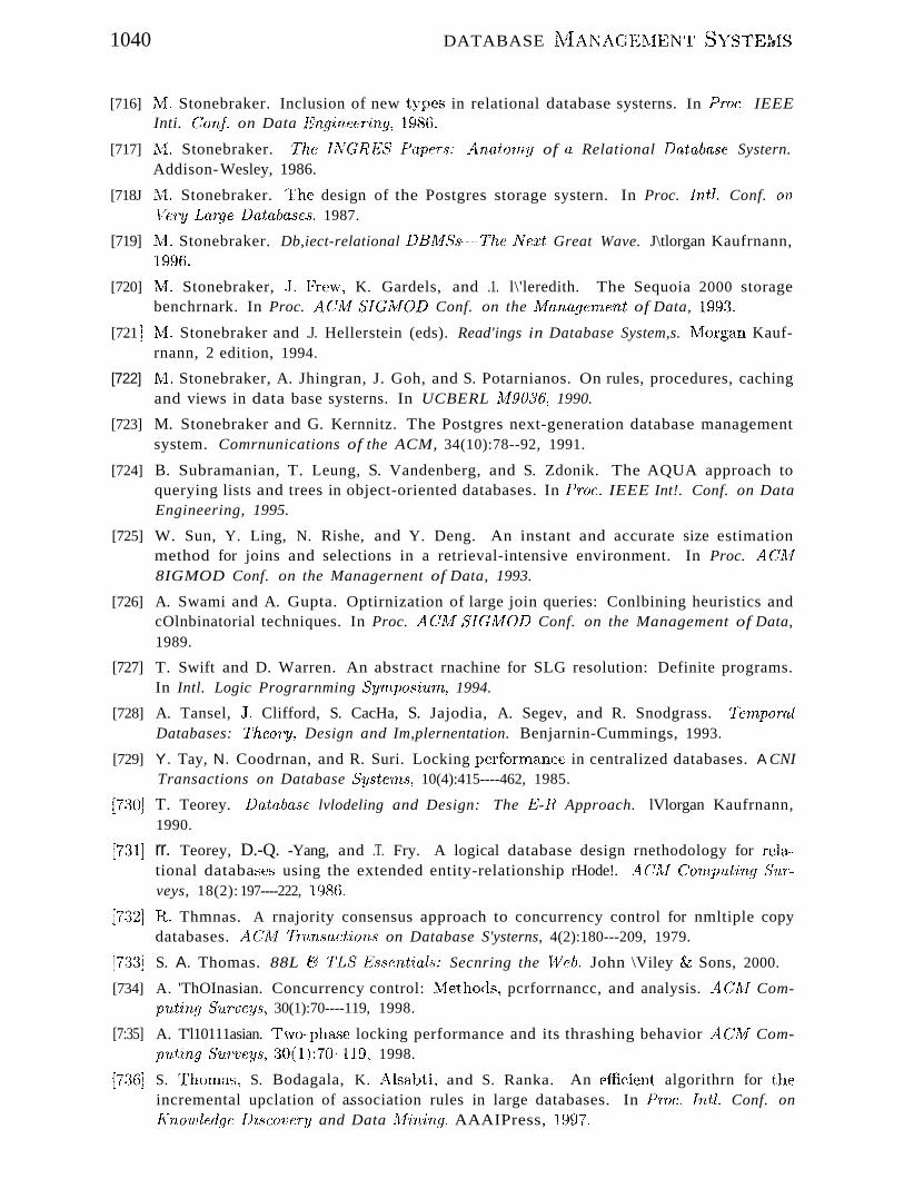
1040 DATABASE l\!IANAGENiENT SVS'I'g'iJ1S
[716] ?vI. Stonebraker. Inclusion of new types in relational database systerns. In Proc. IEEEInti. ()onf. on Data Engineering, 1986.
[717] 1v1. Stonebraker. The INGRBS Papers: Anatorny of a Relational Database Systern.Addison- Wesley, 1986.
[718J IV!. Stonebraker. 'The design of the Postgres storage systern. In Proc. Inti. Conf. OTt
\le'f7.) Large Do,tabases, 1987.
[719] IvI. Stonebraker. Db,iect-relational DBA1Ss-,-,,-The NeTt Great Wave. J\tlorgan Kaufrnann,H)96.
[720] :LvI. Stonebraker, J.f.):ew, K. Gardels, and .1. l\'leredith. The Sequoia 2000 storagebenchrnark. In Proc. AClv[ SIGi\,fOD Conf. on the AIanagernent of Data, 199~3.
[721 J wI. Stonebraker and .J. Hellerstein (eds). Read'ings in Database System,s. Nlorgan Kaufrnann, 2 edition, 1994.
[722] N1. Stonebraker, A. Jhingran, J. Goh, and S. Potarnianos. On rules, procedures, cachingand views in data base systerns. In UCBERL Jv19086, 1990.
[723] M. Stonebraker and G. Kernnitz. The Postgres next-generation database managementsystem. Comrnunications of the ACM, 34(10):78--92, 1991.
[724] B. Subramanian, T. Leung, S. Vandenberg, and S. Zdonik. The AQUA approach toquerying lists and trees in object-oriented databases. In Proc. IEEE Int!. Conf. on DataEngineering, 1995.
[725] W. Sun, Y. Ling, N. Rishe, and Y. Deng. An instant and accurate size estimationmethod for joins and selections in a retrieval-intensive environment. In Proc. AC1\18IGMOD Conf. on the Managernent of Data, 1993.
[726] A. Swami and A. Gupta. Optirnization of large join queries: Conlbining heuristics andcOlnbinatorial techniques. In Proc. ACiVf 8IGJtv10D Conf. on the Management of Data,1989.
[727] T. Swift and D. Warren. An abstract rnachine for SLG resolution: Definite programs.In Intl. Logic Prograrnming Syrnposium, 1994.
[728] A. Tansel, J. Clifford, S. CacHa, S. Jajodia, A. Segev, and R. Snodgrass. TernporalDatabases: TheoT"'y, Design and Im,plernentation. Benjarnin-Cummings, 1993.
[729] Y. Tay, N. Coodrnan, and R. Suri. Locking perfornutnce in centralized databases. A CNITransactions on Database Syste'fns, 10(4):415----462, 1985.
(7~30] T. Teorey. Database lvlodeling and Design: The E-R Approach. lVlorgan Kaufrnann,1990.
[7:31] rr. Teorey, D.-Q. -Yang, and .T. Fry. A logical database design rnethodology for rela-tional databa.."cs using the extended entity-relationship rHode!. ACJlvf Computing Surveys, 18(2): 197----222, 1986.
[7:32] H" Thmnas. A rnajority consensus approach to concurrency control for nmltiple copydatabases. ACl\1 'Trnn8acLions on Database S'ysterns, 4(2):180---209, 1979.
[7:3:3] S. A. Thomas. 88L E1 TL8 Es.sent'ial8: Secnring the ~Veb. John \Viley & Sons, 2000.
[734] A. 'ThOInasian. Concurrency control: ~1ethods, pcrforrnancc, and analysis. ACA1 Computing Surueys, 30(1):70----119, 1998.
[7:35] A. T'l10111asian. Two-phase locking performance and its thrashing behavior A()A1 Com]J'l1t:ing Surveys, :30(1):70-119, 1998.
[7:36] S. 'I'hOIua.') , S. Bodagala, K. Alsabti, and S. Ranka. An efficient algorithrn for theincremental upclation of a..ssociation rules in large databases. In Proc. Intl. Conf. onj{nowledgc !Ji8covcrl/ and Data A1'ining. AAAIPress, 1997.
1041
[737] S. Todd. The Peterlee relational test vehicle. IBAJ 8ysterns Jour'no.l, 15(4):285··-:307,Hl76.
(738) H. Toivonen. Sarnpling large databases for association rules. In Pn)c. Inti. GonIonYery Large Databases, 1996.
[739] TP Perforrnance Council. TPC Benclllnark D: Standard specification, rev. 1.2. Technicalreport, http://www . tpc. org/dspec .html, 1996.
[740] 1. Traiger, J. Gray, C. Galtieri, and B. Lindsay. T'ransactions and consistency in distributed databa.,se systems. ACAI Transactions on Databa8e Systerns, 25(9), 1982.
[741] 1'vi. Tsangaris and J. Naughton. On the performance of object clustering techniques. InProc. AClVI SIGl\10D Conf. on the ]Vlanagement of Data, 1992.
[742] D.-:N1. Tsou and P. Fischer. Decomposition of a relation scheme into Boyce-C oddnonnal form. SIGACT News, 14(3):23-29, 1982.
[743) D. Tsur, J. D. Ullman, S. Abiteboul, C. Clifton, R. Motwani, S. Nestorov, and A. Rosenthal. Query flocks: A generalization of association-rule mining. In Proc. ACM SIGMODConf. on Managernent of Data, pages 1-12,1998.
[744] A. Tucker (ed.). Computer- Science and Engineering Handbook. CRC Press, 1996.
[745] J. W. Thkey. Exploratory Data Analysis. Addison-Wesley, 1977.
[746] J. Ullman. The U.R. strikes back. In ACM Symp. on Principles of Database Systems,1982.
[747] J. Ullman. Principles of Database and Knowledgebase Systems, Vols. 1 and 2. ComputerScience Press, 1989.
[748) J. Ullman. Infonnation integration using logical views. In Intl. Conf. on DatabaseTheory, 1997.
(749) S. Urban and L. Delcarnbre. An analysis of the structural, dynamic, and temporalaspects of semantic data models. In Proc. IEEE Intl. Conf. on Data Engineering, 1986.
[750] G. Valentin, M. Zuliani, D. C. Zilio, G. M. Lohman, and A. Skelley. Db2 advisor: Anoptirnizer smart enough to recomrnend its own indexes. In Proc. Intl. Conf. on DataEngineering (ICDE) , pages 101-110. IEEE COlnputer Society, 2000.
[751] lVI. Van Emden and R. Kowalski. The semantics of predicate logic as a prograrrnninglanguage. Journal of the ACM, 23(4):7:~3~742, 1976.
[752] A. Van Gelder. Negation as failure using tight derivations for general logic programs. InJ. Minker, editor, Fo'undations of Deductive Databases and Logic ProgTarnrn'ing. i\1organKaufmann, 1988.
[753) C. J. van Rijsbergen. Infomwtion Retrieval. Butterworths, London, United Kingdorn,1990.
[754] Jvt Vardi. Incomplete information and default reasoning. In ACM Symp. on Principlesof Database Syste'ms, 1986.
[755] M. Vardi. Fundamentals of dependency theory. In Trends in Theoretical CornputeTScience. ed. E. Borger, Computer Science Press, 1987.
[756] L. Vieille. Recursive axioms in deductive databases: The query-subquery approach. InIntl. Conf. on Expert Database Systems, 1986.
(757] L. Vieille. FraIn QSQ towards QoSaQ: global optimization of recursive queries. In Intl.Can]. on El:pert Database Systerns, 1988.
[758] L. Vieille, P. Bayer, V. Kuchenhoff, and A. Lefebvre. EKS-VI , a short overview. InAAAI-90 Wor-kshop on Knowledge Base lvlanageutent Systerns, 1990.
1042 DATABASE MANAGEMENT SYSTEMS
[759] .J. S. Vitter and Ivi. Wang. Approxirnate conlputation of rnultidinlensional aggregatesof sparse data using wavelets. In Proc. ACM SICA10D Conf. on the ft..1anagc7nent ofData, pages 193-204. ACtvI Press, 1999.
[760] G. von Bultzingsloewen. Translating and optinlizing SQL queries having aggregates. InProc. Intl. Conf. on Very Large Databases, 1987.
[761] G. von Bultzingsloewen, K. Dittrich, C. Iochpe, R.-P. Liedtke, P. Lockemaun, andM. Schryro. Kardamom······-A dataflow database machine for real-tiule applications. InProc. ACM SICNfOD Conf. on the Management of Data, 1988.
[762] G. Vossen. Data A10dels, Database Languages and Database lvlanagement Systems.Addison-Wesley, 1991.
[763] N. Wade. Citation analysis: A new tool for science administrators. Science,188(4183) :429-432, 1975.
[764] R. Wagner. Indexing design considerations. IBM Systems Journal, 12(4):351-367, 1973.
[765] X. Wang, S. Jajodia, and V. Subrahmanian. Temporal modules: An approach towardfederated temporal databases. In Proc. ACM SIGMOD Conf. on the Management ofData, 1993.
[766] K. Wang and H. Liu. Schema discovery for semistructured data. In Third InternationalConference on Knowledge Discovery and Data Mining (KDD -97), pages 271-274, 1997.
[767] R. Weber, H. Sehek, and S. Blott. A quantitative analysis and performance study forsimilarity-search methods in high-dimensional spaces. In Proc. Inti. Conf. on Very LargeData Bases, 1998.
[768] G. Weddell. Reasoning about functional dependencies generalized for semantic datamodels. ACM Transactions on Database Systems, 17(1), 1992.
[769] W. Weih!. The impact of recovery on concurrency control. In ACM Symp. on Principlesof Database Systems, 1989.
[770] G. Weikum and G. Vossen. Transactional Information Systems. Morgan Kaufrnann,2001.
[771] R. Weiss, B. V. lez, M. A. Sheldon, C. Manprenlpre, P. Szilagyi, A. Duda, and D. K.Gifford. HyPursuit: A hierarchical network search engine that exploits content-linkhypertext clustering. In Proc. A CM Conf. on Hypertext, 1996.
[772] C.White. Let the replication battle begin. In Database Progrnmm,ing and Design, pages21-24, May 1994.
[773] S. White, M. Fisher, R. Cattell, G. Hanlilton, and IvL Hapner. JDBC API Tutorial andReference: Universal Data Access for the Java 2 Platform. Addison-Wesley, 2 edition,1999.
[774] J. Widorn and S. Ceri. Active Database Systerns. Morgan KaufInann, 1996.
[775] G. Wiederhold. Database Design (2nd cd.). ~/1cGraw-Hill, 1983.
[776] G. Wiederhold, S. Kaplan, and D. Sagalowicz. Physical database design research atStanford. IEEE Database Engineering, 1:117--·-119, 1983.
(777] R. Williams, D. Daniels, L. H8.<1.S, G. Lapis, B. Lindsay, P. Ng, R. Oberrnarck,P. Selinger, A. v\lalker, P. ""1'"ilrns, and R. Yost. R*: An overview of the architecture.Technical report, IBIvI RJ3325, San Jose, CA, 1981.
[778] 1\1. S. Winslett. A rnodel-based approach to updating databases with 1ncornplete information. A CA1 Transactions on Database Systerns, 1i3(2): 167--196, 1988.
REFERENCES 1043
[779J G. vViorkowski and D. KulI. DB2: Design and Developrnent Guide (8rd ed.). AddisonWesley, 1992.
[780] 1. H. Witten, A. rvloffat, and T. C. Bell. Alanaging Gigabytes: Compressing and IndexingDocuments and Images. Van Nostrand Reinhold, 1994.
[781] 1. H. Witten and E. Frank. Data Afining: Pr'actical Machine Learning Tools and Techniques with Java Im,plementations. Morgan Kaufmann Publishers, 1999.
[782] O. Wolfson, A. Sistla, , B. Xu, J. Zhou, and S. Chamberlain. Domino: Databases formoving objects tracking. In Prnc. ACM SIGlvIOD Int. Conf. on Afanagement of Data,1999.
[783] Y. Yang and R. lI1iller. Association rules over interval data. In Proc. ACM SIGlv/ODConf. on the Management of Data, 1997.
[784] K. Youssefi and E. Wong. Query processing in a relational database management system.In Proc. Intl. Conf. on Very Larye Databases, 1979.
[785] C. Yu and C. Chang. Distributed query processing. ACM Computing Surveys,16(4):399~433, 1984.
[786] O. R. Zaiane, M. EI-Hajj, and P. Lu. Fast Parallel Association Rule Mining WithoutCandidacy Generation. In Proc. IEEE Intl. Conf. on Data Mining (ICDM) , 200l.
[787] M. J. Zaki. Scalable algorithms for association mining. In IEEE Transactions onKnowledge and Data Engineering, volume 12, pages 372-390, May/June 2000.
[788] M. J. Zaki and C.-T. Ho, editors. Large-Scale Parallel Data Mining. Springer Verlag,2000.
[789] C. Zaniolo. Analysis and design of relational schemata. Technical report, Ph.D. Thesis,UCLA, TR UCLA-ENG-7669, 1976.
[790] C. Zaniolo. Database relations with null values. Journal of Computer and SystemSciences, 28(1):142~166, 1984.
[791] C. Zaniolo. The database language GEM. In Readings in Object-Oriented Databases.eds. S.B. Zdonik and D. Maier, Morgan Kaufmann, 1990.
[792] C. Zaniolo. Active databa~e rules with transaction-conscious stable-model semantics.In Intl. Conj. on Deductive and Object-Oriented Databases, 1996.
[793] C. Zaniolo, N. Arni, and K. Ong. Negation and aggregates in recursive rules: theLDL++ approach. In Intl. Conf. on Deductive and Object-Oriented Databases, 1993.
[794] C. Zaniolo, S. Ceri, C. Faloutsos, R. Snodgrass, V. Subrahmanian, and R. Zicari. Advanced Database Systems. Morgan Kaufmann, 1997.
[795] S. Zdonik, U. Cetintemel, M. Cherniack, C. Convey, S. Lee, G. Seidlnan, M. Stonebraker, N. Tatbul, and D. Carney Monitoring streams--·..··A new class of data management applications. In Proc. Intl. Conf. on Very Large Data Bases, 2002.
[796] S. Zdonik and D. lVfaier (eds.). Readings in Object-Oriented Databases. Morgan Kaufrnann, 1990.
[797] A. Zhang, 1.1. Nodine, B. Bhargava, and O. Bukhres. Ensuring relaxed atornicity for£le"'Cible transactions in multidatabao:;e systerns. In PTOC. A CAf SIGMOD Conf. on thelvlanaqe-rnent of Data, 1994.
[798] T. Zhang, R. Hamakrishnan, and IV!. Livny. BIRCH: an efficient data clustering rnethodfor very large databases. In Proc. AClvf SIGA10D Conf. on Alanagement of Data, 1996.
[799] Y. Zhao, P. Deshpande, J. F. Naughton, and A. Shukla. Silllultaneous optirnizationand evaluation of multiple dirnensional queries. In Proc. AClvl SIGlvlOD Intl. C'onj. onlvIanagernent of Data, 1998.
1044 D.ATABASE ~{ANAGErvIENT SYSTEItlS
[800] Y. Zhuge, H. Garcia-1Vlo1ina, J. Hanuner, and .1. Widom. View maintenance in a warehousing enviroIllnent. In Pl'oc. AGArf SIGAI0D Conf. on the A,lanagernent of Data,1995.
[801J 111. ,?vL Zloof. Query-by-exaIllple: a database language. IBlv! System,s JO'1rmal, 16(4):324-~~43, 1977.
[802J J. Zobel, ,A. tvloffat, and K. RalnarIlohanarao. Inverted files versus signature files fortext indexing. A CA1 Transactions on Database System,s, 23, 1998.
[80~{] .J. Zobel, A. lVlotfat, and R. Sacks-Davis. An efficient indexing technique for full textdatabases. In Froc. Intl. Co'nj. on Very Large Databases., Iv!07:qan Kaufman pubs. (San})'Q,ncisco" CAy is] Vancou'veT, 1992.
[804] U. Zukowski and B. Freitag. The deductive database system LOLA. In Proc. Intl. Conf.on Log'ic Programming and N'on-A10notonic Reasoning, 1997.

AUTHOR INDEX
Abbott, R., 578, 1005, 1001Abdali, K., 270, 1015Abdellatif, A., 771, 1029Abiteboul, S., 24, 98, 648, 816,
844, 925, 967, 1005, 1030,1033, 1041, 1001
Aboulnaga, A., 967, 1005Acharya, S., 888, 1005Achyutuni, K.J., 578, 1005Ackaouy, E., xxixAdali, S., 771, 1005Adiba, M.E., 771, 1005, 1038Adleman, L.I\i1., 722, 1036Adya, A., 815, 1029Agarwal, R.C., 924, 1005Agarwal, S., 887, 1005Aggarwal, C.C., 924, 1005Agrawal, D., 578, 771, 1005Agrawal, R., 181, 602, 815, 887,
924925, 1005~1006, 1008,1024, 1030, 1037-~1039
Ahad, R., 516, 1006Ahlberg, C., 1006, 1001Ahmed, R., 1026, 1001Aho, A.V., 303, 516, 648, 1006Aiken, A., 181, 1006, 1001Ailamaki, A., 1006Alameldeen, A.R., 9G7, 1005Albert, J.A., xxxi, 1026, 1001Alon, N., 887Alonso, R., 966, 10:35Alsabti, K., 925, 1041Anupam, V., 10:34, 1001Anwar, E., 181, 1007Apt, K.R., 845, 1007Armstrong, W.W., 648, 1007Arni, N., 816, 1044Arocena, G., 967, 1007Asgarian, Iv1., 691, 1012Astrahan, MJvL 98, 180, 516,
1007, 10121013, 1038Atkinson, M.P., 815816, 1007Attar, R., 771, 100~
Atzeni, P., 24, 98, 648, 8Ui,967, 1007
Avnur, R., 888, 1007Babcock, B., 1007Balm, S., 888, 1007Badal, D.Z., 98, 1007Badia, A., 129, 887, 1007, 10:35
Badrinath, B.R., 1025, 1001Baeza-Yates, R., 966, 1019Bailey, P., 1007Balbin, 1., 845, 1008Ballou, N., 815, 1026Balsters, H., xxxiBancilhon, F., 99, 816, 845,
1008BapaRao, K.V., 516, 1006Baralis, E., 181, 1008Barbara, D., 771, 888, 966,
1008, 1020, 1035Barclay, T., 438, 1033Barnes, I\iLG., :30:3, 1039Barnett, J.R., 337, 1008Barquin, R., 887, 1008Batini, C., 55--56, 1008Batory, D.S., 516, 1008, 1026Baugsto, B.A.W., 438, 1008Baum, M.S., 722, 1019Bawa, Iv!., 924, 1038Bayardo, R.J., 924----·925, 1008,
10:35Bayer, P., 844, 1042Bayer, R., 369, 1008Beck, M., 438, 1008Beckmann, N., 991, 1008Beech, D., 815, 1018Beeri, C., 648, 816, 845, 1006,
1009Bektas, H., xxixBell, D., 771, 1009Bell, T.e., 966, 104:3Bentley, J. L., ~369, 1009Berchtold, S., 991, 1009Bergstein, P., xxxiiBernstein, A.J., 24, 771,
1027-1028Bernstein, P.A., 99, 548, 576,
578, 648, 771, 1007,10091010, 1015, HX36
Beyer, K.S., 887, 991, 1010,1029, 10:'35, lOCH
Bhalotia, G., 924, 10:38Bhargava, 13.K., xxxii, 771,
HHOBiJiris, A., 337, 1010Biskup, J., 56, 648, UHOBitton, [)., /1:38, 477, 1008, 1010Blajr, H., 845, 1007
1045
Blakeley, J.A., 887, 1010Blanchard, L., xxxBlasgen, M.W., 98, 477,602,
1007, 1010, 1012, 1022Blaustein, B.T., 99, 1009Blott, S., 991, 1043Bodagala, S., 925, 1041Bohannon, P., 967, 1010, 1026,
1001Bohm, C., 991, 1009Bonaparte, N., 847Bonnet, P., 1010Booeh, G., 56, 1010, 1036Boral, H., 477, 516, 1027Boroclin, A., 966, 1010Bosworth, A., 887, 1022Boyce, R.F., 180, 1010Bradley, P.S., 887, 1010, 1038,
925Bratbergsengen, K., 477, 1010Breiman, L., 925, 1010Breitbart, Y., 771, 1010--1011,
1030Brin, S., 924, 966, 1011Brinkhoff, T., 991, 1011Brown, K.P., :337, 1011Bruno, N., 888, 1011Bry, F., 99, 845, 1011Bukhres, O.A., 771, 1017Buneman, a.p., 56, 181,
815·816, 967, 1007, 1011,1032
Bunker, R., 477, 1021Burdick, D., 924, 1011Burger, J., 10:34, IDOlBurke, E., 422Cabibbo, L., 816, 1007Cai, L., xxxiCalimlinl, M., 924, 1011Ca.mpbell, D., xxxiCandan, K.S., 771, 1005Carey, 1'1,11..1., xxix, xxxi....·xxxii,
:3:37, 578, 691, 771,815816, 888, 967, 1004,1006, 1011-1012, 1019,1022-102:3, J(J:39
Carney, D., 888, 1044Carroll, L., 440Casanova, M.A., 56, 99, 1012,
1019

1046
Ca.,>tano~ S., 722, 1012Castro, :tv!., 815, 1029Cate, H.P., 815, 1018Cattell, R.G.G., 219, 816, 1012,
102:3, 1043Ceri, S., 55, 99, 181, 771, 816,
844, 925, 1008, 1012, 1031,1043·"'·1044, 1001
Cesarini, F., 691, 1012Cetintemel, U., 888, 1044Chakravarthy, U.S., 181, 516,
578, 1007, 1012, 1024,1036
Chamberlain, S., 991, 1043Chamberlin, D.D., 98-99,
180-181, 516, 816, 967,1007, 1010--1013, 1017,1038
Chan, 11.C., 771Chan, P., 924, 1025Chandra, A.K., 516, 845, 1013Chandy, M.K., 771, 1013Chang, C.C., 771, 1013, 1043Chang, D., 270, 1013Chang, S.K., 771Chang, W., 815, 1022Chanliau, M., xxxiChao, D., xxxiCharikar, M., 888, 1013Chatziantoniou, D., 887, 1013Chaudhuri, S., 691, 816,
887--888, 924, 1011, 1013Chawathe, S., 967, 1032Cheiney, J.P., 477, 1013Chen, C.M., 337, 516, 1013Chen, G., 1029, 1001Chen, H., xxxiChen, J., 1006, 1001Chen, P.M., 337, 1014Chen, P.P.S., 1014Chen, Y., 887, 1014Cheng, W.H., 771Cherniack, :tv'L, 888, 1044Cheung, D.J., 925, 1014Childs, D.L., 98, 1014Chimenti, D., 844, 1014Chin, F.Y., 722, 1014Chisholm, K., 1007Chiu, D.W., 771, 1009Chiueh, T-C., 966, 1014Chomicki, .1., 99, 1014Chou, H., :3~H, 815, 101.4, 1016Chow, E.C., 815, 1018Christodoulakis, S., 516, 966,
1025Chrysanthis, P.K., 548, 1014Chu, F., 516, 1014Chu, !')., 5Ui, l(l:30Churchill, W., 992
Civelek, F.N., 56, 1014Clarke, EJvL, 99, 1009Clemons, E.K., 181, 1011Clifford, J., 1041, 1001Clifton, C., 925, 1041Cochrane, R.J., 181, 1014Cockshott, P., 1007Codd, E.F., 98, 129,648,887,
1014..·..1015Colby, L.S., 887, 1015Collier, R., 25Comer, D., 369, 1015Connell, C., 516Connolly, D., 270, 1015Connors, T., 815, 1018Convent, B., 56, 1010Convey, C., 888, 1044Cooper, B., 967, 1015Cooper, S., 477, 1021Copeland, D., 815, 1015Cornelio, A., 1039, 56Cornell, C., 516, 1034Cornell, G., 270, 1015Cortes, C., 888Cosmadakis, 8.S., 99Cristian, F., 771, 1017Cristodoulakis, S., 1018Cvetanovic, Z., 438, 1033Dadam, P., 337, 816, 1028Daemen, J., 722, 1015Daniels, D., 771, 1043Dar, S., 887, 1040Das, G., 888, 1013Datal', M., 888, 1007Date, C.J., 24, 98--99, 637, 648,
1015Davidson, S., 967, 1011Davis, J.W., 815, 1018Davis, K.C., xxxiDayal, D., 99, 181, 516, 648,
771, 887, 1010, 1013, 1015,10301031
Day, M., 815, 1029De Antonellis, V., 24, 98, 648,
1007De i\1aindreville, C., 181, 1039DeBono, E., 304DeBra, P., 648, 1015Deep, J., 270, 1015Delcambre, L.M.L., xxxi, 56,
1042Delobel, C., 648, 816, 1008,
1015Deng, Y., 516, 1041Denning, D.E., 722, 1015, 1029Deppisch, U., 3:37, 10;{4Derr, M., 1016Derrett, N., 815, 1018Dersta,dt, .J., 267
AUTH(}R, INDF~X
Deshpande, A., 816, 1016Deshpande, P., 887, 1005, 1016,
1039, 1044Deutsch, A., 967, 1016Deux, 0., 815, 1016DeWitt, D ..J.) xxviii, 337, 438,
477, 516, 602, 691,770'--771, 815--816, 1004,1006, 1010···1012, 1014,1016, 1021, 1024--1025,1030, 1032, 10:34, 1001
Diaz, 0., 181, 1016Dickens, C., 605Dietrich, S.W., 845, 887, 1016,
1023Diffie, W., 722, 1016Dimino, L., xxxiDittrich, K.R., 816, 1042, 1001Dogac, A., 56, 771, 1014, 1023Domingos, P., 925, 1016Domingos, R., 925, 1024Dong, G., 887, 1014Donjerkovic, D., xxix, 516,
887···-888, 1016, 1029, 1035,1001
Donne, J., 726Doole, D., 816, 1011Doraiswamy, S., xxxiDoyle, A.C., 773Dubes, R., 925Dubes, R.C., 1016, 1025Du, K., 1033, 1001Du, W., 771, 1016Duda, A., 966, 1043DuMouchel, W., 888, 1008Dupont, L., 967, 1037Dupont, Y., 56, 1039Duppel, N., 477, 1016Eaglin, R., xxxiiEdelstein, H., 771, 887, 1008,
1017Effelsberg, W., :-3;37, 1017Eich, M.H., xxxi, 602, 1017Eisenberg, A., 180, 816, 1017El Abbadi, A., 578, 771, 1005,
1017EI-Hajj, 11., 924, 1043Ellis, C.8., 578, 1017Ellman, C., 10~34, 1001Elmagarmid, A.K., 771, 1000,
1015-1017Elmasri, R., 24, 5Ei, 1017Epstein, R., 477, 771, 1017Erbe, R., 3:n, 816, 1028Ester, M., 925, 1017, 1037Eswaran, K.P., 98, 180181,
477, 548, 1007, uno, 101':-3,1017
A UTHOR INDEX
Fagin, R., xxix, 390, 637, 648,1009, 1015, 1017--1018
Falonts().,;, C., 181, :3:W, :369,816, 844, 888, 925, 966,991, 1008, 1018, 1027,1044, 1001
Fan, C., 967, 1038Fang, N!., 924, 1018Fandemay, P., 477, 101:3Fayyad, U.M., 887, 924--925,
1006, 1010, 1018,1038~-1039
Fendrich, .1., xxxiiFernandez, M., 967, 1016, 1018Finkelstein, S.J., 516, 691, 845,
1018, 1032Fischer, C.N., xxxFischer, P.C., 648, 1025, 1041Fisher, K., 888Fisher, iVI., 219, 1023, 1043Fishman, D.H., 815, 1018Fitzgerald, E., 817Fleming, C.C., 691, 1019Flisakowski, S., xxix~xxxFlorescu, D., 967, 1012--1013,
1016, 1018-1019Ford, W., 722, 1019Fotouhi, F., 477, 1019:Fowler, M., 56, 1019Fox, S., 771, 1036Frakes, W.B., 966, 1019Franaszek, P.A., 578, 1019Franazsek, P.A., 1019Frank, E., 924, 1043Franklin, M.J., 771, 815816,
967, 1011, 1015, 1019:Fraternali, P., 181, 1012, 1019Frawley, W.J., 924, 1034Freeston, ~1.'W., 991, 1019I~eire, .1., 967, 1010Freitag, B., 844, 1044French, .1., 1020Frew, .1., 691, 1040Freytag, J.C., 516, 1019Friedman, J.B., :369, 924 925,
1009----1010, 102:3Friesen, 0., 816, 1019Fry, J.P., 24, 56, 99, 1019, 1041Fuchs, IV!., 270, 1028Fu, Y., 925, 1023Fugini, M.G., 722, 1012Fuhr, N., 966, 1019Fukuda, 1'.,924, 1019Funderburk, .I., 967, 10:38Furtado, A.1., 99, 1012, 1019Fushimi, S., 477, 1019GacHa, S., 1041, lOCHGaede, V., 991, 1020
Gallaire, H., 98.._·99, 648, 844,1020
Galtieri, C.A., 602, 771, 1028,1041
Gamboa, R., 844, 1014Ganguly, S., 771, 1020Ganski, R.A., 516, 1020Ganti, V., 925, 1020Garcia-:Molina, H., 24, 578, 771,
887, 924, 966----967, 1005,1010, 1018, 1020·..·1021,1033-1035, 1044, 1001
Gardels, K., 691, 1040Garfield, E., 966, 1020Garg, A.K., 390, 1020Garza, J.F., 337, 815, 1008,
1026Gehani, N.H., 181, 815, 1006Gehrke, .I.E., 691, 888,
924-925, 1006, 1011-~1012,
1020Gerber, R.H., 477, 770, 1016Ghemawat, S., 815, 1029Ghosh, S.P., 303, 1020Gibbons, P.B., 887-888, 1005,
1021Gibson, D., 925, 966, 1021Gibson, G.A., 337, 1014, 1021,
1034Gifford, D.K., 771, 1021, 1043Gifford, K., 966Gilbert, A.C., 888Gionis, A., 888Goh, .1., 181, 1040Goldfarb, C.F., 270, 1021Goldman, R., 967, 1021, 1030Goldstein, .1., xxxi, 991, 1010,
1021Goldweber, M., xxixGoodman, N., 57(), 578, 771,
1007, 1009, 1036, 1038,1041
Gopalan, H... , xxxiGotlieb, C.C., 390, 1020Gottlob, G., 844, 1012Graefe, G., xxxi, 4:38, 477, 51G,
770--771, 815, 1011, 1016,1021, 1028
Graham, M.H., 648, 1021Grahne, G., 98, 1021Grant, .J., 516, 1012Gravano, L., 888, 966, 1011,
1021Gray, .LN., 98, 4:_~8, 548, (i02,
691, 770--771, 887, 1000,l007, ]012, 10l(i~1017,
1021-1022, 1028, 103:3,1037, 1041
1047$
Gray, PJvl.D., 24, 181, IOI6,1022
Greenwald, :NI., 887, 1022Greipsland, J.F., 438, 1008Griffin, T., 887, 1015Griffiths, P.P., 98, 180, 602,
722, 1007, lCll:3, 1022Grimson, J., 771, 1009Grinstein, G., 1022, 1001Grosky, W., xxxiGruber, R., 815, 1029Guenther, 0., 991, 1020Guha, S., 888, 925, 1022, 1033Gunopulos, D., 924-~925, 1006,
1008, 1022Guo, S., 1034, 1001Gupta, A., 516, 887, 1005,
1022, 1041Guruswamy, S., 1033, 1001Guttman, A., 991, 1022Gyssens, M., 129, 1007Haas, L.M., 771, 815, 1013,
1022, 1043Haas, P.J., 516, 888,
1022---1023, 1034Haber, E., xxxHaderle, D., 602, 771, 1031Hadzilacos, V., 576, 578, 1009Haerder, T., 337, 602, 1017,
1023Haight, D.M., 815, 1011Haines, M., xxixHalici, U., 771, 1023Hall, M., 270, 1023Hall, N.E., 815, 1011, 1034,
1001Hall, P.A.V., 477, 102:'3Halpern, J.Y., 516, 1014Hamilton, G., 219, 102:'3, 104;3Hammer, .1., xxxi, 887, 1044Hammer, M., 98, 771, 102:3,
1036Han, J., 887, 924·-925, 1014,
102:3, 1028, 10:'32, :10:34Hand, D.J., 924925, 1023,
1D::WHanson, E.N., 181, 887, 102:3Hapner, M., 219, 104:3Barel, D., 845, 101:3Harinarayan, V., 887, 102::~
Haritsa, J., 578,924,1023, l(X38Harkey, D., 270, 101:3Harrington, .I., xxxHarris, S., xxixHarrison, .I., 887, 1023Ha..san, "V., 771, 1020Hass, P.or., 888, 1008Ha.stie, T., 924, 1023Hearst, M_, xxxii

1048
Beckerman, D., !J24, 1014,102:,3, 1041
Heckman, ?v1., 722, 1029HeH<:md, P., 771Hellerstein, JJv1., xxix, 181,
516, 772, 816, 845, 888,967, 991, 1()06·_·1008,10221024, 1027,1034,,·,,1035, 1038, 1040, 77:3
Hellman, lVLE., 722, 1016Heilschen, L.J., 99, 10:30Heytens, l\ILL., 477, 770, 1016Hidber, C., 925, 1024Hill, IvLD., 1006Hillebrand, G., 967, 1011Himmeroeder, R., 967, 1024Hinterberger, H., 991, 1033Hjaltason, G.R., 967, 1015Hoch, C.G., 815, 1018Ho, C-T., 887, 924, 1024, 1044Holfelder, P., 270, 1015Hollaar, L.A., 966, 1036, 1001Holzner, S., 270, 1024Honeyman, P., 648, 1009Hong, D., 578, 1024Hong, W., 771, 1024Hopcroft, J.E., 303, 1006Hou, W-C., 516, 1024, 1033,
1001Howard, .J .H., 648, 1009Hsiao, H., 771, 1024Hsu, C., xxxiiHuang, .1.,578, 1024Huang, L., 966, 1014I-Iuang, W., xxixHuang, Y., 771, 1024, 1001Hull, H.. , 24, 56, 98, 648, 816,
844, 1005, 1024, 1001Hulten, G., 925, 1016, 1024Hunter, .1., 270, 1024Imielinski, T., 98, 924, 1006,
1024-1025, 1001Joannidis, Y.E., xxix, 56, 516,
888, 1008, 1025, 10:-n,10:34
Iochpe, C., 1042, lOCHIves, Z., 967, 1012Jacobson, 1., 56, 1010, Hn6Jacobsson, H., xxxiJagadish, H.V., :3:31, :369,
887-,·888, 991, 1008, 1018,1025, 1027, 1040, lOCH
.Ja-in, A.K., 925, 1016, 1025Jajodia, S., 722, 771, 1025,
1041,1042, 1001.larke, 1vt, 516, 1025Jean, 1"., 10:34, 1001Jeffers, R., 578, 1005.Jhingran, A., 181, 1040
Jing, .J., 771, 1017Johnson, T., 578, 888, 1008,
1024Jones, K.S., 966, 1025Jonsson, B.T., 771, 1019Jou, J.H., 648, 1025Kabra, N., 516, 1025, 10:34,
1001Kambaya,shi, Y., 771, 1025Kamber, NI., 924, 1023Kane, S., xx.xiiKanellakis, P.C., 98, 648, 816,
1005, 1008, 102,5, 1001Kang, J., 967, 1018Kang, Y.C., 516, 1025Kaplan, S..1., 1043Karabatis, G., 771, 1036, 1001Kargupta, H., 924, 1025Katz, R.H., 337, 477, 1014,
1016, 1034Kaufman, L., 925, 1025Kaushik, R., xxxii, 967, 1026,
926Kawaguchi, A., xxxii, 887, 1015Keats, J., 130Kedem, Z.I'v1., 924, 1028Keim, D.A., 1026, 1001Keller, A.M., 99, 1026Kemnitz, G., 815, 1040Kemper, A.A., 3:37, 816, 1028Kent, W., 24, 616, 815, 1018,
1026, 1001Kerisit, J.M., 845, 10:36Kerschberg, L., 24, 1026Ketabchi, M.A., 1026, 1001Khanna, S., 887, 1022Khardon, R.., 924, 1022Khayyam, 0., 817Khoshafian, S., 816, 1008Kiernan, J., 181, 967,
10:38-1039Kiessling, \V., 516, 1026Kifer, Tvi., 24, xxix, 816, 845,
1026, 1028Kimball, H.., 887, 1026Kim, vV., 516, 771, 815 ..816,
1017, 1026Kimmel, W., xxxKing, .LT., 516, 1026King, R., 50, 1024King, VvT.F., 98, 1007, 1012Kirk, (:., 270, 10:34J<'itsuregawa, ?Y1., 477, 1019Kleinberg, .1.R'!., 925,966, 1021,
1026Klf.!in, J.D., xxxiKlug, A.C., 24, 129, :,337, 516,
1016, 1026Knapp, E., 1027
AlJ'rH()R INI)EX
Knuth, D.E., 30:3, 4:38, 1027Koch, G., 99, 1027Koch, J., 5Ui, 1025Kodavalla, H., xxxiKohler, \V.H., 1027Konopnicki, D., 967, 1027, 1001Kornacker, M., 816, 991~ 1027Korn, F., 888, 1027Korth, II.F., 24, 578, 771, 967,
1024, 1026-1027, HX30,1039, IDOl
Kossman, D., 771, 888, 10l2~
1019, 1027Kotidis, Y., 887--888, 1027,
1036Koudas, N., 888, 1022Koutsoupias, E., 967, 991,
1023·--1024Kowalski, R.A., 844, 1042Kriegel, H-P., 925, 991,
1008--1009, 1011, 1017,1026, 1037, 1001
Krishnakumar, N., 771, 1027Krishnamurthy, R., 516, 771,
844, 1014, 1016, 1020,1027
Krishnaprasad, NL, xxxi, 887,10~35
Kuchenhoff, V., 844, 1042Kuhns, J.L., 98, 129, 1027Kulkarni, K., xxixKull, D., 691, 104~3
Kumar, K.B., 477, 770, 1016Kumar, V., 578, 1027Kunchithapadarn, K., xxxKung, H.T., 578, 1027Kuo, D., 1027Kupsch, J., 1034, 1001Kuspert, IC, 337, 816, 1028LaCroix, M., 129, 1027Ladner, R.E., 578, 10~30
Lai, :tv'L, 578, 1027Lakslnnanan, L.V.S., 924925,
967, 1027-1028, 10~32, IO:~4
LaIn, C., 815, 1028Lamport, L., 771, 1028Lampson, B.vV., 771, 1028Landers, 'I'.A., 771, 10:36Landis, G., 815, 1028Landwehr, C.L., 722LangE~rak, R., 99, 1028Lapis, G., 771, 815, 1022, 1043Larson, J.A., 56, 771, lO::~9
Larson, P., 390, '·1:38, 887, 1010,1028, HX35
L1St, M., xxxiiLausen, G., 8Ui, 967, 1024,
1026Lawan(lE~, S., 1029, 1001
~4lJT}I()R INDE~Y
Layman, A., 887, 1022Lebowitz, F., 100Lee, E.K., 337, 1014Lee, 1V1., xxixLee, S., 888, 1044Lefebvre, A.) 816, 844, 1019,
1042Leff, A., 771, 1034Lehman, P.L., 578, 1027-··1028Leinbaugh, P., 1010, 1001Lenzerini, M., 56, 1008Lescoeur, F., 845, 1036Leu, D.F., 1013Leung, T.vV., 816, 1040Leung, T.Y.C., 516, 845, 887,
1028, 1038Leventhal, JV1., 270, 1028Levine, F., 578, 602, 1032Levy, A.Y., xxxii, 887, 967,
1018'-1019, 1040Lewis, D., 270, 1028Lewis, P.M., 24, 771, 1028,
1036Ley, lVI., xxixLibkin, L., 887, 1015Liedtke, H., 1042, 1001Lieuwen, D.F., 337, 887, 1015,
1025, 1034, 1001Lim, E-P., 771, 1028, 1001Lin, D., 924, 1028Lin, K-I., 991Lindsay, B.G., xxxi, 98, 337,
602, 771, 815, 887, 1012,1022, 1028, 10~30-1032,
1041, 1043Ling,Y., 516, 1041Linnemann, V., :3:37, 816, 1028Lipski, vV., 98, 1024Lipton, R.J., 1020, 516, 1028,
lOCHLiskov, 13.,815, 1029Litwin, \V., 390, 771, 1029Liu, H., 967, 104:3Liu, 1'/1.1'., 771, 1017, 1029Livny, tv'L, :3:37, 578, 771, 816,
887, 925, 1006, 10111012,1019, 102:3, 1029, 10:38,1044, 1001
Loclu)vsk~ F., 816, 1026Lockemann, P.C., 1042, 10011..,0, B., 888, 1007Loh, \>\7- Y., 925, 1020Lohman, G.!vI., 516, 691, 771,
815, 1022, 1029, 1042Lornet, D.B., 4~38, 578, 771,
991, 10281029, 10:3:3Lone~ K., 99, 1027Loo, B.'1'., 771, 10:n
Lorie, R.A., 98, 180, 438, 51n,548, 602, 1007, 1012,,··1013,1017, 1022, 1028-····1029,10:38
Lou, Y., 816, 1029Lozinskii, E.L., 845, 1026 .Lucchesi, C.L., 648, 1029Lu, H., 770, 1029Lu, P., 924, 104~3
Lu, Y., 967, 1012Ludaescher, B., 967, 1024Lueder, R., 10~~4, 1001Lum, V.Y., 369, 887, 1029,
1040Lunt, T., 722, 1029Lupash, E., xxxiiLyngbaek, P., 815, 1018Mackert, L.F., 771, 1029NlacNicol, R., xxxiMadigan, D., 924, 1013Mahbod, E., 815, 1018Mah, T., 924Maheshwari, D., 815, 1029Nlaier, D., 24, 98, 648, 815-·-816,
844-845, 1008, 1015,1029-·10:30, 1044
Makinouchi, A., 816, 1030JVlanber, D., 578, 1030Manku, G., 887, 1030JVlannila, H., 648, 924··925,
1006, 1014, 1022--1024,1030, 1041
Mannino, M.V., 516, 1030Manolopoulos, Y., 925, 1018Nlanprempre, C., 966, 1043Manthey, H., 99, lOllMark, 1., 771, 1029IvIarkowitz, V.JV!., 56, 99, 10301vlartella, G., 722, 1012Maryanski, P., 55, 1034Matias, Y., 887···-888, 1021Matos, V., 129, 816, 10;n~vlattos, N., 181,816, 1011,
1014IVlaugis, 1.,., 181, 1007IVIcAuliffe, :N1.L., 815, 1011l\ilcCarthy, D.R., 181, 1030lVIcCreight, E.l'vl., 369, 1008McCune, V'll. V'!. , 99, 10~'W
McGill, M.J., 966, 10:37IVIcGoveran, D., 99, 1015McHugh, J., 967, lo:ml\'1cJones, P.R., 98, 602, 1007,
1022Mclj~od, I)., 98, 516, 1006,
102:3McPherson, .J., 3:37, 815, 1022,
1028I:vlecca, G., 816, 967, 1007
1049
wleenakshi, K., 845, 1008Iviegiddo, N., 887, 1024?vlehl, J.\N., 98, 180, 1007,
1012.. ··1.01:3IVlehrotra, S., 771, 10:.m?vIehta, lvI., 770, 925, uno, HX38:NIelton, J., xxix, xx.-xii, 180,
816, 887, 1017, 1030···-1031N:lenasce, D.A., 771, 1mnNlendelzon, A.O., 648, 925,
967, 1007, 10l9, 1021,1029, 1031, 1035, 1001
:NIeo, R.., 925, 1031Meredith, J., 691, 1040Merialdo, P., 967, 1007Ivlerlin, P.M., 516, 1013Merrett, T.H., 129, 303, 1031Meyerson, A., 925, 103311ichel, H., 477, 1013Michie, D., 925, 1031Mihaila, G.A., 967, 1031JVIikkilineni, K.P., 477, 10:31IvIiller, R.J., 56, 924, 1031, 1043IvIilne, A.A., 550Milo, T., 816, 967, 1009, 1031,
1.001Minker, J., 98·····99, 516, 648,
844, 1007, 1012, 1020,1031
JVlinoura, T., 771, 1031Mishra, N., 925, 1022, 1033Misra, J., 771, 1013Missikoff, M., 691, 1012Mitchell, G., 516, 10:,31Moffat, A., 966, 1031,
104:3··..·1044Mohan, (;., xxix, xxxi, 578,
602, 771, 816, 991, 1027,10~n··l032
Moran, J., xxxii1'l/lorimoto, Y., 924, 1019Morishita, S., 844, 924, 10If>,
1019Morris, K.A., 844, 1032I\!lorrison, R., 1007f\·10tro, A., 56, 1032Motwarli, IL, 888, 924 925,
1007, 1011, 101:3, 1018,1022, 103:3, 1041
Mukkamala, R., 771, HX32Mumick, 1.S., 516, 816, 845,
887, 1015, 1022, 10:32f\·luntz, ILIL, 771, 887, 1028,
10~31
l\iIuralikrishna,M., xxxi, 477,516, 770, 1016, 10~12
lvlutchlm', D., 771., 1025Muthukrishnan, S., 888lvIyers, A.C., 815, 1029

1050
?vlyllymaki, J., 1029, 1001Nag, B., 1034, 1001Naqvi, S.A., 816, 844·--845,
1009, 1011, 1014, 1032Narang, L, 578, 10:32Narasayya, V.R., 691, 888, 1013Narayanan, S., 816, 1011Nash, 0., 338Naughton, J.F., 1026, xxix,
438, 477, 516, 691, 770,815-816, 844, 887, 967,991, 1005, 1011~··1012,
1016, 1022, 1024, 1028,1032, 1034, 1039, 1041,1044, 1001
Navathe, S.B., 24, 55~56, 578,924, 1005, 1008, 1017,1037, 1039
Negri, M., 180, 1032Neimat, M-A., 390, 815, 1018,
1029Nestorov, S., 925, 967, 1032,
1041Newcomer, E., 548, 1009Ng, P., 771, 1043Ng, R.T., 337, 888, 924--925,
1008, 1018, 1025, 1028,1032
Ng, V.T., 925, 1014Nguyen, T., 967, 1033, 1037,
1001Nicolas, J-M., 99, 648, 1020Nievergelt, J., 390, 991, 1018,
1033Nodine, M.H., 771Noga, A., 887Nyberg, C., 438, 1033Obermarck, R., 771,
10321033, 1043O'C(lllaghan, L., 925, 1022,
10:3:3Olken, F., 477, 516, 887, 1016,
10:3:3Olshen, R.A., 925, 1010Olston, C., 771, 10:3:3, 888, 1007Orniecinski, E., 578, 924, 1005,
10:37Onassis, A., 889O'Neil, E., 24, 1033O'Neil, P., 24, 771, 887, HJ:3:3Ong, K., 816, 1044Ooi, B-C., 770, 1029Oracle, 651Orenstein, .I., 815, 1028Osborn, S.1., 648, 1029Osborne, R., xxxiiOzden, B., 1033, lOCHOzsoyoglu, G., 129, 516, 722,
816, 1014, 1024, 10:3:3,
lOOIOzsoyoglu, 2.1\11., 129, 516, 816,
1029, 1033, 1038Ozsu, M.T., 771, 1033Page, L., 966, 1011Pang, A., 924925, 1028, 1032Papadimitriou, C.H., 99, 548,
578, 967, 991, 1023-1024,1033
Papakonstantinou, Y., 771,967, 1005, 1033,...10:M
Paraboschi, S., 181, 1008, 1012Paredaens, J., 648, 1015Parent, C., 56, 1039Park, J., 516, 887, 10:34, 1038Patel, JJvl., 1034, 1001Paton, N., 181, 1016Patterson, D.A., 337, 1014,
1034Paul, H., 337, 815, 1034, 1037Peckham, J., 55, 1034Pei, J., 924, 1023, 1034Pelagatti, G., 180, 771, 1012,
1032Petajan, E., 1034, 1001Petrov, S.V., 648, 1034Petry, F., xxxiPfeffer, A., 816, 991, 1024Phipps, G., 844, 1016Piatetsky-Shapiro, G., 516,
924, 1006, 1018, 1034Piotr, 1., 888Pippenger, N., :390, 1018Pirahesh, H., 181, 3:37, 516,
602, 771, 815, 845, 887,1014, 1022, 1028,1031-1032, 1034, 1038
Pirotte, A., 129, 1027Pistol', P., ~337, 816, 1028Pitts-Moultis, N., 270, 1034Poosala, V., 516, 888, 1005,
1008, 10:34Pope, A., :370Popek, G.,1., ~)8, 1007Port, G.S., 845, 1008Potarnianos, S., 181, 1040Powell, A., 1020Pramanik, S., 477, 1019Prasad, V.V.V., 924, 1005Pregibon, 1)., 888, 924, 1014,
102:3, 1041I)rescod, P., 270, 1021Price, T.G., 98, 516, 602, 1012,
1022, 1m{8Prock, A., xxxPruyn.e, J., xxixPsaila, G., 925, 1006, 1031Pu, C., 771, 10:34
AlJTHOR, INDeX
Putzolu, G.R., 98, 578, 602,1007, 1022, 1028
Qian, X., 887, 1034Quass, D., 887, 967, 1030,
10:331034Quinlan, J .R., 925, 1035Rafiei, D., xxxi, 925, 1035Raghavan, P., 925, 966, 1006,
1021Raiha, K-J., 648, 10:30Rajagopalan , S., 887, 1030Rajaraman, A., 887, 967, 1023,
1034Ramakrishna, J\lLV., 390, 1035Ramakrishnan, LV., 845, 1035Ramakrishnan, R., 56, 516,
816, 844--845, 887~-888,
924-"925, 991, 1004--1005,1008--1010, 1016,102(}·1021, 1025, 1029,1031'-1032, 1035, 1038,1040, 1044, 1001
Ramamohanarao, K., 390,844~845, 966, 1008, 1035,1044
Ramamritham, K., 548, 578,1014, 1024
Ramamurty, R., xxxRaman, B., 888, 1007Raman, V., 888, 1007, 1035Ramasamy, K., 887, 1016,
10:34, 1039, 1001Ramaswamy, S., 888, 1005Ranganathan, A., 887, 1035Ranganathan, M., 925, 1018Ranka, S., 925, 1041Rao, P., 845, 1035Rae, S.G., 887, 10:35Rastogi, R., :337, 771, 925,
1010, 1.022, 1025, 10~~0,
10:3:3, 10:35, 1001Rcarnes, Iv1., xxxReed, D.P., 578, 771, 1.035Rees(~, G., 219, 10:35Reeve, C.L., 771., 1009, 1036Reina, C., 925, unoReiner, D.S., 516, 1026Reisner, P., 180, 101:1Reiter, R., 98, 10:35Rengarajan, 1'., xxxiR(~scorla, E., 722, HX35lleuter, A., 548, 602, 1000,
1022... ,102:3, 10~l6
Richardson, J.E., 815, 337,1011·····1012
RiehuI, S., 816, 1011Rijrnen, V., 722, 1015Riloff, E., 96G, l():.l6, 1001Rishe, N., 516, 1041

A UTHOR INDEX
Ris.<mnen, J., 648, 925, 1030,1036
Rivest, R.L., 390, 722, 1036Roberts, G.O., 966Robie, J., 967, 1013Robinson, J.T., 578, 991, 1019,
1027, 1036Rogers, A., 888Rohmer, J., 845, 10;36Rosemall, S., 991, 1018Rosenkrantz, D.J., 771, 10:36Rosenthal, A., 516, 925,
10~36~1037, 1041, IDOlRosenthal, J.S., 966, 1010Ross, K.A., 816, 887·..·-888, 1008,
1013, 1015, 1032, 10~36
Rotem, D., 516, 887, 1033, 1040Roth, T., 888, 1007Rothnie, J.B., 771, 1009, 1036Rousseeuw, P.J., 925, 1025Roussopoulos, M., 887, 1036Roussopoulos, N., 337, 516,
771, 887, 991, 1013, 1027,1029, 1036
Roy, P., 967, 1010Rozen, S., 691, 1036Rumbaugh, J., 56, 1010, 1036Rusinkiewicz, M., 771, 1036,
1001Ryan, T.A., 815, 1018Sacca, D., 845, 1036Sacks-Davis, R., 390, 966, 1035,
1044Sadri, F., 967, 1027Sagalowicz, D., 104~3
Sager, T., 516, 1030Sagiv, Y., 516, 648, 816, 845,
967, 1006, 1008, 1026,1029, 10:34, 10:36
Sagona." K.F., 844···845, 1035,1037
Sahuguet, A., 967, 10:37Salton, G., 966, l(X)7Saluja, S., 924, 1022Salveter, S., 516, 10~39
Salzberg, B.J., 30:3, :n7, 438,578, 991, 1029, 1037
Sarnarati, P., 722, 1012Samet, H., 991, 10:37Sample, N., 9G7, 1015Sander, .I., 925, 1017, 10:37Sanders, It.E., 219, 10:37Sandhu, R., 722, 1025Saraiya, Y., 844, 1032Sarawagi, S., 816, 887, 925,
1005, 10:37Sathaye, A., xxxiiSavasere, A., 924, 1037Sbattella, L., 180, 10:32
Schauble, P., 966, 1037Schek, H-J., 337, 815, 991,
1034, 1037, 1043Schell, R., 722, 1029Schiesl, G., xxxiiSchkolnick, IVLJVL, 98, 578, 691,
1008, 1012, 1018, 1037Schlageter, G., 771, 1037Schlepphorst, C., 967, 1024Schneider, D.A., 390, 438, 477,
516, 770, 1016, 1028··-1029Schneider, R., 991, 1008, 1011Schneier, B., 722, 10~n
Scholl, NLH., 337, 815, 1034,1037
Schrefl, M., xxxiSchryro, NI., 1042, 1001Schuh, D.T., 815, 1011Schumacher, L., xxixSchwarz, P., 602, 771, 1031Sciore, E., 516, 648, 1037, 1039,
1001Scott, K., 56Scott, S., 1019Seeger, B., 991, 1008Segev, A., 516, 887, 1034, 1038,
1041, 1001Seidman, G., 888, 1044Selfridge, P.G., 924, 1038Selinger, P.G., 98, 180, 516,
602, 722, 771, 1012, 1028,1038, 1043
Sellis, 1'.K., 337, 51G, 991,1018, 1025, 1038
Seshadri, P., xxix, 516, 816,844'H B45, 887, 1014, 1035,10:38, 1040
Seshadri, S., 477, 516, 1010,101(i, 1022, 1001
Sevcik, K.C., 888, 991, 1008,1033
Shaclrl1on, 1\/1., 967, 1015Shafer, J.C., 924925, 100G,
10:38Shaft, U., xxix xxx, 991, HnO,
1021Shah, D., 691, 924, 1012, 10:38Shamir, A., 722, 10:36Shan, lvi-C., 815, 1016, 1018,
1026, 1.001Shanmuga,'mndaram, :T., 887,
967, 1012, 10~38
Shapiro, L.D., xxix, 477, 101(:),10:38
Shasha, L)., xxix, 578, 691, 771,1010, lO:3E), 1<.n8
Shatkay, H., 925, 10:38Sheard, '1'., 99, 10:38
10~1
Shekita, E.J., 337, 51H, 815,967, 1011-·..·1012, 1022,1034, 1038
Sheldon, NLA., 966, 1043Shelloy, P., 924, 1038Shenoy, S.T., 516, 1038Shepherd, J., 390, 1035Sheth, A.P., 56, 771, 1017,
1029, 103H, 1039, 1001,771
Shim, K., 816, 887~-888, 925,1013, 1022, 1025, 1035
Shipman, D.W., 548, 771, 1009,1036
Shivakumar, N., 924, 1018Shmueli, 0., 845, 967, 1009,
1027, 1001Shockley, W., 722, 1029Shoshani, A., 887, 1038---1039Shrira, L., 815, 1029Shukla, A., xxix, 887, 1016,
10~39, 1044Sibley, E.H., 24, 1019Siegel, M., 516, 1037, 1039,
1001Silberschatz, A., 24, xxx, 337,
578, 771, 10101011, 1025,1027, 1030, 1033, 1039,1001
Silverstein, C., 1011Simeon, J., 967, 1010, 1013Simoll, A.H.., 180, 816, 10:31Simon, E., 181, 691, 1038----1039Simoudis, E., 924, 1018, 1039Singhal, A., 771, 1029Sistla, A.P., 991, 1024, 104:3,
1001Skeen, D., 771, 1017, 1039Skounakis, 1'.1., 1006Slack, J.1L, xxxiSlutz, D.R., 98, 1012Smith, D.C.P., 55, 1039Smith, J.M., 56, 10:39Smith, K.P., :3~37, 722, 1008,
10:39Slnith, P.D., :30~3, 10~39
Smyth, P., 924, 1006, 1018,10:30
Snodgrass, R.T., 181, 816, 844,1041, 1044, lOCH
So, B., xxixSoda, G., 691, 1012Solomon, IvLH., 815, 1011Soloviev, V., 770, HX30Son, S.H., xxxiSoparka.r, N., 578, 1027, 10~39,
1001Sorenson, P., 691, 1037Spaccapietra, S., 5G, 1014, 1039

1052
Speegle, G., xxxiSpencer, L., 925, 1024Spertus, E., 9{j6, 1039Spiegelhalter, D.,]., 925, 1031Spiro, P., xxxiSpyratos, N., 99, 1008Srikant, R., 887, 924925, 1006,
1024, 10:39Srinivasan, V., 578, 10~3~3, 10:39,
1001Sriva..<;tava, D., 516, 816,
844-845, 887--888, 924,1035·..·1036, 1038, 1040
Srivastava, J., 771, 887, 1028,1040, 1001
Stacey, D., 771, 1040Stachour, P., 722, 1040Stankovic, J.A., 578, 1024,
1040, 1001Stavropoulos, H., xxixStearns, R., 771, 1036Steel, T.B., 1040Stefanescu, M., 967, 1013Stemple, D., 99, 1038Stewart, 1\11., 438, 10:37Stokes, L., 516, 1022Stolfo, S., 924, 1035Stolorz, P., 924, 1006Stonebraker, M., 24, 98 ..·99,
181, 337, 477, 691, 771,815-"-816, 887,,,888, 1006,1016--1017, 1024, 1037,1040, 1044, 1001
Stone, C.,J., 925, 1010Strauss, IvLJ., 888Strong, R.R., :390, 1018Stuckey, 1:>..1.,516, 845, 1038Sturgis, H.E., 771, 1028Subrahmanian, V.S., 181, 771,
816, 844, 887, 1005, 1022,1042, 1044, 1001
Subralnanian, B., 816, 1040Subramanian, LN., 967, 1027Subramanian, S., 967, 1012Sueiu, D., xxxii, 967, 1011,
1018, l();31
Su, ,]., 816, 1024Su, S.1'.\V., 477, 1031Sudarshan, S., 10:35, 24, xxix,
:B7, 516, 816, 844'''845,887, 924, 1025, 10351036,10:.38.. ·1040. 1001
Sudkamp, N., :3:37, 816, 1028SUll, \V., 516, 1041Suri, R., 578, 1041Swagerman,R., 816, 1011Swarni, A., 516, 924, 1006,
1022, 1041
Swift, T., 844845, lO:~5, 1037,1041
Szegedy, 1\11., 887Szilagyi, P., 966, 104:3Tam, B.\V., 925, lOlATanaka, H., 477, 1019Tanca, L., 181, 844, 1012, 1019'ran, C.K., 815, 1011Tan, J.S., 887, 1040Tan, K-L., 770, 1029Tan, \V.C., 967, 1018Tang, N., xxxTannen, V.B., 816, 1011Tansel, A.D., 1041, 1001Tatblll, N., 888, 1044Ta~ 1'.C., 578, 1041Taylor, C.C., 925Taylor, C.C., 1031Teng, J., xxxiTeorey, T.J., 55--·56, 99, 1041Therber, A., xx..xThevenin, .I.Ivi., 477, 1013Thomas, R.H., 771, 1041Thomas, S., 925, 1037, 1041Thomas, S.A., 722, 1041Thomasian, A., xxxi-xxxii,
568, 578, 1019, 1041Thompson, C.R., 771,
1010'''1011Thuraisingham, B., 722, 1040Tiberio, P., 691, 1018Tibshirani, R., 924, 102:3Todd, S.J.P., 98, 1041Toivonen, H., 924m -925, 1006,
1022, 10:30, 1041Tokuyama, T., 924, 1.019Tomasic, A., 966, 1021Tompa, F.W., 887, 1010Towsley, D., 578, 1024rn'aiger, I.L., 98, 548, 602, 771,
1007, 1012, 1017, 1022,1028, 1041
Trickey, H., 887, 1015Tsangaris, :tv1., 816, 1041Tsapara.s, P., 966, 1010Tsatalos, O.G., 815, 1011Tsatsoulis, C., xxxiTsichritzis, D.C., 24, 1026Tsotras, V.; xxxiiTsou, D., 648, 1041Tsukerrnan, A., 4:38, 10:37rl'sukuda, K., ;3:37, 1008"I'sur, D., 925, 1041Tsur, S., 844-·845, 924, 1009,
1011, 1014'l\leherman, L., 99, 1012Tucker, A.B., 24, 1041Tufu~, K., 10:34, 10()}Tukcy, J.\N., 924, 1041
AUTHOR,INDEK
'-rwi.chell, B.C., 337, 1008UbelL 1'1., xxxilJgur, A., xxxiiUllman, J.D., 24, xxx, 56, 98,
:303, :390, 5Hi, 648,844~845, 887, 924..··925,9G7, 1006, 1008, 1011,1018, 1020, 102:3, 1032,1034·--1035, 1041 ..1042
Urban, S.D., 56, 1042lJren, S., 438, 1037Uthurusamy, R., 924, 1006,
1018Valdes, .I., 1020, 1001Valduriez, P., 691, 771, 1033,
1038Valentin, G., 691, 1042Van Emden, M., 844, 1042Van Gelder, A., 844....845, 1032,
1042Van Gucht, D., xxix, 129, 816,
887, 1007, 1035Van Rijsbergen, C.J., 966, 1042Vance, B., 816, 1011Vandenberg, S.1., xxxi,
815~-.g16, 1011, 1040Vardi, M.Y., 98, 648, 1021,
1042Vaughan, B., 438, 1037Ve lez, B., 1043Velez, B., 966Verkamo, A.I., 924 925, 1006,
1030Vianu, V., 24, 98, 648, 8Ui,
844, 967, 1005, 1001Vidal, M., 56, 1012Vieille, 1., 816, 844~845, 1019,
1042Viswanathan, S., 1025, 1001Vitter, J.S., 888Von Bultzingsloewen, G., 516,
1042, 1001Von Halle, B., 691, 1019Vossen, G., 24, 548, 10421043Vu, Q., 924, 1039\Vade, B.W., 98, 180, 602, 722,
1007, 1012-~lOl:3, 1022,1028
\Vade, N., 966, 1042Wagner, R.E., :369, 1042\Vah, 13.\V., 887, 1014Walch, G., ~n7, 816, 1028\Valker, A., 771, 845, 1007,
1. ()!'l:3
\VaUrath, M., a:n l 81G, 1028\"'ang, .J., 887, 1014\Vang, K., 967, 104:.3'Nang, M., xxxii, 888\Vang, X.S., 771, 1042
Ii [fTH()R LNDE.:X;
'Nang: H., 888 l 102:3Ward, K., 516, 1021\Varren, D.S., 844-845, 1030,
10:35, 10:37, 1041\Vatson, V., 98, 1007\Neber, R., 991, 1043\Veddell, G.E., 648, 1043\Vei, J., 10~~9
\Veihl, \V., 602, 1043\Veikum, G., 3:37, 548, 815,
1034, 1037, 1043Weiner, J., 967, 1032\Veinreb, D., 815, 1028\Veiss, R., 966, 1043Wenger, K., 1029, 1001West, IVI., 520Whitaker, M., xxxiiWhite, C., 771, 104:3White, S., 219, 1043White, S.J., 815, 1011Widom, J., 24, 99, 181, 771,
887---888, 967, 1006-1007,1012, 1020--·1021, 1030,1033·1034, 1043~1044
Wiederhold, G., 24, xxix, 30:3,:337, 771, 887, 1020, 1031,1034, 1043
Wilkinson, W.K., 438, 477,578, 1008, 1027
Willett, P., 966, 1025Williams, R., 771, 1043Wilms, P.P., 771, 815, 1022,
1043Wilson, L.O., 924, 1038
\Vinuner, 1'v1., 925\Vimmers, E.L., 925, 1006\Vinslett, M.S., 99, 722, 10:39,
104:3\iViorkowski, G., 691, 1043\Vise, T.E., :3:n, 1008\Vistrand, E., 1006, 1001\Vitten, LH., 924, 966, 104:3Woelk, D., 815, 1026vVolfson, 0., 771, 991, 1024,
1043, 1001\Yong, C.Y., 925, 1014vVong, E., 516, 771, 1009, 1017,
1036, 1043Wong, H.K.T., 516, 1020Wong, L., 816, 1011'Nang, W., 548, 1009Wood, D., 477, 1016Woodruff, A., 1006, 1001Wright, F.L., 649Wu, J., 816, 1026Wylie, K., 888, 1007Xu, E., 991, 1043Xu, X., 925, 1017, 1037Yajima, S., 771, 1025Yang, D., 56, 99, 1041Yang, Y., 924, 1043Yannakakis, Iv!., 516, 1036Yao, S.B., 578, 1028Yin, Y., 924, 1023Yoshikawa, Iv!., 771, 816,
1024---1025Yossi, 11., 887---888Yost, R.A., 98, 771, 1012, 104:3
Young, H.C., 4:38, 1029Youssefi, K., 516, 104:3Yuan, L., 816, 10:3:3Ya, C.T., 771, 104:31044'{u, J-B., m.n, 1021, 10:34, 1001Vue, K.B., xxxiYurttas, S.: xx..:xiZaiane, O.R., 924, 104~3
Zaki, IvLJ., 924, 1044Zaniolo, C., 98, 181: 516, 648,
816, 844--·--845, 1014, 1027,1036, 1044, 1001
Zaot, :M., 925, 1006Zdonik, S.B., x,xix, 516, 816,
888, 925, 1031, 1038, 1040,1044
Zhang, A., 771, 1017Zhang, T., 925, 1044Zhang, VV., 1044Zhao, W., 1040, 1001Zhao, Y., 887, 1044Zhou, J., 991, 1043Zhuge, Y., 887, 1044Ziauddin, M., xxxiZicari, R., 181, 816, 844, 1044,
1001Zilio, D.C., 691, 1042Zloof, Iv1.M., x,xix, 98, 1044Zobel, J., 966, 1031, 1044Zukowski, U., 844, 1044Zuliani, ~1., 691, 1042Zwilling, M.J., 815, 1011

SUBJECT INDEX
INF, 6152NF, 6192PC, 759, 761
blocking, 760with Presumed Abort, 762
2PL, 552distributed databases, 755
3NF, 617, 625, 6283PC, 7624NF, 6365NF, 638A priori property, 893Abandoned privilege, 700Abort, 522--523, 533, 535, 583,
593, 759Abstract data types, 784--785ACA schedule, 530Access control, 9, 693-694Access invariance, 569Access mode in SQL, 538Access path, 398
most selective, 400Access privileges, 695Access times for disks, 284, 308ACID transactions, 521Active databases, 132, 168Adding tables in SQL, 91Adorned program, 839ADTs, 784--785
encapsulation, 785storage issues, 799
Advanced Encryption Standard(AES), 710
AES, 710Aggregate functions in
ORDBMSs, 801Aggregation in Datalog, 8:31Aggregation in SQL, 151, 164Aggregation in the ER model,
:39,84Algebra
relational, 102ALTER, 696Alternatives for data entries in
an index, 276Analysis phase of recovery, 580,
588ANSI, 6, 58API, 195Applica.tion architectures, 2:36
Application programmers, 21Application programming
interface, 195Application servers, 251, 253Architecture of a DBIvIS, 19ARIES recovery algorithm,
543, 580, 596Armstrong's Axioms, 612Array chunks, 800, 870Arrays, 781Assertions in SQL, 167Association rules, 897, 900
use for prediction, 902with calendars, 900with item hierarchies, 899
Asynchronous replication, 741,750--751, 871
Capture and Apply, 752---753change data table (CDT), 753conflict resolution, 751peer-to-peer, 751primary site, 751
Atomic formulas, 118Atomicity, 521-522Attribute, 11Attribute closure, 614Attributes in the ER model, 29Attributes in the relational
model, 59Attributes in XNIL, 229Audit trail, 715Authentication, 694Authorities, 941Authorization, 9, 22Authorization graph, 701Authorization ID, 697Autocommit in JDBC, 198AVC set, 909AVG, 151Avoiding cascading aborts, 5;~0
Axioms for FDs, 612B+ trees, 281, 344
bulk-loading, :360deletion, :352for sorting, 4:33height, ;3115insertion, :.~48
key compression, :358locking, 561order, ;~45
1054
search, 347selection operation, 442sequence set, 345
B+ trees vs. ISA~1, 292Bags, 780, 782Base table, 87BCNF, 616, 622Bell-LaPadula security model,
706Benchmarks, 506, 683, 691Binding
early vs. late, 788Bioinformatics, 999BIRCH, 912Birth site, 742Bit-sliced signature files, 939Bitmap indexes, 866Bitmapped join index, 869Bitmaps
for space management, 317,328
Blind writes, 528BLOBs, 775, 799Block evolution of data, 916Block nested loops join, 455Blocked I/O, 430Blocking, .5:3:3, 865Blocks in disks, 306Bloomjoin, 748Boolean queries, 929Bounding box, 982Boyce-Codd nonnal form, 616,
622Buckets, 279
in a hashed file, :371in histograms, 486
Buffer frame, 318Buffer management
DBMS VS. OS, 322double bufl'ering, 432force approach, 541real systems, :322replacernent policy, :321sequential flooding, ;321steal approach, 541
Buffer m,luager, 20, :305, :318forcing a page, :323page replacement, :ng·320pinning, ;U9prefetching, :322
SUBJECT INDEX
Buffer pool, ~n8
Buffered writes, 571Building phase in hash join, 46:3Bulk data types, 780Bulk-loading 13+ trees, 360Bushy trees, 415Caching of methods, 802CADjCA:M, 971Calculus
relational, 116Calendric a..ssociation rules, 900Candidate keys, 29, 64, 76Capture and Apply, 752Cardinality of a relation, 61Cartsian product, 105CASCADE in foreign keys, 71Cascading aborts, 530Cascading operators, 488Cascading Style Sheets, 249Catalogs, 394--395, 480, 483,
741Categorical attribute, 905Centralized deadlock detection,
756Centralized lock management,
755Certification authorities, 712CGI, 251Chained transactions, 536Change data table, 753Change detection, 916·--917Character large object, 776Checkpoint, 19, 587
fuzzy, 587Checkpoints, 543Checksum, 307Choice of indexes, 653Chunking, 800, 870Class hierarchies, :37, 8:3Class interface, 806Classification, 904-905Classification rules, 905Cla.'ssification trees, 906Clearance, 706Client-server architecture, 2:37,
738CL013, 776Clock, 322Clock policy, ~321
Close an iterator, 408Closure of 1"Ds, 612CLR..s, 584, 592, 596Clustered file, 277Clustered files, 287Clustering, 277, 29:~, 660, 911CODASYL, D.B.T.G., 1014Collations in SQL, 140Collection hierarchies, 789Collection hierarchy, 789
Collection types, 780Collisions, :379Column, 59Commit, 523, 535, 58:3, 759Commit protocols, 751, 758
2PC, 759, 7613PC,762
Communication costs, 7:39, 744,749
Communication protocol, 223Compensation log records, 584,
592, 596Complete axioms, 613Complex types, 779, 795
vs. reference types, 795Composite search keys, 295,
297Compressed histogram, 487Compression in B+ trees, 358Computer aided design and
manufacturing, 971Concatenated search keys, 295,
297Conceptual design, 13, 27
tuning, 669Conceptual evaluation strategy,
133Conceptual schema, 13Concurrency, 9, 17Concurrency control
multiversion, 572optimistic, 566timestamp, 569
Concurrent execution, 524Conflict equivalence, 550Conflict resolution, 751Conflict serializability vs.
serializability, 561Conflict serializable schedule,
550Conflicting actions, 526Conjunct, 445
primary, :399Conjunctive normal form
(CNF), :398, 445Connection pooling, 200Connections in .IDBC, 198Conservative 2PL, 559Consistency, 521Content types in X1vlL, 2:32Content-ba",sed queries, 972, 988Convoy phenomenon, 555Cookie, 259Cookies, 2,5~3
Coordinator site, 758Correlated queries, 147, 504,
506Cosine normalization, 9:32Cost estirnatioIl, 48248:3
1055~
for ADT methods. 803real systems, 485
Cost model, 440COUNT, 151Covering constraints, 38Covert channel, 708Crabbing, 5fi2Crash recovery, 9, 18, 22, 541,
580, 583~584, 587--588,590, 592, 595-596
Crawler, 9:39CREATE DOfvlAIN, 166CREATE statement
SQL, 696CREATE TABLE, 62CREATE TRIGGER, 169CREATE TYPE, 167CREATE VIEW, 86Creating a relation in SQL, 62Critical section, 567Cross-product operation, 105Cross-tabulation, 855C8564 at Wisconsin, xxviiiCSS,249CUBE operator, 857, 869, 887Cursors in SQL, 189, 191Cylinders in disks, 306Dali, 1001Data definition language, 12Data Definition Language
(DDL), 12, 62, 131Data dictionary, 395Data Encryption Standard, 710Data Encryption Standard
(DES), 710Data entries in an index, 276Data independence, 9, 15, 74:3
distributed, 736logical, 15, 87, 7:36physical, 15, 736
Data integration, 995Data fvlanipulatioll Language,
16Data ivianiplliation Language
(D1vlL), 131Data mining, 7, 849, 889Data model, 10
multidimensional, 849sernantic, 10, 27
Data partitioning, 7:30skew, 7:30
Data reduction, 747Data skew, 7:30, 73:3Data source, 195Data streams, 916Data striping in RAID, 309 -:310Data sllblanguage, 16Data warehouse, 7, 678, 754,
848, 870871

1056
dean, 871extract, 870load, 871metadata, 872purge, 871refresh. 871transform, 871
Database administrators, 21-·22Database architecture
Client-Server VS.
Collaborating Servers, 738Database design
conceptual design, 13, 27for an ORDBivIS, 79~J
for OLAP, 85~3
impact of concurrent access,678
normal forms, 615null values, 608physical, 291physical design, 14, 28, 650requirements analysis step, 26role of expected workload, 650role of inclusion dependencies,
639schema refinement, 28, 605tools, 27tuning, 22, 28, 650, 667, 670
Database management system,4
Database tuning, 22, 28, 650,652, 667
Databa...,es, 4Dataflow for parallelism, 7~31,
733Dataguides, 959Datalog, 818-·..·819, 822
aggregation, 8:31comparison with relational
algebra, 830input and output, 822least fixpoint, 825-826lea..'3t rnodel, 824, 826model, 82:3rnultiset generation, 8:32negation, 827·828range-restriction and
negation, 828rules, 819safety and range-restriction,
826stratification, 829
DataSpace, lOCHDates and times in SQL, 140DB2
Index Advisor, 665DBA. 22D BI Iibrary, 2.52DBMS. 4
DBrviS architecture, 19DBl\IS vs. as. :322DDL,12Deadlines
hard VS. soft, 994Deadlock, 5:.n
detection, 556distributed, 756global VS. local, 756phantom, 757prevention, 558
Decision support, 847Decision trees, 906
pruning, 907splitting attributes, 907
Decompositions, 609dependency- preservation, 621horizontal, 674in the absence of redundancy,
674into 3NF, 625into BCNF, 622lossless-join, 619
Decorrelation, 506Decryption, 709Deductions, 820Deductive databases, 820
aggregation, 831fixpoint semantics, 824least fixpoint, 826least model, 826least model semantics, 82:3:Nlagic sets rewriting, 838negation, 827·-828optimization, 834repeated inferences, 834Seminaive evaluation, 836unnecessary inferences, 834
Deep equality, 790Denormalization, 652, 6E)9, 672Dependency-preserving
decomposition, 621Dependent attribute, 904DES, 710Deskstar disk, 308DEVise, 1001Difference operation, 105, 141Digital Libraries project, 997Digital signatures, 71:3Dimensions, 849Directory
of pages, :326of slots, :329
Directory doubling, :175Dirty bit, :.H8Dirty page table, 585, 589Dirty read, 526Discretionary access control,
695
SUBJECT INDF~
Disjunctive selection condition,445
Disk array, ~309
Disk spa.ce manager, 21, :304,316
Disk tracks, 30tiDisks, :305
access times, 284, 308blocks, ;306controller, 307cylinders, tracks, sectors, :306head, 307physical structure, 306platters, 306
Distance function, 911Distinct type in SQL, 167Distributed data independence,
736, 743Distributed databases, 726
catalogs, 741commit protocols, 758concurrency control, 755data independence, 743deadlock, 756fragmentation, 739global object names, 742heterogeneous, 737join, 745lock management, 755naming, 741optimizatioIl, 749project, 744query processing, 743recovery, 755, 7,58replication, 741scan, 744select, 744Semijoin and Bloomjoin, 747synchronous vs. asynchronous
replication, 750transaction management, 755transparency, 7:36updates, 750
Distributed deadlock, 756Distributed query processing,
743Distributed transaction
rnanagement I 755Distributed transactions, 73GDivision, 109
in SQL, 150Division operation, 109Dl\fL, 16Document type declarations
(DTDs),2:31Docurncnt vector, 9:30DoD security levels, 708Domain, 29, 59

SU:BJECJ1 INDEX
Domain constraints, 29, Gl, 7:3,166
Domain relational calculus, 122Domain-key normal form, 648Double buffering, <1:32Drill-down, 854Driver, 195·-196
manager, 195~196
types, 196DROP, 696Dropping tables in SQL, 91DTDs, 231Duplicates in an index, 278Duplicates in SQL, 1:36Durability, 521--522Dynamic databases, 560Dynamic hashing, 373, 379Dynamic indexes, 344, 373, :379Dynamic linking, 786Dynamic SQL, 194Early binding, 788Electronic commerce, 221Elements in X]\;IL, 228Embedded SQL, 187Encapsulation, 785Encryption, 709, 712Enforcing integrity constraints,
70Entities, 4, 13Entity references in XML, 229Entity sets in the ER model, 28Enumerating alternative plans,
492Equality
deep vs. shallow, 790Equality selection, 292Equidepth histogram, 487Equijoin, 108Equivalence of relational
algebra expressions, 414Equiwidth histogram, 487ER model
aggregation, 39, 84attribute domains, 29attributes, 29class hierarchies, :37, 8:3descriptive attributes, 30entities and entity sets, 28key constraints, :32:33keys, 29overlap and covering, :38participation constraints, 34,
79EH. rnodel
relationshipsand relationship sets, 29many-to-many, :3:3many-to-one, :t3one-to-many, :.3:3
roles, :32weak entities, :35, 82
ERP, 7Event handler, 247Events activating triggers, 168Example queries
Q1, 110, 120, 123, 137, 145,147, 154
Q2, 112, 120, 12:3, 1:39, 146Q3, 11:3, 139Q4, 113, I:NQ5, 113, 141Q6, 114, 142, 149Q7, 115, 121, 123Q8, 115Q9, 116, 121, 124, 150Q10, 116Q11, 117, 12:3, 135Q12, 119Q13, 120Q14, 121, 124Q15, 134Q16, 138Q17, 140Q18, 140Q19, 143Q20, 144Q21, 146Q22, 148Q23, 148Q24, 149Q25, 151Q26, 151Q27, 152Q28, 152Q29, 15~3
Q30, 153q:n, 154Q32, 155Q33, 158Q34, 159Q35, 160Q3G, 160Q37, 161
Exclusive locks, 5~n
EXEC SQL, 187Execution plan, 19Expensive predicates, 804Exploratory data analysis, 849,
890Expressions in SQL, L39, 16::JExpressiv€~ power
algebra VS. calculus, 124Extendible hashing, ::173
directory doubling, 375global depth, ::376local deptlL 377
Extensibilityin an optimizer, 80:3
lO5t7
indexing ne,'" types, 800Extensible Markup Language
(XtvIL), 228, 231...··232Extensible Style Language
(XSL), 228External schema, 14External sorting, 422, 424, 428,
4::30. 4:32, 732Failure
media, 541, 580system crash, 541, 580
False positives, 938Fan-out, 282, ~345, 358-359Feature vectors, 970, 972Field, 59FIFO, 322Fifth normal form, 638File, 20
of records, 275File organization, 274
clustered, 287hashed, 279indexed, 276random, 284sorted, 285tree, 280
First in first out (FIFO) policy,321
First normal form, 615Fixed-length records, 327Fixpoint, 824
Naive evaluation, 835Seminaive evaluation, 836
Fixpoint evaluationiterations, 834
Fbrce vs. no-force, 586Force-write, 583, 759:Forced reinserts, 985Forcing pages, :~23, 541, 583Foreign key constraints, 6EiForeign keys, 76
versus aids, 796Formulas, 118Fourth normal form, 6:36Fragmentation, 7:39,··740Frequent itemsets, 89:3
a priori property, 893Fully distributed lock
management, 756Functional dependencies, 611
Armstrong's Axioms, 612attribute closure, 614closure, 612minimal cover, 625projecti0I1; 621
.Fuzzy checkpoint, 587Gateways, 737GenBank, 997Generalization, :~8

1058
Generalized Search Tn..'es, 987Geographic Information
Systems (GIS), 971, 998Get next tuple t 408GiST, 801, 987Global deadlock detection, 756Global depth in extendible
ha.shing, 376GRANT OPTION, 696G RANT statement
SQL, 695, 699Granting privileges in SQL, 699Grid directory, 978Grid files, 978
convex regions, 981Group commit, 996Grouping in SQL, 154Hash functions, 279, 372, 379,
735Hash indexes, 279Hash join, 463
parallel databa.ses, 733~~734
Hash partitioning, 730Hashed files, 279Heap files, 20, 276, 284, 324Height of a tree, 282, 345Heterogeneous databases, 737
gateways, 737Hierarchical clustering, 912Hierarchical data model, 6Hierarchical deadlock
detection, 757Histograms, 485,--486
compressed, 487equidepth, 487equiwidth, 487real systems, 485
Horizontal decomposition, 674Horizontal fragmentation,
739~-740
Host language, 16, 187Hot spots, 535, 674, 678, 680HT~/lL, 226, 228, 1001
tags, 226HTf,,1L Fonus, 242HTTP
absence of state, 258request, 224response, 224
HTTP protocol, 223Hubs, 941Hmnan Genome project, 997Hybrid ha..sh join, 465HyperText Markup Language
(HTML), 226, 228IBlvI DB2, 167, ~322,,32:3, :327,
331, 333, 357, 359. 422,446, 45245:3, 485, 496,500, 506, 573, 582, 709,
776, 780, 790, 818, 869,882
Iceberg queries, 896Identifying owner, 36IDS, 61mplementation
aggregation, 469joins, 455, 457..,·458, 465
hash, 46~3
nested loops, 454projections, 447--449
hashing, 449sorting, 448
selections, 401, 441---442,444---446
with disjunction, 446B+ tree, 442hash index, 444no disjunction, 445no index, 401, 441~442
set-operations, 468IMS, 6Inclusion dependencies, 639Incremental algorithms, 403Index, 14, 276
duplicate data entries, 278alternatives for data entries,
276B+ tree, 344bitmap, 866clustered VB. unclustered, 277composite key, 295concatenated key, 295data entry, 276dynamic, 344, 373, 379equality query, 295equality vs. range selection,
292extendible hashing, 373fan-out, 282h&,,;h, 279, ~371
buckets, :371ha.sh functions, ~372
primary and overflow pages,371
in SQL, 299ISAM, 341linear haBhing, :379matching a selection, 296, 398multidimensional, 97:3primary VS. secondary, 277range queries and composite
key indexes, 295spatial, 97:3static, :,341static hashing, :371tree, 280unclustered, 288 289unique, 278
SlJBJECT INl)EOC
Index advisor, 66:3Index configuration, 663Index entries, 3:39Index locking, 561Index nested loops join, 402,
457Index selection, 65:3Index tuning, 667Index-only evaluation, 293, 402Index-only plans, 662Index-only scan, 452, 471, 495Indexes
choice, 291Indexing new data types, 800Inference and security, 715Inferences, 820Information retrieval, 927Informix, 322-323, 327, 331,
:333, 359, 422, 446,452~453, 485, 500, 506,573, 582, 709, 776, 780,866, 869
Informix DDS, 167, 790Inheritance hierarchies, 37, 83Inheritance in object
databases, 787Inheritance of attributes, 37Insertable-into views, 89Instance of a relation, 59Instance of a relationship set,
30Integration, 995Integrity constraints, 9, 12, 32,
34, 38, 6:3, 79in SQL, 167spatial, 971domain, 61, 73foreign key, 66in SQL, 165--·-166key, 64transactions in SQL, 72
Intelligent Miner, 914Interface for a class, 80l)Interference, 728Internet databases, 7Interprocess communication
(IPC), 802Intersection operation, 104, 141Inverse document frequency
(IDF), 9:31Inverted indexes, ~):35
ISA hierarchies, :37, 899ISAtvl, 292, 341ISO, 6, 58Isolation, 521Isolation level. 199Isolation level in SQL, 5:38
READ UNCO?vlMITTED.5:39

SUBJECT INDEX
REPEATABLE READ, 5:39SERlALIZABLE, 5~39
Itemset, 89~3
a priori property, 893frequent, 893support, 89~3
Iterations, 834Iterator interface, 408IVEE, 1001Java
servlet, 254Java Database Connectivity
(JDBC), 195, 219, 737,870
Java virtual machine, 786J avaScript, 245JDBC, 195, 198, 219, 737, 870
architecture, 196autocommit, 198connection, 198data source, 196Database.lVletaData class, 205driver management, 198driver manager, 195-196Exceptions, 203PreparedStatement class, 200ResultSet class, 201Warnings, 203
JDBC URL, 198JDs, 638Join dependencies, 6:38Joins, 107
Bloomjoin, 748definition, 107distributed databases, 745equijoin, 108implementation, 454, 463
block nested loops, 455hybrid hash, 465index nested loops, 457sort-nwrge, 458
natural join, 108outer, 164parallel databases, 732, 7:34Sernijoin, 747
KDD, 891Key, 29, 6llKey compression, :358Key constraints, :32·<nKeys
candidate, 64, 76candidate vs. search, 280composite search, 295foreign, 76foreign key, 6Gprirnary, 65
Keys constraints, 64~-65
Knowledge discovery, 890Larg(} object, 776
LastLSN I 585Latch, 555Late binding, 788Least fixpoints, 822, 825Least model = least fixpoint,
826Least models, 822, 824Least recently used (LRU)
policy, :321Left-deep trees, 415Legal relation instance, 6:3Level counter in linear ha.."hing,
~379
Levels of abstraction, 12Lexicon, 935Linear hashing, 379
family of hash functions, 379level counter, 379
Linear recursion, 831Linear scales, 979LOB, 776Local deadlock detection, 756Local depth in extendible
hashing, 377Locators, 776Lock downgrades, 556Lock escalation, 566Lock manager, 21, 554
distributed databases, 755Lock upgrade, 555Lock-coupling, 562Locking, 18
downgrading, 556B+ trees, 561concurrency, 678Conservative 2PL, 559distributed databases, 755exclusive locks, 531lock escalation, 566lock upgrade, 555IIlultiple-granularity, 564performance implications, 678shared locks, 5:nStrict 2PL, 5:31update locks, 556
Locking protocol, 18, 5:30Log, 18, 522, 542, 582
abort record, 58~3
cornrnit record, 58:3compensation record (CLR),
58:3end record, 58:3force-write, 58:3lastLSN, 585pageLSN, 582sequence number (LSN), 582tail, 582update record format, 58:.3WAL, 18
lO~9
Log recordprevLSN field, 583transID field, 583type field, 583
Log-based Capture, 752Logical data independence, 15,
87, 7:36views, 15
Logical schema, 13, 27Lossless-join decomposition,
619Lost update, 529LRU, :322Machine learning, 890.lViagic Sets, 506Magic sets, 837-838Main memory databases, 996Nlandatory access control, 695
objects and subjects, 706lVlany-to-many relationship, 33Many-to-one relationship, 33Market basket, 892Markup languages, 226Nlaster copy, 751Ma."ter log record, 587Matching index, 398Nlatching pha."e in hash join,
463Materialization of intermediate
tables, 407Materialization of views, 874Materialized views
refresh, 876MathNIL, 2:35MAX, 151.Nlean-time-to-failure, 311Ivleasures, 849:tY1edia failure, 541, 580, 595lVledia recovery, 595Medical imaging, 971lVlelton
,1.,781:MeIIlory hierarchy, :305IVlerge operator, 731Merge sort, 424lVletadata, :.394, 872I'vlethods
caching, 802interpreted VB. compiled, 802security, 801
.lVlicrosoft SQL Server, :322-<32:3,:327, :3::n, :3::3:3, :357, :359,422, 446·~·447, 452--453,485, 49G, 500, 506, 57:3,582, 665, 709, 776, 8G6,869, 882
I\IIN, 151lV1ineset, 1001Miniba..se software, 1002

1060
Minimal cover, 625I'vIirroring in RAID, ~n~3
Lvlobile databases, 995l\'Iodel, 82:.3rVlodel maintenance. 916l'vlodifying a table in SQL, 62MOLAP,850j'viost recently llsed CMRU)
policy, 321lv'IRP, 7.MRU, :322l\ilultidataba..se system, 737.lVlultidimensional data model,
849Multilevel relations, 707Iv1 ultilevel transactions, 994Multimedia databases, 972, 997Multiple-granularity locking,
564Multiple-query optimization,
507Multisets, 135, 780, 782Multivalued dependencies, 634Multiversion concurrency
control, 572MVDs,634Naive fixpoint evaluation, 835Named constraints in SQL, 66Naming in distributed systems,
741Natural join, 108Natural language searches, 930Nearest neighbor queries, 970Negation in Datalog, 828Negative border, 919Nested collections, 783, 798Nested loops join, 454Nested queries, 145
implementation, 504Nestf~d relations
nesting, 784ullIwsting, 78:3
Nested transactions, 535, 994Nesting operation, 784Network data model, 6NO AC'rION in foreign key"s,
71Non-preemptive deadlock
prevention, 559Nonblocking algorithms, 865Nonblocking comrnit protocol,
76:3NolIVolatile storage, :306Normal forms, 615
INF,615BC~NP, 6162NF,619:3NF, 617
Synthesis, 628
4NF, 6:365NF,6:38DKNF,648normalization, 622PJNF, 648tuning, 669
Normalization, 622, 652Null values, 608
implementation, 3:32in SQL, 67, 69, 71, 162
Numerical attribute, 905Object databases, 12Object exchange model
(OEj\iI), 947Object identifiers, 789Object manipulation language,
806Object-oriented DBl\iIS, 773,
805, 809Object-relational DBJ.\!IS, 773,
809ODBC, 195, 219, 737, 995ODL, 805ODMG data model
attribute, 805class, 805inverse relationship, 805method, 806objects, 805relationship, 805
OEM,947Oids, 789·790
referential integrity, 796versus foreign keys, 796versus URLs, 792
OLAP, 684, 848· ..-849, 887cross-tabulation, 855datab~<;;e design, 85~~
dimension table, 852fact table, 850pivoting, 855roll-up and drill-down, 854SQL window queries, 8f)9
OLTP, 847O?vfL, 80GOn-the-fly evaluation, 407Olle-to-rnany relationship, ~3:3
One-to-one relationship, :.34One-way' functions, 710Online aggregation, 864Online analytic processing
(OLAP),848Online transact.ion processing
(OI:rp), 847OODB?vfS vs. ORDBMS. 809Opaque types, 785Open an iterator, 408Open Database Connectivity
(ODBC), 195, 219, 7:37,
SUBJECT INDEX
995Optimistic concurrency control,
566validation, 567
Optimizerscost estimation, 482
real systems, 485decomposing a query into
blocks, 479extensibility, 80:3for OHDBMSs, 803handling expensive
predicates, 804histograms, 485nested queries, 504overview, 479real systems, 485, 496, 500,
506relational algebra
equivalences, 488rule-based, 507
OQL, 805, 807Oracle, 27, :322-,,323, :327, :331,
333, 357, 359, 422,446··447, 452--453, 485,500, 506, 573, 582, 709,776, 780, 790, 803, 866,869, 882
ORDBIvIS database design, 793ORDBMS implementation, 799ORDBMS vs. OODBIVIS, 809ORDBMS vs. RDB.lV1S, 809Order of a B+ tree, 345Outer joins, 164Overflow in hash join, 464Overlap constraints, 38Overloading, 788Owner of a weak entity, :36Packages in SQL:1999, 131Page abstraction, 274, 316Page fonnats, 326
fixed..·length records, 327variable-length records, ~328
Page rephtcement policy,:.:~18 .. 319, :~21
PageLSN, 582Paradise, 1001ParaJlel database architecture
shared-memory VS.
shared-nothing, 727Parallel databases, 726·727
blocking, 729bulk loading, 731data partitioning, 729·730interference, 728join, 7:32, 7:l1merge and split, 7:31optimization, 7:.35pipelining, 729

SlfBJEC}T I1VDE)(
scan, 7:31sorting, 732speed-up VS. scale-up, 728
Parameteric queryoptimization, 507
Parity, ~n1
Partial dependencies, 617Partial participation, ~34
Participation constraints, :34,79
Partition views, 882Partitional clustering, 912Partitioned parallelism, 729Partitioning, 739
hash VS. range, 7~34
Partitioning data, 730Partitioning phase in ha...,h join,
463Path expressions, 781, 948Peer-to-peer replication, 751Perl modules, 252Phantom deadlocks, 757Phantom problem, 560, 986Phantoms, 538, 559
SQL,538539Physical data independence,
15, 736Physical database design, 14,
28, 291, 650Physical design
choices, 652clustered indexes, 293co-clustering, 660index selection, 65~3
index-only plans, 662multiple-attribute indexes,
297nested queries, 677query tuning, 670, 675reducing hot spots, 679role of expected workload, 650tuning queries, 670tuning the choice of indexes,
667tuning the conceptual
schema, 669tuning wizard, 6fj:3, 665
Physical schema, 14Pin count, 318Pinning pages, ~n9
Pipelined €~valuation, 407, 4Hl,496
Pipelined parallelisrn, 729Pivoting, 855Platters on disks, ::W6PI\'li\lL, 891Point data, 969l)ointer swizzling, 802Polyinstantiation, 708
Postings file, 935Precedence graph, 551Precision, 934Precommit, 76:3Predicate locking, 5tHPredictor attribute, 904
categorical, 905numerical, 905
Preemptive deadlockprevention, 559
Prefetchingreal systems, 323
Prefetching pages, 322Prepare messages, 759Presumed Abort, 762PrevLSN, 583Primary conjunct in a
selection, 399Primary copy lock
management, 755Primary index, 277PRH.,,1ARY KEY constraint in
SQL, 66Primary keys, 29, 65
in SQL, 66Primary page for a bucket, 279Primary site replication, 751Primary storage, 305Primary vs. overflow pages, 371Privilege descriptor, 701Probing phase in hash join, 46:3Procedural Capture, 753Process of knowledge discovery,
891Project-join normal form, 648Projections, 744
definition, 10:3ilnplementation, 447
Prolog, 819Pruning, 907Public-key encryption, 710Publish and subscribe, 751Pushing selections, 409Quantifiers, 118Query, 16Query block, 479Query evaluation plan, 405Query language, 16, 7:3, 100
Datalog, 818..·819domain relational calculus,
122OQL, 807relational algebra, 102relational completeness, 126SQL, 130tuple relational calculus, 1.17XQuery, 948
Query rl1odification, 87;.~
Query optirnization, 404, 507
1061it
bushy trees, 415deductive databases, 8:34distributed databases, 749enulneration of alternative
plans, 492left-deep trees, 415overvievv, 405, 479parallel databases, 735pushing selections, 409reduction factors, 483, 485relational algebra
equivalences, 488rule-ba.."ed, 507SQL query block, 479statistics, 395
Query optimizer, 19Query pattern, 838Query processing
distributed databases, 743Query tuning, 670R trees, 982
bounding box, 982R+ trees, 986RAID, 309--310
levels, :310mirroring, 313parity, ~H1
redundancy schemes, :311reliability groups, 312striping unit, 310
Randomized plan generation,507
Range partitioning, 730Range queries, 295, 970Range selection, 292Range-restriction, 826, 828Ranked queries, 929Raster data, 969IlDBJvlS vs. ORDBJvlS, 809Real-time databases, 994Recall, 934Record formats, ~3:30
fixed-length records, ~3:31
real systems, :331, ::3~n
variable-length records, :3~31
Record id, 275, :327Record ids
real systems, :327Records, 11, 60Recoverability, 5:30Recoverable schedulc l 530. 571Recovery, 9, 22, 54:3, 580
Analysis phase, 588AIUES, 580checkpointing, 587compensation log record, 584distributed databa."3cs, 755,
758fuzzy checkpoint, 587

1062
log, 18, 522loser transactions, 592media failure, 595Redo pha.se, 590shadow pages, 596three phases of restart, 587Undo phase, 592update log record, 58~~
Recovery manager, 21, 540, 580Recursive rules, 818Redo phase of recovery, 580,
590Reduction factor, 400Reduction factors, 483, 485Redundancy and anomalies,
607Redundancy in RAID, 309Redundancy schemes, 311Reference types, 795Reference types in SQL:1999,
790Referential integrity, 70
in SQL, 70oids, 796violation options, 70
Refreshing materialized views,876
Region data, 970Regression rules, 905Regression trees, 906Relation, 11, 59
cardinality, 61degree, 61instance, 60legal instance, 63schema, 59
Relational algebra, 103comparison with Datalog, 8~30
division, 109equivalences, 488expression, 102expressive power, 124join, 107projection, 10~1
renaming, 106selection, 10:1set-operatioIls, 104, 468
HelationaJ calculusdomain, 122expressive power, 124safety, 125tuple, 117
Helational completeness, 126Relational data model, 6H..elational database
instance, 61schema, 61
Relational model, 10, 57llelationships, 4, 1;1, 29, :~:~
Renaming in relational algebra,106
Repeating history, 581, 596Replacement policy, 318~;n9
Replacement sort, 428Replication, 739, 741
asynchronous, 741, 750-·751,871
ma..ster copy, 751publish and subscribe, 751synchronous, 741, 750
Resource managers, 99:3Response time, 524Restart after crash, 587Result size estimation, 483REVOKE statement
SQL, 699-700Revoking privileges in SQL, 700Rid, 275, 327Rids
real systems, 327ROLAP, 852Role-based authorization, 697Roles in the ER model, 32Roll-up, 854ROLLUP, 857Root of an XML document, 231Rotational delay for disks, 308Round-robin partitioning, 730Row-level triggers, 170RSA encryption, 710Rule-based query optimization,
507Rules in Datalog, 819Running information for
aggregation, 470Runs in sorting, 42~~
R * trees, 985SABRE, 6Safe queries, 125
in Datalog, 826Safety, 826Sampling
real systems, 485Savepoints, 5:35Scalability, 890Scale-up, 728Scan, 744Schedule, 52~3
avoid ca.."icading abort, 5:30conflict equivalence, 550conflict serializahle, 550recoverable, 530, 571serial, 524serializable, 525, 529strict, 552view serializable, 55:3
Schema, 11, 59, GlSchema decomposition, 609
SUBJECyr INDEX
Schema evolution, 669Schema refinement, 28, 605
denormalizatioIl, 672Schema tuning, 669Search key, 276Search space of plans, 492Search term, 928Second normal form, 619Secondary index, 277Secondary storage, 305Secure Electronic Transaction,
713Secure Sockets Layer, 712Secure Sockets Layer (SSL),
223Security, 22, 694, 696
authentication, 694classes, 695, 706discretionary access control,
695encryption, 712inference, 715mandatory access control, 695mechanisms, 693policy, 693privileges, 695statistical databa..">es, 715using views, 704
Security administrator, 709Security levels, 708Security of methods, 801Seek time for disks, 284, :308Selection condition
conjunct, 445conjunctive normal form, 445term, 444
Selection pushing, 409Selections, 744
definition, 10;3Selectivity
of an access path, 399Semantic data model, 10, 27Semantic integration, 995Semijoin, 747Semijoin reduction, 747Serninaive fixpoint evaluation,
8:36Semistructured data, 946, 1001Sequence data, 91:~
Sequence of itemsets, 902Sequence set in a B+ tree, 345Sequential flooding, ~321, 472Sequential patterns, 901Serial schedule, 524Serializability, 525, 529, 550,
55:3, 561Serializability graph, 551Serializahle schedule, 529Server-side processing, 254

SUBJECT INDEX
Servlet, 254request, 255response, 255
Servlet interface, 255Session key, 712Session management, 25~3
Set comparisons in SQL, 148SET DEFAULT in foreign keys,
71Set operators
implementation, 468in relational algebra, 104in SQL, 141
SET protocol, 713Set-difference operation, 105SG1/IL, 228Shadow page recovery, 596Shallow equality, 790Shared locks, 531Shared-disk architecture, 727Shared-memory architecture,
727Shared-nothing architecture,
727Signature files, 937Single-tier architecture, 236Skew, 730, 733Slot directories, 329Snapshots, 753, 882Snowflake queries, 869SOAP, 222Sort-merge join, 403, 458Sorted files, 285Sorted runs, 423Sorting, 732
applications, 422blocked I/O, 430double buffering, 432external merge sort
algorithm, 424replacement sort, 428using B+ trees, 4~33
Sound axioms, 613Space-filling curves, 975Sparse columns, 866Spatial data, 969
boundary, 969location, 969
Spatial extent, 969Spatial join queries, 971Spatial range queries, 970Specialization, 38Speed-up, 728Split operator, 731Split selection, 908Splitting attributes, 907Splitting vector, 7~32
SQLchained transactions, 5:~6
access mode, 538aggregate operations, 164
definition, 151implementation, 469
ALL, 148, 154ALTER,696ALTER TABLE, 91ANY, 148, 154AS, 139authorization ID, 697AVG, 151BETWEEN, 657CARDINALITY, 781CASCADE, 71collations, 140COMMIT, 535conformance packages, 131correlated queries, 147COUNT, 151CREATE, 696CREATE DO:NIAIN, 166CREATE TABLE, 62creating views, 86CUBE, 857cursors, 189
holdability, 192ordering rows, 193sensitivity, 192updatability, 191
Data Definition Language(DDL), 62, 131
Data Manipulation" Language(D:NIL), 131
DATE values, 140DELETE, 69DISTINCT, 133, 136DISTINCT for aggregation,
151distinct types, 167DROP, 696DROP TABLE, 91dynamic, 194embedded language
programming, 187EXCEPT, 141, 149EXEC, 187EXISTS, 141, 16:3expressing division, 150expressions, 139, 16:3giving names to constraints,
66GRANT, 695, 699
GRANT OPTION, 696GROUP BY, 154HAVING, 154IN, 141indexing, 299INSERT, 52, 69insertable-into views, 89
1003
SQLintegrity constraints
assertions, 69, 167CHECK, 165deferred checking, 72domain constraints, 166effect on modifications, 69PRIMARY KEY, 5t)table constraints, 69, 165UNIQUE, 66
INTERSECT, 141, 149IS NULL, 163isolation level, 538rvIAX, 151:tvlIN, 151multisets, 135
SQLnested subqueries
definition, 145implementation, 504
NO ACTION, 71NOT, 136null values, 67, 69, 71, 162ORDER BY, 193outer joins, 164phantoms, 538~539
privileges, 695DELETE, 696INSERT, t)96REFERENCES, 696SELECT, 695UPDATE, 696
query block, 479READ UNCOMMITTED,
539SQL
referential integrityenforcement, 70
REPEATABLE READ, 539REVOKE, 699~700
CASCADE, 700ROLLBACK, 535ROLLUP, 857savepoints, 535security, 696SELECT-FROM-\VHERE,
1:3:lSERIALIZABLE, 539SOrvIE, 148SQLCODE, 191SQLERROR, 189SQLSTA'I'E, 189standardization, 58standards, 180strings, 1398l.r1\1 , 151transaction support, 535transactions and constraints,
72

1064
UNION, 141UNI(~UE, 16~1
updatable views, 88UPDATED, 6~1, 69vie\-\'" updates, 88views, 90
SQL Serverdata mining, 914
SQL/I'vHvIData I'vlining, 891Framework, 776Full Text, 944Spatial, 969
SQL/PSNI, 212SQL/Xl\iIL, 948SQL:1999, 58, 180, 816, 805
array type constructor, 780reference types and oids, 790role-based authorization, 697row type constructor, 780structured types, 780structured user-defined types,
779triggers, 168
SQL:2003, 180SQLCODE, 191SQLERROR, 189SQLJ, 206
iterators, 208SQLSTATE, 189SRQL, 887SSL protocol, 712Stable storage, 542, 582Standard Generalized l\ilarkup
Language (SGML), 228Standardization, 58Star join queries, 869Star schema, 8,53Starvation, 554Stateless communication
protocols, 225Statement-level triggers, 170Static hashing, :371Static indexes, :341Statistical databases, 715, 855Statistics IIHlintainecl by
DBIVIS, :395Stealing fnunes, 541Stop words, 9:.nStorage
nonvolatile, :306prirnarJr, secondary, and
tertiary, :W5stable, 542
Stored procedures, 209Storing ADTs and structured
t:;rpes, 799Stratification, 829
cmnparison to relationalalgebra, 8:30
Strearning data, 916Strict 2PL, 5:30···5:31, 551, 560Strict schedule, 552Strings in SQL, 139Striping unit, :310Structured types, 780
storage issues, 799Structured user-defined types,
779Style sheets, 247Subcl8..c"is, :38Substitution principle, 788Subtransaction, 755SUlvI, 151Superclass, :38Superkey, 65, 612Support, 89:3
association rule, 897classification and regression,
905frequent itemset, 893itemset sequence, 902
Swizzling, 802Sybase, 27Sybase ASE, 322--323, 327, 3:31,
333, 357, 359, 422,446····447, 452453, 485,500, 506, 573, 582, 709,776
Sybase ASIQ, 446, 452-453Sybase IQ, 447, 866, 869Symrnetric encryption, 710Synchronous replication, 741,
750read-any write-all technique,
751voting technique, 750
System catalog, :394System catalogs, 12, :3:30, :395,
480, 48:3, 741System R, 6System response time, 524System throughput, 524Table, 60'I'ags in HTML, 226Temporal queries, 999Term frequency, 9:31'.['ertiary storage, ~l05
Thin clients, 237Third normal form, 617, 625,
G28'T'hmnas \Nrite Rule, 570rrhrashing, 534Three-I)hELse Cornmit, 762I'hree-tier architecture, 2:.39
rniddle tier, 240presentation ti(~r I 240
STJBJECT INI)EX
Throughput, 524Time-out for deadlock
detection, 757Timestamp
concurrency control, 5G9 ·570buffered writes, 571recoverability, 571
deadlock prevention in 2PL,558
Tioga, 1001Total participation, 34TP monitor I 993TPC-D,506Tracks in disks, :306Trail, 582Transaction, 520--521
abort, 523blind write, 528commit, 523conflicting actions, 526constraints in SQL, 72customer, 892distributed, 736in SQL, 535locks and performance, 678management in a distributed
DBl\iIS, 755multilevel and nested, 994properties, 17, 521read, 523sehedule, 523write, 52~3
Transaction manager, 21, 541Transa.ction processing
moni tor, 993rn'ansaction table, 553, 585, 589T'ransactions
nested, 536savepoints, 5:35
Transactions and JDBC, 199rI'ransfer time for disks, 308TransID, 5g;:~
Transitive dependencies, 617Transparent data distribution,
7~36
Travelocity, 6rrree- based indexing, 28011"ee8
H trees, 982B-+ tree 1 344classification and regression,
906height, 282ISAIVI, :341node forrnat for 13+ tree, :.316·Region Quad trees, 97G
Triggers,l:32, l(38activation, 168row vs. statement level, 170

use in replication, 75~:3
Trivial FD, 61:3TSQL,1001Tuning, 28, 650, 652, 667'runing for concurrency, 678Tuning wizard, 66~3, 665Tllple, 601\lple relational calculus, 117Turing award, (-j
Two-PIHLSe Commit, 759, 761Presumed Abort, 762
Two-phase locking, 552Two-tier architecture, 237Type constructor, 779Type extents, 789Types
complex vs. reference, 795object equality, 790
UDDI, 222UML, 47
class diagrams, 48component diagrams, 49database diagrams, 48
Undo phase of recovery, 580,592
Unicode, 230Unified 1v1odeling Language, 47Uniform resource identifier
(URI), 221Union compatibility, 104Union operation, 104, 141UNIQUE constraint in SQL, 66Unique index, 278Universal resource locator
CURL),223Unnesting operation, 783
Unpinning pages, 319Unrepeatable read, 528Updatable cursors, 191Updatable views, 88Upelate locks, 556Update log record, 58~~
Updates in distributeddatab<:LSes, 750
Upgrading locks, 555URI, 221URL, 223URLs
versus oids, 792User-defined aggregates, 801User-defined types, 784Valid X1H.J documents, 231Validation in optimistic ee,
567Variable-length fields, 332Variable-length records, 328Vector data, 970Vector space model, 930Vertical fragmentation, 739----740Vertical partitioning, 653View maintenance, 876, 881
incremental, 877View materialization, 874View serializability, 553View serializable schedule, 553Views, 14, 86, 90, 653
for security, 704GRANT, 704query modification, 873REVOKE, 704updatable, 88updates on, 88
1065
VisDB, lOCHVisualization. 1000\Vait-die policy, 558Waits-for graph, 556, 756WAL, 18, ~320, 581, 58G\Varehouse, 754, 848, 870\Veak entities, ~~5, 82\Veak entity set, 36Web crawler, 9~39
\Veb services, 222\Vell-formed XML document,
231vVindow queries, 859Wizard
index tuning, 663Workflow management, 993Workload, 291Workloads and databa..'3e
design, 650Wound-wait policy, 558Write-ahead logging, 18, ~320,
581, 586WSDL, 222XML, 228
entity references, 229root, 231
XNIL content, 232XNIL DTDs, 231XML Schema, 2~34
XPath, 250XQuery, 948
path expressions, 948XSL, 228, 250XSLT, 250Z-order curve, 975