Path-aware overlay multicast

Path-aware Overlay Multicast

Minseok Kwon and Sonia Fahmy

Department of Computer Sciences, Purdue University

250 N. University St.

West Lafayette, IN 47907–2066, USA

Tel: +1 (765) 494-6183, Fax: +1 (765) 494-0739

e-mail: {kwonm,fahmy}@cs.purdue.edu

Abstract

We investigate a heuristic application-level (overlay) multicast approach, which we refer to as Topology Aware Group-

ing (TAG). TAG exploits underlying network topology data to construct overlay multicast networks. Specifically, TAG uses the

overlap among routes from the source to group members to construct an efficient overlay network in a distributed, low-overhead

manner. We can easily integrate TAG with delay and bandwidth bounds to construct overlays that satisfy application require-

ments. We study the properties of TAG, and quantify its economies of scale factor, compared to unicast and IP multicast. In

addition, we compare TAG with delay-first and bandwidth-first Narada/End System Multicast (ESM) in a variety of simulation

configurations. We also implement and experiment with TAG on the PlanetLab wide-area platform. Our results demonstrate the

effectiveness of our heuristic in reducing delays and duplicate packets, especially when underlying routes are of high quality.

1 Introduction

A variety of issues, both technical and commercial, have hampered the widespread deployment of IP multicast in the global

Internet [16, 17]. Application-level multicast approaches using overlay networks [11, 13, 14, 22, 28, 39, 52, 7] have been

recently proposed as a viable alternative to IP multicast. In particular, End System Multicast (ESM) [13, 14] has gained

considerable attention due to its success in conferencing applications. The main idea of ESM (and its original Narada protocol)

is that end systems exclusively handle group management, routing information exchange, and forwarding (i.e., data delivery)

tree construction. The efficiency of overlay multicast trees, in terms of both performance and scalability, is the primary subject

of this paper.

In [30], we investigated a simple heuristic, which we refer to as Topology Aware Grouping (TAG). TAG is unique because

it is (to the best of our knowledge) the only overlay multicast approach that exploits underlying network topology data in

constructing efficient overlays for application-level multicast. This paper extends and evaluates the TAG heuristic via analysis,

simulations, and Internet experiments. We find that our heuristic works well, especially when underlying routes are of high

1

quality1, e.g., in intra-domain environments, and when final hop delays are small. The root (primary source) of a multicast

session first determines the path (route) from itself to each new member of the session. The overlap among this path and other

paths from the root is used to partially traverse the overlay forwarding tree, and determine the best parent and children for the

new member in a fully distributed fashion. The constructed overlay network typically exhibits a low delay and limited duplicate

packets sent on the same link. TAG nodes maintain a small amount of state information– IP addresses and paths of only their

parent and children nodes.

TAG constructs its overlay tree based on delay (as used by many current Internet inter-domain routing protocols), with

bandwidth and degree as weak constraints. Bandwidth is also used to break ties among similar paths. We investigate the

properties of TAG and model its economies of scale factor, compared to unicast and IP multicast. We also demonstrate via

simulations and Internet experiments the effectiveness of TAG in terms of delay, number of identical packets, and available

bandwidth. The remainder of this paper is organized as follows. Section 2 describes the TAG algorithm and its extensions.

Section 3 analyzes the complexity of TAG and its economies of scale factor. Section 4 discusses the TAG simulation and

implementation, and compares TAG to ESM on both generated topologies and the Internet. Section 5 gives a brief overview of

related work. Finally, Section 6 summarizes our conclusions and discusses future work.

2 Topology Aware Overlays

Most current overlay multicast proposals employ two basic mechanisms: (1) a protocol for collecting and exchanging end-to-

end measurements among members; and (2) a protocol for constructing an overlay graph using these measurements. Although

overlay multicast has recently gained popularity, performance in terms of delay and number of identical copies of packets

(referred to as “link stress” [14]) for large groups remains a significant concern. In addition, exchange of overlay end-to-end

routing and group management information among all group members limits the scalability of most current overlay multicast

protocols.

We propose to tackle these problems using a unique network-aware approach. Our approach exploits the underlying network

topology information for constructing efficient overlay networks, assuming the underlying routes are of reasonably high quality.

By “underlying network topology,” we mean the shortest path information that IP routers maintain. The definitions of “shortest”

and “high quality” depend on the particular routing protocol employed. Typically, routers maintain shortest paths in terms of

delay or number of hops, or according to administrative policies (as discussed in Section 2.1). A simplified example of the use

of topology information is illustrated in Figure 1. In the figure, source S (the root node) and members D1 to D4 are end systems

that belong to the multicast group, and R1 to R5 are routers. Thick solid lines denote the current forwarding tree from S to

D1 − D4. The dashed lines denote the shortest paths to a new node D5 from S and D1. If D5 wishes to join the forwarding

tree, which member is the best parent node for D5? If D1 becomes the parent of D5, a relay path from D1 to D5 traverses the

same routers as the shortest path from S to D5. Moreover, no duplicate packet copies are necessary in the sub-path S to R2

(packets in one direction are counted separately from packets in the reverse direction). This heuristic is similar to determining

if a friend is, more or less, on your way home, so giving him/her a ride will not excessively delay you, and you can reduce

1The definition of high quality here depends on what metrics the particular routing protocol employs to optimize underlying routes, e.g., delay, bandwidth,

or number of hops.

2

S

R1

R5

R2

R3

R4

D5

D3 D4

D1D2

Figure 1: Determining the parent of a node using route information

overall traffic by car pooling. If he/she is out of your way, however, you decide to drive separately. The “friend” in this scenario

becomes an ancestor of the node in the overlay forwarding tree. Note that this heuristic is subject to both capacity (e.g., space

in your car) and delay (e.g., car pooling will not make the journey excessively long) constraints.

Of course, it is difficult to determine the shortest path and the expected number of identical packets on a link (link stress)

in the absence of any knowledge of the underlying network topology. If network topology information can be obtained by the

multicast participant (as discussed in Section 2.7), nodes need not exchange complete end-to-end measurements, and topology

information can be exploited to construct high quality overlay trees. Therefore, our basic heuristic can be stated as follows: A

TAG member selects as a parent the member whose shortest path from the source has the largest number of hops overlapping

with its own shortest path from the source. We augment this basic heuristic with a number of constraints, as discussed in

Section 2.6.

As with all overlay multicast approaches, TAG does not require class D addressing, or multicast router support. A TAG

session can be identified by (root IP addr, root port), where “root” denotes the primary source in a session. The primary source

serves as the root of the multicast forwarding tree. The case of multiple sources will be discussed in Section 2.9.

2.1 Assumptions

TAG makes a number of assumptions:

1. TAG is used for single-source multicast or core-based multicast: The source node or a selected core node is the root

of the multicast forwarding tree (similar to single-source multicast [25] or core-based multicast [6] for IP multicast).

2. Route discovery methods exist: TAG can obtain the underlying path from a source to a designated member. A number

of route discovery tools are discussed in Section 2.7.

3. All end systems are reachable: Any pair of end systems on the overlay network can communicate using the underlying

network. Note that some studies indicate that some Internet routes are unavailable for certain durations of time [37, 31, 9].

4. Underlying routes are of reasonably high quality: Current intra-domain routing protocols typically compute the short-

est path in terms of delay for a source-destination pair. Recent studies, however, indicate that the current Internet demon-

strates a significant percentage of routing pathologies [46, 37]. Many of these arise because of policy routing techniques

3

employed for inter-domain routing. TAG is best suited for well-optimized routing domains, where parent to child routes

are typically of high quality when both parent and child receive data from the root along similar paths, and duplicate

packets can also be reduced by using such a parent to relay packets.

5. The last hop(s) to end systems exhibits low delay: A long latency last hop to an end system, e.g., a satellite link,

adversely affects TAG performance. This is because such an end system becomes a poor choice for a parent in the TAG

overlay tree. TAG works best with low-delay last hop(s) to an end system (the number of these last hops depends on

constraints, as discussed in Section 2.6). Delay constraints can be augmented with the TAG heuristic to prevent such high

delay paths.

The fourth assumption above merits further discussion. Basic TAG aligns overlay routes with underlying routes, which

works best when underlying routes are of high quality. Unfortunately, today’s Internet inter-domain routing exhibits slow

convergence and node failures. Savage et al. [46, 45] found that there is an alternate path with significantly superior quality to

the IP path in 30−80% of the cases (30−55% for latency, 75−85% for loss rate, and 70−80% for bandwidth). Intra-domain

network-level routes, however, are typically of high quality, and, in the future, research on inter-domain routing and traffic

engineering is expected to improve route quality in general.

2.2 Definitions

We define the following terms, which will be used throughout the paper.

Definition 1 A path from node A to node B in TAG, denoted by P (A, B), is a sequence of routers comprising the shortest

path from node A to node B according to the underlying routing protocol. P (S, A) will be referred to as the spath of A where

S is the root of the tree. The length of a path P or len(P ) is the number of routers in the path.

Definition 2 A � B if P (S, A) is a prefix of P (S, B), where S is the root of the tree.

In Figure 1, the path from S to D5 (or spath of D5) is P (S, D5) =< R1, R2, R4 > with len(P (S, D5)) = 3. Since

P (S, D1) =< R1, R2 >, D1 � D5. Note that A � A holds. Therefore, for two nodes A and B with identical spaths (e.g.,

nodes in the same subnet) both A � B and B � A hold. Further, if a topology discovery method returns multiple spaths, TAG

chooses the path with the shortest delay.

A TAG node maintains a family table (FT) defining parent-child relationships for this node. One FT entry is designated for

the parent node, and the remaining entries define the children. An FT entry consists of a tuple (address, spath). The address

is the IP address of the node, and the spath is the shortest path from the root to this node.

2.3 Basic Path Matching

We define “path matching” as the partial traversal of an overlay forwarding tree to determine the best parent (and possibly

children) for a node. A basic rule to determine the best parent for a node N in a tree rooted at S is:

A node C (C 6= N ) in the tree, such that C � N and len(P (S, C)) ≥ len(P (S, R)) for all nodes R � N in the

tree.

4

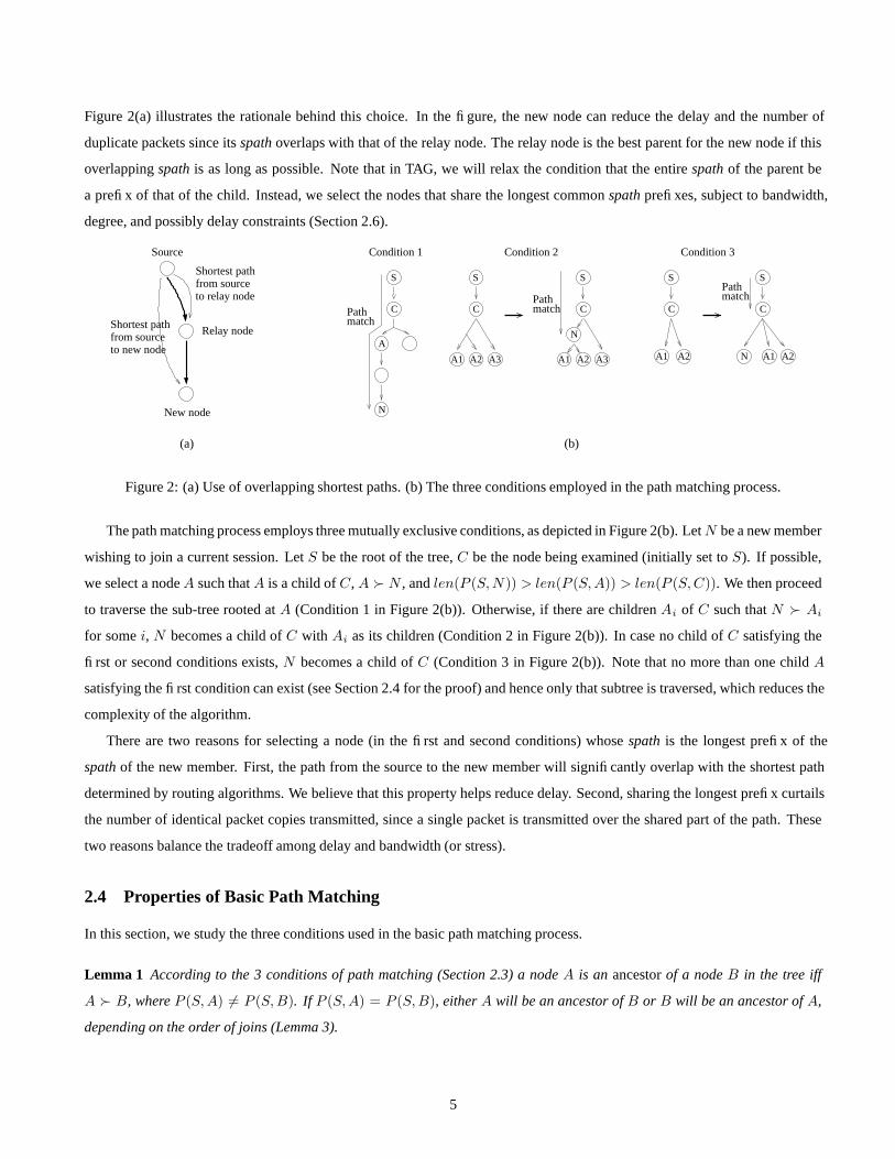
Figure 2(a) illustrates the rationale behind this choice. In the figure, the new node can reduce the delay and the number of

duplicate packets since its spath overlaps with that of the relay node. The relay node is the best parent for the new node if this

overlapping spath is as long as possible. Note that in TAG, we will relax the condition that the entire spath of the parent be

a prefix of that of the child. Instead, we select the nodes that share the longest common spath prefixes, subject to bandwidth,

degree, and possibly delay constraints (Section 2.6).

C

S

AN

C

S

Condition 3

C

N

S

Condition 1

New node

Source

Relay node

(a) (b)

C

S

Condition 2

matchPath

A2A1 A2 A3

matchPath

A1 A2

matchPath

to relay nodefrom sourceShortest path

to new nodefrom sourceShortest path

A3

C

S

A1 A2

N

A1

Figure 2: (a) Use of overlapping shortest paths. (b) The three conditions employed in the path matching process.

The path matching process employs three mutually exclusive conditions, as depicted in Figure 2(b). Let N be a new member

wishing to join a current session. Let S be the root of the tree, C be the node being examined (initially set to S). If possible,

we select a node A such that A is a child of C, A � N , and len(P (S, N)) > len(P (S, A)) > len(P (S, C)). We then proceed

to traverse the sub-tree rooted at A (Condition 1 in Figure 2(b)). Otherwise, if there are children Ai of C such that N � Ai

for some i, N becomes a child of C with Ai as its children (Condition 2 in Figure 2(b)). In case no child of C satisfying the

first or second conditions exists, N becomes a child of C (Condition 3 in Figure 2(b)). Note that no more than one child A

satisfying the first condition can exist (see Section 2.4 for the proof) and hence only that subtree is traversed, which reduces the

complexity of the algorithm.

There are two reasons for selecting a node (in the first and second conditions) whose spath is the longest prefix of the

spath of the new member. First, the path from the source to the new member will significantly overlap with the shortest path

determined by routing algorithms. We believe that this property helps reduce delay. Second, sharing the longest prefix curtails

the number of identical packet copies transmitted, since a single packet is transmitted over the shared part of the path. These

two reasons balance the tradeoff among delay and bandwidth (or stress).

2.4 Properties of Basic Path Matching

In this section, we study the three conditions used in the basic path matching process.

Lemma 1 According to the 3 conditions of path matching (Section 2.3) a node A is an ancestor of a node B in the tree iff

A � B, where P (S, A) 6= P (S, B). If P (S, A) = P (S, B), either A will be an ancestor of B or B will be an ancestor of A,

depending on the order of joins (Lemma 3).

5

Proof: ⇒: We first show that if node X is the parent of node Y , denoted by X = Parent(Y ), then X � Y . In basic path

matching, X can become the parent of Y by the second or by the third path matching conditions. Both cases guarantee X � Y .

We generalize this to the case when node A is an ancestor (not necessarily the parent) of node B. In this case, there must

exist n (n > 0) nodes such that M1 = Parent(B), M2 = Parent(M1), . . ., Mn = Parent(Mn−1), A = Parent(Mn). M1 =

Parent(B) � B holds, according to the previous case. Similarly, M2 � M1 � B. Transitively, A = Parent(Mn) � B.

⇐: This follows from conditions 1 and 2 in basic path matching.

In Figure 1, node D1 is an ancestor of node D5 because P (S, D1) = < R1, R2 > is a prefix of P (S, D5) = < R1, R2, R4 >.

In contrast, the fact that P (S, D2) = < R1, R5 > is not a prefix of P (S, D5) = < R1, R2, R4 > implies that node D2 is not

an ancestor of D5.

We now investigate the relationship between the conditions of basic path matching.

Lemma 2 The three conditions in basic path matching are mutually exclusive and complete.

Proof: To show mutual exclusion is equivalent to proving no two conditions can hold simultaneously. The first and the third

conditions, and the second and the third conditions cannot co-exist by definition. Therefore, we need to show that the first and

second conditions cannot both hold at the same time. Suppose the first and the second conditions occur simultaneously for a

node C that is being examined. A new member N selects B, a child of C, such that B � N for further probing by the first

condition. By the second condition, there must exist a node B ′, another child of C, such that N � B′, and B and B′ are

siblings. However, in this case, basic path matching would have previously ensured that B ′ is a descendant of B, not a child of

C, by Lemma 1, since B � N � B′. This is a contradiction. Since the third condition includes the complement set of the first

and the second conditions, the conditions are complete.

Now we study the number of trees constructed by basic path matching.

Lemma 3 Basic path matching constructs a unique tree if all members have distinct spaths, regardless of the order of joins. If

there are at least two members with the same spaths, the order of joins alters the constructed tree.

Proof: By Lemma 1, a unique relationship among every two nodes (i.e., parent, ancestor, child, descendant, or none) is estab-

lished among every two nodes which have different spaths, independent of the order of joins. If two members have the same

spath, one must be an ancestor of the other. Therefore, n! distinct trees can be constructed by basic path matching if n group

members have the same spaths (according to the order of their joins).

We now study the properties of a parent node.

Lemma 4 According to the 3 path matching conditions, for all i, the spath of the parent of nodes Ai has the longest prefix of

the spath P (S, Ai), where “longest” denotes longest in comparison to the spaths of all members in a session and S is the root

of the tree.

6

Proof: Consider two nodes B and C where B is the parent of C. By Lemma 1, B � C, i.e., P (S, B) is a prefix of P (S, C).

Suppose there exists a node A such that P (S, A) is a prefix of P (S, C) and len(P (S, A)) > len(P (S, B)). If both P (S, A)

and P (S, B) are prefixes of the same path P (S, C) and len(P (S, A)) > len(P (S, B)), then P (S, B) is a prefix of P (S, A).

By definition 2, B � A. Therefore, A must be a descendant of B according to Lemma 1. Basic path matching, however, would

make C a child of A, instead of B, since B � A and A � C. This is a contradiction. Hence, P (S, B) must be the longest

prefix of P (S, C), where B is the parent of C.

Finally, we give a bound for the number of hops on the path from the root to each member.

Lemma 5 For every member i in a tree, SPD(i) ≤ E(i) ≤ 3 × SPD(i) − 2, where SPD(i) is the number of hops on the

shortest path from root S to i, and E(i) is the actual number of hops from S to i in the tree.

Proof: Consider P (S, i), the path from root S to i. By the definition of len, SPD(i) = len(P (S, i)) + 1 since SPD(i) is

the number of hops on the path P (S, i). The fact that SPD(i) is the number of hops on the shortest path P (S, i) ensures

SPD(i) ≤ E(i). The maximum E(i) occurs when i has as many ancestors as len(P (S, i)). For every ancestor, 2 hops are

added to the path. Thus, 2 × len(P (S, i)) hops are added to SPD(i). Therefore, the maximum E(i) is 3 × SPD(i) − 2.

2.5 Tree Management

In this section, we discuss the multicast tree management protocol, including member join and member leave operations, and

fault resilience issues. For simplicity, we only use the basic path matching notion to explain the process.

2.5.1 Member Join

A new member joining a session sends a JOIN message to the primary source S of the session (the root of the tree). Upon

the receipt of a JOIN, S computes the spath to the new member, and executes path matching (checking the three conditions in

Section 2.3). If the new member becomes a child of S, the FT of S is updated accordingly. Otherwise, S propagates a FIND

message to its child that shares the longest spath prefix with the new member spath (according to Condition 1). The FIND

message carries the IP address and the spath of the new member. The FIND is processed by executing path matching and either

updating the FT, or propagating the FIND to one of the children. The propagation of FIND messages continues until the new

member finds a parent. Therefore, the algorithm is distributed, and traverses only a part of the overlay tree.

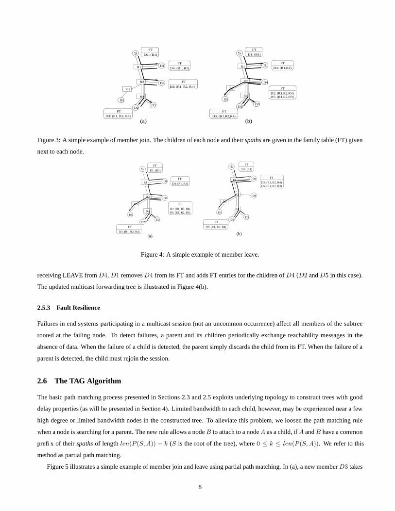
A simple example is illustrated in Figure 3. Source S is the root of the multicast tree, R1 through R4 are routers, and

D1 through D5 are hosts. The thick arrows denote the multicast forwarding tree. The FT of each member (showing only the

children) is given next to it. Suppose that the D1 to D4 are current session members (Figure 3(a)). When D5 joins the session,

D5 executes path matching and determines D4 to be its parent (Figure 3(b)).

2.5.2 Member Leave

A member can leave the session by sending a LEAVE message to its parent. For example, if D4 wishes to leave the session

(Figure 4(a)), D4 sends a LEAVE message to its parent D1. A LEAVE message includes the FT of the leaving member. Upon

7

R4

R3

D5

D3D2

FT

FT

FT

FT

D1: (R1)

D4: (R1, R2)

(a) (b)

D4

R3

D3: (R1, R2, R4)

D2: (R1, R2, R4)

R1

S

D1

R2 D4

R4D5

D3D2

FT

FT

FT

FT

D3: (R1,R2,R4)

D1: (R1)

D4: (R1,R2)

D2: (R1,R2,R4)D5: (R1,R2,R3)

R1

S

D1

R2

Figure 3: A simple example of member join. The children of each node and their spaths are given in the family table (FT) given

next to each node.

(a) (b)

D5: (R1, R2, R3)D2: (R1, R2, R4)

D2D3

D5

R3

R4

D4R2

D1

S

R1

D3: (R1, R2, R4)

D1: (R1)

D4: (R1, R2)

D5: (R1, R2, R3)D2: (R1, R2, R4)

D3: (R1, R2, R4)

D1: (R1)FT

FT

FT

FT

FT

FT

FT

D2D3

D5

R3

R4

D4R2

D1

S

R1

Figure 4: A simple example of member leave.

receiving LEAVE from D4, D1 removes D4 from its FT and adds FT entries for the children of D4 (D2 and D5 in this case).

The updated multicast forwarding tree is illustrated in Figure 4(b).

2.5.3 Fault Resilience

Failures in end systems participating in a multicast session (not an uncommon occurrence) affect all members of the subtree

rooted at the failing node. To detect failures, a parent and its children periodically exchange reachability messages in the

absence of data. When the failure of a child is detected, the parent simply discards the child from its FT. When the failure of a

parent is detected, the child must rejoin the session.

2.6 The TAG Algorithm

The basic path matching process presented in Sections 2.3 and 2.5 exploits underlying topology to construct trees with good

delay properties (as will be presented in Section 4). Limited bandwidth to each child, however, may be experienced near a few

high degree or limited bandwidth nodes in the constructed tree. To alleviate this problem, we loosen the path matching rule

when a node is searching for a parent. The new rule allows a node B to attach to a node A as a child, if A and B have a common

prefix of their spaths of length len(P (S, A)) − k (S is the root of the tree), where 0 ≤ k ≤ len(P (S, A)). We refer to this

method as partial path matching.

Figure 5 illustrates a simple example of member join and leave using partial path matching. In (a), a new member D3 takes

8

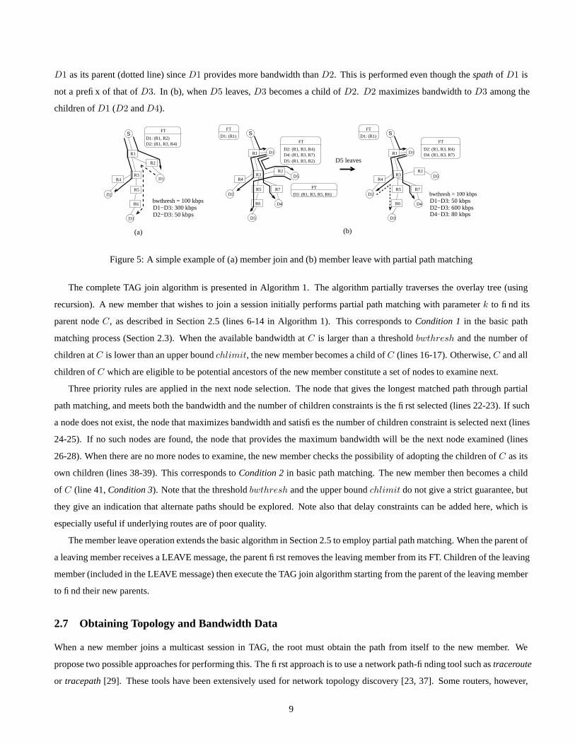
D1 as its parent (dotted line) since D1 provides more bandwidth than D2. This is performed even though the spath of D1 is

not a prefix of that of D3. In (b), when D5 leaves, D3 becomes a child of D2. D2 maximizes bandwidth to D3 among the

children of D1 (D2 and D4).

D2: (R1, R3, R4)D4: (R1, R3, R7)

FT

D5: (R1, R3, R2)

D3: (R1, R3, R5, R6)

FT

FT

D2: (R1, R3, R4)D4: (R1, R3, R7)

FT

R3

S

R1

D1: (R1)

FT

(b)

D1−D3: 50 kbpsD2−D3: 600 kbps

bwthresh = 100 kbps

D4−D3: 80 kbps

D5 leaves

D1−D3: 300 kbpsD2−D3: 50 kbps

bwthresh = 100 kbps

D1: (R1)

R3

S

R1

(a)

R3

S

R1

R2

D1: (R1, R2)D2: (R1, R3, R4)

FT

R5

R6

D3

D1R4

D2R5

R6

D3

R4

D2R7

D4

D1

R2D5

R5

R6

D3

R4

D2R7

D4

D1

R2D5

Figure 5: A simple example of (a) member join and (b) member leave with partial path matching

The complete TAG join algorithm is presented in Algorithm 1. The algorithm partially traverses the overlay tree (using

recursion). A new member that wishes to join a session initially performs partial path matching with parameter k to find its

parent node C, as described in Section 2.5 (lines 6-14 in Algorithm 1). This corresponds to Condition 1 in the basic path

matching process (Section 2.3). When the available bandwidth at C is larger than a threshold bwthresh and the number of

children at C is lower than an upper bound chlimit, the new member becomes a child of C (lines 16-17). Otherwise, C and all

children of C which are eligible to be potential ancestors of the new member constitute a set of nodes to examine next.

Three priority rules are applied in the next node selection. The node that gives the longest matched path through partial

path matching, and meets both the bandwidth and the number of children constraints is the first selected (lines 22-23). If such

a node does not exist, the node that maximizes bandwidth and satisfies the number of children constraint is selected next (lines

24-25). If no such nodes are found, the node that provides the maximum bandwidth will be the next node examined (lines

26-28). When there are no more nodes to examine, the new member checks the possibility of adopting the children of C as its

own children (lines 38-39). This corresponds to Condition 2 in basic path matching. The new member then becomes a child

of C (line 41, Condition 3). Note that the threshold bwthresh and the upper bound chlimit do not give a strict guarantee, but

they give an indication that alternate paths should be explored. Note also that delay constraints can be added here, which is

especially useful if underlying routes are of poor quality.

The member leave operation extends the basic algorithm in Section 2.5 to employ partial path matching. When the parent of

a leaving member receives a LEAVE message, the parent first removes the leaving member from its FT. Children of the leaving

member (included in the LEAVE message) then execute the TAG join algorithm starting from the parent of the leaving member

to find their new parents.

2.7 Obtaining Topology and Bandwidth Data

When a new member joins a multicast session in TAG, the root must obtain the path from itself to the new member. We

propose two possible approaches for performing this. The first approach is to use a network path-finding tool such as traceroute

or tracepath [29]. These tools have been extensively used for network topology discovery [23, 37]. Some routers, however,

9

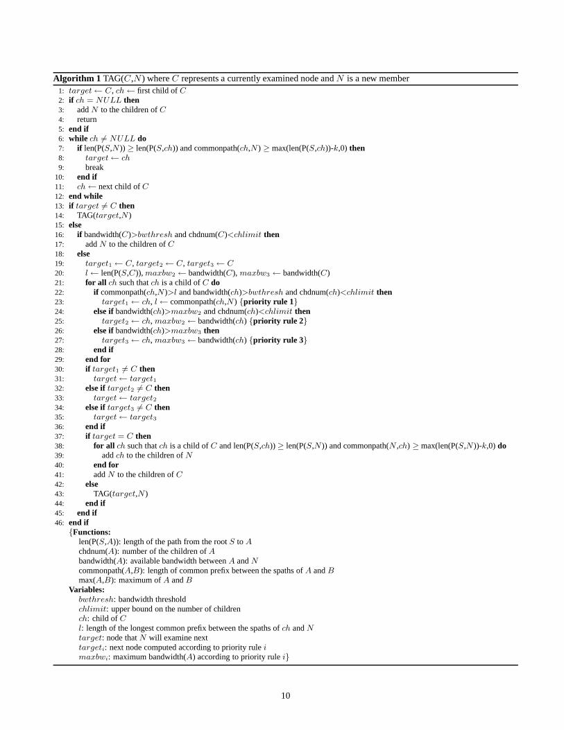
Algorithm 1 TAG(C,N ) where C represents a currently examined node and N is a new member1: target← C, ch← first child of C2: if ch = NULL then3: add N to the children of C

4: return5: end if6: while ch 6= NULL do7: if len(P(S,N )) ≥ len(P(S,ch)) and commonpath(ch,N ) ≥ max(len(P(S,ch))-k,0) then8: target← ch

9: break10: end if11: ch← next child of C

12: end while13: if target 6= C then14: TAG(target,N )15: else16: if bandwidth(C)>bwthresh and chdnum(C)<chlimit then17: add N to the children of C

18: else19: target1← C, target2 ← C, target3← C

20: l← len(P(S,C)), maxbw2 ← bandwidth(C), maxbw3 ← bandwidth(C)21: for all ch such that ch is a child of C do22: if commonpath(ch,N )>l and bandwidth(ch)>bwthresh and chdnum(ch)<chlimit then23: target1 ← ch, l← commonpath(ch,N ) {priority rule 1}24: else if bandwidth(ch)>maxbw2 and chdnum(ch)<chlimit then25: target2 ← ch, maxbw2 ← bandwidth(ch) {priority rule 2}26: else if bandwidth(ch)>maxbw3 then27: target3 ← ch, maxbw3 ← bandwidth(ch) {priority rule 3}28: end if29: end for30: if target1 6= C then31: target← target132: else if target2 6= C then33: target← target234: else if target3 6= C then35: target← target336: end if37: if target = C then38: for all ch such that ch is a child of C and len(P(S,ch)) ≥ len(P(S,N )) and commonpath(N ,ch) ≥ max(len(P(S,N ))-k,0) do39: add ch to the children of N

40: end for41: add N to the children of C

42: else43: TAG(target,N )44: end if45: end if46: end if{Functions:

len(P(S,A)): length of the path from the root S to A

chdnum(A): number of the children of A

bandwidth(A): available bandwidth between A and N

commonpath(A,B): length of common prefix between the spaths of A and Bmax(A,B): maximum of A and B

Variables:bwthresh: bandwidth thresholdchlimit: upper bound on the number of childrench: child of C

l: length of the longest common prefix between the spaths of ch and N

target: node that N will examine nexttargeti: next node computed according to priority rule imaxbwi: maximum bandwidth(A) according to priority rule i}

10

do not send ICMP Time-Exceeded messages when Time-To-Live (TTL) reaches zero. There are several reasons for this, the

most important of which is security. To quantify the impact of this problem, we conducted simple experiments where we used

traceroute for 50 sites in different continents at different times and on different days. Approximately 82−90% of the routers

responded. The average time taken to obtain and print the entire path information was 5.2 seconds, with a maximum of 42.6

seconds and a minimum of 0.2 seconds. 5−8% traceroute failures were reported in [37]. A recent study [24] indicates that

router ICMP generation delays are generally in the sub-millisecond range (< 500 µs). This means that only a few routers in

today’s Internet are slow in generating ICMP Time-Exceeded messages.

The second approach is to exploit topology servers. For example, an OSPF topology server [48] can track intra-domain

topology, either by listening to OSPF link state advertisements, or by pushing and pulling information from routers via SNMP.

Network topology can also be obtained from periodic logs of router configuration files [20], from MPLS traffic engineering

frameworks [4], and from policy-based OSPF monitoring frameworks [5]. Internet topology discovery projects [19, 10, 12]

can also supply topology information to TAG. Topology servers may, however, only include partial or coarse-grained (e.g.,

AS-level) information [35, 19, 10, 12]. Partial information can still be exploited by TAG for partial path matching of longest

common subsequences, and techniques of identifying nodes with multiple addresses can be employed.

Bandwidth estimation tools, in conjunction with in-band measurements, can be used to estimate the available bandwidth

between nodes under dynamic network conditions. Tools similar to pathchar [26] estimate available bandwidth, delay, average

queue, and loss rate of every hop between any source and destination on the Internet. Nettimer [32] is useful for low-overhead

measurement of per-link available bandwidth. Other bandwidth or throughput estimation tools are available through CAIDA [1].

2.8 Adaptivity and Scalability

If network conditions change and the overlay tree becomes inefficient (e.g., when a mobile host moves or paths fail), TAG must

adapt the overlay tree to the new network conditions. An accurate adaptation would entail that the root probe every member

periodically to determine if the paths have changed. When path changes are detected, the root initiates a rejoin process for the

members affected. This mechanism, however, introduces scalability problems in that the root is overloaded and many potential

probe packets are generated.

Several mechanisms mitigate these scalability problems. First, intermediate nodes (non-leaf nodes) participate in periodic

probing, alleviating the burden on the root. The intermediate nodes only probe the paths to their children. Second, path-based

aggregation of members can substantially reduce the number of hops and members probed. Only one member in a member

group is examined every round. During the next round, another member of the group is inspected. When changes are detected

for a certain group, all members of that group are updated. When changes in part of an spath are detected for a member, not

only the member being probed, but also all the members in the same group and all the members in groups with overlapping

spaths, are updated.

Although these TAG reorganizing mechanisms help reduce overhead, the root is likely to experience a high load if a large

number of members join or rejoin simultaneously. To address this limitation, a mechanism similar to that used in Overcast [28]

can be employed. Requests from overlay members to the root are redirected to lightly loaded replicated roots. Strategically

placed nodes can serve as replicated roots under certain performance constraints. For example, a member which has sufficient

11

resources (e.g., bandwidth) can be a replicated root for other members in a same network domain. A hierarchical version of

TAG can be employed so that a TAG overlay is constructed within a network domain and another TAG overlay connects the

replicated roots in different network domains. This mechanism is currently under study.

2.9 Multiple Source Groups

In the current version of TAG, a source other than the root of the tree must first relay its data to the root. The root then multicasts

the data to all members of the session. This approach is suitable for mostly single-source applications, where the primary source

is selected as the root, and other group members may occasionally transmit. In applications where all members transmit with

approximately equal probabilities, the root of the tree should be carefully selected. In this case, the selection problem is similar

to the core selection problem in core-based tree approaches for multicast routing [6]. Multiple (backup) roots are also important

for fault tolerance.

3 Complexity and Network Cost Analysis

In this section, we analyze the complexity of TAG and its economies of scale factor, compared to other overlay multicast

algorithms and IP multicast.

3.1 Time and Space Complexities

We compare the time and space complexities of TAG, ESM [13] and NICE [7] in Table 1. Assume that a multicast group has

n members (end systems). ESM [13] has weak upper and lower bounds (which may sometimes be violated) for the number

of neighbors. TAG also uses a weak upper bound on the number of children. In contrast, the NICE [7] protocol has strong

upper and lower bounds for its cluster size, which are periodically enforced by the cluster maintenance process. The number of

children of each member in NICE is no less than m1 and no greater than m2, i.e., m1 ≤ m ≤ m2, where m is the number of

children of each member in NICE, and 0 < m1, m2 � n.

In TAG, after the source discovers the path to a new member, the member join process entails partial tree traversal (Algo-

rithm 1). For a balanced overlay multicast tree of height logm n, the time complexity of the TAG join algorithm is O(m logm n).

This is because the m children of each node that is visited are examined, and only one branch of the tree is traversed. If m = 1

(one child per node), the tree height becomes n, and thus the worst case time complexity becomes O(n).

As discussed in Section 2.6, children of a leaving member rejoin the session starting from the parent of the leaving member.

In this process, each of the m children of the leaving member requires O(m logm n) operations for the rejoin, for the case of

a balanced tree. Hence, the time complexity of member leave is O(m2 logm n) for this case. For m = 1, the time complexity

becomes O(n). In this case, one child of the root of the tree has to traverse the entire skewed tree.

We have observed in our experiments that TAG trees tend to have a small height and a large number of children. The number

of children depends on the (weak) bandwidth constraint, and number of children (degree) constraint. The case of a skewed tree

of height n is very rare in practice.

12

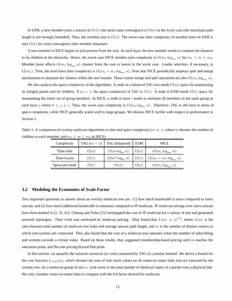
In ESM, a new member joins a session in O(1), but mesh route convergence is O(n) in the worst case (the maximum path

length is not strongly bounded). Thus, the member join is O(n). The worst case time complexity of member leave in ESM is

also O(n) for route convergence after member departure.

A new member in NICE begins its join process from the root. At each layer, the new member needs to compute the distance

to its children in the hierarchy. Hence, the worst case NICE member join complexity is O(m1 logm1n) for m1 ≤ m ≤ m2.

Member leave affects O(m1 logm1n) clusters from the root to leaves in the worst case. Leader selection, if necessary, is

O(m1). Thus, the total leave time complexity is O(m1 + m1 logm1n). Note that NICE periodically employs split and merge

mechanisms to maintain the clusters within the size bounds. These cluster merge and split operations are also O(m1 logm1n).

We also analyze the space complexity of the algorithms. A node in a balanced TAG tree needs O(m) space for maintaining

its (single) parent and its children. If m = 1, the space complexity of TAG is O(1). A node in ESM needs O(n) space for

maintaining the entire set of group members. In NICE, a node at layer i needs to maintain all members in the same group at

each layer j where 0 ≤ j ≤ i. Thus, the worst case complexity is O(m1 logm1n). Therefore, TAG is efficient in terms of

space complexity, while NICE generally scales well to large groups. We discuss NICE further with respect to performance in

Section 5.

Table 1: A comparison of overlay multicast algorithms in time and space complexity (m � n, where m denotes the number of

children at each member, and m1 ≤ m ≤ m2 in NICE)

Complexity TAG (m = 1) TAG (balanced) ESM NICE

Time-Join O(n) O(m logm n) O(n) O(m1 logm1n)

Time-Leave O(n) O(m2 logm n) O(n) O(m1 + m1 logm1n)

Space-per node O(1) O(m) O(n) O(m1 logm1n)

3.2 Modeling the Economies of Scale Factor

Two important questions to answer about an overlay multicast tree are: (1) how much bandwidth it saves compared to naive

unicast; and (2) how much additional bandwidth it consumes compared to IP multicast. IP multicast savings over naive unicast

have been studied in [2, 15, 41]. Chuang and Sirbu [15] investigated the cost of IP multicast for a variety of real and generated

network topologies. Their work was motivated by multicast pricing. They found that L(m) ∝ m0.8, where L(m) is the

ratio between total number of multicast tree links and average unicast path length, and m is the number of distinct routers to

which end systems are connected. They also found that the cost of a multicast tree saturates when the number of subscribing

end systems exceeds a certain value. Based on these results, they suggested membership-based pricing until m reaches the

saturation point, and flat-rate pricing beyond that point.

In this section, we quantify the network resources (or cost) consumed by TAG in a similar method. We derive a bound for

the cost function LTAG(n), which denotes the sum of link stress values on all router-to-router links that are traversed by the

overlay tree, for a multicast group of size n. Link stress is the total number of identical copies of a packet over a physical link.

We only consider router-to-router links to compare with the 0.8 factor derived for multicast.

13

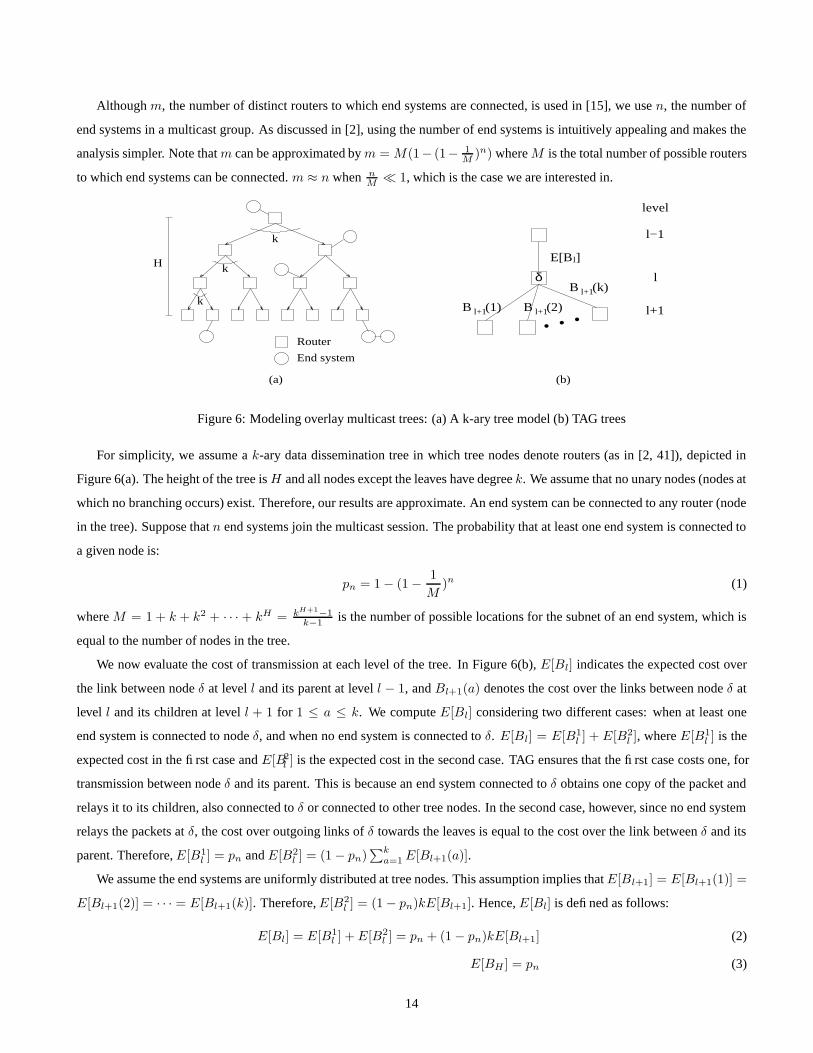
Although m, the number of distinct routers to which end systems are connected, is used in [15], we use n, the number of

end systems in a multicast group. As discussed in [2], using the number of end systems is intuitively appealing and makes the

analysis simpler. Note that m can be approximated by m = M(1− (1− 1M

)n) where M is the total number of possible routers

to which end systems can be connected. m ≈ n when nM

� 1, which is the case we are interested in.

End system

Router

k

k

H

k

l

(k)l+1

l

(1)l+1B (2) l+1

level

l−1

δ

...

B

l+1B

E[B ]

(b)(a)

Figure 6: Modeling overlay multicast trees: (a) A k-ary tree model (b) TAG trees

For simplicity, we assume a k-ary data dissemination tree in which tree nodes denote routers (as in [2, 41]), depicted in

Figure 6(a). The height of the tree is H and all nodes except the leaves have degree k. We assume that no unary nodes (nodes at

which no branching occurs) exist. Therefore, our results are approximate. An end system can be connected to any router (node

in the tree). Suppose that n end systems join the multicast session. The probability that at least one end system is connected to

a given node is:

pn = 1 − (1 −1

M)n (1)

where M = 1 + k + k2 + · · · + kH = kH+1−1

k−1 is the number of possible locations for the subnet of an end system, which is

equal to the number of nodes in the tree.

We now evaluate the cost of transmission at each level of the tree. In Figure 6(b), E[Bl] indicates the expected cost over

the link between node δ at level l and its parent at level l − 1, and Bl+1(a) denotes the cost over the links between node δ at

level l and its children at level l + 1 for 1 ≤ a ≤ k. We compute E[Bl] considering two different cases: when at least one

end system is connected to node δ, and when no end system is connected to δ. E[Bl] = E[B1l ] + E[B2

l ], where E[B1l ] is the

expected cost in the first case and E[B2l ] is the expected cost in the second case. TAG ensures that the first case costs one, for

transmission between node δ and its parent. This is because an end system connected to δ obtains one copy of the packet and

relays it to its children, also connected to δ or connected to other tree nodes. In the second case, however, since no end system

relays the packets at δ, the cost over outgoing links of δ towards the leaves is equal to the cost over the link between δ and its

parent. Therefore, E[B1l ] = pn and E[B2

l ] = (1 − pn)∑k

a=1 E[Bl+1(a)].

We assume the end systems are uniformly distributed at tree nodes. This assumption implies that E[Bl+1] = E[Bl+1(1)] =

E[Bl+1(2)] = · · · = E[Bl+1(k)]. Therefore, E[B2l ] = (1 − pn)kE[Bl+1]. Hence, E[Bl] is defined as follows:

E[Bl] = E[B1l ] + E[B2

l ] = pn + (1 − pn)kE[Bl+1] (2)

E[BH ] = pn (3)

14

1

10

100

1000

10000

100000

1 10 100 1000 10000 100000N

orm

aliz

ed O

verla

y Tr

ee C

ost

Number of Members

k=3,H=6k=3,H=7k=3,H=8k=4,H=5k=4,H=6k=5,H=5

x^0.95

Figure 7: TAG tree cost versus group size

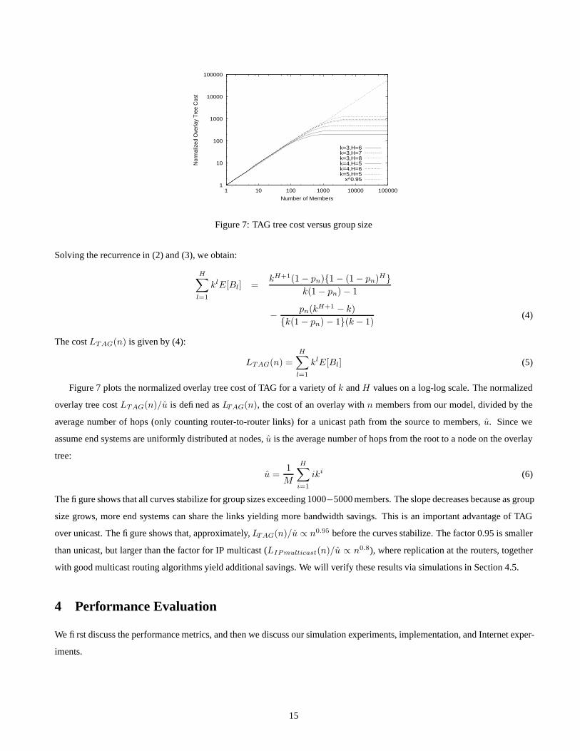
Solving the recurrence in (2) and (3), we obtain:

H∑

l=1

klE[Bl] =kH+1(1 − pn){1 − (1 − pn)H}

k(1 − pn) − 1

−pn(kH+1 − k)

{k(1 − pn) − 1}(k − 1)(4)

The cost LTAG(n) is given by (4):

LTAG(n) =

H∑

l=1

klE[Bl] (5)

Figure 7 plots the normalized overlay tree cost of TAG for a variety of k and H values on a log-log scale. The normalized

overlay tree cost LTAG(n)/u is defined as LTAG(n), the cost of an overlay with n members from our model, divided by the

average number of hops (only counting router-to-router links) for a unicast path from the source to members, u. Since we

assume end systems are uniformly distributed at nodes, u is the average number of hops from the root to a node on the overlay

tree:

u =1

M

H∑

i=1

iki (6)

The figure shows that all curves stabilize for group sizes exceeding 1000−5000 members. The slope decreases because as group

size grows, more end systems can share the links yielding more bandwidth savings. This is an important advantage of TAG

over unicast. The figure shows that, approximately, LTAG(n)/u ∝ n0.95 before the curves stabilize. The factor 0.95 is smaller

than unicast, but larger than the factor for IP multicast (LIPmulticast(n)/u ∝ n0.8), where replication at the routers, together

with good multicast routing algorithms yield additional savings. We will verify these results via simulations in Section 4.5.

4 Performance Evaluation

We first discuss the performance metrics, and then we discuss our simulation experiments, implementation, and Internet exper-

iments.

15

4.1 Performance Metrics

We use the following performance metrics [13, 14] for evaluating TAG, ESM and Narada:

1. Mean Relative Delay Penalty (RDP): RDP is the relative increase in delay between the source and a member in

TAG against unicast delay between the source and the same member. The RDP from source s to member dr is the

ratio latency(s,dr)delay(s,dr) . The latency latency(s, dr) from s to dr is defined to be delay(s, d0) +

∑l−1i=0 delay(di, di+1)

+delay(dl, dr), assuming s delivers data to dr via the sequence of end systems (d0, · · · , dl). Here, delay(di, di+1)

denotes the end-to-end delay from di to di+1. We compute the mean RDP of all members.

2. Link Stress: Link stress is the total number of identical copies of a packet over a physical link. We compute the total

stress for all tree links. We also compute the maximum value of link stress among all links. This is clearly a network-level

metric and is not of importance to the application user.

3. Mean Available Bandwidth (in kbps): This is the mean of the available bottleneck bandwidth between the source and

all members.

The TAG tree cost is also computed in Section 4.5, and compared to IP multicast and unicast cost.

4.2 Simulation Setup

We have implemented session-level simulators for both TAG and ESM [13, 14] to evaluate and compare their performance.

Our simulators model propagation delays, but not queuing delays or packet losses. We use two different flavors of ESM: one

that considers bandwidth as the primary metric and delay as a secondary metric [13], and one with only delay as a metric as

presented in [14]. We refer to the former as ESM and the latter as Narada.

We use router-level Transit-Stub topologies generated by GT-ITM [51]. The Transit-Stub model generates a two-level

hierarchy: interconnected higher level (transit) domains and lower level (stub) domains. We use two different topologies

with different numbers of nodes: 1640 and 4040. (We have experimented with other sizes, but the results included here are

representative.) When the total is 1640 nodes, there are 4 transit domains, 10 nodes per transit domain, 5 stub domains per

transit node, and 10 nodes per stub domain. A similar distribution is used when the total number of nodes is 4040. We label

the two transit-stub topologies TS1 and TS2 respectively, i.e., label “TAG-TS1” denotes the results of TAG on the Transit-Stub

topology with 1640 nodes. Multicast group members are randomly assigned to stub nodes. The multicast group size ranges

from 10 to 1280 members. GT-ITM generates symmetric link delays ranging from 1 to 55 ms for transit-transit or transit-stub

links. We use 1 to 10 ms delays within a stub. We randomly assign bandwidth ranging between 100 Mbps and 1 Gbps to

backbone links. We use 500 kbps to 10 Mbps for the links from edge routers to end systems.

We assume that the IP layer routing algorithm uses delay as a metric for finding shortest paths. The routing algorithm for

the mesh in ESM uses discretized levels of available bandwidth (in 500 kbps increments) as the primary metric, and delay as a

tie breaker. TAG uses k = 1, bwthresh= 100 kbps and chlimit = 25, unless otherwise specified. ESM and Narada compute

routing tables using shortest path algorithms (e.g., the Floyd-Warshall algorithm). Hence, no route convergence problems are

modeled in our simulations. We use the same parameters for ESM and Narada used in the simulations in [13, 14] (lower degree

16

bound = 3, upper degree bound = 6, high delay penalty = 3), except for delay-related parameters (close neighbor delay = 85 ms)

since we assign a wider range of delays to the links. The lower and upper degree bounds limit the number of neighbors for an

ESM node. An ESM node, however, can adopt other nodes as neighbors if these other nodes are closer than the close neighbor

delay, when the current delay penalty (the definition of RDP will be given below) is larger than the high delay penalty.

For each protocol, we run five simulations with different random number generator seeds (for selecting the multicast source

and members) and average the results. We show 95% confidence intervals to indicate variability.

4.3 Simulation Results

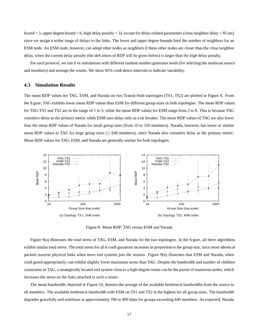
The mean RDP values for TAG, ESM, and Narada on two Transit-Stub topologies (TS1, TS2) are plotted in Figure 8. From

the figure, TAG exhibits lower mean RDP values than ESM for different group sizes in both topologies. The mean RDP values

for TAG-TS1 and TS2 are in the range of 1 to 5, while the mean RDP values for ESM range from 2 to 8. This is because TAG

considers delay as the primary metric while ESM uses delay only as a tie breaker. The mean RDP values of TAG are also lower

than the mean RDP values of Narada for small group sizes (from 10 to 320 members). Narada, however, has lower or similar

mean RDP values to TAG for large group sizes (≥ 640 members), since Narada also considers delay as the primary metric.

Mean RDP values for TAG, ESM, and Narada are generally similar for both topologies.

0

2

4

6

8

10

12

14

10 100 1000

Mea

n R

DP

Group Size (log scale)

TAG-TS1ESM-TS1

Narada-TS1

(a) Topology TS1: 1640 nodes

0

2

4

6

8

10

12

14

10 100 1000

Mea

n R

DP


TAG-TS2ESM-TS2

Narada-TS2

(b) Topology TS2: 4040 nodes

Figure 8: Mean RDP: TAG versus ESM and Narada

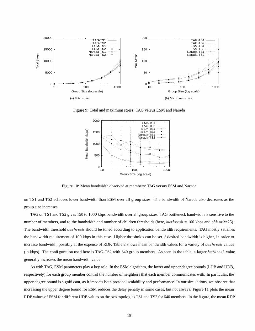
Figure 9(a) illustrates the total stress of TAG, ESM, and Narada for the two topologies. In the figure, all three algorithms

exhibit similar total stress. The total stress for all 6 configurations increases in proportion to the group size, since more identical

packets traverse physical links when more end systems join the session. Figure 9(b) illustrates that ESM and Narada, when

configured appropriately, can exhibit slightly lower maximum stress than TAG. Despite the bandwidth and number of children

constraints in TAG, a strategically located end system close to a high-degree router can be the parent of numerous nodes, which

increases the stress on the links attached to such a router.

The mean bandwidth, depicted in Figure 10, denotes the average of the available bottleneck bandwidths from the source to

all members. The available bottleneck bandwidth with ESM on TS1 and TS2 is the highest for all group sizes. The bandwidth

degrades gracefully and stabilizes at approximately 700 to 800 kbps for groups exceeding 640 members. As expected, Narada

17

0

5000

10000

15000

20000

10 100 1000

Tota

l Stre

ss


TAG-TS1TAG-TS2ESM-TS1ESM-TS2

Narada-TS1Narada-TS2

(a) Total stress

0

50

100

150

200

10 100 1000

Max

Stre

ss




(b) Maximum stress

Figure 9: Total and maximum stress: TAG versus ESM and Narada

0

500

1000

1500

2000

10 100 1000

Mea

n B

andw

idth

(kbp

s)




Figure 10: Mean bandwidth observed at members: TAG versus ESM and Narada

on TS1 and TS2 achieves lower bandwidth than ESM over all group sizes. The bandwidth of Narada also decreases as the

group size increases.

TAG on TS1 and TS2 gives 150 to 1000 kbps bandwidth over all group sizes. TAG bottleneck bandwidth is sensitive to the

number of members, and to the bandwidth and number of children thresholds (here, bwthresh = 100 kbps and chlimit=25).

The bandwidth threshold bwthresh should be tuned according to application bandwidth requirements. TAG mostly satisfies

the bandwidth requirement of 100 kbps in this case. Higher thresholds can be set if desired bandwidth is higher, in order to

increase bandwidth, possibly at the expense of RDP. Table 2 shows mean bandwidth values for a variety of bwthresh values

(in kbps). The configuration used here is TAG-TS2 with 640 group members. As seen in the table, a larger bwthresh value

generally increases the mean bandwidth value.

As with TAG, ESM parameters play a key role. In the ESM algorithm, the lower and upper degree bounds (LDB and UDB,

respectively) for each group member control the number of neighbors that each member communicates with. In particular, the

upper degree bound is significant, as it impacts both protocol scalability and performance. In our simulations, we observe that

increasing the upper degree bound for ESM reduces the delay penalty in some cases, but not always. Figure 11 plots the mean

RDP values of ESM for different UDB values on the two topologies TS1 and TS2 for 640 members. In the figure, the mean RDP

18

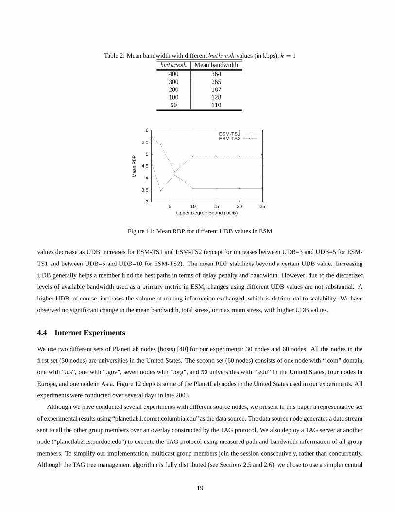
Table 2: Mean bandwidth with different bwthresh values (in kbps), k = 1

bwthresh Mean bandwidth

400 364300 265200 187100 12850 110

3

3.5

4

4.5

5

5.5

6

5 10 15 20 25

Mea

n R

DP

Upper Degree Bound (UDB)

ESM-TS1ESM-TS2

Figure 11: Mean RDP for different UDB values in ESM

values decrease as UDB increases for ESM-TS1 and ESM-TS2 (except for increases between UDB=3 and UDB=5 for ESM-

TS1 and between UDB=5 and UDB=10 for ESM-TS2). The mean RDP stabilizes beyond a certain UDB value. Increasing

UDB generally helps a member find the best paths in terms of delay penalty and bandwidth. However, due to the discretized

levels of available bandwidth used as a primary metric in ESM, changes using different UDB values are not substantial. A

higher UDB, of course, increases the volume of routing information exchanged, which is detrimental to scalability. We have

observed no significant change in the mean bandwidth, total stress, or maximum stress, with higher UDB values.

4.4 Internet Experiments

We use two different sets of PlanetLab nodes (hosts) [40] for our experiments: 30 nodes and 60 nodes. All the nodes in the

first set (30 nodes) are universities in the United States. The second set (60 nodes) consists of one node with “.com” domain,

one with “.us”, one with “.gov”, seven nodes with “.org”, and 50 universities with “.edu” in the United States, four nodes in

Europe, and one node in Asia. Figure 12 depicts some of the PlanetLab nodes in the United States used in our experiments. All

experiments were conducted over several days in late 2003.

Although we have conducted several experiments with different source nodes, we present in this paper a representative set

of experimental results using “planetlab1.comet.columbia.edu” as the data source. The data source node generates a data stream

sent to all the other group members over an overlay constructed by the TAG protocol. We also deploy a TAG server at another

node (“planetlab2.cs.purdue.edu”) to execute the TAG protocol using measured path and bandwidth information of all group

members. To simplify our implementation, multicast group members join the session consecutively, rather than concurrently.

Although the TAG tree management algorithm is fully distributed (see Sections 2.5 and 2.6), we chose to use a simpler central

19

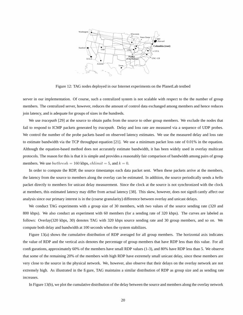
Washington

StanfordUIUC

Wisconsin

Columbia (root)

Notre Dame

UVA

UNC−CH(TAG Server)Purdue

Arizona

MIT

UCLA

Harvard

Texas

Utah

Figure 12: TAG nodes deployed in our Internet experiments on the PlanetLab testbed

server in our implementation. Of course, such a centralized system is not scalable with respect to the the number of group

members. The centralized server, however, reduces the amount of control data exchanged among members and hence reduces

join latency, and is adequate for groups of sizes in the hundreds.

We use tracepath [29] at the source to obtain paths from the source to other group members. We exclude the nodes that

fail to respond to ICMP packets generated by tracepath. Delay and loss rate are measured via a sequence of UDP probes.

We control the number of the probe packets based on observed latency estimates. We use the measured delay and loss rate

to estimate bandwidth via the TCP throughput equation [21]. We use a minimum packet loss rate of 0.01% in the equation.

Although the equation-based method does not accurately estimate bandwidth, it has been widely used in overlay multicast

protocols. The reason for this is that it is simple and provides a reasonably fair comparison of bandwidth among pairs of group

members. We use bwthresh = 160 kbps, chlimit = 5, and k = 0.

In order to compute the RDP, the source timestamps each data packet sent. When these packets arrive at the members,

the latency from the source to members along the overlay can be estimated. In addition, the source periodically sends a hello

packet directly to members for unicast delay measurement. Since the clock at the source is not synchronized with the clock

at members, this estimated latency may differ from actual latency [38]. This skew, however, does not significantly affect our

analysis since our primary interest is in the (coarse granularity) difference between overlay and unicast delays.

We conduct TAG experiments with a group size of 30 members, with two values of the source sending rate (320 and

800 kbps). We also conduct an experiment with 60 members (for a sending rate of 320 kbps). The curves are labeled as

follows: Overlay(320 kbps, 30) denotes TAG with 320 kbps source sending rate and 30 group members, and so on. We

compute both delay and bandwidth at 100 seconds when the system stabilizes.

Figure 13(a) shows the cumulative distribution of RDP averaged for all group members. The horizontal axis indicates

the value of RDP and the vertical axis denotes the percentage of group members that have RDP less than this value. For all

configurations, approximately 60% of the members have small RDP values (1-3), and 80% have RDP less than 5. We observe

that some of the remaining 20% of the members with high RDP have extremely small unicast delay, since these members are

very close to the source in the physical network. We, however, also observe that their delays on the overlay network are not

extremely high. As illustrated in the figure, TAG maintains a similar distribution of RDP as group size and as sending rate

increases.

In Figure 13(b), we plot the cumulative distribution of the delay between the source and members along the overlay network

20

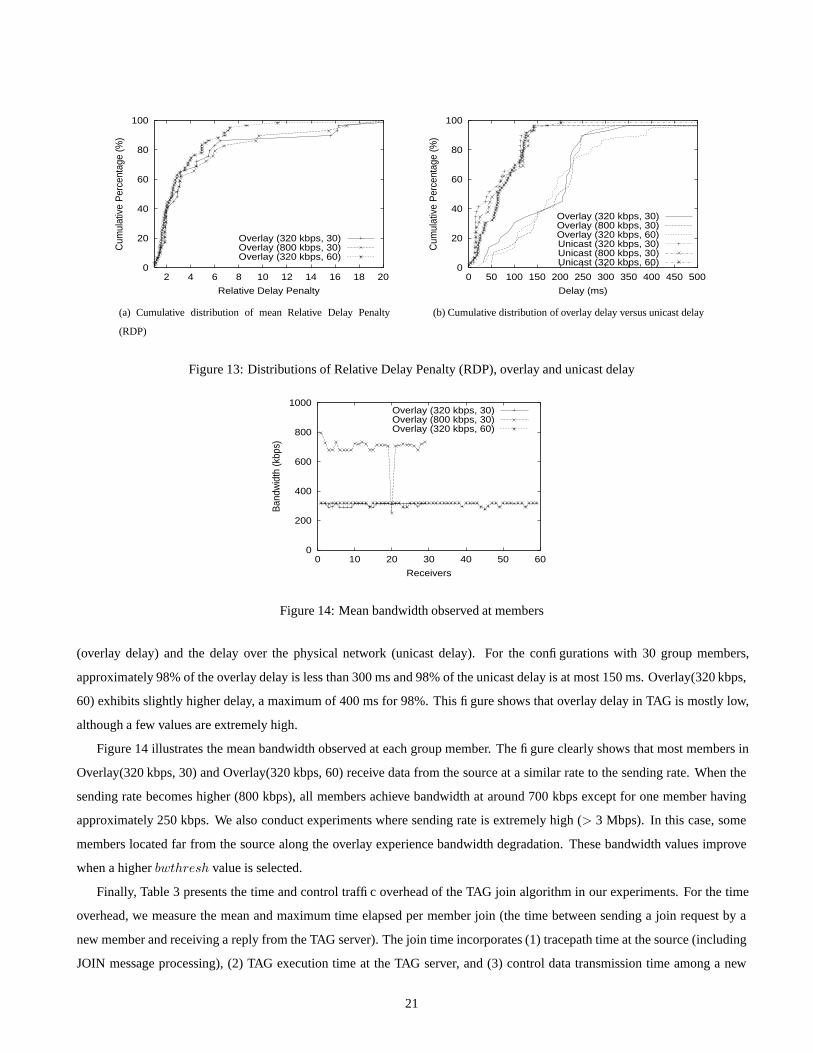
0

20

40

60

80

100

2 4 6 8 10 12 14 16 18 20

Cum

ulat

ive

Per

cent

age

(%)

Relative Delay Penalty

Overlay (320 kbps, 30)Overlay (800 kbps, 30)Overlay (320 kbps, 60)

(a) Cumulative distribution of mean Relative Delay Penalty

(RDP)

0

20

40

60

80

100

0 50 100 150 200 250 300 350 400 450 500

Cum

ulat

ive

Per

cent

age

(%)

Delay (ms)

Overlay (320 kbps, 30)Overlay (800 kbps, 30)Overlay (320 kbps, 60)Unicast (320 kbps, 30)Unicast (800 kbps, 30)Unicast (320 kbps, 60)

(b) Cumulative distribution of overlay delay versus unicast delay

Figure 13: Distributions of Relative Delay Penalty (RDP), overlay and unicast delay

0

200

400

600

800

1000

0 10 20 30 40 50 60

Ban

dwid

th (k

bps)

Receivers

Overlay (320 kbps, 30)Overlay (800 kbps, 30)Overlay (320 kbps, 60)

Figure 14: Mean bandwidth observed at members

(overlay delay) and the delay over the physical network (unicast delay). For the configurations with 30 group members,

approximately 98% of the overlay delay is less than 300 ms and 98% of the unicast delay is at most 150 ms. Overlay(320 kbps,

60) exhibits slightly higher delay, a maximum of 400 ms for 98%. This figure shows that overlay delay in TAG is mostly low,

although a few values are extremely high.

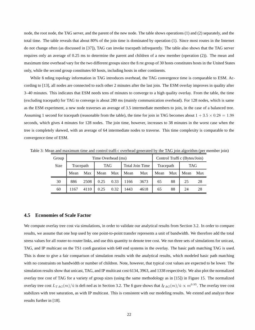
Figure 14 illustrates the mean bandwidth observed at each group member. The figure clearly shows that most members in

Overlay(320 kbps, 30) and Overlay(320 kbps, 60) receive data from the source at a similar rate to the sending rate. When the

sending rate becomes higher (800 kbps), all members achieve bandwidth at around 700 kbps except for one member having

approximately 250 kbps. We also conduct experiments where sending rate is extremely high (> 3 Mbps). In this case, some

members located far from the source along the overlay experience bandwidth degradation. These bandwidth values improve

when a higher bwthresh value is selected.

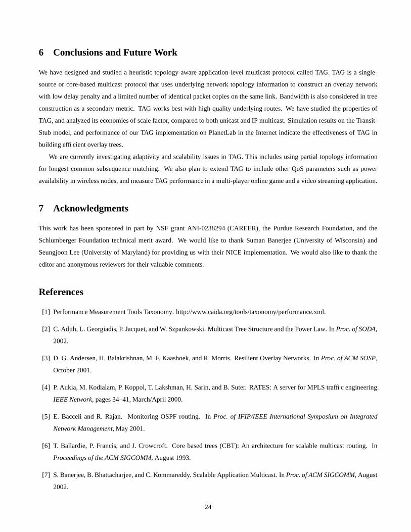
Finally, Table 3 presents the time and control traffic overhead of the TAG join algorithm in our experiments. For the time

overhead, we measure the mean and maximum time elapsed per member join (the time between sending a join request by a

new member and receiving a reply from the TAG server). The join time incorporates (1) tracepath time at the source (including

JOIN message processing), (2) TAG execution time at the TAG server, and (3) control data transmission time among a new

21

node, the root node, the TAG server, and the parent of the new node. The table shows operations (1) and (2) separately, and the

total time. The table reveals that about 80% of the join time is dominated by operation (1). Since most routes in the Internet

do not change often (as discussed in [37]), TAG can invoke tracepath infrequently. The table also shows that the TAG server

requires only an average of 0.25 ms to determine the parent and children of a new member (operation (2)). The mean and

maximum time overhead vary for the two different groups since the first group of 30 hosts constitutes hosts in the United States

only, while the second group constitutes 60 hosts, including hosts in other continents.

While finding topology information in TAG introduces overhead, the TAG convergence time is comparable to ESM. Ac-

cording to [13], all nodes are connected to each other 2 minutes after the last join. The ESM overlay improves in quality after

3–40 minutes. This indicates that ESM needs tens of minutes to converge to a high quality overlay. From the table, the time

(excluding tracepath) for TAG to converge is about 280 ms (mainly communication overhead). For 128 nodes, which is same

as the ESM experiment, a new node traverses an average of 3.5 intermediate members to join, in the case of a balanced tree.

Assuming 1 second for tracepath (reasonable from the table), the time for join in TAG becomes about 1 + 3.5 × 0.28 = 1.98

seconds, which gives 4 minutes for 128 nodes. The join time, however, increases to 38 minutes in the worst case when the

tree is completely skewed, with an average of 64 intermediate nodes to traverse. This time complexity is comparable to the

convergence time of ESM.

Table 3: Mean and maximum time and control traffic overhead generated by the TAG join algorithm (per member join)

Group Time Overhead (ms) Control Traffic (Bytes/Join)

Size Tracepath TAG Total Join Time Tracepath TAG

Mean Max Mean Max Mean Max Mean Max Mean Max

30 886 2508 0.25 0.33 1166 3673 65 88 25 28

60 1167 4110 0.25 0.32 1443 4618 65 88 24 28

4.5 Economies of Scale Factor

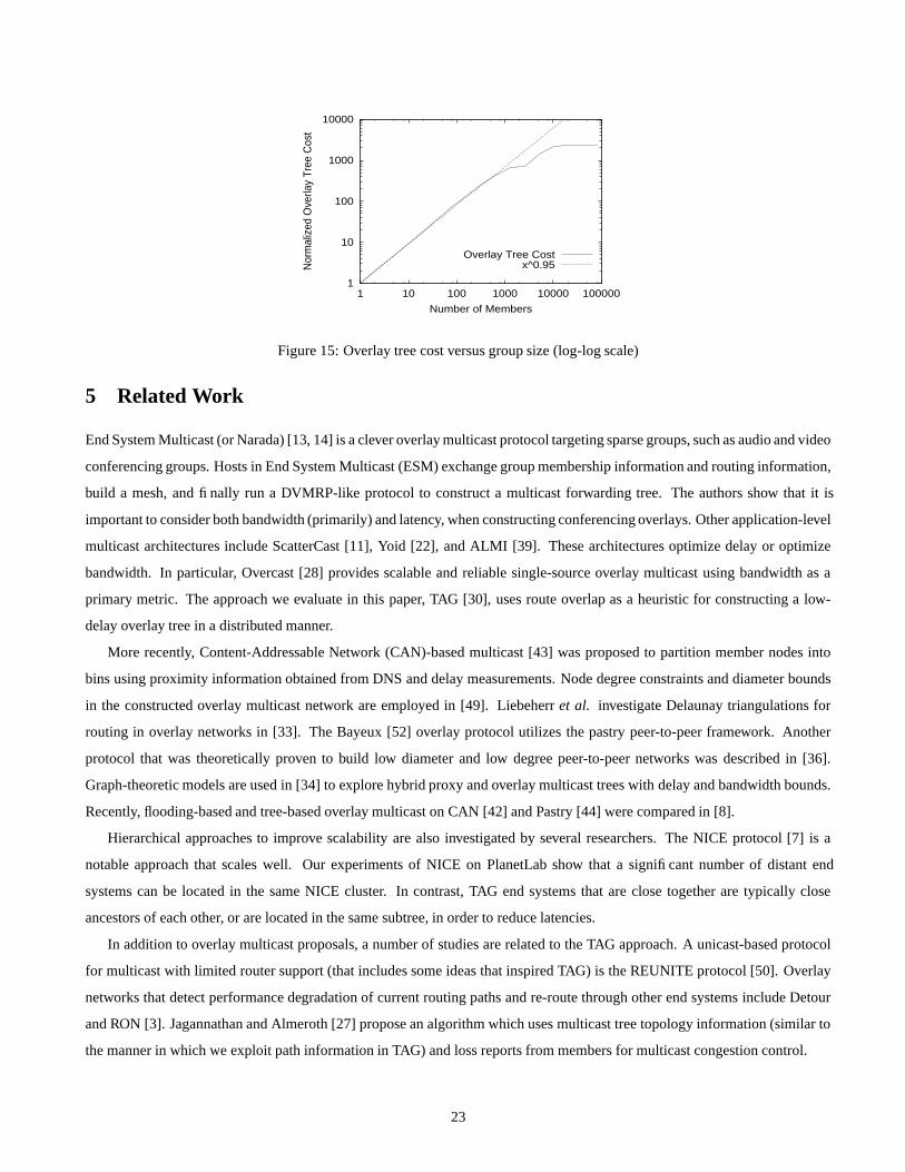
We compute overlay tree cost via simulations, in order to validate our analytical results from Section 3.2. In order to compare

results, we assume that one hop used by one point-to-point transfer represents a unit of bandwidth. We therefore add the total

stress values for all router-to-router links, and use this quantity to denote tree cost. We run three sets of simulations for unicast,

TAG, and IP multicast on the TS1 configuration with 640 end systems in the overlay. The basic path matching TAG is used.

This is done to give a fair comparison of simulation results with the analytical results, which modeled basic path matching

with no constraints on bandwidth or number of children. Note, however, that typical cost values are expected to be lower. The

simulation results show that unicast, TAG, and IP multicast cost 6134, 3963, and 1338 respectively. We also plot the normalized

overlay tree cost of TAG for a variety of group sizes (using the same methodology as in [15]) in Figure 15. The normalized

overlay tree cost LTAG(m)/u is defined as in Section 3.2. The figure shows that LTAG(m)/u ∝ m0.95. The overlay tree cost

stabilizes with tree saturation, as with IP multicast. This is consistent with our modeling results. We extend and analyze these

results further in [18].

22

1

10

100

1000

10000

1 10 100 1000 10000 100000N

orm

aliz

ed O

verla

y Tr

ee C

ost

Number of Members

Overlay Tree Costx^0.95

Figure 15: Overlay tree cost versus group size (log-log scale)

5 Related Work

End System Multicast (or Narada) [13, 14] is a clever overlay multicast protocol targeting sparse groups, such as audio and video

conferencing groups. Hosts in End System Multicast (ESM) exchange group membership information and routing information,

build a mesh, and finally run a DVMRP-like protocol to construct a multicast forwarding tree. The authors show that it is

important to consider both bandwidth (primarily) and latency, when constructing conferencing overlays. Other application-level

multicast architectures include ScatterCast [11], Yoid [22], and ALMI [39]. These architectures optimize delay or optimize

bandwidth. In particular, Overcast [28] provides scalable and reliable single-source overlay multicast using bandwidth as a

primary metric. The approach we evaluate in this paper, TAG [30], uses route overlap as a heuristic for constructing a low-

delay overlay tree in a distributed manner.

More recently, Content-Addressable Network (CAN)-based multicast [43] was proposed to partition member nodes into

bins using proximity information obtained from DNS and delay measurements. Node degree constraints and diameter bounds

in the constructed overlay multicast network are employed in [49]. Liebeherr et al. investigate Delaunay triangulations for

routing in overlay networks in [33]. The Bayeux [52] overlay protocol utilizes the pastry peer-to-peer framework. Another

protocol that was theoretically proven to build low diameter and low degree peer-to-peer networks was described in [36].

Graph-theoretic models are used in [34] to explore hybrid proxy and overlay multicast trees with delay and bandwidth bounds.

Recently, flooding-based and tree-based overlay multicast on CAN [42] and Pastry [44] were compared in [8].

Hierarchical approaches to improve scalability are also investigated by several researchers. The NICE protocol [7] is a

notable approach that scales well. Our experiments of NICE on PlanetLab show that a significant number of distant end

systems can be located in the same NICE cluster. In contrast, TAG end systems that are close together are typically close

ancestors of each other, or are located in the same subtree, in order to reduce latencies.

In addition to overlay multicast proposals, a number of studies are related to the TAG approach. A unicast-based protocol

for multicast with limited router support (that includes some ideas that inspired TAG) is the REUNITE protocol [50]. Overlay

networks that detect performance degradation of current routing paths and re-route through other end systems include Detour

and RON [3]. Jagannathan and Almeroth [27] propose an algorithm which uses multicast tree topology information (similar to

the manner in which we exploit path information in TAG) and loss reports from members for multicast congestion control.

23

6 Conclusions and Future Work

We have designed and studied a heuristic topology-aware application-level multicast protocol called TAG. TAG is a single-

source or core-based multicast protocol that uses underlying network topology information to construct an overlay network

with low delay penalty and a limited number of identical packet copies on the same link. Bandwidth is also considered in tree

construction as a secondary metric. TAG works best with high quality underlying routes. We have studied the properties of

TAG, and analyzed its economies of scale factor, compared to both unicast and IP multicast. Simulation results on the Transit-

Stub model, and performance of our TAG implementation on PlanetLab in the Internet indicate the effectiveness of TAG in

building efficient overlay trees.

We are currently investigating adaptivity and scalability issues in TAG. This includes using partial topology information

for longest common subsequence matching. We also plan to extend TAG to include other QoS parameters such as power

availability in wireless nodes, and measure TAG performance in a multi-player online game and a video streaming application.

7 Acknowledgments

This work has been sponsored in part by NSF grant ANI-0238294 (CAREER), the Purdue Research Foundation, and the

Schlumberger Foundation technical merit award. We would like to thank Suman Banerjee (University of Wisconsin) and

Seungjoon Lee (University of Maryland) for providing us with their NICE implementation. We would also like to thank the

editor and anonymous reviewers for their valuable comments.

References

[1] Performance Measurement Tools Taxonomy. http://www.caida.org/tools/taxonomy/performance.xml.

[2] C. Adjih, L. Georgiadis, P. Jacquet, and W. Szpankowski. Multicast Tree Structure and the Power Law. In Proc. of SODA,

2002.

[3] D. G. Andersen, H. Balakrishnan, M. F. Kaashoek, and R. Morris. Resilient Overlay Networks. In Proc. of ACM SOSP,

October 2001.

[4] P. Aukia, M. Kodialam, P. Koppol, T. Lakshman, H. Sarin, and B. Suter. RATES: A server for MPLS traffic engineering.

IEEE Network, pages 34–41, March/April 2000.

[5] E. Bacceli and R. Rajan. Monitoring OSPF routing. In Proc. of IFIP/IEEE International Symposium on Integrated

Network Management, May 2001.

[6] T. Ballardie, P. Francis, and J. Crowcroft. Core based trees (CBT): An architecture for scalable multicast routing. In

Proceedings of the ACM SIGCOMM, August 1993.

[7] S. Banerjee, B. Bhattacharjee, and C. Kommareddy. Scalable Application Multicast. In Proc. of ACM SIGCOMM, August

2002.

24

[8] M. Castro, M. B. Jones, A.-M. Kermarrec, A. Rowstron, M. Theimer, H. Wang, and A. Wolman. An Evaluation of

Scalable Application-level Multicast Built Using Peer-to-peer Overlays. In Proc. of IEEE INFOCOM, March-April 2003.

[9] B. Chandra, M. Dahlin, L. Gao, and A. Nayate. End-to-end WAN Service Availability. In Proc. of 3rd USITS, pages

97–108, 2001.

[10] H. Chang, R. Govindan, S. Jamin, S. Shenker, and W. Willinger. Towards Capturing Representative AS-Level Internet

Topologies. Technical Report UM-CSE-TR-454-02, Michigan, 2002.

[11] Y. Chawathe, S. McCanne, and E. A. Brewer. An Architecture for Internet Content Distribution as an Infrastructure

Service. Ph.D. Thesis, Fall 2000.

[12] Q. Chen, H. Chang, R. Govindan, S. Jamin, S. Shenker, and W. Willinger. The Origin of Power Laws in Internet Topologies

Revisited. In Proc. of IEEE INFOCOM, June 2002.

[13] Y. Chu, S. Rao, S. Seshan, and H. Zhang. Enabling Conferencing Applications on the Internet using an Overlay Multicast

Architecture. In Proc. of ACM SIGCOMM, August 2001.

[14] Y. Chu, S. Rao, and H. Zhang. A Case for End System Multicast. In Proc. of ACM Sigmetrics, June 2000.

[15] J. Chuang and M. Sirbu. Pricing Multicast Communications: A Cost-Based Approach. In Proc. of Internet Society INET,

July 1998.

[16] S. Deering and D. Cheriton. Multicast routing in datagram inter-networks and extended LANs. ACM Trans. on Computer

Systems, 2(8):85–110, May 1990.

[17] C. Diot, B. N. Levine, B. Lyles, H. Kassem, and D. Balensiefen. Deployment Issues for the IP Multicast Service and

Architecture. IEEE Network Magazine, January/February 2000.

[18] S. Fahmy and M. Kwon. Characterizing Overlay Multicast Networks. In Proceedings of the IEEE ICNP, pages 61–70,

November 2003.

[19] M. Faloutsos, P. Faloutsos, and C. Faloutsos. On Power-Law Relationships of the Internet Topology. In Proc. of ACM

SIGCOMM, pages 251–262, August 1999.

[20] A. Feldmann and J. Rexford. IP network configuration for traffic engineering. Technical Report 000526-02, AT&T

Labs-Research, May 2000.

[21] S. Floyd, M. Handley, J. Padhye, and J. Widmer. Equation-based congestion control for unicast applications. In Proceed-

ings of the ACM SIGCOMM, August 2000. http://www.aciri.org/tfrc/.

[22] P. Francis. Yoid: Your Own Internet Distribution, April 2000. http://www.aciri.org/yoid/.

[23] P. Francis, S. Jamin, C. Jin, Y. Jin, D. Raz, Y. Shavitt, and L. Zhang. IDMaps: A Global Internet Host Distance Estimation

Service. IEEE/ACM Transactions on Networking, October 2001.

25

[24] R. Govindan and V. Paxson. Estimating Router ICMP Generation Delays. In Proc. of Passive and Active Measurement,

2002.

[25] H. Holbrook and B. Cain. Source-Specific Multicast for IP. Internet-Draft, November 2001.

[26] V. Jacobson. Pathchar. http://www.caida.org/tools/utilities/others/pathchar/.

[27] S. Jagannathan and K. Almeroth. Using Tree Topology for Multicast Congestion Control. In Proc. of International

Conference on Parallel Processing, September 2001.

[28] J. Jannotti, D. Gifford, K. Johnson, M. Kaashoek, and J. O. Jr. Overcast: Reliable multicasting with an overlay network.

In Proc. of OSDI, October 2000.

[29] A. Kuznetsov. Tracepath. ftp://ftp.inr.ac.ru/ip-routing/iputils-current.tar.gz.

[30] M. Kwon and S. Fahmy. Topology-Aware Overlay Networks for Group Communication. In Proc. of ACM NOSSDAV,

pages 127–136, May 2002.

[31] C. Labovitz, R. Malan, and F. Jahanian. Internet Routing Instability. IEEE/ACM Trans. on Networking, 6(5):515–526,

1998.

[32] K. Lai and M. Baker. Nettimer: A Tool for Measuring Bottleneck Link Bandwidth. In Proc. of USENIX Symposium on

Internet Technologies and Systems, March 2001.

[33] J. Liebeherr and M. Nahas. Application-layer Multicast with Delaunay Triangulations. In Proc. of IEEE GLOBECOM,

November 2001.

[34] N. Malouch, Z. Liu, D. Rubenstein, and S. Sahu. A Graph Theoretic Approach to Bounding Delay in Proxy-Assisted,

End-System Multicast. In Proc. of IWQoS, May 2002.

[35] NLANR. National Laboratory for Applied Network Research, 2000. http://moat.nlanr.net/Routing/rawdata.

[36] G. Pandurangan, P. Raghavan, and E. Upfal. Building Low-Diameter P2P Networks. In Proc. of the 42nd Annual IEEE

Symposium on the Foundations of Computer Science, 2001.

[37] V. Paxson. End-to-End Routing Behavior in the Internet. In Proc. of ACM SIGCOMM, pages 25–38, August 1996.

[38] V. Paxson. On Calibrating Measurements of Packet Transit Times. In Proceedings of the ACM SIGMETRICS, June 1998.

[39] D. Pendarakis, S. Shi, D. Verma, and M. Waldvogel. ALMI: an Application Level Multicast Infrastructure. In Proc. of

USENIX Symposium on Internet Technologies, March 2001.

[40] L. Peterson, T. Anderson, D. Culler, and T. Roscoe. A Blueprint for Introducing Disruptive Technology into the Internet.

In Proceedings of the HotNets-I, October 2002.

[41] G. Phillips, S. Shenker, and H. Tangmunarunkit. Scaling of multicast trees: Comments on the Chuang-Sirbu scaling law.

In Proc. of ACM SIGCOMM, 1999.

26

[42] S. Ratnasamy, P. Francis, M. Handley, R. Karp, and S. Shenker. A Scalable Content-Addressable Network. In Proc. of

ACM SIGCOMM, August 2001.

[43] S. Ratnasamy, M. Handley, R. Karp, and S. Shenker. Topologically-Aware Overlay Construction and Server Selection. In

Proc. of IEEE INFOCOM, June 2002.

[44] A. Rowstron and P. Druschel. Pastry: Scalable, Decentralized Object Location and Routing for Large-scale Peer-to-Peer

Systems. In Proc. of ACM/IFIP Middleware, 2001.

[45] S. Savage, T. Anderson, A. Aggarwal, D. Becker, N. Cardwell, A. Collins, E. Hoffman, J. Snell, A. Vahdat, G. Voelker,

and J. Zahorjan. Detour: a Case for Informed Internet Routing and Transport. IEEE Micro, 1(19):50–59, January 1999.

[46] S. Savage, A. Collins, E. Hoffman, J. Snell, and T. Anderson. The End-to-End Effects of Internet Path Selection. In Proc.

of ACM SIGCOMM, pages 289–299, September 1999.

[47] D. Senie. Network Address Translator (NAT)-Friendly Application Design Guidelines. RFC 3235, January 2002.

[48] A. Shaikh, M. Goyal, A. Greenberg, R. Rajan, and K. K. Ramakrishnan. An OSPF Topology Server: Design and Evalua-

tion. IEEE Journal of Selected Areas in Communications, 20(4):746–755, May 2002.

[49] S. Shi and J. Turner. Routing in Overlay Multicast Networks. In Proc. of IEEE INFOCOM, June 2002.

[50] I. Stoica, T. S. E. Ng, and H. Zhang. REUNITE: A Recursive Unicast Approach to Multicast. In Proc. of IEEE INFOCOM,

2000.

[51] E. Zegura, K. Calvert, and S. Bhattacharjee. How to model an internetwork. In Proceedings of IEEE INFOCOM, 1996.

[52] S. Q. Zhuang, B. Y. Zhao, A. D. Joseph, R. H. Katz, and J. D. Kubiatowicz. Bayeux: An Architecture for Scalable and

Fault-tolerant Wide-area Data Dissemination. In Proc. of ACM NOSSDAV, June 2001.

Minseok Kwon received his BS and MS degrees from Seoul National University, Korea, in 1994 and 1996, respectively, and

his MS degree from Purdue University in 2001. Since 1998, he has been a PhD student at the Computer Sciences department

at Purdue University. His research interests include overlay networks, peer-to-peer networks, wireless mobile networks, and

network congestion control. He is a member of the ACM, IEEE, and Upsilon Pi Epsilon. For more information, please see

http://www.cs.purdue.edu/homes/kwonm/. His email address is: [email protected].

Sonia Fahmy received her PhD degree at the Ohio State University in August 1999. Since then, she has been an assistant

professor at the Computer Sciences department at Purdue University. Her research interests are in the design and evaluation

of network architectures and protocols. She is currently investigating Internet tomography, overlay networks, network security,

and wireless sensor networks. Please see http://www.cs.purdue.edu/homes/fahmy/ for more information. Her email address is:

[email protected]

27

Documents

Path-aware overlay multicast