Embed Size (px)
Citation preview
Optimal Abandonment
of Coal-Fired Stations in the EU
Luis M. Abadie, Mikel González-Eguino
and José M. Chamorro
May 2010
BC3 WORKING PAPER SERIES
2010-07

The Basque Centre for Climate Change (BC3) is a Research Centre based in the Basque Country, which aims at contributing to long-term research on the causes and consequences of Climate Change in order to foster the creation of knowledge in this multidisciplinary science.
The BC3 promotes a highly-qualified team of researchers with the primary objective of achieving excellence in research, training and dissemination. The Scientific Plan of BC3 is led by the Scientific Director, Prof. Anil Markandya.
The core research avenues are:
• Adaptation to and the impacts of climate change
• Measures to mitigate the amount of climate change experienced
• International Dimensions of Climate Policy
• Developing and supporting research that informs climate policy in the Basque Country
See www.bc3research.org for further details.
The BC3 Working Paper Series is available on the internet at http://www.bc3research.org/working_papers/view.html
Enquiries (Regarding the BC3 Working Paper Series):
Roger Fouquet
Email: [email protected]
The opinions expressed in this working paper do not necessarily reflect the position of Basque Centre for Climate Change (BC3) as a whole.
Note: If printed, please remember to print on both sides. Also, perhaps try two pages on one side.

Optimal Abandonment of Coal-Fired Stations in the EU
Luis M. Abadie1, Mikel Gonzalez-Eguino2, José M. Chamorro3
Carbon-fired power plants could face some difficulties in a carbon-constrained world. The traditional advantage of coal as a cheaper fuel may decrease in the future if CO2 allowance prices start to increase. This paper seeks to answer empirically the most drastic question that an operating coal-fired power plant may ask itself: under what conditions would it be optimal to abandon the plant and obtain its salvage value? We try to assess this question from a financial viewpoint following a real option approach at firm level so as to attract the interest of utilities and the broader investment community. We consider the specific case of a coal-fired power plant that operates under restrictions on carbon dioxide emissions in an electricity market where gas-fired plants are considered as marginal units. We also consider three sources of uncertainty or stochastic variables: the coal price, the gas price and the emission allowance price. These parameters are derived from future markets and are used in a three-dimensional binomial lattice to assess the value of the option to abandon. Our results (and sensitivity analysis) show the conditions that have to be met for the abandonment option to be exercised. This option to abandon coal-fired plants is, however, hardly likely to be exercised if plants can operate as peaking plants. However, the decision may go differently in different circumstances, such as high CO2 allowance prices, very low volatility of allowance price or a decrease in the price of gas. The decision is also influenced by the remaining lifetime of the plant and its thermal efficiency. In any case the price of CO2 will work to bring forward the decision to abandon in older and less efficient coal-fired plants, which are less likely to be retrofitted in the future.
Keywords: power plants, coal, natural gas, emission allowances, futures markets, stochastic processes, abandonment, real options
JEL Classification: Q4, Q5, C6
Cite as: Abadie, LM., González-Eguino, M., Chamorro, JM. (2010), Optimal Abandonment of Coal-Fired Stations in the EU, BC3 Working Paper Series 2010-07. Basque Centre for Climate Change (BC3). Bilbao, Spain.
1 Basque Centre for Climate Change (BC3), Gran Via, 35-2, 48009, Bilbao, Spain: Corresponding author: [email protected] 2 Basque Centre for Climate Change (BC3), Bilbao, Spain. 3 University of the Basque Country. Bilbao, Spain

1 INTRODUCTION
The mitigation of anthropogenic greenhouse gas emissions is a key issue inthe international agenda. A post-Kyoto agreement is still being negotiated [APRINCIPIOS DEL AÑO 2010], but developed countries have already presentednational reduction plans up to 2020. For that year the EU has set the objectiveof reducing its emissions by 20-30% (below 1990 levels), Japan is committedto a reduction of 25% and, according to the Markey-Waxman law, the US hascommitted to at least a 4% decrease. Therefore, it is reasonable to expect thatemissions of CO2 will start to be increasingly scrutinized, regulated and priced(Schelling [24]).In the European Union many �rms are already subject to the EU Emissions-
Trading Scheme (ETS), the largest multi-national emissions trading scheme inthe world and a major pillar of EU climate policy. The ETS was establishedin 2005 and currently covers over 10,000 installations, responsible for some 45%of CO2 emissions. In the near future other sectors, like aviation, and othergreenhouse gases are planned to be incorporated to ETS. Similar systems havealready been discussed in the United States, Australia and Japan and are ex-pected to be implemented in the near future. It could even be the case thatsome national cap and trade systems may join together.At the same time as prices for CO2 are coming in, subsidies on fossil fuel
are on their way out. In one of the latest meetings of the G20 (Pittsburgh,September 2009) it was agreed to �phase out ine¢ cient subsidies for fossil fu-els�. If these subsidies are �nally withdrawn the impact will be signi�cant, asthey amount to nearly $300 billion globally. These subsidies are particularlyimportant in the coal industry and for those countries that maintain them forenergy security reasons.The role of coal-�red power plants in a new, carbon-constraining world has
yet to be determined. In developing countries more than four �fths of all the coalconsumed is normally used in the power industry (IEA [13]). Updated versionsof traditional pulverized coal technology still o¤er one of the cheapest sourcesof power (total levelized, IEA [10]), especially when crude oil and natural gasprices have been high. However, increasing prices for carbon emissions maychange this situation, and pro�tability could be substantially reduced.Although many utilities are not facing high CO2 prices, the mere prospect
of them in the future is already altering utilities�decision-making and resourcechoices (Barbose et al. [5]). This may be why in the US construction of aroundone hundred projected coal-�red power plants has been cancelled or delayedsince 2000 (NETL [18]). The number of coal-�red plants planned across Americahas plummeted from 150 to 60 in the past �ve years. Moreover, in 2008 5.4gigawatts (GW) of new electricity capacity were announced, but instead only1.2 GW were completed because of cancellations or delays. In Europe, in spiteof plans to construct at least 38 new plants with a capacity of over 300 MW in2006-2012, from 2000-2005 only 4 projects of this type were completed, addingup just 3.5 GW in total, which means around 0.7 GW/year. In fact, new coalplants are not keeping up with closures and, in a context of growing demand,
1
many utilities are switching new investments from coal to natural gas.Another explanation for the decline in investment in coal plants can be
found in environmental requirements. The European Union�s Large combustionPlant Directive (LCPD) has set new emission standards for Member States fornitrogen oxides (NOx), sulfur dioxide (SO2) and dust particulate matter (PM)from all power stations with an installed capacity greater than 50 megawatts(EU [8]). Under this directive those power stations that do not meet the speci�edemission standards must either retro�t appropriate pollution control equipmentor close down. Plants that �opt out�of meeting the new standards can operatefor a maximum of 20,000 hours after January 2008 and must shut down by2015 at the latest. The opt-out decision could be optimal in the case of plantsthat operate at signi�cantly lower load factors and for which investment in newequipment does not make much commercial sense. In any case, plants will haveto face CO2 prices.In the medium/long term coal plants will depend greatly on regulations, on
the availability of carbon capture and storage (CCS) technology and on cost. InBritain any coal plants must now deploy the possibility of adding a CCS uniton at least 400 megawatts of their output. Also signi�cant, for example, is thedecision taken in 2008 by the banks Citigroup, JP Morgan Chase, and MorganStanley. In view of the real possibility that a system might be introduced tolimit emissions in the US in the coming years, they have developed a new systemfor environmental standards with tougher �nancial conditions for coal plants inthe US (as they believe that there is increased risk in investment with higheremissions). These banks require anyone who invests in coal plants to havediscussed other options �rst, such as improvements in energy e¢ ciency andrenewables, and require proof that those choices are not viable. If coal plant is�nanced, it must be �capture-ready�, i.e. must have �exibility in its design toallow for emission capture when the relevant technology becomes commerciallyavailable.CCS technology could put a maximum price on the cost of producing elec-
tricity with coal. In 2003 a study carried out at MIT (Ansolabehere et al. [4])came to the conclusion that coal use could increase in the future but would behighly dependant in the developing world on the development and cost of CCStechnology. According to this study the best technology options will increasethe cost per kW from 32% (Pre-combustion in an Integrated coal Gasi�cationcombined Cycle or ICGC) to 62% (Post-combustion in supercritical pulverizedcoal or SCPC). Newer technologies such as IGCC o¤er the prospect of more af-fordable carbon capture and other potential advantages, but these technologieshave higher up-front investment costs and there are few plants of this type upand running. According to the studies carried out, CCS could be ready on acommercial scale by 2020-2030 in a range of $14-91 per ton of emissions avoided(IPCC [15]). In one of its latest reports (IEA [12]) the International EnergyAgency estimates that the price (per tCO2 avoided) for the �rst big plantswould be $40-90 and McKinsey, a consultancy, has arrived at an estimate of$75-115. Although CCS could be a solution for coal-�red power plants in thefuture it will need time to become �nancially viable.
2

The current economic downturn, with lower demand for emission allowancesand lower prices, has temporarily delayed the decline in coal-�red stations�pro�tmargins. A change in the macroeconomic outlook, with higher electricity de-mand and a strong push in allowance prices, could reverse the situation andjeopardize plants�pro�ts. This could be the case for a large proportion of coal-plants, which are too old or too ine¢ cient to wait for the possibility to install aCSS facility in the future an remain competitive. According to the IEA, CCSwill not be viable for plants with low electric e¢ ciency due to the increase incost per kWh of electricity. Therefore, �investing in high e¢ ciency power plantsis a �rst step in a CCS strategy�(IEA [11]). In the US around 75% of the totalinstalled coal-�red capacity (around 250GW) are plants older than 35 years. InEurope the average age of the coal-�red plants currently operating is 26 years,but 9% of the total units are more than 40 years old (Tzimas et al. [26]). Plantsmore than 35-40 years old generally have net e¢ ciency levels of between 25 and30% (IEA [14])To date, several papers have analyzed the prospects for coal in a carbon-
constraint situation, using di¤erent approaches and techniques. There are anumber of studies that have examined the economics of coal, with and withoutcarbon capture. Many of these papers use computable general equilibrium mod-els to analyze how competing technologies, input prices and general equilibriume¤ects can in�uence coal plants and CCS adoption. For example, McFarlandet al. [22] [21] use the MIT-EPPA model in a study that shows that carbonprice, dispatch and the gap between coal and gas prices have the most signi�-cant e¤ects on coal consumption. With carbon prices approaching 400 $/tC or109$/tCO2 (reference scenario) in the period after 2050, coal capture technolo-gies will quickly start to dominate electricity production and conventional coalwill be phased out.Other papers follow di¤erent but complementary perspectives as they focus
more on analyzing �rms�decisions. Laurikka and Koljonen [19]) study quantita-tive investment appraisal of fossil fuel-�red power plants following a real optionapproach. Using Monte Carlo simulation and the prices of electricity and emis-sion allowances as stochastic variables, they extend standard discounted cash�ow analysis to take into account the value of two real options: the option towait and the option to alter the scale of operation. The case study shows thatthe uncertainty regarding the allocation of emission allowances is critical in aquantitative investment appraisal of fossil fuel-�red power plants.Abadie and Chamorro [2] value the income risk facing coal plants assuming
separate dynamics for alternative input (coal, natural gas) and output (elec-tricity, carbon dioxide) prices in a liberalized market. The prices of inputs aregoverned by stochastic processes and Monte Carlo simulation is used to computethe expected value and risk pro�le of earnings by coal-�red plants. According tothis study the margins remain positive over the Kyoto Protocol�s commitmentperiod, but may drop signi�cantly immediately afterwards. Expected marginsmay turn negative or remain slightly positive but with a high risk of becomingnegative in many cases. In such scenarios, this would lead to the temporaryshutdown of coal-�red plants, thus reducing the chances of recovering invest-
3
ment costs.This paper goes one step further and analyzes the conditions under which a
coal-�red power plant could take its most drastic decision: to abandon the plantand obtain its residual value. We assess this question from the perspective of�rms and �nances (following a real option approach), so as attract the interest ofutilities and the investment community. We consider the speci�c case of a coal-�red power plant that operates under restrictions on carbon dioxide emissionsin an electricity market. In our model we consider that gas-�red plants are themarginal units that set the price of electricity. In this sense the margin betweenthe price obtained for electricity and the cost of natural gas and emissionsallowances can be estimated as a �xed value. We also consider three sources ofuncertainty or stochastic variables: the coal price, the gas price and the emissionallowance price. The underlying parameters are derived from futures marketsand are used in a three-dimensional binomial lattice to assess the value of theoption to abandon.The contribution of this paper takes several directions. Firstly, it comple-
ments current research into the prospects for coal using a �rm-level approach,as most of the studies that analyze the future of coal use partial or generalequilibrium models applied at energy-system or macroeconomic level (Paltsevet al. [23]). Secondly, most models assume scenarios for energy prices and donot capture the intrinsic uncertainty of these variables. Our study considers theprice of coal, carbon and gas as stochastic variables that are estimated fromactual futures prices. Finally, it adds new knowledge to the growing literatureon the application of �nancial economics instruments to the energy investmentdecisions of �rms. One of the innovations of our approach is to use numericalestimates in a three-dimensional binomial lattice to assess the value of the op-tion to abandon. The methodology is similar to that in Boyle et al. [6] andGamba and Trigeorgis [9]. However, our procedure allows for mean-revertingstochastic processes (as opposed to standard geometric Brownian motions), andis later used to value American-type options (as opposed to European-type op-tions). Finally, another aspect of this paper is the inclusion of a methodology toestimate seasonality underlying futures gas prices for non homogeneous periods(months, quarters, seasons and years).Our results show that (strong) conditions have to be satis�ed for coal-�red
plants to decide to abandon. However, this decision may be made due to highCO2 allowance prices, very low allowance volatility or a decrease in the price ofgas. The remaining life of the plant and its thermal e¢ ciency are also importantvariables. We show that the price of CO2 can bring forward the decision toabandon and that older, less e¢ cient coal-�red plants are most likely to beabandoned. We also show that the possibility of coal-�red plants working aspeak load units is one of the key reasons for not abandoning plants.The rest of the paper is organized as follows. Section 2 brie�y introduces
the topic and provides some market background. Section 3 sets the theoreticalframework. The particular stochastic processes for the three uncertain variablesare presented. We also derive the formula for the value of a stochastic annuityand the margins for gas- and coal-�red plants. Section 4 outlines the estimation
4
procedure and shows the numerical values of the underlying parameters andSection 5 describes the margin for coal-�red power plant. Section 6 explainsthe three-dimensional binomial lattice method used. Section 7 gives the generalresults and the sensitivity analysis, and Section 8 concludes.
2 SOME PRELIMINARIES
2.1 Coal-�red power plants: background
Coal is the world�s most abundant fossil fuel. The coal sector accounted in2008 for nearly 32% of all global fossil fuel consumption and 38% of all emis-sions. The electricity generated from coal accounted for 80% of the total inAustralia, 50% in the US and 30% in Europe (EU-27). Most of the coal-�redelectricity-generating plants installed are conventional pulverized plants (PC),with e¢ ciencies of about 35% for the more modern units. New supercriticalsteam plants can reach about 40%, but are more costly.According to the IEA, if no restriction or technology transfer is implemented,
around �ve hundred new 500MW coal-�red power plants will be built up to 2030in developing countries to meet electricity demand there (IEA [12]). This pic-ture contrasts with the prospect for new coal investments in developed countries.coal investment in these countries is highly dependent on carbon prices, environ-mental regulations and energy prices. The future of capture and storage (CCS)availability and costs are determinant variables for the future of coal in the longterm (Abadie and Chamorro [1]).The average age of the existing power plant stock di¤ers from country to
country depending on the historical electricity demand and supply mix. Fig-ure 1 shows the coal-�red plant construction pro�le for Europe and the USA.The �gure shows a clear peak around 1970 followed by a sharp decrease. Newconstructions of power plants have being declining, with other options such asgas-�red power plant and renewable being used instead. Between 2000 and 2005few new coal plants were built in Europe and the Unites States. This meansthat the net capacity of this technology is decreasing, as is its contribution tothe energy mix.The coal plant �eet is getting old quickly. In Europe the average age in 2005
for this type of plant was 26 years, and 10% of the stock was more than 40 yearsold. In the US at least 10% of the total stock has an average age of 35 years.Given a lifespan of 40 years many plants on both sides of the Atlantic will needto be replaced around 2010-2020, and in this time frame CCS will probably notyet be available on the market at reasonable prices. Moreover these old plantsare the less likely to be retro�tted with CCS facilities as their net e¢ ciency isbetween 25 and 30%.
5

0
4
8
12
16
20
1940 1950 1960 1970 1980 1990 2000
USUE
Figure 1: New coal-�red power plant capacity addition (GW/year).
2.2 The dark spread and the clean dark spread
The electricity industry has traditionally been organized as a regulated monopoly,where the electricity price was set such that investors received adequate returnson investments and a desirable mix of technologies was assured. Today, manycountries have switched to a deregulated market, where utilities provide elec-tricity at a variable price that is determined on the market and where marginsare determined largely by technology choice and fuel price volatility.Only units for which there is a positive di¤erence between the price of elec-
tricity and the price of a particular fuel are operated. It is this spread thatdetermines the economic value of a generation asset that can be used to trans-form input fuel into electricity output. Therefore, power operators pay closeattention to the so called "dark" and "spark" spreads. The �dark spread� isthe theoretical gross margin of a coal-�red power plant from selling a unit ofelectricity; having bought the fuel required to produce that unit of electricity.All other costs (operation and maintenance, capital and other �nancial costs)must be covered from the dark spread. The term �spark spread�is similar butrefers to gas-�red power plants. Dark and spark spreads can provide a goodreference concerning the pro�ts of a plant. They can also be used as a proxy toassess the loss of revenue if a power station is switched from a normal runningscenario to one where it is held in reserve or is unable to generate.In countries where there is a price for carbon, generators also have to consider
the cost of carbon dioxide emission allowances. Therefore, it is useful to referto the Clean Dark Spread (CDS), the result of subtracting carbon allowancecosts from the dark spread and, similarly, to the Clean Spark Spread (CSS).A positive CDS or a positive CSS would mean that it is pro�table to generateelectricity in that period, while a negative spread means that generation would
6
be a loss-making activity. A positive dark spread with a negative CDS meansthat production becomes non pro�table when carbon costs are included 1 .Finally, the di¤erence between the CDS and CSS, is sometimes known as
the "Climate Spread" (CS). In a carbon-constrained economy where gas is themarginal technology that normally sets the electricity price and coal-�red plantsoperate as baseload plants, coal may eventually encounter a negative CS ifcarbon credit prices rise given its higher emission factors per kWh. A logicalresponse to this would be to operate the coal plant as peak unit or to switchfrom coal to gas. In many cases the transformation from coal to gas meanspractically having to build a completely new plant, though some elements ofthe old one may be used (land, transport infrastructures, etc.).
2.3 Sample data
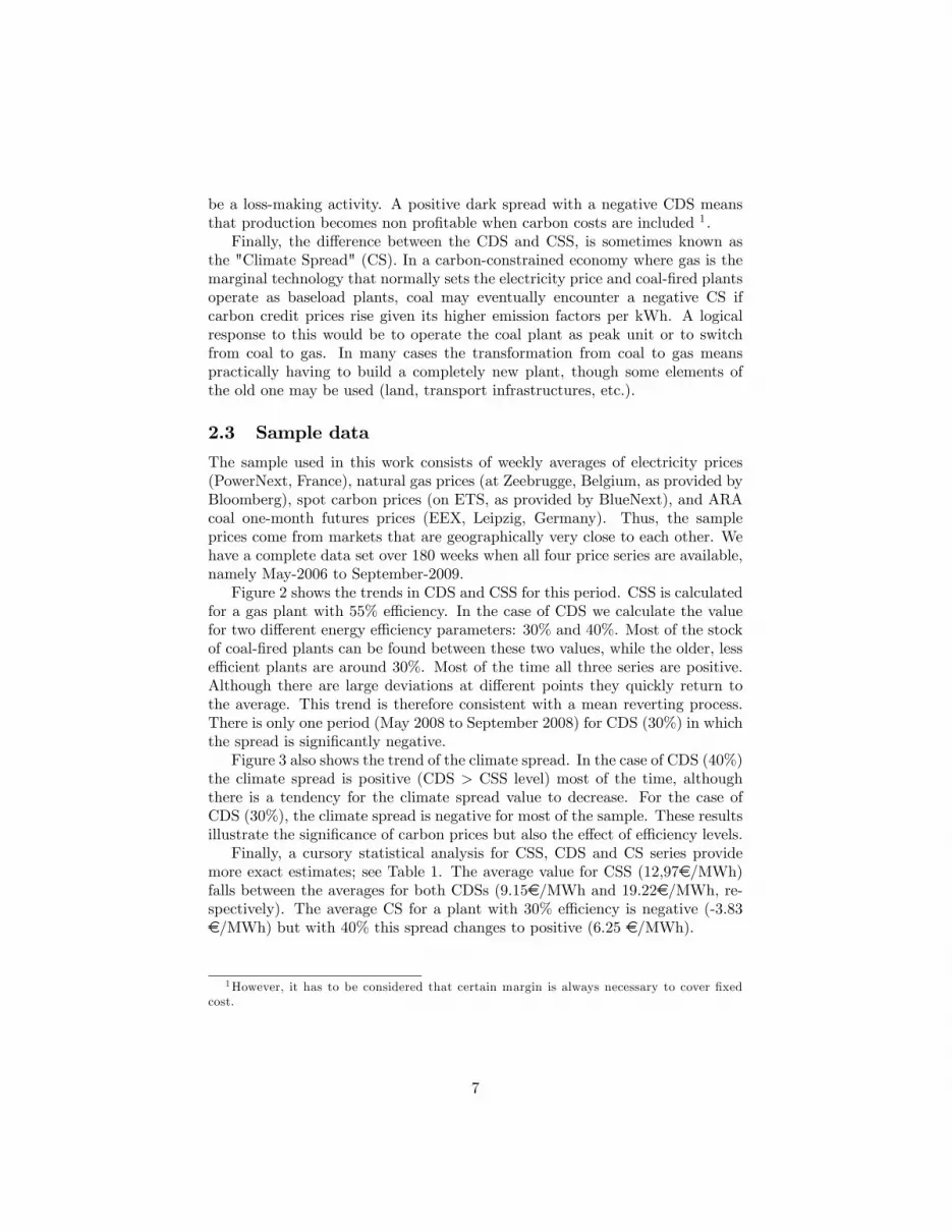
The sample used in this work consists of weekly averages of electricity prices(PowerNext, France), natural gas prices (at Zeebrugge, Belgium, as provided byBloomberg), spot carbon prices (on ETS, as provided by BlueNext), and ARAcoal one-month futures prices (EEX, Leipzig, Germany). Thus, the sampleprices come from markets that are geographically very close to each other. Wehave a complete data set over 180 weeks when all four price series are available,namely May-2006 to September-2009.Figure 2 shows the trends in CDS and CSS for this period. CSS is calculated
for a gas plant with 55% e¢ ciency. In the case of CDS we calculate the valuefor two di¤erent energy e¢ ciency parameters: 30% and 40%. Most of the stockof coal-�red plants can be found between these two values, while the older, lesse¢ cient plants are around 30%. Most of the time all three series are positive.Although there are large deviations at di¤erent points they quickly return tothe average. This trend is therefore consistent with a mean reverting process.There is only one period (May 2008 to September 2008) for CDS (30%) in whichthe spread is signi�cantly negative.Figure 3 also shows the trend of the climate spread. In the case of CDS (40%)
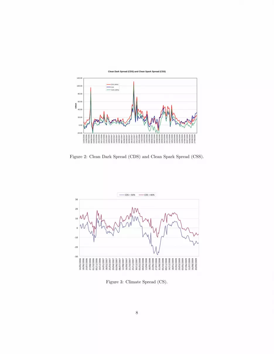
the climate spread is positive (CDS > CSS level) most of the time, althoughthere is a tendency for the climate spread value to decrease. For the case ofCDS (30%), the climate spread is negative for most of the sample. These resultsillustrate the signi�cance of carbon prices but also the e¤ect of e¢ ciency levels.Finally, a cursory statistical analysis for CSS, CDS and CS series provide
more exact estimates; see Table 1. The average value for CSS (12,97e/MWh)falls between the averages for both CDSs (9.15e/MWh and 19.22e/MWh, re-spectively). The average CS for a plant with 30% e¢ ciency is negative (-3.83e/MWh) but with 40% this spread changes to positive (6.25 e/MWh).
1However, it has to be considered that certain margin is always necessary to cover �xedcost.
7
Clean Dark Spread (CDS) and Clean Spark Spread (CSS)
20.00
0.00
20.00
40.00
60.00
80.00
100.00
120.00
14/0
5/20
0611
/06/
2006
09/0
7/20
0606
/08/
2006
03/0
9/20
0601
/10/
2006
29/1
0/20
0626
/11/
2006
24/1
2/20
0621
/01/
2007
18/0
2/20
0718
/03/
2007
15/0
4/20
0713
/05/
2007
10/0
6/20
0708
/07/
2007
05/0
8/20
0702
/09/
2007
30/0
9/20
0728
/10/
2007
25/1
1/20
0723
/12/
2007
20/0
1/20
0817
/02/
2008
16/0
3/20
0813
/04/
2008
11/0
5/20
0808
/06/
2008
06/0
7/20
0803
/08/
2008
31/0
8/20
0828
/09/
2008
26/1
0/20
0823
/11/
2008
21/1
2/20
0818
/01/
2009
15/0
2/20
0915
/03/
2009
12/0
4/20
0910
/05/
2009
07/0
6/20
0905
/07/
2009
02/0
8/20
0930
/08/
2009
27/0
9/20
09
€/M
wh
CDS (40%)
CSS
"CDS (30%)
Figure 2: Clean Dark Spread (CDS) and Clean Spark Spread (CSS).
30
20
10
0
10
20
30
14/0
5/20
0618
/06/
2006
23/0
7/20
06
27/0
8/20
0601
/10/
2006
05/1
1/20
0610
/12/
2006
14/0
1/20
0718
/02/
2007
25/0
3/20
07
29/0
4/20
0703
/06/
2007
08/0
7/20
0712
/08/
2007
16/0
9/20
0721
/10/
2007
25/1
1/20
07
30/1
2/20
0703
/02/
2008
09/0
3/20
0813
/04/
2008
18/0
5/20
0822
/06/
2008
27/0
7/20
0831
/08/
2008
05/1
0/20
0809
/11/
2008
14/1
2/20
08
18/0
1/20
0922
/02/
2009
29/0
3/20
0903
/05/
2009
07/0
6/20
0912
/07/
2009
16/0
8/20
09
20/0
9/20
09CDS = 30% CDS = 40%
Figure 3: Climate Spread (CS).
8
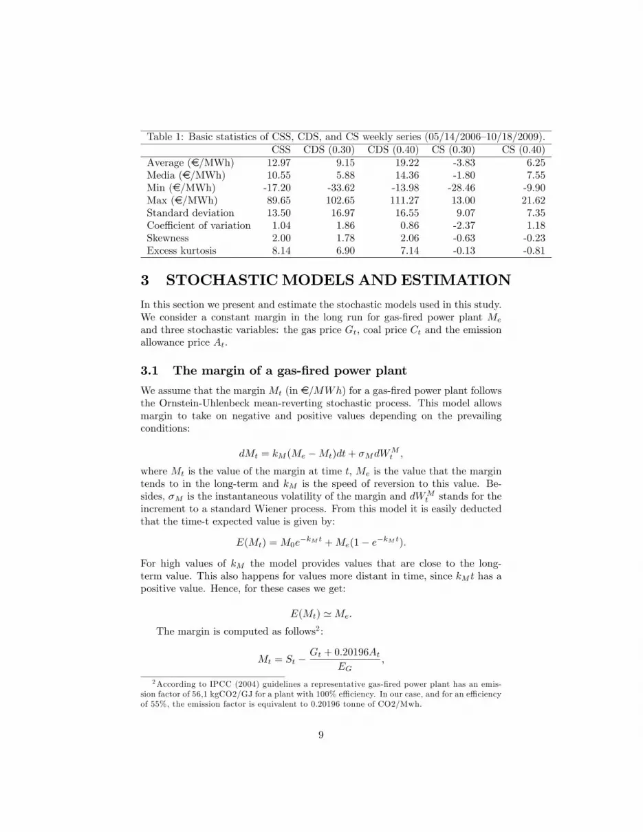
Table 1: Basic statistics of CSS, CDS, and CS weekly series (05/14/2006�10/18/2009).CSS CDS (0.30) CDS (0.40) CS (0.30) CS (0.40)
Average (e/MWh) 12.97 9.15 19.22 -3.83 6.25Media (e/MWh) 10.55 5.88 14.36 -1.80 7.55Min (e/MWh) -17.20 -33.62 -13.98 -28.46 -9.90Max (e/MWh) 89.65 102.65 111.27 13.00 21.62Standard deviation 13.50 16.97 16.55 9.07 7.35Coe¢ cient of variation 1.04 1.86 0.86 -2.37 1.18Skewness 2.00 1.78 2.06 -0.63 -0.23Excess kurtosis 8.14 6.90 7.14 -0.13 -0.81
3 STOCHASTICMODELS ANDESTIMATION
In this section we present and estimate the stochastic models used in this study.We consider a constant margin in the long run for gas-�red power plant Me
and three stochastic variables: the gas price Gt, coal price Ct and the emissionallowance price At.
3.1 The margin of a gas-�red power plant
We assume that the marginMt (in e=MWh) for a gas-�red power plant followsthe Ornstein-Uhlenbeck mean-reverting stochastic process. This model allowsmargin to take on negative and positive values depending on the prevailingconditions:
dMt = kM (Me �Mt)dt+ �MdWMt ;
where Mt is the value of the margin at time t, Me is the value that the margintends to in the long-term and kM is the speed of reversion to this value. Be-sides, �M is the instantaneous volatility of the margin and dWM
t stands for theincrement to a standard Wiener process. From this model it is easily deductedthat the time-t expected value is given by:
E(Mt) =M0e�kM t +Me(1� e�kM t):
For high values of kM the model provides values that are close to the long-term value. This also happens for values more distant in time, since kM t has apositive value. Hence, for these cases we get:
E(Mt) 'Me:
The margin is computed as follows2 :
Mt = St �Gt + 0:20196At
EG;
2According to IPCC (2004) guidelines a representative gas-�red power plant has an emis-sion factor of 56,1 kgCO2/GJ for a plant with 100% e¢ ciency. In our case, and for an e¢ ciencyof 55%, the emission factor is equivalent to 0.20196 tonne of CO2/Mwh.
9
where S denotes electricity price (e=MWh), G is the price of natural gas(e=MWh), EG is the net thermal e¢ ciency of a gas plant, and A is the priceof a EU emission allowance (e=tCO2).Estimation. In order to estimate the margin of gas-�red power plants, we
use the sample data presented in Section 2.3. It contains observations for 180weeks ranging between 05/14/2006 and 10/18/2009. We use the following OLSregression model to estimate the parameter Me:
Mt+�t = aM + bMMt + "t+�t:
Hence we obtained:
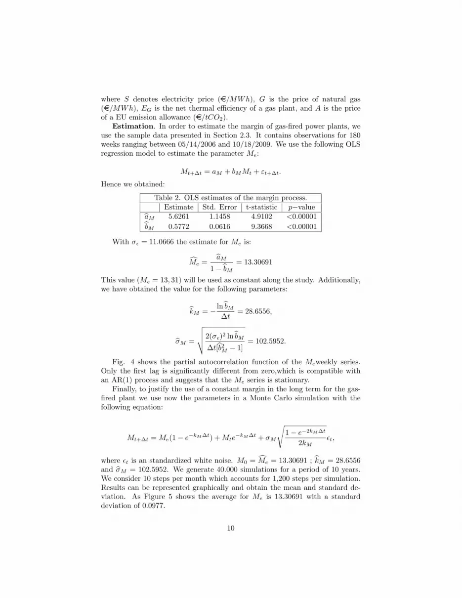
Table 2. OLS estimates of the margin process.Estimate Std. Error t-statistic p�valuebaM 5.6261 1.1458 4.9102 <0.00001bbM 0.5772 0.0616 9.3668 <0.00001
With �� = 11:0666 the estimate for Me is:
cMe =baM
1�bbM = 13:30691
This value (Me = 13; 31) will be used as constant along the study. Additionally,we have obtained the value for the following parameters:
bkM = � lnbbM�t
= 28:6556;
b�M =
vuut2(��)2 lnbbM�t[bb2M � 1]
= 102:5952:
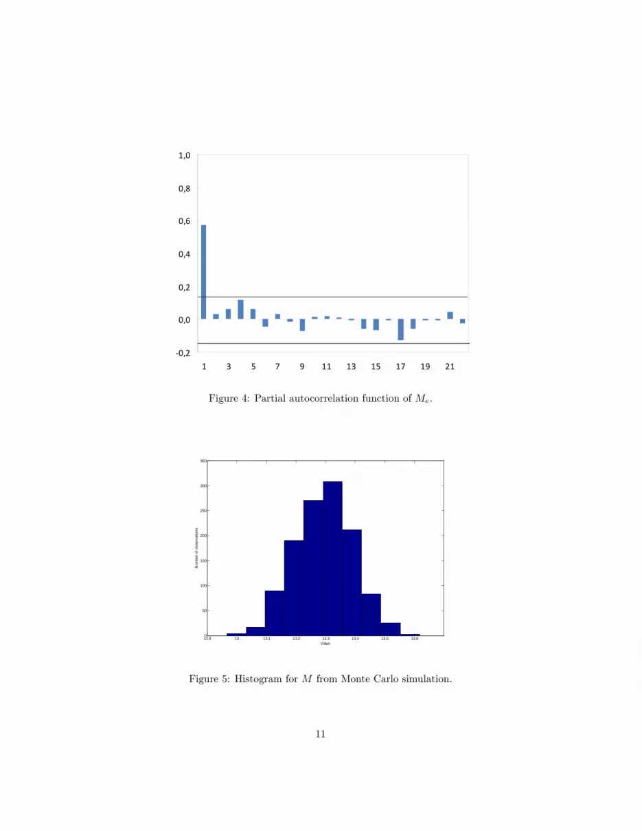
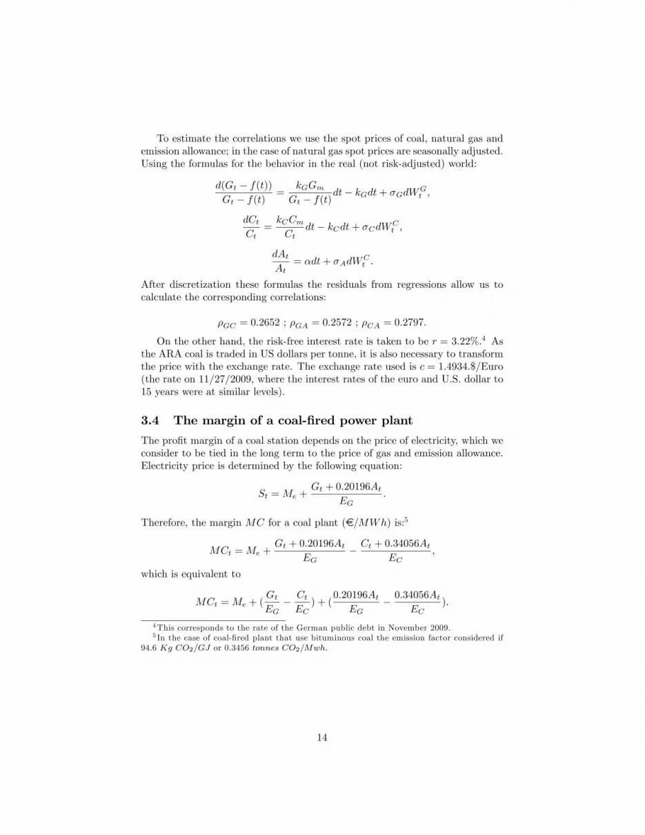
Fig. 4 shows the partial autocorrelation function of the Meweekly series.Only the �rst lag is signi�cantly di¤erent from zero,which is compatible withan AR(1) process and suggests that the Me series is stationary.Finally, to justify the use of a constant margin in the long term for the gas-
�red plant we use now the parameters in a Monte Carlo simulation with thefollowing equation:
Mt+�t =Me(1� e�kM�t) +Mte�kM�t + �M
s1� e�2kM�t
2kM�t;
where �t is an standardized white noise. M0 = cMe = 13:30691 ; bkM = 28:6556and b�M = 102:5952. We generate 40.000 simulations for a period of 10 years.We consider 10 steps per month which accounts for 1,200 steps per simulation.Results can be represented graphically and obtain the mean and standard de-viation. As Figure 5 shows the average for Me is 13.30691 with a standarddeviation of 0.0977.
10
0,2
0,0
0,2
0,4
0,6
0,8
1,0
1 3 5 7 9 11 13 15 17 19 21
Figure 4: Partial autocorrelation function of Me.
12.9 13 13.1 13.2 13.3 13.4 13.5 13.60
50
100
150
200
250
300
350
Value
Num
ber o
f obs
erva
tions
Figure 5: Histogram for M from Monte Carlo simulation.
11

3.2 Stochastic Models for natural gas, coal, and carbon
We specify the long-term prices as mean-reverting stochastic processes describedby the following system of di¤erential equations in a risk-neutral world:
dGt = df(t) + [kG(Gm � (Gt � f(t)))� �G(Gt � f(t))]dt+ �G(Gt � f(t))dWGt =
= df(t) + [kGGm � (kG + �G)(Gt � f(t))]dt+ �G(Gt � f(t))dWGt ;
dCt = [kC(Cm � Ct)� �CCt]dt+ �CCtdWCt ;
dAt = (�� �A)Atdt+ �AAtdWAt ;
with:
dWGt dW
Ct = �GCdt ; dW
Gt dW
At = �GAdt ; dW
Ct dW
At = �CAdt:
Regarding notation, Gt , Ct and At are the price at time t of natural gas, coaland carbon. Gm and Cm are the levels to which deseasonalized natural gas andcoal prices tend in the long run. f(t) is a deterministic function that capturesthe e¤ect of seasonality in natural gas prices. This function is de�ned as followsf(t) = cos(2�(t+ ')), where the time t is measured in years and the angle inradians; when f(t = �')= the seasonal maximum value is reached. kG and kCare the speed of reversion towards the �normal�level of gas and coal. They canbe computed as kG = ln 2=tG1=2, where t
G1=2 is the expected half-life for natural
gas deseasonalized, i.e. the time required for the gap between G0�f(0) and Gmto halve; similarly kC = ln 2=tC1=2. � is the drift rate of carbon price. �G , �Cand �A are the instantaneous volatility of natural gas, coal and carbon, whichdetermines the variances at t of Gt, Ct and At. �G, �C and �A are the riskpremium for gas, coal and carbon. dWG
t , dWCt and dWA
t are the increments toa standard Wiener process. They are normally distributed with mean zero andvariance dt.The time�0 expected value of gas price at time t, or equivalently the futures
price of natural gas for delivery at t, is:
F (G0; t) = E(Gt) = f(t) +kGGmkG + �G
[1� e�(kG+�G)t] + (G0 � f(0))e�(kG+�G)t:
In this case, F (G0;1)� f(1) = kGGm=(kG + �G).In the case of a commodity that is traded for a period, e.g., when an amount
of natural gas equivalent to 1 MWh is delivered every hour over a month, wecan compute
12

F (G0; �2; �1) =1
�2 � �1
Z �2
�1
f(t)dt+1
�2 � �1
Z �2
�1
[E(Gt)� f(t)]dt =
=1
2�
1
�2 � �1 [sin(2�(�2 + '))� sin(2�(�1 + '))] +
+kGGmkG + �G
+1
�2 � �1(G0 � f(0))� kGGm
kG+�G
kG + �G
he�(kG+�G)�1 � e�(kG+�G)�2
i:
The same equation applies for the case of coal, but without seasonality:
F (C0; �2; �1) =1
�2 � �1
Z �2
�1
E(Ct)dt =
=kCCmkC + �C
+1
�2 � �1C0 � kCCm
kC+�C
kC + �C
he�(kC+�C)�1 � e�(kG+�G)�2
i:
Concerning the price of the emission allowance we adopt a GMB process.The expression for the futures price is a particular case of that used for the fuelcommodity, speci�cally:
F (A0; t) = E(At) = A0e(���A)t:
3.3 Estimation
We estimate the parameters in the three stochastic models using daily pricesand non-linear least-squares. The sample period stretches from 01/02/2009 to11/27/2009, i.e., 231 days. The data available on each day include futures pricesof contracts with monthly, quarterly, seasonal3 and yearly maturities.In Table 3 we show the results from this estimation. The second column
present the estimated value and the third a con�dence interval of 95%.
Table 3:Parameter Value Interval 95%C�m =
kCCmkC+�C
105.27 101.57 108.96kC + �C 0.69 0.58 0.79
G�m =kGGm
kG+�G25.04 24.04 26.04
kG + �G 0.85 0.65 1.05' (days) -21.7 -33.20 -10.24
3.29 2.64 3.93�� � �� �A 0.054 0.048 0.061
�A 0.4879
3The seasonal natural gas futures prices include two semester seasons: April-Septemberand October-March.
13
To estimate the correlations we use the spot prices of coal, natural gas andemission allowance; in the case of natural gas spot prices are seasonally adjusted.Using the formulas for the behavior in the real (not risk-adjusted) world:
d(Gt � f(t))Gt � f(t)
=kGGmGt � f(t)
dt� kGdt+ �GdWGt ;
dCtCt
=kCCmCt
dt� kCdt+ �CdWCt ;
dAtAt
= �dt+ �AdWCt :
After discretization these formulas the residuals from regressions allow us tocalculate the corresponding correlations:
�GC = 0:2652 ; �GA = 0:2572 ; �CA = 0:2797:
On the other hand, the risk-free interest rate is taken to be r = 3.22%.4 Asthe ARA coal is traded in US dollars per tonne, it is also necessary to transformthe price with the exchange rate. The exchange rate used is c = 1:4934:$/Euro(the rate on 11/27/2009, where the interest rates of the euro and U.S. dollar to15 years were at similar levels).
3.4 The margin of a coal-�red power plant
The pro�t margin of a coal station depends on the price of electricity, which weconsider to be tied in the long term to the price of gas and emission allowance.Electricity price is determined by the following equation:
St =Me +Gt + 0:20196At
EG:
Therefore, the margin MC for a coal plant (e=MWh) is:5
MCt =Me +Gt + 0:20196At
EG� Ct + 0:34056At
EC;
which is equivalent to
MCt =Me + (GtEG
� CtEC
) + (0:20196AtEG
� 0:34056AtEC
):
4This corresponds to the rate of the German public debt in November 2009.5 In the case of coal-�red plant that use bituminous coal the emission factor considered if
94.6 Kg CO2=GJ or 0.3456 tonnes CO2=Mwh:
14
As a result, the margin at time t is a function of the three stochastic variables:the gas price, Gt, the coal price, Ct,6 and the emission allowance price, At,alongside the e¢ ciency parameters for coal EC and gas-�red power plants EG.At one level, the second term of the equation is positive (as the price gap
between gas and coal is normally positive), although is e¤ect main be reducedby the e¢ ciency parameter:
GtEG
� CtEC
:
On the other hand, the third term of the equation is negative. The emissionfactor of a coal plant is greater which implies that more emissions allowanceshould be paid. Similarly, the lower the e¢ ciency the greater the cost in termsof emissions:
0:20196AtEG
� 0:34056AtEC
:
Finally, when both price processes are expected to reach their long-term equi-librium levels we have:
GmEG
� CmEC
:
The evolution of the margins of the coal plants will be in�uenced by theevolution of the price of emission allowances. If they increase over time themargins will decline.We choose a e¢ ciency value for gas-�red plants EG = 0:55 and EC = 0:30
7 for coal plants. An e¢ ciency of 30% is a representative value for old coalplants, although the average value of the coal plant stock is around 40% (IPCC[16]). For a coal plant with EC = 0:30 emissions are 1.135 tCO2/MWh; forEC = 0:40 the emissions are 0.851 tCO2/MWh:
4 VALUING THE OPTION TO ABANDON
We assess the option to abandon an operating coal-�red power (in exchange fora salvage value) using a multidimensional lattice method8 . The value of a coalplant as considered in our model depends, primarily, on three price processes.Two of them follow a mean-reverting process (gas and coal) whereas the other
6Firstly, we transform coal Ara from USD/tonne to EUR/tonne using 1.4934 USD/EUR asexchange rate. Secondly, we transform from EUR/tonne to EUR/Mwh using the the followingfactors: 29.31 GJ/tonne and 1 GJ=0.27777 Mwh. Therefore: Ct(e=tonne)=29:31=0:2777 =Ct(e=Mwh)
7Data from new stations suggest e¢ ciency levels that are close to 40%.8Solutions for multi-dimensional options must resort to numerical methods which fall within
three main categories, namely: lattice methods, �nite di¤erence methods, and Monte Carlosimulation. Lattice methods are generally considered to be simpler, more �exible and, ifdimensionality is not too large, more e¢ cient than other methods.
15

one is governed by a standard GBM (emission allowances). The numerical es-timates are used in a three-dimensional binomial lattice to assess the value ofthe option to abandon. The methodology is similar to that in Boyle et al.[6] and Gamba and Trigeorgis [9], but our procedure allows for mean-revertingstochastic processes (as opposed to standard GBMs) and can be used to valueAmerican-type options (as opposed to European-type options). More informa-tion of this approach can be found in Abadie et al.[3].At time t, the option to abandon a coal-�red power plant will depend on
gas Gt , coal Ct and emission allowance At price process. In the base case weassume a remaining life of 10 years. Assuming 12 steps per year (�t = 1=12),the number of steps in the lattice are 120. Proceeding backwards through thelattice we get an amount which shows the value of the plant with its options9 .At �nal time T we assume a remaining value for the plant (RV ). At earliertimes we choose the best of the following three options:a) produce and continue:
PM (MCt � V C)�FC
12+ e�r�t(p�uuuW
+++ + p�uudW++� + p�uduW
+�+ +
+p�uddW+�� + p�duuW
�++ + p�dudW�+� + p�dduW
��+ + p�dddW���);
where V C (per MWh) is monthly variable cost (that included the fuel cost andthe CO2 emission allowance cost). FC is the �xed cost, computed monthly,that are also paid even if the plant is not producing.10
b) temporarily close down and wait:11
�FC12
+ e�r�t(p�uuuW+++ + p�uudW
++� + p�uduW+�+ + p�uddW
+�� +
+p�duuW�++ + p�dudW
�+� + p�dduW��+ + p�dddW
���):
c) abandon and obtain the remaining (salvage) value RV .12
Thus we obtain the value at the initial time (W0). By �xing some para-meters while changing another ones we can derive the optimal carbon pricesfor switching among states. The early exercise boundary is obtained when thevalue of the plant is equal to the residual value (W0 = RV ).The parameter values adopted, based on IEA [10], Tester et al. [25], and
U.S. DoE13 are the following:
9We assume a 500 MW coal plant with a capacity factor of 80%. This accounts for amonthly production of PM = 292; 000 MWh when operating and zero otherwise.10Both �xed and variable costs (FC, V C) are considered net of any potential subsidy.
Public subsidies would alter the decision making process.11We are assuming there are no cost associated to plant state changes, or that these costs
are negligible.12This residual value RV is considered net of abandonment costs (those of decommissioning
and others).13www.eia.doe.gov/oiaf/aeo/excel/aeo2010%20tab8%202.xls
16

� We assume a 500 MW coal plant with a capacity factor of 80%. Thisaccounts for a monthly production of PM = 292; 000MWh when operating(and zero otherwise).
� We assume a remaining value RV that is 25% of the investment in anew gas-�red plant14 . The remaining value depends of numerous speci�cfactors such as the value of land or some infrastructures associated. Foran average cost of 1,111.5 M$ for a 500 MW gas station (IEA [14]) andexchange rate 1.4943 $/e. The RV is 186.1 Me; its relevance is limitedas this value is obtained in any case at the end of the life of the facility.
� O&M �xed cost are 28.15 $/kW. This is equivalent to 785,400 e permonth.
� O&M variable cost are 4.69 $/MWh. This is equivalent to 3,14 e/MWh.
5 RESULTS
This section presents the results from the data and price models. To explore thefuture of coal-�red power plants in more detail we study di¤erent possibilitiesfor the main parameters considered in the base case. We focus on the impactof di¤erent relevant variables, such as allowance prices, allowance volatility, thecoal and gas prices, the e¢ ciency of coal-�red plants and their remaining valueand remaining life. Finally, we also study the impact of a situation where thepossibility of a coal-�red plant operating as a peak time plant is not available.
5.1 Results in the base case
Table 4 shows the total value of the coal-�red plant considered for di¤erentCO2 prices. The second column shows the total present value (in Me) for aplant with a remaining lifetime of 10 years. The third column shows the totalpresent value of a plant with 5 years remaining. The last column representsthe residual value. In the base case we assume a remaining value of 25% of theinitial investment in a gas plant. This value is therefore constant for all theprice scenarios.A coal-�red plant with 5 years of useful lifetime remaining, as shown in the
third column, would need to face CO2 prices of e80-90/tCO2 in order to decideto switch from operating to closing. The precise breakpoint price is e83.2/tCO2.Above this price the value of the plant if it continues in operation is exceededby its salvage value if it is abandoned. Since optimal management is requiredfor maximizing the plant value, above the trigger carbon price the option toabandon will be exercised, in which case the plant will be worth 186.1 Me; thus
14We assume that part of the initial investment can be used again, for instance the plot ofland.
17

keeping the plant alive is no longer optimal. In the case of an operating coal-�red plant with 10 years ahead (base case) the chances for closing are tighter;CO2 prices would have to reach e162.40/tCO2 to make the switch worthwhile.Figure 6 shows this result. The blue and red lines, respectively, show the
value of operating plants with remaining lifetimes of 5 and 10 years for di¤erentCO2 prices. The green line shows the residual value. Since operating a plantis a right, not an obligation, its value cannot be lower than the abandonmentvalue. As can be seen, for low CO2 prices, the best decision is to operate, andfor higher prices the values start to converge to the residual value. When theblue and red lines merge with the green line keeping the plant operative is nolonger a rational decision.These base case results show that a very restrictive situation is necessary
before coal-�red power plants are abandoned for other alternatives. For 10years of remaining lifetime the CO2 price needed for this to occur is almost tentimes the average value of CO2 on the ETS market. However, an interestingpoint shown in Figure 6 is that when a coal-�red plant gets older the value ofoperating decreases, i.e. the blue and red lines move down leftward. Therefore,although CO2 prices alone are very unlikely to make a plant close they cancertainly bring forward this decision.
Table 4. Value of the option to operate or abandon (Me).At (e/tCO2) Operate (RL =10y) Operate (RL =5y) Residual Value
10 574.2 356.0 186.120 451.9 287.4 186.130 375.2 246.5 186.140 323.8 221.1 186.150 287.5 205.1 186.160 261.3 195.2 186.170 241.8 189.4 186.180 227.1 186.6 186.190 215.9 186.1 186.1100 207.4 186.1 186.1110 200.8 186.1 186.1120 195.9 186.1 186.1130 192.2 186.1 186.1140 189.5 186.1 186.1150 187.8 186.1 186.1160 186.6 186.1 186.1170 186.1 186.1 186.1180 186.1 186.1 186.1190 186.1 186.1 186.1
18

0
100
200
300
400
500
600
10 30 50 70 90 110 130 150 170Allowance price ( At )
Val
ue (M
€)
Operate RL=5 yearsOperate RL=10 years (Base)Abandon
Figure 6: Value of the option to operate or abandon as a function of the al-lowance price (At).
19

5.2 Sensitivity analysis
5.2.1 Sensitivity to changes in allowance price
CO2 prices have been very volatile over the �rst �ve years of functioning ofthe Emissions Trading Scheme (EU ETS) in Europe. In Phase I (2005-2007)the CO2 futures prices for 2007 delivery ranged between almost e0 and e30per ton of CO2 just in the twelve months from May 2006 to May 2007. Sofar, in Phase II (2008-2012) allowance future prices have been relatively morestable, but they still ranged between e15 and e25 per ton. Upon the economicrecession prices have dropped between e10 and e18 per ton from January 2009to October 2009.In this section we analyze the e¤ect of CO2 price volatility together with the
remaining life (RL) of the plant. Given the past trend, the �gure for volatilityof CO2 prices used in this study in the base case scenario can be considered asan upper value. As this could change in the future, so a sensitivity analysis ofthis parameter is vital.Table 5 shows the e¤ect of volatility. Each row represents the threshold
CO2 price at which it is worth exercising the option to abandon the plant. Thecolumns represent three alternatives considered for the remaining lifetime of theplant: 5, 10 (the base case) and 15 years.The result for a plant with a residual lifetime of 10 years shows that the
higher the volatility is the higher the CO2 price required to trigger the optionto abandon the plant is. High volatility means that very high CO2 prices arepossible, but also very low ones. As coal-�red plants always have the possibilityof producing or waiting for better conditions, high volatility negatively a¤ectsthe abandonment option. coal-�re plants enjoy the bene�ts of producing whenCO2 prices are low, but when prices are high they can always decide to waitand assume only the �xed cost. For a volatility of 0.05 the price for plant withRL = 5 years abandonment would be e39:1=tCO2. If volatility increases to0:2 or to 0:5 the price also with RL = 5 increases to e44:4and e86:3=tCO2,respectively.This result is also sensitive to the remaining life (RL) parameter. The higher
RL considered is, the higher the CO2 required to trigger the option to abandonthe plant is . A longer residual lifetime means more possibilities of obtainingpro�ts through production. Again, under those circumstances when the con-ditions are not favorable the plant can simply wait. Since residual value isconsidered as �xed and proportional to the initial investment in the plant, it isobvious that a longer RL means more value in the option to continue.Figure 7 shows this trend. The top left part of each line represents the
abandonment option and the bottom right part the operation region. The linerepresents exactly the threshold between the two options for the three alterna-tive RLs. The e¤ect of RL is not to be very great for low volatility levels butwhen volatility increases the di¤erence is not negligible. For a volatility of 0.3the optimal price of CO2 is e52.7/tCO2 for 5 years, e73.8/tCO2 for 10 yearsand e88.5/tCO2 for 15 years.
20

020406080
100120140160180
0,05 0,1 0,2 0,3 0,4 0,5Allowance price volatility (σA)
Opt
imal
car
bon
pric
e ( A
t )
RL = 5 yearsRL = 10 years (Base)RL = 15 years
Abandon region
Operate region
Figure 7: Threshold allowance price (At) for di¤erent residual life (RL) as afunction of allowance price volatility (�A).
Table 5. Sensitivity to changes in allowance volatility (�� = 0:054).�A RL =5y RL =10y RL =15y0.05 39.1 41.8 42.00.1 40.0 43.9 44.60.2 44.4 54.1 58.60.3 52.7 73.8 88.50.4 66.0 109.9 151.20.5 86.3 176.5 270.5
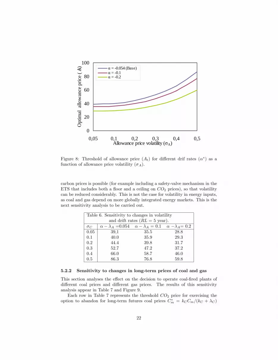
We can also analyze the e¤ect of a change in the parameter referring toan increase in the slope �� � � � �A of price in the futures markets, in thecontext of the allowance price, and separately from volatility. Table 6 showsthe results for the base case parameter and expected growth rates of 10 and20 percent for the case of a coal-�red plant with an RL of 5 years. The resultsshow that the expectation of higher allowance prices in the future means a lowerprice of CO2 for triggering abandonment. Therefore, as Figure 8 suggests, fora 20% growth in expected price and volatility below 0.3, prices of around 30e/tCO2are enough to trigger abandonment of plants.Finally, as we have seen, high volatility in CO2 prices signi�cantly delays the
abandonment of coal and, therefore, the possibilities of encouraging other invest-ments in low-carbon technologies. Hopefully, a regime with more predictable
21
0
20
40
60
80
100
0,05 0,1 0,2 0,3 0,4 0,5Allowance price volatility (σA)
Opt
imal
allo
wan
ce p
rice
( At) α = 0.054 (Base)
α = 0.1α = 0.2
Figure 8: Threshold of allowance price (At) for di¤erent drif rates (��) as afunction of allowance price volatility (�A).
carbon prices is possible (for example including a safety-valve mechanism in theETS that includes both a �oor and a ceiling on CO2 prices), so that volatilitycan be reduced considerably. This is not the case for volatility in energy inputs,as coal and gas depend on more globally integrated energy markets. This is thenext sensitivity analysis to be carried out.
Table 6. Sensitivity to changes in volatilityand drift rates (RL = 5 year).
�C �� �A =0.054 �� �A = 0.1 � ��A= 0.20.05 39,1 35.5 28.80.1 40.0 35.9 29.30.2 44.4 39.8 31.70.3 52.7 47.2 37.20.4 66.0 58.7 46.00.5 86.3 76.8 59.8
5.2.2 Sensitivity to changes in long-term prices of coal and gas
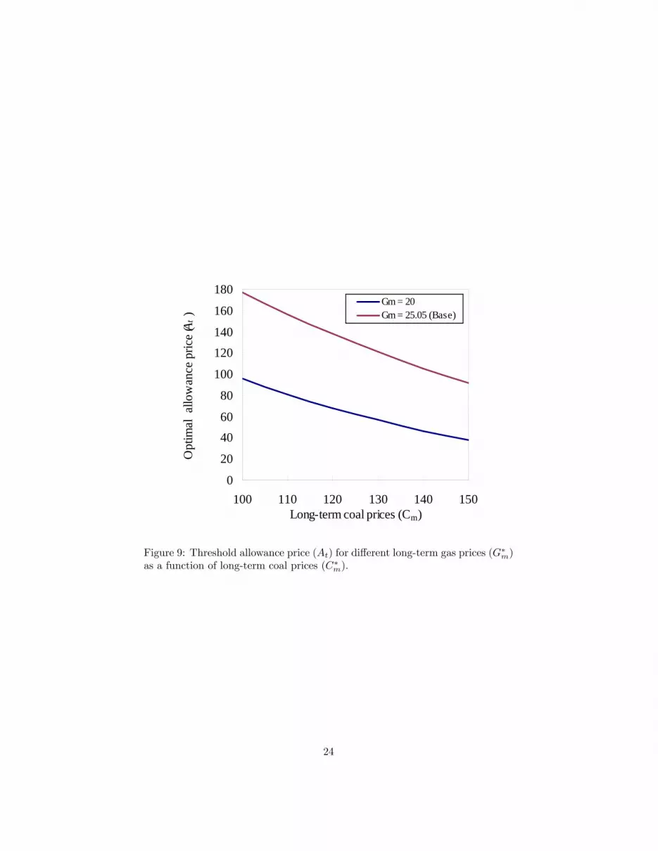
This section analyses the e¤ect on the decision to operate coal-�red plants ofdi¤erent coal prices and di¤erent gas prices. The results of this sensitivityanalysis appear in Table 7 and Figure 9.Each row in Table 7 represents the threshold CO2 price for exercising the
option to abandon for long-term futures coal prices C�m = kCCm=(kC + �C)
22

$/tcoal increasing from 100 (units) to 150. The columns represent the twoalternatives considered for long-term deseasonalized futures gas prices G�m =kGGm=(kG + �G) e/MWh: 25.04 (base case) and 20. These two alternativesare represented in Figure 9 by red and blue lines respectively. The result forthe base case shows that as the price of coal increases the CO2 price needed totrigger the option to abandon drops. For a coal price of 100 $/tonne the CO2price for making the switch e¤ective is e176.8/tCO2. When it increases to 120$/tonne the threshold price decreases to e138/tCO2 and when it reaches 150the latter price drops to e91/tCO2. This trend is shown in Figure 9, where thistime the right-hand parts of the lines represent the abandonment region andthe left-hand part represent the operation region.From the table and the �gure the great impact of variation in gas prices is
also very clear. If the price of gas decreases it is more likely that coal-�red plantswill be abandoned, as the threshold price of CO2 moves down. This impact canbe shown by the gap between the red and blue lines.Conversely, only very high CO2 prices could o¤set an increase in gas prices.
In fact, for a coal price of 100 $/tonne an increase in gas prices from 20 e/MWh(base case) to 25.04 causes the optimal price of CO2 to rocket from e95.6/tCO2to e176.8/tCO2. This means that a 25% increase in the price of gas needs anincrease of 85% in the price of CO2.
Table 7. Sensitivity to changesin long-term coal and gas prices.C�m G�m=20 G�m=25.05100 95.6 176.8110 81.0 156.3120 67.9 138.0130 56.6 120.9140 46.4 105.3150 37.9 91.6
5.3 Sensitivity to changes in useful life and residual valueof the coal plant
The decision whether to abandon a coal-�red plant in operation is also a¤ectedby the remaining life of the plant. In this section we analyze the e¤ect of thisvariable together with the residual value.The results appear in Table 8. Each row represents the threshold CO2 price
for triggering the option to abandon the plant for di¤erent remaining usefullifetimes ranging from 1 to 10 years. The columns represent three alternativesconsidered for the residual value of the plant: 0%, 25% (the base case) and 50%of the investment cost. In the �rst alternative we are assuming that there isno inherent value in the plant to be recovered and, therefore, the value of theoption to abandon is zero. In this case the abandonment option would be chosenonly if the present value of continuing in operation is negative.
23
0
20
4060
80
100
120140
160
180
100 110 120 130 140 150Longterm coal prices (Cm)
Opt
imal
allo
wan
ce p
rice
(At
)
Gm = 20Gm = 25.05 (Base)
Figure 9: Threshold allowance price (At) for di¤erent long-term gas prices (G�m)as a function of long-term coal prices (C�m).
24
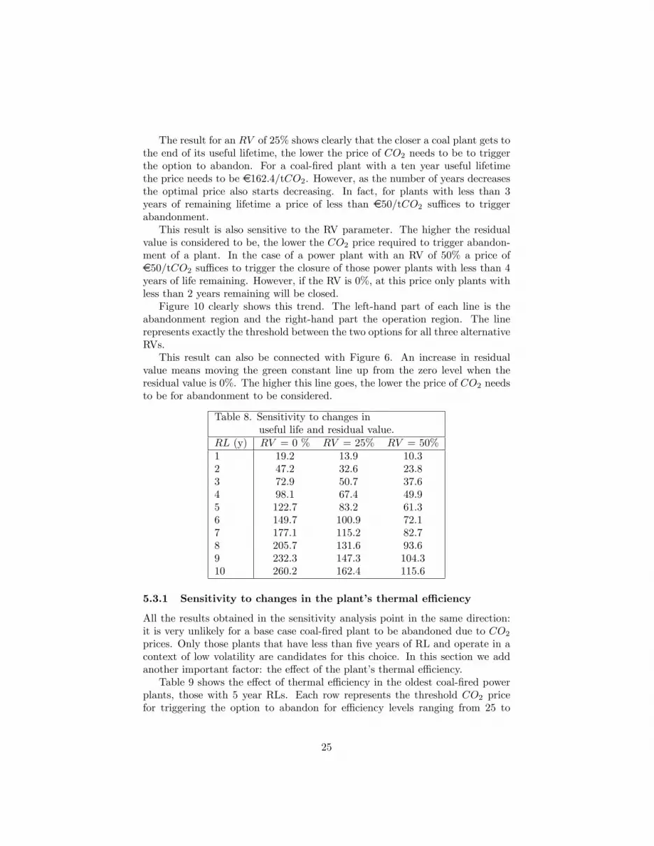
The result for an RV of 25% shows clearly that the closer a coal plant gets tothe end of its useful lifetime, the lower the price of CO2 needs to be to triggerthe option to abandon. For a coal-�red plant with a ten year useful lifetimethe price needs to be e162.4/tCO2. However, as the number of years decreasesthe optimal price also starts decreasing. In fact, for plants with less than 3years of remaining lifetime a price of less than e50/tCO2 su¢ ces to triggerabandonment.This result is also sensitive to the RV parameter. The higher the residual
value is considered to be, the lower the CO2 price required to trigger abandon-ment of a plant. In the case of a power plant with an RV of 50% a price ofe50/tCO2 su¢ ces to trigger the closure of those power plants with less than 4years of life remaining. However, if the RV is 0%, at this price only plants withless than 2 years remaining will be closed.Figure 10 clearly shows this trend. The left-hand part of each line is the
abandonment region and the right-hand part the operation region. The linerepresents exactly the threshold between the two options for all three alternativeRVs.This result can also be connected with Figure 6. An increase in residual
value means moving the green constant line up from the zero level when theresidual value is 0%. The higher this line goes, the lower the price of CO2 needsto be for abandonment to be considered.
Table 8. Sensitivity to changes inuseful life and residual value.
RL (y) RV = 0 % RV = 25% RV = 50%1 19.2 13.9 10.32 47.2 32.6 23.83 72.9 50.7 37.64 98.1 67.4 49.95 122.7 83.2 61.36 149.7 100.9 72.17 177.1 115.2 82.78 205.7 131.6 93.69 232.3 147.3 104.310 260.2 162.4 115.6
5.3.1 Sensitivity to changes in the plant�s thermal e¢ ciency
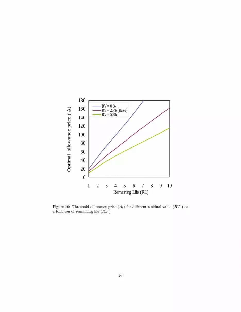
All the results obtained in the sensitivity analysis point in the same direction:it is very unlikely for a base case coal-�red plant to be abandoned due to CO2prices. Only those plants that have less than �ve years of RL and operate in acontext of low volatility are candidates for this choice. In this section we addanother important factor: the e¤ect of the plant�s thermal e¢ ciency.Table 9 shows the e¤ect of thermal e¢ ciency in the oldest coal-�red power
plants, those with 5 year RLs. Each row represents the threshold CO2 pricefor triggering the option to abandon for e¢ ciency levels ranging from 25 to
25
020406080
100120140160180
1 2 3 4 5 6 7 8 9 10Remaining Life (RL)
Opt
imal
allo
wan
ce p
rice
( A t
) RV = 0 %RV = 25% (Base)RV = 50%
Figure 10: Threshold allowance price (At) for di¤erent residual value (RV ) asa function of remaining life (RL ).
26
0
20
40
60
80
100
120
140
25 27,5 30 32,5 35Thermal Efficienciy (EC)
Opt
imal
allo
wan
ce p
rice
( At )
σA = 0.1σA = 0.3σA = 0.5
Figure 11: Threshold allowance price (At) for di¤erent allowance price volatility(�A) as a function of thermal e¢ ciency (EC).
35%. The columns represent three alternatives considered for the volatility ofthe plant: 0.1, 0.3 and 0.5.The results show clearly that the more e¢ cient the plant the higher the
price of CO2 needs to be to trigger the option to abandon. For a volatility �A=0.3 and e¢ ciency EC = 30% the price needs to be 52.7 e/tCO2. However, ase¢ ciency decreases to 25% this price falls to 33.4 e/tCO2. With volatility ofless than 0.1 the optimal price decreases from 56.2 e/tCO2 for an e¢ ciency of35% to 26.2 e/tCO2 for an e¢ ciency of 25%. This trend can be seen in Figure11.
Table 9. Sensitivity to changes in thermale¢ ciency and allowance price volatility (RL = 5y).EC (%) �A = 0.1 �A = 0.3 �A= 0.525 26.2 33.4 52.327,5 32.8 42.6 68.530 39.9 52.7 86.332,5 47.5 63.6 106.135 56.2 75.8 128.1
5.4 Results for the case of no �exibility
The above sections analyze the circumstances under which coal-�red plantswould opt-out. Results and sensitivity analyses show that this option is very
27
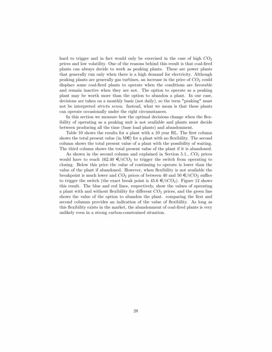
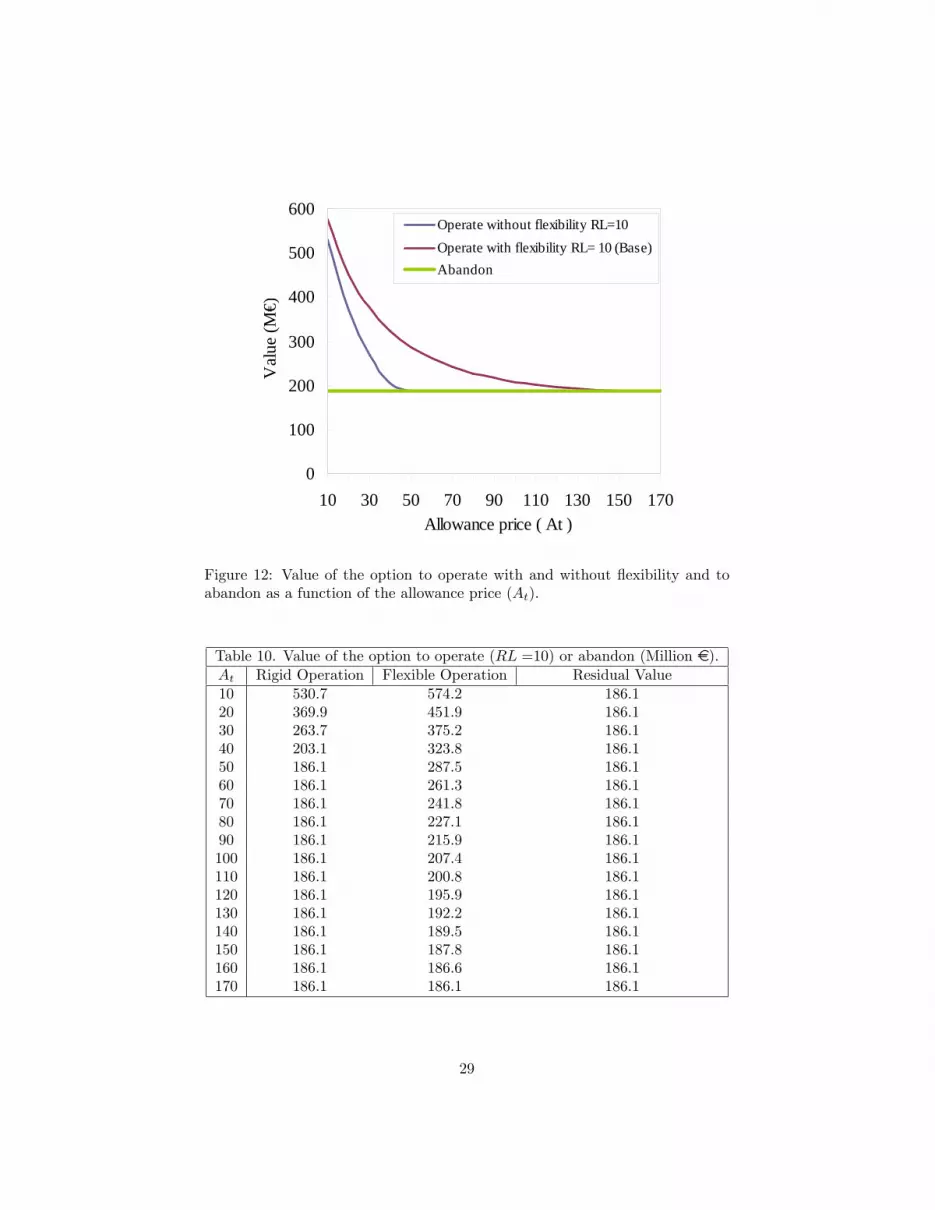
hard to trigger and in fact would only be exercised in the case of high CO2prices and low volatility. One of the reasons behind this result is that coal-�redplants can always decide to work as peaking plants. These are power plantsthat generally run only when there is a high demand for electricity. Althoughpeaking plants are generally gas turbines, an increase in the price of CO2 coulddisplace some coal-�red plants to operate when the conditions are favorableand remain inactive when they are not. The option to operate as a peakingplant may be worth more than the option to abandon a plant. In our case,decisions are taken on a monthly basis (not daily), so the term "peaking" mustnot be interpreted strictu sensu. Instead, what we mean is that these plantscan operate occasionally under the right circumstances.In this section we measure how the optimal decisions change when the �ex-
ibility of operating as a peaking unit is not available and plants must decidebetween producing all the time (base load plants) and abandonment.Table 10 shows the results for a plant with a 10 year RL. The �rst column
shows the total present value (in Me) for a plant with no �exibility. The secondcolumn shows the total present value of a plant with the possibility of waiting.The third column shows the total present value of the plant if it is abandoned.As shown in the second column and explained in Section 5.1., CO2 prices
would have to reach 162.40 e/tCO2 to trigger the switch from operating toclosing. Below this price the value of continuing to operate is lower than thevalue of the plant if abandoned. However, when �exibility is not available thebreakpoint is much lower and CO2 prices of between 40 and 50 e/tCO2 su¢ ceto trigger the switch (the exact break point is 45.6 e/tCO2). Figure 12 showsthis result. The blue and red lines, respectively, show the values of operatinga plant with and without �exibility for di¤erent CO2 prices, and the green lineshows the value of the option to abandon the plant. comparing the �rst andsecond columns provides an indication of the value of �exibility. As long asthis �exibility exists in the market, the abandonment of coal-�red plants is veryunlikely even in a strong carbon-constrained situation.
28
0
100
200
300
400
500
600
10 30 50 70 90 110 130 150 170Allowance price ( At )
Val
ue (M
€)
Operate without flexibility RL=10Operate with flexibility RL= 10 (Base)Abandon
Figure 12: Value of the option to operate with and without �exibility and toabandon as a function of the allowance price (At).
Table 10. Value of the option to operate (RL =10) or abandon (Million e).At Rigid Operation Flexible Operation Residual Value10 530.7 574.2 186.120 369.9 451.9 186.130 263.7 375.2 186.140 203.1 323.8 186.150 186.1 287.5 186.160 186.1 261.3 186.170 186.1 241.8 186.180 186.1 227.1 186.190 186.1 215.9 186.1100 186.1 207.4 186.1110 186.1 200.8 186.1120 186.1 195.9 186.1130 186.1 192.2 186.1140 186.1 189.5 186.1150 186.1 187.8 186.1160 186.1 186.6 186.1170 186.1 186.1 186.1
29

6 CONCLUDING REMARKS
Climate policy is altering the role of coal-�red power plants in the developedworld. Rising prices for carbon emissions will increase the risk associated to thistechnology if compared to other options such as gas, nuclear or renewable. Infact, although many utilities are not facing climate policy, the prospect of higherCO2 prices and environmental regulations is already altering utilities�decisions.Many projects for building new coal-�red power plants in the US and the EUhave been cancelled or delayed, even though electricity consumption has steadilybeen growing. CCS technology could be a solution for this dilemma, by settinga maximum price on coal-based electricity, but still needs to be developed. In anoptimist case CCS could be ready at commercial scale by 2020-2030 with a costper kW 32-62% higher if compared with the traditional pulverized coal powerplant. Therefore, there could be a period where the coal-�red plants wouldhave to face (presumably) high CO2 prices which will erode its pro�tability.This situation could be harder for those coal-�red plants that are older and lesse¢ cient. In the US around 75% of the total installed coal-�red capacity consistsof plants older than 35 years and in Europe 25% of the total stock have morethan 25 years.To date, several papers have analyzed the prospects for coal in a carbon-
constrained situation, using di¤erent approaches and techniques. This paperanalyzes the conditions under which a coal-�red station that is currently oper-ating could decide to abandon the plant and obtain its rescue value. We assessthis question from the viewpoint of a �rm following a real options approach.We consider a coal-�red power plant that operates under restrictions on carbondioxide emissions in an electricity market where gas-�red plants are the marginalunits that set the price of electricity. We consider three sources of uncertaintyor stochastic variables: the coal price, the gas price and the emission allowanceprice. The underlying parameters are derived from futures markets and areused in a three-dimensional binomial lattice to assess the value of the option toabandon.Our results show that the conditions that have to be satis�ed to abandon an
operational coal-�red plant are very hard to be met. Given the actual trends inprices a coal-�red plant with 5-10 years of useful lifetime remaining would needto face CO2 prices between 83.2-162.40 e/tCO2 in order to decide to switchfrom operating to closing. CO2 prices alone are very improbable to make aplant close as coal-�red plants. However, as the value of operating decreaseswhen the plant gets older, it can bring forward this decision.The sensitivity analysis conducted shows also the impact of di¤erent key
variables, such as coal, gas and CO2 allowance prices, the e¢ ciency of coal-�redplants or their residual (salvage) value and remaining life. One of the relevantfactors is the volatility of CO2 allowances prices. Allowance volatility has beenvery high in the past and reducing this uncertainty would be determinant. Afterall, this is a variable that reasonably can be reasonably kept under control withthe correct policy measures, such as introducing a �oor/ceiling in the CO2market or using a tax instrument.
30

Finally, these quantitative results show that although it seems very unlikelythat new coal-�red power plants will be built in the future in developed coun-tries, the existing ones will opt (if they can) to work as peaking plants and runonly when the conditions are favorable. This situation could displace the meritorder in some liberalized electricity markets.
References
[1] Abadie, L.M., Chamorro, J.M., (2008) European CO2 prices and carboncapture investments, Energy Economics, 30, 2992�3015.
[2] Abadie, L.M., Chamorro, J.M., (2009) Income risk of EU coal-�red powerplants after Kyoto, Energy Policy, 37(12), 5304-5316.
[3] Abadie, L.M., Chamorro, J.M.,González-Eguino, M. (2009) Optimal in-vestment in energy e¢ ciency under uncertainty, BC3 Working Paper Series,Bilbao.
[4] Ansolabehere, S., Beer, J., Deutch, J., Ellerman, A. D., Friedmann, S. J.,Herzog, H., et al. (2007) The future of coal. An interdisciplinary MIT study.Cambridge, USA.
[5] Barbose, G.,Wiser,R.,Phadke,A.,Goldman,C. (2008) Managing carbon reg-ulatory risk in utility resource planning: current practices in the WesternUnited States. Energy Policy, 36, 3300�3311.
[6] Boyle, P.P., Evnine, J. and Gibbs S. (1989) Numerical Evaluation of Mul-tivariate contingent Claims. Review of Financial Studies 2(2), 241-250.
[7] EIA (2003) Analysis of S.139, the Climate Stewardship Act of 2003. EnergyInformation Administration SR/OIAF/2003-02.
[8] EU (2001), Directive 2001/80/EC of the European Union Parliament andthe council on the limitation of emissions of certain pollutants into the airfrom large combustion plants, European Union, October 23, 2001.
[9] Gamba A. and Trigeorgis L. (2007) An improved binomial lattice methodfor multi-dimensional options. Applied Mathematical Finance 14(5), 453-475.
[10] IEA (2005) Projected costs of Generating Electricity, IEA and NuclearEnergy Agency, Paris.
[11] IEA (2005b) Prospect for Carbon Capture and Storage, OECD/IEA, Paris.
[12] IEA (2009) World Energy Outlook. OECD/IEA, Paris.
[13] IEA (2009b) How the energy sector can deliver on a climate agreement inCopenhagen, OECD/IEA, Paris.
31

[14] IEA (2010) The economics of transition in the power sector, InformationPaper, IEA, Paris.
[15] IPCC (2005) Special Report on Carbon Dioxide Capture and Storage. Pre-pared by Working Group III of the Intergovernmental Panel on ClimateChange [Metz, B.,O. Davidson, H. C. de coninck, M. Loos, and L. A.Meyer (eds.)]. Cambridge University Press, Cambridge, United Kingdomand New York, NY, USA.
[16] IPCC (2006) Guidelines for National Greenhouse Gas Inventaries, Paris.
[17] IPCC (2007) Fourth assessment report. Climate Change. Working GroupIII (WG III) Mitigation of Climate Change, Paris.
[18] NETL(2009) Tracking New coal-Fired Power Plants, National EnergyTechology Laboratory, US Departament of Energy.
[19] Laurikka, H., Koljonen, T., (2006) Emissions trading and investment de-cisions in the power sector: a case study in Finland. Energy Policy 34,1063�1074
[20] Lucia, J. and E.S. Schwartz, (2002) Electricity Prices and Power Deriva-tives: Evidence from the Nordic Power Exchange, Review of DerivativesResearch, 5(1), 5-50.
[21] McFarland, H.J., Paltsev, S. Jacoby, H.D. (2009) Analysis of the coal Sectorunder Carbon constraints, Journal of Policy Modeling, 31, 3, 404-424.
[22] McFarland, H.J., Herzog (2006) Incorporating carbon capture and storagetechnologies in integrated assessment models, Energy Economics, 28, 632�652
[23] Paltsev, S., Reilly, J., Jacoby, H. D., Eckaus, R. S., McFarland, J., Saro�m,M., et al. (2005) The MIT Emissions Prediction and Policy Analysis(EPPA) Model Version 4. MIT Joint Program on the Science and Policy ofGlobal Change, Report 125. Massachusetts Institute of Technology
[24] Schelling, Thomas C. (2007). Climate Change: The uncertainties, the cer-tainties, and what they imply about action. Economists�Voice, 4(3), article3.
[25] Tester, J. Drake, E, Driscoll, M. Golay, M., Peters, W. (2005), SustainableEnergy: Choosing Among Options. The MIT press, Cambridge, USA.
[26] Tzimas, E., Georgakaki, A., Peteves, S.D. (2009) Future fossil fuel electric-ity generation in Europe: options and consequences, JRC reports, Euro-pean comission.
32

BC3 WORKING PAPER SERIES
Basque Centre for Climate Change (BC3), Bilbao, Spain
The BC3 Working Paper Series is available on the internet at the following addresses:
http://www.bc3research.org/lits_publications.html
http://ideas.repec.org/s/bcc/wpaper.html
BC3 Working Papers available (see website for full list):
2009-04 Ibon Galarraga, Mikel González-Eguino and Anil Markandya: The Role of Regions in Climate Change Policy
2009-05 M.C. Gallastegui and Ibon Galarraga: Climate Change and Knowledge Communities
2009-06 Ramon Arigoni Ortiz and Anil Markandya: Literature Review of Integrated Impact Assessment Models of Climate Change with Emphasis on Damage Functions
2009-07 Agustin del Prado, Anita Shepherd, Lianhai Wu, Cairistiona Topp, Dominic Moran, Bert Tolkamp and David Chadwick: Modelling the Effect of Climate Change on Environmental Pollution Losses from Dairy Systems in the UK
2009-08 Ibon Galarraga and Anil Markandya: Climate Change and Its Socioeconomic Importance
2009-09 Julia Martin-Ortega and Anil Markandya: The Costs of Drought: the Exceptional 2007-2008 Case of Barcelona
2009-10 Elena Ojea, Ranjan Ghosh, Bharat B. Agrawal and P. K. Joshi: The Costs of Ecosystem Adaptation: Methodology and Estimates for Indian Forests
2009-11 Luis M. Abadie, José M. Chamorro, Mikel Gonzáez-Eguino: Optimal Investment in Energy Efficiency under Uncertainty
2010-01 Sara L. M. Trærup, Ramon Arigoni Ortiz and Anil Markandya: The Health Impacts of Climate Change: A Study of Cholera in Tanzania
2010-02 Mikel González-Eguino, Ibon Galarraga and Alberto Ansuategi: Carbon leakage and the Future of Old Industrial Regions after Copenhagen
2010-03 Roger Fouquet: Divergences in the Long Run Trends in the Price of Energy and of Energy Services
2010-04 Giacomo Giannoccaro and Julia Martin-Ortega. Environmental Concerns in Water Pricing Policy: an Application of Data Envelopment Analysis (DEA)
2010-05 Roger Fouquet: The Slow Search for Solutions: Lessons from Historical Energy Transitions by Sector and Service
2010-06 Ibon Galarraga, Mikel González-Eguino and Anil Markandya: Evaluating the Role of Energy Efficiency Labels: the Case of Dish Washers
2010-07 Luis M. Abadie, Mikel González-Eguino and José M. Chamorro: Optimal Abandonment of Coal-Fired Stations in the EU


