On the application of SAR interferometry to geomorphological studies: estimation of landform attributes and mass movements

www.elsevier.com/locate/geomorph

Geomorphology 66 (

On the application of SAR interferometry to geomorphological

studies: Estimation of landform attributes and mass movements

Filippo Catania, Paolo Farinaa, Sandro Morettia, Giovanni Nicob,*, Tazio Strozzic

aEarth Sciences Department, University of Firenze, ItalybItaly’s National Research Council-Institute of RadioAstronomy (CNR-IRA), Matera, Italy

cGamma Remote Sensing, Muri BE, Switzerland

Received 27 January 2003; received in revised form 26 January 2004; accepted 14 August 2004

Abstract

This paper presents two examples of application of Synthetic Aperture Radar (SAR) interferometry (InSAR) to typical

geomorphological problems. The principles of InSAR are introduced, taking care to clarify the limits and the potential of this

technique for geomorphological studies. The application of InSAR to the quantification of landform attributes such as the slope

and to the estimation of landform variations is investigated. Two case studies are presented. A first case study focuses on the

problem of measuring landform attributes by interferometric SAR data. The interferometric result is compared with the

corresponding one obtained by a Digital Elevation Model (DEM). In the second case study, the use of InSAR for the estimation

of landform variations caused by a landslide is detailed.

D 2004 Elsevier B.V. All rights reserved.

Keywords: Terrain analysis; Digital Elevation Model (DEM); Synthetic Aperture Radar (SAR) interferometry; Landslides

1. Introduction

Geomorphologists have long recognized the impor-

tance of remote sensing as a helpful means to quan-

titatively describe the Earth’s surface and its properties

with the aim of relating landforms to formative land

processes. Such an approach allows for the investiga-

tion of the interactions in time and space among the

processes that create these forms. Furthermore, it

enables the definition of easily measurable quantities

0169-555X/$ - see front matter D 2004 Elsevier B.V. All rights reserved.

doi:10.1016/j.geomorph.2004.08.012

* Corresponding author.

E-mail address: [email protected] (G. Nico).

approximating the geomorphological variables gener-

ally difficult to quantify in the field.

Since the launch of Seasat, the first civilian Synthe-

tic Aperture Radar (SAR), in 1978, this quantitative

geomorphological analysis benefited from the use of

spaceborne SAR sensors (Sabino et al., 1980; Elachi et

al., 1986; Domik et al., 1988; Dong and Wang, 1990;

Evans et al., 1992; Pubellier et al., 1999). The SAR

response is modulated by the terrain slope, the soil

moisture and the roughness of the land surface, as seen

at the scale of the radar wavelength. Limitations in

interpretation are mainly related to the SAR geometry

of acquisition and the spatial and temporal variations in

2005) 119–131

F. Catani et al. / Geomorphology 66 (2005) 119–131120

soil moisture. Some of these limitations can be over-

come by the use of multipolarization, multifrequency

and multimode SAR missions (Domik et al., 1986;

Evans et al., 1986; Blom, 1988). A further contribution

to geomorphological studies has come with the deve-

lopment of the SAR interferometry (InSAR) technique

(Gens and Van Genderen, 1996; Massonnet and Feigl,

1998). This technique relies on the property that two

coherent SAR signals scattered by the same surface

maybe, within certain conditions, interferometrically

processed. The interferometric phase resulting from

this processing is related to the terrain topography

(Gens and Van Genderen, 1996). In addition, the

correlation coefficient between the two coherent SAR

signals, also known as interferometric coherence, can

be used in synergy with the intensity information of

SAR images taken at different times to generate land-

use maps (Strozzi et al., 2000). Moreover, a slightly

different interferometric processing, known as differ-

ential SAR Interferometry (DInSAR), can be used to

measure changes of the terrain morphology to sub-

centimetric accuracies (Massonnet and Feigl, 1998).

Examples of morphological changes successfully

measured by DInSAR encompass both terrain changes

due to natural phenomena such as earthquakes (Mas-

sonnet et al., 1993, 1994, 1996), volcanic activity

(Massonnet et al., 1995; Lanari et al., 1998), land-

slides (Carnec et al., 1996; Fruneau et al., 1996;

Singhroy et al., 1998; Rott et al., 1999) and those

related to the human activity such as terrain inflation/

deflation caused by ground-water pumping and oil/gas

extraction (Fielding et al., 1998; Strozzi et al., 2001,

Raucules et al., 2003) stability of urban areas (Tesauro

et al., 2000).

The structure of this paper is the following. Section

2 is devoted to a short description of the SAR

interferometry technique. The issue of the quantifica-

tion of geomorphological attributes is detailed in

Section 3. An example of measurement of landslide-

induced slope deformation is given in Section 4.

Finally, some conclusions are drawn in Section 5.

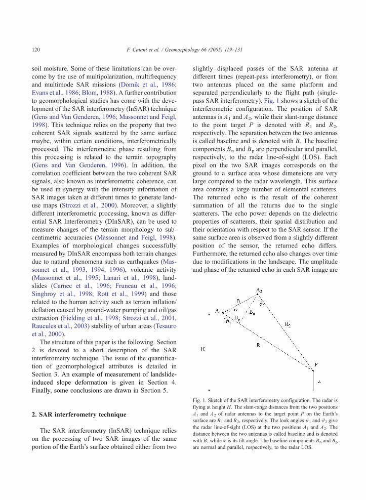
Fig. 1. Sketch of the SAR interferometry configuration. The radar is

flying at height H. The slant-range distances from the two positions

A1 and A2 of radar antennas to the target point P on the Earth’s

surface are R1 and R2, respectively. The look angles #1 and #2 give

the radar line-of-sight (LOS) at the two positions A1 and A2. The

distance between the two antennas is called baseline and is denoted

with B, while a is its tilt angle. The baseline components Bn and Bp

are normal and parallel, respectively, to the radar LOS.

2. SAR interferometry technique

The SAR interferometry (InSAR) technique relies

on the processing of two SAR images of the same

portion of the Earth’s surface obtained either from two

slightly displaced passes of the SAR antenna at

different times (repeat-pass interferometry), or from

two antennas placed on the same platform and

separated perpendicularly to the flight path (single-

pass SAR interferometry). Fig. 1 shows a sketch of the

interferometric configuration. The position of SAR

antennas is A1 and A2, while their slant-range distance

to the point target P is denoted with R1 and R2,

respectively. The separation between the two antennas

is called baseline and is denoted with B. The baseline

components Bn and Bp are perpendicular and parallel,

respectively, to the radar line-of-sight (LOS). Each

pixel on the two SAR images corresponds on the

ground to a surface area whose dimensions are very

large compared to the radar wavelength. This surface

area contains a large number of elemental scatterers.

The returned echo is the result of the coherent

summation of all the returns due to the single

scatterers. The echo power depends on the dielectric

properties of scatterers, their spatial distribution and

their orientation with respect to the SAR sensor. If the

same surface area is observed from a slightly different

position of the sensor, the returned echo differs.

Furthermore, the returned echo also changes over time

due to modifications in the landscape. The amplitude

and phase of the returned echo in each SAR image are

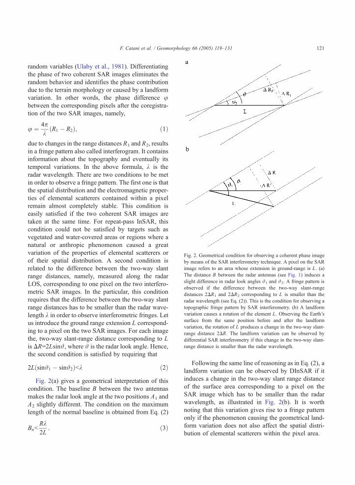
Fig. 2. Geometrical condition for observing a coherent phase image

by means of the SAR interferometry technique. A pixel on the SAR

image refers to an area whose extension in ground-range is L. (a

The distance B between the radar antennas (see Fig. 1) induces a

slight difference in radar look angles #1 and #2. A fringe pattern is

observed if the difference between the two-way slant-range

distances 2DR1 and 2DR2 corresponding to L is smaller than the

radar wavelength (see Eq. (2)). This is the condition for observing a

topographic fringe pattern by SAR interferometry. (b) A landform

variation causes a rotation of the element L. Observing the Earth’s

surface from the same position before and after the landform

variation, the rotation of L produces a change in the two-way slant

range distance 2DR. The landform variation can be observed by

differential SAR interferometry if this change in the two-way slant

range distance is smaller than the radar wavelength.

F. Catani et al. / Geomorphology 66 (2005) 119–131 121

random variables (Ulaby et al., 1981). Differentiating

the phase of two coherent SAR images eliminates the

random behavior and identifies the phase contribution

due to the terrain morphology or caused by a landform

variation. In other words, the phase difference ubetween the corresponding pixels after the coregistra-

tion of the two SAR images, namely,

u ¼ 4pk

R1 � R2ð Þ; ð1Þ

due to changes in the range distances R1 and R2, results

in a fringe pattern also called interferogram. It contains

information about the topography and eventually its

temporal variations. In the above formula, k is the

radar wavelength. There are two conditions to be met

in order to observe a fringe pattern. The first one is that

the spatial distribution and the electromagnetic proper-

ties of elemental scatterers contained within a pixel

remain almost completely stable. This condition is

easily satisfied if the two coherent SAR images are

taken at the same time. For repeat-pass InSAR, this

condition could not be satisfied by targets such as

vegetated and water-covered areas or regions where a

natural or anthropic phenomenon caused a great

variation of the properties of elemental scatterers or

of their spatial distribution. A second condition is

related to the difference between the two-way slant

range distances, namely, measured along the radar

LOS, corresponding to one pixel on the two interfero-

metric SAR images. In the particular, this condition

requires that the difference between the two-way slant

range distances has to be smaller than the radar wave-

length k in order to observe interferometric fringes. Let

us introduce the ground range extension L correspond-

ing to a pixel on the two SAR images. For each image

the, two-way slant-range distance corresponding to L

is DR=2Lsin#, where # is the radar look angle. Hence,

the second condition is satisfied by requiring that

2L sin#1 � sin#2ð Þbk ð2Þ

Fig. 2(a) gives a geometrical interpretation of this

condition. The baseline B between the two antennas

makes the radar look angle at the two positions A1 and

A2 slightly different. The condition on the maximum

length of the normal baseline is obtained from Eq. (2)

BnbRk2L

: ð3Þ

)

-

-

Following the same line of reasoning as in Eq. (2), a

landform variation can be observed by DInSAR if it

induces a change in the two-way slant range distance

of the surface area corresponding to a pixel on the

SAR image which has to be smaller than the radar

wavelength, as illustrated in Fig. 2(b). It is worth

noting that this variation gives rise to a fringe pattern

only if the phenomenon causing the geometrical land-

form variation does not also affect the spatial distri-

bution of elemental scatterers within the pixel area.

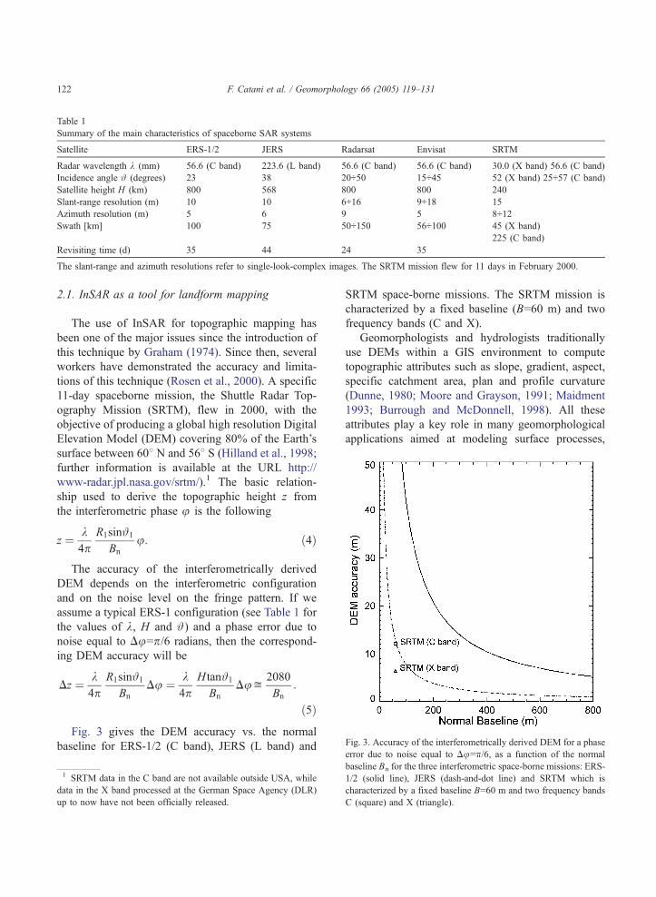
Table 1

Summary of the main characteristics of spaceborne SAR systems

Satellite ERS-1/2 JERS Radarsat Envisat SRTM

Radar wavelength k (mm) 56.6 (C band) 223.6 (L band) 56.6 (C band) 56.6 (C band) 30.0 (X band) 56.6 (C band)

Incidence angle # (degrees) 23 38 20H50 15H45 52 (X band) 25H57 (C band)

Satellite height H (km) 800 568 800 800 240

Slant-range resolution (m) 10 10 6H16 9H18 15

Azimuth resolution (m) 5 6 9 5 8H12Swath [km] 100 75 50H150 56H100 45 (X band)

225 (C band)

Revisiting time (d) 35 44 24 35

The slant-range and azimuth resolutions refer to single-look-complex images. The SRTM mission flew for 11 days in February 2000.

Fig. 3. Accuracy of the interferometrically derived DEM for a phase


2.1. InSAR as a tool for landform mapping

The use of InSAR for topographic mapping has

been one of the major issues since the introduction of

this technique by Graham (1974). Since then, several

workers have demonstrated the accuracy and limita-

tions of this technique (Rosen et al., 2000). A specific

11-day spaceborne mission, the Shuttle Radar Top-

ography Mission (SRTM), flew in 2000, with the

objective of producing a global high resolution Digital

Elevation Model (DEM) covering 80% of the Earth’s

surface between 608 N and 568 S (Hilland et al., 1998;

further information is available at the URL http://

www-radar.jpl.nasa.gov/srtm/).1 The basic relation-

ship used to derive the topographic height z from

the interferometric phase u is the following

z ¼ k4p

R1sin#1

Bn

u: ð4Þ

The accuracy of the interferometrically derived

DEM depends on the interferometric configuration

and on the noise level on the fringe pattern. If we

assume a typical ERS-1 configuration (see Table 1 for

the values of k, H and #) and a phase error due to

noise equal to Du=p/6 radians, then the correspond-

ing DEM accuracy will be

Dz ¼ k4p

R1sin#1

Bn

Du ¼ k4p

H tan#1

Bn

Dui2080

Bn

:

ð5Þ

Fig. 3 gives the DEM accuracy vs. the normal

baseline for ERS-1/2 (C band), JERS (L band) and

1 SRTM data in the C band are not available outside USA, while

data in the X band processed at the German Space Agency (DLR)

up to now have not been officially released.

SRTM space-borne missions. The SRTM mission is

characterized by a fixed baseline (B=60 m) and two

frequency bands (C and X).

Geomorphologists and hydrologists traditionally

use DEMs within a GIS environment to compute

topographic attributes such as slope, gradient, aspect,

specific catchment area, plan and profile curvature

(Dunne, 1980; Moore and Grayson, 1991; Maidment

1993; Burrough and McDonnell, 1998). All these

attributes play a key role in many geomorphological

applications aimed at modeling surface processes,

error due to noise equal to Du=k/6, as a function of the norma

baseline Bn for the three interferometric space-borne missions: ERS-

1/2 (solid line), JERS (dash-and-dot line) and SRTM which is

characterized by a fixed baseline B=60 m and two frequency bands

C (square) and X (triangle).

l

http://www-Eradar.jpl.nasa.gov/srtm/


providing watershed information, mapping land com-

ponents and classifying landscape character. The

slope, which is the most widely used topographic

measurement, influences flow rates of water and

sediment by controlling the rate of energy expenditure

or stream power available to drive a flow, erosion

potential, landslide and soil formation. Aspect, the

orientation of the line of steepest descent, defines the

slope direction and therefore the down-slope flow

direction. Knowledge of how aspect varies throughout

a catchment provides the necessary information to

determine what upslope land area contributes to the

flow at any point in the catchment. Hillslope profile

curvature reveals important quantitative information

on acceleration and deceleration of flow or on the

stability of slopes, whereas plan curvature is a

fundamental descriptor of landscape dissection, con-

vergence of flow and hillslope form.

Instead of generating an interferometric DEM, the

information on secondary landform attributes can be

obtained directly from the fringe pattern, thus avoiding

all difficulties related to the processing needed to

derive a DEM, e.g., the solution of the phase

unwrapping problem (Gens and Van Genderen,

1996). As a first step, the fringe pattern is transformed

from the slant-range/azimuth coordinate system typical

of SAR images to the ground-range/azimuth coordi-

nate system where the ground-range coordinate has

been obtained by projecting the slant-range coordinate

on a horizontal plane. It is worth noting that the

azimuth direction az is along the satellite flight track

while the ground range gr direction is perpendicular to

the track. The topographic gradients along these two

directions are computed as (Wegmuller et al., 1994)

BzBgr

BzBaz

" #¼

� cot#

0

� �þ R1

k4pB

d sinn þ cosnd tan #� nð Þf gdBuBgr

BuBaz

" #; ð6Þ

where Bu/Bgr and Bu/Baz are estimates of the absolute

phase gradients along the ground-range and azimuth

directions, respectively. The angle n is defined as

n ¼ #þ a tanBp

Bn

� �; ð7Þ

with Bn and Bp as the baseline components perpendic-

ular and parallel to the radar LOS. The relative error of

this approximation of the topographic gradient estima-

tion is below 1% (Gens and Van Genderen, 1996).

Starting from the topographic gradients, all the land-

form attributes can be computed.

2.2. InSAR as a tool for the study of morphology

variations

The principle of differential InSAR (DInSAR) was

first described by Gabriel et al. (1989). Since then, the

ability of DInSAR to detect terrain displacements on

large areas and with an accuracy of a fraction of radar

wavelength has been demonstrated (Massonnet and

Feigl, 1998; Ferretti et al., 2000, 2001). DInSAR is

based on a repeat pass SAR configuration. A simple

way to implement this interferometric technique con-

sists in computing an interferogram from two SAR

images acquired at different times, before and after the

event, which induced the landform variation. Let us

introduce the complex interferogram Ic, and define it in

terms of the two complex SAR images S1 and S2 as

Ic ¼ S1S24 ð8Þ

where the sign * denotes the operation of complex

conjugation. Hence, the complex differential interfero-

gram Idc, corrected for the phase contribution due to

topography, is defined as follows

Idc ¼ Icdexp � iutop

� �ð9Þ

where the phase contribution due to topography utop is

computed using a DEM of the area and the knowledge

of satellite ephemeris. The differential fringe pattern

obtained by extracting the argument of the complex

differential interferogram is related to the landform

variation d in the line-of-sight direction via the

relationship

d ¼ k4p

ud; ð10Þ

where ud is the absolute differential phase obtained

after having solved the 2p-phase ambiguity, a problem

also known as phase unwrapping. The accuracy of this

estimation depends on the radar wavelength and on the

amount of noise. For instance, in the C band (k=5.6 cm)

and with a phase uncertainty due to noise equal to


Dud=p/6, the accuracy of the estimation of landform

variation is

Dd ¼ k4p

dDud ¼k24

i2:5mm: ð11Þ

3. Estimation of geomorphological attributes

In this section, the result of an experiment to compute

geomorphological attributes from interferometric SAR

data is shown. Further, the quality of such estimates is

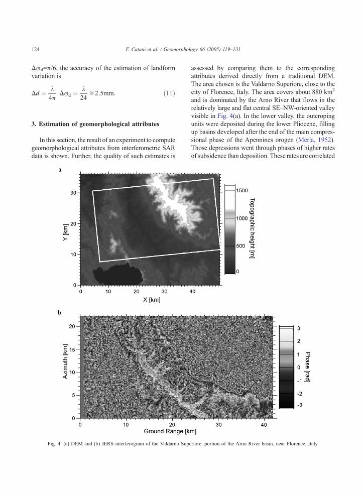
Fig. 4. (a) DEM and (b) JERS interferogram of the Valdarno Sup

assessed by comparing them to the corresponding

attributes derived directly from a traditional DEM.

The area chosen is the Valdarno Superiore, close to the

city of Florence, Italy. The area covers about 880 km2

and is dominated by the Arno River that flows in the

relatively large and flat central SE–NW-oriented valley

visible in Fig. 4(a). In the lower valley, the outcroping

units were deposited during the lower Pliocene, filling

up basins developed after the end of the main compres-

sional phase of the Apennines orogen (Merla, 1952).

Those depressions went through phases of higher rates

of subsidence than deposition. These rates are correlated

eriore, portion of the Arno River basin, near Florence, Italy.


with an eastward asymmetry caused by normal faults on

the eastern side with respect to antithetic faults that

border the basin along its western side. The outcroping

formations are marine and lacustrine sediments (Plio-

cene to Pleistocene) deposited in almost horizontal

bedding, over which recent fluvial deposits of the Arno

River are deposited. On the flanks of the valley, different

geological formations outcrop, predominantly sand-

stone and calcareous flysch on the NE part and shales

and structurally complex melange-like formations on

the SW side. These geological differences are reflected

in the prevalence of different slope processes. While the

Arno valley is essentially dependent upon the Arno

fluvial dynamics, the surrounding uplands and hillsides

are controlled by soil erosion and landsliding. Mass

movements are recurrent in the majority of the study

area and are mainly reactivated rotational Earth slides

(Canuti et al., 1994). The slope gradient and slope

curvature are the keys in the definition of geomorphic

processes and related forms.

The DEM of the test area, depicted in Fig. 4(a), has a

20-m planimetric resolution. It has been developed by

the Italian Military Geographic Institute (IGMI) from

interpolation of 1:25,000 scale contour-based maps.

For this reason, while sufficiently accurate and precise

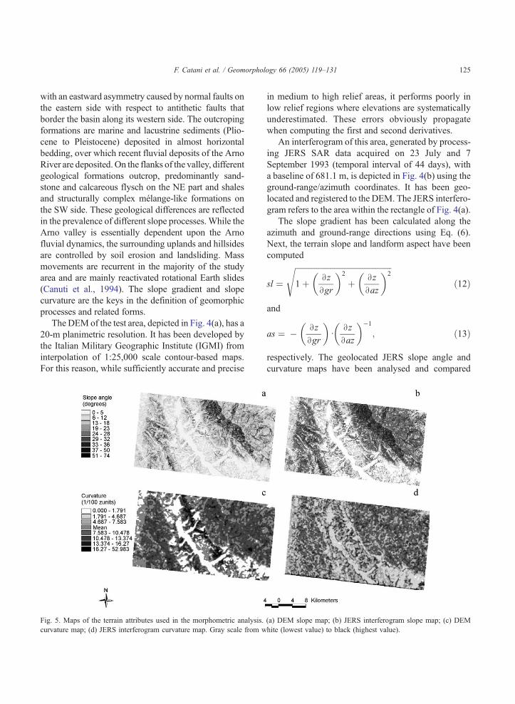
Fig. 5. Maps of the terrain attributes used in the morphometric analysis.

curvature map; (d) JERS interferogram curvature map. Gray scale from w

in medium to high relief areas, it performs poorly in

low relief regions where elevations are systematically

underestimated. These errors obviously propagate

when computing the first and second derivatives.

An interferogram of this area, generated by process-

ing JERS SAR data acquired on 23 July and 7

September 1993 (temporal interval of 44 days), with

a baseline of 681.1 m, is depicted in Fig. 4(b) using the

ground-range/azimuth coordinates. It has been geo-

located and registered to the DEM. The JERS interfero-

gram refers to the area within the rectangle of Fig. 4(a).

The slope gradient has been calculated along the

azimuth and ground-range directions using Eq. (6).

Next, the terrain slope and landform aspect have been

computed

sl ¼

ffiffiffiffiffiffiffiffiffiffiffiffiffiffiffiffiffiffiffiffiffiffiffiffiffiffiffiffiffiffiffiffiffiffiffiffiffiffiffiffiffiffiffiffiffiffiffiffiffi1þ Bz

Bgr

� �2

þ Bz

Baz

� �2s

ð12Þ

and

as ¼ � Bz

Bgr

� �d

Bz

Baz

� ��1

; ð13Þ

respectively. The geolocated JERS slope angle and

curvature maps have been analysed and compared

(a) DEM slope map; (b) JERS interferogram slope map; (c) DEM

hite (lowest value) to black (highest value).

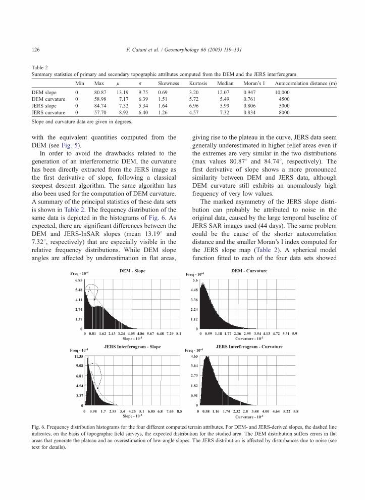
Table 2

Summary statistics of primary and secondary topographic attributes computed from the DEM and the JERS interferogram

Min Max l r Skewness Kurtosis Median Moran’s I Autocorrelation distance (m)

DEM slope 0 80.87 13.19 9.75 0.69 3.20 12.07 0.947 10,000

DEM curvature 0 58.98 7.17 6.39 1.51 5.72 5.49 0.761 4500

JERS slope 0 84.74 7.32 5.34 1.64 6.96 5.99 0.806 5000

JERS curvature 0 57.70 8.92 6.40 1.26 4.57 7.32 0.834 8000

Slope and curvature data are given in degrees.


with the equivalent quantities computed from the

DEM (see Fig. 5).

In order to avoid the drawbacks related to the

generation of an interferometric DEM, the curvature

has been directly extracted from the JERS image as

the first derivative of slope, following a classical

steepest descent algorithm. The same algorithm has

also been used for the computation of DEM curvature.

A summary of the principal statistics of these data sets

is shown in Table 2. The frequency distribution of the

same data is depicted in the histograms of Fig. 6. As

expected, there are significant differences between the

DEM and JERS-InSAR slopes (mean 13.198 and

7.328, respectively) that are especially visible in the

relative frequency distributions. While DEM slope

angles are affected by underestimation in flat areas,

Fig. 6. Frequency distribution histograms for the four different computed te

indicates, on the basis of topographic field surveys, the expected distribut

areas that generate the plateau and an overestimation of low-angle slopes.

text for details).

giving rise to the plateau in the curve, JERS data seem

generally underestimated in higher relief areas even if

the extremes are very similar in the two distributions

(max values 80.878 and 84.748, respectively). The

first derivative of slope shows a more pronounced

similarity between DEM and JERS data, although

DEM curvature still exhibits an anomalously high

frequency of very low values.

The marked asymmetry of the JERS slope distri-

bution can probably be attributed to noise in the

original data, caused by the large temporal baseline of

JERS SAR images used (44 days). The same problem

could be the cause of the shorter autocorrelation

distance and the smaller Moran’s I index computed for

the JERS slope map (Table 2). A spherical model

function fitted to each of the four data sets showed

rrain attributes. For DEM- and JERS-derived slopes, the dashed line

ion for the studied area. The DEM distribution suffers errors in flat

The JERS distribution is affected by disturbances due to noise (see

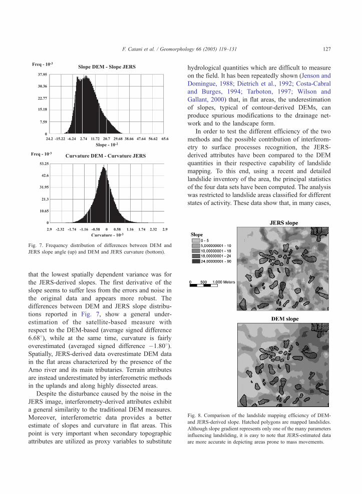
Fig. 7. Frequency distribution of differences between DEM and

JERS slope angle (up) and DEM and JERS curvature (bottom).

Fig. 8. Comparison of the landslide mapping efficiency of DEM

and JERS-derived slope. Hatched polygons are mapped landslides

Although slope gradient represents only one of the many parameters

influencing landsliding, it is easy to note that JERS-estimated data

are more accurate in depicting areas prone to mass movements.


that the lowest spatially dependent variance was for

the JERS-derived slopes. The first derivative of the

slope seems to suffer less from the errors and noise in

the original data and appears more robust. The

differences between DEM and JERS slope distribu-

tions reported in Fig. 7, show a general under-

estimation of the satellite-based measure with

respect to the DEM-based (average signed difference

6.688), while at the same time, curvature is fairly

overestimated (averaged signed difference �1.808).Spatially, JERS-derived data overestimate DEM data

in the flat areas characterized by the presence of the

Arno river and its main tributaries. Terrain attributes

are instead underestimated by interferometric methods

in the uplands and along highly dissected areas.

Despite the disturbance caused by the noise in the

JERS image, interferometry-derived attributes exhibit

a general similarity to the traditional DEM measures.

Moreover, interferometric data provides a better

estimate of slopes and curvature in flat areas. This

point is very important when secondary topographic

attributes are utilized as proxy variables to substitute

hydrological quantities which are difficult to measure

on the field. It has been repeatedly shown (Jenson and

Domingue, 1988; Dietrich et al., 1992; Costa-Cabral

and Burges, 1994; Tarboton, 1997; Wilson and

Gallant, 2000) that, in flat areas, the underestimation

of slopes, typical of contour-derived DEMs, can

produce spurious modifications to the drainage net-

work and to the landscape form.

In order to test the different efficiency of the two

methods and the possible contribution of interferom-

etry to surface processes recognition, the JERS-

derived attributes have been compared to the DEM

quantities in their respective capability of landslide

mapping. To this end, using a recent and detailed

landslide inventory of the area, the principal statistics

of the four data sets have been computed. The analysis

was restricted to landslide areas classified for different

states of activity. These data show that, in many cases,

-

.

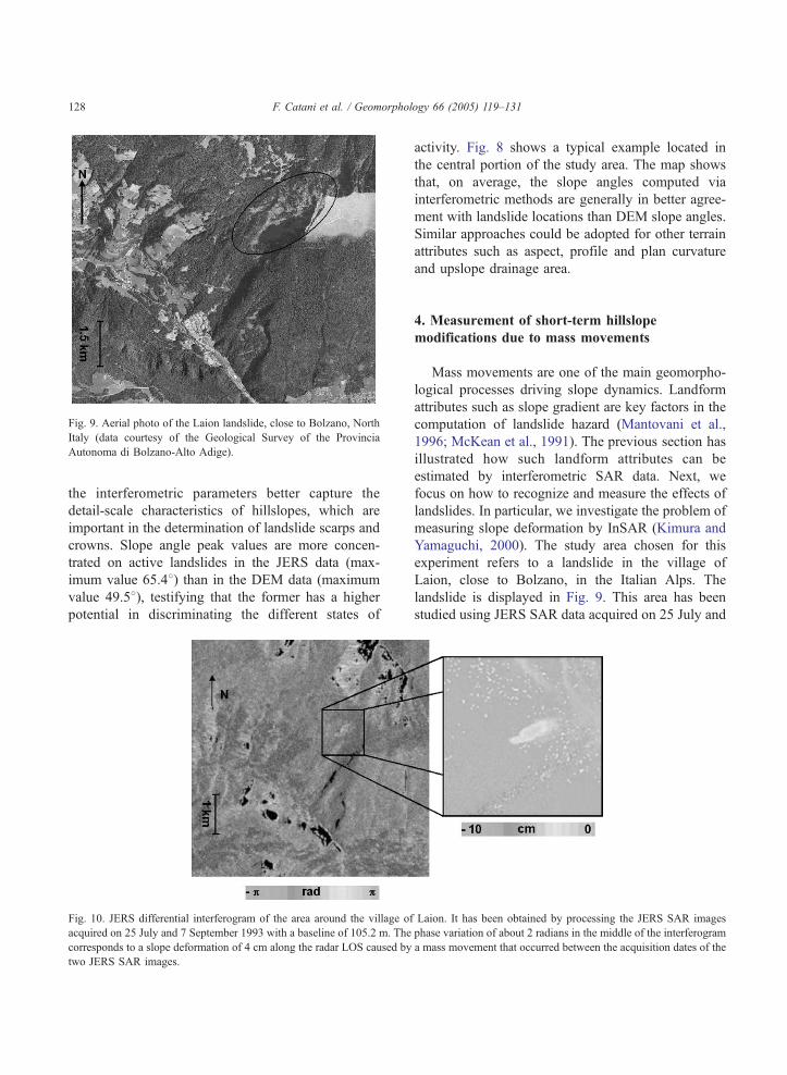
Fig. 9. Aerial photo of the Laion landslide, close to Bolzano, North

Italy (data courtesy of the Geological Survey of the Provincia

Autonoma di Bolzano-Alto Adige).


the interferometric parameters better capture the

detail-scale characteristics of hillslopes, which are

important in the determination of landslide scarps and

crowns. Slope angle peak values are more concen-

trated on active landslides in the JERS data (max-

imum value 65.48) than in the DEM data (maximum

value 49.58), testifying that the former has a higher

potential in discriminating the different states of

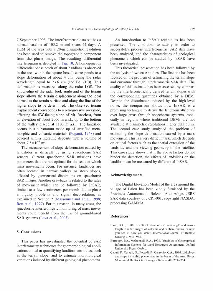
Fig. 10. JERS differential interferogram of the area around the village of

acquired on 25 July and 7 September 1993 with a baseline of 105.2 m. The

corresponds to a slope deformation of 4 cm along the radar LOS caused by

two JERS SAR images.

activity. Fig. 8 shows a typical example located in

the central portion of the study area. The map shows

that, on average, the slope angles computed via

interferometric methods are generally in better agree-

ment with landslide locations than DEM slope angles.

Similar approaches could be adopted for other terrain

attributes such as aspect, profile and plan curvature

and upslope drainage area.

4. Measurement of short-term hillslope

modifications due to mass movements

Mass movements are one of the main geomorpho-

logical processes driving slope dynamics. Landform

attributes such as slope gradient are key factors in the

computation of landslide hazard (Mantovani et al.,

1996; McKean et al., 1991). The previous section has

illustrated how such landform attributes can be

estimated by interferometric SAR data. Next, we

focus on how to recognize and measure the effects of

landslides. In particular, we investigate the problem of

measuring slope deformation by InSAR (Kimura and

Yamaguchi, 2000). The study area chosen for this

experiment refers to a landslide in the village of

Laion, close to Bolzano, in the Italian Alps. The

landslide is displayed in Fig. 9. This area has been

studied using JERS SAR data acquired on 25 July and

Laion. It has been obtained by processing the JERS SAR images

phase variation of about 2 radians in the middle of the interferogram

a mass movement that occurred between the acquisition dates of the


7 September 1993. The interferometric data set has a

normal baseline of 105.2 m and spans 44 days. A

DEM of the area with a 20-m planimetric resolution

has been used to remove the topographic component

from the phase image. The resulting differential

interferogram is depicted in Fig. 10. A homogeneous

differential phase patch of about 2 radians is observed

in the area within the square box. It corresponds to a

slope deformation of about 4 cm, being the radar

wavelength equal to 23.6 cm (see Eq. (10)). This

deformation is measured along the radar LOS. The

knowledge of the radar look angle and of the terrain

slope allows the terrain displacement along the local

normal to the terrain surface and along the line of the

higher slope to be determined. The observed terrain

displacement corresponds to a retrogressive rockslide,

affecting the SW-facing slope of Mt. Rasciesa, from

an elevation of about 2000 m a.s.l., up to the bottom

of the valley placed at 1100 m a.s.l. The landslide

occurs in a substratum made up of stratified meta-

morphic and volcanic materials (Fuganti, 1968) and

covered with a morainic deposits with a volume of

about 7.5�106 m3.

The measurement of slope deformation caused by

landslides is difficult by using spaceborne SAR

sensors. Current spaceborne SAR missions have

parameters that are not optimal for the scale at which

mass movements occur. For instance, landslides are

often located in narrow valleys or steep slopes,

affected by geometrical distorsions on spaceborne

SAR images. Another drawback is related to the rates

of movement which can be followed by InSAR,

limited to a few centimeters per month due to phase

ambiguity problems and signal decorrelation, as

explained in Section 2 (Massonnet and Feigl, 1998;

Rott et al., 1999). For this reason, in many cases, the

spaceborne interferometric monitoring of mass move-

ments could benefit from the use of ground-based

SAR systems (Leva et al., 2003).

5. Conclusions

This paper has investigated the potential of SAR

interferometry techniques for geomorphological appli-

cations aimed at quantifying landform attributes, such

as the terrain slope, and to estimate morphological

variations induced by different geological phenomena.

An introduction to InSAR techniques has been

presented. The conditions to satisfy in order to

successfully process interferometric SAR data have

been analysed, and the characteristics of geological

phenomena which can be studied by InSAR have

been investigated.

This theoretical presentation has been followed by

the analysis of two case studies. The first one has been

focused on the problem of estimating the terrain slope

and curvature through interferometric SAR data. The

quality of this estimate has been assessed by compar-

ing the interferometrically derived terrain slopes with

the corresponding quantities obtained by a DEM.

Despite the disturbance induced by the high-level

noise, the comparison shows how InSAR is a

promising technique to derive the landform attributes

over large areas through spaceborne systems, espe-

cially in regions where traditional DEMs are not

available at planimetric resolutions higher than 50 m.

The second case study analysed the problem of

estimating the slope deformation caused by a mass

movement. This is a very difficult task, which depends

on critical factors such as the spatial extension of the

landslide and the viewing geometry of the satellite.

This case study shows that if the above factors do not

hinder the detection, the effects of landslides on the

landform can be measured by differential InSAR.

Acknowledgements

The Digital Elevation Model of the area around the

village of Laion has been kindly furnished by the

Provincia Autonoma di Bolzano-Alto Adige. JERS

SAR data courtesy of J-2RI-001, copyright NASDA,

processing GAMMA.

References

Blom, R.G., 1988. Effects of variations in look angle and wave-

length in radar images of volcanic and eaolian terrains, or now

you see it, now you don’t. International Journal of Remote

Sensing 9, 945–965.

Burrough, P.A., McDonnell, R.A., 1998. Principles of Geographical

Information Systems for Land Resources Assessment. Oxford

University Press, Oxford.

Canuti, P., Casagli, N., Focardi, P., Garzonio, C.A., 1994. Lithology

and slope instability phenomena in the basin of the Arno River.

Memorie della Societa Geologica Italiana 48, 739–754.


Carnec, C., Massonet, D., King, C., 1996. Two examples of the use

SAR interferometry on displacement fields of small spatial

extent. Geophysical Research Letters 23, 3579–3582.

Costa-Cabral, M., Burges, S.J., 1994. Digital elevation model

networks: a model of flow over hillslopes for computation of

contributing and dispersal areas. Water Resources Research 30,

1681–1692.

Dietrich, W.E., Wilson, C.J., Montgomery, D.R., McKean, J.,

Bauer, R., 1992. Erosion thresholds and land surface morphol-

ogy. Geology 20, 675–679.

Domik, G., Leberl, F., Cimono, J., 1986. Multiple incidence angle

SIR-B experiment over Argentina: generation of secondary

image products. IEEE Transactions on Geoscience and Remote

Sensing 24, 492–497.

Domik, G., Leberl, F., Cimono, J., 1988. Dependence of image grey

values on topography in SIR-B images. International Journal of

Remote Sensing 9, 1013–1022.

Dong, C., Wang, L., 1990. Recognition of lithological units n

airborne SAR images using new texture features. International

Journal of Remote Sensing 11, 2337–2344.

Dunne, T., 1980. Formation and control of channel networks.

Progress in Physical Geography 4, 211–239.

Elachi, C., Cimono, J., Settle, M., 1986. Overview of the Shuttle

imaging Radar-B preliminary scientific results. Science 232,

1511–1516.

Evans, D., Farr, T.G., Ford, J.P., Thomson, T.W., Werner, C.L.,

1986. Multipolarization radar images for geologic mapping and

vegetation discrimination. IEEE Transactions on Geoscience

and Remote Sensing 24, 246–257.

Evans, D., Farr, T.G., van Zyl, J., 1992. Estimates of surface

roughness derived from Synthetic Aperture Radar (SAR) data.

IEEE Transactions on Geoscience and Remote Sensing 30,

382–389.

Ferretti, A., Prati, C., Rocca, F., 2000. Nonlinear subsidence rate

estimation using permanent scatterers in differential SAR

interferometry. IEEE Transactions on Geoscience and Remote

Sensing 38, 2202–2212.

Ferretti, A., Prati, C., Rocca, F., 2001. Permanent scatterers in SAR

interferometry. IEEE Transactions on Geoscience and Remote

Sensing 39, 8–20.

Fielding, E.J., Blom, R.G., Goldstein, R.M., 1998. Rapid sub-

sidence over oil fields measured by SAR interferometry.

Geophysical Research Letters 25, 3215–3218.

Fruneau, B., Achache, J., Delacourt, C., 1996. Observation and

modelling of the Saint-Etienne-de-Tinee landslide using SAR

interferometry. Tectonophysics 265, 181–190.

Fuganti, A., 1968–69. La frana di Rasciesa. Mem. Museo

Tridentino Scienze Naturali, XXXI–XXXII, Vol. XVII, Fac.

III, pp. 107–117.

Gabriel, A.K., Goldstein, R.M., Zebker, H.A., 1989. Mapping small

elevation changes over large areas: differential radar interfer-

ometry. Journal of Geophysical Research 94, 9183–9191.

Gens, R., Van Genderen, J.L., 1996. SAR interferometry—issues,

techniques, applications. International Journal of Remote Sens-

ing 17, 1803–1835.

Graham, L.C., 1974. Synthetic interferometric radar for topographic

mapping. Proceedings of the IEEE 62, 763–768.

Hilland, J.E., Stuhr, F.V., Freeman, A., Imel, D., Shen, Y., Jordan,

S.L., Caro, E.R., 1998. Future NASA spaceborne SAR

missions. IEEE Aerospace and Electronic Systems Magazine

13, 9–16.

Jenson, S.K., Domingue, J.O., 1988. Extracting topographic

structure from digital elevation data for geographic information

system analysis. Photogrammetric Engineering and Remote

Sensing 54, 1593–1600.

Kimura, H., Yamaguchi, Y., 2000. Detection of landslide areas

using radar interferometry. Photogrammetric Engineering and


Lanari, R., Lundgren, P., Sansosti, E., 1998. Dynamic deformation

of Etna volcano observed by satellite radar interferometry.

Geophysical Research Letters 24, 2519–2522.

Leva, D., Nico, G., Tarchi, D., Fortuny-Guasch, J., Sieber, A.J.,

2003. Temporal analysis of a landslide by means of a ground-

based SAR interferometer. IEEE Transactions on Geoscience

and Remote Sensing 41, 745–752.

Maidment, D.R., 1993. GIS and hydrological modelling. In:

Goodchild, M.F., Parks, B.O., Steyaert, L.T. (Eds.), Environ-

mental Modelling with GIS. New York, Oxford University

Press, pp. 147–167.

Mantovani, F., Soeters, R., Van Western, C.J., 1996. Remote

sensing techniques for landslide studies and hazard zonation in

Europe. Geomorphology 15, 213–225.

Massonnet, D., Feigl, K.L., 1998. Radar interferometry and its

application to changes in the Earth’s surface. Reviews of

Geophysics 36, 441–500.

Massonnet, D., Rossi, M., Carmona, C., Adragna, A., Peltzer, G.,

Geigl, K.L., Rabaute, T., 1993. The displacement field of the

Landers earthquake mapped by radar interferometry. Nature

364, 138–142.

Massonnet, D., Feigl, K.L., Rossi, M., Adragna, F., 1994. Radar

interferometric mapping of deformation in the year after the

Landers earthquake. Nature 369, 227–230.

Massonnet, D., Briole, P., Arnaud, A., 1995. Deflation of Mount

Etna monitored by spaceborne radar interferometry. Nature 375,

567–570.

Massonnet, D., Thatcher, W., Vadon, H., 1996. Detection of post-

seismic fault zone collapse following the Landers earthquake.

Nature 382, 612–616.

McKean, J., Bouchel, S., Gaydos, L., 1991. Remote sensing and

landslide hazard assessment. Photogrammetric Engineering and


Merla, G., 1952. Geologia dell’Appennino settentrionale. Bollettino

della Societa Geologica Italiana 70 (1951), 95–382.

Moore, I.D., Grayson, R.B., 1991. Terrain-based catchment

partitioning and runoff prediction using vector elevation data.

Water Resources Research 27, 1177–1191.

Pubellier, M., Deffontaines, B., Chorowicz, J., Rudant, J.P.,

Permana, H., 1999. Active denudation of morphostructures

from SAR ERS-1 images (SW Irian Jaya). International Journal

of Remote Sensing 20, 789–800.

Raucules, D., Le Mouelic, S., Carnec, C., King, C., 2003. Urban

subsidence in the city of Prato (Italy) monitored by satellite

radar interferometry. International Journal of Remote Sensing

20, 891–897.


Rosen, P.A., Hensley, S., Joughin, I.R., Li, F.K., Madsen, S.N.,

Rodriguez, E., Goldstein, R.M., 2000. Synthetic aperture radar

interferometry. Proceedings of the IEEE 88, 333–382.

Rott, H., Scheuchl, B., Siegel, A., Grasemann, B., 1999. Monitoring

very slow slope movements by means of SAR interferometry: a

case study from a mass waste above a reservoir in the Otztal

Alps, Austria. Geophysical Research Letters 26, 1629–1632.

Sabino, F., Blom, R., Elachi, C., 1980. Seasat radar images of San

Andreas fault California. American Association of Petroleum

Geologists 64, 619.

Singhroy, V., Mattar, K.E., Gray, A.L., 1998. Landslide

characterization in Canada using interferometric SAR and

combined SAR and TM images. Advances in Space Research

21, 465–476.

Strozzi, T., Dammert, P.B.G., Wegmqller, U., Martinez, J.-M.,

Askne, J.I.H., Beaudoin, A., Hallikainen, M.T., 2000. Landuse

mapping with ERS SAR interferometry. IEEE Transactions on

Geoscience and Remote Sensing 38, 766–775.

Strozzi, T., Wegmqller, U., Tosi, L., Bitelli, G., Spreckels, V., 2001.Land subsidence monitoring with differential SAR interferom-

etry. Photogrammetric Engineering and Remote Sensing 67,

1261–1270.

Tarboton, D.G., 1997. A new method for the determination of flow

directions and contributing areas in grid digital elevation

models. Water Resources Research 33, 309–319.

Tesauro, M., Berardino, P., Lanari, R., Sansosti, E., Fornaro, G.,

Franceschetti, G., 2000. Urban subsidence inside the city of

Napoli (Italy) observed by satellite radar interferometry. Geo-

physical Research Letters 27, 1954–1961.

Ulaby, F.T., Moore, R.K., Fung, A.K., 1981. Microwave Remote

Sensing Fundamentals and Radiometry. Artech House.

Wegmqller, U., Werner, C.L., Rosen, P.A., 1994. Derivation of

terrain slope from SAR interferometric phase gradient. ESA SP

361, 711–715.

Wilson, J.P., Gallant, J.C., 2000. Terrain Analysis. John Wiley &

Sons, New York.

Documents

On the application of SAR interferometry to geomorphological studies: estimation of landform attributes and mass movements