arX

iv:q

uant

-ph/

0204

094v

1 1

7 A

pr 2

002

DISSIPATION AND DECOHERENCE

IN PHOTON INTERFEROMETRY

F. Benatti

Dipartimento di Fisica Teorica, Universita di TriesteStrada Costiera 11, 34014 Trieste, Italy

andIstituto Nazionale di Fisica Nucleare, Sezione di Trieste

R. Floreanini

Istituto Nazionale di Fisica Nucleare, Sezione di TriesteDipartimento di Fisica Teorica, Universita di Trieste

Strada Costiera 11, 34014 Trieste, Italy

Abstract

The propagation of polarized photons in optical media can be effectivelymodeled by means of quantum dynamical semigroups. These general-ized time evolutions consistently describe phenomena leading to loss ofphase coherence and dissipation originating from the interaction with alarge, external environment. High sensitive experiments in the labora-tory can provide stringent bounds on the fundamental energy scale thatcharacterizes these non-standard effects.

1

1. INTRODUCTION

Quantum systems are usually treated as isolated: their time evolution is unitary,driven by the appropriate hamiltonian operator. In general however, this should be re-garded as an approximation: any external environment E unavoidably interacts with thesystem S under study, making the resulting dynamics rather involved.[1-3]

The global system S+E is closed, and its time evolution is determined by the operatore−iHtott, involving the total hamiltonian, that can be always decomposed as:

Htot = H + HE + H ′ , (1.1)

where H drives the system S in absence of E , HE describes the internal environmentdynamics, while H ′ takes into account the interaction between S and E . Nevertheless,being interested only in the evolution of the subsystem S and not in the details of thedynamics of E , one finally integrates over the environment degrees of freedom. Describingthe states of subsystem and environment by appropriate density matrices, the evolution intime of S will then be given by the transformation:

ρ(0) 7→ ρ(t) = TrE

[e−iHtott ρ(0) ⊗ ρE eiHtott

], (1.2)

where ρE describes the state of the environment at t = 0 (for simplicity, we assume S andE to be initially uncorrelated; see [4] for a generalization).

The resulting map ρ(0) 7→ ρ(t) is rather complex, involving in general non-linear andmemory effects; it consistently describes decoherence effects, leading to irreversibility anddissipation. An explicit and mathematically precise description in terms of quantum dy-namical semigroups is however possible when the interaction between the subsystem Sand the environment is weak. These generalized time evolutions are represented by lineartransformations, mapping density matrices into density matrices, while preserving verybasic physical properties, like forward in time composition law (semigroup property), en-tropy increase (irreversibility) and complete positivity (that guarantees the correct physicalinterpretation of the dynamics in all situations).[1-3]

Thanks to its generality and physical self-consistency, the description of open systemsin terms of quantum dynamical semigroups can be applied to model the dynamics of anysystem in weak interaction with a large environment.[1-7] In particular, it has recentlybeen applied to describe possible effects of irreversibility and dissipation induced by theevolution of strings and branes. Indeed, quite in general the fundamental dynamics ofthese extended objects gives rise at low energies to a weakly coupled environment, and asa consequence to decoherence phenomena.[8, 9]

From a more phenomenological point of view, similar effects have also been describedin the framework of quantum gravity: the quantum fluctuation of the gravitational fieldand the appearance of virtual black holes make space-time look “foamy” at distancescomparable to Planck’s length, inducing non-standard phenomena leading to possible lossof quantum coherence.[10-16] Dissipation and decoherence are also the general result of thedynamics in theories with large extra dimensions;[17] indeed, the possible energy leakageinto the bulk of space-time due to gravity effects would inevitably inject noise into theboundary, thus inducing irreversibility and dissipation at low energy in our brane-world.

2

Our present knowledge of string theory does not allow precise estimates of the mag-nitude of these non-standard effects. Using a rough dimensional analysis, one can nev-ertheless conclude that they should be rather small, being suppressed by at least oneinverse power of a large, fundamental mass scale (most likely the Planck mass). Despiteof this, they can be studied using interferometric phenomena. Indeed, detailed investiga-tions involving various elementary particle systems (neutral mesons [18-22], neutrons [23],neutrinos [24, 25]) have shown that present and future experiments might soon reach therequired sensitivity in order to detect the new, non-standard phenomena.

This possibility looks particularly promising for photon interferometry and more ingeneral optical physics.[5-7] The sophistication of present laboratory experiments in quan-tum optics is so high that decoherence effects induced by a fundamental, “stringy” dynam-ics might be studied using available setups.

In the present work, we shall discuss in detail how these non-standard, dissipativephenomena can affect the propagation of polarized photons immersed in optically activemedia. A preliminary discussion has been presented in [26]. There, it has been shown thatthe dissipative phenomena manifest themselves via depolarizing effects, that accumulatewith time. Limits on the magnitude of the parameters describing the new phenomena cantherefore be obtained from astrophysical and cosmological observations.[27]

In the following, different aspects of the quantum dynamical semigroup descriptionof photon propagation will be analyzed, focusing on the discussion of possible laboratorytests. As we shall see, the possibility of actually detecting the new, dissipative effects aregreatly enhanced by making them interfere with those induced by time-dependent opticalmedia. For slowly varying media, the use of the adiabatic approximation is justified. Inthis case, explicit expressions for relevant physical observables will be given and discussed;the formulas can be used to fit actual experimental data. The outcome of our investigationis that, at least in principle, bounds on some of the parameters describing dissipation anddecoherence can be obtained using existing laboratory setups.

2. QUANTUM DYNAMICAL SEMIGROUPS

In describing the evolution of polarized photons we shall adopt the standard effectivedescription in terms of a two-dimensional Hilbert space, the space of helicity states.[28-31]A convenient basis in this space is given by the circularly polarized states |R〉, |L〉. Withrespect to this basis, any partially polarized photon state can be represented by a 2 × 2density matrix ρ, i.e. by an hermitian operator, with positive eigenvalues and constanttrace:

ρ =

[ρ1 ρ3

ρ4 ρ2

], ρ4 = ρ∗

3 . (2.1)

As explained in the Introduction, the evolution in time of ρ will be described bymean of a quantum dynamical semigroup, i.e. by a linear transformation generated by anequation of the following form:[1-3, 32-34]

∂ρ(t)

∂t= −i

[H(t) , ρ(t)

]+ L[ρ(t)] . (2.2)

3

The first term in the r.h.s. is of hamiltonian form, while the piece L[ρ] takes into accountthe interaction with the external environment and leads to irreversibility and dissipation.†

As mentioned in the introductory remarks, it is convenient to make the photons crossan additional, non-dissipative, time-dependent optical medium, whose properties can besuitably controlled. This will in general induce extra birefringence effects on the polarizedphotons, and these can be conveniently described in terms of a time-dependent, effectivehamiltonian H(t). We shall assume a simple harmonic dependence on time:

H(t) =

[ω0 + µ ν e−iλt

ν eiλt ω0 − µ

]; (2.3)

this form is of sufficient generality for the considerations that follow. In (2.3), the parameterω0 represents the average photon energy, while the real constants µ and ν induce the level-splitting ω = (µ2 + ν2)1/2 among the two instantaneous eigenstates. As compared withthe effects of this splitting, the dependence on time of H(t), characterized by the realfrequency λ, will be assumed to be slow: λ ≪ ω; this is the situation that is most likely tobe reproduced by actual laboratory setups.

The additional piece L[ρ] in the evolution equation (2.2) is not of hamiltonian form,and induces a mixing-enhancing mechanism leading in general to irreversibility and lossof quantum coherence. In order to write it down explicitly, it is useful to adopt a vector-like notation and collect the entries ρ1, ρ2, ρ3, ρ4 of the density matrix (2.1) as thecomponents of the four-dimensional abstract vector |ρ〉. The evolution equation (2.2) canthen be rewritten as a Schrodinger (or diffusion) equation:

∂

∂t|ρ(t)〉 =

[H(t) + L

]|ρ(t)〉 , (2.4)

where the 4 × 4 matrix H takes into account the hamiltonian contributions,

H(t) = i

0 0 ν eiλt −ν e−iλt

0 0 −ν eiλt ν e−iλt

ν e−iλt −ν e−iλt −2µ 0−ν eiλt ν eiλt 0 2µ

, (2.5)

while the dissipative part L can be fully parametrized in terms of six real constants a, b,c, α, β, and γ, as follows:[1, 18]

L =

−D D −C −C∗

D −D C C∗

−C∗ C∗ −A B−C C B∗ −A

, (2.6)

† It should be noticed that in general the interaction with the environment can also pro-duce hamiltonian pieces in (2.2);[1-3, 9, 25] however, in the present case these contributionscan not be distinguished from those originating from other birefringence phenomena.

4

where for later convenience the combinations:

A = α + a , B = α − a + 2ib , C = c + iβ , D = γ , (2.7)

have been introduced. The six parameters are not all independent: they need to satisfythe following inequalities:[1-3, 18, 35]

2 R ≡ α + γ − a ≥ 0 ,

2 S ≡ a + γ − α ≥ 0 ,

2 T ≡ a + α − γ ≥ 0 ,

RST − 2 bcβ − Rβ2 − Sc2 − Tb2 ≥ 0 .

RS − b2 ≥ 0 ,

RT − c2 ≥ 0 ,

ST − β2 ≥ 0 ,

a ≥ 0 ,

α ≥ 0 ,

γ ≥ 0 ,(2.8)

These relations are the consequence of the property of complete positivity that assuresthe correct physical interpretation of the time evolution |ρ(0)〉 → |ρ(t)〉 generated by (2.4)in all situations; without this condition, serious inconsistencies in general arise (for moredetails, see [35]).

The effective environment generated by the fundamental “stringy” dynamics can beconsidered to be in thermal equilibrium;[9] the decoherence effects induced on the photonsare therefore stationary, so that the six parameters a, b, c, α, β, γ in (2.6), (2.7) can betaken to be time-independent. Nevertheless, let us mention that the evolution equation(2.2) can be generalized to take into account non-stationary dissipative contributions: thesewould typically arise for environments that are out of equilibrium, giving rise in generalto time-dependent intractions with the photons.[32-34] On the other hand, a physicallyconsistent, general formulation of non-linear dissipative dynamics is not yet available.

Once the evolution equation (2.4) is solved, one can easily compute any physicalproperty involving polarized photons. Indeed, in the formalism of density matrices, anyobservable O is represented by an hermitian matrix, that can be decomposed as in (2.1).The evolution in time of its mean value is then obtained by taking its trace with the densityoperator ρ(t):

〈O(t)〉 ≡ Tr[O ρ(t)

]= O1 ρ1(t) + O2 ρ2(t) + O3 ρ4(t) + O4 ρ3(t) ≡ 〈O|ρ(t)〉 . (2.9)

In the case of photons, of particular interest is the observable that correspond to afully polarized state, identified by the two angles θ and ϕ; it is explicitly given by thefollowing projector operator

Oθ,ϕ =1

2

[1 + sinϕ sin 2θ cos 2θ − i cos ϕ sin 2θ

cos 2θ + i cos ϕ sin 2θ 1 − sin ϕ sin 2θ

]. (2.10)

Its mean value gives the probability Pθ,ϕ(t) that the evolved state |ρ(t)〉 be found at timet in the polarization state determined by θ and ϕ; it is proportional to the intensity curvethat can be detected at an appropriate interferometric apparatus.

5

3. TRANSITION PROBABILITIES

In order to find explicit solutions of the evolution equation (2.4), it is convenient toperform a time-dependent unitary transformation and study it in the basis of instantaneouseigenvectors |v(±)(t)〉 of the hamiltonian (2.3), H(t) |v(±)(t)〉 = (ω0 ± ω) |v(±)(t)〉; usingthe four-vector notation, one then writes

|ρ(t)〉 = U(t) |ρ(t)〉 , (3.1)

where

U(t) =1

2ω

ω + µ ω − µ ν eiλt ν e−iλt

ω − µ ω + µ −ν eiλt −ν e−iλt

−ν e−iλt ν e−iλt ω + µ −(ω − µ)e−2iλt

−ν eiλt ν eiλt −(ω − µ)e2iλt ω + µ

. (3.2)

In the new basis, the hamiltonian contribution in (2.4) becomes diagonal:

H = U(t)H(t)U†(t) = diag[0, 0,−2iω, 2iω] ; (3.3)

the four entries coincide with the eigenvalues of the operator −i[H(t), · ], and therefore aregiven by the differences of the eigenvalues ω0 ± ω of H(t). However, since U(t) is timedependent, the evolution equation for the transformed vector |ρ(t)〉 involves an effectivehamiltonian:

∂

∂t|ρ(t)〉 =

[Heff (t) + L(t)

]|ρ(t)〉 , (3.4)

withHeff(t) = H + U(t)U†(t) ; (3.5)

further, the dissipative contribution becomes time-dependent:

L(t) = U(t)L U†(t) . (3.6)

One can check that its explicit form is as in (2.6), with the new parameters A, B, C, Dlinear combinations of the old ones A, B, C, D:†

A = A +ν2

2ω2

[2D − A + Re

(Be2iλt

)]−

2µν

ω2Re

(Ce−iλt

), (3.7a)

B = e−2iλt

(1 −

ν2

2ω2

)Re

(Be2iλt

)+

iµ

ωIm

(Be2iλt

)+

2µν

ω2Re

(Ce−iλt

)

−2iν

ωIm

(Ce−iλt

)−

ν2

2ω2

(2D − A

), (3.7b)

C = eiλt

(1 −

2ν2

ω2

)Re

(Ce−iλt

)+

iµ

ωIm

(Ce−iλt

)−

µν

2ω2

[2D − A + Re

(Be2iλt

)]

+iν

2ωIm

(Be2iλt

), (3.7c)

D = D −ν2

2ω2

[2D − A + Re

(Be2iλt

)]+

2µν

ω2Re

(Ce−iλt

). (3.7d)

† This is a general property of any quantum dynamical semigroup, whose explicit formis in fact basis-independent.[1-3]

6

When the system hamiltonian H(t) is slowly varying, the explicit dependence on timeof Heff (t) is very mild, so that the adiabatic approximation can be used in studying (3.4).In general, this is justified when the transitions induced by the explicit time dependenceof the hamiltonian are suppressed with respect to its natural level splitting.[36] In thepresent case, this condition is guaranteed by the starting assumption: λ ≪ ω. Within thisapproximation, one can neglect the off-diagonal terms in the contribution U(t)U†(t), sothat Heff becomes diagonal:

Heff = diag[0, 0,−2i(ω + λB), 2i(ω + λB)

]. (3.8)

(As explained in the Appendix, in the case of the hamiltonian (2.3) this result can bedirectly checked.† ) The additional phase contribution λB to the finite-time evolutionoperator eHeff t has a precise physical meaning: it gives the Berry phase that in generalaccumulates with time;[37, 38] indeed, one easily checks that:

λB =λ

2

(1 −

µ

ω

)≡ ∓ i 〈v(±)(t)|

∂

∂t|v(±)(t)〉 . (3.9)

Being encoded in the diagonal part of U(t)U†(t), Berry’s contribution is directly connectedto the characteristic properties of the starting hamiltonian H(t), and not to the use of theadiabatic approximation.

In absence of the dissipative piece, L = 0, the evolution in time of any given initialstate |ρ(0)〉 can then be written as:

|ρ(t)〉 = U†(t) ·M0(t) · U(0) |ρ(0)〉 , M0(t) = eHeff t . (3.10)

Using this expression, one can compute the evolution of physically relevant observables,and in particular transition probabilities. An experimentally relevant example is givenby the probability Pθ(t) of finding an initially left-polarized photon in a state with linearpolarization along the direction θ at time t. Using the general definition (2.9) and theexpression in (2.10) with ϕ = 0, from the evolution map (3.10) one explicitly finds:

Pθ(t) =1

2

1 +

µν

ω2cos(2θ − λt)

[cos

[2(ω + λB)t − λt

]− 1

]

+ν

ωsin(2θ − λt) sin[2(ω + λB)t − λt

].

(3.11)

This expression further simplifies for a vanishingly small µ; in this case, it can be conve-niently rewritten as:

Pθ(t) =1

2

1 +

1

2

[cos(2ωt + λt − 2θ) + cos(2ωt − λt + 2θ + π)

]. (3.12)

† Indeed, the evolution generated by the hamiltonian H(t) in (2.3) can be written inclosed form. In general however, this is no longer possible when the dissipative contributionin (2.2) is non-vanishing.

7

This intensity pattern can be studied by means of an interferometric setup: one canthen extract amplitudes and phases of the various Fourier components that characterize theprobability (3.12). In particular, the presence of the modulation e−iλt in the hamiltonian(2.3) describing in the optical medium crossed by the photon beam leads to a symmetricshift of the fundamental birefringence frequency 2ω by the small amount λ. Notice thatthis result is a consequence of the presence of Berry’s phase contribution, that now takesthe simplified expression λB = λ/2; indeed, neglecting this contribution would have pro-duced an asymmetric split of the fundamental frequency. An experimental analysis of theintensity pattern (3.12) can then allow a direct identification of Berry’s phase.

To see how this description is modified by the presence of dissipative phenomena, oneneeds to study the evolution equation (3.4) with a non-vanishing L. Although in generalthe effects induced by the interaction with the environment are parametrized by the sixreal constants a, b, c, α, β, and γ, there are physically motivated instances for which onlyone of them is actually non-zero. For example, this happens when γ is vanishingly small;in this case, the inequalities (2.8) further imply a = α and b = c = β = 0.† In this case,

the entries of the matrix L are all proportional to α, and assuming as before µ = 0, from(3.7) one explicitly obtains:

A = D = α , B = αe−2iλt , C = 0 . (3.13)

Although the resulting expression for L is still explicitly time-dependent, the evolutionequation (3.4) can be exactly integrated; one finds:

|ρ(t)〉 = M(t) |ρ(0)〉 , M(t) = e−αt

[Θ(t) 0

0 Ξ(t)

], (3.14)

where the 2 × 2 matrices Θ(t) and Ξ(t) can be expressed in terms of the Pauli matricesσ1, σ3 and the identity σ0:

Θ(t) = eαtσ1 , Ξ(t) = e−iλt σ3

[cos 2Ωt σ0 −

iω

Ωsin 2Ωt σ3 +

α

2Ωsin 2Ωt σ1

], (3.15)

andΩ =

√ω2 − α2/4 . (3.16)

Using the expression of the evolution matrix M(t) above in place of M0(t) in (3.10),one finally obtains the dynamical map |ρ(0)〉 → |ρ(t)〉 in presence of dissipative effects.Accordingly, the expressions of physically interesting observables change. In particular, the

† There are essentially two known ways of implementing the condition of weak inter-action between subsystem and environment:[1-3] the singular coupling limit (in which thetime-correlations in the environment are assumed to be much smaller than the typicaltime scale of the subsystem) and the weak coupling limit (in which it is the subsystemcharacteristic time scale that becomes large). One can check that the second situationleads precisely to the condition γ = 0.[9, 25]

8

transition probability Pθ(t) of finding an initial circularly polarized photon in a linearlypolarized state at time t becomes:

Pθ(t) =1

2

1 +

ω

2Ωe−αt

[cos

(2Ωt + λt − 2θ

)+ cos

(2Ωt − λt + 2θ + π

)]. (3.17)

The presence of dissipation affects the expression of Pθ(t) through the introduction of theexponential damping term together with the amplitude rescaling by the factor ω/Ω, andthe change in the birefringence frequency from ω to Ω. On the other hand, note thatthe symmetric shift in frequency by the amount λ induced by Berry’s phase contributionremains unchanged. This is not surprising: the geometrical mechanism leading to thepresence of Berry’s phase is completely different from the physical phenomena leadingto irreversibility and dissipation, and this fact is clearly reflected in the expression ofthe transition probability (3.17). As a result, the dissipative contributions and thoseoriginating from Berry’s phase can be independently probed.

Similarly to the expression in (3.12), also the intensity pattern described by (3.17) canbe, at least in principle, experimentally studied using Fourier analysis. Notice however thatthe oscillatory behaviour in (3.17) critically depends on the magnitude of the non-standardeffects induced by the presence of the environment; indeed, for sufficiently large α, thefrequency Ω becomes purely imaginary, so that the only remaining harmonic dependencein Pθ(t) is driven by the small frequency λ:

Pθ(t) =1

2

1 +

ω

Ωe−αt sinh(Ωt) sin(2θ − λt)

. (3.18)

In any case, independently from the relative magnitude of α and ω, the damping ef-fects always prevail for large times: in this limit, the transition probability Pθ(t) takes theconstant value 1/2. One can show that this result is independent from the approximationused to derive (3.17). Actually, in presence of dissipative phenomena all transition proba-bilities asymptotically tend to constant values, corresponding to the transition to a totallydepolarized state.[39, 26]

A different treatment is possible when the non-standard parameters a, b, c, α, β, and γcan be considered to be small in comparison with the characteristic system energy ω. Thisis likely to be the case in most standard laboratory situations: indeed, the main source ofbirefringence effects is usually the propagation in laboratory controlled optical media, andnot the weak interaction with an external environment. In this case, the additional pieceL in (3.4) can be treated as a perturbation, and the evolution matrix M(t) in (3.14) canthus be expressed as the following series expansion:

M(t) = eHeff t

1 +

∫ t

0

dt1 e−Heff t1 L(t1) eHeff t1

+

∫ t

0

dt1

∫ t1

0

dt2 e−Heff t1 L(t1) eHeff(t1−t2) L(t2) eHeff t2 + . . .

.

(3.19)

Useful information on the presence of dissipative effects can already be obtained byconsidering only first order terms in the small parameters. Within this approximation, the

9

transition probability Pθ(t) takes the following explicit form:

Pθ(t) =1

2+

e−(D+A/2)t

2

− ∆(t) cos(2θ − λt)

+

[(1 +

|B|

2λsin λt sin(λt + φB)

)sin 2ωt − Φ(t)

]sin(2θ − λt)

,

(3.20)

where

∆(t) =|C|

2

[2λ

4ω2 − λ2sin φC −

sin(2ωt + λt − φC)

2ω + λ−

sin(2ωt − λt + φC)

2ω − λ

]

+|B|

8

[2ω

ω2 − λ2sin φB +

sin(2ωt − 2λt − φB)

ω − λ−

sin(2ωt + 2λt + φB)

ω + λ

], (3.21a)

Φ(t) =|B|

4sin(λt + φB)

[sin(2ω + λ)t

2ω + λ−

sin(2ω − λ)t

2ω − λ

]

+ 2|C| sin(λt/2 − φC)

[sin(2ω − λ/2)t

4ω − λ+

sin(2ω + λ/2)t

4ω + λ

], (3.21b)

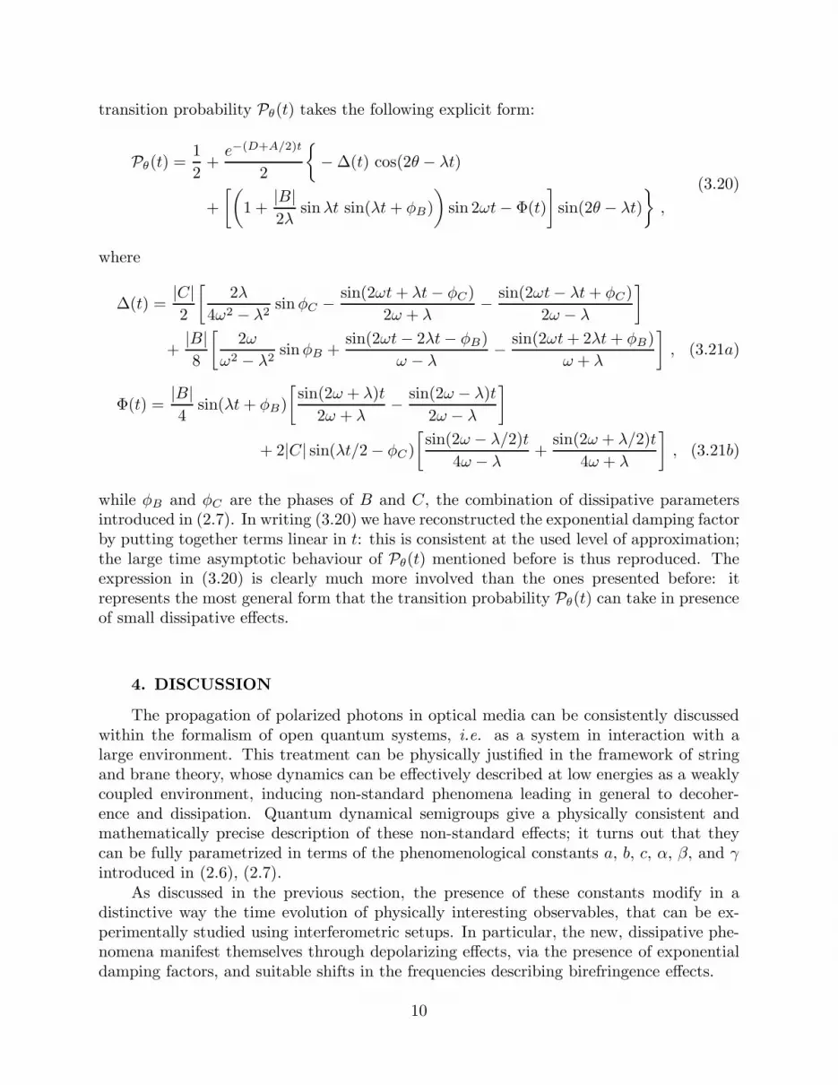
while φB and φC are the phases of B and C, the combination of dissipative parametersintroduced in (2.7). In writing (3.20) we have reconstructed the exponential damping factorby putting together terms linear in t: this is consistent at the used level of approximation;the large time asymptotic behaviour of Pθ(t) mentioned before is thus reproduced. Theexpression in (3.20) is clearly much more involved than the ones presented before: itrepresents the most general form that the transition probability Pθ(t) can take in presenceof small dissipative effects.

4. DISCUSSION

The propagation of polarized photons in optical media can be consistently discussedwithin the formalism of open quantum systems, i.e. as a system in interaction with alarge environment. This treatment can be physically justified in the framework of stringand brane theory, whose dynamics can be effectively described at low energies as a weaklycoupled environment, inducing non-standard phenomena leading in general to decoher-ence and dissipation. Quantum dynamical semigroups give a physically consistent andmathematically precise description of these non-standard effects; it turns out that theycan be fully parametrized in terms of the phenomenological constants a, b, c, α, β, and γintroduced in (2.6), (2.7).

As discussed in the previous section, the presence of these constants modify in adistinctive way the time evolution of physically interesting observables, that can be ex-perimentally studied using interferometric setups. In particular, the new, dissipative phe-nomena manifest themselves through depolarizing effects, via the presence of exponentialdamping factors, and suitable shifts in the frequencies describing birefringence effects.

10

Although a detailed discussion on possible devices that can be used to measure sucheffects is surely beyond the scope of the present investigation, some general considerationscan nevertheless be given.† Recalling for instance the expression (3.17) for the transitionprobability Pθ(t), one immediately realizes that the possibility of detecting the depolarizingeffects induced by the non-standard, dissipative phenomena is connected with the abilityof isolating and extracting the exponential factor e−αt from the experimental data. Thesensitivity of this measure clearly increases with t, so that large optical paths are in generalrequired. This can be achieved by using high quality optical cavities. By adjusting ina controlled way the “finesse” and the optical properties of the cavity, one should beable to reconstruct from the measured signal the time (or path-length) dependence of theprobability Pθ(t), and therefore extract information on the dissipative parameters bothfrom the damping factors and the oscillating terms.

The actual visibility of these parameters clearly depends on their magnitude. A precisea priori evaluation would require a detailed knowledge of string theory; nevertheless, anorder of magnitude estimate can be obtained using the general theory of open systems.Indeed, quite in general the dissipative effects induced by the weak interaction with anexternal environment can be roughly evaluated to be at most proportional to the squareof the typical energy scale of the system, while suppressed by an inverse power of thecharacteristic energy scale of the environment.

In the case of polarized photons, the system energy coincides with the average photonenergy ω0, while the typical energy scale of the environment coincides with the mass MF

that characterizes the fundamental, underlying dynamics. As a consequence, the values ofthe parameters a, b, c, α, β, and γ can be predicted to be roughly of order ω2

0/MF .

In the case of laboratory experiments using ordinary laser beams, the photon energy ω0

is fixed; therefore the expected magnitude of the new, non-standard effects is determined bythe value of MF . This fundamental scale can be as large as the Planck mass, but can also beconsiderably smaller in models of large extra dimensions. Fortunately, as stressed before,the description of decoherence phenomena by means of quantum dynamical semigroups isvery general, and quite independent from the actual microscopic mechanism responsiblefor the appearance of the new effects. As a result, an experimental study of the transitionprobabilities discussed in the previous section can give model-independent indications ofthe presence of the non-standard, dissipative phenomena. In turn, this would allow thederivation of interesting bounds on the magnitude of the fundamental scale MF , thusproviding useful information on the underlying “stringy” dynamics.

The analysis of the previous sections have been limited to the study of dissipativeevolutions for polarization states of a single photon. The whole treatment can be naivelyextended by linearity to include also the case of multi-photon states. Generalizing theone-photon dissipative dynamics generated by (2.2) to the case of multi-photon states ishowever not completely straightforward. Indeed, the photons obey the Bose statistics,and this property should be preserved by the time-evolution. It turns out that physically

† An additional discussion, although referred to the analysis of a specific experimentalapparatus, can be found in Ref.[40].

11

acceptable multi-photon dissipative dynamics can not be simply expressed as the productof single-photon time-evolutions: a more refined treatment is necessary (see [41] for details).This fact might have interesting consequences in various aspects of quantum optics.

APPENDIX

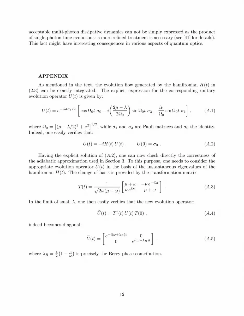
As mentioned in the text, the evolution flow generated by the hamiltonian H(t) in(2.3) can be exactly integrated. The explicit expression for the corresponding unitaryevolution operator U(t) is given by:

U(t) = e−iλtσ3/2

[cos Ω0t σ0 − i

(2µ − λ

2Ω0

)sin Ω0t σ3 −

iν

Ω0sin Ω0t σ1

], (A.1)

where Ω0 =[(µ − λ/2)2 + ν2

]1/2, while σ1 and σ3 are Pauli matrices and σ0 the identity.

Indeed, one easily verifies that:

U(t) = −iH(t) U(t) , U(0) = σ0 . (A.2)

Having the explicit solution of (A.2), one can now check directly the correctness ofthe adiabatic approximation used in Section 3. To this purpose, one needs to consider theappropriate evolution operator U(t) in the basis of the instantaneous eigenvalues of thehamiltonian H(t). The change of basis is provided by the transformation matrix

T (t) =1√

2ω(µ + ω)

[µ + ω −ν e−iλt

ν eiλt µ + ω

]. (A.3)

In the limit of small λ, one then easily verifies that the new evolution operator:

U(t) = T †(t) U(t) T (0) , (A.4)

indeed becomes diagonal:

U(t) =

[e−i(ω+λB)t 0

0 ei(ω+λB)t

], (A.5)

where λB = λ2

(1 − µ

ω

)is precisely the Berry phase contribution.

12

REFERENCES

1. R. Alicki and K. Lendi, Quantum Dynamical Semigroups and Applications, Lect.Notes Phys. 286, (Springer-Verlag, Berlin, 1987)

2. V. Gorini, A. Frigerio, M. Verri, A. Kossakowski and E.C.G. Surdarshan, Rep. Math.Phys. 13 (1978) 149

3. H. Spohn, Rev. Mod. Phys. 53 (1980) 569

4. A. Royer, Phys. Rev. Lett. 77 (1996) 3272

5. W.H. Louisell, Quantum Statistical Properties of Radiation, (Wiley, New York, 1973)

6. M.O. Scully and M.S. Zubairy, Quantum Optics (Cambridge University Press, Cam-bridge, 1997)

7. C.W. Gardiner and P. Zoller, Quantum Noise, 2nd. ed. (Springer, Berlin, 2000)

8. J. Ellis, N.E. Mavromatos and D.V. Nanopoulos, Phys. Lett. B293 (1992) 37; Int.J. Mod. Phys. A11 (1996) 1489

9. F. Benatti and R. Floreanini, Ann. of Phys. 273 (1999) 58

10. S. Hawking, Comm. Math. Phys. 87 (1983) 395; Phys. Rev. D 37 (1988) 904; Phys.Rev. D 53 (1996) 3099; S. Hawking and C. Hunter, Phys. Rev. D 59 (1999) 044025

11. J. Ellis, J.S. Hagelin, D.V. Nanopoulos and M. Srednicki, Nucl. Phys. B241 (1984)381;

12. S. Coleman, Nucl. Phys. B307 (1988) 867

13. S.B. Giddings and A. Strominger, Nucl. Phys. B307 (1988) 854

14. M. Srednicki, Nucl. Phys. B410 (1993) 143

15. W.G. Unruh and R.M. Wald, Phys. Rev. D 52 (1995) 2176

16. L.J. Garay, Phys. Rev. Lett. 80 (1998) 2508; Phys. Rev. D 58 (1998) 124015

17. For a presentation of these models, see: V.A. Rubakov, Phys. Usp. 44 (2001) 871

18. F. Benatti and R. Floreanini, Nucl. Phys. B488 (1997) 335

19. F. Benatti and R. Floreanini, Phys. Lett. B401 (1997) 337

20. F. Benatti and R. Floreanini, Nucl. Phys. B511 (1998) 550

21. F. Benatti and R. Floreanini, Phys. Lett. B465 (1999) 260

22. F. Benatti, R. Floreanini and R. Romano, Nucl. Phys. B602 (2001) 541

23. F. Benatti and R. Floreanini, Phys. Lett. B451 (1999) 422

24. F. Benatti and R. Floreanini, JHEP 02 (2000) 032

25. F. Benatti and R. Floreanini, Phys. Rev. D 64 (2001) 085015

26. F. Benatti and R. Floreanini, Phys. Rev. D 62 (2000) 125009

27. S. Carroll, G. Field and R. Jackiw, Phys. Rev. D 41 (1990) 1231

28. M. Born and E. Wolf, Principles of Optics, (Pergamon Press, Oxford, 1980)

29. L.D. Landau and E.M. Lifshitz, The Classical Theory of Fields, (Pergamon Press,New York, 1975); Quantum Mechanics, (Pergamon Press, New York, 1975)

13

30. E. Collett, Polarized Light, (Marcel Dekker, New York, 1993)

31. C. Brosseau, Fundamentals of Polarized Light, (Wiley, New York, 1998)

32. E.B. Davies and H. Spohn, J. Stat. Phys. 19 (1978) 511

33. R. Alicki, J. Phys. A 12 (1979) L103

34. K. Lendi, Phys. Rev. A 33 (1986) 3358

35. F. Benatti and R. Floreanini, Mod. Phys. Lett. A12 (1997) 1465; Banach CenterPublications, 43 (1998) 71; Phys. Lett. B468 (1999) 287; Chaos, Solitons andFractals 12 (2001) 2631

36. A. Messiah, Quantum Mechanics, vol. II, (North-Holland, Amsterdam, 1961)

37. M.V. Berry, Proc. R. Soc. Lond. A 392 (1984) 45

38. A. Shapere and F. Wilczek, Geometric Phases in Physics, (World Scientific, Singapore,1989)

39. K. Lendi, J. Phys. A 20 (1987) 13

40. F. Benatti and R. Floreanini, Dissipative effects in the propagation of polarized pho-tons, in Quantum Electrodynamics and Physics of the Vacuum, G. Cantatore ed.,AIP Conference Proceedings, Vol. 564, 2001, p. 37

41. F. Benatti, R. Floreanini and A. Lapel, Cybernetics and Systems, 32 (2001) 343

14