Constraints in dual phase shifting interferometry

Constraints in dual phase shiftinginterferometry

Abhijit Patil, Rajesh Langoju, and Pramod RastogiApplied Computing and Mechanics Laboratory, Ecole Polytechnique Federale de Lausanne,

1015 Lausanne, Switzerland

[email protected], [email protected], [email protected]

Abstract: The paper presents approaches based on traditional phaseshifting, flexible least-squares, and signal processing methods in dual phaseshifting interferometry primarily applied to holographic moire for retrievingmultiple phases. The study reveals that these methods cannot be appliedstraightforward to retrieve phase information and discusses the constraintsassociated with these methods. Since the signal processing method is themost efficient among these approaches, the paper discusses significantissues involved in the successful implementation of the concept. In thisapproach the knowledge of the pair of phase steps is of paramount interest.Thus the paper discusses the choice of the pair of phase steps that can beapplied to the phase shifting devices (PZTs) in the presence of noise. In thiscontext, we present a theoretical study using Cramer-Rao bound with re-spect to the selection of the pair of phase step values in the presence of noise.

© 2006 Optical Society of America

OCIS codes: (120.3180) Interferometry, (120.5050) Phase measurement, (999.9999) Fre-quency estimation

References and links1. P. K. Rastogi, “Phase shifting applied to four-wave holographic interferometers,” Appl. Opt. 31, 1680-1681

(1992).2. P. K. Rastogi, “Phase-shifting holographic moire: phase-shifter error-insensitive algorithms for the extraction of

the difference and sum of phases in holographic moire,” Appl. Opt 32, 3669-3675 (1993).3. P. K. Rastogi, “Phase shifting four wave holographic interferometry,” J. Mod. Opt. 39, 677-680 (1992).4. C. J. Morgan, “Least squares estimation in phase-measurement interferometry,” Opt. Lett. 7, 368-370 (1982).5. J. E. Grievenkamp, “Generalized data reduction for heterodyne interferometry,” Opt. Eng. 23, 350-352 (1984).6. A. Patil, R. Langoju, and P. Rastogi, “An integral approach to phase shifting interferome-

try using a super-resolution frequency estimation method,” Opt. Express 12, 4681-4697 (2004),http://www.opticsexpress.org/abstract.cfm?URI=OPEX-12-20-4681.

7. A. Patil and P. Rastogi, “Subspace-based method for phase retrieval in interferometry,” Opt. Express 13, 1240-1248 (2005), http://www.opticsexpress.org/abstract.cfm?URI=OPEX-13-4-1240.

8. A. Patil and P. Rastogi, “Estimation of multiple phases in holographic moire in presence ofharmonics and noise using minimum-norm algorithm,” Opt. Express 13, 4070-4084 (2005),http://www.opticsexpress.org/abstract.cfm?URI=OPEX-13-11-4070.

9. A. Patil and P. Rastogi, “Rotational invariance approach for the evaluation of multiple phases in interferometryin presence of nonsinusoidal waveforms and noise,” J. Opt. Soc. Am. A 9, 1918-1928 (2005).

10. A. Patil and P. Rastogi, “Maximum-likelihood estimator for dual phase extraction in holographic moire,” Opt.Lett. 17, 2227-2229 (2005).

11. D. C. Rife and R. R. Boorstyn, “Single-tone parameter estimation from discrete-time observations,”IEEE Trans-actions on Information Theory IT-20, 591-598 (1974).

12. M. Marcus and H. Minc, “Vandermonde Matrix,”in A Survey of Matrix Theory and Matrix Inequalities(Dover,New York), pp. 15-16 (1992).

13. http://www.mathworks.com/.

#8715 - $15.00 USD Received 7 September 2005; revised 6 December 2005; accepted 6 December 2005

(C) 2006 OSA 9 January 2006 / Vol. 14, No. 1 / OPTICS EXPRESS 88

mailto:[email protected]



http://www.opticsexpress.org/abstract.cfm?URI=OPEX-12-20-4681



http://www.mathworks.com/

14. http://mathworld.wolfram.com/VandermondeMatrix.html.15. K. M. Hoffman and R. Kunze, “Linear Algebra, 2nd ed.,” (Englewood Cliffs, New Jersey: Prentice Hall), 1971.16. G. Lai and T. Yatagai, “Generalized phase-shifting interferometry,” J. Opt. Soc. Am. A 8, 822-827 (1991).17. Abhijit Patil, Benny Raphael, and Pramod Rastogi, “Generalized phase-shifting interferometry by use of a direct

stochastic algorithm for global search,” Opt. Lett. 12, 1381-1383 (2004).

1. Introduction

Holographic moire is an efficient technique for the nondestructive evaluation of rough objects.The method functions by integrating two holographic interferometers within one system. Theresult is produced in the form of a moire. However, the complex nature of the interferometerand the beat inherent in the process precludes the use of standard phase shifting procedures toholographic moire [1-3]. It has been shown previously that the design of special phase shift-ing procedures to holographic moire allows for simultaneously determining the informationregarding the out-of-plane and in-plane displacement components [1-3]. In this configuration,the phase terms corresponding to the sum of phases (carrier) and difference of phases (moire)carry information regarding the out-of-plane and in-plane displacement components, respec-tively. This capability adds new dimension to the measurement of displacement componentsand in the nondestructive testing of rough objects.

Information carried by the carrier and moire can be decoded by either the traditional phaseshifting approach or by least-squares fit techniques or, by the introduction of signal processingconcepts in phase shifting interferometry. In the traditional approach, we refer to three-frame,five-frame, and seven-frame algorithms [1-2] which allow for accommodating dual PZTs. Byleast-squares fit technique, we extend the least squares fit data reduction method proposedby Morgan [4] and Grievenkamp [5] to accommodate dual phase shifting devices PZTs. Onthe other hand, the signal processing approach allows for applying high resolution frequencyestimation techniques such as polynomial rooting (annihilation method) [6], MUltiple-SIgnalClassification (MUSIC) [7], Minimum-Norm (min-norm) [8], Estimation of Signal Parametersvia Rotational Invariance Technique (ESPRIT) [9], and the Maximum-Likelihood Estimation(MLE) [10] to optical configurations including two PZTs.

However, these approaches have inherent limitations and cannot be applied straightforwardto configurations such as holographic moire for the simultaneous extraction of two orthogonaldisplacement components. For instance, in the traditional approach, the retrieval of informa-tion is not straightforward and the phase map corresponding to the carrier yields a phase pat-tern corrupted by moire and vice-versa. Hence, additional step needs to be associated to themeasurement to yield uncorrupted phase maps. On the other hand, in both the least squares fittechnique and the signal processing approach, though the phase steps imparted by the PZTscan be arbitrary, the selection of phase steps in the presence of noise is crucial to the successfulimplementation of the concept.

In this context, the objective of this paper is to discuss in detail the constraints encoun-tered while following these approaches. We believe that understanding the conditions that arenecessary to employing these algorithms is of paramount importance for the successful imple-mentation of the proposed concept. Since, the signal processing approach is the most efficientamong these approaches, we present a statistical analysis using Cramer-Rao lower bound [11]for the selection of the optimal pair of phase steps in the presence of noise. Once the phasesteps have been estimated within an allowable accuracy, the Vandermonde system of equations[12] can be designed for the determination of phases.

As a case study, we will consider the five-frame algorithm (traditional approach) [2] and theannihilation method (spectral estimation approach) [6]. The performance of other estimatorssuch as MUSIC, MIN-NORM and ESPRIT can also be studied in a similar way. The present



http://mathworld.wolfram.com/VandermondeMatrix.html

study is expected to provide the guidelines for applying dual phase shifting procedures to holo-graphic moire.

The paper is organized as follows. Section 2 presents the three approaches and discusses theconstraints associated with each of these approaches. Section 3 presents the Cramer-Rao bound(CRB) analysis for the estimation of phase steps and studies the performance of the annihilationmethod in estimating the phase steps with respect to noise.

2. Dual phase shifting interferometry: methods and their limitations

2.1. Tradition approach: a five-frame algorithm

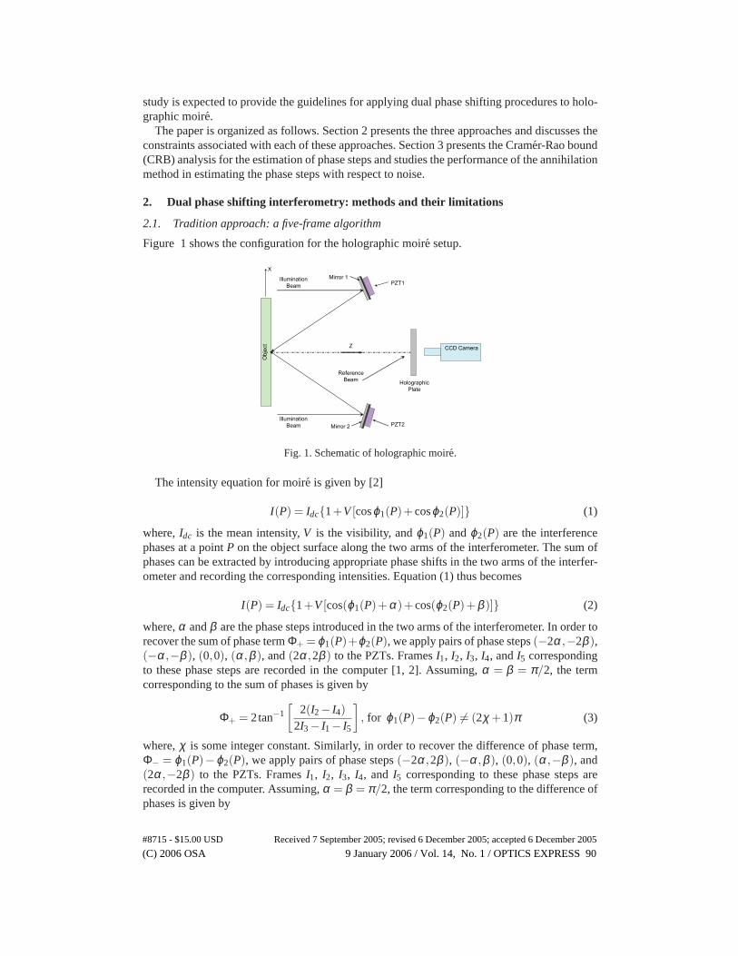
Figure 1 shows the configuration for the holographic moire setup.

Obje

ct

PZT1

PZT2Mirror 2

Mirror 1Illumination

Beam

Illumination

Beam

Reference

BeamHolographic

Plate

CCD Camera

X

Z

Fig. 1. Schematic of holographic moire.

The intensity equation for moire is given by [2]

I(P) = Idc{1+V[cosϕ1(P)+ cosϕ2(P)]} (1)

where, Idc is the mean intensity, V is the visibility, and ϕ1(P) and ϕ2(P) are the interferencephases at a point P on the object surface along the two arms of the interferometer. The sum ofphases can be extracted by introducing appropriate phase shifts in the two arms of the interfer-ometer and recording the corresponding intensities. Equation (1) thus becomes

I(P) = Idc{1+V[cos(ϕ1(P)+α )+ cos(ϕ2(P)+β)]} (2)

where, α and β are the phase steps introduced in the two arms of the interferometer. In order torecover the sum of phase term Φ+ = ϕ1(P)+ϕ2(P), we apply pairs of phase steps (−2α ,−2β),(−α ,−β), (0,0), (α ,β), and (2α ,2β) to the PZTs. Frames I1, I2, I3, I4, and I5 correspondingto these phase steps are recorded in the computer [1, 2]. Assuming, α = β = π/2, the termcorresponding to the sum of phases is given by

Φ+ = 2tan−1[

2(I2 − I4)2I3 − I1 − I5

], for ϕ1(P)−ϕ2(P) �= (2χ +1)π (3)

where, χ is some integer constant. Similarly, in order to recover the difference of phase term,Φ− = ϕ1(P)−ϕ2(P), we apply pairs of phase steps (−2α ,2β), (−α ,β), (0,0), (α ,−β), and(2α ,−2β) to the PZTs. Frames I1, I2, I3, I4, and I5 corresponding to these phase steps arerecorded in the computer. Assuming, α = β = π/2, the term corresponding to the difference ofphases is given by



Φ− = 2tan−1[

2(I2 − I4)2I3 − I1 − I5

], for ϕ1(P)+ϕ2(P) �= (2χ +1)π (4)

2.1.1. Constraints in tradition approach

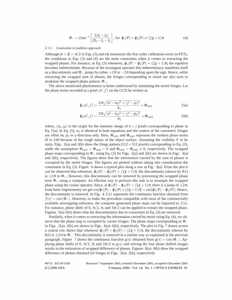
Although α = β = π/2 in Eqs. (3) and (4) minimizes the first order calibration errors in PZTs,the conditions in Eqs. (3) and (4) are the main constraints when it comes to extracting thewrapped phases. For instance, in Eq. (3) whenever, ϕ1(P)−ϕ2(P) = (2χ + 1)π, the equationbecomes indeterminate. Because of the arctangent operator this indeterminacy manifests itselfas a discontinuity and Φ+ jumps by either +2π or −2π depending upon the sign. Hence, whileextracting the wrapped sum of phases, the fringes corresponding to moire are also seen tomodulate the wrapped phase pattern, Φ+.

The above mentioned phenomenon is better understood by simulating the moire fringes. Letthe phase terms recorded at a pixel (n′, j ′) on the CCD be written as

ϕ1(n′, j ′) =2π

√(n′ −n0)2 +( j ′ − j0)2

λ1+Φran1 (5a)

ϕ2(n′, j ′) =2π

√(n′ −n0)2 +( j ′ − p0)2

λ2+Φran2 (5b)

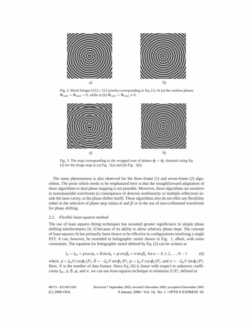
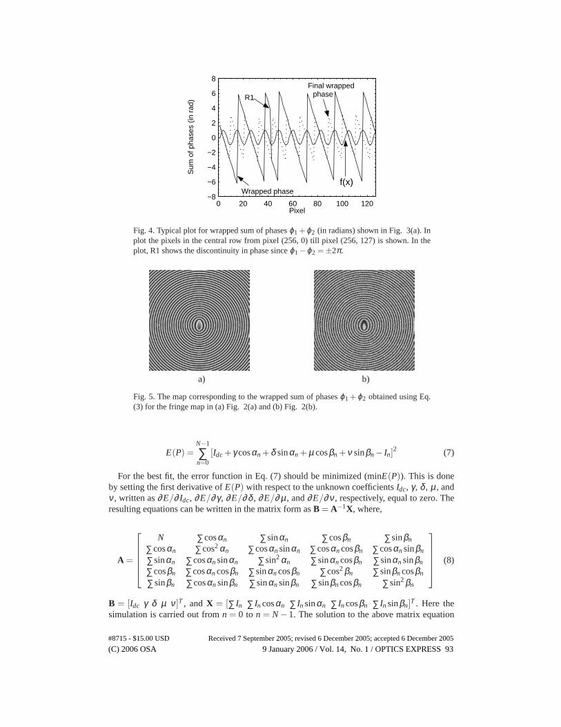
where, (n0, j0) is the origin for the intensity image of n× j pixels corresponding to phase inEq. (5a). In Eq. (5), n0 is identical in both equations and the centers of the concentric fringesare offset by p0 in y-direction only. Here, Φran1 and Φran2 represent the random phase terms(0 to 2π) because of the rough nature of the object surface. Assuming the visibility V to beunity, Figs. 2(a) and 2(b) show the fringe pattern (512×512 pixels) corresponding to Eq. (2),under the assumption Φran1 = Φran2 = 0 and Φran1 = Φran2 �= 0, respectively. The wrappedphase maps corresponding to Φ+ using Eq. (3) for Figs. 2(a) and 2(b) are shown in Figs. 3(a)and 3(b), respectively. The figures show that the information carried by the sum of phases iscorrupted by the moire fringes. The figures are plotted without taking into consideration theconstraints in Eq. (3). Figure 4 shows a typical plot along a row in Fig. 3(a). From the plot itcan be observed that whenever, ϕ1(P)−ϕ2(P) = (2χ + 1)π, the discontinuity (shown by R1)is ±2π in Φ+. However, this discontinuity can be removed by processing the wrapped phaseterm Φ+ using a computer. An efficient way to perform this task is to resample the wrappedphase using the cosine operator. Since, at ϕ1(P)−ϕ2(P) = (2χ +1)π, there is a jump of ±2π,from basic trigonometry we get cos[ϕ1(P)−ϕ2(P)± (2χ +1)π] = cos[ϕ1(P)−ϕ2(P)]. Hence,the discontinuity is removed. In Fig. 4 f (x) represents the continuous function obtained fromf (x) = cos(Φ+). However, to make the procedure compatible with most of the commerciallyavailable unwrapping softwares, the computer generated phase steps can be imparted to f (x).For instance, phase shifts of 0, π/2, π, and 3π/2 can be applied to extract the wrapped phase.Figures 5(a)-5(b) shows that the discontinuities due to constraints in Eq. (3) are removed.

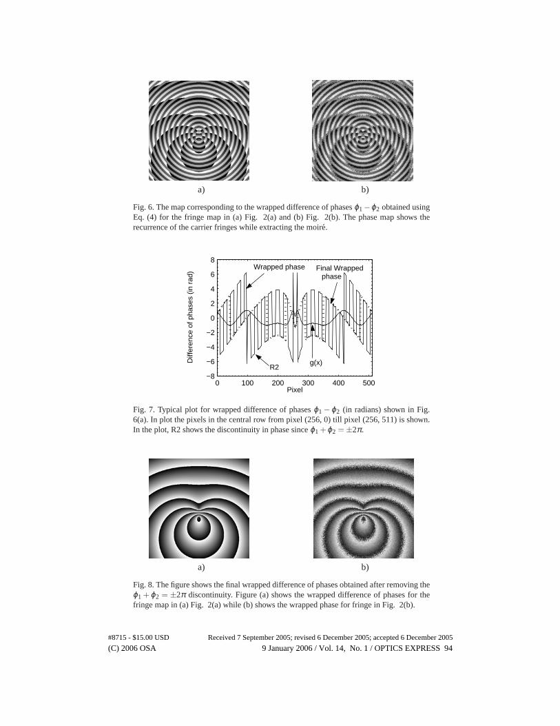
Similarly, when it comes to extracting the information carried by moire using Eq. (4), we ob-serve that the phase map is corrupted by carrier fringes. The phase maps corresponding to Φ−in Figs. 2(a)- 2(b) are shown in Figs. 6(a)- 6(b), respectively. The plot in Fig. 7 drawn acrossa central row shows that whenever ϕ1(P)+ ϕ2(P) = (2χ + 1)π, the discontinuity (shown byR2) is ±2π in Φ−. This discontinuity is removed in a similar way as explained in the previousparagraph. Figure 7 shows the continuous function g(x) obtained from g(x) = cos(Φ−). Ap-plying phase shifts of 0, π/2, π, and 3π/2 to g(x) and solving the four phase shifted imagesresults in the estimation of wrapped difference of phases. Figures 8(a)- 8(b) show the wrappeddifference of phases obtained for fringes in Figs. 2(a)- 2(b), respectively.



a) b)

Fig. 2. Moire fringes (512×512 pixels) corresponding to Eq. (1). In (a) the random phasesΦran1 = Φran2 = 0, while in (b) Φran1 = Φran2 �= 0.

a) b)

Fig. 3. The map corresponding to the wrapped sum of phases ϕ1 + ϕ2 obtained using Eq.(3) for the fringe map in (a) Fig. 2(a) and (b) Fig. 2(b).

The same phenomenon is also observed for the three-frame [1] and seven-frame [2] algo-rithms. The point which needs to be emphasized here is that the straightforward adaptation ofthese algorithms to dual phase stepping is not possible. Moreover, these algorithms are sensitiveto nonsinusoidal wavefronts (a consequence of detector nonlinearity or multiple reflections in-side the laser cavity, or the phase shifter itself). These algorithms also do not offer any flexibilityeither in the selection of phase step values α and β or in the use of non-collimated wavefrontsfor phase shifting.

2.2. Flexible least-squares method

The use of least squares fitting techniques has assumed greater significance in simple phaseshifting interferometry [4, 5] because of its ability to allow arbitrary phase steps. The conceptof least-squares fit has primarily been shown to be effective in configurations involving a singlePZT. It can, however, be extended to holographic moire shown in Fig. 1, albeit, with someconstraints. The equation for holographic moire defined by Eq. (2) can be written as

In = Idc+γcosαn +δ sinαn + µ cosβn +ν sinβn for n = 0,1,2, ....,N−1 (6)

where, γ = IdcV cosϕ1(P), δ = −IdcV sinϕ1(P), µ = IdcV cosϕ2(P), and ν = −IdcV sinϕ2(P).Here, N is the number of data frames. Since Eq. (6) is linear with respect to unknown coeffi-cients Idc, γ, δ, µ , and ν , we can use least-squares technique to minimize E(P), defined as



0 20 40 60 80 100 120−8

−6

−4

−2

0

2

4

6

8

Pixel

Sum

of p

hase

s (in

rad

) Wrapped phase

Final wrapped phase

f(x)

R1

Fig. 4. Typical plot for wrapped sum of phases ϕ1 +ϕ2 (in radians) shown in Fig. 3(a). Inplot the pixels in the central row from pixel (256, 0) till pixel (256, 127) is shown. In theplot, R1 shows the discontinuity in phase since ϕ1 −ϕ2 = ±2π.

a) b)

Fig. 5. The map corresponding to the wrapped sum of phases ϕ1 + ϕ2 obtained using Eq.(3) for the fringe map in (a) Fig. 2(a) and (b) Fig. 2(b).

E(P) =N−1

∑n=0

[Idc+γcosαn +δ sinαn + µ cosβn +ν sinβn− In]2 (7)

For the best fit, the error function in Eq. (7) should be minimized (minE(P)). This is doneby setting the first derivative of E(P) with respect to the unknown coefficients Idc, γ, δ, µ , andν , written as ∂E/∂ Idc, ∂E/∂γ, ∂E/∂δ, ∂E/∂ µ , and ∂E/∂ν , respectively, equal to zero. Theresulting equations can be written in the matrix form as B = A−1X, where,

A =

N ∑cosαn ∑sinαn ∑cosβn ∑sinβn

∑cosαn ∑cos2 αn ∑cosαn sinαn ∑cosαn cosβn ∑cosαn sinβn

∑sinαn ∑cosαn sinαn ∑sin2 αn ∑sinαn cosβn ∑sinαn sinβn

∑cosβn ∑cosαn cosβn ∑sinαn cosβn ∑cos2 βn ∑sinβn cosβn

∑sinβn ∑cosαn sinβn ∑sinαn sinβn ∑sinβn cosβn ∑sin2 βn

(8)

B = [Idc γ δ µ ν]T , and X = [∑ In ∑ In cosαn ∑ In sinαn ∑ In cosβn ∑ In sinβn]T . Here thesimulation is carried out from n = 0 to n = N− 1. The solution to the above matrix equation



a) b)

Fig. 6. The map corresponding to the wrapped difference of phases ϕ1 −ϕ2 obtained usingEq. (4) for the fringe map in (a) Fig. 2(a) and (b) Fig. 2(b). The phase map shows therecurrence of the carrier fringes while extracting the moire.

0 100 200 300 400 500−8

−6

−4

−2

0

2

4

6

8

Pixel

Diff

eren

ce o

f pha

ses

(in r

ad)

g(x)

Wrapped phase Final Wrapped phase

R2

Fig. 7. Typical plot for wrapped difference of phases ϕ1 −ϕ2 (in radians) shown in Fig.6(a). In plot the pixels in the central row from pixel (256, 0) till pixel (256, 511) is shown.In the plot, R2 shows the discontinuity in phase since ϕ1 +ϕ2 = ±2π.

a) b)

Fig. 8. The figure shows the final wrapped difference of phases obtained after removing theϕ1 + ϕ2 = ±2π discontinuity. Figure (a) shows the wrapped difference of phases for thefringe map in (a) Fig. 2(a) while (b) shows the wrapped phase for fringe in Fig. 2(b).



results in the determination of the unknown coefficients Idc, γ, δ, µ , and ν , and subsequently,in the determination of ϕ1 and ϕ2. The sum and difference of phases can then be obtained using

Φ+ = tan−1 δ µ +νγδν−µγ

(9a)

Φ− = tan−1 γν−µδγµ+νδ

(9b)

2.2.1. Constraints in flexible least-squares method

The main constraint in flexible least-squares method is that the phase steps should be carefullyselected such that matrix A is non-singular. It has also been observed that the use of sequentialphase steps such as nα and nβ in matrix A results in the determinant to be zero. In practicalsituations although the successive phase steps cannot be exact multiples of nα and nβ , theresulting matrix in this case will be nearly singular or poorly conditioned. Therefore, if theleast squares technique is applied, then only few arbitrary phase steps should be selected suchthat the matrix A is non-singular. For instance, if thirteen data frames are acquired and, α = 40°and β = 20°, then five data frames corresponding to frames n= 0,2,5,8 and 10 can be selectedin a non-regular order. This would result in matrix A to be non-singular. It is also observed thateven if the matrix A is not well conditioned, mathematical tools such as MATLAB [13] maystill compute the inverse of the matrix A. Therefore, it is always advisable to check whether thematrix is well conditioned or not.

Hence, the well know generalized data reduction technique proposed by Morgan [4] andGrievenkamp [5] cannot be extended straightforward to holographic moire, since utmost careis required in the selection of the pair of phase steps. The other method by which the general-ized holographic moire can be realized is by designing the Vandermonde system of equations.A Vandermonde matrix usually arises in the polynomial least squares fitting, Lagrange inter-polating polynomials, or in the statistical distribution of the distribution moments [14-16]. Thesolution of N×N Vandermonde matrix requires N2 operations. The advantage of Vandermondematrix is that its determinant is always nonzero (hence invertible) for different values of nα andnβ . Hence, the matrix for determining phases ϕ1 and ϕ2 can be written in the form

exp( jα0) exp(− jα0) exp( jβ0) exp(− jβ0) 1exp( jα1) exp(− jα1) exp( jβ1) exp(− jβ1) 1

......

......

...exp( jκαN) exp(− jκαN) exp( jβN) exp(− jβN) 1

��∗℘℘ ∗Idc

=

I0

I1...

IN−1

(10)

where, (α0,β0), (α1,β1),..,and (αN−1,βN−1) are phase steps for frames I0, I1, I2,...,and IN−1,respectively. The phase distribution ϕ1 and ϕ2 are subsequently computed from the argument of� and ℘ , where � = 0.5IdcV exp( jϕ1) and ℘ = 0.5IdcV exp( jϕ2). Here, ∗ denotes the complexconjugate.

A point to note is that in phase shifting interferometry using the least-squares fit method, thefirst step involves the exact determination of the phase steps while the second step involves thedetermination of the phase distribution. The method proposed by Lai and Yatagai [16] for theestimation of phase steps in real time cannot be applied in a straight-forward manner here as theprocedure is applicable to a single PZT based configuration only. In such a case the algorithmsuggested by Patil et al. [17] using stochastic approach seems to be the most appropriate. Thealgorithm however is sensitive to noise and can only work well if the data is assumed to havea high signal to noise ratio (SNR). To overcome this problem, high resolution techniques have



been proposed. Limitations associated with the use of high-resolution techniques is the topic ofthe next subsection.

2.3. Signal processing approach

In the signal processing approach, a parallelism is drawn between the frequencies that arepresent in the spectrum and the phase steps imparted to the PZTs. The problem therefore re-duces to estimating the frequencies or in other words the phase steps. Once the phase steps havebeen estimated, the Vandermonde system of equation shown in Eq. (10) can be applied for theextraction of phase distributions. Patil et al.[6-10] have introduced signal processing algorithmsto configurations involving single and multiple PZTs. The advantage of the these approacheslies in their ability to compensate for the errors arising due to non-sinusoidal wavefronts andPZT miscalibrations. These algorithms also allow the use of spherical wavefronts and arbitraryphase steps between 0 and π radians. The number of data frames that these methods require isequal to at least twice the number of frequencies that are present in the spectrum. Hence, fordual PZTs and for harmonic κ = 1 (assuming sinusoidal wavefronts), we need at least N = 10data frames. Since, discussion of these signal processing algorithms is beyond the scope of thispaper, let us consider, as a case study, the case of one such algorithm based on the design of anannihilation filter.

2.3.1. Annihilation filter method

In the annihilation filter method, we transform the discrete time domain signal In in Eq. (2) intoa complex frequency domain by taking its Z-transform. Let the Z-transform of In be denoted byI(z). The objective is to design another polynomial P(z) termed as annihilation filter which haszeros at frequencies associated with I(z). This in turn would result in I(z)P(z) = 0. The phasesteps α and β are estimated by extracting the roots of the polynomial P(z).

In brief, let us consider the presence of multiple-order harmonics in the wavefront and hence,Eq. (2) for κ th order harmonics can be written as

In =Idc+−κ

∑k=−1

ak exp[ jk(ϕ1 +nα )]+κ

∑k=1

ak exp[ jk(ϕ1 +nα )]

−κ

∑k=−1

bk exp[ jk(ϕ2 +nβ)]+κ

∑k=1

bk exp[ jk(ϕ2 +nβ)];

(11)

where, ak and bk are the complex Fourier coefficients of the κ th order harmonic; j =√−1. Let

us rewrite Eq. (11) in the following form

In = Idc+κ

∑k=1

�′kunk +

κ

∑k=1

�′k∗(u∗k)

n +κ

∑k=1

℘ kϑ nk +

κ

∑k=1

℘ ∗k(ϑ

∗k )n (12)

where, �′k = ak exp( jkϕ1), uk = exp( jkα ), ℘ k = bk exp( jkϕ2), and ϑk = exp( jkα ). The tasknow reduces to designing an annihilation filter of the form

P(z) =(z−1)κ

∏k=1

(z−uk)(z−u∗k)(z−ϑk)(z−ϑ ∗k )

=4κ+2

∑k=0

Pkzk

(13)



The multiplication in the frequency domain corresponds to discrete convolution in the timedomain. Thus, the discrete convolution of the polynomial P(z), represented as Pn, with theintensity signal, represented as In, vanishes identically, and can be written as

4κ+2

∑k=0

PkIn−k = 0 ∀m∈ {4κ +2,4κ +3, ....,N−1} (14)

Hence, finding the roots of the polynomial P(z) yields the phase steps α and β . Since themeasurement is sensitive to noise this method necessitates acquiring additional data frames asphase steps cannot be estimated reliably at lower SNR’s with minimum required (N = 10) dataframes. To reduce the effect of noise, a denoising procedure is suggested in Reference [6] sothat phase steps can be estimated even at lower SNR’s. The reader is referred to Reference [6]for details on the annihilation technique and the denoising method.

2.3.2. Constraints in signal processing approach

Of the three approaches, the signal processing approach seems to be the most promising as it iseffective in minimizing some of the commonly occurring systematic and random errors duringthe measurement. However, the constraint in the signal processing approach is the selection ofthe pair of phase steps that are applied to dual PZT’s. In the presence of low signal-to-noiseratio (SNR), a careful selection of the pair of phase steps with limited number of data frames isnecessary. Since, noise plays an important role in the successful implementation of the concept,a sound knowledge of the allowable phase steps is of prime importance. Hence, there is a needto study the statistical characteristics of phase shifted holographic moire (which is independentof the estimator itself) using Cramer-Rao bound. In the next section we present the CRB forholographic moire in the context of the selection of the phase steps. Once the CRB is obtainedthe study will focus on the performance evaluation of the annihilation filter method.

3. Optimizing phase shifts by signal processing approach

This section provides useful guidelines to optimizing the selection of phase step values ob-tained by signal processing approach. This study can be performed by deriving the CRB forholographic moire. The CRB provides valuable information on the potential performance ofthe estimators. The CRBs are independent of the estimation procedure and the precision of theestimators cannot surpass the CRBs. In this context, we will first derive the CRB for the phasesteps α and β as a function of SNR and N. Although the phase steps α and β can be arbitraryfor pure intensity signal, the central question is: what is the smallest difference between thephase steps α and β that can be retrieved reliably by any estimator as a function of SNR andN? Hence, we need to determine all the allowable values of phase steps α and β at a particularSNR and N. The reason why we are interested in computing the smallest phase step differenceis to provide an experimentalist with a fair idea of phase steps which must be selected at a par-ticular SNR and N, so that the phase values ϕ1 and ϕ2 can be estimated reliably. Suppose thatinadvertently, the two phase steps are chosen very close to one another and the measurementsare performed at a low value of SNR. In such as case, the phase values ϕ1 and ϕ2 cannot beestimated reliably. However, for the same value of SNR, if the two phase steps α and β are farapart, the phase values ϕ1 and ϕ2 can be reasonably estimated. Hence, there is a need to set upguidelines for the selection of the phase steps.

In order to respond to this query, we will derive the mean square error (MSE) for differencein phase steps α −β as a function of SNR which will indicate the theoretical Cramer-Rao lowerbounds to the MSE. The Cramer-Rao bound can then be compared with the MSE obtained by



any estimator (in the present case we will study the annihilation filter method). For this, weperform 500 Monte-Carlo simulations at each SNR and the separation between the phase stepsα and β is varied from 0 to 100%.

Two scenarios are possible. First, the MSE obtained from the estimator is below the CRB.We attribute this observation to the non-reliability in the estimated phase steps and discardthose values of separation between α and β in which the MSE is below the CRB. Second, theMSE of the estimator is above the CRB. In such a case, we infer that closer the MSE of theestimator is to the CRB, the more efficient is the estimator. Of course, for an unbiased estimator,the MSE obtained by the estimator can never reach the theoretical CRB for limited number ofsample points. In the present study, we derive the CRB for the phase steps and compare theperformance of the annihilation filter method with the CRB.

3.1. Cramer-Rao bound for holographic moire

Let I′ = I +η denote the vector consisting of measured intensities in the presence of noise η ,where I = [I0 I1 I2 · IN−1]T . The vector I′ is characterized by the probability density functionp(I′;Ψ) = p(I′), where Ψ is the set of unknown parameters in the moire fringes. In the presentcase, Ψ = (Idc1, Idc2,V1,V2,ϕ1,ϕ2,α ,β)T , where subscripts 1 and 2 refer individually to thetwo arms of the interferometer. Note that in Eq. (2), it was assumed that Idc1 = Idc2 = Idc andV1 = V2 = V. Therefore, Idc1 and Idc2 and are the average intensities while V1 and V2 are thefringe visibilities in the two arms. Now, if Ψ is an unbiased estimator of the deterministic Ψ,then the covariance matrix of the unbiased estimator, E{ΨΨT}, where E is an expectationoperator, is bounded by its lower value given by [11]

E{ΨΨT} ≥ J−1 (15)

where, J is the Fisher Information matrix. This matrix is defined as [9]

J = E

{[∂

∂Ψlog p(I′)

][∂

∂Ψlog p(I′)

]T}

(16)

In other words, if ψr (any rth element of Ψ) is an unbiased estimator of deterministic ψr , basedon I′, whose CRB is given by

E{Ψ2r } ≥ J−1

r,r , for r = 1,2,3, ...,8 (17)

where, J−1r,r is the (r, r) element in matrix J−1. Assuming η is the additive white Gaussian noise

with zero mean and variance σ2, the probability density function p(I′;Ψ) is defined by themean and variance of the noise. Thus, the joint probability of the vector I′ is given by

p(I′;Ψ) =(

1√2πσ

)N

exp

[− 1

2σ2

N−1

∑n=0

(I ′n− In)2

](18)

It is well understood that the CRB for each unknown parameter can be determined by observingthe diagonal elements of the inverse of the Fisher Information matrix, J−1 . Simplifying Eq. (18)by taking the logarithmic function (note that log p is asymptotic to p(I′;Ψ)), we obtain



log p = constant − 12σ2

N−1

∑n=0

(I ′n− In)2 (19)

Differentiating Eq. (19) with the rth element in Ψ, say ψr , we obtain,

∂ log p∂ψr

=1

σ2

N−1

∑n=0

∂ In∂ψr

(I ′n− In) (20)

Similarly, Eq. (19) can be differentiated with respect to ψs. Therefore Eq. (15) for the rth andsth element in Ψ can be written as

Jr,s = E

{1

σ4

N−1

∑n=0

∂ In∂ψr

(I ′n− In)N−1

∑l=0

∂ Il∂ψs

(I ′l − Il )

}(21)

Equation (21) can be simplified into the following compact form

Jr,s =1

σ2

N−1

∑n=0

∂ In∂ψr

∂ In∂ψs

(22)

Finally, the lower bounds are given by variance, var(ψr) ≥ J−1r,r . In the present example the

typical Fisher Information matrix will be

J =

JIdc1,Idc1 JIdc1,Idc2 JIdc1,V1 JIdc1,V2 JIdc1,ϕ1 JIdc1,ϕ2 JIdc1,α JIdc1,βJIdc2,Idc1 JIdc2,Idc2 JIdc2,V1 JIdc2,V2 JIdc2,ϕ1 JIdc2,ϕ2 JIdc2,α JIdc2,βJV1,Idc1 JV1,Idc2 JV1,V1 JV1,V2 JV1,ϕ1 JV1,ϕ2 JV1,α JV1,βJV2,Idc1 JV2,Idc2 JV2,V1 JV2,V2 JV2,ϕ1 JV2,ϕ2 JV2,α JV2,βJϕ1,Idc1 Jϕ1,Idc2 Jϕ1,V1 Jϕ1,V2 Jϕ1,ϕ1 Jϕ1,ϕ2 Jϕ1,α Jϕ1,βJϕ2,Idc1 Jϕ2,Idc2 Jϕ2,V1 Jϕ2,V2 Jϕ2,ϕ1 Jϕ2,ϕ2 Jϕ2,α Jϕ2,βJα ,Idc1 Jα ,Idc2 Jα ,V1 Jα ,V2 Jα ,ϕ1 Jα ,ϕ2 Jα ,α Jα ,βJβ ,Idc1

Jβ ,Idc2Jβ ,V1

Jβ ,V2Jβ ,ϕ1

Jβ ,ϕ2Jβ ,α Jβ ,β

(23)

where, the subscripts in Eq. (23) represent derivatives with respect to the unknown parameters.Hence, to determine the allowable values of phase steps α and β as function of SNR and N,let us first look at the following simple calculation. Suppose that, we have a variable q = ΨTU,which represents the difference between the phase steps α and β , then the variance of q is givenby

E[|q− q|2] =E[(q− q)(q− q)T ]

=E[UT(Ψ− Ψ)(Ψ− Ψ)TU]

=UTE[(Ψ− Ψ)(Ψ− Ψ)T ]U

≥UTJ−1U

(24)

The problem, therefore, narrows down to selecting a matrix U such that the minimum differencebetween α and β is computed. Since all the parameters are unknown, the matrix U is given byU = [0 0 0 0 0 0 −1 1]T .



0

50

100 020

4060

10−2

100

102

SNR (dB)β − α (as % of α)

MS

E (

rad2 )

N = 11

0

50

100 020

4060

10−2

100

102


MS

E (

rad2 )

N = 11

a) b)

0

50

100 020

4060

10−2

100

102


MS

E (

rad2 )

N = 15

0

50

100 020

4060

10−2

100

102


MS

E (

rad2 )

N = 15

c) d)

0

50

100 020

4060

10−2

100

102


MS

E (

rad2 )

N = 20

0

50

100 020

4060

10−2

100

102


MS

E (

rad2 )

N = 20

e) f)

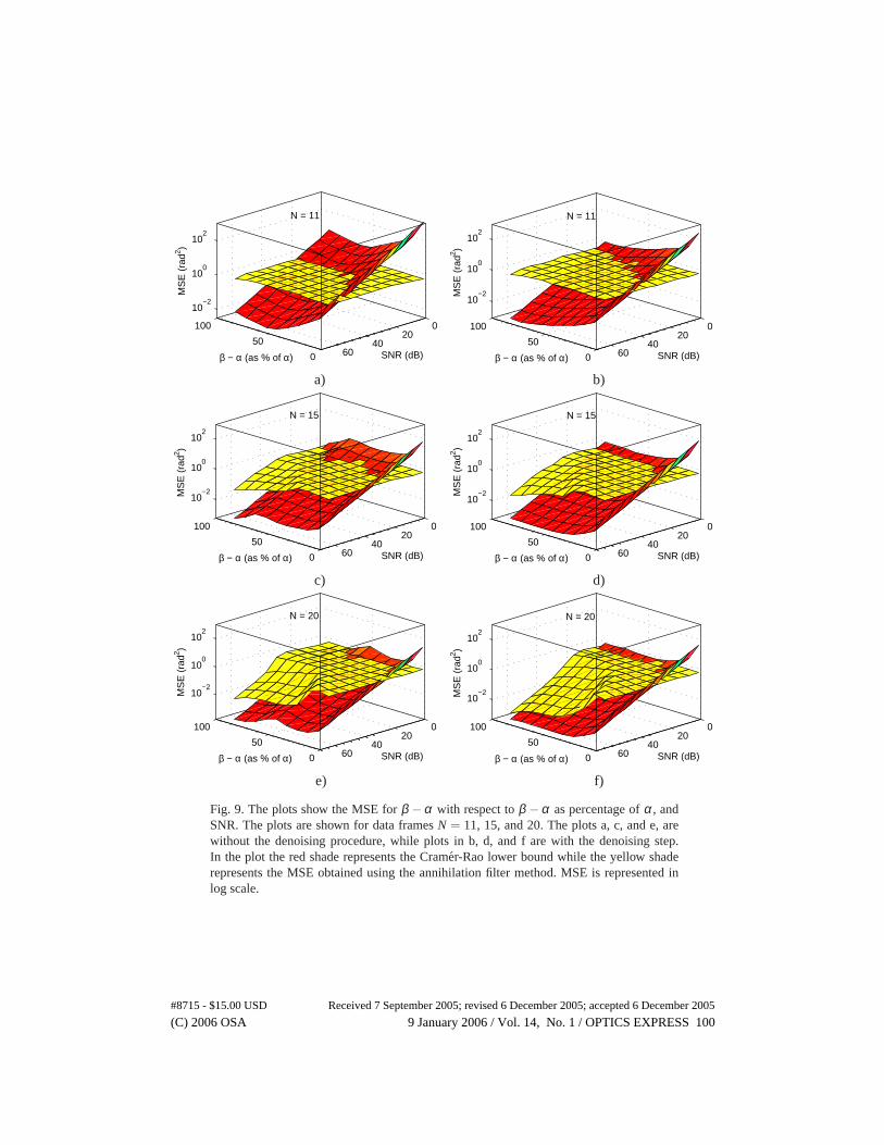
Fig. 9. The plots show the MSE for β −α with respect to β −α as percentage of α , andSNR. The plots are shown for data frames N = 11, 15, and 20. The plots a, c, and e, arewithout the denoising procedure, while plots in b, d, and f are with the denoising step.In the plot the red shade represents the Cramer-Rao lower bound while the yellow shaderepresents the MSE obtained using the annihilation filter method. MSE is represented inlog scale.



10 20 30 40 50 60 70

−0.5

0

0.5

1

1.5

SNR (dB)

Bou

nds

(for

α in

rad

)

α = 30°

10 20 30 40 50 60 70−0.5

0

0.5

1

1.5

SNR (dB)

Bou

nds

(for

β in

rad

)

β = 36°

a) b)

10 20 30 40 50 60 70−0.2

0

0.2

0.4

0.6

0.8

1

1.2

SNR (dB)

Bou

nds

(for

α in

rad

)

α = 30°

10 20 30 40 50 60 70

0

0.5

1

1.5

SNR (dB)

Bou

nds

(for

β in

rad

)

β = 45°

c) d)

10 20 30 40 50 60 70−0.2

0

0.2

0.4

0.6

0.8

1

1.2

SNR (dB)

Bou

nds

(for

α in

rad

)

α = 30°

10 20 30 40 50 60 70

0.5

1

1.5

SNR (dB)

Bou

nds

(for

β in

rad

)

β = 54°

e) f)

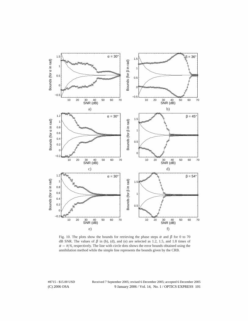
Fig. 10. The plots show the bounds for retrieving the phase steps α and β for 0 to 70dB SNR. The values of β in (b), (d), and (e) are selected as 1.2, 1.5, and 1.8 times ofα = π/6, respectively. The line with circle dots shows the error bounds obtained using theannihilation method while the simple line represents the bounds given by the CRB.



3.2. Results of CRB analysis

We now perform 500 Monte-Carlo simulations at each SNR and study the performance of theannihilation filter method in retrieving the difference of the phase steps at a pixel point. Duringthe analysis the phases ϕ1 and ϕ2 are kept the same as described earlier in Eqs. (5a) and (5b),respectively. Additive white Gaussian noise having SNR between 0 and 70 dB is consideredduring the simulations. Our analysis consists of two parts.

During the first part, we determine the MSE of β − α as a function of the SNR and thedifference between the phase steps α and β as percentage of α . During the analysis we chooseα = π/6 and vary the difference of α and β between 0 to 100% of α . Given the fixed value ofα , this analysis indicates the reliable values of β which can be selected for a particular SNR andN. It is important to note that the value of α can be selected anywhere between 0 and π radians.However, to keep the analysis simple we have selected just one value of α in the present study.The allowable values of β can be determined by comparing the plot of MSE of β −α , obtainedusing the annihilation filter method for 500 iterations at each SNR, with respect to the meansquare error obtained from the CRB given by Eq. (24). The values in the plot where the MSEof β − α , obtained from the annihilation filter method, goes below the MSE obtained usingthe CRB, are considered as prohibited for the selection of separation between the phase stepvalues α and β . The test is carried out for data frames N = 11, 15, and 20. The study showsthat separation between the phase steps can be reduced as the number of data frames increases.Moreover, the incorporation of denoising procedure substantially improves the allowable lowerrange of phase step separation. For instance, Fig. 9(f) shows that for the separation between αand β as 70% of α , and for SNR 30 dB, the MSE is 0.01 rad2 using the annihilation method.

In the second analysis, we perform 1000 simulations at a pixel to compare the bounds in theretrieval of phase steps α and β obtained using the annihilation filter method, with theoreticalbounds obtained by the CRB for various phase step values in the presence of noise. Since theprevious analysis showed that the denoising procedure is effective, the present study is per-formed with the incorporation of a denoising step and for N = 20. Figure 10 shows that as theseparation between the phase steps α and β increases, their values can be reliably estimated atlower SNRs. Figures 10(e)-10(f) show that as the separation between the phase steps increasesthe bounds obtained by annihilation filter method reaches the theoretical bounds given by theCRB at much lower SNR as compared to that obtained in Figs. 10(a)-10(d). This analysis onceagain reemphasizes the fact that larger the separation between the phase steps, more reliably isthe phase obtained at lower SNRs. Similar analysis can also be performed for other algorithms.

4. Conclusion

To conclude, this paper has presented three approaches namely, the traditional approach, theleast-squares method, and the signal processing (annihilation filter method) approach in dualphase shifting interferometry. The traditional approach suggests that an additional processingstep needs to be incorporated to extract the wrapped phases. The study of the least squares fitand the signal processing approaches reveals that a proper choice of the pair of phase stepsis of paramount importance. The analysis using Cramer-Rao bound can act as a guideline toselect the optimal pair of phase steps in the presence of noise. We believe that a thoroughunderstanding of the issues associated with each of these approaches will pave the way fora real-time and automated simultaneous measurement of two components of displacement inholographic moire.

Acknowledgments

The financial support of the Swiss National Science Foundation is gratefully acknowledged.



Documents

Constraints in dual phase shifting interferometry