Observation of conical electron distributions over Martian crustal magnetic fields

Observation of conical electron distributions over Martian crustalmagnetic fields

Demet Ulusen,1 David A. Brain,1 and David L. Mitchell1

Received 15 October 2010; revised 24 March 2011; accepted 5 April 2011; published 15 July 2011.

[1] Electron angular distributions similar to bidirectional electron conics (BECs) nearEarth’s auroral regions have been previously reported at Mars. They are almost alwayssymmetric about 90° pitch angle, having peaks between 35°–70° and 110°–145°.Signatures of Martian BECs are clearly observable from ∼90 eV to ∼640 eV and theyare mainly observed in darkness (60% of 150,000 conic events identified globally).Statistical analysis shows that BECs mostly occur on horizontal magnetic field lines overmoderate crustal fields (∼15 nT). They are surrounded by regions containing electrons withtrapped/mirroring pitch angle distributions, which suggests that BECs form on closedfield lines. The energy spectra of the conics exhibit substantial decreases in all energylevels in relation to neighboring regions, which mostly have access to the Martianmagnetotail or magnetosheath. Upstream conditions (draped IMF direction, solar windpressure, and EUV flux) do not affect the observation of the events. Therefore stabilityinferred from observations of similar BECs over the same geographical locations suggeststhat the driving conditions resulting in their formation operate on the crustal fields. Wepropose that conical electron distributions may be generated by merging of neighboringopen crustal magnetic field lines resulting in the trapping of the incident plasma theycarry initially. Electrons at ∼90° pitch angle may subsequently be pushed into the loss coneby wave‐particle interactions, static, or time varying electric fields, resulting in the conics.BECs may also be generated by mirroring of the particles that are streamed to loweraltitudes on nearby open field lines, which then diffuse and/or scatter onto innerclosed field lines.

Citation: Ulusen, D., D. A. Brain, and D. L. Mitchell (2011), Observation of conical electron distributions over Martian crustalmagnetic fields, J. Geophys. Res., 116, A07214, doi:10.1029/2010JA016217.

1. Introduction

[2] Mars is a weakly magnetized solar system body witha substantial ionosphere. Therefore on a global scale itsinteraction with the solar wind is an example of a typicalunmagnetized body interaction (such as the Venus interac-tion) [Luhmann, 1986]. As the upstream solar wind plasmadeviates around the body, the Interplanetary Magnetic Field(IMF) frozen into the plasma drapes around the conductingionosphere forming a two‐lobed induced magnetotail down-stream [Luhmann and Brace, 1991; Nagy et al., 2004].Although the main obstacle to the solar wind is the Martianionosphere, the strong crustal magnetic fields localizedmainly in the southern hemisphere on Mars also interact withthe solar wind [Mitchell et al., 2001; Acuña et al., 1998]. Thisinteraction creates several local dynamic and transient events,many ofwhich are theMartian counterparts of events observedon Earth, such as daytime and nighttime auroral events[Bertaux et al., 2005], temporary trapped radiation [Mitchell

et al., 2001], local electron flux enhancements [Soobiahet al., 2006; Ulusen and Linscott, 2008b], magnetic recon-nection [Krymskii et al., 2002], and conical electron dis-tributions [Brain et al., 2007]. This paper focuses on analysisof one of these phenomena, conical electron distributions,which were first reported near the strong crustal sources atMars by Brain et al. [2007].[3] On Earth, several different types of electron distribu-

tions referred to as conics have been observed since theirdiscovery in Dynamics Explorer 1 (DE 1) data by Meniettiand Burch [1985]. An electron conic is defined as an angu-lar flux distribution having peaks oblique to the local mag-netic field direction. Most of the observations in DE andViking data reported previously are monodirectional conicshaving a peak outside the loss cone in the upward goingelectron flux at the highest energy present (these are referredto as just “conics” in the literature). A number of observationshave bidirectional peaks in the electron flux at the sameenergy moving in both upward and downward directions[Lundin et al., 1987; Menietti et al., 1992, 1994; Meniettiand Weimer, 1998; Eliasson et al., 1996; Burch et al., 1990;Hultqvist et al., 1988]. Both types of conical distribution areobserved on the dayside and nightside above the polar capsand auroral ovals (between 8000 and 11,000 km altitudes)

1Space Sciences Laboratory, University of California, Berkeley,California, USA.

Copyright 2011 by the American Geophysical Union.0148‐0227/11/2010JA016217

JOURNAL OF GEOPHYSICAL RESEARCH, VOL. 116, A07214, doi:10.1029/2010JA016217, 2011

A07214 1 of 13

http://dx.doi.org/10.1029/2010JA016217

and they are both associated with trapped particles, potentialdrops, ions beams, or ion conics. Variety in the characteristicsof the observed conical distributions demonstrates the com-plexity and variability of the auroral acceleration processes aswell as the plasma processes responsible for ionosphericescape. Therefore a number of different mechanisms havebeen proposed for their generation including perpendicularor oblique heating due to wave‐particle interactions (anal-ogous to ion conics [Menietti and Burch, 1985;Menietti et al.,1992; Wong et al., 1988; Roth et al., 1989]), parallel heatingdue to field aligned potential or wave‐particle interactions[Burch et al., 1990; Burch, 1995; Roth et al., 1989; Temerinand Cravens, 1990; André and Eliasson, 1992; Thompsonand Lysak, 1994], and acceleration due to time‐varyingfield‐aligned electric fields [Lundin et al., 1987; André andEliasson, 1992].[4] At Mars, previous satellite observations over the crustal

sources have shown auroral‐like emissions and peakedelectron energy distributions implying that regions of radialcrustal field exhibit similar signatures to Earth’s cusp regions[Bertaux et al., 2005; Leblanc et al., 2006; Dubinin et al.,2008; Brain et al., 2006a; Lundin et al., 2006]. This sug-gests that the same acceleration mechanisms, plasma‐waveinteractions, and ionospheric escape processes may operateat Mars and therefore we might expect to observe similarassociated electron flux distributions. In fact, bidirectionalconical distributions having peaks both in the upward anddownwardmoving electron fluxes have been reported inMarsGlobal Surveyor (MGS) data previously, as well as mono-directional conical distributions with peaks in the upwardmoving flux and incident distributions that are either isotropicor field‐aligned beams [Brain et al., 2007]. This paper pre-sents results from the first study of the detailed characteristicsof these observations and their generation mechanism. Wefocus on bidirectional conical distributions, determine theirfeatures and operating conditions, discuss the main simi-larities and differences betweenMars and Earth observations,and provide a physical explanation for their occurrence.Revealing the actual formation mechanism behind the elec-tron conical distributions is important for understating thesources and sinks of the ionosphere as well as the state andevolution of the upper atmosphere at Mars. In addition,association of these observations with the crustal fields showsthe influence of the crustal sources on the Martian plasmainteraction and a study of this influence allows us to under-stand the Martian nightside region better.[5] In this paper, section 2 describes the data used in this

study. Section 3 introduces the electron conic observationsat Mars and compares them to Earth observations. Section 4gives geographical distributions and section 5 analyzes oneelectron conic example in detail describing its detailed fea-tures. Section 6 gives statistical analysis of the observationsin addition to their IMF dependence. Section 7 discusses pos-sible formation mechanisms and includes our interpretationof the observations. And finally section 8 gives a briefsummary and discusses future directions.

2. MGS Data

[6] This study is based on observations from the MGSMagnetometer/Electron Reflectometer (MAG/ER) instru-ment. The MGS MAG/ER instrument consisted of two

redundant triaxial fluxgate magnetometers (MAG) and anelectron reflectometer (ER) (for details, see Acuña et al.[1992] and Mitchell et al. [2001]). The MAG provided vec-tor measurements of the in situ magnetic field at rates up to32 samples per second over a dynamic range from (+/−)4 nTto (+/−)65,536 nT with a typical instrumental noise level of∼0.5 nT at night, and ∼1 nT in sunlight. The ER measuredthe local electron distributions over a 360° × 14° disk‐shapedfield of view in 16 angular sectors (each 22.5° wide) and 19different energy channels between 10 eV and 20 keV every2 s, with an energy resolution of 25%. Detailed description ofthe MGS MAG/ER instrument and data processing can befound in the work of Acuña et al. [1992, 2001]. Electron fluxdistributions with respect to the local direction of the mag-netic field, in other words pitch angle distributions (PADs),can be determined from coupled MAG and ER measurementsevery 2, 4, or 8 s. Since the orientation of the local magneticfield with respect to ER varies and the MGS spacecraftdid not spin, only 2‐D PADs with a variable width can beobtained [Mitchell et al., 2001].[7] In this study, more than 7 years worth of magne-

tometer and electron reflectometer (MAG/ER) data wereused, acquired during the MGS mission’s mapping phasebetween July 1999 and November 2006. During the mappingphase, the polar orbit of MGS was nearly circular at a nearlyconstant altitude of ∼400 km, fixed at 0200–1400 local time,with MGS completing an orbit every 2 h and orbiting almost12 times in one Martian day [Albee et al., 2001].

3. Detection of Conical Electron Distributions

[8] Previously, more than 60 million pitch angle dis-tributions obtained from the MGS mapping phase MAG/ERdata were analyzed by Brain et al. [2007] in an attempt toconstruct a geographic map of the local magnetic topology.In their analysis, pitch angle distributionswere categorized into26 different types of PADs considering their shape, and elec-tron conic like distributions atMars were reported among thesecategories. In our study, we use the same method to detect theelectron conics in MGS data and analyze these observationsto study their characteristics and formation mechanisms.[9] ER records PADs in 19 energy channels between 10 eV

and 20 keV; however, electron conic signatures are observ-able typically at energies between ∼90 eV and ∼640 eV. Fromthe ER data it is not possible to reliably determine whetherthe reason for undetectable conic signatures at low‐energyand high‐energy channels is instrumental or if it is the natureof the events. The signal‐to‐noise ratio of the PADs at highenergies (>500 eV) is low due to low electron flux levelsand the measurements at low energies can be contaminatedby the spacecraft potential, attenuator, and secondary elec-trons generated at the spacecraft through photoionization orparticle impact [Brain et al., 2007]. Therefore in this studywe primarily use data from the energy channel at 115 eV,which is representative of the energy channels at which theelectron conic signatures are clearly observed.[10] In obtaining a PAD for each MGS measurement, we

map the field of view (FOV) of the ER into pitch angleusing the magnetic field measurements. In‐flight calibration(see discussion by Mitchell et al. [2001]) yielded fluxmeasurements accurate to within ∼5–10% for most sectorsbut 10–15% for two sectors significantly affected by FOV

ULUSEN ET AL.: CONICAL ELECTRON DISTRIBUTIONS AT MARS A07214A07214

2 of 13

blockage from the solar array gimbal and the spacecraft bus.Since the range of pitch angles measured by ER at any givenmoment is sampled twice (ER has a 360° FOV but pitchangles goes from 0° to 180°), we conservatively chose toomit data from these two sectors without substantial lossof information (and preventing possible identification of“features” in the PAD due to calibration issues). The pitchangle coverage is reduced only when the two masked sectorsare at the minimum or maximum pitch angles. Next, back-ground noise estimated from each measurement is sub-tracted from the ER data in all sectors. Then the data foreach observation are resampled into 128 equal‐sized pitchangle bins (using simultaneous MAG data) ranging from0° to 180°. “Normalized flux” for each measurement isobtained by calculating an average flux from all 128 binsand dividing the flux at each bin with this average value.Observations with poor statistics resulting from a variety ofuncertainties, such as instrument saturation, statisticallyinsignificant count rates, the ambient field direction (corre-sponding to field magnitudes of less than 12 nT), or thewidth of the measured PAD (smaller than 90°) are excludedin the present analysis. In all, 43% of the available observa-tions meet our selection criteria and are sorted as “usableobservations.” Detailed description of this selection pro-cess can be found in the work of Brain et al. [2007]. In orderto separate BECs out of these usable observations, twohalves of a PAD, from 0° to 90° and from 90° to 180°, aretreated separately. Observations having flux levels at theintermediate pitch angles in the two halves exceed the fluxat 90° pitch angle by more than 2.58s are recorded as bidi-rectional electron conics.[11] Over a period of 7 years, we detected ∼150,000

bidirectional electron conics by using the above method inthe MGS mapping data at ∼400 km altitude. One typicalexample of an electron conic detected on 31 January 2003 isshown in Figure 1. The staircase nature of this plot is due tothe fact that adjacent bins that are mapped to the same ERsector sample the same flux level. In addition, for thismeasurement, the local magnetic field is aligned slightlyaway from the center of one of the ER sectors resulting inuneven number of bins having the same flux level at bothsides of the PAD. As seen in Figure 1, the electron flux at115 eV is enhanced at oblique angles, having peaks at 65°and 115°. For a typical conic event in MGS data, thesepeaks are symmetric about 90° pitch angles and located

between 35°–70° and 110°–145°. As evident in Figure 1,conical distributions analyzed in this study are bidirectional,with upgoing and downgoing electrons having about thesame flux. This feature is representative for the energy rangeover which we observed these events, between ∼90 eV and∼640 eV. Outside of this band for the lower‐energy andhigher‐energy channels of ER we do not observe clearconical distribution signatures. The conical distributions atEarth having features similar to the observations we analyzein this paper were reported in Viking data by Lundin et al.[1987] and in DE 1 data by Burch et al. [1990]. Takinginto account the classification scheme proposed for the manydifferent types of conics in the work of Lundin et al. [1987],we call these events “bidirectional electron conics” (referredto as BECs hereafter). Common features of this type ofconic include the energy band of the observations, thelocation of the peaks about the 90° pitch angle, and therelative magnitude of the peaks with respect to the flux at90° pitch angle. Details of these features will be discussed inthe following sections. First, the geographical distribution ofthese events and their association with the strong crustalsources are studied in section 4.

4. Geographical Distribution

[12] To examine the geographical extent and the occur-rence likelihood of electron conics, we examine the per-centage of BECs out of all observations as a functionof location. Then we classify location as Martian darkness(solar zenith angle (SZA) > 120°, as SZA = 120° corre-sponds roughly to the eclipse boundary at 400 km altitudes),over the terminator (60° < SZA < 120°), and on the dayside(SZA < 60°) are obtained as a function of geographicallocation. Percentages are obtained by determining the ratio ofthe number of BECs to the total number of usable observa-tions obtained by MGS. From these percentage maps we findthat BECs detected from 115 eV electron flux measurementsare observed mostly in darkness and over the terminator butless frequently on the dayside. The total number of electronconics observed over 7 years is ∼150,000, 60% of which areobserved in darkness (Figure 2), 25% are observed over theterminator, and ∼15% are observed on the dayside. Themaximum number of observations is ∼105 observed at 10°S,165°Ewith an occurrence rate of 35% in shadow. This featureimplies that the physical conditions that favor the formationof conical PADs occur more frequently in darkness and/orMGS MAG/ER is not be capable of detecting all conics onthe dayside. One likely reason for the lower conic detectionrate on the dayside may be constant dayside photoionization,which can cover the BEC signatures by producing isotropicPADs with dominating photoelectrons. As the governingprocesses are more complex and the conic observation rate isrelatively low over the terminator region, we focus on theobservations in darkness for the rest of this paper.[13] In eclipse, conics are clearly observable between 115 eV

and 515 eV. Percentage maps for the occurrence of BECs ateach energy channel, similar to the one shown for 115 eV inFigure 2, are obtained for all other energy levels of ER (notshown here). Analysis of these maps shows that the typicalenergy detection range of the BECs is from ∼90 eV to∼640 eV. However, we noted previously that it is not pos-sible from the ER data to determine whether the absence of

Figure 1. One typical PAD example of the electronconics observed by MGS from the 115 eV energy bandon 31 January 2003.


3 of 13

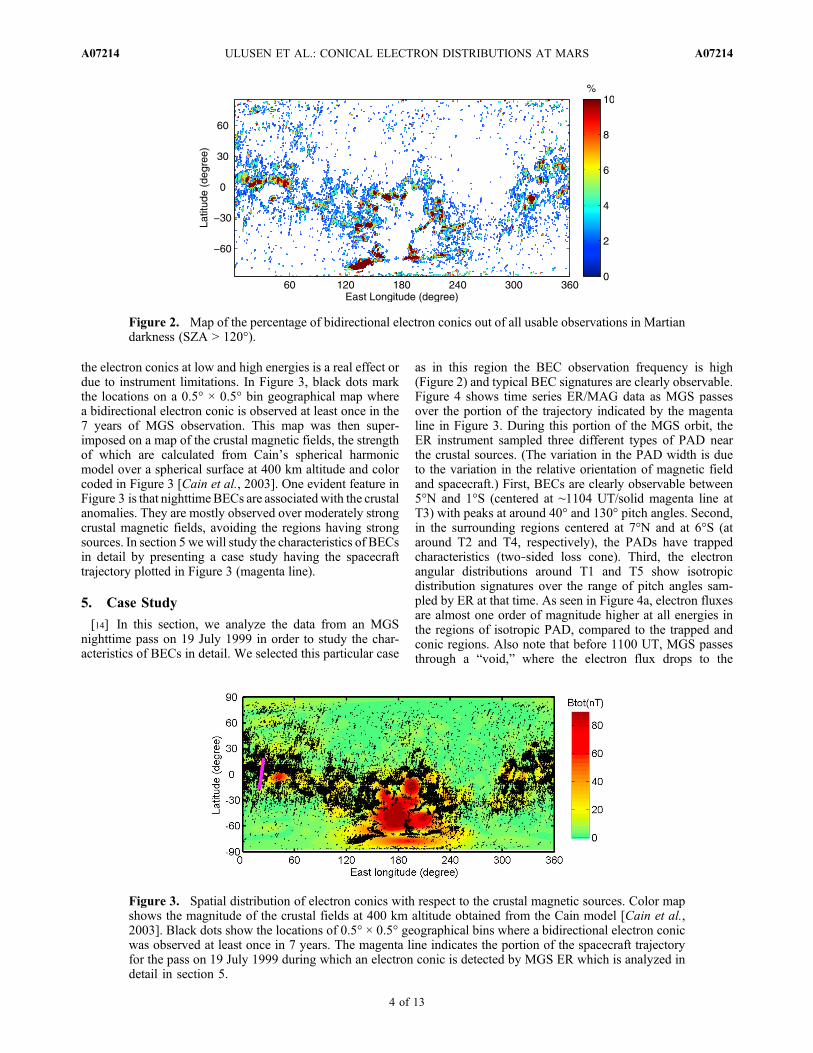
the electron conics at low and high energies is a real effect ordue to instrument limitations. In Figure 3, black dots markthe locations on a 0.5° × 0.5° bin geographical map wherea bidirectional electron conic is observed at least once in the7 years of MGS observation. This map was then super-imposed on a map of the crustal magnetic fields, the strengthof which are calculated from Cain’s spherical harmonicmodel over a spherical surface at 400 km altitude and colorcoded in Figure 3 [Cain et al., 2003]. One evident feature inFigure 3 is that nighttime BECs are associatedwith the crustalanomalies. They are mostly observed over moderately strongcrustal magnetic fields, avoiding the regions having strongsources. In section 5 we will study the characteristics of BECsin detail by presenting a case study having the spacecrafttrajectory plotted in Figure 3 (magenta line).

5. Case Study

[14] In this section, we analyze the data from an MGSnighttime pass on 19 July 1999 in order to study the char-acteristics of BECs in detail. We selected this particular case

as in this region the BEC observation frequency is high(Figure 2) and typical BEC signatures are clearly observable.Figure 4 shows time series ER/MAG data as MGS passesover the portion of the trajectory indicated by the magentaline in Figure 3. During this portion of the MGS orbit, theER instrument sampled three different types of PAD nearthe crustal sources. (The variation in the PAD width is dueto the variation in the relative orientation of magnetic fieldand spacecraft.) First, BECs are clearly observable between5°N and 1°S (centered at ∼1104 UT/solid magenta line atT3) with peaks at around 40° and 130° pitch angles. Second,in the surrounding regions centered at 7°N and at 6°S (ataround T2 and T4, respectively), the PADs have trappedcharacteristics (two‐sided loss cone). Third, the electronangular distributions around T1 and T5 show isotropicdistribution signatures over the range of pitch angles sam-pled by ER at that time. As seen in Figure 4a, electron fluxesare almost one order of magnitude higher at all energies inthe regions of isotropic PAD, compared to the trapped andconic regions. Also note that before 1100 UT, MGS passesthrough a “void,” where the electron flux drops to the

Figure 2. Map of the percentage of bidirectional electron conics out of all usable observations in Martiandarkness (SZA > 120°).

Figure 3. Spatial distribution of electron conics with respect to the crustal magnetic sources. Color mapshows the magnitude of the crustal fields at 400 km altitude obtained from the Cain model [Cain et al.,2003]. Black dots show the locations of 0.5° × 0.5° geographical bins where a bidirectional electron conicwas observed at least once in 7 years. The magenta line indicates the portion of the spacecraft trajectoryfor the pass on 19 July 1999 during which an electron conic is detected by MGS ER which is analyzed indetail in section 5.


4 of 13

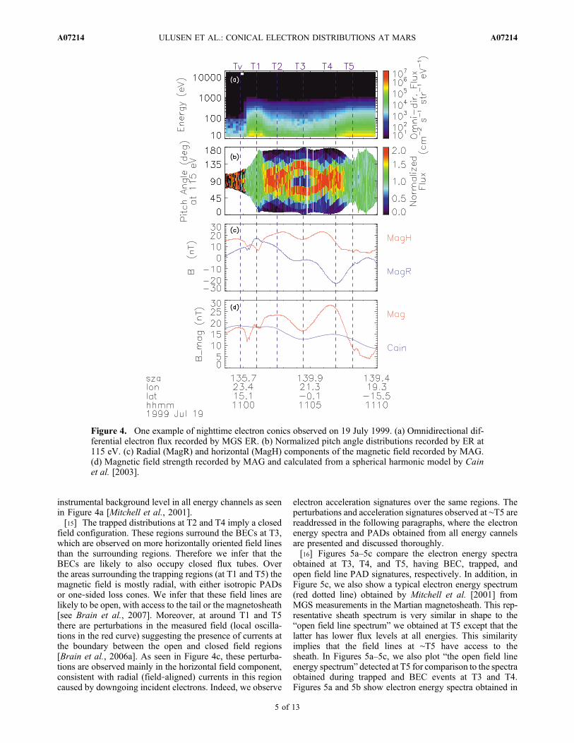
instrumental background level in all energy channels as seenin Figure 4a [Mitchell et al., 2001].[15] The trapped distributions at T2 and T4 imply a closed

field configuration. These regions surround the BECs at T3,which are observed on more horizontally oriented field linesthan the surrounding regions. Therefore we infer that theBECs are likely to also occupy closed flux tubes. Overthe areas surrounding the trapping regions (at T1 and T5) themagnetic field is mostly radial, with either isotropic PADsor one‐sided loss cones. We infer that these field lines arelikely to be open, with access to the tail or the magnetosheath[see Brain et al., 2007]. Moreover, at around T1 and T5there are perturbations in the measured field (local oscilla-tions in the red curve) suggesting the presence of currents atthe boundary between the open and closed field regions[Brain et al., 2006a]. As seen in Figure 4c, these perturba-tions are observed mainly in the horizontal field component,consistent with radial (field‐aligned) currents in this regioncaused by downgoing incident electrons. Indeed, we observe

electron acceleration signatures over the same regions. Theperturbations and acceleration signatures observed at ∼T5 arereaddressed in the following paragraphs, where the electronenergy spectra and PADs obtained from all energy cannelsare presented and discussed thoroughly.[16] Figures 5a–5c compare the electron energy spectra

obtained at T3, T4, and T5, having BEC, trapped, andopen field line PAD signatures, respectively. In addition, inFigure 5c, we also show a typical electron energy spectrum(red dotted line) obtained by Mitchell et al. [2001] fromMGS measurements in the Martian magnetosheath. This rep-resentative sheath spectrum is very similar in shape to the“open field line spectrum” we obtained at T5 except that thelatter has lower flux levels at all energies. This similarityimplies that the field lines at ∼T5 have access to thesheath. In Figures 5a–5c, we also plot “the open field lineenergy spectrum” detected at T5 for comparison to the spectraobtained during trapped and BEC events at T3 and T4.Figures 5a and 5b show electron energy spectra obtained in

Figure 4. One example of nighttime electron conics observed on 19 July 1999. (a) Omnidirectional dif-ferential electron flux recorded by MGS ER. (b) Normalized pitch angle distributions recorded by ER at115 eV. (c) Radial (MagR) and horizontal (MagH) components of the magnetic field recorded by MAG.(d) Magnetic field strength recorded by MAG and calculated from a spherical harmonic model by Cainet al. [2003].


5 of 13

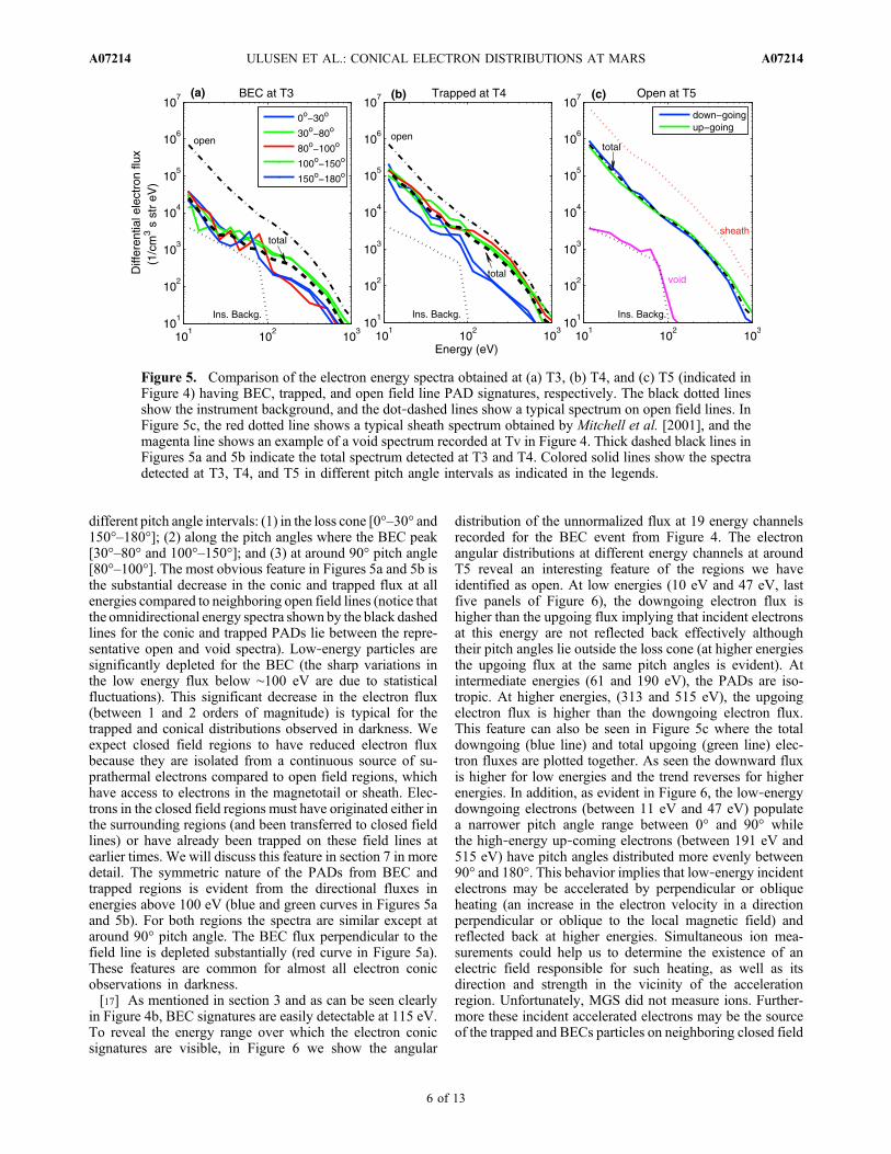
different pitch angle intervals: (1) in the loss cone [0°–30° and150°–180°]; (2) along the pitch angles where the BEC peak[30°–80° and 100°–150°]; and (3) at around 90° pitch angle[80°–100°]. The most obvious feature in Figures 5a and 5b isthe substantial decrease in the conic and trapped flux at allenergies compared to neighboring open field lines (notice thatthe omnidirectional energy spectra shown by the black dashedlines for the conic and trapped PADs lie between the repre-sentative open and void spectra). Low‐energy particles aresignificantly depleted for the BEC (the sharp variations inthe low energy flux below ∼100 eV are due to statisticalfluctuations). This significant decrease in the electron flux(between 1 and 2 orders of magnitude) is typical for thetrapped and conical distributions observed in darkness. Weexpect closed field regions to have reduced electron fluxbecause they are isolated from a continuous source of su-prathermal electrons compared to open field regions, whichhave access to electrons in the magnetotail or sheath. Elec-trons in the closed field regions must have originated either inthe surrounding regions (and been transferred to closed fieldlines) or have already been trapped on these field lines atearlier times. We will discuss this feature in section 7 in moredetail. The symmetric nature of the PADs from BEC andtrapped regions is evident from the directional fluxes inenergies above 100 eV (blue and green curves in Figures 5aand 5b). For both regions the spectra are similar except ataround 90° pitch angle. The BEC flux perpendicular to thefield line is depleted substantially (red curve in Figure 5a).These features are common for almost all electron conicobservations in darkness.[17] As mentioned in section 3 and as can be seen clearly

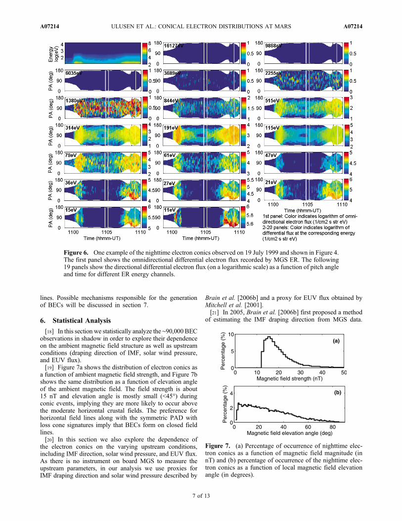
in Figure 4b, BEC signatures are easily detectable at 115 eV.To reveal the energy range over which the electron conicsignatures are visible, in Figure 6 we show the angular

distribution of the unnormalized flux at 19 energy channelsrecorded for the BEC event from Figure 4. The electronangular distributions at different energy channels at aroundT5 reveal an interesting feature of the regions we haveidentified as open. At low energies (10 eV and 47 eV, lastfive panels of Figure 6), the downgoing electron flux ishigher than the upgoing flux implying that incident electronsat this energy are not reflected back effectively althoughtheir pitch angles lie outside the loss cone (at higher energiesthe upgoing flux at the same pitch angles is evident). Atintermediate energies (61 and 190 eV), the PADs are iso-tropic. At higher energies, (313 and 515 eV), the upgoingelectron flux is higher than the downgoing electron flux.This feature can also be seen in Figure 5c where the totaldowngoing (blue line) and total upgoing (green line) elec-tron fluxes are plotted together. As seen the downward fluxis higher for low energies and the trend reverses for higherenergies. In addition, as evident in Figure 6, the low‐energydowngoing electrons (between 11 eV and 47 eV) populatea narrower pitch angle range between 0° and 90° whilethe high‐energy up‐coming electrons (between 191 eV and515 eV) have pitch angles distributed more evenly between90° and 180°. This behavior implies that low‐energy incidentelectrons may be accelerated by perpendicular or obliqueheating (an increase in the electron velocity in a directionperpendicular or oblique to the local magnetic field) andreflected back at higher energies. Simultaneous ion mea-surements could help us to determine the existence of anelectric field responsible for such heating, as well as itsdirection and strength in the vicinity of the accelerationregion. Unfortunately, MGS did not measure ions. Further-more these incident accelerated electrons may be the sourceof the trapped and BECs particles on neighboring closed field

Figure 5. Comparison of the electron energy spectra obtained at (a) T3, (b) T4, and (c) T5 (indicated inFigure 4) having BEC, trapped, and open field line PAD signatures, respectively. The black dotted linesshow the instrument background, and the dot‐dashed lines show a typical spectrum on open field lines. InFigure 5c, the red dotted line shows a typical sheath spectrum obtained by Mitchell et al. [2001], and themagenta line shows an example of a void spectrum recorded at Tv in Figure 4. Thick dashed black lines inFigures 5a and 5b indicate the total spectrum detected at T3 and T4. Colored solid lines show the spectradetected at T3, T4, and T5 in different pitch angle intervals as indicated in the legends.


6 of 13

lines. Possible mechanisms responsible for the generationof BECs will be discussed in section 7.

6. Statistical Analysis

[18] In this section we statistically analyze the ∼90,000 BECobservations in shadow in order to explore their dependenceon the ambient magnetic field structure as well as upstreamconditions (draping direction of IMF, solar wind pressure,and EUV flux).[19] Figure 7a shows the distribution of electron conics as

a function of ambient magnetic field strength, and Figure 7bshows the same distribution as a function of elevation angleof the ambient magnetic field. The field strength is about15 nT and elevation angle is mostly small (<45°) duringconic events, implying they are more likely to occur abovethe moderate horizontal crustal fields. The preference forhorizontal field lines along with the symmetric PAD withloss cone signatures imply that BECs form on closed fieldlines.[20] In this section we also explore the dependence of

the electron conics on the varying upstream conditions,including IMF direction, solar wind pressure, and EUV flux.As there is no instrument on board MGS to measure theupstream parameters, in our analysis we use proxies forIMF draping direction and solar wind pressure described by

Brain et al. [2006b] and a proxy for EUV flux obtained byMitchell et al. [2001].[21] In 2005, Brain et al. [2006b] first proposed a method

of estimating the IMF draping direction from MGS data.

Figure 6. One example of the nighttime electron conics observed on 19 July 1999 and shown in Figure 4.The first panel shows the omnidirectional differential electron flux recorded by MGS ER. The following19 panels show the directional differential electron flux (on a logarithmic scale) as a function of pitch angleand time for different ER energy channels.

Figure 7. (a) Percentage of occurrence of nighttime elec-tron conics as a function of magnetic field magnitude (innT) and (b) percentage of occurrence of the nighttime elec-tron conics as a function of local magnetic field elevationangle (in degrees).


7 of 13

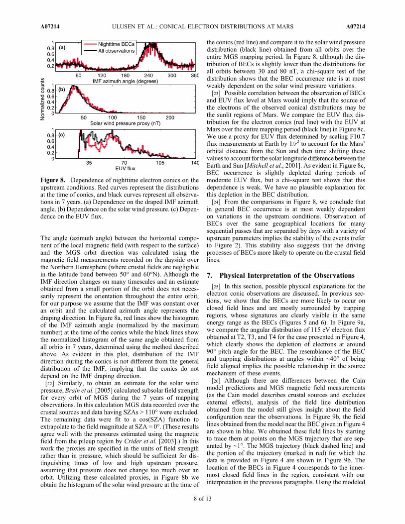
The angle (azimuth angle) between the horizontal compo-nent of the local magnetic field (with respect to the surface)and the MGS orbit direction was calculated using themagnetic field measurements recorded on the dayside overthe Northern Hemisphere (where crustal fields are negligiblein the latitude band between 50° and 60°N). Although theIMF direction changes on many timescales and an estimateobtained from a small portion of the orbit does not neces-sarily represent the orientation throughout the entire orbit,for our purpose we assume that the IMF was constant overan orbit and the calculated azimuth angle represents thedraping direction. In Figure 8a, red lines show the histogramof the IMF azimuth angle (normalized by the maximumnumber) at the time of the conics while the black lines showthe normalized histogram of the same angle obtained fromall orbits in 7 years, determined using the method describedabove. As evident in this plot, distribution of the IMFdirection during the conics is not different from the generaldistribution of the IMF, implying that the conics do notdepend on the IMF draping direction.[22] Similarly, to obtain an estimate for the solar wind

pressure, Brain et al. [2005] calculated subsolar field strengthfor every orbit of MGS during the 7 years of mappingobservations. In this calculation MGS data recorded over thecrustal sources and data having SZAs > 110° were excluded.The remaining data were fit to a cos(SZA) function toextrapolate to the field magnitude at SZA = 0°. (These resultsagree well with the pressures estimated using the magneticfield from the pileup region by Crider et al. [2003].) In thiswork the proxies are specified in the units of field strengthrather than in pressure, which should be sufficient for dis-tinguishing times of low and high upstream pressure,assuming that pressure does not change too much over anorbit. Utilizing these calculated proxies, in Figure 8b weobtain the histogram of the solar wind pressure at the time of

the conics (red line) and compare it to the solar wind pressuredistribution (black line) obtained from all orbits over theentire MGS mapping period. In Figure 8, although the dis-tribution of BECs is slightly lower than the distributions forall orbits between 30 and 80 nT, a chi‐square test of thedistribution shows that the BEC occurrence rate is at mostweakly dependent on the solar wind pressure variations.[23] Possible correlation between the observation of BECs

and EUV flux level at Mars would imply that the source ofthe electrons of the observed conical distributions may bethe sunlit regions of Mars. We compare the EUV flux dis-tribution for the electron conics (red line) with the EUV atMars over the entire mapping period (black line) in Figure 8c.We use a proxy for EUV flux determined by scaling F10.7flux measurements at Earth by 1/r2 to account for the Mars’orbital distance from the Sun and then time shifting thesevalues to account for the solar longitude difference between theEarth and Sun [Mitchell et al., 2001]. As evident in Figure 8c,BEC occurrence is slightly depleted during periods ofmoderate EUV flux, but a chi‐square test shows that thisdependence is weak. We have no plausible explanation forthis depletion in the BEC distribution.[24] From the comparisons in Figure 8, we conclude that

in general BEC occurrence is at most weakly dependenton variations in the upstream conditions. Observation ofBECs over the same geographical locations for manysequential passes that are separated by days with a variety ofupstream parameters implies the stability of the events (referto Figure 2). This stability also suggests that the drivingprocesses of BECs more likely to operate on the crustal fieldlines.

7. Physical Interpretation of the Observations

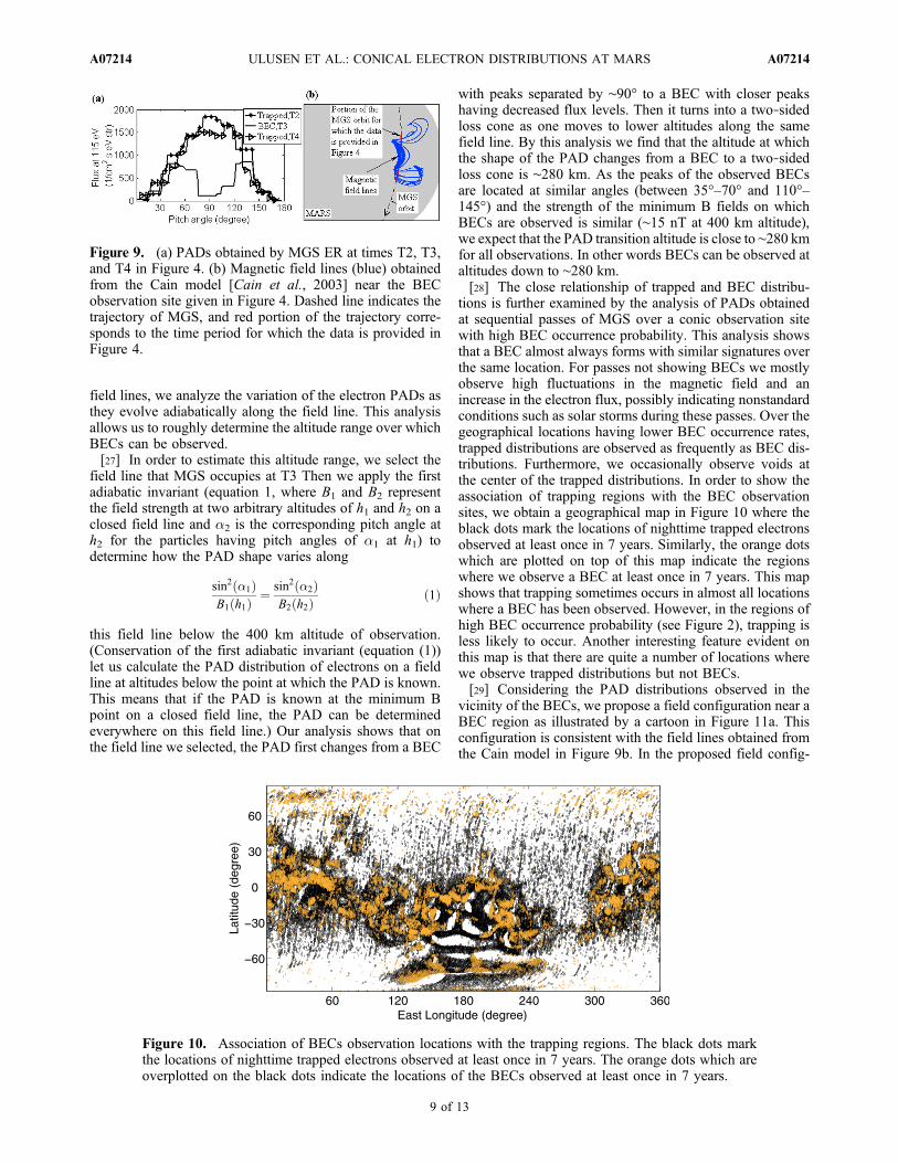
[25] In this section, possible physical explanations for theelectron conic observations are discussed. In previous sec-tions, we show that the BECs are more likely to occur onclosed field lines and are mostly surrounded by trappingregions, whose signatures are clearly visible in the sameenergy range as the BECs (Figures 5 and 6). In Figure 9a,we compare the angular distribution of 115 eV electron fluxobtained at T2, T3, and T4 for the case presented in Figure 4,which clearly shows the depletion of electrons at around90° pitch angle for the BEC. The resemblance of the BECand trapping distributions at angles within ∼40° of beingfield aligned implies the possible relationship in the sourcemechanism of these events.[26] Although there are differences between the Cain

model predictions and MGS magnetic field measurements(as the Cain model describes crustal sources and excludesexternal effects), analysis of the field line distributionobtained from the model still gives insight about the fieldconfiguration near the observations. In Figure 9b, the fieldlines obtained from the model near the BEC given in Figure 4are shown in blue. We obtained these field lines by startingto trace them at points on the MGS trajectory that are sep-arated by ∼1°. The MGS trajectory (black dashed line) andthe portion of the trajectory (marked in red) for which thedata is provided in Figure 4 are shown in Figure 9b. Thelocation of the BECs in Figure 4 corresponds to the inner-most closed field lines in the region, consistent with ourinterpretation in the previous paragraphs. Using the modeled

Figure 8. Dependence of nighttime electron conics on theupstream conditions. Red curves represent the distributionsat the time of conics, and black curves represent all observa-tions in 7 years. (a) Dependence on the draped IMF azimuthangle. (b) Dependence on the solar wind pressure. (c) Depen-dence on the EUV flux.


8 of 13

field lines, we analyze the variation of the electron PADs asthey evolve adiabatically along the field line. This analysisallows us to roughly determine the altitude range over whichBECs can be observed.[27] In order to estimate this altitude range, we select the

field line that MGS occupies at T3 Then we apply the firstadiabatic invariant (equation 1, where B1 and B2 representthe field strength at two arbitrary altitudes of h1 and h2 on aclosed field line and a2 is the corresponding pitch angle ath2 for the particles having pitch angles of a1 at h1) todetermine how the PAD shape varies along

sin2 �1ð ÞB1 h1ð Þ ¼ sin2 �2ð Þ

B2 h2ð Þ ð1Þ

this field line below the 400 km altitude of observation.(Conservation of the first adiabatic invariant (equation (1))let us calculate the PAD distribution of electrons on a fieldline at altitudes below the point at which the PAD is known.This means that if the PAD is known at the minimum Bpoint on a closed field line, the PAD can be determinedeverywhere on this field line.) Our analysis shows that onthe field line we selected, the PAD first changes from a BEC

with peaks separated by ∼90° to a BEC with closer peakshaving decreased flux levels. Then it turns into a two‐sidedloss cone as one moves to lower altitudes along the samefield line. By this analysis we find that the altitude at whichthe shape of the PAD changes from a BEC to a two‐sidedloss cone is ∼280 km. As the peaks of the observed BECsare located at similar angles (between 35°–70° and 110°–145°) and the strength of the minimum B fields on whichBECs are observed is similar (∼15 nT at 400 km altitude),we expect that the PAD transition altitude is close to ∼280 kmfor all observations. In other words BECs can be observed ataltitudes down to ∼280 km.[28] The close relationship of trapped and BEC distribu-

tions is further examined by the analysis of PADs obtainedat sequential passes of MGS over a conic observation sitewith high BEC occurrence probability. This analysis showsthat a BEC almost always forms with similar signatures overthe same location. For passes not showing BECs we mostlyobserve high fluctuations in the magnetic field and anincrease in the electron flux, possibly indicating nonstandardconditions such as solar storms during these passes. Over thegeographical locations having lower BEC occurrence rates,trapped distributions are observed as frequently as BEC dis-tributions. Furthermore, we occasionally observe voids atthe center of the trapped distributions. In order to show theassociation of trapping regions with the BEC observationsites, we obtain a geographical map in Figure 10 where theblack dots mark the locations of nighttime trapped electronsobserved at least once in 7 years. Similarly, the orange dotswhich are plotted on top of this map indicate the regionswhere we observe a BEC at least once in 7 years. This mapshows that trapping sometimes occurs in almost all locationswhere a BEC has been observed. However, in the regions ofhigh BEC occurrence probability (see Figure 2), trapping isless likely to occur. Another interesting feature evident onthis map is that there are quite a number of locations wherewe observe trapped distributions but not BECs.[29] Considering the PAD distributions observed in the

vicinity of the BECs, we propose a field configuration near aBEC region as illustrated by a cartoon in Figure 11a. Thisconfiguration is consistent with the field lines obtained fromthe Cain model in Figure 9b. In the proposed field config-

Figure 9. (a) PADs obtained by MGS ER at times T2, T3,and T4 in Figure 4. (b) Magnetic field lines (blue) obtainedfrom the Cain model [Cain et al., 2003] near the BECobservation site given in Figure 4. Dashed line indicates thetrajectory of MGS, and red portion of the trajectory corre-sponds to the time period for which the data is provided inFigure 4.

Figure 10. Association of BECs observation locations with the trapping regions. The black dots markthe locations of nighttime trapped electrons observed at least once in 7 years. The orange dots which areoverplotted on the black dots indicate the locations of the BECs observed at least once in 7 years.


9 of 13

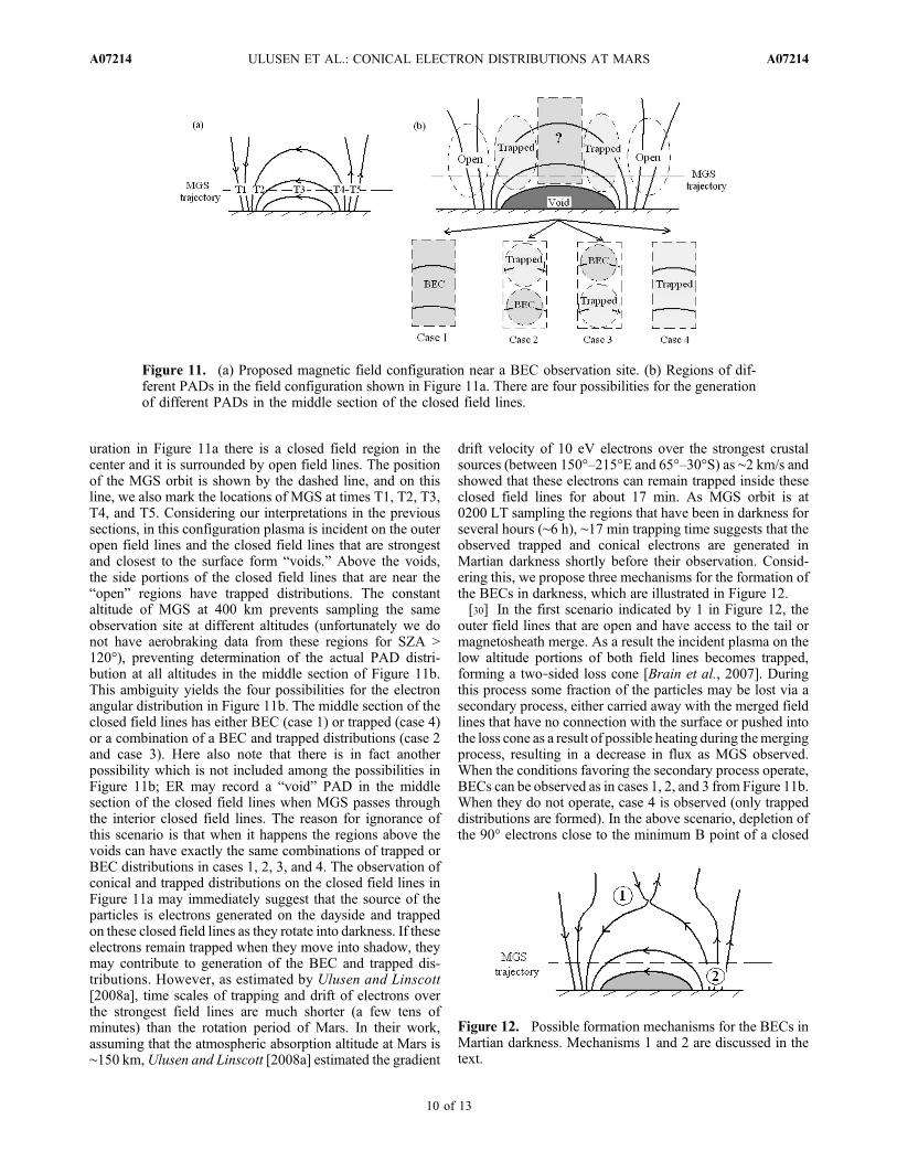
uration in Figure 11a there is a closed field region in thecenter and it is surrounded by open field lines. The positionof the MGS orbit is shown by the dashed line, and on thisline, we also mark the locations of MGS at times T1, T2, T3,T4, and T5. Considering our interpretations in the previoussections, in this configuration plasma is incident on the outeropen field lines and the closed field lines that are strongestand closest to the surface form “voids.” Above the voids,the side portions of the closed field lines that are near the“open” regions have trapped distributions. The constantaltitude of MGS at 400 km prevents sampling the sameobservation site at different altitudes (unfortunately we donot have aerobraking data from these regions for SZA >120°), preventing determination of the actual PAD distri-bution at all altitudes in the middle section of Figure 11b.This ambiguity yields the four possibilities for the electronangular distribution in Figure 11b. The middle section of theclosed field lines has either BEC (case 1) or trapped (case 4)or a combination of a BEC and trapped distributions (case 2and case 3). Here also note that there is in fact anotherpossibility which is not included among the possibilities inFigure 11b; ER may record a “void” PAD in the middlesection of the closed field lines when MGS passes throughthe interior closed field lines. The reason for ignorance ofthis scenario is that when it happens the regions above thevoids can have exactly the same combinations of trapped orBEC distributions in cases 1, 2, 3, and 4. The observation ofconical and trapped distributions on the closed field lines inFigure 11a may immediately suggest that the source of theparticles is electrons generated on the dayside and trappedon these closed field lines as they rotate into darkness. If theseelectrons remain trapped when they move into shadow, theymay contribute to generation of the BEC and trapped dis-tributions. However, as estimated by Ulusen and Linscott[2008a], time scales of trapping and drift of electrons overthe strongest field lines are much shorter (a few tens ofminutes) than the rotation period of Mars. In their work,assuming that the atmospheric absorption altitude at Mars is∼150 km,Ulusen and Linscott [2008a] estimated the gradient

drift velocity of 10 eV electrons over the strongest crustalsources (between 150°–215°E and 65°–30°S) as ∼2 km/s andshowed that these electrons can remain trapped inside theseclosed field lines for about 17 min. As MGS orbit is at0200 LT sampling the regions that have been in darkness forseveral hours (∼6 h), ∼17 min trapping time suggests that theobserved trapped and conical electrons are generated inMartian darkness shortly before their observation. Consid-ering this, we propose three mechanisms for the formation ofthe BECs in darkness, which are illustrated in Figure 12.[30] In the first scenario indicated by 1 in Figure 12, the

outer field lines that are open and have access to the tail ormagnetosheath merge. As a result the incident plasma on thelow altitude portions of both field lines becomes trapped,forming a two‐sided loss cone [Brain et al., 2007]. Duringthis process some fraction of the particles may be lost via asecondary process, either carried away with the merged fieldlines that have no connection with the surface or pushed intothe loss cone as a result of possible heating during themergingprocess, resulting in a decrease in flux as MGS observed.When the conditions favoring the secondary process operate,BECs can be observed as in cases 1, 2, and 3 from Figure 11b.When they do not operate, case 4 is observed (only trappeddistributions are formed). In the above scenario, depletion ofthe 90° electrons close to the minimum B point of a closed

Figure 11. (a) Proposed magnetic field configuration near a BEC observation site. (b) Regions of dif-ferent PADs in the field configuration shown in Figure 11a. There are four possibilities for the generationof different PADs in the middle section of the closed field lines.

Figure 12. Possible formation mechanisms for the BECs inMartian darkness. Mechanisms 1 and 2 are discussed in thetext.


10 of 13

field line may involve wave‐particle interactions and staticor time‐varying potential drops. Possible parallel heating(increase in the parallel velocity) due to such processesacting near the minimum B point of a closed field line mayscatter the electrons from ∼90° pitch angle toward 0° and180° pitch angles, forming the peaks of the BEC. Thismechanism may also push some oblique electrons into theloss cone, where they are then lost in the atmosphere.Similar mechanisms have been suggested for the generationof the conics at Earth by Burch et al. [1990] and Lundinet al. [1987]. Using numerical simulations, Burch et al.showed that distributions similar to observed two‐sided conicscan form when the spacecraft passes through a region offield aligned electric fields. Verification of these sourcemechanisms would be possible by simultaneous electricfield and/or ion measurements in the source region. (Thegyrofrequency of the electrons near the horizontal field lineswith strength of 15 nT is ∼2.5 kHz.) Unfortunately, neitherMGS nor Mars Express has the appropriate combination ofinstrumentation.[31] In the second scenario indicated by 2 in Figure 12,

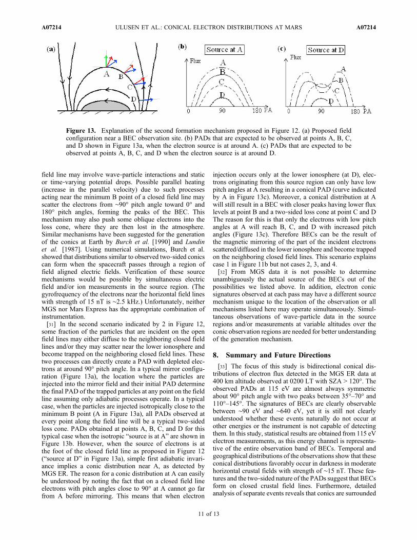
some fraction of the particles that are incident on the openfield lines may either diffuse to the neighboring closed fieldlines and/or they may scatter near the lower ionosphere andbecome trapped on the neighboring closed field lines. Thesetwo processes can directly create a PAD with depleted elec-trons at around 90° pitch angle. In a typical mirror configu-ration (Figure 13a), the location where the particles areinjected into the mirror field and their initial PAD determinethe final PAD of the trapped particles at any point on the fieldline assuming only adiabatic processes operate. In a typicalcase, when the particles are injected isotropically close to theminimum B point (A in Figure 13a), all PADs observed atevery point along the field line will be a typical two‐sidedloss cone. PADs obtained at points A, B, C, and D for thistypical case when the isotropic “source is at A” are shown inFigure 13b. However, when the source of electrons is atthe foot of the closed field line as proposed in Figure 12(“source at D” in Figure 13a), simple first adiabatic invari-ance implies a conic distribution near A, as detected byMGS ER. The reason for a conic distribution at A can easilybe understood by noting the fact that on a closed field lineelectrons with pitch angles close to 90° at A cannot go farfrom A before mirroring. This means that when electron

injection occurs only at the lower ionosphere (at D), elec-trons originating from this source region can only have lowpitch angles at A resulting in a conical PAD (curve indicatedby A in Figure 13c). Moreover, a conical distribution at Awill still result in a BEC with closer peaks having lower fluxlevels at point B and a two‐sided loss cone at point C and DThe reason for this is that only the electrons with low pitchangles at A will reach B, C, and D with increased pitchangles (Figure 13c). Therefore BECs can be the result ofthe magnetic mirroring of the part of the incident electronsscattered/diffused in the lower ionosphere and become trappedon the neighboring closed field lines. This scenario explainscase 1 in Figure 11b but not cases 2, 3, and 4.[32] From MGS data it is not possible to determine

unambiguously the actual source of the BECs out of thepossibilities we listed above. In addition, electron conicsignatures observed at each pass may have a different sourcemechanism unique to the location of the observation or allmechanisms listed here may operate simultaneously. Simul-taneous observations of wave‐particle data in the sourceregions and/or measurements at variable altitudes over theconic observation regions are needed for better understandingof the generation mechanism.

8. Summary and Future Directions

[33] The focus of this study is bidirectional conical dis-tributions of electron flux detected in the MGS ER data at400 km altitude observed at 0200 LT with SZA > 120°. Theobserved PADs at 115 eV are almost always symmetricabout 90° pitch angle with two peaks between 35°–70° and110°–145°. The signatures of BECs are clearly observablebetween ∼90 eV and ∼640 eV, yet it is still not clearlyunderstood whether these events naturally do not occur atother energies or the instrument is not capable of detectingthem. In this study, statistical results are obtained from 115 eVelectron measurements, as this energy channel is representa-tive of the entire observation band of BECs. Temporal andgeographical distributions of the observations show that theseconical distributions favorably occur in darkness in moderatehorizontal crustal fields with strength of ∼15 nT. These fea-tures and the two‐sided nature of the PADs suggest that BECsform on closed crustal field lines. Furthermore, detailedanalysis of separate events reveals that conics are surrounded

Figure 13. Explanation of the second formation mechanism proposed in Figure 12. (a) Proposed fieldconfiguration near a BEC observation site. (b) PADs that are expected to be observed at points A, B, C,and D shown in Figure 13a, when the electron source is at around A. (c) PADs that are expected to beobserved at points A, B, C, and D when the electron source is at around D.


11 of 13

by trapping regions and their electron flux decreases sub-stantially at all energy levels in relation to the neighboringregions that do not have conics but have access to either thetail or the magnetosheath.[34] Exploration of the dependency of BECs on the

upstream conditions shows that they do not depend stronglyon the variations in the draped IMF direction, solar windpressure, and EUV flux level. Observation of similar BECsover the same geographical locations for many sequentialpasses that are separated by days and have a variety ofupstream parameters reveals the stability of the events. Theindependence of the BECs from the varying external con-ditions suggests that the driving processes of BECs morelikely to operate in areas of crustal fields.[35] We propose two main source mechanisms that may

be responsible for the generation of BECs. In the formula-tion of these two proposals we have considered the fact thattime scales of trapping and drift of electrons estimated overthe strongest field lines are much shorter than the planet’srotation period. Therefore the observed trapped and conicalelectrons must be generated in Martian darkness shortlybefore their observation [Ulusen and Linscott, 2008a]. Thefirst proposed mechanism involves the merging of openfield lines neighboring the closed field lines on whichtrapping and BECs are observed. By this mechanism theincident electrons on the open field lines become trapped.Electrons at ∼90° pitch angles can be either directly lostduring the merging process or pushed to the loss cone bywave‐particle interactions, static, or time varying electricfields. Similar mechanisms were proposed for the generationof the bidirectional electron conics observed at Earth [Burchet al., 1990; Lundin et al., 1987]. A second proposed mech-anism involves the mirroring of particles that are streamed tolower altitudes on the nearby open field lines, which are thendiffused and/or scattered into regions dominated by the innerclosed field lines. Both mechanisms are consistent with theindependent nature of BECs from the external conditions, yetverification of the role of these processes in the generation ofthe BECS requires simultaneous observations of waves,measurements of ions, and sampling of PADs at a variety ofaltitudes near the source regions.[36] Analysis of dayside and terminator observations of

MGS along with the ion data of Mars Express (ion com-position, energy, and angular distributions) would helpevaluate the potential drops at the measurement altitude.Such an analysis should be addressed in a follow up study.Other useful observations that would allow a more definitivestatement to be made about the production mechanism of theconics are measurements of high‐frequency variations inthe magnetic and electric field. These measurements wouldhelp understand the wave activity and presence of particleacceleration nearby BECs. Future Mars Atmosphere andVolatile Evolution (MAVEN) spacecraft observations willprovide more complete measurements of the definite char-acteristics of BECs, requiring further observational and theo-retical studies to reveal the underlying mechanism of electronconics at Mars. Understanding generation mechanisms ofthe conics and plasma processes causing or resulting fromthem near the Martian minimagnetospheres will give betterinsight for different types of conical distribution observed atEarth or other planets with global magnetospheres.

[37] Acknowledgments. Thanks to Robert J. Lillis for preliminarysimulation work in support of this research and thanks to Jasper S. Halekasfor useful discussions. This study was supported by NASA grantNNX08BA59G.[38] Masaki Fujimoto thanks Ying Juan Ma and another reviewer for

their assistance in evaluating this paper.

ReferencesAcuña, M. H., et al. (1992), Mars Observer magnetic fields investigation,J. Geophys. Res., 97(E5), 7799–7814, doi:10.1029/92JE00344.

Acuña, M. H., et al. (1998), Magnetic field and plasma observations atMars: Initial results of Mars Global Surveyor mission, Science, 279,1676–1680, doi:10.1126/science.279.5357.1676.

Acuña, M. H., et al. (2001), Magnetic field of Mars: Summary of resultsfrom the aerobraking and mapping orbits, J. Geophys. Res., 106(E10),23,403–23,417, doi:10.1029/2000JE001404.

Albee, A. L., R. E. Arvidson, F. Palluconi, and T. Thorpe (2001), Overviewof the Mars Global Surveyor mission, J. Geophys. Res., 106(E10),23,291–23,316, doi:10.1029/2000JE001306.

André, M., and L. Eliasson (1992), Electron acceleration by low‐frequencyelectric field fluctuations: Electron conics, Geophys. Res. Lett., 19,1073–1076, doi:10.1029/92GL01022.

Bertaux, J. L., F. Leblanc, O. Witasse, E. Quemerais, J. Lilensten, A. S.Stern, B. Sandel, and O. Korablev (2005), Discovery of aurora on Mars,Nature, 435, 790–794, doi:10.1038/nature03603.

Brain, D. A., J. S. Halekas, R. Lillis, D. L. Mitchell, and R. P. Lin (2005),Variability of the altitude of the Martian sheath, Geophys. Res. Lett., 32,L18203, doi:10.1029/2005GL023126.

Brain, D. A., J. S. Halekas, L. M. Peticolas, R. P. Lin, J. G. Luhmann, D. L.Mitchell, G. T. Delory, S. W. Bougher, M. H. Acuña, and H. Reme(2006a), On the origin of aurorae on Mars, Geophys. Res. Lett., 33,L01201, doi:10.1029/2005GL024782.

Brain, D. A., D. L. Mitchell, and J. S. Halekas (2006b), The magnetic fielddraping direction at Mars from April 1999 through August 2004, Icarus,182, 464–473, doi:10.1016/j.icarus.2005.09.023.

Brain, D. A., R. J. Lillis, D. L. Mitchell, J. S. Halekas, and R. P. Lin (2007),Electron pitch angle distributions as indicators of magnetic field topologynear Mars, J. Geophys. Res., 112, A09201, doi:10.1029/2007JA012435.

Burch, J. L. (1995), Dynamics Explorer observations of the production ofelectron conics, Geophys. Res. Lett., 22, 2705–2708, doi:10.1029/95GL02817.

Burch, J. L., C. Gurgiolo, and J. D. Menietti (1990), The electron signatureof parallel electric fields, Geophys. Res. Lett., 17, 2329–2332,doi:10.1029/GL017i013p02329.

Cain, J. C., B. B. Ferguson, and D. Mozzoni (2003), An n = 90 internalpotential function of the Martian crustal magnetic field, J. Geophys.Res., 108(E2), 5008, doi:10.1029/2000JE001487.

Crider, D. H., D. Vignes, A. M. Krymskii, T. K. Breus, N. F. Ness, D. L.Mitchell, J. A. Slavin, and M. H. Acuña (2003), A proxy for determiningsolar wind dynamic pressure at Mars using Mars Global Surveyor data,J. Geophys. Res., 108(A12), 1461, doi:10.1029/2003JA009875.

Dubinin, E. M., M. Fraenz, J. Woch, E. Roussos, J. D. Winningham, R. A.Frahm, A. Coates, F. Leblanc, R. Lundin, and S. Barabash (2008),Access of solar wind electrons into the Martian magnetosphere, Ann.Geophys., 26(11), 3511–3524, doi:10.5194/angeo-26-3511-2008.

Eliasson, L., M. Andre, R. Lundin, R. Pottelette, G. Marklund, andG. Holmgren (1996), Observations of electron conics by the Viking satel-lite, J. Geophys. Res., 101(A6), 13,225–13,238, doi:10.1029/95JA02386.

Hultqvist, B., R. Lundin, K. Stasiewicz, L. Block, P.‐A. Lindqvist,G. Gustafsson, H. Koskinen, A. Bahnsen, T. A. Potemra, and L. J. Zanetti(1988), Simultaneous observation of upward moving field aligned ener-getic electrons and ions on auroral zone field lines, J. Geophys.Res., 93(A9), 9765–9776, doi:10.1029/JA093iA09p09765.

Krymskii, A. M., T. K. Breus, N. F. Ness, M. H. Acuña, J. E. P. Connerney,D. H. Crider, D. L. Mitchell, and S. J. Bauer (2002), Structure of the mag-netic field fluxes connected with crustal magnetization and topside iono-sphere at Mars, J. Geophys. Res., 107(A9), 1245, doi:10.1029/2001JA000239.

Leblanc, F., O. Witasse, J. Winningham, D. Brain, J. Lilensten, P.‐L.Blelly, R. A. Frahm, J. S. Halekas, and J. L. Bertaux (2006), Originsof the Martian aurora observed by Spectroscopy for Investigation ofCharacteristics of the Atmosphere of Mars (SPICAM) on board MarsExpress, J. Geophys. Res., 111, A09313, doi:10.1029/2006JA011763.

Luhmann, J. G. (1986), The solar wind interaction with Venus, Space Sci.Rev., 44, 241–306.

Luhmann, J. G., and L. H. Brace (1991), Near‐Mars space, Rev. Geophys.,29, 121–140, doi:10.1029/91RG00066.


12 of 13

Lundin, R., L. Eliasson, B. Hultqvist, and K. Stasiewicz (1987), Plasmaenergization on auroral field lines as observed by the Viking spacecraft,Geophys. Res. Lett., 14, 443–446, doi:10.1029/GL014i004p00443.

Lundin, R., et al. (2006), Plasma acceleration above Martian magneticanomalies, Science, 311, 980–983, doi:10.1126/science.1122071.

Menietti, J. D., and J. L. Burch (1985), “Electron conic” signaturesobserved in the nightside auroral zone and over the polar cap, J. Geophys.Res., 90(A6), 5345–5353, doi:10.1029/JA090iA06p05345.

Menietti, J. D., and D. R. Weimer (1998), DE observations of electric fieldoscillations associated with an electron conic, J. Geophys. Res., 103(A1),431–438, doi:10.1029/97JA02496.

Menietti, J. D., C. S. Lin, H. K. Wong, A. Bahnsen, and D. A. Gurnett(1992), Association of electron conical distributions with upper hybridwaves, J. Geophys. Res., 97(A2), 1353–1361, doi:10.1029/91JA02392.

Menietti, J. D., D. R. Weimer, M. Andre, and L. Eliasson (1994), DE1and Viking observation associated with electron conical distributions,J. Geophys. Res., 99(A12), 23,673–23,684, doi:10.1029/94JA02133.

Mitchell, D. L., R. P. Lin, C. Mazelle, H. Reme, P. A. Cloutier, J. E. P.Connerney, M. H. Acuña, and N. F. Ness (2001), Probing Mars’ crustalmagnetic field and ionosphere with the MGS electron reflectometer,J. Geophys. Res., 106(E10), 23,419–23,427, doi:10.1029/2000JE001435.

Nagy, A. F., D. Winterhalter, and K. Sauer (2004), Plasma environ-ment of Mars, Space Sci. Rev., 111, 33–114, doi:10.1023/B:SPAC.0000032718.47512.92.

Roth, I., M. K. Hudson, and M. Ternerin (1989), Generation models ofelectron conics, J. Geophys. Res., 94(A8), 10,095–10,102, doi:10.1029/JA094iA08p10095.

Soobiah, Y., et al. (2006), Observations of magnetic anomaly signatures inMars Express ASPERA‐3 ELS data, Icarus, 182, 396–405, doi:10.1016/j.icarus.2005.10.034.

Temerin, M. A., and D. Cravens (1990), Production of electron conics bystochastic acceleration parallel to the magnetic field, J. Geophys. Res.,95(A4), 4285–4290, doi:10.1029/JA095iA04p04285.

Thompson, B., and R. L. Lysak (1994), Electron acceleration by the iono-spheric Alfven resonator, inPhysics of Space Plasmas, edited by T. Chang,p. 525, Scientific, Cambridge, Mass.

Ulusen, D., and I. Linscott (2008a), Transient events in the solar wind inter-action of Mars due to the strong crustal fields, paper presented at ChapmanConference on the Solar Wind Interaction With Mars, AGU, San Diego,Calif.

Ulusen, D., and I. Linscott (2008b), Low energy electron current in theMartian tail due to reconnection of draped IMF and crustal magneticfields, J. Geophys. Res., 113, E06001, doi:10.1029/2007JE002916.

Wong, H. K., J. D. Menietti, C. S. Lin, and J. L. Burch (1988), Generationof electron conical distributions by upper hybrid waves in the Earth’spolar region, J. Geophys. Res., 93(A9), 10,025–10,028, doi:10.1029/JA093iA09p10025.

D. A. Brain, D. L. Mitchell, and D. Ulusen, Space Sciences Laboratory,University of California, Berkeley, CA 94720, USA. ([email protected])


13 of 13

Documents

Observation of conical electron distributions over Martian crustal magnetic fields