ORI GIN AL PA PER

Numerical issues in computing inundation areas overnatural terrains using Savage-Hutter theory

Bin Yu Æ Keith Dalbey Æ Amy Webb Æ Marcus Bursik Æ Abani Patra ÆE. Bruce Pitman Æ Camil Nichita

Received: 16 May 2008 / Accepted: 2 December 2008� Springer Science+Business Media B.V. 2008

Abstract When characterizing geologic natural hazards, specifically granular flows

including pyroclastic flows, debris avalanches and debris flows, perhaps the most important

factor to consider is the area of inundation. One of the key parameters demarcating the

leading edge of inundation is the run-out distance. To define the run-out distance, it is

necessary to know when the flow stops. Numerical experiments are presented for deter-

mining a stopping criterion and exploring the suitability of the Savage-Hutter theory for

computing inundation areas of granular flows. The stopping criterion is a function of

dimensionless average velocity, pile aspect ratio and internal and bed friction angle and

can be implemented on either a global (entire flow) or local (small areas of the flow) level.

Slumping piles on a horizontal surface, and geophysical flows over complex topography

were simulated. Mountainous areas, such as Colima volcano, Mexico; Casita, Nicaragua;

Little Tahoma Peak, USA, and the San Bernardino Mountains, USA, were used as test

regions. These areas have combinations of steep, open slopes and sinuous channels.

Because of differences in topography and physical scaling, slumping piles in the laboratory

and geophysical flows in natural terrain must be scaled differently to determine a rea-

sonable dimensionless relationship for the stopping criterion.

Keywords Geologic hazard � Debris flow � Inundation area � Run-out �Numerical model � TITAN2D � Colima � Casita � Little Tahoma Peak �San Bernardino Mountains � Mexico � Nicaragua � Washington � California

B. Yu � K. Dalbey � A. Webb � M. Bursik � A. Patra � E. B. Pitman � C. NichitaGeophysical Mass Flow Group, University at Buffalo, SUNY, Buffalo, NY 14260, USA

M. Bursike-mail: mib@buffalo.edu

B. Yu (&)State Key Laboratory of Geohazard Prevention, Chengdu University of Technology,No.1, Erxianiaodongsan Road, Chengdu 6100, People’s Republic of Chinae-mail: drbinyu@yahoo.com

123

Nat HazardsDOI 10.1007/s11069-008-9336-1

1 Introduction

Gray et al. (1999) and Pudasaini and Hutter (2003) recently discussed the potential

for computation of granular flows over realistic topography. They looked forward to

the day when such computations could be implemented on digital elevation models

within Geographic Information Systems (GIS), but cautioned about the potential

difficulties involved in calculations over complex digital terrain. In a series of arti-

cles, Iverson and Denlinger (2001), and Denlinger and Iverson (2001, 2004) presented

results comparing numerical models with laboratory flows over somewhat complex

simulated terrain.

In recent study, we have developed a numerical granular flow model (TITAN2D)

that works in conjunction with a standard Geographic Information System (GIS)

program on digital elevation models of terrain from standard sources, such as the U.S.

Geological Survey and the National Geospatial-Intelligence Agency (NGA) (Patra

et al. 2005).

Despite our current position in being able to calculate flow paths over complex

topography, there is yet no discussion in the literature of several critical issues involved

with numerical computation of flow over natural terrain as depicted by standard digital

elevation models. We explore in this article issues related to defining a numerical ‘‘stop-

ping criterion’’, i.e., a basis upon which we can decide that a flow has stopped. In so doing,

we also address the relative importance of flow resistance due to internal and basal fric-

tional dissipation, and the appropriateness of a dry granular flow model verses a viscous

flow model for some classes of flows. We investigate aspects of shallow-water models that

relate to flow inundation area (perhaps the critical parameter for any potential future user

of such models) by analyzing flow interaction with channels and flow run-out lengths. We

develop a model of run-out length, and use numerical experimentation to determine the

coefficients characterizing run-out distance for a simple, well-characterized laboratory

‘‘collapsing column’’ or ‘‘slumping pile’’ test case, and for several geophysical granular

flows over complex topography.

2 Conceptual framework

2.1 Modeling geophysical flow

We begin our discussion by briefly reviewing the models of geophysical flows used in

our studies. The basic methodology was introduced by Savage and Hutter (1989), and

developed further by many researchers (Pudasaini and Hutter 2007). The governing

equations are obtained by applying conservation laws to an incompressible contin-

uum, providing appropriate constitutive modeling assumptions and then taking

advantage of the shallowness of flows (flows are much longer and wider than they are

deep) to obtain simpler depth-averaged representations. In this study, we deal only

with granular material that has not been fluidized. Therefore, following Patra et al.

(2005), the continuity and momentum equations can be written in Cartesian

coordinates:

oh

otþ o h�vxð Þ

oxþ

o h�vy

� �

oy¼ 0 ð1Þ

Nat Hazards

123

o h�vxð Þotþ

o h�v2x

� �

oxþ

o h�vx�vy

� �

oy

¼ � �vxffiffiffiffiffiffiffiffiffiffiffiffiffiffiffi�v2

x þ �v2y

q gh cos hx 1þ �v2x

rxg cos hx

� �tan /bed � ehk act

pass

o

oxgh cos hxð Þ

� sgno�vx

oy

� �ehk act

pass

o

oygh cos hxð Þ sin /int þ gh sin hx

ð2Þ

where [x, y, t] are the independent variables, h is the flow depth, g is the gravitational

acceleration, ½�vx; �vy are the velocity components, hx is the slope angle in the x-direction, rx

is the slope curvature in the x-direction, /bed is the basal friction angle, kact/pass is the earth

pressure coefficient, and /int is the internal friction angle. There is a cognate expression for

the y-momentum.

For laboratory slumping pile experiments referenced herein, O(H*) = 0.1, and

O(L*) = 1, so O(e) = 0.1. However, for geophysical flows, O(H*) = 10 m,

O(L*) = 1,000–10,000 m, so O(e )\0.01 is typical. In Eq. 2, all terms on the right-hand

side that depend on the internal friction angle are multiplied by the scaling factor e. Since eis small, only the bed friction angle and topography play important roles in flow propa-

gation. That is to say, most flows spread out a great deal reducing the amount of influence

internal friction may have on flow dynamics making it a relatively unimportant parameter

in geophysical flows.

Many real geophysical flows, such as debris flows are fluidized. Recent study including

that of Iverson and Denlinger (2001) has attempted to model the effects of the fluid using

appropriate constitutive modeling and additional field variables describing pore pressure.

However, there remain many open questions regarding the modeling of fluidized debris

flows by this and other such approaches. For the purposes of exploring some aspects of the

suitability of granular flow models for particular geophysical flows, we introduce here a

viscous flow model wherein a simple basal resistance term is used. A form of the St.

Venant equations is used for the depth-averaged mass and momentum conservation

equations of viscous flow for motion in the x- and y-directions:

oh

otþ o h�vxð Þ

oxþ

o h�vy

� �

oy¼ 0 ð3Þ

o h�vxð Þotþ

o h�v2x þ 1

2gzh

2� �

oxþ

o h�vx�vy

� �

oy¼ gh sin hx � sbf h�vx ð4Þ

o h�vy

� �

otþ

o h�v2y þ 1

2gzh

2�

oyþ

o h�vx�vy

� �

ox¼ gyh� sbf h�vy ð5Þ

where sbf is a parameter with dimension s-1 that characterizes the resistance to movement,

expressible in any standard Manning, Chezy, or friction factor form (Molinaro and Natale

1994).

TITAN2D uses a parallel, adaptive grid, second-order accurate Godunov shock cap-

turing method to solve the equations for dry granular flow (Patra et al. 2005). A principal

feature of the code is the incorporation of topographical data into the simulation and grid

structure. We have written a preprocessing routine in which digital elevation data is

imported from one of several GIS sources. Because of its wide use in the geoscience

community and its easy availability, we principally use Geographic Resources Analysis

Nat Hazards

123

Support System (GRASS) which is an open source software for data management, spatial

modeling, image processing, and visualization. The GIS data define a two-dimensional

spatial box in which the simulation will occur and consist of elevations at specified grid

locations. Using these data, and interpolating between data points where necessary, creates

a rectangular Cartesian mesh. This mesh is then indexed in a manner consistent with our

computational solver. The elevations provided on this mesh are used to create surface

normals, tangents, and curvatures, ingredients in the governing equations. Computational

load balancing is handled using a space filling curve and bin-weighting to distribute work

among participating processor units. Finally, together with simulation output the grid data

is written out for use in post-computation visualization. The synthesis of these computa-

tional techniques makes possible the solution of geophysical flow propagation problems

over realistic terrain.

2.2 Inundation area computation

In this contribution, inundation area is considered in an overall sense as characterized by

the run-out distance. The inundation area is the area covered by a geophysical flow over the

course of its run-out. The front or leading edge of the flow causes the most damage and is

the most dangerous part. For this reason determining the run-out distance for inundation is

very important. For large block and ash flows on volcanoes, the run-out distance is on the

order of several kilometers (Saucedo et al. 2005); for large debris flows, it is on the order

of tens of kilometers (Vallance and Scott 1997; Plafker and Ericksen 1978; Pierson 1985;

Fairchild and Wigmosta 1983). This contribution investigates run-out distance from a

numerical perspective. It is important to keep in mind that the stopping criteria investigated

may or may not be physically significant in nature, even though they appear to have some

meaning in numerical experiments.

To estimate the run-out distance, it is necessary to know when the flow stops. In

numerical simulations the flow velocity will never be zero. Thus we cannot construct a

criterion based on this notion. Instead, it is necessary to suppose that when the velocity of a

flow is reasonably small, it essentially stops in nature. A small absolute velocity will not

work for this stopping velocity because piles of different sizes have different initial

energies and different characteristic velocities. It is possible (even easy) to define a

dimensionless velocity for a geophysical flow, such as

V�1 ¼ Vave=ðgH0Þ1=2 ð6Þ

where Vave ¼Rj�vjdh=

Rdh is the mass-averaged pile velocity, and H0 is the maximum

thickness of initial mass. However, V1* does not rely upon internal friction angle, bed

friction angle, or transient aspect ratio, which intuitively can be thought to play important

roles in the momentum equations describing granular flows.

One idea that has been proposed is to use a critical value of the basal friction force to

stop a simulated flow (Mangeney-Castelnau et al. 2003):

Tt\rc ¼ qgrzh tan ubedð Þ ! s ð7Þ

where s means stop; Tt = friction force, the amplitude of the stress at the bottom;

rc = upper bound of the admissible stresses; rz = cosb, with b defined as the angle

between the vertical axis and the normal to the topography. In this stopping criterion

internal friction is ignored, utilizing only bed friction. In general, however, internal friction

must be taken into account in granular flow models for the following reasons: (1) The

Nat Hazards

123

internal friction force can sometimes be large relative to the bed friction force, as shown in

numerical collapse column experiments (Fig. 1); (2) thus in geophysical flows where the

pile height is large such as in steep, narrow channels, the aspect ratio can be more than

unity, in which case, internal friction is important and cannot be thrown out, and finally

(3) although the scaling of the internal friction term often results in it having a small

magnitude, the cross-channel internal friction can be still high. A stopping criterion that

includes internal friction is thus needed to stop model simulations when the flow moves

extremely slowly and the velocity is negligible.

Fig. 1 Relationship between non-dimensionalized time, t*, internal and bed friction force, and initial aspectratio, AR, for simulated slumping pile. In each case, initial pile radius is 0.1 m and shape is cylindrical.a AR = 0.5, b AR = 1, and c AR = 2.5. As AR increases, the magnitude of the aggregate internal frictionforce can exceed the basal friction force. The ratio friction force/weight is taken as ratio between given forceterms in equations of motion and similarly normalized vertical gravitational term

Nat Hazards

123

A stopping criterion can be implemented on either a local or global level. For the global

stopping criterion, after Vave reaches a predetermined minimum value the entire flow stops.

For the local stopping criterion, the flow is sectioned into small areas. Each area can be

analyzed individually to measure flow velocity. Once flow velocity in an area reaches a

predetermined minimum value, flow in that area stops. To further characterize the good-

ness of the stopping criteria discussed in the following sections, we also investigate

inundation area on the local level by studying how granular flows interact with channel

elements. We have observed that some computed flows go uphill with excessive super-

elevation when channels in mountainous areas have a sharp bend around a topographic

buttress. These computed flows could make the simulations invalid when the velocity is

large. In low friction angle simulations (ubed \ 10�), flowing masses sometimes go over

mountainous areas irrespective of peak or valley. Physically this does not make sense, and

is a result of attempting to push a granular flow model beyond its limit.

2.3 Theory of run-out distance

Although we all know when something has stopped, the mechanics of a continuum that can

be said to be no longer moving remains ill-defined. In general, one cannot define ‘‘stop-

ping’’ such that it requires every parcel within a mass to lack momentum. Such a situation

cannot last for any long period given the ensuing numerical instabilities if no control is

placed on the solver.

The derivation of numerical stopping criteria may be done by exploring either a global

criterion based on the motion of the entire flow, as characterized by a flow average

velocity, or a local criterion based on force balances which indicate when the flow is

considered to be stopped in a small area as characterized by individual computational cell

analysis.

2.3.1 Global stopping criterion

In the first method, we seek a global minimum critical average pile velocity, Vave, below

which the entire flow has essentially stopped. Based on the work of Pouliquen and Forterre

(2002), it is hypothesized that this velocity can be found as:

f Vave; g;H; a; tan uint; tan ubedð Þ ¼ 0 ð8ÞIn which H is the transient maximum pile height and a = H/A1/2 is the transient aspect

ratio of pile (A is the pile area). According to the Buckingham P-theorem, we have six

parameters and only two dimensions; thus, there are four dimensionless groups that can be

formed. Given that three of the variables are dimensionless angles, we already have three

of these groups, thus:

VaveffiffiffiffiffiffiffiffigH0

p ¼ f a; tan uint; tan ubedð Þ ð9Þ

or assuming that the function f is homogeneous

VaveffiffiffiffiffiffiffiffigH0

p ¼ c0ac1 tan uc2

int tan uc3

bed ð10Þ

where the ci are the constants determined by numerical experimentation. The relationship

in Eq. 10 can also be stated as:

Nat Hazards

123

V�2 ¼Vaveffiffiffiffiffiffiffiffi

gH0

pac1 tan uc2

int tan uc3

bed

¼ c0 ð11Þ

where V2* is a second global dimensionless stopping velocity for a given type of granular

flow. Pouliquen (1999) and Pouliquen and Forterre (2002) have already noted a velocity of

this form and that for a uniform, steady, open-channel granular flow of glass beads

(regardless of bed roughness), c0 = 0.136 and ci = 0 for i = [1,2,3].

2.3.2 Local stopping criterion

In the case of a local stopping criterion, we can examine flow characteristics in each

computational cell. This stopping criterion can be formulated as a two-part test. First we

check if the pile will continue to slide and then we check if it will slump. Sliding is motion

of the mass relative to the substrate. Slumping is motion of particles relative to other

particles in the flow. Stopping occurs only if both tests are passed. Test 1 (T1) checks to see

if the pile will stop sliding within a negligible amount of time that is less than the

characteristic time to slump, t*. It is of the form:

a

vt�>1! T2 ð12Þ

where T2 is Test 2, a, acceleration, is the net force per unit mass, v is the local flow speed,

and ? indicates go to Test 2 if the criterion is met.

Including the pressure from adjacent cells, for a control volume within a moving

granular mass, acceleration is given by:

a ¼ g kact=pass

dh

dsþ de

ds� tan ubedffiffiffiffiffiffiffiffiffiffiffiffiffiffiffiffiffiffi

1þ deds

� �2q

0

B@

1

CA ð13Þ

where the first term on the right-hand side is the acceleration from the change in height

within the volume, the second term is the acceleration from the change in elevation, and

the third term is the deceleration from the basal friction resolved onto the elevation

plane. In addition, e is the basal surface elevation, s is the distance in the direction of

maximum velocity or downhill if speed is zero. In the event that v is zero, the flow is

locally stopped.

The second test consists of a check on whether the internal friction can support the pile

shape:

tan uint �dðhþ eÞ

ds

>0! s ð14Þ

where

oðhþ eÞos

� �2

¼ oðhþ eÞox

� �2

þ oðhþ eÞoy

� �2

ð15Þ

for which the derivatives are computed by difference quotient.

There remains a question of ‘‘what to do?’’ in the computation when the criteria are

satisfied. For the global criterion, the calculations are halted. For the local criterion the

options are:

Nat Hazards

123

1. Zero the (local) momenta (velocities)

2. Treat the momenta as if they were zero until such time as additional material entering

the cell causes the stopping criterion to become unsatisfied, or

3. Increase frictional dissipation such that ubed = uint (bed friction must be able to

support the pile specified to be supported by the internal friction)

4. Reset the magnitude of the driving force on the bed so that it is at most the value for a

static mass and does not exceed the net frictional forces

Although it is likely that option 1 is too simplistic, it is not otherwise clear which of the

options best reflects the physical reality.

3 Numerical experiments on run-out distance

3.1 Simulations of slumping piles

Slumping pile experiments were conducted by Lajeunesse et al. (2004, p. 2371) and Lube

et al. (2004, p. 175; 2005). In their experiments, slumping piles were rapidly released onto

a horizontal surface and allowed to spread out unhindered. For the purpose of estimating

parameter values for a global stopping criterion sufficient to model the slumping pile

experiments performed by Lube et al. (2005), slumping pile simulations were performed

using two different equations for velocity. What we will call the ‘‘dimensionless velocity’’,

V1* (Eq. 6), does not incorporate initial pile geometry (aspect ratio), internal friction angle

or bed friction angle, whereas ‘‘stopping velocity’’, V2* (Eq. 11), incorporates all of the

previously stated variables. In the slumping pile numerical simulation, the bed is flat and

bed slope is 0.

Figure 1 shows the relationship between time (non-dimensionalized by the free fall time

of a particle released at the initial pile height), internal and bed friction angle, and initial

aspect ratio (AR) for slumping pile experiments. The initial pile radius is 0.1 m. In all

cases the initial pile shape is cylindrical with uniform height. As mentioned previously, the

internal friction angle is generally unimportant in controlling granular flow movement.

However, if the aspect ratio is high enough it is possible for the sum of the internal friction

forces to be more dominant than the bed forces. This behavior is demonstrated in Fig. 1

graphs A, B, and C: as the aspect ratio increases so does the influence of the internal

friction angle on the granular flow dynamics of a slumping pile.

In Fig. 2, each graph (A, B, C, D, E, and F) exhibits the same two trends: as the initial

aspect ratio increases, the velocity at time 1 increases, and the average velocity decreases

smoothly with increasing time, leveling out to nearly constant values at large time. When

the pile reaches this large-time velocity, it has essentially stopped moving; we therefore

give this ‘‘final’’ velocity the label ‘‘negligible’’.

In most cases, the pile is not circular in the x–y plane. The effective radius is the radius

of a circle with the same area as the ellipse. If rx and ry are the radii along the major axis

and minor axis then:

r ¼ ffiffiffiffiffiffiffiffirxryp ð16Þ

where r = effective radius of pile. In Titan, the pile can be rotated so that the major and

minor axes are not aligned with the x- and y-axes. Simulations of slumping piles show that

no matter what the shape of the pile is in the x–y plane, the average velocity is only a

function of effective radius.

Nat Hazards

123

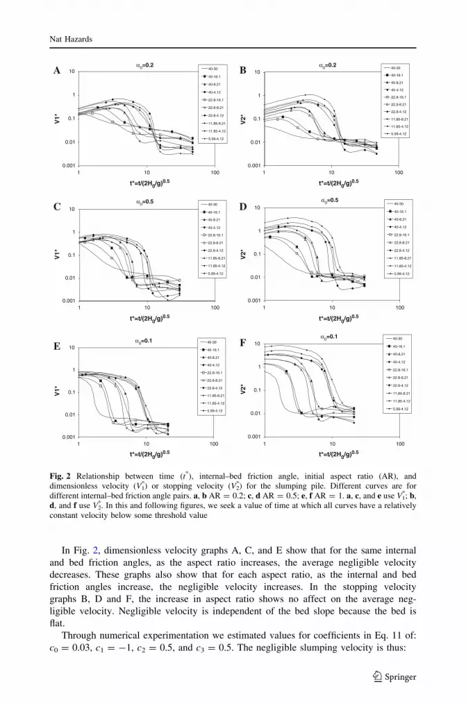
In Fig. 2, dimensionless velocity graphs A, C, and E show that for the same internal

and bed friction angles, as the aspect ratio increases, the average negligible velocity

decreases. These graphs also show that for each aspect ratio, as the internal and bed

friction angles increase, the negligible velocity increases. In the stopping velocity

graphs B, D and F, the increase in aspect ratio shows no affect on the average neg-

ligible velocity. Negligible velocity is independent of the bed slope because the bed is

flat.

Through numerical experimentation we estimated values for coefficients in Eq. 11 of:

c0 = 0.03, c1 = -1, c2 = 0.5, and c3 = 0.5. The negligible slumping velocity is thus:

α0=0.2 α0=0.2

α0=0.5 α0=0.5

α0=0.1α0=0.1

0.001

0.01

0.1

1

10

t*=t/(2H0/g)0.5 t*=t/(2H0/g)0.5

t*=t/(2H0/g)0.5 t*=t/(2H0/g)0.5

t*=t/(2H0/g)0.5 t*=t/(2H0/g)0.5

40-30

40-16.1

40-8.21

40-4.12

22.8-16.1

22.8-8.21

22.8-4.12

11.85-8.21

11.85-4.12

5.99-4.12

0.001

0.01

0.1

1

1040-30

40-16.1

40-8.21

40-4.12

22.8-16.1

22.8-8.21

22.8-4.12

11.85-8.21

11.85-4.12

5.99-4.12

0.001

0.01

0.1

1

1040-30

40-16.1

40-8.21

40-4.12

22.8-16.1

22.8-8.21

22.8-4.12

11.85-8.21

11.85-4.12

5.99-4.12

0.001

0.01

0.1

1

1040-30

40-16.1

40-8.21

40-4.12

22.8-16.1

22.8-8.21

22.8-4.12

11.85-8.21

11.85-4.12

5.99-4.12

0.001

0.01

0.1

1

1040-30

40-16.1

40-8.21

40-4.12

22.8-16.1

22.8-8.21

22.8-4.12

11.85-8.21

11.85-4.12

5.99-4.12

0.001

0.01

0.1

1

10

BA

101 100 101 100

DC

101 100 101 100

FE

101 100 101 100

40-30

40-16.1

40-8.21

40-4.12

22.8-16.1

22.8-8.21

22.8-4.12

11.85-8.21

11.85-4.12

5.99-4.12

V1*

V1*

V1*

V2*

V2*

V2*

Fig. 2 Relationship between time (t*), internal–bed friction angle, initial aspect ratio (AR), anddimensionless velocity (V1

*) or stopping velocity (V2*) for the slumping pile. Different curves are for

different internal–bed friction angle pairs. a, b AR = 0.2; c, d AR = 0.5; e, f AR = 1. a, c, and e use V1*; b,

d, and f use V2*. In this and following figures, we seek a value of time at which all curves have a relatively

constant velocity below some threshold value

Nat Hazards

123

V�2 ¼Vaveaffiffiffiffiffiffiffiffi

gH0

ptan u0:5

int tan u0:5bed

¼ 0:03 ð17Þ

Regardless of initial shape, the transient aspect ratio takes on the same value after one

dimensionless time, t* = t/(2h0/g)0.5. The dimensionless time when the pile ‘‘stops’’ is

approximately t* = 2, which is close to the total time for collapse in the experiments

performed by Lube et al. (2005):

t1 ¼ 2:62h0

g

� �0:5

ð18Þ

By using an internal friction angle of 40� and bed friction angle of 30�, we achieved results

that most closely matched the results of the experiments of Lube et al. (2005).

In the simulations of collapsing columns, when the radius and height of pile match with

those of experiment, the simulation time is one third to a half as long as experiment time.

At this time, the average velocity in the simulation is still increasing. If the simulation is

stopped at the stopping velocity, the radius is larger and height smaller than in the

experimental deposit. This is because the model uses the shallow water formulation for the

equations of motion. The initial collapse column has un-modeled variations in the vertical

direction and is poorly modeled by a thin layer assumption.

3.2 Simulations of geophysical flows

For the global stopping criterion, digital elevation models of complex mountainous terrain

are used to determine the coefficients characterizing the stopping criterion to use in

numerical experimentation. The following areas were chosen for the locations of their

relict debris and block and ash flows. They are generally representative of mountainous

areas and have experienced a variety of geophysical flow events. Colima Volcano located

in Southwestern Mexico had experienced block and ash flows occurring throughout the

1990s, probably with little interstitial fluid having contributed to propagation, and situated

on steep open slopes leading to lower confining channels (Saucedo et al. 2005; Rupp et al.

2006). Waterman Canyon and City Creek in the San Bernardino Mountains, southern

California, during Christmas, 2003, experienced debris flows in sinuous channels (Cannon

et al. 2008). Casita Volcano, western Nicaragua, recently (1998) experienced a large debris

avalanche/debris flow situated on steep open slopes (Scott et al. 2004). Little Tahoma Peak

located on Mount Rainier in Washington experienced a debris avalanche (1963) on steep

open slopes as well as in a broad channel (Crandell and Fahnestock 1965; Sheridan et al.

2005). At the completion of a numerical simulation, visual output is available at regular

time-step intervals on the distribution of inundation depth and propagation velocity.

At each simulation location, Colima, Little Tahoma Peak, Casita, and San Bernardino

Mountains (Figs. 3, 4, 5, 6, 7), the following trends were observed in both the dimen-

sionless velocity and stopping velocity graphs: first, the average velocity decreases

smoothly with increasing time, leveling out to nearly constant values at large time. This

nearly constant, negligible velocity increases with decreasing bed friction angle and is not

related to the position of the modeled flow within the local topography. Second, runs with

the same bed friction angles achieved similar average velocities even though they had quite

different internal friction angles. Third, the average velocity decreases with increasing bed

friction angle. Fourth, in each graph at large time, regardless of bed friction angle, all of the

runs converge close to the same negligible velocity. The dimensionless velocity runs

Nat Hazards

123

converge to within ±0.2 and the stopping velocity runs converge to within ±0.06. Fifth,

the stopping velocity compared to the dimensionless velocity for the same location always

shows a smaller average velocity in the first time step and a smaller negligible velocity.

Because the scaling terms associated with the internal friction angle are small, the

negligible velocity is independent of the internal friction angle. The negligible velocity is

also independent of the initial aspect ratio because the relative height of the pile is

insignificant when compared to the fall height of the pile. We found the best-fit coefficients

in Eq. 11 to be: c0 = 0.03,c1 = -0.5, c2 = 0, and c3 = 0.5. The stopping velocity is thus:

B

AColima 646000

0.001

0.01

0.1

1

10

10 100 1000

t*=t/(2H0/g)0.5t*=t/(2H0/g)0.5

t*=t/(2H0/g)0.5t*=t/(2H0/g)0.5

t*=t/(2H0/g)0.5t*=t/(2H0/g)0.5

40-30

40-23.4

40-16.1

32.2-23.4

32.2-16.1

22.8-16.1

Colima 646000

0.001

0.01

0.1

1

10

10 100

40-30

40-23.4

40-16.1

32.2-23.4

32.2-16.1

22.8-16.1

Colima 649000

0.001

0.01

0.1

1

10

10 100 1000 10000

40-30

40-16.1

40-8.21

22.8-16.1

22.8-8.21

11.85-8.21

Colima 649000

0.001

0.01

0.1

1

10

10 100 1000 10000

40-30

40-16.1

40-8.21

22.8-16.1

22.8-8.21

11.85-8.21

1000

DC

FEColima 652000

0.001

0.01

0.1

1

10

10 100 1000 10000

40-30

40-16.1

40-8.21

40-4.12

22.8-16.1

22.8-8.21

22.8-4.12

11.85-8.21

11.85-4.12

5.99-4.12

Colima 652000

0.001

0.01

0.1

1

10

10 100 1000 10000

40-30

40-16.1

40-8.21

40-4.12

22.8-16.1

22.8-8.21

22.8-4.12

11.85-8.21

11.85-4.12

5.99-4.12

V1*

V1*

V1*

V2*

V2*

V2*

Fig. 3 Colima volcano, Mexico. Relationship between dimensionless time (t*), and velocities V1* and V2

*, andinternal–bed friction angles (in legend). Initial pile: height = 50 m, radius = 300 m, and shape = paraboloid.Individual simulations have different initial pile locations. At location 646000, the x-coordinate of the startingpile is at the summit of Colima. At this location, the bed slope is large, flow thickness is small, flow length islarge, and e is very small. Location 652000 is situated on the slope of Colima close to the bottom of the uppersteep cone. Compared to location 646000, the bed slope is small, flow thickness is large, flow length is small,and e is large (small in an absolute sense). Location 649000 is situated midway down Colima’s steep upperslope, between the initial locations 649000 and 652000. The values for bed slope, flow thickness, flow length,e, and velocity of location 649000 are between those for locations 646000 and 652000

Nat Hazards

123

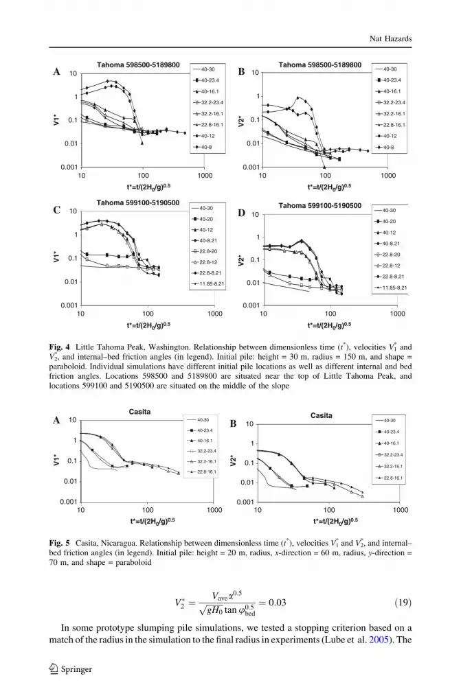
V�2 ¼Vavea0:5

ffiffiffiffiffiffiffiffigH0

ptan u0:5

bed

¼ 0:03 ð19Þ

In some prototype slumping pile simulations, we tested a stopping criterion based on a

match of the radius in the simulation to the final radius in experiments (Lube et al. 2005). The

Tahoma 598500-5189800

0.001

0.01

0.1

1

10

10 100 1000

t*=t/(2H0/g)0.5 t*=t/(2H0/g)0.5

t*=t/(2H0/g)0.5 t*=t/(2H0/g)0.5

40-30

40-23.4

40-16.1

32.2-23.4

32.2-16.1

22.8-16.1

40-12

40-8

Tahoma 598500-5189800

0.001

0.01

1

10

10 100 1000

40-30

40-23.4

40-16.1

32.2-23.4

32.2-16.1

22.8-16.1

40-12

40-8

BA

DCTahoma 599100-5190500

0.001

0.01

0.1

1

10

10 100 1000

40-30

40-20

40-12

40-8.21

22.8-20

22.8-12

22.8-8.21

11.85-8.21

Tahoma 599100-5190500

0.001

0.01

0.1

1

10

10 100 1000

40-30

40-20

40-12

40-8.21

22.8-20

22.8-12

22.8-8.21

11.85-8.21

V1*

V1*

V2*

V2*

0.1

Fig. 4 Little Tahoma Peak, Washington. Relationship between dimensionless time (t*), velocities V1* and

V2*, and internal–bed friction angles (in legend). Initial pile: height = 30 m, radius = 150 m, and shape =

paraboloid. Individual simulations have different initial pile locations as well as different internal and bedfriction angles. Locations 598500 and 5189800 are situated near the top of Little Tahoma Peak, andlocations 599100 and 5190500 are situated on the middle of the slope

BACasita

10 100 1000

t*=t/(2H0/g)0.5t*=t/(2H0/g)0.5

40-30

40-23.4

40-16.1

32.2-23.4

32.2-16.1

22.8-16.1

Casita

0.001

0.01

0.1

1

10

10 100 1000

40-30

40-23.4

40-16.1

32.2-23.4

32.2-16.1

22.8-16.1

0.001

0.01

0.1

1

10

V1*

V2*

Fig. 5 Casita, Nicaragua. Relationship between dimensionless time (t*), velocities V1* and V2

*, and internal–bed friction angles (in legend). Initial pile: height = 20 m, radius, x-direction = 60 m, radius, y-direction =70 m, and shape = paraboloid

Nat Hazards

123

edge of the simulated pile was estimated to be where the minimum pile height, h* = H0/512.

Using this edge definition, an internal friction angle of 40� and bed friction angle of 30� was

found to most closely match the final maximum pile height in the experiments of Lube et al.

(2005). However, the resulting definition of final time in the simulations was much shorter

than in the experiments. This error increased with increasing aspect ratio, which suggests that

it may be due to a breakdown of the thin layer or ‘‘shallow water’’ approximation, although

other causes for model breakdown have been suggested (Doyle et al. 2007).

SBM 474130-3787860

0.001

0.01

0.1

1

10

10 100 1000 10000

t*=t/(2H0/g)0.5 t*=t/(2H0/g)0.5

t*=t/(2H0/g)0.5 t*=t/(2H0/g)0.5

40-30

40-16.1

40-8.21

22.8-16.1

22.8-8.21

11.85-8.21

SBM 474130-3787860

0.001

0.01

0.1

1

10

10 100 1000 10000

40-30

40-16.1

40-8.21

22.8-16.1

22.8-8.21

11.85-8.21

BA

DCSBM 475160-3786730

0.001

0.01

0.1

1

10

10 100 1000 10000

40-30

40-16.1

40-8.21

22.8-16.1

22.8-8.21

11.85-8.21

SBM 475160-3786730

0.001

0.01

0.1

1

10

10 100 1000 10000

40-30

40-16.1

40-8.21

22.8-16.1

22.8-8.21

11.85-8.21

V1*

V1*

V2*

V2*

Fig. 6 Waterman Canyon, San Bernardino Mountains, California. Relationship between dimensionlesstime (t*), velocities V1

* and V2*, and internal–bed friction angles (in legend). Initial pile: height = 20 m, radius

= 100 m, and shape = paraboloid. In the Waterman Canyon area, geophysical flows occurred in channels.For all runs, the initial pile height is 20 m, the radius of the pile is 100 m, and the pile shape is paraboloid.As before, individual simulations have different initial pile locations as well as different internal and bedfriction angles. The two starting locations used were (474130, 3787860) and (475160, 3786730)

BASBM 487000

0.001

0.01

0.1

1

10

10 100 1000 10000

t*=t/(2H0/g)0.5 t*=t/(2H0/g)0.5

40-30

40-16.1

40-8.21

40-4.12

22.8-16.1

22.8-8.21

22.8-4.12

11.85-8.21

11.85-4.12

5.99-4.12

SBM 487000

0.001

0.01

0.1

1

10

10 100 1000 10000

40-30

40-16.1

40-8.21

40-4.12

22.8-16.1

22.8-8.21

22.8-4.12

11.85-8.21

11.85-4.12

5.99-4.12

V1*

V2*

Fig. 7 City Creek, San Bernardino Mountains, California: Relationship between dimensionless time (t*),velocities V1

* and V2*, and internal–bed friction angles (in legend). Initial pile: height = 20 m, radius = 200 m,

and shape = paraboloid. In the City Creek area, geophysical flows occurred in channels

Nat Hazards

123

3.3 Local inundation

Figure 8 is a comparison of the three runs from Fig. 3e to results with the same three

simulations rerun using the two-step local stopping criterion. Option 3 is implemented

when the stopping criterion is met (bed friction angle is locally reset to the internal friction

angle). The propagation histories are similar at all friction angles no matter whether a

global or local criterion is used, indicating that stopping takes place during a small fraction

of the entire history. Because a global criterion is easier to implement, it may be that for

some applications, the details of stopping are not important.

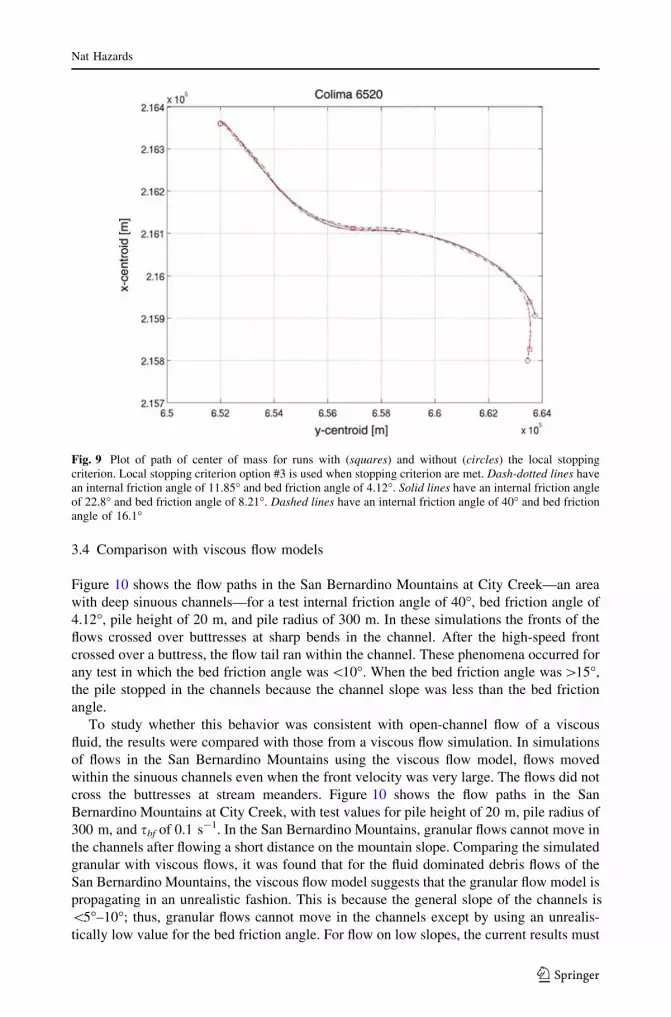
Figure 9 is a plot of the center of mass throughout flow duration for the same six runs as

plotted in Fig. 8. In the simulations that used the local stopping criterion, the final center of

mass is only slightly closer to the initiation point than is the final center of mass using the

global criterion. Qualitatively this is same as one might intuitively suspect, and is also

consistent with the observation that the details of stopping may not generally be important.

The granular flow model was used to simulate flows in the mountain areas of Colima,

Little Tahoma Peak, Casita, and San Bernardino Mountains. In areas that do not have deep,

narrow channels (Colima, Little Tahoma Peak, and Casita), the simulation results are good.

For these simulations when the initial piles were located on the summit, or close to the

summit the granular flow models worked well with a large bed friction angle ([15�). The

geophysical flows were able to flow with such a large bed friction angle because the bed

slope was larger than the bed friction angle. When the initial pile was located close to the

bottom of the mountain where the bed slope is small a small bed friction angle (\10�)

allowed flows to go a long distance, in some sense, similar to like debris flows in nature.

Fig. 8 Nondimensional velocity, V�1 ¼ V=ffiffiffiffiffiffiffiffigH0

pversus time, for local stopping criterion (squares) and

global stopping criterion (circles). Option # 3 is used when stopping criteria are met for local stoppingcriterion. Dash-dotted lines have an internal friction angle of 11.85� and bed friction angle of 4.12�. Solidlines have an internal friction angle of 22.8� and bed friction angle of 8.21�. Dashed lines have an internalfriction angle of 40� and bed friction angle of 16.1�

Nat Hazards

123

3.4 Comparison with viscous flow models

Figure 10 shows the flow paths in the San Bernardino Mountains at City Creek—an area

with deep sinuous channels—for a test internal friction angle of 40�, bed friction angle of

4.12�, pile height of 20 m, and pile radius of 300 m. In these simulations the fronts of the

flows crossed over buttresses at sharp bends in the channel. After the high-speed front

crossed over a buttress, the flow tail ran within the channel. These phenomena occurred for

any test in which the bed friction angle was\10�. When the bed friction angle was[15�,

the pile stopped in the channels because the channel slope was less than the bed friction

angle.

To study whether this behavior was consistent with open-channel flow of a viscous

fluid, the results were compared with those from a viscous flow simulation. In simulations

of flows in the San Bernardino Mountains using the viscous flow model, flows moved

within the sinuous channels even when the front velocity was very large. The flows did not

cross the buttresses at stream meanders. Figure 10 shows the flow paths in the San

Bernardino Mountains at City Creek, with test values for pile height of 20 m, pile radius of

300 m, and sbf of 0.1 s-1. In the San Bernardino Mountains, granular flows cannot move in

the channels after flowing a short distance on the mountain slope. Comparing the simulated

granular with viscous flows, it was found that for the fluid dominated debris flows of the

San Bernardino Mountains, the viscous flow model suggests that the granular flow model is

propagating in an unrealistic fashion. This is because the general slope of the channels is

\5�–10�; thus, granular flows cannot move in the channels except by using an unrealis-

tically low value for the bed friction angle. For flow on low slopes, the current results must

Fig. 9 Plot of path of center of mass for runs with (squares) and without (circles) the local stoppingcriterion. Local stopping criterion option #3 is used when stopping criterion are met. Dash-dotted lines havean internal friction angle of 11.85� and bed friction angle of 4.12�. Solid lines have an internal friction angleof 22.8� and bed friction angle of 8.21�. Dashed lines have an internal friction angle of 40� and bed frictionangle of 16.1�

Nat Hazards

123

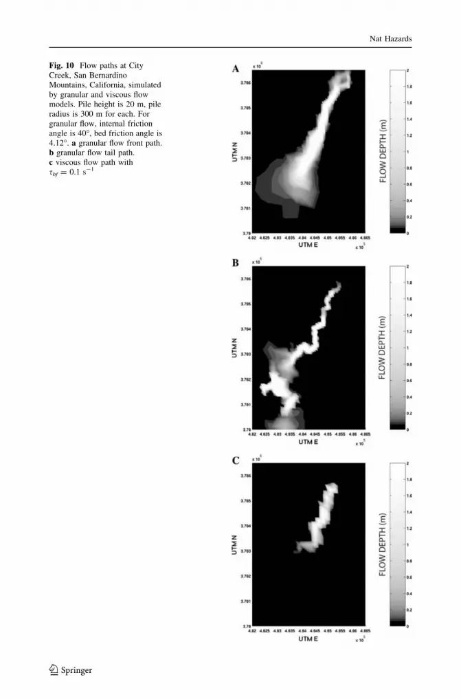
Fig. 10 Flow paths at CityCreek, San BernardinoMountains, California, simulatedby granular and viscous flowmodels. Pile height is 20 m, pileradius is 300 m for each. Forgranular flow, internal frictionangle is 40�, bed friction angle is4.12�. a granular flow front path.b granular flow tail path.c viscous flow path withsbf = 0.1 s-1

Nat Hazards

123

be accepted only with caution, as they clearly are based on unrealistic propagation patterns.

At Colima, Casita, and Little Tahoma Peak, the slope is [20� allowing granular flows to

move. The granular flow model produced good simulation results at these locations—these

flows may have propagated as granular materials.

4 Discussion and conclusions

An important characteristic to capture when modeling geologic hazards such as granular

flows is the area of inundation. The run-out distance of a flow can be used to delineate this

feature. To define the run-out distance, it is necessary to determine when a flow stops. In

this article, numerical experiments are presented to determine a stopping criterion defined

by the velocity of a flow. Numerical experiment results are also used to explore the

suitability of the Savage–Hutter theory for computing the inundation area of granular

flows.

In this contribution, we sought a reasonable, small velocity to be used as a stopping

criterion when simulating geophysical flows. To analyze the importance of using initial

pile geometry and internal and bed friction angles to determine when a flow stops,

numerical experiments were run using three different velocity stopping criteria. A different

mechanism of stopping is described by each stopping criterion. The first stopping criterion,

a global ‘‘dimensionless’’ velocity, V1*, is only dependent upon the average velocity,

gravitational forces and the height of the initial pile. The second stopping criterion, a

global ‘‘stopping’’ velocity, V2*, incorporates average velocity, gravitational forces, initial

pile height, aspect ratio, internal friction angle, and bed friction angle. The third stopping

criterion, a local stopping velocity v, examines force balances in each computational cell.

Simulations were performed of slumping piles on a horizontal surface, and geophysical

flows over complex topography.

First, a collapsing column with different initial aspect ratio, and different internal and

bed friction angles was simulated by granular flow model. It was found that the internal

and bed friction angles are important for the moving velocity but transient aspect ratio is

not important: it is almost the same after one dimensionless time no matter what the initial

geometry. This is because the kinetic energy of a collapse column arises from the pile

height and if the bed is flat, only the initial aspect ratio plays an important role in collapse.

Comparing the different power law values of initial aspect ratio, and internal and bed

friction angles, it is not difficult to get a nearly constant V2* value for a range of initial pile

geometries, AR = 0.2, 0.5, and 1.

Second, geophysical flows in mountainous areas with (San Bernardino Mountains,

California) and without (Colima, Mexico; Little Tahoma Peak, Washington, and Casita,

Nicaragua) channels were simulated. In these simulations a range of values were used for

the internal and bed friction angle input parameter. It was found that because the scaling

terms associated with internal friction angle are small and because the relative height of a

pile in a mountainous area is small when compared to the fall height of the pile, the

negligible velocity is independent of both the internal friction angle and initial aspect ratio.

However, stopping velocities in Figs. 3, 4, 5, 6, 7 generally exhibit a better similarity

collapse than the dimensionless velocity, which means that it is important to use bed

friction when determining a stopping criterion.

For a geophysical flow it is more complicated to determinate V2* than for a collapsing

column. This is because terrain has a variety of topographic elements: open slopes and/or

channels, divergences, convergences, and even changing slope angles. Although the initial

Nat Hazards

123

aspect ratio is not important in geophysical flow, the transient aspect ratio probably is, and

has a value dependent on the topographic setting: on open slopes, the maximum pile height

is small and the area of the pile is large; in channels, the maximum pile height is large and

the area covered by the flow is small.

The topography traversed by geophysical flows is complex and can be dominated by

open slopes as at Colima, location 646000 and Casita, or by channels as in the San

Bernardino Mountains at Waterman Canyon and City Creek. Real topography can also

have both open slopes and channels as at Colima, locations 649000, and 652000 and Little

Tahoma Peak. On an open slope, a pile spreads wide and pile height rapidly becomes small

relative to lateral extent. Due to the low aspect ratio, continued spreading is negligible at

large times. In channels, pile height always has a significant value because of confinement.

A pile will continue moving when the bed friction angle is less than channel slope even

though the velocity is small because there is always a driving slope gradient within the pile.

The pile will move until it propagates out of the channel onto a fan. For topography having

both channels and open slopes, flow is more complex. Simple visualization techniques

were introduced to check whether flow is confined to a channel, or collapses on an open

slope, or both. With the aid of visualization one can obtain reasonable values for the

parameters that control V2*.

Geophysical flows were simulated using both a local and global stopping criterion.

These runs suggest that for many applications, there may not be sufficient difference in

propagation behavior to warrant use of a local stopping criterion, which is more difficult to

implement.

The results of these numerical experiments suggest that reasonable estimates of run-out

distance for geophysical flows can be obtained by using the stopping criterion with values

of V2* = 0.03 for flows both on open slopes and in channels. Three-dimensional, animated

visualization shows that once this value is reached, the flowing material is spreading

mostly around a stationary center of mass, and is therefore restricted in lateral extent.

In granular flow models, unreasonable simulation results are produced at the sharp

bends of sinuous channels as the flow head passes. Thus, as one would suspect intuitively

to be true, one cannot use granular flow models at low basal friction angles, despite the

observation that such a model produces inundation areas similar to those seen in nature.

Natural flows do not in general behave as a low-friction angle granular materials.

Acknowledgments We thank two anonymous reviewers for very thorough reviews that improved thearticle. The research was supported by National Science Foundation grants ITR0121254 and EAR06209991.

References

Cannon SH, Gartner JE, Wilson RC, Bowers JC, Laber JL (2008) Storm rainfall conditions for floods anddebris flows from recently burned areas in southwestern Colorado and southern California. Geomor-phology 96:250–269

Crandell DR, Fahnestock RK (1965) Rockfalls and avalanches from little Tahoma Peak on Mount Rainier,Washington. US Geol Surv Bull 1221-A:A1–A30

Denlinger RP, Iverson RM (2001) Flow of variably fluidized granular masses across three-dimensionalterrain 2. Numerical predictions and experimental tests. J Geophys Res 106(B1):553–566

Denlinger RP, Iverson RM (2004) Granular avalanches across irregular three-dimensional terrain: 1. Theoryand computation. J Geophys Res 109(F01014):1–14

Doyle E, Huppert H, Lube G, Mader H, Sparks S (2007) Satic and flowing regions in granular collapse downchannels: insights from a sedimenting shallow water model. Phys Fluids 19:106601

Fairchild LH, Wigmosta M (1983) Dynamic and volumetric characteristics of the 18 May 1980 lahars on theToutle River, Washington. In: Proceeding of the symposium on erosion control in volcanic areas

Nat Hazards

123

technical memorandum 1908. Japan Public Works Research Institute, Ministry of Construction, Tokyo,pp 131–153

Gray JMNT, Wieland M, Hutter K (1999) Gravity-driven free surface flow of granular avalanches overcomplex basal topography. Proc Roy Soc London Ser A 455:1841–1874

Iverson RM, Denlinger RP (2001) Flow of variably fluidized granular masses across three-dimensionalterrain 1. Coulomb mixture theory. J Geophys Res 106(B1):537–552

Lajeunesse E, Mangeney-Castelnau A, Vilotte JP (2004) Spreading of a granular mass on a horizontal plane.Phys Fluids 16(7):2371–2381

Lube G, Huppert H, Sparks S, Hallworth M (2004) Axisymmetric collapses of granular columns. J FluidMech 508:175

Lube G, Huppert HE, Sparks RSJ, Freundt A (2005) Collapses of two-dimensional granular columns. PhysRev E Stat Nonlin Soft Matter Phys 72(4130):1–11

Mangeney-Castelnau A, Vilotte JP, Bristeau MO, Perthame B, Bouchut F, Simeoni C, Yerneni S (2003)Numerical modeling of avalanches based on Saint-Venant equations using a kinetic scheme. J GeophysRes 108(B11):2527

Molinaro P, Natale L (eds) (1994) Modelling of flood propagation over initially dry areas. American Societyof Civil Engineers, New York, 373 pp

Patra AK, Bauer AC, Nichita CC, Pitman EB, Sheridan MF, Bursik M, Rupp B, Webber A, Stinton AJ,Namikawa LM, Renschler CS (2005) Parallel adaptive numerical simulation of dry avalanches overnatural terrain. J Volcanol Geotherm Res 139:1–21

Pierson TC (1985) Initiation and flow behavior of the 1980 Pine Creek and Muddy river lahars, MountSt. Helens, Washington. Geol Soc Am Bull 96:1056–1069

Plafker G, Ericksen GE (1978) Nevado Huascaran avalanches, Peru. In: Voight B (ed) Rockslides andavalanches, vol 1: natural phenomena. Elsevier, New York, pp 277–314

Pouliquen O (1999) Scaling laws in granular flows down rough incline planes. Phys Fluids 11:542–548Pouliquen O, Forterre Y (2002) Friction law for dense granular flows: application to the motion of a mass

down a rough inclined plane. J Fluid Mech 453:133–151Pudasaini SP, Hutter K (2003) Rapid shear flows of dry granular masses down curved and twisted channels.

J Fluid Mech 495:193–208Pudasaini SP, Hutter K (2007) Avalanche dynamics: dynamics of rapid flows of dense granular avalanches.

Springer, BerlinRupp B, Bursik M, Namikawa L, Webb A, Patra AK, Saucedo R, Macias JL, Renschler C (2006) Com-

putational modeling of the 1991 block and ash flows at Colima Volcano, Mexico. In: Siebe C, MaciasJL, Aguirre-Diaz GJ (eds) Neogene-quaternary continental margin volcanism: a perspective fromMexico. Geological Society of America special paper 402, pp 223–237. doi:10.1130/2006.2402(11)

Saucedo R, Macias JL, Sheridan MF, Bursik MI, Komorowski JC (2005) Modeling of pyroclastic flows ofColima volcano, Mexico: implications for hazard assessment. J Volcanol Geotherm Res 139:103–115

Savage S, Hutter K (1989) The motion of a finite mass of granular material down a rough incline. J FluidMech 199:177–215

Scott KM, Vallance JW, Kerle N, Macias JL, Strauch W, Devoli G (2004) Catastrophic precipitation-triggered lahar at Casita volcano, Nicaragua: occurrence, bulking and transformation. Earth SurfProcess Landf 30:59–79

Sheridan MF, Stinton AJ, Patra A, Pitman EB, Bauer A, Nichita CC (2005) Evaluating Titan2D mass-flowmodel using the 1963 Little Tahoma Peak avalanches, Mount Rainier, Washington. J Volcanol Geo-therm Res 139:89–102

Vallance JW, Scott KM (1997) The Osceola mudflow from Mount Rainier: sedimentology and hazardimplications of huge clay-rich debris flow. Geol Soc Am Bull 109(2):143–163

Nat Hazards

123