Adaptation of Rescue Robot Behaviour in Unknown TerrainsBased on Stochastic and Fuzzy Logic Approaches

Ashraf AboshoshaRA Dept.- Prof. Dr. A. Zell, WSI, University of T¨ubingen

Sand 1, D-72076 T¨ubingen, Germanyshosha@informatik.uni-tuebingen.de

http://www-ra.informatik.uni-tuebingen.de

Abstract— The purpose of this article is to provide rescuerobots with an adaptive behaviour during searching forvictims in disasters such as fire, earthquake, flood, wars etc.This experimental research work took place in previouslyunknown dynamic indoor terrains. The main phases of thisframework are; 1) modelling of robot behaviours/dynamicsin collapsed environments, 2) designing an adaptive con-troller, which regulates robot longitudinal velocity and head-ing (collision avoidance) based on the obstacles distributionhistogram, 3) prediction of robot behaviours in anotherunknown terrain. Two approaches have been used to designthe adaptive controller: the first one is the stochastic controltheory, based on Kalman filter algorithms [10][8]. Thesecond approach relies on fuzzy inference systems (FIS)[5][17][7]. Throughout this work, robot dynamics have beenmodelled using the auto regressive exogenous (ARX) scheme,while ARX model parameters have been identified usingrecursive least squares (RLS) [18]. This contribution presentsa description and some discussion of the discrete Kalmanfilter, modelling techniques, and some discussion of robotbehaviour analysis. Furthermore, the design of adaptivecontrollers using FIS-based techniques versus stochasticcontrol systems has been demonstrated.1

Keywords: rescue robot, stochastic control, Kalmanfilter, fuzzy logic, adaptive navigation.

I. I NTRODUCTION

In disasters, autonomous mobile systems are highlyneeded to help in finding trapped victims. Intelligentmobile robots and cooperative robotic systems can be veryefficient tools to speed up searching and rescue operations.Rescue robots usually have 48 hours to find trappedsurvivors. They are also useful to do rescuing jobs in sit-uations that are hazardous for humans. Promising projectsof rescue robots got recently a lot of attention worldwide,although the available technologies do not yet provideenough autonomy or precision as needed. Adaptive con-trollers compensate fluctuations of internal/external pa-rameters of dynamic systems to preserve the stability andto increase the robustness. Based on the histogram ofsurrounding obstacles, the robot adapts its translationalvelocity and avoids collisions during exploration of the

1This study has been implemented on the B21-RWI robot platform(Colin and Robin - laboratory for autonomous mobile robots, Universityof Tubingen).

collapsed structure seeking for alive victims. Adaptivecontrollers reinforce rescue robot navigation safety bysteering the robot behaviour smoothly to the desired setpoint, instead of abrupt variations that might cause aharmful effect on the internal structure of robots. In thisstudy, stochastic Kalman filters have been employed tomodel robot dynamics, to identify model parameters, topredict robot behaviours in another terrain and to regulatethe rescue robot velocity related to the free front space[16][14][4]. Kalman filters belong to algorithms (e.g.ARX, ARMA, LMS, RLS, FIR, IIR, LQR, LQG, etc.) thatwidely involved in adaptive systems to underlay subjectsof modelling, identification, prediction, signal processing,behaviour learning and controller design [9][12]. On theother side, adaptive FIS techniques enable the robot tointeract adaptively with the static or dynamic eventsduring navigation. FIS have been successfully employedin automatic control, data classification, decision analy-sis, expert systems, time series prediction, and patternrecognition. Furthermore, FIS are considered in manyrobotic applications, such as velocity control, collisionavoidance, path tracking, dynamic objects pursuing [1],map building and in sensor fusion [11]. In this paper, thefollowing topics will be discussed: part (II) focuses on theformulation of discrete Kalman filter. Part (III) outlinessignal and system modelling approaches, ARX modelbuilding, and using the RLS technique in identificationof rescue robot model parameters. Part (IV) demonstrateshow to regulate the robot velocity based on the obstaclesdistribution histogram using adaptive Kalman filters andpractical results are presented. Part (V) illustrates applyingFIS techniques to regulate robot behaviours. Part (VI)introduces a comparison between stochastic based and FISbased control approaches.

II. D ISCRETEKALMAN FILTER

Kalman filters are widely used in studies of dynamicsystems, analysis, estimation, prediction, processing andcontrol. The Kalman filter is an optimal solution for thediscrete data linear filtering problem. The Kalman filter isa set of mathematical equations that provides an efficientcomputational solution to sequential systems. The filter is

very powerful in several aspects: it supports estimationsof past, present, and even future states (prediction), and itcan do so even when the precise nature of the modelledsystem is unknown. The filter is derived by finding theestimator for a linear system, subject to additive whiteGaussian noise [10]. The discrete form of Kalman filtersaddresses the general problem of trying to estimate thestate of a discrete time process that is governed by thelinear stochastic difference equation. The Kalman filterformulation begins with definition of the system andassumptions. Consider a process f(.) given by the statespace model defined by its linear difference equation form

υk+1 = f (υk,λk,ξk) = Akυk + Bkλk + ξk (1)

The observation or measurement model is a mappingof the actual system stateυ to an observed state y. Thesystem is driven by a control signalλ , while measure-ments are associated with Gaussian white noisesξ andγ.The discrete time observation model is given by the lineardifference equation

yk = f (υk,γk) = Skυk +γk (2)

In our case the observed output is the rescue robot longi-tudinal velocity/heading and the reference control signalis the obstacles distribution histogram. The coefficients A,B and S are Kalman filter parameters.

III. ROBOT DYNAMICS MODELLING

A. Signal and System Modelling

There are two different approaches to the characteri-zation of dynamic systems: In linear systems theory, onecan assume either some structure in the signals or somestructure in the system. Attempts have been made tocombine these two approaches e.g. harmonic identificationtechniques in the Fourier domain.First approach: Structure the signal can be found usinglinear transforms. This approach does not take into accountthat the system has some structure. In the time domain,filtering is a linear transformation. The Fourier, Wavelet,and Karhunen-Loeve transforms have compression Capa-bility and can be used to identify some structure in thesignals. When we are using these transforms, we do nottake into account any structure in the system.Second approach: Structure the system can be found byfitting a model to the system.

B. Approaches to System Modelling

Physical models of robots are either reduced-size copiesof the original dynamics following the laws of modelsimilarity, or analogies. The idea of an analogy impliesthat there exists ”something” at every instant of time that isto be analogous to the dependent variables of the originalphysical system. Mathematical models map the relation-ships between the physical variables in the robot dynamics

to be modelled onto mathematical structures like simplealgebraic equations, systems of differential equations oreven difference equations. Mathematical modelling ofrobots can be developed in different ways: either purelytheoretically based on the physical relationships (sensorsactuators Interaction), which are a priori known about therobot dynamics, or purely empirically by experiments onthe already existing robot, or by a sensible combination ofboth ways. Models obtained by the first method are oftencalled priori, first principle or theoretical models, whilemodels obtained in the second way are called posteriori orexperimental models. Theoretical model building becomesunavoidable if experiments in the respective system cannotor must not be carried out. If the system to be modelleddoes not yet exist, theoretical modelling is the onlypossibility to obtain a mathematical model.

C. ARX Modelling

The discrete ARX modelling scheme is derived fromKalman filter, see figure (1). The ARX scheme is widelyused in modelling of sequential system dynamics. Thisstructure takes into account both the observed stateυ k

and the driving control signalλ k which is given by:

υk =na

∑i=1

aiυ(k−i)+nb

∑i=0

biλ(k−i)+ηk (3)

Fig. 1. ARX modelling of rescue robot dynamics

Where; η is the modelling residual, representing thewhite noise.na is the model order of the observed state(also called the number of poles).nb is the model order ofthe control signal (also called the number of zeros). Theoperatorq−1 is the back shift operator or delay, which isgiven byq−1υk = υ(k−1), that follows:

A(q−1)υk = q−1B(q−1)λk +ηk

A(q−1) = 1−a1q−1−a2q−2− . . .−anaq−na

B(q−1) = b0 + b1q−1+ b2q−2+ . . .+ bnaq−nb

(4)

The observed stateυk is the longitudinal veloc-ity/heading while the control signalλ k is the obsta-cles distribution histogram, acquired by laser/sonar. TheGaussian distributed noise, associated with the observedoutput, allows applying identification algorithms such as;RLS or least mean squares (LMS) to estimate modelparameters (coefficients). This modelling scheme is onlyapplicable within linear or quasi-linear systems. There-fore, it is applied within this framework to regulate the

velocity/heading, while this algorithm failed to cope withposition control of mobile robots due to enormous non-linear odometric errors [2].

D. RLS Estimation of Model Parameters

Now let us explain, how to estimate ARX modelparametersA(q−1) and B(q−1). The RLS is a stepwiselearning algorithm, this means that, the estimation ofmodel parameters has a gradual convergence. Comparedwith the LMS algorithm (batch-wise learning), the RLSneeds a lower computational power and it is more stablethan the LMS. The LMS formulation depends on thematrix inversion and some matrices are not invertible.We can initialize the RLS identification process using anempty vector. Also, we can initialize it using fuzzy andneural nets. Figure (2) shows outputs of both the ARXmodel and an actual robot output. The ARX model outputis smooth due to filtering of high frequencies. Figure (7)shows the convergence of parameters during the learningprocess.

Fig. 2. Output of both the rescue robot and its ARX model

The RLS estimation process can be accomplished ac-cording to the following. At time step (k +1):

1) Form Γ(k+1)using the new data (input-output pat-terns)

ΓT(k+1) = [υ(k+1)....υ(k−na)λ(k).........λ(k−nb)] (5)

2) Form the estimation errorε(k+1) using

ε(k+1) = υ(k+1)− υ(k+1) = υ(k+1)−ΓT(k+1)Θ(k) (6)

3) FormΨ(k+1) (based on Kalman gain) using

Ψ(k+1) = Ψ(k)

[Im −

Γ(k+1)ΓT(k+1)Ψ(k)

(1+ΓT(k+1)Ψ(k)Γ(k+1))

](7)

4) Update parameters

Θ(k+1) = Θ(k) +Ψ(k+1)Γ(k+1)ε(k+1) (8)

where

ΘT(k+1) =

[1−a1.....−ana + b0+ .....+ bnb

](9)

5) Wait for the next time step to elapse and loop backto step (1)

IV. V ELOCITY CONTROL BASED ON KALMAN FILTER

Applying adaptive control theories to autonomousrobots leads to a smooth transition among operation levels.Moreover, these systems own a deliberative structure,which involves reference signal generation, modelling,identification, controller design and sometimes optimizingunits, see figure (3). To generate a reference signal,environment maps have been built using two B21-RWIrobots, equipped with 24 Polaroid 6500 sonar sensor anda Sick LMS 200 laser range finder. The characteristics,advantages and disadvantages of map building using bothof time of flight (TOF) sensors (laser and sonar) can bereviewed in [13] and [2]. To build an obstacles histogramof an environment, different methods can be used. Thereare: 1) nearest obstacle of the front free space, 2) area ofthe surrounding free space or 3) the free front space area.What has been used throughout this work, is the nearestobstacle of the free front space. Figures (4, 5) present twomodels of map building using the laser range finder andsonar modules [2]. The implementation of the adaptive

Fig. 3. Adaptive control of rescue robot longitudinal velocity

Fig. 4. Map building using the Sick LMS 200 laser scanner

Fig. 5. Map building using Polaroid 6500 sonar sensors

control starts with data acquisition of input/output patterns

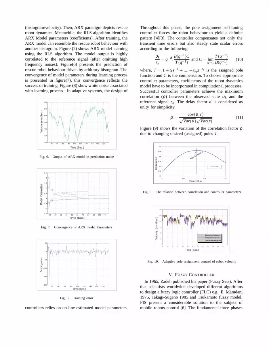
(histogram/velocity). Then, ARX paradigm depicts rescuerobot dynamics. Meanwhile, the RLS algorithm identifiesARX Model parameters (coefficients). After training, theARX model can resemble the rescue robot behaviour withanother histogram. Figure (2) shows ARX model learningusing the RLS algorithm. The model output is highlycorrelated to the reference signal (after omitting highfrequency noises). Figure(6) presents the prediction ofrescue robot behaviour driven by arbitrary histogram. Theconvergence of model parameters during learning processis presented in figure(7), this convergence reflects thesuccess of training. Figure (8) show white noise associatedwith learning process. In adaptive systems, the design of

Fig. 6. Output of ARX model in prediction mode

Fig. 7. Convergence of ARX model Parameters

Fig. 8. Training error

controllers relies on on-line estimated model parameters.

Throughout this phase, the pole assignment self-tuningcontroller forces the robot behaviour to yield a definitepattern [4][3]. The controller compensates not only thetransient time errors but also steady state scalar errorsaccording to the following:

υk

rk= q−d.

B(q−1)CT (q−1)

andC = limq→1

T (q−1)B(q−1)

(10)

where,T = 1+ t1z−1 + .... + tnt z−nt is the assigned pole

function and C is the compensator. To choose appropriatecontroller parameters, coefficients of the robot dynamicsmodel have to be incorporated in computational processes.Successful controller parameters achieve the maximumcorrelation (ρ) between the observed stateυ k and thereference signalrk. The delay factord is considered asunity for simplicity.

ρ =cov(υ ,r)√

Var(υ)√

Var(r)(11)

Figure (9) shows the variation of the correlation factorρdue to changing desired (assigned) polesT .

Fig. 9. The relation between correlation and controller parameters

Fig. 10. Adaptive pole assignment control of robot velocity

V. FUZZY CONTROLLER

In 1965, Zadeh published his paper (Fuzzy Sets). Afterthat scientists worldwide developed different algorithmsto design a fuzzy logic controller (FLC) e.g.; E. Mamdani1975, Takagi-Sugeno 1985 and Tsukamoto fuzzy model.FIS present a considerable solution to the subject ofmobile robots control [6]. The fundamental three phases

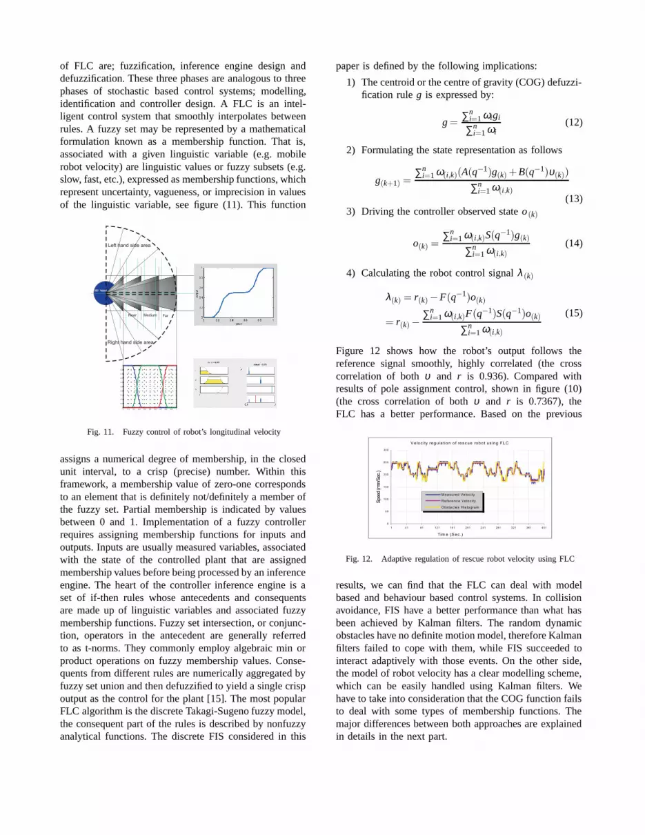
of FLC are; fuzzification, inference engine design anddefuzzification. These three phases are analogous to threephases of stochastic based control systems; modelling,identification and controller design. A FLC is an intel-ligent control system that smoothly interpolates betweenrules. A fuzzy set may be represented by a mathematicalformulation known as a membership function. That is,associated with a given linguistic variable (e.g. mobilerobot velocity) are linguistic values or fuzzy subsets (e.g.slow, fast, etc.), expressed as membership functions, whichrepresent uncertainty, vagueness, or imprecision in valuesof the linguistic variable, see figure (11). This function

Fig. 11. Fuzzy control of robot’s longitudinal velocity

assigns a numerical degree of membership, in the closedunit interval, to a crisp (precise) number. Within thisframework, a membership value of zero-one correspondsto an element that is definitely not/definitely a member ofthe fuzzy set. Partial membership is indicated by valuesbetween 0 and 1. Implementation of a fuzzy controllerrequires assigning membership functions for inputs andoutputs. Inputs are usually measured variables, associatedwith the state of the controlled plant that are assignedmembership values before being processed by an inferenceengine. The heart of the controller inference engine is aset of if-then rules whose antecedents and consequentsare made up of linguistic variables and associated fuzzymembership functions. Fuzzy set intersection, or conjunc-tion, operators in the antecedent are generally referredto as t-norms. They commonly employ algebraic min orproduct operations on fuzzy membership values. Conse-quents from different rules are numerically aggregated byfuzzy set union and then defuzzified to yield a single crispoutput as the control for the plant [15]. The most popularFLC algorithm is the discrete Takagi-Sugeno fuzzy model,the consequent part of the rules is described by nonfuzzyanalytical functions. The discrete FIS considered in this

paper is defined by the following implications:

1) The centroid or the centre of gravity (COG) defuzzi-fication ruleg is expressed by:

g = ∑ni=1ωigi

∑ni=1ωi

(12)

2) Formulating the state representation as follows

g(k+1) =∑n

i=1ω(i,k)(A(q−1)g(k) + B(q−1)υ(k))

∑ni=1ω(i,k)

(13)3) Driving the controller observed stateo (k)

o(k) =∑n

i=1ω(i,k)S(q−1)g(k)

∑ni=1ω(i,k)

(14)

4) Calculating the robot control signalλ (k)

λ(k) = r(k) −F(q−1)o(k)

= r(k) −∑n

i=1ω(i,k)F(q−1)S(q−1)o(k)

∑ni=1ω(i,k)

(15)

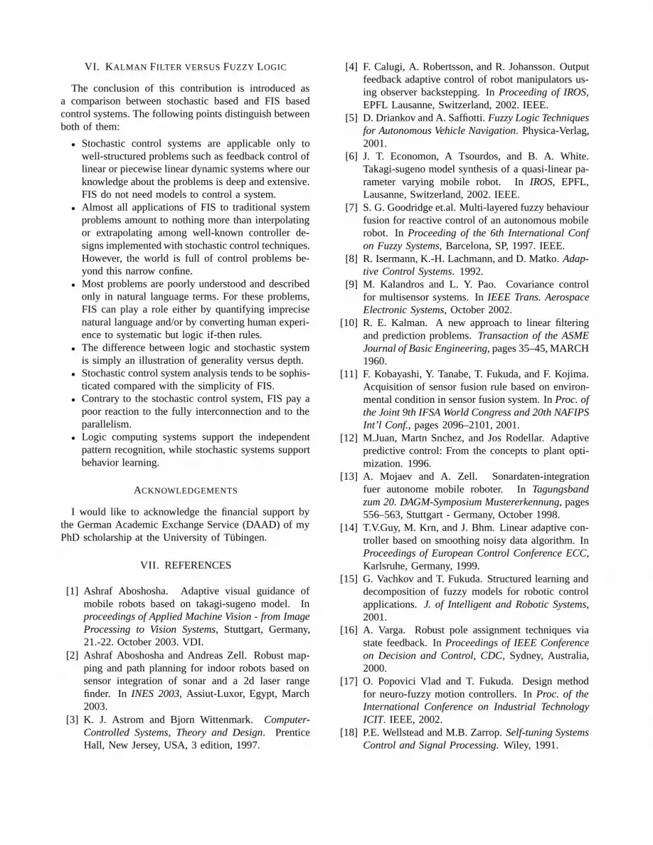
Figure 12 shows how the robot’s output follows thereference signal smoothly, highly correlated (the crosscorrelation of bothυ and r is 0.936). Compared withresults of pole assignment control, shown in figure (10)(the cross correlation of bothυ and r is 0.7367), theFLC has a better performance. Based on the previous

Fig. 12. Adaptive regulation of rescue robot velocity using FLC

results, we can find that the FLC can deal with modelbased and behaviour based control systems. In collisionavoidance, FIS have a better performance than what hasbeen achieved by Kalman filters. The random dynamicobstacles have no definite motion model, therefore Kalmanfilters failed to cope with them, while FIS succeeded tointeract adaptively with those events. On the other side,the model of robot velocity has a clear modelling scheme,which can be easily handled using Kalman filters. Wehave to take into consideration that the COG function failsto deal with some types of membership functions. Themajor differences between both approaches are explainedin details in the next part.

VI. K ALMAN FILTER VERSUSFUZZY LOGIC

The conclusion of this contribution is introduced asa comparison between stochastic based and FIS basedcontrol systems. The following points distinguish betweenboth of them:

• Stochastic control systems are applicable only towell-structured problems such as feedback control oflinear or piecewise linear dynamic systems where ourknowledge about the problems is deep and extensive.FIS do not need models to control a system.

• Almost all applications of FIS to traditional systemproblems amount to nothing more than interpolatingor extrapolating among well-known controller de-signs implemented with stochastic control techniques.However, the world is full of control problems be-yond this narrow confine.

• Most problems are poorly understood and describedonly in natural language terms. For these problems,FIS can play a role either by quantifying imprecisenatural language and/or by converting human experi-ence to systematic but logic if-then rules.

• The difference between logic and stochastic systemis simply an illustration of generality versus depth.

• Stochastic control system analysis tends to be sophis-ticated compared with the simplicity of FIS.

• Contrary to the stochastic control system, FIS pay apoor reaction to the fully interconnection and to theparallelism.

• Logic computing systems support the independentpattern recognition, while stochastic systems supportbehavior learning.

ACKNOWLEDGEMENTS

I would like to acknowledge the financial support bythe German Academic Exchange Service (DAAD) of myPhD scholarship at the University of T¨ubingen.

VII. REFERENCES

[1] Ashraf Aboshosha. Adaptive visual guidance ofmobile robots based on takagi-sugeno model. Inproceedings of Applied Machine Vision - from ImageProcessing to Vision Systems, Stuttgart, Germany,21.-22. October 2003. VDI.

[2] Ashraf Aboshosha and Andreas Zell. Robust map-ping and path planning for indoor robots based onsensor integration of sonar and a 2d laser rangefinder. In INES 2003, Assiut-Luxor, Egypt, March2003.

[3] K. J. Astrom and Bjorn Wittenmark. Computer-Controlled Systems, Theory and Design. PrenticeHall, New Jersey, USA, 3 edition, 1997.

[4] F. Calugi, A. Robertsson, and R. Johansson. Outputfeedback adaptive control of robot manipulators us-ing observer backstepping. InProceeding of IROS,EPFL Lausanne, Switzerland, 2002. IEEE.

[5] D. Driankov and A. Saffiotti.Fuzzy Logic Techniquesfor Autonomous Vehicle Navigation. Physica-Verlag,2001.

[6] J. T. Economon, A Tsourdos, and B. A. White.Takagi-sugeno model synthesis of a quasi-linear pa-rameter varying mobile robot. InIROS, EPFL,Lausanne, Switzerland, 2002. IEEE.

[7] S. G. Goodridge et.al. Multi-layered fuzzy behaviourfusion for reactive control of an autonomous mobilerobot. In Proceeding of the 6th International Confon Fuzzy Systems, Barcelona, SP, 1997. IEEE.

[8] R. Isermann, K.-H. Lachmann, and D. Matko.Adap-tive Control Systems. 1992.

[9] M. Kalandros and L. Y. Pao. Covariance controlfor multisensor systems. InIEEE Trans. AerospaceElectronic Systems, October 2002.

[10] R. E. Kalman. A new approach to linear filteringand prediction problems.Transaction of the ASMEJournal of Basic Engineering, pages 35–45, MARCH1960.

[11] F. Kobayashi, Y. Tanabe, T. Fukuda, and F. Kojima.Acquisition of sensor fusion rule based on environ-mental condition in sensor fusion system. InProc. ofthe Joint 9th IFSA World Congress and 20th NAFIPSInt’l Conf., pages 2096–2101, 2001.

[12] M.Juan, Martn Snchez, and Jos Rodellar. Adaptivepredictive control: From the concepts to plant opti-mization. 1996.

[13] A. Mojaev and A. Zell. Sonardaten-integrationfuer autonome mobile roboter. InTagungsbandzum 20. DAGM-Symposium Mustererkennung, pages556–563, Stuttgart - Germany, October 1998.

[14] T.V.Guy, M. Krn, and J. Bhm. Linear adaptive con-troller based on smoothing noisy data algorithm. InProceedings of European Control Conference ECC,Karlsruhe, Germany, 1999.

[15] G. Vachkov and T. Fukuda. Structured learning anddecomposition of fuzzy models for robotic controlapplications. J. of Intelligent and Robotic Systems,2001.

[16] A. Varga. Robust pole assignment techniques viastate feedback. InProceedings of IEEE Conferenceon Decision and Control, CDC, Sydney, Australia,2000.

[17] O. Popovici Vlad and T. Fukuda. Design methodfor neuro-fuzzy motion controllers. InProc. of theInternational Conference on Industrial TechnologyICIT. IEEE, 2002.

[18] P.E. Wellstead and M.B. Zarrop.Self-tuning SystemsControl and Signal Processing. Wiley, 1991.