Performance Evaluation 66 (2009) 311–326

Contents lists available at ScienceDirect

Performance Evaluation

journal homepage: www.elsevier.com/locate/peva

Numerical computation algorithms for sequential checkpointplacementI

Tatsuya Ozaki a, Tadashi Dohi a,∗, Naoto Kaio ba Department of Information Engineering, Hiroshima University, 1-4-1 Kagamiyama, Higashi-Hiroshima 739–8527, Japanb Department of Economic Informatics, Hiroshima Shudo University, 1-1-1 Ozukahigashi, Asaminamiku, Hiroshima 731-3195, Japan

a r t i c l e i n f o

Article history:Received 17 August 2006Accepted 27 November 2008Available online 10 December 2008

Keywords:File systemsCheckpointingSequential checkpointsAvailabilityExpected rewardNumerical algorithms

a b s t r a c t

This paper concerns sequential checkpoint placement problems under two dependabilitymeasures: steady-state system availability and expected reward per unit time in thesteady state. We develop numerical computation algorithms to determine the optimalcheckpoint sequence, based on the classical Brender’s fixed point algorithm and furthergive three simple approximation methods. Numerical examples with the Weibullfailure time distribution are devoted to illustrate quantitatively the overestimation andunderestimation of the sub-optimal checkpoint sequences based on the approximationmethods.

© 2008 Elsevier B.V. All rights reserved.

1. Introduction

System failures in large scaled computer systems can lead to a huge economic or critical social loss. Checkpointing androllback recovery is a commonly used solution for improving the dependability of file systems, and is regarded as a low-cost environment diversity technique from the standpoint of fault-tolerant computing. Especially, when the file system towrite and/or read data is designed in terms of preventive maintenance, checkpoint generations can back up occasionally orperiodically the significant data on the primary medium to the safe secondary medium, and can play a significant role tolimit the amount of data processing for the recovery actions after system failures occur. If checkpoints are frequently taken,a larger overhead by checkpointing itself will be incurred. Conversely, if checkpoints are seldom placed, a larger recoveryoverhead after a system failure will be required. Hence, it is important to determine the optimal checkpoint sequencetaking account of the trade-off between two kinds of overhead factor above. Since the system failure phenomenon underuncertainty is described by a probability distribution, called the system failure time distribution, the optimal checkpointsequence should be determined based on any stochastic model [1–5].Young [6] obtained the optimal checkpoint interval approximately for the computation restart after system failures.

Baccelli [7], Chandy et al. [2], Dohi et al. [8], Gelenbe and Derochette [9], Gelenbe [10], Gelenbe and Hernandez [11], Goesand Sumita [12], Grassi et al. [13], Kulkarni et al. [14], Nicola and Van Spanje [15], Sumita et al. [16] proposed performanceevaluation models for database recovery, and calculated the optimal checkpoint intervals which maximize the systemavailability orminimize themean overhead during the normal operation. L’Ecuyer andMalenfant [17] formulated a dynamiccheckpoint placement problem by a Markov decision process. Ziv and Bruck [18] reconsidered a checkpoint placementproblem under a random environment, by taking account of the change of operation circumstance. Vaidya [19] examined

I This work is supported by a Grant-in-Aid for Scientific Research from the Ministry of Education, Sports, Science and Culture of Japan under Grant No.18510138 (2006-2008) and the Research Program 2008 under the Center for Academic Development and Cooperation of the Hiroshima Shudo University,Japan. The authors very much appreciate two reviewers’ comments to improve the first version of this paper.∗ Corresponding author. Tel.: +81 82 424 7648; fax: +81 82 422 7025.E-mail addresses: dohi@rel.hiroshima-u.ac.jp (T. Dohi), kaio@shudo-u.ac.jp (N. Kaio).

0166-5316/$ – see front matter© 2008 Elsevier B.V. All rights reserved.doi:10.1016/j.peva.2008.11.003

312 T. Ozaki et al. / Performance Evaluation 66 (2009) 311–326

the impact of checkpoint latency onoverhead ratio for a simple checkpointmodel. Recently, Okamura et al. [20] reformulatedthe Vaidya’s model [19] with a semi-Markov decision process.On the other hand, some authors discussed the sequential checkpoint placement problems where the checkpoint

intervals were not always constant. For instance, in almost all checkpoint models for transaction-based systems [7–12,16], it could be proved theoretically that the constant checkpoint intervals maximizing the system availability were betterthan the independent and identically distributed random checkpoint intervals. For any case, however, the sequentialpolicy with aperiodic checkpoint interval can provide the general framework on the checkpoint placement, because thesequential checkpoint involves theperiodic one as a special case. Duda [21] derived a recursive formula satisfying the optimalaperiodic checkpoint sequencemaximizing themeanprogramexecution time. Toueg andBabaog̃lu [22] developed a discretedynamic programming algorithmwhichmminimizes the expected execution time of tasks placing checkpoints between twoconsecutive tasks under very general assumptions. Kaio and Osaki [23] and Ling et al. [24] proposed approximate methodsto calculate the optimal checkpoint sequence minimizing the expected cumulative operation cost until the system failure.In the sequential checkpoint placement problem, it is assumed that the system failure time obeys the commonprobability

distribution, i.e. does not always obey the negative exponential distribution. Actually, the non-exponential system failuretime distribution with increasing failure rate can be assumed for some real workstation failure data [25]. Also, it is reportedthat some system failures are caused by software aging such as resource exhaustion and that the system failure time cannotbe regarded as an exponentially distributed random variable any more (see e.g. [26]). The sequential checkpoint placementproblem is formulated as a complex non-linear optimization problem with unknown number of decision variables. Thisleads to the computational difficulty to place optimally the aperiodic checkpoint sequence even for a simple centralizedsystem under a criterion of optimality.Although the checkpointing models mentioned above mainly focused on centralized systems, the analytical techniques

for reliability and performance evaluation can be applied to distributed systems [27]. Wong and Franklin [28] consideredsimple Markov models to determine the frequency of checkpointing in parallel systems. Plank and Thomaso [29] modeledthe performance of coordinated checkpointing systems [30–32]where the number of processors dedicated to the applicationand the checkpoint intervals are selected by the user before running the program. They employed a birth and death Markovchain to determine the system availability of the parallel system over the long term. Agbaria et al. [33] took account ofthe rollback propagation [34] and evaluated the coordinated checkpointing protocols based on both the overhead ratioand simple Markov chain models. On the other hand, uncoordinated checkpointing techniques [35] are used to reduce thecheckpointing overhead in normal processing. Soliman and Elmaghraby [36] developed the so-called hybrid state savingtechnique to reduce themean time to execute a finite length task for an uncoordinated checkpointing system. However, theaperiodic checkpoint scheme has not been developed yet in the literature on parallel and distributed systems.In this paper we consider sequential checkpoint placement problems for centralized systems under two dependability

measures: steady-state system availability and expected reward per unit time in the steady state [37,38]. When thecheckpoint strategy is restricted to constant intervals, the past literature [7,2,8–12,16,6] provided satisfactory answers onthe optimal constant checkpoint intervalwith the negative exponential or the general system failure time distribution underthe specific cost criteria. Surprisingly, it should be noted that the general sequential checkpoint placement problems havenot been studied sufficiently during the last three decades except for a few examples [21,23,24,22]. Recently, Ozaki et al. [39]dealt with the same problem under the expected cumulative operation cost over infinite/finite time horizon, and developedan effective computation algorithm to calculate the optimal checkpoint sequence. However, the algorithm proposed intheir paper [39] was not all-round and could not be applied to the general problems. In this paper, we develop numericalcomputation algorithms for the optimal sequential checkpoint placement under the steady-state system availability andthe expected reward per unit time in the steady state. The basic idea is due to the Brender’s classical fixed-point theorem[40], that is, the computation algorithms proposed here converge to the real optimal solutions eventually.The rest part of this paper is planned as follows: in Section 2, we define the notation and describe two sequential

checkpoint placement models with perfect and imperfect checkpointing, referred as Model A and Model B, respectively.The system availability and the expected reward rate are formulated in Section 3 and Section 4, respectively, wherethe numerical computation algorithms to maximize them are derived. In Section 5 we introduce three approximationmethods to calculate the sub-optimal checkpoint sequence. Numerical examples with the Weibull failure time distributionare devoted in Section 6 to illustrate the overestimation and underestimation of the sub-optimal checkpoint sequencesbased on the approximation methods. We compare the real optimal checkpoint sequence and its associated dependabilitymeasureswith three approximate solutions. Finally, the paper is concludedwith some remarks in Section 7. The computationalgorithms in this paper provide evidently exact solutions for unsolved problems during the last three decades and theirimpact to the actual fault-tolerant file management will be very significant, because the underlying techniques may beapplied to the aperiodic and distributed checkpointing protocols.

2. Sequential checkpoint placement

2.1. Model A

Consider a simple file systemwith sequential checkpointing over an infinite time horizon. The system operation starts attime t0 = 0, and the checkpoint (CP) is sequentially placed at time {t1, t2, . . . , tk, . . .}. At each CP, tk (k = 1, 2, . . .), all the

T. Ozaki et al. / Performance Evaluation 66 (2009) 311–326 313

Fig. 1. Configuration of Model A.

file data on themainmemory is saved to a safe secondarymedium such as CD-Rom, where the cost (time overhead) c0 (>0)is needed per each CP placement. It is assumed at the moment that the system operation stops during the checkpointingand the file system has not deteriorated. System failure occurs according to an absolutely continuous and non-decreasingprobability distribution function F(t) having density function f (t) and finite mean 1/µ (>0), which depends on thecumulative system operation time excluded the checkpointing period. Upon a system failure, a rollback recovery takes placeimmediately where the file data saved at the last CP creation is used. Next, a checkpoint restart is performed and the filedata is recovered to the state just before the system failure point. The time length required for the checkpoint restart isgiven by the function L(·), which depends on the system failure time and is assumed to be differentiable and increasing.More specifically, suppose that the recovery function is an affine function of the time interval between the begin of the lastcheckpointing before system failure and the system failure time, i.e., L(t−tk) = a0(t−tk−1)+b0, (t > tk−1, k = 1, 2, . . .) [7,2,8–12,23,15,39,16,6], where a0 (>0) and b0 (>0) are constants. The first term a0 denotes the constant restart time neededper unit of time passed since the last checkpointing, and the second term is a fixed time associated with the CP restart.Throughout this paper, it is assumed that no failure occurs during the recovery period with probability one. We define thetime interval from t = 0 to the completion time of recovery operation from the system failure as one cycle. The same cyclerepeats again and again over an infinite time span. Fig. 1 depicts the possible realization of the above CP model referred asModel A.Define the indicator function I{·}, where for the probabilistic eventA,

I{A} ={1 : eventA occurs0 : otherwise. (1)

Let Ak be the event that the system failure time X is strictly greater than the (k − 1)-st CP time, tk−1 on the cumulativeoperation time, and is equal to or less than tk (k = 1, 2, . . .). Then, we have

P(Ak) = F(tk−1)− F(tk), k = 1, 2, . . . , (2)

where P(A) = Pr{eventA occurs} and F(·) = 1− F(·).Let N , C and X be the number of CPs, the time to place a CP just before the system failure and the time to system failure,

respectively. Then, for the CP sequence t = {t1, t2, . . .}, the mean number of CPs for one cycle is given by

E[N | t] =∞∑k=1

kP(Ak) =∞∑k=1

k{F(tk−1)− F(tk)

}= 1+

∞∑k=1

F(tk). (3)

Similar to Eq. (3), the expected time to the last checkpointing before system failure is given by

E[C | t] =∞∑k=1

tk−1P(Ak) =∞∑k=1

tk−1{F(tk−1)− F(tk)

}=

∞∑k=1

(tk − tk−1)F(tk). (4)

Since the mean time to system failure (MTTF) obviously becomes

E[X | t] =∞∑k=1

∫ tk

tk−1xdF(x) = µ−1 (5)

with t0 = 0, we obtain the expected time length between the last checkpointing before system failure and the failureoccurrence during one cycle as

E[D | t] = E[X | t] − E[C | t] = µ−1 −∞∑k=1

(tk − tk−1)F(tk). (6)

314 T. Ozaki et al. / Performance Evaluation 66 (2009) 311–326

Fig. 2. Configuration of Model B.

From the above results, the mean time length of one cycle is given by

T (t) = c0E[N | t] + E[X |t] + a0E[D | t] + b0

= c0

{1+

∞∑k=1

F(tk)

}+ µ−1 + a0

{µ−1 −

∞∑k=1

(tk − tk−1)F(tk)

}+ b0. (7)

2.2. Model B

Next we consider a different model from Model A, where the system may deteriorate even during the checkpointingperiod. In general, most of the checkpoint libraries do not suspend the application during checkpointing, because acheckpoint can be taken concurrently with the main application by a delicate process/thread in many cases. Vaidya [19]treated a similar but somewhat different model for a parallel program where the sub-process can run with lowerperformance when the main process is checkpointed. However, it is worth noting that the system failure duringcheckpointing may occur even for centralized systems in practice. The most plausible reason for such an imperfectcheckpointing is due to the human error when the checkpointing is hand-tuned. Also, even if a checkpoint can be takenconcurrently with applications, the system state at that timing may go to an unstable state based on the aging-relatedbugs [26]. The simplest approach to treat the imperfection of checkpointing is to introduce an imperfect checkpointingprobability (coverage) at each checkpoint placement. This type of stochastic model can be easily considered by using asimilar technique to the References [41,42]. Since imperfect checkpointing as well as the system failure are both rareevents, however, it will be quite difficult to quantify the imperfect checkpointing probability in practice. In other words, theassumption that the system failure may occur during checkpointing with the same failure mode as the normal operationcan be validated approximately if the checkpoint overhead is relatively small with respect to the time length of normaloperation.Suppose that the system failure time distribution F(t) is defined on the calender time since the time t0 = 0. In our model

referred asModel B, the imperfect checkpointing scheme is introduced under the assumption that the checkpointing periodmay be in out-of-control state. As recognized intuitively, the possibility of imperfect checkpointing cannot be ignored inpractice, though it seldom happens for a short overhead at a CP. The configuration of Model B is illustrated in Fig. 2.In a fashion similar to Model A, define the following events. LetBk be the event that the system failure time X is strictly

greater than the (k− 1)-st CP complete time, tk−1 + c0, and is equal to or less than tk (k = 2, 3, . . .), where especiallyB1 isgiven by

B1 = {t0 < X ≤ t1}, k = 1, 2, . . . . (8)

Also, let

Ck = {tk < X ≤ tk + c0}, k = 1, 2, . . . (9)

denote the event that the system failure occurs during the k-th CP placement. Then we have

P(B1) = F(t0)− F(t1), (10)

P(Bk) = F(tk−1 + c0)− F(tk), k = 2, 3, . . . (11)

P(Ck) = F(tk)− F(tk + c0), k = 1, 2, . . . . (12)

T. Ozaki et al. / Performance Evaluation 66 (2009) 311–326 315

From Eqs. (10)–(12), we obtain the expected number of CPs, themean time length to place a CP just before the system failureand the mean time length to system failure as

E[N | t] = 1 · P(B1)+ 2 · {P(C1)+ P(B2)} + · · · + k · {P(Ck−1)+ P(Bk)} + · · ·= 1 · {F(t0)− F(t1)} + 2 · {F(t1)− F(t2)} + · · · + k · {F(tk−1)− F(tk)} + · · ·

=

∞∑k=1

k{F(tk−1)− F(tk)

}= 1+

∞∑k=1

F(tk), (13)

E[C | t] = t0{P(B1)+ P(C1)} + (t1 + c0){P(B2)+ P(C2)} + · · · + (tk−1 + c0){P(Bk)+ P(Ck)} + · · ·= t0{F(t0)− F(t1 + c0)} + (t1 + c0){F(t1 + c0)− F(t2 + c0)}+ · · · + (tk−1 + c0){F(tk−1 + c0)− F(tk + c0)} + · · ·

=

∞∑k=2

(tk−1 + c0){F(tk−1 + c0)− F(tk + c0)

}= (t1 + c0)F(t1 + c0)+

∞∑k=2

(tk − tk−1)F(tk + c0), (14)

E[X | t] = µ−1. (15)

From Eqs. (13)–(15), we get the mean system down time and the mean time length of one cycle:

E[D | t] = E[X | t] − E[C | t]

= µ−1 −

{(t1 + c0)F(t1 + c0)+

∞∑k=2

(tk − tk−1)F(tk + c0)

}, (16)

T (t) = E[X | t] + a0E[D | t] + b0

= µ−1 + a0

{µ−1 −

[(t1 + c0)F(t1 + c0)+

∞∑k=2

(tk − tk−1)F(tk + c0)

]}+ b0. (17)

3. Availability analysis

3.1. Model A

From the previous discussion in Section 2, the steady-state system availability for Model A is given by

AA(t) =E[X | t]T (t)

=

{c0

[1+

∞∑k=1

F(tk)

]+ µ−1 + a0

[∞∑k=1

∫ tk

tk−1xdF(x)−

∞∑k=1

(tk − tk−1)F(tk)

]+ b0

}−1/µ. (18)

It should be noted that obtaining the optimal CP sequence maximizing AA(t) is equivalent to minimizing T (t) because thenumerator of Eq. (18) is constant with respect to t. Recently, this type of optimal CP placement problem was consideredby the same authors [39], where the sequence of intervals between two successive checkpointings {t1, t2 − t1, t3 − t2, . . .}is a non-increasing sequence under the assumption that the system failure time distribution F(t) is PF2 (Polya FrequencyFunction of Order 2) [43]:∣∣∣∣f (u1 − v1) f (u1 − v2)

f (u2 − v1) f (u2 − v2)

∣∣∣∣ ≥ 0 (19)

for arbitrary u1 < u2 and v1 < v2. If F(t) is PF2 then it has to be IFR (increasing failure rate), i.e the system failure rater(t) = f (t)/F(t) is increasing in operation time t . With no loss of generality, it is assumed that the system failure timedistribution belongs to the class of PF2.Then the first order condition of optimality for AA(t) is given by

tk − tk−1 =F(tk+1)− F(tk)

f (tk)+c0a0, (20)

where tk − tk−1 > c0 (k = 1, 2, 3, . . .). This condition is obtained by setting derivations of Eq. (17) with regard to thetks equal to 0. From the condition of optimality, an algorithm to derive the optimal CP sequence t

∗= {t∗1 , t

∗

2 , . . .} which

316 T. Ozaki et al. / Performance Evaluation 66 (2009) 311–326

maximizes AA(t) can be derived. More precisely, we set the initial value t1 satisfying c0 = a0∫ t10 F(t)dt , and compute the CP

sequence {t2, t3, . . .} using Eq. (20). Next, for k-th CP (k = 1, 2, . . .), if tk+1 − tk > tk − tk−1 then decrease t1 and computethe CP sequence {t2, t3, . . .} again. On the other hand, if tk+1 − tk < c0, then increase t1 and compute the CP sequence. Thebisectionmethod is used for adjustment of t1. Let n (>0) be theminimum integer satisfying F(tn) = ε (>0) for a sufficientlysmall constant ε (≈ 0). Finally, for the CP sequence t1 < t2 < · · · < tn, if

∫ tn+1tn[c0(n + 1) + L(t − tn)]dF(t) ≈ ε then the

procedure is stopped. We call this algorithm Algorithm 0 in this paper.

Algorithm 0. Step 1: Set the initial value t1 satisfying c0 = a0∫ t1 tdF(t)+ b0F(t1).

Step 2: Compute the CP sequence {t2, t3, . . .} using Eq. (20).Step 3: For k-th CP (k = 1, 2, . . .), if tk+1 − tk > tk − tk−1 then decrease t1 and Go to Step 2.Step 4: For k-th CP (k = 1, 2, . . .), if tk+1 − tk < c0 then increase t1 and Go to Step 2.Step 5: For the CP sequence t1 < t2 < · · · < tn, if

∫ tn+1tn[c0(n+ 1)+ L(t − tn)]dF(t) ≈ ε then Stop the procedure.

3.2. Model B

Next consider the maximization problem of the steady-state system availability for Model B. From the similar argumentto Model A, we obtain the steady-state system availability:

AB(t) =E[X | t] − c0E[N | t]

T (t)

=

{µ−1 − c0

[1+

∞∑k=1

F(tk)

]}/{µ−1 + a0

[µ−1 −

((t1 + c0)F(t1 + c0)

+

∞∑k=2

(tk − tk−1)F(tk + c0)

)]+ b0

}. (21)

Unfortunately, it is impossible to apply Algorithm 0 toModel B since the numerator of Eq. (21) involves the term of t. Definethe constant sequence {l1, l2, . . . , li, . . .} and the function:

D(li, t) = E[X | t] − c0E[N | t] − liT (t)

= µ−1 − c0

{1+

∞∑k=1

F(tk)

}− li

{µ−1 + a0

[µ−1 −

((t1 + c0)F(t1 + c0)

+

∞∑k=2

(tk − tk−1)F(tk + c0)

)]+ b0

}. (22)

If there exists li∗ = argmaxi{li} satisfying D(li∗ , t) = 0, then it has to be the maximum system availability AB(t∗) = li∗ . Thissimple argument can be validated by applying Brender’s theorem [40] as follows.

Theorem. D(li∗ , t) = 0 = argmaxi{D(li, t)} if li∗ = argmaxi{li}. That is, the optimal CP sequence is given by t∗ = t(li∗) as afunction of li.

Proof. From c0/(1/µ) ≤ a0, it is evident thatD(a0, t(a0)) = c0−a0/µ ≤ 0 andD(0, t(0)) > 0. SinceD(li, t(li)) is absolutelycontinuous with respect to li (≤ a0), there exists li = li∗ satisfying D(li∗ , t(li∗)) = 0. For an arbitrary t, we find that

D(li∗ , t(li∗)) ≤ D(li∗ , t(li)), (23)

D(li∗ , t(li∗)) = 0, (24)D(li∗ , t(li)) = E[X | t] − c0E[N | t] − li∗T (t).

(25)

It is immediate to see that AB(t(li)) ≥ li∗ . Since D(li∗ , t(li∗)) = 0, we get li∗ = AB(t(li∗)) and show that for all t,AB(t) ≥ AB(t(li∗)). That is, t(li∗) is the optimal CP sequence to maximize the steady-state system availability. The proofis completed. �

Hence, the optimal CP sequence t∗ = t(li∗) can be calculated once AB(t∗) is given. Differentiating D(li, t)with respect totk and setting it equal to 0 yields

tk − tk−1 =F(tk+1 + c0)− F(tk + c0)

f (tk + c0)+

c0 f (tk)a0 li f (tk + c0)

, (26)

where tk − tk−1 > c0 (k = 1, 2, 3, . . .). The following iterative scheme determines the optimal CP sequence t∗ maximizing

AB(t).

T. Ozaki et al. / Performance Evaluation 66 (2009) 311–326 317

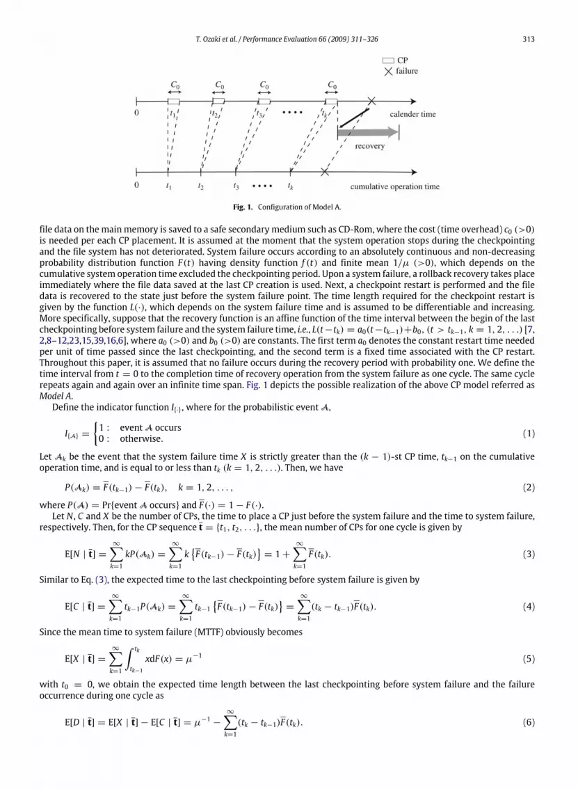
Algorithm 1. Step 1: Set l1 := 0.Step 2: Compute the CP sequence {t2, t3, . . .}with a fixed li using Eq. (26) and Algorithm 0.Step 3: Compute D(li, t). If

∣∣argmaxi{D(li, t)}∣∣ < ε ≈ 0, then Stop the procedure, otherwise update li by

li+1 = li +D(li, t)T (t)

(27)

and Go to Step 2.

This is a fixed-point algorithm and has not been developed in the long history of the optimal CP placement problems.

4. Performability analysis

Our next concern is the expected reward per unit time in the steady state. Define:

• a: reward per unit time in the normal state• b: reward per unit time during the CP is placed• c: reward per unit recovery time in the system down state• P1(t): steady-state probability that the system is in normal state• P2(t): steady-state probability that the system is in checkpointing state• P3(t): steady-state probability that the system is recovering from a system failure.

Then, the expected reward per unit time in the steady state, if the ergodic probabilities Pj(t) (j = 1, 2, 3) exist, is givenby

Ri(t) = aP1(t)+ bP2(t)+ cP3(t) (28)

for Model i (= A, B). It is clear that Ri(t) is reduced to Ai(t) when a = 1, b = 0 and c = 0. In the following discussion, wesuppose that a = 0 to simplify the discussion. That is, for the negative reward parameters b and c , the expected reward canbe regarded as the expected cost per unit time in the steady state. It should be noted that even for Model A one cannot applyAlgorithm 0 under the expected reward criterion because the CP sequence t is involved in both denominator and numeratorof the reward function. Hence, similar to the maximization problem of system availability for Model B we develop a fixedpoint type algorithm for the expected reward measure.

4.1. Model A

For Model A, the expected reward per unit time in the steady state is formulated as

RA(t) =b · c0E[N | t] + c · {a0E[D | t] + b0}

T (t)

=

{b · c0

[1+

n∑k=1

F(tk)

]+ c ·

[a0

(µ−1 −

n∑k=1

(tk − tk−1)F(tk)

)+ b0

]}/{c0

[1+

n∑k=1

F(tk)

]

+ µ−1 + a0

[µ−1 −

n∑k=1

(tk − tk−1)F(tk)

]+ b0

}. (29)

For constant sequence {h1, h2, . . . , hi, . . .}, define the function:

QA(hi, t) = b · c0E[N | t] + c · a0E[D | t] + b0 − hiT (t)

=

{b · c0

[1+

n∑k=1

F(tk)

]+ c · a0

[µ−1 −

n∑k=1

(tk − tk−1)F(tk)

]+ b0

}

− hi

{c0

[1+

n∑k=1

F(tk)

]+ µ−1 + a0

[µ−1 −

n∑k=1

(tk − tk−1)F(tk)

]+ b0

}. (30)

Partially differentiating Eq. (30) with respect to tk, we have

tk − tk−1 =F(tk+1)− F(tk)

f (tk)+bc0(1− hi)ca0(c − hi)

, (31)

where tk − tk−1 > c0 (k = 1, 2, 3, . . .). Based on Algorithm 1, we develop a numerical computation method that convergesto the real optimal solution maximizing R1(t).

318 T. Ozaki et al. / Performance Evaluation 66 (2009) 311–326

Algorithm 2. Step 1: Set h1 := 0.Step 2: For an arbitrary hi compute the CP sequence {t1, t2, t3, . . .} by using Eq. (31) and Algorithm 0.Step 3: Calculate RA(t). If

∣∣argmaxiQA(hi, t)∣∣ < ε ≈ 0 then Stop the procedure, otherwise Go to Step 2 after updating hiwith

hi+1 = hi +QA(hi, t)T (t)

. (32)

4.2. Model B

In a fashion similar to Model A, the expected reward per unit time in the steady state for Model B is given by

RB(t) =b · c0E[N | t] + c · {a0E[D | t] + b0}

T (t)

=

{b · c0

[1+

n∑k=1

F(tk)

]+ c · a0

[µ−1 −

((t1 + c0)F(t1 + c0)+

∞∑k=2

(tk − tk−1)F(tk + c0)

)

+ b0

]}/{µ−1 + a0

[µ−1 −

((t1 + c0)F(t1 + c0)+

∞∑k=2

(tk − tk−1)F(tk + c0)

)]+ b0

}. (33)

Define the following function with a constant hi:

QB(hi, t) = b · c0E[N | t] + c · {a0E[D | t] + b0} − hiT (t)

=

{b · c0

[1+

n∑k=1

F(tk)

]+ c · a0

[µ−1 −

((t1 + c0)F(t1 + c0)+

∞∑k=2

(tk − tk−1)F(tk + c0)

)+ b0

]}

− hi

{µ−1 + a0

[µ−1 −

((t1 + c0)F(t1 + c0)+

∞∑k=2

(tk − tk−1)F(tk + c0)

)]+ b0

}. (34)

By differentiating Eq. (34) with respect to tk, we get

tk − tk−1 =F(tk+1)− F(tk)

f (tk)+b · c0f (tk − c0)c · a0(c − hi)f (tk)

, (35)

where tk− tk−1 > c0 (k = 1, 2, 3, . . .). The computation algorithm for Model B is given by replacing QA(hi, t) by QB(hi, t) inAlgorithm 2.

5. Approximate algorithms

5.1. Exponential approximation

For Model A under the availability criterion, it is well known that the optimal CP interval is constant, i.e., t1 = t2 − t1 =· · · = tk+1 − tk = · · ·, if F(t) is the exponential distribution with mean 1/µ. Under the assumptions that a0 = 1 andb0 = 0, Young [6] considered the checkpoint restart model with constant CP interval with the exponential system failuretime distribution, and derived the following non-linear equation which satisfies the optimal CP interval t1:

ec0µ − t1µ− e−t1µ = 0. (36)

Based on the second order approximation exp(−µt) ≈ 1−µt +µ2t2/2, he obtained the approximate form of the optimalCP interval:

t1 ≈√2(ec0µ − 1)/µ ≈

√2c0/µ, (37)

which is due to exp(c0µ) ≈ 1+ c0µ.For the general system failure time distribution F(t), the simplest method is to approximate F(t) with an exponential

distribution Fe(t) = 1− exp{−µt}, where the parameterµ is determined by the MTTF of F(t), say, 1/µ. Since the resultingoptimal CP sequence is given by the constant sequence kt1 (k = 1, 2, . . .) maximizing the system availability with Fe(t),the optimal t∗1 is a unique solution of Eq. (36). For Model B with the system availability and the other cases with expected

T. Ozaki et al. / Performance Evaluation 66 (2009) 311–326 319

reward, the corresponding dependability measures are defined by AeB(t1) and Rei (t1) (i = A, B) as univariate functions of t1.

That is, from a few algebraic manipulations, we have

AeB(t1) ={1/µ− c0

[1/(1− e−µt1)

]}/{1/µ+ a0

[1/µ−

((t1 + c0)e−µ(t1+c0)

+ (t1e−µ(2t1+c0))/(1− e−µt1))]+ b0

}, (38)

ReA(t1) ={b · c0

[1/(1− e−µt1)

]+ c ·

[a0(1/µ− (t1e−µt1)/(1− e−µt1)

)+ b0

]}/{c0[1/(1− e−µt1)

]+ 1/µ+ a0

[1/µ− (t1e−µt1)/(1− e−µt1)

]+ b0

}, (39)

ReB(t1) ={b · c0

[1/(1− e−µt1)

]+ c ·

[a0(1/µ−

((t1 + c0)e−µ(t1+c0) + (t1e−µ(2t1+c0))/(1− e−µt1)

))+ b0

]}/{1/µ+ a0

[1/µ−

((t1 + c0)e−µ(t1+c0) + (t1e−µ(2t1+c0))/(1− e−µt1)

)]+ b0

}. (40)

5.2. Constant-sequence approximation

Next, we treat the general system failure time distribution F(t) but restrict our concern to the periodic CP interval t1. Inthis case, the dependability measures under consideration can be approximated by

AcA(t1) = µ−1/{

c0

[(1+

∞∑k=1

F

)(kt1)

]+ µ−1 + a0

[µ−1 −

∞∑k=1

t1F(kt1)

]+ b0

}, (41)

AcB(t1) =

{µ−1 − c0

[1+

∞∑k=1

F(kt1)

]}/{µ−1 + a0

[µ−1 −

((t1 + c0)F(t1 + c0)

+

∞∑k=1

t1F(kt1 + c0)

)]+ b0

}, (42)

RcA(t1) =

{b · c0

[1+

∞∑k=1

F(kt1)

]+ c ·

[a0

(µ−1 −

∞∑k=1

t1F(kt1)

)+ b0

]}/{c0

[1+

∞∑k=1

F(kt1)

]

+µ−1 + a0

[µ−1 −

∞∑k=1

t1F(kt1)

]+ b0

}, (43)

RcB(t2) =

{b · c0

[1+

∞∑k=1

F(kt1)

]+ c ·

[a0

(µ−1 −

((t1 + c0)F(t1 + c0)+

∞∑k=1

t1F(kt1 + c0)

))

+ b0

]}/{µ−1 + a0

[µ−1 −

((t1 + c0)F(t1 + c0)+

∞∑k=1

t1F(kt1 + c0)

)]+ b0

}. (44)

When F(t) is replaced by Fe(t), Eqs. (42)–(44) are reduced to Eqs. (38)–(40), respectively.

5.3. Constant-hazard approximation

The third approximation method was proposed by Kaio and Osaki [23] and could be applied only for Model A. Inthis approximate scheme, the conditional probability that the system failure occurs during (tk−1, tk] (k = 1, 2, . . .) isapproximated by a constant p ∈ (0, 1) satisfying

F(tk)− F(tk−1)1− F(tk−1)

= p. (45)

This assumption can be validatedwhen the time interval between successive CPs is relatively small. Since the system failuretime distribution is given by

F(tk) = 1− (1− p)k, (46)

the CP sequence is determined by t∗k = F−1(1− {1− p∗}k). Using this approximation, the steady-state system availability

for Model A is represented as a function of p as follows:

AA(p) = µ−1/{

c0/p+ µ−1 + a0

[λ−

∞∑i=1

(F−1(1− (1− p)i−1)p(1− p)i

)]+ b0

}, (47)

320 T. Ozaki et al. / Performance Evaluation 66 (2009) 311–326

Fig. 3. Optimal CP sequence under the availability in the steady state (Model A):m = 2.0, η = 60.0, a0 = 0.2, b0 = 0.0, c0 = 0.2, b = −1.0, c = −20.0.

if the inverse function F−1(·) exits. Also, we obtain the expected reward rate by

RA(p) =

{b · c0/p+ c ·

[a0

(µ−1 −

∞∑i=1

(F−1(1− (1− p)i−1)p(1− p)i

))+ b0

]}/{c0/p+ µ−1 + a0

[µ−1 −

∞∑i=1

(F−1(1− (1− p)i−1)p(1− p)i

)]+ b0

}. (48)

The resulting sub-optimal checkpoint sequence can be derived from Eq. (46) with the optimal p∗maximizing AA(p) or RA(p).

6. Numerical examples

In this section we calculate numerically the exact and approximate optimal CP sequences, and compare them in termsof dependability measures. Here we represent the approximations by an exponential distribution, the constant CP intervalwith general distribution and the constant hazard by Approximation 1, Approximation 2 and Approximation 3, respectively.Suppose that the system failure time obeys the Weibull distribution:

F(t) = 1− e−(tη )m

(49)

with shape parameterm (>0) and scale parameter η (>0). We show the results on the system availability and the expectedreward per unit time in the steady state. Throughout numerical examples, we set the design parameter in algorithms asε = 10−10.

6.1. System availability

First, we show the result on the system availability in the steady state. In Figs. 3 and 4, we depict the comparison resultson the optimal and sub-optimal CP sequences. From Fig. 3, Approximation 3 overestimates the optimal CP interval in theinitial phase and eventually underestimates the exact CP interval in the latter phase. On the other hand, from Figs. 3 and4, both sub-optimal CP sequences based on Approximation 1 and Approximation 2 also underestimate the real optimalsolution in early phase, but they tend to overestimate in the latter phase.Tables 1 and 2 present the dependence of shape parameter of the Weibull distribution on the maximum system

availability in respective cases. The approximate availability is calculated by substituting the approximate CP sequence intoEq. (18) or (21), where the relative error is defined by

Relative error (%) =|approximation−maximum availability|

|maximum availability|× 100. (50)

In general, the availability requirement for real mission-critical systems is said to be over five nines, say, 99.99%, so thatthe relative error 0.06% for m = 1.5 can not be negligible in Table 1. As the shape parameter in the Weibull distributionincreases, the failure rate r(t) = (m/η)(t/η)m−1 monotonically increases inm (>1) and the MTTF = 1/µ = η0(1+ 1/m)decreases, where 0(·) is the standard gamma function. For a larger shape parameter, the difference is significant if oneapplies the approximation methods. Whenm = 1, i.e. the system failure time is exponentially distributed random variable,the resulting CP sequences and their associated system availability take same values as those based on Approximations

T. Ozaki et al. / Performance Evaluation 66 (2009) 311–326 321

Fig. 4. Optimal CP sequence under the availability in the steady state (Model B):m = 2.0, η = 60.0, a0 = 0.2, b0 = 0.0, c0 = 0.2, b = −1.0, c = −20.0.

Table 1Dependence of shape parameter on the availability in the steady state (Model A): η = 60.0, a0 = 0.2, b0 = 0.0, c0 = 0.2, b = −1.0, c = −20.0.

m Approximation 1 Approximation 2 Approximation 3 ExactAvailability Error (%) Availability Error (%) p∗ Availability Error (%) availability

1.0 0.96371 0.000 0.96371 0.000 0.17163 0.96371 0.000 0.963711.5 0.96133 −0.061 0.96134 −0.060 0.17149 0.96051 −0.147 0.961922.0 0.96090 −0.177 0.96092 −0.175 0.16625 0.95877 −0.398 0.962612.5 0.96092 −0.302 0.96094 −0.300 0.16132 0.95761 −0.646 0.963833.0 0.96105 −0.421 0.96107 −0.419 0.15731 0.95676 −0.866 0.965123.5 0.96120 −0.530 0.96122 −0.528 0.15408 0.95610 -1.058 0.966324.0 0.96134 −0.629 0.96136 −0.627 0.15148 0.95558 -1.224 0.967434.5 0.96147 −0.717 0.96149 −0.715 0.14935 0.95515 -1.370 0.96842

Table 2Dependence of shape parameter on the availability in the steady state (Model B): η = 60.0, a0 = 0.2, b0 = 0.0, c0 = 0.2, b = −1.0, c = −20.0.

m Approximation 1 Approximation 2 ExactAvailability Error (%) Availability Error (%) availability

1.0 0.96297 0.000 0.96297 0.000 0.962971.5 0.96047 −0.063 0.96049 −0.061 0.961072.0 0.96002 −0.181 0.96004 −0.179 0.961772.5 0.96004 −0.309 0.96006 −0.307 0.963023.0 0.96018 −0.432 0.96020 −0.429 0.964343.5 0.96033 −0.543 0.96035 −0.541 0.965584.0 0.96048 −0.644 0.96050 −0.642 0.966714.5 0.96062 −0.735 0.96064 −0.733 0.96773

1–3. That is, all the approximate methods are consistent in the case of exponential system failure time. However, as MTTFdecreases and the system tends to be more unreliable, the difference from the real optimal solution becomes remarkablefor all approximation methods.Tables 3 and 4 present the dependence of scale parameter. In Tables 3 and 4, we can see that the system availability

monotonically increases as the scale parameter increases. This is because the MTTF increases as the scale parameterincreases. On the other hand, the errors of Approximations 1–3 decrease as the scale parameter increases. From these results,it is seen that both exact and approximate methods have monotone properties of shape and scale parameters on the systemavailability in the steady state.

6.2. Expected reward

Next, we show the result on the expected reward per unit time in the steady state. In Figs. 5 and 6, we illustrate thecomparison results between the optimal and sub-optimal CP sequences. From Figs. 5 and 6, the trend of CP sequences basedon Approximations 1–3 is same as the case of the system availability.Tables 5 and 6 present the dependence of shape parameter of the Weibull distribution on the minimum expected

operation costs (maximized negative rewards) in respective cases, where each reward in the column is given by the absolutevalue of negative reward (cost). The approximate expected operation cost is calculated by substituting the approximate CP

322 T. Ozaki et al. / Performance Evaluation 66 (2009) 311–326

Table 3Dependence of scale parameter on the availability in the steady state (Model A):m = 2.0, a0 = 0.2, b0 = 0.0, c0 = 0.2, b = −1.0, c = −20.0.

η Approximation 1 Approximation 2 Approximation 3 ExactAvailability Error (%) Availability Error (%) p∗ Availability Error (%) availability

55 0.95915 −0.181 0.95917 −0.179 0.17303 0.95692 −0.413 0.9608960 0.96090 −0.177 0.96092 −0.175 0.16625 0.95877 −0.398 0.9626165 0.96245 −0.173 0.96246 −0.171 0.16022 0.96040 −0.385 0.9641270 0.96382 −0.170 0.96383 −0.168 0.15483 0.96186 −0.373 0.9654675 0.96505 −0.167 0.96507 −0.165 0.14996 0.95515 -1.191 0.9666680 0.96617 −0.164 0.96618 −0.162 0.14555 0.96435 −0.352 0.9677585 0.96719 −0.161 0.96720 −0.159 0.14151 0.96542 −0.343 0.9687490 0.96812 −0.158 0.96813 −0.157 0.13780 0.96641 −0.334 0.9696595 0.96897 −0.155 0.96898 −0.154 0.13438 0.96732 −0.326 0.97048100 0.96976 −0.153 0.96977 −0.152 0.13121 0.96815 −0.318 0.97125

Table 4Dependence of scale parameter on the availability in the steady state (Model B):m = 2.0, a0 = 0.2, b0 = 0.0, c0 = 0.2, b = −1.0, c = −20.0.

η Approximation 1 Approximation 2 ExactAvailability Error (%) Availability Error (%) availability

55 0.95819 −0.185 0.95821 −0.183 0.9599760 0.96002 −0.181 0.96004 −0.179 0.9617765 0.96164 −0.177 0.96166 −0.175 0.9633570 0.96307 −0.174 0.96309 −0.172 0.9647575 0.96436 −0.170 0.96438 −0.169 0.9660180 0.96552 −0.167 0.96554 −0.166 0.9671485 0.96658 −0.164 0.96659 −0.163 0.9681790 0.96754 −0.161 0.96756 −0.160 0.9691195 0.96843 −0.159 0.96844 −0.158 0.96997100 0.96925 −0.156 0.96926 −0.155 0.97077

Fig. 5. Optimal CP sequence under the expected reward per unit time in the steady state (Model A): m = 2.0, η = 60.0, a0 = 0.2, b0 = 0.0, c0 = 0.2,b = −1.0, c = −20.0.

sequence into Eq. (29) or (33). Here, the relative error on the expected cost is defined by

Relative error (%) =|approximate−minimum cost|

|minimum cost|× 100. (51)

From Tables 5 and 6, the errors of Approximations 1–3 increase as the shape parameter increases, similar to Tables 1 and 2.However, the increasing trend is in particular remarkable in this case. Especially, when m = 4.5 we see that approximateerrors become 30%–50%. Also, Tables 7 and 8 signify the dependence of the scale parameter. In Tables 7 and 8, as the scaleparameter increases, both exact and approximate cost functions monotonically decrease, but the relative errors betweenthem increase. On the other hand, Tables 9 and 10 present the dependence of the reward parameter per unit recovery time.From these results, the errors on Approximations 1–3 monotonically increase as the reward parameter increases. Finally,we conclude that both exact and approximate methods have monotone dependence of shape, scale and reward parameterson the expected reward in the steady state. This trend is also quite similar to the case with the system availability.

T. Ozaki et al. / Performance Evaluation 66 (2009) 311–326 323

Fig. 6. Optimal CP sequence under the expected reward per unit time in the steady state (Model B): m = 2.0, η = 60.0, a0 = 0.2, b0 = 0.0, c0 = 0.2,b = −1.0, c = −20.0.

Table 5Dependence of shape parameter on the expected reward (cost) per unit time in the steady state (Model A): η = 60.0, a0 = 0.2, b0 = 0.0, c0 = 0.2,b = −1.0, c = −20.0.

m Approximation 1 Approximation 2 Approximation 3 ExactReward Error (%) Reward Error (%) p∗ Reward Error (%) reward

1.0 0.15086 0.000 0.15086 0.000 0.03729 0.15086 0.000 0.150861.5 0.15855 4.863 0.15856 4.868 0.03806 0.16042 6.097 0.151202.0 0.15994 7.593 0.15993 7.591 0.03711 0.16535 11.235 0.148652.5 0.15985 11.846 0.15985 11.844 0.03593 0.16909 18.308 0.142923.0 0.15938 16.570 0.15938 16.568 0.03485 0.17221 25.951 0.136723.5 0.15883 21.341 0.15883 21.339 0.03394 0.17487 33.597 0.130894.0 0.15829 26.007 0.15829 26.004 0.03316 0.17717 41.036 0.125624.5 0.15780 30.524 0.15780 30.521 0.03252 0.17917 48.200 0.12090

Table 6Dependence of shape parameter on the expected reward (cost) per unit time in the steady state (Model B): η = 60.0, a0 = 0.2, b0 = 0.0, c0 = 0.2,b = −1.0, c = −20.0.

m Approximation 1 Approximation 2 ExactReward Error (%) Reward Error (%) reward

1.0 0.164011 0.000 0.164011 0.000 0.1640111.5 0.173257 4.217 0.173253 4.214 0.1662472.0 0.174914 7.673 0.174910 7.671 0.1624492.5 0.174812 12.551 0.174807 12.548 0.1553183.0 0.174245 17.752 0.174241 17.749 0.1479763.5 0.173582 22.915 0.173578 22.912 0.1412214.0 0.172937 27.929 0.172933 27.926 0.1351824.5 0.172346 32.768 0.172341 32.764 0.129810

Table 7Dependence of scale parameter on the expected reward (cost) in the steady state (Model A):m = 2.0, a0 = 0.2, b0 = 0.0, c0 = 0.2, b = −1.0, c = −20.0.

η Approximation 1 Approximation 2 Approximation 3 ExactReward Error (%) Reward Error (%) p∗ Reward Error (%) reward

55 0.16644 7.278 0.16644 7.276 0.03855 0.17213 10.946 0.1551560 0.15994 7.593 0.15993 7.591 0.03711 0.16535 11.235 0.1486565 0.15416 7.946 0.15415 7.944 0.03580 0.15933 11.566 0.1428170 0.14898 8.339 0.14897 8.337 0.03466 0.15392 11.938 0.1375175 0.14429 8.770 0.14429 8.768 0.03361 0.14905 12.352 0.1326680 0.14004 9.237 0.14004 9.236 0.03266 0.14461 12.805 0.1282085 0.13614 9.740 0.13614 9.738 0.03179 0.14055 13.295 0.1240690 0.13256 10.276 0.13256 10.274 0.03098 0.13683 13.821 0.1202195 0.12926 10.844 0.12926 10.842 0.03024 0.13338 14.381 0.116613100 0.12619 11.441 0.12619 11.439 0.02955 0.13019 14.970 0.113238

324 T. Ozaki et al. / Performance Evaluation 66 (2009) 311–326

Table 8Dependence of scale parameter on the expected reward (cost) in the steady state (Model B):m = 2.0, a0 = 0.2, b0 = 0.0, c0 = 0.2, b = −1.0, c = −20.0.

η Approximation 1 Approximation 2 ExactReward Error (%) Reward Error (%) reward

55 0.18278 7.461 0.18277 7.458 0.1700960 0.17491 7.673 0.17491 7.671 0.1624565 0.16799 7.923 0.16798 7.920 0.1556570 0.16182 8.210 0.16182 8.208 0.1495475 0.15629 8.537 0.15628 8.534 0.1439980 0.15128 8.901 0.15128 8.899 0.1389285 0.14673 9.305 0.14672 9.303 0.1342490 0.14256 9.747 0.14256 9.744 0.1299095 0.13873 10.224 0.13873 10.222 0.12586100 0.13519 10.736 0.13519 10.734 0.12209

Table 9Dependence of the reward per unit recovery time on the expected reward (cost) in the steady state (Model A): m = 2.0, η = 60.0, a0 = 0.2, b0 = 0.0,c0 = 0.2, b = −1.0.

c Approximation 1 Approximation 2 Approximation 3 ExactReward Error (%) Reward Error (%) p∗ Reward Error (%) reward

5 0.08404 6.091 0.08403 6.082 0.07555 0.08784 10.892 0.0792110 0.1163 6.500 0.11630 6.495 0.05320 0.12091 10.724 0.1092015 0.14026 6.860 0.14026 6.857 0.04315 0.14535 10.736 0.1312620 0.15994 7.593 0.15993 7.591 0.03711 0.16535 11.235 0.1486525 0.17688 8.835 0.17688 8.833 0.03297 0.18254 12.315 0.1625230 0.19189 10.555 0.19189 10.554 0.02990 0.19774 13.922 0.1735735 0.20544 12.656 0.20544 12.655 0.02751 0.21144 15.943 0.1823640 0.21784 15.040 0.21784 15.039 0.02558 0.22396 18.271 0.1893645 0.2293 17.622 0.22929 17.621 0.02398 0.23552 20.814 0.19494350 0.23997 20.335 0.23997 20.334 0.02263 0.24628 23.501 0.199415

Table 10Dependence of the reward per unit recovery time on the expected reward (cost) in the steady state (Model B): m = 2.0, η = 60.0, a0 = 0.2, b0 = 0.0,c0 = 0.2, b = −1.0.

c Approximation 1 Approximation 2 ExactReward Error (%) Reward Error (%) reward

5 0.08802 6.250 0.08801 6.23919 0.0828410 0.12401 6.785 0.12401 6.77935 0.1161315 0.15163 7.147 0.15163 7.1426 0.1415220 0.17491 7.673 0.17491 7.67072 0.1624525 0.19543 8.516 0.19542 8.51403 0.1800930 0.21397 9.707 0.21397 9.70514 0.1950435 0.23103 11.220 0.23102 11.2184 0.2077240 0.24690 13.010 0.24690 13.0082 0.2184845 0.26181 15.028 0.26181 15.0263 0.2276150 0.27591 17.230 0.27591 17.228 0.23536

7. Conclusion

In this paper, we have developed numerical computation algorithms for sequential checkpoint placement, so as tomaximize the steady-state system availability and the expected reward per unit time in the steady state, and comparednumerically the real optimal solutions with some approximate ones. The lesson learned from the numerical study in thispaper is that three approximation methods provide rather different checkpoint sequences with larger error in the earlieroperational phase, as the shape parameter of the Weibull distribution increases and the corresponding MTTF is shorter. Inother words, as the degree of IFR property is more remarkable, the sub-optimal checkpointing policies developed in thepast literature do not function better. In fact, for Model A with m = 4.5, the system availabilities for Approximations 1–3are given by 0.961474, 0.961492 and 0.955153, respectively. Since the exact maximum availability is 0.968421, the relativeerrors for respective approximation methods are 0.717 (%), 0.715 (%) and 1.370 (%). In other words, these approximationmethods cannot be used formission critical systemswith higher availability requirement. Hence, the numerical computationalgorithms for the optimal checkpoint sequence will be useful to back-up the information for the general file systems.Though the constant checkpoint placement which is hand-tuned by some system expert is very often employed in industry,of course, such a heuristic checkpointing is not always optimal in terms of system availability and performability.In the future, the same idea will be applied to distributed checkpointing systems. For instance, Soliman and

Elmaghraby [36] considered an uncoordinated checkpointing protocol with periodic time interval to minimize the mean

T. Ozaki et al. / Performance Evaluation 66 (2009) 311–326 325

overhead to execute a finite length task. This will be extended to the aperiodic checkpointing scheme by using anyalgorithmic way under the general failure time distribution assumption. In a fashion similar to this paper, when thecheckpoint sequence is determined under the system availability and the expected reward rate per unit time in the steadystate, the Brender’s fixed-point type algorithm [40] will be useful to calculate the optimal solution iteratively.

References

[1] K.M. Chandy, A survey of analytic models of roll-back and recovery strategies, Computer 8 (5) (1975) 40–47.[2] K.M. Chandy, J.C. Browne, C.W. Dissly, W.R. Uhrig, Analytic models for rollback and recovery strategies in database systems, IEEE Transactions onSoftware Engineering SE-1 (1) (1975) 100–110.

[3] G.M. Lohman, J.A.Muckstadt, Optimal policy for batch operations: Backup, checkpointing, reorganization and updating, ACMTransactions onDatabaseSystems 2 (3) (1977) 209–222.

[4] V.F. Nicola, Checkpointing and modeling of program execution time, in: M.R. Lyu (Ed.), Software Fault Tolerance, JohnWiley & Sons, New York, 1995,pp. 167–188.

[5] A.N. Tantawi, M. Ruschitzka, Performance analysis of checkpointing strategies, ACM Transactions on Computer Systems 2 (2) (1984) 123–144.[6] J.W. Young, A first order approximation to the optimum checkpoint interval, Communications of ACM 17 (9) (1974) 530–531.[7] F. Baccelli, Analysis of s service facility with periodic checkpointing, Acta Informatica 15 (1981) 67–81.[8] T. Dohi, N. Kaio, K.S. Trivedi, Availability models with age dependent-checkpointing, in: Proceedings of 21st Symposium on Reliable DistributedSystems, IEEE CS Press, 2002, pp. 130–139.

[9] E. Gelenbe, D. Derochette, Performance of rollback recovery systems under intermittent failures, Communications of the ACM 21 (6) (1978) 493–499.[10] E. Gelenbe, On the optimum checkpoint interval, Journal of the ACM 26 (2) (1979) 259–270.[11] E. Gelenbe, M. Hernandez, Optimum checkpoints with age dependent failures, Acta Informatica 27 (1990) 519–531.[12] P.B. Goes, U. Sumita, Stochastic models for performance analysis of database recovery control, IEEE Transactions on Computers C-44 (4) (1995)

561–576.[13] V. Grassi, L. Donatiello, S. Tucci, On the optimal checkpointing of critical tasks and transaction-oriented systems, IEEE Transactions on Software

Engineering SE-18 (1) (1992) 72–77.[14] V.G. Kulkarni, V.F. Nicola, K.S. Trivedi, Effects of checkpointing and queueing on program performance, Stochastic Models 6 (4) (1990) 615–648.[15] V.F. Nicola, J.M. Van Spanje, Comparative analysis of differentmodels of checkpointing and recovery, IEEE Transactions on Software Engineering SE-16

(8) (1990) 807–821.[16] U. Sumita, N. Kaio, P.B. Goes, Analysis of effective service time with age dependent interruptions and its application to optimal rollback policy for

database management, Queueing Systems 4 (1989) 193–212.[17] P. L’Ecuyer, J. Malenfant, Computing optimal checkpointing strategies for rollback and recovery systems, IEEE Transactions on Computers C-37 (4)

(1988) 491–496.[18] A. Ziv, J. Bruck, An on-line algorithm for checkpoint placement, IEEE Transactions on Computers C-46 (9) (1997) 976–985.[19] N.H. Vaidya, Impact of checkpoint latency on overhead ratio of a checkpointing scheme, IEEE Transactions on Computers C-46 (8) (1997) 942–947.[20] H. Okamura, Y. Nishimura, T. Dohi, A dynamic checkpointing scheme based on reinforcement learning, in: Proceedings of 2004 Pacific Rim

International Symposium on Dependable Computing, IEEE CS Press, 2004, pp. 151–158.[21] A. Duda, The effects of checkpointing on program execution time, Information Processing Letters 16 (5) (1983) 221–229.[22] S. Toueg, Ö. Babaog̃lu, On the optimum checkpoint selection problem, SIAM Journal of Computing 13 (3) (1984) 630–649.[23] N. Kaio, N. Osaki, A note on optimum checkpointing policies, Microelectronics and Reliability 25 (1985) 451–453.[24] Y. Ling, J. Mi, X. Lin, A variational calculus approach to optimal checkpoint placement, IEEE Transactions on Computers 50 (7) (2001) 699–707.[25] D. Long, A. Muir, R. Golding, A longitudinal survey of internet host reliability, in: Proceedings of the 14th IEEE Symposium on Reliable Distributed

Systems, IEEE CS Press, 1995, pp. 2–9.[26] V. Castelli, R.E. Harper, P. Heidelberger, S.W. Hunter, K.S. Trivedi, K. Vaidyanathan,W.P. Zeggert, Proactivemanagement of software aging, IBM Journal

of Research & Development 45 (2001) 311–332.[27] E.N. Elnozahy, L. Alvisi, Y.M. Wang, D.B. Johnson, A survey of rollback-recovery protocols in message-passing systems, ACM Computing Survey 34 (3)

(2002) 375–408.[28] K.F. Wong, M. Franklin, Checkpointing in distributed systems, Journal of Parallel and Distributed Systems 35 (1996) 67–75.[29] J.S. Plank, M.G. Thomaso, Processor allocation and checkpoint interval selection in cluster computing systems, Journal of Parallel and Distributed

Computing 61 (11) (2001) 1570–1590.[30] K. Li, J.F. Naughton, J.S. Plank, Low-latency concurrent checkpointing for parallel programs, IEEE Transactions on Parallel and Distributed Systems 5

(8) (1994) 874–879.[31] J.S. Plank, K. Li, M.A. Puening, Diskless checkpointing, IEEE Transactions on Parallel and Distributed Systems 9 (10) (1998) 972–986.[32] N.H. Vaidya, Staggered consistent checkpointing, IEEE Transactions on Parallel and Distributed Systems 10 (7) (1999) 694–702.[33] A. Agbaria, A. Freund, R. Friedman, Evaluating distributed checkpointing protocols, in: Proceedings of the 23rd International Conference onDistributed

Computing Systems, IEEE CS Press, 2003, pp. 266–273.[34] A. Agbaria, H. Attiya, R. Friedman, R. Vitenberg, Quantifying rollback propagation in distributed checkpointing, in: Proceedings of the 20th IEEE

Symposium on Reliable Distributed Systems, IEEE CS Press, 2001, pp. 36–45.[35] Y. Wang, P. Chung, I. Lin, W. Fuchs, Checkpoint space reclamation for uncoordinated checkpointing in message-passing systems, IEEE Transactions on

Parallel and Distributed Systems 6 (5) (1995) 546–554.[36] H.M. Soliman, A.S. Elmaghraby, An analytical model for hybrid checkpointing in time warp distributed simulation, IEEE Transactions on Parallel and

Distributed Systems 9 (10) (1998) 947–951.[37] K. Gos̆eva-Popstojanova, K.S. Trivedi, Stochastic modeling formalisms for dependability, performance and performability, in: G. Haring, C. Lindemann,

M. Reiser (Eds.), Performance Evaluation – Origins and Directions, in: LNCS, vol. 1769, Springer-Verlag, Berlin, 2000, pp. 385–404.[38] J.F. Meyer, On evaluating the performability of degradable computer systems, IEEE Transactions on Computers C-29 (8) (1981) 720–731.[39] T. Ozaki, T. Dohi, H. Okamura, N. Kaio, Distribution-free checkpoint placement algorithms based on min–max principle, IEEE Transactions on

Dependable and Secure Computing 3 (2) (2006) 130–140.[40] D.M. Brender, A surveillance model for recurrent events, IBMWatson Research Center Report, 1963.[41] T. Dohi, H. Okamura, N. Kaio, Optimal age-dependent checkpoint strategy with retry of rollback recovery, in: Proceedings of the 2nd IEEE Computer

Society International Workshop on Autonomous Decentralized Systems, IEEE CS Press, 2002, pp. 113–118.[42] S. Fukumoto, S. Nakagawa, N. Kaio, S. Osaki, Optimum checkpoint policies attending with unsuccessful rollback recovery, International Journal of

Reliability, Quality and Safety Engineering 4 (4) (1997) 427–439.[43] R.E. Barlow, F. Proschan, Mathematical Theory of Reliability, SIAM, Philadelphia, 1996.

326 T. Ozaki et al. / Performance Evaluation 66 (2009) 311–326

Tatsuya Ozaki received the B.S.E. and M.S. from Hiroshima University, Japan, in 2001 and 2005, respectively. In 2005, he joinedNTT Facilities, Inc., Japan as a Technical Stuff. His research interests are dependable computing and performance evaluation. Hispapers appeared in IEEE Transactions on Dependable and Secure Computing and several major conferences like DSN 2004, DASC2006, etc.

Tadashi Dohi received the B.S.E., M.S. and Dr. of Engineering degrees from Hiroshima University, Japan, in 1989, 1991 and 1995,respectively. In 1992, he joined theDepartment of Industrial and Systems Engineering, HiroshimaUniversity, Japan, as an AssistantProfessor. Now, he is working as a Full Professor in the Department of Information Engineering, Graduate School of Engineering,Hiroshima University, Japan, since 2002. In 1992 and 2000, he was a Visiting Research Scholar in University of British Columbia,Canada andDukeUniversity, USA, respectively, on leave of absence fromHiroshimaUniversity. His research areas include softwarereliability engineering, dependable computing and performance evaluation. He is a Regular Member of ORSJ, JSIAM, IEICE, ISCIEand IEEE. He published over 200 journal papers and refereed conference papers. Dr. Dohi is serving as an Associate Editor ofIEICE Transactions on Fundamentals of Electronics, Communications and Computer Sciences (A) and Asia-Pacific Journal of OperationalResearch, and an Editorial BoardMember of Journal of Risk and Reliability, Journal of Autonomic and Trusted Computing, InternationalJournal of Reliability and Quality Performance, etc. He published over 300 refereed papers. Dr. Dohi served as a General Chair ofseveral international conferences likeAIWARM2004–2008 andWoSAR2008 and as a ProgramCommittee Chair ofRASOR2005–2007

and ISAS 2009.

Naoto Kaio received the B.S.E., M.S. and Dr. of Engineering degrees from Hiroshima University, Japan, in 1976, 1978 and 1982,respectively. He is a Full Professor in the Department of Economic Informatics, Hiroshima Shudo University, Japan. From 1986to 1987, he was a Visiting Research Scholar in the William E. Simon Graduate School of Business Administration, University ofRochester, USA. His research areas include systems science, operations research and reliability theory. He is a Regular Member ofORSJ, IEICE, JIMA, IPSJ, JSQC, REAJ and IEEE. Also, Dr. Kaio is serving as Regional Editor for Asia in Journal of Quality in MaintenanceEngineering.