Embed Size (px)
Citation preview
Analyzing and Classifying Neural Dynamics from IntracranialElectroencephalography Signals in Brain-Computer Interface
Applications
Naresh Nagabushan
Thesis submitted to the Faculty of the
Virginia Polytechnic Institute and State University
in partial fulfillment of the requirements for the degree of
Master of Science
in
Computer Engineering
Pratap Tokekar, Chair
Sujith Vijayan, Co-chair
Amos L. Abbott
May 8, 2019
Blacksburg, Virginia
Keywords: Brain Computer Interfaces, Signal Processing, Electroencephalography,
Machine Learning.
Copyright 2019, Naresh Nagabushan
Analyzing and Classifying Neural Dynamics from IntracranialElectroencephalography Signals in Brain-Computer Interface
Applications
Naresh Nagabushan
(ABSTRACT)
Brain-Computer Interfaces (BCIs) that rely on motor imagery currently allow subjects to
control quad-copters, robotic arms, and computer cursors. Recent advancements have been
made possible because of breakthroughs in fields such as electrical engineering, computer sci-
ence, and neuroscience. Currently, most real-time BCIs use hand-crafted feature extractors,
feature selectors, and classification algorithms. In this work, we explore the different clas-
sification algorithms currently used in electroencephalographic (EEG) signal classification
and assess their performance on intracranial EEG (iEEG) data. We first discuss the motor
imagery task employed using iEEG signals and find features that clearly distinguish between
different classes. Second, we compare the different state-of-the-art classifiers used in EEG
BCIs in terms of their error rate, computational requirements, and feature interpret-ability.
Next, we show the effectiveness of these classifiers in iEEG BCIs and last, show that our
new classification algorithm that is designed to use spatial, spectral, and temporal informa-
tion reaches performance comparable to other state-of-the-art classifiers while also allowing
increased feature interpret-ability.
Analyzing and Classifying Neural Dynamics from IntracranialElectroencephalography Signals in Brain-Computer Interface
Applications
Naresh Nagabushan
(GENERAL AUDIENCE ABSTRACT)
Brain-Computer Interfaces (BCIs) as the name suggests allows individuals to interact with
computers using electrical activity captured from different regions of the brain. These de-
vices have been shown to allows subjects to control a number of devices such as quad-copters,
robotic arms, and computer cursors. Applications such as these obtain electrical signals from
the brain using electrodes either placed non-invasively on the scalp (also known as an elec-
troencephalographic signal, EEG) or invasively on the surface of the brain (Electrocortico-
graphic signal, ECoG). Before a participant can effectively communicate with the computer,
the computer is calibrated to recognize different signals by collecting data from the subject
and learning to distinguish them using a classification algorithm. In this work, we were
interested in analyzing the effectiveness of using signals obtained from deep brain structures
by using electrodes place invasively (also known as intracranial EEG, iEEG). We collected
iEEG data during a two hand movement task and manually analyzed the data to find regions
of the brain that are most effective in allowing us to distinguish signals during movements.
We later showed that this task could be automated by using classification algorithms that
are borrowed from electroencephalographic (EEG) signal experiments.

Dedication
This work is dedicated to the open source community.
iv
Acknowledgments
Research isn’t easy, there are a lot of lows and very little highs. But, the lows are what
makes the highs worth doing it all over again. I would like to thank my advisor Dr. Sujith
Vijayan for instilling this thought right from the very beginning and encouraging me during
this entire process. I am also very grateful to my committee members Dr. Pratap Tokekar
and Dr. Lynn Abbott for taking the time to sit down and brainstorm my ideas.
v
Contents
List of Figures viii
List of Tables xi
1 Introduction 1
2 Previous Work 7
3 iEEG Motor Imagery Task: Implementation Details 9
3.1 BCI Experiment Overview . . . . . . . . . . . . . . . . . . . . . . . . . . . . 9
3.2 Stage 1: Calibration Stage . . . . . . . . . . . . . . . . . . . . . . . . . . . . 12
3.3 Stage 2: Training Stage . . . . . . . . . . . . . . . . . . . . . . . . . . . . . 13
3.4 Stage 3: Online Stage . . . . . . . . . . . . . . . . . . . . . . . . . . . . . . 14
4 iEEG Motor Imagery Task: Relevant Feature Estimation 16
4.1 Subject description . . . . . . . . . . . . . . . . . . . . . . . . . . . . . . . . 16
4.2 Feature Estimation . . . . . . . . . . . . . . . . . . . . . . . . . . . . . . . . 18
4.2.1 Spatial and Spectral Features . . . . . . . . . . . . . . . . . . . . . . 19
4.2.2 Temporal Features . . . . . . . . . . . . . . . . . . . . . . . . . . . . 23
5 EEG Signal Classifiers 27
vi
5.1 Previous methods . . . . . . . . . . . . . . . . . . . . . . . . . . . . . . . . . 28
5.1.1 Common Spatial Pattern . . . . . . . . . . . . . . . . . . . . . . . . 28
5.1.2 Filter Bank Common Spatial pattern . . . . . . . . . . . . . . . . . . 29
5.1.3 Deep4Net . . . . . . . . . . . . . . . . . . . . . . . . . . . . . . . . . 29
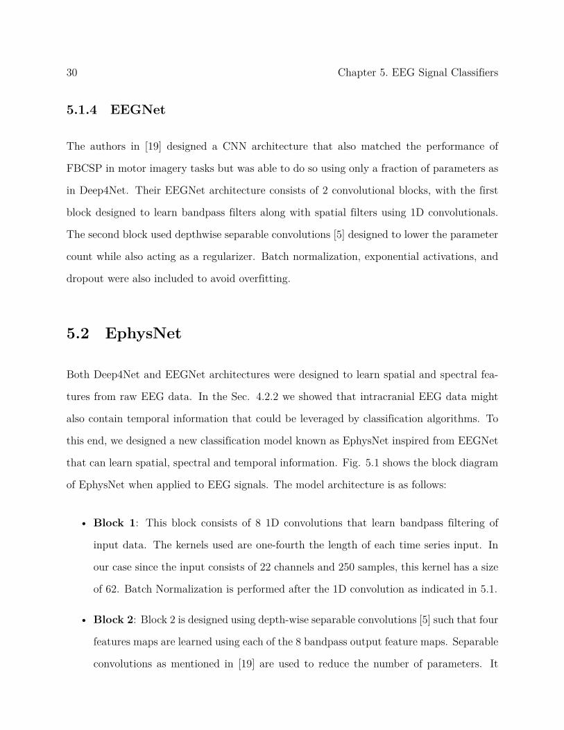
5.1.4 EEGNet . . . . . . . . . . . . . . . . . . . . . . . . . . . . . . . . . . 30
5.2 EphysNet . . . . . . . . . . . . . . . . . . . . . . . . . . . . . . . . . . . . . 30
5.3 EEG dataset description and experimental setup . . . . . . . . . . . . . . . 33
5.4 EEG Motor Imagery Classification Results . . . . . . . . . . . . . . . . . . . 33
5.5 Feature Visualization . . . . . . . . . . . . . . . . . . . . . . . . . . . . . . . 34
6 iEEG Signal Classifiers 40
6.1 Experimental Setup . . . . . . . . . . . . . . . . . . . . . . . . . . . . . . . . 40
6.2 iEEG Motor Imagery Classification Results . . . . . . . . . . . . . . . . . . 42
6.3 Feature Visualization . . . . . . . . . . . . . . . . . . . . . . . . . . . . . . . 44
7 Conclusions and Future Work 48
Bibliography 50
Appendix A 56
vii

List of Figures
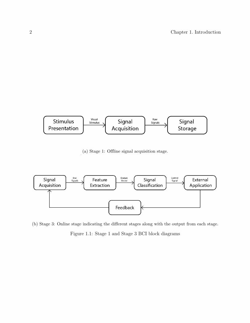
1.1 Stage 1 and Stage 3 BCI block diagrams . . . . . . . . . . . . . . . . . . . . 2
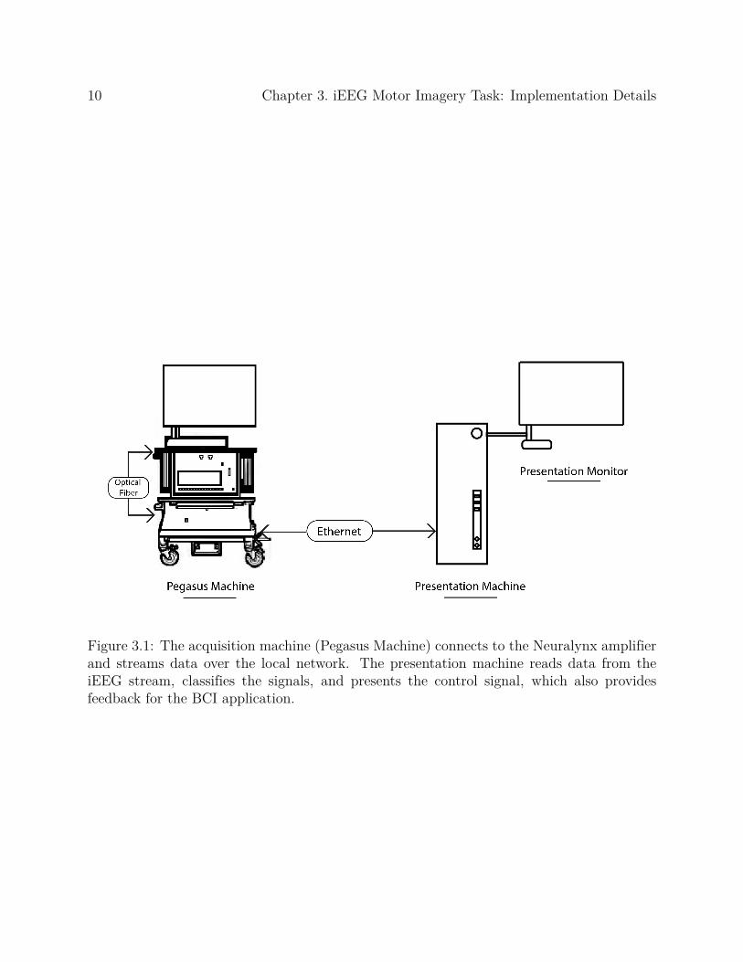
3.1 The acquisition machine (Pegasus Machine) connects to the Neuralynx ampli-
fier and streams data over the local network. The presentation machine reads
data from the iEEG stream, classifies the signals, and presents the control
signal, which also provides feedback for the BCI application. . . . . . . . . . 10
3.2 Visual cues as seen by the subject during the calibration stage . . . . . . . . 12
3.3 Visual Cues as seen by each subject during the online stage . . . . . . . . . 14
4.1 Electrode map of subject CAR 10. The colored dots indicate the location of
the electrode contacts with the same color assigned to electrode contacts in
the same depth electrode. . . . . . . . . . . . . . . . . . . . . . . . . . . . . 17
4.2 CAR 04 power and power significance plots . . . . . . . . . . . . . . . . . . 20
4.3 Power spectrum during left- and right-hand movements in both hemispheres
for subjects CAR04 and CAR10 . . . . . . . . . . . . . . . . . . . . . . . . . 21
4.4 Spectrogram at one of the hippocampal electrodes in CAR04 showing the
difference at both low and high frequencies between imagination of left- and
right-hand movements. . . . . . . . . . . . . . . . . . . . . . . . . . . . . . . 24
4.5 The average cross correlation between low and high frequency components
during both left and right movements . . . . . . . . . . . . . . . . . . . . . . 26
viii
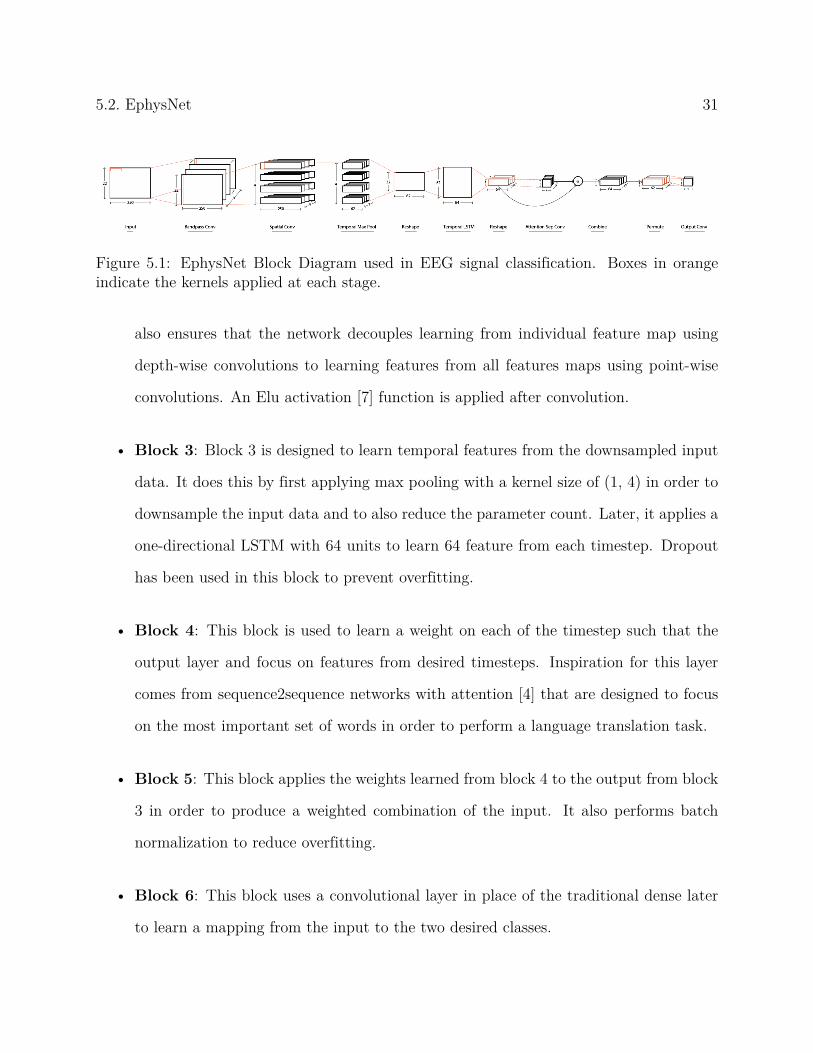
5.1 EphysNet Block Diagram used in EEG signal classification. Boxes in orange
indicate the kernels applied at each stage. . . . . . . . . . . . . . . . . . . . 31
5.2 Visualizing Bandpass Convolutional Kernels: Top row represents the band-
pass kernels learnt by EphyNet and the bottom row represents the power
spectral density of the kernel above it for subject 3 during 2 hand motor
imagery . . . . . . . . . . . . . . . . . . . . . . . . . . . . . . . . . . . . . . 35
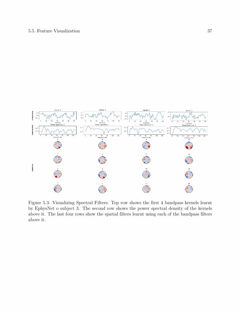
5.3 Visualizing Spectral Filters: Top row shows the first 4 bandpass kernels learnt
by EphysNet o subject 3. The second row shows the power spectral density
of the kernels above it. The last four rows show the spatial filters learnt using
each of the bandpass filters above it. . . . . . . . . . . . . . . . . . . . . . . 37
5.4 SHAP based feature visualization: Top row shows the raw signals at all chan-
nels for subject 3 during left hand movement along with its importance values
towards its right. The topoplot consists of the average of importance values
assigned during the left hand movement time samples. Bottom row indicates
the same thing but for the right trials. Both the left and right trials are 1s
segments from [-0.5, 0.5]s . . . . . . . . . . . . . . . . . . . . . . . . . . . . . 38
5.5 SHAP based feature visualization to track features: Left Column shows the
raw eeg traces along a continuous set of data 1s long data chunks. The right
column shows the SHAP values of the chunks towards their left.The signal
moves forward in time as we proceed from the top to the bottom row. . . . . 39
6.1 EphysNet when applied to iEEG data. The sizes of feature map after each
layer is indicatd along with the kernel shapes used in each layer with orange
boxes. . . . . . . . . . . . . . . . . . . . . . . . . . . . . . . . . . . . . . . . 41
ix
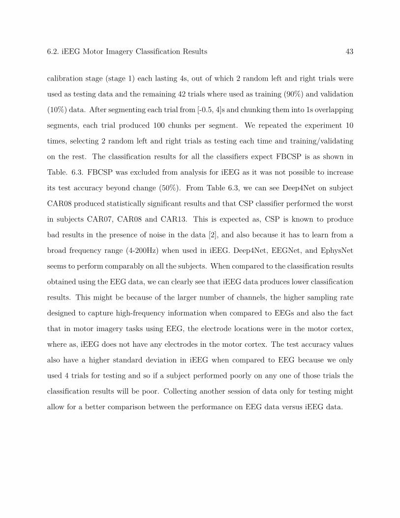
6.2 Visualizing Bandpass Convolutional Kernels: The top row shows the raw
bandpass kernel values learnt by EPhysNet along with its power spectral
density in the bottom row. . . . . . . . . . . . . . . . . . . . . . . . . . . . . 45
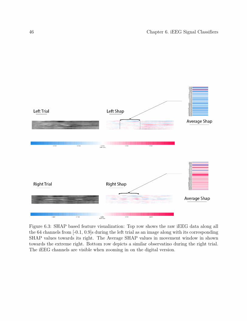
6.3 SHAP based feature visualization: Top row shows the raw iEEG data along
all the 64 channels from [-0.1, 0.9]s during the left trial as an image along
with its corresponding SHAP values towards its right. The Average SHAP
values in movement window in shown towards the extreme right. Bottom row
depicts a similar observatino during the right trial. The iEEG channels are
visible when zooming in on the digital version. . . . . . . . . . . . . . . . . . 46
6.4 SHAP based feature visualization: Left column shows 10 consecutive (top to
bottom) raw iEEG traces as image and the right column shows its correspond-
ing SHAP values. All chunks were obtained during right hand movement from
subject CAR08. . . . . . . . . . . . . . . . . . . . . . . . . . . . . . . . . . . 47
A.1 CAR 10 Hilbert power and Hilbert Power Significance plots . . . . . . . . . 56
A.2 CAR 08 Hilbert power and Hilbert Power Significance plots . . . . . . . . . 57
x
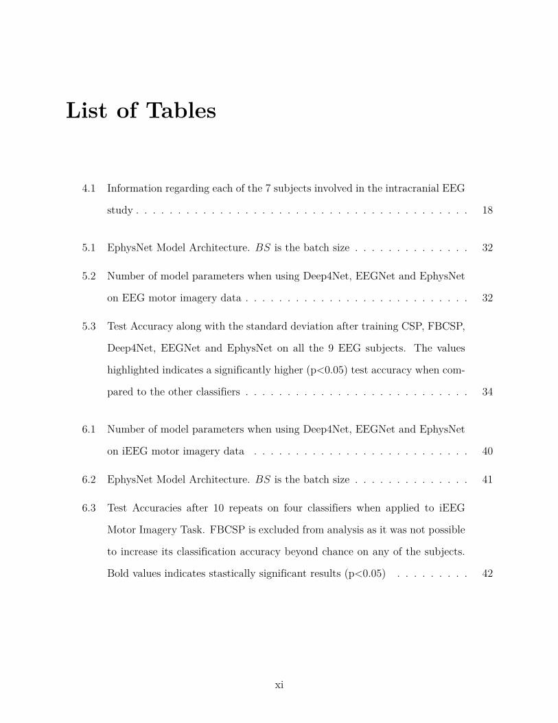
List of Tables
4.1 Information regarding each of the 7 subjects involved in the intracranial EEG
study . . . . . . . . . . . . . . . . . . . . . . . . . . . . . . . . . . . . . . . . 18
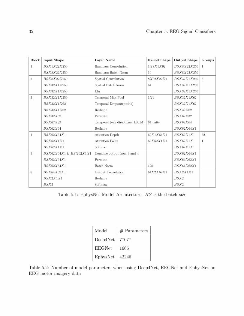
5.1 EphysNet Model Architecture. BS is the batch size . . . . . . . . . . . . . . 32
5.2 Number of model parameters when using Deep4Net, EEGNet and EphysNet
on EEG motor imagery data . . . . . . . . . . . . . . . . . . . . . . . . . . . 32
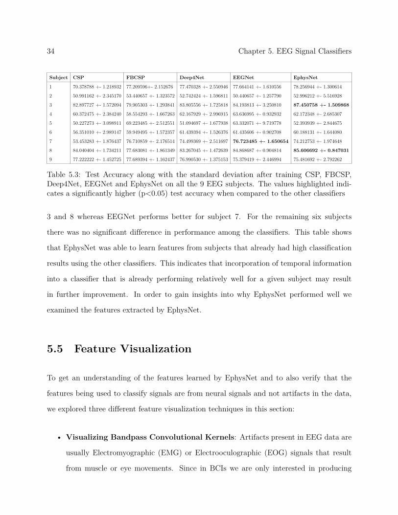
5.3 Test Accuracy along with the standard deviation after training CSP, FBCSP,
Deep4Net, EEGNet and EphysNet on all the 9 EEG subjects. The values
highlighted indicates a significantly higher (p<0.05) test accuracy when com-
pared to the other classifiers . . . . . . . . . . . . . . . . . . . . . . . . . . . 34
6.1 Number of model parameters when using Deep4Net, EEGNet and EphysNet
on iEEG motor imagery data . . . . . . . . . . . . . . . . . . . . . . . . . . 40
6.2 EphysNet Model Architecture. BS is the batch size . . . . . . . . . . . . . . 41
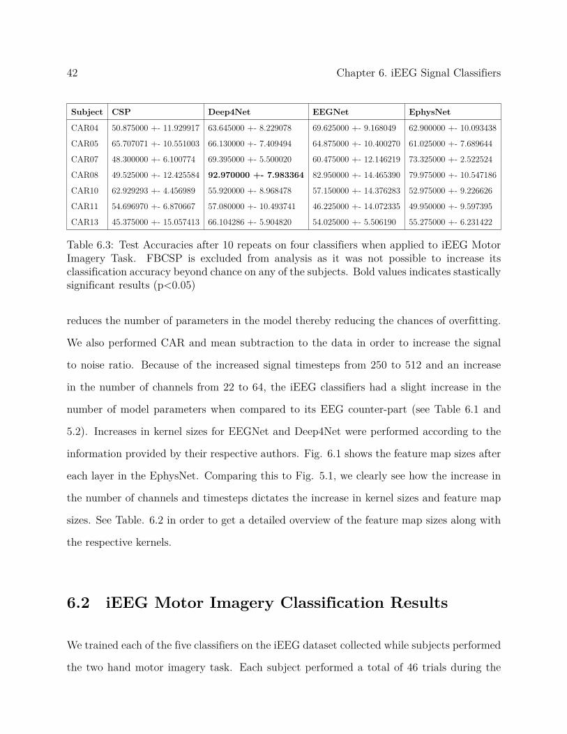
6.3 Test Accuracies after 10 repeats on four classifiers when applied to iEEG
Motor Imagery Task. FBCSP is excluded from analysis as it was not possible
to increase its classification accuracy beyond chance on any of the subjects.
Bold values indicates stastically significant results (p<0.05) . . . . . . . . . 42
xi

List of Abbreviations
BCI Brain Computer Interface
ECoG Electrocorticography
EEG Electroencephalography
ERD Event Related Desynchronization
ERS Event Related Synchronization
iEEG Intracranial Electroencephalography
xii
Chapter 1
Introduction
Brain-Computer Interfaces (BCIs) allow individuals to control external devices such as
robotic arms ([45], [13]), electric wheelchairs ([42], [35]), and even quad-copters ([18]) by
modulating their neural activity. They work by collecting neurophysiological signals di-
rectly from the brain and mapping these signals to the user’s intents. Recently, BCIs have
seen increasing applications such as enabling disabled individuals to control motor pros-
thetics ([42]), allowing users to control input in the gaming industry ([23]), and enabling
individuals to control applications in a variety of other contexts ([6], [29], [1], [15], [24]).
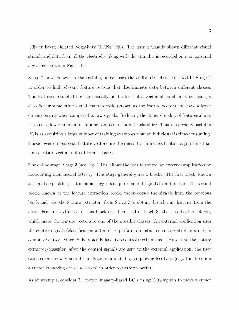
BCI systems are typically divided into three stages. Stage 1, also known as the offline signal
acquisition stage (see Fig. 1.1a), collects calibration data to train a classification algorithm
that can learn a mapping between brain signals and classes (i.e., the desired set of actions).
Based on the types of electrodes used during this stage, BCIs can broadly be divided into
invasive and non-invasive methods. Invasive methods use electrodes that are either placed
on the surface of the cortex (Electrocorticography, ECoG) or penetrate the cortex; the latter
are either depth electrodes, hybrid depth electrodes, or microelectrodes that can record from
an individual neuron or small group of neurons (Local Field Potentials, LFPs). Noninvasive
techniques, on the other hand, use electrodes placed on the scalp (Electroencephalography,
EEG). The classes, depending on the BCI application, can be different imagined movements
([22]) such as left hand, right hand, both feet, or both hands. The signals associated with
the imagined movements could be, among other things, Event-Related Potentials (ERPs,
1
2 Chapter 1. Introduction
(a) Stage 1: Offline signal acquisition stage.
(b) Stage 3: Online stage indicating the different stages along with the output from each stage.
Figure 1.1: Stage 1 and Stage 3 BCI block diagrams
3
[33]) or Event Related Negativity (ERNs, [28]). The user is usually shown different visual
stimuli and data from all the electrodes along with the stimulus is recorded onto an external
device as shown in Fig. 1.1a.
Stage 2, also known as the training stage, uses the calibration data collected in Stage 1
in order to find relevant feature vectors that discriminate data between different classes.
The features extracted here are usually in the form of a vector of numbers when using a
classifier or some other signal characteristic (known as the feature vector) and have a lower
dimensionality when compared to raw signals. Reducing the dimensionality of features allows
us to use a lower number of training samples to train the classifier. This is especially useful in
BCIs as acquiring a large number of training examples from an individual is time-consuming.
These lower dimensional feature vectors are then used to train classification algorithms that
maps feature vectors onto different classes.
The online stage, Stage 3 (see Fig. 1.1b), allows the user to control an external application by
modulating their neural activity. This stage generally has 5 blocks. The first block, known
as signal acquisition, as the name suggests acquires neural signals from the user. The second
block, known as the feature extraction block, preprocesses the signals from the previous
block and uses the feature extractors from Stage 2 to obtain the relevant features from the
data. Features extracted in this block are then used in block 3 (the classification block),
which maps the feature vectors to one of the possible classes. An external application uses
the control signals (classification outputs) to perform an action such as control an arm or a
computer cursor. Since BCIs typically have two control mechanisms, the user and the feature
extractor/classifier, after the control signals are sent to the external application, the user
can change the way neural signals are modulated by employing feedback (e.g., the direction
a cursor is moving across a screen) in order to perform better.
As an example, consider 2D motor imagery-based BCIs using EEG signals to move a cursor
4 Chapter 1. Introduction
left, right, up, or down. Stage 1 acquires ([36]) EEG signals while the subject imagines,
for instance, moving their left arm, right arm, both feet, or both arms. In stage 2, the
recorded EEG data is then used to train a feature extractor and classifier that maps the
EEG signals of each imagined movement to one of the four classes, for example, imagined
left-hand movement to left class, right hand to right class, both feet to down class and both
hands to up class. Finally in stage 3, the classification results can then be fed as control
signals to an external application to control the 2D movement of a cursor.
Inspired by recent advances, in this work, we have used intracranial electroencephalographic
(iEEG) data, collected using depth electrodes, in a two class BCI task using motor imagery.
We first performed a thorough data analysis to manually find features that discriminated
between the two motor imagery classes after the offline data acquisition stage and later
implemented the training stage with the aim of automatically finding good features from
raw data. We also compared various state of the art EEG classification algorithms along
with our own classifier for iEEG data and also explored the features learned by our classifier.
Non invasive BCIs using EEG have several limitations ([37], [38]) such as:
• low signal amplitude (10-20 µV ) when compared with invasive techniques such as
ECoG or iEEG (50-100 µV )
• low spatial resolution, a few centimeters in non invasive vs a few millimeters in invasive
techniques
• higher vulnerability to Electrooculograph (EOG) and Electromyograph (EMG) arti-
facts
• lower frequency range (0-40Hz) when compared with invasive techniques that can
record frequencies up to several kiloHertz
5
The advantages of invasive BCIs clearly seem to make them a better alternative to EEGs
with respect to signal quality and the information content in the signal ([38], [37]). The only
major downside is the risk associated with undergoing surgery in order to implant recording
electrodes. This limitation makes BCI applications with invasive methodologies extremely
rare in humans and is currently possible only in human subjects who have electrodes im-
planted for clinical reasons.
A good BCI system needs to automatically find discriminative information in order to dis-
tinguish between different classes in a BCI task. Most of the current studies ([38], [20],
[21]) that perform BCI tasks using invasive techniques rely on manual data analysis and
counterintuitive subject tasks to find clearly discriminative features; these tasks can include
things such as saying words or protruding the tongue in order to move a cursor. A number
of EEG BCI studies have shown that machine learning models such as CSP [46] and FBCSP
[2] along with deep learning based methods such as EEGNet [19] and Deep4Net [39] can
automatically find discriminative features for classifying data. Deep learning models extract
relevant features by learning directly from raw data (with mean subtraction and bandpassing
between 0-40Hz). Deep4Net and EEGNet models have also been designed to learn features
with relatively minimal amounts of data and also to use as little computational resources
during the online phase as possible when compared with CSP and FBCSP. Inspired by these
advances in EEG signal classification, we have applied a number of classical machine learning
and deep learning techniques from EEG classification onto iEEG signals and have assessed
their performance on our dataset collected using depth electrodes in a binary motor imagery
task.
Since deep learning models have been known as black boxes that make it hard for researchers
to visualize the features learned, we also aim to provide a detailed feature analysis for all
the models used in both the EEG and invasive datasets in this work. In order to get an
6 Chapter 1. Introduction
estimate of some of the good features that must be learned to classify between left and right
hand motor imagery in iEEG data, we perform a thorough data analysis to find the relevant
frequency bands, relevant regions (electrodes) and cross co-variance between left and right
hand movements that might give good results in BCI experiments.
We have made three main contributions in this work:
1. We have implemented an entire BCI experimental pipeline that allows data to be
collected during Stage 1, allows classifiers to be trained using either MATLAB or
Python during Stage 2, and also allows the trained classifiers to be used during an
online experiment in Stage 3 (Sec. 3).
2. We collected iEEG data from 7 subjects during a two hand motor imagery task and
later performed a thorough data analysis in order to determine the most useful spatial,
spectral, and temporal features (Sec. 4).
3. Finally, we have implemented a novel classification algorithm that learns to classify
iEEG data end-to-end and compared its performance in EEG (Sec. 5) and iEEG
data (6) during two hand motor imagery. Features learned by the new classification
algorithm have also been discussed in Sec. 5 and Sec. 6.
Chapter 2
Previous Work
In this section, we discuss some of the previous efforts done in classifying electrophysiological
data from the brain using automated techniques and also previous work involved in using
invasive signal acquisition techniques in order to perform a BCI task.
[20] is one of the earliest efforts in using invasive ECoG data in BCIs. The authors had shown
the by using ECoG signals a subject could perform a 1D movement task after only about
3-24 minutes of training. The features used to control the cursor were manually selected for
each subject and the tasks performed by each subject were counterintuitive such as saying
words and protruding the tongue. The authors in [38], for the first time showed that 2D
motor control could be achieved using ECoG data to control a computer cursor, but, features
were still selected manually for each individual when preforming counterintutive tasks. In
this work, we are interested in determining if automatic feature extraction techniques could
be used in intracranial EEG data. Since, intracranial EEG is obtained from electrodes
placed within deep brain structures and not the surface of the cortex like in ECoG, the
amount of literature available that analyses iEEG is limited. Most of the literature on
using intracranial EEG comes from work on detecting of interictal epileptic discharges ([44],
[3]). The authors here, used a variety of deep learning algorithms to detect the presence of
interictal epileptic discharge, but did not analyze iEEG features during a BCI task. The
authors in [45], demonstrated that using signals from a group of neurons allowed them to
encode arm movements thereby allowing an individual to control a robotic arm. This study
7
8 Chapter 2. Previous Work
also uses specific regions of the brain and specific frequency ranges to select desired features
and is different from our work which aims to automatically extract features from raw iEEG
data.
Because of the limited amount of literature available for invasive BCIs and almost no previous
work done in using iEEG for BCIs, we turned to the EEG literature to help find classification
algorithms that could help extract features from the raw data. Because of its non invasive
nature there has been a lot of research done on using EEG for Brain Computer Interfaces.
The authors in [2], showed that using Common Spatial Pattern [46] on a number of different
bandpassed input signals and then using a feature selection algorithm to select relevant
features could perform well on data used at a BCI competition [43] which had 4 motor
imagery classes. The authors in [39], showed that one could use an end-to-end deep learning
algorithm that learns directly from raw EEG data to perform motor imagery tasks and reach
FBCSP performance. Using a variety of feature visualization techniques, they were also able
to visualize the features learned by their classifier. The authors in [19], used a similar
technique as in [39], but replaced convolutions layers with depth-wise separable convolutions
along with other modifications to implement a classification algorithm that performed well
in a variety of BCI task settings such as P300 spellers [12], Error Related Negativity (ERN)
[10] and motor imagery. The authors were also able to show the features used during each
paradigm using a variety of techniques. Inspired by these papers, here we implemented
a classification algorithm that classifies iEEG data during motor imagery tasks and have
also applied a number of feature visualization techniques to find the features used during
classification. We have also manually analyzed the iEEG data in order to determine the most
important features that helps discriminate between classes and verified if our classification
algorithm was able to automatically learn them.

Chapter 3
iEEG Motor Imagery Task:
Implementation Details
In this section, we describe the experimental setup we used to collect iEEG data during the
different stages of our motor imagery task. We start with an overview of the BCI experiment
along with a brief description of the experimental hardware setup and later give a detailed
description of each stage used in the experiment.
3.1 BCI Experiment Overview
An online BCI experiment mainly consists of three stages. In the calibration stage (Stage
1), the subjects are shown markers on the screen and asked to imagine a specific movement
based on the instructions shown. The training stage (Stage 2) uses data collected in Stage
1 to find features in the iEEG data that clearly distinguish between motor imagery tasks
(left and right hand movement in our case). This is done either manually by looking at an
r2 feature plot (r2 vs frequency vs channel) or automatically by using a classifier that learns
a spatial filter and classifier weights. Finally, the online stage (Stage 3) allows the user to
control a BCI feedback application (computer cursor in our case) by modulating their neural
activity by imagining motor movements. Stage 3 uses the trained classifier from stage 2 to
distinguish between different motor imagery categories by classifying the associated neural
9
10 Chapter 3. iEEG Motor Imagery Task: Implementation Details
Figure 3.1: The acquisition machine (Pegasus Machine) connects to the Neuralynx amplifierand streams data over the local network. The presentation machine reads data from theiEEG stream, classifies the signals, and presents the control signal, which also providesfeedback for the BCI application.
3.1. BCI Experiment Overview 11
signals in real time to generate control signals and then passes the control signals onto the
feedback application.
In order to ensure reliable data collection and training mechanisms, we conducted the ex-
periment using two different PCs, each having a specific role (see Fig. 3.1). The first one
of these machines, called the Pegasus Machine, is responsible for collecting data from the
amplifier and streaming this data over a local LAN network. The other PC, known as the
Presentation Machine, is responsible for collecting the iEEG data streams from each of the
channels, training a classifier using this collected data, and presenting feedback during stage
3 (i.e., moving the cursor on the screen to the left or right).
We used the Digital Lynx 16SX amplifier from Neuralynx and connected it to the Pegasus
Machine using an optical fiber cable and used an ethernet cable to connect the Pegasus
Machine to the Presentation Machine. The Pegasus Machine uses the Pegasus Acquisition
Software from Neuralynx to communicate with the amplifier and to stream data from it.
Using the Pegasus Acquisition Software, we created a local data stream on the Pegasus
Machine and used the ethernet cable to stream data to the Presentation Machine. We
decided to only use wired connections to ensure that there were no dropped connections
during the experiment and to also avoid any unnecessary latencies introduced by a wireless
connection. The Presentation machine collected the data streams using FieldTrip [30], which
internally uses the MATLAB-Netcom client API provided by Neuralynx.
We ensured that the latency was kept under 30ms during the entire experiment by limiting
the number of channel streams to 64 and by downsampling the signals from 32kHz to 2kHz.
Data from the Pegasus Machine was sent to the Presentation machine in chunks of 512
timesteps, where each timestep contained data from 64 channels. The TTL pulses that
indicated the start of each trial, the point when the motor imagery was performed during
each trial, and the end of each trial were sent from the Presentation Machine to the Pegasus
12 Chapter 3. iEEG Motor Imagery Task: Implementation Details
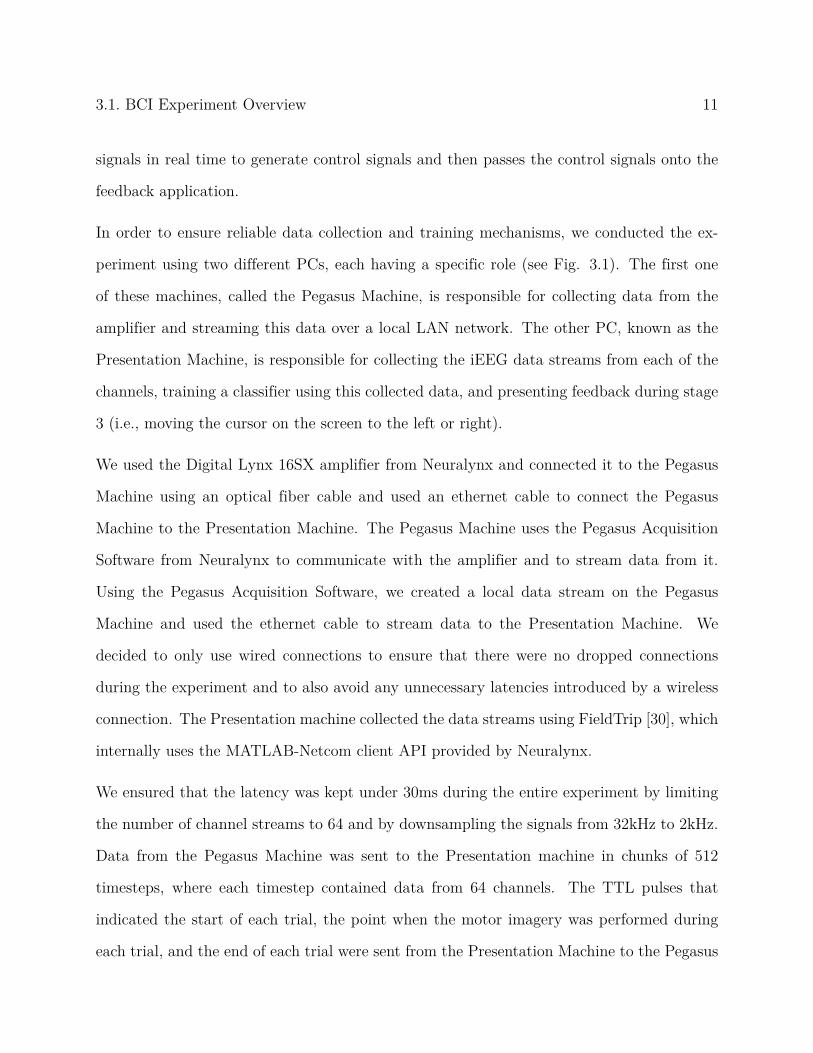
(a) Instructions Screen (b) Rest Screen
(c) Left Hand Imagery Screen (d) Right Hand Imagery Screen
Figure 3.2: Visual cues as seen by the subject during the calibration stage
Machine using the ethernet cable.
We now give a detailed description of each of the three stages of the iEEG BCI task below.
3.2 Stage 1: Calibration Stage
BCIs need a way to distinguish signals from each imagined motor movement. This is usually
done by either manually selecting signal characteristics that show a clear distinction between
the motor imagery task and the rest period or by training a classification algorithm that
can accurately classify user intents. In order to select appropriate signal characteristics or
to train a classification algorithm, we need to collect training data. This is done during the
calibration stage.
3.3. Stage 2: Training Stage 13
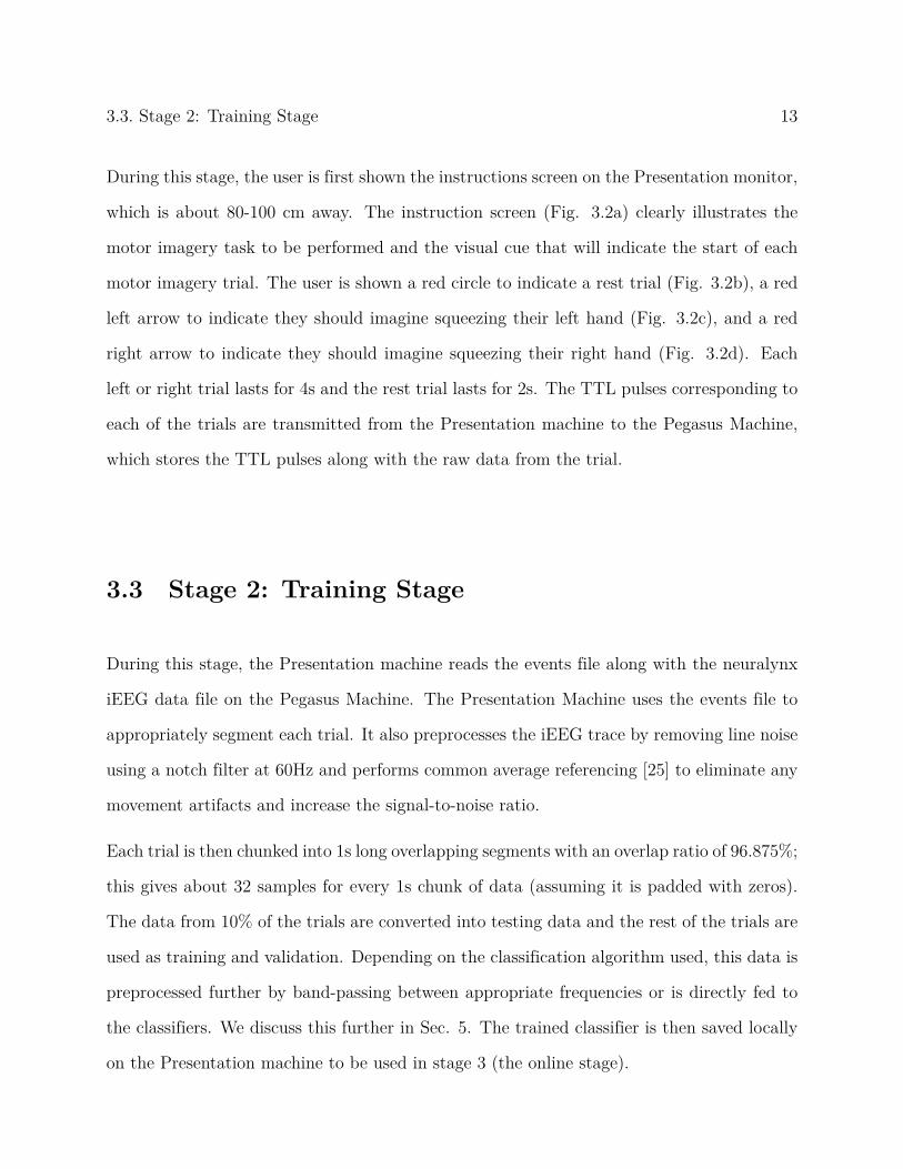
During this stage, the user is first shown the instructions screen on the Presentation monitor,
which is about 80-100 cm away. The instruction screen (Fig. 3.2a) clearly illustrates the
motor imagery task to be performed and the visual cue that will indicate the start of each
motor imagery trial. The user is shown a red circle to indicate a rest trial (Fig. 3.2b), a red
left arrow to indicate they should imagine squeezing their left hand (Fig. 3.2c), and a red
right arrow to indicate they should imagine squeezing their right hand (Fig. 3.2d). Each
left or right trial lasts for 4s and the rest trial lasts for 2s. The TTL pulses corresponding to
each of the trials are transmitted from the Presentation machine to the Pegasus Machine,
which stores the TTL pulses along with the raw data from the trial.
3.3 Stage 2: Training Stage
During this stage, the Presentation machine reads the events file along with the neuralynx
iEEG data file on the Pegasus Machine. The Presentation Machine uses the events file to
appropriately segment each trial. It also preprocesses the iEEG trace by removing line noise
using a notch filter at 60Hz and performs common average referencing [25] to eliminate any
movement artifacts and increase the signal-to-noise ratio.
Each trial is then chunked into 1s long overlapping segments with an overlap ratio of 96.875%;
this gives about 32 samples for every 1s chunk of data (assuming it is padded with zeros).
The data from 10% of the trials are converted into testing data and the rest of the trials are
used as training and validation. Depending on the classification algorithm used, this data is
preprocessed further by band-passing between appropriate frequencies or is directly fed to
the classifiers. We discuss this further in Sec. 5. The trained classifier is then saved locally
on the Presentation machine to be used in stage 3 (the online stage).
14 Chapter 3. iEEG Motor Imagery Task: Implementation Details
(a) Instructions Screen (b) Trial Onset
(c) Cursor movement towards the left (d) Cursor movement towards the right
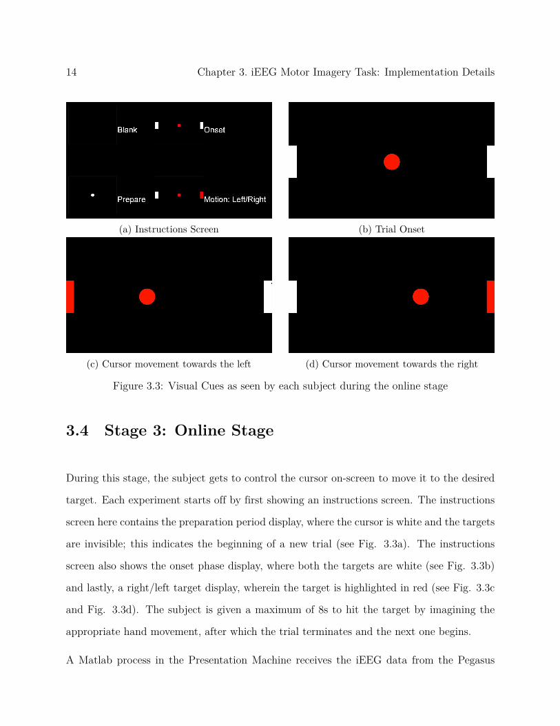
Figure 3.3: Visual Cues as seen by each subject during the online stage
3.4 Stage 3: Online Stage
During this stage, the subject gets to control the cursor on-screen to move it to the desired
target. Each experiment starts off by first showing an instructions screen. The instructions
screen here contains the preparation period display, where the cursor is white and the targets
are invisible; this indicates the beginning of a new trial (see Fig. 3.3a). The instructions
screen also shows the onset phase display, where both the targets are white (see Fig. 3.3b)
and lastly, a right/left target display, wherein the target is highlighted in red (see Fig. 3.3c
and Fig. 3.3d). The subject is given a maximum of 8s to hit the target by imagining the
appropriate hand movement, after which the trial terminates and the next one begins.
A Matlab process in the Presentation Machine receives the iEEG data from the Pegasus

3.4. Stage 3: Online Stage 15
Machine and preprocesses each data chunk using the same pipeline as in Stage 2. It later
sends the preprocessed chunks to a second Matlab process that classifies these data chunks
and streams the classification output as a LabStreamingLayer [17] stream. A third and final
Matlab process connects to the LSL stream and moves the cursor 30 pixels to the right or
left depending on the classification result. Code for all the stages is available on request.
Chapter 4
iEEG Motor Imagery Task: Relevant
Feature Estimation
The iEEG BCI task described in the previous section was performed for 7 participants with
46 trials of left or right hand imagined movements. In order to get an estimate of the
most relevant features for an online task, we performed an offline analysis, described in this
section, of the data collected during the calibration stage. We first give a brief overview
of the clinical profiles of the subjects involved in the study in section 4.1, followed by an
analysis of the data collected during the calibration stage in section 4.2.
4.1 Subject description
The calibration data for the motor imagery task was collected from 7 subjects who were all
patients undergoing treatment for intractable epilepsy, which included invasive monitoring
to localize their seizures. Of the 7 subjects, 3 were female and the median age for the
participants was 39 (see Table 4.1 for more details). An informed consent approved by
the Institutional Review Board (IRB) at Carilion Hospital was obtained from the patients
before performing the study. Adtech depth (hybrid) electrodes capable of recording Local
Field Potentials (LFPs) and single unit activity were implanted for each subject and all the
electrode positions were chosen solely for clinical purposes without considering our research
16
4.1. Subject description 17
(a) Anterior View (b) Posterior View
(c) Left Lateral View (d) Right Lateral View
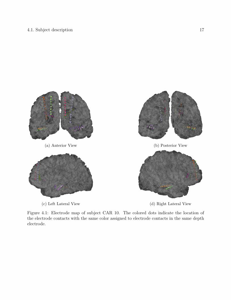
Figure 4.1: Electrode map of subject CAR 10. The colored dots indicate the location ofthe electrode contacts with the same color assigned to electrode contacts in the same depthelectrode.
18 Chapter 4. iEEG Motor Imagery Task: Relevant Feature Estimation
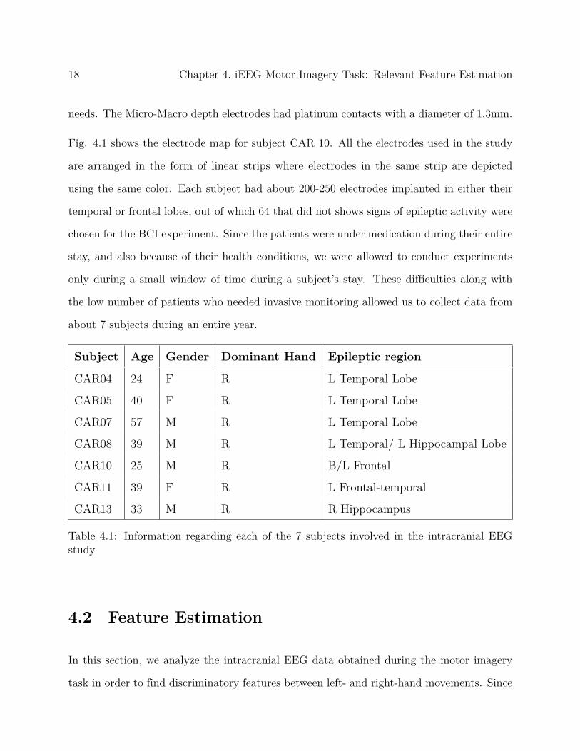
needs. The Micro-Macro depth electrodes had platinum contacts with a diameter of 1.3mm.
Fig. 4.1 shows the electrode map for subject CAR 10. All the electrodes used in the study
are arranged in the form of linear strips where electrodes in the same strip are depicted
using the same color. Each subject had about 200-250 electrodes implanted in either their
temporal or frontal lobes, out of which 64 that did not shows signs of epileptic activity were
chosen for the BCI experiment. Since the patients were under medication during their entire
stay, and also because of their health conditions, we were allowed to conduct experiments
only during a small window of time during a subject’s stay. These difficulties along with
the low number of patients who needed invasive monitoring allowed us to collect data from
about 7 subjects during an entire year.
Subject Age Gender Dominant Hand Epileptic region
CAR04 24 F R L Temporal Lobe
CAR05 40 F R L Temporal Lobe
CAR07 57 M R L Temporal Lobe
CAR08 39 M R L Temporal/ L Hippocampal Lobe
CAR10 25 M R B/L Frontal
CAR11 39 F R L Frontal-temporal
CAR13 33 M R R Hippocampus
Table 4.1: Information regarding each of the 7 subjects involved in the intracranial EEGstudy
4.2 Feature Estimation
In this section, we analyze the intracranial EEG data obtained during the motor imagery
task in order to find discriminatory features between left- and right-hand movements. Since
4.2. Feature Estimation 19
most of our electrode positions do not fall in the motor area of the brain, which has been well
studied in previous work ([42], [6], [32]), we were interested in exploring the possibilities of the
involvement of deep brain structures such as the amygdala, hippocampus, or the cingulate
in motor-related tasks. We were particularly interested in the hippocampal electrodes and
the temporal lobe in general, since recent studies ([9], [8]) have indicated its potential role in
encoding and retrieving sequences of events that are involved in memories. Furthermore, all
our subjects had electrodes that were in the hippocampus and other parts of the temporal
lobe. Almost all of the previous work involving motor imagery looked at the spatial and
spectral content in EEG or ECoG signals. These two recording modalities primarily provide
signals from surface brain structures, while iEEG recordings provide us with the unique
opportunity to examine the neural correlates of motor imagery in deep brain structures. We
were also interested in studying the temporal nature of data across brain regions and also
if there were any interactions between low- and high-frequency signals in brain structures
during the motor task; such neural dynamics could potentially be leveraged as features to
control BCI applications.
To find channels that were most discriminative during the motor imagery task, we first
found the power difference between the left and right-hand imagined movements for all the
channels from 3-200 Hz; this has been described in section 4.2.1. We later discuss our findings
regarding high- and low-frequency interactions in the amygdala and the hippocampus in
section 4.2.2.
4.2.1 Spatial and Spectral Features
To find channels that help distinguish between left- and right-hand movement tasks, we found
the difference between the power of the signal envelope obtained from Hilbert Transform (we
20 Chapter 4. iEEG Motor Imagery Task: Relevant Feature Estimation
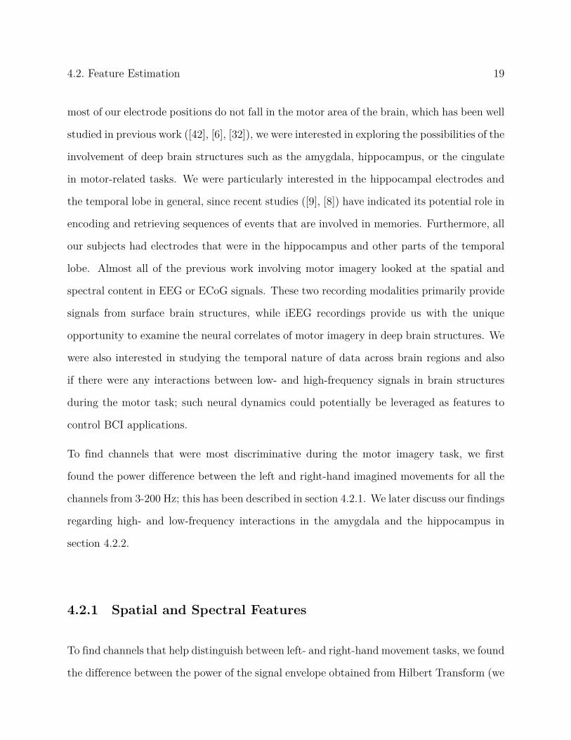
(a) Power difference between left- and right-hand movement as a function of frequency in all chan-nels in subject CAR 04. The figure also shows the three selected frequency ranges of interest.
(b) Significant Power difference between left- and right-hand movements as a function of frequencyin all channels in subject CAR 04. The red values indicate significant differences.
Figure 4.2: CAR 04 power and power significance plots
4.2. Feature Estimation 21
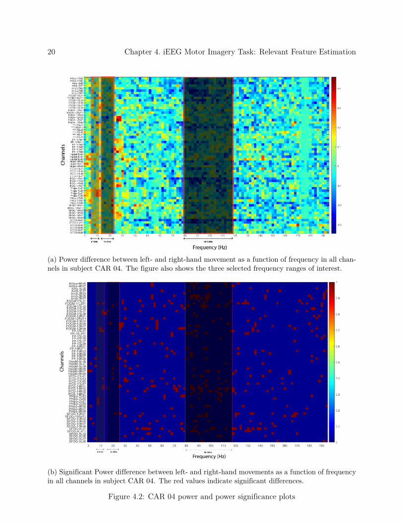
(a) Coronal view of subject CAR 04 showing the implanted electrodes (red markers) along withthe power spectra for left- and right-hand movements at both electrodes.
(b) Coronal view of subject CAR 10 showing the implanted electrodes (red markers) along withthe power spectra for left- and right-hand movements at both electrodes
Figure 4.3: Power spectrum during left- and right-hand movements in both hemispheres forsubjects CAR04 and CAR10
22 Chapter 4. iEEG Motor Imagery Task: Relevant Feature Estimation
call this the power difference) for left and right movements in all frequencies from 3-200Hz
for all channels. An example of this is shown in Fig. 4.2a for one of our subjects. We found
the power difference by first finding the averaged power for each 2Hz bin from 3-300Hz for all
the left and right trials (each trial was segmented at [-0.1, 2]s i.e., 0.1s before stimulus onset
to 2s after stimulus onset) and then we found the difference in power between left and right
trials across each frequency bin. Based on the power plots we segmented the plot into three
frequency regions of interest: 8-13Hz, 15-25Hz, and 80-120Hz as shown in 4.2a. We later
found channels that were significantly different during left and right trials after conducting
a paired t-test of the signal powers for left and right movements. The significance plot is
shown in Fig. 4.2b. The red values indicate the frequency bin at which the left vs right
power is most significant and the blue regions indicate regions wherein the difference is not
significant. Looking at Fig. 4.2a, it is clear that channels such as PHipp-7Ld3, PHipp-7Ld5,
PHipp-7Ld7 and PHipp-7Ld9, which are in the left posterior hippocampus, have a higher left
power when compared to right power at frequencies between 8-13Hz and 15-25Hz, whereas
Phipp-8Rd5, Phipp-8Rd7, and Phipp-8Rd9, which are in the right posterior hippocampus,
seem to have a lower left power when compared to right at the same frequencies. Signals
from 8-13Hz known as the mu band and 15-25 Hz known as the beta band have been studied
before in the motor areas and have been shown to produce Event Related Synchronizations
(ERSs) and Event-Related Desynchronizations (ERDs) following actual or imagined hand
movements ([37]). ERDs that occur in contralateral hemispheres at and around the mu and
beta bands cause signal power to decrease as soon as the subject thinks about moving their
hands followed by an increase in signal (ERS) after the hand movement.
Fig. 4.3a shows the coronal view of subject CAR 04 along with the power spectrum at
two electrode locations, FP-16Rd9 and PHipp-7Ld7. These electrodes are in contralateral
hemispheres. The electrode FP-16Rd9 has a lower power at frequencies around the mu-beta
4.2. Feature Estimation 23
bands during left-hand movements whereas electrode PHipp-7Ld7 has a lower power at the
mu-beta bands during right-hand movements. Looking at the light grey regions on the power
spectrum at PHipp-7Ld7, we can clearly see a decrease in power during right-hand movement
along with an increase in power during right-hand movement at higher frequencies. A similar
but opposite phenomenon can be observed in electrode FP-16Rd9, where we see a decrease in
power at the low-frequency band (light gray region) during left-hand movement followed by
an increase in power for right-hand movement at the high-frequency band (dark grey region).
Fig. 4.3b shows a similar observation in subject CAR 10 (see Fig. 4.3b). These electrodes
suggest that there is a lateralization of activity in temporal regions as seen in motor regions
during imagined movements. This lateralization of power in the brain can be seen only in a
small number of electrodes but is visible in all of the subjects; however, we were not able to
consistently find these lateralizations in the same set of electrodes across all subjects. This
might be because of problems such as the depth electrode strip not being located exactly
in the region indicated by the label or some other biological phenomenon that hasn’t been
investigated yet. For these reasons we leave investigation of this phenomenon to future work.
4.2.2 Temporal Features
As discussed earlier, because of its role in sequential memory, a high difference in power
between left and right-hand movement, and also because of its presence in all 7 subjects, we
were interested in further analyzing the temporal signal characteristics in the hippocampus.
We found that electrodes in the amygdala (present in 6 of the subjects) also showed a large
power difference at lower and higher frequencies between left and right imagined movements.
Because of these reasons we were interested in further analyzing the temporal signal char-
acteristics in the amygdala and hippocampus electrodes; this analysis is described in this
section.
24 Chapter 4. iEEG Motor Imagery Task: Relevant Feature Estimation
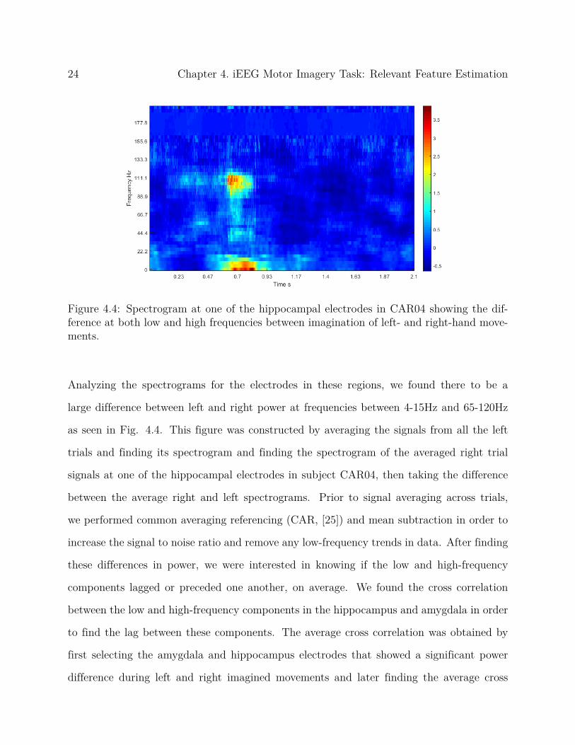
Figure 4.4: Spectrogram at one of the hippocampal electrodes in CAR04 showing the dif-ference at both low and high frequencies between imagination of left- and right-hand move-ments.
Analyzing the spectrograms for the electrodes in these regions, we found there to be a
large difference between left and right power at frequencies between 4-15Hz and 65-120Hz
as seen in Fig. 4.4. This figure was constructed by averaging the signals from all the left
trials and finding its spectrogram and finding the spectrogram of the averaged right trial
signals at one of the hippocampal electrodes in subject CAR04, then taking the difference
between the average right and left spectrograms. Prior to signal averaging across trials,
we performed common averaging referencing (CAR, [25]) and mean subtraction in order to
increase the signal to noise ratio and remove any low-frequency trends in data. After finding
these differences in power, we were interested in knowing if the low and high-frequency
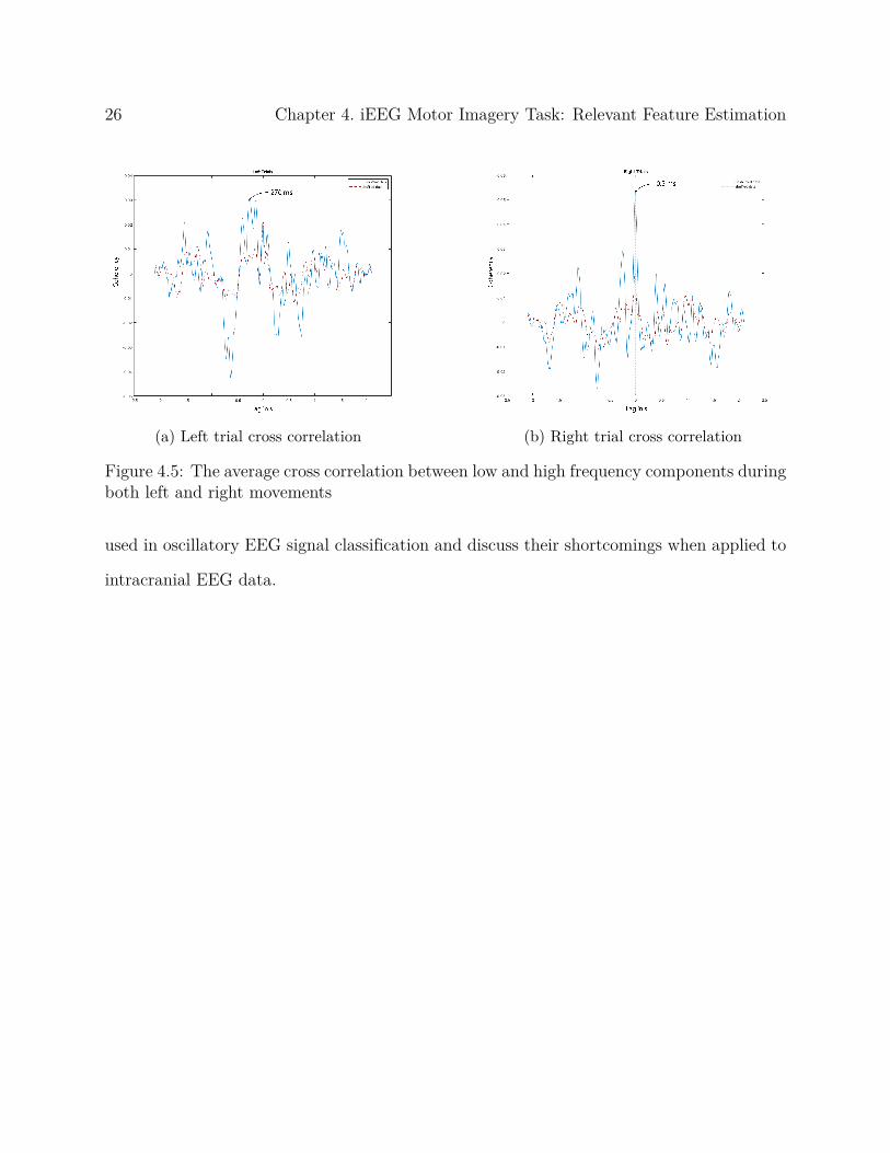
components lagged or preceded one another, on average. We found the cross correlation
between the low and high-frequency components in the hippocampus and amygdala in order
to find the lag between these components. The average cross correlation was obtained by
first selecting the amygdala and hippocampus electrodes that showed a significant power
difference during left and right imagined movements and later finding the average cross
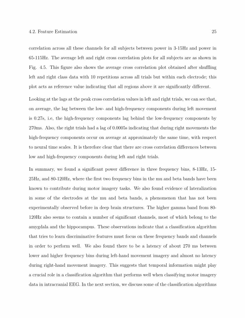
4.2. Feature Estimation 25
correlation across all these channels for all subjects between power in 3-15Hz and power in
65-115Hz. The average left and right cross correlation plots for all subjects are as shown in
Fig. 4.5. This figure also shows the average cross correlation plot obtained after shuffling
left and right class data with 10 repetitions across all trials but within each electrode; this
plot acts as reference value indicating that all regions above it are significantly different.
Looking at the lags at the peak cross correlation values in left and right trials, we can see that,
on average, the lag between the low- and high-frequency components during left movement
is 0.27s, i.e, the high-frequency components lag behind the low-frequency components by
270ms. Also, the right trials had a lag of 0.0005s indicating that during right movements the
high-frequency components occur on average at approximately the same time, with respect
to neural time scales. It is therefore clear that there are cross correlation differences between
low and high-frequency components during left and right trials.
In summary, we found a significant power difference in three frequency bins, 8-13Hz, 15-
25Hz, and 80-120Hz, where the first two frequency bins in the mu and beta bands have been
known to contribute during motor imagery tasks. We also found evidence of lateralization
in some of the electrodes at the mu and beta bands, a phenomenon that has not been
experimentally observed before in deep brain structures. The higher gamma band from 80-
120Hz also seems to contain a number of significant channels, most of which belong to the
amygdala and the hippocampus. These observations indicate that a classification algorithm
that tries to learn discriminative features must focus on these frequency bands and channels
in order to perform well. We also found there to be a latency of about 270 ms between
lower and higher frequency bins during left-hand movement imagery and almost no latency
during right-hand movement imagery. This suggests that temporal information might play
a crucial role in a classification algorithm that performs well when classifying motor imagery
data in intracranial EEG. In the next section, we discuss some of the classification algorithms
26 Chapter 4. iEEG Motor Imagery Task: Relevant Feature Estimation
(a) Left trial cross correlation (b) Right trial cross correlation
Figure 4.5: The average cross correlation between low and high frequency components duringboth left and right movements
used in oscillatory EEG signal classification and discuss their shortcomings when applied to
intracranial EEG data.
Chapter 5
EEG Signal Classifiers
As described earlier, classifiers are used to map signals to the desired classes. This can be
done either using classical machine learning techniques ([2], [46]) that generally require raw
signals to be transformed into lower dimensional features or by using deep learning techniques
([19], [39]) that directly use minimally preprocessed signals. Most of the recent literature that
has studied brain-computer interfaces using invasive signal collection techniques ([37], [22])
have used manual feature selection to find discriminative features which are later classified
using a simple linear classifier. While this technique allows researchers to have control over
the features being used to classify data, it might also prevent classification algorithms from
finding new features not already employed in BCI tasks. With the limitations of different
techniques in mind, in this section, we analyze 4 different EEG signal classification algorithms
by applying them to an EEG motor imagery dataset and by comparing them with our new
classification technique that is designed to use spectral, spatial and temporal features. Our
main aim in the next two chapters will be to access the possibilities of using the current state
of the art oscillatory EEG classification algorithms for classifying intracranial EEG data. We
will also verify if the new classification technique performs better than the previous EEG
classification techniques when applied to iEEG.
The remaining part of this chapter is organized as follows. In Sec. 5.1, we provide a brief
overview of the different oscillatory EEG signal classification algorithms. Later in Sec. 5.3,
we describe the motor imagery dataset and lastly, in Sec. 5.4, we discuss the classification
27
28 Chapter 5. EEG Signal Classifiers
results and also the features learned by different classification algorithms.
5.1 Previous methods
5.1.1 Common Spatial Pattern
Common Spatial Pattern (CSP, [34], [25]) aims to learn a set of spatial filters that transform
the high dimensional multichannel time series data into time-series that contains a lower
number of channels. The spatial filters learned are such that data from two different classes
are placed as far as possible in a low dimensional space. The spatial filters are found us-
ing a technique called simultaneous diagonalization of two covariance matrices which is as
described in [34]. Usually, a set of m filters are extracted for each class and applied to the
EEG data as shown below:
Z = WE (5.1)
Where E is the input epoched EEG data containing N channels and T timesteps with shape
NXT . And, W contains the 2m spatial filters (m filters of each class) each of shape 1XN .
Z is the output of shape mXT .
The log transform of each channel p in Z is then calculated using the equation below:
Zp = log
(var(Zp)∑2mi=1 var(Zp)
)(5.2)
This reduces the dimensionality of the data to mX1. The output is then classified using
a linear classifier such as Linear Discriminate Analysis (LDA, [27]). CSP used along with
5.1. Previous methods 29
a linear classifier has low computational requirements but is known to be susceptible to
artifacts in the EEG data.
5.1.2 Filter Bank Common Spatial pattern
The Common Spatial Pattern (CSP) patterns described in the previous section required EEG
data to be bandpass filtered between specific frequency bands and is prone to artifacts in the
data. Filter Bank Common Spatial Pattern (FBCSP, [2]) was designed to overcome these
shortcomings by allowing a feature selection algorithm to select features from required fre-
quency bands. The FBCSP algorithm has four stages: a frequency filtering stage that filters
the raw data into a number of bands, a spatial filter stage that applies CSP filters to signals
from each of the frequency bins, a feature selection algorithm such as Mutual Information
Based Best Individual Feature (MIBIF, [2]) that selects the most important CSP features
and finally a classification stage that classifies the selected features using a classifier, for
example by using a Support Vector Machine (SVM, [40]). FBCSP is more computationally
intensive when compared to CSP, but, avoids manual frequency band selection.
5.1.3 Deep4Net
The authors in [39] implemented an end-to-end deep learning model (which we call Deep4net
here) that is designed to learn a broad range of features from raw EEG data. Their 4 layers
deep neural network is implemented using convolutions that learn spatial filters and temporal
filters using 1D convolutions. By using techniques such as dropout [41], batch normalization
[14] and an exponential linear activation function [7], they showed that their model could
match FBCSP performance in motor imagery tasks.
30 Chapter 5. EEG Signal Classifiers
5.1.4 EEGNet
The authors in [19] designed a CNN architecture that also matched the performance of
FBCSP in motor imagery tasks but was able to do so using only a fraction of parameters as
in Deep4Net. Their EEGNet architecture consists of 2 convolutional blocks, with the first
block designed to learn bandpass filters along with spatial filters using 1D convolutionals.
The second block used depthwise separable convolutions [5] designed to lower the parameter
count while also acting as a regularizer. Batch normalization, exponential activations, and
dropout were also included to avoid overfitting.
5.2 EphysNet
Both Deep4Net and EEGNet architectures were designed to learn spatial and spectral fea-
tures from raw EEG data. In the Sec. 4.2.2 we showed that intracranial EEG data might
also contain temporal information that could be leveraged by classification algorithms. To
this end, we designed a new classification model known as EphysNet inspired from EEGNet
that can learn spatial, spectral and temporal information. Fig. 5.1 shows the block diagram
of EphysNet when applied to EEG signals. The model architecture is as follows:
• Block 1: This block consists of 8 1D convolutions that learn bandpass filtering of
input data. The kernels used are one-fourth the length of each time series input. In
our case since the input consists of 22 channels and 250 samples, this kernel has a size
of 62. Batch Normalization is performed after the 1D convolution as indicated in 5.1.
• Block 2: Block 2 is designed using depth-wise separable convolutions [5] such that four
features maps are learned using each of the 8 bandpass output feature maps. Separable
convolutions as mentioned in [19] are used to reduce the number of parameters. It
5.2. EphysNet 31
Figure 5.1: EphysNet Block Diagram used in EEG signal classification. Boxes in orangeindicate the kernels applied at each stage.
also ensures that the network decouples learning from individual feature map using
depth-wise convolutions to learning features from all features maps using point-wise
convolutions. An Elu activation [7] function is applied after convolution.
• Block 3: Block 3 is designed to learn temporal features from the downsampled input
data. It does this by first applying max pooling with a kernel size of (1, 4) in order to
downsample the input data and to also reduce the parameter count. Later, it applies a
one-directional LSTM with 64 units to learn 64 feature from each timestep. Dropout
has been used in this block to prevent overfitting.
• Block 4: This block is used to learn a weight on each of the timestep such that the
output layer and focus on features from desired timesteps. Inspiration for this layer
comes from sequence2sequence networks with attention [4] that are designed to focus
on the most important set of words in order to perform a language translation task.
• Block 5: This block applies the weights learned from block 4 to the output from block
3 in order to produce a weighted combination of the input. It also performs batch
normalization to reduce overfitting.
• Block 6: This block uses a convolutional layer in place of the traditional dense later
to learn a mapping from the input to the two desired classes.
32 Chapter 5. EEG Signal Classifiers
Block Input Shape Layer Name Kernel Shape Output Shape Groups
1 BSX1X22X250 Bandpass Convolution 1X8X1X62 BSX8X22X250 1
BSX8X22X250 Bandpass Batch Norm 16 BSX8X22X250
2 BSX8X22X250 Spatial Convolution 8X32X22X1 BSX32X1X250 8
BSX32X1X250 Spatial Batch Norm 64 BSX32X1X250
BSX32X1X250 Elu BSX32X1X250
3 BSX32X1X250 Temporal Max Pool 1X4 BSX32X1X62
BSX32X1X62 Temporal Dropout(p=0.5) BSX32X1X62
BSX32X1X62 Reshape BSX32X62
BSX32X62 Permute BSX62X32
BSX62X32 Temporal (one directional LSTM) 64 units BSX62X64
BSX62X64 Reshape BSX62X64X1
4 BSX62X64X1 Attention Depth 62X1X64X1 BSX62X1X1 62
BSX62X1X1 Attention Point 62X62X1X1 BSX62X1X1 1
BSX62X1X1 Softmax BSX62X1X1
5 BSX62X64X1 & BSX62X1X1 Combine output from 3 and 4 BSX62X64X1
BSX62X64X1 Permute BSX64X62X1
BSX62X64X1 Batch Norm 128 BSX64X62X1
6 BSX64X62X1 Output Convolution 64X2X62X1 BSX2X1X1
BSX2X1X1 Reshape BSX2
BSX2 Softmax BSX2
Table 5.1: EphysNet Model Architecture. BS is the batch size
Model # Parameters
Deep4Net 77677
EEGNet 1666
EphysNet 42246
Table 5.2: Number of model parameters when using Deep4Net, EEGNet and EphysNet onEEG motor imagery data
5.3. EEG dataset description and experimental setup 33
5.3 EEG dataset description and experimental setup
The EEG data used to compare different classification algorithms on the motor imagery task
comes from BCI Competition IV Dataset 2a [43]. This EEG dataset comes from 9 subjects
performing 4 motor imagery tasks (left hand, right hand, both feet and tongue movement).
EEG data from 22 channels were recorded during two sessions each containing 288 trials.
The first session is used as a training dataset and the second session is used for evaluation
purposes. We segmented the data from 0.5s prior to stimulus onset to 4s after stimulus
onset and bandpass filtered the data from 4-100Hz using a zero phase Butterworth filter
of 3rd order. Then we removed the feet and tongue movement trials from the dataset and
chunked each trial into segments of 1s with an overlap of 32ms. We decided to chunk the
data to simulate a real BCI experiment that usually employs data in similar chunk sizes
and to also increase the amount of training data. We performed a 10 fold cross-validation
on the training set and tested the model on session 2 data. All the deep learning classifiers
used Adam [16] optimizer implemented in PyTorch along with an exponential learning rate
decay during training. The classifiers were constructed using PyTorch [31] with the data
preprocessing done using python MNE [11]. We trained the model on a Nvidia P100 GPU
using the resources provided by the Advanced Research Computing facility at Virginia Tech.
Code for all the classifiers is available upon request.
5.4 EEG Motor Imagery Classification Results
We compared the different models discussed earlier on the BCI competition dataset in the 2
hand motor imagery task. Table 5.3 gives the test accuracy for all the 9 subjects using each of
the classifiers. EphysNet performs significantly better than the other classifiers for subjects
34 Chapter 5. EEG Signal Classifiers
Subject CSP FBCSP Deep4Net EEGNet EphysNet
1 70.378788 +- 1.218932 77.209596+- 2.152676 77.470328 +- 2.550946 77.664141 +- 1.610556 78.256944 +- 1.300614
2 50.991162 +- 2.345170 53.440657 +- 1.323572 52.742424 +- 1.596811 50.440657 +- 1.257790 52.996212 +- 5.516928
3 82.897727 +- 1.572094 79.905303 +- 1.293841 83.805556 +- 1.725818 84.193813 +- 3.250810 87.450758 +- 1.509868
4 60.372475 +- 2.384240 58.554293 +- 1.667263 62.167929 +- 2.996915 63.636995 +- 0.932932 62.172348 +- 2.685307
5 50.227273 +- 3.098911 69.223485 +- 2.512551 51.094697 +- 1.677938 63.332071 +- 9.719778 52.393939 +- 2.844675
6 56.351010 +- 2.989147 59.949495 +- 1.572357 61.439394 +- 1.526376 61.435606 +- 0.902708 60.188131 +- 1.644080
7 53.453283 +- 1.876437 76.710859 +- 2.176514 74.499369 +- 2.511697 76.723485 +- 1.650654 74.212753 +- 1.974648
8 84.040404 +- 1.734211 77.683081 +- 1.861349 83.267045 +- 1.472639 84.868687 +- 0.904814 85.606692 +- 0.847031
9 77.222222 +- 1.452725 77.689394 +- 1.162437 76.990530 +- 1.375153 75.379419 +- 2.446994 75.481692 +- 2.792262
Table 5.3: Test Accuracy along with the standard deviation after training CSP, FBCSP,Deep4Net, EEGNet and EphysNet on all the 9 EEG subjects. The values highlighted indi-cates a significantly higher (p<0.05) test accuracy when compared to the other classifiers
3 and 8 whereas EEGNet performs better for subject 7. For the remaining six subjects
there was no significant difference in performance among the classifiers. This table shows
that EphysNet was able to learn features from subjects that already had high classification
results using the other classifiers. This indicates that incorporation of temporal information
into a classifier that is already performing relatively well for a given subject may result
in further improvement. In order to gain insights into why EphysNet performed well we
examined the features extracted by EphysNet.
5.5 Feature Visualization
To get an understanding of the features learned by EphysNet and to also verify that the
features being used to classify signals are from neural signals and not artifacts in the data,
we explored three different feature visualization techniques in this section:
• Visualizing Bandpass Convolutional Kernels: Artifacts present in EEG data are
usually Electromyographic (EMG) or Electrooculographic (EOG) signals that result
from muscle or eye movements. Since in BCIs we are only interested in producing
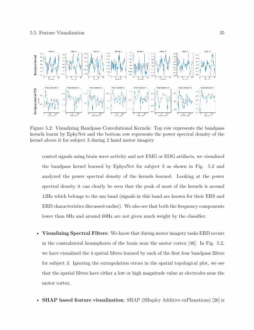
5.5. Feature Visualization 35
Figure 5.2: Visualizing Bandpass Convolutional Kernels: Top row represents the bandpasskernels learnt by EphyNet and the bottom row represents the power spectral density of thekernel above it for subject 3 during 2 hand motor imagery
control signals using brain wave activity and not EMG or EOG artifacts, we visualized
the bandpass kernel learned by EphysNet for subject 3 as shown in Fig. 5.2 and
analyzed the power spectral density of the kernels learned. Looking at the power
spectral density it can clearly be seen that the peak of most of the kernels is around
12Hz which belongs to the mu band (signals in this band are known for their ERS and
ERD characteristics discussed earlier). We also see that both the frequency components
lower than 8Hz and around 60Hz are not given much weight by the classifier.
• Visualizing Spectral Filters: We know that during motor imagery tasks ERD occurs
in the contralateral hemispheres of the brain near the motor cortex [46]. In Fig. 5.2,
we have visualized the 4 spatial filters learned by each of the first four bandpass filters
for subject 3. Ignoring the extrapolation errors in the spatial topological plot, we see
that the spatial filters have either a low or high magnitude value at electrodes near the
motor cortex.
• SHAP based feature visualization: SHAP (SHapley Additive exPlanations) [26] is
36 Chapter 5. EEG Signal Classifiers
designed to assign each feature in the input with a numerical value that indicates the
importance of a feature during each classification category. We used SHAP in order to
find the important features during each of the classes and to also verify if the features
learned were near the contralateral motor area. Fig. 5.4 shows the raw EEG signals
represented as an image along with the importance values assigned by SHAP towards
its right. From the topological plots of average importance values during the hand
movements, it is clear that the model has, in fact, placed importance on the signals
from the contralateral side of the imagined movement. Furthermore, the signals given
importance are mostly located near the motor region. Since we trained EphysNet using
overlapping chunks of data, we were also interested in whether the model learned to
recognize features from different time points. We passed the right trial chunks with
an overlap of 32ms from [0.5, 2]s and found the corresponding features at each chunk.
Fig. 5.5 shows the right trials in the left column along with their right SHAP values in
the right column. We can clearly see the chunk of importance values moves from the
right of the chunk to the left, as the chunk moves forward in time. This figure includes
that our model has in fact learned to track importance features through time.
5.5. Feature Visualization 37
Figure 5.3: Visualizing Spectral Filters: Top row shows the first 4 bandpass kernels learntby EphysNet o subject 3. The second row shows the power spectral density of the kernelsabove it. The last four rows show the spatial filters learnt using each of the bandpass filtersabove it.
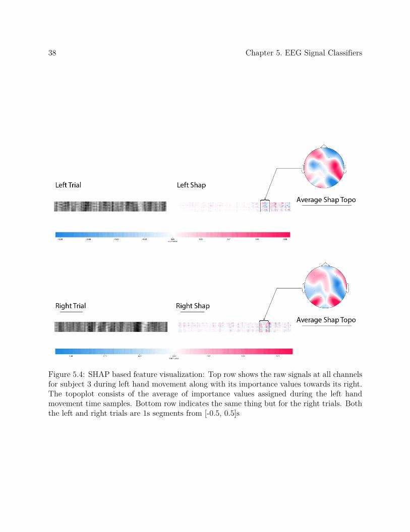
38 Chapter 5. EEG Signal Classifiers
Figure 5.4: SHAP based feature visualization: Top row shows the raw signals at all channelsfor subject 3 during left hand movement along with its importance values towards its right.The topoplot consists of the average of importance values assigned during the left handmovement time samples. Bottom row indicates the same thing but for the right trials. Boththe left and right trials are 1s segments from [-0.5, 0.5]s
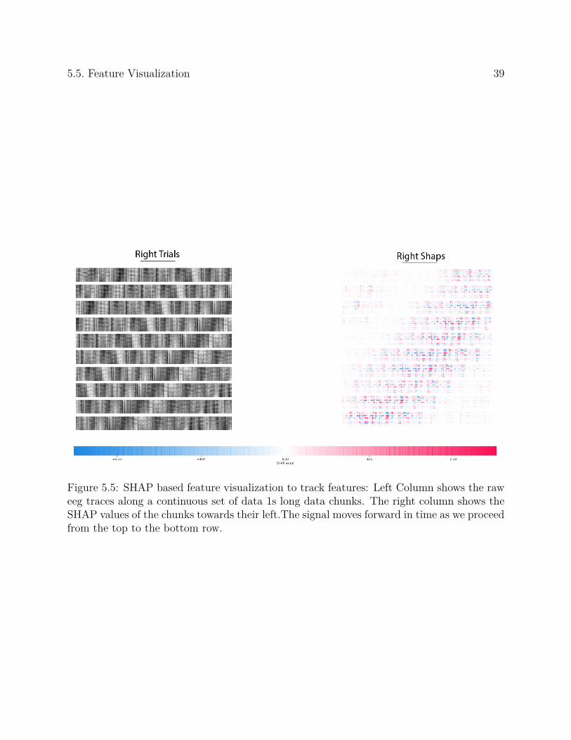
5.5. Feature Visualization 39
Figure 5.5: SHAP based feature visualization to track features: Left Column shows the raweeg traces along a continuous set of data 1s long data chunks. The right column shows theSHAP values of the chunks towards their left.The signal moves forward in time as we proceedfrom the top to the bottom row.
Chapter 6
iEEG Signal Classifiers
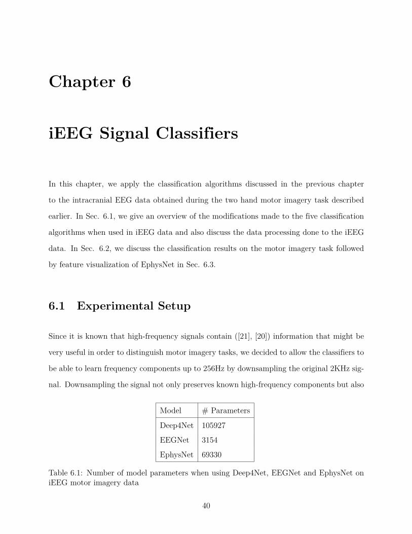
In this chapter, we apply the classification algorithms discussed in the previous chapter
to the intracranial EEG data obtained during the two hand motor imagery task described
earlier. In Sec. 6.1, we give an overview of the modifications made to the five classification
algorithms when used in iEEG data and also discuss the data processing done to the iEEG
data. In Sec. 6.2, we discuss the classification results on the motor imagery task followed
by feature visualization of EphysNet in Sec. 6.3.
6.1 Experimental Setup
Since it is known that high-frequency signals contain ([21], [20]) information that might be
very useful in order to distinguish motor imagery tasks, we decided to allow the classifiers to
be able to learn frequency components up to 256Hz by downsampling the original 2KHz sig-
nal. Downsampling the signal not only preserves known high-frequency components but also
Model # Parameters
Deep4Net 105927
EEGNet 3154
EphysNet 69330
Table 6.1: Number of model parameters when using Deep4Net, EEGNet and EphysNet oniEEG motor imagery data
40
6.1. Experimental Setup 41
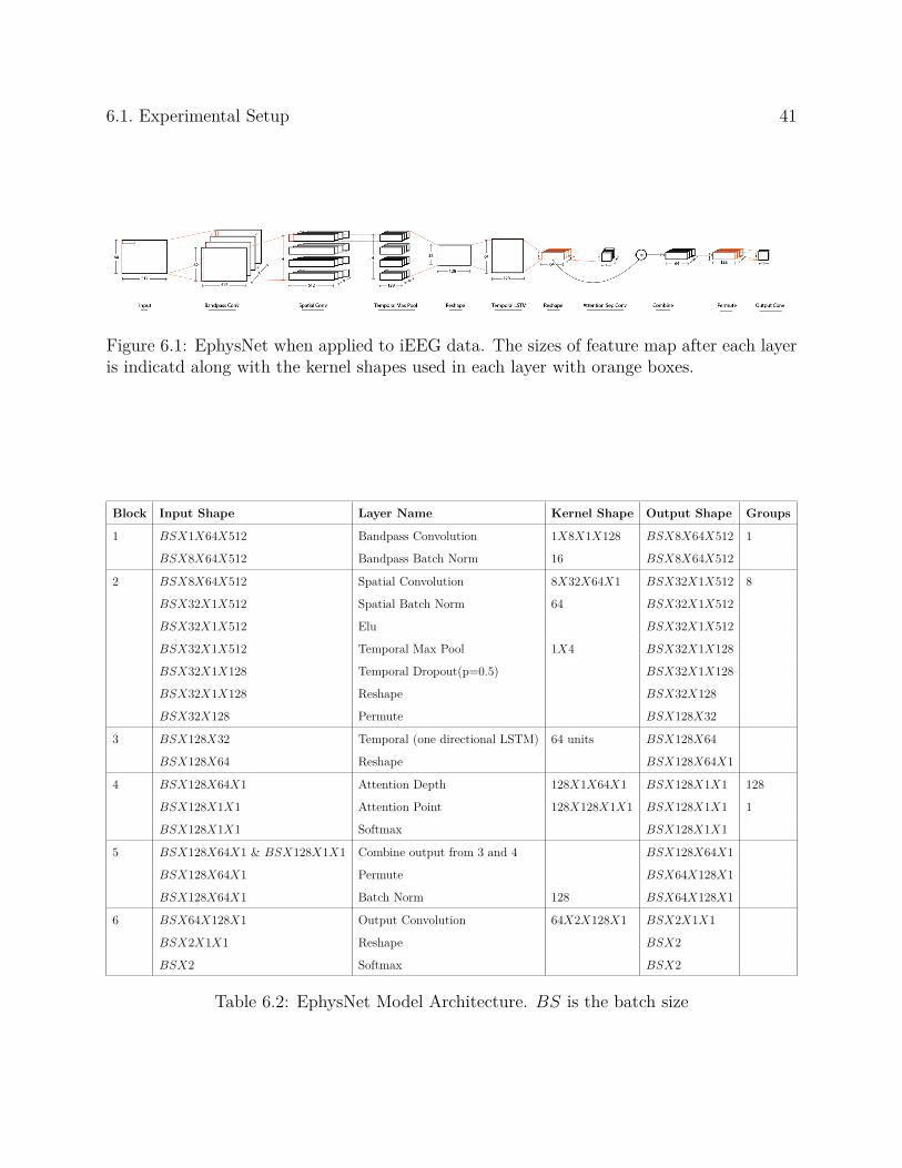
Figure 6.1: EphysNet when applied to iEEG data. The sizes of feature map after each layeris indicatd along with the kernel shapes used in each layer with orange boxes.
Block Input Shape Layer Name Kernel Shape Output Shape Groups
1 BSX1X64X512 Bandpass Convolution 1X8X1X128 BSX8X64X512 1
BSX8X64X512 Bandpass Batch Norm 16 BSX8X64X512
2 BSX8X64X512 Spatial Convolution 8X32X64X1 BSX32X1X512 8
BSX32X1X512 Spatial Batch Norm 64 BSX32X1X512
BSX32X1X512 Elu BSX32X1X512
BSX32X1X512 Temporal Max Pool 1X4 BSX32X1X128
BSX32X1X128 Temporal Dropout(p=0.5) BSX32X1X128
BSX32X1X128 Reshape BSX32X128
BSX32X128 Permute BSX128X32
3 BSX128X32 Temporal (one directional LSTM) 64 units BSX128X64
BSX128X64 Reshape BSX128X64X1
4 BSX128X64X1 Attention Depth 128X1X64X1 BSX128X1X1 128
BSX128X1X1 Attention Point 128X128X1X1 BSX128X1X1 1
BSX128X1X1 Softmax BSX128X1X1
5 BSX128X64X1 & BSX128X1X1 Combine output from 3 and 4 BSX128X64X1
BSX128X64X1 Permute BSX64X128X1
BSX128X64X1 Batch Norm 128 BSX64X128X1
6 BSX64X128X1 Output Convolution 64X2X128X1 BSX2X1X1
BSX2X1X1 Reshape BSX2
BSX2 Softmax BSX2
Table 6.2: EphysNet Model Architecture. BS is the batch size
42 Chapter 6. iEEG Signal Classifiers
Subject CSP Deep4Net EEGNet EphysNet
CAR04 50.875000 +- 11.929917 63.645000 +- 8.229078 69.625000 +- 9.168049 62.900000 +- 10.093438
CAR05 65.707071 +- 10.551003 66.130000 +- 7.409494 64.875000 +- 10.400270 61.025000 +- 7.689644
CAR07 48.300000 +- 6.100774 69.395000 +- 5.500020 60.475000 +- 12.146219 73.325000 +- 2.522524
CAR08 49.525000 +- 12.425584 92.970000 +- 7.983364 82.950000 +- 14.465390 79.975000 +- 10.547186
CAR10 62.929293 +- 4.456989 55.920000 +- 8.968478 57.150000 +- 14.376283 52.975000 +- 9.226626
CAR11 54.696970 +- 6.870667 57.080000 +- 10.493741 46.225000 +- 14.072335 49.950000 +- 9.597395
CAR13 45.375000 +- 15.057413 66.104286 +- 5.904820 54.025000 +- 5.506190 55.275000 +- 6.231422
Table 6.3: Test Accuracies after 10 repeats on four classifiers when applied to iEEG MotorImagery Task. FBCSP is excluded from analysis as it was not possible to increase itsclassification accuracy beyond chance on any of the subjects. Bold values indicates stasticallysignificant results (p<0.05)
reduces the number of parameters in the model thereby reducing the chances of overfitting.
We also performed CAR and mean subtraction to the data in order to increase the signal
to noise ratio. Because of the increased signal timesteps from 250 to 512 and an increase
in the number of channels from 22 to 64, the iEEG classifiers had a slight increase in the
number of model parameters when compared to its EEG counter-part (see Table 6.1 and
5.2). Increases in kernel sizes for EEGNet and Deep4Net were performed according to the
information provided by their respective authors. Fig. 6.1 shows the feature map sizes after
each layer in the EphysNet. Comparing this to Fig. 5.1, we clearly see how the increase in
the number of channels and timesteps dictates the increase in kernel sizes and feature map
sizes. See Table. 6.2 in order to get a detailed overview of the feature map sizes along with
the respective kernels.
6.2 iEEG Motor Imagery Classification Results
We trained each of the five classifiers on the iEEG dataset collected while subjects performed
the two hand motor imagery task. Each subject performed a total of 46 trials during the
6.2. iEEG Motor Imagery Classification Results 43
calibration stage (stage 1) each lasting 4s, out of which 2 random left and right trials were
used as testing data and the remaining 42 trials where used as training (90%) and validation
(10%) data. After segmenting each trial from [-0.5, 4]s and chunking them into 1s overlapping
segments, each trial produced 100 chunks per segment. We repeated the experiment 10
times, selecting 2 random left and right trials as testing each time and training/validating
on the rest. The classification results for all the classifiers expect FBCSP is as shown in
Table. 6.3. FBCSP was excluded from analysis for iEEG as it was not possible to increase
its test accuracy beyond change (50%). From Table 6.3, we can see Deep4Net on subject
CAR08 produced statistically significant results and that CSP classifier performed the worst
in subjects CAR07, CAR08 and CAR13. This is expected as, CSP is known to produce
bad results in the presence of noise in the data [2], and also because it has to learn from a
broad frequency range (4-200Hz) when used in iEEG. Deep4Net, EEGNet, and EphysNet
seems to perform comparably on all the subjects. When compared to the classification results
obtained using the EEG data, we can clearly see that iEEG data produces lower classification
results. This might be because of the larger number of channels, the higher sampling rate
designed to capture high-frequency information when compared to EEGs and also the fact
that in motor imagery tasks using EEG, the electrode locations were in the motor cortex,
where as, iEEG does not have any electrodes in the motor cortex. The test accuracy values
also have a higher standard deviation in iEEG when compared to EEG because we only
used 4 trials for testing and so if a subject performed poorly on any one of those trials the
classification results will be poor. Collecting another session of data only for testing might
allow for a better comparison between the performance on EEG data versus iEEG data.
44 Chapter 6. iEEG Signal Classifiers
6.3 Feature Visualization
Similar to Sec. 5.5 in this section, we look at the temporal kernels, SHAP values during left
and right trials and the SHAP features over time in order to get an understanding of the
features learned by EphysNet.
• Visualizing Bandpass Convolutional Kernels: Fig. 6.2 shows the bandpass ker-
nels along with the power spectral density of the kernels. Looking at the peaks in the
power spectral density, we observe that activity around 100Hz is captured by kernels 2
and 6 whereas kernels 1, 2 and 4 mainly capture lower frequency activity from 20-70Hz.
Based on the offline analysis done earlier, we found there to be high-frequency activity
around 80-120Hz and also around 15-26Hz. We do in fact see some signals in these
frequency bands being learned by the filters, we do not, however, observe a high power
in the mu band.
• SHAP based feature visualization: Fig. 6.3 shows the raw left and right trials
along with their SHAP values for subject CAR08. We selected a time window that
represents the instance when the subject imagined moving their arms and took the
average of the SHAP values during that time period as indicated in the Average SHAP
plot. Looking the left average SHAP plot, we see that electrodes AHipp-3Ld6, Amg-
1Ld5 and Amg-2Rd2 contributed during the left movement and from the right average
SHAP plot the LSFG-9L strip seems to contain high SHAP values. From Hilbert Power
difference in Fig. A.2, we see that some channels in the Hippocampus and Amygdala
along with the LSFG-9L strip had significant differences in power during left and right-
hand movement. In order to determine if the features learned to distinguish between
left and right movement are being tracked during each of the signal chunks, we plotted
10 consecutive signal chunks along with their SHAP values in Fig. 6.4. Similar to
6.3. Feature Visualization 45
Figure 6.2: Visualizing Bandpass Convolutional Kernels: The top row shows the raw band-pass kernel values learnt by EPhysNet along with its power spectral density in the bottomrow.
EEG results, we again see that the classifiers were able to track the required features
in time.
46 Chapter 6. iEEG Signal Classifiers
Figure 6.3: SHAP based feature visualization: Top row shows the raw iEEG data along allthe 64 channels from [-0.1, 0.9]s during the left trial as an image along with its correspondingSHAP values towards its right. The Average SHAP values in movement window in showntowards the extreme right. Bottom row depicts a similar observatino during the right trial.The iEEG channels are visible when zooming in on the digital version.
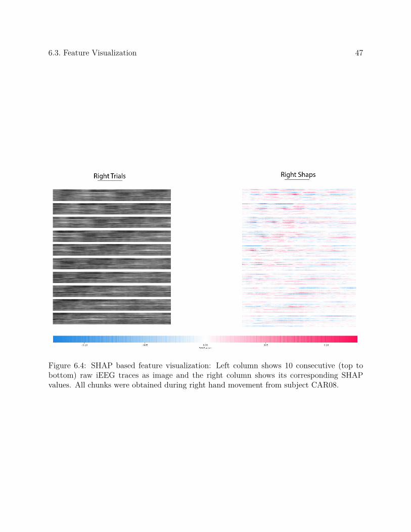
6.3. Feature Visualization 47
Figure 6.4: SHAP based feature visualization: Left column shows 10 consecutive (top tobottom) raw iEEG traces as image and the right column shows its corresponding SHAPvalues. All chunks were obtained during right hand movement from subject CAR08.
Chapter 7
Conclusions and Future Work
With the final goal of developing a classifier and analyzing its performance on intracranial
EEG, in this work, we started off by designing a robust iEEG data acquisition and signal
processing pipeline. We implemented the data acquisition pipeline using MATLAB with
the added ability to use a classifier from Python. We also discussed the BCI experimental
paradigm used to collect our iEEG data along with the preprocessing done. We later analyzed
the iEEG data obtained from the two hand motor imagery task from 7 subjects in order
to find relevant spectral, spatial and temporal features manually. Looking at the power
difference between left and right-hand movements, we found there to be a large number of
significant frequency bins that differed in power at three major frequency bands. Two of
these bands were also found to include the mu and beta band that is known to play a role
during motor movements. Inspired by the fact that the hippocampal electrodes are involved
in processing sequential memory and also because the hippocampal and amygdala electrodes
were present in 6 of the 7 subjects, we further showed there to be a time lag in the high
(65-115Hz) and low (3-15Hz) frequency signals during imagined left hand movement and
that this lag was absent during imagined right movement.
Using the results from this offline data analysis, we hypothesized that a good classification
algorithm must learn these features in order to perform well in an online task. To this
end, we designed EphysNet, a classification algorithm that learns to automatically extract
spatial, spectral and temporal information from electrophysiological data. We tested this
48
49
classification algorithm on EEG motor imagery data and also compared it to other classifiers.
We found there to be a significant performance increase when using our classifier on subjects
that performed well during the calibration stage. Feature visualization was performed on
EphysNet when used on EEG data and we found the classifier to use frequency components
in the mu and beta band from contralateral electrodes in the motor region of the brain. We
finally compared the performance of EphsyNet along with several other classifiers on the two
hand iEEG motor imagery dataset and found there to be so significant difference between
Conv4Net, EEGNet, and EphysNet except in subject CAR08, where Deep4Net seemed to
perform better. We later performed feature visualization on EphysNet when used on iEEG
and found spatial filters that agreed with power difference between the left-right power
difference and also found that the bandpass filters had mainly learned to used frequency
components around 100Hz and from 2–70Hz. These findings clearly show the potential of
using end-to-end classification algorithms on electrophysiological data as they do not any
manual feature selection to be done, they also require minimal data preprocessing and have
a low number of parameters thereby allowing them to be used in online tasks.
Comparing the classification results on the two hand EEG and iEEG datasets, we clearly see
that the EEG task seems to perform better on average. This might be because the subjects
used in the EEG experiments might have a better mental health condition, not subjected
to constant medication and worry about seizures. Also, because the electrodes used in the
EEG experiment come from the motor cortex which has well studied previously, but, the
depth electrodes used in our case are not in the motor cortex. Also, because of the lower
number of test samples available during iEEG classification, its test accuracy had a higher
variance when compared to the EEG classifiers. An entire session dedicated to collecting
only test samples would give us a better estimation of the classifiers abilities on iEEG data.
Bibliography
[1] Kai Keng Ang et al. “Clinical study of neurorehabilitation in stroke using EEG-based
motor imagery brain-computer interface with robotic feedback”. In: 2010 Annual In-
ternational Conference of the IEEE Engineering in Medicine and Biology. IEEE. 2010,
pp. 5549–5552.
[2] Kai Keng Ang et al. “Filter bank common spatial pattern (FBCSP) in brain-computer
interface”. In: 2008 IEEE International Joint Conference on Neural Networks (IEEE
World Congress on Computational Intelligence). IEEE. 2008, pp. 2390–2397.
[3] Andreas Antoniades et al. “Deep learning for epileptic intracranial EEG data”. In:
2016 IEEE 26th International Workshop on Machine Learning for Signal Processing
(MLSP). IEEE. 2016, pp. 1–6.
[4] Dzmitry Bahdanau, Kyunghyun Cho, and Yoshua Bengio. “Neural machine translation
by jointly learning to align and translate”. In: arXiv preprint arXiv:1409.0473 (2014).
[5] François Chollet. “Xception: Deep learning with depthwise separable convolutions”. In:
Proceedings of the IEEE conference on computer vision and pattern recognition. 2017,
pp. 1251–1258.
[6] Febo Cincotti et al. “Non-invasive brain–computer interface system: towards its appli-
cation as assistive technology”. In: Brain research bulletin 75.6 (2008), pp. 796–803.
[7] Djork-Arné Clevert, Thomas Unterthiner, and Sepp Hochreiter. “Fast and accurate
deep network learning by exponential linear units (elus)”. In: arXiv preprint arXiv:1511.07289
(2015).
50
BIBLIOGRAPHY 51
[8] Loren M DeVito and Howard Eichenbaum. “Memory for the order of events in specific
sequences: contributions of the hippocampus and medial prefrontal cortex”. In: Journal
of Neuroscience 31.9 (2011), pp. 3169–3175.
[9] Norbert J Fortin, Kara L Agster, and Howard B Eichenbaum. “Critical role of the
hippocampus in memory for sequences of events”. In: Nature neuroscience 5.5 (2002),
p. 458.
[10] William J Gehring et al. “The error-related negativity”. In: Perspectives on Psycholog-
ical Science 13.2 (2018), pp. 200–204.
[11] Alexandre Gramfort et al. “MNE software for processing MEG and EEG data”. In:
Neuroimage 86 (2014), pp. 446–460.
[12] Cuntai Guan, Manoj Thulasidas, and Jiankang Wu. “High performance P300 speller
for brain-computer interface”. In: IEEE International Workshop on Biomedical Circuits
and Systems, 2004. IEEE. 2004, S3–5.
[13] Leigh R Hochberg et al. “Reach and grasp by people with tetraplegia using a neurally
controlled robotic arm”. In: Nature 485.7398 (2012), p. 372.
[14] Sergey Ioffe and Christian Szegedy. “Batch normalization: Accelerating deep network
training by reducing internal covariate shift”. In: arXiv preprint arXiv:1502.03167
(2015).
[15] Christopher L Jones et al. “Design and development of the cable actuated finger ex-
oskeleton for hand rehabilitation following stroke”. In: IEEE/ASME Transactions on
Mechatronics 19.1 (2014), pp. 131–140.
[16] Diederik P Kingma and Jimmy Ba. “Adam: A method for stochastic optimization”. In:
arXiv preprint arXiv:1412.6980 (2014).
52 BIBLIOGRAPHY
[17] C Kothe. “Lab streaming layer (LSL)”. In: https://github. com/sccn/labstreaminglayer.
Accessed on October 26 (2014), p. 2015.
[18] Karl LaFleur et al. “Quadcopter control in three-dimensional space using a noninvasive
motor imagery-based brain–computer interface”. In: Journal of neural engineering 10.4
(2013), p. 046003.
[19] Vernon Lawhern et al. “EEGNet: A Compact Convolutional Network for EEG-based
Brain-Computer Interfaces”. In: Journal of neural engineering 15 5 (2018), p. 056013.
[20] Eric C Leuthardt et al. “A brain-computer interface using electrocorticographic signals
in humans”. In: Journal of neural engineering 1.2 (2004), p. 63.
[21] Eric C Leuthardt et al. “Electrocorticography-based brain computer interface-the Seat-
tle experience”. In: IEEE Transactions on Neural Systems and Rehabilitation Engineer-
ing 14.2 (2006), pp. 194–198.
[22] Simon P Levine et al. “Identification of electrocorticogram patterns as the basis for a
direct brain interface”. In: Journal of clinical neurophysiology 16.5 (1999), p. 439.
[23] Lun-De Liao et al. “Gaming control using a wearable and wireless EEG-based brain-
computer interface device with novel dry foam-based sensors”. In: Journal of neuro-
engineering and rehabilitation 9.1 (2012), p. 5.
[24] Chin-Teng Lin et al. “Brain computer interface-based smart living environmental auto-
adjustment control system in UPnP home networking”. In: IEEE Systems Journal 8.2
(2014), pp. 363–370.
[25] Kip A Ludwig et al. “Using a common average reference to improve cortical neuron
recordings from microelectrode arrays”. In: Journal of neurophysiology 101.3 (2009),
pp. 1679–1689.
BIBLIOGRAPHY 53
[26] Scott M Lundberg and Su-In Lee. “A unified approach to interpreting model predic-
tions”. In: Advances in Neural Information Processing Systems. 2017, pp. 4765–4774.
[27] Sebastian Mika et al. “Fisher discriminant analysis with kernels”. In: Neural networks
for signal processing IX: Proceedings of the 1999 IEEE signal processing society work-
shop (cat. no. 98th8468). Ieee. 1999, pp. 41–48.
[28] Wolfgang HR Miltner, Christoph H Braun, and Michael GH Coles. “Event-related
brain potentials following incorrect feedback in a time-estimation task: evidence for a
“generic” neural system for error detection”. In: Journal of cognitive neuroscience 9.6
(1997), pp. 788–798.
[29] Melody M Moore. “Real-world applications for brain-computer interface technology”.
In: IEEE Transactions on Neural Systems and Rehabilitation Engineering 11.2 (2003),
pp. 162–165.
[30] Robert Oostenveld et al. “FieldTrip: open source software for advanced analysis of
MEG, EEG, and invasive electrophysiological data”. In: Computational intelligence
and neuroscience 2011 (2011), p. 1.
[31] Adam Paszke et al. “Pytorch: Tensors and dynamic neural networks in python with
strong gpu acceleration”. In: PyTorch: Tensors and dynamic neural networks in Python
with strong GPU acceleration 6 (2017).
[32] Gert Pfurtscheller and FH Lopes Da Silva. “Event-related EEG/MEG synchronization
and desynchronization: basic principles”. In: Clinical neurophysiology 110.11 (1999),
pp. 1842–1857.
[33] John Polich. “Updating P300: an integrative theory of P3a and P3b”. In: Clinical
neurophysiology 118.10 (2007), pp. 2128–2148.
54 BIBLIOGRAPHY
[34] Herbert Ramoser, Johannes Muller-Gerking, and Gert Pfurtscheller. “Optimal spatial
filtering of single trial EEG during imagined hand movement”. In: IEEE transactions
on rehabilitation engineering 8.4 (2000), pp. 441–446.
[35] Brice Rebsamen et al. “A brain controlled wheelchair to navigate in familiar environ-
ments”. In: IEEE Transactions on Neural Systems and Rehabilitation Engineering 18.6
(2010), pp. 590–598.
[36] Audrey S Royer et al. “EEG control of a virtual helicopter in 3-dimensional space
using intelligent control strategies”. In: IEEE Transactions on neural systems and
rehabilitation engineering 18.6 (2010), pp. 581–589.
[37] Gerwin Schalk and Eric C Leuthardt. “Brain-computer interfaces using electrocortico-
graphic signals”. In: IEEE reviews in biomedical engineering 4 (2011), pp. 140–154.
[38] Gerwin Schalk et al. “Two-dimensional movement control using electrocorticographic
signals in humans”. In: Journal of neural engineering 5.1 (2008), p. 75.
[39] RT Schirrmeister et al. “Deep learning with convolutional neural networks for brain
mapping and decoding of movement-related information from the human EEG. arXiv,
2017”. In: arXiv preprint arXiv:1703.05051 ().
[40] Bernhard Scholkopf and Alexander J Smola. Learning with kernels: support vector
machines, regularization, optimization, and beyond. MIT press, 2001.
[41] Nitish Srivastava et al. “Dropout: a simple way to prevent neural networks from over-
fitting”. In: The Journal of Machine Learning Research 15.1 (2014), pp. 1929–1958.
[42] Kazuo Tanaka, Kazuyuki Matsunaga, and Hua O Wang. “Electroencephalogram-based
control of an electric wheelchair”. In: IEEE transactions on robotics 21.4 (2005),
pp. 762–766.
BIBLIOGRAPHY 55
[43] Michael Tangermann et al. “Review of the BCI competition IV”. In: Frontiers in neu-
roscience 6 (2012), p. 55.
[44] Yogatheesan Varatharajah et al. “Integrating artificial intelligence with real-time in-
tracranial EEG monitoring to automate interictal identification of seizure onset zones
in focal epilepsy”. In: Journal of neural engineering 15.4 (2018), p. 046035.
[45] Meel Velliste et al. “Cortical control of a prosthetic arm for self-feeding”. In: Nature
453.7198 (2008), p. 1098.
[46] Yijun Wang, Shangkai Gao, and Xiaornog Gao. “Common spatial pattern method for
channel selection in motor imagery based brain-computer interface”. In: 2005 IEEE
Engineering in Medicine and Biology 27th Annual Conference. IEEE. 2006, pp. 5392–
5395.
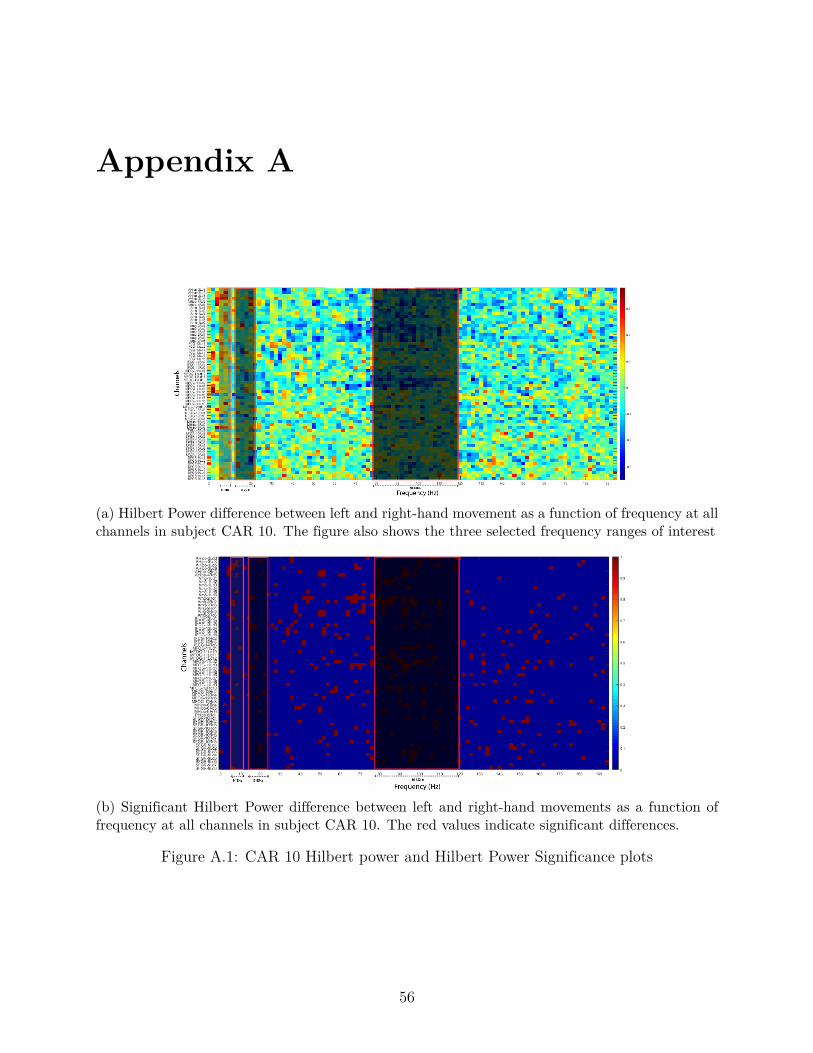
Appendix A
(a) Hilbert Power difference between left and right-hand movement as a function of frequency at allchannels in subject CAR 10. The figure also shows the three selected frequency ranges of interest
(b) Significant Hilbert Power difference between left and right-hand movements as a function offrequency at all channels in subject CAR 10. The red values indicate significant differences.
Figure A.1: CAR 10 Hilbert power and Hilbert Power Significance plots
56
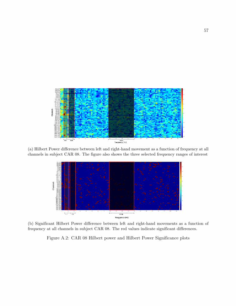
57
(a) Hilbert Power difference between left and right-hand movement as a function of frequency at allchannels in subject CAR 08. The figure also shows the three selected frequency ranges of interest
(b) Significant Hilbert Power difference between left and right-hand movements as a function offrequency at all channels in subject CAR 08. The red values indicate significant differences.
Figure A.2: CAR 08 Hilbert power and Hilbert Power Significance plots


