Embed Size (px)
Citation preview
Microcellular Radio Channel Prediction Using Ray Tracing
by
Kurt Richard Schaubach
Thesis submitted to the Faculty of the
Virginia Polytechnic Institute and State University
in partial fulfillment of the requirements for the degree of
Master of Science
in
Electrical Engineering
APPROVED
Nathaniel J. Davis, IV, chairman
SN el for
Theodore S. Rappaport Charles W. Bostian
August 1992
Blacksburg, Virginia
LY 5656
Cr. Ay
WuSS W942
$332 (2
Microcellular Radio Channel Prediction Using Ray Tracing
by
Kurt Richard Schaubach
Nathaniel J. Davis, IV, chairman
Electrical Engineering
(ABSTRACT)
The radio interface greatly affects performance of wireless communication sys-
tems. Hard-wired communication links use transmission lines to connect communication
terminals. The propagation characteristics of radio frequency signals on these transmis-
sion lines are well known. In wireless communication systems, however, the transmission
line with a known impulse response is replaced by a radio channel with an impulse
response that is constantly changing as the users roam throughout the coverage area. The
varying impulse response is due to the multiple path propagation of the signals from the
transmitter to the receiver. The design of emerging small cellular (commonly known as
microcellular) wireless systems is limited by the multipath propagation characteristics of
the channel. Once these propagation conditions are understood, systems may be designed
more efficiently in terms of cell layout, interference reduction, and system performance.
This thesis presents a technique for automated propagation prediction in outdoor
microcellular radio channels using ray tracing. The basic method is to integrate site-spe-
cific environmental data with a geometrical optics model to trace the propagation of
energy from the transmitter to the receiver. Software written in C++ is used to automati-
cally trace rays that are reflected, transmitted, scattered, or diffracted as they propagate
through the channel. The automated software uses AutoCAD® to maintain the Site-spe-
cific building data incorporated into the model. Details of the building database, propaga-
tion model, and software implementation are included in this thesis. The accuracy of the
model and its software implementation is tested against wide band measurements taken on
the Virginia Tech campus. Results, included here, indicate that the received signal can be
accurately predicted in both line-of-sight and obstructed microcell topographies.

Acknowledgments
“You could put in this room, DeForest, all the radiotelephone apparatus
that the country will ever need”
- W. W. Dean (President of Dean Telephone Company) to American radio pioneer Lee DeForest wie had visited Dean's office to pitch his audion tube, 1907
My sincere appreciation goes to my academic advisor, Professor Nathaniel Davis.
His guidance and patience helped to make this research possible, and his friendship helped
to make it an enjoyable experience. My thanks go to Professor Theodore Rappaport for the
opportunity to work with the Mobile and Portable Radio Research Group as well as for his
interest and enthusiasm in my research. I also extended thanks to Professor Charles Bos-
tian, whose lectures first introduced me to electromagnetics, for his corrections and sug-
gestions for improving this thesis.
I am indebted to the graduate students, research associates, and staff that provided
assistance throughout the course of this research. I am grateful to Greg Bump, Weifeng
Huang, Mike Keitz, Orlando Landron, Joe Liberti, and all others who provided assistance
while conducting measurements necessary to validate this work. I am also very grateful to
Prab Koushik and Graham Stead for sharing their C programming and UNIX expertise.
Most importantly, I would like to thank Scott Seidel for many valuable discussions on
propagation prediction and for his contributions on ray tracing. Scott’s input was a valu-
able resource throughout the course of this research.
I gratefully recognize the financial support provided by the Mobile and Portable
Radio Group Industrial Affiliates Program and the Bradley Department of Electrical Engi-
neering.
My deepest appreciation goes to my family and friends who have provided immea-
surable support and encouragement throughout my academic career. I would not have pur-
sued a graduate degree had it not been for my father’s insistence that “education is an
experience to value for a lifetime”, and my mother’s reminders of their love and pride was
a consistent source of motivation. It is to them it that I owe the greatest thanks.
Microcellular Radio Channel Prediction Using Ray Tracing
Table of Contents
INtroductiOn.............ccccscscscscsscscsscssccsseccesscesccessescssscsseasseassenssescsoasescscecsssesesesassosssess 1
2 Theoretical Propagation Models.. sane - sesecscsssscseees 6
2.1 . Geometrical Optics 20... cesscccssecsssessacesseeceesecsececceesceeeeeeaseseceeeeeeeeaucecsasenses 6
2.2 Free Space Path Loss ..............cssssssscsessseeceeeseeneners waccesseesecsnacceceeesesssseeeesesstes 9
2.3. ~~ Properties of an Electromagnetic Wave at an Interface ..............cesssseeeees 12 2.3.1 The Laws of Reflection and Transmission...............sssscccsssscseseseees 12
2.3.2 The Rayleigh Criterion and Rough Surface Scattering................. 16
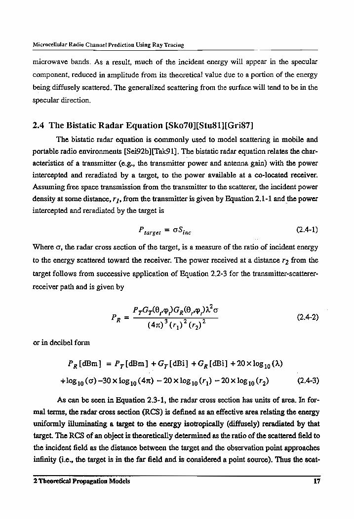
2.4 The Bistatic Radar Equation .........ccscessssssssssscssssscsessssscsecsesessssotsneacesesnsseeees 17 2.4.1 Radar Cross Section of @ Flat Plate... esesccesscecceesesssseeseeees 18
2.5 Diffraction... eeecceccescssecensescenssscececsonsesessecsacsccescenesssecseesecsecceasenaeeearees 19 2.5.1 Knife Edge Diffraction.............cscccsscssssscssssscsseccssnssssensnscssasscceenaes 20
2.5.2 Wedge Diffraction ...............ccccccssscccssssceecccssssnsscccccesesesscaccceessessees 24
2.6 = SUMIMALY oe cecsscssesscccecscesssscensensacsaccncsacsucsscsecsssscassecssecsceaseaesacenssaceass 26
3 Literature Review . sasees 27
3.1 Background ..........eececessssessssssessssssessssssaceesenseeceeeseseeseeaseeseeseseneesseneeeeesees 27 3.1.1 Multipath Propagation. ..............ccccsscssssssssssccesssecesssneccsssssescessaceeoes 27
3.1.2 Delay Spread and Coherence Bandwidth... ssscsssseecesseeceees 29
3.1.3 Narrow Band versus Wide Band Channels.................c:cccssscsseseesees 30
3.1.4 Characterization of Narrow Band and Wide Band Channels........ 31
3.2 Propagation in the Mobile and Portable Radio Environment.................... 32
3.2.1 Conventional Cellular Radio... csscscsessseecesccessetescesssceeceees 33 3.2.2 Microcellular Radio..............cssscssssccecssssssscscsssssssecesssssseancessceseees 34
3.3 Statistical Propagation Models .0.0...........ccsssccssssesscsssssesssccssessssecsssecesseees 36
3.4 Terrain Based Models for Conventional Cellular Radio Service............... 37
3.5 Deterministic Propagation Models .....0..........ccsssscscscesscecccsssccesscssneesecesnees 38
3.6 —- SUMMATY 0. ce ceseceesccecccersesccesessessasscsnsseassscosscescsecessecssaseseasseasanessnceaseees 43
4 Ray Tracing Validation on the Virginia Tech Campus..........000+ 44
41 Virginia Tech Campus Measurements ................:csscsscssesesssssecseeceeceeecceeeees 46 4.1.1 900 MHz Narrow Band Measurement System ...................sscceeeee 46
4.1.2 Measurement Procedure ..............ccccssccsssssoscessessecessnessseccsssoseeseesees 47
4.2 Propagation Prediction using Simple Ray Tracing. ..............csscsssssssseseeeees 49 4.2.1 Propagation Model ...............sccscssssssssocssssssscsessessssscssscssesssassnscenssees 49 4.2.2 Manual Ray Tracing for the Virginia Tech Campus............scs000 52 4.2.3 Comparison of Measured and Predicted Data. .............scccssssessseees 52
4.3 CONIUSIONS.............seessssscssecesssceacceccecssncsscsnacsosssacsecssascenesssseeceseeesscseacsaees 56
5 The Building Database 59
5.1 Requirements for Modeling Buildings in the Database................sssssesee 59
Table of Contents iv

Microcellular Radio Channel Prediction Using Ray Tracing
5.2. Using AutoCAD® for Building Database Management.............0. eee 60
5.2.1 AutoCAD Drawings and Drawing Interchange File Formats....... 61
5.2.2 Drawing Levels .0.........ccssccsssseceeceeceseceseeeececsseeeesceeeeesseereeseesseeeeeees 64 5.2.3 Creating Three Dimensional Entities as Polyface Objects............ 64 5.2.4 Creating Three Dimensional Entities from Two Dimensional
DIAWINGS ............ccccecceececccssesssceccecsessceccceeeeeeseeeseeadoceseesseseeeeeeenaees 65
5.2.5 Using Drawing Attributes 2.0... eecescceeceeceeeeceseeeeteneeeecseeeneeenees 65
5.2.6 Adding a Transmitter and Receivers ......0....ceeeseeececesseeeceeeeeenssees 67
5.3. Creating A Building Database - The Virginia Tech Campus.................... 67
5.4 Bounding Volumes and Ray Tracing Acceleration Techniques................. 69
5.5 DXF File Conversion Utility (Q0fimgr.cc) .o.c.cescecssssssssssessscssssssseesesesssssees 70
5.6 The Ray Tracing Definition Language and *.ray Files..............:.secsseesees 70
5.7 —-_- COMCIUSIONS...... eee eeeccssseccesncccesssscnaccescceccancaceeseseccecaccescaececceesseeseseeetetsas 74
6 Computer Ray Tracing , sscsescscscesesee 1D
6.1 The Channel Model ................ccccsssccsssesssseesccsscesscssccensesececosseeseses Beseeessceee 75
6.2 The Propagation Model .....0.........csceeseseccssecoesceeccesececceccesacesseeeseeeecerseeees 76
6.3 Ray Tracing Techmiques................eseesssssscencssesscecceseeecscesceeeceeceseeeceesseeeceets 80 6.3.1 Brute Force Ray Tracing versus Image Theory .................sccssees 80 6.3.2 Graphical Ray Tracing ............sccccsscsssssseecesseeees Vessecesseccseneeseeeeseeees 81
6.3.3 Available Computer Software for Ray Tracing ............:.ssscseesee 83
6.4 Source Ray Directions ..............cccsscsssccsscesesesecesncssecsesccssecessteeetcseresncenseaes 84
6.5 —— Tracing the Rays 20... ccecccccescecesseccssscsceesaseccseccsceeescesscesssssenesensesseeceasees 89 6.5.1 Recursive Ray Tracing and The Ray Tree ..0........ccssccseceseeseeceees 89
6.5.2 Reflected and Transmitted Rays .............::cccsssscccscsssrecessecessecseaceees 90
6.5.3 Scattered RAyS .......ccsscccsscscscssecesscesssceessscensssssscnaccesesesnsseasssnseneeeees 94 6.5.4 Diffracted Rays ..........cccssscssssssscsssccesessscsessscssccssecessccsssesseceensesesces 98
6.6 Processing the Ray Tracing Data File..............cssssccsssscssssssssseceseesenseenens 100
6.7 SUMIMATY oa. eecceccetcsscceseccnscescccsncencssncecncstestseneeeaeesucessseesercaasensessesersecens 103
7.0 Propagation Measurements and Predictions 105
7.1 ‘Verification of the Automated Ray Tracing System 2.0.0.0... cescssssseeees 105
7.2 Propagation Measurements...............ssssssssscsseccsescsercscseccssccesseceeacessceaceens 108 7.2.1 Measurement Locations and Procedure .............ccsscsseccsscesncseceers 108 7.2.2 1900 MHz Spread Spectrum Channel Soundet..............c.sssceseees 113
7.3. Comparison of Measured and Predicted Results .0............ccscsscsssesccsceesers 116 7.3.1 Summary of Comparisons...............ssccsccssccesssssccsssecsecssesssssnencsees 132 7.3.2 Discussion of Profile Statistics..............scsssccssscssssccsssccssccseseesenss 132 7.3.3 Enhancing Model Accuracy ..............cccsscccssescssssscessscesssecesscesceees 135
74 ——- COMCIUSIONS.............sessscsnsssccecssecceocssccocssccsacsarsacsecssnssesssnessncencsseenssencsacersee 146
8 Conclusions 148
8.1 Extensions of this Research «0.0.0.0... csscssecessseccenccscncssccesncesccesesecseaseesenes 150
Table of Contents v
Microcellular Radio Channel Prediction Using Ray Tracing
8.2 SUMMA Y oo. ce cceceseeeeeceseeesesenteeensenseeseeseneesseseeseaeesessessaseeesestecseeas 151
9.0 References............. ecccescecescecsccccsecccccececcccccssscccsccscoccecccececcccccscccscecsccescsscsecccecsescesee LOD
Table of Contents vi
Microcellular Radio Channel Prediction Using Ray Tracing
List of Figures
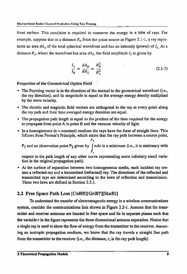
FIGURE 2.1-1. A tube of rays diverging from a point SOULCE. 2.0.0... cssssesssssscsetsssseeeeees 8
FIGURE 2.2-1. Free space wireless communications link from [Col85]. ......0....0.... 10
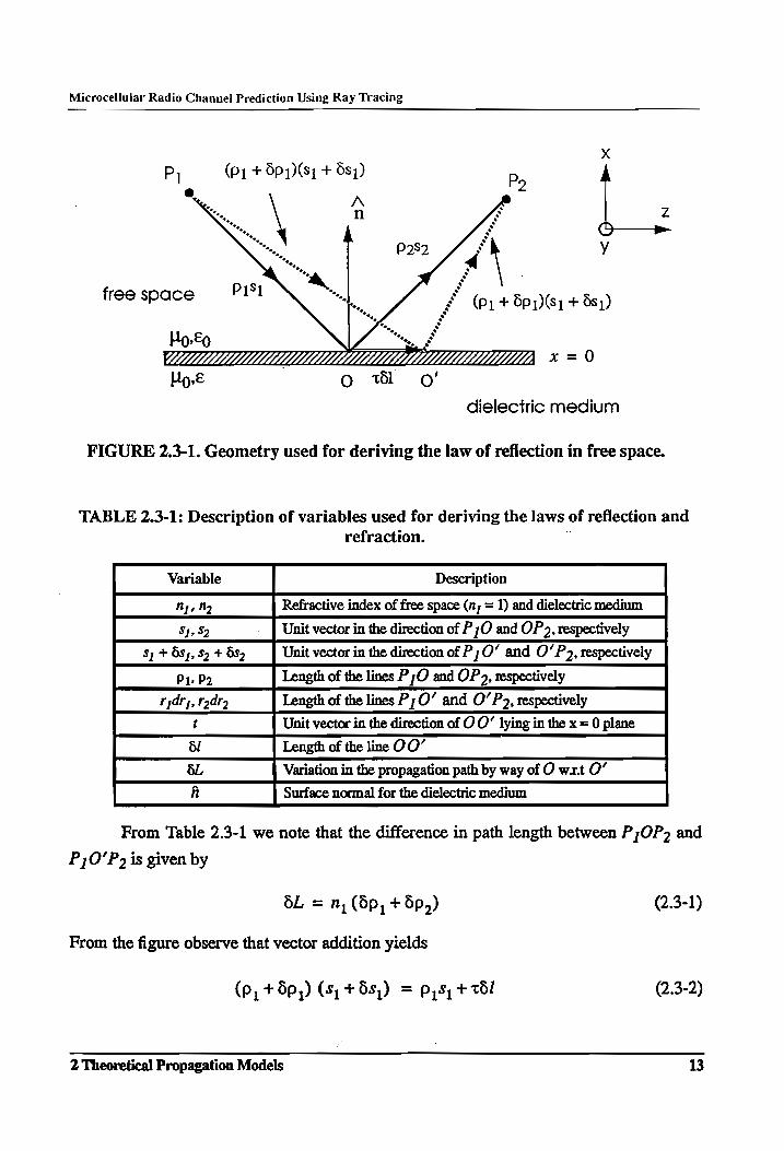
FIGURE 2.3-1. Geometry used for deriving the law of reflection in free space........... 13
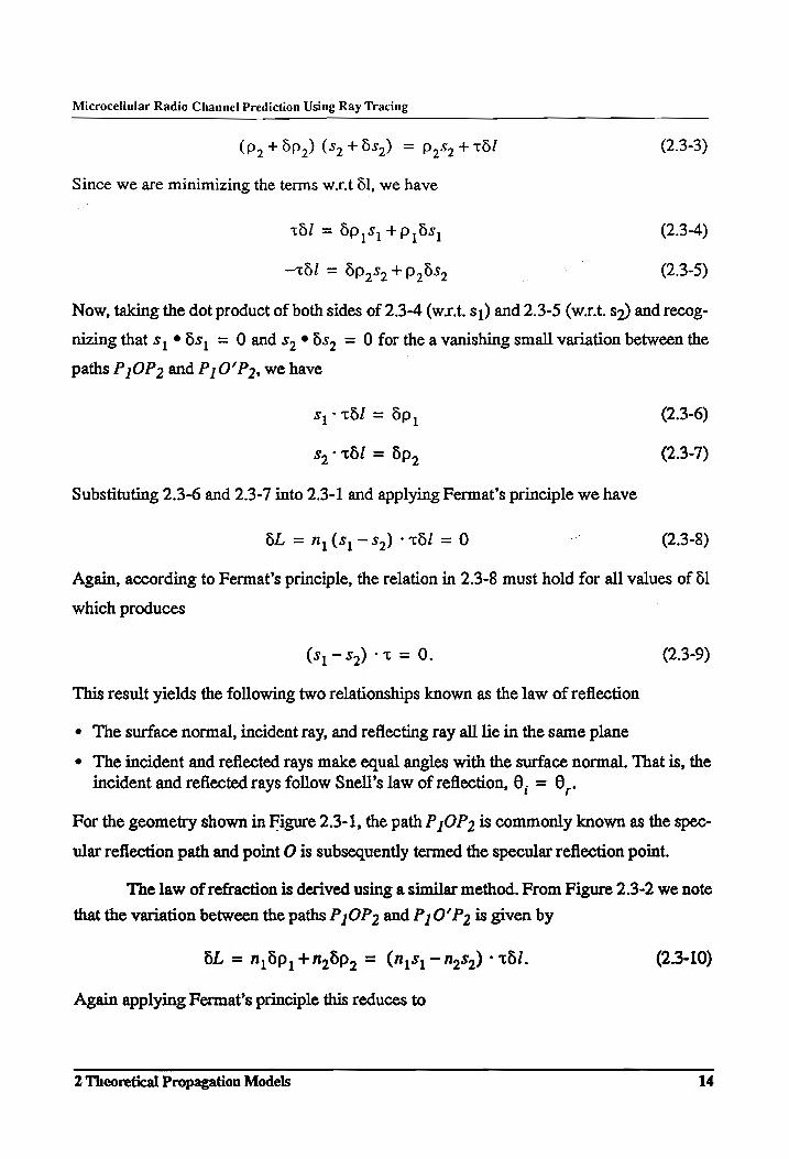
FIGURE 2.3-2. Geometry used for deriving the law of refraction in free SPace. ......... 15
FIGURE 2.4-1. Geometry to evaluate the scattering from a flat, conducting plate ......19
FIGURE 2.5-1. Diffraction example. The diffracted ray is added to predict the field in the shadowed region ...........s:cscsssssssscesscecsscessesscccscconssecesssececeseuesnseseass 20
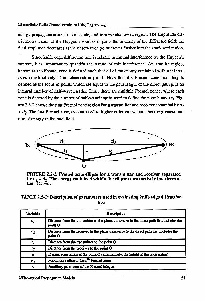
FIGURE 2.5-2. Fresnel zone ellipse for a transmitter and receiver separated by dj + d>. The energy contained within the ellipse constructively interferes at fhe TECCIVET. ..........ceccccccrssesssccssnssssecsscesscsscsscessccsssscesessscssescsscescescsssesens 21
FIGURE 2.5-3. Knife edge diffraction example. ..........c.cssssssscssssssesssssesssssssssesesessssseees 23
FIGURE 2.5-4. Knife edge diffraction loss as a function of the Fresnel integral auxiliary parameter, v, from [Par89].................cssccssseccseseseccssersecteees 23
FIGURE 2.5-5. Wedge diffraction configuration. The wedge is assumed infinite in the direction transverse (z -axis) to the ray propagation................:csseeeees 25
FIGURE 3.1-1. Multipath propagation in a microcellular environment....................0 28
FIGURE 3.1-2. The relation of a received multipath signal to different types of transmitted Signals. ...............ccssscecsccessssesscccesssesecescccesssesessscesssecesseeeeees 33
FIGURE 4.0-1. Sample CW fading waveform. The continuous trace is the instantaneous measured signal and the dashed trace is the spatial average which corresponds to the large-scale fading component........ 45
FIGURE 4.1-1. Block diagram of CW measurement systeM................scccssssssesesesseeenees 47
FIGURE 4.1-2. A portion of the Academic Quad on the Virginia Tech Campus. The transmitter antenna is located on the roof of Whittemore Hall............ 49
FIGURE 4.2-1. An example of the simple ray propagation model. This example illustrates a direct diffracted ray and a diffracted-reflected ray. .......... 51
FIGURE 4.2-2. Measured 900 MHz CW signal strength................sccccssscssssssesenrcetenees 54
FIGURE 4.2-3. Predicted 900 MHz CW signal strength .................cscscsscssesscecssrceesenees 55
FIGURE 4.2-4. Comparison of measured and predicted CW signal strength for a sidewalk path in front of Randolph Hall. The diffracted and diffracted- reflected rays are added coherently. ...............0s00 . 56
FIGURE 4.3-1. Structure for the proposed automated ray tracing system................00+ 58
FIGURE 5.2-1. Sample portion of a *.dxf file. This portion of the file contains data
List of Figures
Microcellular Radio Channel Prediction Using Ray Tracing
FIGURE 5.2-2. FIGURE 5.3-1.
FIGURE 5.4-1.
FIGURE 5.6-1.
FIGURE 6.2-1.
FIGURE 6.3-1.
FIGURE 6.4-1.
FIGURE 6.4-2.
FIGURE 6.4-3.
FIGURE 6.4-4.
FIGURE 6.4-S.
FIGURE 6.4-6.
FIGURE 6.4-7.
FIGURE 6.5-1.
FIGURE 6.5-2.
FIGURE 6.5-3.
FIGURE 6.5-4.
which would be processed by the DXF file manage. .............::ccscessee 63
Example of a 2D drawing (a.) extruded into a 3D entity (b.).............. 66
Sample 3D building database. The buildings shown here represent a portion of the Virginia Tech Campus. ................:ccssesccecesceeeesseeceseeeeees 68
Example of a axis-aligned bounding volume. Notice the sides of the bounding volume coincide with the coordinate axes, not the object AXES. ..secsssscessecsscescsecsccssccssccecscescseescssecsessnssenseseseeasenessesenssacsesesecsneateseaes 69
A sample *.ray data file. The *.ray file is used for supplying the ray tracing modules with the data describing the propagation channel. ....72
The physical propagation model. This model includes reflected, transmitted, and scattered rays as SHOWN. ..............cscccssssceeessceeeseeeeeseees 77
Ray tracing geometry for rendering graphical images...................:0+ 82
Spherical coordinate system used to reference the ray departure and arrival angles at the transmitter and reCeIVEF. ............s.cssssscceseceseeeesees 84
Ideal wavefront represented by each SOUrCE Fay. ...........ceccseecseecoteeeees 85
Two views of a regular icosahedron that is inscribed inside a unit sphere. Rays are launched at tetrahedron vertices (from [Sei92a]). ....86
Tessellation of tetrahedron face. Ray wavefronts are hexagonal for edge and interior vertices (from [Sei92a])............csscssscsssssssscesceseneeees 87
Nearly hexagonal ray wavefront projected onto the surface of the unit sphere. Note that the drawing is exaggerated for illustration purposes (from [Sei92a]). ..............ccccccersesssscsccessscescscsscscasceseccesscecasseessscsccccseesens 87
a.) The number of source rays generated for a given tessellation frequency. b.) The maximum and minimum ray separation between nearest neighbors as a function of the number of rays traced. Figure b.) is from [Sei92a]. 0.0... cecessssccssesccccsssecccssessscssssscscsscssccessssseeces 88
Difference between maximum and minimum ray separation between nearest neighbors as a function of the number of rays traced.............. 89
The ray tree in schematic form. This figure illustrates how a ray can be reflected, transmitted, and scattered by different objects along the Propagation path. ............scsssssccsscecseccsccensssscencssnccesesesescesscsnssssceeessceees 91
The impact of tracing a finite number of rays in discrete directions. If the transmitter and receiver are modeled as point sources, a method must be implemented to guarantee that a unique, reflected ray will be TECELVE, 00.0... ceesceeccesseccccsscscessccensssensessscecsesccecsssccscsesscsesceesesessssensceseesss 92
Two dimensional representation of the reception sphere. The total ray path length is d yielding a reception sphere radius of ad/./3............... 93
Scattering model for flat surfaces. The total scattering area is
List of Figures

Microcellular Radio Channel Prediction Using Ray Tracing
subdivided by the rays incident on the surface. 0.0... ee eeeceeeseeeeeees 97
FIGURE 6.5-5. Wedge diffraction example. The diffraction along the path connecting the transmitter and receiver is considered in the model... 101
FIGURE 6.6-1. Example of a simulated channel impulse response (a.) convolved with a 50 nsec (b.), 100 nsec (c.), and 150 nsec (d.) base width Gaussian
shaped pulse. The delay shift in the pulse peak is a result of causality Of the SYSteM, ...............cceeessssecssssssenstecenenssnsensceceecececececeessesesseaseesessees 102
FIGURE 7.2-1. Three dimensional AutoCAD map illustrating the measurement locations near the Cowgill Plaza Microcell. ..0.........csscsssscsercsescsteesaes 109
FIGURE 7.2-2._ Three dimensional AutoCAD map illustrating the measurement locations for the Upper Quad Microcell, ..0.........cccsccssscessessseesseesnseees 111
FIGURE 7.2-3. The spread spectrum transmitter system...............ccccsssseccesssrsessereeeeees 114
FIGURE 7.2-4. The spread spectrum receiver System. ................cccssssseseeceessceesceesconees 115
FIGURE 7.2-5. Typical back-to-back calibration pulse. The minor correlation peaks are nominally 25 dB below the desired correlation peak................... 116
FIGURE 7.2-6. Calibration curve relating input power at the antenna terminal to the oscilloscope deflection voltage. ...........scsceesseeeeeees stesscesesesssessseneseees 117
FIGURE 7.3-1. Measured and predicted power delay profiles for the Burruss Hall MEASUFEMENE SILC... eeessssecccescessecessccesccscececeeseseeecsacesacesseseusenseesees 120
FIGURE 7.3-2. Measured and predicted power delay profiles for the Rasche Hall MEASUPEMENLE SiC... ceeeeeeeeeeseececsscceceseecceesseecsescencececeaeessceeeneeeeseees 121
FIGURE 7.3-3. Measured and predicted power delay profiles for the Brodie Hall MEASUFEMENE SItC.........cceccsesccesscecscscesreccssssecceresscsscerssssesseseesenseeserseees 122
FIGURE 7.3-4. Measured and predicted power delay profiles for the Hancock Hall MEASUFEMENLE SItC............cssessssececscsccaccccesssecseceessaceeceesssatscessuaeeestesesses 123
FIGURE 7.3-5. _ Illustration of time dispersion due to the scattering model. The shape of the envelope depends on the scattering geometry. ..............c:c0000 124
FIGURE 7.3-6. Measured and predicted power delay profiles for the Johnston Student Center measurement Site. ..............csssescsssceeecsesesecessecescscesssecceeseseceees 125
FIGURE 7.3-7. a.) Graphical representation of ray paths in AutoCAD. b.) The delays in the Johnston Hall power delay profile corresponding to these ray PAths. 0.0... ccsscceeccescsccessessssscccessesessrercseneecessessssceseeseascessseseassacesesees 126
FIGURE 7.3-8. Measured and predicted power delay profiles for the Lane Hall MEASUFEMENE SItC...........csssseecsccscscccssscsscsssssecesccesseseseesssassccssseeesesecters 128
FIGURE 7.3-9. Measured and predicted power delay profiles for the Norris Hall MEASUFEMENE SItC............-cesscsscceccscrcsescssssessscocsscasenserssccssscrsecsssacsnssesses 129
FIGURE 7.3-10. Measured and predicted power delay profiles for the Major Williams Hall measurement Site..............sccsccssscsesccssscsssecesessncccssnsssscsensscneeecees 131
List of Figures ix
Microcellular Radio Channel Prediction Using Ray Tracing
FIGURE 7.3-11.
FIGURE 7.3-12.
FIGURE 7.3-13.
FIGURE 7.3-14.
FIGURE 7.3-15.
FIGURE 7.3-16.
FIGURE 7.3-17.
FIGURE 7.3-18.
Two dissimilar delay profiles. Both profiles, though, have the same mean excess delay and nearly identical rms delay spread. ................ 134
Location of secondary scatterers in Microcell Site B. Trees, lamp posts, and a large flag pole are all located in close proximity to the transmitter and PeECOLVET. .........ccccsssesescessceesesecceeesaceeccaceesceceeseaeesaeesees 136
Geometry for a possible scattered component identified in the measured impulse response near Brodie Hall. The tree closest to the receiver is assumed to be the best scattering SOUICE. ..............ssccssseees 137
Geometry for a possible scattered components identified in the measured impulse response near Lane Hall. There are several available sources of secondary multipath. .............scssssssecsesecneeseseeses 138
Representation of secondary scatterers in the building database. The mean tree diameter is used as the extent of the octagonal cylinder. ..140
Simulated results using the building database a.) with and b.) without secondary scatterers for the Brodie Hall measurement site. ....:......... 141
Simulated results using the building database a.) with and b.) without secondary scatterers for the Lane Hall measurement site.................. 143
Simulated results using the building database a.) without and b.) with secondary scatterers for the Rasche-Lane Hall measurement site. ....145
List of Figures
Microcellular Radio Channel Prediction Using Ray Tracing
1 Introduction
Over the past decades, wireless communication has had a significant impact on the
commercial, business, and public safety sectors. The advent of wireless communications
in the 1920’s provided a means of dispatching police cars, fire trucks, and taxi cabs in
urban areas. These early systems operated in the 2 MHz band. However, as demand
increased and technology improved, higher frequencies were employed and new land
mobile radio applications evolved. In the years following World War II, a period when
wireless communication exhibited rapid growth, frequency allocations by the Federal
Communication Commission (FCC) enabled companies to begin experimental work and
start commercial ventures to develop improved mobile radio services for personal use
[Par89].
In the late 1960’s and early 1970’s, Citizens Band (CB) radio became a popular
form of wireless personal communications. The popularity of CB radio quickly waned,
however, due to limited coverage (users could only speak to others in their transmitter’s
coverage region), overcrowded spectrum, and a lack of services. The wide scale accep-
tance of CB radio, though, did illustrate the interest in low cost, personal, wireless com-
munication systems that have sufficient infrastructure to permit communication in a
fashion similar to wireline systems.
The U. S. cellular telephone system, established in 1983, was the first step to satis-
fying this public interest. Using an automobile-based telephone unit, mobile users could
communicate over relatively large distances while having services comparable to wired
telephone systems. Cellular telephony enjoyed a phenomenal growth rate over the follow-
ing years. For example, today in the United States there are more than 6.3 million cellular
telephone users, and the number of users is projected to grow to more than 10 million by
late 1992 [Rap91]. This demand is not restricted to the United States alone, the popularity
of cellular telephone is a worldwide trend and is particularly keen in Europe.
In large urban markets where there are likely hundreds of thousands of users, cur-
rent cellular systems cannot accommodate this number of users and methods for increas-
ing capacity are in need. Additionally, as the popularity of cellular technology grows and
1 Introduction 1
Microcellular Radio Channel Prediction Using Ray Tracing
the technology matures, subscribers will expect a better grade of service and more user
options. This places considerable demands on present-day cellular systems, suggesting
that a new system architecture is necessary to supplant the current cellular technology.
Other wireless devices, such as the cordless telephone have exhibited similar pop-
ularity and growth [Rap91]. The popularity of these units show that individuals desire a
means of initiating and receiving telephone calls wherever they are. Although cordless
telephones have limited portability since the hand-held unit must remain with the cover-
age region of a specific base unit (which is, in turn, connected to the wired telephone net-
work), the cordless telephone concept is. the bridge between land mobile radio
communications (e.g., conventional cellular technology) and a universal personal commu-
nication system.
The future in wireless communication is the evolution of personal communication
networks (PCN) and personal communication services (PCS) and will depend upon the
merging of conventional cellular and cordless services and technologies. The ambition of
PCN and PCS is to enable universal access over a large geographic area (PCN) while pro-
viding the user with improved performance, increased flexibility, and more user options
than present-day cellular or cordless telephone (PCS) [Ste89]. Although no spectrum is
currently available for PCN or PCS, there is intense interest in this area and many major
companies have begun researching and developing PCN systems so that they can be in
place within the next few years. The FCC has issued several experimental licenses for
companies to begin propagation measurements and modeling of propagation for PCN
[Rap91].
The implementation of a PCN for a considerable user base over a large geographic
area will be accomplished by a sizeable infrastructure of compact, low powered base sta-
tions. These low powered base stations will comprise a microcellular structure
[Ste89][Rus91] where the cell size (less than 1 km in diameter) is much less than that of
current cellular systems (typically 10 km or more in diameter). Ideally, this technology
will enhance radio coverage in urban areas since the propagation characteristics are more
controlled and since the system is able to accommodate more users in the same spectrum
due to the additional channelization provided by the microcellular structure. The base sta-
tions of the microcells will be mounted on lamp posts, building rooftops, or at other loca-
tions where a high user density is expected, and will be connected to the public telephone
1 Introduction . 2
Microcellular Radio Channel Prediction Using Ray Tracing
network via wired (optical fiber) or wireless (mircowave) links. The objective of PCN is to
provide tetherless access to the public telephone network at a grade of service comparable
to wire-based systems. Of course, the widespread distribution of these networks will
require engineering tools that allow accurate and rapid propagation prediction and system
design [Rap91].
One of the most immediate problems inhibiting deployment of PCN 1s the unavail-
ability spectrum in the UHF and low microwave regions. A proposed solution is to permit
PCN service providers to operate in the 1800 MHz band currently used by point-to-point
microwave operators. Many companies with experimental licenses believe that spectrum
in the 1800 MHz band is being underutilized by the current operators and it may be possi-
ble to overlay PCN over the existing fixed-point microwave systems. This overlaying is to
be accomplished by defining exclusion zones where PCN operation is restricted due to the
possibility of high mutual interference levels, or by using broadband modulation tech-
niques, such as code division multiple access (CDMA), to permit many users to coexist in
the same spectrum. For either of these methods to be realizable, it is necessary to keep
mutual interference levels between PCN users and fixed-point operators at a minimum.
Clearly, a specific design tool for accurate propagation prediction is essential for system
layout to minimize interference levels while maximizing coverage.
In view of the current growth of wireless systems, there is a potential for billions of
dollars of revenue in the deployment of PCN [Bis91]. In order for these systems and ser-
vices to become a reality, the propagation of radio signals must be clearly understood.
Hard wired communication systems use transmission lines to connect users communica-
tions terminals. The behavior (i.e., impulse response) of these transmission lines is well
known. However, as wireless communication systems evolve, the transmission line with a
known, generally time-invariant impulse response is replaced by a transmission medium
(i.e., the channel) with an impulse response that changes with time as users move through-
out the coverage region. This impulse response is highly variable and is generally
unknown. As such, the radio channel becomes the greatest limiting factor in the perfor-
mance of a tetherless communication system.
The surroundings in a radio channel greatly impact the received signal; a relatively
small variation in the surroundings can effect a considerable change in the received signal.
The location and orientation of objects that surround the transmitter and receiver in the
channel can severely effect the propagation of radio signals through the channel. Since
1 Introduction 3
Microcellular Radio Channel Prediction Using Ray Tracing
system performance is limited by the propagation characteristics, it is important to quan-
tify how the physical environment affects the channel behavior. Once the propagation is
understood, it is possible to use this knowledge to predict the effects of given surroundings
on system performance. Such a technique can enable efficient system design since cell
sizes and interference levels can be automatically determined for optimal site layout.
Accurate propagation prediction tools can further allow researchers to determine appropri-
ate equalization, modulation techniques, and multiple access schemes most suitable for
maximizing system performance.
For present-day cellular systems, accurate propagation models do not currently
exist. System installations are generally accomplished by conducting extensive field mea-
surements for which a collection of statistics are compiled to describe the channel behav-
ior. This crude technique is costly, and generally results in an over-designed system or a
system that requires “back-engineering” after installation to correct coverage or interfer-
ence problems the measurement statistics did not detect. The net effect is a costly, poorly
designed system that does not achieve maximum capacity. Additionally, after the system is
in place, the data collected for system design are of limited usefulness for future installa-
tions since there is little reason to believe the propagation in different environments to be
similar.
The purpose of this research is to develop an accurate propagation technique
which is applicable in a generic microcellular channel. The technique employs theoretical
and experimental models integrated with site-specific environmental data to predict radio-
wave propagation in urban microcells. Use of site-specific data can enable accurate propa-
gation analysis without a priori knowledge of the specific channel type to be investigated.
The propagation models are automated using a modified geometrical (ray) optics to trace
the propagation of energy from the transmitter to the receiver. A building database is
employed to supply the propagation prediction computer programs with data such as
building size, location, orientation, and electrical properties that are necessary for the pre-
diction.
This thesis makes the following contributions toward developing an accurate prop-
agation prediction technique:
¢ Review of published work regarding measurement and modeling of propagation
in conventional cellular and microcellular channels.
1 Introduction 4
Microcellular Radio Channel Prediction Using Ray Tracing
* Development of a propagation model suitable for computer implementation.
* Implementation of the propagation model on a Sun SparcStation 2 workstation
using C++. |
¢ Implementation of a building database using AutoCAD.
* Validation of the computer ray tracing model and its accuracy by comparing pre-
dictions against measured wide band data collected on the Virginia Tech Cam-
pus.
This thesis is arranged in eight chapters. Chapter 1 has summarized the growth of
wireless communications over the past decades and has given insight to the importance of
accurate propagation prediction models. In Chapter 2 propagation modeling tools to pro-
vide sufficient theoretical background for the computer propagation model are presented.
A summary of published work regarding measurements and modeling of multipath propa-
gation in urban cellular and microcellular channels is provided in Chapter 3. Some prelim-
inary results, presented in Chapter 4, demonstrate the feasibility of propagation prediction
in microcellular environments and indicate the specific features that an automated propa-
gation prediction program needs to posses. In Chapter 5, the building database require-
ments as well as the database management techniques and software are discussed.
Computer implementation of the propagation model and the technical issues required for
propagation prediction are presented in Chapter 6. Next, Chapter 7 shows comparisons of
computer predicted results versus actual field measurements taken on the Virginia Tech
campus. Finally, Chapter 8 summarizes this work and concludes the thesis.
1 Introduction 5
Microcellular Radio Channel Prediction Using Ray Tracing
2 Theoretical Propagation Models
This chapter presents several different theoretical models for describing the trans-
port of electromagnetic energy. Many of these models have been widely used in research
areas extending from optics to radar. As such, the theoretical background is quite mature
and is readily available in textbooks or journals. The intent of this chapter is to connect
these different concepts so that their application in later chapters is easily understood. For
a more thorough discussion of the topics presented here, refer to the references provided in
the major subheadings. -
2.1 Geometrical Optics [Bor65][Sil49][Des72][Fel73]
Geometrical optics, or ray optics, is used to analyze the propagation of light where
the frequency of the electomagnetic wave is sufficiently high so that the wave nature of
light can be neglected. When the wavelength is small in relation to the surfaces with which
the wave interacts, geometrical optics (GO) provides a reasonable approximation to the
Maxwell’s laws for the general case of a propagating electromagnetic wave. The vanish-
ing wavelength approximation (solution of Maxwell’s equations for A, — 0) implies that
a GO solution can be found independently of whether the transport mechanism is wave or
particle in nature, and thus the energy transport can be determined from the laws of geom-
etry.
Consider a general time-harmonic field in an isotropic non-conducting medium
(refer to Table 2.1-1 for definitions of the variables used in this section)
E(?,t) = E,(ne™™ (2.1-1)
H(#,t) = H,(hee™ (2.1-2)
The complex vectors E, and H, obey Maxwell’s equations, and in a source free region
with refractive index n = (Rs 9? can be written as [Bor65]
E,(#) = e,(?er (2.1-3)
H,(?) =h, (He (2.1-4)
2 Theoretical Propagation Models 6
Microcellular Radio Channel Prediction Using Ray Tracing
TABLE 2.1-1: Description of variables for geometrical optics.
Variable Description [units]
E Electric field vector [V/m]
H Magnetic field vector [A/m]
Lo Permeability of free space [H/m]
£ Permittivity of free space [F/m]
n Index of refraction
@ Radian frequency [radians/second]
nN Impedance of medium [Q]
E(r) Complex magnitude of geometrical optics electric field [V/m]
H(r) Complex magnitude of geometrical optics magnetic field [A/m]
E,(¥) Amplitude vector of geometrical optics electric filed [V/m]
H,(?) Amplitude vector of geometrical optics magnetic field [A/m]
ko Free space wavenumber [radians/m]
ro Free space carrier wavelength [meters]
T(r) Geometrical optics field phase function [meters] Where e, (7) and A, (7) are vector functions of position and where I(r) represents the
optical path of the GO field (i.e., the GO field phase function). Notice that these equations
lead to a set of relations between E, (7), H, (7) .and I(r) which is given by [Sil49]
ar? mr? mr’ 4, G) +) +G) =? @x2 2.1-5) x
The function I’(7) is often termed the eikonal, and the relation in Equation 2.1-5 is com-
monly known as the eikonal equation. The eikonal equation is the fundamental relation of
geometrical optics, and the surfaces given by
I'(*) = constant (2.1-6)
describe a series of equi-phase surfaces (wavefronts) known as the geometrical wave-
fronts. Orthogonal trajectories of these wavefronts are represented by rays that point in the
direction of the electromagnetic wave propagation. In applying geometrical optics it is
2 Theoretical Propagation Models 7
Microcellular Radio Channel Prediction Using Ray Tracing
only necessary to know the eikonal equation or the ray paths, as the two are integrally
related [Stu81]. Thus, the term “ray tracing” originates from the attempt to determine the
ray paths, and thus describe the transport of energy, geometrically. For a plane wave in a
homogeneous medium, the eikonal surfaces are planes and the rays are a family of parallel
lines orthogonal to these planes. For a spherical (point) source, the eikonal surfaces are
spheres circumscribed about the source, and the rays emanating from the point source are
orthogonal to planes tangent to the eikonal surface. Thus, at a large distance from the
source, each ray represents a local plane wave in the vicinity of the eikonal surface.
Notice from Equation 2.1-5 that the ray directions are given by Poynting’s vector
in an isotropic, lossless media. However, the transport of energy is not represented by the
rays alone, but rather by the portion of the wavefront represented by each ray. For exam-
ple, a set of neighboring rays forms a tube (beam) with a variable cross-section dA as
shown in Figure 2.1-1. (this is the wavefront for a ray equidistant from the four rays
shown). In order to conserve energy, the intensity of the energy transported along a tube of
FIGURE 2.1-1. A tube of rays diverging from a point source.
rays must be inversely proportional to the wavefront surface area. Hence, the field ampli-
tudes are inversely proportional to the square root of the cross-sectional area of the wave-
2 Theoretical Propagation Models 8
Microcellular Radio Channel Prediction Using Ray Tracing
front surface. This condition is required to conserve the energy in a tube of rays. For
example, suppose that at a distance R, from the point source in Figure 2.1-1, a ray repre-
sents an area dA, of the total spherical wavefront and has an intensity (power) of I, Ata
distance R;, where the wavefront has area dA;, the field amplitude /; is given by
“1 _ &0 _ *o (2.1-7)
Properties of the Geometrical Optics Field; :
e The Poynting vector is in the direction of the normal to the geometrical wavefront (i.e., the ray direction), and its magnitude is equal to the average energy density multiplied by the wave velocity.
e The electric and magnetic field vectors are orthogonal to the ray at every point along the ray path and their time averaged energy densities are equal.
e The propagation path length is equal to the product of the time required for the energy
to propagate from point A to point B and the vacuum velocity of light.
¢ In a homogeneous (n = constant) medium the rays have the form of straight lines. This follows from Fermat’s Principle, which states that the ray path between a source point,
P 2
P, and an observation point P> given by [rds is a minimum (i.e., it is stationary with
P 1
respect to the path length of any other curve representing some infinitely small varia- tion in the original propagation path).
e At the surface of separation between two homogeneous media, each incident ray cre-
ates a reflected ray and a transmitted (refracted) ray. The directions of the reflected and transmitted rays are determined according to the laws of reflection and transmission. These two laws are defined in Section 2.3.1.
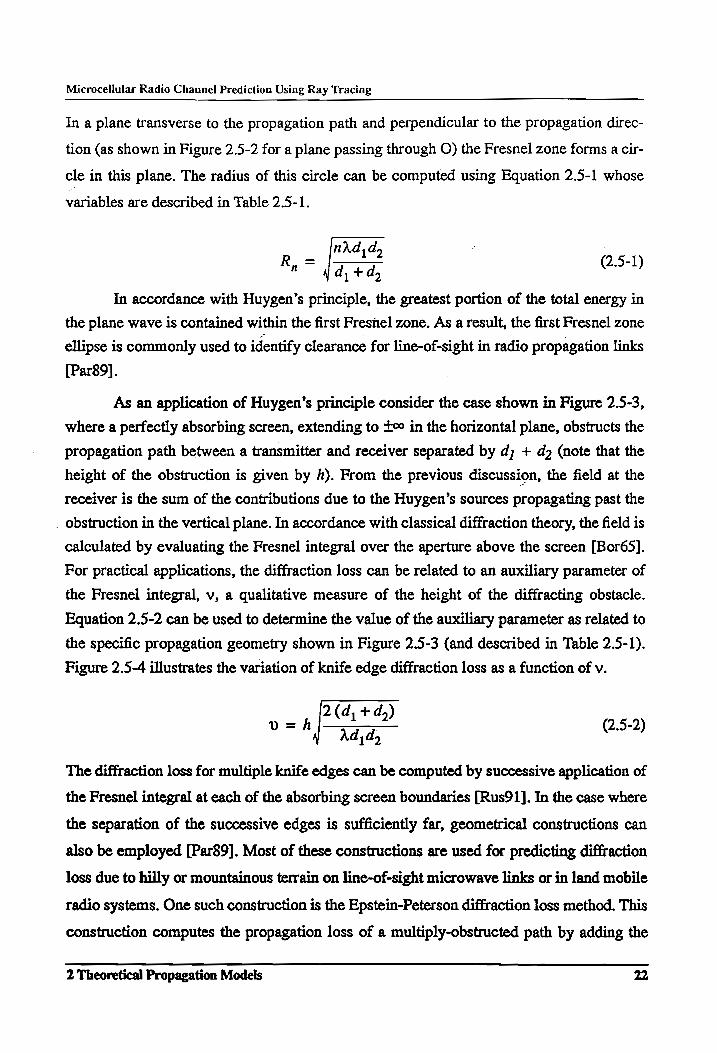
2.2 Free Space Path Loss [Col85][Gri87][Stu81]
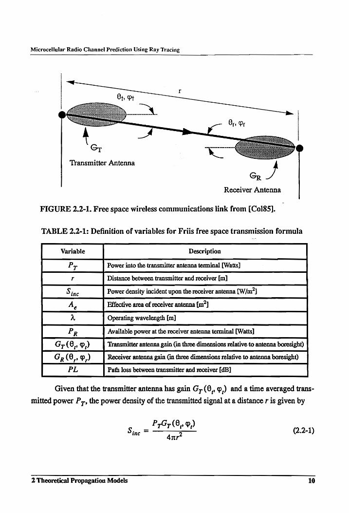
To understand the transfer of electromagnetic energy in a wireless communications
system, consider the communications link shown in Figure 2.2-1. Assume that the trans-
mitter and receiver antennas are located in free space and lie in separate planes such that
the variable r in the figure represents the three dimensional antenna separation. Notice that
a single ray is used to show the flow of energy from the transmitter to the receiver. Assum-
ing an isotropic propagation medium, we know that the ray travels a straight line path
from the transmitter to the receiver (i.e., the distance, 7, is the ray path length).
2 Theoretical Propagation Models 9
Microcellular Radio Channel Prediction Using Ray Tracing
Transmitter Antenna
SESS Receiver Antenna
FIGURE 2.2-1. Free space wireless communications link from [Col85].
TABLE 2.2-1: Definition of variables for Friis free space transmission formula
Variable Description
Pr Power into the transmitter antenna terminal [Watts]
r Distance between transmitter and receiver [m]
Sinc Power density incident upon the receiver antenna [W/m]
A, Effective area of receiver antenna [m7]
A Operating wavelength [m]
Pr Available power at the receiver antenna terminal [Watts]
Gr (0, 9,) Transmitter antenna gain (in three dimensions relative to antenna boresight)
Gp(8.,,) Receiver antenna gain (in three dimensions relative to antenna boresight)
PL Path loss between transmitter and receiver [dB]
Given that the transmitter antenna has gain G, (0, ,) and a time averaged trans-
mitted power P,,, the power density of the transmitted signal at a distance r is given by
_ P7Gr (0, ?,)
inc Anr?
(2.2-1)
2 Theoretical Propagation Models 10
Microcellular Radio Channel Prediction Using Ray Tracing
The effective area of an antenna A, is a measure of the ability of the antenna to convert the
incident power density of an incoming wave to a time-average power level at the antenna
terminals. The effective area of the receiver antenna is related to the receiver antenna gain
by (Stu81]
42
A, = Ga(8,,,) 7 (2.2-2)
Thus, the time-averaged power available at the receiver antenna terminals (Equation 2.2-
3) is the incident power density (;,,) multiplied by the effective area of the receiver
antenna (A,)
x 2
Pp = P7G7O9,)GRO»9,) (FZ) : (2.2-3)
Equation 2.2-3 is commonly known as Friis free space transmission formula. Note that the
received power is inversely related to the square of the propagation length r which agrees
with the intensity law of Geometrical Optics.
A more convenient form of Equation 2.2-3 considers each of the individual quanti-
ties in decibel form
A Pp(dBm] = P;[dBm] +G,[(dBi] + Gp [dBi] +20 xlog,, (7) . (2.2-4)
Path loss is defined here as the difference between the transmitted and received power.
PL[dB] = P;(dBm] —P, [dBm] (2.2-5)
Thus, the path loss between two antennas located in free space is given by
PL(r) [4B] = 20xlog (~~) — Gy [dBi] - Gp [dBi] (2.2-6)
Equation (2.2-6) is independent of Py since free space is a homogenous medium
(behaves linearly) for practical transmitter power levels. Equation 2.2-6 is the actual free
space path loss between two antennas. If path loss is referenced to isotropic antennas
(G; = Gp = 1 = 0 dBi), then
2 Theoretical Propagation Models il
Microcellular Radio Channel Prediction Using Ray Tracing
PL(r) [dB] = 20 x log yg (~) (2.2-7)
Referencing the path loss to isotropic radiators is equivalent to evaluating path loss strictly
due to the radio channel, without the influence of the antenna patterns.
Equivalently, free space path loss at an arbitrary distance r can be scaled to the free
space path loss at a reference distance r,, and is given by :
PL (r) [4B] = 20Xlog49(—) ~ Gp [4Bi] ~ Gg [dBi]. (2.2-8)
Although this formulation is less common in practice, it is shown here to empha-
size that in ideal wireless links, path loss is a function of the propagation path length
alone, as it is a measure of the spreading loss incurred as the wave propagates through
space. The power in the wave is distributed over a larger area in space. When characteriz-
ing a mobile radio channel, it is common to use a free space reference for path loss
[Rap90][Dev87][Par89]. This is done so that the propagation path loss is independent of
the transmitter power level, and thus is a useful quantity for system design.
2.3 Properties of an Electromagnetic Wave at an Interface
In order to model propagation in the mobile and portable radio environment, it is
important to understand how the electromagnetic wave interacts with the environment. A
reasonable approximation to this interaction is to assume the incident energy is a plane
wave impinging on some infinite electromagnetic boundary representing the actual finite
obstruction (e.g., a building face, ground, etc.).
2.3.1 The Laws of Reflection and Transmission [Sil49]
As an application of geometrical optics and Fermat’s principle, we shall consider
the derivation of the laws of reflection and transmission at the interface between two infi-
nite, homogeneous media. Let the point O in Figure 2.3-1 represent the point for which the
propagation path length from P; to O to P> is a minimum. From Fermat’s principle, we
know that the total path is composed of two straight line segments P ;O and OP 2. Consider
a neighboring reflecting point O’ separated from O by tl. To derive the law of reflection,
we shall determine the variation in path length as the location of O’ is changed.
2 Theoretical Propagation Models 12
Microcellular Radio Channel Prediction Using Ray Tracing
x Py (py + 5p, )(s} + dsj) P.
e
“ee, Y
P181 free space (Pp; + 5p 1)(S] + S31)
Ho,Eo x=0
Uy,€ O tol O'
dielectric medium
FIGURE 2.3-1. Geometry used for deriving the law of reflection in free space.
TABLE 2.3-1: Description of variables used for deriving the laws of reflection and
refraction.
Variable Description
Ny, Ny Refractive index of free space (, = 1) and dielectric medium
Sy, 52 . | Unit vector in the direction of P7O and OP 9, respectively
5, + Bs), 52 + bs, Unit vector in the diréction of P7 O’ and O’ P9, respectively
Py P2 Length of the lines P7O and OP, respectively
1dr, Pedr, Length of the lines P; O’ and O’ P9, respectively t Unit vector in the direction of OO’ lying in the x = 0 plane
di Length of the line OO’
8L Variation in the propagation path by way of O w.r.t O”
n Surface normal for the dielectric medium
From Table 2.3-1 we note that the difference in path length between P;OP> and
PO’P> is given by
SL = n, (dp, + 5p,) (2.3-1)
From the figure observe that vector addition yields
(p, + 5p,) (5, +55,) = ps5, + 15! (2.3-2)
2 Theoretical Propagation Models 13
Microcellular Radio Channel Prediction Using Ray Tracing
(p, + dp,) (s,+8s,) = P55y + TS! (2.3-3)
Since we are minimizing the terms w.r.t 51, we have
tO! = p,5,+p,d5, (2.3-4)
—t8! = 3p,5, + p,55, a (2.3-5)
Now, taking the dot product of both sides of 2.3-4 (w.r.t. s,) and 2.3-5 (w.r.t. sz) and recog-
nizing that s, 5s, = 0 and s,°¢6s, = 0 for the a vanishing small variation between the
paths P;OP>2 and P;O’P2, we.have
s,°t5l = Sp, (2.3-6)
S,° T5] = dp, - (2.3-7)
Substituting 2.3-6 and 2.3-7 into 2.3-1 and applying Fermat’s principle we have
SL = n,(s,—5,) > td! = 0 ~ (2.3-8)
Again, according to Fermat’s principle, the relation in 2.3-8 must hold for all values of 51
which produces
(s]—55) °t = 0. (2.3-9)
This result yields the following two relationships known as the law of reflection
e The surface normal, incident ray, and reflecting ray all lie in the same plane
¢ The incident and reflected rays make equal angles with the surface normal. That is, the incident and reflected rays follow Snell’s law of reflection, 8, = @..
For the geometry shown in Figure 2.3-1, the path P;OP 2 is commonly known as the spec-
ular reflection path and point O is subsequently termed the specular reflection point.
The law of refraction is derived using a similar method. From Figure 2.3-2 we note
that the variation between the paths P;OP and P;O’P2 is given by
OL = n, dp, +n 5p, = (ns, — NyS>) ° tol. (2.3-10)
Again applying Fermat’s principle this reduces to
2 Theoretical Propagation Models 14
Microcellular Radio Channel Prediction Using Ray Tracing
(n,5)—M 5.) °tT = 0 (2.3-11)
This result yields the following two relationships known as the law of transmission
¢ The surface normal, incident ray, and refracted ray all lie in the same plane
e The angles the incident and transmitted rays make with surface normal is proportional
to the ratio of the refractive indexes of the two media and is given by
sin0, n,
1 My
Equation 2.3-12 is also known as Snell’s law of refraction.
Py AN X n
A e, Zz
free space P15) A“. | (Py + SpyNs1 + bs)) _Y %e
1 “tea O ,
Ho,E9 CLLLLLLLLLLLLLLLLLLLLLLLLL LL
Lig,€ x=
&
dielectric medium
PPP OLD Ow.
Y (py + 8p1)(s1 + Bs}) FIGURE 2.3-2. Geometry used for deriving the law of refraction in free space.
When dealing with the reflection and transmission of energy at an interface, it is
important to guarantee that energy is always conserved. That is, at any interface the sum of
the energy reflected, transmitted, or otherwise dispersed by the medium (scattered or
absorbed) must be equal to the incident energy. For media with well known dielectric
properties, the Fresnel coefficients can be used to determine the ratio of reflected and
transmitted fields to the incident electromagnetic field that impinges on a boundary
[Col85]. For parallel (vertical) and perpendicular (horizontal) polarization the reflection
coefficients, I’, are defined as
2 Theoretical Propagation Models | 15
Microcellular Radio Channel Prediction Using Ray Tracing
N,cos68,— 1, cos. r= fl ! (2.3-13)
| 1], c0s8, + 1), cos6;
N,cos8,— 1, cos8,
r= 1),cos8, + 7], cos8,” (2.3-14)
Alternatively, the corresponding transmission coefficient, T, is found from T =1-Fr.
2.3.2 The Rayleigh Criterion and Rough Surface Scattering [Bec63]
In the mobile and portable radio environment, it is unlikely that the reflecting sur-
faces will always satisfy the conditions necessary for specular reflection (i.e., the surfaces
must be smooth, infinite, and homogeneous). When variations in the surface are present,
and these variations are on the order of the carrier wavelength, the surface appears rough
(i.e., the reflecting surface appears to be a multifaceted surface yielding several reflections
for a single incident wave) and the incident energy is scattered by the surface. Thus we
shall consider the energy scattered from a generalized surface to be composed of two com-
ponents: a specular component and a diffusely scattered component. In’the limiting cases,
scattering from a perfectly smooth surface results only in a specular reflection and scatter-
ing from a “perfectly” rough surface results in diffuse component. Diffuse scattering is a
phenomenon that occurs over some finite region of a surface and consequently it has little
directivity [Bec63].
The measure of the roughness of a surface is commonly determined by the Ray-
leigh Criterion. Rough surfaces are those where h, the maximum height of the surface
irregularities, obeys the following inequality
Ar
he Fond (2.3-15)
Note that 6 is the angle the incident wave makes with the scattering surface. The Rayleigh
Criterion is selected to delineate between diffuse scattering (where the phase variation
between scattered rays is m) and specular reflection (where the phase variation is 0), as it
is the region where the maximum phase variation between the rays scattered from the sur-
face is m/2. Considering the surfaces typically found in a microcellular environment
(e.g., building walls, pavement, ground, etc.) it is unlikely that, other than at near normal
incidence, these surfaces will satisfy the criterion for roughness in the UHF and low
2 Theoretical Propagation Models 16
Microcellular Radio Channel Prediction Using Ray Tracing
microwave bands. As a result, much of the incident energy will appear in the specular
component, reduced in amplitude from its theoretical value due to a portion of the energy
being diffusely scattered. The generalized scattering from the surface will tend to be in the
specular direction.
2.4 The Bistatic Radar Equation [Sko70][Stu81][Gri87]
The bistatic radar equation is commonly used to model scattering in mobile and
portable radio environments [Sei92b][Tak91]. The bistatic radar equation relates the char-
acteristics of a transmitter (e.g., the transmitter ‘power and antenna gain) with the power
intercepted and reradiated by a target, to the power available at a co-located receiver.
Assuming free space transmission from the transmitter to the scatterer, the incident power
density at some distance, 7, from the transmitter is given by Equation 2.1-1 and the power
intercepted and reradiated by the target is
P target ~ OS inc (2.4-1)
Where o, the radar cross section of the target, is a measure of the ratio of incident energy
to the energy scattered toward the receiver. The power received at a distance rz from the
target follows from successive application of Equation 2.2-3 for the transmitter-scatterer-
receiver path and is given by
P7G7(0,9)Gp0,9)¥o R= (2.4-2)
(42)? (ry)? (72)?
or in decibel form
Pp{dBm] = P;[dBm] +G,[dBi] + Gp [dBi] + 20 x log ,, (A)
+1og 19 (a) —30 x log ;) (4) — 20 x log 19 (7) — 20 x log 19 (72) (2.4-3)
As can be seen in Equation 2.3-1, the radar cross section has units of area. In for-
mal terms, the radar cross section (RCS) is defined as an effective area relating the energy
uniformly illuminating a target to the energy isotropically (diffusely) reradiated by that
target. The RCS of an object is theoretically determined as the ratio of the scattered field to
the incident field as the distance between the target and the observation point approaches
infinity (i.ec., the target is in the far field and is considered a point source). Thus the scat-
2 Theoretical Propagation Models 17
Microcellular Radio Channel Prediction Using Ray Tracing
tered field is the ratio of the field due to the presence of the target to the field that would
exist if the target were absent and the source properties were not changed. The bistatic
RCS is a function of the incident and scattering directions, the shape, orientation, and sur-
face characteristics of the target, and the polarization of the incident field. Even with the
far field condition in place, RCS evaluation is a complicated, tedious procedure and ana-
lytical results are only available for simple geometric shapes [Kno85][Ruc70}[Cri68].
2.4.1 Radar Cross Section of a Flat Plate
One shape for which an analytical result is available is the flat conducting plate.
The result is obtained by using physical optics to approximate the induced surface fields
on a flat, perfectly conducting, plate and then integrating these fields over the surface of
the plate to obtain the total scattered field [Ruc70]. In the high frequency limit, the physi-
cal optics solution is identical to a geometric optics solution. However, for practical prob-
lems, physical optics overcomes the limitations of geometrical optics by including the
dimensions of the scatterer. For the flat plate shown in Figure 2.4-1, physical optics yields
a bistatic RCS given by [Kno85]
_kL,. ALT Am Az sin (sinOcos@ + sinOcos¢)
o= 2 cos8cosp
> (sinOcose + sin6cos¢@)
sin (sinOsing + sinOsing) (2.4-4)
mn (sin@sing + sin6sing)
where A is the wavelength, k = 2n/A is the wavenumber, L is the length of the plate,
W is the width of the plate, and A is the area of the plate. Observe from the figure that the
angles @,@ describe the direction of the incident ray and the angles 6, p describe the
direction of the scattered ray. For future reference, the specular direction is given by
6=0 andp=nx+Q.
The relation given by Equation 2.4-4 is valid for plates whose dimensions are large
as compared with the wavelength. The scattering pattern described by this relation is a
three-dimensional sin (x) /x pattern with the main scattering lobe in the specular direc-
tion. The width of the main lobe, and the subsequent spacing the pattern nulls, is inversely
2 Theoretical Propagation Models 18
Microcellular Radio Channel Prediction Using Ray Tracing
proportional to the dimensions of the plate. That is, as the length and width of the plate
increases, the return decays rapidly as the scattering angle increases relative to the specu-
lar angle. The bistatic RCS of a flat, conducting plate is a useful tool for modeling scatter-
ing in mobile and portable radio environments.
FIGURE 2.4-1. Geometry to evaluate the scattering from a flat, conducting plate
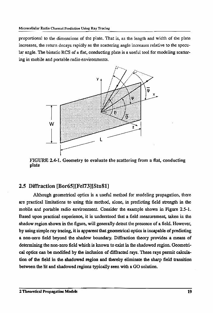
2.5 Diffraction [Bor65][Fel73][Stu81]
Although geometrical optics is a useful method for modeling propagation, there
are practical limitations to using this method, alone, in predicting field strength in the
mobile and portable radio environment. Consider the example shown in Figure 2.5-1.
Based upon practical experience, it is understood that a field measurement, taken in the
shadow region shown in the figure, will generally detect the presence of a field. However,
by using simple ray tracing, it is apparent that geometrical optics is incapable of predicting
a non-zero field beyond the shadow boundary. Diffraction theory provides a means of
determining the non-zero field which is known to exist in the shadowed region. Geometri-
cal optics can be modified by the inclusion of diffracted rays. These rays permit calcula-
tion of the field in the shadowed region and thereby eliminate the sharp field transition
between the lit and shadowed regions typically seen with a GO solution.
2 Theoretical Propagation Models 19
Microcellular Radio Channel Prediction Using Ray Tracing
Diffraction and scattering are variations of the same physical process, in fact, the
terms diffraction and scattering can be used interchangeably when referring to the field in
the presence of an obstacle. Similar to the radar backscatter problem, diffraction problems
tend to be difficult electromagnetic problems and analytical results are available for only a
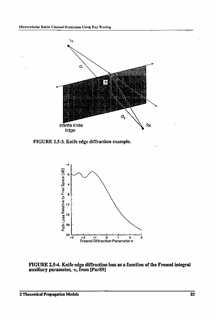
handful of simple geometric forms. Two such analytical results, the infinite knife edge and
the infinite 90° wedge are summarized in the following sections
Lit Region
Incident Rays
Shadowed Region
SE
Ces Diffracted Ray
a
Obstruction
FIGURE 2.5-1. Diffraction example. The diffracted ray is added to predict the field in the shadowed region
2.5.1 Knife Edge Diffraction [Gri87][Par$2]
Central to the theory of knife edge diffraction is Huygen’s principle, which states
that each point on a plane wave acts as an independent point source (Huygen’s source) and
that these point sources combine in a way to yield a new plane wave in the direction of
propagation. However, in order for each of these sources to combine in a way that the
resulting plane wave has uniform intensity, the ensemble of point sources has an ampli-
tude distribution. This amplitude distribution is a maximum in the plane wave propagation
direction. We can use this concept of independent sources to explain the existence of the
diffracted field shown in Figure 2.5-1. As some of the secondary sources are absorbed (or
blocked) by the obstacle, the remaining sources no longer combine to produce a plane
wave radiating in the original direction of propagation. Rather, a portion of the incident
2 Theoretical Propagation Models 20
Microcellular Radio Channel Prediction Using Ray Tracing
energy propagates around the obstacle, and into the shadowed region. The amplitude dis-
tribution on each of the Huygen’s sources impacts the intensity of the diffracted field; the
field amplitude decreases as the observation point moves farther into the shadowed region.
Since knife edge diffraction loss is related to mutual interference by the Huygen’s
sources, it is important to quantify the nature of this interference. An annular region,
known as the Fresnel zone is defined such that all of the energy contained within it inter-
feres constructively at an observation point. Note that the Fresnel zone boundary is
defined as the locus of points which are equal to the path length of the direct path plus an
integral number of half-wavelengths. Thus, there are multiple Fresnel zones, where each
zone is denoted by the number of half-wavelengths used to define the zone boundary. Fig-
ure 2.5-2 shows the first Fresnel zone region for a transmitter and receiver separated by d;
+ a. The first Fresnel zone, as compared to higher order zones, contains the greatest por-
tion of energy in the total field
1X
FIGURE 2.5-2. Fresnel zone ellipse for a transmitter and receiver separated by dj + dz. The energy contained within the ellipse constructively interferes at the receiver.
TABLE 2.5-1: Description of parameters used in evaluating knife edge diffraction
loss
Variable Description
d, Distance from the transmitter to the plane transverse to the direct path that includes the point O
d, Distance from the receiver to the plane transverse to the direct path that includes the point O
ry Distance from the transmitter to the point O
ro Distance from the receiver to the point O
h Fresnel zone radius at the point O (alternatively, the height of the obstruction)
R, Maximum radius of the n' Fresnel zone v Auxiliary parameter of the Fresnel integral
2 Theoretical Propagation Models 21
Microcellular Radio Channel Prediction Using Ray Tracing
In a plane transverse to the propagation path and perpendicular to the propagation direc-
tion (as shown in Figure 2.5-2 for a plane passing through O) the Fresnel zone forms a cir-
cle in this plane. The radius of this circle can be computed using Equation 2.5-1 whose
variables are described in Table 2.5-1.
R= [ae (2.5-1) nda, +d, ,
In accordance with Huygen’s principle, the greatest portion of the total energy in
the plane wave is contained within the first Fresnel zone. As a result, the first Fresnel zone
ellipse is commonly used to identify clearance for line-of-sight in radio propagation links
{Par89].
As an application of Huygen’s principle consider the case shown in Figure 2.5-3,
where a perfectly absorbing screen, extending to to in the horizontal plane, obstructs the
propagation path between a transmitter and receiver separated by dj; + dz (note that the
height of the obstruction is given by A). From the previous discussion, the field at the
receiver is the sum of the contributions due to the Huygen’s sources propagating past the
. obstruction in the vertical plane. In accordance with classical diffraction theory, the field is
calculated by evaluating the Fresnel integral over the aperture above the screen [Bor65].
For practical applications, the diffraction loss can be related to an auxiliary parameter of
the Fresnel integral, v, a qualitative measure of the height of the diffracting obstacle.
Equation 2.5-2 can be used to determine the value of the auxiliary parameter as related to
the specific propagation geometry shown in Figure 2.5-3 (and described in Table 2.5-1).
Figure 2.5-4 illustrates the variation of knife edge diffraction loss as a function of v.
2 (d, +d,)
The diffraction loss for multiple knife edges can be computed by successive application of
the Fresnel integral at each of the absorbing screen boundaries [Rus91]. In the case where
the separation of the successive edges is sufficiently far, geometrical constructions can
also be employed [Par89]. Most of these constructions are used for predicting diffraction
loss due to hilly or mountainous terrain on line-of-sight microwave links or in land mobile
radio systems. One such construction is the Epstein-Peterson diffraction loss method. This
construction computes the propagation loss of a multiply-obstructed path by adding the
2 Theoretical Propagation Models 22
Microcellular Radio Channel Prediction Using Ray Tracing
TX
Infinite Knife Edge
FIGURE 2.5-3. Knife edge diffraction example.
-—4r
Path Loss Re
lati
ve
to Free Sp
ace
(dB)
24 : 4 4 a 1 : i a | ,
-3 -2 -1 0 1 2 3 Fresnel Diffraction Parameter vy
FIGURE 2.5-4. Knife edge diffraction loss as a function of the Fresnel integral auxiliary parameter, v, from [Par89]
2 Theoretical Propagation Models 23
Microcellular Radio Channel Prediction Using Ray Tracing
attenuations (in dB relative to free space) produced by each individual knife edge. Com-
parisons of the geometric construction against rigorous solutions shows that the method is
most accurate when the separation between successive knife edges is large (e.g., two
mountains separated by several kilometers) [Eps53]. Although errors are introduced in the
transition region or when the obstacles are closely spaced, the Epstein-Peterson method is
a tractable alternative for modeling diffraction loss in an automated fashion.
2.5.2 Wedge Diffraction [Fel73]
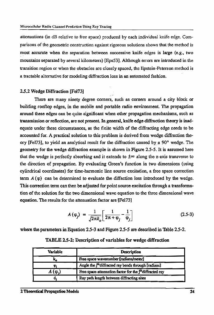
There are many ninety degree corners, such as corners around a city block or
building rooftop edges, in the mobile and portable radio environment. The propagation
around these edges can be quite significant when other propagation mechanisms, such as
transmission or reflection, are not present. In general, knife edge diffraction theory is inad-
equate under these circumstances, as the finite width of the diffracting edge needs to be
accounted for. A practical solution to this problem is derived from wedge diffraction the-
ory [Fel73], to yield an analytical result for the diffraction caused by a 90° wedge. The
geometry for the wedge diffraction example is shown in Figure 2.5-5. It is assumed here
that the wedge is perfectly absorbing and it extends to +o along the z-axis transverse to
the direction of propagation. By evaluating Green’s function in two dimensions (using
cylindrical coordinates) for time-harmonic line source excitation, a free space correction
term A(@) can be determined to evaluate the diffaction loss introduced by the wedge.
This correction term can then be adjusted for point source excitation through a transforma-
tion of the solution for the two dimensional wave equation to the three dimensional wave
equation. The results for the attenuation factor are [Fel73]
1 1 1 A(g) = ——)| ~~ - — 2.5-3 (e) PE | Te =| (2.5-3)
where the parameters in Equation 2.5-3 and Figure 2.5-5 are described in Table 2.5-2.
TABLE 2.5-2: Description of variables for wedge diffraction
Variable Description
k, Free space wavenumber [radians/meter]
9; Angle the j"diffracted ray bends through [radians]
A(9,) Free space attenuation factor for the j"diffracted ray
d, Ray path length between diffracting sites
2 Theoretical Propagation Models 24
Microcellular Radio Channel Prediction Using Ray Tracing
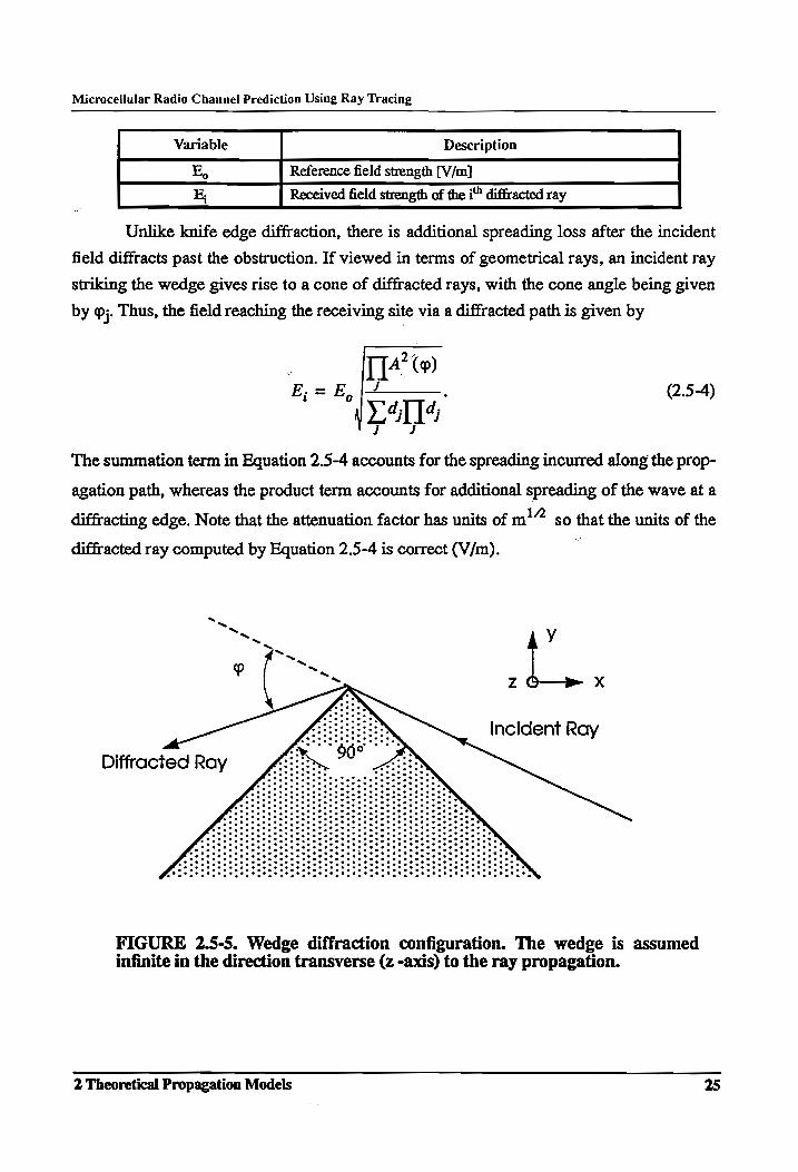
Variable Description
E, Reference field strength [V/m]
E, Received field strength of the i” diffracted ray
Unlike knife edge diffraction, there is additional spreading loss after the incident
field diffracts past the obstruction. If viewed in terms of geometrical rays, an incident ray
striking the wedge gives rise to a cone of diffracted rays, with the cone angle being given
by 9. Thus, the field reaching the receiving site via a diffracted path is given by
2@ — (2.5-4) Yas J Jj
The summation term in Equation 2.5-4 accounts for the spreading incurred along the prop-
agation path, whereas the product term accounts for additional spreading of the wave at a
diffracting edge. Note that the attenuation factor has units of m!” s0 that the units of the
diffracted ray computed by Equation 2.5-4 is correct (V/m). .
~. y
Y oe SL ,
el el lele e ele lele ecole ele
(CREE Incident Ray ee a eee ew et or oe ee et ee eee eee
Diffracted Ray
wm ete tate Me Sate te wear ate WF Fw we Ce ee ee ee ee ee re Se eo wr ere ew a we et ee ew ew ele Ce ee ee ee a ee i ee Se ee Se er | Ce ee Ge ee ee ee ee a)
eat e tata eter tata eta at at ate ew wae tae ware e ee ae ela ele wre wl aot ew we wwe ea tae eee Ce ee ee Ge ee | Be oe ew st oe we ee we te ee ele ae se Soe ee oe wee ee eet ee eee ee a oe oe wee we we ee we ae ee wae tet ete eta te tat arate tate tetas arte tet acts ew eae we a ee ae ew oe ee oa wae e Ce i er i ee ee ee Pe er) ear a ew ea eae a ee ee ee ee ee te ee ee A | ee a ew ee ea et we et ee ee ee tee ae ere te oe ee tt ee tt ee ew te we ee
ena ete tat et eta tata tot at aot oat ere te tat ete tet et ete ee aa eee wee aC et ee wet a orate al ols ere ee oe ew we ee ew ee te ee ee et ee ee oe Ce ee Oe ee ee OG ee SO Se ee ee a | Ce ee ee | eo ee a ee ee ee oe eee we eet ole ee eee! Se ee Ge OG SR ee A
orate t ase tat ate tata ate ete tate tat ete tate tates ato te tetates ee ee ee ee ew ae ew a we wr ew ee eo ee ee ee eee ee eee ee ce we et wee eee ee ele le ee ee eet te tet eee eee wate ete te wate ete et we a a ate eta ne ct ee arte ete
FIGURE 2.5-5. Wedge diffraction configuration. The wedge is assumed infinite in the direction transverse (z -axis) to the ray propagation.
2 Theoretical Propagation Models 25

Microcellular Radio Channel Prediction Using Ray Tracing
2.6 Summary
This chapter has presented several theoretical models and specific analytical
results for modeling energy transport in mobile and portable radio environments. The fol-
lowing observations can be made regarding the information presented here:
e Using geometrical optics, the transport of energy can be determined without the need to
explicitly solve Maxwell’s equations. Rather, it can be determined strictly through geo-
metrical concerns by modeling the propagating wave as a collection of rays.
¢ The direction of a reflected and transmitted wave after impinging on a dielectric bound- ary can be determined from the angle of incidence of the wave and the properties of the
boundary. Energy must be conserved at the boundary.
¢ The actual received power level can be determined by relating the characteristics of the transmitter, receiver, and most importantly, the environment, using Friis’ free space
equation or the bistatic radar equation.
e Knife and wedge diffraction provide a direct method for evaluating the energy received in shadowed topographies when geometrical optics solution is inadequate. These tech-
niques provide a means of quantifying diffraction loss without the need of time-con- suming numerical evaluations.
2 Theoretical Propagation Models 26
Microcellular Radio Channel Prediction Using Ray Tracing
3 Literature Review
- This chapter provides a review of literature regarding propagation measurements
and modeling in the mobile and portable radio environment. For clarity, some definitions
are presented first. Most of the terms defined here are used throughout the thesis, and thus
deserve a formal definition and a brief explanation of their significance. The literature
review which follows is divided into several sections. Each section is devoted to a particu-
lar aspect of propagation measurements and modeling. The sections are arranged so that
the discussion moves progressively toward site-specific propagation.
3.1 Background
This section defines several terms used throughout the thesis. A brief discussion
regarding the significance of each of these terms is also provided.
3.1.1 Multipath Propagation
As discussed in Section 2.2, a signal propagating in free space follows a 1/ a
dependence where d is the propagation path length traveled by the signal. In an idealized
radio channel, this same power law dependence holds. However, practical wireless com-
munication channels are not ideal as they are subjected to conditions where the signal can
propagate to the receiver via multiple paths. These multiple paths are the result of the sig-
nal reflection, transmission, and scattering by obstacles such as buildings, trees, and auto-
mobiles along the propagation path. Radio waves therefore arrive at the receiver from
different directions and with different time delays, but combine vectorially at the receiver
to yield a resultant signal. Depending upon the characteristics of each multipath signal, the
summation results in large fluctuations (fading) of the received signal voltage. A receiver
at one location may exhibit a received signal strength several orders of magnitude greater
than a receiver only a short distance away.
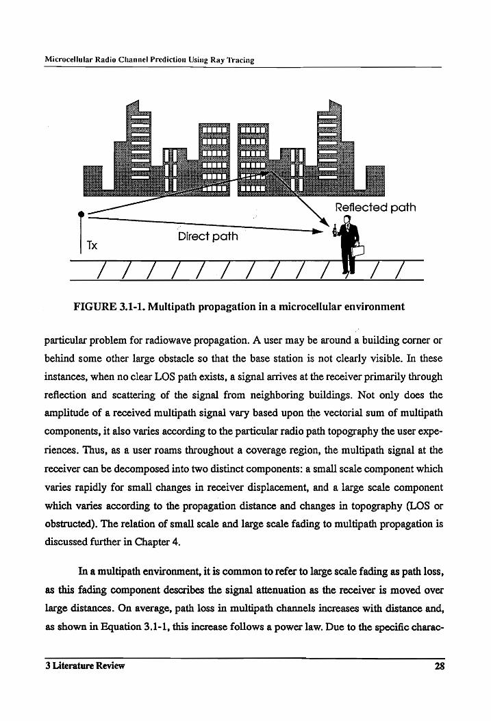
A simplified example of multipath propagation, in an urban environment, is shown
in Figure 3.1-1, where a direct or line-of-sight (LOS) and building reflected ray are shown
to arrive at the receiver. In these environments, large buildings and other obstacles pose a
3 Literature Review 27
Microcellular Radio Channel Prediction Using Ray Tracing
Reflected path
Direct path
TX
S/S SF SS SSS SBS /
FIGURE 3.1-1. Multipath propagation in a microcellular environment
particular problem for radiowave propagation. A user may be around a building corner or
behind some other large obstacle so that the base station is not clearly visible. In these
instances, when no clear LOS path exists, a signal arrives at the receiver primarily through
reflection and scattering of the signal from neighboring buildings. Not only does the
amplitude of a received multipath signal vary based upon the vectorial sum of multipath
components, it also varies according to the particular radio path topography the user expe-
riences. Thus, as a user roams throughout a coverage region, the multipath signal at the
receiver can be decomposed into two distinct components: a small scale component which
varies rapidly for small changes in receiver displacement, and a large scale component
which varies according to the propagation distance and changes in topography (LOS or
obstructed). The relation of small scale and large scale fading to multipath propagation is
discussed further in Chapter 4.
In a multipath environment, it is common to refer to large scale fading as path loss,
as this fading component describes the signal attenuation as the receiver is moved over
large distances. On average, path loss in multipath channels increases with distance and,
as shown in Equation 3.1-1, this increase follows a power law. Due to the specific charac-
3 Literature Review 28
Microcellular Radio Channel Prediction Using Ray Tracing
teristics of the propagation path, however, path loss varies around some mean value. This
has led several researchers to statistically describe path loss in multipath channels by a
log-normal distribution about this mean value, given by [Dev86][Rap89][Sei9 1]
PL(d) «d’. (3.1-1)
In (3.1-1), d represents the transmitter-receiver separation and n represents the mean path
loss exponent (for free space propagation 7 = 2). The use of this model to describe propa-
gation characteristics in the mobile and portable radio environment is discussed in the fol-
lowing sections.
3.1.2 Delay Spread and Coherence Bandwidth [Lee82]
As indicated in Section 3.1.1, the signal received in a multipath channel is com-
posed of several attenuated, time delayed replicas of the transmitted signal. The attenua-
tion of the signal is due spreading loss and the interaction of the transmitted signal with
obstructions along the propagation path, whereas the time delay corresponds to the time
required for transmission over the propagation path. Each replica, or multipath compo-
nent, propagates to the receiver along different propagation path which has a specific path
length associated with it. This path length corresponds to a specific arrival time at the
receiver. Consider a specific case where the transmitted signal is an impulse. When this
signal is received after propagating through a multipath channel, it is no longer an impulse
but rather a pulse with a finite width. This pulse width is termed the delay spread of the
signal.
Measured data indicate that delay spread is a function of the multipath environ-
ment (methods for calculating delay spread from measured data are described in Section
6.6). For example, longer delay spreads (At between 2 and 10 |tsec) are generally
observed in urban areas such as New York City or San Francisco rather than in suburban
areas where At is near 0.5 |tsec [Cox73][Rap90]. Delay spread is important when consid-
ering digital transmission through multipath channels, since it limits the maximum data
transmission rate that can be achieved in the medium (1.e., delay spread must be less than
the transmission bandwidth to ensure that the signal can propagate through the channel
3 Literature Review 29
Microcellular Radio Channel Prediction Using Ray Tracing
without significant distortion). As a result, it is important to have measures for both the
delay spread that exists in the channel, and how the delay spread impacts the maximum
data transmission rate that can be achieved.
A common measure for a practical transmission rate (i.e., transmission bandwidth)
in a multipath channel is known as the coherence bandwidth. Since the message signal
occupies a finite bandwidth, it is important to understand the effects of multipath propaga-
tion over the entire message signal bandwidth. The coherence bandwidth is a measure of
this effect, since it is the frequency band over which the statistics (amplitude or phase) of
each multipath component are highly correlated. Consider two spectral components within
the message bandwidth. If the frequency separation between these signals is small, the dif-
ferent propagation paths are approximately the same electrical length for both components
and the amplitude and phase of these components is highly correlated. As the frequency
separation increases, however, the electrical lengths change and, in turn, the amplitudes
and phases of the components become uncorrelated. Signals occupying a bandwidth
greater than the correlation bandwidth become distorted due to the variable nature in
which each of the spectral components fade. This effect is known as frequency selective
fading. Frequency selective fading degrades the received signal by causing intersymbol
interference (or ISI, which is signal distortion due to the overlap of adjacent bits) and bit
errors.
3.1.3 Narrow Band versus Wide Band Channels [Par89]
To avoid later confusion, it is important to define the difference between narrow
band and wide band channels. Although it is true that narrow band channels (generally <
30 kHz) occupy a smaller frequency band than wide band channels (generally 2 1 MHz),
using bandwidth alone is insufficient to fully differentiate these two channel types. For-
mally, a narrow band channel occupies a bandwidth significantly narrower than the coher-
ence bandwidth, whereas a wide band channel generally occupies a bandwidth several
times the coherence bandwidth.
Based upon the discussion in Section 3.1.2, it would appear that narrow band chan-
nels are desirable for wireless communication systems because the received signal is rela-
3 Literature Review 30
Microcellular Radio Channel Prediction Using Ray Tracing
tively undistorted relative to the originally broadcasted signal (since the signal bandwidth
is less than the channel bandwidth only noise and interference cause signal distortion).
Wide band channels, on the other hand, can suffer from distortion leading to signal degra-
dation and ISI, in turn, thereby producing unsatisfactory system performance. This is a
one sided, simplistic view of the problem. Wide band systems using digital transmission
can employ modulation, error correction coding, equalization, and signal processing tech-
niques to negate the effects of frequency selective fading. Using these techniques, higher
capacity can be achieved at a grade of service comparable to current analog systems. Dig-
ital transmission provides additional benefits which are not easily realized in the current
analog systems, such as simultaneous voice and data transmission or encryption. These
favorable properties suggest why emerging personal communication systems (PCS) are
digitally based.
3.1.4 Characterization of Narrow Band and Wide Band Channels
To understand how multipath channels are characterized, it 1s important to discuss
the impact of multipath propagation on the received signal for different types of transmit-
ted signals. For example, consider the two different signal profiles shown in Figure 3.1-2.
The two profiles shown in this figure have unique properties, and both profiles are gener-
ated using two very different measurement techniques and systems. However, both pro-
files correspond to signals propagating through the same multipath channel. This
distinction is important; there are several different methods of characterizing the same
channel.
Path loss due multipath propagation and the environment is commonly determined
with a narrow band (CW) measurement system as shown in Figure 3.1-2a. Path loss (the
large scale fading component) is obtained by moving the receiver antenna over a local area
which is on the order of a few wavelengths. This signal is then averaged to remove small
scale fluctuations. The path loss is then determined from this mean signal strength mea-
surement. This measurement technique is typically known as a narrow band characteriza-
tion of the channel [Har89].
3 Literature Review 31
Microcellular Radio Channel Prediction Using Ray Tracing
An alternative method of studying the multipath radio channel, to obtain more
information than signal attenuation alone, is to record its impulse response. The channel
impulse response can be measured directly, in the time domain, by broadcasting short
pulses [Cox73][Dev86][Rap89]. As can be seen by the impulse response profile in Figure
3.1-2b, the narrow pulses yield an approximation to the true impulse response of the chan-
nel. The envelope (power) of the received signal varies with time. The time of arrival, or
delay, of different multipath components correspond to the peaks in the envelope, where
the amplitude of each delayed component is weighted by the signal amplitude at that
delay. Thus, the area under the profile corresponds to the total received power seen at the
measurement location. The impulse response measurement method provides data on both
the average received signal, and the time delay of each multipath component (i.e., the
delay spread of the channel). This technique is commonly known as a wide band charac-
terization of the channel since a wide RF bandwidth is required to transmit the narrow
time pulses. The profile recorded by the receiver is commonly known as a power delay
profile, as it is a measure of the power and delay of each multipath component. Although it
is a powerful measurement technique, wide band channel characterizations are not without
limitations; the resolution of multipath component delays is limited by the transmitted
pulse width.
3.2 Propagation in the Mobile and Portable Radio Environment
Probably the most obvious approach to cellular or microcellular system design is
through extensive field measurements. Statistics on path loss and delay spread are com-
piled from the measurement database, and are then used as system design parameters.
Although simple and direct, there are drawbacks to this method. Field measurements are
costly and are only useful for one site installation. Considerable “back engineering” after
site installation is also necessary to correct for problem areas not detected in the field mea-
surements. Although they have limited usefulness as a universal design tool, field mea-
surements provide valuable insight into the mechanisms governing propagation in the
mobile and portable radio environment. Some of these propagation mechanisms, for con-
ventional cellular and microcellular environments, are discussed in this section.
3 Literature Review 32
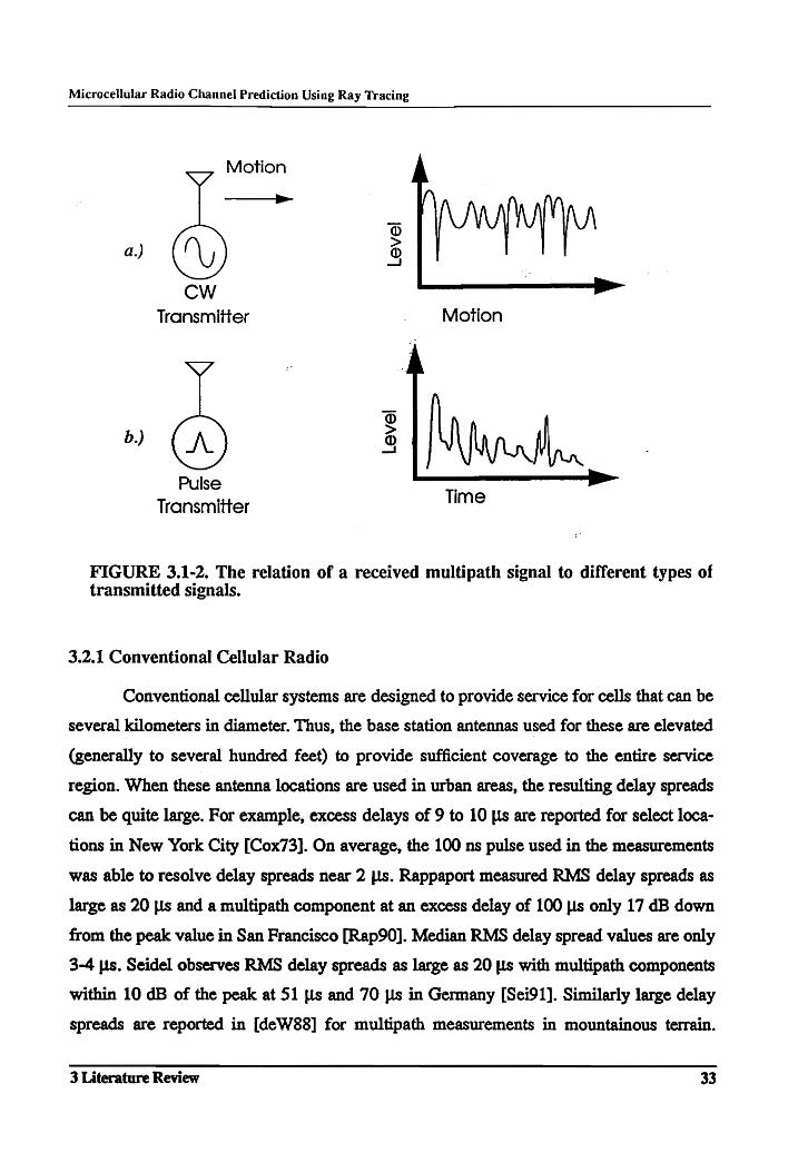
Microcellular Radio Channel Prediction Using Ray Tracing
Motion
—_>
Q a.) o
CW , > Transmitter . Motion
g ™ a Le
Pulse Ti > Transmitter Ime
FIGURE 3.1-2. The relation of a received multipath signal to different types of transmitted signals.
3.2.1 Conventional Cellular Radio
Conventional cellular systems are designed to provide service for cells that can be
several kilometers in diameter. Thus, the base station antennas used for these are elevated
(generally to several hundred feet) to provide sufficient coverage to the entire service
region. When these antenna locations are used in urban areas, the resulting delay spreads
can be quite large. For example, excess delays of 9 to 10 [ls are reported for select loca-
tions in New York City [Cox73]. On average, the 100 ns pulse used in the measurements
was able to resolve delay spreads near 2 [ts. Rappaport measured RMS delay spreads as
large as 20 [is and a multipath component at an excess delay of 100 [ls only 17 dB down
from the peak value in San Francisco [Rap90]. Median RMS delay spread values are only
3-4 ps. Seidel observes RMS delay spreads as large as 20 Ls with multipath components
within 10 dB of the peak at 51 [ls and 70 [ls in Germany [Sei91]. Similarly large delay
spreads are reported in [deW88] for multipath measurements in mountainous terrain.
3 Literature Review 33
Microcellular Radio Channel Prediction Using Ray Tracing
Delays spreads as large as 10 [ts and median RMS delay spreads between 4-5 [Us are
observed.
Even with elevated antennas, the path loss in dense urban environments can still be
excessive. Due to large buildings surrounding the mobile receiver, there is usually no LOS
path between the base station and the mobile. The signal, therefore, arrives at the mobile
mainly through diffraction (over the building rooftops to street level) and reflections off
neighboring buildings. Based upon measurements, a path loss exponent of n = 4 is com-
monly recommended as a conservative figure for evaluating coverage [Lee82][Par89]. For
measurements in four European cities, [Sei91] reports path loss exponents between n = 2.5
and n = 3.0, with a worst case value of n = 3.8. Results here also indicate that the exponent
varies according to the reference distance used to compute path loss.
3.2.2 Microcellular Radio
The propagation characteristics of microcells are much differerit than that of con-
ventional, large cell, cellular systems. Instead of a simple mean path loss exponent, several
researchers use a double regression to model the path loss with distance [Gre89][Har89]
[Bla92] for line-of-sight microcells. In the double regression model, path loss increases
slowly (7 is approximately 2) with distance until a breakpoint is reached. After the break-
point, path loss increases very rapidly with distance (7 can range between 4 and 9). The
breakpoint depends on antenna height and frequency. This phenomenon is often described
by a two ray and four ray propagation model [Gre89][Rus91][Tel91]. The two ray model
considers a direct path and a ground reflected path, and the breakpoint is determined
according to Fresnel zone theory. For the four ray model, two additional wall reflected
rays are added, and the breakpoint distance changes according to the street width. This
simple model is very appropriate for microcellular systems since the antennas are
mounted at heights below the roof line of the surrounding buildings. The geometry of the
surroundings make the multi-ray model plausible for computing the regression lines and
breakpoint distance.
In [Gre89], 905.15 MHz narrow band measurements, taken with omni-directional
antennas mounted at 5 meters and 1.5 meters, produce breakpoints at 200 and 300 m. The
3 Literature Review 34
Microcellular Radio Channel Prediction Using Ray Tracing
fading statistics of the CW signals was found to be Rician in microcells, with the Rice K-
factor varying over a measurement path. In traditional cellular systems, the CW fading
follows the Rayleigh distribution [Lee82]. Rician statistics provide a better description for
the small scale, narrow band fading because, in these microcellular channels, the dominant
LOS component prevents the fading from being as extreme as Rayleigh. Microcellular
measurements at 870.15 MHz and 1.8 GHz show that path loss at both frequencies is very
similar, except that the spread, or variation, of path loss for 1.8 GHz signals appears to be
larger [Har89]. It is also observed that the 1.8 GHz signal is more sensitive to shadowing
than the 870.15 MHz signal. That is, when. an obstructing object such as a bus passes
between the transmitter and receiver, deeper fades are observed at 1.8 GHz as compared
with 870.15 MHz.
Multi-frequency measurements at 950 MHz and 1.8 GHz show that a hilly envi-
ronment has a larger standard deviation of path loss than a flat environment [Pie91]. For
the measurements, the base station antennas range from 9 meters to 30 meters in height
and the receiver antenna is fixed at 1.4 meters. The path loss of the two frequencies is
closely related. It is reported that there are more areas exceeding a minimum threshold
(“coverage holes”) at 1.8 GHz due to the increased diffraction loss. More coverage holes
exist at the lower antenna height as well.
Multi-frequency measurements at 955 MHz and 1845 MHz with a base station
antenna height of 5 to 14 meters are presented in [Mog91]. Measurements with antennas
on the top of buildings are also performed. The reported measurements are for streets lined
with three- to five-story apartment buildings. The long term variations of path loss are
highly correlated for the two frequencies and for the two antenna heights. An additional
path loss of 8.7 to 11 dB is observed for 1845 MHz as compared to 955 MHz path loss val-
ues. The base station height-gain is very sensitive at antenna heights near roof top levels,
and is less sensitive for low antenna heights where the relative shadowing effect remains
fairly invariant.
Similar results, for measurements using base station antenna heights of 3.7 meters,
8.5 meters, 13.3 meters for the San Francisco Bay Area are reported in [Tel91]. Path loss
3 Literature Review 35
Microcellular Radio Channel Prediction Using Ray Tracing
exponents ranging between 1.9 and 2.6, with standard deviations between 9.6 and 18.3
dB, are reported. RMS delay spreads range from a worst case value of 549 ns for down-
town San Francisco to 1.86 [1s in Oakland, CA. It is shown that, in built up areas, the
height of the base station antenna does not severely impact the propagation statistics.
However, when the surroundings are on the order of the base station antenna height, the
propagation statistics depend on the exact antenna height.
The penetration of outdoor microcellular signals into buildings at 1735 MHz has
been studied in [Chi91]. Measurements indicate that building penetration loss is a function
of the distance the signal travels within the building and, in many cases, is in excess of 20-
30 dB. Furthermore, the results shown that if the building is located at a distance greater
than the breakpoint, then the penetration is minimal.
3.3 Statistical Propagation Models
The first extension beyond propagation measurements for system design is statisti-
cal modeling and simulation of the channel. The classical statistical model for urban radio
propagation is proposed in [Tur72] and is enhanced in [Suz77][Has79]. The basic
approach is to model the transmission medium as a linear filter, and then analyze peaks in
measured multipath profiles to derive statistical distributions for the multipath component
amplitude and arrival time. Based upon the analysis of measured data, [Suz77] found
component amplitudes, with short excess delays, tend to a Nakagami distribution and late
arriving components (large excess delays) are log-normally distributed. The component
arrival times can be modeled by a modified Poisson process.
Although statistical models are an improvement over purely measurement-based
system design, they still have certain disadvantages. The model is inherently biased by the
ensemble statistics and can not account for the varagies in the environment which impact
the actual propagation conditions. As shown previously, to claim propagation in different
urban areas is statistically similar can not be justified. Clearly, site-specific environmental
data is necessary for accurate evaluation of the channel properties.
3 Literature Review 36
Microcellular Radio Channel Prediction Using Ray Tracing
3.4 Terrain Based Models for Conventional Cellular Radio Service
One of the first applications using site-specific data to predict channel properties
was route planning for line of sight microwave relay links. As use of these links for point-
to-point communication became widespread, adequate carrier-to-noise ratios became diffi-
cult to provide without producing unacceptable interference levels. Thus, terrain based
propagation models were developed so that route planners could analyze the effect of ter-
rain in calculating a link budget and the magnitude of signal interference. Since early cel-
lular systems exhibited propagation characteristics similar to these microwave links, it is
easy to see why these models were applied for planning coverage and interference in areas
with irregular terrain (e.g., trees, hills, buildings, etc.).
Several methods for predicting propagation over irregular terrain appear in the lit-
erature ([Par89] and [Par92] provide an excellent summary). Most of these methods use a
geographic database to construct a terrain profile from a transmitter to several regions
within a proposed service area and then compute the path loss associated with each profile.
For modeling purposes the terrain is segmented into small cells that are stored in the data-
base. These cells are assigned an elevation value and surface characteristics (1.e., bare
ground, foliage cover, water, etc.) based upon field observations. The corresponding path
attenuation is then calculated by computing the free space path loss adjusted by the (knife-
edge) diffraction along the path [Edw69], by a set of ad hoc correction functions for the
terrain profile [Oku68][Hat80][Loe83], or by a hybrid statistical-theoretical technique
[Lon68].
Comparisons of these prediction models against 900 MHz measured data appears
in [Fou87]. The results indicate that theoretical models are more accurate (smaller stan-
dard deviation in error) than empirical models. In addition, it is shown that prediction
accuracy could be enhanced when specific data on building locations of building density is
integrated into the model. In [Ibr83], a modified theoretical model, that adjusts the predic-
tion according to an urban clutter factor, is proposed. Although an improvement in the pre-
diction accuracy is achieved, the authors recognize the need for a predictive model using
an actual building database.
3 Literature Review 37
Microcellular Radio Channel Prediction Using Ray Tracing
3.5 Deterministic Propagation Models
Recently, the need for accurate, site-specific propagation prediction methods has
been identified within the wireless industry. In any recently published technical journal or
conference record related to wireless technology, there is likely to be at least one paper
proposing a new propagation model or automation technique. Considering the breadth of
published material available on different propagation models, it is impractical to attempt a
discussion that includes all of this material. Instead, some of the more essential papers
which address different aspects of propagation prediction are discussed here.
One of the most well known site-specific propagation models is the Ikegami model
[Ike84]. This model is possibly the first model to incorporate both environmental data and
a theoretically-based model to predict propagation for urban cellular radio. It assumes
that, in conventional urban cellular systems, there are two main ray paths by which signif-
icant energy arrives at the street level. The first path relies on a pure diffraction process for
propagation to the mobile while the other includes a reflection from the face of a nearby
building. As the prediction method seeks only to predict mean field strength (i.e., average
narrow band path loss or shadowing loss) the signal power at the receiver is determined
via a summation of the power in each ray. If averaged over a sufficient distance, the mea-
sured signal should closely correspond to this quantity because the interference of the
multipath components should average to zero. The model assumes an ideal city structure
with uniform building heights and uses the receiver antenna height, the street width, and
building heights as input parameters. Diffraction loss is determined using knife-edge dif-
fraction theory and is computed only for the diffracting edge closest to the receiver. A loss
of 6 dB is applied to all reflections, regardless of incidence angle.
For the sites reported, predicted field strength is within 10 dB of the measured
value. However, the variation in predicted field strength as a function of propagation dis-
tance does not conform with measured data. This is most likely due to neglecting the base
Station antenna height, as well as any midpath obstacles, in the diffraction calculation.
This model works when the diffraction loss is less than about 35 dB, but should not be
applied in areas where large diffraction losses exist. Thus, it is most applicable to small
3 Literature Review 38
Microcellular Radio Channel Prediction Using Ray Tracing
and medium sized cities, where the uniform building height assumptions are reasonable.
Although this work is only a fundamental step, it is still encouraging. If well developed,
theoretical methods integrated with topographical data can be used to predict coverage
zones and interference levels.
Aspects of the Ikegami model are improved in [Tak91] which uses the model for
predicting delay spread for conventional cellular systems. Using similar assumptions
about the environment, the model considers a direct-diffracted ray and rays scattered by
building faces visible to both the transmitter anid receiver. Scattered rays are included in
the model to explain discrepancies between measured and predicted results when diffrac-
tion loss is large, and scattering can be significant (especially for predicting delay spread).
An additional enhancement is inclusion of midpath obstacles in diffraction loss calcula-
tions. Preliminary analysis of predicted results against measured data indicates that the
multipath delays can be predicted with a ray optics model. However, differences in the
component amplitudes are prevalent.
Another variant of the Ikegami model is found in [Wal88]. This model attempts to
correct errors resulting from the simple knife edge diffraction model by numerical evalua-
tion of the Kirchoff-Huygens integral to determine the fields diffracted past a series of half
screens (each screen represents a building in the propagation path). The numerical solu-
tion is valid for the case of a large number of diffracting buildings of equal height and
spacing. Results of the Walfish model indicate a dependence of field strength on range
which is in good agreement with measurements when overall mean values at a given range
are considered, but the basic method does not consider location variability due to non-uni-
form heights and spacings of buildings met in practice. Moreover, the result is only valid
for forward diffraction past a minimum number of screens, as there is a settling behavior
to the numerical routines used to evaluate the Kirchoff-Huygens integral.
Work presented in [Sau91] improves on deficiencies in the Walfish model. Local
variability in shadowing loss is considered by a statistical description of the environment.
For the model, building heights over a small area follow a statistical distribution derived
from field data, and the electrical properties of these buildings are assumed. The buildings
3 Literature Review 39
Microcellular Radio Channel Prediction Using Ray Tracing
closest to the mobile are given a height according to this statistical distribution, whereas
more distant buildings are assumed to have constant height and uniform spacing. The dif-
fracted field is computed using the Walfish model for distant buildings, and using a multi-
ple integral formulation for local variability. Results conform well with measured data.
In [Ran89] two different aspects of site-specific propagation are explored: charac-
terization of building reflections using geometrical optics (GO), and automated access toa
three dimensional building database in the prediction process. These aspects are combined
together in a computer simulation for studying interference effects on performance of
local access radio links. To simplify the processing of environmental data, the base of each
building is modeled as a convex polygon (any line connecting two point on this polygon is
itself inside the polygon), where building shape, location, and height are derived from tax
maps and U.S. Geological Survey maps. All of the buildings are perfect reflectors and all
of the reflections are assumed to be specular. A graphical interface is supplied for viewing
the environmental database, and the simulation results can be graphically displayed over
the building data. The simulation results indicate that reflections can improve coverage
and for the case of a strong component arriving from a distant reflector, can increase inter-
ference.
A propagation simulator for microcellular and indoor propagation is presented in
[McK91]. The simulator uses coherent ray tracing and image theory to trace the propaga-
tion of rays through the environment (both reflected and transmitted rays are considered).
The amplitude of each ray is determined by the free space path loss and a coefficient of 0.5
is applied for each reflection or transmission. A deterministic phase, based upon the prop-
agation path length, is assigned to each ray for computing the phasor sum. For computa-
tional efficiency, image theory is employed to directly locate specular reflection and
transmission points. The simulator operates in three-space, but only considers rectangular
shapes for walls, ceilings, and floors (e.g., an entirely planiform environment) that are per-
pendicular to the Cartesian coordinate axes. Up to six reflections and/or transmissions are
considered for each ray path. Simulated signal power attenuation (i.e., instantaneous path
loss) and RMS delay spread at 18 GHz are given for a simple office environment. The
3 Literature Review 40
Microcellular Radio Channel Prediction Using Ray Tracing
results are displayed, in color, on two dimensional maps and clearly represent the impact
of the surroundings on path loss and delay spread.
Another propagation simulator, for wireless indoor communication systems in the
20-60 GHz range is provided in [Dri92]. The model considers both the deterministic as
well as the statistical aspects of electromagnetic theory. The.deterministic aspects are
embodied in a geometrical optics model which uses image theory ray tracing to evaluate
the reflected and transmitted fields available at a receiver. The statistical aspects encom-
pass scattering from random rough surfaces, which can be quite significant in the high
mircowave region. Both the angular dependence on reflection and transmission loss (e.g.,
Fresnel formulations) and the wave polarization, for oblique incidence with arbitrary
polarization, are considered in the model. Numerical results for the channel impulse
response are given for a box-like structure using different antenna patterns and polariza-
tions. The simulation results indicate that antenna patterns and wave polarization may
affect the accuracy of the predicted result.
Two very recent site-specific propagation models for microcellular and indoor
wireless communication system design appear in [Law92] and [Hon92]. The model pro-
posed by Lawton uses geometrical optics and image theory ray tracing to evaluate the con-
tribution of reflected and transmitted fields at the receiver. The Fresnel formulations are
used to compute the loss for these rays. For non-LOS conditions, the GO approximation
suffers from its exclusion of diffracted rays, so the geometric theory of diffraction (GTD)
is added to improve model accuracy. Using GTD, the formulation of diffracted paths is
similar to that of reflected fields, except that the Fresnel reflection coefficient is replaced
by a diffraction coefficient and the spatial attenuation factor is adjusted for the additional
spreading loss.
The Lawton technique makes good use of environmental data. Reflecting building
surfaces are modeled as flat planes and are assigned electrical properties based on their
material construction. Although it is a 2-D model, ground reflections are considered by
adding an additional ground reflection to each detected path (transmitter and receiver
heights are still inputs to the model). An “environmental descriptor” is used to reduce the
3 Literature Review 41
Microcellular Radio Channel Prediction Using Ray Tracing
number of reflecting planes that need to be considered (i.e., more distant building faces are
considered unnecessary and are eliminated) and all of these planes must be aligned with
the coordinate axes.
The accuracy of the model is verified against measured wide band data at 1900
MHz. Measured and predicted cumulative distribution functions (cdf’s) of RMS delay
spread are used for the comparisons. Although there is good agreement between modeled
and measured data, the prediction usually has a lower maximum RMS delay spread than
seen in the measured data. It is possible that the environmental descriptor affects this max-
imum value, as large excess delays are often caused by distant scatterers. Unfortunately,
direct comparisons of measured and modelled power delay profiles are not included, so it
is not possible to see where discrepancies in the data arise.
Honcharenko proposes a 2-D model that uses “brute force” ray tracing for indoor
environments in [Hon92]. This method is a departure from image theory in that a finite
number of source ray are launched to determine the paths by which energy arrives at the
receiver. The method does not determine a specular reflection (or transmission) point a
priori, rather, the reflection path is evaluated by a ray coming in close proximity to the
exact specular location. A novel technique is employed to guarantee that reflected or trans-
mitted rays are not missed due to the discrete nature of the ray tracing. A reception circle,
proportional to the path length and ray spacing, is used at a receiving location. If correctly
sized, the reception circle guarantees that specular rays are not missed.
Similar to previous techniques, the Honcharenko model predicts large scale path
loss by a power summation of the incident rays. A distance dependent path loss is applied
to each received ray. It is assumed that for relatively long propagation distances, diffrac-
tion causes results in additional attenuation of the field. Thus, a distance dependent path
loss model, based on the Walfish model applied to indoor environments, is included. The
Honcharenko method also effectively uses site-specific data. The location of reflecting
walls (for arbitrary orientation) and the respective reflection and transmission properties
are integrated into the model.
3 Literature Review 42
Microcellular Radio Channel Prediction Using Ray Tracing
The model is tested against measured narrow band data for several different build-
ing floor plans. Greater accuracy is observed when the T-R separation is small (5.1 dB
maximum error for separations less than 30 meters, 8 dB maximum error for separations
between 30 - 70 meters) and when the receiver is in a hallway (2.9 dB of error in hallways,
7.6 dB of error in rooms). Although narrow band comparisons show close agreement,
without wide band comparisons, it is difficult to discern if individual path amplitudes and
delays are being identified correctly.
3.6 Summary
This chapter has provided some basic definitions used to describe features of a
multipath channel. The terms that have been defined are used at various points throughout
the thesis. This chapter has also provided a survey of propagation measurements and mod-
els available in the literature. Based on the previous discussion, the following observations
are made.
¢ Propagation in microcellular environments is much different than in conventional cel-
lular environments. Microcellular channels exhibit less path loss and shorter delay
spreads than are typically seen in traditional cellular systems. Although energy is more confined in microcellular environments, the propagation characteristics are still very
dependent on the topography and propagation geometry.
e Although helpful, statistical models are insufficient for economical system design. The models are naturally biased by the data used to create them, and can not adequately account for variations in the environment under current evaluation.
e A topographical database is an appealing method for enhancing the accuracy of a pre- diction tool. For example, empirical models that use terrain data have been successfully applied for coverage prediction in conventional cellular and land mobile radio applica- tions.
¢ Geometrical optics is a useful theoretical model for predicting propagation in multipath channels. Although phase information can be easily incorporated, a noncoherent or power summation method can provide an accurate measure of large scale path loss.
e As the quantity and the accuracy of site-specific data is increased, it is possible to improve the modeling accuracy (within the theoretical bounds of the model).
e A general propagation model is needed for use in microcellular channels. Several dif- ferent models are available for conventional cellular topographies, however, each model makes several assumptions on the features of the environment. A model that can be applied to a variety of microcellular topographies is needed.
3 Literature Review 43
Microcellular Radio Channel Prediction Using Ray Tracing
4 Ray Tracing Validation on the Virginia Tech Campus
. As seen in the final sections of Chapter 3, several promising ray tracing models
have been investigated by other researchers. For example, [Law92], [Hon92], and
[McK91], propose models to accomplish a goal similar to the one this research is directed
toward: integration of site-specific environmental data with a theoretical propagation
model to predict propagation in microcells. Unfortunately, when this research first began,
these papers had not yet appeared in the literature. Moreover, at that time, implementation
of microcells for PCS appeared to be several years away and limited published data on
propagation measurements and models for microcells were available. Although ray trac-
ing was being investigated for determining coverage and co-channel interference in con-
ventional large-cell cellular systems [Ike84][Wal88], there was no conclusive evidence to
suggest that a ray tracing technique could be applied to microcellular environments. Due
to the lack of published information on the applicability of ray tracing to microcellular
channels, a preliminary ray tracing study was conducted using data collected on the Vir-
ginia Tech campus. This chapter summarizes the results of this prelirninary study. First,
general modeling and measurement techniques are discussed. Next, a specific multipath
propagation model is proposed. Finally, predicted results are compared against measured
data.
Before proposing a model to predict signal levels, it is important to distinguish the
signal characteristics that require modeling. This is accomplished by analyzing the fea-
tures of a typical narrow band fading waveform. As shown in Chapter 3, a narrow band
(CW) signal can generally be separated into two components: a fast fading component and
a slow fading component [Lee82][Par89]. The fast fading component is due to the interac-
tion of each of the multipath components adding coherently at the receiver. Due to the ran-
dom phases of each of the multipath components, the fast fading can lead to deep nulls (40
dB or more below the average received signal level). However, the spatial extent of these
fades is generally limited to less than a half wavelength. Similarly, it is possible for the
components to sum, resulting in instantaneous signal amplitudes as much as 6 dB above
the average signal level. An example of a typical narrow band fading waveform, for a
receiver displacement of 20 meters, is shown in Figure 4.1-1.
In general, the fast fading component is influenced by the small scale features of
the environment (e.g., small motion in the channel, surface irregularities, or scattering)
4 Ray Tracing Validation on the Virginia Tech Campus 44
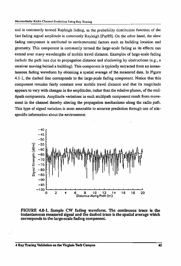
Microceliular Radio Channel Prediction Using Ray Tracing
and is commonly termed Rayleigh fading, as the probability distribution function of the
fast fading signal amplitude is commonly Rayleigh [Par89]. On the other hand, the slow
fading component is attributed to environmental factors such as building location and
geometry. This component is commonly termed the large-scale fading as its effects can
extend over many wavelengths of mobile travel distance. Examples of large-scale fading
include the path loss due to propagation distance and shadowing by obstructions (e.g., a
receiver moving behind a2 building). This component is typically extracted from an instan-
taneous fading waveform by obtaining a spatial average of the measured data. In Figure
4.1-1, the dashed line corresponds to the large-scale fading component. Notice that this
component remains fairly constant over mobile travel distance and that its magnitude
appears to vary with changes in the amplitudes, rather than the relative phases, of the mul-
tipath components. Amplitude variations in each multipath component result from move-
ment in the channel thereby altering the propagation mechanisms along the radio path.
This type of signal variation is most amenable to accurate prediction through use of site-
specific information about the environment.
—-40r,
45 50 b
‘e ~551 S 60} AK = —65 rf 1 We
© -70} | 2 nm —-75t
2 -80 Hw —85
—90 F
—95 F
~199 C4» i 0 2 4 6 8 10 12 14 #16 18 20
Distance Along Path (m)
FIGURE 4.0-1. Sample CW fading waveform. The continuous trace is the instantaneous measured signal and the dashed trace is the spatial average which corresponds to the large-scale fading component.
4 Ray Tracing Validation on the Virginia Tech Campus 45

Microcellular Radio Channel Prediction Using Ray Tracing
In terms of system design, it is also the large-scale fading which is of primary
interest. Since this component represents the average signal level that will be experienced
at a specific location, the large-scale fading determines the coverage region and interfer-
ence levels that are present. Although, small scale fading can impact system performance,
its effect can be included in the link margin or obviated using diversity reception [Lee82].
4.1 Virginia Tech Campus Measurements
To examine the application of a propagation prediction model, 900 MHz narrow
band (CW) measurements were made on the Virginia Tech campus. Since the Tech cam-
pus was familiar and accessible, it provided an ideal location for the measurements. Most
importantly, though, two dimensional campus maps and tables containing building heights
were readily available from the University Architect. This way, the measurements could
easily be related to the building geometry, and site-specific data could be incorporated in
the propagation prediction model.
The propagation measurements were taken with a narrow band measurement sys-
tem. Narrow band propagation measurements have been shown to be useful for determin-
ing signal strength coverage areas and for acquiring a large quantity of signal strength data
in a Short period of time [Rap89][Rus91]. Also, the narrow band measurement system had
sufficient dynamic range to measure large path loss values and was less susceptible to in-
band interference. Since the measurements were to be conducted in a band with a number
of possible interferers (paging, amateur radio operators, etc.) and in heavily shadowed
topographies, the narrow band measurement system was the most suitable alternative.
4.1.1 900 MHz Narrow Band Measurement System
A block diagram of the narrow band system used for the measurements is shown in
Figure 4.1-1. A CW signal was generated by a Fluke 6062A synthesized signal generator,
amplified by a MiniCircuits ZHL4240 wide band, low noise amplifier, and transmitted
through a commercial 54/8 vertical monopole above a ground plane. With cable and con-
nector losses approximately offsetting antenna gain, the system had an EIRP of 1 watt.
The receiver consisted of a commercial ICOM receiver and a laptop PC. The receiver was
modified through the addition of an A/D converter in the receiver AGC loop. The modifi-
cation permitted the received signal to be continuously monitored and stored on disk. A
calibration curve, generated by feeding a known input signal level directly into the
receiver for the entire receiver dynamic range, was used to convert the AGC byte value
4 Ray Tracing Validation on the Virginia Tech Campus 46
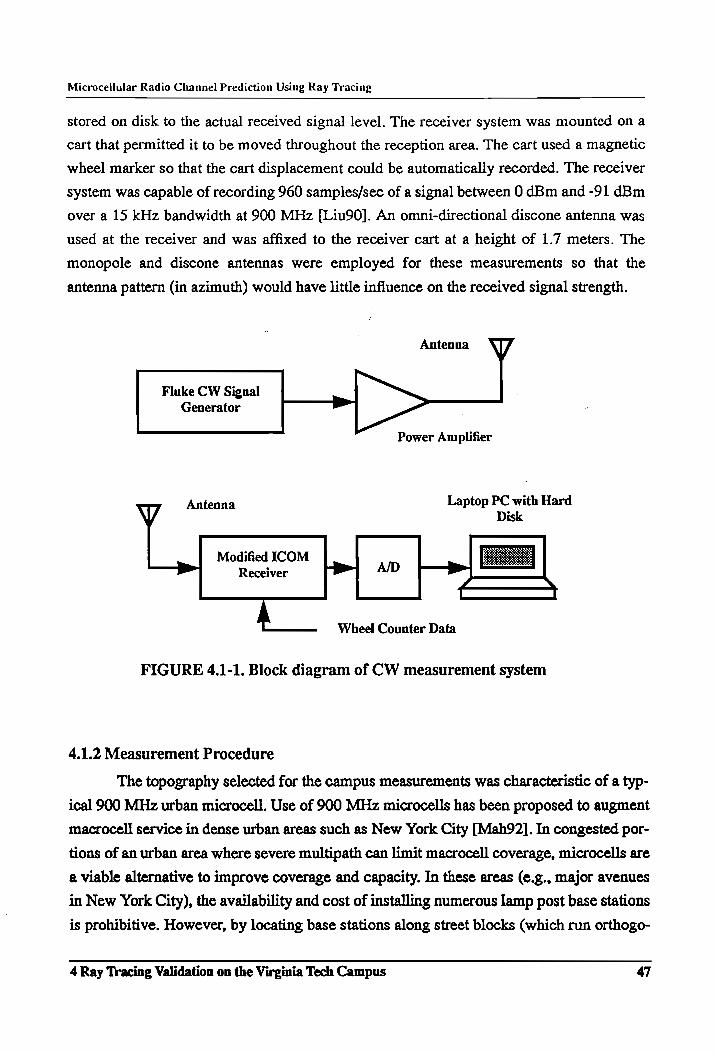
Microcellular Radio Channel Prediction Using Ray Tracing
stored on disk to the actual received signal level. The receiver system was mounted on a
cart that permitted it to be moved throughout the reception area. The cart used a magnetic
wheel marker so that the cart displacement could be automatically recorded. The receiver
system was capable of recording 960 samples/sec of a signal between 0 dBm and -91 dBm
over a 15 kHz bandwidth at 900 MHz [Liu90]. An omni-directional discone antenna was
used at the receiver and was affixed to the receiver cart at a height of 1.7 meters. The
monopole and discone antennas were employed for these measurements so that the
antenna pattern (in azimuth) would have little influence on the received signal strength.
Antenna
Fluke CW Signal Generator
Power Amplifier
Antenna Laptop PC with Hard Disk
Modified ICOM
Receiver AD -— PP
A Wheel Counter Data
FIGURE 4.1-1. Block diagram of CW measurement system
4.1.2 Measurement Procedure
The topography selected for the campus measurements was characteristic of a typ-
ical 900 MHz urban microcell. Use of 900 MHz microcells has been proposed to augment
macrocell service in dense urban areas such as New York City [Mah92]. In congested por-
tions of an urban area where severe multipath can limit macrocell coverage, microcells are
a viable alternative to improve coverage and capacity. In these areas (e.g., major avenues
in New York City), the availability and cost of installing numerous lamp post base stations
is prohibitive. However, by locating base stations along street blocks (which run orthogo-
4 Ray Tracing Validation on the Virginia Tech Campus 47
Microcellular Radio Channel Prediction Using Ray Tracing
nal to the avenues), it is possible to provide coverage and capacity relief at a reasonable
cost. The buildings along the street blocks are generally lower in height and are sur-
rounded by open areas such as building alleys, parking lots, etc. Ideally, by mounting an
antenna on a street block building, the lower building height and building alleys could be
used to control the propagation.
The narrow band measurements were taken on the Academic Quad of the Virginia
Tech campus. The buildings in this quad are between one and six floors in height and are
generally arranged in an orthogonal fashion, similar to a city block. The stationary trans-
mitter was placed on the rooftop of Whittemore’Hall in the southwest comer of the build-
ing (antenna elevation = 2156’ above sea level). At this location, the transmitter antenna
provided acceptable coverage for most locations within the quad. The mobile receiver
canvassed the sidewalks surrounding the academic buildings on the upper portion of the
campus.
Notice from Figure 4.1-2, that the sidewalks are physically close to and generally
aligned with the building faces. As a result, much of the data were collected along shad-
owed paths which were tangential to the propagation (direct transmitter to receiver) path.
For these paths, the change in propagation path length was relatively small as compared to
the receiver cart displacement (e.g., a 20 meter measurement run might have exhibited
only a 2 meter change in the propagation path length). In collecting data along tangential
paths it was assumed that the influence of large-scale building geometry on the received
signal strength would be emphasized. Since the receiver was shadowed by buildings on
either side of the street, generally only buildings in a local area of the receiver will have a
noticeable effect on the received signal. As such, the height and position variations of the
buildings lining the street will have an impact on received signal strength. The typical
measured waveform, shown in Figure 4.0-1, was made along a sidewalk in front of the
two-floor portion of Randolph Hall. The dashed trace is spatial average of the measured
data obtained by filtering the instantaneous measured data with a 5A Hamming window.
Notice that the shadowing component (dashed traced) remains fairly constant over the
measurement run. This effect suggests that stable multipath components also exist in
urban microcellular topographies and these components dominate the average signal
strength (recall that [Ike91] proposed this for urban macrocellular). These multipath com-
ponents are assumed to be influenced by the large-scale building geometry.
4 Ray Tracing Validation on the Virginia Tech Campus 48
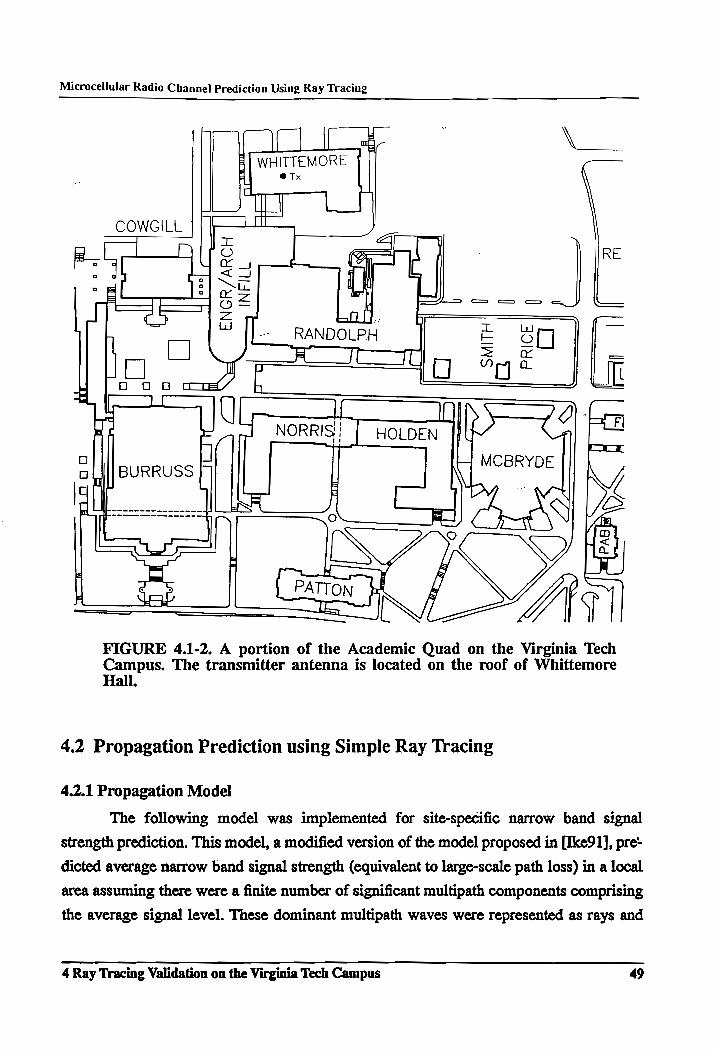
Microcellular Radio Channel Prediction Using Ray Tracing
:
WHITTEMORE @ Tx
| |
COWGILL
RE
ENGR/ARCH
INFILL
RANDOLPH
BURRUSS
FIGURE 4.1-2. A portion of the Academic Quad on the Virginia Tech Campus. The transmitter antenna is located on the roof of Whittemore Hall,
4.2 Propagation Prediction using Simple Ray Tracing
4.2.1 Propagation Model
The following model was implemented for site-specific narrow band signal
strength prediction. This model, a modified version of the model proposed in [Ike91], pre-
dicted average narrow band signal strength (equivalent to large-scale path loss) in a local
area assuming there were a finite number of significant multipath components comprising
the average signal level. These dominant multipath waves were represented as rays and
4 Ray Tracing Validation on the Virginia Tech Campus 49
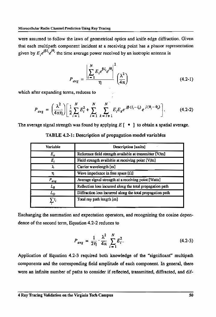
Microcellular Radio Channel Prediction Using Ray Tracing
were assumed to follow the laws of geometrical optics and knife edge diffraction. Given
that each multipath component incident at a receiving point has a phasor representation
given by E ie Pi /* the time average power received by an isotropic antenna is
N ° 2 y Ee 'e i ,
i=l r Pave = yh (*) (4.2-1)
which after expanding terms, reduces to |
> TY "a, NN’ EE eBUHW 4 i,- 8) (4.2.2)
ue 4m 2 dy Do oe, me
The average signal strength was found by applying E[ ® ] to obtain a spatial average.
TABLE 4.2-1: Description of propagation model variables
Variable Description [units]
E, Reference field strength available at transmitter [V/m]
E; Field strength available at receiving point [V/n]
A Carrier wavelength [m]
n Wave impedance in free space [Q]
Pavg Average signal strength at a receiving point [Watts]
Lr Reflection loss incurred along the total propagation path
Lp Diffraction loss incurred along the total propagation path
Yi Total ray path length [m] Exchanging the summation and expectation operators, and recognizing the cosine depen-
dence of the second term, Equation 4.2-2 reduces to
1 w N 2 Pave = Oy FR LF (4.2-3)
Application of Equation 4.2-3 required both knowledge of the “significant” multipath
components and the corresponding field amplitude of each component. In general, there
were an infinite number of paths to consider if reflected, transmitted, diffracted, and dif-
4 Ray Tracing Validation on the Virginia Tech Campus 50
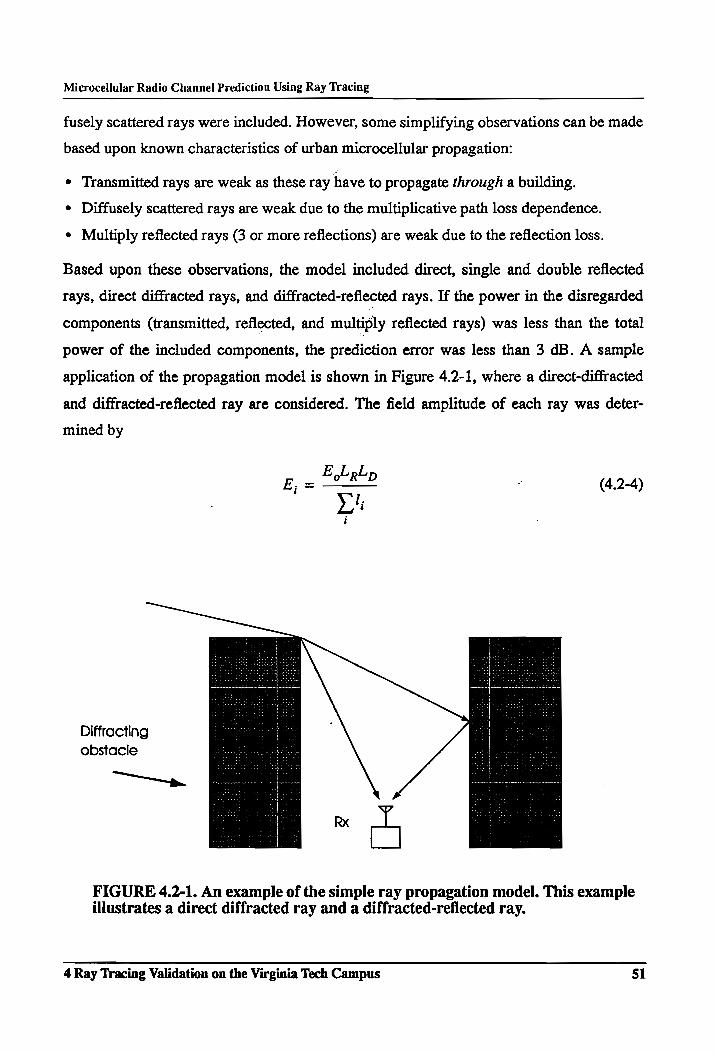
Microcellular Radio Channel Prediction Using Ray Tracing
fusely scattered rays were included. However, some simplifying observations can be made
based upon known characteristics of urban microcellular propagation:
¢ Transmitted rays are weak as these ray have to propagate through a building.
e Diffusely scattered rays are weak due to the multiplicative path loss dependence.
* Multiply reflected rays (3 or more reflections) are weak due to the reflection loss.
Based upon these observations, the model included direct, single and double reflected
rays, direct diffracted rays, and diffracted-reflected rays. If the power in the disregarded
components (transmitted, reflected, and multiply reflected rays) was less than the total
power of the included components, the prediction error was less than 3 dB. A sample
application of the propagation model is shown in Figure 4.2-1, where a direct-diffracted
and diffracted-reflected ray are considered. The field amplitude of each ray was deter-
mined by
E. = E oRLp i (4.2-4)
Li i
Diffracting
obstacle
te
oe
FIGURE 4.2-1. An example of the simple ray propagation model. This example illustrates a direct diffracted ray and a diffracted-reflected ray.
4 Ray Tracing Validation on the Virginia Tech Campus S1
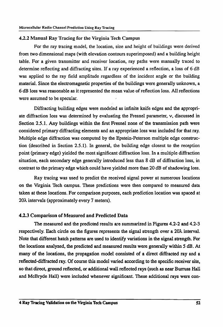
Microcellular Radio Channel Prediction Using Ray Tracing
4.2.2 Manual Ray Tracing for the Virginia Tech Campus
For the ray tracing model, the location, size and height of buildings were derived
from two dimensional maps (with elevation contours superimposed) and a building height
table. For a given transmitter and receiver location, ray paths were manually traced to
determine reflecting and diffracting sites. If a ray experienced a reflection, a loss of 6 dB
was applied to the ray field amplitude regardless of the incident angle or the building
material. Since the electromagnetic properties of the buildings were generally unknown, a
6 dB loss was reasonable as it represented the mean value of reflection loss. All reflections
were assumed to be specular.
Diffracting building edges were modeled as infinite knife edges and the appropri-
ate diffraction loss was determined by evaluating the Fresnel parameter, v, discussed in
Section 2.5.1. Any buildings within the first Fresnel zone of the transmission path were
considered primary diffracting elements and an appropriate loss was included for that ray.
Multiple edge diffraction was computed by the Epstein-Peterson multiple edge construc-
tion (described in Section 2.5.1). In general, the building edge closest to the reception
point (primary edge) yielded the most significant diffraction loss. In a multiple diffraction
situation, each secondary edge generally introduced less than 8 dB of diffraction loss, in
contrast to the primary edge which could have yielded more than 20 dB of shadowing loss.
Ray tracing was used to predict the received signal power at numerous locations
on the Virginia Tech campus. These predictions were then compared to measured data
taken at these locations. For comparison purposes, each prediction location was spaced at
20A intervals (approximately every 7 meters).
4.2.3 Comparison of Measured and Predicted Data
The measured and the predicted results are summarized in Figures 4.2-2 and 4.2-3
respectively. Each circle on the figures represents the signal strength over a 20A interval.
Note that different hatch patterns are used to identify variations in the signal strength. For
the locations analyzed, the predicted and measured results were generally within 5 dB. At
many of the locations, the propagation model consisted of a direct diffracted ray and a
reflected-diffracted ray. Of course this model varied according to the specific receiver site,
so that direct, ground reflected, or additional wall reflected rays (such as near Burruss Hall
and McBryde Hall) were included whenever significant. These additional rays were con-
4 Ray Tracing Validation on the Virginia Tech Campus §2
Microcellular Radio Channel Prediction Using Ray Tracing
sidered significant if their amplitude was within 10 dB of the amplitude of the strongest
arriving component.
. The measurement path along the sidewalk in between Holden Hall and Patton
Hall and extending from McBryde Hall toward Burruss Hall deserved particular attention.
This path was of interest because the path profile varied significantly over the measure-
ment run. At the beginning of the path (near McBryde) the receiver was heavily shadowed
by the three-floor portions of Randolph Hall and Holden Hall. However, as the receiver
moved toward Burruss Hall, Randolph Hall transitioned from three floors to two floors
and Holden Hall transitioned from three floors to one floor. Notice that a strong increase
(approximately 10 dB) was observed as the receiver moved out of the shadow of Holden
Hall. As the receiver continued along the path, the propagation path again became heavily
shadowed, this time by the three-floor portion of Norris Hall. Notice that the predicted sig-
nal strength closely followed this variation in signal strength with diffraction loss. Similar
results were reported by Russell [Rus91] when a rigorous three-dimensional diffraction
model was used.
The prediction error was most significant along the path beside McBryde Hall.
Although not shown in the figure, the predicted signal strength was generally 10 to 15 dB
below the measured value with a worst case error of 17 dB at one location (also refer to
[Sch91]). The disparity between these two results can be attributed to the method of deter-
mining diffracted energy arriving at the receiver. McBryde Hall is a six floor building (and
has a similar maximum elevation as the transmitter antenna) surrounded by buildings
between one and three floors in height. For such an arrangement, it is likely that the field
will diffract both over the building rooftop and around the lateral building edge. However,
only the rooftop diffraction field was considered in the calculation. Furthermore, in a
heavily shadowed environment such as this, diffusely scattered fields are more significant
since dominant multipath components are no longer present.
The ability to predict small scale signal fluctuations was also investigated in this
preliminary study. Although statistical models may be more appropriate for modeling
these variations, it was felt that predicting these fluctuations, even with limited environ-
mental data, might provide some insight into the mechanisms controlling small scale fad-
ing. For this case, the signal strength was computed by a direct application of Equation
4.2-1 where each multipath component was given a deterministic phase based upon the
propagation path length (i.e., no phase variations for reflection or diffraction were
4 Ray Tracing Validation on the Virginia Tech Campus 53
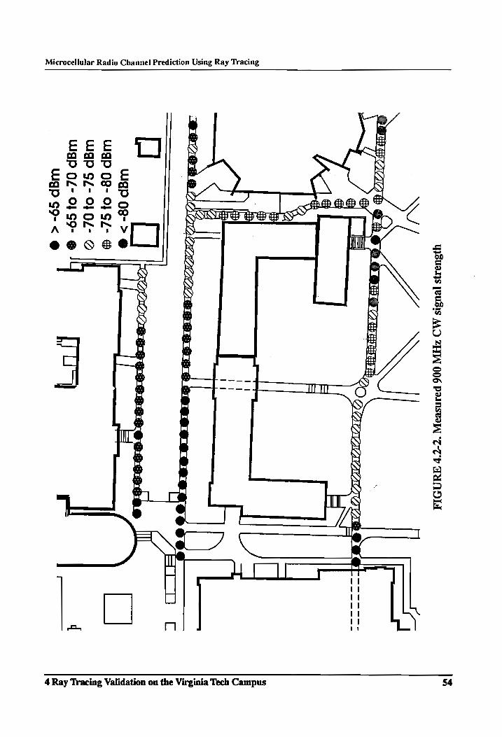
Microcellular Radio Channel Prediction Using Ray Tracing
yysuaays [BUSIS
AAD ZHW
006 Panseayy]
°7-7'b TANOLA
a C]
WgP
08- >
@ WagP
08- Of
SZ- WgP
GL- OF0Z-
©
@ WP
OL- 0} G9-
@ - [o>
gp
S9- <
54 4 Ray Tracing Validation on the Virginia Tech Campus
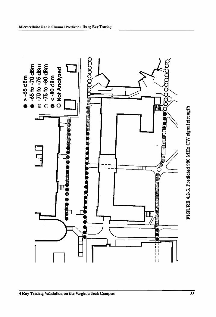
Microcellular Radio Channel Prediction Using Ray Tracing
yysuaays [BUSIS
MD ZHI
006 P2}!P21d
“€-7'r AMNDA
ODGWCLUDE CCL GEE
-====
| ee
pezdAjpuy
JON O
—
|
WgP 08->
© WP
08- OF
GZ- @
| WaP
GZ- O}0Z-
@ 4
iyo
——
WP
0Z- 0}
G9- @
WgP S9-<
@
55 4 Ray Tracing Validation on the Virginia Tech Campus
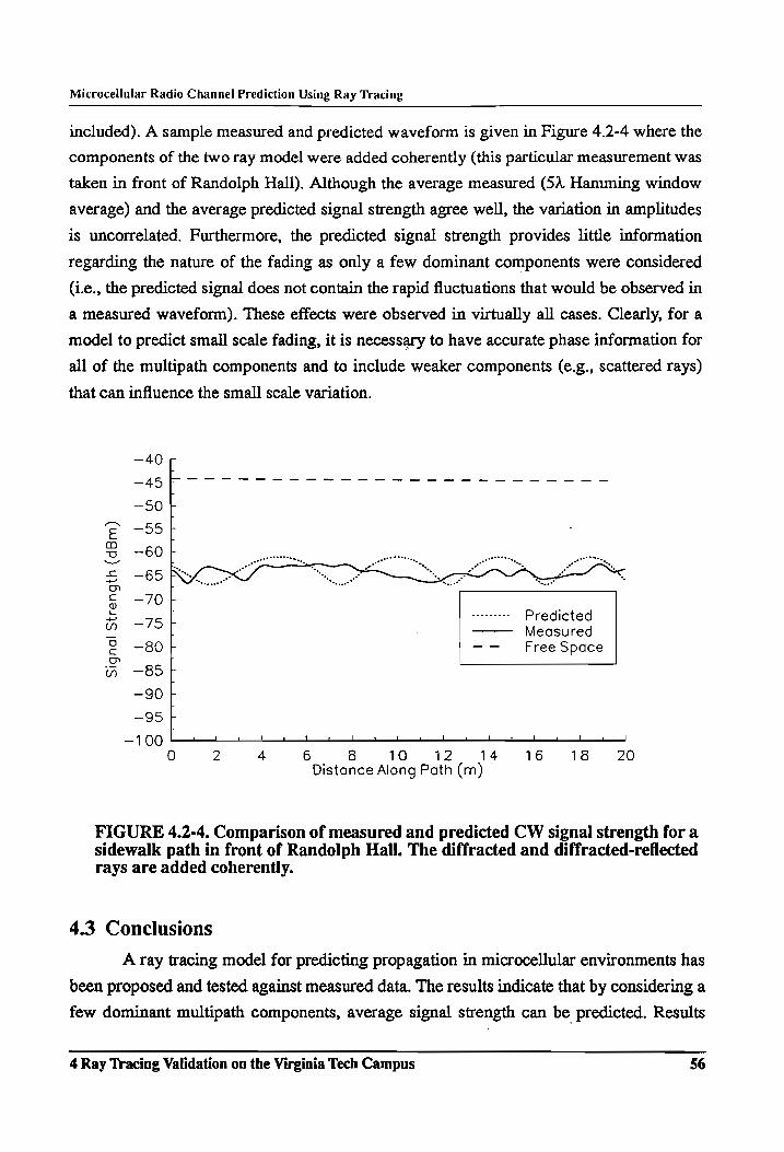
Microcellular Radio Channel Prediction Using Ray Tracing
included). A sample measured and predicted waveform is given in Figure 4.2-4 where the
components of the two ray model were added coherently (this particular measurement was
taken in front of Randolph Hall). Although the average measured (5A Hamming window
average) and the average predicted signal strength agree well, the variation in amplitudes
is uncorrelated. Furthermore, the predicted signal strength provides little information
regarding the nature of the fading as only a few dominant components were considered
(i.e., the predicted signal does not contain the rapid fluctuations that would be observed in
a measured waveform). These effects were observed in virtually all cases. Clearly, for a
model to predict small scale fading, it is necessary to have accurate phase information for
all of the multipath components and to include weaker components (e.g., scattered rays)
that can influence the small scale variation.
E o
ZS co
a © = a Predicted W797 — Measured ce —80F —-— Free Space C f mM —85F
—90 L
—~95 x
— 00 2 1 l ] 1 1 i | i l 1 | l 1 L i J
0 2 4 6 8 10 12 14 16 18 20 Distance Along Path (m)
FIGURE 4.2-4. Comparison of measured and predicted CW signal strength for a sidewalk path in front of Randolph Hall. The diffracted and diffracted-reflected rays are added coherently.
4.3 Conclusions
A ray tracing model for predicting propagation in microcellular environments has
been proposed and tested against measured data. The results indicate that by considering a
few dominant multipath components, average signal strength can be predicted. Results
4 Ray Tracing Validation on the Virginia Tech Campus 56

Microcellular Radio Channel Prediction Using Ray Tracing
also indicate that diffraction models must be included in areas of heavy shadowing. Ray
tracing, is therefore a viable method for predicting propagation in mobile and portable
radio environments; the method can yield reasonably accurate results without the need to
explicitly solve complicated electromagnetic problems. Moreover, as exhibited by the
analysis of measured and predicted data near Holden Hall, the accuracy of a prediction is
directly related to the quantity and precision of site-specific environment data.
The manual efforts described here provided proof-of-concept for use of ray tracing
to predict propagation in microcellular environments. As a result, an automated ray trac-
ing system was developed. Based upon the results presented here as well as information
appearing in the literature, the following design goals were established:
e The propagation prediction system should incorporate site-specific environmental data.
A facility for managing this data should be integrated into the system so that the data can be entered, processed, and then accessed by the ray tracing program. This facility
should also have a user-interface that permits data to be entered in a straightforward fashion. )
e The system should predict path loss and delay spread in microcellular environments. The prediction model should be generic, such that it can achieve acceptable accuracy
for both line-of-sight and shadowed topographies in urban and dense urban environ- ments (i.e., geographic areas in which PCS and microcells are targeted).
e The system should process and graphically display the path loss and delay spread
results. Preferably, the system should overlay these results, in color, on a two dimen-
sional map.
e The system must be modular. This way, as new interfaces become available, or as new propagation models are developed, these new items can be included in the program without extensive modifications to the code.
A ray tracing system was developed according to these specifications. A diagram illustrat-
ing the basic operation of the system is given in Figure 4.3-1. AutoCAD was selected as
the site-specific data manager and interface. The process of using AutoCAD for entering
site-specific data and processing this data is described in Chapter 5. The second portion of
the system, the ray tracing model, programs, and data processing routines are presented in
Chapter 6. Finally, Chapter 7 provides some comparisons of measured data against predic-
tions made with the automated system.
4 Ray Tracing Validation on the Virginia Tech Campus 57
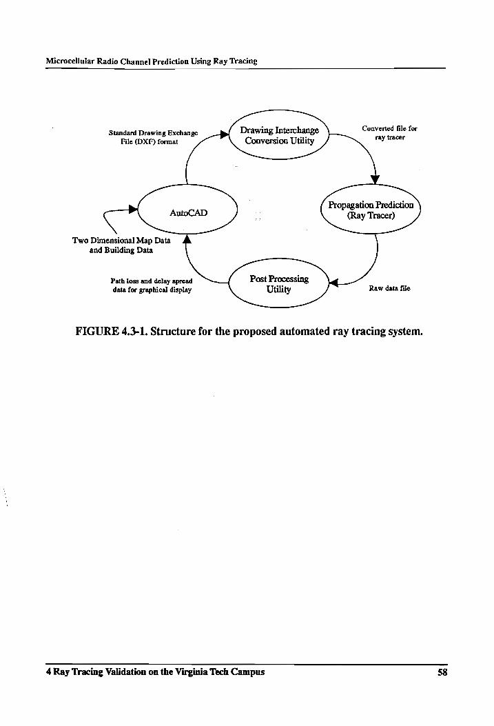
Microcellular Radio Channel Prediction Using Ray Tracing
Converted file for
ray tracer Drawing Interchange Conversion Utility
Standard Drawing Exchange File (DXF) format
Propagation Prediction (Ray Tracer)
Two Dimensional Map Data
and Building Data
Path loss and delay spread
data for graphical display Raw data file
FIGURE 4.3-1. Structure for the proposed automated ray tracing system.
4 Ray Tracing Validation on the Virginia Tech Campus 58
Microcellular Radio Channel Prediction Using Ray Tracing
5 The Building Database
This chapter describes the important features of the AutoCAD three dimensional
building database used to supply site-specific data to the ray tracing modules. Specific
information on standard representation of building database entities, and the techniques
used to create these entities within AutoCAD are discussed here. This information is then
applied to a specific example, creation of a building database for the Virginia Tech cam-
pus. Finally, the process of converting AutoCAD data into a form usable by the ray tracing
modules is described. “
5.1 Requirements for Modeling Buildings in the Database
In general, the availability of site-specific data is highly dependent upon the loca-
tion that needs to be described. Federal agencies (U.S. Geological Survey or the Army
Corps of Engineers) and local governments (city planners and architects) typically main-
tain building and terrain databases for major urban areas as well as for smaller municipal-
ities. Other resources, such as aerial photogrammetry, satellite imaging, or even
investment and insurance companies [Ran89] can supply environmental data. However,
each resource collects this data for specific purposes, and as such, the quantity of useful
data will be highly variable. In order to establish a standard for data representation within
the building database, it is necessary to select a specific set or quantity of useful data that
will be available in virtually all cases. Considering this, the task is to now define what is
meant by useful. This is accomplished by defining the requirements for site-specific data
in terms of our propagation prediction goals.
Emerging PCN and PCS will employ spread spectrum or other wide bandwidth
(RF bandwidth > 1 MHz) digital modulation techniques and so, due to the inherent fre-
quency diversity within the signal, predicting the instantaneous signal level is less impor-
tant. Thus, average path loss and multipath delay spread are the important system design
parameters. In Chapter 4, it was shown that large scale building geometry dominates the
average path loss of narrow band signals. This is a reasonable assumption for wide band
signals as well. Measurements in [Tel91] indicate individual multipath components
exhibit little fading (~ 3 dB) as a receiver is moved in a microcellular channel over several
wavelengths without major topography changes, or as the terminals remain stationary over
several seconds. In addition, the time dispersion of the channel is related to the location
§ The Building Database 59

Microcellular Radio Channel Prediction Using Ray Tracing
and orientation of large scattering surfaces within the channel. In a typical microcellular
channel, the large scale signal component is controlled by the location, size, and orienta-
tion of the surrounding buildings. Other scatterers, such as trees and lamp posts, may also
impact this signal component, but these effects are secondary. As was shown in Chapter 2,
the amplitude of reflected, transmitted, and scattered fields, from an arbitrary surface, can
be determined from the electrical properties (i.e., the reflection and transmission coeffi-
cient) of that surface. Thus, the data required for a propagation model would consist of the
geometrical and electrical characteristics of the buildings.
From an electromagnetic standpoint, buildings are surprisingly complicated sur-
faces. A building face is generally composed of a series of flat planes, where each plane
may have a different location and tilt relative to neighboring planes. Additionally, as each
plane may be of a different material composition (glass, stone, or brick), inhomogeneities
and material surface roughness can result in different electrical characteristics. Since this
building-specific information may be difficult to obtain, the building surfaces need to
described in a more generic way.
Buildings are represented in the building database as follows. Each building is
modeled as a solid bounded by individual planar panels (polygons). Any number of panels
can be used to model the building surface, based upon the desired accuracy. A planiform
environment is assumed, where buildings are given an effective height above the terrain
level. This assumption is valid in most cases due to the small geographic regions required
for analysis. Exact building heights are used when available, otherwise, the building is
assigned a height (in meters) according to 4.2N, where N represents the number of build-
ing floors. Reflection and transmission coefficients (loss ratios or Fresnel coefficients) are
associated with each planar face, and are specified according to the building material or by
user specification.
5.2 Using AutoCAD® for Building Database Management
To make economical use of large quantities of site-specific environmental data the
prediction system must be able to keep data collection and processing times to a mini-
mum. Thus, the software used for building database management must have the capability
to process input data which may be obtained in many different formats. Moreover, the
interface must directly interact with the propagation prediction modules, and be able to
graphically display the building database along with the prediction results. Clearly, com-
5 The Building Database 60

Microcellular Radio Channel Prediction Using Ray Tracing
mercially available software would be more capable of satisfying these requirements than
any custom software. Since support of detailed terrain data is currently not a database
requirement, it is possible to make use of other graphical database management software
(e.g., computer-aided design (CAD) software) for modeling the buildings and effective
terrain levels. As a result, AutoCAD Release 11, a commercially available CAD package,
has been selected as the building database manager. AutoCAD is proposed for this work
for the following reasons:
e AutoCAD is an industry standard CAD Package - building data may be readily avail.
able in AutoCAD form.
e AutoCAD has an open software architecture - personal customization is possible and many third party applications are available.
e AutoCAD drawings can easily be transferred between different computers and operat- ing platforms as well as different CAD packages.
e AutoCAD has numerous drawing macros for converting two dimensional images (e.g., plan view maps) into three dimensional objects.
AutoCAD Release 11 has a newly added feature for further software customiza-
tion. A C programming interface has been built into this latest release, allowing direct
access to the drawing database within AutoCAD. This interface was thoroughly investi-
gated as it appeared that C programs executed directly as AutoCAD macro commands
would provide the best user interface. Unfortunately, little documentation is provided in
the AutoCAD manuals for programming with the very complex interface (C libraries).
Future releases of AutoCAD may provide more documentation making the C interface a
viable alternative. However, as this documentation is not currently available, an alternate
approach is taken. The AutoCAD drawing data file is processed externally, converting an
AutoCAD specific data file to a standard ASCTI file that can be used by the propagation
prediction software. This external interface between AutoCAD and the propagation pre-
diction modules provides the most flexibility at little cost of convenience. Future improve-
ments within AutoCAD or the prediction software can occur independently, and new
database management software can easily be integrated with the prediction software.
5.2.1 AutoCAD Drawings and Drawing Interchange File Formats
File storage of AutoCAD drawings is accomplished using an AutoCAD drawing
database file format (*.dwg file) which stores a drawing database in a compact form. This
format changes with each Autodesk revision of AutoCAD as new features or drawing util-
5 The Building Database 61

Microcellular Radio Channel Prediction Using Ray Tracing
ities are added to AutoCAD. As such, Autodesk does not provide file format documenta-
tion for *.dwg files and it is recommended that external AutoCAD applications should not
directly use *.dwg drawing file as the application will be version specific. To facilitate
interchange of drawings from AutoCAD to external applications, the Drawing Interchange
file format (DXF) has been defined. All versions of AutoCAD accept this file format and
are able to convert the format to and from the internal drawing file representation.
DXF files (*.dxf) are standard ASCII text files. The DXF file contains the drawing
entity data (lines, circles, three-dimensional wireframes, etc.) that comprise the actual
drawing as well as the drawing-related specifics (linestyles, drawing layers, viewport, etc.)
that are necessary for visual recreation of the drawing. A sample portion of a DXF file is
given in Figure 5.2-1. The DXF file uses keywords and numeric codes, all of which are
fully documented in [CAD90], to define the drawing entities. The use of this format per-
mits DXF files to be translated or rearranged in a direct manner.
The overall organization of a DXF file is as follows:
1. HEADER section - General information regarding the drawing such as default drawing settings. Each drawing parameter is assigned a specific variable name and an associated
value.
2. TABLES section - Contains data for the drawing tables such as the drawing layer table,
linetype table, etc.
3. BLOCKS section - Contains the block definition entities and block references
4. ENTITIES section - Contains the drawing entities and any instances of a user-defined block.
5. END OF FILE
The BLOCKS and ENTITIES sections of the DXF file are the sections used for the
database conversion.
A limitation of the DXF file format is that each entity is written to the file in a spe-
cific format according to how that entity was created within AutoCAD. For example, con-
sider the different methods possible for creating a parallelepiped (rectangular box) within
AutoCAD. The user could create the entity by using an AutoCAD specific command for
drawing 3D objects, by drawing a set of connected 2D planes, or by drawing a set of inter-
connected lines. All of these renderings are visually identical, but, each will have a differ-
ent representation within the *.dxf file and will require a different conversion routine.
Since the varagies of different drawing styles can not be accounted for, a standard drawing
§ The Building Database 62
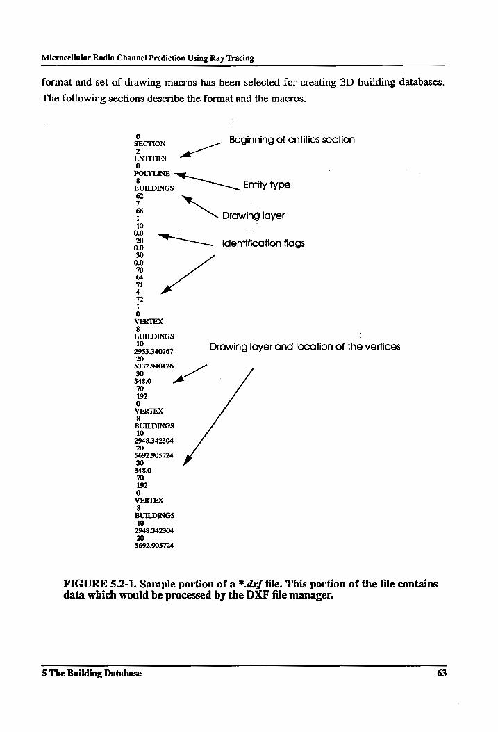
Microcellular Radio Channel Prediction Using Ray Tracing
format and set of drawing macros has been selected for creating 3D building databases.
The following sections describe the format and the macros.
Beginning of entities section 0 SECTION 2 -_o
ENTITIES
FOLYLINE
62 . 7 we
6 Drawing layer
2 “*——___ identification flags
8 BUILDINGS 10
$332.940426
30 a. 348.0 70 192 0 VERTEX 8 BUILDINGS 10 2948.342304 20 5692.905724 30 348.0 70 192 0 VERTEX 8 BUILDINGS 10 2948.342304 20 5692.905724
2953 340767 Drawing layer and location of the vertices 20
FIGURE 5.2-1. Sample portion of a *.dxf file. This portion of the file contains data which would be processed by the DXF file manager.
5 The Building Database
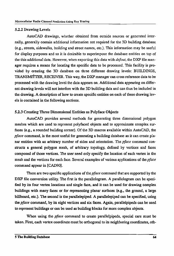
Microcellular Radio Channel Prediction Using Ray Tracing
§.2.2 Drawing Levels
AutoCAD drawings, whether obtained from outside sources or generated inter-
nally, generally contain additional information not required for the 3D building database
(e.g., streets, sidewalks, building and street names, etc.). This information may be useful
for display purposes and so it is desirable to superimpose the database entities on top of
the this additional data. However, when exporting this data with dxfout, the DXF file man-
ager requires a means for locating the specific data to be processed. This facility is pro-
vided by creating the 3D database on three different drawing levels: BUILDINGS,
TRANSMITTER, RECEIVER. This way, the DXF manager can cross reference data to be
processed with the drawing level the data appears on. Additional data appearing on differ-
ent drawing levels will not interfere with the 3D building data and can thus be included in
the drawing. A description of how to create specific entities on each of these drawing lev-
els is contained in the following sections.
5.2.3 Creating Three Dimensional Entities as Polyface Objects
AutoCAD provides several methods for generating three dimensional polygon
meshes which are used to represent polyfaced objects and to approximate complex sur-
faces (e.g., a rounded building corner). Of the 3D macros available within AutoCAD, the
pface command, is the most useful for generating a building database as it can create pla-
nar entities with an arbitrary number of sides and orientation. The pface command con-
structs a general polygon mesh, of arbitrary topology, defined by vertices and faces
composed of those vertices. The user need only specify the location of each vertex in the
mesh and the vertices for each face. Several examples of various applications of the pface
command appear in [CAD90].
There are two specific applications of the pface command that are supported by the
DXF file conversion utility. The first is the parallelogram. A parallelogram can be speci-
fied by its four vertex locations and single face, and it can be used for drawing complex
buildings with many faces or for representing planar surfaces (e.g., the ground, a large
billboard, etc.). The second is the parallelepiped. A parallelepiped can be specified, using
the pface command, by its eight vertices and six faces. Again, parallelpipeds can be used
to represent buildings or can be used as building blocks for more complex objects.
When using the pface command to create parallelpipeds, special care must be
taken. First, each vertex coordinate must be orthogonal to its neighboring coordinates, oth-
5 The Building Database 64

Microcellular Radio Channel Prediction Using Ray Tracing
erwise, the parallelepiped faces are skew and the entity cannot be processed. Additionally,
a convention (e.g., clockwise around face) must be selected when specifying the coordi-
nates for an individual face; the command is sensitive to the ordering of the vertices.
Finally, note that all database entities created with the pface command must be drawn on
the BUILDINGS level if it is to be processed by the DXF file conversion utility.
5.2.4 Creating Three Dimensional Entities from Two Dimensional Drawings
One of the most useful features of AutoCAD is the ability to convert two dimen-
sional (e.g., xy plane or plan view) drawings into three dimensional views in a straightfor-
ward manner. The extrusion of buildings in the z-dimension is accomplished with the
change edit macro. To extrude an object in a drawing, select this command from the edit
menu and then select items to change at the item selection prompt. Next select thickness
from the Change Menu. Enter the building height as the thickness. The vpoint command
can then be used to view the three dimensional entity. An example of a 2D drawing
extruded into a 3D entity is given in Figure 5.2-2.
As can be seen by Figure 5.2-2, after creating a 3D entity using extrusion, some
additional editing is generally required to remove extraneous data. The original 2D repre-
sentation may contain many small scale building features which do not need to be
included in the database. In this case, it is recommended that a wireframe be constructed
around the extruded entity. This can be accomplished by drawing polygons (using pface)
to bound the pertinent features of the building surface thereby reducing the number of
polygons required to represent the entity. When this conversion process is being done on
large drawings, zooming in on the entity to edit and setting the osnap mode to endpoint or
intersection simplifies drawing the polyfaces and guarantees that each face will be con-
nected to neighboring faces.
§.2.5 Using Drawing Attributes
For complicated databases containing many buildings with varying electrical prop-
erties, attributes can be used to attach electrical properties to a specific database entity. In
AutoCAD, attributes (special drawing entities composed of a keyword or tag and a numer-
ical value) work in conjunction with AutoCAD blocks. An AutoCAD block is a set of
entities grouped together into a compound object, and once so grouped, they are given a
block name. Refer to the AutoCAD Reference Manual [CAD90] for a complete descrip-
tion of blocks, attributes, and their interdependence. The DXF file conversion utility sup-
5 The Building Database 65
Microcellular Radio Channel Prediction Using Ray Tracing
FIGURE 5.2-2, Example of a 2D drawing (a.) extruded into a 3D entity (b.).
ports four attribute keywords for describing the characteristics of an object: transmission,
reflection, relative epsilon, and height. The first three attributes correspond to the trans,
reflect, and rel_epsilon object data variables described in Section 5.5. The height attribute
provides a means for interfacing AutoCAD with other database management tools, such as
GRASS, that do not have a facility for drawing buildings in 3D [Raj92].
The interrelation of attributes and blocks is a shortcoming of AutoCAD; it is not
possible to merely select an object and attach attributes to it. The basic process for creating
an entity with attributes is to predefine the attributes (using attdef), create the drawing
entity, redefine the drawing entity as a block (using block), attach the attributes to this
block, and then create an instance (using insert) of the block that was just defined. This is
a rather time consuming process, especially if the database is to require many different
block definitions to represent different entities. Although AutoCAD provides many
attribute utilities, attributes are not currently used within the database for most practical
situations (such as with the database described in Section 5.3). This is due to the excessive
time that would be required to attach attributes. The DXF file conversion utility, however,
provides the basic functions necessary to process block/attribute definitions. These func-
tions are included because future upgrades of AutoCAD may provide more direct methods
for attaching attributes, or macros may be developed that could automate block definition
process.
5 The Building Database 66
Microcellular Radio Channel Prediction Using Ray Tracing
5.2.6 Adding a Transmitter and Receivers
A single transmitter and multiple receivers can be drawn, in 3D, in the database
using the point command. Currently, the ray tracing code will trace rays from only one
transmitter location, but the rays can be received at multiple receiver locations. As a result,
the DXF manager processes only one point found on the TRANSMITTER drawing level
(but can process multiple points found on the RECEIVER level). When drawing transmit-
ters or receivers in the database, change the pdmode and pdsize point display variable from
the default settings so that the points can be easily seen in the display. It is also possible to
extend a line from the point location to the reference (ground) plane to provide a height
reference. This operation does not interfere with the data processing.
5.3 Creating A Building Database - The Virginia Tech Campus
A sample construction of a 3D building database for the Academic Quad and
Upper Quad on the Virginia Tech campus (this database is used in actual simulations
described in Chapter 7) is examined as a practical application of the database modeling
techniques. The resulting database is shown in Figure 5.3-1. The 3D building database is
derived from a 2D (plan view) map obtained from Virginia Tech Facilities Planning &
Control in an AutoCAD format. The original drawing contained a comprehensive view of
the campus with more than 20 drawing levels. Much of the extraneous data (e.g., sewer
system, golf course, etc.) was deleted from the file before converting it to a 3D database.
Fortunately, the map was drawn to scale and all building locations were located (in feet)
relative to an absolute reference point in the xz plane.
A height of 2082.5 feet above sea level (the elevation of the front door to Randolph
Hall) is used as the building height reference. The University Architect also provided
topographical maps and exact building heights for buildings in the Academic Quad. For
the Upper Quad, the height of each building is given by 4.2N (meters), where N was
derived from a field observation. All of the buildings were extruded to 3D using the tech-
niques described in Section 5.2.4. The extruded images are used as templates for drawing
the 3D objects. Considerable editing is necessary beyond the extrusion process to remove
extraneous vertical building faces (such as on McBryde Hall, Patton Hall, and Lane Hall),
and add additional faces where the building had a floor change (e.g., Randolph Hall).
Some portions of the file required particular care, such as representing the curved front of
Hancock Hall with a series of connected flat planes. Roofs were not added for buildings
above two floors (~ 30 feet) since these building faces would be above the transmitter and
5 The Building Database 67
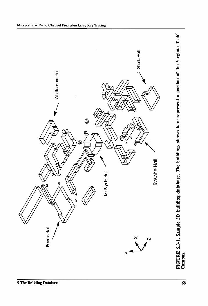
Microcellular Radio Channel Prediction Using Ray Tracing
McBryde
Hall
oO = 2 3 E 5 a
“t~_
_ Whittemore
Hall
J > & A
ae
Shultz
Hall
FIGURE
5.3-1. Sample
3D
buil
ding
da
taba
se.
The
buildings
show
n he
re re
pres
ent
a po
rtio
n of
th
e Vi
rgin
ia
Tech”
Campus.
Rasche
Hall
5 The Building Database B
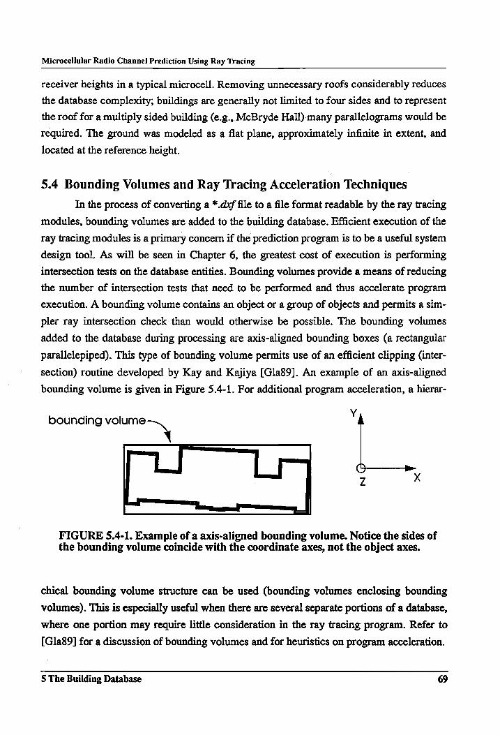
Microcellular Radio Channel Prediction Using Ray Tracing
receiver heights in a typical microcell. Removing unnecessary roofs considerably reduces
the database complexity; buildings are generally not limited to four sides and to represent
the roof for a multiply sided building (e.g., McBryde Hall) many parallelograms would be
required. The ground was modeled as a flat plane, approximately infinite in extent, and
located at the reference height.
5.4 Bounding Volumes and Ray Tracing Acceleration Techniques
In the process of converting a *.dxf file to a file format readable by the ray tracing
modules, bounding volumes are added to the building database. Efficient execution of the
ray tracing modules is a primary concern if the prediction program is to be a useful system
design tool. As will be seen in Chapter 6, the greatest cost of execution is performing
intersection tests on the database entities. Bounding volumes provide a means of reducing
the number of intersection tests that need to be performed and thus accelerate program
execution. A bounding volume contains an object or a group of objects and permits a sim-
pler ray intersection check than would otherwise be possible. The bounding volumes
added to the database during processing are axis-aligned bounding boxes (a rectangular
parallelepiped). This type of bounding volume permits use of an efficient clipping (inter-
section) routine developed by Kay and Kajiya [Gla89]. An example of an axis-aligned
bounding volume is given in Figure 5.4-1. For additional program acceleration, a hierar-
bounding vue L
FIGURE 5.4-1. Example of a axis-aligned bounding volume. Notice the sides of the bounding volume coincide with the coordinate axes, not the object axes.
chical bounding volume structure can be used (bounding volumes enclosing bounding
volumes). This is especially useful when there are several separate portions of a database,
where one portion may require little consideration in the ray tracing program. Refer to
[Gla89] for a discussion of bounding volumes and for heuristics on program acceleration.
§ The Building Database 69
Microcellular Radio Channel Prediction Using Ray Tracing
5.5 DXF File Conversion Utility (dxfmgr.cc)
The DXF file conversion utility is a C++ program that converts an ASCII *.dxf
into an ASCII *.ray file (the file format is described in Section 5.5) used by the ray tracing
modules. A basic overview of the program operation is provided here, for more specific
information refer to the code documentation (a listing of the code appears in [Sch92b)).
The DXF file conversion utility consists of a header file (dxfmgr.h) and a main program
(dxfmgr.cc). The header file contains a series of class definitions, function prototypes, and
#define statements which are used for parsing the file. The main program contains all of
the functions necessary for program operation. °
A very intuitive technique is employed for parsing a *.dxf file. The program reads
the *.dxf file string-by-string and then uses a series of case statements to take the necessary
action to process the DXF file data. The case statements are arranged hierarchically in
order to branch to subroutines for processing different drawing entities contained within
the file. Several string variables are used within the program to assist in differentiating
between file keywords (e.g., the drawing level, object type, attribute name, etc.) and the
data associated with that keyword (e.g., the object location, attribute value, etc.). This
method of processing the text file is reasonably flexible and simple to understand. Other
techniques for parsing a text file, such as using lexical commands in the creation of a finite
state machine, are more general and might be suitable in future upgrades.
5.6 The Ray Tracing Definition Language and *.ray Files
This section describes the method of communicating the database information to
the ray tracing program modules. The method is to develop a standard ray tracing defini-
tion language to define the primitive objects (parallelograms, parallelpipeds, etc.), the
electrical characteristics of these objects, and the location of the transmitter and receivers.
The ray tracing definition language and the format for the *.ray file (the file which is read
by the ray tracing modules) was adopted from the definition language provided in [Ste90].
This format was selected because it is has a less stringent format than typical definition
languages, thereby relaxing the requirements on the input parser. The language uses a
“building block” style language set. This format, together with the object-oriented features
of C++, allows for additional objects and features to be added to the descriptive language
in a direct fashion. A sample *.ray file is given in Figure 5.5-1.
5 The Building Database 70
Microcellular Radio Channel Prediction Using Ray Tracing
The definition language is described with the aid of Figure 5.5-1. Pay careful atten-
tion to the specific data format shown in this figure as the number and placement of paren-
thesis is important. For readability, the *.ray file can be annotated with comments by
enclosing text, upper or lower case, in braces ({ and }). Acceptable string type characters
are defined as alphanumerics, the underscore character, the decimal point, and the minus
sign. Definitions of the pertinent elements of the description language set are as follows
(At this point, some of the parameters appearing here are specific to the propagation pre-
diction and have not been discussed. Refer to [Sch92b] for further information).
FILE_NAME
A string type after this keyword specifies the destination file name for the raw data
generated by the ray tracing modules. The file name must be UNIX compatible.
OBJECT_DATA
Object data, the electrical properties of the primitive objects can be specified in
two ways. First, there is a default object data set which is used for any object
which does not have object data expressly defined. The default object data may be
set by including this string in the file followed by the object data file parameters
specified below. Second, object data can be included with the definition of a partic-
ular object in the file. This method is used by the DXF conversion utility, as shown in Figure 5.5-1.
¢ trans denotes the transmission characteristics of the object. It is specified by the ratio E, onsmitted’ “incident 804 is independent of the incidence angle and polar- ization of the incident wave.
e refiect denotes the reflection characteristics of the object. It is specified by the
ratio Fy nected’ E incident 204 is independent of the incidence angle and polariza-
tion of the incident wave.
* rel_epsilon denotes the value for €, used in Fresnel reflection and transmission coefficients. A value of zero is specified here acts as a flag, instructing the ray tracing modules to use the values specified by trans and reflect.
PARALLELOGRAM
This string defines denotes the group of data for an entity which is a parallelogram. The strings used to define a parallelogram are:
¢ loc denotes the vector location of the parallelogram. The three numeric values (separated by one or more non-string type characters) represent the absolute x,y,z coordinate values of the location vector. Note that the location vector specifies the first corner of the parallelogram.
5 The Building Database 71
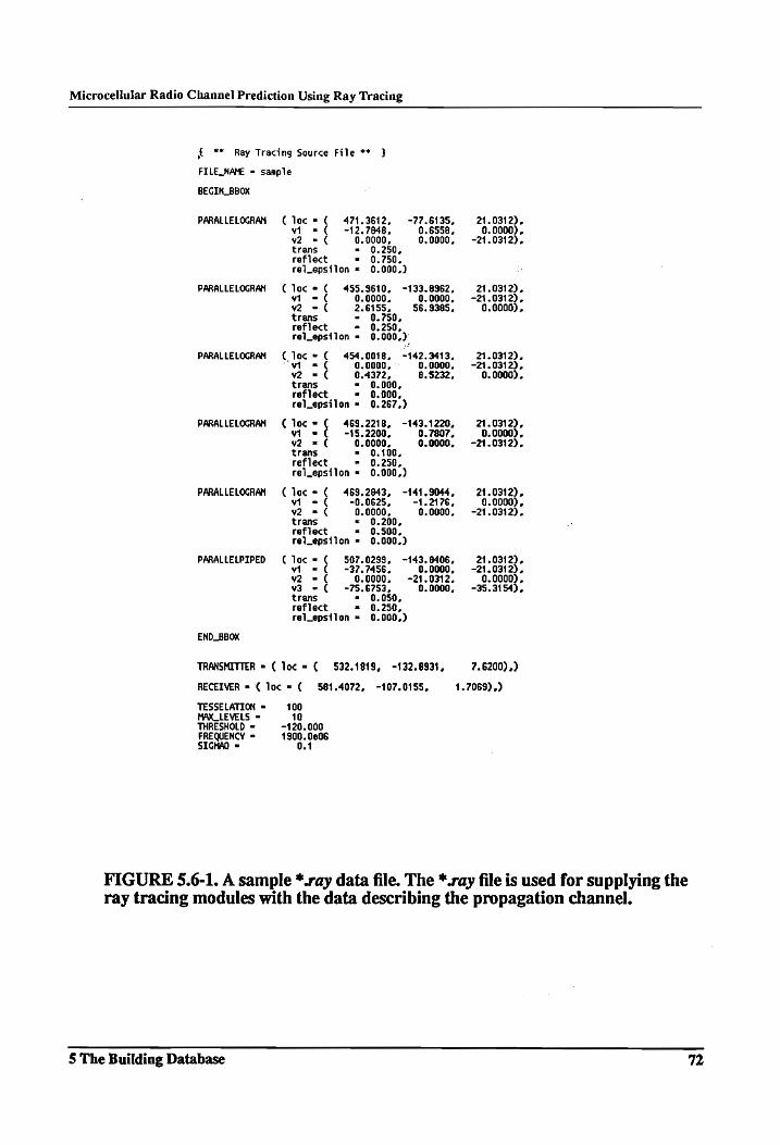
Microcellular Radio Channel Prediction Using Ray Tracing
£ “* Ray Tracing Source File ** }
FILE_LNAME = sample
BEGIN_BBOX
PARALLELOGRAM ( lec = ( 471.3612, -77.6135, 21.0312). vio = ( -12.7648, 0.6558, 0.0000}. v2 = ¢ 0.0000, 0.0000, -21.0312), trans = 0.250, reflect = 0.750, rel_epsilon = 0.000.)
PARALLELOGRAM vV_ loc = ( 455.9610, -133.6962, 21.0312),
vi = ¢ 0.9000, 0.0000, -21.0312), v2 = ( 2.6155, 56.9385, 0.0000), trans = 0.750, reflect = 0.250, rel_epsilon = 0.000,)
PARALLELOGRAM (loc = ( 454.0018, -142.3413, 21.0312), “vt = ¢ 0.0000, 0.0000, -21.0312),
v2 = ( 0.4372, 8.5232, 0.0000), trans = 0.000, reflect = 0.000, rel_epsilon = 0.267,)
PARALLELOGRAM ( loc = ( 469.2218, -143.1220, 21.0312), vio=( -15.2200, 0.7807, 0.0000). v2 =f 0.0000, 0.0000, -21.0312). trans = 0.106, reflect = 0.250. rel_epsilon = 0.000,)
PARALLELOGRAM (loc = ( 469.2843, -141.9044, 21.0312), vie ¢ -0.0625, -1.2176, 0.0000), v2 = ¢ 0.0000, 0.0000, -21.0312). trans = 0.200, reflect = 0.500, rel_epsilon = 0.000,)
PARALLELPIPED ( loc = ( 507.0299, -143.6406, 21.0312), v1 = ( -37.7456, 0.0000, -21.0312), v2 = ( 0.0000, -21.0312, 0.0000). v3 = ( +-75.6753, 0.0000, -35.3154), trans = 0.650, reflect = 0.250, rel_epsilon = 0.000,)
END_BBOX
TRANSMITTER = ( loc = ( 532.1819, -132.8931, 7.6200) ,)
RECEIVER = ( loc = ( 581.4072, -107.0155, 1.7069) ,)
TESSELATION = 100 MAX_LEVELS = 10 THRESHOLD = -120.000 FREQUENCY = 1900.0e06 STCMAQ = 0.1
FIGURE 5.6-1. A sample *.ray data file. The *.ray file is used for supplying the ray tracing modules with the data describing the propagation channel.
5 The Building Database 72
Microcellular Radio Channel Prediction Using Ray Tracing
e vJ denotes the second corner of the parallelogram relative to the first corner. The
three numeric values represent the local x,y,z coordinates of the second corner
and the magnitude of this vector is the length of the parallelogram.
e v2 denotes the third corner of the parallelogram relative to the first corner. The three numeric values represent the local x,y,z coordinates of the third corner and
the magnitude of this vector is the width of the parallelogram.
¢ any information specified in OBJECT_DATA can be also be specified here.
PARALLELPIPED
This string denotes the group of data for an entity which is a parallelepiped. A par-
allelepiped can have a random orientation relative to the x and y axes (1.e., the ver-
. tical sides of the object must be aligned with the z axis where one parallelepiped face is parallel to the xy plane). The strings used to define a parallelepiped are:
e loc denotes the vector location of the parallelepiped. The three numeric values
(separated by one or more non-string type characters) represent the absolute x,y,z coordinate values of the location vector. Note that the location vector specifies
the first corner of the parallelepiped.
e vl denotes the second corner of the parallelepiped relative to the first corner. The
numeric values represent the local x,y,z coordinates of the second corner of the
parallelepiped. This vector lies in a plane parallel to the xz plane (.e., y = 0 for
this vector) and it represents the length of the parallelepiped.
e v2 denotes the third corner of the parallelogram relative to the first corner. The
three numeric values represent the local x,y,z coordinates. This vector is parallel
to the y axis (i.e., x and z are zero for this vector) and it represents the length of the parallelepiped.
e v3 denotes the third corner of the parallelogram relative to the first corner. The
numeric values represent the local x,y,z coordinates of the second corner of the
parallelepiped. This vector lies in a plane parallel to the xz plane (i.e., y = 0 for this vector) and it represents the width of the parallelepiped.
e any information specified in OBJECT_DATA can be also be specified here.
BEGIN_BBOX and END_BOX
The BEGIN_BBOxX string denotes the beginning of a bounding volume (box) that
will enclose several objects. The string is followed by several descriptions of objects to enclose. The list of objects to enclose is terminated with the END_B-
BOX string.
5 The Building Database 73

Microcellular Radio Channel Prediction Using Ray Tracing
TESSELATION
This string is followed by an integer value representing the tessellation of the geo-
desic dome faces used in the ray launching algorithm.
MAX_LEVELS
This string is followed by an integer value representing the maximum number of
levels a ray is traced (i.e., the maximum depth of the ray tree).
FREQUENCY A floating point value following this string represents the carrier frequency (Hz)
used for diffraction and radar cross section backscatter calculations.
SIGMAO
A floating point value following this string denotes the roughness factor applied to
the radar cross section calculation for different building surfaces.
5.7 Conclusions
This chapter has described the important features of the AutoCAD three dimen-
sional building database used to supply site-specific data to the ray tracing modules. The
AutoCAD program along with some custom software permit the transfer of this data to the
ray tracing modules. A sample database has been constructed and successfully converted
to the correct file format.
5 The Building Database 74
Microcellular Radio Channel Prediction Using Ray Tracing
6 Computer Ray Tracing
Chapter 4, showed that large scale environmental factors, such as the position and
orientation of buildings, dominated the average path loss of narrow band signals. Further-
more, using a simple ray propagation model and site-specific data regarding these environ-
mental factors, it was possible to accurately predict average path loss. These observations
were extended in Chapter 5, where it was proposed that the large-scale building geometry
dominated average path loss in wide band signals as well. In addition, it was proposed that
the time dispersion of the channel is related to the location of these building scatterers.
Thus, it may be possible to employ a ray propagation model to predict both wide band and
narrow band channel characteristics.
This chapter presents the ray propagation model and the technical issues required
for automating this model in a ray tracing system. The principal propagation model uses
geometrical optics to trace the propagation of direct, reflected, transmitted, scattered, and
diffracted fields. The rays, which represent a local plane wave of the total field, originate
from point sources and propagate in three-dimensional space. Some of the technical issues
discussed in this chapter include the optimal method for launching the rays, tracing the
rays in three dimensions, and receiving rays. Data processing techniques for comparing
predicted results against measured data are also provided.
6.1 The Channel Model
The equation used to describe a multipath channel is first proposed in [Tur72] and
is subsequently used by several other researchers [Dev86][Rap89][Sei91]. The equation
takes the form of a bandlimited impulse response, h(t). For a general multipath channel
this impulse response is composed of several attenuated and time delayed impulses, result-
ing in
h(t) = ya,5 (t-t,). (6.1-1)
k
6 Computer Ray Tracing 75
Microcellular Radio Channel Prediction Using Ray Tracing
The emphasis of the computer ray tracing is to determine suitable values for the parame-
ters given in Equation 6.1-1. This requires evaluation of the amplitude (cj,) and the arrival
times (t,) for each multipath component and will result in an accurate prediction of the
propagation characteristics. Geometrical optics, or ray tracing, is the method selected for
evaluating these parameters.
6.2 The Propagation Model
The model assumes the propagation of energy from the transmitter to the receiver
occurs along direct, reflected, transmitted, diffracted, and diffusely scattered paths. In con-
sidering each type of ray path, it is important to recognize the path loss dependence of the
ray. As discussed in Section 2.2, direct (line-of-sight) rays exhibit a 1fd? power depen-
dence according to Friis free space transmission. Specularly reflected and transmitted rays
follow a 1/d” dependence, where d represents the total ray path length. For example, the
specularly reflected ray shown in Figure 6.2-1, whose path segments are labeled r; and r2
has a path loss proportional to 1/(r; + ry). Alternatively, the diffusely scattered field com-
prised of the path segments s; and s2 exhibits a multiplicative dependence given by 1/
(s 189)? The multiplicative dependence is due to the additional spreading loss the ray expe-
riences after re-radiation from the scattering surface.
The diffuse component is commonly neglected in propagation models because its
magnitude decreases more rapidly with distance than the specular component [Ike84]
{[Hon92][Law92]. In computing average path loss, this is generally a valid assumption
since the specular component contains a greater portion of the total energy and thus con-
tributes more to the received power. However, the diffuse component influences the local
average at locations that are close to the scattering point (i.e., when sz is small). This
accounts for scattering objects in a local area of the receiving point which may have a sig-
nificant quantity of incident energy but do not satisfy the geometric requirements to spec-
ularly refiect this energy toward the receiver. In, [Sei92] measurements indicate that when
the line-of-sight component is blocked, a significant quantity of the incident energy can be
attributed to scattering. Moreover, scattered rays, although weak, can have long time
delays that can influence the channel time dispersion. For these reasons, the diffuse com-
6 Computer Ray Tracing 76
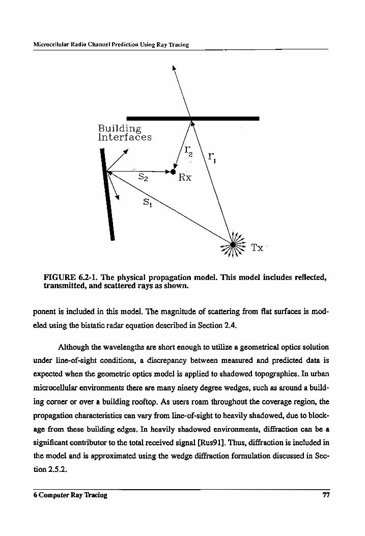
Microcellular Radio Channel Prediction Using Ray Tracing
Building Interfaces
Tx”
FIGURE 6.2-1. The physical propagation model. This model includes reflected, transmitted, and scattered rays as shown.
ponent is included in this model. The magnitude of scattering from flat surfaces is mod-
eled using the bistatic radar equation described in Section 2.4.
Although the wavelengths are short enough to utilize a geometrical optics solution
under line-of-sight conditions, a discrepancy between measured and predicted data is
expected when the geometric optics model is applied to shadowed topographies. In urban
microcellular environments there are many ninety degree wedges, such as around a build-
ing corner or over a building rooftop. As users roam throughout the coverage region, the
propagation characteristics can vary from line-of-sight to heavily shadowed, due to block-
age from these building edges. In heavily shadowed environments, diffraction can be a
significant contributor to the total received signal [Rus91]. Thus, diffraction is included in
the model and is approximated using the wedge diffraction formulation discussed in Sec-
tion 2.5.2.
6 Computer Ray Tracing 77
Microcellular Radio Channel Prediction Using Ray Tracing
In summary, the model includes direct, reflected, transmitted, and scattered fields
represented by the rays. Table 6.2-1 summarizes the variables used to describe the model.
Each propagation mechanism is treated separately, and the total field is determined via
noncoherent superposition of the individual contributions of each ray. Noncoherent energy
reception (i.e., a sum of the power contributed by each received ray) is used since the pro-
gram predicts mean field strength (or path loss) as influenced by large-scale variations in
the environment. Although the constructive and destructive interference of the individual
multipath components still exist in the actual channel, these effects are not modeled here.
This model approximates the channel impulse response, providing a wide band character-
ization of the channel. In [Tel91] wide band signals are shown to exhibit little variation
over small distances where the large scale geometry of the environment remains constant.
Although a more accurate approximation to the channel could be obtained by pre-
dicting the complex channel impulse response, this accuracy could only be achieved if
exact data regarding the electromagnetic properties of the surface as well as wave polar-
ization is included in the model. Although researchers are attempting to characterize the
electromagnetic properties of common building materials (brick, stone, glass, etc.) on both
a micro- and macroscopic scale [Sou92][Lan92], there is currently little published data on
these properties in the UHF and low microwave regions. Until this data is readily avail-
able, it is impossible to account for the phase variations induced by interaction of the wave
with building surfaces (due to a complex dielectric constant).
An accurate estimate to the complex channel impulse response also requires polar-
ization effects. Currently, there is no provision for polarization in the model. It is likely
that there will be instances where a reflection from a planar interface occurs at oblique
incidence and with arbitrary wave polarization. That is, due to the incident wave polariza-
tion and surface orientation, the refiection obeys neither perfectly parallel of perfectly per-
pendicular polarization. This causes wave depolarization (relative to the transmitter and/or
receiver antenna polarizations) and results in a change in the received field amplitude. It is
possible to resolve a reflection for oblique incidence and arbitrary polarization by splitting
the incident ray into parallel and perpendicularly polarized components and then recom-
bining after reflection or transmission [Bec63]. However, this can only be done if the
6 Computer Ray Tracing , 78
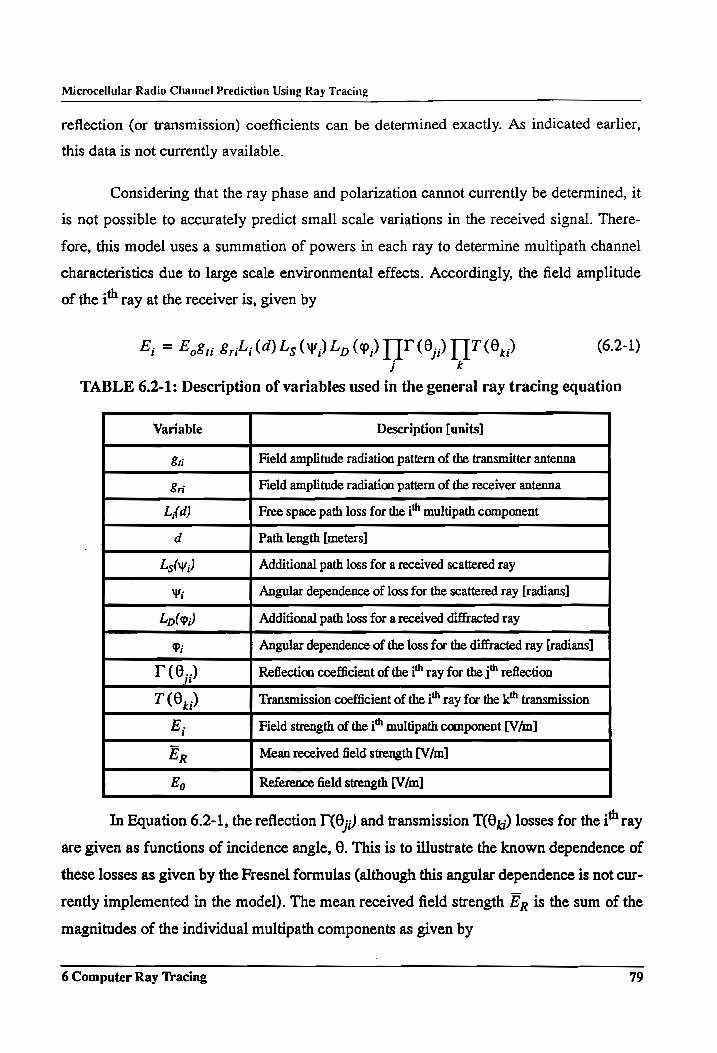
Microcellular Radio Channel Prediction Using Ray Tracing
reflection (or transmission) coefficients can be determined exactly. As indicated earlier,
this data is not currently available.
Considering that the ray phase and polarization cannot currently be determined, it
is not possible to accurately predict small scale variations in the received signal. There-
fore, this model uses a summation of powers 1n each ray to determine multipath channel
characteristics due to large scale environmental effects. Accordingly, the field amplitude
of the i‘ ray at the receiver is, given by
i= E084; 8h (OD) Ls (W) Lp (0) TT (8) T]7 Od (6.2-1) j k
TABLE 6.2-1: Description of variables used in the general ray tracing equation
Variable Description [units]
Li Field amplitude radiation pattern of the transmitter antenna
Sri Field amplitude radiation pattern of the receiver antenna
Ld) Free space path loss for the i multipath component
d Path length [meters]
Ls(y;) Additional path loss for a received scattered ray
W; Angular dependence of loss for the scattered ray [radians]
Ly(9;) Additional path loss for a received diffracted ray
®; Angular dependence of the loss for the diffracted ray [radians]
a) Py Reflection coefficient of the i" ray for the j" reflection
T (0,;) Transmission coefficient of the i" ray for the k™ transmission
E; Field strength of the i“ multipath component [V/m]
Er Mean received field strength [V/m]
Eo Reference field strength [V/m]
In Equation 6.2-1, the reflection I'(0;;) and transmission T(,;) losses for the i ray
are given as functions of incidence angle, 8. This is to illustrate the known dependence of
these losses as given by the Fresnel formulas (although this angular dependence is not cur-
rently implemented in the model). The mean received field strength Ep is the sum of the
magnitudes of the individual multipath components as given by
6 Computer Ray Tracing 79
Microcellular Radio Channel Prediction Using Ray Tracing
Ep = VE? (6.2-2)
Path loss is computed by referencing the result of (6.2.2) to a 1-meter free space path loss
reference. Using a 1-meter free space path loss reference, the modeled path loss is given
by
PL (dB wrt 1-meter FSPL] = 10x log, of 7 | (6.2-3) I
6.3 Ray Tracing Techniques
6.3.1 Brute Force Ray Tracing versus Image Theory
Tracing the paths of significant energy arriving at a receiver can be accomplished
by using either brute force ray or image theory ray tracing. For brute force ray tracing a
finite number of rays, representing “tubes” of energy, are launched from the transmitter
and these rays are traced until either no (further) objects intersect the ray path or the
amplitude of each ray falls below some threshold. The rays passing through the receiver
location contribute to the total received signal. The alternative technique is to employ
image theory, or equivalence. For a given transmitter and receiver location, image theory
locates the exact locations where reflections (and transmissions) occur. Tests are then per-
formed to determine which of these image points are visible at the receiver location to
contribute to the received signal.
At first, image theory would appear to be the best method; the solution requires
fewer computations, as rays that do not reach the receiver are not considered, and it
appears to be a better theoretical approach (i.e., an “exact” solution). These observations
may have provided the impetus for several researchers to adopt image theory for tracing
rays in their propagation model [Law92][Dri92][McK91]. In contrast, this research uses a
brute force ray tracing approach. There are several compelling reasons to believe that this
is a superior method. Image theory works quite well for simple environments, but can
become complicated as the number of reflections/transmissions or the complexity of the
site-specific database increases. More importantly, by tracing tubes of energy from a trans-
6 Computer Ray Tracing 80
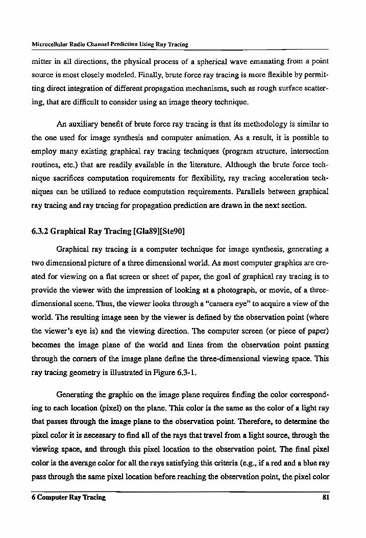
Microcellular Radio Channel Prediction Using Ray Tracing
mitter in all directions, the physical process of a spherical wave emanating from a point
source is most closely modeled. Finally, brute force ray tracing is more flexible by permit-
ting direct integration of different propagation mechanisms, such as rough surface scatter-
ing, that are difficult to consider using an image theory technique.
An auxiliary benefit of brute force ray tracing is that its methodology is similar to
the one used for image synthesis and computer animation. As a result, it is possible to
employ many existing graphical ray tracing techniques (program structure, intersection
routines, etc.) that are readily available in the literature. Although the brute force tech-
nique sacrifices computation requirements for flexibility, ray tracing acceleration tech-
niques can be utilized to reduce computation requirements. Parallels between graphical
ray tracing and ray tracing for propagation prediction are drawn in the next section.
6.3.2 Graphical Ray Tracing [Gla89][Ste90]
Graphical ray tracing is a computer technique for image synthesis, generating a
two dimensional picture of a three dimensional world. As most computer graphics are cre-
ated for viewing on a flat screen or sheet of paper, the goal of graphical ray tracing is to
provide the viewer with the impression of looking at a photograph, or movie, of a three-
dimensional scene. Thus, the viewer looks through a “camera eye” to acquire a view of the
world. The resulting image seen by the viewer is defined by the observation point (where
the viewer’s eye is) and the viewing direction. The computer screen (or piece of paper)
becomes the image plane of the world and lines from the observation point passing
through the corners of the image plane define the three-dimensional viewing space. This
ray tracing geometry is illustrated in Figure 6.3-1.
Generating the graphic on the image plane requires finding the color correspond-
ing to each location (pixel) on the plane. This color is the same as the color of a light ray
that passes through the image plane to the observation point. Therefore, to determine the
pixel color it is necessary to find all of the rays that travel from a light source, through the
viewing space, and through this pixel location to the observation point. The final pixel
color is the average color for all the rays satisfying this criteria (e.g., if ared and a blue ray
pass through the same pixel location before reaching the observation point, the pixel color
6 Computer Ray Tracing 81
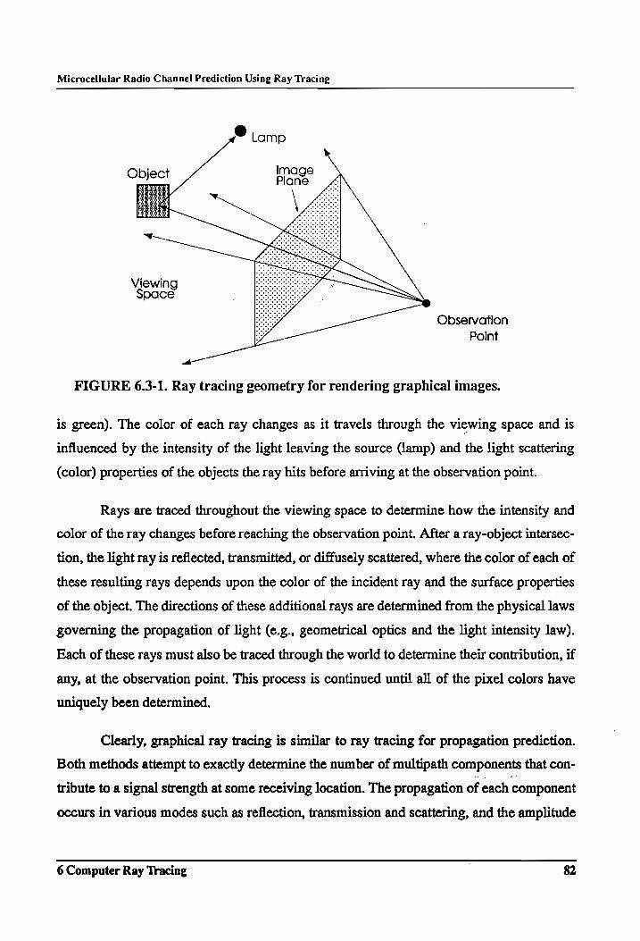
Microcellular Radio Channel Prediction Using Ray Tracing
e Lamp
Object Image
Viewing Space
Observation
Point
FIGURE 6.3-1. Ray tracing geometry for rendering graphical images.
is green). The color of each ray changes as it travels through the viewing space and is
influenced by the intensity of the light leaving the source (lamp) and the light scattering
(color) properties of the objects the ray hits before arriving at the observation point.
Rays are traced throughout the viewing space to determine how the intensity and
color of the ray changes before reaching the observation point. After a ray-object intersec-
tion, the light ray is reflected, transmitted, or diffusely scattered, where the color of each of
these resulting rays depends upon the color of the incident ray and the surface properties
of the object. The directions of these additional rays are determined from the physical laws
governing the propagation of light (e.g., geometrical optics and the light intensity law).
Each of these rays must also be traced through the world to determine their contribution, if
any, at the observation point. This process is continued until all of the pixel colors have
uniquely been determined.
Clearly, graphical ray tracing is similar to ray tracing for propagation prediction.
Both methods attempt to exactly determine the number of multipath components that con-
tribute to a signal strength at some receiving location. The propagation of each component
occurs in various modes such as reflection, transmission and scattering, and the amplitude
6 Computer Ray Tracing 82
Microcellular Radio Channel Prediction Using Ray Tracing
for each multipath component is highly dependent upon the properties of the objects that it
encounters along the propagation path. Although the general principles are similar, there
are several distinct differences between the two methods. First, graphical ray tracing uses
backward ray tracing. As shown in Figure 6.3-1, rays are traced backward from the obser-
vation point, through the image plane and viewing space, and then to the lamp. This is
done to reduce the number of rays traced since only the rays that reach the observation
point need to be considered. Ray tracing for propagation prediction requires rays to be
traced in three dimensions to guarantee that all possible propagation paths are considered.
Moreover, the models for reflection, transmission, and scattering are generally more com-
plex than the simple models used for tracing light rays. Finally, unlike graphical ray trac-
ing the data regarding the propagation of the ray (e.g., propagation path length, amplitude,
etc.) must be maintained in the program and written to a file. This additional data 1s
needed to re-create the modeled channel impulse response, and it adds another degree of
complexity to the computer code. The similarities between the two techniques allow use
of graphical ray tracing computer code as a starting point. However, this code must be
extensively modified to include the added features necessary for predicting radio wave
propagation.
6.3.3 Available Computer Software for Ray Tracing
Several ray tracing programs are readily available as freeware on UNIX servers at
other universities and research institutes. The ray tracing code used as the foundation of
this research is available in [Ste90]. This code is selected because it has several desirable
features. Most importantly, the code is written in C++ and it is supplied with extensive
documentation. The object-oriented features of C++ provide direct methods for manipu-
lating the types of data structures that are necessary in the ray tracing program. The origi-
nal source code is written for operation on a PC platform using Borland C++. A filter is
also provided with the ray tracing code so that the results can be viewed on a VGA display
system. The filter is necessary to convert the raw ray tracing data into a 640 pixel by 480
pixel standard VGA format. The graphical display feature is useful as a learning tool as
well as for dynamically viewing the impact of (early) modifications to the program.
According to M&T Books, the text’s publisher, the software can be used for any form of
6 Computer Ray Tracing 83
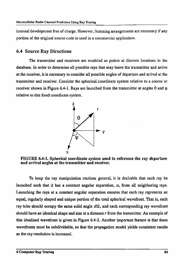
Microcellular Radio Channel Prediction Using Ray Tracing
internal development free of charge. However, licensing arrangements are necessary if any
portion of the original source code is used in a commercial application.
6.4 Source Ray Directions
The transmitter and receivers are modeled as points at discrete locations in the
database. In order to determine all possible rays that may leave the transmitter and arrive
at the receiver, it is necessary to consider all possible angles of departure and arrival at the
transmitter and receiver. Consider the spherical. coordinate system relative to a source or
receiver shown in Figure 6.4-1. Rays are launched from the transmitter at angles @ and
relative to this fixed coordinate system.
Z
X
FIGURE 6.4-1. Spherical coordinate system used to reference the ray departure and arrival angles at the transmitter and receiver.
To keep the ray manipulation routines general, it is desirable that each ray be
launched such that it has a constant angular separation, a, from all neighboring rays.
Launching the rays at a constant angular separation ensures that each ray represents an
equal, regularly shaped and unique portion of the total spherical wavefront. That is, each
ray tube should occupy the same solid angle dQ, and each corresponding ray wavefront
should have an identical shape and size at a distance r from the transmitter. An example of
this idealized wavefront is given in Figure 6.4-2. Another important feature is that these
wavefronts must be subdividable, so that the propagation model yields consistent results
as the ray resolution is increased.
6 Computer Ray Tracing 84
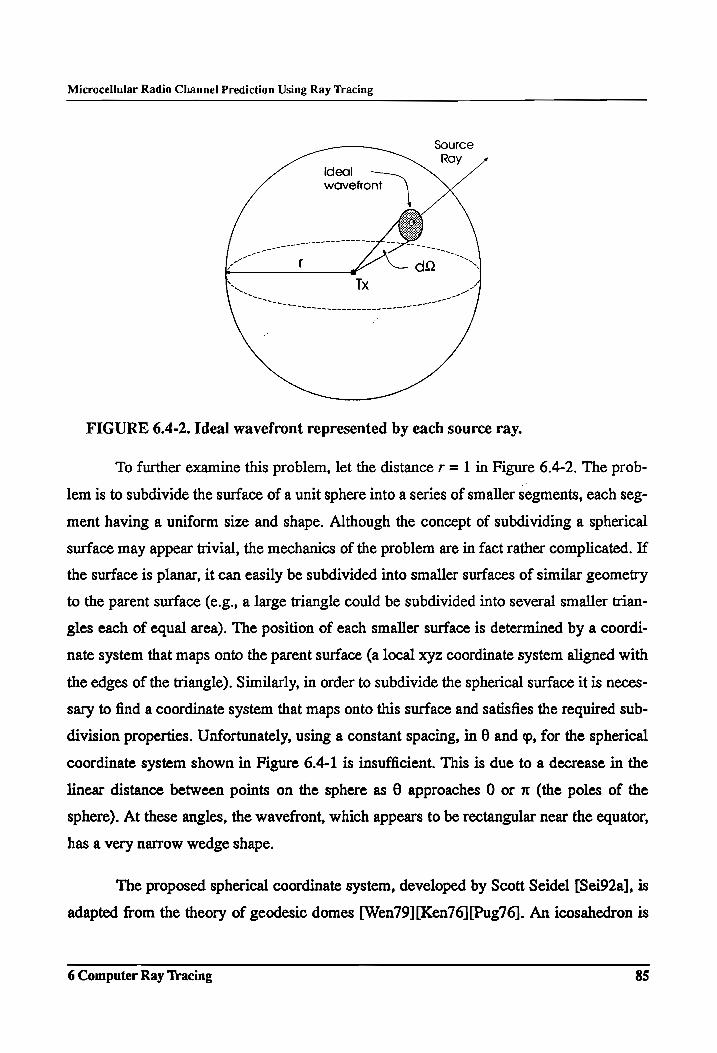
Microcellular Radio Channel Prediction Using Ray Tracing
Source
ideal
wavetront
oo me
7s
~ - ~~. “— ~ -" ~— -
TO eae a ee el
FIGURE 6.4-2. Ideal wavefront represented by each source ray.
To further examine this problem, let the distance r = 1 in Figure 6.4-2. The prob-
lem is to subdivide the surface of a unit sphere into a series of smaller segments, each seg-
ment having a uniform size and shape. Although the concept of subdividing a spherical
surface may appear trivial, the mechanics of the problem are in fact rather complicated. If
the surface is planar, it can easily be subdivided into smaller surfaces of similar geometry
to the parent surface (e.g., a large triangle could be subdivided into several smaller trian-
gles each of equal area). The position of each smaller surface is determined by a coordi-
nate system that maps onto the parent surface (a local xyz coordinate system aligned with
the edges of the triangle). Similarly, in order to subdivide the spherical surface it is neces-
sary to find a coordinate system that maps onto this surface and satisfies the required sub-
division properties. Unfortunately, using a constant spacing, in 0 and 9, for the spherical
coordinate system shown in Figure 6.4-1 is insufficient. This is due to a decrease in the
linear distance between points on the sphere as 6 approaches 0 or x (the poles of the
sphere). At these angles, the wavefront, which appears to be rectangular near the equator,
has a very narrow wedge shape.
The proposed spherical coordinate system, developed by Scott Seidel [Sei92a], is
adapted from the theory of geodesic domes [Wen79][Ken76][Pug76]. An icosahedron is
6 Computer Ray Tracing 85
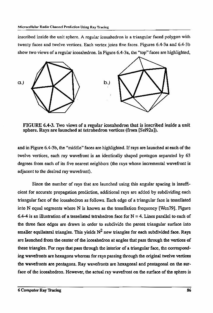
Microcellular Radio Channel Prediction Using Ray Tracing
inscribed inside the unit sphere. A regular icosahedron is a triangular faced polygon with
twenty faces and twelve vertices. Each vertex joins five faces. Figures 6.4-3a and 6.4-3b
show two views of a regular icosahedron. In Figure 6.4-3a, the “top” faces are highlighted,
a.) b.)
FIGURE 6.4-3. Two views of a regular icosahedron that is inscribed inside a unit sphere. Rays are launched at tetrahedron vertices (from [Sei92a)).
and in Figure 6.4-3b, the “middle” faces are highlighted. If rays are launched at each of the
twelve vertices, each ray wavefront is an identically shaped pentagon separated by 63
degrees from each of its five nearest neighbors (the rays whose incremental wavefront is
adjacent to the desired ray wavefront).
Since the number of rays that are launched using this angular spacing is insuffi-
cient for accurate propagation prediction, additional rays are added by subdividing each
triangular face of the icosahedron as follows. Each edge of a triangular face is tessellated
into N equal segments where N is known as the tessellation frequency [Wen79]. Figure
6.4-4 is an illustration of a tessellated tetrahedron face for N = 4. Lines parallel to each of
the three face edges are drawn in order to subdivide the parent triangular surface into
smaller equilateral triangles. This yields N? new triangles for each subdivided face. Rays
are launched from the center of the icosahedron at angles that pass through the vertices of
these triangles. For rays that pass through the interior of a triangular face, the correspond-
ing wavefronts are hexagons whereas for rays passing through the original twelve vertices
the wavefronts are pentagons. Ray wavefronts are hexagonal and pentagonal on the sur-
face of the icosahedron. However, the actual ray wavefront on the surface of the sphere is
6 Computer Ray Tracing 86
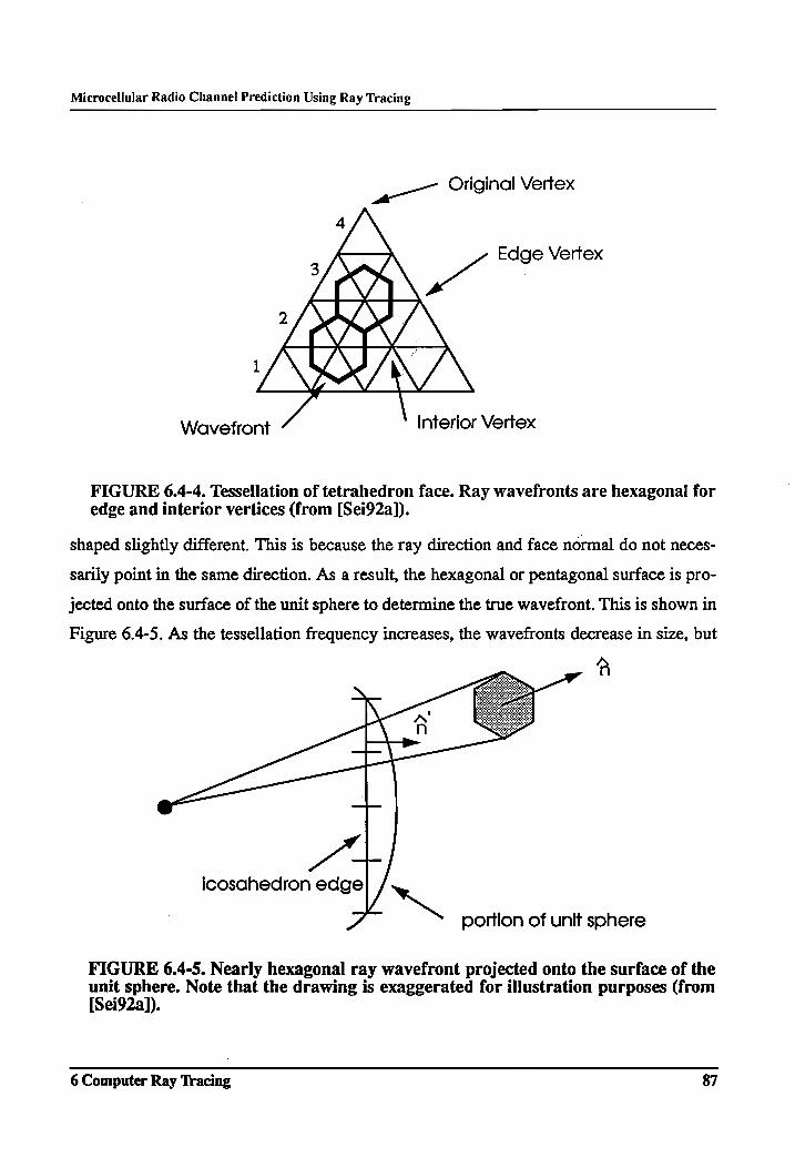
Microcellular Radio Channel Prediction Using Ray Tracing
Original Vertex -—_ g
Wavefront Interior Vertex
FIGURE 6.4-4. Tessellation of tetrahedron face. Ray wavefronts are hexagonal for edge and interior vertices (from [Sei92a]).
shaped slightly different. This is because the ray direction and face normal do not neces-
sarily point in the same direction. As a result, the hexagonal or pentagonal surface is pro-
jected onto the surface of the unit sphere to determine the true wavefront. This is shown in
Figure 6.4-5. As the tessellation frequency increases, the wavefronts decrease in size, but
n
icosahedron edge NK
7 portion of unit sohere
FIGURE 6.4-5. Nearly hexagonal ray wavefront projected onto the surface of the unit sphere. Note that the drawing is exaggerated for illustration purposes (from [Sei92a]).
6 Computer Ray Tracing 87
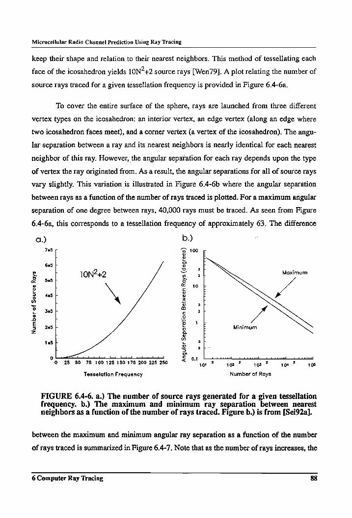
Microcellular Radio Channel Prediction Using Ray Tracing
keep their shape and relation to their nearest neighbors. This method of tessellating each
face of the icosahedron yields 10N*+2 source rays [Wen79]. A plot relating the number of
source rays traced for a given tessellation frequency is provided in Figure 6.4-6a.
To cover the entire surface of the sphere, rays are launched from three different
vertex types on the icosahedron: an interior vertex, an edge vertex (along an edge where
two icosahedron faces meet), and a corner vertex (a vertex of the icosahedron). The angu-
lar separation between a ray and its nearest neighbors is nearly identical for each nearest
neighbor of this ray. However, the angular separation for each ray depends upon the type
of vertex the ray originated from. As a result, the angular separations for all of source rays
vary slightly. This variation is illustrated in Figure 6.4-6b where the angular separation
between rays as a function of the number of rays traced is plotted. For a maximum angular
separation of one degree between rays, 40,000 rays must be traced. As seen from Figure
6.4-6a, this corresponds to a tessellation frequency of approximately 63. The difference
a.) b.) 7e5 7 “m 100
605 F
a ® ee
oO o
z Maxi S o 2 aximum
ec ses} o
8 < TOE L.
> 405, o r ° 3 E . a os ~ L
© 3e5 4 ot © 3
E ae: 5 2054 S F Minimum z o r
a 105 F 5 3
L 3 2 a
0 es oe ee eee eee ee ee ee | < 0.1 al pital Lo | j
0 25 50 75 160 125 150 175 200 225 250 101 2 102 2 103 2 104 2 105
Tesselation Frequency Number of Rays
FIGURE 6.4-6. a.) The number of source rays generated for a given tessellation frequency. b.) The maximum and minimum ray separation between nearest neighbors as a function of the number of rays traced. Figure b.) is from [Sei92a].
between the maximum and minimum angular ray separation as a function of the number
of rays traced is summarized in Figure 6.4-7. Note that as the number of rays increases, the
6 Computer Ray Tracing 88
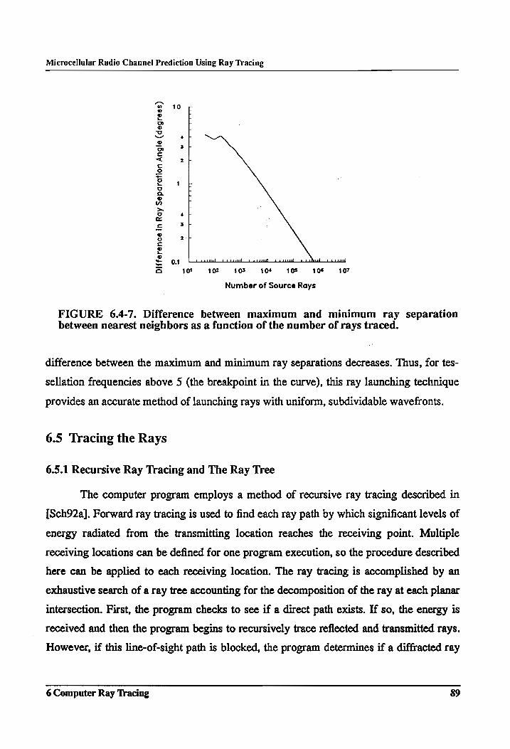
Microcellular Radio Channel Prediction Using Ray Tracing
10 ¢
0.1
Difference
in Ray
Sepa
rati
on Angle
(degrees)
101 102 105 104 105 106 107
Number of Source Rays
FIGURE 6.4-7. Difference between maximum and minimum ray separation between nearest neighbors as a function of the number of rays traced.
difference between the maximum and minimum ray separations decreases. Thus, for tes-
sellation frequencies above 5 (the breakpoint in the curve), this ray launching technique
provides an accurate method of launching rays with uniform, subdividable wavefronts.
6.5 Tracing the Rays
6.5.1 Recursive Ray Tracing and The Ray Tree
The computer program employs a method of recursive ray tracing described in
[Sch92a]. Forward ray tracing is used to find each ray path by which significant levels of
energy radiated from the transmitting location reaches the receiving point. Multiple
receiving locations can be defined for one program execution, so the procedure described
here can be applied to each receiving location. The ray tracing is accomplished by an
exhaustive search of a ray tree accounting for the decomposition of the ray at each planar
intersection. First, the program checks to see if a direct path exists. If so, the energy is
received and then the program begins to recursively trace reflected and transmitted rays.
However, if this line-of-sight path is blocked, the program determines if a diffracted ray
6 Computer Ray Tracing 89
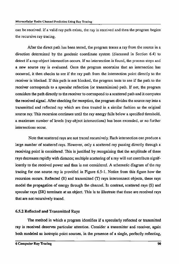
Microcellular Radio Channel Prediction Using Ray Tracing
can be received. If a valid ray path exists, the ray is received and then the program begins
the recursive ray tracing.
After the direct path has been tested, the program traces a ray from the source in a
direction determined by the geodesic coordinate system (discussed in Section 6.4) to
detect if a ray-object intersection occurs. If no intersection is found, the process stops and
a new source ray is evaluated. Once the program ascertains that an intersection has
occurred, it then checks to see if the ray path from the intersection point directly to the
receiver is blocked. If this path is not blocked, the program tests to see if the path to the
receiver corresponds to a specular reflection (or transmission) path. If not, the program
considers the path directly to the receiver to correspond to a scattered path and it computes
the received signal. After checking for reception, the program divides the source ray into a
transmitted and reflected ray which are then treated in a similar fashion as the original
source ray. This recursion continues until the ray energy falls below a specified threshold,
a maximum number of levels (ray-object intersections) has been exceeded, or no further
intersections occur.
Note that scattered rays are not traced recursively. Each intersection can produce a
large number of scattered rays. However, only a scattered ray passing directly through a
receiving point is considered. This is justified by recognizing that the amplitude of these
rays decreases rapidly with distance; multiple scattering of a ray will not contribute signif-
icantly to the received power and thus is not considered. A schematic diagram of the ray
tracing for one source ray is provided in Figure 6.5-1. Notice from this figure how the
recursion occurs. Reflected (R) and transmitted (T) rays interconnect objects, these rays
model the propagation of energy through the channel. In contrast, scattered rays (S) and
specular rays (SR) terminate at an object. This is to illustrate that these are received rays
that are not recursively traced.
6.5.2 Reflected and Transmitted Rays
The method in which a program identifies if a specularly reflected or transmitted
ray is received deserves particular attention. Consider a transmitter and receiver, again
both modeled as isotropic point sources, in the presence of a single, perfectly reflecting,
6 Computer Ray Tracing 90
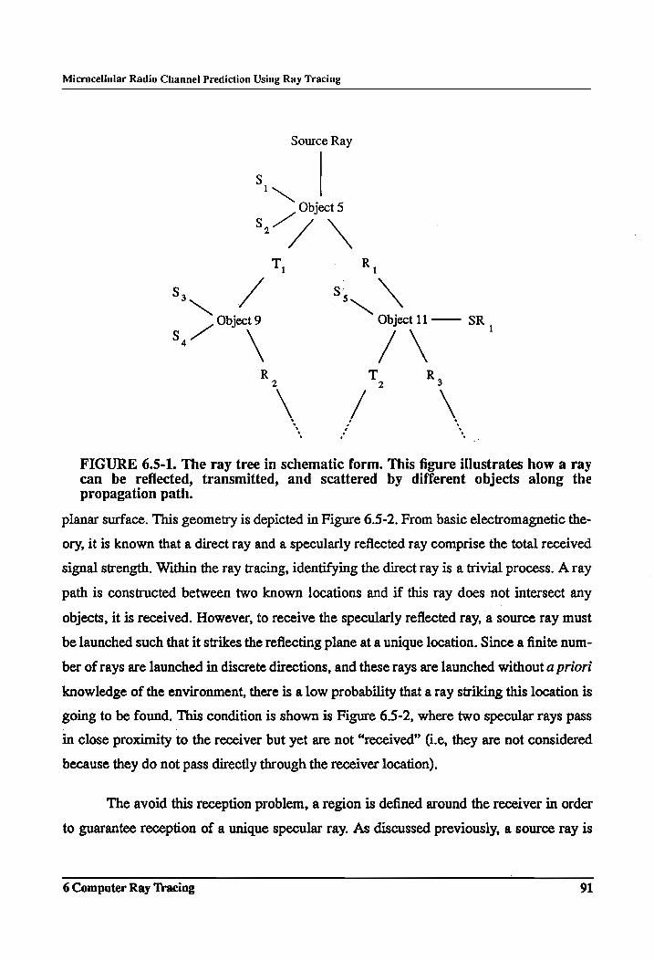
Microcellular Radio Channel Prediction Using Ray Tracing
Source Ray
1
U7 ool 5
J uo \ eN Object 9 Object 11—— SR '
S,~ At \ /\
FIGURE 6.5-1. The ray tree in schematic form. This figure illustrates how a ray can be reflected, transmitted, and scattered by different objects along the propagation path.
planar surface. This geometry is depicted in Figure 6.5-2. From basic electromagnetic the-
ory, it is known that a direct ray and a specularly reflected ray comprise the total received
signal strength. Within the ray tracing, identifying the direct ray is a trivial process. A ray
path is constructed between two known locations and if this ray does not intersect any
objects, it is received. However, to receive the specularly reflected ray, a source ray must
be launched such that it strikes the reflecting plane at a unique location. Since a finite num-
ber of rays are launched in discrete directions, and these rays are launched without a priori
knowledge of the environment, there is a low probability that a ray striking this location is
going to be found. This condition is shown is Figure 6.5-2, where two specular rays pass
in close proximity to the receiver but yet are not “received” (i.e, they are not considered
because they do not pass directly through the receiver location).
The avoid this reception problem, a region is defined around the receiver in order
to guarantee reception of a unique specular ray. As discussed previously, a source ray is
6 Computer Ray Tracing 91
Microcellular Radio Channel Prediction Using Ray Tracing
Tx direct ray
specularly reflected rays
FIGURE 6.5-2. The impact of tracing ‘a finite number of rays in discrete directions. If the transmitter and receiver are modeled as point sources, a method must be implemented to guarantee that a unique, reflected ray will be received.
launched with a constant angular separation, a, from all other source rays. From Section
2.3-1, we know that the rays do not diverge after being reflected from planar surfaces.
Thus, if the straight line segments comprising the total ray path are “unfolded,” each ray
would still be separated from all other unfolded ray paths by a. Using this information, the
test to determine if the ray reaches a receiving point is accomplished as follows. A perpen-
dicular projection from the receiving location to the ray path is computed and the total
(unfolded) path length, d, that the ray travels from the transmitter to the projection point is
determined. A reception sphere (from [Hon92], extended to three dimensions [Sch92a]) is
constructed about the receiving location with a radius proportional to the unfolded path
length and the angular spacing between neighboring rays at the source. If the ray intersects
the sphere, it is considered to be received and thus contributes to the total received signal.
Otherwise, the ray is not received and the recursion proceeds as previously described. The
reception sphere effectively accounts for the divergence of the rays from the source. For
the ray separation a sufficiently small, the ray intercepting the sphere is an accurate mea-
sure of the ray that would pass directly through the receiving point. The physical interpre-
tation of the reception sphere can be justified with the aid of Figure 6.5-3. This figure is a
two dimensional representation of a ray being traced. Two adjacent rays, launched at ta
relative to the test ray, are also shown. Note that in three dimensions, any ray has more
than two adjacent rays and the angular separation of the adjacent rays does not necessarily
coincide with the coordinate axes. As shown in Figure 6.5-3, a reception sphere with the ad
correct radius can receive only one of the rays. If the radius is greater than ——, two of the 3
6 Computer Ray Tracing 92
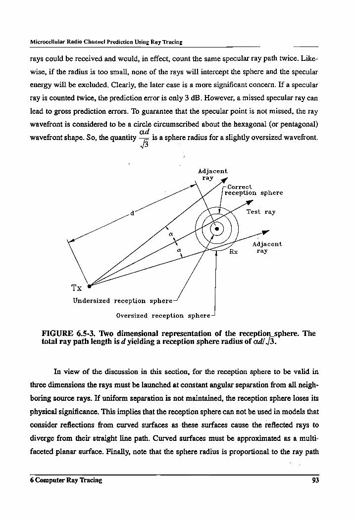
Microcellular Radio Channel Prediction Using Ray Tracing
rays could be received and would, in effect, count the same specular ray path twice. Like-
wise, if the radius is too small, none of the rays will intercept the sphere and the specular
energy will be excluded. Clearly, the later case is a more significant concern. If a specular
ray is counted twice, the prediction error is only 3 dB. However, a missed specular ray can
lead to gross prediction errors. To guarantee that the specular point is not missed, the ray
wavefront is considered to be a circle circumscribed about the hexagonal (or pentagonal) d
wavefront shape. So, the quantity Of isa sphere radius for a slightly oversized wavefront. 3
Adjacent ray
Correct reception sphere
Test ray
Adjacent ray
Tx
Undersized reception sphere Oversized reception sphere
FIGURE 6.5-3. Two dimensional representation of the reception_sphere. The total ray path length is d yielding a reception sphere radius of ad/./3.
In view of the discussion in this section, for the reception sphere to be valid in
three dimensions the rays must be launched at constant angular separation from all neigh-
boring source rays. If uniform separation is not maintained, the reception sphere loses its
physical significance. This implies that the reception sphere can not be used in models that
consider reflections from curved surfaces as these surfaces cause the reflected rays to
diverge from their straight line path. Curved surfaces must be approximated as a multi-
faceted planar surface. Finally, note that the sphere radius is proportional to the ray path
6 Computer Ray Tracing 93
Microcellular Radio Channel Prediction Using Ray Tracing
length, so large T-R separations require a small angular separation of the rays to ensure a
reflection point is not be contained within the reception sphere.
6.5.3 Scattered Rays
Recall from Section 2.4, the bistatic radar equation is used for computing the
power at the terminals of a receiver, separated by some distance from the transmitter, after
the transmitted signal has been isotropically scattered by an object visible at both antenna
locations. Also recall that the instantaneous multipath signal is composed of energy arriv-
ing at the receiver via multiple paths, and these paths are a result of the original signal
being reflected, transmitted, or scattered as it propagates from the transmitter to the
receiver. Considering the similarities, the bistatic radar equation is a plausible method for
modeling the propagation of diffusely scattered energy in a microcellular environment. In
fact, several researchers have used this model to predict scattering from buildings in large
cellular environments [Tak91], or to predict the impact of surrounding buildings on in-
building wireless communication systems [Sei92][Van87]. .
As can be seen by Equation 2.4-2, the magnitude of the power in the scattered field
decreases rapidly with distance, as it follows a multiplicative dependence. There are occa-
sions, though, when the amplitude of the scattered field can be large enough to influence
the local mean. This can occur when a large surface is sufficiently rough to scatter energy
in directions other than the specular direction, and can be particularly significant when the
scattering point is “close” to the receiver (i.e, when rp is small in Equation 2.4-2). For
these rays, the amplitude of the scattered component is determined using the bistatic radar
equation. Note that the scattering model used here is for computing the scattering from
large, rough building surfaces. In a typical microcellular channel, there are numerous
potential scatterers. Smaller scatterers, such as lamp posts, automobiles, and trees, can
also affect the received signal. However, these effects are assumed to be secondary.
For the computed scattered field amplitude to be a realistic measure of the true
scattering level, it is necessary to determine an appropriate value for the radar cross sec-
tion (RCS), o. In [Sei92], the radar cross sections of large scatterers in the mobile and por-
table radio environment is experimentally investigated. Using a simple model to “back
6 Computer Ray Tracing 94
Microcellular Radio Channel Prediction Using Ray Tracing
solve” for the radar cross section from measured data, the effective building RCS varied
from 0 to +45 dBm (dB meters squared) for data collected within the dynamic range of
the measurement device. Although a purely empirical model may be useful as a first order
approximation to worst case scattering, an uncertainty of the relationship between the
physical description of the scattering object and the scattered signal strength is unaccept-
able for the goals of this research. Unfortunately, a purely theoretical RCS model for
building scattering is a difficult problem to solve. The solution requires rigorous electro-
magnetic theory and closed form results are available for only a few, simple geometrical
shapes. Thus, a heuristic approach is necessary to attain a reasonable measure for the
amplitude of the scattered component, since measured data are inconclusive and solving
complex electromagnetic problems is undesirable.
Two simplifying observations are made to determine a representative model for
scattering from building surfaces. First, a general building surface is composed of several
segmented panels and each panel has different surface characteristics (i.e., surface rough-
ness) and different electrical properties. For example, many of the buildings on the Vir-
ginia Tech campus are constructed of rough hewn stone and have glass windows or
metallic doors inset at various locations on the building surface. Each of these panels have
different roughness characteristics and reflectivity. However, these platelets are generally
large as compared to the wavelength and can thus be approximated as independent scatter-
ers.
Secondly, in the UHF and low microwave regions it is unlikely that, other than at
near normal incidence, the Rayleigh Criterion can be satisfied by each platelet (i.e.,
although each panel has different surface characteristics, it is unlikely that any can be con-
sidered “rough”). Thus the generalized scattering from the entire surface is in the specular
direction, with a spread in the geometrical optics beam resulting from scattering from each
platelet. The magnitude of the surface scattering is found by summing the contribution of
each independent scatterer. This model can be considered a second-order correction to
geometrical optics by accounting for both the specularly reflected energy as well as the
diffusely scattered field. A similar modeling method has been successfully used to charac-
terize building scatter in [Noe86].
6 Computer Ray Tracing 95
Microcellular Radio Channel Prediction Using Ray Tracing
Given that an arbitrary surface can be subdivided into several smaller surfaces, it
would be most appealing to compute the magnitude of the scattering on a per ray basis.
There are several reasons why this method is the most tractable solution to the subdivision
problem. First, since the rays are launched with constant angular separation, the wave-
fronts for each incident ray do not overlap, so the surface can be uniquely subdivided in a
direct fashion. Second, the scattering model can be integrated into the ray tracing program
without any extensive modifications to the computer code. Finally, the physical scattering
mechanism is most closely modeled on a per ray basis (e.g., the variations in the building
surface can be directly considered). An example of the subdivision process is illustrated in
Figure 6.5-4. The scattering surface is subdivided into several, smaller rectangular sec-
tions. The area of each section is proportion to the projected area of the ray wavefront.
Thus, the area of a rectangular section is a function of the ray path length and incidence
angle. For example, in Figure 6.5-4, the areas for the rectangular sections farthest from the
transmitter are larger than the closer segments. The backscatter from each rectangular seg-
ment is determined according to the following criteria. Note that scattered rays are not
traced recursively, since their amplitude decreases rapidly with distance. Only the ray that
is scattered directly from the surface is considered.
¢ For the bistatic radar equation to be valid, the transmitter and receiver must be in the far
field with respect to each other and each of the scattering segments. A common mea-
sure of when an object is in the far field is r >2D*/A where r is the distance from the radiator to the observation point, D is the maximum dimension of the radiating device,
and A is the carrier wavelength. In addition to this inequality, the distance, r, must be many times larger than the dimensions of the radiating device or the carrier wavelength
(r>> Dandr>>A).
e The radar cross section for each segment is evaluated in the high frequency limit. That
is, the dimensions of the scattering surface are large as compared to the carrier wave-
length (D >> A).
The incremental radar cross section, oj, for the jth rectangular segment is determined by
Equation 6.5-1. This relation is a simplification of the radar cross section for a conducting
metal plate as discussed in Section 2.4-1. Only the rays that meet the criteria specified
above are included in the received signal.
6 Computer Ray Tracing 96
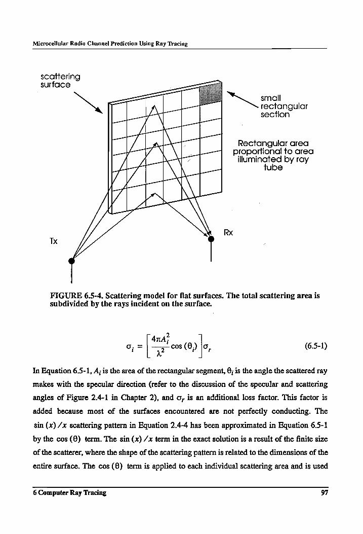
Microcellular Radio Channel Prediction Using Ray Tracing
scattering surface
———
N, r | UN rectangul rectangular — section
|
— — Rectangular area _— |---| _~—« proportional to area
| illuminated by ray | tube
7 La
V ~ a
Rx Tx
FIGURE 6.5-4. Scattering model for flat surfaces. The total scattering area is subdivided by the rays incident on the surface.
4nd?
Oo, = 2 cos 0) [, (6.5-1)
In Equation 6.5-1, A; is the area of the rectangular segment, 6; is the angle the scattered ray
makes with the specular direction (refer to the discussion of the specular and scattering
angles of Figure 2.4-1 in Chapter 2), and 0; is an additional loss factor. This factor is
added because most of the surfaces encountered are not perfectly conducting. The
sin (x) /x scattering pattern in Equation 2.4-4 has been approximated in Equation 6.5-1
by the cos (6) term. The sin (x) /x term in the exact solution is a result of the finite size
of the scatterer, where the shape of the scattering pattern is related to the dimensions of the
entire surface. The cos (9) term is applied to each individual scattering area and is used
6 Computer Ray Tracing 97
Microcellular Radio Channel Prediction Using Ray Tracing
as a first order approximation to the true scattering pattern for the entire surface. It is
assumed here that the scattered energy has some directivity (in the specular direction).
However, since the entire area of the scattering surface and the phase of each scattered ray
is not included in the calculation, the exact sin (x) /x scattering pattern can not be used.
Since the exact scattering characteristics of the buildings are generally unknown,
the amplitude of the scattered field is restricted to
E E,= min| Ep enected a! scattered | (6.5-2)
Where E veretectea 18 the amplitude of a specularly reflected field from the surface and
EF catered 18 the amplitude of the scattered field computed over the entire surface. Thus the
amplitude of the received scattered field is always less than or equal to the amplitude of
specularly reflected field for the same surface and geometry (regardless of whether the
specular component is actually received). This restriction may very well be conservative
in some cases, especially for a very large scattering surface close to, and clearly visible at,
a receiver location. For this particular geometry, it may be possible to receive many rela-
tively strong rays all of which have nearly the same delay. If these components are added
coherently, they would exhibit a self-interference effect. However, since the model adds
the components noncoherently, many strong components arriving with nearly the same
delay may over estimate the true amplitude of the scatter path. The restriction indicated by
Equation 6.5-2 ensures that the amplitude of the scatter path remains within reasonable
bounds. Although arbitrary, if the relation of the frequency and surface variations to the
Rayleigh Criterion are considered, the scattered field being restricted to the amplitude of
the reflected field is a practical limit.
6.5.4 Diffracted Rays
As indicated in Chapter 4, when a receiver is heavily shadowed, a significant por-
tion of the received signal is due to energy diffracting over, or around the building edges.
Clearly, for a propagation model to yield accurate results for both line-of-sight and shad-
owed topographies, diffraction must be included. Unfortunately, unlike reflection, trans-
mission, or even diffuse scattering, the physical process of diffraction does not lend itself
6 Computer Ray Tracing 98
Microcellular Radio Channel Prediction Using Ray Tracing
to an automated ray tracing method. This is due to the manner that diffraction loss is eval-
uated. Recall the simple knife-edge diffraction model discussed in Chapter 2. Beyond the
diffracting obstacle, the incident plane wave spreads around the building obstacle and
extends into the shadowed region. The amplitude of the field after diffraction depends
upon the relative locations of the source, the obstacle and the observation point. Thus, in
order to have a truly integrated diffraction model it is necessary to have knowledge of the
ray direction after diffraction. For example, consider a ray that is reflected, diffracted, and
then refiected as it propagates from the transmitter to the receiver. Locating the first reflec-
tion point and the diffraction location is straightforward since the ray direction and inter-
section locations can be found using simple geometry and the law of reflection. However,
at the diffraction point, the ray direction is no longer clearly defined. To locate the final
reflection point, one option is to model this diffraction location as a new point source and
repeat the entire ray tracing procedure. However, as multiple diffracting edges are encoun-
tered, this complexity of this technique quickly increases by several orders of magnitude.
An alternative is to predetermine the ray direction prior to diffraction so that only the ray
that undergoes the final reflection needs to be traced. Unfortunately, this also becomes a
complicated “book keeping” procedure when several diffracting locations are considered.
A simplification of the diffraction phenomenon is as follows. Consider a mobile
unit located on a street in a typical urban microcell. This mobile unit is shadowed from the
base station, which is located on a cross street, by the building edges at the street-cross
street intersections. Furthermore, consider the signal received by the mobile possesses two
major features: a first arriving component and several delayed components. The first arriv-
ing component, is assumed to be due to energy which diffracts around the obstacle and
propagates directly to the receiver, whereas the delayed components are assumed to be due
to energy that propagates around the corner through reflections from buildings lining the
street. Although these components may also diffract as they propagate past a building cor-
ner, it is assumed here that reflection is the dominant propagation mode for these delayed
components. Thus a reasonable, first approximation to predicting coverage in shadowed
topographies is to predict the diffraction along the path connecting the transmitter and
6 Computer Ray Tracing 99
Microcellular Radio Channel Prediction Using Ray Tracing
receiver, and then let the reflection and scattering models account for the delayed compo-
nents.
The diffraction model implemented in the prediction model evaluates diffraction
loss along the transmitter-receiver (T-R) path using the wedge diffraction model presented
in Section 2.5.2. The vertical edges of a building are modeled as perfectly absorbing 90°
wedges that are infinite in the vertical plane. Since the diffraction model is two-dimen-
sional, the field variation due the relative height of the transmitter and receiver is not con-
sidered. Although multiple edge diffraction is included in the model, only one diffracting
edge per building is permitted. This is done to eliminate diffraction to points behind a
building which are heavily shadowed and do not significantly contribute to the received
signal strength. A sample geometry for the wedge diffraction model is provided in Figure
6.5-5. Also note from the figure that the building edges closest to the T-R path are consid-
ered in the calculation. There is generally more than one possible diffracted ray along the
direct T-R path. As a simplification, though, only the edges closest to the direct path are
considered (it is assumed that these edges are most significant).
6.6 Processing the Ray Tracing Data File
For each received ray, the total propagation path length and ray path loss relative to
a 1-meter free space path loss reference are written to a raw data file. Additional informa-
tion, such as the location the ray was received at (for multiple receivers in one data file)
and vectors describing the departure and arrival directions of the ray are also written to
file. Currently, there are no polarization specific operations in the model, so antenna pat-
terns can be superimposed in the post processing of the data [Sch92a]. This way, any num-
ber of antenna patterns can be tested using the same raw data file.
Two data processing routines have been implemented for comparing predicted
results against measured data. First, a power delay profile is generated by convolving a
Gaussian-shaped pulse with the impulse response generated by the ray tracing program
(i.e., the raw data). Sample power delay profiles generated by the convolution program
using different pulse widths are given in Figure 6.6-1. Note that the convolution is nonco-
6 Computer Ray Tracing 100
Microcellular Radio Channel Prediction Using Ray Tracing
TX
FIGURE 6.5-5. Wedge diffraction example. The diffraction along the path connecting the transmitter and receiver is considered in the model.
herent, so the peak pulse amplitude is determined by the number of discrete components
that are summed within one pulse width. Thus, if the results are being compared against
measured data with a wide pulse width, the Gaussian pulse width should be varied in the
data processing to verify that the convolution process is not biasing the results.
The second method of comparing measured and predicted data is to determine the
Statistical properties of both data sets. Wide band multipath channels are commonly quan-
tified by their mean excess delay (T) , root mean square (RMS) delay spread (0), and
average path loss [Rap90][deW88][Dev87]. The mean excess delay is the first moment of
the power delay profile and is defined as
2 a
>
da
6 Computer Ray Tracing 101
T= (6.6-1)
Microcellular Radio Channel Prediction Using Ray Tracing
a.) 1. Db) oe
-30 + -30 +
~40 + ~ —40bF co Zz ~5O + —~ -SsO- ©
eS 3 & -60 a ~60 — © . = ; -70 5 70 a « 2-0 -80 —
2 c -00 90
=-1909 ($1 td tt 4 a -100 4 po, 1 ao
~50 130 350 550 750 950 1150 -50 150 350 550 750 950 1150
Excess Delay (ns) _ Excess Delay (ns)
Cc ) -20 d ) ~20 -
r 5
~30 + ~30
~40 + . a @ * z z i s ~50 Fr . 50
3 $ 9 } a 607 o ~-60
= $ 3 ~70 5 70} © cy 5 a o
—80 | ~80 |
-00 + ~s0 +
={00 ‘ 3 1. rT La whe 1 1 do J -100 4 1 i L 2 ab 4 don J
-5O 180 350 550 750 950 861150 -50 150 350 6. 550 750 950 1150
Excess Delay (ns) Excess Delay (ns)
FIGURE 6.6-1. Example of a simulated channel impulse response (a.) convolved with a 50 nsec (b.), 100 nsec (c.), and 150 nsec (d.) base width Gaussian shaped pulse. The delay shift in the pulse peak is a result of causality of the system.
The RMS delay spread is the square root of the second central moment of the power delay
profile and is defined as
22
_ OT o = fe (@? where v= . > (6.6-2)
a k
In Equations 6.6-1 and 6.6-2, a represents the power and t, the time delay of the xh
multipath component. For both of these relations, the multipath component time delay is
measured relative to the first detectable signal arriving at t), = 0. The term yo is a
6 Computer Ray Tracing 102
Microcellular Radio Channel Prediction Using Ray Tracing
measure of the relative power (or path loss) in a power delay profile (similar to Equations
6.2-1 and 6.2-2). Large scale, path loss is defined here as the spatial average of the instan-
taneous path loss, and is found by computing the mean value of at for several profiles
corresponding to a local area around a receiver location. A path loss value for the pre-
dicted data can be determined directly from the raw data. However, for the measured data,
path loss is determined by computing the integrated power under the profile and then ref-
erencing this result to the integrated power in a single calibration pulse [Rap89].
6.7 Summary
This chapter has discussed a brute-force ray tracing method for automated propa-
gation prediction. It has been shown that although brute-force ray tracing requires more
computations than image theory, it is still a superior method because of its generality.
Unlike brute force ray tracing, image theory has difficulties when the building database is
complex. Additionally, it can not easily integrate other propagation modes, such as rough
surface scattering and diffraction, in a direct fashion.
The propagation model considers direct, reflected, transmitted, scattered, and dif-
fracted rays to trace the paths by which significant energy arrives at a receiver. In the
model, direct and diffracted ray paths are traced only along the path connecting the trans-
mitter and receiver. However, reflected and transmitted paths are considered for any possi-
ble three-dimensional path. To guarantee that specular reflections and transmissions are
correctly identified, a reception region (sphere) is defined about the observation point.
Given that source rays are launched at a constant angular separation and the environment
is entirely planiform, the reception sphere can identify these rays.
Scattered rays are included to model the broadening of the (reflected) geometrical
optics beam due to surface irregularities and edge effects. The beam broadening is mod-
eled by assuming a general building surface is comprised of several independent scatterers
(platelets), and the effect of each can be determined independently on a per-ray basis. The
amplitude of the ray diffusely scattered from each platelet is computed by the bistatic
radar equation.
6 Computer Ray Tracing 103
Microcellular Radio Channel Prediction Using Ray Tracing
The raw ray tracing data is processed in two ways. First, a sample probing pulse is
convolved with the impulse response data to generate a power delay profile for the chan-
nel. Power delay profiles can be used for a qualitative comparison of the predicted results
against measured data. Statistics such as path loss and RMS delay spread are computed to
provide quantitative comparisons.
6 Computer Ray Tracing 104
Microcellular Radio Channel Prediction Using Ray Tracing
7.0 Propagation Measurements and Predictions
The material presented in this chapter is divided into three major sections. The first
section is an overview of results from simulations conducted to verify the accuracy in
automating the ray tracing propagation model. The second section of the chapter describes
multipath propagation measurements made in two dissimilar areas on the Virginia Tech
campus. The final section compares power delay profiles, generated by the ray tracing sys-
tem, with measured data. Some additional analysis into the precision of the ray tracing
model is also provided. )
7.1 Verification of the Automated Ray Tracing System
In order for the ray tracing system to be useful as a prediction tool, it must be capa- _
ble of producing uniform and repeatable results. There must also be some assurance that a
prediction is a result of the propagation model and assumptions, and not an artifact of the
automation process (e.g., an undesirable change in the results according to the number of
rays traced). Verification of the ray tracing automation process can be accomplished
through controlled simulations. A brief verification study of the automation process was
undertaken as part of this research. However, since the accuracy of the prediction model
also needed to be verified, only a limited examination was conducted. The major results of
this study are summarized as follows:
e In most cases, a high tessellation frequency (generally N 2 50) was required to gener-
ate identical results. Unfortunately, a specific requirement for a minimum tessellation frequency could not be directly specified. This was because the value depends upon several factors that cannot be controlled, or adjusted for, within the program (e.g., the transmitter-receiver (T-R) separation and the location of reflecting objects). For typical microcellular environments, with T-R separations between 50 to 150 meters, N 250
yielded very uniform results. At values below 50, the program usually reported that there was insufficient resolution to identify if a particular ray is specular (a test is per- formed by the program to determine if the reception sphere is large enough to enclose the last intersection point of the ray). For all of the cases simulated, as the T-R separa- tion increased or the environment became more complex, a higher tessellation fre- quency was required.
¢ The reception sphere technique consistently detected specular rays. Several simulations were run, for two different environments and several different tessellation frequencies, where the radius of the reception sphere was arbitrarily adjusted (to values both larger and smaller than the desired value). When the radius was smaller than the theoretical
result, specular rays that should have been received were not identified. On the other
7.0 Propagation Measurements and Predictions 105
Microcellular Radio Channel Prediction Using Ray Tracing
hand, when the reception sphere was larger than the required value, an excessive num-
ber of specular rays were received. In the data processing, these rays were identified as
duplicate specular rays (i.e., both the true specular ray and one of its nearest neighbors
was received). No unique specular rays, different than those found with the correctly
sized sphere, were identified by the oversized reception sphere.
¢ Numerical precision was adequate. In all simulations, the program performed intersec-
tion tests by solving a system of simultaneous equations describing the incident ray
path and the surface to intersect. This system of equations often had zero as one of the
roots. However, due to numerical imprecisions, the program sometimes returned a very small floating point value as one of the roots rather than zero, the actual solution. As a
result, the location where the ray originated was considered the next closest intersection location (i.e., the ray intersected the same surface more than once). To account for these
numerical imprecisions, a minimum distance (MINTIME) was specified which had to be exceeded before an intersection location could be considered legitimate. Obviating numerical imprecision with this error check permitted all variables to be typecast as single precision floating point variables. As there were several large arrays, double pre-
cision variables were not used because they would have increased the amount of mem- ory swapping done by the processor. In general, memory swapping dramatically increases the computation time.
These results provided sufficient verification of the automation process so that there was
sufficient assurance that repeatable results could be generated. All of the automation fea-
tures, such as the ray launching algorithm, reception sphere technique, and bounding vol-
ume procedure have been verified.
Typical run-time statistics for four simulations of the Burruss Hall measurement
site described in Section 7.3 are summarized in Table 7.1-1. All four simulations used the
same building database (i.e., all of the building, transmitter, and receiver locations are the
same) and identical model parameters (i.e., all of the electrical properties are the same).
However, two simulation parameters were varied to produce the four test cases shown.
Two separate groups of simulations were performed to test the reduction in computation
time achieved by using bounding volumes. For each simulation group, the ray tracing sys-
tem was run for a specular only propagation model and a specular with scattering propaga-
tion model. The specular only model considered only direct, reflected, and transmitted
rays, whereas the specular with scattering model considered these rays as well as diffusely
scattered rays. The modeling results from the specular only model are identical to results
that could be generated by an image theory ray tracing model. Some qualitative remarks
on the relative efficiency of both methods can be made from this data.
7.0 Propagation Measurements and Predictions 106
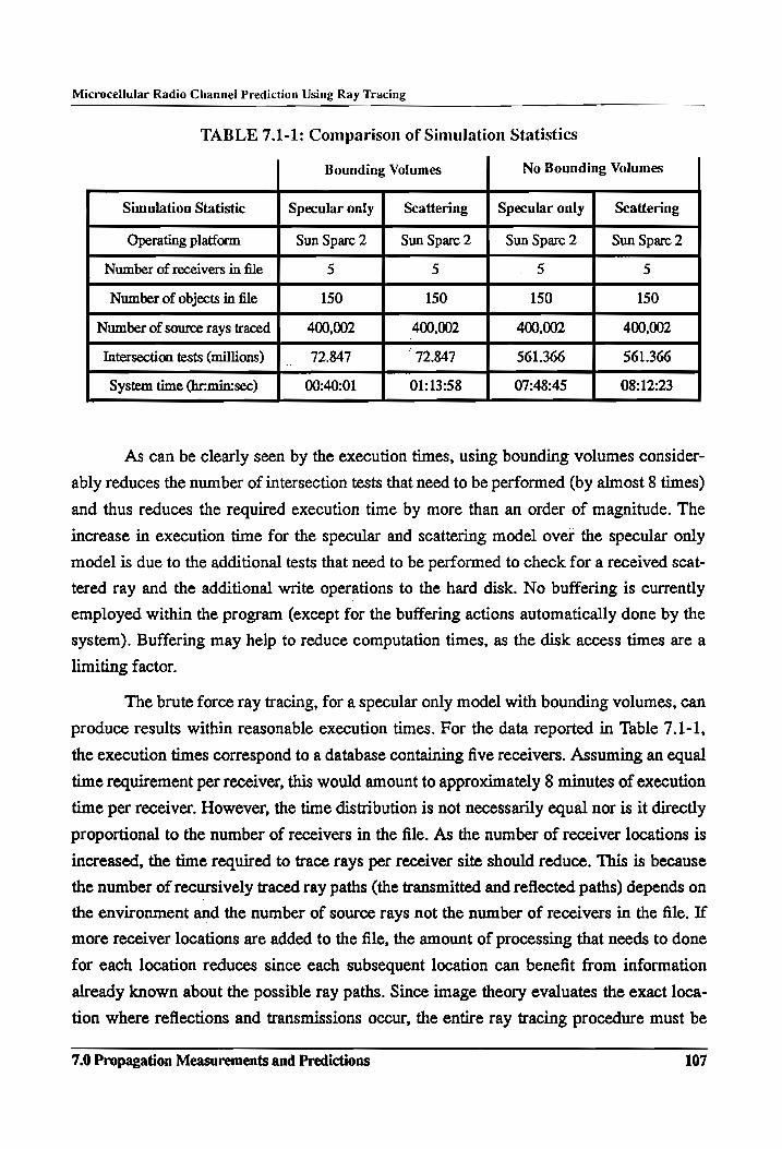
Microcellular Radio Channel Prediction Using Ray Tracing
TABLE 7.1-1: Comparison of Simulation Statistics
Bounding Volumes No Bounding Volumes
Simulation Statistic Specular only Scattering Specular only Scattering
Operating platform Sun Sparc 2 Sun Sparc 2 Sun Sparc 2 Sun Sparc 2
Number of receivers in file 5 5 5 5
Number of objects in file 150 150 150 150
Number of source rays traced 400,002 400,002 400,002 400,002
Intersection tests (millions) | 72.847 "72.847 561.366 561.366
System time (hr:min:sec) 00:40:01 01:13:58 07:48:45 08:12:23 As can be clearly seen by the execution times, using bounding volumes consider-
ably reduces the number of intersection tests that need to be performed (by almost 8 times)
and thus reduces the required execution time by more than an order of magnitude. The
increase in execution time for the specular and scattering model over the specular only
model is due to the additional tests that need to be performed to check for a received scat-
tered ray and the additional write operations to the hard disk. No buffering is currently
employed within the program (except for the buffering actions automatically done by the
system). Buffering may help to reduce computation times, as the disk access times are a
limiting factor.
The brute force ray tracing, for a specular only model with bounding volumes, can
produce results within reasonable execution times. For the data reported in Table 7.1-1,
the execution times correspond to a database containing five receivers. Assuming an equal
time requirement per receiver, this would amount to approximately 8 minutes of execution
time per receiver. However, the time distribution is not necessarily equal nor is it directly
proportional to the number of receivers in the file. As the number of receiver locations is
increased, the time required to trace rays per receiver site should reduce. This is because
the number of recursively traced ray paths (the transmitted and reflected paths) depends on
the environment and the number of source rays not the number of receivers in the file. If
more receiver locations are added to the file, the amount of processing that needs to done
for each location reduces since each subsequent location can benefit from information
already known about the possible ray paths. Since image theory evaluates the exact loca-
tion where reflections and transmissions occur, the entire ray tracing procedure must be
7.0 Propagation Measurements and Predictions 107
Microcellular Radio Channel Prediction Using Ray Tracing
repeated for each receiver location. Thus, the time required to generate data for path loss
or delay spread contour maps may be quite comparable to the time that an image theory
ray tracer can compute the same results.
7.2 Propagation Measurements
The purpose of the propagation measurements was to provide a database for verifi-
cation of the propagation prediction program. These measurements were not intended to
be a survey of multipath propagation in microcellular environments. Rather, the intent was
to select specific channel geometries useful for: evaluating the accuracy of the prediction
program. Since the ray tracing program predicted both the amplitude and time delay of an
individual multipath component, the channel was characterized with a wide band mea-
surement system. Although the narrow band data described in Chapter 4 would have been
useful for comparing measured and predicted path loss, it would have been difficult to
ascertain from this data whether individual multipath components were being correctly
identified. As such, a wide band channel sounder (i.e., narrow channel probe) was used to
provide an estimate to the channel impulse response.
7.2.1 Measurement Locations and Procedure
Measurements were made in two separate locations on the Virginia Tech campus.
These two sites were selected because they represent two different, yet typical microcellu-
lar environments.
Microcell Site A - Cowgill Plaza Microcell
This site was an open site with a line-of-sight path to most locations and only a few
localized scattering surfaces. Although simple, this location was quite representative of a
typical microcell topography, being very similar to a courtyard near a shopping mall,
hotel, or office complex. Figure 7.2-1 illustrates the base station location and the four mea-
surement sites. The base station location provided an unobstructed propagation path to all
possible measurement locations within the courtyard and also to most of the reflecting sur-
faces surrounding the plaza. The four receiver locations were selected to provide sufficient
channel characterization for validating the propagation model since both line-of-sight (at
Hancock Hall, Johnston Student Center, and Burruss Hall) and shadowed (in front of Nor-
ris Hall) topographies were represented.
7.0 Propagation Measurements and Predictions 108
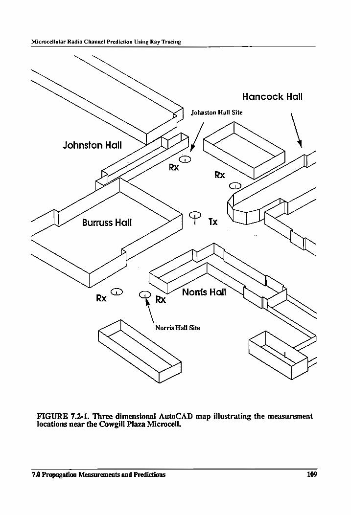
Microcellular Radio Channel Prediction Using Ray Tracing
Hancock Hail
4 Johnston Hall Site >
Ke > 7
Rx > RX
ON @
| YP tx Burruss Hall
>
Rx *
Norris Hall Site
Norris Hall
FIGURE 7.2-1. Three dimensional AutoCAD map illustrating the measurement locations near the Cowgill Plaza Microcell.
7.0 Propagation Measurements and Predictions 109
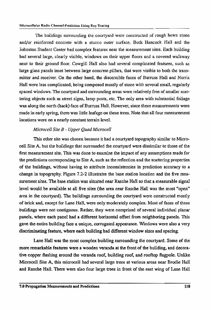
Microcellular Radio Channel Prediction Using Ray Tracing
The buildings surrounding the courtyard were constructed of rough hewn stone
and/or reinforced concrete with a stucco outer surface. Both Hancock Hall and the
Johnston Student Center had complex features near the measurement sites. Each building
had several large, clearly visible, windows on their upper floors and a covered walkway
next to their ground floor. Cowgill Hall also had several complicated features, such as
large glass panels inset between large concrete pillars, that were visible to both the trans-
mitter and receiver. On the other hand, the discernible faces of Burruss Hall and Norris
Hall were less complicated, being composed mostly of stone with several small, regularly
spaced windows. The courtyard and surrounding areas were relatively free of smaller scat-
tering objects such as street signs, lamp posts, etc. The only area with substantial foliage
was along the north (back) face of Burruss Hall. However, since these measurements were
made in early spring, there was little leafage on these trees. Note that all four measurement
locations were on a nearly constant terrain level.
Microcell Site B - Upper Quad Microcell
This other site was chosen because it had a courtyard topography similar to Micro-
cell Site A, but the buildings that surrounded the courtyard were dissimilar to those of the
first measurement site. This was done to examine the impact of any assumptions made for
the predictions corresponding to Site A, such as the reflection and the scattering properties
of the buildings, without having to attribute inconsistencies in prediction accuracy to a
change in topography. Figure 7.2-2 illustrates the base station location and the five mea-
surement sites. The base station was situated near Rasche Hall so that a measurable signal
level would be available at all five sites (the area near Rasche Hall was the most “open”
area in the courtyard). The buildings surrounding the courtyard were constructed mostly
of brick and, except for Lane Hall, were only moderately complex. Most of faces of these
buildings were not contiguous. Rather, they were comprised of several individual planar
panels, where each panel had a different horizontal offset from neighboring panels. This
gave the entire building face a unique, corrugated appearance. Windows were also a very
discriminating feature, where each building had different window sizes and spacing.
Lane Hall was the most complex building surrounding the courtyard. Some of the
more remarkable features were a wooden veranda at the front of the building, and decora-
tive copper flashing around the veranda roof, building roof, and rooftop flagpole. Unlike
Microcell Site A, this microcell had several large trees at various areas near Brodie Hall
and Rasche Hall. There were also four large trees in front of the east wing of Lane Hall
7.0 Propagation Measurements and Predictions 110
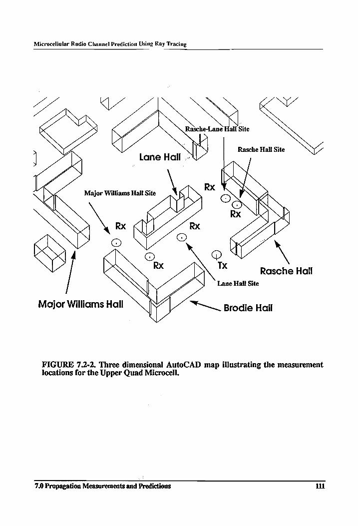
Microcellular Radio Channel Prediction Using Ray Tracing
cy < Z |
<
WY
Lane Hall .-
TX
Major Williams Hall Site \
\ Rx RX
oO ©
© RX
Lane Hall Site
—_ Brodie Hall
Rasche Hall
Major Williams Hall
FIGURE 7.2-2. Three dimensional AutoCAD map illustrating the measurement locations for the Upper Quad Microcell.
7.0 Propagation Measurements and Predictions 11
Microcellular Radio Channel Prediction Using Ray Tracing
(side closest to Rasche Hall). Unfortunately, the measurements at this microcell site were
made in late spring, when the trees were most densely foliated. As was the case with
Microcell Site A, all five measurement locations in this microcell were on a nearly con-
stant terrain level.
The measurements were made at both measurement sites using the following pro-
cedure. First, the measurements locations were tested when there was light pedestrian or
automobile traffic so that the channel could be considered wide sense stationary. At both
microcells, the transmitter antenna was elevated to a height of 7.6 meters (approximately
25 feet) which was considered typical for a lamp post mounted microcell base station. The
transmitter EIRP was 30 dBm. However, at times during the measurements, it was neces-
sary to reduce the EIRP at the transmitter through an HP variable attenuator before the
antenna terminal. This was necessary to ensure the system was operating in its linear
region when strong, generally LOS, components were present.
The receiver antenna was mounted at 1.7 meters (5.6 feet) to simulate the signal
that would be received by a user in the cell. This antenna, as well as the receiver system
hardware, was mounted on a push cart so that it could be easily transported around the
microcell. At each measurement site, five profiles were recorded over a one-half meter
track, and these profiles were averaged in the data processing to generate a single power
delay profile. Spatial averaging was necessary to ensure that individual multipath compo-
nents were not fading over a local area (due to components arriving within the same pulse
width), and to improve the dynamic display range of the measurement system. Oscillo-
scope sample averaging was not used because a logarithmic amplifier was used in the
receiver system (the oscilloscope would have been averaging dB values).
Both the transmitter and receiver employed omnidirectional discone antennas.
This was done so that multipath components arriving at the receiver could be detected
regardless of the angle of arrival in azimuth. At the first measurement site, the receiver
was operated in a dual channel mode, and a log-periodic antenna with approximately 8
dBi of gain was connected to the second receiving channel. It was hoped that, by record-
ing profiles with the antenna pointed at different scattering objects, individual sources of
multipath could be identified and more accurate refiection and scattering models could be
developed. Unfortunately, the 60° half-power beamwidth of the antenna was insufficient
for resolving the arrival angle for different multipath components. Since different multi-
7.0 Propagation Measurements and Predictions 112
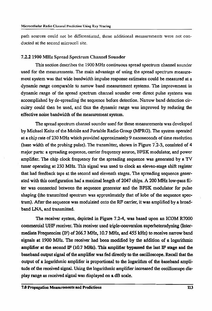
Microcellular Radio Channel Prediction Using Ray Tracing
path sources could not be differentiated, these additional measurements were not con-
ducted at the second microcell site.
7.2.2 1900 MHz Spread Spectrum Channel Sounder
This section describes the 1900 MHz continuous spread spectrum channel sounder
used for the measurements. The main advantage of using the spread spectrum measure-
ment system was that wide bandwidth impulse response estimates could be measured at a
dynamic range comparable to narrow band measurement systems. The improvement in
dynamic range of the spread spectrum channel sounder over direct pulse systems was
accomplished by de-spreading the sequence before detection. Narrow band detection cir-
cuitry could then be used, and thus the dynamic range was improved by reducing the
effective noise bandwidth of the measurement system.
The spread spectrum channel sounder used for these measurements was developed
by Michael Keitz of the Mobile and Portable Radio Group (MPRG). The system operated
at a chip rate of 230 MHz which provided approximately 9 nanoseconds of time resolution
(base width of the probing pulse). The transmitter, shown in Figure 7.2-3, consisted of 4
major parts: a spreading sequence, carrier frequency source, BPSK modulator, and power
amplifier. The chip clock frequency for the spreading sequence was generated by a TV
tuner operating at 230 MHz. This signal was used to clock an eleven-stage shift register
that had feedback taps at the second and eleventh stages. The spreading sequence gener-
ated with this configuration had a maximal length of 2047 chips. A 200 MHz low-pass fil-
ter was connected between the sequence generator and the BPSK modulator for pulse
shaping (the transmitted spectrum was approximately that of lobe of the sequence spec-
trum). After the sequence was modulated onto the RF carrier, it was amplified by a broad-
band LNA, and transmitted.
The receiver system, depicted in Figure 7.2-4, was based upon an ICOM R7000
commercial UHF receiver. This receiver used triple-conversion superheterodyning (Inter-
mediate Frequencies (IF) of 266.7 MHz, 10.7 MHz, and 455 kHz) to receive narrow band
signals at 1900 MHz. The receiver had been modified by the addition of a logarithmic
amplifier at the second IF (10.7 MHz). This amplifier bypassed the last IF stage and the
baseband output signal of the amplifier was fed directly to the oscilloscope. Recall that the
output of a logarithmic amplifier is proportional to the logarithm of the baseband ampli-
tude of the received signal. Using the logarithmic amplifier increased the oscilloscope dis-
play range as received signal was displayed on a dB scale.
7.0 Propagation Measurements and Predictious 113
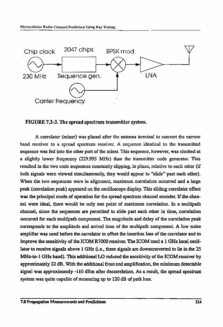
Microcellular Radio Channel Prediction Using Ray Tracing
Chip clock 2947 chips BPSK mod. VY
-)— 230 MHz sequence gen.
Carrier frequency
FIGURE 7.2-3. The spread spectrum transmitter system.
A correlator (mixer) was placed after the antenna terminal to convert the narrow
band receiver to a spread spectrum receiver. A sequence identical to the transmitted
sequence was fed into the other port of the mixer. This sequence, however, was clocked at
a slightly lower frequency (229.995 MHz) than the transmitter code generator. This
resulted in the two code sequences constantly slipping, in phase, relative to each other (if
both signals were viewed simultaneously, they would appear to “slide” past each other).
When the two sequences were in alignment, maximum correlation occurred and a large
peak (correlation peak) appeared on the oscilloscope display. This sliding correlator effect
was the principal mode of operation for the spread spectrum channel sounder. If the chan-
nel were ideal, there would be only one point of maximum correlation. In a multipath
channel, since the sequences are permitted to slide past each other in time, correlation
occurred for each multipath component. The magnitude and delay of the correlation peak
corresponds to the amplitude and arrival time of the multipath component. A low noise
amplifier was used before the correlator to offset the insertion loss of the correlator and to
improve the sensitivity of the ICOM R7000 receiver. The ICOM used a 1 GHz local oscil-
lator to receive signals above 1 GHz (i.e., these signals are downconverted to lie in the 25
MHz-to-1 GHz band). This additional LO reduced the sensitivity of the ICOM receiver by
approximately 22 dB. With the additional front end amplification, the minimum detectable
signal was approximately -110 dBm after decorrelation. As a result, the spread spectrum
system was quite capable of measuring up to 120 dB of path loss.
7.0 Propagation Measurements and Predictions 114
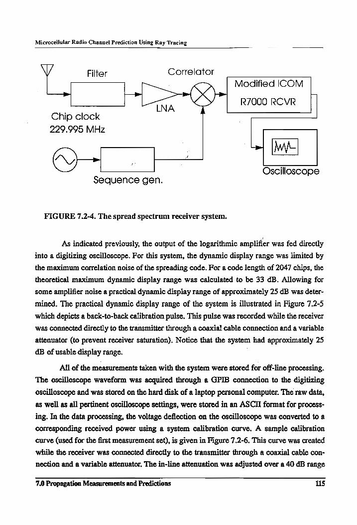
Microceljular Radio Channel Prediction Using Ray Tracing
VV Filter Correlator Modified ICOM
—————— Ve
R7000 RCVR
Chip clock
229.995 MHz
Y _ | Oscilloscope Sequence gen.
FIGURE 7.2-4. The spread spectrum receiver system.
As indicated previously, the output of the logarithmic amplifier was fed directly
into a digitizing oscilloscope. For this system, the dynamic display range was limited by
the maximum correlation noise of the spreading code. For a code length of 2047 chips, the
theoretical maximum dynamic display range was calculated to be 33 dB. Allowing for
some amplifier noise a practical dynamic display range of approximately 25 dB was deter-
mined. The practical dynamic display range of the system is illustrated in Figure 7.2-5
which depicts a back-to-back calibration pulse. This pulse was recorded while the receiver
was connected directly to the transmitter through a coaxial cable connection and a variable
attenuator (to prevent receiver saturation). Notice that the system had approximately 25
dB of usable display range. |
All of the measurements taken with the system were stored for off-line processing.
The oscilloscope waveform was acquired through a GPIB connection to the digitizing
oscilloscope and was stored on the hard disk of a laptop personal computer. The raw data,
as well as all pertinent oscilloscope settings, were stored in an ASCII format for process-
ing. In the data processing, the voltage deflection on the oscilloscope was converted to a
coiresponding received power using a system calibration curve. A sample calibration
curve (used for the first measurement set), is given in Figure 7.2-6. This curve was created
while the receiver was connected directly to the transmitter through a coaxial cable con-
nection and a variable attenuator. The in-line attenuation was adjusted over a 40 dB range
7.0 Propagation Measurements and Predictions 115
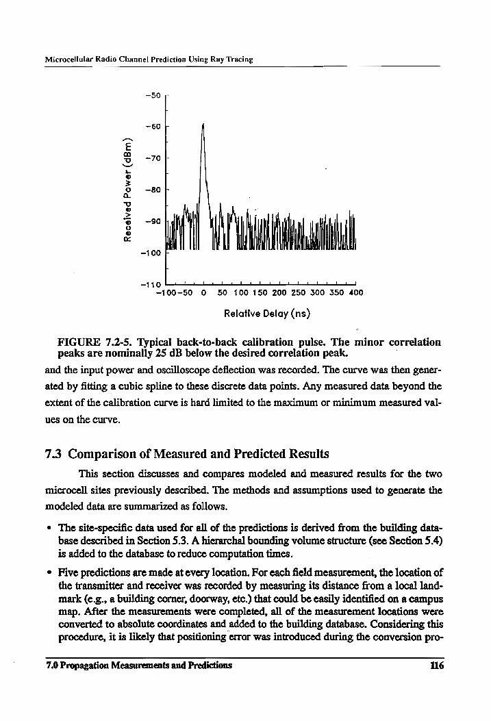
Microcellular Radio Channel Prediction Using Ray Tracing
Rece
ived
Po
wer
(dBm)
a o
-100 —-110 i l 1 l 1 l 2! 1 l l 4 l 1 l L { i ]
-~100-50 0 50 100 150 200 250 300 350 400
Relative Delay (ns)
FIGURE 7.2-5. Typical back-to-back calibration pulse. The minor correlation peaks are nominally 25 dB below the desired correlation peak.
and the input power and oscilloscope deflection was recorded. The curve was then gener-
ated by fitting a cubic spline to these discrete data points. Any measured data beyond the
extent of the calibration curve is hard limited to the maximum or minimum measured val-
ues on the curve.
7.3 Comparison of Measured and Predicted Results
This section discusses and compares modeled and measured results for the two
microcell sites previously described. The methods and assumptions used to generate the
modeled data are summarized as follows.
e The site-specific data used for all of the predictions is derived from the building data- base described in Section 5.3. A hierarchal bounding volume structure (see Section 5.4)
is added to the database to reduce computation times.
e Five predictions are made at every location. For each field measurement, the location of the transmitter and receiver was recorded by measuring its distance from a local land- mark (e.g., a building corner, doorway, etc.) that could be easily identified on a campus map. After the measurements were completed, all of the measurement locations were
converted to absolute coordinates and added to the building database. Considering this procedure, it is likely that positioning error was introduced during the conversion pro-
7.0 Propagation Measurements and Predictions 116
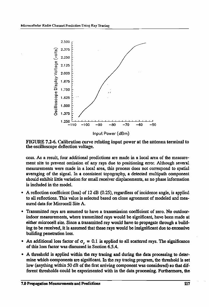
Microcellular Radio Channel Prediction Using Ray Tracing
2.500 5
2.375 -
2.250
2.125
2.000 F
1.875 :
1.750 C
1.625 : -
1.500 F Osci
llos
cope
Di
spla
y Vo
ltag
e (volts)
1.375 F 1.950 beet
-110 -100 -90 -80 -70 -60 -50
Input Power (dBm)
FIGURE 7.2-6. Calibration curve relating input power at the aiitenna terminal to the oscilloscope deflection voltage.
cess. As a result, four additional predictions are made in a local area of the measure- ment site to prevent omission of any rays due to positioning error. Although several
measurements were made in a local area, this process does not correspond to spatial averaging of the signal. In a consistent topography, a detected multipath component
should exhibit little variation for small receiver displacements, as no phase information is included in the model.
¢ Areflection coefficient (loss) of 12 dB (0.25), regardless of incidence angle, is applied to all reflections. This value is selected based on close agreement of modeled and mea- sured data for Microcell Site A.
¢ Transmitted rays are assumed to have a transmission coefficient of zero. No outdoor- indoor measurements, where transmitted rays would be significant, have been made at
either microcell site. Since a transmitted ray would have to propagate through a build- ing to be received, it is assumed that these rays would be insignificant due to excessive building penetration loss. |
¢ An additional loss factor of 0, = 0.1 is applied to all scattered rays. The significance of this loss factor was discussed in Section 6.5.4.
e A threshold is applied within the ray tracing and during the data processing to deter- mine which components are significant. In the ray tracing program, the threshold is set low (anything within 50 dB of the first arriving component was considered) so that dif- ferent thresholds could be experimented with in the data processing. Furthermore, the
7.0 Propagation Measurements and Predictions 117
Microcellular Radio Channel Prediction Using Ray Tracing
restriction for maximum number of levels is set to ten to guarantee that a ray would be
disregarded strictly on a path loss basis (1.e., the ray tracing threshold should be exceed
before reaching the maximum number of tracing levels).
Selecting a threshold to process the modeled data is not a trivial process. Since the
power is added noncoherently, components always add constructively. If many weak
rays, each with nearly the same time delay, are predicted in the ray tracing, these com- ponents can sum to produce an unrealistically large estimate to the received power. It is
recognized that, in a real multipath measurement, all of the components incident at the
receiver terminals add vectorially regardless of their relative strengths. However, based
upon practical experience, the number of weak components predicted in the ray tracing
is much greater than the amount that would be observed experimentally (there are other
factors that preclude these components from being received).
The measurement system threshold is used for the process the predicted data. This is considered the most practical selection because it corresponds directly to measured data
and also because of theoretical arguments based upon the modeling technique (since a power sum is being computed, the power in each ray must above the receiver threshold for it to correspond to measured data).
¢ A 9 nanosecond base-width Gaussian-shaped pulse is convolved with the predicted
data for visual comparison. The convolution process is noncoherent..-
Figures 7.3-1 through 7.3-4, and Figures 7.3-6 through 7.3-10 depict the measured and
predicted results for all of the measured locations. For future discussion, a particular mea-
surement site is referred to by the building name nearest to the measurement location as
illustrated in Figure 7.2-1 and Figure 7.2-2. In reviewing these results, notice that the data
are plotted as path loss above a 1-meter free space path loss (FSPL) versus excess delay.
Additionally, note that the thin trace in the figure corresponds to the measured data and the
thick trace corresponds to the predicted results. In the following discussion, visual com-
parisons of the results are given first (a qualitative comparison of the data). Next, a sum-
mary of the profile statistics for both measured and predicted data is provided (a
quantitative comparison of the data). Finally, some analysis and discussion toward
enhancing the accuracy of the model is made.
LOS reflective environments - Burruss Hall, Rasche Hall, and Brodie Hall
These three measurement sites are grouped together because each had a LOS
geometry that could allow for both single and multiple specular reflections to be received.
Moreover, at each site, the receiver is located at an appreciable distance from nearby
7.0 Propagation Measurements and Predictions 118
Microcellular Radio Channel Prediction Using Ray Tracing
building faces. It was believed that this deemphasizes any localized scattering from the
buildings so that specular reflections would be the primary source of multipath.
The results for the Burruss Hall location are shown in Figure 7.3-1. The prediction
accurately determines both the amplitude of the LOS component (within 3 dB) and the
spread in first arriving energy due to a ground reflection appearing immediately after the
LOS component. Several scattered components, with relatively short delays also cause a
spread in the pulse width. The simulation results indicate arrival of specular rays with
excess delays of 68, 72, and 160 ns. These arrival times appear to correspond to the mea-
sured energy near 60 ns and 130 ns. Although difficult to discern in the figure, the model
also predicts the presence of energy at 225 ns and 440 ns. However, these components are
predicted as being a summation many scattered rays which are just above threshold. This
may account for the 10 dB discrepancy between measured and predicted results.
Figure 7.3-2 displays the results for the Rasche Hall site. The measured first arriv-
ing component is approximately 3 dB stronger than the predicted result. Also note that an
additional component, with an delay of approximately 15 ns, is not identified in the pre-
diction. There are several possible explanations for this discrepancy. First, it is possible
that a scatterer close to the direct T-R path could have redirected a substantial quantity of
energy toward the receiver. Second, it is possible that this not a distinct multipath compo-
nent, but rather the interference pattern caused by two components arriving within a single
pulse width.
For the Rasche Hall site, the LOS component and ground reflected component
have a differential path length of less than 9 feet (approximately 9 ns). It is possible that
the disagreement in power could be due to the vectorial sum of these two components
within one pulse width. When autocorrelation peaks for two multipath components over-
lap, the nature of the interference can lead to an erroneous interpretation of the results.
Depending upon the relative phases of each component, both constructive and destructive
interference can occur. The destructive interference can cause the observed arrival times
of the components to differ from the physical arrival times (e.g., the second component
actually arrives at the “null”). Thus, it is possible that the second component is a spurious
peak caused by the interference of the LOS and the ground reflected energy. This type of
interference is not predicted with the noncoherent ray tracing model.
As seen in Figure 7.3-2, the simulation correctly identifies both the amplitude and
delay of the reflection from Rasche Hall. Several specular components, arriving with
7. Propagation Measurements and Predictions 119
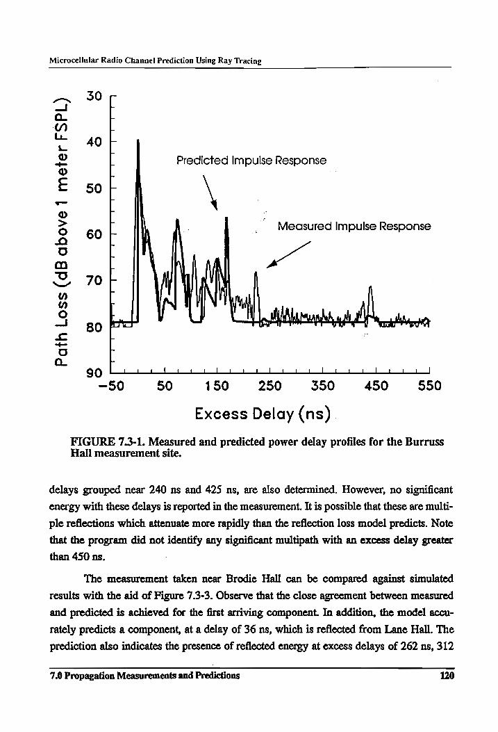
Microcellular Radio Channel Prediction Using Ray Tracing
GW © 1
40
Predicted Impulse Response
sot | \
r . _ Measured Impulse Response - }
70 + |
| | v ti le MMA, Al
60
Path Lo
ss (dB
above
1 meter
FSPL
)
gO CH Ht
-50 50 150 250 350 450 950
Excess Delay (ns)
FIGURE 7.3-1. Measured and predicted power delay profiles for the Burruss Hall measurement site.
delays grouped near 240 ns and 425 ns, are also determined. However, no significant
energy with these delays is reported in the measurement. It is possible that these are multi-
ple reflections which attenuate more rapidly than the reflection loss model predicts. Note
that the program did not identify any significant multipath with an excess delay greater
than 450 ns.
The measurement taken near Brodie Hall can be compared against simulated
results with the aid of Figure 7.3-3. Observe that the close agreement between measured
and predicted is achieved for the first arriving component. In addition, the model accu-
rately predicts a component, at a delay of 36 ns, which is reflected from Lane Hall. The
prediction also indicates the presence of reflected energy at excess delays of 262 ns, 312
7.0 Propagation Measurements and Predictions 120
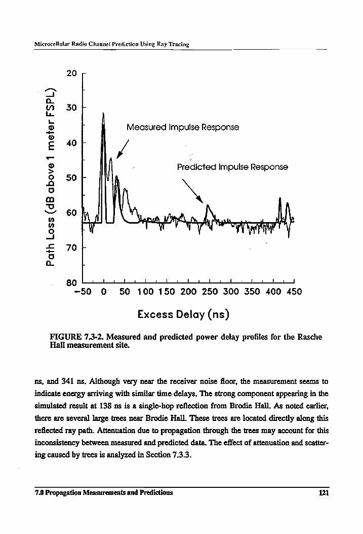
Microcellular Radio Channel Prediction Using Ray Tracing
20 -
30 fF
Measured Impulse Response >
40 + | J
Predicted Impulse Response
Path
Lo
ss (d
B ab
ove
1 meter
FSPL)
80 ! { | i ! | | | \ | ! | l t \ { | ] l }
~50 0 50 100 150 200 250 300 350 400 450
Excess Delay (ns)
FIGURE 7.3-2. Measured and predicted power delay profiles for the Rasche Hall measurement site.
ns, and 341 ns. Although very near the receiver noise floor, the measurement seems to
indicate energy arriving with similar time delays. The strong component appearing in the
simulated result at 138 ns is a single-hop reflection from Brodie Hall. As noted earlier,
there are several large trees near Brodie Hall. These trees are located directly along this
reflected ray path. Attenuation due to propagation through the trees may account for this
inconsistency between measured and predicted data. The effect of attenuation and scatter-
ing caused by trees is analyzed in Section 7.3.3.
7.9 Propagation Measurements and Predictions 121
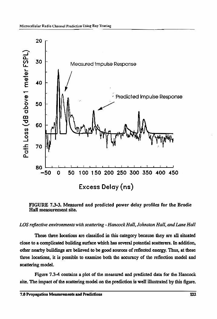
Microcellular Radio Channel Prediction Using Ray Tracing
20 -
“_s - — a. “ 30 fF Measured Impulse Response © L
© c 40 F
© : ' Predicted Impulse Response 2 i . gS 50
5 s
co ~~ 60 F-
w (" “ov L
° | I
= 70 o a :
80 | | 1 i i | i | LI — | l { ! 1 ! | | } -50 0 50 100 150 200 250 300 350 400 450 |
Excess Delay (ns)
FIGURE 7.3-3. Measured and predicted power delay profiles for the Brodie Hall measurement site.
LOS reflective environments with scattering - Hancock Hall, Johnston Hall, and Lane Hall
These three locations are classified in this category because they are all situated
close to a complicated building surface which has several potential scatterers. In addition,
other nearby buildings are believed to be good sources of reflected energy. Thus, at these
three locations, it is possible to examine both the accuracy of the reflection model and
scattering model.
Figure 7.3-4 contains a plot of the measured and predicted data for the Hancock
site. The impact of the scattering model on the prediction is well illustrated by this figure.
7.0 Propagation Measurements and Predictions 122
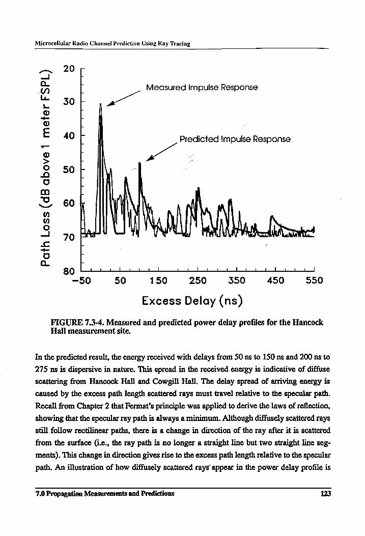
Microcellular Radio Channel Prediction Using Ray Tracing
=z OF oO P Measured Impulse Response to 30} @
-—— -
@
c 40 i Predicted Impulse Response ® L
o r | a 50 r : :
5 i Mm r F
cS cok \y , ” ” | | ANIA)
Ss 70 a ye | seh
<= . . = r
Qo. .
80 ae oe | Lt | | _ { | pf | | Li __J
-50 50 150 250 350 450 550
Excess Delay (ns)
FIGURE 7.3-4. Measured and predicted power delay profiles for the Hancock Hall measurement site.
In the predicted result, the energy received with delays from 50 ns to 150 ns and 200 ns to
275 ns is dispersive in nature. This spread in the received energy is indicative of diffuse
scattering from Hancock Hall and Cowgill Hall. The delay spread of arriving energy is
caused by the excess path length scattered rays must travel relative to the specular path.
Recall from Chapter 2 that Fermat’s principle was applied to derive the laws of reflection,
showing that the specular ray path is always a minimum. Although diffusely scattered rays
still follow rectilinear paths, there is a change in direction of the ray after it is scattered
from the surface (i.e., the ray path is no longer a straight line but two straight line seg-
ments). This change in direction gives rise to the excess path length relative to the specular
path. An illustration of how diffusely scattered rays’ appear in the power delay profile is
7.0 Propagation Measurements and Predictions 123
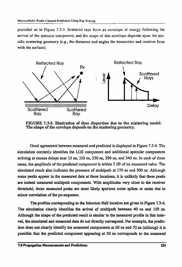
Microcellular Radio Channel Prediction Using Ray Tracing
provided as in Figure 7.3-5. Scattered rays form an envelope of energy following the
arrival of the specular component, and the shape of this envelope depends upon the spe-
cific scattering geometry (e.g., the distances and angles the transmitter and receiver form
with the surface).
Reflected Ray R Reflected Ray x
Oo \ Scattered _ > ays
a y
, ‘ PP
WA AAD) Delay seattered scattered
ay ay
FIGURE 7.3-5. Illustration of time dispersion due to the scattering model. The shape of the envelope depends on the scattering geometry.
Good agreement between measured and predicted is displayed in Figure 7.3-4. The
simulation correctly identifies the LOS component and additional specular components
arriving at excess delays near 15 ns, 110 ns, 250 ns, 290 ns, and 340 ns. In each of these
cases, the amplitude of the predicted component is within 5 dB of its measured value. The
simulated result also indicates the presence of multipath at 170 ns and 300 ns. Although
some peaks appear in the measured data at these locations, it is unlikely that these peaks
are indeed measured multipath components. With amplitudes very close to the receiver
threshold, these measured peaks are most likely spurious noise spikes or noise due to
minor correlation of the pn-sequence.
The profiles corresponding to the Johnston Hall location are given in Figure 7.3-6.
The simulation clearly identifies the arrival of multipath between 40 ns and 150 ns.
Although the shape of the predicted result is similar to the measured profile in this inter-
val, the simulated and measured data do not directly correspond. For example, the predic-
tion does not clearly identify the measured components at 60 ns and 70 ns (although it is
possible that the predicted component appearing at 50 ns corresponds to the measured
7.0 Propagation Measurements and Predictions 124
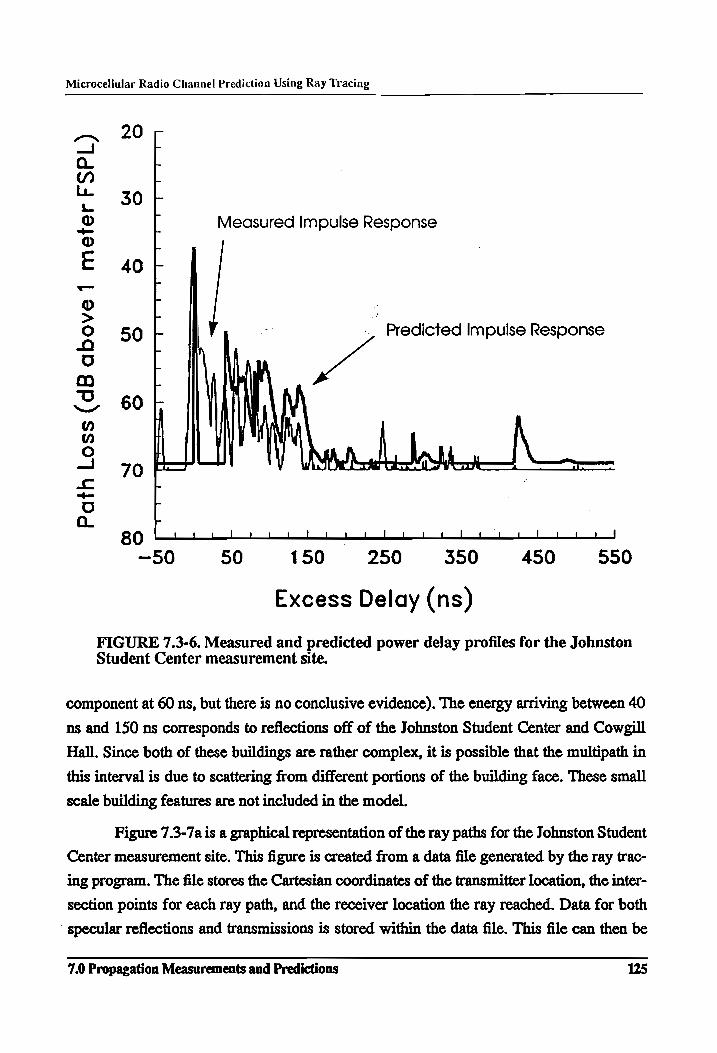
Microcellular Radio Channel Prediction Using Ray Tracing
—~ 207 —/ &
a. | " L
~ 30+ & i Measured Impulse Response © L
E 40+ =< a
o | : & 50; ., Predicted Impulse Response
oO | @ L
2 605 “ \ o” ‘5
o Sia,
a | 70 a =
<= L >= 5 .
a. 80 i peo ld td -50 50 150 250 350 450 950
Excess Delay (ns)
FIGURE 7.3-6. Measured and predicted power delay profiles for the Johnston Student Center measurement site.
component at 60 ns, but there is no conclusive evidence). The energy arriving between 40
ns and 150 ns corresponds to reflections off of the Johnston Student Center and Cowgill
Hall. Since both of these buildings are rather complex, it is possible that the multipath in
this interval is due to scattering from different portions of the building face. These small
scale building features are not included in the model.
Figure 7.3-7a is a graphical representation of the ray paths for the Johnston Student
Center measurement site. This figure is created from a data file generated by the ray trac-
ing program. The file stores the Cartesian coordinates of the transmitter location, the inter-
section points for each ray path, and the receiver location the ray reached. Data for both
specular reflections and transmissions is stored within the data file. This file can then be
7.0 Propagation Measurements and Predictions 125
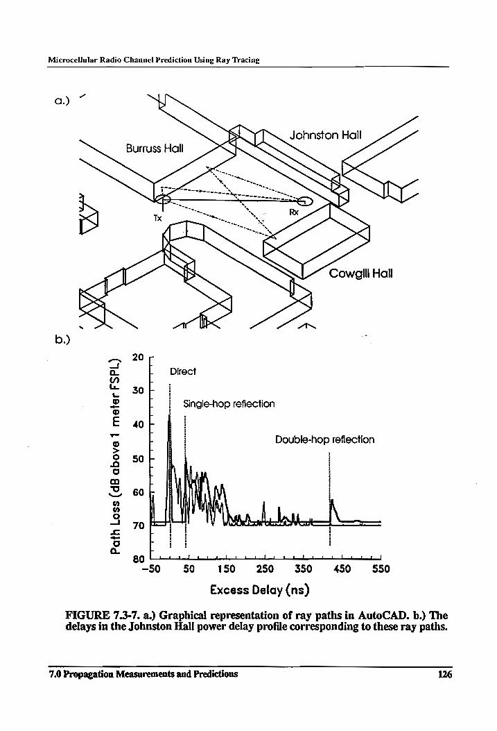
Microcellular Radio Channel Prediction Using Ray Tracing
a.)
Johnston Hall
Burruss Hall
x ‘ S> : >
S Cowgill Hall
20 -
} Direct
30 fr
[ Single-hop reflection
40 + Double-hop reflection
50
60
—=—-_)T.
7 7
70 Path
Loss (d
B above
1 meter
FSPL
)
80 eh Ne eh eee eae ee Bee pena Loe Here Semele eee
—50 50 150 250 8 350 450 550
Excess Delay (ns)
FIGURE 7.3-7. a.) Graphical representation of ray paths in AutoCAD. b.) The delays in the Johnston Hall power delay profile corresponding to these ray paths.
7.0 Propagation Measurements and Predictions 126
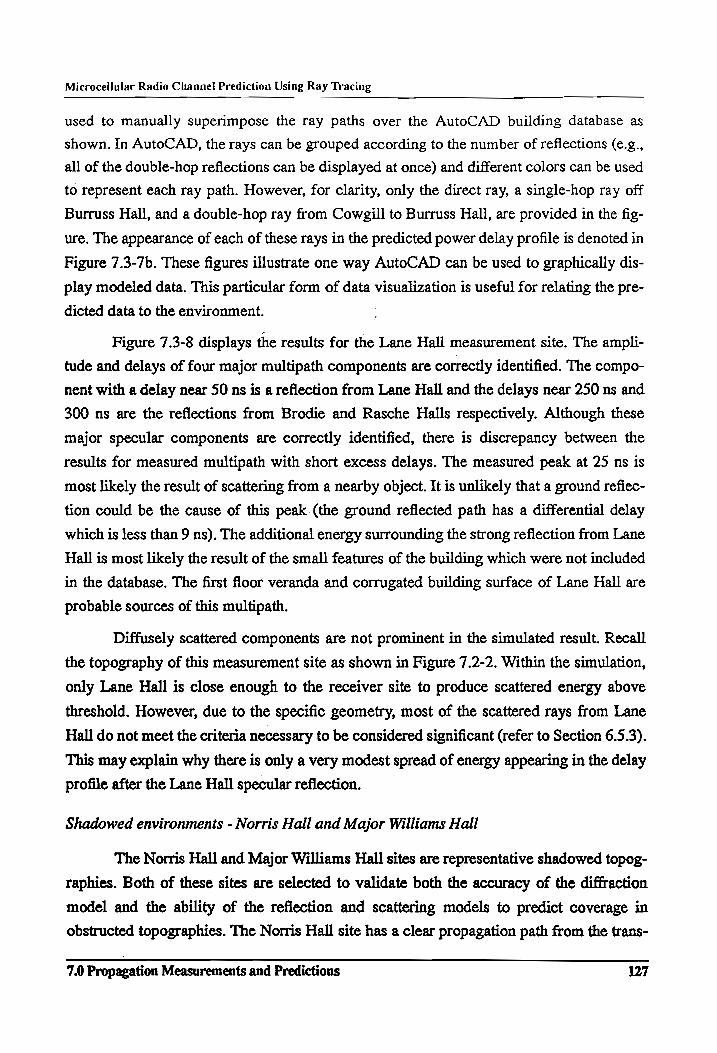
Microcellular Radio Channel Prediction Using Ray Tracing
used to manually superimpose the ray paths over the AutoCAD building database as
shown. In AutoCAD, the rays can be grouped according to the number of reflections (e.g.,
all of the double-hop reflections can be displayed at once) and different colors can be used
to represent each ray path. However, for clarity, only the direct ray, a single-hop ray off
Burruss Hall, and a double-hop ray from Cowgill to Burruss Hall, are provided in the fig-
ure. The appearance of each of these rays in the predicted power delay profile is denoted in
Figure 7.3-7b. These figures illustrate one way AutoCAD can be used to graphically dis-
play modeled data. This particular form of data visualization is useful for relating the pre-
dicted data to the environment.
Figure 7.3-8 displays the results for the Lane Hall measurement site. The ampli-
tude and delays of four major multipath components are correctly identified. The compo-
nent with a delay near 50 ns is a reflection from Lane Hall and the delays near 250 ns and
300 ns are the reflections from Brodie and Rasche Halls respectively. Although these
major specular components are correctly identified, there is discrepancy between the
results for measured multipath with short excess delays. The measured peak at 25 ns is
most likely the result of scattering from a nearby object. It is unlikely that a ground refiec-
tion could be the cause of this peak (the ground reflected path has a differential delay
which is less than 9 ns). The additional energy surrounding the strong reflection from Lane
Hall is most likely the result of the small features of the building which were not included
in the database. The first floor veranda and corrugated building surface of Lane Hall are
probable sources of this multipath.
Diffusely scattered components are not prominent in the simulated result. Recall
the topography of this measurement site as shown in Figure 7.2-2. Within the simulation,
only Lane Hall is close enough to the receiver site to produce scattered energy above
threshold. However, due to the specific geometry, most of the scattered rays from Lane
Hall do not meet the criteria necessary to be considered significant (refer to Section 6.5.3).
This may explain why there is only a very modest spread of energy appearing in the delay
profile after the Lane Hall specular reflection.
Shadowed environments - Norris Hall and Major Williams Hall
The Norris Hall and Major Williams Hall sites are representative shadowed topog-
raphies. Both of these sites are selected to validate both the accuracy of the diffraction
model and the ability of the reflection and scattering models to predict coverage in
obstructed topographies. The Norris Hall site has a clear propagation path from the trans-
7.0 Propagation Measurements and Predictions 127

Microcellular Radio Channel Prediction Using Ray Tracing
20 -
; Measured Impulse Response 30 -
| Predicted Impulse Response 40 +
Path
Loss
(dB
above
1 meter
FSPL
)
80 pot ld dl
-50 0 50 100 150 200 250 300 350 400 450
Excess Delay (ns)
FIGURE 7.3-8. Measured and predicted power delay profiles for the Lane Hall measurement site.
mitter to the (diffracting) building corner and from this building corner to the receiver. In
contrast, the Major Williams Hall measurement is more complicated, as several trees are
interspersed along the transmitter-to-building path. At both receiver sites, though, the sur-
rounding buildings are potential sources of reflected or scattered energy.
Measured and predicted data for the Norris Hall measurement site is provided in
Figure 7.3-9. The first peak in the predicted result corresponds to the component diffracted
by the corner of Norris Hall. The model predicts the remaining portion of energy to be a
result of scattering. The multipath components arriving immediately after the diffracted
component is due to ground scattering, and the energy appearing at an excess delay
between 100 ns and 200 ns is a result of scattering from Burruss Hall (after a reflection
from Norris Hall).
7.0 Propagation Measurements and Predictions 128
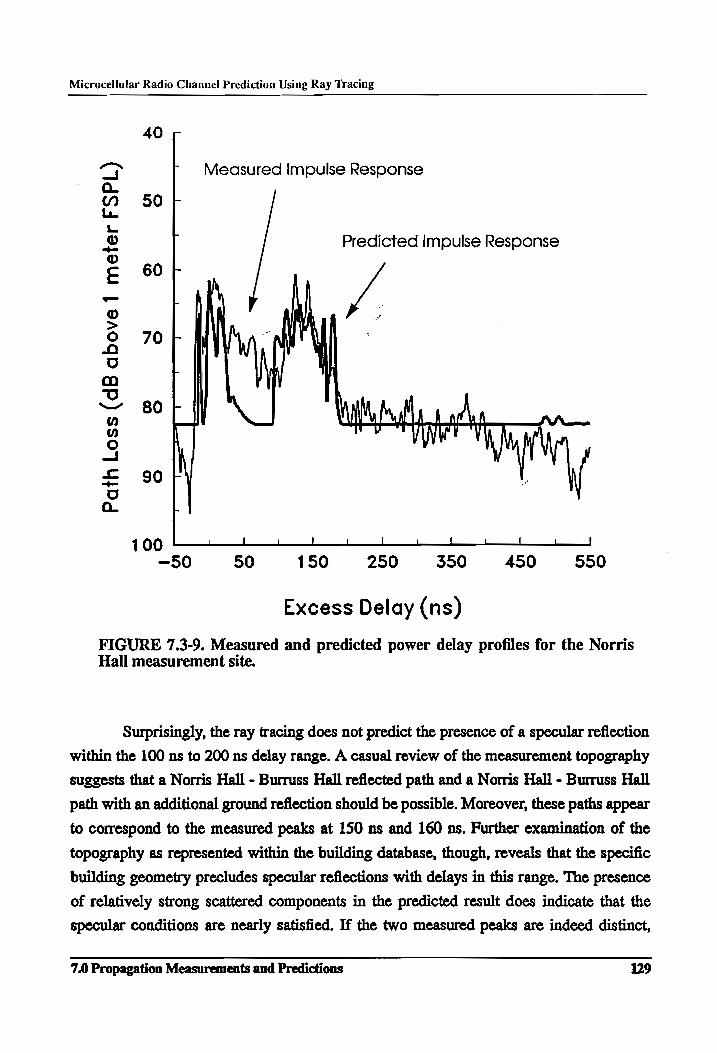
Microcellular Radio Channel Prediction Using Ray Tracing
40 -
ay r Measured impulse Response
a. i Mm 50 Le.
Ss P Predicted Impulse Response @ © 60, J
‘o i! ; 2
& 70b “AWE a | | | Go | !
Oct WM Poet a an 3 PTE VI I —
= 90F J o
on | 100 | | l ! | = | t L { | J
—50 50 150 250 350 450 550
Excess Delay (ns)
FIGURE 7.3-9. Measured and predicted power delay profiles for the Norris Hall measurement site.
Surprisingly, the ray tracing does not predict the presence of a specular reflection
within the 100 ns to 200 ns delay range. A casual review of the measurement topography
suggests that a Norris Hall - Burruss Hall reflected path and a Norris Hall - Burruss Hall
path with an additional ground reflection should be possible. Moreover, these paths appear
to correspond to the measured peaks at 150 ns and 160 ns. Further examination of the
topography as represented within the building database, though, reveals that the specific
building geometry precludes specular reflections with delays in this range. The presence
of relatively strong scattered components in the predicted result does indicate that the
specular conditions are nearly satisfied. If the two measured peaks are indeed distinct,
7.0 Propagation Measurements and Predictions 129
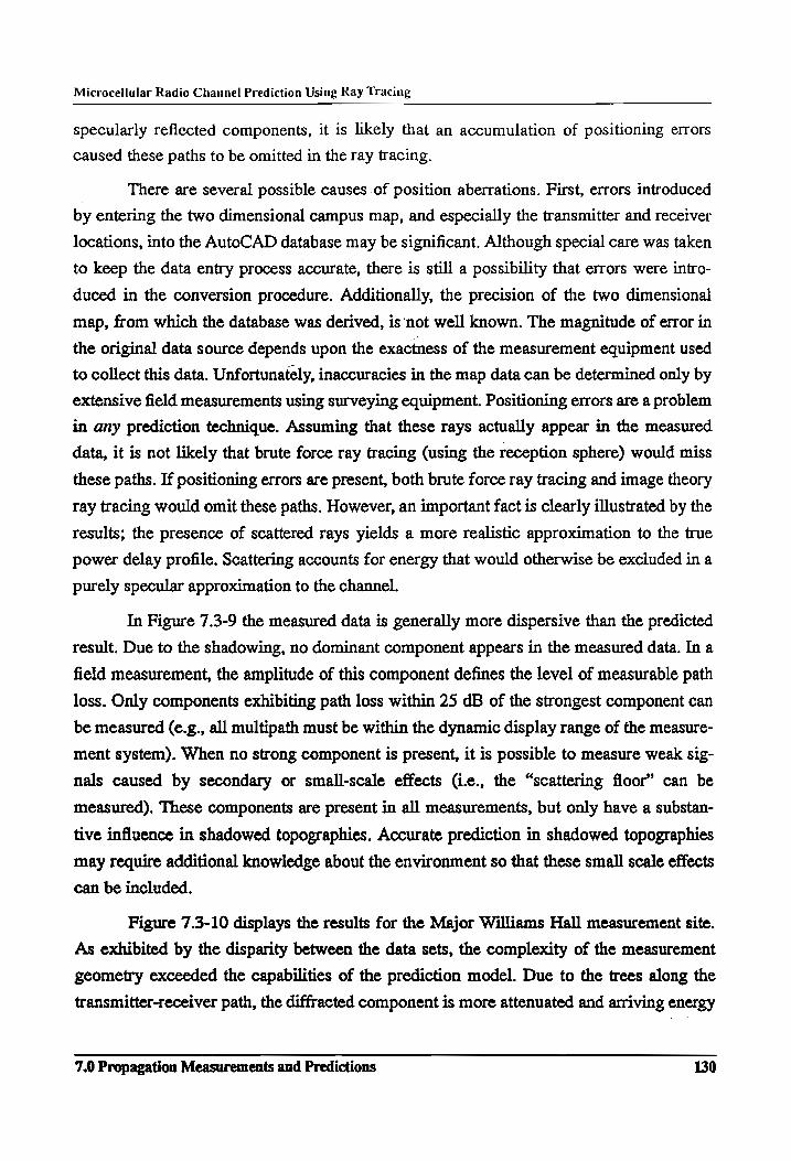
Microcellular Radio Channel Prediction Using Ray Tracing
specularly reflected components, it is likely that an accumulation of positioning errors
caused these paths to be omitted in the ray tracing.
There are several possible causes of position aberrations. First, errors introduced
by entering the two dimensional campus map, and especially the transmitter and receiver
locations, into the AutoCAD database may be significant. Although special care was taken
to keep the data entry process accurate, there is still a possibility that errors were intro-
duced in the conversion procedure. Additionally, the precision of the two dimensional
map, from which the database was derived, is not well known. The magnitude of error in
the original data source depends upon the exactness of the measurement equipment used
to collect this data. Unfortunately, inaccuracies in the map data can be determined only by
extensive field measurements using surveying equipment. Positioning errors are a problem
in any prediction technique. Assuming that these rays actually appear in the measured
data, it is not likely that brute force ray tracing (using the reception sphere) would miss
these paths. If positioning errors are present, both brute force ray tracing and image theory
ray tracing would omit these paths. However, an important fact is clearly illustrated by the
results; the presence of scattered rays yields a more realistic approximation to the true
power delay profile. Scattering accounts for energy that would otherwise be excluded in a
purely specular approximation to the channel.
In Figure 7.3-9 the measured data is generally more dispersive than the predicted
result. Due to the shadowing, no dominant component appears in the measured data. In a
field measurement, the amplitude of this component defines the level of measurable path
loss. Only components exhibiting path loss within 25 dB of the strongest component can
be measured (e.g., all multipath must be within the dynamic display range of the measure-
ment system). When no strong component is present, it is possible to measure weak sig-
nals caused by secondary or small-scale effects (i.c., the “scattering floor” can be
measured). These components are present in all measurements, but only have a substan-
tive influence in shadowed topographies. Accurate prediction in shadowed topographies
may require additional knowledge about the environment so that these small scale effects
can be included.
Figure 7.3-10 displays the results for the Major Williams Hall measurement site.
As exhibited by the disparity between the data sets, the complexity of the measurement
geometry exceeded the capabilities of the prediction model. Due to the trees along the
transmitter-receiver path, the diffracted component is more attenuated and arriving energy
7.0 Propagation Measurements and Predictions 130
Microcellular Radio Channel Prediction Using Ray Tracing
30
40 + Measured Impulse Response
50 fF
we Impulse Response
60 + i |
70 yi ‘att vi wd
#7
Path
Lo
ss (dB
above
1 me
ter
FSPL
)
90 pd Ll l ! I i ! { {+i J ! | ! i a |
-50 0 50 100 150 200 250 300 350 400 450
Excess Delay (ns)
FIGURE 7.3-10. Measured and predicted power delay profiles for the Major Williams Hall measurement site.
more diffuse than predicted by the ray tracing. Furthermore, several specular reflections
appearing in the predicted result are not at all detected in the measured data. This could
also be due to blockage from trees or other, smaller obstacles within the courtyard.
Note that precise data was difficult to collect at this measurement site. To improve
linearity, the LNA at receiver front end was removed for the second measurement set. This
reduced the path loss that could be measured by the system by approximately 20 dB. Due
to weak amplification of the signal, the oscilloscope had difficulty locating the strongest
peak in the profile for triggering purposes. As a result, there was appreciable timing jitter
between the five measured profiles. Although some of these errors were corrected in the
data processing, some question regarding the accuracy of the measured data still remains.
7.0 Propagation Measurements and Predictions 131
Microcellular Radio Channel Prediction Using Ray Tracing
7.3.1 Summary of Comparisons
A set of wide band measurements, taken in two different areas on the Virginia Tech
campus, have been used to examine the accuracy of the model in predicting propagation in
several different topographies. Visual comparison of measured and predicted data has
been conducted and the results indicate that good agreement was possible for a variety of
channel topographies. The following specific items can be inferred from visual compari-
sons of the data.
¢ A 12dB reflection loss, regardless of incidence angle or polarization, is a practical first- order approximation to the reflective properties of most buildings. Since the quantity of
data collected was limited, it is not possible to make any specific comments regarding
the reflective properties of common building materials. However, a 12 dB loss per reflection is a reasonable value until exact data become available.
¢ By approximating a building with simple geometric shapes, it is possible to identify the major component of energy reflected from the building surface. However, for compli- cated building surfaces, small scale building features can have an impact on the fine
structure of the power delay profile.
e Secondary scatterers, which are in close proximity to the T-R propagation path, may impact the received power delay profile. To enhance the accuracy of a prediction, it
may be necessary to include these scatterers in the site-specific environmental database.
This is especially true in shadowed topographies where weak, scattered components
can have a more significant effect on the power delay profile.
Additional comparisons, from a statistical standpoint, are provided in the following sub-
section. The final subsection discusses possible enhancements to the prediction model.
7.3.2 Discussion of Profile Statistics
Path loss and RMS delay spread values are computed, for both measured and pre-
dicted data, at the eight measurement locations. The results are summarized in Table 7.3-1.
Note that the RMS delay spread values are reported in nanoseconds, and the average path
loss (average of the five measurements taken at a single site) values are reported as path
loss above a 1 meter free space path loss reference.
A general trend can be clearly seen in the statistics for the eight sites. With the
exception of the Burruss Hall measurement site, ray tracing predicts more path loss and
larger delay spreads than seen in the measured data. Comparing the measured and pre-
dicted power delay profiles previously shown, these results are not particularly surprising.
7.0 Propagation Measurements and Predictions 132
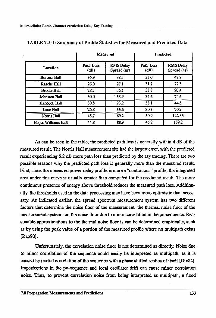
Microcellular Radio Channel Prediction Using Ray Tracing
TABLE 7.3-1: Summary of Profile Statistics for Measured and Predicted Data
Measured Predicted
ee ed Burruss Hall 36.9 38.5 33.0 47.9
Rasche Hall 26.0 27.1 31.7 773
Brodie Hall 28.7 36.1 33.8 93.4
Johnston Hall 30.0 * 33.9 34.6 74.6
Hancock Hail 30.8 "232 33.1 448
Lane Hall 26.8 55.6 30.3 70.9
Norris Hall 45.7 69.2 50.9 142.86
Major Williams Hall 44.8 88.9 46.2 159.2
As can be seen in the table, the predicted path loss is generally within 4 dB of the
measured result. The Norris Hall measurement site had the largest error, with the predicted
result experiencing 5.2 dB more path loss than predicted by the ray tracing. There are two
possible reasons why the predicted path loss is generally more than the measured result.
First, since the measured power delay profile is more a “continuous” profile, the integrated
area under this curve is usually greater than computed for the predicted result. The more
continuous presence of energy above threshold reduces the measured path loss. Addition-
ally, the thresholds used in the data processing may have been more optimistic than neces-
sary. As indicated earlier, the spread spectrum measurement system has two different
factors that determine the noise floor of the measurement: the thermal noise floor of the
measurement system and the noise floor due to minor correlation in the pn-sequence. Rea-
sonable approximations to the thermal noise floor is can be determined empirically, such
as by using the peak value of a portion of the measured profile where no multipath exists
(Rap90].
Unfortunately, the correlation noise floor is not determined as directly. Noise due
to minor correlation of the sequence could easily be interpreted as multipath, as it is
caused by partial correlation of the sequence with a phase shifted replica of itself [Dix84].
Imperfections in the pn-sequence and local oscillator drift can cause minor correlation
noise. Thus, to prevent correlation noise from being interpreted as multipath, a fixed
7.0 Propagation Measurements and Predictions 133
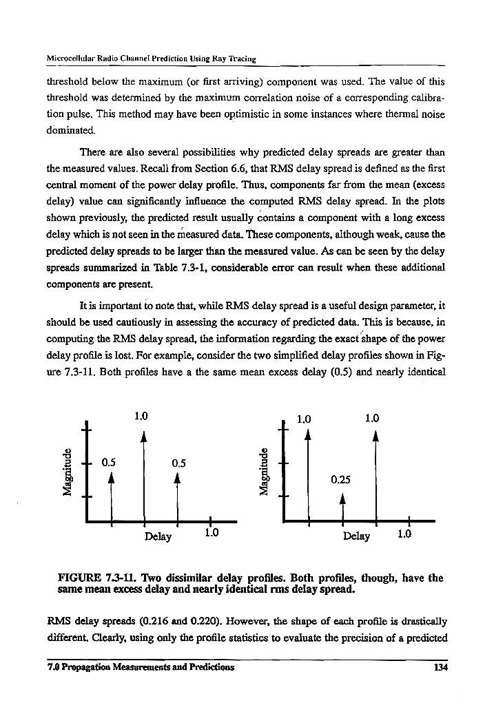
Microcellular Radio Channel Prediction Using Ray Tracing
threshold below the maximum (or first arriving) component was used. The value of this
threshold was determined by the maximum correlation noise of a corresponding calibra-
tion pulse. This method may have been optimistic in some instances where thermal noise
dominated.
There are also several possibilities why predicted delay spreads are greater than
the measured values. Recall from Section 6.6, that RMS delay spread is defined as the first
central moment of the power delay profile. Thus, components far from the mean (excess
delay) value can significantly influence the computed RMS delay spread. In the plots
shown previously, the predicted result usually contains a component with a long excess
delay which is not seen in the measured data. These components, although weak, cause the
predicted delay spreads to be larger than the measured value. As can be seen by the delay
spreads summarized in Table 7.3-1, considerable error can result when these additional
components are present.
It is important to note that, while RMS delay spread is a useful design parameter, it
should be used cautiously in assessing the accuracy of predicted data. This is because, in
computing the RMS delay spread, the information regarding the exact ‘shape of the power
delay profile is lost. For example, consider the two simplified delay profiles shown in Fig-
ure 7.3-11. Both profiles have a the same mean excess delay (0.5) and nearly identical
1.0 1.0 l 410 A A
© ©
H Los 0.5 z + 0.25 ow
Ss | s |
Delay 1.0 Delay 1.0
FIGURE 7.3-11. Two dissimilar delay profiles. Both profiles, though, have the same mean excess delay and nearly identical rms delay spread.
RMS delay spreads (0.216 and 0.220). However, the shape of each profile is drastically
different. Clearly, using only the profile statistics to evaluate the precision of a predicted
7.0 Propagation Measurements and Predictions 134
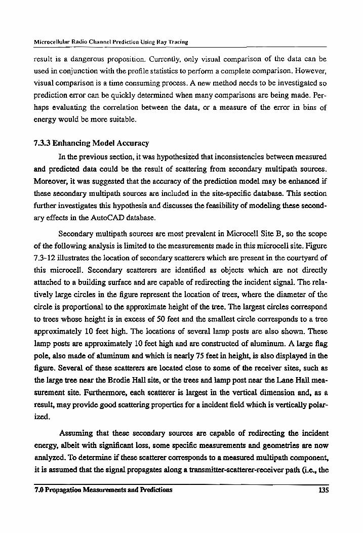
Microcellular Radio Channel Prediction Using Ray Tracing
result is a dangerous proposition. Currently, only visual comparison of the data can be
used in conjunction with the profile statistics to perform a complete comparison. However,
visual comparison is a time consuming process. A new method needs to be investigated so
prediction error can be quickly determined when many comparisons are being made. Per-
haps evaluating the correlation between the data, or a measure of the error in bins of
energy would be more suitable.
7.3.3 Enhancing Model Accuracy
In the previous section, it was hypothesized that inconsistencies between measured
and predicted data could be the result of scattering from secondary multipath sources.
Moreover, it was suggested that the accuracy of the prediction model may be enhanced if
these secondary multipath sources are included in the site-specific database. This section
further investigates this hypothesis and discusses the feasibility of modeling these second-
ary effects in the AutoCAD database.
Secondary multipath sources are most prevalent in Microcell Site B, so the scope
of the following analysis is limited to the measurements made in this microcell site. Figure
7.3-12 illustrates the location of secondary scatterers which are present in the courtyard of
this microcell. Secondary scatterers are identified as objects which are not directly
attached to a building surface and are capable of redirecting the incident signal. The rela-
tively large circles in the figure represent the location of trees, where the diameter of the
circle is proportional to the approximate height of the tree. The largest circles correspond
to trees whose height is in excess of 50 feet and the smallest circle corresponds to a tree
approximately 10 feet high. The locations of several lamp posts are also shown. These
lamp posts are approximately 10 feet high and are constructed of aluminum. A large flag
pole, also made of aluminum and which is nearly 75 feet in height, is also displayed in the
figure. Several of these scatterers are located close to some of the receiver sites, such as
the large tree near the Brodie Hall site, or the trees and lamp post near the Lane Hall mea-
surement site. Furthermore, each scatterer is largest in the vertical dimension and, as a
result, may provide good scattering properties for a incident field which is vertically polar-
ized.
Assuming that these secondary sources are capable of redirecting the incident
energy, albeit with significant loss, some specific measurements and geometries are now
analyzed. To determine if these scatterer corresponds to a measured multipath component,
it is assumed that the signal propagates along a transmitter-scatterer-receiver path (i.e., the
7.0 Propagation Measurements and Predictions 135
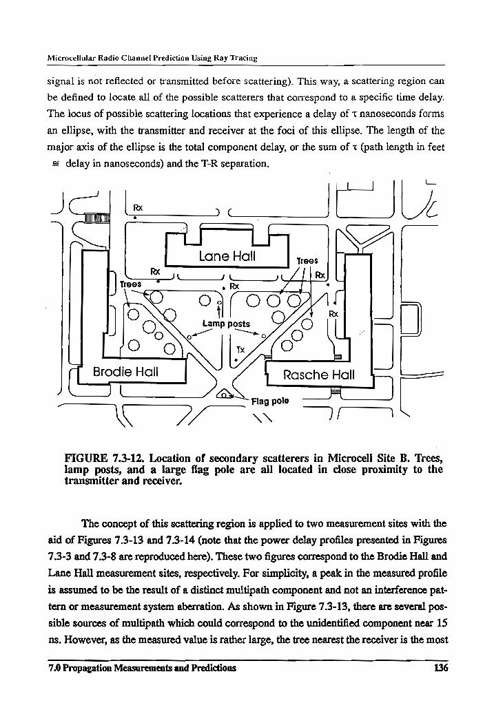
Microcellular Radio Channel Prediction Using Ray Tracing
signal is not reflected or transmitted before scattering). This way, a scattering region can
be defined to locate all of the possible scatterers that correspond to a specific time delay.
The locus of possible scattering locations that experience a delay of t nanoseconds forms
an ellipse, with the transmitter and receiver at the foci of this ellipse. The length of the
major axis of the ellipse is the total component delay, or the sum of t (path length in feet
= delay in nanoseconds) and the T-R separation.
| —
J = >) IL JLE
5 LT SAF] [
Lane Hall trees
| Re Je LZ [| = Trees a kX / * c
O7( O Lamp posts
a, Wrelixe ] (L Brodie Hall | Rasche Hall — ——
~ | COs bag pole FL
NOD RN FIGURE 7.3-12. Location of secondary scatterers in Microcell Site B. Trees, lamp posts, and a large flag pole are all located in close proximity to the transmitter and receiver.
NN
The concept of this scattering region is applied to two measurement sites with the
aid of Figures 7.3-13 and 7.3-14 (note that the power delay profiles presented in Figures
7.3-3 and 7.3-8 are reproduced here). These two figures correspond to the Brodie Hall and
Lane Hall measurement sites, respectively. For simplicity, a peak in the measured profile
is assumed to be the result of a distinct multipath component and not an interference pat-
tern or measurement system aberration. As shown in Figure 7.3-13, there are several pos-
sible sources of multipath which could correspond to the unidentified component near 15
ns. However, as the measured value is rather large, the tree nearest the receiver is the most
7.0 Propagation Measurements and Predictions 136
Microcellular Radio Channel Prediction Using Ray Tracing
I¢
> CAF Z Lane Hall Na
UL -
—__
Brodie Hall ! Rasche Hall _—~
J L Co» scattering Region i
20 +
Possible scattered component
Path Lo
ss (dB
abov
e 1 me
ter
FSPL)
14 | 1 |L_s__f_t__f 1 I : {___s___- 1 a | 80 ~50 0 50 100 150 200 250 300 350 400 450
Excess Delay (ns)
FIGURE 7.3-13. Geometry for a possible scattered component identified in the measured impulse response near Brodie Hall. The tree closest to the receiver is assumed to be the best scattering source.
7.0 Propagation Measurements and Predictions 137
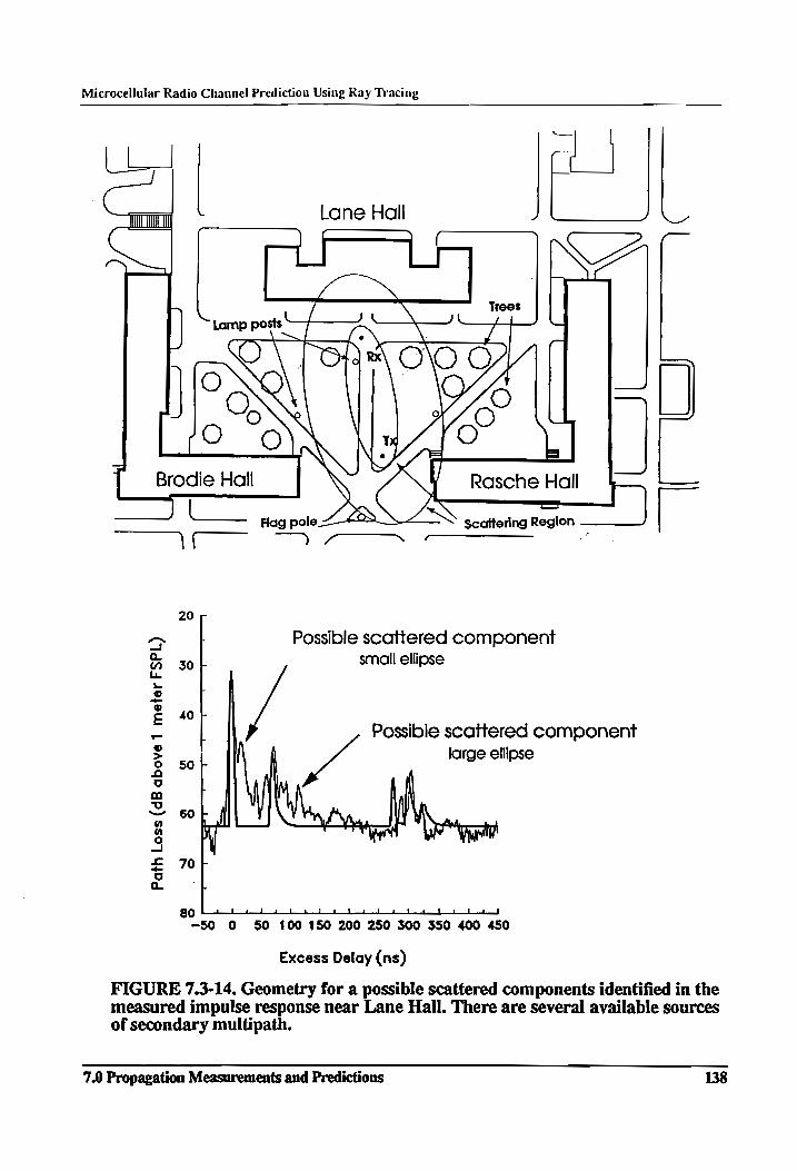
Microcellular Radio Channel Prediction Using Ray Tracing
LL
Lane Hall \
c
VC
[/o “o
‘I
| Rasche Hall l
Lat Scattering Region —___U
jt | Brodie Hall
7 Le Flag pole SS
Vi 7 *
20 r
> Possible scattered component “i 30 b small ellipse
hee
2 = 40+ - Possible scattered component ® * So J large ellipse a2 0 ma
2 60 ” “a
Ss £ 70}
So ct 4 1 a | l 2d Dee nbenmnl 1 1 eens Apel Le eheemel 80 -50 0 50 100 150 200 250 300 350 400 450
Excess Delay (ns)
FIGURE 7.3-14. Geometry for a possible scattered components identified in the measured impulse response near Lane Hall. There are several available sources of secondary multipath.
7.0 Propagation Measurements and Predictions 138
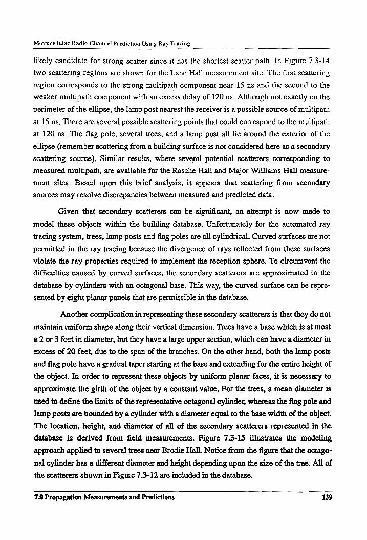
Microcellular Radio Channel Prediction Using Ray Tracing
likely candidate for strong scatter since it has the shortest scatter path. In Figure 7.3-14
two scattering regions are shown for the Lane Hall measurement site. The first scattering
region corresponds to the strong multipath component near 15 ns and the second to the
weaker multipath component with an excess delay of 120 ns. Although not exactly on the
perimeter of the ellipse, the lamp post nearest the receiver is a possible source of multipath
at 15 ns. There are several possible scattering points that could correspond to the multipath
at 120 ns. The flag pole, several trees, and a lamp post all lie around the exterior of the
ellipse (remember scattering from a building surface is not considered here as a secondary
scattering source). Similar results, where several potential scatterers corresponding to
measured multipath, are available for the Rasche Hall and Major Williams Hall measure-
ment sites. Based upon this brief analysis, it appears that scattering from secondary
sources may resolve discrepancies between measured and predicted data.
Given that secondary scatterers can be significant, an attempt is now made to
model these objects within the building database. Unfortunately for the automated ray
tracing system, trees, lamp posts and flag poles are all cylindrical. Curved surfaces are not
permitted in the ray tracing because the divergence of rays reflected from these surfaces
violate the ray properties required to implement the reception sphere. To circumvent the
difficulties caused by curved surfaces, the secondary scatterers are approximated in the
database by cylinders with an octagonal base. This way, the curved surface can be repre-
sented by eight planar panels that are permissible in the database.
Another complication in representing these secondary scatterers is that they do not
maintain uniform shape along their vertical dimension. Trees have a base which is at most
a 2 or 3 feet in diameter, but they have a large upper section, which can have a diameter in
excess of 20 feet, due to the span of the branches. On the other hand, both the lamp posts
and flag pole have a gradual taper starting at the base and extending for the entire height of
the object. In order to represent these objects by uniform planar faces, it is necessary to
approximate the girth of the object by a constant value. For the trees, a mean diameter is
used to define the limits of the representative octagonal cylinder, whereas the flag pole and
lamp posts are bounded by a cylinder with a diameter equal to the base width of the object.
The location, height, and diameter of all of the secondary scatterers represented in the
database is derived from field measurements. Figure 7.3-15 illustrates the modeling
approach applied to several trees near Brodie Hall. Notice from the figure that the octago-
nal cylinder has a different diameter and height depending upon the size of the tree. All of
the scatterers shown in Figure 7.3-12 are included in the database.
7.0 Propagation Measurements and Predictions 139
Microcellular Radio Channel Prediction Using Ray Tracing
Brodie Hall
w
~— ~N
QN "trees
FIGURE 7.3-15. Representation of secondary scatterers -in the building database. The mean tree diameter is used as the extent of the octagonal cylinder.
A sample of simulation results using the building database with secondary scatter-
ers is provided in Figure 7.3-16 through 7.3-18. The parameters used for the simulations
are identical to those outlined at the beginning of Section 7.3. For the purposes of these
simulations, the exact reflection and transmission properties of the secondary scatterers
. are not considered essential. The objective of this study is to investigate the feasibility of
representing these objects in the ray tracing and thus reasonable approximations to the
exact properties is acceptable. In any case, all of the secondary scatterers are assumed to
have a reflection loss of 12 dB. Based upon previous results and data in [Lee82], this is a
reasonable value, although it may very well be conservative for the lamp posts and flag
pole (both of which are made of aluminum). Trees are also assigned a transmission loss of
12 dB as it is very possible signals can propagate through trees with little change in the
properties of the incident field (1.e., the trees act as attenuators and do not redirect the inci-
dent signal).
Figure 7.3-16 displays the simulation results for the Brodie Hall measurement site.
For comparison purposes, the results from the Brodie Hall prediction where only buildings
are considered (Figure 7.3-3) are duplicated here. The inclusion of secondary scatterers
does not appear to have improved the simulation results dramatically. Additionally, two
7.0 Propagation Measurements and Predictions 140
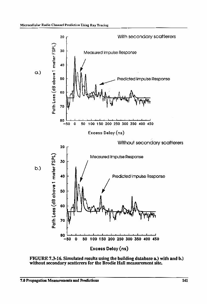
Microcellular Radio Channel Prediction Using Ray Tracing
a.)
b.)
Path
Loss
(d
B above1
mete
r FSPL)
Path
Lo
ss (dB
abov
e 1 me
ter
FSPL
)
20
30
40
50
60
70
With secondary scatterers
Measured Impulse Response
/ Predicted Impulse Response
a
ji dd i 4 l 1 1 I L { rt 80 -50 0 50 100 150 200 250 300 350 400 450
20
30
40
50
60
70
Excess Delay (ns)
Without secondary scatterers
Measured Impulse Response
Predicted Impulse Response
Dh ee he fer eel le Seer Herrereilerreeee 80 ‘— -50 0 50 100 150 200 250 300 350 400 450
Excess Delay (ns)
FIGURE 7.3-16. Simulated results using the building database a.) with and b.) without secondary scatterers for the Brodie Hall measurement site.
7.0 Propagation Measurements and Predictions 141
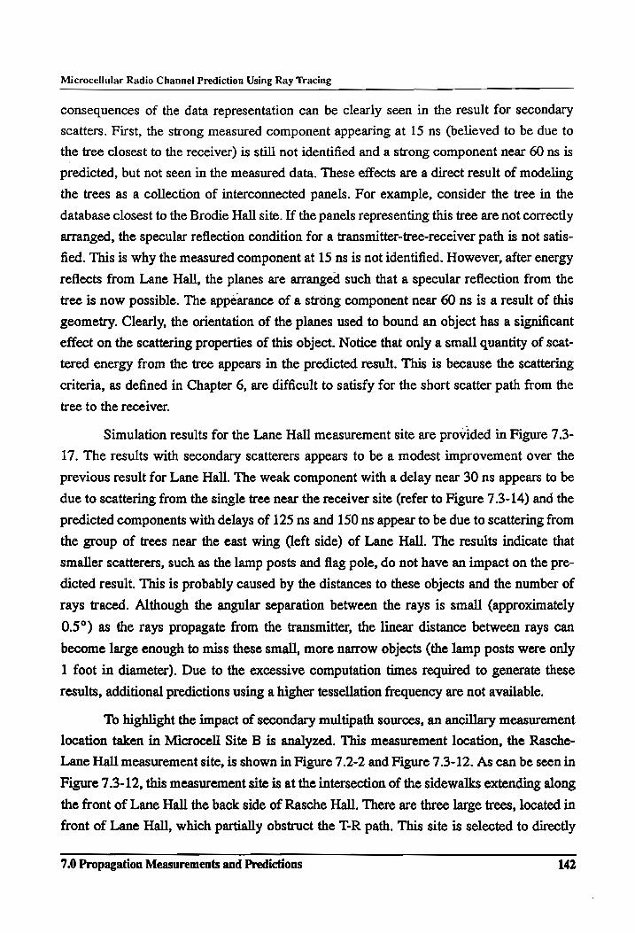
Microcellular Radio Channel Prediction Using Ray Tracing
consequences of the data representation can be clearly seen in the result for secondary
scatters. First, the strong measured component appearing at 15 ns (believed to be due to
the tree closest to the receiver) is still not identified and a strong component near 60 ns is
predicted, but not seen in the measured data. These effects are a direct result of modeling
the trees as a collection of interconnected panels. For example, consider the tree in the
database closest to the Brodie Hall site. If the panels representing this tree are not correctly
arranged, the specular reflection condition for a transmitter-tree-receiver path is not satis-
fied. This is why the measured component at 15 ns is not identified. However, after energy
reflects from Lane Hall, the planes are arranged such that a specular reflection from the
tree is now possible. The appearance of a strong component near 60 ns is a result of this
geometry. Clearly, the orientation of the planes used to bound an object has a significant
effect on the scattering properties of this object. Notice that only a small quantity of scat-
tered energy from the tree appears in the predicted result. This is because the scattering
criteria, as defined in Chapter 6, are difficult to satisfy for the short scatter path from the
tree to the receiver.
Simulation results for the Lane Hall measurement site are provided in Figure 7.3-
17. The results with secondary scatterers appears to be a modest improvement over the
previous result for Lane Hall. The weak component with a delay near 30 ns appears to be
due to scattering from the single tree near the receiver site (refer to Figure 7.3-14) and the
predicted components with delays of 125 ns and 150 ns appear to be due to scattering from
the group of trees near the east wing (left side) of Lane Hall. The results indicate that
smaller scatterers, such as the lamp posts and flag pole, do not have an impact on the pre-
dicted result. This is probably caused by the distances to these objects and the number of
rays traced. Although the angular separation between the rays is small (approximately
0.5°) as the rays propagate from the transmitter, the linear distance between rays can
become large enough to miss these small, more narrow objects (the lamp posts were only
1 foot in diameter). Due to the excessive computation times required to generate these
results, additional predictions using a higher tessellation frequency are not available.
To highlight the impact of secondary multipath sources, an ancillary measurement
location taken in Microcell Site B is analyzed. This measurement location, the Rasche-
Lane Hall measurement site, is shown in Figure 7.2-2 and Figure 7.3-12. As can be seen in
Figure 7.3-12, this measurement site is at the intersection of the sidewalks extending along
the front of Lane Hall the back side of Rasche Hall. There are three large trees, located in
front of Lane Hall, which partially obstruct the T-R path. This site is selected to directly
7.0 Propagation Measurements and Predictions 142
Microcellular Radio Channel Prediction Using Ray Tracing
20
30
40 a.)
50
70
Path Lo
ss (d
B above
1 me
ter
FSPL
)
80
20
30
b.) 40
50
60
70
Path
Lo
ss (dB
abov
e 1 me
ter
FSPL)
60 |- f
With secondary scatterers
Measured Impulse Response
Predicted Impulse Response
i} i { l l i { rf pt | |
-50 O 50 100 150 200 250 300 350 400 450
Excess Delay (ns)
Without secondary scatterers
Measured Impulse Response
Predicted Impulse Response
\
Lt pt |» | 1 l L { a 80 -50 0 50 100 150 200 250 300 350 400 450
Excess Delay (ns)
FIGURE 7.3-17. Simulated results using the building database a.) with and b.) without secondary scatterers for the Lane Hall measurement site.
7.0 Propagation Measurements and Predictions 143
Microcellular Radio Channel Prediction Using Ray Tracing
analyze the impact of trees along the propagation path. The measured data and simulated
results are given in Figure 7.3-18. The predicted results, where trees and other scatterers
are not considered, is shown as Figure 7.3-18a. A considerable discrepancy between mea-
sured and predicted data is seen when secondary effects are not included. For example, the
first arriving component is approximately 15 dB above the measured result. This is
because the prediction does not account for the attenuation caused by trees partially block-
ing the T-R propagation path. Several additional components, such as the peaks at 185 ns,
260 ns, and 380 ns appear in the predicted data but there is no measured multipath corre-
sponding to these time delays.
As can be seen in Figure 7.3-18b, including trees and other localized scatterers
effects a modest improvement in the prediction. The amplitude of the first arriving compo-
nent is attenuated after transmission through a tree along the propagation path (since the
diameter of the upper portion of the trees 1s approximated in the database, only one tree
directly blocks the propagation path). Additionally, the specular reflection from Rasche
Hall, appearing in the profile at 50 ns, is reinforced by additional reflections and scattering
from trees lining the T-R propagation path. Several weak components, with rather long
excess delays, appear in the predicted profile but do not correspond to measured multi-
path. However, in this predicted profile, the maximum excess delay for a spurious compo-
nent above threshold is approximately 250 ns whereas the previous prediction has a
maximum excess delay closer to 425 ns. Clearly, the accuracy of the prediction has
improved by considering trees and other scatterers in the ray tracing.
The results presented in this section illustrate that while it is possible to effect an
improvement in the modeled data by including secondary scatterers, this improvement
depends upon the ability to accurately represent the geometry (and scattering properties)
of these objects in the database. As shown here, representing trees and lamp posts is not as
straightforward as modeling buildings. Other methods for modeling these scatterers, such
as bounding regions containing trees by convex polygons or using a different number of
sides for the tree and lamp post cylinders, have also been investigated and produced simi-
lar simulation results. It appears that the fine structure of these objects requires particular
attention when modeling them in the database.
7.0 Propagation Measurements and Predictions 144
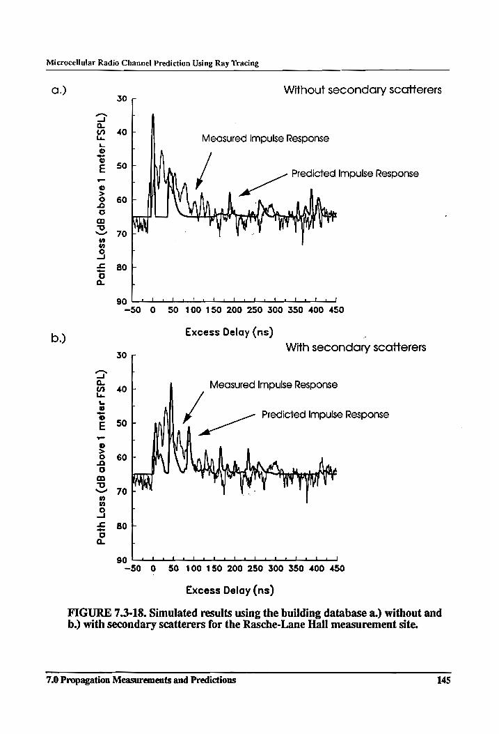
Microcellular Radio Channel Prediction Using Ray Tracing
a.)
b.)
Path
Loss (dB
abov
e 1 me
ter
FSPL)
Path
Lo
ss (d
B ab
ove
1 meter
FSPL
) 30
40
50
60
70
80
Without secondary scatterers
Measured Impulse Response
/ a Predicted Impulse Response
pt | dd ld ld dn 90 -50 0 50 100 150 200 250 300 350 400 450
30
40
50
60
70
80
Excess Delay (ns) .
With secondary scatierers
Measured impulse Response
—_ Predicted Impulse Response
|
I i I a | 1 l 1 i 1 — it Ea Deed 90 -50 0 50 100 150 200 250 300 350 400 450
Excess Delay (ns)
FIGURE 7.3-18. Simulated results using the building database a.) without and b.) with secondary scatterers for the Rasche-Lane Hall measurement site.
7.0 Propagation Measurements and Predictions 145
Microcellular Radio Channel Prediction Using Ray Tracing
7.4 Conclusions
This chapter has presented results generated with the automated ray tracing sys-
tem. Simulations have been performed to demonstrate the precision in automating the ray
tracing model. The results, which were summarized in Section 7.1, show that the predic-
tion tool is capable of producing consistent results when a sufficient number of rays are
traced. The reception sphere technique has also been proven to. be an acceptable method
for identifying specular rays when brute force ray tracing is employed.
Wide band measurements were made in two dissimilar areas on the Virginia Tech
campus for purposes of evaluating the accuracy of the ray tracing model. The wide band
data was collected using a spread spectrum measurement system. This particular measure-
ment system was employed because it had high resolution (9 ns channel probe) and was
capable of measuring considerable path loss (up to nearly 120 dB). Both of these features
in the measurement system were necessary so that individual multipath components could
be resolved, and so multipath data could be collected in both line-of-sight and obstructed
topographies. Although the measurement system had some practical limitations, it was an
excellent resource in gathering this data. :
Locations for the measurements were carefully selected to provide adequate char-
acterization of microcellular channels, by considering reflective environments, reflective
environments with scattering, and shadowed topographies. Additional, the two sites had
buildings constructed of different materials (primarily stone in one location, primarily
brick in the other). Thus, assumptions on the electrical characteristics of buildings could
also be tested.
Verification of the ray tracing model has been performed with a trial set of mea-
sured data. The accuracy of the prediction method has been demonstrated by both visual
comparisons of measured and predicted data as well as through calculating the profile sta-
tistics for both data sets. The results indicate the ray tracing model is capable of evaluating
both the amplitude and delay of discrete multipath components, for a variety of channel
topographies, and with a greater degree of accuracy than can be currently achieved with
statistical models. The following observations were made based upon the visual compari-
sons of the data
7.0 Propagation Measurements and Predictions 146
Microcellular Radio Channel Prediction Using Ray Tracing
e Using simple geometric shapes to represent buildings and terrain in the database, it is
possible to predict the principal features of a multipath profile. Predicting the fine struc-
ture of the profile necessitates that small scale building features and secondary scatter- ers be included in the site-specific database.
e A reflection loss of 12 dB, regardless of incidence angle or material construction, is a suitable first order approximation to the actual electrical properties of a surface.
e The scattering model accounts for discrepancies between measured and predicted data
when specular conditions are not met or when the receiver is near a large scattering sur-
face. This model is particularly useful in shadowed topographies where localized scat- tering has a greater influence on the dispersive qualities of the channel.
e The precision of the ray tracing system is limited by the accuracy of the site-specific
environmental database. Positioning errors within the database can result in consider-
able error between measured and predicted data.
Comparisons of the profile statistics were also conducted. The ray tracing gener-
ally computed more path loss and larger delay spreads than was observed in the measured
data. Predicted path loss was generally within 5 db of the measured value. However, pre-
dicted delay spreads did not exhibit as good agreement, in the worst case the predicted
delay spread was more than twice the measured result. The large errors in delay spread
values were attributed to relatively weak components, with long excess delays, that have
considerable influence on the delay spread calculation.
Modeling secondary sources of multipath within the building database has also
been investigated. Analysis of specific measurement geometries revealed that secondary
effects, such as scattering from trees and lamp posts can explain inconsistencies between
measurements and predictions. However, it has been shown that modeling these multipath
sources in the site-specific database requires particular attention, the fine detail of the
object needs to be considered in the modeling process.
7.0 Propagation Measurements and Predictions 147
Microcellular Radio Channel Prediction Using Ray Tracing
8 Conclusions
An important aspect of wireless system design has been addressed in this thesis-
the impact of the environment on the propagation of radio signals. As cellular-based com-
munication systems evolve, and new wireless technologies are developed, a more accurate
understanding of the propagation characteristics is necessary for efficient system design.
Currently, conventional cellular systems are designed using statistical or empirical models
to determine the coverage and interference levels. However, as interest in wireless tech-
nology continues to grow, a greater number of users need to be supported and the demand
for more services and greater reliability needs to be satiated. To alleviate the current
capacity and reliability problems, next generation cellular technologies (PCS/PCN)
require more accurate methods of predicting propagation. This is especially true in urban
and semi-urban environments, where the diverse topography poses a particular problem to
the radio interface. Clearly, accurate and deterministic propagation prediction tools are
needed. The purpose of the research that has been presented in this thesis is to fulfil this
need,
Propagation characteristics in mobile and portable radio environments and current
research toward predicting propagation in these environments has been presented.
Although the limitations introduced by multipath propagation are known and the need for
site-specific propagation prediction models is clearly recognized within the wireless
industry, only a select number of researchers have been investigating these methods.
When this research first began, the possibility of using simple theoretical techniques to
evaluate propagation characteristics still had not been proven.
As a result, a preliminary study to assess the feasibility of propagation prediction
in microcellular environments, was conducted. The results of this study were presented in
Chapter 4. In this chapter, it was shown that using ray tracing and a simple knife-edge dif-
fraction model, average narrow band signal strength can generally be predicted within 5
dB of the actual value. In addition to the results, three necessary features of an automated
prediction tool were clearly defined. First, the prediction method must incorporate site-
specific environmental data. Second, this data must be integrated with a model capable of
accurate and direct determination of available signal at any location (i.e., ray tracing).
Third, the prediction results need to be processed and displayed in a format useful for
8 Conclusions 148
Microcellular Radio Channel Prediction Using Ray Tracing
rapid system design. All three of these aspects have been demonstrated by the automated
prediction method presented in this thesis.
In Chapter 5, the first characteristic of the prediction method, the use of site-spe-
cific data, was established. It was proposed that the propagation model should make use of
large scale environmental factors, such as the size and shape of buildings, to evaluate
propagation characteristics for urban topographies. A commercial software package,
AutoCAD, was selected for the user interface and for managing the building data. Addi-
tional software was developed to process this building data so it could be transferred to the
ray tracing programs. A sample three dimensional building database was constructed, in
AutoCAD, for a portion of the Virginia Tech campus. This database was then used to con-
firm operation of the processing software.
The second and third aspects of the prediction method have been analyzed in
Chapters 6 and 7. In Chapter 6, the ray tracing model was developed and techniques for
automating this model were discussed. The prediction model was based upon ray tracing
for determining the propagation of energy in three dimensions. Direct, reflected, transmit-
ted, scattered, and diffracted rays were included in the propagation model. Since the auto-
mated system uses a “brute force” approach for tracing ray propagation, a ray launching
algorithm and reception method were developed to guarantee that energy arriving from
any direction was always considered.
Results of the ray tracing system verification were presented in Chapter 7. Two
approaches were taken test the system. First, the precision of the automation techniques
were confirmed through simulation. The simulation results indicated that, in a typical
microcellular environment, consistent results were possible if the ray separation is suffi-
ciently small. Additionally, the reception sphere was shown to correctly identify specular
rays. The accuracy of the ray tracing system was validated using data collected on the Vir-
ginia Tech campus. This procedure was conducted against measured data collected on two
different areas on the campus, and collected in a variety of different channel topographies.
The following items were observed from the comparisons.
e Simple descriptors for the electrical properties of common surfaces can be used to obtain acceptable results. For example, a constant reflection loss regardless of inci- dence angle of material composition, can be used as a reasonable, first order approxi-
mation to the true reflective properties of a surface.
§ Conclusions 149
Microcellular Radio Channel Prediction Using Ray Tracing
¢ Using simple geometric shapes to represent buildings and terrain, the amplitudes and
delays of multipath components can be accurately determined. However, it is not nec- essarily the quantity of site-specific data that defines the precision of a result. Incorrect
positioning of buildings or other objects within the database can introduce substantial
errors. Rather, it is the accuracy of the data which has the most substantial impact.
e The ray tracing generally predicts pessimistic, or worst case, values for path loss and
delay spread. Worst case parameters can be useful when defining a coverage region of maximum data rate, but are less useful for evaluating interference levels.
e Scattering can account for discrepancies between measured and predicted data when a
receiving point is near a large scattering surface, or when a specific geometry does not
allow for the specular conditions to be satisfied. The contribution of scattered rays can
be most significant in shadowed topographies where weak scattering is significant.
e Ray tracing has practical limitations. As the complexity of the environment increases, the measured and predicted data is more inconsistent. In many cases, small scale build-
ing features and secondary sources of multipath can be the cause of this discrepancy. Although it is possible to model these secondary effects in the environmental database,
this should be done cautiously, as the modeling method has a substantial impact on the results.
The third aspect of the ray tracing system, data processing of the raw data and dis-
play of this data in a form useful for system design has also been demonstrated. As indi-
cated profile statistics can be used for some aspects of worst case system design, and
graphical display of the ray paths in AutoCAD may provide some insight into the source
of multipath in a particular environment. Identification of these sources can be very useful
for selecting a location and antenna radiation pattern for a base station.
8.1 Extensions of this Research
The accuracy of a model and its software implementation can always be advanced. The
work presented in this thesis is certainly not an exception. Some possible enhancements to
this research are summarized as follows.
e The propagation model and ray tracing system requires more extensive experimental confirmation. This should be done in conjunction with an in-depth study into multipath propagation in mobile and portable radio environments. Carefully controlled, multi-fre- quency measurements, are necessary to identify both the sources and the frequency dependence of multipath. Various transmitter and receiver polarization combinations (using both linear and circular polarization) should also be used in the measurements. Additionally, these measurements should be made in a wide variety of channel topogra-
phies for more complete verification of the ray tracing model.
§ Conclusions 150
Microcellular Radio Channel Prediction Using Ray Tracing
Exact data on the electromagnetic properties of building materials should be incorpo-
rated. Approximations to these characteristics are currently used because exact data is
not yet available. Reasonable accuracy can be achieved using a simplified reflection
model. However, accurate material data may improve accuracy, as the phase and polar-
ization of a ray can then determined. The program has been designed to permit this data to be integrated directly into the database and program modifications to the computer
code.
The scattering model needs to be further studied. This investigation should include both
a theoretical and experimental approach.
A better metric for the accuracy of a prediction should be developed. Visual compari- sons along with the profile statistics is a suitable method. However, this technique is
time consuming, and it is impractical if a comparisons are being made against a large measurement set.
The ray tracing interfaces need to be expanded. The ray tracing software uses a generic file format so that is can be interfaced, with any type of CAD or cis! system. Other
commercial products, such as GRASS? , require data conversion routines so that their
output data is in the required file format. Additionally, the interface from the ray tracing to AutoCAD needs to be developed. Color contour plots of path loss, » delay spread, pre-
diction error, etc. need to be investigated.
The code needs to be optimized. It may be possible to restructure the code to reduce the number of intersection tests that are performed. Use of parallel processing to reduce
execution times should also be investigated.
8.2 Summary
In summary, this thesis has investigated propagation prediction for urban microcel-
lular channels. A propagation model, which uses ray tracing and incorporates site-specific
data, has been developed and implemented on a Sun SparcStation 2. Validation of the
model against measured data indicates this method can predict propagation more accu-
rately than previously been possible with statistical or empirical models. In the future,
accurate propagation prediction tools, such as this one, may permit rapid and economical
deployment of wireless communication systems (PCS/PCN).
1. Geographical Information Systems.
2. Geographical Resources Analysis Support System.
§ Conclusions 151
Microcellular Radio Channel Prediction Using Ray Tracing
9.0 References
[Bec63]
[Bec68]
[Bis91]
[Bla92]
[Bor65]
[CAD90]
[Chi91]
[Col85]
[Cox73]
[Cri68]
[Des72]
—~ [Dev86]
[Dev87]
P. Beckmann and A. Spizzichino, The Scattering of Electromagnetic Waves
from Rough Surfaces, Pergamon Press, Oxford, England, 1963.
P. Beckmann, The Depolarization of Electromagnetic Waves, Golem Press,
Boulder, Colorado, 1968.
D. Bishop, “Personal Communications Service,” Mobile Radio Technology, p.
4, July 1991.
K. L. Blackard, et. al., “Path Loss and Delay Spread Models as Functions of Antenna Height for Microcellular System Design,” 1992 IEEE Veh. Technol. Conference, Denver, CO, May 1992.
M.Born and E. Wolf, Principles of Optics, Pergammon Press, New York, 1965.
AutoCAD Reference Manual, Release 11, Autodesk Publication AC11RM,
1990.
S. T. S. Chia, “1700 MHz Urban Microcells and Their Coverage Into Build-
ings,” IEE Conference on Antennas and Propagation, York, UK, pp. 504-511, April 1991.
R.E. Collin, Antennas and Radiowave Propagation, McGraw-Hill, 1985.
D. C. Cox, “910 MHz Urban Mobile Radio Propagation: Multipath Character-
istics in New York City,”"JEEE Transactions on Communications, Vol. COM-
21, No. 11, February 1973, pp. 1188 - 1194..
J. W. Crispin, Jr., ed., Methods of Radar Cross Section Analysis, Academic
Press, New York, 1968.
G.A. Deschamps, “Ray Techniques in Electromagnetics,” Proceedings of the IEEE, Vol. 60, No. 9, Sep. 1972, pp. 1022-1035.
D.M.J. Devasirvatham, “Time Delay Spread and Signal Level Measurements of 850 MHz Radio Waves in Building Environments,” JEEE Transactions on
Antennas and Propagation, Vol. AP-34, No. 11, Nov. 1986, pp. 1300-1305.
D.M.J. Devasirvatham “Multipath Time Delay Spread in the Digital Portable Radio Environment,” JEEE Communications Magazine, Vol. 25, No. 6, June 1987, pp. 13-21.
9.0 References 152
Microcellular Radio Channel Prediction Using Ray Tracing
_IdeW83s]
[Gla89]
_...[Gre89]
[Gri87]
~~[Har89]
[Has79] ge CEE
_ [Hat80] eres
J.P. deWeck, P. Merki, and R. Lorenz, “Power Delay Profiles Measured in
Mountainous Terrain,” 38th IEEE Vechicular Technology Conference, June 15,
1988, Philadelphia, PA, pp. 105-111.
R. C. Dixon, Spread Spectrum Systems, gnd ed., John Wiley and Sons, New York, 1984.
P. F. Driessen, et. al., “Ray Model of Indoor Propagation,” in proceedings of
2" Annual Virgina Tech Symposium on Wireless Personal Communications,
Blacksburg, VA, June 17-19, 1992, pp. 17-1 through 17-12.
R. Edwards and J. Durkin, “Computer Prediction of Service Areas for VHF
Mobile Radio Networks," Proceedings of IEE, Vol. 116, No. 9, 1969 pp. 1493-
1500.
J. Epstein and D. W. Peterson, “An Experimental Study of Wave Propagation
at 850 Mc.,” Proceedings of IRE, Vol. 41, No. 5, 1953. pp. 595-611.
L. B. Felsen, Radiation and Scattering of Waves, Prentice-Hall, New Jersey,
1973, pp. 630-661.
A. Fouladpouri and J. D. Parsons, “Comparison of Propagation Prediction
Models for VHF Mobile Radio," in proceedings of JEE Conference on Land-
Mobile Radio, pp. 139-145, 1987.
A. Glassner, ed., An Introduction to Ray Tracing, Academic Press, San Diego,
1989.
E. Green, “Path Loss and Signal Variability Analysis for Microcells,” in pro- ceedings for JEE 5th International Conference on Mobile Radio and Personal
Communications, Warwick, UK, Dec. 11-14, 1989, pp. 38-42.
J. Griffiths, Radio Wave Propagation and Antennas, Prentice-Hall, London,
1987.
P. Harley, “Short Distance Attenuation Measurements at 900 MHz and 1.8 GHz Using Low Antenna Heights for Microcells,” JEEE J. Select. Areas Com- mun., Vol.7, No. 1, January 1989, pp. 5-11.
H. Hashemi, “Simulation of the Urban Radio Propagation Channel,” JEEE
Transactions on Vehicular Technology,Vol. VT-28, No. 3, pp. 317-325, August
1980.
M. Hata, “Emperical Formula for Propagation Loss in Land Mobile Radio Ser-
vices,” IEEE Transactions on Vehicular Technology, Vol. VT-29, No. 3, pp.
213-225, August 1979.
9.0 References 153
Microcellular Radio Channel Prediction Using Ray Tracing
[Hon92]
[Ibr83]
[Ike84]
[Ike9 1]
[Ken76]
[Kno85]
{Lan92]
{[Law92]
~~ [Lee82]
[Liu90]
[Loe83]
{Lon68]
[Mah92]
W. Honcharenko, et. al., “UHF Propagation in Modern Office Buildings,”
accepted for publication in JEEE Transactions on Vehicular Technology, 1992.
M. F. A. Ibrahim, et. al., “Signal Strength Prediction in Urban Areas Using a Topographical and Environmental Database," in proceedings for JEEE Int.
Conf. Commun., (ICC’83), Boston, MA, pp. 64-67, June 1983.
F, Ikegami, et. al., "Propagation factors controlling mean field strength on urban streets," JEEE Transactions on Antennas and Propagation, Vol. AP-32,
No. 8, pp. 822-829, Aug. 1984.
F, Ikegami, T. Takeuchi, and S. Yoshida., “Theoretical Prediction of Mean
Field Strength for Urban Mobile Radio,” JEEE Transactions on Antennas and
Propagation, Vol. 39, pp. 299-302, Mar. 1991.
H. Kenner, Geodesic Math and How to Use It, University of California Press,
Berkeley, 1976.
E. F. Knott, et. al., Radar Cross Section - Its Prediction, Measurement, and
Reduction, Artech House, Dedham, MA, 1985.
O. Landron, “Microwave Multipath Resolution in Microcellular Environ- ments,” Master’s Thesis, VPI&SU, August 1992.
M. C. Lawton and J. P, McGeehan, “The application of GTD and Ray Launch- ing Techniques to Channel Modelling for Cordless Radio Systems,” 42nd IEEE Vehicular Technology Conference, Denver, May 1992, pp. 125-130.
W.C.Y. Lee, Mobile Communications Engineering, McGraw-Hill, 1982.
J.T-K. Lui, “Narrow Band Microwave Propagation Measurement System for
Indoor Communication,” Undergraduate Thesis, MPRG-TR-90-2, May 1990.
K. Loew and R. W. Lorenz, “Determination of Service Areas for Mobile Com- munication with a Topographical Database," in proceedings for JEEE Inil. Conf. Commun., (ICC’83), Boston, MA, pp. 54-58, June 1983.
A. G. Longley and P. L. Rice, “Prediction of Tropospheric Transmission Loss Over Irregular Terrain - A Computer Method,” ESSA Technical Report, ERL 791T567, 1968
K. Mahbobi, “Radio Wave Propagation in Urban Microcellular Environment,”
1992 IEEE Vehicular Technology Conference, Denver, CO, May 1992, pp.
951-955.
9.0 References 154
Microcellular Radio Channel Prediction Using Ray Tracing
[McK9 1}
[Mog91]
[Noe86]
[Oku68] amen te
[Omu89]
~~ [Par89]
_.~fPar92]
[Pie9 1]
[Pug76]
[Raj92]
[Ran89]
* fRap89]
__ [Rap90]
[Rap91]
J. W. McKown and R. L. Hamilton, Jr., “Ray Tracing as a Design Tool for Radio Networks,” JEEE Network Magazine, pp. 27-30, November 1991.
P. E. Mogensen, P. Eggers, and C. Jensen, “Urban Area Radio Propagation Measurements for GSM/DCS 1800 Macro and Micro cells,” JEE Conference
on Antennas and Propagation, York, UK, April 1991, pp. 1-5.
A. R. Noerpel, "Use of Physical Optics to Characterize Building Reflections," in proceedings for JEEE Int. Conf. Commun., ICC'86), pp. 847-851, 1986.
Y. Okumura, et. al., "Field Strength and its Variability in VHF and UHF Land Mobile Service," Rev. Elec. Comm. Lab., Vol. 16, pp. 825-873, Sept.-Oct.1968.
G. Omura, Mastering AutoCAD, 3" ¢ edition, Sybex, San Francisco, 1989.
J.D. Parsons, and J.G. Gardiner, Mobile Communication Systems, Blackie,
London, 1989.
J. D. Parsons, The Mobile Radio Propagation Channel, Halsted Press, New
York, 1992.
J. M. Pielou, “Preliminary Analysis of 1.8 GHz Measurements for Personal
Communications,” JEE Conference on Antennas and Propagation, York, UK,
April 1991, pp. 508-511.
A. Pugh, Polyhedra, A Visual Approach, University of California Press, Berke-
ley, 1976.
C. S. Rajguru, “Application of GIS in Mobile Communications,” Master’s Thesis, VPI&SU, August 1992.
A. Ranade, “Local Access Radio Interference Due to Building Reflections,"
IEEE Transactions on Communications, Vol. 37, No. 1, pp. 70-74, January 1989.
T.S. Rappaport, “Characterization of UHF Multipath Radio Channels in Fac- tory Buildings,” JEEE Transactions on Antennas and Propagation, Vol. 37, No. 8, August 1989, pp. 1058-1069.
T. S. Rappaport, S. Y. Seidel, and R. Singh, “900-MHz Multipath Propagation Measurements for U.S. Digital Cellular Radiotelephone,” JEEE Transactions
on Vehicular Technology, Vol. 39, pp. 132-139, May 1990.
T. S. Rappaport, “The Wireless Revolution,” JEEE Communications Maga-
zine, Vol. 29, No. 11, November 1991, pp. 52-71.
9.0 References 155
Microcellular Radio Channel Prediction Using Ray Tracing
[Ruc70]
[Rus9 1]
[Rus91]
[Sau91]
(Sch91]
[Sch92a]
[Sch92b]
[Sei91]
[Sei92a]
[Sei92b]
[Sil49]
[Sko70]
G. T. Ruck, ed., Radar Cross Section Handbook, Plenum Press, New York,
1970.
T. A. Russell, “Predicting Microwave Diffraction in the Shadows of Build-
ings,” Master’s Thesis, VPI&SU, 1991.
A.J. Rustako, Jr., N. Amitay, G. J. Owens, and R. S. Roman, “Radio propaga-
tion at microwave frequencies for line-of-sight microcellular mobile and per- sonal communications,” JEEE Transactions on Vehicular Technology,Vol. 40,
pp. 203-210, Feb 1991.
S. R. Saunders and F. R. Bonar, “Mobile Radio Propagation in Built-up Areas: A Numerical Model of Slow Fading,” 41° IEEE Vehicular Technology Confer-
ence, St. Louis, May 1992, pp. 295-299.
K. R. Schaubach, N. J. Davis IV, and T. S. Rappaport, “Propagation Models for Microcellular Environments Using a Building Database,” poster presented at First Virginia Tech Symposium on Wireless Personal Communications, Blacks- burg, VA, June 5, 1991.
K.R. Schaubach, N.J. Davis IV, and T.S. Rappaport, “A Ray Tracing Method
for ' Predicting Path Loss and Delay Spread in Microcellular Environments,”
42"4 IEEE Vehicular Technology Conference, Denver, May 1992, pp. 932-935.
K.R. Schaubach et. al., “Microcellular Radio Channel Prediction Using Ray
Tracing - Computer Software,” MPRG/VTIP publication, August 1992.
S.Y. Seidel, et.al, “Path Loss, Scattering, and Multipath Delay Statistics in
Four European cities for Digital Cellular and Microcellular Radiotelephone,” IEEE Transactions on Vehicular Technology, Vol. 40, No. 4, Nov. 1991, pp.
721-730.
S.Y. Seidel, “Site-Specific Propgation Prediction for Wireless In-Building Per-
sonal Communication System Design,” report prepared for the Ph.D. Prelimi- nary Examination, MPRG-TR-92-07, February 1992.
S.Y. Seidel, et.al, “The Impact of Surrounding Buildings on Propagation for Wireless In-Building Personal Communications System Design”, 42"4 IEEE Vehicular Technology Society Conference, Denver, CO, May 1992.
S. Silver, ed., Microwave Antenna Theory and Design, McGraw-Hill, London,
1949.
M.I. Skolnik, ed., Radar Handbook, McGraw-Hill, New York, 1970.
9.0 References 156
Microcellular Radio Channel Prediction Using Ray Tracing
[Sko80]
[Sou92]
[Ste89]
[Ste90]
[stu81]
Be
[Tak91]
[Tel9 1]
[Tur72]
[Van87]
[Wal88]
[Wen79]
M. I. Skolnik, Introduction to Radar Systems, Second Edition, McGraw-Hill,
New York, 1980.
C. K. Sou, O. Landron, and M. J. Feuerstein, “Characterization of Electromag-
netic Properties of Building Materials for use in Site-Specific Propgation Pre-
diction,” MPRG-TR-92-12, June 1992.
R. Steele, “The Cellular Environment of Lightweight Handheld Portables,”
IEEE Communications Magazine, July 1989, pp. 20 - 29.
R. Stevens, Fractal Programming and Ray Tracing with C++, M&T Books,
Redwood City, CA, 1990.
W.L. Stutzman and G.A. Thiele, Antenna Theory and Design, Wiley, New
York, 1981.
H. Suzuki, “A Statistical Model for Urban Radio Propagation,” JEEE Transac- tions on Communications, Vol. COM-25, No. 7, July 1977, pp. 673 - 680.
T. Takeuchi, M. Sako, and S. Yoshida, “Multipath Delay Prediction on a Work- station for Urban Mobile Radio Environment,” JEEE Globecom 199], Denver,
CO, June 23-26, pp. 1308 - 1312.
Telesis Technologies Laboratory, Experimental License Report to the FCC,
Aug. 1991.
G. L. Turin, et. al., “A Statistical Model of Urban Multipath Propagation,” IEEE Transactions on Vehicular Technology, Vol. 21, pp. 1-9, Feb. 1972.
J. van Rees, “Measurements of the Wide-Band Radio Channel Characteristics
for Rural, Residential, and Suburban Areas,” JEEE Transaction on Vehicular
Technology, Vol. VT-36, No. 1, Feb. 1987, pp. 2-6.
J. Walfish and H. L. Bertoni, “A Theoretical Model of UHF Propagation in Urban Environments,” JEEE Transactions on Antennas and Propagation, Vol. 36, pp. 1788-1796, Dec. 1988.
M.J. Wenninger, Spherical Models, Cambridge University Press, New York,
1979.
9.0 References 157

Vita
Kurt Richard Schaubach was born in Passaic, New Jersey on June 28, 1968. He received
the Bachelor of Science degree in Electrical Engineering from Virginia Polytechnic Insti-
tute and State University in 1990. While completing his degree requirements, he worked
summers as an engineering intern at AT&T Quality Management and Engineering and
Kearfott Guidance and Navigation. In 1991, he joined the Mobile and Portable Radio
Research Group at Virginia Tech where his research has focused on characterizing RF
propagation for wireless communication system design. During his graduate studies, he
served two semesters as a teaching assistant for courses in electromagnetic fields, commu-
nications systems, and RF hardware design. In October 1992, Mr. Schaubach begins
employment at Southwestern Bell Technology Resources.
Mr. Schaubach is a member of the Eta Kappa Nu honor society and the IEEE.
Pe Dapaen
Vita 158


