Embed Size (px)
Citation preview
'
A A CAD/CAM Interface for Computer—Aided Design of Cams
i · I ShyAshit R. Gandhi
Thesis submitted to the Faculty of the
Virginia Polytechnic Institute and State University .
in partial fulfillment of the requirements for the degree of
Master of Science
· inMechanical Engineering
APPROVED:
,Dr. Arvid Myklébust, Chairman Dr. Charles F. Reinholtz S?)
< .. 2 „ “ _ ·
Dr. Hamilton H. Mabie Dr. Said W. Zewari
December, 1985
- Blacksburg, Virginia
i A CAD/CAM Interface for Computer—Aided Design of Cams
Y byAshit R. Gandhi
xa Dr. Arvid Myklebust, Chairmanj
§§— Mechanical Engineering
(ABSTRACT)
The purpose of this thesis is to provide a complete package for
the design and three dimensional modeling display of cams. _
The software producmd as a part of this work will operate as a
module of CADAM to produce cam designs and enter the resulting cam as a
CAD model and produce the graphical display of the cam.
In addition to the introductory material, this thesis is divided
into four sections. The section on the graphics packages used in this
thesis includes a brief history and capabilities of each of the packages.
The second section details the procedure to be adopted in order to design
a cam. The next section details ANICAM, the program that has been de-
veloped to incorporate the design and display procedure. The fourth
section of this thesis contains recommendations for further work in this
area.
The theoretical work in this project is a combination of original
derivations and applications of the theory in the design literature.
I
‘ ACKNOWLEDGEMENTS
My deepest gratitude is extended to the chairman of my supervisory
committee, Dr. Arvid Myklebust, for his guidance, encouragement and sup-
port throughout my graduate studies.
I wish to express my sincere appreciation to the members of the
supervisory committee, Dr. Charles Reinholtz, Dr. Hamilton Mabie and Dr. ·
Said Zewari for their advice and support.
For their support, my thanks to the fellow students who provided
technical help and moral support. In particular, I thank
Finally, I am indebted to my parents and family members for their
unfailing love and support which made my studies in United States possi-
ble.
iii
TABLE OF CONTENTS
Chapter 1 Introduction ..................... 1
Chapter 2 Literature Review. 3
Chapter 3 Graphics Support .................. 6
3.1 Graphical Kernel System ................... 6
3.1.1 Capabilities of GKS ................... 7
3.2 CADAM ............................ 9
3.2.1 Capabilities of CADAM .................. 9
3.3 MOVIE.BYU ...................I ....... 12
3.3.1 Capabilities of MOVIE .................. 13
Chapter 4 Design Consideration .................16
4.1 Introduction ..............·.......... 16
4.2 Cam Displacement Curves ................... 17
4.2.1 Simple Harmonic Motion ................. 20
4.2.2 Cycloidal Motion .................... 29
4.2.3 Constant Velocity .................... 38
4.2.4 Constant Acceleration .................. 39
4.2.5 Polynomial Curves .................... 41
4.2.6 Fourier Series Curves .............l ..... 47
4.2.7 Modified Cam Curves .....r.............. 514.3 Cam Profile Determination ......·............ 58
· iv
1
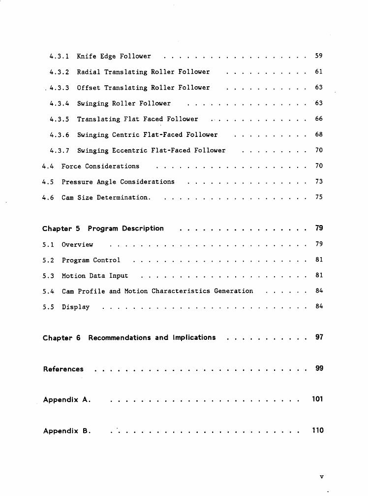
4.3.1 Knife Edge Follower ................... 59
4.3.2 Radial Translating Roller Follower ........... 61
. 4.3.3 Offset Translating Roller Follower ........... 63
4.3.4 Swinging Roller Follower63
4.3.5 Translating Flat Faced Follower .—............ 66
4.3.6 Swinging Centric Flat—Faced Follower .......... 68
4.3.7 Swinging Eccentric Flat-Faced Follower ......... 70
4.4 Force Considerations .................... 70
4.5 Pressure Angle Considerations ................ 73
1 4.6 Cam Size Determination. ................... 75
Chapter 5 Program Description .................79
5.1 Overview .......................... 79
5.2 Program Control ....................... 81
5.3 Motion Data Input ...................... 81
5.4 Cam Profile and Motion Characteristics Generation ...... 84
5.5 Display ........................... 84
Chapter 6 Recommendations and Implications ...........97
References ............................99
Appendix A. ......................... 101
Appendix B. . °........................ 110
v

1
Appendix C. ......................... 112
Vita .............................. 160
vi
LIST OF ILLUSTRATIONS 3
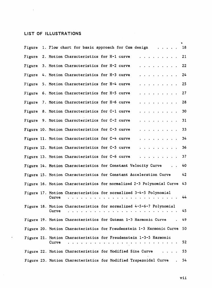
Figure 1. Flow chart for basic approach for Cam design ..... ·18
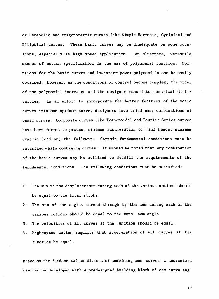
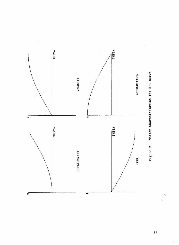
Figure 2. Motion Characteristics for H-1 curve ......... 21
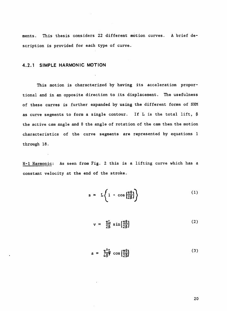
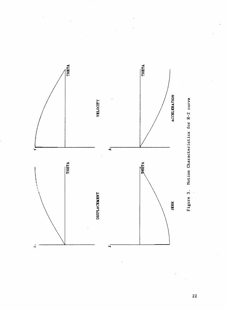
Figure 3. Motion Characteristics for H·2 curve ......... 22
Figure 4. Motion Characteristics for H-3 curve ......... 24
Figure 5. Motion Characteristics for H·4 eurve ......... 25
Figure 6. Motion Characteristics for H-5 curve ......... 27
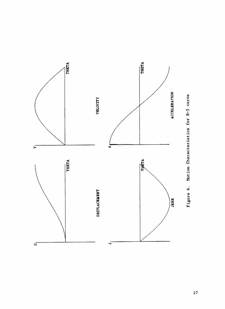
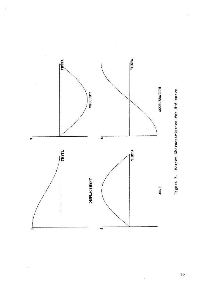
Figure 7. Motion Characteristics for H-6 curve ......... 28
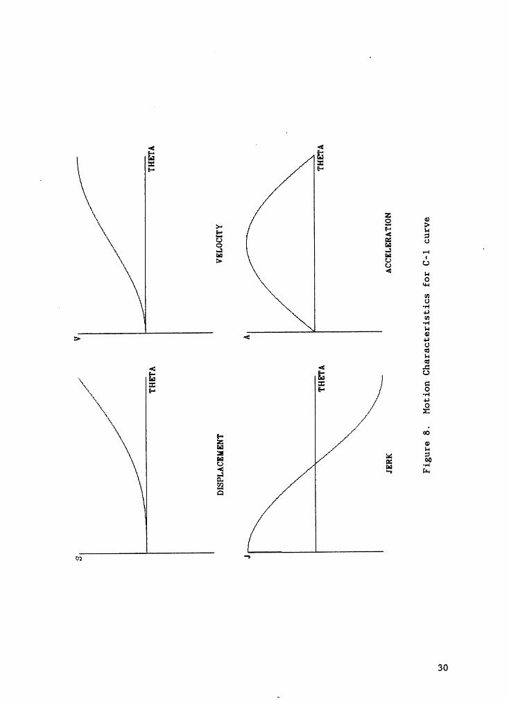
Figure 8. Motion Characteristics for C-1 curve ......... 30
Figure 9. Motion Characteristics for C-2 curve ......... 31
Figure 10. Motion Characteristics for C—3 curve ......... 33
Figure 11. Motion Characteristics for C-4 curve ......... 34
Figure 12. Motion Characteristics for C-5 eurve ......... 36
Figure 13. Motion Characteristics for C-6 curve ......... 37
Figure 14. Motion Characteristics for Constant Velocity Curve . . 40
Figure 15. Motion Characteristics for Constant Acceleration Curve 42
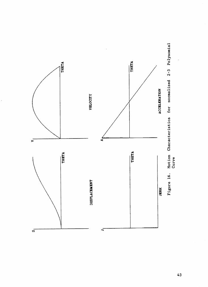
Figure 16. Motion Characteristics for normalized 2-3 Polynomial Curve 43
Figure 17. Motion Characteristics for normalized 3-4-5 PolynomialCurve ......................... 44
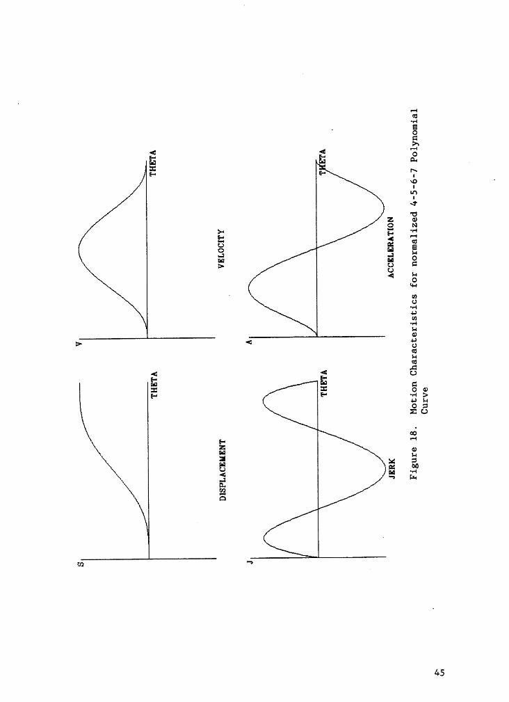
Figure 18. Motion Characteristics for normalized 4-5-6-7 PolynomialCurve ......................... 45
Figure 19. Motion Characteristics for Gutman 1-3 Harmonie Curve . 49
Figure 20. Motion Characteristics for Freudenstein 1-3 Harmonie Curve 50‘ Figure 21. Motion Characteristics for Freudenstein 1-3-5 Harmonie
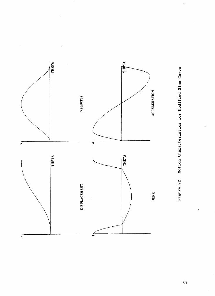
Curve ..............u........... 52Figure 22. Motion Characteristics for Modified Sine Curve .... 53
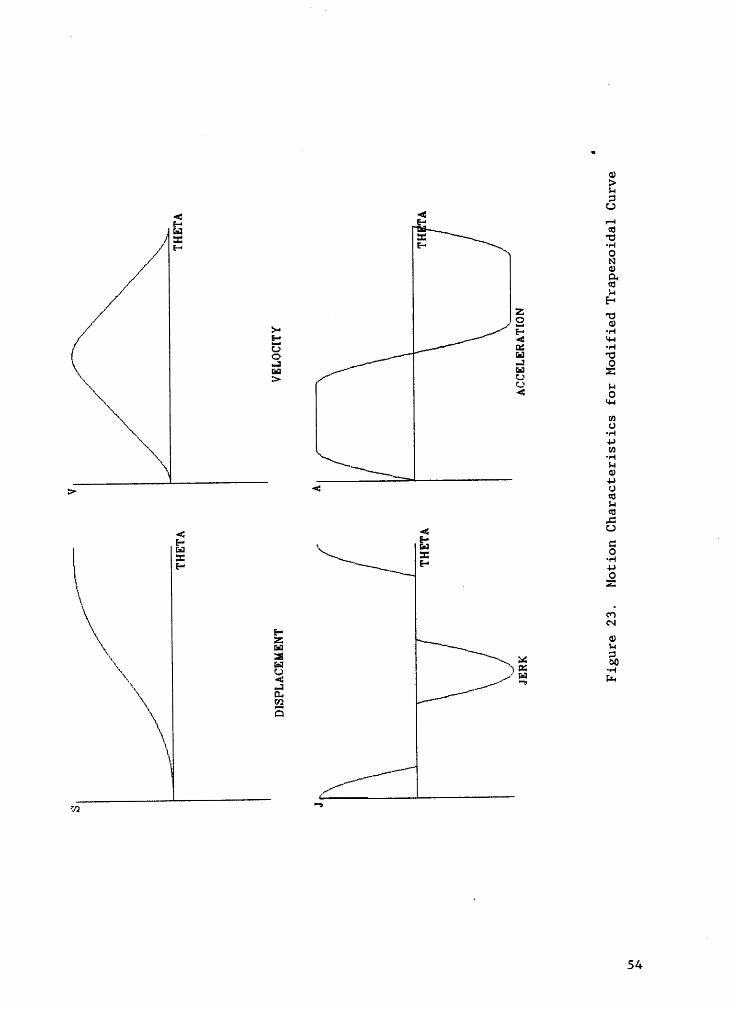
Figure 23. Motion Characteristics for Modified Trapezoidal Curve . 54
lvii
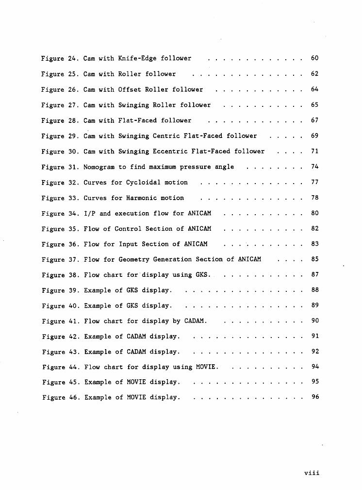
Figure 24. Cam with Knife-Edge follower ............. 60
Figure 25. Cam with Roller follower ............... 62
Figure 26. Cam with Offset Roller follower ............ 64
Figure 27. Cam with Swinging Roller follower ........... 65
Figure 28. Cam with Flat-Faced follower ............. 67
Figure 29. Cam with Swinging Centric Flat-Faced follower ..... 69
Figure 30. Cam with Swinging Eccentric Flat•Faced follower .... 71
Figure 31. Nomogram to find maximum pressure angle ........ 74
Figure 32. Curves for Cycloidal motion .............. 77
Figure 33. Curves for Harmonic motion .............. 78
Figure 34. I/P and execution flow for ANICAM ........... 80
Figure 35. Flow of Control Section of ANICAM ........... 82I
Figure 36. Flow for Input Section of ANICAM ...‘. ....... 83
Figure 37. Flow for Geometry Generation Section of ANICAM .... 85
Figure 38. Flow chart for display using GKS. ........... 87l
Figure 39. Example of GKS display. ................ 88
Figure 40. Example of GKS display. ................ 89
Figure 41. Flow chart for display by CADAM. ........... 90
Figure 42. Example of CADAM display. ............... 91
Figure 43. Example of CADAM display. ............... 92
Figure 44. Flow chart for display using MOVIE. .......... 94
Figure 45. Example of MOVIE display. ............... 95
Figure 46. Example of MOVIE display. ............... 96
viii
a
CHAPTERT INTRODUCTION
Today°s fast changing technology has put tremendous pressure on
corporations for the development of new systems and also to improve the
current designs. This has turned out to be a complex, time consuming and
often costly process. In the past, engineers would run into errors from
even the most detailed blueprints. That meant redesigns which would cost
several thousand dollars or more. The computer helped, eliminate. many
errors in recent years, giving engineers more flexibility to experiment
with a design before it was actually manufactured. Still much of that
early Computer-Aided engineering was executed in 2-D on the computer
screen, like sketching on an electronic piece of paper.
Today however the so called 3-D systems are available. The addition
of depth, on 19-inch full·color screens has led to significant advances
in engineering speed and accuracy. Using portable workstations, design
engineers are able to work independently, as well as away from the office.
This means that an engineer can check the designs in progress to avoid
missteps as the design takes shape. It accelerates the communication
between various engineers on a project and eliminates what could turn out
to be costly errors. The reduced errors will also improve productivity.
The 3-D systems are able to store design information from the early stages
of a project. Since engineers know how to retrieve it, they are free to
spend more time on problem solving. Software packages developed can help
engineers deduce where the moving parts will show early· stress signs,
which parts can be cut by the manufacturer from the same piece of material
l
(to be ground) and what illustrations might be best included in the user°s A
manual.
The ability to model in 3-D is significant since the designer no
longer has to tie up time in manufacturing a model. This has been espe-
cially true when many design iterations are required to satisfy motion
constraints. While many programs have been written to handle design and
analysis, almost nothing can be found to link the analysis step to a 3-D Amodeler. Transferring data between these two steps has been very labo-
rious. If a method had been available to do this automatically, a great
savings in time and accuracy would have resulted. The purpose of this
study is to create a program which will make it possible to tie these
design steps together and present a. method for creating 3-D animated
models automatically. .
This thesis introduces a program, ANICAM which has been created to
animate the motion of cams in a 3-D format. It has been written in FORTRAN
77 computer language using the IBM4341 running the VM/CMS system and has
been designed to serve as an interface between cam design and three ex-
isting programs: GKS, a graphics package, CADAM, and MOVIE.BYU which are
packages for generating 3-DAgraphics and CAD models.
· 2
CHAPTER 2 LITERATURE REVIEW.
The history of cams can be traced back several centuries. However
it is very difficult to say where and when cams got started. In spite
of being in use for a long time, it was only in the last four decades that
major developments in the area of cam design have taken place.
While the kinematics of the cam-follower system have been thor-
oughly investigated by many including Rothbart(1), Jensen(2) and Chen(3),
the absence of literature on the dynamic response has made it very dif-
ficult to validate analytic advances in this field. In recent years,
investigations into the dynamics of the cam-follower systems have. been
performed by Johnson(4), Donkin and Clark(5) and others. However little
experimental data, either in the form of system parameters or dynamic
quantities, is available. Pisano(6) has gathered data on the description
and recording of such measurements. The dynamics of cam-follower systems
- remains an active field of research and development.
The last two decades have seen a lot of work in the fields of design
synthesis, design optimization, and computer-aided design. Many* math-
ematical techniques have been used to find the optimal or best solution
to the design problem. These consist of two phases: first, to generate
alternative solutions and second, to identify the optimal solution amongI
the acceptable ones based on certain criteria. Work on optimal designI
of the cam-follower systems has been done by Berzak(7) who optimally
synthesized the system by the polydyne cam design method. Sermon and
~ Liniecki(8) have used pressure angle and maximum stress constraints to
3
design minimum volume cams. Sandler(9) uses the spectral theory of random
processes for the synthesis while Chen and Shah(l0) have used the se-
quential random vector technique for the optimal design of geometric pa-
rameters of the system. Chew, Freudenstein and Longman(l1) have suggested
a model using the optimal-control theory.
The need to improve manufacturing productivity has generated large
scale interest in computer-aided design and computer-aided manufacturing.
In recent years, several computer programs have been written to perform
basic design functions.
A number· of programs for designing cam and follower systems are
available. Most of these packages use the well known aspects of kinematic
·and static force analysis of cam mechanisms. COMMEND(l2) is a program
which considers almost every design aspect for the cam. An integrated
program constisting of CAM, KAVM, and NCCAM(l3) allows the: design and
graphical display' of the cam-follower system. Other programs for the
analysis and design of cam rnechanisms include CAMPAK(14), DYCAM and
CAMCHK(l5). All the above programs allow two dimensional display of the
physical characteristics and geometry of the cam-follower systems.
If computer graphics is to be exploited fully, then the design and
analysis of the cam should be supported by high resolution, three dimen-
sional shaded color images. Coupled with animation, this would give a
realistic picture of the cam and follower. Three dimensional modeling
packages like GEOMOD, CATIA, PADL-1 and 2, UNISOLIDS, UNISCAD(l6) andl
recently CADAM have been developed by private corporations for commercial
purposes. Another package, MOVIE.BYU, has been developed and distributed
by the Brigham Young University. The availability of 3-D graphics pack·
V 4

ages has helped reduce the time required in tedious verifications of the
practicality of the design.
While this review is by no means complete, it forms the backbone
of this project which aims at developing a computer program (to be named
ANICAM) for design and three dimensional display of cams.
l5
CHAPTER 3 GRAPHICS SUPPORT
3.1 GRAPHICAL KERNEL SYSTEM
Though standards in programming languages have existed for 25 yearsu
it was not until June 1982 that the Graphical Kernel System (GKS) was
adopted by the International Organization for Standardization (ISO) as a
draft International Standard. It was in the late 60°s that some standard
approaches began to appear in computer graphics. Had developments con-
tinued in this manner a standard would have been evolved much earlier.
However in the late 60°s, interactive graphics required an expensive re·
fresh display and a dedicated host computer. A total cost of $400,000
was not uncommon and thus such systems were only available to a few. TheI
advent of time sharing systems along with the emergence of storage tube
display had a dramatic impact. Interactive graphics was now available
to a larger number of users. The rapid changes in both hardware and
patterns of usage left little time for evolving standardization in com-
puter graphics. As widely differing devices were put into different fa- l
cilities the need for a standard received more attention. Standards would
help guard against the unproductive diversity of systems.
The process of working towards a common specification of a core
graphics system began in August 1974, at an IFIP WG5.2 meeting in Malmo,n
Sweden. In February 1977 a meeting of the programming language subcom-
mittee ISO/TC97/WG5 was held in London. It was resolved that no existing
graphics package could be a suitable candidate for a graphics standard.
6
It was decided that a working group of SC5 should be established to deal
with the standardization process.
GKS was first reported in the first formal meeting of WG2 (the
graphics working group) in Bologna in September 1978. It was decided that
GKS be put forward to the parent body for registration as a Work Item with
the aim of it becoming a Draft Proposal in a year. Technical meetings
were held to resolve outstanding issues, incorporate changes into the GKS
document and present it to the parent body. GKS was accepted as a
standard in June 1982. GKS was revised and is now Draft International
Standard (DIS) 7942(lO).
3.].] CAPABILITIES OF GKS
GKS is a subroutine package that provides functions for· managing
graphical output and input. It is a general-purpose graphics package that
provides facilities designed ‘to address a wide range of applications.
An application program uses it as a standard interface to graphic devices.
The package is a large one with well over a hundred functions defined.
Although its size gives GKS the appearance of complexity, the concepts
embodied in the package are quite simple. The principal concepts of GKS
are enumerated in the following list:
• Separate functions are provided for input and output. There is someU
interplay between the functions.
7
• Graphical primitives for output go either directly to the display or
into a segment. Segments are used to manage interactive changes tou
a display.• Primitive attributes are ‘set to control the appearance of each
graphical output primitive.• Segment attributes affect all the primitives in a segment.• The regeneration of the display from a set of segments can be con-
trolled explicitly. GKS may also provide implicit or immediate dis-
play updating.• Graphical input is provided by a set of logical devices, which are
not really "devices", but interactive techniques for obtaining a
particular kind of information.• Inquiry functions allow the application program to obtain a great deal
of information about the output and input devices available to GKS.
The program can use this information to tailor its operation to the
capabilities of the device.
GKS provides functions for 2-D graphics only; extensions to GKS now being
designed for 3-D graphics. A complementary standard for 3-D grahics and
animation, PHIGS, is under development. At present, 3-D objects can be
displayed if the application program projects the 3-D information to 2-D
before calling GKS. The most common approach is to make a perspective
drawing of the object. Perspective, however, is not the only mechanism
for communicating depth information to the viewer. Images that show solid
objects with simulated lighting, shadows, texture and color can achieve
' 8
startling realism. Unlike making perspective drawings, generating these
pictures, require a great deal of computations. ·
The GKS functions are a set of tools for making a display device
present the picture or for implementing an interactive graphical dialog
the user has designed. While understanding the functions is essential
to undertake a programming project, a feeling for the strategy used to
design an interactive program is also essential for the tactics that get
the most out of GKS._
3.2 CADAM
The CADAM (Computer-graphics Augmented Design and Manufacturing)
system is an integrated set of computer programs with a common data base
that can be used to prepare mechauical drawings on a computer terminal,
similar to using a drawing board. This system can be used for design and
manufacturing tasks in a wide variety of industries. CADAM programs were
first. developed and marketed in the mid 60°s by the Lockheed Aircraft
Corporation. Today, the CADAM system is one of the most widely used
packages throughout the world. Recently a new version of the CADAM system .
was released. The system now has 3-D capabilities, allowing the user to
create wire frame models.
3.2.1 CAPABILITIES OF CADAM
The CADAM software is a set of interrelated computer programs that
allow the user to perform a variety of design or NC (Numerical Control)
‘ 9
tasks. The system uses a computer and various peripheral computer devices
to accomplish this task. The capabilities of the CADAM system are so
widespread and versatile that it is impossible to dictate a mode of use.i
Detailed drawings from any model can be picked in a matter of seconds, ”
making the system well suited for layout design. By combining user design
skills with the power of the computer, it is possible to solve a variety
of engineering problems much faster and.with greater accuracy. The CADAM
system does much·of the drafting work, freeing the user from the repeti-
tious job of drawing and redrawing the same objects over and over again.
An interesting and extremely useful feature is the Geometry Inter-_
face module which allows the user to access.and modify the CADAM data
base. This can be accomplished by the following methods:
CREATION of a collection of CADAM elements (a CADAM model) and adding
it to the collection of CADAM models.
RETRIEVAL from a collection of CADAM models for use in the user ap-
plication program.
Each geometry interface function is separate and distinct. There
are 4 geometry interface programs. They are listed below with a brief
description of the modules used in this thesis work.
LOFT takes curve and surface shape definitions and assembles them into a
CADAM model which can be stored to the CADAM data base.
10
CADET is a collection of CALL statements which calls passive subroutines
that are designed to receive disassembled CADAM elements.
CADCD provides a collection. of subroutines which are driven. by CALL
statements to produce CADAM elements which can be added as a CADAM modelto a drawing file. Using CADCD it is possible to put new drawings in the A
data base, make additions to existing drawings or to add details in a
batch mode. All the user needs to do is to write an application program
using the subroutines and link it together with the CADCD module.
CADMACGM is a collection of subroutines that are driven by CALL statements
to produce CADAM elements. In fact it is an enhanced version of the CADCD
module and contains all CADCD subroutine calls except data management.
All parameters in the calling sequence in CADCD and CADMACGM are
either REAL*4 or INTEGER*4 and follow default FORTRAN naming conventions.
It must be noted that CADCD and CADMACGM use blank common. Hence the user
must be extremely careful while passing any information to these module
subroutines. Since the blank common will override information. passed,
the user must not make use of blank common in his application program.
An useful variation of using the CADCD subroutine is Macro Geometry.
Macro Geometry allows the user to build load modules from the CADCD
subroutines to be executed from the CADAM scope. This capability is
created by linking the CADMACGM module (instead of CADCD) with the user
developed application program. The program is accessed via the /MACRO
GEO/ umuux option of the function key DETAIL for the interactive CADAM
system. This displays a list of available application programs and the
ll
required parameters whose program names, variable lists and/or menus were
previously defined by an application programmer through the use of the ,
CADPARMC assembler routine.
3.3 MOVIE.BYU ·U
In 1966 the Computer Science department at the University of Utah,
under the direction of David Evans, began to develop a hardware and
l software capability in graphics. The main thrust of the research work
was in the area, of continuous tone image generation. By 1968 Hank
Christiansen. had joined with Evans to explore engineering applications
for shaded pictures. This led to the development of MOVIE.BYU, a general
purpose computer graphics software system. The MOVIE.BYU system requires
a time sharing digital computer with a word length of at least 32 bits.
The system has been distributed by Brigham Young University since 1976.
The original display programs of MOVIE.BYU were written at the
University of Utah and used to produce raster driven displays with the
option of a visible surface processor to solve the hidden surface problem
in hardware. This problem was solved with the availability of Watkin's
algorithm (24) which was optionally called by the display program if the
hardware processor was down. The development of new' editions of the
program led to significant improvement in the line drawing capabilities
of the routines. This system was distributed under the name MOVIE.NUC.·
Research by Mike Stephenson and Christiansen at Utah produced an expanded
capability for MOVIE as well as refinement of data editing routines,
character generators, and the capability to process 3-D finite element
E 12
models. These developments were incorporated into the MOVIE.NUC program
thus producing the 1976 edition of MOVIE.BYU. Since then revisions have
been made each year.
3.3.] CAPABILITIES OF MOVIE
The elements of the MOVIE system ( DISPLAY, UTILITY, SECTION, TITLE,
MOSAIC and COMPOSE ) are FORTRAN programs for display and manipulation
of data representing mathematical, topological and architectural models
whose geometries may be described in terms of polygonal elements or con-
tour line definitions. These six programs work in harmony to provide
displays of the data in line drawing or continuous tone image format, to
clip and cap 3-D systems to expose internal surfaces, to modify geometry,
displacement, and/or scalar function files by way of correction, append-
age, or symmetry operation, to generate new models or title represent-
ations, to convert complex contour line definitions into polygonal
element mosaics, or to view multiple models simultaneously. A brief de-
scription of each program will help the user to understand their inter-
relationships. I
DISPLAY is the heart of the system. It is the display program for the
polygonal element models. The executable program consists of a minimum
of six source files compiled and loaded together. The program allows the
model to be translated in any direction and rotation about any of the
global or local cartesian axes using rigid body commands. The capability
to select color for the background and individual parts and the ability
13
to shade give the system an excellent capacity to produce a smooth surface
simulation. Animated sequences involving the scene manipulation commands
allow the specification of harmonic oscillations and incremental or
smooth animation of the rigid body motion. The program also allows
casting of shadows from multiple light sources, transparency, fog simu-
lation and anti-aliasing.
UTILITY is the data generation and editing program which allows the user
to produce and/or edit models of 2-D or 3-D polygonal systems. The pro-
gram allows the generation of 2 and 3-D finite element models in shell
or solid element format. The user may also use UTILITY to read data files
° for the purpose of modification, appendage to other files or to subject
the model to symmetry operations.
SECTION is a special purpose program to modify solid data representations
so that they are compatible with the display program. The algorithm also
allows the repeated dividing of a solid model along a arbitrary set of
planes and user defined curves in space, generation of elements on the
cut surface and the deletion of all elements and corresponding coordi-
nates, displacements and scaler functions that are interior to the model.
TITLE is a program to generate 2 and 3-D characters whose data format is
the same as that used by other programs. The user enters a line of text
which is converted into characters composed of polygons according to
specifications given by the user. ·
14
MOSAIC is a program for processing complex contours to produce element ·
mosaics which are suitable for line drawing and continuous tone display.I
lMOSAIC includes node thinning and selective reduction of triangular pairs
to quadrilaterals. A
COMPOSE is a program which, in combination with a "Record" command in
DISPLAY, allows the user to create multiple image line drawings. Several
line drawings are saved on disk as named ASCII files before the user runs
the COMPOSE program which retrieves the files and builds up multiple image
displays in an automatic or manual mode.
- 15
CHAPTER 4 DESIGN CONSIDERATION
4.] INTRODUCTION
It is almost impossible to produce a cam which can meet all its
functional requirements. Since present day requirements usually dictate
that components move in a prescribed, exact path, it is important to have
a cam which satisfies the displacements exactly. In most of the cases
the designer is confronted with a set of requirements which must be sat-
isfied. Generally, a cam must be optimized to meet most of its require-
ments. Thus the cam produced by the optimization technique would be the
best one for a given set of conditions. A cam may be designed in two ways:
T1. By assuming the required motion for the follower and designing the
cam to give this motion.
2. By assuming the shape of the cam and determining what characteristics
of displacement, velocity and acceleration this contour will give.
The first method is a good example of synthesis. In fact, designing a
cam mechanism from the desired motion is an application of synthesis that
can be solved every time. Hence, in any cam mechanism the first decision
always relates to motion specifications. In order to select a simple,
optimum cam profile it is necessary to develop a complete timing diagram
·showing the displacement of the mechanism and its proper spacing and place
in the time cycle. A good cam profile is often one that has the lowest
16
maximum acceleration. If there are other considerations to be met, a
compromise must be made with other optimizing parameters. On the other A
hand, if two or more umchanisms must be synchronized and have theirmotions closely coordinated, it may be necessary to use a less than op-
timum cam profile for a part of the total displacement. This brings about
the need for careful boundary matching and the blending together of com-
posite profiles.
Very little is available concerning methods of selecting the most
suitable profile for a given application and of accurately producing the
profile in cam manufacture. This difficulty is eliminated by making the
. cam symmetrical and by using shapes for cam contours that can be generated
easily. Besides motion considerations, a primary concern of the designer
must be the type and magnitude of the load between the cam and follower.
For low speeds and low masses, the inertia load is low and will cause no
appreciable deflection of components. Hence, almost any cam curve can
be used. At high speeds (or masses), however, the inertia load increases
and the cam mechanism becomes prone to deflection and creates vibrations
which will produce vibratory stresses in the follower system. Now the
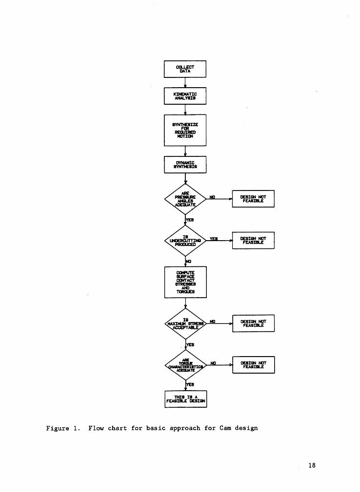
cam profile becomes of utmost importance. Figure l displays the flow
chart for the basic approach for cam design.
4.2 CAM DISPLACEMENT CURVES
QThere are infinitely many follower motions that can be used for the
rise and return of the follower. There are a number of so called "basic
curves" like Constant Velocity or Straight Line, Constant Acceleration
17V
CILLECTDATA
KIEMTIC‘
ANALYSIS
SYNTPESIEFGREUJIREDIIJTIW
DYNAHICSYNTIESIS
AREPRE$RE .1 $8IGN WTA&ES FEASIBLE
AEGJATE
3:
mmcnämns · s ¤=~ ~¤r
CGPUTESRFAGü'I’ACTSTREXSMD_ TCRGES
IMQSSTRESS so ucsxsu mrACCEPTABLE ‘E^°m‘·E
_ YES
Tg! .1 ESIGJ IÜT· · ¤·. —. FEASIBLEAEUJATE
THIS IS AFEASIBLE ESIGN
Figure 1. Flow chart for basic approach for Cam design
. 18
or Parabolic and trigonometric curves like Simple Harmonic, Cycloidal and
Elliptical curves. These basic curves may be inadequate on some occa-
sions, especially in high speed application. An alternate, versatile
manner of motion specification is the use of polynomial function. Sol-
utions for the basic curves and low-order power polynomials can be easily
obtained. However, as the conditions of control become complex, the order
of the polynomial increases and the designer runs into numerical diffi· ‘
culties. In an effort to incorporate the better features of the basic
curves into one optimum curve, designers have tried many combinations of
basic curves. Composite curves like Trapeaoidal and Fourier Series curves
have been formed to produce minimum acceleration of (and hence, minimum
dynamic load on) the follower. Certain fundamental conditions must be
satisfied while combining curves. It should be noted that any combination
of the basic curves may be utilized to fulfill the requirements of the
fundamental conditions. The following conditions must be satisfied:
l. The sum of the displacements during each of the various motions should
be equal to the total stroke.
2. The sum of the angles turned through by the cam during each of the
various motions should be equal to the total cam angle.
3. The velocities of all curves at the junction should be equal.V
4. High-speed action requires that acceleration of all curves at the
junction be equal.
Based on the fundamental conditions of combining cam curves, a customized
cam can be developed with a predesigned building block of cam curve seg-
19
ments. This thesis considers 22 different motion curves. A brief de-
scription is provided for each type of curve.
4.2.1 SIMPLE HARMONIC MOTION
This motion is characterized by having its acceleration propor-
tional and in an opposite direction to its displacement. The usefulness
of these curves is further expanded by using the different forms of SHM
as curve segments to form a single contour. If L is the total lift, B
the active cam angle and 6 the angle of rotation of the cam then the motion
eharaeteristics of the curve segments are represented by equations 1
through 18.
H-1 Harmonic: As seen from Fig. 2 this is a lifting curve which has a
constant Velocity at the end of the stroke.
-_ LQ (1)s
qq . qq (2)V · zß Smlzßl
- ¤*L iq (6)_ a - E- cos(2B)
20
4 · 4E—•Gd
: I5-« E-•
Q.g>‘EE3 2 °2 2 T'ca ra =°·. > « Q-I
= 3·•-1\ 2·v·|\ seQ.)
*5:> < mS-•<¤„-C!
4 <¤ UE- 9* CI‘ C13\•\·ä
ä.2
\ POZ
/ Ö;P\z §\ z 24 -·-•
E3 M *~j ECLEQ
///co "° .,
21
4E-·?==’=’ 2E—•
>-• 'Z
F:E ev
'U
E-• >
/ 2 2 2if W
H Q
2>
ä N{4{HO~1-1/”’O--1cn
<
'•'|H
. 0*6*
g <¤an
gQ
E¤ ä
Az·•-Ag4-*=
2\_·—·
\ "\
Z .1 2 \ 2 1
2“~ 2
¥:2
¤= ääEL
E --1
Q
xx
15 2 —>
22
H-2 Harmonic: In the case of the H-2 lift curve the velocity goes to zero
at the end of the stroke. However the acceleration at this point is not
zero. The characteristics are as shown in Fig. 3.
_ . _gQ (4)s — L S1H(2ß) . A
- JE-. zu). (5)v — ZB cos[2ß)
_2
a (6)
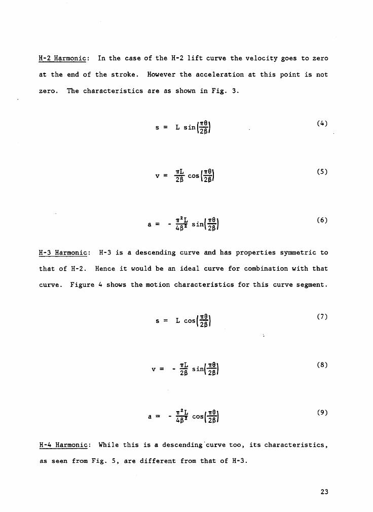
H·3 Harmonic: H-3 is a descending curve and has properties symmetric to
that of H-2. Hence it would be an ideal curve for combination with that
curve. Figure 4 shows the motion characteristics for this curve segment.
- E2 (7)s — L cos(2ß)
- ß - E (8)v — ZB sin(2ß)
--¤’L nä (9)a 48* °°S(z6)
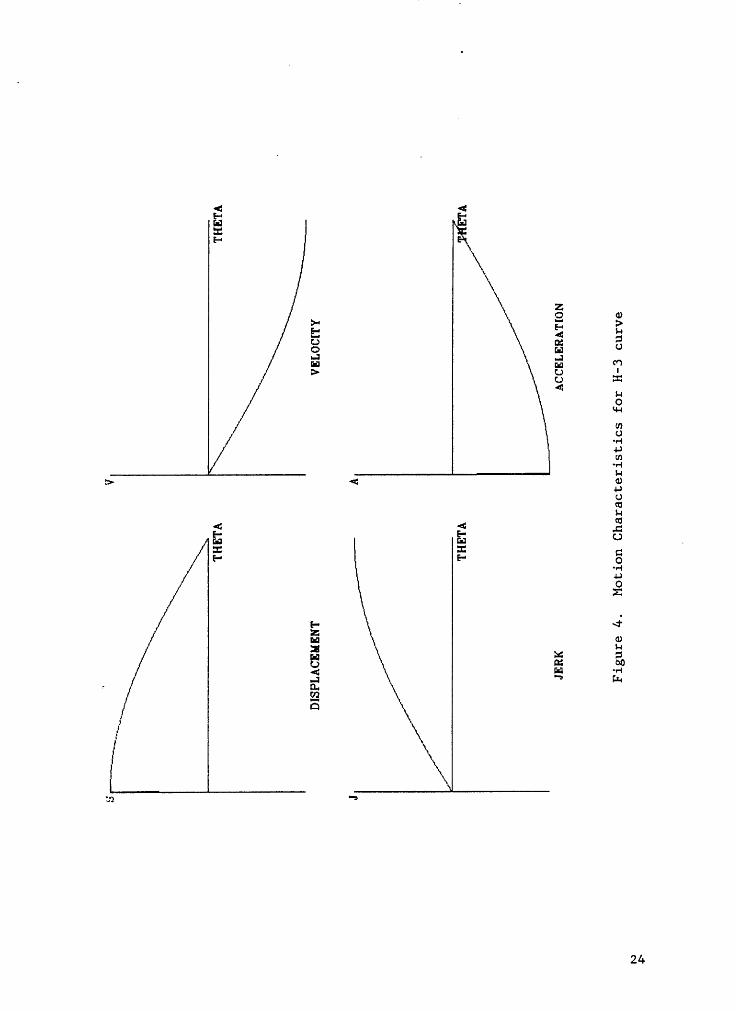
H-4 Harmonic: While this is a descending curve too, its characteristics,
as seen from Fig. 5, are different from that of H-3.
23
g 4filICt—•
\Z
x O ¤>>- ; >I-•HU E U2 EE ä ‘?
/
”°U·«-4
/ 3~•-1H
:> 4 cl4->U<U3<$ •$ L-E E ¤ .I I C.[" P O·•-14->.9A4
/ ; ~¥/ ¤¤ \ ggz ac sE? ä .221 Q-=_° ‘* ¤=—9 / 22 \
sl Q \\a:° \*I
{{ \\
U2 ">
24
4E 2EE-··
gi Q>-·=.:. E E
U EE :3Q Cd 0S S SA > B u
4 IHO\ u-4
\ rnU-64-*ua·6
:> <4-*U<¤*6-¤ <¢ _¤
E: E ¤: = ¤E" E O/ ‘·'*4-*/ 2¢-4„. / „;
ZS 3*< :sÜ ä ¤o” 3 S L2/ ¤„/ ä////
te} "
·25
_ _ . nö i (10)s — L (1
_ ß E (11)V · 26 °°s(za)
_ n2L . _g§ (12)S · ZE? SS¤(2a)H-5 Harmonie: H-5 eurve is the most frequently used harmonic curve. This
is because it produces a smooth transition point for the combining eurve.
H-5 characteristics are shown in Fig. 6.
‘ _ Q. _ Q (13) .S · gz ll SSS(Val)
- ß . 9, (14)V “ ZB S‘“(“6)
28 = ä COS (15)
H-6 Harmonie: The H-6 eurve is often used in conjunction with the H-5
eurve and has properties symmetric to it. The motion characteristics of
H-6 are as shown in Fig. 7.
.. L 9 (16)s — 2 [1 + eos(nB,’
26
4E ZCIS
El6-•E-•Z
q H
Olg QU
> ° Ü vsU •U 24 HO—*4-4
cnU
·v-·|4->fl)
>
·v-4
4H4)4->OG34H
E Z EICU
[-·E-• ¢¥O
= U\ ¤\ 2
\ „.. \ .
\ E*9
E3
UN S3
4M GO
-1F:} ·•-4
D1 "LI-:
E
/
/0*
m—.»
I 27
Ü
‘” äZ5-4 E
xä:E2 gC)3 Ean Ü Y‘°‘
:-40
-4-44->· ua·4-4:-4> <¤ 306:::-4
<: oE E: Z C3E-· E- _g
u£/ gg "
<:EJ..¤ "’ELE¤{\\
an '”
28
V V = - gä sin(n%, (17)
_ 2_1:*1. 6 (18)6 am- (**61
4.2.2 CYCLOIDAL MOTION
This motion is obtained by rolling a circle on a straight line and
generating the locus of a fixed point on the circumference of the circle.
From the generating principle it is easy to write the motion equations
for these curve segments (Equations 19 to 36).
C-1 Cycloidalz The motion characteristics of this curve are shown in Fig.
8. As seen from the figure, this curve has characteristics similar to
the H-1 curve.
- Q-; - Q ums — L( B v SlH(Hß))
- L _ 9, (20)V — B (1 cos(nß))
a (21)
29
~ <z" E5E :-4:E-•\ “ *9z2 gxE-·
H\ ä 6 6Ü ·QJv-IS S '> ¤ U‘°*6\„\ ¤.«x mu..2*6< *3><¤
6.:1¢ :4E E g[-I' *6
\\//E\//
.\\oo\ E 8¤¤ :sxS gg 292 ·= *‘*.4cn.mÄca
E{Q
30
4EE-• E-•
\
ZQ Q}>-• E';} >E a QO/ ä Q/ =,;= S ‘?‘/ _
1 4 *·-•1 Q
*4-4
· U)U·•-•4-JU)EQ)> I <p0cnli?
S S "Cu! H UI I ggE·• E" 2\U‘ O
\ zx .ECN
ggG)z Q QÜ cz °¤<: W ""_} *1 [-*4
~ ä\ rs\ .\\
\\x\ X\x
an '*
3 1 .
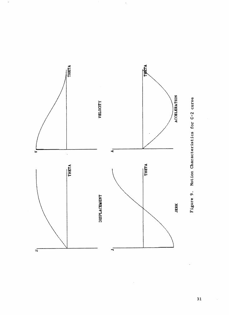
C—2 Cycloidal: Figure 9 shows the motion characteristics of the C-2
curve. Its Velocity and acceleration. are symmetric to that of the C-1
curve.
- 1*. 1 - 2 <22>s L ( B + H sinlnßl
- L Q (23)v B (1 + cos (1rB)
a = · % sin(1r%) (24)
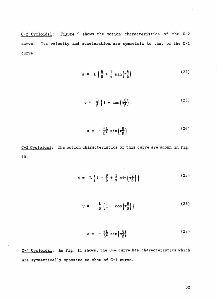
C—3 Cycloidal: The motion characteristics of this curve are shown in Fig. V
10.
.. _ Q L • Q (25)s L(1
_ L _ Q (26)V 6 ll °°S(“6))
L . 8 27a = - gg Sll'l(1T‘B") ( )
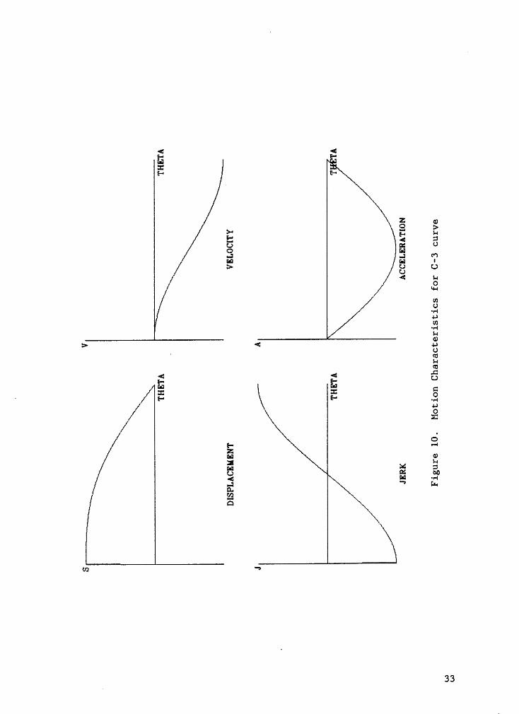
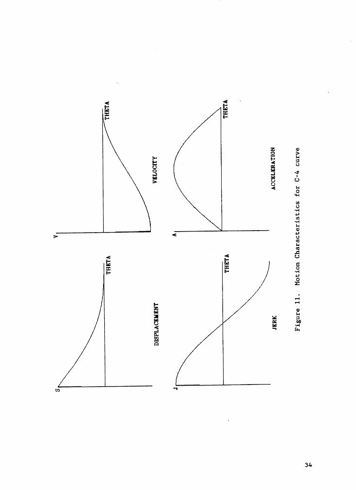
C·4 Cycloidalz As Fig. 11 shows, the C·4 curve has charecteristics which
are symmetrically opposite to that of C-1 curve.
32
E; 4SE—• E
>-• ä ä5 E 5O HS S °?/ > 8 U
/ / <: s-4O/ / “*cnU-•-1
4-*tn·¤-1*8> 4 4.s_U
<¤28<: -¤: ·¤z- 6- UEJ EI QS S O
/ *8Z# \ .2; \" E:11 QZ >< *3Ü ¤= ¤o4 E
·•·4E LuU21lQ
\\\
V; e
3 3
ä ä‘EE-•
Z Q)x 2 ä>· 6-•5\ ‘·“ é Ora
..:1 —¤ *9nn: H '> ¤ O
2 H\ o2 u-6rnU-2-e4->cn·«-1s-aO:> "‘H
E< "UE E ..·= E .9.E-. 4-*2
/.-2.-4¤¤ 8* z ¤E'} ,5 .29I3 OO ¤~ILFBQ
(IQ "5
34
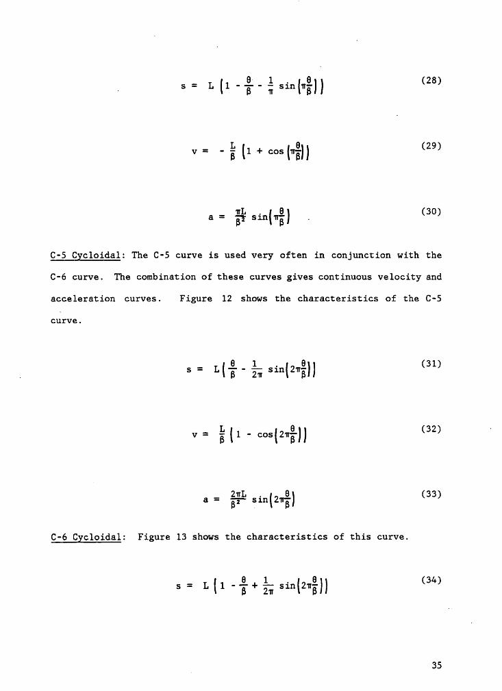
_ _Q__1 . Q (28)I s — L (1 B n sinlnßll
- _L 9 (29)v B (1 + cos(wE))
a = %% sin(n%) . (30)
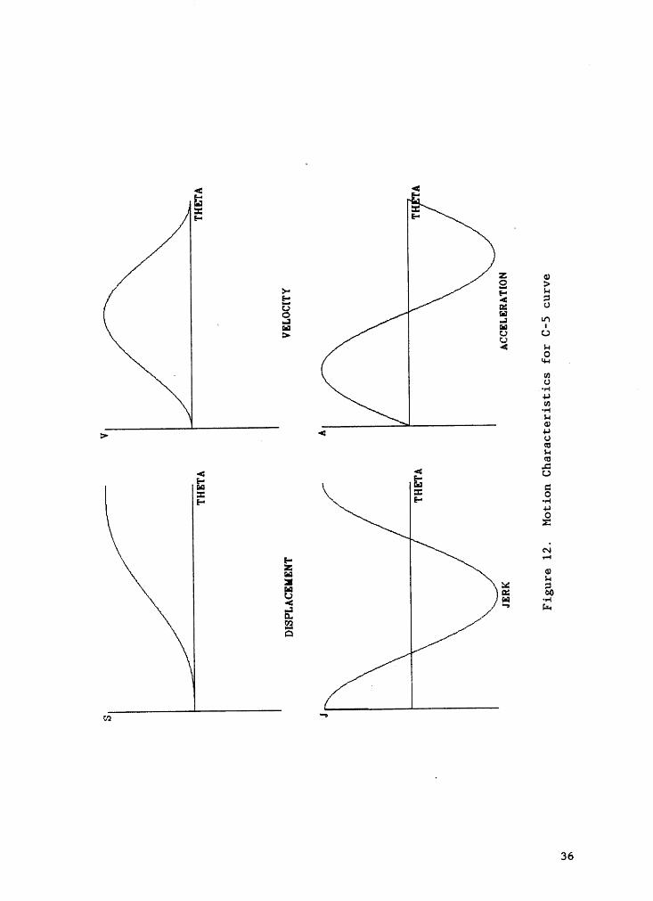
C-5 Cycloidalz The C-5 curve is used very often in conjunction with theC•6 curve. The combination of these curves gives continuous Velocity and
acceleration. curves. Figure 12 shows the characteristics of the C-5
curve.
- 1L-L · Q (31)n s — L[ B Zn SlH(2UB))
- L _ Ei (32) ‘v - B [1 cos(2nß))
- M - 8 (33)a B2 SlH(2TE)
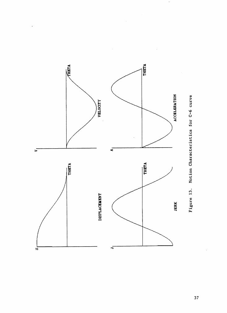
C-6 Cycloidal: Figure 13 shows the characteristics of this curve.
- -.9. 1. · Si (3*)s — L (1 B + zu S1H(2Hß))
‘ 35
ä 4ZI:E-·
Z as
: *2 ¤2 ä °‘ .4 .4 W"“ Ü Es> U4 HOu-s .
—vsU·.-14-lcn·•-•La0)> „ " *8<¤HE<z <'¢ 0ss E 2: = oE.; E" ••-I4-*OZ'.
.~i[__ .-1ä 2*' M ssFS ,5.3 -.. k,CLU2*6 /
an "‘°
36
E äS S .&·
z,„ 2 3E-• HE 6 6G :-1·-¤ ..1 ~oE E J;0
8mo-«-1‘ 4->um°L'
:> <: 8éäS.-C1E ä 6S S ¤:—· s-· ,2*6*
Z!
E-·z
ä 8E ä E2,E E °"B-. nr-rnFl!Q
{Q "5
3 7
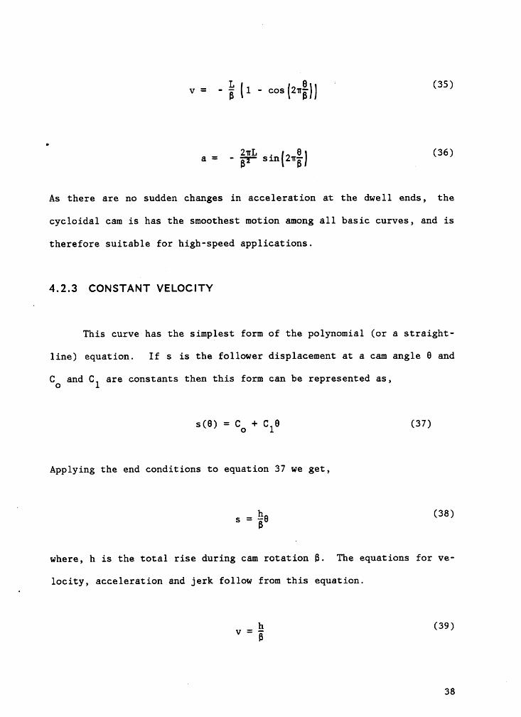
- L _ Q, ‘ (35)v — B [1 cos(2¤ß))
· _ _ 2nL . 6 (36)a Ey- s1n(2¤B) l
As there are no sudden changes in acceleration at the dwell ends, the
cycloidal cam is has the smoothest motion among all basic curves, and is
therefore suitable for high-speed applications.
4.2.3 CONSTANT VELOCITY
This curve has the simplest form of the polynomial (or a straight-
line) equation. If s is the follower displacement at a cam angle 6 and
CO and C1 are constants then this form can be represented as,
s(6) = Co + C16 (37)
Applying the end conditions to equation 37 we get,
· _ h (38)S - E9
where, h is the total rise during cam rotation B. The equations for ve-
locity, acceleration and jerk follow from this equation.
- E (39)" ‘ 6
L38
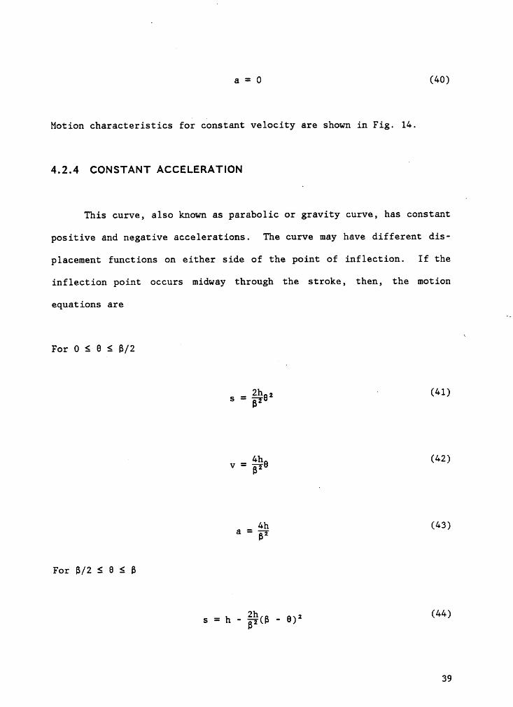
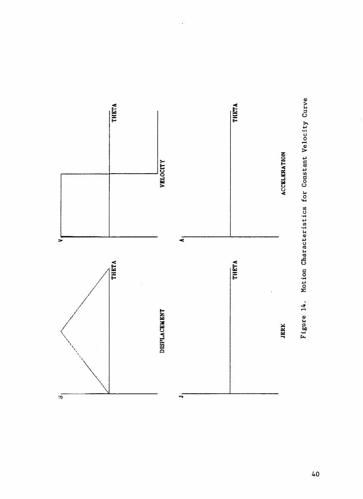
a = 0 (40)
Motion characteristics for constant velocity are shown in Fig. 14.
4.2.4 CONSTANT ACCELERATIONl
This curve, also known as parabolic or gravity curve, has constant
positive and negative accelerations. The curve may have different dis-
placement functions on either side of the point of inflection. If the
inflection point occurs midway through the stroke, then, the. motion
equations are
For O S 6 S B/24
S =‘B
V = (42)B
a = gg (43)
For B/2 S 6 S B
S G)239
GJ< < EE E J ¤I E U _E-• E·• >‘
ii0O'ZSZ >
>-· 9 E,6-· Q cu"" 4-»U I2•:> u "*S 1 ,1 S> Cd U‘” S'~H
rn0••-I*5}·•-•$-4_GJ:» < 46*EQ: 1 S
E E C;I I QE- E-· ·«-1_. ,4J1'I£
JIP
ä ¤·1‘ I ,5gg N/ c.> M °°2 <: M ‘·"
gl J *1 llt-•2‘ :3..xx _ 2-QE_‘‘¤
40
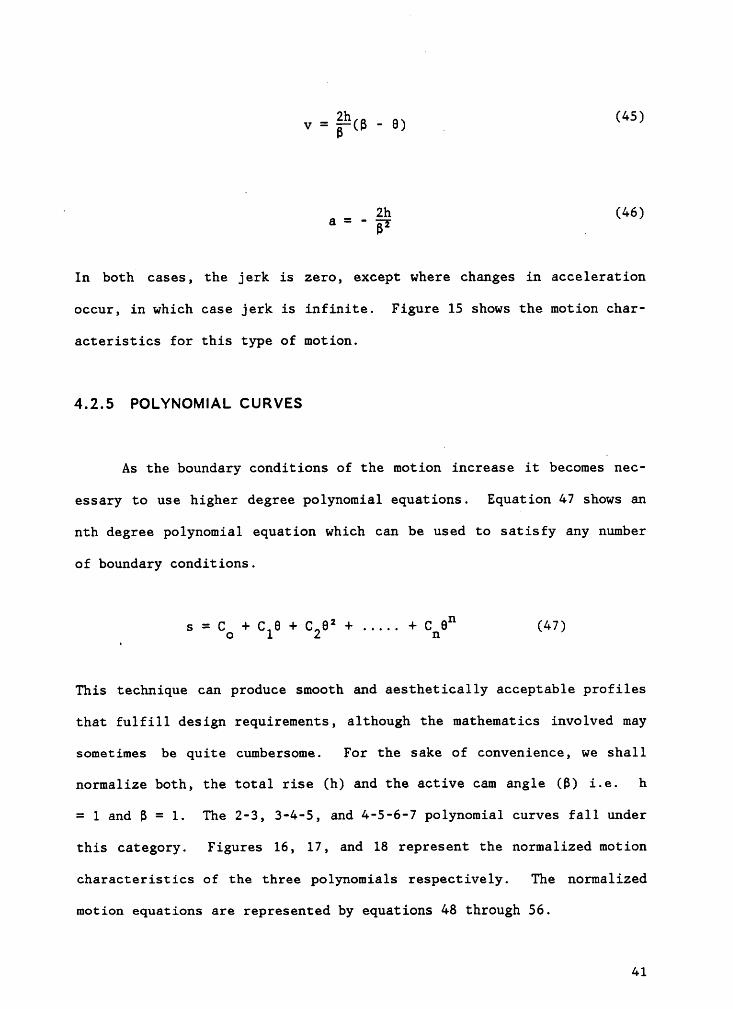
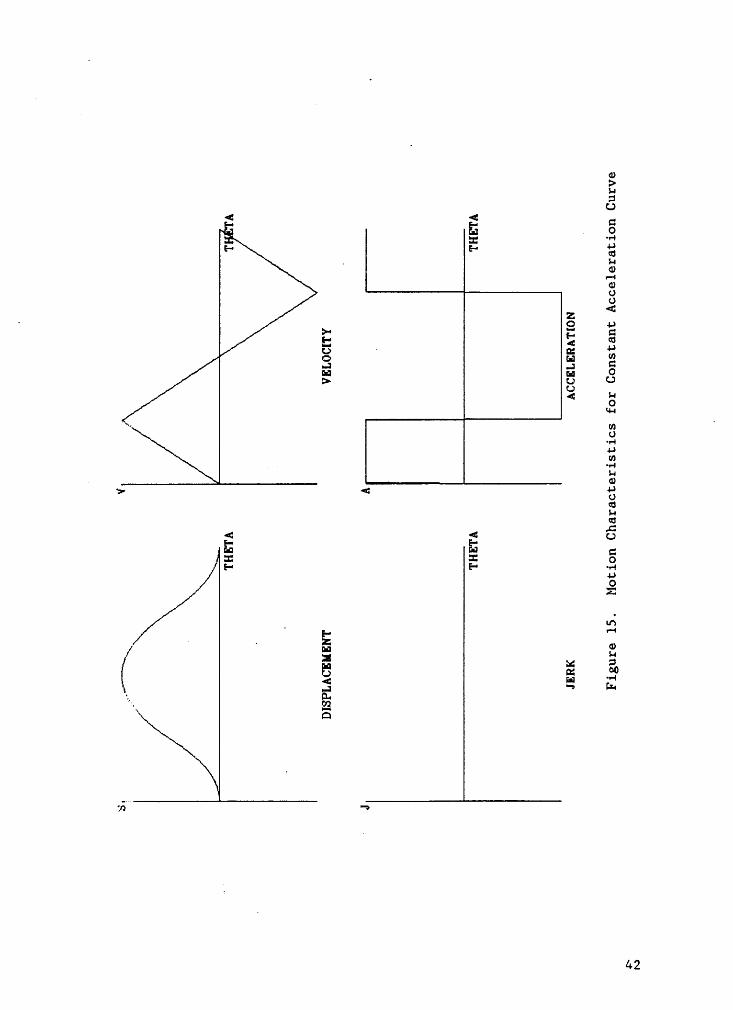
2h 45V = E—(B · 6) _ ( )
‘ 8 = _ % · (46)In txnüx cases, the jerk is zero, except where changes in acceleration
occur, in which case jerk is infinite. Figure 15 shows the motion char-
acteristics for this type of motion.
4.2.5 POLYNOMIAL CURVES
As the boundary conditions of the motion increase it becomes nec-
essary to use higher degree polynomial equations. Equation 47 shows an
nth degree polynomial equation which can be used to satisfy any number
of boundary conditions.
- 2 Hs — Co + C16 + C26 + ..... + CHS (47)
This technique can produce smooth and aesthetically acceptable profiles
that fulfill design requirements, although the mathematics involved may
sometimes be quite cumbersome. For the sake of convenience, we shall
normalize both, the total rise (h) and the active cam angle (B) i.e. h
= l and B = 1. The 2-3, 3-4-5, and 4-5-6-7 polynomial curves fall under
this category. Figures 16, 17, and 18 represent the normalized motion
characteristics of the three polynomials respectively. The ·normalized
motion equations are represented by equations 48 through 56.
41
ab>H5
4 4 cs5 4 .2
HE" eu. H2
GJUéäZI
>- Q" IéE-•*.3 es ‘°c.> · ¤: *"o ra WS ai S:> ¤
4 H43U·•-•Hcn·•-1H2 ·· 3v 4 O<¤HE4 4 (_;C;
I I QE- E-· -.-1‘ H.9A-•
_ .6P I'Ü
xI Igg
:3E 5 .293 —.~ ke
Z ¤-··. U2· F-!Q
zöm ·=
42
•-4as
· ·C-1EOc:
4 4Fä-
£—•¤¤ E Q"I I6-• e mCL
'U0E6 TJZ F: E
.o E s:ä ..1:> gg
EQ w-«vz.2
Cs->vz·C-1s-C3.> ~¤ g
ää6E E ciI I
us-COZ!zu
CCSP C-•
\x g §I
x 3 " "‘CLC
\ $2Q
U1 *5
43

•—•<¤·•-1E0ä
g I-Iz—· " 0E Q-«
IE-* E4 L?1*m
BZ N>~ 2 "*"6-· ¤··· "‘6 ·= 2Q ä 5.;-1 0¤¤ ä c:> 0
\I)‘ 8
cnU·•-•
_ +->cn~•-•ää
> 4 45<¤HE
S < 0: Z omE" En .,.g>us-•05ZU
E- 0\ z \ g\ Ü Ü °¤
~ 4 EI °"‘\‘ ä ·= P!-•
tnI-!\ Q
U2 w
44
-1¢¤·•-1. EOCJE
ä E ‘=—¤-· 'T
•nnl+"UZ Q)
s: *2 ~·u ns QO H H•-1 J:-1 u O>4H8O·•-1-8-*cn·«-•8-8B:> < O<¤HEes <¤ o*' EW CI: I o oE-• F" ·•-8 >-8-* HO 5Z U
«$x
ua 3\ Ü :3uI3 ·· ¤«
\ D-•E\
*5
45
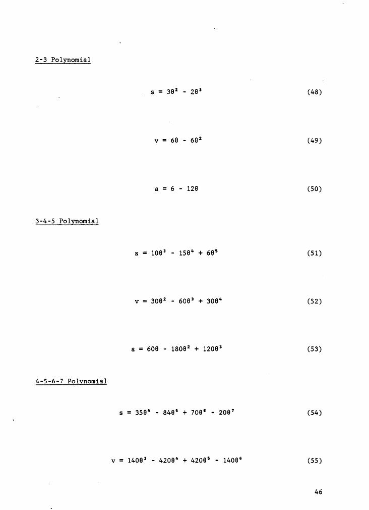
2-3 Polgnomial
7 S = 66* - 26* (48)
v = 66 — 66* (49) 6
a = 6 - 126 (50)
3-4-5 Polggomial
S = 106* - 166* + 66* (51)
v = 306* - 606* + 306“ (52)
a = 606 - 1806* + 1206* (S3)
4-5-6-7 Polvnomial
s = 356‘ - 846* + 706* - 2067 (S4)
v = 1406* - 4206* + 4206* — 1406* (55)
46
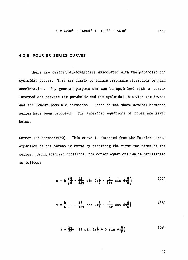
a = 42062 · 168063 + 210065 - 84065 (56)
4.2.6 FOURIER SERIES CURVES
There are certain disadvantages associated with the parabolic and
cycloidal curves. They are likely to induce resonance Vibrations or high
acceleration. Any general purpose cam can be optimized with za curve-
intermediate between the parabolic and the cycloidal, but with the fewest
and the lowest possible harmonics. Based on the above several harmonic
series have been proposed. The kinematic equations of three are given
below:
Gutman 1-3 Harmonic(90}: This curve is obtained from the Fourier series
expansion of the parabolic curve by retaining the first two terms of the
series. Using standard notations, the motion equations can be represented
as follows:
- Q. - lé. — Q - ;_ . 6 ($7)· s — h (B 32u sin Znß 96w sin öwg)
- Q - LQ. Q - L. Q (58)v - B (1 lön cos Znß lön cos önß)
a = 2%; (15 sin 2n%·+ 3 sin 6w%) (59)
I47
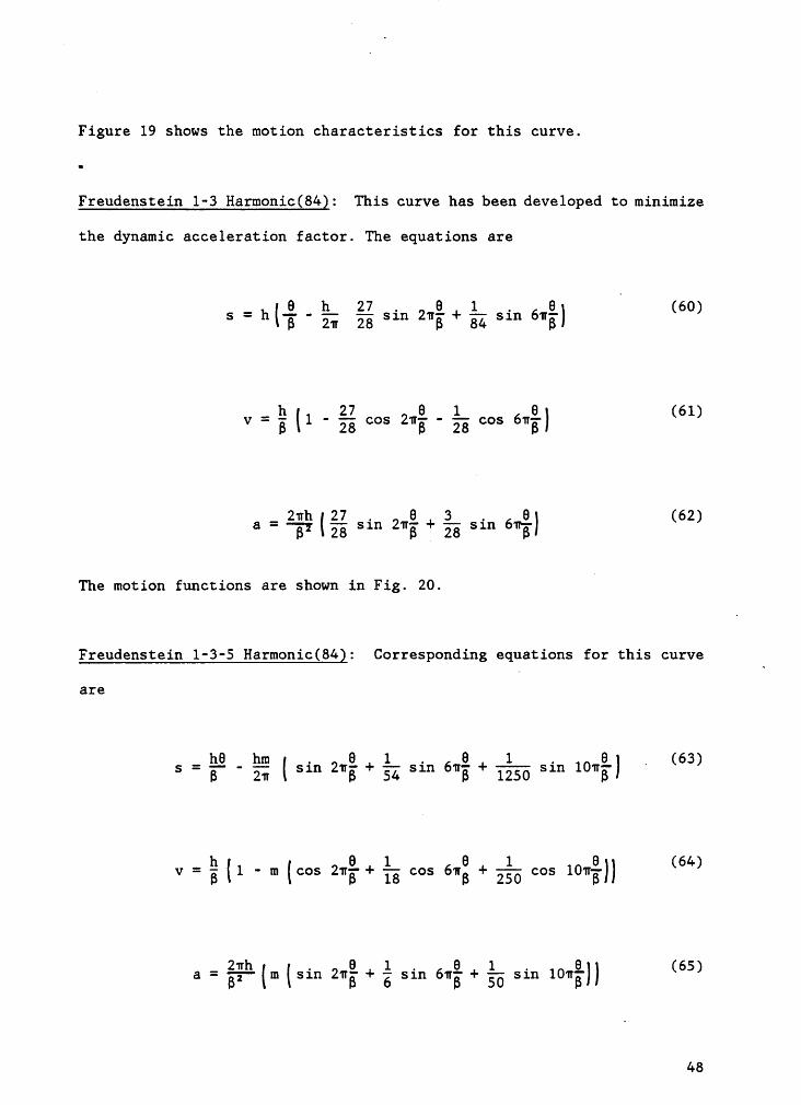
Figure 19 shows the motion characteristics for this curve.
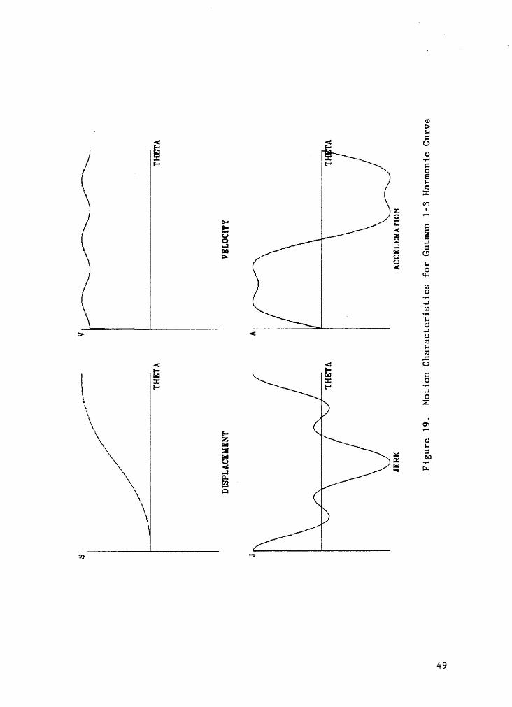
Freudenstein 1-3 Harmonic(84Q: This curve has been developed to minimizethe dynamic acceleration factor. The equations are
-.<1-L21—ä1.-Q6 (60)s — h( B zu 28 sin Zuß + 84 sin 6uB)
v = ä (1 - äé cos Zug - ég cos öugq (61)
a sin Zug { gg sin 6u%) (62)
The motion functions are shown in Fig. Z0.i
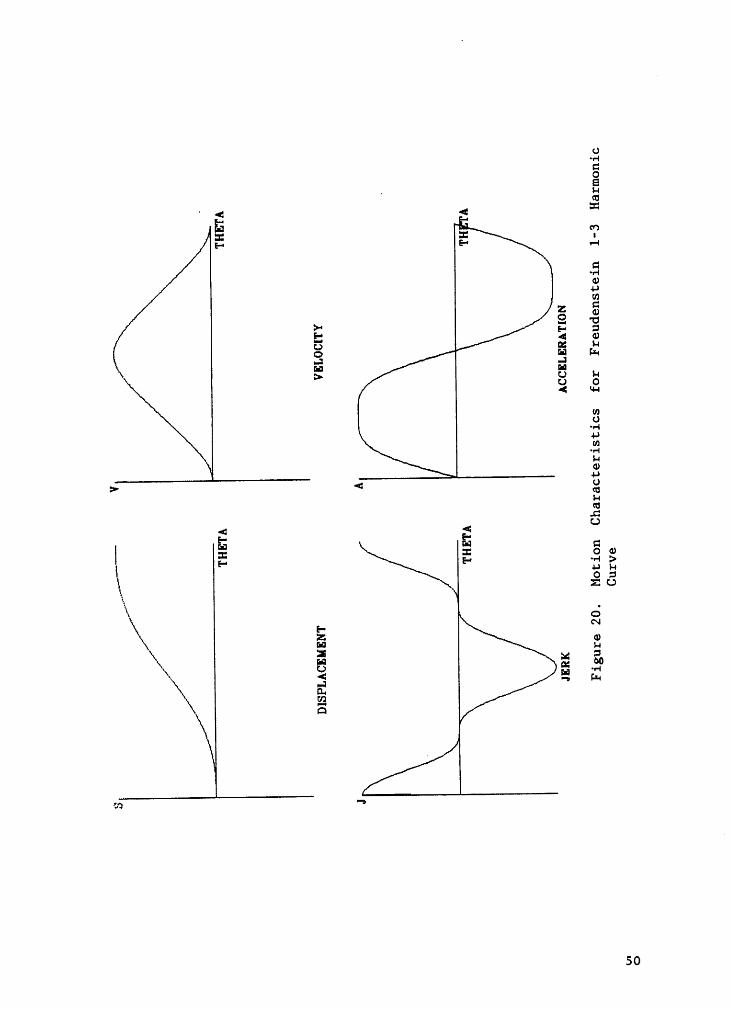
Freudenstein 1-3-5 Harmonic(84}: Corresponding equations for this curve
are
_ QQ _ hg . Q 1_ . Q 1 . Q_ , (63)s - B zu ( sin Zuß + 54 sin 6uß + 1250 sin 10uB)
v (1 - m (cos Zu%·+ äg cos öugcosa
= §g§·(m (sin Zug + é sin 6u% + éö sin 10u%)) (65)
48
0>‘E
E " 6:1: :: .°6-· E-· QVoEeu:::
°?E v-4>‘ z-·E < Ä0 ¤: EO H .5.:ä ä =’
" ou-•cn0·•-4
•-51--%_ ·•-1Z3
:> < {j<¤s-«an
ez ECS-<:
c:: : 0z-·c-5OZ:
cäv-IE¤ Ü
E g -29E ·~ "'¤..vzIl-!¤
Q- -2
49
0·«-nC10E_ s-«§E : °?E-• •-•
C3·-e012C3z2 3EZ Z 33 ra Mä :3\ 1-4‘ ‘°’* 8 o
\« H
cn0·•-14-•um--1s-•03:> "‘ <¤s-•0„-G
4 U<z
$3l = : o 0c-· F' “"‘ >1 12 S1 zu
X 6NE-Z 0ä 3\ zux Q} ¤= _fi,°\ Ms g _, pg-.
\¤_rnKl¤
wie "’
50
where,
m = 1125 V1192
The motion characteristics are shown in Fig. 21.
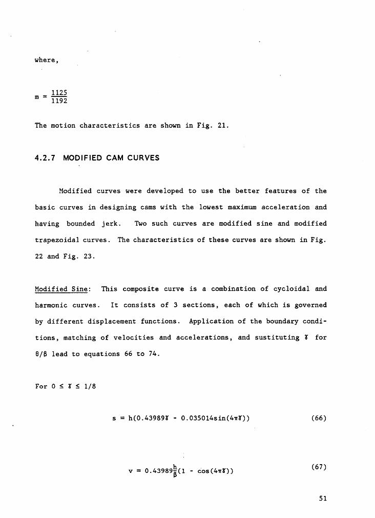
4.2.7 MODIFIED CAM CURVES „
Modified curves were developed to use the better features of the
basic curves in designing cams with the lowest maximum acceleration and
having bounded. jerk. Two such curves are modified sine and modified
trapezoidal curves. The characteristics of these curves are shown in Fig.
22 and Fig. 23.
Modified Sine: This composite curve is a combination of cycloidal and
harmonic curves. It consists of 3 sections, each of which is governed
by different displacement functions. Application of the boundary condi-
tions, matching of velocities and accelerations, and sustituting X' for
6/B lead to equations 66 to 74.
For 0 S X S 1/8
s = h(0.43989K - 0.035014sin(4nX)) (66)
v = 0.43989%(1 - cos(4nK)) (67)
51

O·«-4·GO
- EH „
é'4 4E ·:·I=— ‘?. •-1
G·•-1Brn
ää>-• [_, ·¤P: 4 ¤za esä4 ..1 V-*-•rd rd!>4
u-4cnU33*cn·«-1H8:> < äH<¤*5
4 4GI I gw[-· E- paOGZU
.-EN; 0s-•
:5x E ä ¤0
\ zaQ
(n *9
· 52
Ef <¤C:] Q:P
I! Ua>/ “·•-e, / Z 2//‘
2 q)/ P" E··* .,.4/ E-· <¤ ~+-•.,.4x 2 E 2ua E Z:>
" o\///4,
2 .\. 3\.,.4
B:» ”°ä:1cu'5<: czL1]
= O= E,. °H
\_E-\'xx
Z \ Q)xx :.:1 4 HZ 4; 5x H N °°x\‘¤4 l
"7 L;.\ .1\\ D4[
‘ E r\ ¤ ,»·‘xxrxx/
‘"5va
5 3
Q)>$-1,*3O"’78
4E ::: T2:„· 2 ¤—·
o/ ‘“äC1-E[—•
2 "O/'
E1>—4 "‘·‘ä ¤= QQ fdO J O 11.: ¤ EagLJ:> 'ZP *"
\4 O
x_""‘
InQ·•-1
12~„\04
Q=—
ä-¢'-ZU·== ä SP
: •'-{E+-12 P O
‘*'2:Ix
,\
cn
\
Ng-ä:s\ Q °H
\\E, kl
\_4•\AQ4\ E
~ Q\\\k‘
rf//·sU2
54
6 = 5.52794%5sin(4nX) (68)
For 1/8 S X S 7/8
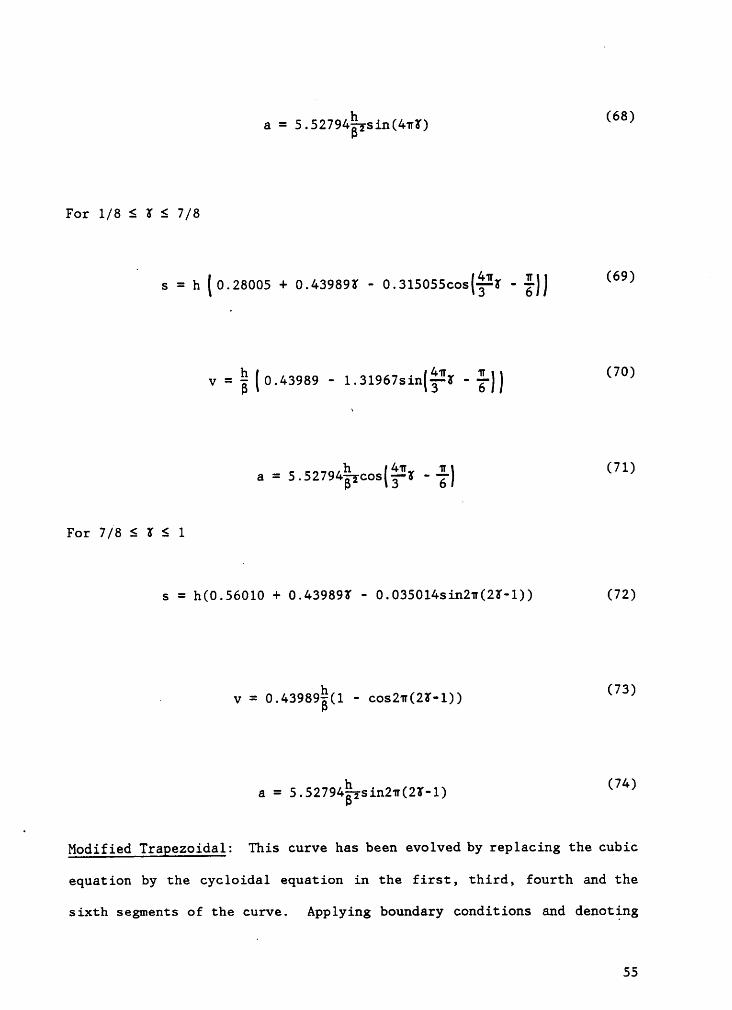
s = h (0.28005 + 0.43989X - 0.31SO55cost%£K —·%)) (69)
- 1; - - $1 _ 1 C70)V B (0.43989 1.31967s1n(3 X 6))
_ h gg _ jL (71)a — S.52794Eqcos(3 X 6)
For 7/8 S X S 1
s = h(0.56010 + 0.43989X · 0.0350l4sin2H(2K·1)) (72)
6 V = 0.43989%(1 - cos2w(2X—l)) (78)
6 = 5.52794%7sin2n(2X-1) (7“)
Modified Tragezoidalz This curve has been evolved by replacing the cubic
equation by the cycloidal equation in the first, third, fourth and the
sixth S€g!IIBI'ltS of the CUIV€• bOUndaIy conditions and denoting
SS
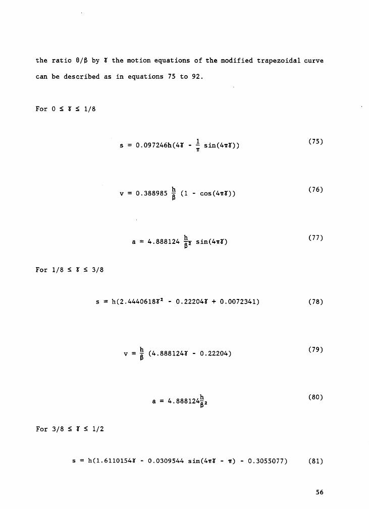
the ratio 0/8 by X the motion equations of the modified trapezoidal curve
can be described as in equations 75 to 92.
For 0 S X S 1/8s
= 0.097246h(4X - sin(4nK)) (75)
v = 0.388985 ä (1 - cos(4uX)) (76)
a = 4.888124 gg sin(4nX) (77)
For 1/8 S X S 3/8
s = h(2.4440618X2 - 0.22204X + 0.0072341) (78)
V = % (4.666124: — 0.22204) (79)
6 = 4.666124%, (80)
For 3/8 S X S 1/2
s = h(1.61l0l54X - 0.0309544 sin(4nX - H) · 0.3055077) (81)
56
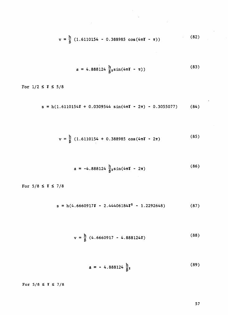
V = % (1.6110154 - 0.388985 666(46x - 6)) ’(82)6
= 4.666124 %,616(46x - 6)) (85)
For 1/2 S X S 5/8
6 = h(1.6l10l54Z + 0.0609544 s16(46x - 26) - 0.3055077) (64)
V = ä (1.6110154 + 0.388985 666(46x - 26) (85)
6 = -4.666124 %,616(46x - 26) (88)
For 5/6 s x s 7/8
6 = h(4.66609l7X - 2.44406164x* - 1.2292646) (87)
V = % (4.6660917 — 4.6661246) (88)
6 = - 4.666124 ä, (88)
For S/8 S X S 7/8
57
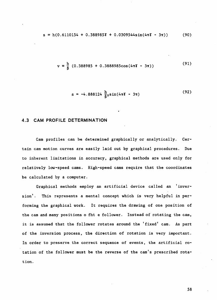
s = h(0.6l10l5& + 0.388985X + 0.0309544sin(4nX · 3n)) (90)
v = ä (0.388985 + 0.3888985cos(4nX - 3n)) (91)
a = -4.888124 %2sin(4nX - an) (92)
4.3 CAM PROFILE DETERMINATION
Cam profiles can be determined graphically or analytically. Cer-
tain cam motion curves are easily laid out by graphical procedures. Due
to inherent limitations in accuracy, graphical methods are used only for
relatively low-speed cams. High·speed cams require that the coordinates
be calculated by a computer.
Graphical methods employ an artificial device. called. an °inver·
sion°. This represents a mental concept which is very helpful in per-
forming the graphical work. It requires the drawing of one position of
the cam and many positions o fht e follower. Instead of rotating the cam,I
it is assumed that the follower rotates around the °fixed' cam. As part ·
of the inversion process, the direction of rotation is very important. —
In order to preserve the correct sequence of events, the artificial ro·
Itation of the follower must be the reverse of the cam°s prescribed rota-tion. I58 .
Because of the voluminous calculations required in conjunction with
its complicated geometry, the analytical methods of determining cam pro- _
files coordinates were subordinated to graphical techniques. This thesis
uses the °Theory of Envelopes° (3) to determine certain cam profile co-
ordinates equations for seven major types of cam followers. We shall ·
consider them in sequence.
In the equations shown in the following pages, rb is the base circle
radius, rf the roller radius, Ia the distance between swinger pivot point
and cam center, Ir the length of follower arm, s the follower rise for *
angular displacement 6, ¢O the intial angular postion of swinging fol-,
lower, ¢ the change in angular position of swinging follower, cz the
pressure angle at angular displacement 8, and e the eccentricity of the °
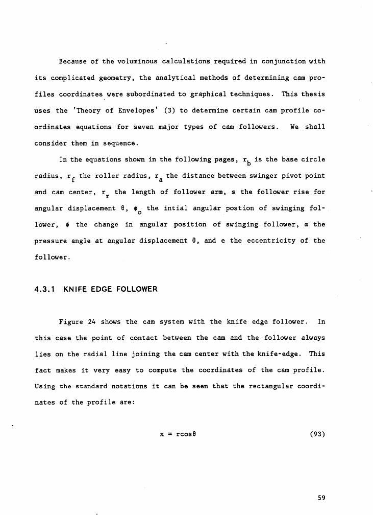
follower.4.3.1
KNIFE EDGE FOLLOWERl
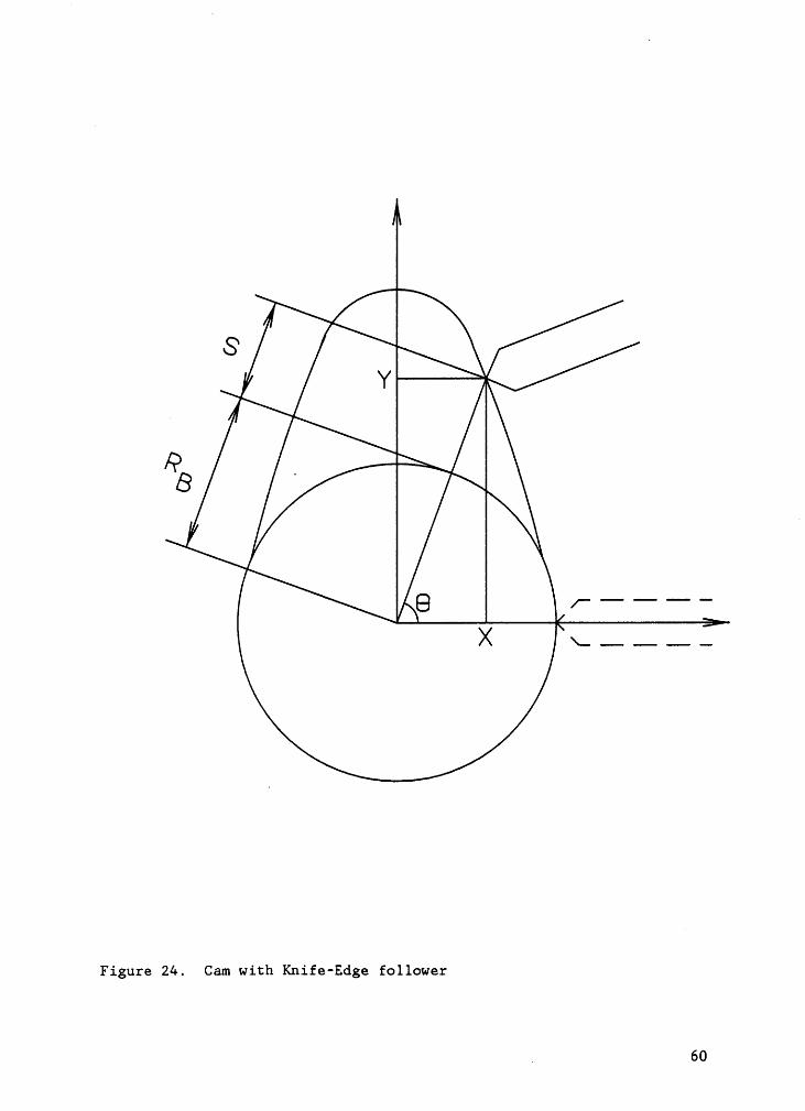
Figure ZA shows the cam system with the knife edge follower. In
this case the point of contact between the cam and the follower always
lies on the radial line joining the cam center with the knife-edge. This
fact makes it very easy to compute the coordinates of the cam profile.
Using the standard notations it can be seen that the rectangular coordi-
nates of the profile are:
'x = rcos8 (93)
59
‘A " _ — °" '
Figure 24. Cam with Knife-Edge follower
A 60
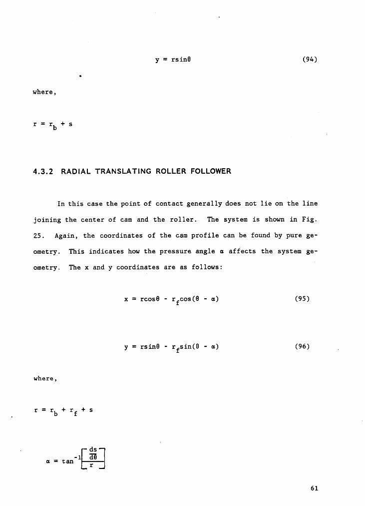
y = rsin8 (94)
where,
r = rb + s
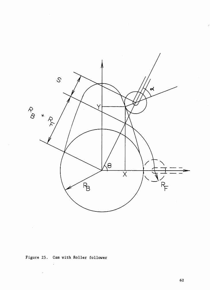
4.3.2 RADIAL TRANSLATING ROLLER FOLLOWER
In this case the point of contact generally does not lie on the line
joining the center of cam and the roller. The system is shown in Fig.
25. Again, the coordinates of the cam profile can be found by pure ge-
ometry. This indicates how the pressure angle u affects the system ge-
ometry. The x and y coordinates are as followsz
x = rcosö - rfcos(6 — a) (95)
y = rsin8 · rfsin(B · a) (96) _
where,
·r = rb + rf + s
. ds_ -1l E5]a — tan r
61
~
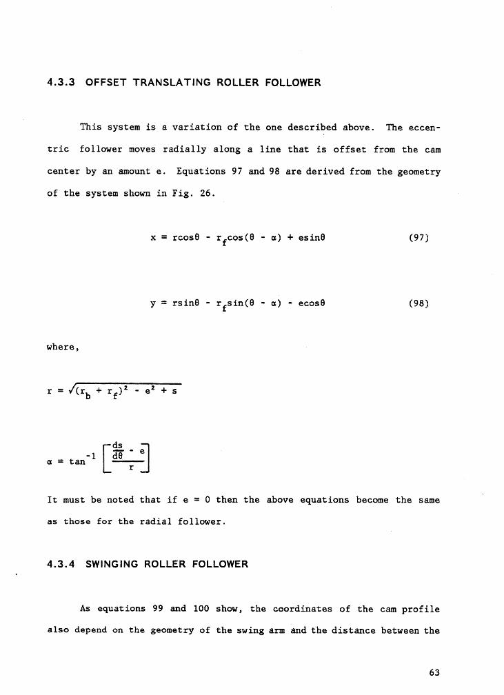
4.3.3 OFFSET TRANSLATING ROLLER FOLLOWER
lThis system is a variation of the one described above. The eccen—
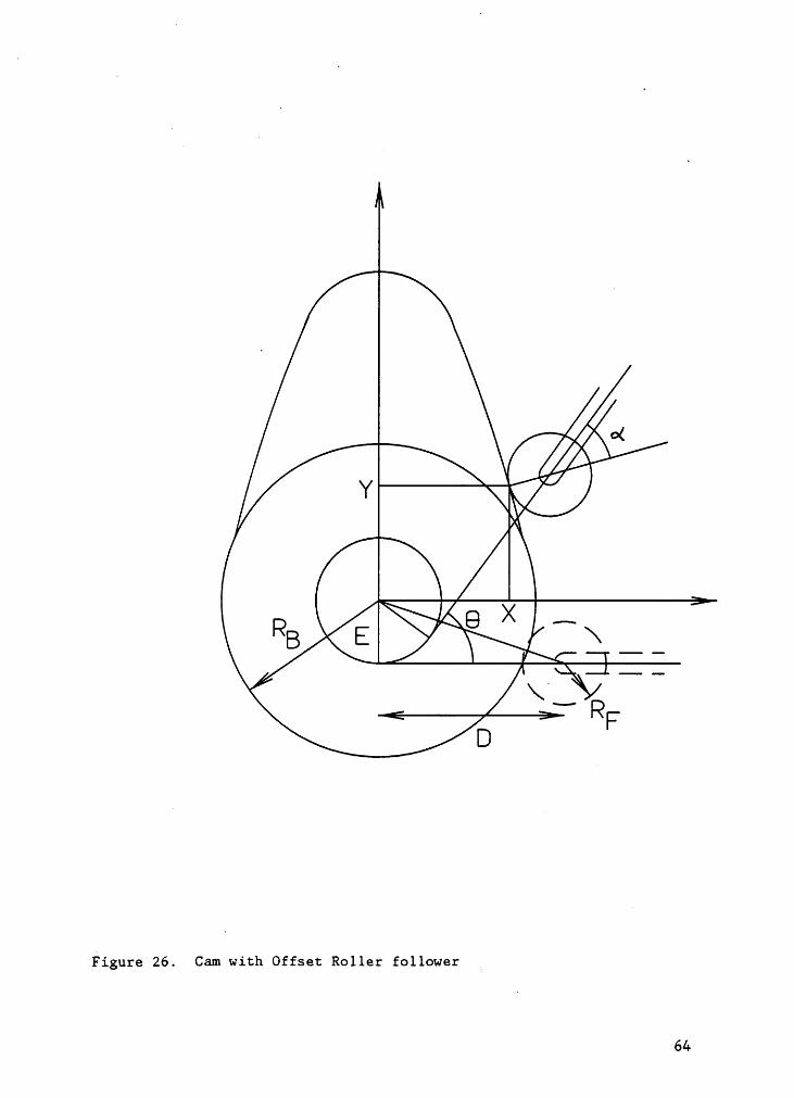
tric follower moves radially along a line that is offset from the cam
center by an amount e. Equations 97 and 98 are derived from the geometry
of the system shown in Fig. 26.
x = rcosß - rfcos(6 — a) + esinü (97)
y = rsin8 - rfsin(9 - a) - ecos6 (98)
where,
r = ¢(rb + rf): - ez + s
ü • ·
r
It must be noted that if e = 0 then the above equations become the sameE
as those for the radial follower.
4.3.4 SWINGING ROLLER FOLLOWER
As equations 99 and 100 show, the coordinates of the cam profile
also depend on the geometry of the swing arm and the distance between the
63
ü'd
dv,Ä
„_\ä
A
RF
Q?2:( 1) ? E
A4A65
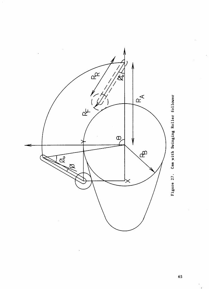
cam center and the swinger pivot point. Figure 27 shows a schematic di-
agram of this system. _
x = racosü · rIcos(6 · ¢ - ¢o) - rfsin(a - 6 + ¢ + ¢O)
(99)
y = rasinß - rrsin(9 — ¢ - ¢o) - rfcos(¤ · 6 + ¢ + ¢O)
(100)
where,
2 2 2_ _l It + Ia (rb + rf)¢ — cos ·—-—--—--————-———
o Zrärr
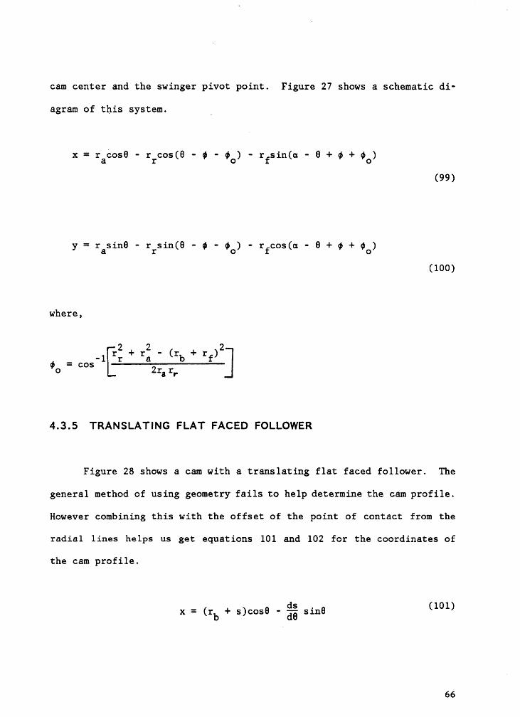
4.3.5 TRANSLATING FLAT FACED FOLLOWER
Figure 28 shows a cam with a translating flat faced follower. The
general method of using geometry fails to help determine the cam profile.
However combining this with the offset of the point of contact from the
radial lines helps us get equations 101 and 102 for the coordinates of
the cam profile.
x = (rb + s)cos8 · ää sin6 (101)
66
1 I
‘V,= 1 — —.
Tw1 1L)
y = (rb + s)cosB + ää cos6 (102)
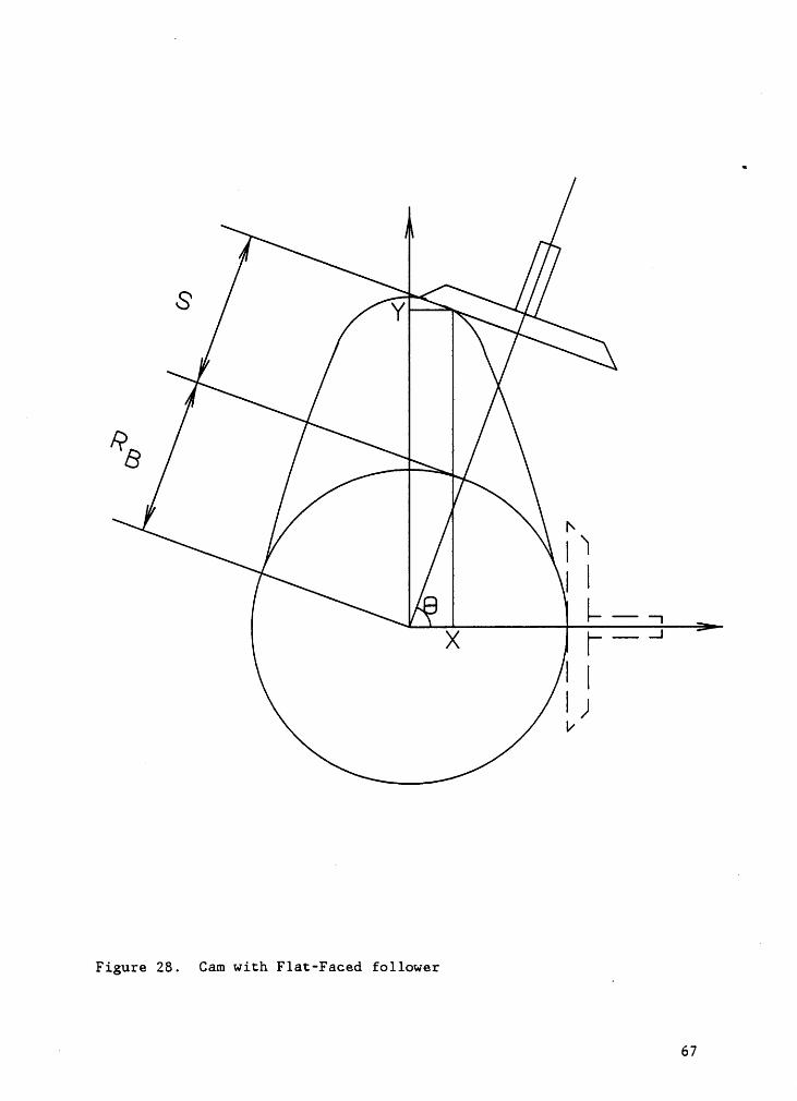
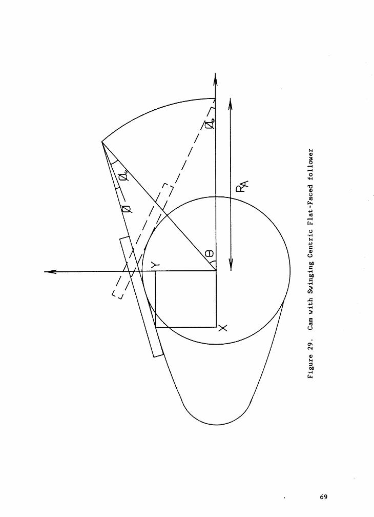
4.3.6 SWINGING CENTRIC FLAT·FACED FOLLOWER
Figure 29 shows a swinging flat faced follower system. Using „a
method similar to the one used in the case of swinging roller follower,
it is possible to derive equations 103 and 104 for the cam profile coor-
dinates.
x = ra(cos6 + Acosß) (103)
ly = ra(sin6 — Asinß) (104)
where,
A = cos(6 + ß)
--M - 1dB
B = ¢o + ¢ - 6
l68
\ äE'Jä¤?‘ 94-JGE1U°L‘
A'\‘ _é°z
ENLGO
EZ
• 69
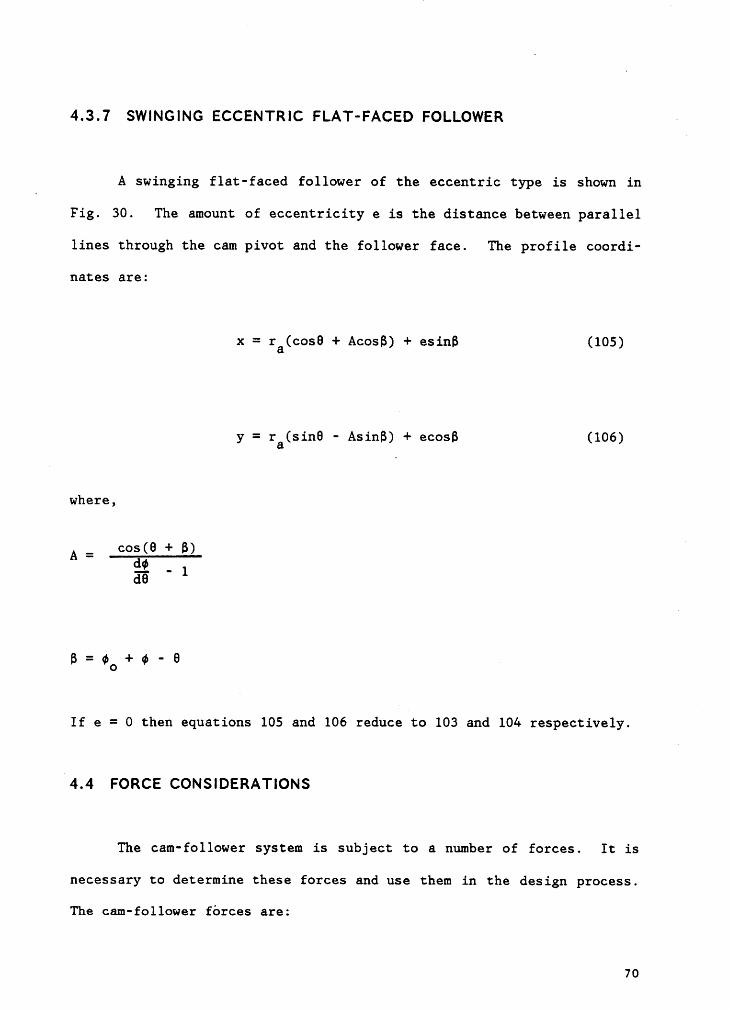
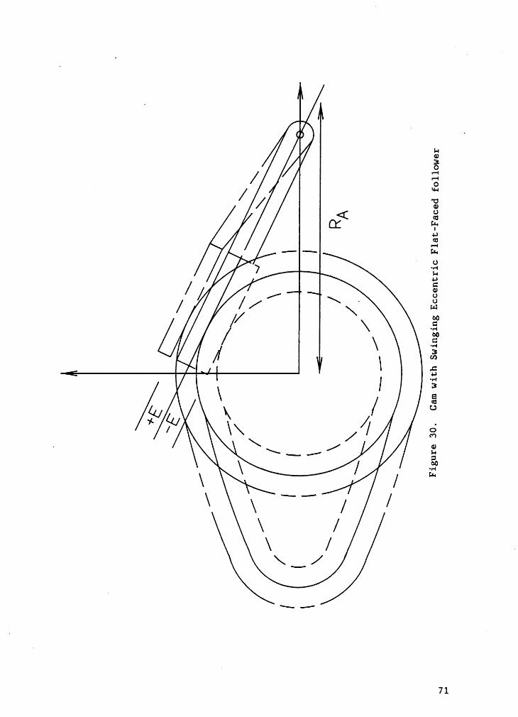
4.3.7 SWINGING ECCENTRIC FLAT-FACED FOLLOWER ~
A swinging flat-faced follower of the eccentric type is shown in
Fig. 30. The amount of eccentricity e is the distance between parallel
lines through the cam pivot and the follower face. The profile coordi·
nates are:
x = ra(cos8 + Acosß) + esinß (105)
y = ra(sin6 - Asinß) + ecosß (106)
where,
A = cos(8 + B) E
92 · 1dB
B = ¢O + ¢ · 9 1 E
If e = 0 then equations 105 and 106 reduce to 103 and 104 respectively.9
94.4 FORCE CONSIDERATIONS
The cam—follower system is subject to a number of forces. It is
necessary to determine these forces and use them in the design process.
The cam—follower forces are:
70
J -/ E6I'7V
Ö
71
1. The static force due to the external load on the cam.
2. The inertia force due to follower acceleration. _
3. The acceleration forces which produce Vibrations.
4. Frictional forces.”
Static forces: These are gradually applied forces and are characteristic
of slow moving cams. The equilibrium conditions applied in static force
analysis are:
F = 0 (in the X, Y, and Z directions)
M = 0 (about any point)
Inertia Forces: If a rotating body has an external unbalanced torque,
it will have an angular acceleration which will be resisted by a reaction
torque. The direction of this torque will be opposite to the direction
of rotation.
T = Ia
where I = Moment of Inertia about the center of rotation.
a = angular acceleration.
Vibratory Forces: It is known that a large pulse (jerk) induces unde-
sirable Vibrations which occur at the natural frequency of the system.
The forces produced by these Vibrations add on to the inertia forces.
Hence while designing cams for high speed applications, a dynamic magni·
fication factor of 2 or more should be used (3).
72
Frictional Forces Relative movement of contacting surfaces is always
opposed by frictional resistance. Friction can rarely be neglected. The
best and most accurate method of including friction in the design is to
use values from tests.
4.5 PRESSURE ANGLE CONSIDERATIONS
Pressure angle is important in cam design. Pressure angle is de-
fined as the angle between the line of action and the center line of the
follower. Pressure angles result in side thrusts on the follower and
possible deflection and jamming of the follower stem. The maximum pres-
sure angle affects the cam size, torque, loads, accelerations, wear life,
and other factors. Thus the maximum pressure angle must be kept as small
as possible. At present, the maximum recommended value this angle can
achieve has been arbitrarily set at 30°. However, for light loads with
accurate low-friction bearings, Rothbart(l) was successful in using
pressure angles up to 47°.
Pressure angles can be easily measured from the graphical con-
struction of a cam. However, analytical methods have been developed to
calculate these angles for different follower types. Since solving
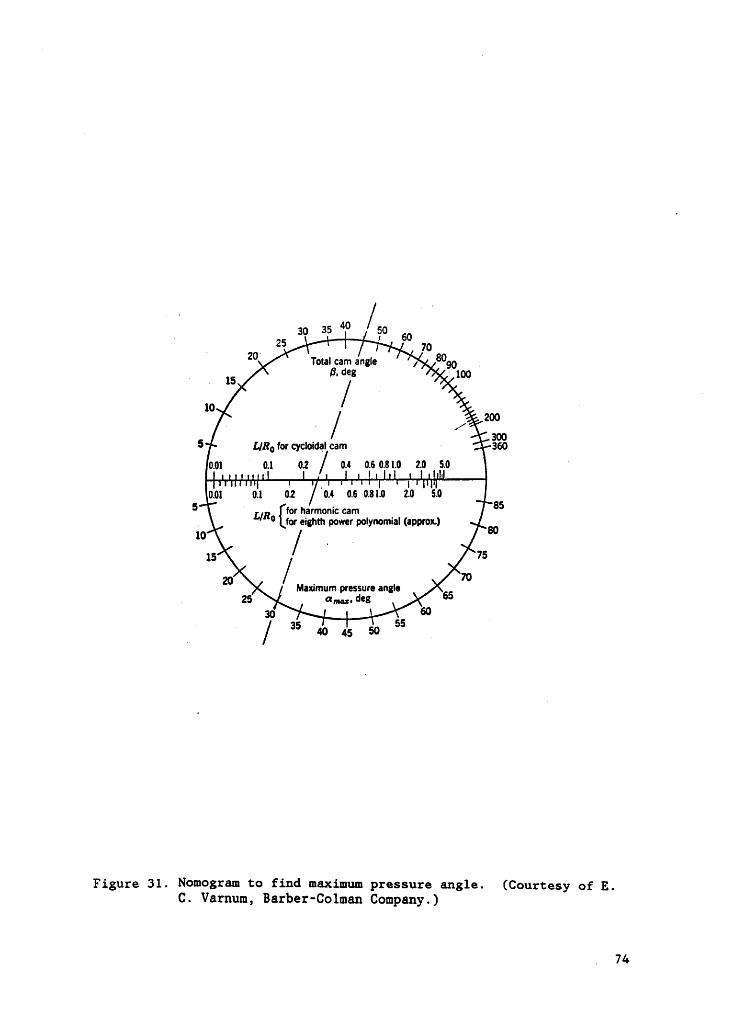
equations for maximum pressure angles is very difficult, Mabie and
Ocvirk(l7) use a nomogram (Fig. 3l) developed by E. C. Varnum to determine
the maximum pressure angle. This chart can be used for three different
types of motion. The nomogram uses Bo and L/Ro as parameters.
Pressure angles can be reduced by increasing the minimum radius of
the cam so that the follower will have to travel a greater linear distance
473
‘ 25 ' 702° Total cam angle , 80,,, 7I d
”1 . 15 B Fg ‘°°10 / 200. ’ /
5 L/R° for cycloidql cam—0.010.1 02 / ‘ 0.4 076 0.6 1.0 2.0 6.0 ·
. 10.01 0.1 02 0.4 0.6 0.s1.0 2.0 6.05 ' UR for harmonic cam 85
. ° for eighth power polynomial (approx.) _10 / _ °°15 75 '· 702°I Maximum pf¢SSUf! angI•. 25 a,„„. deg 66
ao 66 77 / as 40 45 50 65
Figure 31. Nomogram to find maximum pressure angle. (Courtesy of E.C. Varnum, Barber-Colman Company.)
. 74
on the cam for a given rise. If the workspace does not permit such an
increase, then the active cam angle B can be increased along with the
rotational speed to maintain a constant lift time.
4.6 CAM SIZE DETERMINATION.
Care should be taken to avoid cusps or undercutting. Cusp or point
formation takes place when, both, dx/dB and dy/dB become zero simultane-
ously. Based on this principle, equations have been developed to check
cusp formation for different types of followers. Two simple cases are
listed below:
Flat Faced Follower: If f(6) is the displacement function for the fol-
lower and f"(0) the acceleration function, then the minimum radius of the
cam (C) required, to avoid cusps or undercutting, can be easily determined
by solving equation 107 for C.
c + s(6) + f"(6) > 0 (107)
Radial Followerz For this type of follower, a different parameter, the
radius of curvature (p) of the pitch surface is considered. In order to
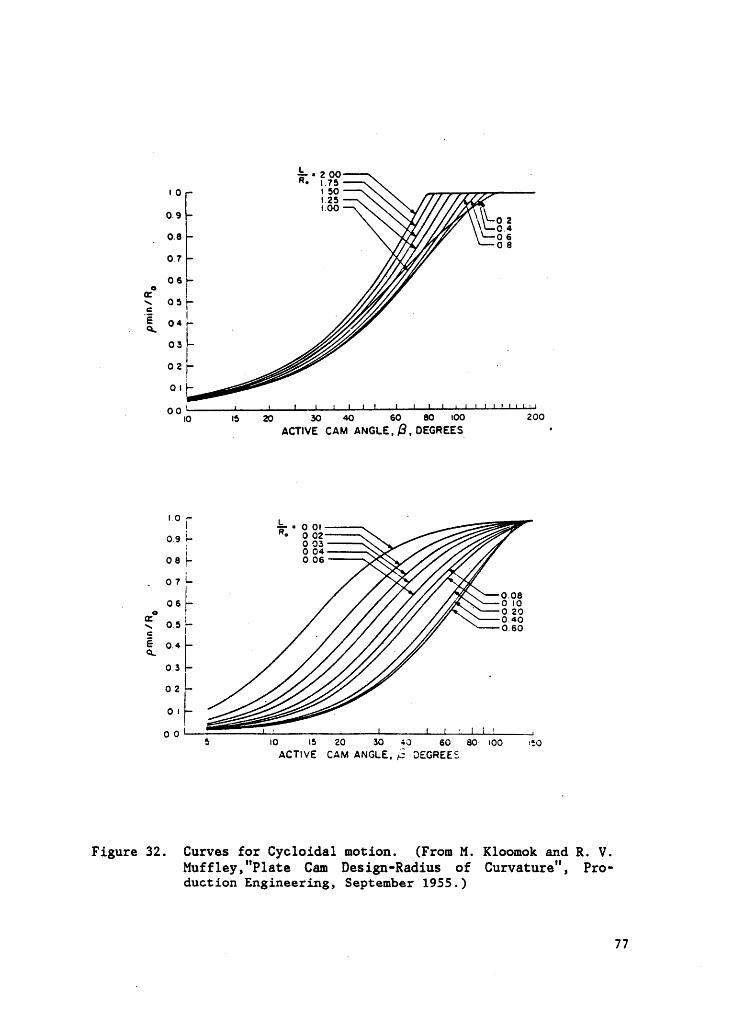
prevent undercutting or point formation pmin must be determined. Two sets
of curves, that show the plot of pmin/Ro versus B for different values
of L/Ro, have been developed and used in Mabie & Orvick (17). Here B is
the active cam angle, L is the total lift and Ro the minimum pitch circle
75

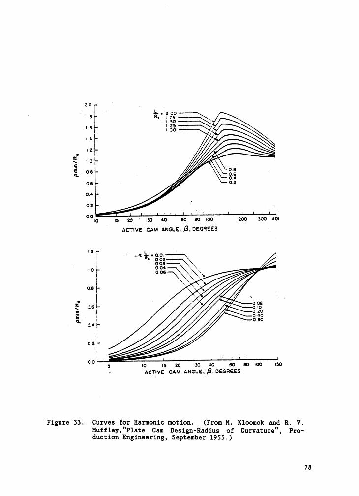
radius. Figures 32 and 33 show the graphs for Cycloidal and Harmonic
IIIOCÄOIIS 1'€SP8CtiV€1y.
76
L . .R- ?.$§°|_Q I 50I.25I.00 \0.9 \—O·2\_o4
0.8 0 6' _ 0 80.706 ‘
¤x 05E {“ .. ¤. °° -
-03 _ _— 0 2 V ·
0 I;
” ' OOIO I5 20 30 40 60 80 I00 200_ ACTIVE CAM ANGLE, B, DEGREES '
RR I- ° S3?.5 0.04o 6 I- 0 06
& ,. 0 7 I- $‘ $0/
|/ · f 0.06„ 06 _ O I0¤=° I°·5 5' 0.60E 0.4IiQ
0.30 20 I - .
T
O OI: I . I I I - I I ·5 IO I5 20 30 40 60 80- I00 IE0
ACTIVE CAM ANGLE, OEGREES
Figure 32. Curves for Cycloidal motion. (From M. Kloomok and R. V.Muffley,"P1ate Cam Design-Radius of Curvature", Pro-duction Engineering, September 1955.)
77
2.0 ' . A‘ ‘ L • 2 oo —-—=I I 8 R• I T5
·I 4·I 2 Ĥ 6
1; I°O° .ä O. ·
M . 0.2
0.2 I - _0.4_oo If _ ° _ I I I
IQ I5 20 so 60 GO ao •oo zoo soo 4o:ACTIVE CAM ANGLE„ß,OEGREE$ ‘
I 2 __ __;·_•oo:voo.e_
\ In 6 .cg ‘
~" ooeI I
\ O.6 I- [ O IOQ I O ZOä E SSSQ 0.4I-
0.2%-
°° IO es 20 so 4O 60 ao ·o0 I50- ACTIVE CAM ANGLE• ß.0EGREES
Figure 33. Curves for Harmonic motion. (From M. Kloomok and R. V.Muff1ey,"Plate Cam Design-Radius of Curvature", Pro-duction Engineering, September 1955.)
78
CHAPTER 5 PROGRAM DESCRIPTION
5.] OVERVIEW
ANICAM has been written to allow the user to create animated se-
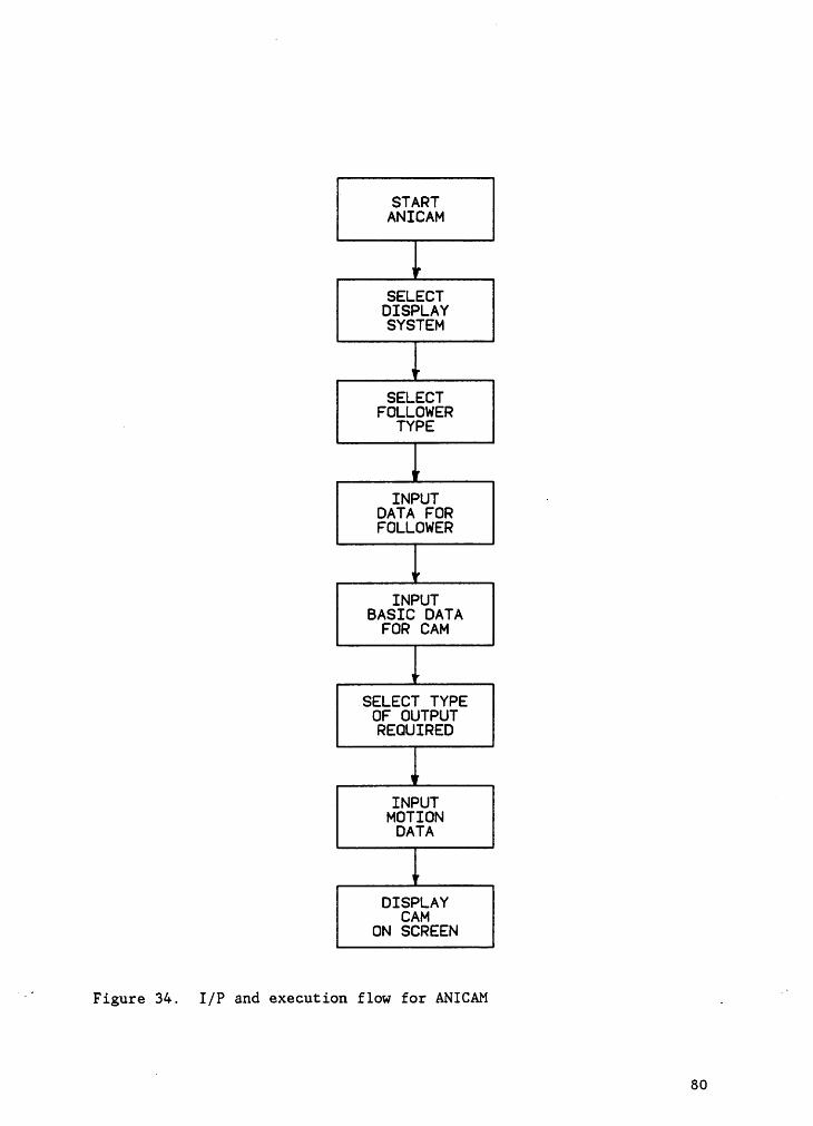
quences for disk cams. Figure 34 illustrates the input and execution flow
that a user would take to design and display the cam. Upon starting
ANICAM, the user will be asked to select the system on which the cam model
has to be displayed. Whether the user will be able to animate the cam,
depends on the choice of the display system. The two systems which have
animation capability' are. GKS and MOVIE.BYU. Based on the design re-
quirements the user would sequentially select the follower type (there
are 7) and the basic data of the cam and the motion (displacement) char-
acteristics . The user has a choice of 22 different displacement func-
tions and is expected to select compatible motions. The last input asked
of the user is to enter the type of output required. The user may specify
any of the 3 graphics options.
ANICAM is a fairly large program and will occupy a lot of memory
space. By overlaying the program, it is possible to have only a part of
the program in active memory. However one shortcoming of overlaying is
that it can significantly slow the progrmm execution. To facilitate
possible overlays ANICAM is broken into four major parts with the func-·
tions of program control, motion data input, motion characteristics and
profile generation and display. Since ANICAM is currently running on a
system with virtual memory, overlaying is not needed.
79
STARTANICAM
SELECTDISPLAYSYSTEM
SELECTFDLLOWER
· TYPE
INPUT ·DATA FORFOLLOWER
INPUTBASIC DATA
FDR CAM
.SELECT TYPEDF OUTPUTREDUIRED
INPUTMOTION
DATA
DISPLAYCAM
ON SCREEN
*' Figure 34. I/P and execution flow for ANICAM _ °
380
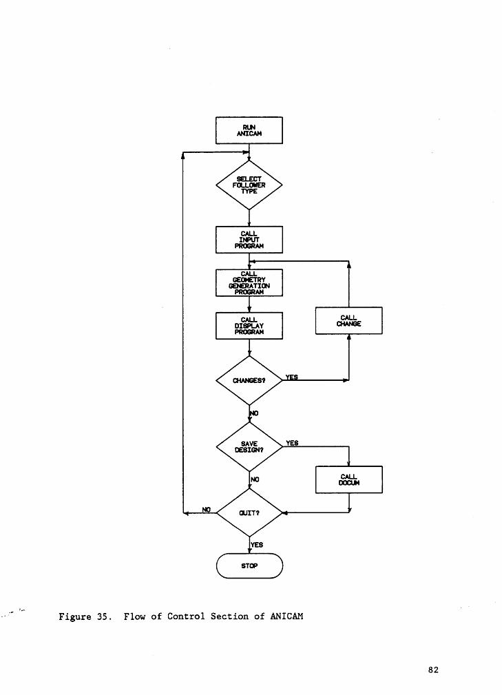
5.2 PROGRAM CONTROL
The control portion of ANICAM is its heart. It calls the. other
program sections and passes the necessary data between them. This portion
is kept small since it must always occupy active memoryn The use of
overlaying allows larger program segments to be called into memory above
the root segment. Figure 35 illustrates a flow for the control section
of the program. After starting the program the user is asked to key in
the basic data for the cam and follower system. All this data is trans-
ferred through FORTRAN common blocks to the. motion input program and
continues on until the program has completed its operation. This process
is repeated until the user indicates that he would like to stop.
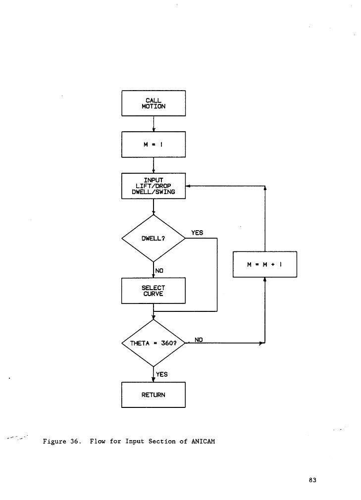
5.3 MOTION DATA INPUT Ip
The input section of the program takes the data regarding the dis-
placement requirements and the functions governing the motion to be im-
parted to the follower. This continues until the user has specified these
requirements for all the 360 degrees of the cam rotation. Once all data
has been accepted, it is passed to the control section which in turn
passes it to the generation section of the program. The flow chart for
the input segment is shown in Fig. 36.
81
SELECTFCLLOWERTYPE
cm.IIPUTPnocum
cau.GEGETRYGEPERATIGWPnocnm
cw.¤1%«·^“ö«
I
¤+^~¤¤Pnosnm
YES
cm.
€
YES
··°‘ MFigure 35. Flow of Control Section of ANICAM
l
82
lCALL
MOTION
INPUTLIFT/DROP
DWELL/SWING
M = M + I
SELECTCURVE
_ YES
RETURN
INT}-.Figure 36. Flow for Input Section of ANICAM
83
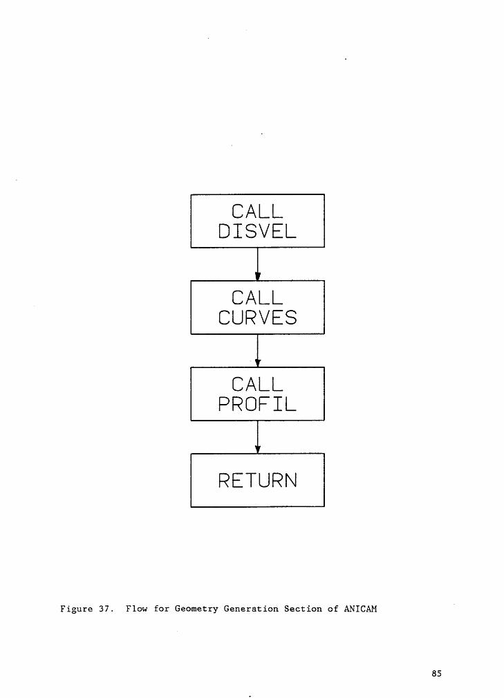
5.4 CAM PROFILE AND MOTION CHARACTERISTICS GENERATION -
This part of the program calculates the displacement, Velocity,
acceleration, jerk, and the cam profile coordinates at l degree intervals
of angular displacement of the cam. lt accepts the data regarding fol-
lower motion and jumps to the proper equations for the evaluation of the
motion characteristics. Data regarding the follower type, along with data
just entered is passed through to the subroutine for profile calculations. -
Here too, the segment goes to the correct equations for cam profile co-
ordinate calculations. Once the coordinates are evaluated all data ispassed to the display segment of the program. Figure 37 shows the flow-
I
chart for the generation segment.
5.5 DISPLAY
This portion takes all data and generated information and executes
appropriate commands for the required display system. Each display system
works independently and displays the designed model using different
methods. By far, this is the most important part of the program. Dis-
playing the designed cam helps the user to decide whether the design is
feasible.
If the user has chosen GKS as the display system then he is asked
to enter the type of TEKTRONIX terminal on which the model is to be dis-
played. GKS then proceeds to display the cam profile and the motion
characteristics that would be imparted to the follower if that cam model
is used.· Various GKS subroutines are called in order to produce a color
84
CALLDISVEL
CALLCURVES
CALLRRCEIL
RETURN
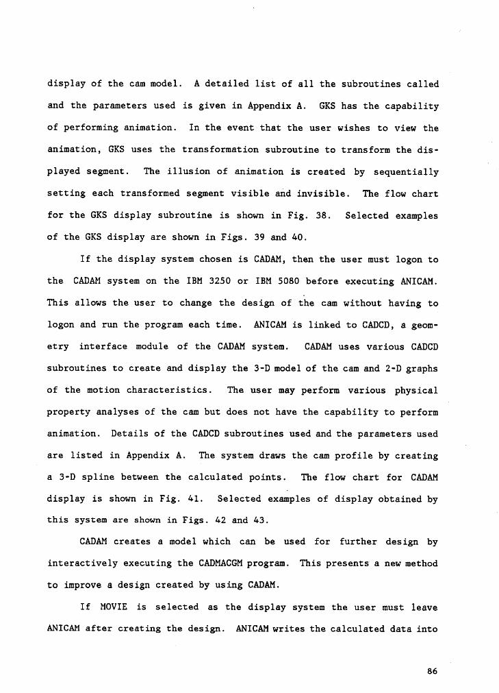
display of the cam model. A detailed list of all the subroutines called
and the parameters used is given in Appendix A. GKS has the capability
of performing animation. In the event that the user wishes to view the
animation, GKS uses the transformation subroutine to transform the dis·4
played segment. The illusion of animation is created tw' sequentially4
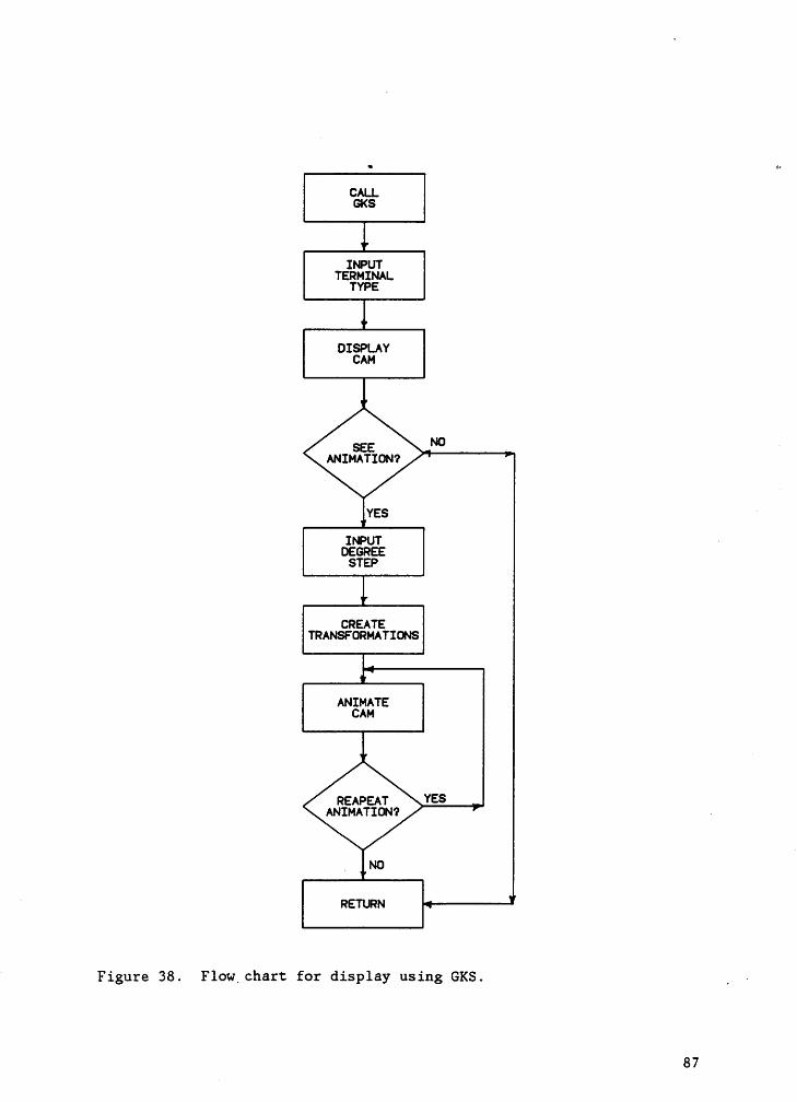
setting each transformed segment visible and invisible. The flow chart
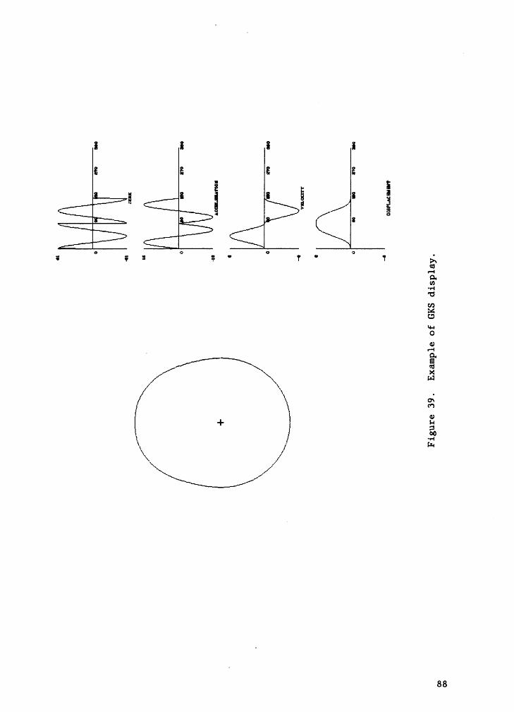
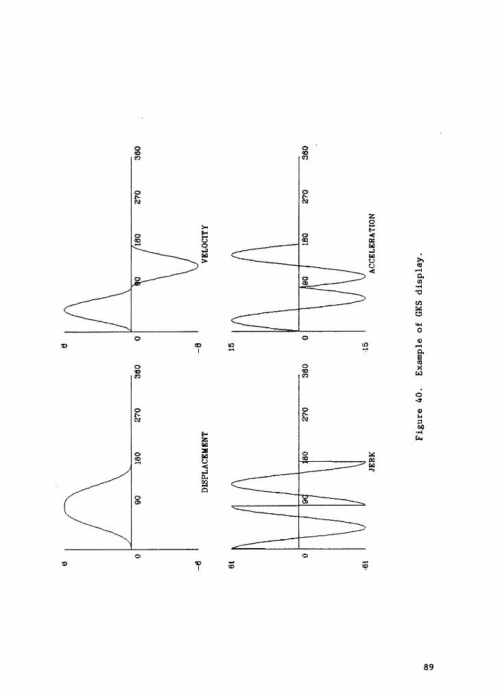
for the GKS display subroutine is shown in Fig. 38. Selected examples
of the GKS display are shown in Figs. 39 and 40.
If the display system chosen is CADAM, then the user must logon to
the CADAM system on the IBM 3250 or IBM 5080 before executing ANICAM.
This allows the user to change the design of the cam without having to
logon and run the program each time. ANICAM is linked to CADCD, a geom· _
etry interface module of the CADAM system. CADAM uses various CADCD
subroutines to create and display the 3·D model of the cam and 2-D graphs
of the motion characteristics. The user may perform ·various physical
property analyses of the cam but does not have the capability to perform
animation. Details of the CADCD subroutines used and the parameters used
are listed in Appendix A. The system draws the cam profile by creatingA
a 3·D spline between the calculated points. The flow chart for CADAM
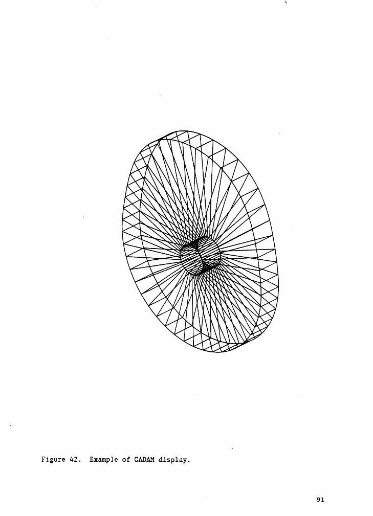
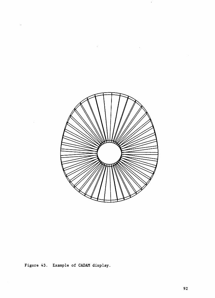
display is shown in Fig. 41. Selected examples of display obtained by
this system are shown in Figs. 42 and 43.4
CADAM creates a model which can be used for further design by
interactively executing the CADMACGM program. This presents a new method
to improve a design created by using CADAM.
If MOVIE is selected as the display system the user must leave
ANICAM after creating the design. ANICAM writes the calculated data into
86A
CALLGKS
INPUTTERMINALTYPE
DISPLAYCAM
MINPUT ~DEGREESTEP
CREATETRANSFORMATIUNS
ANIMATECAM
REAPEATANIMATIDN? .
' Figure 38. Flow_chart for display using GKS. _.-
8 7
S S S SE E E E
ä Eg a S s E s *-•U g g< ( 8 ¤
\6° 6 = ° 6 • ° v · ° ·r ,;„
Q'§—3ä“6‘B
88
9.
e
99
*:0 9C'}
9l*
ON
l¥N
Z
Z E§ 6 g Z
Ö•-ul G
JIE
I':} J>
EI•
U >·•U Gd
9 O4°°rn~•-I’O
</1MCD
O
“‘8Iä D to
OLD 0
I ""H
,-4’ 29 <¤
*:*3O ><W I-rl
62 Q **N
l‘— däO2 I-e:5
E ·?·°rn
Lu
¤ 2Q4 M_;| ErlQ-.*1
* GQF-!Q
OG
I89
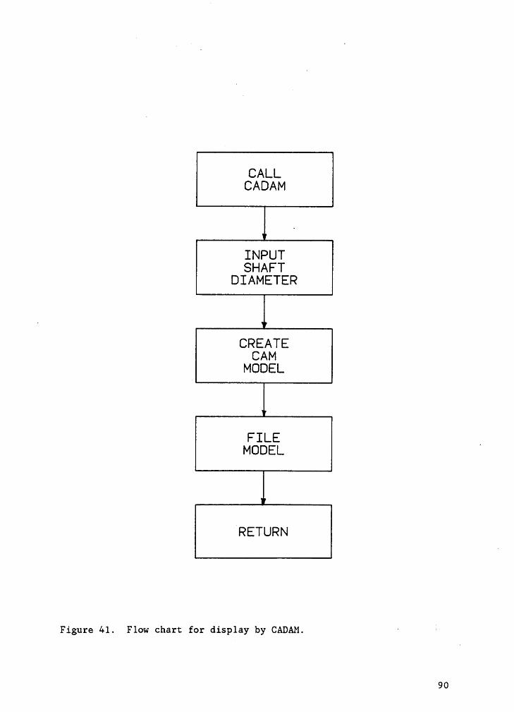
CALLCADAM
INPUTSHAFT
DIAMETER
CREATECAM
MODEL
FILE _MODEL
CRETURN
Figure 41. Flow chart for display by CADAM. · ?
90
~
~
FILE.CAM, a file which has been formatted on lines of the geometry files
created by the UTILITY subroutine of MOVIE.BYU. The creation of FILE.CAM
enables the user to run DISPLAY without running UTILITY. The user will
be asked for the name of the geometry file created using ANICAM. DISPLAY
allows the model to be displayed in 3-D and be viewed at various angles.
Hidden line elimination can be performed by giving a series of DISPLAYl
commands. If the user has chosen to animate this model while in ANICAM,he has created a command file, FILE.COM, which can be used by a modified
version of DISPLAY to create and store all the frames of' motion cu1 a
flexible. disc. These frames can be animated by running ANIMATE (**).
ANIMATE loads the data from the disc to the memory of the TEKTRONIX ter-
minal, and sequentially displays each frame with refresh or raster
graphics, giving an illusion of motion. A detailed list of all the DIS-
PLAY commands and the format of the geometry file created are given in
Appendix A. Figure 44 shows the flow chart for the MOVIE display sub-
routine. Selected examples of the output obtained by this display system
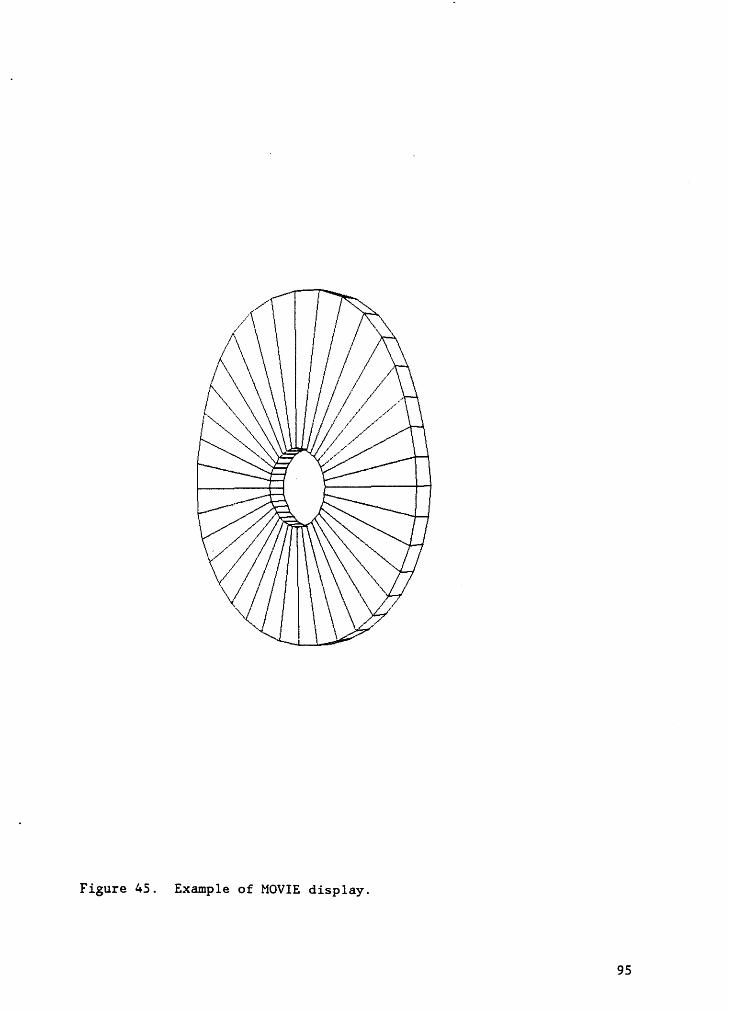
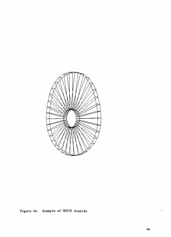
are shown in Figs. 45 and 46. ‘
93
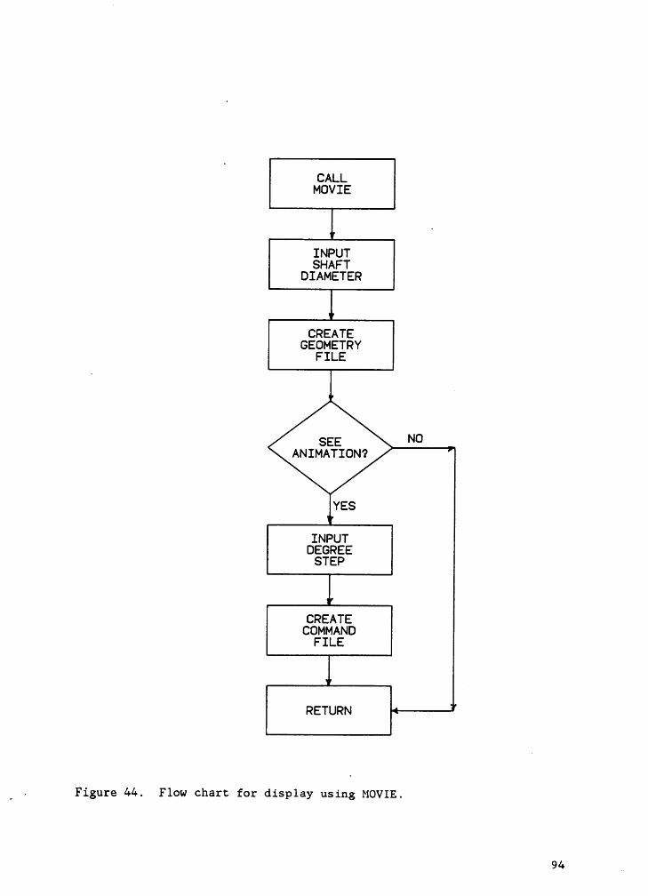
CALLMOVIE
INPUTSHAFT
OIAMETER
CREATEGEOMETRY
FILE
ses NOANIMATION?
INPUTOEGREE
STEP
CREATECOMMAND
FILE
RETURN
_ » Figure 44. Flow chart for display using MOVIE.
94 p
Ä «’ ///Q
0///I · ,/
~«-„,/ .¤//\
/ 4/
Figure 45. Example of MOVIE display.
95
V / v/ I \\/‘\‘\ ‘— /:/4/;" ’
\ / ’·-·· .
I}; tglP'/;, gi!C9 ·\\<—\/ /1 \\ \\{\
\\ ,/
Figure A6. Example 6s r10v11-: display, U E
96
CHAPTER 6 RECOMMENDATIONS AND IMPLICATIONS
ANICAM is intended to be an interactive program which has the ca-
pability to design and display a cam model, and the motion characteristics
which will be imparted to the follower. With full color 3-D capabilities, .
it can be used as a powerful tool to create wire-frame or solid models
by linking it with a CAD/CAM package, and a widely used graphic display
package Viz. CADAM and MOVIE.BYU. While CADAM allows the analysis of the ·
physical properties of the cam designed and futher use in design or man-
ufacturing, the ANICAM link with MOVIE and GKS can be used as one of the
most powerful tool for purpose of simulation. ANICAM can be seen having
many industrial applications.
Though the system has fulfilled most of the requirements of de-
signing principles it has a tremendous potential for increased capabili-
ties. This design is based on kinematic considerations only, and does
not consider the dynamic effects on the cam. While the cam must be de-
veloped to meet motion constraints, care must be taken to see that the
kinematically sound design does not fail dynamically. Dynamic effects
like the loads acting on the cam, Vibrations, and the stresses caused by
both may also lead to the cam not being able to perform the task it was
created for. In order to make the design more comprehensive and reliable,
it is recommended that dynamic analysis be incorporated in the program.A
I.The ability of the program to use 3-D display systems brings the
design of 3-D cams to the mind. 3-D cams are finding increasing appli-
cations in industries. The present ability of ANICAM tx: display 3-D
97
models would. be highly enhanced by the capability of solid modelling.
Solid modelling packages like CATIA can be easily incorporated into the
program giving it the added ability to shade, giving the model a moreV
realistic look. These abilities are expected to be available in CADAM
in the near future.
The ability of the system to simulate the cam rotation would be put
to better use if the follower is displayed and animated along with the
cam. This would give the designer a better perspective of what to expect
of the designed system and the actual design models which can be modified
interactively.
One of the big advantages of the program structure is the separation
of the design and display routines. By simply changing the design routine
it would be possible to display other machine components like gears,
linkages, pulleys, bearings, joints, chains, brakes, and clutches. It
is also possible to add the design routines of the above components to
ANICAM thus increasing the scope of the program.
98
REFERENCES
1. Rothbart, H. H., Cams, John Wiley and Sons, 1956.
15. Vallard, H., "Computer programs for analysis of valve train dynamicsand cam profile evaluation", The Institute of Internal CombustionEngines Bulletin No. IF-H5, Trondheim, Norway, 1969.16. Keil, M. J., "A Method for Automatically Generating and Animating 3-DModels of Planar Linkages", Master°s thesis, Florida Atlantic Uni-versity, 1984.
17. Mabie, H. H., and Ocvirk F. W., Mechanisms and D amics of_ _ ............_....XE........Machinery, John Wiley and Sons, 1978.
18. Ballaney, P. L., Theopy of Machines, Khanna Publishers, New! Delhi,1980._
19. Tausworthe, R. C., Standardized..Development of Computer Software(Part 1}, Prentice-Hall Inc., 1977.20. Foley, JZ D., Vam Dam, A., Fundamentals of Interactive ComputerGraphics, Addison·Wesley Publishing Company, 1984.21. Sproull, R. F., Sutherland, W. R., Ullner, M. K., Device·IndependentGraphics, McGraw·Hi1l Book Company, 1985.22. Hopgood, F. R. A., Duce, D. A., Gallop, J. R., Sutcliffe, D. C., Ip;troduction to the Gra hical Kernel S stem, Academic Press, 1983............_..._......Jl..............JL....23. Myklebust, A., "ANIMATE", Florida Atlantic University, 1983.24. Brigham Young University, MOVIE.BYU.-— General Pur ose Com uter
_.............T............lL.......JL....Graphics System, Depatment of Computer Sc1ence,l984.
25. CADAM Inc., Computer·Graphics Augmented Zbesigp and. ManufacturingSystem — User Training Manual SH20·2035-3, IBM, 1982.26. CADAM Inc., CADAM System - Geometry Interface Module Installationand Programmers Guide SH20·2099·6, IBM, 1983.27. CADAM Inc., CADAM System - Geometry Interface Module InstallationGuide SH20-6227-0, IBM, 1985.
100
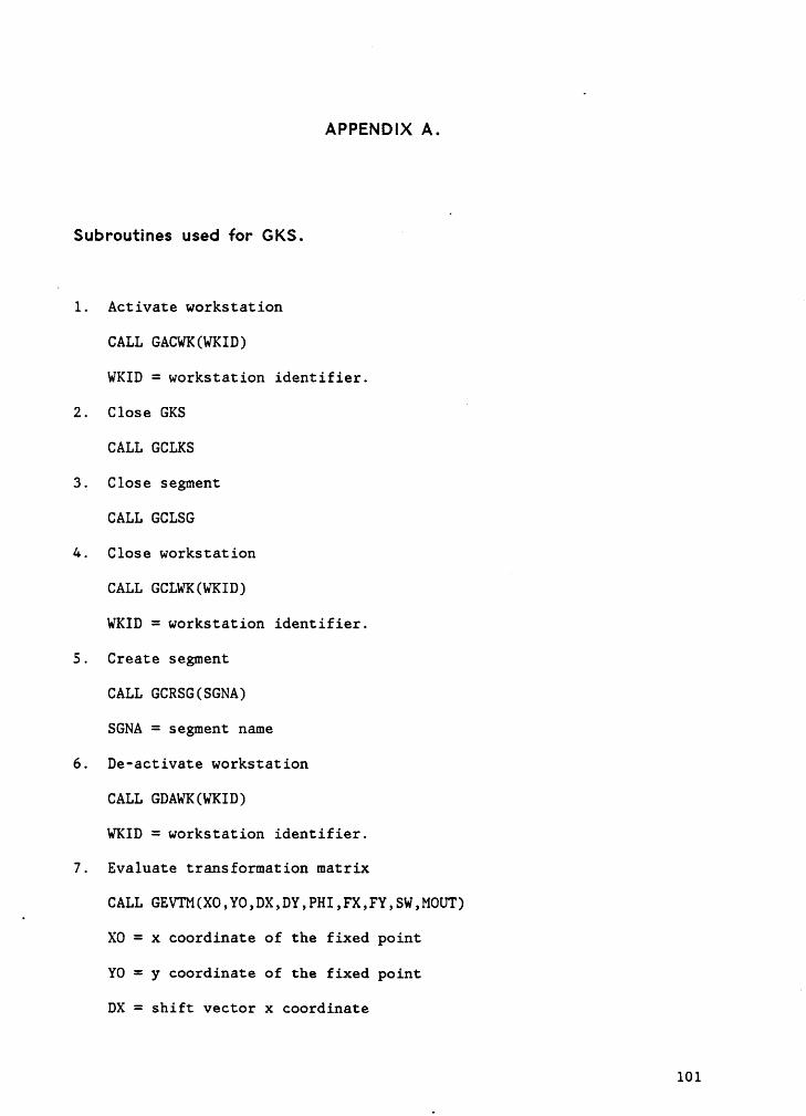
APPENDIX A.
Subroutines used for GKS. ‘
e1. Activate workstation
CALL GACWK(WKID)
WKID = workstation identifier.
2. Close GKS
CALL GCLKS
3. Close segment
CALL GCLSG
4. Close workstation
CALL GCLWK(WKID)
WKID = workstation identifier.
5. Create segment
CALL GCRSG(SGNA)
SGNA = segment name
6. De-activate workstation
CALL GDAWK(WKID)
WKID = workstation identifier.
7. Evaluate transformation matrix
CALL GEVTM(X0,YO,DX,DY,PHI,FX,FY,SW,MOUT)
XO = x coordinate of the fixed point
Y0 = y coordinate of the fixed point
DX = shift vector x coordinatel
101
DY = shift vector y coordinate
PHI = Rotation angle in radians
FX = x coordinate scale factor
FX = x coordinate scale factor
SW = Coordinate system
MOUT = Resulting transformation matrix
8. Draw fill area
CALL GFA(N,PX,PY)
N = Number of points _
PX(N) = x coordinates of points inWCV
PY(N) = y coordinates of points in WC ' „
9. Open GKS
CALL GOPKS(ERRFIL)W
ERRFIL = Error message file.
10. Open workstation
CALL GOPWK(WKID,CONID,WTYPE)
WKID = workstation identifier.
CONID = Connection identifier
WTYPE = Workstation type
11. Draw polylineA
CALL GPL(N,PX,PY)
N = Number of points
PX(N) = x coordinates of points in WC
PY(N) = y coordinates of points in WC
12. Draw polymarker
CALL GPM(N,PX,PY)
102A
N = Number of points
PX(N) = x coordinates of points in.WC
PY(N) = y coordinates of points in WC
13. Set character height.
CALL GSCHH(CHH)
CHH = Character height in WC
14. Set character expansion factor.
CALL GSCHXP(CHXP)
CHXP = Character expansion factor
15. Set normalization transformation.
CALL GSELNT(TNR)
TNR = Transformation identifier
16. Set fill area color index.‘
CALL GSFACI(COLI)
COLI = Integer number corresponding to one color
17. Set fill area interior style.
CALL GSFAIS(INST)
INST = Integer number corresponding one style
18. Set line type.
CALL GSLN((LTYP)
LTYP = Integer number corresponding to one line typeu
19. Set marker type.
CALL GSMK(MTYPE)·
MTYP = Integer number corresponding to one marker type
20. Set polyline color index.
CALL GSPLCI(COLI)
103
COLI = Integer number corresponding to one color
21. Set polymarker color index.
·CALL GSPMCI(COLI)
COLI = Integer number corresponding to one color
22. Set segment transformation.
CALL GSSGT(SGNA,M)
SGNA = Segment name
M = Transformation matrix
23. Set text alignment.
CALL GSTXAL(TXALH,TXALV)
TXALH = Horizontal alignment of text
TXALV = Vertical alignment of text
24. Set text color index.
CALL GSTXCI(COLI)‘ COLI = Integer number corresponding to one color
25. Set text font and precision.
CALL GSTXFP(FONT,PREC)
FONT = Integer corresponding to one font
PREC = Integer corresponding to one precision value
26. Set segment visibility.
CALL GSVIS(SGNA,I)
SGNA = Segment name
I = 0 for invisible, 1 for visible
27. Set viewport.
CALL GSVP(TNR,XMIN,XMAX,YMIN,YMAX)
TNR = Transformation identifier _
104
XMIN = Minimum value of x in NDC coordinates
XMAX = Maximum value of x in NDC coordinates
YMIN = Minimum value of y in NDC coordinates _
YMIN = Maximum value of y in NDC coordinates '
28. Set workstation viewport.
CALL GSWKVP(WKID,XMIN,XMAX,YMIN,YMAX)
WKID = Workstation identifier
XMIN = Minimum value of x in DC coordinates
XMAX = Maximum value of x in DC coordinates
YMIN = Minimum value of y in DC coordinates
YMIN = Maximum value of y in DC coordinates
29. Set workstation window.
CALL GSWKWN(WKID,XMIN,XMAX,YMIN,YMAX)
WKID = Workstation identifier
XMIN = Minimum value of x in NDC coordinates
XMAX = Maximum value of x in NDC coordinates
YMIN = Minimum value of y in NDC coordinates
YMIN = Maximum value of y in NDC coordinates
30. Set window.
‘CALL GSWN(TNR,XMIN,XMAX,YMIN,YMAX)
TNR = Transformation number
XMIN = Minimum value of x in WC coordinates
XMAX = Maximum value of x in WC coordinates
YMIN = Minimum value of y in WC coordinates
YMIN = Maximum value of y in WC coordinates
31. Draw text.
105
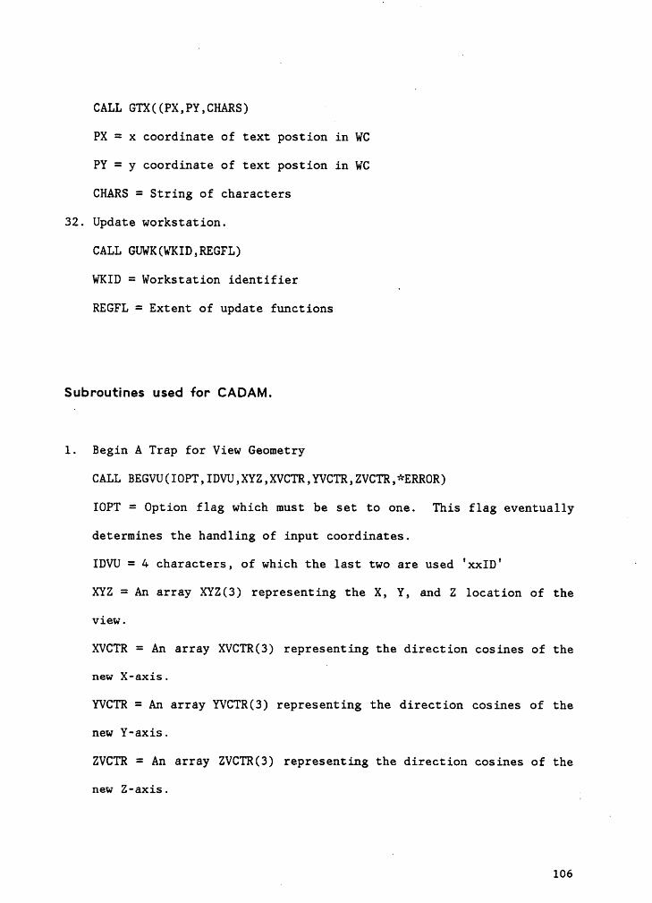
CALL GTX((PX,PY,CHARS) ‘ _
PX = x coordinate of text postion in WC
PY = y coordinate of text postion in WC
CHARS = String of characters
32. Update workstation.
CALL GUWK(WKID,REGFL)
WKID = WorkstationidentifierREGFL= Extent of update functions
Subroutines used for CADAM.
1. Begin A Trap for View Geometry
CALL BEGVU(IOPT,IDVU,XYZ,XVCTR,YVCTR,ZVCTR,*ERROR)
IOPT = Option flag which must be set to one. This flag eventually
determines the handling of input coordinates.
IDVU = 4 characters, of which the last two are used °xxID° ‘
XYZ = An array XYZ(3) representing the X, Y, and Z location of the
view.XVCTR = An array XVCTR(3) representing the direction cosines of the
new X—axis.I
YVCTR = An array YVCTR(3) representing the direction cosines of the
new Y·axis.ZVCTR = An array ZVCTR(3) representing the direction cosines of thenew Z·axis.106
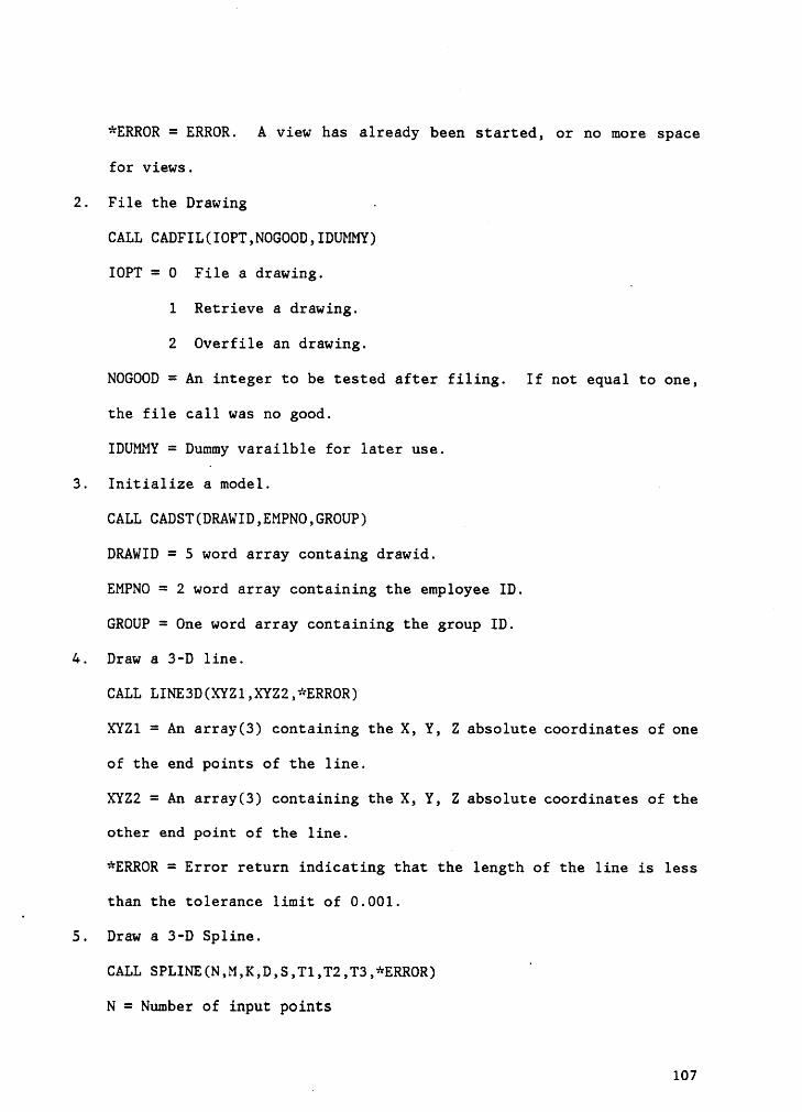
*ERROR = ERROR. A view has already been started, or no more space
for views.
2. File the Drawing -
CALL CADFIL(IOPT,NOGOOD,IDUMMY)
IOPT = 0 File a drawing.·
1 Retrieve a drawing.
2 Overfile an drawing.
NOGOOD = An integer to be tested after filing. If not equal to one,
the file call was no good.
IDUMMY = Dummy varailble for later use.
3. Initialize a model.
CALL CADST(DRAWID,EMPNO,GROUP)
DRAWID = 5 word array containg drawid.
EMPNO = 2 word array containing the employee ID.
GROUP = One word array containing the group ID.
4. Draw a 3-D line.
CALL LINE3D(XYZl,XYZ2,*ERROR)
XYZ1 = An array(3) containing the X, Y, Z absolute coordinates of one
of the end points of the line.
XYZ2 = An array(3) containing the X, Y, Z absolute coordinates of the
other end point of the line.
*ERROR = Error return indicating that the length of the line is less
than the tolerance limit of 0.001.
5. Draw a 3-D Spline.
CALL SPLINE(N,M,K,D,S,Tl,T2,T3,*ERROR)e
N = Number of input points
107
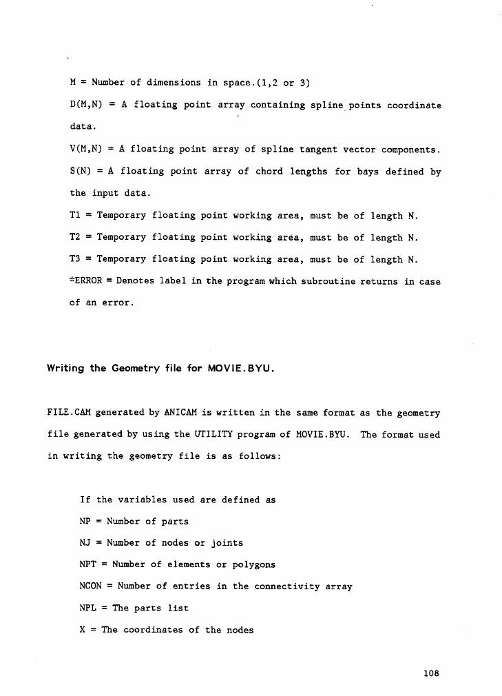
M = Number of dimensions in space.(1,2 or 3)
D(M,N) = A floating point array containing spline points coordinate
data.V(M,N)
= A floating point array of spline tangent vector components.
S(N) = A floating point array of chord lengths for bays defined by
the input data.
Tl = Temporary floating point working area, must be of length N.
T2 = Temporary floating point working area, must be of length N.
T3 = Temporary floating point working area, must be of length N.
*ERROR = Denotes label in the program which subroutine returns in case
of an error.
Writing the Geometry file for MOVIE.BYU.
FILE.CAM generated by ANICAM is written in the same format as the geometry
file generated by using the UTILITY program of MOVIE.BYU. The format used
in writing the geometry file is as follows:
If the variables used are defined as
NP = Number of parts
NJ = Number of nodes or joints
NPT = Number of elements or polygons
NCON = Number of entries in the connectivity array
NPL = The parts list
X = The coordinates of the nodes
108
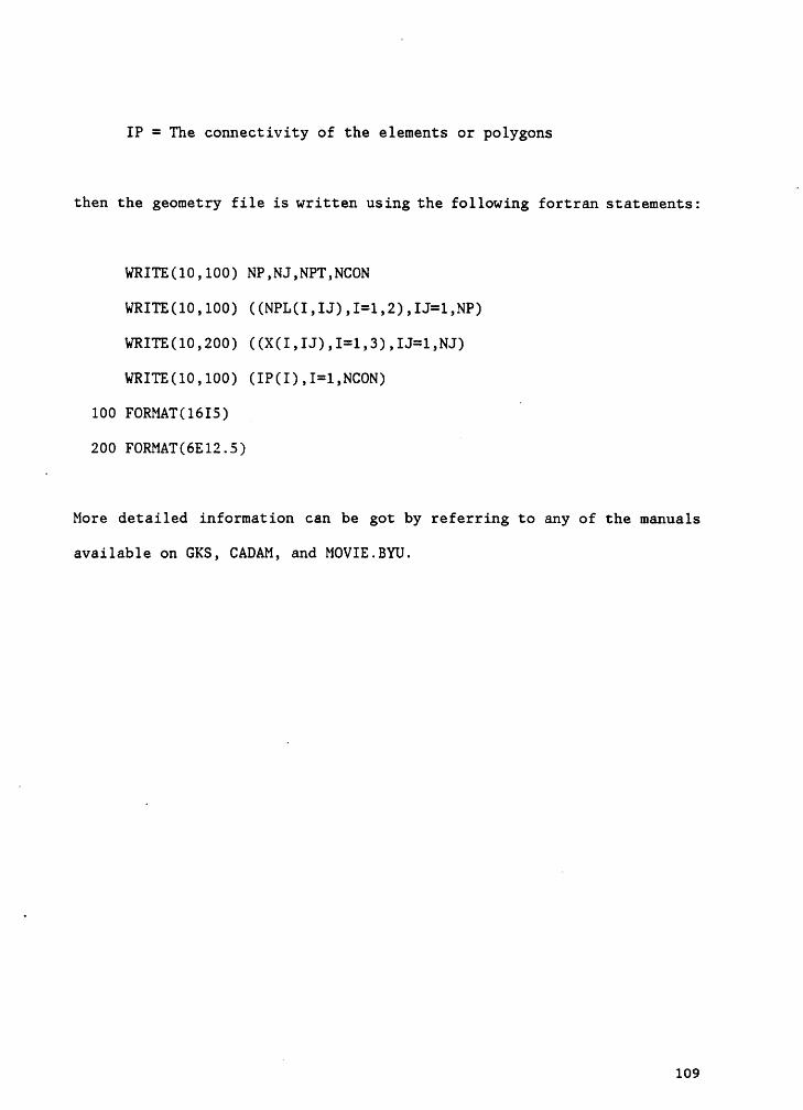
IP = The connectivity of the elements or polygons
then the geometry file is written using the following fortran statements:
WRITE(10,100) NP,NJ,NPT,NCON
WRITE(10,lO0) ((NPL(I,IJ),I=1,2),IJ=l,NP)
WRITE(l0,200) ((X(I,IJ),I=l,3),IJ=l,NJ)
WRITE(10,100) (IP(I),I=1,NCON)
100 FORMAT(16I5)l
200 FORMAT(6E12.5)
More detailed information can be got by referring to any of the manuals
available on GKS, CADAM, and MOVIE.BYU.
4109
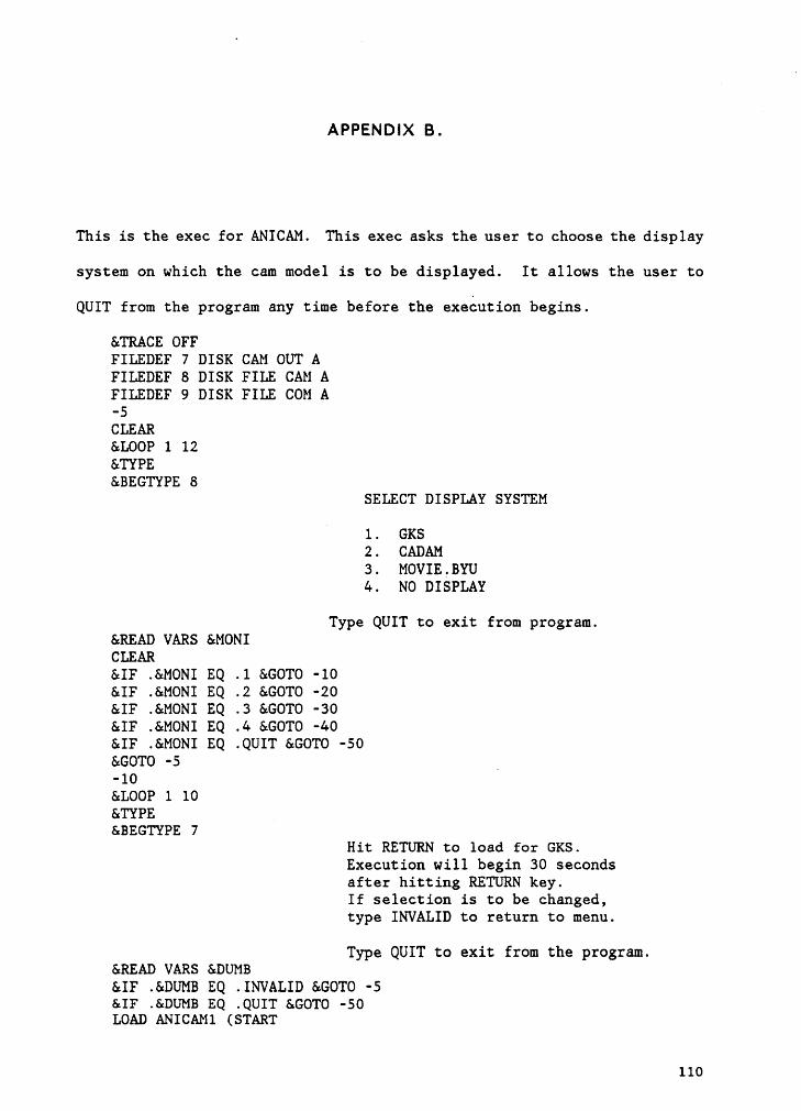
APPENDIX B.
This is the exec for ANICAM. This exec asks the user to choose the display
system on which the cam model is to be displayed. It allows the user to
QUIT from the program any time before the execution begins.
&TRACE OFFFILEDEF 7 DISK CAM OUT AFILEDEF 8 DISK FILE CAM AFILEDEF 9 DISK FILE COM A-5CLEAR&LOOP 1 12&TYPE&BEGTYPE 8
SELECT DISPLAY SYSTEM
1. GKSV 2. CADAM3. MOVIE.BYU4. NO DISPLAY
Type QUIT to exit from program.&READ VARS &MONICLEAR&IF .&MONI EQ .1 &GOT0 -10&IF .&MONI EQ .2 &GOTO -20&IF .&MONI EQ .3 &GOTO -30&IF .&MONI EQ .4 &GOTO -40&IF .&MONI EQ .QUIT &GOT0 -50&GOT0 -5 4-10&LOOP 1 10&TYPE&BEGTYPE 7
Hit RETURN to load for GKS.Execution will begin 30 secondsafter hitting RETURN key.If selection is to be changed,type INVALID to return to menu.
Type QUIT to exit from the program.&READ VARS &DUMB&IF .&DUMB EQ .INVALID &GOT0 -5&IF .&DUMB EQ .QUIT &GOT0 -50LOAD ANICAM1 (START
110
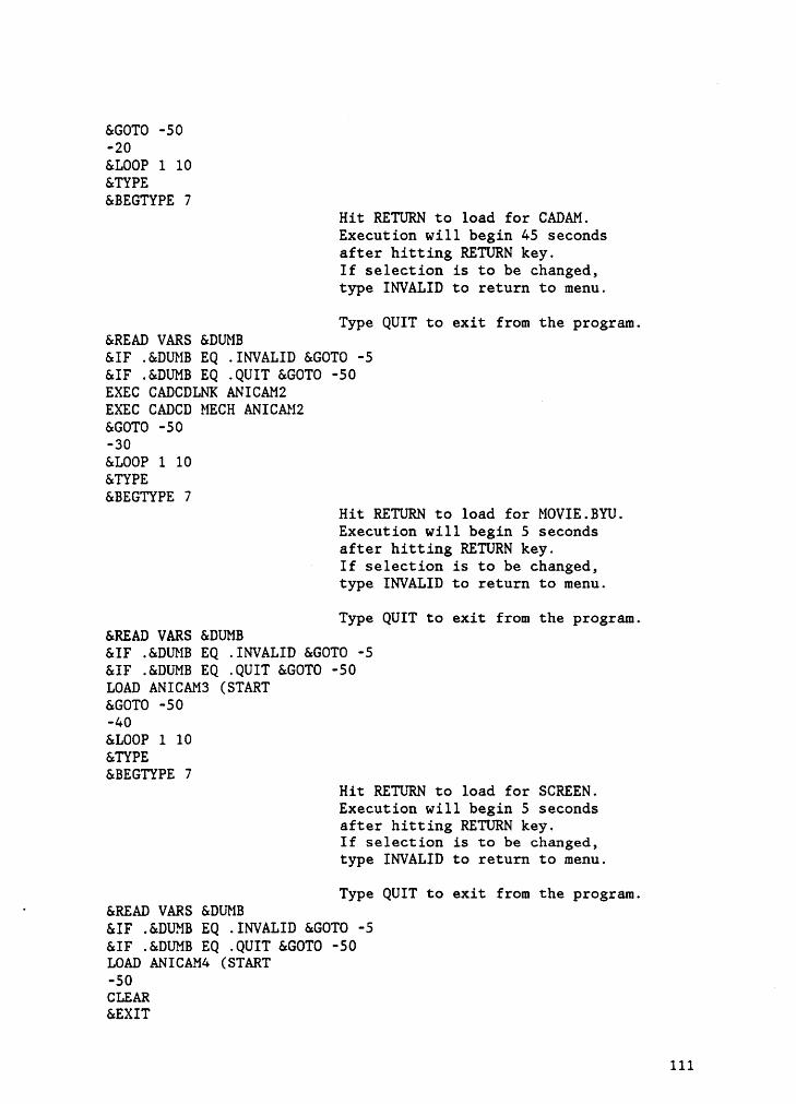
&GOT0 -50-20&LOOP 1 10&TYPE&BEGTYPE 7
Hit RETURN to load for CADAM.Execution will begin 45 secondsafter hitting RETURN key.If selection is to be changed,type INVALID to return to menu.
Type QUIT to exit from the program.&READ VARS &DUMB&IF .&DUMB EQ .INVALID &GOT0 -5&IF .&DUMB EQ .QUIT &GOT0 -50EXEC CADCDLNK ANICAM2 _EXEC CADCD MECH ANICAM2&GOT0 -50 _-30&LOOP 1 10&TYPE&BEGTYPE 7
Hit RETURN to load for MOVIE.BYU.Execution will begin 5 secondsafter hitting RETURN key.If selection is to be changed,type INVALID to return to menu.
Type QUIT to exit from the program.&READ VARS &DUMB&IF .&DUMB EQ .INVALID &GOT0 -5&lF .&DUMB EQ .QUIT &GOT0 -50LOAD ANICAM3 (START&GOT0 -50-40&LOOP 1 10&TYPE&BEGTYPE 7
Hit RETURN to load for SCREEN.Execution will begin 5 secondsafter hitting RETURN key.If selection is to be changed,type INVALID to return to menu.
Type QUIT to exit from the program.‘ &READ VARS &DUMB&IF .&DUMB EQ .INVALID &GOT0 -5&IF .&DUMB EQ .QUIT &GOT0 -50LOAD ANICAM4 (START-50CLEAR&EXIT
111
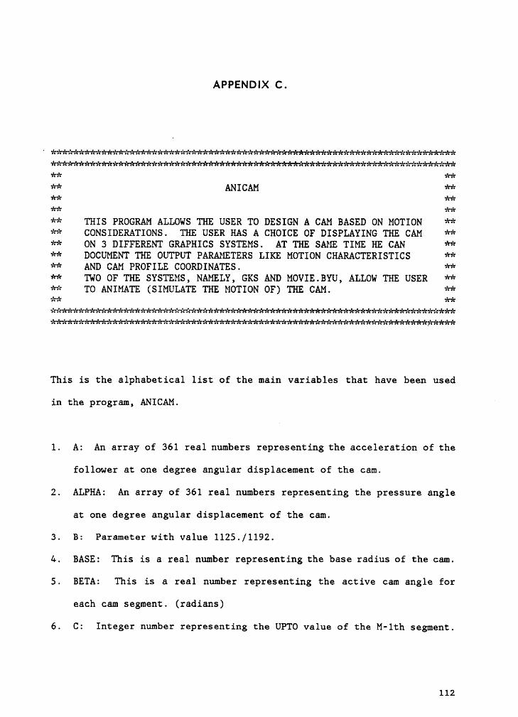
APPENDIX C.
‘ kkkkkkkkkkkkkkkkkkkkkkkkkkkkkkkkkkkkkkkkkkkkkkkkkkkkkkkkkkkkkkkkkkkkkkkkkkkkkkkkkkkkkkkkkkkkkkkkkkkkkkkkkkkkkkkkkkkkkkkkkkkkkkkkkkkkkkkkkkkkkkkk** ANICAM **kk kkkk kk** THIS PROGRAM ALLOWS THE USER TO DESIGN A CAM BASED ON MOTION **** CONSIDERATIONS. THE USER HAS A CHOICE OF DISPLAYING THE CAM **** ON 3 DIFFERENT GRAPHICS SYSTEMS. AT THE SAME TIME HE CAN **** DOCUMENT THE OUTPUT PARAMETERS LIKE MOTION CHARACTERISTICS **** AND CAM PROFILE COORDINATES. **** TWO OF THE SYSTEMS, NAMELY, GKS AND MOVIE.BYU, ALLOW THE USER **** TO ANIMATE (SIMULATE THE MOTION OF) THE CAM. **kk kkkkkkkkkkkkkkkkkkkkkkkkkkkkkkkkkkkkkkkkkkkkkkkkkkkkkkkkkkkkkkkkkkkkkkkkkkkkkkkkkkkkkkkkkkkkkkkkkkkkkkkkkkkkkkkkkkkkkkkkkkkkkkkkkkkkkkkkkkkkkkkkkk
This is the alphabetical list of the main variables that have been used
in the program, ANICAM. ‘
1. A: An array of 361 real numbers representing the acceleration of the
follower at one degree angular displacement of the cam.
2. ALPHA: An array of 361 real numbers representing the pressure angle
at one degree angular displacement of the cam.
3. B: Parameter with value 1125./1192.
4. BASE: This is a real number representing the base radius of the cam.
S. BETA: This is a real number representing the active cam angle for
each cam segment. (radians)
6. C: Integer number representing the UPTO value of the M—1th segment.
112
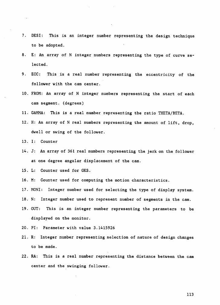
17. DESI: This is an integer number representing the design technique
to be adopted. °
8. E: An array of N integer numbers representing the type of curve se-
lected. 4
9. ECC: This is a real number representing the eccentricity of the
follower with the cam center.·
10. FROM: An array of N integer numbers representing the start of each
cam segment. (degrees)
11. GAMMA: This is a real number representing the ratio THETA/BETA.
12. H: An array of N real numbers representing the amount of lift, drop,
dwell or swing of the follower.L
13. I: Counter
14. J: An array of 361 real numbers representing the jerk on the follower
at one degree angular displacement of the cam.
15. L: Counter used for GKS.
16. M: Counter used for computing the motion characteristics.
17. MONI: Integer number used for selecting the type of display system.
18. N: Integer number used to represent number of segments in the cam.
19. OUT: This is an integer number representing the parameters ‘u¤ be
displayed on the monitor.
20. PI: Parameter with value 3.1415926
21. R: Integer number representing selection of nature of design changes
to be made.
22. RA: This is a real number representing the distance between the cam
center and the swinging follower.
. 113
23. RF: This is a real number representing the length of the follower
arm.
~ 24. ROLL: This is a real number representing the radius of the roller
follower. l
25. RPM: ‘This is an integer number representing the rotational speed of
the cam in rotations per minute.
26. S: An array of 361 real numbers representing the displacement of the
follower at one degree angular displacement of the cam.
27. THETA: This is a real number representing the angular dispalcement
of the cam. (radians)
28. TYPE: This is an integer number representing the type of follower
selected.
29. UPTO: An array of N integer numbers representing the start of each
cam segment. (degrees)
30. V: An array of 361 real numbers representing the Velocity of the
follower at one degree angular displacement of the cam.
31. WIDTH: This is a real number representing the width of the cam.
32. X: An array of 361 real numbers representing the x—coordinate of the
cam profile at one degree interval.
33. Y: An array of 361 real numbers representing the y·coordinate of the
cam profile at one degree interval.
34. Z: An array of 361 real numbers representing the z-coordinate of the
cam profile at one degree interval.
aw *«** MAIN PROGRAM **aa *«
114
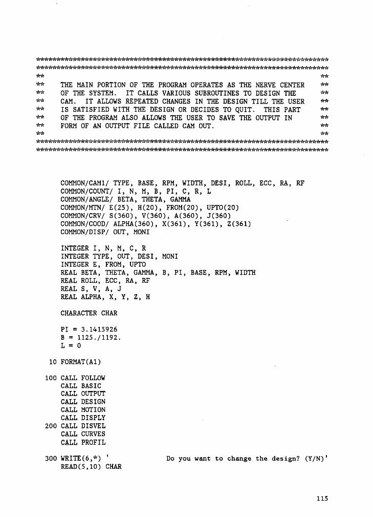
eew**«****«***«**##*«****«*«#w*****##*#**«##«**%***««*#*«**«****wwsäwnweweäsxewksäewxexeenk**«#*****«**#*«##*#«*«*«******«*«#*****«**#********«*«* es** THE MAIN PORTION OF THE PROGRAM OPERATES AS THE NERVE CENTER **** OF THE SYSTEM. IT CALLS VARIOUS SUBROUTINES TO DESIGN THE **** CAM. IT ALLOWS REPEATED CHANGES IN THE DESIGN TILL THE USER **** IS SATISFIED WITH THE DESIGN OR DECIDES TO QUIT. THIS PART **** OF THE PROGRAM ALSO ALLOWS THE USER TO SAVE THE OUTPUT IN **** FORM OF AN OUTPUT FILE CALLED CAM OUT. **
COMMON/CAM1/ TYPE, BASE, RPM, WIDTH, DESI, ROLL, ECC, RA, RFCOMMON/COUNT/ I, N, M, B, PI, C, R, LCOMMON/ANGLE/ BETA, THETA, GAMMACOMMON/MTN/ E(25), H(20), FROM(20), UPTO(20)COMMON/CRV/ S(360), V(360), A(360), J(360)COMMON/COOD/ ALPHA(360), X(361), Y(361),Z(361)COMMON/DISP/OUT, MONI
INTEGER I, N, M, C, RINTEGER TYPE, OUT, DESI, MONIINTEGER E, FROM, UPTOREAL BETA, THETA, GAMMA, B, PI, BASE, RPM, WIDTHREAL ROLL, ECC, RA, RFREAL S, V, A, JREAL ALPHA, X, Y, Z, H
CHARACTER CHAR
PI = 3.1415926B = 1125./1192.L = 0
10 FORMAT(A1) _
100 CALL FOLLOWCALL BASICCALL OUTPUTCALL DESIGNCALL MOTIONCALL DISPLY
200 CALL DISVELCALL CURVESCALL PROFIL
300 WRITE(6,*) ° Do you want to change the design? (Y/N)'READ(5,10) CHAR
115
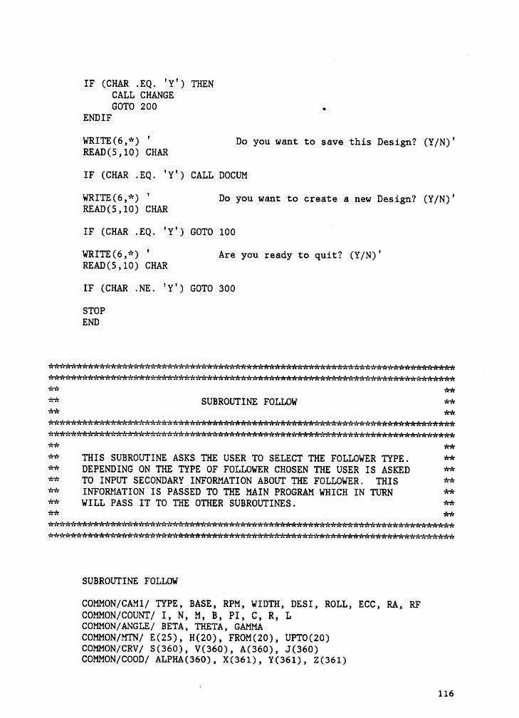
IF (CHAR .EQ. °Y°) THENCALL CHANGEGOTO 200 •
ENDIF
WRITE(6,*) ° Do you want to save this Design? (Y/N)°READ(S,10) CHAR
IF (cHAR .EQ. 'Y') CALL Docuu
WRITE(6,*) ' Do you want to create a new Design? (Y/N)'READ(S,10) CHAR
IF (CHAR .EQ. °Y') GOTO 100
WRITE(6,*) ° Are you ready to quit? (Y/N)°READ(S,l0) CHAR
IF (cHAR .NE. 'Y') 60To 300STOPEND
** SUBROUTINE FOLLOW **** *«
** **** THIS SUBROUTINE ASKS THE USER TO SELECT THE FOLLOWER TYPE. **** DEPENDING ON THE TYPE OF FOLLOWER CHOSEN THE USER IS ASKED **** TO INPUT SECONDARY INFORMATION ABOUT THE FOLLOWER. THIS **** INFORMATION IS PASSED TO THE MAIN PROGRAM WHICH IN TURN **** WILL PASS IT TO THE OTHER SUBROUTINES. **ik
kkSUBROUTINEFOLLOW
COMMON/CAMl/ TYPE, BASE, RPM, WIDTH, DESI, ROLL, ECC, RA, RFCOMMON/COUNT/ I, N, M, B, PI, C, R, LCOMMON/ANGLE/ BETA, THETA, GAMMACOMMON/MTN/ E(2S), H(20), FROM(20), UPTO(20)COMMON/CRV/ $(360), V(360), A(360), J(360)COMMON/COOD/ ALPHA(360), X(36l), Y(361), Z(361)
116
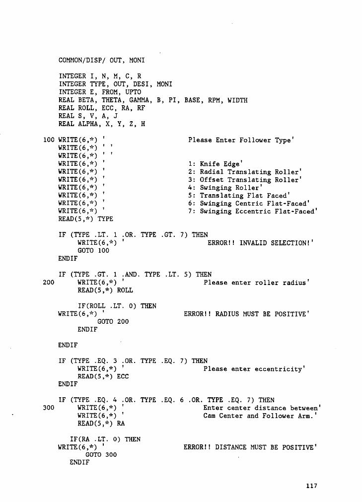
COMMON/DISP/ OUT, MONI
INTEGER I, N, M, C, RINTEGER TYPE, OUT, DESI, MONIINTEGER E, FROM, UPTOREAL BETA, THETA, GAMMA, B, PI, BASE, RPM, WIDTHREAL ROLL, ECC, RA, RFREAL S, V, A, JREAL ALPHA, X, Y, Z, H
100 WRITE(6,*) ' Please Enter Follower Type'WRITE(6,*) ' 'WRITE(6,*) ' 'WRITE(6,*) ' 1: Knife Edge°WRITE(6,*) ' 2: Radial Translating Roller'WRITE(6,*) ' 3: Offset Translating Roller'WRITE(6,*) ' 4: Swinging Roller'WRITE(6,*) ° S: Translating Flat Faced'WRITE(6,*) ° 6: Swinging Centric Flat—Faced'WRITE(6,*) ' 7: Swinging Eccentric Flat·Faced°READ(S,*) TYPE
IF (TYPE .LT. 1 .OR. TYPE .GT. 7) THENWRITE(6,*) ° ERROR!! INVALID SELECTION!'GOTO 100
ENDIF
IF (TYPE .GT. 1 .AND. TYPE .LT. 5) THEN200 WRITE(6,*) ° Please enter roller radius'
READ(5,*) ROLL
IF(ROLL .LT. 0) THENWRITE(6,*) ° ERROR!! RADIUS MUST BE POSITIVE°
GOTO 200ENDIF
_ ENDIFIF(TYPE .EQ. 3 .OR. TYPE .EQ. 7) THEN
WRITE(6,*) ' Please enter eccentricity‘READ(5,*) ECC
”
ENDIF
IF (TYPE .EQ. 4 .OR. TYPE .EQ. 6 .OR. TYPE .EQ. 7) THEN300 WRITE(6,*) ° Enter center distance between°
' WRITE(6,*) ° Cam Center and Follower Arm.°READ(5,*) RA
IF(RA .LT. 0) THENWRITE(6,*) ° ERROR!! DISTANCE MUST BE POSITIVE°
GOTO 300 _ENDIF
117
ENDIF
IF (TYPE .EQ. 4 .OR. TYPE ,EQ. 6) THEN400 WRITE(6,*) ° Enter length of the Follower Arm'
READ(5,='=) RF
IF(RF .LT. 0) THENWRITE(6,*) ° ERROR!! LENGTH MUST BE POSITIVE°
GOTO 400ENDIF
ENDIF
RETURN_ END
kkkkkkkkkkkkkkkkkkkkkkkkkkkkkkkkkkkkkkkkkkkkkkkkkkkkkkkkkkkkkkkkkkkkkkkkkkkkkkkkkkkkkkkkkkkkkkkkkkkkkkkkkkkkkkkkkkkkkkkkkkkkkkkkkkkkkkkkkkkkkkkkkk kk** SUBROUTINE BASIC **kk kk
kkkkkkkkkkkkkkkkkkkkkkkkkkkkkkkkkkkkkkkkkkkkkkkkkkkkkkkkkkkkkkkkkkkkkkkkkk kk
** THIS SUBROUTINE ASKS THE USER TO INPUT BASIC INFORMATION OF **** THE CAM THAT HAS TO BE DESIGNED. THE USER IS ASKED TO INPUT **** THE BASE RADIUS, ROTATATIONAL SPEED AND THE WIDTH OF THE CAM. **** THIS INFORMATION IS PASSED TO THE MAIN PROGRAM WHICH IN TURN **** WILL PASS IT TO THE OTHER SUBROUTINES. **kk kkkkkkkkkkkkkkkkkkkkkkkkkkkkkkkkkkkkkkkkkkkkkkkkkkkkkkkkkkkkkkkkkkkkkkkkkkkkkwkkkkkkkkkkkkkkkkkwwkkkkwkwkwkkkkkwkkkkkkkkkkkkwkkkkkkkkkkkkkkkkkkkkw
SUBROUTINE BASIC
COMMON/CAMl/ TYPE, BASE, RPM, WIDTH, DESI, ROLL, ECC, RA, RFCOMMON/COUNT/ I, N, M, B, PI, C, R, LCOMMON/ANGLE/ BETA, THETA, GAMMACOMMON/MTN/ E(25), H(20), FROM(20), UPTO(20)COMMON/CRV/ $(360), V(360), A(360), J(360)COMMON/COOD/ ALPHA(360), X(36l), Y(36l), Z(36l)COMMON/DISP/ OUT, MONI
INTEGER I, N, M, C, RINTEGER TYPE, OUT, DESI, MONIINTEGER E, FROM, UPTOREAL BETA, THETA, GAMMA, B, PI, BASE, RPM, WIDTH
118
REAL ROLL, ECC, RA, RF · _REAL S, V, A, JREAL ALPHA, X, Y, Z, H
100 WRITE(6,*) ' Please enter base radius'READ(5,*) BASE
IF(BASE .LT. 0) THENWRITE(6,*) ° ERROR!! RADIUS MUST BE POSITIVE°GOTO 100
ENDIF
200 WRITE(6,*) ' Please Enter RPM'READ(5,*) RPM °
IF(RPM .LT. 0) THENWRITE(6,*) ' ERROR!! RPM MUST BE POSITIVE°GOTO 200
ENDIF
300 WRITE(6,*) ' Please enter Width°READ(S,*) WIDTH
IF(WIDTH .LT. 0) THENWRITE(6,*) ° ERROR!! WIDTH MUST BE POSITIVE°GOTO 300
ENDIF
RETURNEND
** kk 1
** SUBROUTINE OUTPUT **
ke kk** THIS SUBROUTINE ASKS THE USER TO SELECT THE GRAPHICS OUTPUT **** WHICH HE/SHE DESIRES. THE USER HAS THREE CHOICES. HE CAN **** SELECT TO SEE THE PROFILE EITHER/OR/AND THE MOTION CURVES. **** THIS INFORMATION IS PASSED TO THE MAIN PROGRAM WHICH IN TURN **** WILL PASS IT TO THE OTHER SUBROUTINES. **ww aw
1'¤‘€7'€1‘¥1'=}'€$'€1'f7°€$'f?'f7'€7‘?1‘$7'¥7%*****************1%******%%*%%********%%*****7%*********
119
SUBROUTINE OUTPUT
COMMON/CAMl/ TYPE, BASE, RPM, WIDTH, DESI, ROLL, ECC, RA, RFCOMMON/COUNT/ I, N, M, B, PI, C, R, LCOMMON/ANGLE/ BETA, THETA, GAMMA .COMMON/MTN/ E(25), H(20), FROM(20), UPTO(20)COMMON/CRV/ S(360), V(360), A(360), J(360)COMMON/COOD/ ALPHA(360), X(36l), Y(361), Z(361)COMMON/DISP/ OUT, MONI
INTEGER I, N, M, C, RINTEGER TYPE, OUT, DESI, MONIINTEGER E, FROM, UPTO ~REAL BETA, THETA, GAMMA, B, PI, BASE, RPM, WIDTHREAL ROLL, ECC, RA, RFREAL S, V, A, JREAL ALPHA, X, Y, Z, H
100 WRITE(6,*) ° Please select type of Output° VwRma(6mama(6
1: Profile on1y'WRITE(6,*) ° 2: Curves on1y'WRITE(6,*) ° 3: Profile and Curves°READ(5,*) OUT
IF (OUT .LT. 1 .OR. OUT .GT. 3) THENWRITE(6,*) ° ERRORE! INVALID SELECTION!°GOTO 100
ENDIF
RETURNEND
ww ww** SUBROUTINE DESIGN **ww ww
** THIS SUBROUTINE ASKS THE USER TO SELECT THE DESIGN PROCESS **' ** TO BE ADOPTED IN ORDER TO DESIGN THE CAM. ONLY THE FIRST **** OPTION IS OPERATING AT THIS MOMENT. THIS SUBROUTINE WILL **** ALLOW THE OPTIMIZATION PROCESS TO BE INCORPORATED IN THE _ **** PROGRAM WITHOUT MANY COMPLICATIONS. **ww ww
120
SUBROUTINE DESIGN » u ‘
” COMMON/CAMl/ TYPE, BASE, RPM, WIDTH, DESI, ROLL, ECC, RA, RF' COMMON/COUNT/ I, N, M, B, PI, C, R, L
COMMON/ANGLE/ BETA, THETA, GAMMACOMMON/MTN/ E(25), H(20), FROM(20), UPTO(20)COMMON/CRV/ $(360), V(360), A(360), J(360)COMMON/COOD/ ALPHA(360), X(361), Y(36l), Z(36l)COMMON/DI$P/ OUT, MONI
INTEGER I, N, M, C, RINTEGER TYPE, OUT, DESI, MONIINTEGER E, FROM, UPTOREAL BETA, THETA, GAMMA, B, PI, BASE, RPM, WIDTHREAL ROLL, ECC, RA, RFREAL S, V, A, JREAL ALPHA, X, Y, Z, H
100 WRITE(6,*) ° Please select Design Process'WRITE(6,*) ' 'WRITE(6,*) ' 'WRITE(6,*) ° 1: Conventional'WRITE(6,*) ' 2: 0p¤1m1zed'READ(5,*) DESI
IF (DESI .LT. 1 .0R. DESI .GT. 2) THENWRITE(6,*) ° ERROR!! INVALID$ELECTION!°GOTO
100ENDIF
RETURNEND
°
** **V
** SUBROUTINE MOTION **·:':=':1%* '**7%****%%%******%%**%%*7°f7'€7‘€7'f1'f$‘87‘{7'?7'€7'f7'f7,¥7‘¢7'€7%*******7%%%**%**********%%*7%*7%***7%7%***
V
** **** THIS SUBROUTINE ASKS THE USER TO DEFINE THE DISPLACEMENT **** CHARACTERISTICS EXPECTED OF THE CAM BEING DESIGNED. IT IS **** STRUCTURED SUCH THAT THE USER WILL BE PROMPTED TO GIVE THE **** DISPLACEMENT REQUIREMENT FOR EACH SEGMENT OF THE CAM. THIS **** INFORMATION IS STORED AND PASSED TO THE CORRESPONDING **** SUBROUTINES THROUGH THE MAIN PROGRAM. **
121
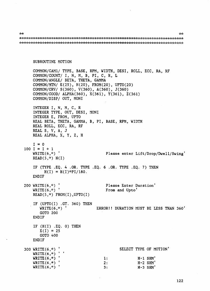
wh':wh':
ükkkkkükkkkkkkükküääkkäkükükkkükükkkkkäkküükküäk
SUBROUTINE MOTION
COMMON/CAMl/ TYPE, BASE, RPM, WIDTH, DESI, ROLL, ECC, RA, RFCOMMON/COUNT/ I, N, M, B, PI, C, R, LCOMMON/ANGLE/ BETA, THETA, GAMMACOMMON/MTN/ E(25), H(20), FROM(20), UPTO(20)COMMON/CRV/ S(360), V(360), A(360), J(360)COMMON/COOD/ ALPHA(360), X(361), Y(36l), Z(36l)COMMON/DISP/ OUT, MONI
INTEGER I, N, M, C, R _INTEGER TYPE, OUT, DESI, MONIINTEGER E, FROM, UPTOREAL BETA, THETA, GAMMA, B, PI, BASE, RPM, WIDTHREAL ROLL, ECC, RA, RFREAL S, V, A, J YREAL ALPHA, X, Y, Z, H
I = 0100 I = I + 1
WRITE(6,*) ° Please enter Lift/Drop/Dwell/Swing'READ(5,*) H(I)
IF (TYPE .EQ. 4 .OR. TYPE .EQ. 6 .OR. TYPE .EQ. 7) THENH(I) = H(I)*PI/180.
ENDIF
200 WRITE(6,*) ° Please Enter Duration'WRITE(6,*) ' From and ¤p:¤'READ(5,*) FROM(I),UPTO(I)
l IF (UPTO(I) .GT. 360) THENWRITE(6,*) ° ERROR!! DURATION MUST BE LESS THAN 360'GOTO 200 ‘
ENDIF
IF (H(I) .EQ. 0) THEN _E(I) = 25GOTO 400
' ENDIF
300 WRITE(6,*) ° SELECT TYPE OF MOTION°WRITE(6,*) ' 'WRITE(6,*) ° 1: H-1 SHM'WRITE(6,*) ' 2: H-2 sHM'WRITE(6,*) ' 3: H-3 sum'
E122
wR1TE(6,+=) ' az H-:. sm'WRITE(6,*) ' 5: H-5 SHM°
. WRITE(6,='=) ' 6: :1-6 sHM'WRI'1'E(6,='*) ‘ 7: c-1 Cyc1oida1'WRITE(6,*) ° 8: C·2 Cyc1oida1'WRITE(6,='=) ' 9: c-2 Cyc1oida1'WRITE(6,*) ° 10: C·4 Cyc1oida1°WRITE(6,*) ° ll: C·S Cycloida1°WRITE(6,='=) ' 12: c-6 Cycloidal°WRITE(6,*) ° 13: Constant Velocity°WRITE(6,*) ° 14: Constant Accl/Dcc1'WRITE(6,*) ° 15: 2-3 Po1ynomia1°WRITE(6,*)
‘16: 3-4-5 Polynomia1'
WRITE(6,*) ° 17: 4-5-6-7 Po1ynomial'WRITE(6,*) ' 18: Gutman 1-3 Harmonic(90)°WRITE(6,*) ° 19: Freudenstein 1-3 Harmouic(84)°WRITE(6,*) ° 20: Freudeustein 1-3-5 Harmouic(84)'WRITE(6,*) ' 21: Modified Sine'WRITE(6,*) ° 22: Modified Trapezoidal‘READ(5,*) 15(I)IF (E(I) .LT. l .OR. E(I) .GT. 22) THEN
WRITE(6,*) ° ERROR!! INVALID SELECTION!'GOTO 300
ENDIF ”
400 IF (UPTO(I) .LT. 360) GOTO 100 u
N = I ·
RETURNEND
k*%*%%***%küäk**%%*%***kkkk#**kkükükkükkkkükkkkkkkkkkükkkkkkkkkkäkkkkäkkkk '
**** SUBROUTINE DISVEL **** **
kk **** THIS SUBROUTINE COMPUTES THE DISPLACEMENTS AND VELOCITIES AT **** OF THE FOLLOWER AT ONE DEGREE INTERVALS. THE SUBROUTINE IS **** STRUCTURED SUCH THAT THE CALCULATIONS FOR EACH SEGMENT ARE 1 **** DONE INSIDE A DO LOOP. THIS SUBROUTINE IS REQUIRED IN EACH **** OF THE DISPLAY OPTIONS CHOSEN BY THE USER. IT IS ALSO USED **** IN THE COMPUTATIONS OF THE CAM PROFILE COORDINATES. **kä kw
123
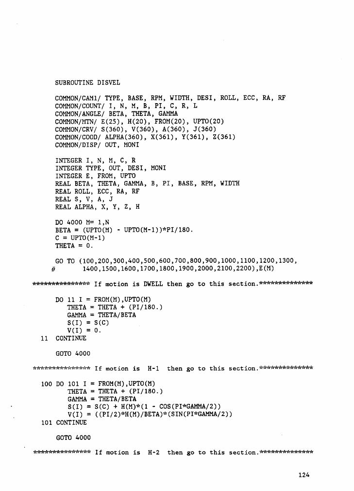
SUBROUTINE DISVEL
COMMON/CAM1/ TYPE, BASE, RPM, WIDTH, DESI, ROLL, ECC, RA, RFCOMMON/COUNT/ I, N, M, B, PI, C, R, LCOMMON/ANGLE/ BETA, THETA, GAMMACOMMON/MTN/ E(25), H(20), FROM(20), UPTO(20)COMMON/CRV/ $(360), V(360), A(360), J(360)COMMON/COOD/ ALPHA(360), X(36l), Y(361), Z(361)COMMON/DISP/ OUT, MONI
INTEGER I, N, M, C, RINTEGER TYPE, OUT, DESI, MONIINTEGER E, FROM, UPTOREAL BETA, THETA, GAMMA, B, PI, BASE, RPM, WIDTHREAL ROLL, ECC, RA, RFREAL S, V, A, JREAL ALPHA, X, Y, Z, H
DO 4000 M= 1,NBETA = (UPTO(M) · UPTO(M·1))*PI/180.C = UPTO(M-1)THETA = 0.
GO TO (100,200,300,400,500,600,700,800,900,1000,1100,1200,1300,# 1400,1500,1600,1700,1800,1900,2000,2100,2200),E(M)
*************** If motion is DWELL then go to this section.**************
DO 11 I = FROM(M),UPTO(M)THETA = THETA + (PI/180.)GAMMA = THETA/BETA$(1) = S(C) 4V(I) = 0.
11 CONTINUE
GOTO 4000
*************** If motion is H·1 then go to this section.**************
100 DO 101 I = FROM(M),UPTO(M)THETA = THETA + (PI/180.)GAMMA = THETA/BETA
· S(I) = S(C) + H(M)*(1 - COS(PI*GAMMA/2))_ V(I) = ((PI/2)*H(M)/BETA)*(SIN(PI*GAMMA/2))
101 CONTINUE
GOTO 4000‘
If motion is H—2 then go to this124
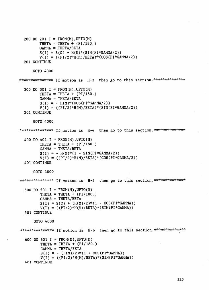
200 DO 201 I = FROM(M),UPTO(M)THETA = THETA + (PI/180.)GAMMA = THETA/BETAS(I) = S(C) + H(M)*(SIN(PI*GAMMA/2))V(I) = ((PI/2)*H(M)/BETA)*(COS(PI*GAMMA/2))201 CONTINUE V
GOTO 4000I f mot ion is H- 3 then go to S ect
ion300DO 301 I = FROM(M),UPTO(M)THETA = THETA + (PI/180.)GAMMA = THETA/BETAS(I) = · H(M)*(COS(PI*GAMMA/2))V(I) = ((PI/2)*H(M)/BETA)*(SIN(PI*GAMMA/2))301 CONTINUE ~
GOTO 4000*************** If motion is H-4 then go to this section.************** .
400 DO 401 I = FROM(M),UPTO(M)THETA = THETA + (PI/180.)GAMMA = THETA/BETAS(I) = · H(M)*(1 - SIN(PI*GAMMA/2))V(I) = ((PI/2)*H(M)/BETA)*(COS(PI*GAMMA/2))401 CONTINUEGOTO 4000 V
*************** If motion is H—5 then go to this section.**************
500 DO 501 I = FROM(M),UPTO(M)THETA = THETA + (PI/180.)GAMMA = THETA/BETAS(I) = S(C) + (H(M)/2)*(1 - COS(PI*GAMMA))V(I) = ((PI/2)*H(M)/BETA)*(SIN(PI*GAMMA))501 CONTINUE
GOTO 4000*%%*****7%******* I f mot ion is H- 6 then go to is Sect ion _ *7‘f7°€7'€7'¥7':7'f7‘$%°f7°€7%?‘¢7’f7°f
‘ 600 DO 601 I = FROM(M),UPTO(M)THETA = THETA + (PI/180.) ·GAMMA = THETA/BETAS(I) = - (H(M)/2)*(1 + COS(PI*GAMMA))V(I) = ((PI/2)*H(M)/BETA)*(SIN(PI*GAMMA))60 1 CONTINUE
125
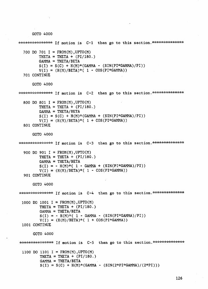
- GOTO 4000 _
If motion is Q-} thon go tothis700
DO 701 I = FROM(M),UPTO(M)THETA = THETA + (PI/180.)GAMMA = THETA/BETAS(I) = S(C) + H(M)*(GAMMA - (SIN(PI*GAMMA)/PI))V(I) = (H(M)/BETA)*( 1 - COS(PI*GAMMA)) „
701 CONTINUE .
GOTO 4000
I f mot ion is C • 2 then go to is S ection800
DO 801 I = FROM(M),UPTO(M) ·THETA = THETA + (PI/180.)GAMMA = THETA/BETAS(I) = S(C) + H(M)*(GAMMA + (SIN(PI*GAMMA)/PI))V(I) = (H(M)/BETA)*( 1 + COS(PI*GAMMA))
801 CONTINUE
GOTO 4000
I f mot ion is C • 3 then go to sect
ion900DO 901 I = FROM(M),UPTO(M)THETA = THETA + (PI/180.)GAMMA = THETA/BETAS(I) = · H(M)*( 1 - GAMMA + (SIN(PI*GAMMA)/PI))V(I) = (H(M)/BETA)*( 1 - COS(PI*GAMMA))
901 CONTINUE
GOTO 40004
*************** If motion is C-4 then go tothis1000
DO 1001 I = FROM(M),UPTO(M)THETA = THETA + (PI/180.)GAMMA = THETA/BETAS(I) = — H(M)*( 1 · GAMMA - (SIN(PI*GAMMA)/PI))V(I) = (H(M)/BETA)*( 1 + COS(PI*GAMMA))
1001 CONTINUE
GOTO 4000
If motion is C·5 then go tothis1100
DO 1101 I = FROM(M),UPTO(M)THETA = THETA + (PI/180.)GAMMA =THETA/BETAS(I)
= S(C) + H(M)*(GAMMA — (SIN(2*PI*GAMMA)/(2*PI)))
126 ‘
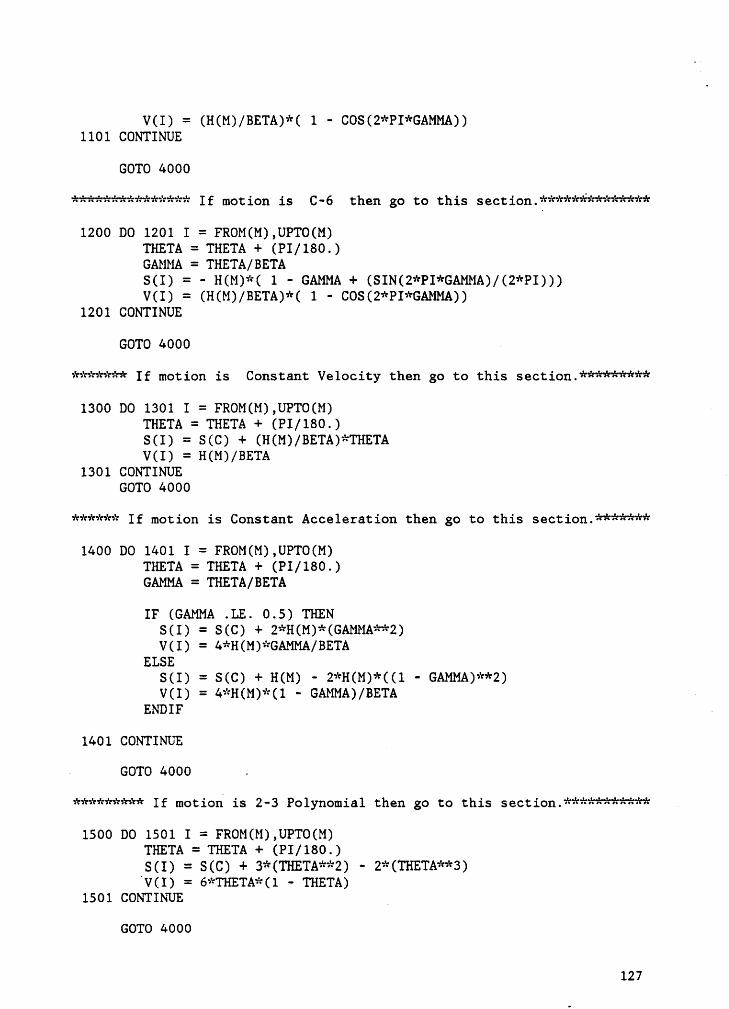
V(I) = (H(M)/BETA)*( 1 — COS(2*PI*GAMMA))1101 CONTINUE
GOTO 4000
*************** If motion is C-6 then go to this section.#*************1200 DO 1201 I = FROM(M),UPTO(M)
THETA = THETA + (PI/180.)GAMMA = THETA/BETAS(I) = - H(M)*( 1 · GAMMA + (SIN(2*PI*GAMMA)/(2*PI)))V(I) = (H(M)/BETA)*( 1 · COS(2*PI*GAMMA))
1201 CONTINUE
GOTO 4000 «
******* If motion is Constant Velocity then go to this section.*********1300 DO 1301 I = FROM(M),UPTO(M)
THETA = THETA + (PI/180.)S(I) = S(C) + (H(M)/BETA)*THETAV(I) = H(M)/BETA
1301 CONTINUEGOTO 4000
****** If motion is Constant Acceleration then go to this section.*******1400 DO 1401 I = FROM(M),UPTO(M)
THETA = THETA + (PI/180.)GAMMA = THETA/BETA
IF (GAMMA .LE. 0.5) THENS(I) = S(C) + 2*H(M)*(GAMMA**2)V(I) = 4*H(M)*GAMMA/BETA
ELSES(I) = S(C) + H(M) - 2*H(M)*((l · GAMMA)**2)V(I) = 4*H(M)*(1 - GAMMA)/BETA
ENDIF -
1401 CONTINUE
- GOTO 4000 .
********* If motion is 2-3 Polynomial then go to this section.***********1500 DO 1501 I = FROM(M),UPTO(M)
THETA = THETA + (PI/180.)S(I) = S(C) + 3*(THETA**2) - 2*(THETA**3)”V(I)
= 6*THETA*(1 - THETA)1501 CONTINUE _
GOTO 4000
127
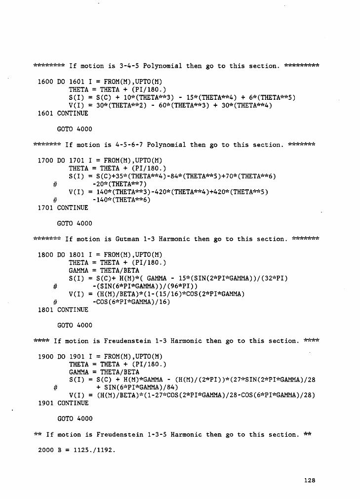
******** If motion is 3-4-S Polynomial then go to this section. *********h
1600 DO 1601 I = FROM(M),UPTO(M)THETA = THETA + (PI/180.)S(I) = S(C) + 10*(THETA**3) - 15*(THETA**4) + 6*(THETA**5) „V(I) = 30*(THETA**2) - 60*(THETA**3) + 30*(THETA**4)
1601 CONTINUE
GOTO 4000
******* If motion is 4-5-6-7 Polynomial then go to this section. *******1700 DO 1701 I = FROM(M),UPTO(M)
THETA = THETA + (PI/180.)$(1) = S(C)+35*(THETA**4)-84*(THETA**5)+70*(THETA**6)
# -20*(THETA**7)V(I) = 140*(THETA**3)-420*(THETA**4)+420*(THETA**5)
# -140*(THETA**6)1701 CONTINUE _GOTO 4000
******* If motion is Gutman 1-3 Harmonic then go to this section. *******1800 DO 1801 I = FROM(M),UPTO(M)
THETA = THETA + (PI/180.)GAMMA = THETA/BETA$(1) = S(C)+ H(M)*( GAMMA - 15*(SIN(2*PI*GAMMA))/(32*PI)
# -(SIN(6*PI*GAMMA))/(96*P1))V(I) = (H(M)/BETA)*(1-(15/16)*COS(2*PI*GAMMA)
- # -COS(6*PI*GAMMA)/16)1801 CONTINUE
GOTO 4000
**** If motion is Freudenstein 1-3 Harmonic then go to this section. ****1900 DO 1901 I = FROM(M),UPTO(M)
A
THETA = THETA + (PI/180.)GAMMA = THETA/BETA$(1) = S(C) + H(M)*GAMMA - (H(M)/(2*PI))*(27*S1N(2*PI*GAMMA)/28
# + SIN(6*PI*GAMMA)/84)V(I) = (H(M)/BETA)*(1-27*COS(2*PI*GAMMA)/28-COS(6*PI*GAMMA)/28)
1901 CONTINUE
GOTO 4000
** If motion is Freudenstein 1-3-5 Harmonic then go to this section. **2000 B = 1125./1192.
128
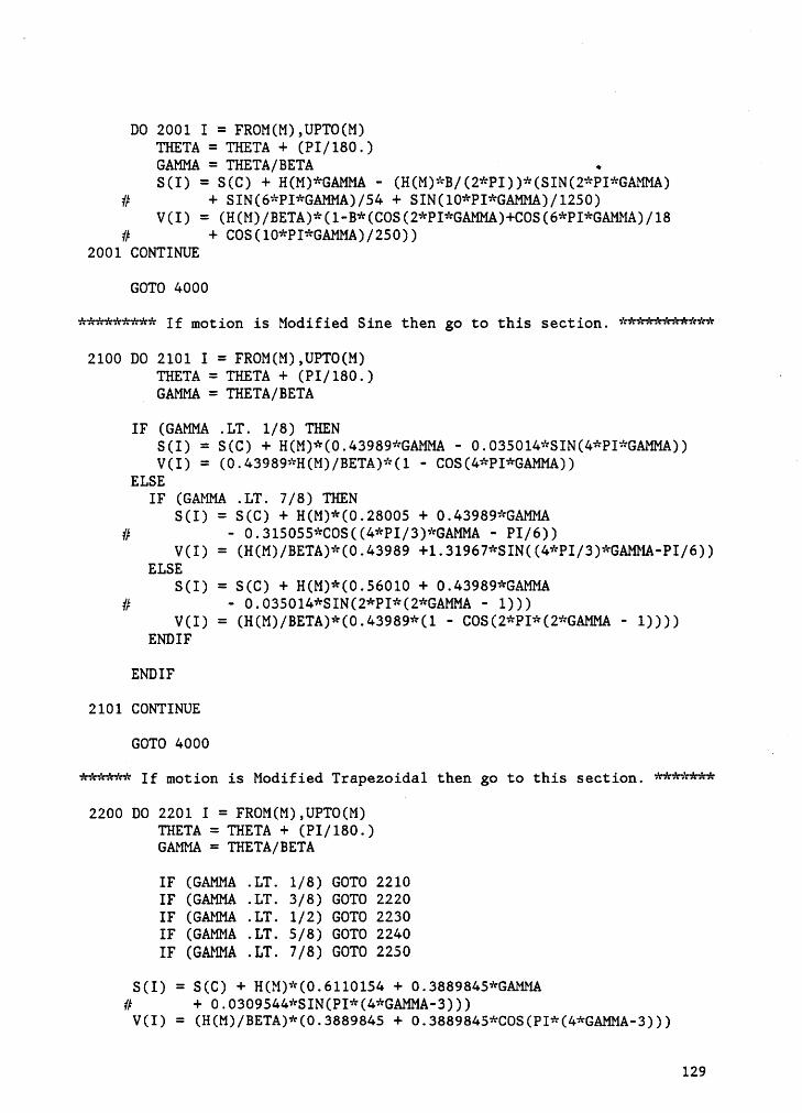
DO 2001 I = FROM(M),UPTO(M)THETA = THETA + (PI/180.)GAMMA = THETA/BETA •S(I) = S(C) + H(M)*GAMMA — (H(M)*B/(2*PI))*(SIN(2*PI*GAMMA)
# + SIN(6*PI*GAMMA)/54 + SIN(10*PI*GAMMA)/1250)V(I) = (H(M)/BETA)*(1-B*(COS(2*PI*GAMMA)+COS(6*PI*GAMMA)/18
# + COS(10*PI*GAMMA)/250))2001 CONTINUE
GOTO 4000
********* If motion is Modified Sine then go to this section. ***********2100 DO 2101 I = FROM(M),UPTO(M)
THETA = THETA + (PI/180.) ·_ GAMMA = THETA/BETA
IF (GAMMA .LT. 1/8) THEN$(1) = S(C) + H(M)*(0.43989*GAMMA · 0.035014*S1N(4*P1*GAMMA))V(I) = (0.43989*H(M)/BETA)*(l · COS(4*PI*GAMMA))
ELSEIF (GAMMA .LT. 7/8) THEN
S(I) = S(C) + H(M)*(0.2800S + 0.43989*GAMMA# - 0.3l5055*COS((4*PI/3)*GAMMA - PI/6))
V(I) = (H(M)/BETA)*(0.43989 +1.31967*SIN((4*PI/3)*GAMMA—PI/6))ELSE
S(I) = S(C) + H(M)*(0.56010 + 0.43989*GAMMA# · 0.035014*SIN(2*PI*(2*GAMMA · 1)))
V(I) = (H(M)/BETA)*(0.43989*(1 - COS(2*PI*(2*GAMMA — 1))))ENDIF
ENDIF
2101 CONTINUE
GOTO4000******If motion is Modified Trapezoidal then go to this section. *******
‘
2200 DO 2201 I = FROM(M),UPTO(M)THETA = THETA + (PI/180.)GAMMA = THETA/BETA
IF (GAMMA .LT. 1/8) GOTO 2210IF (GAMMA .LT. 3/8) GOTO 2220IF (GAMMA .LT. 1/2) GOTO 2230IF (GAMMA .LT. 5/8) GOTO 2240IF (GAMMA .LT. 7/8) GOTO 2250
S(I) = S(C) + H(M)*(0.6110154 + 0.3889845*GAMMA# + 0.0309544*SIN(PI*(4*GAMMA-3)))V(I) = (H(M)/BETA)*(0.388984S + 0.3889845*COS(PI*(4*GAMMA-3)))
129
GOTO 2201E
2210 S(I) = S(C) + 0.09724612*H(M)*(4*GAMMA · SIN(4*PI*GAMMA)/PI)V(I) = (0.3889845*H(M)/BETA)*(1 - COS(4*PI*GAMMA))GOTO 2201
2220 S(I) = S(C) + H(M)*(2.44406184*(GAMMA**2) • 0.22203097*GAMMA# + 0.00723407)V(I) = (H(M)/BETA)*(4.888124*GAMMA - 0.222031)GOTO 2201
2230 S(I) = S(C) + H(M)*(1.6110154*GAMMA·0.0309544*SIN(PI*(4*GAMMA·1))# · 0.3055077)A V(I) = (H(M)/BETA)*(l.6110154 - 0.3889845*COS(PI*(4*GAMMA - 1)))
GOTO 22012240 S(I) = S(C) + H(M)*(l.6l10154*GAMMA+0.0309544*SIN(PI*(4*GAMMA-2))
# - 0.3055077)V(I) = (H(M)/BETA)*(1.6l10154 + 0.3889845*COS(PI*(4*GAMMA - 2)))GOTO 2201
2250 S(I) = S(C) + H(M)*(4.6660917*GAMMA · 2.44406184*(GAMMA**2)# - 1.2292648) _V(I) = (H(M)/BETA)*(4.6660917 - 4.888124*GAMMA)
2201 CONTINUE
4000 CONTINUE
RETURN
>END
.kkkkkkkkkkkkkkkkkkkkkkkkkkkkkkkkkkkkkkkkkkkkkkkkkkkkkkkkkkkkkkkkkkkkkkk
kk kk** SUBROUTINE CURVES **kk kkkkkkkkkkkkkkkkkkkkkkkkkkkkkkkkkkkkkkkkkkkkkkkkkkkkkkkkkkkkkkkkkkkkkkkkkkkkkkkkkkkkkkkkkkkkkkkkkkkkkkkkkkkkkkkkkkkkkkkkkkkkkkkkkkkkkkkkkkkkkkkkkkkk kk
** THIS SUBROUTINE COMPUTES THE ACCELERATION OF AND JERK ON ****
” THE FOLLOWER AT ONE DEGREE INTERVALS. THE SUBROUTINE IS **** STRUCTURED SUCH THAT THE CALCULATIONS FOR EACH SEGMENT ARE **** DONE INSIDE A DO LOOP. THIS SUBROUTINE IS NOT REQUIRED IN **** ALL THE DISPLAY OPTIONS CHOSEN BY THE USER. HOWEVER IT MUST **** BE CALLED IN CASE THE USER DECIDES TO DOCUMENT THE DATA. **kk kkkkkkkkkkkkkkkkkkkkkkkkkkkkkkkkkkkkkkkkkkkkkkkkkkkkkkkkkkkkkkkkkkkkkkkkkkkkkkkkkkkkkkkkkkkkkkkkkkkkkkkkkkkkkkkkkkkkkkkkkkkkkkkkkkkkkkkkkkkkkkkkkk
SUBROUTINE CURVES ~
COMMON/CAM1/ TYPE, BASE, RPM, WIDTH, DESI, ROLL, ECC, RA, RFCOMMON/COUNT/ I, N, M, B, PI, C, R, L '
130
COMMON/ANGLE/ BETA, THETA, GAMMACOMMON/MTN/ E(25), H(20), FROM(20), UPTO(20)COMMON/CRV/ $(360), V(360), A(360), J(360)COMMON/COOD/ ALPHA(360), X(361), Y(361), Z(361)COMMON/DISP/ OUT, MONI
INTEGER I, N, M, C, R‘
INTEGER TYPE, OUT, DESI, MONI —INTEGER E, FROM, UPTOREAL BETA, THETA, GAMMA, B, PI, BASE, RPM, WIDTHREAL ROLL, ECC, RA, RFREAL S, V, A, JREAL ALPHA, X, Y, Z, H
00 4000 M= 1,N ·BETA = (UPTO(M) - UPTO(M-1))*PI/180.C = UPTO(M-1)THETA = 0.
GO TO (100,200,300,400,500,600,700,800,900,1000,1100,1200,1300,# 1400,1500,1600,1700,1800,1900,2000,2100,2200),E(M)
*************** If motion is DWELL then go to this section.**************
DO 11 I = FROM(M),UPTO(M)THETA = THETA + (PI/180.)GAMMA = THETA/BETAA(I) = 0.J(I) = 0.
11 CONTINUEGOTO 4000
*************** If motion is H-1 then go to this section.**************
100 DO 101 I = FROM(M),UPTO(M)THETA = THETA + (PI/180.)GAMMA = THETA/BETA
_ A(I) = H(M)*((PI*0.5/BETA)**2)*(COS(PI*GAMMA/2))J(I) = —H(M)*((PI*0.5/BETA)**3)*(SIN(PI*GAMMA/2))
101 CONTINUEGOTO 4000
*************** If motion is H-2 then go to this section.**************
' 200 DO 201 I = FROM(M),UPTO(M)H
THETA = THETA + (PI/180.)GAMMA = THETA/BETAA(I) = -((PI/(2*BETA))**2)*H(M)*(SIN(PI*GAMMA/2))J(I) = -H(M)*((PI*0.5/BETA)**3)*(COS(PI*GAMMA/2))
201 CONTINUEGOTO 4000
131
I f mot ion is H•3 then go to is S ection300
DO 301 I = FROM(M),UPTO(M)THETA = THETA + (PI/180.)GAMMA = THETA/BETAA(I) = ((PI/(2*BETA))**2)*H(M)*(COS(PI*GAMMA/2))J(I) = -H(M)*((PI*0.5/BETA)**3)*(SIN(PI*GAMMA/2))
301 CONTINUEGOTO 4000
*************** If motion is H·4 then go tothis400
DO 401 I = FROM(M),UPTO(M) °THETA = THETA + (PI/180.)
— GAMMA = THETA/BETAA(I) = -((PI/(2*BETA))**2)*H(M)*(SIN(PI*GAMMA/2))J(I) = - H(M)*((PI*0.5/BETA)**3)*(COS(PI*GAMMA/2))
401 CONTINUEGOTO 4000
I f mot ion is H•5 then go to S Sect
ion500DO 501 I = FROM(M),UPTO(M)THETA = THETA + (PI/180.)GAMMA = THETA/BETAA(I) = 2*((PI/(2*BETA))**2)*H(M)*(COS(PI*GAMMA))J(I) = -4*((PI/(2*BETA))**3)*H(M)*(SIN(PI*GAMMA))
501 CONTINUEGOTO 4000
I f mot ion is H•6 then go to is S ection600
DO 601 I = FROM(M),UPTO(M)THETA = THETA + (PI/180.)GAMMA = THETA/BETAA(I) = 2*((PI/(2*BETA))**2)*H(M)*(COS(PI*GAMMA))J(I) = -4*((PI/(2*BETA))**3)*H(M)*(SIN(PI*GAMMA))
601 CONTINUEGOTO 4000 D
*************** If motion is C·l then go to this section.**************700 D0 701 I = FROM(M),UPTO(M)
THETA = THETA + (PI/180.)GAMMA = THETA/BETAA(I) = (PI/BETA)*(H(M)/BETA)*(SIN(PI*GAMMA))J(I) = ((PI/BETA)**2)*(H(M)/BETA)*(COS(PI*GAMMA))
701 CONTINUE DGOTO 4000
_ *************** If motion is C-2 then go to this132
800 DO 801 I = FROM(M),UPTO(M)” THETA = THETA + (PI/180.)GAMMA = THETA/BETAA(I) = -(PI/BETA)*(H(M)/BETA)*(SIN(PI*GAMMA)) .J(I) = -((PI/BETA)**2)*(H(M)/BETA)*(COS(PI*GAMMA))
801 CONTINUEGOTO 4000 _*************** If motion is C·3 then go to this section.**************
900 DO 901 I = FROM(M),UPTO(M)THETA = THETA + (PI/180.)GAMMA = THETA/BETAA(I) = (PI/BETA)*(H(M)/BETA)*(SIN(PI*GAMMA))J(I) = ((PI/BETA)**2)*(H(M)/BETA)*(COS(PI*GAMMA))
901 CONTINUEGOTO 4000
If motion is C-Q then go tothis1000
DO 1001 I = FROM(M),UPTO(M)THETA = THETA + (PI/180.)GAMMA = THETA/BETAA(I) = ·(PI/BETA)*(H(M)/BETA)*(SIN(PI*GAMMA))J(I) = ·((PI/BETA)**2)*(H(M)/BETA)*(COS(PI*GAMMA))
1001 CONTINUEGOTO 4000*************** If motion is C-5 then go to this section.**************
1100 DO 1101 I = FROM(M),UPTO(M)THETA = THETA + (PI/180.)GAMMA = THETA/BETAA(I) = 2*(PI/BETA)*(H(M)/BETA)*(SIN(2*PI*GAMMA))J(I) = ((2*(PI/BETA))**2)*(H(M)/BETA)*(COS(2*PI*GAMMA))
1101 CONTINUEGOTO 4000*************** If motion is C-6 then go to this section.**************
11200 DO 1201 I = FROM(M),UPTO(M) »
THBTA = THETA + (PI/180.) 'GAMMA = THETA/BETAA(I) = 2*(PI/BETA)*(H(M)/BETA)*(SIN(2*PI*GAMMA))
~‘ J(I) = ((2*(PI/BETA))**2)*(H(M)/BETA)*(COS(2*PI*GAMMA))1201 CONTINUEGOTO 4000 _
******* If motion is Constant Velocity then go to this section.*********
1300 DO 1301 I = FROM(M),UPTO(M)
133
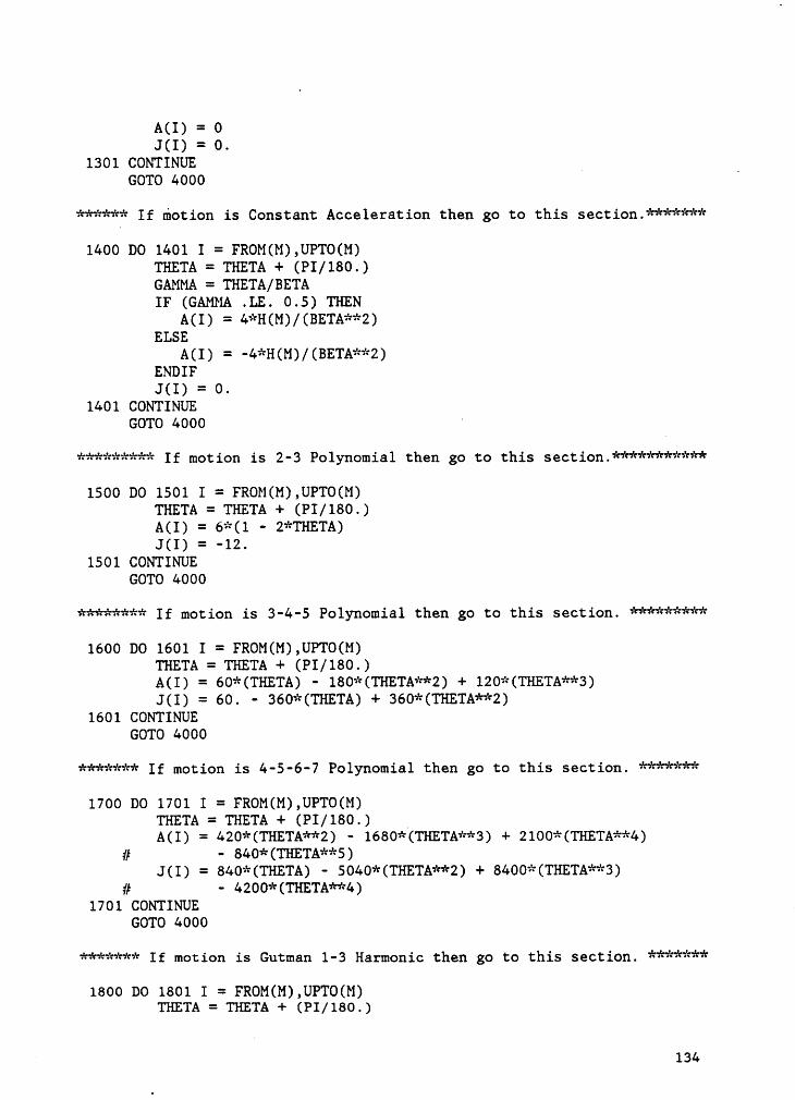
A(I) = 0J(I) = 0.
1301 CONTINUE _GOTO 4000 ”****** If motion is Constant Acceleration then go to this section.*******
1400 DO 1401 I = FROM(M),UPTO(M)THETA = THETA + (PI/180.)GAMMA = THETA/BETAIF (GAMMA .LE. 0.5) THEN
A(I) = 4*H(M)/(BETA**2)ELSEA(I) = -4*H(M)/(BETA**2)ENDIF
J(I) = O.1401 CONTINUEGOTO 4000 ‘********* If motion is 2-3 Polynomial then go to this section.***********
1500 DO 1501 I = FROM(M),UPTO(M)THETA = THETA + (PI/180.)A(I) = 6*(1 · 2*THETA)J(I) = -12.1501 CONTINUEGOTO 4000
******** If motion is 3-4-S Polynomial then go to this section. *********
1600 DO 1601 I = FROM(M),UPTO(M)THETA = THETA + (PI/180.)A(I) = 60*(THETA) · 180*(THETA**2) + l20*(THETA**3)J(I) = 60. - 360*(THETA) + 360*(THETA**2)1601 CONTINUEGOTO 4000
******* If motion is 4-5-6-7 Polynomial then go to this section. *******
1700 DO 1701 I = FROM(M),UPTO(M)THETA = THETA +(PI/180.)A(I)
= 420*(THETA**2) - 1680*(THETA**3) + 2l00*(THETA**4)# - 840*(THETA**5)
J(I) = 840*(THETA) - 5040*(THETA**2) + 8400*(THETA**3)# - 4200*(THETA**4)1701 CONTINUEGOTO 4000 ‘
******* If motion is Gutman 1-3 Harmonic then go to this section. *******
1600 00 1801 1 = FROM(M),UPTO(M)THETA = THETA + (PI/180.)
134
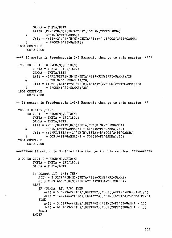
GAMMA = THETA/BETAA(I)= (PI/8)*H(M)/(BETA**2)*(15*SIN(2*PI*GAMMA)
# +3*SIN(6*PI*GAMMA)) ”J(I) = ((PI**2)/4)*(H(M)/(BETA**3))*( l5*COS(2*PI*GAMMA)
# + 9*COS(6*PI*GAMMA))1801 CONTINUE
GOTO 4000
**** If motion is Freudenstein 1-3 Harmonie then go to this section. ****1900 DO 1901 I = FROM(M),UPTO(M)
THETA = THETA + (PI/180.)GAMMA = THETA/BETAA(I) = (2*PI/BETA)*(H(M)/BETA)*(27*SIN(2*PI*GAMMA)/28# + 3*SIN(6*PI*GAMMA)/28)J(I) = ((2*PI/BETA)**2)*(H(M)/BETA)*(27*COS(2*PI*GAMMA)/28
# + 9*COS(6*PI*GAMMA)/28)1901 CONTINUE
l
GOTO 4000
** If motion is Frendenstein 1-3-5 Harmonie then go to this section. **
2000 B = 1125./1192.DO 2001 I = FROM(M),UPTO(M)
THETA = THETA + (PI/180.)GAMMA = THETA/BETAA(I) = (2*PI/BETA)*(H(M)/BETA)*B*(SIN(2*PI*GAMMA)
# + SIN(6*PI*GAMMA)/6 + SIN(l0*PI*GAMMA)/S0)J(I) = ((2*PI/BETA)**2)*(H(M)/BETA)*B*(COS(2*PI*GAMMA)
# + COS(6*PI*GAMMA)/2 + COS(10*PI*GAMMA)/10)2001 CONTINUE
GOTO 4000
********* If motion is Modified Sine then go to this section. ***********2100 DO 2101 I = FROM(M),UPTO(M)
THETA = THETA + (PI/180.)GAMMA = THETA/BETA
IF (GAMMA .LT. 1/8) THENAU) = 5-5279‘+*(H(l‘i)/(BETA°'*"‘2))=‘=SIN(4='*PI='=GAMMA)J(I) = 69.4659*(H(M)/(BETA**3))*COS(4*PI*GAMMA)
ELSE _IF (GAMMA .LT. 7/8) THEN
A(I) = 5.52794*(H(M)/(BETA**2))*COS((4*PI/3)*GAMMA-PI/6)' J(I) = -23.1553*(H(M)/(BETA**3))*SIN((4*PI/3)*GAMMA-PI/6)
ELSEA(I) = 5.52794*(H(M)/(BETA**2))*SIN(2*PI*(2*GAMMA — 1))J(I) = 69.46S9*(H(M)/(BETA**3))*COS(2*PI*(2*GAMMA — 1))
ENDIFENDIF
135
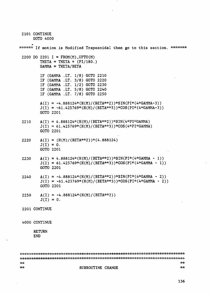
2101 CONTINUE 1GOTO 4000
*****£ If motion is Modified Trapezoidal then go to this section. *******
2200 DO 2201 I = FROM(M),UPTO(M)THETA = THETA + (PI/180.)GAMMA = THETA/BETA
IF (GAMMA .LT. 1/8) GOTO 2210 ·IF (GAMMA .LT. 3/8) GOTO 2220IF (GAMMA .LT. 1/2) GOTO 2230IF (GAMMA .LT. 5/8) GOTO 2240IF (GAMMA .LT. 7/8) GOTO 2250
A(I) = -4.888124*(H(M)/(BETA**2))*SIN(PI*(4*GAMMA-3))J(I) = -61.425769*(H(M)/(BETA**3))*COS(PI*(4*GAMMA·3))GOTO 2201
2210 A(I) = 4.888124*(H(M)/(BETA**2))*SIN(4*PI*GAMMA)J(I) = 61.425769*(H(M)/(BETA**3))*COS(4*PI*GAMMA)GOTO 2201
2220 A(I) = (H(M)/(BETA**2))*(4.888124)J(I) = O.GOTO 2201 A
2230 A(I) = 4.888124*(H(M)/(BETA**2))*SIN(PI*(4*GAMMA - 1))J(I) = 61.425769*(H(M)/(BETA**3))*COS(PI*(4*GAMMA - 1)) ·GOTO 2201
2240 A(I) = -4.888124*(H(M)/(BETA**2))*SIN(PI*(4*GAMMA - 2))J(I) = -61.425769*(H(M)/(BETA**3))*COS(PI*(4*GAMMA - 2))GOTO 2201
2250 A(I) = -4.888124*(H(M)/(BETA**2))J(I) = 0. ·
2201 CONTINUE
4000 CONTINUE
RETURNEND
*«**ne«*«*****««***««*««***«*&*««**«§««**«**w*«*«**##*«****#«#«***«*«***
«* **** SUBROUTINE CHANGE **
_ 136
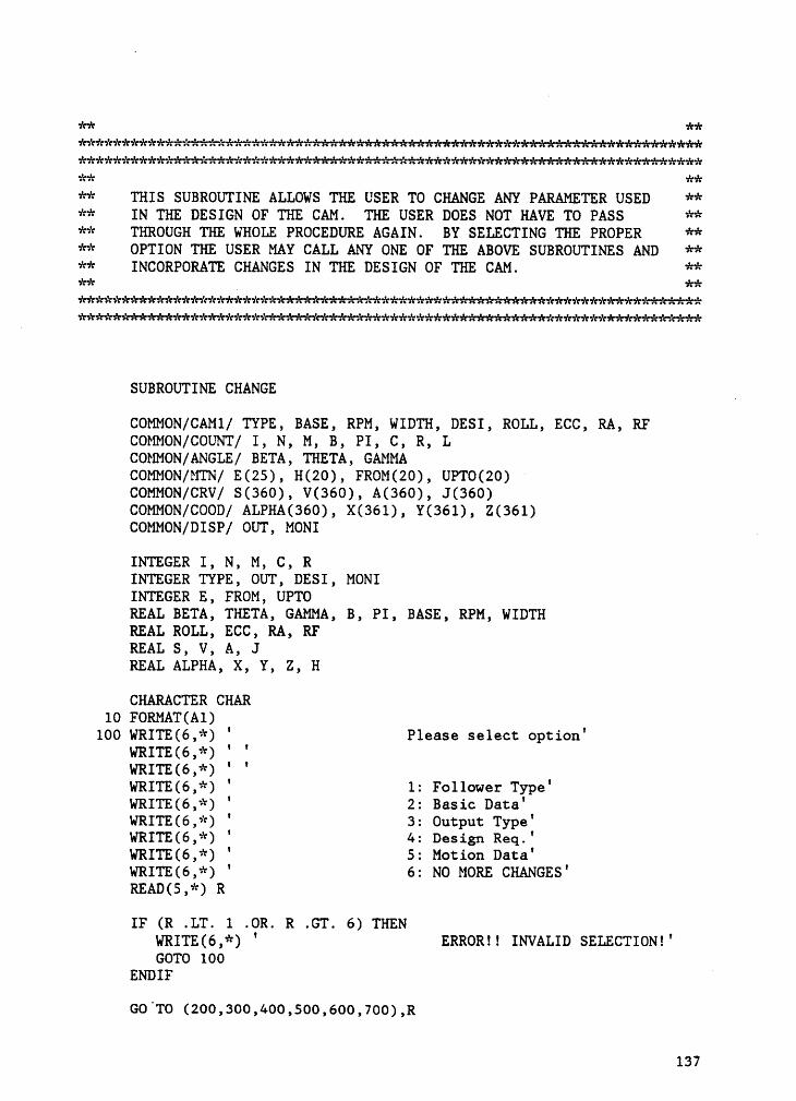
#* **
wa kk** THIS SUBROUTINE ALLOWS THE USER TO CHANGE ANY PARAMETER USED **** IN THE DESIGN OF THE CAM. THE USER DOES NOT HAVE TO PASS **** THROUGH THE WHOLE PROCEDURE AGAIN. BY SELECTING THE PROPER **** OPTION THE USER MAY CALL ANY ONE OF THE ABOVE SUBROUTINES AND **** INCORPORATE CHANGES IN THE DESIGN OF THE CAM. **kk kküwwwwkwwwww***«#w**«w#««**#«***«w#*«#«*«wa***«**#*«****«*««*«*«****w**«*
SUBROUTINE CHANGE _COMMON/CAMl/ TYPE, BASE, RPM, WIDTH, DESI, ROLL, ECC, RA, RFCOMMON/COUNT/ I, N, M, B, PI, C, R, LCOMMON/ANGLE/ BETA, THETA, GAMMACOMMON/MTN/ E(2S), H(20), FROM(20), UPTO(20) ‘COMMON/CRV/ S(360), V(360), A(360), J(360)COMMON/COOD/ ALPHA(360), X(361), Y(361), Z(361)COMMON/DISP/ OUT, MONI .
INTEGER I, N, M, C, RINTEGER TYPE, OUT, DESI, MONIINTEGER E, FROM, UPTOREAL BETA, THETA, GAMMA, B, PI, BASE, RPM, WIDTHREAL ROLL, ECC, RA, RFREAL S, V, A, JREAL ALPHA, X, Y, Z, H
CHARACTER CHAR10 FORMATCAI)
100 WRITE(6,*) ° Please select option'WRITE(6,*) ' 'WRITE(6,*) ° °WRITE(6,*) ' 1; Follower Type'WRITE(6,*) ' 2; Basic Data'WRITE(6,*) ' 3: Output Type'WRITE(6,*) ° 4: Design Req.°WRITE(6,*) ° 5: Motion Data'WRITE(6,*) ° 6: NO MORE CHANGES°READ(S,*) R
IF (R .LT. 1 .OR. R .GT. 6) THENWRITE(6,*) ' ERROR!! INVALID SELECTION!°GOTO 100
ENDIF
GO TO (200,300,400,S00,600,700),R
137
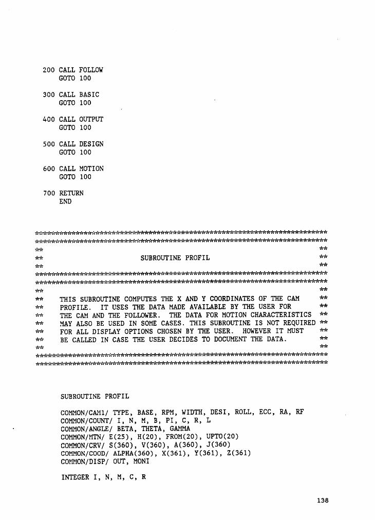
200 CALL FOLLOWGOTO 100
300 CALL BASICGOTO 100 °
&00 CALL OUTPUTGOTO 100
500 CALL DESIGNGOTO 100
600 CALL MOTIONGOTO 100
700 RETURNEND
kkkkkkkkkkkkkkkkkkkkkkkkkkkkkkkkkkkkkkkkkkkkkkkkkkkkkkkkkkkkkkkkkkkkkkkkkkkkkkkkkkkkkkkkkkkkkkkkkkkkkkkkkkkkkkkkkkkkkkkkkkkkkkkkkkkkkkkkkkkkkkkkkk kk
** SUBROUTINE PROFIL **kk kk
kk kk** THIS SUBROUTINE COMPUTES THE X AND Y COORDINATES OF THE CAM **** PROFILE. IT USES THE DATA MADE AVAILABLE BY THE USER FOR **** THE CAM AND THE FOLLOWER. THE DATA FOR MOTION CHARACTERISTICS **** MAY ALSO BE USED IN SOME CASES. THIS SUBROUTINE IS NOT REQUIRED **** FOR ALL DISPLAY OPTIONS CHOSEN BY THE USER. HOWEVER IT MUST **** BE CALLED IN CASE THE USER DECIDES TO DOCUMENT THE DATA. **kk kkkkkkkkkkkkkkkkkkkkkkkkkkkkkkkkkkkkkkkkkkkkkkkkkkkkkkkkkkkkkkkkkkkkkkkkkkkkkkkkkkkkkkkkkkkkkkkkkkkkkkkkkkkkkkkkkkkkkkkkkkkkkkkkkkkkkkkkkkkkkkkkkk
SUBROUTINE PROFIL
COMMON/CAMl/ TYPE, BASE, RPM, WIDTH, DESI, ROLL, ECC, RA, RFCOMMON/COUNT/ I, N, M, B, PI, C, R, L
‘ COMMON/ANGLE/ BETA, THETA, GAMMACOMMON/MTN/ E(25), H(20), FROM(20), UPTO(20)COMMON/CRV/ $(360), V(360), A(360), J(360)COMMON/COOD/ ALPHA(360), X(361), Y(361), Z(36l)COMMON/DISP/ OUT, MONI
INTEGER I, N, M, C, R
138
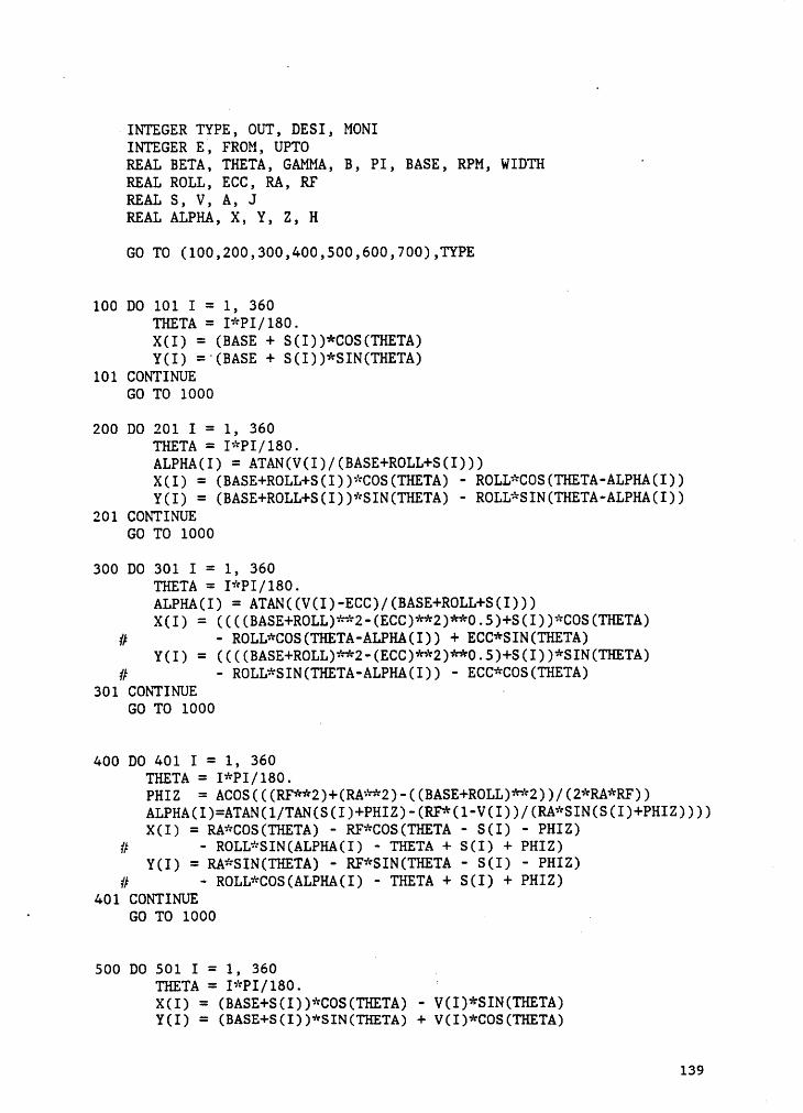
—INTEGER TYPE, OUT, DESI, MONIINTEGER E, FROM, UPTOREAL BETA, THETA, GAMMA, B, PI, BASE, RPM, WIDTH ‘REAL ROLL, ECC, RA, RFREAL S, V, A, JREAL ALPHA, X, Y, Z, H
GO TO (100,200,300,400,500,600,700),TYPE
100 DO 101 I = 1, 360THETA = I*PI/180.X(I) = (BASE + S(I))*COS(THETA)Y(I) = (BASE + S(I))*SIN(THETA)
101 CONTINUEGO TO 1000
200 DO 201 I = 1, 360THETA = I*PI/180.ALPHA(I) = ATAN(V(I)/(BASE+ROLL+S(I)))X(I) = (BASE+ROLL+S(I))*COS(THETA) · ROLL*COS(THETA·ALPHA(I))Y(I) = (BASE+ROLL+S(I))*SIN(THETA) - ROLL*SIN(THETA-ALPHA(I))
201 CONTINUEGO TO 1000 _
300 DO 301 I = 1, 360THETA = I*PI/180.ALPHA(I) = ATAN((V(I)-ECC)/(BASE+ROLL+S(I)))X(I) = ((((BASE+ROLL)**2-(ECC)**2)**0.5)+S(I))*COS(THETA)
# - ROLL*COS(THETA·ALPHA(I)) + ECC*SIN(THETA)Y(I) = ((((BASE+ROLL)**2—(ECC)**2)**0.5)+S(I))*SIN(THETA)
# — ROLL*SIN(THETA·ALPHA(I)) - ECC*COS(THETA)301 CONTINUE -
GO TO 1000
400 DO 401 I = 1, 360THETA = I*PI/180.PHIZ = ACOS(((RF**2)+(RA**2)-((BASE+ROLL)**2))/(2*RA*RF))
_ ALPHA(I)=ATAN(1/TAN(S(I)+PHIZ)-(RF*(l-V(I))/(RA*SIN(S(I)+PHIZ))))X(I) = RA*COS(THETA) - RF*COS(THETA - S(I) · PHIZ)
# · ROLL*SIN(ALPHA(I) - THETA + S(I) + PHIZ)Y(I) = RA*SIN(THETA) - RF*SIN(THETA - S(I) - PHIZ) „
# - ROLL*COS(ALPHA(I) - THETA + S(I) + PHIZ)401 CONTINUE‘ GO TO 1000 .
500 DO 501 I = 1, 360 „THETA = I*PI/180. ’X(I) = (BASE+S(I))*COS(THETA) - V(I)*SIN(THETA)Y(I) = (BASE+S(I))*SIN(THETA) + V(I)*COS(THETA)
139
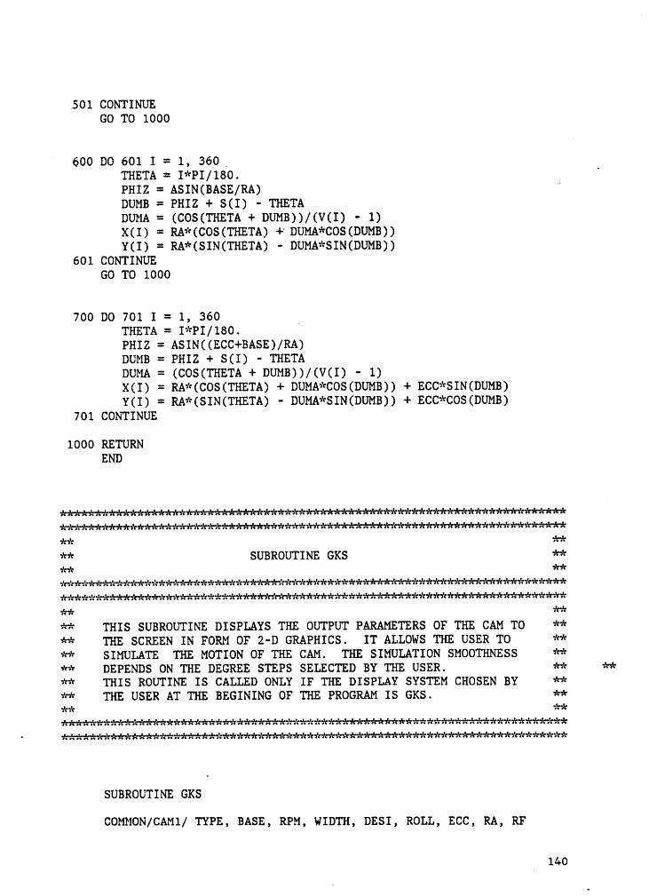
501 CONTINUEGO TO 1000
I 600 DO 601 I = 1, 360,THETA = I*PI/180.
”
PHIZ = ASIN(BASE/RA)DUMB = PHIZ + S(I) · THETADUMA = (COS(THETA + DUMB))/(V(I) · 1)X(I) = RA*(COS(THETA) +°DUMA*COS(DUMB))Y(I) = RA*(SIN(THETA) · DUMA*SIN(DUMB))
601 CONTINUEGO TO 1000
700 DO 701 I = 1, 360THETA = I*PI/180.PHIZ = ASIN((ECC+BASE)/RA)DUMB = PHIZ + S(I) · THETADUMA = (COS(THETA + DUMB))/(V(I) - 1)X(I) = RA*(COS(THETA) + DUMA*COS(DUMB)) + ECC*SIN(DUMB)Y(I) = RA*(SIN(THETA) - DUMA*SIN(DUMB)) + ECC*COS(DUMB)
701 CONTINUE
1000 RETURNEND
kkkkkkkkkkkkkkkkkkkükkkkkükkkk*%*****#%*#*****##**
** **** SUBROUTINE GKS **«* «*kkkükkkäkkükkükkük*%#****k*%*%k********#***kkkäkkkkk
*****««***w*«*«««**«********#*««««**«**«***«****kk **** THIS SUBROUTINE DISPLAYS THE OUTPUT PARAMETERS OF THE CAM TO **** THE SCREEN IN FORM OF 2-D GRAPHICS. IT ALLOWS THE USER TO **** SIMULATE THE MOTION OF THE CAM. THE SIMULATION SMOOTHNESS **** DEPENDS ON THE DEGREE STEPS SELECTED BY THE USER. ** **** THIS ROUTINE IS CALLED ONLY IF THE DISPLAY SYSTEM CHOSEN BY **** THE USER AT THE BEGINING OF THE PROGRAM IS GKS. **1%:%1%:%
· **«**«*#*****«****#***#***#*«**w«««««**«««**«**«********«*******««*«****
SUBROUTINE GKS
COMMON/CAM1/ TYPE, BASE, RPM, WIDTH, DESI, ROLL, ECC, RA, RF
ä 140
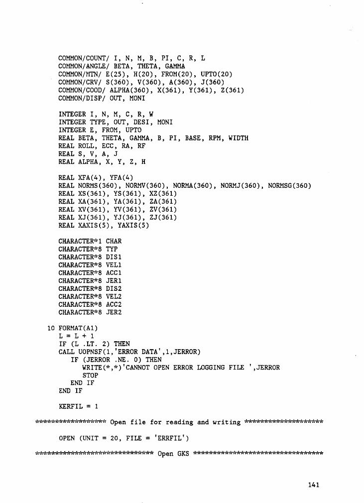
COMMON/COUNT/ I, N, M, B, PI, C, R, LCOMMON/ANGLE/ BETA, THETA, GAMMACOMMON/MTN/ E(25), H(20), FROM(20), UPTO(20)J COMMON/CRV/ $(360), V(360), A(360), J(360)COMMON/COOD/ ALPHA(360), X(361), Y(361), Z(361)COMMON/DISP/ OUT, MONI
INTEGER I, N, M, C, R, WINTEGER TYPE, OUT, DESI, MONIINTEGER E, FROM, UPTOREAL BETA, THETA, GAMMA, B, PI, BASE, RPM, WIDTHREAL ROLL, ECC, RA, RFREAL S, V, A, JREAL ALPHA, X, Y, Z, H
REAL XFA(4), YFA(4)REAL NORMS(360), NORMV(360), NORMA(360), NORMJ(360), NORMSG(360)REAL XS(361), Y$(36l), XZ(361)REAL XA(361), YA(361), ZA(361)REAL XV(36l), YV(361), ZV(361)REAL XJ(361), YJ(361), ZJ(361)REAL XAXIS(5), YAXI$(5)
CHARACTER*1 CHARCHARACTER*8 TYPCHARACTER*8 DIS1
E CHARACTER*8 VEL1CHARACTER*8 ACC1CHARACTER*8 JERICHARACTER*8 DIS2CHARACTER*8 VEL2CHARACTER*8 ACC2CHARACTER*8 JER2
10 FORMAT(A1)L = L + 1IF (L .LT. 2) THENCALL UOPNSF(l,°ERROR DATA°,1,JERROR) _
IF (JERROR .NE. O) THENWRITE(*,*)°CANNOT OPEN ERROR LOGGING FILE °,JERRORSTOP
END IFEND IF
KERFIL = 1
Open for reading and
wrOPEN(UNIT = 20, FILE = °ERRFIL°)
*««****«***««*«*««w«***#*«w«*# Open OKS141
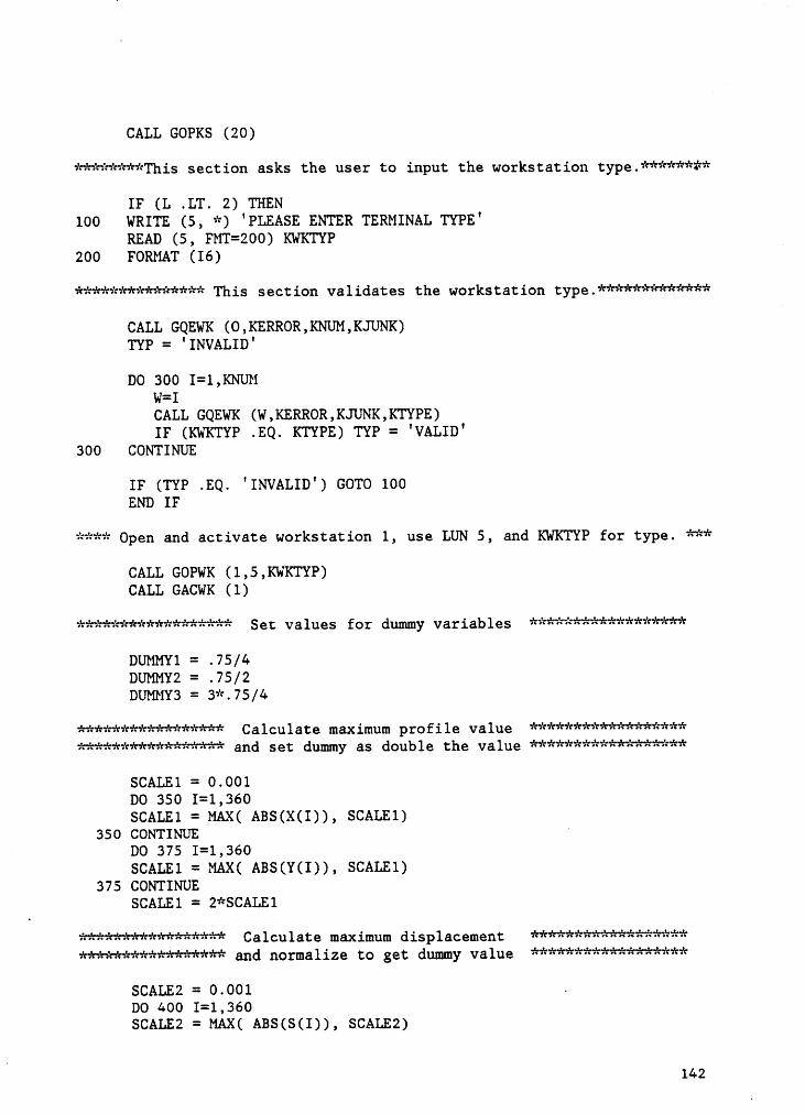
CALL GOPKS (20)
********This section asks the user to input the workstation type.******#*
IF (L .LT. 2) THEN100 WRITE (5, *) ‘PLEASE ENTER TERMINAL TYPE°
READ (5, FMT=200) KWKTYP200 FORMAT (I6)
*************** This section validates the workstation type.*************
CALL GQEWK (O,KERROR,KNUM,KJUNK)TYP = 'INVALID°DO 300 I=1,KNUM
W=1CALL GQEWK (W,KERROR,KJUNK,KTYPE)IF (KWKTYP .PQ. KTYPE) TYP = 'VALID°
3006 CONTINUE
IF (TYP .E0. °INVALID°) 60T0 100END IF
**** Open and activate workstation 1, use LUN 5, and KWKTYP for type. ***
CALL GOPWK (1,5,KWKTYP)CALL GACWK (1)
Set Values for dummy variables äkäkkäkäkkkkkäkkkk
DUMMY1 = .75/4DUMMY2 = .75/2DUMMY3 = 3*.75/4
C alCu 1atQ maximum Profi lQ Va lueand Set dummy as dcublQ the ValueSCALE1
= 0.001DO 350 I=1,360SCALE1 = MAX( ABS(X(I)), SCALE1)
350 CONTINUE‘
DO 375 I=1,360SCALE1 = MAX( ABS(Y(I)), SCALE1)
375 CONTINUESCALE1 = 2*SCALE1
CalculatemaximumSCALE2
= 0.001 ,DO 400 I=1,360SCALE2 = MAX( ABS(S(I)), SCALE2)
A142
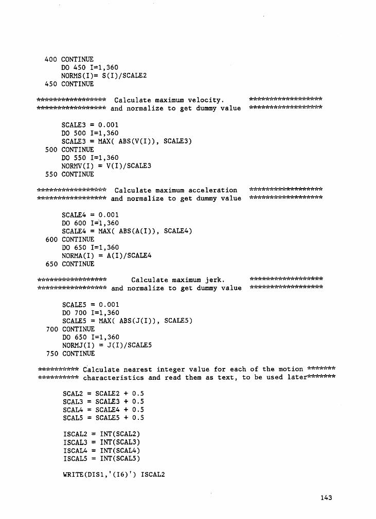
400 CONTINUEDO 450 I=l,360 °NORMS(I)= $(1)/SCALE2
450 CONTINUECalculate maximum V8lQcity_
norma 1 iZ8 tQ ge
VSCALE3= 0.001DO 500 I=l,360 ‘SCALE3 = MAX( ABS(V(I)), SCALE3)
500 CONTINUEDO 550 I=l,360NORMV(I) = V(I)/SCALE3
550 CONTINUECalculate maximum aucelaratiun
and noIma 1 iZ8 tQ
VaSCALE4= 0.001DO600SCALE4
= MAX( ABS(A(I)), SCALE4)600 CONTINUE
DO 650 I=l,360NORMA(I) = A(I)/SCALE4
650 CONTINUECa 1Cu1 at8 maximum j 8rk
and ROrma1iZ8 tQ Va ]_
ueSCALE5= 0.001DO 700 I=l,360SCALE5 = MAX( ABS(J(I)), SCALE5)
700 CONTINUEDO 650 I=l,360NORMJ(I) = J(I)/SCALE5
750 CONTINUE********** Calculate nearest integer value for each of the motion ***************** characteristics and read them as text, to be used 1ater*******
SCAL2 = SCALE2 + 0.5SCAL3 = SCALE3 + 0.5 _SCAL4 = SCALE4 + 0.5SCAL5 = SCALES + 0.5ISCAL2 = INT(SCAL2)ISCAL3 = INT(SCAL3)ISCAL4 = INT(SCAL4)ISCAL5 = INT(SCAL5)
WRITE(DIS1,°(I6)') ISCAL2
4 143
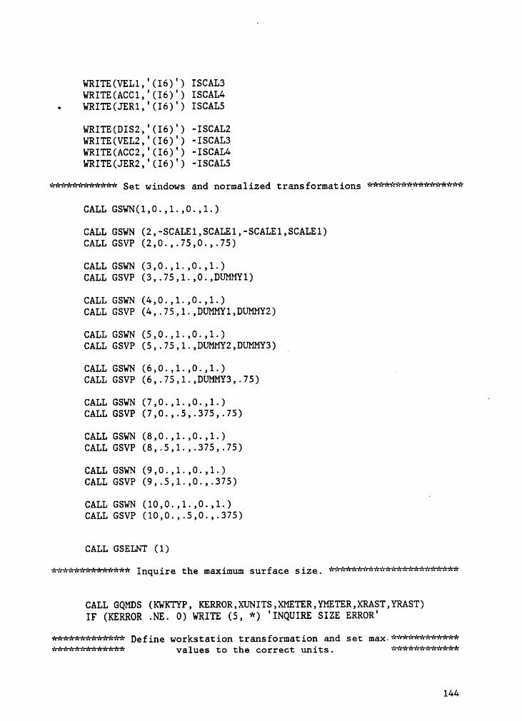
WRITE(VELl,°(I6)°) ISCAL3WRITE(ACC1,'(I6)°) ISCAL4
. WRITE(JERl,°(I6)°) ISCAL5
WRITE(DIS2,'(I6)°) —1scAL2WRITE(VEL2,°(I6)°) ·ISCAL3WRITE(ACC2,°(I6)°) -ISCAL4WRITE(JER2,°(I6)‘) -ISCAL5
************ Set windows and normalized transformations *******#*********
CALL GSWN(l,O.,1.,0.,1.)
CALL GSWN (2,·SCALEl,SCALEl,-SCALEl,SCALEl)CALL GSVP (2,0.,.75,0.,.75)
CALL GSWN (3,0.,l.,0.,l.)CALL GSVP (3,.75,1.,0.,DUMMYl)
CALL GSWN (4,0.,1.,O.,1.)CALL GSVP (4,.75,1.,DUMMYl,DUMMY2)
CALL GSWN (5,0.,l.,0.,1.)CALL GSVP (S,.75,l.,DUMMY2,DUMMY3)
CALL GSWN (6,0.,l.,0.,l.)CALL GSVP (6,.75,l.,DUMMY3,.75)
CALL GSWN (7,0.,l.,0.,l.) °CALL GSVP (7,0.,.5,.375,.75)
CALL GSWN (8,0.,1.,0.,1.)CALL GSVP (8,.5,l.,.375,.75)
CALL GSWN (9,0.,l.,O.,1.)CALL GSVP (9,.5,l.,O.,.37S)
CALLGSWNCALLGSVP (10,0.,.5,0.,.37S)
CALL GSELNT (1)
*7%*******7%**** InquiIe the maximum Sul-face S ize _ 7'$°$7'¥%'f7'€7°$7‘f7'f7°f7'€%'€¥€7'€******7%***
CALL GQMDS (KWKTYP, KERROR,XUNITS,XMETER,YMETER,XRAST,YRAST)IF (KERROR .NE. 0) WRITE (S, *) °INQUIRE SIZE ERROR°
************* Define workstation transformation andset*************values to the correct units} ************
144
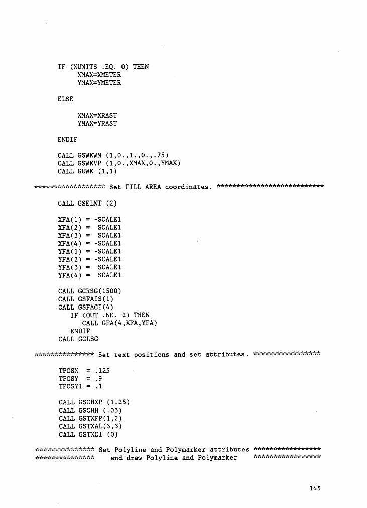
IF (XUNITS .EQ. 0) THENXMAX=XMETERYMAX=YMETER
ELSE
XMAX=XRASTYMAX=YRAST
ENDIF
CALL GSWKWN (1,0.,1.,0.,.75)CALL GSWKVP (1,0.,XMAX,0.,YMAX)CALL GUWK (1,1)
7’?%°$1°€7'f7'f7%1°$7°¢7'€7‘€%'r?‘81'€1'f7°€%°¢$°¥3°f Set FI A COOrdinates _ 7%******7%*****7%%%*%%*7%%%*7%%%***7%
CALL GSELNT (2)
XFA(1) = -SCALElXFA(2) = SCALE1XFA(3) = SCALE1XFA(4) = -SCALEl 'YFA(1) = ·SCALE1YFA(2) = -SCALElYFA(3) = SCALE1YFA(4) = SCALE1
CALL GCRSG(1500)CALL GSFAIS(1)CALL GSFACI(4)
IF (OUT .NE. 2) THENCALL GFA(4,XFA,YFA)
ENDIFCALL GCLSG
7'€%%7‘€%'€$‘€1'f%'f1’=%’t7°?$°?7°¥%°7%°f7‘€ Set text pos ions and S et att es _ 7'€7°7'k7°€7°f7°¥7?7'f7°¥%‘€7‘€7°€7°f7'€7‘¢%’f1'€
TPOSX = .125 ·TPOSY = .9TPOSY1 = .1
CALL GSCHXP (1.25)CALL GSCHH (.03) .‘ CALL GSTXFP(1,2)CALL GSTXAL(3,3)CALL GSTXCI (0)
Set Polyline and Polymarker attributesdraw PO PoarkerL
145
CALL GSPLCI(l)CALL GSLN(l)CALL GSMK(2)CALL GSPMCI(1)CALL GCRSG(2000)
IF (OUT .NE. 2) THEN °CALL GPL(360,X,Y)CALL GPM(1,0.,0.)
ENDIFCALL GCLSG
Select the right transfgrmationand give right value to FILLAREAIF
(OUT .NE. 1) THEN
IF (OUT .EQ. 3) THENCALL GSELNT (3)
ELSEIF (OUT .EQ. 2) THENCALL GSELNT (7)
ENDIF
XFA(1) = 0. ·XFA(2) = 1.XFA(3) = 1.XFA(4) = 0.YFA(1) = 0.YFA(2) = 0.YFA(3) = 1.YFA(4) = 1.
Set axes pgsitions and Set attributeS_Draw the curves and write the text
in='=1'==':='¤'=='==':v‘:=':=':1‘:s':=‘:='=1'=the right pos it iohs _ ='=1’:=':=':=':='=v‘:='=='=='==‘:=':=':=':=’:=‘:='=
XAXIS(1) = 0.1XAXIS(2) = 0.1 VXAXIS(3) = 0.9XAXIS(4) = 0.1XAXIS(5) = 0.1YAXIS(1) = 0.1YAXIS(2) = 0.5YAXIS(3) = 0.5YAXIS(4) = 0.5YAXIS(5) = 0.9
CALL GCRSG(3000)CALL GSFAIS(1)CALL GSFACI(2)CALL GFA(4,XFA,YFA)
146
XS(1) = 0.1 VYS(1) = 0.5 ‘
DO 800 IS=1,360XS(IS+1) = 0.1 + 0.8*15/360.YS(IS+l) = (0.5 + 0.4*NORMS(IS))
800 CONTINUE
CALL GSPLCI(1) .CALL GPL(S,XAXIS,YAXIS)CALL GSPLCI(0)CALL GPL(361,XS,YS)CALL GTX (TPOSX,TPOSY,DIS1)CALL GTX (TPOSX,TPOSY1,DIS2)CALL GTX (.08,.46,°0°)CALL GTX (.35,.46,‘90°)CALL GTX (.55,.46,°180°)CALL GTX (.75,.46,°270°)CALL GTX (.95,.46,°360°)
CALL GSTXAL(2,3)CALL GTX (.5,.06,°DISPLACEMENT')CALL GSTXAL(3,3)
CALL GCLSG
IF (OUT .EQ. 3) THENCALL GSELNT (4)
ELSEIF (OUT .EQ. 2) THENCALL GSELNT (8)
ENDIF
CALL GCRSG(4000)CALL GSFAIS(l)CALL GSFACI(6)CALL GFA(4,XPA,YFA)
XV(1) = 0.1_ YV(1) = 0.5
DO 900 IV=1,360XV(IV+l) = 0.1 + 0.8*IV/360.YV(IV+l) = (0.5 + 0.4*NORMV(IV))
900 CONTINUE
CALL GSPLCI(1)CALL GPL(S,XAXIS,YAXIS)CALL GSPLCI(0) _CALL GPL(361,XV,YV) ‘CALL GTX (TPOSX,TPOSY,VELl) ~CALL GTX (TPOSX,TPOSY1,VE‘.L2)
147
CALL GTX (.08,.46,'0°)CALL GTX (.35,.46,'90°)CALL GTX (.55,.46,°180°)CALL GTX (.75,.46,°270°)
. CALL GTX (.95,.46,°360°)
CALL GSTXAL(2,3)”
CALL GTX (.5,.06,°VELOCITY°)CALL GSTXAL(3,3)
CALL GCLSG
IF (OUT .EQ. 3) THENCALL GSELNT (5)
ELSEIF (OUT .EQ. 2) THENCALL GSELNT (9)
ENDIF
CALL GCRSG(5000)CALL GSFAIS(1)CALL GSFACI(2) .CALL GFA(4,XFA,YFA)
XA(1) = 0.1YA(1) = 0.5
DO 1000 IA=1,360XA(IA+1) = 0.1 + 0.8*IA/360. _YA(IA+1) = (0.5 + 0.4*NORMA(IA))
1000 CONTINUE
CALL GSPLCI(1)CALL GPL(5,XAXIS,YAXIS)CALL GSPLCI(0)CALL GPL(361,XA,YA)CALL GTX (TPOSX,TPOSY,ACC1)CALL GTX (TPOSX,TPOSY1,ACC2)CALL GTX (.o6,.a6,'o')CALL GTX (.35,.46,°90')CALL GTX (.55,.46,'180°)CALL GTX (.75,.46,'270°)CALL GTX (.95,.46,'360')
CALL GSTXAL(2,3)CALL GTX (.5,.06,°ACCELERATION°)CALL GSTXAL(3,3)
CALL GCLSG-IF (OUT .EQ. 3) THEN
CALL GSELNT (6)ELSEIF (OUT .EQ. 2) THEN
148
CALL GSELNT (10)ENDIF
ACALL GCRSG(6000)CALL GSFAIS(1)CALL GSFACI(6)CALL GFA(4,XFA,YFA)
XJ(1) = 0.1YJ(1) = 0.5
D0 1100 IJ=1,360XJ(IJ+1) = 0.1 + 0.8*IJ/360.YJ(IJ+l) = (0.5 + 0.4='=NORMJ(1J))
1100 CONTINUE
CALL GSPLCI(1)CALL GPL(5,XAXIS,YAXIS)CALL GSPLCI(0)CALL GPL(36l,XJ,YJ) _CALL GTX (TPOSX,TPOSY,JER1)CALL GTX (TPOSX,TPOSY1,JER2)CALL GTX (.08,.46,'0°)CALL Grx (.35,.46,°90')CALL GTX (.55,.46,°l80°)CALL GTX (.75,.46,°270°)CALL GTX (.95,.46,'360°)
CALL GSTXAL(2,3)CALL GTX (.5,.06,°JERK°)CALL GSTXAL(3,3)
CALL GCLSG
ENDIF
WRITE(6,*) ° Do you want to animate this cam? (Y/N)°READ(5,10)CHAR _
IF (CHAR .EQ. °Y') THEN1200 WRITE(6,*) ° Enter the degree step you want'
READ(5,*)ITE
WRITE(6,*) ° Transformations being performed.'WRITE(6,*) ° Please wait.'‘ CALL GSELNT (2)CALL GSPLCI(1)CALL GSMK(2)CALL GSPMCI(1)
APHI = O.NSTEP = 360/ITE
A149
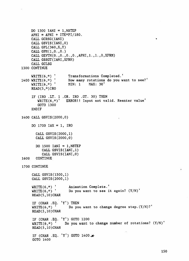
DO 1300 IANI = 1,NSTEPAPHI = APHI + ITE*PI/180.CALL GCRSG(IANI) •CALL GSVIS(IANI,0)CALL GPL(360,X,Y)CALL GPM(1,0.,0.)CALL GEVTM(0.,0.,0.,0.,APHI,1.,1.,0,XFRM)CALL GSSGT(IANI,XFRM)CALL GCLSG
1300 CONTINUE
WRITE(6,*) ° Transformations Comp1eted.°1400 WRITE(6,*) ° How many rotations do you want to see?°
WRITE(6,*) ° MIN: 1 MAX: 30'READ(5,*)IRO
IF (IRO .LT. 1 .OR. IRO .GT. 30) THENWRITE(6,*)° ERROR!! Input not valid. Reenter value'GOTO 1300
ENDIF
1400 CALL GSVIS(2000,0) ,
DO 1700 IAX = 1, IRO
CALL GSVIS(2000,1)CALL GSVIS(2000,0)
DO 1500 IANI = 1,NSTEPCALL GSVIS(IANI,1)CALL GSVIS(IANI,0)
1600 CONTINUE
1700 CONTINUE
CALL GSVIS(1500,1)CALL GSVIS(2000,1)
WRITE(6,*) ° Animation Comp1ete.'WRITE(6,*) ° Do you want to see it again? (Y/N)°READ(5,10)CHAR
IF (CHAR .EQ0 °Y°) THENWRITE(6,*) ° Do you want to change degree step.(Y/N)?°READ(5,l0)CHAR
IF (0262 .20. 'Y') 6020 1200WRITE(6,*) ° Do you want to change number of rotations? (Y/N)'READ(5,10)CHAR
IF (cHAR .20. 'Y') 6010 IÖOOJFGOTO 1400
150
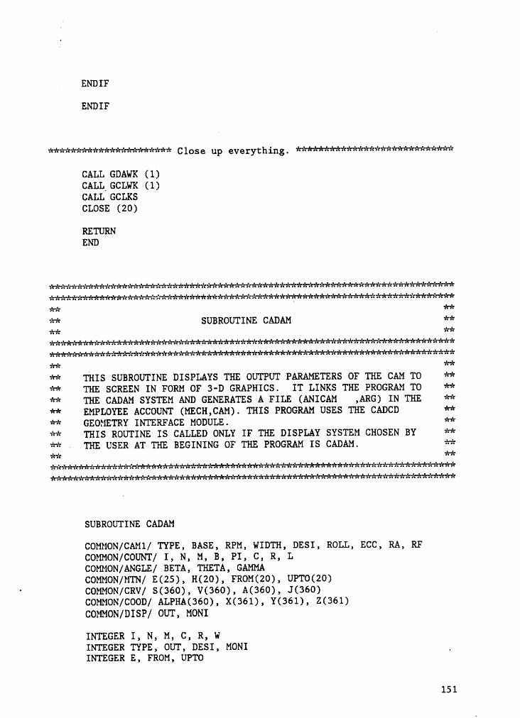
ENDIF
ENDIF
kkkkkkkkkkkkkkkkkkkkkk Close up eVerything_ kkkkkkkkkkkkkkkkkkkkkkkkkkkk
CALL GDAWK (1)CALL GCLWK (1)CALL GCLKSCLOSE (20)
RETURNEND
kkkkkkkkkkkkkkkkkkkkkkkkkkkkkkkkkkkkkkkkkkkkkkkkkkkkkkkkkkkkkkkkkkkkkkkkkkkkkkkkkkkkkkkkkkkkkkkkkkkkkkkkkkkkkkkkkkkkkkkkkkkkkkkkkkkkkkkkkkkkkkkkkk kk
** SUBROUTINE CADAM **kk kkkkkkkkkkkkkkkkkkkkkkkkkkkkkkkkkkkkkkkkkkkkkkkkkkkkkkkkkkkkkkkkkkkkkkkkkkkkkkkkkkkkkkkkkkkkkkkkkkkkkkkkkkkkkkkkkkkkkkkkkkkkkkkkkkkkkkkkkkkkkkkkkkkk kk
** THIS SUBROUTINE DISPLAYS THE OUTPUT PARAMETERS OF THE CAM TO **** THE SCREEN IN FORM OF 3-D GRAPHICS. IT LINKS THE PROGRAM TO **** THE CADAM SYSTEM AND GENERATES A FILE (ANICAM ,ARG) IN THE **** EMPLOYEE ACCOUNT (MECH,CAM). THIS PROGRAM USES THE CADCD **** GEOMETRY INTERFACE MODULE. **** THIS ROUTINE IS CALLED ONLY IF THE DISPLAY SYSTEM CHOSEN BY **** - THE USER AT THE BEGINING OF THE PROGRAM IS CADAM. **kk kkkkkkkkkkkkkkkkkkkkkkkkkkkkkkkkkkkkkkkkkkkkkkkkkkkkkkkkkkkkkkkkkkkkkkkkkkkkkkkkkkkkkkkkkkkkkkkkkkkkkkkkkkkkkkkkkkkkkkkkkkkkkkkkkkkkkkkkkkkkkkkkkk
SUBROUTINE CADAM
COMMON/CAM1/ TYPE, BASE, RPM, WIDTH, DESI, ROLL, ECC, RA, RFCOMMON/COUNT/ I, N, M, B, PI, C, R, LCOMMON/ANGLE/ BETA, THETA, GAMMACOMMON/MTN/ E(25), H(20), FROM(20), UPTO(20)
‘ COMMON/CRV/ $(360), V(360), A(360), J(360)COMMON/COOD/ ALPHA(360), X(36l), Y(36l), Z(361)COMMON/DISP/ OUT, MONI
INTEGER I, N, M, C, R, WINTEGER TYPE, OUT, DESI, MONI _INTEGER E, FROM, UPTO
151
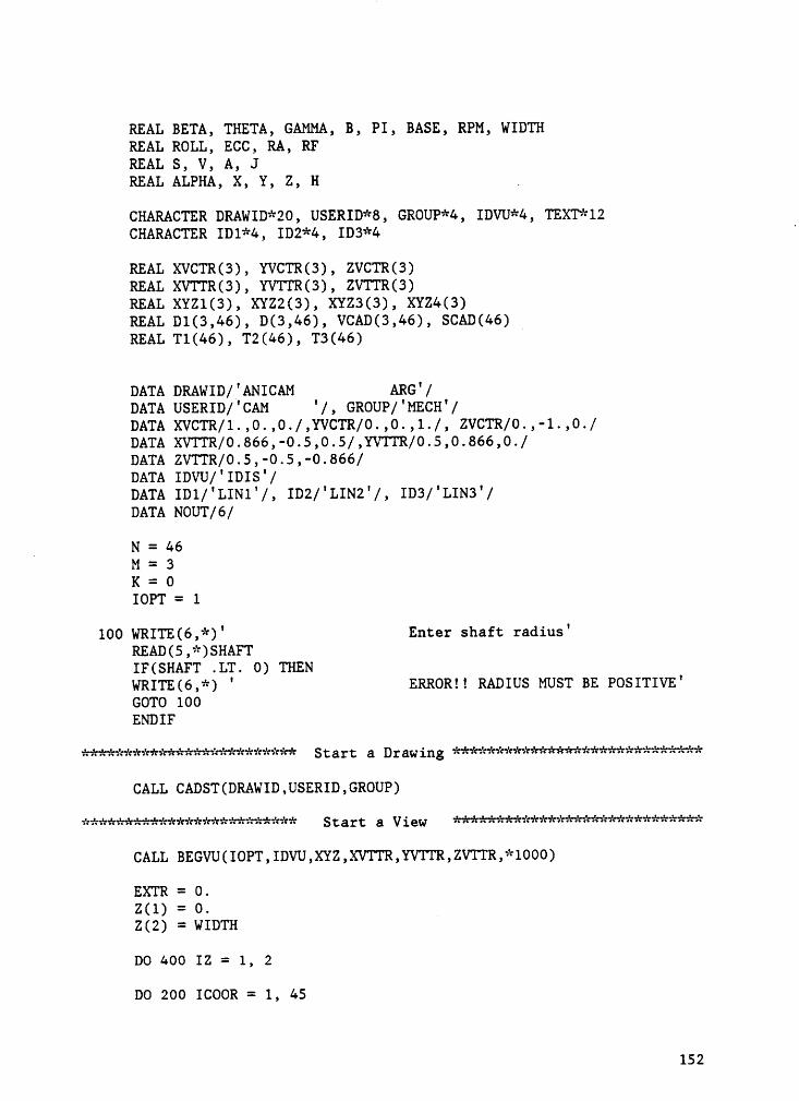
REAL BETA, THETA, GAMMA, B, PI, BASE, RPM, WIDTHREAL ROLL, ECC, RA, RFREAL S, V, A, JREAL ALPHA, X, Y, Z, H .
CHARACTER DRAWID*20, USERID*8, GROUP*4, IDVU*4, TEXT*12CHARACTER ID1*4, ID2*4, ID3*4
“
REAL XVCTR(3), YVCTR(3), ZVCTR(3)REAL XVTTR(3), YVTTR(3), ZVTTR(3)REAL XYZl(3), XYZ2(3), XYZ3(3), XYZ4(3)REAL Dl(3,46), D(3,46), VCAD(3,46), SCAD(46) _REAL T1(46), T2(46), T3(46)
DATA DRAWID/AANICAM ARG°/DATA USERID/°CAM °/, GROUP/°MECH°/DATA XVCTR/1.,0.,0./,YVCTR/0.,0.,1./, ZVCTR/0.,—1.,0./DATA XVTTR/0.866,-0.5,0.5/,YVTTR/O.5,0.866,0./DATA ZVTTR/0.S,-0.5,-0.866/DATA IDVU/°IDIS°/DATA ID1/°LINl°/, ID2/°LIN2°/, ID3/'LIN3°/DATA NOUT/6/
_ N = 46M = 3K = 0IOPT = 1
100 WRITE(6,*)° Enter shaft radius°READ(5,*)SHAFTIF(SHAFT .LT. 0) THENWRITE(6,*) ° ERROR!! RADIUS MUST BE POSITIVE°GOTO 100ENDIF
Start aDrawingCALL
CADST(DRAWID,USERID,GROUP)
8CALLBEGVU(IOPT,IDVU,XYZ,XVTTR,YVTTR,ZVTTR,*1000)
EXTR = 0.Z(1) = 0.Z(2) = WIDTH
DO 400 IZ = 1, 2
DO 200 ICOOR = 1, 45
152
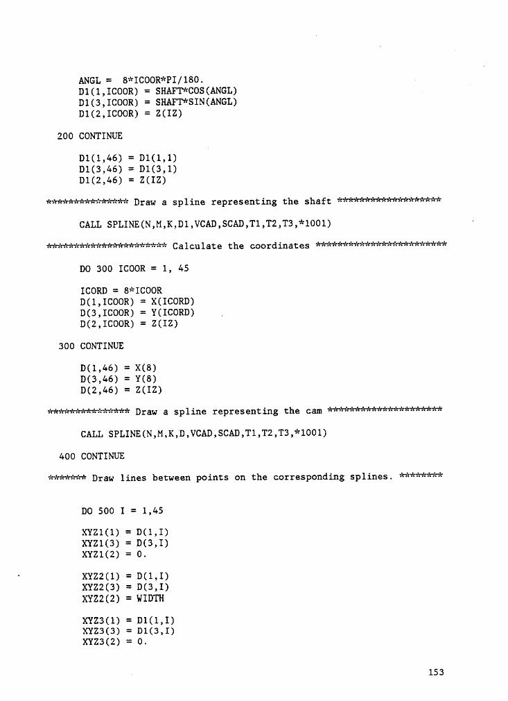
ANGL = 8*ICOOR*PI/180. „D1(1,ICOOR) = SHAFT*COS(ANGL)D1(3,ICOOR) = SHAFT*SIN(ANGL)D1(2,ICOOR) = Z(IZ)
200 CONTINUE
Dl(1,46) = Dl(l,1)Dl(3,46) = Dl(3,l)Dl(2,46) =
Draw a SP]_ ine repIesent ing the Shaf
tCALLSPLINE(N,M,K,Dl,VCAD,SCAD,Tl,T2,T3,*1001) ‘
Calculate theCoordinatesDO
300 ICOOR = 1, 45
ICORD = 8*ICOORD(1,ICOOR) = X(ICORD)D(3,ICOOR) = Y(ICORD) ,D(2,ICOOR) = Z(IZ)
300 CONTINUE
D(1,46) = X(8)D(3 ,46) = Y(8)
Draw a S P 1 ine represent ing the C
amCALLSPLINE(N,M,K,D,VCAD,SCAD,T1,T2,T3,*l001)
400 CONTINUE
******* Draw lines between points on the corresponding splines. ********
DO 500 I = 1,45
XYZ1(1) = D(l,I)XYZ1(3) = D(3,I)XYZl(2) = 0.
‘ XYZ2(1) = D(l,I)XYZ2(3) = D(3,I)XYZ2(2) = WIDTH
XYZ3(1) = Dl(l,I)XYZ3(3) = D1(3,I)XYZ3(2) = 0.
153
XYZ4(1) = D1(1,I)XYZ4(3) = D1(3,I)XYZ4(2) = WIDTH
CALL LINE3D (XYZ1,XYZ2,*1004)~
CALL LINEBD (XYZ3,XYZ4,*1004)CALL LINEBD (XYZ1,XYZ3,*1004)CALL LINE3D (XYZ2,XYZ4,*1004)
u500 CONTINUE
kkkkkkkkkkkkkkkkkkkkkkkkkkkkk File the drawing kkkkkkkkkkkkkkkkkkkkkkkkkk
IOPT=2NOGOOD=0
CALL CADFIL(IOPT,NOGOOD,IDUMMY)
IF(NOGOOD.NE.1)THEN —WRITE(NOUT,*)°ERROR IN CADFIL°
ENDIF
GOTO 2000
1000 WRITE(NOUT,*)°ERROR EXISTS IN BEGVU°1001 WRITE(NOUT,*)°ERROR EXISTS IN SPLINE°1002 WRITE(NOUT,*)°ERROR EXISTS IN NAME°1003 WRITE(NOUT,*)°ERROR EXISTS IN SRFRUL°1004 WRITE(NOUT,*)°ERROR EXISTS IN LINE3D°
· 2000 RETURNEND
kkkkkkkkkkkkkkkkkkkkkkkkkkkkkkkkkkkkkkkkkkkkkkkkkkkkkkkkkkkkkkkkkkkkkkkk
kk kk
** SUBROUTINE MOVIE **kkkkkkkkkkkkkkkkkkkkkkkkkkkkkkkkkkkkkkkkkkkkkkkkkkkkkkkkkkkkkkkkkkkkkkkkH
kk kk
** THIS SUBROUTINE DISPLAYS THE OUTPUT PARAMETERS OF THE CAM TO **** THE SCREEN IN FORM OF 3-D GRAPHICS. IT GENERATES THE GEOMETRY **** FILE (FILE.CAM) FOR DISPLAY, USING MOVIE.BYU. IF REQUIRED, IT ** _** CREATES A COMMAND FILE (FILE.COM) TO BE USED IN CONJUNCTION **** WITH THE ANIMATE SOFTWARE DEVELOPED BY A. MYKLEBUST. **** THIS ROUTINE IS CALLED ONLY IF THE DISPLAY SYSTEM CHOSEN BY **** THE USER AT THE BEGINING OF THE PROGRAM IS MOVIE. **
154
ww kä
SUBROUTINE MOVIE
COMMON/CAM1/ TYPE, BASE, RPM, WIDTH, DESI, ROLL, ECC, RA, RFCOMMON/COUNT/ I, N, M, B, PI, C, R, LCOMMON/ANGLE/ BETA, THETA, GAMMACOMMON/MTN/ E(25), H(20), FROM(20), UPTO(20)COMMON/CRV/ $(360), V(360), A(360), J(360)COMMON/COOD/ ALPHA(360), X(36l), Y(36I), Z(36l)COMMON/DISP/ OUT, MONI
INTEGER I, N, M, C, R, WINTEGER TYPE, OUT, DESI, MONIINTEGER E, FROM, UPTOREAL BETA, THETA, GAMMA, B, PI, BASE, RPM, WIDTHREAL ROLL, ECC, RA, RFREAL S, V, A, JREAL ALPHA, X, Y, Z, H
REAL Xl(3,150), XS(36l), Y$(361)INTEGER IP(600), NPL(2,2)CHARACTER*8 FILECHARACTER*l CHAR
IJ = 1NP = 1NJ = 148NPT= 144NCON = 576NPL(1,l) = 1NPL(2,1) = 144
25 WRITE(6,*)° Enter shaft radius°READ(5,*)SHAFTIF(SHAFT .LT. 0) THENWRITE(6,*) ' ERROR!! RADIUS MUST BE POSITIVE°GOTO 25ENDIF
Calculate peints on shaft circumference *************
DO 50 I = 1, 360
ANGL = I*PI/180.XS(I) = SHAFT*CO$(ANGL)YS(I) = SHAFT*SIN(ANGL)
155
50 CONTINUE
XS(361) = XS(1) ‘YS(361) = YS(1)
X(361) = X(1)Y(361) = Y(1)
*****ü*****%* Calculate the points on the Cam and Shaft ****************kükkükkkkkkkk to be used for the representation **%k#%***%#*ük**
DO 100 I = 1, 361, 10X1(1,1J) = X(I)X1(2,1J) = Y(I)X1(3,IJ) = 0.1J=1J+1
100 CONTINUE _
DO 200 I = 1, 361, 10X1(1,1J) = XS(I) _X1(2,1J) = YS(I)Xl(3,IJ) = 0.IJ = IJ + 1
200 CONTINUE
DO 300 I = 1, 74X1(1,1+74) = X1(1,I)X1(2,1+74) = X1(2,I)X1(3,I+74) = WIDTH
300 CONTINUE
DO 400 I = 1,36
1P(4*1-3) = I1P(4*I-2) = 1+11P(4*1—1) = 1+381P(4*1) = -(1+37)
400 CONTINUE · ‘
DO 500 I = 37,72
IP(4*1-3) = I-361P(4*1·2) = 1+38IP(4*I-1) = 1+39
' IP(4*1) = -(I-35)
500 CONTINUE
DO 600 1 = 73,108
1P(4*1—3) = 1-35
l156
IP(4*1-2) = 1+39IP(4*I-1) = 1+40IP(4*I)• = —(1—34)
600 CONTINUE
DO 700 I = 109,144
1P(4*1-3) = I-34IP(4*I-2) = 1-33 _IP(4*I-1) = 1+4IP(4*I) = -(I+3)
700 CONTINUE
Create the geometry
fileREWIND(8)
WR1TE(8,800) NP,NJ,NPT,NCONWR1TE(8,800) ((NPL(1,IJ),I=l,2),1J=1,NP)WRITE(8,900) ((X1(1,IJ),I=1,3),IJ=1,NJ)WR1TE(8,800) (1P(I),I=1,NCON)
800 FORMAT(l615)900 FORMAT(6E12.5)
WR1TE(6,*)°Do you want to animate this cam?°I
READ(5,1000)CHAR
IF (0aAR .aQ. 'N') 00w0 2000
7‘€7‘f7‘€7‘!7'f7'€7‘§1‘€$°f7'?7°?%‘€7°€7°f7'¥7°f7°?1°f7‘? Q Command fi1 Q if Iequired _********%%*********7%**
REWIND(10)
1000 FORMAT(Al)WRITE(6,*)°GIVE NAME OF DISK F1LE‘READ(5,1100)FILE
I
1100 FORMAT(A8)WRITE(6,*)°G1VE swap AN0La'READ(5,*) STEPNSTEP = 360/STEP
WRITE(9,*)'F1LE.CAM'WRITE(9,1200) _
1200 FORMAT(/)WR1TE(9,*)‘CLSG'DZ = 360/NSTEPZANG = 0.
IDO 1500 IJ = 1,NSTEPWR1TE(9,*)'ROTA°
157
WRITE(9,*)°Z°WRITE(9,l300)ZANG
1300 FORMAT(F10.4)WRITE(9,*)°OSEG°WRITE(9,1400)IJ
1&00 FORMAT(I2)WRITE(9,*)°VIEW°WRITE(9,*)°CSEG°ZANG = DZ
1500 CONTINUEWRITE(9,*)°SAVT°WRITE(9,1600)FILE
1600 FORMAT(A8,/,'EXIT°)
2000 RETURNEND
kkkkkkkkkkkkkkkkkkkkkkkkkkkkkkkkkkkkkkkkkkkkkkkkkkkkkkkkkkkkkkkkkkkkkkkkkk kk
** SUBROUTINE DOCUM **kk wwkkkkkkkkkkkkkkkkkkkkkkkkkkkkkkkkkkkkkkkkkkkkkkkkkkkkkkkkkkkkkkkkkkkkkkkkkkkkkkkkkkkkkkkkkkkkkkkkkkkkkkkkkkkkkkkkkkkkkkkkkkkkkkkkkkkkkkkkkkkkkkkkkk kk
** THIS SUBROUTINE SAVES THE LAST CAM DESIGNED BY THE USER. THE **** DOCUMENTATION IS DONE UNDER THE FILE CAM.OUT. THIS HELPS THE **** USER TO MAINTAIN RECORDS OF THE CAMS DESIGNED AND THEN SELECT **** THE BEST OF ALL OF THEM. **** THIS ROUTINE IS CALLED ONLY IF THE USER WANTS THE DESIGN TO **** BE SAVED. **** *«kkkkkkkkkkkkkkkkkkkkkkkkkkkkkkkkkkkkkkkkkkkkkkkkkkkkkkkkkkkkkkkkkkkkkkkkkkkkkkkkkkkkkkkkkkkkkkkkkkkkkkkkkkkkkkkkkkkkkkkkkkkkkkkkkkkkkkkkkkkkkkkk
SUBROUTINE DOCUMCOMMON/CAM1/ TYPE, BASE, RPM, WIDTH, DESI, ROLL, ECC, RA, RFCOMMON/COUNT/ I, N, M, B, PI, C, R, LCOMMON/ANGLE/ BETA, THETA, GAMMACOMMON/MTN/ E(25), H(20), FROM(20), UPTO(20)
‘ COMMON/CRV/ $(360), V(360), A(360), J(360)COMMON/COOD/ ALPHA(360), X(36l), Y(36l), Z(36l)COMMON/DISP/ OUT, MONI
INTEGER 1, N, M, c, R, wINTEGER TYPE, OUT, DESI, MONIINTEGER E, FROM, UPTO
158

REAL BETA, THETA, GAMMA, B, PI, BASE, RPM, WIDTHREAL ROLL, ECC, RA, RFREAL S, V, A, J
_ REAL ALPHA, X, Y, Z, H
write all Parameters in a
fileREWIND(8)DO 100 K = 10,360,10WRITE(8,10) K,S(K),V(K),A(K),X(K),Y(K)
10 FORMAT(1X,I3,5(2X,F7.3))100 CONTINUE
RETURNEND
159