Embed Size (px)
Citation preview
arX
iv:0
812.
3817
v2 [
nlin
.SI]
30
Dec
200
8
Multiple orthogonal polynomials, string equations
and the large-n limit ∗
L. Martınez Alonso1 and E. Medina2
1 Departamento de Fısica Teorica II, Universidad Complutense
E28040 Madrid, Spain2 Departamento de Matematicas, Universidad de Cadiz
E11510 Puerto Real, Cadiz, Spain
Abstract
The Riemann-Hilbert problems for multiple orthogonal polynomials of types I and II are usedto derive string equations associated to pairs of Lax-Orlov operators. A method for determin-ing the quasiclassical limit of string equations in the phase space of the Whitham hierarchy ofdispersionless integrable systems is provided. Applications to the analysis of the large-n limitof multiple orthogonal polynomials and their associated random matrix ensembles and models ofnon-intersecting Brownian motions are given.
Key words: Multiple orthogonal polynomials. String equations.Whitham hierarchies. PACS number: 02.30.Ik.
∗Partially supported by MEC project FIS2008-00200/FIS and ESF programme MISGAM
1

1 Introduction
The set of orthogonal polynomials Pn(x) = xn + · · · , with respect to an exponential weight
∫ ∞
−∞Pn(x)Pm(x) eV (c,x) dx = hnδnm, V (c, x) :=
∑
k≥1
ck xk,
is an essential ingredient of the methods [1]-[2] for studying the large-n limit of the Hermitianmatrix model
Zn =
∫dM exp
(Tr V (c,M)
). (1)
One of the main tools used in these methods is the pair of equations
z Pn(z) = Z Pn(z), ∂z Pn(z) = MPn(z), n ≥ 0, (2)
where (Z,M) is a pair of Lax-Orlov operators of the form
Z = Λ + un + vn Λ∗, M = −∑
k≥1
k ck (Zk−1)+. (3)
Here Λ is the shift matrix acting in the linear space of sequences, Λ∗ is its transposed matrix and( )+ denotes the lower part (below the main diagonal) of semi-infinite matrices.
The first equation in (2) represents the standard three-term relation for orthogonal polynomials.Both equations are referred to as the string equations in the matrix models of 2D quantum gravity[1] and provide the starting point of several techniques to characterize the large-n limit of (1). Adeeper mathematical insight of these methods was achieved after the introduction by Fokas, Itsand Kitaev [3] of a matrix valued Riemann-Hilbert (RH) problem which characterizes orthogonalpolynomials on the real line, and the formulation by Deift and Zhou [2],[4] of steepest descentmethods for studying asymptotic properties of RH problems .
The RH problem of Fokas-Its-Kitaev was generalized by Van Assche, Geronimo and Kuijlaars[5] to characterize multiple orthogonal polynomials. Moreover, it was found [6]-[10] that thesefamilies of polynomials are closely connected to important statistical models such as Gaussianensembles with external sources and one-dimensional non-intersecting Brownian motions.
In this paper we generalize the string equations (2) to multiple orthogonal polynomials of typesI and II, and show how these equations can be applied to analyze the large-n limit of multipleorthogonal polynomials and their associated statistical models. Section 2 introduces the basicstrategy of our approach to derive string equations, which is inspired by standard methods usedin the theory of multi-component integrable systems [11]-[15]. As it was proved in [5] the multipleorthogonal polynomials of types I and II are elements of the first row of the fundamental solutionf of the corresponding RH problem. Then, in Sections 3 and 4 we formulate systems of stringequations for the elements of the first row of the fundamental solution f . In both cases the functionf depends on a set of discrete variables
s = (s1, s2, . . . , sq) ∈ Zq, where
si ≥ 0 for type I polynomials
si ≤ 0 for type II polynomials.
2

Therefore, special care is required to determine the form of the string equations on the boundaryof the domain of the discrete variables. Thus, we obtain closed-form expressions, free of boundaryterms, for the string equations satisfied by these types of multiple orthogonal polynomials. Thesestring equations are associated to pairs (Zi,Mi) of Lax-Orlov operators. In particular thoseinvolving the Lax operators Zi lead to the well-known recurrence relations for multiple orthogonalpolynomials [5].
We take advantage of an interesting observation due to Takasaki and Takebe [16] who showedthat the dispersionless limit of a row of a matrix-valued KP wave function is a solution of thezero genus Whitham hierarchy [11]. This is an additional incentive for using Lax-Orlov operators[12]-[15] in order to characterize the large-n limit in terms of quasiclassical (dispersionless limit)expansions. Thus, in Section 5 we show how the leading term of the expansion of the first rowof f is determined by a system of dispersionless string equations for q + 1 Lax-Orlov functions(zα,mα) in the phase space of the Whitham hierarchy. The unknowns of this system reduce to aset of q pairs of functions (uk, vk), which are determined by means of a system of hodograph typeequations. Finally, Section 6 is devoted to illustrate the applications of our results to models ofrandom matrix ensembles and non-intersecting Brownian motions.
The present work deals with multiple orthogonal polynomials of types I and II only, but thesame considerations apply to the study of multiple orthogonal polynomials of mixed type [17]. Onthe other hand, we concentrate on the description of the leading terms of the asymptotic solutionsin the dispersionless limit. However, as it was showed in [18]-[19] for the case of the Toda hierarchyand the Hermitian matrix model, the scheme used in the present paper can be further elaboratedfor determining the general terms of these expansions, as well as their critical points and theircorresponding double scaling limit regularizations.
2 Riemann-Hilbert problems
In this work we will consider (q + 1) × (q + 1) matrix valued functions. Unless otherwise statedGreek α, β, . . . and Latin i, j, . . . suffixes will label indices of the sets 0, 1, . . . , q and 1, 2, . . . , q,respectively. We will denote by Eαβ the matrices (Eαβ)α′β′ = δαα′ δββ′ of the canonical basis and,in particular, its diagonal members will be denoted by Eα := Eαα. Some useful relations whichwill be frequently used in the subsequent discussion are
Eαβ Eγλ = δβγ Eαλ; Eα aEβ = aαβ Eαβ , ∀ matrix a.
We will also denote by V (c, z) the scalar function
V (c, z) :=∑
n≥1
cn zn, c = (c1, c2, . . .) ∈ C∞, (4)
and will assume that only a finite number of the coefficients cn are different from zero.
Given a matrix function g = g(z) (z ∈ R) such that det g(z) ≡ 1, we will consider the RHproblem
m−(z) g(z) = m+(z), z ∈ R, (5)
where m(z) is a sectionally holomorphic function and m±(z) := limǫ→0+ m(z ± iǫ). We areinterested in solutions f = f(s, z) of (5) depending on q discrete variables s = (s1, . . . , sq) ∈ Z
q
3

such that
f(s, z) =(I + O
(1
z
))f0(s, z), z → ∞, (6)
where
f0(s, z) :=
q∑
α=0
zsα Eα, (s0 := −q∑
i=1
si).
The set of points s ∈ Zq for which (5) admits a solution f(s, z) satisfying (6) will be denoted by
Γ. The solution f(s, z), (s ∈ Γ) is unique and will be referred to as the fundamental solution ofthe RH problem (5).
We will apply (5) and (6) to derive certain difference-differential equations for f . These equa-tions contain two basic ingredients: the coefficients of the asymptotic expansion of f(s, z) as z → ∞
f(s, z) =(I +
∑
n≥1
an(s)
zn
)f0(s, z), (7)
and the q pairs of shift operators Ti, T ∗i acting on functions h(s) (s ∈ Γ) defined as
(Ti h)(s) :=
h(s − ei) if s − ei ∈ Γ
0 if s − ei /∈ Γ
, (T ∗i h)(s) :=
h(s + ei) if s + ei ∈ Γ
0 if s + ei /∈ Γ,
where ei are the elements of the canonical basis of Cq.
We will often consider series of the form
A :=
∞∑
n=1
cn(s) (T ∗i )n + c′0 +
∞∑
n=1
c′n(s)T ni ,
and will denote
(A)(i,+) :=∞∑
n=1
cn(s) (T ∗i )n, (A)(i,−) := c′0 +
∞∑
n=1
c′n(s)T ni . (8)
The RH problem (5) admits the following symmetries.
Proposition 1. 1. If h(s, z) (s ∈ Γ) is an entire function of z, then h(s, z) f(s, z) satisfies (5)for all s ∈ Γ.
2. The functions (Ti f)(s, z) and (T ∗i f)(s, z) satisfy (5) for all s ∈ Γ.
3. If g(z) is an entire function, then for any entire function φ(z) verifying
g−1 φ g = φ − g−1 ∂z g, (9)
the covariant derivativeDz f := ∂z f − f φ, (10)
satisfies (5) for all s ∈ Γ.
4

Our strategy to obtain difference-differential equations for f is based on applying the nextsimple statement to the symmetries of (5).
Proposition 2. Let f(s, z) be a a solution of (5) defined for s in a certain subset Γ0 ⊂ Γ. If
f(s, z) f(s, z)−1 − P (s, z) → 0 as z → ∞, where P (s, z) is a polynomial in z, then
f(s, z) = P (s, z) f(s, z).
Proof. Since det g(z) ≡ 1 it follows from (5) and (6) that det f(s, z) ≡ 1 so that the inverse matrixf(s, z)−1 is analytic for z ∈ C − R and satisfies the jump condition
g(z)−1 f−(s, z)−1 = f+(s, z)−1, z ∈ R.
As a consequence f f−1 is an entire function of z and the statements follow at once.
3 Multiple orthogonal polynomials of type I
Given q exponential weights wi on the real line
wi(x) := e−V (ci,x), ci = (ci1, ci2, . . .) ∈ C∞,
and n = (n1, . . . , nq) ∈ Nq with |n| ≥ 1, the type I orthogonal polynomials
A(n, x) = (A1(n, x), . . . , Aq(n, x))
are determined by means of the following conditions:
i) If nj ≥ 1 then the polynomial Aj(n, x) has degree nj − 1. If nj = 0 then Aj(n, z) ≡ 0
ii) The following orthogonality relations are satisfied
∫
R
dx
2πixl
q∑
j=1
Aj(n, x)wj(x)
=
0 l = 0, 1, . . . , |n| − 2,1 l = |n| − 1.
We assume that all the multi-indices n are strongly normal [17] so that Aj(n, z) are unique.
The RH problem which characterizes these polynomials [5] is determined by
g(z) =
1 0 0 . . . 0−w1(z) 1 0 . . . 0
......
......
−wq(z) 0 . . . 0 1
. (11)
The corresponding fundamental solution f(s, z) exists on the domain
ΓI = s ∈ Zq : si ≥ 0, ∀i = 1, . . . , q. (12)
5

For s 6= 0 it is given by
f(s, z) =
R(s, z) A(s, z)
d−11 R(s + e1, z) d−1
1 A(s + e1, z)...
...d−1
q R(s + eq, z) d−1q A(s + eq, z)
,
(13)
R(s, z) :=
∫
R
dx
2πi
∑qj=1 Aj(s, x)wj(x)
z − x,
where dj is the leading coefficient of Aj(s + ej , z). Furthermore, for s = 0
f(0, z) =
1 0 0 · · · 0R1(z) 1 0 · · · 0R2(z) 0 1 · · · 0
......
......
Rq(z) 0 0 · · · 1
, Rj(z) :=
∫
R
dx
2πi
wj(x)
z − x. (14)
Because of the form of ΓI we have that
(T ∗i h)(s) = h(s + ei), (Ti h)(s) :=
h(s − ei) if si ≤ 1
0 if si = 0,
for functions h(s) (s ∈ ΓI). It is clear that
T ∗i Ti = I, Ti T
∗i = (1 − δsi,0) I,
where I stands for the identity operator. Sometimes it is helpful to think of the functions h(s)as column vectors (h|si=0, h|si=1, h|si=2, . . .)
T . Thus, in this representation, Ti, T ∗i become the
infinite-dimensional matrices
T ∗i =
0 1 0 . . . . . .0 0 1 0 . . .0 0 0 1 . . ....
......
......
, Ti =
0 0 0 . . . . . .1 0 0 0 . . .0 1 0 0 . . ....
......
......
.
3.1 The first system of string equations
From the asymptotic expansion (7) we have that as z → ∞
(Ti f) f−1 =(I +
a(s − ei)
z+ O
( 1
z2
))(z E0 +
Ei
z+ I − E0 − Ei
)(I − a(s)
z+ O
( 1
z2
))
= z E0 + a(s − ei)E0 − E0 a(s) + I − E0 − Ei + O(1
z
), ∀s ∈ ΓI + ei,
6

where we are denotinga(s) := a1(s).
Hence by applying Proposition 2 it follows that
(Ti f)(s, z) =(z E0 + a(s − ei)E0 − E0 a(s) + I − E0 − Ei
)f(s, z), s ∈ ΓI + ei
which implies
(TiE0f)(s, z) =((z − ui(s))E0 −
∑
j
a0j(s)E0j
)f(s, z), ∀s ∈ ΓI + ei, (15)
whereui(s) := a00(s) − a00(s − ei).
Similarly one finds(T ∗
j E0f)(s, z) = a0j(s + ej)E0j f(s, z), ∀s ∈ ΓI . (16)
Note that as det f(s, z) ≡ 1 for all (s, z) ∈ ΓI × C then , as a consequence of (16) we deduce that
a0j(s + ej) 6= 0, ∀s ∈ ΓI .
If we now define
vj(s) :=a0j(s)
a0j(s + ej), s ∈ ΓI , (17)
then from (15) it follows that
Proposition 3. The function f satisfies the equations
z (E0 f)(s, z) =(Ti + ui(s) +
∑
j
vj(s)T ∗j
)(E0 f)(s, z), (18)
for all s ∈ ΓI + ei and i = 1, . . . , q.
As a consequence we get the following system of string equations
Theorem 1. The multiple orthogonal polynomials of type I verify
z A(n, z) =(Ti + ui(n) +
∑
j
vj(n)T ∗j
)A(n, z), (19)
for all n ∈ ΓI + ei and i = 1, . . . , q.
For q = 1 Eq.(19) reduces to the classical three-term recurrence relation for systems of orthog-onal polynomials on the real line.
On the other hand Eq.(19) implies
A(n−ei, z)−A(n−ej, z) = (a00(n−ei)−a00(n−ej))A(n, z), ∀s ∈ ΓI +ei +ej, i 6= j. (20)
The relations (19) and (20) lead to a recursive method to construct the multiple orthogonal poly-nomials of type I. Indeed, it is clear that for n = niei we have
A(niei, z) = A(i)1 (ni, z)ei = (0, . . . , 0, A
(i)1 (ni, z), 0, . . . , 0),
where A(i)1 (ni, z) are the orthogonal polynomials with respect to the weight wi(x). Then starting
from A(i)1 (ni, z) and using (20) we can generate the multiple orthogonal polynomials of type I for
higher q.
7

Example
Let us denote by Ij,n the moments with respect to the weight wj
Ij,n :=
∫
R
dx
2πixnwj(x). (21)
We have that
A1(1, z) =1
I1,0, A1(2, z) =
I1,0z − I1,1
I1,0I1,2 − I21,1
.
The recurrence relation (19) for q = 1 is
A1(n + 1, z) =a01(n + 1)
a01(n)[(z + a00(n − 1) − a00(n))A1(n, z) − A1(n − 1, z)], ∀n ≥ 2, (22)
where according to (13)
a00(n) =
∫
R
dx
2πixnA(n, x)w1(x). (23)
Moreover, the normalization condition gives us
a01(n)
a01(n + 1)=
∫dx
2πixn[(x + a00(n − 1) − a00(n))A(n, x) − A(n − 1, x)]w1(x). (24)
The system (22)-(23)-(24) allows us to construct the polynomials A(n, z) for n ≥ 3. For exampleone gets
A1(3, z) =
(I21,1 − I1,0I1,2
)z2 − I1,1I1,3 + (I1,0I1,3 − I1,1I1,2)z + I2
1,2
I31,2 − (2I1,1I1,3 + I1,0I1,4)I1,2 + I1,0I
21,3 + I2
1,1I1,4.
If we write (20) in the form
A(n, z) =A(n − ei, z) − A(n − ej, z)
a00(n − ei) − a00(n − ej), n ∈ ΓI + ei + ej , (25)
and take into account that
a00(n) =
∫
R
dx
2πix|n|
q∑
k=1
Ak(n, x)wk(x). (26)
we can construct all the multiple orthogonal polynomials of type I. Thus, for example for q = 2 weobtain
A(1, 1, z) =1
C1
(I2,0,−I1,0
),
A(2, 1, z) =1
C2
(I1,2I2,0 − I1,1I2,1 + z(I1,0I2,1 − I1,1I2,0) , I2
1,1 − I1,0I2,0
),
where
C1 : = I1,1I2,0 − I1,0I2,1,
C2 : = I2,2I21,1 − I1,3I2,0I1,1 − I1,2I2,1I1,1 + I2
1,2I2,0 + I1,0I1,3I2,1 − I1,0I1,2I2,2.
8

3.2 Lax operators
The functions f0i(s, z) = Ai(s, z) can be written as series expansions of the form
f0i(s, z) =
(αi1(s)
z+
αi2(s)
z2+ · · ·
)zsi ,
whereαin(s) = 0, ∀n ≥ si + 1. (27)
On the other hand, it is easy to see that
T ni zsi =
1
zn(zsi −
n−1∑
k=0
zk δsi−k,0), (28)
Hence, from (27) and (28) it is clear that
αi,n+1(s + ei)
znzsi = αi,n+1(s + ei)T
ni zsi , ∀n ≥ 1,
so that we may write
f0i(s + ei, z) = (Gi ξi)(s, z), ξi(s, z) := zsi , s ∈ ΓI ,
where the symbols Gi are dressing operators defined by the expansions
Gi =∑
n≥1
αin(s + ei)T n−1i , αin(s + ei) := (an)0i(s + ei), (29)
or, equivalently, by the triangular matrices
Gi =
G00 0 0 . . . . . .G10 G11 0 0 . . .G20 G21 G22 0 . . .
......
......
...
, Gnm = αi,n−m+1(s + ei)
∣∣∣si=m
.
The inverse operators can be written as
G−1i :=
∑
n≥1
βin(s)T n−1i , βi1(s) =
1
αi1(s + ei)=
1
a0i(s + ei).
We define the Lax operators Zi by
Zi := Gi T ∗i G−1
i . (30)
It follows at once that they can be expanded as
Zi = γi(s)T ∗i +
∑
n≥0
γin(s)T ni , (31)
where
γi(s) = αi1(s + ei) (T ∗i βi1)(s) =
αi1(s + ei)
αi1(s + 2ei)= vi(s + ei). (32)
9
Proposition 4. The functions f0i satisfy the equations
z f0i(s + ei, z) = (Zi f0i)(s + ei, z), ∀s ∈ ΓI . (33)
Proof. From the definition of Gi we have
z f0i(s + ei, z) = Gi (z ξi) = (Gi T ∗i ) (ξi) = (Zi f0i)(s + ei, z).
3.3 The second system of string equations
Let us consider diagonal solutions
Φ(z) =∑
α
φα(z)Eα
of the condition (9) corresponding to the function g(z) of (11). They are characterized by
∂z wi − φ0 wi + φi wi = 0, i = 1, . . . , q.
In this way, by setting φ0 ≡ 0 we get
Φ(z) =∑
i
V ′(ci, z)Ei.
The corresponding covariant derivative is
Dz f := ∂zf −∑
i
V ′(ci, z) f Ei. (34)
Hence we haveDz(E0 f) = ∂zf00 E0 +
∑
i
(∂zf0i − V ′(ci, z) f0i)E0i. (35)
It is clear that (33) implies
zn f0i(s + ei, z) = (Zni f0i)(s + ei, z), ∀s ∈ ΓI . (36)
On the other hand, as z → ∞
((T ∗j )n f0α)(s, z) =
O( 1
zn
)zs0 , for α = 0,
O(1
z
)zsi , for α = i 6= j ,
, n ≥ 1,
(37)
(T ni f0i)(s, z) =
O( 1
zn+1
)zsi , for si ≥ n,
0, for si < n
, n ≥ 0.
10

Proposition 5. The function f satisfies the equation
(Dz + H) (E0 f)(s, z) = 0, ∀s ∈ ΓI +∑
j
ej , (38)
where H is the operator
H :=
q∑
j=1
V ′(cj ,Zj)(j,+) (39)
Proof. Given s ∈ ΓI +∑
j ej let us denote
s(i) := s − ei ∈ ΓI +
∑
k 6=i
ek.
From (35) it follows that
(Dz + H) (E0 f) =
∂zf00 +
q∑
j=1
V ′(cj,Zj)(j,+) f00
E0
+
q∑
i=1
∂zf0i +
q∑
j=1
V ′(cj,Zj)(j,+) f0i − V ′(ci, z) f0i
E0i
(40)
Now from (37) we have
∂zf00 +
q∑
j=1
V ′(cj,Zj)(j,+) f00 = O(1
z
)zs0 ,
∂zf0i +∑
j 6=i
V ′(cj,Zj)(j,+) f0i = O(1
z
)zsi .
(V ′(ci,Zi)(i,+) − V ′(ci, z)
)f0i(s, z) =
(V ′(ci,Zi) − V ′(ci, z)
)f0i(s, z) + O
(1
z
)zsi ,
Moreover, from (36) it is clear that
(V ′(ci,Zi) − V ′(ci, z)
)f0i(s, z) =
(V ′(ci,Zi) − V ′(ci, z)
)f0i(s
(i) + ei, z)
=∑
n≥1
n cin
(Zn−1
i − zn−1)
f0i(s(i) + ei, z) = 0
Therefore we find
(Dz + H) (E0 f)(s, z) = O(1
z) f0(s, z), z → ∞.
The first member f := (Dz + H) (E0 f) of this equation is a solution of (5) for all s ∈ ΓI +∑
j ej
and f(s, z) f(s, z)−1 → 0 as z → ∞. Therefore, the statement of Proposition 2 implies f ≡ 0 .
As a consequence we deduce the following system of string equations
11

Theorem 2. The multiple orthogonal polynomials of type I verify
∂z Ai(n, z) = V ′(ci,Zi)Ai(n, z) −q∑
j=1
V ′(cj,Zj)(j,+) Ai(n, z), (41)
for all n ∈ ΓI +∑
k ek and i = 1, . . . , q.
3.4 Orlov operators
We define the Orlov operators Mi by
Mi := Gi · si · Ti · G−1i . (42)
They satisfy [Zi,Mi] = I and can be expanded as
Mi =∑
n≥1
µin(s)T ni , (43)
whereµi1(s) =
si
vi(s). (44)
Proposition 6. The functions f0i satisfy the equations
∂z f0i(s + ei, z) = (Mi f0i)(s, z + ei), ∀s ∈ ΓI . (45)
Proof. From the definition of Gi we have
∂z f0i(s + ei, z) = Gi (si z−1 ξi) = G · si(Ti ξi) = Gi · si · Ti · G−1
i f0i = Mi f0i(s + ei, z).
4 Multiple orthogonal polynomials of type II
We consider now q exponential weights wi on the real line
wi(x) := eV (ci,x), ci = (ci1, ci2, . . .) ∈ C∞.
Note the difference in the sign of the exponents with respect to the weights for multiple orthogonalpolynomials of type I. Given n = (n1, . . . , nq) ∈ N
q, the associated type II monic orthogonalpolynomial P (n, x) = x|n| + · · · is determined by the conditions
∫
R
P (n, x)wi(x)xj dx = 0, j = 0, . . . , ni − 1.
We assume that all the multi-indices n are strongly normal [17] so that P (n, z) is unique.The RH problem for the multiple orthogonal polynomials of type II is determined by [17]
g(z) =
1 w1(z) w2(z) . . . wq(z)0 1 0 . . . 0...
......
......
0 0 . . . 0 1
, (46)
12

Its fundamental solution f(s, z) exists on the domain
ΓII = s ∈ Zq : si ≤ 0, ∀i = 1, . . . , q, (47)
For si ≤ −1∀i, it is given by
f(s, z) =
P (n, z) R(n, z)d1 P (n − e1, z) d1 R(n − e1, z)
......
dq P (n − eq, z) dq R(n − eq, z)
, s = −n,
(48)
Rj(n, z) :=
∫
R
dx
2πi
P (n, x)wj(x)
x − z,
1
dj:= −
∫
R
dx
2πiP (n − ej, x)wj(x)xnj−1.
For the remaining cases, in which one or several si vanish, one must insert the following corre-sponding row substitutions in (48)
(di P (n − ei, z) di R(n − ei, z)) −→ (0 ei). (49)
In particular
f(0, z) =
1 R1(z) R2(z) · · · Rq(z)0 1 0 · · · 0...
......
...0 0 0 · · · 1
, Rj(z) :=
∫
R
dx
2πi
wj(x)
x − z.
In view of (47) we have that
(Ti h)(s) = h(s − ei), (T ∗i h)(s) :=
h(s + ei) if si ≤ −1
0 if si = 0,
for functions h(s) (s ∈ ΓII). Note also that
Ti T∗i = I, T ∗
i Ti = (1 − δsi,0) I
where I stands for the identity operator. If we think of h(s) as a column vector (h|si=0, h|si=−1, h|si=−2, . . .)T ,
then Ti, T ∗i are represented by the infinite-dimensional matrices
Ti =
0 1 0 . . . . . .0 0 1 0 . . .0 0 0 1 . . ....
......
......
, T ∗
i =
0 0 0 . . . . . .1 0 0 0 . . .0 1 0 0 . . ....
......
......
.
13

4.1 The first system of string equations
The same analysis as in the subsection 3.1 leads now to the equations
(TiE0f)(s, z) =((z − ui(s))E0 −
∑
j
a0j(s)E0j
)f(s, z), ∀s ∈ ΓII , (50)
whereui(s) := a00(s) − a00(s − ei).
Similarly one finds
(T ∗j E0f)(s, z) = a0j(s + ej)E0j f(s, z), ∀s ∈ ΓII − ei, (51)
and taking into account that det f(s, z) ≡ 1 for all (s, z) ∈ ΓII × C, from (51) we obtain
a0j(s) 6= 0, ∀s ∈ ΓII .
Now we define
vj(s) :=
a0j(s)
a0j(s + ej), s ∈ ΓII − ei,
0, for sj = 0.
(52)
Notice that the functions vj(s) (s ∈ ΓI) for multiple orthogonal polynomials of type I defined in(17) also satisfies vj(s) = 0 for sj = 0.
If we now recall that according to (49)
E0j f(s, z) = E0j , for sj = 0,
from (50) it follows that
Proposition 7. The function f satisfies the equations
z E0 f(s, z) =(Ti + ui(s) +
∑
j
vj(s)T ∗j
)(E0 f)(s, z) +
∑
j
δsj ,0 a0j(s)E0j , (53)
for all s ∈ ΓII and i = 1 . . . q.
As a consequence we get the string equations
Theorem 3. The multiple orthogonal polynomials of type II verify
z P (n, z) =(Ti + ui(−n) +
∑
j
vj(−n)T ∗j
)P (n, z), (54)
for all n and i = 1, . . . , q.
These equation provide a recursive method to construct multiple orthogonal polynomials oftype II. We may write (54) as
P (n +ej, z)−a00(n +ej)P (n, z) = (z − a00(n))P (n, z)−q∑
k=1,nk≥1
a0k(n)
a0k(n − ek)P (n− ek, z), (55)
14

where, according to(48), we have that
a00(n) = coeff[P (n, z), z|n|−1],
a0k(n) = −∫
R
dx
2πiP (n, x)xnkwk(x)dx.
(56)
On the other hand, multiplying the equation (55) by znjwj(z), integrating on R and using theorthogonality condition for P (n + ej , z), we obtain
a00(n + ej)
[−
∫
R
dx
2πiP (n, x)xnj wj(x)
]=
∫
R
(x − a00(n))P (n, x) −
q∑
k=1,nk≥1
a0k(n)
a0k(n − ek)P (n − ek, x)
xnjwj(x)dx,
so that
a00(n + ej) =1
a0j(n)
∫
R
(x − a00(n))P (n, x) −
q∑
k=1,nk≥1
a0k(n)
a0k(n − ek)P (n − ek, x)
xnjwj(x)dx.
(57)The system (55)-(56)-(57) determines the multiple orthogonal polynomials of type II in terms ofthe moments Ij,n .
Example
For q = 1 is clear that
P (0, z) = 1, P (1, z) = z − I1,1
I1,0.
From (55)-(56)-(57) we easily obtain that
P (2, z) = z2 +(I1,0I1,3 − I1,1I1,2)z
I21,1 − I1,0I1,2
+I21,2 − I1,1I1,3
I21,1 − I1,0I1,2
,
P (3, z) = z3 +
(−I1,5I
21,1 + I2
1,3I1,1 + I1,2I1,4I1,1 − I21,2I1,3 − I1,0I1,3I1,4 + I1,0I1,2I1,5
)z2
I31,2 − (2I1,1I1,3 + I1,0I1,4)I1,2 + I1,0I2
1,3 + I21,1I1,4
+
(−I1,4I
21,2 + I2
1,3I1,2 + I1,1I1,5I1,2 + I1,0I21,4 − I1,1I1,3I1,4 − I1,0I1,3I1,5
)z
I31,2 − 2I1,1I1,3I1,2 − I1,0I1,4I1,2 + I1,0I2
1,3 + I21,1I1,4
−I31,3 − 2I1,2I1,4I1,3 − I1,1I1,5I1,3 + I1,1I
21,4 + I2
1,2I1,5
I31,2 − 2I1,1I1,3I1,2 − I1,0I1,4I1,2 + I1,0I
21,3 + I2
1,1I1,4.
To determine the orthogonal polynomials for q ≥ 2 we use the property
P (niei, z) = P (i)(ni, z),
15
where P (i)(ni, z) are the orthogonal polynomials for q = 1 with respect to the weight wi(x). Forexample for q = 2 and j = 2, Eq.(55) yields
P (1, 1, z) = z2 +(I1,2I2,0 − I1,0I2,2)z
I1,0I2,1 − I1,1I2,0+
I1,2I2,1 − I1,1I2,2
I1,1I2,0 − I1,0I2,1,
P (2, 1, z) = z3 +
(−I2,3I
21,1 + I1,4I2,0I1,1 + I1,3I2,1I1,1 − I1,2I1,3I2,0 − I1,0I1,4I2,1 + I1,0I1,2I2,3
)z2
I2,2I21,1 − I1,3I2,0I1,1 + I2
1,2I2,0 + I1,0I1,3I2,1 − I1,2(I1,1I2,1 + I1,0I2,2)
+
(I2,0I
21,3 − I1,1I2,2I1,3 − I1,0I2,3I1,3 − I1,2I1,4I2,0 + I1,0I1,4I2,2 + I1,1I1,2I2,3
)z
I2,2I21,1 − I1,3I2,0I1,1 − I1,2I2,1I1,1 + I2
1,2I2,0 + I1,0I1,3I2,1 − I1,0I1,2I2,2
+I2,3I
21,2 − I1,4I2,1I1,2 + I2
1,3I2,1 + I1,1I1,4I2,2 − I1,3(I1,2I2,2 + I1,1I2,3)
−I2,2I21,1 + I1,3I2,0I1,1 + I1,2I2,1I1,1 − I2
1,2I2,0 − I1,0I1,3I2,1 + I1,0I1,2I2,2.
4.2 Lax operators
Let us introduce dressing operators Gi according to
f0i(s, z) = (Gi ξi)(s, z), Gi :=∑
n≥0
αin(s)T ni , αin(s) := (an+1)0i(s),
where s ∈ ΓII and ξi(s, z) := zsi−1. In the matrix representation they are given by the triangularmatrices
Gi =
G00 G01 G02 . . . . . .0 G11 G12 G13 . . .0 0 G22 G23 . . ....
......
......
, Gnm = αi,m−n(s)
∣∣∣si=−m
.
The corresponding inverse operators are characterized by expansions of the form
G−1i :=
∑
n≥0
βin(s)T ni , βi0(s) =
1
αi0(s)=
1
a0i(s).
We define the Lax operators Zi by
Zi := Gi T ∗i G−1
i . (58)
It follows at once that they can be expanded as
Zi = γi(s)T ∗i +
∑
n≥0
γin(s)T ni , (59)
whereγi(s) = αi0(s) (T ∗
i βi0)(s) = vi(s). (60)
16

Proposition 8. The functions f0i satisfy the equations
z f0i(s, z) = (Zi f0i)(s, z) + a0i(s) δsi0, ∀s ∈ ΓII . (61)
Proof. From the definition of Gi we have
z f0i(s, z) = Gi (z ξi) = Gi (T ∗i (ξi) + δsi0) = (Zi f0i)(s, z) + αi0(s) δsi0,
where we have taken into account that
T ni (δsi0) = δsi−n,0 = 0, ∀n ≥ 1, s ∈ ΓII .
4.3 The second system of string equations
The diagonal solutions
Φ(z) =∑
α
φα(z)Eα
of the condition (9) corresponding to the function g(z) of (46) are characterized by
∂z wi + φ0 wi − φi wi = 0, i = 1, . . . , q.
Hence, setting φ0 ≡ 0 we get
Φ(z) =∑
i
V ′(ci, z)Ei. (62)
The corresponding covariant derivative is
Dz f :=∂f
∂z−
∑
i
V ′(ci, z) f Ei, (63)
so that we may write
Dz(E0 f) = ∂zf00 E0 +∑
i
(∂zf0i − V ′(ci, z) f0i)E0i. (64)
In order to take advantage of the last identity we observe that (61) can be generalized to
zn f0i(s, z) = (Zni f0i)(s, z) −
n−1∑
r=0
p(n)(i,r)(s, z) δsi+r,0, ∀s ∈ ΓII . (65)
where the coefficients p(n)(i,r)(s, z) are polynomials in z. On the other hand we have that as z → ∞
((T ∗j )n f0α)(s, z) =
O( 1
zn
)zs0 , for α = 0, sj ≤ −n,
O(1
z
)zsi , for α = i 6= j and sj ≤ −n,
0, for sj > −n
, n ≥ 1,
(66)
(T ni f0i)(s, z) = O
( 1
zn+1
)zsi , n ≥ 0.
We are now ready to prove the following result.
17

Proposition 9. The function f satisfies the equation
(Dz + H) (E0 f)(s, z) =
q∑
i=1
∆i(s, z)E0i, ∀s ∈ ΓII , (67)
where H is the operator
H :=
q∑
j=1
V ′(cj,Zj)(j,+), (68)
and ∆i(s, z) are functions of the form
∆i(s, z) =
Ni∑
n=1
p(i,n)(s, z) δsi+n,0. (69)
with p(i,n)(s, z) being polynomials in z and Ni = degree V (ci, z) − 2.
Proof. From (64) it follows that
Dz(E0 f)(s, z) + H(E0 f)(s, z) =
∂zf00 +
q∑
j=1
V ′(cj ,Zj)(j,+) f00
E0
+
q∑
i=1
∂zf0i +
q∑
j=1
V ′(cj ,Zj)(j,+) f0i − V ′(ci, z) f0i
E0i.
(70)
Using (66) we find
∂zf00 +
q∑
j=1
V ′(cj,Zj)(j,+) f00 = O(1
z
)zs0,
∂zf0i +∑
j 6=i
V ′(cj ,Zj)(j,+) f0i = O(1
z
)zsi , (71)
(V ′(ci,Zi)(i,+) − V ′(ci, z)
)f0i =
(V ′(ci,Zi) − V ′(ci, z)
)f0i + O
(1
z
)zsi .
On the other hand (65) implies(V ′(ci,Zi) − V ′(ci, z)
)f0i =
∑
n≥1
n cin (Zn−1i − zn−1) f0i = ∆i(s, z) f0i, (72)
where
∆i(s, z) :=∑
n≥1
n cin
n−2∑
r=0
p(n−1)(i,r) (s, z) δsi+r,0. (73)
Hence Eq.(70) says that
(Dz + H) (E0 f)(s, z) −q∑
i=1
∆i(s, z)E0i = O(1
z) f0(s, z).
The first member of this equation is a solution of the Riemann-Hilbert problem for all s ∈ ΓII sothat from Proposition 2 the statement follows.
18

As a consequence we deduce the string equations
Theorem 4. The multiple orthogonal polynomials of type II verify
∂z P (n, z) +
q∑
j=1
V ′(cj,Zj)(j,+) P (n, z) = 0. (74)
4.4 Orlov operators
We define the Orlov operators Mi by
Mi := Gi · (si − 1) · Ti · G−1i . (75)
They satisfy [Zi,Mi] = I and can be expanded as
Mi =∑
n≥1
µin(s)T ni , (76)
where
µi1(s) =si − 1
vi(s − ei). (77)
Proposition 10. The functions f0i satisfy the equations
∂z f0i(s, z) = (Mi f0i)(s, z), ∀s ∈ ΓII . (78)
Proof. From the definition of Gi we have
∂z f0i = Gi ((si − 1) z−1 ξi) = G · (si − 1)(Ti ξi) = Gi · (si − 1) · Ti · G−1i f0i = Mi f0i.
5 The large-n limit
The large-n limit of multiple orthogonal polynomials is closely connected to the quasiclassical limitof the functions f0α(s, z). In this section we will consider these functions for large values of thediscrete parameters si
si >> 1,∀i (Type I case); si << −1,∀i (Type II case).
Note that in particular the string equations (53) and (67) simplify since all the δ terms vanish. As aconsequence the resulting equations are the same for both types of multiple orthogonal polynomialsand can be summarized as follows:
z f0α =(Ti + ui(s) +
∑j vj(s)T ∗
j
)f0α, ∀α, i;
∂z f00 = −H f00, ∂z f0i =(−H + V ′(ci,Zi)
)f0i.
(79)
19

In order to define the large-n limit we introduce an small parameter ǫ, define slow variables
ti := ǫ si, ; t0 := −q∑
i=1
ti, t := (t1, . . . , tq), (80)
and rescale the exponents of the weight functions (11) and (46) as
wi(ǫ, z) = exp(∓ V (ci, z)
ǫ
),
where the exponent sign is negative (positive) for polynomials of type I (type II). Moreover, weperform a continuum limit in which as ǫ → 0, the discrete parameters si tend to +∞ (−∞) forthe type I case (type II case) and tα become continuous variables.
The problem now is to determine solutions f0α(ǫ, t, z) of (79) defined for t on some domain Ωof R
q, that have the quasiclassical form [16]
f0α(ǫ, t, z) = zδ0α−1 exp(1
ǫSα
), Sα = tα log z +
∑
n≥0
1
znSαn, (81)
whereSαn =
∑
k≥0
ǫkS
(k)αn(t), n ≥ 0; S00 ≡ 0.
Note the leading behaviour
f0α(ǫ, t, z) = zδ0α−1 exp(1
ǫSα + O(1)
), as ǫ → 0, (82)
where
Sα(t, z) := tα log z +∑
n≥0
1
znSαn(t), Sαn = S
(0)αn, S00 ≡ 0, (83)
are the classical action functions.
In terms of slow variables the operators Ti and T ∗i become translation operators
Ti = exp(−ǫ ∂i), T ∗i = T−1
i = exp(ǫ ∂i), ∂i :=∂
∂ ti. (84)
Hence, we have the following useful relations
T±1i f0α = exp
(∓ ∂i Sα + O(ǫ)
)f0α. (85)
It is now a simple matter to deal with the corresponding dressing and Lax-Orlov operators. Indeed,expressing the functions (81) in the form
f0µ =(δ0µ +
∑
n≥1
αµn(ǫ, t)
zn
)exp
( tµǫ
log z),
20

we have
f0i = Gi exp( ti
ǫlog z
), Gi :=
∑
n≥1
αin(ǫ, t)T ni
Zi : = Gi T−1i G−1
i , Mi := Gi · ti · Ti · G−1i
We can also introduce Lax-Orlov associated with f00. In fact we may do it in q different ways
f00 = G(i)0 exp
(t0ǫ
log z), G
(i)0 = 1 +
∑
n≥1
α0n(ǫ, t)T−ni ,
Z(i)0 : = G
(i)0 Ti (G
(i)0 )−1, M(i)
0 := G(i)0 · t0 · T−1
i · (G(i)0 )−1.
In terms of Lax-Orlov operators and taking into account the assumption (81) the system ofstring equations (79) becomes
z f0α = Zα f0α =(Tj + uj(ǫ, t) +
∑
k
vk(ǫ, t)T ∗k
)f0α, ∀α, j;
ǫ ∂z f00 = M0 f00 = −H f00, ǫ ∂z f0j = Mj f0j =(−H + V ′(cj,Zj)
)f0i,
(86)
for all choices Z0 = Z(i)0 ,M0 = M(i)
0 . It follows from (81) that the recurrence coefficients uj andvj can be written as quasiclassical expansions of the form
ui = ui(t) +∞∑
n=1
ǫn ui,n(t), vi = vi(t) +∞∑
n=1
ǫn vi,n(t), (87)
5.1 Leading behaviour and hodograph equations
Our next aim is to characterize the leading behaviour of the solutions f0α of (86). More concretelywe are going to see how the leading terms
u := (u1(t), . . . , uq(t)), v := (v1(t), . . . , vq(t)),
of the recurrence coefficients (87) are determined by a system of hodograph type equations.In order to formulate the classical limits (zα,mα) of the Lax-Orlov operators (Zα,Mα) we
observe that as a consequence of the first group of string equations in (86) we have that
(Ti + ui(ǫ, t)
)f0α =
(Tj + uj(ǫ, t)
)f0α, ∀i, j, α. (88)
Then, using (85) we get
exp(− ∂i Sα(t, z)
)+ ui(t) = exp
(− ∂j Sα(t, z)
)+ uj(t), ∀i, j. (89)
21
In view of these identities we define zα(t, p) by the implicit equations
p = exp(− ∂i Sα(t, zα(t, p))
)+ ui(t). (90)
Notice that according to (89) these definitions are independent of the value of the index i used in(90). Moreover, (90) imply
∂i Sα(t, zα) = − log(p − ui(t)). (91)
From the asymptotic expansion (83) of the action functions Sα and the defining equations (90) itis straightforward to prove that the Lax functions can be expanded as
z0 = p +
∞∑
n=1
v0n(t)
pn, p → ∞,
zi =vi(t)
p − ui(t)+
∞∑
n=0
vin(t) (p − ui(t))n, p → ui(t).
(92)
On the other hand, we define the corresponding Orlov functions mα(t, zα) by
mα(t, zα) := ∂z Sα(t, zα). (93)
The definitions (90) and (93) provide the classical limits of the Lax-Orlov operators. Indeed, from(86) it follows at once that
(Zα f0α)(t, zα(t, p)) = zα(t, p) f0α(t, zα(t, p)),
(94)
(Mα f0α)(t, zα(t, p)) =(mα + O(ǫ)
)f0α(t, zα(t, p)),
for all choices of Z0 = Z(i)0 ,M0 = M(i)
0 . In particular this means that all the pairs of Lax-Orlov
operators (Z(i)0 ,M(i)
0 ) have the same classical limit given by (z0(t, p),m0(t, p)).
Theorem 5. The Lax-Orlov functions satisfy the classical string equations
z0 = z1 = · · · = zq = E(u,v, p),
m0 = m1 − V ′(c1, z1) = · · · = mq − V ′(cq, zq) = −H(u,v, p),
(95)
where
E := p +
q∑
k=1
vk(t)
p − uk(t), H :=
q∑
k=1
V ′(ck, zk)(k,+), (96)
and ( )(k,+) stand for the projections of power series in (p − uk)n, (n ∈ Z) on the subspaces
generated by (p − uk)−n (n ≥ 1).
Proof. Taking into account that
T nj f0α(t, zα(p, t)) =
((p − uj)
n + O(ǫ))
f0α(t, zα(t, p)), n = ±1,±2, . . . ,
it is easy to see that the equations (95) are the classical limit (ǫ → 0) of the system (86).
22

In view of the first group of equations in (95), it is clear that the functions u and v are the onlyunknowns for determining the Lax-Orlov functions. However, the Lax-Orlov functions must verifythe correct asymptotic expansions. Obviously, the functions zα = E satisfy (92). Nevertheless,Eq.(83) requires the Orlov functions to satisfy
mα =tαzα
−∑
n≥1
n Sαn(t)
zn+1α
, as zα → ∞, (97)
and this behaviour must be compatible with the second group of equations in (95)
m0 = −H(u,v, p), mi = V ′(ci, E) − H(u,v, p), (98)
where we have already inserted the substitutions zi = E. Let us analyze the equations (98) interms of series expansions as p → ∞ for m0, and as p → ui(t) for mi. If we take into account that
1
z0=
1
p+ O
( 1
p2
), H = O
(1
p
), p → ∞,
1
zi= O((p − ui)),
1
p − uj= O(1); V ′(ci, E) − H = O(1), j 6= i, p → ui(t),
then the consistency between (98) and (97) requires
∮
γ0
dp
2iπH(u,v, p) = −t0, (99)
and
∮
γi
dp
2iπ
V ′(ci, E(u,v, p)) − H(u,v, p)
p − ui= 0
∮
γi
dp
2iπ
V ′(ci, E(u,v, p)) − H(u,v, p)
(p − ui)2=
tivi
.
(100)
These conditions are obtained by comparing coefficients of p−1 and (p − ui(t))n with (n = 0, 1) in
the equations (98) for m0 and mi, respectively. Here γi are positively oriented small circles aroundp = ui such that p = uj is outside γi for all j 6= i, and γ0 is a large positively oriented circles whichencircles all the γi (see fig.1).
Identifying the coefficients of the remaining powers p−n and (p−ui(t))n in (98) determines the
Orlov functions in terms of (u,v).The equation (99) is a consequence of the second group of equations in (100) and the fact that
t0 := −∑i ti. To see this, notice that
∮
γ0
H(p) dp =
∮
γ0
H(p) ∂p E(p) dp,
∮
γi
(V ′(ci, E(p)) − H(p))vi
(p − ui)2dp = −
∮
γi
(V ′(ci, E(p)) − H(p)) ∂p E(p) dp.
Hence
23
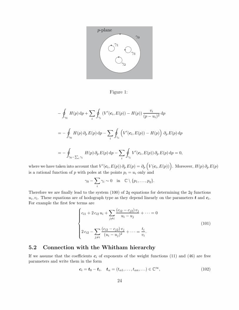
p-plane
γ0
γ1
γ2
γ3
Figure 1:
−∮
γ0
H(p) dp +∑
i
∮
γi
(V ′(ci, E(p)) − H(p))vi
(p − ui)2dp
= −∮
γ0
H(p) ∂p E(p) dp −∑
i
∮
γi
(V ′(ci, E(p)) − H(p)
)∂p E(p) dp
= −∮
γ0−P
i γi
H(p) ∂p E(p) dp −∑
i
∮
γi
V ′(ci, E(p)) ∂p E(p) dp = 0,
where we have taken into account that V ′(ci, E(p)) ∂p E(p) = ∂p
(V (ci, E(p))
). Moreover, H(p) ∂p E(p)
is a rational function of p with poles at the points pi = ui only and
γ0 −∑
i
γi ∼ 0 in C \ p1, . . . , pq.
Therefore we are finally lead to the system (100) of 2q equations for determining the 2q functionsui, vi. These equations are of hodograph type as they depend linearly on the parameters t and ci.For example the first few terms are
ci1 + 2 ci2 ui +∑
j 6=i
(ci2 − cj2) vj
ui − uj+ · · · = 0
2 ci2 −∑
j 6=i
(ci2 − cj2) vj
(ui − uj)2+ · · · =
tivi
.
(101)
5.2 Connection with the Whitham hierarchy
If we assume that the coefficients ci of exponents of the weight functions (11) and (46) are freeparameters and write them in the form
ci = t0 − ti, tα = (tα1, . . . , tαn, . . .) ∈ C∞, (102)
24

then, as we are going to see, the solution of (95) turns out to determine a solution of the Whithamhierarchy of dispersionless integrable system [11].
Let us introduce the modified Orlov functions
mα = V ′(tα, zα) + mα. (103)
It is clear that (zα, mα) solve the system
z0 = z1 = · · · = zq,
m0 = m1 = · · · = mq.
(104)
Moreover, they are rational functions of p with poles at the points pi = ui only. Furthermore, theysatisfy the asymptotic properties (92) and
mα =∑
n≥1
n tαn zn−1α +
tαzα
−∑
n≥1
n Sαn(t)
zn+1α
, as zα → ∞.
Thus, the functions (zα, mα) satisfy all the conditions of Theorem 1 of [15] and, as a consequence,they verify the equations of the Whitham hierarchy
∂zα
∂tµn= Ωµn, zα,
∂mα
∂tµn= Ωµn, mα (105)
where the Poisson bracket is given by
F,G :=∂F
∂p
∂G
∂x− ∂F
∂x
∂G
∂p, x := t01.
and the Hamiltonian functions are
Ωµn :=
(znµ)(µ,+), n ≥ 1,
− log(p − ui), n = 0, µ = i = 1, . . . , q.
(106)
Here (·)(0,+) stands for the projector on pn∞n=0 .
In this way we conclude that (zα, mα), as functions of the coupling constants ci = t0 − ti,determine a reduced solution of the Whitham hierarchy. This property is in complete agreementwith the results of recents works [16] which prove that the universal Whitham hierarchy can beobtained as a particular dispersionless limit of the multi-component KP hierarchy. Moreover, as itas been observed in [24], appropriate deformations of the Riemann-Hilbert problems for multipleorthogonal polynomials determine solutions of the multi-component KP hierarchy. In fact thesedeformations correspond to the flows induced by changes in the parameters tα. Indeed, for bothtypes of multiple orthogonal polynomials, (102) implies
∂tαn g = [zn Eα, g].
Therefore the covariant derivatives
Dαn f := ∂αn f + zn f Eα,
25
are symmetries of the corresponding Riemman-Hilbert problems. Hence, using Proposition 2 oneconcludes that
∂αn f + (zn f Eα f−1)− f = 0, (107)
where ( )− stands for the projections of power series in zk, (k ∈ Z) on the subspaces generatedby z−k (k ≥ 1). The equations (107) constitute the linear system of the multi-component KPhierarchy.
6 Applications: random matrix models and
non-intersecting Brownian motions
As we have seen the multiple orthogonal polynomials of type I are the elements f0i of the funda-mental solution of their associated RH problem. Thus, in the quasiclassical limit we have
Ai(n, z) ∼ 1
zexp
(1
ǫSi(t, z))
), as ǫ → 0,
where Si = Si(t, z) are the classical action functions defined in (83). Hence
ǫ ∂z log Ai(n, z) ∼ ∂z Si(t, z) − ǫ
z= mi(t, z) − ǫ
z. (108)
On the other hand, if we denote by xi the roots of Ai(n, z) we have
∂z log Ai(n, z) =
ni−1∑
i=1
1
z − xi.
Thus if we assume that in the large-n limit the roots of Ai are distributed with a continuous densityρi = ρi(x) on some compact (possibly disconnected) support Ii ⊂ R
ǫ
ni−1∑
i=1
1
z − xi∼
∫
Ii
ρi(x)
z − xdx, as ǫ → 0. (109)
from (108) and (109) we deduce the important relation
mi(z) =
∫
Ii
ρi(x)
z − xdx, (110)
where mi, Ii and ρi depend on the slow variables t. This means that the Orlov functions mi arethe Cauchy transforms of the root densities ρi. Hence, they determines the distribution of roots inthe large-n limit according to
mi+(x) − mi−(x) = −2 iπ ρi(x), x ∈ Ii. (111)
Moreover, from (97) we see that ∫
Iρi(x) dx = ti. (112)
26

On the other hand, the multiple orthogonal polynomials of type II represent the element f00 oftheir associated RH problem. Therefore, in the quasiclassical limit we have
P (n, z) ∼ exp(1
ǫS0(t, z)
), as ǫ → 0,
Thus if we assume that in the large-n limit the roots of P (n, z) tend to be distributed with acontinuous density ρ0 = ρ0(x) on some compact support I0 ⊂ R, we deduce
m0(z) =
∫
I0
ρ0(x)
z − xdx, (113)
where m0, I0 and ρ0 depend on the slow variables t. Thus the Orlov function m0 is the Cauchytransform of the density ρ0 and therefore
m0+(x) − m0−(x) = −2 iπ ρ0(x), x ∈ I0. (114)
Note also that ∫
I0
ρ0(x) dx = t0. (115)
The string equations (95) provide also useful information to determine the limiting supportsand the root densities. They imply
m0(z) = −H(p0(z)), mi(z) = V ′(ci, z) − H(pi(z)),
where pα(z) denote the q + 1 inverses of the map
z(p) := E(p) = p +
q∑
k=1
vk(t)
p − uk(t),
verifying
p0(z) = z + O(1
z
), pi(z) = ui + O
(1
z
); as z → ∞.
Therefore (111) and (114) reduce to
H(pα+(x)) − H(pα−(x)) = 2 iπ ρα(x), x ∈ Iα. (116)
In general the limiting supports Iα may consist of several disconnected segments
Iα =
dα⋃
k=1
Iαk
which, due to (116), constitute the branch cuts of the functions H(pα(z)) . As a consequence theend-points of the segments Iαk are the branch points of these functions, which are in turn givenby the critical points xi of the function z(p) = E(p)
xi = E(qi) ∈ R, ∂pE(qi) = 0. (117)
27

6.1 The Hermitian matrix model
For q = 1 the multiple orthogonal polynomials of type II reduce to the orthogonal polynomials onthe real line associated to the weight function w = exp V (c, z). These polynomials are connectedto the random matrix model of n×n Hermitian matrices [1]-[2]
Zn =
∫dM exp
(Tr V (c,M)
), (118)
through the crucial relationPn(z) = E [det(z − M)], (119)
where E denotes the expectation value with respect to the probability measure determined by(118). This means that in the large-n limit the eigenvales of M converge with unit probability tothe roots of Pn. As a consequence the root density ρ0 of the family of polynomials represents theeigenvalue density of the matrix model.
The Hermitian matrix model provides an appropriate example to illustrate all the aspects ofour method for characterizing the quasiclassical limit. In this case we set ǫ := 1/n, t0 = 1 and wehave
z(p) = E(u, v, p) = p +v
p − u.
Here u and v depend on the coupling constants c = (c1, c2, . . .) and can be determined by meansof the hodograph equations (99)-(100)
∮
γ0
dp
2iπH(p) = −1,
∮
γ1
dp
2iπ
V ′(c, E(p)) − H(p)
p − u= 0.
By introducing the change of variable p − u → p these equations are equivalent to the well-knownsystem [1] ∮
γ
dp
2iπV ′(c, p + u +
v
p) = −1,
∮
γ
dp
2iπ pV ′(c, p + u +
v
p) = 0, (120)
which characterizes the spherical limit in the Hermitian matrix model of 2D gravity. Here γ is alarge positively oriented circle around the origin.
The critical points of E are q± = u ±√v, so that the support of eigenvalues is
I = [x−, x+], x± := u ± 2√
v. (121)
We use (116) to determine the density of eigenvalues according to
H(p0+(x)) − H(p0−(x)) = 2 iπ ρ0(x), x ∈ [x−, x+]. (122)
Furthermore, the two inverses of z(p) are
p0(z) :=1
2(z + u +
√(z − x−)(z − x+) ), p1(z) :=
1
2(z + u −
√(z − x−)(z − x+) ) (123)
and we haveH(p0(z)) = V ′(c, z(p))(1,+)
∣∣∣p=p0(z)
.
28
Now, using the identities
v
p − u= z − p, p2 = (u + z) p − z u − v,
it is clear that there exist polynomials αk(z) and βk(z) satisfying
(z(p)k
)
(1,+)
∣∣∣p=p0(z)
= αk(z) + βk(z) p0(z),(z(p)k
)
(1,+)
∣∣∣p=p1(z)
= αk(z) + βk(z) p1(z). (124)
In particular, taking into account that
p0(z) = z + O(1
z
), p1(z) = u + O
(1
z
); as z → ∞,
from (124) we deduce
βk(z) = −( zk
p0 − p1
)⊕
= −( zk
√(z − x−)(z − x+)
)⊕, (125)
where ( )⊕ means the projection of power series in zn, (n ∈ Z) on the subspace generated byzn, (n ≥ 0). Hence it follows that
H(p0(z)) =∑
k≥1
k ck
(αk−1(z) + βk−1(z) p0(z)
),
and therefore we get
ρ(x) =1
2 iπ
∑
k≥1
kckβk−1(x)(p0+(x) − p0−(x)) = − 1
2π
( V ′(c, x)√(x − x−)(x − x+)
)⊕
√(x − x−)(x+ − x),
which represents the well-known eigenvalue density for the Hermitian model in the one-cut case.
6.2 Gaussian models with an external source and non-intersecting
Brownian motions
For q > 1 the multiple orthogonal polynomials of type II are connected to the Gaussian Hermitianmatrix model with an external source term AM [6]-[9], where A is a fixed diagonal n×n realmatrix. The partition function of this model is given by
Zn =
∫dM exp
(− Tr
(1
2M2 − AM
)). (126)
It turns out that if the eigenvalues of A are given by aj , (j = 1, . . . , q) with multiplicities nj, thenthe expectation values
P (n, z) = E [det(z − M)], n := (n1, . . . , nq), (127)
are multiple orthogonal polynomials with respect to the Gaussian weights
wj(x) = exp(aj x − 1
2x2).
29

These matrix models are deeply connected to one-dimensional non-intersecting Brownian motion[20]-[22]. More concretely, the joint probability density for the eigenvalues (λ1, . . . , λn) of M is thesame as the probability density at time t ∈ (0, 1) for the positions (x1, . . . , xn) of n non-intersectingBrownian motions starting at the origin at t = 0 and forming q groups ending at q fixed pointsbi, (i = 1, . . . , q) at t = 1. The corresponding dictionary for this duality is
λj =xj√
t(1 − t), ak = bk
√t
1 − t.
We discuss next an example of application to the large-n limit of non-intersecting Brownianmotions. Let us consider an even number n non-intersecting Brownian motions ending at twopoints ±b with n1 = n2 = n/2 [9]. In this case the slow variables take the values t1 = t2 = −1/2.Moreover, we have
V (c1, z) = a z − z2
2, V (c2, z) = −a z − z2
2, a := b
√t
1 − t,
andz(p) = E(p) = p +
v1
p − u1+
v2
p − u2, H(p) = − v1
p − u1− v2
p − u2= p − z(p). (128)
Using the hodograph equations (101) one finds
u1 = a, u2 = −a, v1 = v2 =1
2,
so that
z(p) =p3 + (1 − a2)p
p2 − a2.
The corresponding algebraic function p = p(z) satisfies the Pastur equation [23]
p3 − z p2 + (1 − a2) p + a2 z = 0,
which defines a three-sheeted Riemann surface. The restrictions of p(z) to the three sheets are thefunctions pα(z) characterized by the asymptotic behaviour
p0(z) = z + O(1
z
), pi(z) = ui + O
(1
z
), i = 1, 2; as z → ∞.
There are four critical points of z(p) which give rise to four branch points ±x1, ±x2 in the z-planewhere
x1 = q1
√1 + 8 a2 + 3√1 + 8 a2 + 1
, x2 = q2
√1 + 8 a2 − 3√1 + 8 a2 − 1
,
q1,2 =
√1
2+ a2 ± 1
2
√1 + 8 a2.
It is easy to see that x1 is real for all a ≥ 0, while x2 is real for a ≥ 1 (x2 < x1) and purelyimaginary for 0 < a < 1. Now, from (122) and taking into account that H(p) = p−z(p) we deducethat the eigenvalue density is given by
ρ0(x) =1
2 iπ(H(p0+(x)) − H(p0−(x)) =
1
2 iπ(p0+(x) − p0−(x)), x ∈ I0. (129)
30

0.2 0.4 0.6 0.8 1.0 t
-1.0
-0.5
0.5
1.0
x
Figure 2: Limit support for Brownian motions with two symmetric endpoints for b = 1
-3 -2 -1 0 1 2 3x
0.1
0.2
Ρ0
-3 -2 -1 0 1 2 3x
0.1
0.2
Ρ0
-3 -2 -1 0 1 2 3x
0.1
0.2
Ρ0
-3 -2 -1 0 1 2 3x
0.1
0.2
Ρ0
Figure 3: The density of Brownian motions ρ0(x) for a = 1/2, 3/4, 1 and 3/2, respectively
Using Cardano’s formula for p0 one finds
ρ0(x) =2x2 + 6 (a2 − 1) − 3
√2
(r(x) −
√r(x)2 − 4 s(x)3
)2/3
25/3√
3 π 3
√r(x) −
√r(x)2 − 4 s(x)3
,
wherer(x) := −2x3 + 18 a2 x + 9x, s(x) := x2 + 3 (a2 − 1).
The form of the support I0 depends on the analytic properties of the function p0(z) ( see [6]-[9]):
a) For 0 < a ≤ 1 the function p0 is analytic in C − [−x1, x1] and I0 = [−x1, x1].
b) For a > 1 the function p0 is analytic in C− ([−x1,−x2]∪ [x2, x1]) and I0 = [−x1,−x2]∪ [x2, x1].
31

Acknowledgements
The authors wish to thank the Spanish Ministerio de Educacion y Ciencia (research projectFIS2008-00200/FIS) for its finantial support. This work is also part of the MISGAM programmeof the European Science Foundation.
References
[1] P. Di Francesco, P. Ginsparg and Z. Zinn-Justin, Phys. Rept. 254,1 (1995)
[2] P. Deift, Orthogonal Polynomials and Random Matrices: A Riemann-Hilbert approach,Courant Lecture Notes in Mathematics Vol. 3, Amer. Math. Soc., Providence R.I. 1999.
[3] A.S. Fokas, A.R. Its and A.V. Kitaev, Commun. Math. Phys. 147, 395 (1992)
[4] P. Deift and X. Zhou, Ann. Math. 2, 137 (1993)
[5] W. Van Assche, J.S. Geronimo, and A.B.J. Kuijlaars, Riemann-Hilbert problems for mul-
tiple orthogonal polynomials, In: Special Functions 2000: Current Perspectives and Future
Directions (J. Bustoz et al., eds.), Kluwer, Dordrecht, (2001) 2359.
[6] P.M. Bleher and A.B.J. Kuijlaars, Int. Math. Research Notices 2004, no 3 (2004), 109129.
[7] P.M. Bleher and A.B.J. Kuijlaars, Comm. Math. Phys. 252 (2004), 4376.
[8] A.I. Aptekarev, P.M. Bleher and A.B.J. Kuijlaars, Comm. Math. Phys. 259 (2005), 367289.
[9] P.M. Bleher and A.B.J. Kuijlaars, , Comm. Math. Phys. 270 (2007), 481.
[10] E. Daems, Asymptotics for non-intersecting Brownian motions using multiple orthogonal poly-
nomials, Ph.D. thesis, K.U.Leuven, 2006, URL http://hdl.handle.net/1979/324.
[11] I. M. Krichever, Comm. Pure. Appl. Math. 47 (1994), 437.
[12] K. Takasaki and T. Takebe, Rev. Math. Phys. 7, 743 (1995)
[13] M. J. Bergvelt and A. P. E. ten Kroode, Pacific J. Math. 171 23 (1995).
[14] M. Manas, E. Medina and L. Martınez Alonso, J. Phys.A: Math. Gen. 39 (2006) 2349.
[15] L. Martınez Alonso, E. Medina and M. Manas, J. Math. Phys. 47 (2006) 083512.
[16] K. Takasaki, Dispersionless integrable hierarchies revisited, talk delivered at SISSA at septem-ber 2005 (MISGAM program); K. Takasaki and T. Takebe, Physica D 235 (2007) 109.
[17] E. Daems and A.B.J. Kuijlaars, J. of Approx. Theory 146 (2007) 91.
[18] L. Martınez Alonso and E. Medina, J. Phys.A: Math. Gen. 40 (2007) 14223.
[19] L. Martınez Alonso and E. Medina, J. Phys.A: Math. Gen. 41 (2008) 335202.
[20] K. Johansson, Probab. Theory Related Fields 123 (2002), 225.
[21] M. Katori and H. Tanemura, Phys. Rev. E 66 (2002) Art. No. 011105.
[22] T. Nagao and P.J Forrester, Nuclear Phys. B 620 (2002), 551.
[23] L. Pastur, Teoret. Mat. Fiz. 10 (1972), 102112.
[24] Mark Adler, Pierre van Moerbeke and Pol Vanhaecke, Moment matrices and multi-component
KP, with applications to random matrix theory, preprint math-ph/0612064
32


