Embed Size (px)
Citation preview
Mooring Line Damping In Very Large Water Depths
byRicardo Balzola
Master of Engineering in LogisticsDepartment of Civil and Environmental Engineering
Massachusetts Institute of Technology (1999)
Ocean Engineer and Naval ArchitectUniversidad Politecnica de Madrid, Spain (1997)
SUBMITTED TO THE DEPARTMENT OF OCEAN ENGINEERINGIN PARTIAL FULFILLMENT OF THE REQUIREMENTS FOR THE DEGREE OF
MASTER OF SCIENCE IN NAVAL ARCHITECTURE AND OCEANENGINEERING
at the
MASSACHUSETTS INSTITUTE OF TECHNOLOGY
September 1999
@ 1999 Ricardo Balzola, All Rights Reserved
The author hereby grants to MIT permission to reproduce and distribute publicly paperand electronic copies of this thesis document in whole or in part
Signature of the Author...................... ......... ...........epartment of Ocean Engineering
Aygust, 1999
Certified by ...........................................Paul D. Sclavounos
Professor of Naval ArchitectureThesis Supervisor
A ccepted b y .................................... r......... . . ..................................Professor A. Baggeroer
Chairman, Departmental Committee on Graduate Studies
MASSACHUSE
NOV 2
LIBRARIES-
Mooring Line Damping In Very Large Water Depth
by
Ricardo Balzola
Submitted to the Department of Ocean Engineering
on August , 1999, in partial fulfillment of the
requirements for the degree of
Master of Science in Naval Architecture and Ocean Engineering
Abstract
Precise position and motion control are indispensable factors for the operation of offshoreplatforms. Mooring systems are, by all means, the most common devices to obtain therequired control.
The response to the motions of the platform performed by the moor will, in many cases,dictate the overall offshore platform behavior as a result of environmental loads. Theseloads induce in the system two typical modes of oscillation; slow drift and wavefrequency motions.
The objective of this thesis is to investigate the dynamic responses and the dampingachieved by cable and synthetic mooring systems when the water depth is very large.Numerical simulations for different modes of oscillation and initial conditions of themooring lines have been executed, as to establish a comparison between the dynamicproperties of the diverse mooring solutions.
Finally, in order to analyze the relative importance of the mooring damping results, theplatform-moor systems are approximated to a one-dimensional mechanical dampedoscillator. This approximation highlights the motion modes where the moor response iscritical as well as exploring the advantages and disadvantages of each mooring solution.
Thesis supervisor: Professor Paul D. SclavounosTitle: Professor of Naval Architecure

Acknowledgements
First of all, I would like to thank my parents for all the support and help they have given
me throughout my life.
I wish to thank Jennifer, her patience with me is enormous, her help and encouragement
when I most needed has been crucial for me to be able to finish this work in time. Thank
you very much Jennifer, you really deserve it.
I also want to thank my advisor, Professor Paul Sclavounos, for his guidance during this
last 18 months. I want to thank him how much I have learnt from him, not only about
science and physics, but also about live and motivation. It has been very hard but also
very educating.
I also want to thank Sungeun Kim, who has made possible this thesis helping me
understand LINES 1.1 and obtain the results that are the basis for this work.
Finally, I want to thank the rest of my family, and friends, those over here and those in
Spain, for making my life so enjoyable and fulfilling.
3
CHAPTER 1: INTRODUCTION 9
1.1 MOTIVATION 9
1.2 OFFSHORE PLATFORMS 10
1.3 MOORING SYSTEMS 11
1.4 THESIS OVERVIEW 11
CHAPTER 2: MATHEMATICAL FORMULATION: 13
2.1.PLATFORM DYNAMICS FORMULATION: 13
2.2.MOORING LINE FORMULATION: 14
2.2. 1.CHARACTERISTIC EQUATIONS OF THE LINES 14
2.2.2.INTERNAL FORCES: 17
2.2.3.EXTERNAL FORCES: 18
2.2.4.BOUNDARY CONDITIONS: 23
2.3.5.INTERACTION WITH THE SEABED: 24
2.4.MOORING LINE DAMPING GENERATION 25
2.4. WHOLE MOORING SYSTEM FORMULATION 28
CHAPTER 3: INITIAL CONFIGURATIONS 29
3.1.MAIN CHARACTERISTICS OF THE SPAR PLATFORM: 31
3.2.MAIN CHARACTERISTICS OF THE MOORING SYSTEMS: 32
3.2. 1.CABLE MOORING SYSTEM SOLUTION 33
3.2.2.SYNTHETIC MOORING CONFIGURATIONS: 35
CHAPTER 4: NUMERICAL RESULTS. 40
4.1.COMPARISON OF THE DYNAMIC PROPERTIES OF THE FOUR MOORS
4.2.SLOW DRIFT OSCILLATION:
40
41
4
4.3.LINEAR SURGE OSCILLATIONS
4.4.HEAVE OSCILLATIONS
49
55
CHAPER 5: DAMPING RELATIVE IMPORTANCE 60
5.1 LINEAR DAMPED OSCILLATOR 60
5.2. PLATFORM-MOOR COEFFICIENTS 63
5.3 LINEAR APPROXIMATION 65
CHAPTER 6: CONCLUSIONS 72
REFERENCES: 74
APPENDIX A: ROPE PROPERTIES 76
5
Index of Tables:
Table 2-2: V iscous coeficients................................................................................... 21
Table 3-1: Main Characteristics of Spar Hull............................................................. 31
Table 3-2: Main Characteristics of cable mooring system ......................................... 33
Table 3-3: Synthetic moor line's properties .............................................................. 38
Table 4-1: Equivalent excursion for slow-drift motions ............................................. 41
Table 4-2: Linear surge amplitudes............................................................................ 50
Table 5-1: Linear approximation coefficients for slow drift motion. ........................... 65
Table 5-2: Linear approximation coefficients for linear surge motion. ....................... 66
Table 5-3: Linear approximation coefficients for linear heave motion........................66
Table 5-4: Linear approximation non-dimensional coefficients for slow drift motion.....67
Table 5-5: Linear approximation non-dimensional coefficients for linear surge motion. 67
Table 5-6: Linear approximation non-dimensional coefficients for heave motion. ......... 68
6
Index of Figures:
Figure 4-18: Heave damping. Synth. Medium tension. .................................................... 8
Figure 4-19: Heave damping. Synth. High tension...................................................... 8
Figure 5-2.A: Unstable oscillation ................................................................................ 8
Figure 5-2.B: Neutrally stable..................................................................................... 8
Figure 2-1: Mooring line local coordinates ................................................................. 15
Figure 2-2: Mooring line segment .............................................................................. 16
Figure 2-3: Internal tensions....................................................................................... 18
Figure 2-4: Relative velocities...................................................................................20
Figure 2-5: Static position of mooring line..................................................................25
Figure 2-6: Fairlead oscillations ................................................................................ 26
Figure 2-6 A: Force of fairlead ................................................................................... 27
Figure 2-6 C: Hysteresis Cycle ................................................................................... 27
Figure 2-6 B: Fairlead oscillations..............................................................................27
Figure 3-1: Spar Platform....................................................................... 30
Figure 3-2: Spar platform dimensions............................................................................ 32
Figure 3-3 Catenary type mooring system.................................................................. 34
Figure 3-4: Synthetic Line pretension........................................................................ 35
Figure 3-5: Moor static restoring forces...................................................................... 36
Figure 3-6: Synthetic mooring system ........................................................................ 39
Figure 4-1: Slow drift damping. Cable....................................................... 42
Figure 4-2: Slow drift damping. Synth. Low tension.........................................42
Figure 4-3: Slow drift damping. Synth. Medium tension.....................................43
Figure 4-4: Slow drift damping. Synth. High tension............................................... 43
Figure 4-5: Slow drift damping. Period 50 s. ............................................................. 45
Figure 4-6: Slow drift damping. Period 100 s. ........................................................... 45
Figure 4-8: Slow drift hysteresis Cycles. Period 100s. .............................................. 47
Figure 4-9: Linear surge damping. Cable........................................................51
Figure 4-10: Linear surge damping. Synth. Low tension...................................51
Figure 4-11: Linear surge damping. Synth. Med. tension...................................52
7
Figure 4-12: Linear surge damping. Synth. High tension................................... 52
Figure 4-13: Linear surge damping. Period 10 s......................................................... 53
Figure 4-14: Linear surge hysteresis cycles. Period 7s. .............................................. 54
Figure 4-15: Linear surge hysteresis cycles. Period 15s. ............................................ 55
Figure 4-16: Heave damping. Cable..............................................................56
Figure 4-17: Heave damping. Synth. Low tension.............................................56
Figure 4-18: Heave damping. Synth. Medium tension...............................................57
Figure 4-19: Heave damping. Synth. High tension.................................................... 57
Figure 4-20: Vertical damping. Period 10s. ................................................................ 58
Figure 4-21: Heave hysteresis Cycles. Period 10s...................................................... 59
Figure 5-1: Simple model for damped oscillator........................................................ 60
Figure 5-2.A: Unstable oscillation....................................................................... 62
Figure 5-2.C: Damped oscillations............................................................ 62
Figure 5-2.B : N eutrally stable........................................................................... 62
Figure 5-2.D: Collapse response ............................................................... 62
Figure 5-3: Natural oscillation for slow drift linear approximation..............................69
8
CHAPTER 1:
INTRODUCTION
1.1 Motivation
Precise position and motion control are indispensable factors for the operation of offshore
platforms. Although there are other means of obtaining this control, mooring lines are,
without any doubt, the most important solution.
Among the mooring line solutions, there are at least two subdivisions. One division is the
vertical tension leg mooring, for which the buoyancy of the platform exceeds the weight,
and the cables provide the net equilibrating force.
The second class, which is the object of study of this thesis, are the spread mooring
systems, that consist of several pre-tensioned anchor lines arrayed around the structure to
hold the mooring in the desired position. This thesis will study in detail the dynamics of
this type of mooring systems for large water depths.
9
1.2 Offshore Platforms
Offshore platform designs vary from gravity platforms sitting on the seabed, to semi-
submergible platforms, purely large free-floating bodies. The semi-submergible offshore
platforms are used for large to very large water depths, and are typically kept in position
by a spread mooring system. A set of pipes and risers are used to connect this floating
structure with the exploration and drilling equipment on the seabed.
Semi-submergible platforms are subject to environmental loads, mainly created by
waves, wind and ocean currents. These environmental loads induce motion responses on
the platform-moor group. Typically, motions of floating structures can be divided into
wave-frequency, high frequency, and slow drift motions.
The wave frequency motion is mainly produced by first order interactions between waves
and the floating body. The amplitude and frequency of these motions are, in general,
similar to those of the waves that induce them.
High frequency motions are generated by non-linear wave excitation. Their natural
periods are in the order of two to four seconds and they are frequently significant for TLP
structures. They are out of the scope of this thesis, since they do not appear in catenary-
type moored platforms.
Similar non-linear interactions between the floating body and the waves cause slow and
mean drift motions. This kind of motion appears in every type of floating platform. They
arise from resonant slow-drift oscillations. The typical period of these oscillations are in
the range of 50 to 150 seconds for conventional moored platforms. This type of motion
for a moored floating body typically occurs in surge, sway and yaw. Slow drift motions
are characterized by large horizontal excursions of the platforms that drive, as a result,
enormous forces on the mooring lines.
10

These types of oscillations are critical in catenary type moored platforms and are being
studied in this thesis.
1.3 Mooring systems
Spread mooring systems hold semi-submergible platforms and floating production ships
in their desired position. Moreover, the moor provides the floating body the required
restoring forces to return to that equilibrium position when environmental loads force the
structure away from it.
The increasing water depth of oil exploration and drilling is creating the necessity for
new solutions of spread mooring systems. Cable moors are becoming increasingly
expensive for very large water depths, since the complexity of their installation is
growing rapidly due to the large weight of the lines. Therefore, lighter moorings are
becoming more attractive, especially for large water depths.
This thesis studies and compares three synthetic mooring solutions with a regular cable-
catenary type moor. The static and dynamic responses of these moors has been studied in
order to compare the restoring and damping properties among each of these four
solutions.
1.4 Thesis overview
This thesis has been divided into six chapters.
Chapter two covers the analytical formulation of the problem, starting with a brief review
of platform dynamics, and then deriving the characteristic equations of the mooring lines.
This mooring line formulation neglects the contribution of bending effects. Finally this
11
chapter covers the derivation of energy absorption achieved by the lines and moor as they
are forced to undergo oscillatory motions.
Chapter three presents the platform specifications that have been used as a base for this
study and the mooring line designs that have been tested along this thesis. These designs
include material and geometrical properties as well as all the static responses of the
different systems to offset the fairlead from the initial position.
Chapter four presents the numerical results of the motion simulations for the mooring line
designs. These results present the dynamic properties of the mooring systems for 3
distinct modes of oscillation, slow drift surge, wave frequency surge and finally wave
frequency heave motions. Diverse amplitudes and periods have been used for all mooring
systems in order to understand the non-linear dynamics of these simulations.
Chapter five compares the results from chapter four using a linear damped oscillator. A
brief introduction to the formulation of a linear damped oscillator is included in this
section. Then, the mooring damping results from chapter four and the restoring forces of
chapter three are converted to the constant coefficients that the formulation of the
damping physical approximation requires. The results from this approximation are
displayed in this chapter.
The computations presented in this thesis were carried out with the computer program
LINES 1.1 licensed by Boston Marine Consulting Inc. Further details on the methods
presented in this thesis along with the capabilities of LINES 1.1 may be found in the
LINES 1.1 user manual which can be downloaded from the BMC web site at
www.bmarc.com.
Finally chapter six draws the main conclusions of the thesis.
12
CHAPTER 2:
MATHEMATICAL FORMULATION:
2.1.Platform Dynamics formulation:
The dynamics of a floating offshore structure can be modeled through a second order
coupled linear system of differential equations. For all practical purposes, the platform is
considered a rigid structure with 6 degrees of freedom. The general equation for such a
system can be expressed in matrix form as:
[M + A]d ' + [B]- +([C ].i=Nt(21dt dt
Where the i is a 6x1 vector that holds the six degrees of freedom that characterize the
response of the structure. The first three values of this vector represent the platform
translations along the coordinate system axes while the last three values describe
rotations around these same axes. M, A, B and C are six by six matrices that incorporate
the mass, added mass, damping and restoring coefficients of the floating structure. The
13
magnitude and distribution of the coefficients in these matrices reflect the dynamic and
static characteristics of each degree of freedom and the coupling effects among them.
The force term in the previous equation comprises the sum of all the environmental loads
to the floating body plus the force due to the mooring system. For all practical purposes,
the forces on the fairlead of the mooring lines are, as those of the platform, dependent on
acceleration, velocity and position of the system. Therefore, it is natural to bring them to
the left-hand side of the equation.
Not all the contributions, however, of the moor to the L.H.S. matrices are equally
important. The inertia related terms for the mooring system are very small compared to
those of the platform. The mass and added mass of the mooring lines are several orders of
magnitude smaller than those of the platform.
On the other hand, the contribution to the damping and restoring coefficients are very
important, and in some cases they are the dominant contribution to the damping and
restoring forces. For example, the restoring coefficient in sway, surge or yaw comes
solely from the mooring system. To fully understand the dynamics of a floating platform,
we must comprehend the interaction between this body and the mooring that maintains at
a fixed position.
2.2.Mooring Line Formulation:
2.2.1.Characteristic equations of the lines
Let a generic mooring line be defined by the so-called natural coordinates of a 3-
dimensional line. The anchor end in the material line would be defined as the origin and
the direction towards the fairlead as positive along the cable.
14
Fairlead
Z
Y
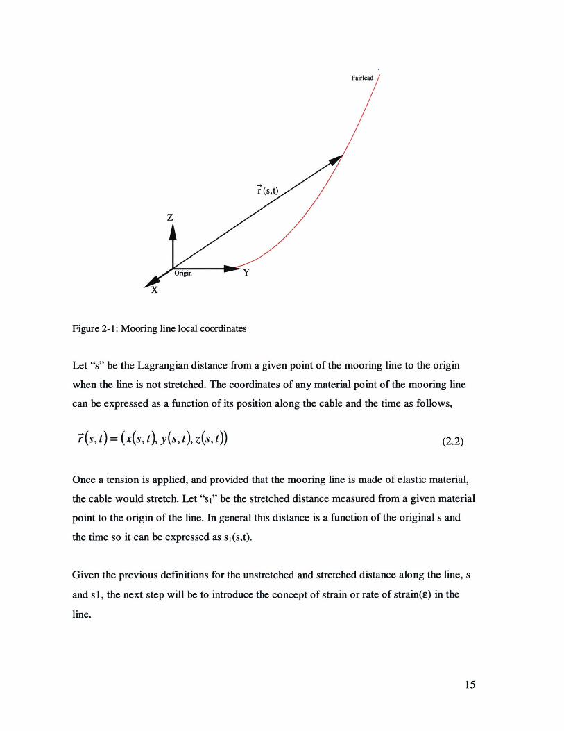
Figure 2-1: Mooring line local coordinates
Let "s" be the Lagrangian distance from a given point of the mooring line to the origin
when the line is not stretched. The coordinates of any material point of the mooring line
can be expressed as a function of its position along the cable and the time as follows,
r(s, t) = (x(s, t), y(s, t), z(s, t)) (2.2)
Once a tension is applied, and provided that the mooring line is made of elastic material,
the cable would stretch. Let "si" be the stretched distance measured from a given material
point to the origin of the line. In general this distance is a function of the original s and
the time so it can be expressed as si(s,t).
Given the previous definitions for the unstretched and stretched distance along the line, s
and si, the next step will be to introduce the concept of strain or rate of strain(E) in the
line.
15
Strain e: A cable segment with unstretched length s has at some point a Lagragian
arclength of si. Let the strain E then be defined as follows:
E=lim C =ds-1s->0 & ds
ds
ds(2.3)
Let then t be the tangential vector to the stretched position of the material line. As such
it can be expressed as the first derivative of the vector i with respect to si, the stretched
distance. Then,
- di dF ds dF 1 dit = - = -- > - = (1+,C) t
ds, ds ds, ds1+E ds(2.4)
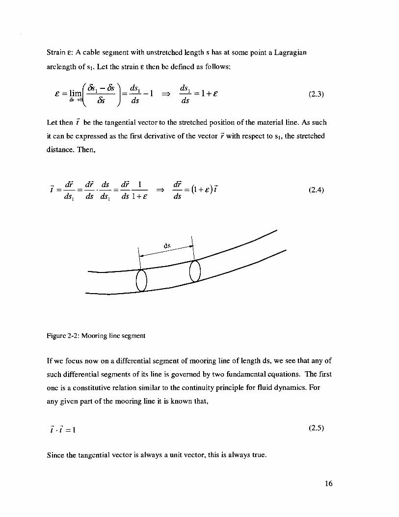
Figure 2-2: Mooring line segment
If we focus now on a differential segment of mooring line of length ds, we see that any of
such differential segments of its line is governed by two fundamental equations. The first
one is a constitutive relation similar to the continuity principle for fluid dynamics. For
any given part of the mooring line it is known that,
(2.5)t =1
Since the tangential vector is always a unit vector, this is always true.
16
Then combining equation 2.4 and equation 2.5 we obtain,
dFd= (1+ ) ~ = + 2Eds ds
(2.6)
The second equation that governs the mooring line motion is Newton's Law that can be
expressed as,
m - = I External Forces + 1 Internal Forces (2.7)
2.2.2.Internal Forces:
The fundamental internal force present in a mooring line is the tension. For mooring
lines, it is a normal practice to introduce the concept of an effective tension Te. This
tension is defined by:
Te=T+Pf Af (2.8)
Where,
Pf is the fluid pressure in the position of this particular segment of the mooring line
discarding the line-induced disturbance and, Af is the cross sectional area of the line.
The utilization of the effective tension causes the mooring line equations to look like their
equivalent in air with the exception that when calculating the force due to the weight of
the cable or line, the regular weight must be replaced by the weight of the line in water.
17
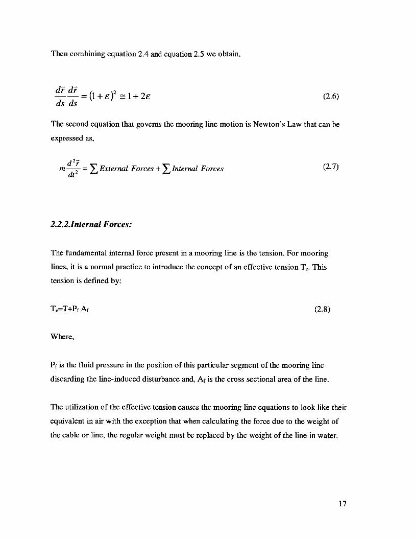
T2
Figure 2-3: Internal tensions
The tension inside the line will, generally, have the same direction as the line itself.
Therefore, the internal force on a segment with unstretched length can be written as:
d T- d 1 dInternal Force =-dTe t sds Tdsce (etds=±(1+) e ds) (2.9)
2.2.3.External Forces:
The external forces to a segment of mooring line can be subdivided into 3 components,
F1 due to weight and buoyancy effects
F2 due to flow inertial effects. (Added mass related forces)
F3 due to fluid viscous effects.
Line Weight. Buoyancy.
The total vertical force of the segment due to weight and buoyancy effects is given by:
F; = (gpf Af -ws-k (2.10)
18
Where,
pf is the fluid density and,
w is the line weight in water per unit length.
Added mass forces:
The inertia related forces can be divided into two different components. The first one is
due to the motion of the fluid around the mooring line segment. The second component is
to the motion of the segment itself considering the fluid surrounding it stationary.
For the calculation of both of these terms we will need the following linear operator, [N],
which is a 3x3 matrix, that multiplied by a vector, yields the component of this vector
normal to the mooring line. Lets define [N] as,
[N] =[I] -[d(2.11)ds .ds
With the aid of the matrix [N] and using GI Taylor's Theorem to calculate the normal
inertial forces, the added mass terms exerted upon the line are split into,
diiF21 = pf Afds(1 + Cm)[N] dL (2.12)
dt
Due to the fluid velocity ii, around a fixed segment and,
F22 = -PfAfds(Cm)[N] d (2.13)
F22~~ 2P f t
Due to the acceleration of the material segment 2 assuming the surrounding fluid isdt 2
stationary.
19
Note that the flow velocity and acceleration are free of disturbance effects caused by their
interaction with the line. This last fact being only an approximation is very reasonable,
since the flow is most affected by other large structures as the platform itself or the flow
initial velocity components due to currents or waves. Taking into account the possible
disturbances in the flow due to the presence of the mooring line would make the problem
far more complicated and provide only marginal changes to the final result.
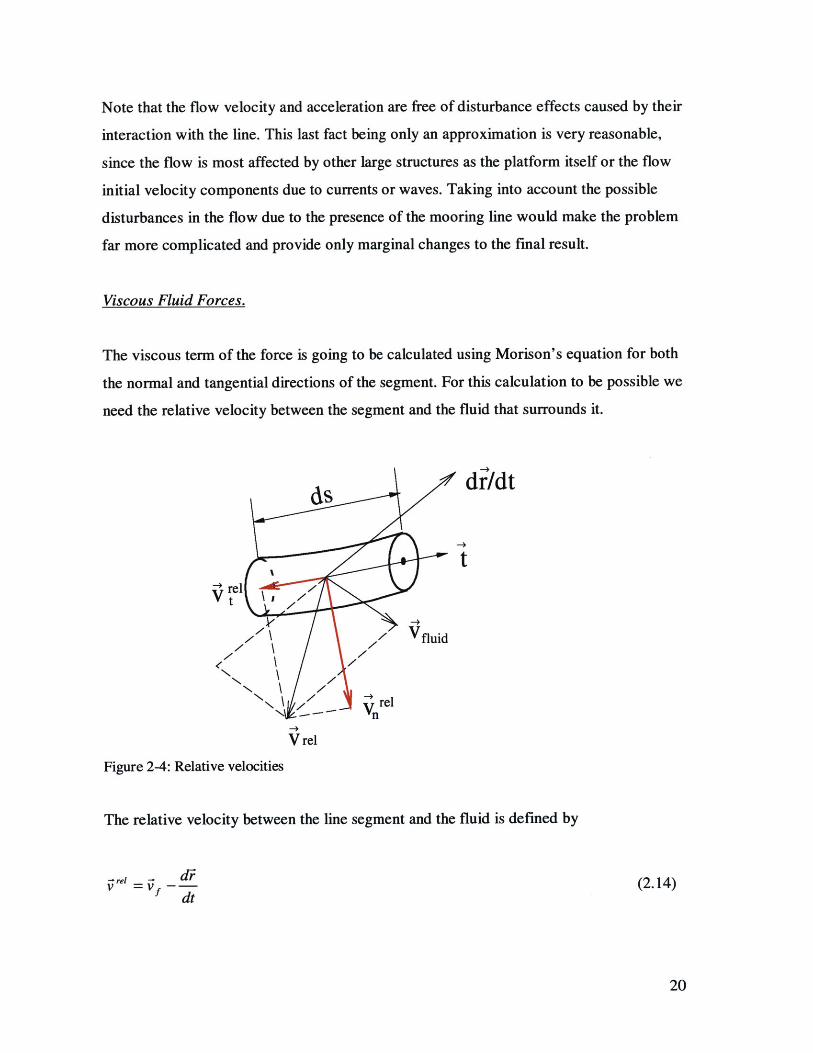
Viscous Fluid Forces.
The viscous term of the force is going to be calculated using Morison's equation for both
the normal and tangential directions of the segment. For this calculation to be possible we
need the relative velocity between the segment and the fluid that surrounds it.
df/dt
t
V t
V rel
Figure 2-4: Relative velocities
The relative velocity between the line segment and the fluid is defined by
rel = -
' dt(2.14)
20
Now, if we decompose this relative velocity in tangential and normal direction relative to
the mooring line we obtain,
rel =[N]irel (2.15)
for the relative normal velocity and,
--re -- re) I( _ -~rel 1 d 1 -- re
I+E ds 1+e ds (1+E)2 ds -I (2.16)
rel 1 (di -. ,e di_-~re I _r _ vl r
1+2e ds ds
for the relative tangential velocity. Once we know this two components of the relative
velocity the viscous force acting along the line can be approximated through Morrison's
equation in both directions as,
=1Ire + ;r' CI ;'relI -trel d (.73 = pf (D,,C + 1 " Vt jds (2.17 )
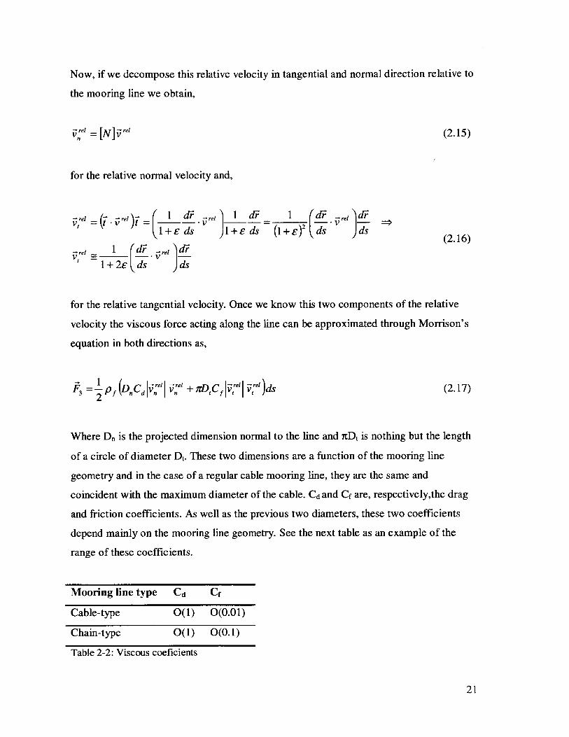
Where Dn is the projected dimension normal to the line and nDt is nothing but the length
of a circle of diameter Dt. These two dimensions are a function of the mooring line
geometry and in the case of a regular cable mooring line, they are the same and
coincident with the maximum diameter of the cable. Cd and Cf are, respectively,the drag
and friction coefficients. As well as the previous two diameters, these two coefficients
depend mainly on the mooring line geometry. See the next table as an example of the
range of these coefficients.
Mooring line type Cd Cr
Cable-type O(1) 0(0.01)
Chain-type O(1) 0(0.1)
Table 2-2: Viscous coeficients
21
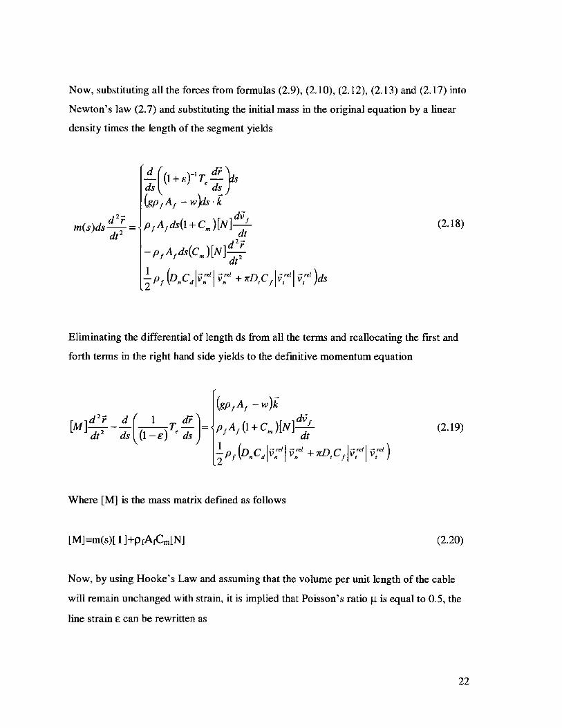
Now, substituting all the forces from formulas (2.9), (2.10), (2.12), (2.13) and (2.17) into
Newton's law (2.7) and substituting the initial mass in the original equation by a linear
density times the length of the segment yields
m(s)ds dr =2dt 2
- (1 + E)- T -ds *ds
(gpf Af - wds -kdi
P, Afds(1+ C, )[N] !dt
P Ads(Cm )[N] dF
p,(D,,Cd I' re' + 7D,C f, ,"rel )ds
Eliminating the differential of length ds from all the terms and reallocating the first and
forth terms in the right hand side yields to the definitive momentum equation
d 2 i d 1 di[M] 2I T, - =<
dt2 ds y(-) E ds)
(gpf Af -w)k
di,Pf Af (1+ Cm )[N] '
dt
2P, (D,C '' + DC
Where [M] is the mass matrix defined as follows
[M]=m(s)[ I ]+pfAfCm[N]
(2.19)
(2.20)
Now, by using Hooke's Law and assuming that the volume per unit length of the cable
will remain unchanged with strain, it is implied that Poisson's ratio g is equal to 0.5, the
line strain F can be rewritten as
22
(2.18)
Te= e (2.21)
EA,
And plugging this definition of the line strain into the original "Continuity" equation
(2.6) leads to the following constitutive relation:
&& T_- =1+ 2 Te (2.22)
ds ds AE
that can be rewritten as:
Te = - 1 (2.23)2 (ds ds
Momentum equation (2.19) plus this last constitutive relation (2.23) comprise a full close
form of equations to study the dynamics of a mooring line. From this system we are able
to obtain the displacement of every segment, F = (s, t), and the effective tension, Te.
However, for the problem to be complete, these equations have to be supplemented with
two extra requirements. On one hand, the non-linear system of partial differential
equations requires a set of boundary conditions, and on the other hand, due to the nature
of the problem, the interaction of the mooring line with the seabed requires a special
treatment.
2.2.4.Boundary Conditions:
Although different authors [9] use different boundary conditions, probably the most
natural set of conditions for catenary-like problems are the positions of both ends of the
mooring line. Therefore LINES 1.1 uses the following as boundary condition inputs. The
first boundary condition is given by fixing the position of the anchor to the line
coordinate system origin. The second B.C. is simply given by the position of the fairlead
23
in time referred, again, to the same mooring line coordinate system. These two conditions
can be expressed as follows,
(O, t)= 0 (2.24)
r (L, t)= R(t) (2.25)
Where s=O is nothing but the origin in arclength of the mooring line and L is the
maximum unstretched arclength of the line and consequently where the fairlead stands.
2.3.5.Interaction with the seabed:
Typical wire rope and chains used in mooring systems have generally a significant length
of line that lies on the ocean floor. The interaction with the seabed adds a new dimension
to the classic catenary problem. Apart from the exterior forces that have been discussed
up to now, introducing the presence of the seabed adds another force to the problem. Any
part of the mooring line laying on the plane z=O gets a supporting force from the seabed
that cancels out the remaining weight of that particular part of the line.
To solve this problem, LINES uses the following approach: Whenever any segment of
the mooring line lays under the z=O plane, the regular weight force of the segment is
inverted to point upwards. The idea is to create an artificial medium below the seabed
with a higher density than the mooring line. The density in this artificial medium is
linear; it has a value equal to the density of the mooring line for z=O and increases
linearly as z tends to higher numbers in the negative range. With such a medium the
segments of the mooring line that might be under the seabed will eventually float to the
surface of the seabed as the simulation runs to their real static position.
The weight and buoyancy force components that were displayed in equation (x) for z>O
are changed into
F1= (gAfp(1-kz)-w)k for z 0 (2.26)
24
Where ki is the slope of the density in the artificial medium and ps is the modified density
of the line. p, is such that for z=O the vertical force turns out to be zero as well. For any
z<O the magnitude of this force would increase linearly as shown by equation 2.26.
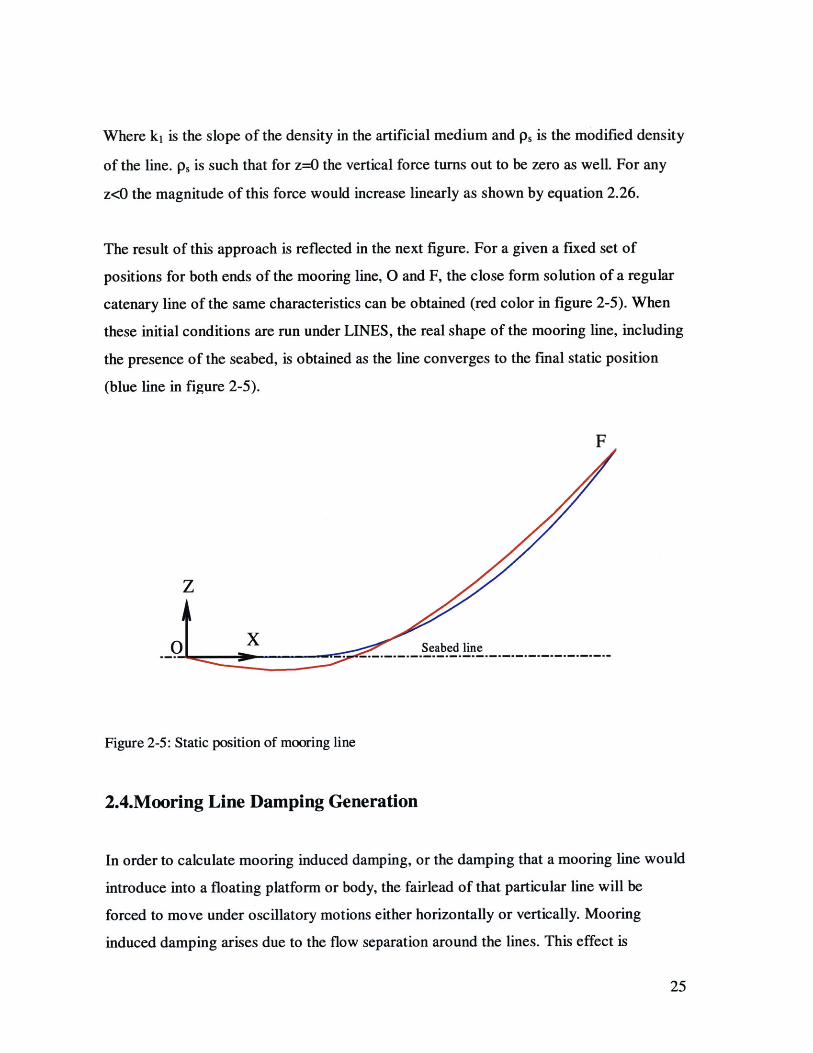
The result of this approach is reflected in the next figure. For a given a fixed set of
positions for both ends of the mooring line, 0 and F, the close form solution of a regular
catenary line of the same characteristics can be obtained (red color in figure 2-5). When
these initial conditions are run under LINES, the real shape of the mooring line, including
the presence of the seabed, is obtained as the line converges to the final static position
(blue line in figure 2-5).
F
Z
X
Figure 2-5: Static position of mooring line
2.4.Mooring Line Damping Generation
In order to calculate mooring induced damping, or the damping that a mooring line would
introduce into a floating platform or body, the fairlead of that particular line will be
forced to move under oscillatory motions either horizontally or vertically. Mooring
induced damping arises due to the flow separation around the lines. This effect is
25
simulated in a non-linear manner by the usage of the viscous effects under Morrison's
equation.
The damping contribution of the mooring line is calculated as the energy that the material
line absorbs along a complete oscillation cycle. To calculate this damping, we need the
pair (Tension, Position) on the fairlead for every time step along this cycle. With that
pair, the damping contribution would be calculated as,
(2.27)E =f F(t )- d -Jt Pe (T) -Ai
t dt ,eio
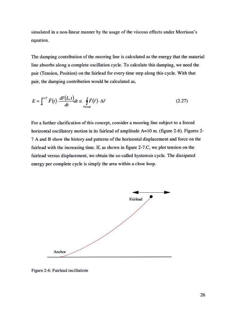
For a further clarification of this concept, consider a mooring line subject to a forced
horizontal oscillatory motion in its fairlead of amplitude A=10 m. (figure 2-6). Figures 2-
7 A and B show the history and patterns of the horizontal displacement and force on the
fairlead with the increasing time. If, as shown in figure 2-7.C, we plot tension on the
fairlead versus displacement, we obtain the so-called hysteresis cycle. The dissipated
energy per complete cycle is simply the area within a close loop.
Fairlead
Anchor
Figure 2-6: Fairlead oscillations
26

0
0
0Z
t
Figure 2-6 A: Force of fairlead
Horizontal Displacement
Figure 2-6 C: Hysteresis Cycle
Figure 2-6 B: Fairlead oscillations
The area embedded in the hysteresis cycle represents the amount of energy absorbed by
the line in every oscillation and corresponds to the result obtained from the integration
2.27. Note that while this hysteresis loop figure presents several oscillation cycles figures
A and B represent only about a period and a half of the fairlead oscillating motions and
forces. It is clear from the hysteresis loop graph that the system has reached a reasonable
27
steady motion. Note that mooring lines, being a dynamic system, cause the results from
the first period or periods in the simulation to be discharged since they are sensitive to the
start-up transients.
2.4. Whole Mooring System formulation
The previous procedure for a single mooring line has been generalized to take account for
the coupled responses of all the lines comprising the mooring system.
The relationships for the total force that the mooring system exerts on the platform can be
found by considering the individual line contributions. In general,
L
F =I F i =1,2,3 (2.28)n=1
Where F is the total force on the direction i and L is the total number of lines. And,
L
M = " XF" (2.29)n=1
Where M is the total torque that the mooring system applies into the platform and F" is
the position of the fairlead of line n relative to the platform coordinate system.
Knowing these extensions, the damping created by the assemblage of all mooring lines
creates is obtained by adding the contributions of all the forces in the integration along
the complete motion loop.
28
CHAPTER 3
INITIAL CONFIGURATIONS
As off shore oil exploration and production moves into areas of greater ocean depths, the
necessity to create and implement new concepts in mooring designs becomes
increasingly apparent.
As water depths increase, the regular cable catenary moorings become less and less
attractive. For large and especially very large water depths, the cable mooring lines
become extremely long and heavy. This large weights and lengths carry several
disadvantages. The first disadvantage is seen in the dramatic increase of the cable cost
and, particularly, the cost of the moor installation. Secondly, as depth increases, the
restoring force to horizontal motion decreases drastically, allowing very large horizontal
excursions of the offshore system. These large offsets of the platform increase the cost of
the riser solutions.
In recent years the trends of the mooring systems for offshore devices have been shifted
into different approaches than the regular steel catenary moorings. Taut mooring systems
using synthetic fibers are an interesting alternative. Some of the potential benefits of the
usage of synthetic lines when compared with catenary mooring systems are:
29
* Low weight: This fact diminishes the cost of handling and installation of the mooring
system.
e Smaller horizontal offsets. The offsets are reduced by a factor of 2-5 with respect to a
regular catenary system.
e No potential hazard to the sub-sea equipment in case of a line breakage and fall into
the seabed.
e Smaller lengths of cable that drives the total cost of the line down.
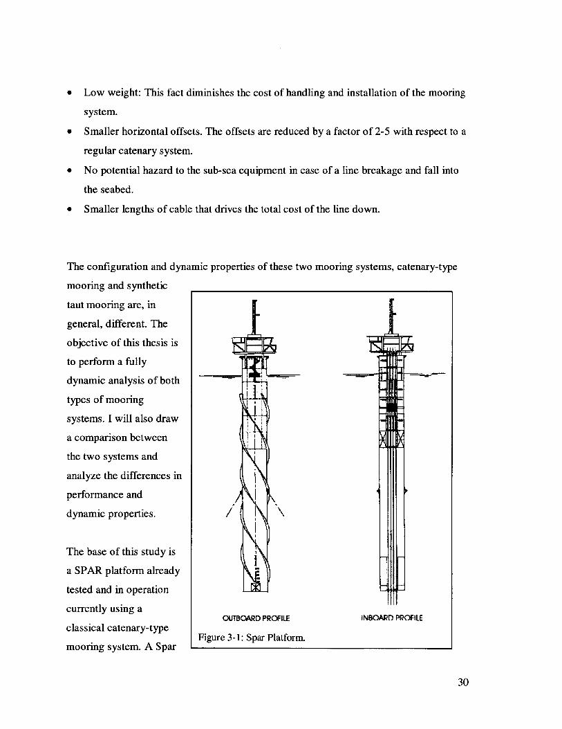
The configuration and dynamic properties of these two mooring systems, catenary-type
mooring and synthetic
taut mooring are, in
general, different. The
objective of this thesis is
to perform a fully
dynamic analysis of both ~ - -
types of mooring
systems. I will also draw -
a comparison between
the two systems and
analyze the differences in
performance and
dynamic properties.
The base of this study is
a SPAR platform already
tested and in operation
currently using aOUTBOCARD PROFILE INBOARD PROFILE
classical catenary-type
mooring system. A Spar Figure 3-1: Spar Platform.
30
platform is a deep draft offshore structure. This type of offshore platform consists of a
cylindrical hull and a deck. The hull might be used for storage purposes. The deck on this
type of platform is a more typical deck that can be found on many other offshore
platforms.
The analysis for all systems, the existing mooring lines and a synthetic cable taut
moorings, are based on the hull motion results and the response to the environmental
loads of the system. The responses of the platform to the environmental loads have been
obtained from experimental data and state-of-the-art computational tools such as SWIM
(Slow Wave Motion of Platforms). While only one configuration for the catenary-type
has been studied since this solution has already been installed in the platform, I have run
extensive experiments with different solutions for synthetic taut mooring lines.
3.1.Main characteristics of the SPAR platform:
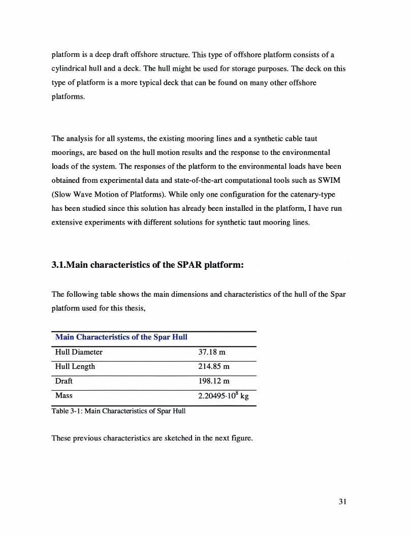
The following table shows the main dimensions and characteristics of the hull of the Spar
platform used for this thesis,
Main Characteristics of the Spar Hull
Hull Diameter
Hull Length
Draft
Mass
Table 3-1: Main Characteristics of Spar Hull
37.18 m
214.85 m
198.12 m
2.20495.108 kg
These previous characteristics are sketched in the next figure.
31

Figure 3-2: Spar platform dimensions
The weight of this type of platform and the amount of water that her hull displaces causes
the platform to rest in vertical stable equilibrium. The purpose of the moor is to hold the
platform over a specific point of the seabed and not to fix her vertical position. However,
given the shape and position of lines in the mooring systems, the platform receives an
extra vertical tension that pulls it down. The magnitude of this tension is very small
compared to the buoyancy or the weight effects of the platform.
3.2.Main characteristics of the mooring systems:
The platform is held at a fixed position by the mooring system. This mooring system
provides the platform with the restoring forces and damping to balance out the
displacements and motions that the environmental loads induce on the floating structure.
This platform particular moor consists on a set of 14 lines evenly distributed in a circular
shape around the hull. The geometry and physical properties of all the lines are the same.
This study consists of full numerical dynamic simulations for each different set of
mooring lines. The first test coincides with the existing one in the platform, while the rest
are based on synthetic lines. All these synthetic lines will have similar material
properties, but different initial pretensions. To achieve the variation in the pretension of
32
the lines, the initial position of the anchor is going to be variable. The rest of the
geometrical properties of these lines are going to be the same so that the reason for all
possible differences in the dynamic properties is only due to the initial pretension.
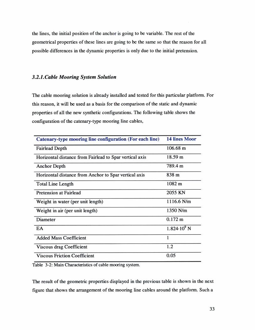
3.2.1.Cable Mooring System Solution
The cable mooring solution is already installed and tested for this particular platform. For
this reason, it will be used as a basis for the comparison of the static and dynamic
properties of all the new synthetic configurations. The following table shows the
configuration of the catenary-type mooring line cables,
Catenary-type mooring line configuration (For each line) 14 lines Moor
Fairlead Depth 106.68 m
Horizontal distance from Fairlead to Spar vertical axis 18.59 m
Anchor Depth 789.4 m
Horizontal distance from Anchor to Spar vertical axis 838 m
Total Line Length 1082 m
Pretension at Fairlead 2055 KN
Weight in water (per unit length) 1116.6 N/m
Weight in air (per unit length) 1350 N/m
Diameter 0. 172 m
EA 1.824-109 N
Added Mass Coefficient 1
Viscous drag Coefficient 1.2
Viscous Friction Coefficient 0.05
Table 3-2: Main Characteristics of cable mooring system.
The result of the geometric properties displayed in the previous table is shown in the next
figure that shows the arrangement of the mooring line cables around the platform. Such a
33
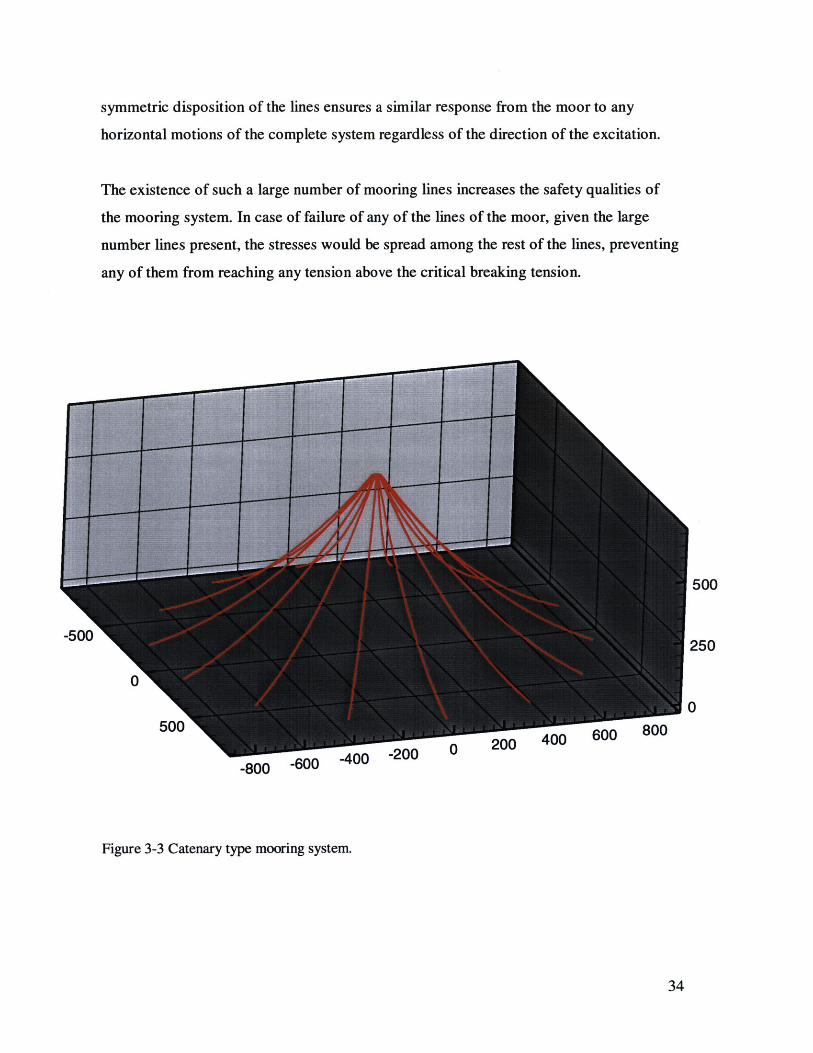
symmetric disposition of the lines ensures a similar response from the moor to any
horizontal motions of the complete system regardless of the direction of the excitation.
The existence of such a large number of mooring lines increases the safety qualities of
the mooring system. In case of failure of any of the lines of the moor, given the large
number lines present, the stresses would be spread among the rest of the lines, preventing
any of them from reaching any tension above the critical breaking tension.
500
250
0
-400 -200
Figure 3-3 Catenary type mooring system.
34
3.2.2.Synthetic Mooring Configurations:
All the synthetic lines tested configurations are also composed of a set of 14 lines evenly
distributed around the vertical axis of the platform. The fundamental reason behind this
decision was to eliminate all possible reasons of misleading results of the experiments. A
secondary reason for using the set of 14 lines is to ensure similar safety qualities and to
preserve the axisymmetric properties of the moor.
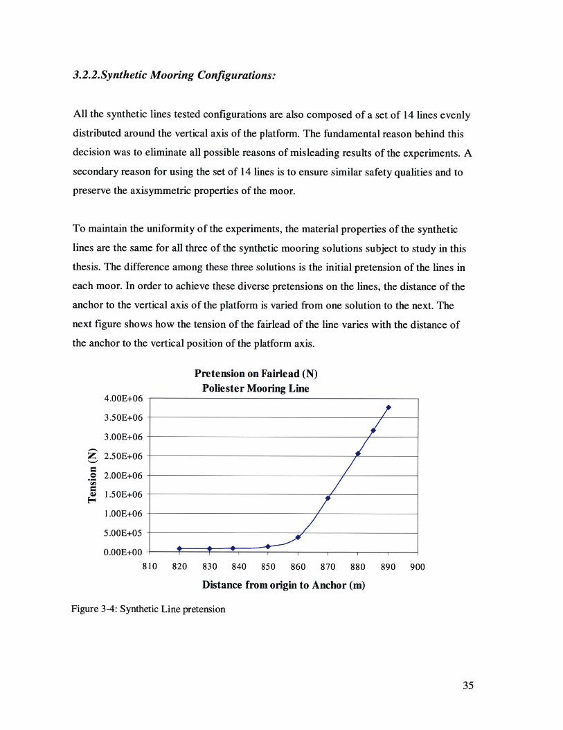
To maintain the uniformity of the experiments, the material properties of the synthetic
lines are the same for all three of the synthetic mooring solutions subject to study in this
thesis. The difference among these three solutions is the initial pretension of the lines in
each moor. In order to achieve these diverse pretensions on the lines, the distance of the
anchor to the vertical axis of the platform is varied from one solution to the next. The
next figure shows how the tension of the fairlead of the line varies with the distance of
the anchor to the vertical position of the platform axis.
Pretension on Fairlead (N)Poliester Mooring Line
4.OOE+06
3.50E+06
3.OOE+06
4 2.50E+06
.5 2.OOE+06
1.50E+06
1.OOE+06
5.OOE+05
O.OOE+00
810 820 830 840 850 860 870 880 890 900
Distance from origin to Anchor (m)
Figure 3-4: Synthetic Line pretension
35
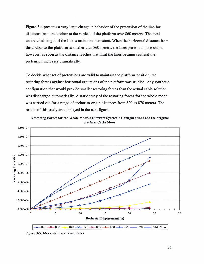
Figure 3-4 presents a very large change in behavior of the pretension of the line for
distances from the anchor to the vertical of the platform over 860 meters. The total
unstretched length of the line is maintained constant. When the horizontal distance from
the anchor to the platform is smaller than 860 meters, the lines present a loose shape,
however, as soon as the distance reaches that limit the lines became taut and the
pretension increases dramatically.
To decide what set of pretensions are valid to maintain the platform position, the
restoring forces against horizontal excursions of the platform was studied. Any synthetic
configuration that would provide smaller restoring forces than the actual cable solution
was discharged automatically. A static study of the restoring forces for the whole moor
was carried out for a range of anchor-to-origin distances from 820 to 870 meters. The
results of this study are displayed in the next figure.
Restoring Forces for the Whole Moor. 8 Different Synthetic Configurationa and the originalplatform Cable Moor.
1.80E-07
1.60E+07
1.40E+07
1.20E+07
1.OOE+07
.~8.OOE-i06
8A
- 6.OOE+06
4.OOE+06 _
2.OOE+06
0.00E+00 I-. . ,--4
0 5 10 15 20 25 30
Horizontal Displacement (m)
-+-820 -U-830 840 -%-850 -*-855 -- 860 -- 865 - 870 - Cable Moor
Figure 3-5: Moor static restoring forces
36
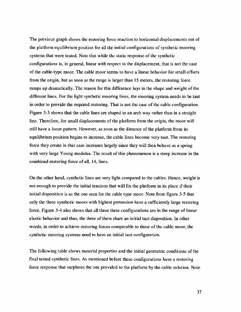
The previous graph shows the restoring force reaction to horizontal displacements out of
the platform equilibrium position for all the initial configurations of synthetic mooring
systems that were tested. Note that while the static response of the synthetic
configurations is, in general, linear with respect to the displacement, that is not the case
of the cable-type moor. The cable moor seems to have a linear behavior for small offsets
from the origin, but as soon as the range is larger than 15 meters, the restoring force
ramps up dramatically. The reason for this difference lays in the shape and weight of the
different lines. For the light synthetic mooring lines, the mooring system needs to be taut
in order to provide the required restoring. That is not the case of the cable configuration.
Figure 3-3 shows that the cable lines are shaped in an arch way rather than in a straight
line. Therefore, for small displacements of the platform from the origin, the moor will
still have a loose pattern. However, as soon as the distance of the platform from its
equilibrium position begins to increase, the cable lines become very taut. The restoring
force they create in that case increases largely since they will then behave as a spring
with very large Young modulus. The result of this phenomenon is a steep increase in the
combined restoring force of all, 14, lines.
On the other hand, synthetic lines are very light compared to the cables. Hence, weight is
not enough to provide the initial tensions that will fix the platform in its place if their
initial disposition is as the one seen for the cable type moor. Note from figure 3-5 that
only the three synthetic moors with highest pretension have a sufficiently large restoring
force. Figure 3-4 also shows that all these three configurations are in the range of linear
elastic behavior and thus, the three of them share an initial taut disposition. In other
words, in order to achieve restoring forces comparable to those of the cable moor, the
synthetic mooring systems need to have an initial taut configuration.
The following table shows material properties and the initial geometric conditions of the
final tested synthetic lines. As mentioned before these configurations have a restoring
force response that surpluses the one provided to the platform by the cable solution. Note
37
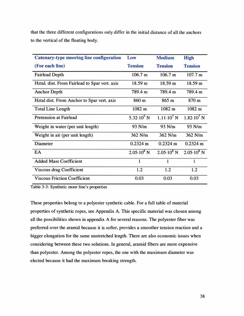
that the three different configurations only differ in the initial distance of all the anchors
to the vertical of the floating body.
Catenary-type mooring line configuration
(For each line)
Fairlead Depth
Hztal. dist. From Fairlead to Spar vert. axis
Anchor Depth
Hztal dist. From Anchor to Spar vert. axis
Total Line Length
Low
Tension
106.7 m
18.59 m
789.4 m
860 m
1082 m
Medium
Tension
106.7 m
18.59 m
789.4 m
865 m
1082 m
High
Tension
107.7 m
18.59 m
789.4 m
870 m
1082 m
Pretension at Fairlead 5.32-10' N 1.11-i0 7 N 1.82-10' N
Weight in water (per unit length) 93 N/m 93 N/m 93 N/m
Weight in air (per unit length) 362 N/m 362 N/m 362 N/m
Diameter 0.2324 m 0.2324 m 0.2324 m
EA 2.05.108 N 2.05. 108 N 2.05. 108 N
Added Mass Coefficient
Viscous drag Coefficient
Viscous Friction Coefficient
Table 3-3: Synthetic moor line's properties
1
1.2
0.03
1
1.2
0.03
1
1.2
0.03
These properties belong to a polyester synthetic cable. For a full table of material
properties of synthetic ropes, see Appendix A. This specific material was chosen among
all the possibilities shown in appendix A for several reasons. The polyester fiber was
preferred over the aramid because it is softer, provides a smoother tension reaction and a
bigger elongation for the same unstretched length. There are also economic issues when
considering between these two solutions. In general, aramid fibers are more expensive
than polyester. Among the polyester ropes, the one with the maximum diameter was
elected because it had the maximum breaking strength.
38

The aspect of the whole synthetic mooring system is shown in the next figure:
500
250
500 0
-500. 500 0
Figure 3-6: Synthetic mooring system
This last figure shows that even at an equilibrium position, the synthetic cables are
shaped as straight lines. For the 3 synthetic mooring systems examined in this study, the
shape looks the same and the only difference among them is the distance of the anchor
and the consequent different rate of strain since all the lines have the same unstretched
length.
This initial taut shape of the lines explains why the static force response of these mooring
systems to offsets is linear. Provided that the tension in the lines does not reach ranges
close to their breaking strength, the strain behavior of these synthetic ropes can be
assumed as linear with respect to the internal tension in the lines. Given then, the initial
taut disposition of this type of moor, it is expected for the static restoring force response
not to show the non-linearities that the cable mooring system shows.
39
CHAPTER 4:
NUMERICAL RESULTS.
4.1.Comparison of the dynamic properties of the four moors
As mentioned in the second chapter, any floating body can sustain motions in 6 different
directions. For the specific case of a SPAR platform held by means of a mooring line
three of these motions are of special interest; surge, sway and heave. In the particular
case of the first two, we can expect an axisymmetric behavior around the vertical axis due
to the large number of lines and their specific disposition around the platform. Hence,
only horizontal motions along the X-axis have been studied.
As also mentioned in the second chapter, when dealing with wave induced motions in
floating bodies, there has to be a clear distinction among, linear and non-linear effects.
Heave motions are fundamentally induced by wave linear effects, while in the surge
direction, both linear and non-linear effects are important. Linear effects excite platform
motions of amplitude in the same order as the amplitude of the waves that induce them,
while the amplitude of the oscillations induced by slow drift effects are much larger. The
natural periods of these two types of oscillations also differ a great deal, the natural
period of the linear induced motions are also in the same order of that of the waves that
40
excite them. On the other hand, the natural periods of oscillation induced by slow drift
effects are very long, typically in the order of one minute to a hundred seconds.
4.2.Slow Drift Oscillation:
The value of the maximum amplitude of oscillation induced to the platform due to slow
drift effects is known, at least for the cable mooring system. From this maximum
excursion and using information from figure 3-4 the value of the maximum excursions
for different mooring systems is obtained. The taut synthetic moors should incur in
smaller offsets since the restoring forces of the synthetic lines are larger for the same
displacement.
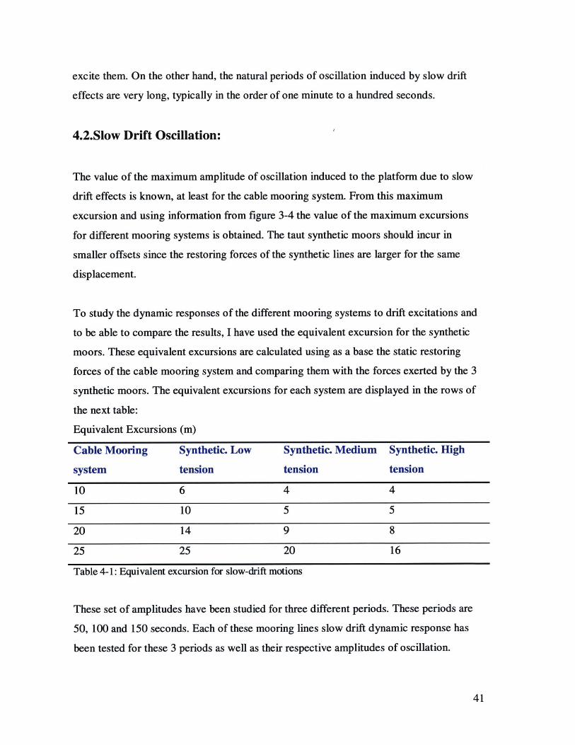
To study the dynamic responses of the different mooring systems to drift excitations and
to be able to compare the results, I have used the equivalent excursion for the synthetic
moors. These equivalent excursions are calculated using as a base the static restoring
forces of the cable mooring system and comparing them with the forces exerted by the 3
synthetic moors. The equivalent excursions for each system are displayed in the rows of
the next table:
Equivalent Excursions (m)
Cable Mooring Synthetic. Low Synthetic. Medium Synthetic. High
system tension tension tension
10 6 4 4
15 10 5 5
20 14 9 8
25 25 20 16
Table 4-1: Equivalent excursion for slow-drift motions
These set of amplitudes have been studied for three different periods. These periods are
50, 100 and 150 seconds. Each of these mooring lines slow drift dynamic response has
been tested for these 3 periods as well as their respective amplitudes of oscillation.
41
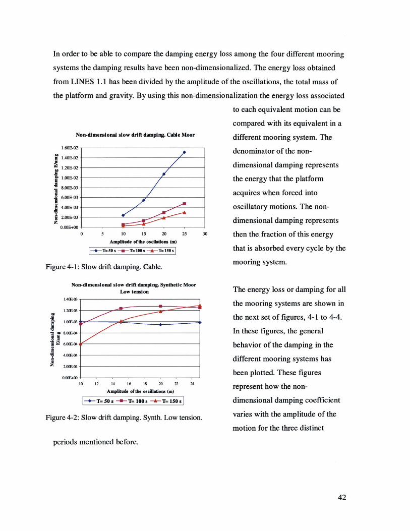
In order to be able to compare the damping energy loss among the four different mooring
systems the damping results have been non-dimensionalized. The energy loss obtained
from LINES 1.1 has been divided by the amplitude of the oscillations, the total mass of
the platform and gravity. By using this non-dimensionalization the energy loss associated
to each equivalent motion can be
compared with its equivalent in aNon-dimensional slow drift damping. Cable Moor different mooring system. The
L.60E-02 denominator of the non-E 1.40E-02
1.20E-02 dimensional damping represents
'OOE-02 the energy that the platform8.O,033
6.0033 acquires when forced into
4.O-03 oscillatory motions. The non-S2.00E303
z 2.OOE-03 dimensional damping represents
0 5 10 15 20 25 30 then the fraction of this energyAmplitnde of the oscilations (m)
-+-T-50s -- T-100s -A-T-150s that is absorbed every cycle by the
Figure 4-1: Slow drift damping. Cable. mooring system.
Non-dimensional slow drift damping. Synthetic MoorLow tension
1AE 03
1.20B-03
8.WGE-04
6.0E-04
4.OE-04
2.O(E-04
O.Ot400 10 12 14 16 18 20 22
Amplitude of the oscilations (m)
-+-T=.50 -ST=100 -+-T=1.50 s
The energy loss or damping for all
the mooring systems are shown in
the next set of figures, 4-1 to 4-4.
In these figures, the general
behavior of the damping in the
different mooring systems has
been plotted. These figures
represent how the non-
dimensional damping coefficient
varies with the amplitude of the
motion for the three distinct
24
Figure 4-2: Slow drift damping. Synth. Low tension.
periods mentioned before.
42
*1
II0
a0
I

Figure 4-1 shows the resulting damping for the cable mooring system, while the other
three plots show the damping results for the synthetic cases, starting with the low tension
graph, figure 4-2 and finishing with the high tension one, figure 4-4.
Non-dimensional slow drift damping. Synthetic MoorMedium tension The behavior of the damping
s.ooso4 coefficients in these graphs
- OOE-04 follows, up to some point, the
expected shape. From theseog4.00E04
graphs we see that as the
2.OOE-04 - amplitude of the motionsO.OOE-00 increases, so does the
0 5 10 15 20 25 amplitude of the coefficient.Amplitude of the oscilations (m)
-+-T-50s-U-T-100s A+T-150s The first of these graphs, 4-1,
Figure 4-3: Slow drift damping. Synth. Medium tension. represents the cable catenary-
Non-diensional slow ddft daning. Syntheic Moor type mooring system. From
High temion this graph, we notice that the
smaller periods the larger the4.OOE-04
damping becomes. The reason3.50E-04
S.0OE-04 for this behavior is that for al2.5004
similar amplitude, as the
e1-50E0' period of oscillation|| 1.OO-04
5.oo-o5 - decreases, the faster theo.OOE+00
0 5 10 15 20 velocities and accelerations ofAmplItude of the oscIations (m) the line segments increase.
-4-- T=50 s - T= 100 s -A- T= 150 s
Figure 4-4: Slow drift damping. Synth. High tension. The viscous and inertial terms
in the governing equation
become, therefore, very
crucial for two reasons. The first reason is the large weight of this line, considerably
larger than the synthetic one, makes the inertial effects very important. The second
affects the viscous terms of the governing equation. The transversal fluid-segment
43
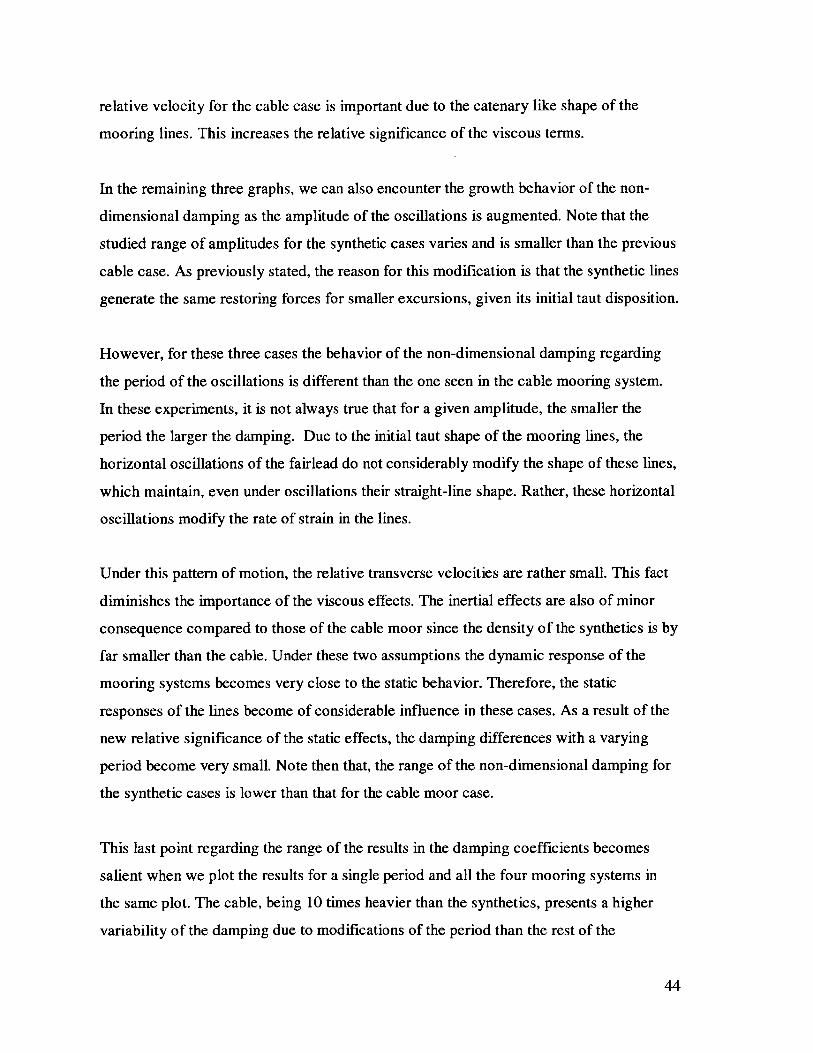
relative velocity for the cable case is important due to the catenary like shape of the
mooring lines. This increases the relative significance of the viscous terms.
In the remaining three graphs, we can also encounter the growth behavior of the non-
dimensional damping as the amplitude of the oscillations is augmented. Note that the
studied range of amplitudes for the synthetic cases varies and is smaller than the previous
cable case. As previously stated, the reason for this modification is that the synthetic lines
generate the same restoring forces for smaller excursions, given its initial taut disposition.
However, for these three cases the behavior of the non-dimensional damping regarding
the period of the oscillations is different than the one seen in the cable mooring system.
In these experiments, it is not always true that for a given amplitude, the smaller the
period the larger the damping. Due to the initial taut shape of the mooring lines, the
horizontal oscillations of the fairlead do not considerably modify the shape of these lines,
which maintain, even under oscillations their straight-line shape. Rather, these horizontal
oscillations modify the rate of strain in the lines.
Under this pattern of motion, the relative transverse velocities are rather small. This fact
diminishes the importance of the viscous effects. The inertial effects are also of minor
consequence compared to those of the cable moor since the density of the synthetics is by
far smaller than the cable. Under these two assumptions the dynamic response of the
mooring systems becomes very close to the static behavior. Therefore, the static
responses of the lines become of considerable influence in these cases. As a result of the
new relative significance of the static effects, the damping differences with a varying
period become very small. Note then that, the range of the non-dimensional damping for
the synthetic cases is lower than that for the cable moor case.
This last point regarding the range of the results in the damping coefficients becomes
salient when we plot the results for a single period and all the four mooring systems in
the same plot. The cable, being 10 times heavier than the synthetics, presents a higher
variability of the damping due to modifications of the period than the rest of the
44

considered moors. The next two figures, 4-5 and 4-6, show the values of the non-
dimensional damping for harmonic oscillation simulations with periods of 50 and 100
seconds. They show the resulting damping for all the different mooring systems.
Slow drift non-dimensional damping. T= 50 s
cc
0
*0
0i
0z
L.OE-01
1.OE-02
1.OE-03
L.OE-04
1.OE-05
Amplitude of the motion (m)
- Cable -+- Syn. Low Tens. -U- Syn. Med. Tens. -&-Syn. High Tens.
Figure 4-5: Slow drift damping. Period 50 s.
Slow drift non-dimensional damping. T= 100 s
00
0
00
0
-o0
0U,
0z
L.OE-01
1.OE-02
1.OE-03
1.OE-04
1.OE-05 '
Amplitude of the motion (m)
-e- Cable -+- Syn. Low Tens. -- Syn. Med. Tens. -A- Syn. High Tens.
Figure 4-6: Slow drift damping. Period 100 s.
45
5 10 15 20 25
* .
The plots in the previous page, 4-5 and 4-6, show that for "high" frequencies in the slow
drift motions, the larger inertial effects of the cable mooring system create a large
disparity in the outcome damping of the mooring lines. Remember that due to the
equivalent excursion, an oscillation of amplitude 10 m. with the cable moor must be
compared with the 4 m. amplitude motion in the case of synthetics under high pretension.
Taking into account this aspect, the jump of non-dimensional damping from the original
cable solution to the synthetic moors with highest pretension can almost reach two orders
of magnitude.
The lower pretension synthetic mooring system presents much better damping qualities
than the other two, at least regarding slow drift motions. The relative damping achieved
by the original cable solution is typically bigger than that achieved by the low-tension
synthetic moor, yet the differences are not as important. Moreover, when the oscillations
became slower, and the inertial contributions are not as important, the damping attained
by the low-tension synthetic moor turns out to be even larger than the cable solution. This
is the result of a decrease in the damping of the cable moor when dealing with very long
periods, rather than an increase of the damping in the synthetic solution. When the period
of the oscillation becomes so long, we could even consider studying the damping using a
quasi-static solution.
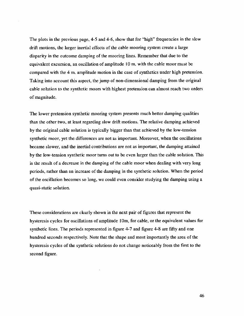
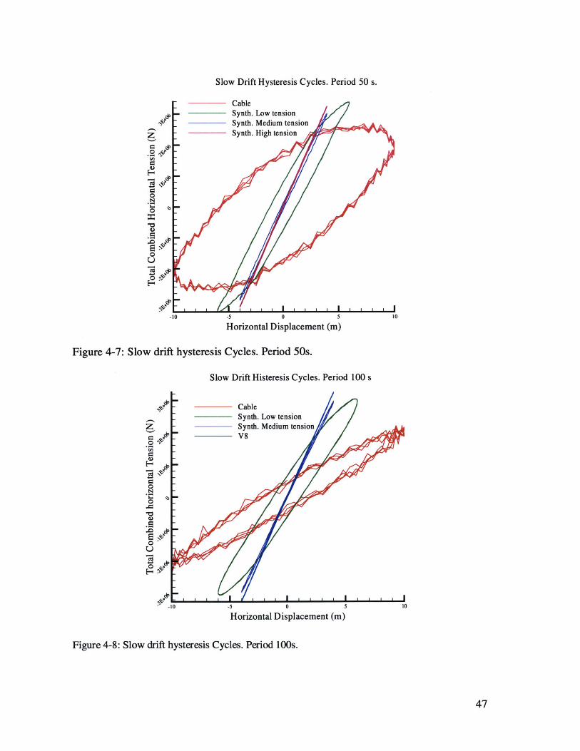
These considerations are clearly shown in the next pair of figures that represent the
hysteresis cycles for oscillations of amplitude 10m, for cable, or the equivalent values for
synthetic lines. The periods represented in figure 4-7 and figure 4-8 are fifty and one
hundred seconds respectively. Note that the shape and most importantly the area of the
hysteresis cycles of the synthetic solutions do not change noticeably from the first to the
second figure.
46
Slow Drift Hysteresis Cycles. Period 50 s.
0
0
0
0
CableSynth. Low tensionSynth. Medium tensionSynth. High tension ,
-10 -5 0 5
Horizontal Displacement (m)
Figure 4-7: Slow drift hysteresis Cycles. Period 50s.
Slow Drift Histeresis Cycles. Period 100 s
CableSynth. Low tension
- Synth. Medium tensionV8
U
10 -5 0 5
Horizontal Displacement (m)
Figure 4-8: Slow drift hysteresis Cycles. Period 100s.
47
10
10

On the other hand, the hysteresis loop of the original cable solution suffers a noticeable
area decrease when the period goes from 50 seconds to 100 seconds. The shape of this
loop turns thinner as the frequency of the oscillation decreases and it appears more like
the static or quasi-static response. The 100 seconds period cycle for the cable mooring
system tends to a series of quasi-static solutions of the mooring system's restoring forces
because the period of oscillation is very long.
These graphs, 4-7 and 4-8, also show why the damping of the two synthetic lines with
higher pretension is so small. It is important to notice that due to the high tension and the
initial taut conditions, they behave almost like springs providing very little slow drift
damping to the floating structure. These two moors are relatively insensitive to the period
variation, at least in this range of motions. The reason for this is that they already behave
as a linear quasi-static system for the smaller period, so increasing the length of the
period cannot force them to lose any more area in their associated hysteresis cycles.
The low-tension synthetic system, also, presents very little modification in its area due to
the variation in the period of the motion. The result displayed in figures 4-7 and 4-8 for
the low-tension synthetic damping looks counter intuitive because the 50 seconds
hysteresis loop presents sharper ends that the 100 seconds loop. The most probable
reason for this is that the faster oscillation induces higher fairlead tensions of the moor on
the extremes of the cycle. As a result of these higher tensions, the mooring system reacts
quicker, sharpening the extremes of the hysteresis loop.
The range of the forces is very similar for all the cases proving that the initial
consideration of the equivalent excursion is accurate. The dynamic reaction of the moors
does not introduce, in the slow drift case, a big enough modification in the tensions for a
reconsideration of the equivalent excursion hypothesis.
48
Finally, note that the excursions are variable, and each mooring system range of
displacements is different. In this context, the responses with lower motions have to lose
less energy because the platform, principal mass of the whole linear system, is also
undergoing smaller oscillations and therefore presents less motion energy.
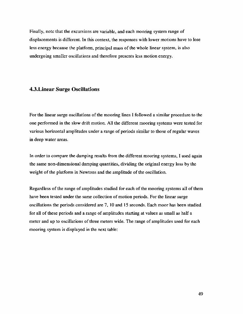
4.3.Linear Surge Oscillations
For the linear surge oscillations of the mooring lines I followed a similar procedure to the
one performed in the slow drift motion. All the different mooring systems were tested for
various horizontal amplitudes under a range of periods similar to those of regular waves
in deep water areas.
In order to compare the damping results from the different mooring systems, I used again
the same non-dimensional damping quantities, dividing the original energy loss by the
weight of the platform in Newtons and the amplitude of the oscillation.
Regardless of the range of amplitudes studied for each of the mooring systems all of them
have been tested under the same collection of motion periods. For the linear surge
oscillations the periods considered are 7, 10 and 15 seconds. Each moor has been studied
for all of these periods and a range of amplitudes starting at values as small as half a
meter and up to oscillations of three meters wide. The range of amplitudes used for each
mooring system is displayed in the next table:
49

Amplitudes studied for each mooring system. All in meters.
Cable Moor Synth. Moor. Low Synth. Moor. Synth. Moor. High
Tension Medium Tension Tension
1 0.5 0.3 0.3
2 1 0.6 0.6
3 1.5 0.9 0.9
2 1 1
3 2 2
3 3
Table 4-2: Linear surge amplitudes
The concept of equivalent excursion has not been used for linear oscillations. The
frequency of these harmonic motions is much faster than the slow drift case. Now, the
dynamic effects in the internal tension are considerable. The maximum tensions involved
in these oscillations are higher than the static restoring forces that would result from a
similar platform displacement. The dynamic effects are very influential in the case of the
cable mooring due to its heavy weight. Therefore, if we tried to use equivalent
excursions, we would find that the forces involved in the existent cable moor would be
much higher than those that would appear in the case of synthetic mooring systems. The
meaning of equivalent excursion would disappear since the range of tensions involved in
two "equivalent" oscillations would be different.
The results of the linear surge damping experiments are displayed in the next set of
figures, 4-9 to 4-12. Each moor configuration is shown in a different graph. These graphs
show how the damping for different period series vary with the amplitude of the motion.
Figure 4-9 demonstrates the damping behavior for the cable mooring system. As
expected, the damping increases with the amplitude and frequency of the motion. Figures
4-10, 4-11 and 4-12 represent the synthetic cases for low, medium and high initial
tension. These three other figures display the same behavior with regard to the amplitude
of the oscillations. The larger the amplitude of the oscillation is, the larger the equivalent
50
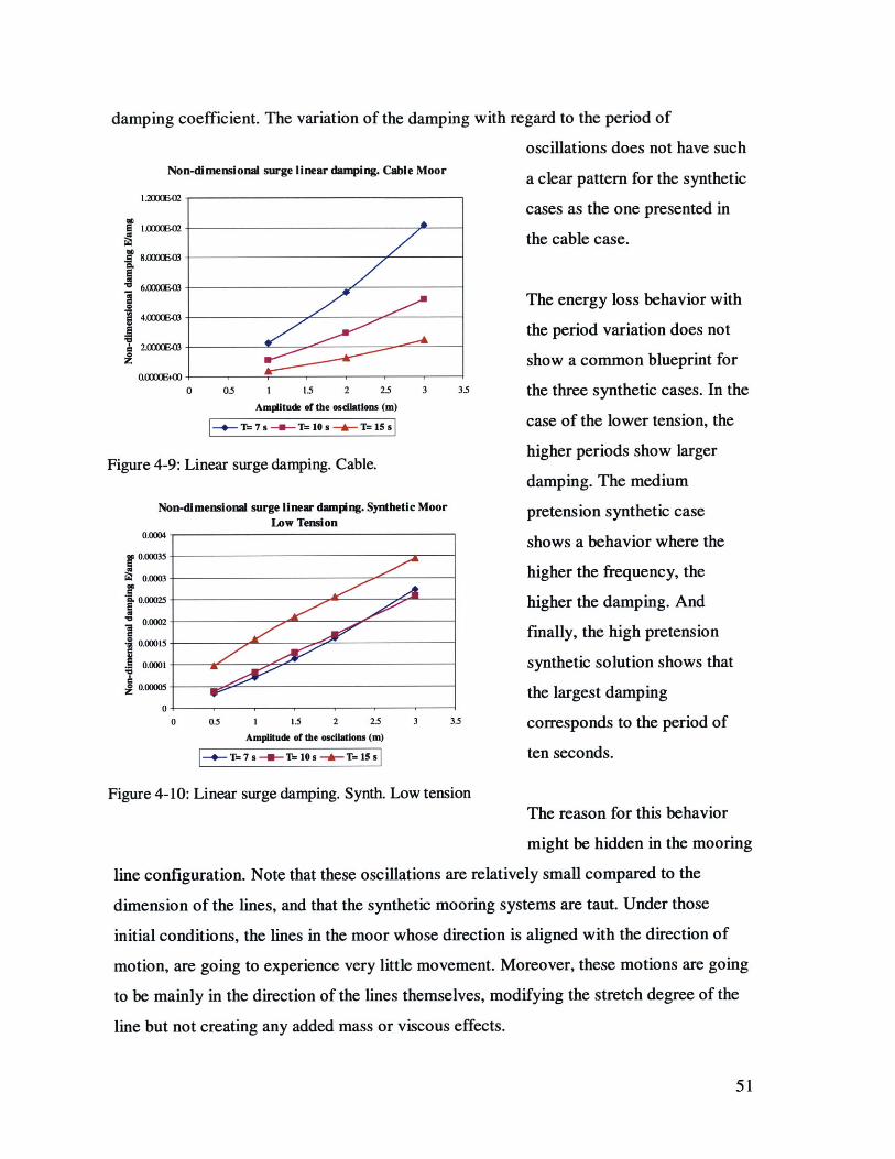
damping coefficient. The variation of the damping with
Non-dimensional surge linear damping. Cable Moor
1.20X02
1.0X6XE02-
8.00 -03-
6.0[XXEG3
4.0000ME-
4.OOE-032XXE04
0 0.5 1 1.5 2 2.5
Amplitude of the osdlations (m)
1'-- r7s -.- =1 s 15
3
Figure 4-9: Linear surge damping. Cable.
Non-dimensional surge linear damping. Synthetic MoorLow Tension
0.0004-
I0.00035-0.0003-
em00.00025
0.0002-V
0.00015-
0.0001-
oo.ooos
0 -
0 05 1 . 2 2.5
Amplitude of the osclations (m)
-- r=7s-U-r=10a - T=15s
3.5
3 3.5
regard to the period of
oscillations does not have such
a clear pattern for the synthetic
cases as the one presented in
the cable case.
The energy loss behavior with
the period variation does not
show a common blueprint for
the three synthetic cases. In the
case of the lower tension, the
higher periods show larger
damping. The medium
pretension synthetic case
shows a behavior where the
higher the frequency, the
higher the damping. And
finally, the high pretension
synthetic solution shows that
the largest damping
corresponds to the period of
ten seconds.
Figure 4-10: Linear surge damping. Synth. Low tensionThe reason for this behavior
might be hidden in the mooring
line configuration. Note that these oscillations are relatively small compared to the
dimension of the lines, and that the synthetic mooring systems are taut. Under those
initial conditions, the lines in the moor whose direction is aligned with the direction of
motion, are going to experience very little movement. Moreover, these motions are going
to be mainly in the direction of the lines themselves, modifying the stretch degree of the
line but not creating any added mass or viscous effects.
51
I
*1I0
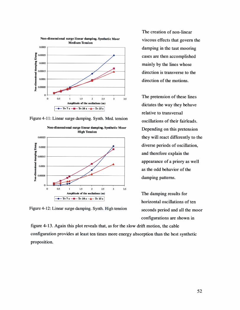
Non-dimensional surge linear damping. Synthetic MoorMedium Tension
0.0003
000025
0.00
0.00015
OI OO0.00005
0
0 0.5 1 1.5 2 2.5
Amplitude of the oscilations (m)
-4-- T= 7 s -§-- T= 10 s -dr- T= 15 s
Figure 4-11: Linear surge damping. Synth. Med. tensio
Non-dimensional surge linear damping. Synthetic MooHigh Tension
1 1.5 2 2.5
The creation of non-linear
viscous effects that govern the
damping in the taut mooring
cases are then accomplished
mainly by the lines whose
direction is transverse to the
direction of the motions.
'zi
3 3.5
Amplitude of the oscilations (m) The damping results for-4-T= 7s -U-- T= 10 s -*- T=15 s
horizontal oscillations of ten
Figure 4-12: Linear surge damping. Synth. High tension seconds period and all the moor
configurations are shown in
figure 4-13. Again this plot reveals that, as for the slow drift motion, the cable
configuration provides at least ten times more energy absorption than the best synthetic
proposition.
52
iO.0'X
0.000
.(~ o0(
12
15
11,
0-0 0.5
The pretension of these lines
dictates the way they behave
relative to transversal)n oscillations of their fairleads.
r Depending on this pretension
they will react differently to the
diverse periods of oscillation,
and therefore explain the
appearance of a priory as well
as the odd behavior of the
damping patterns.
all
go
.2
1.OE-02
1.OE-03
1.OE-04
1.OE-05
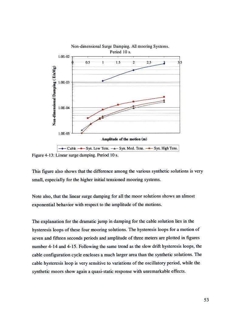
Non-dimensional Surge Damping. All mooring Systems.Period 10 s.
0.5 1 1.5 35
Amplitude of the motion (m)
-+- Cable --w- Syn. Low Tens. -+- Syn. Med. Tens. -+- Syn. High Tens.
Figure 4-13: Linear surge damping. Period 10 s.
This figure also shows that the difference among the various synthetic solutions is very
small, especially for the higher initial tensioned mooring systems.
Note also, that the linear surge damping for all the moor solutions shows an almost
exponential behavior with respect to the amplitude of the motions.
The explanation for the dramatic jump in damping for the cable solution lies in the
hysteresis loops of these four mooring solutions. The hysteresis loops for a motion of
seven and fifteen seconds periods and amplitude of three meters are plotted in figures
number 4-14 and 4-15. Following the same trend as the slow drift hysteresis loops, the
cable configuration cycle encloses a much larger area than the synthetic solutions. The
cable hysteresis loop is very sensitive to variations of the oscillatory period, while the
synthetic moors show again a quasi-static response with unremarkable effects.
53
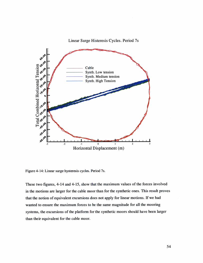
Linear Surge Histeresis Cycles. Period 7s
-3 -2 -1 0 1 2 3
Horizontal Displacement (m)
Figure 4-14: Linear surge hysteresis cycles. Period 7s.
These two figures, 4-14 and 4-15, show that the maximum values of the forces involved
in the motions are larger for the cable moor than for the synthetic ones. This result proves
that the notion of equivalent excursions does not apply for linear motions. If we had
wanted to ensure the maximum forces to be the same magnitude for all the mooring
systems, the excursions of the platform for the synthetic moors should have been larger
than their equivalent for the cable moor.
54
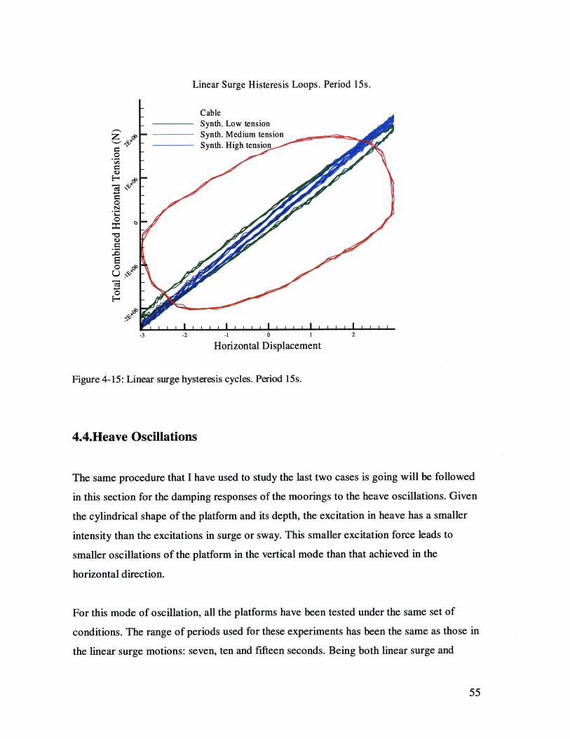
Linear Surge Histeresis Loops. Period 15s.
CableSynth. Low tension
- Synth. Medium tension
-Synth. High tension
0
N
-o-
0
-3 -2 -1 0 1 2
Horizontal Displacement
Figure 4-15: Linear surge hysteresis cycles. Period 15s.
4.4.Heave Oscillations
The same procedure that I have used to study the last two cases is going will be followed
in this section for the damping responses of the moorings to the heave oscillations. Given
the cylindrical shape of the platform and its depth, the excitation in heave has a smaller
intensity than the excitations in surge or sway. This smaller excitation force leads to
smaller oscillations of the platform in the vertical mode than that achieved in the
horizontal direction.
For this mode of oscillation, all the platforms have been tested under the same set of
conditions. The range of periods used for these experiments has been the same as those in
the linear surge motions: seven, ten and fifteen seconds. Being both linear surge and
55
heave oscillations induced by first order interactions, their respective motions would also
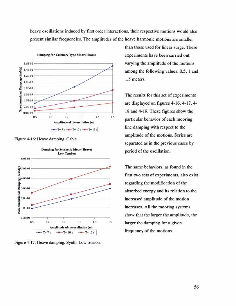
present similar frequencies. The amplitudes of the heave harmonic motions are smaller
than those used for linear surge. These
Damping for Catenary Type Moor (Heave) experiments have been carried out
-02 varying the amplitude of the motions-02 among the following values: 0.5, 1 and-02 1
_ I 1.5 meters.
0.7 0.9 1.1
Amplitude of the oscilation (n)
-.- T=7s -.-- T= 10s --.- T=15
Figure 4-16: Heave damping. Cable.
Damping for Synthetic Moor (Heave)Low Tension
6.OE-04
U 5 .E-04
4.0E-04
IL3.OE-04
2.OE-04
1.OE-04
0.OE+00
0.5 0.7 0.9 1.1
Amplitude of the oscilation (m)
-+-T=7 s -U-T=10 s -- T= 15
The results for this set of experiments
are displayed on figures 4-16, 4-17, 4-
18 and 4-19. These figures show the1.3 1.5 particular behavior of each mooring
line damping with respect to the
amplitude of the motions. Series are
separated as in the previous cases by
period of the oscillation.
The same behaviors, as found in the
first two sets of experiments, also exist
regarding the modification of the
absorbed energy and its relation to the
increased amplitude of the motion
increases. All the mooring systems
show that the larger the amplitude, the
1.3 1.5 larger the damping for a given
s frequency of the motions.
Figure 4-17: Heave damping. Synth. Low tension.
56
1.6E-
1.4E
1.2E
-
a0*
1.OE-02 --
8.OE-03 --
6.OE-03 -
4.OE-03 -
2.OE-03 -
0.OE+00
0.5
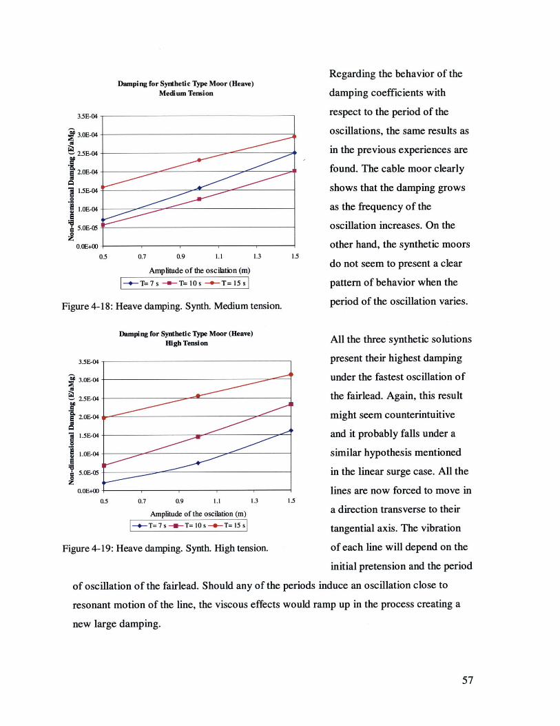
Damping for Synthetic Type Moor (HeaveMedium Tension
40"1
0.5 0.7 0.9 1.1
Amplitude of the oscilation (m)
-- T= 7 s -- T= 10 s -*- T= 15 s
Figure 4-18: Heave damping. Synth. Medium t
Regarding the behavior of the
damping coefficients with
respect to the period of the
oscillations, the same results as
in the previous experiences are
found. The cable moor clearly
shows that the damping grows
as the frequency of the
oscillation increases. On the
other hand, the synthetic moors1.3 1.5
do not seem to present a clear
pattern of behavior when the
ension. period of the oscillation varies.
Damping for Synthetic Type Moor (Heave)High Tension All the three synthetic solutions
3.5E-04 present their highest damping
3.0E-04 - under the fastest oscillation of
2.5E-04 -the fairlead. Again, this result
2.OE-04 I might seem counterintuitive
1.5E-04 and it probably falls under a
1.oE-04 similar hypothesis mentioned
5.0E-05 in the linear surge case. All the
o.oE+00 lines are now forced to move in0.5 0.7 0.9 1.1 1.3 1.5
Amplitude of the oscilation (m) a direction transverse to their-- T= 7 s -- T= 10 s-e-T= 15 s tangential axis. The vibration
gure 4-19: Heave damping. Synth. High tension. of each line will depend on the
initial pretension and the period
of oscillation of the fairlead. Should any of the periods induce an oscillation close to
resonant motion of the line, the viscous effects would ramp up in the process creating a
new large damping.
57
3.5E-04
3.OE-04
2.5E-04
2.OE-04
1.5E-04
10E-04
5.0E-05
0.0E+00
1
Fi
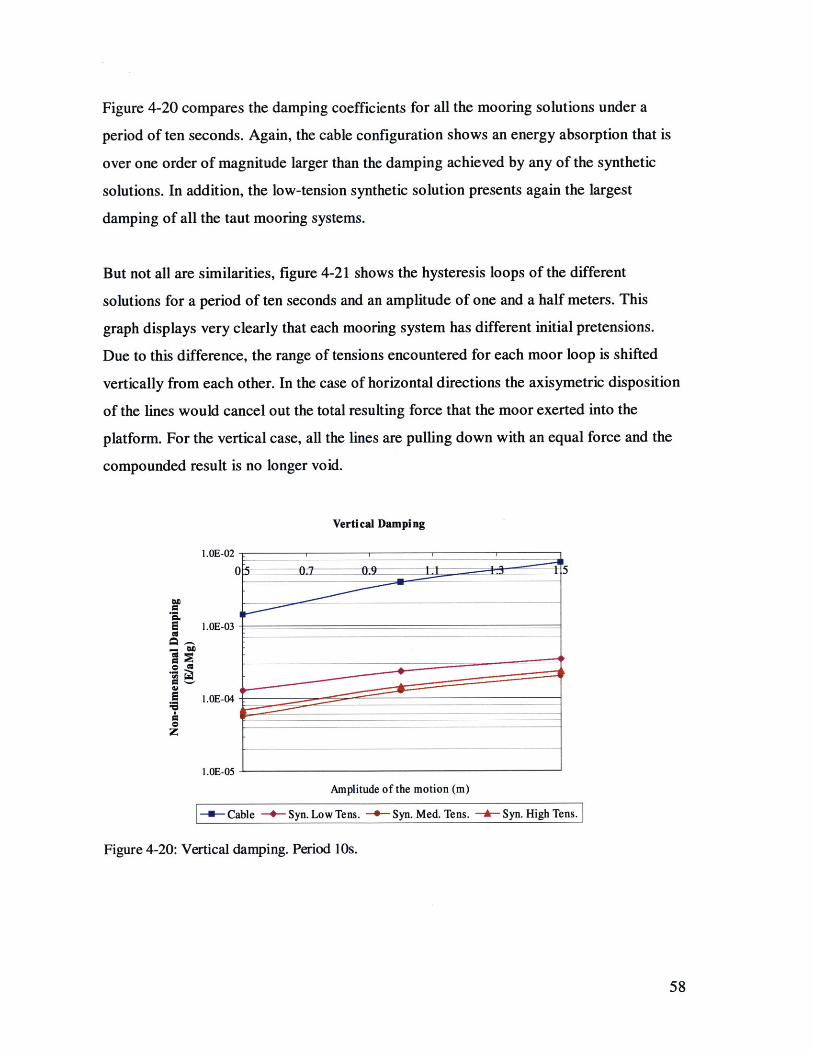
Figure 4-20 compares the damping coefficients for all the mooring solutions under a
period of ten seconds. Again, the cable configuration shows an energy absorption that is
over one order of magnitude larger than the damping achieved by any of the synthetic
solutions. In addition, the low-tension synthetic solution presents again the largest
damping of all the taut mooring systems.
But not all are similarities, figure 4-21 shows the hysteresis loops of the different
solutions for a period of ten seconds and an amplitude of one and a half meters. This
graph displays very clearly that each mooring system has different initial pretensions.
Due to this difference, the range of tensions encountered for each moor loop is shifted
vertically from each other. In the case of horizontal directions the axisymetric disposition
of the lines would cancel out the total resulting force that the moor exerted into the
platform. For the vertical case, all the lines are pulling down with an equal force and the
compounded result is no longer void.
Vertical Damping
1.OE-02
SE 1.OE-03
1.OE-04
1.OE-05
Amplitude of the motion (m)
-U- Cable -+- Syn. Low Tens. -*- Syn. Med. Tens. -- Syn. High Tens.
Figure 4-20: Vertical damping. Period 10s.
58
19. 3I~ U. I 3
-
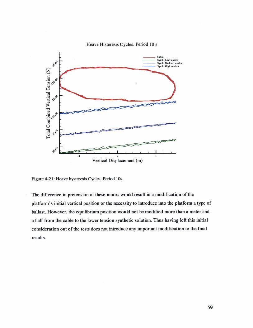
Heave Histeresis Cycles. Period 10 s
z0
.0P
Vertical Displacement (m)
Figure 4-2 1: Heave hysteresis Cycles. Period 10Os.
The difference in pretension of these moors would result in a modification of the
platform's initial vertical position or the necessity to introduce into the platform a type of
ballast. However, the equilibrium position would not be modified more than a meter and
a half from the cable to the lower tension synthetic solution. Thus having left this initial
consideration out of the tests does not introduce any important modification to the final
results.
59
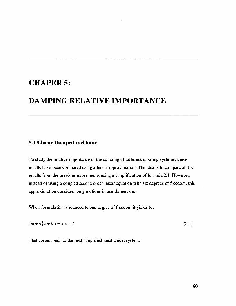
CHAPER 5:
DAMPING RELATIVE IMPORTANCE
5.1 Linear Damped oscillator
To study the relative importance of the damping of different mooring systems, these
results have been compared using a linear approximation. The idea is to compare all the
results from the previous experiments using a simplification of formula 2.1. However,
instead of using a coupled second order linear equation with six degrees of freedom, this
approximation considers only motions in one dimension.
When formula 2.1 is reduced to one degree of freedom it yields to,
(m + a) + b x + k x = f (5.1)
That corresponds to the next simplified mechanical system.
60

m+a
Figure 5-1: Simple model for damped oscillator.
Where "m+a" represents the mass of the oscillator plus its added mass, k is the
coefficient of the spring and b is the linear damping of the system.
Now, dividing by the coefficients of the second order term and considering only the
unforced oscillations, the equation can be rewritten as,
j +2ai+a_ x=O
Where sigma and the natural frequency of the system, ow, are defined as,
b2(m + a)
_ ko =(ma)
" (+ a)
(5.2)
(5.3)
This equation presents a close form solution that depends on the damping ratio of the
system, (, that is defined as,
(5.4)(00
The damping ratio is an index of the stability of the system's stability to non-forced
oscillations, if ( is negative, the system is unstable and the initial motion would grow
61
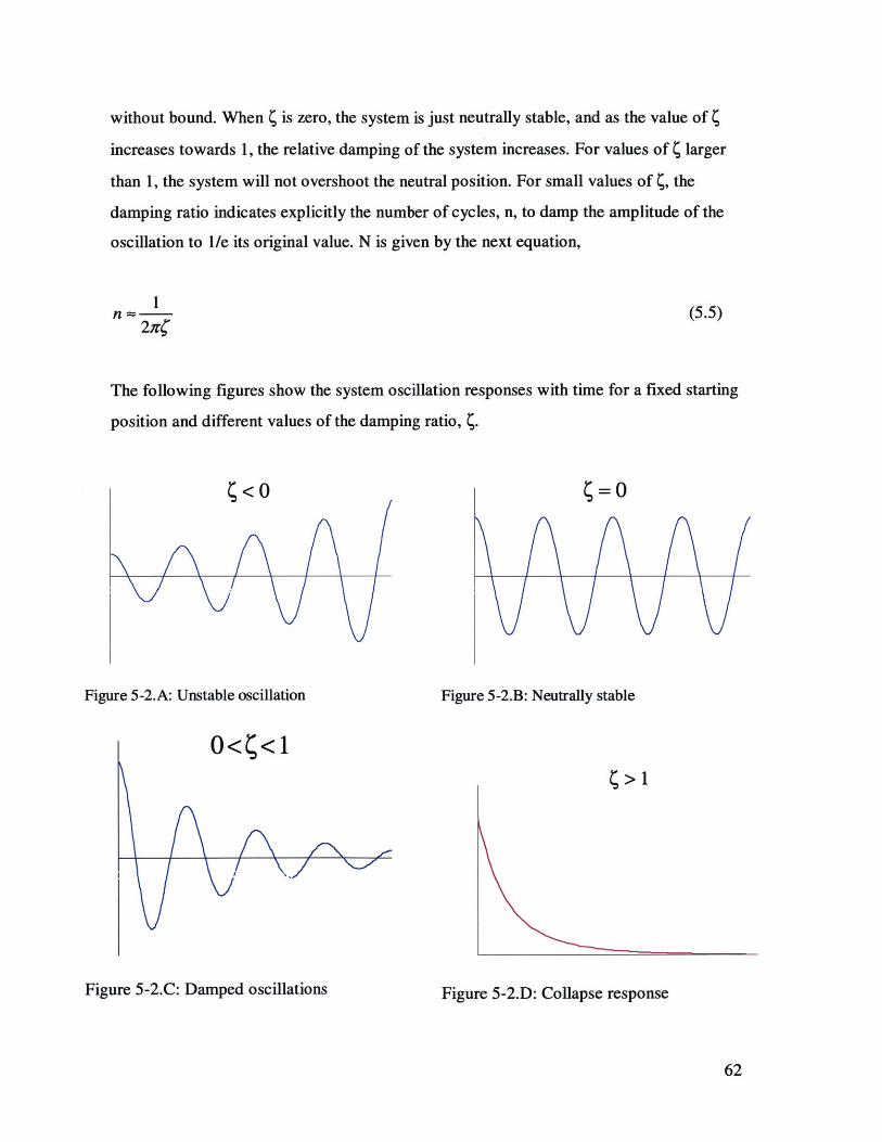
without bound. When ( is zero, the system is just neutrally stable, and as the value of (
increases towards 1, the relative damping of the system increases. For values of ( larger
than 1, the system will not overshoot the neutral position. For small values of (, the
damping ratio indicates explicitly the number of cycles, n, to damp the amplitude of the
oscillation to l/e its original value. N is given by the next equation,
1n ~
2;r{(5.5)
The following figures show the system oscillation responses with time for a fixed starting
position and different values of the damping ratio, (.
Figure 5-2.A: Unstable oscillation
Figure 5-2.C: Damped oscillations
Figure 5-2.B: Neutrally stable
Figure 5-2.D: Collapse response
62
n \J / A
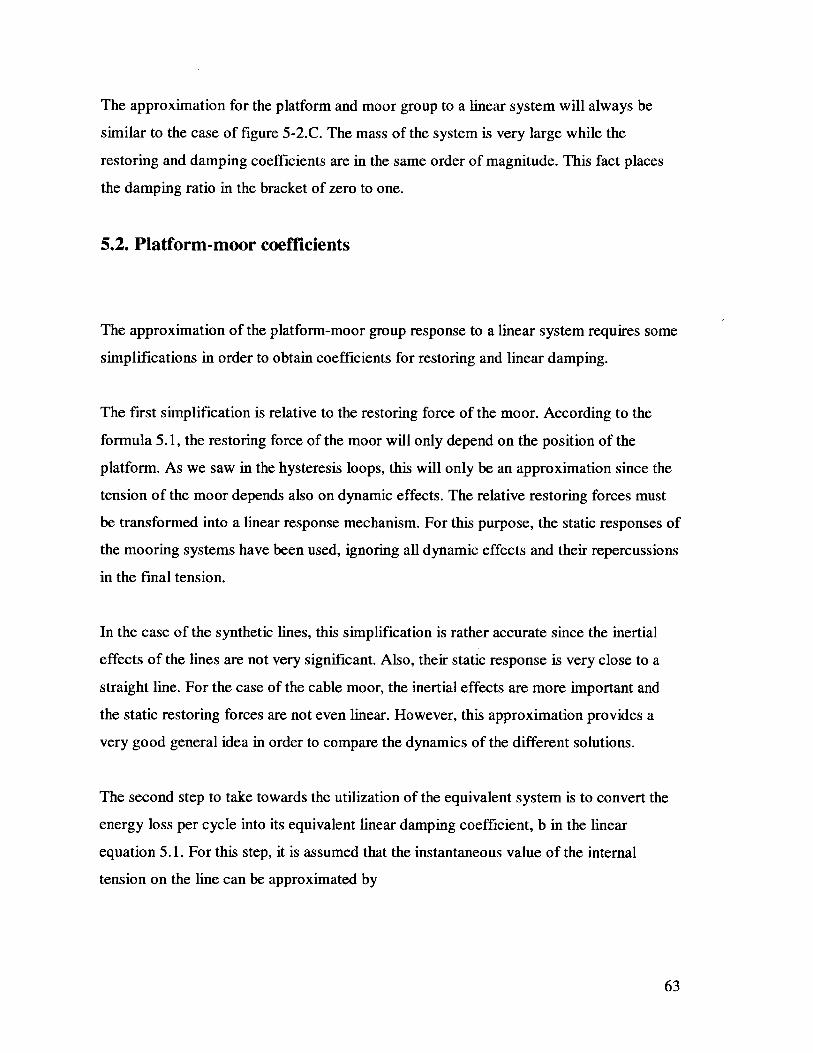
The approximation for the platform and moor group to a linear system will always be
similar to the case of figure 5-2.C. The mass of the system is very large while the
restoring and damping coefficients are in the same order of magnitude. This fact places
the damping ratio in the bracket of zero to one.
5.2. Platform-moor coefficients
The approximation of the platform-moor group response to a linear system requires some
simplifications in order to obtain coefficients for restoring and linear damping.
The first simplification is relative to the restoring force of the moor. According to the
formula 5.1, the restoring force of the moor will only depend on the position of the
platform. As we saw in the hysteresis loops, this will only be an approximation since the
tension of the moor depends also on dynamic effects. The relative restoring forces must
be transformed into a linear response mechanism. For this purpose, the static responses of
the mooring systems have been used, ignoring all dynamic effects and their repercussions
in the final tension.
In the case of the synthetic lines, this simplification is rather accurate since the inertial
effects of the lines are not very significant. Also, their static response is very close to a
straight line. For the case of the cable moor, the inertial effects are more important and
the static restoring forces are not even linear. However, this approximation provides a
very good general idea in order to compare the dynamics of the different solutions.
The second step to take towards the utilization of the equivalent system is to convert the
energy loss per cycle into its equivalent linear damping coefficient, b in the linear
equation 5.1. For this step, it is assumed that the instantaneous value of the internal
tension on the line can be approximated by
63

T =b- (5.6)dt
Now, combining formula 2.27 (in this case only for one dimension) with 5.6 we can
obtain the relation between the energy loss per cycle obtained through a numerical
simulation, and the linear damping coefficient that is needed for the linear approximation.
E~jF(,)fk'r [ Fdl 2)r~at+T -. x t X]&-2d 2a
E= F (t)- -dt~b dt =b (5.7)t dt f dt. T
Now, rewriting this equation we obtain the equivalent linear damping,
Erb = r (5.8)
21r 2 a 2
However, the linear damping results vary for different periods and amplitudes of the
motion. The linear approximation requires a constant damping, so I have used the mean
value of all the damping results as a definitive approximation to the linear mechanical
system.
Slow drift surge, linear surge and heave, have been studied using separate linear
approximations because the difference among the damping coefficients is rather large,
and the character of the three modes of oscillations is very different. Even for only one of
these modes of oscillation, the linear damping coefficient is far from being constant. Note
in table 5-1 that the standard deviation of the mean linear damping coefficients are of the
order of their respective averages themselves.
Regardless of these facts, the linear approximation still gives a very good sense of the
dynamics of the platform with the different mooring solutions. They are only a first
estimate, yet an improvement of these results would take a full numerical resolution of
the differential equation using non-constant coefficients.
64
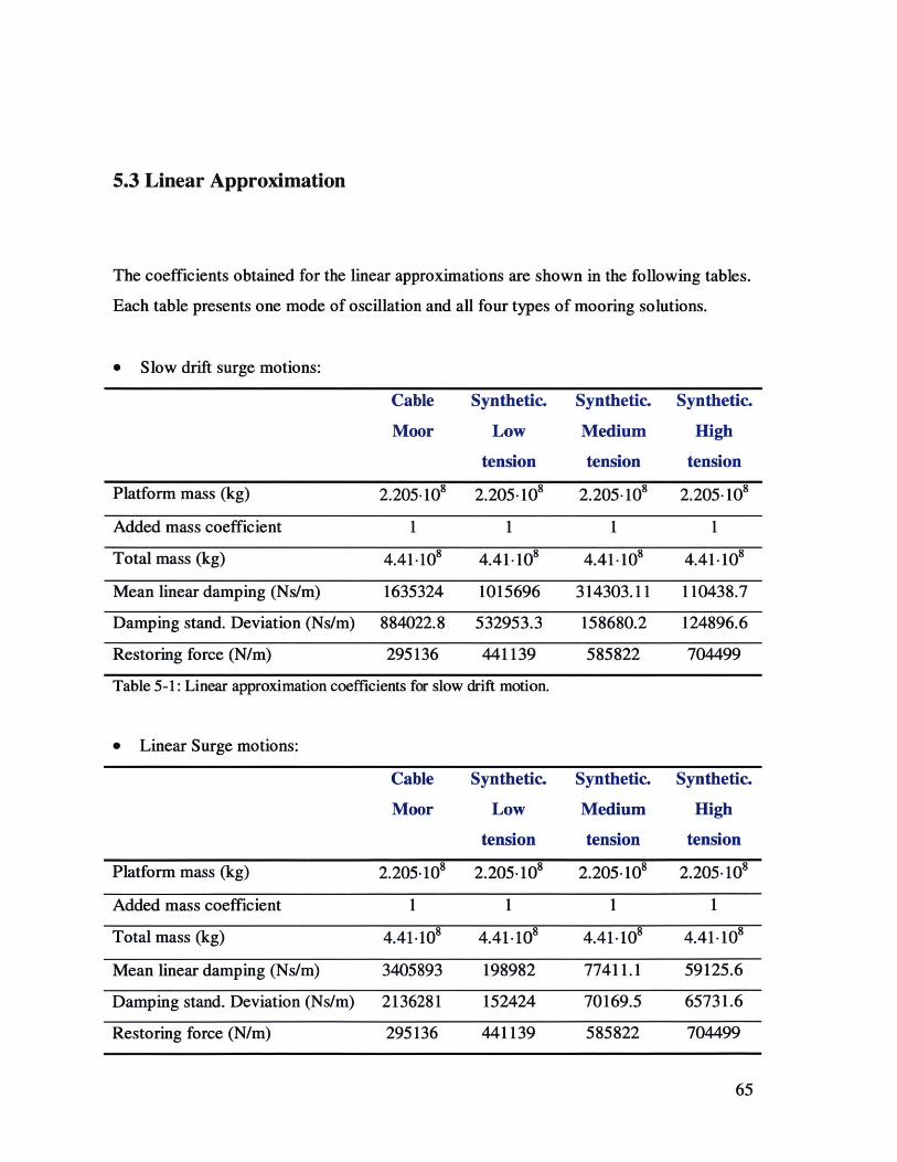
5.3 Linear Approximation
The coefficients obtained for the linear approximations are shown in the following tables.
Each table presents one mode of oscillation and all four types of mooring solutions.
0 Slow drift surge motions:
Cable
Moor
Platform mass (kg)
Added mass coefficient
Total mass (kg)
Mean linear damping (Ns/m)
Damping stand. Deviation (Ns/m)
Restoring force (N/m)
2.205.108
1
4.41.108
1635324
884022.8
295136
Synthetic.
Low
tension
2.205-10
1
4.41. 108
1015696
532953.3
441139
Synthetic.
Medium
tension
2.205-10'
1
4.41-108
314303.11
158680.2
585822
Synthetic.
High
tension
2.205.108
1
4.41. 108
110438.7
124896.6
704499
Table 5-1: Linear approximation coefficients for slow drift motion.
* Linear Surge motions:
Cable Synthetic. Synthetic. Synthetic.
Moor Low Medium High
tension tension tension
Platform mass (kg)
Added mass coefficient
Total mass (kg)
Mean linear damping (Ns/m)
Damping stand. Deviation (Ns/m)
Restoring force (N/m)
2.205-10'
1
4.41. 108
3405893
2136281
295136
2.205.108
1
4.41.108
198982
152424
441139
2.205.108
1
4.41.108
77411.1
70169.5
585822
2.205.108
1
4.41.108
59125.6
65731.6
704499
65
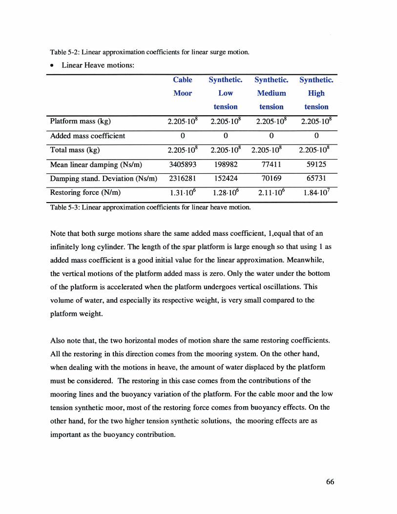
Table 5-2: Linear approximation coefficients for linear surge motion.
e Linear Heave motions:
Cable
Moor
Platform mass (kg)
Added mass coefficient
Total mass (kg)
Mean linear damping (Ns/m)
Damping stand. Deviation (Ns/m)
Restoring force (N/m)
2.205.108
0
2.205.108
3405893
2316281
1.31-106
Synthetic.
Low
tension
2.205-108
0
2.205.10
198982
152424
1.28-106
Synthetic.
Medium
tension
2.205.108
0
2.205- 108
77411
70169
2.11. 106
Table 5-3: Linear approximation coefficients for linear heave motion.
Note that both surge motions share the same added mass coefficient, 1,equal that of an
infinitely long cylinder. The length of the spar platform is large enough so that using 1 as
added mass coefficient is a good initial value for the linear approximation. Meanwhile,
the vertical motions of the platform added mass is zero. Only the water under the bottom
of the platform is accelerated when the platform undergoes vertical oscillations. This
volume of water, and especially its respective weight, is very small compared to the
platform weight.
Also note that, the two horizontal modes of motion share the same restoring coefficients.
All the restoring in this direction comes from the mooring system. On the other hand,
when dealing with the motions in heave, the amount of water displaced by the platform
must be considered. The restoring in this case comes from the contributions of the
mooring lines and the buoyancy variation of the platform. For the cable moor and the low
tension synthetic moor, most of the restoring force comes from buoyancy effects. On the
other hand, for the two higher tension synthetic solutions, the mooring effects are as
important as the buoyancy contribution.
66
Synthetic.
High
tension
2.205.108
0
2.205.108
59125
65731
1.84. 107
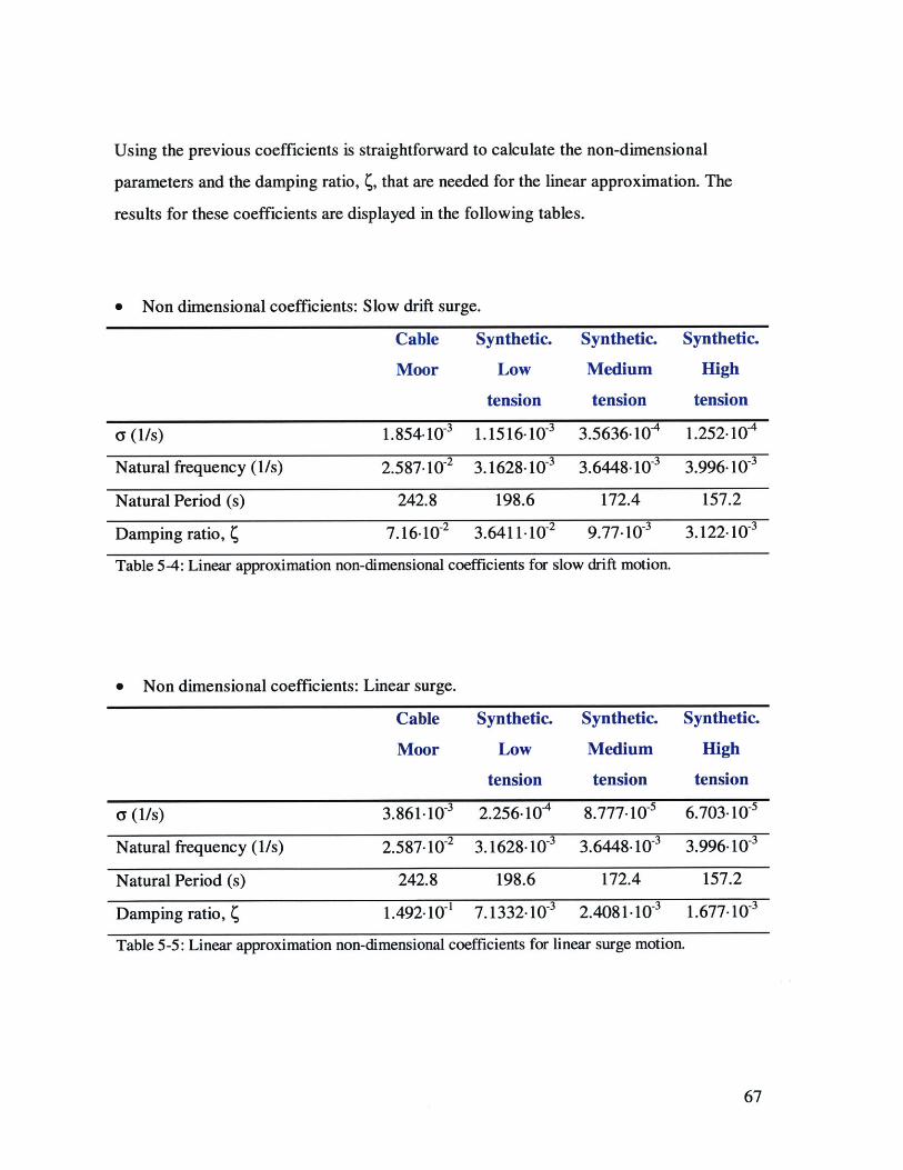
Using the previous coefficients is straightforward to calculate the non-dimensional
parameters and the damping ratio, (, that are needed for the linear approximation. The
results for these coefficients are displayed in the following tables.
* Non dimensional coefficients: Slow drift surge.
Cable Synthetic. Synthetic. Synthetic.
Moor Low Medium High
tension tension tension
a(l/s) 1.854-10-3 1.1516-10-3 3.5636-10~ 1.252-10~4
Natural frequency (1/s) 2.587.10-2 3.1628-10-3 3.6448-10-3 3.996-10-3
Natural Period (s) 242.8 198.6 172.4 157.2
Damping ratio, ( 7.16.10-2 3.6411-10-2 9.77-10-3 3.122-10-3
Table 5-4: Linear approximation non-dimensional coefficients for slow drift motion.
* Non dimensional coefficients: Linear surge.
Cable Synthetic. Synthetic. Synthetic.
Moor Low Medium High
tension tension tension
a(1/s) 3.861-10-3 2.256- 10- 8.777 10-5 6.703-10-5
Natural frequency (1/s) 2.587.10-2 3.1628-10-3 3.6448-10-3 3.996-10-3
Natural Period (s) 242.8 198.6 172.4 157.2
Damping ratio, ( 1.492.10-1 7.1332-10-3 2.4081-10-3 1.677-10~3
Table 5-5: Linear approximation non-dimensional coefficients for linear surge motion.
67
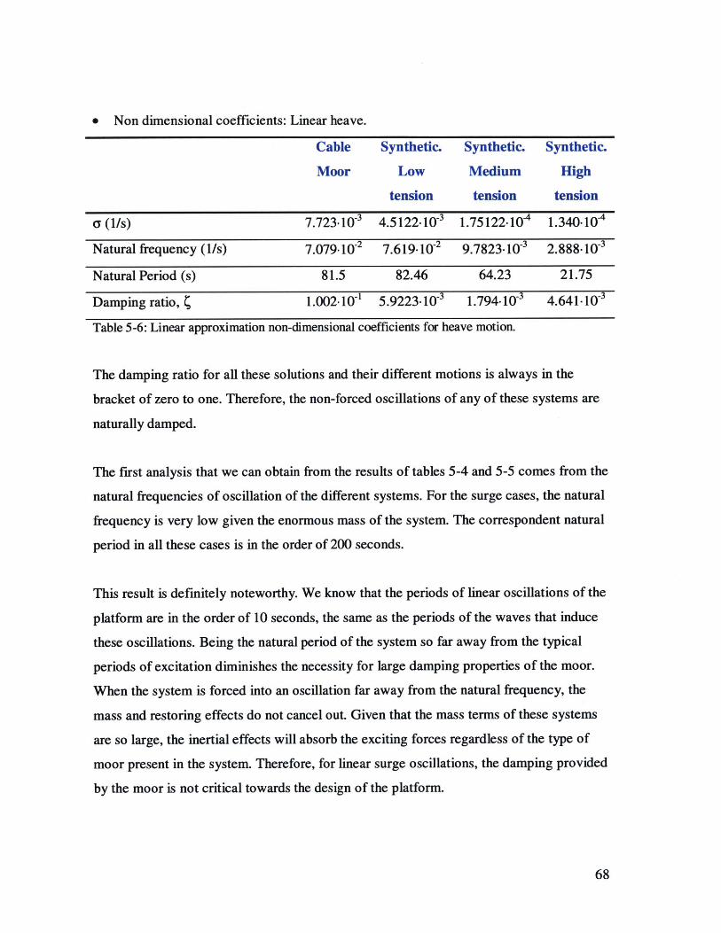
* Non dimensional coefficients: Linear heave.
Cable Synthetic. Synthetic. Synthetic.
Moor Low Medium High
tension tension tension
a (1/s) 7.723-10-3 4.5122-10- 1.75122-10~ 1.340-10-
Natural frequency (1/s) 7.079.10-2 7.619.10-2 9.7823. 103 2.888-10-
Natural Period (s) 81.5 82.46 64.23 21.75
Damping ratio, ( 1.002.101 5.9223 10-3 1.794. 103 4.641.10-3
Table 5-6: Linear approximation non-dimensional coefficients for heave motion.
The damping ratio for all these solutions and their different motions is always in the
bracket of zero to one. Therefore, the non-forced oscillations of any of these systems are
naturally damped.
The first analysis that we can obtain from the results of tables 5-4 and 5-5 comes from the
natural frequencies of oscillation of the different systems. For the surge cases, the natural
frequency is very low given the enormous mass of the system. The correspondent natural
period in all these cases is in the order of 200 seconds.
This result is definitely noteworthy. We know that the periods of linear oscillations of the
platform are in the order of 10 seconds, the same as the periods of the waves that induce
these oscillations. Being the natural period of the system so far away from the typical
periods of excitation diminishes the necessity for large damping properties of the moor.
When the system is forced into an oscillation far away from the natural frequency, the
mass and restoring effects do not cancel out. Given that the mass terms of these systems
are so large, the inertial effects will absorb the exciting forces regardless of the type of
moor present in the system. Therefore, for linear surge oscillations, the damping provided
by the moor is not critical towards the design of the platform.
68
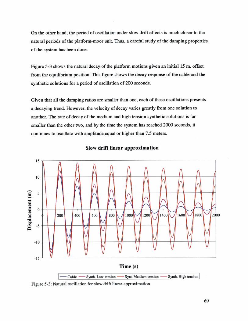
On the other hand, the period of oscillation under slow drift effects is much closer to the
natural periods of the platform-moor unit. Thus, a careful study of the damping properties
of the system has been done.
Figure 5-3 shows the natural decay of the platform motions given an initial 15 m. offset
from the equilibrium position. This figure shows the decay response of the cable and the
synthetic solutions for a period of oscillation of 200 seconds.
Given that all the damping ratios are smaller than one, each of these oscillations presents
a decaying trend. However, the velocity of decay varies greatly from one solution to
another. The rate of decay of the medium and high tension synthetic solutions is far
smaller than the other two, and by the time the system has reached 2000 seconds, it
continues to oscillate with amplitude equal or higher than 7.5 meters.
Slow drift linear approximation
15
10
5
0
-5
-10
-15
Time (s)
- Cable - Synth. Low tension - Synt. Medium tension - Synth. High tension
Figure 5-3: Natural oscillation for slow drift linear approximation.
69
10=1200 400 600 800 1000 1200 1400 1600 1800 2C00
For slow drift motions close to the resonance frequencies of the system, figure 5-3 also
shows that the low-tension synthetic moor, even when compared with the cable solution,
presents very good damping qualities.
Moreover, the average damping coefficient, used for these approximations, handicaps the
results of the low-tension synthetic mooring system. Figures 4-1 and 4-2 show how the
damping for the cable decreases as the period of oscillation increases. This pattern is not
found in the low-synthetic solution. Therefore, when considering periods as high as 200
seconds, the cable damping is considerably smaller than its average damping. This fact
makes the low tension synthetic solution even more attractive, since its respective
damping does not decrease with the growth of the period of the oscillations.
Following the same train of thought used for the linear surge, as the slow drift motions
move further away from the resonance frequency, the relative importance of the damping
in the system diminishes. Therefore, the election of mooring system, when the period of
the oscillations are in the order of 1 minute, should not be governed by the damping
capabilities of the system. Above all, this study is only considering the damping effects of
the mooring system, discharging all the inherit platform viscous damping. If we
considered the complete damping, the relative damping difference among the cable and
the low-tension synthetic solution will became even smaller.
Regarding the oscillations in heave, we can see in table 5-6, that the natural period of
these systems are in general very large compared to the period of the exciting waves. This
is clearly the case for all solutions apart from the high-tension synthetic moor. An
analogy to the linear surge case can then be established. In general, the motions in heave
will be most affected by the mass of the platform. This factor along with the exciting
force will determine the nature of the motions regardless of the mooring system used.
Note that for a SPAR platform in this mode, motions in this mode of oscillation, will be
typically very small, given the very large depth of the body and its vertical cylindrical
shape. The only surface on the floating body where pressure can cause vertical resulting
70

forces is on its' bottom, and at a depth of 200 meters, the wave effects create very small
variations in the overall pressure of the fluid.
Unless the mooring system is very taut, and thus its natural period becomes close to the
period of the exciting waves, the damping contributions of the moor in vertical direction
are not a major concern for the dynamics of the platform.
71
CHAPTER 6:
CONCLUSIONS
As the water depth for offshore oil drilling increases, the trend in the mooring systems
design is shifting from classical cable mooring line into solutions based of synthetic
ropes.
The mechanical responses, especially to dynamic excitations, of these synthetic moor
solutions, under very large water depth conditions, have not yet been tested.
There are several reasons for the consideration of light synthetic rope solutions, among
which, the most significant is based purely on economics. Not only the cheaper cost of
the synthetics, but also, its lower cost of installation make them an extremely attractive
alternative for large and very large water depths.
Regarding the mechanical properties of the synthetic mooring systems, Chaper 3
demonstrates that the restoring forces achieved by regular catenary-type moor can be
easily attained by light taut mooring systems.
72
These restoring forces, however, can create misleading interpretations. The fact that the
moor is more taut does not automatically imply smaller oscillations of the moored
floating body. In the case of the mooring systems considered in this thesis, the mass of
the platform is so vast that the inertial terms of the motion equation govern the response
of the system to external loads. Therefore, the amplitude of the motions when the off-
shore platform is forced to oscillate under external loads will not vary significantly from
one mooring system to another. The damping becomes a second-order consideration.
If one further increased the initial pretension of the synthetics, provided that the
maximum tension in the lines was not a critical concern, this increase would only make
the natural frequency of the heave response to move towards the frequency of the waves
that generates that heave. Then, the amplitude of the oscillations would become
dangerous for the integrity of the moor.
Regarding the dynamic responses, and particularly the damping that the system
introduces into the platform motions, Chapter 5 shows that only the damping qualities of
the moor regarding slow-drift oscillations are critical when designing spread-mooring
systems for large water depths.
In Chapter 5 we also proved that the low-tension synthetic mooring solution presents
excellent dynamic properties. It provides the platform with restoring forces even larger
than the original cable solution as well as behaves favorably under slow-drift oscillations.
A fully coupled platform-mooring system numerical analysis would provide a more
accurate solution and could be utilized to ensure the validity of these results.
These considerations about the low-tension synthetic moor, added to its lower cost, make
this a viable alternative for the positioning and control of floating structures in large
water depths.
73

REFERENCES:
[1] Cannon, Dynamics of physical systems
[2] Michael S. Triantafyllou, Mooring Dynamics for offshore applications. Part one I.
Theory.
[3] Genevieve Tcheou, Non-Linear dynamics of mooring lines
[4] Finn Gunnar Nielsen, Arne Ulrik Bindingb*, Extreme loads in taut mooring
lines and mooring line induced damping. An asymptotic approach.
[5] F.G. Nielsen, A.U. Bindingsb*, Alternative configurations and materials for
deep water mooring. Results from a three year joint research effort. OTC Paper
10755.
[6] John Magne Johnsen, Ola Oritsland, Design and optimisation of Taut-leg
mooring systems. OTC Paper 10776.
[7] Ivan De Pellegrin, Manmade fiber ropes in deepwater mooring applications.
OTC Paper 10907.
[8] D. L. Garret, Dynamic analysis of slender rods
[9] William C. Webster, Mooring-induced damping
[10] Boston Marine Consulting Inc. LINES 1.1 User Manual
[11] R. M. Raaijmakers and J.A. Battjes, An experimental verification of Huse's
model on the calculation of mooring line damping.
[12] A.C. Fernandes, M. M. Mourelle, O.B. Sert*, S. da Silva and P.H.C.C.
Parra, Hydrodinamic coefficients in thedesign of steel catenary risers.
74

[13] C.R. Chaplin, Reading U. and C.J.M. Del Vecchio, Appraisal of lightweight
moorings for deep water. OTC 6965.
[14] Bob Wilde, Patrick Kelly, Filipo Librino, and Simeon Whitehill, Conceptual
design and comparison of aramid and polyester taut leg spread moorings for deep
water applications. OTC Paper 8145.
75

APPENDIX A: ROPE PROPERTIES
Polyester rope properties:
Breaking Weigh in air Weigh in water Diameter (m) EA (N)
Strength (N)
6.23E+06
6.67E+06
7.12E+06
7.56E+06
8.01E+06
8.45E+06
8.90E+06
9.34E+06
9.79E+06
1.02E+07
1.07E+07
1.11E+07
1. 16E+07
1.20E+07
1.25E+07
1.29E+07
1.33E+07
(N/m)
159.3856
171.6348
184.0299
196.4249
208.82
221.3608
234.0475
202.8412
257.8168
271.9618
284.7943
297.481
310.4593
323.2918
336.1243
349.1027
362.081
(N/m)
40.97654
44.18467
47.24698
50.4551
53.66323
56.87136
60.07949
63.43344
66.64157
69.8497
73.20365
76.41178
79.76573
83.11968
86.32781
89.68176
93.03571
0.154178
0.16002
0.165608
0.171196
0.17653
0.18161
0.18669
0.19177
0.196596
0.201422
0.205994
0.210566
0.215138
0.219456
0.223774
0.228092
0.23241
95898880
1.03E+08
1. 1E+08
1.16E+08
1.23E+08
1.3E+08
1.37E+08
1.44E+08
1.51E+08
1.58E+08
1.64E+08
1.71E+08
1.78E+08
1.85E+08
1.92E+08
1.99E+08
2.05E+08
76
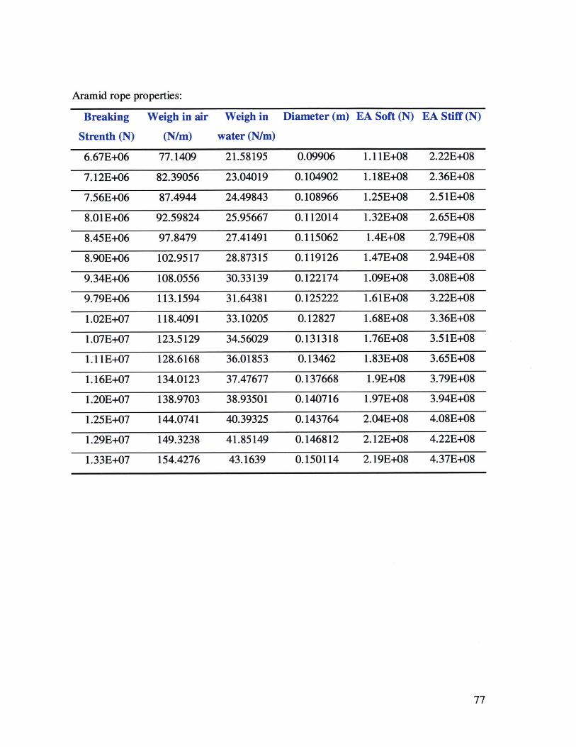
Aramid rope properties:
Breaking Weigh in air Weigh in Diameter (m) EA Soft (N) EA Stiff (N)
Strenth (N)
6.67E+06
7.12E+06
7.56E+06
8.01E+06
8.45E+06
8.90E+06
9.34E+06
9.79E+06
1.02E+07
1.07E+07
1.11E+07
1. 16E+07
1.20E+07
1.25E+07
1.29E+07
1.33E+07 154.4276 43.1639 0.150114 2.19E+08 4.37E+08
77
(N/m)
77.1409
82.39056
87.4944
92.59824
97.8479
102.9517
108.0556
113.1594
118.4091
123.5129
128.6168
134.0123
138.9703
144.0741
149.3238
water (N/m)
21.58195
23.04019
24.49843
25.95667
27.41491
28.87315
30.33139
31.64381
33.10205
34.56029
36.01853
37.47677
38.93501
40.39325
41.85149
0.09906
0.104902
0.108966
0.112014
0.115062
0.119126
0.122174
0.125222
0.12827
0.131318
0.13462
0.137668
0.140716
0.143764
0.146812
1.11E+08
1.18E+08
1.25E+08
1.32E+08
1.4E+08
1.47E+08
1.09E+08
1.61E+08
1.68E+08
1.76E+08
1.83E+08
1.9E+08
1.97E+08
2.04E+08
2.12E+08
2.22E+08
2.36E+08
2.5 1E+08
2.65E+08
2.79E+08
2.94E+08
3.08E+08
3.22E+08
3.36E+08
3.5 1E+08
3.65E+08
3.79E+08
3.94E+08
4.08E+08
4.22E+08


