Embed Size (px)
Citation preview
Molecular dynamics simulations of silicate and borate glasses and melts:
Structure, diffusion dynamics and vibrational properties
Dissertation
zur Erlangung des Grades
“Doktor
der Naturwissenschaften”
am Fachbereich Physik, Mathematik und Informatik
der Johannes Gutenberg-Universitat
in Mainz
Christoph Scherer
geb. in Zweibrucken (Rheinland-Pfalz)
Mainz, im April 2015

Datum der mundlichen Prufung: 06.07.2015

“My friends and I have been thinking another year had come gone
And so we started drinking and singing new years songs.
Like Auld Lang Syne, There Comes a Time, and Prince’s 1999...
But none of those songs seem to do it for us, at the time...
This year a lot of things have come to pass
Raise a glass, raise a glass
Some made us cry some made us laugh
Raise a glass, raise a glass
Next year will be better
The old year is gone forever
Thank god it’s over, thank god it’s over
Thank god it’s over, it’s over now
Thank god it’s over, thank god it’s over
Thank god it’s over, it’s over now
To all are friends and those we’ve left behind
Sing Auld Lang Syne, sing Auld Lang Syne
Thou you’re gone you’re never far from mind
Auld Lang Syne, sing Auld Lang Syne
Let bygones be bygones
Bye-bye gone we’re moving on
Thank god it’s over, thank god it’s over
Thank god it’s over, it’s over now
Thank god it’s over, thank god it’s over
Thank god it’s over, it’s over now
This year many things have come to pass
Raise a glass, raise a glass
Some things really kicked our ass
Raise a glass, raise a glass
Come raise your spirits
Sing loud so the dead will hear it
Thank god it’s over, thank god it’s over
Thank god it’s over, it’s over now
Thank god it’s over, thank god it’s over
Thank god it’s over, it’s over now
Thank god it’s over, thank god it’s over
Thank god it’s over, it’s over now
Thank god it’s over, thank god it’s over
Thank god it’s over, it’s over now”
Jim’S Big Ego - New Lang Syne (Thank God It’s Over)
Molecular dynamics simulations of silicate and borate glasses and melts: Structure,
diffusion dynamics and vibrational properties
In this work, computer simulations of the model glass formers SiO2 and B2O3 are presented,
using the techniques of classical molecular dynamics (MD) simulations and quantum mechanical
calculations, based on density functional theory (DFT). The latter limits the system size to about
100 − 200 atoms. SiO2 and B2O3 are the two most important network formers for industrial
applications of oxide glasses.
In case of SiO2, classical MD simulations are carried out, employing two different classical
potentials: the well studied BKS potential and the CHIK potential. In agreement with previous
results, it is found that small systems (as small as 165 atoms) show all characteristic features
of glassy dynamics, the main finite size effect is a dynamical slowing down and the temperature
dependence of the self-diffusion constants shows an Arrhenius behavior at low temperatures.
Glass samples are generated by means of a quench from the melt with classical MD simulations
and a subsequent structural relaxation with DFT forces. The latter mainly reduces the mean
Si-O-Si angle by about 4 − 6. After the relaxation, the glass configurations of the BKS
and the CHIK potential show no significant structural differences. In addition, the structural
properties are in good agreement to the ones of a full ab initio quench from the melt and
to experimental results from neutron and X-ray scattering. A special focus is on the study
of vibrational properties, as they give access to low-temperature thermodynamic properties.
Therefore, a comparison of the calculated vibrational spectrum g (ν) with the experimental one
is a good test for the quality of a glass structure. The vibrational spectra are calculated by
the so-called ”frozen phonon” method, employing classical and quantum mechanical forces. In
accordance to previous work, the DFT curves show excellent agreement with experimental results
of inelastic neutron scattering. The same is observed, regarding the heat capacity at constant
volume CV (T ).
These glass configurations after the structural relaxation are the basis for calculations of the
linear thermal expansion coefficients αL (T ), employing the quasi-harmonic approximation. The
striking observation is a change of sign of αL (T ), both, using quantum mechanical (DFT) and
classical forces for all but one examined glass configuration. To my knowledge this has not been
reported before. The temperature range of negative thermal expansion is below about 130 K to
160 K (DFT forces) and 290 K to 325 K (classical forces). At temperatures below about 200 K,
the DFT curves show a very good agreement with experimental results.
There is strong experimental evidence that in vitreousB2O3, about 60%−80% of the boron atoms
are located in planar, 3-membered boroxol rings. Having this in mind, ab initio MD simulations
of the glass melt are carried out, showing an increased amount of 3-membered rings at 2300 K.
The liquid trajectory at 2300 K is the basis for the development of a new classical interaction
potential by extending the structural fitting procedure used for the development of the CHIK
potential. The inclusion of 3-body angular terms leads to a significantly improved agreement of
the liquid properties of the classical MD and ab initio MD simulations. In the course of this, a
new angular potential type is introduced that is smoothly switched on and off, depending on the
inter-atomic distances. It is implemented as a new pair style of the LAMMPS software package.
Again, glass samples are generated by quenches from the melt with classical MD simulations and
a subsequent quantum mechanical relaxation, comparing two different parametrizations of the
new potential type and the original parameter set before the fitting procedure. In addition, 4
full ab initio quenches are conducted. In all cases, the mean B-O and O-O distances are in good
agreement with experimental results from neutron diffraction. The glass structures of the new 3-
body potentials show an improvement, in terms of a slightly smaller mean B-B distance and the
occurrence of some boroxol rings, compared to the ones of the original parameter set. However,
the mean boroxol ring fraction is still quite small (f = 2.5±1.1% to f = 8±2.3%). The ab initio
quenches show a slightly larger mean boroxol ring fractions of f = 5± 5% (quench from 3600 K)
and f = 15 ± 5% (quench from 2300 K). In agreement with previous work, this demonstrates
that the occurrence of boroxol rings is a particularly sensitive measure of the quality of a classical
force field and that the very high quench rates in computer experiments prevent the emergence
of boroxol ring fractions comparable to the experimental one. The DFT vibrational spectra g (ν)
show an acceptable agreement with results from inelastic neutron scattering. The peak height
of the boroxol ring signature depends on the value of f .
Summarizing the above results, a quench from the melt with a classical MD simulation and a
subsequent structural relaxation can lead to a glass configuration comparable to the one of a
full ab initio quench, given a suitable classical force field. No general statement can be given,
which method leads to a glass structure that is in better agreement with the one obtained in a
real laboratory experiment.
Molekulardynamiksimulationen von Silikat- und Boratglasern: Struktur, Diffusions-
dynamik und Vibrationseigensschaften
In dieser Arbeit werden Computersimulationen der Modellglasbildner SiO2 undB2O3 vorgestellt,
mittels klassischer Molekulardynamik(MD)-Simulationen und quantenmechanischer Rechnun-
gen, basierend auf der Dichtefunktionaltheorie (DFT). Letzteres limitiert die Systemgroße auf
in etwa 100 − 200 Atome. SiO2 und B2O3 sind die beiden wichtigsten Netzwerkbildner fur
industrielle Anwendungen oxidischer Glaser.
Im Falle von SiO2 werden klassische MD-Simulationen mit zwei verschiedenen klassischen Po-
tentialen durchgefuhrt: Dem gut untersuchten BKS und dem CHIK Potential. In Uberein-
stimmung mit bisherigen Ergebnissen zeigen auch kleine Systeme (ca. 165 Atome) alle charak-
teristischen Merkmale glasiger Dynamik, der vorwiegende “Finite Size Effekt” ist eine Ver-
langsamung der Dynamik und die Diffusionskonstanten weisen ein Arrheniusverhalten in der
Temperaturabhangigkeit bei niedrigen Temperaturen auf. Glaskonfigurationen werden durch
einen Quench aus der Schmelze mit klassischen MD Simulationen und einer nachfolgenden
strukturellen Relaxation mit DFT Kraften generiert. Letzteres verringert im Wesentlichen den
mittleren Si-O-Si Winkel um etwa 4 − 6. Nach der Relaxation weisen die Glasproben des
BKS Potential und des CHIK Potentials keine signifikanten strukturellen Unterschiede auf. Des
Weiteren stimmen die strukturellen Eigenschaften gut mit denen eines Ab Initio Quenches und
mit experimentellen Ergebnissen von Rontgen- und Neutronenstreuung uberein. Ein besonderer
Fokus liegt auf den Vibrationseigenschaften, da diese die Berechnung der Niedertemperatur-
Thermodynamik ermoglichen. Daher ist ein Vergleich des berechneten mit dem experimentellen
Vibrationsspektrums g (ν) ein guter Test fur die Qualitat einer Glasstruktur. Die Vibrationsspek-
tren werden unter Verwendung von klassischen und quantenmechanischen Kraften mit der so-
genannten ”Frozen Phonon”-Methode berechnet. In Analogie zu bisherigen Arbeiten zeigen die
DFT-Kurven eine hervorragende Ubereinstimmung mit experimentellen Ergebnissen inelasti-
scher Neutronenstreuung. Entsprechendes gilt fur die Warmekapazitat bei konstantem Volumen
CV (T ).
Diese Glaskonfigurationen nach der strukturellen Relaxation sind Basis fur Berechnung der
linearen thermischen Ausdehnungskoeffizienten αL (T ) in quasiharmonischer Naherung. Be-
merkenswert ist die Beobachtung eines Vorzeichenwechsels in αL (T ) sowohl im Falle von quan-
tenmechanischen (DFT) als auch von klassischen Kraften bei allen außer einer Glaskonfiguration,
was meines Wissens bis jetzt noch nicht berichtet wurde. Der Temperaturbereich der negativen
thermischen Ausdehnung reicht von 0 K bis hin zu etwa 130 K und 160 K (DFT Krafte) und
bis hin zu etwa 90 K und 325 K (klassische Krafte). Bei Temperaturen unter 200 K zeigen die
DFT-Kurven eine sehr gute Ubereinstimmung mit experimentellen Daten.
Es gibt starke experimentelle Belege dafur, dass sich in purem B2O3-Glas etwa 60%− 80% der
Boratome in planaren Boroxolringen mit je 3 Bor- und 3 Sauerstoffatomen befinden. Dies vorweg
geschickt, werden Ab Initio MD Simulationen der Glasschmelze durchgefuhrt, welche bei 2300 K
eine vermehrte Anzahl von Dreiringen aufweisen. Die Flussig-Trajektorie bei 2300 K dient als
Grundlage fur die Entwicklung eines neuen klassischen Wechselwirkungspotentials, basierend auf
einer erweiterten Version der strukturellen Fitprozedur, welche dem CHIK Potential zugrunde
liegt. Die Einbeziehung von Dreikorper-Winkeltermen fuhrt zu einer signifikant verbesserten
Ubereinstimmung der Eigenschaften von klassischen MD und Ab Initio MD Simulationen. Ein
neuer Typ Winkelpotential wird eingefuhrt, bei welchem die Wechselwirkungen kontinuierlich
ein- und ausgeschaltet werden abhangig vom interatomaren Abstand. Dieser wird als neuer
Pair Style des LAMMPS Softwarepakets implementiert. Wiederum werden Glaskonfigurationen
generiert durch Quenches aus der Schmelze mit klassischen MD Simulationen und nachfolgen-
der quantenmechanischer Relaxation. Zwei unterschiedliche Parametrisierungen des neuen Po-
tentialtyps werden mit den Originalparametern vor der Fitprozedur verglichen. Des Weiteren
werden 4 Ab Initio Quenches durchgefuhrt. In allen Fallen stimmen die mittleren B-O und O-O
Abstande gut mit experimentellen Daten aus Neutronenstreuung uberein. Die Glasstrukturen
des neuen Dreikorperpotentials zeigen eine Verbesserung im Vergleich zu den Originalparame-
tern bezuglich leicht kleinerer mittlerer B-B Abstande und des Vorkommens von Boroxolringen.
Allerdings ist der mittlere Anteil von Boroxolringen immer noch recht klein (f = 2.5 ± 1.1% -
f = 8± 2.3%). Die Ab Initio Quenches weisen leicht großere mittlere Anteile von Boroxolringen
auf: f = 5 ± 5% (Quench von 3600 K) und f = 15 ± 5% (Quench von 2300 K). In Uberein-
stimmung mit bisherigen Arbeiten demonstriert dies, dass das Auftreten von Boroxolringen ein
besonders sensitives Maß fur die Qualitat eines klassischen Kraftfelds ist und dass sehr hohe
Quenchraten in Computerexperimenten das Entstehen von Boroxolringen in einer Großenord-
nung, wie sie im Experiment beobachtet wird, verhindern. Die DFT-Vibrationsspektren g (ν)
zeigen eine akzeptable Ubereinstimmung mit den Ergebnissen inelastischer Neutronenstreuung.
Die Peakhohe der Boroxolring-Signatur hangt von f ab.
Durch einem Quench aus der Schmelze mittels klassischer MD Simulation und nachfolgender
struktureller Relaxation kann eine Glasstruktur generiert werden, die vergleichbar ist mit der
eines Ab Initio Quenches, wenn man ein zweckmaßiges klassisches Kraftfeld verwendet. Es kann
keine generelle Aussage getroffen werden, welche Methode zu einer Glasstruktur fuhrt, welche
besser mit der eines echten Laborexperiments ubereinstimmt.
Contents
Abstract v
Contents ix
List of Figures xi
List of Tables xvii
1 Introduction 1
2 Simulation of real glass formers? 3
2.1 The glass transition - phenomenology . . . . . . . . . . . . . . . . . . . . . . . . 3
2.2 Vibrational properties, structure and anomalies of oxide glasses . . . . . . . . . . 6
2.3 Modeling of oxide glasses . . . . . . . . . . . . . . . . . . . . . . . . . . . . . . . 9
2.4 Themes of this work . . . . . . . . . . . . . . . . . . . . . . . . . . . . . . . . . . 11
3 Simulation techniques and analysis 13
3.1 Classical MD simulations . . . . . . . . . . . . . . . . . . . . . . . . . . . . . . . 13
3.1.1 Basic concept . . . . . . . . . . . . . . . . . . . . . . . . . . . . . . . . . . 13
3.1.2 MD sampling in different statistical ensembles . . . . . . . . . . . . . . . 22
3.2 Density functional theory . . . . . . . . . . . . . . . . . . . . . . . . . . . . . . . 25
3.2.1 Basic concepts of quantum mechanics . . . . . . . . . . . . . . . . . . . . 25
3.2.2 Hohenberg-Kohn theorems . . . . . . . . . . . . . . . . . . . . . . . . . . 28
3.2.3 Kohn-Sham equations . . . . . . . . . . . . . . . . . . . . . . . . . . . . . 28
3.2.4 Exchange-correlation functionals . . . . . . . . . . . . . . . . . . . . . . . 32
3.2.5 Pseudopotentials . . . . . . . . . . . . . . . . . . . . . . . . . . . . . . . . 33
3.3 Static and dynamic correlation functions . . . . . . . . . . . . . . . . . . . . . . . 34
3.4 Vibrational properties . . . . . . . . . . . . . . . . . . . . . . . . . . . . . . . . . 40
3.5 Determination of classical potentials . . . . . . . . . . . . . . . . . . . . . . . . . 43
4 Model glass former SiO2 49
4.1 Liquid properties by means of classical MD simulation . . . . . . . . . . . . . . . 50
4.1.1 Tests . . . . . . . . . . . . . . . . . . . . . . . . . . . . . . . . . . . . . . . 51
4.1.2 Comparison of different system sizes . . . . . . . . . . . . . . . . . . . . . 56
4.1.3 Liquid properties at different temperatures . . . . . . . . . . . . . . . . . 60
4.2 Glass Structure . . . . . . . . . . . . . . . . . . . . . . . . . . . . . . . . . . . . . 67
4.3 Vibrational Properties . . . . . . . . . . . . . . . . . . . . . . . . . . . . . . . . . 77
ix
Contents x
5 Calculating thermal expansion 85
5.1 Theoretical considerations . . . . . . . . . . . . . . . . . . . . . . . . . . . . . . . 85
5.2 Application to model glass former SiO2 . . . . . . . . . . . . . . . . . . . . . . . 88
6 Model glass former B2O3 101
6.1 Experimental evidence for the existence of boroxol rings and overview over pre-vious classical molecular dynamics simulations . . . . . . . . . . . . . . . . . . . 102
6.2 Liquid properties by means of ab initio calculations . . . . . . . . . . . . . . . . . 107
6.3 Determination of classical potential parameters . . . . . . . . . . . . . . . . . . . 113
6.4 Liquid properties by means of classical MD simulations . . . . . . . . . . . . . . 126
6.5 Glass structure . . . . . . . . . . . . . . . . . . . . . . . . . . . . . . . . . . . . . 146
6.6 Vibrational properties . . . . . . . . . . . . . . . . . . . . . . . . . . . . . . . . . 157
7 Discussion and Conclusions 167
A Calculation of forces for new 3-body interaction term 173
Bibliography 177
Acknowledgements 189
List of Figures
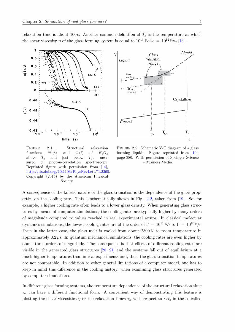
2.1 Structural relaxation functions Φ(t)/A and Φ (t) of B2O3 above Tg and just belowTg, measured by photon-correlation spectroscopy. Taken from [14]. . . . . . . . . 4
2.2 Schematic V-T diagram of a glass forming liquid. Taken from [19]. . . . . . . . . 4
2.3 Angell plots of the shear viscosity η and structural relaxation time τα with respectto Tg/T for different glass forming systems, including computer simulations. Takenfrom [12] and [13]. . . . . . . . . . . . . . . . . . . . . . . . . . . . . . . . . . . . 5
2.4 Illustration of two connected SiO4 tetrahedra. . . . . . . . . . . . . . . . . . . . . 6
2.5 Illustration of BO3 triangle and boroxol ring. . . . . . . . . . . . . . . . . . . . . 6
2.6 Raman spectrum of vitreous SiO2. Taken from [25]. . . . . . . . . . . . . . . . . 7
2.7 Raman spectrum of vitreous B2O3. Taken from [26]. . . . . . . . . . . . . . . . . 7
2.8 Longitudinal (M) and shear (G) elastic moduli of SiO2, B2O3 and GeO2 glasswith respect to temperature. Taken from [35]. . . . . . . . . . . . . . . . . . . . . 8
2.9 Raman spectrum of vitreous B2O3 at different temperatures. Taken from [36]. . 8
3.1 Illustration of periodic boundary conditions. Taken from [40]. . . . . . . . . . . . 16
3.2 Illustration of minimum image convention. Taken from [40]. . . . . . . . . . . . . 16
4.1 Comparison between the original BKS potential (3.122) and the modified potential(4.1) with harmonic correction for small r. . . . . . . . . . . . . . . . . . . . . . . 52
4.2 Total short-range pair potential used in simulation in case of the BKS parameters. 52
4.3 Dependence of the pair distance r on the position in a table of bitmap style with216 table entries. . . . . . . . . . . . . . . . . . . . . . . . . . . . . . . . . . . . . 53
4.4 Comparison of Loop times on the precision of the bitmap table . . . . . . . . . . 53
4.5 Test of relation |Etot − 〈Etot〉| ∝ (δt)2 with V CS only cut off at rewc . . . . . . . . . 55
4.6 Test of relation |Etot − 〈Etot〉| ∝ (δt)2 for totally smoothed short-range potential. 55
4.7 |Etot,end − Etot,beg| in microcanonical production runs with respect to time step δt. 56
4.8 Scaling of Loop times with respect to the number of processors. . . . . . . . . . . 56
4.9 SSiSi (k) for different system sizes at 3200 K . . . . . . . . . . . . . . . . . . . . . 58
4.10 gSiSi (k) for different system sizes at 3200 K . . . . . . . . . . . . . . . . . . . . . 58
4.11 pSiSiSi (Φ) for different system sizes at 3200 K . . . . . . . . . . . . . . . . . . . . 58
4.12 pSi (n) for different system sizes at 3200 K . . . . . . . . . . . . . . . . . . . . . . 58
4.13 FS,Si (k, t) for different system sizes at 3200 K. . . . . . . . . . . . . . . . . . . . . 59
4.14⟨r2Si (t)
⟩for different system sizes at 3200 K. . . . . . . . . . . . . . . . . . . . . . 59
4.15 Dependence of Diffusion constant for Si and O on system size at 3200 K. . . . . . 59
4.16 Dependence of 1/e relaxation time τ1/e,α of FS,α (k, t) on system size at 3200 K. . . 59
4.17⟨r2α (t)
⟩, α ∈ Si,O, comparison of BKS and CHIK potential . . . . . . . . . . 61
4.18 FS,α (k, t) , α ∈ Si,O, comparison of BKS and CHIK potential . . . . . . . . . 61
4.19 gαβ (r) , α, β ∈ Si,O, comparison of BKS and CHIK potential . . . . . . . . . 63
xi
List of Figures xii
4.20 Sαβ (k) , α, β ∈ Si,O, comparison of BKS and CHIK potential . . . . . . . . . 63
4.21 pαβγ (Φ) , α, β, γ ∈ Si,O, comparison of BKS and CHIK potential. . . . . . . . 64
4.22 Probability that a Si atom is member of a ring of size n, pSi (n), at differenttemperatures, comparison of BKS and CHIK potential . . . . . . . . . . . . . . . 64
4.23 pαβ (n) , α, β ∈ Si,O at different temperatures, comparison of BKS and CHIKpotential . . . . . . . . . . . . . . . . . . . . . . . . . . . . . . . . . . . . . . . . . 65
4.24 Arrhenius plot of self diffusion constants for Si and O at different temperatures,comparison of BKS and CHIK potential . . . . . . . . . . . . . . . . . . . . . . . 66
4.25 Dependence of E0 and Sαα on the number of k-points . . . . . . . . . . . . . . . 68
4.26 Dependence of E0 and Sαα on the accuracy of the electronic relaxation . . . . . . 69
4.27 Dependence of E0 and Sαα on the plane wave cutoff Ecut . . . . . . . . . . . . . 69
4.28 gαβ (r) , α, β ∈ Si,O at 0 K, before and after structural relaxation . . . . . . . 71
4.29 pαβγ (Φ) , α, β, γ ∈ Si,O at 0 K, before and after structural relaxation . . . . . 71
4.30 Snapshot of the glass structure of a 165 atom system SiO2 after the full ab initioquench and the structural relaxation. . . . . . . . . . . . . . . . . . . . . . . . . . 72
4.31 pSi (n) at 0 K. Comparison to 3000 K . . . . . . . . . . . . . . . . . . . . . . . . . 73
4.32 pOO (n) at 0 K, before and after structural relaxation. . . . . . . . . . . . . . . . 73
4.33 pSi (n) at 0 K. Comparison of BKS and CHIK potential after structural relaxationwith full ab initio quench. . . . . . . . . . . . . . . . . . . . . . . . . . . . . . . . 74
4.34 pOO (n) at 0 K. Comparison of BKS and CHIK potential after structural relax-ation with full ab initio quench. . . . . . . . . . . . . . . . . . . . . . . . . . . . . 74
4.35 Sneutr. (k). Comparison of BKS and CHIK potential after structural relaxationwith experimental results. . . . . . . . . . . . . . . . . . . . . . . . . . . . . . . . 76
4.36 Sneutr. (k). Comparison of full ab initio quench at 0 K and 300 K with experimentalresults. . . . . . . . . . . . . . . . . . . . . . . . . . . . . . . . . . . . . . . . . . . 76
4.37 g (ν) of SiO2. Comparison of different software packages . . . . . . . . . . . . . . 78
4.38 g (ν) of SiO2. Comparison of classical with quantum mechanical forces . . . . . . 79
4.39 G (ν) of SiO2. Comparison with inelastic neutron scattering . . . . . . . . . . . . 80
4.40 g (ν) of SiO2. Comparison with Raman scattering. Measured at Otto SchottResearch Centre in Mainz. . . . . . . . . . . . . . . . . . . . . . . . . . . . . . . . 81
4.41 CV (T ) of SiO2. Comparison with experimental results of Cp (T ) . . . . . . . . . 82
5.1 Helmholtz free energy F (T, V ) of one glass configuration SiO2 at different tem-peratures, DFT forces. . . . . . . . . . . . . . . . . . . . . . . . . . . . . . . . . . 89
5.2 V (T ) of one glass configuration SiO2. Evaluation according to 4 and 10 differentsystem densities, DFT forces. . . . . . . . . . . . . . . . . . . . . . . . . . . . . . 91
5.3 V (T ) of one glass configuration SiO2. Evaluation according to different equationsof state (equations (5.10) to (5.12)), DFT forces. . . . . . . . . . . . . . . . . . . 91
5.4 V (T ) of 5 different glass configurations SiO2. BKS and CHIK potential, DFTforces. . . . . . . . . . . . . . . . . . . . . . . . . . . . . . . . . . . . . . . . . . . 92
5.5 V (T ) of 10 different glass configurations SiO2. BKS and CHIK potential, classicalforces. . . . . . . . . . . . . . . . . . . . . . . . . . . . . . . . . . . . . . . . . . . 92
5.6 αL (T ) of 5 different glass configurations SiO2. BKS and CHIK potential, DFTforces. . . . . . . . . . . . . . . . . . . . . . . . . . . . . . . . . . . . . . . . . . . 93
5.7 αL (T ) of 10 different glass configurations SiO2. BKS and CHIK potential, clas-sical forces. . . . . . . . . . . . . . . . . . . . . . . . . . . . . . . . . . . . . . . . 93
5.8 νn with respect to V . Mode n = 4 and n = 5. Two configurations of SiO2. BKSpotential, DFT forces. . . . . . . . . . . . . . . . . . . . . . . . . . . . . . . . . . 95
List of Figures xiii
5.9 νn with respect to V . Mode n = 150 and n = 300. Two configurations of SiO2.BKS potential, DFT forces. . . . . . . . . . . . . . . . . . . . . . . . . . . . . . . 95
5.10 γn of 5 different glass configurations SiO2. BKS and CHIK potential, DFT forces. 96
5.11 γn of 10 different glass configurations SiO2. BKS and CHIK potential, classicalforces. . . . . . . . . . . . . . . . . . . . . . . . . . . . . . . . . . . . . . . . . . . 97
5.12 Average αL (T ), SiO2. BKS and CHIK potential, DFT forces. Comparison withexperimental measurements of NIST Standard Reference Material 739, Spectrosiland Vitreosil [32, 33]. . . . . . . . . . . . . . . . . . . . . . . . . . . . . . . . . . 98
5.13 Average αL (T ), SiO2. BKS and CHIK potential, classical forces. Comparisonwith experimental measurements of NIST Standard Reference Material 739, Spec-trosil and Vitreosil [32, 33]. . . . . . . . . . . . . . . . . . . . . . . . . . . . . . . 98
6.1 Dependence of E0 and Sαα on the plane wave cutoff Ecut . . . . . . . . . . . . . 107
6.2⟨r2α (t)
⟩, α ∈ B,O, B2O3. Ab initio MD at different temperatures. . . . . . . . 109
6.3 FS,α (k, t) , α, β ∈ B,O, B2O3. Ab initio MD at different temperatures. . . . . 109
6.4 gαβ (r) , α, β ∈ B,O, B2O3. Ab initio MD at different temperatures. Compar-ison with ab initio MD simulation at 2500 K and 1.92 g/cm3 [162]. . . . . . . . . . 110
6.5 Sαβ (k) , α, β ∈ B,O, B2O3. Ab initio MD at different temperatures. . . . . . . 110
6.6 pαβγ (Φ) , α, β, γ ∈ B,O, B2O3. Ab initio MD at different temperatures. . . . . 112
6.7 pB (n) at different temperatures, B2O3. Ab initio MD. . . . . . . . . . . . . . . . 113
6.8 pB (n). Temporal development at 2300 K, B2O3. Ab initio MD. . . . . . . . . . . 113
6.9 χ2 with respect to iteration step. Parameter fitting of pair potentials for B2O3 at3600 K and 2300 K. . . . . . . . . . . . . . . . . . . . . . . . . . . . . . . . . . . . 117
6.10 λ with respect to iteration step. Parameter fitting of pair potentials for B2O3 at3600 K and 2300 K. . . . . . . . . . . . . . . . . . . . . . . . . . . . . . . . . . . . 117
6.11 gBB (r) and gOO (r). Result of parameter fitting of pair potentials for B2O3 at3600 K and comparison with original parameter set [97]. . . . . . . . . . . . . . . 119
6.12 pBOB (Φ) and pOBO (Φ). Result of parameter fitting of pair potentials for B2O3
at 3600 K and comparison with original parameter set [97]. . . . . . . . . . . . . 119
6.13 gBB (r) and gOO (r). Result of parameter fitting of pair potentials for B2O3 at2300 K and comparison with original parameter set [97]. . . . . . . . . . . . . . . 120
6.14 pBOB (Φ) and pOBO (Φ). Result of parameter fitting of pair potentials for B2O3
at 2300 K and comparison with original parameter set [97]. . . . . . . . . . . . . 120
6.15 r123 (r12) for N = 5, 10, 100 and ∞ and r23 = 1.0 A. . . . . . . . . . . . . . . . . 122
6.16 G (r123 (r12)) for N = 5, 10, 100 and ∞ and r23 = 1.0 A with rangc = 2 A and
dang = 0.05 A2. . . . . . . . . . . . . . . . . . . . . . . . . . . . . . . . . . . . . . 122
6.17 χ2 with respect to iteration step. Parameter fitting of potentials including 3-bodyterms for B2O3 at 2300 K. . . . . . . . . . . . . . . . . . . . . . . . . . . . . . . . 124
6.18 λ with respect to iteration step. Parameter fitting of potentials including 3-bodyterms for B2O3 at 2300 K. . . . . . . . . . . . . . . . . . . . . . . . . . . . . . . . 124
6.19 gBB (r) and gOO (r). Results of parameter fitting of potentials including 3-bodyterms for B2O3 at 2300 K. . . . . . . . . . . . . . . . . . . . . . . . . . . . . . . . 125
6.20 pBOB (Φ) and pOBO (Φ). Results of parameter fitting of potentials including 3-body terms for B2O3 at 2300 K. . . . . . . . . . . . . . . . . . . . . . . . . . . . . 125
6.21 Test of relation |Etot − 〈Etot〉| ∝ (δt)2 for potential including 3-body terms and
COO = 0 eV A6. . . . . . . . . . . . . . . . . . . . . . . . . . . . . . . . . . . . . . 126
6.22 |Etot,end − Etot,beg| in microcanonical production run for potential including 3-
body terms and COO = 0 eV A6. . . . . . . . . . . . . . . . . . . . . . . . . . . . . 126
List of Figures xiv
6.23 FS,B (k, t) at 2300 K and 3600 K. Comparison of classical potential including 3-body terms with ab initio MD. . . . . . . . . . . . . . . . . . . . . . . . . . . . . 129
6.24⟨r2B (t)
⟩at 3600 K and at 2300 K. Comparison of classical potential including
3-body terms with ab initio MD. . . . . . . . . . . . . . . . . . . . . . . . . . . . 129
6.25 gBB (r) and gOO (r) at 3600 K and at 2300 K. Comparison of classical potentialincluding 3-body terms with ab initio MD. . . . . . . . . . . . . . . . . . . . . . . 130
6.26 pBOB (Φ) and pOBO (Φ) at 3600 K and at 2300 K. Comparison of classical poten-tial including 3-body terms with ab initio MD. . . . . . . . . . . . . . . . . . . . 130
6.27 pB (n) at 3600 K and at 2300 K. Comparison of classical potential including 3-body terms with ab initio MD. . . . . . . . . . . . . . . . . . . . . . . . . . . . . 131
6.28 pBBB (Φ) at 3600 K and at 2300 K. Comparison of classical potential including3-body terms with ab initio MD. . . . . . . . . . . . . . . . . . . . . . . . . . . . 131
6.29 Mean system density ρ with respect to T at constant external pressure p = 0 for1200 atom systems. Classical potentials including 3-body terms. . . . . . . . . . 131
6.30 Mean internal pressure pint with respect to T for 150 atom systems at constantdensity ρ = 1.83 g/cm3. Classical potentials including 3-body terms. . . . . . . . . 131
6.31⟨r2α (t)
⟩, α ∈ B,O, at different temperatures for 1200 atom system at constant
external pressure p = 0. Classical potential with 3-body terms and COO = 0 eV A6.132
6.32⟨r2α (t)
⟩, α ∈ B,O, at different temperatures for 1200 atom system at constant
external pressure p = 0. Classical potential with 3-body terms and COO 6= 0 eV A6.133
6.33⟨r2α (t)
⟩, α ∈ B,O, at different temperatures for 150 atom system at constant
density ρ = 1.83 g/cm3. Classical potential with 3-body terms and COO = 0 eV A6. 133
6.34⟨r2α (t)
⟩, α ∈ B,O, at different temperatures for 150 atom system at constant
density ρ = 1.83 g/cm3. Classical potential with 3-body terms and COO 6= 0 eV A6. 134
6.35⟨r2B (t)
⟩. Comparison of 1200 (p = 0) and 150 (ρ = 1.83 g/cm3) atom system.
Classical potential with 3-body terms and COO = 0 eV A6. . . . . . . . . . . . . . 134
6.36⟨r2B (t)
⟩. Comparison of 1200 (p = 0) and 150 (ρ = 1.83 g/cm3) atom system.
Classical potential with 3-body terms and COO 6= 0 eV A6. . . . . . . . . . . . . . 134
6.37 FS,B (k, t). Comparison of 1200 (p = 0) and 150 (ρ = 1.83 g/cm3) atom system.
Classical potential with 3-body terms and COO = 0 eV A6. . . . . . . . . . . . . . 135
6.38 FS,B (k, t). Comparison of 1200 (p = 0) and 150 (ρ = 1.83 g/cm3) atom system.
Classical potential with 3-body terms and COO 6= 0 eV A6. . . . . . . . . . . . . . 135
6.39 gBB (r) and gOO (r). Comparison of 1200 (p = 0) and 150 (ρ = 1.83 g/cm3) atom
system. Classical potential with 3-body terms and COO = 0 eV A6. . . . . . . . . 137
6.40 gBB (r) and gOO (r). Comparison of 1200 (p = 0) and 150 (ρ = 1.83 g/cm3) atom
system. Classical potential with 3-body terms and COO 6= 0 eV A6. . . . . . . . . 137
6.41 pαβγ (Φ) , α, β, γ ∈ B,O. Comparison of 1200 (p = 0) and 150 (ρ = 1.83 g/cm3)
atom system. Classical potential with 3-body terms and COO = 0 eV A6. . . . . . 138
6.42 pαβγ (Φ) , α, β, γ ∈ B,O. Comparison of 1200 (p = 0) and 150 (ρ = 1.83 g/cm3)
atom system. Classical potential with 3-body terms and COO 6= 0 eV A6. . . . . . 138
6.43 pB (n). Comparison of 1200 (p = 0) and 150 (ρ = 1.83 g/cm3) atom system.
Classical potential with 3-body terms and COO = 0 eV A6. . . . . . . . . . . . . . 139
6.44 pB (n). Comparison of 1200 (p = 0) and 150 (ρ = 1.83 g/cm3) atom system.
Classical potential with 3-body terms and COO 6= 0 eV A6. . . . . . . . . . . . . . 139
List of Figures xv
6.45 Arrhenius plot of self diffusion constants for B and O at different temperaturesfor 1200 atom systems at constant external pressure p = 0. Different classicalpotentials with 3-body terms. . . . . . . . . . . . . . . . . . . . . . . . . . . . . . 140
6.46 Arrhenius plot of self diffusion constants for B and O at different temperatures for150 atom systems at constant density ρ = 1.83 g/cm3. Different classical potentialswith 3-body terms. . . . . . . . . . . . . . . . . . . . . . . . . . . . . . . . . . . . 141
6.47 Arrhenius plot of self diffusion constants for B and O at different temperaturesfor 150 atom systems at constant density ρ = 1.83 g/cm3. Comparison of differentclassical potentials with 3-body terms with ab initio MD simulations. . . . . . . . 142
6.48 Temporal development of mean B-O-B angle. Comparison of different classicalpotentials with 3-body terms with ab initio MD simulations. . . . . . . . . . . . 143
6.49 Temporal development of mean B-B and B-O coordination. Comparison of dif-ferent classical potentials with 3-body terms with ab initio MD simulations. . . . 144
6.50 Temporal development of probability of B atom to be in a ring of size n, pB (n),for n = 3, n = 4, n = 7 and n = 8. Comparison of different classical potentialswith 3-body terms with ab initio MD simulations. . . . . . . . . . . . . . . . . . 145
6.51 gBB (r) and gOO (r) at 0 K, before and after structural relaxation. 3-body poten-
tial with COO = 0 eV A6. . . . . . . . . . . . . . . . . . . . . . . . . . . . . . . . . 147
6.52 gBB (r) and gOO (r) at 0 K, before and after structural relaxation. Original po-
tential [97] and 3-body potential with COO 6= 0 eV A6. . . . . . . . . . . . . . . . 147
6.53 pBOB (Φ) and pOBO (Φ) at 0 K, before and after structural relaxation. 3-body
potential with COO = 0 eV A6. . . . . . . . . . . . . . . . . . . . . . . . . . . . . . 148
6.54 pBOB (Φ) and pOBO (Φ) at 0 K, before and after structural relaxation . . . . . . . 148
6.55 pB (n) at 0 K, before and after structural relaxation. 3-body potential with COO =
0 eV A6. . . . . . . . . . . . . . . . . . . . . . . . . . . . . . . . . . . . . . . . . . 150
6.56 pB (n) at 0 K, before and after structural relaxation. Original potential [97] and
3-body potential with COO 6= 0 eV A6. . . . . . . . . . . . . . . . . . . . . . . . . 150
6.57 pB (n) at 0 K. Comparison of full ab initio quenches with one classical quench
after structural relaxation (COO = 0 eV A6, 800 K) and model glass structure with
f = 75% [131–133]. . . . . . . . . . . . . . . . . . . . . . . . . . . . . . . . . . . . 151
6.58 gBB (r) at 0 K. Comparison of full ab initio quenches with one classical quench
after structural relaxation (COO = 0 eV A6, 800 K) and model glass structure with
f = 75% [131–133]. . . . . . . . . . . . . . . . . . . . . . . . . . . . . . . . . . . . 151
6.59 Snapshot of the glass structure of a 150 atom system B2O3 containing 4 boroxolrings. Configuration of one full ab initio quench from 2300 K. . . . . . . . . . . . 154
6.60 Sneutr. (k) at 0 K, before and after structural relaxation. 3-body potential with
COO = 0 eV A6. Comparison with experimental results [29], taken from [141]. . . 156
6.61 Sneutr. (k) at 0 K, before and after structural relaxation. Original potential [97]
and 3-body potential with COO 6= 0 eV A6. Comparison with experimental results
[29], taken from [141]. . . . . . . . . . . . . . . . . . . . . . . . . . . . . . . . . . 156
6.62 Sneutr. (k) at 0 K. Comparison of full ab initio quenches with experimental results[29], taken from [141]. . . . . . . . . . . . . . . . . . . . . . . . . . . . . . . . . . 157
6.63 Sneutr. (k) at 300 K. Comparison of full ab initio quenches with experimentalresults [29], taken from [141]. . . . . . . . . . . . . . . . . . . . . . . . . . . . . . 157
6.64 g (ν) of B2O3, classical quench. Comparison of classical with quantum mechanical
forces. 3-body potential with COO = 0 eV A6. . . . . . . . . . . . . . . . . . . . . 158
List of Figures xvi
6.65 g (ν) of B2O3, classical quench. Comparison of classical with quantum mechanical
forces. Original potential [97] and 3-body potential with COO 6= 0 eV A6. . . . . . 158
6.66 g (ν) of B2O3, DFT forces. Comparison of classical quenches with subsequentstructural relaxation to full ab initio quenches and alternative model structure[131–133]. . . . . . . . . . . . . . . . . . . . . . . . . . . . . . . . . . . . . . . . . 160
6.67 G (ν) ofB2O3, according to quantum mechanical forces. Different classical quenches.Comparison with inelastic neutron scattering. . . . . . . . . . . . . . . . . . . . . 162
6.68 G (ν) of B2O3, according to quantum mechanical forces. Ab initio quenches.Comparison with inelastic neutron scattering. . . . . . . . . . . . . . . . . . . . . 162
6.69 CV (T ) of B2O3, according to classical and quantum mechanical forces. 3-body
potential with COO = 0 eV A6. Comparison with experimental results of Cp (T ) . 163
6.70 CV (T ) of B2O3, according to classical and quantum mechanical forces. Origi-
nal potential [97] and 3-body potential with COO 6= 0 eV A6. Comparison with
experimental results of Cp (T ) . . . . . . . . . . . . . . . . . . . . . . . . . . . . . 163
6.71 CV (T ) of B2O3, according to classical and quantum mechanical forces. Ab initioquenches at different equilibration temperatures and alternative model structure[131–133]. Comparison with experimental results of Cp (T ) . . . . . . . . . . . . 164
List of Tables
4.2 Parameters of the BKS [22] and the CHIK [43] potential. . . . . . . . . . . . . . 50
4.4 Parameters of short-range the repulsive substitution V Harm (r) (see equation (4.2))of the BKS [22] and the CHIK [43] potential at distances r ≤ rin. . . . . . . . . . 52
4.6 Comparison of mean total energies per atom and mean pressures for partly andfully tabulated, partly and fully smoothed short-range potentials and differentEwald precisions. NVT runs at 4300 K of 165 atom system at a system densityof ρ = 2.37 g/cm3. . . . . . . . . . . . . . . . . . . . . . . . . . . . . . . . . . . . . 54
4.8 Cooling procedure of liquid SiO2 with number of time steps and equilibrationtimes at each temperature. . . . . . . . . . . . . . . . . . . . . . . . . . . . . . . 57
4.10 Mean first neighbor distances and average angles of classical quenches and one fullab initio quench at 0 K after the structural relaxation. Comparison with singleab initio run at 300 K and experimental results [113, 114]. . . . . . . . . . . . . . 75
5.2 Fit parameters V0, E0, K0 and K ′0 for fits of different equations of state E (V ) tothe numerical values of F (T, V ), based on DFT forces. One glass configuration,generated with the BKS potential, after the structural relaxation. Fits to all 10and 4 data points at T = 0 K and T = 500 K. . . . . . . . . . . . . . . . . . . . . 90
6.2 Number of time steps and simulation time at each temperature for ab initio MDsimulations of liquid B2O3 (150 atom system at constant density of ρ = 1.83 g/cm3).108
6.5 Different parametrizations of the pair potential (see equation (3.122)) for B2O3.Comparison of original parameter set [97] to 3 different parametrizations afterstructural fits at 3600 K and 2300 K. . . . . . . . . . . . . . . . . . . . . . . . . . 115
6.7 Different parametrizations of the pair potential (see equation (3.122)) and 3-bodypotentials (see equation (6.1)) for B2O3. Comparison of different parametrizationsafter structural fits at 2300 K. . . . . . . . . . . . . . . . . . . . . . . . . . . . . . 123
6.9 Cooling procedure of liquid B2O3 with number of time steps and equilibrationtimes at each temperature. . . . . . . . . . . . . . . . . . . . . . . . . . . . . . . 128
6.11 Probabilities pαβ (n) , α, β ∈ B,O, of having the exact number of atomic neigh-bors n of an “ideal” glass configuration. Glass structures after classical classi-cal quench with 3-body potentials and structural relaxation. In case of COO =
0 eV A6, quenches from the melt at two different temperatures. . . . . . . . . . . 150
6.13 Mean first neighbor distances and average angles of B2O3 for all examined glassconfigurations after the structural relaxation at 0 K. Comparison with experi-mental results [29]. . . . . . . . . . . . . . . . . . . . . . . . . . . . . . . . . . . . 153
xvii

Chapter 1
Introduction
In the year 1893, the first laboratory borosilicate glass was introduced onto the market by the
“Glastechnisches Laboratorium Schott & Genossen Jena”, which nowadays is the “Schott AG”.
Since 1887 borosilicate glasses, containing the glass former B2O3, as well as the glass former
SiO2, have been developed by Otto Schott and patented in 1891 [1]. In 1938 the name DURAN R©was introduced for the marketing of laboratory borosilicate glass. DURAN R© has the chemical
composition in weight percent of 81 %SiO2, 13 %B2O3, 4 %Na2O+K2O and 2 %Al2O3 [2]. This
was a great progress with respect to the alkaline silicate (soda-lime) or lead silicate glasses, as
borosilicate glasses have an improved chemical resistance, mechanical strength, heat resistance
and thermal shock resistance. The latter is connected to a significantly lower coefficient of
thermal expansion. Regarding these properties, pure SiO2 glass, or vitreous silica, shows even
superior behavior. However, it is very hard and expensive to process, due to its very high glass
transition temperature of Tg ' 1475 K [3]. Adding glass modifiers, like alkaline oxides, alkaline
earth oxides and aluminum oxide, significantly reduces the glass transition temperature and leads
to glasses that are easy and cheap to process [4]. However, the before mentioned properties are
significantly deteriorated, making these glasses unusable, for example, as laboratory glasses.
Adding the glass former B2O3 (boric acid, Tg ' 526 K [5]) and reducing the amount of glass
modifiers, helps in producing a glass, which shows a significant improvement of the relevant
properties, in combination with a significantly lower glass transition temperature than pure
SiO2.
This substantiates the interest in the model glass former SiO2, as well as the model glass former
B2O3. Regarding glasses with different components, as the aforementioned borosilicate glasses,
the exact glass structure is still not known in many cases. Furthermore, the dependence of the
properties of a glass on its composition is still hard to predict. In practice, glass development
goes along with conducting a series of test melts with a slight variation of the glass compositions
and a subsequent interpolation of the glass properties, one is interested in. Therefore, a better
understanding of the glass structure on an atomistic level and the prediction of resulting glass
properties is desirable.
1
Chapter 1. Introduction 2
The first model of oxide glasses was proposed by Zachariasen’s random network theory [6]. In
this model, the glass consists of a three-dimensional random network built up by glass formers
and modified by glass modifiers, following certain rules. However, it turns out that the degree
of randomness varies from glass to glass. Some glasses are closer to Zachariasen’s picture,
whereas others show a more microcrystalline structure [4]. Nowadays, computer simulations
are an important tool in the modeling of oxide glasses on an atomistic level. For instance,
classical molecular dynamics (MD) [7] or Monte Carlo (MC) [8] simulations can be carried out.
Here, typical system sizes are of the order of 1000 to a few 100000 atoms and time scales up
to the order of microseconds are accessible. However, the inter-atomic forces are described
on the basis of empirical force fields, which are less accurate than a full quantum-mechanical
description. The latter can be accomplished on the basis of density functional theory (DFT) [9],
limiting the system sizes to about 100 - 200 atoms and the accessible time scales to the order
of picoseconds. In principle, both techniques can be combined, which, for example, has already
been successfully done in case of the model glass former SiO2 [10, 11]. Here, the glass structure
is generated by means of a classical MD simulation, with a subsequent structural relaxation
by means of a quantum-mechanical calculation and a computation of the vibrational properties
based on quantum-mechanical forces. This method requires a suitable classical force field to
generate a realistic glass structure in the first place.
The work presented in this thesis follows this direction. Due to the aforementioned reasons,
the model glass formers SiO2 and B2O3 are examined and glass structures are generated by
means of cooling down a glass melt with classical MD simulations, followed by a subsequent
quantum-mechanical relaxation (see chapters 4 and 6). In case of SiO2, two different classical
force fields are employed. In case of B2O3, a new classical force field is developed, based on the
liquid structure at high temperatures extracted from a quantum-mechanical (DFT) calculation.
The structural properties of the generated glasses are compared to experimental results. In
addition, special focus is placed on the vibrational properties, as the latter give access to the
low-temperature thermodynamics. It turns out that a realistic glass structure, in combination
with quantum-mechanical forces, leads to a vibrational density of states comparable to the
experimental one and a good accordance of the specific heat with respect to temperature. The
thermal expansion also shows a good agreement with experimental results in the low-temperature
regime. This is demonstrated in case of SiO2 in chapter 5. Here, a change of sign of the linear
expansion coefficient and a range of negative thermal expansion at low temperatures is observed,
in agreement to experimental results. To my knowledge, this has not been reported before in
case of DFT calculations of vitreous silica.
Chapter 2
Simulation of real glass formers?
2.1 The glass transition - phenomenology
Glass is a non-equilibrium state of matter. At temperatures below the solid-liquid phase transi-
tion the equilibrium configuration is a crystalline structure and the corresponding phase depends
on the ambient conditions. However, many liquids can form a glass if they are cooled fast enough
to avoid crystallization. In this way, a so-called supercooled phase can be reached at tempera-
tures below the melting temperature Tm of the corresponding crystalline structure. In a glass
forming liquid the distinction of two typical timescales becomes necessary when cooling the sys-
tem down [12]. The atom trajectories are constituted of frequent collisions with the neighboring
particles. This rattling motion happens on a very short timescale of typically about 10− 100 fs
in oxide glasses. After several collisions, an atom can break out of the cage of the surrounding
particles and change its relative position. This diffusive motion is typically a collective phe-
nomenon and occurs on longer timescales than the rattling motion. This structural relaxation
time or α-relaxation time τα [13] increases by many orders of magnitude, when cooling the sys-
tem down and at some point the glass transition temperature Tg is reached. In Fig. 2.1 this
two-step relaxation process and the increase of the α-relaxation time by orders of magnitude
is impressively demonstrated by means of photon-correlation spectroscopy of the “strong” net-
work forming glass former B2O3 at different temperatures [14]. In contrast to the crystallization
transition, this is not a phase transition in the sense of the Ehrenfest classification [15], but a
kinetic transition. The glass transition temperature Tg is the temperature at which the system
falls out of equilibrium and no stress relaxation is possible anymore on the timescale of the ex-
periment. Therefore, there is no unique definition of Tg, but it depends on the experiment. One
way of measuring Tg is the increase of the heat capacity Cp from a solid-like to a liquid-like value
by means of scanning calorimetry [16]. This is connected to the fact that the configurational
contribution to the specific heat decreases to zero at temperatures below Tg [17] and leads to
one possible definition of Tg as the onset temperature of the jump in heat capacity at a heating
rate of 10 K/min [18]. At the glass transition temperature Tg defined in this way, the structural
3
Chapter 2. Simulation of real glass formers? 4
relaxation time is about 100 s. Another common definition of Tg is the temperature at which
the shear viscosity η of the glass forming system is equal to 1013 Poise = 1012 Pa/s [13].
Figure 2.1: Structural relaxationfunctions Φ(t)/A and Φ (t) of B2O3
above Tg and just below Tg, mea-sured by photon-correlation spectroscopy.Reprinted figure with permission from [14],http://dx.doi.org/10.1103/PhysRevLett.71.2260.Copyright (2015) by the American Physical
Society.
Figure 2.2: Schematic V-T diagram of a glassforming liquid. Figure reprinted from [19],page 380. With permission of Springer Science
+Business Media.
A consequence of the kinetic nature of the glass transition is the dependence of the glass prop-
erties on the cooling rate. This is schematically shown in Fig. 2.2, taken from [19]. So, for
example, a higher cooling rate often leads to a lower glass density. When generating glass struc-
tures by means of computer simulations, the cooling rates are typically higher by many orders
of magnitude compared to values reached in real experimental setups. In classical molecular
dynamics simulations, the lowest cooling rates are of the order of Γ = 1011 K/s to Γ = 1010 K/s.
Even in the latter case, the glass melt is cooled from about 2300 K to room temperature in
approximately 0.2µs. In quantum mechanical simulations, the cooling rates are even higher by
about three orders of magnitude. The consequence is that effects of different cooling rates are
visible in the generated glass structures [20, 21] and the systems fall out of equilibrium at a
much higher temperatures than in real experiments and, thus, the glass transition temperatures
are not comparable. In addition to other general limitations of a computer model, one has to
keep in mind this difference in the cooling history, when examining glass structures generated
by computer simulations.
In different glass forming systems, the temperature dependence of the structural relaxation time
τα can have a different functional form. A convenient way of demonstrating this feature is
plotting the shear viscosities η or the relaxation times τα with respect to T/Tg in the so-called
Chapter 2. Simulation of real glass formers? 5
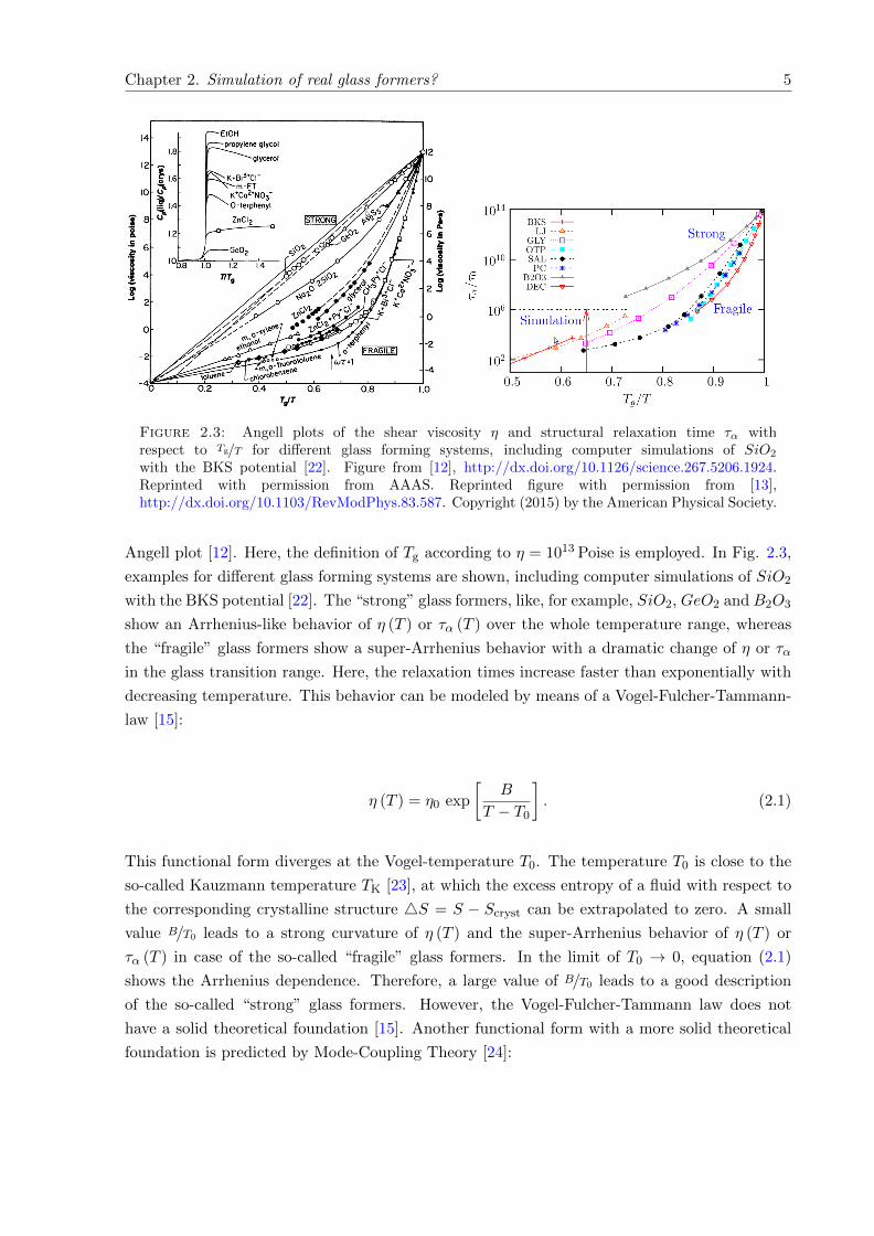
Figure 2.3: Angell plots of the shear viscosity η and structural relaxation time τα withrespect to Tg/T for different glass forming systems, including computer simulations of SiO2
with the BKS potential [22]. Figure from [12], http://dx.doi.org/10.1126/science.267.5206.1924.Reprinted with permission from AAAS. Reprinted figure with permission from [13],http://dx.doi.org/10.1103/RevModPhys.83.587. Copyright (2015) by the American Physical Society.
Angell plot [12]. Here, the definition of Tg according to η = 1013 Poise is employed. In Fig. 2.3,
examples for different glass forming systems are shown, including computer simulations of SiO2
with the BKS potential [22]. The “strong” glass formers, like, for example, SiO2, GeO2 and B2O3
show an Arrhenius-like behavior of η (T ) or τα (T ) over the whole temperature range, whereas
the “fragile” glass formers show a super-Arrhenius behavior with a dramatic change of η or τα
in the glass transition range. Here, the relaxation times increase faster than exponentially with
decreasing temperature. This behavior can be modeled by means of a Vogel-Fulcher-Tammann-
law [15]:
η (T ) = η0 exp
[B
T − T0
]. (2.1)
This functional form diverges at the Vogel-temperature T0. The temperature T0 is close to the
so-called Kauzmann temperature TK [23], at which the excess entropy of a fluid with respect to
the corresponding crystalline structure 4S = S − Scryst can be extrapolated to zero. A small
value B/T0 leads to a strong curvature of η (T ) and the super-Arrhenius behavior of η (T ) or
τα (T ) in case of the so-called “fragile” glass formers. In the limit of T0 → 0, equation (2.1)
shows the Arrhenius dependence. Therefore, a large value of B/T0 leads to a good description
of the so-called “strong” glass formers. However, the Vogel-Fulcher-Tammann law does not
have a solid theoretical foundation [15]. Another functional form with a more solid theoretical
foundation is predicted by Mode-Coupling Theory [24]:
Chapter 2. Simulation of real glass formers? 6
η (T ) = η0 (T − Tc)−γ . (2.2)
Here, Tc is the critical temperature, corresponding to the transition temperature of the system
to an ideal glass and γ is a critical exponent. The parameters Tc and γ depend on the material
and can be calculated.
Another matter of fact, clearly visible in Fig. 2.3, is that the timescales accessible by computer
simulations only allow the calculation of equilibrium properties at higher temperatures than the
ones accessible in experiments. A way to overcome this gap is to extrapolate different properties
to lower temperatures if the temperature dependence is known. At least for rather strong glass
formers, many properties should show an Arrhenius-like temperature dependence and therefore
an extrapolation is possible in some cases.
2.2 Vibrational properties, structure and anomalies of oxide
glasses
As already described in the introduction, oxide glasses consist of network formers and network
modifiers. The most important network formers for industrial applications are silicon oxide SiO2
and boron oxide B2O3. Other oxides that are capable of forming a three-dimensional network
are, for example, water H2O and germanium oxide GeO2.
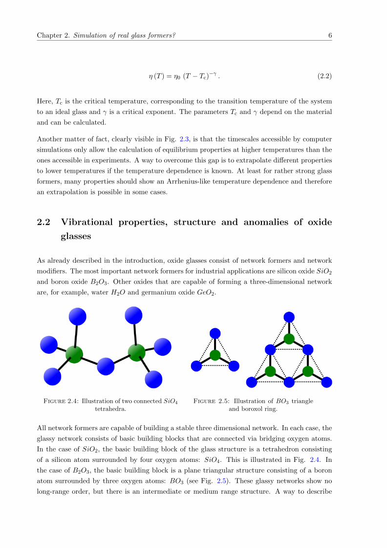
Figure 2.4: Illustration of two connected SiO4
tetrahedra.Figure 2.5: Illustration of BO3 triangle
and boroxol ring.
All network formers are capable of building a stable three dimensional network. In each case, the
glassy network consists of basic building blocks that are connected via bridging oxygen atoms.
In the case of SiO2, the basic building block of the glass structure is a tetrahedron consisting
of a silicon atom surrounded by four oxygen atoms: SiO4. This is illustrated in Fig. 2.4. In
the case of B2O3, the basic building block is a plane triangular structure consisting of a boron
atom surrounded by three oxygen atoms: BO3 (see Fig. 2.5). These glassy networks show no
long-range order, but there is an intermediate or medium range structure. A way to describe
Chapter 2. Simulation of real glass formers? 7
the intermediate range structure is the notation of ring sizes n. Here, n is the number of Si-O or
B-O pairs that are linearly connected in a way that the first and last oxygen atom are identical.
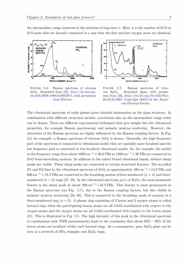
Figure 2.6: Raman spectrum of vitreousSiO2. Reprinted from [25], http://dx.doi.org/10.1016/0038-1098(82)90329-5, with permission
from Elsevier.
Figure 2.7: Raman spectrum of vitre-ous B2O3. Reprinted figure with permis-sion from [26], http://dx.doi.org/10.1103/PhysRevB.22.3983. Copyright (2015) by the Ameri-
can Physical Society.
The vibrational spectrum of oxide glasses gives valuable information on the glass structure. In
combination with different structural models, conclusions also on the intermediate range order
can be drawn. There are different experimental techniques that give insight into the vibrational
properties, for example Raman spectroscopy and inelastic neutron scattering. However, the
intensities of the Raman spectrum are highly influenced by the Raman coupling factors. In Fig.
2.6, for example, a Raman spectrum of vitreous SiO2 is shown. Generally, the high frequency
part of the spectrum is connected to vibrational modes that are spatially more localized and the
low frequency part is connected to less localized vibrational modes. So, for example, the modes
in the frequency range from about 1000 cm−1 = 30.0 THz to 1200 cm−1 = 36 THz are connected to
Si-O bond-stretching motions. In addition to the rather broad vibrational bands, distinct sharp
peaks are visible. These sharp peaks are connected to certain structural features. The so-called
D1 and D2 lines in the vibrational spectrum of SiO2 at approximately 495 cm−1 = 14.8 THz and
606 cm−1 = 18.2 THz are connected to the breathing motion of four-membered (n = 4) and three-
membered (n = 3) rings [27, 28]. In the vibrational spectrum g (ν) of B2O3, the most prominent
feature is the sharp peak at about 808 cm−1 = 24.2 THz. This feature is most pronounced in
the Raman spectrum (see Fig. 2.7), due to the Raman coupling factors, but also visible in
inelastic neutron scattering [29, 30]. This is connected to the breathing mode of oxygens in a
three-membered ring (n = 3). A planar ring consisting of 3 boron and 3 oxygen atoms is called
boroxol ring, when the participating boron atoms are all 3-fold coordinated with respect to the
oxygen atoms and the oxygen atoms are all 2-fold coordinated with respect to the boron atoms
[31]. This is illustrated in Fig. 2.5. The high intensity of this peak in the vibrational spectrum
in combination with NMR measurements leads to the conclusion that about 60%− 80% of the
boron atoms are localized within such boroxol rings. As a consequence, pure B2O3 glass can be
seen as a network of BO3 triangles and B3O6 rings.
Chapter 2. Simulation of real glass formers? 8
The above mentioned oxide glasses have rather striking thermo-mechanical properties. For
example, vitreous SiO2 shows a change of sign of the the linear expansion coefficient αL (T ) and
a range of negative thermal expansion near the absolute zero at temperatures below about 200 K
[32, 33]. In addition, a density maximum occurs in the molten state at approximately 1823 K
[34].
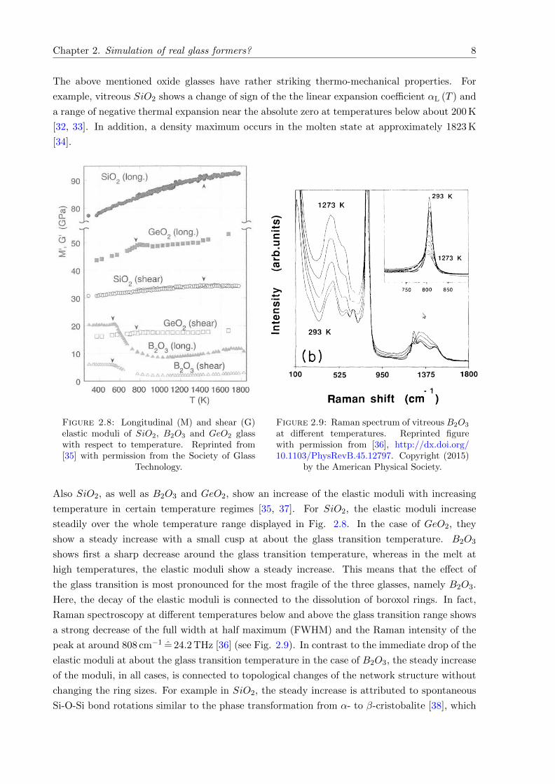
Figure 2.8: Longitudinal (M) and shear (G)elastic moduli of SiO2, B2O3 and GeO2 glasswith respect to temperature. Reprinted from[35] with permission from the Society of Glass
Technology.
Figure 2.9: Raman spectrum of vitreous B2O3
at different temperatures. Reprinted figurewith permission from [36], http://dx.doi.org/10.1103/PhysRevB.45.12797. Copyright (2015)
by the American Physical Society.
Also SiO2, as well as B2O3 and GeO2, show an increase of the elastic moduli with increasing
temperature in certain temperature regimes [35, 37]. For SiO2, the elastic moduli increase
steadily over the whole temperature range displayed in Fig. 2.8. In the case of GeO2, they
show a steady increase with a small cusp at about the glass transition temperature. B2O3
shows first a sharp decrease around the glass transition temperature, whereas in the melt at
high temperatures, the elastic moduli show a steady increase. This means that the effect of
the glass transition is most pronounced for the most fragile of the three glasses, namely B2O3.
Here, the decay of the elastic moduli is connected to the dissolution of boroxol rings. In fact,
Raman spectroscopy at different temperatures below and above the glass transition range shows
a strong decrease of the full width at half maximum (FWHM) and the Raman intensity of the
peak at around 808 cm−1 = 24.2 THz [36] (see Fig. 2.9). In contrast to the immediate drop of the
elastic moduli at about the glass transition temperature in the case of B2O3, the steady increase
of the moduli, in all cases, is connected to topological changes of the network structure without
changing the ring sizes. For example in SiO2, the steady increase is attributed to spontaneous
Si-O-Si bond rotations similar to the phase transformation from α- to β-cristobalite [38], which
Chapter 2. Simulation of real glass formers? 9
both show a structure with six-membered rings (n = 6). The α-cristobalite has a higher density
and less symmetric six-membered rings, whereas β-cristobalite has a lower density and six-
membered rings with a higher symmetry. In vitreous SiO2, the dominant ring size is n = 6, as
well, and the so-called amorphous-amorphous transition leads to a structure with a lower density
and, at the same time, higher elastic moduli.
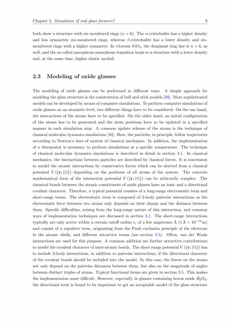
2.3 Modeling of oxide glasses
The modeling of oxide glasses can be performed in different ways. A simple approach for
modeling the glass structure is the construction of ball and stick models [39]. More sophisticated
models can be developed by means of computer simulations. To perform computer simulations of
oxide glasses on an atomistic level, two different things have to be considered: On the one hand,
the interactions of the atoms have to be specified. On the other hand, an initial configuration
of the atoms has to be generated and the atom positions have to be updated in a specified
manner in each simulation step. A common update scheme of the atoms is the technique of
classical molecular dynamics simulations [40]. Here, the particles, in principle, follow trajectories
according to Newton’s laws of motion of classical mechanics. In addition, the implementation
of a thermostat is necessary to perform simulations at a specific temperature. The technique
of classical molecular dynamics simulations is described in detail in section 3.1. In classical
mechanics, the interactions between particles are described by classical forces. It is convenient
to model the atomic interactions by conservative forces which can be derived from a classical
potential V (ri (t)) depending on the positions of all atoms of the system. The concrete
mathematical form of the interaction potential V (ri (t)) can be arbitrarily complex. The
chemical bonds between the atomic constituents of oxide glasses have an ionic and a directional
covalent character. Therefore, a typical potential consists of a long-range electrostatic term and
short-range terms. The electrostatic term is composed of 2-body pairwise interactions as the
electrostatic force between two atoms only depends on their charge and the distance between
them. Specific difficulties, arising from the long-range nature of this interaction, and common
ways of implementation techniques are discussed in section 3.1. The short-range interactions
typically are only active within a certain cutoff radius rc of a few angstroms A (1 A = 10−10 m)
and consist of a repulsive term, originating from the Pauli exclusion principle of the electrons
in the atomic shells, and different attractive terms (see section 3.5). Often, van der Waals
interactions are used for this purpose. A common addition are further attractive contributions
to model the covalent character of inter-atomic bonds. The short-range potential V (ri (t)) has
to include 3-body interactions, in addition to pairwise interactions, if the directional character
of the covalent bonds should be included into the model. In this case, the forces on the atoms
not only depend on the pairwise distances between them, but also on the magnitude of angles
between distinct triples of atoms. Typical functional forms are given in section 3.5. This makes
the implementation more difficult. However, especially in glasses containing boron oxide B2O3,
the directional term is found to be important to get an acceptable model of the glass structure
Chapter 2. Simulation of real glass formers? 10
(see chapter 6). In the case of SiO2, it is possible to simulate good model glasses only using
2-body interactions (see chapter 4).
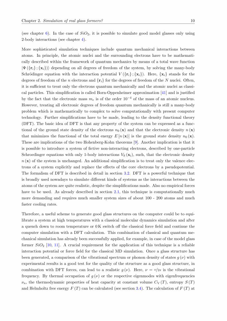
More sophisticated simulation techniques include quantum mechanical interactions between
atoms. In principle, the atomic nuclei and the surrounding electrons have to be mathemati-
cally described within the framework of quantum mechanics by means of a total wave function
|Ψ (ri ; xi)〉 depending on all degrees of freedom of the system, by solving the many-body
Schrodinger equation with the interaction potential V (ri ; xi). Here, xi stands for the
degrees of freedom of the n electrons and ri for the degrees of freedom of the N nuclei. Often,
it is sufficient to treat only the electrons quantum mechanically and the atomic nuclei as classi-
cal particles. This simplification is called Born-Oppenheimer approximation [41] and is justified
by the fact that the electronic mass me is of the order 10−4 of the mass of an atomic nucleus.
However, treating all electronic degrees of freedom quantum mechanically is still a many-body
problem which is mathematically to complex to solve computationally with present computer
technology. Further simplifications have to be made, leading to the density functional theory
(DFT). The basic idea of DFT is that any property of the system can be expressed as a func-
tional of the ground state density of the electrons n0 (x) and that the electronic density n (x)
that minimizes the functional of the total energy E [n (x)] is the ground state density n0 (x).
These are implications of the two Hohenberg-Kohn theorems [9]. Another implication is that it
is possible to introduce a system of fictive non-interacting electrons, described by one-particle
Schroedinger equations with only 1-body interactions VS (xi), such, that the electronic density
n (x) of the system is unchanged. An additional simplification is to treat only the valence elec-
trons of a system explicitly and replace the effects of the core electrons by a pseudopotential.
The formalism of DFT is described in detail in section 3.2. DFT is a powerful technique that
is broadly used nowadays to simulate different kinds of systems as the interactions between the
atoms of the system are quite realistic, despite the simplifications made. Also no empirical forces
have to be used. As already described in section 2.1, this technique is computationally much
more demanding and requires much smaller system sizes of about 100 - 200 atoms and much
faster cooling rates.
Therefore, a useful scheme to generate good glass structures on the computer could be to equi-
librate a system at high temperatures with a classical molecular dynamics simulation and after
a quench down to room temperature or 0 K switch off the classical force field and continue the
computer simulation with a DFT calculation. This combination of classical and quantum me-
chanical simulation has already been successfully applied, for example, in case of the model glass
former SiO2 [10, 11]. A crucial requirement for the application of this technique is a reliable
interaction potential or force field for the classical MD simulation. Once a glass structure has
been generated, a comparison of the vibrational spectrum or phonon density of states g (ν) with
experimental results is a good test for the quality of the structure as a good glass structure, in
combination with DFT forces, can lead to a realistic g (ν). Here, ν = ω/2π is the vibrational
frequency. By thermal occupation of g (ν) or the respective eigenmodes with eigenfrequencies
νn, the thermodynamic properties of heat capacity at constant volume CV (T ), entropy S (T )
and Helmholtz free energy F (T ) can be calculated (see section 3.4). The calculation of F (T ) at
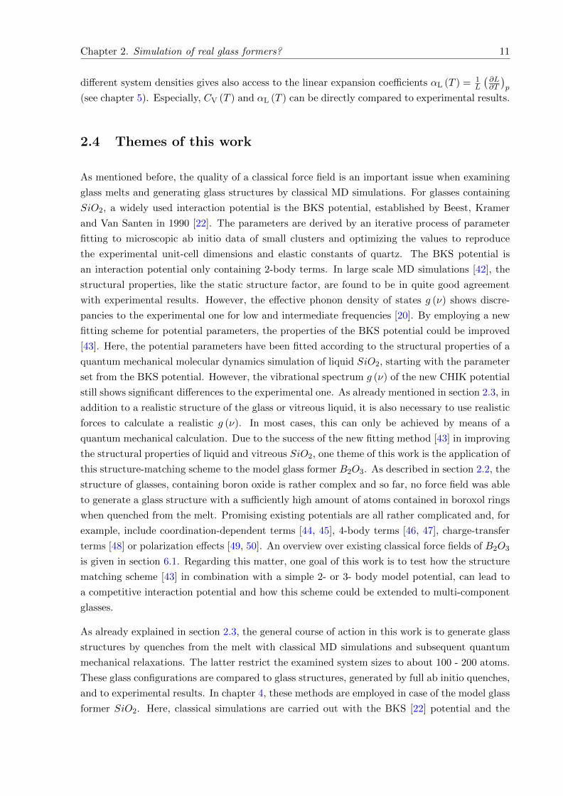
Chapter 2. Simulation of real glass formers? 11
different system densities gives also access to the linear expansion coefficients αL (T ) = 1L
(∂L∂T
)p
(see chapter 5). Especially, CV (T ) and αL (T ) can be directly compared to experimental results.
2.4 Themes of this work
As mentioned before, the quality of a classical force field is an important issue when examining
glass melts and generating glass structures by classical MD simulations. For glasses containing
SiO2, a widely used interaction potential is the BKS potential, established by Beest, Kramer
and Van Santen in 1990 [22]. The parameters are derived by an iterative process of parameter
fitting to microscopic ab initio data of small clusters and optimizing the values to reproduce
the experimental unit-cell dimensions and elastic constants of quartz. The BKS potential is
an interaction potential only containing 2-body terms. In large scale MD simulations [42], the
structural properties, like the static structure factor, are found to be in quite good agreement
with experimental results. However, the effective phonon density of states g (ν) shows discre-
pancies to the experimental one for low and intermediate frequencies [20]. By employing a new
fitting scheme for potential parameters, the properties of the BKS potential could be improved
[43]. Here, the potential parameters have been fitted according to the structural properties of a
quantum mechanical molecular dynamics simulation of liquid SiO2, starting with the parameter
set from the BKS potential. However, the vibrational spectrum g (ν) of the new CHIK potential
still shows significant differences to the experimental one. As already mentioned in section 2.3, in
addition to a realistic structure of the glass or vitreous liquid, it is also necessary to use realistic
forces to calculate a realistic g (ν). In most cases, this can only be achieved by means of a
quantum mechanical calculation. Due to the success of the new fitting method [43] in improving
the structural properties of liquid and vitreous SiO2, one theme of this work is the application of
this structure-matching scheme to the model glass former B2O3. As described in section 2.2, the
structure of glasses, containing boron oxide is rather complex and so far, no force field was able
to generate a glass structure with a sufficiently high amount of atoms contained in boroxol rings
when quenched from the melt. Promising existing potentials are all rather complicated and, for
example, include coordination-dependent terms [44, 45], 4-body terms [46, 47], charge-transfer
terms [48] or polarization effects [49, 50]. An overview over existing classical force fields of B2O3
is given in section 6.1. Regarding this matter, one goal of this work is to test how the structure
matching scheme [43] in combination with a simple 2- or 3- body model potential, can lead to
a competitive interaction potential and how this scheme could be extended to multi-component
glasses.
As already explained in section 2.3, the general course of action in this work is to generate glass
structures by quenches from the melt with classical MD simulations and subsequent quantum
mechanical relaxations. The latter restrict the examined system sizes to about 100 - 200 atoms.
These glass configurations are compared to glass structures, generated by full ab initio quenches,
and to experimental results. In chapter 4, these methods are employed in case of the model glass
former SiO2. Here, classical simulations are carried out with the BKS [22] potential and the
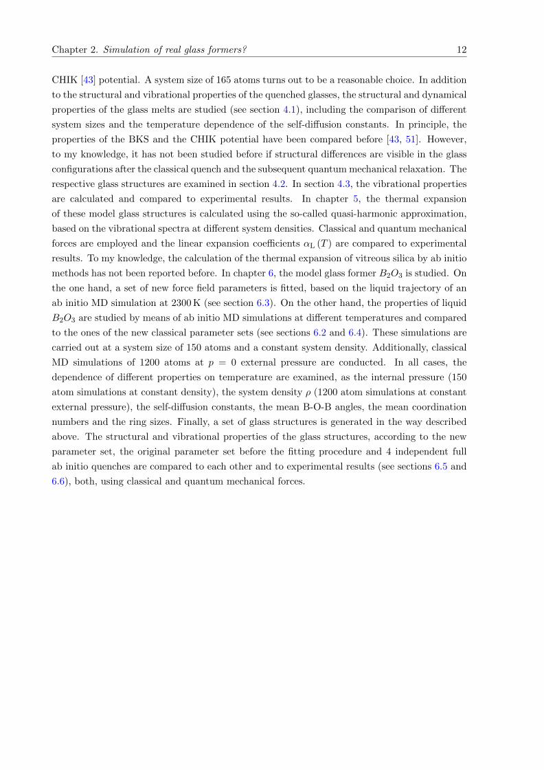
Chapter 2. Simulation of real glass formers? 12
CHIK [43] potential. A system size of 165 atoms turns out to be a reasonable choice. In addition
to the structural and vibrational properties of the quenched glasses, the structural and dynamical
properties of the glass melts are studied (see section 4.1), including the comparison of different
system sizes and the temperature dependence of the self-diffusion constants. In principle, the
properties of the BKS and the CHIK potential have been compared before [43, 51]. However,
to my knowledge, it has not been studied before if structural differences are visible in the glass
configurations after the classical quench and the subsequent quantum mechanical relaxation. The
respective glass structures are examined in section 4.2. In section 4.3, the vibrational properties
are calculated and compared to experimental results. In chapter 5, the thermal expansion
of these model glass structures is calculated using the so-called quasi-harmonic approximation,
based on the vibrational spectra at different system densities. Classical and quantum mechanical
forces are employed and the linear expansion coefficients αL (T ) are compared to experimental
results. To my knowledge, the calculation of the thermal expansion of vitreous silica by ab initio
methods has not been reported before. In chapter 6, the model glass former B2O3 is studied. On
the one hand, a set of new force field parameters is fitted, based on the liquid trajectory of an
ab initio MD simulation at 2300 K (see section 6.3). On the other hand, the properties of liquid
B2O3 are studied by means of ab initio MD simulations at different temperatures and compared
to the ones of the new classical parameter sets (see sections 6.2 and 6.4). These simulations are
carried out at a system size of 150 atoms and a constant system density. Additionally, classical
MD simulations of 1200 atoms at p = 0 external pressure are conducted. In all cases, the
dependence of different properties on temperature are examined, as the internal pressure (150
atom simulations at constant density), the system density ρ (1200 atom simulations at constant
external pressure), the self-diffusion constants, the mean B-O-B angles, the mean coordination
numbers and the ring sizes. Finally, a set of glass structures is generated in the way described
above. The structural and vibrational properties of the glass structures, according to the new
parameter set, the original parameter set before the fitting procedure and 4 independent full
ab initio quenches are compared to each other and to experimental results (see sections 6.5 and
6.6), both, using classical and quantum mechanical forces.
Chapter 3
Simulation techniques and analysis
3.1 Classical MD simulations
3.1.1 Basic concept
Basic idea of molecular dynamics (MD) simulations
There are different ways to sample the equilibrium properties of a classical many-body system.
One way are classical Monte Carlo (MC) simulations [52]. Here, the positions of the particles
are updated in a stochastic manner, depending on a sequence of random numbers. Another
approach is the one of classical molecular dynamics (MD) simulations. Here, in principle, the
classical equations of motion are solved [40]:
Mi ri = −∇ri V = Fi. (3.1)
This allows to follow the real-time trajectory of the particles and to compute time dependent
quantities of the system, such as time correlation functions. The interaction-potential V =
V (ri (t)) can be written as a series of different 1-, 2- and many-body contributions:
V =
N∑
i=1
V1 (ri) +1
2!
N∑
i,j 6=i=1
V2 (rij) +1
3!
N∑
i,j 6=i,k 6=i=1
V3 (rij , rik) + . . . , rij = ri − rj . (3.2)
In principle, it can contain up to N-body terms. If no external fields are applied, it is convenient
to chose V1 = 0. In general, equation 3.1 can not be solved analytically, but has to be integrated
numerically. The most naive algorithm would be to just make a Taylor-expansion up to a specific
order:
13
Chapter 3. Simulation techniques and analysis 14
ri (t+ δt) = ri (t) + vi (t) δt+Fi (t)
2Miδt2, Fi (t) = −∇ri V (ri (t)) , (3.3)
vi (t+ δt) = vi (t) +Fi (t)
Miδt, (3.4)
This Euler algorithm has some severe drawbacks [7]: It is not time-reversible, meaning that
ri (t+ δt) − vi (t+ δt) δt + Fi(t+δt)2Mi
δt2 6= ri (t). Furthermore, it is not symplectic, meaning the
volume in phase space is not preserved. This can result in a long-term energy drift, which is, of
course, unfavorable. A time-reversible and symplectic form of the numerical integration scheme
can be achieved by adding the second-order Taylor expansion of ri (t) with negative sign to the
one, according to equation (3.3). This leads to the Verlet algorithm [53] for the update of the
particle positions:
ri (t+ δt) = 2 ri (t)− ri (t− δt) +Fi (t)
2Miδt2. (3.5)
In this algorithm, the velocities are not included explicitly to compute the trajectories. However,
they are needed to calculate the kinetic energy and the total energy of the system
Ekin (t) =
N∑
i=1
vi (t)2
2Mi, Etot (t) = Ekin (t) + V (ri (t)) (3.6)
The velocities can be obtained by means of the particle positions at times t+ δt and t− δt:
vi (t) =ri (t+ δt)− ri (t− δt)
2δt, (3.7)
meaning they can only be calculated when the particle positions at ri (t+ δt) are known. This
drawback can be overcome by using the velocity Verlet algorithm [54]. Here, the particle positions
are updated, according to equation (3.3) and the velocities are update in the following way:
vi (t+ δt) = vi (t) +Fi (t) + Fi (t+ δt)
2Miδt. (3.8)
In fact, this algorithm is equivalent to the Verlet algorithm (equation (3.5)). This can be seen
by substituting vi (t) = vi (t− δt)+ δt2Mi
[Fi (t− δt) + Fi (t)] (equation (3.8) evaluated at t−δt)into equation (3.3). Usually this algorithm is implemented in the following way:
Update the particle positions according to equation 3.3.
Chapter 3. Simulation techniques and analysis 15
Update the velocities according to: vi(t+ 1
2δt)
= vi (t) + Fi(t)Mi
12δt.
Calculate the inter-particle forces according to the particle positions ri (t+ δt): Fi (t+ δt) =
−∇ri V (ri (t+ δt) , .., rN (t+ δt)).
Update the velocities according to: vi (t+ δt) = vi(t+ 1
2δt)
+ Fi(t+δt)Mi
12δt.
Integrating the equations of motion (3.1), using one of the above integration schemes, leads to
the statistical sampling of the system in the microcanonical (NVE) ensemble, meaning the total
energy of the system (see equation (3.6)) is conserved. In the limit of δt→ 0 this is exactly the
case, meaning the Hamiltonian
H =
N∑
i=1
p2i
2Mi+ V (ri) , (3.9)
which is the Legendre transform of the Lagrangian
L =
N∑
i=1
Mi
(∂ri∂t
)2
2− V (ri) , (3.10)
is a conserved quantity. In practice, the total energy fluctuates around the mean value during a
simulation run. This is connected to the fact that the discretized equations of motion with finite
δt have a different conserved quantity, called shadow Hamiltonian [55]. The leading corrections
to the functional form of equation (3.9) are of the order δt2. Therefore, the amplitude of the
total energy fluctuations δEtot = |Etot − 〈Etot〉| should be proportional to the time step squared
(δt)2:
|Etot − 〈Etot〉| ∝ (δt)2 . (3.11)
This relation is tested in case of the model glass formers SiO2 and B2O3 in subsection 4.1.1 and
section 6.4.
More details of molecular dynamics (MD) simulations
In a MC, as well as an MD simulation, the typical number of particles N is of the order of
a few 10000 to 100000. In practice, they are confined in a finite simulation box with box length
LBox. When studying the bulk properties of the system, one is not interested in the effects
due to the surface of the system. As the surface area scales with N 1/3, surface effects become
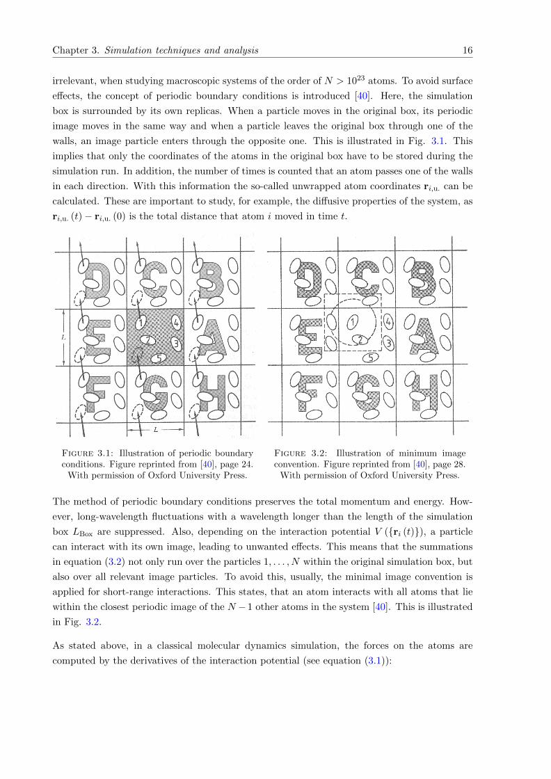
Chapter 3. Simulation techniques and analysis 16
irrelevant, when studying macroscopic systems of the order of N > 1023 atoms. To avoid surface
effects, the concept of periodic boundary conditions is introduced [40]. Here, the simulation
box is surrounded by its own replicas. When a particle moves in the original box, its periodic
image moves in the same way and when a particle leaves the original box through one of the
walls, an image particle enters through the opposite one. This is illustrated in Fig. 3.1. This
implies that only the coordinates of the atoms in the original box have to be stored during the
simulation run. In addition, the number of times is counted that an atom passes one of the walls
in each direction. With this information the so-called unwrapped atom coordinates ri,u. can be
calculated. These are important to study, for example, the diffusive properties of the system, as
ri,u. (t)− ri,u. (0) is the total distance that atom i moved in time t.
Figure 3.1: Illustration of periodic boundaryconditions. Figure reprinted from [40], page 24.
With permission of Oxford University Press.
Figure 3.2: Illustration of minimum imageconvention. Figure reprinted from [40], page 28.
With permission of Oxford University Press.
The method of periodic boundary conditions preserves the total momentum and energy. How-
ever, long-wavelength fluctuations with a wavelength longer than the length of the simulation
box LBox are suppressed. Also, depending on the interaction potential V (ri (t)), a particle
can interact with its own image, leading to unwanted effects. This means that the summations
in equation (3.2) not only run over the particles 1, . . . , N within the original simulation box, but
also over all relevant image particles. To avoid this, usually, the minimal image convention is
applied for short-range interactions. This states, that an atom interacts with all atoms that lie
within the closest periodic image of the N −1 other atoms in the system [40]. This is illustrated
in Fig. 3.2.
As stated above, in a classical molecular dynamics simulation, the forces on the atoms are
computed by the derivatives of the interaction potential (see equation (3.1)):
Chapter 3. Simulation techniques and analysis 17
Fi = −∇ri V (ri (t)) . (3.12)
As already stated above, the total interaction potential (see equation (3.2)) can contain short-
range and long-range interactions. Normally, the number of contributions to the total potential
energy of the system, according to the individual 2- and 3- body terms of the interaction potential
V2 (rij) and V3 (rij , rik), increases with increasing inter-particle distances rij = |rij |. This is the
case, as the number of particles at a distance rij increases asymptotically with rd−1ij , when d is
the dimension of the system [7]. Therefore, interactions are classified as short-range interactions
when the respective potential term decreases faster than r−dij and vice versa. In section 3.5,
examples of typical short-range 2-body and 3-body potentials are given. To fulfill the minimum
image convention, it is necessary to truncate all short-range parts of the potential at a specific
cutoff radius rc < LBox/2. Usually, the potential term has already decayed to a value close
to 0 at inter-particle distances of rij = rc. However, it is convenient to shift the short-range
potential to zero at rij = rc by subtracting the numerical value at the cutoff radius V (rc). This
guarantees an overall continuous potential V (ri (t)). However, it is still not differentiable at
the cutoff rc. According to equation (3.12), the forces between atoms at inter-atomic distances
of rij = rc would be proportional to delta-distributions: Fi ∝ δ (rij). To avoid this, the short-
range potential can be multiplied with a smoothing function after shifting it to zero at rij = rc.
In this work, the functional form of
G (r) = exp
[− d
(r − rc)2
](3.13)
is chosen, leading to a short-range potential of
V S,Shifted+Smoothed =(V S (r)− V S (rc)
)G (r) . (3.14)
In subsection 4.1.1 and section 6.4, the effect of the smoothing on the long term energy drift
and the fluctuations of the total energy δEtot is studied in the case of SiO2 and B2O3.
The most prominent example of a long-range interaction is the Coulomb interaction. Of course,
this plays an important role in the modeling of oxide glasses. In case of periodic boundary
conditions, the summations of the 2-body terms in equation (3.2) would run over infinite numbers
of particles, leading to:
Chapter 3. Simulation techniques and analysis 18
V =1
2
∑
n∈Z3
N∑
i,j=1,i 6=jforn=0
V Coul (rij + nLBox) =1
2
∑
n∈Z3
N∑
i,j=1,i 6=jforn=0
CCoul qi qj|rij + nLBox|
. (3.15)
The proportionality constant CCoul depends on the units used in the simulation. In case of
[E] = eV, [q] = e and [r] = A, the value is CCoul = 14.399644846 eV A. In equation (3.15),
an infinite summation over all n ∈ Z3 has to be carried out. Here, the standard method for
the numerical treatment of this problem is presented, the Ewald summation [56]. Following the
description of [57], a potential decaying with 1r can be re-written as:
1
r=
1
r− 2√
π
ˆ gew
0dt exp
[−r2 t2
]+
2√π
ˆ gew
0dt exp
[−r2 t2
](3.16)
⇔ 1
r=
erfc (gew r)
r+
2√π
ˆ gew
0dt exp
[−r2 t2
]. (3.17)
Here, erfc (x) is the complementary error function erfc (x) = 2√π
´∞x dt exp
[−t2]. It has the
property that it is fast decaying to zero with increasing x. Putting this into equation (3.15) the
sum can be split into two parts:
V = V S + V L (3.18)
V S :=1
2
∑
n∈Z3
N∑
i,j=1,i 6=jforn=0
V CS (|rij + nLBox|) (3.19)
⇔ V S =1
2
∑
n∈Z3
N∑
i,j=1,i 6=jforn=0
CCoul qi qj|rij + nLBox|
erfc (gew |rij + nLBox|) (3.20)
V L :=1
2
∑
n∈Z3
N∑
i,j=1,i 6=jforn=0
2CCoul qi qj√π
ˆ gew
0dt exp
[− |rij + nLBox|2 t2
]. (3.21)
Due to the properties of erfc (x), the 2-body term V CS (r) in equation (3.20) is a short-range
interaction and can be cut off at an appropriate cutoff rewc , according to the minimum image
convention. When adding the terms for n = 0 to i = j = 0 in equation (3.21), the long-range
part of the potential, V L, becomes a periodic function expanded in a Fourier series. For f being
the Fourier transform of f
f (k) =
ˆR3
dx f (x) exp [−ik · x] , f (x) =1
(2π)3
ˆR3
dk f (k) exp [ik · x] , (3.22)
Chapter 3. Simulation techniques and analysis 19
the Poisson summation formula holds [58]:
∑
n∈Z3
f (n) =∑
n∈Z3
f (2πn) =∑
k∈ 2π nLBox
f (kLBox) . (3.23)
This in mind, the term V L in equation (3.21) can be reformulated:
V L =1
2
N∑
i,j=1
2CCoul qi qj√π
ˆ gew
0dt
∑
k∈ 2π nLBox
\k≡0
ˆR3
dn exp[− |rij + nLBox|2 t2 − LBox k · n
]
− V Lself.
(3.24)
The solution of the integrals leads to [40]:
V L =1
2πL3Box
∑
k∈ 2π nLBox
\k≡0
(2π)2 exp
[−(
k2 gew
)2]
k2
N∑
i,j=1
CCoul qi qj exp [ik · rij ]− V Lself . (3.25)
The self term V Lself in equations (3.24) and (3.25) contains the terms for n = 0 to i = j = 0 that
have been added to V L before. It can be calculated in the limit of εi := rij → 0:
V Lself =
1
2
N∑
i=1
2CCoul q2i√
πlimεi→0
ˆ gew
0dt exp
[−ε2i t2
](3.26)
⇔ V Lself =
1
2
N∑
i=1
CCoul q2i limεi→0
1− erfc (gew εi)
εi' gew√
π
N∑
i=1
CCoul q2i , (3.27)
as erfc (x) = 1− 2√πx+O
(x3).
The exclusion of k ≡ 0 in equations (3.24) and (3.25) is a direct consequence of the conditional
convergence of the Ewald sum. This assumption is consistent with a situation, where the periodic
system (the original simulation box with its infinite periodic images) is embedded in a medium
with infinite dielectric constant, meaning an ideal conductor [7].
In practice, the complementary error function can be approximated as
Chapter 3. Simulation techniques and analysis 20
erfc (x) = tp (x) exp[−x2
]+ ε (x) , |ε (x)| ≤ 1.5 · 10−7.
Here, tp (x) is a polynomial of the order 5 in (1 + 0.3275911x)−1 [59].
As limx→∞ erfc(x)/x = exp(−x2)/x2, the error, due to the cutting off of the short-range term V CS
at rewc , scales as exp[−(gew rew
c )2]/(gew rewc )2 (see equations (3.19) and (3.20)). According to equation
(3.25), the cutoff error in reciprocal space is exp
[−(
kc2 gew
)2]/(
kc2 gew
)2. In practice, the choice of the
real space cutoff and the cutoff error determines the parameters gew and kc and therefore the
number of k-vectors included in the summation.
As stated above, the numerical integration of equation (3.1) leads to the trajectories in the NVE
ensemble. When calculating the statistical average of certain quantities, the ensemble average
is equal to the time average of this quantity with respect to particular simulation times t, where
the atom configurations ri (t) are uncorrelated to the previous ones. It should be mentioned that
the exact trajectory of the individual atoms is not important for the statistical sampling and the
accurate prediction of an atomic trajectory is not possible for longer simulation times, due to
the Lyapunov instability. It states that the difference between two different particle trajectories
diverges as |∆r (t)| ∝ ε exp [λt], when the initial conditions are disturbed by a small amount ε
[7].
Techniques to speed up simulations
As explained above, all short-range interactions are cut off at a certain cutoff distance rc (or
rewc ). This means that particles with larger minimum image distances do not interact. This
motivates the utilization of Verlet neighbor lists [40] for each atom in the simulation box. This
list contains all neighboring atoms within a first neighbor distance less than the cutoff distance
plus a so-called skin distance rskin. Interactions between the atoms are only calculated for atoms
contained in the neighbor list, reducing the computational cost significantly. In an ideal case
the computational costs scale like O (N) instead of O(N2).
Nowadays, it is convenient to run a simulation program on more than one processor in parallel.
There are different schemes for parallelization of a computer program. The parallelization of
the LAMMPS software package [60, 61], used for all classical MD simulations in this work, is
based on the Message Passing Interface (MPI) standard [62]. Here, the program is started on
Nproc processors in parallel. Each of the processes carries out a part of the simulation and
communicates with the other processes in terms of messages. Input and output is only done by
one process. In case of classical MD simulations and the LAMMPS software package, a domain
decomposition is applied. Here, the simulation box is divided into a 3-dimensional grid of Nproc
domains. Each processor calculates the interactions and integrates the equations of motion for
the atoms within its domain. Therefore, the positions of all atoms in the Verlet neighbor lists
have to be known. Atoms, contained in the neighbor list that are not located in the respective
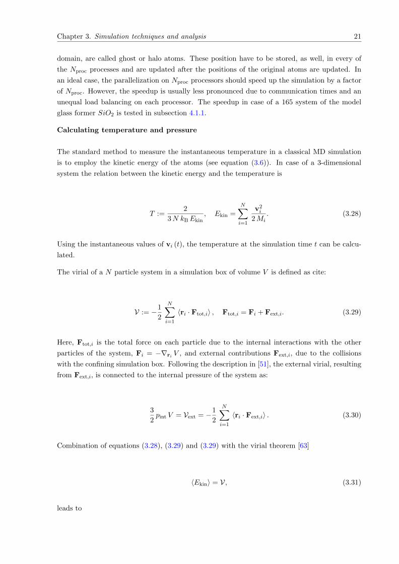
Chapter 3. Simulation techniques and analysis 21
domain, are called ghost or halo atoms. These position have to be stored, as well, in every of
the Nproc processes and are updated after the positions of the original atoms are updated. In
an ideal case, the parallelization on Nproc processors should speed up the simulation by a factor
of Nproc. However, the speedup is usually less pronounced due to communication times and an
unequal load balancing on each processor. The speedup in case of a 165 system of the model
glass former SiO2 is tested in subsection 4.1.1.
Calculating temperature and pressure
The standard method to measure the instantaneous temperature in a classical MD simulation
is to employ the kinetic energy of the atoms (see equation (3.6)). In case of a 3-dimensional
system the relation between the kinetic energy and the temperature is
T :=2
3N kBEkin, Ekin =
N∑
i=1
v2i
2Mi. (3.28)
Using the instantaneous values of vi (t), the temperature at the simulation time t can be calcu-
lated.
The virial of a N particle system in a simulation box of volume V is defined as cite:
V := −1
2
N∑
i=1
〈ri · Ftot,i〉 , Ftot,i = Fi + Fext,i. (3.29)
Here, Ftot,i is the total force on each particle due to the internal interactions with the other
particles of the system, Fi = −∇ri V , and external contributions Fext,i, due to the collisions
with the confining simulation box. Following the description in [51], the external virial, resulting
from Fext,i, is connected to the internal pressure of the system as:
3
2pint V = Vext = −1
2
N∑
i=1
〈ri · Fext,i〉 . (3.30)
Combination of equations (3.28), (3.29) and (3.29) with the virial theorem [63]
〈Ekin〉 = V, (3.31)
leads to
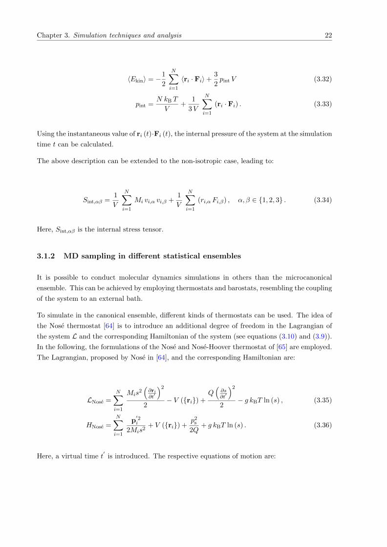
Chapter 3. Simulation techniques and analysis 22
〈Ekin〉 = −1
2
N∑
i=1
〈ri · Fi〉+3
2pint V (3.32)
pint =N kB T
V+
1
3V
N∑
i=1
(ri · Fi) . (3.33)
Using the instantaneous value of ri (t)·Fi (t), the internal pressure of the system at the simulation
time t can be calculated.
The above description can be extended to the non-isotropic case, leading to:
Sint,αβ =1
V
N∑
i=1
Mi vi,α vi,β +1
V
N∑
i=1
(ri,α Fi,β) , α, β ∈ 1, 2, 3 . (3.34)
Here, Sint,αβ is the internal stress tensor.
3.1.2 MD sampling in different statistical ensembles
It is possible to conduct molecular dynamics simulations in others than the microcanonical
ensemble. This can be achieved by employing thermostats and barostats, resembling the coupling
of the system to an external bath.
To simulate in the canonical ensemble, different kinds of thermostats can be used. The idea of
the Nose thermostat [64] is to introduce an additional degree of freedom in the Lagrangian of
the system L and the corresponding Hamiltonian of the system (see equations (3.10) and (3.9)).
In the following, the formulations of the Nose and Nose-Hoover thermostat of [65] are employed.
The Lagrangian, proposed by Nose in [64], and the corresponding Hamiltonian are:
LNose =N∑
i=1
Mis2(∂ri∂t′
)2
2− V (ri) +
Q(∂s∂t′
)2
2− g kBT ln (s) , (3.35)
HNose =
N∑
i=1
p′2i
2Mis2+ V (ri) +
p2s
2Q+ g kBT ln (s) . (3.36)
Here, a virtual time t′
is introduced. The respective equations of motion are:
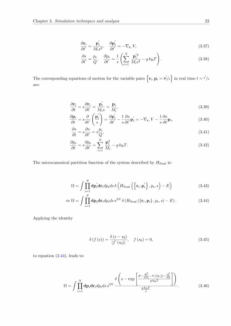
Chapter 3. Simulation techniques and analysis 23
∂ri∂t′
=p′i
Mis2,
∂p′i
∂t′= −∇ri V, (3.37)
∂s
∂t′=ps
Q,
∂ps
∂t′=
1
s
(N∑
i=1
p′2i
Mis2− g kBT
). (3.38)
The corresponding equations of motion for the variable pairs
ri,pi = p′i/s
in real time t = t′/s
are:
∂ri∂t
= s∂ri∂t′
=p′i
Mis=
piMi
, (3.39)
∂pi∂t
= s∂
∂t′
(p′i
s
)=∂p′i
∂t′− 1
s
∂s
∂t′p′i = −∇ri V −
1
s
∂s
∂tpi, (3.40)
∂s
∂t= s
∂s
∂t′= s
ps
Q, (3.41)
∂ps
∂t= s
∂ps
∂t′=
N∑
i=1
p2i
Mi− g kBT. (3.42)
The microcanonical partition function of the system described by HNose is:
Ω =
ˆ N∏
i=1
dp′idridpsds δ
(HNose
(ri,p
′i
, ps, s
)− E
)(3.43)
⇔ Ω =
ˆ N∏
i=1
dpidridpsds s3N δ (HNose (ri,pi , ps, s)− E) . (3.44)
Applying the identity
δ (f (s)) =δ (s− s0)
|f ′ (s0)| , f (s0) = 0, (3.45)
to equation (3.44), leads to:
Ω =
ˆ N∏
i=1
dpidridpsds s3N
δ
(s− exp
[E− p2
i2Mi−V (ri)− p2s
2Q
g kBT
])
g kBTs
. (3.46)
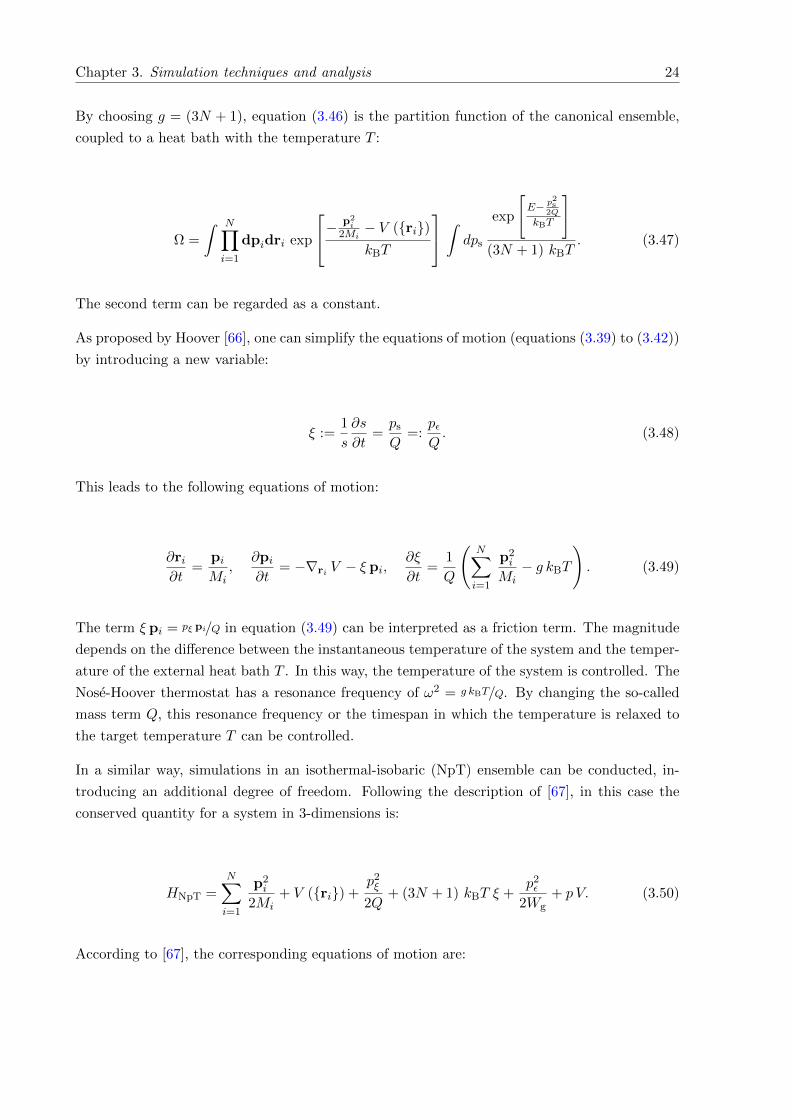
Chapter 3. Simulation techniques and analysis 24
By choosing g = (3N + 1), equation (3.46) is the partition function of the canonical ensemble,
coupled to a heat bath with the temperature T :
Ω =
ˆ N∏
i=1
dpidri exp
−
p2i
2Mi− V (ri)kBT
ˆdps
exp
[E− p2s
2Q
kBT
]
(3N + 1) kBT. (3.47)
The second term can be regarded as a constant.
As proposed by Hoover [66], one can simplify the equations of motion (equations (3.39) to (3.42))
by introducing a new variable:
ξ :=1
s
∂s
∂t=ps
Q=:
pεQ. (3.48)
This leads to the following equations of motion:
∂ri∂t
=piMi
,∂pi∂t
= −∇ri V − ξ pi,∂ξ
∂t=
1
Q
(N∑
i=1
p2i
Mi− g kBT
). (3.49)
The term ξ pi = pξ pi/Q in equation (3.49) can be interpreted as a friction term. The magnitude
depends on the difference between the instantaneous temperature of the system and the temper-
ature of the external heat bath T . In this way, the temperature of the system is controlled. The
Nose-Hoover thermostat has a resonance frequency of ω2 = g kBT/Q. By changing the so-called
mass term Q, this resonance frequency or the timespan in which the temperature is relaxed to
the target temperature T can be controlled.
In a similar way, simulations in an isothermal-isobaric (NpT) ensemble can be conducted, in-
troducing an additional degree of freedom. Following the description of [67], in this case the
conserved quantity for a system in 3-dimensions is:
HNpT =
N∑
i=1
p2i
2Mi+ V (ri) +
p2ξ
2Q+ (3N + 1) kBT ξ +
p2ε
2Wg+ p V. (3.50)
According to [67], the corresponding equations of motion are:
Chapter 3. Simulation techniques and analysis 25
∂ri∂t
=piMi
+pεWg
ri,∂pi∂t
= −∇ri V (ri)−(
1 +1
N
)pεWg
pi −pξQ
pi, (3.51)
∂V
∂t=
3V pεWg
,∂pε∂t
= 3V (pint − p) +1
N
N∑
i=1
p2i
Mi− pξpε
Q(3.52)
ξ =pξQ,
∂pξ∂t
=
N∑
i=1
p2i
Mi+
p2ε
Wg− (3N + 1) kBT. (3.53)
These equations, in principle, generate the isothermal-isobaric partition function at external
temperature T and pressure p. Here, the volume of the simulation box V is allowed to change as
well and pint is the internal pressure of the system (see equation (3.33)). As above, the frequency
of the barostat can be controlled by altering the mass term Wg.
In [68], a set of equations of motion are given that allow the shape of the simulation box to
fluctuate as well, due to an arbitrary external stress, following the ideas of [69]. In addition to
the latter, a chain of k = 1, . . . ,M Nose-Hoover thermostats is coupled to the system, to simulate
the system at arbitrary external temperature as well. As described above, the frequencies of
the fluctuations can be controlled by changing the mass terms Wg and Qk, k = 1, . . . ,M . The
implementation in the LAMMPS software package [60, 61], used for all classical MD simulations
in this work, is based on the formulations of [68].
3.2 Density functional theory
In this section, an overview over the basic concepts is given, describing a quantum mechanical
many-body system in terms of density functional theory (DFT).
3.2.1 Basic concepts of quantum mechanics
In principle, a system of N atoms and n electrons located at positions ri and xi is described
by a many-body Schrodinger equation. When the Hamiltonian H does not depend on time
explicitly, which is the case for the system of N atoms and n electrons in absence of time-
dependent external potentials, the time-independent Schrodinger equation is given as:
H |Ψ (ri ; xi)〉 = E |Ψ (ri ; xi)〉 , (3.54)
with the many-body Hamiltonian
Chapter 3. Simulation techniques and analysis 26
H = TN + Te + VNN + VNe + Vee. (3.55)
In the whole section 3.2, atomic units are used, meaning e2 = ~ = me = 1. The different terms
in equation (3.55) are the operators of the kinetic energy of the N nuclei and n electrons,
TN =N∑
i=1
−∇2ri
2Mi, Te =
n∑
i=1
−∇2xi
2, (3.56)
and the potential energy operators for the nuclei-nuclei, nuclei-electron and electron-electron
interaction:
VNN =1
2
N∑
i,j 6=i=1
Zi Zj|ri − rj |
, VNe =N∑
i=1
n∑
j=1
Zi|ri − xj |
, Vee =1
2
n∑
i,j 6=i=1
1
|xi − xj |. (3.57)
Here, Mi are the masses and Zi the charge numbers of the nuclei. Equation (3.54) is analytically
not solvable.
Equation (3.54), in combination with equation (3.55), can be reduced to the Schrodinger equation
only for the electronic degrees of freedom, applying the Born-Oppenheimer approximation [41].
This states that because of the difference between the masses of the nuclei and the electrons of
about 4 orders of magnitude, it is an excellent approximation to separate the total wave function
|Ψ (ri ; xi)〉 into a product of the wave function of the nuclei and the one of the electrons:
|Ψ (ri ; xi)〉 ' |Φ (ri〉 |Ψ xi)〉 . (3.58)
Furthermore, it is assumed that, at room temperature, the electrons are always in the ground
state. This is a reasonable assumption as the typical energies of electronic excitations are of the
order of several eV which is much greater than the thermal energy of an electron at 300K of
about 0.026 eV. Following the formulations in [70], the energy eigenvalues E of equation (3.54)
can be written as
Etotal (ri) = VNN (ri) + Eelec (ri) . (3.59)
Chapter 3. Simulation techniques and analysis 27
This means that quantum mechanical many-body problem is reduced to the one of n electrons
in an external potential, due to the N nuclei at fixed positions ri, leading to
H |Ψ (xi)〉 = Eelec (ri) |Ψ (xi)〉 , H = Te + Vext + Vee, (3.60)
and the potential energy of the N nuclei VNN (ri) is just treated as a constant energy term.
In the case of absent additional external fields, the potential operator Vext =∑n
j=1 vext (xj) is
the one due to the nuclei-electron interaction VNe in equation (3.57). Here, Vext is a one-body
operator with respect to the electron positions xi with
vext (xj) =N∑
i=1
Zi|ri − xj |
(3.61)
in the case of Vext = VNe. In the following, the notation of the eigenvalue Eelec (ri) is replaced
by E again, in the sense of being the energy eigenvalue of the n electron system for a fixed set
of nuclei positions ri.
The ground state energy, according to equation (3.60), satisfies the variational principle
E = minΨ
⟨Ψ∣∣∣H∣∣∣Ψ⟩, (3.62)
minimizing over all antisymmetric n-body wave functions |Ψ〉. This is the basis for the Hartree-
Fock (HF) approximation, where the many-body wave function |Ψ〉 is approximated by an
anti-symmetrized product of single-particle wave functions [71], based on the so-called Slater
determinant [72].
The one-particle density, which is defined as expectation value of the density operator n (x) =∑ni=1 δ (x− xi), is given as:
n (x) = 〈Ψ |n (x)|Ψ〉 = n∑
σ1
· · ·∑
σn
ˆdx2 . . .dxn |Ψ (xσ1,x2 σ2, . . . ,xn σn)|2 . (3.63)
Here, the spin degrees of freedom σi are explicitly included that have been omitted in the above
equations and it is assumed that |Ψ〉 is normalized to |Ψ|2 = 1. The one-particle density is a
much simpler quantity than the many-body wave function |Ψ〉 and n (x) dx gives the probability
to find any electron in a volume element dx around x.
Chapter 3. Simulation techniques and analysis 28
3.2.2 Hohenberg-Kohn theorems
The basis for the description of the many-body system of n electrons in terms of the one-
particle density (see equation (3.63)) are the two Hohenberg-Kohn theorems [9]. Following the
description in [73], they can be written as:
Theorem I
The ground state one-particle density n (x) of a many body-system (see equation (3.60)) uniquely
determines the external potential Vext up to a constant.
This implies that any property of the system can be written as a function of the ground state
density n0 (x), because by determining Vext, the Hamiltonian H in equation (3.60) is fixed up to
a constant. This means that also the wave functions |Ψ〉 are, in principle, uniquely determined.
Theorem II
The energy functional in equation (3.62) can be written as a functional E [n (x)] of the one-
particle density n (x) for any external potential Vext. The global minimum of this functional is
the ground state energy and the density n (x) that minimizes the functional is the ground state
density n0 (x).
This implies that the functional E [n (x)] by itself determines the ground state energy and ground
state density. Following [70], the variational problem can be formulated in two steps. In the
first step,
F [n (x)] = minΨ→n
⟨Ψ∣∣∣T + Vee
∣∣∣Ψ⟩
(3.64)
is minimized. This has to be understood as a minimization over all antisymmetric wave functions
yielding a given density n (x). In the second step,
E [n] = minn
(F [n] +
ˆdxn (x) vext (x)
)(3.65)
is minimized over all reasonable densities fulfilling n (x) ≥ 0,´
dxn (x) = N , with vext (x),
according to equation (3.61).
3.2.3 Kohn-Sham equations
The main statement of the two Hohenberg-Kohn theorems (see subsection 3.2.2) is that any
system property can be expressed in terms of the one-particle density n (x). Due to Kohn
Chapter 3. Simulation techniques and analysis 29
and Sham [74], one can replace the complex many-body system of interacting electrons with a
set of fictive non-interacting electrons in some effective local potentials vs,σ (x). Following the
descriptions in [70] and [73], the so-called Kohn-Sham (KS) system can be described by:
(−1
2∇2
x + vs,σ (x)
)φi,σ (x) = εi,σ φi,σ (x) . (3.66)
Here, the spin variables σ ∈ ↑, ↓ are introduced explicitly. Depending on the type of system,
it makes sense to treat the two different spin states separately, leading to more accurate approx-
imations for systems with an odd number of electrons. Consequently, all considered quantities
are functionals of the spin up and down densities nσ (x), σ ∈ ↑, ↓, separately. As in the
Hartree-Fock case, the wave function of the KS system is usually an anti-symmetrized product
of the orbitals or eigenstates φi,σ (x) of the n = n↑ + n↓ electrons of the system. In the ground
state, usually all of the n↑ and n↓ eigenstates are occupied and the total ground state density
can be written as
n (x) =∑
σ
nσ (x) =∑
σ
nσ∑
i=1
|φi (x)|2 . (3.67)
The local potential has to be chosen in a way that the ground state density of the KS system
is equal to the ground state density of the fully interacting system. The relation between the
energy terms of the KS system and the real electrons in equation (3.60) is the following:
E = Te + Vext + Vee = Ts + U + Vext + Exc = Ts + Vs, (3.68)
with
Vext =∑
σ=↑,↓
ˆdxnσ (x) vext (x) , Vs =
∑
σ=↑,↓
ˆdxnσ (x) vs (x) . (3.69)
Here,
Ts = −1
2
∑
σ=↑,↓
nσ∑
i=1
⟨φi,σ
∣∣∇2x
∣∣φi,σ⟩
=1
2
∑
σ=↑,↓
nσ∑
i=1
ˆdx |∇xφi,σ (x)|2 > 0 (3.70)
Chapter 3. Simulation techniques and analysis 30
is the kinetic energy of the KS eigenstates and
U =1
2
∑
σ,σ′=↑,↓
ˆdx
ˆdx′ nσ (x) nσ′
(x′)
|x− x′ | > 0 (3.71)
is the electrostatic or Hartree repulsive self-energy, according to the one-particle densities of
charged electrons nσ (x), σ ∈ ↑, ↓.
Equations (3.67) and (3.70) allow the calculation of the functional derivatives of Ts and nσ (x)
with respect to the KS eigenstates φi,σ:
δnσ (x)
δφi,σ (x)= φi,σ (x) ,
δTs
δφi,σ (x)= −1
2∇2
x φi,σ (x) . (3.72)
The set of KS eigenstates that minimize E = Ts+U+Vext+Exc, according to equation (3.68), can
be obtained employing a variational principle. Using equation (3.72) this leads to the following
expression:
δE
δφi,σ (x)=
δTs
δφi,σ (x)+
[δU
δnσ (x)+
δVext
δnσ (x)+
δExc
δnσ (x)
]δnσ (x)
δφi,σ (x)= 0 (3.73)
⇔ δE
δφi,σ (x)= −1
2∇2
x φi,σ (x) +
[δU
δnσ (x)+
δVext
δnσ (x)+
δExc
δnσ (x)
]φi,σ (x) = 0. (3.74)
Using equations (3.68), (3.69) and (3.71), this leads to the one-electron Schrodinger equations
of the KS system (3.66) with
vs (x) = vext (x) + u (x) +δExc
δnσ (x)(3.75)
and
u (x) =∑
σ=↑,↓
ˆdx′ nσ
(x′)
|x− x′ | . (3.76)
This implies that the exact ground state energy E and ground state density n0,σ (x) could be
calculated, if the so-called exchange-correlation functional Exc was known. In practice, the
Chapter 3. Simulation techniques and analysis 31
computation works by an initial guess of the density nσ (x). Then, the potential term vs (x) is
calculated, according to equation (3.75). Subsequently, the KS equations (3.66) are solved and
a new density is obtained from the resulting φi,σ (x) (see equation (3.67)). The procedure is
iterated until the differences in nσ (x) are lower than a desired cutoff value.
This means that the KS equations, in principle, allow for an exact solution of the complex many-
body problem, limited by the numerical accuracy of the iteration process. The approximative
nature of the Kohn-Sham approach is caused by the guess of a suitable exchange-correlation
functional
Exc = Ex + Ec. (3.77)
The exchange part Ex of the exchange-correlation energy is given by
Ex = −1
2
∑
σ,i,j
ˆdx
ˆdx′ φ∗i,σ (x)φ∗j,σ
(x′)φi,σ
(x′)φ∗j,σ (x)
|x− x′ | . (3.78)
According to [70], this is the energy contribution due to Vee (see equation (3.57)), evaluated in
terms of the KS eigenstates φi,σ minus the respective the Hartree energy (see equation (3.71)).
This means, Ex follows exactly the same anti-symmetrized product of the Hartree-Fock method
[71], based on the Slater determinant [72]. The correlation part Ec, in principle, is everything
else needed to make equation (3.68) exact. This can be understood as the remaining differences
between the non-interacting KS electrons and the interacting real electrons with correlation
effects. However, no general formulation of Ec can be found.
At this point it should be stated that the KS eigenstates φi,σ (x) have no physical meaning at
all [75], but in many cases their interpretation as real electronic states works quite well.
As explained in subsection 3.1.1, the set of atoms is located in a simulation box with periodic
boundary conditions and surrounding replicas of the latter. In this sense, the system can be
viewed as a crystalline structure with the unit cell being the simulation box. According to Bloch’s
theorem [76], the one-electron wave functions, which are solutions of the stationary Schrodinger
equation with a periodic potential V (x) = V (x + R) (R ∈ nLBox, n ∈ Z3, in case of a cubic
simulation box with box length LBox), have the functional form:
φi,σ (x) = eik·x ui,σ;k (x) , with ui,σ;k (x) = ui,σ;k (x + R) . (3.79)
Chapter 3. Simulation techniques and analysis 32
Here, k is a wave-vector of the reciprocal space of the first Brillouin zone, according to the
periodicity of uj,σ;k (x).
In practice, the terms ui,σ;k in equation (3.79) are expanded in terms of an orthonormal basis
set. It is convenient to expand ui,σ;k in terms of plane waves as in this approach the boundary
conditions are automatically satisfied. This results in:
ui,σ;k (x) =1√V
∑
G∈ 2π nLBox
Ci,σ;G,k eiG·x and φi,σ =1√V
∑
G∈ 2π nLBox
Ci,σ;G,k ei(G+k)·x. (3.80)
The summation over vectors G is restricted to reciprocal lattice vectors, meaning G ∈ 2π nLBox
,
n ∈ Z3, to fulfill equation (3.79). In this work, all DFT calculations are carried out with the
Vienna Ab initio Simulation Package (VASP) [77–79], which is a plane wave code. In practice,
only distinct k-values of the Brillouin zone are chosen and the expansion over G-vectors has to
be cut off at a certain value Gcut such that only plane waves are included with
1
2|G + k|2 < Ecut. (3.81)
The number of k-points included and the cutoff energy Ecut influence the accuracy of the cal-
culation.
3.2.4 Exchange-correlation functionals
As explained in subsection 3.2.3, the solution of the complex quantum mechanical many-body
problem of n electrons in an external potential Vext in terms of the KS approach depends on the
a-priori unknown choice of the exchange-correlation functional Exc [nσ (x)].
The simplest approximation of an exchange-correlation functional is the local (spin) density
approximation (LDA):
ELDAxc =
ˆdx ehom
xc (n↑ (x) , n↓ (x)) . (3.82)
Here, ehomxc (n↑ (x) , n↓ (x)) is the energy density of a homogeneous electron gas with the density
nσ (x). This means that the corresponding eigenstates are plane waves. The exchange part of
equation (3.77) can be calculated by inserting the latter in equation (3.78). The correlation
part can be parametrized [80]. The justification for this approach is that, in solids with slowly
varying electron density, the density is often close to the one of a homogeneous electron gas [74].
Chapter 3. Simulation techniques and analysis 33
The exchange-correlation functional ELDAxc is uniquely defined. It tends to lead to systematically
too large binding energies by about 1 eV per bond [70] and too short bond lengths by about 1%
[81].
The next step in improving the exchange-correlation functional is taking into account the gra-
dient of the electron density, leading to the generalized gradient approximation (GGA):
EGGAxc =
ˆdx eGGA
xc (n↑ (x) , n↓ (x) , |∇xn↑ (x)| , |∇xn↓ (x)|) . (3.83)
Another approach is the use of so-called hybrid functionals [70]:
EHybridxc = c
(Ex − EGGA
x
)+ EGGA
xc . (3.84)
Here, EGGAx is the exchange part of equation (3.83) and Ex is the “exact” exchange energy,
obtained by putting the KS eigenstates into equation (3.78) and c ∈ [0, 1] is some parameter.
In contrast to the local (spin) density approximation (LDA), the functionals of the generalized
gradient approximation (GGA) and hybrid functionals are not uniquely defined. On the one
hand, they can be parametrized empirically by parameter fits to reference data of atoms and
molecules. On the other hand, they can be parametrized without the empirical data by known
exact conditions of the functional. The standard GGA potential, parametrized in the second way,
is the Perdew-Burke-Ernzerhof (PBE) type [82, 83]. The GGA exchange-correlation functional
of the PBE type reduces the overbinding of the LDA potential to about 0.3 eV [70]. However,
it tends to lead to overestimate the bond lengths systematically by about 1%[81]. In this work,
the GGA potential of type PBE, revised for solids, is used [84]. This leads to a slightly better
fitting of the bond lengths [81].
3.2.5 Pseudopotentials
In subsections 3.2.1 to 3.2.4, the basic ideas of calculating quantum mechanical properties on the
basis of density functional theory are explained. However, the chemical properties of a system
are largely determined by the outer or valence electrons of the atoms, in contrast to the core
electrons which are localized close to the nuclei. The strong Coulomb potentials of the nuclei
VNe (see equation (3.57)) lead to strongly varying electronic wave functions in their vicinity,
increasing the computational effort, as more plane waves have to be included (see equations
(3.80) and (3.81)). Also, in principle, relativistic effects play a role, due to the rather high
(kinetic) energy (E = k2/2) of the electrons close to the nuclei. A way to overcome this, is
the employment of pseudopotentials. Here, the potential terms of the nuclei VNe (see equation
(3.57)) are replaced by effective potentials that include the effects of core electrons within a core
Chapter 3. Simulation techniques and analysis 34
radius rcore around the nuclei. This means that the external potential Vext = VNe in equations
(3.68) and (3.69) is replaced by an effective potential Veff and only the valence electrons are
treated explicitly in the way described in the subsections 3.2.1 to 3.2.4. The KS eigenstates
φi,σ (x) and the respective gradients ∇xφi,σ (x) of the valence electrons, according to Veff, must
agree with the ones, resulting from calculations with the original Vext = VNe with all electrons,
outside the core radius rcore.
There are different types of pseudopotentials. In general, it is desired that the pseudopotentials
are a smooth function of x− ri, with ri being the positions of the ith nuclei. This allows a lower
cutoff energy Ecut, according to equation (3.81). For the norm-conserving pseudopotentials, the
integrated charge density, due to equation (3.67), is the same for the eigenstates of the effective
potential Veff, as well, as for the ones of the original potential Vext = VNe. For the ultrasoft
pseudopotentials (USPP) [85], this restriction is given up, leading to an increased smoothness
of the pseudopotentials and a lower Ecut.
In this work, the projector augmented-wave method [86, 87] is applied. Here, the contributions
of all electrons are treated explicitly. The all-electron wave function |Ψ〉 is replaced by a pseudo
wave function∣∣∣Ψ⟩
inside the core radius rcore (or augmentation sphere). Here, |Ψ〉 =∑
i,σ (|φi,σ〉is the all-electron wave function of the KS system, not of the real system. Outside the augmen-
tation sphere, the two are constructed to be the same. This can be achieved by means of a
projection operator T:
|Ψ〉 = T∣∣∣Ψ⟩. (3.85)
3.3 Static and dynamic correlation functions
During a simulation run, several structural and dynamical quantities are measured. As explained
in section 3.1, classical molecular dynamics simulations allow the calculation of ensemble averages
in terms of time averages over the respective trajectories. In the following, 〈·〉 represents such a
time average. In practice, every Ndis time steps the atom configurations are stored to calculate
the structural properties. This is done Nrep times. A typical value of Nrep is Nrep = 1000,
meaning the quantities are averaged over 1000 (independent) configurations. This requires to
select the value of Ndis in a way that the configurations are uncorrelated. In the following, the
indices α, β and γ stand for the different occurring atom types, namely α, β, γ ∈ B,Si,O, in
this work.
Pair correlation function
One important structural quantity is the partial pair correlation function or pair distribution
function gαβ (r). The pair correlation function gαβ (r) describes the probability density of finding
Chapter 3. Simulation techniques and analysis 35
two particles, one of type α and the other of type β, at a distance r, divided by the probability
density of the same event in a noninteracting system, namely an ideal gas. It is defined as:
gαβ (r) := Nαβ⟨Nα∑
i=1
Nβ∑
j=1
1
4π r2δ (r − |ri − rj |)
⟩, (3.86)
with i 6= j for α 6= β and the normalization constant
Nαβ =
NρNα(Nα−1) = V
Nα(Nα−1) , α = β
NρNαNβ
= VNαNβ
, α 6= β. (3.87)
Here, N is the total number of atoms in the system, ρ = N/V is the total particle number density,
Nα and Nβ are the total numbers of atoms of type α, β in the configuration and V is the volume
of the simulation box. This means that limr→∞ gαβ (r) = 1 as then no correlations between the
particles due to inter-atomic interactions are visible.
In practice, the pair correlation function can be calculated, applying the following formula [40]:
gαβ (r) = 〈Nαβ (r)〉 Nαβ(
4π
3
[(r + dr)3 − r3
])−1
. (3.88)
In equation (3.88), the distance r refers to the minimal image distance between the atoms of
types α and β, according to the considerations in subsection 3.1.1. Nαβ (r) is the number of
particles, one of type α and the other of type β, within a minimal image distance between r and
r+dr and 4π3
[(r + dr)3 − r3
]is the volume of a 2-dimensional shell of width dr. This means that
the computation is done with respect to bins of width dr. In case of a cubic simulation box with
box length LBox, the formulation of equation (3.88) holds for all minimal image distances smaller
than LBox/2, restricting the distances r, gαβ (r) can be calculated for. In case of a simulation box
with a different shape, the same holds for distances smaller than half of the smallest dimension
of the box.
Static structure factor
Scattering experiments give access to information in reciprocal space, in contrast to real space.
A structural quantity in reciprocal space corresponding to the partial pair correlation function
is the partial static structure factor. It is defined by:
Chapter 3. Simulation techniques and analysis 36
Sαβ (k) :=fαβN
⟨Nα∑
i=1
Nβ∑
j=1
exp [ik · (ri − rj)]
⟩, (3.89)
with N being the total atom number, Nα and Nβ being the atom numbers of types α and β
and fαβ = 0.5 for α 6= β and fαβ = 1 for α = β being normalization constants, correcting for
the double counting in case of α 6= β. For an isotropic system, Sαβ (k) only depends on the
magnitude of the wave-vector k = |k|. The connection between Sαβ (k) and gαβ (r) is as follows
[40]:
Sαβ (k) = 1 +N
V
ˆdr exp [ik · r] gαβ (r) . (3.90)
Regarding this expression, it can be seen that Sαβ (k) diverges at k = 0 ( Sαβ (k = 0) ∝ δ (k) as
limr→∞ gαβ (r) = 1). This contribution, of course, is inaccessible experimentally and is ignored
in the following.
For simulations in a finite box, only specific k-values are allowed in the calculation of Sαβ (k). In
this work Sαβ (k) is calculated only in the case of a cubic simulation box. This leads to k ∈ 2π nLBox
,
n ∈ Z3, as in equations (3.24) and (3.25) for the calculation of the long-range part of the Ewald
summation. In practice, first all possible k-vectors are determined with 0 ≤ k1 ≤ nmax2πLBox
,
−nmax2πLBox
≤ k2 ≤ nmax2πLBox
and −nmax2πLBox
≤ k3 ≤ nmax2πLBox
for some maximum nmax ∈ N.
If k1 = 0, the minimum value of k2 considered is 0 and if k1 = 0 and k2 = 0, the minimum value of
k3 considered is 0. Then, the degeneracy d (k) of possible k-vectors with the same absolute value
k is determined. In this way, all vectors k, together with all vectors −k, represent all allowed
k-vectors with |kα| ≤ nmax2πLBox
, α ∈ 1, 2, 3. For k ≤ kall, all possible k-vectors are included
in the calculation of the partial static structure factors. Whereas, for k > kall, the k-range up to
a maximum value of k is divided into a certain number of intervals and for each interval a fixed
number of k-vectors is chosen randomly. Regarding this, the partial static structure factors are
calculated by implementing the following formulas:
Sαβ (k) =1
Nd (k)
∑
k,|k|=k
⟨(Nα∑
i=1
eik·ri)(
Nα∑
i=1
e−ik·ri)⟩
(3.91)
=1
Nd (k)
∑
k,|k|=k
⟨(Nα∑
i=1
cos k · ri)2
+
(Nα∑
i=1
sin k · ri)2⟩
(3.92)
and
Chapter 3. Simulation techniques and analysis 37
Sαβ (k) =1
2Nd (k)
∑
k,|k|=k
⟨(Nα∑
i=1
eik·ri)
Nβ∑
i=1
e−ik·ri
+
Nβ∑
i=1
eik·ri
(Nα∑
i=1
e−ik·ri)⟩
(3.93)
=1
2Nd (k)
∑
k,|k|=k
⟨(Nα∑
i=1
cos k · ri)
Nβ∑
i=1
cos k · ri
+
(Nα∑
i=1
sin k · ri)
Nβ∑
i=1
sin k · ri
⟩.
(3.94)
In sections 4.2 and 6.5, the simulation results are compared to neutron diffraction experiments.
According to [88], the neutron structure factors Sneutr. (k) can be extracted from the partial
static structure factors Sαβ (k):
Sneutr. (k) =N∑
α (Nα b2α)
∑
α,β
bαbβSαβ (k) . (3.95)
In fact, in [88], the factor N is not present. However, without N , wrong results are obtained.
Here, bα and bβ are the neutron scattering lengths of the respective elements [89].
Angular distributions
In addition to the partial pair correlation functions and partial static structure factors it is
also interesting to get information about the distribution of angles in the system. This can be
obtained by the angular distribution. Following the description of [51], the latter is defined as:
pαβγ (Φ) :=1
C
⟨Nα∑
i=1
Nβ∑
j=1
Nγ∑
k=1
δ (Φijk − Φ) θ (rmin,αβ − rij) θ (rmin,γβ − rkj)⟩. (3.96)
Here, C is a normalization constant. In this work it is chosen in a way that the integrated
distribution is equal to´ 180
0 dΦ pαβγ (Φ) = 1. Here, rij = |rij | = |ri − rj | and rkj = |rkj | =
|rk − rj | are the actual minimal image distances between the triplet of atoms i, j and k, forming
an angle, and Φijk = arccos[rijrij· rkjrkj
]are the respective angles. The function θ (x) is the
Heaviside step function which, in equation (3.96), is equal to zero for distances greater than
rmin,αβ and rmin,γβ. These distances are chosen as the positions of the first minima in the
corresponding partial pair correlation functions (see equation (3.86)). This is a common way to
define the maximum bond length of an atom correlation.
Distribution of coordination numbers
Other structural quantities of interest are the partial coordination numbers of all correlations
Chapter 3. Simulation techniques and analysis 38
of atom types. In principle, the average partial coordination numbers nαβ are equal to the
integrated areas of the first peaks in the corresponding partial pair correlation functions:
nαβ =
ˆ rmin,αβ
0dr gαβ (r) . (3.97)
In practice, the number of atomic neighbors of the specific type with a minimal image distance
r < rmin,αβ is counted in each case. Again, rmin,αβ is the distance corresponding to the first
minimum in gαβ (r). In this way, the average coordination number nαβ and the distribution of
coordination numbers pαβ (n) can be determined for each atom correlation.
Probability of an atom to be a member of a ring of size n
Additional interesting quantities are the probability that an atom of type α is member of a
ring of size n, pα (n), or the probability to find a ring of size n. According to [20], these are two
different quantities. In this work, the first one is computed. For that, starting with an atom of
type α, all neighboring atoms of type β are explored and, subsequently, all atom neighbors of
type α of the latter. This procedure is repeated until the starting atom α is reached again. The
number n of atoms of type α defines the ring size n. Again, neighboring atoms are all atoms
with a minimal image distance r < rmin,αβ. Rings of size n = 1 are defined as follows: Either
an atom of type α with only one atom neighbor of type β or vice versa. In this work, only rings
are examined with α ∈ Si,O and β ∈ O.
Computation of time correlation functions on a logarithmic time scale
In addition to these structural quantities, also dynamical properties are of interest. For this
purpose, atom configurations are stored on a logarithmic time scale, to calculate the time cor-
relation functions for time differences that differ in many orders of magnitude. This is done by
first choosing a fixed number Ns of time steps for each considered order of magnitude nm. Sub-
sequently, for each order of magnitude nm = 1, . . . , nmax, the relevant time steps are computed
by truncation of 10nm−1 · 101/Ns ts, 10nm−1 · 102/Ns ts, . . . , 10nm−1 · 101 ts to integer values. The
time step 0 is always included. So, for instance, for nmax = 4 and Ns = 4, the appropriate time
steps are: 0, 1, 3, 5, 10, 17, 31, 56, 100, 177, 316, 562, 1000, 1778, 3162, 5623, 10000. Next,
Nrep repetitions of these lists are constructed with starting points shifted on a linear timescale
by 0 ·Ndis, . . . , (Nrep−1) ·Ndis. Therefore, the total list contains Nrep ·nmax ·Ns time steps. This
list is sorted and double counted time steps are rejected. Typical values of the parameters are,
for example, nmax = 7, Ns = 5, Nrep = 1000 and Ndis = 100000. After sorting and rejecting the
double counted time steps, the final list for these values of the parameters, for example, contains
33100 time steps. In the course of a simulation run, the atom configurations are saved at the
distinct time steps, contained in the final list.
Chapter 3. Simulation techniques and analysis 39
Mean square displacement
One important time correlation function is the mean square displacement⟨r2α (t)
⟩. It is de-
fined as:
⟨r2α (t)
⟩:=
1
Nα
Nα∑
i=1
⟨(ri,u. (t)− ri,u. (0))2
⟩. (3.98)
In fact,√〈r2α (t)〉 is the mean absolute distance, an atom of type α moved away from its starting
position in the simulation time t. In equation (3.98), ri,u. (t) are the unwrapped atom coordinates,
as explained in subsection 3.1.1. In case of normal diffusion, the mean square displacement is
proportional to t in the limit of t→∞ and the self-diffusion constant Dα can be determined as
follows [7]:
Dα = limt→∞
⟨r2α (t)
⟩
6t. (3.99)
Incoherent intermediate scattering function
Another important time correlation function is the incoherent intermediate scattering function
FS,α (k, t). It characterizes how a density fluctuation of a tagged particle of type α decays. It is
formally defined as:
FS,α (k, t) :=1
N
⟨Nα∑
i=1
exp [ik · (ri (t)− ri (0))]
⟩. (3.100)
Here, ri are the atom coordinates within the original simulation box, in contrast to the un-
wrapped coordinates in case of the mean square displacement⟨r2α (t)
⟩. In practice, the incoherent
intermediate scattering functions are calculated in the following way:
Chapter 3. Simulation techniques and analysis 40
FS,α (k, t) :=1
2Nd (k)
∑
k,|k|=k
⟨Nα∑
i=1
eik·(ri(t)−ri(0)) +
Nα∑
i=1
e−ik·(ri(t)−ri(0))
⟩(3.101)
=1
2Nd (k)
∑
k,|k|=k
⟨Nα∑
i=1
(eik·ri(t) e−ik·ri(0)
)+
Nα∑
i=1
(e−ik·ri(t) eik·ri(0)
)⟩(3.102)
=1
Nd (k)
∑
k,|k|=k
⟨Nα∑
i=1
(cos (k · ri (t)) cos (k · ri (0)) + sin (k · ri (t)) sin (k · ri (0)))
⟩.
(3.103)
FS,α (k, t) is computed for one absolute value k = |k| and all possible k-vectors with this absolute
value are considered. As in case of the partial static structure factors, using the formulas above,
a summation over k and over −k is performed.
3.4 Vibrational properties
In this section, the basic concepts of the theory of lattice vibrations are given. As explained in
subsection 3.2.3, the set of atoms is located in a simulation box with periodic boundary conditions
and surrounding replicas of the latter can be viewed as a crystalline structure with the unit
cell being the simulation box. Therefore, the theory of lattice vibrations can be applied to the
amorphous structures as well. Here, the so-called “frozen-phonon” method is explained, meaning
the vibrational properties are calculated at a temperature of T = 0K. This method is based
on the assumption that for small displacements of the atoms from their equilibrium position at
0 K, the potential energy V of the system increases proportionally to the displacement of the
respective atom. Therefore, it is named harmonic approximation. Following the description
in the manual of the open source package Phonopy [90, 91], this allows to calculate the force
constants
Fi,α := −∂V (ri)∂ri,α
, i ∈ 1, . . . , N , α ∈ 1, 2, 3 . (3.104)
Here, V (ri) is the total potential energy of the system for the equilibrium atom positions ri.
In this description, only the case of the restriction of the calculation to the original unit cell is
presented. In principle, the calculation can be extended to larger supercells in a straightforward
way by introducing another index, labeling the unit cells. Calculating the force constants Fi,α
for all N atoms of the unit cell and all Cartesian directions 1, 2, 3 leads to the force constant
matrix:
Chapter 3. Simulation techniques and analysis 41
Φαβ;i,j :=∂2V (ri)∂ri,α∂rj,β
= −∂Fj,β∂ri,α
. (3.105)
In practice, the derivatives with respect to the particle positions ri,α are calculated numerically
with respect to finite displacements ∆ri,α. Therefore, all atoms of the equilibrium configuration
are displaced by ∆ri,α in each Cartesian direction and the resulting forces on all atoms are
computed: Fj,β (∆ri,α) with i, j ∈ 1, N and α, β ∈ 1, 2, 3. This results in the approximation:
Φαβ;i,j := −Fj,β (∆ri,α)− Fj,β∆ri,α
. (3.106)
Based on the force constant matrix, the dynamical matrix can be calculated [92]:
Dαβ;i,j (k) :=1√
MiMj
Φαβ;i,j exp [ik · (ri − rj)] (3.107)
Here, Mi and Mj are the masses of the atoms. The k vector can take all possible values in the
first Brillouin zone, as described in subsection 3.2.3.
The dynamical matrix can be diagonalized:
N∑
j=1
N∑
j=1
Dαβ;i,j (k) ej;n := [2π νn (k)]2 ei;n. (3.108)
Here, νn (k), n ∈ 1, . . . , 3N is the nth eigenfrequency, according to the nth eigenvalue of the
3N × 3N dimensional dynamical matrix and ei;n is the contribution of the ith atom to the
eigenvector of the corresponding vibrational mode. The product Dαβ;i,j (k) ej;n in equation has
to be understood as a product of the 3×3-dimensional matrix Dαβ;i,j (k) with the 3-dimensional
vector ej;n. In case of an amorphous system, no degeneracy of the eigenfrequencies is observed
due to lattice symmetries and all 3N eigenfrequencies ν (k)n are different.
Based on νn (k) the phonon density of states can be calculated [93]. In case of discrete k-values,
it is defined as:
g (ν) :=1
3N Nk
∑
k
3N∑
n=1
δ (ν − νn (k)) . (3.109)
Chapter 3. Simulation techniques and analysis 42
Following the description in [93], the vibrations can be treated as 3N independent quantum
mechanical oscillators. This leads to a description of the internal energy of the system in terms
of the 3N eigenfrequencies νn (k):
UVib (T ) =1
Nk
∑
k
3N∑
n=1
hνn (k)
[n (νn (k)) +
1
2
](3.110)
⇔ UVib (T ) =1
Nk
∑
k
3N∑
n=1
hνn (k)
1
exp[hνn(k)kBT
]− 1
+1
2
(3.111)
⇔ UVib (T ) =1
2Nk
∑
k
3N∑
n=1
hνn coth
[hνn (k)
2 kBT
]. (3.112)
The quantum mechanical treatment of the vibrations in lattices as a phonon gas is reflected in
the occupation number due to a Bose-Einstein statistics n (νn (k)) [63]. According to statistical
mechanics, the internal energy can be written as derivative of the canonical partition function
ZVib
UVib (T ) = kBT2 ∂
∂Tln [ZVib] , ZVib =
∑
i
e−UVib,i
kBT , (3.113)
for a system with discrete energy levels UVib,i:
UVib,i =1
Nk
∑
k,n
UVib,i;n (k) =1
Nk
∑
k,n
hνn (k)
[ni;n (k) +
1
2
]. (3.114)
Here, UVib,i is expressed as a sum over individual modes ni;n (k), with ni;n (k) being an integer
value ni;n ∈ N0. This leads to the following expression for the canonical partition function ZVib:
ZVib (T ) =∏
k,n
[∑
i
e−UVib,i;n(k)
kBT
] 1Nk
(3.115)
⇔ ZVib (T ) =∏
k,n
[(e−hνn(k)
2 kBT + e−3hνn(k)
2 kBT + e−5hνn(k)
2 kBT + . . .
)] 1Nk
(3.116)
⇔ ZVib (T ) =∏
k,n
e
−hνn(k)2 kBT
1− e−hνn(k)
kBT
1Nk
. (3.117)
Chapter 3. Simulation techniques and analysis 43
From this, the vibrational part of the Helmholtz free energy FVib (T ) follows as
FVib (T ) = −kBT ln [ZVib (T )] = kBT1
Nk
∑
k
3N∑
n=1
ln
[2 sinh
(hνn (k)
2kBT
)](3.118)
and the vibrational entropy follows as:
SVib (T ) = −∂FVib (T )
∂T=UVib (T )
T+ kB ln [ZVib (T )] (3.119)
⇔ SVib (T ) =1
2T Nk
∑
k
3N∑
n=1
hνn coth
[hνn (k)
2 kBT
]− kB
Nk
∑
k
3N∑
n=1
ln
[2 sinh
(hνn (k)
2kBT
)].
(3.120)
The specific heat at constant volume can be calculated using the following thermodynamic
relation:
CV (T ) =
(∂UVib (T )
∂T
)
V
=kB
Nk
∑
k
3N∑
n=1
(hνn (k)
kBT
)2 exp[hνn(k)kBT
]
(exp
[hνn(k)kBT
]− 1)2 . (3.121)
3.5 Determination of classical potentials
As explained in subsection 3.1.1, the classical interaction potential V (ri (t)), in principle,
includes up to N -body interactions for a system of N particles (see equation (3.2)). For many
systems, 2-body terms Vij (rij) are sufficient to get appropriate estimates for the structural and
dynamical properties of the system. Here, rij = |ri − rj | is the minimal image distance between
a pair of atoms i and j. As explained in chapter 4, in the case of the model glass former SiO2,
the description with only 2-body potentials leads to reasonable results. In this case, the system
can be described quite well in terms of a Buckingham potential [94] with Coulomb interactions:
V Buck+Coul (r) = V Buck (r) + V Coul (r) = Aαβ exp [−bαβ r]−Cαβr6
+ CCoulqα qβr
. (3.122)
As in section 3.3, the indices α and β stand for the different atom types, namely α, β ∈ B,Si,O.The different terms of the short-range Buckingham potential describe the Pauli repulsion energy
Aαβ exp [−bαβ r] and the attractive van der Waals energy −Cαβr6 for non-bonded atoms. Other
common functional forms of short-range 2-body potentials are the Lennard-Jones potential [95]:
Chapter 3. Simulation techniques and analysis 44
V LJ (r) = 4εαβ
[(σαβr
)12−(σαβr
)6]
(3.123)
and the Morse potential [96]:
V Morse (r) = Aαβ (1− exp [−bαβ (r − r0,αβ)])2 . (3.124)
The two terms in the Lennard-Jones potential describe the Pauli repulsion energy(σαβ
r
)12and
the attractive van der Waals energy −(σαβ
r
)6, as in the case of the Buckingham potential. On
the other hand, the Morse potential describes the potential energy of a 2-atomic molecule with
equilibrium distance r0,αβ.
However, any classical potential is an approximation of the real interactions with some empirical
force field parameters. This means that a priori, no functional form is preferred. In fact, the
depth and gradient around the local minimum is most important. For all functional forms, the
latter strongly depend on the parameter set. As the description of the model glass former SiO2
in terms of the Buckingham potential with Coulomb interactions is quite successful, in this work
only this functional form is considered.
Regarding 3-body potentials, typically angular potentials Vijk (Φijk) , i, j, k ∈ 1, . . . , N, are
studied. Here, Φijk = arccos[rijrij· rkjrkj
]is the angle between the triplet of atoms with positions
ri, rj and rk. Usually, angular potentials are only included for certain triplets of atom types, for
example the O-B-O or the B-O-B angle in case of the model glass former B2O3, with minimal
image distances rij and rkj closer than the maximum bond lengths. In section 6.3, a way to
smoothly switch on and off the 3-body angular potentials, depending on the distances between
the corresponding atoms, is presented.
Common functional forms of 3-body angular potentials are a harmonic potential
V Harm (Φ) =1
2Kαβγ (Φ− Φ0,αβγ)2 , (3.125)
or a cosine potential
V Cos (Φ) = Kαβγ [1 + cos (Φ− Φ0,αβγ)] . (3.126)
Another possible functional form, used in [97], is the one of a Gaussian type with negative sign
Chapter 3. Simulation techniques and analysis 45
V Gauss (Φ) = −Kαβγ exp[−σαβγ (Φ− Φ0,αβγ)2
]. (3.127)
In all cases, an equilibrium angle Φ0,αβγ is defined and the potential increases steadily for
Φ < Φ0,αβγ and Φ > Φ0,αβγ . Again, αβγ ∈ B,Si,O stand for the different considered atom
types.
There are different ways to determine the potential parameters of force fields. Typically, force
fields are parametrized with respect to ab initio data from crystals or small molecules in con-
junction with experimental data. In contrast to this, in the work of Carre [43], the force field
parameters of the BKS potential [22] for SiO2 are improved, according to an ab initio MD
simulation of liquid SiO2 at high temperature of 3600 K. In this case, the parameter fitting,
according to the structural properties of the liquid leads to better results than a force matching
scheme [51]. In the work of Carre [43], the structure matching is done by means of a minimiza-
tion of the differences in r gαβ (r) between the classical MD simulation and the ab initio MD
run at the same temperature. In this work, this scheme is adapted and extended to include the
angular distributions pαβγ (Φ) as well.
Following the description of [51], one can define a Chi-Square χ2 as:
χ2 (ai) :=∑
α,β
Nd∑
i=1
[gab initioαβ
(4d
(i− 1
2
))− gclassical
αβ
(4d
(i− 1
2
); ai
)
σαβ(4d
(i− 1
2
))]2
+∑
α,β,γ
Na∑
i=1
[pab initioαβγ
(4a
(i− 1
2
))− pclassical
αβγ
(4a
(i− 1
2
); ai
)
σαβγ(4a
(i− 1
2
))]2
.
(3.128)
Here, gab initioαβ and pab initio
αβγ are the pair correlation functions and the angular distributions of
the liquid ab initio MD simulation, the structural fit is based on. The label classical in gclassicalαβ
and pclassicalαβγ stands for the corresponding structural quantities of the classical MD simulation
at the same temperature with some interaction potential with a parameter set of M potential
parameters: ai, i ∈ 1, . . . ,M. The values of Nd and Na refer to the number of discretization
points or bins of the pair correlation functions and angular distributions. As the pair correlation
functions are calculated only for distances smaller than LBox/2 (see section 3.3), the corresponding
bin width is 4d = LBox/2Nd. The bin width of the angular distributions is 4a = 180/2Nd. In
equation (3.128), different data points can be given different statistical weight, according to their
statistical error or standard deviation, namely σαβ(4d
(i− 1
2
))and σαβγ
(4a
(i− 1
2
)). In case
of σαβ = σαβγ all data points are equally weighted. In fact, χ2 (ai) is a measure of the quality
of the actual parameter set ai, i ∈ 1, . . . ,M, implying that, the lower χ2, the lower are the
mean-squared differences between the structural quantities of the ab initio and the classical MD
simulation.
Chapter 3. Simulation techniques and analysis 46
In the procedure of parameter fitting, starting with an initial guess of ai, the next (local)
minimum of χ2 (ai) is searched employing a Levenberg-Marquardt procedure. This is a com-
bination of searching the next minimum via the gradient of χ2 (ai) and a second order method,
using the Hessian of χ2 (ai) with respect to the fit parameters ai. Following the description
in [51], the following notations are introduced:
βi := −1
2
∂χ2 (ai)∂ai
(3.129)
=∑
α,β
Nd∑
i=1
gab initioαβ − gclassical
αβ
σ2αβ
∂gclassicalαβ
(4d
(i− 1
2
); ai
)
∂ai
+∑
α,βγ
Na∑
i=1
pab initioαβγ − pclassical
αβγ
σ2αβγ
∂pclassicalαβγ
(4a
(i− 1
2
); ai
)
∂ai
(3.130)
and
αij :=1
2
∂2χ2 (ai)∂ai∂aj
(3.131)
=∑
α,β
Nd∑
i=1
1
σ2αβ
[∂gclassical
αβ
∂ai
∂gclassicalαβ
∂aj−[gab initioαβ − gclassical
αβ
] ∂2gclassicalαβ
∂ai∂aj
]
+∑
α,βγ
Na∑
i=1
1
σ2αβγ
[∂pclassical
αβγ
∂ai
∂pclassicalαβγ
∂aj−[pab initioαβγ − pclassical
αβγ
] ∂2pclassicalαβγ
∂ai∂aj
].
(3.132)
Regarding these definitions, the Levenberg-Marquardt procedure can be written as follows:
M∑
j=1
αij (1 + λ δij)(a
(n+1)i − a(n)
i
)=:
M∑
j=1
α′ij(a
(n+1)i − a(n)
i
)= βi. (3.133)
Here, a(n)i stands for the actual value of the parameter ai at the nth iteration step of the iterative
procedure. Equation (3.133) has to be understood in the sense that, starting with a parameter
set ai(n), the next set of parameters ai(n+1) is found by inverting the matrix α′ij , leading to
a(n+1)i =
M∑
j=1
(α′)−1
ijβj + a
(n)i . (3.134)
Close to the (local) minimum, the following assumption holds
Chapter 3. Simulation techniques and analysis 47
[gab initioαβ
(4d
(i− 1
2
))− gclassical
αβ
(4d
(i− 1
2
); ai
)]' 0 (3.135)
and the matrix αij can be approximated as:
αij '∑
α,β
Nd∑
i=1
1
σ2αβ
[∂gclassical
αβ
∂ai
∂gclassicalαβ
∂aj
]. (3.136)
The parameter λ in equation (3.133) controls the balance between the first-order and second-
order terms. For λ 1, the redefined α′ij is basically equal to the original Hessian matrix αij
and for λ 1, the diagonal terms in α′ij dominate. During the iterative solving process λ is
divided by the factor 1.5 if the new parameter set leads to a decrease of χ2 (a1, . . . , aM ) and λ
is multiplied by the factor 1.5 if the new parameters give a higher χ2 (a1, . . . , aM ) (see equation
(3.128)).
To apply this algorithm, the numerical derivatives
∂gclassicalαβ
∂ai= lim
εi→0
gclassicalαβ (ai, . . . , ai + εi, . . . , aM )− gclassical
αβ (ai, . . . , ai − εi, . . . , aM )
2εi(3.137)
and
∂pclassicalαβγ
∂ai= lim
εi→0
pclassicalαβγ (ai, . . . , ai + εi, . . . , aM )− pclassical
αβγ (ai, . . . , ai − εi, . . . , aM )
2εi(3.138)
have to be calculated. This is done by calculating gclassicalαβ (r) for a small perturbation of the
specific parameter ai, while keeping the other parameters constant and evaluating the numeric
derivative for each of the Nd and Na discretization points. This implies that for each iteration
step 2 ·M + 1 different classical MD simulations have to be carried out.

Chapter 4
Model glass former SiO2
In this chapter, the simulation results of the model glass former SiO2 are summarized. In section
4.1, the structural and dynamical properties of liquid SiO2 are described in a temperature range
between 4300 K and 2700 K. After conducting several test runs, simulations at different system
sizes are carried out at a constant system density of ρ = 2.37 g/cm3, employing the BKS [22]
potential. The BKS potential has the unphysical property that the mean density is slightly
higher than ρ = 2.2 g/cm3 in a temperature range from about 6000 K down to 0 K [20], meaning
the mean pressure of a system at ρ = 2.2 g/cm3 is negative in this temperature range. This
motivates to study also a slightly higher mass density. The main finite size effects are the
slowing down of the dynamics and a decrease of the number of rings containing more than 6
Si atoms with decreasing system size. Next, the properties, according to the BKS [22], are
compared to the ones, according to the CHIK [43] potential, at a constant system density of
ρ = 2.2 g/cm3, which is the experimental density of vitreous SiO2 [98]. These simulation results
are in agreement with the ones, presented in [43], taking into account finite size effects. In
section 4.2, glass structures are generated by means of a quench from the melt with classical
MD simulations, using the BKS and the CHIK potential. The corresponding glass structures
before and after a structural relaxation with quantum mechanical forces are compared to one
glass structure generated by means of a full ab initio quench. The glass structures after the
quantum mechanical relaxation are in good agreement with experimental results, in all cases.
In section 4.3, the vibrational spectra are calculated, using classical and quantum mechanical
forces. The vibrational spectra, according to the quantum mechanical forces, show a significantly
improved agreement with results from inelastic neutron scattering [99, 100], compared to the
ones, according to the classical forces of the BKS, as well as the CHIK potential.
In principle, the liquid properties of the BKS and the CHIK potential are well studied. Also, the
structural differences of glass structures before and after a structural relaxation with quantum
mechanical forces have been examined before [10, 11] for glass samples, generated initially by a
quench from the melt with classical MD simulations. However, it has not been investigated if
there are differences in the glass structures, generated with the BKS and the CHIK potential,
both, before and after a structural relaxation with DFT forces.
49
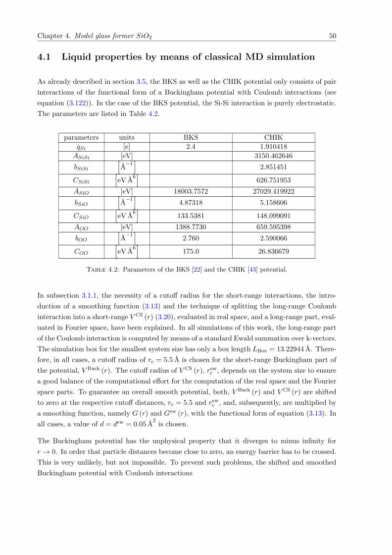
Chapter 4. Model glass former SiO2 50
4.1 Liquid properties by means of classical MD simulation
As already described in section 3.5, the BKS as well as the CHIK potential only consists of pair
interactions of the functional form of a Buckingham potential with Coulomb interactions (see
equation (3.122)). In the case of the BKS potential, the Si-Si interaction is purely electrostatic.
The parameters are listed in Table 4.2.
parameters units BKS CHIK
qSi [e] 2.4 1.910418
ASiSi [eV] 3150.462646
bSiSi
[A−1]
2.851451
CSiSi
[eV A
6]
626.751953
ASiO [eV] 18003.7572 27029.419922
bSiO
[A−1]
4.87318 5.158606
CSiO
[eV A
6]
133.5381 148.099091
AOO [eV] 1388.7730 659.595398
bOO
[A−1]
2.760 2.590066
COO
[eV A
6]
175.0 26.836679
Table 4.2: Parameters of the BKS [22] and the CHIK [43] potential.
In subsection 3.1.1, the necessity of a cutoff radius for the short-range interactions, the intro-
duction of a smoothing function (3.13) and the technique of splitting the long-range Coulomb
interaction into a short-range V CS (r) (3.20), evaluated in real space, and a long-range part, eval-
uated in Fourier space, have been explained. In all simulations of this work, the long-range part
of the Coulomb interaction is computed by means of a standard Ewald summation over k-vectors.
The simulation box for the smallest system size has only a box length LBox = 13.22944 A. There-
fore, in all cases, a cutoff radius of rc = 5.5 A is chosen for the short-range Buckingham part of
the potential, V Buck (r). The cutoff radius of V CS (r), rewc , depends on the system size to ensure
a good balance of the computational effort for the computation of the real space and the Fourier
space parts. To guarantee an overall smooth potential, both, V Buck (r) and V CS (r) are shifted
to zero at the respective cutoff distances, rc = 5.5 and rewc , and, subsequently, are multiplied by
a smoothing function, namely G (r) and Gew (r), with the functional form of equation (3.13). In
all cases, a value of d = dew = 0.05 A2
is chosen.
The Buckingham potential has the unphysical property that it diverges to minus infinity for
r → 0. In order that particle distances become close to zero, an energy barrier has to be crossed.
This is very unlikely, but not impossible. To prevent such problems, the shifted and smoothed
Buckingham potential with Coulomb interactions
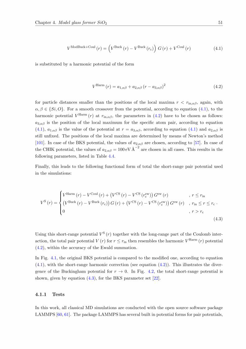
Chapter 4. Model glass former SiO2 51
V ModBuck+Coul (r) =(V Buck (r)− V Buck (rc)
)G (r) + V Coul (r) (4.1)
is substituted by a harmonic potential of the form
V Harm (r) = a1,αβ + a2,αβ (r − a3,αβ)2 (4.2)
for particle distances smaller than the positions of the local maxima r < rin,αβ, again, with
α, β ∈ Si,O. For a smooth crossover from the potential, according to equation (4.1), to the
harmonic potential V Harm (r) at rin,αβ, the parameters in (4.2) have to be chosen as follows:
a3,αβ is the position of the local maximum for the specific atom pair, according to equation
(4.1), a1,αβ is the value of the potential at r = a3,αβ, according to equation (4.1) and a2,αβ is
still unfixed. The positions of the local maxima are determined by means of Newton’s method
[101]. In case of the BKS potential, the values of a2,αβ are chosen, according to [57]. In case of
the CHIK potential, the values of a2,αβ = 100 eV A−2
are chosen in all cases. This results in the
following parameters, listed in Table 4.4.
Finally, this leads to the following functional form of total the short-range pair potential used
in the simulations:
V S (r) =
V Harm (r)− V Coul (r) +(V CS (r)− V CS (rew
c ))Gew (r) , r ≤ rin
(V Buck (r)− V Buck (rc)
)G (r) +
(V CS (r)− V CS (rew
c ))Gew (r) , rin ≤ r ≤ rc
0 , r > rc
.
(4.3)
Using this short-range potential V S (r) together with the long-range part of the Coulomb inter-
action, the total pair potential V (r) for r ≤ rin then resembles the harmonic V Harm (r) potential
(4.2), within the accuracy of the Ewald summation.
In Fig. 4.1, the original BKS potential is compared to the modified one, according to equation
(4.1), with the short-range harmonic correction (see equation (4.2)). This illustrates the diver-
gence of the Buckingham potential for r → 0. In Fig. 4.2, the total short-range potential is
shown, given by equation (4.3), for the BKS parameter set [22].
4.1.1 Tests
In this work, all classical MD simulations are conducted with the open source software package
LAMMPS [60, 61]. The package LAMMPS has several built in potential forms for pair potentials,
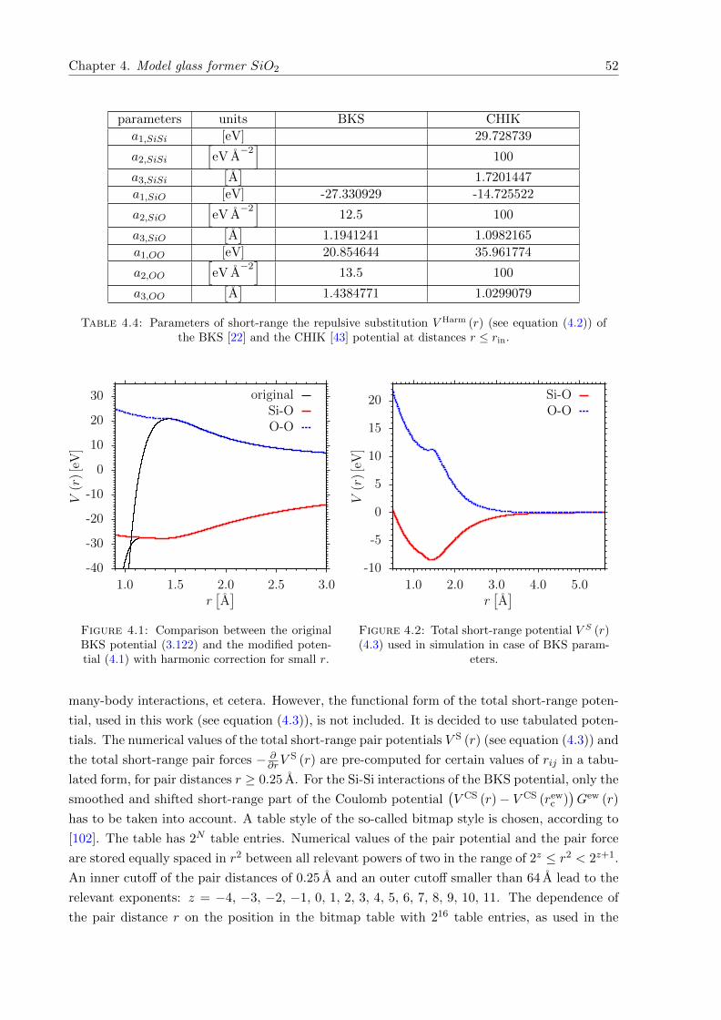
Chapter 4. Model glass former SiO2 52
parameters units BKS CHIK
a1,SiSi [eV] 29.728739
a2,SiSi
[eV A
−2]
100
a3,SiSi
[A]
1.7201447
a1,SiO [eV] -27.330929 -14.725522
a2,SiO
[eV A
−2]
12.5 100
a3,SiO
[A]
1.1941241 1.0982165
a1,OO [eV] 20.854644 35.961774
a2,OO
[eV A
−2]
13.5 100
a3,OO
[A]
1.4384771 1.0299079
Table 4.4: Parameters of short-range the repulsive substitution V Harm (r) (see equation (4.2)) ofthe BKS [22] and the CHIK [43] potential at distances r ≤ rin.
-40
-30
-20
-10
0
10
20
30
1.0 1.5 2.0 2.5 3.0
V(r
)[e
V]
r[A]
originalSi-OO-O
Figure 4.1: Comparison between the originalBKS potential (3.122) and the modified poten-tial (4.1) with harmonic correction for small r.
-10
-5
0
5
10
15
20
1.0 2.0 3.0 4.0 5.0
V(r
)[e
V]
r[A]
Si-OO-O
Figure 4.2: Total short-range potential V S (r)(4.3) used in simulation in case of BKS param-
eters.
many-body interactions, et cetera. However, the functional form of the total short-range poten-
tial, used in this work (see equation (4.3)), is not included. It is decided to use tabulated poten-
tials. The numerical values of the total short-range pair potentials V S (r) (see equation (4.3)) and
the total short-range pair forces − ∂∂rV
S (r) are pre-computed for certain values of rij in a tabu-
lated form, for pair distances r ≥ 0.25 A. For the Si-Si interactions of the BKS potential, only the
smoothed and shifted short-range part of the Coulomb potential(V CS (r)− V CS (rew
c ))Gew (r)
has to be taken into account. A table style of the so-called bitmap style is chosen, according to
[102]. The table has 2N table entries. Numerical values of the pair potential and the pair force
are stored equally spaced in r2 between all relevant powers of two in the range of 2z ≤ r2 < 2z+1.
An inner cutoff of the pair distances of 0.25 A and an outer cutoff smaller than 64 A lead to the
relevant exponents: z = −4, −3, −2, −1, 0, 1, 2, 3, 4, 5, 6, 7, 8, 9, 10, 11. The dependence of
the pair distance r on the position in the bitmap table with 216 table entries, as used in the
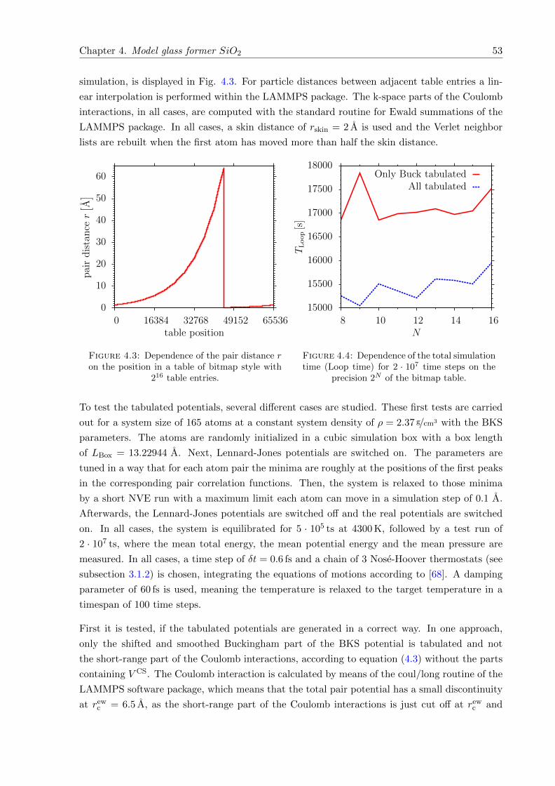
Chapter 4. Model glass former SiO2 53
simulation, is displayed in Fig. 4.3. For particle distances between adjacent table entries a lin-
ear interpolation is performed within the LAMMPS package. The k-space parts of the Coulomb
interactions, in all cases, are computed with the standard routine for Ewald summations of the
LAMMPS package. In all cases, a skin distance of rskin = 2 A is used and the Verlet neighbor
lists are rebuilt when the first atom has moved more than half the skin distance.
0
10
20
30
40
50
60
0 16384 32768 49152 65536
pai
rdis
tance
r[ A]
table position
Figure 4.3: Dependence of the pair distance ron the position in a table of bitmap style with
216 table entries.
15000
15500
16000
16500
17000
17500
18000
8 10 12 14 16
TLoop[s]
N
Only Buck tabulatedAll tabulated
Figure 4.4: Dependence of the total simulationtime (Loop time) for 2 · 107 time steps on the
precision 2N of the bitmap table.
To test the tabulated potentials, several different cases are studied. These first tests are carried
out for a system size of 165 atoms at a constant system density of ρ = 2.37 g/cm3 with the BKS
parameters. The atoms are randomly initialized in a cubic simulation box with a box length
of LBox = 13.22944 A. Next, Lennard-Jones potentials are switched on. The parameters are
tuned in a way that for each atom pair the minima are roughly at the positions of the first peaks
in the corresponding pair correlation functions. Then, the system is relaxed to those minima
by a short NVE run with a maximum limit each atom can move in a simulation step of 0.1 A.
Afterwards, the Lennard-Jones potentials are switched off and the real potentials are switched
on. In all cases, the system is equilibrated for 5 · 105 ts at 4300 K, followed by a test run of
2 · 107 ts, where the mean total energy, the mean potential energy and the mean pressure are
measured. In all cases, a time step of δt = 0.6 fs and a chain of 3 Nose-Hoover thermostats (see
subsection 3.1.2) is chosen, integrating the equations of motions according to [68]. A damping
parameter of 60 fs is used, meaning the temperature is relaxed to the target temperature in a
timespan of 100 time steps.
First it is tested, if the tabulated potentials are generated in a correct way. In one approach,
only the shifted and smoothed Buckingham part of the BKS potential is tabulated and not
the short-range part of the Coulomb interactions, according to equation (4.3) without the parts
containing V CS. The Coulomb interaction is calculated by means of the coul/long routine of the
LAMMPS software package, which means that the total pair potential has a small discontinuity
at rewc = 6.5 A, as the short-range part of the Coulomb interactions is just cut off at rew
c and
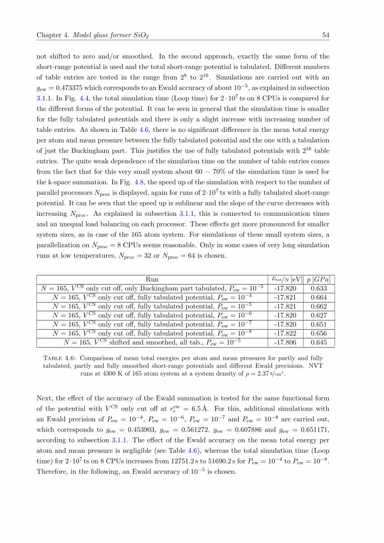
Chapter 4. Model glass former SiO2 54
not shifted to zero and/or smoothed. In the second approach, exactly the same form of the
short-range potential is used and the total short-range potential is tabulated. Different numbers
of table entries are tested in the range from 28 to 216. Simulations are carried out with an
gew = 0.473375 which corresponds to an Ewald accuracy of about 10−5, as explained in subsection
3.1.1. In Fig. 4.4, the total simulation time (Loop time) for 2 · 107 ts on 8 CPUs is compared for
the different forms of the potential. It can be seen in general that the simulation time is smaller
for the fully tabulated potentials and there is only a slight increase with increasing number of
table entries. As shown in Table 4.6, there is no significant difference in the mean total energy
per atom and mean pressure between the fully tabulated potential and the one with a tabulation
of just the Buckingham part. This justifies the use of fully tabulated potentials with 216 table
entries. The quite weak dependence of the simulation time on the number of table entries comes
from the fact that for this very small system about 60 − 70% of the simulation time is used for
the k-space summation. In Fig. 4.8, the speed up of the simulation with respect to the number of
parallel processors Nproc is displayed, again for runs of 2·107 ts with a fully tabulated short-range
potential. It can be seen that the speed up is sublinear and the slope of the curve decreases with
increasing Nproc. As explained in subsection 3.1.1, this is connected to communication times
and an unequal load balancing on each processor. These effects get more pronounced for smaller
system sizes, as in case of the 165 atom system. For simulations of these small system sizes, a
parallelization on Nproc = 8 CPUs seems reasonable. Only in some cases of very long simulation
runs at low temperatures, Nproc = 32 or Nproc = 64 is chosen.
Run Etot/N [eV] p [GPa]
N = 165, V CS only cut off, only Buckingham part tabulated, Pew = 10−5 -17.820 0.633
N = 165, V CS only cut off, fully tabulated potential, Pew = 10−4 -17.821 0.664
N = 165, V CS only cut off, fully tabulated potential, Pew = 10−5 -17.821 0.662
N = 165, V CS only cut off, fully tabulated potential, Pew = 10−6 -17.820 0.627
N = 165, V CS only cut off, fully tabulated potential, Pew = 10−7 -17.820 0.651
N = 165, V CS only cut off, fully tabulated potential, Pew = 10−8 -17.822 0.656
N = 165, V CS shifted and smoothed, all tab., Pew = 10−5 -17.806 0.645
Table 4.6: Comparison of mean total energies per atom and mean pressures for partly and fullytabulated, partly and fully smoothed short-range potentials and different Ewald precisions. NVT
runs at 4300 K of 165 atom system at a system density of ρ = 2.37 g/cm3.
Next, the effect of the accuracy of the Ewald summation is tested for the same functional form
of the potential with V CS only cut off at rewc = 6.5 A. For this, additional simulations with
an Ewald precision of Pew = 10−4, Pew = 10−6, Pew = 10−7 and Pew = 10−8 are carried out,
which corresponds to gew = 0.453903, gew = 0.561272, gew = 0.607886 and gew = 0.651171,
according to subsection 3.1.1. The effect of the Ewald accuracy on the mean total energy per
atom and mean pressure is negligible (see Table 4.6), whereas the total simulation time (Loop
time) for 2 ·107 ts on 8 CPUs increases from 12751.2 s to 51690.2 s for Pew = 10−4 to Pew = 10−8.
Therefore, in the following, an Ewald accuracy of 10−5 is chosen.
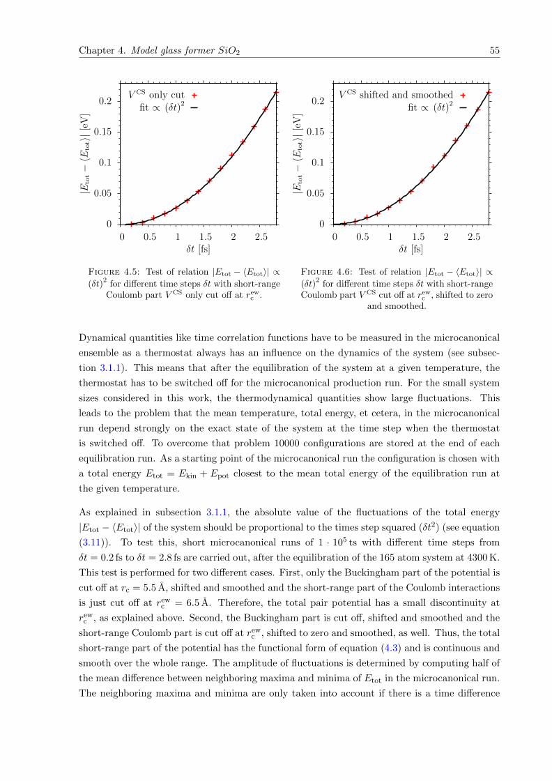
Chapter 4. Model glass former SiO2 55
0
0.05
0.1
0.15
0.2
0 0.5 1 1.5 2 2.5
|Etot−〈E
tot〉|
[eV
]
δt [fs]
V CS only cutfit ∝ (δt)2
Figure 4.5: Test of relation |Etot − 〈Etot〉| ∝(δt)
2for different time steps δt with short-range
Coulomb part V CS only cut off at rewc .
0
0.05
0.1
0.15
0.2
0 0.5 1 1.5 2 2.5
|Etot−〈E
tot〉|
[eV
]
δt [fs]
V CS shifted and smoothedfit ∝ (δt)2
Figure 4.6: Test of relation |Etot − 〈Etot〉| ∝(δt)
2for different time steps δt with short-range
Coulomb part V CS cut off at rewc , shifted to zero
and smoothed.
Dynamical quantities like time correlation functions have to be measured in the microcanonical
ensemble as a thermostat always has an influence on the dynamics of the system (see subsec-
tion 3.1.1). This means that after the equilibration of the system at a given temperature, the
thermostat has to be switched off for the microcanonical production run. For the small system
sizes considered in this work, the thermodynamical quantities show large fluctuations. This
leads to the problem that the mean temperature, total energy, et cetera, in the microcanonical
run depend strongly on the exact state of the system at the time step when the thermostat
is switched off. To overcome that problem 10000 configurations are stored at the end of each
equilibration run. As a starting point of the microcanonical run the configuration is chosen with
a total energy Etot = Ekin + Epot closest to the mean total energy of the equilibration run at
the given temperature.
As explained in subsection 3.1.1, the absolute value of the fluctuations of the total energy
|Etot − 〈Etot〉| of the system should be proportional to the times step squared (δt2) (see equation
(3.11)). To test this, short microcanonical runs of 1 · 105 ts with different time steps from
δt = 0.2 fs to δt = 2.8 fs are carried out, after the equilibration of the 165 atom system at 4300 K.
This test is performed for two different cases. First, only the Buckingham part of the potential is
cut off at rc = 5.5 A, shifted and smoothed and the short-range part of the Coulomb interactions
is just cut off at rewc = 6.5 A. Therefore, the total pair potential has a small discontinuity at
rewc , as explained above. Second, the Buckingham part is cut off, shifted and smoothed and the
short-range Coulomb part is cut off at rewc , shifted to zero and smoothed, as well. Thus, the total
short-range part of the potential has the functional form of equation (4.3) and is continuous and
smooth over the whole range. The amplitude of fluctuations is determined by computing half of
the mean difference between neighboring maxima and minima of Etot in the microcanonical run.
The neighboring maxima and minima are only taken into account if there is a time difference
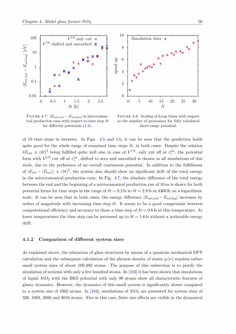
Chapter 4. Model glass former SiO2 56
0.01
0.1
1
10
100
0 0.5 1 1.5 2 2.5
|Etot,en
d−E
tot,beg|[eV
]
δt [fs]
V CS only cutV CS shifted and smoothed
Figure 4.7: |Etot,end − Etot,beg| in microcanon-ical production runs with respect to time step δt
for different potentials (4.3).
0
2
4
6
8
10
0 5 10 15 20 25 30
speedup
N
Simulation data
Figure 4.8: Scaling of Loop times with respectto the number of processors for fully tabulated
short-range potential.
of 10 time steps in between. In Figs. 4.5 and 4.6, it can be seen that the prediction holds
quite good for the whole range of examined time steps δt, in both cases. Despite the relation
δEtot ∝ (δt)2 being fulfilled quite well also in case of V CS, only cut off at rewc , the potential
form with V CS cut off at rewc , shifted to zero and smoothed is chosen in all simulations of this
work, due to the preference of an overall continuous potential. In addition to the fulfillment
of |Etot − 〈Etot〉| ∝ (δt)2, the system also should show no significant drift of the total energy
in the microcanonical production runs. In Fig. 4.7, the absolute difference of the total energy
between the end and the beginning of a microcanonical production run of 10 ns is shown for both
potential forms for time steps in the range of δt = 0.2 fs to δt = 2.8 fs at 4300 K on a logarithmic
scale. It can be seen that in both cases, the energy difference |Etot,end − Etot,beg| increases by
orders of magnitude with increasing time step δt. It seems to be a good compromise between
computational efficiency and accuracy to chose a time step of δt = 0.6 fs at this temperature. At
lower temperatures the time step can be increased up to δt = 1.6 fs without a noticeable energy
drift.
4.1.2 Comparison of different system sizes
As explained above, the relaxation of glass structures by means of a quantum mechanical DFT
calculation and the subsequent calculation of the phonon density of states g (ν) requires rather
small system sizes of about 100-200 atoms. The purpose of this subsection is to justify the
simulation of systems with only a few hundred atoms. In [103] it has been shown that simulations
of liquid SiO2 with the BKS potential with only 99 atoms show all characteristic features of
glassy dynamics. However, the dynamics of this small system is significantly slower compared
to a system size of 1002 atoms. In [104], simulations of SiO2 are presented for system sizes of
336, 1002, 3006 and 8016 atoms. Also in this case, finite size effects are visible in the dynamical
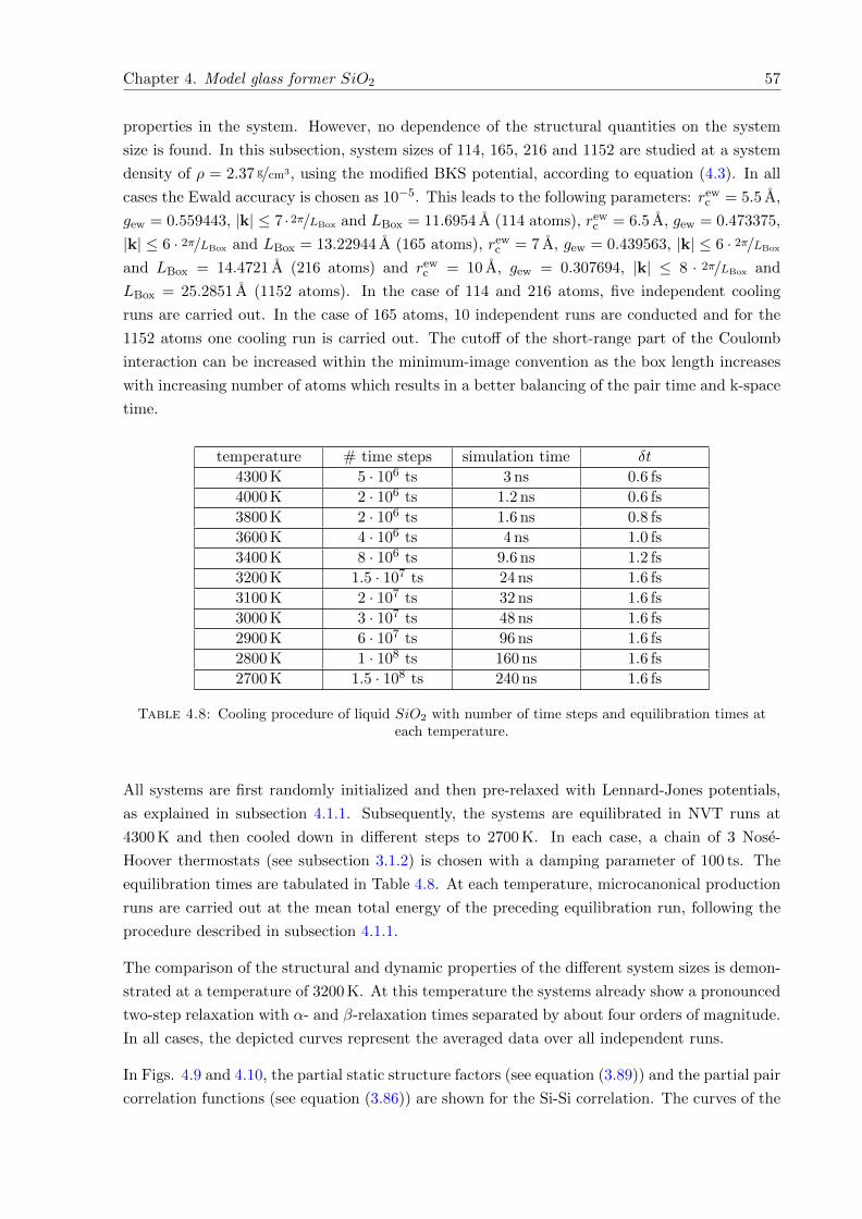
Chapter 4. Model glass former SiO2 57
properties in the system. However, no dependence of the structural quantities on the system
size is found. In this subsection, system sizes of 114, 165, 216 and 1152 are studied at a system
density of ρ = 2.37 g/cm3, using the modified BKS potential, according to equation (4.3). In all
cases the Ewald accuracy is chosen as 10−5. This leads to the following parameters: rewc = 5.5 A,
gew = 0.559443, |k| ≤ 7 ·2π/LBox and LBox = 11.6954 A (114 atoms), rewc = 6.5 A, gew = 0.473375,
|k| ≤ 6 · 2π/LBox and LBox = 13.22944 A (165 atoms), rewc = 7 A, gew = 0.439563, |k| ≤ 6 · 2π/LBox
and LBox = 14.4721 A (216 atoms) and rewc = 10 A, gew = 0.307694, |k| ≤ 8 · 2π/LBox and
LBox = 25.2851 A (1152 atoms). In the case of 114 and 216 atoms, five independent cooling
runs are carried out. In the case of 165 atoms, 10 independent runs are conducted and for the
1152 atoms one cooling run is carried out. The cutoff of the short-range part of the Coulomb
interaction can be increased within the minimum-image convention as the box length increases
with increasing number of atoms which results in a better balancing of the pair time and k-space
time.
temperature # time steps simulation time δt
4300 K 5 · 106 ts 3 ns 0.6 fs
4000 K 2 · 106 ts 1.2 ns 0.6 fs
3800 K 2 · 106 ts 1.6 ns 0.8 fs
3600 K 4 · 106 ts 4 ns 1.0 fs
3400 K 8 · 106 ts 9.6 ns 1.2 fs
3200 K 1.5 · 107 ts 24 ns 1.6 fs
3100 K 2 · 107 ts 32 ns 1.6 fs
3000 K 3 · 107 ts 48 ns 1.6 fs
2900 K 6 · 107 ts 96 ns 1.6 fs
2800 K 1 · 108 ts 160 ns 1.6 fs
2700 K 1.5 · 108 ts 240 ns 1.6 fs
Table 4.8: Cooling procedure of liquid SiO2 with number of time steps and equilibration times ateach temperature.
All systems are first randomly initialized and then pre-relaxed with Lennard-Jones potentials,
as explained in subsection 4.1.1. Subsequently, the systems are equilibrated in NVT runs at
4300 K and then cooled down in different steps to 2700 K. In each case, a chain of 3 Nose-
Hoover thermostats (see subsection 3.1.2) is chosen with a damping parameter of 100 ts. The
equilibration times are tabulated in Table 4.8. At each temperature, microcanonical production
runs are carried out at the mean total energy of the preceding equilibration run, following the
procedure described in subsection 4.1.1.
The comparison of the structural and dynamic properties of the different system sizes is demon-
strated at a temperature of 3200 K. At this temperature the systems already show a pronounced
two-step relaxation with α- and β-relaxation times separated by about four orders of magnitude.
In all cases, the depicted curves represent the averaged data over all independent runs.
In Figs. 4.9 and 4.10, the partial static structure factors (see equation (3.89)) and the partial pair
correlation functions (see equation (3.86)) are shown for the Si-Si correlation. The curves of the
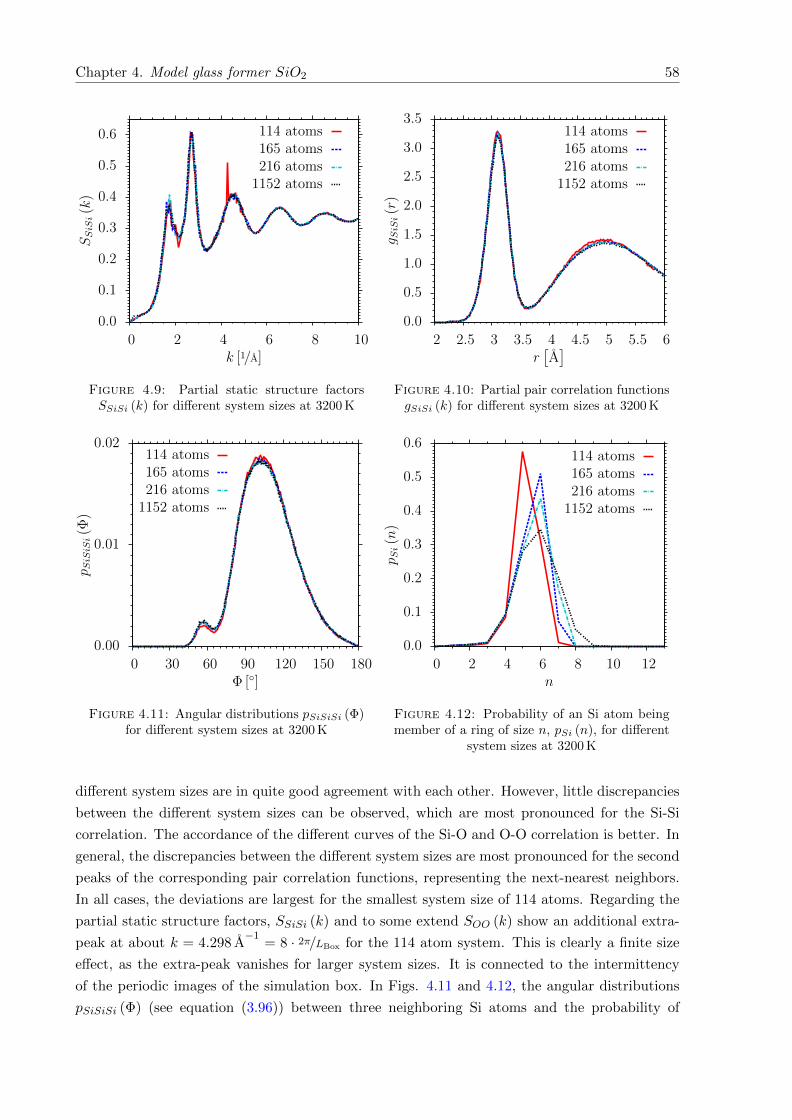
Chapter 4. Model glass former SiO2 58
0.0
0.1
0.2
0.3
0.4
0.5
0.6
0 2 4 6 8 10
SSiS
i(k)
k [1/A]
114 atoms165 atoms216 atoms1152 atoms
Figure 4.9: Partial static structure factorsSSiSi (k) for different system sizes at 3200 K
0.0
0.5
1.0
1.5
2.0
2.5
3.0
3.5
2 2.5 3 3.5 4 4.5 5 5.5 6
g SiS
i(r
)
r[A]
114 atoms165 atoms216 atoms
1152 atoms
Figure 4.10: Partial pair correlation functionsgSiSi (k) for different system sizes at 3200 K
0.00
0.01
0.02
0 30 60 90 120 150 180
p SiS
iSi(Φ
)
Φ []
114 atoms165 atoms216 atoms
1152 atoms
Figure 4.11: Angular distributions pSiSiSi (Φ)for different system sizes at 3200 K
0.0
0.1
0.2
0.3
0.4
0.5
0.6
0 2 4 6 8 10 12
p Si(n)
n
114 atoms165 atoms216 atoms1152 atoms
Figure 4.12: Probability of an Si atom beingmember of a ring of size n, pSi (n), for different
system sizes at 3200 K
different system sizes are in quite good agreement with each other. However, little discrepancies
between the different system sizes can be observed, which are most pronounced for the Si-Si
correlation. The accordance of the different curves of the Si-O and O-O correlation is better. In
general, the discrepancies between the different system sizes are most pronounced for the second
peaks of the corresponding pair correlation functions, representing the next-nearest neighbors.
In all cases, the deviations are largest for the smallest system size of 114 atoms. Regarding the
partial static structure factors, SSiSi (k) and to some extend SOO (k) show an additional extra-
peak at about k = 4.298 A−1
= 8 · 2π/LBox for the 114 atom system. This is clearly a finite size
effect, as the extra-peak vanishes for larger system sizes. It is connected to the intermittency
of the periodic images of the simulation box. In Figs. 4.11 and 4.12, the angular distributions
pSiSiSi (Φ) (see equation (3.96)) between three neighboring Si atoms and the probability of
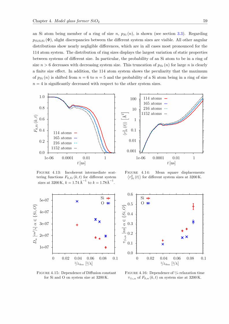
Chapter 4. Model glass former SiO2 59
an Si atom being member of a ring of size n, pSi (n), is shown (see section 3.3). Regarding
pSiSiSi (Φ), slight discrepancies between the different system sizes are visible. All other angular
distributions show nearly negligible differences, which are in all cases most pronounced for the
114 atom system. The distribution of ring sizes displays the largest variation of static properties
between systems of different size. In particular, the probability of an Si atom to be in a ring of
size n > 6 decreases with decreasing system size. This truncation of pSi (n) for large n is clearly
a finite size effect. In addition, the 114 atom system shows the peculiarity that the maximum
of pSi (n) is shifted from n = 6 to n = 5 and the probability of a Si atom being in a ring of size
n = 4 is significantly decreased with respect to the other system sizes.
0.0
0.2
0.4
0.6
0.8
1.0
1e-06 0.0001 0.01 1
FS,Si(k,t)
t [ns]
114 atoms165 atoms216 atoms1152 atoms
Figure 4.13: Incoherent intermediate scat-tering functions FS,Si (k, t) for different system
sizes at 3200 K, k = 1.74 A−1
to k = 1.78A−1
.
0.001
0.01
0.1
1
10
100
1e-06 0.0001 0.01 1
〈r2 Si(t
)〉[ A
2]
t [ns]
114 atoms165 atoms216 atoms
1152 atoms
Figure 4.14: Mean square displacements⟨r2Si (t)
⟩for different system sizes at 3200 K.
1e-07
2e-07
3e-07
4e-07
5e-07
0 0.02 0.04 0.06 0.08 0.1
Dα[c
m2 /
s]α∈Si,O
1/LBox [1/A]
SiO
Figure 4.15: Dependence of Diffusion constantfor Si and O on system size at 3200 K.
0.0
0.1
0.2
0.3
0.4
0.5
0.6
0 0.02 0.04 0.06 0.08 0.1
τ 1/e,α
[ns]α∈Si,O
1/LBox [1/A]
SiO
Figure 4.16: Dependence of 1/e relaxation timeτ1/e,α of FS,α (k, t) on system size at 3200 K.
Chapter 4. Model glass former SiO2 60
Next, the dynamical properties are compared. In Figs. 4.13 and 4.14, the incoherent interme-
diate scattering functions FS,Si (k, t) (see equation (3.100)) and the mean square displacements⟨r2Si (t)
⟩(see equation (3.98)) are shown. The incoherent intermediate scattering functions are
evaluated at k = 1.78 A−1
(114 and 165 atoms) and k = 1.74 A−1
(216 and 1152 atoms). This
is about the k-value of the so-called first sharp diffraction peak (FSDP) visible in all partial
static structure factors. It can be seen that the curves of the different system sizes show the
same qualitative characteristics of a two-step decay with an intermediate plateau. However, the
α-relaxation times and the plateau heights of the normalized incoherent intermediate scattering
functions decrease with increasing system size. The same feature is visible in the mean square
displacements, whereas the plateau heights increase with increasing system size. In Fig. 4.15,
the self-diffusion constants Dα, α ∈ Si,O, are displayed with respect to the inverse box length
1/LBox, to further illustrate the dependence of the dynamical properties on the system size. They
are determined by means of the slope of a linear fit to the corresponding mean square displace-
ments at large simulation times, where the Einstein relation Dα = limt→∞〈r2α(t)〉6t [15] holds (see
equation (3.99)). In Fig. 4.16, the 1/e relaxation times are displayed, meaning the times τ1/e,α at
which the incoherent intermediate scattering functions FS,α (k, t) have decayed to the numerical
value of 1/e. The shown statistical errors are computed as the standard deviation of the mean,
with respect to the independent runs, σ = σ√N
. It can be seen that the diffusion constants of
the 114 atom system are about 2.5 times (O) and 3 times (Si) as large as the ones of the 1152
atom system. This is in agreement with the 1/e relaxation times being about 3.5 (O) to 4 (Si)
times as large in case of the 114 atom system compared to the 1152 atom system. In all cases,
the differences between the 165 and the 216 atom system are the smallest. The slowing down of
the dynamics with decreasing system size is clearly a finite size effect [103, 104].
Summarizing, the structural properties show only a small dependence on the system size. The
most pronounced differences between the different system sizes are visible in the distribution of
ring sizes, which show a decrease of the number of rings containing more than 6 Si atoms with
decreasing system size. In contrast to all other considered system sizes, the maximum of pSi (n)
is shifted from n = 5 to n = 6 for the 114 atom system. This feature is reflected in the other
structural quantities, where the 114 atom system also shows the largest finite-size effects. The
dynamical properties show a greater dependence on the system size. However, all system sizes
show the generic features of glassy dynamics like the two-step decay process with the separation
of time scales. Having this in mind, this subsection motivates and justifies the choice of a 165
atom system for further considerations.
4.1.3 Liquid properties at different temperatures
This subsection provides an overview over the structural and dynamical properties of liquid
SiO2 at different temperatures, comparing the BKS [22] with the CHIK [43] potential. Here,
simulations are carried out for 165 atom systems at the experimental glass density of ρ = 2.2 g/cm3
[98]. For all simulations the modified form of the Buckingham potential (4.3) is used, as explained
in subsection 4.1.1. This leads to the following parameters: rewc = 5.5 A, gew = 0.473375,
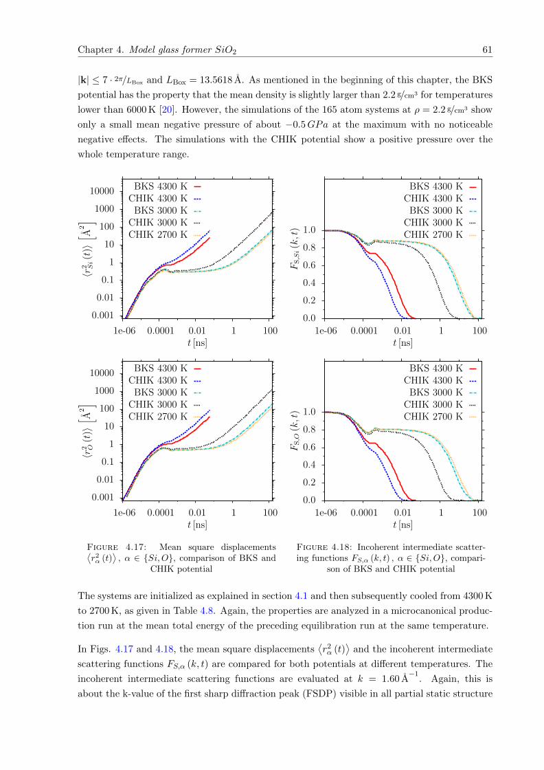
Chapter 4. Model glass former SiO2 61
|k| ≤ 7 · 2π/LBox and LBox = 13.5618 A. As mentioned in the beginning of this chapter, the BKS
potential has the property that the mean density is slightly larger than 2.2 g/cm3 for temperatures
lower than 6000 K [20]. However, the simulations of the 165 atom systems at ρ = 2.2 g/cm3 show
only a small mean negative pressure of about −0.5GPa at the maximum with no noticeable
negative effects. The simulations with the CHIK potential show a positive pressure over the
whole temperature range.
0.001
0.01
0.1
1
10
100
1000
10000
1e-06 0.0001 0.01 1 100
〈r2 Si(t
)〉[ A
2]
t [ns]
BKS 4300 KCHIK 4300 K
BKS 3000 KCHIK 3000 KCHIK 2700 K
0.001
0.01
0.1
1
10
100
1000
10000
1e-06 0.0001 0.01 1 100
〈r2 O
(t)〉[ A
2]
t [ns]
BKS 4300 KCHIK 4300 K
BKS 3000 KCHIK 3000 KCHIK 2700 K
Figure 4.17: Mean square displacements⟨r2α (t)
⟩, α ∈ Si,O, comparison of BKS and
CHIK potential
0.0
0.2
0.4
0.6
0.8
1.0
1e-06 0.0001 0.01 1 100
FS,Si(k,t)
t [ns]
BKS 4300 KCHIK 4300 KBKS 3000 K
CHIK 3000 KCHIK 2700 K
0.0
0.2
0.4
0.6
0.8
1.0
1e-06 0.0001 0.01 1 100
FS,O(k,t)
t [ns]
BKS 4300 KCHIK 4300 KBKS 3000 K
CHIK 3000 KCHIK 2700 K
Figure 4.18: Incoherent intermediate scatter-ing functions FS,α (k, t) , α ∈ Si,O, compari-
son of BKS and CHIK potential
The systems are initialized as explained in section 4.1 and then subsequently cooled from 4300 K
to 2700 K, as given in Table 4.8. Again, the properties are analyzed in a microcanonical produc-
tion run at the mean total energy of the preceding equilibration run at the same temperature.
In Figs. 4.17 and 4.18, the mean square displacements⟨r2α (t)
⟩and the incoherent intermediate
scattering functions FS,α (k, t) are compared for both potentials at different temperatures. The
incoherent intermediate scattering functions are evaluated at k = 1.60 A−1
. Again, this is
about the k-value of the first sharp diffraction peak (FSDP) visible in all partial static structure
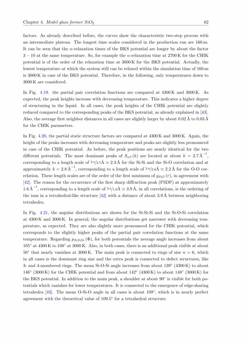
Chapter 4. Model glass former SiO2 62
factors. As already described before, the curves show the characteristic two-step process with
an intermediate plateau. The longest time scales considered in the production run are 160 ns.
It can be seen that the α-relaxation times of the BKS potential are longer by about the factor
3− 10 at the same temperature. So, for example the α-relaxation time at 2700 K for the CHIK
potential is of the order of the relaxation time at 3000 K for the BKS potential. Actually, the
lowest temperature at which the system still can be relaxed within the simulation time of 160 ns
is 3000 K in case of the BKS potential. Therefore, in the following, only temperatures down to
3000 K are considered.
In Fig. 4.19. the partial pair correlation functions are compared at 4300 K and 3000 K. As
expected, the peak heights increase with decreasing temperature. This indicates a higher degree
of structuring in the liquid. In all cases, the peak heights of the CHIK potential are slightly
reduced compared to the corresponding peaks of the BKS potential, as already explained in [43].
Also, the average first neighbor distances in all cases are slightly larger by about 0.02 A to 0.03 A
for the CHIK parameters.
In Fig. 4.20, the partial static structure factors are compared at 4300 K and 3000 K. Again, the
height of the peaks increases with decreasing temperature and peaks are slightly less pronounced
in case of the CHIK potential. As before, the peak positions are nearly identical for the two
different potentials. The most dominant peaks of Sαβ (k) are located at about k = 2.7 A−1
,
corresponding to a length scale of 2π/2.7A ' 2.3 A for the Si-Si and the Si-O correlation and at
approximately k = 2.8 A−1
, corresponding to a length scale of 2π/2.8A ' 2.2 A for the O-O cor-
relation. These length scales are of the order of the first minimum of gSiO (r), in agreement with
[42]. The reason for the occurrence of the first sharp diffraction peak (FSDP) at approximately
1.6 A−1
, corresponding to a length scale of 2π/1.6A ' 3.9 A, in all correlations, is the ordering of
the ions in a tetrahedral-like structure [42] with a distance of about 3.9 A between neighboring
tetrahedra.
In Fig. 4.21, the angular distributions are shown for the Si-Si-Si and the Si-O-Si correlation
at 4300 K and 3000 K. In general, the angular distributions get narrower with decreasing tem-
perature, as expected. They are also slightly more pronounced for the CHIK potential, which
corresponds to the slightly higher peaks of the partial pair correlation functions at the same
temperature. Regarding pSiSiSi (Φ), for both potentials the average angle increases from about
105 at 4300 K to 108 at 3000 K. Also, in both cases, there is an additional peak visible at about
56 that nearly vanishes at 3000 K. The main peak is connected to rings of size n = 6, which
in all cases is the dominant ring size and the extra peak is connected to defect structures, like
3- and 4-membered rings. The mean Si-O-Si angle increases from about 139 (4300 K) to about
146 (3000 K) for the CHIK potential and from about 142 (4300 K) to about 148 (3000 K) for
the BKS potential. In addition to the main peak, a shoulder at about 90 is visible for both po-
tentials which vanishes for lower temperatures. It is connected to the emergence of edge-sharing
tetrahedra [43]. The mean O-Si-O angle in all cases is about 109, which is in nearly perfect
agreement with the theoretical value of 109.5 for a tetrahedral structure.
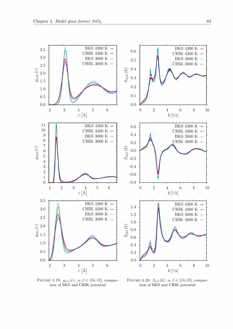
Chapter 4. Model glass former SiO2 63
0.0
0.5
1.0
1.5
2.0
2.5
3.0
3.5
2 3 4 5 6
g SiS
i(r
)
r[A]
BKS 4300 KCHIK 4300 K
BKS 3000 KCHIK 3000 K
0123456789
1011
1 2 3 4 5 6
g SiO
(r)
r[A]
BKS 4300 KCHIK 4300 K
BKS 3000 KCHIK 3000 K
0.0
0.5
1.0
1.5
2.0
2.5
3.0
3.5
2 3 4 5 6
g OO
(r)
r[A]
BKS 4300 KCHIK 4300 K
BKS 3000 KCHIK 3000 K
Figure 4.19: gαβ (r) , α, β ∈ Si,O, compar-ison of BKS and CHIK potential
0.0
0.1
0.2
0.3
0.4
0.5
0.6
0 2 4 6 8 10
SSiS
i(k)
k [1/A]
BKS 4300 KCHIK 4300 KBKS 3000 K
CHIK 3000 K
-0.8
-0.6
-0.4
-0.2
0.0
0.2
0.4
0.6
0 2 4 6 8 10
SSiO
(k)
k [1/A]
BKS 4300 KCHIK 4300 KBKS 3000 K
CHIK 3000 K
0.0
0.2
0.4
0.6
0.8
1.0
1.2
1.4
0 2 4 6 8 10
SOO(k)
k [1/A]
BKS 4300 KCHIK 4300 KBKS 3000 K
CHIK 3000 K
Figure 4.20: Sαβ (k) , α, β ∈ Si,O, compar-ison of BKS and CHIK potential
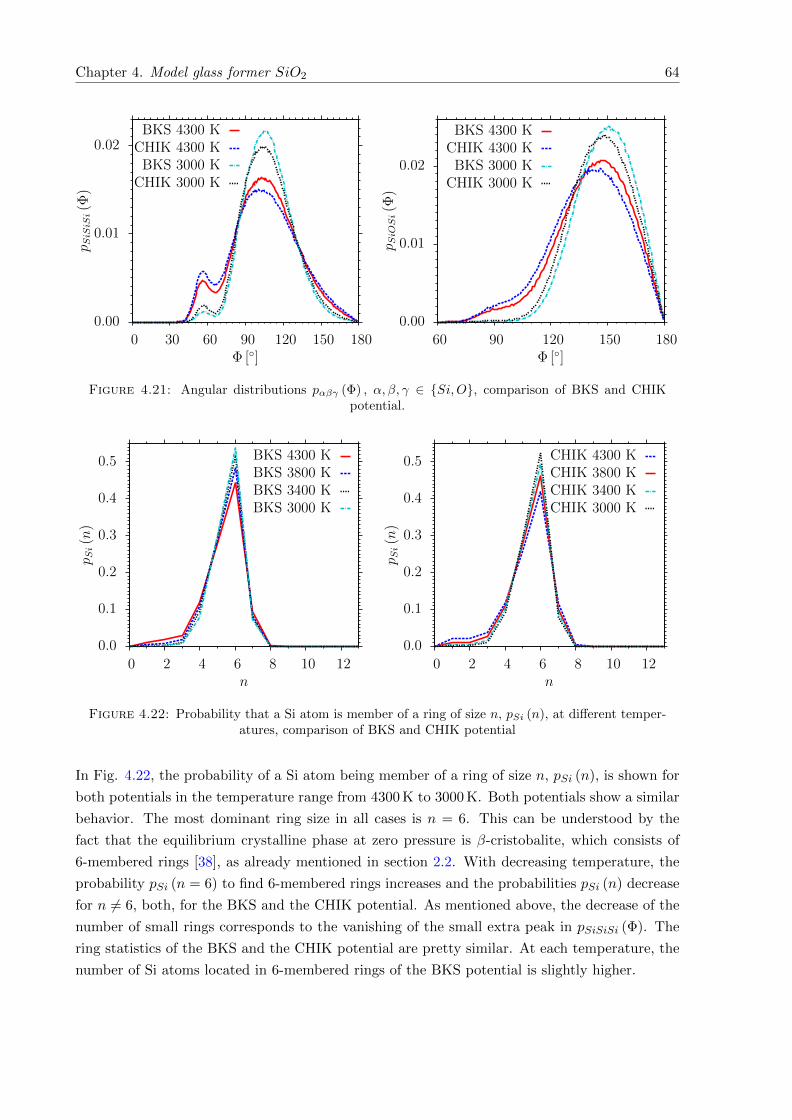
Chapter 4. Model glass former SiO2 64
0.00
0.01
0.02
0 30 60 90 120 150 180
p SiS
iSi(Φ
)
Φ []
BKS 4300 KCHIK 4300 K
BKS 3000 KCHIK 3000 K
0.00
0.01
0.02
60 90 120 150 180
p SiO
Si(Φ
)
Φ []
BKS 4300 KCHIK 4300 K
BKS 3000 KCHIK 3000 K
Figure 4.21: Angular distributions pαβγ (Φ) , α, β, γ ∈ Si,O, comparison of BKS and CHIKpotential.
0.0
0.1
0.2
0.3
0.4
0.5
0 2 4 6 8 10 12
p Si(n)
n
BKS 4300 KBKS 3800 KBKS 3400 KBKS 3000 K
0.0
0.1
0.2
0.3
0.4
0.5
0 2 4 6 8 10 12
p Si(n)
n
CHIK 4300 KCHIK 3800 KCHIK 3400 KCHIK 3000 K
Figure 4.22: Probability that a Si atom is member of a ring of size n, pSi (n), at different temper-atures, comparison of BKS and CHIK potential
In Fig. 4.22, the probability of a Si atom being member of a ring of size n, pSi (n), is shown for
both potentials in the temperature range from 4300 K to 3000 K. Both potentials show a similar
behavior. The most dominant ring size in all cases is n = 6. This can be understood by the
fact that the equilibrium crystalline phase at zero pressure is β-cristobalite, which consists of
6-membered rings [38], as already mentioned in section 2.2. With decreasing temperature, the
probability pSi (n = 6) to find 6-membered rings increases and the probabilities pSi (n) decrease
for n 6= 6, both, for the BKS and the CHIK potential. As mentioned above, the decrease of the
number of small rings corresponds to the vanishing of the small extra peak in pSiSiSi (Φ). The
ring statistics of the BKS and the CHIK potential are pretty similar. At each temperature, the
number of Si atoms located in 6-membered rings of the BKS potential is slightly higher.
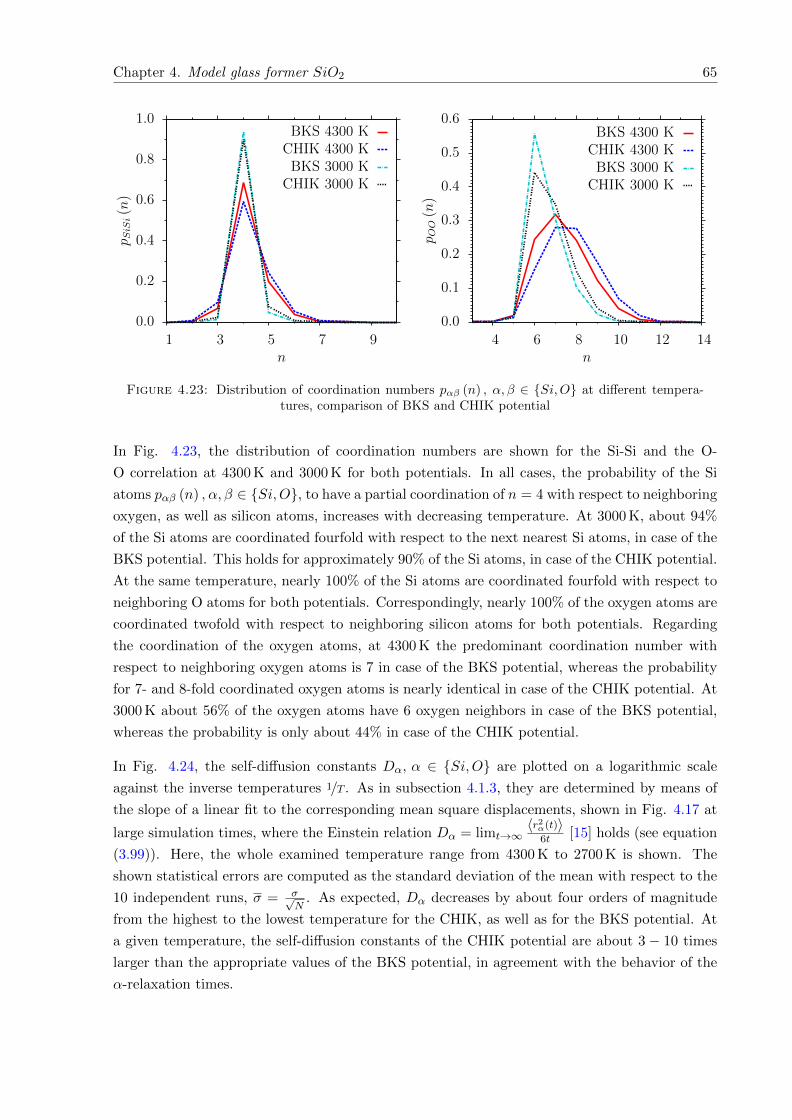
Chapter 4. Model glass former SiO2 65
0.0
0.2
0.4
0.6
0.8
1.0
1 3 5 7 9
p SiS
i(n)
n
BKS 4300 KCHIK 4300 KBKS 3000 K
CHIK 3000 K
0.0
0.1
0.2
0.3
0.4
0.5
0.6
4 6 8 10 12 14
p OO(n)
n
BKS 4300 KCHIK 4300 KBKS 3000 K
CHIK 3000 K
Figure 4.23: Distribution of coordination numbers pαβ (n) , α, β ∈ Si,O at different tempera-tures, comparison of BKS and CHIK potential
In Fig. 4.23, the distribution of coordination numbers are shown for the Si-Si and the O-
O correlation at 4300 K and 3000 K for both potentials. In all cases, the probability of the Si
atoms pαβ (n) , α, β ∈ Si,O, to have a partial coordination of n = 4 with respect to neighboring
oxygen, as well as silicon atoms, increases with decreasing temperature. At 3000 K, about 94%
of the Si atoms are coordinated fourfold with respect to the next nearest Si atoms, in case of the
BKS potential. This holds for approximately 90% of the Si atoms, in case of the CHIK potential.
At the same temperature, nearly 100% of the Si atoms are coordinated fourfold with respect to
neighboring O atoms for both potentials. Correspondingly, nearly 100% of the oxygen atoms are
coordinated twofold with respect to neighboring silicon atoms for both potentials. Regarding
the coordination of the oxygen atoms, at 4300 K the predominant coordination number with
respect to neighboring oxygen atoms is 7 in case of the BKS potential, whereas the probability
for 7- and 8-fold coordinated oxygen atoms is nearly identical in case of the CHIK potential. At
3000 K about 56% of the oxygen atoms have 6 oxygen neighbors in case of the BKS potential,
whereas the probability is only about 44% in case of the CHIK potential.
In Fig. 4.24, the self-diffusion constants Dα, α ∈ Si,O are plotted on a logarithmic scale
against the inverse temperatures 1/T . As in subsection 4.1.3, they are determined by means of
the slope of a linear fit to the corresponding mean square displacements, shown in Fig. 4.17 at
large simulation times, where the Einstein relation Dα = limt→∞〈r2α(t)〉6t [15] holds (see equation
(3.99)). Here, the whole examined temperature range from 4300 K to 2700 K is shown. The
shown statistical errors are computed as the standard deviation of the mean with respect to the
10 independent runs, σ = σ√N
. As expected, Dα decreases by about four orders of magnitude
from the highest to the lowest temperature for the CHIK, as well as for the BKS potential. At
a given temperature, the self-diffusion constants of the CHIK potential are about 3 − 10 times
larger than the appropriate values of the BKS potential, in agreement with the behavior of the
α-relaxation times.
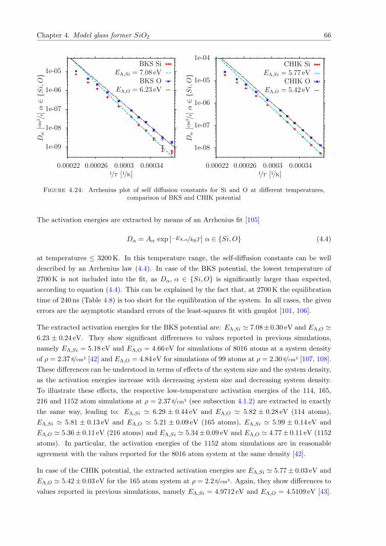
Chapter 4. Model glass former SiO2 66
1e-09
1e-08
1e-07
1e-06
1e-05
0.00022 0.00026 0.0003 0.00034
Dα[cm
2 /s]α∈Si,O
1/T [1/K]
BKS SiEA,Si = 7.08 eV
BKS OEA,O = 6.23 eV
1e-08
1e-07
1e-06
1e-05
1e-04
0.00022 0.00026 0.0003 0.00034
Dα[cm
2 /s]α∈Si,O
1/T [1/K]
CHIK SiEA,Si = 5.77 eV
CHIK OEA,O = 5.42 eV
Figure 4.24: Arrhenius plot of self diffusion constants for Si and O at different temperatures,comparison of BKS and CHIK potential
The activation energies are extracted by means of an Arrhenius fit [105]
Dα = Aα exp [−EA,α/kBT ] α ∈ Si,O (4.4)
at temperatures ≤ 3200 K. In this temperature range, the self-diffusion constants can be well
described by an Arrhenius law (4.4). In case of the BKS potential, the lowest temperature of
2700 K is not included into the fit, as Dα, α ∈ Si,O is significantly larger than expected,
according to equation (4.4). This can be explained by the fact that, at 2700 K the equilibration
time of 240 ns (Table 4.8) is too short for the equilibration of the system. In all cases, the given
errors are the asymptotic standard errors of the least-squares fit with gnuplot [101, 106].
The extracted activation energies for the BKS potential are: EA,Si ' 7.08±0.30 eV and EA,O '6.23 ± 0.24 eV. They show significant differences to values reported in previous simulations,
namely EA,Si = 5.18 eV and EA,O = 4.66 eV for simulations of 8016 atoms at a system density
of ρ = 2.37 g/cm3 [42] and EA,O = 4.84 eV for simulations of 99 atoms at ρ = 2.30 g/cm3 [107, 108].
These differences can be understood in terms of effects of the system size and the system density,
as the activation energies increase with decreasing system size and decreasing system density.
To illustrate these effects, the respective low-temperature activation energies of the 114, 165,
216 and 1152 atom simulations at ρ = 2.37 g/cm3 (see subsection 4.1.2) are extracted in exactly
the same way, leading to: EA,Si ' 6.29 ± 0.44 eV and EA,O ' 5.82 ± 0.28 eV (114 atoms),
EA,Si ' 5.81 ± 0.13 eV and EA,O ' 5.21 ± 0.09 eV (165 atoms), EA,Si ' 5.99 ± 0.14 eV and
EA,O ' 5.36± 0.11 eV (216 atoms) and EA,Si ' 5.34± 0.09 eV and EA,O ' 4.77± 0.11 eV (1152
atoms). In particular, the activation energies of the 1152 atom simulations are in reasonable
agreement with the values reported for the 8016 atom system at the same density [42].
In case of the CHIK potential, the extracted activation energies are EA,Si ' 5.77± 0.03 eV and
EA,O ' 5.42± 0.03 eV for the 165 atom system at ρ = 2.2 g/cm3. Again, they show differences to
values reported in previous simulations, namely EA,Si = 4.9712 eV and EA,O = 4.5109 eV [43].
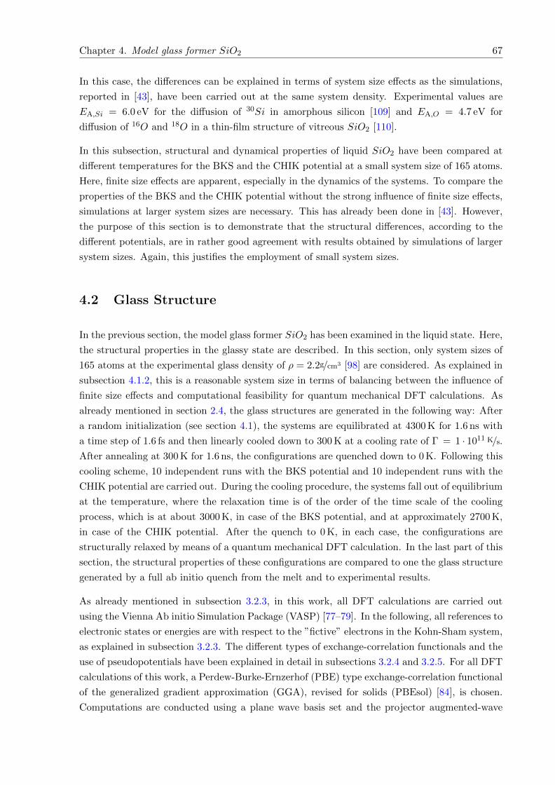
Chapter 4. Model glass former SiO2 67
In this case, the differences can be explained in terms of system size effects as the simulations,
reported in [43], have been carried out at the same system density. Experimental values are
EA,Si = 6.0 eV for the diffusion of 30Si in amorphous silicon [109] and EA,O = 4.7 eV for
diffusion of 16O and 18O in a thin-film structure of vitreous SiO2 [110].
In this subsection, structural and dynamical properties of liquid SiO2 have been compared at
different temperatures for the BKS and the CHIK potential at a small system size of 165 atoms.
Here, finite size effects are apparent, especially in the dynamics of the systems. To compare the
properties of the BKS and the CHIK potential without the strong influence of finite size effects,
simulations at larger system sizes are necessary. This has already been done in [43]. However,
the purpose of this section is to demonstrate that the structural differences, according to the
different potentials, are in rather good agreement with results obtained by simulations of larger
system sizes. Again, this justifies the employment of small system sizes.
4.2 Glass Structure
In the previous section, the model glass former SiO2 has been examined in the liquid state. Here,
the structural properties in the glassy state are described. In this section, only system sizes of
165 atoms at the experimental glass density of ρ = 2.2g/cm3 [98] are considered. As explained in
subsection 4.1.2, this is a reasonable system size in terms of balancing between the influence of
finite size effects and computational feasibility for quantum mechanical DFT calculations. As
already mentioned in section 2.4, the glass structures are generated in the following way: After
a random initialization (see section 4.1), the systems are equilibrated at 4300 K for 1.6 ns with
a time step of 1.6 fs and then linearly cooled down to 300 K at a cooling rate of Γ = 1 · 1011 K/s.
After annealing at 300 K for 1.6 ns, the configurations are quenched down to 0 K. Following this
cooling scheme, 10 independent runs with the BKS potential and 10 independent runs with the
CHIK potential are carried out. During the cooling procedure, the systems fall out of equilibrium
at the temperature, where the relaxation time is of the order of the time scale of the cooling
process, which is at about 3000 K, in case of the BKS potential, and at approximately 2700 K,
in case of the CHIK potential. After the quench to 0 K, in each case, the configurations are
structurally relaxed by means of a quantum mechanical DFT calculation. In the last part of this
section, the structural properties of these configurations are compared to one the glass structure
generated by a full ab initio quench from the melt and to experimental results.
As already mentioned in subsection 3.2.3, in this work, all DFT calculations are carried out
using the Vienna Ab initio Simulation Package (VASP) [77–79]. In the following, all references to
electronic states or energies are with respect to the ”fictive” electrons in the Kohn-Sham system,
as explained in subsection 3.2.3. The different types of exchange-correlation functionals and the
use of pseudopotentials have been explained in detail in subsections 3.2.4 and 3.2.5. For all DFT
calculations of this work, a Perdew-Burke-Ernzerhof (PBE) type exchange-correlation functional
of the generalized gradient approximation (GGA), revised for solids (PBEsol) [84], is chosen.
Computations are conducted using a plane wave basis set and the projector augmented-wave
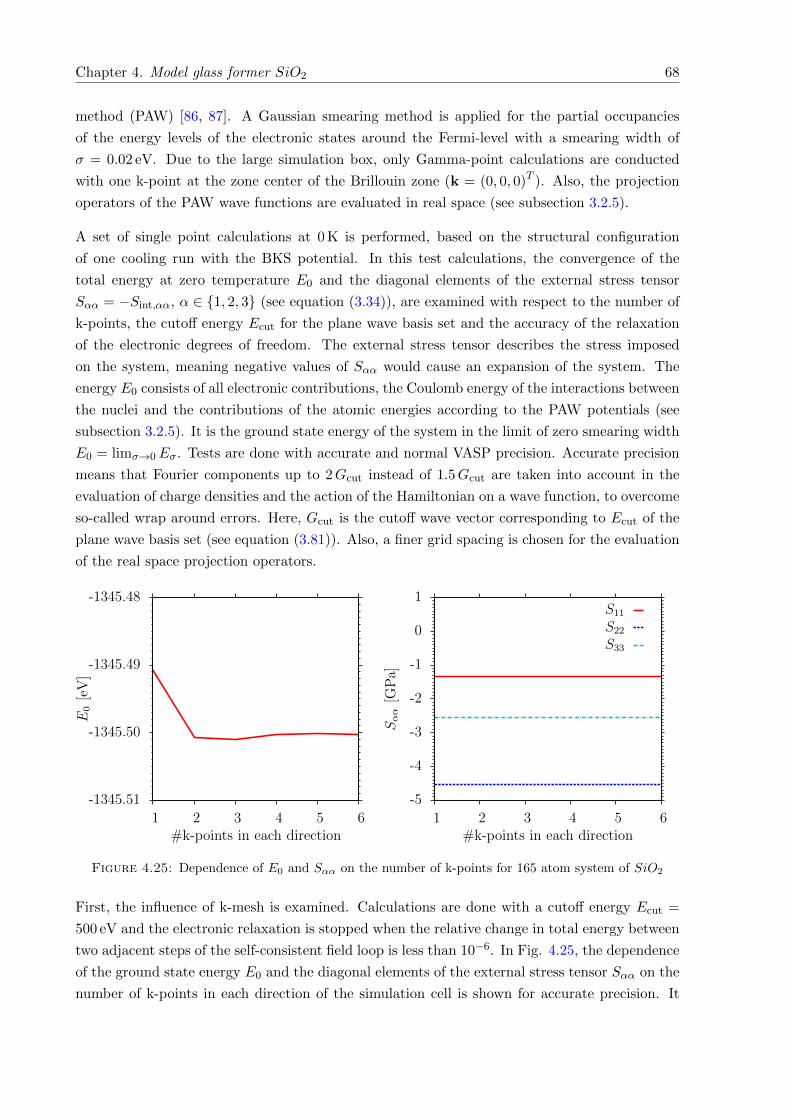
Chapter 4. Model glass former SiO2 68
method (PAW) [86, 87]. A Gaussian smearing method is applied for the partial occupancies
of the energy levels of the electronic states around the Fermi-level with a smearing width of
σ = 0.02 eV. Due to the large simulation box, only Gamma-point calculations are conducted
with one k-point at the zone center of the Brillouin zone (k = (0, 0, 0)T ). Also, the projection
operators of the PAW wave functions are evaluated in real space (see subsection 3.2.5).
A set of single point calculations at 0 K is performed, based on the structural configuration
of one cooling run with the BKS potential. In this test calculations, the convergence of the
total energy at zero temperature E0 and the diagonal elements of the external stress tensor
Sαα = −Sint,αα, α ∈ 1, 2, 3 (see equation (3.34)), are examined with respect to the number of
k-points, the cutoff energy Ecut for the plane wave basis set and the accuracy of the relaxation
of the electronic degrees of freedom. The external stress tensor describes the stress imposed
on the system, meaning negative values of Sαα would cause an expansion of the system. The
energy E0 consists of all electronic contributions, the Coulomb energy of the interactions between
the nuclei and the contributions of the atomic energies according to the PAW potentials (see
subsection 3.2.5). It is the ground state energy of the system in the limit of zero smearing width
E0 = limσ→0Eσ. Tests are done with accurate and normal VASP precision. Accurate precision
means that Fourier components up to 2Gcut instead of 1.5Gcut are taken into account in the
evaluation of charge densities and the action of the Hamiltonian on a wave function, to overcome
so-called wrap around errors. Here, Gcut is the cutoff wave vector corresponding to Ecut of the
plane wave basis set (see equation (3.81)). Also, a finer grid spacing is chosen for the evaluation
of the real space projection operators.
-1345.51
-1345.50
-1345.49
-1345.48
1 2 3 4 5 6
E0[eV]
#k-points in each direction
-5
-4
-3
-2
-1
0
1
1 2 3 4 5 6
Sαα[G
Pa]
#k-points in each direction
S11
S22
S33
Figure 4.25: Dependence of E0 and Sαα on the number of k-points for 165 atom system of SiO2
First, the influence of k-mesh is examined. Calculations are done with a cutoff energy Ecut =
500 eV and the electronic relaxation is stopped when the relative change in total energy between
two adjacent steps of the self-consistent field loop is less than 10−6. In Fig. 4.25, the dependence
of the ground state energy E0 and the diagonal elements of the external stress tensor Sαα on the
number of k-points in each direction of the simulation cell is shown for accurate precision. It
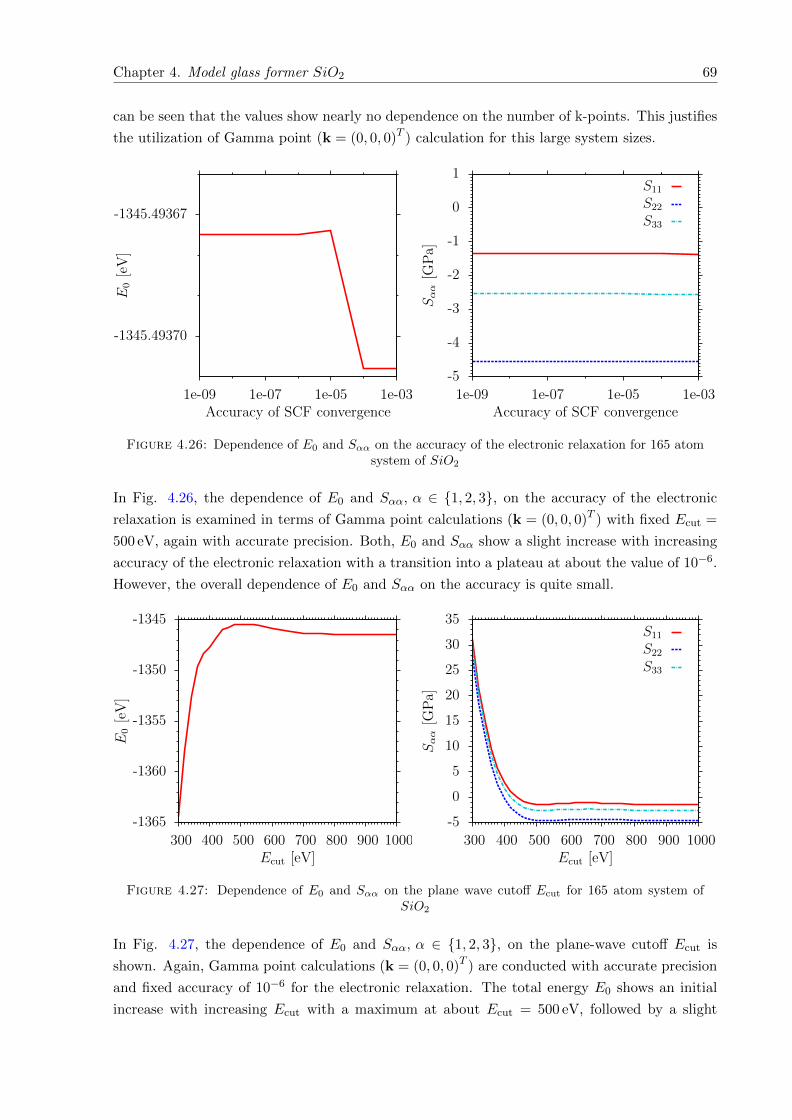
Chapter 4. Model glass former SiO2 69
can be seen that the values show nearly no dependence on the number of k-points. This justifies
the utilization of Gamma point (k = (0, 0, 0)T ) calculation for this large system sizes.
-1345.49370
-1345.49367
1e-09 1e-07 1e-05 1e-03
E0[eV]
Accuracy of SCF convergence
-5
-4
-3
-2
-1
0
1
1e-09 1e-07 1e-05 1e-03
Sαα[G
Pa]
Accuracy of SCF convergence
S11
S22
S33
Figure 4.26: Dependence of E0 and Sαα on the accuracy of the electronic relaxation for 165 atomsystem of SiO2
In Fig. 4.26, the dependence of E0 and Sαα, α ∈ 1, 2, 3, on the accuracy of the electronic
relaxation is examined in terms of Gamma point calculations (k = (0, 0, 0)T ) with fixed Ecut =
500 eV, again with accurate precision. Both, E0 and Sαα show a slight increase with increasing
accuracy of the electronic relaxation with a transition into a plateau at about the value of 10−6.
However, the overall dependence of E0 and Sαα on the accuracy is quite small.
-1365
-1360
-1355
-1350
-1345
300 400 500 600 700 800 900 1000
E0[eV]
Ecut [eV]
-5
0
5
10
15
20
25
30
35
300 400 500 600 700 800 900 1000
Sαα[G
Pa]
Ecut [eV]
S11
S22
S33
Figure 4.27: Dependence of E0 and Sαα on the plane wave cutoff Ecut for 165 atom system ofSiO2
In Fig. 4.27, the dependence of E0 and Sαα, α ∈ 1, 2, 3, on the plane-wave cutoff Ecut is
shown. Again, Gamma point calculations (k = (0, 0, 0)T ) are conducted with accurate precision
and fixed accuracy of 10−6 for the electronic relaxation. The total energy E0 shows an initial
increase with increasing Ecut with a maximum at about Ecut = 500 eV, followed by a slight
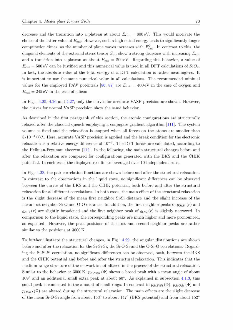
Chapter 4. Model glass former SiO2 70
decrease and the transition into a plateau at about Ecut = 800 eV. This would motivate the
choice of the latter value of Ecut. However, such a high cutoff energy leads to significantly longer
computation times, as the number of plane waves increases with E2cut. In contrast to this, the
diagonal elements of the external stress tensor Sαα show a strong decrease with increasing Ecut
and a transition into a plateau at about Ecut = 500 eV. Regarding this behavior, a value of
Ecut = 500 eV can be justified and this numerical value is used in all DFT calculations of SiO2.
In fact, the absolute value of the total energy of a DFT calculation is rather meaningless. It
is important to use the same numerical value in all calculations. The recommended minimal
values for the employed PAW potentials [86, 87] are Ecut = 400 eV in the case of oxygen and
Ecut = 245 eV in the case of silicon.
In Figs. 4.25, 4.26 and 4.27, only the curves for accurate VASP precision are shown. However,
the curves for normal VASP precision show the same behavior.
As described in the first paragraph of this section, the atomic configurations are structurally
relaxed after the classical quench employing a conjugate gradient algorithm [111]. The system
volume is fixed and the relaxation is stopped when all forces on the atoms are smaller than
5 ·10−4 eV/A. Here, accurate VASP precision is applied and the break condition for the electronic
relaxation is a relative energy difference of 10−8. The DFT forces are calculated, according to
the Hellman-Feynman theorem [112]. In the following, the main structural changes before and
after the relaxation are compared for configurations generated with the BKS and the CHIK
potential. In each case, the displayed results are averaged over 10 independent runs.
In Fig. 4.28, the pair correlation functions are shown before and after the structural relaxation.
In contrast to the observations in the liquid state, no significant differences can be observed
between the curves of the BKS and the CHIK potential, both before and after the structural
relaxation for all different correlations. In both cases, the main effect of the structural relaxation
is the slight decrease of the mean first neighbor Si-Si distance and the slight increase of the
mean first neighbor Si-O and O-O distance. In addition, the first neighbor peaks of gSiSi (r) and
gSiO (r) are slightly broadened and the first neighbor peak of gOO (r) is slightly narrowed. In
comparison to the liquid state, the corresponding peaks are much higher and more pronounced,
as expected. However, the peak positions of the first and second-neighbor peaks are rather
similar to the positions at 3000 K.
To further illustrate the structural changes, in Fig. 4.29, the angular distributions are shown
before and after the relaxation for the Si-Si-Si, the Si-O-Si and the O-Si-O correlations. Regard-
ing the Si-Si-Si correlation, no significant differences can be observed, both, between the BKS
and the CHIK potential and before and after the structural relaxation. This indicates that the
medium-range structure of the network is not altered in the process of the structural relaxation.
Similar to the behavior at 3000 K, pSiSiSi (Φ) shows a broad peak with a mean angle of about
109 and an additional small extra peak at about 60. As explained in subsection 4.1.3, this
small peak is connected to the amount of small rings. In contrast to pSiSiSi (Φ), pSiOSi (Φ) and
pOSiO (Φ) are altered during the structural relaxation. The main effects are the slight decrease
of the mean Si-O-Si angle from about 153 to about 147 (BKS potential) and from about 152
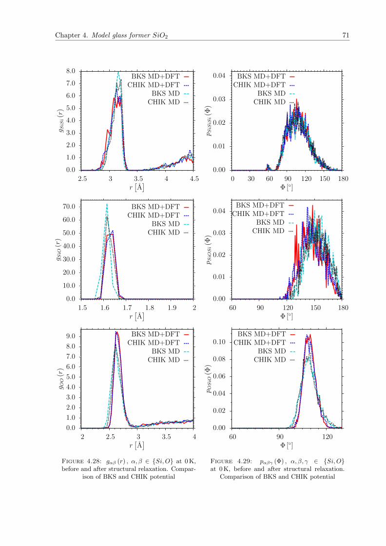
Chapter 4. Model glass former SiO2 71
0.0
1.0
2.0
3.0
4.0
5.0
6.0
7.0
8.0
2.5 3 3.5 4 4.5
g SiS
i(r
)
r[A]
BKS MD+DFTCHIK MD+DFT
BKS MDCHIK MD
0.0
10.0
20.0
30.0
40.0
50.0
60.0
70.0
1.5 1.6 1.7 1.8 1.9 2
g SiO
(r)
r[A]
BKS MD+DFTCHIK MD+DFT
BKS MDCHIK MD
0.0
1.0
2.0
3.0
4.0
5.0
6.0
7.0
8.0
9.0
2 2.5 3 3.5 4
g OO
(r)
r[A]
BKS MD+DFTCHIK MD+DFT
BKS MDCHIK MD
Figure 4.28: gαβ (r) , α, β ∈ Si,O at 0 K,before and after structural relaxation. Compar-
ison of BKS and CHIK potential
0.00
0.01
0.02
0.03
0.04
0 30 60 90 120 150 180
p SiS
iSi(Φ
)
Φ []
BKS MD+DFTCHIK MD+DFT
BKS MDCHIK MD
0.00
0.01
0.02
0.03
0.04
60 90 120 150 180
p SiO
Si(Φ
)
Φ []
BKS MD+DFTCHIK MD+DFT
BKS MDCHIK MD
0.00
0.02
0.04
0.06
0.08
0.10
60 90 120
p OSiO
(Φ)
Φ []
BKS MD+DFTCHIK MD+DFT
BKS MDCHIK MD
Figure 4.29: pαβγ (Φ) , α, β, γ ∈ Si,Oat 0 K, before and after structural relaxation.
Comparison of BKS and CHIK potential
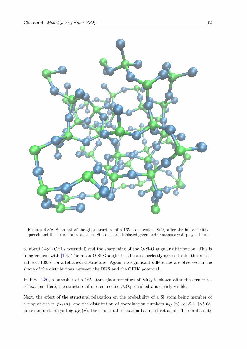
Chapter 4. Model glass former SiO2 72
Figure 4.30: Snapshot of the glass structure of a 165 atom system SiO2 after the full ab initioquench and the structural relaxation. Si atoms are displayed green and O atoms are displayed blue.
to about 148 (CHIK potential) and the sharpening of the O-Si-O angular distribution. This is
in agreement with [10]. The mean O-Si-O angle, in all cases, perfectly agrees to the theoretical
value of 109.5 for a tetrahedral structure. Again, no significant differences are observed in the
shape of the distributions between the BKS and the CHIK potential.
In Fig. 4.30, a snapshot of a 165 atom glass structure of SiO2 is shown after the structural
relaxation. Here, the structure of interconnected SiO4 tetrahedra is clearly visible.
Next, the effect of the structural relaxation on the probability of a Si atom being member of
a ring of size n, pSi (n), and the distribution of coordination numbers pαβ (n) , α, β ∈ Si,Oare examined. Regarding pSi (n), the structural relaxation has no effect at all. The probability
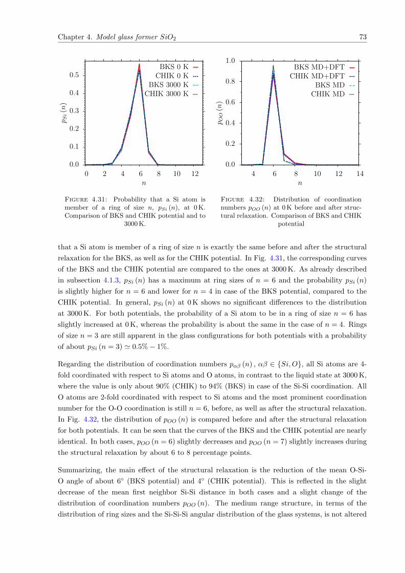
Chapter 4. Model glass former SiO2 73
0.0
0.1
0.2
0.3
0.4
0.5
0 2 4 6 8 10 12
p Si(n)
n
BKS 0 KCHIK 0 K
BKS 3000 KCHIK 3000 K
Figure 4.31: Probability that a Si atom ismember of a ring of size n, pSi (n), at 0 K.Comparison of BKS and CHIK potential and to
3000 K.
0.0
0.2
0.4
0.6
0.8
1.0
4 6 8 10 12 14
p OO(n)
n
BKS MD+DFTCHIK MD+DFT
BKS MDCHIK MD
Figure 4.32: Distribution of coordinationnumbers pOO (n) at 0 K before and after struc-tural relaxation. Comparison of BKS and CHIK
potential
that a Si atom is member of a ring of size n is exactly the same before and after the structural
relaxation for the BKS, as well as for the CHIK potential. In Fig. 4.31, the corresponding curves
of the BKS and the CHIK potential are compared to the ones at 3000 K. As already described
in subsection 4.1.3, pSi (n) has a maximum at ring sizes of n = 6 and the probability pSi (n)
is slightly higher for n = 6 and lower for n = 4 in case of the BKS potential, compared to the
CHIK potential. In general, pSi (n) at 0 K shows no significant differences to the distribution
at 3000 K. For both potentials, the probability of a Si atom to be in a ring of size n = 6 has
slightly increased at 0 K, whereas the probability is about the same in the case of n = 4. Rings
of size n = 3 are still apparent in the glass configurations for both potentials with a probability
of about pSi (n = 3) ' 0.5%− 1%.
Regarding the distribution of coordination numbers pαβ (n) , αβ ∈ Si,O, all Si atoms are 4-
fold coordinated with respect to Si atoms and O atoms, in contrast to the liquid state at 3000 K,
where the value is only about 90% (CHIK) to 94% (BKS) in case of the Si-Si coordination. All
O atoms are 2-fold coordinated with respect to Si atoms and the most prominent coordination
number for the O-O coordination is still n = 6, before, as well as after the structural relaxation.
In Fig. 4.32, the distribution of pOO (n) is compared before and after the structural relaxation
for both potentials. It can be seen that the curves of the BKS and the CHIK potential are nearly
identical. In both cases, pOO (n = 6) slightly decreases and pOO (n = 7) slightly increases during
the structural relaxation by about 6 to 8 percentage points.
Summarizing, the main effect of the structural relaxation is the reduction of the mean O-Si-
O angle of about 6 (BKS potential) and 4 (CHIK potential). This is reflected in the slight
decrease of the mean first neighbor Si-Si distance in both cases and a slight change of the
distribution of coordination numbers pOO (n). The medium range structure, in terms of the
distribution of ring sizes and the Si-Si-Si angular distribution of the glass systems, is not altered
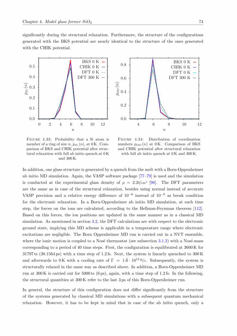
Chapter 4. Model glass former SiO2 74
significantly during the structural relaxation. Furthermore, the structure of the configurations
generated with the BKS potential are nearly identical to the structure of the ones generated
with the CHIK potential.
0.0
0.1
0.2
0.3
0.4
0.5
0 2 4 6 8 10 12
p Si(n)
n
BKS 0 KCHIK 0 KDFT 0 K
DFT 300 K
Figure 4.33: Probability that a Si atom ismember of a ring of size n, pSi (n), at 0 K. Com-parison of BKS and CHIK potential after struc-tural relaxation with full ab initio quench at 0 K
and 300 K.
0.0
0.2
0.4
0.6
0.8
4 6 8 10 12
p OO(n)
n
BKS 0 KCHIK 0 KDFT 0 K
DFT 300 K
Figure 4.34: Distribution of coordinationnumbers pOO (n) at 0 K. Comparison of BKSand CHIK potential after structural relaxation
with full ab initio quench at 0 K and 300 K.
In addition, one glass structure is generated by a quench from the melt with a Born-Oppenheimer
ab initio MD simulation. Again, the VASP software package [77–79] is used and the simulation
is conducted at the experimental glass density of ρ = 2.2g/cm3 [98]. The DFT parameters
are the same as in case of the structural relaxation, besides using normal instead of accurate
VASP precision and a relative energy difference of 10−6 instead of 10−8 as break condition
for the electronic relaxation. In a Born-Oppenheimer ab initio MD simulation, at each time
step, the forces on the ions are calculated, according to the Hellman-Feynman theorem [112].
Based on this forces, the ion positions are updated in the same manner as in a classical MD
simulation. As mentioned in section 3.2, the DFT calculations are with respect to the electronic
ground state, implying this MD scheme is applicable in a temperature range where electronic
excitations are negligible. The Born Oppenheimer MD run is carried out in a NVT ensemble,
where the ionic motion is coupled to a Nose thermostat (see subsection 3.1.2) with a Nose-mass
corresponding to a period of 40 time steps. First, the configuration is equilibrated at 3600 K for
31797 ts (38.1564 ps) with a time step of 1.2 fs. Next, the system is linearly quenched to 300 K
and afterwards to 0 K with a cooling rate of Γ = 1.6 · 1014 K/s. Subsequently, the system is
structurally relaxed in the same way as described above. In addition, a Born-Oppenheimer MD
run at 300 K is carried out for 5000 ts (6 ps), again, with a time step of 1.2 fs. In the following,
the structural quantities at 300 K refer to the last 3 ps of this Born-Oppenheimer run.
In general, the structure of this configuration does not differ significantly from the structure
of the systems generated by classical MD simulations with a subsequent quantum mechanical
relaxation. However, it has to be kept in mind that in case of the ab initio quench, only a
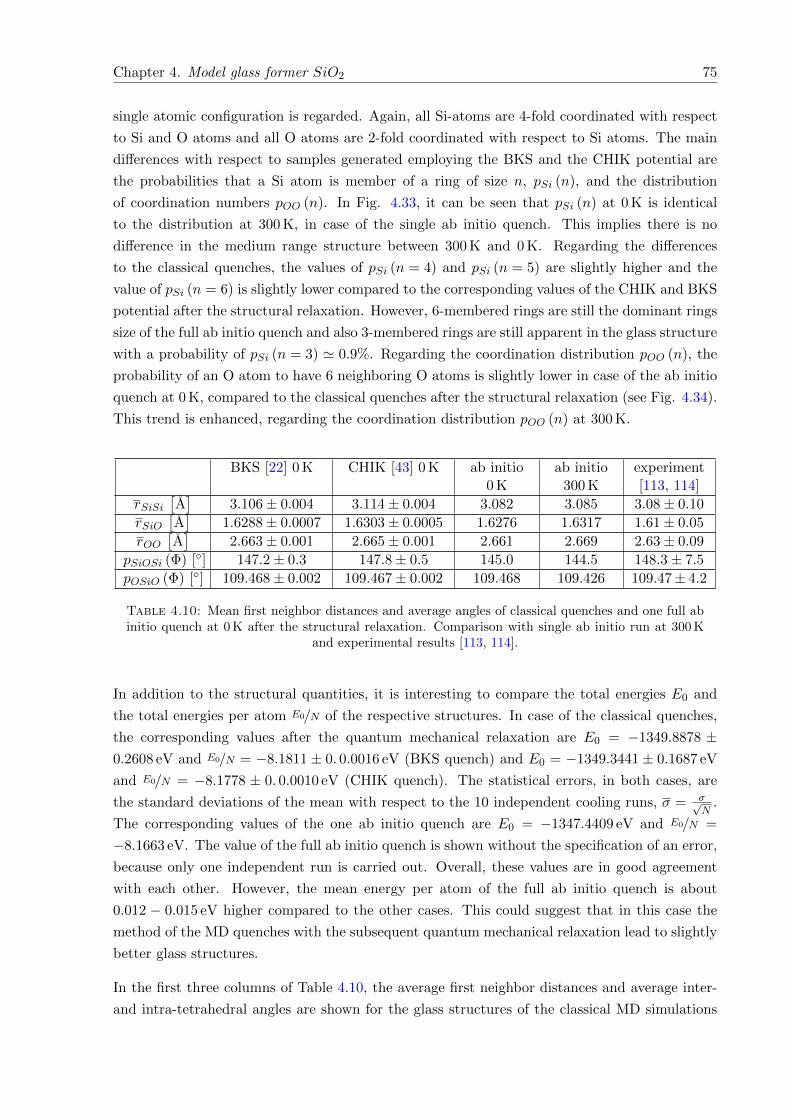
Chapter 4. Model glass former SiO2 75
single atomic configuration is regarded. Again, all Si-atoms are 4-fold coordinated with respect
to Si and O atoms and all O atoms are 2-fold coordinated with respect to Si atoms. The main
differences with respect to samples generated employing the BKS and the CHIK potential are
the probabilities that a Si atom is member of a ring of size n, pSi (n), and the distribution
of coordination numbers pOO (n). In Fig. 4.33, it can be seen that pSi (n) at 0 K is identical
to the distribution at 300 K, in case of the single ab initio quench. This implies there is no
difference in the medium range structure between 300 K and 0 K. Regarding the differences
to the classical quenches, the values of pSi (n = 4) and pSi (n = 5) are slightly higher and the
value of pSi (n = 6) is slightly lower compared to the corresponding values of the CHIK and BKS
potential after the structural relaxation. However, 6-membered rings are still the dominant rings
size of the full ab initio quench and also 3-membered rings are still apparent in the glass structure
with a probability of pSi (n = 3) ' 0.9%. Regarding the coordination distribution pOO (n), the
probability of an O atom to have 6 neighboring O atoms is slightly lower in case of the ab initio
quench at 0 K, compared to the classical quenches after the structural relaxation (see Fig. 4.34).
This trend is enhanced, regarding the coordination distribution pOO (n) at 300 K.
BKS [22] 0 K CHIK [43] 0 K ab initio0 K
ab initio300 K
experiment[113, 114]
rSiSi[A]
3.106± 0.004 3.114± 0.004 3.082 3.085 3.08± 0.10
rSiO[A]
1.6288± 0.0007 1.6303± 0.0005 1.6276 1.6317 1.61± 0.05
rOO[A]
2.663± 0.001 2.665± 0.001 2.661 2.669 2.63± 0.09
pSiOSi (Φ) [] 147.2± 0.3 147.8± 0.5 145.0 144.5 148.3± 7.5
pOSiO (Φ) [] 109.468± 0.002 109.467± 0.002 109.468 109.426 109.47± 4.2
Table 4.10: Mean first neighbor distances and average angles of classical quenches and one full abinitio quench at 0 K after the structural relaxation. Comparison with single ab initio run at 300 K
and experimental results [113, 114].
In addition to the structural quantities, it is interesting to compare the total energies E0 and
the total energies per atom E0/N of the respective structures. In case of the classical quenches,
the corresponding values after the quantum mechanical relaxation are E0 = −1349.8878 ±0.2608 eV and E0/N = −8.1811 ± 0. 0.0016 eV (BKS quench) and E0 = −1349.3441 ± 0.1687 eV
and E0/N = −8.1778 ± 0. 0.0010 eV (CHIK quench). The statistical errors, in both cases, are
the standard deviations of the mean with respect to the 10 independent cooling runs, σ = σ√N
.
The corresponding values of the one ab initio quench are E0 = −1347.4409 eV and E0/N =
−8.1663 eV. The value of the full ab initio quench is shown without the specification of an error,
because only one independent run is carried out. Overall, these values are in good agreement
with each other. However, the mean energy per atom of the full ab initio quench is about
0.012 − 0.015 eV higher compared to the other cases. This could suggest that in this case the
method of the MD quenches with the subsequent quantum mechanical relaxation lead to slightly
better glass structures.
In the first three columns of Table 4.10, the average first neighbor distances and average inter-
and intra-tetrahedral angles are shown for the glass structures of the classical MD simulations
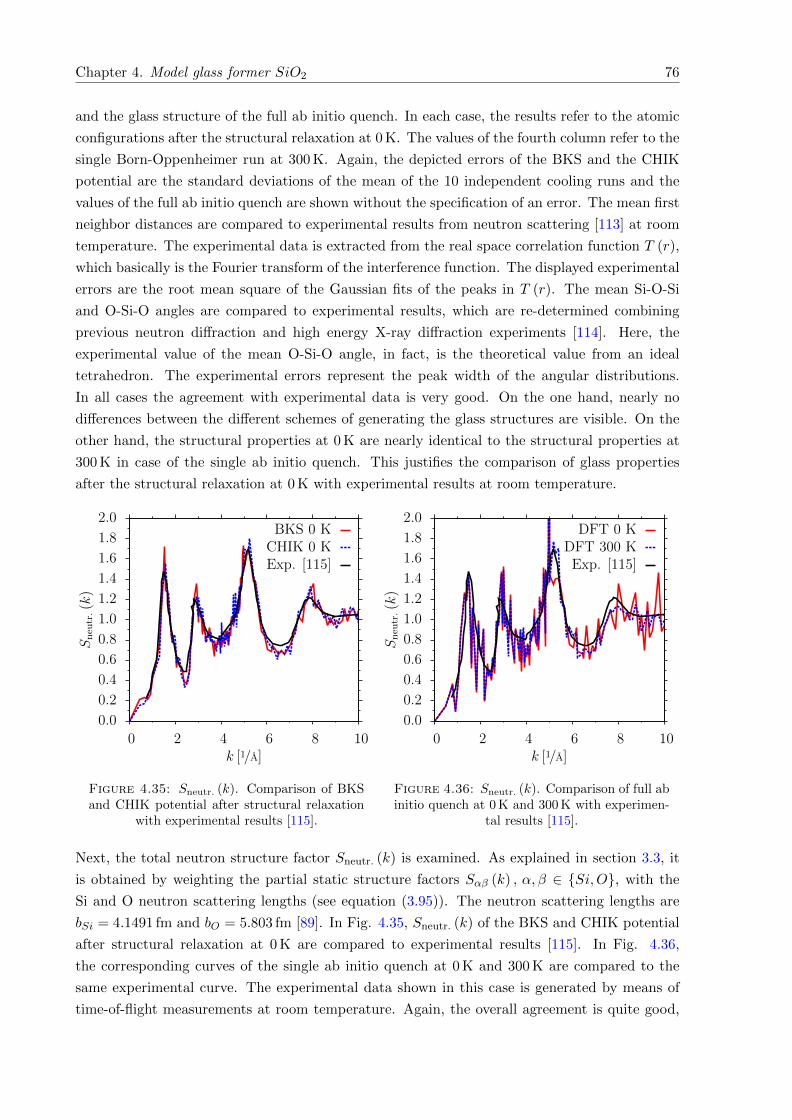
Chapter 4. Model glass former SiO2 76
and the glass structure of the full ab initio quench. In each case, the results refer to the atomic
configurations after the structural relaxation at 0 K. The values of the fourth column refer to the
single Born-Oppenheimer run at 300 K. Again, the depicted errors of the BKS and the CHIK
potential are the standard deviations of the mean of the 10 independent cooling runs and the
values of the full ab initio quench are shown without the specification of an error. The mean first
neighbor distances are compared to experimental results from neutron scattering [113] at room
temperature. The experimental data is extracted from the real space correlation function T (r),
which basically is the Fourier transform of the interference function. The displayed experimental
errors are the root mean square of the Gaussian fits of the peaks in T (r). The mean Si-O-Si
and O-Si-O angles are compared to experimental results, which are re-determined combining
previous neutron diffraction and high energy X-ray diffraction experiments [114]. Here, the
experimental value of the mean O-Si-O angle, in fact, is the theoretical value from an ideal
tetrahedron. The experimental errors represent the peak width of the angular distributions.
In all cases the agreement with experimental data is very good. On the one hand, nearly no
differences between the different schemes of generating the glass structures are visible. On the
other hand, the structural properties at 0 K are nearly identical to the structural properties at
300 K in case of the single ab initio quench. This justifies the comparison of glass properties
after the structural relaxation at 0 K with experimental results at room temperature.
0.0
0.2
0.4
0.6
0.8
1.0
1.2
1.4
1.6
1.8
2.0
0 2 4 6 8 10
Sn
eutr
.(k)
k [1/A]
BKS 0 KCHIK 0 KExp. [115]
Figure 4.35: Sneutr. (k). Comparison of BKSand CHIK potential after structural relaxation
with experimental results [115].
0.0
0.2
0.4
0.6
0.8
1.0
1.2
1.4
1.6
1.8
2.0
0 2 4 6 8 10
Sn
eutr
.(k)
k [1/A]
DFT 0 KDFT 300 KExp. [115]
Figure 4.36: Sneutr. (k). Comparison of full abinitio quench at 0 K and 300 K with experimen-
tal results [115].
Next, the total neutron structure factor Sneutr. (k) is examined. As explained in section 3.3, it
is obtained by weighting the partial static structure factors Sαβ (k) , α, β ∈ Si,O, with the
Si and O neutron scattering lengths (see equation (3.95)). The neutron scattering lengths are
bSi = 4.1491 fm and bO = 5.803 fm [89]. In Fig. 4.35, Sneutr. (k) of the BKS and CHIK potential
after structural relaxation at 0 K are compared to experimental results [115]. In Fig. 4.36,
the corresponding curves of the single ab initio quench at 0 K and 300 K are compared to the
same experimental curve. The experimental data shown in this case is generated by means of
time-of-flight measurements at room temperature. Again, the overall agreement is quite good,
Chapter 4. Model glass former SiO2 77
in all cases. Nearly no difference is visible between the ab initio results at 0 K and 300 K. The
greatest differences between the experimental data and the simulation results are visible in the
position of first sharp diffraction peak (FSDP) (see 4.1.2). The experimental peak is located
at about k = 1.45 A−1
. In case of the single ab initio quench the peak position is about the
same, whereas the position of the BKS and the CHIK potential after the structural relaxation
is shifted to slightly larger k-values by approximately k = 0.1 A−1
. However, the curve of the
single ab initio quench is much more noisy.
4.3 Vibrational Properties
In this section, different vibrational properties of the model glass former SiO2 are examined and
compared with experimental results. As explained in section 3.4, the thermal occupation of the
phonon density of states g (ν) (see equation (3.109)) or the respective eigenmodes with eigenfre-
quencies νn, gives access to the thermodynamic properties at low temperatures. In principle, the
vibrational density of states includes harmonic and anharmonic terms. However, the importance
of anharmonic terms decreases with decreasing temperature and at low temperatures, g (ν) can
be well described in terms of the harmonic approximation. Therefore, in this section all vibra-
tional properties are calculated employing the so-called ”frozen phonon” method. For a detailed
description, see section 3.4. In this approach, the vibrational properties are described in terms
of the dynamical matrix Dαβ;i,j (k), α, β, ∈ 1, 2, 3 and i, j, ∈ 1, N (see equation (3.107)).
The latter is based on the force constant matrix Φαβ;i,j (see equation (3.105)). In this approach,
the glass structures are treated as crystalline structures with a large unit cell containing all 165
atoms.
In principle, it is favorable to consider larger supercells of the original system to increase the
accuracy of the calculation. However, the 165 atom system is already quite large regarding
quantum mechanical calculations. As a consequence, the calculations of the vibrational proper-
ties of vitreous SiO2 are restricted to the original system size. In this section, the vibrational
properties, due to quantum mechanical forces are compared to the vibrational properties, due to
the BKS [22] and the CHIK [43] potential. The basis for calculating the vibrational properties
are the corresponding glass configurations at 0 K after structural relaxation, as explained in
section 4.2. Ideally, in these structures the forces on all atoms are equal to zero. To calculate
the vibrational spectra for the BKS and the CHIK potential, also a structural relaxation of the
configurations at 0 K is performed with respect to the classical forces. Again, this is done by
means of a conjugate gradient algorithm [111]. After the structural relaxation, in each case,
all atoms i ∈ 1, N are displaced by ∆rα;i = ± 0.02 A, α 1, 2, 3 and the forces on all atoms
Fα;i (∆rβ;j) are computed. Again, all quantum mechanical calculations are conducted with the
VASP package, using the same DFT parameters as in section 4.2 for the structural relaxation
and the DFT forces are calculated, according to the Hellman-Feynman theorem [112]. The
classical forces are computed with the LAMMPS package [60, 61].
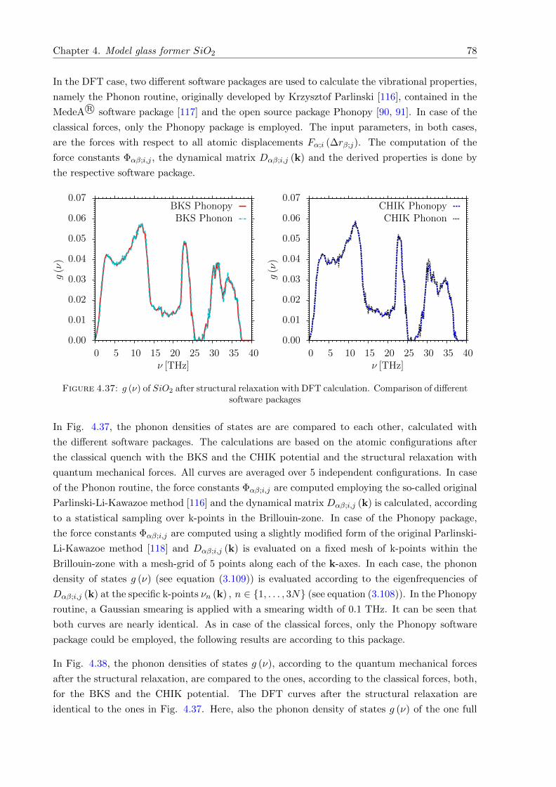
Chapter 4. Model glass former SiO2 78
In the DFT case, two different software packages are used to calculate the vibrational properties,
namely the Phonon routine, originally developed by Krzysztof Parlinski [116], contained in the
MedeA R© software package [117] and the open source package Phonopy [90, 91]. In case of the
classical forces, only the Phonopy package is employed. The input parameters, in both cases,
are the forces with respect to all atomic displacements Fα;i (∆rβ;j). The computation of the
force constants Φαβ;i,j , the dynamical matrix Dαβ;i,j (k) and the derived properties is done by
the respective software package.
0.00
0.01
0.02
0.03
0.04
0.05
0.06
0.07
0 5 10 15 20 25 30 35 40
g(ν)
ν [THz]
BKS PhonopyBKS Phonon
0.00
0.01
0.02
0.03
0.04
0.05
0.06
0.07
0 5 10 15 20 25 30 35 40
g(ν)
ν [THz]
CHIK PhonopyCHIK Phonon
Figure 4.37: g (ν) of SiO2 after structural relaxation with DFT calculation. Comparison of differentsoftware packages
In Fig. 4.37, the phonon densities of states are are compared to each other, calculated with
the different software packages. The calculations are based on the atomic configurations after
the classical quench with the BKS and the CHIK potential and the structural relaxation with
quantum mechanical forces. All curves are averaged over 5 independent configurations. In case
of the Phonon routine, the force constants Φαβ;i,j are computed employing the so-called original
Parlinski-Li-Kawazoe method [116] and the dynamical matrix Dαβ;i,j (k) is calculated, according
to a statistical sampling over k-points in the Brillouin-zone. In case of the Phonopy package,
the force constants Φαβ;i,j are computed using a slightly modified form of the original Parlinski-
Li-Kawazoe method [118] and Dαβ;i,j (k) is evaluated on a fixed mesh of k-points within the
Brillouin-zone with a mesh-grid of 5 points along each of the k-axes. In each case, the phonon
density of states g (ν) (see equation (3.109)) is evaluated according to the eigenfrequencies of
Dαβ;i,j (k) at the specific k-points νn (k) , n ∈ 1, . . . , 3N (see equation (3.108)). In the Phonopy
routine, a Gaussian smearing is applied with a smearing width of 0.1 THz. It can be seen that
both curves are nearly identical. As in case of the classical forces, only the Phonopy software
package could be employed, the following results are according to this package.
In Fig. 4.38, the phonon densities of states g (ν), according to the quantum mechanical forces
after the structural relaxation, are compared to the ones, according to the classical forces, both,
for the BKS and the CHIK potential. The DFT curves after the structural relaxation are
identical to the ones in Fig. 4.37. Here, also the phonon density of states g (ν) of the one full
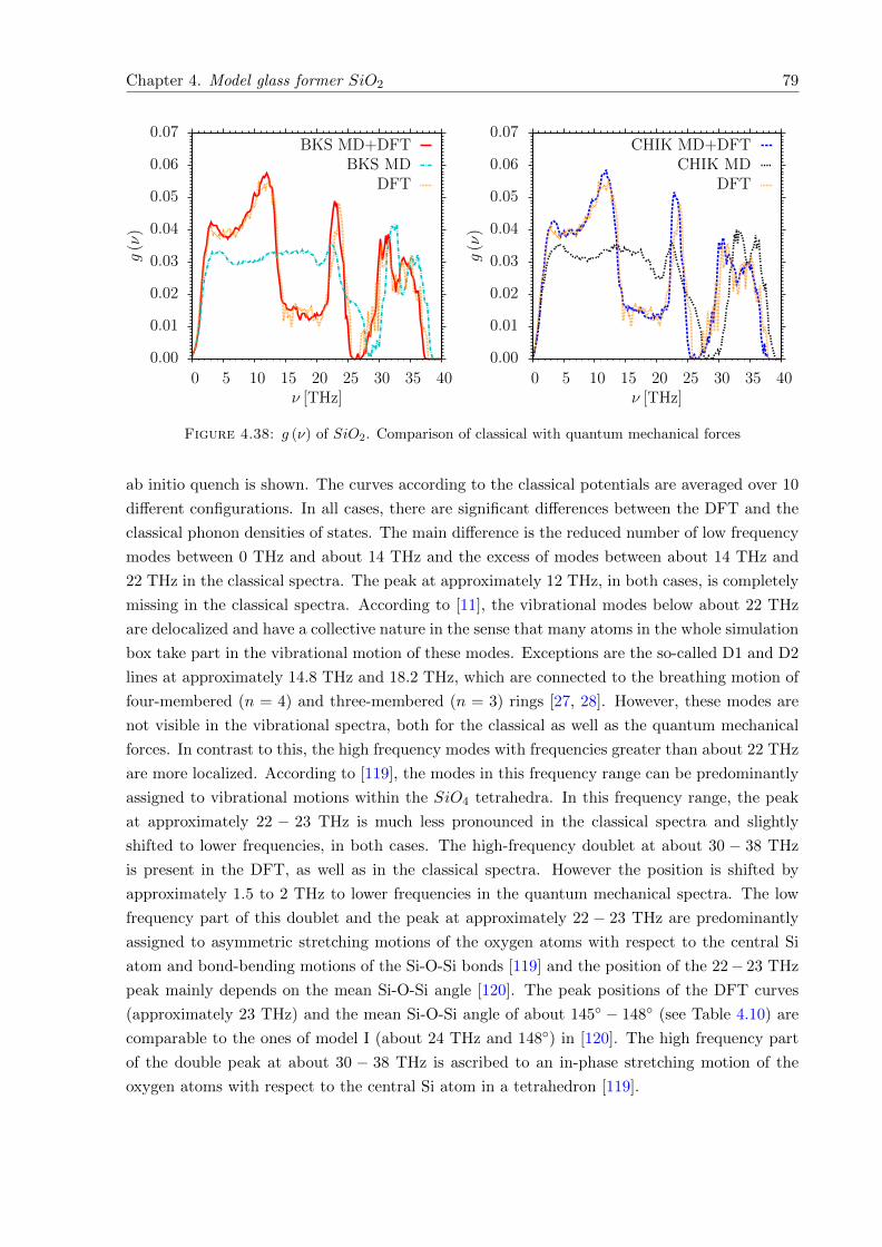
Chapter 4. Model glass former SiO2 79
0.00
0.01
0.02
0.03
0.04
0.05
0.06
0.07
0 5 10 15 20 25 30 35 40
g(ν)
ν [THz]
BKS MD+DFTBKS MD
DFT
0.00
0.01
0.02
0.03
0.04
0.05
0.06
0.07
0 5 10 15 20 25 30 35 40
g(ν)
ν [THz]
CHIK MD+DFTCHIK MD
DFT
Figure 4.38: g (ν) of SiO2. Comparison of classical with quantum mechanical forces
ab initio quench is shown. The curves according to the classical potentials are averaged over 10
different configurations. In all cases, there are significant differences between the DFT and the
classical phonon densities of states. The main difference is the reduced number of low frequency
modes between 0 THz and about 14 THz and the excess of modes between about 14 THz and
22 THz in the classical spectra. The peak at approximately 12 THz, in both cases, is completely
missing in the classical spectra. According to [11], the vibrational modes below about 22 THz
are delocalized and have a collective nature in the sense that many atoms in the whole simulation
box take part in the vibrational motion of these modes. Exceptions are the so-called D1 and D2
lines at approximately 14.8 THz and 18.2 THz, which are connected to the breathing motion of
four-membered (n = 4) and three-membered (n = 3) rings [27, 28]. However, these modes are
not visible in the vibrational spectra, both for the classical as well as the quantum mechanical
forces. In contrast to this, the high frequency modes with frequencies greater than about 22 THz
are more localized. According to [119], the modes in this frequency range can be predominantly
assigned to vibrational motions within the SiO4 tetrahedra. In this frequency range, the peak
at approximately 22 − 23 THz is much less pronounced in the classical spectra and slightly
shifted to lower frequencies, in both cases. The high-frequency doublet at about 30 − 38 THz
is present in the DFT, as well as in the classical spectra. However the position is shifted by
approximately 1.5 to 2 THz to lower frequencies in the quantum mechanical spectra. The low
frequency part of this doublet and the peak at approximately 22 − 23 THz are predominantly
assigned to asymmetric stretching motions of the oxygen atoms with respect to the central Si
atom and bond-bending motions of the Si-O-Si bonds [119] and the position of the 22− 23 THz
peak mainly depends on the mean Si-O-Si angle [120]. The peak positions of the DFT curves
(approximately 23 THz) and the mean Si-O-Si angle of about 145 − 148 (see Table 4.10) are
comparable to the ones of model I (about 24 THz and 148) in [120]. The high frequency part
of the double peak at about 30 − 38 THz is ascribed to an in-phase stretching motion of the
oxygen atoms with respect to the central Si atom in a tetrahedron [119].
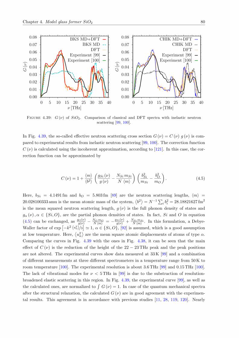
Chapter 4. Model glass former SiO2 80
0.00
0.01
0.02
0.03
0.04
0.05
0.06
0.07
0.08
0 5 10 15 20 25 30 35 40
G(ν)
ν [THz]
BKS MD+DFTBKS MD
DFTExperiment [99]Experiment [100]
0.00
0.01
0.02
0.03
0.04
0.05
0.06
0.07
0.08
0 5 10 15 20 25 30 35 40
G(ν)
ν [THz]
CHIK MD+DFTCHIK MD
DFTExperiment [99]Experiment [100]
Figure 4.39: G (ν) of SiO2. Comparison of classical and DFT spectra with inelastic neutronscattering [99, 100].
In Fig. 4.39, the so-called effective neutron scattering cross section G (ν) = C (ν) g (ν) is com-
pared to experimental results from inelastic neutron scattering [99, 100]. The correction function
C (ν) is calculated using the incoherent approximation, according to [121]. In this case, the cor-
rection function can be approximated by
C (ν) = 1 +〈m〉〈b2〉
(gSi (ν)
g (ν)− NSimSi
N 〈m〉
) (b2SimSi
− b2OmO
). (4.5)
Here, bSi = 4.1491 fm and bO = 5.803 fm [89] are the neutron scattering lengths, 〈m〉 =
20.028100333 amu is the mean atomic mass of the system,⟨b2⟩
= N−1∑
i b2i = 28.18821627 fm2
is the mean squared neutron scattering length, g (ν) is the full phonon density of states and
gα (ν) , α ∈ Si,O, are the partial phonon densities of states. In fact, Si and O in equation
(4.5) can be exchanged, as gO(ν)g(ν) −
NOmON 〈m〉 = −gSi(ν)
g(ν) + NSimSiN 〈m〉 . In this formulation, a Debye-
Waller factor of exp[−k2 〈u2
α〉/3]' 1, α ∈ Si,O, [92] is assumed, which is a good assumption
at low temperature. Here,⟨u2α
⟩are the mean square atomic displacements of atoms of type α.
Comparing the curves in Fig. 4.39 with the ones in Fig. 4.38, it can be seen that the main
effect of C (ν) is the reduction of the height of the 22 − 23 THz peak and the peak positions
are not altered. The experimental curves show data measured at 33 K [99] and a combination
of different measurements at three different spectrometers in a temperature range from 50 K to
room temperature [100]. The experimental resolution is about 3.6 THz [99] and 0.15 THz [100].
The lack of vibrational modes for ν < 5 THz in [99] is due to the substraction of resolution-
broadened elastic scattering in this region. In Fig. 4.39, the experimental curve [99], as well as
the calculated ones, are normalized to´G (ν) = 1. In case of the quantum mechanical spectra
after the structural relaxation, the calculated G (ν) are in good agreement with the experimen-
tal results. This agreement is in accordance with previous studies [11, 28, 119, 120]. Nearly
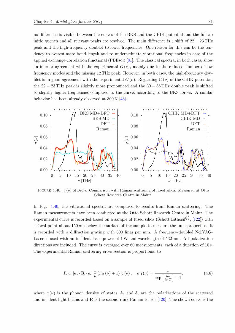
Chapter 4. Model glass former SiO2 81
no difference is visible between the curves of the BKS and the CHIK potential and the full ab
initio quench and all relevant peaks are resolved. The main difference is a shift of 22− 23 THz
peak and the high-frequency doublet to lower frequencies. One reason for this can be the ten-
dency to overestimate bond-length and to underestimate vibrational frequencies in case of the
applied exchange-correlation functional (PBEsol) [81]. The classical spectra, in both cases, show
an inferior agreement with the experimental G (ν), mainly due to the reduced number of low
frequency modes and the missing 12 THz peak. However, in both cases, the high-frequency dou-
blet is in good agreement with the experimental G (ν). Regarding G (ν) of the CHIK potential,
the 22 − 23 THz peak is slightly more pronounced and the 30 − 38 THz double peak is shifted
to slightly higher frequencies compared to the curve, according to the BKS forces. A similar
behavior has been already observed at 300 K [43].
0.00
0.02
0.04
0.06
0.08
0.10
0 5 10 15 20 25 30 35 40
g(ν)
ν [THz]
BKS MD+DFTBKS MD
DFTRaman
0.00
0.02
0.04
0.06
0.08
0.10
0 5 10 15 20 25 30 35 40
g(ν)
ν [THz]
CHIK MD+DFTCHIK MD
DFTRaman
Figure 4.40: g (ν) of SiO2. Comparison with Raman scattering of fused silica. Measured at OttoSchott Research Centre in Mainz.
In Fig. 4.40, the vibrational spectra are compared to results from Raman scattering. The
Raman measurements have been conducted at the Otto Schott Research Centre in Mainz. The
experimental curve is recorded based on a sample of fused silica (Schott Lithosil R©, [122]) with
a focal point about 150µm below the surface of the sample to measure the bulk properties. It
is recorded with a diffraction grating with 600 lines per mm. A frequency-doubled Nd:YAG-
Laser is used with an incident laser power of 1 W and wavelength of 532 nm. All polarization
directions are included. The curve is averaged over 60 measurements, each of a duration of 10 s.
The experimental Raman scattering cross section is proportional to
Is ∝ |es ·R · ei|1
ν(nB (ν) + 1) g (ν) , nB (ν) =
1
exp[hνkB T
]− 1
, (4.6)
where g (ν) is the phonon density of states, es and ei are the polarizations of the scattered
and incident light beams and R is the second-rank Raman tensor [120]. The shown curve is the
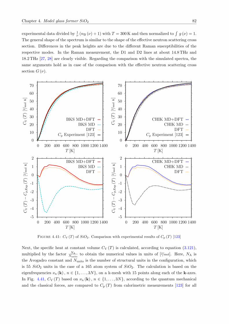
Chapter 4. Model glass former SiO2 82
experimental data divided by 1ν (nB (ν) + 1) with T = 300 K and then normalized to
´g (ν) = 1.
The general shape of the spectrum is similar to the shape of the effective neutron scattering cross
section. Differences in the peak heights are due to the different Raman susceptibilities of the
respective modes. In the Raman measurement, the D1 and D2 lines at about 14.8 THz and
18.2 THz [27, 28] are clearly visible. Regarding the comparison with the simulated spectra, the
same arguments hold as in case of the comparison with the effective neutron scattering cross
section G (ν).
0
10
20
30
40
50
60
70
0 200 400 600 800 1000 1200 1400
CV(T
)[J/m
olK]
T [K]
BKS MD+DFTBKS MD
DFTCp Experiment [123]
-5
-4
-3
-2
-1
0
1
2
0 200 400 600 800 1000 1200 1400
CV(T
)−C
p,E
xp(T
)[J/m
olK]
T [K]
BKS MD+DFTBKS MD
DFT
0
10
20
30
40
50
60
70
0 200 400 600 800 1000 1200 1400
CV(T
)[J/m
olK]
T [K]
CHIK MD+DFTCHIK MD
DFTCp Experiment [123]
-5
-4
-3
-2
-1
0
1
2
0 200 400 600 800 1000 1200 1400
CV(T
)−C
p,E
xp(T
)[J/m
olK]
T [K]
CHIK MD+DFTCHIK MD
DFT
Figure 4.41: CV (T ) of SiO2. Comparison with experimental results of Cp (T ) [123]
Next, the specific heat at constant volume CV (T ) is calculated, according to equation (3.121),
multiplied by the factor NANunits
to obtain the numerical values in units of [J/mol]. Here, NA is
the Avogadro constant and Nunits is the number of structural units in the configuration, which
is 55 SiO2 units in the case of a 165 atom system of SiO2. The calculation is based on the
eigenfrequencies νn (k) , n ∈ 1, . . . , 3N, on a k-mesh with 15 points along each of the k-axes.
In Fig. 4.41, CV (T ) based on νn (k) , n ∈ 1, . . . , 3N, according to the quantum mechanical
and the classical forces, are compared to Cp (T ) from calorimetric measurements [123] for all
Chapter 4. Model glass former SiO2 83
considered cases. The difference between CV and Cp per mol is expressed by the thermodynamic
relation [124]
Cp − CV = TM
ρα2
VK, αV =1
V
(∂V
∂T
)
p
, K = −V(∂p
∂V
)
T
(4.7)
where M is the molar mass, ρ the density, αV the volumetric coefficient of thermal expansion at
constant pressure and K the bulk modulus at constant temperature. In case of SiO2, the values
at room temperature are M = 60.08430 g/mol (molar mass of one SiO2 unit), ρ ' 2.2 g/cm3 [98],
αV ' 3×αL ' 3× 5.5 · 10−7K−1 [122] and K ' 37 GPa (derived from the values of the Young’s
modulus, Shear modulus and Poisson’s ratio, given in [122]). Due to the low thermal expansion
of SiO2, the difference between Cp and CV is only about Cp−CV = 2.75 · 10−6 JK2 mol
T [K] and
can be neglected. The agreement between the theoretical curves and the experimental curve
is rather good, in all cases. However, in the temperature range between 50 K and 900 K the
agreement with the experimental curve is significantly better for the data based on the quantum
mechanical forces, both for the BKS and the CHIK potential, as well as for the full ab initio
quench. In this temperature range, CV (T ) based on the classical forces is visibly below the
experimental curve, which can be explained due to the reduced number of low frequency modes
in the vibrational spectrum. Comparing the BKS and the CHIK potential, the corresponding
curves are virtually on top of each other.
In this chapter, the simulation results of the model glass former SiO2 are summarized. First,
simulations of the liquid state are presented in a temperature range between 4300 K and 2700 K.
On the one hand, the effects of different system sizes are studied, carrying out simulations of
114, 165, 216 and 1152 systems with the BKS potential [22] at a constant system density of
ρ = 2.37 g/cm3. The main finite size effects are the slowing down of the dynamics and a decrease
of the number of rings, containing more than 6 Si atoms, with decreasing system size. The 114
atom system shows some additional artifacts in the curves of the static structure factors. This
motivates the choice of a 165 atom system for further considerations. On the other hand, the
structural and dynamical properties of the BKS [22] and the CHIK [43] potential are compared.
The main differences are slightly larger peak heights and about 3− 10 times larger α-relaxation
times, in case of the BKS potential. In addition, the temperature dependence of of the self-
diffusion constants Dα, α ∈ Si,O, is studied. At temperatures below about 3200 K, the
curves of Dα with respect to 1/T show an Arrhenius behavior (see equation (4.4)). Regarding
the BKS potential, the extracted activation energies EA,α, α ∈ Si,O, are significantly larger
than the ones reported in [42] and [107, 108]. The differences can be explained in terms of
finite size effects and effects due to different system densities. Regarding the CHIK potential,
the values of EA,α, α ∈ Si,O, are also larger than the ones reported in [43], which can be
explained in terms of finite size effects. Next, glass structures are generated by quenches from the
melt with classical MD simulations, employing the BKS and the CHIK potential. Afterwards, a
structural relaxation is carried out with respect to quantum mechanical forces, mainly reducing
Chapter 4. Model glass former SiO2 84
the mean Si-O-Si angle by about 4−6, in agreement with [10]. After the quantum mechanical
relaxation, no significant differences are visible in the glass structures generated by the BKS
and the CHIK potential and the agreement, both, with one glass structure generated by a full
ab initio quench from the melt and with experimental results is good. Finally, the vibrational
properties are studied. Here, the vibrational spectra, according to the quantum mechanical
forces, show a good agreement with results from inelastic neutron scattering [99, 100]. The
agreement is significantly better compared to the spectra, according to the classical forces of the
BKS, as well as the CHIK potential. The latter show a reduced number of vibrational modes in
the low frequency range. This leads to a significantly better agreement of the specific heat at
constant volume CV (T ) with experimental results as well. The results of this chapter suggest
that, both, a classical quench with a subsequent quantum mechanical relaxation and a full ab
initio quench can lead to comparable glass structures, given a reliable classical potential.
Chapter 5
Calculating thermal expansion
In this chapter, the temperature dependence of the system volume, V (T ), is examined for the
model glass former SiO2. The calculations are based on the glass structures, generated in section
4.2, and the concept of the so-called quasi-harmonic approximation is applied. In section 5.1,
the theoretical background is summarized. In section 5.2, the numerical results of the model
glass former SiO2 are presented for quantum mechanical and classical forces. Here, a change of
sign of the linear coefficient of thermal expansion αL (T ) is observed with a range of negative
thermal expansion at temperatures below approximately 130 K to 160 K (quantum mechanical
forces) and 290 K to 325 K (classical forces). This behavior is in accordance with experimental
results. To my knowledge, the calculation of the thermal expansion of vitreous silica by means
of ab initio calculations has not been done before.
5.1 Theoretical considerations
In section 3.4, the theory of lattice vibrations within the harmonic approximation has been sum-
marized. As already explained in section 4.3, the simulated glass structures are theoretically
treated as crystalline structures with a large unit cell containing 165 atoms. In this context,
harmonic approximation means that the forces on each of the N atoms of a solid are consid-
ered to be proportional to the atomic displacements and the individual atoms can be treated as
3-dimensional harmonic oscillators. Therefore, the vibrational properties of the whole configu-
ration can be mathematically treated as an ensemble of 3N independent quantum mechanical
harmonic oscillators. According to equations (3.113), (3.120) and (3.118), the relevant ther-
modynamical properties, as the internal energy, the entropy and the free energy of the lattice
vibrations can be described in terms of the respective eigenfrequencies νn (k) , n ∈ 1, . . . 3N.This model is not capable to describe the thermal expansion of the solid as the eigenfrequencies
νn (k) are independent of the temperature.
The quasi-harmonic approximation [125] is a way to introduce the temperature dependence of
the eigenmodes νn (k) and provides a way to describe thermal expansion. In this model, the
85
Chapter 5. Calculating thermal expansion 86
lattice vibrations are still described within the harmonic approximation, however the assumption
is that the eigenfrequencies depend on the volume of the system: νn (k;V ). As a consequence,
the phonon density of states and the thermodynamical properties have a volume dependence,
as well. The exact relation between the Helmholtz free energy F (T, V ) and the internal energy
U (T, V ) of a system is [63]:
F (T, V ) = U (T, V )− T S (T, V ) . (5.1)
Neglecting effects due to electronic excitations and configurational degrees of freedom, the rela-
tion can be written in the following form:
F (T, V ) = E0 (V ) + UVib (T, V )− T SVib (T, V ) , (5.2)
⇔ F (T, V ) = E0 (V ) + FVib (T, V ) . (5.3)
Here, UVib (T, V ) is the internal energy, SVib (T, V ) the entropy and FVib (T, V ) the free energy
of the lattice vibrations. They have the same functional forms as in equations (3.113), (3.120)
and (3.118), introducing the volume dependence by means of the volume dependence of the
eigenfrequencies νn (k;V ). This leads to the functional form of the vibrational free energy of
FVib (T, V ) =RT
NunitsNk
∑
k
3N∑
n=1
ln
[2 sinh
(hνn (k;V )
2kBT
)](5.4)
in units of [J/mol] (equation (3.118) multiplied by NANunits
). Here, Nunits is the number of structural
units in the configuration, which is 55 SiO2 units in the case of a 165 atom system of SiO2. The
energy E0 (V ) in equations (5.2) and (5.3) is the total energy of the structural configuration at
0 K at a given volume V . It consists of all electronic contributions, the Coulomb energy of the
interactions between the nuclei and the contributions of the atomic energies, according to the
PAW potentials, as already explained in section 4.2. Given the Helmholtz free energy F (T, V ),
the Gibbs free energy G (T, p) can be written as
G (T, p) = minV
[F (T, V ) + p V ] = minV
[E0 (V ) + FVib (T, V ) + p V ] . (5.5)
Equation (5.5) has to be understood in a sense that for each temperature T and external pres-
sure p, the minimization of [F (T, V ) + p V ] with respect to V yields the Gibbs free energy of
the system. Following the volume with minimal [F (T, V ) + p V ], the volume dependence on
temperature V (T ) can be obtained.
Chapter 5. Calculating thermal expansion 87
This means that in this approximation, the overall volume dependence of the Helmholtz free
energy F (T, V ) and the Gibbs free energy G (T, p) comes from the volume dependence of the
total energy E0 (V ) of the atomic configuration at 0 K and the volume dependence of the eigen-
frequencies νn (k;V ).
In this chapter, only properties at normal conditions are studied, meaning an external pressure
of p = 1 atm ' 0.1 MPa. The magnitude of relevant pressures in solids is of the order of GPa,
meaning an external pressure of p ' 0 is a reasonable assumption. In practice, the unit cell
of the given structure has to be slightly compressed and enlarged, without altering the relative
coordinates of the atoms in the system. This leads to a series of configurations at slightly
different volumes V . For each of the configurations, a structural relaxation has to be conducted
to obtain the total energy for the specific system volume E0 (V ), followed by a calculation of the
vibrational properties with the ”frozen phonon” method to compute FVib (T, V ). Given the set
of F (T, V ) at discrete cell volumes V , at each temperature T , the volume with minimal F (T, V )
(p ' 0) is found by means of a fit to a given functional form of E (V ).
To describe the volume-dependence of the eigenfrequencies νn (k), the so-called dimensionless
microscopic mode Gruneisen parameters can be defined [93]:
γn (k) = − V
νn (k)
∂νn (k)
∂V. (5.6)
Based on equation (5.6), the macroscopic Gruneisen parameter γ (T ) can be defined in terms of
a weighted average of the microscopic γn (k):
γ (T ) =
∑k
∑3Nn=1 γn (k) cV,n (k;T )
∑k
∑3Nn=1 cV,n (k;T )
, (5.7)
cV,n (k;T ) =
(hνn (k)
kBT
)2 exp[hνn(k)kBT
]
[exp
[hνn(k)kBT
]− 1]2 . (5.8)
Here, cV,n (k;T ) is the contribution of each individual vibrational mode n to the specific heat at
constant volume CV (T ), according to equation (3.121). It can be shown that the macroscopic
Gruneisen parameter γ (T ) correlates CV (T ) with the volumetric thermal expansion coefficient
αV (T ) and the isothermal bulk modulus K (T ) (see equation (4.7)) by the following relation:
γ (T ) =αV (T ) K (T ) M
CV (T ) ρ. (5.9)
Chapter 5. Calculating thermal expansion 88
Here, M is the molar mass, ρ is the density of the system and CV (T ) is given in units of [J/mol].
As a result of equation (5.9), a temperature regime with negative thermal expansion coefficient
αV (T ) relates to a negative macroscopic Gruneisen parameter γ (T ) in the respective tempera-
ture range and, due to equation (5.7), a negative γ (T ) relates to negative microscopic Gruneisen
parameters γn (k). As a consequence of equation (5.6), the vibrational modes contributing to
a temperature regime with negative thermal expansion show a positive frequency dependence
with respect to the system volume V , namely ∂νn(k)/∂V > 0. This means that the corresponding
force constants increase with V .
5.2 Application to model glass former SiO2
In this section, the method to calculate thermal expansion is applied to the model glass former
SiO2. The basis for the calculations are the 165 atom glass structures after the classical quench
and the subsequent quantum mechanical relaxation, as explained in section 4.2. Following the
considerations of section 4.3, the analysis is done for 5 independent glass structures generated
with the BKS potential and 5 configurations generated with the CHIK potential. Additionally,
the thermal expansion is calculated for 10 independent configurations generated by the BKS and
the CHIK potential, where all calculations are done with respect to the classical force fields (see
section 4.3). As explained in section 5.1, it is necessary to calculate the vibrational properties
of the same structural configuration at different system volumes. Therefore, the densities of
the configurations are manually changed to ρ = 2.1 g/cm3, ρ = 2.3 g/cm3 and ρ = 2.4 g/cm3,
corresponding to box lengths of LBox = 13.7737 A, LBox = 13.3623 A and LBox = 13.17407 A.
In case of the classical force fields, the system density of ρ = 2.0 g/cm3 is included, as well, in
all calculations. The latter corresponds to a box length of LBox = 13.99954 A. In case of the
DFT forces, the additional system densities of ρ = 2.0 g/cm3, ρ = 2.15 g/cm3, ρ = 2.22 g/cm3, ρ =
2.23 g/cm3, ρ = 2.25 g/cm3 and ρ = 2.275 g/cm3 are examined for one glass configuration, generated
with the BKS potential. These densities correspond to box lengths of LBox = 13.99954 A,
LBox = 13.6661 A, LBox = 13.52173767 A, LBox = 13.501 A, LBox = 13.4606 A and LBox =
13.411 A. In each case, a structural relaxation at constant box size is performed by means of a
conjugate gradient algorithm [111]. Again, the VASP software package [77–79] is used in case of
DFT forces and the LAMMPS package [60, 61] is employed in case of the classical force fields.
The computational details and DFT parameters are the same as in section 4.2 for the structural
relaxation. The vibrational properties are calculated with the ”frozen phonon” method, using the
Phonopy package [90, 91]. The respective parameters are the same as in section 4.3. Again, the
atomic displacements are d = 0.02 A and the thermodynamic properties are evaluated according
to the eigenfrequencies νn (k) , n ∈ 1, . . . , 3N, on a k-mesh with a grid of 15 points along each
of the k-axes.
In Fig. 5.1, the Helmholtz free energy F (T, V ) is shown at 0 K and 500 K, according to equation
(5.3). Calculations are done with respect to quantum mechanical forces for one glass configu-
ration of the BKS potential after the structural relaxation. Here, the configuration is chosen
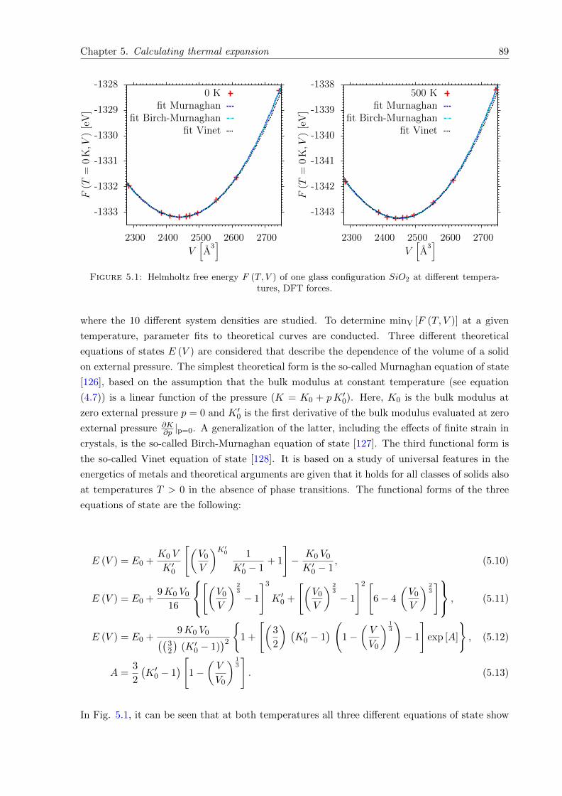
Chapter 5. Calculating thermal expansion 89
-1333
-1332
-1331
-1330
-1329
-1328
2300 2400 2500 2600 2700
F(T
=0
K,V
)[e
V]
V[A
3]
0 Kfit Murnaghan
fit Birch-Murnaghanfit Vinet
-1343
-1342
-1341
-1340
-1339
-1338
2300 2400 2500 2600 2700
F(T
=0
K,V
)[e
V]
V[A
3]
500 Kfit Murnaghan
fit Birch-Murnaghanfit Vinet
Figure 5.1: Helmholtz free energy F (T, V ) of one glass configuration SiO2 at different tempera-tures, DFT forces.
where the 10 different system densities are studied. To determine minV [F (T, V )] at a given
temperature, parameter fits to theoretical curves are conducted. Three different theoretical
equations of states E (V ) are considered that describe the dependence of the volume of a solid
on external pressure. The simplest theoretical form is the so-called Murnaghan equation of state
[126], based on the assumption that the bulk modulus at constant temperature (see equation
(4.7)) is a linear function of the pressure (K = K0 + pK ′0). Here, K0 is the bulk modulus at
zero external pressure p = 0 and K ′0 is the first derivative of the bulk modulus evaluated at zero
external pressure ∂K∂p |p=0. A generalization of the latter, including the effects of finite strain in
crystals, is the so-called Birch-Murnaghan equation of state [127]. The third functional form is
the so-called Vinet equation of state [128]. It is based on a study of universal features in the
energetics of metals and theoretical arguments are given that it holds for all classes of solids also
at temperatures T > 0 in the absence of phase transitions. The functional forms of the three
equations of state are the following:
E (V ) = E0 +K0 V
K ′0
[(V0
V
)K′0 1
K ′0 − 1+ 1
]− K0 V0
K ′0 − 1, (5.10)
E (V ) = E0 +9K0 V0
16
[(V0
V
) 23
− 1
]3
K ′0 +
[(V0
V
) 23
− 1
]2 [6− 4
(V0
V
) 23
] , (5.11)
E (V ) = E0 +9K0 V0((
32
)(K ′0 − 1)
)2
1 +
[(3
2
) (K ′0 − 1
)(
1−(V
V0
) 13
)− 1
]exp [A]
, (5.12)
A =3
2
(K ′0 − 1
)[
1−(V
V0
) 13
]. (5.13)
In Fig. 5.1, it can be seen that at both temperatures all three different equations of state show
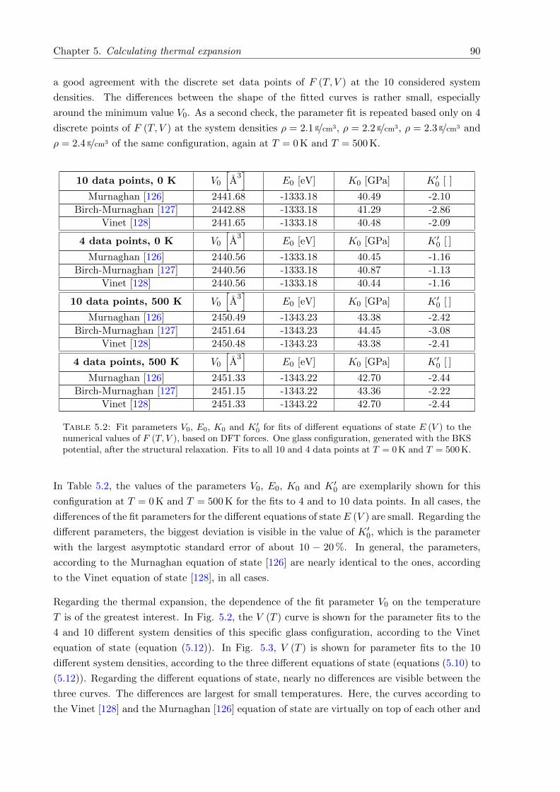
Chapter 5. Calculating thermal expansion 90
a good agreement with the discrete set data points of F (T, V ) at the 10 considered system
densities. The differences between the shape of the fitted curves is rather small, especially
around the minimum value V0. As a second check, the parameter fit is repeated based only on 4
discrete points of F (T, V ) at the system densities ρ = 2.1 g/cm3, ρ = 2.2 g/cm3, ρ = 2.3 g/cm3 and
ρ = 2.4 g/cm3 of the same configuration, again at T = 0 K and T = 500 K.
10 data points, 0 K V0
[A
3]
E0 [eV] K0 [GPa] K ′0 [ ]
Murnaghan [126] 2441.68 -1333.18 40.49 -2.10
Birch-Murnaghan [127] 2442.88 -1333.18 41.29 -2.86
Vinet [128] 2441.65 -1333.18 40.48 -2.09
4 data points, 0 K V0
[A
3]
E0 [eV] K0 [GPa] K ′0 [ ]
Murnaghan [126] 2440.56 -1333.18 40.45 -1.16
Birch-Murnaghan [127] 2440.56 -1333.18 40.87 -1.13
Vinet [128] 2440.56 -1333.18 40.44 -1.16
10 data points, 500 K V0
[A
3]
E0 [eV] K0 [GPa] K ′0 [ ]
Murnaghan [126] 2450.49 -1343.23 43.38 -2.42
Birch-Murnaghan [127] 2451.64 -1343.23 44.45 -3.08
Vinet [128] 2450.48 -1343.23 43.38 -2.41
4 data points, 500 K V0
[A
3]
E0 [eV] K0 [GPa] K ′0 [ ]
Murnaghan [126] 2451.33 -1343.22 42.70 -2.44
Birch-Murnaghan [127] 2451.15 -1343.22 43.36 -2.22
Vinet [128] 2451.33 -1343.22 42.70 -2.44
Table 5.2: Fit parameters V0, E0, K0 and K ′0 for fits of different equations of state E (V ) to thenumerical values of F (T, V ), based on DFT forces. One glass configuration, generated with the BKSpotential, after the structural relaxation. Fits to all 10 and 4 data points at T = 0 K and T = 500 K.
In Table 5.2, the values of the parameters V0, E0, K0 and K ′0 are exemplarily shown for this
configuration at T = 0 K and T = 500 K for the fits to 4 and to 10 data points. In all cases, the
differences of the fit parameters for the different equations of state E (V ) are small. Regarding the
different parameters, the biggest deviation is visible in the value of K ′0, which is the parameter
with the largest asymptotic standard error of about 10 − 20 %. In general, the parameters,
according to the Murnaghan equation of state [126] are nearly identical to the ones, according
to the Vinet equation of state [128], in all cases.
Regarding the thermal expansion, the dependence of the fit parameter V0 on the temperature
T is of the greatest interest. In Fig. 5.2, the V (T ) curve is shown for the parameter fits to the
4 and 10 different system densities of this specific glass configuration, according to the Vinet
equation of state (equation (5.12)). In Fig. 5.3, V (T ) is shown for parameter fits to the 10
different system densities, according to the three different equations of state (equations (5.10) to
(5.12)). Regarding the different equations of state, nearly no differences are visible between the
three curves. The differences are largest for small temperatures. Here, the curves according to
the Vinet [128] and the Murnaghan [126] equation of state are virtually on top of each other and
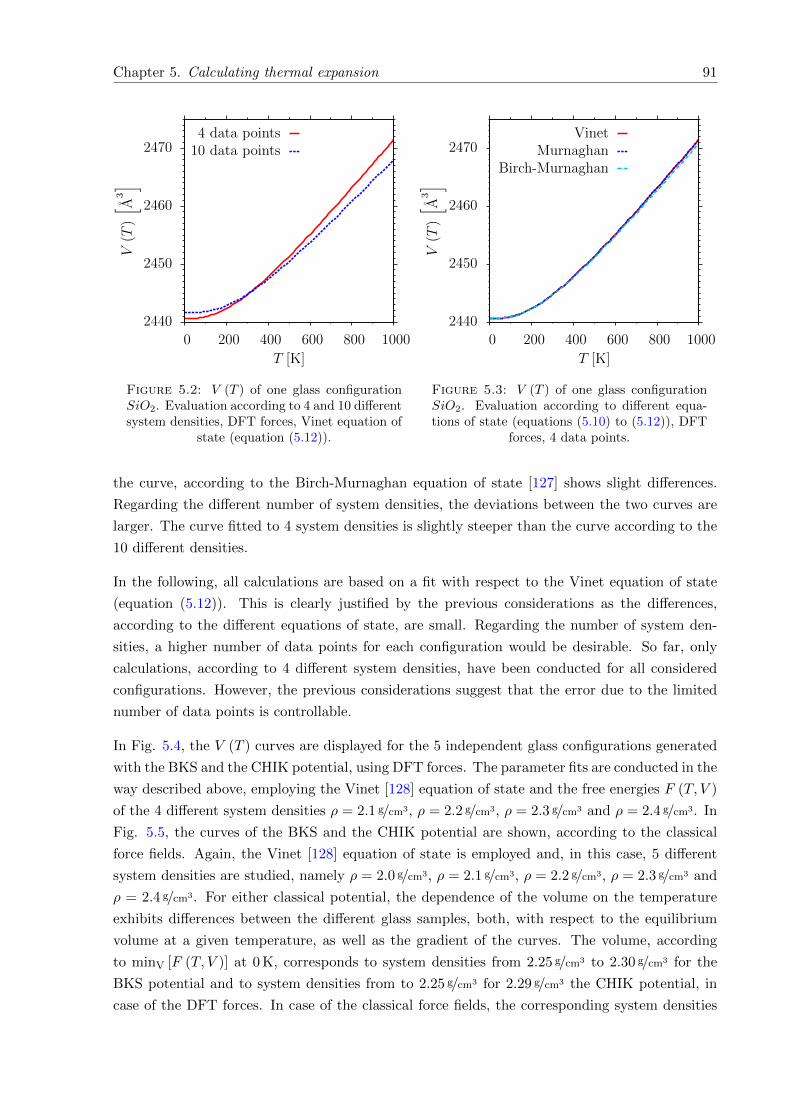
Chapter 5. Calculating thermal expansion 91
2440
2450
2460
2470
0 200 400 600 800 1000
V(T
)[ A
3]
T [K]
4 data points10 data points
Figure 5.2: V (T ) of one glass configurationSiO2. Evaluation according to 4 and 10 differentsystem densities, DFT forces, Vinet equation of
state (equation (5.12)).
2440
2450
2460
2470
0 200 400 600 800 1000
V(T
)[ A
3]
T [K]
VinetMurnaghan
Birch-Murnaghan
Figure 5.3: V (T ) of one glass configurationSiO2. Evaluation according to different equa-tions of state (equations (5.10) to (5.12)), DFT
forces, 4 data points.
the curve, according to the Birch-Murnaghan equation of state [127] shows slight differences.
Regarding the different number of system densities, the deviations between the two curves are
larger. The curve fitted to 4 system densities is slightly steeper than the curve according to the
10 different densities.
In the following, all calculations are based on a fit with respect to the Vinet equation of state
(equation (5.12)). This is clearly justified by the previous considerations as the differences,
according to the different equations of state, are small. Regarding the number of system den-
sities, a higher number of data points for each configuration would be desirable. So far, only
calculations, according to 4 different system densities, have been conducted for all considered
configurations. However, the previous considerations suggest that the error due to the limited
number of data points is controllable.
In Fig. 5.4, the V (T ) curves are displayed for the 5 independent glass configurations generated
with the BKS and the CHIK potential, using DFT forces. The parameter fits are conducted in the
way described above, employing the Vinet [128] equation of state and the free energies F (T, V )
of the 4 different system densities ρ = 2.1 g/cm3, ρ = 2.2 g/cm3, ρ = 2.3 g/cm3 and ρ = 2.4 g/cm3. In
Fig. 5.5, the curves of the BKS and the CHIK potential are shown, according to the classical
force fields. Again, the Vinet [128] equation of state is employed and, in this case, 5 different
system densities are studied, namely ρ = 2.0 g/cm3, ρ = 2.1 g/cm3, ρ = 2.2 g/cm3, ρ = 2.3 g/cm3 and
ρ = 2.4 g/cm3. For either classical potential, the dependence of the volume on the temperature
exhibits differences between the different glass samples, both, with respect to the equilibrium
volume at a given temperature, as well as the gradient of the curves. The volume, according
to minV [F (T, V )] at 0 K, corresponds to system densities from 2.25 g/cm3 to 2.30 g/cm3 for the
BKS potential and to system densities from to 2.25 g/cm3 for 2.29 g/cm3 the CHIK potential, in
case of the DFT forces. In case of the classical force fields, the corresponding system densities
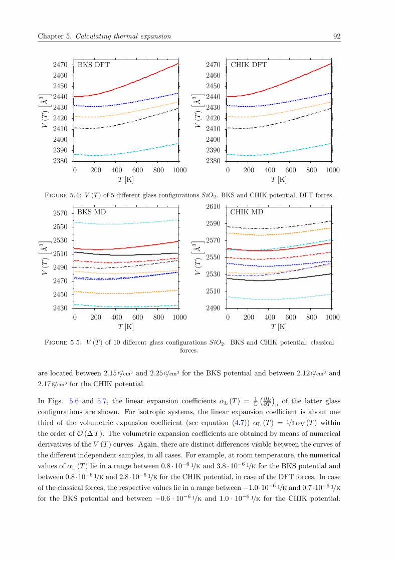
Chapter 5. Calculating thermal expansion 92
2380
2390
2400
2410
2420
2430
2440
2450
2460
2470
0 200 400 600 800 1000
V(T
)[ A
3]
T [K]
BKS DFT
2380
2390
2400
2410
2420
2430
2440
2450
2460
2470
0 200 400 600 800 1000
V(T
)[ A
3]
T [K]
CHIK DFT
Figure 5.4: V (T ) of 5 different glass configurations SiO2. BKS and CHIK potential, DFT forces.
2430
2450
2470
2490
2510
2530
2550
2570
0 200 400 600 800 1000
V(T
)[ A
3]
T [K]
BKS MD
2490
2510
2530
2550
2570
2590
2610
0 200 400 600 800 1000
V(T
)[ A
3]
T [K]
CHIK MD
Figure 5.5: V (T ) of 10 different glass configurations SiO2. BKS and CHIK potential, classicalforces.
are located between 2.15 g/cm3 and 2.25 g/cm3 for the BKS potential and between 2.12 g/cm3 and
2.17 g/cm3 for the CHIK potential.
In Figs. 5.6 and 5.7, the linear expansion coefficients αL (T ) = 1L
(∂L∂T
)p
of the latter glass
configurations are shown. For isotropic systems, the linear expansion coefficient is about one
third of the volumetric expansion coefficient (see equation (4.7)) αL (T ) = 1/3αV (T ) within
the order of O (∆T ). The volumetric expansion coefficients are obtained by means of numerical
derivatives of the V (T ) curves. Again, there are distinct differences visible between the curves of
the different independent samples, in all cases. For example, at room temperature, the numerical
values of αL (T ) lie in a range between 0.8 · 10−6 1/K and 3.8 · 10−6 1/K for the BKS potential and
between 0.8 ·10−6 1/K and 2.8 ·10−6 1/K for the CHIK potential, in case of the DFT forces. In case
of the classical forces, the respective values lie in a range between −1.0·10−6 1/K and 0.7·10−6 1/K
for the BKS potential and between −0.6 · 10−6 1/K and 1.0 · 10−6 1/K for the CHIK potential.
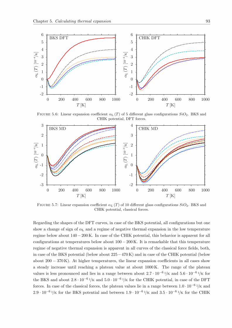
Chapter 5. Calculating thermal expansion 93
-2
-1
0
1
2
3
4
5
6
0 200 400 600 800 1000
αL(T
)[10−6 /
K]
T [K]
BKS DFT
-2
-1
0
1
2
3
4
5
6
0 200 400 600 800 1000
αL(T
)[10−6 /
K]
T [K]
CHIK DFT
Figure 5.6: Linear expansion coefficient αL (T ) of 5 different glass configurations SiO2. BKS andCHIK potential, DFT forces.
-3
-2
-1
0
1
2
3
0 200 400 600 800 1000
αL(T
)[10−6 /
K]
T [K]
BKS MD
-2
-1
0
1
2
3
4
0 200 400 600 800 1000
αL(T
)[10−6 /
K]
T [K]
CHIK MD
Figure 5.7: Linear expansion coefficient αL (T ) of 10 different glass configurations SiO2. BKS andCHIK potential, classical forces.
Regarding the shapes of the DFT curves, in case of the BKS potential, all configurations but one
show a change of sign of αL and a regime of negative thermal expansion in the low temperature
regime below about 140−200 K. In case of the CHIK potential, this behavior is apparent for all
configurations at temperatures below about 100− 200 K. It is remarkable that this temperature
regime of negative thermal expansion is apparent in all curves of the classical force fields, both,
in case of the BKS potential (below about 225−470 K) and in case of the CHIK potential (below
about 200− 370 K). At higher temperatures, the linear expansion coefficients in all cases show
a steady increase until reaching a plateau value at about 1000 K. The range of the plateau
values is less pronounced and lies in a range between about 2.7 · 10−6 1/K and 5.6 · 10−6 1/K for
the BKS and about 2.8 · 10−6 1/K and 5.0 · 10−6 1/K for the CHIK potential, in case of the DFT
forces. In case of the classical forces, the plateau values lie in a range between 1.0 · 10−6 1/K and
2.9 · 10−6 1/K for the BKS potential and between 1.9 · 10−6 1/K and 3.5 · 10−6 1/K for the CHIK
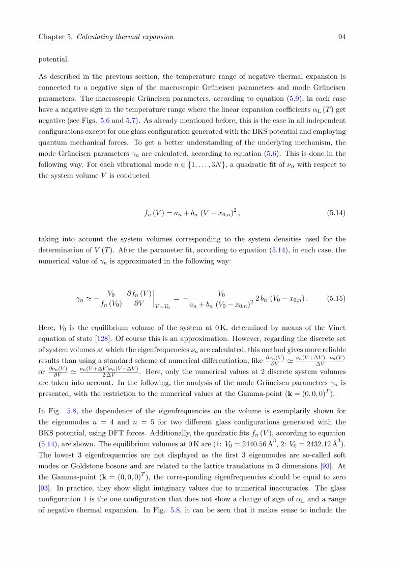
Chapter 5. Calculating thermal expansion 94
potential.
As described in the previous section, the temperature range of negative thermal expansion is
connected to a negative sign of the macroscopic Gruneisen parameters and mode Gruneisen
parameters. The macroscopic Gruneisen parameters, according to equation (5.9), in each case
have a negative sign in the temperature range where the linear expansion coefficients αL (T ) get
negative (see Figs. 5.6 and 5.7). As already mentioned before, this is the case in all independent
configurations except for one glass configuration generated with the BKS potential and employing
quantum mechanical forces. To get a better understanding of the underlying mechanism, the
mode Gruneisen parameters γn are calculated, according to equation (5.6). This is done in the
following way. For each vibrational mode n ∈ 1, . . . , 3N, a quadratic fit of νn with respect to
the system volume V is conducted
fn (V ) = an + bn (V − x0,n)2 , (5.14)
taking into account the system volumes corresponding to the system densities used for the
determination of V (T ). After the parameter fit, according to equation (5.14), in each case, the
numerical value of γn is approximated in the following way:
γn ' −V0
fn (V0)
∂fn (V )
∂V
∣∣∣∣V=V0
= − V0
an + bn (V0 − x0,n)2 2 bn (V0 − x0,n) . (5.15)
Here, V0 is the equilibrium volume of the system at 0 K, determined by means of the Vinet
equation of state [128]. Of course this is an approximation. However, regarding the discrete set
of system volumes at which the eigenfrequencies νn are calculated, this method gives more reliable
results than using a standard scheme of numerical differentiation, like ∂νn(V )∂V ' νn(V+∆V )−νn(V )
∆V
or ∂νn(V )∂V ' νn(V+∆V )νn(V−∆V )
2 ∆V . Here, only the numerical values at 2 discrete system volumes
are taken into account. In the following, the analysis of the mode Gruneisen parameters γn is
presented, with the restriction to the numerical values at the Gamma-point (k = (0, 0, 0)T ).
In Fig. 5.8, the dependence of the eigenfrequencies on the volume is exemplarily shown for
the eigenmodes n = 4 and n = 5 for two different glass configurations generated with the
BKS potential, using DFT forces. Additionally, the quadratic fits fn (V ), according to equation
(5.14), are shown. The equilibrium volumes at 0 K are (1: V0 = 2440.56 A3, 2: V0 = 2432.12 A
3).
The lowest 3 eigenfrequencies are not displayed as the first 3 eigenmodes are so-called soft
modes or Goldstone bosons and are related to the lattice translations in 3 dimensions [93]. At
the Gamma-point (k = (0, 0, 0)T ), the corresponding eigenfrequencies should be equal to zero
[93]. In practice, they show slight imaginary values due to numerical inaccuracies. The glass
configuration 1 is the one configuration that does not show a change of sign of αL and a range
of negative thermal expansion. In Fig. 5.8, it can be seen that it makes sense to include the
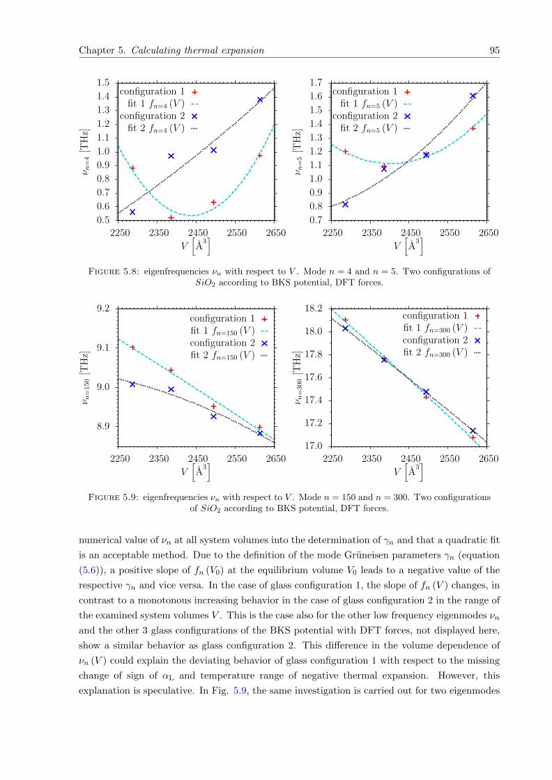
Chapter 5. Calculating thermal expansion 95
0.5
0.6
0.7
0.8
0.9
1.0
1.1
1.2
1.3
1.4
1.5
2250 2350 2450 2550 2650
ν n=4
[TH
z]
V[A
3]
configuration 1fit 1 fn=4 (V )
configuration 2fit 2 fn=4 (V )
0.7
0.8
0.9
1.0
1.1
1.2
1.3
1.4
1.5
1.6
1.7
2250 2350 2450 2550 2650
ν n=5
[TH
z]
V[A
3]
configuration 1fit 1 fn=5 (V )
configuration 2fit 2 fn=5 (V )
Figure 5.8: eigenfrequencies νn with respect to V . Mode n = 4 and n = 5. Two configurations ofSiO2 according to BKS potential, DFT forces.
8.9
9.0
9.1
9.2
2250 2350 2450 2550 2650
ν n=150
[TH
z]
V[A
3]
configuration 1fit 1 fn=150 (V )configuration 2fit 2 fn=150 (V )
17.0
17.2
17.4
17.6
17.8
18.0
18.2
2250 2350 2450 2550 2650
ν n=300
[TH
z]
V[A
3]
configuration 1fit 1 fn=300 (V )configuration 2fit 2 fn=300 (V )
Figure 5.9: eigenfrequencies νn with respect to V . Mode n = 150 and n = 300. Two configurationsof SiO2 according to BKS potential, DFT forces.
numerical value of νn at all system volumes into the determination of γn and that a quadratic fit
is an acceptable method. Due to the definition of the mode Gruneisen parameters γn (equation
(5.6)), a positive slope of fn (V0) at the equilibrium volume V0 leads to a negative value of the
respective γn and vice versa. In the case of glass configuration 1, the slope of fn (V ) changes, in
contrast to a monotonous increasing behavior in the case of glass configuration 2 in the range of
the examined system volumes V . This is the case also for the other low frequency eigenmodes νn
and the other 3 glass configurations of the BKS potential with DFT forces, not displayed here,
show a similar behavior as glass configuration 2. This difference in the volume dependence of
νn (V ) could explain the deviating behavior of glass configuration 1 with respect to the missing
change of sign of αL and temperature range of negative thermal expansion. However, this
explanation is speculative. In Fig. 5.9, the same investigation is carried out for two eigenmodes
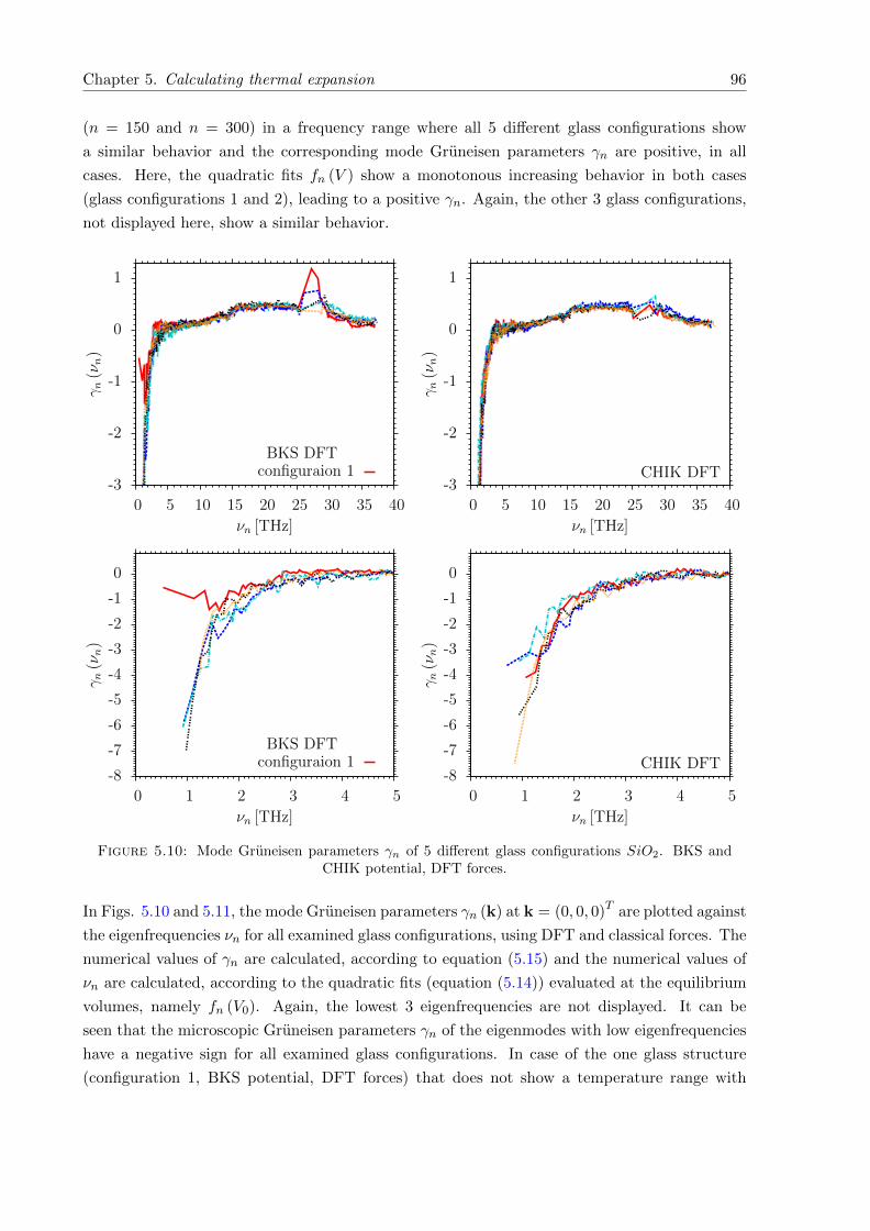
Chapter 5. Calculating thermal expansion 96
(n = 150 and n = 300) in a frequency range where all 5 different glass configurations show
a similar behavior and the corresponding mode Gruneisen parameters γn are positive, in all
cases. Here, the quadratic fits fn (V ) show a monotonous increasing behavior in both cases
(glass configurations 1 and 2), leading to a positive γn. Again, the other 3 glass configurations,
not displayed here, show a similar behavior.
-3
-2
-1
0
1
0 5 10 15 20 25 30 35 40
γn
(νn)
νn [THz]
BKS DFTconfiguraion 1
-8
-7
-6
-5
-4
-3
-2
-1
0
0 1 2 3 4 5
γn
(νn)
νn [THz]
BKS DFTconfiguraion 1
-3
-2
-1
0
1
0 5 10 15 20 25 30 35 40
γn(ν
n)
νn [THz]
CHIK DFT
-8
-7
-6
-5
-4
-3
-2
-1
0
0 1 2 3 4 5
γn(ν
n)
νn [THz]
CHIK DFT
Figure 5.10: Mode Gruneisen parameters γn of 5 different glass configurations SiO2. BKS andCHIK potential, DFT forces.
In Figs. 5.10 and 5.11, the mode Gruneisen parameters γn (k) at k = (0, 0, 0)T are plotted against
the eigenfrequencies νn for all examined glass configurations, using DFT and classical forces. The
numerical values of γn are calculated, according to equation (5.15) and the numerical values of
νn are calculated, according to the quadratic fits (equation (5.14)) evaluated at the equilibrium
volumes, namely fn (V0). Again, the lowest 3 eigenfrequencies are not displayed. It can be
seen that the microscopic Gruneisen parameters γn of the eigenmodes with low eigenfrequencies
have a negative sign for all examined glass configurations. In case of the one glass structure
(configuration 1, BKS potential, DFT forces) that does not show a temperature range with
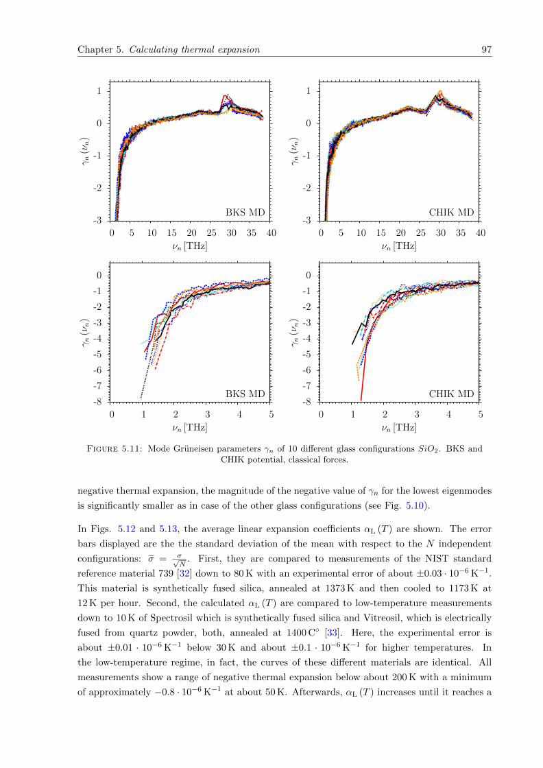
Chapter 5. Calculating thermal expansion 97
-3
-2
-1
0
1
0 5 10 15 20 25 30 35 40
γn(ν
n)
νn [THz]
BKS MD
-8
-7
-6
-5
-4
-3
-2
-1
0
0 1 2 3 4 5
γn(ν
n)
νn [THz]
BKS MD
-3
-2
-1
0
1
0 5 10 15 20 25 30 35 40
γn(ν
n)
νn [THz]
CHIK MD
-8
-7
-6
-5
-4
-3
-2
-1
0
0 1 2 3 4 5
γn(ν
n)
νn [THz]
CHIK MD
Figure 5.11: Mode Gruneisen parameters γn of 10 different glass configurations SiO2. BKS andCHIK potential, classical forces.
negative thermal expansion, the magnitude of the negative value of γn for the lowest eigenmodes
is significantly smaller as in case of the other glass configurations (see Fig. 5.10).
In Figs. 5.12 and 5.13, the average linear expansion coefficients αL (T ) are shown. The error
bars displayed are the the standard deviation of the mean with respect to the N independent
configurations: σ = σ√N
. First, they are compared to measurements of the NIST standard
reference material 739 [32] down to 80 K with an experimental error of about ±0.03 · 10−6 K−1.
This material is synthetically fused silica, annealed at 1373 K and then cooled to 1173 K at
12 K per hour. Second, the calculated αL (T ) are compared to low-temperature measurements
down to 10 K of Spectrosil which is synthetically fused silica and Vitreosil, which is electrically
fused from quartz powder, both, annealed at 1400 C [33]. Here, the experimental error is
about ±0.01 · 10−6 K−1 below 30 K and about ±0.1 · 10−6 K−1 for higher temperatures. In
the low-temperature regime, in fact, the curves of these different materials are identical. All
measurements show a range of negative thermal expansion below about 200 K with a minimum
of approximately −0.8 · 10−6 K−1 at about 50 K. Afterwards, αL (T ) increases until it reaches a
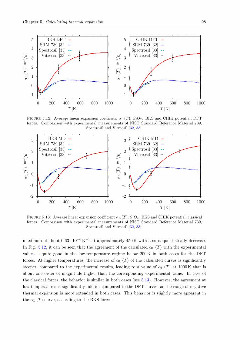
Chapter 5. Calculating thermal expansion 98
-1
0
1
2
3
4
5
0 200 400 600 800 1000
αL(T
)[10−6 /
K]
T [K]
BKS DFTSRM 739 [32]Spectrosil [33]Vitreosil [33]
-1
0
1
2
3
4
5
0 200 400 600 800 1000
αL(T
)[10−6 /
K]
T [K]
CHIK DFTSRM 739 [32]Spectrosil [33]Vitreosil [33]
Figure 5.12: Average linear expansion coefficient αL (T ), SiO2. BKS and CHIK potential, DFTforces. Comparison with experimental measurements of NIST Standard Reference Material 739,
Spectrosil and Vitreosil [32, 33].
-2
-1
0
1
2
3
0 200 400 600 800 1000
αL(T
)[10−6 /
K]
T [K]
BKS MDSRM 739 [32]Spectrosil [33]Vitreosil [33]
-2
-1
0
1
2
3
0 200 400 600 800 1000
αL(T
)[10−6 /
K]
T [K]
CHIK MDSRM 739 [32]Spectrosil [33]Vitreosil [33]
Figure 5.13: Average linear expansion coefficient αL (T ), SiO2. BKS and CHIK potential, classicalforces. Comparison with experimental measurements of NIST Standard Reference Material 739,
Spectrosil and Vitreosil [32, 33].
maximum of about 0.63 · 10−6 K−1 at approximately 450 K with a subsequent steady decrease.
In Fig. 5.12, it can be seen that the agreement of the calculated αL (T ) with the experimental
values is quite good in the low-temperature regime below 200 K in both cases for the DFT
forces. At higher temperatures, the increase of αL (T ) of the calculated curves is significantly
steeper, compared to the experimental results, leading to a value of αL (T ) at 1000 K that is
about one order of magnitude higher than the corresponding experimental value. In case of
the classical forces, the behavior is similar in both cases (see 5.13). However, the agreement at
low temperatures is significantly inferior compared to the DFT curves, as the range of negative
thermal expansion is more extended in both cases. This behavior is slightly more apparent in
the αL (T ) curve, according to the BKS forces.
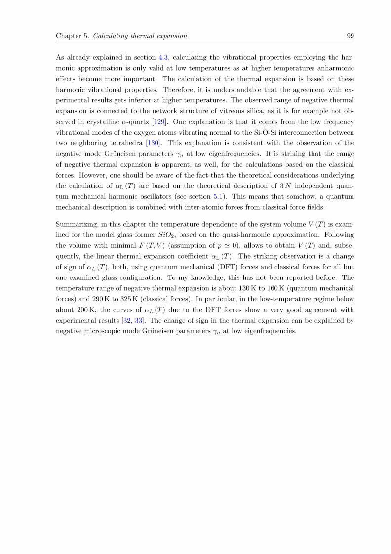
Chapter 5. Calculating thermal expansion 99
As already explained in section 4.3, calculating the vibrational properties employing the har-
monic approximation is only valid at low temperatures as at higher temperatures anharmonic
effects become more important. The calculation of the thermal expansion is based on these
harmonic vibrational properties. Therefore, it is understandable that the agreement with ex-
perimental results gets inferior at higher temperatures. The observed range of negative thermal
expansion is connected to the network structure of vitreous silica, as it is for example not ob-
served in crystalline α-quartz [129]. One explanation is that it comes from the low frequency
vibrational modes of the oxygen atoms vibrating normal to the Si-O-Si interconnection between
two neighboring tetrahedra [130]. This explanation is consistent with the observation of the
negative mode Gruneisen parameters γn at low eigenfrequencies. It is striking that the range
of negative thermal expansion is apparent, as well, for the calculations based on the classical
forces. However, one should be aware of the fact that the theoretical considerations underlying
the calculation of αL (T ) are based on the theoretical description of 3N independent quan-
tum mechanical harmonic oscillators (see section 5.1). This means that somehow, a quantum
mechanical description is combined with inter-atomic forces from classical force fields.
Summarizing, in this chapter the temperature dependence of the system volume V (T ) is exam-
ined for the model glass former SiO2, based on the quasi-harmonic approximation. Following
the volume with minimal F (T, V ) (assumption of p ' 0), allows to obtain V (T ) and, subse-
quently, the linear thermal expansion coefficient αL (T ). The striking observation is a change
of sign of αL (T ), both, using quantum mechanical (DFT) forces and classical forces for all but
one examined glass configuration. To my knowledge, this has not been reported before. The
temperature range of negative thermal expansion is about 130 K to 160 K (quantum mechanical
forces) and 290 K to 325 K (classical forces). In particular, in the low-temperature regime below
about 200 K, the curves of αL (T ) due to the DFT forces show a very good agreement with
experimental results [32, 33]. The change of sign in the thermal expansion can be explained by
negative microscopic mode Gruneisen parameters γn at low eigenfrequencies.

Chapter 6
Model glass former B2O3
In this chapter, the simulation results of the model glass former B2O3 are summarized. As
already emphasized in sections 2.2 and 2.4, the glass structure of pure B2O3 has the special
feature that about 60% − 80% of the boron atoms are localized within planar rings, consisting
of 3 boron and 3 oxygen atoms. These are called boroxol rings when the participating boron
atoms are all 3-fold coordinated with respect to the oxygen atoms and the oxygen atoms are all
2-fold coordinated with respect to the boron atoms [31]. In section 6.1, different experiments
are summarized, supporting the high fraction of boroxol rings in vitreous B2O3. Additionally,
an overview over several previous classical molecular dynamics studies of boron oxide is given
with classical potentials, as simple as pair potentials, up to complicated many-body potentials.
In section 6.2, the results of Born-Oppenheimer molecular dynamics (MD) simulations based on
quantum mechanical DFT forces are presented. Here, the structural and dynamical properties
of liquid B2O3 in a temperature range between 3600 K and 2300 K are discussed. The latter is
the lowest temperature at which the system still can be equilibrated by means of an ab initio
MD simulation. The liquid structure at 2300 K shows an increased amount of rings containing 3
boron and 3 oxygen atoms, compared to the liquid structures at 2500 K and 2700 K. In section
6.3, the fitting of new force field parameters for classical MD simulations is discussed, using
a modified form of the structural fitting procedure, described in [43]. Basis for the parameter
fits is the ab initio MD trajectory at 2300 K. The inclusion of 3-body terms leads to improved
results, regarding the accordance of the liquid properties of the classical MD and ab initio
MD simulations. In section 6.4, the structural and dynamical properties of liquid B2O3 are
examined, in detail, at different temperatures for the two most promising parameter sets after
the structural fit in the previous section. Special focus is on the temperature dependence of
certain structural quantities and the self-diffusion constants Dα, α ∈ B,O. The latter show
an unusual temperature dependence, not observed in case of the model glass former SiO2. In
section 6.5, a set of glass samples is analyzed, generated in different ways, namely by classical
quenches from the melt with a subsequent quantum mechanical relaxation and by full ab initio
quenches from different starting temperatures. The classical MD simulations are conducted with
the two different parameter sets employed in section 6.4 and the original parameter set before
101
Chapter 6. Model glass former B2O3 102
the structural fit. The structural properties of this set of glass structures are in reasonable
agreement with experimental results from neutron scattering [29]. However, the boroxol ring
fraction is significantly lower than the experimental prediction and varies from about f = 2.5%
(one classical potential with 3-body terms) to f = 15% (full ab initio quench from 2300 K).
In addition, a comparison to a structural model is presented, generated in an alternative way
[131–133], where f = 75% of the boron atoms are located in boroxol rings. In section 6.6,
the vibrational properties of the glass configurations are studied. The calculated vibrational
spectra show an acceptable agreement with experimental results from inelastic neutron scattering
[30, 134]. The significantly too low boroxol ring fraction is reflected in the significantly reduced
intensity of the corresponding peak.
6.1 Experimental evidence for the existence of boroxol rings and
overview over previous classical molecular dynamics simu-
lations
First, a summary of different experiments is given, supporting the hypothesis of a boroxol ring
fraction of about 60% − 80% in B2O3 glass. Second, an overview over several previous studies
of boron oxide by means of classical MD simulations is given, including pair interactions and
many-body potentials.
Regarding the experimental evidence of the existence of boroxol rings in vitreous B2O3, the
first summary is given in [135]. Here, it is concluded that the best structural model is the one
of a random three-dimensional network of BO3 triangles with a high fraction of boroxol rings.
One experimental evidence for the existence of boroxol rings comes from Raman measurements,
showing a very sharp and pronounced peak in the horizontal-horizontal (HH) Raman spectrum
at 808 cm−1 = 24.2 THz, where the polarization of the incident and the scattered laser beam
are parallel [26]. This peak is assigned to the breathing mode of a symmetric boroxol ring.
Regarding Raman measurements, in [36], the Raman spectrum of vitreous and liquid B2O3 is
measured in a temperature range from room temperature to 1273 K. Here, a decrease of the
boroxol ring fraction from about f ' 0.62 to f ' 0.22 at 1273 K is derived with an experimental
error of 4f ' 0.15.
Another independent evidence comes from nuclear magnetic resonance (NMR) measurements.
In [136], 10B, 11B and 17O NMR is used to study the respective chemical environment in B2O3
glass. From the 17O spectra the presence of two distinct oxygen sites is predicted of oxygen
atoms within and outside of boroxol rings. From this, a boroxol ring fraction of f ' 0.82± 0.08
is deduced. In [137], a boroxol ring fraction of f ' 0.7 is derived from 11B dynamic angle
spinning (DAS) NMR results. This value is in agreement to 17O high-resolution magic angle
spinning (MAS) NMR measurements, reported [138]. Here, a value of 0.5 ± 0.1 is reported for
the fraction of oxygen atoms in boroxol rings, corresponding to f = 0.75± 0.15.
Chapter 6. Model glass former B2O3 103
In addition, X-ray and neutron diffraction experiments are in good agreement with model struc-
tures, containing a high amount of boroxol rings. In [139], the real space correlation function
T (r) derived from X-ray diffraction is found to be in good agreement with a structural model
containing a high fraction of B atoms localized within boroxol rings. In [140] it is stated that a
model structure with f ' 0.6± 0.2 shows the best agreement with the T (r), according to [139],
and to the one derived from neutron scattering in their work. A fit to the neutron diffraction
results in [29], yields a value of f ' 0.8± 0.05. In the same work, results from inelastic neutron
scattering are reported. The neutron-weighted vibrational density of states has a signature at
the energy of the boroxol ring breathing mode at about 100.2 meV = 24.2 THz with a similar area
to the one predicted for a structural model with f = 0.75. In [30], inelastic neutron scattering
experiments also show a sharp peak at 100.2 meV = 24.2 THz. In addition, another small peak
at 151.1 meV = 36.5 THz is visible, which is also assigned to boroxol rings. Here, no estimate of
the boroxol ring fraction is given.
A boroxol ring fraction of f ' 0.75 is also supported by two DFT studies. In [141], a 160 atom
glass sample is generated by an ab initio MD quench from the melt, using the Car-Parrinello
method [142]. The resulting model glass structure contains 2 boroxol rings, corresponding to
f = 0.094. By comparing the intensity of the boroxol ring peak in the HH Raman spectrum
of the simulated structure to the experimental one [26] and by comparing the simulated 11B
NMR chemical shift to the experimental one [137], a value of f ' 0.75 is derived. In [133], DFT
calculations of an alternative model structure with f = 0.75 are presented. This model structure
is obtained, starting from the crystal structure of caesium enneaborate Cs2O.9B2O3 [143] and
extracting the Cs2O units and several BO3 units from the original structure [131, 132]. The
calculated 11B DAS and 17O MAS NMR spectra show a good agreement with the experimental
ones [137, 138]. In addition, the simulated HH Raman spectrum matches the experimental one
[26], within an estimated error, associated to the comparison, of 15%. This supports a boroxol
ring fraction of f ' 0.75 in pure B2O3 glass.
Regarding the computer modeling of B2O3, in [144], [145] and [146, 147], classical molecular
dynamics simulations are presented with pure pair interactions. In all cases, an interaction po-
tential of the so-called Born-Mayer-Huggins type is employed. This corresponds to the functional
form of the Buckingham potential with Coulomb interactions (see equation (3.122)), without
the attractive van der Waals term −C/r6. In [144], the potential parameters are determined
empirically, according to the size of the respective ions. The same set of parameters for the B
and O atoms is used in [146, 147]. The potential parameters in [145] are determined in a way
that the MD simulations reproduce the experimental crystal structures. In all cases, the full
atomic charges (qB = 3 e, qO = −2 e) are used and the glass structures resemble a network of
BO3 triangles, containing no boroxol rings at all. Also, the first neighbor B-B distances (2.71 A
[144], 2.72 A [145], 2.68 A [146] and 2.71 A [147]) are significantly larger as derived from neu-
tron diffraction [29]. This reflects in the distribution of B-O-B angles, having a maximum at
significantly too large values of 155 to 156, compared to the experimental value of about 130
for boron atoms outside of boroxol rings [139, 140], in all cases. These values correspond to
simulations at the experimental glass density [144, 146, 147] or an external pressure of 1 GPa to
Chapter 6. Model glass former B2O3 104
obtain a reasonable glass density [145]. Simulations at external pressure of about p = 0 which
is a reasonable assumption for normal conditions (p = 1 atm ' 0.1 MPa) lead to a glass density
of about ρ = 1.21 g/cm3 in [146].
In the following, classical molecular dynamics simulations are discussed, including 2-body and 3-
body interactions. In [148], the pair potentials are of the Born-Mayer-Huggins type, as described
above. Here, the 3-body terms are introduced by assuming an additional ion at the center of
mass of the BO3 triangles and additional pair potentials between this artificial ion and the B
and O atoms are introduced. Here, the full atomic charges (qB = 3 e, qO = −2 e) are used.
The resulting glass structure for simulations at the experimental glass density shows a rather
sharp B-O-B angular distribution with a maximum at about 120 and a boroxol ring fraction of
f ' 0.225 (3 boroxol rings and 40 B atoms).
In [149], angular potentials for the O-B-O and the B-O-B angle of the harmonic form (3.125) are
introduced with equilibrium angles of Φ0,OBO = 120 and Φ0,BOB = 130 in potential 4. The
constant KOBO is chosen in a way, to obtain the correct energy for the high frequency mode
in the simulated infrared spectra and the constant KBOB is chosen empirically. Here, partial
charges are employed (qB = 2 e, qO = −1.3 e). Simulations at constant experimental density lead
to a glass structure with a maximum of the B-O-B angular distribution at approximately 140.5,
which is significantly lower than in case of the pure 2-body potentials [146, 147]. However, no
boroxol rings are found in the glass structure.
In [44, 45], the most promising potential sets C1 and C2 are derived by means of a simulta-
neous fit to ab initio calculations of the energy surfaces of both known crystalline polymorphs
B2O3 − I and B2O3 − II with additional constraints. The potential form is of the Buckingham
type with Coulomb interactions (see equation (3.122)) for the O-O and the B-B interactions
and the Morse type with Coulomb interactions (see equation (3.124)) for the B-O interactions.
Additional harmonic 3-body terms (see equation (3.125)) for the O-B-O and the B-O-B interac-
tions with equilibrium angles of Φ0,BOB = 120, Φ0,OBO = 120 for 3-fold coordinated B atoms
and Φ0,OBO = 109.47 for 4-fold coordinated B atoms are used. Here, the atomic charges are
qB = 1.2 e, qO = −0.8 e (C1) and qB = 0.9 e, qO = −0.6 e (C2). The parameters of the B-O and
the O-O interactions depend on the coordination number around the oxygen atoms. To study
liquids and glasses, a continuous interpolation between the parameter sets of the different co-
ordination states is introduced, depending on the local coordination numbers. Also, a bonding
state function is introduced, which allows bonds to break. The resulting glass structures for
simulations at the experimental glass density show B-O-B bond angle distributions with ΦBOB
between about 120 and 130 and boroxol ring fractions of about f ' 0.25 (C1) to f ' 0.42
(C2). However, in the latter case about 6% of the B atoms are fourfold coordinated with respect
to O atoms. Simulations at p = 0 external pressure lead to configurations with about f ' 0.36
(C1) to f ' 0.53 (C2) and glass densities of 1.43 g/cm3 (C1) and 1.15 g/cm3 (C2). In [150], a
coupled MD/MC simulation is presented. Starting with a model crystal structure with f = 0.5
[131], BO3 units and B3O6 are exchanged randomly and the resulting structures are quenched to
0 K without allowing bond breakage. After each sampling, the structure with the lower energy
Chapter 6. Model glass former B2O3 105
is chosen. Also the box volume is varied to keep the system at the experimental glass den-
sity. Calculations are performed based on the before mentioned classical potential, according
to [44, 45]. For the final structure, corresponding to a (local) energy minimum, a boroxol ring
fraction of f = 0.74 is reported and two corresponding maxima in pBOB (Φ) are reported at 120
and 130. In [151], the dependence of the total energy on the boroxol ring concentration is stud-
ied, based on the same classical potential [44, 45] without the coordination dependence. Here,
glass configurations are generated by MD quenches from the melt. Samples with boroxol ring
contents from 0% to 100% are generated by preparing initial configurations with a mixture of
randomly distributed boroxol rings and additional B and O atoms and constraining the boroxol
rings during the simulation. Here, system sizes of 90 atoms at fixed experimental density are
studied. After the quench, a structural relaxation is carried out with a quantum mechanical
DFT calculation, using GGA and LDA exchange-correlation functionals (see subsection 3.2.4).
Here, mean first neighbor B-O distances of 1.36 A, O-O distances of 2.33 A and B-B distances
of 2.44 A to 2.55 A are reported, depending on the number of boroxol rings. Minima of the total
energy with respect to f at about f = 0.15 and f = 0.7 are reported.
In [152], exactly the same functional forms of the 2- and 3-body potentials is applied. In
addition, the angular potential is multiplied by a term, decaying exponentially with respect to
the inter-atomic distances. Following [45], the strength of the interaction depends on the local
coordination of the oxygen atoms. The atomic charges of the atoms and exact parameters are
not given. Simulations at constant glass density lead to glass structures with a boroxol ring
fraction of about f ' 0.15 and a good agreement of the real space correlation function T (r)
with the experimental one from neutron scattering [29].
Another study of B2O3 with a potential including 3-body terms is presented in [37]. Here, a
potential of the Born-Mayer-Huggins type (as explained above) is combined with 3-body terms
of the Gaussian type with negative sign (see equation (3.127)), multiplied with a term decaying
exponentially with respect to the inter-atomic distances. The parameters are determined em-
pirically, based on a potential for SiO2 [153]. The atomic charges, first neighbor B-B distances
and B-O-B angles are not stated. However, a boroxol ring fraction of f ' 0.2 is reported.
In [154], the 3-body potential with O-B-O and B-O-B angular interactions, according to [149] is
refined to yield a better agreement with the experimental total neutron structure factor Sneutr. (k)
[140], leading, for example to Φ0,BOB = 110. In addition, a O-B-O-B 4-body dihedral term
is introduced, parametrized according to Hartree-Fock calculations [71] on model B3O3 (OH)3
structures [46]. The partial charges are the same as in potential 4 of [149]. However, simulations
at the experimental glass density lead to a boroxol ring fraction of only f ' 0.036 (2 boroxol
rings in a 420 atom sample). The first neighbor B-B distances and B-O-B angles are not stated.
In [47], the functional form of the 2-body and 3-body terms correspond to the ones in [45, 152].
Here, only a 3-body term is chosen for the O-B-O interaction with Φ0,OBO = 120. In addition, a
B-O-B-O 4-body term is introduced with a minimum at the torsion angle of Φ0 = 0. Parameters
are obtained by DFT calculations of BO3, B2O5, BO3H3, B3O6, B3O6H3, B4O8 and B4O8H4
aggregates. The atomic charges of the atoms and exact parameters are not stated. The glass
Chapter 6. Model glass former B2O3 106
structures are generated in NVT runs at the experimental glass density, with a subsequent NpT
run at room temperature at atmospheric external pressure, leading to system densities of about
ρ = 1.67g/cm3 to ρ = 1.77g/cm3 in the slow cooling case and boroxol ring fractions of f ' 0.1 to
f ' 0.32, depending on the system size. The first neighbor B-B distances are 2.367 A, showing
a good agreement to the one of B atoms in boroxol rings in [29]. However, the system density
and boroxol ring fraction decreases with increasing system size.
In [48], a coordination dependent charge-transfer potential is presented, based on a previous
one for the study of SiO2 [155]. The potential consists of 2-body terms of the Born-Mayer-
Huggins type (Buckingham potential with Coulomb interactions (see equation (3.122)), without
the van der Waals term −C/r6) and 3-body terms of the Gaussian type with negative sign (see
equation (3.127)), multiplied with a term decaying exponentially with respect to the inter-atomic
distances. The equilibrium angles are Φ0,BOB = 120 and Φ0,OBO = 120 or Φ0,OBO = 109.47,
depending on the local coordination environment of the B atom (3-fold or 4-fold with respect to
O atoms). In addition to this local coordination dependence, the atomic charge is determined
dynamically depending on the coordination number (qB = 1.7 e for 3-fold and qB = 1.48 e for
4-fold coordinated B atoms). The potential is parametrized, according to the crystal structure
of B2O3− I in combination with the adjustment to available experimental data of the structure
and vibrational properties of vitreous B2O3. Here, glass structures are generated in NpT runs,
with the starting configuration of the alternative model structure with f = 0.75 [131, 132].
Depending on the equilibration time at 2500 K, glass structures with different values of f ' 0.1
to f ' 0.75 are generated with corresponding system densities of ρ = 1.75 g/cm3 to ρ = 1.81 g/cm3
[35, 48, 156]. However, no additional rings are generated in the cooling process. The first
neighbor B-B distances and B-O-B angles are not stated. The calculated Sneutr. (k) shows good
agreement with experimental results.
In [49], a many-body polarizable force field is introduced. This force field includes a non-
additive interaction, describing the dipole moments induced by local electric fields and is rather
complicated. The parameters are confirmed by a comparison of the minimum energy structures,
according to the classical force field, with experimental and ab initio structures of B2O3, HBO2,
H3BO3, H3B3O6 and H4B2O5. Also, the system is confined by external forces as an alternative
to periodic boundary conditions. For a system of 81 boron and 124 oxygen atoms, equilibrated
at 1800 K, 4 boroxol rings are reported, corresponding to f ' 0.15. The first neighbor peak
of gBB (r) is located at approximately 2.4 A and the density differs less than 1% from the
experimental glass density. In [157], boroxol ring fractions of about f ' 0.22 are reported in a
temperature range between 1761 K and 2163 K in the liquid state at experimental glass density.
Another complicated interaction potential is reported in [50], including polarization terms and
changes in the shape of the ions due to dipolar and quadrupolar shape distortions. The repulsive
and polarization terms of the aspherical ion model (AIM) are parametrized, according to forces
and dipoles from ab initio calculations on glass structures of 100 atoms, with boroxol ring
fractions from f = 0.0 to f = 0.22, according to [133]. In [50], the focus is on structural
transformations in B2O3 glass under pressure. The simulations are performed with a starting
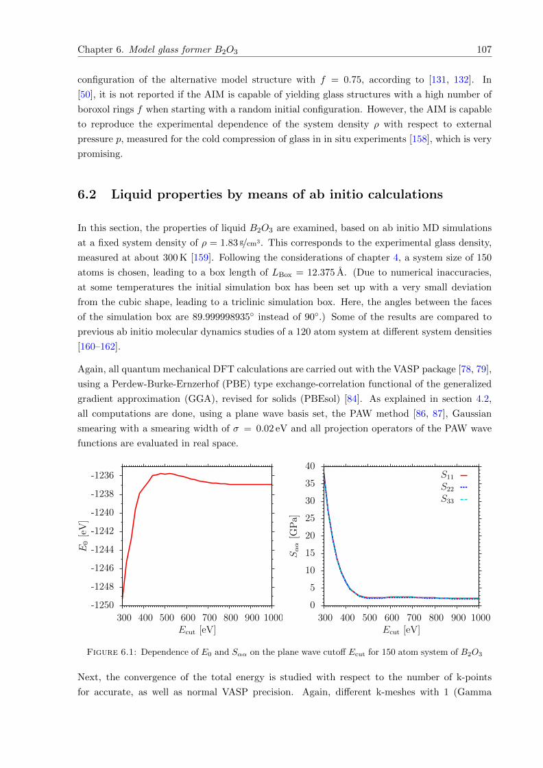
Chapter 6. Model glass former B2O3 107
configuration of the alternative model structure with f = 0.75, according to [131, 132]. In
[50], it is not reported if the AIM is capable of yielding glass structures with a high number of
boroxol rings f when starting with a random initial configuration. However, the AIM is capable
to reproduce the experimental dependence of the system density ρ with respect to external
pressure p, measured for the cold compression of glass in in situ experiments [158], which is very
promising.
6.2 Liquid properties by means of ab initio calculations
In this section, the properties of liquid B2O3 are examined, based on ab initio MD simulations
at a fixed system density of ρ = 1.83 g/cm3. This corresponds to the experimental glass density,
measured at about 300 K [159]. Following the considerations of chapter 4, a system size of 150
atoms is chosen, leading to a box length of LBox = 12.375 A. (Due to numerical inaccuracies,
at some temperatures the initial simulation box has been set up with a very small deviation
from the cubic shape, leading to a triclinic simulation box. Here, the angles between the faces
of the simulation box are 89.999998935 instead of 90.) Some of the results are compared to
previous ab initio molecular dynamics studies of a 120 atom system at different system densities
[160–162].
Again, all quantum mechanical DFT calculations are carried out with the VASP package [78, 79],
using a Perdew-Burke-Ernzerhof (PBE) type exchange-correlation functional of the generalized
gradient approximation (GGA), revised for solids (PBEsol) [84]. As explained in section 4.2,
all computations are done, using a plane wave basis set, the PAW method [86, 87], Gaussian
smearing with a smearing width of σ = 0.02 eV and all projection operators of the PAW wave
functions are evaluated in real space.
-1250
-1248
-1246
-1244
-1242
-1240
-1238
-1236
300 400 500 600 700 800 900 1000
E0[eV]
Ecut [eV]
0
5
10
15
20
25
30
35
40
300 400 500 600 700 800 900 1000
Sαα[G
Pa]
Ecut [eV]
S11
S22
S33
Figure 6.1: Dependence of E0 and Sαα on the plane wave cutoff Ecut for 150 atom system of B2O3
Next, the convergence of the total energy is studied with respect to the number of k-points
for accurate, as well as normal VASP precision. Again, different k-meshes with 1 (Gamma
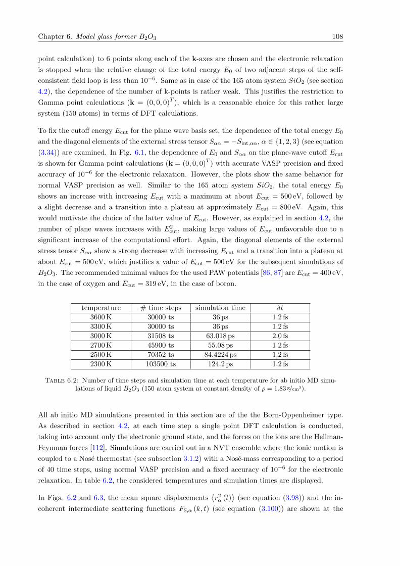
Chapter 6. Model glass former B2O3 108
point calculation) to 6 points along each of the k-axes are chosen and the electronic relaxation
is stopped when the relative change of the total energy E0 of two adjacent steps of the self-
consistent field loop is less than 10−6. Same as in case of the 165 atom system SiO2 (see section
4.2), the dependence of the number of k-points is rather weak. This justifies the restriction to
Gamma point calculations (k = (0, 0, 0)T ), which is a reasonable choice for this rather large
system (150 atoms) in terms of DFT calculations.
To fix the cutoff energy Ecut for the plane wave basis set, the dependence of the total energy E0
and the diagonal elements of the external stress tensor Sαα = −Sint,αα, α ∈ 1, 2, 3 (see equation
(3.34)) are examined. In Fig. 6.1, the dependence of E0 and Sαα on the plane-wave cutoff Ecut
is shown for Gamma point calculations (k = (0, 0, 0)T ) with accurate VASP precision and fixed
accuracy of 10−6 for the electronic relaxation. However, the plots show the same behavior for
normal VASP precision as well. Similar to the 165 atom system SiO2, the total energy E0
shows an increase with increasing Ecut with a maximum at about Ecut = 500 eV, followed by
a slight decrease and a transition into a plateau at approximately Ecut = 800 eV. Again, this
would motivate the choice of the latter value of Ecut. However, as explained in section 4.2, the
number of plane waves increases with E2cut, making large values of Ecut unfavorable due to a
significant increase of the computational effort. Again, the diagonal elements of the external
stress tensor Sαα show a strong decrease with increasing Ecut and a transition into a plateau at
about Ecut = 500 eV, which justifies a value of Ecut = 500 eV for the subsequent simulations of
B2O3. The recommended minimal values for the used PAW potentials [86, 87] are Ecut = 400 eV,
in the case of oxygen and Ecut = 319 eV, in the case of boron.
temperature # time steps simulation time δt
3600 K 30000 ts 36 ps 1.2 fs
3300 K 30000 ts 36 ps 1.2 fs
3000 K 31508 ts 63.018 ps 2.0 fs
2700 K 45900 ts 55.08 ps 1.2 fs
2500 K 70352 ts 84.4224 ps 1.2 fs
2300 K 103500 ts 124.2 ps 1.2 fs
Table 6.2: Number of time steps and simulation time at each temperature for ab initio MD simu-lations of liquid B2O3 (150 atom system at constant density of ρ = 1.83 g/cm3).
All ab initio MD simulations presented in this section are of the the Born-Oppenheimer type.
As described in section 4.2, at each time step a single point DFT calculation is conducted,
taking into account only the electronic ground state, and the forces on the ions are the Hellman-
Feynman forces [112]. Simulations are carried out in a NVT ensemble where the ionic motion is
coupled to a Nose thermostat (see subsection 3.1.2) with a Nose-mass corresponding to a period
of 40 time steps, using normal VASP precision and a fixed accuracy of 10−6 for the electronic
relaxation. In table 6.2, the considered temperatures and simulation times are displayed.
In Figs. 6.2 and 6.3, the mean square displacements⟨r2α (t)
⟩(see equation (3.98)) and the in-
coherent intermediate scattering functions FS,α (k, t) (see equation (3.100)) are shown at the
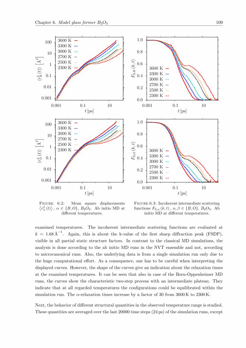
Chapter 6. Model glass former B2O3 109
0.001
0.01
0.1
1
10
100
0.001 0.1 10
〈r2 B
(t)〉[ A
2]
t [ps]
3600 K3300 K3000 K2700 K2500 K2300 K
0.001
0.01
0.1
1
10
100
0.001 0.1 10
〈r2 O
(t)〉[ A
2]
t [ps]
3600 K3300 K3000 K2700 K2500 K2300 K
Figure 6.2: Mean square displacements⟨r2α (t)
⟩, α ∈ B,O, B2O3. Ab initio MD at
different temperatures.
0.0
0.2
0.4
0.6
0.8
1.0
0.001 0.1 10
FS,B(k,t)
t [ps]
3600 K3300 K3000 K2700 K2500 K2300 K
0.0
0.2
0.4
0.6
0.8
1.0
0.001 0.1 10
FS,O(k,t)
t [ps]
3600 K3300 K3000 K2700 K2500 K2300 K
Figure 6.3: Incoherent intermediate scatteringfunctions FS,α (k, t) , α, β ∈ B,O, B2O3. Ab
initio MD at different temperatures.
examined temperatures. The incoherent intermediate scattering functions are evaluated at
k = 1.68 A−1
. Again, this is about the k-value of the first sharp diffraction peak (FSDP),
visible in all partial static structure factors. In contrast to the classical MD simulations, the
analysis is done according to the ab initio MD runs in the NVT ensemble and not, according
to microcanonical runs. Also, the underlying data is from a single simulation run only due to
the huge computational effort. As a consequence, one has to be careful when interpreting the
displayed curves. However, the shape of the curves give an indication about the relaxation times
at the examined temperatures. It can be seen that also in case of the Born-Oppenheimer MD
runs, the curves show the characteristic two-step process with an intermediate plateau. They
indicate that at all regarded temperatures the configurations could be equilibrated within the
simulation run. The α-relaxation times increase by a factor of 30 from 3600 K to 2300 K.
Next, the behavior of different structural quantities in the observed temperature range is studied.
These quantities are averaged over the last 20000 time steps (24 ps) of the simulation runs, except
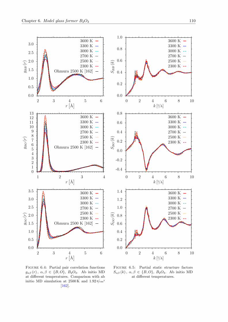
Chapter 6. Model glass former B2O3 110
0.0
0.5
1.0
1.5
2.0
2.5
3.0
2 3 4 5 6
g BB
(r)
r[A]
3600 K3300 K3000 K2700 K2500 K2300 K
Ohmura 2500 K [162]
0123456789
10111213
1 2 3 4
g BO
(r)
r[A]
3600 K3300 K3000 K2700 K2500 K2300 K
Ohmura 2500 K [162]
0.0
0.5
1.0
1.5
2.0
2.5
3.0
3.5
2 3 4 5 6
g OO
(r)
r[A]
3600 K3300 K3000 K2700 K2500 K2300 K
Ohmura 2500 K [162]
Figure 6.4: Partial pair correlation functionsgαβ (r) , α, β ∈ B,O, B2O3. Ab initio MDat different temperatures. Comparison with abinitio MD simulation at 2500 K and 1.92 g/cm3
[162].
0.0
0.2
0.4
0.6
0.8
1.0
0 2 4 6 8 10
SBB(k)
k [1/A]
3600 K3300 K3000 K2700 K2500 K2300 K
-0.4
-0.2
0.0
0.2
0.4
0.6
0.8
0 2 4 6 8 10
SBO(k)
k [1/A]
3600 K3300 K3000 K2700 K2500 K2300 K
0.0
0.2
0.4
0.6
0.8
1.0
1.2
1.4
0 2 4 6 8 10
SOO(k)
k [1/A]
3600 K3300 K3000 K2700 K2500 K2300 K
Figure 6.5: Partial static structure factorsSαβ (k) , α, β ∈ B,O, B2O3. Ab initio MD
at different temperatures.
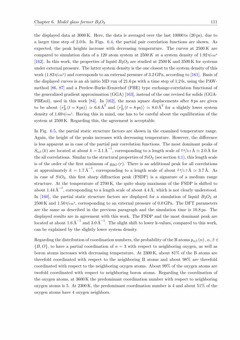
Chapter 6. Model glass former B2O3 111
the displayed data at 3000 K. Here, the data is averaged over the last 10000 ts (20 ps), due to
a larger time step of 2.0 fs. In Figs. 6.4, the partial pair correlation functions are shown. As
expected, the peak heights increase with decreasing temperature. The curves at 2500K are
compared to simulation data of a 120 atom system at 2500K at a system density of 1.92 g/cm3
[162]. In this work, the properties of liquid B2O3 are studied at 2500 K and 3500 K for systems
under external pressure. The latter system density is the one closest to the system density of this
work (1.83 g/cm3) and corresponds to an external pressure of 3.2 GPa, according to [161]. Basis of
the displayed curves is an ab initio MD run of 21.6 ps with a time step of 1.2 fs, using the PAW-
method [86, 87] and a Perdew-Burke-Ernzerhof (PBE) type exchange-correlation functional of
the generalized gradient approximation (GGA) [163], instead of the one revised for solids (GGA-
PBEsol), used in this work [84]. In [162], the mean square displacements after 8 ps are given
to be about⟨r2B (t = 8 ps)
⟩' 6.6 A
2and
⟨r2B (t = 8 ps)
⟩' 8.0 A
2for a slightly lower system
density of 1.69 g/cm3. Having this in mind, one has to be careful about the equilibration of the
system at 2500 K. Regarding this, the agreement is acceptable.
In Fig. 6.5, the partial static structure factors are shown in the examined temperature range.
Again, the height of the peaks increases with decreasing temperature. However, the difference
is less apparent as in case of the partial pair correlation functions. The most dominant peaks of
Sαβ (k) are located at about k = 3.1 A−1
, corresponding to a length scale of 2π/3.1 A ' 2.0 A for
the all correlations. Similar to the structural properties of SiO2 (see section 4.1), this length scale
is of the order of the first minimum of gBO (r). There is an additional peak for all correlations
at approximately k = 1.7 A−1
, corresponding to a length scale of about 2π/1.7 A ' 3.7 A. As
in case of SiO2, this first sharp diffraction peak (FSDP) is a signature of a medium range
structure. At the temperature of 2700 K, the quite sharp maximum of the FSDP is shifted to
about 1.44 A−1
, corresponding to a length scale of about 4.4 A, which is not clearly understood.
In [160], the partial static structure factors are displayed for a simulation of liquid B2O3 at
2500 K and 1.50 g/cm3, corresponding to an external pressure of 0.0 GPa. The DFT parameters
are the same as described in the previous paragraph and the simulation time is 10.8 ps. The
displayed results are in agreement with this work. The FSDP and the most dominant peak are
located at about 1.6 A−1
and 3.0 A−1
. The slight shift to lower k-values, compared to this work,
can be explained by the slightly lower system density.
Regarding the distribution of coordination numbers, the probability of the B atoms pαβ (n) , α, β ∈B,O, to have a partial coordination of n = 3 with respect to neighboring oxygen, as well as
boron atoms increases with decreasing temperature. At 2300 K, about 81% of the B atoms are
threefold coordinated with respect to the neighboring B atoms and about 98% are threefold
coordinated with respect to the neighboring oxygen atoms. About 99% of the oxygen atoms are
twofold coordinated with respect to neighboring boron atoms. Regarding the coordination of
the oxygen atoms, at 3600 K the predominant coordination number with respect to neighboring
oxygen atoms is 5. At 2300 K, the predominant coordination number is 4 and about 51% of the
oxygen atoms have 4 oxygen neighbors.
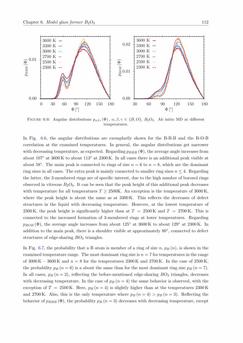
Chapter 6. Model glass former B2O3 112
0.00
0.01
0 30 60 90 120 150 180
p BBB
(Φ)
Φ []
3600 K3300 K3000 K2700 K2500 K2300 K
0.00
0.01
0.02
30 60 90 120 150 180
p BOB
(Φ)
Φ []
3600 K3300 K3000 K2700 K2500 K2300 K
Figure 6.6: Angular distributions pαβγ (Φ) , α, β, γ ∈ B,O, B2O3. Ab initio MD at differenttemperatures.
In Fig. 6.6, the angular distributions are exemplarily shown for the B-B-B and the B-O-B
correlation at the examined temperatures. In general, the angular distributions get narrower
with decreasing temperature, as expected. Regarding pBBB (Φ), the average angle increases from
about 107 at 3600 K to about 113 at 2300 K. In all cases there is an additional peak visible at
about 58. The main peak is connected to rings of size n = 6 to n = 8, which are the dominant
ring sizes in all cases. The extra peak is mainly connected to smaller ring sizes n ≤ 4. Regarding
the latter, the 3-membered rings are of specific interest, due to the high number of boroxol rings
observed in vitreous B2O3. It can be seen that the peak height of this additional peak decreases
with temperature for all temperatures T ≥ 2500K. An exception is the temperature of 3000 K,
where the peak height is about the same as at 3300 K. This reflects the decreases of defect
structures in the liquid with decreasing temperature. However, at the lowest temperature of
2300 K, the peak height is significantly higher than at T = 2500 K and T = 2700 K. This is
connected to the increased formation of 3-membered rings at lower temperatures. Regarding
pBOB (Φ), the average angle increases from about 125 at 3600 K to about 129 at 2300 K. In
addition to the main peak, there is a shoulder visible at approximately 80, connected to defect
structures of edge-sharing BO3 triangles.
In Fig. 6.7, the probability that a B atom is member of a ring of size n, pB (n), is shown in the
examined temperature range. The most dominant ring size is n = 7 for temperatures in the range
of 3000 K − 3600 K and n = 8 for the temperatures 2300 K and 2700 K. In the case of 2500 K,
the probability pB (n = 6) is a about the same than for the most dominant ring size pB (n = 7).
In all cases, pB (n = 2), reflecting the before-mentioned edge-sharing BO3 triangles, decreases
with decreasing temperature. In the case of pB (n = 4) the same behavior is observed, with the
exception of T = 2500 K. Here, pB (n = 4) is slightly higher than at the temperatures 2300 K
and 2700 K. Also, this is the only temperature where pB (n = 4) > pB (n = 3). Reflecting the
behavior of pBBB (Φ), the probability pB (n = 3) decreases with decreasing temperature, except
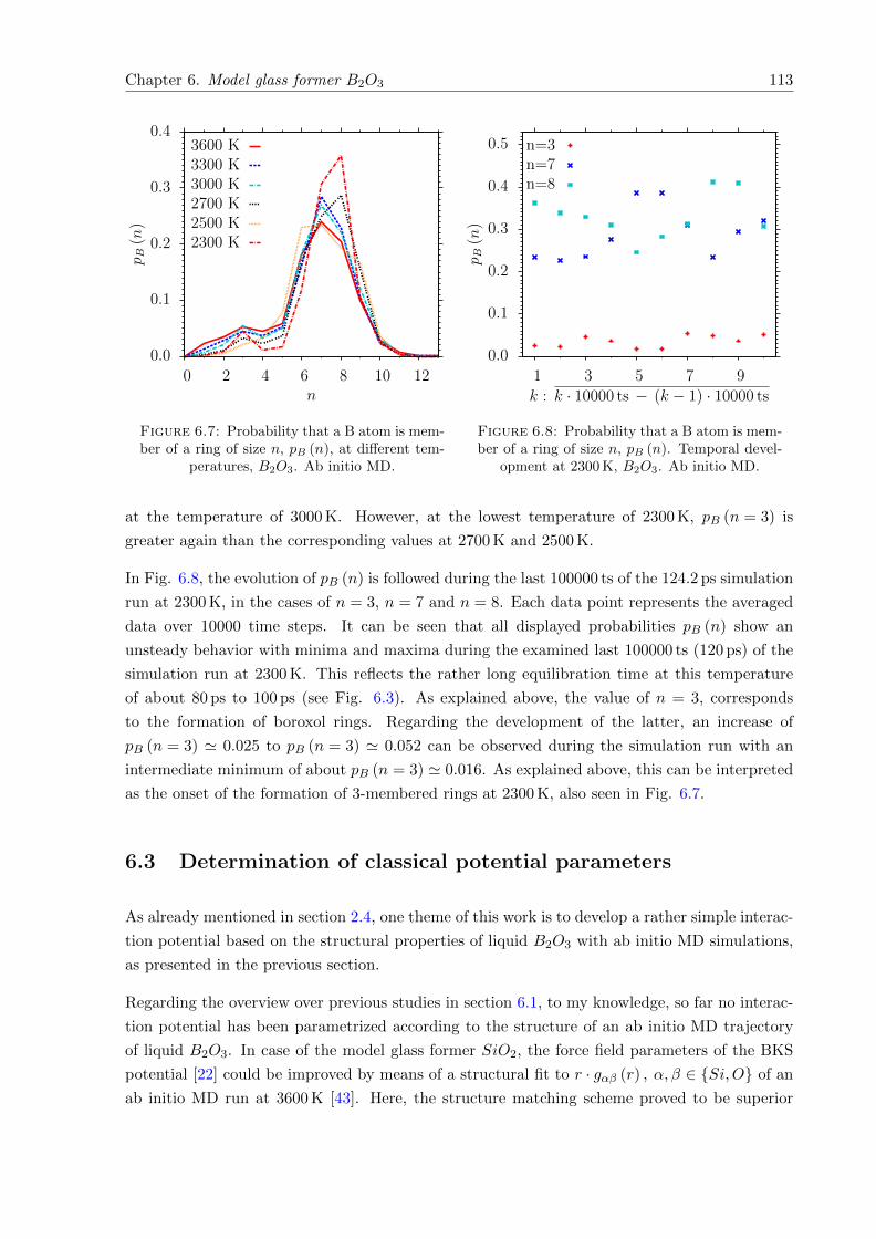
Chapter 6. Model glass former B2O3 113
0.0
0.1
0.2
0.3
0.4
0 2 4 6 8 10 12
p B(n)
n
3600 K3300 K3000 K2700 K2500 K2300 K
Figure 6.7: Probability that a B atom is mem-ber of a ring of size n, pB (n), at different tem-
peratures, B2O3. Ab initio MD.
0.0
0.1
0.2
0.3
0.4
0.5
1 3 5 7 9
p B(n)
k : k · 10000 ts − (k − 1) · 10000 ts
n=3n=7n=8
Figure 6.8: Probability that a B atom is mem-ber of a ring of size n, pB (n). Temporal devel-
opment at 2300 K, B2O3. Ab initio MD.
at the temperature of 3000 K. However, at the lowest temperature of 2300 K, pB (n = 3) is
greater again than the corresponding values at 2700 K and 2500 K.
In Fig. 6.8, the evolution of pB (n) is followed during the last 100000 ts of the 124.2 ps simulation
run at 2300 K, in the cases of n = 3, n = 7 and n = 8. Each data point represents the averaged
data over 10000 time steps. It can be seen that all displayed probabilities pB (n) show an
unsteady behavior with minima and maxima during the examined last 100000 ts (120 ps) of the
simulation run at 2300 K. This reflects the rather long equilibration time at this temperature
of about 80 ps to 100 ps (see Fig. 6.3). As explained above, the value of n = 3, corresponds
to the formation of boroxol rings. Regarding the development of the latter, an increase of
pB (n = 3) ' 0.025 to pB (n = 3) ' 0.052 can be observed during the simulation run with an
intermediate minimum of about pB (n = 3) ' 0.016. As explained above, this can be interpreted
as the onset of the formation of 3-membered rings at 2300 K, also seen in Fig. 6.7.
6.3 Determination of classical potential parameters
As already mentioned in section 2.4, one theme of this work is to develop a rather simple interac-
tion potential based on the structural properties of liquid B2O3 with ab initio MD simulations,
as presented in the previous section.
Regarding the overview over previous studies in section 6.1, to my knowledge, so far no interac-
tion potential has been parametrized according to the structure of an ab initio MD trajectory
of liquid B2O3. In case of the model glass former SiO2, the force field parameters of the BKS
potential [22] could be improved by means of a structural fit to r · gαβ (r) , α, β ∈ Si,O of an
ab initio MD run at 3600 K [43]. Here, the structure matching scheme proved to be superior
Chapter 6. Model glass former B2O3 114
to a force matching method [51]. This motivates the application of this method also to the
model glass former B2O3. In this section it is tested, whether this structure matching scheme
in combination with a rather simple interaction potential leads to an acceptable classical force
field for the model glass former B2O3. The basis for the development of an improved inter-
action potential is the classical force field, due to the dissertation of C. R. Trott [97]. In the
second part of this thesis, a classical force field has been developed for a general composition
of wLi2O − xSiO2 − yB2O3 − zP2O5. The basis of this force field is the existing interaction
potential of J. Habasaki [164] for alkali silicates which has been developed by quantum mechan-
ical calculations of potential energy surfaces of small clusters. The interaction potential has
the functional form of a Buckingham potential with Coulomb interactions V Buck+Coul (r) (see
equation (3.122)), in all cases. In addition, angular 3-body terms are introduced for the O-B-O
angle and the O-P-O angle.
The parameters of the B-B, B-O and O-O interaction are tabulated in Table 6.5. It is found
that the simulation results are practically the same if the B-B interaction is chosen to be purely
electrostatic, meaning ABB = 0 eV. This can be understood by the very large value of bBB =
15.2207 A−1
and the value of CBB = 0 eV A6. Therefore, the short-range Buckingham part of
the potential V Buck (r) (see equation (3.122)) only consists of a fast decaying exponential term,
which is virtually equal to zero at relevant inter-particle distances. Therefore, in the following
considerations, only the Coulomb part of the potential is considered for the B-B interaction.
As in case of the model glass former SiO2, all classical MD simulations are carried out with the
LAMMPS software package [60, 61] and a slightly modified form of the Buckingham potential
is used. Following the considerations of section 4.1, the Coulomb interaction is split up into a
short-range part V CS (r) (see equation (3.20)), evaluated in real space, and a long-range part,
evaluated in Fourier space employing a standard Ewald summation over k-vectors. Again, a
skin distance of rskin = 2 A is used and the Verlet neighbor lists are rebuilt when the first
atom has moved more than half the skin distance. In all cases, rc = 5.5 A is chosen as cutoff
radius for the short-range Buckingham part of the potential V Buck (r). In this section, the
cutoff distance of V CS (r) is equal to rewc = 5.5, as well, as the system size of the classical MD
simulations is chosen to be equivalent to the one of the ab initio MD simulations in section
6.2, namely 150 atoms. This means that the box length is LBox = 12.375 A, when simulating
at the experimental glass density of ρ = 1.83 g/cm3 [159]. Computations are carried out with
an gew = 0.599052, which corresponds to an Ewald accuracy of about 10−5, as explained in
subsection 3.1.1. Again, V Buck (r) and V CS (r) are shifted to zero at rc = 5.5 and rewc and
subsequently multiplied by a smoothing function, namely G (r) and Gew (r), with the functional
form of equation (3.13). In all cases, a value of d = dew = 0.05 A2
is chosen. As explained
in section 4.1, the shifted and smoothed Buckingham potentials with Coulomb interactions are
substituted by harmonic potentials V Harm (r) (see equation (4.2)) for particle distances smaller
than the positions of the local maxima r < rin,αβ, α, β ∈ B,O. In cases where V Buck+Coul (r)
shows no local maximum, the shifted and smoothed V Buck+Coul (r) is substituted by a harmonic
potential V Harm (r) for pair distances smaller than r = 1 A. As explained in section 4.1, a3,αβ
is the position of local maximum for the specific atom pair, according to equation (4.1), and
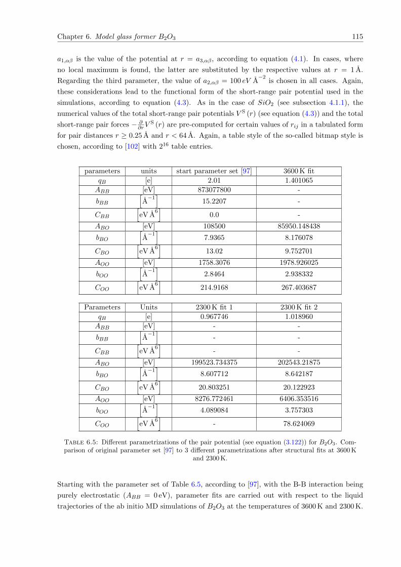
Chapter 6. Model glass former B2O3 115
a1,αβ is the value of the potential at r = a3,αβ, according to equation (4.1). In cases, where
no local maximum is found, the latter are substituted by the respective values at r = 1 A.
Regarding the third parameter, the value of a2,αβ = 100 eV A−2
is chosen in all cases. Again,
these considerations lead to the functional form of the short-range pair potential used in the
simulations, according to equation (4.3). As in the case of SiO2 (see subsection 4.1.1), the
numerical values of the total short-range pair potentials V S (r) (see equation (4.3)) and the total
short-range pair forces − ∂∂rV
S (r) are pre-computed for certain values of rij in a tabulated form
for pair distances r ≥ 0.25 A and r < 64 A. Again, a table style of the so-called bitmap style is
chosen, according to [102] with 216 table entries.
parameters units start parameter set [97] 3600 K fit
qB [e] 2.01 1.401065
ABB [eV] 873077800 -
bBB
[A−1]
15.2207 -
CBB
[eV A
6]
0.0 -
ABO [eV] 108500 85950.148438
bBO
[A−1]
7.9365 8.176078
CBO
[eV A
6]
13.02 9.752701
AOO [eV] 1758.3076 1978.926025
bOO
[A−1]
2.8464 2.938332
COO
[eV A
6]
214.9168 267.403687
Parameters Units 2300 K fit 1 2300 K fit 2
qB [e] 0.967746 1.018960
ABB [eV] - -
bBB
[A−1]
- -
CBB
[eV A
6]
- -
ABO [eV] 199523.734375 202543.21875
bBO
[A−1]
8.607712 8.642187
CBO
[eV A
6]
20.803251 20.122923
AOO [eV] 8276.772461 6406.353516
bOO
[A−1]
4.089084 3.757303
COO
[eV A
6]
- 78.624069
Table 6.5: Different parametrizations of the pair potential (see equation (3.122)) for B2O3. Com-parison of original parameter set [97] to 3 different parametrizations after structural fits at 3600 K
and 2300 K.
Starting with the parameter set of Table 6.5, according to [97], with the B-B interaction being
purely electrostatic (ABB = 0 eV), parameter fits are carried out with respect to the liquid
trajectories of the ab initio MD simulations of B2O3 at the temperatures of 3600 K and 2300 K.
Chapter 6. Model glass former B2O3 116
These are the highest and the lowest temperatures at which ab initio MD simulations are carried
out, described in detail in section 6.2. Therefore, it is interesting to examine if the fitting
procedures at these two temperatures lead to significantly different parameter sets. At the
temperature of 2300 K, two different fits are carried out. In the second one, the O-O interaction
is chosen to be purely repulsive, meaning a fixed value of COO = 0 eV A6
is chosen. This means
that, in each case, a set of M = 7 (M = 6 in the case of COO = 0 eV A6) parameters a1, . . . , aM
is optimized, including the charge of the boron atoms, namely qB, ABO, bBO, CBO, AOO, bOO
and COO. The charge of the oxygen atoms follows from the requirement of charge neutrality
(qO = −2/3 qB). The basis for the structural fits are the last 20000 time steps of the liquid
trajectories at 3600 K and 2300 K. The parameter optimization is performed by a Levenberg-
Marquardt algorithm, which is an iterative scheme to find the (local) minimum of the sum of
squares χ2 of the deviations between a set of data points and a model curve depending on a
set of parameters. The method of structure matching and the Levenberg-Marquardt procedure
are described in detail in section 3.5. The optimization of the force field parameters is carried
out with respect to the partial pair correlation functions of all correlations gBB (r), gBO (r) and
gOO (r) and all 6 relevant angular distributions pαβγ (Φ) , α, β, γ ∈ B,O, meaning pBBB (Φ),
pBBO (Φ), pBOB (Φ), pBOO (Φ), pOBO (Φ) and pOOO (Φ). (pOBB (Φ) is identical to pBBO (Φ)
and pOOB (Φ) is identical to pBOO (Φ).) The values of the relevant pαβγ (Φ) , α, β, γ ∈ B,O,are multiplied by the factor 100. This ensures that the numerical values of pαβγ (Φ) are of
the same order of magnitude as the ones of gαβ (r). The determination of new parameters is
based on the original fitting routine of A. Carre [51], which is extended to include the relevant
angular distributions into the fitting procedure. Regarding these considerations, the numerical
value of Chi-Square χ2 (a1, . . . , aM ) at each iteration step is calculated, according to equation
(3.128) with σαβ = 1, α, β, γ ∈ B,O, in case of the pair correlation functions and σαβγ =
0.01, α, β, γ ∈ B,O, in case of the angular distributions. (The multiplication of the angular
distributions by a factor 100 is equivalent to the choice of σαβγ = 0.01.) gclassical MDαβ (r) and
P classical MDαβγ (Φ) in equation (3.128) are computed with respect to a classical molecular dynamics
run of the same system size (150 atoms, LBox = 12.375 A) and at the same temperature as in
case of the ab initio molecular dynamics run. In each case, a numerical discretization of 250
data points is chosen, meaning that the corresponding parameters in equation (3.128) are 4d =LBox2·250 = 12.375 A
2·250 = 0.02475 A, in case of the pair correlation functions and 4a = 1802·250 = 0.36,
in case of the angular distributions. Except for the reweighting of pαβγ (Φ) with respect to
gαβ (r), all data points are considered to have the same weight.
At each iteration step of the Levenberg-Marquardt procedure (see section 3.5), the numerical
derivatives with respect to the independent fit parameters a1, . . . , aM (M = 7 or M = 6)
have to be calculated (see equations (3.129) to (3.132) and (3.137) to (3.138)). This requires
two additional classical MD runs per parameter for each iteration step with the parameter
sets a1, . . . , ai ± εai , . . . , aM , i ∈ 1, . . . ,M, meaning a total of 2M + 1 classical MD runs
per iteration step. In each case, the parameters εai are chosen in the following way: εqB =
0.02 · qB = 0.0402 e, εABO = 0.1 · ABO = 10850 eV, εbBO = 0.03 · bBO = 0.238095 A−1
, εCBO =
0.05 · CBO = 0.651 eV A6, εAOO = 0.1 · AOO = 175.83076 eV, εbOO = 0.03 · bOO = 0.085392 A
−1
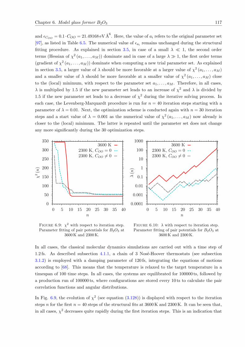
Chapter 6. Model glass former B2O3 117
and εCOO = 0.1 ·COO = 21.49168 eV A6. Here, the value of ai refers to the original parameter set
[97], as listed in Table 6.5. The numerical value of εai remains unchanged during the structural
fitting procedure. As explained in section 3.5, in case of a small λ 1, the second order
terms (Hessian of χ2 (a1, . . . , aM )) dominate and in case of a large λ 1, the first order terms
(gradient of χ2 (a1, . . . , aM )) dominate when computing a new trial parameter set. As explained
in section 3.5, a larger value of λ should be more favorable at a larger value of χ2 (a1, . . . , aM )
and a smaller value of λ should be more favorable at a smaller value of χ2 (a1, . . . , aM ) close
to the (local) minimum, with respect to the parameter set a1, . . . , aM . Therefore, in all cases,
λ is multiplied by 1.5 if the new parameter set leads to an increase of χ2 and λ is divided by
1.5 if the new parameter set leads to a decrease of χ2 during the iterative solving process. In
each case, the Levenberg-Marquardt procedure is run for n = 40 iteration steps starting with a
parameter of λ = 0.01. Next, the optimization scheme is conducted again with n = 30 iteration
steps and a start value of λ = 0.001 as the numerical value of χ2 (a1, . . . , aM ) now already is
closer to the (local) minimum. The latter is repeated until the parameter set does not change
any more significantly during the 30 optimization steps.
0
50
100
150
200
250
300
350
0 5 10 15 20 25 30 35 40
χ2(n)
n
3600 K2300 K, COO = 02300 K, COO 6= 0
Figure 6.9: χ2 with respect to iteration step.Parameter fitting of pair potentials for B2O3 at
3600 K and 2300 K.
0.0001
0.001
0.01
0.1
1
10
100
1000
0 5 10 15 20 25 30 35 40
λ(n)
n
3600 K2300 K, COO = 02300 K, COO 6= 0
Figure 6.10: λ with respect to iteration step.Parameter fitting of pair potentials for B2O3 at
3600 K and 2300 K.
In all cases, the classical molecular dynamics simulations are carried out with a time step of
1.2 fs. As described subsection 4.1.1, a chain of 3 Nose-Hoover thermostats (see subsection
3.1.2) is employed with a damping parameter of 120 fs, integrating the equations of motions
according to [68]. This means that the temperature is relaxed to the target temperature in a
timespan of 100 time steps. In all cases, the systems are equilibrated for 100000 ts, followed by
a production run of 100000 ts, where configurations are stored every 10 ts to calculate the pair
correlation functions and angular distributions.
In Fig. 6.9, the evolution of χ2 (see equation (3.128)) is displayed with respect to the iteration
steps n for the first n = 40 steps of the structural fits at 3600 K and 2300 K. It can be seen that,
in all cases, χ2 decreases quite rapidly during the first iteration steps. This is an indication that
Chapter 6. Model glass former B2O3 118
the structural fitting procedure according to the Levenberg-Marquardt scheme works reasonably
well and the start parameter of λ = 0.01 is a sensible choice. In Fig. 6.10, the evolution of λ is
displayed with respect to the iteration steps n, again for the first n = 40 steps of the structural
fits at 3600 K and 2300 K. The decrease of λ at a specific iteration step implies that at this step
a parameter optimization could be achieved and vice versa. It can be seen that, in all cases, after
several iteration steps at which λ decreases, an increase can be observed at the end of this set of
iteration steps. In general, the parameter λ stays larger for the optimization at 3600 K, meaning
there are less iteration steps, where the fit parameters could be optimized. It should be noted
that the optimization procedures at 2300 K, displayed in Figs. 6.9 and 6.10, are conducted with
respect to the liquid structure between time steps 62000 and 72000 of the 124.2 ps ab initio run
at 2300 K. At the point in time where these structural fits have been performed, the simulation
of the liquid trajectory at 2300 K has not yet been completed. However, no significant change
of the fit parameters is observed when the optimization scheme is rerun with respect to the
last 20000 ts of the 124.2 ps run, starting with the already optimized parameter set after 72000
time steps and a start parameter of λ = 0.001. The final values of χ2 after all iterations of the
parameter optimizations are: χ2 = 43.1828 at 3600 K and χ2 = 50.267151 (COO = 0 eV A6) and
χ2 = 50.831890 (COO 6= 0 eV A6) at 2300 K.
The optimized parameter sets are displayed in table 6.5 together with the start parameters,
according to [97]. It can be seen that at T = 3600 K, as well as T = 2300 K, a main effect of the
structure matching scheme is to reduce the charge of the boron atoms qB (and as a consequence
also the charge of the oxygen atoms qO). The decrease of the atomic charges is more pronounced
at the temperature of 2300 K. Of course, in this considerations, qB only is a force field parameter
and the numerical value of qB (and qO) should not be taken literally. However, it is known that
the bonding of B2O3 is partly covalent [165]. In this work, the Mulliken charges of crystalline
B2O3 are calculated and it is found that both investigated crystalline phases show a degree of
covalency in the bonding, which is more pronounced for the low-pressure phase B2O3− I. Also,
the most-promising classical force fields, according to [44], show a partial charge of qB = 1.2 e
(C1) and qB = 0.9 e (C2). These values of the parameter qB agree quite well with the results of
this work.
In Figs. 6.11 and 6.12, the partial pair correlation functions gBB (r) and gOO (r) and the an-
gular distributions pBOB (Φ) and pOBO (Φ), according to the structural fit at T = 3600 K, are
compared to the curves, based on the last 20000ts of the ab initio MD trajectory at the same
temperature, and to the curves of the original parameter set [97]. These are the correlations that
show the most pronounced differences between the classical and the ab initio MD run. The main
difference between the classical MD simulation with the new parameter set and the ab initio MD
run is that the peak position of the first neighbor peak in gBB (r) is shifted to a larger distance
r of about 0.1 A in the classical MD run. This reflects in the peak position of the main peak in
pBOB (Φ) being shifted to larger angles by about 10, as well. The classical gOO (r) curve shows
some irregularities for small r-values. In general, the peak heights of the classical curves after
the structural fit are slightly lower than in the ab initio MD run. However, these curves show
a significantly improved agreement to the ab initio curves, compared to the original parameter
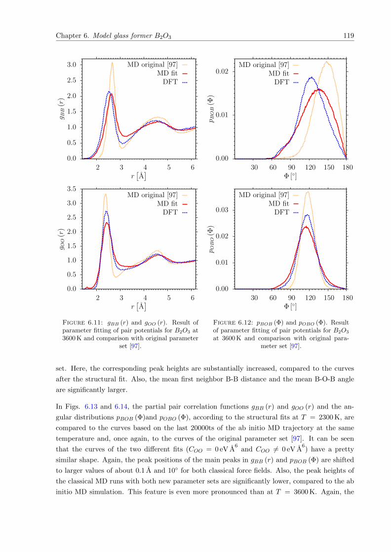
Chapter 6. Model glass former B2O3 119
0.0
0.5
1.0
1.5
2.0
2.5
3.0
2 3 4 5 6
g BB
(r)
r[A]
MD original [97]MD fit
DFT
0.0
0.5
1.0
1.5
2.0
2.5
3.0
3.5
2 3 4 5 6
g OO
(r)
r[A]
MD original [97]MD fit
DFT
Figure 6.11: gBB (r) and gOO (r). Result ofparameter fitting of pair potentials for B2O3 at3600 K and comparison with original parameter
set [97].
0.00
0.01
0.02
30 60 90 120 150 180
p BOB
(Φ)
Φ []
MD original [97]MD fit
DFT
0.00
0.01
0.02
0.03
30 60 90 120 150 180
p OBO
(Φ)
Φ []
MD original [97]MD fit
DFT
Figure 6.12: pBOB (Φ) and pOBO (Φ). Resultof parameter fitting of pair potentials for B2O3
at 3600 K and comparison with original para-meter set [97].
set. Here, the corresponding peak heights are substantially increased, compared to the curves
after the structural fit. Also, the mean first neighbor B-B distance and the mean B-O-B angle
are significantly larger.
In Figs. 6.13 and 6.14, the partial pair correlation functions gBB (r) and gOO (r) and the an-
gular distributions pBOB (Φ)and pOBO (Φ), according to the structural fits at T = 2300 K, are
compared to the curves based on the last 20000ts of the ab initio MD trajectory at the same
temperature and, once again, to the curves of the original parameter set [97]. It can be seen
that the curves of the two different fits (COO = 0 eV A6
and COO 6= 0 eV A6) have a pretty
similar shape. Again, the peak positions of the main peaks in gBB (r) and pBOB (Φ) are shifted
to larger values of about 0.1 A and 10 for both classical force fields. Also, the peak heights of
the classical MD runs with both new parameter sets are significantly lower, compared to the ab
initio MD simulation. This feature is even more pronounced than at T = 3600 K. Again, the
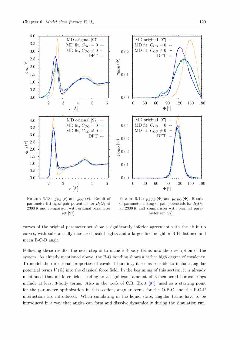
Chapter 6. Model glass former B2O3 120
0.0
0.5
1.0
1.5
2.0
2.5
3.0
3.5
4.0
2 3 4 5 6
g BB
(r)
r[A]
MD original [97]MD fit, COO = 0MD fit, COO 6= 0
DFT
0.0
0.5
1.0
1.5
2.0
2.5
3.0
3.5
4.0
2 3 4 5 6
g OO
(r)
r[A]
MD original [97]MD fit, COO = 0MD fit, COO 6= 0
DFT
Figure 6.13: gBB (r) and gOO (r). Result ofparameter fitting of pair potentials for B2O3 at2300 K and comparison with original parameter
set [97].
0.00
0.01
0.02
0 30 60 90 120 150 180
p BOB
(Φ)
Φ []
MD original [97]MD fit, COO = 0MD fit, COO 6= 0
DFT
0.00
0.01
0.02
0.03
0.04
0 30 60 90 120 150 180
p OBO
(Φ)
Φ []
MD original [97]MD fit, COO = 0MD fit, COO 6= 0
DFT
Figure 6.14: pBOB (Φ) and pOBO (Φ). Resultof parameter fitting of pair potentials for B2O3
at 2300 K and comparison with original para-meter set [97].
curves of the original parameter set show a significantly inferior agreement with the ab initio
curves, with substantially increased peak heights and a larger first neighbor B-B distance and
mean B-O-B angle.
Following these results, the next step is to include 3-body terms into the description of the
system. As already mentioned above, the B-O bonding shows a rather high degree of covalency.
To model the directional properties of covalent bonding, it seems sensible to include angular
potential terms V (Φ) into the classical force field. In the beginning of this section, it is already
mentioned that all force-fields leading to a significant amount of 3-membered boroxol rings
include at least 3-body terms. Also in the work of C.R. Trott [97], used as a starting point
for the parameter optimization in this section, angular terms for the O-B-O and the P-O-P
interactions are introduced. When simulating in the liquid state, angular terms have to be
introduced in a way that angles can form and dissolve dynamically during the simulation run.
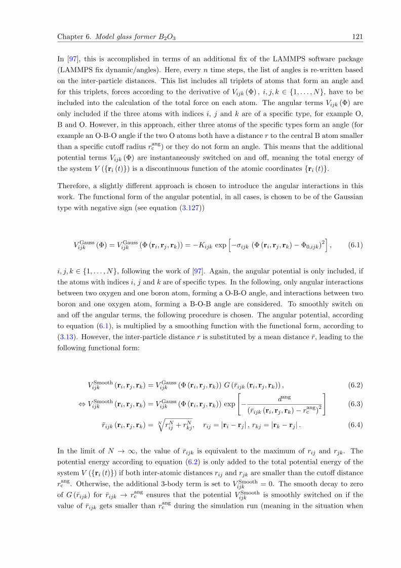
Chapter 6. Model glass former B2O3 121
In [97], this is accomplished in terms of an additional fix of the LAMMPS software package
(LAMMPS fix dynamic/angles). Here, every n time steps, the list of angles is re-written based
on the inter-particle distances. This list includes all triplets of atoms that form an angle and
for this triplets, forces according to the derivative of Vijk (Φ) , i, j, k ∈ 1, . . . , N, have to be
included into the calculation of the total force on each atom. The angular terms Vijk (Φ) are
only included if the three atoms with indices i, j and k are of a specific type, for example O,
B and O. However, in this approach, either three atoms of the specific types form an angle (for
example an O-B-O angle if the two O atoms both have a distance r to the central B atom smaller
than a specific cutoff radius rangc ) or they do not form an angle. This means that the additional
potential terms Vijk (Φ) are instantaneously switched on and off, meaning the total energy of
the system V (ri (t)) is a discontinuous function of the atomic coordinates ri (t).
Therefore, a slightly different approach is chosen to introduce the angular interactions in this
work. The functional form of the angular potential, in all cases, is chosen to be of the Gaussian
type with negative sign (see equation (3.127))
V Gaussijk (Φ) = V Gauss
ijk (Φ (ri, rj , rk)) = −Kijk exp[−σijk (Φ (ri, rj , rk)− Φ0,ijk)
2], (6.1)
i, j, k ∈ 1, . . . , N, following the work of [97]. Again, the angular potential is only included, if
the atoms with indices i, j and k are of specific types. In the following, only angular interactions
between two oxygen and one boron atom, forming a O-B-O angle, and interactions between two
boron and one oxygen atom, forming a B-O-B angle are considered. To smoothly switch on
and off the angular terms, the following procedure is chosen. The angular potential, according
to equation (6.1), is multiplied by a smoothing function with the functional form, according to
(3.13). However, the inter-particle distance r is substituted by a mean distance r, leading to the
following functional form:
V Smoothijk (ri, rj , rk) = V Gauss
ijk (Φ (ri, rj , rk)) G (rijk (ri, rj , rk)) , (6.2)
⇔ V Smoothijk (ri, rj , rk) = V Gauss
ijk (Φ (ri, rj , rk)) exp
[− dang
(rijk (ri, rj , rk)− rangc )
2
](6.3)
rijk (ri, rj , rk) = N
√rNij + rNkj , rij = |ri − rj | , rkj = |rk − rj | . (6.4)
In the limit of N → ∞, the value of rijk is equivalent to the maximum of rij and rjk. The
potential energy according to equation (6.2) is only added to the total potential energy of the
system V (ri (t)) if both inter-atomic distances rij and rjk are smaller than the cutoff distance
rangc . Otherwise, the additional 3-body term is set to V Smooth
ijk = 0. The smooth decay to zero
of G (rijk) for rijk → rangc ensures that the potential V Smooth
ijk is smoothly switched on if the
value of rijk gets smaller than rangc during the simulation run (meaning in the situation when
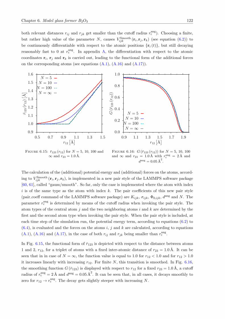
Chapter 6. Model glass former B2O3 122
both relevant distances rij and rjk get smaller than the cutoff radius rangc ). Choosing a finite,
but rather high value of the parameter N , causes V Smoothijk (ri, rj , rk) (see equation (6.2)) to
be continuously differentiable with respect to the atomic positions ri (t), but still decaying
reasonably fast to 0 at rangc . In appendix A, the differentiation with respect to the atomic
coordinates ri, rj and rk is carried out, leading to the functional form of the additional forces
on the corresponding atoms (see equations (A.1), (A.16) and (A.17)).
0.9
1.0
1.1
1.2
1.3
1.4
1.5
1.6
0.5 0.7 0.9 1.1 1.3 1.5
r 123
(r12)[ A]
r12[A]
N = 5N = 10N = 100N = ∞
Figure 6.15: r123 (r12) for N = 5, 10, 100 and∞ and r23 = 1.0 A.
0.0
0.2
0.4
0.6
0.8
1.0
0.9 1.1 1.3 1.5 1.7 1.9
G(r
123
(r12))
r12[A]
N = 5N = 10N = 100N = ∞
Figure 6.16: G (r123 (r12)) for N = 5, 10, 100and ∞ and r23 = 1.0 A with rang
c = 2 A and
dang = 0.05 A2.
The calculation of the (additional) potential energy and (additional) forces on the atoms, accord-
ing to V Smoothijk (ri, rj , rk), is implemented in a new pair style of the LAMMPS software package
[60, 61], called “gauss/smooth”. So far, only the case is implemented where the atom with index
i is of the same type as the atom with index k. The pair coefficients of this new pair style
(pair coeff command of the LAMMPS software package) are Kijk, σijk, Φ0,ijk, dang and N . The
parameter rangc is determined by means of the cutoff radius when invoking the pair style. The
atom types of the central atom j and the two neighboring atoms i and k are determined by the
first and the second atom type when invoking the pair style. When the pair style is included, at
each time step of the simulation run, the potential energy term, according to equations (6.2) to
(6.4), is evaluated and the forces on the atoms i, j and k are calculated, according to equations
(A.1), (A.16) and (A.17), in the case of both rij and rjk being smaller than rangc .
In Fig. 6.15, the functional form of r123 is depicted with respect to the distance between atoms
1 and 2, r12, for a triplet of atoms with a fixed inter-atomic distance of r23 = 1.0 A. It can be
seen that in in case of N =∞, the function value is equal to 1.0 for r12 < 1.0 and for r12 > 1.0
it increases linearly with increasing r12. For finite N , this transition is smoothed. In Fig. 6.16,
the smoothing function G (r123) is displayed with respect to r12 for a fixed r23 = 1.0 A, a cutoff
radius of rangc = 2 A and dang = 0.05 A
2. It can be seen that, in all cases, it decays smoothly to
zero for r12 → rangc . The decay gets slightly steeper with increasing N .
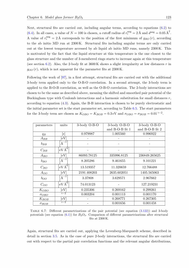
Chapter 6. Model glass former B2O3 123
Next, structural fits are carried out, including angular terms, according to equations (6.2) to
(6.4). In all cases, a value of N = 100 is chosen, a cutoff radius of rangc = 2 A and dang = 0.05 A
2.
A value of rangc = 2 A corresponds to the position of the first minimum of gBO (r), according
to the ab initio MD run at 2300 K. Structural fits including angular terms are only carried
out at the lowest temperature accessed by ab liquid ab initio MD runs, namely 2300 K. This
is motivated by the fact that the liquid structure at this temperature is the one closest to the
glass structure and the number of 3-membered rings starts to increase again at this temperature
(see section 6.2). Also, the 2-body fit at 3600 K shows a slight irregularity at low distances r in
gOO (r), which is not apparent for the parameter fits at 2300 K.
Following the work of [97], in a first attempt, structural fits are carried out with the additional
3-body term applied only to the O-B-O correlation. In a second attempt, the 3-body term is
applied to the B-O-B correlation, as well as the O-B-O correlation. The 2-body interactions are
chosen to be the same as described above, meaning the shifted and smoothed pair potential of the
Buckingham type with Coulomb interactions and a harmonic substitution for small distances r,
according to equation (4.3). Again, the B-B interaction is chosen to be purely electrostatic and
the initial parameter set is the start parameter set, according to Table 6.5. The start parameters
for the 3-body term are chosen as KOBO = KBOB = 0.3 eV and σOBO = σBOB = 0.01 −2.
parameters units 3-body O-B-O 3-body O-B-Oand B-O-B fit 1
3-body O-B-Oand B-O-B fit 2
qB [e] 0.979987 1.005560 0.996922
ABB [eV] - - -
bBB
[A−1]
- - -
CBB
[eV A
6]
- - -
ABO [eV] 86093.78125 335996.8125 236849.265625
bBO
[A−1]
8.205286 9.461655 9.101221
CBO
[eV A
6]
13.519357 11.320659 12.766488
AOO [eV] 2191.408203 2635.602051 1405.565063
bOO
[A−1]
3.37808 3.629571 2.967662
COO
[eV A
6]
74.013123 - 127.219231
KOBO [eV] 0.235306 0.269162 0.299261
σOBO−2 0.003204 0.001113 0.001170
KBOB [eV] - 0.268771 0.267305
σBOB−2 - 0.001656 0.001458
Table 6.7: Different parametrizations of the pair potential (see equation (3.122)) and 3-bodypotentials (see equation (6.1)) for B2O3. Comparison of different parametrizations after structural
fits at 2300 K.
Again, structural fits are carried out, applying the Levenberg-Marquardt scheme, described in
detail in section 3.5. As in the case of pure 2-body interactions, the structural fits are carried
out with respect to the partial pair correlation functions and the relevant angular distributions,
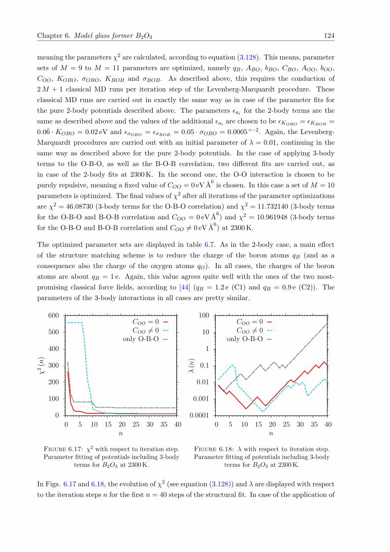
Chapter 6. Model glass former B2O3 124
meaning the parameters χ2 are calculated, according to equation (3.128). This means, parameter
sets of M = 9 to M = 11 parameters are optimized, namely qB, ABO, bBO, CBO, AOO, bOO,
COO, KOBO, σOBO, KBOB and σBOB. As described above, this requires the conduction of
2M + 1 classical MD runs per iteration step of the Levenberg-Marquardt procedure. These
classical MD runs are carried out in exactly the same way as in case of the parameter fits for
the pure 2-body potentials described above. The parameters εai for the 2-body terms are the
same as described above and the values of the additional εai are chosen to be εKOBO = εKBOB =
0.06 ·KOBO = 0.02 eV and εσOBO = εσBOB = 0.05 · σOBO = 0.0005 −2. Again, the Levenberg-
Marquardt procedures are carried out with an initial parameter of λ = 0.01, continuing in the
same way as described above for the pure 2-body potentials. In the case of applying 3-body
terms to the O-B-O, as well as the B-O-B correlation, two different fits are carried out, as
in case of the 2-body fits at 2300 K. In the second one, the O-O interaction is chosen to be
purely repulsive, meaning a fixed value of COO = 0 eV A6
is chosen. In this case a set of M = 10
parameters is optimized. The final values of χ2 after all iterations of the parameter optimizations
are χ2 = 46.08730 (3-body terms for the O-B-O correlation) and χ2 = 11.732140 (3-body terms
for the O-B-O and B-O-B correlation and COO = 0 eV A6) and χ2 = 10.961948 (3-body terms
for the O-B-O and B-O-B correlation and COO 6= 0 eV A6) at 2300 K.
The optimized parameter sets are displayed in table 6.7. As in the 2-body case, a main effect
of the structure matching scheme is to reduce the charge of the boron atoms qB (and as a
consequence also the charge of the oxygen atoms qO). In all cases, the charges of the boron
atoms are about qB = 1 e. Again, this value agrees quite well with the ones of the two most-
promising classical force fields, according to [44] (qB = 1.2 e (C1) and qB = 0.9 e (C2)). The
parameters of the 3-body interactions in all cases are pretty similar.
0
100
200
300
400
500
600
0 5 10 15 20 25 30 35 40
χ2(n)
n
COO = 0COO 6= 0
only O-B-O
Figure 6.17: χ2 with respect to iteration step.Parameter fitting of potentials including 3-body
terms for B2O3 at 2300 K.
0.0001
0.001
0.01
0.1
1
10
100
0 5 10 15 20 25 30 35 40
λ(n)
n
COO = 0COO 6= 0
only O-B-O
Figure 6.18: λ with respect to iteration step.Parameter fitting of potentials including 3-body
terms for B2O3 at 2300 K.
In Figs. 6.17 and 6.18, the evolution of χ2 (see equation (3.128)) and λ are displayed with respect
to the iteration steps n for the first n = 40 steps of the structural fit. In case of the application of
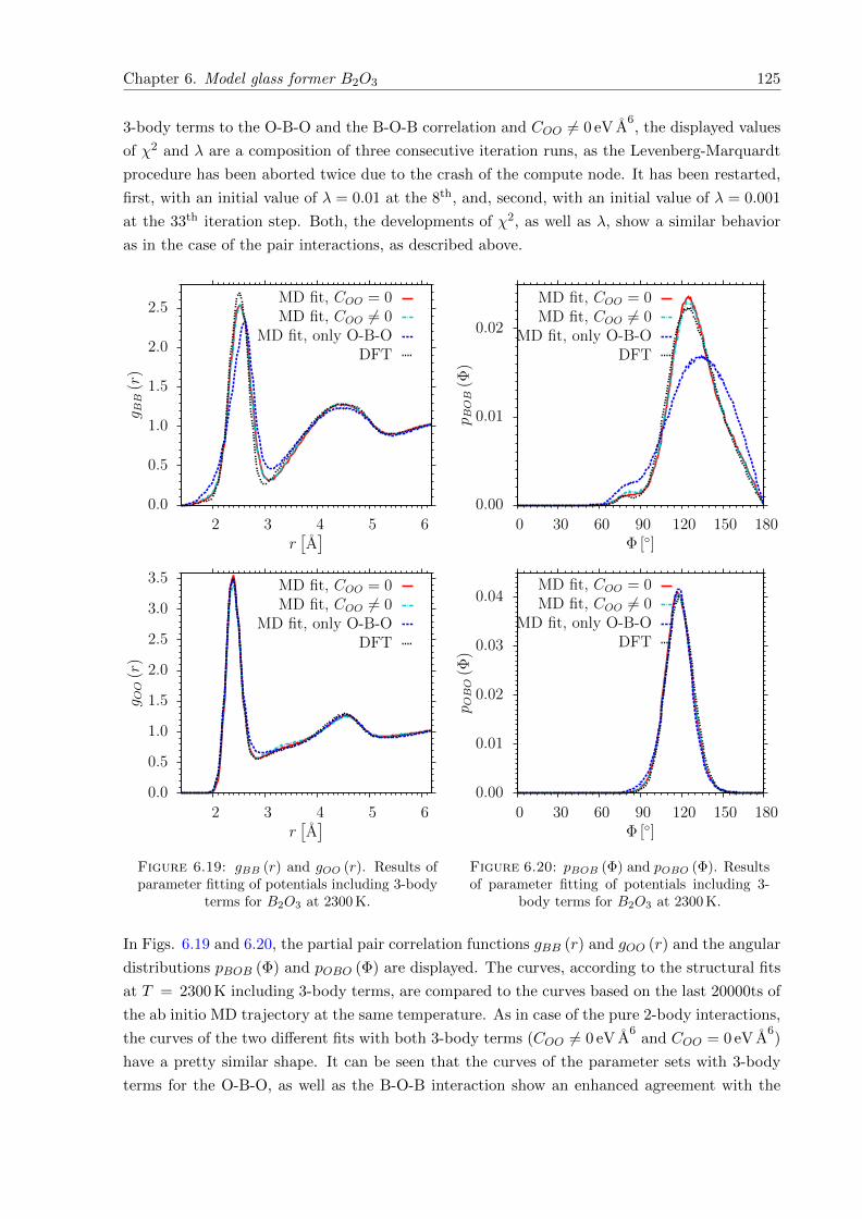
Chapter 6. Model glass former B2O3 125
3-body terms to the O-B-O and the B-O-B correlation and COO 6= 0 eV A6, the displayed values
of χ2 and λ are a composition of three consecutive iteration runs, as the Levenberg-Marquardt
procedure has been aborted twice due to the crash of the compute node. It has been restarted,
first, with an initial value of λ = 0.01 at the 8th, and, second, with an initial value of λ = 0.001
at the 33th iteration step. Both, the developments of χ2, as well as λ, show a similar behavior
as in the case of the pair interactions, as described above.
0.0
0.5
1.0
1.5
2.0
2.5
2 3 4 5 6
g BB
(r)
r[A]
MD fit, COO = 0MD fit, COO 6= 0
MD fit, only O-B-ODFT
0.0
0.5
1.0
1.5
2.0
2.5
3.0
3.5
2 3 4 5 6
g OO
(r)
r[A]
MD fit, COO = 0MD fit, COO 6= 0
MD fit, only O-B-ODFT
Figure 6.19: gBB (r) and gOO (r). Results ofparameter fitting of potentials including 3-body
terms for B2O3 at 2300 K.
0.00
0.01
0.02
0 30 60 90 120 150 180
p BOB
(Φ)
Φ []
MD fit, COO = 0MD fit, COO 6= 0
MD fit, only O-B-ODFT
0.00
0.01
0.02
0.03
0.04
0 30 60 90 120 150 180
p OBO
(Φ)
Φ []
MD fit, COO = 0MD fit, COO 6= 0
MD fit, only O-B-ODFT
Figure 6.20: pBOB (Φ) and pOBO (Φ). Resultsof parameter fitting of potentials including 3-
body terms for B2O3 at 2300 K.
In Figs. 6.19 and 6.20, the partial pair correlation functions gBB (r) and gOO (r) and the angular
distributions pBOB (Φ) and pOBO (Φ) are displayed. The curves, according to the structural fits
at T = 2300 K including 3-body terms, are compared to the curves based on the last 20000ts of
the ab initio MD trajectory at the same temperature. As in case of the pure 2-body interactions,
the curves of the two different fits with both 3-body terms (COO 6= 0 eV A6
and COO = 0 eV A6)
have a pretty similar shape. It can be seen that the curves of the parameter sets with 3-body
terms for the O-B-O, as well as the B-O-B interaction show an enhanced agreement with the
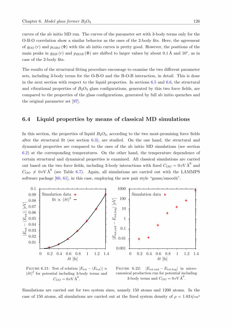
Chapter 6. Model glass former B2O3 126
curves of the ab initio MD run. The curves of the parameter set with 3-body terms only for the
O-B-O correlation show a similar behavior as the ones of the 2-body fits. Here, the agreement
of gOO (r) and pOBO (Φ) with the ab initio curves is pretty good. However, the positions of the
main peaks in gBB (r) and pBOB (Φ) are shifted to larger values by about 0.1 A and 10, as in
case of the 2-body fits.
The results of the structural fitting procedure encourage to examine the two different parameter
sets, including 3-body terms for the O-B-O and the B-O-B interaction, in detail. This is done
in the next section with respect to the liquid properties. In sections 6.5 and 6.6, the structural
and vibrational properties of B2O3 glass configurations, generated by this two force fields, are
compared to the properties of the glass configurations, generated by full ab initio quenches and
the original parameter set [97].
6.4 Liquid properties by means of classical MD simulations
In this section, the properties of liquid B2O3, according to the two most-promising force fields
after the structural fit (see section 6.3), are studied. On the one hand, the structural and
dynamical properties are compared to the ones of the ab initio MD simulations (see section
6.2) at the corresponding temperatures. On the other hand, the temperature dependence of
certain structural and dynamical properties is examined. All classical simulations are carried
out based on the two force fields, including 3-body interactions with fixed COO = 0 eV A6
and
COO 6= 0 eV A6
(see Table 6.7). Again, all simulations are carried out with the LAMMPS
software package [60, 61], in this case, employing the new pair style “gauss/smooth”.
0.01
0.02
0.03
0.04
0.05
0.06
0.07
0.08
0.09
0.1
0 0.2 0.4 0.6 0.8 1 1.2 1.4
|Etot−〈E
tot〉|
[eV
]
δt [fs]
Simulation datafit ∝ (δt)2
Figure 6.21: Test of relation |Etot − 〈Etot〉| ∝(δt)
2for potential including 3-body terms and
COO = 0 eV A6.
0.001
0.01
0.1
1
10
100
1000
0 0.2 0.4 0.6 0.8 1 1.2 1.4
|Etot,en
d−E
tot,beg|[eV
]
δt [fs]
Simulation data
Figure 6.22: |Etot,end − Etot,beg| in micro-canonical production run for potential including
3-body terms and COO = 0 eV A6.
Simulations are carried out for two system sizes, namely 150 atoms and 1200 atoms. In the
case of 150 atoms, all simulations are carried out at the fixed system density of ρ = 1.83 g/cm3
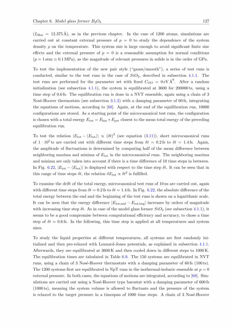
Chapter 6. Model glass former B2O3 127
(LBox = 12.375 A), as in the previous chapter. In the case of 1200 atoms, simulations are
carried out at constant external pressure of p = 0 to study the dependence of the system
density ρ on the temperature. This system size is large enough to avoid significant finite size
effects and the external pressure of p = 0 is a reasonable assumption for normal conditions
(p = 1 atm ' 0.1 MPa), as the magnitude of relevant pressures in solids is in the order of GPa.
To test the implementation of the new pair style (“gauss/smooth”), a series of test runs is
conducted, similar to the test runs in the case of SiO2, described in subsection 4.1.1. The
test runs are performed for the parameter set with fixed COO = 0 eV A6. After a random
initialization (see subsection 4.1.1), the system is equilibrated at 3600 for 200000 ts, using a
time step of 0.6 fs. The equilibration run is done in a NVT ensemble, again using a chain of 3
Nose-Hoover thermostats (see subsection 3.1.2) with a damping parameter of 60 fs, integrating
the equations of motions, according to [68]. Again, at the end of the equilibration run, 10000
configurations are stored. As a starting point of the microcanonical test runs, the configuration
is chosen with a total energy Etot = Ekin +Epot closest to the mean total energy of the preceding
equilibration run.
To test the relation |Etot − 〈Etot〉| ∝ (δt)2 (see equation (3.11)), short microcanonical runs
of 1 · 105 ts are carried out with different time steps from δt = 0.2 fs to δt = 1.4 fs. Again,
the amplitude of fluctuations is determined by computing half of the mean difference between
neighboring maxima and minima of Etot in the microcanonical runs. The neighboring maxima
and minima are only taken into account if there is a time difference of 10 time steps in between.
In Fig. 6.22, |Etot − 〈Etot〉| is displayed with respect to the time step δt. It can be seen that in
this range of time steps δt, the relation δEtot ∝ δt2 is fulfilled.
To examine the drift of the total energy, microcanonical test runs of 10 ns are carried out, again
with different time steps from δt = 0.2 fs to δt = 1.4 fs. In Fig. 6.22, the absolute difference of the
total energy between the end and the beginning of the test runs is shown on a logarithmic scale.
It can be seen that the energy difference |Etot,end − Etot,beg| increases by orders of magnitude
with increasing time step δt. As in case of the model glass former SiO2 (see subsection 4.1.1), it
seems to be a good compromise between computational efficiency and accuracy, to chose a time
step of δt = 0.6 fs. In the following, this time step is applied at all temperatures and system
sizes.
To study the liquid properties at different temperatures, all systems are first randomly ini-
tialized and then pre-relaxed with Lennard-Jones potentials, as explained in subsection 4.1.1.
Afterwards, they are equilibrated at 3600 K and then cooled down in different steps to 1000 K.
The equilibration times are tabulated in Table 6.9. The 150 systems are equilibrated in NVT
runs, using a chain of 3 Nose-Hoover thermostats with a damping parameter of 60 fs (100 ts).
The 1200 systems first are equilibrated in NpT runs in the isothermal-isobaric ensemble at p = 0
external pressure. In both cases, the equations of motions are integrated, according to [68]. Sim-
ulations are carried out using a Nose-Hoover type barostat with a damping parameter of 600 fs
(1000 ts), meaning the system volume is allowed to fluctuate and the pressure of the system
is relaxed to the target pressure in a timespan of 1000 time steps. A chain of 3 Nose-Hoover
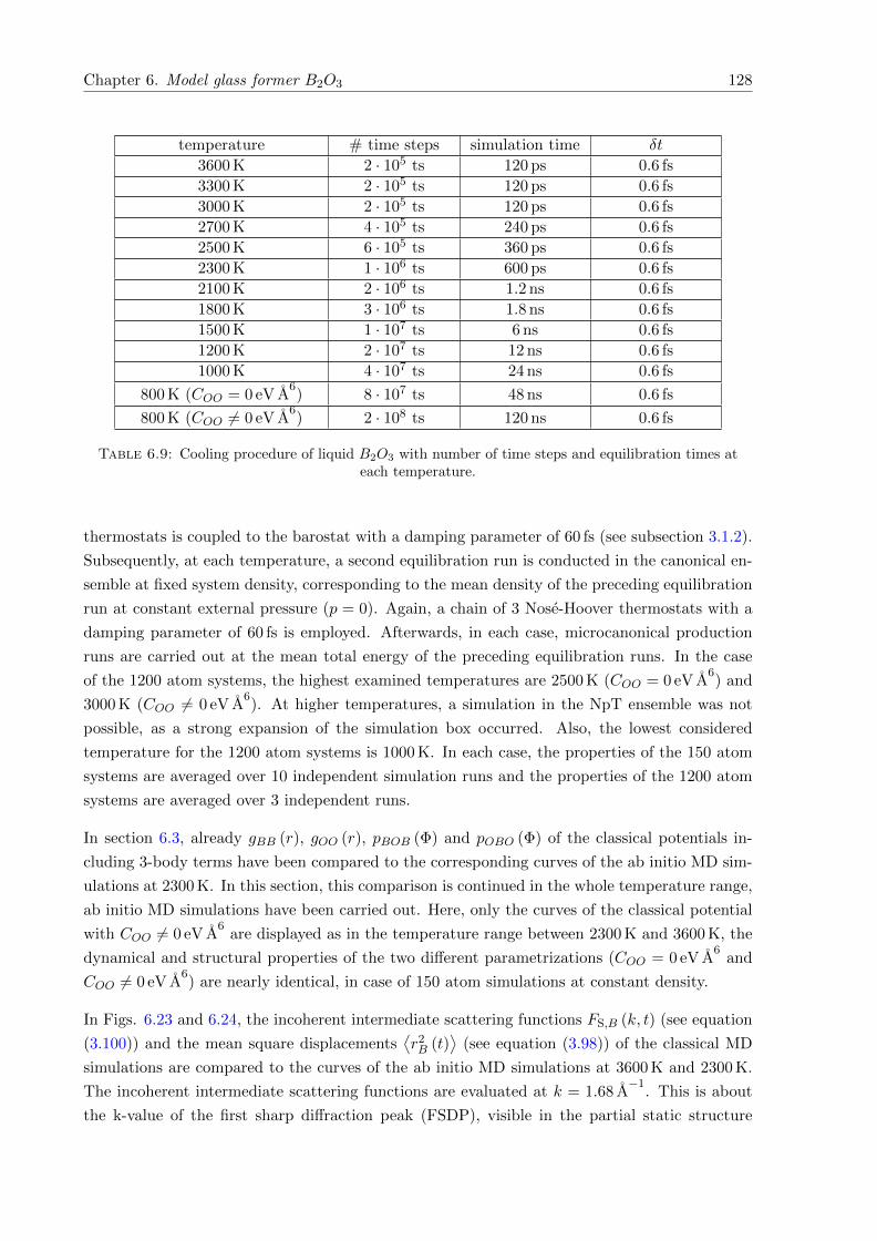
Chapter 6. Model glass former B2O3 128
temperature # time steps simulation time δt
3600 K 2 · 105 ts 120 ps 0.6 fs
3300 K 2 · 105 ts 120 ps 0.6 fs
3000 K 2 · 105 ts 120 ps 0.6 fs
2700 K 4 · 105 ts 240 ps 0.6 fs
2500 K 6 · 105 ts 360 ps 0.6 fs
2300 K 1 · 106 ts 600 ps 0.6 fs
2100 K 2 · 106 ts 1.2 ns 0.6 fs
1800 K 3 · 106 ts 1.8 ns 0.6 fs
1500 K 1 · 107 ts 6 ns 0.6 fs
1200 K 2 · 107 ts 12 ns 0.6 fs
1000 K 4 · 107 ts 24 ns 0.6 fs
800 K (COO = 0 eV A6) 8 · 107 ts 48 ns 0.6 fs
800 K (COO 6= 0 eV A6) 2 · 108 ts 120 ns 0.6 fs
Table 6.9: Cooling procedure of liquid B2O3 with number of time steps and equilibration times ateach temperature.
thermostats is coupled to the barostat with a damping parameter of 60 fs (see subsection 3.1.2).
Subsequently, at each temperature, a second equilibration run is conducted in the canonical en-
semble at fixed system density, corresponding to the mean density of the preceding equilibration
run at constant external pressure (p = 0). Again, a chain of 3 Nose-Hoover thermostats with a
damping parameter of 60 fs is employed. Afterwards, in each case, microcanonical production
runs are carried out at the mean total energy of the preceding equilibration runs. In the case
of the 1200 atom systems, the highest examined temperatures are 2500 K (COO = 0 eV A6) and
3000 K (COO 6= 0 eV A6). At higher temperatures, a simulation in the NpT ensemble was not
possible, as a strong expansion of the simulation box occurred. Also, the lowest considered
temperature for the 1200 atom systems is 1000 K. In each case, the properties of the 150 atom
systems are averaged over 10 independent simulation runs and the properties of the 1200 atom
systems are averaged over 3 independent runs.
In section 6.3, already gBB (r), gOO (r), pBOB (Φ) and pOBO (Φ) of the classical potentials in-
cluding 3-body terms have been compared to the corresponding curves of the ab initio MD sim-
ulations at 2300 K. In this section, this comparison is continued in the whole temperature range,
ab initio MD simulations have been carried out. Here, only the curves of the classical potential
with COO 6= 0 eV A6
are displayed as in the temperature range between 2300 K and 3600 K, the
dynamical and structural properties of the two different parametrizations (COO = 0 eV A6
and
COO 6= 0 eV A6) are nearly identical, in case of 150 atom simulations at constant density.
In Figs. 6.23 and 6.24, the incoherent intermediate scattering functions FS,B (k, t) (see equation
(3.100)) and the mean square displacements⟨r2B (t)
⟩(see equation (3.98)) of the classical MD
simulations are compared to the curves of the ab initio MD simulations at 3600 K and 2300 K.
The incoherent intermediate scattering functions are evaluated at k = 1.68 A−1
. This is about
the k-value of the first sharp diffraction peak (FSDP), visible in the partial static structure
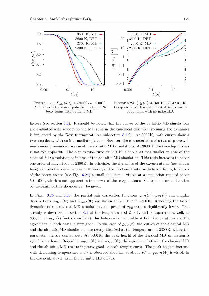
Chapter 6. Model glass former B2O3 129
0.0
0.2
0.4
0.6
0.8
1.0
0.001 0.1 10
FS,B(k,t)
t [ps]
3600 K, MD3600 K, DFT2300 K, MD2300 K, DFT
Figure 6.23: FS,B (k, t) at 2300 K and 3600 K.Comparison of classical potential including 3-
body terms with ab initio MD.
0.001
0.01
0.1
1
10
100
0.001 0.1 10
〈r2 B
(t)〉[ A
2]
t [ps]
3600 K, MD3600 K, DFT2300 K, MD
2300 K, DFT
Figure 6.24:⟨r2B (t)
⟩at 3600 K and at 2300 K.
Comparison of classical potential including 3-body terms with ab initio MD.
factors (see section 6.2). It should be noted that the curves of the ab initio MD simulations
are evaluated with respect to the MD runs in the canonical ensemble, meaning the dynamics
is influenced by the Nose thermostat (see subsection 3.1.2). At 2300 K, both curves show a
two-step decay with an intermediate plateau. However, the characteristics of a two-step decay is
much more pronounced in case of the ab initio MD simulations. At 3600 K, the two-step process
is not yet apparent. The α-relaxation time at 3600 K is about 2-times smaller in case of the
classical MD simulation as in case of the ab initio MD simulation. This ratio increases to about
one order of magnitude at 2300 K. In principle, the dynamics of the oxygen atoms (not shown
here) exhibits the same behavior. However, in the incoherent intermediate scattering functions
of the boron atoms (see Fig. 6.24) a small shoulder is visible at a simulation time of about
50− 60 fs, which is not apparent in the curves of the oxygen atoms. So far, no clear explanation
of the origin of this shoulder can be given.
In Figs. 6.25 and 6.26, the partial pair correlation functions gBB (r), gOO (r) and angular
distributions pBOB (Φ) and pOBO (Φ) are shown at 3600 K and 2300 K. Reflecting the faster
dynamics of the classical MD simulations, the peaks of gBB (r) are significantly lower. This
already is described in section 6.3 at the temperature of 2300 K and is apparent, as well, at
3600 K. In gBO (r) (not shown here), this behavior is not visible at both temperatures and the
agreement in both cases is very good. In the case of gOO (r), the curves of the classical MD
and the ab initio MD simulations are nearly identical at the temperature of 2300 K, where the
parameter fits are carried out. At 3600 K, the peak height of the classical MD simulation is
significantly lower. Regarding pBOB (Φ) and pOBO (Φ), the agreement between the classical MD
and the ab initio MD results is pretty good at both temperatures. The peak heights increase
with decreasing temperature and the observed shoulder at about 80 in pBOB (Φ) is visible in
the classical, as well as in the ab initio MD curves.
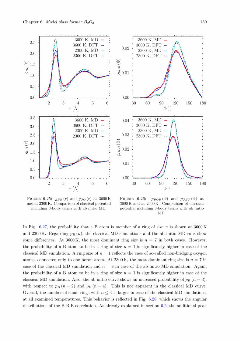
Chapter 6. Model glass former B2O3 130
0.0
0.5
1.0
1.5
2.0
2.5
2 3 4 5 6
g BB
(r)
r[A]
3600 K, MD3600 K, DFT2300 K, MD
2300 K, DFT
0.0
0.5
1.0
1.5
2.0
2.5
3.0
3.5
2 3 4 5 6
g OO
(r)
r[A]
3600 K, MD3600 K, DFT2300 K, MD
2300 K, DFT
Figure 6.25: gBB (r) and gOO (r) at 3600 Kand at 2300 K. Comparison of classical potential
including 3-body terms with ab initio MD.
0.00
0.01
0.02
30 60 90 120 150 180
p BOB
(Φ)
Φ []
3600 K, MD3600 K, DFT2300 K, MD
2300 K, DFT
0.00
0.01
0.02
0.03
0.04
30 60 90 120 150 180
p OBO
(Φ)
Φ []
3600 K, MD3600 K, DFT2300 K, MD
2300 K, DFT
Figure 6.26: pBOB (Φ) and pOBO (Φ) at3600 K and at 2300 K. Comparison of classicalpotential including 3-body terms with ab initio
MD.
In Fig. 6.27, the probability that a B atom is member of a ring of size n is shown at 3600 K
and 2300 K. Regarding pB (n), the classical MD simulations and the ab initio MD runs show
some differences. At 3600 K, the most dominant ring size is n = 7 in both cases. However,
the probability of a B atom to be in a ring of size n = 1 is significantly higher in case of the
classical MD simulation. A ring size of n = 1 reflects the case of so-called non-bridging oxygen
atoms, connected only to one boron atom. At 2300 K, the most dominant ring size is n = 7 in
case of the classical MD simulation and n = 8 in case of the ab initio MD simulation. Again,
the probability of a B atom to be in a ring of size n = 1 is significantly higher in case of the
classical MD simulation. Also, the ab initio curve shows an increased probability of pB (n = 3),
with respect to pB (n = 2) and pB (n = 4). This is not apparent in the classical MD curve.
Overall, the number of small rings with n ≤ 4 is larger in case of the classical MD simulations,
at all examined temperatures. This behavior is reflected in Fig. 6.28, which shows the angular
distributions of the B-B-B correlation. As already explained in section 6.2, the additional peak
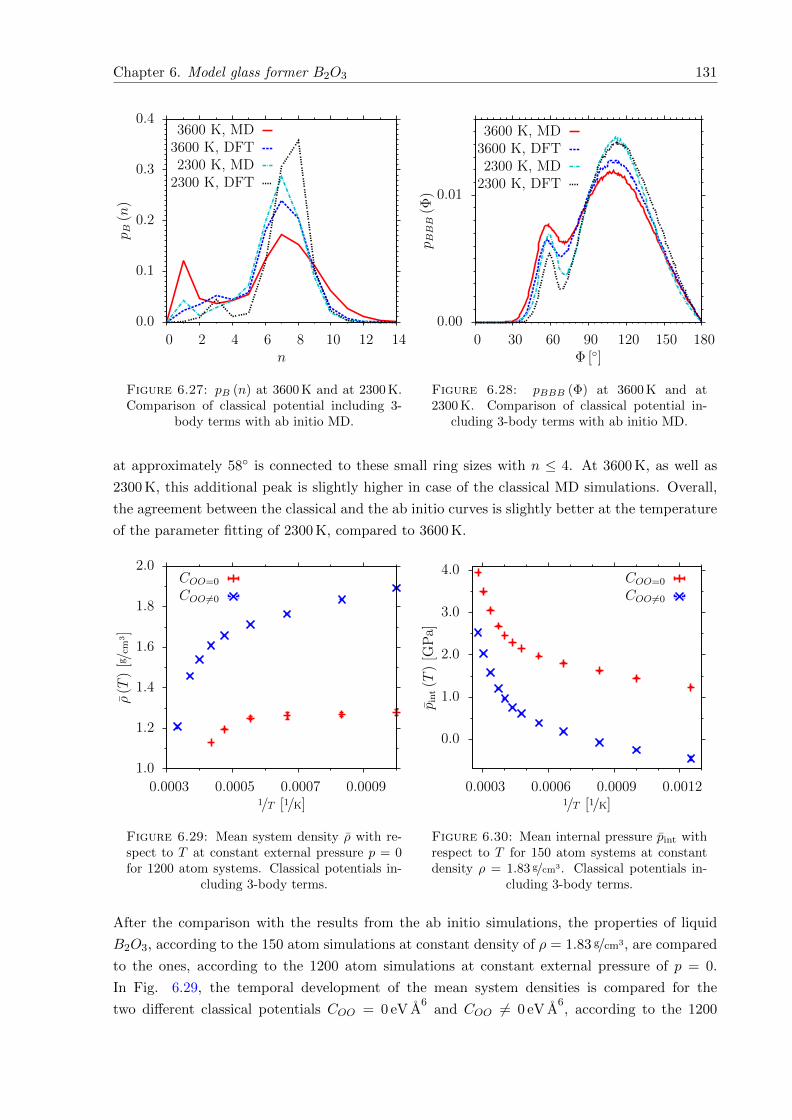
Chapter 6. Model glass former B2O3 131
0.0
0.1
0.2
0.3
0.4
0 2 4 6 8 10 12 14
p B(n)
n
3600 K, MD3600 K, DFT2300 K, MD2300 K, DFT
Figure 6.27: pB (n) at 3600 K and at 2300 K.Comparison of classical potential including 3-
body terms with ab initio MD.
0.00
0.01
0 30 60 90 120 150 180
p BBB
(Φ)
Φ []
3600 K, MD3600 K, DFT2300 K, MD
2300 K, DFT
Figure 6.28: pBBB (Φ) at 3600 K and at2300 K. Comparison of classical potential in-
cluding 3-body terms with ab initio MD.
at approximately 58 is connected to these small ring sizes with n ≤ 4. At 3600 K, as well as
2300 K, this additional peak is slightly higher in case of the classical MD simulations. Overall,
the agreement between the classical and the ab initio curves is slightly better at the temperature
of the parameter fitting of 2300 K, compared to 3600 K.
1.0
1.2
1.4
1.6
1.8
2.0
0.0003 0.0005 0.0007 0.0009
ρ(T
)[g/c
m3]
1/T [1/K]
COO=0
COO 6=0
Figure 6.29: Mean system density ρ with re-spect to T at constant external pressure p = 0for 1200 atom systems. Classical potentials in-
cluding 3-body terms.
0.0
1.0
2.0
3.0
4.0
0.0003 0.0006 0.0009 0.0012
p int(T
)[G
Pa]
1/T [1/K]
COO=0
COO 6=0
Figure 6.30: Mean internal pressure pint withrespect to T for 150 atom systems at constantdensity ρ = 1.83 g/cm3. Classical potentials in-
cluding 3-body terms.
After the comparison with the results from the ab initio simulations, the properties of liquid
B2O3, according to the 150 atom simulations at constant density of ρ = 1.83 g/cm3, are compared
to the ones, according to the 1200 atom simulations at constant external pressure of p = 0.
In Fig. 6.29, the temporal development of the mean system densities is compared for the
two different classical potentials COO = 0 eV A6
and COO 6= 0 eV A6, according to the 1200
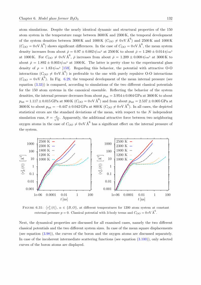
Chapter 6. Model glass former B2O3 132
atom simulations. Despite the nearly identical dynamic and structural properties of the 150
atom system in the temperature range between 3600 K and 2300 K, the temporal development
of the system densities between 3000 K and 1000 K (COO 6= 0 eV A6) and 2500 K and 1000 K
(COO = 0 eV A6) shows significant differences. In the case of COO = 0 eV A
6, the mean system
density increases from about ρ = 0.97 ± 0.002 g/cm3 at 2500 K to about ρ = 1.280 ± 0.014 g/cm3
at 1000 K. For COO 6= 0 eV A6, ρ increases from about ρ = 1.209 ± 0.008 g/cm3 at 3000 K to
about ρ = 1.892 ± 0.003 g/cm3 at 1000 K. The latter is pretty close to the experimental glass
density of ρ = 1.83 g/cm3 [159]. Regarding this behavior, the potential with attractive O-O
interactions (COO 6= 0 eV A6) is preferable to the one with purely repulsive O-O interactions
(COO = 0 eV A6). In Fig. 6.29, the temporal development of the mean internal pressure (see
equation (3.33)) is compared, according to simulations of the two different classical potentials
for the 150 atom systems in the canonical ensemble. Reflecting the behavior of the system
densities, the internal pressure decreases from about pint = 3.954±0.004 GPa at 3600 K to about
pint = 1.117± 0.015 GPa at 800 K (COO = 0 eV A6) and from about pint = 2.537± 0.005 GPa at
3600 K to about pint = −0.447± 0.042 GPa at 800 K (COO 6= 0 eV A6). In all cases, the depicted
statistical errors are the standard deviations of the mean, with respect to the N independent
simulation runs, σ = σ√N
. Apparently, the additional attractive force between two neighboring
oxygen atoms in the case of COO 6= 0 eV A6
has a significant effect on the internal pressure of
the system.
0.001
0.01
0.1
1
10
100
1000
1e-06 0.0001 0.01 1 100
〈r2 B
(t)〉[ A
2]
t [ns]
2500 K2300 K1800 K1200 K1000 K
0.001
0.01
0.1
1
10
100
1000
1e-06 0.0001 0.01 1 100
〈r2 O
(t)〉[ A
2]
t [ns]
2500 K2300 K1800 K1200 K1000 K
Figure 6.31:⟨r2α (t)
⟩, α ∈ B,O, at different temperatures for 1200 atom system at constant
external pressure p = 0. Classical potential with 3-body terms and COO = 0 eV A6.
Next, the dynamical properties are discussed for all examined cases, namely the two different
classical potentials and the two different system sizes. In case of the mean square displacements
(see equation (3.98)), the curves of the boron and the oxygen atoms are discussed separately.
In case of the incoherent intermediate scattering functions (see equation (3.100)), only selected
curves of the boron atoms are displayed.
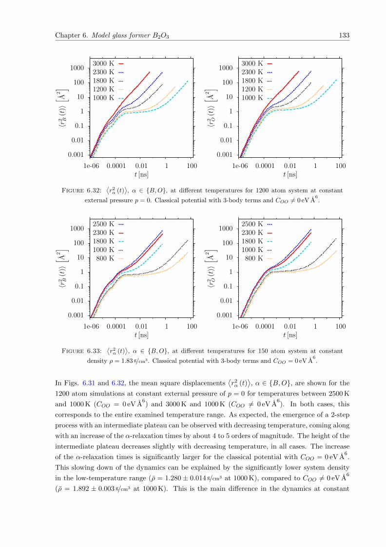
Chapter 6. Model glass former B2O3 133
0.001
0.01
0.1
1
10
100
1000
1e-06 0.0001 0.01 1 100
〈r2 B
(t)〉[ A
2]
t [ns]
3000 K2300 K1800 K1200 K1000 K
0.001
0.01
0.1
1
10
100
1000
1e-06 0.0001 0.01 1 100
〈r2 O
(t)〉[ A
2]
t [ns]
3000 K2300 K1800 K1200 K1000 K
Figure 6.32:⟨r2α (t)
⟩, α ∈ B,O, at different temperatures for 1200 atom system at constant
external pressure p = 0. Classical potential with 3-body terms and COO 6= 0 eV A6.
0.001
0.01
0.1
1
10
100
1000
1e-06 0.0001 0.01 1 100
〈r2 B
(t)〉[ A
2]
t [ns]
2500 K2300 K1800 K1000 K800 K
0.001
0.01
0.1
1
10
100
1000
1e-06 0.0001 0.01 1 100
〈r2 O
(t)〉[ A
2]
t [ns]
2500 K2300 K1800 K1000 K800 K
Figure 6.33:⟨r2α (t)
⟩, α ∈ B,O, at different temperatures for 150 atom system at constant
density ρ = 1.83 g/cm3. Classical potential with 3-body terms and COO = 0 eV A6.
In Figs. 6.31 and 6.32, the mean square displacements⟨r2α (t)
⟩, α ∈ B,O, are shown for the
1200 atom simulations at constant external pressure of p = 0 for temperatures between 2500 K
and 1000 K (COO = 0 eV A6) and 3000 K and 1000 K (COO 6= 0 eV A
6). In both cases, this
corresponds to the entire examined temperature range. As expected, the emergence of a 2-step
process with an intermediate plateau can be observed with decreasing temperature, coming along
with an increase of the α-relaxation times by about 4 to 5 orders of magnitude. The height of the
intermediate plateau decreases slightly with decreasing temperature, in all cases. The increase
of the α-relaxation times is significantly larger for the classical potential with COO = 0 eV A6.
This slowing down of the dynamics can be explained by the significantly lower system density
in the low-temperature range (ρ = 1.280 ± 0.014 g/cm3 at 1000 K), compared to COO 6= 0 eV A6
(ρ = 1.892 ± 0.003 g/cm3 at 1000 K). This is the main difference in the dynamics at constant
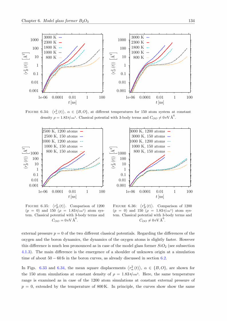
Chapter 6. Model glass former B2O3 134
0.001
0.01
0.1
1
10
100
1000
1e-06 0.0001 0.01 1 100
〈r2 B
(t)〉[ A
2]
t [ns]
3000 K2300 K1800 K1000 K800 K
0.001
0.01
0.1
1
10
100
1000
1e-06 0.0001 0.01 1 100
〈r2 O
(t)〉[ A
2]
t [ns]
3000 K2300 K1800 K1000 K800 K
Figure 6.34:⟨r2α (t)
⟩, α ∈ B,O, at different temperatures for 150 atom system at constant
density ρ = 1.83 g/cm3. Classical potential with 3-body terms and COO 6= 0 eV A6.
0.001
0.01
0.1
1
10
100
1000
1e-06 0.0001 0.01 1 100
〈r2 B
(t)〉[ A
2]
t [ns]
2500 K, 1200 atoms2500 K, 150 atoms
1000 K, 1200 atoms1000 K, 150 atoms800 K, 150 atoms
Figure 6.35:⟨r2B (t)
⟩. Comparison of 1200
(p = 0) and 150 (ρ = 1.83 g/cm3) atom sys-tem. Classical potential with 3-body terms and
COO = 0 eV A6.
0.001
0.01
0.1
1
10
100
1000
1e-06 0.0001 0.01 1 100
〈r2 B
(t)〉[ A
2]
t [ns]
3000 K, 1200 atoms3000 K, 150 atoms
1000 K, 1200 atoms1000 K, 150 atoms800 K, 150 atoms
Figure 6.36:⟨r2B (t)
⟩. Comparison of 1200
(p = 0) and 150 (ρ = 1.83 g/cm3) atom sys-tem. Classical potential with 3-body terms and
COO 6= 0 eV A6.
external pressure p = 0 of the two different classical potentials. Regarding the differences of the
oxygen and the boron dynamics, the dynamics of the oxygen atoms is slightly faster. However
this difference is much less pronounced as in case of the model glass former SiO2 (see subsection
4.1.3). The main difference is the emergence of a shoulder of unknown origin at a simulation
time of about 50− 60 fs in the boron curves, as already discussed in section 6.2.
In Figs. 6.33 and 6.34, the mean square displacements⟨r2α (t)
⟩, α ∈ B,O, are shown for
the 150 atom simulations at constant density of ρ = 1.83 g/cm3. Here, the same temperature
range is examined as in case of the 1200 atom simulations at constant external pressure of
p = 0, extended by the temperature of 800 K. In principle, the curves show show the same
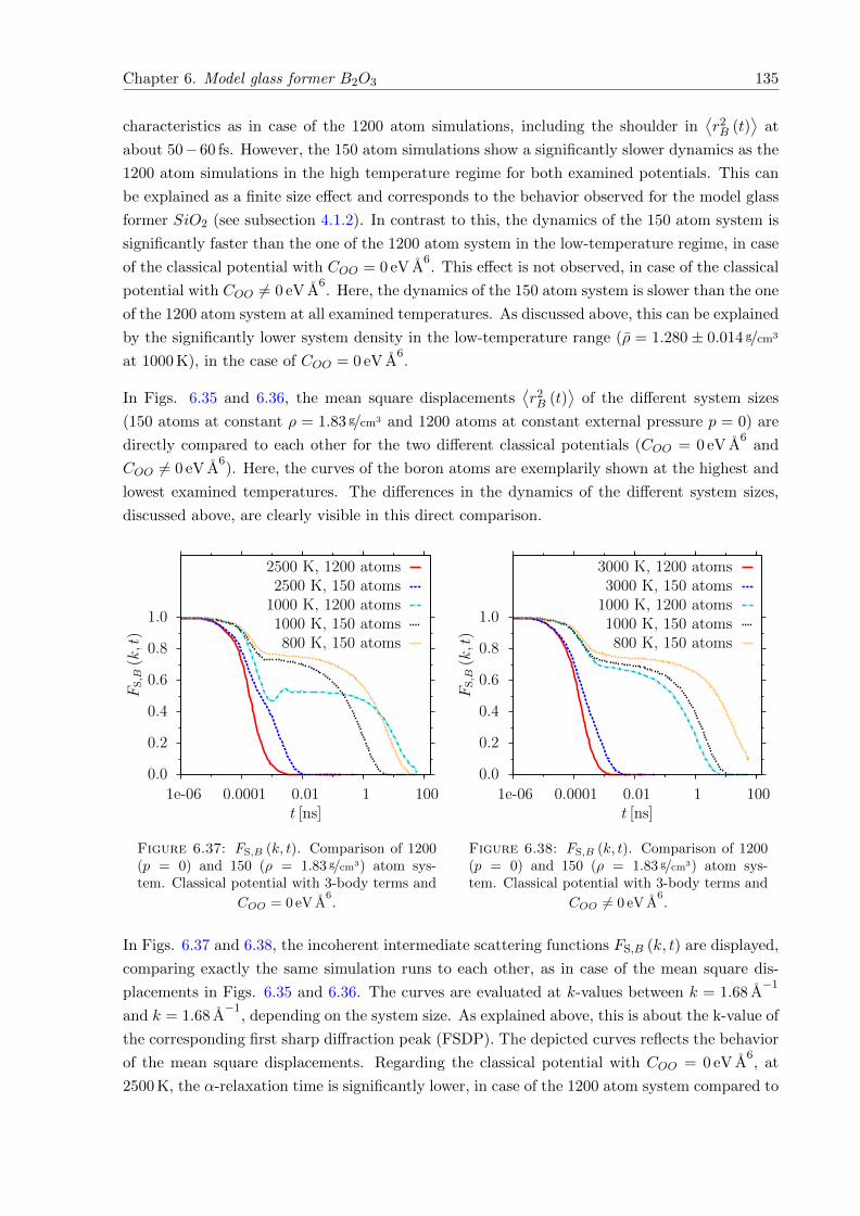
Chapter 6. Model glass former B2O3 135
characteristics as in case of the 1200 atom simulations, including the shoulder in⟨r2B (t)
⟩at
about 50−60 fs. However, the 150 atom simulations show a significantly slower dynamics as the
1200 atom simulations in the high temperature regime for both examined potentials. This can
be explained as a finite size effect and corresponds to the behavior observed for the model glass
former SiO2 (see subsection 4.1.2). In contrast to this, the dynamics of the 150 atom system is
significantly faster than the one of the 1200 atom system in the low-temperature regime, in case
of the classical potential with COO = 0 eV A6. This effect is not observed, in case of the classical
potential with COO 6= 0 eV A6. Here, the dynamics of the 150 atom system is slower than the one
of the 1200 atom system at all examined temperatures. As discussed above, this can be explained
by the significantly lower system density in the low-temperature range (ρ = 1.280± 0.014 g/cm3
at 1000 K), in the case of COO = 0 eV A6.
In Figs. 6.35 and 6.36, the mean square displacements⟨r2B (t)
⟩of the different system sizes
(150 atoms at constant ρ = 1.83 g/cm3 and 1200 atoms at constant external pressure p = 0) are
directly compared to each other for the two different classical potentials (COO = 0 eV A6
and
COO 6= 0 eV A6). Here, the curves of the boron atoms are exemplarily shown at the highest and
lowest examined temperatures. The differences in the dynamics of the different system sizes,
discussed above, are clearly visible in this direct comparison.
0.0
0.2
0.4
0.6
0.8
1.0
1e-06 0.0001 0.01 1 100
FS,B(k,t)
t [ns]
2500 K, 1200 atoms2500 K, 150 atoms1000 K, 1200 atoms1000 K, 150 atoms800 K, 150 atoms
Figure 6.37: FS,B (k, t). Comparison of 1200(p = 0) and 150 (ρ = 1.83 g/cm3) atom sys-tem. Classical potential with 3-body terms and
COO = 0 eV A6.
0.0
0.2
0.4
0.6
0.8
1.0
1e-06 0.0001 0.01 1 100
FS,B(k,t)
t [ns]
3000 K, 1200 atoms3000 K, 150 atoms1000 K, 1200 atoms1000 K, 150 atoms800 K, 150 atoms
Figure 6.38: FS,B (k, t). Comparison of 1200(p = 0) and 150 (ρ = 1.83 g/cm3) atom sys-tem. Classical potential with 3-body terms and
COO 6= 0 eV A6.
In Figs. 6.37 and 6.38, the incoherent intermediate scattering functions FS,B (k, t) are displayed,
comparing exactly the same simulation runs to each other, as in case of the mean square dis-
placements in Figs. 6.35 and 6.36. The curves are evaluated at k-values between k = 1.68 A−1
and k = 1.68 A−1
, depending on the system size. As explained above, this is about the k-value of
the corresponding first sharp diffraction peak (FSDP). The depicted curves reflects the behavior
of the mean square displacements. Regarding the classical potential with COO = 0 eV A6, at
2500 K, the α-relaxation time is significantly lower, in case of the 1200 atom system compared to
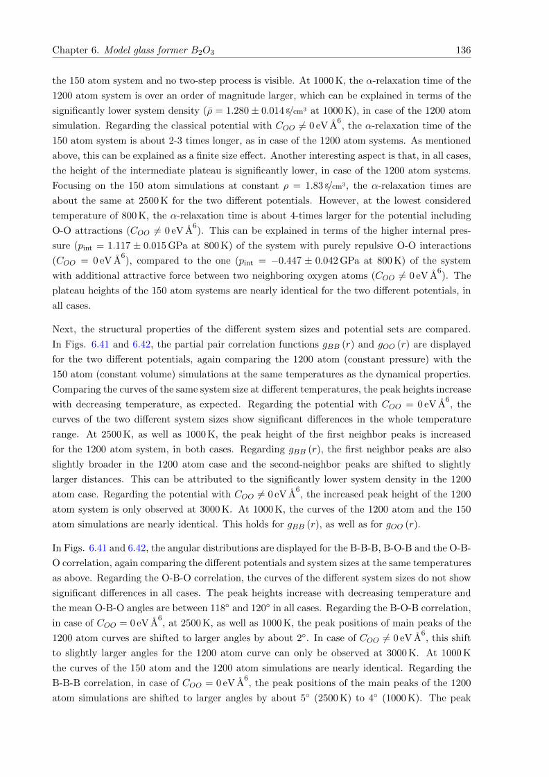
Chapter 6. Model glass former B2O3 136
the 150 atom system and no two-step process is visible. At 1000 K, the α-relaxation time of the
1200 atom system is over an order of magnitude larger, which can be explained in terms of the
significantly lower system density (ρ = 1.280± 0.014 g/cm3 at 1000 K), in case of the 1200 atom
simulation. Regarding the classical potential with COO 6= 0 eV A6, the α-relaxation time of the
150 atom system is about 2-3 times longer, as in case of the 1200 atom systems. As mentioned
above, this can be explained as a finite size effect. Another interesting aspect is that, in all cases,
the height of the intermediate plateau is significantly lower, in case of the 1200 atom systems.
Focusing on the 150 atom simulations at constant ρ = 1.83 g/cm3, the α-relaxation times are
about the same at 2500 K for the two different potentials. However, at the lowest considered
temperature of 800 K, the α-relaxation time is about 4-times larger for the potential including
O-O attractions (COO 6= 0 eV A6). This can be explained in terms of the higher internal pres-
sure (pint = 1.117 ± 0.015 GPa at 800 K) of the system with purely repulsive O-O interactions
(COO = 0 eV A6), compared to the one (pint = −0.447 ± 0.042 GPa at 800 K) of the system
with additional attractive force between two neighboring oxygen atoms (COO 6= 0 eV A6). The
plateau heights of the 150 atom systems are nearly identical for the two different potentials, in
all cases.
Next, the structural properties of the different system sizes and potential sets are compared.
In Figs. 6.41 and 6.42, the partial pair correlation functions gBB (r) and gOO (r) are displayed
for the two different potentials, again comparing the 1200 atom (constant pressure) with the
150 atom (constant volume) simulations at the same temperatures as the dynamical properties.
Comparing the curves of the same system size at different temperatures, the peak heights increase
with decreasing temperature, as expected. Regarding the potential with COO = 0 eV A6, the
curves of the two different system sizes show significant differences in the whole temperature
range. At 2500 K, as well as 1000 K, the peak height of the first neighbor peaks is increased
for the 1200 atom system, in both cases. Regarding gBB (r), the first neighbor peaks are also
slightly broader in the 1200 atom case and the second-neighbor peaks are shifted to slightly
larger distances. This can be attributed to the significantly lower system density in the 1200
atom case. Regarding the potential with COO 6= 0 eV A6, the increased peak height of the 1200
atom system is only observed at 3000 K. At 1000 K, the curves of the 1200 atom and the 150
atom simulations are nearly identical. This holds for gBB (r), as well as for gOO (r).
In Figs. 6.41 and 6.42, the angular distributions are displayed for the B-B-B, B-O-B and the O-B-
O correlation, again comparing the different potentials and system sizes at the same temperatures
as above. Regarding the O-B-O correlation, the curves of the different system sizes do not show
significant differences in all cases. The peak heights increase with decreasing temperature and
the mean O-B-O angles are between 118 and 120 in all cases. Regarding the B-O-B correlation,
in case of COO = 0 eV A6, at 2500 K, as well as 1000 K, the peak positions of main peaks of the
1200 atom curves are shifted to larger angles by about 2. In case of COO 6= 0 eV A6, this shift
to slightly larger angles for the 1200 atom curve can only be observed at 3000 K. At 1000 K
the curves of the 150 atom and the 1200 atom simulations are nearly identical. Regarding the
B-B-B correlation, in case of COO = 0 eV A6, the peak positions of the main peaks of the 1200
atom simulations are shifted to larger angles by about 5 (2500 K) to 4 (1000 K). The peak
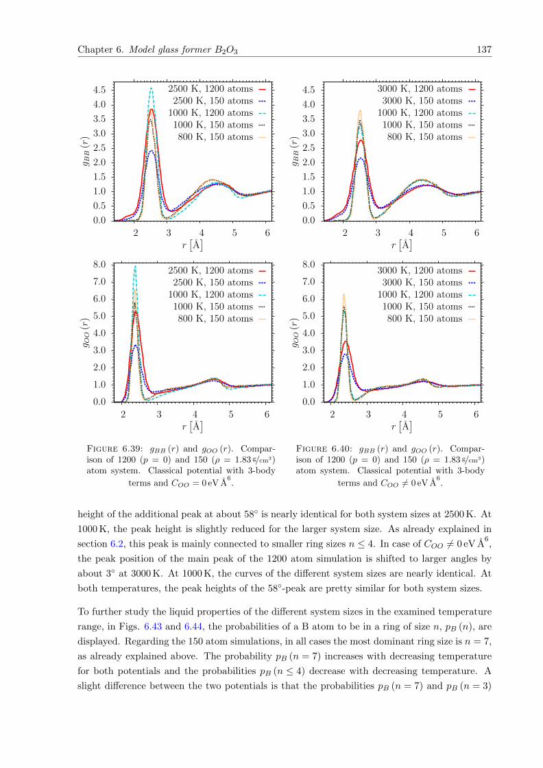
Chapter 6. Model glass former B2O3 137
0.0
0.5
1.0
1.5
2.0
2.5
3.0
3.5
4.0
4.5
2 3 4 5 6
g BB
(r)
r[A]
2500 K, 1200 atoms2500 K, 150 atoms
1000 K, 1200 atoms1000 K, 150 atoms800 K, 150 atoms
0.0
1.0
2.0
3.0
4.0
5.0
6.0
7.0
8.0
2 3 4 5 6
g OO
(r)
r[A]
2500 K, 1200 atoms2500 K, 150 atoms
1000 K, 1200 atoms1000 K, 150 atoms800 K, 150 atoms
Figure 6.39: gBB (r) and gOO (r). Compar-ison of 1200 (p = 0) and 150 (ρ = 1.83 g/cm3)atom system. Classical potential with 3-body
terms and COO = 0 eV A6.
0.0
0.5
1.0
1.5
2.0
2.5
3.0
3.5
4.0
4.5
2 3 4 5 6
g BB
(r)
r[A]
3000 K, 1200 atoms3000 K, 150 atoms
1000 K, 1200 atoms1000 K, 150 atoms800 K, 150 atoms
0.0
1.0
2.0
3.0
4.0
5.0
6.0
7.0
8.0
2 3 4 5 6
g OO
(r)
r[A]
3000 K, 1200 atoms3000 K, 150 atoms
1000 K, 1200 atoms1000 K, 150 atoms800 K, 150 atoms
Figure 6.40: gBB (r) and gOO (r). Compar-ison of 1200 (p = 0) and 150 (ρ = 1.83 g/cm3)atom system. Classical potential with 3-body
terms and COO 6= 0 eV A6.
height of the additional peak at about 58 is nearly identical for both system sizes at 2500 K. At
1000 K, the peak height is slightly reduced for the larger system size. As already explained in
section 6.2, this peak is mainly connected to smaller ring sizes n ≤ 4. In case of COO 6= 0 eV A6,
the peak position of the main peak of the 1200 atom simulation is shifted to larger angles by
about 3 at 3000 K. At 1000 K, the curves of the different system sizes are nearly identical. At
both temperatures, the peak heights of the 58-peak are pretty similar for both system sizes.
To further study the liquid properties of the different system sizes in the examined temperature
range, in Figs. 6.43 and 6.44, the probabilities of a B atom to be in a ring of size n, pB (n), are
displayed. Regarding the 150 atom simulations, in all cases the most dominant ring size is n = 7,
as already explained above. The probability pB (n = 7) increases with decreasing temperature
for both potentials and the probabilities pB (n ≤ 4) decrease with decreasing temperature. A
slight difference between the two potentials is that the probabilities pB (n = 7) and pB (n = 3)
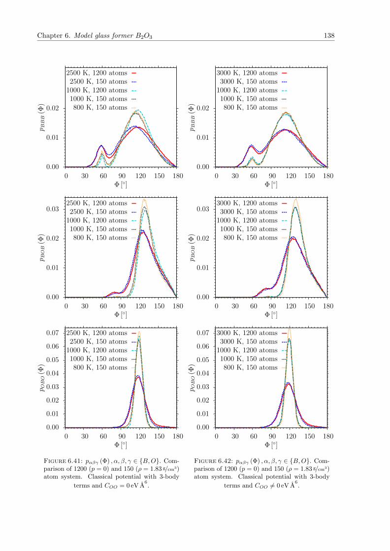
Chapter 6. Model glass former B2O3 138
0.00
0.01
0.02
0 30 60 90 120 150 180
p BBB
(Φ)
Φ []
2500 K, 1200 atoms2500 K, 150 atoms
1000 K, 1200 atoms1000 K, 150 atoms800 K, 150 atoms
0.00
0.01
0.02
0.03
0 30 60 90 120 150 180
p BOB
(Φ)
Φ []
2500 K, 1200 atoms2500 K, 150 atoms
1000 K, 1200 atoms1000 K, 150 atoms800 K, 150 atoms
0.00
0.01
0.02
0.03
0.04
0.05
0.06
0.07
0 30 60 90 120 150 180
p OBO
(Φ)
Φ []
2500 K, 1200 atoms2500 K, 150 atoms
1000 K, 1200 atoms1000 K, 150 atoms800 K, 150 atoms
Figure 6.41: pαβγ (Φ) , α, β, γ ∈ B,O. Com-parison of 1200 (p = 0) and 150 (ρ = 1.83 g/cm3)atom system. Classical potential with 3-body
terms and COO = 0 eV A6.
0.00
0.01
0.02
0 30 60 90 120 150 180
p BBB
(Φ)
Φ []
3000 K, 1200 atoms3000 K, 150 atoms
1000 K, 1200 atoms1000 K, 150 atoms800 K, 150 atoms
0.00
0.01
0.02
0.03
0 30 60 90 120 150 180
p BOB
(Φ)
Φ []
3000 K, 1200 atoms3000 K, 150 atoms
1000 K, 1200 atoms1000 K, 150 atoms800 K, 150 atoms
0.00
0.01
0.02
0.03
0.04
0.05
0.06
0.07
0 30 60 90 120 150 180
p OBO
(Φ)
Φ []
3000 K, 1200 atoms3000 K, 150 atoms
1000 K, 1200 atoms1000 K, 150 atoms800 K, 150 atoms
Figure 6.42: pαβγ (Φ) , α, β, γ ∈ B,O. Com-parison of 1200 (p = 0) and 150 (ρ = 1.83 g/cm3)atom system. Classical potential with 3-body
terms and COO 6= 0 eV A6.
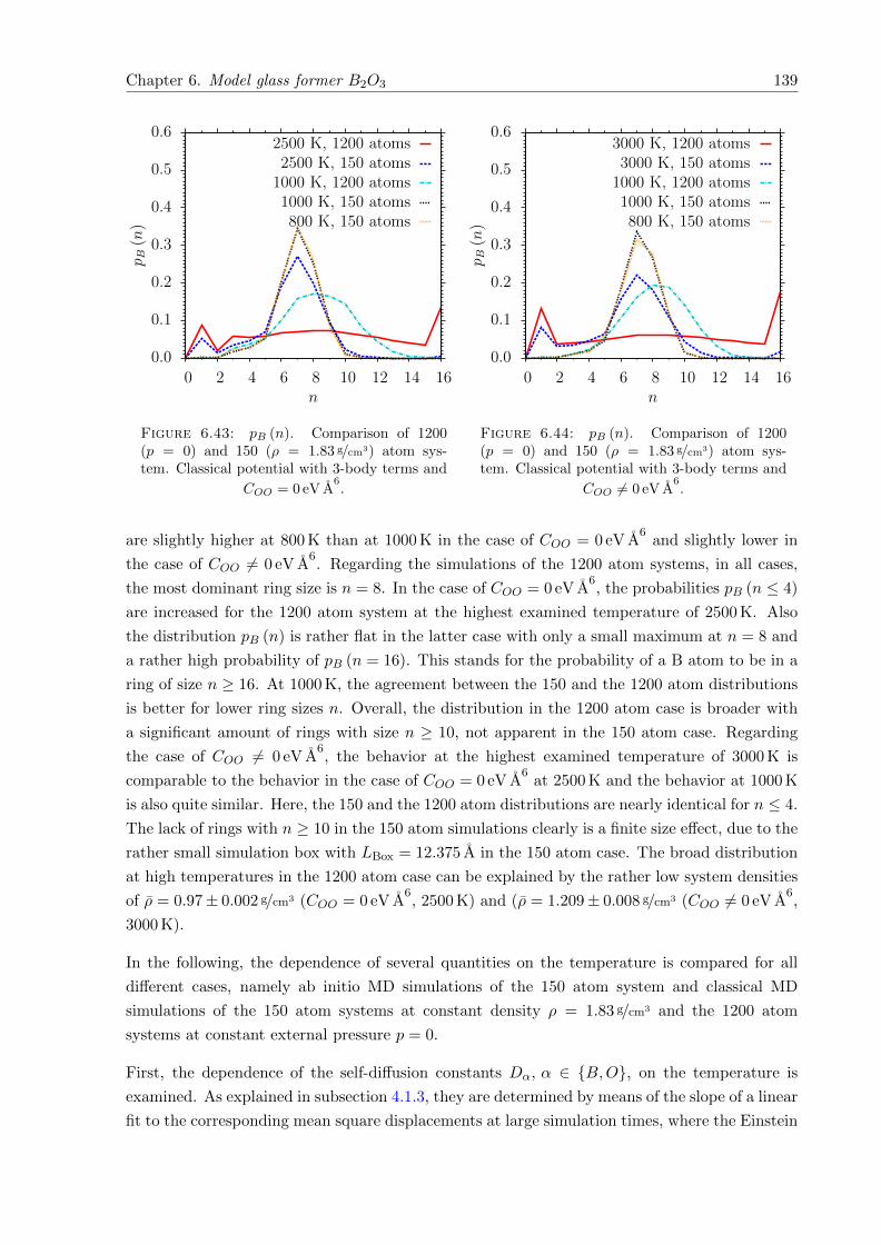
Chapter 6. Model glass former B2O3 139
0.0
0.1
0.2
0.3
0.4
0.5
0.6
0 2 4 6 8 10 12 14 16
p B(n)
n
2500 K, 1200 atoms2500 K, 150 atoms1000 K, 1200 atoms1000 K, 150 atoms800 K, 150 atoms
Figure 6.43: pB (n). Comparison of 1200(p = 0) and 150 (ρ = 1.83 g/cm3) atom sys-tem. Classical potential with 3-body terms and
COO = 0 eV A6.
0.0
0.1
0.2
0.3
0.4
0.5
0.6
0 2 4 6 8 10 12 14 16
p B(n)
n
3000 K, 1200 atoms3000 K, 150 atoms1000 K, 1200 atoms1000 K, 150 atoms800 K, 150 atoms
Figure 6.44: pB (n). Comparison of 1200(p = 0) and 150 (ρ = 1.83 g/cm3) atom sys-tem. Classical potential with 3-body terms and
COO 6= 0 eV A6.
are slightly higher at 800 K than at 1000 K in the case of COO = 0 eV A6
and slightly lower in
the case of COO 6= 0 eV A6. Regarding the simulations of the 1200 atom systems, in all cases,
the most dominant ring size is n = 8. In the case of COO = 0 eV A6, the probabilities pB (n ≤ 4)
are increased for the 1200 atom system at the highest examined temperature of 2500 K. Also
the distribution pB (n) is rather flat in the latter case with only a small maximum at n = 8 and
a rather high probability of pB (n = 16). This stands for the probability of a B atom to be in a
ring of size n ≥ 16. At 1000 K, the agreement between the 150 and the 1200 atom distributions
is better for lower ring sizes n. Overall, the distribution in the 1200 atom case is broader with
a significant amount of rings with size n ≥ 10, not apparent in the 150 atom case. Regarding
the case of COO 6= 0 eV A6, the behavior at the highest examined temperature of 3000 K is
comparable to the behavior in the case of COO = 0 eV A6
at 2500 K and the behavior at 1000 K
is also quite similar. Here, the 150 and the 1200 atom distributions are nearly identical for n ≤ 4.
The lack of rings with n ≥ 10 in the 150 atom simulations clearly is a finite size effect, due to the
rather small simulation box with LBox = 12.375 A in the 150 atom case. The broad distribution
at high temperatures in the 1200 atom case can be explained by the rather low system densities
of ρ = 0.97± 0.002 g/cm3 (COO = 0 eV A6, 2500 K) and (ρ = 1.209± 0.008 g/cm3 (COO 6= 0 eV A
6,
3000 K).
In the following, the dependence of several quantities on the temperature is compared for all
different cases, namely ab initio MD simulations of the 150 atom system and classical MD
simulations of the 150 atom systems at constant density ρ = 1.83 g/cm3 and the 1200 atom
systems at constant external pressure p = 0.
First, the dependence of the self-diffusion constants Dα, α ∈ B,O, on the temperature is
examined. As explained in subsection 4.1.3, they are determined by means of the slope of a linear
fit to the corresponding mean square displacements at large simulation times, where the Einstein
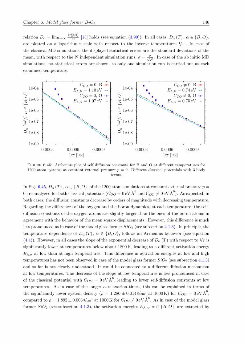
Chapter 6. Model glass former B2O3 140
relation Dα = limt→∞〈r2α(t)〉6t [15] holds (see equation (3.99)). In all cases, Dα (T ) , α ∈ B,O,
are plotted on a logarithmic scale with respect to the inverse temperatures 1/T . In case of
the classical MD simulations, the displayed statistical errors are the standard deviations of the
mean, with respect to the N independent simulation runs, σ = σ√N
. In case of the ab initio MD
simulations, no statistical errors are shown, as only one simulation run is carried out at each
examined temperature.
1e-09
1e-08
1e-07
1e-06
1e-05
1e-04
0.0003 0.0006 0.0009
Dα[cm
2 /s]α∈B
,O
1/T [1/K]
COO = 0, BEA,B = 1.10 eV
COO = 0, OEA,O = 1.07 eV
1e-09
1e-08
1e-07
1e-06
1e-05
1e-04
0.0003 0.0006 0.0009
Dα[cm
2 /s]α∈B
,O
1/T [1/K]
COO 6= 0, BEA,B = 0.74 eV
COO 6= 0, OEA,O = 0.75 eV
Figure 6.45: Arrhenius plot of self diffusion constants for B and O at different temperatures for1200 atom systems at constant external pressure p = 0. Different classical potentials with 3-body
terms.
In Fig. 6.45, Dα (T ) , α ∈ B,O, of the 1200 atom simulations at constant external pressure p =
0 are analyzed for both classical potentials (COO = 0 eV A6
and COO 6= 0 eV A6). As expected, in
both cases, the diffusion constants decrease by orders of magnitude with decreasing temperature.
Regarding the differences of the oxygen and the boron dynamics, at each temperature, the self-
diffusion constants of the oxygen atoms are slightly larger than the ones of the boron atoms in
agreement with the behavior of the mean square displacements. However, this difference is much
less pronounced as in case of the model glass former SiO2 (see subsection 4.1.3). In principle, the
temperature dependence of Dα (T ) , α ∈ B,O, follows an Arrhenius behavior (see equation
(4.4)). However, in all cases the slope of the exponential decrease of Dα (T ) with respect to 1/T is
significantly lower at temperatures below about 1800 K, leading to a different activation energy
EA,α at low than at high temperatures. This difference in activation energies at low and high
temperatures has not been observed in case of the model glass former SiO2 (see subsection 4.1.3)
and so far is not clearly understood. It could be connected to a different diffusion mechanism
at low temperatures. The decrease of the slope at low temperatures is less pronounced in case
of the classical potential with COO = 0 eV A6, leading to lower self-diffusion constants at low
temperatures. As in case of the longer α-relaxation times, this can be explained in terms of
the significantly lower system density (ρ = 1.280 ± 0.014 g/cm3 at 1000 K) for COO = 0 eV A6,
compared to ρ = 1.892± 0.003 g/cm3 at 1000 K for COO 6= 0 eV A6. As in case of the model glass
former SiO2 (see subsection 4.1.3), the activation energies EA,α, α ∈ B,O, are extracted by
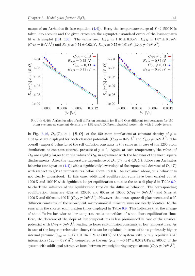
Chapter 6. Model glass former B2O3 141
means of an Arrhenius fit (see equation (4.4)). Here, the temperature range of T ≤ 1500 K is
taken into account and the given errors are the asymptotic standard errors of the least-squares
fit with gnuplot [101, 106]. The values are: EA,B ' 1.10 ± 0.03eV, EA,O ' 1.07 ± 0.02eV
(COO = 0 eV A6) and EA,B ' 0.74± 0.02eV, EA,O ' 0.75± 0.01eV (COO 6= 0 eV A
6).
1e-09
1e-08
1e-07
1e-06
1e-05
1e-04
0.0003 0.0006 0.0009 0.0012
Dα[cm
2 /s]α∈B
,O
1/T [1/K]
COO = 0, BEA,B = 0.75 eV
COO = 0, OEA,O = 0.75 eV
1e-09
1e-08
1e-07
1e-06
1e-05
1e-04
0.0003 0.0006 0.0009 0.0012Dα[cm
2 /s]α∈B
,O
1/T [1/K]
COO 6= 0, BEA,B = 0.87 eV
COO 6= 0, OEA,O = 0.86 eV
Figure 6.46: Arrhenius plot of self diffusion constants for B and O at different temperatures for 150atom systems at constant density ρ = 1.83 g/cm3. Different classical potentials with 3-body terms.
In Fig. 6.46, Dα (T ) , α ∈ B,O, of the 150 atom simulations at constant density of ρ =
1.83 g/cm3 are displayed for both classical potentials (COO = 0 eV A6
and COO 6= 0 eV A6). The
overall temporal behavior of the self-diffusion constants is the same as in case of the 1200 atom
simulations at constant external pressure of p = 0. Again, at each temperature, the values of
DO are slightly larger than the values of DB, in agreement with the behavior of the mean square
displacements. Also, the temperature dependence of Dα (T ) , α ∈ B,O, follows an Arrhenius
behavior (see equation (4.4)) with a significantly lower slope of the exponential decrease ofDα (T )
with respect to 1/T at temperatures below about 1800 K. As explained above, this behavior is
not clearly understood. In this case, additional equilibration runs have been carried out at
1200 K and 1000 K with significant longer equilibration times as the ones displayed in Table 6.9,
to check the influence of the equilibration time on the diffusive behavior. The corresponding
equilibration times are 42 ns at 1200 K and 600 ns at 100 K (COO = 0 eV A6) and 54 ns at
1200 K and 600 ns at 100 K (COO 6= 0 eV A6). However, the mean square displacements and self-
diffusion constants of the subsequent microcanonical measure runs are nearly identical to the
runs with the shorter equilibration times displayed in Table 6.9. This indicates that the change
of the diffusive behavior at low temperatures is no artifact of a too short equilibration time.
Here, the decrease of the slope at low temperatures is less pronounced in case of the classical
potential with COO 6= 0 eV A6, leading to lower self-diffusion constants at low temperatures. As
in case of the longer α-relaxation times, this can be explained in terms of the significantly higher
internal pressure (pint = 1.117 ± 0.015 GPa at 800 K) of the system with purely repulsive O-O
interactions (COO = 0 eV A6), compared to the one (pint = −0.447± 0.042 GPa at 800 K) of the
system with additional attractive force between two neighboring oxygen atoms (COO 6= 0 eV A6).
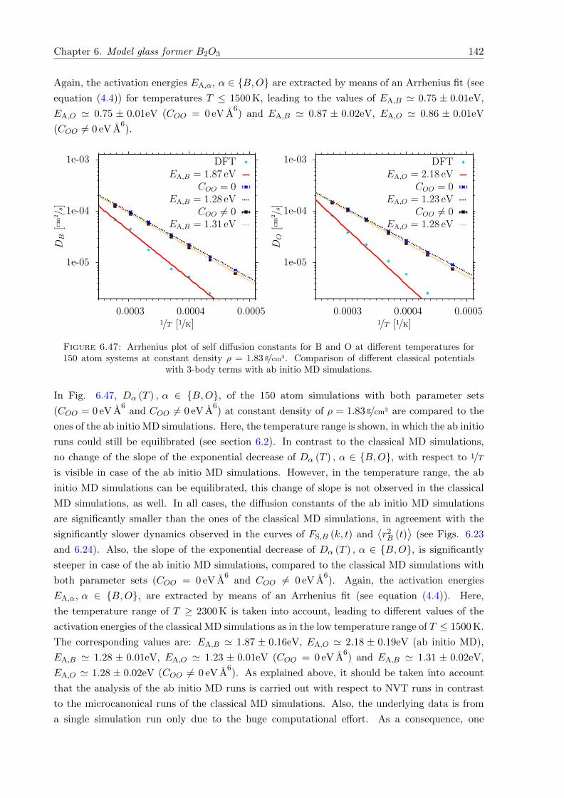
Chapter 6. Model glass former B2O3 142
Again, the activation energies EA,α, α ∈ B,O are extracted by means of an Arrhenius fit (see
equation (4.4)) for temperatures T ≤ 1500 K, leading to the values of EA,B ' 0.75 ± 0.01eV,
EA,O ' 0.75 ± 0.01eV (COO = 0 eV A6) and EA,B ' 0.87 ± 0.02eV, EA,O ' 0.86 ± 0.01eV
(COO 6= 0 eV A6).
1e-05
1e-04
1e-03
0.0003 0.0004 0.0005
DB[cm
2 /s]
1/T [1/K]
DFTEA,B = 1.87 eV
COO = 0EA,B = 1.28 eV
COO 6= 0EA,B = 1.31 eV
1e-05
1e-04
1e-03
0.0003 0.0004 0.0005
DO[cm
2 /s]
1/T [1/K]
DFTEA,O = 2.18 eV
COO = 0EA,O = 1.23 eV
COO 6= 0EA,O = 1.28 eV
Figure 6.47: Arrhenius plot of self diffusion constants for B and O at different temperatures for150 atom systems at constant density ρ = 1.83 g/cm3. Comparison of different classical potentials
with 3-body terms with ab initio MD simulations.
In Fig. 6.47, Dα (T ) , α ∈ B,O, of the 150 atom simulations with both parameter sets
(COO = 0 eV A6
and COO 6= 0 eV A6) at constant density of ρ = 1.83 g/cm3 are compared to the
ones of the ab initio MD simulations. Here, the temperature range is shown, in which the ab initio
runs could still be equilibrated (see section 6.2). In contrast to the classical MD simulations,
no change of the slope of the exponential decrease of Dα (T ) , α ∈ B,O, with respect to 1/T
is visible in case of the ab initio MD simulations. However, in the temperature range, the ab
initio MD simulations can be equilibrated, this change of slope is not observed in the classical
MD simulations, as well. In all cases, the diffusion constants of the ab initio MD simulations
are significantly smaller than the ones of the classical MD simulations, in agreement with the
significantly slower dynamics observed in the curves of FS,B (k, t) and⟨r2B (t)
⟩(see Figs. 6.23
and 6.24). Also, the slope of the exponential decrease of Dα (T ) , α ∈ B,O, is significantly
steeper in case of the ab initio MD simulations, compared to the classical MD simulations with
both parameter sets (COO = 0 eV A6
and COO 6= 0 eV A6). Again, the activation energies
EA,α, α ∈ B,O, are extracted by means of an Arrhenius fit (see equation (4.4)). Here,
the temperature range of T ≥ 2300 K is taken into account, leading to different values of the
activation energies of the classical MD simulations as in the low temperature range of T ≤ 1500 K.
The corresponding values are: EA,B ' 1.87 ± 0.16eV, EA,O ' 2.18 ± 0.19eV (ab initio MD),
EA,B ' 1.28 ± 0.01eV, EA,O ' 1.23 ± 0.01eV (COO = 0 eV A6) and EA,B ' 1.31 ± 0.02eV,
EA,O ' 1.28 ± 0.02eV (COO 6= 0 eV A6). As explained above, it should be taken into account
that the analysis of the ab initio MD runs is carried out with respect to NVT runs in contrast
to the microcanonical runs of the classical MD simulations. Also, the underlying data is from
a single simulation run only due to the huge computational effort. As a consequence, one
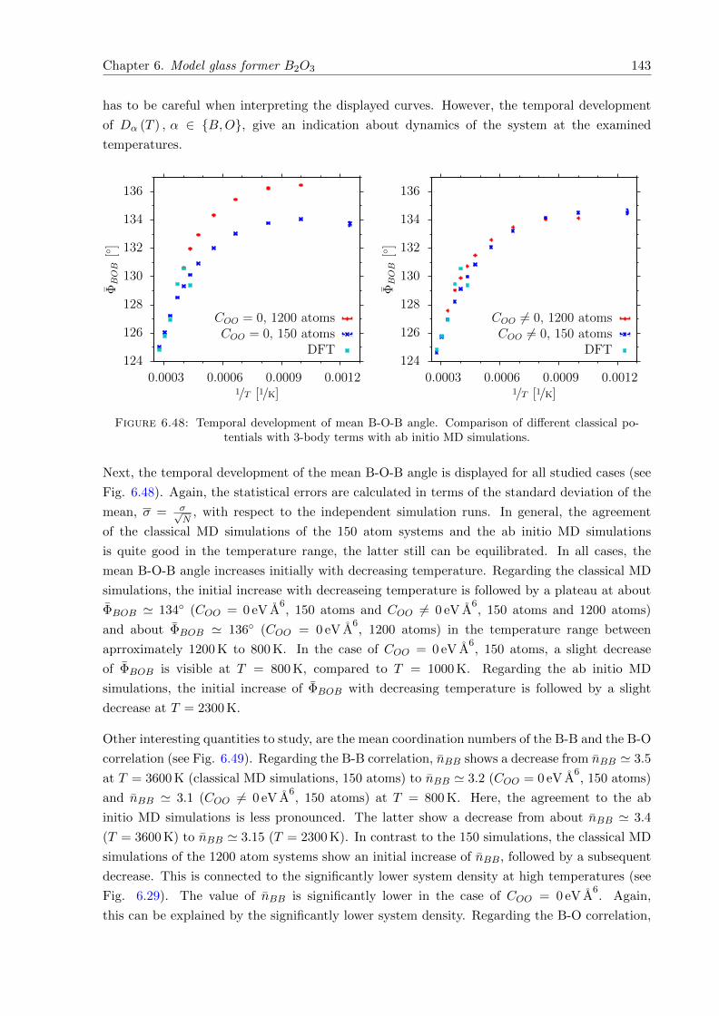
Chapter 6. Model glass former B2O3 143
has to be careful when interpreting the displayed curves. However, the temporal development
of Dα (T ) , α ∈ B,O, give an indication about dynamics of the system at the examined
temperatures.
124
126
128
130
132
134
136
0.0003 0.0006 0.0009 0.0012
ΦBOB
[]
1/T [1/K]
COO = 0, 1200 atomsCOO = 0, 150 atoms
DFT124
126
128
130
132
134
136
0.0003 0.0006 0.0009 0.0012Φ
BOB
[]
1/T [1/K]
COO 6= 0, 1200 atomsCOO 6= 0, 150 atoms
DFT
Figure 6.48: Temporal development of mean B-O-B angle. Comparison of different classical po-tentials with 3-body terms with ab initio MD simulations.
Next, the temporal development of the mean B-O-B angle is displayed for all studied cases (see
Fig. 6.48). Again, the statistical errors are calculated in terms of the standard deviation of the
mean, σ = σ√N
, with respect to the independent simulation runs. In general, the agreement
of the classical MD simulations of the 150 atom systems and the ab initio MD simulations
is quite good in the temperature range, the latter still can be equilibrated. In all cases, the
mean B-O-B angle increases initially with decreasing temperature. Regarding the classical MD
simulations, the initial increase with decreaseing temperature is followed by a plateau at about
ΦBOB ' 134 (COO = 0 eV A6, 150 atoms and COO 6= 0 eV A
6, 150 atoms and 1200 atoms)
and about ΦBOB ' 136 (COO = 0 eV A6, 1200 atoms) in the temperature range between
aprroximately 1200 K to 800 K. In the case of COO = 0 eV A6, 150 atoms, a slight decrease
of ΦBOB is visible at T = 800 K, compared to T = 1000 K. Regarding the ab initio MD
simulations, the initial increase of ΦBOB with decreasing temperature is followed by a slight
decrease at T = 2300 K.
Other interesting quantities to study, are the mean coordination numbers of the B-B and the B-O
correlation (see Fig. 6.49). Regarding the B-B correlation, nBB shows a decrease from nBB ' 3.5
at T = 3600 K (classical MD simulations, 150 atoms) to nBB ' 3.2 (COO = 0 eV A6, 150 atoms)
and nBB ' 3.1 (COO 6= 0 eV A6, 150 atoms) at T = 800 K. Here, the agreement to the ab
initio MD simulations is less pronounced. The latter show a decrease from about nBB ' 3.4
(T = 3600 K) to nBB ' 3.15 (T = 2300 K). In contrast to the 150 simulations, the classical MD
simulations of the 1200 atom systems show an initial increase of nBB, followed by a subsequent
decrease. This is connected to the significantly lower system density at high temperatures (see
Fig. 6.29). The value of nBB is significantly lower in the case of COO = 0 eV A6. Again,
this can be explained by the significantly lower system density. Regarding the B-O correlation,
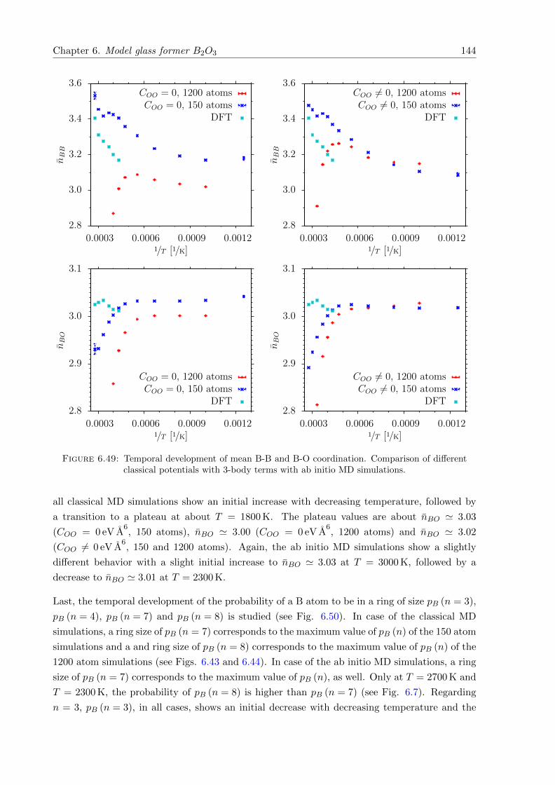
Chapter 6. Model glass former B2O3 144
2.8
3.0
3.2
3.4
3.6
0.0003 0.0006 0.0009 0.0012
nBB
1/T [1/K]
COO = 0, 1200 atomsCOO = 0, 150 atoms
DFT
2.8
2.9
3.0
3.1
0.0003 0.0006 0.0009 0.0012
nBO
1/T [1/K]
COO = 0, 1200 atomsCOO = 0, 150 atoms
DFT
2.8
3.0
3.2
3.4
3.6
0.0003 0.0006 0.0009 0.0012
nBB
1/T [1/K]
COO 6= 0, 1200 atomsCOO 6= 0, 150 atoms
DFT
2.8
2.9
3.0
3.1
0.0003 0.0006 0.0009 0.0012
nBO
1/T [1/K]
COO 6= 0, 1200 atomsCOO 6= 0, 150 atoms
DFT
Figure 6.49: Temporal development of mean B-B and B-O coordination. Comparison of differentclassical potentials with 3-body terms with ab initio MD simulations.
all classical MD simulations show an initial increase with decreasing temperature, followed by
a transition to a plateau at about T = 1800 K. The plateau values are about nBO ' 3.03
(COO = 0 eV A6, 150 atoms), nBO ' 3.00 (COO = 0 eV A
6, 1200 atoms) and nBO ' 3.02
(COO 6= 0 eV A6, 150 and 1200 atoms). Again, the ab initio MD simulations show a slightly
different behavior with a slight initial increase to nBO ' 3.03 at T = 3000 K, followed by a
decrease to nBO ' 3.01 at T = 2300 K.
Last, the temporal development of the probability of a B atom to be in a ring of size pB (n = 3),
pB (n = 4), pB (n = 7) and pB (n = 8) is studied (see Fig. 6.50). In case of the classical MD
simulations, a ring size of pB (n = 7) corresponds to the maximum value of pB (n) of the 150 atom
simulations and a and ring size of pB (n = 8) corresponds to the maximum value of pB (n) of the
1200 atom simulations (see Figs. 6.43 and 6.44). In case of the ab initio MD simulations, a ring
size of pB (n = 7) corresponds to the maximum value of pB (n), as well. Only at T = 2700 K and
T = 2300 K, the probability of pB (n = 8) is higher than pB (n = 7) (see Fig. 6.7). Regarding
n = 3, pB (n = 3), in all cases, shows an initial decrease with decreasing temperature and the
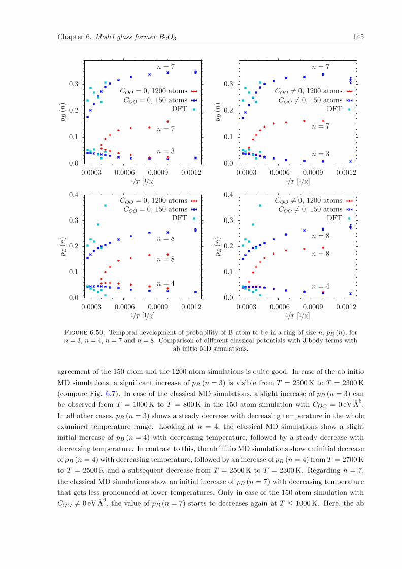
Chapter 6. Model glass former B2O3 145
0.0
0.1
0.2
0.3
0.0003 0.0006 0.0009 0.0012
p B(n)
1/T [1/K]
n = 3
n = 7
n = 7
COO = 0, 1200 atomsCOO = 0, 150 atoms
DFT
0.0
0.1
0.2
0.3
0.4
0.0003 0.0006 0.0009 0.0012
p B(n)
1/T [1/K]
n = 4
n = 8
n = 8
COO = 0, 1200 atomsCOO = 0, 150 atoms
DFT
0.0
0.1
0.2
0.3
0.0003 0.0006 0.0009 0.0012
p B(n)
1/T [1/K]
n = 3
n = 7
n = 7
COO 6= 0, 1200 atomsCOO 6= 0, 150 atoms
DFT
0.0
0.1
0.2
0.3
0.4
0.0003 0.0006 0.0009 0.0012
p B(n)
1/T [1/K]
n = 4
n = 8
n = 8
COO 6= 0, 1200 atomsCOO 6= 0, 150 atoms
DFT
Figure 6.50: Temporal development of probability of B atom to be in a ring of size n, pB (n), forn = 3, n = 4, n = 7 and n = 8. Comparison of different classical potentials with 3-body terms with
ab initio MD simulations.
agreement of the 150 atom and the 1200 atom simulations is quite good. In case of the ab initio
MD simulations, a significant increase of pB (n = 3) is visible from T = 2500 K to T = 2300 K
(compare Fig. 6.7). In case of the classical MD simulations, a slight increase of pB (n = 3) can
be observed from T = 1000 K to T = 800 K in the 150 atom simulation with COO = 0 eV A6.
In all other cases, pB (n = 3) shows a steady decrease with decreasing temperature in the whole
examined temperature range. Looking at n = 4, the classical MD simulations show a slight
initial increase of pB (n = 4) with decreasing temperature, followed by a steady decrease with
decreasing temperature. In contrast to this, the ab initio MD simulations show an initial decrease
of pB (n = 4) with decreasing temperature, followed by an increase of pB (n = 4) from T = 2700 K
to T = 2500 K and a subsequent decrease from T = 2500 K to T = 2300 K. Regarding n = 7,
the classical MD simulations show an initial increase of pB (n = 7) with decreasing temperature
that gets less pronounced at lower temperatures. Only in case of the 150 atom simulation with
COO 6= 0 eV A6, the value of pB (n = 7) starts to decreases again at T ≤ 1000 K. Here, the ab
Chapter 6. Model glass former B2O3 146
initio MD simulations show a different behavior. An initial increase of pB (n = 7) is followed by a
decrease of pB (n = 7) from T = 3300 K to T = 2500 K and an increase at T = 2300 K. Finally,
looking at n = 8, a steady increase of pB (n = 8) with decreasing temperature is observed
in all classical MD simulations. The ab initio MD simulations show an unsteady temporal
development of pB (n = 8), reflecting the fact that the maximum of pB (n) is observed at n = 8
at T = 2700 K and T = 2300 K and at n = 7 at all other temperatures (see Fig. 6.7). In
general, the temporal development of pB (n) reflects the decrease of defects (small ring sizes)
with decreasing temperature and the narrowing of the distribution of pB (n) with decreasing
temperature (compare Figs. 6.7, 6.27, 6.43 and 6.44). An exception is the rather strong increase
of pB (n = 3) at T = 2300 K, in case of the ab initio MD simulations.
6.5 Glass structure
After examining the properties of the model glass former B2O3 in the liquid state, in this section
the structural properties of the vitreous state are examined. The glass structures investigated
in this section are generated in different ways. However, in all cases systems of 150 atoms are
regarded at the experimental glass density of ρ = 1.83 g/cm3 [159]. As in case of the model glass
former SiO2 (see section 4.2), this is a reasonable system size in terms of balancing between
the influence of finite size effect and computational feasibility for quantum mechanical DFT
calculations.
In one approach, the glass configurations are generated by a quench from the melt with classical
molecular dynamics simulations after an initial random initialization, as described in subsection
4.1.1. Here, in all cases, 10 independent simulation runs are carried out in the NVT ensemble,
using a chain of 3 Nose-Hoover thermostats (see subsection 3.1.2) with a damping parameter of
100 ts (see section 6.3). First, 10 independent glass configurations are generated with the original
potential parameters before the structural fit [97], according to Table 6.5, again choosing the B-B
interaction to be purely electrostatic. After an equilibration at 3600 K for 240 ps (ts = 1.2 fs),
the configurations are cooled linearly down to 300 K with a cooling rate of Γ = 1 · 1011 K/s.
After annealing at 300 K for 240 ps, the configurations are quenched down to 0 K. Next, glass
configurations are generated with the two different parameter sets of the classical force field,
including 3-body terms, as displayed in Table 6.7. This is done in two different ways. On the
one hand, the configurations are equilibrated at 2300 K for 300 ps (ts = 0.6 fs), followed by a
quench to 300 K with a cooling rate of Γ = 1 ·1011 K/s. On the other hand, the configurations are
quenched down to 300 K after the stepwise cooling procedure down to 800 K and equilibration at
800 K, according to Table 6.9. In both cases, the configurations are quenched down to 0 K after
annealing at 300 K for 600 ps. The first procedure is only applied in the case of COO = 0 eV A6.
The second one is applied for both classical potentials.
In another approach, glass configurations are generated by quenches from the melt with ab
initio MD simulations. Here, two different cases are studied. First, the system is equilibrated at
3600 K for 36 ps (30000 ts, δt = 1.2 fs), as described in section 6.2. To generate two independent
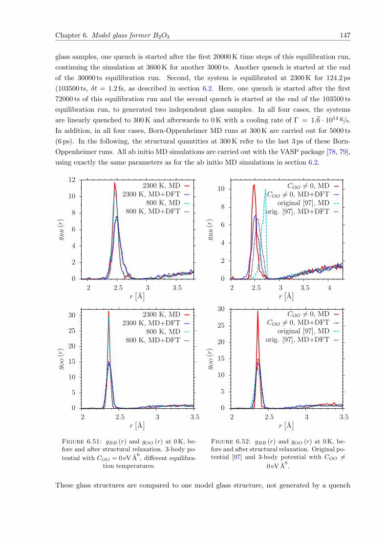
Chapter 6. Model glass former B2O3 147
glass samples, one quench is started after the first 20000 K time steps of this equilibration run,
continuing the simulation at 3600 K for another 3000 ts. Another quench is started at the end
of the 30000 ts equilibration run. Second, the system is equilibrated at 2300 K for 124.2 ps
(103500 ts, δt = 1.2 fs, as described in section 6.2. Here, one quench is started after the first
72000 ts of this equilibration run and the second quench is started at the end of the 103500 ts
equilibration run, to generated two independent glass samples. In all four cases, the systems
are linearly quenched to 300 K and afterwards to 0 K with a cooling rate of Γ = 1.6 · 1014 K/s.
In addition, in all four cases, Born-Oppenheimer MD runs at 300 K are carried out for 5000 ts
(6 ps). In the following, the structural quantities at 300 K refer to the last 3 ps of these Born-
Oppenheimer runs. All ab initio MD simulations are carried out with the VASP package [78, 79],
using exactly the same parameters as for the ab initio MD simulations in section 6.2.
0
2
4
6
8
10
12
2 2.5 3 3.5
g BB
(r)
r[A]
2300 K, MD2300 K, MD+DFT
800 K, MD800 K, MD+DFT
0
5
10
15
20
25
30
2 2.5 3 3.5
g OO
(r)
r[A]
2300 K, MD2300 K, MD+DFT
800 K, MD800 K, MD+DFT
Figure 6.51: gBB (r) and gOO (r) at 0 K, be-fore and after structural relaxation. 3-body po-
tential with COO = 0 eV A6, different equilibra-
tion temperatures.
0
2
4
6
8
10
2 2.5 3 3.5 4
g BB
(r)
r[A]
COO 6= 0, MDCOO 6= 0, MD+DFT
original [97], MDorig. [97], MD+DFT
0
5
10
15
20
25
30
2 2.5 3 3.5
g OO
(r)
r[A]
COO 6= 0, MDCOO 6= 0, MD+DFT
original [97], MDorig. [97], MD+DFT
Figure 6.52: gBB (r) and gOO (r) at 0 K, be-fore and after structural relaxation. Original po-tential [97] and 3-body potential with COO 6=
0 eV A6.
These glass structures are compared to one model glass structure, not generated by a quench
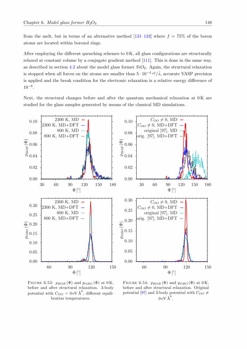
Chapter 6. Model glass former B2O3 148
from the melt, but in terms of an alternative method [131–133] where f = 75% of the boron
atoms are located within boroxol rings.
After employing the different quenching schemes to 0 K, all glass configurations are structurally
relaxed at constant volume by a conjugate gradient method [111]. This is done in the same way,
as described in section 4.2 about the model glass former SiO2. Again, the structural relaxation
is stopped when all forces on the atoms are smaller than 5 · 10−4 eV/A, accurate VASP precision
is applied and the break condition for the electronic relaxation is a relative energy difference of
10−8.
Next, the structural changes before and after the quantum mechanical relaxation at 0 K are
studied for the glass samples generated by means of the classical MD simulations.
0.00
0.02
0.04
0.06
0.08
0.10
30 60 90 120 150 180
p BOB
(Φ)
Φ []
2300 K, MD2300 K, MD+DFT
800 K, MD800 K, MD+DFT
0.00
0.05
0.10
0.15
0.20
0.25
0.30
60 90 120 150
p OBO
(Φ)
Φ []
2300 K, MD2300 K, MD+DFT
800 K, MD800 K, MD+DFT
Figure 6.53: pBOB (Φ) and pOBO (Φ) at 0 K,before and after structural relaxation. 3-body
potential with COO = 0 eV A6, different equili-
bration temperatures.
0.00
0.02
0.04
0.06
0.08
0.10
30 60 90 120 150 180
p BOB
(Φ)
Φ []
COO 6= 0, MDCOO 6= 0, MD+DFT
original [97], MDorig. [97], MD+DFT
0.00
0.05
0.10
0.15
0.20
0.25
0.30
60 90 120 150
p OBO
(Φ)
Φ []
COO 6= 0, MDCOO 6= 0, MD+DFT
original [97], MDorig. [97], MD+DFT
Figure 6.54: pBOB (Φ) and pOBO (Φ) at 0 K,before and after structural relaxation. Originalpotential [97] and 3-body potential with COO 6=
0 eV A6.
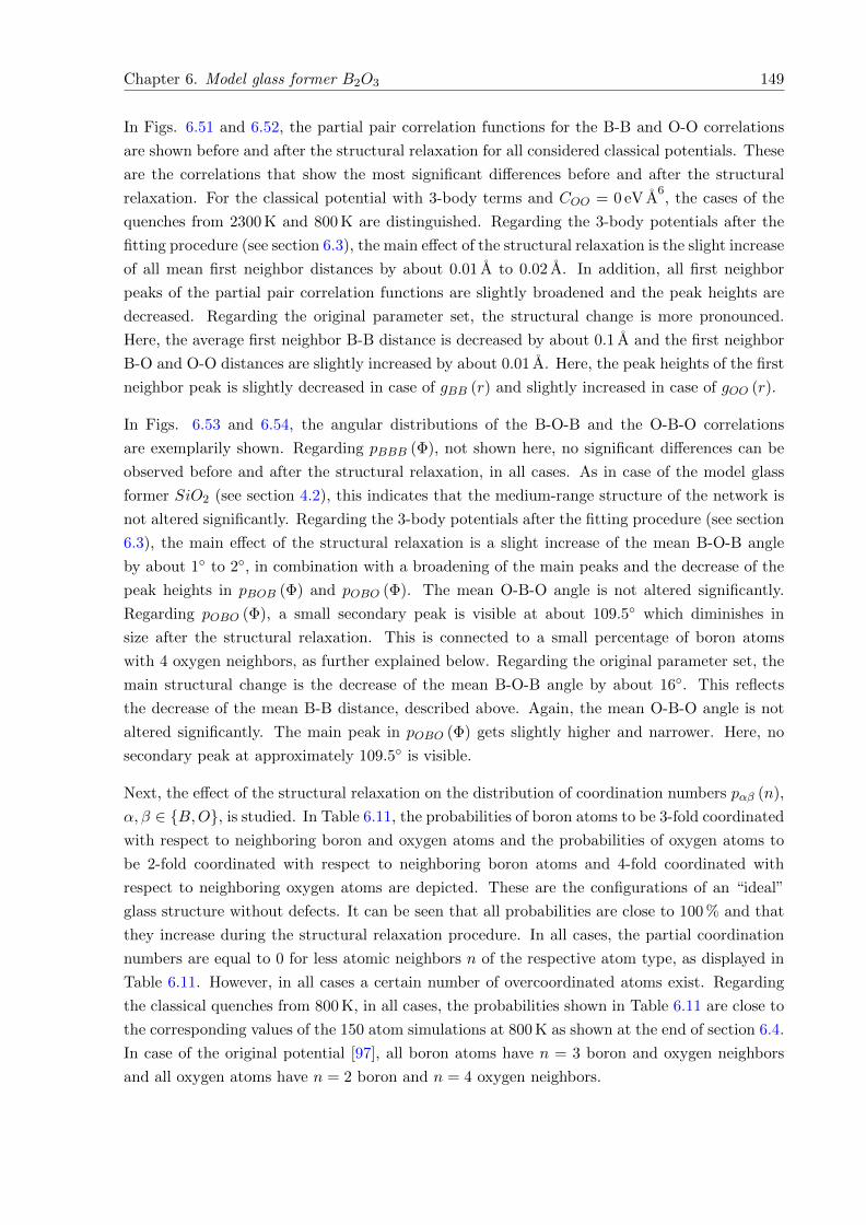
Chapter 6. Model glass former B2O3 149
In Figs. 6.51 and 6.52, the partial pair correlation functions for the B-B and O-O correlations
are shown before and after the structural relaxation for all considered classical potentials. These
are the correlations that show the most significant differences before and after the structural
relaxation. For the classical potential with 3-body terms and COO = 0 eV A6, the cases of the
quenches from 2300 K and 800 K are distinguished. Regarding the 3-body potentials after the
fitting procedure (see section 6.3), the main effect of the structural relaxation is the slight increase
of all mean first neighbor distances by about 0.01 A to 0.02 A. In addition, all first neighbor
peaks of the partial pair correlation functions are slightly broadened and the peak heights are
decreased. Regarding the original parameter set, the structural change is more pronounced.
Here, the average first neighbor B-B distance is decreased by about 0.1 A and the first neighbor
B-O and O-O distances are slightly increased by about 0.01 A. Here, the peak heights of the first
neighbor peak is slightly decreased in case of gBB (r) and slightly increased in case of gOO (r).
In Figs. 6.53 and 6.54, the angular distributions of the B-O-B and the O-B-O correlations
are exemplarily shown. Regarding pBBB (Φ), not shown here, no significant differences can be
observed before and after the structural relaxation, in all cases. As in case of the model glass
former SiO2 (see section 4.2), this indicates that the medium-range structure of the network is
not altered significantly. Regarding the 3-body potentials after the fitting procedure (see section
6.3), the main effect of the structural relaxation is a slight increase of the mean B-O-B angle
by about 1 to 2, in combination with a broadening of the main peaks and the decrease of the
peak heights in pBOB (Φ) and pOBO (Φ). The mean O-B-O angle is not altered significantly.
Regarding pOBO (Φ), a small secondary peak is visible at about 109.5 which diminishes in
size after the structural relaxation. This is connected to a small percentage of boron atoms
with 4 oxygen neighbors, as further explained below. Regarding the original parameter set, the
main structural change is the decrease of the mean B-O-B angle by about 16. This reflects
the decrease of the mean B-B distance, described above. Again, the mean O-B-O angle is not
altered significantly. The main peak in pOBO (Φ) gets slightly higher and narrower. Here, no
secondary peak at approximately 109.5 is visible.
Next, the effect of the structural relaxation on the distribution of coordination numbers pαβ (n),
α, β ∈ B,O, is studied. In Table 6.11, the probabilities of boron atoms to be 3-fold coordinated
with respect to neighboring boron and oxygen atoms and the probabilities of oxygen atoms to
be 2-fold coordinated with respect to neighboring boron atoms and 4-fold coordinated with
respect to neighboring oxygen atoms are depicted. These are the configurations of an “ideal”
glass structure without defects. It can be seen that all probabilities are close to 100 % and that
they increase during the structural relaxation procedure. In all cases, the partial coordination
numbers are equal to 0 for less atomic neighbors n of the respective atom type, as displayed in
Table 6.11. However, in all cases a certain number of overcoordinated atoms exist. Regarding
the classical quenches from 800 K, in all cases, the probabilities shown in Table 6.11 are close to
the corresponding values of the 150 atom simulations at 800 K as shown at the end of section 6.4.
In case of the original potential [97], all boron atoms have n = 3 boron and oxygen neighbors
and all oxygen atoms have n = 2 boron and n = 4 oxygen neighbors.
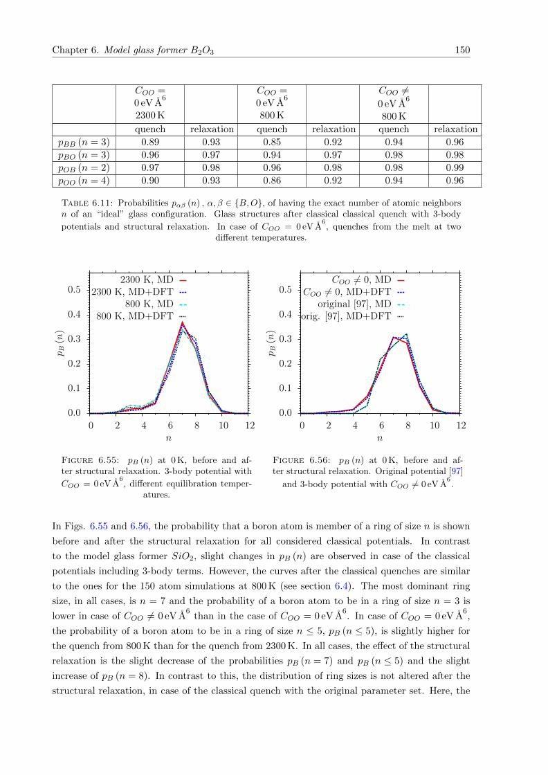
Chapter 6. Model glass former B2O3 150
COO =0 eV A
6
2300 K
COO =0 eV A
6
800 K
COO 6=0 eV A
6
800 K
quench relaxation quench relaxation quench relaxation
pBB (n = 3) 0.89 0.93 0.85 0.92 0.94 0.96
pBO (n = 3) 0.96 0.97 0.94 0.97 0.98 0.98
pOB (n = 2) 0.97 0.98 0.96 0.98 0.98 0.99
pOO (n = 4) 0.90 0.93 0.86 0.92 0.94 0.96
Table 6.11: Probabilities pαβ (n) , α, β ∈ B,O, of having the exact number of atomic neighborsn of an “ideal” glass configuration. Glass structures after classical classical quench with 3-body
potentials and structural relaxation. In case of COO = 0 eV A6, quenches from the melt at two
different temperatures.
0.0
0.1
0.2
0.3
0.4
0.5
0 2 4 6 8 10 12
p B(n)
n
2300 K, MD2300 K, MD+DFT
800 K, MD800 K, MD+DFT
Figure 6.55: pB (n) at 0 K, before and af-ter structural relaxation. 3-body potential with
COO = 0 eV A6, different equilibration temper-
atures.
0.0
0.1
0.2
0.3
0.4
0.5
0 2 4 6 8 10 12
p B(n)
n
COO 6= 0, MDCOO 6= 0, MD+DFT
original [97], MDorig. [97], MD+DFT
Figure 6.56: pB (n) at 0 K, before and af-ter structural relaxation. Original potential [97]
and 3-body potential with COO 6= 0 eV A6.
In Figs. 6.55 and 6.56, the probability that a boron atom is member of a ring of size n is shown
before and after the structural relaxation for all considered classical potentials. In contrast
to the model glass former SiO2, slight changes in pB (n) are observed in case of the classical
potentials including 3-body terms. However, the curves after the classical quenches are similar
to the ones for the 150 atom simulations at 800 K (see section 6.4). The most dominant ring
size, in all cases, is n = 7 and the probability of a boron atom to be in a ring of size n = 3 is
lower in case of COO 6= 0 eV A6
than in the case of COO = 0 eV A6. In case of COO = 0 eV A
6,
the probability of a boron atom to be in a ring of size n ≤ 5, pB (n ≤ 5), is slightly higher for
the quench from 800 K than for the quench from 2300 K. In all cases, the effect of the structural
relaxation is the slight decrease of the probabilities pB (n = 7) and pB (n ≤ 5) and the slight
increase of pB (n = 8). In contrast to this, the distribution of ring sizes is not altered after the
structural relaxation, in case of the classical quench with the original parameter set. Here, the
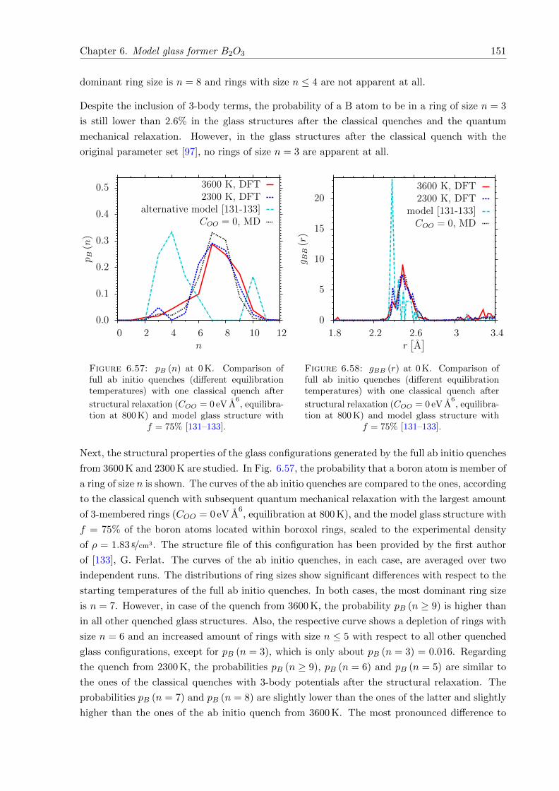
Chapter 6. Model glass former B2O3 151
dominant ring size is n = 8 and rings with size n ≤ 4 are not apparent at all.
Despite the inclusion of 3-body terms, the probability of a B atom to be in a ring of size n = 3
is still lower than 2.6% in the glass structures after the classical quenches and the quantum
mechanical relaxation. However, in the glass structures after the classical quench with the
original parameter set [97], no rings of size n = 3 are apparent at all.
0.0
0.1
0.2
0.3
0.4
0.5
0 2 4 6 8 10 12
p B(n)
n
3600 K, DFT2300 K, DFT
alternative model [131-133]COO = 0, MD
Figure 6.57: pB (n) at 0 K. Comparison offull ab initio quenches (different equilibrationtemperatures) with one classical quench after
structural relaxation (COO = 0 eV A6, equilibra-
tion at 800 K) and model glass structure withf = 75% [131–133].
0
5
10
15
20
1.8 2.2 2.6 3 3.4
g BB
(r)
r[A]
3600 K, DFT2300 K, DFT
model [131-133]COO = 0, MD
Figure 6.58: gBB (r) at 0 K. Comparison offull ab initio quenches (different equilibrationtemperatures) with one classical quench after
structural relaxation (COO = 0 eV A6, equilibra-
tion at 800 K) and model glass structure withf = 75% [131–133].
Next, the structural properties of the glass configurations generated by the full ab initio quenches
from 3600 K and 2300 K are studied. In Fig. 6.57, the probability that a boron atom is member of
a ring of size n is shown. The curves of the ab initio quenches are compared to the ones, according
to the classical quench with subsequent quantum mechanical relaxation with the largest amount
of 3-membered rings (COO = 0 eV A6, equilibration at 800 K), and the model glass structure with
f = 75% of the boron atoms located within boroxol rings, scaled to the experimental density
of ρ = 1.83 g/cm3. The structure file of this configuration has been provided by the first author
of [133], G. Ferlat. The curves of the ab initio quenches, in each case, are averaged over two
independent runs. The distributions of ring sizes show significant differences with respect to the
starting temperatures of the full ab initio quenches. In both cases, the most dominant ring size
is n = 7. However, in case of the quench from 3600 K, the probability pB (n ≥ 9) is higher than
in all other quenched glass structures. Also, the respective curve shows a depletion of rings with
size n = 6 and an increased amount of rings with size n ≤ 5 with respect to all other quenched
glass configurations, except for pB (n = 3), which is only about pB (n = 3) = 0.016. Regarding
the quench from 2300 K, the probabilities pB (n ≥ 9), pB (n = 6) and pB (n = 5) are similar to
the ones of the classical quenches with 3-body potentials after the structural relaxation. The
probabilities pB (n = 7) and pB (n = 8) are slightly lower than the ones of the latter and slightly
higher than the ones of the ab initio quench from 3600 K. The most pronounced difference to
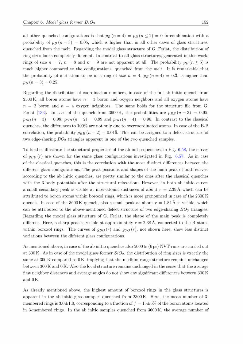
Chapter 6. Model glass former B2O3 152
all other quenched configurations is that pB (n = 4) = pB (n ≤ 2) = 0 in combination with a
probability of pB (n = 3) = 0.05, which is higher than in all other cases of glass structures,
quenched from the melt. Regarding the model glass structure of G. Ferlat, the distribution of
ring sizes looks completely different. In contrast to all glass structures, generated in this work,
rings of size n = 7, n = 8 and n = 9 are not apparent at all. The probability pB (n ≤ 5) is
much higher compared to the configurations, quenched from the melt. It is remarkable that
the probability of a B atom to be in a ring of size n = 4, pB (n = 4) = 0.3, is higher than
pB (n = 3) = 0.25.
Regarding the distribution of coordination numbers, in case of the full ab initio quench from
2300 K, all boron atoms have n = 3 boron and oxygen neighbors and all oxygen atoms have
n = 2 boron and n = 4 oxygen neighbors. The same holds for the structure file from G.
Ferlat [133]. In case of the quench from 3600 K, the probabilities are pBB (n = 3) = 0.95,
pBO (n = 3) = 0.98, pOB (n = 2) = 0.99 and pOO (n = 4) = 0.96. In contrast to the classical
quenches, the differences to 100% are not only due to overcoordinated atoms. In case of the B-B
correlation, the probability pBB (n = 2) = 0.016. This can be assigned to a defect structure of
two edge-sharing BO3 triangles apparent in one of the two quenched samples.
To further illustrate the structural properties of the ab initio quenches, in Fig. 6.58, the curves
of gBB (r) are shown for the same glass configurations investigated in Fig. 6.57. As in case
of the classical quenches, this is the correlation with the most distinct differences between the
different glass configurations. The peak positions and shapes of the main peak of both curves,
according to the ab initio quenches, are pretty similar to the ones after the classical quenches
with the 3-body potentials after the structural relaxation. However, in both ab initio curves
a small secondary peak is visible at inter-atomic distances of about r = 2.39 A which can be
attributed to boron atoms within boroxol rings, which is more pronounced in case of the 2300 K
quench. In case of the 3600 K quench, also a small peak at about r = 1.84 A is visible, which
can be attributed to the above-mentioned defect structure of two edge-sharing BO3 triangles.
Regarding the model glass structure of G. Ferlat, the shape of the main peak is completely
different. Here, a sharp peak is visible at approximately r = 2.38 A, connected to the B atoms
within boroxol rings. The curves of gBO (r) and gOO (r), not shown here, show less distinct
variations between the different glass configurations.
As mentioned above, in case of the ab initio quenches also 5000 ts (6 ps) NVT runs are carried out
at 300 K. As in case of the model glass former SiO2, the distribution of ring sizes is exactly the
same at 300 K compared to 0 K, implying that the medium range structure remains unchanged
between 300 K and 0 K. Also the local structure remains unchanged in the sense that the average
first neighbor distances and average angles do not show any significant differences between 300 K
and 0 K.
As already mentioned above, the highest amount of boroxol rings in the glass structures is
apparent in the ab initio glass samples quenched from 2300 K. Here, the mean number of 3-
membered rings is 3.0±1.0, corresponding to a fraction of f = 15±5% of the boron atoms located
in 3-membered rings. In the ab initio samples quenched from 3600 K, the average number of
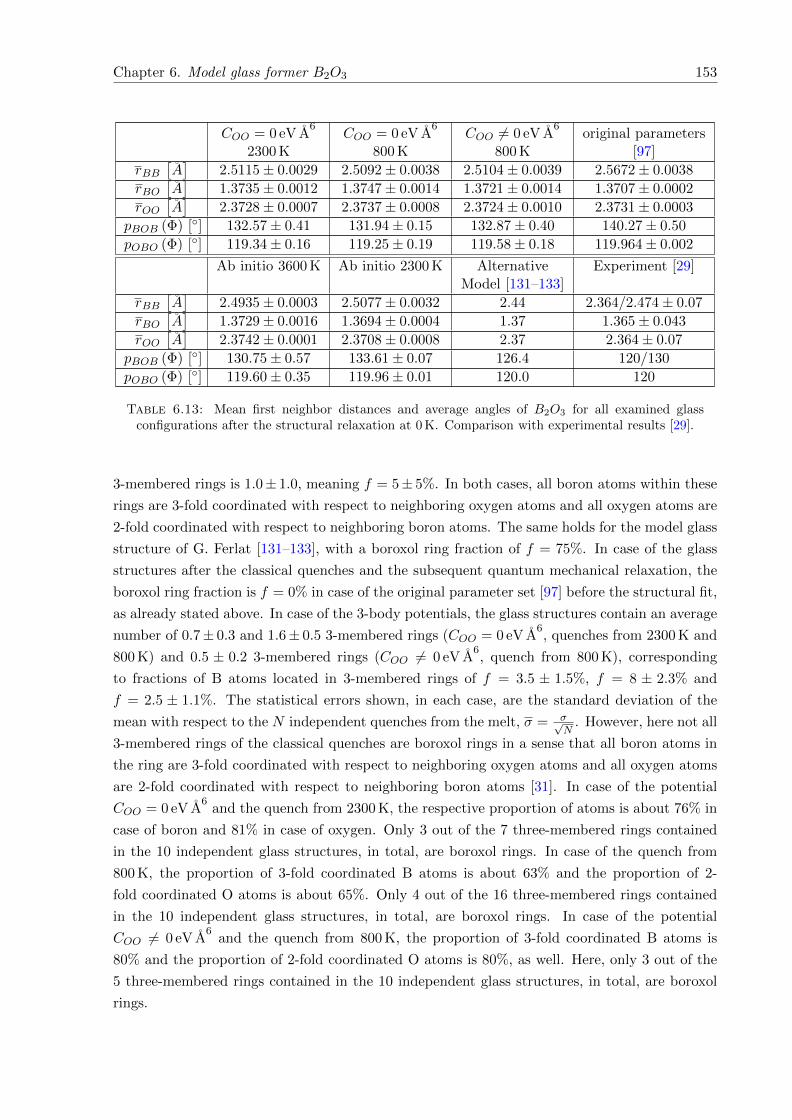
Chapter 6. Model glass former B2O3 153
COO = 0 eV A6
2300 KCOO = 0 eV A
6
800 KCOO 6= 0 eV A
6
800 Koriginal parameters
[97]
rBB[A]
2.5115± 0.0029 2.5092± 0.0038 2.5104± 0.0039 2.5672± 0.0038
rBO[A]
1.3735± 0.0012 1.3747± 0.0014 1.3721± 0.0014 1.3707± 0.0002
rOO[A]
2.3728± 0.0007 2.3737± 0.0008 2.3724± 0.0010 2.3731± 0.0003
pBOB (Φ) [] 132.57± 0.41 131.94± 0.15 132.87± 0.40 140.27± 0.50
pOBO (Φ) [] 119.34± 0.16 119.25± 0.19 119.58± 0.18 119.964± 0.002
Ab initio 3600 K Ab initio 2300 K AlternativeModel [131–133]
Experiment [29]
rBB[A]
2.4935± 0.0003 2.5077± 0.0032 2.44 2.364/2.474± 0.07
rBO[A]
1.3729± 0.0016 1.3694± 0.0004 1.37 1.365± 0.043
rOO[A]
2.3742± 0.0001 2.3708± 0.0008 2.37 2.364± 0.07
pBOB (Φ) [] 130.75± 0.57 133.61± 0.07 126.4 120/130
pOBO (Φ) [] 119.60± 0.35 119.96± 0.01 120.0 120
Table 6.13: Mean first neighbor distances and average angles of B2O3 for all examined glassconfigurations after the structural relaxation at 0 K. Comparison with experimental results [29].
3-membered rings is 1.0± 1.0, meaning f = 5± 5%. In both cases, all boron atoms within these
rings are 3-fold coordinated with respect to neighboring oxygen atoms and all oxygen atoms are
2-fold coordinated with respect to neighboring boron atoms. The same holds for the model glass
structure of G. Ferlat [131–133], with a boroxol ring fraction of f = 75%. In case of the glass
structures after the classical quenches and the subsequent quantum mechanical relaxation, the
boroxol ring fraction is f = 0% in case of the original parameter set [97] before the structural fit,
as already stated above. In case of the 3-body potentials, the glass structures contain an average
number of 0.7± 0.3 and 1.6± 0.5 3-membered rings (COO = 0 eV A6, quenches from 2300 K and
800 K) and 0.5 ± 0.2 3-membered rings (COO 6= 0 eV A6, quench from 800 K), corresponding
to fractions of B atoms located in 3-membered rings of f = 3.5 ± 1.5%, f = 8 ± 2.3% and
f = 2.5 ± 1.1%. The statistical errors shown, in each case, are the standard deviation of the
mean with respect to the N independent quenches from the melt, σ = σ√N
. However, here not all
3-membered rings of the classical quenches are boroxol rings in a sense that all boron atoms in
the ring are 3-fold coordinated with respect to neighboring oxygen atoms and all oxygen atoms
are 2-fold coordinated with respect to neighboring boron atoms [31]. In case of the potential
COO = 0 eV A6
and the quench from 2300 K, the respective proportion of atoms is about 76% in
case of boron and 81% in case of oxygen. Only 3 out of the 7 three-membered rings contained
in the 10 independent glass structures, in total, are boroxol rings. In case of the quench from
800 K, the proportion of 3-fold coordinated B atoms is about 63% and the proportion of 2-
fold coordinated O atoms is about 65%. Only 4 out of the 16 three-membered rings contained
in the 10 independent glass structures, in total, are boroxol rings. In case of the potential
COO 6= 0 eV A6
and the quench from 800 K, the proportion of 3-fold coordinated B atoms is
80% and the proportion of 2-fold coordinated O atoms is 80%, as well. Here, only 3 out of the
5 three-membered rings contained in the 10 independent glass structures, in total, are boroxol
rings.
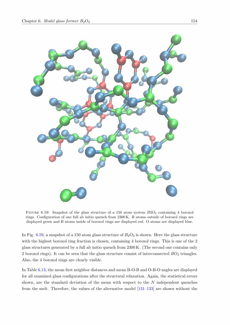
Chapter 6. Model glass former B2O3 154
Figure 6.59: Snapshot of the glass structure of a 150 atom system B2O3 containing 4 boroxolrings. Configuration of one full ab initio quench from 2300 K. B atoms outside of boroxol rings aredisplayed green and B atoms inside of boroxol rings are displayed red. O atoms are displayed blue.
In Fig. 6.59, a snapshot of a 150 atom glass structure of B2O3 is shown. Here the glass structure
with the highest boroxol ring fraction is chosen, containing 4 boroxol rings. This is one of the 2
glass structures generated by a full ab initio quench from 2300 K. (The second one contains only
2 boroxol rings). It can be seen that the glass structure consist of interconnected BO3 triangles.
Also, the 4 boroxol rings are clearly visible.
In Table 6.13, the mean first neighbor distances and mean B-O-B and O-B-O angles are displayed
for all examined glass configurations after the structural relaxation. Again, the statistical errors
shown, are the standard deviation of the mean with respect to the N independent quenches
from the melt. Therefore, the values of the alternative model [131–133] are shown without the
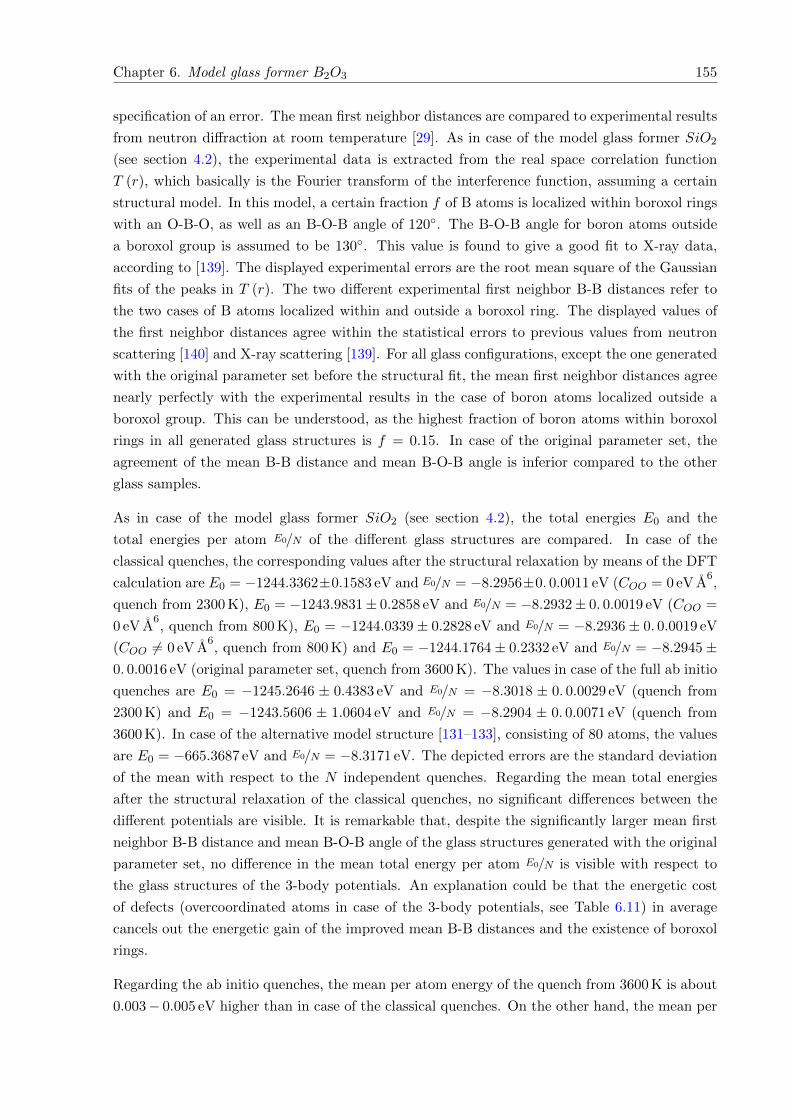
Chapter 6. Model glass former B2O3 155
specification of an error. The mean first neighbor distances are compared to experimental results
from neutron diffraction at room temperature [29]. As in case of the model glass former SiO2
(see section 4.2), the experimental data is extracted from the real space correlation function
T (r), which basically is the Fourier transform of the interference function, assuming a certain
structural model. In this model, a certain fraction f of B atoms is localized within boroxol rings
with an O-B-O, as well as an B-O-B angle of 120. The B-O-B angle for boron atoms outside
a boroxol group is assumed to be 130. This value is found to give a good fit to X-ray data,
according to [139]. The displayed experimental errors are the root mean square of the Gaussian
fits of the peaks in T (r). The two different experimental first neighbor B-B distances refer to
the two cases of B atoms localized within and outside a boroxol ring. The displayed values of
the first neighbor distances agree within the statistical errors to previous values from neutron
scattering [140] and X-ray scattering [139]. For all glass configurations, except the one generated
with the original parameter set before the structural fit, the mean first neighbor distances agree
nearly perfectly with the experimental results in the case of boron atoms localized outside a
boroxol group. This can be understood, as the highest fraction of boron atoms within boroxol
rings in all generated glass structures is f = 0.15. In case of the original parameter set, the
agreement of the mean B-B distance and mean B-O-B angle is inferior compared to the other
glass samples.
As in case of the model glass former SiO2 (see section 4.2), the total energies E0 and the
total energies per atom E0/N of the different glass structures are compared. In case of the
classical quenches, the corresponding values after the structural relaxation by means of the DFT
calculation are E0 = −1244.3362±0.1583 eV and E0/N = −8.2956±0. 0.0011 eV (COO = 0 eV A6,
quench from 2300 K), E0 = −1243.9831± 0.2858 eV and E0/N = −8.2932± 0. 0.0019 eV (COO =
0 eV A6, quench from 800 K), E0 = −1244.0339± 0.2828 eV and E0/N = −8.2936± 0. 0.0019 eV
(COO 6= 0 eV A6, quench from 800 K) and E0 = −1244.1764± 0.2332 eV and E0/N = −8.2945±
0. 0.0016 eV (original parameter set, quench from 3600 K). The values in case of the full ab initio
quenches are E0 = −1245.2646 ± 0.4383 eV and E0/N = −8.3018 ± 0. 0.0029 eV (quench from
2300 K) and E0 = −1243.5606 ± 1.0604 eV and E0/N = −8.2904 ± 0. 0.0071 eV (quench from
3600 K). In case of the alternative model structure [131–133], consisting of 80 atoms, the values
are E0 = −665.3687 eV and E0/N = −8.3171 eV. The depicted errors are the standard deviation
of the mean with respect to the N independent quenches. Regarding the mean total energies
after the structural relaxation of the classical quenches, no significant differences between the
different potentials are visible. It is remarkable that, despite the significantly larger mean first
neighbor B-B distance and mean B-O-B angle of the glass structures generated with the original
parameter set, no difference in the mean total energy per atom E0/N is visible with respect to
the glass structures of the 3-body potentials. An explanation could be that the energetic cost
of defects (overcoordinated atoms in case of the 3-body potentials, see Table 6.11) in average
cancels out the energetic gain of the improved mean B-B distances and the existence of boroxol
rings.
Regarding the ab initio quenches, the mean per atom energy of the quench from 3600 K is about
0.003− 0.005 eV higher than in case of the classical quenches. On the other hand, the mean per
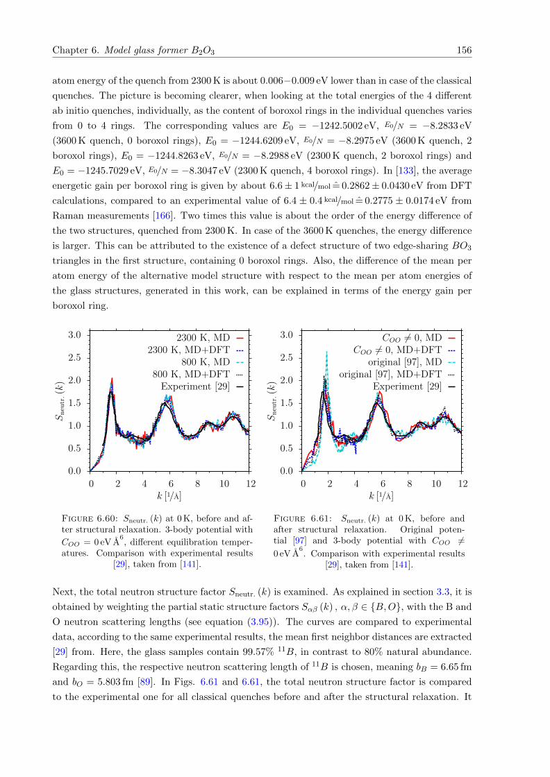
Chapter 6. Model glass former B2O3 156
atom energy of the quench from 2300 K is about 0.006−0.009 eV lower than in case of the classical
quenches. The picture is becoming clearer, when looking at the total energies of the 4 different
ab initio quenches, individually, as the content of boroxol rings in the individual quenches varies
from 0 to 4 rings. The corresponding values are E0 = −1242.5002 eV, E0/N = −8.2833 eV
(3600 K quench, 0 boroxol rings), E0 = −1244.6209 eV, E0/N = −8.2975 eV (3600 K quench, 2
boroxol rings), E0 = −1244.8263 eV, E0/N = −8.2988 eV (2300 K quench, 2 boroxol rings) and
E0 = −1245.7029 eV, E0/N = −8.3047 eV (2300 K quench, 4 boroxol rings). In [133], the average
energetic gain per boroxol ring is given by about 6.6± 1 kcal/mol = 0.2862± 0.0430 eV from DFT
calculations, compared to an experimental value of 6.4 ± 0.4 kcal/mol = 0.2775 ± 0.0174 eV from
Raman measurements [166]. Two times this value is about the order of the energy difference of
the two structures, quenched from 2300 K. In case of the 3600 K quenches, the energy difference
is larger. This can be attributed to the existence of a defect structure of two edge-sharing BO3
triangles in the first structure, containing 0 boroxol rings. Also, the difference of the mean per
atom energy of the alternative model structure with respect to the mean per atom energies of
the glass structures, generated in this work, can be explained in terms of the energy gain per
boroxol ring.
0.0
0.5
1.0
1.5
2.0
2.5
3.0
0 2 4 6 8 10 12
Sn
eutr
.(k)
k [1/A]
2300 K, MD2300 K, MD+DFT
800 K, MD800 K, MD+DFTExperiment [29]
Figure 6.60: Sneutr. (k) at 0 K, before and af-ter structural relaxation. 3-body potential with
COO = 0 eV A6, different equilibration temper-
atures. Comparison with experimental results[29], taken from [141].
0.0
0.5
1.0
1.5
2.0
2.5
3.0
0 2 4 6 8 10 12
Sn
eutr
.(k)
k [1/A]
COO 6= 0, MDCOO 6= 0, MD+DFT
original [97], MDoriginal [97], MD+DFT
Experiment [29]
Figure 6.61: Sneutr. (k) at 0 K, before andafter structural relaxation. Original poten-tial [97] and 3-body potential with COO 6=0 eV A
6. Comparison with experimental results
[29], taken from [141].
Next, the total neutron structure factor Sneutr. (k) is examined. As explained in section 3.3, it is
obtained by weighting the partial static structure factors Sαβ (k) , α, β ∈ B,O, with the B and
O neutron scattering lengths (see equation (3.95)). The curves are compared to experimental
data, according to the same experimental results, the mean first neighbor distances are extracted
[29] from. Here, the glass samples contain 99.57% 11B, in contrast to 80% natural abundance.
Regarding this, the respective neutron scattering length of 11B is chosen, meaning bB = 6.65 fm
and bO = 5.803 fm [89]. In Figs. 6.61 and 6.61, the total neutron structure factor is compared
to the experimental one for all classical quenches before and after the structural relaxation. It
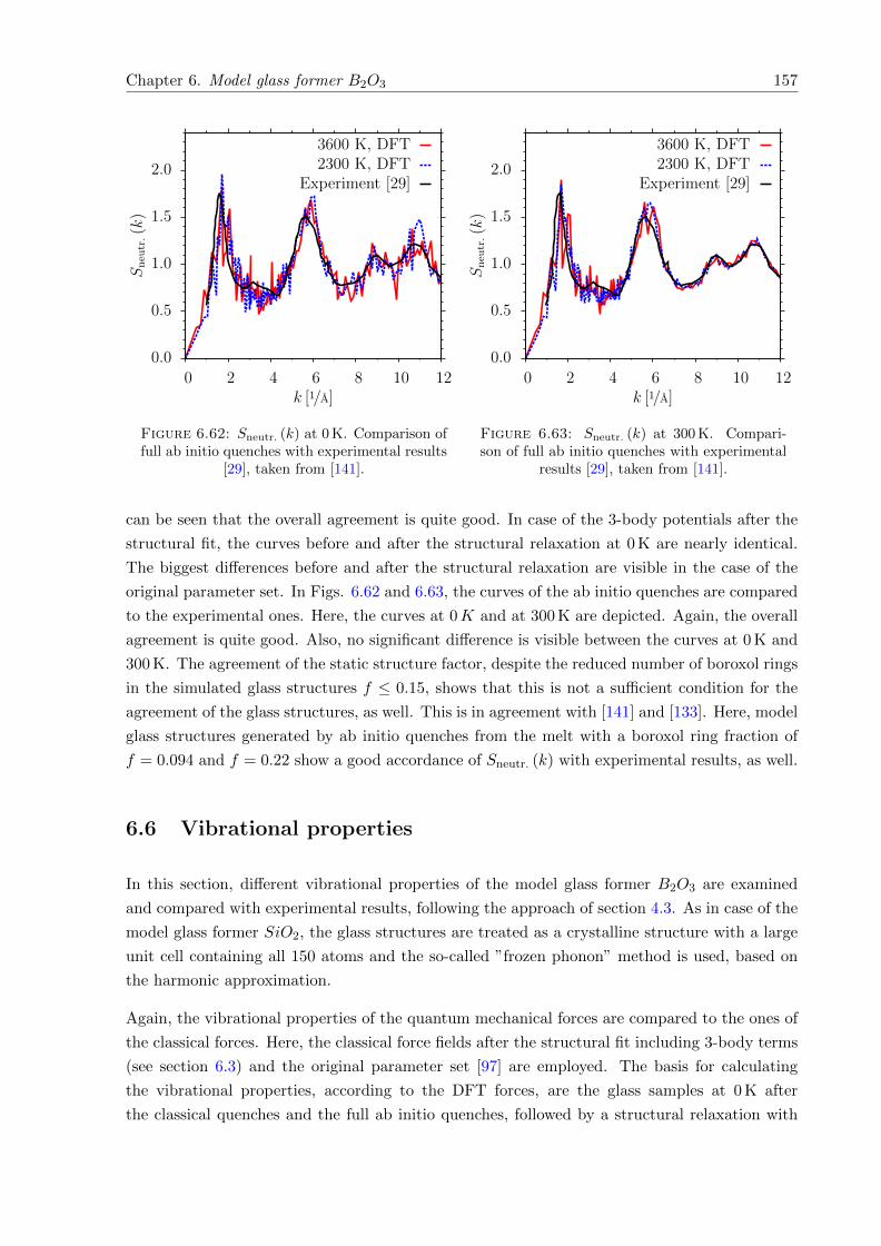
Chapter 6. Model glass former B2O3 157
0.0
0.5
1.0
1.5
2.0
0 2 4 6 8 10 12
Sn
eutr
.(k)
k [1/A]
3600 K, DFT2300 K, DFT
Experiment [29]
Figure 6.62: Sneutr. (k) at 0 K. Comparison offull ab initio quenches with experimental results
[29], taken from [141].
0.0
0.5
1.0
1.5
2.0
0 2 4 6 8 10 12
Sn
eutr
.(k)
k [1/A]
3600 K, DFT2300 K, DFT
Experiment [29]
Figure 6.63: Sneutr. (k) at 300 K. Compari-son of full ab initio quenches with experimental
results [29], taken from [141].
can be seen that the overall agreement is quite good. In case of the 3-body potentials after the
structural fit, the curves before and after the structural relaxation at 0 K are nearly identical.
The biggest differences before and after the structural relaxation are visible in the case of the
original parameter set. In Figs. 6.62 and 6.63, the curves of the ab initio quenches are compared
to the experimental ones. Here, the curves at 0K and at 300 K are depicted. Again, the overall
agreement is quite good. Also, no significant difference is visible between the curves at 0 K and
300 K. The agreement of the static structure factor, despite the reduced number of boroxol rings
in the simulated glass structures f ≤ 0.15, shows that this is not a sufficient condition for the
agreement of the glass structures, as well. This is in agreement with [141] and [133]. Here, model
glass structures generated by ab initio quenches from the melt with a boroxol ring fraction of
f = 0.094 and f = 0.22 show a good accordance of Sneutr. (k) with experimental results, as well.
6.6 Vibrational properties
In this section, different vibrational properties of the model glass former B2O3 are examined
and compared with experimental results, following the approach of section 4.3. As in case of the
model glass former SiO2, the glass structures are treated as a crystalline structure with a large
unit cell containing all 150 atoms and the so-called ”frozen phonon” method is used, based on
the harmonic approximation.
Again, the vibrational properties of the quantum mechanical forces are compared to the ones of
the classical forces. Here, the classical force fields after the structural fit including 3-body terms
(see section 6.3) and the original parameter set [97] are employed. The basis for calculating
the vibrational properties, according to the DFT forces, are the glass samples at 0 K after
the classical quenches and the full ab initio quenches, followed by a structural relaxation with
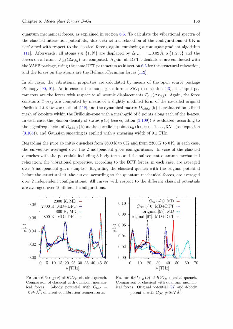
Chapter 6. Model glass former B2O3 158
quantum mechanical forces, as explained in section 6.5. To calculate the vibrational spectra of
the classical interaction potentials, also a structural relaxation of the configurations at 0 K is
performed with respect to the classical forces, again, employing a conjugate gradient algorithm
[111]. Afterwards, all atoms i ∈ 1, N are displaced by ∆rα;i = ±0.02 A, α 1, 2, 3 and the
forces on all atoms Fα;i (∆rβ;j) are computed. Again, all DFT calculations are conducted with
the VASP package, using the same DFT parameters as in section 6.5 for the structural relaxation,
and the forces on the atoms are the Hellman-Feynman forces [112].
In all cases, the vibrational properties are calculated by means of the open source package
Phonopy [90, 91]. As in case of the model glass former SiO2 (see section 4.3), the input pa-
rameters are the forces with respect to all atomic displacements Fα;i (∆rβ;j). Again, the force
constants Φαβ;i,j are computed by means of a slightly modified form of the so-called original
Parlinski-Li-Kawazoe method [118] and the dynamical matrix Dαβ;i,j (k) is evaluated on a fixed
mesh of k-points within the Brillouin-zone with a mesh-grid of 5 points along each of the k-axes.
In each case, the phonon density of states g (ν) (see equation (3.109)) is evaluated, according to
the eigenfrequencies of Dαβ;i,j (k) at the specific k-points νn (k) , n ∈ 1, . . . , 3N (see equation
(3.108)), and Gaussian smearing is applied with a smearing width of 0.1 THz.
Regarding the pure ab initio quenches from 3600 K to 0 K and from 2300 K to 0 K, in each case,
the curves are averaged over the 2 independent glass configurations. In case of the classical
quenches with the potentials including 3-body terms and the subsequent quantum mechanical
relaxation, the vibrational properties, according to the DFT forces, in each case, are averaged
over 5 independent glass samples. Regarding the classical quench with the original potential
before the structural fit, the curves, according to the quantum mechanical forces, are averaged
over 2 independent configurations. All curves with respect to the different classical potentials
are averaged over 10 different configurations.
0.00
0.02
0.04
0.06
0.08
0 5 10 15 20 25 30 35 40 45 50
g(ν)
ν [THz]
2300 K, MD2300 K, MD+DFT
800 K, MD800 K, MD+DFT
Figure 6.64: g (ν) of B2O3, classical quench.Comparison of classical with quantum mechan-ical forces. 3-body potential with COO =
0 eV A6, different equilibration temperatures.
0.00
0.02
0.04
0.06
0.08
0.10
0 10 20 30 40 50 60 70
g(ν)
ν [THz]
COO 6= 0, MDCOO 6= 0, MD+DFT
original [97], MDoriginal [97], MD+DFT
Figure 6.65: g (ν) of B2O3, classical quench.Comparison of classical with quantum mechan-ical forces. Original potential [97] and 3-body
potential with COO 6= 0 eV A6.
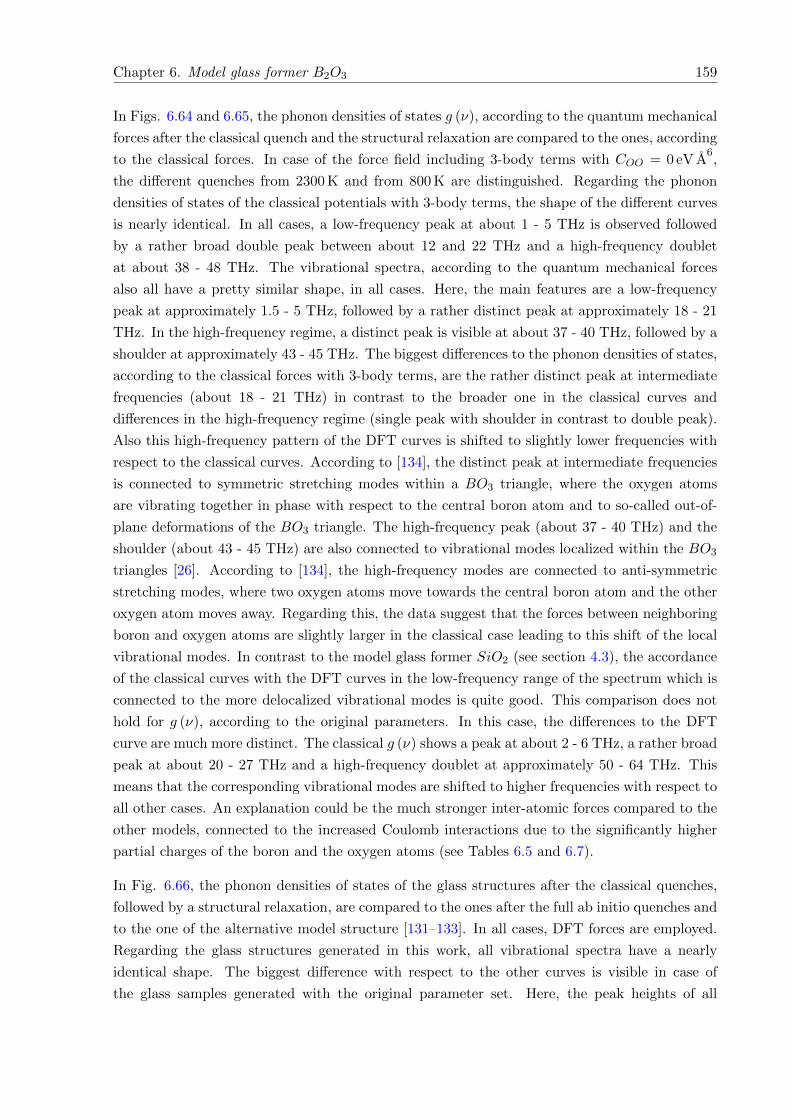
Chapter 6. Model glass former B2O3 159
In Figs. 6.64 and 6.65, the phonon densities of states g (ν), according to the quantum mechanical
forces after the classical quench and the structural relaxation are compared to the ones, according
to the classical forces. In case of the force field including 3-body terms with COO = 0 eV A6,
the different quenches from 2300 K and from 800 K are distinguished. Regarding the phonon
densities of states of the classical potentials with 3-body terms, the shape of the different curves
is nearly identical. In all cases, a low-frequency peak at about 1 - 5 THz is observed followed
by a rather broad double peak between about 12 and 22 THz and a high-frequency doublet
at about 38 - 48 THz. The vibrational spectra, according to the quantum mechanical forces
also all have a pretty similar shape, in all cases. Here, the main features are a low-frequency
peak at approximately 1.5 - 5 THz, followed by a rather distinct peak at approximately 18 - 21
THz. In the high-frequency regime, a distinct peak is visible at about 37 - 40 THz, followed by a
shoulder at approximately 43 - 45 THz. The biggest differences to the phonon densities of states,
according to the classical forces with 3-body terms, are the rather distinct peak at intermediate
frequencies (about 18 - 21 THz) in contrast to the broader one in the classical curves and
differences in the high-frequency regime (single peak with shoulder in contrast to double peak).
Also this high-frequency pattern of the DFT curves is shifted to slightly lower frequencies with
respect to the classical curves. According to [134], the distinct peak at intermediate frequencies
is connected to symmetric stretching modes within a BO3 triangle, where the oxygen atoms
are vibrating together in phase with respect to the central boron atom and to so-called out-of-
plane deformations of the BO3 triangle. The high-frequency peak (about 37 - 40 THz) and the
shoulder (about 43 - 45 THz) are also connected to vibrational modes localized within the BO3
triangles [26]. According to [134], the high-frequency modes are connected to anti-symmetric
stretching modes, where two oxygen atoms move towards the central boron atom and the other
oxygen atom moves away. Regarding this, the data suggest that the forces between neighboring
boron and oxygen atoms are slightly larger in the classical case leading to this shift of the local
vibrational modes. In contrast to the model glass former SiO2 (see section 4.3), the accordance
of the classical curves with the DFT curves in the low-frequency range of the spectrum which is
connected to the more delocalized vibrational modes is quite good. This comparison does not
hold for g (ν), according to the original parameters. In this case, the differences to the DFT
curve are much more distinct. The classical g (ν) shows a peak at about 2 - 6 THz, a rather broad
peak at about 20 - 27 THz and a high-frequency doublet at approximately 50 - 64 THz. This
means that the corresponding vibrational modes are shifted to higher frequencies with respect to
all other cases. An explanation could be the much stronger inter-atomic forces compared to the
other models, connected to the increased Coulomb interactions due to the significantly higher
partial charges of the boron and the oxygen atoms (see Tables 6.5 and 6.7).
In Fig. 6.66, the phonon densities of states of the glass structures after the classical quenches,
followed by a structural relaxation, are compared to the ones after the full ab initio quenches and
to the one of the alternative model structure [131–133]. In all cases, DFT forces are employed.
Regarding the glass structures generated in this work, all vibrational spectra have a nearly
identical shape. The biggest difference with respect to the other curves is visible in case of
the glass samples generated with the original parameter set. Here, the peak heights of all
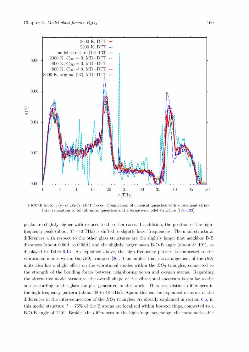
Chapter 6. Model glass former B2O3 160
0.00
0.02
0.04
0.06
0.08
0 5 10 15 20 25 30 35 40 45 50
g(ν)
ν [THz]
3600 K, DFT2300 K, DFT
model structure [131-133]2300 K, COO = 0, MD+DFT800 K, COO = 0, MD+DFT800 K, COO 6= 0, MD+DFT
3600 K, original [97], MD+DFT
Figure 6.66: g (ν) of B2O3, DFT forces. Comparison of classical quenches with subsequent struc-tural relaxation to full ab initio quenches and alternative model structure [131–133].
peaks are slightly higher with respect to the other cases. In addition, the position of the high-
frequency peak (about 37 - 40 THz) is shifted to slightly lower frequencies. The main structural
differences with respect to the other glass structures are the slightly larger first neighbor B-B
distances (about 0.06A to 0.08A) and the slightly larger mean B-O-B angle (about 8 10), as
displayed in Table 6.13. As explained above, the high frequency pattern is connected to the
vibrational modes within the BO3 triangles [26]. This implies that the arrangement of the BO3
units also has a slight effect on the vibrational modes within the BO3 triangles, connected to
the strength of the bonding forces between neighboring boron and oxygen atoms. Regarding
the alternative model structure, the overall shape of the vibrational spectrum is similar to the
ones according to the glass samples generated in this work. There are distinct differences in
the high-frequency pattern (about 38 to 48 THz). Again, this can be explained in terms of the
differences in the inter-connection of the BO3 triangles. As already explained in section 6.5, in
this model structure f = 75% of the B atoms are localized within boroxol rings, connected to a
B-O-B angle of 120. Besides the differences in the high-frequency range, the most noticeable
Chapter 6. Model glass former B2O3 161
feature of this model structure is the very prominent peak at about 23.2 to 23.4 THz. This
peak can be assigned to the breathing mode of the boroxol ring [26, 30]. Also a second distinct
peak at approximately 36 to 36.4 THz is visible in this g (ν), which is a boroxol ring signature,
as well [30]. As examined in section 6.5, the ratio of B atoms localized in 3-membered rings
varies from about f = 2.5% (classical potential with 3-body terms, COO 6= 0 eV A6) to f = 15%
(full ab initio quench from 2300 K). In all cases, a small distinct peak is visible at about 23.2
to 23.4 THz, increasing in size with increasing ratio f . Also, in all cases, a small pattern at
approximately 36 to 36.4 THz is visible. However, this is not as pronounced as the distinct peak
at about 23.2 to 23.4 THz. In case of the model glass structure with f = 0% (classical potential
with original parameter set) this peak is clearly missing. Regarding once again the vibrational
spectra according to the classical forces (see Figs. 6.64 and 6.65), this signature is missing as
well. As explained in section 6.5, the distribution of ring sizes is only altered insignificantly by
the structural relaxation. This means that the value of f is about the same in the respective
glass structures. In the vibrational spectra of the classical force fields with 3-body interactions,
a small feature is visible between about 27.5 and 28.5. This could be connected to vibrations
within the 3-membered rings.
Next, the so-called effective neutron scattering cross sections G (ν) = C (ν) g (ν) are compared to
experimental results from inelastic neutron scattering [30, 134]. Here, only the case of DFT forces
is studied. As in case of the model glass former SiO2 (see section 4.3), the correction function
C (ν) is calculated using the incoherent approximation, according to [121]. This means that the
functional form of C (ν) is equal to the one of equation (4.5), substituting Si with B. As in case
of the static neutron structure factor [29], the glass samples, according to [30], contain 99.57% of
the isotope 11B, in contrast to 80% natural abundance. In [134], the isotope composition is not
stated. However, the authors of [134] are also authors of the corresponding publications [29] and
[30]. Having this in mind and the enhanced absorption of neutrons of 11B, it is assumed that
also in the latter case a 11B sample is used. Regarding this, the respective neutron scattering
length of 11B is chosen, meaning bB = 6.65 fm and bO = 5.803 fm [89] and the atomic mass of
the isotope 11B is chosen, meaning mB = 11.0093 amu and mO = 15.9994 amu. This means
that in equation (4.5) (Si substituted with B), 〈m〉 = 14.00336 amu is the mean atomic mass of
the system,⟨b2⟩
= N−1∑
i b2i = 37.8938854 fm2 is the mean squared neutron scattering length,
g (ν) is the full phonon density of states and gα (ν) , α ∈ B,O, are the partial phonon densities
of states. As in case of the model glass former SiO2, a Debye-Waller factor exp[−k2 〈u2
α〉/3]'
1, α ∈ B,O, is assumed [92] which is a good assumption at low temperature. Comparing the
curves in Figs. 6.67 and 6.68 with the ones in Fig. 6.66, it can be seen that the main effect of
C (ν) is the slight increase of the height of the peaks at intermediate (about 18 - 21 THz) and high
frequencies (about 37 - 40 THz) and a slight reduction of the peak height of the low-frequency
peak (about 1.5 - 5 THz). In [134], the experimental spectrum is composed of two parts, a low-
and a high-frequency part, measured at two different spectrometers and temperatures of 15 K
and 300 K, respectively. In [30], the full spectrum is measured in a single scattering experiment
at 20 K with an incident neutron energy of E0 = 250 meV = 60.45 THz. Here, the experimental
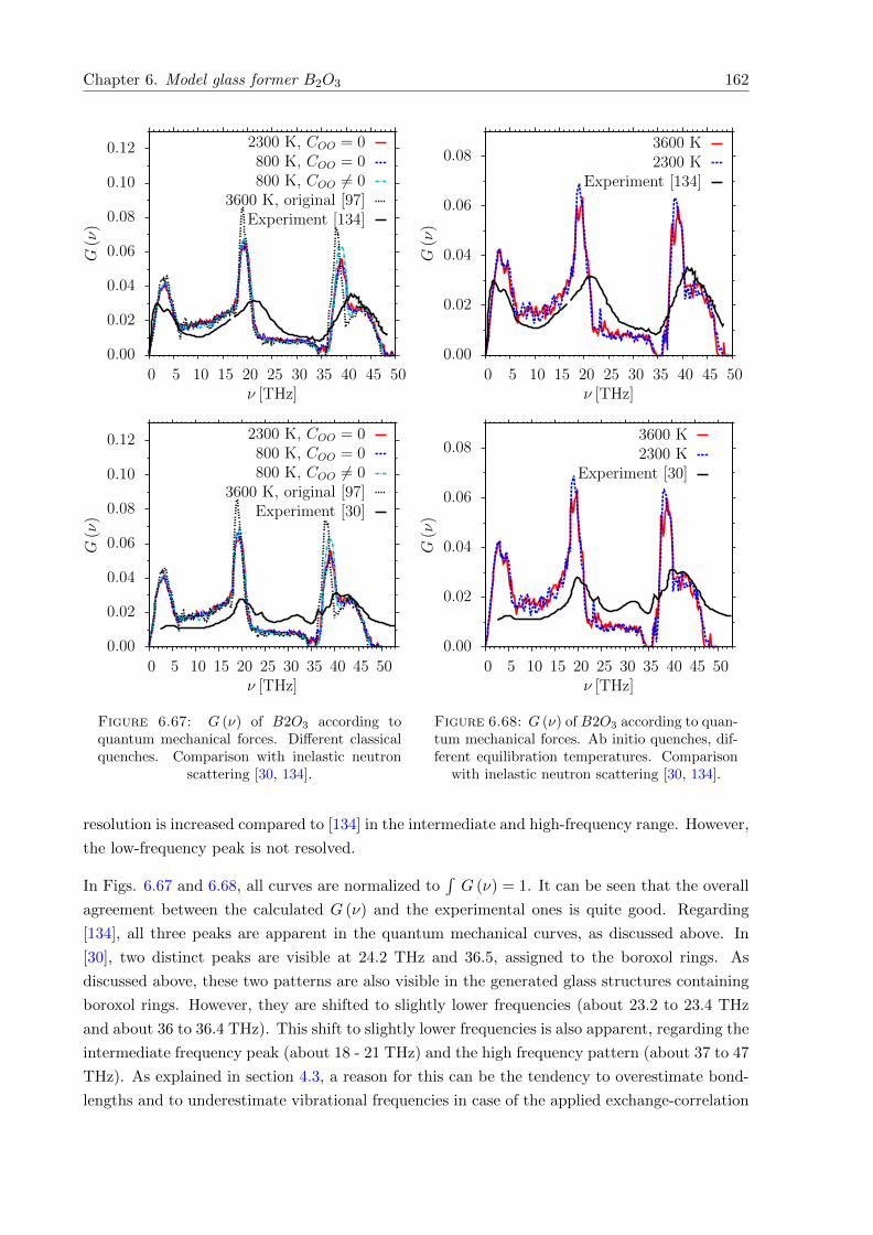
Chapter 6. Model glass former B2O3 162
0.00
0.02
0.04
0.06
0.08
0.10
0.12
0 5 10 15 20 25 30 35 40 45 50
G(ν)
ν [THz]
2300 K, COO = 0800 K, COO = 0800 K, COO 6= 0
3600 K, original [97]Experiment [134]
0.00
0.02
0.04
0.06
0.08
0.10
0.12
0 5 10 15 20 25 30 35 40 45 50
G(ν)
ν [THz]
2300 K, COO = 0800 K, COO = 0800 K, COO 6= 0
3600 K, original [97]Experiment [30]
Figure 6.67: G (ν) of B2O3 according toquantum mechanical forces. Different classicalquenches. Comparison with inelastic neutron
scattering [30, 134].
0.00
0.02
0.04
0.06
0.08
0 5 10 15 20 25 30 35 40 45 50
G(ν)
ν [THz]
3600 K2300 K
Experiment [134]
0.00
0.02
0.04
0.06
0.08
0 5 10 15 20 25 30 35 40 45 50
G(ν)
ν [THz]
3600 K2300 K
Experiment [30]
Figure 6.68: G (ν) of B2O3 according to quan-tum mechanical forces. Ab initio quenches, dif-ferent equilibration temperatures. Comparison
with inelastic neutron scattering [30, 134].
resolution is increased compared to [134] in the intermediate and high-frequency range. However,
the low-frequency peak is not resolved.
In Figs. 6.67 and 6.68, all curves are normalized to´G (ν) = 1. It can be seen that the overall
agreement between the calculated G (ν) and the experimental ones is quite good. Regarding
[134], all three peaks are apparent in the quantum mechanical curves, as discussed above. In
[30], two distinct peaks are visible at 24.2 THz and 36.5, assigned to the boroxol rings. As
discussed above, these two patterns are also visible in the generated glass structures containing
boroxol rings. However, they are shifted to slightly lower frequencies (about 23.2 to 23.4 THz
and about 36 to 36.4 THz). This shift to slightly lower frequencies is also apparent, regarding the
intermediate frequency peak (about 18 - 21 THz) and the high frequency pattern (about 37 to 47
THz). As explained in section 4.3, a reason for this can be the tendency to overestimate bond-
lengths and to underestimate vibrational frequencies in case of the applied exchange-correlation
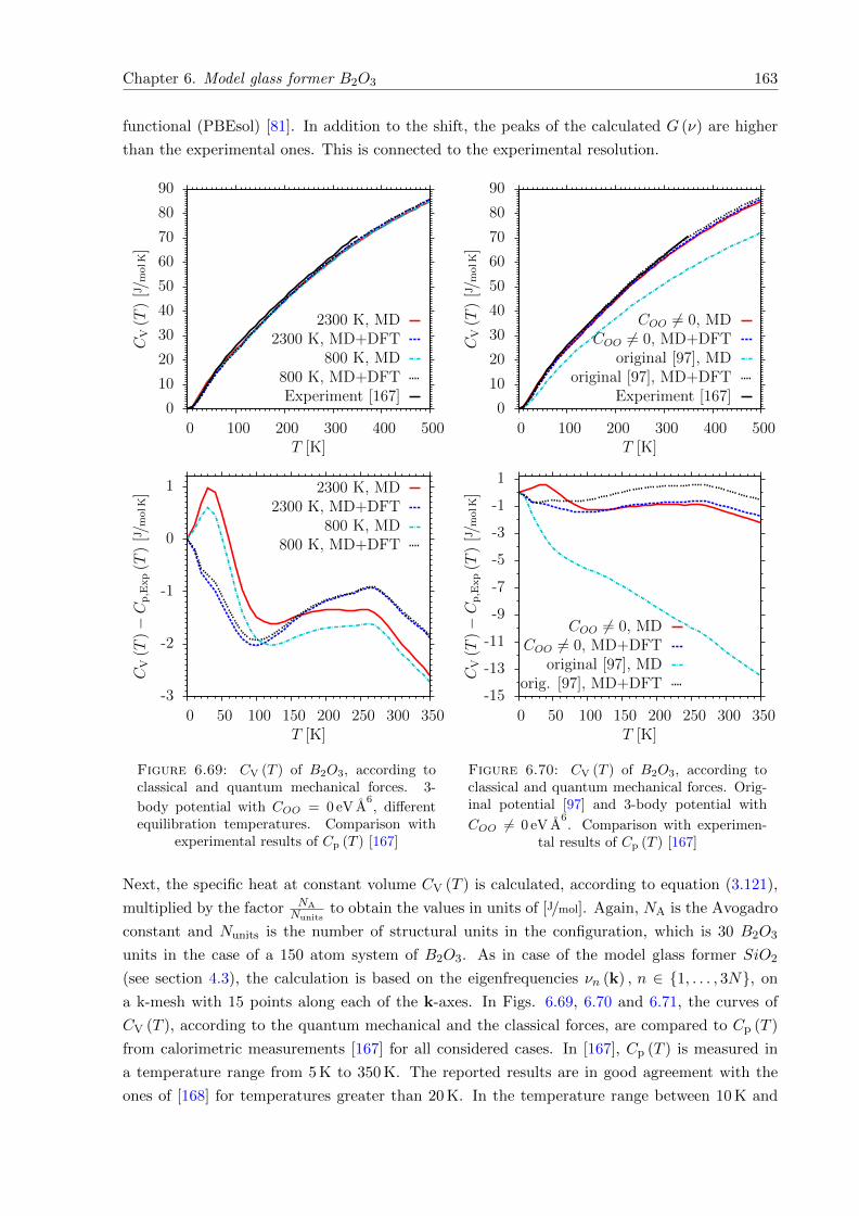
Chapter 6. Model glass former B2O3 163
functional (PBEsol) [81]. In addition to the shift, the peaks of the calculated G (ν) are higher
than the experimental ones. This is connected to the experimental resolution.
0
10
20
30
40
50
60
70
80
90
0 100 200 300 400 500
CV(T
)[J/m
olK]
T [K]
2300 K, MD2300 K, MD+DFT
800 K, MD800 K, MD+DFTExperiment [167]
-3
-2
-1
0
1
0 50 100 150 200 250 300 350
CV(T
)−C
p,E
xp(T
)[J/m
olK]
T [K]
2300 K, MD2300 K, MD+DFT
800 K, MD800 K, MD+DFT
Figure 6.69: CV (T ) of B2O3, according toclassical and quantum mechanical forces. 3-
body potential with COO = 0 eV A6, different
equilibration temperatures. Comparison withexperimental results of Cp (T ) [167]
0
10
20
30
40
50
60
70
80
90
0 100 200 300 400 500
CV(T
)[J/m
olK]
T [K]
COO 6= 0, MDCOO 6= 0, MD+DFT
original [97], MDoriginal [97], MD+DFT
Experiment [167]
-15
-13
-11
-9
-7
-5
-3
-1
1
0 50 100 150 200 250 300 350
CV(T
)−C
p,E
xp(T
)[J/m
olK]
T [K]
COO 6= 0, MDCOO 6= 0, MD+DFT
original [97], MDorig. [97], MD+DFT
Figure 6.70: CV (T ) of B2O3, according toclassical and quantum mechanical forces. Orig-inal potential [97] and 3-body potential with
COO 6= 0 eV A6. Comparison with experimen-
tal results of Cp (T ) [167]
Next, the specific heat at constant volume CV (T ) is calculated, according to equation (3.121),
multiplied by the factor NANunits
to obtain the values in units of [J/mol]. Again, NA is the Avogadro
constant and Nunits is the number of structural units in the configuration, which is 30 B2O3
units in the case of a 150 atom system of B2O3. As in case of the model glass former SiO2
(see section 4.3), the calculation is based on the eigenfrequencies νn (k) , n ∈ 1, . . . , 3N, on
a k-mesh with 15 points along each of the k-axes. In Figs. 6.69, 6.70 and 6.71, the curves of
CV (T ), according to the quantum mechanical and the classical forces, are compared to Cp (T )
from calorimetric measurements [167] for all considered cases. In [167], Cp (T ) is measured in
a temperature range from 5 K to 350 K. The reported results are in good agreement with the
ones of [168] for temperatures greater than 20 K. In the temperature range between 10 K and
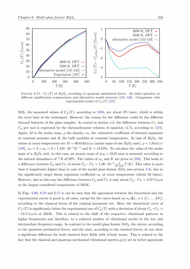
Chapter 6. Model glass former B2O3 164
0
10
20
30
40
50
60
70
80
90
0 100 200 300 400 500
CV(T
)[J/m
olK]
T [K]
3600 K, DFT2300 K, DFT
alternative model [131-133]Experiment [167]
-4
-3
-2
-1
0
1
0 50 100 150 200 250 300 350
CV(T
)−C
p,E
xp(T
)[J/m
olK]
T [K]
3600 K, DFT2300 K, DFT
alternative model [131-133]
Figure 6.71: CV (T ) of B2O3, according to quantum mechanical forces. Ab initio quenches atdifferent equilibration temperatures and alternative model structure [131–133]. Comparison with
experimental results of Cp (T ) [167]
20 K, the measured values of Cp (T ), according to [168], are about 3% lower, which is within
the error bars of the techniques. However, the reason for the difference could be the different
thermal histories of the glass samples. As stated in section 4.3, the difference between CV and
Cp per mol is expressed by the thermodynamic relation of equation (4.7), according to [124].
Again, M is the molar mass, ρ the density, αV the volumetric coefficient of thermal expansion
at constant pressure and K the bulk modulus at constant temperature. In case of B2O3, the
values at room temperature are M = 69.6182 g/mol (molar mass of one B2O3 unit), ρ = 1.83 g/cm3
[159], αV ' 3× αL ' 3× 1.545 · 10−5K−1 and K ' 13 GPa. To calculate the value of the molar
mass of a B2O3 unit, in this case, an atomic mass of mB = 10.81 amu is assumed, according to
the natural abundance of 11B of 80%. The values of αL and K are given in [168]. This leads to
a difference between Cp and CV of about Cp−CV = 1.06 · 10−3 JK2 mol
T [K]. This value is more
than 2 magnitudes higher than in case of the model glass former SiO2 (see section 4.3), due to
the significantly larger linear expansion coefficient αL at room temperature (about 28 times).
However, also in this case the difference between Cp and CV is only about Cp−CV = 0.37 J/mol K
at the largest considered temperature of 350 K.
In Figs. 6.69, 6.70 and 6.71 it can be seen that the agreement between the theoretical and the
experimental curves is good in all cases, except for the curve based on νn (k) , n ∈ 1, . . . , 3N,according to the classical forces of the original parameter set. Here, the theoretical curve of
CV (T ) is significantly below the experimental one of Cp (T ) with a deviation of about Cp−CV '−13.5 J/mol K at 350 K. This is related to the shift of the respective vibrational patterns to
higher frequencies and therefore, to a reduced number of vibrational modes in the low and
intermediate frequency-range. In contrast to the model glass former SiO2, the curves, according
to the quantum mechanical forces, and the ones, according to the classical forces, do not show
a significant difference for both classical force fields with 3-body terms. This is related to the
fact that the classical and quantum mechanical vibrational spectra g (ν) are in better agreement
Chapter 6. Model glass former B2O3 165
with each other in the low and intermediate frequency range as observed in case of SiO2 for the
BKS and the CHIK potential (see Figs. 6.64 and 6.65). In addition, there are also no significant
differences visible in CV (T ) of the glass samples after the classical quench and subsequent
quantum mechanical relaxation and the ab initio quenches. Here, the highest differences between
the theoretical and the experimental values at 350 K are about Cp − CV ' −2.8 J/mol K. In case
of the alternative model structure [131–133], the agreement is slightly inferior with a deviation
of about Cp − CV ' −4 J/mol K at 350 K.
In this chapter, the simulation results of the model glass former B2O3 are summarized. First,
an overview over different experimental results is given, supporting the special feature of about
60% − 80% of the boron atoms located in planar, 3-membered boroxol rings in vitreous B2O3.
In addition, a summary over previous classical molecular dynamics studies of boron oxide is
presented. Next, the results of ab initio molecular dynamics (MD) simulations of 150 atom
systems at the experimental density of ρ = 1.83 g/cm3 are depicted in a temperature range,
the systems still can be equilibrated, namely between 3600 K and 2300 K. At 2300 K, an
increased amount of 3-membered rings is observed, compared to the liquid structures at 2500
K and 2700 K. This motivates to take the latter as a basis for the development of a new
interaction potential for classical MD simulations of liquid B2O3. The parameter fits are carried
out, using a modified form of the structural fitting procedure, presented in [43]. Starting with
the parameter set, according to [97], the differences in the pair correlation functions and the
angular distributions of the classical and the ab initio MD simulation are minimized, using
a Levenberg-Marquardt procedure. The best results are obtained, including 3-body angular
interactions for the O-B-O and the B-O-B angles. A new angular potential type is introduced,
namely an inverse Gaussian potential that is smoothly switched on and off, depending on the
inter-atomic distances (see equations (6.1) to (6.4)). This potential type is implemented into
a new LAMMPS pair style, called “gauss/smooth”. Classical MD simulations of 150 are atom
systems are carried out at the experimental glass density of ρ = 1.83 g/cm3 in a temperature
range between 3600 K and 800 K, using two different parametrizations of the 3-body potential,
with (COO 6= 0 eV A6) and without (COO = 0 eV A
6) O-O attractions. The main difference
between these simulation runs and the ab initio MD simulations are reduced peak heights and
2−10 times shorter α-relaxation times in the classical MD simulations. In addition, classical MD
simulations of 1200 atom systems at constant external pressure p = 0 are presented. Here, the
parametrization with O-O attractions leads to a system density comparable to the experimental
one at low temperatures (ρ = 1.892±0.003 g/cm3 at 1000 K), whereas the parametrization without
O-O attractions leads to a significantly lower system density at low temperatures (ρ = 1.280±0.014 g/cm3 at 1000 K). Regarding the temperature dependence of the self-diffusion constants Dα,
α ∈ B,O, in principle, an Arrhenius behavior can be observed (see equation (4.4)). However,
the slope of the exponential decrease of Dα (T ) with respect to 1/T significantly decreases at
temperatures below about 1800 K, leading to a different activation energy EA,α, α ∈ B,O,at low than at high temperatures. So far, this behavior is not clearly understood. It could be
connected to a different diffusion mechanism at low temperatures. Finally, glass structures are
generated in different ways, namely by quenches from the melt with classical MD and ab initio
Chapter 6. Model glass former B2O3 166
MD simulations with a subsequent structural relaxation with quantum mechanical forces. The
main improvement of the glass structures, generated by the new 3-body potentials, are a slightly
smaller B-B distance and the occurrence of some boroxol rings, compared to the ones generated
by the original parameter set before the structural fit. However, the boroxol ring fraction is still
small (f = 2.5 ± 1.1% to f = 8 ± 2.3%). The ab initio quenches show slightly larger boroxol
ring fractions of f = 5± 5% (3600 K quench) and f = 15± 5% (2300 K quench). Regarding the
vibrational properties, the phonon densities of state, according to the quantum mechanical forces
show an acceptable agreement with results from inelastic neutron scattering [30, 134]. However,
the peak height of the peak, assigned to boroxol rings, is significantly lower than in case of an
alternative model structure with a boroxol ring fraction of f = 75%. The vibrational spectra,
according to the classical forces of the new 3-body potentials, show an acceptable agreement
with experimental results, as well.
Chapter 7
Discussion and Conclusions
In this work, computer simulations of the model glass formers SiO2 and B2O3 are carried out by
means of classical molecular dynamics (MD) simulations with the LAMMPS software package
[60, 61] and quantum mechanical calculations, based on density functional theory (DFT) with
the VASP software package [77–79].
Regarding the model glass former SiO2, the structural and dynamical properties of the liquid
state are studied at different temperatures between 4300 K and 2700 K by classical MD simula-
tions (see section 4.1). First, different system sizes of 114, 165, 256 and 1152 are compared at
constant density of ρ = 2.37 g/cm3, which is slightly larger than the experimental density of vitre-
ous SiO2 of ρ = 2.2 g/cm3 [98] (see subsection 4.1.2). These studies are carried out using a slightly
modified form of the BKS potential [22], leading to an overall smooth pair potential. As already
reported in [104], the main finite size effect is a dynamical slowing down, visible the mean square
displacements⟨r2α (t)
⟩and the incoherent intermediate scattering functions FS,α (k, t). Regard-
ing the structural quantities, nearly no dependence on the system size is found in the static
structure factors Sαβ (k), pair correlation functions gαβ (r) and angular distributions pαβγ (Φ)
(α, β, γ ∈ Si,O). The distribution of ring sizes shows a reduced probability pSi (n) for rings
of size n > 6 in the small system sizes. Finite size effects are significantly larger for the 114
atom than for the 165 atom system, justifying the choice of the latter system size in the fol-
lowing considerations. In subsection 4.1.3, the structural and dynamical properties of the BKS
[22] and the CHIK [43] potential are compared to each other for the system size of 165 atoms,
again, in the temperature range between 4300 K and 2700 K. Here, simulations are carried out
at ρ = 2.2 g/cm3. In agreement to [43], the structural relaxation times τα of the CHIK potential
are about 3 − 10 times shorter at the same temperature than in case of the BKS potential.
Regarding the structural quantities Sαβ (k), gαβ (r) and pαβγ (Φ), the peak heights of the CHIK
potential are slightly lower and the mean Si-O-Si angles are slightly smaller by approximately
2 − 3 at all examined temperatures. This is in agreement with [43]. The activation energies
EA,α, α ∈ Si,O, are determined by means of the temperature dependence of the self-diffusion
constants Dα. In case of the BKS potential, they are about 1.9 eV (Si) to 1.6 eV (O) larger than
the ones reported in [42] for simulations of 8016 atoms at ρ = 2.37 g/cm3 and about 1.4 eV (O)
167
Chapter 7. Discussion and Conclusions 168
larger than the ones reported in [107, 108] for simulations of 99 atoms at ρ = 2.30 g/cm3. These
differences can be understood in terms of effects of the system size and the system density, as
the activation energies increase with decreasing system size and decreasing system density. In
case of the CHIK potential, the activation energies are approximately 0.8 eV (Si) to 0.9 eV (O)
larger than the ones reported in [43] for simulations of 1152 atoms at ρ = 2.2 g/cm3. Here, the
differences are due to the different system sizes.
In section 4.2, glass structures are generated by quenches from the melt from 4300 K to 0 K with
a cooling rate of Γ = 1 · 1011 K/s. The BKS and CHIK potential are employed and the glass
configurations at 0 K are structurally relaxed in terms of a quantum mechanical DFT calculation.
The main effect of the structural relaxation, in both cases, is the decrease of the mean Si-O-Si
angle by about 4 − 6, in agreement with [10]. After the structural relaxation, no significant
differences are visible in the glass structures generated with the BKS potential and the CHIK
potential. These glass structures are compared to the one of a full ab initio quench from the
melt from 3600 K to 0 K with Γ = 1.6 · 1014 K/s. A good agreement is observed. However,
the latter shows a slightly smaller mean Si-O-Si angle by approximately 2 − 3. All mean
first neighbor distances and mean angles of the different glass structures are in good agreement
with experimental results of neutron and X-ray scattering [113, 114]. This aspect has not been
investigated so far for the CHIK potential. The mean total energies per atom of the glass
structures generated with the BKS and the CHIK potential are comparable (E0/N = −8.1811±0. 0.0016 eV and E0/N = −8.1778± 0. 0.0010 eV) and slightly lower than the value of the full ab
initio quench (E0/N = −8.1663 eV). In section 4.3, the vibrational properties are calculated using
the so-called ”frozen phonon” method, based on the harmonic approximation. All vibrational
spectra, according to the DFT forces, show excellent accordance with experimental results from
inelastic neutron scattering [99, 100], in agreement with [11, 28, 119, 120]. The accordance
with experimental results is clearly improved, compared to the classical forces. Also the specific
heat CV (T ) shows a significantly improved agreement with the experimental curve at constant
pressure [123] in the DFT case, compared to both classical force fields.
In chapter 5, the thermal expansion of vitreous silica is calculated, based on the vibrational
properties of glass structures, generated in section 4.2, at different system densities. The applied
method is the so-called quasi-harmonic approximation [125]. It is based on the dependence of the
Helmholtz free energy F (T, V ) on the volume of the system, due to the volume dependence of
the eigenfrequencies νn (k;V ). The calculated curves of the linear expansion coefficients αL (T )
show the striking result of a change of sign in αL (T ) and a temperature range of negative thermal
expansion, both, using quantum mechanical and classical forces for all but one examined glass
configuration. To my knowledge this has not been reported before. The temperature range of
negative thermal expansion is below approximately 140 K to 160 K, in case of the DFT forces. In
fact, the DFT curves are in good agreement with experimental results [32, 33] at temperatures
below approximately 200 K. At higher temperatures, however, the calculated curves of αL (T )
are significantly higher than the experimental ones. The linear expansion coefficients, according
to the classical forces of the BKS and the CHIK potential, show a negative sign at temperatures
below about 290 K to 325 K. Here, the agreement with experimental results is less pronounced, as
Chapter 7. Discussion and Conclusions 169
in case of the DFT forces. The change of sign in the linear thermal expansion coefficient αL (T ),
in all cases, can be explained in terms of negative microscopic mode Gruneisen parameters γn
at low eigenfrequencies.
In chapter 6, the model glass former B2O3 is studied. In vitreous B2O3, about 60%−80% of the
boron atoms are localized within 3-membered boroxol rings (see section 6.1). A 3-membered ring
is called boroxol ring when the participating boron atoms are all 3-fold coordinated with respect
to the oxygen atoms and the oxygen atoms are all 2-fold coordinated with respect to the boron
atoms [31]. Therefore, these 3-membered rings are of special interest in the study of B2O3. First,
the structural and dynamical properties of liquid B2O3 are studied by means of ab initio Born-
Oppenheimer MD simulations of a 150 atom system in a temperature range between 3600 K
and 2300 K at the experimental glass density of ρ = 1.83 g/cm3 [159] (see section 6.2). Regarding
the dynamical properties, the structural relaxation time increases by about the factor 30 from
3600 K to 2300 K. The pair correlation functions gαβ (r) at 2500 K are compared to the ones in
[162] at a system density of 1.92 g/cm3, showing an acceptable agreement. In principle, pB (n = 3)
decreases with decreasing temperature. However, at 2300 K, the probability pB (n = 3) starts to
increase again, reflecting the emergence of new 3-membered rings.
In section 6.3, a set of new force field parameters is obtained by means of a structural fit to
gαβ (r) and pαβγ (Φ) of the ab initio MD trajectory at 2300 K. Here, the structural fitting routine
of A. Carre is applied [43, 51], extended in terms of including the relevant angular distributions
pαβγ (Φ) into the fitting procedure. Starting with the parameter set of the force field of C. R.
Trott [97], the agreement of the structural quantities of the MD simulation with the ones of
the ab initio MD trajectory can be significantly improved. One effect, is the reduction of the
partial charge of the boron atom to approximately qB = 1 e, in all cases. The best agreement
is obtained in the case of including 3-body angular interactions for the O-B-O and the B-O-B
angles, in addition to the pair potential of a slightly modified form of the Buckingham type [94]
with Coulomb interactions. In this course, a new angular potential type is introduced, namely an
inverse Gaussian potential that is smoothly switched on and off, depending on the inter-atomic
distances. It is implemented into a new LAMMPS pair style, called “gauss/smooth”. This leads
to an overall smooth interaction potential. The main improvement of the additional angular
terms is a reduction of the mean B-B distance and mean B-O-B angle. Trials of the structural
fitting procedure at 3600 K lead to inferior results.
In section 6.4, the static and dynamic properties of the two parameter sets with angular in-
teractions are calculated in a temperature range between 3600 K and 800 K. In one case, the
O-O interaction is purely repulsive (COO = 0 eV A6). The results of 150 atom simulations at
constant experimental glass density ρ = 1.83 g/cm3 [159] are compared to the ones of the ab initio
MD simulations, in the temperature range the latter can still be equilibrated, namely between
3600 K and 2300 K. In general, the agreement is acceptable. The main differences are the 2− 10
times shorter α-relaxation times τα and the reduced peak heights in case of the classical MD
simulations. In contrast to the ab initio MD simulations, the probability for a B atom to be
in a 3-membered ring pB (n = 3) is smaller than pB (n = 3) in the classical MD simulations. In
Chapter 7. Discussion and Conclusions 170
addition, NpT MD simulations at p = 0 external pressure are carried out for a system size of
1200 atoms, where finite size effects play a less significant role. Here, distinct differences between
the two different parameter sets are visible. The parameter set with COO = 0 eV A6
shows a
significantly too low system density of approximately ρ = 1.280 ± 0.024g/cm3 at 1000 K. The
corresponding value of the potential with COO 6= 0 eV A6
is about ρ = 1.892 ± 0.005g/cm3 at
1000 K. This is in quite good agreement with the experimental glass density of ρ = 1.83 g/cm3
[159]. Regarding the dynamical properties, at high temperatures, the structural relaxation times
of the 1200 atom simulations are significantly lower than the ones of the 150 atom simulations,
in both cases. The same holds for all other examined temperatures, in case of the potential with
COO 6= 0 eV A6. This is due to finite size effects. In the case of COO = 0 eV A
6, τα is over an order
of magnitude larger for the 1200 than for the 150 atom system at 1000 K. This can be explained
in terms of the significantly lower system density of the 1200 simulation at this temperature.
Regarding the structural properties, the most significant difference between the large and the
small systems is seen in the distribution of ring sizes. The distribution is much broader in case
of 1200 atom simulations and the 150 atom simulations show a lack of ring sizes with n ≥ 10, in
both cases. As in case of SiO2, the temperature dependence of the self-diffusion constants Dα
is studied, in all cases. Here, the slope of the exponential decrease of Dα (T ), α ∈ B,O, with
respect to 1/T significantly decreases at temperatures below approximately 1800 K, leading to
different activation energies EA,α, α ∈ B,O at low than at high temperatures. So far, this be-
havior is not clearly understood. It could be connected to a different diffusion mechanism at low
temperatures. To exclude effects of insufficient equilibration, in case of the 150 atom systems,
additional equilibration runs are carried out at 1200 K and 1000 K with significant longer equi-
libration times. The activation energies at low temperatures are between EA,B ' 0.74± 0.02eV
and EA,B ' 1.10± 0.03eV and EA,O ' 0.75± 0.01eV and EA,O ' 1.07± 0.02eV. The respective
values at high temperatures are between EA,B ' 1.28 ± 0.01eV and EA,B ' 1.31 ± 0.02eV and
EA,O ' 1.23 ± 0.02eV and EA,O ' 1.28 ± 0.02eV for the classical potentials, compared to the
values of EA,B ' 1.87 ± 0.16eV and EA,O ' 2.18 ± 0.19eV, extracted from the ab initio MD
runs.
In section 6.5, glass structures, generated by quenches from the melt with classical MD simula-
tions and subsequent quantum mechanical relaxations, are compared to the ones, generated by
pure ab initio quenches. In the first case, the quench rate is Γ = 1 · 1011 K/s and the starting
temperatures of the quenches are 2300 K (COO = 0 eV A6) and 800 K (both parameter sets). In
addition, classical quenches from 3600 K are studied with the original parameter set before the
structural fit. In the second case, the quench rate is Γ = 1.6 · 1014 K/s and the starting tem-
peratures of the quenches are 3600 K and 2300 K. Regarding the different glass configurations,
the mean first neighbor B-O and O-O distances show a very good agreement with experimental
results [29], in all cases. In contrast to this, the mean B-B distances and the number of boroxol
rings show significant differences between the different glass samples. In case of the original pa-
rameter set, all atoms show “ideal” coordination numbers. However, no boroxol rings are present
in the structures and the mean B-B distance is significantly larger by about 0.06 A than in all
other cases. In case of the 3-body potentials after the structural fit, between 4% and 7% of the
Chapter 7. Discussion and Conclusions 171
boron atoms are overcoordinated with respect to B atoms and approximately 3% and 4% of the
B atoms are overcoordinated with respect to O atoms, after the structural relaxation. However,
the mean first neighbor B-B distances show an acceptable agreement with experimental results
[29] for the B atoms, not located in boroxol rings. These glass structures have a boroxol ring
fraction of approximately f = 2.5 ± 1.1% to f = 8 ± 2.3%, which is significantly lower than
the experimentally predicted value of about f = 60% to f = 80%. In case of the glass struc-
tures generated by means of ab initio MD simulations, the corresponding values are f = 5± 5%
(3600 K quench) and f = 15±5% (2300 K quench) and the mean first neighbor distances show an
acceptable agreement with experimental results, as well. Here, the first neighbor peak in gBB (r)
shows clearly a second maximum attributed to B atoms within a boroxol ring. As in case of
SiO2, the mean total energies per atom of the different glass structures are studied. Regarding
the classical quenches and subsequent structural relaxations, the values are of comparable size
in all cases, namely between E0/N = −8.2956± 0. 0.0011 eV and E0/N = −8.2932± 0. 0.0019 eV.
An explanation is that the energetic cost of defects (overcoordinated atoms in case of the 3-body
potentials) in average cancels out the energetic gain of the improved mean B-B distances and
the existence of boroxol rings, with respect to the original parameter set [97]. Comparing the 4
different full ab initio quenches, the energies per atom are in a range between E0/N = −8.3047 eV
one (2300 K quench with 4 boroxol rings) and E0/N = −8.2833 eV (one 3600 K quench with 0
boroxol rings). These value (regarding the total energy of the whole 150 atom systems, namely
E0/N · 150) fit to the average energetic gain per boroxol ring of about 0.2862 ± 0.0430 eV [133],
in addition to the defect energy of two edge-sharing BO3 triangles in the one 3600 K quench
without boroxol rings.
In section 6.6, the vibrational properties of the glass structures are examined in terms of classi-
cal and DFT forces, again using the so-called ”frozen phonon” method. Regarding the 3-body
potentials after the structural fit, the classical spectra show an improved agreement to quan-
tum mechanical spectra, compared to the one, according to the classical forces of the original
parameter set [97]. Overall, the agreement of the quantum mechanical spectra with results from
inelastic neutron scattering [30, 134] is acceptable. Also the boroxol ring signature is visible
for all glass structures containing boroxol rings. The corresponding sharp peak is shifted to
slightly lower frequencies as in the experimental curves (23.2 to 23.4 THz in contrast to 24.2
THz). However, the peak heights of the boroxol ring signatures are significantly lower as in case
of the alternative model structure with f = 0.75. In addition, the specific heat CV (T ) shows
good agreement with the experimental curve at constant pressure [167]. In contrast to SiO2,
the agreement, according to the DFT forces, is comparable to the one, according to the classical
forces of the new 3-body potentials after the structural fit.
Summarizing the above results, it is possible to generate glass structures by quenches from the
melt with classical MD simulations and a subsequent quantum mechanical relaxation that are
comparable to the ones generated by quenches from the melt with ab initio MD calculations.
The requirement is to employ a classical force field that leads to glass structures which are close
to the ones obtained from pure ab initio quenches. No general statement can be given, which
method leads to a glass structure that is in better agreement with the ”real” one obtained by a
Chapter 7. Discussion and Conclusions 172
quench from the melt in a laboratory experiment. On the one hand, in case of the classical MD
simulations, the system can be equilibrated at lower temperatures and slower quench rates by
about 3 - 4 orders of magnitude are possible. On the other hand, in ab initio MD simulations
the inter-atomic forces are described much more realistically. In case of the model glass former
SiO2, both methods lead to comparable results. Regarding the mean total energy per atom, the
MD quenches lead to a slightly lower value after the structural relaxation. In case of the model
glass former B2O3, the best results with the lowest energies per atom (and also containing the
largest amount of boroxol rings) are obtained by full ab initio quenches from 2300 K. In case
of the glass structures after the classical quench and the structural relaxation, the accordance
of the mean B-B distances and B-O-B angles is improved applying new force field parameters,
including 3-body terms. Regarding the significantly improved agreement of the structural and
dynamical properties of liquid B2O3 with ab initio MD results, the structural differences of the
generated glass structures are less than expected, compared to the original parameter set [97].
This is reflected in nearly identical mean total energies per atom. The existence of boroxol rings
in the glass structures generated with the new parameter sets goes along with approximately
2% to 3% overcoordinated B atoms with respect to the next nearest O atoms. In principle,
the structure matching scheme according to a liquid ab initio MD trajectory, developed by A.
Carre [43] for the model glass former SiO2, is proven to be successfully also in case of the
model glass former B2O3. In the latter case (at least) angular terms have to be included. The
perspective is to apply this fitting scheme to more complicated systems as alkaline borate or
alkaline borosilicate glasses.
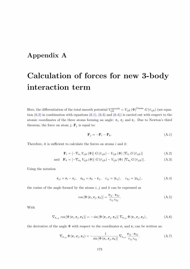
Appendix A
Calculation of forces for new 3-body
interaction term
Here, the differentiation of the total smooth potential V smoothijk = Vijk (Φ)Gauss G (rijk) (see equa-
tion (6.2) in combination with equations (6.1), (6.3) and (6.4)) is carried out with respect to the
atomic coordinates of the three atoms forming an angle: ri, rj and ri. Due to Newton’s third
theorem, the force on atom j, Fj is equal to:
Fj = −Fi − Fk. (A.1)
Therefore, it is sufficient to calculate the forces on atoms i and k:
Fi = [−∇ri Vijk (Φ)] G (rijk)− Vijk (Φ) [∇ri G (rijk)] (A.2)
and Fk = [−∇rk Vijk (Φ)] G (rijk)− Vijk (Φ) [∇rk G (rijk)] . (A.3)
Using the notation
rij = ri − rj , rkj = rk − rj , rij = |rij | , rkj = |rkj | , (A.4)
the cosine of the angle formed by the atoms i, j and k can be expressed as
cos [Φ (ri, rj , rk)] =rij · rkjrij rkj
. (A.5)
With
∇ri,k cos [Φ (ri, rj , rk)] = − sin [Φ (ri, rj , rk)] ∇ri,k Φ (ri, rj , rk) , (A.6)
the derivative of the angle Φ with respect to the coordinates ri and ri can be written as:
∇ri,k Φ (ri, rj , rk) = − 1
sin [Φ (ri, rj , rk)]∇ri,k
rij · rkjrij rkj
. (A.7)
173
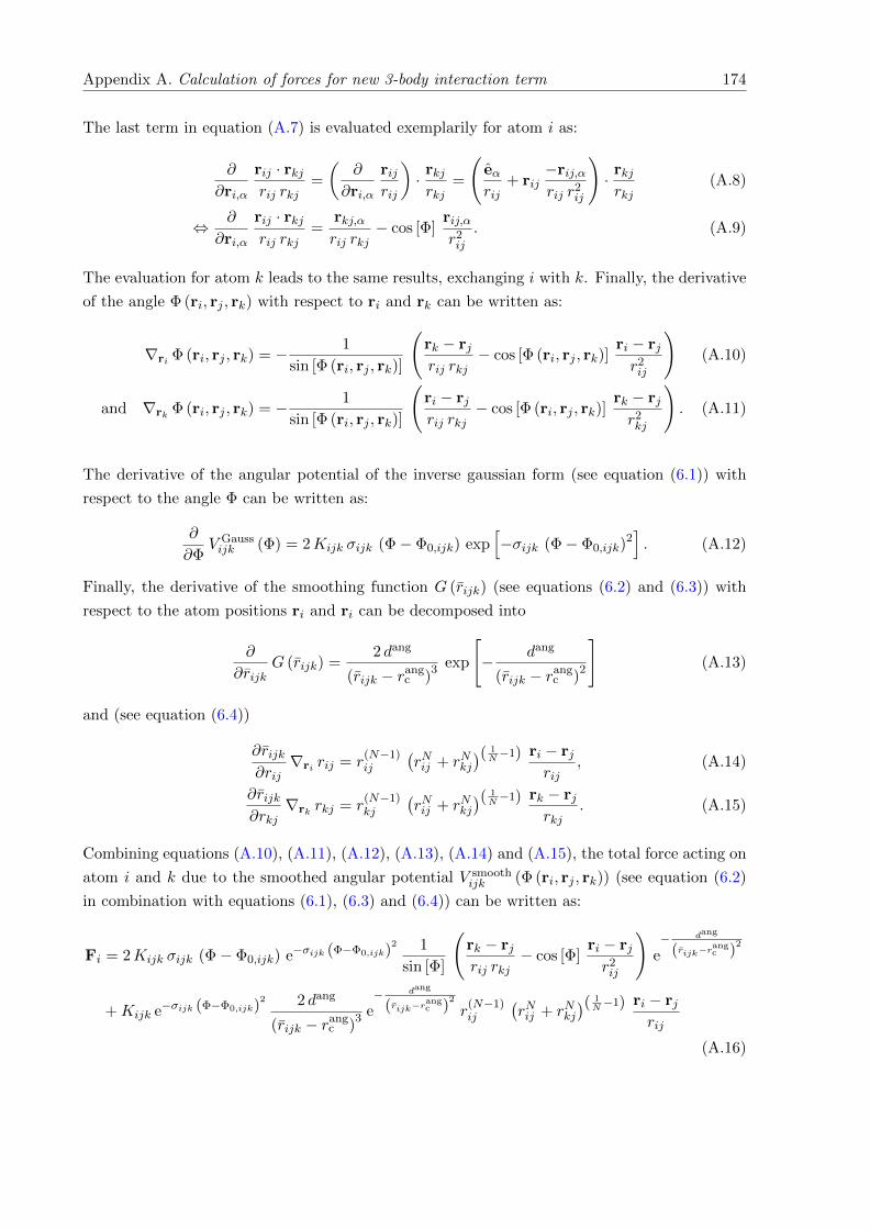
Appendix A. Calculation of forces for new 3-body interaction term 174
The last term in equation (A.7) is evaluated exemplarily for atom i as:
∂
∂ri,α
rij · rkjrij rkj
=
(∂
∂ri,α
rijrij
)· rkjrkj
=
(eαrij
+ rij−rij,αrij r2
ij
)· rkjrkj
(A.8)
⇔ ∂
∂ri,α
rij · rkjrij rkj
=rkj,αrij rkj
− cos [Φ]rij,αr2ij
. (A.9)
The evaluation for atom k leads to the same results, exchanging i with k. Finally, the derivative
of the angle Φ (ri, rj , rk) with respect to ri and rk can be written as:
∇ri Φ (ri, rj , rk) = − 1
sin [Φ (ri, rj , rk)]
(rk − rjrij rkj
− cos [Φ (ri, rj , rk)]ri − rjr2ij
)(A.10)
and ∇rk Φ (ri, rj , rk) = − 1
sin [Φ (ri, rj , rk)]
(ri − rjrij rkj
− cos [Φ (ri, rj , rk)]rk − rjr2kj
). (A.11)
The derivative of the angular potential of the inverse gaussian form (see equation (6.1)) with
respect to the angle Φ can be written as:
∂
∂ΦV Gaussijk (Φ) = 2Kijk σijk (Φ− Φ0,ijk) exp
[−σijk (Φ− Φ0,ijk)
2]. (A.12)
Finally, the derivative of the smoothing function G (rijk) (see equations (6.2) and (6.3)) with
respect to the atom positions ri and ri can be decomposed into
∂
∂rijkG (rijk) =
2 dang
(rijk − rangc )
3 exp
[− dang
(rijk − rangc )
2
](A.13)
and (see equation (6.4))
∂rijk∂rij
∇ri rij = r(N−1)ij
(rNij + rNkj
)( 1N−1) ri − rj
rij, (A.14)
∂rijk∂rkj
∇rk rkj = r(N−1)kj
(rNij + rNkj
)( 1N−1) rk − rj
rkj. (A.15)
Combining equations (A.10), (A.11), (A.12), (A.13), (A.14) and (A.15), the total force acting on
atom i and k due to the smoothed angular potential V smoothijk (Φ (ri, rj , rk)) (see equation (6.2)
in combination with equations (6.1), (6.3) and (6.4)) can be written as:
Fi = 2Kijk σijk (Φ− Φ0,ijk) e−σijk (Φ−Φ0,ijk)2 1
sin [Φ]
(rk − rjrij rkj
− cos [Φ]ri − rjr2ij
)e− dang
(rijk−rangc )
2
+Kijk e−σijk (Φ−Φ0,ijk)2 2 dang
(rijk − rangc )
3 e− dang
(rijk−rangc )
2
r(N−1)ij
(rNij + rNkj
)( 1N−1) ri − rj
rij
(A.16)
Appendix A. Calculation of forces for new 3-body interaction term 175
and
Fk = 2Kijk σijk (Φ− Φ0,ijk) e−σijk (Φ−Φ0,ijk)2 1
sin [Φ]
(ri − rjrij rkj
− cos [Φ]rk − rjr2kj
)e− dang
(rijk−rangc )
2
+Kijk e−σijk (Φ−Φ0,ijk)2 2 dang
(rijk − rangc )
3 e− dang
(rijk−rangc )
2
r(N−1)kj
(rNij + rNkj
)( 1N−1) rk − rj
rkj.
(A.17)

Bibliography
[1] Schott & Genossen. Glastechnisches Laboratorium, Genossenschaft, in Jena. Verfahren
zur Herstellung von Verbund-Hartglas. Patent, Kaiserliches Patentamt, April 5, 1891.
[2] Properties of DURAN R© from DURAN Group GmbH [Online]. http://www.duran-
group.com/en/about-duran/duran-properties.html, April 2, 2015.
[3] R. Bruning. On the glass transition in vitreous silica by differential thermal analysis
measurements. J. Non-Cryst. Solids, 330:13–22, 2003.
[4] A. K. Varshneya. Fundamentals of inorganic glasses. The Society of Glass Technology,
Sheffield, UK, 2nd edition, 2006.
[5] R. Bruning and K. Samwer. Glass transition on long time scales. Phys. Rev. B, 46:11318–
11322, 1992.
[6] W. H. Zachariasen. The atomic arrangement in glass. J. Am. Chem. Soc., 54:3841–3851,
1932.
[7] D. Frenkel and B. Smit. Understanding molecular simulations. Academic Press, Inc., San
Diego, CA, USA, 2nd edition, 2002.
[8] K. Binder and D. W. Heermann. Monte Carlo simulations in statistical physics. Springer,
Berlin, Heidelberg, DE, 5th edition, 2010.
[9] P. Hohenberg and W. Kohn. Inhomogeneous electron gas. Phys. Rev., 136:B864–B871,
1964.
[10] M. Benoit, S. Ispas, P. Jund, and R. Jullien. Model of silica glass from combined classical
and ab initio molecular-dynamics simulations. Eur. Phys. J. B, 13:631–636, 2000.
[11] M. Benoit and W. Kob. The vibrational dynamics of vitreous silica: Classical force fields
vs. first principles. Europhys. Lett., 60:269–275, 2002.
[12] C. A. Angell. Formation of glasses from liquids and biopolymers. Science, 267:1924–1935,
1995.
[13] L. Berthier and G. Biroli. Theoretical perspective on the glass transition and amorphous
materials. Rev. Mod. Phys., 83:587–645, 2011.
177
Bibliography 178
[14] D. Sidebottom, R. Bergman, L. Borjesson, and L. M. Torell. Two-step relaxation decay
in a strong glass former. Phys. Rev. Lett., 71:2260–2263, 1993.
[15] K. Binder and W. Kob. Glassy materials and disordered solids: An introduction to their
statistical mechanics. World Scientific, Singapore, 1st edition, 2005.
[16] J. E. Shelby. Introduction to glass science and technology. The Royal Society of Chemistry,
Cambridge, UK, 2nd edition, 2005.
[17] T. V. Tropin, J W. P. Schmelzer, and C. Schick. On the dependence of the properties
of glasses on cooling and heating rates II: Prigogine–Defay ratio, fictive temperature and
fictive pressure. J. Non-Cryst. Solids, 357:1303–1309, 2011.
[18] C. T. Moynihan and et. al. Structural relaxation in vitreous materials. Ann. N.Y. Acad.
Sci., 279:15–35, 1976.
[19] C. B. Carter and M. G. Norton. Ceramic materials. Springer, Berlin, Heidelberg, DE, 1st
edition, 2007.
[20] K. Vollmayr, W. Kob, and K. Binder. Cooling-rate effects in amorphous silica: A
computer-simulation study. Phys. Rev. B, 54:15808–15827, 1996.
[21] A. Takada and A. N. Cormack. Computer simulation models of glass structure. Phys.
Chem. Glasses: Eur. J. Glass Sci. Technol. B, 49:127–135, 2008.
[22] B. W. H. van Beest, G. J. Kramer, and R. A. van Santen. Force fields for silicas and
aluminophosphates based on ab initio calculations. Phys. Rev. Lett., 64:1955–1958, 1990.
[23] W. Kauzmann. The nature of the glassy state and the behavior of liquids at low temper-
atures. Chem. Rev., 43:219–256, 1948.
[24] W. Gotze. Complex dynamics of glass-forming liquids: A mode-coupling theory. Oxford
University Press, Oxford, UK, 1st edition, 2009.
[25] F. L. Galeener. Planar rings in glasses. Solid State Commun., 44:1037–1040, 1982.
[26] F. L. Galeener, G. Lucovsky, and J. C. Mikkelsen Jr. Vibrational spectra and the structure
of pure vitreous B2O3. Phys. Rev. B, 22:3983–3990, 1980.
[27] F. L. Galeener, R. A. Barrio, E. Martinez, and R. J. Elliot. Vibrational decoupling of rings
in amorphous solids. Phys. Rev. Lett., 53:2429–2432, 1984.
[28] A. Rahmani, M. Benoit, and C. Benoit. Signature of small rings in the Raman spectra of
normal and compressed amorphous silica: A combined classical and ab initio study. Phys.
Rev. B, 68:184202, 2003.
[29] A. C. Hannon, D. I. Grimley, R. A. Hulme, A. C. Wright, and R. N. Sinclair. Boroxol
groups in vitreous boron oxide: new evidence from neutron diffraction and inelastic neutron
scattering studies. J. Non-Cryst. Solids, 177:299–316, 1994.
Bibliography 179
[30] R. N. Sinclair, C. E. Stone, A. C. Wright, I. G. Polyakova, N. M. Vedishcheva, B. A.
Shakhmatkin, S. A. Feller, B. C. Johanson, P. Venhuizen, R. B. Williams, and A. C.
Hannon. Inelastic neutron scattering studies of superstructural units in borate glasses and
crystalline phases. Phys. Chem. Glasses, 41:286–289, 2000.
[31] J. Goubeau and H. Keller. Raman-Spektren und Struktur von Boroxol-Verbindungen. Z.
anorg. allg. Chem., 272:303–312, 1953.
[32] W. P. Reed. Standard Reference Material 739. Fused-silica thermal expansion. Revision
of certificate dated 5-12-71. National Institute of Standards and technology, Gaithersburg,
MD, 20899, 1991.
[33] G. K. White. Thermal expansion of reference materials: copper, silica and silicon. J. Phys.
D: Appl. Phys., 6:2070–2078, 1973.
[34] C. A. Angell and H. Kanno. Density maxima in high-pressure supercooled water and liquid
silicon dioxide. Science, 193:1121–1122, 1976.
[35] J. Kieffer. Understanding the anomalous behaviours of B2O3 glass. Phys. Chem. Glasses:
Eur. J. Glass Sci. Technol. B, 50:294–300, 2009.
[36] A. K. Hassan, L. M. Torell, L. Borjesson, and H. Doweidar. Structural changes of B2O3
through the liquid-glass transition range: A Raman-scattering study. Phys. Rev. B,
45:12797–12805, 1992.
[37] R. E. Youngman, J. Kieffer, J. D. Bass, and L. Duffrene. Extended sturcutral integriy in
network glasses and liquids. J. Non-Cryst. Solids, 222:190–198, 1997.
[38] L. Huang and J. Kieffer. Amorphous-amorphous transitions in silica glass. I. Reversible
transitions and thermomechanical anomalies. Phys. Rev. B, 69:224203, 2004.
[39] R. J. Bell and P. Dean. The stucture of vitreous silica: Validity of the random network
theory. Philos. Mag., 25:1381–1398, 1972.
[40] M. P. Allen and D. J. Tildesley. Computer simulation of liquids. Oxford Science Publica-
tions, Oxford, UK, 1st edition, 1999.
[41] M. Born and B. Oppenheimer. Zur Quantentheorie der Molekeln. Ann.Phys., 84:457–484,
1927.
[42] J. Horbach and W. Kob. Static and dynamic properties of viscious silica melt. Phys. Rev.
B, 60:3169–3181, 1999.
[43] A. Carre, J. Horbach, S. Ispas, and W. Kob. New fitting scheme to obtain effective poten-
tial from Car-Parrinello molecular-dynamics simulations: Application to silica. Europhys.
Lett., 82:17001, 2008.
Bibliography 180
[44] A. Takada, C. R. A. Catlow, and G. D.. Price. Computer modelling of B2O3. I. New
interatomic potentials, crystalline phases and predicted polymorphs. J. Phys.: Condens.
Matter, 7:8659–8693, 1995.
[45] A. Takada, C. R. A. Catlow, and G. D.. Price. Computer modelling of B2O3. II. Molecular
dynamics simulations of vitreous structures. J. Phys.: Condens. Matter, 7:8693–8722,
1995.
[46] R. Fernandez-Perea, F. J. Bermejo, and M. L. Senent. Importance of rings on the micro-
scopic properties of a strong glass. Phys. Rev. B, 54:6039–6042, 1996.
[47] E. Kashchieva, B. Shivachev, and Y. Dimitriev. Molecular dynamics studies of vitreous
boron oxide. J. Non-Cryst. Solids, 351:1158–1161, 2005.
[48] L. Huang and J. Kieffer. Thermomechanical anomalies and polyamorphism in B2O3 glass:
A molecular dynamics simulation study. Phys. Rev. B, 74:224107, 2006.
[49] J. K. Maranas, Y. Chen, D. K. Stillinger, and F. H. Stillinger. Polarization interactions
and boroxol ring formation in boron oxide: A molecular dynamics study. J. Chem. Phys.,
115:6578–6589, 2001.
[50] A. Zeidler, K. Wezka, D. A. J. Whittaker, P. S. Salmon, A. Baroni, S. Klotz, H. E. Fischer,
M. C. Wilding, C. L. Bull, M. G. Tucker, M. Salanne, G. Ferlat, and M. Micoulaut.
Density-driven structural transformations in B2O3 glass. Phys. Rev. B, 90:024206, 2014.
[51] A. Carre. Development of empirical potentials for amorphous silica. PhD thesis, Johannes
Gutenberg-Universitat Mainz, 2007.
[52] David P. Landau and K. Binder. A Guide to Monte Carlo simulations in statistical physics.
Cambridge University Press, Cambride, UK, 1st edition, 2002.
[53] L. Verlet. Computer “experiments” on classical fluids. I. Thermodynamical properties of
Lennard-Jones molecules. Phys. Rev., 159:98–103, 1967.
[54] W. C. Swope, H. C. Andersen, P. H. Berens, and K. R. Wilson. A computer simulation
method for the calculation of equilibrium constants for the formation of physical clusters
of molecules: Application to small water clusters. J. Chem. Phys., 76:637–649, 1982.
[55] B. Leimkuhler. Simulating Hamiltonian dynamics. Cambridge University Press, Cambride,
UK, 1st edition, 2005.
[56] P. P. Ewald. Die Berechnung optischer und elektrostatischer Gitterpotentiale. Ann.Phys.,
64:253–287, 1921.
[57] A. Winkler. Molekulardynamik-Untersuchungen zur atomistischen Struktur und Dynamik
von binaren Mischglasern (Na2O)(x ·SiO2) und (Al2O3)(2 ·SiO2). PhD thesis, Johannes
Gutenberg-Universitat Mainz, 2002.
Bibliography 181
[58] J. J. Benedetto and G. Zimmermann. Sampling multipliers and the poisson summation
formula. J. Fourier Anal. Appl., 3:505–523, 1997.
[59] M. Abramowitz and I. A. Stegun. Handbook of mathematical functions. Dover Publications,
New York, NY, USA, 9th Dover print, 1970.
[60] Large-scale Atomic/Molecular Massively Parallel Simulator (LAMMPS) [Online].
http://lammps.sandia.gov/, April 2, 2015.
[61] S. J. Plimpton. Fast parallel algorithms for short-range molecular dynamics. J. Comput.
Phys., 117:1–19, 1995.
[62] Message Passing Interface Forum. MPI: A Message-Passing Interface Standard, Version
3.0. Hochstleistunsrechenzentrum Stuttgart, HLRS, Stuttart, DE, 2012.
[63] J. Honerkamp. Statistical Physics: An advanced approach with applications. Springer,
Berlin, Heidelberg, DE, 2nd edition, 2002.
[64] S. Nose. A unified formulation of the constant temperature molecular dynamics methods.
J. Chem. Phys., 81:511–519, 1984.
[65] H. Okumura. Nose Thermostat and Nose-Hoover Thermostat [Online]. Univer-
sity Lecture, Rutgers University, New Jersey, USA, http://www.biomaps.rutgers.edu/
nose hoover notes.pdf, 2008, website from April 2, 2015.
[66] W. G. Hoover. Canonical dynamics: Equilibrium phase-space distributions. Phys. Rev.
A, 31:1695–1697, 1985.
[67] G. J. Martyna, D. J. Klein, and M. L. Klein. Constant pressure molecular dynamics
algorithms. J. Chem. Phys., 101:4177–4189, 1994.
[68] W. Shinoda, M. Shiga, and M. Mikami. Rapid estimation of elastic constants by molecular
dynamics simulation under constant stress. Phys. Rev. B, 69:134103, 2004.
[69] M. Parrinello and A. Rahman. Polymorphic transitions in single crystals: A new molecular
dynamics method. J. Appl. Phys., 52:7182–7190, 1981.
[70] K. Burke and L. O. Wagner. DFT in a nutshell. Int. J. Quant. Chem., 113:96–101, 2013.
[71] V. Fock. Naherungsmethode zur Losung des quantenmechanischen Mehrkorperproblems.
Z. Phys., 61:126–148, 1930.
[72] J. C. Slater. The theory of complex spectra. Phys. Rev., 136:B864–B871, 1929.
[73] S. Rix. Radiation-induced defects in calcium fluoride and their influence on material
properties under 193 nm laser irradiation. PhD thesis, Johannes Gutenberg-Universitat
Mainz, 2011.
[74] W. Kohn and L. J. Sham. Self-consistent equations including exchange and correlation
effects. Phys. Rev., 140:A1133–A1138, 1965.
Bibliography 182
[75] K. Burke. Perspective on density functional theory. J. Chem. Phys., 136:150901, 2012.
[76] F. Bloch. Uber die Quantenmechanik der Elektronen in Kristallgittern. Z. Phys., 52:555–
600, 1929.
[77] Vienna Ab-initio Simulation Package (VASP) [Online]. http://www.vasp.at/,
http://cms.mpi.univie.ac.at/vasp/vasp/, April 2, 2015.
[78] G. Kresse and J. Furthmueller. Efficiency of ab-initio total energy calculations for metals
and semiconductors using a plane-wave basis set. Comp. Mater. Sci., 6:15–50, 1996.
[79] G. Kresse and J. Furthmueller. Efficient iterative schemes for ab initio total-energy calcu-
lations using a plane-wave basis set. Phys. Rev. B, 54:11169 – 11186, 1996.
[80] J. P. Perdew and Y. Wang. Accurate and simple analytic representation of the electron-gas
correlation energy. Phys. Rev. B, 45:13244–13249, 1992.
[81] M. De La Pierre, R. Orlando, L. Maschio, K. Doll, P. Ugliengo, and R. Dovesi. Performance
of six functionals (LDA, PBE, PBESOL, B3LYP, PBE0, and WC1LYP) in the simulation
of vibrational and dielectric properties of crystalline compounds. The case of forsterite
Mg2SiO4. J. Comput. Chem., 32:1775–1784, 2011.
[82] J. P. Perdew, K. Burke, and M. Ernzerhof. Generalized gradient approximation made
simple. Phys. Rev. Lett., 77:3865–3868, 1996.
[83] J. P. Perdew, K. Burke, and M. Ernzerhof. Generalized gradient approximation made
simple [Phys. Rev. Lett. 77, 3865 (1996)]. Phys. Rev. Lett., 78:1396, 1997.
[84] J. P. Perdew, A. Ruzsinszky, G. I. Csonka, O. A. Vydrov, G. E. Scuseria, L. Constantin,
X. Zhou, and K. Burke. Restoring the density-gradient expansion for exchange in solids
and surfaces. Phys. Rev. Lett., 100:136406, 2008.
[85] D. Vanderbilt. Soft self-consistent pseudopotentials in a generalized eigenvalue formalism.
Phys. Rev. B, 41:7892–7895, 1990.
[86] P. E. Blochl. Projector augmented-wave method. Phys. Rev. B, 50:17953–17979, 1994.
[87] G. Kresse and D. Joubert. From ultrasoft pseudopotentials to the projector augmented-
wave method. Phys. Rev. B, 59:1758–1775, 1999.
[88] P. Ganster, M. Benoit, J.-M. Delay, and W. Kob. Structural and vibrational properties
of a calcium aluminosilicate glass: classical force fields vs. first-principles. Mol. Simulat.,
33:1093–1103, 2007.
[89] National Institute of Standards and Technology (NIST), NIST center for neutron research
[Online]. www.ncnr.nist.gov/resources/n-lengths/elements, April 2, 2015.
[90] Phonopy software package [Online]. http://phonopy.sourceforge.net/, April 4, 2015.
Bibliography 183
[91] A Togo, F Oba, and I Tanaka. First-principles calculations of the ferroelastic transition
between rutile-type and CaCl2-type SiO2 at high pressures. Phys. Rev. B, 78:134106,
2008.
[92] M. Dove. Introduction to lattice dynamics. Cambridge University Press, Cambride, UK,
1st edition, 1993.
[93] J. Solyom. Fundamentals of the physics of solids. Volume 1 - structure and dynamics.
Springer, Berlin, Heidelberg, DE, 1st edition, 2007.
[94] R. A. Buckingham. The classical equation of state of gaseous helium, neon and argon.
Proc. R. Soc. Lond. A, 168:264–283, 1938.
[95] J. E. Jones. On the determination of molecular fields. II. From the equation of state of a
gas. Proc. R. Soc. Lond. A, 106:463–477, 1924.
[96] P. M. Morse. Diatomic molecules according to the wave mechanics. II. Vibrational levels.
Phys. Rev., 34:57–64, 1929.
[97] C. R. Trott. LAMMPSCUDA - A new GPU accelerated molecular dynamics simulations
pacakge and its application to ion-conducting glasses. PhD thesis, Technische Universitaet
Ilmenau, 2011.
[98] O. V. Mazurin, M. V. Streltsina, and T. P. Shvaiko-Shvaikovskaya. Handbook of glass
data, Part A. Silica glass and binary silicate glasses (physical sciences data), volume 15.
Elsevier, Amsterdam, NL, 1983.
[99] J. M. Carpenter and D. L. Price. Correlated motions in glasses studied by coherent inelastic
neutron scattering. Phys. Rev. Lett., 54:441–443, 1985.
[100] U. Buchenau, M. Prager, N. Nuecker, A. J. Dianoux, N. Ahmad, and W. A. Phillips.
Low-frequency modes in vitreous silica. Phys. Rev. B, 34:5665–5673, 1986.
[101] P. Deuflhard and A. Hohmann. Numerische Mathematik: Eine algorithmisch orientierte
Einfuhrung. de Gruyter, Berlin, DE, 1st edition, 1991.
[102] D. Wolff and W. G. Rudd. Tabulated potentials in molecular dynamics simulations. Com-
put. Phys. Commun., 120:20–32, 1999.
[103] A. Saksaengwijit and A. Heuer. Finite-size effects in silica: a landscape perspective. J.
Phys.: Condens. Matter, 19:205143, 2007.
[104] J. Horbach, W. Kob, K. Binder, and C. A. Angell. Finite size effects in simulations of
glass dynamics. Phys. Rev. E, 54:R5897–R5900, 1996.
[105] J. Karger, P. Heitjans, and R. Haberlandt. Diffusion in condensed matter. Vieweg, Braun-
schweig, Wiesbaden, DE, 1st edition, 1998.
Bibliography 184
[106] P. Young. Everything you wanted to know about data analysis and fitting but were afraid
to ask. arXiv:1210.3781v3 [physics.data-an], 2014.
[107] A. Saksaengwijit, J. Reinisch, and A. Heuer. Origin of the fragile-to-strong crossover in
liquid silica as expressed by its potential-energy landscape. Phys. Rev. Lett., 93:235701,
2004.
[108] A. Saksaengwijit and A. Heuer. Dynamics of liquid silica as explained by properties of the
potential energy landscape. Phys. Rev. E, 73:061503, 2006.
[109] G. Brebec, R. Sequin, C. Sella, J. Bevenot, and J. C. Martin. Diffusion du silicium dans
la silice amorphe. Acta Metall., 28:327–333, 1980.
[110] J. C. Mikkelsen Jr. Self-diffusivity of network oxygen in vitreous SiO2. Appl. Phys. Lett.,
45:1187–1189, 1984.
[111] W. H. Press, S. A. Teukolsky, W. T. Vetterling, and B. P. Flannery. Numerical recipes:
The art of scientific computing. Cambridge University Press, Cambride, UK, 2007.
[112] R. P. Feynman. Forces in molecules. Phys. Rev., 56:340–343, 1939.
[113] P. A. V. Johnson, A. C. Wright, and R. N. Sinclair. Neutron scattering from vitreous silica
II. Twin-axis diffraction experiments. J. Non-Cryst. Solids, 58:109–130, 1983.
[114] J. Neuefeind and K.-D. Liss. Bond angle distribution in amorphous germania and silica.
Ber. Bunsenges. Phys. Chem., 100:1341–1349, 1996.
[115] S. Susman, J. Volin, D. L. Price, M. Grimsditch, J. P. Rino, R. K. Kalia, P. Vashishta,
G. Gwanmesia, Y. Wang, and R. C. Liebermann. Intermediate-range order in permanently
densified vitreous SiO2: A neutron-diffraction and molecular-dynamics study. Phys. Rev.
B, 43:1194–1197, 1991.
[116] K. Parlinski, Z. Q. Li, and Y. Kawazoe. First-principles determination of the soft mode
in cubic ZrO2. Phys. Rev. Lett., 78:4063–4066, 1997.
[117] MedeA R© software package of Materials Design, including MedeA R© Phonon [Online].
http://www.materialsdesign.com/medea, http://www.materialsdesign.com/medea/phonon,
April 5, 2015.
[118] L. Chaput, A. Togo, I. Tanaka, and G. Hug. Phonon-phonon interactions in transition
metals. Phys. Rev. B, 84:094302, 2011.
[119] A. Pasquarello, J. Sarnthein, and R. Car. Dynamic structure factor of vitreous silica from
first principles: Comparison to neutron-inelastic-scattering experiments. Phys. Rev. B,
57:14133–14140, 1998.
[120] L. Giacomazzi, P. Umari, and A. Pasquarello. Medium-range structure of vitreous
SiO2 obtained through first-principles investigation of vibrational spectra. Phys. Rev.
B, 79:064202, 2009.
Bibliography 185
[121] S. N. Taraskin and S. R. Elliot. Connection between the true vibrational density of states
and that derived from inelastic neutron scattering. Phys. Rev. B, 55:117–123, 1997.
[122] Properties of Lithosil R©, synthetic fused silica from Schott Lithotec R© [Online].
http://itos.de/dateien/fusedsilicia/lithotec fused silica jan2009.pdf, Jan 2009, website
from April 2, 2015.
[123] P. Richet, Y. Bottinga, L. Denielou, J. P. Petite, and C. Tequi. Thermodynamic properties
of quartz, cristobalite and amorphous SiO2: drop calorimetry measurements between 1000
and 1800 K and a review from 0 to 2000 K. Geochim. cosmochim. acta, 46:2639–2658,
1982.
[124] J. Horbach, W. Kob, and K. Binder. Specific heat of amorphous silica within the harmonic
approximation. J. Phys. Chem. B, 103:4104–4108, 1999.
[125] A Togo, L. Chaput, I Tanaka, and G. Hug. First-principles phonon calculations of thermal
expansion in Ti3SiC2, Ti3AlC2, and Ti3GeC2. Phys. Rev. B, 81:174301, 2010.
[126] F. D. Murnaghan. The compressibility of media under extreme pressures. Proc. Natl.
Acad. Sci. USA, 30:244–247, 1944.
[127] F. Birch. Finite Elastic Strain of Cubic Crystals. Phys. Rev., 71:809–824, 1947.
[128] P. Vinet, J. H. Rose, J. Ferrante, and J. R. Smith. Universal features of the equation of
state of solids. J. Phys.: Condens. Matter, 1:1941–1963, 1989.
[129] T. H. K. Barron, J. F. Collins, T. W. Smith, and G. K. White. Thermal expansion,
Gruneisen functions and static lattice properties of quartz. J. Phys. C:Solid State Phys.,
15:4311–4326, 1982.
[130] G. K. White. Thermal expansion of silica at low temperatures. Cryogenics, 4:2–7, 1964.
[131] A. Takada, C. R. A. Catlow, and G. D. Price. ’Computer synthesis’ of B2O3 polymorphs.
Phys. Chem. Glasses, 44:147–149, 2003.
[132] A. Takada. Molecular dynamics study of pressure induced structural changes in B2O3.
Phys. Chem. Glasses, 45:156–159, 2004.
[133] G. Ferlat, T. Charpentier, A. P. Seitsonen, A. Takada, M. Lazzeri, L. Cormier, G. Calas,
and F. Mauri. Boroxol Rings in Liquid and Vitreous B2O3 from First Principles. Phys.
Rev. Lett., 101:065504, 2008.
[134] A. C. Hannon, R. N. Sinclair, and A. C. Wright. The vibrational modes of vitreous B2O3.
Physica A, 201:375–380, 1993.
[135] J. Krogh-Moe. The structure of vitreous and liquid boron oxide. J. Non-Cryst. Solids,
1:269–284, 1969.
Bibliography 186
[136] G. E. Jellison Jr., L. W. Panek, P. J. Bray, and G. B. Rouse Jr. Determinations of
structure and bonding in vitreous B2O3 by means of 10B, 11B and 17O NMR. J. Chem.
Phys., 66:802–812, 1977.
[137] R. E. Youngman and J. W. Zwanziger. Multiple boron sites in borate glass detected with
dynamic angle spinning nuclear magnetic resonance. J. Non-Cryst. Solids, 168:293–297,
1994.
[138] R. E. Youngman, S. T. Haubrich, J. W. Zwanziger, M. T. Janicke, and B. F. Chmelka.
Short-and intermediate-range structural ordering in glassy boron oxide. Science, 269:1416–
1420, 1995.
[139] R. L. Mozzi and B. E. Warren. The structure of vitreous boron oxide. J. Appl. Cryst.,
3:251–257, 1970.
[140] P. A. V. Johnson, A. C. Wright, and R. N. Sinclair. A neutron diffraction investigation of
the structure of vitreous boron trioxide. J. Non-Cryst. Solids, 50:281–311, 1982.
[141] P. Umari and A. Pasquarello. Fraction of boroxol rings in vitreous boron oxide from a
first-principles analysis of Raman and NMR spectra. Phys. Rev. Lett., 95:137401, 2005.
[142] R. Car and M. Parrinello. Unified approach for molecular dynamics and density-functional
theory. Phys. Rev. Lett., 55:2471–2474, 1985.
[143] J. Krogh-Moe and M. Ihara. The crystal structure of caesium enneaborate, Cs20.9B2O3.
Acta Cryst., 23:427–430, 1967.
[144] T. F. Soules. A molecular dynamic calculation of the structure of B2O3 glass. J. Chem.
Phys., 73:4032–4036, 1980.
[145] Q. Xu, K. Kawamura, and T. Yokokawa. Molecular dynamics calculations for boron oxide
and sodium borate glasses. J. Non-Cryst. Solids, 104:261–272, 1988.
[146] W. Soppe, C. van der Marel, W. F. Gunsteren, and H. W. den Hartog. New insights into
the structure of B2O3 glass. J. Non-Cryst. Solids, 103:201–209, 1988.
[147] W. Soppe and H. W. den Hartog. A molecular dynamics study of (B2O3)1−x−y(Li2O)x (Li2Cl2)y and (B2O3)1−x−y (Li2O)x (Cs2O)y. J. Non-Cryst. Solids, 108:260–268,
1989.
[148] H. Inoue, N. Aoki, and I. Yasui. Molecular dynamics simulation of the structure of borate
glasses. J. Am. Ceram. Soc., 70:622–627, 1987.
[149] A. H. Verhoef and H. W. den Hartog. A molecular dynamics study of B2O3 glass using
different interaction potentials. J. Non-Cryst. Solids, 146:267–278, 1992.
[150] A. Takada. Modelling of B2O3 glass structure by coupled MD/MC simulation. Phys.
Chem. Glasses: Eur. J. Glass Sci. Technol. B, 47:493–496, 2006.
Bibliography 187
[151] B. Park, E. Bylaska, and L. R. Corrales. Energy dependence of vitreous B2O3 on boroxol
ring concentration. Phys. Chem. Glasses, 44:174–177, 2003.
[152] A. N. Cormack and B. Park. Molecular dynamics simulations of borate glasses. Phys.
Chem. Glasses, 41:272–277, 2000.
[153] D. C. Anderson, J. Kieffer, and S. Klarsfeld. Molecular dynamic simulations of the infrared
dielectric response of silica structures. J. Chem. Phys., 98:8978–8986, 1993.
[154] R. Fernandez-Perea, F. J. Bermejo, and E. Enciso. Molecular dynamics on a realistic
model for a strong glass. Phys. Rev. B, 53:6215–6224, 1996.
[155] L. Huang and J. Kieffer. Molecular dynamics study of cristobalite silica using a charge
transfer three-body potential: Phase transformation and structural disorder. J. Chem.
Phys., 118:1487–1498, 2003.
[156] L. Huang, J. Nicholas, J. Kieffer, and J. Bass. Polyamorphic transitions in vitreous B2O3
under pressure. J. Phys.: Condens. Matter, 20:075107, 2008.
[157] S. K. Fullerton and J. K. Maranas. A molecular interpretation of vitreous boron oxide
dynamics. J. Chem. Phys., 121:8562–8570, 2004.
[158] V. V. Brazhkin, Y. Katayama, K. Trachenko, O. B. Tsiok, A. G. Lyapin, E. Artacho,
M. Dove, G. Ferlat, Y. Inamura, and H. Saitoh. Nature of the structural transformations
in B2O3 glass under high pressure. Phys. Rev. Lett., 101:035702, 2008.
[159] P. B. Macedo, W. Capps, and T. A. Litovitz. Two-state model for the free volume of
vitreous B2O3. J. Chem. Phys., 44:3357–3364, 1965.
[160] S. Ohmura and F. Shimojo. Mechanism of atomic diffusion in liquid B2O3: An ab initio
molecular dynamics study. Phys. Rev. B, 78:224206, 2008.
[161] S. Ohmura and F. Shimojo. Anomalous pressure dependence of self-diffusion in liquid
B2O3: An ab initio molecular dynamics study. Phys. Rev. B, 80:020202(R), 2009.
[162] S. Ohmura and F. Shimojo. Ab initio molecular-dynamics study of structural, bonding,
and dynamic properties of liquid B2O3 under pressure. Phys. Rev. B, 81:014208, 2010.
[163] J. P. Perdew, K. Burke, and M. Ernzerhof. Generalized gradient approximation made
simple. Phys. Rev. Lett., 77:3865–3868, 1996.
[164] J. Habasaki and I. Okada. Molecular dynamics simulation of alkali silicates based on the
quantum mechanical potential surfaces. Mol. Simul., 9:319–326, 1992.
[165] D. Li and W. Y. Ching. Electronic structures and optical properties of low- and high-
pressure phases of crystalline B2O3. Phys. Rev. B, 54:13616–13622, 1996.
[166] G. E. Walrafen, S. R. Samanta, and P. N. Krishnan. Raman investigations of vitreous and
molten boric oxide. J. Chem. Phys., 72:113–120, 1980.
Bibliography 188
[167] P. Richet, D. de Ligny, and E. F. Westrum Jr. Low-temperature heat capacity of GeO2 and
B2O3 glasses: thermophysical and structural implications. J. Non-Cryst. Solids, 315:20–
30, 2003.
[168] G. K. White, S. J. Collocott, and J. S. Cook. Thermal expansion and heat capacity of
vitreous B2O3. Phys. Rev. B, 29:4778–4781, 1984.

Acknowledgements
Aus Datenschutzgrunden entfernt.
189