Embed Size (px)
Citation preview
PHYSIK - DEPARTMENT
Dynamics of Water Bearing Silicate Melts as
seen by Quasielastic Neutron Scattering
at High Temperature and Pressure
Dissertation
von
Fan Yang
TECHNISCHE UNIVERSITATMUNCHEN

Physik-Department der
Technischen Universitat Munchen
Lehrstuhl fur Experimentalphysik IV
Dynamics of Water Bearing Silicate Melts as
seen by Quasielastic Neutron Scattering
at High Temperature and Pressure
Fan Yang
Vollstandiger Abdruck der von der Fakultat fur Physik der Technischen
Universitat Munchen zur Erlangung des akademischen Grades eines
Doktors der Naturwissenschaften (Dr. rer. nat.)
genehmigten Dissertation
Vorsitzender: Univ.-Prof. Dr. R. Metzler
Prufer der Dissertation:
1. Univ.-Prof. Dr. A. Meyer
2. Univ.-Prof. Chr. Pfleiderer, Ph. D.
Die Dissertation wurde am 29.01.2009 bei der Technischen UniversitatMunchen eingereicht und durch die Fakultat fur Physik am 03.04.2009angenommen.

Dedi ated to Qi
Contents
Summary v
Zusammenfassung vii
1 Introduction and motivation 1
1.1 Geological importance . . . . . . . . . . . . . . . . . . . . . . . . . . . . . 11.2 The glass transition . . . . . . . . . . . . . . . . . . . . . . . . . . . . . . . 2
1.3 Interplay of structure and dynamics in silicate melts . . . . . . . . . . . . 41.4 The hydrous silicate system . . . . . . . . . . . . . . . . . . . . . . . . . . 71.5 Present work . . . . . . . . . . . . . . . . . . . . . . . . . . . . . . . . . . . 9
2 Sample synthesis 11
2.1 Preparation of the dry silicates . . . . . . . . . . . . . . . . . . . . . . . . 112.2 Dissolution of water . . . . . . . . . . . . . . . . . . . . . . . . . . . . . . 13
2.2.1 Sample capsules . . . . . . . . . . . . . . . . . . . . . . . . . . . . 132.2.2 High temperature and pressure process . . . . . . . . . . . . . . . 15
2.3 Sample characterization . . . . . . . . . . . . . . . . . . . . . . . . . . . . 19
2.3.1 Calorimetry . . . . . . . . . . . . . . . . . . . . . . . . . . . . . . . 192.3.2 Dilatometry . . . . . . . . . . . . . . . . . . . . . . . . . . . . . . . 20
3 Theoretical background 24
3.1 Neutron scattering . . . . . . . . . . . . . . . . . . . . . . . . . . . . . . . 243.1.1 Basic theory . . . . . . . . . . . . . . . . . . . . . . . . . . . . . . . 243.1.2 Coherent/incoherent scattering and correlation functions . . . . 27
3.1.3 Neutron scattering on liquids and glasses . . . . . . . . . . . . . . 293.2 Diffusion . . . . . . . . . . . . . . . . . . . . . . . . . . . . . . . . . . . . . 33
3.2.1 Diffusion in simple liquid . . . . . . . . . . . . . . . . . . . . . . . 333.2.2 Hopping model and anomalous diffusion . . . . . . . . . . . . . . 34
3.3 Mode coupling theory and the glass transition . . . . . . . . . . . . . . . 37
3.3.1 Basic approach . . . . . . . . . . . . . . . . . . . . . . . . . . . . . 373.3.2 Structural relaxation processes and scaling laws . . . . . . . . . . 38
3.3.3 Schematic models of glass transition in MCT . . . . . . . . . . . . 40
iii
4 Sample environment 42
4.1 Basic concepts . . . . . . . . . . . . . . . . . . . . . . . . . . . . . . . . . . 424.1.1 High pressure high temperature vessel . . . . . . . . . . . . . . . 42
4.1.2 Materials . . . . . . . . . . . . . . . . . . . . . . . . . . . . . . . . . 454.2 Construction and operation of the autoclave . . . . . . . . . . . . . . . . 46
4.2.1 High pressure components . . . . . . . . . . . . . . . . . . . . . . 474.2.2 High temperature furnace . . . . . . . . . . . . . . . . . . . . . . . 494.2.3 Other components and adaption to TOFTOF . . . . . . . . . . . . 51
4.3 Neutron scattering characteristics . . . . . . . . . . . . . . . . . . . . . . . 55
5 Neutron scattering experiment 59
5.1 Time-of-flight spectroscopy . . . . . . . . . . . . . . . . . . . . . . . . . . 59
5.2 Experimental setup . . . . . . . . . . . . . . . . . . . . . . . . . . . . . . . 635.3 Reduction of neutron data . . . . . . . . . . . . . . . . . . . . . . . . . . . 645.4 Neutron backscattering spectroscopy . . . . . . . . . . . . . . . . . . . . . 70
6 Dynamics in hydrous silicate melts 73
6.1 Dry sodium trisilicates . . . . . . . . . . . . . . . . . . . . . . . . . . . . . 736.2 Hydrous sodium trisilicate melt . . . . . . . . . . . . . . . . . . . . . . . . 74
6.2.1 Energy domain analysis . . . . . . . . . . . . . . . . . . . . . . . . 756.2.2 Time domain analysis . . . . . . . . . . . . . . . . . . . . . . . . . 79
6.3 Deuterated sodium trisilicate melt . . . . . . . . . . . . . . . . . . . . . . 83
6.4 Backscattering measurement . . . . . . . . . . . . . . . . . . . . . . . . . . 846.5 Other silicate systems . . . . . . . . . . . . . . . . . . . . . . . . . . . . . . 86
7 Outlook 89
7.1 Neutron scattering experiments . . . . . . . . . . . . . . . . . . . . . . . . 897.2 Diffusion couple measurements . . . . . . . . . . . . . . . . . . . . . . . . 90
7.2.1 Ex-situ experiments . . . . . . . . . . . . . . . . . . . . . . . . . . 90
7.2.2 Neutron radiography . . . . . . . . . . . . . . . . . . . . . . . . . 91
Appendix 93
A Neutron scattering cross sections 93
B List of neutron scattering experiments 94
List of figures 97
List of tables 99
Acknowledgement 101
Bibliography 103
Declaration of authorship 109
iv
Summary
The aims of current thesis are to construct a high temperature high pressure sam-
ple environment for neutron time-of-flight experiments and to study water dynamics
in hydrous silicate melts under high temperature and high pressure conditions with
quasielastic neutron scattering techniques.
The understanding of the relaxation behaviour of silicate melts is very important
for many geological processes, especially active volcanism. The addition of water to
silicates causes a drastic, non-linear drop of the melt viscosity by 5-10 orders of magni-
tude. Water is known to partially react with silicates upon its dissolution, which results
in two different species to be present in the silicates: OH-groups and molecular water.
The knowledge of the water dynamics represents an essential key to understand the
melt properties. However, the dissolution and transport mechanisms of water species
in silicate melts is still not understood.
Neutron scattering techniques give access to investigate dynamics on microscopic
timescales in the order of picoseconds to nanoseconds and on interatomic distances
in the A range. The intrinsic q resolution of the quasielastic neutron scattering allows
to study diffusion mechanisms in great detail by analyzing the q dependence of the
scattering amplitude and line shape of the quasielastic signal.
Hydrous silicate samples are prepared by fusion of dry silicates with water at high
temperature under high pressure with a total water content of 10 mol%. The charac-
terization of sample glass transition temperatures using calorimetric and dilatometric
methods show that water is homogeneously dissolved in the silicate glasses.
To study the hydrous silicates at temperatures higher than their glass transition
temperatures, high pressure in the order of 1-2 kbars is simultaneously required to
suppress water evaporation. Therefore, a high temperature high pressure sample en-
vironment was built which is optimized for the neutron time-of-flight spectrometer
TOFTOF at FRM II. Nb1Zr alloy is chosen as the cell material. Nb is a refractory class
metal which provides sufficient mechanical strength at elevated temperatures. Nb has
also an extremely small incoherent neutron scattering cross section. Hence, an accept-
able signal-to-background ratio of about 10:1 can be achieved within the elastic and
quasielastic region even with such a massive pressure cell with a 35 mm outer diame-
ter and 12mmwall thickness. An internal heating setup is used to heat up the samples.
This is favorable for high pressure apparatus operated at high temperatures. With such
setup the sample environment provides a temperature range from ambient tempera-
ture up to 1500 K at pressures up to 2 kbar at the sample position. Samples with a
volume of around 1 cm3 can be measured, which meets the intensity requirements for
the neutron time-of-flight experiments.
v
The realization of the high temperature high pressure sample environment opens
a new possibility of using quasielastic neutron scattering techniques to study hydrous
silicates. This enables direct observations of water dynamics in silicate melts under
magma chamber conditions on an absolute scale. Neutron scattering also provides the
possibility to perform a contrast variation via H2O/D2O substitution. As a result pure
proton signals can be extracted.
In the hydrous NaAlSi3O8 and SiO2 system, The proton dynamics is not so fast
as expected, although the macroscopic glass transition temperature of the samples has
already dropped almost by a factor of 2 compared to that of the dry silicates. No
resolvable quasielastic broadening or decay of the intermediate scattering function has
been observed with the instrumental energy resolutions available on TOFTOF at the
highest measured temperature. The lower boundary value of the diffusion coefficients
is on the order of 10−10 m2s−1 in the investigated temperature range.
An unusual relaxation behaviour of the proton in hydrous sodium trisilicate melt
has been observed. In the energy domain analysis, the scattering function S(q,ω) of
the pure proton signal shows a clear elastic contribution which cannot be described
by a simple Lorentzian or Kohlrausch-Williams-Watts (KWW, Fourier transformed
stretched exponential) function. The analysis of the high frequency wing of the spectra
indicates an anomalous diffusive behaviour.
In the time domain analysis, the intermediate scattering function S(q, t) exhibits
an extreme stretching. Instead of using an unphysical stretching exponent value, the
signal is best fitted with a logarithmic like decay to an intermediate non-zero con-
stant value f 2(q) at large time around 20∼25 ps. The further decay of this constant
value towards zero is out of the accessible time window at TOFTOF. Through a careful
analysis of the q and temperature dependence of f 2(q), an attribution of the fast/slow
relaxations to different proton environments cannot be satisfied. Within the neutron
experiment results no evidence of different dynamics induced by different proton en-
vironments due to different water species has been identified.
Logarithmic like decay is a signature of the dynamics in systems which have dif-
ferent competitive arrest mechanisms as expected by mode coupling theory. This has
been confirmed to be present in binary hard spheres mixtures with a sufficient large
size disparity like sodium trisilicate melt under certain conditions. The observations
on hydrous sodium silicate melts have shown qualitatively agreements with such the-
oretical predictions. The proton dynamics can be understood under a glass-glass tran-
sition scenario, where the proton is still able to diffuse in the immobile, glassy Si-O
matrix before the complete system is frozen. To verify such interpretation it is neces-
sary to further study the final decay of the intermediate plateau value f 2(q) to zero,
which is expected by the mode coupling theory to be a stretched exponential decay.
vi
Zusammenfassung
Ziel der vorliegenden Arbeit war die Entwicklung einer Hochtemperatur Druckzelle,
fur den Einsatz bei der Neutronen Flugzeitspektrometrie, um die Wasserdynamik in
wasserhaltigen Silikatschmelzen unter hohen Temperaturen und Drucken mit quasi-
elastischer Neutronenstreuung zu untersuchen. Das Verstandniss des Relaxationsver-
haltens von Silikatschmelzen spielt bei vielen geologischen Prozessen eine wichtige
Rolle, zum Beispiel bei aktiven Vulkanismus. Das Hinzufuhren von Wasser zu Sili-
kat verursacht eine dramatische nicht-lineare Verringerung der Viskositat um etwa 5-
10 Großenordnungen. Durch Losung des Wassers in der Silikatschmelze entsteht OH
Gruppen und H2O. Die Untersuchung der Wasserdynamik spielt eine Schlusselrolle
um die Eigenschaften der Schmelze zu verstehen. Der Losungs- und Transportmecha-
nismus desWassers in der Silikatschmelze ist noch unverstanden.Mit Neutronenstreu-
experimenten ist es moglich mikroskopische Dynamik auf Zeitskalen von Pico- bis Na-
nosekunden, sowie auf interatomaren Abstanden zu untersuchen. Dank der intrinsi-
schen q Auflosung konnen Diffusionsmechanismen durch Analyse der q Abhangigkeit
der Streuamplitude und Linienform untersucht werden.
Wasserhaltige Silikatproben wurden durch Verschmelzen der trockenen Silikate
mit Wasser, bei hohen Temperaturen und Drucken mit einem totalenWassergehalt von
10% mol, hergestellt. Durch Einordnen der entsprechenden Glassuergangstemperatur
mittels Kalor- und Dilatometrischen Methoden konnte eine homogene Verteilung des
Wassers in der Silikatschmelze nachgewiesen werden.
Um wasserhaltige Silikatschelzen bei Temperaturen weit uber deren Glasuber-
gangstemperatur zu untersuchen, werdenDrucke um 1-2 kbar benotigt, umdieWasser-
verdunstung zu unterdrucken. Um dies zu gewahrleisten wurde eine Hochtempe-
ratur Druckzelle konstruiert, die fur das Flugzeitspektrometer TOFTOF am FRM II
ausgelegt war. Nb ist ein Hochtemperaturwerkstoff der im relevanten Temperaturbe-
reich stabil ist. Der inkoharente Netronenstreuquerschnitt ist ausergewohnlich klein.
Im elastischen und quasielastischen Bereich kann damit ein Signal zu Untergrund-
verhaltniss von 10:1 erzielt werden, trotz der mit einem Durchmesser von 35mm und
12mm starken Wanden versehenen massiven Druckzelle. Die Proben werden durch
eine Innenbeheizung auf Temperatur gebracht, die optimal fur einen Hochtempera-
tur und Druckapparat ist. Mit dieser Hochtemperatur Druckzelle sind Temperaturen
bis zu 1500 K und Drucke bis zu 2kbar an der Probenposition moglich. In der Flug-
zeitspektrometrie konnen aus Intensitatsgrunden Proben bis zu einem Volumen von 1
cm3 untersucht werden.
Die Umsetzung der Hochtemperatur Druckzelle eroffnet neue Moglichkeiten um
wasserhaltige Silikatschmelzen durch quasielastische Neutronenstreuung zu unter-
vii
suchen. Die mikroskopische Wasserdynamik kann unter Bedingungen untersucht wer-
den wie sie inMagmakammern vorherrschen. Durch Kontrastvariation mit D2O/H2O
kann das Protonsignal erschlossenwerden. Inwasserhaltigen Albit- und SiO2-systemen
ist die Protondynamik langsamer als erwartet, obwohl die makroskopische Glasuber-
gangstemperatur der Proben, durch Wasserzugabe um einen Faktor 2 verringert wur-
de. Keine auflosbare quasielastische Verbreiterung oder ein Zerfall der intermediaren
Streufunktion wurde bei der hochsten gemessenen Temperatur mit der Energieauf-
losung des TOFTOF beobachtet. Die untere Grenze des Diffusionskoeffizienten liegt
im untersuchten Temperatubereich in der Großenordnung von 10−10 m2s−1.
Ein nichttriviales Relaxationsverhalten des Protons in derwasserhaltigenNatrium-
trisilikatschmelze wurde beobachtet. Im Energieraum zeigt die Streufunktion S(q,ω)
des Protonsignals einen rein elastischen Beitrag, der nicht mit einer einfachen Lorentz-
oder Kohlrausch-Williams-Watt- Funktion beschrieben werden kann.
Im Zeitraum zeigt die intermediare Streufunktion S(q, t) einen langsameren Ab-
fall. Am besten lasst sich das Signal mit einem logarithmischen Zerfall vergleichen,
der bei langen Zeiten um die 20-25 ps auf einen konstanten Wert f 2(q) abfallt. Der
weitere Verlauf dieses Plateaus liegt außerhalb des exprimentell zuganglichen Zeitska-
len. Durch Analyse der q- und Temperaturabhangigkeit kann keine Aussage uber die
langsame oder schnelle Dynamik in unterschiedlichen Wasserspecies getroffen wer-
den. Durch die Neutronenstreuexperimente konnte kein Beweis fur unterschiedliche
Dynamik aufgrund unterschiedlicher Protonumgebungen erbracht werden.
Ein logarithmischer Zerfall ist ein Anzeichen fur mikroskopische Dynamik die
durch gegensatzliche ”Cageing”-Mechansimen bestimmt ist, wie man im Rahmen der
Modenkopplungstheorie erwarten wurde. Dies wurde unteranderem fur binare harte
Kugel Systeme mit stark abweichenden Durchmessern bestatigt, wie die Natriumtri-
silikatschmelze unter gewissen Bedingungen. Die Beobachtungen an der wasserhalti-
gen Natriumsilikatschmelze stimmen qualitativ mit diesen theoretischen Vorhersagen
uberein. Die Protondynamik kann als ein Glas-Glas-Ubergangs Szenario verstanden
werden, indem das Proton noch durch die eingefrorrene Si-O Matrix diffundiert, be-
vor auch dieses seine Beweglichkeit verliert. Um diese Interpretation nachzuweisen ist
es notwendig den Abfall des Plateaus f 2(q) auf 0 zu untersuchen, der im Rahmen der
Modenkopplungstheorie einer gestreckten Exponentialfunktion folgen sollte.
viii
Chapter 1
Introduction and motivation
1.1 Geological importance
Silicon and oxygen are the two most abundant elements which are present in the earth
crust and mantle [MA80]. Silicate based minerals are the largest and most important
class of rock forming materials. Consequently, their physical and chemical properties,
either in the solid or molten state, are highly relevant for geological processes and have
drawn enormous research interests.
Explosive volcanism is one example in which the knowledge of the melt properties
of the silicates is essential. Explosive volcanic eruption is one of the most spectacular
and dangerous geological events. However, not all of the volcanic eruptions are ex-
plosive. Effusive eruptions can also occur in which the magma can just flow out from
its chamber. Those two different styles can even occur within a single volcanic center.
The understanding of the mechanisms, which determine the eruption style, is impor-
tant for the estimation of the danger in such events [Din96].
It has already been discovered that volatiles in magma are highly relevant to the
explosive volcanic eruption. Water is the major component of those volatiles (Others
are: CO2, H2S, etc.). In nature, several weight percent of water can be stably dissolved
in silicate melts in the magma chamber at a temperature up to 1500 K under a pressure
of several kbars. In volcanic eruptions, decompression of such silicate melts during
the ascending to the earth surface causes the dissolved water to diffuse from the over-
saturated melt into the growing bubbles. This leads to the acceleration of the melt in
the magma chamber due to the expansion of the bubbles.
Whether the melt shows a viscous liquid or a glass (solid) like response to such
strain rate of deformation determines the eruption style [DW89]. The (structure) re-
laxation timescale can be estimated according to the simple Maxwell relation of linear
1
2 1.2. THE GLASS TRANSITION
visco-elasticity of shear which links the relaxation time τ0 with the melt viscosity by
τs =ηs
G∞. (1.1)
ηs is the shear viscosity and G∞ is the shear modulus at infinite frequency. The shear
modulus of silicates is in the order of 10 GPa. It can be regarded as fairly constant for
different compositions, while the viscosity of their melts varies considerably as a func-
tion of composition and temperature by many orders of magnitude. The dissolution
of the water into the silicate also leads to a drastic, non-linear drop of the melt vis-
cosity. Thus, being dehydrated during the ascending , the magma viscosity increases
significantly. If the strain rate is much higher than the relaxation rate defined by τs,
the melt cannot relax as a viscous liquid which will result a brittle failure of the mix-
ture: a process called fragmentation. For reviews on this topic see [SMD95]. Therefore,
the knowledge of the melt viscosity and dehydration kinetics represent two keys to
understand such processes.
It is generally known that water is chemically dissolved and the reaction between
water and silicates is connected with the melt properties. Also the transport properties
and mechanisms of waters are very important to understand the dehydration kinet-
ics. Many investigations have been performed in the glassy state or using a quenching
method to address those questions. However, due to the complex reaction of the wa-
ter with the silicates upon dissolution, many corrections must be taken into account.
Therefore, the dissolution and transport mechanisms of the water species in the melt
is still not understood yet.
Direct investigation of the water dynamics in the melt will be a large step further
towards the understanding of the system. In order to study hydrous silicate in the
melt high pressure in the order of 1-2 kbars is required besides high temperature to
prevent water evaporation. Till now only very few investigations have been conducted
since to perform experiments under high temperature and high pressure conditions
with optical spectroscopy methods and NMR is still quite challenging due to technical
reasons.
1.2 The glass transition
When cooling down a liquid below its melting point the thermodynamic equilibrium
state is the crystalline phase. However, for kinetic reasons this phase transition can be
hindered since nucleation is necessary. The supercooled liquid must cross this energy
barrier in order to crystallize. If the cooling rate is fast enough, the molecules or atoms
do not have enough mobility to overcome this nucleation barrier and the supercooled
CHAPTER 1. INTRODUCTION ANDMOTIVATION 3
liquid can be frozen in an amorphous state.
For glass forming materials, the critical cooling rate which can prevent crystalliza-
tion, is in the experimental accessible range. There are a large numbers of different
kinds of materials, which belong to the class. This includes small molecules like glyc-
erol, inorganic network formers like silicates and complex macromolecules like poly-
mers.
(a) (b)
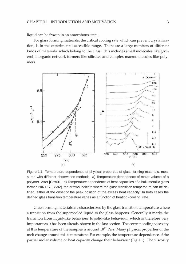
Figure 1.1: Temperature dependence of physical properties of glass forming materials, mea-
sured with different observation methods. a) Temperature dependence of molar volume of a
polymer. After [Cow01]. b) Temperature dependence of heat capacities of a bulk metallic glass
former PdNiPSi [BS92], the arrows indicate where the glass transition temperature can be de-
fined, either at the onset or the peak position of the excess heat capacity. In both cases the
defined glass transition temperature varies as a function of heating (cooling) rate.
Glass formingmaterials are characterized by the glass transition temperature where
a transition from the supercooled liquid to the glass happens. Generally it marks the
transition from liquid-like behaviour to solid-like behaviour, which is therefore very
important as it has been already shown in the last section. The corresponding viscosity
at this temperature of the samples is around 1012 Pa·s. Many physical properties of the
melt change around this temperature. For example, the temperature dependence of the
partial molar volume or heat capacity change their behaviour (Fig.1.1). The viscosity
4 1.3. INTERPLAY OF STRUCTURE AND DYNAMICS IN SILICATEMELTS
around the glass transition temperature also increases strongly . Instead of following
an Arrhenius law, the temperature dependence is frequently described by the empiri-
cal Vogel-Fulcher formula
η(T ) = Aexp(B/(T − T0)) (1.2)
or some other equations, which have stronger temperature dependence than that of
the Arrhenius law (for a overview see e.g.: [CLH+97]).
However, this transition temperature from a supercooled liquid to a glass is some-
how arbitrary defined because it only corresponds to a macroscopic relaxation time in
the orders of seconds to minutes (cf. Eqn.1.1): a timescale which is normally accessible
in the laboratory. As it has already been shown in Fig.1.1 the measured glass transition
temperature depends on the experimental techniques as well as timescales of obser-
vation . The T0 defined in the Vogel-Fulcher equation is not a well defined physical
quantity.
Many experiment techniques, particularly dielectric spectroscopy, have shown al-
ready that there are different relaxation processes in glass forming materials. In many
systems so called α- and β-relaxation processes can be identified. The α-relaxation
is well known to be connected with the glass transition since in glasses the atoms or
molecules have negligible long range mobility and α-relaxation or structural relaxation
is frozen. Thus the temperature at the onset of the α relaxations gives a microscopic
definition of the glass transition. Such microscopic approach is described in the frame-
work of mode coupling theory (MCT), which will be introduced in chapter 3 with a
critical temperature Tc as the mark between the supercooled liquid and the glasses.
1.3 Interplay of structure and dynamics in silicate melts
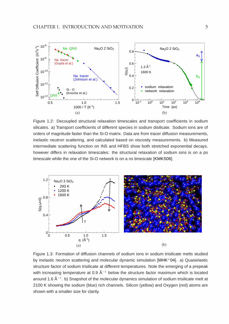
In sodium silicate melts the dynamics of sodium ions and the Si-O matrix have been
studiedwith inelastic neutron scattering combinating neutron time-of-flight and backscat-
tering methods [MSD02]. Structural relaxations of these different species, despite the
large difference in their timescales, have all shown a stretched exponential decay, as
predicted by mode coupling theory. This indicates that they are not simple activated
processes. Dry sodium (tri)silicates are known as fast ion conductors for very long
time. The transport coefficient of the sodium ions is decoupled from that of the Si-
O network by several orders of magnitude which has been studied in detail with the
tracer diffusion measurements [JBB51], with measurements of the viscosity [KDSW96]
and also recently with the inelastic neutron scattering experiments [KMKS06] (Fig.1.2).
In silicates there are generally two classes of constitutes: network former and net-
CHAPTER 1. INTRODUCTION ANDMOTIVATION 5
0.5 1.0 1.5
10-12
10-11
10-10
10-9
10-8
1000 / T (K-1)
Sel
f Diff
usio
n C
oeffi
cien
t (m
2 s-1)
Na tracer(Johnson et al.)
Na QNS
QNS
Si - O(Knoche et al.)
Na tracer(Gupta et al.)
Na2O 2 SiO2
(a)
10-1 100 101 102 103 1040
0.2
0.4
0.6
0.8
Time (ps)
S(q
,t)
Na2O 2 SiO2
1.3 A-1
1600 Kbq
aq
sodium relaxationnetwork relaxation
(b)
Figure 1.2: Decoupled structural relaxation timescales and transport coefficients in sodium
silicates. a) Transport coefficients of different species in sodium disilicate. Sodium ions are of
orders of magnitude faster than the Si-O matrix. Data are from tracer diffusion measurements,
inelastic neutron scattering, and calculated based on viscosity measurements. b) Measured
intermediate scattering function on IN5 and HFBS show both stretched exponential decays,
however differs in relaxation timescales: the structural relaxation of sodium ions is on a ps
timescale while the one of the Si-O network is on a ns timescale [KMKS06].
0 0.5 1.0 1.50
0.4
0.8
1.2
q (A-1)
S(q
,ω=
0)
293 K1200 K1600 K
Na2O 3 SiO2
T
(a) (b)
Figure 1.3: Formation of diffusion channels of sodium ions in sodium trisilicate melts studied
by inelastic neutron scattering and molecular dynamic simulation [MHK+04]. a) Quasielastic
structure factor of sodium trisilicate at different temperatures. Note the emerging of a prepeak
with increasing temperature at 0.9 A−1 below the structure factor maximum which is located
around 1.6 A−1. b) Snapshot of the molecular dynamics simulation of sodium trisilicate melt at
2100 K showing the sodium (blue) rich channels. Silicon (yellow) and Oxygen (red) atoms are
shown with a smaller size for clarity.
6 1.3. INTERPLAY OF STRUCTURE AND DYNAMICS IN SILICATEMELTS
work modifier, distinguished by their different roles in the formation of silicates. Net-
work formers build up the silicate matrix, for example SiO2 and Al2O3. Network mod-
ifiers disrupted the silicate matrix, like alkali oxides or water. The addition of alkali ox-
ides to silicates causes a non-linear viscosity decrease [HDW95]. Together with the ob-
servation of the transport properties of the sodium ions, there is a strong indication of a
non-homogeneous distribution of the alkali ions in the silicate matrix. The existence of
preferential diffusion pathways of the sodium ions has been recently confirmed by
neutron scattering experiments in combination with molecular dynamics computer
simulations [MHK+04] (Fig.1.3). The prepeak around 0.9 A−1 in the quasielastic struc-
ture factor which emerges at elevated temperatures, corresponds to the distance be-
tween the sodium rich channels around 6-8 A. These channels allow fast sodium ion
diffusion to be decoupled from the relaxation of the Si-O network. The existence of
the channel structure provides as well an explanation for the non-linear drop of the
melt viscosity. The Si-O network is only disrupted to certain extent by the addition of
sodium oxide. A further increase in its concentration will only fill the channels instead
of breaking the Si-O bonds.
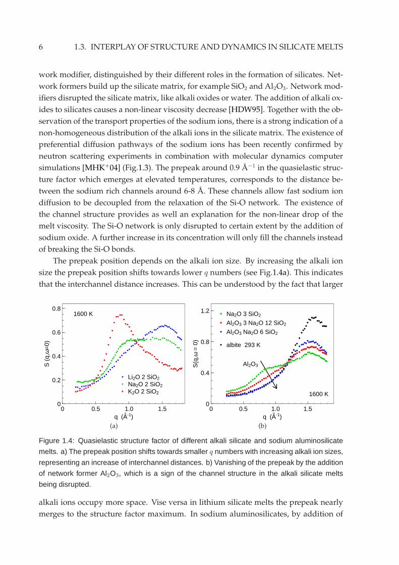
The prepeak position depends on the alkali ion size. By increasing the alkali ion
size the prepeak position shifts towards lower q numbers (see Fig.1.4a). This indicates
that the interchannel distance increases. This can be understood by the fact that larger
0 0.5 1.0 1.50
0.2
0.4
0.6
0.8
q (A-1)
S (
q,ω
=0)
Li2O 2 SiO2
Na2O 2 SiO2
K2O 2 SiO2
1600 K
(a)
0 0.5 1.0 1.50
0.4
0.8
1.2
q (A-1)
S(q
,ω =
0)
Na2O 3 SiO2
Al2O3 3 Na2O 12 SiO2
Al2O3 Na2O 6 SiO2
albite 293 K
1600 K
Al2O3
(b)
Figure 1.4: Quasielastic structure factor of different alkali silicate and sodium aluminosilicate
melts. a) The prepeak position shifts towards smaller q numbers with increasing alkali ion sizes,
representing an increase of interchannel distances. b) Vanishing of the prepeak by the addition
of network former Al2O3, which is a sign of the channel structure in the alkali silicate melts
being disrupted.
alkali ions occupy more space. Vise versa in lithium silicate melts the prepeak nearly
merges to the structure factor maximum. In sodium aluminosilicates, by addition of
CHAPTER 1. INTRODUCTION ANDMOTIVATION 7
another network former Al2O3 the diffusion channels are disrupted. Consequently, the
prepeak vanishes and the sodium relaxation in the melt becomes slower [KM04]. The
melt viscosity also increases considerably as compared to that of the alkali silicates.
The observation on these silicate melts by means of inelastic neutron scattering
shows a clear interplay between microscopic structure and dynamics in the systems.
Due to the stoichiometric similarity between the alkali oxides and water, such be-
haviours could also exist in hydrous silicate melts.
1.4 The hydrous silicate system
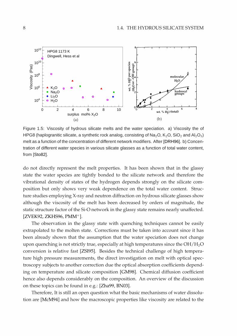
Water has a very similar effect on the silicate melt viscosity as that of the alkali oxides.
On the addition of only very small amount of less than 1 wt% of water to silicates the
melt viscosity drops already by several orders of magnitude, whereas further increas-
ing the water content only changes slightly the viscosity [DRH96] (Fig.1.5a).
It is generally accepted that upon its dissolution, water reacts with the Si-O matrix
via the following reaction:
2SiO2+H2O −→ 2Si-OH.
Systematic studies show that water is dissolved into silicate in two fundamental forms:
hydroxyl group and molecular water. This chemical equilibrium, which can be driven
by external conditions, puts a major challenge in the study of hydrous silicate systems.
The ratio between the concentration of these two species depends on pressure, temper-
ature, total water content and composition of silicates. The water speciation has been
studied with different spectroscopy methods, for instance infra-red and near infra-red
experiments [Sto82, MPSR93] or NMR spectroscopy [KDS89] in the glassy state as well
as in the melt [BN03], in order to understand its dependence on different silicate sys-
tems and conditions.
The motivation behind these studies is to be able to predicts the melt viscosity us-
ing the knowledge of the water speciation. It is believed that the hydroxyl group is
responsible for the huge viscosity drop since it is the resulting product from the water-
silicate reaction which breaks the Si-O bonds. The dependence of the hydroxyl group
concentration on the total water content seems also to be correlated with the non-linear
viscosity change. At low total water content hydroxyl group is the dominant species.
With increasing total water content its concentration levels off and at high water con-
tent the concentration of the molecular water increases correspondingly (see Fig.1.5b).
The majority of these studies are performed in the glassy state or employed a
quenching techniques to reveal the melt properties, thus high pressure condition is
not required for measurements. However, the results measured in the glassy state
8 1.4. THE HYDROUS SILICATE SYSTEM
0 2 4 6 8 10
104
106
108
1010
1012
surplus mol% X2O
Vis
cosi
ty (
Pas
)
K2ONa2OLi2OH2O
HPG8 1173 KDingwell, Hess et al
(a)
O(total)wt. % H2
wt.
% H
2O p
er
speci
es
(H2O
or
−O
H g
rou
p)
molecular
H2O
hydroxylgroups
(b)
Figure 1.5: Viscosity of hydrous silicate melts and the water speciation. a) Viscosity the of
HPG8 (haplogranitic silicate, a synthetic rock analog, consisting of Na2O, K2O, SiO2 and Al2O3)
melt as a function of the concentration of different network modifiers. After [DRH96]. b) Concen-
tration of different water species in various silicate glasses as a function of total water content,
from [Sto82].
do not directly represent the melt properties. It has been shown that in the glassy
state the water species are tightly bonded to the silicate network and therefore the
vibrational density of states of the hydrogen depends strongly on the silicate com-
position but only shows very weak dependence on the total water content. Struc-
ture studies employing X-ray and neutron diffraction on hydrous silicate glasses show
although the viscosity of the melt has been decreased by orders of magnitude, the
static structure factor of the Si-O network in the glassy state remains nearly unaffected.
[ZVEK92, ZKHS96, PMM+].
The observation in the glassy state with quenching techniques cannot be easily
extrapolated to the molten state. Corrections must be taken into account since it has
been already shown that the assumption that the water speciation does not change
upon quenching is not strictly true, especially at high temperatures since the OH/H2O
conversion is relative fast [ZSI95]. Besides the technical challenge of high tempera-
ture high pressure measurements, the direct investigation on melt with optical spec-
troscopy subjects to another correction due the optical absorption coefficients depend-
ing on temperature and silicate composition [GM98]. Chemical diffusion coefficient
hence also depends considerably on the composition. An overview of the discussion
on these topics can be found in e.g.: [Zha99, BN03].
Therefore, It is still an open question what the basic mechanisms of water dissolu-
tion are [McM94] and how the macroscopic properties like viscosity are related to the
CHAPTER 1. INTRODUCTION ANDMOTIVATION 9
microscopic structure and dynamics. For transport properties, the chemical diffusion
coefficient of water varies considerably as function of silicate composition. However,
the basic diffusion mechanism of water is not known.
1.5 Present work
Quasielastic neutron scattering allows model free investigations of dynamics on a mi-
croscopic time and length scales. In these experiments usually neutrons with long
wavelengths are used and the accessible momentum transfers are limited compared
to neutron diffraction experiments. Hence, the measurements are not optimized for
structural investigations. However, the intrinsic q resolution of the quasielastic neutron
scattering allows to study the diffusion mechanisms by analyzing the q dependence of
the scattering amplitude and its line shape in great detail. Such technique has been
already demonstrated to be a powerful tool for the study of water species dynamics in
hydrous silicate glasses. A temperature range up to the glass transition temperature of
the system has been investigated [IHB+05] under ambient pressure conditions.
Dynamics in the temperature range well above the glass transition in the molten
state has not yet been studied with neutron scattering techniques. However, since
neutron beams exhibit large penetration depths in metals, studies with massive high
pressure apparatus is possible. Therefore, neutron scattering techniques at high tem-
perature high pressure conditions open up new possibilities to directly investigate dy-
namics in hydrous silicate melts under magma chamber conditions on an absolute
scale. Owing to the huge difference between the scattering cross sections of H and D,
a contrast variation via H2O/D2O substitution gives access to the pure proton signal.
Pure silica, sodium trisilicate and sodium aluminosilicate with Na2O/Al2O3 ratio
equal to unity are chosen as the dry silicate compositions for current work. Their com-
position varies from a single component system (SiO2) to a three components system
(Na2O, Al2O3, SiO2). Hydrous silica is the most simple hydrous silicate system. Car-
Parrinello computer simulation has been performed on the SiO2-H2O system at very
high temperature (3000 K) in the liquid state [PBK04]. On the other hand, only a few
experimental studies have been conducted till now above the glass transition temper-
ature.
The sodium aluminosilicate NaAlSi3O8 is known as the albite composition. It is
the most simple nature volcanic rock composition and was thus largely interested in
the geoscience. Lots of data exist on the concentration of water species and melt vis-
cosities at different pressure, temperature and water content conditions. Therefore,
neutron scattering is a complimentary method which can provide additional informa-
tions of the system and the results can be easily compared with the results from other
10 1.5. PRESENT WORK
investigations.
The melt viscosity of these three systems spans over many orders of magnitudes.
In the hydrous silica glass with 10 mol% total water content, water is known to be
exclusive dissolved as OH groups [Poh05]. In the hydrous albite glass with the same
water content both OH and H2O groups exist. In dry SiO2 and albite the silicate net-
work is fully polymerized, whereas in sodium trisilicate open structure of diffusion
channels is known to be present. With the comparison of the neutron scattering exper-
iments on different compositions, current work tries to address the question whether
and how the microscopic water dynamics depends on the water speciation, melt vis-
cosity, silicate composition as well as the melt structure in order to understand the
dissolution and transport mechanisms of water in the hydrous silicate melts.
It will be shown later that interestingly the water dynamics in pure silica and albite
systems is not so fast as expected, if one considers the fact that the glass transition tem-
perature of the samples with 10 mol% water content has dropped almost by a factor
of two compared to that of the dry samples. Unfortunately the slow dynamics cannot
be studied with the neutron time-of-flight experiment since it is out of the measurable
timescales. Further investigations with larger timescales should give access to these
diffusive dynamics. In hydrous sodium trisilicates a diffusion mechanism has been
proposed, which is not correlated with the water speciation according to the observa-
tion with neutron time-of-flight spectroscopy.
Chapter 2
Sample synthesis
The procedure of synthesis and characterization of water bearing silicate glasses are described in
the following sections. Sodium trisilicate (Na2O·3SiO2, NS3), sodium aluminosilicate (Na2O
·Al2O3·6SiO2) and pure silica (SiO2) samples with different H2O/D2O contents are prepared.
Characterization methods including calorimetry and dilatometry measurements.
2.1 Preparation of the dry silicates
Dry silicates are synthesized by high temperature fusion of ultrapure powder of cor-
responding oxides and carbonates. Synthesis temperatures are 1250 °C for sodium
trisilicate and 1450 °C for sodium aluminosilicate samples, respectively. Typical syn-
thesis times are 12 - 24 hours. Even longer preparation time is not preferred due to
the increasing amount of the sodium evaporation, which will lead to alternation of the
sample composition. This issue is more important for the sodium aluminosilicate com-
position since the samples are prepared at higher temperatures and the macroscopic
properties depend strongly on the exact Al2O3 / Na2O ratio when it is close to unity.
Typically 25-40 g of silicate glasses were synthesized to reduce the uncertainties of
the composition. The deviation of the sample masses from the theoretical calculation is
typically below 10 mg. The uncertainty of the composition is therefore in the per mille
range. Such small uncertainties will not lead to changes in the microscopic dynamics.
Sodium trisilicate samples are synthesized from Na2CO3 (Merck 99.999% metal
basis) and SiO2 (Alfa Aesar 99.995% metal basis, Suprasil1). Sodium aluminosilicate
samples are prepared with additional Al2O3 (Alfa Aesar 99.995% metal basis).
All powders were kept in a dry oven at 114 °C for at least 24 hours prior to the
synthesis. Al2O3 and SiO2 powders were dried separately again at 1000 °C for 1 hour
1Suprasil® is the trademark of W. C. Heraeus-Schott Company, Germany. It represents silica glassesproduced by hydrolyzation of SiCl4. This material is practically free of metallic impurities [Bru70].
11
12 2.1. PREPARATIONOF THE DRY SILICATES
at the beginning of the preparation. Oxides and sodium carbonate were then mixed up
with a proper amount of each component for the desired silicate composition.
To prepare sodium trisilicate the well mixed powder was then transferred into a
Pt-0.5% Au crucible. At elevated temperature sodium carbonate is decomposed and
sodium trisilicate is obtained via following reaction:
Na2CO3 + 3 SiO2 −→ Na2O·3SiO2 + CO2 ↑
The mixture was stepwisely transferred into the crucible. In each step 8-10 g powder
were filled. Between each step the crucible was heated to 1250 °C and kept for about
1 hour. Therefore the amount of gasses which is evaporated during each filling step
is relatively small and sample material losses due to foaming out of the crucible can
be avoided. After all of the raw materials were transferred into the crucible the melt
was annealed at 1250 °C for 12-15 hours. Due to the relatively low viscosity of sodium
trisilicate at this temperature (around 101.37Pa·s [KDSW96]) such annealing time is suf-
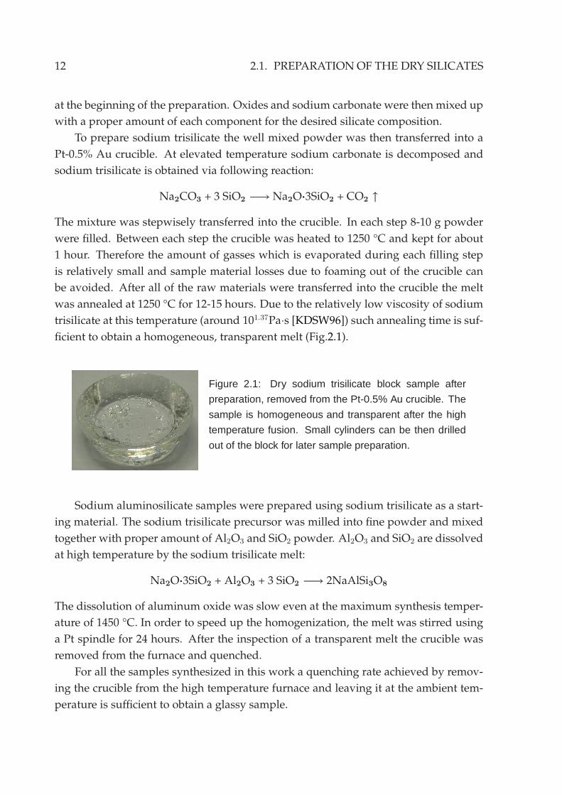
ficient to obtain a homogeneous, transparent melt (Fig.2.1).
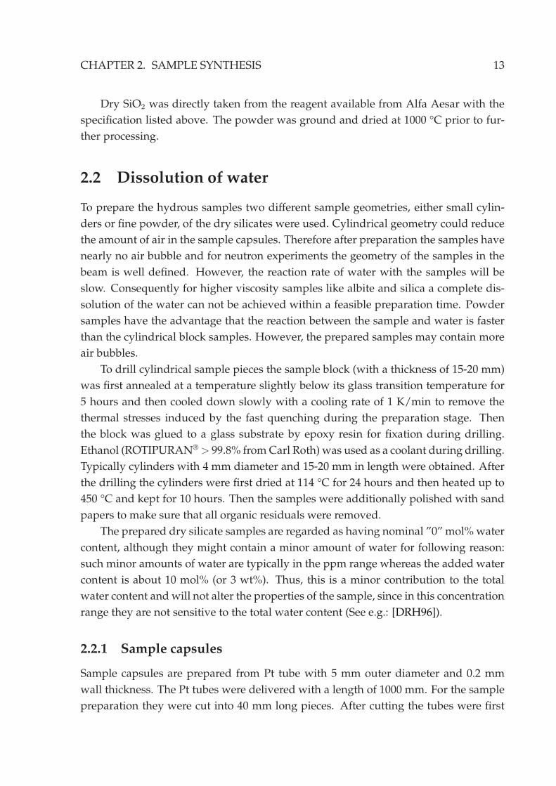
Figure 2.1: Dry sodium trisilicate block sample after
preparation, removed from the Pt-0.5% Au crucible. The
sample is homogeneous and transparent after the high
temperature fusion. Small cylinders can be then drilled
out of the block for later sample preparation.
Sodium aluminosilicate samples were prepared using sodium trisilicate as a start-
ing material. The sodium trisilicate precursor was milled into fine powder and mixed
together with proper amount of Al2O3 and SiO2 powder. Al2O3 and SiO2 are dissolved
at high temperature by the sodium trisilicate melt:
Na2O·3SiO2 + Al2O3 + 3 SiO2 −→ 2NaAlSi3O8
The dissolution of aluminum oxide was slow even at the maximum synthesis temper-
ature of 1450 °C. In order to speed up the homogenization, the melt was stirred using
a Pt spindle for 24 hours. After the inspection of a transparent melt the crucible was
removed from the furnace and quenched.
For all the samples synthesized in this work a quenching rate achieved by remov-
ing the crucible from the high temperature furnace and leaving it at the ambient tem-
perature is sufficient to obtain a glassy sample.
CHAPTER 2. SAMPLE SYNTHESIS 13
Dry SiO2 was directly taken from the reagent available from Alfa Aesar with the
specification listed above. The powder was ground and dried at 1000 °C prior to fur-
ther processing.
2.2 Dissolution of water
To prepare the hydrous samples two different sample geometries, either small cylin-
ders or fine powder, of the dry silicates were used. Cylindrical geometry could reduce
the amount of air in the sample capsules. Therefore after preparation the samples have
nearly no air bubble and for neutron experiments the geometry of the samples in the
beam is well defined. However, the reaction rate of water with the samples will be
slow. Consequently for higher viscosity samples like albite and silica a complete dis-
solution of the water can not be achieved within a feasible preparation time. Powder
samples have the advantage that the reaction between the sample and water is faster
than the cylindrical block samples. However, the prepared samples may contain more
air bubbles.
To drill cylindrical sample pieces the sample block (with a thickness of 15-20 mm)
was first annealed at a temperature slightly below its glass transition temperature for
5 hours and then cooled down slowly with a cooling rate of 1 K/min to remove the
thermal stresses induced by the fast quenching during the preparation stage. Then
the block was glued to a glass substrate by epoxy resin for fixation during drilling.
Ethanol (ROTIPURAN®> 99.8% from Carl Roth) was used as a coolant during drilling.
Typically cylinders with 4 mm diameter and 15-20 mm in length were obtained. After
the drilling the cylinders were first dried at 114 °C for 24 hours and then heated up to
450 °C and kept for 10 hours. Then the samples were additionally polished with sand
papers to make sure that all organic residuals were removed.
The prepared dry silicate samples are regarded as having nominal ”0” mol% water
content, although they might contain a minor amount of water for following reason:
such minor amounts of water are typically in the ppm range whereas the added water
content is about 10 mol% (or 3 wt%). Thus, this is a minor contribution to the total
water content and will not alter the properties of the sample, since in this concentration
range they are not sensitive to the total water content (See e.g.: [DRH96]).
2.2.1 Sample capsules
Sample capsules are prepared from Pt tube with 5 mm outer diameter and 0.2 mm
wall thickness. The Pt tubes were delivered with a length of 1000 mm. For the sample
preparation they were cut into 40 mm long pieces. After cutting the tubes were first
14 2.2. DISSOLUTION OFWATER
cleaned using ultrasonic bath with acetone and de-ionized water to remove organic
residuals. They were then put into a hydrofluoric acid bath for at least 24 hours to
remove metal and oxide impurities. After taken out from the acid bath and cleaned
again with de-ionized water, the tubes were annealed at 1000 °C for 12 hours followed
by cooling down slowly (∼5 °C/min) to ambient temperature. This cleaning procedure
makes the Pt tubes relative soft and ready to load the sample. The tubes are stored in
a desiccator to avoid moisture exposure.
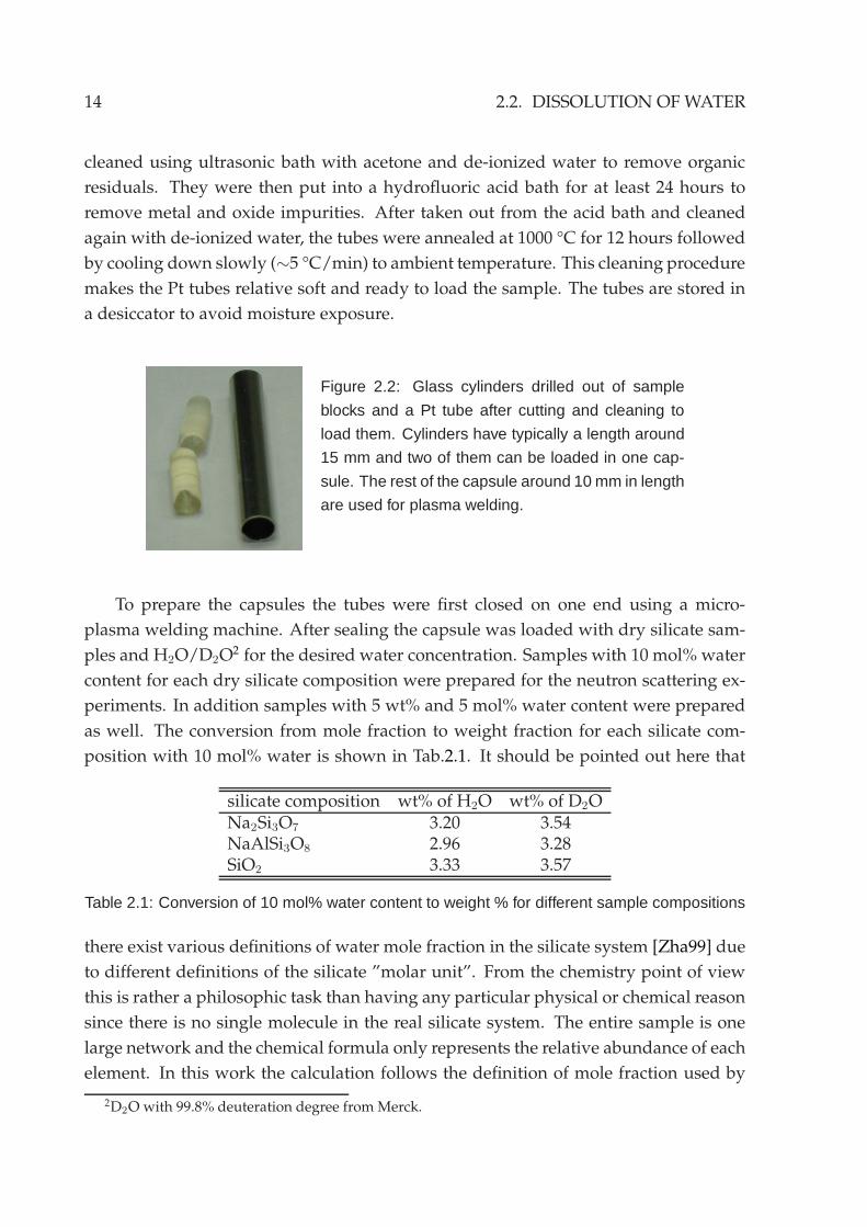
Figure 2.2: Glass cylinders drilled out of sample
blocks and a Pt tube after cutting and cleaning to
load them. Cylinders have typically a length around
15 mm and two of them can be loaded in one cap-
sule. The rest of the capsule around 10 mm in length
are used for plasma welding.
To prepare the capsules the tubes were first closed on one end using a micro-
plasma welding machine. After sealing the capsule was loaded with dry silicate sam-
ples and H2O/D2O2 for the desired water concentration. Samples with 10 mol% water
content for each dry silicate composition were prepared for the neutron scattering ex-
periments. In addition samples with 5 wt% and 5 mol% water content were prepared
as well. The conversion from mole fraction to weight fraction for each silicate com-
position with 10 mol% water is shown in Tab.2.1. It should be pointed out here that
silicate composition wt% of H2O wt% of D2ONa2Si3O7 3.20 3.54NaAlSi3O8 2.96 3.28SiO2 3.33 3.57
Table 2.1: Conversion of 10 mol% water content to weight % for different sample compositions
there exist various definitions of water mole fraction in the silicate system [Zha99] due
to different definitions of the silicate ”molar unit”. From the chemistry point of view
this is rather a philosophic task than having any particular physical or chemical reason
since there is no single molecule in the real silicate system. The entire sample is one
large network and the chemical formula only represents the relative abundance of each
element. In this work the calculation follows the definition of mole fraction used by
2D2O with 99.8% deuteration degree fromMerck.
CHAPTER 2. SAMPLE SYNTHESIS 15
[MVC98] which is also used commonly by geologists. Each oxide is considered as one
unit. Therefore, sodium trisilicate has four units and albite composition is treated as
having eight units.
After loading these capsules were sealed on the other end. During the second
welding procedure most part of the capsule body was pressed into a copper block
for heat dissipation so that the capsule was kept at ambient temperature except at
the welding position. Therefore, water loss during the welding process is negligible.
Typical amount of 0.5-0.6 g dry silicate together with of about 20 mg of water were
loaded in one capsule.
Sealed capsules were weighted and put into a dry oven at 114 °C for at least 12
hours. Then capsules were checked by weight to eliminate leakages. Only capsules
without significant weight loss (<1 mg) after the heating were used in further prepa-
ration. Water content is then controlled by means of capsules’ weight after each step of
processing. This is performed directly after the high temperature high pressure fusion
as well as after the capsules being opened and subsequently heated up in the dry oven.
For the samples used for neutron scattering experiments weight losses in the prepara-
tion stage are smaller then 5% of the added water amount. Hence, most of the water is
dissolved in the silicate sample.
2.2.2 High temperature and pressure process
To dissolve water into the silicates, the sample capsules have to be heated at high tem-
perature under high pressure. Therefore, an autoclave with built-in furnace is used
for sample preparation. In current work a pressure vessel from the company Dustec®
was used. The pressure vessel can be operated under a pressure range of 0-3000 bar, a
temperature range of 0-300 °C with a pressurized volume of 0.65 l. Pressures are gen-
erated by a membrane compressor fromNova Swiss using Ar gas as pressure medium.
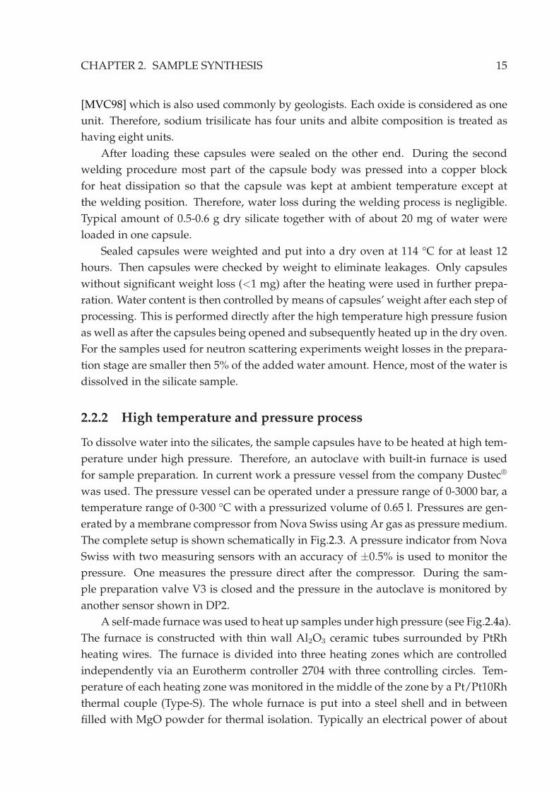
The complete setup is shown schematically in Fig.2.3. A pressure indicator from Nova
Swiss with two measuring sensors with an accuracy of ±0.5% is used to monitor the
pressure. One measures the pressure direct after the compressor. During the sam-
ple preparation valve V3 is closed and the pressure in the autoclave is monitored by
another sensor shown in DP2.
A self-made furnace was used to heat up samples under high pressure (see Fig.2.4a).
The furnace is constructed with thin wall Al2O3 ceramic tubes surrounded by PtRh
heating wires. The furnace is divided into three heating zones which are controlled
independently via an Eurotherm controller 2704 with three controlling circles. Tem-
perature of each heating zone was monitored in the middle of the zone by a Pt/Pt10Rh
thermal couple (Type-S). The whole furnace is put into a steel shell and in between
filled with MgO powder for thermal isolation. Typically an electrical power of about
16 2.2. DISSOLUTION OFWATER
DP2DP1
Autoclave
PneumaticValve
V3
V2
V1 VentilationCompressor300 MPa
Ar 150−300 bar
Figure 2.3: Schematic view of the sample preparation setup. The compressor is supplied by Ar
gas with a pressure of 150 - 300 bar, controlled via valve V1. With valve V2 closed and valve V3
open, the compressor is able to provide a pressure in the autoclave up to 300 MPa. Pressure
direct after the compressor is measured and displayed in DP1. During the sample preparation
V3 is closed to keep the pressure in the autoclave relative constant, which is measured and
displayed in DP2. After preparation with both V2 and V3 open, the pressure in the autoclave
can be slowly released.
1.2 kW is needed to heat the furnace to the sample preparation temperature around
1500 K under a pressure of 300 MPa.
Samples were mounted on a movable stage with an additional thermal couple
close to the capsules to monitor its temperature. Using a three heating-zone setup
provides a relatively homogeneous temperature over the sample region, which can be
seen in Fig.2.5b measured by driving the stage into different positions in the furnace
by a motor.
The hydrous sodium trisilicate samples were prepared at a temperature of 1250 °C
and the albite and pure SiO2 samples were prepared at 1400 °C. The preparation time
of the samples varies from 5 up to 15 hours. Samples were pressurized and placed
between 2nd and 3rd heating zone (see Fig.2.5a) before heating. At beginning the auto-
clave is filled with Ar to reach a pressure of about 180-200MPa in the cold state. During
heating up the furnace, the pressure will be built up to 300MPa. The autoclave is water
cooled from outside during the sample preparation. The samples were heated up with
CHAPTER 2. SAMPLE SYNTHESIS 17
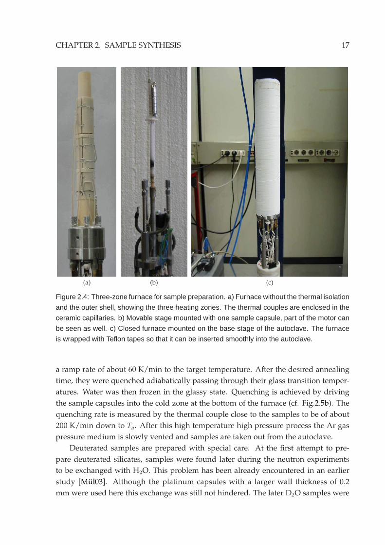
(a) (b) (c)
Figure 2.4: Three-zone furnace for sample preparation. a) Furnace without the thermal isolation
and the outer shell, showing the three heating zones. The thermal couples are enclosed in the
ceramic capillaries. b) Movable stage mounted with one sample capsule, part of the motor can
be seen as well. c) Closed furnace mounted on the base stage of the autoclave. The furnace
is wrapped with Teflon tapes so that it can be inserted smoothly into the autoclave.
a ramp rate of about 60 K/min to the target temperature. After the desired annealing
time, they were quenched adiabatically passing through their glass transition temper-
atures. Water was then frozen in the glassy state. Quenching is achieved by driving
the sample capsules into the cold zone at the bottom of the furnace (cf. Fig.2.5b). The
quenching rate is measured by the thermal couple close to the samples to be of about
200 K/min down to Tg. After this high temperature high pressure process the Ar gas
pressure medium is slowly vented and samples are taken out from the autoclave.
Deuterated samples are prepared with special care. At the first attempt to pre-
pare deuterated silicates, samples were found later during the neutron experiments
to be exchanged with H2O. This problem has been already encountered in an earlier
study [Mul03]. Although the platinum capsules with a larger wall thickness of 0.2
mm were used here this exchange was still not hindered. The later D2O samples were
18 2.2. DISSOLUTION OFWATER
(a)
0 40 80 1200
500
1000
1500
position (mm)
Tem
pera
ture
(o C
)
Temperature Profile 1400 oCTemperature Profile 1250 oC
T3T2T1
Sample
first second thirdHZ HZ HZ
(b)
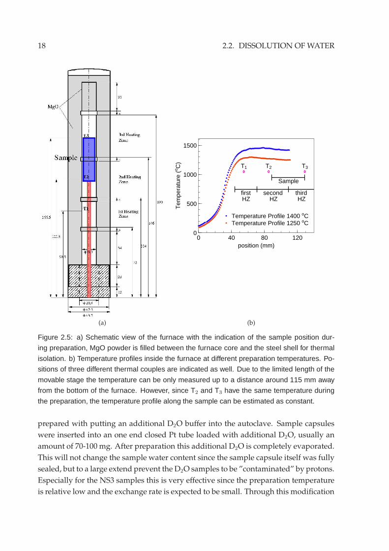
Figure 2.5: a) Schematic view of the furnace with the indication of the sample position dur-
ing preparation, MgO powder is filled between the furnace core and the steel shell for thermal
isolation. b) Temperature profiles inside the furnace at different preparation temperatures. Po-
sitions of three different thermal couples are indicated as well. Due to the limited length of the
movable stage the temperature can be only measured up to a distance around 115 mm away
from the bottom of the furnace. However, since T2 and T3 have the same temperature during
the preparation, the temperature profile along the sample can be estimated as constant.
prepared with putting an additional D2O buffer into the autoclave. Sample capsules
were inserted into an one end closed Pt tube loaded with additional D2O, usually an
amount of 70-100 mg. After preparation this additional D2O is completely evaporated.
This will not change the sample water content since the sample capsule itself was fully
sealed, but to a large extend prevent the D2O samples to be ”contaminated” by protons.
Especially for the NS3 samples this is very effective since the preparation temperature
is relative low and the exchange rate is expected to be small. Through this modification
CHAPTER 2. SAMPLE SYNTHESIS 19
D2O containing samples were successfully prepared. Further improvement could be to
enclose the sample capsule completely in another capsule with D2O buffer loaded and
using some H blocking noble metals or alloys as outer capsule material (e.g.: Pt-Au
alloy).
The prepared samples were taken out from the capsules and kept in a desiccator.
Usually single piece of samples with 0.4-0.5 g can be obtained from one capsule. The
rest of the samples either stick to the Pt capsule or break into small pieces. For sample
characterization small pieces of samples can be used.
2.3 Sample characterization
The macroscopic properties of the sample are measured with calorimetry/dilatometry
for Tg in order to confirm that the samples are homogeneous and having the correct
water content before the neutron scattering experiments.
2.3.1 Calorimetry
The glass transition temperature of the hydrous sodium trisilicate samples were mea-
sured with differential scanning calorimetry (DSC). Pieces from different positions of
one and the same sample were taken. The weight of these pieces is usually in the range
of 10-15 mg. The ramp rate used is 15 K/min for all measurements. Fig.2.6 shows the
150 200 250 300T (oC)
Hea
t flo
w (
a.u.
) (E
ndot
h do
wn)
bottom parttop part
NS3+10 mol% H2O
(a)
150 200 250 300T (oC)
Hea
t flo
w (
a.u.
) (E
ndot
h do
wn)
bottom parttop part
NS3+10 mol% D2O
(b)
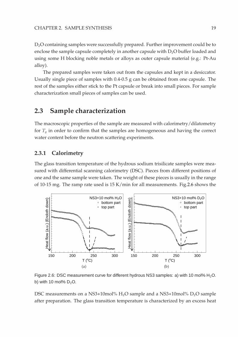
Figure 2.6: DSC measurement curve for different hydrous NS3 samples: a) with 10 mol% H2O.
b) with 10 mol% D2O.
DSC measurements on a NS3+10mol% H2O sample and a NS3+10mol% D2O sample
after preparation. The glass transition temperature is characterized by an excess heat
20 2.3. SAMPLE CHARACTERIZATION
flow required by the samples. The measured calorimetry Tg depends on the experi-
mental factors like thermal history, ramp rate during the measurement, and methods
of data evaluation. Therefore, the resulting Tg’s are normally subjected to an uncer-
tainty of about 10-15 °C. The transition temperatures here were obtained by fitting a
parabola to the peak minimum. This algorithm of evaluation has already been used in
a previous study [Kar05].
It can be seen from the measurement curves that the top and bottom part of each
sample are close to each other. This is an indication that the water content in the sample
is homogeneous. The Tg of D2O samples with the same sample is around 20 K higher
than the H2O sample. However, this is believed to be mainly caused by the difference
in the quenching rate of the sample since the D2O samples cannot be completely driven
to the bottom of the furnace due to the presence of the buffer capsule. According to
the weight controlling, the samples should have the same water content3. This is later
confirmed by the counting rate in the neutron experiment according to the scattering
cross sections of the samples. Although the Tg measured here can not be used as a
direct measure of the water content, the obtained values are closed to the reported
values [TTA+83]. One should note as well that the glass transition temperature of the
dry sodium trisilicate is located at approximately 470 °C [MSS83]. The dissolution of
water into silicates drastically reduces the Tg of the silicates.
2.3.2 Dilatometry
For albite and pure silica composition the Tg of the water bearing glasses with 10
mol% water content (around 600-700 °C) is out of the measurable range of the DSC
instrument. Thus the samples were measured with dilatometry at the department of
earth and environmental sciences, section for mineralogy, petrology and geochemistry,
Ludwig-Maximilians-University Munich together with Dr. K.-U. Hess. Instead of mea-
suring the heat flow in dilatometry the change of the sample dimension is recorded
as a function of temperature. Thus the basic physical quantity behind is essentially
the thermal expansion coefficient of the sample, which is changing at Tg. Typically
a sample disk of about 4 mm in diameter and 1 mm in thickness is prepared with
plane parallel surfaces. Measurements were performed using Bahr DIL 802V vertical
dilatometer equippedwith an alumina push rod under constant Ar gas flow. A heating
rate of 10 K/min was used for all measurements. The change of the push rod position
is recorded against the sample temperature. It should be mentioned that the data pre-
3The glass transition temperature of the samples are very sensitive to the cooling rate of the samplesclose to their glass transition temperature. In case of the samples which are not quenched by beingdriven to the cold zone but cooled down with the furnace, the glass transition temperatures at differentpositions of the sample can differ from each other by more than 100 K due to the different cooling ratesin the furnace which vary by a factor of about two.
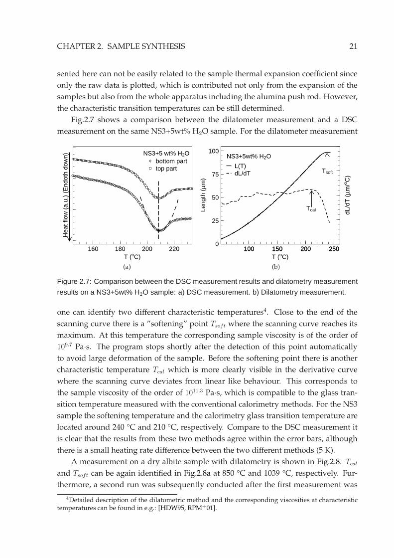
CHAPTER 2. SAMPLE SYNTHESIS 21
sented here can not be easily related to the sample thermal expansion coefficient since
only the raw data is plotted, which is contributed not only from the expansion of the
samples but also from the whole apparatus including the alumina push rod. However,
the characteristic transition temperatures can be still determined.
Fig.2.7 shows a comparison between the dilatometer measurement and a DSC
measurement on the same NS3+5wt% H2O sample. For the dilatometer measurement
160 180 200 220T (oC)
Hea
t flo
w (
a.u.
) (E
ndot
h do
wn)
bottom parttop part
NS3+5 wt% H2O
(a)
100 150 200 2500
25
50
75
100
T (oC)
Leng
th (
µm)
NS3+5wt% H2O
Tcal
TsoftL(T)dL/dT
100 150 200 250
dL/d
T (
µm/o C
)
(b)
Figure 2.7: Comparison between the DSC measurement results and dilatometry measurement
results on a NS3+5wt% H2O sample: a) DSC measurement. b) Dilatometry measurement.
one can identify two different characteristic temperatures4. Close to the end of the
scanning curve there is a ”softening” point Tsoft where the scanning curve reaches its
maximum. At this temperature the corresponding sample viscosity is of the order of
109.7 Pa·s. The program stops shortly after the detection of this point automatically
to avoid large deformation of the sample. Before the softening point there is another
characteristic temperature Tcal which is more clearly visible in the derivative curve
where the scanning curve deviates from linear like behaviour. This corresponds to
the sample viscosity of the order of 1011.3 Pa·s, which is compatible to the glass tran-
sition temperature measured with the conventional calorimetry methods. For the NS3
sample the softening temperature and the calorimetry glass transition temperature are
located around 240 °C and 210 °C, respectively. Compare to the DSC measurement it
is clear that the results from these two methods agree within the error bars, although
there is a small heating rate difference between the two different methods (5 K).
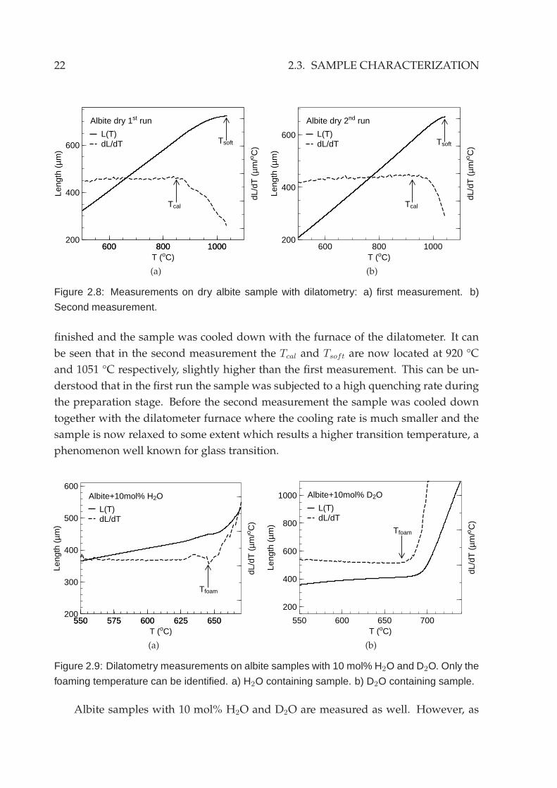
A measurement on a dry albite sample with dilatometry is shown in Fig.2.8. Tcal
and Tsoft can be again identified in Fig.2.8a at 850 °C and 1039 °C, respectively. Fur-
thermore, a second run was subsequently conducted after the first measurement was
4Detailed description of the dilatometric method and the corresponding viscosities at characteristictemperatures can be found in e.g.: [HDW95, RPM+01].
22 2.3. SAMPLE CHARACTERIZATION
600 800 1000200
400
600
T (oC)
Leng
th (
µm)
Albite dry 1st run
Tcal
TsoftL(T)dL/dT
600 800 1000dL
/dT
(µm
/o C)
(a)
600 800 1000200
400
600
T (oC)
Leng
th (
µm)
Albite dry 2nd run
Tcal
Tsoft
L(T)dL/dT
dL/d
T (
µm/o C
)
(b)
Figure 2.8: Measurements on dry albite sample with dilatometry: a) first measurement. b)
Second measurement.
finished and the sample was cooled down with the furnace of the dilatometer. It can
be seen that in the second measurement the Tcal and Tsoft are now located at 920 °C
and 1051 °C respectively, slightly higher than the first measurement. This can be un-
derstood that in the first run the sample was subjected to a high quenching rate during
the preparation stage. Before the second measurement the sample was cooled down
together with the dilatometer furnace where the cooling rate is much smaller and the
sample is now relaxed to some extent which results a higher transition temperature, a
phenomenon well known for glass transition.
550 575 600 625 650200
300
400
500
600
T (oC)
Leng
th (
µm)
Albite+10mol% H2O
Tfoam
L(T)dL/dT
550 575 600 625 650
dL/d
T (
µm/o C
)
(a)
550 600 650 700
200
400
600
800
1000
T (oC)
Leng
th (
µm)
Albite+10mol% D2O
Tfoam
L(T)dL/dT
dL/d
T (
µm/o C
)
(b)
Figure 2.9: Dilatometry measurements on albite samples with 10 mol% H2O and D2O. Only the
foaming temperature can be identified. a) H2O containing sample. b) D2O containing sample.
Albite samples with 10 mol% H2O and D2O are measured as well. However, as
CHAPTER 2. SAMPLE SYNTHESIS 23
plotted in Fig.2.9 no softening point nor calorimetric glass transition temperature can
be found. In stead the sample shows enhanced expansion after certain temperature.
Actually this is the temperature where the foaming process starts in the sample. In
the water bearing NS3 samples this can be also observed in the DSC measurement at
a temperature around Tg+50 K. In the hydrous albite samples it seems that the glass
transition temperature and the foaming temperature are no longer well separated and
foaming starts directly after the glass transition temperature is reached. Thus only the
foaming temperature can be used to characterize the sample. Nevertheless, it can be
seen that the foaming temperatures of the H2O and D2O containing samples are still
close. Therefore, no large difference in the water content between these two samples is
expected.
During the neutron experiments, the water content of the samples (H2O and D2O)
can be verified according to their cross sections (see Appendix A) by compared them
to a standard scatterer. Thus one has a measure of the sample water content on an
absolute scale.
Chapter 3
Theoretical background
In this chapter a basic introduction on neutron scattering theory especially the definition of
useful corelation functions is presented in the first section. The second section shows how some
diffusion cases could be seen by neutron scattering. The third part gives a brief introduction
of the mode coupling theory of viscous liquids and glass transitions which provides general
explanations and predictions on the structure relaxation of these disorder systems.
3.1 Neutron scattering
Neutron scattering provides simultaneously structural and dynamic informations on
the sample. Basic equations of neutron scattering are presented here. For detailed
derivation the reader is referred to text books on neutron scattering theory like [Squ78]
or [Lov84].
3.1.1 Basic theory
In a neutron scattering experiment the basic quantity is the double differential scatter-
ing cross section, which counts the number of scattered neutrons in a solid angle dΩ
and carrying an energy within the interval [E, E + dE]. In the neutron time-of-flight
experiments performed in this study the measured intensity is directly related to the
double differential scattering cross section as will be shown in the following sections.
In general the scattering of neutrons on a target can be either elastic or inelastic,
which means the energy of the scattered neutrons can differ from the incident ones.
According to the energy and momentum conservation, the double differential scatter-
ing cross section of a single scattering process can be written in the form
(
∂2σ
∂Ω∂E ′
)
λ→λ′
=k′
k
(
mN
2πh2
)2
|〈~k′λ′|V |~kλ〉|2δ (hω +Eλ −Eλ′) (3.1a)
24
CHAPTER 3. THEORETICAL BACKGROUND 25
where
hω =h2
2mN(k2 − k′2) = E −E ′ (3.1b)
denotes the energy transfer to the neutrons1.
The incident neutrons have the state |~k〉 which changes after the scattering to |~k′〉.The state of the target changes from |λ〉 to |λ′〉, with corresponding energies Eλ and
Eλ′ . The interaction between the target and the neutrons is included in the potential V .
The matrix element 〈~k′λ′|V |~kλ〉 represents the transition probability of the whole
system from the state ~k, λ to ~k′, λ′. This has to be evaluated in order to give a proper
expression of the double differential cross section. According to quantum mechanics
this matrix element is given explictly by
〈~k′λ′|V |~kλ〉 =
∫
ψ∗~k′χ∗
λ′ V ψ~k χλ d~Rd~r (3.2)
where ψ and χ are the wave functions of the neutrons and the target system, respec-
tively. For nuclear scattering the interaction between the neutrons and the nuclei is
of short range order compared to the wavelength of the neutron. This only holds for
non magnetic scattering, whereas for magnetic scattering the interaction range is in
the order of the neutron wavelength but rather weak. In the following section only the
case of nuclear scattering is discussed, since magnetic scattering where the change of
the spin states happens does not present in the sample systems studied in this work.
Therefore the Fermi pseudopotential can be used and the Born approximation is valid
as well. The pseudopotential of a single fixed nucleus j can be thus written in the form
of a δ-function:
Vj(~r − ~Rj) =2πh2
mN
bjδ(~r − ~Rj) (3.3)
that the neutron at the position ~r feels the potential of the nucleus only at ~Rj where
it is sitting. The bj is the scattering length of the j atom. The potential of the whole
scattering system can be given by a sum over all the nuclei
V =∑
j
Vj(~r − ~Rj) =2πh2
mN
∑
j
bjδ(~r − ~Rj). (3.4)
After inserting the potential and the wavefunction of the neutrons (as plan wave), the
integral over the neutron position ~r can be carried out. The double differential scatter-
1Here a positive energy difference represents neutron energy loss according to the common definitionof the energy transfer hω in the neutron scattering theory and a negative sign means neutron energygain. In the experimental data however, conventionally an opposite definition is used: a positive energydifference denotes neutron energy gain.
26 3.1. NEUTRON SCATTERING
ing cross section reads
(
∂2σ
∂Ω∂E ′
)
λ→λ′
=k′
k|∑
j
bj〈λ′|ei~q· ~Rj |λ〉|2δ (hω+Eλ −Eλ′) (3.5a)
where
〈λ′|ei~q· ~Rj |λ〉 =
∫
χ∗λ′ ei~q· ~Rj χλ d~R (3.5b)
and
~q = ~k − ~k′. (3.5c)
Replacing the δ-function by its integral form
δ (hω+Eλ −Eλ′) =1
2πh
∫ ∞
−∞
ei(Eλ′−Eλ)t/he−iωtdt (3.6)
and using the relation H|λ〉 = Eλ|λ〉, H|λ′〉 = Eλ′ |λ′〉 gives the result(
∂2σ
∂Ω∂E ′
)
λ→λ′
=k′
k
1
2πh
∑
jj′
bj′bj
∫ ∞
−∞
〈λ|e−i~q· ~Rj′ |λ′〉〈λ′|eiHt/hei~q· ~Rje(−iHt/h)|λ〉e−iωtdt
(3.7)
where H is the Hamiltonian of the scattering system and the scattering lengths of the
nuclei are assumed to be real numbers. A summation over the final and initial states
λ′ and λ then averaging over all λ is necessary since in a real experiment not only a
single process λ→ λ′ but an average over all possible transitions is measured. This is
represented in the thermal or ensemble average. For an operator A at temperature T it
is defined by
〈A〉T =∑
λ
pλ(T )〈λ|A|λ〉 (3.8)
where pλ is the probability of finding the scattering system in the state λ determined
by the Boltzmann distribution. Using the closure relation for a pair of operators and
the definition of the time-dependent Heisenberg operator ~Rj(t) = eiHt/h ~Rje−iHt/h the
double differential scattering cross section becomes finally
(
∂2σ
∂Ω∂E ′
)
=k′
k
1
2πh
∑
jj′
bj′bj
∫ ∞
−∞
〈e−i~q· ~Rj′ (0)ei~q· ~Rj (t)〉T e−iωtdt (3.9)
and the scattering function is defined via
S(~q, ω) =1
2πh
∫ ∞
−∞
1
N
∑
jj′
〈e−i~q· ~Rj′ (0)ei~q· ~Rj (t)〉T e−iωtdt. (3.10)
CHAPTER 3. THEORETICAL BACKGROUND 27
It can be shown that the scattering function is an asymmetric function of ω. The
up-scattering (neutron energy gain) probability is the not same as that of the down-
scattering (neutron energy loss). In a scattering event the probability of the scattering
system being initially in the higher energy state is reduced by a temperature dependent
prefactor of e−hω/kBT compared to its probability of being in the lower energy state due
to the Boltzmann weighting factor pλ.
S(~q,−ω) = e−hω/kBTS(~q, ω) (3.11)
This is know as the principle of detailed balance.
3.1.2 Coherent/incoherent scattering and correlation functions
For a system that contains a large number of different nuclei: a mixture of either dif-
ferent isotopes from one element and/or different atoms from various elements, the
double differential cross section measured in an experiment is an average over all dif-
ferent scattering lengths, which is given by
(
∂2σ
∂Ω∂E ′
)
=k′
k
1
2πh
∑
jj′
bj′bj
∫
〈e−i~q· ~Rj′ (0)ei~q· ~Rj (t)〉T e−iωtdt. (3.12)
This average can be separated into two parts under the assumption that there is no
correlation between the scattering length of different nuclei
bj′bj = (b)2 = (∑
i
fibi)2, j′ 6= j
bj′bj = b2 =∑
i
fib2i , j′ = j
(3.13)
where fi is the relative abundance of the i atom and bi is the corresponding scattering
length. Use the definition of coherent and incoherent scattering cross sections σcoh =
4π(b)2 and σinc = 4π[b2 − (b)2], the double differential scattering cross section can be
represented in the form of
(
∂2σ
∂Ω∂E ′
)
=
(
∂2σ
∂Ω∂E ′
)
coh
+
(
∂2σ
∂Ω∂E ′
)
inc
(3.14)
where(
∂2σ
∂Ω∂E ′
)
coh
=σcoh
4π
k′
k
1
2πh
∑
jj′
∫
〈e−i~q· ~Rj′ (0)ei~q· ~Rj (t)〉T e−iωtdt (3.15a)
28 3.1. NEUTRON SCATTERING
(
∂2σ
∂Ω∂E ′
)
inc
=σinc
4π
k′
k
1
2πh
∑
j
∫
〈e−i~q· ~Rj (0)ei~q· ~Rj(t)〉T e−iωtdt. (3.15b)
VanHove [Hov54] introduced the time dependent pair-distribution functionG(~r, t)
which describes the correlation between the presence of a particle at ~r′ and time t = 0
and the presence of a particle at ~r′ + ~r and a later time t, averaged over ~r′
G(~r, t) =1
N〈∑
jj′
∫
δ(~r′ − ~Rj(0))δ(~r′ + ~r − ~Rj′(t))d~r′〉. (3.16)
By introducing the particle density operator
ρ(~r, t) =∑
j
δ(~r − ~Rj(t)) (3.17)
the pair-distribution function can be rewritten in the form of the general definition of
a correlation function - an ensemble average of two operators
G(~r, t) =1
N
∫
〈ρ(~r′,0)ρ(~r′ + ~r, t)〉d~r′. (3.18)
Therefore, G(~r, t) is also known as the density-density correlation function.
For systems which obey Boltzmann statistics, the pair-distribution function splits
naturally into a part which contains only the correlation of the positions of a single
particle at different timesGs (self) and a part which correlates pairs of distinct particles
Gd (distinct), namely
Gs(~r, t) =1
N
∑
j
∫
〈δ(~r′ − ~Rj(0))δ(~r′ + ~r − ~Rj(t))d~r′ (3.19a)
Gd(~r, t) =1
N
∑
j 6=j′
∫
〈δ(~r′ − ~Rj(0))δ(~r′ + ~r − ~R′
j(t))d~r′ (3.19b)
with the boundary conditions
∫
G(~r, t)d~r = N,
∫
Gs(~r, t)d~r = 1. (3.19c)
Applying the definition of the reciprocal particle density operator ρ(~q, t) =∑
j
e−i~q· ~Rj (t)
the intermediate scattering function S(~q, t) can be obtained
S(~q, t) =1
N
∑
jj′
e−i~q· ~Rj′ (0)ei~q· ~Rj (t) (3.20)
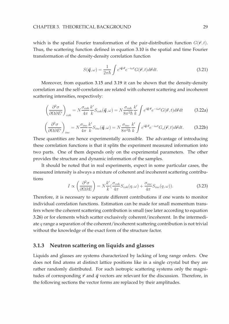
CHAPTER 3. THEORETICAL BACKGROUND 29
which is the spatial Fourier transformation of the pair-distribution function G(~r, t).
Thus, the scattering function defined in equation 3.10 is the spatial and time Fourier
transformation of the density-density correlation function
S(~q, ω) =1
2πh
∫
ei~q·~re−iωtG(~r, t)d~rdt. (3.21)
Moreover, from equation 3.15 and 3.19 it can be shown that the density-density
correlation and the self-correlation are related with coherent scattering and incoherent
scattering intensities, respectively:
(
∂2σ
∂Ω∂E ′
)
coh
= Nσcoh
4π
k′
kScoh(~q, ω) = N
σcoh
8π2h
k′
k
∫
ei~q·~re−iωtG(~r, t)d~rdt (3.22a)
(
∂2σ
∂Ω∂E ′
)
inc
= Nσinc
4π
k′
kSinc(~q, ω) = N
σinc
8π2h
k′
k
∫
ei~q·~re−iωtGs(~r, t)d~rdt. (3.22b)
These quantities are hence experimentally accessible. The advantage of introducing
these correlation functions is that it splits the experiment measured information into
two parts. One of them depends only on the experimental parameters. The other
provides the structure and dynamic information of the samples.
It should be noted that in real experiments, expect in some particular cases, the
measured intensity is always a mixture of coherent and incoherent scattering contribu-
tions
I ∝(
∂2σ
∂Ω∂E
)
= Nk′
k(σcoh
4πScoh(q,ω) +
σinc
4πSinc(q,ω)). (3.23)
Therefore, it is necessary to separate different contributions if one wants to monitor
individual correlation functions. Estimation can be made for small momentum trans-
fers where the coherent scattering contribution is small (see later according to equation
3.26) or for elements which scatter exclusively coherent/incoherent. In the intermedi-
ate q range a separation of the coherent/incoherent scattering contribution is not trivial
without the knowledge of the exact form of the structure factor.
3.1.3 Neutron scattering on liquids and glasses
Liquids and glasses are systems characterized by lacking of long range orders. One
does not find atoms at distinct lattice positions like in a single crystal but they are
rather randomly distributed. For such isotropic scattering systems only the magni-
tudes of corresponding ~r and ~q vectors are relevant for the discussion. Therefore, in
the following sections the vector forms are replaced by their amplitudes.
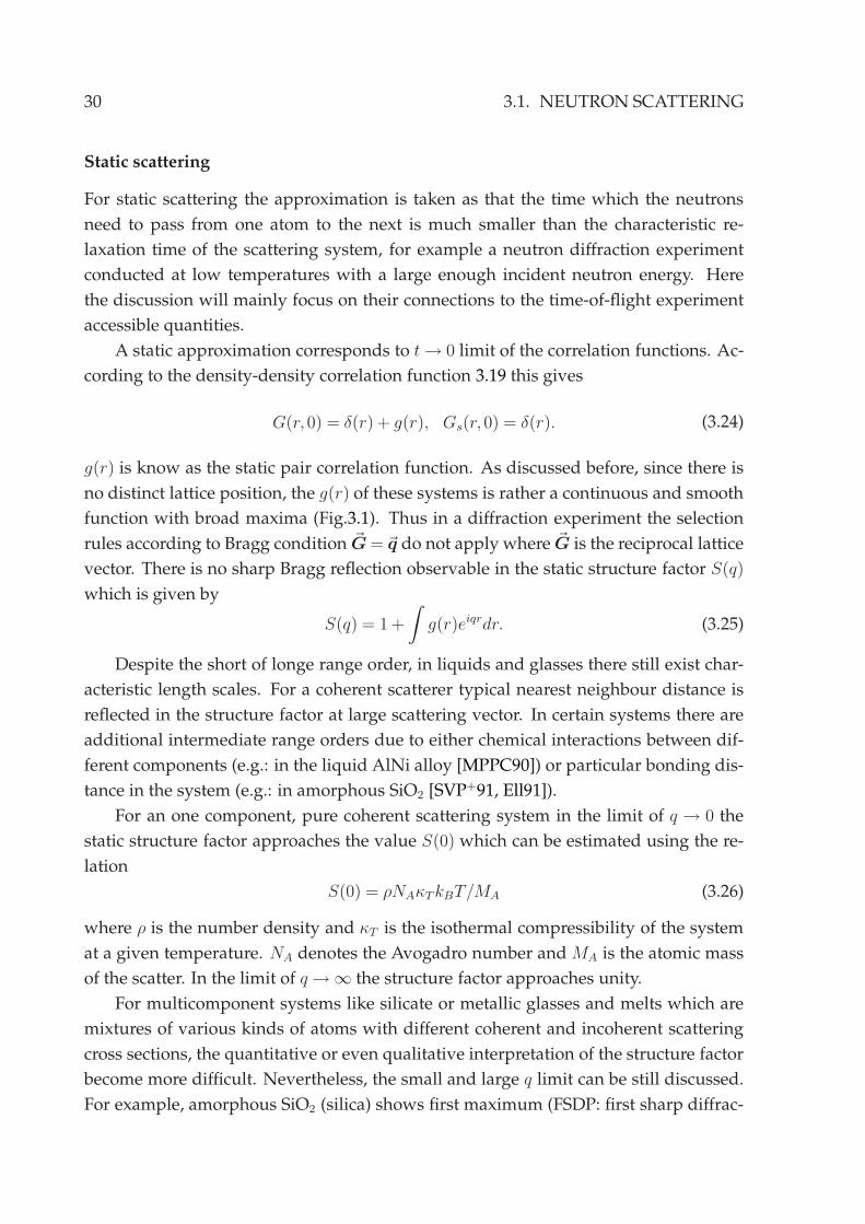
30 3.1. NEUTRON SCATTERING
Static scattering
For static scattering the approximation is taken as that the time which the neutrons
need to pass from one atom to the next is much smaller than the characteristic re-
laxation time of the scattering system, for example a neutron diffraction experiment
conducted at low temperatures with a large enough incident neutron energy. Here
the discussion will mainly focus on their connections to the time-of-flight experiment
accessible quantities.
A static approximation corresponds to t→ 0 limit of the correlation functions. Ac-
cording to the density-density correlation function 3.19 this gives
G(r,0) = δ(r) + g(r), Gs(r,0) = δ(r). (3.24)
g(r) is know as the static pair correlation function. As discussed before, since there is
no distinct lattice position, the g(r) of these systems is rather a continuous and smooth
function with broad maxima (Fig.3.1). Thus in a diffraction experiment the selection
rules according to Bragg condition ~G = ~q do not apply where ~G is the reciprocal lattice
vector. There is no sharp Bragg reflection observable in the static structure factor S(q)
which is given by
S(q) = 1 +
∫
g(r)eiqrdr. (3.25)
Despite the short of longe range order, in liquids and glasses there still exist char-
acteristic length scales. For a coherent scatterer typical nearest neighbour distance is
reflected in the structure factor at large scattering vector. In certain systems there are
additional intermediate range orders due to either chemical interactions between dif-
ferent components (e.g.: in the liquid AlNi alloy [MPPC90]) or particular bonding dis-
tance in the system (e.g.: in amorphous SiO2 [SVP+91, Ell91]).
For an one component, pure coherent scattering system in the limit of q → 0 the
static structure factor approaches the value S(0) which can be estimated using the re-
lation
S(0) = ρNAκTkBT/MA (3.26)
where ρ is the number density and κT is the isothermal compressibility of the system
at a given temperature. NA denotes the Avogadro number andMA is the atomic mass
of the scatter. In the limit of q→ ∞ the structure factor approaches unity.
For multicomponent systems like silicate or metallic glasses and melts which are
mixtures of various kinds of atoms with different coherent and incoherent scattering
cross sections, the quantitative or even qualitative interpretation of the structure factor
become more difficult. Nevertheless, the small and large q limit can be still discussed.
For example, amorphous SiO2 (silica) shows first maximum (FSDP: first sharp diffrac-
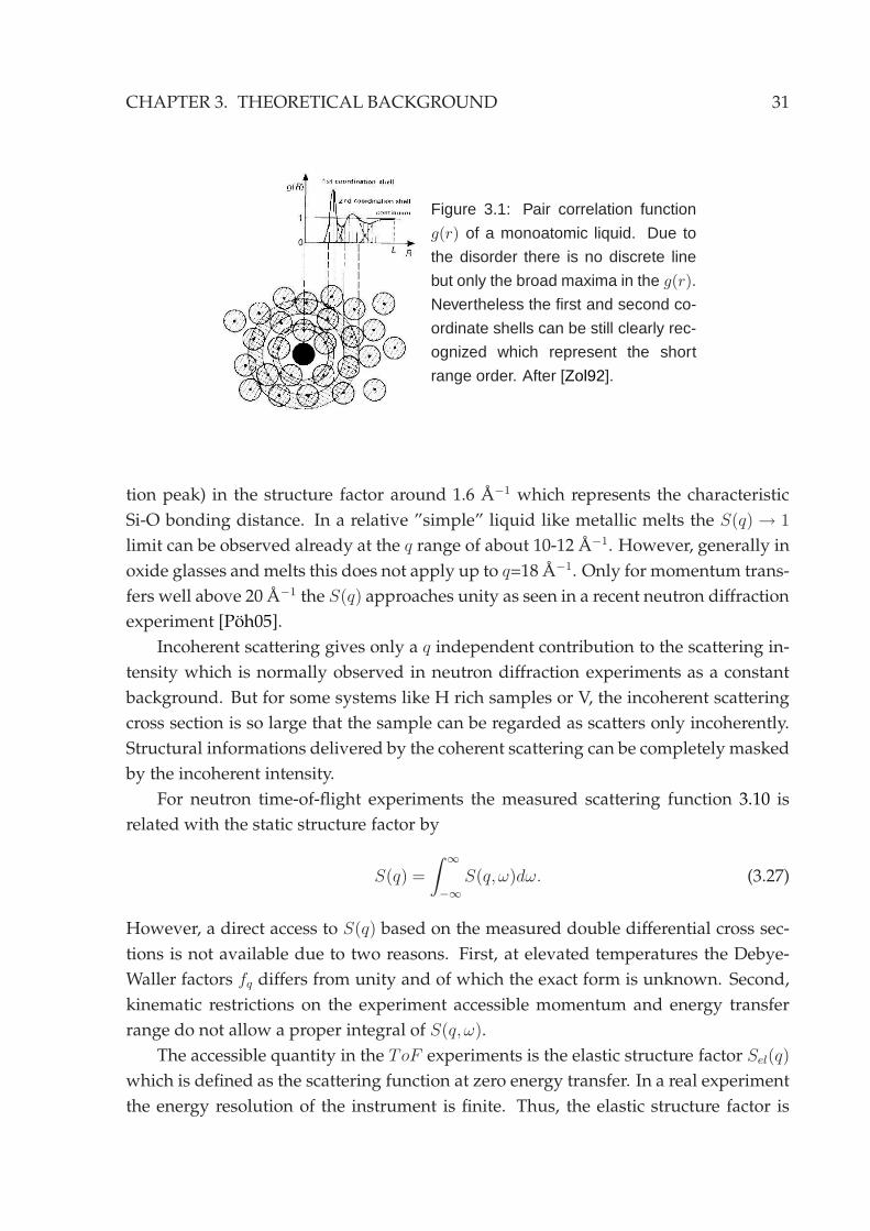
CHAPTER 3. THEORETICAL BACKGROUND 31
Figure 3.1: Pair correlation function
g(r) of a monoatomic liquid. Due to
the disorder there is no discrete line
but only the broad maxima in the g(r).
Nevertheless the first and second co-
ordinate shells can be still clearly rec-
ognized which represent the short
range order. After [Zol92].
tion peak) in the structure factor around 1.6 A−1 which represents the characteristic
Si-O bonding distance. In a relative ”simple” liquid like metallic melts the S(q) → 1
limit can be observed already at the q range of about 10-12 A−1. However, generally in
oxide glasses andmelts this does not apply up to q=18 A−1. Only for momentum trans-
fers well above 20 A−1 the S(q) approaches unity as seen in a recent neutron diffraction
experiment [Poh05].
Incoherent scattering gives only a q independent contribution to the scattering in-
tensity which is normally observed in neutron diffraction experiments as a constant
background. But for some systems like H rich samples or V, the incoherent scattering
cross section is so large that the sample can be regarded as scatters only incoherently.
Structural informations delivered by the coherent scattering can be completely masked
by the incoherent intensity.
For neutron time-of-flight experiments the measured scattering function 3.10 is
related with the static structure factor by
S(q) =
∫ ∞
−∞
S(q,ω)dω. (3.27)
However, a direct access to S(q) based on the measured double differential cross sec-
tions is not available due to two reasons. First, at elevated temperatures the Debye-
Waller factors fq differs from unity and of which the exact form is unknown. Second,
kinematic restrictions on the experiment accessible momentum and energy transfer
range do not allow a proper integral of S(q,ω).
The accessible quantity in the ToF experiments is the elastic structure factor Sel(q)
which is defined as the scattering function at zero energy transfer. In a real experiment
the energy resolution of the instrument is finite. Thus, the elastic structure factor is
32 3.1. NEUTRON SCATTERING
obtained via an integration of S(q,ω) over the instrument energy resolution function
R(q,ω)
Sel(q) =
∫
R(q,ω)
S(q,ω)dω. (3.28)
The elastic structure factor is a good approximation of the static structure factor multi-
plied by the Debye-Waller factor
Sel(q) = fqS(q). (3.29)
Dynamic scattering
Liquid and glasses are isotropic systems of which the density can be assumed to be
uniform for sufficient large length scale r. Thus, the long time limit t→ ∞ of the time
dependent density-density correlation function is given by
G(r,∞) = ρ0 (3.30a)
and its self part by
Gs(r,∞) =ρ0
N(3.30b)
where ρ0 is the particle number density of the scattering system. The long time limit
of the self correlation function is effectively zero for large length scale since N becomes
a large number.
The self part of the density correlation function Gs(r, t) represents the self motion
of a particular atom. It can be assumed to have a Gaussian form (Gaussian approxima-
tion)
Gs(r, t) =1
(6π〈r2(t)〉)3/2e−3
2r2
〈r2(t)〉 (3.31)
and its time Fourier transformation - the intermediate scattering function - is an expo-
nential like function
Ss(q, t) = e−32〈r2(t)〉. (3.32)
Characteristic relaxation time τ can be defined here for the exponential function decays
to the value e−1. The quantity 〈r2(t)〉 = 〈[~r(t)− ~r(0)]2〉, where ~r(t) is the position of an
atom at time t, is known as themean square displacement of which its time dependence
describes atomic motions.
The physical meaning of the density-density correlation function which represents
the collective atomic motions is more difficult to understand. On the long time scale
the correlation function of a simple liquid still follows an exponential decay but with
a relaxation time related to the structure factor. This behaviour is observed already for
CHAPTER 3. THEORETICAL BACKGROUND 33
example in liquidArgon [DR65]. In glasses δ(w) like peak exist in the coherent dynamic
scattering function corresponding to the quasi-equilibrium sites in the system.
In this work the studies are mainly focused on the time and length scales which are
close to the typical τs for structural relaxation and atomic transport in the silicate melts,
corresponding to the elastic and quasielastic part of the dynamic scattering function
measured in the neutron time-of-flight experiments. On much smaller time and length
scales, atomic motion is governed by local vibrations. This will reduce the elastic and
quasi-elastic scattering intensities by additional factors, known as Debye-Waller factor
for a coherent scatterer and Lamb-Mossbauer factor for an incoherent scatterer. These
intensities are then recovered in the inelastic part of the spectra represent phonon-like
modes in liquids and glasses.
3.2 Diffusion
3.2.1 Diffusion in simple liquid
For simple monoatomic liquid on times and distances which are much larger than the
local vibration of atoms, atomic motion is governed by diffusion processes via Brow-
nian motion. Thus the mean square displacement shows linear time dependence. The
basic equation for diffusion is the Fick’s law
∂C(~r, t)
∂t= D∇2C(~r, t) (3.33)
where C(~r, t) is the concentration (volume number density) of the diffusing particles
at the position ~r at time t and D is the diffusion coefficient. For an isotropic diffusion
all sites are equivalent and C(~r, t) is nothing but the self-correlation function Gs(r, t).
It can be easily verified that the Gaussian approximation 3.31 is a solution of the Fick’s
law 3.33 with the Einstein relation
Dst =1
6〈r2(t)〉. (3.34)
The self part of intermediate scattering function hence exhibits a simple exponential
decay
Ss(q, t) = e−(t/τ(q)) = e−Dsq2t (3.35)
and its time Fourier transformation Ss(q,ω) is a Lorentzian function
Ss(q,ω) =1
πh
Dsq2
Dsq2 + ω2(3.36)
34 3.2. DIFFUSION
with the full width at half maximum (FWHM) increases linearly with q2. For long
range translation diffusion corresponding to the q → 0 limit the diffusion coefficient
can be measured by
Ds =1
2πh
ΓSs(q,ω)
q2=
1
τq2(3.37)
At very short length scale the atoms can be regarded as free flying particles having bal-
listic motion. It can be show further via the derivation of the velocity autocorrelation
function [HM86] that in thermal equilibrium the time dependence of the mean square
displacement is
〈r2(t)〉 =3kBT
MAt2. (3.38)
Therefore, the FWHM of the measured scattering function is no longer proportional to
q2. In the intermediate q range a cross over from a ballistic motion to a diffusive motion
happens.
3.2.2 Hopping model and anomalous diffusion
The transport phenomena of mobile atoms in frozen media is often described by hop-
ping like motions. A jump-diffusion model originally discussed by Chudley and El-
liott [CE61] to describe such kind of motion in liquids proposes following hypotheses.
The diffusing particle is assumed to resident at one site for a given time τ0. After this
time, it jumps rapidly to another site, within a negligible jumping time. Based on such
assumption, the diffusion equation can be written down as:
∂
∂tP (~r) =
1
nτ
∑
~li
[P (~r + ~li)−P (~r)] (3.39)
Where P (~r) is the probability of finding a particle at ~r and it can jump to another site
which is connected by a displacement vector ~li. The jumping distance |~li| is assumed
to be much larger than the thermal vibration cloud created by the atom around its
equilibrium position. As shown already in the last section, P (~r, t) is equivalent to the
self-correlation function Gs(~r, t). Solving such differential equation with the boundary
condition Gs(~r,0)=δ(~r) and performing a spatial and time Fourier transformation, one
gets the neutron scattering function
Ss(~q, ω) =1
π
∆ω(~q)
[∆ω(~q)]2 + ω2(3.40)
CHAPTER 3. THEORETICAL BACKGROUND 35
by denoting
∆ω(~q) =1
nτ
∑
~li
[1− exp(−i~q · ~li)]. (3.41)
Note that the ∆ω(~q) function has a part which only depends for the scattering vector
~q and a part which only depends on the hopping rate ν=1/τ . So it can be rewritten in
the form of ∆ω(~q)=f(~q)ν. The f(~q) is also known as Chudley-Elliott function.
This model has been applied to describe hydrogen diffusion in various metallic
systems like Pd [RRGF72] as well as to charge transport phenomena in porous medium
[BMK+95]. If a characteristic hopping length l is available for a particular system, for
the q → 0 limit a characteristic diffusion coefficient can be related to the resident time
τ0 and the hopping length l by
Ds ∝ l2/τ0. (3.42)
The physical picture behind is that although on a small time and local length scale the
motion of atoms are characterized by discrete steps, the mean square displacement still
shows long time linear behaviour like it is in a Brownian motion.
However, even towards the long time limit, a diffusive behaviour is not necessar-
ily always having a linear time dependence of the mean square displacement. Diffu-
sive behaviours which deviates from Brownianmotion are called anomalous diffusion,
which shows the time dependence of the mean square displacement
〈r2(t)〉 ∝ tα (3.43)
with the time exponent α 6= 1.
Anomalous diffusion behaviours can be phenomenologically described by a gen-
eralized hopping diffusion model. Hopping can be regarded as thermally activated
processes. The hopping rate ν depends on the energy barriers between different sites.
If one assumes there exists a distribution of different energy barriers as well as relax-
ation times, the relaxation behaviour of the complete system is then a superposition of
different elementary processes. The relaxation function is hence given by
Ss(q, t) =
∫
(τ)e−(t/τ(q))dτ = e−(t/τ(q))β
(3.44)
which is well approximated by a stretched exponential function used frequently to
fit experimental data. The energy distribution function (τ) can be then obtained by
inverse Laplace transformation [LP90].
The exponent β here is not directly connected to the time exponent α in the time
dependence of the mean square displacement equation 3.43. To illustrate more clearly
the time exponent, it is necessary to look at the time dependent velocity autocorrelation
36 3.2. DIFFUSION
function. A theoretical approach in such framework, especially for disordered system,
is the effective medium approximation (EMA). It uses the same model of a distribution
of energy barriers. [SB91]. The theory generalizes the hopping rates ν to a frequency
dependent one ν(ω) which can be then solved via self consistent equations depending
on the energy barrier distribution. At small q the limit a generalized diffusion coeffi-
cient can be related to the hopping rate via again the Einstein relation
Ds(ω) =1
6〈r2〉ν(ω) (3.45)
and the long range diffusion coefficient is given by the ω → 0 limit. Ds(ω) is essen-
tially the time Fourier transform of the velocity autocorrelation function. Thus, the
time exponent is included by Ds(ω) ∝ ω1−α. In the regime where |w| ≫ |f(q)ν(ω)|, thescattering function can be reduced to
Ss(q,ω) ∝ ν(ω)/ω2 (3.46)
EMA provides hence a description of the anomalous diffusion behaviour which
can be used for the interpretation of neutron scattering data [SPSH90]: the high fre-
quency wing of the S(q,ω) spectra shows an frequency dependence of ω−(1+α). De-
spite the wide spectrum of the activation energies and the anomaly of the diffusion
behaviour, an Arrhenius law still holds for the temperature dependence of the relax-
ation time and the diffusion coefficient obtained in such approach.
The time exponent can be derived via fitting the S(q,ω) with a exponential func-
tion. However, a reliable fitting result can be only obtained by fitting at least two
decades in the frequency range. Such condition is usually not fulfilled with a single
time-of-flight experimental setup. Combination of different experiment results which
covers a sufficient large time window is necessary in order to get a proper determina-
tion of the time exponent.
It should be pointed out here that such description of the anomalous diffusion is
purely phenomenological. In some systems like hydrogen containing crystalline and
amorphous metals, the energy barrier distribution can be modeled based on different
neighbouring site pairs. But generally the anomalous diffusion behaviour can be also
caused by interactions such as liquids near the glass transition [GS92] or diffusion on
fractal topology [Hil99]. There is no general microscopic interpretation of anomalous
diffusion as well as its time exponent in the description.
CHAPTER 3. THEORETICAL BACKGROUND 37
3.3 Mode coupling theory and the glass transition
Mode coupling theory provides universal quantities and predictions which describe
the dynamics of viscous liquids and their relation to the structure. Especially it gives
a general model for idealized glass transition which can be used to understand ex-
perimental data. Detailed summary of mode coupling theory can be found in [Got91,
GS92]. In the following section only a brief introduction of basic ideals and results will
be presented.
3.3.1 Basic approach
Mode coupling theory uses the normalized density correlation function to describe the
dynamics in liquids which is defined by
Φ(q, t) =〈ρ∗(q, t)|ρ(q,0)〉〈ρ∗(q,0)|ρ(q,0)〉 = S(q, t)/S(q). (3.47)
The correlation functions can be obtained by solving the general Langevin equa-
tion of the Mori-Zwanzig projector formalism
Φ(q, t) + Ω2qΦ(q, t) + νΦ(q, t) + Ω2
q
∫ t
0
mq(t− t′)Φ(q, t′)dt′ = 0. (3.48)
In this differential equation the first three terms are similar to the equation of mo-
tion of a damped harmonic oscillator with a characteristic frequency Ωq and a friction
force νΦ(q, t). The integral term describes the forces which are coupled with the veloc-
ity at an earlier time t′ by the memory kernelmq(t). Thus, the state of the system at the
time t is linked to its previous state at time t′.
Gotze and coworkers used a microscopic approach in the mode coupling theory
by expressing the memory kernel mq(t) in the terms of a Polymonial of coupling con-
stants vn and density correlators. The coupling constants vn are determined by the
static structure factors [Got91] and depend on the external control parameters like tem-
perature, packing fraction, interaction potentials, etc. A closed set of equations can be
then formulated and the density correlators can be evaluated. Mode coupling theory
uses only static structure factors as input, therefore the dynamics in the system is fully
determined by its structure.
On the experimental side the number of studies on microscopic dynamics on the
order of ps to ns timescales are growing very quickly in the recent years due to the
development of neutron scattering techniques. In many experiments the dynamics of
liquids close to their glass transitions has been shown to be in good agreement at least
qualitatively with the predictions of mode coupling theory, e.g.: in molecular liquids
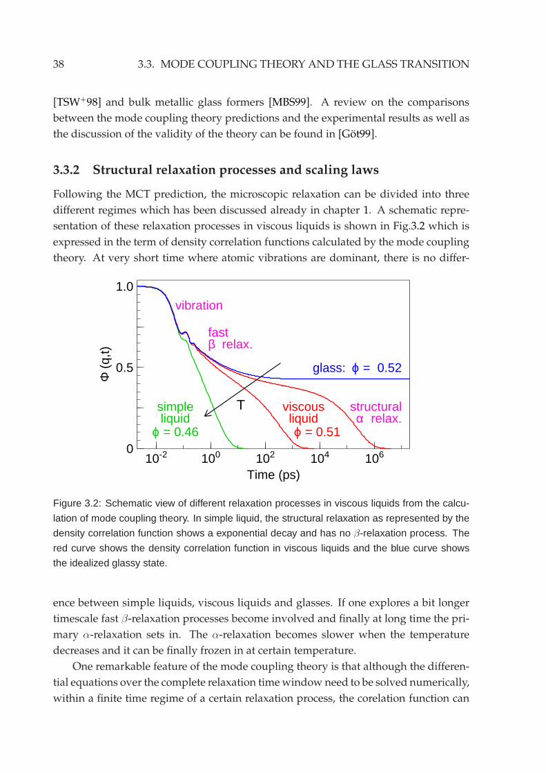
38 3.3. MODE COUPLING THEORY AND THE GLASS TRANSITION
[TSW+98] and bulk metallic glass formers [MBS99]. A review on the comparisons
between the mode coupling theory predictions and the experimental results as well as
the discussion of the validity of the theory can be found in [Got99].
3.3.2 Structural relaxation processes and scaling laws
Following the MCT prediction, the microscopic relaxation can be divided into three
different regimes which has been discussed already in chapter 1. A schematic repre-
sentation of these relaxation processes in viscous liquids is shown in Fig.3.2 which is
expressed in the term of density correlation functions calculated by the mode coupling
theory. At very short time where atomic vibrations are dominant, there is no differ-
10-2 100 102 104 1060
0.5
1.0
Time (ps)
Φ (
q,t)
simpleliquid
ϕ = 0.46
structuralα relax.
fastβ relax.
vibration
glass: ϕ = 0.52
viscousliquidϕ = 0.51
T
Figure 3.2: Schematic view of different relaxation processes in viscous liquids from the calcu-
lation of mode coupling theory. In simple liquid, the structural relaxation as represented by the
density correlation function shows a exponential decay and has no β-relaxation process. The
red curve shows the density correlation function in viscous liquids and the blue curve shows
the idealized glassy state.
ence between simple liquids, viscous liquids and glasses. If one explores a bit longer
timescale fast β-relaxation processes become involved and finally at long time the pri-
mary α-relaxation sets in. The α-relaxation becomes slower when the temperature
decreases and it can be finally frozen in at certain temperature.
One remarkable feature of the mode coupling theory is that although the differen-
tial equations over the complete relaxation timewindow need to be solved numerically,
within a finite time regime of a certain relaxation process, the corelation function can
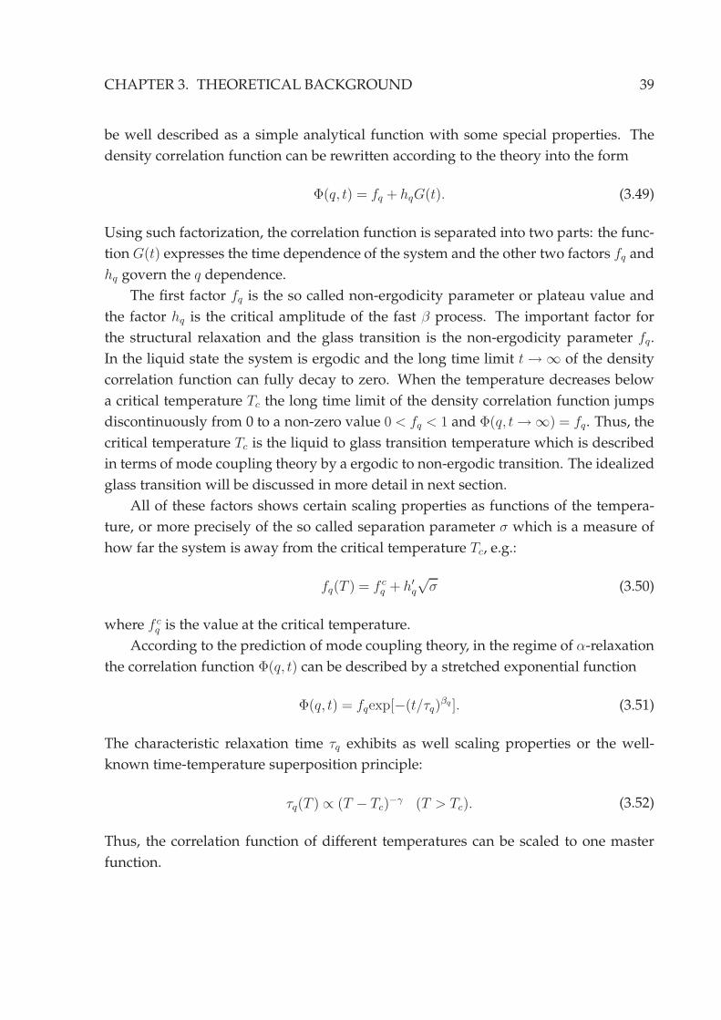
CHAPTER 3. THEORETICAL BACKGROUND 39
be well described as a simple analytical function with some special properties. The
density correlation function can be rewritten according to the theory into the form
Φ(q, t) = fq + hqG(t). (3.49)
Using such factorization, the correlation function is separated into two parts: the func-
tionG(t) expresses the time dependence of the system and the other two factors fq and
hq govern the q dependence.
The first factor fq is the so called non-ergodicity parameter or plateau value and
the factor hq is the critical amplitude of the fast β process. The important factor for
the structural relaxation and the glass transition is the non-ergodicity parameter fq.
In the liquid state the system is ergodic and the long time limit t→ ∞ of the density
correlation function can fully decay to zero. When the temperature decreases below
a critical temperature Tc the long time limit of the density correlation function jumps
discontinuously from 0 to a non-zero value 0 < fq < 1 and Φ(q, t→ ∞) = fq. Thus, the
critical temperature Tc is the liquid to glass transition temperature which is described
in terms of mode coupling theory by a ergodic to non-ergodic transition. The idealized
glass transition will be discussed in more detail in next section.
All of these factors shows certain scaling properties as functions of the tempera-
ture, or more precisely of the so called separation parameter σ which is a measure of
how far the system is away from the critical temperature Tc, e.g.:
fq(T ) = f cq + h′q
√σ (3.50)
where f cq is the value at the critical temperature.
According to the prediction of mode coupling theory, in the regime of α-relaxation
the correlation function Φ(q, t) can be described by a stretched exponential function
Φ(q, t) = fqexp[−(t/τq)βq ]. (3.51)
The characteristic relaxation time τq exhibits as well scaling properties or the well-
known time-temperature superposition principle:
τq(T ) ∝ (T − Tc)−γ (T > Tc). (3.52)
Thus, the correlation function of different temperatures can be scaled to one master
function.
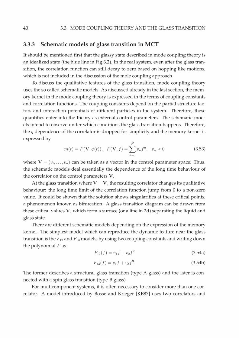
40 3.3. MODE COUPLING THEORY AND THE GLASS TRANSITION
3.3.3 Schematic models of glass transition in MCT
It should be mentioned first that the glassy state described in mode coupling theory is
an idealized state (the blue line in Fig.3.2). In the real system, even after the glass tran-
sition, the correlation function can still decay to zero based on hopping like motions,
which is not included in the discussion of the mole coupling approach.
To discuss the qualitative features of the glass transition, mode coupling theory
uses the so called schematic models. As discussed already in the last section, the mem-
ory kernel in the mode coupling theory is expressed in the terms of coupling constants
and correlation functions. The coupling constants depend on the partial structure fac-
tors and interaction potentials of different particles in the system. Therefore, these
quantities enter into the theory as external control parameters. The schematic mod-
els intend to observe under which conditions the glass transition happens. Therefore,
the q dependence of the correlator is dropped for simplicity and the memory kernel is
expressed by
m(t) = F (V, φ(t)), F (V, f) =
N∑
n=1
vnfn, vn ≥ 0 (3.53)
where V = (vi, . . . , vn) can be taken as a vector in the control parameter space. Thus,
the schematic models deal essentially the dependence of the long time behaviour of
the correlator on the control parameters V.
At the glass transition whereV = Vc the resulting correlator changes its qualitative
behaviour: the long time limit of the correlation function jump from 0 to a non-zero
value. It could be shown that the solution shows singularities at these critical points,
a phenomenon known as bifurcation. A glass transition diagram can be drawn from
these critical values Vc which form a surface (or a line in 2d) separating the liquid and
glass state.
There are different schematic models depending on the expression of the memory
kernel. The simplest model which can reproduce the dynamic feature near the glass
transition is the F12 and F13 models, by using two coupling constants andwriting down
the polynomial F as
F12(f) = v1f + v2f2 (3.54a)
F13(f) = v1f + v3f3. (3.54b)
The former describes a structural glass transition (type-A glass) and the later is con-
nected with a spin glass transition (type-B glass).
For multicomponent systems, it is often necessary to consider more than one cor-
relator. A model introduced by Bosse and Krieger [KB87] uses two correlators and
CHAPTER 3. THEORETICAL BACKGROUND 41
expresses the memory kernel as
m1(t) = v1f21 + v2f
22
m2(t) = v3f1f2
(3.55)
In the Bosse-Krieger mode, depending the position in the glass transition diagram, dif-
ferent dynamics feature can be obtained including for example a glass-glass transition
with higher orders of singularities. It is hence quite useful to describe the dynamics in
multicomponent systems close to the glass transition.
Chapter 4
Sample environment
In the chapter a detailed description of the high pressure high temperature sample environment
is presented. The first section discusses some criteria which should be considered for a high
temperature / pressure neutron scattering sample container. The construction of the cell is
described in the second section. The characterization of the neutron scattering signals of the
empty cell is shown in the last section.
4.1 Basic concepts
As already mentioned for the study of hydrous silicate melts with inelastic neutron
scattering a sample environment which provides a temperature range up to 1500 K
with a pressure up to several kbars and an available sample volume around 1 cm3 is
necessary. The relative large sample volume is mainly due to the intensity requirement
of a time-of-flight neutron spectroscopy. In this section some considerations for the
design of the high temperature high pressure cell are presented.
4.1.1 High pressure high temperature vessel
One of the most widely used geometries for high pressure vessels is a thick-wall cylin-
der. However, in the following paragraphs it will be shown that even such a simple
geometry needs a proper design in order to reach the maximum possible pressure for
a certain material.
Dawson [Daw77] proposed a general calculation on cylindrical tube based pres-
sure vessels. The basic mechanical model behind is a thick-wall tube under internal
pressure. Therefore, according to the classical mechanics the general stress-strain equa-
42
CHAPTER 4. SAMPLE ENVIRONMENT 43
tions can be easily written down as
σr =p
ω2 − 1(1− b2
r2) (4.1a)
σt =p
ω2 − 1(1 +
b2
r2) (4.1b)
σz = Eεz +2µp
ω2 − 1(4.1c)
where σr, σt and σz are the stresses in radial, tangential and longitudinal directions,
respectively. b is the outer diameter of the pressure vessel. ω is the so called wall
ratio, which is the ratio of the container outer diameter b to its inner diameter a, ω =
b/a represents a measure of the wall thickness of the pressure vessel. E is the elastic
constant of the vessel material and εz is the strain in longitudinal direction. Hook’s law
is hence included already in the equation. The Poisson’s ratio of thematerial is denoted
as µ. Boundary conditions are taken into account as such, that at the outer surface of
the cylinder the pressure P0 = 0 and inside the cylinder there is a uniform pressure
Pi = p. For a closed-end cylinder the longitudinal stress is uniform (independent of z
position) and can be rewritten as
σz =p
ω2 − 1=σr + σt
2. (4.2)
According to the two equations it can be shown that the largest stress occur at the
bore of the cylinder where r = a. The pressure vessel should be operated in the elastic
regime. In real apparatus some safety margins should be taken into account as well.
This means none of these maximum values should exceed the yield strength of the
material. Thus according to the distortion energy theory one has
2Y0 = (σt − σr)2 + (σr − σz)
2 + (σz − σt)2 (4.3)
which leads readily to the maximum pressure can be held in the vessel
p =Y0(ω
2 − 1)√3ω2
, pmax =Y0√
3≈ 0.577Y0 (ω→∞). (4.4)
Y0 is determined by the material used for the pressure vessel. The calculation clearly
shows that a monobloc cylinder will only provide a maximum operation pressure less
than 60% of the material strength. In order to increase the capability of the pressure
vessel strengthening methods have to be applied.
There are various ways to strengthen pressure vessels. The general idea is to in-
duce compressive residual stresses in the cell material to compensate the applied pres-
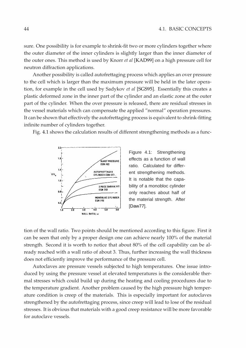
44 4.1. BASIC CONCEPTS
sure. One possibility is for example to shrink-fit two or more cylinders together where
the outer diameter of the inner cylinders is slightly larger than the inner diameter of
the outer ones. This method is used by Knorr et al [KAD99] on a high pressure cell for
neutron diffraction applications.
Another possibility is called autofrettaging process which applies an over pressure
to the cell which is larger than the maximum pressure will be held in the later opera-
tion, for example in the cell used by Sadykov et al [SGS95]. Essentially this creates a
plastic deformed zone in the inner part of the cylinder and an elastic zone at the outer
part of the cylinder. When the over pressure is released, there are residual stresses in
the vessel materials which can compensate the applied ”normal” operation pressures.
It can be shown that effectively the autofrettaging process is equivalent to shrink-fitting
infinite number of cylinders together.
Fig. 4.1 shows the calculation results of different strengthening methods as a func-
Figure 4.1: Strengthening
effects as a function of wall
ratio. Calculated for differ-
ent strengthening methods.
It is notable that the capa-
bility of a monobloc cylinder
only reaches about half of
the material strength. After
[Daw77].
tion of the wall ratio. Two points should be mentioned according to this figure. First it
can be seen that only by a proper design one can achieve nearly 100% of the material
strength. Second it is worth to notice that about 80% of the cell capability can be al-
ready reached with a wall ratio of about 3. Thus, further increasing the wall thickness
does not efficiently improve the performance of the pressure cell.
Autoclaves are pressure vessels subjected to high temperatures. One issue intro-
duced by using the pressure vessel at elevated temperatures is the considerable ther-
mal stresses which could build up during the heating and cooling procedures due to
the temperature gradient. Another problem caused by the high pressure high temper-
ature condition is creep of the materials. This is especially important for autoclaves
strengthened by the autofrettaging process, since creep will lead to lose of the residual
stresses. It is obvious that materials with a good creep resistance will be more favorable
for autoclave vessels.
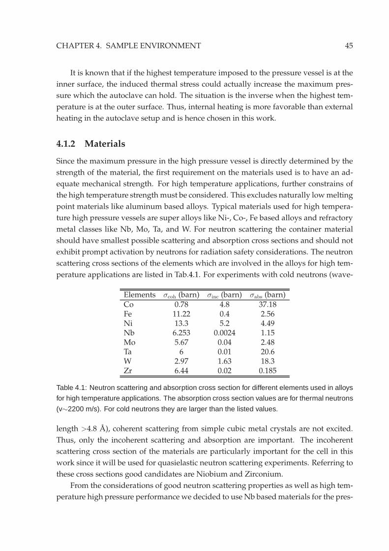
CHAPTER 4. SAMPLE ENVIRONMENT 45
It is known that if the highest temperature imposed to the pressure vessel is at the
inner surface, the induced thermal stress could actually increase the maximum pres-
sure which the autoclave can hold. The situation is the inverse when the highest tem-
perature is at the outer surface. Thus, internal heating is more favorable than external
heating in the autoclave setup and is hence chosen in this work.
4.1.2 Materials
Since the maximum pressure in the high pressure vessel is directly determined by the
strength of the material, the first requirement on the materials used is to have an ad-
equate mechanical strength. For high temperature applications, further constrains of
the high temperature strength must be considered. This excludes naturally lowmelting
point materials like aluminum based alloys. Typical materials used for high tempera-
ture high pressure vessels are super alloys like Ni-, Co-, Fe based alloys and refractory
metal classes like Nb, Mo, Ta, and W. For neutron scattering the container material
should have smallest possible scattering and absorption cross sections and should not
exhibit prompt activation by neutrons for radiation safety considerations. The neutron
scattering cross sections of the elements which are involved in the alloys for high tem-
perature applications are listed in Tab.4.1. For experiments with cold neutrons (wave-
Elements σcoh (barn) σinc (barn) σabs (barn)Co 0.78 4.8 37.18Fe 11.22 0.4 2.56Ni 13.3 5.2 4.49Nb 6.253 0.0024 1.15Mo 5.67 0.04 2.48Ta 6 0.01 20.6W 2.97 1.63 18.3Zr 6.44 0.02 0.185
Table 4.1: Neutron scattering and absorption cross section for different elements used in alloys
for high temperature applications. The absorption cross section values are for thermal neutrons
(v∼2200 m/s). For cold neutrons they are larger than the listed values.
length >4.8 A), coherent scattering from simple cubic metal crystals are not excited.
Thus, only the incoherent scattering and absorption are important. The incoherent
scattering cross section of the materials are particularly important for the cell in this
work since it will be used for quasielastic neutron scattering experiments. Referring to
these cross sections good candidates are Niobium and Zirconium.
From the considerations of good neutron scattering properties as well as high tem-
perature high pressure performance we decided to use Nb basedmaterials for the pres-
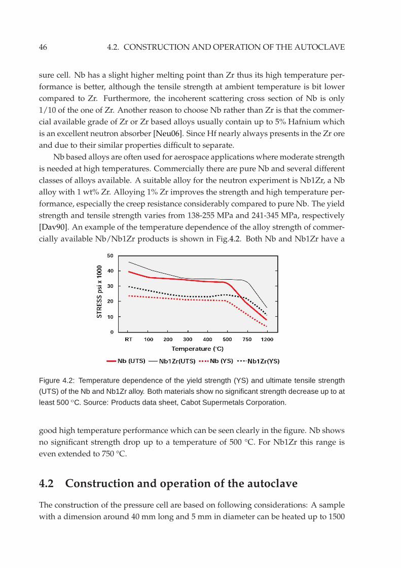
46 4.2. CONSTRUCTION AND OPERATION OF THE AUTOCLAVE
sure cell. Nb has a slight higher melting point than Zr thus its high temperature per-
formance is better, although the tensile strength at ambient temperature is bit lower
compared to Zr. Furthermore, the incoherent scattering cross section of Nb is only
1/10 of the one of Zr. Another reason to choose Nb rather than Zr is that the commer-
cial available grade of Zr or Zr based alloys usually contain up to 5% Hafnium which
is an excellent neutron absorber [Neu06]. Since Hf nearly always presents in the Zr ore
and due to their similar properties difficult to separate.
Nb based alloys are often used for aerospace applications wheremoderate strength
is needed at high temperatures. Commercially there are pure Nb and several different
classes of alloys available. A suitable alloy for the neutron experiment is Nb1Zr, a Nb
alloy with 1 wt% Zr. Alloying 1% Zr improves the strength and high temperature per-
formance, especially the creep resistance considerably compared to pure Nb. The yield
strength and tensile strength varies from 138-255 MPa and 241-345 MPa, respectively
[Dav90]. An example of the temperature dependence of the alloy strength of commer-
cially available Nb/Nb1Zr products is shown in Fig.4.2. Both Nb and Nb1Zr have a
Figure 4.2: Temperature dependence of the yield strength (YS) and ultimate tensile strength
(UTS) of the Nb and Nb1Zr alloy. Both materials show no significant strength decrease up to at
least 500 oC. Source: Products data sheet, Cabot Supermetals Corporation.
good high temperature performance which can be seen clearly in the figure. Nb shows
no significant strength drop up to a temperature of 500 °C. For Nb1Zr this range is
even extended to 750 °C.
4.2 Construction and operation of the autoclave
The construction of the pressure cell are based on following considerations: A sample
with a dimension around 40 mm long and 5 mm in diameter can be heated up to 1500
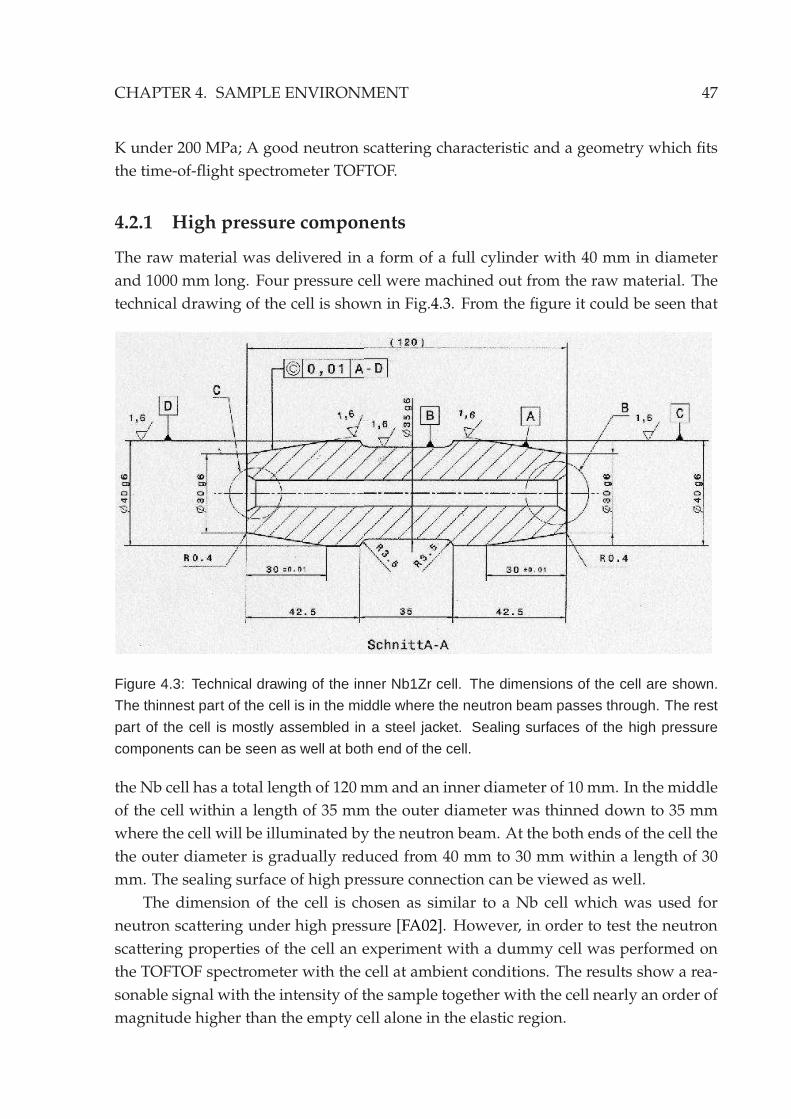
CHAPTER 4. SAMPLE ENVIRONMENT 47
K under 200 MPa; A good neutron scattering characteristic and a geometry which fits
the time-of-flight spectrometer TOFTOF.
4.2.1 High pressure components
The raw material was delivered in a form of a full cylinder with 40 mm in diameter
and 1000 mm long. Four pressure cell were machined out from the raw material. The
technical drawing of the cell is shown in Fig.4.3. From the figure it could be seen that
Figure 4.3: Technical drawing of the inner Nb1Zr cell. The dimensions of the cell are shown.
The thinnest part of the cell is in the middle where the neutron beam passes through. The rest
part of the cell is mostly assembled in a steel jacket. Sealing surfaces of the high pressure
components can be seen as well at both end of the cell.
the Nb cell has a total length of 120 mm and an inner diameter of 10 mm. In the middle
of the cell within a length of 35 mm the outer diameter was thinned down to 35 mm
where the cell will be illuminated by the neutron beam. At the both ends of the cell the
the outer diameter is gradually reduced from 40 mm to 30 mm within a length of 30
mm. The sealing surface of high pressure connection can be viewed as well.
The dimension of the cell is chosen as similar to a Nb cell which was used for
neutron scattering under high pressure [FA02]. However, in order to test the neutron
scattering properties of the cell an experiment with a dummy cell was performed on
the TOFTOF spectrometer with the cell at ambient conditions. The results show a rea-
sonable signal with the intensity of the sample together with the cell nearly an order of
magnitude higher than the empty cell alone in the elastic region.
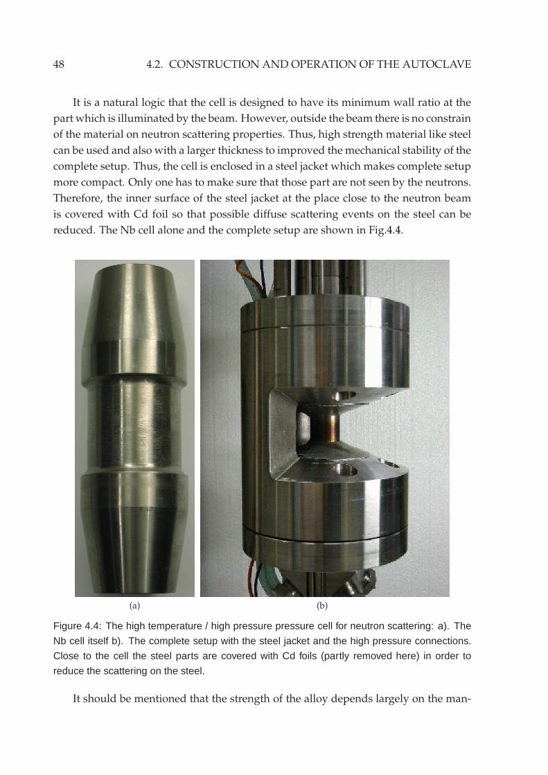
48 4.2. CONSTRUCTION AND OPERATION OF THE AUTOCLAVE
It is a natural logic that the cell is designed to have its minimum wall ratio at the
part which is illuminated by the beam. However, outside the beam there is no constrain
of the material on neutron scattering properties. Thus, high strength material like steel
can be used and also with a larger thickness to improved the mechanical stability of the
complete setup. Thus, the cell is enclosed in a steel jacket which makes complete setup
more compact. Only one has to make sure that those part are not seen by the neutrons.
Therefore, the inner surface of the steel jacket at the place close to the neutron beam
is covered with Cd foil so that possible diffuse scattering events on the steel can be
reduced. The Nb cell alone and the complete setup are shown in Fig.4.4.
(a) (b)
Figure 4.4: The high temperature / high pressure pressure cell for neutron scattering: a). The
Nb cell itself b). The complete setup with the steel jacket and the high pressure connections.
Close to the cell the steel parts are covered with Cd foils (partly removed here) in order to
reduce the scattering on the steel.
It should be mentioned that the strength of the alloy depends largely on the man-
CHAPTER 4. SAMPLE ENVIRONMENT 49
ufactory and processing procedures (for example whether it is recrystallized or cold
rolled its strength can be highly different). Thus, no exact strength data is available
when we brought the raw material from the supplier.
For safety reasons the cell has to be tested under pressure. A test on the cell with
a larger inner diameter of 11 mm under a pressure of about 300 MPa was conducted.
The test experiment was done by adapting the cell embedded in the steel jacket to the
sample preparation pressure apparatus. The initial idea to enlarge the inner diameter
was to perform a bursting experiment. If the bursting pressure of the cell with this di-
mension could bemeasured the one of the 10 mm inner diameter cell could be revealed
via calculation.
However, it turned out that the cell can sustain a pressure of 300 MPa even with
a inner diameter of 11 mm, which is the maximum pressure the compressor used for
sample preparation can provide. The maximum pressure was charged four times with
each time holding at the pressure for about 3 minutes before releasing. Since the cell
with 11 mm inner diameter was not destroyed after the test experiment it is used for
further development, although the bursting pressure of such geometry remains un-
known. If one considers the tensile strength data in Fig.4.2 applying 300 MPa pressure
should also act as an autofrettaging strengthening process for the cell to some extend.
In the neutron experiments a maximum pressure of 200 MPa was used, which is
a factor of 1.5 smaller than the test pressure for safety margin. Besides the 300 MPa
pressure test, a long time test which held the pressure of 200 MPa for 24 hours was
performed as well. After these experiments no deformation was measured within a
precision of about 0.1 mm.
4.2.2 High temperature furnace
The next step is to build a small furnace in the pressure cell which can heat up the
sample. Several technical requirements should be taken into account. The furnace
should have a good isolation from the cell. Thus, with a moderate power the desired
sample temperature can be reached and the Nb cell itself also does not get too hot to
lose its strength. The sample, furnace and cell should have a relative tight fit in order to
reduce the gas pressure medium at the hot zone. This is mainly due to two intentions:
1) to reduced the background due to scattering on the pressure medium. 2) to limit
strong convective gas flow which will leads a large temperature instability. Small gas
volume is also favorable for safety issues.
The furnace is mainly composed of three parts. An ceramic tube with an outer
diameter of 10.8 mm and a thickness of 1.5 mm serves as a thermal isolation of the
furnace from the cell. Another thin ceramic tube with a inner diameter of 5.2 mm and a
thickness of 0.8 mmwas used to isolate the heating wire electrically from the Pt sample
50 4.2. CONSTRUCTION AND OPERATION OF THE AUTOCLAVE
capsules. Thus, no short circle of the heating element can happen. The tube is only 0.2
mm larger in diameter than the one of the sample to ensure a tight fitting. On the outer
surface of this thin ceramic tube a thread was cut with a depth of 0.3 mm, a width of
0.6 mm and a slope of 1 mm for the mounting of the heating wires. Due to special
dimensions of the ceramic parts they were machined at the crystal lab of the Physik-
Department. To cut the thread on the thin ceramic tube a special tool was made in
order to reduce the risk that the tube breaks during machining. Basically the thin tube
was glued on a metal rod during cutting and removed afterwards. As heating wire
PtRh alloy was used which has a higher electrical resistance than the pure Pt wires
and therefore more electrical power can be loaded with the same current. The wire
was first rolled into spring-like shape and recrystallized at 1100 °C to remove residual
stress then mounted on the inner ceramic tube.
At the bottom of the furnace the heating wire was welded to a Pt tube with a outer
diameter of 5 mm and a wall thickness of 0.2 mmwhich extends the wire outside of the
Nb cell. The Pt tube is then connected to massive wires and eventually reaches the high
pressure adaptor for external connections. The resistance of the Pt tube is negligible
compared to the heating wire. At the top of the furnace the heating wire was welded
to a Pt plate which acts as electrical contact for external connection. This connection is
later on grounded to the steel part since it is fairly difficult to make another connection
from the upper feed-through where the samples are introduced in.
The furnace has a heating zone of 70 mm in length which is about 35 mm longer
than the length of the samples. At the bottom of the sample a thermal couple of
Pt/Pt10%Rh is inserted into the furnace with a depth of about 15 mm to monitor the
temperature below the sample. Samples are inserted from the top of the furnace with
an additional thermal couple above the sample to monitor the sample temperature.
During the experiment a temperature difference up to 200-300 °C between the upper
and lower thermal couples could be built up depending on the pressure and tempera-
ture conditions.
In order to test the real temperature and the temperature homogeneity in the cell, a
dummy sample (a 4 mm diameter ceramic rod) was inserted into the cell coated with a
temperature indicating paint1 and heated up to 977 °C (upper thermal couple reading)
under a pressure of 200 MPa. The result is shown in Fig.4.5. The determined temper-
ature from the paint is around 1000 °C, which is close to the indication of the upper
thermal couple. However, due to the coarse temperature steps in the specification a
precision smaller than ±20 °C cannot be expected from such estimation. Nevertheless,
it can be clearly seen that the temperature is relative homogeneous since the colour is
nearly uniform. This is probably due to the factor that the gas convection in the cell is
1Typ MC150-12 from Kager Industrieprodukte GmbH.
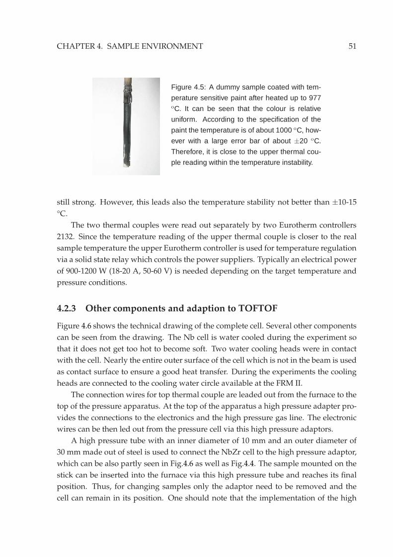
CHAPTER 4. SAMPLE ENVIRONMENT 51
Figure 4.5: A dummy sample coated with tem-
perature sensitive paint after heated up to 977oC. It can be seen that the colour is relative
uniform. According to the specification of the
paint the temperature is of about 1000 oC, how-
ever with a large error bar of about ±20 oC.
Therefore, it is close to the upper thermal cou-
ple reading within the temperature instability.
still strong. However, this leads also the temperature stability not better than ±10-15
°C.
The two thermal couples were read out separately by two Eurotherm controllers
2132. Since the temperature reading of the upper thermal couple is closer to the real
sample temperature the upper Eurotherm controller is used for temperature regulation
via a solid state relay which controls the power suppliers. Typically an electrical power
of 900-1200 W (18-20 A, 50-60 V) is needed depending on the target temperature and
pressure conditions.
4.2.3 Other components and adaption to TOFTOF
Figure 4.6 shows the technical drawing of the complete cell. Several other components
can be seen from the drawing. The Nb cell is water cooled during the experiment so
that it does not get too hot to become soft. Two water cooling heads were in contact
with the cell. Nearly the entire outer surface of the cell which is not in the beam is used
as contact surface to ensure a good heat transfer. During the experiments the cooling
heads are connected to the cooling water circle available at the FRM II.
The connection wires for top thermal couple are leaded out from the furnace to the
top of the pressure apparatus. At the top of the apparatus a high pressure adapter pro-
vides the connections to the electronics and the high pressure gas line. The electronic
wires can be then led out from the pressure cell via this high pressure adaptors.
A high pressure tube with an inner diameter of 10 mm and an outer diameter of
30 mm made out of steel is used to connect the NbZr cell to the high pressure adaptor,
which can be also partly seen in Fig.4.6 as well as Fig.4.4. The sample mounted on the
stick can be inserted into the furnace via this high pressure tube and reaches its final
position. Thus, for changing samples only the adaptor need to be removed and the
cell can remain in its position. One should note that the implementation of the high
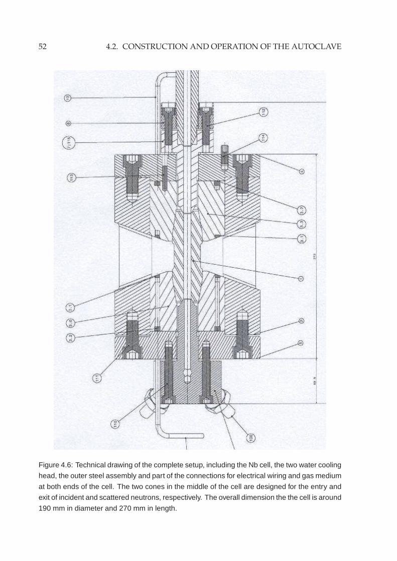
52 4.2. CONSTRUCTION AND OPERATION OF THE AUTOCLAVE
Figure 4.6: Technical drawing of the complete setup, including the Nb cell, the two water cooling
head, the outer steel assembly and part of the connections for electrical wiring and gas medium
at both ends of the cell. The two cones in the middle of the cell are designed for the entry and
exit of incident and scattered neutrons, respectively. The overall dimension the the cell is around
190 mm in diameter and 270 mm in length.
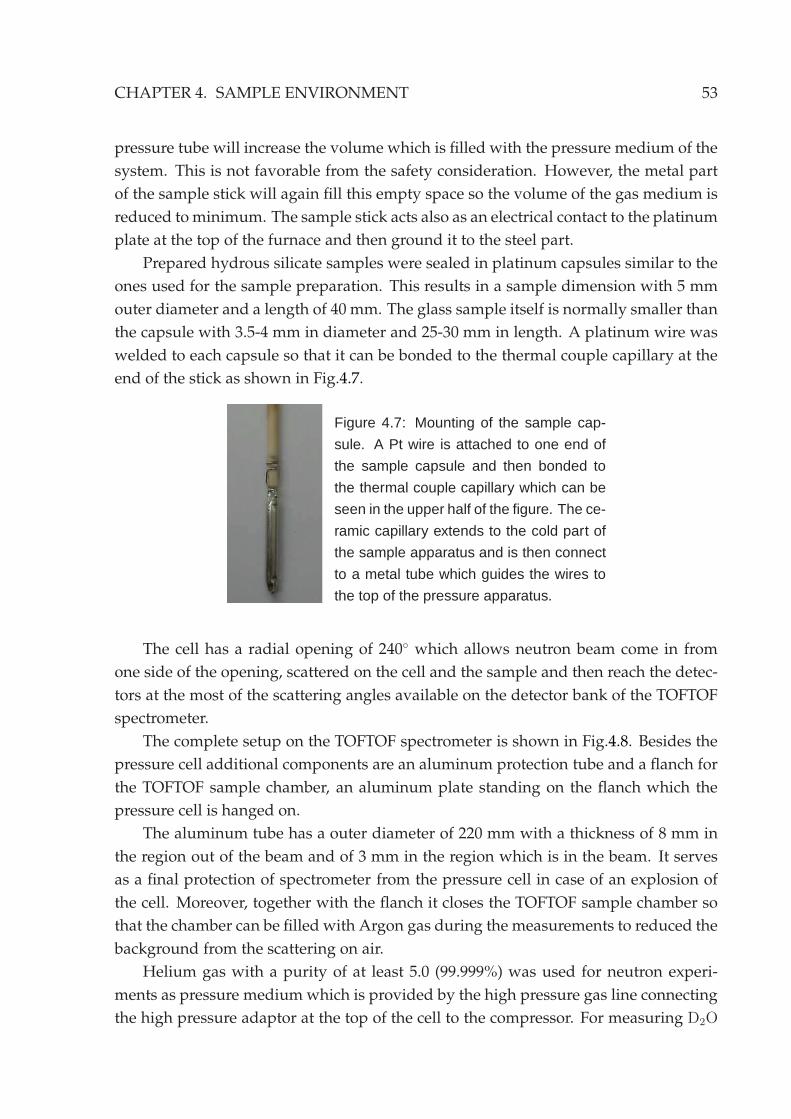
CHAPTER 4. SAMPLE ENVIRONMENT 53
pressure tube will increase the volume which is filled with the pressure medium of the
system. This is not favorable from the safety consideration. However, the metal part
of the sample stick will again fill this empty space so the volume of the gas medium is
reduced to minimum. The sample stick acts also as an electrical contact to the platinum
plate at the top of the furnace and then ground it to the steel part.
Prepared hydrous silicate samples were sealed in platinum capsules similar to the
ones used for the sample preparation. This results in a sample dimension with 5 mm
outer diameter and a length of 40 mm. The glass sample itself is normally smaller than
the capsule with 3.5-4 mm in diameter and 25-30 mm in length. A platinum wire was
welded to each capsule so that it can be bonded to the thermal couple capillary at the
end of the stick as shown in Fig.4.7.
Figure 4.7: Mounting of the sample cap-
sule. A Pt wire is attached to one end of
the sample capsule and then bonded to
the thermal couple capillary which can be
seen in the upper half of the figure. The ce-
ramic capillary extends to the cold part of
the sample apparatus and is then connect
to a metal tube which guides the wires to
the top of the pressure apparatus.
The cell has a radial opening of 240 which allows neutron beam come in from
one side of the opening, scattered on the cell and the sample and then reach the detec-
tors at the most of the scattering angles available on the detector bank of the TOFTOF
spectrometer.
The complete setup on the TOFTOF spectrometer is shown in Fig.4.8. Besides the
pressure cell additional components are an aluminum protection tube and a flanch for
the TOFTOF sample chamber, an aluminum plate standing on the flanch which the
pressure cell is hanged on.
The aluminum tube has a outer diameter of 220 mm with a thickness of 8 mm in
the region out of the beam and of 3 mm in the region which is in the beam. It serves
as a final protection of spectrometer from the pressure cell in case of an explosion of
the cell. Moreover, together with the flanch it closes the TOFTOF sample chamber so
that the chamber can be filled with Argon gas during the measurements to reduced the
background from the scattering on air.
Helium gas with a purity of at least 5.0 (99.999%) was used for neutron experi-
ments as pressure medium which is provided by the high pressure gas line connecting
the high pressure adaptor at the top of the cell to the compressor. For measuring D2O

54 4.2. CONSTRUCTION AND OPERATION OF THE AUTOCLAVE
Figure 4.8: Schematic view of the complete setup on the TOFTOF spectrometer at FRM II. The
neutron beam is coming from the right hand side of the pressure cell, part of the neutron guide
was drawn. The pressure cell is surrounded by an aluminum tube. This aluminum tube also
seals sample chamber of the spectrometer since it is filled with Ar gas during the measurement.
The cell is hanged on an aluminum plate which is mount on the top of the sample chamber.
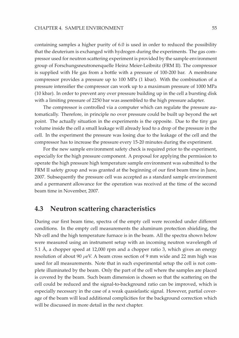
CHAPTER 4. SAMPLE ENVIRONMENT 55
containing samples a higher purity of 6.0 is used in order to reduced the possibility
that the deuterium is exchanged with hydrogen during the experiments. The gas com-
pressor used for neutron scattering experiment is provided by the sample environment
group of Forschungsneutronenquelle Heinz Meier-Leibnitz (FRM II). The compressor
is supplied with He gas from a bottle with a pressure of 100-200 bar. A membrane
compressor provides a pressure up to 100 MPa (1 kbar). With the combination of a
pressure intensifier the compressor can work up to a maximum pressure of 1000 MPa
(10 kbar). In order to prevent any over pressure building up in the cell a bursting disk
with a limiting pressure of 2250 bar was assembled to the high pressure adapter.
The compressor is controlled via a computer which can regulate the pressure au-
tomatically. Therefore, in principle no over pressure could be built up beyond the set
point. The actually situation in the experiments is the opposite. Due to the tiny gas
volume inside the cell a small leakage will already lead to a drop of the pressure in the
cell. In the experiment the pressure was losing due to the leakage of the cell and the
compressor has to increase the pressure every 15-20 minutes during the experiment.
For the new sample environment safety check is required prior to the experiment,
especially for the high pressure component. A proposal for applying the permission to
operate the high pressure high temperature sample environment was submitted to the
FRM II safety group and was granted at the beginning of our first beam time in June,
2007. Subsequently the pressure cell was accepted as a standard sample environment
and a permanent allowance for the operation was received at the time of the second
beam time in November, 2007.
4.3 Neutron scattering characteristics
During our first beam time, spectra of the empty cell were recorded under different
conditions. In the empty cell measurements the aluminum protection shielding, the
Nb cell and the high temperature furnace is in the beam. All the spectra shown below
were measured using an instrument setup with an incoming neutron wavelength of
5.1 A, a chopper speed at 12,000 rpm and a chopper ratio 3, which gives an energy
resolution of about 90 µeV. A beam cross section of 9 mm wide and 22 mm high was
used for all measurements. Note that in such experimental setup the cell is not com-
plete illuminated by the beam. Only the part of the cell where the samples are placed
is covered by the beam. Such beam dimension is chosen so that the scattering on the
cell could be reduced and the signal-to-background ratio can be improved, which is
especially necessary in the case of a weak quasielastic signal. However, partial cover-
age of the beam will lead additional complicities for the background correction which
will be discussed in more detail in the next chapter.
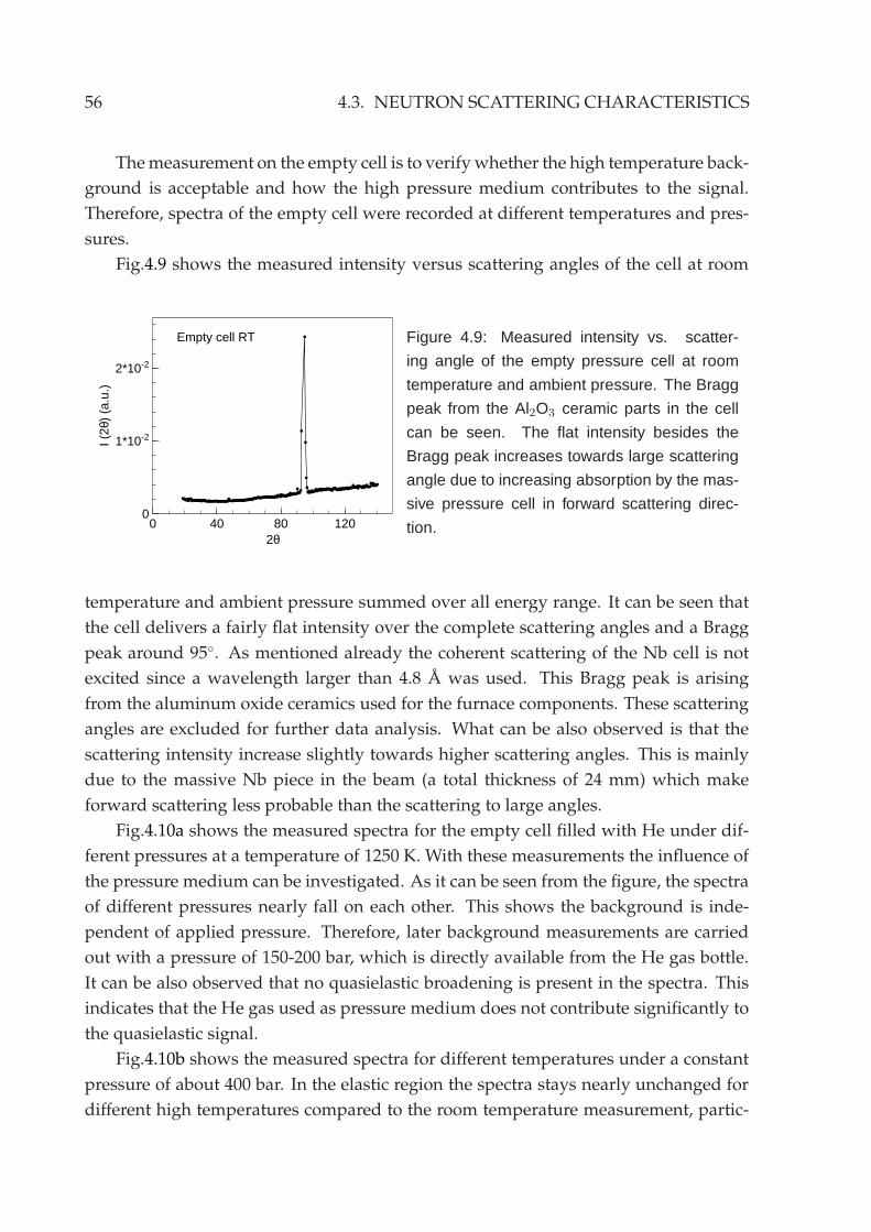
56 4.3. NEUTRON SCATTERING CHARACTERISTICS
Themeasurement on the empty cell is to verify whether the high temperature back-
ground is acceptable and how the high pressure medium contributes to the signal.
Therefore, spectra of the empty cell were recorded at different temperatures and pres-
sures.
Fig.4.9 shows the measured intensity versus scattering angles of the cell at room
0 40 80 1200
1*10-2
2*10-2
2θ
I (2θ
) (a
.u.)
Empty cell RT Figure 4.9: Measured intensity vs. scatter-
ing angle of the empty pressure cell at room
temperature and ambient pressure. The Bragg
peak from the Al2O3 ceramic parts in the cell
can be seen. The flat intensity besides the
Bragg peak increases towards large scattering
angle due to increasing absorption by the mas-
sive pressure cell in forward scattering direc-
tion.
temperature and ambient pressure summed over all energy range. It can be seen that
the cell delivers a fairly flat intensity over the complete scattering angles and a Bragg
peak around 95. As mentioned already the coherent scattering of the Nb cell is not
excited since a wavelength larger than 4.8 A was used. This Bragg peak is arising
from the aluminum oxide ceramics used for the furnace components. These scattering
angles are excluded for further data analysis. What can be also observed is that the
scattering intensity increase slightly towards higher scattering angles. This is mainly
due to the massive Nb piece in the beam (a total thickness of 24 mm) which make
forward scattering less probable than the scattering to large angles.
Fig.4.10a shows the measured spectra for the empty cell filled with He under dif-
ferent pressures at a temperature of 1250 K. With these measurements the influence of
the pressure medium can be investigated. As it can be seen from the figure, the spectra
of different pressures nearly fall on each other. This shows the background is inde-
pendent of applied pressure. Therefore, later background measurements are carried
out with a pressure of 150-200 bar, which is directly available from the He gas bottle.
It can be also observed that no quasielastic broadening is present in the spectra. This
indicates that the He gas used as pressure medium does not contribute significantly to
the quasielastic signal.
Fig.4.10b shows the measured spectra for different temperatures under a constant
pressure of about 400 bar. In the elastic region the spectra stays nearly unchanged for
different high temperatures compared to the room temperature measurement, partic-
CHAPTER 4. SAMPLE ENVIRONMENT 57
0 0.5 1 1.510-5
10-4
10-3
10-2
tof (msec/m)
I(T
oF)
(a.u
.)
Empty cell 1250K airEmpty cell 1250K 400 bar HeEmpty cell 1250K 1800 bar He
summed over 2θ=43-69o
(a)
0 0.5 1 1.510-5
10-4
10-3
10-2
tof (msec/m)
I(T
oF)
(a.u
.)
Empty cell RTEmpty cell 850 KEmpty cell 1150 KEmpty cell 1250 K
summed over 2θ=43-69o
(b)
Figure 4.10: Measured spectra of the empty pressure cell under various pressure and temper-
ature conditions. All spectra were summed over a scattering angle range of 43-69, corre-
sponding to the q values from 0.9 A−1 to 1.4 A−1. a) Pressure dependence of the empty cell
measurements at a temperature of 1250 K. b) Temperature dependence of empty cell mea-
surements under a pressure of about 400 bar.
ularly no linewidth broadening can be identified. Hence, a good resolution for mea-
suring a quasielastic signal from the samples can be obtained for the high temperature
measurements. In the inelastic region the intensity increases with increasing tempera-
ture, which is due to the higher population of phonon levels in the Nb alloy since the
cell itself also gets heated up during the measurement. However, after certain time a
steady condition of the heat exchange process is reached and the inelastic spectra do
not vary largely with respect to temperature.
Fig.4.11 shows the empty pressure cell measurements together with aNS3+10mol%
H2O sample at 1250 K under 1800 bar. It can be seen that the sample signal is well
above the signal coming from the empty cell within the elastic and quasielastic region.
The signal-to-background ratio is of about 10:1 in this region. The quasielastic broad-
ening of the spectrum is dominantly contributed from the sample. In the deep inelastic
region the intensity of the sample and the empty cell are rather close to each other. It
will be difficult to get access to the inelastic spectra of the samples. It should be noted
here that the spectrum of the empty cell at 1250 K and 1800 bar was recorded where
the sample volume was completely occupied by He gas under such condition. The gas
volume in the beam will be significantly reduced when there is a sample in the cell.
The cell is hence not operated under the optimum conditions since a larger gas volume
leads significant increase of the convection in the cell and a higher electrical power is
needed in order to reach steady conditions. Even though no quasielastic contribution
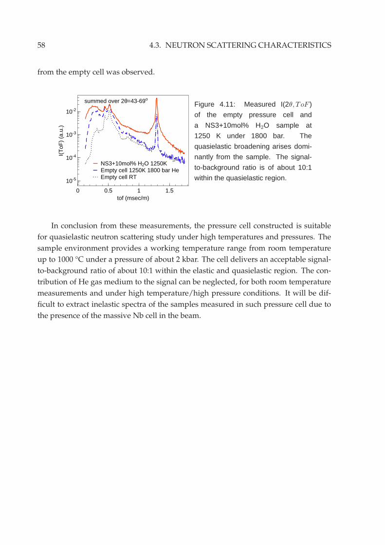
58 4.3. NEUTRON SCATTERING CHARACTERISTICS
from the empty cell was observed.
0 0.5 1 1.5
10-5
10-4
10-3
10-2
tof (msec/m)
I(T
oF)
(a.u
.)
NS3+10mol% H2O 1250KEmpty cell 1250K 1800 bar HeEmpty cell RT
summed over 2θ=43-69o
Figure 4.11: Measured I(2θ,ToF )
of the empty pressure cell and
a NS3+10mol% H2O sample at
1250 K under 1800 bar. The
quasielastic broadening arises domi-
nantly from the sample. The signal-
to-background ratio is of about 10:1
within the quasielastic region.
In conclusion from these measurements, the pressure cell constructed is suitable
for quasielastic neutron scattering study under high temperatures and pressures. The
sample environment provides a working temperature range from room temperature
up to 1000 °C under a pressure of about 2 kbar. The cell delivers an acceptable signal-
to-background ratio of about 10:1 within the elastic and quasielastic region. The con-
tribution of He gas medium to the signal can be neglected, for both room temperature
measurements and under high temperature/high pressure conditions. It will be dif-
ficult to extract inelastic spectra of the samples measured in such pressure cell due to
the presence of the massive Nb cell in the beam.
Chapter 5
Neutron scattering experiment
The neutron experimental setup is described in the following chapter. The basic principle of
neutron time-of-flight spectroscopy and the instrument setup used for the investigation of the
hydrous silicate melts is presented. The data reduction processes are shown in the third section.
Especially the problems caused by the massive pressure cell on signal correction are discussed.
The last section presents the principle of the neutron backscattering experiments.
5.1 Time-of-flight spectroscopy
Neutron time-of-flight spectrometers are one major class of spectrometers for inelastic
neutron scattering. In neutron time-of-flight spectroscopy the energy and momentum
transfer of the scattered neutrons are determined simultaneously by measuring the
neutron flight time from the sample position to the detectors and the scattering angles.
Hence the dynamic scattering function S(q,w) is measured directly in a broad range of
q and ω.
The neutron time-of-flight experiments in this work were carried out exclusively
at the TOFTOF spectrometer at FRM II. The schematic view of the instrument setup is
shown in Fig.5.1. The instrument provides a high neutron flux (∼1010n/cm2/s, unper-
turbed) at the sample position accompaniedwith an excellent signal-to-background ra-
tio [UMNP07]. A detailed description of the spectrometer could be found at [UNP07].
In the next paragraphs a brief introduction on the instrument setup will be presented.
The white neutron beam is delivered from the FRM II cold source operated with
liquid D2 at a temperature of 25 K. The white beam has a Maxwellian velocity distri-
bution with a maximum located at the wavelength around 3 A.
The TOFTOF spectrometer is a chopper time-of-flight spectrometer, the neutron
beam ismonochromated with amulti-disc chopper systemwhich can be seen at the left
side of Fig.5.1. The chopper disks are made of carbon-fiber-reinforced plastics coated
59
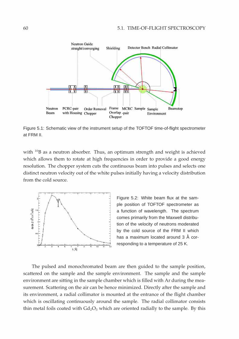
60 5.1. TIME-OF-FLIGHT SPECTROSCOPY
Figure 5.1: Schematic view of the instrument setup of the TOFTOF time-of-flight spectrometer
at FRM II.
with 10B as a neutron absorber. Thus, an optimum strength and weight is achieved
which allows them to rotate at high frequencies in order to provide a good energy
resolution. The chopper system cuts the continuous beam into pulses and selects one
distinct neutron velocity out of the white pulses initially having a velocity distribution
from the cold source.
Figure 5.2: White beam flux at the sam-
ple position of TOFTOF spectrometer as
a function of wavelength. The spectrum
comes primarily from the Maxwell distribu-
tion of the velocity of neutrons moderated
by the cold source of the FRM II which
has a maximum located around 3 A cor-
responding to a temperature of 25 K.
The pulsed and monochromated beam are then guided to the sample position,
scattered on the sample and the sample environment. The sample and the sample
environment are sitting in the sample chamber which is filled with Ar during the mea-
surement. Scattering on the air can be hence minimized. Directly after the sample and
its environment, a radial collimator is mounted at the entrance of the flight chamber
which is oscillating continuously around the sample. The radial collimator consists
thin metal foils coated with Gd2O3 which are oriented radially to the sample. By this
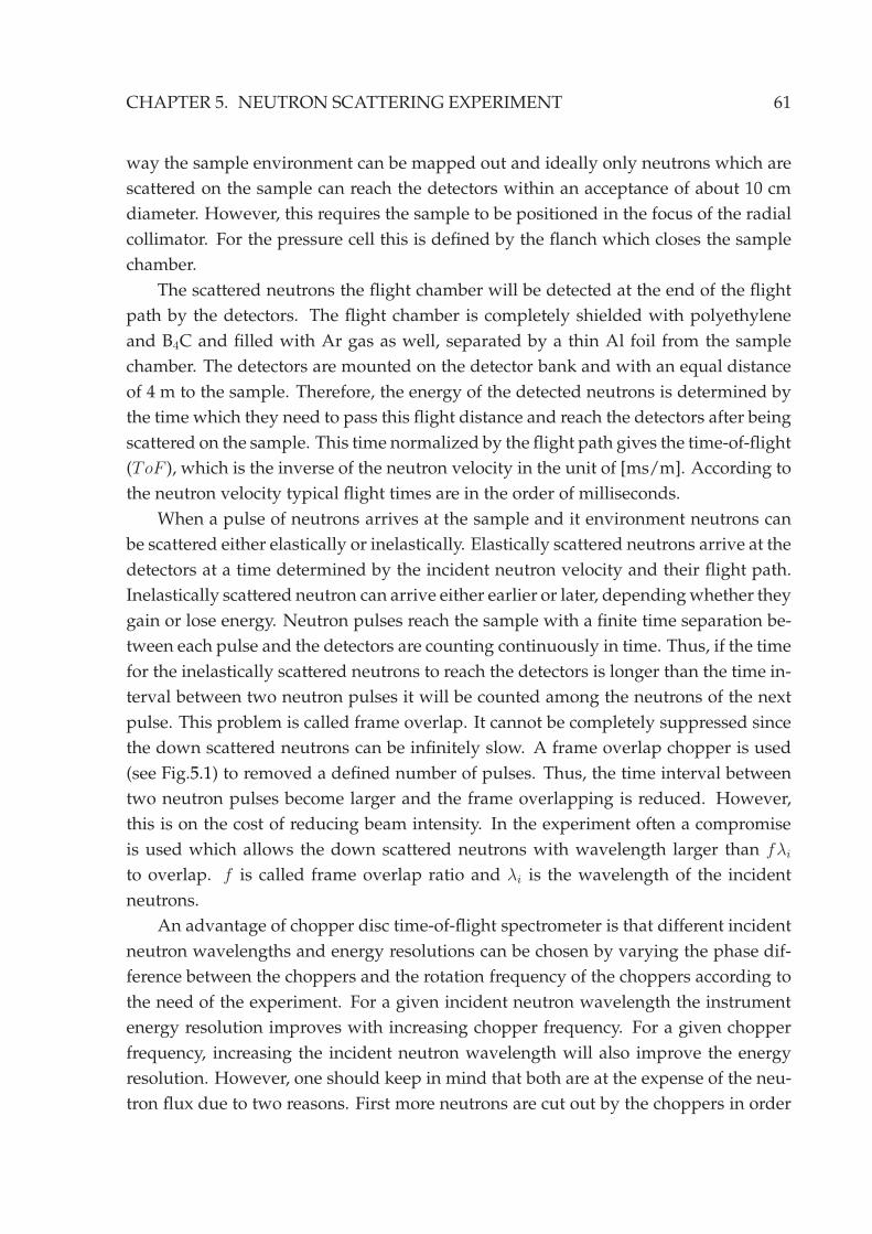
CHAPTER 5. NEUTRON SCATTERING EXPERIMENT 61
way the sample environment can be mapped out and ideally only neutrons which are
scattered on the sample can reach the detectors within an acceptance of about 10 cm
diameter. However, this requires the sample to be positioned in the focus of the radial
collimator. For the pressure cell this is defined by the flanch which closes the sample
chamber.
The scattered neutrons the flight chamber will be detected at the end of the flight
path by the detectors. The flight chamber is completely shielded with polyethylene
and B4C and filled with Ar gas as well, separated by a thin Al foil from the sample
chamber. The detectors are mounted on the detector bank and with an equal distance
of 4 m to the sample. Therefore, the energy of the detected neutrons is determined by
the time which they need to pass this flight distance and reach the detectors after being
scattered on the sample. This time normalized by the flight path gives the time-of-flight
(ToF ), which is the inverse of the neutron velocity in the unit of [ms/m]. According to
the neutron velocity typical flight times are in the order of milliseconds.
When a pulse of neutrons arrives at the sample and it environment neutrons can
be scattered either elastically or inelastically. Elastically scattered neutrons arrive at the
detectors at a time determined by the incident neutron velocity and their flight path.
Inelastically scattered neutron can arrive either earlier or later, dependingwhether they
gain or lose energy. Neutron pulses reach the sample with a finite time separation be-
tween each pulse and the detectors are counting continuously in time. Thus, if the time
for the inelastically scattered neutrons to reach the detectors is longer than the time in-
terval between two neutron pulses it will be counted among the neutrons of the next
pulse. This problem is called frame overlap. It cannot be completely suppressed since
the down scattered neutrons can be infinitely slow. A frame overlap chopper is used
(see Fig.5.1) to removed a defined number of pulses. Thus, the time interval between
two neutron pulses become larger and the frame overlapping is reduced. However,
this is on the cost of reducing beam intensity. In the experiment often a compromise
is used which allows the down scattered neutrons with wavelength larger than fλi
to overlap. f is called frame overlap ratio and λi is the wavelength of the incident
neutrons.
An advantage of chopper disc time-of-flight spectrometer is that different incident
neutron wavelengths and energy resolutions can be chosen by varying the phase dif-
ference between the choppers and the rotation frequency of the choppers according to
the need of the experiment. For a given incident neutron wavelength the instrument
energy resolution improves with increasing chopper frequency. For a given chopper
frequency, increasing the incident neutron wavelength will also improve the energy
resolution. However, one should keep in mind that both are at the expense of the neu-
tron flux due to two reasons. First more neutrons are cut out by the choppers in order
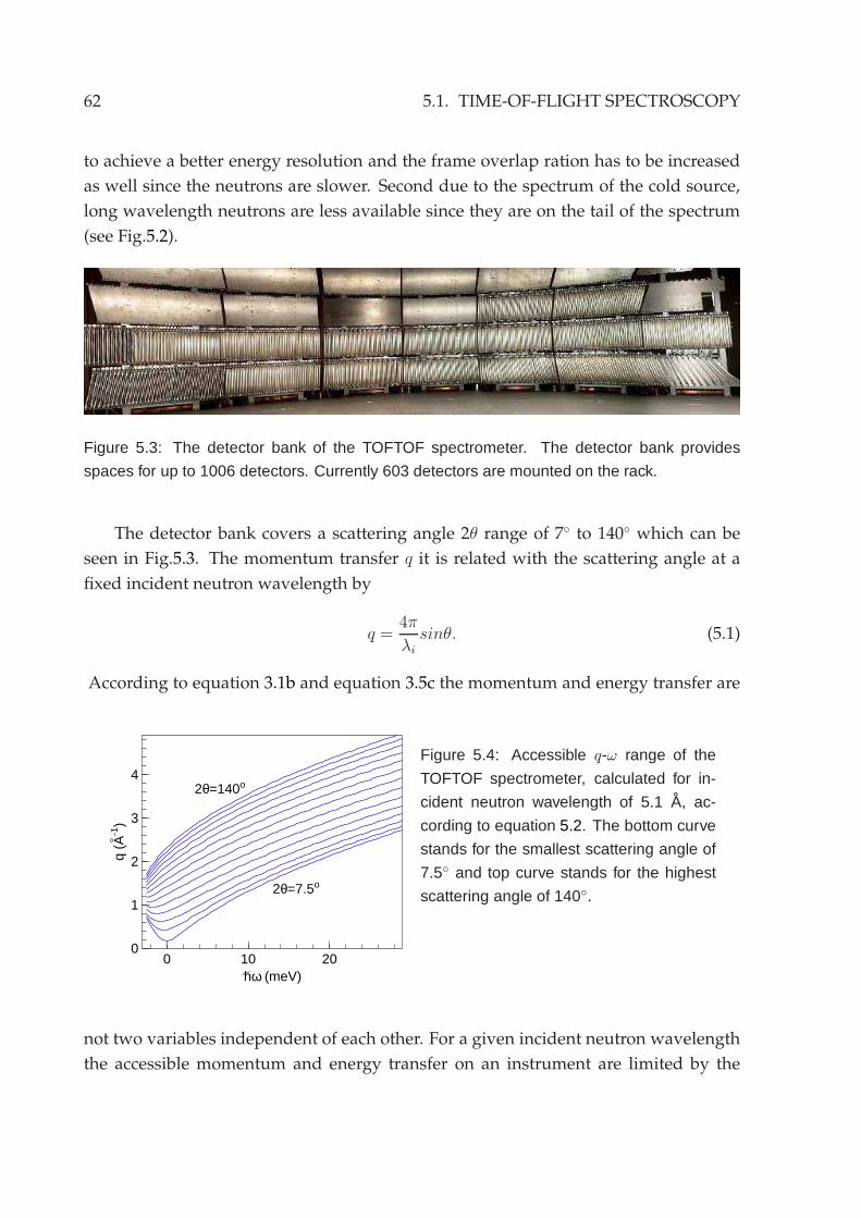
62 5.1. TIME-OF-FLIGHT SPECTROSCOPY
to achieve a better energy resolution and the frame overlap ration has to be increased
as well since the neutrons are slower. Second due to the spectrum of the cold source,
long wavelength neutrons are less available since they are on the tail of the spectrum
(see Fig.5.2).
Figure 5.3: The detector bank of the TOFTOF spectrometer. The detector bank provides
spaces for up to 1006 detectors. Currently 603 detectors are mounted on the rack.
The detector bank covers a scattering angle 2θ range of 7 to 140 which can be
seen in Fig.5.3. The momentum transfer q it is related with the scattering angle at a
fixed incident neutron wavelength by
q =4π
λi
sinθ. (5.1)
According to equation 3.1b and equation 3.5c the momentum and energy transfer are
0 10 200
1
2
3
4
hω (meV)
q (A
-1)
2θ=140o
2θ=7.5o
Figure 5.4: Accessible q-ω range of the
TOFTOF spectrometer, calculated for in-
cident neutron wavelength of 5.1 A, ac-
cording to equation 5.2. The bottom curve
stands for the smallest scattering angle of
7.5 and top curve stands for the highest
scattering angle of 140.
not two variables independent of each other. For a given incident neutron wavelength
the accessible momentum and energy transfer on an instrument are limited by the
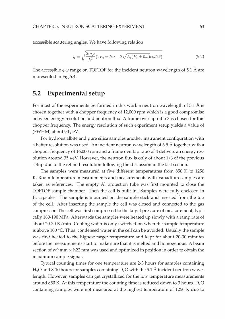
CHAPTER 5. NEUTRON SCATTERING EXPERIMENT 63
accessible scattering angles. We have following relation
q =
√
2mN
h2 (2Ei ± hω− 2√
Ei(Ei ± hω)cos2θ). (5.2)
The accessible q-ω range on TOFTOF for the incident neutron wavelength of 5.1 A are
represented in Fig.5.4.
5.2 Experimental setup
For most of the experiments performed in this work a neutron wavelength of 5.1 A is
chosen together with a chopper frequency of 12,000 rpm which is a good compromise
between energy resolution and neutron flux. A frame overlap ratio 3 is chosen for this
chopper frequency. The energy resolution of such experiment setup yields a value of
(FWHM) about 90 µeV.
For hydrous albite and pure silica samples another instrument configuration with
a better resolution was used. An incident neutron wavelength of 6.5 A together with a
chopper frequency of 16,000 rpm and a frame overlap ratio of 4 delivers an energy res-
olution around 35 µeV. However, the neutron flux is only of about 1/3 of the previous
setup due to the refined resolution following the discussion in the last section.
The samples were measured at five different temperatures from 850 K to 1250
K. Room temperature measurements and measurements with Vanadium samples are
taken as references. The empty Al protection tube was first mounted to close the
TOFTOF sample chamber. Then the cell is built in. Samples were fully enclosed in
Pt capsules. The sample is mounted on the sample stick and inserted from the top
of the cell. After inserting the sample the cell was closed and connected to the gas
compressor. The cell was first compressed to the target pressure of measurement, typi-
cally 180-190 MPa. Afterwards the samples were heated up slowly with a ramp rate of
about 20-30 K/min. Cooling water is only switched on when the sample temperature
is above 100 °C. Thus, condensed water in the cell can be avoided. Usually the sample
was first heated to the highest target temperature and kept for about 20-30 minutes
before the measurements start to make sure that it is melted and homogenous. A beam
section of w9 mm× h22 mmwas used and optimized in position in order to obtain the
maximum sample signal.
Typical counting times for one temperature are 2-3 hours for samples containing
H2O and 8-10 hours for samples containing D2Owith the 5.1 A incident neutron wave-
length. However, samples can get crystallized for the low temperature measurements
around 850 K. At this temperature the counting time is reduced down to 3 hours. D2O
containing samples were not measured at the highest temperature of 1250 K due to
64 5.3. REDUCTION OF NEUTRON DATA
a measurable exchange with the proton during the measurements (observation of in-
creasing of counting rate with time) and samples were only measured at four differ-
ent temperatures. For the measurements with 6.5 A incident neutron wavelength the
counting time is larger due to the reduction in neutron flux. It should be noted that
due to the presence of the massive cell good statistics of the raw spectrum still does
not necessarily indicate good statistics of the sample signal since the signal of the cell
contributes substantially to the raw spectrum. After the measurement the sample was
first heated above 900 °C for some minutes before cooling down rapidly below its glass
transition temperature in order to prevent crystallization. After cooled down to room
temperature the pressure was released gradually and the cell can be opened again for
changing samples.
For both incident neutron wavelength the Bragg peak of the Nb1Zr cell is not ex-
cited. However, due to the presence of the ceramic components of the furnace the
Bragg peak of the Al2O3 is excited and can be seen already in the empty cell mea-
surements (see e.g.: Fig.4.9). This corresponds to the scattering angle range around
90.3-96.8. Consequently at the momentum transfer q around 1.7-1.8 A the measured
signals were cut out.
5.3 Reduction of neutron data
In this section the reduction of raw neutron scattering data is presented. For the data
reduction and analysis the FRIDA program [WK07] developed originally by Joachim
Wuttke was used.
The raw data reduction includes normalization to a Vanadium standard, correction
of detector efficiency (of the neutron wavelength), correction for self-absorption and
interpolation to constant wavenumbers q.
The incident neutron beam is measured by a monitor which gives the monitor
counting rate
RM = PMAMΦi (5.3)
where PM is detector efficiency of monitor for a given incident neutron wavelength.
AM is the detection area of the monitor and Φi is the incoming neutron flux. The num-
ber of the counted scattered neutrons on the sample and its container which is detected
within a solid angle ∆Ω and the time interval ∆t is given by
NSC = P (2θ)P (λ)ASCΦiISC(2θ,ToF )∆t∆Ω. (5.4)
P (2θ) is the detection probability of the neutron as a function of the scattering an-
gle, which represents the difference in detection efficiency between different detectors.
CHAPTER 5. NEUTRON SCATTERING EXPERIMENT 65
P (λ) is the detection efficiency of different neutron wavelengths. ASC is the area of the
samples illuminated by the beam. Normalizing the counted neutron number NSC by
the monitor counting rate leads the counts to be independent of the incident neutron
flux.
Normalization to an incoherent scattering standard gives the scattered neutron in-
tensity on an absolute scale independent of the detection time interval and detection
probabilities. This is typically done with a Vanadium standard. Vanadium can be con-
sidered as a pure incoherent scatterer. Only the intensities of the elastically scattered
neutrons from the Vanadium sample are taken for the normalization
NV = P (2θ)P (λel)AV ΦiIV (2θ)∆Ω. (5.5)
which is then corrected with the Debye-Waller factor of the Vanadium calculated at the
measurement temperature. After normalized to the Vanadium intensity the scattering
intensity can be obtained by
ISIG(2θ,ToF ) =NSC
NV
P (λel)
P (λ)
AV
ASC
IV (2θ)
∆t(5.6)
The time-of-flight ToF represents the energy of the neutrons. It can be related to
the energy transfer hω by
hω =1
2mN [(1/ToFel)
2 − (1/ToF )2]. (5.7)
Thus, the double differential scattering cross section can be represented in terms of the
neutron flight time given by
∂2σ
∂Ω∂ω=
∂2σ
∂Ω∂ToF
∂ToF
∂ω=
∂2σ
∂Ω∂ToF
hToF 3
mN. (5.8)
The measured intensity is proportional to the double differential scattering cross sec-
tion∂2σ
∂Ω∂ω∝ kf
kiSSIG(2θ,ω);
∂2σ
∂Ω∂ToF∝ ISIG(2θ,ToF ) (5.9)
and by inserting equation 5.8 the measured intensity can be converted from ToF to
energy ω using
SSIG(2θ,ω) = Aki
kf
hT oF 3
mNISIG(2θ,ToF ) (5.10)
The prefactor A is related with the number density of the scatterers, the flight path
of the neutron (scattering geometry) in the sample and the Vanadium. The final neu-
tron wavenumber kf also depends on the ToF which leads a ToF 4 dependence of the
66 5.3. REDUCTION OF NEUTRON DATA
scattering intensity on the neutron time-of-flight spectra. In order to obtain the cor-
rect scattering intensity SSIG the detector efficiency for different neutron wavelength
should be taken into account as well.
The measured intensity in a neutron scattering experiment is contributed from the
sample (SS) and the pressure cell (SC), which are not additive. A simple subtraction
of the scattering signal of the empty cell from the one of the sample with the cell (SSC)
is not possible. Necessary corrections from the calculation of Paalman and Pings for
cylindrical sample geometry is used here to take into account the loss of the intensity
due to absorption [PP62]. Different correction factors are used which are functions
of the scattering angle and the neutron energy transfer. The correction factor AS,SC
counts for the intensity loss of the neutrons which are scattered on the sample and
absorbed by either the sample or its container. AC,SC counts for the intensity loss of the
neutrons which are scattered on the container and absorbed by either the sample or the
container. AC,C takes account for the intensity loss which is only from the container.
These factors are calculated using the absorption cross sections of the sample and the
cell and an optical path length (depends on the sample geometry) of the incoming and
scattered neutron beam. The factors AC,SC and AC,C are often grouped into one factor
Arel =AC,SC
AC,Csince they correct the scattering from the container.
The normalization and background subtraction are done within the FRIDA pro-
gram. However, several points should be noted due to presence of the massive pres-
sure cell which leads the resulting intensity cannot be compared with the measure-
ments results obtained with a standard sample environment on an absolute scale.
The Paalmann and Pings calculation can be further developed for partial beam
coverage. These calculations are all based on a homogenous beam profile which is pre-
sented at TOFTOF. The advantage of these formalisms is that the correction factors can
be expressed in terms of analytical functions. However, due to the complex structure
of sample environment (aluminum protection, cell, ceramic furnace, sample capsule)
and the partial beam coverage these calculations only provide an approximation. The
exact value of these factors can be only deduced with numerical methods like for ex-
ample Monto-Carlo simulations [BBTC91]. Thus the calculation done by the FRIDA
program only gives an estimation of these factors.
In order to perform the calculation, the knowledge of cell transmission, scatterer
number density of the sample and the scattering and absorption cross sections are
necessary. The exact values of the first two quantities are unknown. The absorptance
of the cell needs to be measured under a transmission geometry which is not available
on the TOFTOF spectrometer. The transmission of the cell is taken from a Nb cell
with a similar amount of Nb material in the beam [FA02]. The number density of
the sample need to be calculated with the knowledge of the density of the samples.
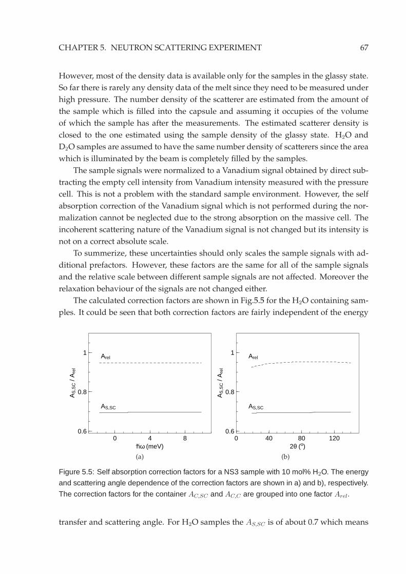
CHAPTER 5. NEUTRON SCATTERING EXPERIMENT 67
However, most of the density data is available only for the samples in the glassy state.
So far there is rarely any density data of the melt since they need to be measured under
high pressure. The number density of the scatterer are estimated from the amount of
the sample which is filled into the capsule and assuming it occupies of the volume
of which the sample has after the measurements. The estimated scatterer density is
closed to the one estimated using the sample density of the glassy state. H2O and
D2O samples are assumed to have the same number density of scatterers since the area
which is illuminated by the beam is completely filled by the samples.
The sample signals were normalized to a Vanadium signal obtained by direct sub-
tracting the empty cell intensity from Vanadium intensity measured with the pressure
cell. This is not a problem with the standard sample environment. However, the self
absorption correction of the Vanadium signal which is not performed during the nor-
malization cannot be neglected due to the strong absorption on the massive cell. The
incoherent scattering nature of the Vanadium signal is not changed but its intensity is
not on a correct absolute scale.
To summerize, these uncertainties should only scales the sample signals with ad-
ditional prefactors. However, these factors are the same for all of the sample signals
and the relative scale between different sample signals are not affected. Moreover the
relaxation behaviour of the signals are not changed either.
The calculated correction factors are shown in Fig.5.5 for the H2O containing sam-
ples. It could be seen that both correction factors are fairly independent of the energy
0 4 80.6
0.8
1
hω (meV)
AS
,SC /
Are
l
AS,SC
Arel
(a)
0 40 80 1200.6
0.8
1
2θ (o)
AS
,SC /
Are
l
AS,SC
Arel
(b)
Figure 5.5: Self absorption correction factors for a NS3 sample with 10 mol% H2O. The energy
and scattering angle dependence of the correction factors are shown in a) and b), respectively.
The correction factors for the container AC,SC and AC,C are grouped into one factor Arel.
transfer and scattering angle. For H2O samples the AS,SC is of about 0.7 which means
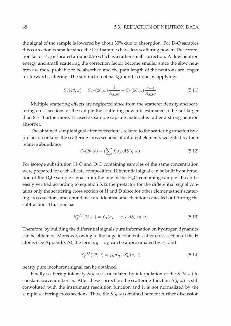
68 5.3. REDUCTION OF NEUTRON DATA
the signal of the sample is lowered by about 30% due to absorption. For D2O samples
this correction is smaller since the D2O samples have less scattering power. The correc-
tion factorArel is located around 0.95which is a rather small correction. At low neutron
energy and small scattering the correction factor become smaller since the slow neu-
tron are more probable to be absorbed and the path length of the neutrons are longer
for forward scattering. The subtraction of background is done by applying:
SS(2θ,ω) = SSC(2θ,ω)1
AS,SC
− SC(2θ,ω)Arel
AS,SC
. (5.11)
Multiple scattering effects are neglected since from the scatterer density and scat-
tering cross sections of the sample the scattering power is estimated to be not larger
than 8%. Furthermore, Pt used as sample capsule material is rather a strong neutron
absorber.
The obtained sample signal after correction is related to the scattering function by a
prefactor contains the scattering cross sections of different elements weighted by their
relative abundance
SS(2θ,ω) = (∑
j
fjσj)AS(q,ω). (5.12)
For isotope substitution H2O and D2O containing samples of the same concentration
were prepared for each silicate composition. Differential signal can be built by subtrac-
tion of the D2O sample signal from the one of the H2O containing sample. It can be
easily verified according to equation 5.12 the prefactor for the differential signal con-
tains only the scattering cross section of H and D since for other elements their scatter-
ing cross sections and abundance are identical and therefore canceled out during the
subtraction. Thus one has
SdiffS (2θ,ω) = fH(σH − σD)ASH(q,ω) (5.13)
Therefore, by building the differential signals pure information on hydrogen dynamics
can be obtained. Moreover, owing to the huge incoherent scatter cross section of the H
atoms (see Appendix A), the term σH − σD can be approximated by σiH and
SdiffS (2θ,ω) = fHσ
iHAS
iH(q,ω) (5.14)
nearly pure incoherent signal can be obtained.
Finally scattering intensity S(q,ω) is calculated by interpolation of the S(2θ,ω) to
constant wavenumbers q. After these correction the scattering function S(q,ω) is still
convoluted with the instrument resolution function and it is not normalized by the
sample scattering cross sections. Thus, the S(q,ω) obtained here for further discussion
CHAPTER 5. NEUTRON SCATTERING EXPERIMENT 69
are weighted by the scattering cross sections.
There are two ways to analyze the data, either in the energy domain or in the time
domain, both should give the same results. For energy domain analysis the fitting
functions need be convoluted with the instrument resolution function. The instrument
resolution function is measured with Vanadium standard and dry samples at room
temperature. The instrument resolution function of the TOFTOF spectrometer can be
well approximated by a Gaussian function [UNP07]. Therefore, the measured signal is
fitted with a Gaussian function and the fitting result is used for further data analysis.
Another way to analysis the data is to perform a Fourier transformation of the
scattering function S(q,ω) to obtain the intermediate scattering function S(q, t). For
100 1010
0.5
1
Time (ps)
S(q
,t) (
a.u.
)
S(q,t)FTS(q,ω)R(q,t)
cutoff
Figure 5.6: Deconvolution of the instrument res-
olution function R(q, t) from the Fourier trans-
formed scattering function S(q,ω) to obtain the
intermediate scattering function S(q, t). The in-
strument resolution function can be well approx-
imated by a Gaussian function (thin solid line).
The cutoff at large time is taken as the resolution
function decays to about 30% of its initial value.
This corresponds to a timescale up to 25 ps.
calculation of the Fourier transformation only data of S(q,ω) on the positive energy
transfer side is used (neutron energy gain). However, due to the finite range of the
energy transfer, a proper t→ 0 limit can not be obtained. For the resolution function
the zero time limit is obtained by extrapolating the small time data to t = 0. Thus, the
sample signal S(q, t = 0) does not correspond to the static structure factor S(q). After
the Fourier transformation the sample signal is still convoluted with the instrument
resolution function. The advantage of the time domain data analysis is that the de-
convoluted signal can be obtained by a simple division of the sample signal by the
instrument resolution, as shown in Fig.5.6. It could also be observed that the instru-
ment resolution function can be well approximated by a Gaussian function. Therefore,
for later data evaluation this Gaussian fitting for the instrument resolution function
were used.
The cutoff at large times is taken where the resolution function decays to about
30% of its initial value, corresponding to a timescale up to 25 ps. For the time larger
than the cutoff time the spectra are dominated by the instrument resolution function.
70 5.4. NEUTRON BACKSCATTERING SPECTROSCOPY
5.4 Neutron backscattering spectroscopy
Neutron backscattering spectroscopy measures the same physical quantity as in the
neutron time-of-flight experiment: the scattering function S(q,ω), however with a
significantly different energy transfer range. Typically neutron backscattering spec-
troscopy measures a dynamic range of maximum several tens of µeV with an energy
resolution in the sub-µeV range. This give access to timescale up to the order of ns.
To achieve an energy resolution in the sub-µeV range neutron backscattering spec-
troscopy uses crystal Bragg reflection for both monochromatization and analyzation of
the neutron energy. The Bragg reflection condition is given by
nλ = 2dsinθ. (5.15)
The uncertainty or in other words the resolution can be easily shown by differentiating
5.15∆λ
λ=
∆d
d+
∆θ
tanθ. (5.16)
According to this relation the uncertainty in crystal monochromatization is coming
from two contributions: lattice misfit of the monochromator crystal ∆d and the diver-
gence in the neutron incident angle ∆θ.
Backscattering benefits from the fact that under the scattering angle 2θ=180o the
angular contribution vanishes. Thus, the energy resolution ∆λ/λ reaches its minimum
which only depends on the degree of lattice mismatch1. Typically Silicon 111 lattice
plane is used for monochromatization and under backscattering condition this results
an incident neutron wavelength of 6.271 A which fulfills the Bragg condition.
However, practically although under backscattering condition the neutron beam
is perpendicular to the crystal Bragg plan, not all the neutrons in the beam will hit the
plan at an angle of 90o since the neutron trajectories in a beamwill never be all parallel.
The ∆θ in the incident angle does contributes to the wavelength uncertainty.
The scattered neutrons energies are analyzed in the same backscattering manner.
In this sense a backscattering spectrometer is very similar to a triple-axis instrument.
However, to cover an energy transfer range which is determined by how much the
incident and scattering neutron energies are shifted to each other, it cannot be realized
by varying the Bragg angle of the monochromator crystal like as it is done on the triple-
axis spectrometer since this will destroy the excellent energy resolution. It can be only
achieved using methods like continuous changing the monochromator d spacing by
changing its temperature, or via a Doppler motion of the monochromator.
1The ∆d/d value will never reaches zero even for a perfect crystal due to dynamical scattering, whichdefines a lower (theoretical) limit for the energy resolution of the backscattering technique, called Dar-win width.
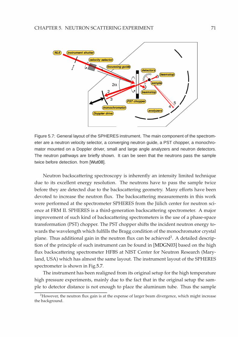
CHAPTER 5. NEUTRON SCATTERING EXPERIMENT 71
Figure 5.7: General layout of the SPHERES instrument. The main component of the spectrom-
eter are a neutron velocity selector, a converging neutron guide, a PST chopper, a monochro-
mator mounted on a Doppler driver, small and large angle analyzers and neutron detectors.
The neutron pathways are briefly shown. It can be seen that the neutrons pass the sample
twice before detection. from [Wut08].
Neutron backscattering spectroscopy is inherently an intensity limited technique
due to its excellent energy resolution. The neutrons have to pass the sample twice
before they are detected due to the backscattering geometry. Many efforts have been
devoted to increase the neutron flux. The backscattering measurements in this work
were performed at the spectrometer SPHERES from the Julich center for neutron sci-
ence at FRM II. SPHERES is a third-generation backscattering spectrometer. A major
improvement of such kind of backscattering spectrometers is the use of a phase-space
transformation (PST) chopper. The PST chopper shifts the incident neutron energy to-
wards the wavelength which fulfills the Bragg condition of the monochromator crystal
plane. Thus additional gain in the neutron flux can be achieved2. A detailed descrip-
tion of the principle of such instrument can be found in [MDGN03] based on the high
flux backscattering spectrometer HFBS at NIST Center for Neutron Research (Mary-
land, USA) which has almost the same layout. The instrument layout of the SPHERES
spectrometer is shown in Fig.5.7.
The instrument has been realigned from its original setup for the high temperature
high pressure experiments, mainly due to the fact that in the original setup the sam-
ple to detector distance is not enough to place the aluminum tube. Thus the sample
2However, the neutron flux gain is at the expense of larger beam divergence, which might increasethe background.
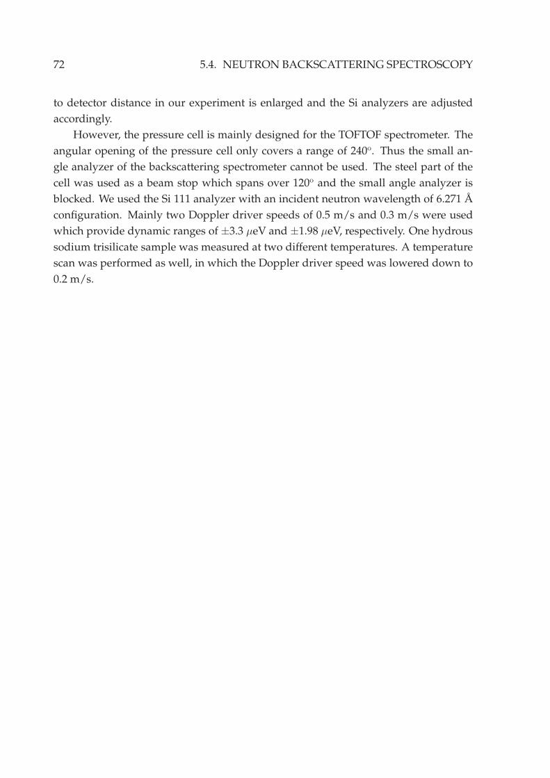
72 5.4. NEUTRON BACKSCATTERING SPECTROSCOPY
to detector distance in our experiment is enlarged and the Si analyzers are adjusted
accordingly.
However, the pressure cell is mainly designed for the TOFTOF spectrometer. The
angular opening of the pressure cell only covers a range of 240o. Thus the small an-
gle analyzer of the backscattering spectrometer cannot be used. The steel part of the
cell was used as a beam stop which spans over 120o and the small angle analyzer is
blocked. We used the Si 111 analyzer with an incident neutron wavelength of 6.271 A
configuration. Mainly two Doppler driver speeds of 0.5 m/s and 0.3 m/s were used
which provide dynamic ranges of ±3.3 µeV and ±1.98 µeV, respectively. One hydrous
sodium trisilicate sample was measured at two different temperatures. A temperature
scan was performed as well, in which the Doppler driver speed was lowered down to
0.2 m/s.
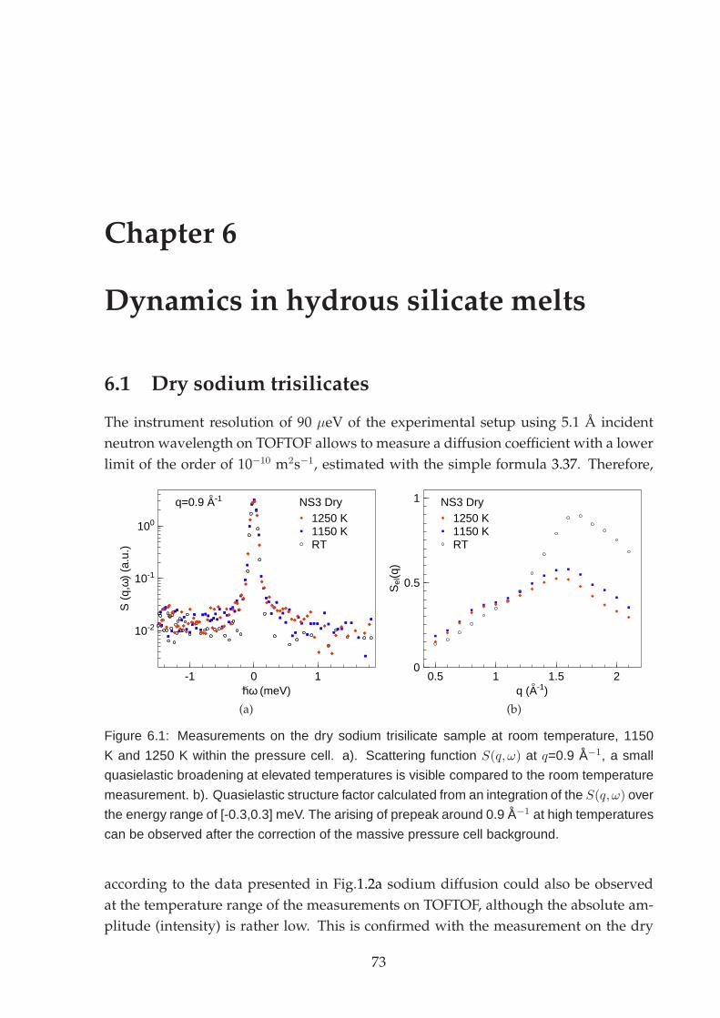
Chapter 6
Dynamics in hydrous silicate melts
6.1 Dry sodium trisilicates
The instrument resolution of 90 µeV of the experimental setup using 5.1 A incident
neutron wavelength on TOFTOF allows to measure a diffusion coefficient with a lower
limit of the order of 10−10 m2s−1, estimated with the simple formula 3.37. Therefore,
-1 0 1
10-2
10-1
100
hω (meV)
S (
q,ω
) (a
.u.)
NS3 Dryq=0.9 A-1
1250 K1150 KRT
(a)
0.5 1 1.5 20
0.5
1
q (A-1)
Sel(q
)
NS3 Dry1250 K1150 KRT
(b)
Figure 6.1: Measurements on the dry sodium trisilicate sample at room temperature, 1150
K and 1250 K within the pressure cell. a). Scattering function S(q,ω) at q=0.9 A−1, a small
quasielastic broadening at elevated temperatures is visible compared to the room temperature
measurement. b). Quasielastic structure factor calculated from an integration of the S(q,ω) over
the energy range of [-0.3,0.3] meV. The arising of prepeak around 0.9 A−1 at high temperatures
can be observed after the correction of the massive pressure cell background.
according to the data presented in Fig.1.2a sodium diffusion could also be observed
at the temperature range of the measurements on TOFTOF, although the absolute am-
plitude (intensity) is rather low. This is confirmed with the measurement on the dry
73
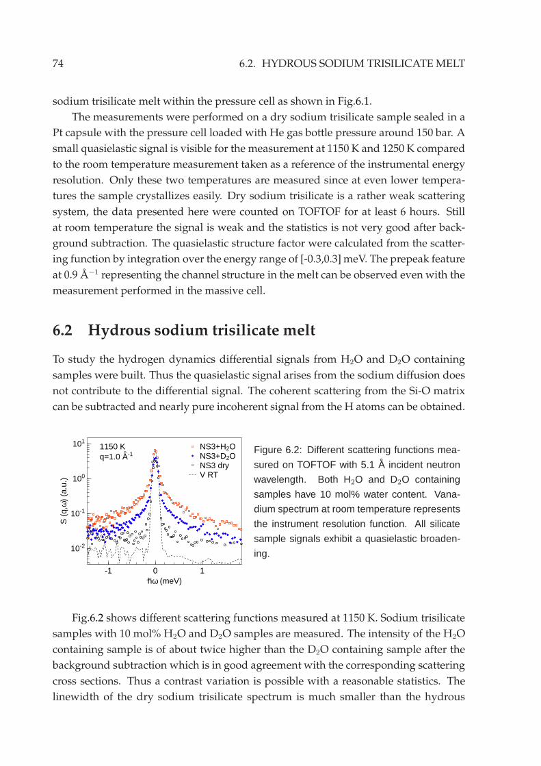
74 6.2. HYDROUS SODIUM TRISILICATEMELT
sodium trisilicate melt within the pressure cell as shown in Fig.6.1.
The measurements were performed on a dry sodium trisilicate sample sealed in a
Pt capsule with the pressure cell loaded with He gas bottle pressure around 150 bar. A
small quasielastic signal is visible for the measurement at 1150 K and 1250 K compared
to the room temperature measurement taken as a reference of the instrumental energy
resolution. Only these two temperatures are measured since at even lower tempera-
tures the sample crystallizes easily. Dry sodium trisilicate is a rather weak scattering
system, the data presented here were counted on TOFTOF for at least 6 hours. Still
at room temperature the signal is weak and the statistics is not very good after back-
ground subtraction. The quasielastic structure factor were calculated from the scatter-
ing function by integration over the energy range of [-0.3,0.3] meV. The prepeak feature
at 0.9 A−1 representing the channel structure in the melt can be observed even with the
measurement performed in the massive cell.
6.2 Hydrous sodium trisilicate melt
To study the hydrogen dynamics differential signals from H2O and D2O containing
samples were built. Thus the quasielastic signal arises from the sodium diffusion does
not contribute to the differential signal. The coherent scattering from the Si-O matrix
can be subtracted and nearly pure incoherent signal from the H atoms can be obtained.
-1 0 1
10-2
10-1
100
101
hω (meV)
S (
q,ω
) (a
.u.)
1150 Kq=1.0 A-1
NS3+H2ONS3+D2ONS3 dryV RT
Figure 6.2: Different scattering functions mea-
sured on TOFTOF with 5.1 A incident neutron
wavelength. Both H2O and D2O containing
samples have 10 mol% water content. Vana-
dium spectrum at room temperature represents
the instrument resolution function. All silicate
sample signals exhibit a quasielastic broaden-
ing.
Fig.6.2 shows different scattering functions measured at 1150 K. Sodium trisilicate
samples with 10 mol% H2O and D2O samples are measured. The intensity of the H2O
containing sample is of about twice higher than the D2O containing sample after the
background subtraction which is in good agreement with the corresponding scattering
cross sections. Thus a contrast variation is possible with a reasonable statistics. The
linewidth of the dry sodium trisilicate spectrum is much smaller than the hydrous
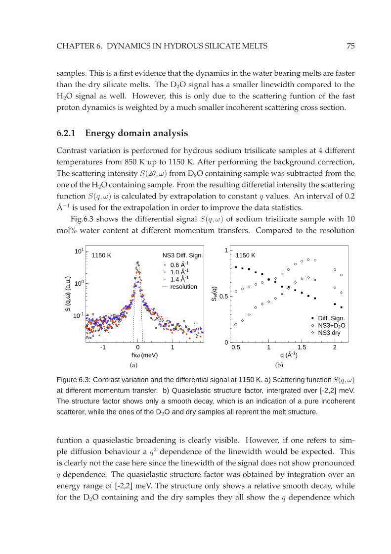
CHAPTER 6. DYNAMICS IN HYDROUS SILICATEMELTS 75
samples. This is a first evidence that the dynamics in the water bearing melts are faster
than the dry silicate melts. The D2O signal has a smaller linewidth compared to the
H2O signal as well. However, this is only due to the scattering funtion of the fast
proton dynamics is weighted by a much smaller incoherent scattering cross section.
6.2.1 Energy domain analysis
Contrast variation is performed for hydrous sodium trisilicate samples at 4 different
temperatures from 850 K up to 1150 K. After performing the background correction,
The scattering intensity S(2θ,ω) from D2O containing sample was subtracted from the
one of theH2O containing sample. From the resulting differetial intensity the scattering
function S(q,ω) is calculated by extrapolation to constant q values. An interval of 0.2
A−1 is used for the extrapolation in order to improve the data statistics.
Fig.6.3 shows the differential signal S(q,ω) of sodium trisilicate sample with 10
mol% water content at different momentum transfers. Compared to the resolution
-1 0 1
10-1
100
101
hω (meV)
S (
q,ω
) (a
.u.)
NS3 Diff. Sign.1150 K
0.6 A-1
1.0 A-1
1.4 A-1
resolution
(a)
0.5 1 1.5 20
0.5
1
q (A-1)
Sel(q
)
1150 K
Diff. Sign.NS3+D2ONS3 dry
(b)
Figure 6.3: Contrast variation and the differential signal at 1150 K. a) Scattering function S(q,ω)
at different momentum transfer. b) Quasielastic structure factor, intergrated over [-2,2] meV.
The structure factor shows only a smooth decay, which is an indication of a pure incoherent
scatterer, while the ones of the D2O and dry samples all reprent the melt structure.
funtion a quasielastic broadening is clearly visible. However, if one refers to sim-
ple diffusion behaviour a q2 dependence of the linewidth would be expected. This
is clearly not the case here since the linewidth of the signal does not show pronounced
q dependence. The quasielastic structure factor was obtained by integration over an
energy range of [-2,2] meV. The structure only shows a relative smooth decay, while
for the D2O containing and the dry samples they all show the q dependence which
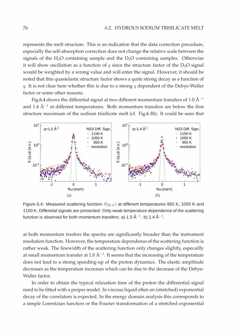
76 6.2. HYDROUS SODIUM TRISILICATEMELT
represents the melt structure. This is an indication that the data correction precedure,
especially the self-absorption correction does not change the relative scale between the
signals of the H2O containing sample and the D2O containing samples. Otherwise
it will show oscillation as a function of q since the structure factor of the D2O signal
would be weighted by a wrong value and will enter the signal. However, it should be
noted that this quasielastic structure factor shows a quite strong decay as a function of
q. It is not clear here whether this is due to a strong q dependent of the Debye-Waller
factor or some other reasons.
Fig.6.4 shows the differetial signal at two different momentum transfers of 1.0 A−1
and 1.4 A−1 at different temperatures. Both momentum transfers are below the first
structure maximum of the sodium trisilicate melt (cf. Fig.6.1b). It could be seen that
-1 0 1
10-1
100
101
hω (meV)
S (
q,ω
) (a
.u.)
NS3 Diff. Sign.q=1.0 A-1
1150 K1050 K 950 Kresolution
(a)
-1 0 1
10-1
100
101
hω (meV)
S (
q,ω
) (a
.u.)
NS3 Diff. Sign.q=1.4 A-1
1150 K1050 K 950 Kresolution
(b)
Figure 6.4: Measured scattering function S(q,ω) at different temperatures 950 K, 1050 K and
1150 K. Differetial signals are presented. Only weak temperature dependence of the scattering
function is observed for both momentum transfers: a) 1.0 A−1. b) 1.4 A−1.
at both momentum trasfers the spectra are significantly broader than the instrument
resolution function. However, the temperature dependence of the scattering function is
rather weak. The linewidth of the scattering function only changes slightly, especailly
at small momentum transfer at 1.0 A−1. It seems that the increasing of the temperature
does not lead to a strong speeding-up of the proton dynamics. The elastic amplitude
decreases as the temperature increases which can be due to the decrease of the Debye-
Waller factor.
In order to obtain the typical relaxation time of the proton the differential signal
need to be fittedwith a propermodel. In viscous liquid often an (stretched) exponential
decay of the correlators is expected. In the energy domain analysis this corresponds to
a simple Lorentzian function or the Fourier transformation of a stretched exponential
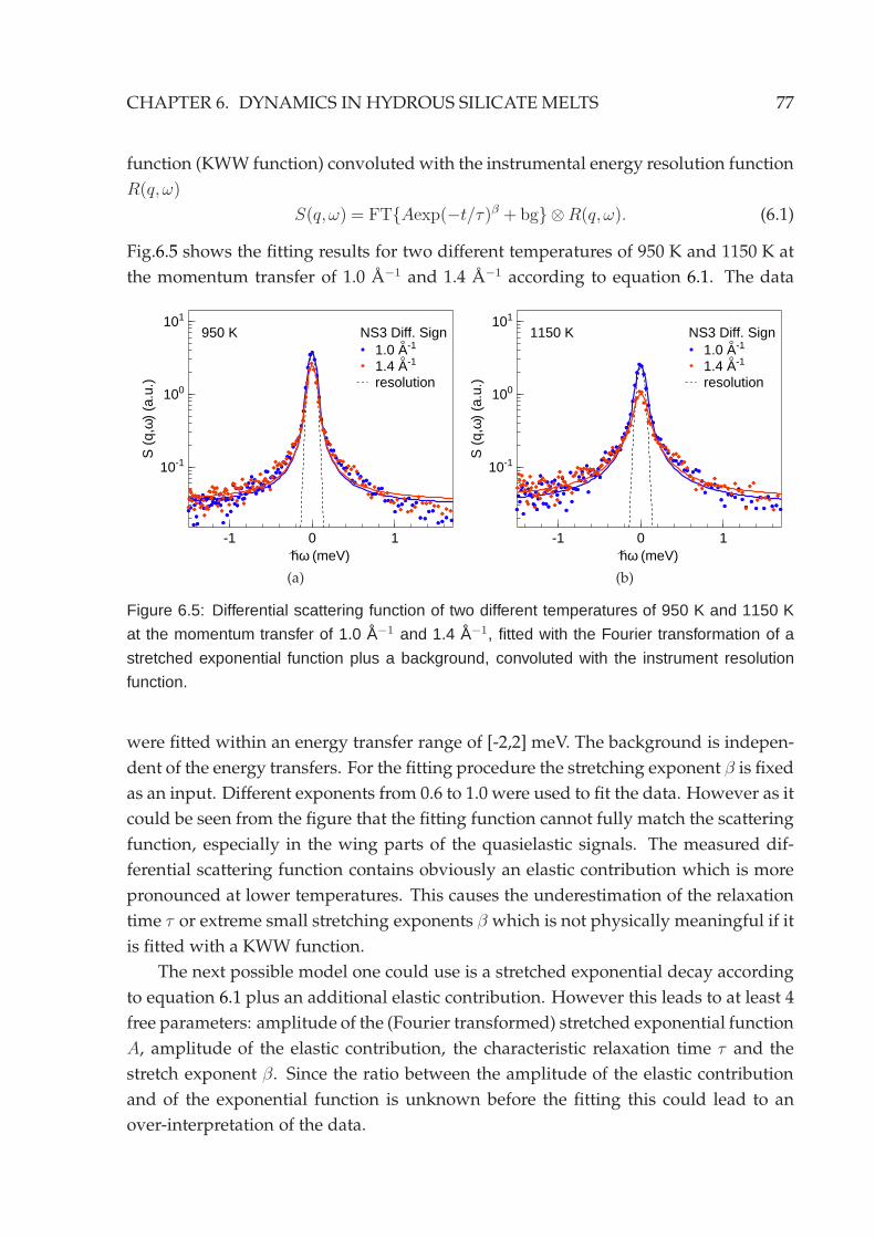
CHAPTER 6. DYNAMICS IN HYDROUS SILICATEMELTS 77
function (KWW function) convoluted with the instrumental energy resolution function
R(q,ω)
S(q,ω) = FTAexp(−t/τ)β + bg ⊗R(q,ω). (6.1)
Fig.6.5 shows the fitting results for two different temperatures of 950 K and 1150 K at
the momentum transfer of 1.0 A−1 and 1.4 A−1 according to equation 6.1. The data
-1 0 1
10-1
100
101
hω (meV)
S (
q,ω
) (a
.u.)
NS3 Diff. Sign950 K1.0 A-1
1.4 A-1
resolution
(a)
-1 0 1
10-1
100
101
hω (meV)
S (
q,ω
) (a
.u.)
NS3 Diff. Sign1150 K1.0 A-1
1.4 A-1
resolution
(b)
Figure 6.5: Differential scattering function of two different temperatures of 950 K and 1150 K
at the momentum transfer of 1.0 A−1 and 1.4 A−1, fitted with the Fourier transformation of a
stretched exponential function plus a background, convoluted with the instrument resolution
function.
were fitted within an energy transfer range of [-2,2] meV. The background is indepen-
dent of the energy transfers. For the fitting procedure the stretching exponent β is fixed
as an input. Different exponents from 0.6 to 1.0 were used to fit the data. However as it
could be seen from the figure that the fitting function cannot fully match the scattering
function, especially in the wing parts of the quasielastic signals. The measured dif-
ferential scattering function contains obviously an elastic contribution which is more
pronounced at lower temperatures. This causes the underestimation of the relaxation
time τ or extreme small stretching exponents β which is not physically meaningful if it
is fitted with a KWW function.
The next possible model one could use is a stretched exponential decay according
to equation 6.1 plus an additional elastic contribution. However this leads to at least 4
free parameters: amplitude of the (Fourier transformed) stretched exponential function
A, amplitude of the elastic contribution, the characteristic relaxation time τ and the
stretch exponent β. Since the ratio between the amplitude of the elastic contribution
and of the exponential function is unknown before the fitting this could lead to an
over-interpretation of the data.
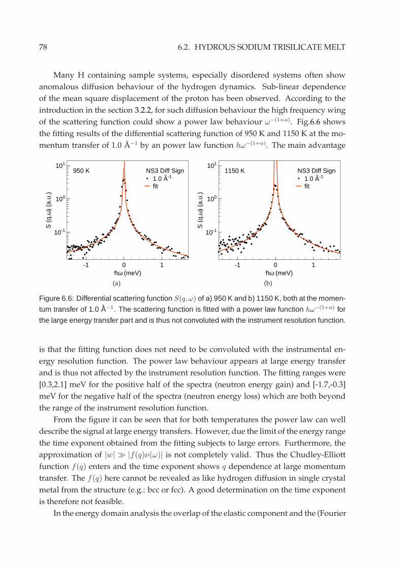
78 6.2. HYDROUS SODIUM TRISILICATEMELT
Many H containing sample systems, especially disordered systems often show
anomalous diffusion behaviour of the hydrogen dynamics. Sub-linear dependence
of the mean square displacement of the proton has been observed. According to the
introduction in the section 3.2.2, for such diffusion behaviour the high frequency wing
of the scattering function could show a power law behaviour ω−(1+α). Fig.6.6 shows
the fitting results of the differential scattering function of 950 K and 1150 K at the mo-
mentum transfer of 1.0 A−1 by an power law function hω−(1+α). The main advantage
-1 0 1
10-1
100
101
hω (meV)
S (
q,ω
) (a
.u.)
NS3 Diff Sign950 K1.0 A-1
fit
(a)
-1 0 1
10-1
100
101
hω (meV)
S (
q,ω
) (a
.u.)
NS3 Diff Sign1150 K1.0 A-1
fit
(b)
Figure 6.6: Differential scattering function S(q,ω) of a) 950 K and b) 1150 K, both at the momen-
tum transfer of 1.0 A−1. The scattering function is fitted with a power law function hω−(1+α) for
the large energy transfer part and is thus not convoluted with the instrument resolution function.
is that the fitting function does not need to be convoluted with the instrumental en-
ergy resolution function. The power law behaviour appears at large energy transfer
and is thus not affected by the instrument resolution function. The fitting ranges were
[0.3,2.1] meV for the positive half of the spectra (neutron energy gain) and [-1.7,-0.3]
meV for the negative half of the spectra (neutron energy loss) which are both beyond
the range of the instrument resolution function.
From the figure it can be seen that for both temperatures the power law can well
describe the signal at large energy transfers. However, due the limit of the energy range
the time exponent obtained from the fitting subjects to large errors. Furthermore, the
approximation of |w| ≫ |f(q)ν(ω)| is not completely valid. Thus the Chudley-Elliott
function f(q) enters and the time exponent shows q dependence at large momentum
transfer. The f(q) here cannot be revealed as like hydrogen diffusion in single crystal
metal from the structure (e.g.: bcc or fcc). A good determination on the time exponent
is therefore not feasible.
In the energy domain analysis the overlap of the elastic component and the (Fourier
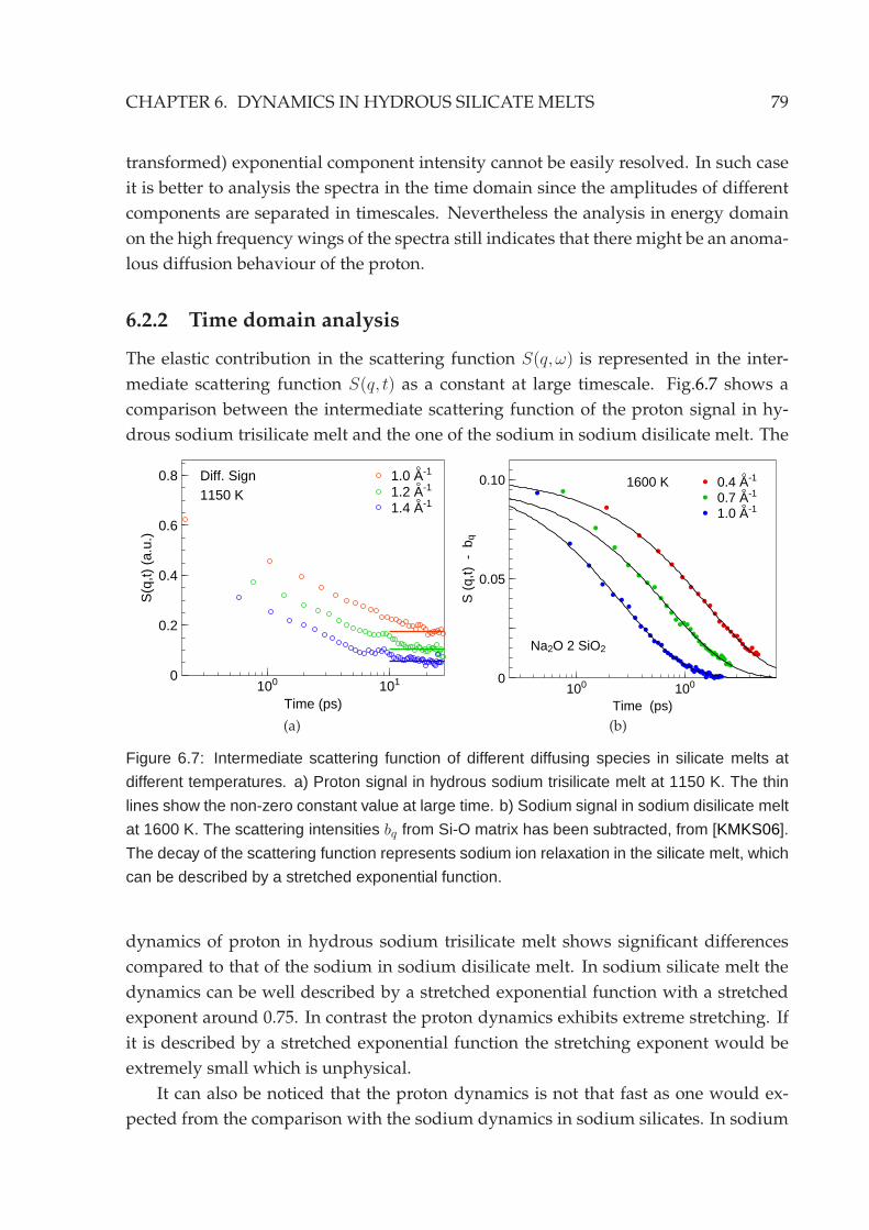
CHAPTER 6. DYNAMICS IN HYDROUS SILICATEMELTS 79
transformed) exponential component intensity cannot be easily resolved. In such case
it is better to analysis the spectra in the time domain since the amplitudes of different
components are separated in timescales. Nevertheless the analysis in energy domain
on the high frequency wings of the spectra still indicates that there might be an anoma-
lous diffusion behaviour of the proton.
6.2.2 Time domain analysis
The elastic contribution in the scattering function S(q,ω) is represented in the inter-
mediate scattering function S(q, t) as a constant at large timescale. Fig.6.7 shows a
comparison between the intermediate scattering function of the proton signal in hy-
drous sodium trisilicate melt and the one of the sodium in sodium disilicate melt. The
100 1010
0.2
0.4
0.6
0.8
Time (ps)
S(q
,t) (
a.u.
)
Diff. Sign1150 K
1.0 A-1
1.2 A-1
1.4 A-1
(a)
100 1000
0.05
0.10
Time (ps)
S (
q,t)
- b
q
Na2O 2 SiO2
1600 K 0.4 A-1
0.7 A-1
1.0 A-1
(b)
Figure 6.7: Intermediate scattering function of different diffusing species in silicate melts at
different temperatures. a) Proton signal in hydrous sodium trisilicate melt at 1150 K. The thin
lines show the non-zero constant value at large time. b) Sodium signal in sodium disilicate melt
at 1600 K. The scattering intensities bq from Si-O matrix has been subtracted, from [KMKS06].
The decay of the scattering function represents sodium ion relaxation in the silicate melt, which
can be described by a stretched exponential function.
dynamics of proton in hydrous sodium trisilicate melt shows significant differences
compared to that of the sodium in sodium disilicate melt. In sodium silicate melt the
dynamics can be well described by a stretched exponential function with a stretched
exponent around 0.75. In contrast the proton dynamics exhibits extreme stretching. If
it is described by a stretched exponential function the stretching exponent would be
extremely small which is unphysical.
It can also be noticed that the proton dynamics is not that fast as one would ex-
pected from the comparison with the sodium dynamics in sodium silicates. In sodium
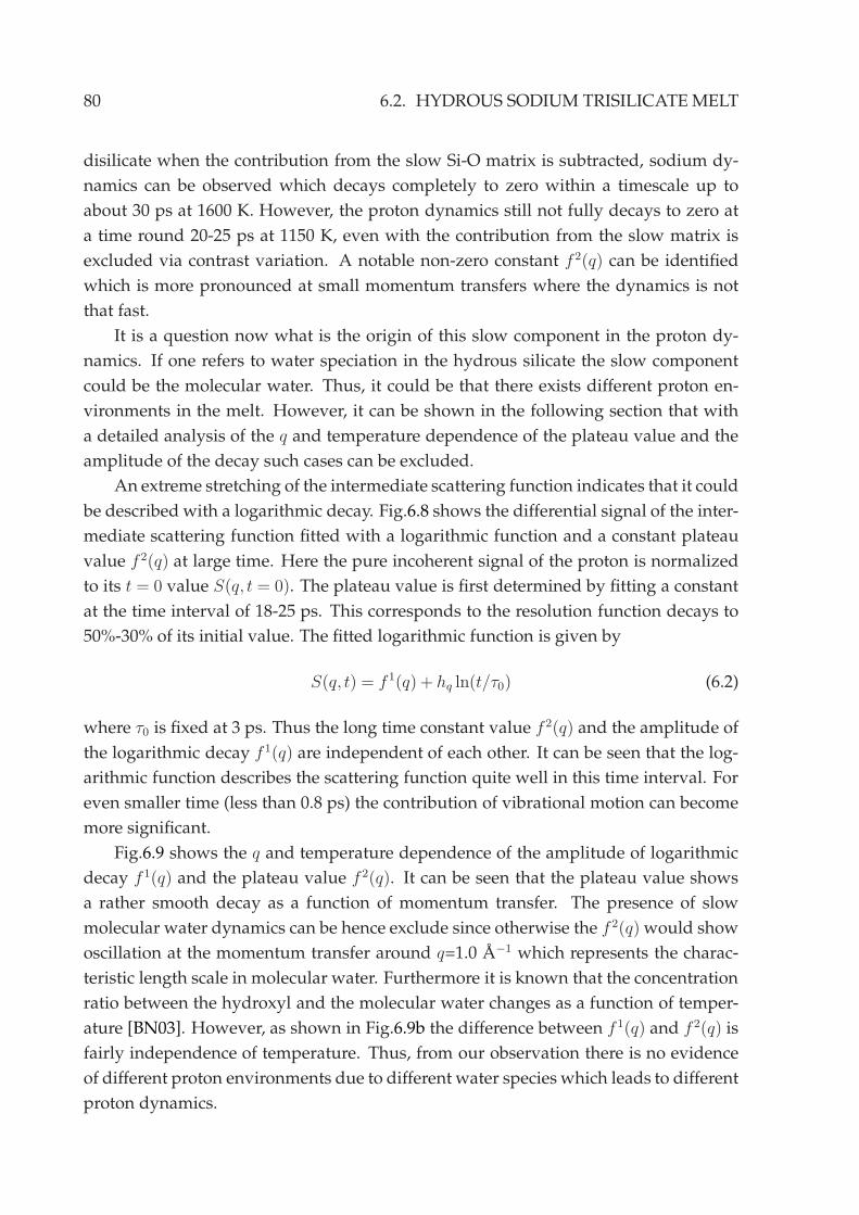
80 6.2. HYDROUS SODIUM TRISILICATEMELT
disilicate when the contribution from the slow Si-O matrix is subtracted, sodium dy-
namics can be observed which decays completely to zero within a timescale up to
about 30 ps at 1600 K. However, the proton dynamics still not fully decays to zero at
a time round 20-25 ps at 1150 K, even with the contribution from the slow matrix is
excluded via contrast variation. A notable non-zero constant f 2(q) can be identified
which is more pronounced at small momentum transfers where the dynamics is not
that fast.
It is a question now what is the origin of this slow component in the proton dy-
namics. If one refers to water speciation in the hydrous silicate the slow component
could be the molecular water. Thus, it could be that there exists different proton en-
vironments in the melt. However, it can be shown in the following section that with
a detailed analysis of the q and temperature dependence of the plateau value and the
amplitude of the decay such cases can be excluded.
An extreme stretching of the intermediate scattering function indicates that it could
be described with a logarithmic decay. Fig.6.8 shows the differential signal of the inter-
mediate scattering function fitted with a logarithmic function and a constant plateau
value f 2(q) at large time. Here the pure incoherent signal of the proton is normalized
to its t = 0 value S(q, t = 0). The plateau value is first determined by fitting a constant
at the time interval of 18-25 ps. This corresponds to the resolution function decays to
50%-30% of its initial value. The fitted logarithmic function is given by
S(q, t) = f 1(q) + hq ln(t/τ0) (6.2)
where τ0 is fixed at 3 ps. Thus the long time constant value f 2(q) and the amplitude of
the logarithmic decay f 1(q) are independent of each other. It can be seen that the log-
arithmic function describes the scattering function quite well in this time interval. For
even smaller time (less than 0.8 ps) the contribution of vibrational motion can become
more significant.
Fig.6.9 shows the q and temperature dependence of the amplitude of logarithmic
decay f 1(q) and the plateau value f 2(q). It can be seen that the plateau value shows
a rather smooth decay as a function of momentum transfer. The presence of slow
molecular water dynamics can be hence exclude since otherwise the f 2(q) would show
oscillation at the momentum transfer around q=1.0 A−1 which represents the charac-
teristic length scale in molecular water. Furthermore it is known that the concentration
ratio between the hydroxyl and the molecular water changes as a function of temper-
ature [BN03]. However, as shown in Fig.6.9b the difference between f 1(q) and f 2(q) is
fairly independence of temperature. Thus, from our observation there is no evidence
of different proton environments due to different water species which leads to different
proton dynamics.
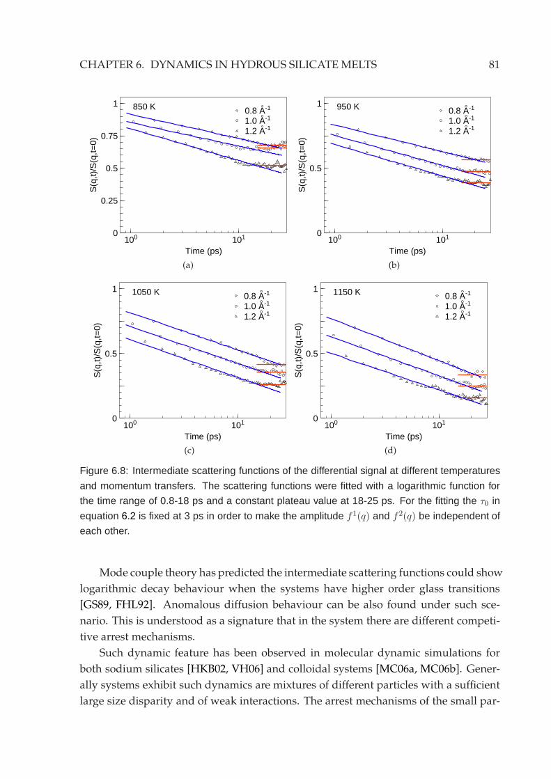
CHAPTER 6. DYNAMICS IN HYDROUS SILICATEMELTS 81
100 1010
0.25
0.5
0.75
1
Time (ps)
S(q
,t)/S
(q,t=
0)
850 K 0.8 A-1
1.0 A-1
1.2 A-1
(a)
100 1010
0.5
1
Time (ps)
S(q
,t)/S
(q,t=
0)
950 K 0.8 A-1
1.0 A-1
1.2 A-1
(b)
100 1010
0.5
1
Time (ps)
S(q
,t)/S
(q,t=
0)
1050 K 0.8 A-1
1.0 A-1
1.2 A-1
(c)
100 1010
0.5
1
Time (ps)
S(q
,t)/S
(q,t=
0)1150 K 0.8 A-1
1.0 A-1
1.2 A-1
(d)
Figure 6.8: Intermediate scattering functions of the differential signal at different temperatures
and momentum transfers. The scattering functions were fitted with a logarithmic function for
the time range of 0.8-18 ps and a constant plateau value at 18-25 ps. For the fitting the τ0 in
equation 6.2 is fixed at 3 ps in order to make the amplitude f1(q) and f2(q) be independent of
each other.
Mode couple theory has predicted the intermediate scattering functions could show
logarithmic decay behaviour when the systems have higher order glass transitions
[GS89, FHL92]. Anomalous diffusion behaviour can be also found under such sce-
nario. This is understood as a signature that in the system there are different competi-
tive arrest mechanisms.
Such dynamic feature has been observed in molecular dynamic simulations for
both sodium silicates [HKB02, VH06] and colloidal systems [MC06a, MC06b]. Gener-
ally systems exhibit such dynamics are mixtures of different particles with a sufficient
large size disparity and of weak interactions. The arrest mechanisms of the small par-
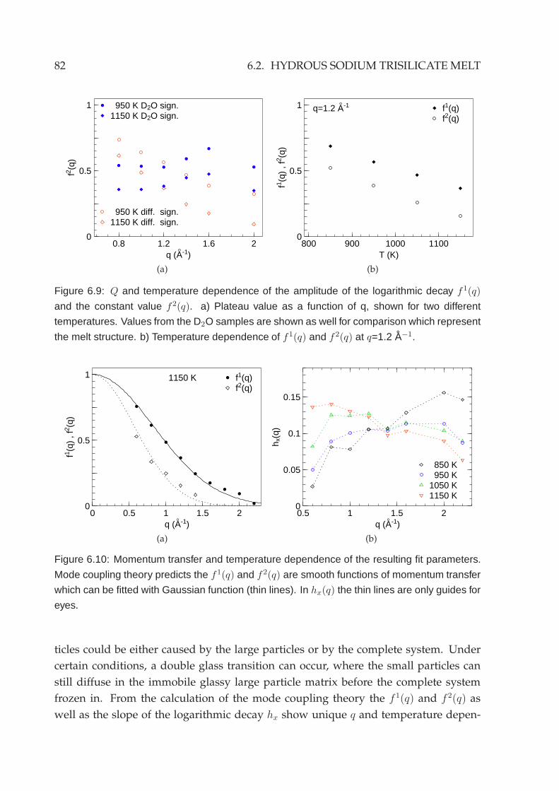
82 6.2. HYDROUS SODIUM TRISILICATEMELT
0.8 1.2 1.6 20
0.5
1
q (A-1)
f2 (q)
950 K D2O sign.1150 K D2O sign.
950 K diff. sign.1150 K diff. sign.
(a)
800 900 1000 11000
0.5
1
T (K)
f1 (q)
, f2 (q
)
f1(q)f2(q)
q=1.2 A-1
(b)
Figure 6.9: Q and temperature dependence of the amplitude of the logarithmic decay f1(q)
and the constant value f2(q). a) Plateau value as a function of q, shown for two different
temperatures. Values from the D2O samples are shown as well for comparison which represent
the melt structure. b) Temperature dependence of f1(q) and f2(q) at q=1.2 A−1.
0 0.5 1 1.5 20
0.5
1
q (A-1)
f1 (q)
, f2 (q
)
f1(q)f2(q)
1150 K
(a)
0.5 1 1.5 20
0.05
0.1
0.15
q (A-1)
h x(q
)
850 K 950 K1050 K1150 K
(b)
Figure 6.10: Momentum transfer and temperature dependence of the resulting fit parameters.
Mode coupling theory predicts the f1(q) and f2(q) are smooth functions of momentum transfer
which can be fitted with Gaussian function (thin lines). In hx(q) the thin lines are only guides for
eyes.
ticles could be either caused by the large particles or by the complete system. Under
certain conditions, a double glass transition can occur, where the small particles can
still diffuse in the immobile glassy large particle matrix before the complete system
frozen in. From the calculation of the mode coupling theory the f 1(q) and f 2(q) as
well as the slope of the logarithmic decay hx show unique q and temperature depen-
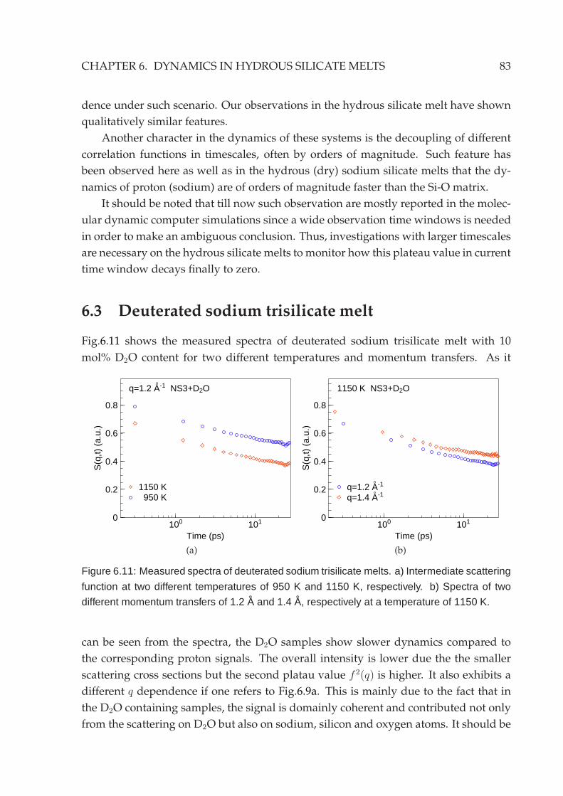
CHAPTER 6. DYNAMICS IN HYDROUS SILICATEMELTS 83
dence under such scenario. Our observations in the hydrous silicate melt have shown
qualitatively similar features.
Another character in the dynamics of these systems is the decoupling of different
correlation functions in timescales, often by orders of magnitude. Such feature has
been observed here as well as in the hydrous (dry) sodium silicate melts that the dy-
namics of proton (sodium) are of orders of magnitude faster than the Si-O matrix.
It should be noted that till now such observation are mostly reported in the molec-
ular dynamic computer simulations since a wide observation time windows is needed
in order to make an ambiguous conclusion. Thus, investigations with larger timescales
are necessary on the hydrous silicate melts to monitor how this plateau value in current
time window decays finally to zero.
6.3 Deuterated sodium trisilicate melt
Fig.6.11 shows the measured spectra of deuterated sodium trisilicate melt with 10
mol% D2O content for two different temperatures and momentum transfers. As it
100 1010
0.2
0.4
0.6
0.8
Time (ps)
S(q
,t) (
a.u.
)
q=1.2 A-1 NS3+D2O
1150 K 950 K
(a)
100 1010
0.2
0.4
0.6
0.8
Time (ps)
S(q
,t) (
a.u.
)
1150 K NS3+D2O
q=1.2 A-1
q=1.4 A-1
(b)
Figure 6.11: Measured spectra of deuterated sodium trisilicate melts. a) Intermediate scattering
function at two different temperatures of 950 K and 1150 K, respectively. b) Spectra of two
different momentum transfers of 1.2 A and 1.4 A, respectively at a temperature of 1150 K.
can be seen from the spectra, the D2O samples show slower dynamics compared to
the corresponding proton signals. The overall intensity is lower due the the smaller
scattering cross sections but the second platau value f 2(q) is higher. It also exhibits a
different q dependence if one refers to Fig.6.9a. This is mainly due to the fact that in
the D2O containing samples, the signal is domainly coherent and contributed not only
from the scattering on D2O but also on sodium, silicon and oxygen atoms. It should be
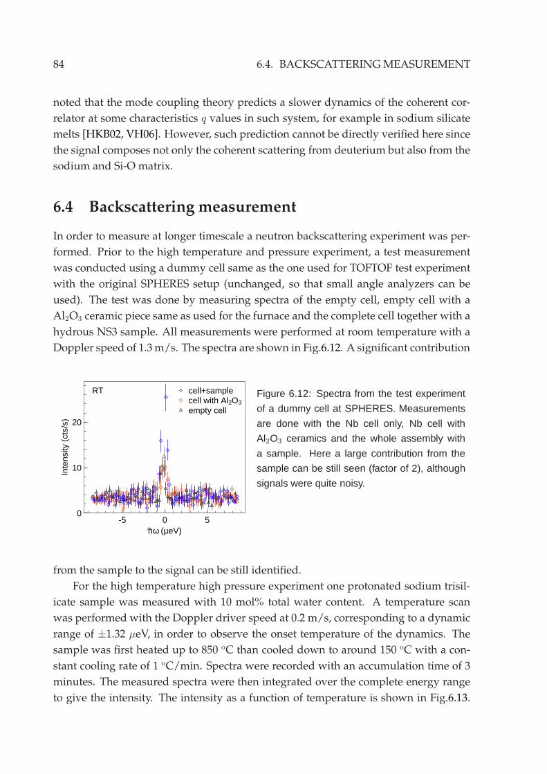
84 6.4. BACKSCATTERINGMEASUREMENT
noted that the mode coupling theory predicts a slower dynamics of the coherent cor-
relator at some characteristics q values in such system, for example in sodium silicate
melts [HKB02, VH06]. However, such prediction cannot be directly verified here since
the signal composes not only the coherent scattering from deuterium but also from the
sodium and Si-O matrix.
6.4 Backscattering measurement
In order to measure at longer timescale a neutron backscattering experiment was per-
formed. Prior to the high temperature and pressure experiment, a test measurement
was conducted using a dummy cell same as the one used for TOFTOF test experiment
with the original SPHERES setup (unchanged, so that small angle analyzers can be
used). The test was done by measuring spectra of the empty cell, empty cell with a
Al2O3 ceramic piece same as used for the furnace and the complete cell together with a
hydrous NS3 sample. All measurements were performed at room temperature with a
Doppler speed of 1.3m/s. The spectra are shown in Fig.6.12. A significant contribution
-5 0 50
10
20
hω (µeV)
Inte
nsity
(ct
s/s)
cell+samplecell with Al2O3
empty cell
RT Figure 6.12: Spectra from the test experiment
of a dummy cell at SPHERES. Measurements
are done with the Nb cell only, Nb cell with
Al2O3 ceramics and the whole assembly with
a sample. Here a large contribution from the
sample can be still seen (factor of 2), although
signals were quite noisy.
from the sample to the signal can be still identified.
For the high temperature high pressure experiment one protonated sodium trisil-
icate sample was measured with 10 mol% total water content. A temperature scan
was performed with the Doppler driver speed at 0.2 m/s, corresponding to a dynamic
range of ±1.32 µeV, in order to observe the onset temperature of the dynamics. The
sample was first heated up to 850 oC than cooled down to around 150 oC with a con-
stant cooling rate of 1 oC/min. Spectra were recorded with an accumulation time of 3
minutes. The measured spectra were then integrated over the complete energy range
to give the intensity. The intensity as a function of temperature is shown in Fig.6.13.
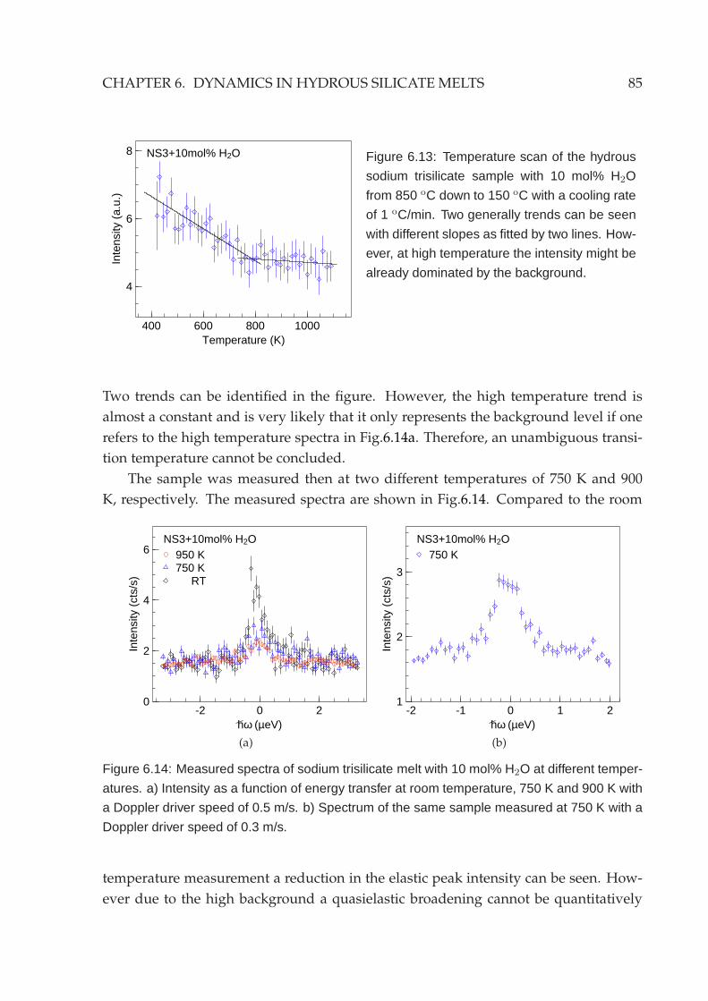
CHAPTER 6. DYNAMICS IN HYDROUS SILICATEMELTS 85
400 600 800 1000
4
6
8
Temperature (K)
Inte
nsity
(a.
u.)
NS3+10mol% H2O Figure 6.13: Temperature scan of the hydrous
sodium trisilicate sample with 10 mol% H2O
from 850 oC down to 150 oC with a cooling rate
of 1 oC/min. Two generally trends can be seen
with different slopes as fitted by two lines. How-
ever, at high temperature the intensity might be
already dominated by the background.
Two trends can be identified in the figure. However, the high temperature trend is
almost a constant and is very likely that it only represents the background level if one
refers to the high temperature spectra in Fig.6.14a. Therefore, an unambiguous transi-
tion temperature cannot be concluded.
The sample was measured then at two different temperatures of 750 K and 900
K, respectively. The measured spectra are shown in Fig.6.14. Compared to the room
-2 0 20
2
4
6
hω (µeV)
Inte
nsity
(ct
s/s)
NS3+10mol% H2O950 K750 K RT
(a)
-2 -1 0 1 21
2
3
hω (µeV)
Inte
nsity
(ct
s/s)
NS3+10mol% H2O750 K
(b)
Figure 6.14: Measured spectra of sodium trisilicate melt with 10 mol% H2O at different temper-
atures. a) Intensity as a function of energy transfer at room temperature, 750 K and 900 K with
a Doppler driver speed of 0.5 m/s. b) Spectrum of the same sample measured at 750 K with a
Doppler driver speed of 0.3 m/s.
temperature measurement a reduction in the elastic peak intensity can be seen. How-
ever due to the high background a quasielastic broadening cannot be quantitatively
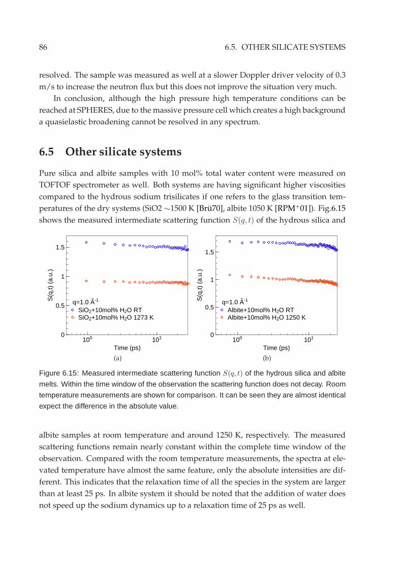
86 6.5. OTHER SILICATE SYSTEMS
resolved. The sample was measured as well at a slower Doppler driver velocity of 0.3
m/s to increase the neutron flux but this does not improve the situation very much.
In conclusion, although the high pressure high temperature conditions can be
reached at SPHERES, due to themassive pressure cell which creates a high background
a quasielastic broadening cannot be resolved in any spectrum.
6.5 Other silicate systems
Pure silica and albite samples with 10 mol% total water content were measured on
TOFTOF spectrometer as well. Both systems are having significant higher viscosities
compared to the hydrous sodium trisilicates if one refers to the glass transition tem-
peratures of the dry systems (SiO2 ∼1500 K [Bru70], albite 1050 K [RPM+01]). Fig.6.15
shows the measured intermediate scattering function S(q, t) of the hydrous silica and
100 1010
0.5
1
1.5
Time (ps)
S(q
,t) (
a.u.
)
q=1.0 A-1
SiO2+10mol% H2O RTSiO2+10mol% H2O 1273 K
(a)
100 1010
0.5
1
1.5
Time (ps)
S(q
,t) (
a.u.
)
q=1.0 A-1
Albite+10mol% H2O RTAlbite+10mol% H2O 1250 K
(b)
Figure 6.15: Measured intermediate scattering function S(q, t) of the hydrous silica and albite
melts. Within the time window of the observation the scattering function does not decay. Room
temperature measurements are shown for comparison. It can be seen they are almost identical
expect the difference in the absolute value.
albite samples at room temperature and around 1250 K, respectively. The measured
scattering functions remain nearly constant within the complete time window of the
observation. Compared with the room temperature measurements, the spectra at ele-
vated temperature have almost the same feature, only the absolute intensities are dif-
ferent. This indicates that the relaxation time of all the species in the system are larger
than at least 25 ps. In albite system it should be noted that the addition of water does
not speed up the sodium dynamics up to a relaxation time of 25 ps as well.
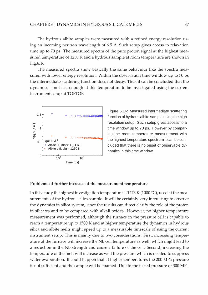
CHAPTER 6. DYNAMICS IN HYDROUS SILICATEMELTS 87
The hydrous albite samples were measured with a refined energy resolution us-
ing an incoming neutron wavelength of 6.5 A. Such setup gives access to relaxation
time up to 70 ps. The measured spectra of the pure proton signal at the highest mea-
sured temperature of 1250 K and a hydrous sample at room temperature are shown in
Fig.6.16.
The measured spectra show basically the same behaviour like the spectra mea-
sured with lower energy resolution. Within the observation time window up to 70 ps
the intermediate scattering function does not decay. Thus it can be concluded that the
dynamics is not fast enough at this temperature to be investigated using the current
instrument setup at TOFTOF.
100 1010
0.5
1
1.5
Time (ps)
S(q
,t) (
a.u.
)
q=1.0 A-1
Albite+10mol% H2O RTAlbite diff. sign. 1250 K
Figure 6.16: Measured intermediate scattering
function of hydrous albite sample using the high
resolution setup. Such setup gives access to a
time window up to 70 ps. However by compar-
ing the room temperature measurement with
the highest temperature spectrum it can be con-
cluded that there is no onset of observable dy-
namics in this time window.
Problems of further increase of the measurement temperature
In this study the highest investigation temperature is 1273 K (1000 °C), used at themea-
surements of the hydrous silica sample. It will be certainly very interesting to observe
the dynamics in silica system, since the results can direct clarify the role of the proton
in silicates and to be compared with alkali oxides. However, no higher temperature
measurement was performed, although the furnace in the pressure cell is capable to
reach a temperature up to 1500 K and at higher temperature the dynamics in hydrous
silica and albite melts might speed up to a measurable timescale of using the current
instrument setup. This is mainly due to two considerations. First, increasing temper-
ature of the furnace will increase the Nb cell temperature as well, which might lead to
a reduction in the Nb strength and cause a failure of the cell. Second, increasing the
temperature of the melt will increase as well the pressure which is needed to suppress
water evaporation. It could happen that at higher temperatures the 200 MPa pressure
is not sufficient and the sample will be foamed. Due to the tested pressure of 300 MPa

88 6.5. OTHER SILICATE SYSTEMS
a further increase of the operation pressure beyond 200 MPa is not allowed according
to the safety margin constrain.
From the measurements here it can only be concluded that the lower boundary
value for diffusion coefficients in these systems is on the order of 10−10 m2s−1 in the
temperature range of this study, although the glass transition temperature of the sam-
ples has already be decreased by a factor of 2 by adding 10 mol% of water.
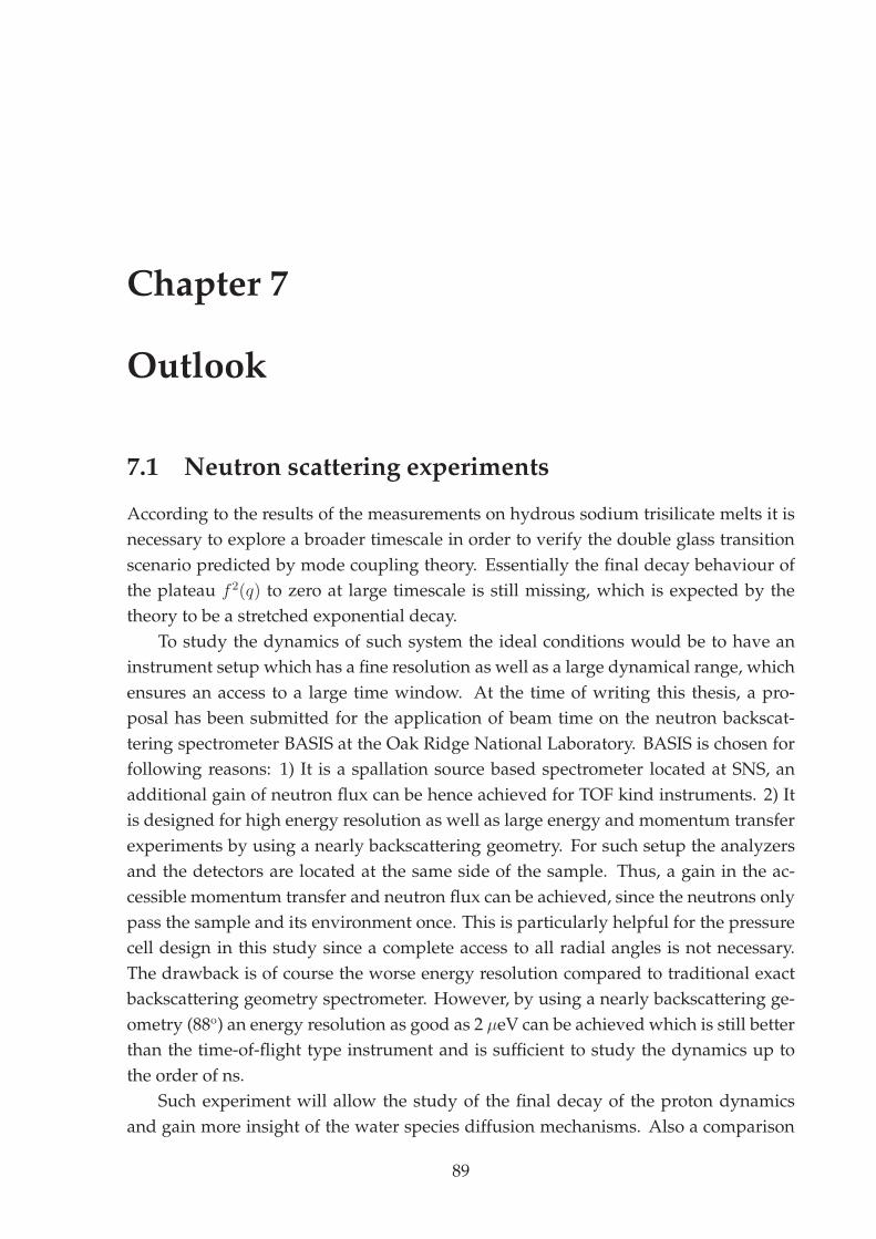
Chapter 7
Outlook
7.1 Neutron scattering experiments
According to the results of the measurements on hydrous sodium trisilicate melts it is
necessary to explore a broader timescale in order to verify the double glass transition
scenario predicted by mode coupling theory. Essentially the final decay behaviour of
the plateau f 2(q) to zero at large timescale is still missing, which is expected by the
theory to be a stretched exponential decay.
To study the dynamics of such system the ideal conditions would be to have an
instrument setup which has a fine resolution as well as a large dynamical range, which
ensures an access to a large time window. At the time of writing this thesis, a pro-
posal has been submitted for the application of beam time on the neutron backscat-
tering spectrometer BASIS at the Oak Ridge National Laboratory. BASIS is chosen for
following reasons: 1) It is a spallation source based spectrometer located at SNS, an
additional gain of neutron flux can be hence achieved for TOF kind instruments. 2) It
is designed for high energy resolution as well as large energy and momentum transfer
experiments by using a nearly backscattering geometry. For such setup the analyzers
and the detectors are located at the same side of the sample. Thus, a gain in the ac-
cessible momentum transfer and neutron flux can be achieved, since the neutrons only
pass the sample and its environment once. This is particularly helpful for the pressure
cell design in this study since a complete access to all radial angles is not necessary.
The drawback is of course the worse energy resolution compared to traditional exact
backscattering geometry spectrometer. However, by using a nearly backscattering ge-
ometry (88o) an energy resolution as good as 2 µeV can be achieved which is still better
than the time-of-flight type instrument and is sufficient to study the dynamics up to
the order of ns.
Such experiment will allow the study of the final decay of the proton dynamics
and gain more insight of the water species diffusion mechanisms. Also a comparison
89
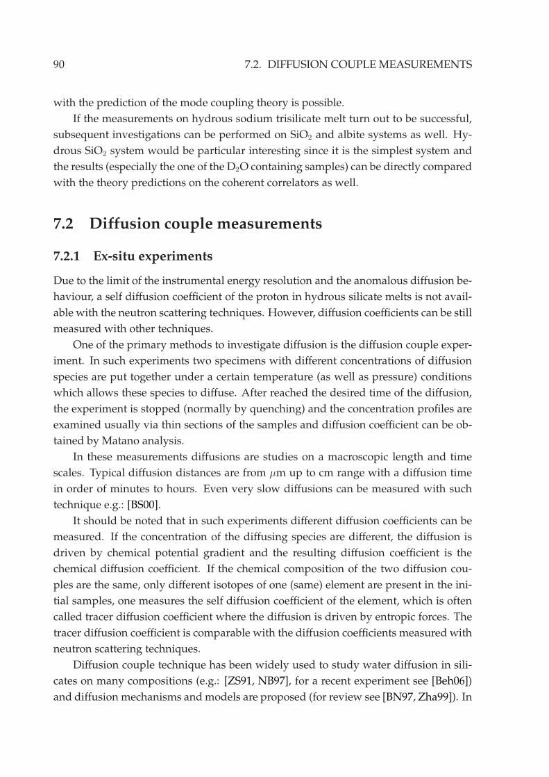
90 7.2. DIFFUSION COUPLE MEASUREMENTS
with the prediction of the mode coupling theory is possible.
If the measurements on hydrous sodium trisilicate melt turn out to be successful,
subsequent investigations can be performed on SiO2 and albite systems as well. Hy-
drous SiO2 system would be particular interesting since it is the simplest system and
the results (especially the one of the D2O containing samples) can be directly compared
with the theory predictions on the coherent correlators as well.
7.2 Diffusion couple measurements
7.2.1 Ex-situ experiments
Due to the limit of the instrumental energy resolution and the anomalous diffusion be-
haviour, a self diffusion coefficient of the proton in hydrous silicate melts is not avail-
able with the neutron scattering techniques. However, diffusion coefficients can be still
measured with other techniques.
One of the primary methods to investigate diffusion is the diffusion couple exper-
iment. In such experiments two specimens with different concentrations of diffusion
species are put together under a certain temperature (as well as pressure) conditions
which allows these species to diffuse. After reached the desired time of the diffusion,
the experiment is stopped (normally by quenching) and the concentration profiles are
examined usually via thin sections of the samples and diffusion coefficient can be ob-
tained by Matano analysis.
In these measurements diffusions are studies on a macroscopic length and time
scales. Typical diffusion distances are from µm up to cm range with a diffusion time
in order of minutes to hours. Even very slow diffusions can be measured with such
technique e.g.: [BS00].
It should be noted that in such experiments different diffusion coefficients can be
measured. If the concentration of the diffusing species are different, the diffusion is
driven by chemical potential gradient and the resulting diffusion coefficient is the
chemical diffusion coefficient. If the chemical composition of the two diffusion cou-
ples are the same, only different isotopes of one (same) element are present in the ini-
tial samples, one measures the self diffusion coefficient of the element, which is often
called tracer diffusion coefficient where the diffusion is driven by entropic forces. The
tracer diffusion coefficient is comparable with the diffusion coefficients measured with
neutron scattering techniques.
Diffusion couple technique has been widely used to study water diffusion in sili-
cates on many compositions (e.g.: [ZS91, NB97], for a recent experiment see [Beh06])
and diffusion mechanisms andmodels are proposed (for review see [BN97, Zha99]). In
CHAPTER 7. OUTLOOK 91
most of these experiments the initial (total) water concentrations in the two diffusion
couples are different and therefore chemical diffusion coefficients are measured. How-
ever, such method can be applied to measure tracer diffusion coefficient as well using
silicate diffusion couple samples having the same water content with H2O/D2O and
the results from such experiments can be compared with the neutron experiments re-
sults. Current sample preparation apparatus is already suitable for such studies with-
out significant modifications since it provides a pressure up to 300 MPa and a quite
homogenous temperature profile over the sample (see Fig.2.5b).
It is not easy to clarify the diffusion mechanisms with the diffusion couple exper-
iment alone since the obtained results is an average over macroscopic scales and is
hence effectively at one q value. However, it provides as well important informations,
for example whether the self diffusion coefficient is connected with melt viscosity ac-
cording to the Einstein relation.
7.2.2 Neutron radiography
Combination of diffusion couple experiments and time-resolved radiography gives the
possibilities of direct in-situ observation of diffusion processes. Such experiments have
been already performed with X-ray radiography on metallic melts [GMMF06].
H is an ideal scatterer for neutron imaging owing to its large scattering cross sec-
tion which can create a good contrast. Neutron radiography and tomography have
been demonstrated to be a very useful tool for non-destructive imaging and time-
resolved imaging can be used to study dynamic properties of the sample. For exam-
ple, it has been applied to measure the viscosity of silicate melts using falling sphere
method [BWK+01, KWHB03]. Perform diffusion couple experiments with H2O/dry
or H2O/D2O samples to create contrast for neutrons imaging should be in principle
possible using the current pressure cell setup and both chemical and self diffusion co-
efficients can be measured. However, to use such technique a major challenge would
be to provide a homogenous and stable temperature profile over the complete sample
under high pressure conditions.

92 7.2. DIFFUSION COUPLE MEASUREMENTS
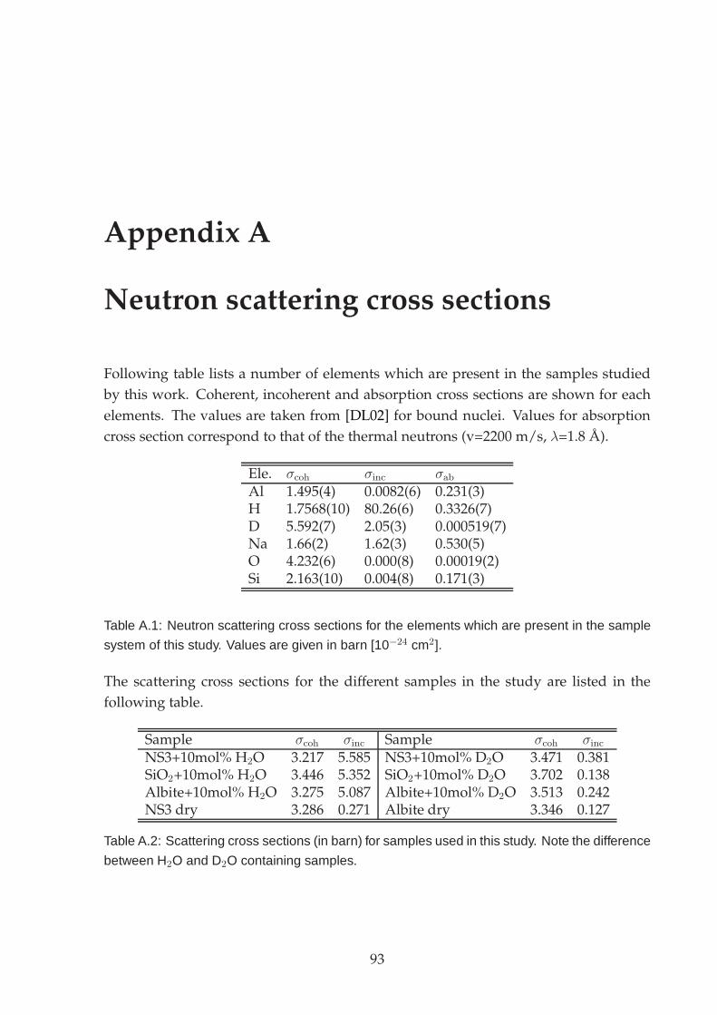
Appendix A
Neutron scattering cross sections
Following table lists a number of elements which are present in the samples studied
by this work. Coherent, incoherent and absorption cross sections are shown for each
elements. The values are taken from [DL02] for bound nuclei. Values for absorption
cross section correspond to that of the thermal neutrons (v=2200 m/s, λ=1.8 A).
Ele. σcoh σinc σab
Al 1.495(4) 0.0082(6) 0.231(3)H 1.7568(10) 80.26(6) 0.3326(7)D 5.592(7) 2.05(3) 0.000519(7)Na 1.66(2) 1.62(3) 0.530(5)O 4.232(6) 0.000(8) 0.00019(2)Si 2.163(10) 0.004(8) 0.171(3)
Table A.1: Neutron scattering cross sections for the elements which are present in the sample
system of this study. Values are given in barn [10−24 cm2].
The scattering cross sections for the different samples in the study are listed in the
following table.
Sample σcoh σinc Sample σcoh σinc
NS3+10mol% H2O 3.217 5.585 NS3+10mol% D2O 3.471 0.381SiO2+10mol% H2O 3.446 5.352 SiO2+10mol% D2O 3.702 0.138Albite+10mol% H2O 3.275 5.087 Albite+10mol% D2O 3.513 0.242NS3 dry 3.286 0.271 Albite dry 3.346 0.127
Table A.2: Scattering cross sections (in barn) for samples used in this study. Note the difference
between H2O and D2O containing samples.
93
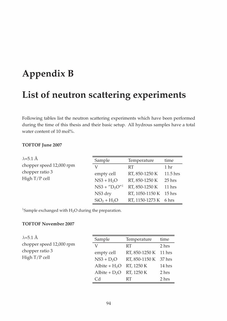
Appendix B
List of neutron scattering experiments
Following tables list the neutron scattering experiments which have been performed
during the time of this thesis and their basic setup. All hydrous samples have a total
water content of 10 mol%.
TOFTOF June 2007
λ=5.1 A
chopper speed 12,000 rpm
chopper ratio 3
High T/P cell
Sample Temperature time
V RT 1 hr
empty cell RT, 850-1250 K 11.5 hrs
NS3 + H2O RT, 850-1250 K 25 hrs
NS3 + ”D2O”1 RT, 850-1250 K 11 hrs
NS3 dry RT, 1050-1150 K 15 hrs
SiO2 + H2O RT, 1150-1273 K 6 hrs
1Sample exchanged with H2O during the preparation.
TOFTOF November 2007
λ=5.1 A
chopper speed 12,000 rpm
chopper ratio 3
High T/P cell
Sample Temperature time
V RT 2 hrs
empty cell RT, 850-1250 K 11 hrs
NS3 + D2O RT, 850-1150 K 37 hrs
Albite + H2O RT, 1250 K 14 hrs
Albite + D2O RT, 1250 K 2 hrs
Cd RT 2 hrs
94
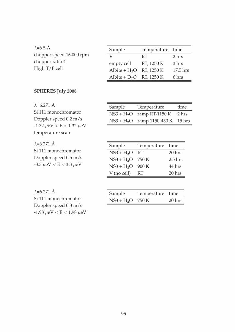
λ=6.5 A
chopper speed 16,000 rpm
chopper ratio 4
High T/P cell
Sample Temperature time
V RT 2 hrs
empty cell RT, 1250 K 3 hrs
Albite + H2O RT, 1250 K 17.5 hrs
Albite + D2O RT, 1250 K 6 hrs
SPHERES July 2008
λ=6.271 A
Si 111 monochromator
Doppler speed 0.2 m/s
-1.32 µeV < E < 1.32 µeV
temperature scan
Sample Temperature time
NS3 + H2O ramp RT-1150 K 2 hrs
NS3 + H2O ramp 1150-430 K 15 hrs
λ=6.271 A
Si 111 monochromator
Doppler speed 0.5 m/s
-3.3 µeV < E < 3.3 µeV
Sample Temperature time
NS3 + H2O RT 20 hrs
NS3 + H2O 750 K 2.5 hrs
NS3 + H2O 900 K 44 hrs
V (no cell) RT 20 hrs
λ=6.271 A
Si 111 monochromator
Doppler speed 0.3 m/s
-1.98 µeV < E < 1.98 µeV
Sample Temperature time
NS3 + H2O 750 K 20 hrs
95

96
List of Figures
1.1 Different techniques to measure the glass transition temperature . . . . . 3
1.2 Structure relaxation and transport coefficients in sodium silicates . . . . 5
1.3 Formation of diffusion channels in sodium trisilicate melts . . . . . . . . 5
1.4 Effects of different components on the structure of silicate melts . . . . . 6
1.5 Viscosity of hydrous silicate melts and the water speciation . . . . . . . . 8
2.1 Dry sodium trisilicate block sample after preparation . . . . . . . . . . . 12
2.2 Preparation of the sample capsules for water dissolution . . . . . . . . . 14
2.3 Schematic view of the sample preparation setup . . . . . . . . . . . . . . 16
2.4 Three-zone furnace for sample preparation . . . . . . . . . . . . . . . . . 17
2.5 Sketch of the preparation furnace and its temperature profile . . . . . . . 18
2.6 DSC measurements on hydrous sodium trisilicate samples . . . . . . . . 19
2.7 Comparison between DSC and dilatometry measurement results . . . . 21
2.8 Dilatometric measurement results of a dry albite sample . . . . . . . . . 22
2.9 Dilatometric measurement results of hydrous albite samples . . . . . . . 22
3.1 Pair correlation function g(r) of a monoatomic liquid . . . . . . . . . . . 31
3.2 MCT calculations of different relaxation processes in viscous liquids . . 38
4.1 Strengthening effects as a function of wall ratio . . . . . . . . . . . . . . . 44
4.2 Temperature dependence of the strength of Nb and Nb1Zr alloy . . . . . 46
4.3 Technical drawing of the inner Nb1Zr cell . . . . . . . . . . . . . . . . . . 47
4.4 The high temperature / high pressure sample environment . . . . . . . . 48
4.5 Temperature measurements using temperature sensitive paints . . . . . 51
4.6 Technical drawing of the complete neutron scattering apparatus . . . . . 52
4.7 Stick to insert the sample capsule into the pressure cell . . . . . . . . . . 53
4.8 Schematic view of the complete setup on the TOFTOF spectrometer . . . 54
4.9 Intensity as a function of scattering angle of the empty pressure cell . . . 56
4.10 Spectra of the empty pressure cell under different temperature and pres-
sure conditions . . . . . . . . . . . . . . . . . . . . . . . . . . . . . . . . . 57
97
4.11 I(2θ,ToF ) of the empty pressure cell and a hydrous silicate sample at
1250 K under 1800 bar . . . . . . . . . . . . . . . . . . . . . . . . . . . . . 58
5.1 Schematic view of the TOFTOF time-of-flight spectrometer setup . . . . 60
5.2 White beam flux at the sample position of TOFTOF spectrometer . . . . 60
5.3 Detector bank of the TOFTOF spectrometer . . . . . . . . . . . . . . . . . 62
5.4 Accessible q-ω range on the TOFTOF spectrometer using 5.1 A incoming
wavelength . . . . . . . . . . . . . . . . . . . . . . . . . . . . . . . . . . . . 62
5.5 Self absorption correction factors for a NS3 sample with 10 mol% H2O . 67
5.6 Deconvolution of the instrument resolution function in time space . . . . 69
5.7 General layout of the neutron backscattering spectrometer SPHERES . . 71
6.1 Measured spectra of dry sodium trisilicate melt on TOFTOF . . . . . . . 73
6.2 Scattering functions of different samples measured on TOFTOF at 1150 K 74
6.3 Contrast variation and the differential signal at 1150 K . . . . . . . . . . 75
6.4 Measured scattering function S(q,ω) at different temperatures . . . . . . 76
6.5 Differential scattering functions fitted with power law equation . . . . . 77
6.6 Comparison between proton relaxation and sodium relaxation . . . . . . 78
6.7 Intermediate scattering function of different diffusing species in dry and
hydrous sodium silicate melts . . . . . . . . . . . . . . . . . . . . . . . . . 79
6.8 Logarithmic decay of the proton relaxation in hydrous sodium trisilicate
melt with 10 mol% water content . . . . . . . . . . . . . . . . . . . . . . . 81
6.9 Q and temperature dependence of the amplitude of the logarithmic de-
cay f 1(q) and the constant value f 2(q) . . . . . . . . . . . . . . . . . . . . 82
6.10 Momentum transfer and temperature dependence of the resulting loga-
rithmic fit parameters . . . . . . . . . . . . . . . . . . . . . . . . . . . . . . 82
6.11 Measured spectra of deuterated sodium trisilicate melts . . . . . . . . . . 83
6.12 Spectra from the test experiment of a dummy cell at SPHERES . . . . . . 84
6.13 Temperature scan of the sodium trisilicate melt with 10 mol% H2Omea-
sured on SPHERES from 1120 K to 420 K . . . . . . . . . . . . . . . . . . 85
6.14 Neutron backscattering spectra of sodium trisilicate melt with 10 mol%
H2O for different temperatures measured at SPHERES . . . . . . . . . . 85
6.15 Intermediate scattering function of the hydrous silica and albite melts . 86
6.16 Intermediate scattering function of hydrous albite samplemeasuredwith
the high resolution setup on TOFTOF . . . . . . . . . . . . . . . . . . . . 87
98
List of Tables
2.1 Conversion from water mol % to wt % of the samples . . . . . . . . . . . 14
4.1 Neutron scattering and absorption cross section for different elements
used in alloys for high temperature applications. . . . . . . . . . . . . . . 45
A.1 Neutron scattering cross sections of elements . . . . . . . . . . . . . . . . 93
A.2 Neutron scattering cross sections of the samples in this study . . . . . . . 93
99

100
Acknowledgement
First I would like to thank Prof. Andreas Meyer for offering me the possibility to
finish this thesis under his supervision, for his continuous support during the complete
thesis time as well as for introducing me into this very interesting field of physics and
geology.
I would like to thank Prof. Winfried Petry for giving me the chance to work on my
thesis in his chair.
For the neutron experiments at FRM II I would like to express my thanks to Dr.
Tobias Unruh, Dr. Jurgen Peters and Dipl.-Ing. Jandal Ringe for many efforts to setup
my new sample environment, for kindly providing the gas pressure generator and
support. I also thank Dr. Tobias Unruh for the discussion on the neutron data.
Special thanks to Dr. Kai-Uwe Hess at the department of earth and environmental
sciences, LMU, who helped me on the measurements there, introduced me on many
geological topics and discussed with me on the results.
At DLR I would like to thank Dr. Thomas Voigtmann for discussions and Dipl.-
Phys. Ines Pommrich for her help during the neutron beam time.
I thank Dr. Joachim Wuttke at JCNS for his support during the neutron backscat-
tering experiment.
For the development of the sample preparation apparatus and the high tempera-
ture high pressure cell I would like to thank Dipl.-Ing. Josef Kaplonski at E13 and Mr.
Michael Stanger at Kristalllabor for their active support.
At E13 I would like to express my thanks to Prof. Walter Schirmacher, my PhD
colleagues Dipl.-Phys. Sebastian Stuber and Dipl.-Phys. Andreas Meier-Koll for dis-
cussions, help during beam times and daily work. I also thank all the other members,
for their help and providing a nice working atmosphere.
The Financial support from DFG under the grant number Me1958/8-2 is kindly
acknowledged.
I thank Prof. Andreas Meyer, Dr. Florian Kargl and Mr. Constantin Tomaras for
reading my manuscript.
Finally I would like to thank my family for continuously supporting my scientific
work abroad.
101

102
Bibliography
[BBTC91] T. Bausenwein, H. Bertagnolli, K. Todheide, and P. Chieux. Nucl. Instr. and
Meth. Phys. Res. B, 61(4), p.527, 1991. 66
[Beh06] H. Behrens. Adv. Sci. Tech., 46, p.79, 2006. 90
[BMK+95] M. Ben-Chorin, F. Moller, F. Koch, W. Schirmacher, and M. Eberhard. Phys.
Rev. B., 51(4), p.2199, 1995. 35
[BN97] H. Behrens and M. Nowak. Contrib. Mineral. Petrol., 126(4), p.377, 1997.
90
[BN03] H. Behrens and M. Nowak. Phase Trans., 76(1&2), p.45, 2003. 7, 8, 80
[Bru70] R. Bruckner. Properties and structure of vitreous silica I. J. Non-Cryst. Solids,
5, p.123–175, 1970. 11, 86
[BS92] R. Bruning and K. Samwer. Phys. Rev. B, 46(18), p.11319, 1992. 3
[BS00] H. Behrens and F. Schulze. In Applied Mineralogy in Research, Economy, Tech-
nology, Ecology and Culture. Proceedings ICAM, D. Rammlmair, J. Mederer,
T. Oberthur, R.B. Heimann, and H. Pentinghaus, editors, page 95. Balkema,
Rotterdam, 2000. 90
[BWK+01] G. Bayon, B. Winkler, A. Kahle, B. Hennion, and P. Boutrouille. Non-destr.
Test. Eval., 16, p.287, 2001. 91
[CE61] C.T. Chudley and R.J. Elliott. Proc. Phys. Soc., 77, p.353, 1961. 34
[CLH+97] H.Z. Cummins, G. Li, Y.H. Hwang, G.Q. Shen, W.M. Du, J. Hernandez, and
N.J. Tao. Z. Phys. B, 103, p.501, 1997. 4
[Cow01] J.M.G. Cowie. Polymers: chemistry & physics of modern materials. Nelson
Thoners Ltd., 2nd edition, 2001. 3
103
[Dav90] J.R. Davis, editor. Metals Handbook Volume 2, Properties and Selection: Nonfer-
rous Alloys and Special-Purpose Materials. ASM International, Metals Park,
Ohio, 10th edition, 1990. 46
[Daw77] V.C.D Dawson. High pressure containment in cylindrical vessels. In High Pres-
sure Teechnology I, Equipment Design, Materials, and Properties, I.L. Spain and
J. Paauwe, editors. Dekker, New York, 1977. 42, 44
[Din96] D.B. Dingwell. Volcanic dilemma: Flow or blow? Science, 273(23), p.1054,
1996. 1
[DL02] A.-J. Dianoux and G. Lander, editors. Neutron Data Booklet, Institut Laue-
Langevin. 2002. 93
[DR65] B.A. Dasannacharya and K.R. Rao. Phys. Rev., 137(2A), p.A417, 1965. 33
[DRH96] D.B. Dingwell, C. Romano, and K.-U. Hess. The effect of water on the viscos-
ity of a haplogranitic melt under P-T-X conditions relevant to silicic volcanism.
Contrib. Mineral. Petrol., 124(19), 1996. 7, 8, 13
[DW89] D.B. Dingwell and S.L. Webb. Phys. Chem. Miner., 16, p.508, 1989. 1
[Ell91] S.R. Elliott. Phys. Rev. Lett., 67(6), p.711, 1991. 30
[FA02] B. Frick and C. Alba-Simionesco. Appl. Phys. A, 74(Suppl.), p.S549, 2002.
47, 66
[FHL92] M. Fuchs, I. Hofacker, and A. Latz. Phys. Rev. A, 45(2), p.898, 1992. 81
[GM98] A. Grzechnik and P.F. McMillan. Am. Mineral., 83, p.331, 1998. 8
[GMMF06] A. Griesche, F.G. Moreno, M.-P. Macht, and G. Frohberg. Mater. Sci. Fo-
rum, 508, p.567, 2006. 91
[Got91] W. Gotze. Aspects of Structural Glass Transitions. In Liquids, freezing and
glass transition, Les Houches 1989, Sesssion LI, J.P. Hansen, D. Levesque, and
J. Zinn-Justin, editors. North-Holland, Amsterdam, 1991. 37
[Got99] W. Gotze. Recent tests of the mode-coupling theory for glassy dynamics. J. Phys.:
Condens. Matter, 11, p.A1–A45, 1999. 38
[GS89] W. Gotze and L. Sjogren. J. Phys.: Condens. Matter, 1, p.4203–4222, 1989.
81
[GS92] W. Gotze and L. Sjogren. Rep. Prog. Phys., 55, p.241–376, 1992. 36, 37
104
[HDW95] K.-U. Hess, D.B. Dingwell, and S.L. Webb. Am. Miner., 80, p.297–304, 1995.
6, 21
[Hil99] R. Hilfer. On fractional diffusion and its relation with continous time random
walks. In Anomalous diffusion: From Basis to Applications, A. Pekalski and
K. Sznajd-Weron, editors, page 77. Springer, Berlin, 1999. 36
[HKB02] J. Horbach, W. Kob, and K. Binder. Phys. Rev. Lett., 88(12), p.125502, 2002.
81, 84
[HM86] J.P. Hansen and I.R. McDonald. Theory of simple liquids. Academic Press,
London, 1986. 34
[Hov54] L. van Hove. Phys. Rev., 95(1), p.249, 1954. 28
[IHB+05] S. Indris, P. Heitjans, H. Behrens, R. Zorn, and B. Frick. Phys. Rev. B, 71,
p.064205, 2005. 9
[JBB51] J.R. Johnson, R.H. Bristow, andH. Blau. Am. Ceram. Soc., 34(6), p.165, 1951.
4
[KAD99] K. Knorr, B. Annighoffer, and W. Depmeier. J. Appl. Cryst., 32, p.373, 1999.
44
[Kar05] F. Kargl. The interplay of structure and microscopic dynamics in oxidic melts ob-
served by means inelastic neutron scattering. Dissertation, Physikdepartment
E13, TU Munchen, 2005. 20
[KB87] U. Krieger and J. Bosse. InAmorphous and LiquidMaterials, vol. 118 of NATO
ASI E: Applied Physics, E. Luscher, G. Fritsch, and G. Jacucci, editors. Ni-
jhoff, Dordrecht, 1987. 40
[KDS89] S.C. Kohn, R. Dupree, and M.E. Smith. Nature, 337(9), p.539, 1989. 7
[KDSW96] R. Knoche, D.B. Dingwell, F.A. Serfert, and S.L. Webb. Chem. Geol, 116,
p.1–16, 1996. 4, 12
[KM04] F. Kargl and A. Meyer. Chem. Geol., 213, p.165, 2004. 7
[KMKS06] F. Kargl, A. Meyer, M.M. Koza, and H. Schober. Phys. Rev. B, 74, p.014304,
2006. 4, 5, 79
[KWHB03] A. Kahle, B. Winkler, B. Hennion, and P. Boutrouille. Rev. Sci. Instr., 74,
p.3717, 2003. 91
105
[Lov84] S.W. Lovesey. Theory of neutron scattering from condensed matter, I+II. Claren-
don Press, Oxford, 1984. 24
[LP90] C.P. Lindsey and G.D. Patterson. J. Chem. Phys., 73(7), p.3348, 1990. 35
[MA80] J.W. Morgan and E. Anders. Proc. Natl. Acad. Sci., 77(3), p.6973–6977, 1980.
1
[MBS99] A. Meyer, R. Busch, and H. Schober. Phys. Rev. Lett., 83(24), p.5027, 1999.
38
[MC06a] A.J. Moreno and J. Colmenero. J. Chem. Phys., 125, p.164507, 2006. 81
[MC06b] A.J. Moreno and J. Colmenero. Phys. Rev. E, 74, p.021409, 2006. 81
[McM94] P.F. McMillian. Rev. Mineral., 30(1), p.132–156, 1994. 8
[MDGN03] A. Meyer, R.M. Dimeo, P.M. Gehring, and D.A. Neumann. Rev. Sci. Instr.,
74(5), p.2759, 2003. 71
[MHK+04] A. Meyer, J. Horbach, W. Kob, F. Kargl, and H. Schober. Phys. Rev. Lett.,
93(2), p.027801, 2004. 5, 6
[MPPC90] M. Maret, T. Pomme, A. Pasturel, and P. Chieux. Phys. Rev. B, 42(3), p.1598,
1990. 30
[MPSR93] P.F. McMillan, B.T Poe, T.R. Stanton, and R.L. Remmele. Phys. Chem. Min-
eral., 19, p.454, 1993. 7
[MSD02] A.Meyer, H. Schober, and D.B. Dingwell. Europhys. Lett, 59(5), p.708, 2002.
4
[MSS83] O.V. Mazurin, M.V. Streltsina, and T.P. Shvaiko-Shvaikovskaya. Handbook
of Glass, Part A: silica glass and binary silicate glasses. Elsevier, 1983. 20
[Mul03] A. Muller. Struktur und Dynamik wasserhaltiger Silikatglaser untersucht mit
Neutronenstreuung. Diploma thesis, Physikdepartment E13, TU Munchen,
2003. 17
[MVC98] G. Moore, T. Vennemann, and I. S. E. Carmichael. Am. Mineral, 83, p.36,
1998. 15
[NB97] M. Nowak and H. Behrens. Contrib. Mineral. Petrol., 126(4), p.365, 1997.
90
[Neu06] J. Neuhaus. Private communication, 2006. 46
106
[PBK04] M. Pohlmann, M. Benoit, and W. Kob. Phys. Rev. B, 70(18), p.184209, 2004.
9
[PMM+] M. Pohlmann, A.R. Muller, A. Meyer, H. Schober, and T. Hansen. Struc-
tural and dynamical properties of hydrous amorphous silicates as seen by neutron
scattering. Submitted to Phys. Rev. B. 8
[Poh05] M. Pohlmann. Structure and Dynamics of Hydrous silica(te) as seen by Molec-
ular Dynamics Computer Simulations and Neutron Scattering. Dissertation,
Physikdepartment E13, TU Munchen, 2005. 10, 31
[PP62] H.H. Paalman and C.J. Pings. J. Appl. Phys., 33(8), 1962. 66
[RPM+01] C. Romano, B. Poe, V. Mincione, K.-U. Hess, and D.B. Dingwell. Chem.
Geol., 174(1-3), p.115, 2001. 21, 86
[RRGF72] J.M. Rowe, J.J. Rush, L.A. de Graaf, and G.A. Ferguson. Phys. Rev. Lett.,
29(18), p.1250, 1972. 35
[SB91] W. Schirmacher and B. Bunsenges. Phys. Chem., 95, p.368, 1991. 36
[SGS95] R.A. Sadykov, P.L. Gruzin, and V.A. Suhoparov. High Pressure Res., 14,
p.199, 1995. 44
[SMD95] J.F. Stebbins, P.F. McMillan, and D.B. Dingwell, editors. Structure, Dynamics
and Properties of Silicate Melts. Reviews in Minerlogy 32. Mineral. Soc. of
Am., Washington, 1995. 2
[SPSH90] W. Schirmacher, M. Prem, J.-B. Suck, and A. Heidemann. Europhys. Lett.,
13(6), p.523, 1990. 36
[Squ78] G.L. Squires. Introduction to the theory of thermal neutron scattering. Cam-
bridge University Press, London, 1978. 24
[Sto82] E. Stolper. Contrib. Mineral. Petrol., 81, p.1–17, 1982. 7, 8
[SVP+91] S. Susman, K.J. Volin, D.L. Price, M. Grimsditch, J.P. Rino, R.K. Kalia,
P. Vashishta, G. Gwanmesia, Y. Wang, and R.C. Liebermann. Phys. Rev.
B, 43(1), p.1194, 1991. 30
[TSW+98] A. Toller, H. Schober, J. Wuttke, O.G. Randl, and F. Fujara. Phys. Rev. Lett,
80(11), p.2374, 1998. 38
[TTA+83] M. Tomozawa, M. Takata, J. Acocella, E.B. Watson, and T. Takamori. J.
Non-Cryst. Solids, 56(1-3), p.343–348, 1983. 20
107
[UMNP07] T. Unruh, A. Meyer, J. Neuhaus, and W. Petry. Neutron News, 18(2), p.22–
24, 2007. 59
[UNP07] T. Unruh, J. Neuhaus, and W. Petry. The high-resolution time-of-flight spec-
trometer TOFTOF. Nucl. Instr. and Meth. A, 580(3), p.1414, 2007. 59, 69
[VH06] Th. Voigtmann and J. Horbach. Europhys. Lett., 74(3), p.459, 2006. 81, 84
[WK07] J.Wuttke and F. Kargl. http://sourceforge.net/projects/frida/,
2007. 64
[Wut08] J. Wuttke. SPHERES online handbook, 2008. Julich Center for Neutron
Science. 71
[Zha99] Y. Zhang. Rev. Geophys., 37(4), p.493, 1999. 8, 14, 90
[ZKHS96] N. Zotov, H. Keppler, A.C. Hannon, and A.K. Soper. J. Non-Cryst. Solid,
202(1-2), p.153, 1996. 8
[Zol92] I.V. Zolotuchin. Physikalische Eigenschaften amorpher metallischer Werkstoffe.
Dt. Verl. fur Grundstoffindustrie, Leipzig, 1992. 31
[ZS91] Y. Zhang and E.M. Stolper. Nature, 305, p.306, 1991. 90
[ZSI95] Y. Zhang, E.M. Stolper, and P.D. Ihinger. Am. Mineral., 80, p.593, 1995. 8
[ZVEK92] N. Zotov, Y. Vanev, M. Epelbaum, and L. Konstantinov. J. Non-Cryst. Solid,
142, p.234, 1992. 8
108

Declaration of authorship
Herewith I certify that I am the author of this thesis and that any assistance I received
in its preparation is fully acknowledged and disclosed in the paper. I have also cited
any sources from which I used data, ideas or words, either quoted directly or para-
phrased.
Garching, January 29, 2009
Fan Yang
109


