Embed Size (px)
Citation preview


The Geology of Stratigraphic Sequences


Andrew D. Miall
The Geology ofStratigraphic Sequences
Second Edition
123
Prof. Andrew D. MiallUniversity of TorontoDept. GeologyToronto ON M5S [email protected]
ISBN 978-3-642-05026-8 e-ISBN 978-3-642-05027-5DOI 10.1007/978-3-642-05027-5Springer Heidelberg Dordrecht London New York
Library of Congress Control Number: 2009943585
© Springer-Verlag Berlin Heidelberg 2010This work is subject to copyright. All rights are reserved, whether the whole or part of the material isconcerned, specifically the rights of translation, reprinting, reuse of illustrations, recitation, broadcasting,reproduction on microfilm or in any other way, and storage in data banks. Duplication of this publication orparts thereof is permitted only under the provisions of the German Copyright Law of September 9, 1965,in its current version, and permission for use must always be obtained from Springer. Violations are liableto prosecution under the German Copyright Law.The use of general descriptive names, registered names, trademarks, etc. in this publication does not imply,even in the absence of a specific statement, that such names are exempt from the relevant protective lawsand regulations and therefore free for general use.
Cover design: deblik
Printed on acid-free paper
Springer is part of Springer Science+Business Media (www.springer.com)
Preface to Second Edition
It has been more than a decade since the appearance of the First Edition of this book.Much progress has been made, but some controversies remain.
The idea that the stratigraphic record could be subdivided into sequences andthat these sequences store essential information about basin-forming and subsi-dence processes remains as powerful an idea as when it was first formulated.L. L. Sloss and P. R. Vail are to be credited with the establishment of the mod-ern era of sequence stratigraphy. The definition and mapping of sequences havebecome a standard part of the basin-analysis process. Subsurface methods make useof advanced seismic-reflection analysis, with three-dimensional seismic methods, andseismic geomorphology adding important new dimensions to the analysis. Severaladvanced textbooks have now appeared that deal with the recognition and definitionof sequences and their interpretation in terms of the evolution of depositional sys-tems, the recognition and correlation of bounding surfaces, and the interpretation ofsequences in terms of changing accommodation and supply. This is not one of thesebooks.
The main purpose of this book remains the same as it was for the first edition,that is, to situate sequences within the broader context of geological processes, and toanswer the question: why do sequences form? Geoscientists might thereby be betterequipped to extract the maximum information from the record of sequences in a givenbasin or region.
Central to the concept of the sequence is the deductive model that sequences carrymessages about the “pulse of the earth”. In the early modern period of sequencestratigraphy (the late 1970s and 1980s) the model of global eustasy was predominant,and it was to offer a critique of that model that provided the impetus for developing thefirst edition of this book. Model-building has been central to the science of geologyfrom the beginning; it was certainly a preoccupation of such early masters of thescience as Lyell, Chamberlin, Barrell, Ulrich and Grabau. A historical evaluation ofthe contrasting deductive and inductive approaches to geology has been added to thisedition of the book, in order to provide a background in methodology and a historicalcontext.
Standard sequence models have become very well described and understood formost depositional settings, and are the subject of several recent texts. Two chapters areprovided in this edition in order to outline modern ideas, and to provide a frameworkof terminology and illustration for the remainder of the book.
A major component of the first edition was devoted to a documentation and illus-tration of the main types of sequence in the geological record, ranging from those
v
vi Preface to Second Edition
representing hundreds of millions of years to the high-frequency sequences formed byrapid cyclic processes lasting a few tens of thousands of years. Such documentationremains a major component of the book, and has been updated with new examples.
The central core of the first edition was composed of a detailed description andevaluation of the major processes by which sequences are formed. This remains thecentral focus of the book and has been updated.
Perhaps partly in response to this book, many geoscientists have recognized thecomplexity of the geological record, have adopted a rigorous inductive approach totheir analyses and remain committed to a multi-process interpretation of their rocks.Such an approach can provide a rich array of ideas regarding regional tectonics andbasin analysis. However, the original Vail model of global eustasy remains convincingto many, and a powerful guide to interpretation. The practical, theoretical and method-ological issues surrounding this still controversial area are the focus of a concludingsection of the book. The philosophy and methodology that are the basis for the ongo-ing work to construct the geological time scale constitute an essential background tothis discussion.
Toronto, ON Andrew D. MiallSeptember 2009
Acknowledgements
My own interest in sequence stratigraphy began slowly, as my work on regional basinanalysis for the Geological Survey of Canada matured in the late 1970s, and I amgrateful to this organization for introducing me to the scope and sweep of large-scaleregional analysis. My developing knowledge of basin analysis provided me with apractical view of the subject that induced skepticism. In particular, my work in theCanadian Arctic included attempts to adjudicate debates between various biostrati-graphic specialists who could not agree on the dating of certain subsurface sectionsthat I was trying to correlate. My critique of sequence stratigraphy as a chronostrati-graphic tool developed from this starting point. A few individuals in GSC discussedthe early concepts with me and helped me to realize that something important wasgoing on. Among these Ashton Embry stands out. Later, Jim Dixon’s work providedfood for thought.
Discussions with the main protagonists of sequence stratigraphy have met withmixed success. I would, however, like to acknowledge these colleagues for contribut-ing to the development of my ideas: Phil Allen, Bert Bally, Chris Barnes, OctavianCatuneanu, Sierd Cloetingh, Jim Coleman, Bill Galloway, Jake Hancock, MakotoIto, David James, Alan Kendall, Chris Kendall, Dale Leckie, Peter McCabe; DagNummedal, Tobi Payenberg, Guy Plint, Henry Posamentier, Brian Pratt, Larry Sloss,John Suter, Peter Vail, John Van Wagoner, Roger Walker, Tony Watts and YongtaiYang.
This book began life as an in-house report prepared for the exclusive use of theJapan National Petroleum Corporation in 1993. I am grateful to the Corporation forpermission to publish their report, and to my employer, the University of Toronto, forproviding the time for me both to write the original report and to prepare the materialfor the revisions incorporated into the final book.
Much of the material in Sect. 14.5 appeared in a contribution to the PaleoSceneseries in Geoscience Canada in 1994. I am grateful to Darrel Long for stimulating thewriting of the paper, and to series editor Godfrey Nowlan and critical reviewers JohnArmentrout and Terry Poulton for their invaluable comments.
The treatment of geological methods in Chap. 1 and the discussion of stratigraphicparadigms in Chap. 12 could not have been written without the essential role playedby my partner and co-investigator, Charlene Miall. Her deep knowledge of scientificmethods and her exploration of the sociology of science led us to prepare three papersbetween 2001 and 2004, from which these parts of the book have been adapted. Ithank Bill Berggren and John Van Couvering for giving us the opportunity to publishthe very first two articles in the new journal Stratigraphy.
vii

viii Acknowledgements
The entire manuscript of the first edition was critically read by Brian Pratt andPhil Allen. The second edition was reviewed in detail by Ray Ingersoll. OctavianCatuneanu advised on sequence concepts and models (Chap. 2). Uli Wortmannassisted with my understanding of chemostratigraphy. I am most grateful to theseindividuals for undertaking these onerous tasks, for their painstaking efforts in com-pleting them, and for their numerous thoughtful and helpful comments. Remainingerrors and omissions are, of course, my responsibility.
And once again, I must thank my wife Charlene and my children Christopher andSarah for their encouragement, love and support.
Contents
Part I The Emergence of Modern Concepts . . . . . . . . . . . . . . . 1
1 Historical and Methodological Background . . . . . . . . . . . . . . 31.1 Introduction . . . . . . . . . . . . . . . . . . . . . . . . . . . . 31.2 Methods in Geology . . . . . . . . . . . . . . . . . . . . . . . . 41.2.1 The Significance of Sequence Stratigraphy . . . . . . . . . . . . 61.2.2 Data and Argument in Geology . . . . . . . . . . . . . . . . . . 71.2.3 The Hermeneutic Circle and the Emergence of Sequence
Stratigraphy . . . . . . . . . . . . . . . . . . . . . . . . . . . . 91.2.4 Paradigms and Exemplars . . . . . . . . . . . . . . . . . . . . . 111.3 The Development of Descriptive Stratigraphy . . . . . . . . . . 131.3.1 The Growth of Modern Concepts . . . . . . . . . . . . . . . . . 131.3.2 Do Stratigraphic Units Have “Time” Significance? . . . . . . . . 161.3.3 The Development of Modern Chronostratigraphy . . . . . . . . 211.4 The Continual Search for a “Pulse of the Earth” . . . . . . . . . 261.5 Problems and Research Trends: The Current Status . . . . . . . 381.6 Current Literature . . . . . . . . . . . . . . . . . . . . . . . . . 411.7 Stratigraphic Terminology . . . . . . . . . . . . . . . . . . . . 43
2 The Basic Sequence Model . . . . . . . . . . . . . . . . . . . . . . . 472.1 Introduction . . . . . . . . . . . . . . . . . . . . . . . . . . . . 472.2 Elements of the Model . . . . . . . . . . . . . . . . . . . . . . 482.2.1 Accommodation and Supply . . . . . . . . . . . . . . . . . . . 492.2.2 Stratigraphic Architecture . . . . . . . . . . . . . . . . . . . . . 502.2.3 Depositional Systems and Systems Tracts . . . . . . . . . . . . 552.3 Sequence Models in Clastic and Carbonate Settings . . . . . . . 572.3.1 Marine Clastic Depositional Systems and Systems Tracts . . . . 572.3.2 Nonmarine Depositional Systems . . . . . . . . . . . . . . . . . 642.3.3 Carbonate Depositional Systems . . . . . . . . . . . . . . . . . 682.4 Sequence Definitions . . . . . . . . . . . . . . . . . . . . . . . 73
3 Other Methods for the Stratigraphic Analysis of Cyclesof Base-Level Change . . . . . . . . . . . . . . . . . . . . . . . . . . 773.1 Introduction . . . . . . . . . . . . . . . . . . . . . . . . . . . . 773.2 Facies Cycles . . . . . . . . . . . . . . . . . . . . . . . . . . . 773.3 Areas and Volumes of Stratigraphic Units . . . . . . . . . . . . 803.4 Hypsometric Curves . . . . . . . . . . . . . . . . . . . . . . . . 81
ix
x Contents
3.5 Backstripping . . . . . . . . . . . . . . . . . . . . . . . . . . . 833.6 Sea-Level Estimation from Paleoshorelines and Other
Fixed Points . . . . . . . . . . . . . . . . . . . . . . . . . . . . 903.7 Documentation of Metre-Scale Cycles . . . . . . . . . . . . . . 933.8 Integrated Tectonic-Stratigraphic Analysis . . . . . . . . . . . . 97
Part II The Stratigraphic Framework . . . . . . . . . . . . . . . . . . . 101
4 The Major Types of Stratigraphic Cycle . . . . . . . . . . . . . . . 1034.1 Introduction . . . . . . . . . . . . . . . . . . . . . . . . . . . . 1034.2 Sequence Hierarchy . . . . . . . . . . . . . . . . . . . . . . . . 1034.3 The Supercontinent Cycle . . . . . . . . . . . . . . . . . . . . . 1124.4 Cycles with Episodicities of Tens of Millions of Years . . . . . . 1134.5 Cycles with Million-Year Episodicities . . . . . . . . . . . . . . 1144.6 Cycles with Episodicities of Less Than One Million Years . . . 117
5 Cycles with Episodicities of Tens to Hundreds of Millionsof Years . . . . . . . . . . . . . . . . . . . . . . . . . . . . . . . . . . 1195.1 Climate, Sedimentation and Biogenesis . . . . . . . . . . . . . 1195.2 The Supercontinent Cycle . . . . . . . . . . . . . . . . . . . . . 1215.2.1 The Tectonic-Stratigraphic Model . . . . . . . . . . . . . . . . 1215.2.2 The Phanerozoic Record . . . . . . . . . . . . . . . . . . . . . 1235.3 Cycles with Episodicities of Tens of Millions of years . . . . . . 1255.3.1 Regional to Intercontinental Correlations . . . . . . . . . . . . . 1255.3.2 Tectonostratigraphic Sequences . . . . . . . . . . . . . . . . . . 1335.4 Main Conclusions . . . . . . . . . . . . . . . . . . . . . . . . . 142
6 Cycles with Million-Year Episodicities . . . . . . . . . . . . . . . . . 1436.1 Continental Margins . . . . . . . . . . . . . . . . . . . . . . . . 1436.1.1 Clastic Platforms and Margins . . . . . . . . . . . . . . . . . . 1436.1.2 Carbonate Cycles of Platforms and Craton Margins . . . . . . . 1486.1.3 Mixed Carbonate-Clastic Successions . . . . . . . . . . . . . . 1536.2 Foreland Basins . . . . . . . . . . . . . . . . . . . . . . . . . . 1606.2.1 Foreland Basin of the North American Western Interior . . . . . 1606.2.2 Other Foreland Basins . . . . . . . . . . . . . . . . . . . . . . . 1646.3 Arc-Related Basins . . . . . . . . . . . . . . . . . . . . . . . . 1676.3.1 Forearc Basins . . . . . . . . . . . . . . . . . . . . . . . . . . . 1676.3.2 Backarc Basins . . . . . . . . . . . . . . . . . . . . . . . . . . 1736.4 Cyclothems and Mesothems . . . . . . . . . . . . . . . . . . . 1736.5 Conclusions . . . . . . . . . . . . . . . . . . . . . . . . . . . . 178
7 Cycles with Episodicities of Less than One Million Years . . . . . . 1797.1 Introduction . . . . . . . . . . . . . . . . . . . . . . . . . . . . 1797.2 Neogene Clastic Cycles of Continental Margins . . . . . . . . . 1807.2.1 The Gulf Coast Basin of the United States . . . . . . . . . . . . 1807.2.2 Wanganui Basin, North Island, New Zealand . . . . . . . . . . . 1887.2.3 Other Examples of Neogene High-Frequency Cycles . . . . . . 1997.2.4 The Deep-Marine Record . . . . . . . . . . . . . . . . . . . . . 2027.3 Pre-neogene Marine Carbonate and Clastic Cycles . . . . . . . . 2067.4 Late Paleozoic Cyclothems . . . . . . . . . . . . . . . . . . . . 209
Contents xi
7.5 Lacustrine Clastic and Chemical Rhythms . . . . . . . . . . . . 2177.6 High-Frequency Cycles in Foreland Basins . . . . . . . . . . . . 2237.7 Main Conclusions . . . . . . . . . . . . . . . . . . . . . . . . . 235
Part III Mechanisms . . . . . . . . . . . . . . . . . . . . . . . . . . . . . 237
8 Summary of Sequence-Generating Mechanisms . . . . . . . . . . . 239
9 Long-Term Eustasy and Epeirogeny . . . . . . . . . . . . . . . . . . 2459.1 Mantle Processes and Dynamic Topography . . . . . . . . . . . 2459.2 Supercontinent Cycles . . . . . . . . . . . . . . . . . . . . . . 2469.3 Cycles with Episodicities of Tens of Millions of Years . . . . . . 2489.3.1 Eustasy . . . . . . . . . . . . . . . . . . . . . . . . . . . . . . 2489.3.2 Dynamic Topography and Epeirogeny . . . . . . . . . . . . . . 2559.3.3 The Origin of Sloss Sequences . . . . . . . . . . . . . . . . . . 2599.4 Main Conclusions . . . . . . . . . . . . . . . . . . . . . . . . . 259
10 Tectonic Mechanisms . . . . . . . . . . . . . . . . . . . . . . . . . . 26110.1 Introduction . . . . . . . . . . . . . . . . . . . . . . . . . . . . 26110.2 Rifting and Thermal Evolution of Divergent Plate Margins . . . 26510.2.1 Basic Geophysical Models and Their Implications for
Sea-Level Change . . . . . . . . . . . . . . . . . . . . . . . . . 26510.2.2 The Origins of Some Tectonostratigraphic Sequences . . . . . . 27110.3 Tectonism on Convergent Plate Margins and in Collision Zones . 27810.3.1 Magmatic Arcs and Subduction . . . . . . . . . . . . . . . . . . 27810.3.2 Rates of Uplift and Subsidence on Convergent Margins . . . . . 28010.3.3 Tectonism Versus Eustasy in Foreland Basins . . . . . . . . . . 28210.4 Intraplate Stress . . . . . . . . . . . . . . . . . . . . . . . . . . 30810.4.1 The Pattern of Global Stress . . . . . . . . . . . . . . . . . . . 30810.4.2 In-Plane Stress as a Control of Sequence Architecture . . . . . . 31110.4.3 In-Plane Stress and Regional Histories of Sea-Level Change . . 31410.5 Basement Control . . . . . . . . . . . . . . . . . . . . . . . . . 31810.6 Sediment Supply and the Importance of Big Rivers . . . . . . . 32010.7 Environmental Change . . . . . . . . . . . . . . . . . . . . . . 32510.8 Main Conclusions . . . . . . . . . . . . . . . . . . . . . . . . . 325
11 Orbital Forcing . . . . . . . . . . . . . . . . . . . . . . . . . . . . . 32711.1 Introduction . . . . . . . . . . . . . . . . . . . . . . . . . . . . 32711.2 The Nature of Milankovitch Processes . . . . . . . . . . . . . . 32811.2.1 Components of Orbital Forcing . . . . . . . . . . . . . . . . . . 32811.2.2 Basic Climatology . . . . . . . . . . . . . . . . . . . . . . . . . 33011.2.3 Variations with Time in Orbital Periodicities . . . . . . . . . . . 33211.2.4 Isostasy and Geoid Changes . . . . . . . . . . . . . . . . . . . 33311.2.5 Nonglacial Milankovitch Cyclicity . . . . . . . . . . . . . . . . 33411.2.6 The Nature of the Cyclostratigraphic Data Base . . . . . . . . . 33811.3 The Geologic Record . . . . . . . . . . . . . . . . . . . . . . . 33911.3.1 The Sensitivity of the Earth to Glaciation . . . . . . . . . . . . . 33911.3.2 The Cenozoic Record . . . . . . . . . . . . . . . . . . . . . . . 34111.3.3 Glacioeustasy in the Mesozoic? . . . . . . . . . . . . . . . . . . 34311.3.4 Late Paleozoic Cyclothems . . . . . . . . . . . . . . . . . . . . 346
xii Contents
11.4 Distinguishing Between Orbital Forcing and TectonicDriving Mechanisms . . . . . . . . . . . . . . . . . . . . . . . 349
11.5 Main Conclusions . . . . . . . . . . . . . . . . . . . . . . . . . 352
Part IV Chronostratigraphy and Correlation: An Assessmentof the Current Status of “Global Eustasy” . . . . . . . . . . . . 355
12 The Concept of the Global Cycle Chart . . . . . . . . . . . . . . . . 35712.1 From Vail to Haq . . . . . . . . . . . . . . . . . . . . . . . . . 35712.2 The Two-Paradigm Problem . . . . . . . . . . . . . . . . . . . 36312.2.1 The Global-Eustasy Paradigm . . . . . . . . . . . . . . . . . . 36312.2.2 The Complexity Paradigm . . . . . . . . . . . . . . . . . . . . 36412.3 Defining and Deconstructing Global Eustasy and
Complexity Texts . . . . . . . . . . . . . . . . . . . . . . . . . 36412.4 Invisible Colleges and the Advancement of Knowledge . . . . . 36812.5 The Global-Eustasy Paradigm—A Revolution in Trouble? . . . 37312.6 Conclusions . . . . . . . . . . . . . . . . . . . . . . . . . . . . 377
13 Time in Sequence Stratigraphy . . . . . . . . . . . . . . . . . . . . 38113.1 Introduction . . . . . . . . . . . . . . . . . . . . . . . . . . . . 38113.2 Hierarchies of Time and the Completeness of the
Stratigraphic Record . . . . . . . . . . . . . . . . . . . . . . . 38113.3 Main Conclusions . . . . . . . . . . . . . . . . . . . . . . . . . 389
14 Chronostratigraphy, Correlation, and Modern Testsfor Global Eustasy . . . . . . . . . . . . . . . . . . . . . . . . . . . . 39114.1 Introduction . . . . . . . . . . . . . . . . . . . . . . . . . . . . 39114.2 Chronostratigraphic Models
and the Testing of Correlations . . . . . . . . . . . . . . . . . . 39214.3 Chronostratigraphic Meaning of Unconformities . . . . . . . . . 39614.4 A Correlation Experiment . . . . . . . . . . . . . . . . . . . . . 40014.5 Testing for Eustasy: The Way Forward . . . . . . . . . . . . . . 40214.5.1 Introduction . . . . . . . . . . . . . . . . . . . . . . . . . . . . 40214.5.2 The Dating and Correlation of Stratigraphic Events:
Potential Sources of Uncertainty . . . . . . . . . . . . . . . . . 40314.5.3 The Value of Quantitative Biostratigraphic Methods . . . . . . . 41014.5.4 Assessment of Relative Biostratigraphic Precision . . . . . . . . 41314.5.5 Correlation of Biozones with the Global Stage Framework . . . 41514.5.6 Assignment of Absolute Ages and the Importance of the
Modern Time Scale . . . . . . . . . . . . . . . . . . . . . . . . 41814.6 Modern Tests of the Global-Eustasy Paradigm . . . . . . . . . . 42514.6.1 Cretaceous-Paleogene Sequence Stratigraphy of New Jersey . . 42614.6.2 Other Modern High-Resolution Studies of
Cretaceous-Paleogene Sequence Stratigraphy . . . . . . . . . . 43314.6.3 Sequence Stratigraphy of the Neogene . . . . . . . . . . . . . . 43514.6.4 The Growing Evidence for Glacioeustasy in the
Mesozoic and Early Cenozoic . . . . . . . . . . . . . . . . . . 43814.7 Cyclostratigraphy and Astrochronology . . . . . . . . . . . . . 44114.7.1 Historical Background of Cyclostratigraphy . . . . . . . . . . . 44114.7.2 The Building of a Time Scale . . . . . . . . . . . . . . . . . . . 443
Contents xiii
14.8 Testing Correlations with Carbon Isotope Chemostratigraphy . . 45314.9 Main Conclusions . . . . . . . . . . . . . . . . . . . . . . . . . 458
15 Future Directions . . . . . . . . . . . . . . . . . . . . . . . . . . . . 46115.1 Research Methods . . . . . . . . . . . . . . . . . . . . . . . . . 46115.2 Remaining Questions . . . . . . . . . . . . . . . . . . . . . . . 46315.2.1 Future Advances in Cyclostratigraphy? . . . . . . . . . . . . . . 46315.2.2 Tectonic Mechanisms of Sequence Generation . . . . . . . . . . 46415.2.3 Orbital Forcing . . . . . . . . . . . . . . . . . . . . . . . . . . 46415.2.4 The Codification of Sequence Nomenclature . . . . . . . . . . . 464
References . . . . . . . . . . . . . . . . . . . . . . . . . . . . . . . . . . . 467
Author Index . . . . . . . . . . . . . . . . . . . . . . . . . . . . . . . . . . 503
Subject Index . . . . . . . . . . . . . . . . . . . . . . . . . . . . . . . . . . 513

Structure of the Book
Part I: The Emergence of Modern Concepts
The first chapter of the book provides some essential historical background to themodern story of sequence stratigraphy. The history of the study of stratigraphyincludes two parallel but largely independent strands of research that have beenunderway since at least the early twentieth century. They are characterized by someprofound differences in underlying principles, references and research methods, oneresearch method being essentially empirical and inductive in approach, while anothergroups of researchers has attempted to develop deductive, theoretical models forunderstanding Earth history. Chapter 1 is based largely on four papers which exploredthis history (Miall and Miall, 2001, 2002, 2004; Miall, 2004). It is to be hopedthat readers will not skip this chapter, because experience suggests that students ofgeology do not learn enough about the history, philosophy, or methodology of theirscience.
The present book is not a treatise on the recognition, mapping and classificationof sequences. Modern work on this subject has been provided in such texts as Emeryand Myers (1996), Posamentier and Allen (1999, focusing on clastic sequences), Coe(2003), Schlager (2006, focusing on carbonate sequences) and Catuneanu (2006), thelast being the most authoritative. The reader is referred to Catuneanu et al. (2009) for acompilation of widely-held concepts concerning sequence classification and nomen-clature. Two chapters dealing with sequence models are provided in the present bookas a basis for the subsequence discussion. Chapter 2 sets out the main frameworkof our current ideas about the sedimentology and architecture of sequences, includ-ing definitions and explanations of terminology. Chapter 3 describes some of thelesser-known, mostly older, techniques, that have been used to explore the importanceconcepts of accommodation and sea-level change.
Part II: The Stratigraphic Framework
The last dozen years of research have revealed that there are five broad types ofsequence, in terms of their origins or driving mechanisms. These types were summa-rized in a review article by Miall (1995), and little has occurred to change this basicsummation since that time. The classification is set out and illustrated in Chap. 4, andthis is followed by three chapters documenting the evidence in greater detail.
xv
xvi Structure of the Book
One of the points made in 1995 was that the original “order” hierarchy ofsequences, based on their duration, that had been proposed by Vail et al. (1977) is notsupportable. The “orders” overlap in time, and the classification does not discriminatebetween sequences having entirely different driving mechanisms.
The worldwide collection of case studies that provide the basis for the rest of PartII range in scale from the hundreds-of-millions-of-years-long supercontinent cycle,to the climate cycles driven by orbital forcing on a time scale of tens of thousands ofyears, and the regional cycles of comparable duration that reflect tectonic effects onaccommodation and sediment supply. Chapter 5, 6, and 7 subdivide this material onthe basis of the temporal scale of the sequences, tens to hundreds of millions of years(Chap. 5), millions of years (Chap. 6) and less than a million years (Chap. 7). The term“episodicity” is used, rather than “periodicity” for this temporal scale because, of thevarious driving mechanisms that have been recognized as the causes of sequencegeneration, only orbital forcing may be said to be truly cyclic, in the sense of apredictable, mathematical regularity. Nor should the chapters be taken to indicatea subdivision or classification in terms of driving mechanisms, because these overlapconsiderably in temporal scale.
Part III: Mechanisms
Eustatic sea-level change is but one of a suite of mechanisms that govern accommo-dation, and which act over widely varying time scales, some regional, some globalin scope, and commonly, in the geological past, acting simultaneously. These are thesubject of Part III of the book. Controversies arising from Vail’s original model ofglobal eustasy (Vail et al., 1977) have triggered a vigorous program of research toexplore, verify, or challenge this concept, and much new work is reported in thispart of the book. A short introductory chapter (Chap. 8) summarizes the variousmechanisms, with an emphasis on rates and scales.
The most important forward strides that have been made since the first edition ofthis book was published in 1997 are in three main areas: Firstly, we are reaching abetter understanding of the importance of dynamic topography—the effects of man-tle thermal processes on the surface elevation of the Earth’s crust. This is the mostsignificant new element in our understanding of 107-year cycles—what have come tobe called Sloss sequences, after their founder, the “grandfather” of modern sequencestratigraphy (Chap. 9). Secondly, much new detailed regional mapping, incorporat-ing refined methods of local and regional correlation, has provided many new casestudies of regional sequence successions and their relationship to local tectonism.This has provided new insights into 104–106-year-scale tectonism and sedimentation(Chap. 10). Thirdly, an increasing number of case studies of high-frequency sequencestratigraphy of the early Cenozoic and Cretaceous record, is casting new light onthe importance of orbital forcing as a sequence-generating mechanism (Chap. 11).Intriguing new arguments from the stable-isotope record are being used to argue thateven during the Cretaceous, supposedly a lengthy period when the earth was charac-terized by a greenhouse climate, there were small, short-lived ice caps on Antarctica,and these may have been the driving mechanism for high-frequency accommodationchanges that may therefore have been glacioeustatic in origin (Chap. 11).
Structure of the Book xvii
Chapter 11 concludes with a short section that explores the ways by which appar-ently similar high-frequency sequences may be identified as either tectonic in originor caused by orbital forcing.
Part IV: Chronostratigraphy and Correlation: An Assessmentof the Current Status of “Global Eustasy”
To set the stage for this final part of the book, Chap. 12 presents much of the method-ological discussion developed by A. D. Miall and C. E. Miall (2001). In this paperwe explored how research methods and the development of technical language set theVail/Exxon “school” of sequence stratigraphy apart (to understand the social frame-work within which this happened the reader is referred to C. E. Miall and A. D. Miall,2002). As suggested by the heading to Sect. 12.5, the global-eustasy paradigm couldbe said to be a “revolution in trouble.”
Global correlation is a key criterion (necessary but insufficient) for the testing of amodel of global eustasy and the validity of any global cycle chart. It is argued in thispart of the book that the case for global correlation has not yet been made, except insome very specific cases, which are enumerated in Chap. 14. Concepts of deep time,the hierarchy of time, and its expression in the geological record, are discussed inChap. 13.
Standard methods of stratigraphic correlation and dating are described in somedetail in the first part of Chap. 14. These have dramatically improved in recentyears, with the use of multiple correlation criteria, the establishment of internationalworking groups to explore specific intervals of geologic time, and, even more impor-tantly, the launching of an authoritative website www.stratigraphy.org, managed bythe International Commission on Stratigraphy, which is continuously updated withnew facts and references. An updated time scale sets out the methodology and latestresults (Gradstein et al., 2004), some of which are already superceded by informationposted online.
With these new concepts and methods in hand, the second half of Chap. 14 thenexamines modern tests of the global eustasy paradigm, focusing on a few key areas,notably New Jersey and New Zealand, where modern data sets provide the basisfor new interpretations. This author concludes that a case can still not be made forglobal eustasy as a primary sedimentary control prior to the Neogene, when the well-documented series of glacioeustatic fluctuations commenced. Overall, however, thenew style of detailed stratigraphic research, supported by meticulous chronostrati-graphic documentation, is encouraging. A eustatic signal seems to be emerging forthe Neogene record—perhaps not surprisingly, given the importance of glacioeustasyduring this most recent period of Earth history.
The methodological discussions of Chaps. 1 and 12 are then brought to bear onanother emerging paradigm: cyclostratigraphy. While valuable work on the construc-tion of a highly accurate time scale is underway, some similarities to the Vail/Exxonpitfalls are pointed out, and some cautions expressed. This author is skeptical that areliable time scale can be developed for the pre-Neogene, which must largely rely on“hanging” sections.
The book concludes with a brief discussion of modern research methods andremaining issues and problem (Chap. 15).
Part IThe Emergence of Modern Concepts
Modern sequence stratigraphy began with the work of L. L. Sloss, although it wasfounded on observations and ideas that developed during the nineteenth century. Thesubject did not move to the centre of the stratigraphic stage until modern develop-ments in seismic stratigraphy were published by Peter Vail and his Exxon colleaguesin the mid-1970s. The purpose of this first part of the book is to set out the historicaland theoretical background, and to present current basic sequence concepts, buildingfrom the original Exxon models with the incorporation of recent work on sequencearchitecture and nomenclature. Supporting and parallel work by other authors isreferred to, some of the problems with the methods and concepts are briefly touchedupon, and some of the major current areas of research are listed. However, the maincritical analysis of the methods and results is contained in Parts III and IV of thereport.
2 Part I The Emergence of Modern Concepts
• It was intimated in the introduction to the symposium on the classification andnomenclature of geologic time divisions published in the last number of this maga-zine [Journal of Geology] that the ulterior basis of classification and nomenclaturemust be dependent on the existence or absence of natural divisions resulting fromsimultaneous phases of action of world-wide extent (Chamberlin, 1898, p. 449).
• Nature vibrates with rhythms, climatic and diastrophic, those finding expressionranging in period from the rapid oscillation of surface waters, recorded in ripplemark, to those long-defended stirrings of the deep titans which have divided earthhistory into periods and eras (Barrell, 1917).
• Psychologists, anthropologists, and philosophers of science have long recognizedthe fact that there is a fundamental need in man to explain the nature of his sur-roundings and to attempt to make order out of randomness . . .. The Western minddoes not willingly accept the concept of a truly random universe even though theremay be much evidence to support this view. . . .. Science, to an extent matched byno other human endeavor, places a premium upon the ability of the individual tomake order out of what appears disordered (Zeller, 1964, p. 631).
• In the late decades of the eighteenth century, geologists were striving toward astratigraphic taxonomy within which their observations could find organizationand structure. Some of the early schemes of classification were largely descriptiveand relatively free of the taint of genetic implication . . . By the middle of the 19thcentury, the gross elements of geochronology and chronostratigraphy, the peri-ods and corresponding systems (Cambrian, Cretaceous, and so on) were widelyrecognized and accepted . . . transplanting classical chronostratigraphic units to theNew World, whether defined by unconformities and other physical changes or bypaleontologic changes, was not a simple or wholly satisfying operation. . . . As thetwentieth century advanced, stratigraphers were made increasingly aware of thenecessity of distinguishing between what are now termed “lithostratigraphic” and“chronostratigraphic” units. . . . In the same decades, the three-dimensional view ofstratified rocks provided by subsurface exploration and the practical requirementsof subsurface stratigraphic nomenclature in the service of industry and governmentproduced an environment within which nonclassical approaches were fostered anddeveloped (Sloss, 1988a, pp. 1661–1662).
• The interpretation of the stratigraphic record has been greatly stimulated over thepast few years by rapid conceptual advances in “sequence stratigraphy,” i.e., theattempt to analyze stratigraphic successions in terms of genetically related pack-ages of strata. The value of the concept of a “depositional sequence” lies both inthe recognition of a consistent three-dimensional arrangement of facies within thesequence, the facies architecture, and the regional (and inter-regional) correlationof the sequence boundaries. It has also been argued that many sequence boundariesare correlatable globally, and that they reflect periods of sea-level lowstand, i.e.“sequence-boundaries are subaerial erosion surfaces.” (Nummedal, 1987, p. iii)
Chapter 1
Historical and Methodological Background
Contents
1.1 Introduction . . . . . . . . . . . . . . . . . 31.2 Methods in Geology . . . . . . . . . . . . . 4
1.2.1 The Significance of Sequence Stratigraphy 61.2.2 Data and Argument in Geology . . . . . 71.2.3 The Hermeneutic Circle and the Emergence
of Sequence Stratigraphy . . . . . . . . 91.2.4 Paradigms and Exemplars . . . . . . . 11
1.3 The Development of Descriptive Stratigraphy . 131.3.1 The Growth of Modern Concepts . . . . 131.3.2 Do Stratigraphic Units Have “Time”
Significance? . . . . . . . . . . . . . 161.3.3 The Development of Modern
Chronostratigraphy . . . . . . . . . . 211.4 The Continual Search for a “Pulse of the Earth” 261.5 Problems and Research Trends: The Current
Status . . . . . . . . . . . . . . . . . . . . 381.6 Current Literature . . . . . . . . . . . . . . 411.7 Stratigraphic Terminology . . . . . . . . . . 43
1.1 Introduction
Many observations and hypotheses regarding regionaland global changes in sea level, and the orderingof stratigraphic successions into predictable pack-ages, were made early in the twentieth century. Theword eustatic was first proposed for global changesof sea level by Suess (1885; English translation:1906). He recognized that sea-level change could bedetermined by plotting the extent of marine trans-gression over continental areas, and by studying thechanges in water depths indicated by successionsof sediments and faunas. Observations, models andhypotheses regarding regional stratigraphy and theprocesses driving subsidence and sedimentation weremade by such scientists as Lyell, Grabau, Chamberlin,
Blackwelder, Ulrich, and Barrell. The North-Americanmid-continent cyclothems are a particularly interestingcase of cyclic sedimentation. Workers such as Wanless,Weller, Moore and Shepard began studying these in the1930s. The reader is referred to Dott (1992a) and thememoir of which this paper is a part, for fascinatingdescriptions of the early controversies, many of themhaving a very modern flavour.
Modern work in the area of sequence stratigra-phy evolved from the research of L. L. Sloss, W. C.Krumbein, and E. C. Dapples in the 1940s and 1950s,beginning with an important address they made toa symposium on Sedimentary facies in geologic his-tory in 1949 (Sloss et al., 1949). H. E. Wheeler alsomade notable contributions during this period, particu-larly in the study of time as preserved in stratigraphicsequences.
Ross (1991) pointed out that all the essential ideasthat form the basis for modern sequence stratigraphywere in place by the 1960s. The concept of repetitiveepisodes of deposition separated by regional uncon-formities was developed by Wheeler and Sloss inthe 1940s and 1950s. The concept of the “ideal” or“model” sequence had been developed for the mid-continent cyclothems in the 1930s. The hypothesis ofglacioeustasy was also widely discussed at that time.Van Siclen (1958) provided a diagram of the strati-graphic response of a continental margin to sea-levelchange and variations in sediment supply that is verysimilar to present-day sequence models. An importantsymposium on cyclic sedimentation convened by theKansas Geological Survey marks a major milestone inthe progress of research in this area (Merriam, 1964);yet the subject did not “catch on.” There are probablytwo main reasons for this. Firstly, during the 1960s and1970s sedimentologists were preoccupied mainly by
3A.D. Miall, The Geology of Stratigraphic Sequences, 2nd ed.,DOI 10.1007/978-3-642-05027-5_1, © Springer-Verlag Berlin Heidelberg 2010
4 1 Historical and Methodological Background
autogenic processes and the process-response model,and by the implications of plate tectonics for large-scale basin architecture. Secondly, geologists lackedthe right kind of data. It was not until the advent ofhigh-quality seismic-reflection data in the 1970s, andthe development of the interpretive skills required toexploit these data, that the value and importance ofsequence concepts became widely appreciated. Shelland Exxon were both actively developing these skillsin their research and development laboratories in the1970s. Peter Vail, working with Exxon, was the first topresent his ideas in public, at the 1975 and 1976 annualmeetings of the American Association of PetroleumGeologists (Vail, 1975; Vail and Wilbur, 1966). Thiswas the beginning of a major revolution in the scienceof stratigraphy.
As the discussion in this chapter demonstrates,there have been two strong but sometimes conflictingmethodological approaches to the science of geology:(1) inductive science, or empiricism, and (2) deductivescience, the building and testing of models. Peter Vailwas a model builder, but his approaches to stratigra-phy have very deep roots in the earth sciences. Someof his concepts were anticipated by others in the early1970s, the 1950s, and in fact as far back as the first twodecades of the twentieth century. It is instructive to fol-low this history. But first, it is necessary to set out thenature of the scientific method.
1.2 Methods in Geology
Geology is historically an empirical science, firmlybased on field data. Hallam (1989, p. 221) has claimedthat “Geologists tend to be staunchly empirical intheir approach, to respect careful observation and dis-trust broad generalization; they are too well aware ofnature’s complexity.” However, interpretive models,including the modern trend towards numerical mod-eling, have become increasingly important in recentyears. As discussed by Miall and Miall (2001), specifi-cally with reference to sequence stratigraphy, there aretwo broad approaches that can be taken to geologicalresearch. Most of this section is based on that study.
The empirical approach to geology, including thebuilding of models, is inductive science, whereasthe use of a model to guide further research is toemploy the deductive approach. This methodologicaldifference was clearly spelled out for geologists by
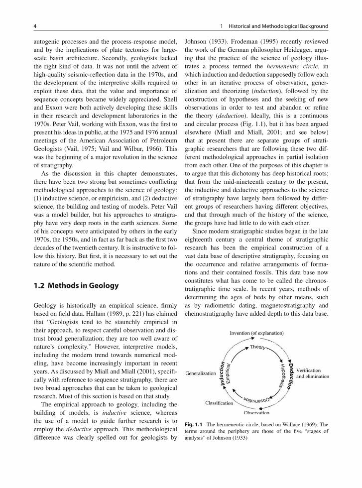
Johnson (1933). Frodeman (1995) recently reviewedthe work of the German philosopher Heidegger, argu-ing that the practice of the science of geology illus-trates a process termed the hermeneutic circle, inwhich induction and deduction supposedly follow eachother in an iterative process of observation, gener-alization and theorizing (induction), followed by theconstruction of hypotheses and the seeking of newobservations in order to test and abandon or refinethe theory (deduction). Ideally, this is a continuousand circular process (Fig. 1.1), but it has been arguedelsewhere (Miall and Miall, 2001; and see below)that at present there are separate groups of strati-graphic researchers that are following these two dif-ferent methodological approaches in partial isolationfrom each other. One of the purposes of this chapter isto argue that this dichotomy has deep historical roots;that from the mid-nineteenth century to the present,the inductive and deductive approaches to the scienceof stratigraphy have largely been followed by differ-ent groups of researchers having different objectives,and that through much of the history of the science,the groups have had little to do with each other.
Since modern stratigraphic studies began in the lateeighteenth century a central theme of stratigraphicresearch has been the empirical construction of avast data base of descriptive stratigraphy, focusing onthe occurrence and relative arrangements of forma-tions and their contained fossils. This data base nowconstitutes what has come to be called the chronos-tratigraphic time scale. In recent years, methods ofdetermining the ages of beds by other means, suchas by radiometric dating, magnetostratigraphy andchemostratigraphy have added depth to this data base.
Fig. 1.1 The hermeneutic circle, based on Wallace (1969). Theterms around the periphery are those of the five “stages ofanalysis” of Johnson (1933)
1.2 Methods in Geology 5
As we show here, research into the preserved recordof deep geological time has grown into an enormouslycomplex, largely inductive science carried out mainlyin the academic realm. From this, a descriptive (induc-tive) classification of Earth history has been built,consisting of the standard eras, periods, epochs, etc.
At various times, deductive models of Earth his-tory have been proposed that have had varying levelsof success in contributing to our understanding ofEarth’s evolution. There have also been many attemptsto develop deductive models of stratigraphic pro-cesses, including the cyclothem model of the 1930s,and modern facies models and sequence stratigraphy.Ideas about the tectonic setting of sedimentary basinshave also included several bold attempts at modelbuilding, including the pre-plate tectonic geosynclinetheory of Kay (1951), the modern petrotectonic assem-blage concepts of Dickinson (1980, 1981), the var-ious geophysically-based basin models of McKenzie(1978), Beaumont (1981) and many later workers,and the actualistic plate-tectonic models of Dickinson(1974), Miall (1984) and Ingersoll (1988).
The concepts of sequence stratigraphy that evolvedfrom seismic-stratigraphy in the 1970s constitute thebasis for the most recent and most elaborate attemptsto develop deductive stratigraphic models. Theseincluded the Exxon global cycle chart (Vail et al., 1977;Haq et al., 1987, 1988a), which, if it had proved tobe a successful explanation of the stratigraphic record,could potentially have become the dominant paradigm,entirely replacing the old inductive classification ofgeologic time, and largely supplanting the complexmethod with which it was being constructed. However,the two distinct intellectual approaches have resultedin the development of two conflicting and competingparadigms which are currently vying for the attentionof practicing earth scientists (Miall and Miall, 2001,2002). It is argued later in this book (Sect. 14.7) thatcurrent research in the field of cyclostratigraphy maybe following a similar pattern of development.
The history of stratigraphy since the end of the eigh-teenth century has encompassed the following broadthemes:
(1) Recognition of the concept of stratigraphic orderand its relationship to Earth history, and the growthfrom this of an empirical, descriptive stratigraphybased on sedimentary rocks and their containedfossils.
(2) The emergence of the concept of “facies” basedon the recognition that rocks may vary in charac-ter from place to place depending on depositionalprocesses and environments. This was one of thefirst deductive models developed to facilitate geo-logical interpretation.
(3) Recognition that rocks are not necessarily an accu-rate or complete record of geologic time, becauseof facies changes and missing section, and theerection of separate units for “time” and for“rocks”.
(4) Development of a multidisciplinary, empiricalapproach to the measurement and documenta-tion of geologic time, an unfinished science stillactively being pursued.
(5) Attempts at different times to recognize pat-terns and themes in the stratigraphic successionand to interpret Earth processes from such pat-terns. Facies models and sequence stratigraphy areamongst the main products of this effort.
(6) Attempts to extract regional or global signals fromthe stratigraphic record and to use them to build analternative measure of geologic time, based on anassumed “pulse of the Earth.”
These themes may be further generalized into adescriptive, inductive approach to the science (themes1–4), which may be categorized as the empiricalparadigm of stratigraphy, and a distinctly different,interpretive approach to the subject (themes 5 and 6),that may be termed the model-building paradigm. Themodel of global eustasy as applied to sequence stratig-raphy is discussed below. The use of cyclostratigraphyas a potential basis for a refined geologic time scale isdiscussed in Sect. 14.7.
The purpose of the present chapter is to sum-marize the parallel development of these two broadapproaches to stratigraphy, The discussion is notintended to be historically complete; there is a sub-stantial literature that addresses the history of stratig-raphy. By establishing the history of stratigraphy, thebody of ideas from which the modern controversyover sequence stratigraphy may be better understood.The mainstream of stratigraphic research has been thedevelopment of an ever more precise and comprehen-sive chronostratigraphic time scale based on the accu-mulation and integration of all types of chronostrati-graphic data. This paradigm is essentially one of metic-ulous empiricism which makes no presuppositions
6 1 Historical and Methodological Background
about the history of the Earth or the evolution of lifeor of geological events in general. The Vail/Exxonsequence models exemplify a quite different paradigm,but one that reflects an equally long intellectual history.They are the latest manifestation of the idea that thereis some kind of “pulse of the earth” that is amenable toelegant classification and broad generalization.
These two strands of research correspond to twoof the modes or “cognitive styles” of research ingeology that were described by Rudwick (1982).Descriptive stratigraphy and the development of thegeological time scale corresponds to the “concrete”style of Rudwick (1982, p. 224), who cites several ofthe great nineteenth-century founders of stratigraphicgeology as examples (e.g., William Smith, Sedgwick,Murchison). These individuals were primarily con-cerned with documenting and classifying the detail ofstratigraphic order. In contrast, the “abstract” style ofresearch includes individuals such as Hutton, Lyell,Phillips and Darwin, who sought underlying principlesin order to understand Earth history.
1.2.1 The Significance of SequenceStratigraphy
The business of research is new ideas. Few things, how-ever, are more unpopular with researchers than truly newideas. (Vail, 1992, p. 83)
Emerging in the 1970s, seismic stratigraphy, asdeveloped by Peter Vail and his coworkers at ExxonCorporation (Vail, 1975; Vail et al., 1977), broughtabout a revolution in the study of stratigraphy (Mialland Miall, 2001). It re-energized a discipline, 200 yearsin the making, offering new theoretical possibilities forknowledge of Earth history and fundamental Earth pro-cesses. It also provided a potentially powerful new ana-lytical and correlation tool for use by practicing basinanalysts, especially those in the petroleum industry.Amongst the new concepts and methods constitutingseismic stratigraphy were the following:
(1) The use of a new form of data—reflection-seismicrecords—for the generation of stratigraphic infor-mation;
(2) Demonstration that the new data could provideimages of large swaths of a basin at once;
(3) Demonstration of the complex internal architec-ture of basin fills;
(4) Demonstration that stratigraphic successions con-sist of “sequences,” which are packages of con-formable strata bounded by regional unconformi-ties;
(5) The proposal that the bounding unconformities aremostly global in extent and were generated byrepeated eustatic changes in sea level. We referhere to this hypothesis as the global eustasy model.
(6) The proposal that Earth’s stratigraphic record, con-sisting of a global record of sequences, could becharacterized by a global cycle chart, which couldbe used as a universal correlation template.
Within the framework of scientific revolutionsestablished by Kuhn (1962, 1996), seismic stratig-raphy could be said to constitute a new paradigm.Kuhn (1962, 1996) explained “paradigms” as univer-sally recognized scientific achievements that for a timeprovide model problems and solutions to a commu-nity of practitioners. These new developments haveproved to be of profound importance to the scienceof stratigraphy. Building on points 1–4, stratigraphersdeveloped an entirely new way of practicing their craft,including application of the concepts to outcrop andsubsurface well data, in a new science termed sequencestratigraphy (Posamentier et al., 1988; Posamentierand Vail, 1988; Van Wagoner et al., 1990). In this sci-ence, the architecture and predictability of sequencesare amongst its most valuable components.
In the early days of seismic stratigraphy, in the late1970s and early 1980s, the global cycle chart was con-sidered an inseparable part of the new method. The1970s were a period when globalization was a themein many facets of scientific and societal development.Marshall McLuhan (1962) was teaching us about a“global village” of humans, linked by the mass media;economists were beginning to argue for increasingglobalization of trade and commerce; and, in the earthsciences, the paradigm of plate tectonics was havingan enormous impact on our understanding of earth his-tory (e.g., Dewey, 1980; Dickinson 1974). Indeed, theglobal reach of seismic stratigraphy was one of its mostpersuasive features.
Miall and Miall (2002) examined social factorsshaping the development, dissemination, and initialvalidation of seismic stratigraphy and the social orga-nizations in which these occurred. The main objectiveof this chapter (based on Miall and Miall, 2001) is toexamine the methods that underlie the global-eustasymodel, and its precursors in stratigraphic modeling,
1.2 Methods in Geology 7
as far back as the work of Charles Lyell in themid-nineteenth century. Later sections deal with theperiod of the initial enthusiastic reception of seis-mic stratigraphy by the scientific community in thelate 1970s, to a period of increasing doubt about theglobal-eustasy model that extends to the present. Mialland Miall (2002) argued that beyond the undoubtednew facts and invigorating new ideas that seismicstratigraphy brought to geology, the popularity of thenew paradigm within the geological community owedmuch to human, “social” factors. The analysis drawsextensively on Kuhn’s work regarding the develop-ment and acceptance of new paradigms in science.The paradigm model has been usefully applied tothe study of several areas of research in the earthsciences, including the development of turbidite con-cepts (Walker, 1973), methods of grain-size analy-sis in sedimentology (Law, 1980), the acceptance ofplate-tectonic theories about the earth’s crust (Stewart,1986), and the controversy surrounding the abiogenicorigins of oil (Cole, 1996).
It is also argued here that because of controver-sies surrounding ideas about the origins of sequences,sequence stratigraphy has now evolved into two dis-tinct, competing paradigms. During the 1980s, a seriesof anomalies and conceptual problems about theglobal-eustasy model emerged. It is argued that thesehave not been fully addressed by proponents of theglobal-eustasy model, many of whom continue to usethis model as a central theme in their stratigraphicwork, despite a growing controversy that surrounds it.In subsequent chapters an examination of the natureof stratigraphic data and its importance in the pro-cess of validating Vail’s new ideas is carried out(Part IV).
The chapter is offered as a contribution to the studyof Dott’s (1998) question: “What is unique about geo-logical reasoning?” As an outcome of the analysis itis to be hoped that geologists will be alerted to thebias that preconceptions and group processes can bringto observations and interpretations in the geologicalrecord.
1.2.2 Data and Argument in Geology
The traditional view of science, as described by thetenets of analytical philosophy (Frodeman, 1995),
is that science proceeds from careful, objectiveobservation and replication of data, to hypotheses andtheory through the workings of the scientific method.According to Popper (1959), scientists engage in thepractice of proposing and falsifying testable hypothe-ses, based on dispassionate experimentation. There issome basis for arguing that this is what actually hap-pens in the so-called “hard” sciences, where ideasmay be tested by carefully designed experiments. Evenhere, however, human factors can intervene, as the con-troversy surrounding “cold fusion” a few years agoattests. The proponents of a new model of cold fusionwere able to convince themselves that their experi-ments had provided evidence for it, but attempts atreplication by other observers demonstrated the fal-sity of the original claims, and the new hypothesis wasquickly discarded (Peat, 1989).
It is not so simple in geology, where we are attempt-ing to understand a past that cannot be replicated byexperiment. As Dott (1998) pointed out, there is muchthat we can replicate, such as the chemistry of min-eral formation, or flume experiments to model bedformgeneration, but we cannot recreate the past in its com-plex entirety. The new science of numerical modelingis providing us with powerful new techniques for sim-ulating complex processes, such as stratigraphic accu-mulation under conditions of varying rates of basinsubsidence and climate change, but these are just sim-ple models, not complete replication experiments, sogeologists have to search for what Frodeman (1995)called “explanations that work.” Much of geologicalpractice constitutes what Dott (1998) referred to assynthetic science.
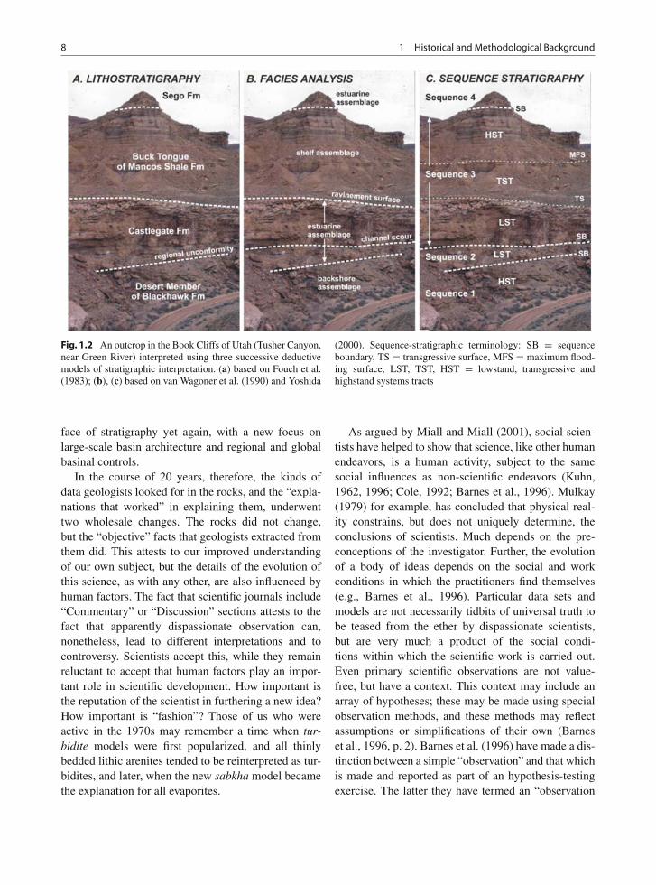
Our views of “what works” have changed dramati-cally as the science has evolved (Fig. 1.2). Consider thescience of stratigraphy, for example. Until the 1950s,stratigraphic practice consisted primarily of what wenow term lithostratigraphy, the mapping, correlatingand naming of formations based on their lithologicsimilarity and their fossil content. In the 1960s, therevolution in process sedimentology led to the emer-gence of a new science, facies analysis, and a focus onwhat came to be termed “autogenic” processes, suchas the meandering of a river channel or the progra-dation of a delta. Most stratigraphic complexity wasinterpreted in facies terms, and the science witnessedan explosion of research on process-response mod-els, otherwise termed facies models. The revolutionin seismic stratigraphy in the late 1970s changed the
8 1 Historical and Methodological Background
Fig. 1.2 An outcrop in the Book Cliffs of Utah (Tusher Canyon,near Green River) interpreted using three successive deductivemodels of stratigraphic interpretation. (a) based on Fouch et al.(1983); (b), (c) based on van Wagoner et al. (1990) and Yoshida
(2000). Sequence-stratigraphic terminology: SB = sequenceboundary, TS = transgressive surface, MFS = maximum flood-ing surface, LST, TST, HST = lowstand, transgressive andhighstand systems tracts
face of stratigraphy yet again, with a new focus onlarge-scale basin architecture and regional and globalbasinal controls.
In the course of 20 years, therefore, the kinds ofdata geologists looked for in the rocks, and the “expla-nations that worked” in explaining them, underwenttwo wholesale changes. The rocks did not change,but the “objective” facts that geologists extracted fromthem did. This attests to our improved understandingof our own subject, but the details of the evolution ofthis science, as with any other, are also influenced byhuman factors. The fact that scientific journals include“Commentary” or “Discussion” sections attests to thefact that apparently dispassionate observation can,nonetheless, lead to different interpretations and tocontroversy. Scientists accept this, while they remainreluctant to accept that human factors play an impor-tant role in scientific development. How important isthe reputation of the scientist in furthering a new idea?How important is “fashion”? Those of us who wereactive in the 1970s may remember a time when tur-bidite models were first popularized, and all thinlybedded lithic arenites tended to be reinterpreted as tur-bidites, and later, when the new sabkha model becamethe explanation for all evaporites.
As argued by Miall and Miall (2001), social scien-tists have helped to show that science, like other humanendeavors, is a human activity, subject to the samesocial influences as non-scientific endeavors (Kuhn,1962, 1996; Cole, 1992; Barnes et al., 1996). Mulkay(1979) for example, has concluded that physical real-ity constrains, but does not uniquely determine, theconclusions of scientists. Much depends on the pre-conceptions of the investigator. Further, the evolutionof a body of ideas depends on the social and workconditions in which the practitioners find themselves(e.g., Barnes et al., 1996). Particular data sets andmodels are not necessarily tidbits of universal truth tobe teased from the ether by dispassionate scientists,but are very much a product of the social condi-tions within which the scientific work is carried out.Even primary scientific observations are not value-free, but have a context. This context may include anarray of hypotheses; these may be made using specialobservation methods, and these methods may reflectassumptions or simplifications of their own (Barneset al., 1996, p. 2). Barnes et al. (1996) have made a dis-tinction between a simple “observation” and that whichis made and reported as part of an hypothesis-testingexercise. The latter they have termed an “observation
1.2 Methods in Geology 9
report.” They have suggested that “our thoughts couldinfluence our perceptions as well as our perceptionsinfluence our thoughts.” Indeed, it has been argued thatthere really is no such thing as a “pure” observation.There may be many assumption sets in a given field.For example, as noted above, the same stratigraphicsection may have been described in at least three differ-ent ways since the 1950s. As Kuhn (1962. p. 129) hasnoted, “one and the same operation, when it attachesto nature through a different paradigm, can become anindex to a quite different aspect of nature’s regular-ity.” This is not intended as a criticism or negation ofthe scientific method, but as an attempt to throw lighton the very human processes involved in the actionof “doing science”, so that we might understand itbetter.
Such an analysis of the very foundations of thescientific method, which points to and incorporatesthe various contextual characteristics of the work,is a dramatically different way of viewing sciencethan the analytical approach. Based on the philo-sophical ideas of Heidegger, this approach is termedhermeneutics, and the back-and-forth thought pro-cesses between observation and interpretation areconceptualized as the hermeneutic circle (Heidegger,1927, 1962; Frodeman, 1995; Barnes et al., 1996).Frodeman (1995), in a discussion of the philosophyof science, noted that Heidegger identified three typesof “prejudgement” or “forestructures” that scientistsbring to each situation: preconceptions; ideas or pre-sumed goals, and a sense of “what will count as ananswer” (Frodeman, 1995, p. 964); and the particu-lar tools and methods of the research. Hermeneuticsargues that our original goals and assumptions resultin certain facts being discovered rather than others,which in turn lead to new avenues of research andsets of facts. Rudwick (1996) argued that, beyond thebasic data directly measurable by technological means,such as the density of pyrite, or the drilling depth ofthe Toronto Formation, “there are no theory-free factsin geology.” While extreme, this viewpoint provides auseful counterweight to the power of a newly populartheory.
One of the themes followed through this book isan attempt to show how “human factors” influenced,and still influence, the progress of a single geologicalmodel, that of global eustasy and its implications forsequence stratigraphy.
1.2.3 The Hermeneutic Circleand the Emergence of SequenceStratigraphy
Sequence concepts, as first developed by Sloss et al.(1949) and Sloss (1963), constituted a resurrectionof the deductive approach to the documentation andinterpretation of the stratigraphic record (one with along prior tradition, as discussed below), but sequencestratigraphy had not become the prevailing strati-graphic method when approaches based on seismicstratigraphy were first introduced in the mid 1970s.The new work that emerged from Exxon in the 1970sbrought about what Kuhn would term a “crisis” in sed-imentary geology; that is, the introduction of a newmethod and a body of ideas that could not be recon-ciled with existing paradigms. As Kuhn (1996, p. 181)has stated:
Crises need not be generated by the work of the commu-nity that experiences them and that sometimes undergoesrevolution as a result. New instruments like the electronmicroscope or new laws like Maxwell’s may developin one specialty and their assimilation creates crises inanother.
The development of high-quality reflection-seismicdata and the new methods of stratigraphic inter-pretation based on these data (e.g. the focus onstratigraphic surfaces and terminations, and on three-dimensional architecture) clearly constituted a new“instrument” in the specialty of petroleum geophysics.These data then affected the field of conventional,largely university- and state-survey-based stratigraphy.To this extent, Vail’s work created “crisis”, which hiswork was, in turn, designed to resolve (Miall and Miall,2001). Indeed, the emergence of sequence stratigra-phy resulted in two additional challenges to what Kuhn(1962) would have referred to as the “normal science”of stratigraphic interpretation:
(1) The proposal that the global cycle chart was asuperior standard of geologic time to that basedon conventional chronostratigraphy. For example,Vail et al. (1977, p. 96) stated: “One of the great-est potential applications of the global cycle chartis its use as an instrument of geochronology.” Vailand Todd (1981, p. 217) stated, with regard to cor-relations in the North Sea Basin: “several uncon-formities cannot be dated precisely; in these cases
10 1 Historical and Methodological Background
their ages are based on our global cycle chart, withage assignments based on the basis of a best fitwith the data.” They proceeded to revise biostrati-graphic ages based on the correlations suggestedby their chart.
(2) The attribution of all changes in sea level to twofavored eustatic mechanisms—eustasy (typicallyglacioeustasy for high-frequency sequences), andchanges in ocean-basin volumes (Vail et al., 1977,pp. 92–94)—and the assertion that other regionalprocesses, including tectonism and changes in sed-iment supply, affected only the amplitude but notthe timing of sea-level changes (Vail et al., 1991,p. 619).
Unlike that which occurred during the develop-ment and acceptance of plate tectonics (Stewart, 1986),there was no “crisis” in normal science, in the senseoriginally intended by Kuhn (1962). Other geolo-gists were not dissatisfied with the body of “nor-mal” stratigraphic science. Conventional chronostrati-graphic methods, based on biostratigraphy, radiometricdating, chemostratigraphy, etc., were, and remain, theprimary means for determining geologic age (e.g.,Harland et al., 1990; Holland, 1998; Gradstein et al.,2004) and, to the extent that there had been nowidespread search for global mechanisms for strati-graphic processes, most were comfortable with the pre-vailing views regarding the complexity of geologicalprocesses. Nonetheless, it could have been expectedthat a geological community, alerted to the power andinfluence of the new global tectonics (plate tectonics)in the mid- to late 1970s, would view a new globalmodel with interest and excitement.
Vail himself attempted to describe his own scientificprocedures. In his memoir on the evolution of sequencestratigraphy (Vail, 1992), he discussed how researchcreativity could be optimized through the applicationof a set of procedures which seemingly reflected thehermeneutic approach. These included what we couldterm forestructures, such as the establishment of a the-matic research program with clearly defined goals forthe overall research, and the definition of concepts thatwould drive the thematic research—driving concepts.However, Vail argued that it was important to definedriving concepts because it would then be possible “toacknowledge and nurture ideas that challenge, and mayprove superior to the existing driving concepts” (Vail,1992, p. 84). He also argued (on the same page) that,
truly new, worthwhile ideas based on competing drivingconcepts may not be accepted within the framework ofthematic research. These competing driving concepts arecommonly ignored or put aside because of the priority ofother work.
Despite this awareness that driving concepts in the-matic research can direct attention away from anoma-lous observations and hypotheses, and based on hisown recollections of his time at Exxon, Vail appearsto have established, within his own seismic researchgroup, a structure likely to yield the kind of hermeneu-tic circle which did not allow for competing drivingconcepts, as argued in the remainder of this section.According to Vail (1992, p. 89), two organizing princi-ples appeared to guide the research. First, a workingenvironment was fostered in which problems wereaccurately defined and interrelated through the estab-lishment of a thematic research program informed bythe driving concepts mentioned above. These conceptsdirected the group’s attention to the problems to besolved, the methods to be used in obtaining solutions,and the types of phenomena to be studied (from Vail,1992, p. 87):
What this driving concept showed was that seismicsections are a high-resolution tool for determiningchronostratigraphy-the time lines in rocks. This wasa “eureka” at that time. We had found the tool anddeveloped the methodology to make regional chronos-tratigraphic correlations and to put stratigraphy into ageologic time framework for mapping and the under-standing of paleogeography. . . . The fact that seismicreflections follow time lines is the second basic drivingconcept
As Sloss (1988a, p. 1661) put it,
the sequence concept was alive and well in a researchfacility of . . . Exxon. here, Peter Vail and a cohort ofpreconditioned colleagues seized upon the stratigraphicimagery made available by multichannel, digitallyrecorded, and computer-massaged reflection seismogra-phy to establish the discipline of seismic stratigraphy.
Second, an environment was created where bothteamwork and individual responsibility co-existed. AsVail (1992, p. 89) has observed, in his article onthe evolution of seismic stratigraphy and the globalsea-level curve,
As a group, we developed an overall plan. We wouldthen try to identify the person who was most interestedand knowledgeable for each task, and then endeavor togive each person a maximum amount of responsibility forhis or her project area. . . We tried to develop a situation
1.2 Methods in Geology 11
wherein each researcher had a clear-cut area of respon-sibility, but we made sure it overlapped with as manyother areas as possible. This ensured good communica-tion, because each person was vitally interested in whatthe others were doing.
What this also ensured, as Law and Lodge (1984)might argue, was that each member of the group hadan interest and an investment in the success of seis-mic stratigraphy and the global eustasy model. Thework of the Exxon team, as described by Vail, is agood example of the “socially constructed” nature ofgroup scientific work. As Clarke and Gerson (1990)have argued, scientific theories, findings and facts aresocially constructed (although, of course, based onobservation and measurement). They note that to solveresearch problems, scientists will make commitmentsto specific theories and methods, to other scientists,to research sponsors, and to various organizations.Clark and Gerson (1990, p. 184) further directed atten-tion to the importance of “. . . structural conditions ofwork, and the concrete processes of actually collatingdifferent lines of evidence.” These, they argued, arecritical to the emergence and maintenance of belief inthe results of a particular line of research in the faceof what they term the “buried uncertainties” of theresearch.
It must be emphasized that the Exxon workis being used here to illustrate common themesin scientific research, not in order to criticize themethod, but in order to help focus in on the impor-tance of group dynamics as the research evolvedand came under scrutiny by the wider geologicalcommunity.
It is instructive to situate Vail’s methodologicalapproach in a historical context. In the next sectionsthe development of two parallel traditions in stratig-raphy is followed from their origins in the nineteenthcentury.
1.2.4 Paradigms and Exemplars
As Kuhn (1962, p. 121) has noted, “given a paradigm,interpretation of data is central to the enterprise thatexplores it, but that interpretive enterprise . . . can onlyarticulate a paradigm, not correct it.” Kuhn (1962,pp. 23–24) has further argued that,
The success of a paradigm . . . is at the start largelya promise of success discoverable in selected and stillincomplete examples. Normal science consists in theactualization of the promise, an actualization achieved byextending the knowledge of those facts that the paradigmdisplays as particularly revealing, by increasing the extentof the match between those facts and the paradigm’spredictions, and by further articulation of the paradigmitself.
The fundamental building blocks of new science,he goes on to state, are “solved problems.” These hereferred to as exemplars, because they are used asexamples for teaching and in order to guide furtherresearch (See also, Barnes et al., 1996, pp. 101–109).
In an historical science like geology, it is difficultto arrive at “truth” or “proof” by the normal processof experimentation and replication (though not alwaysimpossible, as demonstrated by Dott, 1998). It couldbe argued that exemplars are “explanations that work;”what Frodeman (1995) has referred to as a type ofunderstanding having “narrative logic.” Typical exam-ples of exemplars in this case are: “In the North Sea,15 of 17 unconformities identified on the basis of wellresults and seismic data matched Exxon’s global sea-level curve.” (P. R. Vail at a meeting in Woods HoleMassachusetts in April as reported by Kerr, 1980, p.484). And again: “We can correlate ten of them [uncon-formities] perfectly with the Vail curve, five correlatepretty well, and the others still have a few problems.”(Tom Loutit and James Kennett commenting on theirwork in New Zealand as reported by Kerr, 1980, p.485). In a follow-up report on the Vail method 4 yearslater, Kerr (1984) reported several more of these “X outof Y” comparisons, where Y is slightly greater than butnever equal to X.
As we documented elsewhere (Miall and Miall,2002), the publication of exemplars of this type helpedto rapidly convince the geological fraternity of thepower and importance of the new global eustasymodel. This, despite the lack of supporting documen-tation in Vail et al. (1977), including, for example,interpreted seismic lines or biostratigraphically doc-umented subsurface sections. Missing, therefore, arethe “observations” that are supposedly so critical tothe scientific method (Barnes et al., 1996). At best, wehave what Barnes et al. (1996) might have called “areport that such observations exist”. Given the lack ofpublished documentation, there was no opportunity foroutsiders to influence the workings of the hermeneuticcircle on the development of the global eustasy model.
12 1 Historical and Methodological Background
In their discussion of the development of scientificknowledge in general, Barnes et al. (1996) discussedhow an important experiment in physics (determina-tion of the charge of the electron) was gradually refinedby repeated experimentation, documented by extensivelaboratory note-taking, and how the results of a rivalset of experiments that generated different results wereeventually discarded because the results were gradu-ally shown to be inconsistent with the results of newwork. Similarly, at some point, Vail and his coworkersdecided that a given set of sea-level events representedglobal eustatic signals, and the first global cycle chart(Vail et al., 1977) was the result. The global eustasyhypothesis seems to have begun to work a powerfulinfluence on the selection and collation of additionaldata. But how were these events selected? How didVail know that these were the “right” ones? How wereother events discarded as the result of “local tectonics”,or as having been “offset” by biostratigraphic impreci-sion? When consideration is given then to the “solvedproblems” or exemplars of the global cycle chart, themethod of documentation and cross-checking and vir-tually all of the primary data are missing. For example,the reader’s attention is directed to the only publisheddiagram in AAPG Memoir 26 (Vail et al., 1977, Fig. 5on p. 90) that illustrates the synthesis of individualcycle charts into the global average. There are sev-eral events appearing in the average curve that arenot well represented in the individual charts, and viceversa (see also discussion of this subject in Chap. 12).These points have not been explained by Vail or hiscoworkers.
In his discussion of the consensus model of science,Kuhn (1962) has observed that the real function ofexperiment is not the testing of theories. He showedthat commonly, theories are accepted before thereis significant empirical evidence to support them.Results which confirm already accepted theories arepaid attention to, while disconfirming results areignored. Knowing what results should be expectedfrom research, scientists may be able to devise tech-niques that obtain them (Kuhn, 1977; Cole, 1992, pp.7–8). The exercise of correlating new stratigraphicsections to the global cycle chart entails the dangersof self-fulfilling prophecy. As noted by Kuhn (1962,pp. 80, 84):
The bulk of scientific practice is thus a complex andconsuming mopping-up operation that consolidates theground made available by the most recent theoretical
breakthrough and that provides essential preparation forthe breakthrough to follow. In such mopping-up opera-tions, measurement has its overwhelmingly most com-mon scientific function. . . . Often scientists cannot getnumbers that compare well with theory until they knowwhat numbers they should be making nature yield.
The lack of published experimental documentationand detailed analysis in support of the global-eustasymodel makes it difficult for scientists in general toevaluate the importance of these human processes thatKuhn described.
Why did geologists eagerly embrace the global-eustasy model despite the lack of published data thatthey could see for themselves? We suggest that it was(1) because of the current willingness to accept globalexplanations of earth processes in light of the newplate-tectonics paradigm; (2) the ideas offered a util-itarian application—the global correlation template—of apparently considerable potential use in the explo-ration business; (3) because of the assumed authorityof corporate geophysics, or what we term “the ExxonFactor” (Miall and Miall, 2002); and (4) because work-ing petroleum geologists had no investment in thecomplex, confusing and “academic” science of con-ventional chronostratigraphy. Dott (1992b) suggestedan additional factor, the “innate psychological appealof order and simplicity” of a pattern of cyclicity basedon Milankovitch periodicity.
Use of the global cycle chart appeared to offera simple global solution to the problem of strati-graphic correlation so, perhaps, it was not surprisingthat working geologists eagerly adopted it. Indeed, thenon-availability of a data base, with all the messiness,incompleteness and inconsistency such as normallycharacterizes stratigraphic successions from diverseareas characterized by different tectonic histories,undoubtedly made it easier to accept the global cyclechart as is. To cite Law’s (1980, p. 13) summation ofMannheim’s philosophy, the application of the globalcycle chart displayed
the attributes of Mannheim’s natural law style ofthought – they are atomistic, generally quantitative,emphasize the routine nature of scientific practice, seek orutilize general laws, stress continuity, and are in generalreductionist.
The techniques for identifying sea-level events inseismic records and (later) stratigraphic sections, andequating them to existing events in the global cyclechart, became a routine operation ideally suited to
1.3 The Development of Descriptive Stratigraphy 13
petroleum-exploration work. The alternative, holisticapproach to stratigraphy is the traditional one of corre-lation by biostratigraphy and the erection of stratotypeswith no built-in assumptions of global events. It wasthis approach that Vail’s chart seemed destined toreplace. While Vail and his colleagues have repeatedlyreaffirmed the importance of biostratigraphic datingand correlation in the testing of the global cycle chart,the emphasis in much of the work of this group is onthe superiority of the global cycle chart as a method ofcorrelation and stratigraphic standardization (Vail andTodd, 1981, p. 230; Vail et al., 1984, p. 143; Baum andVail, 1988, p. 322; Vail et al., 1991, pp. 622, 659; seeChap. 12).
In the early 1980s, however, problems with theglobal eustasy model began to emerge as alternativeideas about sequence generation began to appear, anddoubts emerged about the accuracy and precision ofchronostratigraphic methods available to test globalcorrelations. These are discussed in Chap. 12, wherethe global cycle chart is examined in detail.
1.3 The Development of DescriptiveStratigraphy
1.3.1 The Growth of Modern Concepts
The development of the science of descriptive stratig-raphy is described by Hancock (1977), Conkin andConkin (1984), and Berry (1987). Earlier discussionsthat include much valuable historical detail includethose by Teichert (1958) and Monty (1968). The fol-lowing summary is intended only to emphasize theevolution in methodologies that took place from thelatest eighteenth century until they stabilized duringthe mid-twentieth century.
Stratigraphy is founded on the ideas of RichardHooke and Nicolaus Steno, physician to the GrandDuke of Tuscany, although Vai (2007) suggested thatseveral key points were anticipated by Leonardo daVinci in about 1500. The Law of Superposition wasenunciated by Nicolaus Steno in his work Prodromus,published in 1669. This law, simply stated, is that inany succession of strata, the oldest and first formedmust be at the bottom, with successively youngerstrata arranged in order above. As described by Berry
(1987), several rock successions were described dur-ing the eighteenth century, primarily because of theirimportance to mining operations, but no fundamentalprinciples emerged from this work until the four-fold subdivision of the Earth’s crust was proposed byAbraham Gottlob Werner.
The foundation of modern stratigraphy is attributedto William Smith, a surveyor for contemporary canalbuilders, who became interested in the rocks that werebeing dug into as a series of canals were constructedacross southern England (Hancock, 1977, pp. 3–4;Berry, 1987, pp. 56–57). His knowledge of geologywas self-taught, owing nothing to such illustrious pre-decessors as James Hutton. As Hancock (1977, p. 5)noted, Smith’s work was entirely empirical, free of anyattempt at grand theory, and free of any influence oftheology—an important point considering the power-ful influence of biblical teachings at the time. Smith’swork began in the Jurassic strata around Bath, in south-west England. He recognized that the stratigraphicsuccession was the same wherever he encountered it,and that particular strata could also be characterized byparticular suites of fossils. From this inductive base,Smith evolved the deductive principle that he couldidentify the stratigraphic position of any outcrop by itsdistinctive rock types and fossil content. He commit-ted his observations to maps that showed the outcroppatterns of his succession, and over a period of about25 years he gradually compiled a complete geologicalmap of England and Wales, the first such map of itskind ever constructed (Smith, 1815). Because Smithwas not a member of the landed or aristocratic classin England, his work was largely ignored until latein his life, when he was appropriately honoured bythe Geological Society of London. The story is toldin detail by Winchester (2001) and Torrens (2001).Others were describing local successions of strata dur-ing the late eighteenth and early nineteenth centuries,such as Cuvier and Brongniart who documented theTertiary strata of the Paris Basin in the first two decadesof the nineteenth century (Conkin and Conkin, 1984;Berry, 1987, p. 66), but Smith was the first to show thatrocks, with their contained fossils, constituted map-pable successions. Cuvier was more concerned withthe history of life on earth (Hancock, 1977, p. 6).Brongniart was amongst the first to appreciate theimportance of Smith’s contribution in creating the pos-sibility of long-distance correlation based on fossilsalone, independent of rock type (Hancock, 1977, p. 7).
14 1 Historical and Methodological Background
As knowledge of regional stratigraphy evolved invarious parts of Europe, the fourfold primary subdi-vision of Werner was broken down locally into various“series”, and these, in turn, were commonly subdividedinto local “formations.” This was an entirely piecemealoperation, reflecting local interests, but from this grad-ually evolved a body of descriptive knowledge of rocksuccessions and their contained fossils. As noted byBerry (1987, p. 63):
Many of the widely used descriptive units did bear fossilsthat, when analyzed using the principle of faunal succes-sion, proved to be a fossil aggregate diagnostic of a timeunit in an interpretive scale; thus many descriptive unitsbecame interpretive ones, and today bear the same names.Among the major units of the interpretive time scale thatwere originally descriptive rock units are the Cambrian,Carboniferous, Jurassic, Cretaceous and Tertiary. Unitsthat were based on interpretation of fossils from theirinception are the Ordovician, Devonian, Permian, and theTertiary Epochs.
During the 1820s and 1830s such workers as Youngand Bird in Yorkshire, and Eaton in New York, rec-ognized that some formations changed in character asthey were traced laterally (Hancock, 1977, pp. 7–8).Amand Gressly (1838; see translation in Conkin andConkin, 1984, pp. 137–139) was the first to sys-tematize the observation of such changes, with theintroduction of the term and concept of facies, basedon his work on the Jurassic rocks of the Jura region ofsouthern France. For example, he was aware of the dif-ferences between the limestones with contained fossilsof coral-bank environments, oolitic deposits (which wenow recognize to be beach deposits), and the “oozy”deposits of deeper-water environments, all of whichmay form at the same time, and may also form oneabove the other as environments shift over time. Thistype of change can be documented by careful obser-vation of rocks in outcrop, by studying the verticalsuccession of rock types or by tracing an individual setof beds laterally, perhaps for many kilometres. Gresslyproposed two new laws: the first that in different placesformations (“terrains” in the French terminology) mayconsist of rocks of different petrologic and paleon-tological character (the original meaning of the termfacies, which we still retain), and, secondly, that asimilar succession of facies may occur in both verti-cal and lateral arrangement, relative to the bedding.As Hancock (1977, p. 9) pointed out, this predatedWalther’s proposal of the law of the correlation offacies by some 56 years. The study of facies became
a central activity of stratigraphic work in the 1960s,with the establishment of the process-response faciesmodel, as noted above.
With Gressly’s concept of facies in place, the stagewas set for the next important development, that of theintroduction of the concept of the stage, by anotherFrench geologist, d’Orbigny (1842–1852). He rec-ognized the vertical variability in fossil assemblageswithin individual series, and realized that stratigraphicsuccessions could be subdivided into smaller unitsbased on careful categorization of these succeedingfossil assemblages. These he called stages. D’Orbignyalso used the term zone, but nowhere clearly defined it(Monty, 1968). Teichert (1958) argued that d’Orbignywas inconsistent in his usage, sometimes using theterm zone as a synonym for stage, and sometimes asa subdivision of a stage. He established, if informally,the idea of the ideal “type” of succession, a localitywhere the stage was well represented, and from thishas grown the concept of the type section or stratotype,to which formal importance has now been assigned asthe first point of reference for establishing the char-acter of a stratigraphic unit. Many of the stage namesd’Orbigny erected are still those used worldwide. Hewas aware of the concept of facies change and of thevariability in the nature of stage boundaries, from con-formable to unconformable. As Conkin and Conkin(1984, p. 83) noted, the importance of d’Orbigny’swork is his consolidation and adaptation of ideas thatalready existed in embryonic form, and the scope ofhis stage classification, which included the erection ofsome 27 stages for the Paleozoic and Mesozoic.
Hancock (1977, p. 12) suggested that the truefoundation of biostratigraphy came with the work ofthe German stratigrapher Albert Oppel (1856–1858),whose work also concentrated on the Jurassic succes-sion of western Europe. Oppel extended the ideas ofd’Orbigny about the subdivision of successions basedon their contained fossils to a more refined level. Herecognized that careful study of the contained fossilswould permit a much more detailed breakdown of therocks, into what he called zones. He investigated “thevertical distribution of each individual species at manydifferent places ignoring the mineralogic character ofthe beds” (Oppel, as quoted in Berry, 1987, p. 127).Some species were discovered to have short verticalranges, others long ranges. Each zone could be char-acterized by several or many fossil species, althoughcommonly one species would be chosen to be used
1.3 The Development of Descriptive Stratigraphy 15
as the name of the zone. Oppel built up stages fromgroups of zones. Stages were referred to as zonegrup-pen, or groups of zones (Teichert, 1958). These wouldusually fit into the stages already defined by d’Orbigny,but as Hancock (1977, p. 13) noted, in some placeshis zones spanned already-defined stage boundaries.This was the beginning of a practical problem thathas still to be fully resolved; but in many cases, suchas at the base and top of the Jurassic, Oppel’s zoneboundaries coincided with the System boundaries. Inpractice, zones became the foundation upon which thewhole framework of biostratigraphy, the zone, stage,series and system, was gradually built. Teichert (1958,p. 109) emphasized the importance of Oppel’s originaldescription of zones as “paleontologically identifiablecomplexes of strata,” not as subdivisions of time. Theoriginal concept was therefore clearly inductive—therecognition of a zone depended on the field geologistfinding specific fossils in the rocks.
In their summation of the work of d’Orbigny andOppel, Teichert (1958, p. 110) and Hancock (1977,p. 11) were at pains to emphasize the empirical,descriptive nature of the stage and zone concepts. Theysuggested that they were later distorted by the intro-duction of concepts about time that, they claimed,served to confuse the science of stratigraphy for someyears. Teichert (1958) attributed these misconcep-tions to individuals such as H. Hedberg and O. H.Schindewolf. Hancock (1977) argued that Hedberg’sinfluence was detrimental to the development of clearstratigraphic concepts. These problems are addressedbelow. However, careful examination and translationof d’Orbigny’s original statements by Monty (1968)and Aubry et al. (1999, Appendix A) cast a differ-ent light on this historical work. Aubry et al. (1999,p. 137) pointed out that in the mid-nineteenth cen-tury no clear distinction between rocks and time hadbeen made, and that paleontology was the only meansof long-distance correlation. Selected translations fromd’Orbigny’s work clearly indicate that he envisionedstages as having a time connotation (Aubry et al., 1999,pp. 137–138).
Shortly after Oppel’s work was completed, CharlesDarwin’s The origin of species was published (1859),and provided the explanation for the gradual changein the assemblage of species that Oppel had observed.However, resistance to the concepts of the stage andthe zone remained strong through the remainder of thenineteenth century in Britain and the United States,
where the concept of facies had also still not takenhold, and reliance for correlation tended to still beplaced on the lithology of formations. (Hancock, 1977,pp. 14–15).
International agreement on the definition and usageof most stratigraphic terms was attempted at the firstInternational Geological Congress in Paris in 1878.A commission was established, that subsequently metin Paris and in Bologna. At the latter meeting, inSeptember–October 1880, the commission:
Decided on definitions of stratigraphic words like seriesand stage, and listed their synonyms in several lan-guages . . .. Rocks, considered from the point of viewof their origin, were formations; the term was notpart of stratigraphic nomenclature at all, but concernedhow the rock had been formed (e.g., marine forma-tions, chemical formations). Stratigraphic divisions wereplaced in an order of hierarchy, with examples, thus:group (Secondary Group) [what we would now termthe Mesozoic], system (Jurassic System), series (LowerOolite Series), stage (Bajocian Stage), substage, assise(Assise à A. Humphriensianus), stratum. A distinctionwas made between stratigraphic and chronologic divi-sions. The duration of time corresponding to a group wasan era, to a system a period, to a series an epoch, and to astage an age (Hancock, 1977, p. 15).
Definitions of the terms “zone” and “horizon” wereadded to the published record of this meeting by thesecretary of the commission, based on national reportssubmitted by the delegates, but full international agree-ment was slow in coming (Hancock, 1977, p. 16).Nonetheless, by the early twentieth century, the follow-ing basic descriptive terms and the concepts on whichthey were based had become firmly established, if notuniversally used:
Law of superposition of strataStratigraphic outcrop maps based on the succession of
sedimentary rocks with its contained fossilsFaciesStageType section or stratotypeZone
At the 8th International Geological Congress inParis in 1900 the stratigraphic hierarchy era, sys-tem/period, epoch/series, age/stage, phase/zone wasaccepted (Vai, 2007).
According to Teichert (1958), the term biostratig-raphy was introduced by the Belgian paleontologistDollo in 1904, for the “entire research field in which
16 1 Historical and Methodological Background
paleontology exercises a significant influence on his-torical geology.”
Codification of these principles by the mid-twentieth century is illustrated by the work of Schenkand Muller (1941). Various national and internationalstratigraphic codes and guides have been developedthat standardize and formalize the definitions of strati-graphic terms and set out the procedures by whichthey should be used. An international guide was pub-lished in 1976 (Hedberg, 1976), with a major revisionappearing in 1994 (Salvador, 1994). A code for NorthAmerica, based on the international guide, appeared in1983 (NACSN, 1983).
1.3.2 Do Stratigraphic Units Have “Time”Significance?
As long ago as 1862 Huxley wrote: “neither physi-cal geology nor paleontology possesses any methodby which the absolute synchronism of two strata canbe demonstrated. All that geology can prove is localorder of succession.” (quoted in Hancock, 1977, p. 17).As an example, Huxley suggested that there was noway to prove or disprove that “Devonian fauna andflora in the British Isles may have been contempora-neous with Silurian life in North America, and witha Carboniferous fauna and flora in Africa.” The vari-ations in fauna and flora could simply be due to thetime it took for the organisms to migrate. There istherefore a need for a distinction between “‘homo-taxis’ or ‘similarity of arrangement’ and ‘synchrony’or ‘identity of date” (Hancock, 1977, p. 17). Conkinand Conkin (1964) suggested that this concept was firstenunciated by DeLapparant (1885; as cited and trans-lated by Conkin and Conkin, 1984, p. 243), althoughCallomon (2001, p. 240) stated that the Principle ofBiosynchroneity”, whereby beds with similar fossilsare assumed to be the same age, is “usually ascribedto William Smith”. As geologists accumulated a verydetailed knowledge of the succession of fossils, theassumption that the same succession of fossil assem-blages indicated synchroneity assumed the status of atruism. However, until the development of radiometricdating and the growth of modern chronostratigraphy(see below) the true “time” value of fossils remaineda problem, because biostratigraphy provides only rel-ative ages. The basic assumption about the temporalvalue of fossils was first made most clearly by Lyell
(1830–1833) and, according to Conkin and Conkin(1984; see in particular their Table 1, p. 2), subse-quent developments by Bronn (1858), Phillips (1860),Lapworth (1879), DeLapparant (1885) and Buckman(1893) established the main framework upon whichthis part of modern stratigraphy is built.
One of Lyell’s (1830–1833) most important con-tributions was his detailed study and classificationof Tertiary deposits, based on their contained fos-sils. Berggren (1998) provided a succinct summaryof this important contribution. Lyell’s subdivisions ofthe Tertiary were based on the idea that, through thecourse of time, contemporary faunas become more andmore like those found at present. Under a heading “Thedistinctness of periods may indicate our imperfectinformation” he stated:
In regard to distinct zoological periods, the reader willunderstand . . .. That we consider the wide lines of demar-cation that sometimes separate different tertiary epochs,as quite unconnected with extraordinary revolutions ofthe surface of the globe, as arising, partly, like chasms inthe history of nations, out of the present imperfect stateof our information, and partly from the irregular mannerin which geological memorials are preserved, as alreadyexplained. We have little doubt that it will be necessaryhereafter to intercalate other periods, and that many ofthe deposits, now referred to a single era, will be found tohave been formed at very distinct periods of time, so that,notwithstanding our separation of tertiary strata into fourgroups, we shall continue to use the term contemporane-ous with a great deal of latitude (Lyell, 1833, vol. 3, pp.56–57).
This quote contains most of the modern concept thatunits defined on the basis of their fossil content mayhave global significance with regard to contemporane-ity, but that the preserved record may be imperfect.Lyell’s “lines of demarcation” are what we wouldnow define as chronostratigraphic boundaries. Thesewere commonly drawn at unconformities until theintroduction of modern practices, as described below.Vai (2007, p. 87) pointed out that Lyell’s originalunits were clearly described as physical rock bodies.Therefore, the separation of “rock” and “time” is not asclear in this early work as has sometimes been reported(e.g., Berggren, 1998).
Phillips (1860, p. xxxii), in comparing fossil succes-sions between localities in different parts of the world(he mentioned several Paleozoic successions that hadbeen described from Europe and North America), sug-gested that “the affinity of the fossils is accepted asevidence of the approximate contemporaneity of the
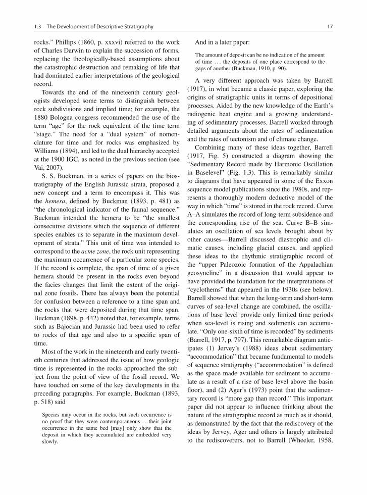
1.3 The Development of Descriptive Stratigraphy 17
rocks.” Phillips (1860, p. xxxvi) referred to the workof Charles Darwin to explain the succession of forms,replacing the theologically-based assumptions aboutthe catastrophic destruction and remaking of life thathad dominated earlier interpretations of the geologicalrecord.
Towards the end of the nineteenth century geol-ogists developed some terms to distinguish betweenrock subdivisions and implied time; for example, the1880 Bologna congress recommended the use of theterm “age” for the rock equivalent of the time term“stage.” The need for a “dual system” of nomen-clature for time and for rocks was emphasized byWilliams (1894), and led to the dual hierarchy acceptedat the 1900 IGC, as noted in the previous section (seeVai, 2007).
S. S. Buckman, in a series of papers on the bios-tratigraphy of the English Jurassic strata, proposed anew concept and a term to encompass it. This wasthe hemera, defined by Buckman (1893, p. 481) as“the chronological indicator of the faunal sequence.”Buckman intended the hemera to be “the smallestconsecutive divisions which the sequence of differentspecies enables us to separate in the maximum devel-opment of strata.” This unit of time was intended tocorrespond to the acme zone, the rock unit representingthe maximum occurrence of a particular zone species.If the record is complete, the span of time of a givenhemera should be present in the rocks even beyondthe facies changes that limit the extent of the origi-nal zone fossils. There has always been the potentialfor confusion between a reference to a time span andthe rocks that were deposited during that time span.Buckman (1898, p. 442) noted that, for example, termssuch as Bajocian and Jurassic had been used to referto rocks of that age and also to a specific span oftime.
Most of the work in the nineteenth and early twenti-eth centuries that addressed the issue of how geologictime is represented in the rocks approached the sub-ject from the point of view of the fossil record. Wehave touched on some of the key developments in thepreceding paragraphs. For example, Buckman (1893,p. 518) said
Species may occur in the rocks, but such occurrence isno proof that they were contemporaneous . . .their jointoccurrence in the same bed [may] only show that thedeposit in which they accumulated are embedded veryslowly.
And in a later paper:
The amount of deposit can be no indication of the amountof time . . . the deposits of one place correspond to thegaps of another (Buckman, 1910, p. 90).
A very different approach was taken by Barrell(1917), in what became a classic paper, exploring theorigins of stratigraphic units in terms of depositionalprocesses. Aided by the new knowledge of the Earth’sradiogenic heat engine and a growing understand-ing of sedimentary processes, Barrell worked throughdetailed arguments about the rates of sedimentationand the rates of tectonism and of climate change.
Combining many of these ideas together, Barrell(1917, Fig. 5) constructed a diagram showing the“Sedimentary Record made by Harmonic Oscillationin Baselevel” (Fig. 1.3). This is remarkably similarto diagrams that have appeared in some of the Exxonsequence model publications since the 1980s, and rep-resents a thoroughly modern deductive model of theway in which “time” is stored in the rock record. CurveA–A simulates the record of long-term subsidence andthe corresponding rise of the sea. Curve B–B sim-ulates an oscillation of sea levels brought about byother causes—Barrell discussed diastrophic and cli-matic causes, including glacial causes, and appliedthese ideas to the rhythmic stratigraphic record ofthe “upper Paleozoic formation of the Appalachiangeosyncline” in a discussion that would appear tohave provided the foundation for the interpretations of“cyclothems” that appeared in the 1930s (see below).Barrell showed that when the long-term and short-termcurves of sea-level change are combined, the oscilla-tions of base level provide only limited time periodswhen sea-level is rising and sediments can accumu-late. “Only one-sixth of time is recorded” by sediments(Barrell, 1917, p. 797). This remarkable diagram antic-ipates (1) Jervey’s (1988) ideas about sedimentary“accommodation” that became fundamental to modelsof sequence stratigraphy (“accommodation” is definedas the space made available for sediment to accumu-late as a result of a rise of base level above the basinfloor), and (2) Ager’s (1973) point that the sedimen-tary record is “more gap than record.” This importantpaper did not appear to influence thinking about thenature of the stratigraphic record as much as it should,as demonstrated by the fact that the rediscovery of theideas by Jervey, Ager and others is largely attributedto the rediscoverers, not to Barrell (Wheeler, 1958,
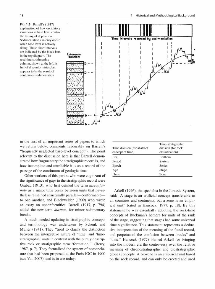
18 1 Historical and Methodological Background
Fig. 1.3 Barrell’s (1917)explanation of how oscillatoryvariations in base level controlthe timing of deposition.Sedimentation can only occurwhen base level is activelyrising. These short intervalsare indicated by the black barsin the top diagram. Theresulting stratigraphiccolumn, shown at the left, isfull of disconformities, butappears to be the result ofcontinuous sedimentation
in the first of an important series of papers to whichwe return below, comments favourably on Barrell’s“frequently neglected base-level concept”). The pointrelevant to the discussion here is that Barrell demon-strated how fragmentary the stratigraphic record is, andhow incomplete and unreliable it is as a record of thepassage of the continuum of geologic time.
Other workers of this period who were cognizant ofthe significance of gaps in the stratigraphic record wereGrabau (1913), who first defined the term disconfor-mity as a major time break between units that never-theless remained structurally parallel—conformable—to one another, and Blackwelder (1909) who wrotean essay on unconformities. Barrell (1917, p. 794)added the new term diastem, for minor sedimentarybreaks.
A much-needed updating in stratigraphic conceptsand terminology was undertaken by Schenk andMuller (1941). They “tried to clarify the distinctionbetween the interpretive nature of ‘time’ and ‘time-stratigraphic’ units in contrast with the purely descrip-tive rock or stratigraphic term ‘formation.’” (Berry,1987, p. 7). They formalized the system of nomencla-ture that had been proposed at the Paris IGC in 1900(see Vai, 2007), and is in use today:
Time division (for abstractconcept of time)
Time-stratigraphicdivision (for rockclassification)
Era ErathemPeriod SystemEpoch SeriesAge StagePhase Zone
Arkell (1946), the specialist in the Jurassic System,said: “A stage is an artificial concept transferable toall countries and continents, but a zone is an empir-ical unit” (cited in Hancock, 1977, p. 18). By thisstatement he was essentially adopting the rock-timeconcepts of Buckman’s hemera for units of the rankof the stage, suggesting that stages had some universaltime significance. This statement represents a deduc-tive interpretation of the meaning of the fossil record,and perpetuated the confusion between “rocks” and“time.” Hancock (1977) blamed Arkell for bringinginto the modern era the controversy over the relativemeaning of chronostratigraphic and biostratigraphic(zone) concepts. A biozone is an empirical unit basedon the rock record, and can only be erected and used
1.3 The Development of Descriptive Stratigraphy 19
for correlation if the fossils on which it is based arepresent in the rocks. Stages are simply groupings ofzones.
Confusion between the meaning of “rock” units and“time” units appeared to be widespread during theearly part of the twentieth century. Teichert (1958)summarized the various approaches taken by French,German, British and North American stratigraphersand paleontologists up to that time. To him it was clearthat there were three distinct concepts (summarizedhere from Teichert, 1958, p. 117):
Biostratigraphic units: the zone is the fundamentalunit of biostratigraphy, consisting of a set of bedscharacterized by one or more fossil species.
Biochronologic units: the unit of time during whichsedimentation of a biostratigraphic unit took place.These are true relative time units.
Time-stratigraphic units: units of rock which havebeen deposited during a defined unit of time.“Arrangement of rock-stratigraphic units within atime-stratigraphic unit and assignment to such a unitare generally made on a variety of lines of evidenceboth physical and paleontologic, including extrapo-lation, conclusion by analogy, and sometime merelyfor reasons of expedience.”
The distinguished American stratigrapher HollisHedberg picked up on Arkell’s idea about the mean-ing of the stage. He stated (Hedberg, 1948, p. 456)“The time value of stratigraphical units based onfossils will fluctuate from place to place in muchthe same manner as the time value of a lithologicformation may vary.” He proposed defining a sepa-rate set of chronostratigraphic units that correspondedto, and could be used to define, units of time. In1952 he became the Chairman of a newly estab-lished International Commission on Stratigraphy, andone of his achievements was to establish this newset of units. These ideas became formalized and cod-ified after many years work in a new internationalstratigraphic guide (Hedberg, 1976). For example, hedefined a chronozone as a zonal unit embracing allrocks anywhere formed during the range of a spec-ified geological feature, such as a local biozone. Intheory, a chronozone is present in the rocks beyondthe point at which the fossil components of the bio-zone cease to be present as a result of lateral facies
changes. Hedberg (1976) used a biostratigraphic exam-ple to illustrate the chronozone concept but, clearly, ifthe fossil components are not present, a chronozonecannot be recognized on biostratigraphic grounds, andits usefulness as a stratigraphic concept may be ratherhypothetical (Johnson, 1992a). However, other meansmay be available to extend the chronozone, includinglocal marker beds or magnetostratigraphic data. This isdiscussed this in the next section.
Hedberg (1976) suggested that the stage be regardedas the basic working unit of chronostratigraphybecause of its practical use in interregional correla-tion. As Hancock (1977, p. 19) and Watson (1983)pointed out, Hedberg omitted to mention that allPhanerozoic stages were first defined on the basis ofgroups of biozones, and they are therefore, histori-cally, biostratigraphic entities. In practice, therefore,so long as biostratigraphy formed the main basisof chronostratigraphy, no useful purpose was servedby treating them as theoretically different subjects.Stages could be defined by more than one systemof biozones, which extended their range and reducedtheir facies dependence, but, although this improvedtheir chronostratigraphic usefulness, it did not changethem into a different sort of unit. We return tothis point in the next section (the modern definitionof the term “stage” is quite different, as discussedbelow).
Harry E. Wheeler of the University of Washingtonpointed out the problems in Hedberg’s concepts oftime-stratigraphic units (Wheeler, 1958, p. 1050)shortly after they appeared in the first American strati-graphic guide (American Commission on StratigraphicNomenclature, 1952). He argued that a time-rock unitcould not be both a “material rock unit,” as describedin the guide, and one whose boundaries could beextended from the type section as isochronous sur-faces, because such isochronous surfaces would inmany localities be represented by an unconformity.Wheeler developed the concept of the chronostrati-graphic cross-section, in which the vertical dimensionin a stratigraphic cross-section is drawn with a timescale instead of a thickness scale (Fig. 1.4). In this way,time gaps (unconformities) become readily apparent,and the nature of time correlation may be accuratelyindicated. Such diagrams have come to be termed“Wheeler plots.” Wheeler cited with approval the earlywork of Sloss and his colleagues, referred to in moredetail below:
20 1 Historical and Methodological Background
Fig. 1.4 Wheeler’s development of chronostratigraphic dia-grams, showing a stratigraphic cross section plotted with avertical time axis in order to portray accurately the durationof stratigraphic units and unconformities from place to place.In the first diagram a generalized cross-section is provided. A
time cross-section of sequence C is shown below, providing thedefinition of some of the terms used by Wheeler. Remaining dia-grams show conversion of these data into chronostratigraphiccharts (Wheeler, 1958)
As a tangible framework on which to hang pertinentfaunal and lithic data, the sequence of Sloss, Krumbeinand Dapples (1949, pp. 110–11) generally fulfills theserequirements. Paraphrasing these authors’ discussion, asequence comprises an assemblage of strata exhibitingsimilar responses to similar tectonic environments overwide areas, separated by objective horizons without spe-cific time significance (Wheeler, 1958, p. 1050; italics asin original).
Sequences came later to be called simply“unconformity-bounded units,” whereas Wheeler’sdescription of them is a logically inconsistent mixtureof empirical description and tectonic interpretation.He proposed a new term for time-rock units, theholostrome, which consists of a sequence (in the Slosset al. sense) together with the “erosional vacuity”representing the part of the sequence lost to erosion.Such a vacuity would not be obvious on a conventionalstratigraphic cross-section, appearing simply as the
line corresponding to an unconformity. However,an erosional vacuity might constitute a significantarea of a Wheeler time plot and would require someknowledge of the lateral variations in the age of theunits immediately above and below the unconformityin order for it to be drawn in accurately. AlthoughWheeler’s concepts and plots are now commonplacein geology (they are cited in Vail’s early work), theterm holostrome has not become an accepted term.
The recognition of the importance of suites of strati-graphic units bounded by unconformities, based on thework of Levorsen, Sloss, Wheeler and others, led tosuggestions for the formal recognition of such unitsin stratigraphic guides and codes. The proposal for atype of unit called a “synthem” by Chang (1975) rep-resents the first formal proposal of this type. Chang(1975, pp. 1546–1547) considered the importance oftectonic cycles in the generation of such deposits,
1.3 The Development of Descriptive Stratigraphy 21
quoting Grabau’s (1940) concept of “pulsations”, andhe was aware of Vail’s early work on eustatic cycles(citing presentations by Vail’s group at a GeologicalSociety of America meeting in 1974). However, heconcluded that “In recognizing the unity or individu-ality of a synthem, the involvement of as little sub-jective judgment as possible is desirable.” In otherwords, Chang was at pains to adhere to a descrip-tive, empirical concept in his definition. Synthemswere included in the International Stratigraphic Guide(Hedberg, 1976, p. 92) as an additional class of time-significant unit, although, because of the variable ageof the bounding unconformities, they were not cat-egorized as strictly chronostratigraphic in character.Unconformity-bounded units were accorded their ownchapter in the revised version of the InternationalStratigraphic Guide (Salvador, 1994, Chap. 6), andalso formed the basis for a new type of stratigraphy,termed allostratigraphy, in the North American guide(NACSN, 1983). But not everybody was content withthese developments. Murphy (1988, p. 155) pointedout that “The statement that they [synthems] are objec-tive and non-interpretive . . .. assumes that particularunconformities have tangible qualities by which theycan be distinguished and identified; this assumptionis false.” He went on to argue that many unconformi-ties can only be recognized on the basis of knowledgeof the units above and below, and interpretation ofthe nature of the unconformity surface itself, and thattherefore unconformity-bounded units are not a classof objective stratigraphic unit. This objection has beenalmost totally ignored in the rush to adopt sequencestratigraphic methods, although attempts to incorpo-rate sequence concepts into formal stratigraphic guidesand codes have yet to achieve agreement.
1.3.3 The Development of ModernChronostratigraphy
One of the central themes of the development ofstratigraphy has been the work to establish an accu-rate geological times scale. Why? McLaren (1978)attempted to answer this question. Here are his ninereasons:
Some of these geological problems and questionsinclude: (1) rates of tectonic processes; (2) rates of sed-imentation and accurate basin history; (3) correlationof geophysical and geological events; (4) correlation of
tectonic and eustatic events; (5) are epeirogenic move-ments worldwide . . . (6) have there been simultaneousextinctions of unrelated animal and plant groups; (7) whathappened at era boundaries; (8) have there been catas-trophes in earth history which have left a simultaneousrecord over a wide region or worldwide; and (9) are theredifferent kinds of boundaries in the geologic succession(That is, “natural” boundaries marked by a worldwidesimultaneous event versus “quiet” boundaries, man-madeby definition).
It is, in fact, fundamental to the understanding ofthe history of Earth that events be meticulously corre-lated in time. For example, current work to investigatethe history of climate change on Earth during the lastfew tens to hundreds of thousands of years has demon-strated how important this is, because of the rapidityof climate change and because different geographicalregions and climatic belts may have had histories ofclimate change that were not in phase. If we are tounderstand Earth’s climate system thoroughly enoughto determine what we might expect from human influ-ences, such as the burning of fossil fuels, a detailedrecord of past climate change will be of fundamentalimportance. That we do not now have such a record isin part because of the difficulty in establishing a timescale precise enough and practical enough to be appli-cable in deposits formed everywhere on Earth in everypossible environmental setting.
Until the early twentieth century, the geologictime scale in use by geologists was a relative timescale dependent entirely on biostratigraphy. The stan-dard systems had nearly all been named., based onEuropean data, by about 1840 (Berry, 1987; Callomon,2001). Estimates about the duration of geologic events,including that of chronostratigraphic units, variedwidely, because they depended on diverse estimationmethods, such as attempts to quantify rates of erosionand sedimentation (Hallam, 1989). The discovery ofthe principle of radioactivity was fundamental, pro-viding a universal clock for direct dating of certainrock types, and the calibration of the results of otherdating methods, especially the relative scale of bios-tratigraphy. Radiometric dating methods may be useddirectly on rocks containing the appropriate radioactivematerials. For example, volcanic ash beds interca-lated with a sedimentary succession provide an idealbasis for precise dating and correlation. Volcanic ashcontains several minerals that include radioactive iso-topes of elements such as potassium and rubidium.Modern methods can date such beds to an accuracy
22 1 Historical and Methodological Background
typically in the ±2% range, that is, ±2 million yearsat an age of 100 Ma (Harland et al., 1990), althoughlocally, under ideal conditions, accuracy and preci-sion are now considerably better than this (±104–105
years; see Fig. 14.22 and discussion thereof). Wherea sedimentary unit of interest (such as a unit with abiostratigraphically significant fauna or flora) is over-lain and underlain by ash beds it is a simple matterto estimate the age of the sedimentary unit. The dif-ference in age between the ash beds corresponds tothe elapsed time represented by the succssion of stratabetween the ash beds. Assuming the sediments accu-mulated at a constant rate, the rate of sedimentation canbe determined by dividing the thickness of the sectionbetween the ash beds by the elapsed time. The amountby which the sediment bed of interest is younger thanthe lowest ash bed is then equal to its stratigraphicheight above the lowest ash bed divided by the rateof sedimentation, thereby yielding an “absolute” age,in years, for that bed. This procedure is typical of themethods used to provide the relative biostratigraphicage scale with a quantitative basis. The method is, ofcourse, not that simple, because sedimentation ratestend not to be constant, and most stratigraphic succes-sions contain numerous sedimentary breaks that resultin underestimation of sedimentation rates. Numerouscalibration exercises are required in order to stabilizethe assigned ages of any particular biostratigraphic unitof importance. I return to this issue later in Chap. 14.
Initially, the use of radiometric dating methods wasrelatively haphazard, but gradually geologists devel-oped the technique of systematically working to cross-calibrate the results of different dating methods, recon-ciling radiometric and relative biostratigraphic ages indifferent geological sections and using different fos-sils groups. In the 1960s the discovery of preserved(“remanent”) magnetism in the rock record led tothe development of an independent time scale basedon the recognition of the repeated reversals in mag-netic polarity over geologic time. Cross-calibration ofradiometric and biostratigraphic data with the mag-netostratigraphic record provided a further means ofrefinement and improvement of precision. The tech-niques are described in all standard textbooks ofstratigraphy (e.g., Miall, 1999; Nichols, 1999).
These modern developments rendered irrele-vant the debate about the value and meaning ofHedberg’s (1976) hypothetical chronostratigraphicunits. The new techniques of radiometric dating and
magnetostratigraphy, where they are precise enoughto challenge the supremacy of biostratigraphy, couldhave led to the case being made for a separate setof chronostratigraphic units, as Hedberg proposed.However, instead of a new set of chronostratigraphicunits, this correlation research is being used to refinethe definitions of the existing, biostratigraphicallybased stages. Different assemblages of zones gener-ated from different types of organism may be usedto define the stages in different ecological settings(e.g., marine versus nonmarine) and in differentbiogeographic provinces, and the entire data base iscross-correlated and refined with the use of radio-metric, magnetostratigraphic and other types ofdata. The stage has now effectively evolved into achronostratigraphic entity of the type visualized byHedberg (1976). This is the essence of the procedurerecommended by Charles Holland (1986, Fig. 10), oneof the leading spokespersons of the time for Britishstratigraphic practitioners. For most of Mesozoic andCenozoic time the standard stages, and in many cases,biozones, are now calibrated using many different datasets, and the global time scale, based on correlationsamong the three main dating methods, is attaininga high degree of accuracy. The Geological Societyof London time scale (GSL, 1964) was an importantmilestone, representing the first attempt to developa comprehensive record of these calibration andcross-correlation exercises. Wheeler’s (1958) formalmethods of accounting for “time in stratigraphy” (thetitle of his first important paper), including the use of“Wheeler plots” for showing the time relationships ofstratigraphic units, provided much needed clarity inthe progress of this work. Time scales for the Cenozoic(Berggren, 1972) and the Jurassic and Cretaceous (VanHinte, 1976a, b) are particularly noteworthy for theircomprehensive data syntheses, although all have nowbeen superseded. More recent detailed summation andreconciliation of the global data base were providedby Harland et al. (1990) and Berggren et al. (1995).Gradstein et al. (2004) provided a comprehensivetreatment of the subject, and nowadays, the globaldata base and updates of definitions are maintained atan official website: www.stratigraphy.org.
In the 1960s, several different kinds of problemswith stratigraphic methods and practice had begun tobe generally recognized (e.g., Newell, 1962). There aretwo main problems. Firstly, stratigraphic boundarieshad traditionally been drawn at horizons of sudden
1.3 The Development of Descriptive Stratigraphy 23
change, such as the facies change between marineSilurian strata and the overlying nonmarine Devoniansuccession in Britain. Changes such as this are obvi-ous in outcrop, and would seem to be logical placesto define boundaries. Commonly such boundaries areunconformities. However, it had long been recognizedthat unconformities pass laterally into conformablecontacts (for example, this was described by Whewell,1872). This raised the question of how to classifythe rocks that formed during the interval representedby the unconformity. Should they be assigned to theoverlying or underlying unit, or used to define a com-pletely new unit? When it was determined that rocksbeing classified as Cambrian and Silurian overlappedin time, Lapworth (1879) defined a new chronostrati-graphic unit—the Ordovician, as a compromise unitstraddling the Cambrian-Silurian interval. The samesolution could be used to define a new unit correspond-ing to the unconformable interval between the Silurianand the Devonian. In fact, rocks of this age began tobe described in central Europe after WWII, and thiswas one reason why the Silurian-Devonian boundarybecame an issue requiring resolution. A new unit couldbe erected, but it seemed likely that with additionaldetailed work around the world many such chronos-tratigraphic problems would arise, and at some pointit might be deemed desirable to stabilize the suite ofchronostratigraphic units. For this reason, the devel-opment of some standardized procedure seemed to bedesirable.
A second problem is that to draw a significant strati-graphic boundary at an unconformity or at some othersignificant stratigraphic change is to imply the hypoth-esis that the change or break has a significance relativeto the stratigraphic classification, that is, that uncon-formities have precise temporal significance. This wasspecifically hypothesized by Chamberlin (1898, 1909)who, as discussed below, was one of many individu-als who generated ideas about a supposed “pulse ofthe earth.” In the case of lithostratigraphic units, whichare descriptive, and are defined by the occurrence andmappability of a lithologically distinctive succession,a boundary of such a unit coinciding with an uncon-formity is of no consequence. However, in the case ofan interpretive classification, in which a boundary isassigned time significance (such as a stage boundary),the use of an unconformity as the boundary is to makethe assumption that the unconformity has time signif-icance; that is, it is of the same age everywhere. This
places primary importance on the model of unconfor-mity formation, be this diastrophism, eustatic sea-levelchange or some other cause. From the methodologi-cal point of view this is most undesirable, because itnegates the empirical or inductive nature of the classifi-cation. It is for this reason that it is inappropriate to usesequence boundaries as if they are chronostratigraphicmarkers.
How to avoid this problem? A time scale is con-cerned with the continuum of time. Given our abilityto assign “absolute” ages to stratigraphic units, albeitnot always with much accuracy and precision, onesolution would be to assign numerical ages to allstratigraphic units and events. However, this wouldcommonly be misleading or clumsy. In many instancesstratigraphic units cannot be dated more precisely than,say, “late Cenomanian” based on a limited recordof a few types of organisms (e.g., microfossils insubsurface well cuttings). Named units are not onlytraditional, but also highly convenient, just as it is con-venient to categorize human history using such termsas the “Elizabethan” or the “Napoleonic” or the “CivilWar” period. What is needed is a categorization ofgeological time that is empirical and all encompass-ing. The familiar terms for periods (e.g., Cretaceous)and for ages/stages (e.g., Aptian) offer such a sub-division and categorization, provided that they canbe made precise enough and designed to encompassall of time’s continuum. A group of British stratigra-phers (e.g., Ager, 1964) is credited with the idea thatseems to have resolved the twin problems describedhere. McLaren (1970, p. 802) explained the solution inthis way:
There is another approach to boundaries, however, whichmaintains that they should be defined wherever possiblein an area where “nothing happened.” The InternationalSubcommission on Stratigraphic Classification, of whichHollis Hedberg is Chairman, has recommended in itsCircular No. 25 of July, 1969, that “Boundary-stratotypesshould always be chosen within sequences of continu-ous sedimentation. The boundary of a chronostratigraphicunit should never be placed at an unconformity. Abruptand drastic changes in lithology or fossil content shouldbe looked at with suspicion as possibly indicating gapsin the sequence which would impair the value of theboundary as a chronostratigraphic marker and shouldbe used only if there is adequate evidence of essentialcontinuity of deposition. The marker for a boundary-stratotype may often best be placed within a certain bedto minimize the possibility that it may fall at a timegap.” This marker is becoming known as “the GoldenSpike.”
24 1 Historical and Methodological Background
By “nothing happens” is meant a stratigraphic suc-cession that is apparently continuous. The choice ofboundary is then purely arbitrary, and depends sim-ply on our ability to select a horizon that can be themost efficiently and most completely documented anddefined (just as there is nothing about time itself thatdistinguishes between, say, February and March, but todefine a boundary between them is useful for purposesof communication and record). This is the epitomeof an empirical approach to stratigraphy. Choosingto place a boundary where “nothing happened” is todeliberately avoid having to deal with some “event”that would require interpretation. This recommenda-tion was accepted in the first International StratigraphicGuide (Hedberg, 1976, pp. 84–85), although Hedberg(1976, p. 84) also noted the desirability of select-ing boundary stratotypes “at or near markers favor-able for long-distance time-correlation”, by which hemeant prominent biomarkers, radiometrically-datablehorizons, or magnetic reversal events. Boundary-stratotypes were to be established to define the baseand top of each chronostratigraphic units, with a formalmarker (a “golden spike”) driven into a specific point ina specific outcrop to mark the designated stratigraphichorizon. Hedberg (1976, p. 85) recommended that suchboundary-stratotypes be used to define both the topof one unit and the base of the next overlying unit.However, further consideration indicates an additionalproblem, which was noted in the North AmericanStratigraphic Code of 1983 (NACSN, p. 868):
Designation of point boundaries for both base and top ofchronostratigraphic units is not recommended, becausesubsequent information on relations between successiveunits may identify overlaps or gaps. One means of min-imizing or eliminating problems of duplication or gapsin chronostratigraphic successions is to define formallyas a point-boundary stratotype only the base of the unit.Thus, a chronostratigraphic unit with its base defined atone locality will have its top defined by the base of anoverlying unit at the same, but more commonly, anotherlocality.
Even beds selected for their apparently continu-ous nature may be discovered at a later date to hidea significant break in time. Detailed work on theBritish Jurassic section using what is probably the mostrefined biostratigraphic classification scheme avail-able for any pre-Neogene section has demonstratedhow common such breaks are (Callomon, 1995; seeMiall and Miall, 2002). The procedure recommendedby NACSN (1983) is that, if it is discovered that a
boundary stratotype does encompass a gap in the tem-poral record, the rocks (and the time they represent) areassigned to the unit below the stratotype. In this way, atime scale can be constructed that can readily accom-modate all of time’s continuum, as our description anddefinition of it continue to be perfected by additionalfield work. This procedure means that, once desig-nated, boundary stratotypes do not have to be revisedor changed. This has come to be termed the concept ofthe “topless stage.”
The modern definition of the term “stage” (e.g., inthe online version of the International StratigraphicGuide by Michael A. Murphy and Amos Salvador atwww.stratigraphy.org) indicates how the concept of thestage has evolved since d’Orbigny. The Guide statesthat “The stage has been called the basic working unitof chronostratigraphy. . . . The stage includes all rocksformed during an age. A stage is normally the lowestranking unit in the chronostratigraphic hierarchy thatcan be recognized on a global scale. . . . A stage isdefined by its boundary stratotypes, sections that con-tain a designated point in a stratigraphic sequence ofessentially continuous deposition, preferably marine,chosen for its correlation potential.”
The first application of the new concepts for defin-ing chronostratigraphic units was to the Silurian-Devonian boundary, the definition of which had begunto cause major stratigraphic problems as internationalcorrelation work became routine in post-WWII years.A boundary stratotype was selected at a location calledKlonk, in what is now the Czech Republic, followingextensive work by an international Silurian-DevonianBoundary Committee on the fossil assemblages innumerous well-exposed sections in Europe and else-where. The results are presented in summary form byMcLaren (1973), and, more extensively, by Chlupác(1972) and McLaren (1977) (see also Miall, 1999, pp.116–117). As reported by Bassett (1985) and Cowie(1986), the establishment of the new procedures led toa flood of new work to standardize and formalize thegeological time scale, one boundary at a time. This isextremely labour-intensive work, requiring the colla-tion of data of all types (biostratigraphic, radiometricand, where appropriate, chemostratigraphic and mag-netostratigraphic) for well-exposed sections aroundthe world, and working to reach international agree-ment amongst ad-hoc international working groupsset up for the purpose. In many instances, once suchdetailed correlation work is undertaken, it is discovered
1.3 The Development of Descriptive Stratigraphy 25
that definitions for particular boundaries being usedin different parts of the world, or definitions estab-lished by different workers using different criteria,do not in fact define contemporaneous horizons (e.g.,Hancock, 1993a). This may be because the originaldefinitions were inadequate or incomplete, and havebeen subject to interpretation as practical correlationwork has spread out across the globe. Resolution ofsuch issues should simply require international agree-ment; the important point being that there is nothingsignificant about, say, the Aptian-Albian boundary, justthat we should all be able to agree on where it is.Following McLaren’s idea that boundaries be placeswhere “nothing happens”, the sole criterion for bound-ary definition is that such definitions be as practicalas possible. The first “golden spike” location (theSilurian-Devonian boundary at Klonk: Chlupác, 1972)was chosen because it represents an area where deep-water graptolite-bearing beds are interbedded withshallow-water brachiopod-trilobite beds, permittingdetailed cross-correlation among the faunas, therebypermitting the application of the boundary criteria toa wide array of different facies. In other cases, thepresence of radiometrically datable units or a well-defined magnetostratigraphic record may be helpful.In all cases, accessibility and stability of the locationare considered desirable features of a boundary strato-type, because the intent is that it serves as a standard.Perfect correlation with such a standard can never beachieved, but careful selection of the appropriate stra-totype is intended to facilitate future refinement in theform of additional data collection.
Despite the apparent inductive simplicity of thisapproach to the refinement of the time scale, furtherwork has been slow, in part because of the inabil-ity of some working groups to arrive at agreement(Vai, 2001). In addition, two contrasting approachesto the definition of chronostratigraphic units and unitboundaries have now evolved, each emphasizing dif-ferent characteristics of the rock record and the accu-mulated data that describe it. Castradori (2002) pro-vided an excellent summary of what became a livelycontroversy within the International Commission onStratigraphy. The first approach, which Castradoridescribed as the historical and conceptual approach,emphasizes the historical continuity of the erection anddefinition of units and their boundaries, the data basefor which has continued to grow since the nineteenthcentury by a process of inductive accretion. Aubry
et al. (1999, 2000) expanded upon and defended thisapproach. The alternative method, which Castradoriterms the hyper-pragmatic approach, focuses on thesearch for and recognition of significant “events” asproviding the most suitable basis for rock-time mark-ers, from which correlation and unit definition canthen proceed. The choice of the term “pragmatic”is unfortunate in this context, because the suggestedmethod is certainly not empirical. The followers ofthis method (see response by J. Ramane, 2000, tothe discussion by Aubry et al., 2000) suggest thatin some instances historical definitions of units andtheir boundaries should be modified or set aside infavour of globally recognizable event markers, suchas a prominent biomarker, a magnetic reversal event,an isotopic excursion, or, eventually, events based oncyclostratigraphy. This approach explicitly sets asideMcLaren’s recommendation (cited above) that bound-aries be defined in places where “nothing happened,”although it is in accord with suggestions in the firststratigraphic guide that “natural breaks” in the stratig-raphy could be used or boundaries defined “at or nearmarkers favorable for long-distance time-correlation”(Hedberg, 1976, pp. 71, 84). The virtue of this methodis that where appropriately applied it may make bound-ary definition easier to recognize. The potential disad-vantage is that is places prime emphasis on a singlecriterion for definition. From the perspective of thisbook, which has attempted to clarify methodologicaldifferences, it is important to note that the hyper-pragmatic approach relies on assumptions about thesuperior time-significance of the selected boundaryevent. The deductive flavour of hypothesis is there-fore added to the method. In this sense the methodis not strictly empirical. As has been demonstratedelsewhere, assumptions about global synchroneity ofstratigraphic events may in some cases be misguided(see Miall and Miall, 2001, 2002).
The hyper-pragmatic approach builds assumptionsinto what has otherwise been an inductive methodfree of all but the most basic of hypotheses aboutthe time-significance of the rock record. The strengthof the historical and conceptual approach is that itemphasizes multiple criteria, and makes use of long-established practices for reconciling different databases, and for carrying correlations into areas whereany given criterion may not be recognizable. For thisreason, this writer is not in favour of the proposal byZalasiewicz et al. (2004), supported by Carter (2007),
26 1 Historical and Methodological Background
to eliminate the distinction between time-rock units(chronostratigraphy) and the measurement of geologictime (geochronology). Their proposal hinges on thesupposed supremacy of the global stratotype boundarypoints. History has repeatedly demonstrated the dif-ficulties that have arisen from the reliance on singlecriteria for stratigraphic definitions, and the incom-pleteness of the rock record, which is why “time”and the “rocks” are so rarely synonymous in prac-tice (see also Sect. 14.5.6 and Aubry, 2007, on thispoint).
Ongoing work on boundary stratotypes is periodi-cally recorded in the IUGS journal Episodes, and issummarized in web pages at www.stratigraphy.org.The reader is referred to Aubry et al. (2000, includ-ing the discussion by Remane which follows) andto Castradori (2002) for additional details aboutthis controversy. The latter article provides severalcase studies of how each approach has worked inpractice.
For our purposes, the importance of this history ofstratigraphy is that the work of building and refin-ing the geological time scale has been largely anempirical, inductive process (with the exception ofthe hyper-pragmatic approach discussed above). Notethat each step in the development of chronostrati-graphic techniques, including the multidisciplinarycross-correlation method, the golden spike concept,and the concept of the topless unit, are designedto enhance the empirical nature of the process.Techniques of data collection, calibration and cross-comparison evolved gradually and, with that devel-opment came many decisions about the nature of thetime scale and how it should be measured, docu-mented, and codified. These decisions typically weretaken at international geological congresses by largemultinational committees established for such pur-poses (See Vai, 2007, for the early history). Forexample, the International Stratigraphic Guide, firstpublished by Hedberg (1976), was an official productof the International Subcommission on StratigraphicClassification of the International Union of GeologicalSciences’ Commission on Stratigraphy. For our pur-poses, the incremental nature of this method of work issignificant because it is completely different from thebasing of stratigraphic history on the broad, sweepingmodels of pulsation or cyclicity that have so frequentlyarisen during the evolution of the science of geology, atopic to which we now turn.
1.4 The Continual Search for a “Pulseof the Earth”
The self-appointed task of geologists is to explain theEarth. Given that Earth is a complex object affected bymultiple processes, there is a natural drive to attemptto systematize and simplify these processes in ourhypotheses of how Earth works. Numerical modeling,which has become popular in many fields with theadvent of small but powerful and cheap computers, isbut the most recent manifestation of this tendency, andis now widely used by earth scientists. The purposeof this section is to show how the idea of a world-wide stratigraphic pattern, as exemplified by the Exxonsequence model of the 1970s, is but the latest exam-ple of a theme that runs through the entire course ofmodern Geology.
Two themes that recur throughout the evolution ofgeological thought are pattern recognition and cyclic-ity. Zeller (1964) demonstrated the ability of geologiststo recognize patterns in data where none exists. Ina famous psychological experiment he constructedsimulated stratigraphic sections from lists of randomnumbers (in fact, digits from lists of phone numbers ina city phone directory), using the numbers to determinerock types and bed thicknesses. Professional geologistswere then asked to “correlate” the sections, that is, toidentify “beds” that extended from one “section” to thenext. All were able to do so and, moreover, were able todevelop comparisons with actual patterns of repetitivevertical order of rock types (sedimentary cyclicity) thathad been well documented in the local outcrop geologyand were well known to the professional geologicalcommunity. Zeller explained these results thus:
Psychologists, anthropologists, and philosophers of sci-ence have long recognized the fact that there is a funda-mental need in man to explain the nature of his surround-ings and to attempt to make order out of randomness . . ..The Western mind does not willingly accept the conceptof a truly random universe even though there may bemuch evidence to support this view. . . .. Science, to anextent matched by no other human endeavor, places a pre-mium upon the ability of the individual to make order outof what appears disordered (Zeller, 1964, p. 631).
Dott (1992a) compiled studies of a particular recurringobsession of geologists, that of the idea of repeatedchanges in global sea-level. The idea that the formationand subsequent melting of continental ice caps wouldaffect sea levels by first locking up on land, and then
1.4 The Continual Search for a “Pulse of the Earth” 27
releasing back to the oceans, large volumes of water, isattributed to a newspaper publisher, Charles Maclarenin 1842, and appeared in his review of Louis Agassiz’glacial theory. The Scotsman James Croll was the firstto develop these ideas into a hypothesis of orbital forc-ing in 1864, but the idea received no serious attentionuntil the 1920s. The word “eustatic,” as applied tosea levels, and meaning sea-level changes of globalscope, was proposed by Suess (1888) (these historicaldevelopments are summarized by Dott, in his intro-duction to the volume). But, as Dott’s book demon-strates, ideas about the repetitiveness or periodicity ofearth history have existed since at least the eighteenthcentury.
Why should periodicity be such a powerful opiatefor geologists? Obviously, periodicity comes naturallythrough the universal human experience of diurnal, tidal,and seasonal cycles. And it has ancient roots in theAristotelian Greek world view of everything in naturebeing cyclic. The answer must lie more directly, however,in the innate psychological appeal of order and simplicity,both of which are provided by rhythmically repetitive pat-terns. For geologists the instinctive appeal to periodicityconstitutes a subtle extension of the uniformity principle,which is in turn a special geological case of simplicity orparsimony (Dott, 1992b, p. 13).
To Charles Lyell, the founder of modern Geology,uniformitarianism included the concept that the Earthhad not fundamentally changed throughout its his-tory, and would not do so in the future. Earth his-tory was not only directionless, but might also becyclic (Rudwick, 1998; Hallam, 1998a). Lyell did notaccept Darwin’s ideas about organic evolution untillate in his career, but held the opinion that most lifeforms had always been present on Earth, and if anywere absent from the fossil record it was becauseof local environmental reasons or because the recordhad been destroyed by post-depositional processes,such as metamorphism. Lyell believed that in thefuture:
Then might those genera of animals return, of whichthe memorials are preserved in the ancient rocks of ourcontinents. The huge iguanodon might reappear in thewoods, and the ichthyosaur in the sea, while the ptero-dactyl might flit again through the umbrageous groves oftree ferns (Lyell, 1830; cited in Hallam, 1998a, p. 134).
Lyell’s ideas about the circularity of earth his-tory were quickly discredited and discarded. However,his combination of inductive and deductive scienceand the attempt at building a grand, all-encompassingmodel that ultimately failed is uncannily similar to the
modern story of sequence stratigraphy set out by Mialland Miall (2001), as discussed in Chap. 12.
Through the latter part of the nineteenth centuryand, in fact, until the modern era of plate tectonics,most theories of Earth processes included some ele-ment of repetition or cyclicity. These theories weredeveloped in the absence of knowledge of the Earth’sinterior, an absence that was not to be fully correcteduntil development of the techniques of seismic tomog-raphy in the 1970s (Anderson, 1989), which revealedfor the first time how Earth’s mantle really works. Theimpetus for the development of theories of cyclicitypresumably arose from the tendency to seek naturalorder, as described by Zeller, Dott, and others. Themore well-known of such theories were proposed bysome of the more prominent geologists of their times,and typically seemed to represent attempts to recon-cile and explain their knowledge of Earth’s complexhistory accumulated over a lifetime’s work.
Among the more important such theories wasthe model of worldwide diastrophism proposed byChamberlin (1898, 1909; useful summaries and inter-pretations of Chamberlin’s ideas are given by Conkinand Conkin, 1984 and Dott, 1992c) and elaborated byUlrich (1911). In some fundamental ways this modelcontains the basis of modern concepts in sequencestratigraphy, although the papers are not cited by themain founder and “grandfather” of modern sequencestratigraphy, L. L. Sloss, in his first major paper (Sloss,1963), or in his later work.
Chamberlin opened his paper with this remark:
It was intimated in the introduction to the symposiumon the classification and nomenclature of geologic timedivisions published in the last number of this mag-azine [Journal of Geology] that the ulterior basis ofclassification and nomenclature must be dependent onthe existence or absence of natural divisions resultingfrom simultaneous phases of action of world-wide extent(Chamberlin, 1898, p. 449).
Chamberlin made note of the widespread transgres-sions and regressions that could be interpreted fromthe stratigraphic record, and he understood the impor-tance of regional uplift and erosion as the cause ofwidespread unconformities, which he termed “base-leveling.” He suggested that “correlation by base-levels is one of the triumphs of American geology.”(Chamberlin, 1909, p. 690) and emphasized that “thebase-leveling process implies a homologous series ofdeposits the world over” (emphasis by italics as in theoriginal).
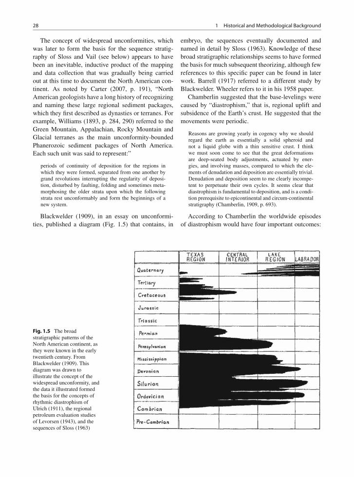
28 1 Historical and Methodological Background
The concept of widespread unconformities, whichwas later to form the basis for the sequence stratig-raphy of Sloss and Vail (see below) appears to havebeen an inevitable, inductive product of the mappingand data collection that was gradually being carriedout at this time to document the North American con-tinent. As noted by Carter (2007, p. 191), “NorthAmerican geologists have a long history of recognizingand naming these large regional sediment packages,which they first described as dynasties or terranes. Forexample, Williams (1893, p. 284, 290) referred to theGreen Mountain, Appalachian, Rocky Mountain andGlacial terranes as the main unconformity-boundedPhanerozoic sediment packages of North America.Each such unit was said to represent:”
periods of continuity of deposition for the regions inwhich they were formed, separated from one another bygrand revolutions interrupting the regularity of deposi-tion, disturbed by faulting, folding and sometimes meta-morphosing the older strata upon which the followingstrata rest unconformably and form the beginnings of anew system.
Blackwelder (1909), in an essay on unconformi-ties, published a diagram (Fig. 1.5) that contains, in
embryo, the sequences eventually documented andnamed in detail by Sloss (1963). Knowledge of thesebroad stratigraphic relationships seems to have formedthe basis for much subsequent theorizing, although fewreferences to this specific paper can be found in laterwork. Barrell (1917) referred to a different study byBlackwelder. Wheeler refers to it in his 1958 paper.
Chamberlin suggested that the base-levelings werecaused by “diastrophism,” that is, regional uplift andsubsidence of the Earth’s crust. He suggested that themovements were periodic.
Reasons are growing yearly in cogency why we shouldregard the earth as essentially a solid spheroid andnot a liquid globe with a thin sensitive crust. I thinkwe must soon come to see that the great deformationsare deep-seated body adjustments, actuated by ener-gies, and involving masses, compared to which the ele-ments of denudation and deposition are essentially trivial.Denudation and deposition seem to me clearly incompe-tent to perpetuate their own cycles. It seems clear thatdiastrophism is fundamental to deposition, and is a condi-tion prerequisite to epicontinental and circum-continentalstratigraphy (Chamberlin, 1909, p. 693).
According to Chamberlin the worldwide episodesof diastrophism would have four important outcomes:
Fig. 1.5 The broadstratigraphic patterns of theNorth American continent, asthey were known in the earlytwentieth century. FromBlackwelder (1909). Thisdiagram was drawn toillustrate the concept of thewidespread unconformity, andthe data it illustrated formedthe basis for the concepts ofrhythmic diastrophism ofUlrich (1911), the regionalpetroleum evaluation studiesof Levorsen (1943), and thesequences of Sloss (1963)
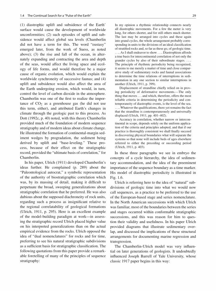
1.4 The Continual Search for a “Pulse of the Earth” 29
(1) diastrophic uplift and subsidence of the Earth’surface would cause the development of worldwideunconformities; (2) such episodes of uplift and sub-sidence would affect global sea levels (Chamberlindid not have a term for this. The word “eustasy”emerged later, from the work of Suess, as notedabove); (3) the rise and fall of the ocean, in alter-nately expanding and contracting the area and depthof the seas, would affect the living space and ecol-ogy of life forms, and would therefore be a majorcause of organic evolution, which would explain theworldwide synchroneity of successive faunas; and (4)uplift and subsidence would also affect the area ofthe Earth undergoing erosion, which would, in turn,control the level of carbon dioxide in the atmosphere.Chamberlin was one of the first to realize the impor-tance of CO2 as a greenhouse gas (he did not usethis term, either), and attributed Earth’s changes inclimate through the geologic past to this process. AsDott (1992c, p. 40) noted, with this theory Chamberlinprovided much of the foundation of modern sequencestratigraphy and of modern ideas about climate change.He illustrated the formation of continental-margin sed-iment wedges by progradation, the sediment beingderived by uplift and “base-leveling.” These pro-cess, because of their effect on the stratigraphicrecord, provided the “ultimate basis of correlation,” forChamberlin.
In his paper, Ulrich (1911) developed Chamberlin’sideas further. He complained (p. 289) about the“Paleontological autocrat,” a symbolic representationof the authority of biostratigraphic correlation whichwas, by its massing of detail, making it difficult toperpetuate the broad, sweeping generalizations aboutstratigraphic correlation that he preferred. He was alsodubious about the supposed diachroneity of rock units,regarding such a process as insignificant relative tothe regional correlatability of geological formations(Ulrich, 1911, p. 295). Here is an excellent exampleof the model-building paradigm at work—in assess-ing the stratigraphic record Ulrich placed higher valueon his interpreted generalizations than on the actualempirical evidence from the rocks. Ulrich opposed theidea of “dual nomenclatures” for rocks and for time,preferring to see his natural stratigraphic subdivisionsas a sufficient basis for stratigraphic classification. Thefollowing quotations from this paper provide a remark-able foretelling of many of the principles of sequencestratigraphy:
In my opinion a rhythmic relationship connects nearlyall diastrophic movements. For a few the meter is verylong, for others shorter, and for still others much shorter.The last may be arranged into cycles and these againinto grand cycles, the whole arrangement probably corre-sponding in units to the divisions of an ideal classificationof stratified rocks and, so far as these go, of geologic time.. . .. As I shall endeavor to show . . .. Diastrophism affordsa true basis for intercontinental correlation of not only thegrander cycles by also of their subordinate stages. . . ..The principle of rhythmic periodicity being recognized,it seems to me merely a matter of time and close compar-ative study of sedimentary rocks and faunal associationsto determine the time relations of interruptions in sedi-mentation in any one section to similar interruptions inanother (Ulrich, 1911, p. 399).
Displacement of strandline chiefly relied on in prov-ing periodicity of deformative movements.—The onlything that moves . . . and which, therefore, offers the mostreliable criteria in determining the periodicity and con-temporaneity of diastrophic events, is the level of the sea.. . .. Whatever the qualifications, there yet remains the factthat the strandline is contemporaneously and universallydisplaced (Ulrich, 1911, pp. 401–402).
Accuracy in correlation, whether narrow or intercon-tinental in scope, depends solely on the uniform applica-tion of the criteria and principles adopted, and that if ourpractice is thoroughly consistent we shall finally succeedin discovering physical boundaries what will separate thesystems so that none will include beds of ages elsewherereferred to either the preceding or succeeding period(Ulrich, 1911, p. 403).
In these three paragraphs we see in embryo theconcepts of a cycle hierarchy, the idea of sedimen-tary accommodation, and the idea of the preeminentimportance of the sequence boundary as a time marker.His model of diastrophic periodicity is illustrated inFig. 1.6.
Ulrich is referring here to the idea of “natural” sub-divisions of geologic time into what we would nowcall sequences, as a practice to be preferred to the useof the European-based stage and series nomenclature.In the North American successions with which Ulrichwas familiar, most of the boundaries between the seriesand stages occurred within conformable stratigraphicsuccessions, and this was reason for him to ques-tion their validity and usefulness. In his paper Ulrichprovided diagrams that illustrate sedimentary over-lap, and discussed the implications of these structuralarrangements for documenting marine regression andtransgression.
The Chamberlin-Ulrich model was very influen-tial on later generations of geologists. It undoubtedlyinfluenced Joseph Barrell of Yale University, whoseclassic 1917 paper begins in this way:
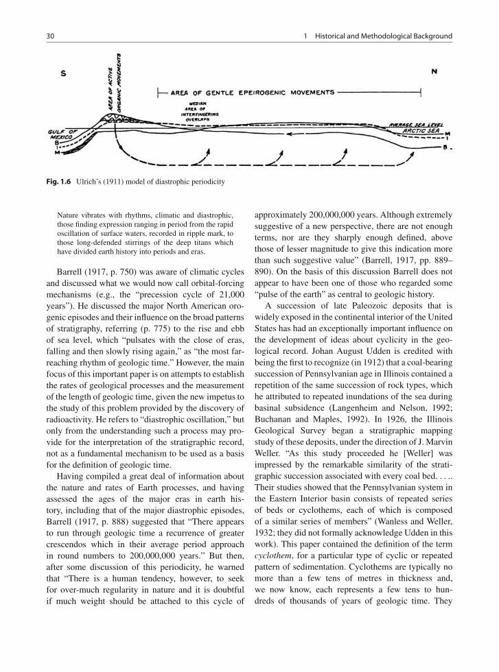
30 1 Historical and Methodological Background
Fig. 1.6 Ulrich’s (1911) model of diastrophic periodicity
Nature vibrates with rhythms, climatic and diastrophic,those finding expression ranging in period from the rapidoscillation of surface waters, recorded in ripple mark, tothose long-defended stirrings of the deep titans whichhave divided earth history into periods and eras.
Barrell (1917, p. 750) was aware of climatic cyclesand discussed what we would now call orbital-forcingmechanisms (e.g., the “precession cycle of 21,000years”). He discussed the major North American oro-genic episodes and their influence on the broad patternsof stratigraphy, referring (p. 775) to the rise and ebbof sea level, which “pulsates with the close of eras,falling and then slowly rising again,” as “the most far-reaching rhythm of geologic time.” However, the mainfocus of this important paper is on attempts to establishthe rates of geological processes and the measurementof the length of geologic time, given the new impetus tothe study of this problem provided by the discovery ofradioactivity. He refers to “diastrophic oscillation,” butonly from the understanding such a process may pro-vide for the interpretation of the stratigraphic record,not as a fundamental mechanism to be used as a basisfor the definition of geologic time.
Having compiled a great deal of information aboutthe nature and rates of Earth processes, and havingassessed the ages of the major eras in earth his-tory, including that of the major diastrophic episodes,Barrell (1917, p. 888) suggested that “There appearsto run through geologic time a recurrence of greatercrescendos which in their average period approachin round numbers to 200,000,000 years.” But then,after some discussion of this periodicity, he warnedthat “There is a human tendency, however, to seekfor over-much regularity in nature and it is doubtfulif much weight should be attached to this cycle of
approximately 200,000,000 years. Although extremelysuggestive of a new perspective, there are not enoughterms, nor are they sharply enough defined, abovethose of lesser magnitude to give this indication morethan such suggestive value” (Barrell, 1917, pp. 889–890). On the basis of this discussion Barrell does notappear to have been one of those who regarded some“pulse of the earth” as central to geologic history.
A succession of late Paleozoic deposits that iswidely exposed in the continental interior of the UnitedStates has had an exceptionally important influence onthe development of ideas about cyclicity in the geo-logical record. Johan August Udden is credited withbeing the first to recognize (in 1912) that a coal-bearingsuccession of Pennsylvanian age in Illinois contained arepetition of the same succession of rock types, whichhe attributed to repeated inundations of the sea duringbasinal subsidence (Langenheim and Nelson, 1992;Buchanan and Maples, 1992). In 1926, the IllinoisGeological Survey began a stratigraphic mappingstudy of these deposits, under the direction of J. MarvinWeller. “As this study proceeded he [Weller] wasimpressed by the remarkable similarity of the strati-graphic succession associated with every coal bed. . . ..Their studies showed that the Pennsylvanian system inthe Eastern Interior basin consists of repeated seriesof beds or cyclothems, each of which is composedof a similar series of members” (Wanless and Weller,1932; they did not formally acknowledge Udden in thiswork). This paper contained the definition of the termcyclothem, for a particular type of cyclic or repeatedpattern of sedimentation. Cyclothems are typically nomore than a few tens of metres in thickness and,we now know, each represents a few tens to hun-dreds of thousands of years of geologic time. They
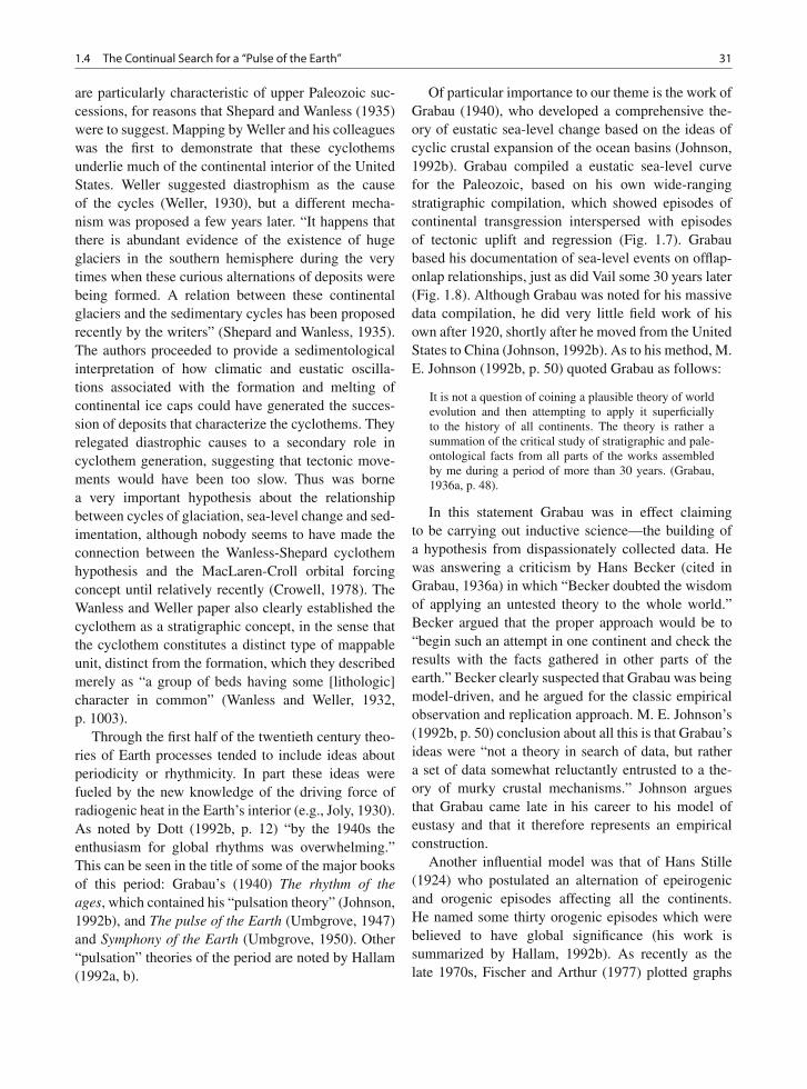
1.4 The Continual Search for a “Pulse of the Earth” 31
are particularly characteristic of upper Paleozoic suc-cessions, for reasons that Shepard and Wanless (1935)were to suggest. Mapping by Weller and his colleagueswas the first to demonstrate that these cyclothemsunderlie much of the continental interior of the UnitedStates. Weller suggested diastrophism as the causeof the cycles (Weller, 1930), but a different mecha-nism was proposed a few years later. “It happens thatthere is abundant evidence of the existence of hugeglaciers in the southern hemisphere during the verytimes when these curious alternations of deposits werebeing formed. A relation between these continentalglaciers and the sedimentary cycles has been proposedrecently by the writers” (Shepard and Wanless, 1935).The authors proceeded to provide a sedimentologicalinterpretation of how climatic and eustatic oscilla-tions associated with the formation and melting ofcontinental ice caps could have generated the succes-sion of deposits that characterize the cyclothems. Theyrelegated diastrophic causes to a secondary role incyclothem generation, suggesting that tectonic move-ments would have been too slow. Thus was bornea very important hypothesis about the relationshipbetween cycles of glaciation, sea-level change and sed-imentation, although nobody seems to have made theconnection between the Wanless-Shepard cyclothemhypothesis and the MacLaren-Croll orbital forcingconcept until relatively recently (Crowell, 1978). TheWanless and Weller paper also clearly established thecyclothem as a stratigraphic concept, in the sense thatthe cyclothem constitutes a distinct type of mappableunit, distinct from the formation, which they describedmerely as “a group of beds having some [lithologic]character in common” (Wanless and Weller, 1932,p. 1003).
Through the first half of the twentieth century theo-ries of Earth processes tended to include ideas aboutperiodicity or rhythmicity. In part these ideas werefueled by the new knowledge of the driving force ofradiogenic heat in the Earth’s interior (e.g., Joly, 1930).As noted by Dott (1992b, p. 12) “by the 1940s theenthusiasm for global rhythms was overwhelming.”This can be seen in the title of some of the major booksof this period: Grabau’s (1940) The rhythm of theages, which contained his “pulsation theory” (Johnson,1992b), and The pulse of the Earth (Umbgrove, 1947)and Symphony of the Earth (Umbgrove, 1950). Other“pulsation” theories of the period are noted by Hallam(1992a, b).
Of particular importance to our theme is the work ofGrabau (1940), who developed a comprehensive the-ory of eustatic sea-level change based on the ideas ofcyclic crustal expansion of the ocean basins (Johnson,1992b). Grabau compiled a eustatic sea-level curvefor the Paleozoic, based on his own wide-rangingstratigraphic compilation, which showed episodes ofcontinental transgression interspersed with episodesof tectonic uplift and regression (Fig. 1.7). Grabaubased his documentation of sea-level events on offlap-onlap relationships, just as did Vail some 30 years later(Fig. 1.8). Although Grabau was noted for his massivedata compilation, he did very little field work of hisown after 1920, shortly after he moved from the UnitedStates to China (Johnson, 1992b). As to his method, M.E. Johnson (1992b, p. 50) quoted Grabau as follows:
It is not a question of coining a plausible theory of worldevolution and then attempting to apply it superficiallyto the history of all continents. The theory is rather asummation of the critical study of stratigraphic and pale-ontological facts from all parts of the works assembledby me during a period of more than 30 years. (Grabau,1936a, p. 48).
In this statement Grabau was in effect claimingto be carrying out inductive science—the building ofa hypothesis from dispassionately collected data. Hewas answering a criticism by Hans Becker (cited inGrabau, 1936a) in which “Becker doubted the wisdomof applying an untested theory to the whole world.”Becker argued that the proper approach would be to“begin such an attempt in one continent and check theresults with the facts gathered in other parts of theearth.” Becker clearly suspected that Grabau was beingmodel-driven, and he argued for the classic empiricalobservation and replication approach. M. E. Johnson’s(1992b, p. 50) conclusion about all this is that Grabau’sideas were “not a theory in search of data, but rathera set of data somewhat reluctantly entrusted to a the-ory of murky crustal mechanisms.” Johnson arguesthat Grabau came late in his career to his model ofeustasy and that it therefore represents an empiricalconstruction.
Another influential model was that of Hans Stille(1924) who postulated an alternation of epeirogenicand orogenic episodes affecting all the continents.He named some thirty orogenic episodes which werebelieved to have global significance (his work issummarized by Hallam, 1992b). As recently as thelate 1970s, Fischer and Arthur (1977) plotted graphs
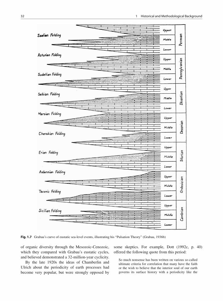
32 1 Historical and Methodological Background
Fig. 1.7 Grabau’s curve of eustatic sea-level events, illustrating his “Pulsation Theory” (Grabau, 1936b)
of organic diversity through the Mesozoic-Cenozoic,which they compared with Grabau’s eustatic cycles,and believed demonstrated a 32-million-year cyclicity.
By the late 1920s the ideas of Chamberlin andUlrich about the periodicity of earth processes hadbecome very popular, but were strongly opposed by
some skeptics. For example, Dott (1992c, p. 40)offered the following quote from this period:
So much nonsense has been written on various so-calledultimate criteria for correlation that many have the faithor the wish to believe that the interior soul of our earthgoverns its surface history with a periodicity like the
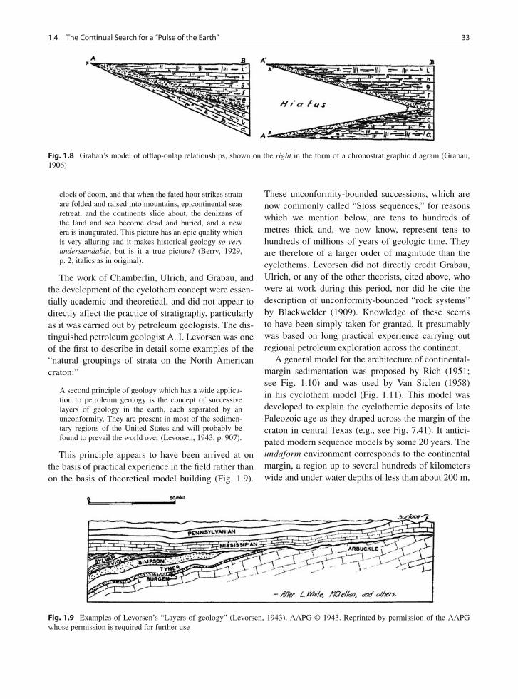
1.4 The Continual Search for a “Pulse of the Earth” 33
Fig. 1.8 Grabau’s model of offlap-onlap relationships, shown on the right in the form of a chronostratigraphic diagram (Grabau,1906)
clock of doom, and that when the fated hour strikes strataare folded and raised into mountains, epicontinental seasretreat, and the continents slide about, the denizens ofthe land and sea become dead and buried, and a newera is inaugurated. This picture has an epic quality whichis very alluring and it makes historical geology so veryunderstandable, but is it a true picture? (Berry, 1929,p. 2; italics as in original).
The work of Chamberlin, Ulrich, and Grabau, andthe development of the cyclothem concept were essen-tially academic and theoretical, and did not appear todirectly affect the practice of stratigraphy, particularlyas it was carried out by petroleum geologists. The dis-tinguished petroleum geologist A. I. Levorsen was oneof the first to describe in detail some examples of the“natural groupings of strata on the North Americancraton:”
A second principle of geology which has a wide applica-tion to petroleum geology is the concept of successivelayers of geology in the earth, each separated by anunconformity. They are present in most of the sedimen-tary regions of the United States and will probably befound to prevail the world over (Levorsen, 1943, p. 907).
This principle appears to have been arrived at onthe basis of practical experience in the field rather thanon the basis of theoretical model building (Fig. 1.9).
These unconformity-bounded successions, which arenow commonly called “Sloss sequences,” for reasonswhich we mention below, are tens to hundreds ofmetres thick and, we now know, represent tens tohundreds of millions of years of geologic time. Theyare therefore of a larger order of magnitude than thecyclothems. Levorsen did not directly credit Grabau,Ulrich, or any of the other theorists, cited above, whowere at work during this period, nor did he cite thedescription of unconformity-bounded “rock systems”by Blackwelder (1909). Knowledge of these seemsto have been simply taken for granted. It presumablywas based on long practical experience carrying outregional petroleum exploration across the continent.
A general model for the architecture of continental-margin sedimentation was proposed by Rich (1951;see Fig. 1.10) and was used by Van Siclen (1958)in his cyclothem model (Fig. 1.11). This model wasdeveloped to explain the cyclothemic deposits of latePaleozoic age as they draped across the margin of thecraton in central Texas (e.g., see Fig. 7.41). It antici-pated modern sequence models by some 20 years. Theundaform environment corresponds to the continentalmargin, a region up to several hundreds of kilometerswide and under water depths of less than about 200 m,
Fig. 1.9 Examples of Levorsen’s “Layers of geology” (Levorsen, 1943). AAPG © 1943. Reprinted by permission of the AAPGwhose permission is required for further use
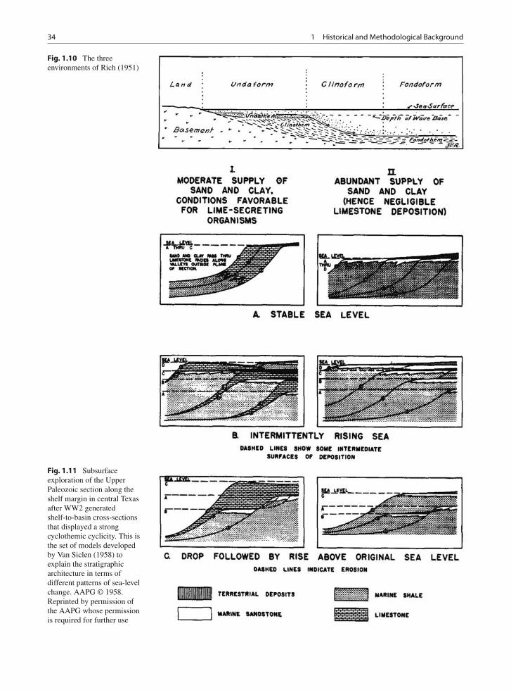
34 1 Historical and Methodological Background
Fig. 1.10 The threeenvironments of Rich (1951)
Fig. 1.11 Subsurfaceexploration of the UpperPaleozoic section along theshelf margin in central Texasafter WW2 generatedshelf-to-basin cross-sectionsthat displayed a strongcyclothemic cyclicity. This isthe set of models developedby Van Siclen (1958) toexplain the stratigraphicarchitecture in terms ofdifferent patterns of sea-levelchange. AAPG © 1958.Reprinted by permission ofthe AAPG whose permissionis required for further use
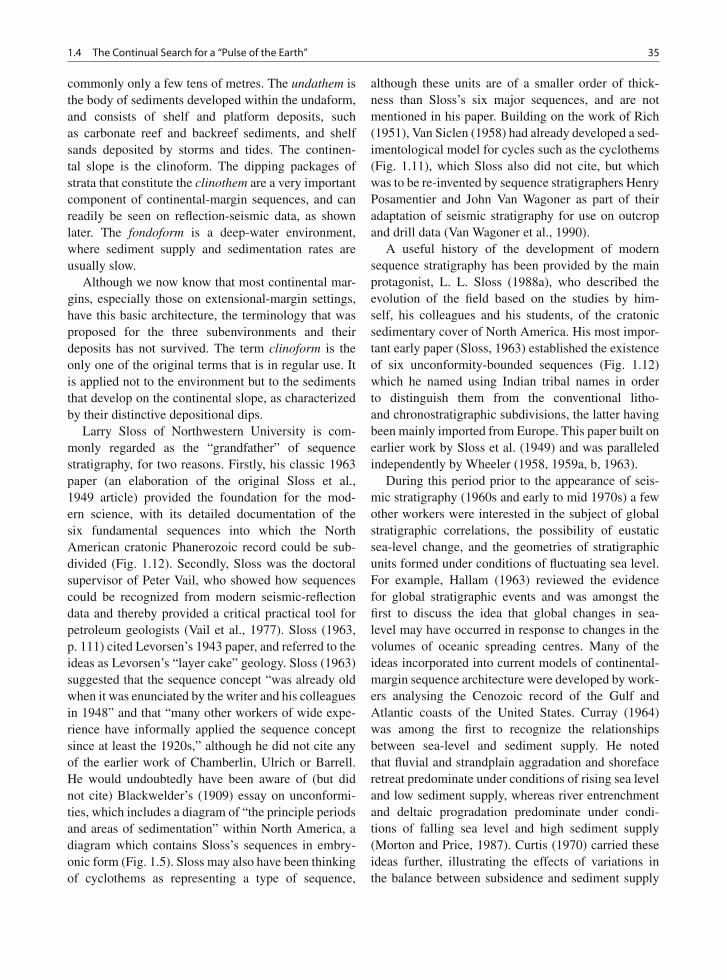
1.4 The Continual Search for a “Pulse of the Earth” 35
commonly only a few tens of metres. The undathem isthe body of sediments developed within the undaform,and consists of shelf and platform deposits, suchas carbonate reef and backreef sediments, and shelfsands deposited by storms and tides. The continen-tal slope is the clinoform. The dipping packages ofstrata that constitute the clinothem are a very importantcomponent of continental-margin sequences, and canreadily be seen on reflection-seismic data, as shownlater. The fondoform is a deep-water environment,where sediment supply and sedimentation rates areusually slow.
Although we now know that most continental mar-gins, especially those on extensional-margin settings,have this basic architecture, the terminology that wasproposed for the three subenvironments and theirdeposits has not survived. The term clinoform is theonly one of the original terms that is in regular use. Itis applied not to the environment but to the sedimentsthat develop on the continental slope, as characterizedby their distinctive depositional dips.
Larry Sloss of Northwestern University is com-monly regarded as the “grandfather” of sequencestratigraphy, for two reasons. Firstly, his classic 1963paper (an elaboration of the original Sloss et al.,1949 article) provided the foundation for the mod-ern science, with its detailed documentation of thesix fundamental sequences into which the NorthAmerican cratonic Phanerozoic record could be sub-divided (Fig. 1.12). Secondly, Sloss was the doctoralsupervisor of Peter Vail, who showed how sequencescould be recognized from modern seismic-reflectiondata and thereby provided a critical practical tool forpetroleum geologists (Vail et al., 1977). Sloss (1963,p. 111) cited Levorsen’s 1943 paper, and referred to theideas as Levorsen’s “layer cake” geology. Sloss (1963)suggested that the sequence concept “was already oldwhen it was enunciated by the writer and his colleaguesin 1948” and that “many other workers of wide expe-rience have informally applied the sequence conceptsince at least the 1920s,” although he did not cite anyof the earlier work of Chamberlin, Ulrich or Barrell.He would undoubtedly have been aware of (but didnot cite) Blackwelder’s (1909) essay on unconformi-ties, which includes a diagram of “the principle periodsand areas of sedimentation” within North America, adiagram which contains Sloss’s sequences in embry-onic form (Fig. 1.5). Sloss may also have been thinkingof cyclothems as representing a type of sequence,
although these units are of a smaller order of thick-ness than Sloss’s six major sequences, and are notmentioned in his paper. Building on the work of Rich(1951), Van Siclen (1958) had already developed a sed-imentological model for cycles such as the cyclothems(Fig. 1.11), which Sloss also did not cite, but whichwas to be re-invented by sequence stratigraphers HenryPosamentier and John Van Wagoner as part of theiradaptation of seismic stratigraphy for use on outcropand drill data (Van Wagoner et al., 1990).
A useful history of the development of modernsequence stratigraphy has been provided by the mainprotagonist, L. L. Sloss (1988a), who described theevolution of the field based on the studies by him-self, his colleagues and his students, of the cratonicsedimentary cover of North America. His most impor-tant early paper (Sloss, 1963) established the existenceof six unconformity-bounded sequences (Fig. 1.12)which he named using Indian tribal names in orderto distinguish them from the conventional litho-and chronostratigraphic subdivisions, the latter havingbeen mainly imported from Europe. This paper built onearlier work by Sloss et al. (1949) and was paralleledindependently by Wheeler (1958, 1959a, b, 1963).
During this period prior to the appearance of seis-mic stratigraphy (1960s and early to mid 1970s) a fewother workers were interested in the subject of globalstratigraphic correlations, the possibility of eustaticsea-level change, and the geometries of stratigraphicunits formed under conditions of fluctuating sea level.For example, Hallam (1963) reviewed the evidencefor global stratigraphic events and was amongst thefirst to discuss the idea that global changes in sea-level may have occurred in response to changes in thevolumes of oceanic spreading centres. Many of theideas incorporated into current models of continental-margin sequence architecture were developed by work-ers analysing the Cenozoic record of the Gulf andAtlantic coasts of the United States. Curray (1964)was among the first to recognize the relationshipsbetween sea-level and sediment supply. He notedthat fluvial and strandplain aggradation and shorefaceretreat predominate under conditions of rising sea leveland low sediment supply, whereas river entrenchmentand deltaic progradation predominate under condi-tions of falling sea level and high sediment supply(Morton and Price, 1987). Curtis (1970) carried theseideas further, illustrating the effects of variations inthe balance between subsidence and sediment supply
36 1 Historical and Methodological Background
Fig. 1.12 The six classic North American sequences of Sloss (1963)
as controls on the stacking patterns of deltas, con-cepts that are now encapsulated by the terms progra-dation, aggradation and retrogradation (Fig. 1.13).Frazier (1974) subdivided the Mississippi deltaic suc-cessions into transgressive, progradational, and aggra-dational phases (Fig. 1.14), and discussed autogenic(delta switching) and glacioeustatic sedimentary con-trols. Brown and Fisher (1977) in a paper that actu-ally deals with seismic data and appears in AAPGMemoir 26, summarized the ideas of an importantgroup of stratigraphers at the Bureau of EconomicGeology, University of Texas, that later became anintegral part of the Exxon sequence-stratigraphy inter-pretive framework—the use of regional facies con-cepts to define depositional systems and systems tracts.Soares et al. (1978) attempted to correlate Phanerozoiccycles in Brazil with those of Sloss, and Hallamcontinued his detailed facies studies of the Jurassicsedimentary record, leading to successive refine-ments of a sea-level curve for that period (Hallam,1978, 1981).
Sloss (1963) defined stratigraphic sequences as“rock-stratigraphic units of higher rank than group,
megagroup, or supergroup, traceable over major areasof a continent and bounded by unconformities ofinterregional scope.” With the advent of seismic strati-graphic research sequences much smaller than groupin equivalent rank were recognized. This raised anomenclature problem, as discussed below.
Wheeler (1958) is credited with the introduction ofchronostratigraphic charts, in which stratigraphic crosssections are plotted with a vertical time axis ratherthan a thickness axis (Fig. 1.4). These diagrams arenow referred to as Wheeler diagrams (Sloss, 1984).They are a useful way of indicating the actual rangein age from place to place of stratigraphic units andunconformities. Vail and his team made use of theseconcepts in their analysis of seismic stratigraphic data(Fig. 1.15).
Sequence stratigraphy remained a subject of rela-tively minor, academic interest throughout the 1960sand 1970s (Ross, 1991), until the publication of amajor memoir by the Exxon group in 1977, whichrevealed the practical utility of the concepts for basinstudies and regional, even global, correlation (Payton,1977). The work was led by Peter R. Vail, the
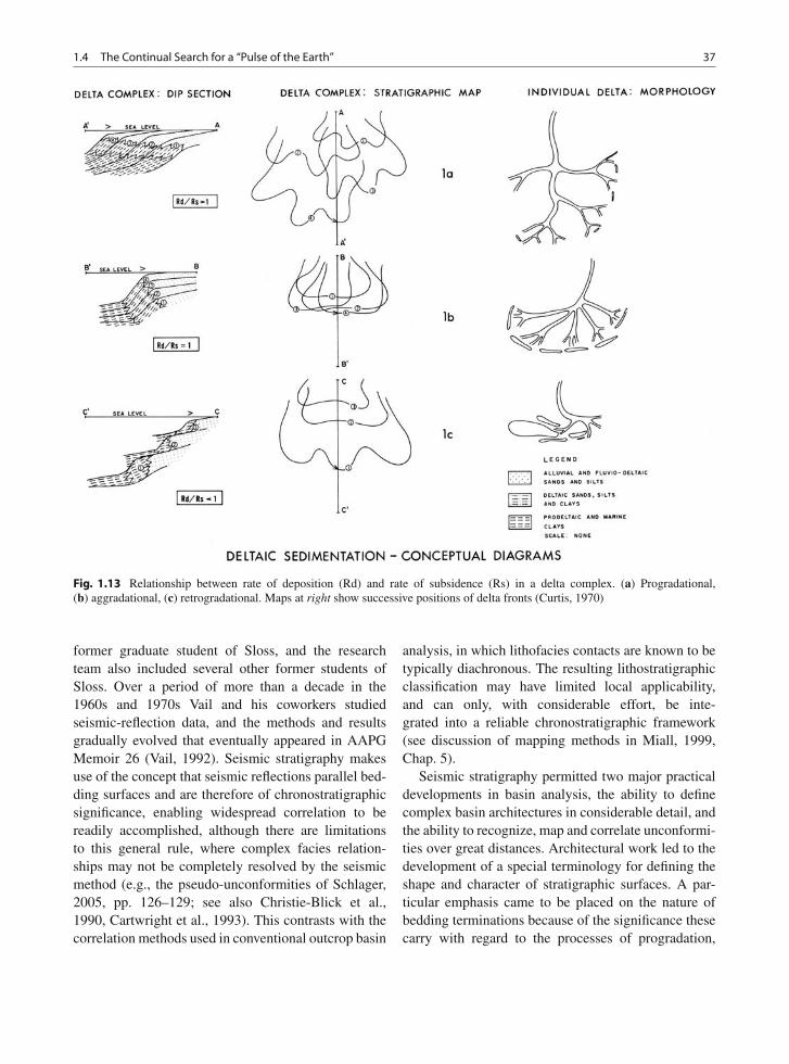
1.4 The Continual Search for a “Pulse of the Earth” 37
Fig. 1.13 Relationship between rate of deposition (Rd) and rate of subsidence (Rs) in a delta complex. (a) Progradational,(b) aggradational, (c) retrogradational. Maps at right show successive positions of delta fronts (Curtis, 1970)
former graduate student of Sloss, and the researchteam also included several other former students ofSloss. Over a period of more than a decade in the1960s and 1970s Vail and his coworkers studiedseismic-reflection data, and the methods and resultsgradually evolved that eventually appeared in AAPGMemoir 26 (Vail, 1992). Seismic stratigraphy makesuse of the concept that seismic reflections parallel bed-ding surfaces and are therefore of chronostratigraphicsignificance, enabling widespread correlation to bereadily accomplished, although there are limitationsto this general rule, where complex facies relation-ships may not be completely resolved by the seismicmethod (e.g., the pseudo-unconformities of Schlager,2005, pp. 126–129; see also Christie-Blick et al.,1990, Cartwright et al., 1993). This contrasts with thecorrelation methods used in conventional outcrop basin
analysis, in which lithofacies contacts are known to betypically diachronous. The resulting lithostratigraphicclassification may have limited local applicability,and can only, with considerable effort, be inte-grated into a reliable chronostratigraphic framework(see discussion of mapping methods in Miall, 1999,Chap. 5).
Seismic stratigraphy permitted two major practicaldevelopments in basin analysis, the ability to definecomplex basin architectures in considerable detail, andthe ability to recognize, map and correlate unconformi-ties over great distances. Architectural work led to thedevelopment of a special terminology for defining theshape and character of stratigraphic surfaces. A par-ticular emphasis came to be placed on the nature ofbedding terminations because of the significance thesecarry with regard to the processes of progradation,
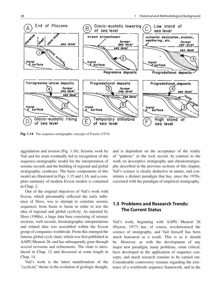
38 1 Historical and Methodological Background
Fig. 1.14 The sequence-stratigraphic concepts of Frazier (1974)
aggradation and erosion (Fig. 1.16). Seismic work byVail and his team eventually led to recognition of thesequence-stratigraphic model for the interpretation ofseismic records and the building of regional and globalstratigraphic syntheses. The basic components of thismodel are illustrated in Figs. 1.15 and 1.16, and a com-plete summary of modern Exxon models is containedin Chap. 2.
One of the original objectives of Vail’s work withExxon, which presumably reflected the early influ-ence of Sloss, was to attempt to correlate seismicsequences from basin to basin in order to test theidea of regional and global cyclicity. As reported bySloss (1988a), a large data base consisting of seismicsections, well records, biostratigraphic interpretationsand related data was assembled within the Exxongroup of companies worldwide. From this emerged thefamous global cycle chart, which was first published inAAPG Memoir 26, and has subsequently gone throughseveral revisions and refinements. The chart is intro-duced in Chap. 12 and discussed at some length inChap. 14.
Vail’s work is the latest manifestation of the“cyclicity” theme in the evolution of geologic thought,
and is dependent on the acceptance of the realityof “patterns” in the rock record. In contrast to thework on descriptive stratigraphy and chronostratigra-phy described in the previous sections of this chapter,Vail’s science is clearly deductive in nature, and con-stitutes a distinct paradigm that has, since the 1970s,coexisted with the paradigm of empirical stratigraphy.
1.5 Problems and Research Trends:The Current Status
Vail’s work, beginning with AAPG Memoir 26(Payton, 1977) has, of course, revolutionized thescience of stratigraphy, and Vail himself has beenmuch honoured as a result. This is as it shouldbe. However, as with the development of anymajor new paradigm, many problems, some critical,have developed in the application of sequence con-cepts, and much research remains to be carried out.Considerable controversy remains regarding the exis-tence of a worldwide sequence framework, and in the
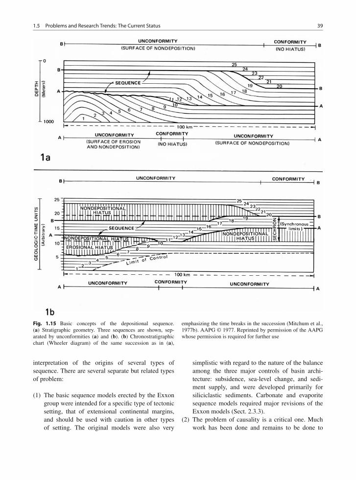
1.5 Problems and Research Trends: The Current Status 39
Fig. 1.15 Basic concepts of the depositional sequence.(a) Stratigraphic geometry. Three sequences are shown, sep-arated by unconformities (a) and (b). (b) Chronostratigraphicchart (Wheeler diagram) of the same succession as in (a),
emphasizing the time breaks in the succession (Mitchum et al.,1977b). AAPG © 1977. Reprinted by permission of the AAPGwhose permission is required for further use
interpretation of the origins of several types ofsequence. There are several separate but related typesof problem:
(1) The basic sequence models erected by the Exxongroup were intended for a specific type of tectonicsetting, that of extensional continental margins,and should be used with caution in other typesof setting. The original models were also very
simplistic with regard to the nature of the balanceamong the three major controls of basin archi-tecture: subsidence, sea-level change, and sedi-ment supply, and were developed primarily forsiliciclastic sediments. Carbonate and evaporitesequence models required major revisions of theExxon models (Sect. 2.3.3).
(2) The problem of causality is a critical one. Muchwork has been done and remains to be done to
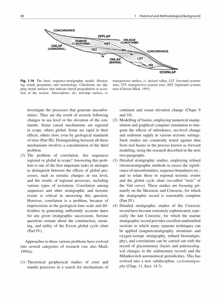
40 1 Historical and Methodological Background
Fig. 1.16 The basic sequence-stratigraphic model, illustrat-ing stratal geometries and terminology. Clinoforms are dip-ping stratal surfaces that indicate lateral progradation or accre-tion of the section. Abreviations: dls, downlap surface, ts,
transgressive surface, iv, incised valley, LST, lowstand systemstract, TST, transgressive systems tract, HST, highstand systemstract (Christie-Blick, 1991)
investigate the processes that generate unconfor-mities. They are the result of erosion followingchanges in sea level or the elevation of the con-tinents. Some causal mechanisms are regionalin scope, others global. Some are rapid in theireffects, others slow, even by geological standardsof time (Part III). Distinguishing between all thesemechanisms involves a consideration of the thirdproblem.
(3) The problem of correlation. Are sequencesregional or global in scope? Answering this prob-lem is one of the first important tasks in attemptsto distinguish between the effects of global pro-cesses, such as eustatic changes in sea level,and the results of regional processes, includingvarious types of tectonism. Correlation amongsequences and other stratigraphic and tectonicevents is critical in answering this question.However, correlation is a problem, because ofimprecisions in the geological time scale and dif-ficulties in generating sufficiently accurate datesfor any given stratigraphic successions. Seriousquestions remain about the construction, mean-ing, and utility of the Exxon global cycle chart(Part IV).
Approaches to these various problems have evolvedinto several categories of research (see also Miall,1995a):
(1) Theoretical geophysical studies of crust andmantle processes in a search for mechanisms of
continent and ocean elevation change (Chaps 9and 10).
(2) Modelling of basins, employing numerical manip-ulation and graphical computer simulation to inte-grate the effects of subsidence, sea-level changeand sediment supply in various tectonic settings.Such studies are commonly tested against datafrom real basins in the process known as forwardmodeling, using the research described in the nexttwo paragraphs.
(3) Detailed stratigraphic studies, employing refinedchronostratigraphic methods to assess the signifi-cance of unconformities, sequence boundaries etc.,and to relate these to regional tectonic eventsand the global cycle chart (so-called “tests” ofthe Vail curve). These studies are focusing pri-marily on the Mesozoic and Cenozoic, for whichthe stratigraphic record is reasonably complete(Part IV).
(4) Detailed stratigraphic studies of the Cenozoicrecord have become extremely sophisticated, espe-cially the late Cenozoic, for which the marinestratigraphic record provides excellent undisturbedsections to which many separate techniques canbe applied (magnetostratigraphy, strontium- andoxygen-isotope stratigraphy, refined biostratigra-phy), and correlations can be carried out with therecord of glacioeustasy (facies and paleoecolog-ical changes in the sedimentary record) and theMilankovitch astronomical periodicities. This hasevolved into a new subdiscipline, cyclostratigra-phy (Chap. 11, Sect. 14.7).
1.6 Current Literature 41
(5) Investigation of modern and very recent sea-level change around the world, and the effects ofglacioeustasy, carried out as a means of provid-ing a base-line of well-constrained studies of whatis happening now, largely as a way to documentthe possible effects on oceanic volumes of meltingcontinental ice caps. This specialized work car-ries the subject to levels of measurement detail andchronostratigraphic refinement that are beyond thescope of most geological research, and the work isnot discussed in this book.
1.6 Current Literature
Good overviews of the subject of sequence stratigra-phy, from various perspectives, can be obtained fromseveral recent books, special journal issues, and reviewarticles. These include the following:
1. Books: Miall’s (1999) textbook on basin analysisincludes a fairly succinct review of sequence stratig-raphy and global stratigraphic cycles written at thegraduate level. It carries the development of techniquesup to the late 1990s. Hallam (1992a) discussed sea-level changes throughout the Phanerozoic, and evalu-ated the various mechanisms that have been proposedfor sea-level change. Walker and James (1992) pro-vided a thorough, updated version of the GeologicalAssociation of Canada “Facies Models” book, writtenat the advanced undergraduate level. It contains exten-sive discussions of the stratigraphic effects of sea-levelchange, but there is little discussion of mechanisms inthis book beyond a useful introductory chapter. Exxonmodels and terminology are deliberately avoided inthis book.
Detailed treatment of sequence-stratigraphic mod-els, including the recognition and documentation ofsequences in outcrop, drill core, well logs and seis-mic data, have been provided by several recent books,including Emery and Myers (1996), Posamentierand Allen (1999, focusing on clastic sequences),Coe (2003), Schlager (2005, focusing on carbonatesequences) and Catuneanu (2006). These books allfocus on the recognition and definition of sequences,and do not examine the mechanisms for generatingsequences, or the problems and controversies sur-rounding the issues of sequence correlation and itsbearing on the testing of eustatic models of sequence
generation. That by Catuneanu (2006) is comprehen-sively referenced, contains examples and illustrationsfrom around the world, and is characterized by aconsistent emphasis on the temporal significance ofsequences, systems tracts and bounding surfaces; itseems likely to achieve recognition as the standardwork on the subject.
2. Research syntheses (books and special journalissues): Essential reading is the first major publicationon sequence stratigraphy, the AAPG Memoir whichestablished seismic stratigraphy as a major new tech-nique (Payton, 1977). A second AAPG collection ofarticles on seismic stratigraphy appeared in 1984, andconstituted an attempt to examine some of the majorpremises of the Exxon work, such as the significanceof condensed successions in the sedimentary record,and the ability to correlate unconformities using thelimited well and seismic data available from specificcontinental margins (Schlee, 1984). Bally (1987) com-piled three volumes of seismic-stratigraphic studies ina large, atlas format. These include important introduc-tory papers dealing with Exxon methods, and numer-ous case studies from many types of basin aroundthe world. Most of these are superbly illustrated withlong seismic sections, many in colour. Berger et al.(1984) edited a major research compilation dealingwith Milankovitch processes, including astronomicaland climatic studies and many papers describing thegeological evidence.
Two research collections published by the Societyof Economic Paleontologists and Mineralogists, oneedited by Nummedal et al. (1987), and the other byWilgus et al. (1988), contain many important papers.The first focuses on studies of Quaternary sea-levelchange, and provides comparisons of coastal stratig-raphy with the ancient record; the second contains amajor suite of papers by the Exxon group, dealing withtheir sequence models. These papers provided contem-porary expositions of the Exxon sequence-stratigraphyresearch, although much has changed since these bookappeared. The papers by Jervey, Posamentier and Vailin Wilgus et al. (1988) constitute the next most impor-tant exposition of the Exxon models following Payton(1977), and contain the first detailed treatment of thesedimentology of sequences. Practical examples of thiswork are illustrated by Van Wagoner et al. (1990)in a well-illustrated review of outcrop and subsurfaceexamples of Exxon-type sequences. In my opinion thisis the best of the Exxon products because it contains
42 1 Historical and Methodological Background
numerous actual examples, and is less “model-driven”than the other papers by this group, although there areproblems with some concepts and terminology (seeChap. 2).
Other collections of case studies include that editedby James and Leckie (1988), which draws partic-ularly on the wealth of subsurface detail availablefor the Western Canada Sedimentary Basin. Collinson(1989) edited a compilation of studies of relevance tothe petroleum industry, including techniques of cor-relation, with examples from the Arctic and NorthSea regions. Cross (1990) put together a uniquecompilation of research articles describing quantita-tive approaches to basin modelling. Many importantdetails of the sequence-stratigraphy story emerged inthis book. Ginsburg and Beaudoin (1990) collectedresearch on the Cretaceous system—a synthesis ofthe first major project of the Global SedimentaryGeology Program. Fischer and Bottjer (1991) pro-vided an introduction to a special issue of Journalof Sedimentary Petrology dealing with Milankovitchrhythms. Macdonald (1991) compiled case studies ofstratigraphic architecture in convergent and collisionalplate settings. One of the major focuses of this book isto examine sequence stratigraphies in a tectonic con-text. A wealth of stratigraphic detail is contained inthis book, but there are no synthesis or overview arti-cles, except that by Carter et al. (1991), who testedthe sequence-stratigraphic model and the global-cycle-chart model of Exxon against data from New Zealand.Revelle (1990) edited an important collection of reviewarticles on sea-level change and its causes, includ-ing several referenced separately, below. Swift et al.(1991a) published a collection of research articleson shelf sedimentation. This includes a major set oftheoretical papers that attempted to establish a quan-titative framework for shelf sedimentation within asequence framework. Cloetingh (1991) edited a specialissue of Journal of Geophysical Research consistingof a collection of papers that examined the measure-ment, causes and consequences of long-term sea-levelchange. Advanced computer modelling and the use ofrefined stratigraphic data sets are two of the featuresof this collection. Another collection of papers in thisarea was edited by Biddle and Schlager (1991). Einseleet al. (1991a) edited a multi-authored compilation ofchapters dealing with many aspects of cyclic and eventstratification, including several useful overview chap-ters. An updated version of the Exxon approach to
sequence-stratigraphic analysis, including their firstrealistic appraisal of the importance of tectonism, isincluded in a chapter by Vail et al. (1991). Franseenet al. (1991) edited a collection of articles on thesubject of sedimentary modeling, focusing on high-frequency cycles. Another useful collection of paperson tectonics and seismic sequence stratigraphy is thatedited by Williams and Dobb (1993).
Weimer and Posamentier (1993) and Loucks andSarg (1993) focus on the broader principles of sili-ciclastic and carbonate sequence stratigraphy, respec-tively. Many useful books consisting largely of casestudies have been published during the last decade orso. Eschard and Doligez (1993) edited a suite of papersdemonstrating how detailed outcrop studies, includingdocumentation of high-resolution sequence stratigra-phy, could be of use in the development of our under-standing about petroleum reservoirs. A book editedby Posamentier et al. (1993) contains papers dealingwith concepts and principles, methods and applica-tions, and case studies. Van Wagoner and Bertram(1995) edited a collection of papers dealing with thesequence stratigraphy of foreland basins. The bookcontains an introductory article by Van Wagoner thatprovides revised definitions of many of the terms usedin sequence stratigraphy. Norwegian work in the NorthSea and Svalbard led to two important collections(Steel et al., 1995; Gradstein et al., 1998). The veryuseful book edited by Gradstein et al. (1998) containsa lengthy historical article by J. P. Nystuen, and sev-eral theoretical studies. Other sets of case studies havebeen compiled by Armentrout and Perkins (1991) andHailwood and Kidd (1993).
One of the issues dealt with in Nystuen’s (1998)article is the existence of several competing models forsequence documentation and classification. This hasled to extensive debate regarding the relative impor-tance of various surfaces that may be recognized instratigraphic successions (see Sect. 1.7, Chap. 2). Huntand Gawthorpe (2000) compiled a book that dealswith one aspect of this debate, the significance ofthe process termed “forced regression,” which is theterm used to refer to the seaward migration of theshoreline, shallow-shelf wave ravinement erosion andshoreface sedimentation under conditions of fallingsea level. Processes of sea-level change and its strati-graphic record are discussed in detail in a specialissue of Basin Research edited by Fulthorpe et al.(2008).
1.7 Stratigraphic Terminology 43
Milankovitch cycles are discussed in books bySchwarzacher (1993) and Weedon (2003) that providedetailed treatments of the nature of orbital pertur-bations and spectral analysis of orbital and cyclicfrequencies. A collection of research papers waspublished by de Boer and Smith (1994a). Houseand Gale (1995) focus on orbital forcing and cyclicsequences. More recent work includes the book editedby D’Argenio et al. (2004a). Shackleton et al. (1999)edited a collection of research papers dealing withdevelopments in a cyclostratigraphic time scale.
A special issue of the journal Stratigraphy (vol. 4,pp. 2–3) published in 2007 contains many use-ful articles discussing the history and developmentof chronostratigraphy, including articles on currentdebates about principles and methods. Christie-Blicket al. (2007) contributed a very thoughtful article aboutsequence stratigraphy to this collection, an article thatis cited at several places in this book.
3. Review articles: Useful reviews of Milankovitch-type cycles were given by Fischer (1986) and Weedon(1993). Burton et al. (1987) reviewed the lack of refer-ence frames in attempts to quantify sea-level change,and the fact that it is very difficult to quantify and iso-late the effects of the three main depositional controls,subsidence, sea-level change, and sediment supply.Cross and Lessenger (1988) reviewed the methods ofseismic stratigraphy, and discussed some of the con-straints on the use of seismic data in stratigraphic stud-ies. Three useful companion studies by Christie-Blicket al. (1990), Christie-Blick (1991) and Christie-Blickand Driscoll (1995) reviewed current work on mech-anisms of sea-level change and numerical modellingtechniques. Schlager (1992a) provided a brief but wellillustrated discussion of the sequence stratigraphy ofcarbonate depositional systems. This is an importantcontribution, containing many original ideas makingthe case that the standard Exxon model for clasticsequences cannot readily be applied to carbonate sys-tems. Miall (1995a) outlined recent developments inresearch in the field of stratigraphy, including sequencestratigraphy. Wilson (1998) provided a set of personalreflections on the sequence stratigraphic “revolution”expressing some skepticism regarding the model ofglobal eustasy.
Catuneanu et al. (2009) published a landmark studyconcerning the documentation, definition and classi-fication of sequences, the objective of which is toreconcile the many debates that have raged in the
lecture theatre, in panel debates, and in the publishedliterature, for more than two decades. This paper isdiscussed below.
4. Web sites: There are numerous Internet resourcesthat now deal with sequence stratigraphy. Many areteaching sites established by universities and con-sist primarily of repetitions of standard textbookfare. A few are exceptional and worth highlighting.That maintained by C. G. St. C. (Chris) Kendall athttp://strata.geol.sc.edu/ is undoubtedly the most use-ful. At this site there are numerous examples, teach-ing modules, movies, galleries of photographs, andsummaries and online debate concerning sequencedefinition and classification. Octavian Catuneanu hasposted most of the illustrations from his 2006 bookon a website from which they may be copied:http://research.eas.ualberta.ca/catuneanu/.
The site at the University of Georgia http://www.uga.edu/∼strata/sequence/index.html providesa useful source of definitions. Basic concepts aredefined by J. W. Mulholland at http://www.aseg.org.au/publications/articles/mul/ss1/htm. There aremany other websites, including an article in Wikipedia,but none particularly recommends itself as a primaryinformation source.
A different type of website is the official websiteof the International Commission on Stratigraphy athttp://www.stratigraphy.org, which contains the onlineversion of the International Stratigraphic Guide andmaintains an up to date reference source for globalstratotypes and the definitions and ages of global stageboundaries.
1.7 Stratigraphic Terminology
Sloss (1963) used the term “sequence” for his pack-ages of strata. The term has had a varied usagesince that time, having been employed informally, ina non-genetic sense, as a synonym for “succession”in some literature, and for cyclic or unconformity-bounded units of varying dimensions and time-spans.Sloss’s original sequences represent sea-level cyclesthat were tens of millions of years in duration. Theywere termed second-order cycles by Vail et al. (1977;see Chap. 3), whereas the term “sequence” was usedfor much smaller packages of strata, representingsea-level cycles of a few million years duration
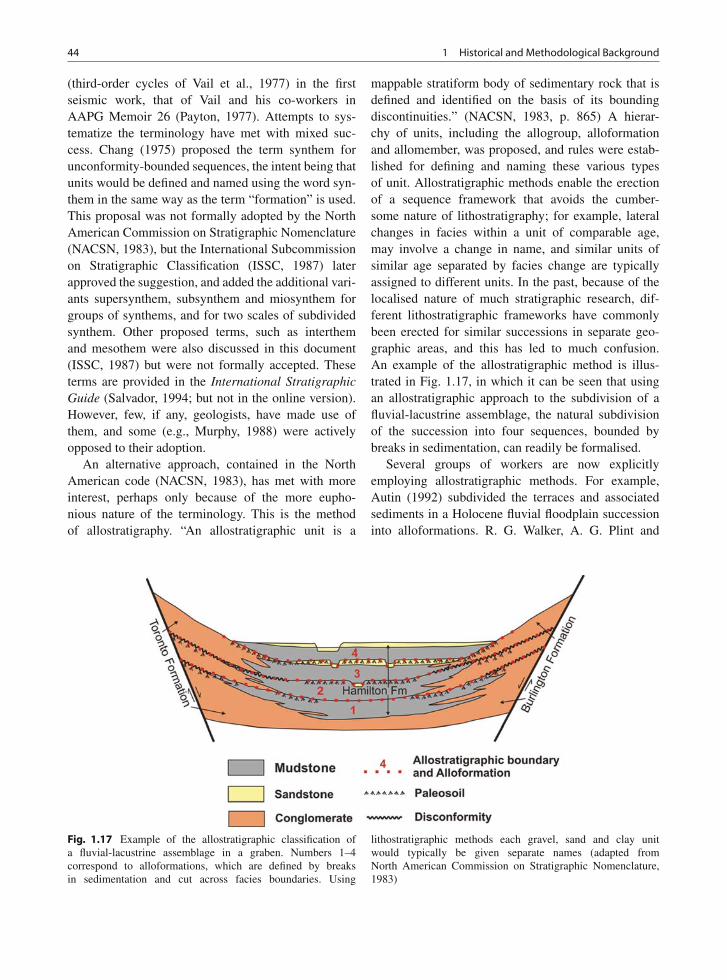
44 1 Historical and Methodological Background
(third-order cycles of Vail et al., 1977) in the firstseismic work, that of Vail and his co-workers inAAPG Memoir 26 (Payton, 1977). Attempts to sys-tematize the terminology have met with mixed suc-cess. Chang (1975) proposed the term synthem forunconformity-bounded sequences, the intent being thatunits would be defined and named using the word syn-them in the same way as the term “formation” is used.This proposal was not formally adopted by the NorthAmerican Commission on Stratigraphic Nomenclature(NACSN, 1983), but the International Subcommissionon Stratigraphic Classification (ISSC, 1987) laterapproved the suggestion, and added the additional vari-ants supersynthem, subsynthem and miosynthem forgroups of synthems, and for two scales of subdividedsynthem. Other proposed terms, such as interthemand mesothem were also discussed in this document(ISSC, 1987) but were not formally accepted. Theseterms are provided in the International StratigraphicGuide (Salvador, 1994; but not in the online version).However, few, if any, geologists, have made use ofthem, and some (e.g., Murphy, 1988) were activelyopposed to their adoption.
An alternative approach, contained in the NorthAmerican code (NACSN, 1983), has met with moreinterest, perhaps only because of the more eupho-nious nature of the terminology. This is the methodof allostratigraphy. “An allostratigraphic unit is a
mappable stratiform body of sedimentary rock that isdefined and identified on the basis of its boundingdiscontinuities.” (NACSN, 1983, p. 865) A hierar-chy of units, including the allogroup, alloformationand allomember, was proposed, and rules were estab-lished for defining and naming these various typesof unit. Allostratigraphic methods enable the erectionof a sequence framework that avoids the cumber-some nature of lithostratigraphy; for example, lateralchanges in facies within a unit of comparable age,may involve a change in name, and similar units ofsimilar age separated by facies change are typicallyassigned to different units. In the past, because of thelocalised nature of much stratigraphic research, dif-ferent lithostratigraphic frameworks have commonlybeen erected for similar successions in separate geo-graphic areas, and this has led to much confusion.An example of the allostratigraphic method is illus-trated in Fig. 1.17, in which it can be seen that usingan allostratigraphic approach to the subdivision of afluvial-lacustrine assemblage, the natural subdivisionof the succession into four sequences, bounded bybreaks in sedimentation, can readily be formalised.
Several groups of workers are now explicitlyemploying allostratigraphic methods. For example,Autin (1992) subdivided the terraces and associatedsediments in a Holocene fluvial floodplain successioninto alloformations. R. G. Walker, A. G. Plint and
Fig. 1.17 Example of the allostratigraphic classification ofa fluvial-lacustrine assemblage in a graben. Numbers 1–4correspond to alloformations, which are defined by breaksin sedimentation and cut across facies boundaries. Using
lithostratigraphic methods each gravel, sand and clay unitwould typically be given separate names (adapted fromNorth American Commission on Stratigraphic Nomenclature,1983)
1.7 Stratigraphic Terminology 45
their students and coworkers have employed allostrati-graphic terminology in their study of the sequencestratigraphy of part of the Alberta Basin, Canada.Their first definition of unconformity-bounded unitsis described in Plint et al. (1986), where the defin-ing concepts are referred to as event stratigraphy,following the developments of ideas in this area byEinsele and Seilacher (1982). Explicit use of allostrati-graphic terms appears in their later papers (e.g., Plint,1990) and has become the standard method for thework of this research group (e.g., Varban and Plint,2008). The standard Canadian text on facies analysisthat builds extensively on the work of this group rec-ommends the use of allostratigraphic methods and ter-minology as a general approach to the study of strati-graphic sequences (Walker, 1992). Martinsen et al.(1993) compared lithostratigraphic, allostratigraphicand sequence concepts as applied to a stratigraphicsuccession in Wyoming. As they were able to demon-strate, each method has its local advantages and disad-vantages.
One of the achievements of seismic stratigraphy hasbeen development of the ability to trace unconformity-bounded units into areas where the unconformablebounding surfaces are no longer recognizable. ThusMitchum et al. (1977b, p. 53) defined a depositionalsequence as “a stratigraphic unit composed of a rel-atively conformable succession of genetically relatedstrata and bounded at its top and base by unconfor-mities or their correlative conformities.” Recognizingthe bounding contacts in a conformable successionmight, in practice, be difficult. The concept of a cor-relative conformity does not appear in the NACSNcode, although some (e.g., Walker, 1992, p. 9) haverecommended that it should (see Sect. 2.2). Great careneeds to be taken in assessing the chronostratigraphicsignificance of unconformities and correlative confor-
mities. Considerable disagreement exists regarding thecorrelation of sequence-bounding unconformities frombasin margins, where they are commonly of subaerialorigin and may be accompanied by major facies shifts,into deeper parts of the basin (Sect. 2.4). These con-cerns are echoed by Christie-Blick et al. (2007) whoremarked (p. 222) that “some level of diachroneity [is]unavoidable” and that “at some scale, unconformitiespass laterally not into correlative conformities but intocorrelative intervals.”
Sequence classifications and allostratigraphic unitsare based on concepts of sequence scale and durationthat are hierarchical in character (first- to sixth-ordersequences; synthem and its variants; alloformationsand allomembers). However, it is increasingly clearthat sequences occur over a wide range of time scalesand physical scales (e.g., thicknesses) that show nosignificant natural breaks, as would justify hierarchi-cal classification (Sect. 4.2). In this book, sequencesare described with reference to their duration (Chaps5, 6 and 7), but formal hierarchical classifications arelargely avoided, except where it is necessary to makereference to earlier literature. At the time of writingthis book, Working Groups of the IUGS InternationalSubcommission on Stratigraphic Classification and theNorth American Commission on Stratigraphy werewrestling with the problem of how to define sequencesand how to incorporate sequence concepts into formalsystems of stratigraphic nomenclature. A review paperby Catuneanu et al. (2009) represents the efforts of alarge and diverse group of stratigraphers worldwideto develop recommendations for the formalization ofsequence terminology. The current state of the debateis touched on in Chap. 2, but this book is not primarilyabout sequence terminology and models (for which thereader is referred to Catuneanu, 2006, and Catuneanuet al., 2009), but about the origins of sequences.
Chapter 2
The Basic Sequence Model
Contents
2.1 Introduction . . . . . . . . . . . . . . . . . 472.2 Elements of the Model . . . . . . . . . . . . 48
2.2.1 Accommodation and Supply . . . . . . 492.2.2 Stratigraphic Architecture . . . . . . . 502.2.3 Depositional Systems and Systems Tracts 55
2.3 Sequence Models in Clastic and CarbonateSettings . . . . . . . . . . . . . . . . . . . 572.3.1 Marine Clastic Depositional Systems and
Systems Tracts . . . . . . . . . . . . 572.3.2 Nonmarine Depositional Systems . . . . 642.3.3 Carbonate Depositional Systems . . . . 68
2.4 Sequence Definitions . . . . . . . . . . . . . 73
2.1 Introduction
The purpose of this chapter is to present a succinctsummary of sequence concepts, focusing on what hasbecome the standard, or most typical, sequence model,and making only brief references to exceptions andcomplexities. These are described more completelyelsewhere, most notably by Catuneanu (2006).
The nomenclature for sequence architecture andsystems tracts was established initially by the Exxongroup, led by Peter Vail, and included much new ter-minology, new concepts and new interpretive methods.It is important to be familiar with these, as the termsand concepts came to be used by virtually all stratig-raphers. Application of the methods to different typesof data (outcrop, well-log, 2-D seismic, 3-D seismic)from around the world permitted a quantum leap inunderstanding of basin architectures, but also revealed
some problems with the Exxon concepts and terminol-ogy that have stimulated vigorous debate over the lasttwo decades. The purpose of this chapter is to bringthe debate up to date by presenting current concepts,with enough historical background that readers famil-iar with the debates will be able to comprehend theneed for revisions and new approaches.
The history of sequence concepts is presented inChap. 1. Current concepts and definitions are presentedby Catuneanu (2006) and Catuneanu et al. (2009), fromwhich much of this chapter is summarized. The readeris referred to these two sources which, at the timeof publication of this book, could be considered themost up to date and definitive sources. The introduc-tion to Chap. 5 in Catuneanu (2006, pp. 165–171) isparticularly useful in providing a history of the con-troversies, the main players and publications, and theconcepts and terminologies about which there havebeen dispute.
Sequence stratigraphic concepts are, to a con-siderable extent, independent of scale (Schlager,2004; Catuneanu, 2006, p. 9). Posamentier and Vail(1988) and Posamentier et al. (1992) gave exam-ples of sequence architecture evolving from base-levelchanges in small natural systems, and much exper-imental work has successfully simulated sequencedevelopment in small laboratory tanks (e.g., Woodet al., 1993; Paola, 2000). Interpretations of the tem-poral significance of sequences can, therefore, bedifficult. However, as discussed later in this book,some aspects of the driving process, notably tecton-ism and climate change, generate facies and architec-ture that are sufficiently distinctive to yield reliableinterpretations.
47A.D. Miall, The Geology of Stratigraphic Sequences, 2nd ed.,DOI 10.1007/978-3-642-05027-5_2, © Springer-Verlag Berlin Heidelberg 2010
48 2 The Basic Sequence Model
2.2 Elements of the Model
A practical, working geologist faces two successivequestions: firstly, is his/her stratigraphy subdivisibleinto stratigraphic sequences? And, secondly, what gen-erated these sequences: regional tectonism, globaleustasy, orbital forcing, or some other cause? The firstpart of this chapter deals with the methods for analyz-ing the sequence record. These include the following:
• The mapping of unconformities as a first step inidentifying unconformity-bounded sequences.
• Clarifying the relationship between regional struc-tural geology and the large-scale configuration ofsequences.
• The mapping of onlap, offlap and other strati-graphic terminations in order to provide informationabout the internal architectural development of eachsequence.
• The mapping of cyclic vertical facies changes inoutcrop or well records in order to subdivide a strati-graphic succession into its component sequencesand depositional-systems tracts, and as an indicatorof changes in accommodation, including changes inrelative sea-level.
The first three steps may be based on seismic-reflection data, well records or outcrops; the last stepcannot be accomplished using seismic data alone. Thefourth step may make use of facies-cycle and otherdata, as described in Chap. 3.
Sequence stratigraphy is based on the recogni-tion of unconformity-bounded units, which may beformally defined and named using the methods ofallostratigraphy, as noted in Sect. 1.7. Mitchum et al.(1977b, p. 53) defined a depositional sequence as“a stratigraphic unit composed of a relatively con-formable succession of genetically related strata andbounded at its top and base by unconformities or theircorrelative conformities.” As noted in Sect. 1.7, anunconformity may be traced laterally into the depositsof deep marine environments, where it may be repre-sented by a correlative conformity. However, recogniz-ing the bounding contacts in a conformable successionmight, in practice, be difficult. Documentation of thetwo- and three-dimensional architecture of sequenceswas one of the most important breakthroughs of theseismic method, as explained in the Sect. 2.2.2.
Sequences reflect the sedimentary response tobase-level cycles—the rise and fall in sea level rel-ative to the shoreline, and changes in the sedimentsupply. Change in sea-level relative to the shorelinemay result from eustasy (absolute changes in sea-level elevation relative to the centre of Earth) or fromvertical movements of the basin floor as a result oftectonism. Because of the difficulty in distinguish-ing between these two different processes, the termrelative sea-level change is normally used in orderto encompass the uncertainty. These basic controlsare explained in Sect. 2.2.1. In nonmarine settings,upstream controls (tectonism and climate change)are the major determinant of sequence architecture(Sect. 2.3.2).
The cycle of rise and fall of base level generatespredictable responses in a sedimentary system, such asthe transgressions that occur during rising relative sealevel, and the widespread subaerial erosion and deliv-ery of clastic detritus to the continental shelf, slope,and deep basin during a fall in relative sea level. Thedepositional systems that result, and their vertical andlateral relationships, provide the basis for subdividingsequences into systems tracts. These are described andexplained in Sect. 2.2.2.
Unconformities provided the basis for the first defi-nitions of sequences, by Blackwelder, Levorsen, Slossand Vail (see Chap. 1). The unconformities that arethe key to sequence recognition are those that developas a result of subaerial exposure. Unconformities maydevelop below sea level as a result of submarine ero-sion, but are not used as the basis for sequence defini-tion. Where subaerial unconformities are present, as innonmarine and coastal settings, sequence definition isrelatively straightforward. Carrying a correlation intothe offshore, including recognition of a correlative con-formity, is not necessarily simple; in fact this has beenthe cause of considerable debate and controversy, asdiscussed in Sect. 2.2.3. Several methods of definingsequences evolved from these controversies, and thishas inhibited further progress in the establishment ofsequence terminology and classification as a formalpart of what might be called the official language ofstratigraphy. Catuneanu (2006) and Catuneanu et al.(2009) have gone a long way towards resolving theseproblems, and their proposals are summarized inSect. 2.3.
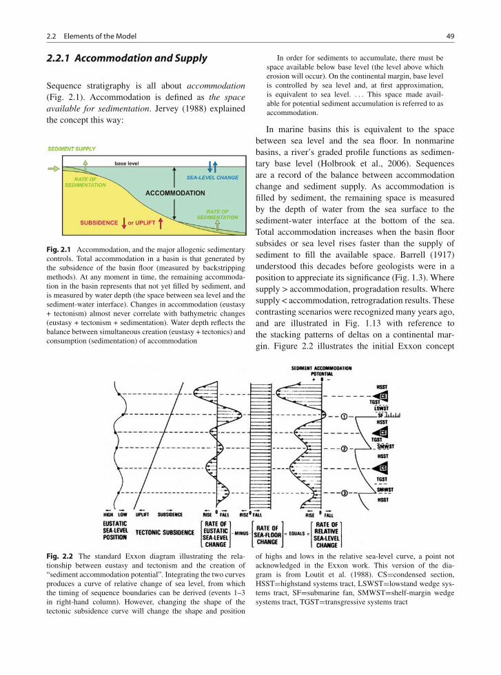
2.2 Elements of the Model 49
2.2.1 Accommodation and Supply
Sequence stratigraphy is all about accommodation(Fig. 2.1). Accommodation is defined as the spaceavailable for sedimentation. Jervey (1988) explainedthe concept this way:
Fig. 2.1 Accommodation, and the major allogenic sedimentarycontrols. Total accommodation in a basin is that generated bythe subsidence of the basin floor (measured by backstrippingmethods). At any moment in time, the remaining accommoda-tion in the basin represents that not yet filled by sediment, andis measured by water depth (the space between sea level and thesediment-water interface). Changes in accommodation (eustasy+ tectonism) almost never correlate with bathymetric changes(eustasy + tectonism + sedimentation). Water depth reflects thebalance between simultaneous creation (eustasy + tectonics) andconsumption (sedimentation) of accommodation
In order for sediments to accumulate, there must bespace available below base level (the level above whicherosion will occur). On the continental margin, base levelis controlled by sea level and, at first approximation,is equivalent to sea level. . . . This space made avail-able for potential sediment accumulation is referred to asaccommodation.
In marine basins this is equivalent to the spacebetween sea level and the sea floor. In nonmarinebasins, a river’s graded profile functions as sedimen-tary base level (Holbrook et al., 2006). Sequencesare a record of the balance between accommodationchange and sediment supply. As accommodation isfilled by sediment, the remaining space is measuredby the depth of water from the sea surface to thesediment-water interface at the bottom of the sea.Total accommodation increases when the basin floorsubsides or sea level rises faster than the supply ofsediment to fill the available space. Barrell (1917)understood this decades before geologists were in aposition to appreciate its significance (Fig. 1.3). Wheresupply > accommodation, progradation results. Wheresupply < accommodation, retrogradation results. Thesecontrasting scenarios were recognized many years ago,and are illustrated in Fig. 1.13 with reference tothe stacking patterns of deltas on a continental mar-gin. Figure 2.2 illustrates the initial Exxon concept
Fig. 2.2 The standard Exxon diagram illustrating the rela-tionship between eustasy and tectonism and the creation of“sediment accommodation potential”. Integrating the two curvesproduces a curve of relative change of sea level, from whichthe timing of sequence boundaries can be derived (events 1–3in right-hand column). However, changing the shape of thetectonic subsidence curve will change the shape and position
of highs and lows in the relative sea-level curve, a point notacknowledged in the Exxon work. This version of the dia-gram is from Loutit et al. (1988). CS=condensed section,HSST=highstand systems tract, LSWST=lowstand wedge sys-tems tract, SF=submarine fan, SMWST=shelf-margin wedgesystems tract, TGST=transgressive systems tract
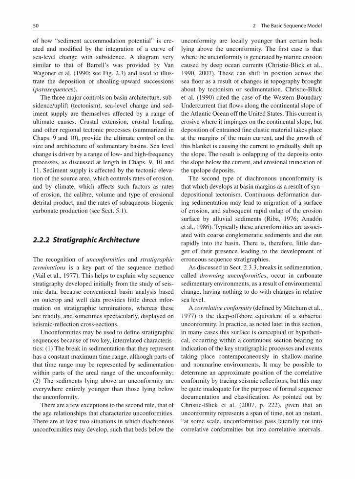
50 2 The Basic Sequence Model
of how “sediment accommodation potential” is cre-ated and modified by the integration of a curve ofsea-level change with subsidence. A diagram verysimilar to that of Barrell’s was provided by VanWagoner et al. (1990; see Fig. 2.3) and used to illus-trate the deposition of shoaling-upward successions(parasequences).
The three major controls on basin architecture, sub-sidence/uplift (tectonism), sea-level change and sed-iment supply are themselves affected by a range ofultimate causes. Crustal extension, crustal loading,and other regional tectonic processes (summarized inChaps. 9 and 10), provide the ultimate control on thesize and architecture of sedimentary basins. Sea levelchange is driven by a range of low- and high-frequencyprocesses, as discussed at length in Chaps. 9, 10 and11. Sediment supply is affected by the tectonic eleva-tion of the source area, which controls rates of erosion,and by climate, which affects such factors as ratesof erosion, the calibre, volume and type of erosionaldetrital product, and the rates of subaqueous biogeniccarbonate production (see Sect. 5.1).
2.2.2 Stratigraphic Architecture
The recognition of unconformities and stratigraphicterminations is a key part of the sequence method(Vail et al., 1977). This helps to explain why sequencestratigraphy developed initially from the study of seis-mic data, because conventional basin analysis basedon outcrop and well data provides little direct infor-mation on stratigraphic terminations, whereas theseare readily, and sometimes spectacularly, displayed onseismic-reflection cross-sections.
Unconformities may be used to define stratigraphicsequences because of two key, interrelated characteris-tics: (1) The break in sedimentation that they representhas a constant maximum time range, although parts ofthat time range may be represented by sedimentationwithin parts of the areal range of the unconformity;(2) The sediments lying above an unconformity areeverywhere entirely younger than those lying belowthe unconformity.
There are a few exceptions to the second rule, that ofthe age relationships that characterize unconformities.There are at least two situations in which diachronousunconformities may develop, such that beds below the
unconformity are locally younger than certain bedslying above the unconformity. The first case is thatwhere the unconformity is generated by marine erosioncaused by deep ocean currents (Christie-Blick et al.,1990, 2007). These can shift in position across thesea floor as a result of changes in topography broughtabout by tectonism or sedimentation. Christie-Blicket al. (1990) cited the case of the Western BoundaryUndercurrent that flows along the continental slope ofthe Atlantic Ocean off the United States. This current iserosive where it impinges on the continental slope, butdeposition of entrained fine clastic material takes placeat the margins of the main current, and the growth ofthis blanket is causing the current to gradually shift upthe slope. The result is onlapping of the deposits ontothe slope below the current, and erosional truncation ofthe upslope deposits.
The second type of diachronous unconformity isthat which develops at basin margins as a result of syn-depositional tectonism. Continuous deformation dur-ing sedimentation may lead to migration of a surfaceof erosion, and subsequent rapid onlap of the erosionsurface by alluvial sediments (Riba, 1976; Anadónet al., 1986). Typically these unconformities are associ-ated with coarse conglomeratic sediments and die outrapidly into the basin. There is, therefore, little dan-ger of their presence leading to the development oferroneous sequence stratigraphies.
As discussed in Sect. 2.3.3, breaks in sedimentation,called drowning unconformities, occur in carbonatesedimentary environments, as a result of environmentalchange, having nothing to do with changes in relativesea level.
A correlative conformity (defined by Mitchum et al.,1977) is the deep-offshore equivalent of a subaerialunconformity. In practice, as noted later in this section,in many cases this surface is conceptual or hypotheti-cal, occurring within a continuous section bearing noindication of the key stratigraphic processes and eventstaking place contemporaneously in shallow-marineand nonmarine environments. It may be possible todetermine an approximate position of the correlativeconformity by tracing seismic reflections, but this maybe quite inadequate for the purpose of formal sequencedocumentation and classification. As pointed out byChristie-Blick et al. (2007, p. 222), given that anunconformity represents a span of time, not an instant,“at some scale, unconformities pass laterally not intocorrelative conformities but into correlative intervals.
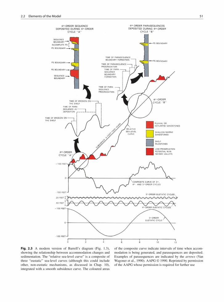
2.2 Elements of the Model 51
Fig. 2.3 A modern version of Barrell’s diagram (Fig. 1.3),showing the relationship between accommodation changes andsedimentation. The “relative sea-level curve” is a composite ofthree “eustatic” sea-level curves (although this could includeother, non-eustatic mechanisms, as discussed in Chap. 10),integrated with a smooth subsidence curve. The coloured areas
of the composite curve indicate intervals of time when accom-modation is being generated, and parasequences are deposited.Examples of parasequences are indicated by the arrows (VanWagoner et al., 1990). AAPG © 1990. Reprinted by permissionof the AAPG whose permission is required for further use
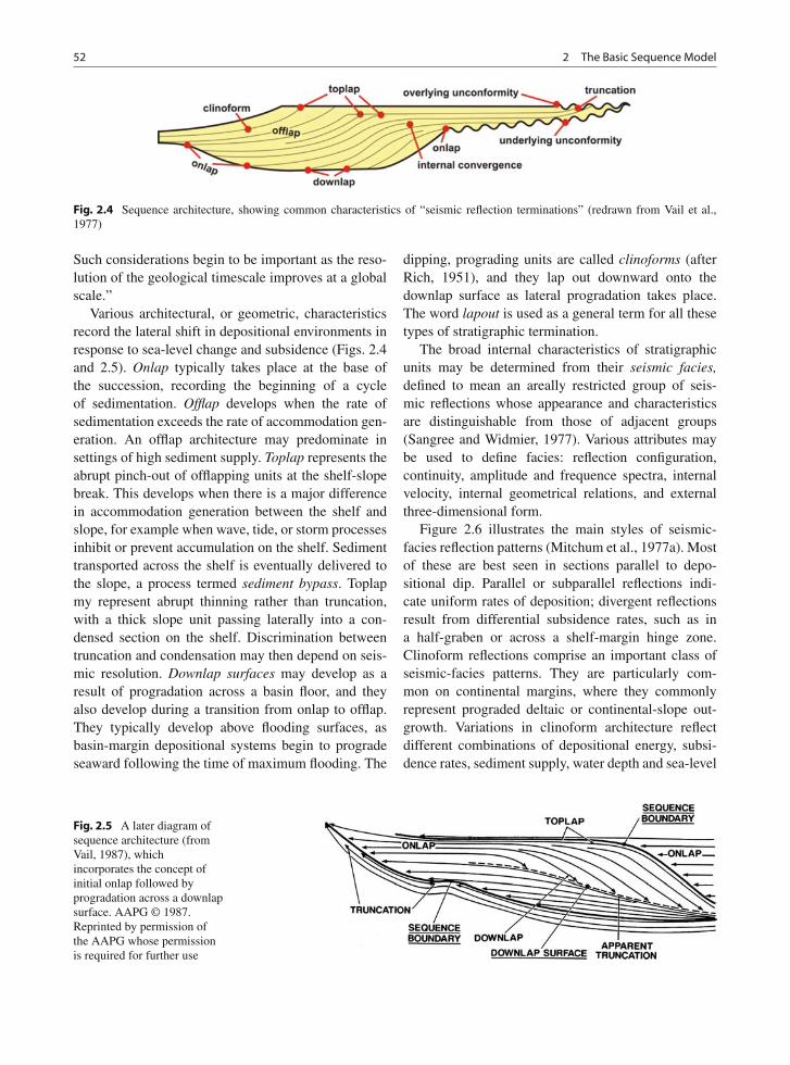
52 2 The Basic Sequence Model
Fig. 2.4 Sequence architecture, showing common characteristics of “seismic reflection terminations” (redrawn from Vail et al.,1977)
Such considerations begin to be important as the reso-lution of the geological timescale improves at a globalscale.”
Various architectural, or geometric, characteristicsrecord the lateral shift in depositional environments inresponse to sea-level change and subsidence (Figs. 2.4and 2.5). Onlap typically takes place at the base ofthe succession, recording the beginning of a cycleof sedimentation. Offlap develops when the rate ofsedimentation exceeds the rate of accommodation gen-eration. An offlap architecture may predominate insettings of high sediment supply. Toplap represents theabrupt pinch-out of offlapping units at the shelf-slopebreak. This develops when there is a major differencein accommodation generation between the shelf andslope, for example when wave, tide, or storm processesinhibit or prevent accumulation on the shelf. Sedimenttransported across the shelf is eventually delivered tothe slope, a process termed sediment bypass. Toplapmy represent abrupt thinning rather than truncation,with a thick slope unit passing laterally into a con-densed section on the shelf. Discrimination betweentruncation and condensation may then depend on seis-mic resolution. Downlap surfaces may develop as aresult of progradation across a basin floor, and theyalso develop during a transition from onlap to offlap.They typically develop above flooding surfaces, asbasin-margin depositional systems begin to progradeseaward following the time of maximum flooding. The
dipping, prograding units are called clinoforms (afterRich, 1951), and they lap out downward onto thedownlap surface as lateral progradation takes place.The word lapout is used as a general term for all thesetypes of stratigraphic termination.
The broad internal characteristics of stratigraphicunits may be determined from their seismic facies,defined to mean an areally restricted group of seis-mic reflections whose appearance and characteristicsare distinguishable from those of adjacent groups(Sangree and Widmier, 1977). Various attributes maybe used to define facies: reflection configuration,continuity, amplitude and frequence spectra, internalvelocity, internal geometrical relations, and externalthree-dimensional form.
Figure 2.6 illustrates the main styles of seismic-facies reflection patterns (Mitchum et al., 1977a). Mostof these are best seen in sections parallel to depo-sitional dip. Parallel or subparallel reflections indi-cate uniform rates of deposition; divergent reflectionsresult from differential subsidence rates, such as ina half-graben or across a shelf-margin hinge zone.Clinoform reflections comprise an important class ofseismic-facies patterns. They are particularly com-mon on continental margins, where they commonlyrepresent prograded deltaic or continental-slope out-growth. Variations in clinoform architecture reflectdifferent combinations of depositional energy, subsi-dence rates, sediment supply, water depth and sea-level
Fig. 2.5 A later diagram ofsequence architecture (fromVail, 1987), whichincorporates the concept ofinitial onlap followed byprogradation across a downlapsurface. AAPG © 1987.Reprinted by permission ofthe AAPG whose permissionis required for further use
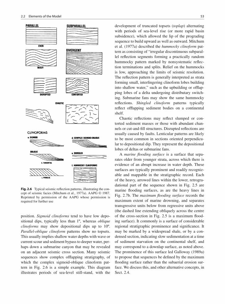
2.2 Elements of the Model 53
Fig. 2.6 Typical seismic reflection patterns, illustrating the con-cept of seismic facies (Mitchum et al., 1977a). AAPG © 1987.Reprinted by permission of the AAPG whose permission isrequired for further use
position. Sigmoid clinoforms tend to have low depo-sitional dips, typically less than 1º, whereas obliqueclinoforms may show depositional dips up to 10º.Parallel-oblique clinoform patterns show no topsets.This usually implies shallow water depths with wave orcurrent scour and sediment bypass to deeper water, per-haps down a submarine canyon that may be revealedon an adjacent seismic cross section. Many seismicsequences show complex offlapping stratigraphy, ofwhich the complex sigmoid-oblique clinoform pat-tern in Fig. 2.6 is a simple example. This diagramillustrates periods of sea-level still-stand, with the
development of truncated topsets (toplap) alternatingwith periods of sea-level rise (or more rapid basinsubsidence), which allowed the lip of the progradingsequence to build upward as well as outward. Mitchumet al. (1977a) described the hummocky clinoform pat-tern as consisting of “irregular discontinuous subparal-lel reflection segments forming a practically randomhummocky pattern marked by nonsystematic reflec-tion terminations and splits. Relief on the hummocksis low, approaching the limits of seismic resolution.The reflection pattern is generally interpreted as strataforming small, interfingering clinoform lobes buildinginto shallow water,” such as the upbuilding or offlap-ping lobes of a delta undergoing distributary switch-ing. Submarine fans may show the same hummockyreflections. Shingled clinoform patterns typicallyreflect offlapping sediment bodies on a continentalshelf.
Chaotic reflections may reflect slumped or con-torted sediment masses or those with abundant chan-nels or cut-and-fill structures. Disrupted reflections areusually caused by faults. Lenticular patterns are likelyto be most common in sections oriented perpendicu-lar to depositional dip. They represent the depositionallobes of deltas or submarine fans.
A marine flooding surface is a surface that sepa-rates older from younger strata, across which there isevidence of an abrupt increase in water depth. Thesesurfaces are typically prominent and readily recogniz-able and mappable in the stratigraphic record. Eachof the heavy, arrowed lines within the lower, retrogra-dational part of the sequence shown in Fig. 2.5 aremarine flooding surfaces, as are the heavy lines inFig. 2.7b. The maximum flooding surface records themaximum extent of marine drowning, and separatestransgressive units below from regressive units above(the dashed line extending obliquely across the centreof the cross-section in Fig. 2.5 is a maximum flood-ing surface). It commonly is a surface of considerableregional stratigraphic prominence and significance. Itmay be marked by a widespread shale, or by a con-densed section, indicating slow sedimentation at a timeof sediment starvation on the continental shelf, andmay correspond to a downlap surface, as noted above.The prominence of this surface led Galloway (1989a)to propose that sequences be defined by the maximumflooding surface rather than the subaerial erosion sur-face. We discuss this, and other alternative concepts, inSect. 2.4.
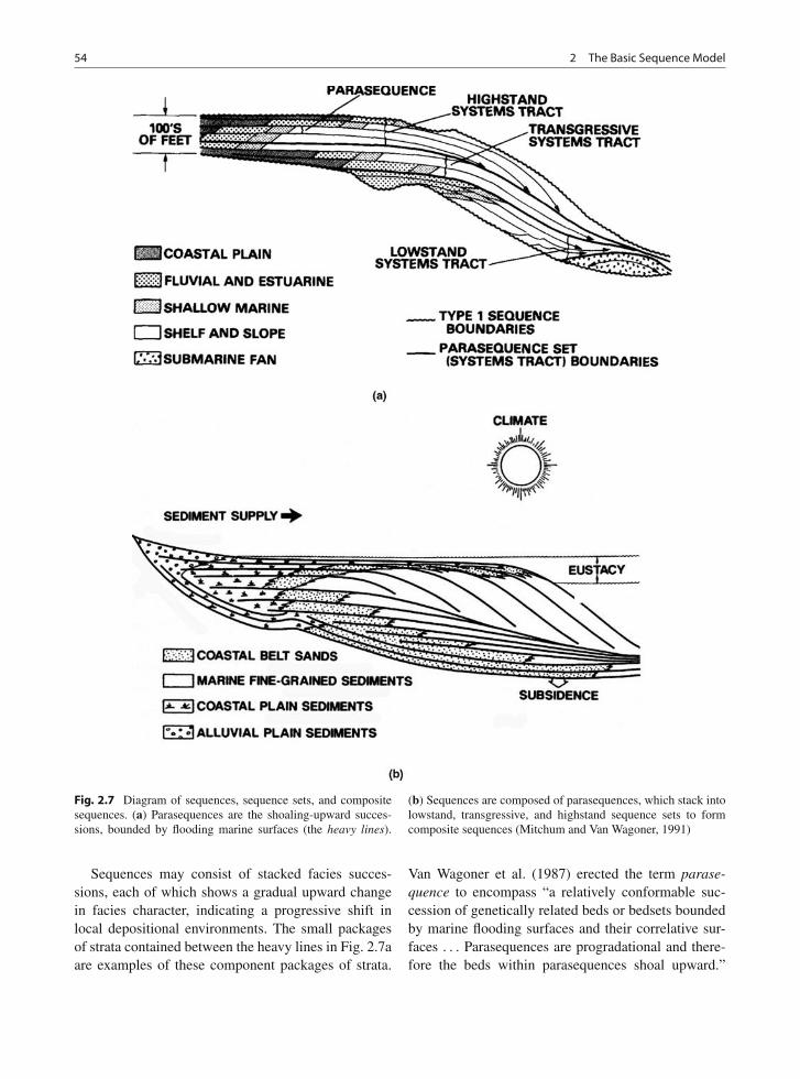
54 2 The Basic Sequence Model
Fig. 2.7 Diagram of sequences, sequence sets, and compositesequences. (a) Parasequences are the shoaling-upward succes-sions, bounded by flooding marine surfaces (the heavy lines).
(b) Sequences are composed of parasequences, which stack intolowstand, transgressive, and highstand sequence sets to formcomposite sequences (Mitchum and Van Wagoner, 1991)
Sequences may consist of stacked facies succes-sions, each of which shows a gradual upward changein facies character, indicating a progressive shift inlocal depositional environments. The small packagesof strata contained between the heavy lines in Fig. 2.7aare examples of these component packages of strata.
Van Wagoner et al. (1987) erected the term parase-quence to encompass “a relatively conformable suc-cession of genetically related beds or bedsets boundedby marine flooding surfaces and their correlative sur-faces . . . Parasequences are progradational and there-fore the beds within parasequences shoal upward.”
2.2 Elements of the Model 55
As Walker (1992) pointed out, “parasequences andfacies successions . . . are essentially the same thing,except that the concept of facies succession isbroader.” However, other types of facies succes-sion occur within sequences (e.g., channel-fill fining-upward successions), and the term parasequenceis therefore unnecessarily restrictive. Many suchsuccessions are generated by autogenic processes, suchas delta-lobe switching, and channel migration, thathave nothing to do with sequence controls, and toinclude them in a term that has the word “sequence”within it may be misleading. Walker (1992) rec-ommended that the term parasequence not be used.Catuneanu (2006, pp. 243–245) pointed out numer-ous problems with the concept of the parasequence,including the imprecise meaning of the term “flood-ing surface” (which it is now recognized, may haveseveral different meanings) and the potential confu-sion with surfaces generated by autogenic processes.He recommended using the term only in the context ofprogradational units in coastal settings. I suggest thatthe term be abandoned altogether. We return to thispoint at the end of the chapter.
2.2.3 Depositional Systemsand Systems Tracts
The concept of the depositional-system and basin-analysis methods based on it were developed largelyin the Gulf Coast region as a means of analyzingand interpreting the immense thicknesses of Mesozoic-Cenozoic sediment there that are so rich in oil and gas.A depositional system is defined in the Schlumbergeronline Oilfied Glossary as
The three-dimensional array of sediments or lithofaciesthat fills a basin. Depositional systems vary according tothe types of sediments available for deposition as wellas the depositional processes and environments in whichthey are deposited. The dominant depositional systemsare alluvial, fluvial, deltaic, marine, lacustrine and eoliansystems.
The principles of depositional-systems analysishave never been formally stated, but have been widelyused, particularly by geologists of the Bureau ofEconomic Geology at the University of Texas (notablyW. L. Fisher, L. F. Brown Jr., J. H. McGowen,W. E. Galloway and D. E. Frazier). Useful papers on
the topic are those by Fisher and McGowen (1967)and Brown and Fisher (1977). Textbook discussionsare given by Miall (1999, Chap. 6) and Walker(1992). The concept of depositional episode was devel-oped by Frazier (1974) to explain the construction ofMississippi delta by progradation of successive deltalobes (Fig. 1.14).
Posamentier et al. (1988, p. 110) defined a depo-sitional system as “a three-dimensional assemblageof lithofacies, genetically linked by active (modern)or inferred (ancient) processes and environments.” Asystems tract is defined as
A linkage of contemporaneous depositional systems . . .
Each is defined objectively by stratal geometries atbounding surfaces, position within the sequence, andinternal parasequence stacking patterns. Each is inter-preted to be associated with a specific segment of theeustatic curve (i.e., eustatic lowstand-lowstand wedge;eustatic rise-transgressive; rapid eustatic fall-lowstandfan, and so on), although not defined on the basis of thisassociation (Posamentier et al., 1988).
Elsewhere, Van Wagoner et al. (1987) stated that“when referring to systems tracts, the terms lowstandand highstand are not meant to imply a unique periodof time or position on a cycle of eustatic or rela-tive change of sea level. The actual time of initiationof a systems tract is interpreted to be a functionof the interaction between eustasy, sediment supply,and tectonics.” There is clearly an inherent, or built-in contradiction here, that results from the use in adescriptive sense of terminology that has a geneticconnotation (e.g., transgressive systems tract impliestransgression). We return to this problem below.
Systems tracts are named with reference to theirassumed position within the sea-level cycle, and thesenames incorporate ideas about the expected responseof a basin to the changing balance between the majorsedimentary controls (accommodation and sedimentsupply) during a base-level cycle. There are four stan-dard systems tracts. These are the highstand, falling-stage, lowstand, and transgressive systems tracts. Eachis illustrated here by a block diagram model with sum-mary remarks outlining the major sedimentary controlsand depositional patterns prevailing at that stage ofsequence development (Fig. 2.8). Other terms havebeen used by different workers, but these four sys-tems tracts and their bounding surfaces provide auseful, easy-to-understand model from which to buildinterpretive concepts.
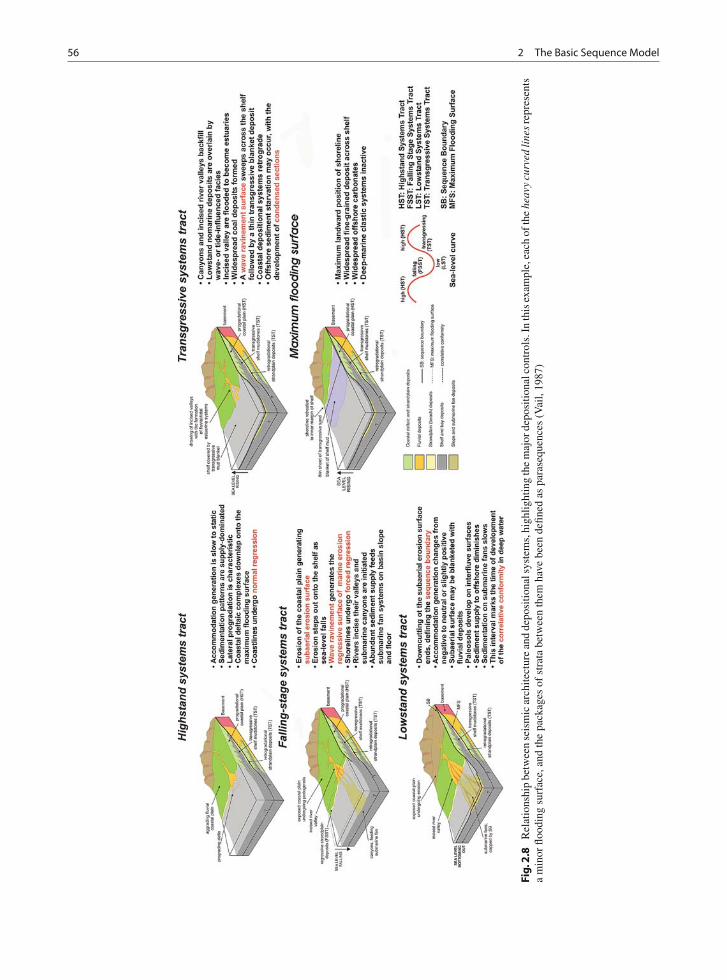
56 2 The Basic Sequence Model
Fig
.2.8
Rel
atio
nshi
pbe
twee
nse
ism
icar
chite
ctur
ean
dde
posi
tiona
lsys
tem
s,hi
ghlig
htin
gth
em
ajor
depo
sitio
nalc
ontr
ols.
Inth
isex
ampl
e,ea
chof
the
heav
ycu
rved
line
sre
pres
ents
am
inor
flood
ing
surf
ace,
and
the
pack
ages
ofst
rata
betw
een
them
have
been
defin
edas
para
sequ
ence
s(V
ail,
1987
)
2.3 Sequence Models in Clastic and Carbonate Settings 57
The linking of systems tracts to stages of thesea-level cycle is unfortunate, because it has nowbeen repeatedly demonstrated that the geometric andbehavioural features that supposedly characterize eachsystems tract and its link to the sea-level cycle arenot necessarily diagnostic of sea level, but may reflectcombinations of several factors. For example, onthe east coast of South Island, New Zealand, differ-ent stretches of coast are simultaneously undergoingcoastal progradation, reflecting a large sediment sup-ply, and coastal retreat and transgression, becauseof locally high wave energy (Leckie, 1994). AndrosIsland, in the Bahamas, currently exhibits three dif-ferent systems-tract conditions. Lowstand conditionscharacterize the eastern (windward) margin of theisland, facing the deep-water channel, the Tongueof the Ocean. Transgressive conditions occur alongthe northwest margin, where tidal flats are undergo-ing erosion, whereas on the more sheltered leewardmargin, along the southwest edge of the Andros coast-line, highstand conditions are suggested by tidal-flatprogradation (Schlager, 2005, Fig. 7.6).
2.3 Sequence Models in Clasticand Carbonate Settings
In this section, a brief overview of sequence modelsis provided for the main areas and styles of deposi-tion, marine and nonmarine clastics, and carbonates.A much more complete treatment of this topic formsthe core of the book by Catuneanu (2006). In addi-tion, many useful review articles and books provideadditional insights into particular areas or themes(e.g., Emery and Myers, 1996; Schlager, 1992,1993, 2005; Posamentier and Allen, 1999; Hunt andGawthorpe, 2000; Yoshida et al., 2007).
2.3.1 Marine Clastic Depositional Systemsand Systems Tracts
The highstand systems tract (HST) corresponds to aperiod when little new accommodation is being addedto the depositional environment. As shown in therelative sea-level curve at the lower right corner of
Fig. 2.8, base-level rise is in the process of slow-ing down as it reaches its highest point, immediatelyprior to commencement of a slow fall. If the sedimentsupply remains more or less constant, then Rd>Rs atthis point (the upper of the three conditions shown inFig. 1.13). The most characteristic feature of thissystems tract is the lateral progradation of coastal sed-imentary environments. Major coastal barrier-lagoonand deltaic complexes are the result. Normal regres-sion is the term used to describe the seaward advanceof the coastline as a result of the progressive addition ofsediment to the front of the beach or the delta systems,developing a broad topset environment (the undathemof Rich, 1951; see Fig. 1.10). This is in contrast tothe condition of forced regression, which is describedbelow.
Where the terrigenous sediment supply is high,delta systems may largely dominate the resulting sed-imentary succession, as shown in the accompanyingexample of the Dunvegan delta, Alberta (Fig. 2.9).The allomember boundaries in this diagram indicatetimes of relative low sea level, followed by flooding.Each allomember boundary is overlain by a mudstonerepresenting the maximum flooding surface, overwhich delta complexes prograded. Sedimentary envi-ronments characteristically include coastal mangroveswamps, and may include significant peat swamps, thesites of future coal development. The numbered subdi-visions of each allomember indicate individual deltaicshingles. Subsurface mapping may indicate that shin-gles of this type shifted laterally as a result of deltaswitching, in a manner similar to the Mississippi deltaand the Yellow River delta. This points to potentialconfusion in terminology, because upward-shoalingsuccessions, such as those illustrated in Fig. 2.9 cor-respond to the Van Wagoner et al. (1987) definition ofparasequence. We return to this point at the end of thechapter (Sect. 2.4).
The thickness of highstand shelf deposits dependson the accommodation generated by marine transgres-sion across the shelf, typically a few tens of metres,up to a maximum of about 200 m. Where the shelf isnarrow or the sediment supply is large, deltas may pro-grade to the shelf-slope break, at which point deltaicsedimentation may extend down slope into the deepbasin (Porebski and Steel, 2003). High-amplitude cli-noforms may result, including significant volumes ofsediment-gravity-flow deposits.
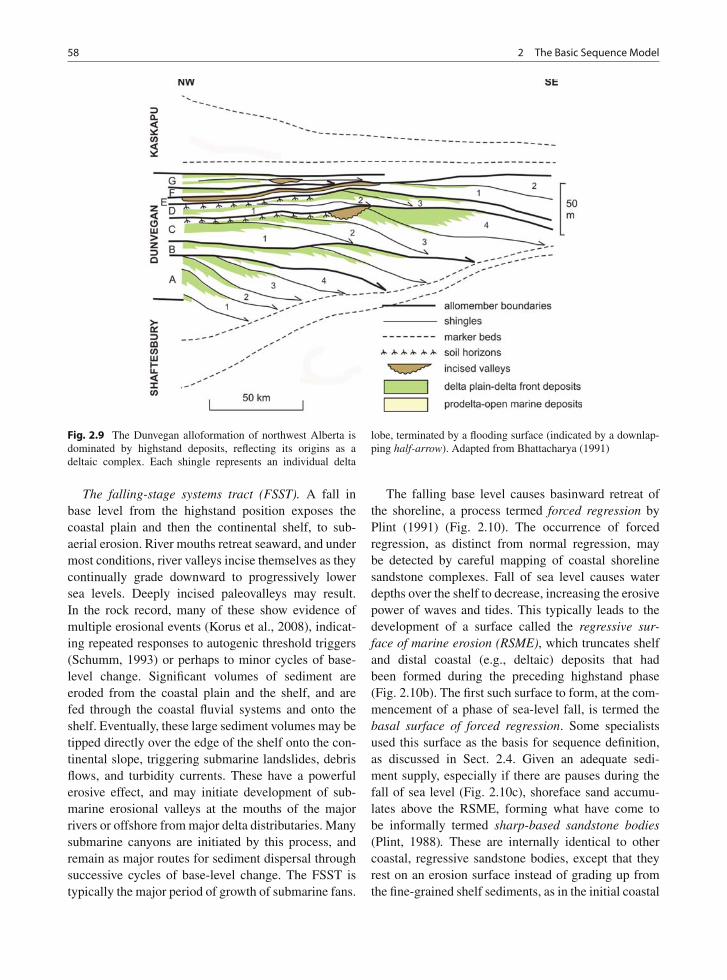
58 2 The Basic Sequence Model
Fig. 2.9 The Dunvegan alloformation of northwest Alberta isdominated by highstand deposits, reflecting its origins as adeltaic complex. Each shingle represents an individual delta
lobe, terminated by a flooding surface (indicated by a downlap-ping half-arrow). Adapted from Bhattacharya (1991)
The falling-stage systems tract (FSST). A fall inbase level from the highstand position exposes thecoastal plain and then the continental shelf, to sub-aerial erosion. River mouths retreat seaward, and undermost conditions, river valleys incise themselves as theycontinually grade downward to progressively lowersea levels. Deeply incised paleovalleys may result.In the rock record, many of these show evidence ofmultiple erosional events (Korus et al., 2008), indicat-ing repeated responses to autogenic threshold triggers(Schumm, 1993) or perhaps to minor cycles of base-level change. Significant volumes of sediment areeroded from the coastal plain and the shelf, and arefed through the coastal fluvial systems and onto theshelf. Eventually, these large sediment volumes may betipped directly over the edge of the shelf onto the con-tinental slope, triggering submarine landslides, debrisflows, and turbidity currents. These have a powerfulerosive effect, and may initiate development of sub-marine erosional valleys at the mouths of the majorrivers or offshore from major delta distributaries. Manysubmarine canyons are initiated by this process, andremain as major routes for sediment dispersal throughsuccessive cycles of base-level change. The FSST istypically the major period of growth of submarine fans.
The falling base level causes basinward retreat ofthe shoreline, a process termed forced regression byPlint (1991) (Fig. 2.10). The occurrence of forcedregression, as distinct from normal regression, maybe detected by careful mapping of coastal shorelinesandstone complexes. Fall of sea level causes waterdepths over the shelf to decrease, increasing the erosivepower of waves and tides. This typically leads to thedevelopment of a surface called the regressive sur-face of marine erosion (RSME), which truncates shelfand distal coastal (e.g., deltaic) deposits that hadbeen formed during the preceding highstand phase(Fig. 2.10b). The first such surface to form, at the com-mencement of a phase of sea-level fall, is termed thebasal surface of forced regression. Some specialistsused this surface as the basis for sequence definition,as discussed in Sect. 2.4. Given an adequate sedi-ment supply, especially if there are pauses during thefall of sea level (Fig. 2.10c), shoreface sand accumu-lates above the RSME, forming what have come tobe informally termed sharp-based sandstone bodies(Plint, 1988). These are internally identical to othercoastal, regressive sandstone bodies, except that theyrest on an erosion surface instead of grading up fromthe fine-grained shelf sediments, as in the initial coastal
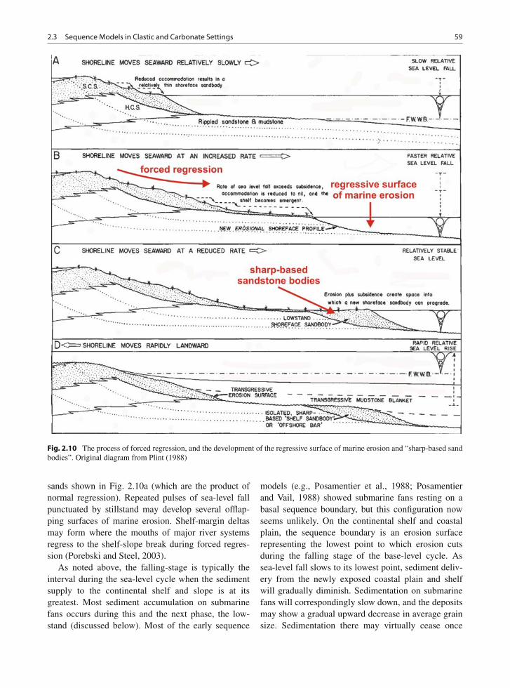
2.3 Sequence Models in Clastic and Carbonate Settings 59
Fig. 2.10 The process of forced regression, and the development of the regressive surface of marine erosion and “sharp-based sandbodies”. Original diagram from Plint (1988)
sands shown in Fig. 2.10a (which are the product ofnormal regression). Repeated pulses of sea-level fallpunctuated by stillstand may develop several offlap-ping surfaces of marine erosion. Shelf-margin deltasmay form where the mouths of major river systemsregress to the shelf-slope break during forced regres-sion (Porebski and Steel, 2003).
As noted above, the falling-stage is typically theinterval during the sea-level cycle when the sedimentsupply to the continental shelf and slope is at itsgreatest. Most sediment accumulation on submarinefans occurs during this and the next phase, the low-stand (discussed below). Most of the early sequence
models (e.g., Posamentier et al., 1988; Posamentierand Vail, 1988) showed submarine fans resting on abasal sequence boundary, but this configuration nowseems unlikely. On the continental shelf and coastalplain, the sequence boundary is an erosion surfacerepresenting the lowest point to which erosion cutsduring the falling stage of the base-level cycle. Assea-level fall slows to its lowest point, sediment deliv-ery from the newly exposed coastal plain and shelfwill gradually diminish. Sedimentation on submarinefans will correspondingly slow down, and the depositsmay show a gradual upward decrease in average grainsize. Sedimentation there may virtually cease once
60 2 The Basic Sequence Model
the next phase of sea-level rise commences, and therivers feeding sediment to the slope become flooded(transgressive systems tract). The sequence boundary,therefore, is likely to be contemporaneous with themiddle to upper part of the submarine-fan succession,possibly with the top of it. However, there is unlikelyto be an actual mappable break in sedimentation at thislevel, and it may be difficult to impossible to locatethe position in the section corresponding to the turn-around from falling to rising sea level. This horizonis, therefore, what Vail et al. (1977) called a correl-ative conformity, although his original application ofthe term was to the fine-grained sediments formed indeep water beyond the submarine-fan wedge, out in thedeep basin where it was assumed sedimentation wouldbe continuous throughout a sea-level cycle.
The sequence boundary (SB) marks the lowest pointreached by erosion during the falling stage of the sea-level cycle. On land this is represented by a subaerialerosion surface, which may extend far onto the con-tinental shelf, depending on how far sea level falls.The sequence boundary cuts into the deposits of thehighstand systems tract and is overlain by the depositsof the lowstand or transgressive systems tracts. It istherefore typically a surface where a marked facieschange takes place, usually from a relatively lower-energy deposit below to a high-energy deposit above.Mapping of such a surface in outcrop or in the sub-surface, using well logs, is facilitated by this facieschange, except where the boundary juxtaposes flu-vial on fluvial facies. In such cases, distinguishingthe sequence boundary from other large-scale channelscours may be a difficult undertaking.
The lowstand systems tract (LST): This systemstract represents the interval of time when sea-levelhas bottomed out, and depositional trends undergo ashift from seaward-directed (e.g., progradational) tolandward-directed (e.g., retrogradational). Within mostdepositional systems there is little that may be con-fidently assigned to the lowstand systems tract. Theinitial basal fill of incised river valleys, and some ofthe fill of submarine canyons are deposited duringthis phase. Volumetrically they are usually of minorimportance, but they may be of a coarser grain sizethan succeeding transgressive deposits. In parts of theincised valley of the Mississippi River, for example(the valley formed during Pleistocene glacioeustaticsea-level lowstands), the basal fill formed during theinitial post-glacial transgression is a coarse braided
stream deposit, in contrast to the sandy meanderingriver deposits that form the bulk of the Mississippi riversediments. The episode of active submarine-fan sedi-mentation on the continental slope and deep basin maypersist through the lowstand phase.
There may be a phase of normal regressive sedi-mentation at the lowstand coastline. On coastal plains,the lowstand is a time of stillstand, when little ero-sion or sedimentation takes place. Between the majorrivers, on the interfluve uplands, this may therefore bea place where long-established plant growth and soildevelopment takes place. Peat is unlikely to accumu-late because of the lack of accommodation, but soils,corresponding in time to the sequence boundary, maybe extensive, and the resulting paleosols may thereforebe employed for mapping purposes (e.g., McCarthyet al., 1999; Plint et al., 2001).
Transgressive systems tract (TST): A rise in baselevel is typically accompanied by flooding of incisedvalleys and transgression across the continental shelf(Fig. 2.8). Base-level rise exceeds sediment sup-ply, leading to retrogradation of depositional systems(Rd<Rs in Fig. 1.13c), except that at the mouths of thelargest rivers sediment supply may be sufficiently largethat deltas may continue to aggrade or prograde.
Flooded river valleys are estuaries; they typicallyprovide ample accommodation for sedimentary accu-mulation. In estuarine successions, the upward tran-sition from lowstand to transgressive systems tractin estuaries and other coastal river systems is com-monly marked by the development of wave- or tide-influenced fluvial facies, such as tidal sand barscontaining sigmoidal crossbedding or flaser bedding.The sedimentology of this environment has receivedmuch attention (Fig. 2.11), because of the poten-tial for the development of stratigraphic sandstonetraps, in the form of valley-fill ribbon sands. Studiesof ancient paleovalley fills have shown that manyare complex, indicating repeated cycles of base levelchange and/or autogenic changes in sediment dispersal(Korus et al., 2008).
On the continental shelf the most distinctive featureof most transgressive systems tracts is the develop-ment of a widespread transgressive surface (TS), aflooding surface covered with an equally widespreadmarine mudstone. A transgressive conglomeratic orsandy lag may blanket the flooding surface. Offshore,rapid transgression may cut the deep-water environ-ment off from its sediment source, leading to slow
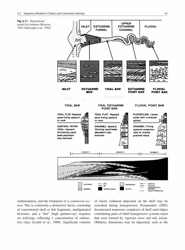
2.3 Sequence Models in Clastic and Carbonate Settings 61
Fig. 2.11 Depositionalmodel for estuaries (Reinson,1992; Dalrymple et al., 1994)
sedimentation, and the formation of a condensed sec-tion. This is commonly a distinctive facies, consistingof concentrated shell or fish fragments, amalgamatedbiozones, and a “hot” (high gamma-ray) responseon well-logs, reflecting a concentration of radioac-tive clays (Loutit et al., 1988). Significant volumes
of clastic sediment deposited on the shelf may bereworked during transgression. Posamentier (2002)documented numerous complexes of shelf sand ridgesconstituting parts of shelf transgressive systems tractsthat were formed by vigorous wave and tide action.Offshore, limestones may be deposited, such as the
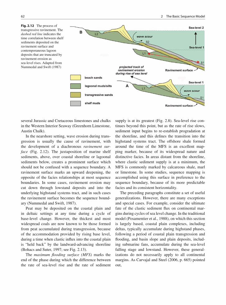
62 2 The Basic Sequence Model
Fig. 2.12 The process oftransgressive ravinement. Thedashed red line indicates thetime correlation between shelfsediments deposited on theravinement surface andcontemporaneous lagoondeposits that are truncated byravinement erosion assea-level rises. Adapted fromNummedal and Swift (1987)
several Jurassic and Cretaceous limestones and chalksin the Western Interior Seaway (Greenhorn Limestone,Austin Chalk).
In the nearshore setting, wave erosion during trans-gression is usually the cause of ravinement, withthe development of a diachronous ravinement sur-face (Fig. 2.12). The juxtaposition of marine shelfsediments, above, over coastal shoreline or lagoonalsediments below, creates a prominent surface whichshould not be confused with a sequence boundary. Aravinement surface marks an upward deepening, theopposite of the facies relationships at most sequenceboundaries. In some cases, ravinement erosion maycut down through lowstand deposits and into theunderlying highstand systems tract, and in such casesthe ravinement surface becomes the sequence bound-ary (Nummedal and Swift, 1987).
Peat may be deposited on the coastal plain andin deltaic settings at any time during a cycle ofbase-level change. However, the thickest and mostwidespread coals are now known to be those formedfrom peat accumulated during transgression, becauseof the accommodation provided by rising base level,during a time when clastic influx into the coastal plainis “held back” by the landward-advancing shoreline(Bohacs and Suter, 1997; see Fig. 2.13).
The maximum flooding surface (MFS) marks theend of the phase during which the difference betweenthe rate of sea-level rise and the rate of sediment
supply is at its greatest (Fig. 2.8). Sea-level rise con-tinues beyond this point, but as the rate of rise slows,sediment input begins to re-establish progradation atthe shoreline, and this defines the transition into thehighstand systems tract. The offshore shale formedaround the time of the MFS is an excellent map-ping marker, because of its widespread nature anddistinctive facies. In areas distant from the shoreline,where clastic sediment supply is at a minimum, theMFS is commonly marked by calcareous shale, marlor limestone. In some studies, sequence mapping isaccomplished using this surface in preference to thesequence boundary, because of its more predictablefacies and its consistent horizontality.
The preceding paragraphs constitute a set of usefulgeneralizations. However, there are many exceptionsand special cases. For example, consider the ultimatefate of the clastic sediment flux on continental mar-gins during cycles of sea level change. In the traditionalmodel (Posamentier et al., 1988), on which this sectionis largely based, coastal plain complexes, includingdeltas, typically accumulate during highstand phases,following a period of coastal plain transgression andflooding, and basin slope and plain deposits, includ-ing submarine fans, accumulate during the sea-levelfalling stage and lowstand. However, these general-izations do not necessarily apply to all continentalmargins. As Carvajal and Steel (2006, p. 665) pointedout,
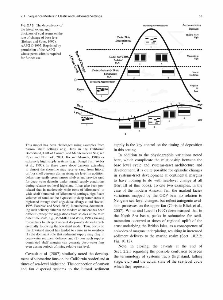
2.3 Sequence Models in Clastic and Carbonate Settings 63
Fig. 2.13 The dependency ofthe lateral extent andthickness of coal seams on therate of change of base level(Bohacs and Suter, 1997).AAPG © 1997. Reprinted bypermission of the AAPGwhose permission is requiredfor further use
This model has been challenged using examples fromnarrow shelf settings (e.g., fans in the CaliforniaBorderland, Gulf of Corinth, and Mediterranean Sea; seePiper and Normark, 2001; Ito and Masuda, 1988) orextremely high supply systems (e.g., Bengal Fan; Weberet al., 1997). In these cases slope canyons extendingto almost the shoreline may receive sand from littoraldrift or shelf currents during rising sea level. In addition,deltas may easily cross narrow shelves and provide sandfor deep-water deposits under normal supply conditionsduring relative sea-level highstand. It has also been pos-tulated that in moderately wide (tens of kilometers) towide shelf (hundreds of kilometers) settings, significantvolumes of sand can be bypassed to deep-water areas athighstand through shelf-edge deltas (Burgess and Hovius,1998; Porebski and Steel, 2006). Nonetheless, document-ing such delivery either in the modern or ancient has beendifficult (except for suggestions from studies at the thirdorder time scale, e.g., McMillen and Winn, 1991), biasingresearchers to interpret ancient deep-water deposits pref-erentially following the lowstand model. Thus, focus onthis lowstand model has tended to cause us to overlook(1) the dominant role that sediment supply may play indeep-water sediment delivery, and (2) how such supply-dominated shelf margins can generate deep-water fanseven during periods of rising relative sea level.
Covault et al. (2007) similarly noted the develop-ment of submarine fans on the California borderland attimes of sea-level highstand. The connection of canyonand fan dispersal systems to the littoral sediment
supply is the key control on the timing of depositionin this setting.
In addition to the physiographic variations notedhere, which complicate the relationship between thebase level cycle and systems-tract architecture anddevelopment, it is quite possible for episodic changesin systems-tract development at continental marginsto have nothing to do with sea-level change at all(Part III of this book). To cite two examples, in thecase of the modern Amazon fan, the marked faciesvariations mapped by the ODP bear no relation toNeogene sea-level changes, but reflect autogenic avul-sion processes on the upper fan (Christie-Blick et al.,2007). White and Lovell (1997) demonstrated that inthe North Sea basin, peaks in submarine fan sedi-mentation occurred at times of regional uplift of thecrust underlying the British Isles, as a consequence ofepisodes of magma underplating, resulting in increasedsediment delivery to the marine realm (Sect. 10.2.2;Fig. 10.12).
Note, in closing, the caveats at the end ofSect. 2.2.3 regarding the possible confusion betweenthe terminology of systems tracts (highstand, fallingstage, etc.) and the actual state of the sea-level cyclewhich they represent.
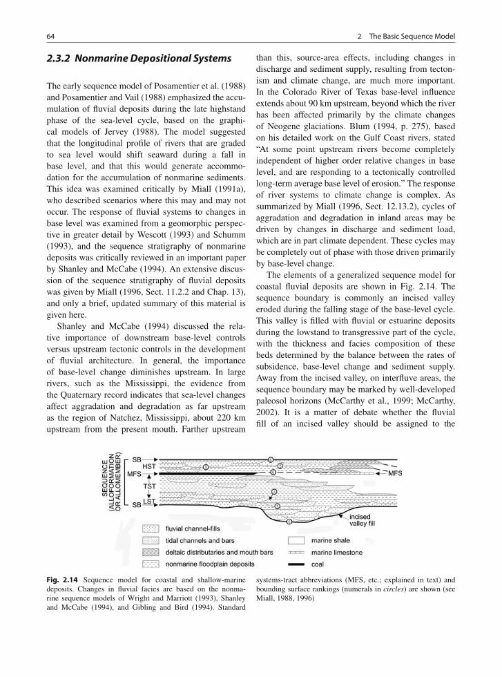
64 2 The Basic Sequence Model
2.3.2 Nonmarine Depositional Systems
The early sequence model of Posamentier et al. (1988)and Posamentier and Vail (1988) emphasized the accu-mulation of fluvial deposits during the late highstandphase of the sea-level cycle, based on the graphi-cal models of Jervey (1988). The model suggestedthat the longitudinal profile of rivers that are gradedto sea level would shift seaward during a fall inbase level, and that this would generate accommo-dation for the accumulation of nonmarine sediments.This idea was examined critically by Miall (1991a),who described scenarios where this may and may notoccur. The response of fluvial systems to changes inbase level was examined from a geomorphic perspec-tive in greater detail by Wescott (1993) and Schumm(1993), and the sequence stratigraphy of nonmarinedeposits was critically reviewed in an important paperby Shanley and McCabe (1994). An extensive discus-sion of the sequence stratigraphy of fluvial depositswas given by Miall (1996, Sect. 11.2.2 and Chap. 13),and only a brief, updated summary of this material isgiven here.
Shanley and McCabe (1994) discussed the rela-tive importance of downstream base-level controlsversus upstream tectonic controls in the developmentof fluvial architecture. In general, the importanceof base-level change diminishes upstream. In largerivers, such as the Mississippi, the evidence fromthe Quaternary record indicates that sea-level changesaffect aggradation and degradation as far upstreamas the region of Natchez, Mississippi, about 220 kmupstream from the present mouth. Farther upstream
than this, source-area effects, including changes indischarge and sediment supply, resulting from tecton-ism and climate change, are much more important.In the Colorado River of Texas base-level influenceextends about 90 km upstream, beyond which the riverhas been affected primarily by the climate changesof Neogene glaciations. Blum (1994, p. 275), basedon his detailed work on the Gulf Coast rivers, stated“At some point upstream rivers become completelyindependent of higher order relative changes in baselevel, and are responding to a tectonically controlledlong-term average base level of erosion.” The responseof river systems to climate change is complex. Assummarized by Miall (1996, Sect. 12.13.2), cycles ofaggradation and degradation in inland areas may bedriven by changes in discharge and sediment load,which are in part climate dependent. These cycles maybe completely out of phase with those driven primarilyby base-level change.
The elements of a generalized sequence model forcoastal fluvial deposits are shown in Fig. 2.14. Thesequence boundary is commonly an incised valleyeroded during the falling stage of the base-level cycle.This valley is filled with fluvial or estuarine depositsduring the lowstand to transgressive part of the cycle,with the thickness and facies composition of thesebeds determined by the balance between the rates ofsubsidence, base-level change and sediment supply.Away from the incised valley, on interfluve areas, thesequence boundary may be marked by well-developedpaleosol horizons (McCarthy et al., 1999; McCarthy,2002). It is a matter of debate whether the fluvialfill of an incised valley should be assigned to the
Fig. 2.14 Sequence model for coastal and shallow-marinedeposits. Changes in fluvial facies are based on the nonma-rine sequence models of Wright and Marriott (1993), Shanleyand McCabe (1994), and Gibling and Bird (1994). Standard
systems-tract abbreviations (MFS, etc.; explained in text) andbounding surface rankings (numerals in circles) are shown (seeMiall, 1988, 1996)
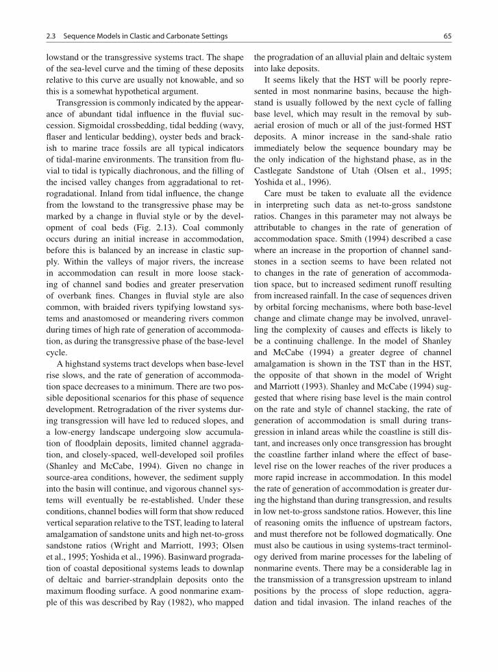
2.3 Sequence Models in Clastic and Carbonate Settings 65
lowstand or the transgressive systems tract. The shapeof the sea-level curve and the timing of these depositsrelative to this curve are usually not knowable, and sothis is a somewhat hypothetical argument.
Transgression is commonly indicated by the appear-ance of abundant tidal influence in the fluvial suc-cession. Sigmoidal crossbedding, tidal bedding (wavy,flaser and lenticular bedding), oyster beds and brack-ish to marine trace fossils are all typical indicatorsof tidal-marine environments. The transition from flu-vial to tidal is typically diachronous, and the filling ofthe incised valley changes from aggradational to ret-rogradational. Inland from tidal influence, the changefrom the lowstand to the transgressive phase may bemarked by a change in fluvial style or by the devel-opment of coal beds (Fig. 2.13). Coal commonlyoccurs during an initial increase in accommodation,before this is balanced by an increase in clastic sup-ply. Within the valleys of major rivers, the increasein accommodation can result in more loose stack-ing of channel sand bodies and greater preservationof overbank fines. Changes in fluvial style are alsocommon, with braided rivers typifying lowstand sys-tems and anastomosed or meandering rivers commonduring times of high rate of generation of accommoda-tion, as during the transgressive phase of the base-levelcycle.
A highstand systems tract develops when base-levelrise slows, and the rate of generation of accommoda-tion space decreases to a minimum. There are two pos-sible depositional scenarios for this phase of sequencedevelopment. Retrogradation of the river systems dur-ing transgression will have led to reduced slopes, anda low-energy landscape undergoing slow accumula-tion of floodplain deposits, limited channel aggrada-tion, and closely-spaced, well-developed soil profiles(Shanley and McCabe, 1994). Given no change insource-area conditions, however, the sediment supplyinto the basin will continue, and vigorous channel sys-tems will eventually be re-established. Under theseconditions, channel bodies will form that show reducedvertical separation relative to the TST, leading to lateralamalgamation of sandstone units and high net-to-grosssandstone ratios (Wright and Marriott, 1993; Olsenet al., 1995; Yoshida et al., 1996). Basinward prograda-tion of coastal depositional systems leads to downlapof deltaic and barrier-strandplain deposits onto themaximum flooding surface. A good nonmarine exam-ple of this was described by Ray (1982), who mapped
the progradation of an alluvial plain and deltaic systeminto lake deposits.
It seems likely that the HST will be poorly repre-sented in most nonmarine basins, because the high-stand is usually followed by the next cycle of fallingbase level, which may result in the removal by sub-aerial erosion of much or all of the just-formed HSTdeposits. A minor increase in the sand-shale ratioimmediately below the sequence boundary may bethe only indication of the highstand phase, as in theCastlegate Sandstone of Utah (Olsen et al., 1995;Yoshida et al., 1996).
Care must be taken to evaluate all the evidencein interpreting such data as net-to-gross sandstoneratios. Changes in this parameter may not always beattributable to changes in the rate of generation ofaccommodation space. Smith (1994) described a casewhere an increase in the proportion of channel sand-stones in a section seems to have been related notto changes in the rate of generation of accommoda-tion space, but to increased sediment runoff resultingfrom increased rainfall. In the case of sequences drivenby orbital forcing mechanisms, where both base-levelchange and climate change may be involved, unravel-ling the complexity of causes and effects is likely tobe a continuing challenge. In the model of Shanleyand McCabe (1994) a greater degree of channelamalgamation is shown in the TST than in the HST,the opposite of that shown in the model of Wrightand Marriott (1993). Shanley and McCabe (1994) sug-gested that where rising base level is the main controlon the rate and style of channel stacking, the rate ofgeneration of accommodation is small during trans-gression in inland areas while the coastline is still dis-tant, and increases only once transgression has broughtthe coastline farther inland where the effect of base-level rise on the lower reaches of the river produces amore rapid increase in accommodation. In this modelthe rate of generation of accommodation is greater dur-ing the highstand than during transgression, and resultsin low net-to-gross sandstone ratios. However, this lineof reasoning omits the influence of upstream factors,and must therefore not be followed dogmatically. Onemust also be cautious in using systems-tract terminol-ogy derived from marine processes for the labeling ofnonmarine events. There may be a considerable lag inthe transmission of a transgression upstream to inlandpositions by the process of slope reduction, aggra-dation and tidal invasion. The inland reaches of the
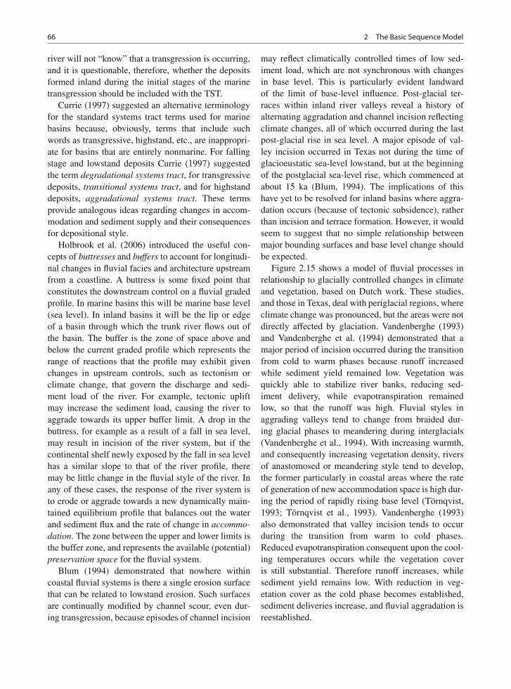
66 2 The Basic Sequence Model
river will not “know” that a transgression is occurring,and it is questionable, therefore, whether the depositsformed inland during the initial stages of the marinetransgression should be included with the TST.
Currie (1997) suggested an alternative terminologyfor the standard systems tract terms used for marinebasins because, obviously, terms that include suchwords as transgressive, highstand, etc., are inappropri-ate for basins that are entirely nonmarine. For fallingstage and lowstand deposits Currie (1997) suggestedthe term degradational systems tract, for transgressivedeposits, transitional systems tract, and for highstanddeposits, aggradational systems tract. These termsprovide analogous ideas regarding changes in accom-modation and sediment supply and their consequencesfor depositional style.
Holbrook et al. (2006) introduced the useful con-cepts of buttresses and buffers to account for longitudi-nal changes in fluvial facies and architecture upstreamfrom a coastline. A buttress is some fixed point thatconstitutes the downstream control on a fluvial gradedprofile. In marine basins this will be marine base level(sea level). In inland basins it will be the lip or edgeof a basin through which the trunk river flows out ofthe basin. The buffer is the zone of space above andbelow the current graded profile which represents therange of reactions that the profile may exhibit givenchanges in upstream controls, such as tectonism orclimate change, that govern the discharge and sedi-ment load of the river. For example, tectonic upliftmay increase the sediment load, causing the river toaggrade towards its upper buffer limit. A drop in thebuttress, for example as a result of a fall in sea level,may result in incision of the river system, but if thecontinental shelf newly exposed by the fall in sea levelhas a similar slope to that of the river profile, theremay be little change in the fluvial style of the river. Inany of these cases, the response of the river system isto erode or aggrade towards a new dynamically main-tained equilibrium profile that balances out the waterand sediment flux and the rate of change in accommo-dation. The zone between the upper and lower limits isthe buffer zone, and represents the available (potential)preservation space for the fluvial system.
Blum (1994) demonstrated that nowhere withincoastal fluvial systems is there a single erosion surfacethat can be related to lowstand erosion. Such surfacesare continually modified by channel scour, even dur-ing transgression, because episodes of channel incision
may reflect climatically controlled times of low sed-iment load, which are not synchronous with changesin base level. This is particularly evident landwardof the limit of base-level influence. Post-glacial ter-races within inland river valleys reveal a history ofalternating aggradation and channel incision reflectingclimate changes, all of which occurred during the lastpost-glacial rise in sea level. A major episode of val-ley incision occurred in Texas not during the time ofglacioeustatic sea-level lowstand, but at the beginningof the postglacial sea-level rise, which commenced atabout 15 ka (Blum, 1994). The implications of thishave yet to be resolved for inland basins where aggra-dation occurs (because of tectonic subsidence), ratherthan incision and terrace formation. However, it wouldseem to suggest that no simple relationship betweenmajor bounding surfaces and base level change shouldbe expected.
Figure 2.15 shows a model of fluvial processes inrelationship to glacially controlled changes in climateand vegetation, based on Dutch work. These studies,and those in Texas, deal with periglacial regions, whereclimate change was pronounced, but the areas were notdirectly affected by glaciation. Vandenberghe (1993)and Vandenberghe et al. (1994) demonstrated that amajor period of incision occurred during the transitionfrom cold to warm phases because runoff increasedwhile sediment yield remained low. Vegetation wasquickly able to stabilize river banks, reducing sed-iment delivery, while evapotranspiration remainedlow, so that the runoff was high. Fluvial styles inaggrading valleys tend to change from braided dur-ing glacial phases to meandering during interglacials(Vandenberghe et al., 1994). With increasing warmth,and consequently increasing vegetation density, riversof anastomosed or meandering style tend to develop,the former particularly in coastal areas where the rateof generation of new accommodation space is high dur-ing the period of rapidly rising base level (Törnqvist,1993; Törnqvist et al., 1993). Vandenberghe (1993)also demonstrated that valley incision tends to occurduring the transition from warm to cold phases.Reduced evapotranspiration consequent upon the cool-ing temperatures occurs while the vegetation coveris still substantial. Therefore runoff increases, whilesediment yield remains low. With reduction in veg-etation cover as the cold phase becomes established,sediment deliveries increase, and fluvial aggradation isreestablished.
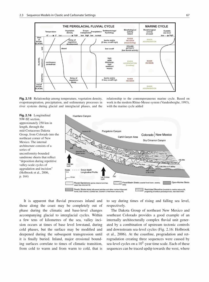
2.3 Sequence Models in Clastic and Carbonate Settings 67
Fig. 2.15 Relationship among temperature, vegetation density,evapotranspiration, precipitation, and sedimentary processes inriver systems during glacial and interglacial phases, and the
relationship to the contemporaneous marine cycle. Based onwork in the modern Rhine-Meuse system (Vandenberghe, 1993),with the marine cycle added
Fig. 2.16 LongitudinalNW-SE section,approximately 250 km inlength, through themid-Cretaceous DakotaGroup, from Colorado into thenortheast corner of NewMexico. The internalarchitecture consists of aseries ofunconformity-boundedsandstone sheets that reflect“deposition during repetitivevalley-scale cycles ofaggradation and incision”(Holbrook et al., 2006,p. 164)
It is apparent that fluvial processes inland andthose along the coast may be completely out ofphase during the climatic and base-level changesaccompanying glacial to interglacial cycles. Withina few tens of kilometres of the sea, valley inci-sion occurs at times of base level lowstand, duringcold phases, but the surface may be modified anddeepened during the subsequent transgression untilit is finally buried. Inland, major erosional bound-ing surfaces correlate to times of climatic transition,from cold to warm and from warm to cold, that is
to say during times of rising and falling sea level,respectively.
The Dakota Group of northeast New Mexico andsoutheast Colorado provides a good example of aninternally architecturally complex fluvial unit gener-ated by a combination of upstream tectonic controlsand downstream sea-level cycles (Fig. 2.16: Holbrooket al., 2006). At the coastline, progradation and ret-rogradation creating three sequences were caused bysea-level cycles on a 105-year time scale. Each of thesesequences can be traced updip towards the west, where
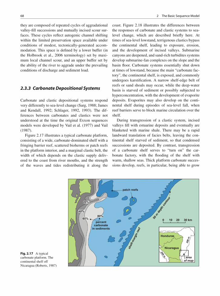
68 2 The Basic Sequence Model
they are composed of repeated cycles of aggradationalvalley-fill successions and mutually incised scour sur-faces. These cycles reflect autogenic channel shiftingwithin the limited preservation space available underconditions of modest, tectonically-generated accom-modation. This space is defined by a lower buffer (inthe Holbrook et al., 2006 terminology) set by maxi-mum local channel scour, and an upper buffer set bythe ability of the river to aggrade under the prevailingconditions of discharge and sediment load.
2.3.3 Carbonate Depositional Systems
Carbonate and clastic depositional systems respondvery differently to sea-level change (Sarg, 1988; Jamesand Kendall, 1992; Schlager, 1992, 1993). The dif-ferences between carbonates and clastics were notunderstood at the time the original Exxon sequencesmodels were developed by Vail et al. (1977) and Vail(1987).
Figure 2.17 illustrates a typical carbonate platform,consisting of a wide, carbonate-dominated shelf with afringing barrier reef, scattered bioherms or patch reefsin the platform interior, and a marginal clastic belt, thewidth of which depends on the clastic supply deliv-ered to the coast from river mouths, and the strengthof the waves and tides redistributing it along the
coast. Figure 2.18 illustrates the differences betweenthe responses of carbonate and clastic systems to sea-level change, which are described briefly here. Attimes of sea-level lowstand, terrigenous clastics bypassthe continental shelf, leading to exposure, erosion,and the development of incised valleys. Submarinecanyons are deepened, and sand-rich turbidites systemsdevelop submarine-fan complexes on the slope and thebasin floor. Carbonate systems essentially shut downat times of lowstand, because the main “carbonate fac-tory”, the continental shelf, is exposed, and commonlyundergoes karstification. A narrow shelf-edge belt ofreefs or sand shoals may occur, while the deep-waterbasin is starved of sediment or possibly subjected tohyperconcentration, with the development of evaporitedeposits. Evaporites may also develop on the conti-nental shelf during episodes of sea-level fall, whenreef barriers serve to block marine circulation over theshelf.
During transgression of a clastic system, incisedvalleys fill with estuarine deposits and eventually areblanketed with marine shale. There may be a rapidlandward translation of facies belts, leaving the con-tinental shelf starved of sediment, so that condensedsuccessions are deposited. By contrast, transgressionof a carbonate shelf serves to “turn on” the car-bonate factory, with the flooding of the shelf withwarm, shallow seas. Thick platform carbonate succes-sions develop, reefs, in particular, being able to grow
Fig. 2.17 A typicalcarbonate platform. Thecontinental shelf offNicaragua (Roberts, 1987)
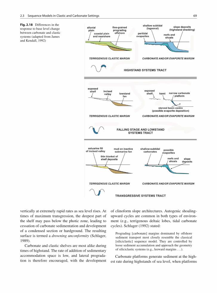
2.3 Sequence Models in Clastic and Carbonate Settings 69
Fig. 2.18 Differences in theresponse to base level changebetween carbonate and clasticsystems (adapted from Jamesand Kendall, 1992)
vertically at extremely rapid rates as sea level rises. Attimes of maximum transgression, the deepest part ofthe shelf may pass below the photic zone, leading tocessation of carbonate sedimentation and developmentof a condensed section or hardground. The resultingsurface is termed a drowning unconformity (Schlager,1989).
Carbonate and clastic shelves are most alike duringtimes of highstand. The rate of addition of sedimentaryaccommodation space is low, and lateral prograda-tion is therefore encouraged, with the development
of clinoform slope architectures. Autogenic shoaling-upward cycles are common in both types of environ-ment (e.g., terrigenous deltaic lobes, tidal carbonatecycles). Schlager (1992) stated:
Prograding [carbonate] margins dominated by offshoresediment transport most closely resemble the classical[siliciclastic] sequence model. They are controlled byloose sediment accumulation and approach the geometryof siliciclastic systems (e.g., leeward margins . . .).
Carbonate platforms generate sediment at the high-est rate during highstands of sea level, when platforms
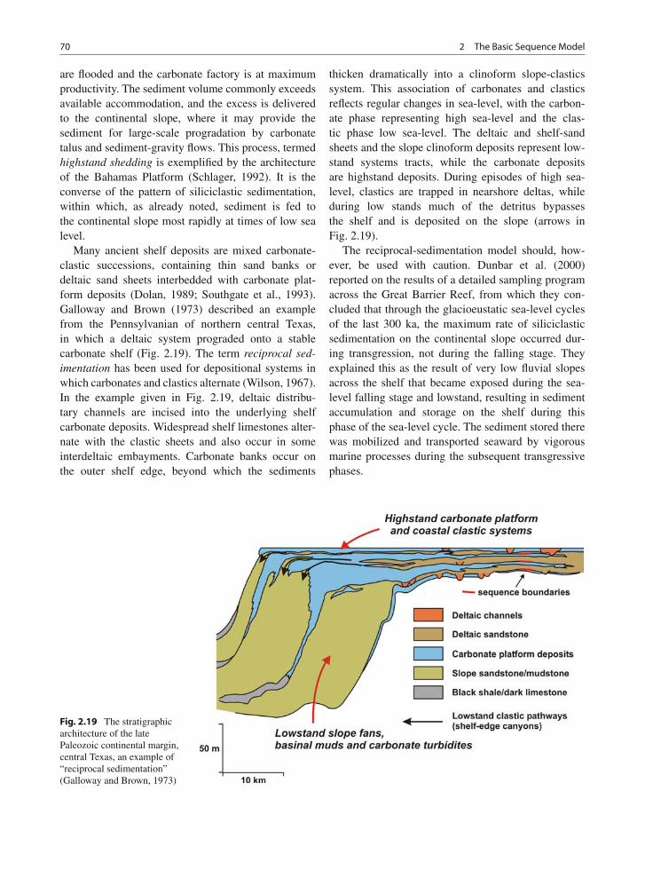
70 2 The Basic Sequence Model
are flooded and the carbonate factory is at maximumproductivity. The sediment volume commonly exceedsavailable accommodation, and the excess is deliveredto the continental slope, where it may provide thesediment for large-scale progradation by carbonatetalus and sediment-gravity flows. This process, termedhighstand shedding is exemplified by the architectureof the Bahamas Platform (Schlager, 1992). It is theconverse of the pattern of siliciclastic sedimentation,within which, as already noted, sediment is fed tothe continental slope most rapidly at times of low sealevel.
Many ancient shelf deposits are mixed carbonate-clastic successions, containing thin sand banks ordeltaic sand sheets interbedded with carbonate plat-form deposits (Dolan, 1989; Southgate et al., 1993).Galloway and Brown (1973) described an examplefrom the Pennsylvanian of northern central Texas,in which a deltaic system prograded onto a stablecarbonate shelf (Fig. 2.19). The term reciprocal sed-imentation has been used for depositional systems inwhich carbonates and clastics alternate (Wilson, 1967).In the example given in Fig. 2.19, deltaic distribu-tary channels are incised into the underlying shelfcarbonate deposits. Widespread shelf limestones alter-nate with the clastic sheets and also occur in someinterdeltaic embayments. Carbonate banks occur onthe outer shelf edge, beyond which the sediments
thicken dramatically into a clinoform slope-clasticssystem. This association of carbonates and clasticsreflects regular changes in sea-level, with the carbon-ate phase representing high sea-level and the clas-tic phase low sea-level. The deltaic and shelf-sandsheets and the slope clinoform deposits represent low-stand systems tracts, while the carbonate depositsare highstand deposits. During episodes of high sea-level, clastics are trapped in nearshore deltas, whileduring low stands much of the detritus bypassesthe shelf and is deposited on the slope (arrows inFig. 2.19).
The reciprocal-sedimentation model should, how-ever, be used with caution. Dunbar et al. (2000)reported on the results of a detailed sampling programacross the Great Barrier Reef, from which they con-cluded that through the glacioeustatic sea-level cyclesof the last 300 ka, the maximum rate of siliciclasticsedimentation on the continental slope occurred dur-ing transgression, not during the falling stage. Theyexplained this as the result of very low fluvial slopesacross the shelf that became exposed during the sea-level falling stage and lowstand, resulting in sedimentaccumulation and storage on the shelf during thisphase of the sea-level cycle. The sediment stored therewas mobilized and transported seaward by vigorousmarine processes during the subsequent transgressivephases.
Fig. 2.19 The stratigraphicarchitecture of the latePaleozoic continental margin,central Texas, an example of“reciprocal sedimentation”(Galloway and Brown, 1973)
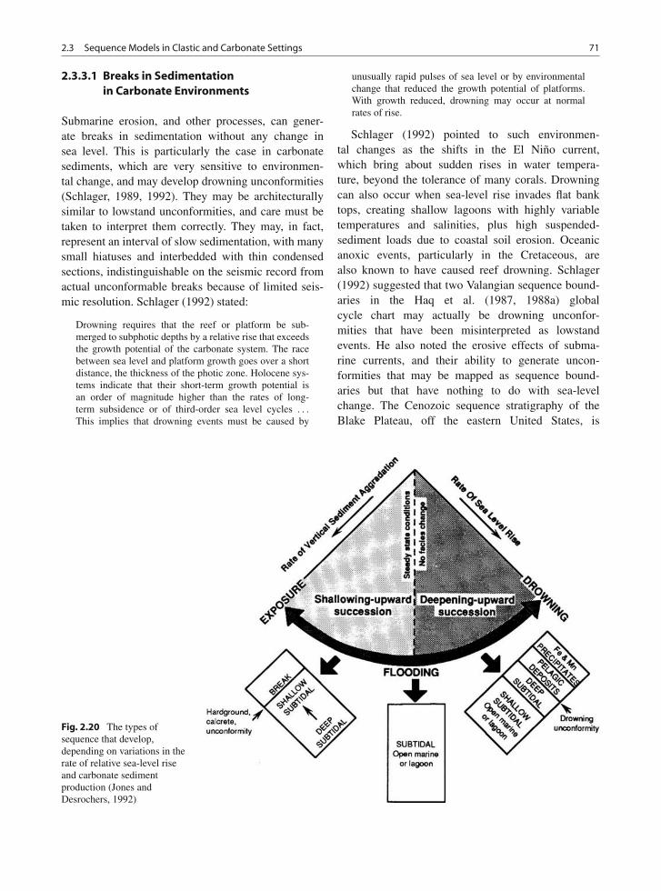
2.3 Sequence Models in Clastic and Carbonate Settings 71
2.3.3.1 Breaks in Sedimentationin Carbonate Environments
Submarine erosion, and other processes, can gener-ate breaks in sedimentation without any change insea level. This is particularly the case in carbonatesediments, which are very sensitive to environmen-tal change, and may develop drowning unconformities(Schlager, 1989, 1992). They may be architecturallysimilar to lowstand unconformities, and care must betaken to interpret them correctly. They may, in fact,represent an interval of slow sedimentation, with manysmall hiatuses and interbedded with thin condensedsections, indistinguishable on the seismic record fromactual unconformable breaks because of limited seis-mic resolution. Schlager (1992) stated:
Drowning requires that the reef or platform be sub-merged to subphotic depths by a relative rise that exceedsthe growth potential of the carbonate system. The racebetween sea level and platform growth goes over a shortdistance, the thickness of the photic zone. Holocene sys-tems indicate that their short-term growth potential isan order of magnitude higher than the rates of long-term subsidence or of third-order sea level cycles . . .
This implies that drowning events must be caused by
unusually rapid pulses of sea level or by environmentalchange that reduced the growth potential of platforms.With growth reduced, drowning may occur at normalrates of rise.
Schlager (1992) pointed to such environmen-tal changes as the shifts in the El Niño current,which bring about sudden rises in water tempera-ture, beyond the tolerance of many corals. Drowningcan also occur when sea-level rise invades flat banktops, creating shallow lagoons with highly variabletemperatures and salinities, plus high suspended-sediment loads due to coastal soil erosion. Oceanicanoxic events, particularly in the Cretaceous, arealso known to have caused reef drowning. Schlager(1992) suggested that two Valangian sequence bound-aries in the Haq et al. (1987, 1988a) globalcycle chart may actually be drowning unconfor-mities that have been misinterpreted as lowstandevents. He also noted the erosive effects of subma-rine currents, and their ability to generate uncon-formities that may be mapped as sequence bound-aries but that have nothing to do with sea-levelchange. The Cenozoic sequence stratigraphy of theBlake Plateau, off the eastern United States, is
Fig. 2.20 The types ofsequence that develop,depending on variations in therate of relative sea-level riseand carbonate sedimentproduction (Jones andDesrochers, 1992)
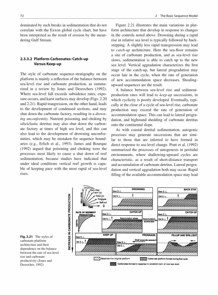
72 2 The Basic Sequence Model
dominated by such breaks in sedimentation that do notcorrelate with the Exxon global cycle chart, but havebeen interpreted as the result of erosion by the mean-dering Gulf Stream.
2.3.3.2 Platform Carbonates: Catch-upVersus Keep-up
The style of carbonate sequence-stratigraphy on theplatform is mainly a reflection of the balance betweensea-level rise and carbonate production, as summa-rized in a review by Jones and Desrochers (1992).Where sea-level fall exceeds subsidence rates, expo-sure occurs, and karst surfaces may develop (Figs. 2.20and 2.21). Rapid trangression, on the other hand, leadsto the development of condensed sections, and mayshut down the carbonate factory, resulting in a drown-ing unconformity. Nutrient poisoning and choking bysiliciclastic detritus may also shut down the carbon-ate factory at times of high sea level, and this canalso lead to the development of drowning unconfor-mities, which may be mistaken for sequence bound-aries (e.g., Erlich et al., 1993). James and Bourque(1992) argued that poisoning and choking were theprocesses most likely to cause a shut down of reefsedimentation, because studies have indicated thatunder ideal conditions vertical reef growth is capa-ble of keeping pace with the most rapid of sea-levelrises.
Figure 2.21 illustrates the main variations in plat-form architecture that develop in response to changesin the controls noted above. Drowning during a rapidrise in relative sea level is typically followed by back-stepping. A slightly less rapid transgression may leadto catch-up architecture. Here the sea-floor remainsa site of carbonate production, and as sea-level riseslows, sedimentation is able to catch up to the newsea level. Vertical aggradation characterizes the firststage of the catch-up, but lateral progradation mayoccur late in the cycle, when the rate of generationof new accommodation space decreases. Shoaling-upward sequences are the result.
A balance between sea-level rise and sediment-production rates will lead to keep-up successions, inwhich cyclicity is poorly developed. Eventually, typi-cally at the close of a cycle of sea-level rise, carbonateproduction may exceed the rate of generation ofaccommodation space. This can lead to lateral progra-dation, and highstand shedding of carbonate detritusonto the continental slope.
As with coastal detrital sedimentation, autogenicprocesses may generate successions that are simi-lar to those that are inferred to have formed indirect response to sea-level change. Pratt et al. (1992)summarized the processes of autogenesis in peritidalenvironments, where shallowing-upward cycles arecharacteristic, as a result of short-distance transportand accumulation of carbonate detritus. Lateral progra-dation and vertical aggradation both may occur. Rapidfilling of the available accommodation space may lead
Fig. 2.21 The styles ofcarbonate-platformarchitecture and theirdependence on the balancebetween the rate of sea-levelrise and carbonateproductivity (Jones andDesrocher, 1992)
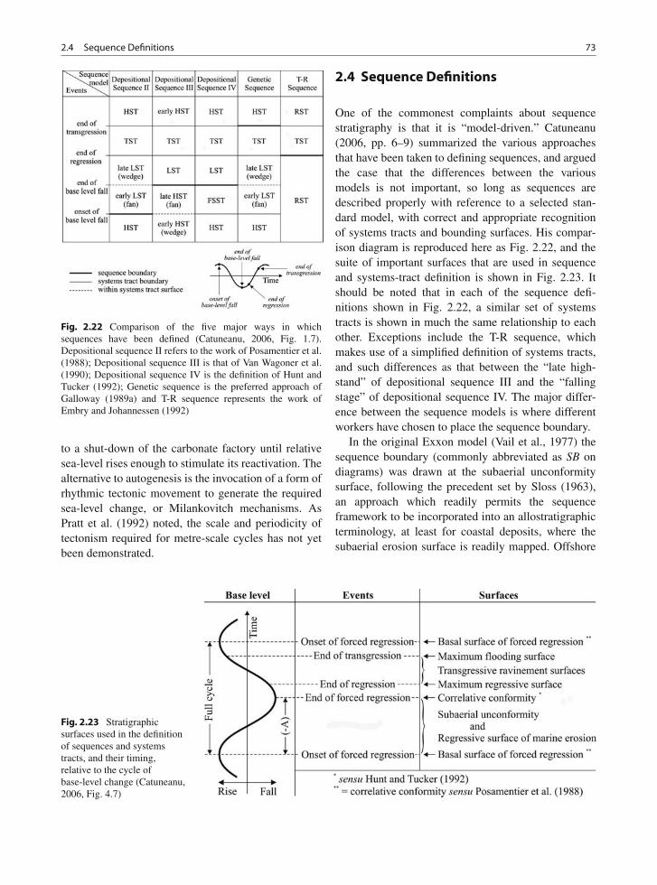
2.4 Sequence Definitions 73
Fig. 2.22 Comparison of the five major ways in whichsequences have been defined (Catuneanu, 2006, Fig. 1.7).Depositional sequence II refers to the work of Posamentier et al.(1988); Depositional sequence III is that of Van Wagoner et al.(1990); Depositional sequence IV is the definition of Hunt andTucker (1992); Genetic sequence is the preferred approach ofGalloway (1989a) and T-R sequence represents the work ofEmbry and Johannessen (1992)
to a shut-down of the carbonate factory until relativesea-level rises enough to stimulate its reactivation. Thealternative to autogenesis is the invocation of a form ofrhythmic tectonic movement to generate the requiredsea-level change, or Milankovitch mechanisms. AsPratt et al. (1992) noted, the scale and periodicity oftectonism required for metre-scale cycles has not yetbeen demonstrated.
2.4 Sequence Definitions
One of the commonest complaints about sequencestratigraphy is that it is “model-driven.” Catuneanu(2006, pp. 6–9) summarized the various approachesthat have been taken to defining sequences, and arguedthe case that the differences between the variousmodels is not important, so long as sequences aredescribed properly with reference to a selected stan-dard model, with correct and appropriate recognitionof systems tracts and bounding surfaces. His compar-ison diagram is reproduced here as Fig. 2.22, and thesuite of important surfaces that are used in sequenceand systems-tract definition is shown in Fig. 2.23. Itshould be noted that in each of the sequence defi-nitions shown in Fig. 2.22, a similar set of systemstracts is shown in much the same relationship to eachother. Exceptions include the T-R sequence, whichmakes use of a simplified definition of systems tracts,and such differences as that between the “late high-stand” of depositional sequence III and the “fallingstage” of depositional sequence IV. The major differ-ence between the sequence models is where differentworkers have chosen to place the sequence boundary.
In the original Exxon model (Vail et al., 1977) thesequence boundary (commonly abbreviated as SB ondiagrams) was drawn at the subaerial unconformitysurface, following the precedent set by Sloss (1963),an approach which readily permits the sequenceframework to be incorporated into an allostratigraphicterminology, at least for coastal deposits, where thesubaerial erosion surface is readily mapped. Offshore
Fig. 2.23 Stratigraphicsurfaces used in the definitionof sequences and systemstracts, and their timing,relative to the cycle ofbase-level change (Catuneanu,2006, Fig. 4.7)
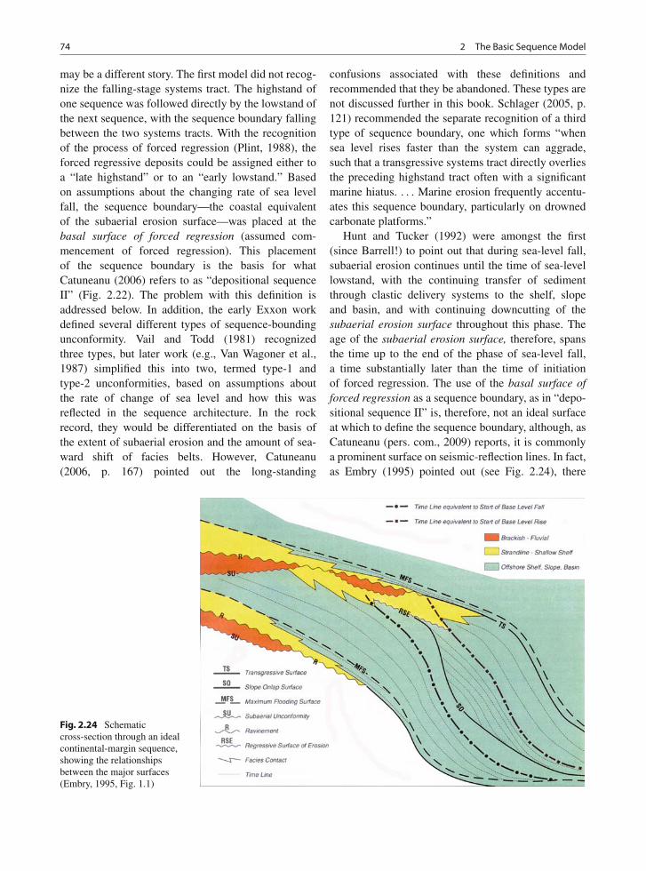
74 2 The Basic Sequence Model
may be a different story. The first model did not recog-nize the falling-stage systems tract. The highstand ofone sequence was followed directly by the lowstand ofthe next sequence, with the sequence boundary fallingbetween the two systems tracts. With the recognitionof the process of forced regression (Plint, 1988), theforced regressive deposits could be assigned either toa “late highstand” or to an “early lowstand.” Basedon assumptions about the changing rate of sea levelfall, the sequence boundary—the coastal equivalentof the subaerial erosion surface—was placed at thebasal surface of forced regression (assumed com-mencement of forced regression). This placementof the sequence boundary is the basis for whatCatuneanu (2006) refers to as “depositional sequenceII” (Fig. 2.22). The problem with this definition isaddressed below. In addition, the early Exxon workdefined several different types of sequence-boundingunconformity. Vail and Todd (1981) recognizedthree types, but later work (e.g., Van Wagoner et al.,1987) simplified this into two, termed type-1 andtype-2 unconformities, based on assumptions aboutthe rate of change of sea level and how this wasreflected in the sequence architecture. In the rockrecord, they would be differentiated on the basis ofthe extent of subaerial erosion and the amount of sea-ward shift of facies belts. However, Catuneanu(2006, p. 167) pointed out the long-standing
confusions associated with these definitions andrecommended that they be abandoned. These types arenot discussed further in this book. Schlager (2005, p.121) recommended the separate recognition of a thirdtype of sequence boundary, one which forms “whensea level rises faster than the system can aggrade,such that a transgressive systems tract directly overliesthe preceding highstand tract often with a significantmarine hiatus. . . . Marine erosion frequently accentu-ates this sequence boundary, particularly on drownedcarbonate platforms.”
Hunt and Tucker (1992) were amongst the first(since Barrell!) to point out that during sea-level fall,subaerial erosion continues until the time of sea-levellowstand, with the continuing transfer of sedimentthrough clastic delivery systems to the shelf, slopeand basin, and with continuing downcutting of thesubaerial erosion surface throughout this phase. Theage of the subaerial erosion surface, therefore, spansthe time up to the end of the phase of sea-level fall,a time substantially later than the time of initiationof forced regression. The use of the basal surface offorced regression as a sequence boundary, as in “depo-sitional sequence II” is, therefore, not an ideal surfaceat which to define the sequence boundary, although, asCatuneanu (pers. com., 2009) reports, it is commonlya prominent surface on seismic-reflection lines. In fact,as Embry (1995) pointed out (see Fig. 2.24), there
Fig. 2.24 Schematiccross-section through an idealcontinental-margin sequence,showing the relationshipsbetween the major surfaces(Embry, 1995, Fig. 1.1)
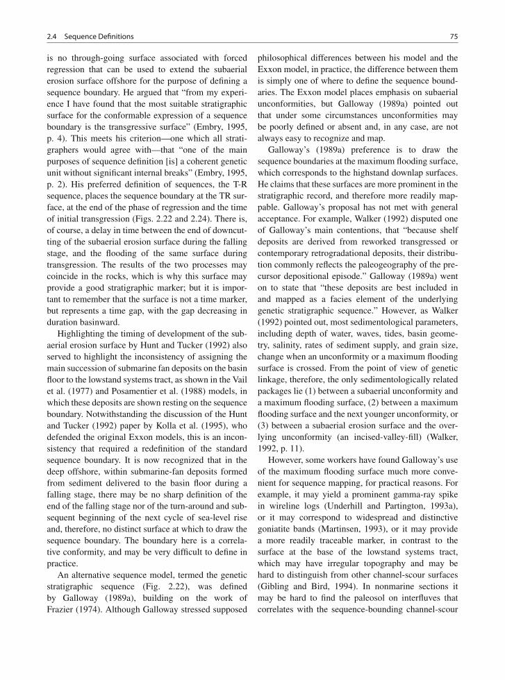
2.4 Sequence Definitions 75
is no through-going surface associated with forcedregression that can be used to extend the subaerialerosion surface offshore for the purpose of defining asequence boundary. He argued that “from my experi-ence I have found that the most suitable stratigraphicsurface for the conformable expression of a sequenceboundary is the transgressive surface” (Embry, 1995,p. 4). This meets his criterion—one which all strati-graphers would agree with—that “one of the mainpurposes of sequence definition [is] a coherent geneticunit without significant internal breaks” (Embry, 1995,p. 2). His preferred definition of sequences, the T-Rsequence, places the sequence boundary at the TR sur-face, at the end of the phase of regression and the timeof initial transgression (Figs. 2.22 and 2.24). There is,of course, a delay in time between the end of downcut-ting of the subaerial erosion surface during the fallingstage, and the flooding of the same surface duringtransgression. The results of the two processes maycoincide in the rocks, which is why this surface mayprovide a good stratigraphic marker; but it is impor-tant to remember that the surface is not a time marker,but represents a time gap, with the gap decreasing induration basinward.
Highlighting the timing of development of the sub-aerial erosion surface by Hunt and Tucker (1992) alsoserved to highlight the inconsistency of assigning themain succession of submarine fan deposits on the basinfloor to the lowstand systems tract, as shown in the Vailet al. (1977) and Posamentier et al. (1988) models, inwhich these deposits are shown resting on the sequenceboundary. Notwithstanding the discussion of the Huntand Tucker (1992) paper by Kolla et al. (1995), whodefended the original Exxon models, this is an incon-sistency that required a redefinition of the standardsequence boundary. It is now recognized that in thedeep offshore, within submarine-fan deposits formedfrom sediment delivered to the basin floor during afalling stage, there may be no sharp definition of theend of the falling stage nor of the turn-around and sub-sequent beginning of the next cycle of sea-level riseand, therefore, no distinct surface at which to draw thesequence boundary. The boundary here is a correla-tive conformity, and may be very difficult to define inpractice.
An alternative sequence model, termed the geneticstratigraphic sequence (Fig. 2.22), was definedby Galloway (1989a), building on the work ofFrazier (1974). Although Galloway stressed supposed
philosophical differences between his model and theExxon model, in practice, the difference between themis simply one of where to define the sequence bound-aries. The Exxon model places emphasis on subaerialunconformities, but Galloway (1989a) pointed outthat under some circumstances unconformities maybe poorly defined or absent and, in any case, are notalways easy to recognize and map.
Galloway’s (1989a) preference is to draw thesequence boundaries at the maximum flooding surface,which corresponds to the highstand downlap surfaces.He claims that these surfaces are more prominent in thestratigraphic record, and therefore more readily map-pable. Galloway’s proposal has not met with generalacceptance. For example, Walker (1992) disputed oneof Galloway’s main contentions, that “because shelfdeposits are derived from reworked transgressed orcontemporary retrogradational deposits, their distribu-tion commonly reflects the paleogeography of the pre-cursor depositional episode.” Galloway (1989a) wenton to state that “these deposits are best included inand mapped as a facies element of the underlyinggenetic stratigraphic sequence.” However, as Walker(1992) pointed out, most sedimentological parameters,including depth of water, waves, tides, basin geome-try, salinity, rates of sediment supply, and grain size,change when an unconformity or a maximum floodingsurface is crossed. From the point of view of geneticlinkage, therefore, the only sedimentologically relatedpackages lie (1) between a subaerial unconformity anda maximum flooding surface, (2) between a maximumflooding surface and the next younger unconformity, or(3) between a subaerial erosion surface and the over-lying unconformity (an incised-valley-fill) (Walker,1992, p. 11).
However, some workers have found Galloway’s useof the maximum flooding surface much more conve-nient for sequence mapping, for practical reasons. Forexample, it may yield a prominent gamma-ray spikein wireline logs (Underhill and Partington, 1993a),or it may correspond to widespread and distinctivegoniatite bands (Martinsen, 1993), or it may providea more readily traceable marker, in contrast to thesurface at the base of the lowstand systems tract,which may have irregular topography and may behard to distinguish from other channel-scour surfaces(Gibling and Bird, 1994). In nonmarine sections itmay be hard to find the paleosol on interfluves thatcorrelates with the sequence-bounding channel-scour
76 2 The Basic Sequence Model
Fig. 2.25 The development and abandonment of delta lobes ina river dominated, Mississippi-type delta (e.g., see Fig. 7.5),based on detailed analysis of the Mississippi delta system byBoyd and Penland (1988). In stage 1, progradation develops anupward-shoaling deltaic succession. Abandonment, followed bysubsidence (resulting from compaction) cause the upper layersof the succession to be reworked (stage 2), resulting in the devel-opment of an extensive barrier island system (stage 3). Finally,
the deposit undergoes transgression and is covered by marineshale (stage 4). Repetition of this succession of events when anew delta lobe progrades back over the older deposit results inshoaling upward successions bounded by transgressive floodingsurfaces, that is, parasequences. In this case, however, they areclearly of autogenic origin. Systems-tract designations for eachof the four stages are indicated in parenthesis
surface (Martinesen, 1993). In some studies (e.g.,Plint et al., 1986; Bhattacharya, 1993) it has beenfound that ravinement erosion during transgression hasremoved the transgressive systems tract, so that themarine flooding surface coincides with the sequenceboundary.
Finally, a word about the parasequence. Proposedoriginally as part of a hierarchy of terms, the bed,bedset, parasequence, parasequence set, and sequence(Van Wagoner et al., 1990; see Table 4.2), the parase-quence has become a source of confusion, as notedabove (Sect. 2.2.2). The shingles that compose manydeltaic successions (e.g., see Fig. 2.9) are shoaling-upward successions bounded by flooding surfaces, andtherefore fit the definition of parasequences. Theyare commonly the product of a process of auto-genic delta switching, as illustrated in Fig. 2.25. This
has been demonstrated to be the case in the exam-ple of the Dunvegan delta illustrated in Fig. 2.9(Bhattacharya, 1991). The shingles and their bound-ing flooding surfaces are therefore local in distribu-tion, and their development has little, if anything,to do with the allogenic mechanisms that generatesequences. However, to apply to these successionsa term that contains the word “sequence” in it isinevitably to introduce the implication that they areallogenic in origin and constitute regionally correlat-able units. The correct interpretation clearly dependson good mapping to determine the extent and corre-latability of each shingle, andit would seem advisablenot to use a term in a descriptive sense that carriesgenetic implications. As noted earlier (Sect. 2.2.2), thisauthor recommends abandoning the term parasequencealtogether.
Chapter 3
Other Methods for the Stratigraphic Analysis of Cyclesof Base-Level Change
Contents
3.1 Introduction . . . . . . . . . . . . . . . . . 773.2 Facies Cycles . . . . . . . . . . . . . . . . 773.3 Areas and Volumes of Stratigraphic Units . . . 803.4 Hypsometric Curves . . . . . . . . . . . . . 813.5 Backstripping . . . . . . . . . . . . . . . . 833.6 Sea-Level Estimation from Paleoshorelines and
Other Fixed Points . . . . . . . . . . . . . . 903.7 Documentation of Metre-Scale Cycles . . . . . 933.8 Integrated Tectonic-Stratigraphic Analysis . . 97
3.1 Introduction
A variety of supplementary methods that have evolvedfor assessing regional and global sea-level changesdirectly from the stratigraphic record. These includethe following:
• Analysing and correlating facies cycles.• The mapping of changes in stratigraphic volumes
or areas covered by successions of a specified agerange as an indication of transgression and regres-sion and changing rates of subsidence.
• The use of hypsometric curves to plot broadchanges in continental elevation and eustatic sea-level changes.
• The study of paleoshorelines.• Graphical and numerical methods for the documen-
tation and analysis of the metre-scale cycles thatare very common in some parts of the stratigraphicrecord (e.g., certain lacustrine and shelf-carbonatesuccessions).
As discussed in several places in this book, one ofthe principal problems with the assessment of causal-ity is that there are no absolute reference frames forthe calibration of sea-level change. The vertical move-ments of sea level can only be measured by the strati-graphic record left on Earth’s crust, but the crust itselfis in constant vertical motion, driven by mantle andlithospheric processes (Burton et al., 1987; Sahagianand Watts, 1991). Much of this book deals with thestrategies earth scientists have evolved in their attemptsto attack and overcome this problem.
3.2 Facies Cycles
Vertical changes in lithofacies and biofacies have longbeen used to reconstruct temporal changes in depo-sitional environments and, with the aid of Walther’sLaw, to interpret lateral shifts in these environments.Such an approach comprises the basis of the methodof facies analysis, as discussed at length in many text-books (e.g., Miall, 1999, Chap. 4) and review articles(e.g., Wanless, 1991). A single example of lithofaciesand biofacies analysis will suffice. Other examples areillustrated elsewhere in this report.
Heckel (1986) presented a basic depositional modelfor the so-called “Kansas cyclothem”, and for theenvironments of deposition occurring on a gently slop-ing tropical shelf (Fig. 3.1). Beds representing eachof these environments are extraordinarily widespread,indicating shifts of environments of hundreds of kilo-metres. Black, phosphatic shales with conodonts indi-cate the deepest marine environments. Skeletal andalgal wackestones and grainstones were depositedin shallow marine settings, whereas sandstones and
77A.D. Miall, The Geology of Stratigraphic Sequences, 2nd ed.,DOI 10.1007/978-3-642-05027-5_3, © Springer-Verlag Berlin Heidelberg 2010
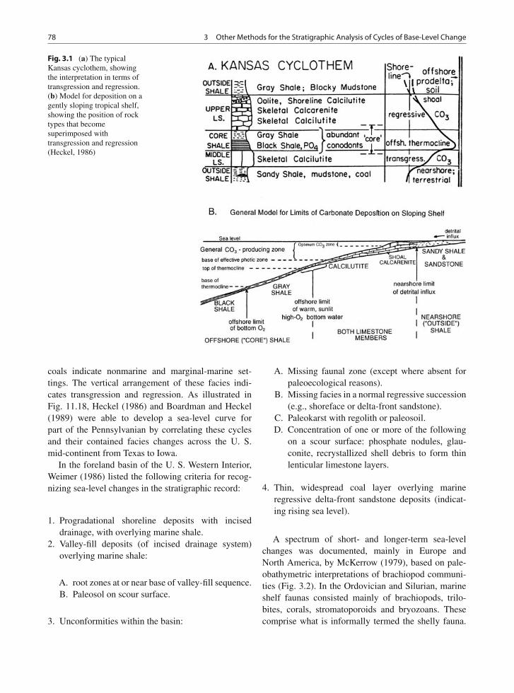
78 3 Other Methods for the Stratigraphic Analysis of Cycles of Base-Level Change
Fig. 3.1 (a) The typicalKansas cyclothem, showingthe interpretation in terms oftransgression and regression.(b) Model for deposition on agently sloping tropical shelf,showing the position of rocktypes that becomesuperimposed withtransgression and regression(Heckel, 1986)
coals indicate nonmarine and marginal-marine set-tings. The vertical arrangement of these facies indi-cates transgression and regression. As illustrated inFig. 11.18, Heckel (1986) and Boardman and Heckel(1989) were able to develop a sea-level curve forpart of the Pennsylvanian by correlating these cyclesand their contained facies changes across the U. S.mid-continent from Texas to Iowa.
In the foreland basin of the U. S. Western Interior,Weimer (1986) listed the following criteria for recog-nizing sea-level changes in the stratigraphic record:
1. Progradational shoreline deposits with inciseddrainage, with overlying marine shale.
2. Valley-fill deposits (of incised drainage system)overlying marine shale:
A. root zones at or near base of valley-fill sequence.B. Paleosol on scour surface.
3. Unconformities within the basin:
A. Missing faunal zone (except where absent forpaleoecological reasons).
B. Missing facies in a normal regressive succession(e.g., shoreface or delta-front sandstone).
C. Paleokarst with regolith or paleosoil.D. Concentration of one or more of the following
on a scour surface: phosphate nodules, glau-conite, recrystallized shell debris to form thinlenticular limestone layers.
4. Thin, widespread coal layer overlying marineregressive delta-front sandstone deposits (indicat-ing rising sea level).
A spectrum of short- and longer-term sea-levelchanges was documented, mainly in Europe andNorth America, by McKerrow (1979), based on pale-obathymetric interpretations of brachiopod communi-ties (Fig. 3.2). In the Ordovician and Silurian, marineshelf faunas consisted mainly of brachiopods, trilo-bites, corals, stromatoporoids and bryozoans. Thesecomprise what is informally termed the shelly fauna.
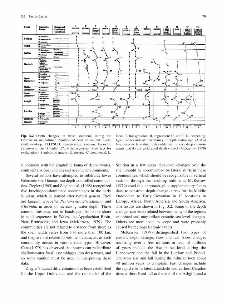
3.2 Facies Cycles 79
Fig. 3.2 Depth changes on three continents during theOrdovician and Silurian. Symbols at head of column: S->D,shallow->deep; TLEPSCD, transgression, Lingula, Eocoelia,Pentamerus, Stricklandia, Clorinda, regression (see text forexplanation). Symbols on graphs: E, eustatic; C, continental; L,
local; T, transgression; R, regression; U, uplift; D, deepening.Open circles indicate uncertainty of depth and/or age. Dashedlines indicate terrestrial, unfossiliferous, or very deep environ-ments that do not yield good depth control (McKerrow, 1979)
It contrasts with the graptolitic fauna of deeper-water,continental-slope, and abyssal oceanic environments.
Several authors have attempted to subdivide lowerPaleozoic shelf faunas into depth-controlled communi-ties. Ziegler (1965) and Ziegler et al. (1968) recognizedfive brachiopod-dominated assemblages in the earlySilurian, which he named after typical genera. Theyare Lingula, Eocoelia, Pentamerus, Stricklandia, andClorinda, in order of increasing water depth. Thesecommunities map out in bands parallel to the shorein shelf sequences in Wales, the Appalachian Basin,New Brunswick, and Iowa (McKerrow, 1979). Thecommunities are not related to distance from shore asthe shelf width varies from 5 to more than 100 km,and they are not related to sediment character, as eachcommunity occurs in various rock types. However,Cant (1979) has observed that storms can redistributeshallow-water fossil assemblages into deep water, andso some caution must be used in interpreting thesedata.
Ziegler’s faunal differentiation has been establishedfor the Upper Ordovician and the remainder of the
Silurian in a few areas. Sea-level changes over theshelf should be accompanied by lateral shifts in thesecommunities, which should be recognizable in verticalsections through the resulting sediments. McKerrow(1979) used this approach, plus supplementary faciesdata, to construct depth-change curves for the MiddleOrdovician to Early Devonian in 13 locations inEurope, Africa, North America and South America.The results are shown in Fig. 3.2. Some of the depthchanges can be correlated between many of the regionsexamined and may reflect eustatic sea-level changes.Others are more local in scope and were probablycaused by regional tectonic events.
McKerrow (1979) distinguished two types ofeustatic depth change, slow and fast. Slow changesoccurring over a few millions or tens of millionsof years include the rise in sea-level during theLlandovery and the fall in the Ludlow and Pridoli.The slow rise and fall during the Silurian took about40 million years to complete. Fast changes includethe rapid rise in latest Llandeilo and earliest Caradoctime, a short-lived fall at the end of the Ashgill, and a
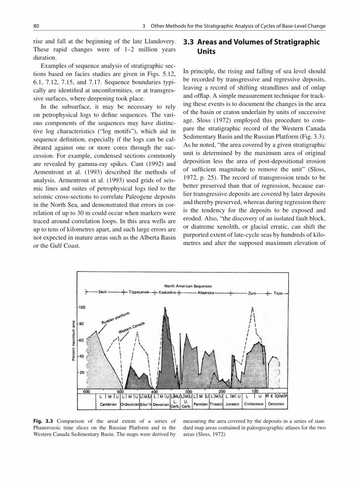
80 3 Other Methods for the Stratigraphic Analysis of Cycles of Base-Level Change
rise and fall at the beginning of the late Llandovery.These rapid changes were of 1–2 million yearsduration.
Examples of sequence analysis of stratigraphic sec-tions based on facies studies are given in Figs. 5.12,6.1, 7.12, 7.15, and 7.17. Sequence boundaries typi-cally are identified at unconformities, or at transgres-sive surfaces, where deepening took place.
In the subsurface, it may be necessary to relyon petrophysical logs to define sequences. The vari-ous components of the sequences may have distinc-tive log characteristics (“log motifs”), which aid insequence definition, especially if the logs can be cal-ibrated against one or more cores through the suc-cession. For example, condensed sections commonlyare revealed by gamma-ray spikes. Cant (1992) andArmentrout et al. (1993) described the methods ofanalysis. Armentrout et al. (1993) used grids of seis-mic lines and suites of petrophysical logs tied to theseismic cross-sections to correlate Paleogene depositsin the North Sea, and demonstrated that errors in cor-relation of up to 30 m could occur when markers weretraced around correlation loops. In this area wells areup to tens of kilometres apart, and such large errors arenot expected in mature areas such as the Alberta Basinor the Gulf Coast.
3.3 Areas and Volumes of StratigraphicUnits
In principle, the rising and falling of sea level shouldbe recorded by transgressive and regressive deposits,leaving a record of shifting strandlines and of onlapand offlap. A simple measurement technique for track-ing these events is to document the changes in the areaof the basin or craton underlain by units of successiveage. Sloss (1972) employed this procedure to com-pare the stratigraphic record of the Western CanadaSedimentary Basin and the Russian Platform (Fig. 3.3).As he noted, “the area covered by a given stratigraphicunit is determined by the maximum area of originaldeposition less the area of post-depositional erosionof sufficient magnitude to remove the unit” (Sloss,1972, p. 25). The record of transgression tends to bebetter preserved than that of regression, because ear-lier transgressive deposits are covered by later depositsand thereby preserved, whereas during regression thereis the tendency for the deposits to be exposed anderoded. Also, “the discovery of an isolated fault block,or diatreme xenolith, or glacial erratic, can shift thepurported extent of late-cycle seas by hundreds of kilo-metres and alter the supposed maximum elevation of
Fig. 3.3 Comparison of the areal extent of a series ofPhanerozoic time slices on the Russian Platform and in theWestern Canada Sedimentary Basin. The maps were derived by
measuring the area covered by the deposits in a series of stan-dard map areas contained in paleogeographic atlases for the twoareas (Sloss, 1972)
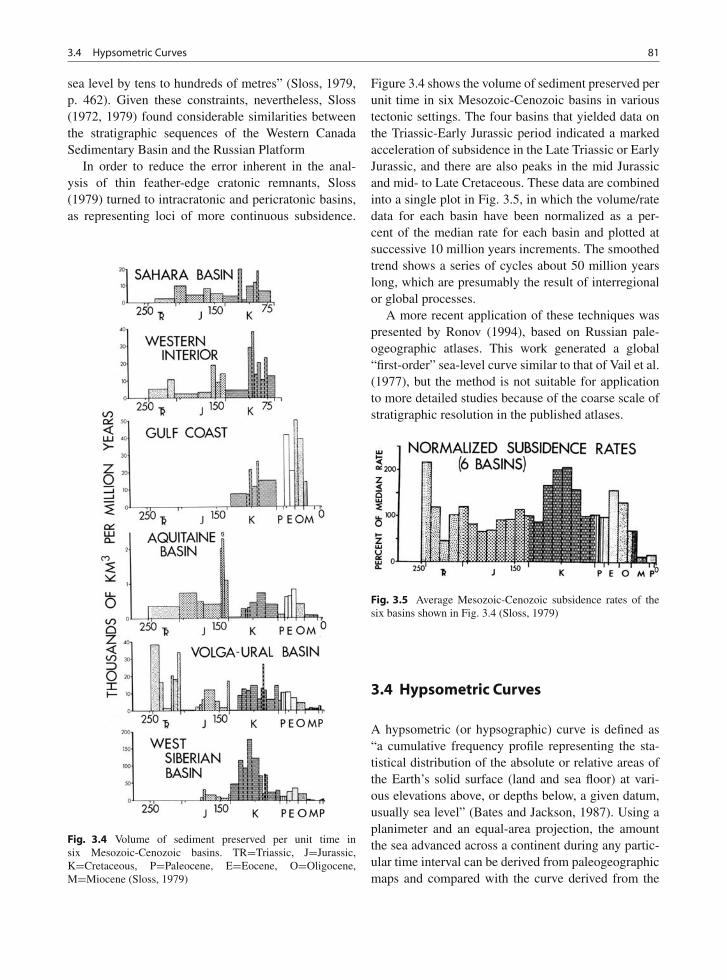
3.4 Hypsometric Curves 81
sea level by tens to hundreds of metres” (Sloss, 1979,p. 462). Given these constraints, nevertheless, Sloss(1972, 1979) found considerable similarities betweenthe stratigraphic sequences of the Western CanadaSedimentary Basin and the Russian Platform
In order to reduce the error inherent in the anal-ysis of thin feather-edge cratonic remnants, Sloss(1979) turned to intracratonic and pericratonic basins,as representing loci of more continuous subsidence.
Fig. 3.4 Volume of sediment preserved per unit time insix Mesozoic-Cenozoic basins. TR=Triassic, J=Jurassic,K=Cretaceous, P=Paleocene, E=Eocene, O=Oligocene,M=Miocene (Sloss, 1979)
Figure 3.4 shows the volume of sediment preserved perunit time in six Mesozoic-Cenozoic basins in varioustectonic settings. The four basins that yielded data onthe Triassic-Early Jurassic period indicated a markedacceleration of subsidence in the Late Triassic or EarlyJurassic, and there are also peaks in the mid Jurassicand mid- to Late Cretaceous. These data are combinedinto a single plot in Fig. 3.5, in which the volume/ratedata for each basin have been normalized as a per-cent of the median rate for each basin and plotted atsuccessive 10 million years increments. The smoothedtrend shows a series of cycles about 50 million yearslong, which are presumably the result of interregionalor global processes.
A more recent application of these techniques waspresented by Ronov (1994), based on Russian pale-ogeographic atlases. This work generated a global“first-order” sea-level curve similar to that of Vail et al.(1977), but the method is not suitable for applicationto more detailed studies because of the coarse scale ofstratigraphic resolution in the published atlases.
Fig. 3.5 Average Mesozoic-Cenozoic subsidence rates of thesix basins shown in Fig. 3.4 (Sloss, 1979)
3.4 Hypsometric Curves
A hypsometric (or hypsographic) curve is defined as“a cumulative frequency profile representing the sta-tistical distribution of the absolute or relative areas ofthe Earth’s solid surface (land and sea floor) at vari-ous elevations above, or depths below, a given datum,usually sea level” (Bates and Jackson, 1987). Using aplanimeter and an equal-area projection, the amountthe sea advanced across a continent during any partic-ular time interval can be derived from paleogeographicmaps and compared with the curve derived from the
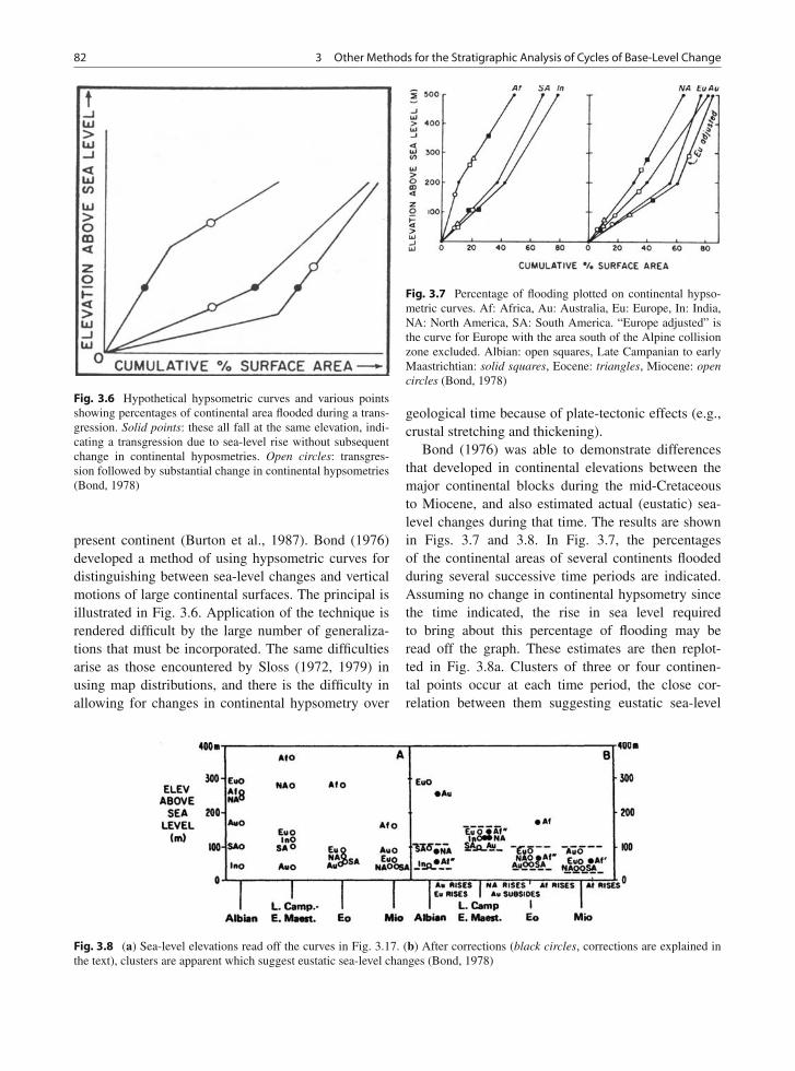
82 3 Other Methods for the Stratigraphic Analysis of Cycles of Base-Level Change
Fig. 3.6 Hypothetical hypsometric curves and various pointsshowing percentages of continental area flooded during a trans-gression. Solid points: these all fall at the same elevation, indi-cating a transgression due to sea-level rise without subsequentchange in continental hyposmetries. Open circles: transgres-sion followed by substantial change in continental hypsometries(Bond, 1978)
present continent (Burton et al., 1987). Bond (1976)developed a method of using hypsometric curves fordistinguishing between sea-level changes and verticalmotions of large continental surfaces. The principal isillustrated in Fig. 3.6. Application of the technique isrendered difficult by the large number of generaliza-tions that must be incorporated. The same difficultiesarise as those encountered by Sloss (1972, 1979) inusing map distributions, and there is the difficulty inallowing for changes in continental hypsometry over
Fig. 3.7 Percentage of flooding plotted on continental hypso-metric curves. Af: Africa, Au: Australia, Eu: Europe, In: India,NA: North America, SA: South America. “Europe adjusted” isthe curve for Europe with the area south of the Alpine collisionzone excluded. Albian: open squares, Late Campanian to earlyMaastrichtian: solid squares, Eocene: triangles, Miocene: opencircles (Bond, 1978)
geological time because of plate-tectonic effects (e.g.,crustal stretching and thickening).
Bond (1976) was able to demonstrate differencesthat developed in continental elevations between themajor continental blocks during the mid-Cretaceousto Miocene, and also estimated actual (eustatic) sea-level changes during that time. The results are shownin Figs. 3.7 and 3.8. In Fig. 3.7, the percentagesof the continental areas of several continents floodedduring several successive time periods are indicated.Assuming no change in continental hypsometry sincethe time indicated, the rise in sea level requiredto bring about this percentage of flooding may beread off the graph. These estimates are then replot-ted in Fig. 3.8a. Clusters of three or four continen-tal points occur at each time period, the close cor-relation between them suggesting eustatic sea-level
Fig. 3.8 (a) Sea-level elevations read off the curves in Fig. 3.17. (b) After corrections (black circles, corrections are explained inthe text), clusters are apparent which suggest eustatic sea-level changes (Bond, 1978)
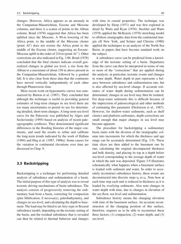
3.5 Backstripping 83
changes. However, Africa appears as an anomaly inthe Campanian-Maastrichtian, Eocene and Miocenecolumns, and there is a scatter of points in the Albiancolumn. Bond (1978) suggested that Africa has beenuplifted since the Miocene. A 90-m lowering of theAfrica point, to the middle of the Miocene cluster(point Af′) does not restore the Africa point to themiddle of the Eocene cluster, suggesting an Eocene-Miocene uplift in the order of 210 m (point Af ′′). Othercorrections are also indicated in Fig. 3.8b. Bond (1978)concluded that the final clusters indicate overall gen-eralized changes in global sea level, a rise from theAlbian to a maximum of about 150 m above present inthe Campanian-Maastrichtian, followed by a gradualfall. It is also clear from these data that the continentshave moved vertically independently of each otherthrough Phanerozoic time.
More recent work on hypsometric curves was sum-marized by Burton et al. (1987). They concluded thatalthough the technique is useful in providing generalestimates of long-term changes in sea level there aretoo many uncertainties to permit its use for determin-ing detailed, short-term changes. A long-term sea-levelcurve for the Paleozoic was published by Algeo andSeslavisnsky (1995) based on analysis of recent pale-ogeographic syntheses. They demonstrated significantdifferences in the flooding histories of the major con-tinents, and used the results to refine and calibratethe long-term trends indicated by the work of Hallam(1984) and Haq et al. (1987, 1988a). Some causes forthe variation in continental elevations over time arediscussed in Chap. 9.
3.5 Backstripping
Backstripping is a technique for performing detailedanalysis of subsidence and sedimentation of a basin.The initial purpose of this type of analysis was to revealtectonic driving mechanisms of basin subsidence. Theanalysis consists of progressively removing the sedi-mentary load from a basin, correcting for compaction(plus lithification, if necessary), paleobathymetry, andchanges in sea-level, and calculating the depth to base-ment. The load may be fitted to an Airy-type or flexuralsubsidence model, depending on the tectonic setting ofthe basin, and the residual subsidence that is revealedcan then be related to thermal behavior and changes
with time in crustal properties. The technique wasdeveloped by Sleep (1971) and was first explored indetail by Watts and Ryan (1976). Steckler and Watts(1978) applied the McKenzie (1978) stretching modelto offshore stratigraphic data from the continental mar-gin off New York, and Sclater and Christie (1980)applied the techniques to an analysis of the North SeaBasin, in papers that have become standard work onthe subject.
A subsidence curve can be predicted from a knowl-edge of the tectonic setting of a basin. Departuresfrom the curve can then be interpreted in terms of oneor more of the “corrections” that are applied duringthe analysis, in particular, tectonic events and changesin water depth. Water depth in part represents a bal-ance between subsidence and sedimentation rate, butis also affected by sea-level change. If accurate esti-mates of water depth during sedimentation can bedetermined, changes in sea level may then be isolated.For deep-water sediments this is difficult because ofthe imprecision of paleoecological and other methodsof estimating this parameter (Dickinson et al., 1987).However, for shallow-water sediments, such as shelfclastics and platform carbonates, depth corrections aresmall enough that major changes in sea level maybecome apparent.
The procedure for backstripping a sedimentarybasin starts with the division of the stratigraphic col-umn into increments for which the thickness and agerange can be accurately determined (Fig. 3.9). Thesetime slices are then added to the basement one byone, calculating the original decompacted thicknessand bulk density, and placing its top at a depth belowsea-level corresponding to the average depth of waterin which the unit was deposited. Figure 3.9 illustratesschematically what happens when a basement surfaceis loaded with sediment and water. In order to accu-rately reconstruct subsidence history, these events aredeconstructed into discrete steps t0 to t4. Note how ateach time step each unit is reduced in thickness as it isloaded by overlying sediments. Also note changes inwater depth with time, due to changes in elevation ofthe sea floor, sea level and sedimentation.
Subsidence history means the changing elevationwith time of the basement surface. An accurate recon-struction of the changing position of this surface,therefore, requires us to be able to reconstruct thesethree factors, (1) compaction, (2) water depth, and (3)sea level.
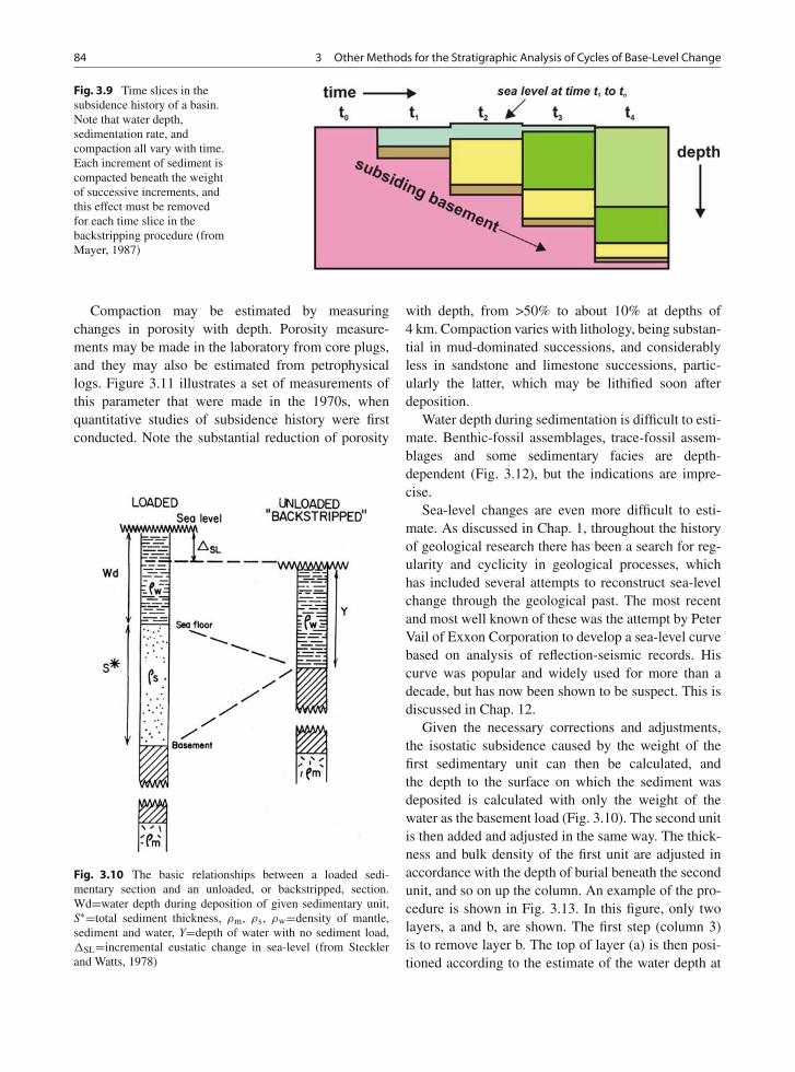
84 3 Other Methods for the Stratigraphic Analysis of Cycles of Base-Level Change
Fig. 3.9 Time slices in thesubsidence history of a basin.Note that water depth,sedimentation rate, andcompaction all vary with time.Each increment of sediment iscompacted beneath the weightof successive increments, andthis effect must be removedfor each time slice in thebackstripping procedure (fromMayer, 1987)
Compaction may be estimated by measuringchanges in porosity with depth. Porosity measure-ments may be made in the laboratory from core plugs,and they may also be estimated from petrophysicallogs. Figure 3.11 illustrates a set of measurements ofthis parameter that were made in the 1970s, whenquantitative studies of subsidence history were firstconducted. Note the substantial reduction of porosity
Fig. 3.10 The basic relationships between a loaded sedi-mentary section and an unloaded, or backstripped, section.Wd=water depth during deposition of given sedimentary unit,S∗=total sediment thickness, ρm, ρs, ρw=density of mantle,sediment and water, Y=depth of water with no sediment load,�SL=incremental eustatic change in sea-level (from Stecklerand Watts, 1978)
with depth, from >50% to about 10% at depths of4 km. Compaction varies with lithology, being substan-tial in mud-dominated successions, and considerablyless in sandstone and limestone successions, partic-ularly the latter, which may be lithified soon afterdeposition.
Water depth during sedimentation is difficult to esti-mate. Benthic-fossil assemblages, trace-fossil assem-blages and some sedimentary facies are depth-dependent (Fig. 3.12), but the indications are impre-cise.
Sea-level changes are even more difficult to esti-mate. As discussed in Chap. 1, throughout the historyof geological research there has been a search for reg-ularity and cyclicity in geological processes, whichhas included several attempts to reconstruct sea-levelchange through the geological past. The most recentand most well known of these was the attempt by PeterVail of Exxon Corporation to develop a sea-level curvebased on analysis of reflection-seismic records. Hiscurve was popular and widely used for more than adecade, but has now been shown to be suspect. This isdiscussed in Chap. 12.
Given the necessary corrections and adjustments,the isostatic subsidence caused by the weight of thefirst sedimentary unit can then be calculated, andthe depth to the surface on which the sediment wasdeposited is calculated with only the weight of thewater as the basement load (Fig. 3.10). The second unitis then added and adjusted in the same way. The thick-ness and bulk density of the first unit are adjusted inaccordance with the depth of burial beneath the secondunit, and so on up the column. An example of the pro-cedure is shown in Fig. 3.13. In this figure, only twolayers, a and b, are shown. The first step (column 3)is to remove layer b. The top of layer (a) is then posi-tioned according to the estimate of the water depth at
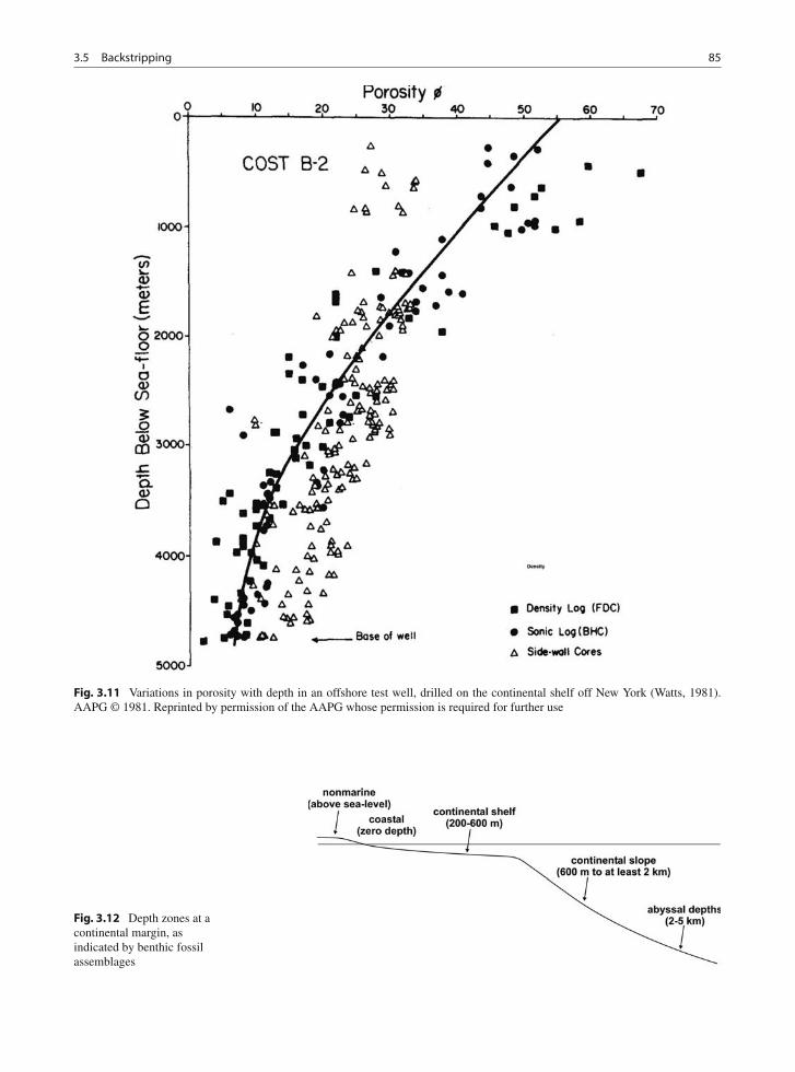
3.5 Backstripping 85
Fig. 3.11 Variations in porosity with depth in an offshore test well, drilled on the continental shelf off New York (Watts, 1981).AAPG © 1981. Reprinted by permission of the AAPG whose permission is required for further use
Fig. 3.12 Depth zones at acontinental margin, asindicated by benthic fossilassemblages
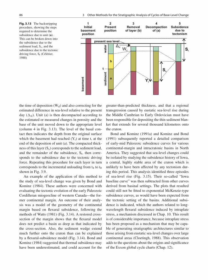
86 3 Other Methods for the Stratigraphic Analysis of Cycles of Base-Level Change
Fig. 3.13 The backstrippingprocedure, showing the stepsrequired to determine thesubsidence due to unit (a).This can be broken down intothe subsidence due to thesediment load, Ss, and thesubsidence due to the tectonicdriving force, St (Célérier,1988)
the time of deposition (Wd) and also correcting for theestimated difference in sea-level relative to the presentday (�sl). Unit (a) is then decompacted according tothe estimated or measured changes in porosity and thebase of the unit moved down to the appropriate level(column 4 in Fig. 3.13). The level of the basal con-tact then indicates the depth from the original surfacewhich the basement had reached (Yt) at time t, at theend of the deposition of unit (a). The compacted thick-ness of this layer (Ss) corresponds to the sediment load,and the remainder of the subsidence, St, then corre-sponds to the subsidence due to the tectonic drivingforce. Repeating this procedure for each layer in turncorresponds to the incremental unloading from t4 to t0shown in Fig. 3.9.
An example of the application of this method tothe study of sea-level change was given by Bond andKominz (1984). These authors were concerned withevaluating the tectonic evolution of the early PaleozoicCordilleran miogeocline of western Canada—the for-mer continental margin. An outcome of their analy-sis was a model of the geometry of the continentalmargin based on flexural subsidence, following themethods of Watts (1981) (Fig. 3.14). A restored cross-section of the margin shows that the flexural modeldoes not predict a basin as deep as that indicated bythe cross-section. Also, the sediment wedge extendmuch further onto the craton than can be explainedby a flexural-subsidence model (Fig. 3.14). Bond andKominz (1984) suggested that thermal subsidence mayhave been underestimated, and could account for the
greater-than-predicted thickness, and that a regionaltransgression caused by eustatic sea-level rise duringthe Middle Cambrian to Early Ordovician must havebeen responsible for depositing the thin sediment blan-ket that extends for several thousand kilometres ontothe craton.
Bond and Kominz (1991a) and Kominz and Bond(1991) subsequently reported a detailed comparisonof early-mid Paleozoic subsidence curves for variouscontinental-margin and intracratonic basins in NorthAmerica. They suggested that sea-level changes couldbe isolated by studying the subsidence history of Iowa,a central, highly stable area of the craton which isunlikely to have been affected by any tectonism dur-ing this period. This analysis identified three episodesof sea-level rise (Fig. 3.15). Their so-called “Iowabaseline curve” was then subtracted from other curvesderived from basinal settings. The plots that resultedcould still not be fitted to exponential McKenzie-typesubsidence curves, as would have been expected fromthe tectonic setting of the basins. Additional subsi-dence is indicated, which the authors related to long-wavelength flexural subsidence induced by intraplatestress, a mechanism discussed in Chap. 10. This resultis of considerable importance, because intraplate stresshas been proposed as a mechanism that may be capa-ble of generating stratigraphic architectures similar tothose arising from eustatic sea-level changes over largecontinental areas (Cloetingh, 1988). This observationadds to the questions about the origins and significanceof the Exxon global cycle charts (Chap. 12).
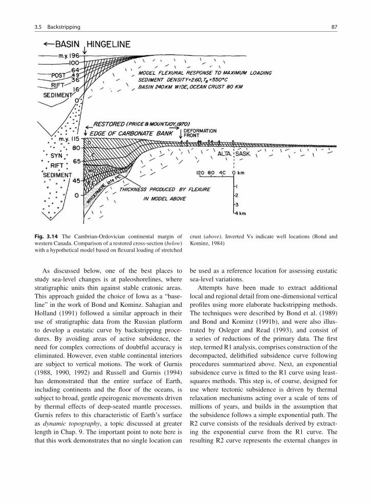
3.5 Backstripping 87
Fig. 3.14 The Cambrian-Ordovician continental margin ofwestern Canada. Comparison of a restored cross-section (below)with a hypothetical model based on flexural loading of stretched
crust (above). Inverted Vs indicate well locations (Bond andKominz, 1984)
As discussed below, one of the best places tostudy sea-level changes is at paleoshorelines, wherestratigraphic units thin against stable cratonic areas.This approach guided the choice of Iowa as a “base-line” in the work of Bond and Kominz. Sahagian andHolland (1991) followed a similar approach in theiruse of stratigraphic data from the Russian platformto develop a eustatic curve by backstripping proce-dures. By avoiding areas of active subsidence, theneed for complex corrections of doubtful accuracy iseliminated. However, even stable continental interiorsare subject to vertical motions. The work of Gurnis(1988, 1990, 1992) and Russell and Gurnis (1994)has demonstrated that the entire surface of Earth,including continents and the floor of the oceans, issubject to broad, gentle epeirogenic movements drivenby thermal effects of deep-seated mantle processes.Gurnis refers to this characteristic of Earth’s surfaceas dynamic topography, a topic discussed at greaterlength in Chap. 9. The important point to note here isthat this work demonstrates that no single location can
be used as a reference location for assessing eustaticsea-level variations.
Attempts have been made to extract additionallocal and regional detail from one-dimensional verticalprofiles using more elaborate backstripping methods.The techniques were described by Bond et al. (1989)and Bond and Kominz (1991b), and were also illus-trated by Osleger and Read (1993), and consist ofa series of reductions of the primary data. The firststep, termed R1 analysis, comprises construction of thedecompacted, delithified subsidence curve followingprocedures summarized above. Next, an exponentialsubsidence curve is fitted to the R1 curve using least-squares methods. This step is, of course, designed foruse where tectonic subsidence is driven by thermalrelaxation mechanisms acting over a scale of tens ofmillions of years, and builds in the assumption thatthe subsidence follows a simple exponential path. TheR2 curve consists of the residuals derived by extract-ing the exponential curve from the R1 curve. Theresulting R2 curve represents the external changes in
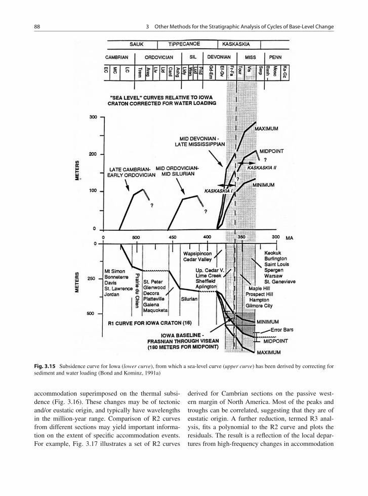
88 3 Other Methods for the Stratigraphic Analysis of Cycles of Base-Level Change
Fig. 3.15 Subsidence curve for Iowa (lower curve), from which a sea-level curve (upper curve) has been derived by correcting forsediment and water loading (Bond and Kominz, 1991a)
accommodation superimposed on the thermal subsi-dence (Fig. 3.16). These changes may be of tectonicand/or eustatic origin, and typically have wavelengthsin the million-year range. Comparison of R2 curvesfrom different sections may yield important informa-tion on the extent of specific accommodation events.For example, Fig. 3.17 illustrates a set of R2 curves
derived for Cambrian sections on the passive west-ern margin of North America. Most of the peaks andtroughs can be correlated, suggesting that they are ofeustatic origin. A further reduction, termed R3 anal-ysis, fits a polynomial to the R2 curve and plots theresiduals. The result is a reflection of the local depar-tures from high-frequency changes in accommodation
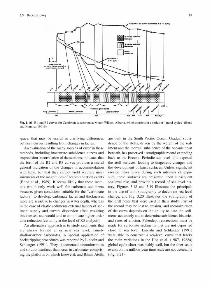
3.5 Backstripping 89
Fig. 3.16 R1 and R2 curves for Cambrian succession at Mount Wilson, Alberta, which consists of a series of “grand cycles” (Bondand Kominz, 1991b)
space, that may be useful in clarifying differencesbetween curves resulting from changes in facies.
An evaluation of the many sources of error in thesemethods, including inaccurate subsidence curves andimprecision in correlation of the sections, indicates thatthe form of the R2 and R3 curves provides a usefulgeneral indication of the changes in accommodationwith time, but that they cannot yield accurate mea-surements of the magnitudes of accommodation events(Bond et al., 1989). It seems likely that these meth-ods would only work well for carbonate sedimentsbecause, given conditions suitable for the “carbonatefactory” to develop, carbonate facies and thicknessesmore are sensitive to changes in water depth, whereasin the case of clastic sediments external factors of sed-iment supply and current dispersion affect resultingthicknesses, and would tend to complicate higher-orderdata reduction (certainly at the level of R3 analysis).
An alternative approach is to study sediments thatare always formed at or near sea level, namelyshallow-water carbonates. A special application ofbackstripping procedures was reported by Lincoln andSchlanger (1991). They documented unconformitiesand solution surfaces that occur in carbonates compris-ing the platform on which Enewetak and Bikini Atolls
are built in the South Pacific Ocean. Gradual subsi-dence of the atolls, driven by the weight of the sed-iment and the thermal subsidence of the oceanic crustbeneath, has preserved a stratigraphic record extendingback to the Eocene. Periodic sea-level falls exposedthe atoll surfaces, leading to diagenetic changes andthe development of karst surfaces. Unless significanterosion takes place during such intervals of expo-sure, these surfaces are preserved upon subsequentsea-level rise, and provide a record of sea-level his-tory. Figures 3.18 and 3.19 illustrate the principalsin the use of atoll stratigraphy to document sea-levelchange, and Fig. 3.20 illustrates the stratigraphy ofthe drill holes that were used in their study. Part ofthe record may be lost to erosion, and reconstructionof the curve depends on the ability to date the sedi-ments accurately and to determine subsidence historiesand rates of erosion. Paleodepth corrections must bemade for carbonate sediments that are not depositedclose to sea level. Lincoln and Schlanger (1991)were able to construct a sea-level curve that tracksthe main variations in the Haq et al. (1987, 1988a)global cycle chart reasonably well, but the finer-scaleevents on the million-year time scale are not detectable(Fig. 3.21).
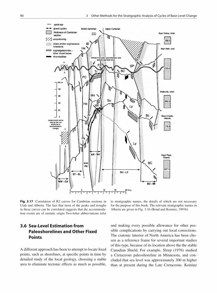
90 3 Other Methods for the Stratigraphic Analysis of Cycles of Base-Level Change
Fig. 3.17 Correlation of R2 curves for Cambrian sections inUtah and Alberta. The fact that most of the peaks and troughsin these curves can be correlated suggests that the accommoda-tion events are of eustatic origin Two-letter abbreviations refer
to stratigraphic names, the details of which are not necessaryfor the purpose of this book. The relevant stratigraphic names inAlberta are given in Fig. 3.16 (Bond and Kominz, 1991b)
3.6 Sea-Level Estimation fromPaleoshorelines and Other FixedPoints
A different approach has been to attempt to locate fixedpoints, such as shorelines, at specific points in time bydetailed study of the local geology, choosing a stablearea to eliminate tectonic effects as much as possible,
and making every possible allowance for other pos-sible complications by carrying out local corrections.The cratonic interior of North America has been cho-sen as a reference frame for several important studiesof this type, because of its location above the the stableCanadian Shield. For example, Sleep (1976) studieda Cretaceous paleoshoreline in Minnesota, and con-cluded that sea level was approximately 300 m higherthan at present during the Late Cretaceous. Kominz
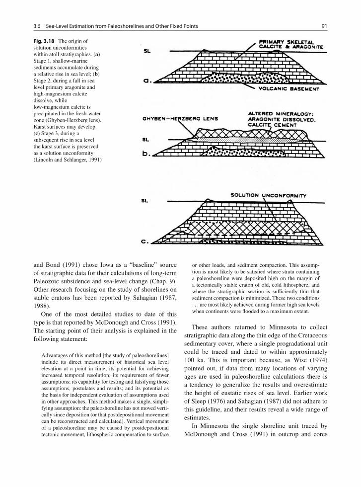
3.6 Sea-Level Estimation from Paleoshorelines and Other Fixed Points 91
Fig. 3.18 The origin ofsolution unconformitieswithin atoll stratigraphies. (a)Stage 1, shallow-marinesediments accumulate duringa relative rise in sea level; (b)Stage 2, during a fall in sealevel primary aragonite andhigh-magnesium calcitedissolve, whilelow-magnesium calcite isprecipitated in the fresh-waterzone (Ghyben-Herzberg lens).Karst surfaces may develop.(c) Stage 3, during asubsequent rise in sea levelthe karst surface is preservedas a solution unconformity(Lincoln and Schlanger, 1991)
and Bond (1991) chose Iowa as a “baseline” sourceof stratigraphic data for their calculations of long-termPaleozoic subsidence and sea-level change (Chap. 9).Other research focusing on the study of shorelines onstable cratons has been reported by Sahagian (1987,1988).
One of the most detailed studies to date of thistype is that reported by McDonough and Cross (1991).The starting point of their analysis is explained in thefollowing statement:
Advantages of this method [the study of paleoshorelines]include its direct measurement of historical sea levelelevation at a point in time; its potential for achievingincreased temporal resolution; its requirement of fewerassumptions; its capability for testing and falsifying thoseassumptions, postulates and results; and its potential asthe basis for independent evaluation of assumptions usedin other approaches. This method makes a single, simpli-fying assumption: the paleoshoreline has not moved verti-cally since deposition (or that postdepositional movementcan be reconstructed and calculated). Vertical movementof a paleoshoreline may be caused by postdepositionaltectonic movement, lithospheric compensation to surface
or other loads, and sediment compaction. This assump-tion is most likely to be satisfied where strata containinga paleoshoreline were deposited high on the margin ofa tectonically stable craton of old, cold lithosphere, andwhere the stratigraphic section is sufficiently thin thatsediment compaction is minimized. These two conditions. . . are most likely achieved during former high sea levelswhen continents were flooded to a maximum extent.
These authors returned to Minnesota to collectstratigraphic data along the thin edge of the Cretaceoussedimentary cover, where a single progradational unitcould be traced and dated to within approximately100 ka. This is important because, as Wise (1974)pointed out, if data from many locations of varyingages are used in paleoshoreline calculations there isa tendency to generalize the results and overestimatethe height of eustatic rises of sea level. Earlier workof Sleep (1976) and Sahagian (1987) did not adhere tothis guideline, and their results reveal a wide range ofestimates.
In Minnesota the single shoreline unit traced byMcDonough and Cross (1991) in outcrop and cores
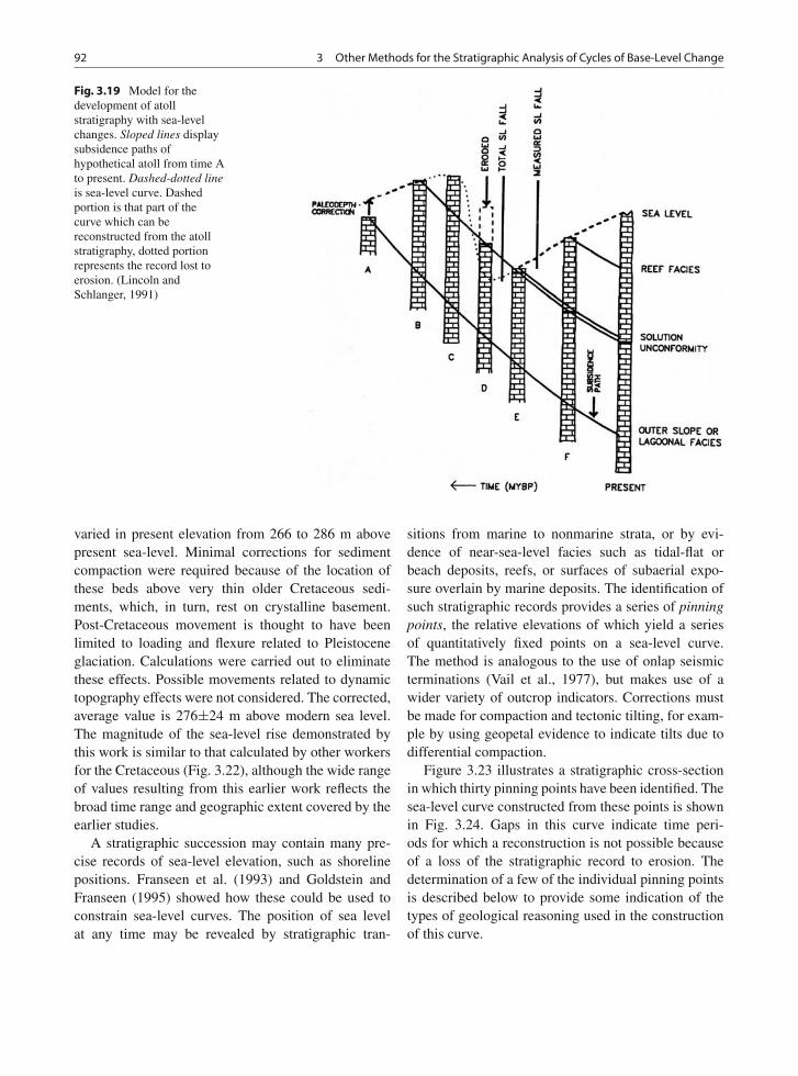
92 3 Other Methods for the Stratigraphic Analysis of Cycles of Base-Level Change
Fig. 3.19 Model for thedevelopment of atollstratigraphy with sea-levelchanges. Sloped lines displaysubsidence paths ofhypothetical atoll from time Ato present. Dashed-dotted lineis sea-level curve. Dashedportion is that part of thecurve which can bereconstructed from the atollstratigraphy, dotted portionrepresents the record lost toerosion. (Lincoln andSchlanger, 1991)
varied in present elevation from 266 to 286 m abovepresent sea-level. Minimal corrections for sedimentcompaction were required because of the location ofthese beds above very thin older Cretaceous sedi-ments, which, in turn, rest on crystalline basement.Post-Cretaceous movement is thought to have beenlimited to loading and flexure related to Pleistoceneglaciation. Calculations were carried out to eliminatethese effects. Possible movements related to dynamictopography effects were not considered. The corrected,average value is 276±24 m above modern sea level.The magnitude of the sea-level rise demonstrated bythis work is similar to that calculated by other workersfor the Cretaceous (Fig. 3.22), although the wide rangeof values resulting from this earlier work reflects thebroad time range and geographic extent covered by theearlier studies.
A stratigraphic succession may contain many pre-cise records of sea-level elevation, such as shorelinepositions. Franseen et al. (1993) and Goldstein andFranseen (1995) showed how these could be used toconstrain sea-level curves. The position of sea levelat any time may be revealed by stratigraphic tran-
sitions from marine to nonmarine strata, or by evi-dence of near-sea-level facies such as tidal-flat orbeach deposits, reefs, or surfaces of subaerial expo-sure overlain by marine deposits. The identification ofsuch stratigraphic records provides a series of pinningpoints, the relative elevations of which yield a seriesof quantitatively fixed points on a sea-level curve.The method is analogous to the use of onlap seismicterminations (Vail et al., 1977), but makes use of awider variety of outcrop indicators. Corrections mustbe made for compaction and tectonic tilting, for exam-ple by using geopetal evidence to indicate tilts due todifferential compaction.
Figure 3.23 illustrates a stratigraphic cross-sectionin which thirty pinning points have been identified. Thesea-level curve constructed from these points is shownin Fig. 3.24. Gaps in this curve indicate time peri-ods for which a reconstruction is not possible becauseof a loss of the stratigraphic record to erosion. Thedetermination of a few of the individual pinning pointsis described below to provide some indication of thetypes of geological reasoning used in the constructionof this curve.
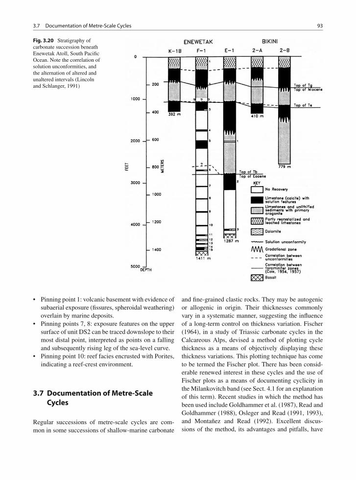
3.7 Documentation of Metre-Scale Cycles 93
Fig. 3.20 Stratigraphy ofcarbonate succession beneathEnewetak Atoll, South PacificOcean. Note the correlation ofsolution unconformities, andthe alternation of altered andunaltered intervals (Lincolnand Schlanger, 1991)
• Pinning point 1: volcanic basement with evidence ofsubaerial exposure (fissures, spheroidal weathering)overlain by marine deposits.
• Pinning points 7, 8: exposure features on the uppersurface of unit DS2 can be traced downslope to theirmost distal point, interpreted as points on a fallingand subsequently rising leg of the sea-level curve.
• Pinning point 10: reef facies encrusted with Porites,indicating a reef-crest environment.
3.7 Documentation of Metre-ScaleCycles
Regular successions of metre-scale cycles are com-mon in some successions of shallow-marine carbonate
and fine-grained clastic rocks. They may be autogenicor allogenic in origin. Their thicknesses commonlyvary in a systematic manner, suggesting the influenceof a long-term control on thickness variation. Fischer(1964), in a study of Triassic carbonate cycles in theCalcareous Alps, devised a method of plotting cyclethickness as a means of objectively displaying thesethickness variations. This plotting technique has cometo be termed the Fischer plot. There has been consid-erable renewed interest in these cycles and the use ofFischer plots as a means of documenting cyclicity inthe Milankovitch band (see Sect. 4.1 for an explanationof this term). Recent studies in which the method hasbeen used include Goldhammer et al. (1987), Read andGoldhammer (1988), Osleger and Read (1991, 1993),and Montañez and Read (1992). Excellent discus-sions of the method, its advantages and pitfalls, have
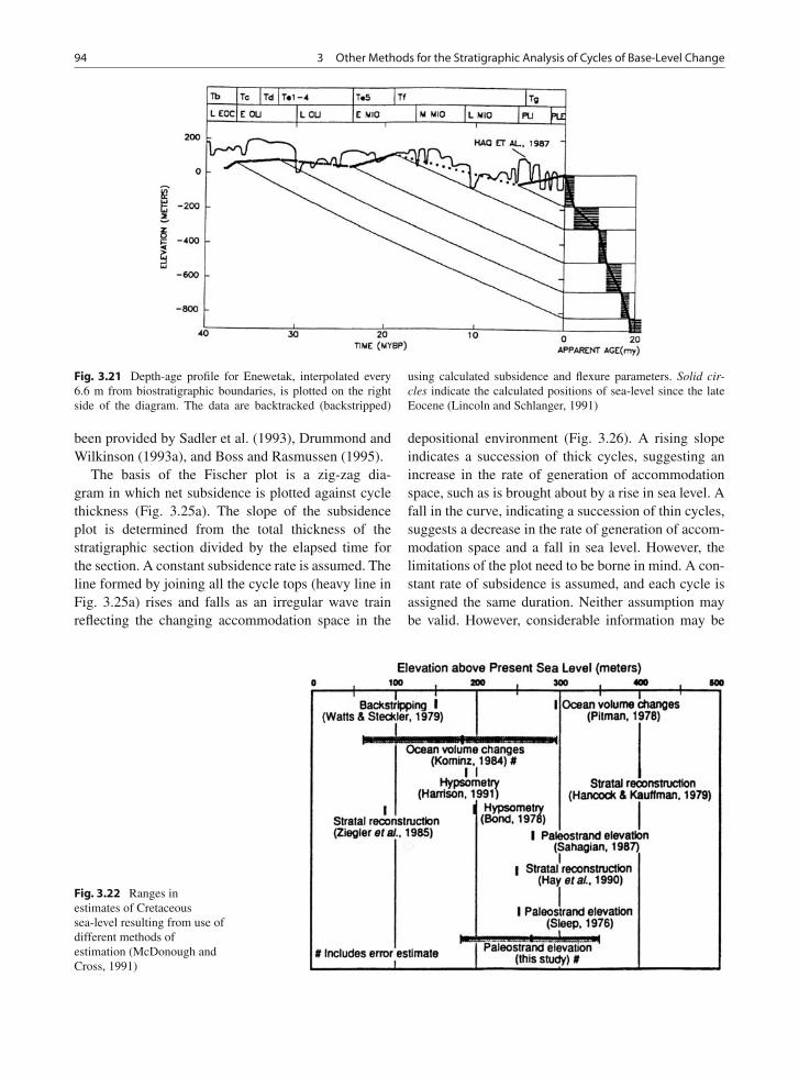
94 3 Other Methods for the Stratigraphic Analysis of Cycles of Base-Level Change
Fig. 3.21 Depth-age profile for Enewetak, interpolated every6.6 m from biostratigraphic boundaries, is plotted on the rightside of the diagram. The data are backtracked (backstripped)
using calculated subsidence and flexure parameters. Solid cir-cles indicate the calculated positions of sea-level since the lateEocene (Lincoln and Schlanger, 1991)
been provided by Sadler et al. (1993), Drummond andWilkinson (1993a), and Boss and Rasmussen (1995).
The basis of the Fischer plot is a zig-zag dia-gram in which net subsidence is plotted against cyclethickness (Fig. 3.25a). The slope of the subsidenceplot is determined from the total thickness of thestratigraphic section divided by the elapsed time forthe section. A constant subsidence rate is assumed. Theline formed by joining all the cycle tops (heavy line inFig. 3.25a) rises and falls as an irregular wave trainreflecting the changing accommodation space in the
depositional environment (Fig. 3.26). A rising slopeindicates a succession of thick cycles, suggesting anincrease in the rate of generation of accommodationspace, such as is brought about by a rise in sea level. Afall in the curve, indicating a succession of thin cycles,suggests a decrease in the rate of generation of accom-modation space and a fall in sea level. However, thelimitations of the plot need to be borne in mind. A con-stant rate of subsidence is assumed, and each cycle isassigned the same duration. Neither assumption maybe valid. However, considerable information may be
Fig. 3.22 Ranges inestimates of Cretaceoussea-level resulting from use ofdifferent methods ofestimation (McDonough andCross, 1991)
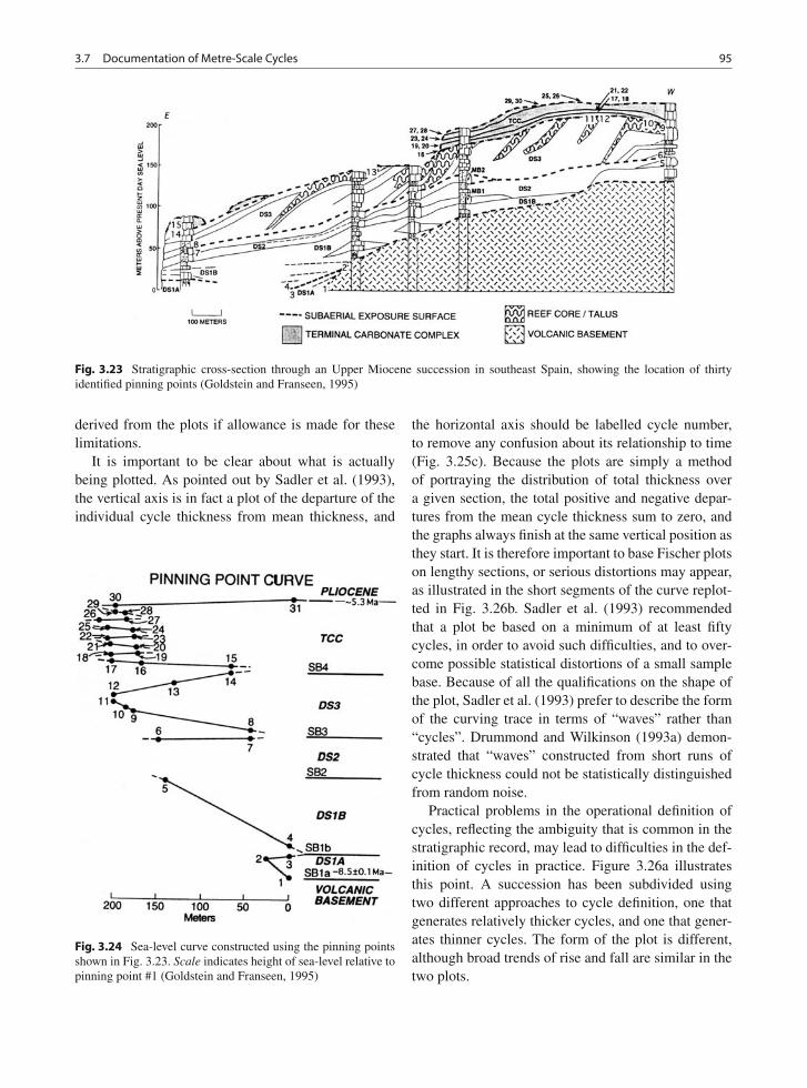
3.7 Documentation of Metre-Scale Cycles 95
Fig. 3.23 Stratigraphic cross-section through an Upper Miocene succession in southeast Spain, showing the location of thirtyidentified pinning points (Goldstein and Franseen, 1995)
derived from the plots if allowance is made for theselimitations.
It is important to be clear about what is actuallybeing plotted. As pointed out by Sadler et al. (1993),the vertical axis is in fact a plot of the departure of theindividual cycle thickness from mean thickness, and
Fig. 3.24 Sea-level curve constructed using the pinning pointsshown in Fig. 3.23. Scale indicates height of sea-level relative topinning point #1 (Goldstein and Franseen, 1995)
the horizontal axis should be labelled cycle number,to remove any confusion about its relationship to time(Fig. 3.25c). Because the plots are simply a methodof portraying the distribution of total thickness overa given section, the total positive and negative depar-tures from the mean cycle thickness sum to zero, andthe graphs always finish at the same vertical position asthey start. It is therefore important to base Fischer plotson lengthy sections, or serious distortions may appear,as illustrated in the short segments of the curve replot-ted in Fig. 3.26b. Sadler et al. (1993) recommendedthat a plot be based on a minimum of at least fiftycycles, in order to avoid such difficulties, and to over-come possible statistical distortions of a small samplebase. Because of all the qualifications on the shape ofthe plot, Sadler et al. (1993) prefer to describe the formof the curving trace in terms of “waves” rather than“cycles”. Drummond and Wilkinson (1993a) demon-strated that “waves” constructed from short runs ofcycle thickness could not be statistically distinguishedfrom random noise.
Practical problems in the operational definition ofcycles, reflecting the ambiguity that is common in thestratigraphic record, may lead to difficulties in the def-inition of cycles in practice. Figure 3.26a illustratesthis point. A succession has been subdivided usingtwo different approaches to cycle definition, one thatgenerates relatively thicker cycles, and one that gener-ates thinner cycles. The form of the plot is different,although broad trends of rise and fall are similar in thetwo plots.
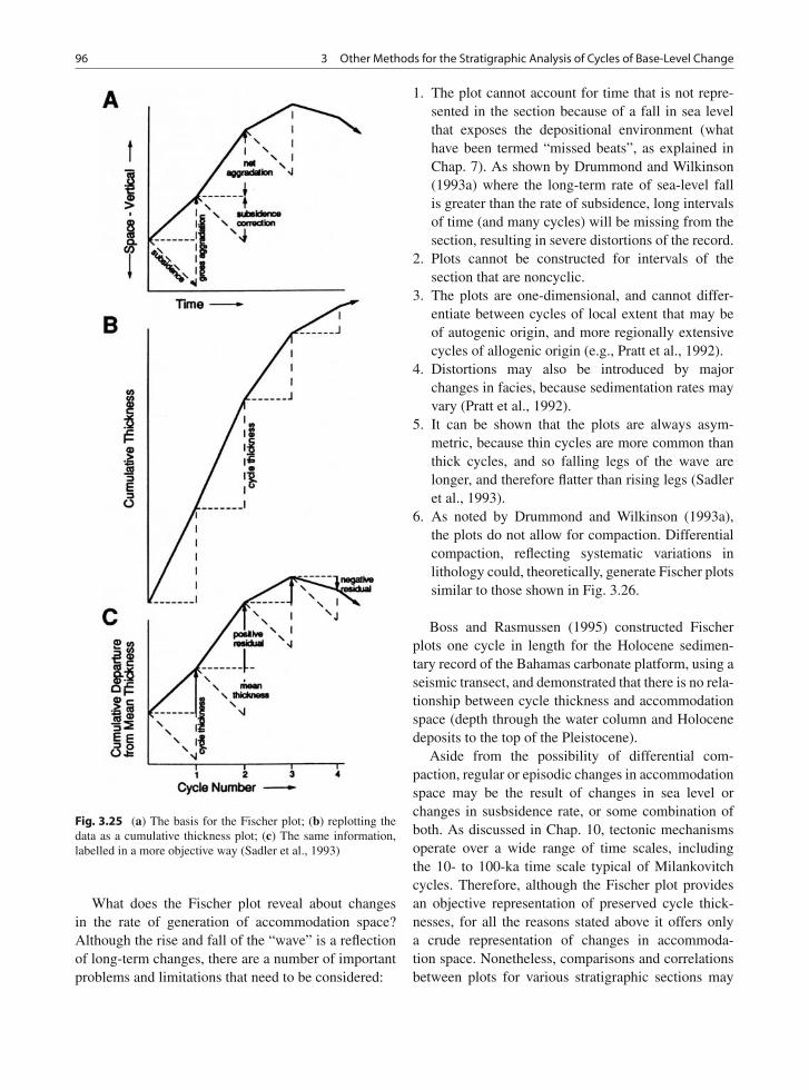
96 3 Other Methods for the Stratigraphic Analysis of Cycles of Base-Level Change
Fig. 3.25 (a) The basis for the Fischer plot; (b) replotting thedata as a cumulative thickness plot; (c) The same information,labelled in a more objective way (Sadler et al., 1993)
What does the Fischer plot reveal about changesin the rate of generation of accommodation space?Although the rise and fall of the “wave” is a reflectionof long-term changes, there are a number of importantproblems and limitations that need to be considered:
1. The plot cannot account for time that is not repre-sented in the section because of a fall in sea levelthat exposes the depositional environment (whathave been termed “missed beats”, as explained inChap. 7). As shown by Drummond and Wilkinson(1993a) where the long-term rate of sea-level fallis greater than the rate of subsidence, long intervalsof time (and many cycles) will be missing from thesection, resulting in severe distortions of the record.
2. Plots cannot be constructed for intervals of thesection that are noncyclic.
3. The plots are one-dimensional, and cannot differ-entiate between cycles of local extent that may beof autogenic origin, and more regionally extensivecycles of allogenic origin (e.g., Pratt et al., 1992).
4. Distortions may also be introduced by majorchanges in facies, because sedimentation rates mayvary (Pratt et al., 1992).
5. It can be shown that the plots are always asym-metric, because thin cycles are more common thanthick cycles, and so falling legs of the wave arelonger, and therefore flatter than rising legs (Sadleret al., 1993).
6. As noted by Drummond and Wilkinson (1993a),the plots do not allow for compaction. Differentialcompaction, reflecting systematic variations inlithology could, theoretically, generate Fischer plotssimilar to those shown in Fig. 3.26.
Boss and Rasmussen (1995) constructed Fischerplots one cycle in length for the Holocene sedimen-tary record of the Bahamas carbonate platform, using aseismic transect, and demonstrated that there is no rela-tionship between cycle thickness and accommodationspace (depth through the water column and Holocenedeposits to the top of the Pleistocene).
Aside from the possibility of differential com-paction, regular or episodic changes in accommodationspace may be the result of changes in sea level orchanges in susbsidence rate, or some combination ofboth. As discussed in Chap. 10, tectonic mechanismsoperate over a wide range of time scales, includingthe 10- to 100-ka time scale typical of Milankovitchcycles. Therefore, although the Fischer plot providesan objective representation of preserved cycle thick-nesses, for all the reasons stated above it offers onlya crude representation of changes in accommoda-tion space. Nonetheless, comparisons and correlationsbetween plots for various stratigraphic sections may
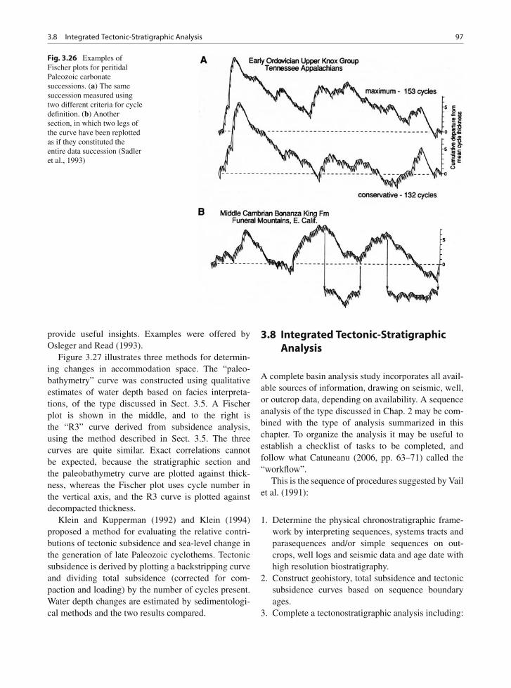
3.8 Integrated Tectonic-Stratigraphic Analysis 97
Fig. 3.26 Examples ofFischer plots for peritidalPaleozoic carbonatesuccessions. (a) The samesuccession measured usingtwo different criteria for cycledefinition. (b) Anothersection, in which two legs ofthe curve have been replottedas if they constituted theentire data succession (Sadleret al., 1993)
provide useful insights. Examples were offered byOsleger and Read (1993).
Figure 3.27 illustrates three methods for determin-ing changes in accommodation space. The “paleo-bathymetry” curve was constructed using qualitativeestimates of water depth based on facies interpreta-tions, of the type discussed in Sect. 3.5. A Fischerplot is shown in the middle, and to the right isthe “R3” curve derived from subsidence analysis,using the method described in Sect. 3.5. The threecurves are quite similar. Exact correlations cannotbe expected, because the stratigraphic section andthe paleobathymetry curve are plotted against thick-ness, whereas the Fischer plot uses cycle number inthe vertical axis, and the R3 curve is plotted againstdecompacted thickness.
Klein and Kupperman (1992) and Klein (1994)proposed a method for evaluating the relative contri-butions of tectonic subsidence and sea-level change inthe generation of late Paleozoic cyclothems. Tectonicsubsidence is derived by plotting a backstripping curveand dividing total subsidence (corrected for com-paction and loading) by the number of cycles present.Water depth changes are estimated by sedimentologi-cal methods and the two results compared.
3.8 Integrated Tectonic-StratigraphicAnalysis
A complete basin analysis study incorporates all avail-able sources of information, drawing on seismic, well,or outcrop data, depending on availability. A sequenceanalysis of the type discussed in Chap. 2 may be com-bined with the type of analysis summarized in thischapter. To organize the analysis it may be useful toestablish a checklist of tasks to be completed, andfollow what Catuneanu (2006, pp. 63–71) called the“workflow”.
This is the sequence of procedures suggested by Vailet al. (1991):
1. Determine the physical chronostratigraphic frame-work by interpreting sequences, systems tracts andparasequences and/or simple sequences on out-crops, well logs and seismic data and age date withhigh resolution biostratigraphy.
2. Construct geohistory, total subsidence and tectonicsubsidence curves based on sequence boundaryages.
3. Complete a tectonostratigraphic analysis including:
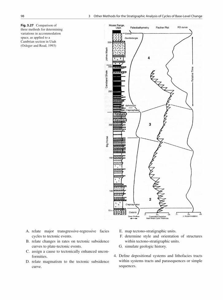
98 3 Other Methods for the Stratigraphic Analysis of Cycles of Base-Level Change
Fig. 3.27 Comparison ofthree methods for determiningvariations in accommodationspace, as applied to aCambrian section in Utah(Osleger and Read, 1993)
A. relate major transgressive-regressive faciescycles to tectonic events.
B. relate changes in rates on tectonic subsidencecurves to plate-tectonic events.
C. assign a cause to tectonically enhanced uncon-formities.
D. relate magmatism to the tectonic subsidencecurve.
E. map tectono-stratigraphic units.F. determine style and orientation of structures
within tectono-stratigraphic units.G. simulate geologic history.
4. Define depositional systems and lithofacies tractswithin systems tracts and parasequences or simplesequences.
3.8 Integrated Tectonic-Stratigraphic Analysis 99
5. Interpret paleogeography, geologic history,and stratigraphic signatures from resultingcross-sections, maps and chronostratigraphiccharts.
6. Locate potential reservoirs and source rocks forpossible sites of exploration.
Step one, the “physical chronostratigraphic frame-work” builds from the original hypothesis of Vailet al. (1977, p. 96) that the global sequence frame-work constitutes “an instrument of geochronology”(see Chap. 1). As discussed in Part IV, there are strongreasons for abandoning this practice. The establish-ment of the sequence framework should be a strictlyempirical process.
It is suggested that subsidence and maturation anal-ysis (Step 2) be carried out at the conclusion of thedetailed analysis, rather than near the beginning, asproposed in the Exxon approach. The reason is thata complete, thorough analysis requires the input of aconsiderable amount of stratigraphic data. Correctionsfor changing water depths and for porosity/lithificationcharacteristics, which are an integral part of suchanalysis, all require a detailed knowledge of the strati-graphic and paleogeographic evolution of the basin.
Catuneanu (2006, p. 63) suggested that the work-flow commence with a determination of the type ofbasin under study. The tectonic setting of the basindetermines its subsidence pattern, and a knowledgeof this may assist in the prediction of depositionalsystems and their spatial relationships. Such informa-tion may be invaluable in carrying out the preliminaryanalysis of regional seismic data.
A modified workflow is summarized below. Thepattern of work will depend on the nature of the project(regional seismic, exploratory well data, detaileddevelopment project, outcrop work) and will involvemoving back and forth between several of these steps(particularly between 2, 3, 4 and 5) as the analysisbecome more refined.
1. Determine tectonic setting of basin, and estab-lish regional style of subsidence and structuraldeformation.
2. If 2-D regional seismic data are available, ana-lyze and document stratal surfaces and seismic
terminations. Incorporate lithostratigraphic wellcorrelations, biostratigraphic and any other infor-mation regarding relative or absolute ages.
3. Develop an allostratigraphic framework.4. Make use of facies data from core and/or out-
crop to determine depositional environments andsystems. Develop a suite of possible stratigraphicmodels (e.g., shelf carbonate, slope submarine fan,coastal deltaic, etc.) that conform with availablestratigraphic and facies data.
5. Compile provenance and paleocurrent data, bylocation and by stratigraphic unit.
6. Establish a regional sequence framework with theuse of all available chronostratigraphic informa-tion.
7. Determine the relationships between sequenceboundaries and tectonic events, e.g., by trac-ing sequence boundaries into areas of structuraldeformation, and documenting the architectureof onlap/offlap relationships, fault offsets, uncon-formable discordancies, etc.
8. Establish the relationship between sequenceboundaries and regional tectonic history, based onplate-kinematic reconstructions.
9. Explore other possible scenarios for sequence gen-eration, such as climate change, and its effectson sediment supply depositional environments andsea levels.
10. Refine the sequence-stratigraphic model.Subdivide sequences into depositional systemstracts and interpret facies.
11. Construct regional structural, isopach, and faciesmaps, interpret paleogeographic evolution, anddevelop plays and prospects based on this analysis.
12. Develop detailed subsidence and thermal-maturation history by backstripping/geohistoryanalysis.
This book is concerned primarily with the inter-pretation of sequences. Parts II and III focus onSteps 7−10. Part IV discusses the issue of chronos-tratigraphy and correlation, and attempts to provide aframework for the use of chronostratigraphic data inthe establishment and interpretation of the sequenceframework (Steps 2−6).
Part IIThe Stratigraphic Framework
Abundant stratigraphic data have been amassed since AAPG Memoir 26 was pub-lished in 1977, setting off the current high level of interest in sequence stratigraphy.Some of this consists of regional seismic surveys, but a great deal of work has alsobeen carried out with well records and outcrops. The purpose of this section of thebook is to present some of the basic stratigraphic data, with a minimum of interpre-tation, as a basis for discussion of mechanisms and controls that constitutes much ofthe remainder of the book.
The wealth of data now available has demonstrated that the original concept ofa simple rank ordering of sequences, from first- to fifth- (and higher?) order, is toosimplistic. Although sequence-generating mechanisms have natural episodicities orperiodicities, the time periods (wavelengths) of these processes overlap, and do notsupport the use of this simple classification (Table 4.1). A subdivision of sequencesaccording to episodicity is used for descriptive purposes in this part of the book; itforms the basis for the subdivision into three chapters; but no genetic interpretationsare implied by this subdivision.
Most of the current interest and controversy regarding sequence stratigraphyfocuses on sequences of a few-million-years duration, and less. For this reason,considerably more space is devoted to these cycles (Chaps. 6 and 7).
It has been necessary to make a judicious selection of examples from the wealth ofdata now available in the published record. The reader is urged to turn to the originalpublications wherever possible for the details of regional setting, stratigraphy, facies,etc.
102 Part II The Stratigraphic Framework
• Sequential ordering of beds is found in nearly all stratigraphic successions on var-ious scales. It is thought to be the result from the combination of regional to globalcausal factors and modifying local environmental processes (Einsele and Ricken,1991, p. 611).
• The Exxon group’s distinction of first-, second- and third-order eustatic cyclesis useful. The first-order cycles are the two Phanerozoic supercycles of Fischer(1984), and general agreement exists that the changes of sea level are gen-uinely global. A fair measure of consensus also exists that the second-ordercycles (10–18 Myr duration) have a eustatic origin as well, but the third-ordercycles (1–10 Myr) are more controversial. Many stratigraphic experts indepen-dent of the Exxon group are, however, persuaded of their reality, on the basis ofcorrelation over extensive regions . . . Besides these larger cycles, some woulddistinguish smaller, fourth- and fifth-order cycles, usually no more than a fewmetres thick and signifying durations of tens to hundreds of thousands of years.One currently popular idea is that late Paleozoic and other comparable cyclothemsare glacioeustatic phenomena under the ultimate control of an orbital forcingmechanism that affects global climate (Hallam, 1992a, p. 204).
• . . . the discrimination of stratigraphic hierarchies and their designation as nth-order cycles may constitute little more than the arbitrary subdivision of anuninterrupted stratigraphic continuum (Drummond and Wilkinson, 1996, p. 1).
• This system of ordering cycles is widely used but has serious shortcomings. Bypretending that there exists a hierarchy of cycles, repetitive patterns, which havenothing in common except their duration, are mixed together. Such a classificationis just as meaningless as grouping elephants and fleas into an order based on theirsize (Schwarzacher, 2000, p. 52, in reference to the Vail et al., 1977, sequencehierarchy)
• Orders of stratigraphic sequences are being used loosely and with widely varyingdefinitions. The orders seem to be subdivisions of convenience rather than an indi-cation of natural structure. It is proposed that, at least at time scales of 103–106
years, sequences and systems tracts are scale-invariant fractal features in whichunits bounded by exposure surfaces and units bounded by flooding surfaces areabout equally likely (Schlager, 2004, p. 185)
Chapter 4
The Major Types of Stratigraphic Cycle
Contents
4.1 Introduction . . . . . . . . . . . . . . . . . 1034.2 Sequence Hierarchy . . . . . . . . . . . . . 1034.3 The Supercontinent Cycle . . . . . . . . . . 1124.4 Cycles with Episodicities of Tens of Millions
of Years . . . . . . . . . . . . . . . . . . . 1134.5 Cycles with Million-Year Episodicities . . . . 1144.6 Cycles with Episodicities of Less Than
One Million Years . . . . . . . . . . . . . . 117
4.1 Introduction
The duration and episodicity of geological events andstratigraphic cyclicity span at least sixteen orders ofmagnitude, ranging from the repeat time of burst-sweep cycles in turbulent boundary layers (10−6
years), to plate-tectonic cycles involving the forma-tion and breakup of supercontinents (109 years) (Miall,1991b; Einsele et al., 1991b; Figs. 4.1 and 4.2).The highest-frequency cyclicity of stratigraphic signif-icance is Milankovitch-band cyclicity, over time scalesof 104–105 years. Minor cyclicity may be apparent inthe geological record as a result of seasonal changesin weather, fluvial discharge, etc., the so-called cal-endar band of cyclicity (Fischer and Bottjer, 1991).Sunspots and other solar processes generate cyclicityon a 101–102-year scale of cyclicity, the solar band ofthe time scale. These processes and their products arenot discussed in this book.
The highest frequency of cyclicity discussed hereoverlaps with that of autogenic cyclicity, such aschannel migration or delta-lobe switching (103–104
years). Deltaic cycles are of the upward shoalingtype, bounded by the flooding surfaces formed by
lobe abandonment, and therefore fit the definition ofparasequences. This is one of the difficulties with thatterm, as touched on later.
There are four basic types of stratigraphic sequence(types A to D in Table 4.1). These four types are intro-duced briefly in this chapter, with detailed discussionand documentation constituting the remainder of PartII. These cycle types reflect the independent operationof at least four type of process, including regional tec-tonism and various controls on eustasy. Work is stillin progress on the analysis of tectonic mechanismsto determine the importance of other processes com-parable in scale, duration and areal effect. Importantsecond-order effects triggered or driven by these pri-mary mechanisms include changes in global climate,magmatism, ocean-water circulation patterns, the car-bon and oxygen cycles, and biogenesis, all of whichhave significant, measurable effects on the sediments.Sorting out the various processes and their effectsis currently one of the most vigorous areas of basinanalysis research.
4.2 Sequence Hierarchy
Depositional units constitute a hierarchy of scales,from the small-scale ripple cross-laminae through thevarious units constituting depositional systems, to thescale of the entire basin fill. This concept of “hierar-chy” is discussed in the context of geological time inChap. 13, and the ideas are summarized in Table 13.1.Important recent papers that deal with the subjectof depositional hierarchy are those of Van Wagoneret al. (1990), Miall (1991b), Mitchum and VanWagoner (1991), Nio and Yang (1991), Drummond
103A.D. Miall, The Geology of Stratigraphic Sequences, 2nd ed.,DOI 10.1007/978-3-642-05027-5_4, © Springer-Verlag Berlin Heidelberg 2010
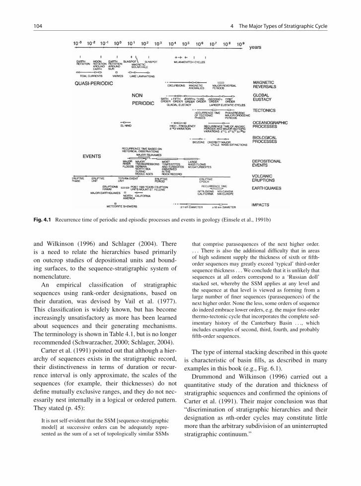
104 4 The Major Types of Stratigraphic Cycle
Fig. 4.1 Recurrence time of periodic and episodic processes and events in geology (Einsele et al., 1991b)
and Wilkinson (1996) and Schlager (2004). Thereis a need to relate the hierarchies based primarilyon outcrop studies of depositional units and bound-ing surfaces, to the sequence-stratigraphic system ofnomenclature.
An empirical classification of stratigraphicsequences using rank-order designations, based ontheir duration, was devised by Vail et al. (1977).This classification is widely known, but has becomeincreasingly unsatisfactory as more has been learnedabout sequences and their generating mechanisms.The terminology is shown in Table 4.1, but is no longerrecommended (Schwarzacher, 2000; Schlager, 2004).
Carter et al. (1991) pointed out that although a hier-archy of sequences exists in the stratigraphic record,their distinctiveness in terms of duration or recur-rence interval is only approximate, the scales of thesequences (for example, their thicknesses) do notdefine mutually exclusive ranges, and they do not nec-essarily nest internally in a logical or ordered pattern.They stated (p. 45):
It is not self-evident that the SSM [sequence-stratigraphicmodel] at successive orders can be adequately repre-sented as the sum of a set of topologically similar SSMs
that comprise parasequences of the next higher order.. . . There is also the additional difficulty that in areasof high sediment supply the thickness of sixth or fifth-order sequences may greatly exceed ‘typical’ third-ordersequence thickness . . . We conclude that it is unlikely thatsequences at all orders correspond to a ‘Russian doll’stacked set, whereby the SSM applies at any level andthe sequence at that level is viewed as forming from alarge number of finer sequences (parasequences) of thenext higher order. None the less, some orders of sequencedo indeed embrace lower orders, e.g. the major first-orderthermo-tectonic cycle that incorporates the complete sed-imentary history of the Canterbury Basin . . ., whichincludes examples of second, third, fourth, and probablyfifth-order sequences.
The type of internal stacking described in this quoteis characteristic of basin fills, as described in manyexamples in this book (e.g., Fig. 6.1).
Drummond and Wilkinson (1996) carried out aquantitative study of the duration and thickness ofstratigraphic sequences and confirmed the opinions ofCarter et al. (1991). Their major conclusion was that“discrimination of stratigraphic hierarchies and theirdesignation as nth-order cycles may constitute littlemore than the arbitrary subdivision of an uninterruptedstratigraphic continuum.”
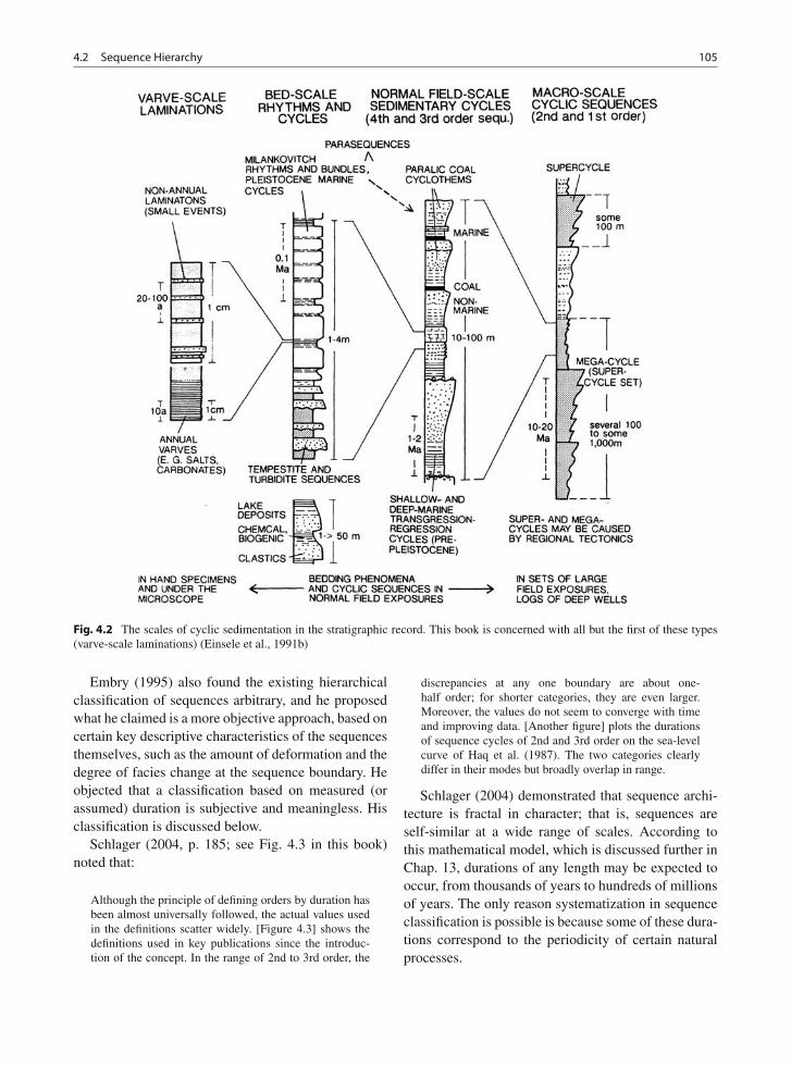
4.2 Sequence Hierarchy 105
Fig. 4.2 The scales of cyclic sedimentation in the stratigraphic record. This book is concerned with all but the first of these types(varve-scale laminations) (Einsele et al., 1991b)
Embry (1995) also found the existing hierarchicalclassification of sequences arbitrary, and he proposedwhat he claimed is a more objective approach, based oncertain key descriptive characteristics of the sequencesthemselves, such as the amount of deformation and thedegree of facies change at the sequence boundary. Heobjected that a classification based on measured (orassumed) duration is subjective and meaningless. Hisclassification is discussed below.
Schlager (2004, p. 185; see Fig. 4.3 in this book)noted that:
Although the principle of defining orders by duration hasbeen almost universally followed, the actual values usedin the definitions scatter widely. [Figure 4.3] shows thedefinitions used in key publications since the introduc-tion of the concept. In the range of 2nd to 3rd order, the
discrepancies at any one boundary are about one-half order; for shorter categories, they are even larger.Moreover, the values do not seem to converge with timeand improving data. [Another figure] plots the durationsof sequence cycles of 2nd and 3rd order on the sea-levelcurve of Haq et al. (1987). The two categories clearlydiffer in their modes but broadly overlap in range.
Schlager (2004) demonstrated that sequence archi-tecture is fractal in character; that is, sequences areself-similar at a wide range of scales. According tothis mathematical model, which is discussed further inChap. 13, durations of any length may be expected tooccur, from thousands of years to hundreds of millionsof years. The only reason systematization in sequenceclassification is possible is because some of these dura-tions correspond to the periodicity of certain naturalprocesses.
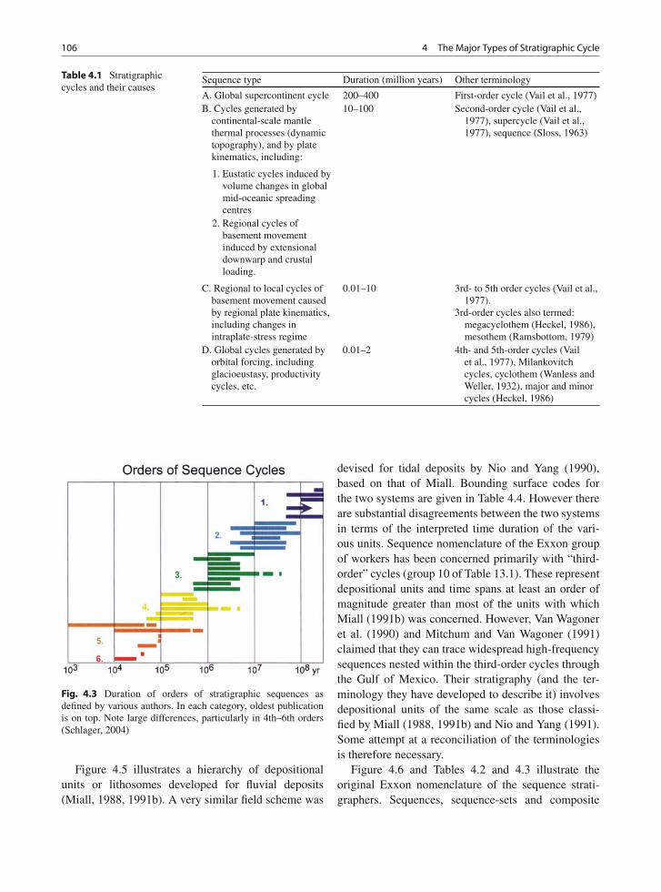
106 4 The Major Types of Stratigraphic Cycle
Table 4.1 Stratigraphiccycles and their causes
Sequence type Duration (million years) Other terminology
A. Global supercontinent cycle 200–400 First-order cycle (Vail et al., 1977)B. Cycles generated by
continental-scale mantlethermal processes (dynamictopography), and by platekinematics, including:
10–100 Second-order cycle (Vail et al.,1977), supercycle (Vail et al.,1977), sequence (Sloss, 1963)
1. Eustatic cycles induced byvolume changes in globalmid-oceanic spreadingcentres
2. Regional cycles ofbasement movementinduced by extensionaldownwarp and crustalloading.
C. Regional to local cycles ofbasement movement causedby regional plate kinematics,including changes inintraplate-stress regime
0.01–10 3rd- to 5th order cycles (Vail et al.,1977).
3rd-order cycles also termed:megacyclothem (Heckel, 1986),mesothem (Ramsbottom, 1979)
D. Global cycles generated byorbital forcing, includingglacioeustasy, productivitycycles, etc.
0.01–2 4th- and 5th-order cycles (Vailet al., 1977), Milankovitchcycles, cyclothem (Wanless andWeller, 1932), major and minorcycles (Heckel, 1986)
Fig. 4.3 Duration of orders of stratigraphic sequences asdefined by various authors. In each category, oldest publicationis on top. Note large differences, particularly in 4th–6th orders(Schlager, 2004)
Figure 4.5 illustrates a hierarchy of depositionalunits or lithosomes developed for fluvial deposits(Miall, 1988, 1991b). A very similar field scheme was
devised for tidal deposits by Nio and Yang (1990),based on that of Miall. Bounding surface codes forthe two systems are given in Table 4.4. However thereare substantial disagreements between the two systemsin terms of the interpreted time duration of the vari-ous units. Sequence nomenclature of the Exxon groupof workers has been concerned primarily with “third-order” cycles (group 10 of Table 13.1). These representdepositional units and time spans at least an order ofmagnitude greater than most of the units with whichMiall (1991b) was concerned. However, Van Wagoneret al. (1990) and Mitchum and Van Wagoner (1991)claimed that they can trace widespread high-frequencysequences nested within the third-order cycles throughthe Gulf of Mexico. Their stratigraphy (and the ter-minology they have developed to describe it) involvesdepositional units of the same scale as those classi-fied by Miall (1988, 1991b) and Nio and Yang (1991).Some attempt at a reconciliation of the terminologiesis therefore necessary.
Figure 4.6 and Tables 4.2 and 4.3 illustrate theoriginal Exxon nomenclature of the sequence strati-graphers. Sequences, sequence-sets and composite
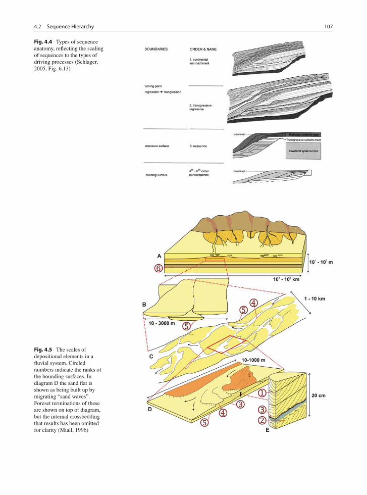
4.2 Sequence Hierarchy 107
Fig. 4.4 Types of sequenceanatomy, reflecting the scalingof sequences to the types ofdriving processes (Schlager,2005, Fig. 6.13)
Fig. 4.5 The scales ofdepositional elements in afluvial system. Circlednumbers indicate the ranks ofthe bounding surfaces. Indiagram D the sand flat isshown as being built up bymigrating “sand waves”.Foreset terminations of theseare shown on top of diagram,but the internal crossbeddingthat results has been omittedfor clarity (Miall, 1996)
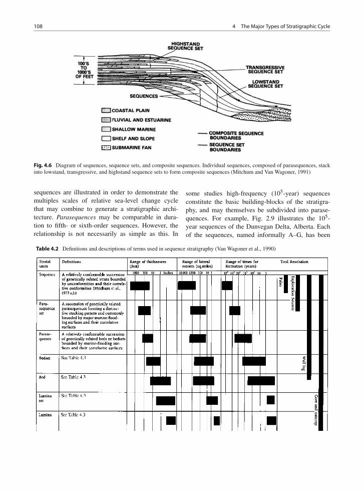
108 4 The Major Types of Stratigraphic Cycle
Fig. 4.6 Diagram of sequences, sequence sets, and composite sequences. Individual sequences, composed of parasequences, stackinto lowstand, transgressive, and highstand sequence sets to form composite sequences (Mitchum and Van Wagoner, 1991)
sequences are illustrated in order to demonstrate themultiples scales of relative sea-level change cyclethat may combine to generate a stratigraphic archi-tecture. Parasequences may be comparable in dura-tion to fifth- or sixth-order sequences. However, therelationship is not necessarily as simple as this. In
some studies high-frequency (105-year) sequencesconstitute the basic building-blocks of the stratigra-phy, and may themselves be subdivided into parase-quences. For example, Fig. 2.9 illustrates the 105-year sequences of the Dunvegan Delta, Alberta. Eachof the sequences, named informally A–G, has been
Table 4.2 Definitions and descriptions of terms used in sequence stratigraphy (Van Wagoner et al., 1990)
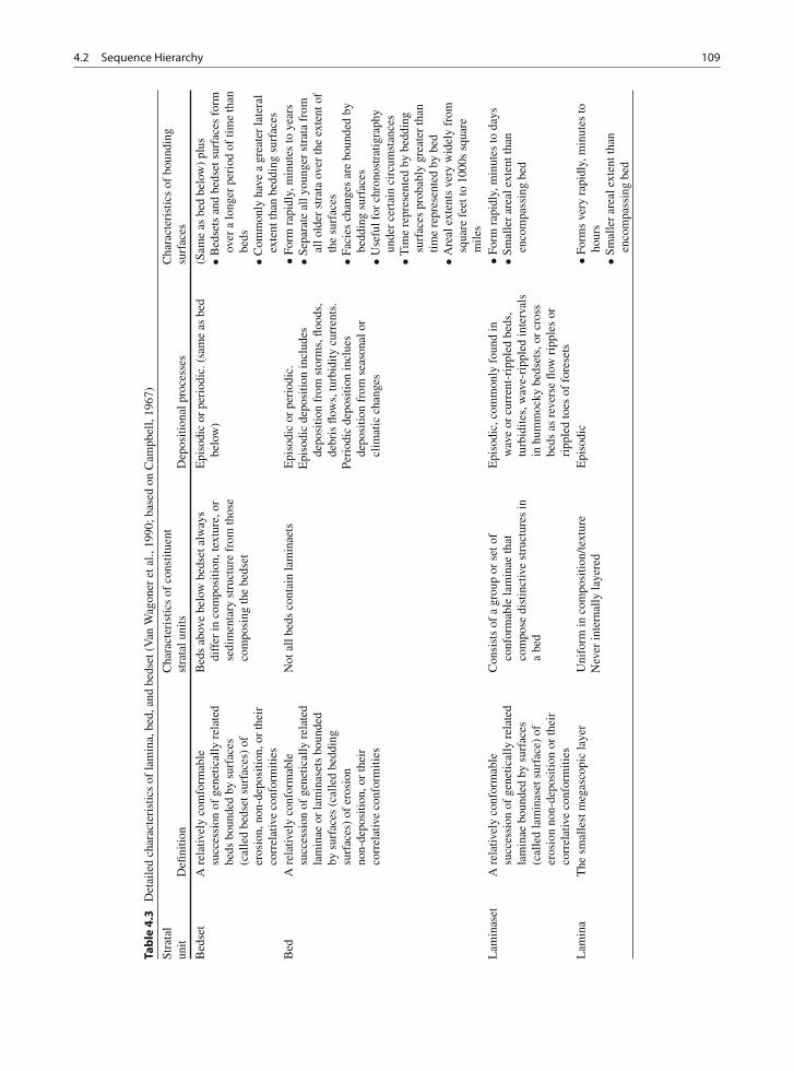
4.2 Sequence Hierarchy 109
Tab
le4
.3D
etai
led
char
acte
rist
ics
ofla
min
a,be
d,an
dbe
dset
(Van
Wag
oner
etal
.,19
90;b
ased
onC
ampb
ell,
1967
)
Stra
tal
unit
Defi
nitio
nC
hara
cter
istic
sof
cons
titue
ntst
rata
luni
tsD
epos
ition
alpr
oces
ses
Cha
ract
eris
tics
ofbo
undi
ngsu
rfac
es
Bed
set
Are
lativ
ely
com
form
able
succ
essi
onof
gene
tical
lyre
late
dbe
dsbo
unde
dby
surf
aces
(cal
led
beds
etsu
rfac
es)
ofer
osio
n,no
n-de
posi
tion,
orth
eir
corr
elat
ive
conf
orm
ities
Bed
sab
ove
belo
wbe
dset
alw
ays
diff
erin
com
posi
tion,
text
ure,
orse
dim
enta
ryst
ruct
ure
from
thos
eco
mpo
sing
the
beds
et
Epi
sodi
cor
peri
odic
.(sa
me
asbe
dbe
low
)(S
ame
asbe
dbe
low
)pl
us•B
edse
tsan
dbe
dset
surf
aces
form
over
alo
nger
peri
odof
time
than
beds
•Com
mon
lyha
vea
grea
ter
late
ral
exte
ntth
anbe
ddin
gsu
rfac
esB
edA
rela
tivel
yco
nfor
mab
lesu
cces
sion
ofge
netic
ally
rela
ted
lam
inae
orla
min
aset
sbo
unde
dby
surf
aces
(cal
led
bedd
ing
surf
aces
)of
eros
ion
non-
depo
sitio
n,or
thei
rco
rrel
ativ
eco
nfor
miti
es
Not
allb
eds
cont
ain
lam
inae
tsE
piso
dic
orpe
riod
ic.
Epi
sodi
cde
posi
tion
incl
udes
depo
sitio
nfr
omst
orm
s,flo
ods,
debr
isflo
ws,
turb
idity
curr
ents
.Pe
riod
icde
posi
tion
incl
ues
depo
sitio
nfr
omse
ason
alor
clim
atic
chan
ges
•For
mra
pidl
y,m
inut
esto
year
s•S
epar
ate
ally
oung
erst
rata
from
allo
lder
stra
taov
erth
eex
tent
ofth
esu
rfac
es•F
acie
sch
ange
sar
ebo
unde
dby
bedd
ing
surf
aces
•Use
fulf
orch
rono
stra
tigra
phy
unde
rce
rtai
nci
rcum
stan
ces
•Tim
ere
pres
ente
dby
bedd
ing
surf
aces
prob
ably
grea
ter
than
time
repr
esen
ted
bybe
d•A
real
exte
nts
very
wid
ely
from
squa
refe
etto
1000
ssq
uare
mile
sL
amin
aset
Are
lativ
ely
conf
orm
able
succ
essi
onof
gene
tical
lyre
late
dla
min
aebo
unde
dby
surf
aces
(cal
led
lam
inas
etsu
rfac
e)of
eros
ion
non-
depo
sitio
nor
thei
rco
rrel
ativ
eco
nfor
miti
es
Con
sist
sof
agr
oup
orse
tof
conf
orm
able
lam
inae
that
com
pose
dist
inct
ive
stru
ctur
esin
abe
d
Epi
sodi
c,co
mm
only
foun
din
wav
eor
curr
ent-
ripp
led
beds
,tu
rbid
ites,
wav
e-ri
pple
din
terv
als
inhu
mm
ocky
beds
ets,
orcr
oss
beds
asre
vers
eflo
wri
pple
sor
ripp
led
toes
offo
rese
ts
•For
mra
pidl
y,m
inut
esto
days
•Sm
alle
rar
eale
xten
ttha
nen
com
pass
ing
bed
Lam
ina
The
smal
lest
meg
asco
pic
laye
rU
nifo
rmin
com
posi
tion/
text
ure
Nev
erin
tern
ally
laye
red
Epi
sodi
c•F
orm
sve
ryra
pidl
y,m
inut
esto
hour
s•S
mal
ler
area
lext
entt
han
enco
mpa
ssin
gbe
d
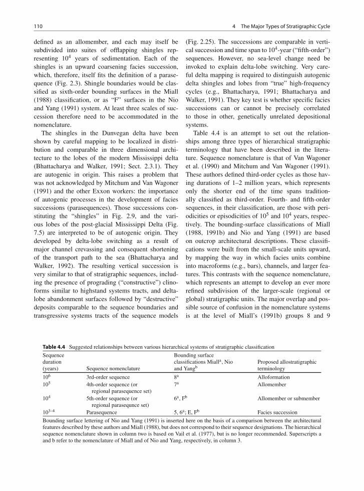
110 4 The Major Types of Stratigraphic Cycle
defined as an allomember, and each may itself besubdivided into suites of offlapping shingles rep-resenting 104 years of sedimentation. Each of theshingles is an upward coarsening facies succession,which, therefore, itself fits the definition of a parase-quence (Fig. 2.3). Shingle boundaries would be clas-sified as sixth-order bounding surfaces in the Miall(1988) classification, or as “F” surfaces in the Nioand Yang (1991) system. At least three scales of suc-cession therefore need to be accommodated in thenomenclature.
The shingles in the Dunvegan delta have beenshown by careful mapping to be localized in distri-bution and comparable in three dimensional archi-tecture to the lobes of the modern Mississippi delta(Bhattacharya and Walker, 1991; Sect. 2.3.1). Theyare autogenic in origin. This raises a problem thatwas not acknowledged by Mitchum and Van Wagoner(1991) and the other Exxon workers: the importanceof autogenic processes in the development of faciessuccessions (parasequences). Those successions con-stituting the “shingles” in Fig. 2.9, and the vari-ous lobes of the post-glacial Mississippi Delta (Fig.7.5) are interpreted to be of autogenic origin. Theydeveloped by delta-lobe switching as a result ofmajor channel crevassing and consequent shorteningof the transport path to the sea (Bhattacharya andWalker, 1992). The resulting vertical succession isvery similar to that of stratigraphic sequences, includ-ing the presence of prograding (“constructive”) clino-forms similar to highstand systems tracts, and delta-lobe abandonment surfaces followed by “destructive”deposits comparable to the sequence boundaries andtransgressive systems tracts of the sequence models
(Fig. 2.25). The successions are comparable in verti-cal succession and time span to 104-year (“fifth-order”)sequences. However, no sea-level change need beinvoked to explain delta-lobe switching. Very care-ful delta mapping is required to distinguish autogenicdelta shingles and lobes from “true” high-frequencycycles (e.g., Bhattacharya, 1991; Bhattacharya andWalker, 1991). They key test is whether specific faciessuccessions can or cannot be precisely correlatedto those in other, genetically unrelated depositionalsystems.
Table 4.4 is an attempt to set out the relation-ships among three types of hierarchical stratigraphicterminology that have been described in the litera-ture. Sequence nomenclature is that of Van Wagoneret al. (1990) and Mitchum and Van Wagoner (1991).These authors defined third-order cycles as those hav-ing durations of 1–2 million years, which representsonly the shorter end of the time spans tradition-ally classified as third-order. Fourth- and fifth-ordersequences, in their classification, are those with peri-odicities or episodicities of 105 and 104 years, respec-tively. The bounding-surface classifications of Miall(1988, 1991b) and Nio and Yang (1991) are basedon outcrop architectural descriptions. These classifi-cations were built from the small-scale units upward,by mapping the way in which facies units combineinto macroforms (e.g., bars), channels, and larger fea-tures. This contrasts with the sequence nomenclature,which represents an attempt to develop an ever morerefined subdivision of the larger-scale (regional orglobal) stratigraphic units. The major overlap and pos-sible source of confusion in the nomenclature systemsis at the level of Miall’s (1991b) groups 8 and 9
Table 4.4 Suggested relationships between various hierarchical systems of stratigraphic classification
Sequenceduration(years) Sequence nomenclature
Bounding surfaceclassifications Mialla, Nioand Yangb
Proposed allostratigraphicterminology
106 3rd-order sequence 8a Alloformation105 4th-order sequence (or
regional parasequence set)7a Allomember
104 5th-order sequence (orregional parasequnce set)
6a, Fb Allomember or submember
103–4 Parasequence 5, 6a; E, Fb Facies succession
Bounding surface lettering of Nio and Yang (1991) is inserted here on the basis of a comparison between the architecturalfeatures described by these authors and Miall (1988), but does not correspond to their sequence designations. The hierarchicalsequence nomenclature shown in column two is based on Vail et al. (1977), but is no longer recommended. Superscripts aand b refer to the nomenclature of Miall and of Nio and Yang, respectively, in column 3.
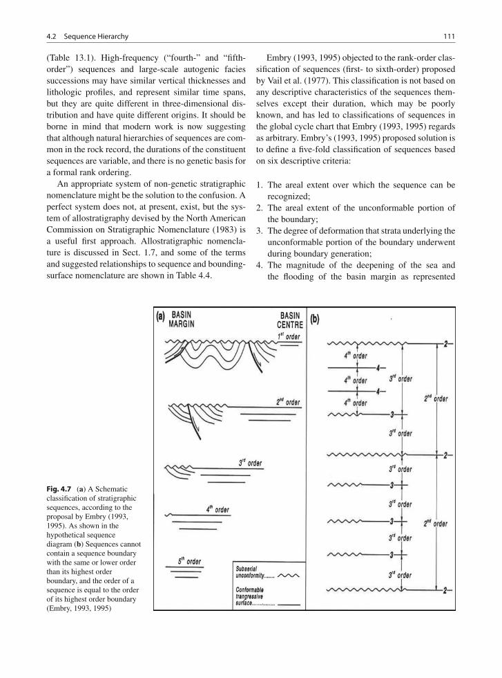
4.2 Sequence Hierarchy 111
(Table 13.1). High-frequency (“fourth-” and “fifth-order”) sequences and large-scale autogenic faciessuccessions may have similar vertical thicknesses andlithologic profiles, and represent similar time spans,but they are quite different in three-dimensional dis-tribution and have quite different origins. It should beborne in mind that modern work is now suggestingthat although natural hierarchies of sequences are com-mon in the rock record, the durations of the constituentsequences are variable, and there is no genetic basis fora formal rank ordering.
An appropriate system of non-genetic stratigraphicnomenclature might be the solution to the confusion. Aperfect system does not, at present, exist, but the sys-tem of allostratigraphy devised by the North AmericanCommission on Stratigraphic Nomenclature (1983) isa useful first approach. Allostratigraphic nomencla-ture is discussed in Sect. 1.7, and some of the termsand suggested relationships to sequence and bounding-surface nomenclature are shown in Table 4.4.
Embry (1993, 1995) objected to the rank-order clas-sification of sequences (first- to sixth-order) proposedby Vail et al. (1977). This classification is not based onany descriptive characteristics of the sequences them-selves except their duration, which may be poorlyknown, and has led to classifications of sequences inthe global cycle chart that Embry (1993, 1995) regardsas arbitrary. Embry’s (1993, 1995) proposed solution isto define a five-fold classification of sequences basedon six descriptive criteria:
1. The areal extent over which the sequence can berecognized;
2. The areal extent of the unconformable portion ofthe boundary;
3. The degree of deformation that strata underlying theunconformable portion of the boundary underwentduring boundary generation;
4. The magnitude of the deepening of the sea andthe flooding of the basin margin as represented
Fig. 4.7 (a) A Schematicclassification of stratigraphicsequences, according to theproposal by Embry (1993,1995). As shown in thehypothetical sequencediagram (b) Sequences cannotcontain a sequence boundarywith the same or lower orderthan its highest orderboundary, and the order of asequence is equal to the orderof its highest order boundary(Embry, 1993, 1995)
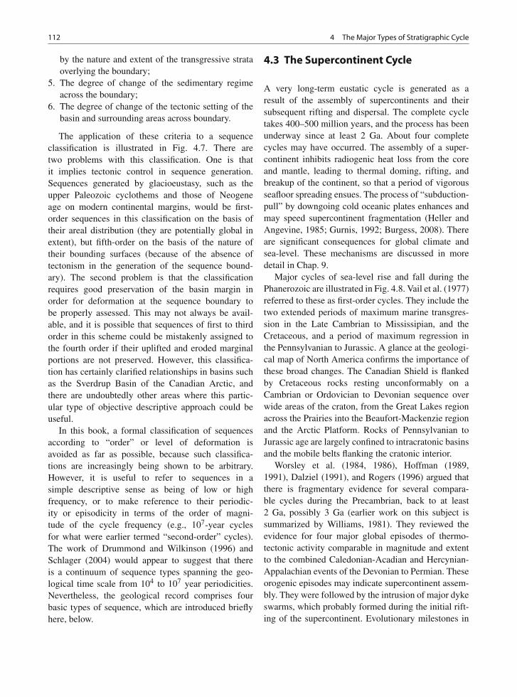
112 4 The Major Types of Stratigraphic Cycle
by the nature and extent of the transgressive strataoverlying the boundary;
5. The degree of change of the sedimentary regimeacross the boundary;
6. The degree of change of the tectonic setting of thebasin and surrounding areas across boundary.
The application of these criteria to a sequenceclassification is illustrated in Fig. 4.7. There aretwo problems with this classification. One is thatit implies tectonic control in sequence generation.Sequences generated by glacioeustasy, such as theupper Paleozoic cyclothems and those of Neogeneage on modern continental margins, would be first-order sequences in this classification on the basis oftheir areal distribution (they are potentially global inextent), but fifth-order on the basis of the nature oftheir bounding surfaces (because of the absence oftectonism in the generation of the sequence bound-ary). The second problem is that the classificationrequires good preservation of the basin margin inorder for deformation at the sequence boundary tobe properly assessed. This may not always be avail-able, and it is possible that sequences of first to thirdorder in this scheme could be mistakenly assigned tothe fourth order if their uplifted and eroded marginalportions are not preserved. However, this classifica-tion has certainly clarified relationships in basins suchas the Sverdrup Basin of the Canadian Arctic, andthere are undoubtedly other areas where this partic-ular type of objective descriptive approach could beuseful.
In this book, a formal classification of sequencesaccording to “order” or level of deformation isavoided as far as possible, because such classifica-tions are increasingly being shown to be arbitrary.However, it is useful to refer to sequences in asimple descriptive sense as being of low or highfrequency, or to make reference to their periodic-ity or episodicity in terms of the order of magni-tude of the cycle frequency (e.g., 107-year cyclesfor what were earlier termed “second-order” cycles).The work of Drummond and Wilkinson (1996) andSchlager (2004) would appear to suggest that thereis a continuum of sequence types spanning the geo-logical time scale from 104 to 107 year periodicities.Nevertheless, the geological record comprises fourbasic types of sequence, which are introduced brieflyhere, below.
4.3 The Supercontinent Cycle
A very long-term eustatic cycle is generated as aresult of the assembly of supercontinents and theirsubsequent rifting and dispersal. The complete cycletakes 400–500 million years, and the process has beenunderway since at least 2 Ga. About four completecycles may have occurred. The assembly of a super-continent inhibits radiogenic heat loss from the coreand mantle, leading to thermal doming, rifting, andbreakup of the continent, so that a period of vigorousseafloor spreading ensues. The process of “subduction-pull” by downgoing cold oceanic plates enhances andmay speed supercontinent fragmentation (Heller andAngevine, 1985; Gurnis, 1992; Burgess, 2008). Thereare significant consequences for global climate andsea-level. These mechanisms are discussed in moredetail in Chap. 9.
Major cycles of sea-level rise and fall during thePhanerozoic are illustrated in Fig. 4.8. Vail et al. (1977)referred to these as first-order cycles. They include thetwo extended periods of maximum marine transgres-sion in the Late Cambrian to Mississipian, and theCretaceous, and a period of maximum regression inthe Pennsylvanian to Jurassic. A glance at the geologi-cal map of North America confirms the importance ofthese broad changes. The Canadian Shield is flankedby Cretaceous rocks resting unconformably on aCambrian or Ordovician to Devonian sequence overwide areas of the craton, from the Great Lakes regionacross the Prairies into the Beaufort-Mackenzie regionand the Arctic Platform. Rocks of Pennsylvanian toJurassic age are largely confined to intracratonic basinsand the mobile belts flanking the cratonic interior.
Worsley et al. (1984, 1986), Hoffman (1989,1991), Dalziel (1991), and Rogers (1996) argued thatthere is fragmentary evidence for several compara-ble cycles during the Precambrian, back to at least2 Ga, possibly 3 Ga (earlier work on this subject issummarized by Williams, 1981). They reviewed theevidence for four major global episodes of thermo-tectonic activity comparable in magnitude and extentto the combined Caledonian-Acadian and Hercynian-Appalachian events of the Devonian to Permian. Theseorogenic episodes may indicate supercontinent assem-bly. They were followed by the intrusion of major dykeswarms, which probably formed during the initial rift-ing of the supercontinent. Evolutionary milestones in
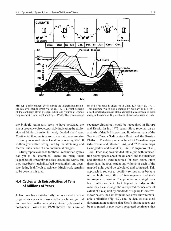
4.4 Cycles with Episodicities of Tens of Millions of Years 113
Fig. 4.8 Supercontinent cycles during the Phanerozoic, includ-ing sea-level change (from Vail et al., 1977), percent floodingof the continents (from Fischer, 1981), and volume of graniteemplacement (from Engel and Engel, 1964). The generation of
the sea-level curve is discussed in Chap. 12 (Vail et al., 1977).This diagram, which was compiled by Worsley et al. (1984),also shows fluctuations in global climate that accompanied thesechanges. I, icehouse; G, greenhouse climate (discussed in text)
the biologic realm also seem to have postdated themajor orogenic episodes, possibly indicating the explo-sion of biotic diversity in newly flooded shelf seas.Continental flooding is caused by eustatic sea-level risedriven by increased rates of seafloor spreading 50–100million years after rifting, and by the stretching andthermal subsidence of new continental margins.
Stratigraphic evidence for these Precambrian cycleshas yet to be assembled. There are many thicksequences of Precambrian strata around the world, butthey have been much disturbed by tectonism, and accu-rate dating is difficult to achieve. Much work remainsto be done in this area.
4.4 Cycles with Episodicities of Tensof Millions of Years
It has now been satisfactorily demonstrated that theoriginal six cycles of Sloss (1963) can be recognizedand correlated with comparable cratonic cycles in othercontinents. Sloss (1972, 1979) showed that a similar
sequence chronology could be recognized in Europeand Russia. In his 1972 paper, Sloss reported on ananalysis of detailed isopach and lithofacies maps of theWestern Canada Sedimentary Basin and the RussianPlatform. The data source included 29 Canadian maps(McCrossan and Glaister, 1964) and 62 Russian maps(Vinogradov and Nalivkin, 1960; Vinogradov et al.,1961). Each map was divided into a grid with intersec-tion points spaced about 60 km apart, and the thicknessand lithofacies were recorded for each point. Fromthese data, the areal extent and volume of each of themapped units could be calculated and compared. Thisapproach is subject to possibly serious error becauseof the high probability of intersequence and evenintrasequence erosion. The presence of a single iso-lated outlier or fault block beyond the edge of themain basin can change the interpreted former area ofextent of a map unit by hundreds of square kilometres.Nevertheless, the data from the two areas show remark-able similarities (Fig. 4.9), and the detailed statisticaldocumentation confirms that Sloss’s six sequences canbe recognized in two widely separated continents that
114 4 The Major Types of Stratigraphic Cycle
Fig. 4.9 Areas of preservation of units in western Canadaand the Russian platform showing relationship to the sixsequences of Sloss (1963). L, M, U = Lower, Middle, Upper;
P = Paleocene, E = Eocene, O = Oligocene, M = Miocene,P = Pliocene (Sloss, 1972)
formerly would have been assumed to have undergonea quite different geological history.
These Phanerozoic cycles are clearly global inscope. They have been attributed to eustatic changesin sea level in response to volume changes of oceanicspreading centres, an interpretation first suggested byHallam (1963), in his summary of Late Cretaceousand Cenozoic events, and subsequently elaborated byPitman (1978). However, eustatic sea-level changescannot explain all the features of the major sequences.They commonly are separated by angular unconfor-mities, and in many cases, the sequences containthick continental deposits. A passive rise in sea levelwould terminate widespread nonmarine deposition,and, therefore, additional processes must be involved.Geophysical studies have demonstrated that the crustflexes on a regional scale in response to convergent,divergent and transcurrent plate movements, a processtermed intraplate stress (Sect. 10.4). Detailed back-strippping and other studies, of the type outlined inChap. 3, show that the crust is constantly undergoinggentle vertical motions and broad continental tilts. Thisform of epeirogeny has recently been termed dynamictopography (Sect. 9.3.2). Broad, regional cycles ofchange in basement elevation occur in response to ther-mal changes in the crust and mantle, crustal thickeningand thinning, and sediment loading.
4.5 Cycles with Million-Year Episodicities
Detailed stratigraphic and facies studies of well datedPhanerozoic strata have yielded a wealth of informa-tion concerning cyclicity over time scales of 1–10million years. Vail et al. (1977) termed these third-order cycles. Examples of sequence-stratigraphic dataare documented in Chap. 6. The intent is not to pro-vide an exhaustive catalog of either the literature orthe results, but to impart an overview of the range oftypes of stratigraphic cycle that have been describedin various tectonic settings, and to provide a flavorof the kinds of research currently being conductedin this area. There is increasing evidence for theoccurrence of the same type of cyclicity during thePrecambrian (Christie-Blick et al., 1988), but the dif-ficulty of achieving accurate chronostratigraphic cor-relations in Precambrian sediments has retarded theapplication of cyclic concepts to Precambrian stratig-raphy (Catuneanu and Eriksson, 1999).
Several different techniques have been used inattempts to reconstruct a chronostratigraphic recordof these stratigraphic cycles. The techniques of Vailand his co-workers (1977) and Haq et al. (1987,1988), as applied to analyses of the Mesozoic andCenozoic sequence, are discussed in Chap. 12. Sloss-type outcrop-area plots have been used by several
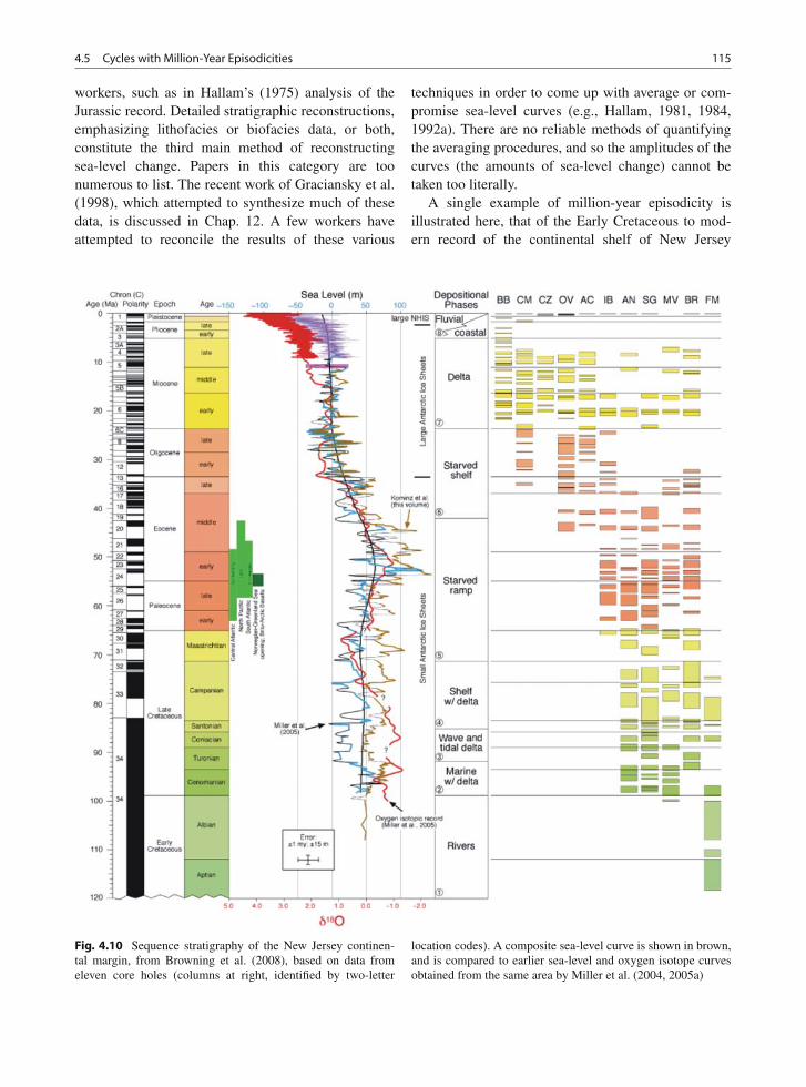
4.5 Cycles with Million-Year Episodicities 115
workers, such as in Hallam’s (1975) analysis of theJurassic record. Detailed stratigraphic reconstructions,emphasizing lithofacies or biofacies data, or both,constitute the third main method of reconstructingsea-level change. Papers in this category are toonumerous to list. The recent work of Graciansky et al.(1998), which attempted to synthesize much of thesedata, is discussed in Chap. 12. A few workers haveattempted to reconcile the results of these various
techniques in order to come up with average or com-promise sea-level curves (e.g., Hallam, 1981, 1984,1992a). There are no reliable methods of quantifyingthe averaging procedures, and so the amplitudes of thecurves (the amounts of sea-level change) cannot betaken too literally.
A single example of million-year episodicity isillustrated here, that of the Early Cretaceous to mod-ern record of the continental shelf of New Jersey
Fig. 4.10 Sequence stratigraphy of the New Jersey continen-tal margin, from Browning et al. (2008), based on data fromeleven core holes (columns at right, identified by two-letter
location codes). A composite sea-level curve is shown in brown,and is compared to earlier sea-level and oxygen isotope curvesobtained from the same area by Miller et al. (2004, 2005a)
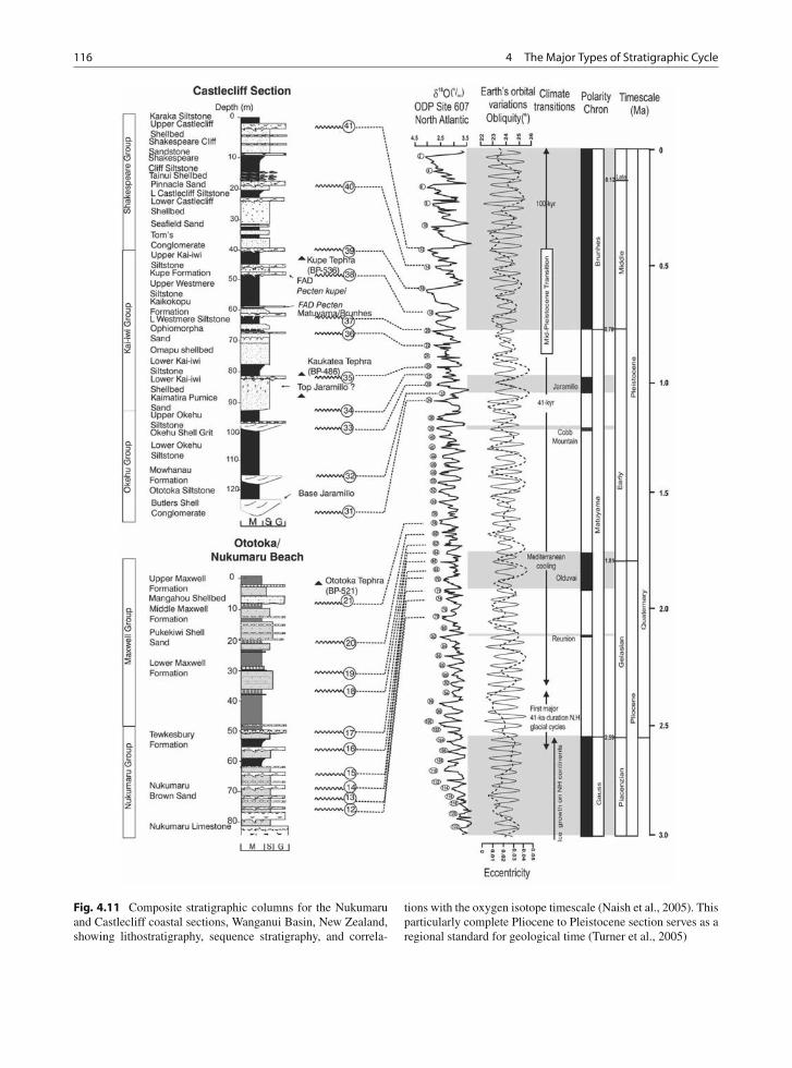
116 4 The Major Types of Stratigraphic Cycle
Fig. 4.11 Composite stratigraphic columns for the Nukumaruand Castlecliff coastal sections, Wanganui Basin, New Zealand,showing lithostratigraphy, sequence stratigraphy, and correla-
tions with the oxygen isotope timescale (Naish et al., 2005). Thisparticularly complete Pliocene to Pleistocene section serves as aregional standard for geological time (Turner et al., 2005)
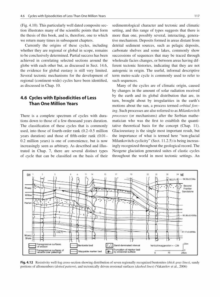
4.6 Cycles with Episodicities of Less Than One Million Years 117
(Fig. 4.10). This particularly well dated composite sec-tion illustrates many of the scientific points that formthe thesis of this book, and is, therefore, one to whichwe return many times in subsequent chapters.
Currently the origins of these cycles, includingwhether they are regional or global in scope, remainsto be conclusively determined. Partial success has beenachieved in correlating selected sections around theglobe with each other but, as discussed in Sect. 14.6,the evidence for global eustasy is still very limited.Several tectonic mechanisms for the development ofregional (continent-wide) cycles have been identified,as discussed in Chap. 10.
4.6 Cycles with Episodicities of LessThan One Million Years
There is a complete spectrum of cycles with dura-tions down to those of a few-thousand years duration.The classification of these cycles that is commonlyused, into those of fourth-order rank (0.2–0.5 millionyears duration) and those of fifth-order rank (0.01–0.2 million years) is one of convenience, but is nowincreasingly seen as arbitrary. As described and illus-trated in Chap. 7, there are several distinct typesof cycle that can be classified on the basis of their
sedimentological character and tectonic and climaticsetting, and this range of types suggests that there ismore than one, possibly several, interacting, genera-tive mechanism. Deposits formed in areas distant fromdetrital sediment sources, such as pelagic deposits,carbonate shelves and some lakes, commonly showsuccessions of sequences that may be traced throughwholesale facies changes, or between areas having dif-ferent tectonic histories, indicating that they are notautogenic in origin. The useful, informal descriptiveterm metre-scale cycle is commonly used to refer tosuch sequences.
Many of the cycles are of climatic origin, causedby changes in the amount of solar radiation receivedby the earth and its global distribution that are, inturn, brought about by irregularities in the earth’smotions about the sun, a process termed orbital forc-ing. Such processes are also referred to as Milankovitchprocesses (or mechanisms) after the Serbian mathe-matician who was the first to establish the quanti-tative theoretical basis for the concept (Chap. 11).Glacioeustasy is the single most important result, butthe importance of what is termed here “non-glacialMilankovitch cyclicity” (Sect. 11.2.5) is being increas-ingly recognized throughout the geological record. TheNeogene glaciation generated suites of clastic cyclesthroughout the world in most tectonic settings. An
Fig. 4.12 Resistivity well-log cross-section showing distribution of seven regionally recognized bentonites (thick gray lines), sandyportions of allomembers (dotted pattern), and tectonically driven erosional surfaces (dashed lines) (Vakarelov et al., 2006)
118 4 The Major Types of Stratigraphic Cycle
example is given in Fig. 4.11. The well-known UpperPaleozoic cyclothems of the northern hemisphere arealso interpreted as glacioeustatic in origin. Other typesof climatic cycle are discussed in Chap. 7. There isgrowing evidence for the occurrence of glacioeustasyduring the Cretaceous and early Cenozoic, as discussedin Chaps. 11 and 13.
Detailed mapping of tectonically-active basins isproviding abundant evidence of the importance of localto regional tectonism as a generator of high-frequencysequence stratigraphies. There are many such exam-ples from ancient foreland basins. Cycles of loadingand unloading due to contractional tectonism, crustalflexure, uplift and erosion, may generate changes inaccommodation and resulting cycles of sedimentationand erosion over time scales as short as a few thou-sand years. An example is illustrated in Fig. 4.12,additional examples are described in Chap. 7, and themechanisms are discussed in Chap. 11.
In the Western Interior Basin of North America,there is excellent evidence from the Cretaceousstratigraphic record of both climatic and tectonicforcing of accommodation and sedimentation. In dif-ferent regions, at different times during the Cretaceous,the evidence appears to indicate one or the other asthe dominant process, and determining the ultimateallogenic controls is one of the current themes ofactive research in this basin. Evidence from the NewJersey coast and from some ODP records is provid-ing increasing evidence of glacioeustasy during theCretaceous and Paleogene (Sects. 11.3.3 and 14.6.4),and there is also evidence from the ancient recordof possible “sub-Milankovitch” cyclicity, that is, withcycle frequencies in the 103-year range (Sect. 14.7.2).
In tectonically active basins, distinguishing tec-tonic mechanisms from the products of orbital forc-ing offers particular challenges, as discussed inSect. 11.4.
Chapter 5
Cycles with Episodicities of Tens to Hundreds of Millionsof Years
Contents
5.1 Climate, Sedimentation and Biogenesis . . . . 1195.2 The Supercontinent Cycle . . . . . . . . . . 121
5.2.1 The Tectonic-Stratigraphic Model . . . . 1215.2.2 The Phanerozoic Record . . . . . . . . 123
5.3 Cycles with Episodicities of Tens of Millions ofyears . . . . . . . . . . . . . . . . . . . . 1255.3.1 Regional to Intercontinental Correlations . 1255.3.2 Tectonostratigraphic Sequences . . . . . 133
5.4 Main Conclusions . . . . . . . . . . . . . . 142
5.1 Climate, Sedimentationand Biogenesis
It is becoming increasingly clear that global climate,oceanic circulation, sedimentation patterns, bioticdiversity, and evolutionary trends are all linked to vari-ations in sea level (Fischer, 1984; Worsley and Nance,1989; Worsley et al., 1984, 1986, 1991; Veevers, 1990;Rogers and Santosh, 2004). These linkages can betraced through the long-term cycle of supercontinentassembly and dispersal (Fig. 5.1), and many of thesame changes can also be observed on shorter timescales. For example, certain trends in sedimentationpatterns are related to the position and direction ofchange of sea level relative to continental margins, andthere is some evidence (touched on below) for suchvariations occurring with episodicities of millions totens of millions of years.
During supercontinent assembly and dispersal, indi-vidual continental plates may undergo latitudinal drift,which carries them through various climate belts. Thisleads to long-term changes in climate and consequent
changes in sedimentary styles, of the type describedby Cecil (1990) and Perlmutter and Matthews (1990).This is discussed further in Chaps. 8 and 9.
Flooding of the continents during the fragmentationphase of the supercontinent cycle causes widespreaddispersion of marine clastic sediments, followed bychemical sedimentation as the supply of clastics fromthermally subsiding continental fragments decreases.Evaporites may be abundant in the newly formedrifted basins and nascent oceans. Clastic sedimenta-tion on the continents decreases to a minimum duringthe maximum-dispersal phase. At times of continen-tal assembly, large volumes of terrigenous detritusare produced by erosion of newly emergent oro-gens, and are deposited as clastic wedges in inlandbasins (e.g., in foredeeps) and along continental mar-gins. During the stasis phase, the presence of large,mountain-rimmed continental-interior basins may leadto climatic extremes in the continental interiors, andcontinental sedimentation may be dominated by eolianor glacial facies.
The depositional systems tracts described in Chap. 2are dependent on sea level over the long and shortterm. Erosional and depositional events in subma-rine canyons and fans are markedly affected by sealevel. During high stands of the sea, continental detri-tus tends to be trapped along the shorelines in deltasand coastal plain complexes (Shanmugam and Moiola,1982). G. deV. Klein (oral communication, 1982)suggested that the major tidalite sequences of thePhanerozoic correspond to periods of high sea level,when shelf widths and tidal effects were at a maximum.
Shelf progradation rates may be high at timesof high sea level; Carbonate platforms may undergowhat Schlager (1991) called “highstand shedding”;but the deep ocean tends to be starved. Clinoform
119A.D. Miall, The Geology of Stratigraphic Sequences, 2nd ed.,DOI 10.1007/978-3-642-05027-5_5, © Springer-Verlag Berlin Heidelberg 2010
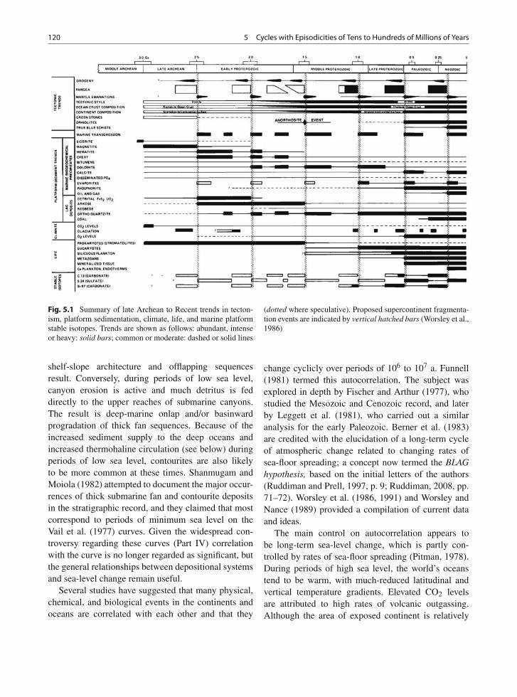
120 5 Cycles with Episodicities of Tens to Hundreds of Millions of Years
Fig. 5.1 Summary of late Archean to Recent trends in tecton-ism, platform sedimentation, climate, life, and marine platformstable isotopes. Trends are shown as follows: abundant, intenseor heavy: solid bars; common or moderate: dashed or solid lines
(dotted where speculative). Proposed supercontinent fragmenta-tion events are indicated by vertical hatched bars (Worsley et al.,1986)
shelf-slope architecture and offlapping sequencesresult. Conversely, during periods of low sea level,canyon erosion is active and much detritus is feddirectly to the upper reaches of submarine canyons.The result is deep-marine onlap and/or basinwardprogradation of thick fan sequences. Because of theincreased sediment supply to the deep oceans andincreased thermohaline circulation (see below) duringperiods of low sea level, contourites are also likelyto be more common at these times. Shanmugam andMoiola (1982) attempted to document the major occur-rences of thick submarine fan and contourite depositsin the stratigraphic record, and they claimed that mostcorrespond to periods of minimum sea level on theVail et al. (1977) curves. Given the widespread con-troversy regarding these curves (Part IV) correlationwith the curve is no longer regarded as significant, butthe general relationships between depositional systemsand sea-level change remain useful.
Several studies have suggested that many physical,chemical, and biological events in the continents andoceans are correlated with each other and that they
change cyclicly over periods of 106 to 107 a. Funnell(1981) termed this autocorrelation. The subject wasexplored in depth by Fischer and Arthur (1977), whostudied the Mesozoic and Cenozoic record, and laterby Leggett et al. (1981), who carried out a similaranalysis for the early Paleozoic. Berner et al. (1983)are credited with the elucidation of a long-term cycleof atmospheric change related to changing rates ofsea-floor spreading; a concept now termed the BLAGhypothesis, based on the initial letters of the authors(Ruddiman and Prell, 1997, p. 9; Ruddiman, 2008, pp.71–72). Worsley et al. (1986, 1991) and Worsley andNance (1989) provided a compilation of current dataand ideas.
The main control on autocorrelation appears tobe long-term sea-level change, which is partly con-trolled by rates of sea-floor spreading (Pitman, 1978).During periods of high sea level, the world’s oceanstend to be warm, with much-reduced latitudinal andvertical temperature gradients. Elevated CO2 levelsare attributed to high rates of volcanic outgassing.Although the area of exposed continent is relatively
5.2 The Supercontinent Cycle 121
low, the rate of release of calcium and phosphorus byweathering remains high because of elevated surfacetemperatures, so that the rate of burial of CO2 ascarbonate remains constant, and the CO2 content ofthe atmosphere rises, increasing the climatic green-house effect. Oceanic circulation is relatively sluggish,leading to increased stratification and severe oxygendepletion at depth. Deposition of organic-rich sedi-ments in the deep ocean becomes widespread, the car-bonate compensation depth rises and faunal diversityincreases. These are the times of global anoxic eventswhen widespread black shales are deposited aroundthe world. Increased nutrient supply caused by highrates of mid-ocean volcanism encourages planktonicgrowth, leading to high general rates of biotic activity,and this may also, in part, account for the developmentof an unusual number of prolific oil source beds duringthe Cretaceous (Larson, 1991).
During periods of low sea level, global climatesare more variable, and the oceans are, in general,cooler and better oxygenated because of better circu-lation. The CO2 content of the atmosphere is reducedby greater combination with calcium and phospho-rus, and burial as carbonates and phosphates, reflectingincreased supply of these elements from continentalweathering. The climatic greenhouse effect is there-fore reduced. Many faunal niches in shelf regions aredestroyed by subaerial exposure. Submarine erosionmay be intensified. Initiation of these episodes of lowersea level may be a cause of biotic crises, in which fau-nal diversity is sharply reduced by major extinctions(Newell, 1967).
Fischer and Arthur (1977) encapsulated these fau-nal variations by applying the terms polytaxic andoligotaxic to periods of, respectively, high and lowfaunal diversity. The corresponding climatic milieusare referred to as greenhouse type when sea levelsare high and climates are globally uniform and rela-tively warm, and icehouse type when variable climatesaccompany times of low sea level. Fischer and Arthur(1977) and Fischer (1981) demonstrated that since theTriassic the oceans have fluctuated between these twomodes during an approximately 32-million years-longcycle. These cycles correlate reasonably well with theSloss-type cycles discussed in Sect. 3.3, although theredoes not seem to be much support for the idea of aprecise 32-million years regularity to the cycles. Theclimate changes are crudely cumulative, and can be
correlated in general terms with the supercontinentcycles of sea-level change, as shown in Fig. 4.7.
Major glaciations occurred during the periodsof icehouse climate in the late Precambrian, LateDevonian-Permian, and mid- to late Cenozoic. Thecauses of these long-term regional glaciations are com-plex (Eyles, 1993, 2008; Eyles and Januszczak, 2004),but widespread uplift as a result of continental colli-sion and/or rifting seem to be major causes. A shorterglacial episode that occurred in the Late Ordovician toEarly Silurian does not fit this pattern. Eyles (2008)suggested that regional uplift, a dynamic topographyeffect resulting from mantle heating, may have helpedto trigger this glacial episode.
Carbonate sedimentation trends reflect the long-term oscillations from icehouse to greenhouse cli-mates. Carbonate production is increased during timesof high global sea level and greenhouse climatebecause of the greater extent of shallow shelf seas. Acompilation by James (1983) showed that reefs tendto be more abundant at times of high global sea level(the long-term highs identified in Fig. 4.7). Lumsden(1985) found that the distribution of dolomite in deep-sea sediments follows the same trend; again, becauseof the greater production of carbonate sediment whenareas of shelf seas are high. Sandberg (1983) suggestedthat low-Mg calcite is the dominant calcium carbonatemineral precipitated during times of high sea level andgreenhouse climates, such as during the Ordovician-Devonian and Jurassic-Cretaceous, whereas high-Mgcalcite and aragonite are dominant at times of lowsea level and icehouse climates. Mackenzie and Pigott(1981) and Worsley et al. (1986) documented parallelchanges in carbon and oxygen distribution and isotopiccomposition (Fig. 5.2).
5.2 The Supercontinent Cycle
5.2.1 The Tectonic-Stratigraphic Model
Evidence for two supercontinent cycles in thePhanerozoic, and several more in the Precambrian wasassembled by Worsley et al. (1984, 1986), who synthe-sized a vast and diverse data base. Rogers and Santosh(2004) have updated and extended these ideas. Themajor elements of the Worsley model are illustrated inFig. 5.2, and are discussed below.
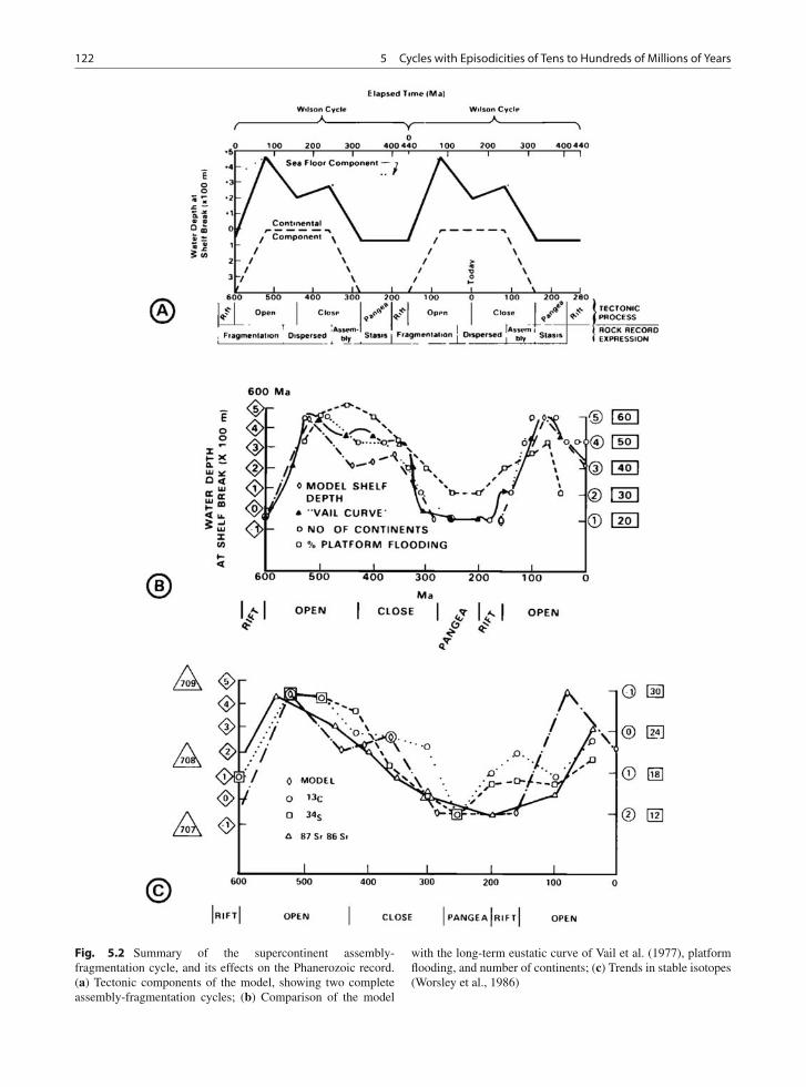
122 5 Cycles with Episodicities of Tens to Hundreds of Millions of Years
Fig. 5.2 Summary of the supercontinent assembly-fragmentation cycle, and its effects on the Phanerozoic record.(a) Tectonic components of the model, showing two completeassembly-fragmentation cycles; (b) Comparison of the model
with the long-term eustatic curve of Vail et al. (1977), platformflooding, and number of continents; (c) Trends in stable isotopes(Worsley et al., 1986)
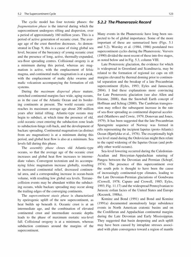
5.2 The Supercontinent Cycle 123
The cyclic model has four tectonic phases: thefragmentation phase is the interval during which thesupercontinent undergoes rifting and dispersion, overa period of approximately 160 million years. This is aperiod of active generation of oceanic crust. The aver-age age of the crust therefore decreases. As demon-strated in Chap. 9, this is a cause of rising global sealevel, because of the buoyancy of young oceanic crustand the presence of long, active, thermally-expanded,sea-floor spreading centres. Collisional orogeny is ata minimum during this period, whereas arc mag-matism is active, with the emplacement of felsicmagma, and continental mafic magmatism is at a peak,with the emplacement of mafic dyke swarms andmafic volcanism accompanying the formation of riftsystems.
During the maximum dispersal phase mature,stretched continental margins face wide, aging oceans,as in the case of the Atlantic Ocean and its border-ing continents at present. The world oceanic crustreaches its maximum average age about 200 millionyears after initial rifting. Atlantic-type oceans maybegin to subduct, at which time the presence of old,cold oceanic crust entering the subduction zone leadsto subduction-hinge roll-back, and the development ofbackarc spreading. Continental magmatism (as distinctfrom arc magmatism) is at a minimum during thisperiod, and global heat flow is also at a minimum. Sealevels fall during this phase.
The assembly phase closes old Atlantic-typeoceans, so that the average age of the oceanic crustincreases and global heat flow increases to interme-diate values. Convergent tectonism and its accompa-nying felsic magmatism increase globally, resultingin increased continental relief, decreased continen-tal area, and a corresponding increase in ocean-basinvolume, with resulting low global sea levels. Terrane-collision events may be abundant within the subduct-ing oceans, while backarc spreading may occur alongthe trailing edges of the converging continents.
The supercontinent stasis phase is characterizedby epeirogenic uplift of the new supercontinent, asheat builds up beneath it. Oceanic crust is at anintermediate age, and the combination of elevatedcontinental crust and intermediate oceanic depthsleads to the phase of maximum eustatic sea-levelfall. Collisional orogeny is at a minimum, whereassubduction continues around the margins of thesupercontinent.
5.2.2 The Phanerozoic Record
Many events in the Phanerozoic have long been sus-pected to be of global importance. Some of the moreimportant of these are summarized here (Figs. 5.1and 5.2). Worsley et al. (1984, 1986) postulated twosupercontinent cycles during the Phanerozoic. Veevers(1990) divided the most recent of these into five stages,as noted below and in Fig. 5.3, column VIII.
Late Proterozoic glaciation, the evidence for whichis widespread in Greenland and Scandinavia, may berelated to the formation of regional ice caps on riftmargins elevated by thermal doming prior to continen-tal separation and the breakup of a late Precambriansupercontinent (Eyles, 1993; Eyles and Janusczak,2004). I find these explanations more convincingfor Late Proterozoic glaciation (see also Allen andEtienne, 2008), than the Snowball Earth concept ofHoffman and Schrag (2000). The Cambrian transgres-sion may reflect the subsequent increase in the rateof sea-floor spreading as continental dispersal acceler-ated (Matthews and Cowie, 1979; Donovan and Jones,1979). It has been suggested that the late PrecambrianSparagmite sequence of Norway was formed inrifts representing the incipient Iapetus (proto-Atlantic)Ocean (Bjørlykke et al., 1976). The exceptionally highsea level stand during the Ordovician might then relateto the rapid widening of the Iapetus Ocean (and prob-ably other world oceans).
Sea-level lowering occurred during the Caledonian-Acadian and Hercynian-Appalachian suturing ofPangea between the Devonian and Permian (Schopf,1974). The presence of this supercontinent overthe south pole is thought to have been the causeof increasingly continental-type climates, leading tothe Late Devonian-Permian glaciations of Gondwana(Crowell, 1978; Caputo and Crowell, 1985; Eyles,1993; Fig. 11.17) and the widespread Pennsylvanian toJurassic eolian facies of the United States and Europe(Kocurek, 1988a).
Kominz and Bond (1991) and Bond and Kominz(1991a) documented anomalously large subsidenceevents in North American cratonic basins and onthe Cordilleran and Appalachian continental marginsduring the Late Devonian and Early Mississippian.They suggested that basin deepening and arch upliftmay have been caused by intraplate stresses associ-ated with plate convergence toward a region of mantle
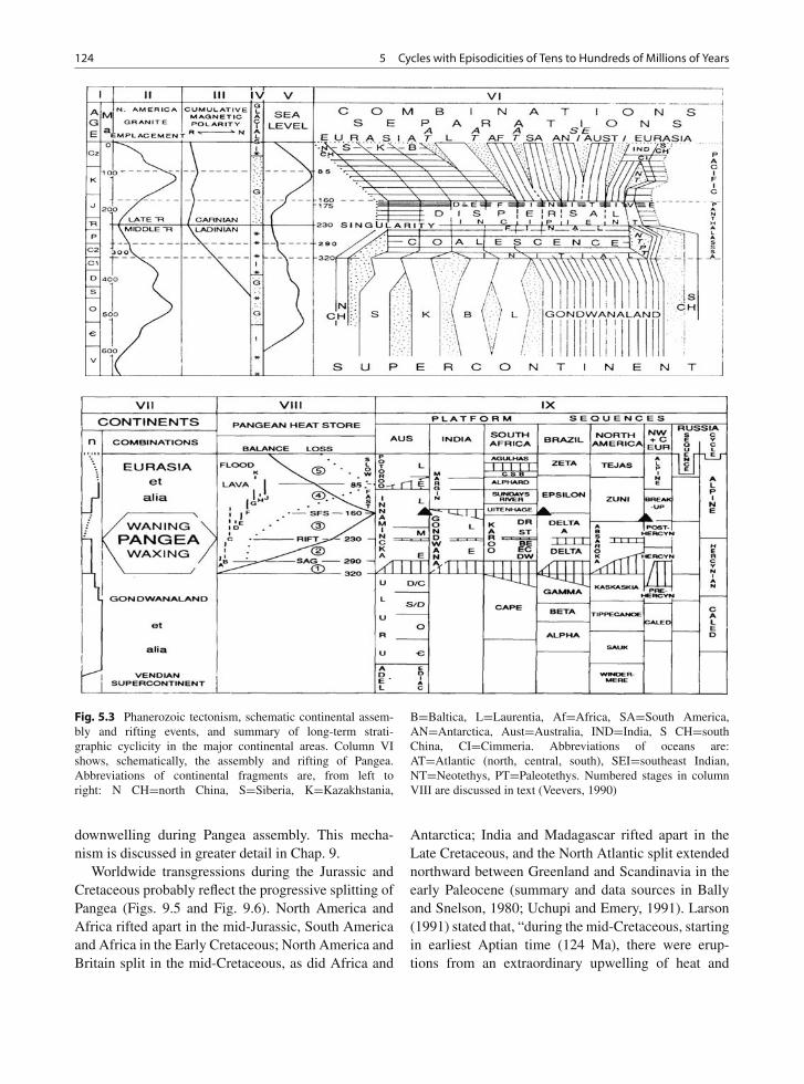
124 5 Cycles with Episodicities of Tens to Hundreds of Millions of Years
Fig. 5.3 Phanerozoic tectonism, schematic continental assem-bly and rifting events, and summary of long-term strati-graphic cyclicity in the major continental areas. Column VIshows, schematically, the assembly and rifting of Pangea.Abbreviations of continental fragments are, from left toright: N CH=north China, S=Siberia, K=Kazakhstania,
B=Baltica, L=Laurentia, Af=Africa, SA=South America,AN=Antarctica, Aust=Australia, IND=India, S CH=southChina, CI=Cimmeria. Abbreviations of oceans are:AT=Atlantic (north, central, south), SEI=southeast Indian,NT=Neotethys, PT=Paleotethys. Numbered stages in columnVIII are discussed in text (Veevers, 1990)
downwelling during Pangea assembly. This mecha-nism is discussed in greater detail in Chap. 9.
Worldwide transgressions during the Jurassic andCretaceous probably reflect the progressive splitting ofPangea (Figs. 9.5 and Fig. 9.6). North America andAfrica rifted apart in the mid-Jurassic, South Americaand Africa in the Early Cretaceous; North America andBritain split in the mid-Cretaceous, as did Africa and
Antarctica; India and Madagascar rifted apart in theLate Cretaceous, and the North Atlantic split extendednorthward between Greenland and Scandinavia in theearly Paleocene (summary and data sources in Ballyand Snelson, 1980; Uchupi and Emery, 1991). Larson(1991) stated that, “during the mid-Cretaceous, startingin earliest Aptian time (124 Ma), there were erup-tions from an extraordinary upwelling of heat and
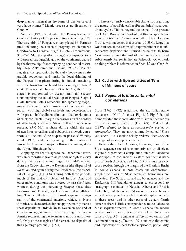
5.3 Cycles with Episodicities of Tens of Millions of years 125
deep-mantle material in the form of one or severalvery large plumes.” Mantle processes are discussed inChap. 9.
Veevers (1990) subdivided the Pennsylvanian toCenozoic history of Pangea into five stages (Fig. 5.3).The assembly of Pangea was completed by Permiantime, including the Ouachita orogeny, which suturedGondwana to Laurasia. Stage 1 (Late Carboniferous,320–290 Ma, the platform stage) corresponds to awidespread stratigraphic gap on the continents, causedby the thermal uplift accompanying continental assem-bly. Stage 2 (Permian-mid Triassic, 290–230 Ma, thesag stage) is represented by the early Gondwana strati-graphic sequences, and marks the local thinning ofthe Pangea lithosphere during its initial stretching,with the formation of broad basins or sags. Stage 3(Late Triassic-Late Jurassic, 230–160 Ma, the riftingstage), is represented by ocean-margin rift succes-sions marking the initial break-up of Pangea. Stage 4(Late Jurassic-Late Cretaceous, the spreading stage),marks the time of maximum rate of continental dis-persal, with high global sea levels and correspondingwidespread shelf sedimentation, and the developmentof thick continental-margin successions on the bordersof Atlantic-type oceans. Stage 5 (Late Cretaceous-present, 85-0 Ma), a phase during which the rateof sea-floor spreading and subduction slowed, corre-sponds to the end of the dispersion phase of Worsleyet al. (1986), and the beginning of the continentalassembly phase, with major collisions occurring alongthe Alpine-Himalayan belt.
Applying this set of stages to the Phanerozoic Earth,we can demonstrate two main periods of high sea levelduring the ocean-opening stage, the mid-Paleozoic,from the Ordovician to the Devonian (the dispersal ofRodinia), and again during the Cretaceous (the disper-sal of Pangea) (Fig. 4.8). During both these periods,much of the cratonic interior of Europe, Asia andother major continents was covered by vast shelf seas,whereas during the intervening Pangea phase (latePaleozoic and Triassic) sea levels were at an all-timelow. This is reflected in the broad sequence stratig-raphy of the continental interiors, which, in NorthAmerica, is characterized by onlapping, mainly marineshelf deposits of Ordovician to Devonian age and ofCretaceous age, separated by a major regional uncon-formity representing the Permian to mid-Jurassic inter-val. Only at the margins of the craton are deposits ofthis age range present (Fig. 5.4).
There is currently considerable discussion regardingthe nature of possible earlier (Precambrian) supercon-tinent cycles. This is beyond the scope of the presentbook (see Rogers and Santosh, 2004). A speculativereconstruction of Rodinia was offered by Hoffman(1991), who suggested that at around 700 Ma Laurentiawas situated at the centre of a supercontinent that sub-sequently dispersed and “turned inside-out” to formGondwana around the end of the Precambrian, andsubsequently Pangea in the late-Paleozoic. Other workon this problem is referenced in Sect. 4.2 and Chap. 9.
5.3 Cycles with Episodicities of Tensof Millions of years
5.3.1 Regional to IntercontinentalCorrelations
Sloss (1963, 1972) established the six Indian-namesequences in North America (Fig. 1.12; Fig. 5.5), anddemonstrated their correlation with similar sequenceson the Russian platform (Fig. 4.9). Vail et al.(1977) referred to these as second-order cycles, orsupercycles. They are now commonly called “Slosssequences.” This section briefly reviews other work onthis type of stratigraphic sequence.
Even within North America, the recognition of theSloss sequence record is commonly not at all clear.Figure 5.6 provides a compilation table of Paleozoicstratigraphy of the ancient western continental mar-gin of north America, and Fig. 5.7 is a stratigraphiccross-section through the margin of the Franklin Basinin Arctic Canada. In both cases, the chronostrati-graphic positions of Sloss sequence boundaries areindicated. The Sauk I, II and III boundaries and theKaskaskia I–II boundaries appear to correspond tostratigraphic contacts in Nevada, Alberta and BritishColumbia, but the other Paleozoic sequence bound-aries do not appear to correlate to stratigraphic contactsin these areas, and in other parts of western NorthAmerica there is little correspondence to the PaleozoicSloss sequence record. In Arctic Canada the recordis even more clearly one of control by local tec-tonism (Fig. 5.7). Syntheses of Arctic tectonism andsedimentation (e.g., Trettin, 1991) indicate the extentand importance of local tectonic episodes, particularly
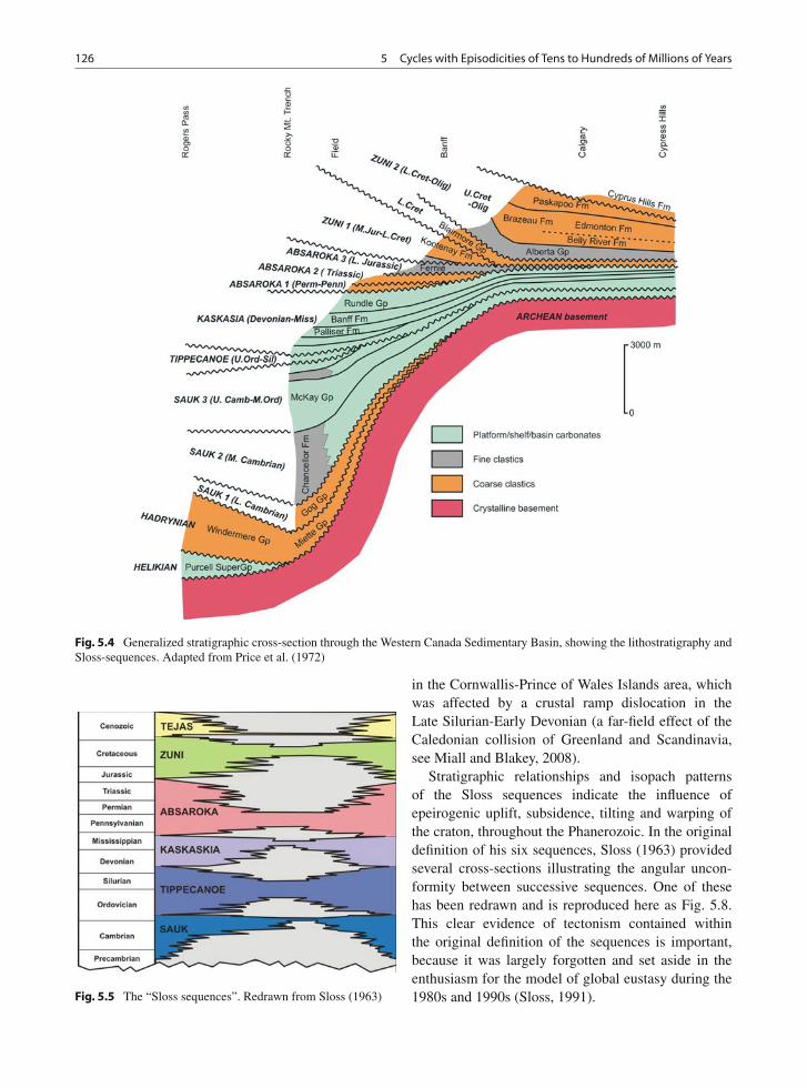
126 5 Cycles with Episodicities of Tens to Hundreds of Millions of Years
Fig. 5.4 Generalized stratigraphic cross-section through the Western Canada Sedimentary Basin, showing the lithostratigraphy andSloss-sequences. Adapted from Price et al. (1972)
Fig. 5.5 The “Sloss sequences”. Redrawn from Sloss (1963)
in the Cornwallis-Prince of Wales Islands area, whichwas affected by a crustal ramp dislocation in theLate Silurian-Early Devonian (a far-field effect of theCaledonian collision of Greenland and Scandinavia,see Miall and Blakey, 2008).
Stratigraphic relationships and isopach patternsof the Sloss sequences indicate the influence ofepeirogenic uplift, subsidence, tilting and warping ofthe craton, throughout the Phanerozoic. In the originaldefinition of his six sequences, Sloss (1963) providedseveral cross-sections illustrating the angular uncon-formity between successive sequences. One of thesehas been redrawn and is reproduced here as Fig. 5.8.This clear evidence of tectonism contained withinthe original definition of the sequences is important,because it was largely forgotten and set aside in theenthusiasm for the model of global eustasy during the1980s and 1990s (Sloss, 1991).
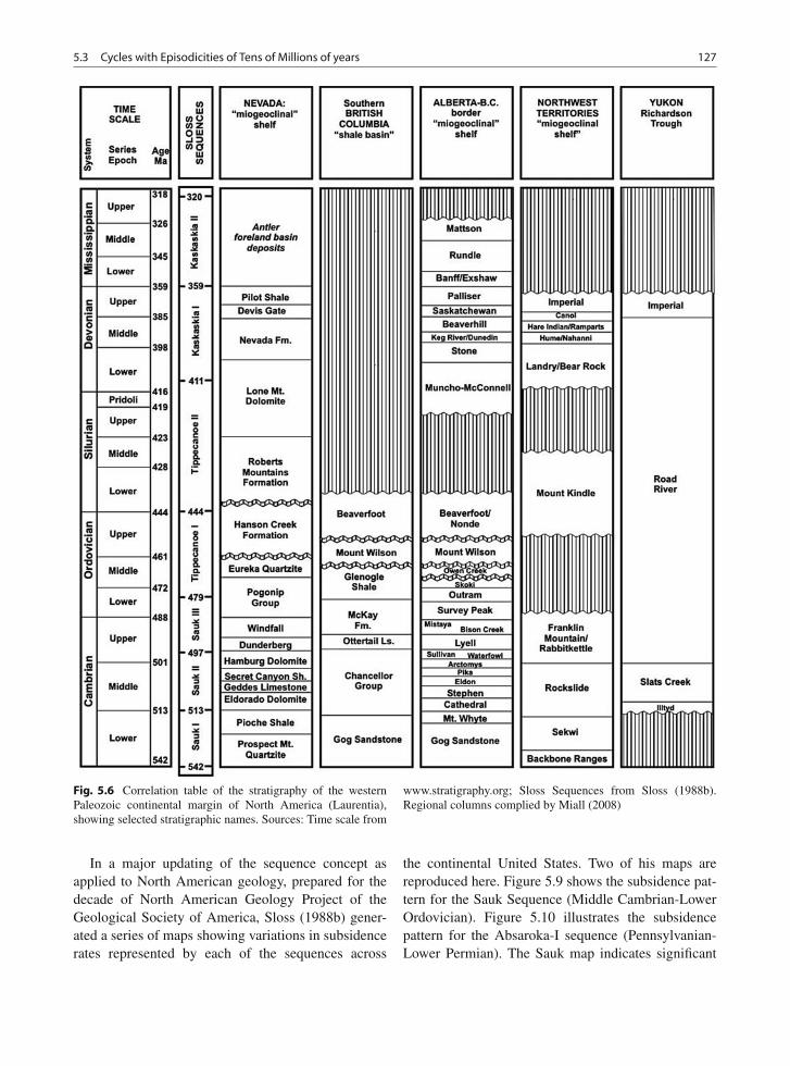
5.3 Cycles with Episodicities of Tens of Millions of years 127
Fig. 5.6 Correlation table of the stratigraphy of the westernPaleozoic continental margin of North America (Laurentia),showing selected stratigraphic names. Sources: Time scale from
www.stratigraphy.org; Sloss Sequences from Sloss (1988b).Regional columns complied by Miall (2008)
In a major updating of the sequence concept asapplied to North American geology, prepared for thedecade of North American Geology Project of theGeological Society of America, Sloss (1988b) gener-ated a series of maps showing variations in subsidencerates represented by each of the sequences across
the continental United States. Two of his maps arereproduced here. Figure 5.9 shows the subsidence pat-tern for the Sauk Sequence (Middle Cambrian-LowerOrdovician). Figure 5.10 illustrates the subsidencepattern for the Absaroka-I sequence (Pennsylvanian-Lower Permian). The Sauk map indicates significant
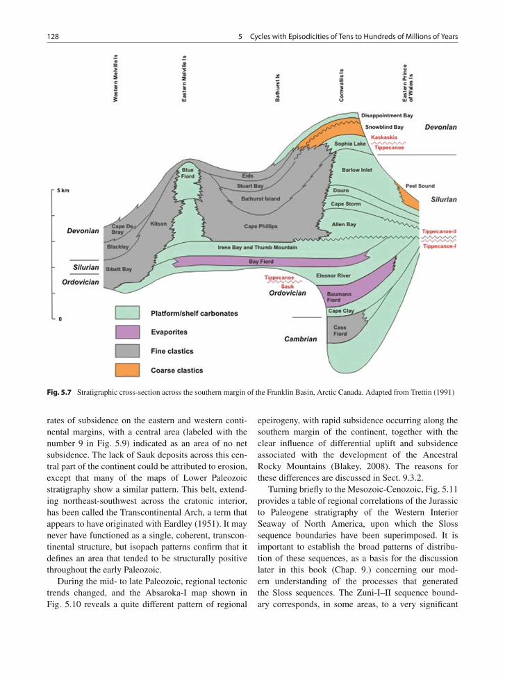
128 5 Cycles with Episodicities of Tens to Hundreds of Millions of Years
Fig. 5.7 Stratigraphic cross-section across the southern margin of the Franklin Basin, Arctic Canada. Adapted from Trettin (1991)
rates of subsidence on the eastern and western conti-nental margins, with a central area (labeled with thenumber 9 in Fig. 5.9) indicated as an area of no netsubsidence. The lack of Sauk deposits across this cen-tral part of the continent could be attributed to erosion,except that many of the maps of Lower Paleozoicstratigraphy show a similar pattern. This belt, extend-ing northeast-southwest across the cratonic interior,has been called the Transcontinental Arch, a term thatappears to have originated with Eardley (1951). It maynever have functioned as a single, coherent, transcon-tinental structure, but isopach patterns confirm that itdefines an area that tended to be structurally positivethroughout the early Paleozoic.
During the mid- to late Paleozoic, regional tectonictrends changed, and the Absaroka-I map shown inFig. 5.10 reveals a quite different pattern of regional
epeirogeny, with rapid subsidence occurring along thesouthern margin of the continent, together with theclear influence of differential uplift and subsidenceassociated with the development of the AncestralRocky Mountains (Blakey, 2008). The reasons forthese differences are discussed in Sect. 9.3.2.
Turning briefly to the Mesozoic-Cenozoic, Fig. 5.11provides a table of regional correlations of the Jurassicto Paleogene stratigraphy of the Western InteriorSeaway of North America, upon which the Slosssequence boundaries have been superimposed. It isimportant to establish the broad patterns of distribu-tion of these sequences, as a basis for the discussionlater in this book (Chap. 9.) concerning our mod-ern understanding of the processes that generatedthe Sloss sequences. The Zuni-I–II sequence bound-ary corresponds, in some areas, to a very significant
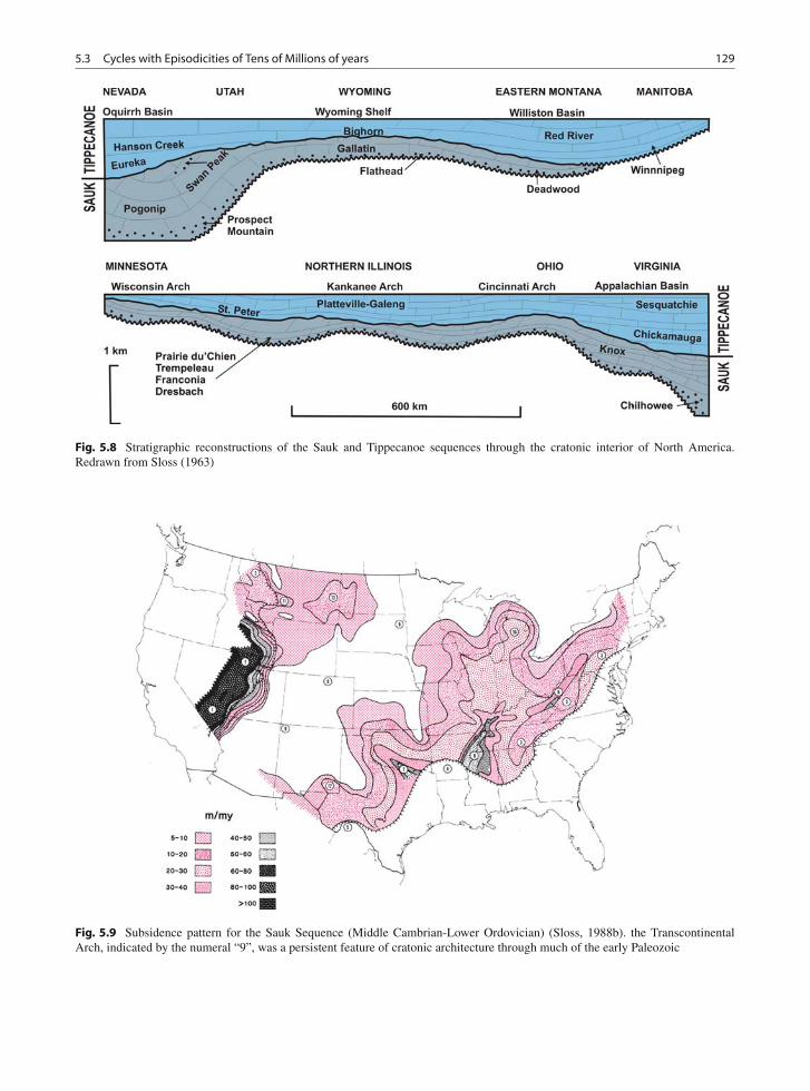
5.3 Cycles with Episodicities of Tens of Millions of years 129
Fig. 5.8 Stratigraphic reconstructions of the Sauk and Tippecanoe sequences through the cratonic interior of North America.Redrawn from Sloss (1963)
Fig. 5.9 Subsidence pattern for the Sauk Sequence (Middle Cambrian-Lower Ordovician) (Sloss, 1988b). the TranscontinentalArch, indicated by the numeral “9”, was a persistent feature of cratonic architecture through much of the early Paleozoic
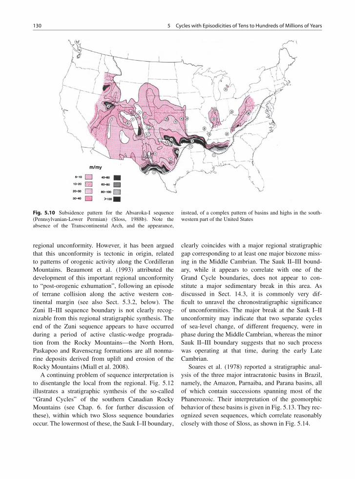
130 5 Cycles with Episodicities of Tens to Hundreds of Millions of Years
Fig. 5.10 Subsidence pattern for the Absaroka-I sequence(Pennsylvanian-Lower Permian) (Sloss, 1988b). Note theabsence of the Transcontinental Arch, and the appearance,
instead, of a complex pattern of basins and highs in the south-western part of the United States
regional unconformity. However, it has been arguedthat this unconformity is tectonic in origin, relatedto patterns of orogenic activity along the CordilleranMountains. Beaumont et al. (1993) attributed thedevelopment of this important regional unconformityto “post-orogenic exhumation”, following an episodeof terrane collision along the active western con-tinental margin (see also Sect. 5.3.2, below). TheZuni II–III sequence boundary is not clearly recog-nizable from this regional stratigraphic synthesis. Theend of the Zuni sequence appears to have occurredduring a period of active clastic-wedge prograda-tion from the Rocky Mountains—the North Horn,Paskapoo and Ravenscrag formations are all nonma-rine deposits derived from uplift and erosion of theRocky Mountains (Miall et al. 2008).
A continuing problem of sequence interpretation isto disentangle the local from the regional. Fig. 5.12illustrates a stratigraphic synthesis of the so-called“Grand Cycles” of the southern Canadian RockyMountains (see Chap. 6. for further discussion ofthese), within which two Sloss sequence boundariesoccur. The lowermost of these, the Sauk I–II boundary,
clearly coincides with a major regional stratigraphicgap corresponding to at least one major biozone miss-ing in the Middle Cambrian. The Sauk II–III bound-ary, while it appears to correlate with one of theGrand Cycle boundaries, does not appear to con-stitute a major sedimentary break in this area. Asdiscussed in Sect. 14.3, it is commonly very dif-ficult to unravel the chronostratigraphic significanceof unconformities. The major break at the Sauk I–IIunconformity may indicate that two separate cyclesof sea-level change, of different frequency, were inphase during the Middle Cambrian, whereas the minorSauk II–III boundary suggests that no such processwas operating at that time, during the early LateCambrian.
Soares et al. (1978) reported a stratigraphic anal-ysis of the three major intracratonic basins in Brazil,namely, the Amazon, Parnaiba, and Parana basins, allof which contain successions spanning most of thePhanerozoic. Their interpretation of the geomorphicbehavior of these basins is given in Fig. 5.13. They rec-ognized seven sequences, which correlate reasonablyclosely with those of Sloss, as shown in Fig. 5.14.
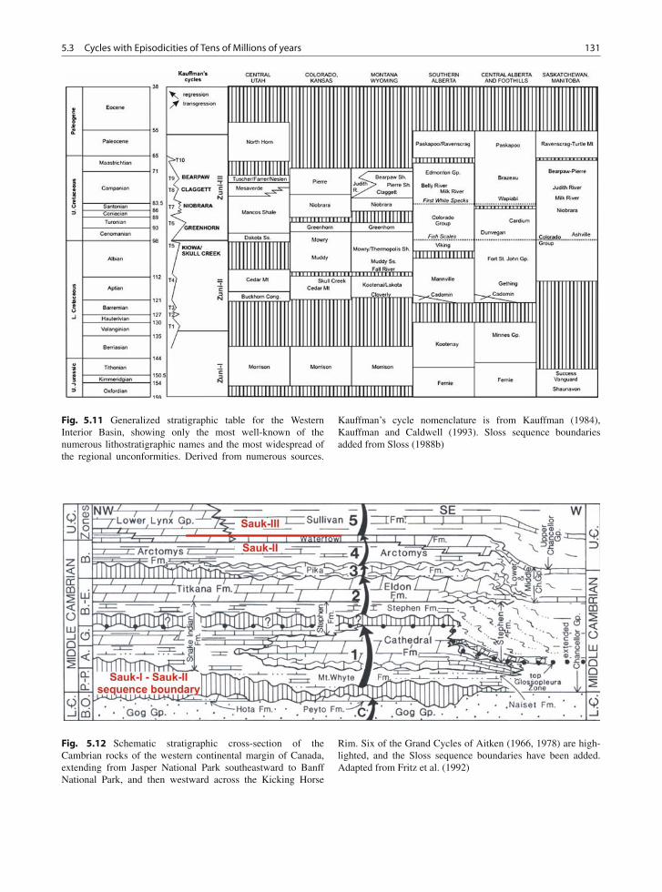
5.3 Cycles with Episodicities of Tens of Millions of years 131
Fig. 5.11 Generalized stratigraphic table for the WesternInterior Basin, showing only the most well-known of thenumerous lithostratigraphic names and the most widespread ofthe regional unconformities. Derived from numerous sources.
Kauffman’s cycle nomenclature is from Kauffman (1984),Kauffman and Caldwell (1993). Sloss sequence boundariesadded from Sloss (1988b)
Fig. 5.12 Schematic stratigraphic cross-section of theCambrian rocks of the western continental margin of Canada,extending from Jasper National Park southeastward to BanffNational Park, and then westward across the Kicking Horse
Rim. Six of the Grand Cycles of Aitken (1966, 1978) are high-lighted, and the Sloss sequence boundaries have been added.Adapted from Fritz et al. (1992)
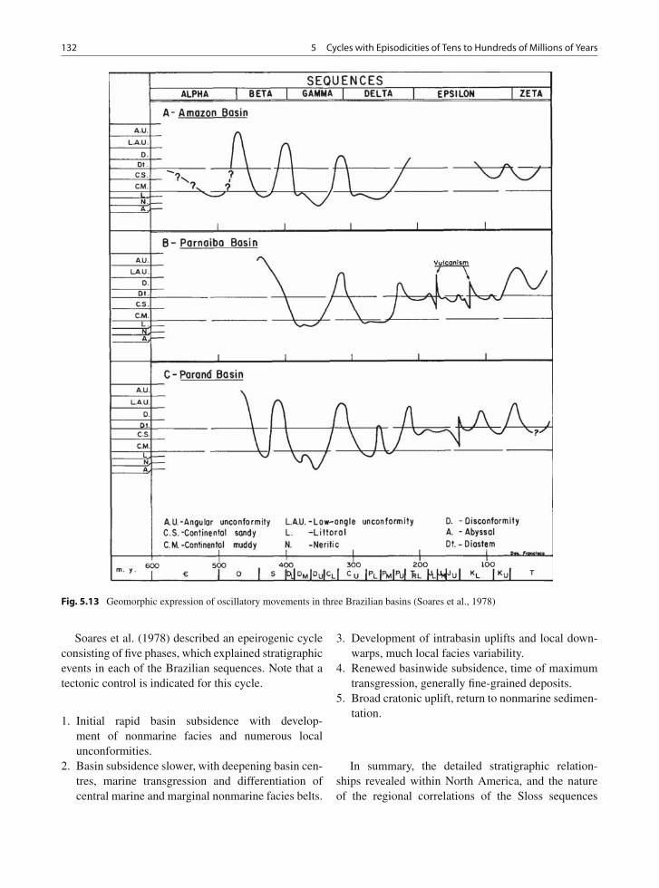
132 5 Cycles with Episodicities of Tens to Hundreds of Millions of Years
Fig. 5.13 Geomorphic expression of oscillatory movements in three Brazilian basins (Soares et al., 1978)
Soares et al. (1978) described an epeirogenic cycleconsisting of five phases, which explained stratigraphicevents in each of the Brazilian sequences. Note that atectonic control is indicated for this cycle.
1. Initial rapid basin subsidence with develop-ment of nonmarine facies and numerous localunconformities.
2. Basin subsidence slower, with deepening basin cen-tres, marine transgression and differentiation ofcentral marine and marginal nonmarine facies belts.
3. Development of intrabasin uplifts and local down-warps, much local facies variability.
4. Renewed basinwide subsidence, time of maximumtransgression, generally fine-grained deposits.
5. Broad cratonic uplift, return to nonmarine sedimen-tation.
In summary, the detailed stratigraphic relation-ships revealed within North America, and the natureof the regional correlations of the Sloss sequences
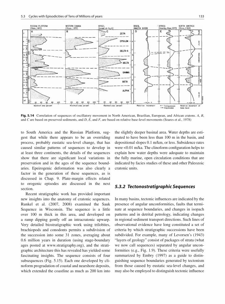
5.3 Cycles with Episodicities of Tens of Millions of years 133
Fig. 5.14 Correlation of sequences of oscillatory movement in North American, Brazilian, European, and African cratons. A, B,and C are based on preserved sediments, and D, E, and F, are based on relative base-level movements (Soares et al., 1978)
to South America and the Russian Platform, sug-gest that while there appears to be an overridingprocess, probably eustatic sea-level change, that hascaused similar patterns of sequences to develop inat least three continents, the details of the sequencesshow that there are significant local variations inpreservation and in the ages of the sequence bound-aries. Epeirogenic deformation was also clearly afactor in the generation of these sequences, as isdiscussed in Chap. 9. Plate-margin effects relatedto orogenic episodes are discussed in the nextsection.
Recent stratigraphic work has provided importantnew insights into the anatomy of cratonic sequences.Runkel et al. (2007, 2008) examined the SaukSequence in Wisconsin. The sequence is a littleover 100 m thick in this area, and developed ona ramp dipping gently off an intracratonic upwarp.Very detailed biostratigraphic work using trilobites,brachiopods and conodonts permits a subdivision ofthe succession into some 31 zones, averaging about0.6 million years in duration (using stage-boundaryages posted at www.stratigraphy.org), and the strati-graphic architecture this has revealed has yielded somefascinating insights. The sequence consists of foursubsequences (Fig. 5.15). Each one developed by cli-noform progradation of coastal and nearshore deposits,which extended the coastline as much as 200 km into
the slightly deeper basinal area. Water depths are esti-mated to have been less than 100 m in the basin, anddepositional slopes 0.1 m/km, or less. Subsidence rateswere <0.01 m/ka. The clinoform configuration helps toexplain how water depths were adequate to maintainthe fully marine, open circulation conditions that areindicated by facies studies of these and other Paleozoiccratonic units.
5.3.2 Tectonostratigraphic Sequences
In many basins, tectonic influences are indicated by thepresence of angular unconformities, faults that termi-nate at sequence boundaries, and changes in isopachpatterns and in detrital petrology, indicating changesin regional sediment transport directions. Such lines ofobservational evidence have long constituted a set ofcriteria by which stratigraphic successions have beensubdivided. For example, many of Levorsen’s (1943)“layers of geology” consist of packages of strata (whatwe now call sequences) separated by angular uncon-formities (e.g., Fig. 1.9). These criteria were usefullysummarized by Embry (1997) as a guide to distin-guishing sequence boundaries generated by tectonismfrom those caused by eustatic sea-level changes, andmay also be employed to distinguish tectonic influence
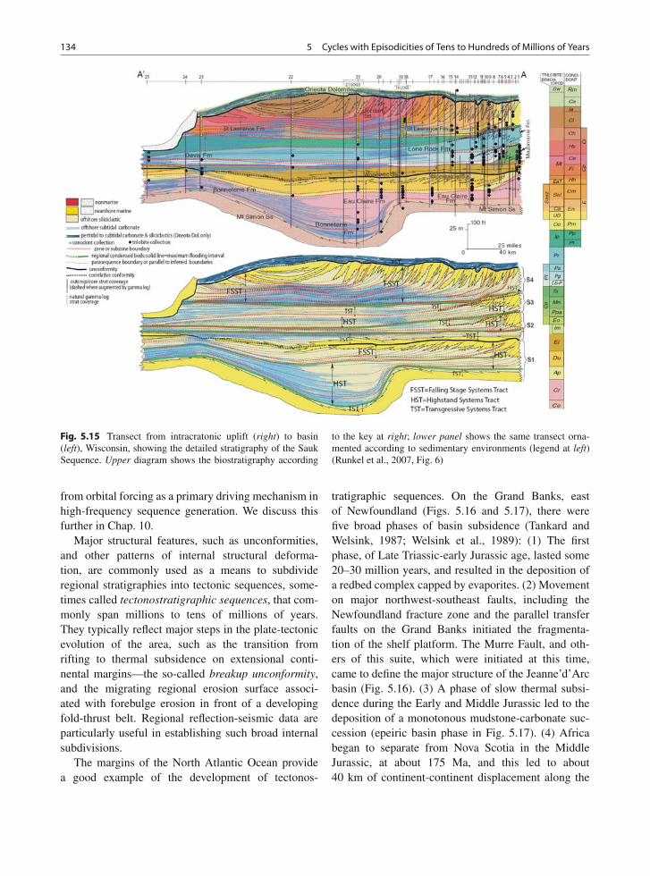
134 5 Cycles with Episodicities of Tens to Hundreds of Millions of Years
Fig. 5.15 Transect from intracratonic uplift (right) to basin(left), Wisconsin, showing the detailed stratigraphy of the SaukSequence. Upper diagram shows the biostratigraphy according
to the key at right; lower panel shows the same transect orna-mented according to sedimentary environments (legend at left)(Runkel et al., 2007, Fig. 6)
from orbital forcing as a primary driving mechanism inhigh-frequency sequence generation. We discuss thisfurther in Chap. 10.
Major structural features, such as unconformities,and other patterns of internal structural deforma-tion, are commonly used as a means to subdivideregional stratigraphies into tectonic sequences, some-times called tectonostratigraphic sequences, that com-monly span millions to tens of millions of years.They typically reflect major steps in the plate-tectonicevolution of the area, such as the transition fromrifting to thermal subsidence on extensional conti-nental margins—the so-called breakup unconformity,and the migrating regional erosion surface associ-ated with forebulge erosion in front of a developingfold-thrust belt. Regional reflection-seismic data areparticularly useful in establishing such broad internalsubdivisions.
The margins of the North Atlantic Ocean providea good example of the development of tectonos-
tratigraphic sequences. On the Grand Banks, eastof Newfoundland (Figs. 5.16 and 5.17), there werefive broad phases of basin subsidence (Tankard andWelsink, 1987; Welsink et al., 1989): (1) The firstphase, of Late Triassic-early Jurassic age, lasted some20–30 million years, and resulted in the deposition ofa redbed complex capped by evaporites. (2) Movementon major northwest-southeast faults, including theNewfoundland fracture zone and the parallel transferfaults on the Grand Banks initiated the fragmenta-tion of the shelf platform. The Murre Fault, and oth-ers of this suite, which were initiated at this time,came to define the major structure of the Jeanne’d’Arcbasin (Fig. 5.16). (3) A phase of slow thermal subsi-dence during the Early and Middle Jurassic led to thedeposition of a monotonous mudstone-carbonate suc-cession (epeiric basin phase in Fig. 5.17). (4) Africabegan to separate from Nova Scotia in the MiddleJurassic, at about 175 Ma, and this led to about40 km of continent-continent displacement along the
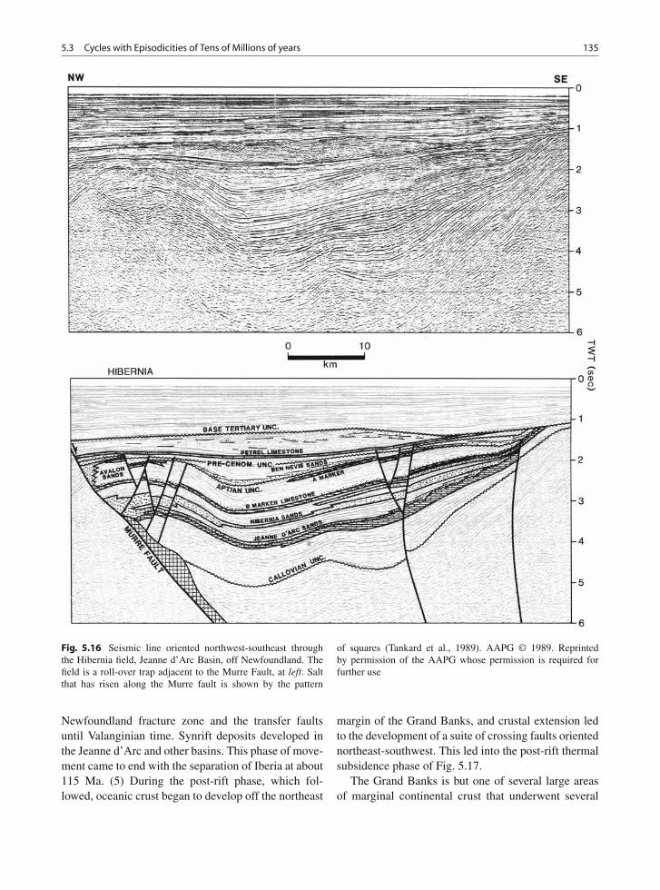
5.3 Cycles with Episodicities of Tens of Millions of years 135
Fig. 5.16 Seismic line oriented northwest-southeast throughthe Hibernia field, Jeanne d’Arc Basin, off Newfoundland. Thefield is a roll-over trap adjacent to the Murre Fault, at left. Saltthat has risen along the Murre fault is shown by the pattern
of squares (Tankard et al., 1989). AAPG © 1989. Reprintedby permission of the AAPG whose permission is required forfurther use
Newfoundland fracture zone and the transfer faultsuntil Valanginian time. Synrift deposits developed inthe Jeanne d’Arc and other basins. This phase of move-ment came to end with the separation of Iberia at about115 Ma. (5) During the post-rift phase, which fol-lowed, oceanic crust began to develop off the northeast
margin of the Grand Banks, and crustal extension ledto the development of a suite of crossing faults orientednortheast-southwest. This led into the post-rift thermalsubsidence phase of Fig. 5.17.
The Grand Banks is but one of several large areasof marginal continental crust that underwent several
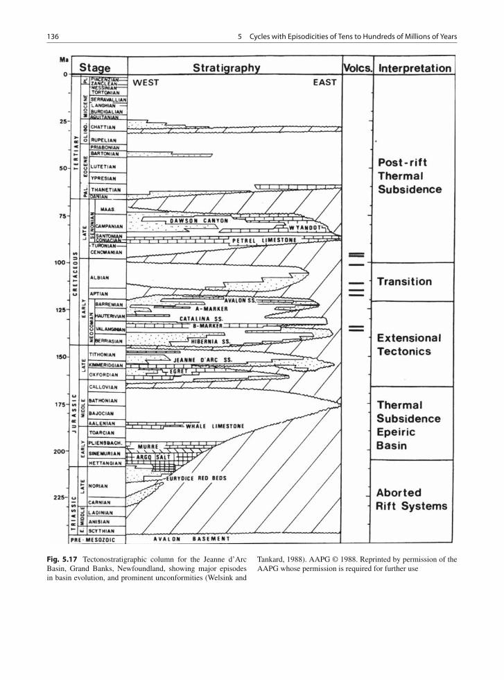
136 5 Cycles with Episodicities of Tens to Hundreds of Millions of Years
Fig. 5.17 Tectonostratigraphic column for the Jeanne d’ArcBasin, Grand Banks, Newfoundland, showing major episodesin basin evolution, and prominent unconformities (Welsink and
Tankard, 1988). AAPG © 1988. Reprinted by permission of theAAPG whose permission is required for further use
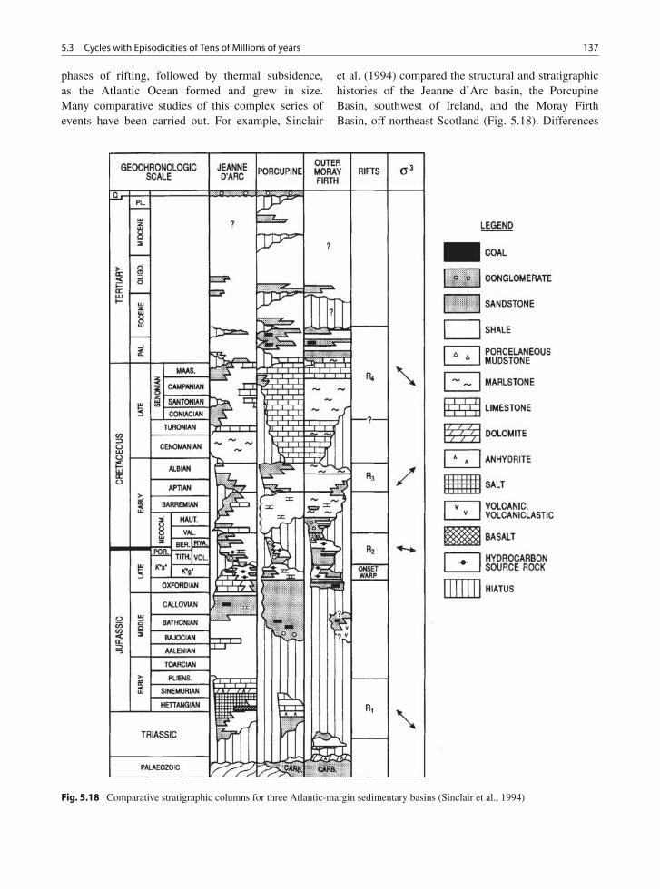
5.3 Cycles with Episodicities of Tens of Millions of years 137
phases of rifting, followed by thermal subsidence,as the Atlantic Ocean formed and grew in size.Many comparative studies of this complex series ofevents have been carried out. For example, Sinclair
et al. (1994) compared the structural and stratigraphichistories of the Jeanne d’Arc basin, the PorcupineBasin, southwest of Ireland, and the Moray FirthBasin, off northeast Scotland (Fig. 5.18). Differences
Fig. 5.18 Comparative stratigraphic columns for three Atlantic-margin sedimentary basins (Sinclair et al., 1994)
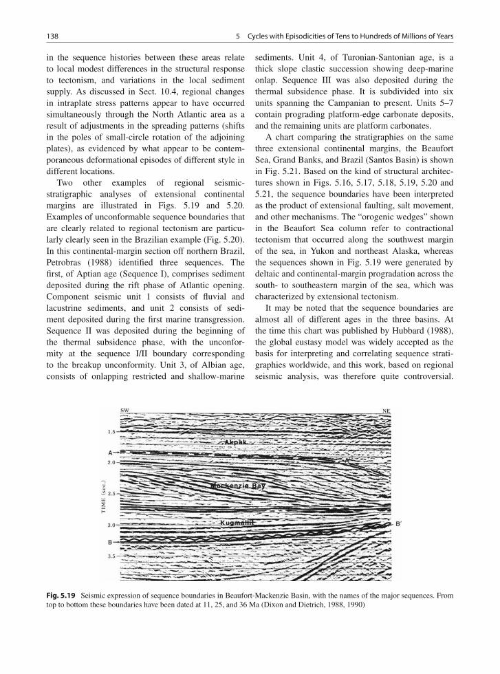
138 5 Cycles with Episodicities of Tens to Hundreds of Millions of Years
in the sequence histories between these areas relateto local modest differences in the structural responseto tectonism, and variations in the local sedimentsupply. As discussed in Sect. 10.4, regional changesin intraplate stress patterns appear to have occurredsimultaneously through the North Atlantic area as aresult of adjustments in the spreading patterns (shiftsin the poles of small-circle rotation of the adjoiningplates), as evidenced by what appear to be contem-poraneous deformational episodes of different style indifferent locations.
Two other examples of regional seismic-stratigraphic analyses of extensional continentalmargins are illustrated in Figs. 5.19 and 5.20.Examples of unconformable sequence boundaries thatare clearly related to regional tectonism are particu-larly clearly seen in the Brazilian example (Fig. 5.20).In this continental-margin section off northern Brazil,Petrobras (1988) identified three sequences. Thefirst, of Aptian age (Sequence I), comprises sedimentdeposited during the rift phase of Atlantic opening.Component seismic unit 1 consists of fluvial andlacustrine sediments, and unit 2 consists of sedi-ment deposited during the first marine transgression.Sequence II was deposited during the beginning ofthe thermal subsidence phase, with the unconfor-mity at the sequence I/II boundary correspondingto the breakup unconformity. Unit 3, of Albian age,consists of onlapping restricted and shallow-marine
sediments. Unit 4, of Turonian-Santonian age, is athick slope clastic succession showing deep-marineonlap. Sequence III was also deposited during thethermal subsidence phase. It is subdivided into sixunits spanning the Campanian to present. Units 5–7contain prograding platform-edge carbonate deposits,and the remaining units are platform carbonates.
A chart comparing the stratigraphies on the samethree extensional continental margins, the BeaufortSea, Grand Banks, and Brazil (Santos Basin) is shownin Fig. 5.21. Based on the kind of structural architec-tures shown in Figs. 5.16, 5.17, 5.18, 5.19, 5.20 and5.21, the sequence boundaries have been interpretedas the product of extensional faulting, salt movement,and other mechanisms. The “orogenic wedges” shownin the Beaufort Sea column refer to contractionaltectonism that occurred along the southwest marginof the sea, in Yukon and northeast Alaska, whereasthe sequences shown in Fig. 5.19 were generated bydeltaic and continental-margin progradation across thesouth- to southeastern margin of the sea, which wascharacterized by extensional tectonism.
It may be noted that the sequence boundaries arealmost all of different ages in the three basins. Atthe time this chart was published by Hubbard (1988),the global eustasy model was widely accepted as thebasis for interpreting and correlating sequence strati-graphies worldwide, and this work, based on regionalseismic analysis, was therefore quite controversial.
Fig. 5.19 Seismic expression of sequence boundaries in Beaufort-Mackenzie Basin, with the names of the major sequences. Fromtop to bottom these boundaries have been dated at 11, 25, and 36 Ma (Dixon and Dietrich, 1988, 1990)
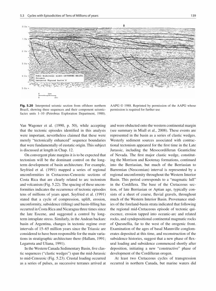
5.3 Cycles with Episodicities of Tens of Millions of years 139
Fig. 5.20 Interpreted seismic section from offshore northernBrazil, showing three sequences and their component seismic-facies units 1–10 (Petrobras Exploration Department, 1988).
AAPG © 1988. Reprinted by permission of the AAPG whosepermission is required for further use
Van Wagoner et al. (1990, p. 50), while acceptingthat the tectonic episodes identified in this analysiswere important, nevertheless claimed that these weremerely “tectonically enhanced” sequence boundariesthat were fundamentally of eustatic origin. This subjectis discussed at length in Chap. 12.
On convergent plate margins it is to be expected thattectonism will be the dominant control on the long-term development of basin architecture. For example,Seyfried et al. (1991) mapped a series of regionalunconformities in Cretaceous-Cenozoic sections ofCosta Rica that are clearly related to arc tectonismand volcanism (Fig. 5.22). The spacing of these uncon-formities indicates the occurrence of tectonic episodestens of millions of years apart. Seyfried et al. (1991)stated that a cycle of compression, uplift, erosion,unconformity, subsidence (tilting) and basin-filling hasoccurred in Costa Rica and Nicaragua three times sincethe late Eocene, and suggested a control by long-term intraplate stress. Similarly, in the Andean backarcbasin of Argentina, changes in tectonic regime overintervals of 15–65 million years since the Triassic areconsidered to have been responsible for the main varia-tions in stratigraphic architecture there (Hallam, 1991;Legarreta and Uliana, 1991).
In the Western Canada Sedimentary Basin, five clas-tic sequences (“clastic wedges”) span the mid-Jurassicto mid-Cenozoic (Fig. 5.23). Crustal loading occurredas a series of pulses, as successive terranes arrived at
and were obducted onto the western continental margin(see summary in Miall et al., 2008). These events arerepresented in the basin as a series of clastic wedges.Westerly sediment sources associated with contrac-tional tectonism appeared for the first time in the LateJurassic, including the Mesocordilleran Geanticlineof Nevada. The first major clastic wedge, constitut-ing the Morrison and Kootenay formations, continuedinto the Berriasian, but much of the Berriasian toBarremian (Neocomian) interval is represented by aregional unconformity throughout the Western InteriorBasin. This period corresponds to a “magmatic lull”in the Cordillera. The base of the Cretaceous sec-tion, of late Berriasian or Aptian age, typically con-sists of a sheet of coarse, fluvial gravels, throughoutmuch of the Western Interior Basin. Provenance stud-ies of the foreland-basin strata indicated that followingthe regional mid-Cretaceous episode of tectonic qui-escence, erosion tapped into oceanic-arc and relatedrocks, and syndepositional continental magmatic rocksof Quesnellia, far to the west of the orogenic front.Examination of the ages of basal Mannville conglom-erates deposited at this time, and reconstruction of thesubsidence histories, suggest that a new phase of flex-ural loading and subsidence commenced shortly afterdeposition, initiating a new “constructive” phase ofdevelopment of the Cordilleran orogen.
At least two Cretaceous cycles of transgressionoccurred in northern Canada, but marine waters did
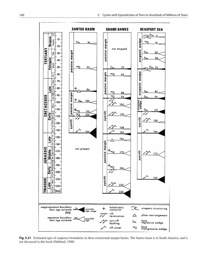
140 5 Cycles with Episodicities of Tens to Hundreds of Millions of Years
Fig. 5.21 Estimated ages of sequence boundaries in three extensional-margin basins. The Santos basin is in South America, and isnot discussed in this book (Hubbard, 1988)
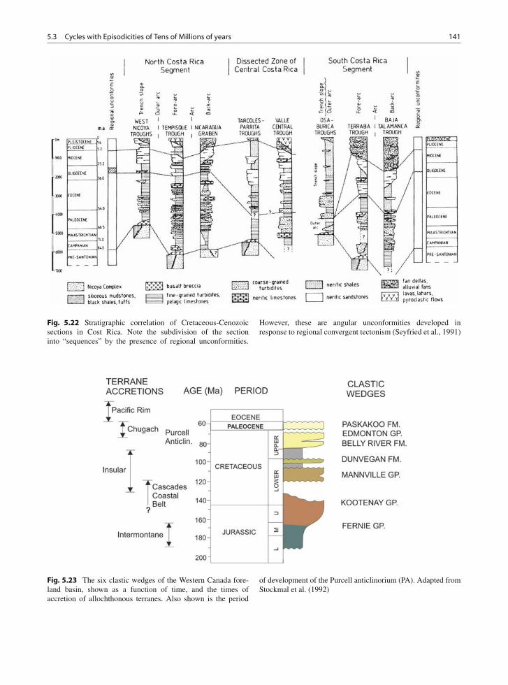
5.3 Cycles with Episodicities of Tens of Millions of years 141
Fig. 5.22 Stratigraphic correlation of Cretaceous-Cenozoicsections in Cost Rica. Note the subdivision of the sectioninto “sequences” by the presence of regional unconformities.
However, these are angular unconformities developed inresponse to regional convergent tectonism (Seyfried et al., 1991)
Fig. 5.23 The six clastic wedges of the Western Canada fore-land basin, shown as a function of time, and the times ofaccretion of allochthonous terranes. Also shown is the period
of development of the Purcell anticlinorium (PA). Adapted fromStockmal et al. (1992)
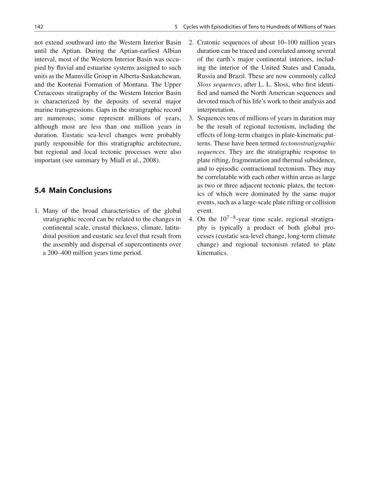
142 5 Cycles with Episodicities of Tens to Hundreds of Millions of Years
not extend southward into the Western Interior Basinuntil the Aptian. During the Aptian-earliest Albianinterval, most of the Western Interior Basin was occu-pied by fluvial and estuarine systems assigned to suchunits as the Mannville Group in Alberta-Saskatchewan,and the Kootenai Formation of Montana. The UpperCretaceous stratigraphy of the Western Interior Basinis characterized by the deposits of several majormarine transgressions. Gaps in the stratigraphic recordare numerous; some represent millions of years,although most are less than one million years induration. Eustatic sea-level changes were probablypartly responsible for this stratigraphic architecture,but regional and local tectonic processes were alsoimportant (see summary by Miall et al., 2008).
5.4 Main Conclusions
1. Many of the broad characteristics of the globalstratigraphic record can be related to the changes incontinental scale, crustal thickness, climate, latitu-dinal position and eustatic sea level that result fromthe assembly and dispersal of supercontinents overa 200–400 million years time period.
2. Cratonic sequences of about 10–100 million yearsduration can be traced and correlated among severalof the earth’s major continental interiors, includ-ing the interior of the United States and Canada,Russia and Brazil. These are now commonly calledSloss sequences, after L. L. Sloss, who first identi-fied and named the North American sequences anddevoted much of his life’s work to their analysis andinterpretation.
3. Sequences tens of millions of years in duration maybe the result of regional tectonism, including theeffects of long-term changes in plate-kinematic pat-terns. These have been termed tectonostratigraphicsequences. They are the stratigraphic response toplate rifting, fragmentation and thermal subsidence,and to episodic contractional tectonism. They maybe correlatable with each other within areas as largeas two or three adjacent tectonic plates, the tecton-ics of which were dominated by the same majorevents, such as a large-scale plate rifting or collisionevent.
4. On the 107−8-year time scale, regional stratigra-phy is typically a product of both global pro-cesses (eustatic sea-level change, long-term climatechange) and regional tectonism related to platekinematics.
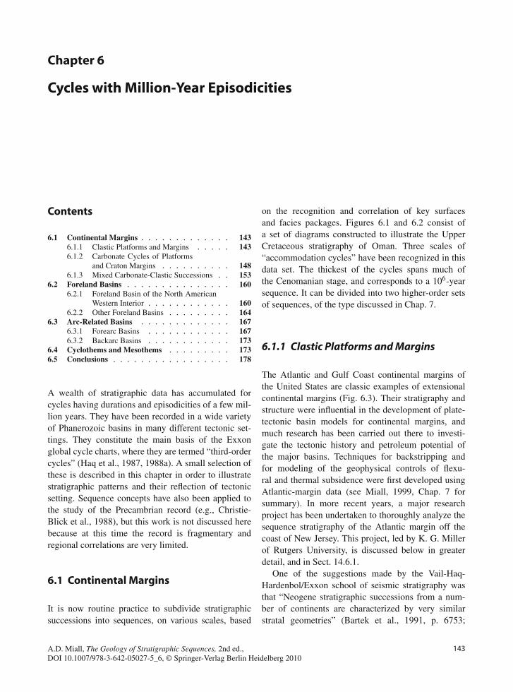
Chapter 6
Cycles with Million-Year Episodicities
Contents
6.1 Continental Margins . . . . . . . . . . . . . 1436.1.1 Clastic Platforms and Margins . . . . . 1436.1.2 Carbonate Cycles of Platforms
and Craton Margins . . . . . . . . . . 1486.1.3 Mixed Carbonate-Clastic Successions . . 153
6.2 Foreland Basins . . . . . . . . . . . . . . . 1606.2.1 Foreland Basin of the North American
Western Interior . . . . . . . . . . . . 1606.2.2 Other Foreland Basins . . . . . . . . . 164
6.3 Arc-Related Basins . . . . . . . . . . . . . 1676.3.1 Forearc Basins . . . . . . . . . . . . 1676.3.2 Backarc Basins . . . . . . . . . . . . 173
6.4 Cyclothems and Mesothems . . . . . . . . . 1736.5 Conclusions . . . . . . . . . . . . . . . . . 178
A wealth of stratigraphic data has accumulated forcycles having durations and episodicities of a few mil-lion years. They have been recorded in a wide varietyof Phanerozoic basins in many different tectonic set-tings. They constitute the main basis of the Exxonglobal cycle charts, where they are termed “third-ordercycles” (Haq et al., 1987, 1988a). A small selection ofthese is described in this chapter in order to illustratestratigraphic patterns and their reflection of tectonicsetting. Sequence concepts have also been applied tothe study of the Precambrian record (e.g., Christie-Blick et al., 1988), but this work is not discussed herebecause at this time the record is fragmentary andregional correlations are very limited.
6.1 Continental Margins
It is now routine practice to subdivide stratigraphicsuccessions into sequences, on various scales, based
on the recognition and correlation of key surfacesand facies packages. Figures 6.1 and 6.2 consist ofa set of diagrams constructed to illustrate the UpperCretaceous stratigraphy of Oman. Three scales of“accommodation cycles” have been recognized in thisdata set. The thickest of the cycles spans much ofthe Cenomanian stage, and corresponds to a 106-yearsequence. It can be divided into two higher-order setsof sequences, of the type discussed in Chap. 7.
6.1.1 Clastic Platforms and Margins
The Atlantic and Gulf Coast continental margins ofthe United States are classic examples of extensionalcontinental margins (Fig. 6.3). Their stratigraphy andstructure were influential in the development of plate-tectonic basin models for continental margins, andmuch research has been carried out there to investi-gate the tectonic history and petroleum potential ofthe major basins. Techniques for backstripping andfor modeling of the geophysical controls of flexu-ral and thermal subsidence were first developed usingAtlantic-margin data (see Miall, 1999, Chap. 7 forsummary). In more recent years, a major researchproject has been undertaken to thoroughly analyze thesequence stratigraphy of the Atlantic margin off thecoast of New Jersey. This project, led by K. G. Millerof Rutgers University, is discussed below in greaterdetail, and in Sect. 14.6.1.
One of the suggestions made by the Vail-Haq-Hardenbol/Exxon school of seismic stratigraphy wasthat “Neogene stratigraphic successions from a num-ber of continents are characterized by very similarstratal geometries” (Bartek et al., 1991, p. 6753;
143A.D. Miall, The Geology of Stratigraphic Sequences, 2nd ed.,DOI 10.1007/978-3-642-05027-5_6, © Springer-Verlag Berlin Heidelberg 2010
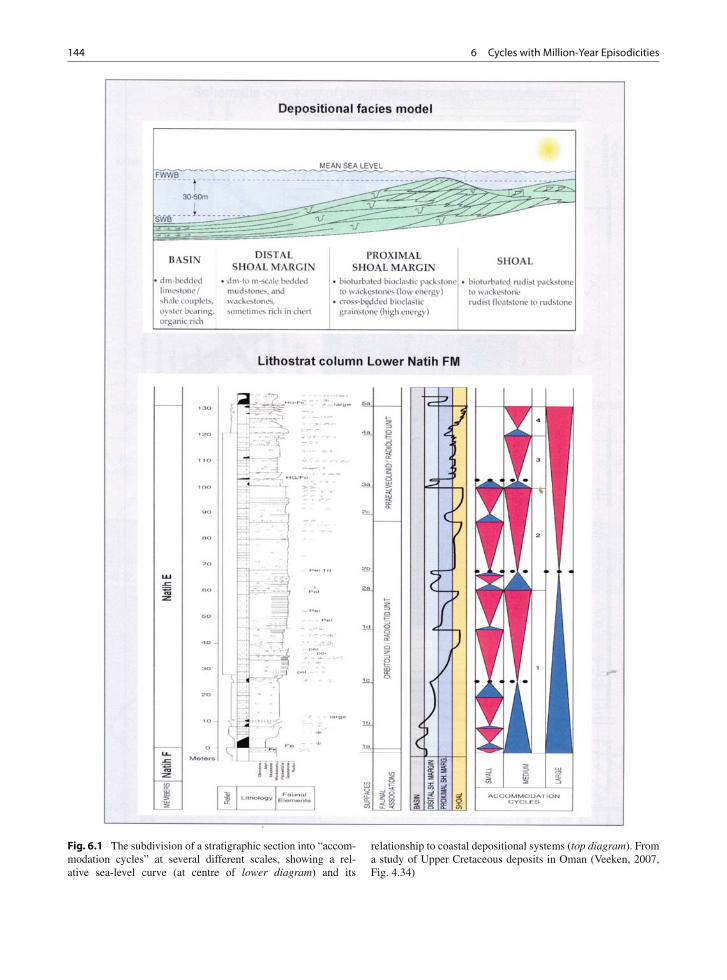
144 6 Cycles with Million-Year Episodicities
Fig. 6.1 The subdivision of a stratigraphic section into “accom-modation cycles” at several different scales, showing a rel-ative sea-level curve (at centre of lower diagram) and its
relationship to coastal depositional systems (top diagram). Froma study of Upper Cretaceous deposits in Oman (Veeken, 2007,Fig. 4.34)
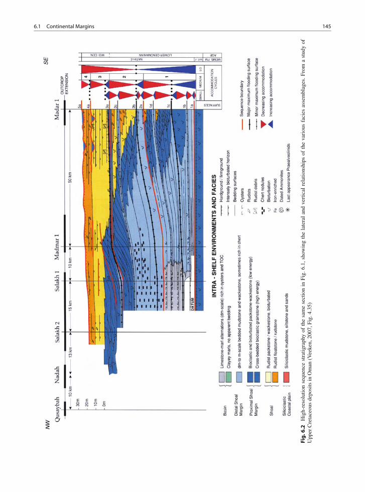
6.1 Continental Margins 145
Fig
.6.2
Hig
h-re
solu
tion
sequ
ence
stra
tigra
phy
ofth
esa
me
sect
ion
inFi
g.6.
1,sh
owin
gth
ela
tera
lan
dve
rtic
alre
latio
nshi
psof
the
vari
ous
faci
esas
sem
blag
es.F
rom
ast
udy
ofU
pper
Cre
tace
ous
depo
sits
inO
man
(Vee
ken,
2007
,Fig
.4.3
5)
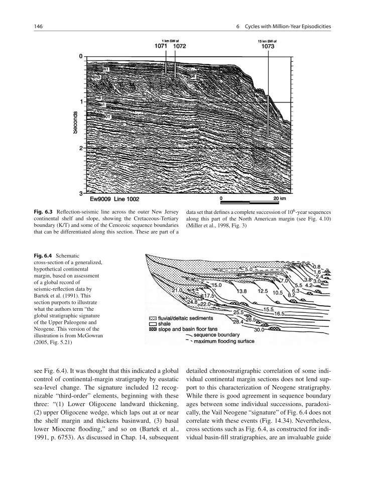
146 6 Cycles with Million-Year Episodicities
Fig. 6.3 Reflection-seismic line across the outer New Jerseycontinental shelf and slope, showing the Cretaceous-Tertiaryboundary (K/T) and some of the Cenozoic sequence boundariesthat can be differentiated along this section. These are part of a
data set that defines a complete succession of 106-year sequencesalong this part of the North American margin (see Fig. 4.10)(Miller et al., 1998, Fig. 3)
Fig. 6.4 Schematiccross-section of a generalized,hypothetical continentalmargin, based on assessmentof a global record ofseismic-reflection data byBartek et al. (1991). Thissection purports to illustratewhat the authors term “theglobal stratigraphic signatureof the Upper Paleogene andNeogene. This version of theillustration is from McGowran(2005, Fig. 5.21)
see Fig. 6.4). It was thought that this indicated a globalcontrol of continental-margin stratigraphy by eustaticsea-level change. The signature included 12 recog-nizable “third-order” elements, beginning with thesethree: “(1) Lower Oligocene landward thickening,(2) upper Oligocene wedge, which laps out at or nearthe shelf margin and thickens basinward, (3) basallower Miocene flooding,” and so on (Bartek et al.,1991, p. 6753). As discussed in Chap. 14, subsequent
detailed chronostratigraphic correlation of some indi-vidual continental margin sections does not lend sup-port to this characterization of Neogene stratigraphy.While there is good agreement in sequence boundaryages between some individual successions, paradoxi-cally, the Vail Neogene “signature” of Fig. 6.4 does notcorrelate with these events (Fig. 14.34). Nevertheless,cross sections such as Fig. 6.4, as constructed for indi-vidual basin-fill stratigraphies, are an invaluable guide
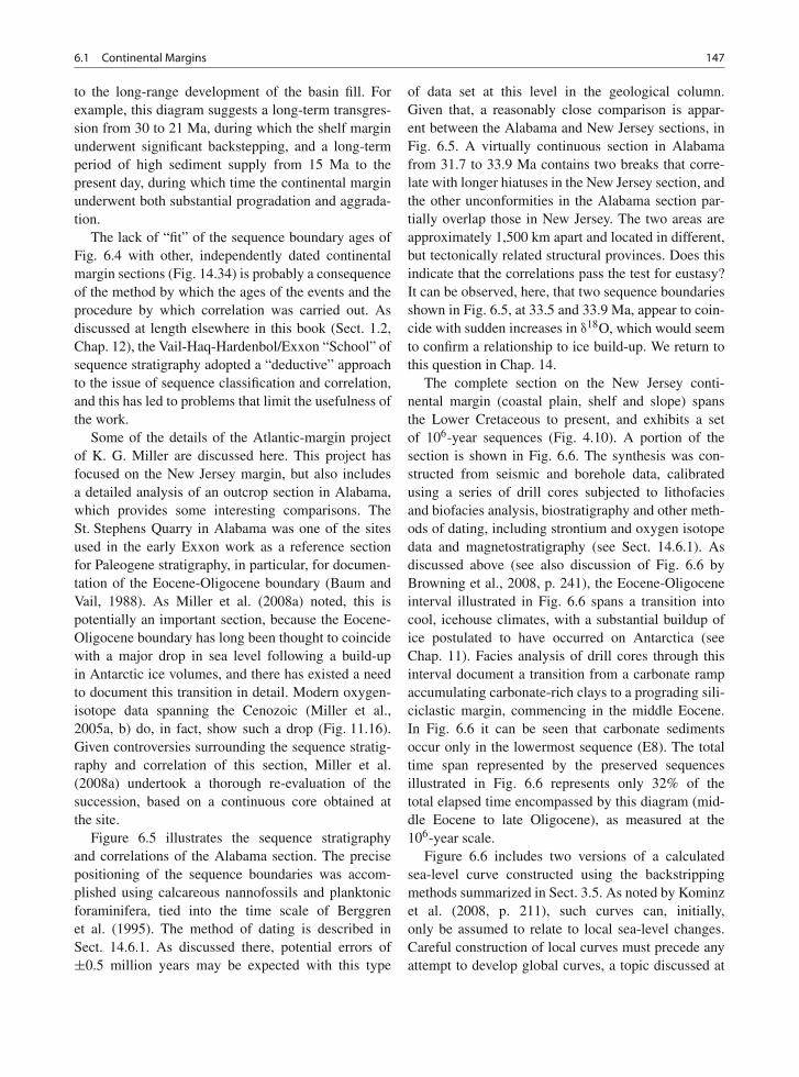
6.1 Continental Margins 147
to the long-range development of the basin fill. Forexample, this diagram suggests a long-term transgres-sion from 30 to 21 Ma, during which the shelf marginunderwent significant backstepping, and a long-termperiod of high sediment supply from 15 Ma to thepresent day, during which time the continental marginunderwent both substantial progradation and aggrada-tion.
The lack of “fit” of the sequence boundary ages ofFig. 6.4 with other, independently dated continentalmargin sections (Fig. 14.34) is probably a consequenceof the method by which the ages of the events and theprocedure by which correlation was carried out. Asdiscussed at length elsewhere in this book (Sect. 1.2,Chap. 12), the Vail-Haq-Hardenbol/Exxon “School” ofsequence stratigraphy adopted a “deductive” approachto the issue of sequence classification and correlation,and this has led to problems that limit the usefulness ofthe work.
Some of the details of the Atlantic-margin projectof K. G. Miller are discussed here. This project hasfocused on the New Jersey margin, but also includesa detailed analysis of an outcrop section in Alabama,which provides some interesting comparisons. TheSt. Stephens Quarry in Alabama was one of the sitesused in the early Exxon work as a reference sectionfor Paleogene stratigraphy, in particular, for documen-tation of the Eocene-Oligocene boundary (Baum andVail, 1988). As Miller et al. (2008a) noted, this ispotentially an important section, because the Eocene-Oligocene boundary has long been thought to coincidewith a major drop in sea level following a build-upin Antarctic ice volumes, and there has existed a needto document this transition in detail. Modern oxygen-isotope data spanning the Cenozoic (Miller et al.,2005a, b) do, in fact, show such a drop (Fig. 11.16).Given controversies surrounding the sequence stratig-raphy and correlation of this section, Miller et al.(2008a) undertook a thorough re-evaluation of thesuccession, based on a continuous core obtained atthe site.
Figure 6.5 illustrates the sequence stratigraphyand correlations of the Alabama section. The precisepositioning of the sequence boundaries was accom-plished using calcareous nannofossils and planktonicforaminifera, tied into the time scale of Berggrenet al. (1995). The method of dating is described inSect. 14.6.1. As discussed there, potential errors of±0.5 million years may be expected with this type
of data set at this level in the geological column.Given that, a reasonably close comparison is appar-ent between the Alabama and New Jersey sections, inFig. 6.5. A virtually continuous section in Alabamafrom 31.7 to 33.9 Ma contains two breaks that corre-late with longer hiatuses in the New Jersey section, andthe other unconformities in the Alabama section par-tially overlap those in New Jersey. The two areas areapproximately 1,500 km apart and located in different,but tectonically related structural provinces. Does thisindicate that the correlations pass the test for eustasy?It can be observed, here, that two sequence boundariesshown in Fig. 6.5, at 33.5 and 33.9 Ma, appear to coin-cide with sudden increases in δ18O, which would seemto confirm a relationship to ice build-up. We return tothis question in Chap. 14.
The complete section on the New Jersey conti-nental margin (coastal plain, shelf and slope) spansthe Lower Cretaceous to present, and exhibits a setof 106-year sequences (Fig. 4.10). A portion of thesection is shown in Fig. 6.6. The synthesis was con-structed from seismic and borehole data, calibratedusing a series of drill cores subjected to lithofaciesand biofacies analysis, biostratigraphy and other meth-ods of dating, including strontium and oxygen isotopedata and magnetostratigraphy (see Sect. 14.6.1). Asdiscussed above (see also discussion of Fig. 6.6 byBrowning et al., 2008, p. 241), the Eocene-Oligoceneinterval illustrated in Fig. 6.6 spans a transition intocool, icehouse climates, with a substantial buildup ofice postulated to have occurred on Antarctica (seeChap. 11). Facies analysis of drill cores through thisinterval document a transition from a carbonate rampaccumulating carbonate-rich clays to a prograding sili-ciclastic margin, commencing in the middle Eocene.In Fig. 6.6 it can be seen that carbonate sedimentsoccur only in the lowermost sequence (E8). The totaltime span represented by the preserved sequencesillustrated in Fig. 6.6 represents only 32% of thetotal elapsed time encompassed by this diagram (mid-dle Eocene to late Oligocene), as measured at the106-year scale.
Figure 6.6 includes two versions of a calculatedsea-level curve constructed using the backstrippingmethods summarized in Sect. 3.5. As noted by Kominzet al. (2008, p. 211), such curves can, initially,only be assumed to relate to local sea-level changes.Careful construction of local curves must precede anyattempt to develop global curves, a topic discussed at
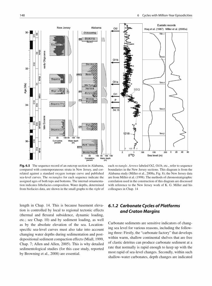
148 6 Cycles with Million-Year Episodicities
Fig. 6.5 The sequence record of an outcrop section in Alabama,compared with contemporaneous strata in New Jersey, and cor-related against a standard oxygen isotope curve and publishedsea-level curves. The rectangles for each sequence indicate theassigned ages of both tops and bottoms. The internal ornamenta-tion indicates lithofacies composition. Water depths, determinedfrom biofacies data, are shown in the small graphs to the right of
each rectangle. Arrows labeled Oi2, Oi1b, etc., refer to sequenceboundaries in the New Jersey sections. This diagram is from theAlabama study (Miller et al., 2008a, Fig. 8); the New Jersey dataare from Miller et al. (1998). The methods of chronostratigraphiccorrelation used in the construction of this diagram are discussedwith reference to the New Jersey work of K. G. Miller and hiscolleagues in Chap. 14
length in Chap. 14. This is because basement eleva-tion is controlled by local to regional tectonic effects(thermal and flexural subsidence, dynamic loading,etc.; see Chap. 10) and by sediment loading, as wellas by the absolute elevation of the sea. Location-specific sea-level curves must also take into accountchanging water depths during sedimentation and post-depositional sediment compaction effects (Miall, 1999,Chap. 7; Allen and Allen, 2005). This is why detailedsedimentological studies (for this case study, reportedby Browning et al., 2008) are essential.
6.1.2 Carbonate Cycles of Platformsand Craton Margins
Carbonate sediments are sensitive indicators of chang-ing sea level for various reasons, including the follow-ing three: Firstly, the “carbonate factory” that developswithin warm, shallow continental shelves that are freeof clastic detritus can produce carbonate sediment at arate that normally is rapid enough to keep up with themost rapid of sea-level changes. Secondly, within suchshallow-water carbonates, depth changes are indicated
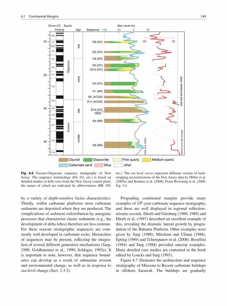
6.1 Continental Margins 149
Fig. 6.6 Eocene-Oligocene sequence stratigraphy of NewJersey. The sequence terminology (E8, O1, etc.) is based ondetailed studies of drill cores from the New Jersey coastal plain,the names of which are indicated by abbreviations (BR, OV,
etc.). The sea level curves represent different version of back-stripping reconstructions of the New Jersey data by Miller et al.(2005a) and Kominz et al. (2008). From Browning et al. (2008,Fig. 11)
by a variety of depth-sensitive facies characteristics.Thirdly, within carbonate platforms most carbonatesediments are deposited where they are produced. Thecomplications of sediment redistribution by autogenicprocesses that characterize clastic sediments (e.g., thedevelopment of delta lobes) therefore are less extreme.For these reasons stratigraphic sequences are com-monly well developed in carbonate rocks. Hierarchiesof sequences may be present, reflecting the integra-tion of several different generative mechanisms (Sarg,1988; Goldhammer et al., 1990; Schlager, 1992a). Itis important to note, however, that sequence bound-aries can develop as a result of submarine erosionand environmental change, as well as in response tosea-level change (Sect. 2.3.3).
Prograding continental margins provide manyexamples of 106-year carbonate sequence stratigraphy,and these are well displayed in regional reflection-seismic records. Eberli and Ginsburg (1988, 1989) andEberli et al. (1997) described an excellent example ofthis, revealing the dramatic lateral growth by progra-dation of the Bahama Platform. Other examples weregiven by Sarg (1988), Mitchum and Uliana (1988),Epting (1989) and Tcherepanov et al. (2008). Bosellini(1984) and Sarg (1988) provided outcrop examples.Many detailed case studies are contained in the bookedited by Loucks and Sarg (1993).
Figure 6.7 illustrates the architecture and sequencestratigraphy of Miocene to Recent carbonate buildupsin offshore Sarawak. The buildups are gradually
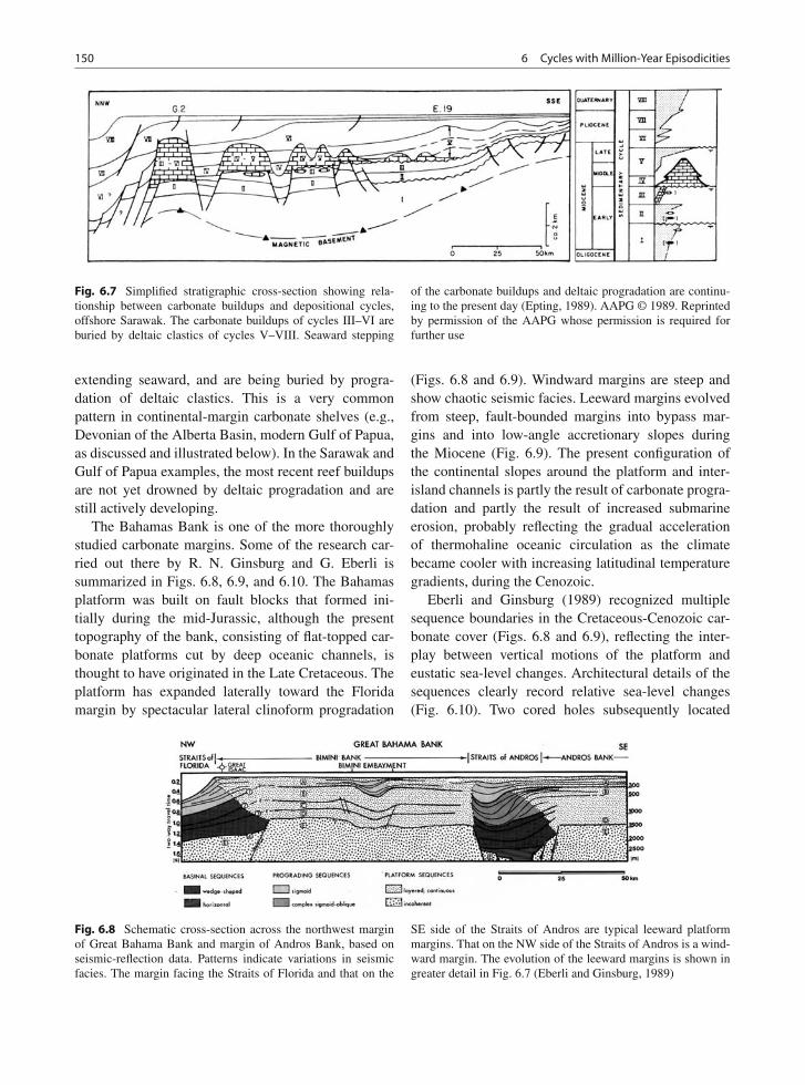
150 6 Cycles with Million-Year Episodicities
Fig. 6.7 Simplified stratigraphic cross-section showing rela-tionship between carbonate buildups and depositional cycles,offshore Sarawak. The carbonate buildups of cycles III–VI areburied by deltaic clastics of cycles V–VIII. Seaward stepping
of the carbonate buildups and deltaic progradation are continu-ing to the present day (Epting, 1989). AAPG © 1989. Reprintedby permission of the AAPG whose permission is required forfurther use
extending seaward, and are being buried by progra-dation of deltaic clastics. This is a very commonpattern in continental-margin carbonate shelves (e.g.,Devonian of the Alberta Basin, modern Gulf of Papua,as discussed and illustrated below). In the Sarawak andGulf of Papua examples, the most recent reef buildupsare not yet drowned by deltaic progradation and arestill actively developing.
The Bahamas Bank is one of the more thoroughlystudied carbonate margins. Some of the research car-ried out there by R. N. Ginsburg and G. Eberli issummarized in Figs. 6.8, 6.9, and 6.10. The Bahamasplatform was built on fault blocks that formed ini-tially during the mid-Jurassic, although the presenttopography of the bank, consisting of flat-topped car-bonate platforms cut by deep oceanic channels, isthought to have originated in the Late Cretaceous. Theplatform has expanded laterally toward the Floridamargin by spectacular lateral clinoform progradation
(Figs. 6.8 and 6.9). Windward margins are steep andshow chaotic seismic facies. Leeward margins evolvedfrom steep, fault-bounded margins into bypass mar-gins and into low-angle accretionary slopes duringthe Miocene (Fig. 6.9). The present configuration ofthe continental slopes around the platform and inter-island channels is partly the result of carbonate progra-dation and partly the result of increased submarineerosion, probably reflecting the gradual accelerationof thermohaline oceanic circulation as the climatebecame cooler with increasing latitudinal temperaturegradients, during the Cenozoic.
Eberli and Ginsburg (1989) recognized multiplesequence boundaries in the Cretaceous-Cenozoic car-bonate cover (Figs. 6.8 and 6.9), reflecting the inter-play between vertical motions of the platform andeustatic sea-level changes. Architectural details of thesequences clearly record relative sea-level changes(Fig. 6.10). Two cored holes subsequently located
Fig. 6.8 Schematic cross-section across the northwest marginof Great Bahama Bank and margin of Andros Bank, based onseismic-reflection data. Patterns indicate variations in seismicfacies. The margin facing the Straits of Florida and that on the
SE side of the Straits of Andros are typical leeward platformmargins. That on the NW side of the Straits of Andros is a wind-ward margin. The evolution of the leeward margins is shown ingreater detail in Fig. 6.7 (Eberli and Ginsburg, 1989)
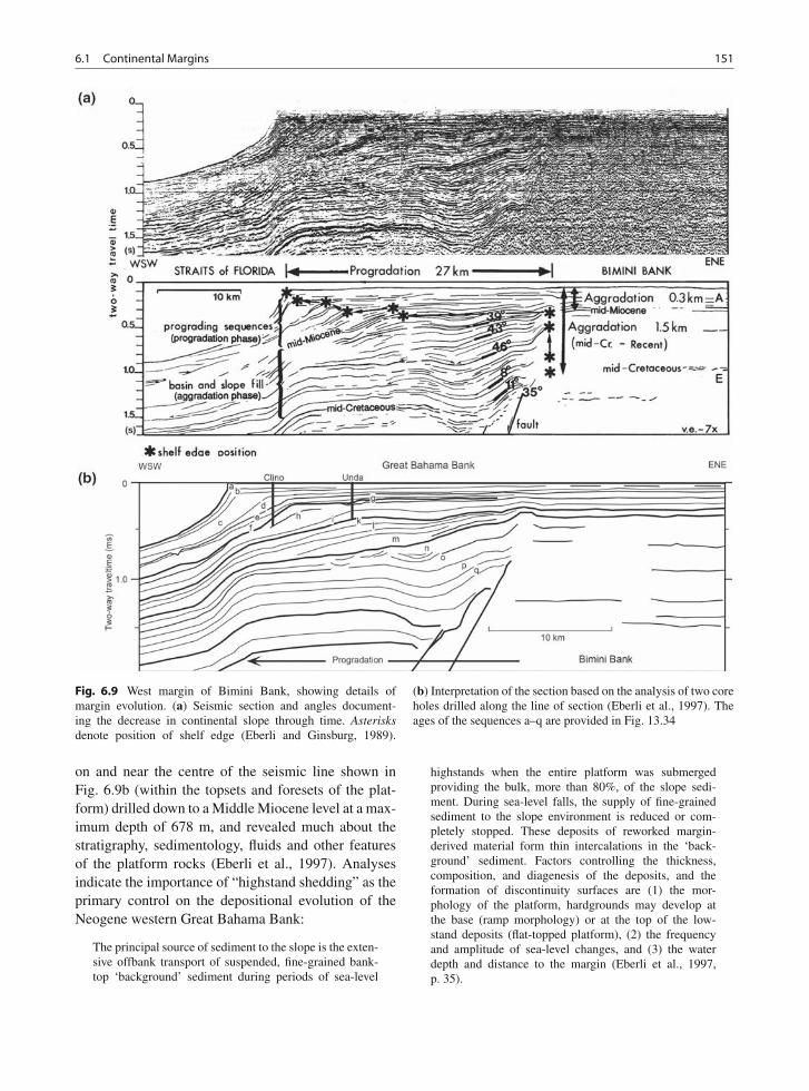
6.1 Continental Margins 151
Fig. 6.9 West margin of Bimini Bank, showing details ofmargin evolution. (a) Seismic section and angles document-ing the decrease in continental slope through time. Asterisksdenote position of shelf edge (Eberli and Ginsburg, 1989).
(b) Interpretation of the section based on the analysis of two coreholes drilled along the line of section (Eberli et al., 1997). Theages of the sequences a–q are provided in Fig. 13.34
on and near the centre of the seismic line shown inFig. 6.9b (within the topsets and foresets of the plat-form) drilled down to a Middle Miocene level at a max-imum depth of 678 m, and revealed much about thestratigraphy, sedimentology, fluids and other featuresof the platform rocks (Eberli et al., 1997). Analysesindicate the importance of “highstand shedding” as theprimary control on the depositional evolution of theNeogene western Great Bahama Bank:
The principal source of sediment to the slope is the exten-sive offbank transport of suspended, fine-grained bank-top ‘background’ sediment during periods of sea-level
highstands when the entire platform was submergedproviding the bulk, more than 80%, of the slope sedi-ment. During sea-level falls, the supply of fine-grainedsediment to the slope environment is reduced or com-pletely stopped. These deposits of reworked margin-derived material form thin intercalations in the ‘back-ground’ sediment. Factors controlling the thickness,composition, and diagenesis of the deposits, and theformation of discontinuity surfaces are (1) the mor-phology of the platform, hardgrounds may develop atthe base (ramp morphology) or at the top of the low-stand deposits (flat-topped platform), (2) the frequencyand amplitude of sea-level changes, and (3) the waterdepth and distance to the margin (Eberli et al., 1997,p. 35).
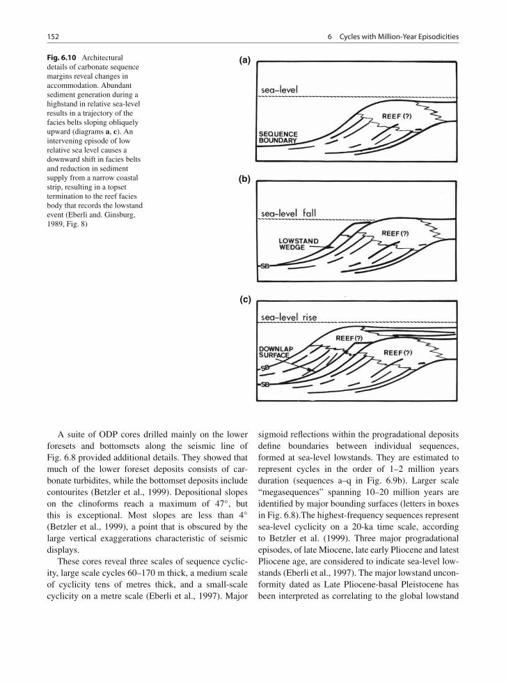
152 6 Cycles with Million-Year Episodicities
(a)
(b)
(c)
Fig. 6.10 Architecturaldetails of carbonate sequencemargins reveal changes inaccommodation. Abundantsediment generation during ahighstand in relative sea-levelresults in a trajectory of thefacies belts sloping obliquelyupward (diagrams a, c). Anintervening episode of lowrelative sea level causes adownward shift in facies beltsand reduction in sedimentsupply from a narrow coastalstrip, resulting in a topsettermination to the reef faciesbody that records the lowstandevent (Eberli and. Ginsburg,1989, Fig. 8)
A suite of ODP cores drilled mainly on the lowerforesets and bottomsets along the seismic line ofFig. 6.8 provided additional details. They showed thatmuch of the lower foreset deposits consists of car-bonate turbidites, while the bottomset deposits includecontourites (Betzler et al., 1999). Depositional slopeson the clinoforms reach a maximum of 47◦, butthis is exceptional. Most slopes are less than 4◦(Betzler et al., 1999), a point that is obscured by thelarge vertical exaggerations characteristic of seismicdisplays.
These cores reveal three scales of sequence cyclic-ity, large scale cycles 60–170 m thick, a medium scaleof cyclicity tens of metres thick, and a small-scalecyclicity on a metre scale (Eberli et al., 1997). Major
sigmoid reflections within the progradational depositsdefine boundaries between individual sequences,formed at sea-level lowstands. They are estimated torepresent cycles in the order of 1–2 million yearsduration (sequences a–q in Fig. 6.9b). Larger scale“megasequences” spanning 10–20 million years areidentified by major bounding surfaces (letters in boxesin Fig. 6.8).The highest-frequency sequences representsea-level cyclicity on a 20-ka time scale, accordingto Betzler et al. (1999). Three major progradationalepisodes, of late Miocene, late early Pliocene and latestPliocene age, are considered to indicate sea-level low-stands (Eberli et al., 1997). The major lowstand uncon-formity dated as Late Pliocene-basal Pleistocene hasbeen interpreted as correlating to the global lowstand
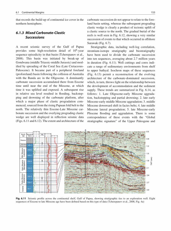
6.1 Continental Margins 153
that records the build-up of continental ice cover in thenorthern hemisphere.
6.1.3 Mixed Carbonate-ClasticSuccessions
A recent seismic survey of the Gulf of Papuaprovides some high-resolution detail of 106-yearsequence episodicity in that basin (Tcherepanov et al.,2008). This basin was initiated by break-up ofGondwana (middle Triassic-middle Jurassic) and mod-ified by spreading of the Coral Sea (Late Cretaceous-Paleocene). It became part of a peripheral foreland(proforeland) basin following the collision of Australiawith the Banda arc in the Oligocene. A dominantlycarbonate succession accumulated there from Eocenetime until near the end of the Miocene, at whichtime it was uplifted and exposed. A subsequent risein relative sea level resulted in flooding, backstep-ping and drowning of the carbonate platform, afterwhich a major phase of clastic progradation com-menced, sourced from the rising Papuan fold belt to thenorth. The relatively thin Eocene-Late Miocene car-bonate succession and the overlying prograding clasticwedge are well displayed in reflection seismic data(Figs. 6.11 and 6.12). The extent and architecture of the
carbonate succession do not appear to relate to the fore-land basin setting, whereas the subsequent progradingclastic wedge is clearly a product of tectonic uplift ofa clastic source to the north. The gradual burial of thereefs is well seen in Fig. 6.12, showing a very similarsuccession of events to that which occurred in offshoreSarawak (Fig. 6.7).
Stratigraphic data, including well-log correlation,strontium-isotope stratigraphy and biostratigraphyhave been used to divide the carbonate successioninto ten sequences, averaging about 2.7 million yearsin duration (Fig. 6.11). Well cuttings and cores indi-cate a range of sedimentary environments from shelfto upper bathyal. Isochron maps of these sequences(Fig. 6.13) permit a reconstruction of the evolvingarchitecture of the carbonate-dominated succession,which, in turn, throws light on the relationship betweenthe development of accommodation and the sedimentsupply. These trends are summarized in Fig. 6.14, asfollows: 1. Late Oligocene-early Miocene aggrada-tion, backstepping and partial drowning; 2. late earlyMiocene-early middle Miocene aggradation; 3. middleMiocene downward shift in facies belts; 4. late middleMiocene lateral progradation; 5. late Miocene-earlyPliocene flooding and aggradation. There is somecorrespondence of these events with the “Globalstratigraphic signature” of the Upper Paleogene and
Fig. 6.11 Seismic profile across the continental shelf, Gulf of Papua, showing stratigraphic ties to an exploration well. Eightsequences of Eocene to late Miocene age have been defined based on this type of data (Tcherepanov et al., 2008, Fig. 4a)

154 6 Cycles with Million-Year Episodicities
Fig. 6.12 An Eocene-middle Miocene carbonate succession(defined by “top carbonate” and “base carbonate” underlying theGulf of Papua is overlain by clastics of Late Miocene to mod-ern, in age. These have prograded from the continental margin,
leaving only the Eastern Fields and a few other small reef bod-ies exposed. The reefs have been largely drowned by rising sealevel, and only the tip of the Eastern Fields reef is still active(Tcherepanov et al., 2008, Fig. 5A)
Fig. 6.13 Isochron maps of selected carbonate sequences, Gulf of Papua, showing their extent and distribution. Sequencenomenclature (top right corner of each map) is as shown in Fig. 6.11 (Tcherepanov et al., 2008, Fig. 7)
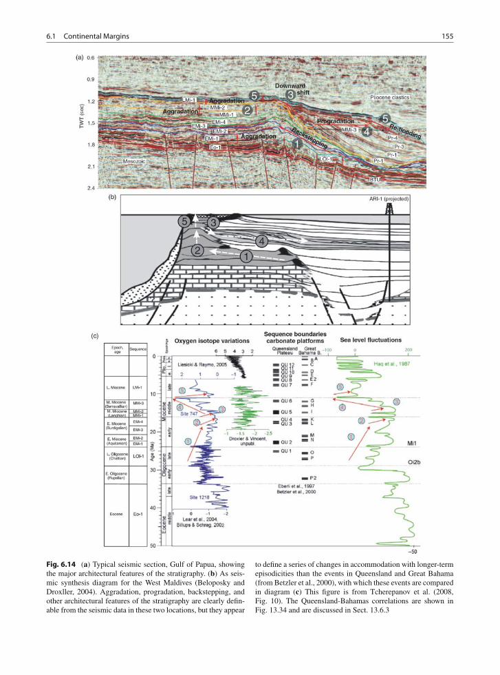
6.1 Continental Margins 155
Fig. 6.14 (a) Typical seismic section, Gulf of Papua, showingthe major architectural features of the stratigraphy. (b) As seis-mic synthesis diagram for the West Maldives (Beloposky andDroxller, 2004). Aggradation, progradation, backstepping, andother architectural features of the stratigraphy are clearly defin-able from the seismic data in these two locations, but they appear
to define a series of changes in accommodation with longer-termepisodicities than the events in Queensland and Great Bahama(from Betzler et al., 2000), with which these events are comparedin diagram (c) This figure is from Tcherepanov et al. (2008,Fig. 10). The Queensland-Bahamas correlations are shown inFig. 13.34 and are discussed in Sect. 13.6.3
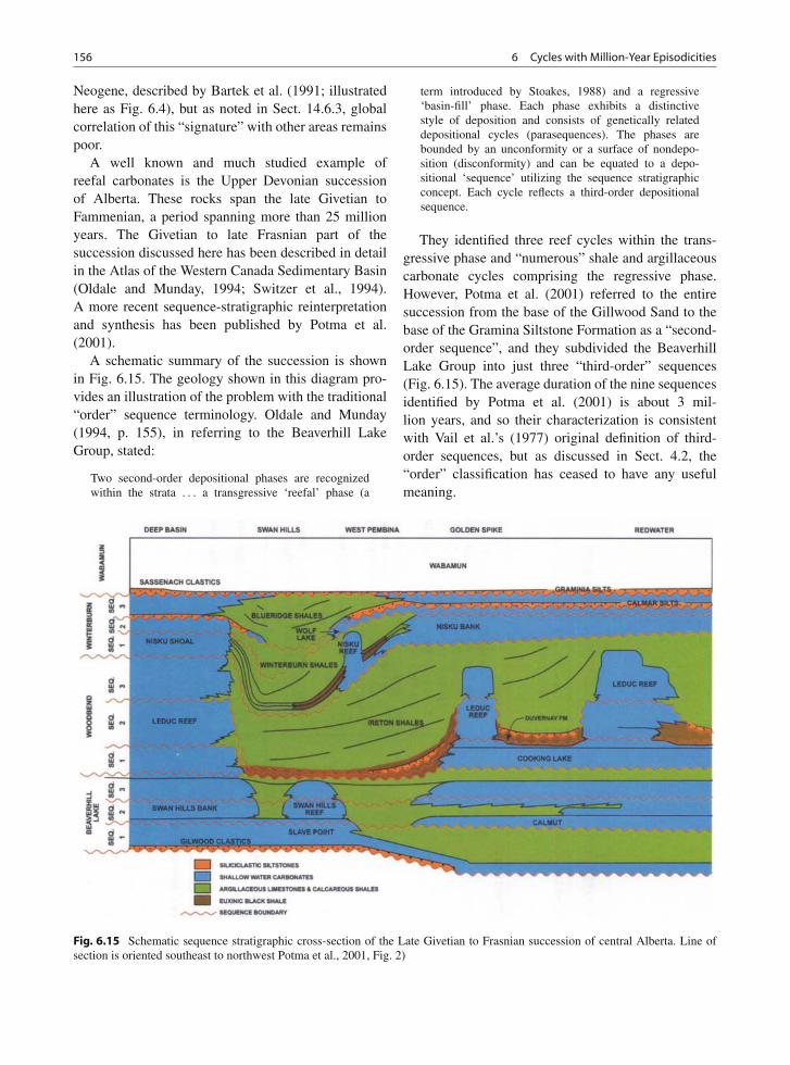
156 6 Cycles with Million-Year Episodicities
Neogene, described by Bartek et al. (1991; illustratedhere as Fig. 6.4), but as noted in Sect. 14.6.3, globalcorrelation of this “signature” with other areas remainspoor.
A well known and much studied example ofreefal carbonates is the Upper Devonian successionof Alberta. These rocks span the late Givetian toFammenian, a period spanning more than 25 millionyears. The Givetian to late Frasnian part of thesuccession discussed here has been described in detailin the Atlas of the Western Canada Sedimentary Basin(Oldale and Munday, 1994; Switzer et al., 1994).A more recent sequence-stratigraphic reinterpretationand synthesis has been published by Potma et al.(2001).
A schematic summary of the succession is shownin Fig. 6.15. The geology shown in this diagram pro-vides an illustration of the problem with the traditional“order” sequence terminology. Oldale and Munday(1994, p. 155), in referring to the Beaverhill LakeGroup, stated:
Two second-order depositional phases are recognizedwithin the strata . . . a transgressive ‘reefal’ phase (a
term introduced by Stoakes, 1988) and a regressive‘basin-fill’ phase. Each phase exhibits a distinctivestyle of deposition and consists of genetically relateddepositional cycles (parasequences). The phases arebounded by an unconformity or a surface of nondepo-sition (disconformity) and can be equated to a depo-sitional ‘sequence’ utilizing the sequence stratigraphicconcept. Each cycle reflects a third-order depositionalsequence.
They identified three reef cycles within the trans-gressive phase and “numerous” shale and argillaceouscarbonate cycles comprising the regressive phase.However, Potma et al. (2001) referred to the entiresuccession from the base of the Gillwood Sand to thebase of the Gramina Siltstone Formation as a “second-order sequence”, and they subdivided the BeaverhillLake Group into just three “third-order” sequences(Fig. 6.15). The average duration of the nine sequencesidentified by Potma et al. (2001) is about 3 mil-lion years, and so their characterization is consistentwith Vail et al.’s (1977) original definition of third-order sequences, but as discussed in Sect. 4.2, the“order” classification has ceased to have any usefulmeaning.
Fig. 6.15 Schematic sequence stratigraphic cross-section of the Late Givetian to Frasnian succession of central Alberta. Line ofsection is oriented southeast to northwest Potma et al., 2001, Fig. 2)
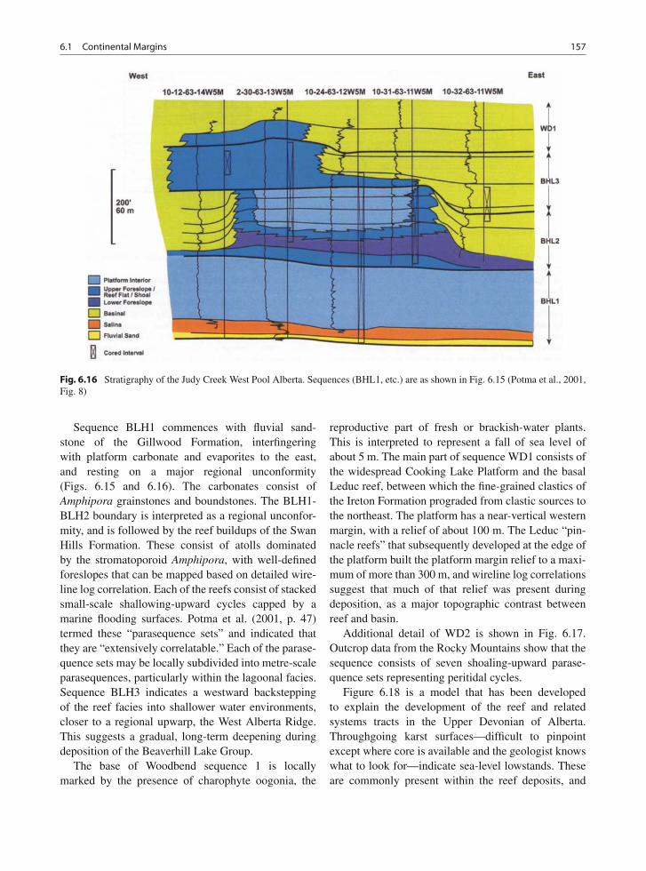
6.1 Continental Margins 157
Fig. 6.16 Stratigraphy of the Judy Creek West Pool Alberta. Sequences (BHL1, etc.) are as shown in Fig. 6.15 (Potma et al., 2001,Fig. 8)
Sequence BLH1 commences with fluvial sand-stone of the Gillwood Formation, interfingeringwith platform carbonate and evaporites to the east,and resting on a major regional unconformity(Figs. 6.15 and 6.16). The carbonates consist ofAmphipora grainstones and boundstones. The BLH1-BLH2 boundary is interpreted as a regional unconfor-mity, and is followed by the reef buildups of the SwanHills Formation. These consist of atolls dominatedby the stromatoporoid Amphipora, with well-definedforeslopes that can be mapped based on detailed wire-line log correlation. Each of the reefs consist of stackedsmall-scale shallowing-upward cycles capped by amarine flooding surfaces. Potma et al. (2001, p. 47)termed these “parasequence sets” and indicated thatthey are “extensively correlatable.” Each of the parase-quence sets may be locally subdivided into metre-scaleparasequences, particularly within the lagoonal facies.Sequence BLH3 indicates a westward backsteppingof the reef facies into shallower water environments,closer to a regional upwarp, the West Alberta Ridge.This suggests a gradual, long-term deepening duringdeposition of the Beaverhill Lake Group.
The base of Woodbend sequence 1 is locallymarked by the presence of charophyte oogonia, the
reproductive part of fresh or brackish-water plants.This is interpreted to represent a fall of sea level ofabout 5 m. The main part of sequence WD1 consists ofthe widespread Cooking Lake Platform and the basalLeduc reef, between which the fine-grained clastics ofthe Ireton Formation prograded from clastic sources tothe northeast. The platform has a near-vertical westernmargin, with a relief of about 100 m. The Leduc “pin-nacle reefs” that subsequently developed at the edge ofthe platform built the platform margin relief to a maxi-mum of more than 300 m, and wireline log correlationssuggest that much of that relief was present duringdeposition, as a major topographic contrast betweenreef and basin.
Additional detail of WD2 is shown in Fig. 6.17.Outcrop data from the Rocky Mountains show that thesequence consists of seven shoaling-upward parase-quence sets representing peritidal cycles.
Figure 6.18 is a model that has been developedto explain the development of the reef and relatedsystems tracts in the Upper Devonian of Alberta.Throughgoing karst surfaces—difficult to pinpointexcept where core is available and the geologist knowswhat to look for—indicate sea-level lowstands. Theseare commonly present within the reef deposits, and
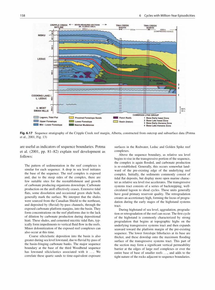
158 6 Cycles with Million-Year Episodicities
Fig. 6.17 Sequence stratigraphy of the Cripple Creek reef margin, Alberta, constructed from outcrop and subsurface data (Potmaet al., 2001, Fig. 13)
are useful as indicators of sequence boundaries. Potmaet al. (2001, pp. 81–82) explain reef development asfollows:
The pattern of sedimentation in the reef complexes issimilar for each sequence. A drop in sea level initiatesthe base of the sequence. The reef complex is exposedand, due to the steep sides of the complex, there arefew suitable sites for the reestablishment and growthof carbonate producing organisms downslope. Carbonateproduction on the atoll effectively ceases. Extensive tidalflats, some dissolution and occasional green shale beds,generally mark the surface. We interpret that the shaleswere sourced from the Canadian Shield to the northeast,and deposited by (fluvial) by-pass channels, through theexposed carbonate platform margins, into the basin. Theyform concentrations on the reef platforms due to the lackof dilution by carbonate production during depositionalhiati. These shales, and cemented micritic tidal flats, typ-ically form impediments to vertical fluid flow in the reefs.Minor dolomitization of the exposed reef complexes canalso occur at this time.
Coarse siliciclastic deposition into the basin is alsogreater during sea level lowstand, due to fluvial by-pass ofthe basin-fringing carbonate banks. The major sequenceboundary at the base of the third Woodbend sequencehas lowstand siliciclastics associated with it . . .. Wecorrelate these quartz sands to time-equivalent exposure
surfaces in the Redwater, Leduc and Golden Spike reefcomplexes.
Above the sequence boundary, as relative sea levelbegins to rise in the transgressive portion of the sequence,the complex is again flooded, and carbonate productionis re-established. Generally, this occurs somewhat land-ward of the pre-existing edge of the underlying reefcomplex. Initially, the sediments commonly consist oftidal flat deposits, but display more open marine charac-ter as relative sea level rise accelerates. The transgressivesystems tract consists of a series of backstepping, well-circulated lagoon to shoal cycles. These units generallyhave good primary reservoir quality. The retrogradationcreates an accretionary high, forming the locus of progra-dation during the early stages of the highstand systemstract.
During highstand of sea level, aggradation, prograda-tion or retrogradation of the reef can occur. The first cycleof the highstand is commonly characterized by strongprogradation that begins at topographic highs on theunderlying transgressive systems tract and then expandsseaward toward the platform margin of the pre-existingsequence. The lower foreslope lithofacies at its base arethicker, and these downlap onto the maximum floodingsurface of the transgressive systems tract. This part ofthe section may form a significant vertical permeabilitybarrier at the edges of large reef complexes or over theentire base of base of smaller reefs . . ., and adds to thetight nature of the rocks adjacent to sequence boundaries.
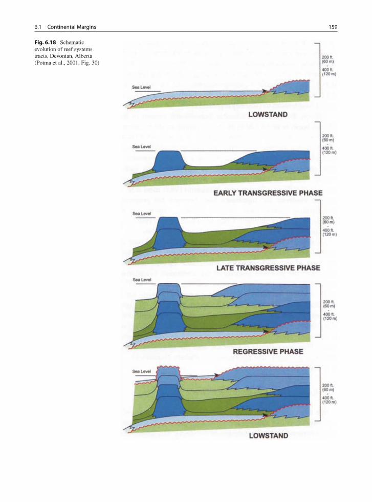
6.1 Continental Margins 159
Fig. 6.18 Schematicevolution of reef systemstracts, Devonian, Alberta(Potma et al., 2001, Fig. 30)
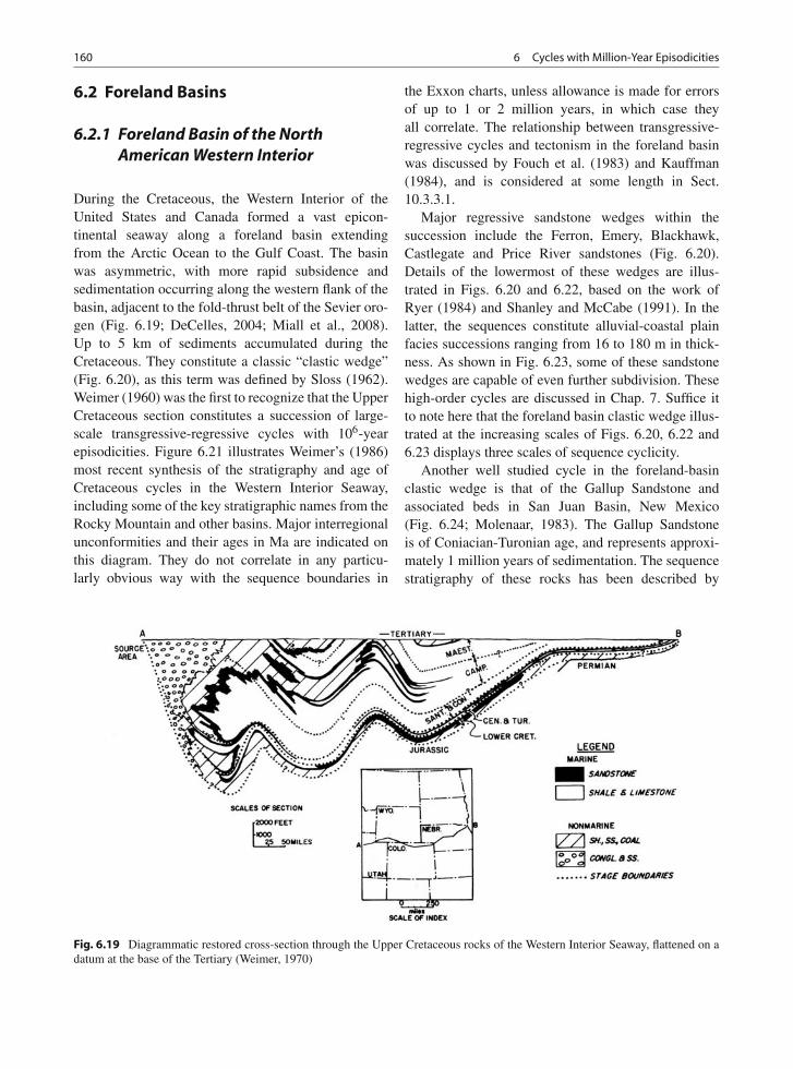
160 6 Cycles with Million-Year Episodicities
6.2 Foreland Basins
6.2.1 Foreland Basin of the NorthAmerican Western Interior
During the Cretaceous, the Western Interior of theUnited States and Canada formed a vast epicon-tinental seaway along a foreland basin extendingfrom the Arctic Ocean to the Gulf Coast. The basinwas asymmetric, with more rapid subsidence andsedimentation occurring along the western flank of thebasin, adjacent to the fold-thrust belt of the Sevier oro-gen (Fig. 6.19; DeCelles, 2004; Miall et al., 2008).Up to 5 km of sediments accumulated during theCretaceous. They constitute a classic “clastic wedge”(Fig. 6.20), as this term was defined by Sloss (1962).Weimer (1960) was the first to recognize that the UpperCretaceous section constitutes a succession of large-scale transgressive-regressive cycles with 106-yearepisodicities. Figure 6.21 illustrates Weimer’s (1986)most recent synthesis of the stratigraphy and age ofCretaceous cycles in the Western Interior Seaway,including some of the key stratigraphic names from theRocky Mountain and other basins. Major interregionalunconformities and their ages in Ma are indicated onthis diagram. They do not correlate in any particu-larly obvious way with the sequence boundaries in
the Exxon charts, unless allowance is made for errorsof up to 1 or 2 million years, in which case theyall correlate. The relationship between transgressive-regressive cycles and tectonism in the foreland basinwas discussed by Fouch et al. (1983) and Kauffman(1984), and is considered at some length in Sect.10.3.3.1.
Major regressive sandstone wedges within thesuccession include the Ferron, Emery, Blackhawk,Castlegate and Price River sandstones (Fig. 6.20).Details of the lowermost of these wedges are illus-trated in Figs. 6.20 and 6.22, based on the work ofRyer (1984) and Shanley and McCabe (1991). In thelatter, the sequences constitute alluvial-coastal plainfacies successions ranging from 16 to 180 m in thick-ness. As shown in Fig. 6.23, some of these sandstonewedges are capable of even further subdivision. Thesehigh-order cycles are discussed in Chap. 7. Suffice itto note here that the foreland basin clastic wedge illus-trated at the increasing scales of Figs. 6.20, 6.22 and6.23 displays three scales of sequence cyclicity.
Another well studied cycle in the foreland-basinclastic wedge is that of the Gallup Sandstone andassociated beds in San Juan Basin, New Mexico(Fig. 6.24; Molenaar, 1983). The Gallup Sandstoneis of Coniacian-Turonian age, and represents approxi-mately 1 million years of sedimentation. The sequencestratigraphy of these rocks has been described by
Fig. 6.19 Diagrammatic restored cross-section through the Upper Cretaceous rocks of the Western Interior Seaway, flattened on adatum at the base of the Tertiary (Weimer, 1970)
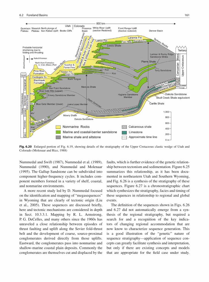
6.2 Foreland Basins 161
Fig. 6.20 Enlarged portion of Fig. 6.19, showing details of the stratigraphy of the Upper Cretaceous clastic wedge of Utah andColorado (Molenaar and Rice, 1988)
Nummedal and Swift (1987), Nummedal et al. (1989),Nummedal (1990), and Nummedal and Molenaar(1995). The Gallup Sandstone can be subdivided intocomponent higher-frequency cycles. It includes com-ponent members formed in a variety of shelf, coastal,and nonmarine environments.
A more recent study led by D. Nummedal focusedon the identification and mapping of “megasequences”in Wyoming that are clearly of tectonic origin (Liuet al., 2005). These sequences are discussed briefly,here and tectonic mechanisms are considered in depthin Sect. 10.3.3.1. Mapping by R. L. Armstrong,P. G. DeCelles, and many others since the 1960s hasunraveled a close relationship between episodes ofthrust faulting and uplift along the Sevier fold-thrustbelt and the development of coarse, source-proximalconglomerates derived directly from those uplifts.Eastward, the conglomerates pass into nonmarine andshallow-marine coastal plain deposits. Commonly theconglomerates are themselves cut and displaced by the
faults, which is further evidence of the genetic relation-ship between tectonism and sedimentation. Figure 6.25summarizes this relationship, as it has been docu-mented in northeastern Utah and Southern Wyoming,and Fig. 6.26 is a synthesis of the stratigraphy of thesesequences. Figure 6.27 is a chronostratigraphic chartwhich synthesizes the stratigraphy, facies and timing ofthese sequences in relationship to regional and globalevents.
The definition of the sequences shown in Figs. 6.26and 6.27 did not automatically emerge from a syn-thesis of the regional stratigraphy, but required asearch for and a recognition of the key indica-tors of changing regional accommodation that arenow know to characterize sequence generation. Thisis a good illustration of the “genetic” nature ofsequence stratigraphy—application of sequence con-cepts can greatly facilitate synthesis and interpretation,but only if there are existing concepts and modelsthat are appropriate for the field case under study.
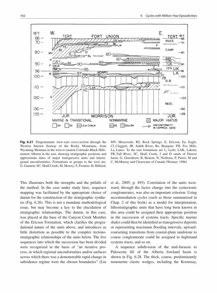
162 6 Cycles with Million-Year Episodicities
Fig. 6.21 Diagrammatic west–east cross-section through theWestern Interior Seaway of the Rocky Mountains, fromWyoming-Montana in the west to eastern Colorado-Black Hills-eastern Alberta in the east, showing stratigraphic positions andapproximate dates of major transgressive units and interre-gional unconformities. Formations or groups to the west are:G, Gannett; SC, Skull Creek; M, Mowry; F, Frontier, H, Hilliard,
MV, Mesaverde; RS, Rock Springs; E, Ericson; Ea, Eagle;Cl, Claggett; JR, Judith River; Be, Bearpaw; FH, Fox Hills;La, Lance. To the east formations are L, Lytle; LAK, Lakota;FR, Fall River; SC, Skull Creek, J and D sands of Denverbasin; G, Greenhorn; B, Benton; N, Niobrara; P, Pierre; M andC, McMurray and Clearwater of Canada (Weimer, 1986)
This illustrates both the strengths and the pitfalls ofthe method. In the case under study here, sequencemapping was facilitated by the appropriate choice ofdatum for the construction of the stratigraphic synthe-sis (Fig. 6.26). This is not a mundane methodologicalissue, but may become a key to the elucidation ofstratigraphic relationships. The datum, in this case,was placed at the base of the Canyon Creek Memberof the Ericson Formation, which clarifies the progra-dational nature of the units above, and introduces aslittle distortion as possible to the complex tectono-stratigraphic relationships of the units below. The fivesequences into which the succession has been dividedwere recognized in the basis of “an iterative pro-cess, in which regional unconformities and/or surfacesacross which there was a demonstrable rapid change insubsidence regime were the chosen boundaries” (Liu
et al., 2005, p. 493). Correlation of the units west-ward, through the facies change into the syntectonicconglomerates, was also an important criterion. Usingaccommodation cycles (such as those summarized inChap. 2 of this book) as a model for interpretation,lithostratigraphic units that have long been known inthis area could be assigned their appropriate positionin the succession of systems tracts. Specific marineshales could then be identified as transgressive depositsor representing maximum flooding intervals, upward-coarsening transitions from coastal-plain sandstone tocoarse conglomerate could be assigned to highstandsystems tracts, and so on.
A sequence subdivision of the mid-Jurassic toPaleocene fill of the Alberta foreland basin isshown in Fig. 6.28. The thick, coarse, predominantlynonmarine clastic wedges, including the Kootenay,
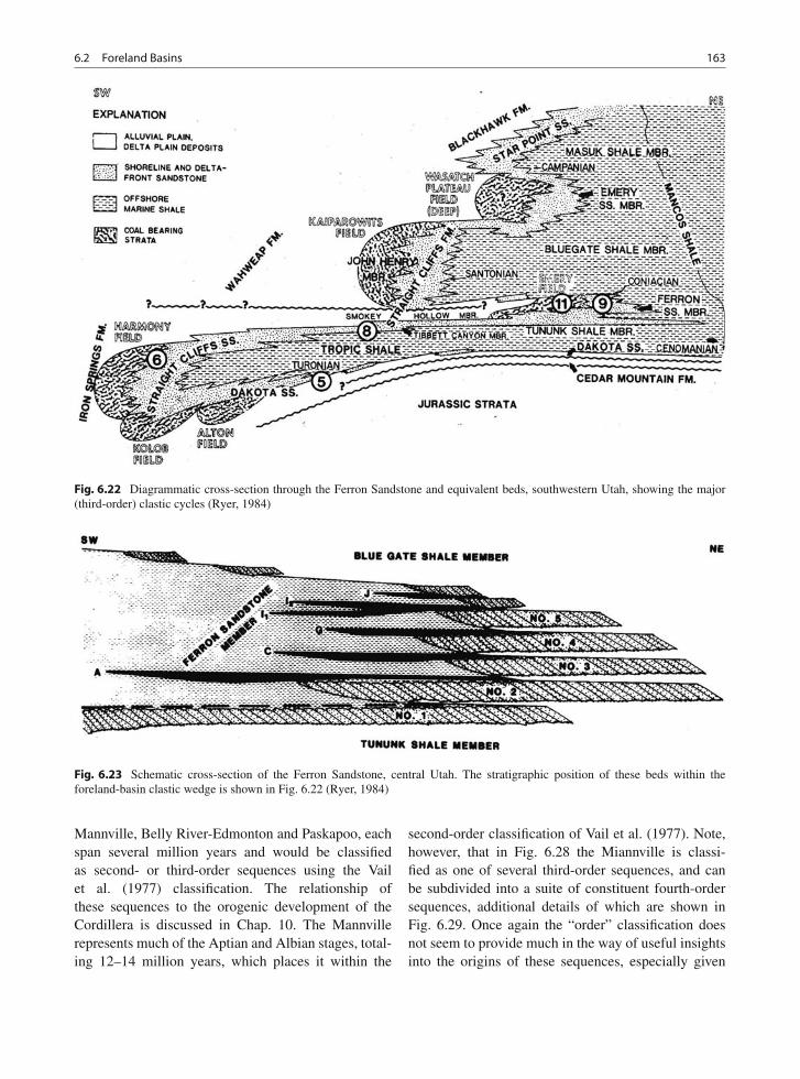
6.2 Foreland Basins 163
Fig. 6.22 Diagrammatic cross-section through the Ferron Sandstone and equivalent beds, southwestern Utah, showing the major(third-order) clastic cycles (Ryer, 1984)
Fig. 6.23 Schematic cross-section of the Ferron Sandstone, central Utah. The stratigraphic position of these beds within theforeland-basin clastic wedge is shown in Fig. 6.22 (Ryer, 1984)
Mannville, Belly River-Edmonton and Paskapoo, eachspan several million years and would be classifiedas second- or third-order sequences using the Vailet al. (1977) classification. The relationship ofthese sequences to the orogenic development of theCordillera is discussed in Chap. 10. The Mannvillerepresents much of the Aptian and Albian stages, total-ing 12–14 million years, which places it within the
second-order classification of Vail et al. (1977). Note,however, that in Fig. 6.28 the Miannville is classi-fied as one of several third-order sequences, and canbe subdivided into a suite of constituent fourth-ordersequences, additional details of which are shown inFig. 6.29. Once again the “order” classification doesnot seem to provide much in the way of useful insightsinto the origins of these sequences, especially given
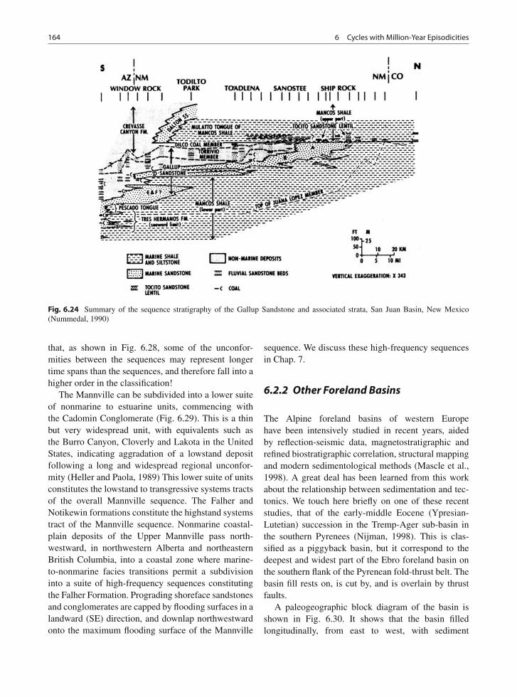
164 6 Cycles with Million-Year Episodicities
Fig. 6.24 Summary of the sequence stratigraphy of the Gallup Sandstone and associated strata, San Juan Basin, New Mexico(Nummedal, 1990)
that, as shown in Fig. 6.28, some of the unconfor-mities between the sequences may represent longertime spans than the sequences, and therefore fall into ahigher order in the classification!
The Mannville can be subdivided into a lower suiteof nonmarine to estuarine units, commencing withthe Cadomin Conglomerate (Fig. 6.29). This is a thinbut very widespread unit, with equivalents such asthe Burro Canyon, Cloverly and Lakota in the UnitedStates, indicating aggradation of a lowstand depositfollowing a long and widespread regional unconfor-mity (Heller and Paola, 1989) This lower suite of unitsconstitutes the lowstand to transgressive systems tractsof the overall Mannville sequence. The Falher andNotikewin formations constitute the highstand systemstract of the Mannville sequence. Nonmarine coastal-plain deposits of the Upper Mannville pass north-westward, in northwestern Alberta and northeasternBritish Columbia, into a coastal zone where marine-to-nonmarine facies transitions permit a subdivisioninto a suite of high-frequency sequences constitutingthe Falher Formation. Prograding shoreface sandstonesand conglomerates are capped by flooding surfaces in alandward (SE) direction, and downlap northwestwardonto the maximum flooding surface of the Mannville
sequence. We discuss these high-frequency sequencesin Chap. 7.
6.2.2 Other Foreland Basins
The Alpine foreland basins of western Europehave been intensively studied in recent years, aidedby reflection-seismic data, magnetostratigraphic andrefined biostratigraphic correlation, structural mappingand modern sedimentological methods (Mascle et al.,1998). A great deal has been learned from this workabout the relationship between sedimentation and tec-tonics. We touch here briefly on one of these recentstudies, that of the early-middle Eocene (Ypresian-Lutetian) succession in the Tremp-Ager sub-basin inthe southern Pyrenees (Nijman, 1998). This is clas-sified as a piggyback basin, but it correspond to thedeepest and widest part of the Ebro foreland basin onthe southern flank of the Pyrenean fold-thrust belt. Thebasin fill rests on, is cut by, and is overlain by thrustfaults.
A paleogeographic block diagram of the basin isshown in Fig. 6.30. It shows that the basin filledlongitudinally, from east to west, with sediment
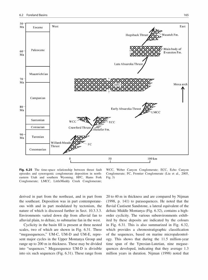
6.2 Foreland Basins 165
Fig. 6.25 The time-space relationship between thrust faultepisodes and synorogenic conglomerate deposition in north-eastern Utah and southern Wyoming. HFC, Hams ForkConglomerate; LMCC, LittleMuddy Creek Conglomerate;
WCC, Weber Canyon Conglomerate; ECC, Echo CanyonConglomerate; FC, Frontier Conglomerate (Liu et al., 2005,Fig. 3)
derived in part from the northeast, and in part fromthe southeast. Deposition was in part contemporane-ous with and in part modulated by tectonism, thenature of which is discussed further in Sect. 10.3.3.3.Environments varied down dip from alluvial fan toalluvial plain, to deltaic, to submarine fan in the west.
Cyclicity in the basin fill is present at three nestedscales, two of which are shown in Fig. 6.31. Three“megasequences,” UM-C, UM-D and UM-E, repre-sent major cycles in the Upper Montanya Group andrange up to 200 m in thickness. These may be dividedinto “sequences.” Megasequence UM-D is divisibleinto six such sequences (Fig. 6.31). These range from
20 to 40 m in thickness and are compared by Nijman(1998, p. 141) to parasequences. He noted that thefluvial Castisent Sandstone, a lateral equivalent of thedeltaic Middle Montanya (Fig. 6.32), contains a high-order cyclicity. The various subenvironments exhib-ited by these deposits are indicated by the coloursin Fig. 6.31. This is also summarized in Fig. 6.32,which provides a chronostratigraphic classificationof the sequences, based on marine micropaleontol-ogy. This shows that during the 11.5 million-yeartime span of the Ypresian-Lutetian, nine megase-quences developed, indicating that they average 1.3million years in duration. Nijman (1998) noted that
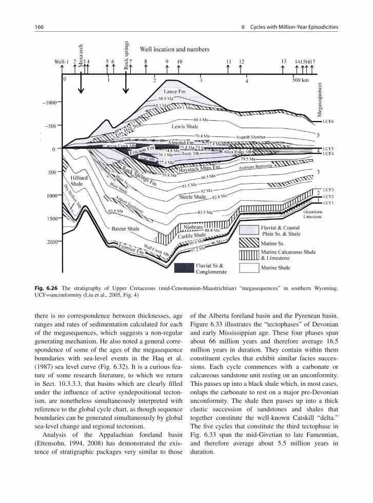
166 6 Cycles with Million-Year Episodicities
Fig. 6.26 The stratigraphy of Upper Cretaceous (mid-Cenomanian-Maastrichtian) “megasequences” in southern Wyoming.UCF=unconformity (Liu et al., 2005, Fig. 4)
there is no correspondence between thicknesses, ageranges and rates of sedimentation calculated for eachof the megasequences, which suggests a non-regulargenerating mechanism. He also noted a general corre-spondence of some of the ages of the megasequenceboundaries with sea-level events in the Haq et al.(1987) sea level curve (Fig. 6.32). It is a curious fea-ture of some research literature, to which we returnin Sect. 10.3.3.3, that basins which are clearly filledunder the influence of active syndepositional tecton-ism, are nonetheless simultaneously interpreted withreference to the global cycle chart, as though sequenceboundaries can be generated simultaneously by globalsea-level change and regional tectonism.
Analysis of the Appalachian foreland basin(Ettensohn, 1994, 2008) has demonstrated the exis-tence of stratigraphic packages very similar to those
of the Alberta foreland basin and the Pyrenean basin.Figure 6.33 illustrates the “tectophases” of Devonianand early Mississippian age. These four phases spanabout 66 million years and therefore average 16.5million years in duration. They contain within themconstituent cycles that exhibit similar facies succes-sions. Each cycle commences with a carbonate orcalcareous sandstone unit resting on an unconformity.This passes up into a black shale which, in most cases,onlaps the carbonate to rest on a major pre-Devonianunconformity. The shale then passes up into a thickclastic succession of sandstones and shales thattogether constitute the well-known Catskill “delta.”The five cycles that constitute the third tectophase inFig. 6.33 span the mid-Givetian to late Famennian,and therefore average about 5.5 million years induration.
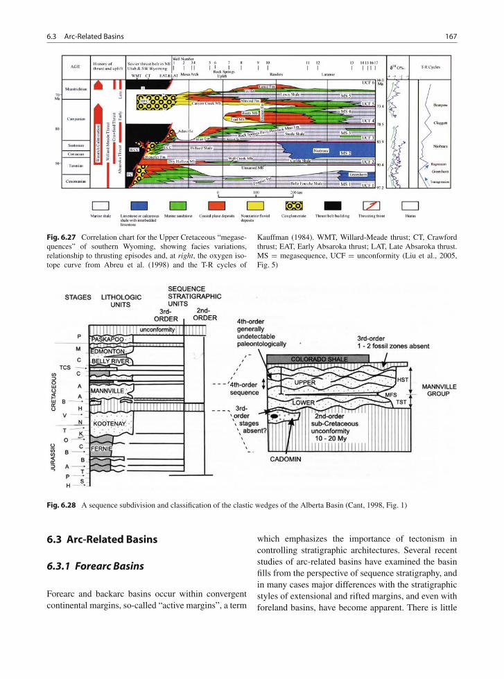
6.3 Arc-Related Basins 167
Fig. 6.27 Correlation chart for the Upper Cretaceous “megase-quences” of southern Wyoming, showing facies variations,relationship to thrusting episodes and, at right, the oxygen iso-tope curve from Abreu et al. (1998) and the T-R cycles of
Kauffman (1984). WMT, Willard-Meade thrust; CT, Crawfordthrust; EAT, Early Absaroka thrust; LAT, Late Absaroka thrust.MS = megasequence, UCF = unconformity (Liu et al., 2005,Fig. 5)
Fig. 6.28 A sequence subdivision and classification of the clastic wedges of the Alberta Basin (Cant, 1998, Fig. 1)
6.3 Arc-Related Basins
6.3.1 Forearc Basins
Forearc and backarc basins occur within convergentcontinental margins, so-called “active margins”, a term
which emphasizes the importance of tectonism incontrolling stratigraphic architectures. Several recentstudies of arc-related basins have examined the basinfills from the perspective of sequence stratigraphy, andin many cases major differences with the stratigraphicstyles of extensional and rifted margins, and even withforeland basins, have become apparent. There is little
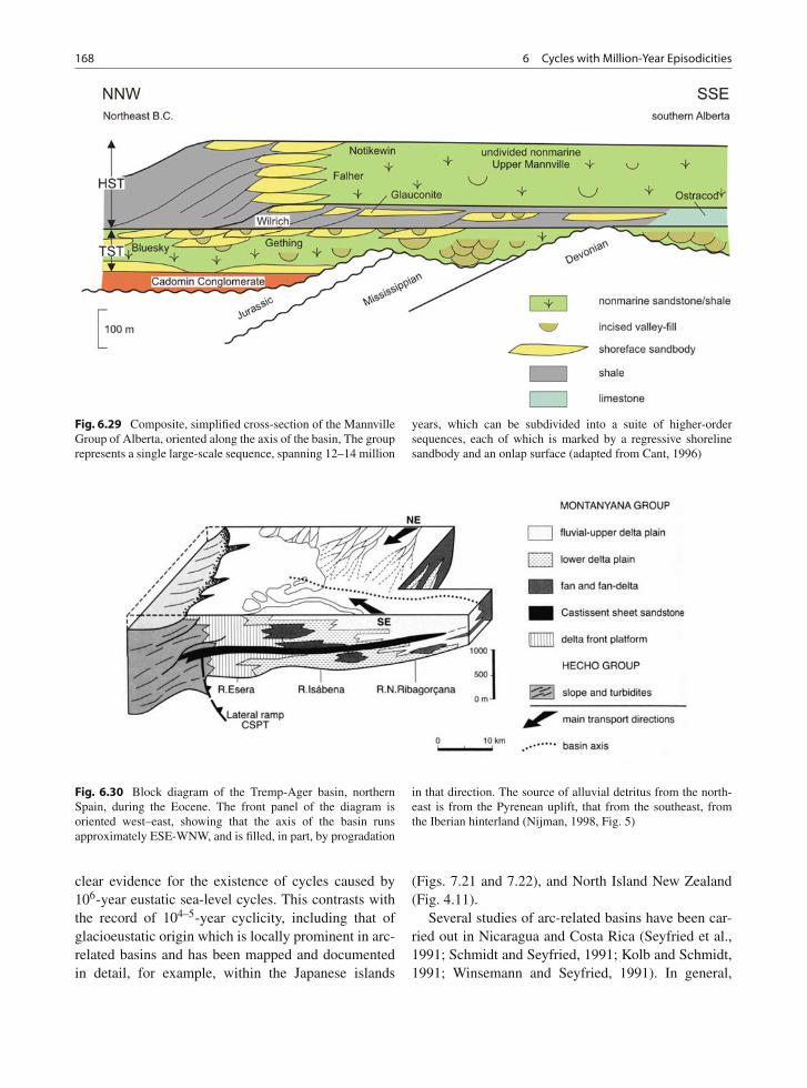
168 6 Cycles with Million-Year Episodicities
Fig. 6.29 Composite, simplified cross-section of the MannvilleGroup of Alberta, oriented along the axis of the basin, The grouprepresents a single large-scale sequence, spanning 12–14 million
years, which can be subdivided into a suite of higher-ordersequences, each of which is marked by a regressive shorelinesandbody and an onlap surface (adapted from Cant, 1996)
Fig. 6.30 Block diagram of the Tremp-Ager basin, northernSpain, during the Eocene. The front panel of the diagram isoriented west–east, showing that the axis of the basin runsapproximately ESE-WNW, and is filled, in part, by progradation
in that direction. The source of alluvial detritus from the north-east is from the Pyrenean uplift, that from the southeast, fromthe Iberian hinterland (Nijman, 1998, Fig. 5)
clear evidence for the existence of cycles caused by106-year eustatic sea-level cycles. This contrasts withthe record of 104–5-year cyclicity, including that ofglacioeustatic origin which is locally prominent in arc-related basins and has been mapped and documentedin detail, for example, within the Japanese islands
(Figs. 7.21 and 7.22), and North Island New Zealand(Fig. 4.11).
Several studies of arc-related basins have been car-ried out in Nicaragua and Costa Rica (Seyfried et al.,1991; Schmidt and Seyfried, 1991; Kolb and Schmidt,1991; Winsemann and Seyfried, 1991). In general,
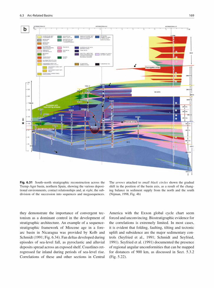
6.3 Arc-Related Basins 169
Fig. 6.31 South–north stratigraphic reconstruction across theTremp-Ager basin, northern Spain, showing the various deposi-tional environments, contact relationships and, at right, the sub-division of the succession into sequences and megasequences.
The arrows attached to small black circles shown the gradualshift in the position of the basin axis, as a result of the chang-ing balance in sediment supply from the north and the south(Nijman, 1998, Fig. 4b)
they demonstrate the importance of convergent tec-tonism as a dominant control in the development ofstratigraphic architecture. An example of a sequence-stratigraphic framework of Miocene age in a fore-arc basin in Nicaragua was provided by Kolb andSchmidt (1991; Fig. 6.34). Fan deltas developed duringepisodes of sea-level fall, as pyroclastic and alluvialdeposits spread across an exposed shelf. Coastlines ret-rogressed far inland during periods of sea-level rise.Correlations of these and other sections in Central
America with the Exxon global cycle chart seemforced and unconvincing. Biostratigraphic evidence forthe correlations is extremely limited. In most cases,it is evident that folding, faulting, tilting and tectonicuplift and subsidence are the major sedimentary con-trols (Seyfried et al., 1991; Schmidt and Seyfried,1991). Seyfried et al. (1991) documented the presenceof regional angular unconformities that can be mappedfor distances of 900 km, as discussed in Sect. 5.3.2(Fig. 5.22).
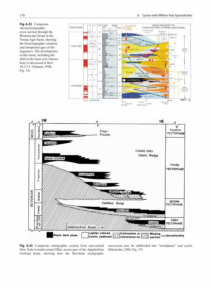
170 6 Cycles with Million-Year Episodicities
Fig. 6.32 Compositechronostratigraphiccross-section through theMontanyana Group in theTremp-Ager basin, showingthe biostratigraphic zonationand interpreted ages of thesequences. The developmentof this basin, including theshift in the basin axis (shownhere) is discussed in Sect.10.3.3.3. (Nijman, 1998,Fig. 13)
Fig. 6.33 Composite stratigraphic section from east-centralNew York to north-central Ohio, across part of the Appalachianforeland basin, showing how the Devonian stratigraphic
succession may be subdivided into “tectophases” and cycles(Ettensohn, 1994, Fig. 13)
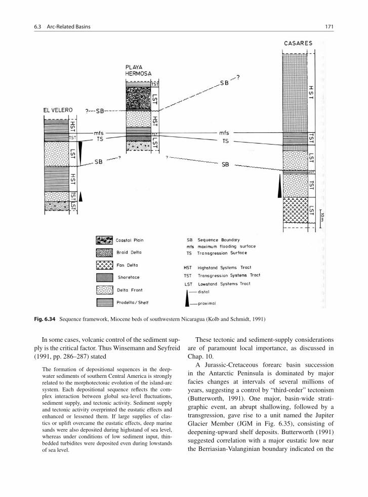
6.3 Arc-Related Basins 171
Fig. 6.34 Sequence framework, Miocene beds of southwestern Nicaragua (Kolb and Schmidt, 1991)
In some cases, volcanic control of the sediment sup-ply is the critical factor. Thus Winsemann and Seyfreid(1991, pp. 286–287) stated
The formation of depositional sequences in the deep-water sediments of southern Central America is stronglyrelated to the morphotectonic evolution of the island-arcsystem. Each depositional sequence reflects the com-plex interaction between global sea-level fluctuations,sediment supply, and tectonic activity. Sediment supplyand tectonic activity overprinted the eustatic effects andenhanced or lessened them. If large supplies of clas-tics or uplift overcame the eustatic effects, deep marinesands were also deposited during highstand of sea level,whereas under conditions of low sediment input, thin-bedded turbidites were deposited even during lowstandsof sea level.
These tectonic and sediment-supply considerationsare of paramount local importance, as discussed inChap. 10.
A Jurassic-Cretaceous forearc basin successionin the Antarctic Peninsula is dominated by majorfacies changes at intervals of several millions ofyears, suggesting a control by “third-order” tectonism(Butterworth, 1991). One major, basin-wide strati-graphic event, an abrupt shallowing, followed by atransgression, gave rise to a unit named the JupiterGlacier Member (JGM in Fig. 6.35), consisting ofdeepening-upward shelf deposits. Butterworth (1991)suggested correlation with a major eustatic low nearthe Berriasian-Valanginian boundary indicated on the
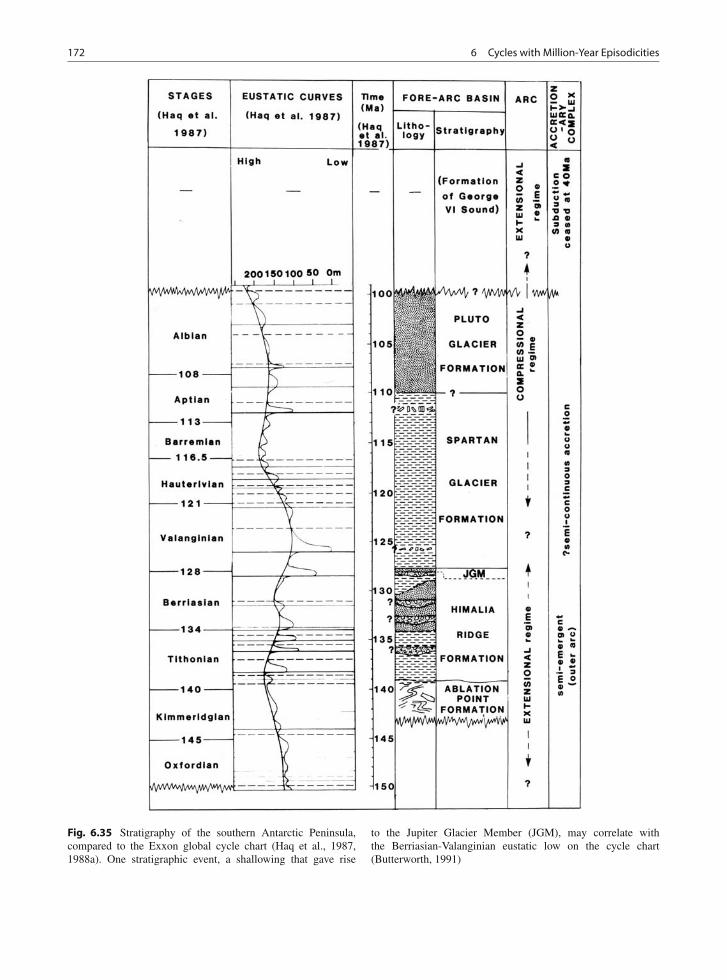
172 6 Cycles with Million-Year Episodicities
Fig. 6.35 Stratigraphy of the southern Antarctic Peninsula,compared to the Exxon global cycle chart (Haq et al., 1987,1988a). One stratigraphic event, a shallowing that gave rise
to the Jupiter Glacier Member (JGM), may correlate withthe Berriasian-Valanginian eustatic low on the cycle chart(Butterworth, 1991)
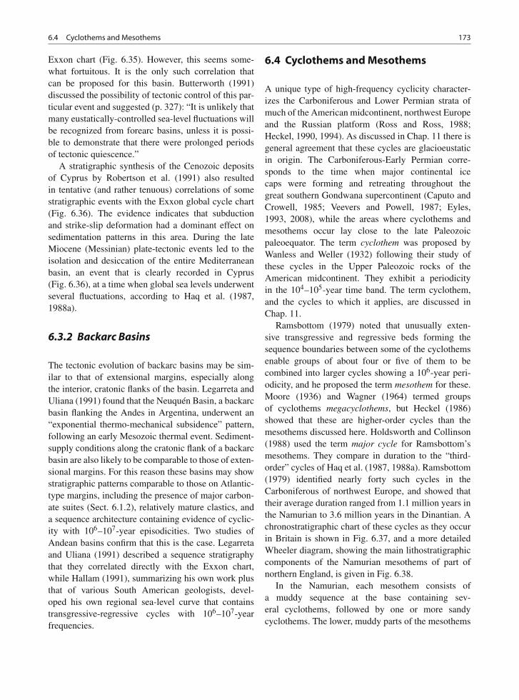
6.4 Cyclothems and Mesothems 173
Exxon chart (Fig. 6.35). However, this seems some-what fortuitous. It is the only such correlation thatcan be proposed for this basin. Butterworth (1991)discussed the possibility of tectonic control of this par-ticular event and suggested (p. 327): “It is unlikely thatmany eustatically-controlled sea-level fluctuations willbe recognized from forearc basins, unless it is possi-ble to demonstrate that there were prolonged periodsof tectonic quiescence.”
A stratigraphic synthesis of the Cenozoic depositsof Cyprus by Robertson et al. (1991) also resultedin tentative (and rather tenuous) correlations of somestratigraphic events with the Exxon global cycle chart(Fig. 6.36). The evidence indicates that subductionand strike-slip deformation had a dominant effect onsedimentation patterns in this area. During the lateMiocene (Messinian) plate-tectonic events led to theisolation and desiccation of the entire Mediterraneanbasin, an event that is clearly recorded in Cyprus(Fig. 6.36), at a time when global sea levels underwentseveral fluctuations, according to Haq et al. (1987,1988a).
6.3.2 Backarc Basins
The tectonic evolution of backarc basins may be sim-ilar to that of extensional margins, especially alongthe interior, cratonic flanks of the basin. Legarreta andUliana (1991) found that the Neuquén Basin, a backarcbasin flanking the Andes in Argentina, underwent an“exponential thermo-mechanical subsidence” pattern,following an early Mesozoic thermal event. Sediment-supply conditions along the cratonic flank of a backarcbasin are also likely to be comparable to those of exten-sional margins. For this reason these basins may showstratigraphic patterns comparable to those on Atlantic-type margins, including the presence of major carbon-ate suites (Sect. 6.1.2), relatively mature clastics, anda sequence architecture containing evidence of cyclic-ity with 106–107-year episodicities. Two studies ofAndean basins confirm that this is the case. Legarretaand Uliana (1991) described a sequence stratigraphythat they correlated directly with the Exxon chart,while Hallam (1991), summarizing his own work plusthat of various South American geologists, devel-oped his own regional sea-level curve that containstransgressive-regressive cycles with 106–107-yearfrequencies.
6.4 Cyclothems and Mesothems
A unique type of high-frequency cyclicity character-izes the Carboniferous and Lower Permian strata ofmuch of the American midcontinent, northwest Europeand the Russian platform (Ross and Ross, 1988;Heckel, 1990, 1994). As discussed in Chap. 11 there isgeneral agreement that these cycles are glacioeustaticin origin. The Carboniferous-Early Permian corre-sponds to the time when major continental icecaps were forming and retreating throughout thegreat southern Gondwana supercontinent (Caputo andCrowell, 1985; Veevers and Powell, 1987; Eyles,1993, 2008), while the areas where cyclothems andmesothems occur lay close to the late Paleozoicpaleoequator. The term cyclothem was proposed byWanless and Weller (1932) following their study ofthese cycles in the Upper Paleozoic rocks of theAmerican midcontinent. They exhibit a periodicityin the 104–105-year time band. The term cyclothem,and the cycles to which it applies, are discussed inChap. 11.
Ramsbottom (1979) noted that unusually exten-sive transgressive and regressive beds forming thesequence boundaries between some of the cyclothemsenable groups of about four or five of them to becombined into larger cycles showing a 106-year peri-odicity, and he proposed the term mesothem for these.Moore (1936) and Wagner (1964) termed groupsof cyclothems megacyclothems, but Heckel (1986)showed that these are higher-order cycles than themesothems discussed here. Holdsworth and Collinson(1988) used the term major cycle for Ramsbottom’smesothems. They compare in duration to the “third-order” cycles of Haq et al. (1987, 1988a). Ramsbottom(1979) identified nearly forty such cycles in theCarboniferous of northwest Europe, and showed thattheir average duration ranged from 1.1 million years inthe Namurian to 3.6 million years in the Dinantian. Achronostratigraphic chart of these cycles as they occurin Britain is shown in Fig. 6.37, and a more detailedWheeler diagram, showing the main lithostratigraphiccomponents of the Namurian mesothems of part ofnorthern England, is given in Fig. 6.38.
In the Namurian, each mesothem consists ofa muddy sequence at the base containing sev-eral cyclothems, followed by one or more sandycyclothems. The lower, muddy parts of the mesothems
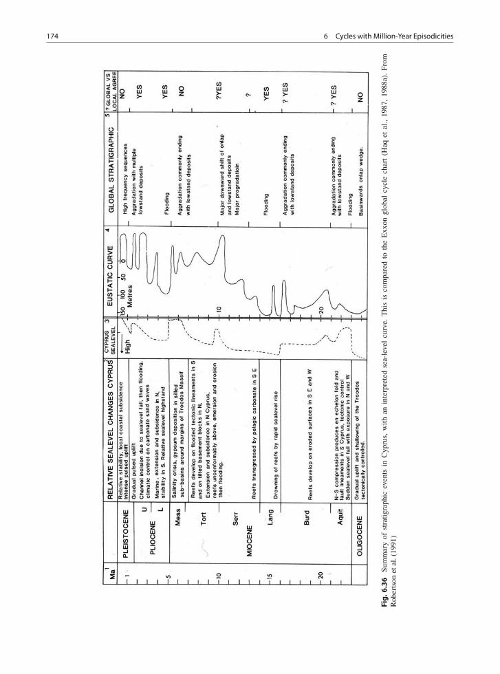
174 6 Cycles with Million-Year Episodicities
Fig
.6.3
6Su
mm
ary
ofst
ratig
raph
icev
ents
inC
ypru
s,w
ithan
inte
rpre
ted
sea-
leve
lcu
rve.
Thi
sis
com
pare
dto
the
Exx
ongl
obal
cycl
ech
art
(Haq
etal
.,19
87,
1988
a).
From
Rob
erts
onet
al.(
1991
)
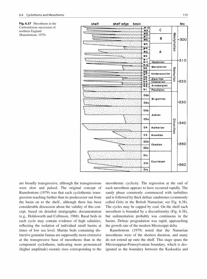
6.4 Cyclothems and Mesothems 175
Fig. 6.37 Mesothems in theCarboniferous succession ofnorthern England(Ramsbottom, 1979)
are broadly transgressive, although the transgressionswere slow and pulsed. The original concept ofRamsbottom (1979) was that each cyclothemic trans-gression reaching further than its predecessor out fromthe basin on to the shelf., although there has beenconsiderable discussion about the validity of this con-cept, based on detailed stratigraphic documentation(e.g., Holdsworth and Collinson, 1988). Basal beds ineach cycle may contain evidence of high salinities,reflecting the isolation of individual small basins attimes of low sea level. Marine beds containing dis-tinctive goniatite faunas are supposedly more extensiveat the transgressive base of mesothems than in thecomponent cyclothems, indicating more pronounced(higher amplitude) eustatic rises corresponding to the
mesothemic cyclicity. The regression at the end ofeach mesothem appears to have occurred rapidly. Thesandy phase commonly commenced with turbiditesand is followed by thick deltaic sandstones (commonlycalled Grits in the British Namurian; see Fig. 6.38).The cycles may be capped by coal. On the shelf eachmesothem is bounded by a disconformity (Fig. 6.38),but sedimentation probably was continuous in thebasins. Deltaic progradation was rapid, approachingthe growth rate of the modern Mississippi delta.
Ramsbottom (1979) noted that the Namurianmesothems were of the shortest duration, and manydo not extend up onto the shelf. This stage spans theMississippian-Pennsylvanian boundary, which is des-ignated as the boundary between the Kaskaskia and
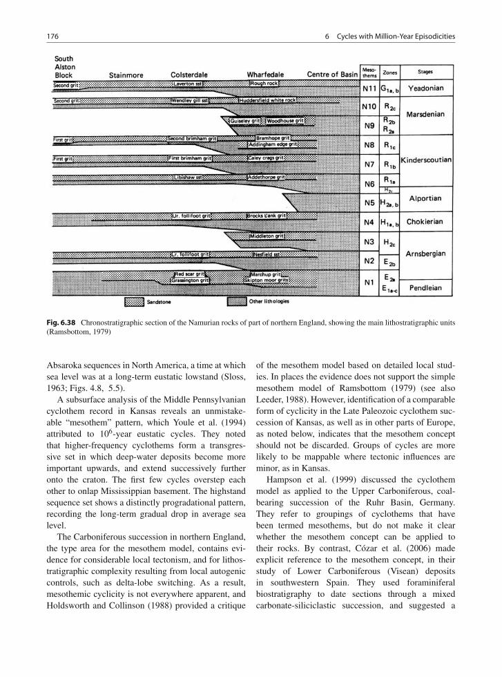
176 6 Cycles with Million-Year Episodicities
Fig. 6.38 Chronostratigraphic section of the Namurian rocks of part of northern England, showing the main lithostratigraphic units(Ramsbottom, 1979)
Absaroka sequences in North America, a time at whichsea level was at a long-term eustatic lowstand (Sloss,1963; Figs. 4.8, 5.5).
A subsurface analysis of the Middle Pennsylvaniancyclothem record in Kansas reveals an unmistake-able “mesothem” pattern, which Youle et al. (1994)attributed to 106-year eustatic cycles. They notedthat higher-frequency cyclothems form a transgres-sive set in which deep-water deposits become moreimportant upwards, and extend successively furtheronto the craton. The first few cycles overstep eachother to onlap Mississippian basement. The highstandsequence set shows a distinctly progradational pattern,recording the long-term gradual drop in average sealevel.
The Carboniferous succession in northern England,the type area for the mesothem model, contains evi-dence for considerable local tectonism, and for lithos-tratigraphic complexity resulting from local autogeniccontrols, such as delta-lobe switching. As a result,mesothemic cyclicity is not everywhere apparent, andHoldsworth and Collinson (1988) provided a critique
of the mesothem model based on detailed local stud-ies. In places the evidence does not support the simplemesothem model of Ramsbottom (1979) (see alsoLeeder, 1988). However, identification of a comparableform of cyclicity in the Late Paleozoic cyclothem suc-cession of Kansas, as well as in other parts of Europe,as noted below, indicates that the mesothem conceptshould not be discarded. Groups of cycles are morelikely to be mappable where tectonic influences areminor, as in Kansas.
Hampson et al. (1999) discussed the cyclothemmodel as applied to the Upper Carboniferous, coal-bearing succession of the Ruhr Basin, Germany.They refer to groupings of cyclothems that havebeen termed mesothems, but do not make it clearwhether the mesothem concept can be applied totheir rocks. By contrast, Cózar et al. (2006) madeexplicit reference to the mesothem concept, in theirstudy of Lower Carboniferous (Visean) depositsin southwestern Spain. They used foraminiferalbiostratigraphy to date sections through a mixedcarbonate-siliciclastic succession, and suggested a
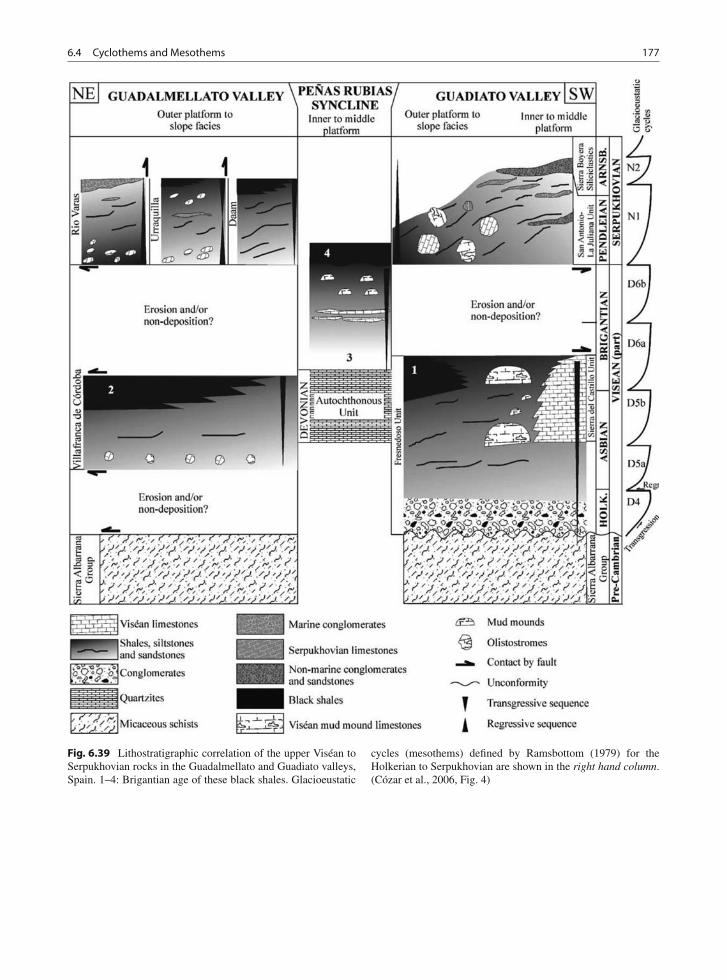
6.4 Cyclothems and Mesothems 177
Fig. 6.39 Lithostratigraphic correlation of the upper Viséan toSerpukhovian rocks in the Guadalmellato and Guadiato valleys,Spain. 1–4: Brigantian age of these black shales. Glacioeustatic
cycles (mesothems) defined by Ramsbottom (1979) for theHolkerian to Serpukhovian are shown in the right hand column.(Cózar et al., 2006, Fig. 4)
178 6 Cycles with Million-Year Episodicities
correlation with Ramsbottom’s (1979) mesothemscheme (Fig. 6.39).
Ross and Ross (1988) carried out a worldwidecomparison of these upper Paleozoic cyclic deposits,and proposed detailed correlations between cratonicsections in the United States, northwest Europeand the Russian platform. They recognized about60 cycles in the Lower Carboniferous to LowerPermian stratigraphic record. They suggested that sim-ilar cyclic successions may occur in contemporaneouscontinental-margin sections, but that because most ofthese have been deformed by post-Paleozoic plate-tectonic events the record from these areas is lesswell known. In view of the scepticism surrounding themesothem concept, and the difficulties in correlationbased on limited chronostratigraphic data, such inter-continental correlation may be regarded as premature.
6.5 Conclusions
1. Stratigraphic sequences with 106-year episodicitiesare common in rifted and extensional continental-margin basins and on cratonic platforms. Theirarchitecture comprises repeated transgressive-regressive packages of siliciclastic or carbonatedeposits, of tabular form on continental shelves,or comprising prograding clinoform slope wedges.Mixed carbonate-siliciclastic sequences formedby reciprocal sedimentation are common. These
sequences can readily be interpreted using standardsystems-tract models.
2. Sequences of comparable duration are also com-mon in foreland basins and can also be interpretedusing the systems-tract approach. Siliciclasticdeposits are dominant, particularly thick alluvialdeposits in proximal settings. Transgressive carbon-ate successions may occur on the distal ramp andforebulge of foreland basins. Evidence for tectoniccontrol is common.
3. In forearc basins, stratigraphic evolution is dom-inated by tectonic subsidence, faulting, andvolcanism.
4. Where backarc basins border a continental margin,the tectonic and stratigraphic history are compara-ble to those of extensional continental margins, andcommonly contain well-developed records of 106-year carbonate or clastic stratigraphic sequences.
5. A distinctive type of cyclicity occurs in upperPaleozoic rocks of the northern hemisphere. Theyare of glacioeustatic origin, resulting from the greatglaciation of the Gondwana supercontinent. High-frequency cycles, called cyclothems, are the mostprominent type of stratigraphic sequence (and arediscussed in Chap. 7), but groupings of these into106-year mesothems or major cycles can be rec-ognized. Some detailed stratigraphic studies havethrown doubt on the mesothem concept as appliedto the Upper Paleozoic record of northwest Europe,whereas some evidence for the concept has beenobtained from the US midcontinent.
Chapter 7
Cycles with Episodicities of Less than One Million Years
Contents
7.1 Introduction . . . . . . . . . . . . . . . . . 1797.2 Neogene Clastic Cycles of Continental Margins 180
7.2.1 The Gulf Coast Basin of the United States 1807.2.2 Wanganui Basin, North Island, New Zealand 1887.2.3 Other Examples of Neogene
High-Frequency Cycles . . . . . . . . 1997.2.4 The Deep-Marine Record . . . . . . . . 202
7.3 Pre-neogene Marine Carbonate and ClasticCycles . . . . . . . . . . . . . . . . . . . . 206
7.4 Late Paleozoic Cyclothems . . . . . . . . . . 2097.5 Lacustrine Clastic and Chemical Rhythms . . 2177.6 High-Frequency Cycles in Foreland Basins . . 2237.7 Main Conclusions . . . . . . . . . . . . . . 235
7.1 Introduction
Cycles of 104–105 years duration can be grouped intofive main types (Sects. 7.2, 7.3, 7.4, 7.5, and 7.6),reflecting their stratigraphic composition, tectonic set-ting, and age. Many of these cycles are thought tohave been generated by global climate changes drivenby orbital forcing, the so-called Milankovitch mech-anisms, as described in Chap. 11. The term derivesfrom the name of the Yugoslavian mathematician whowas the first to provide the mathematical basis for thetheory of astronomical forcing (Milankovitch, 1930,1941). However, there is increasing evidence of thetectonic origin of some of the clastic cycles in forelandbasins (Sect. 7.6), as discussed in Chap. 10.
It has been common practice to subdivide high-frequency sequences into those of fourth order,with durations in the 105-year range, and those offifth-order, with episodicities of 104 years. Thistwofold subdivision has been based largely on
interpretations that invoke low- and high- frequencyMilankovitch mechanisms, respectively. However, thisclassification should now be abandoned. There isincreasing evidence for other sequence-generatingmechanisms that do not readily fall into simple tem-poral classifications, and it has now been demon-strated that sequence thicknesses and durations havelog-normal distributions that lack significant modes(Drummond and Wilkinson, 1996). Schlager (2004)argued that sequence durations have a fractal distribu-tion. This topic is discussed further in Sect. 4.2
As demonstrated by Schwarzacher (1993), orbitalforcing includes a periodicity of 2.035 million years(related to orbital eccentricity), but few examples ofthis have been described in the literature. A modelfor Cretaceous cyclicity that includes this periodicityis discussed in Chap. 11. Most examples of orbitalperiodicities demonstrated from the rock record fallbetween the 413 ka eccentricity period and the 19 kaprecession period. As the examples in this chapterdemonstrate, a range of episodicities has been cal-culated for cycles in the 105-year time band in thegeological record, from a few hundred-thousand yearsto over 1 million years. No preferred time rangesor clustering of these periods around particular fre-quencies has emerged from the analysis, which couldindicate one of two possibilities: (1) the driving forcesare not characterized by temporal regularity, or (2)preferred frequencies do in fact exist (such as harmon-ics of the orbital-forcing process) but are obscured byinaccuracies in the chronostratigraphic control.
This book does not deal with cycles in the so-calledsolar band or calendar band of geological time. Thesolar band refers to cyclicity in the 101–102 year range,including the sun-spot cycle and its possible geologicaleffects (e.g., El Niño current changes). The calendar
179A.D. Miall, The Geology of Stratigraphic Sequences, 2nd ed.,DOI 10.1007/978-3-642-05027-5_7, © Springer-Verlag Berlin Heidelberg 2010
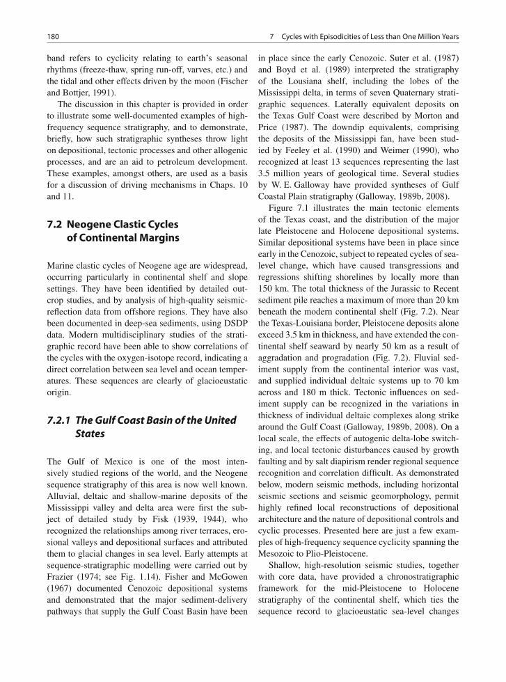
180 7 Cycles with Episodicities of Less than One Million Years
band refers to cyclicity relating to earth’s seasonalrhythms (freeze-thaw, spring run-off, varves, etc.) andthe tidal and other effects driven by the moon (Fischerand Bottjer, 1991).
The discussion in this chapter is provided in orderto illustrate some well-documented examples of high-frequency sequence stratigraphy, and to demonstrate,briefly, how such stratigraphic syntheses throw lighton depositional, tectonic processes and other allogenicprocesses, and are an aid to petroleum development.These examples, amongst others, are used as a basisfor a discussion of driving mechanisms in Chaps. 10and 11.
7.2 Neogene Clastic Cyclesof Continental Margins
Marine clastic cycles of Neogene age are widespread,occurring particularly in continental shelf and slopesettings. They have been identified by detailed out-crop studies, and by analysis of high-quality seismic-reflection data from offshore regions. They have alsobeen documented in deep-sea sediments, using DSDPdata. Modern multidisciplinary studies of the strati-graphic record have been able to show correlations ofthe cycles with the oxygen-isotope record, indicating adirect correlation between sea level and ocean temper-atures. These sequences are clearly of glacioeustaticorigin.
7.2.1 The Gulf Coast Basin of the UnitedStates
The Gulf of Mexico is one of the most inten-sively studied regions of the world, and the Neogenesequence stratigraphy of this area is now well known.Alluvial, deltaic and shallow-marine deposits of theMississippi valley and delta area were first the sub-ject of detailed study by Fisk (1939, 1944), whorecognized the relationships among river terraces, ero-sional valleys and depositional surfaces and attributedthem to glacial changes in sea level. Early attempts atsequence-stratigraphic modelling were carried out byFrazier (1974; see Fig. 1.14). Fisher and McGowen(1967) documented Cenozoic depositional systemsand demonstrated that the major sediment-deliverypathways that supply the Gulf Coast Basin have been
in place since the early Cenozoic. Suter et al. (1987)and Boyd et al. (1989) interpreted the stratigraphyof the Lousiana shelf, including the lobes of theMississippi delta, in terms of seven Quaternary strati-graphic sequences. Laterally equivalent deposits onthe Texas Gulf Coast were described by Morton andPrice (1987). The downdip equivalents, comprisingthe deposits of the Mississippi fan, have been stud-ied by Feeley et al. (1990) and Weimer (1990), whorecognized at least 13 sequences representing the last3.5 million years of geological time. Several studiesby W. E. Galloway have provided syntheses of GulfCoastal Plain stratigraphy (Galloway, 1989b, 2008).
Figure 7.1 illustrates the main tectonic elementsof the Texas coast, and the distribution of the majorlate Pleistocene and Holocene depositional systems.Similar depositional systems have been in place sinceearly in the Cenozoic, subject to repeated cycles of sea-level change, which have caused transgressions andregressions shifting shorelines by locally more than150 km. The total thickness of the Jurassic to Recentsediment pile reaches a maximum of more than 20 kmbeneath the modern continental shelf (Fig. 7.2). Nearthe Texas-Louisiana border, Pleistocene deposits aloneexceed 3.5 km in thickness, and have extended the con-tinental shelf seaward by nearly 50 km as a result ofaggradation and progradation (Fig. 7.2). Fluvial sed-iment supply from the continental interior was vast,and supplied individual deltaic systems up to 70 kmacross and 180 m thick. Tectonic influences on sed-iment supply can be recognized in the variations inthickness of individual deltaic complexes along strikearound the Gulf Coast (Galloway, 1989b, 2008). On alocal scale, the effects of autogenic delta-lobe switch-ing, and local tectonic disturbances caused by growthfaulting and by salt diapirism render regional sequencerecognition and correlation difficult. As demonstratedbelow, modern seismic methods, including horizontalseismic sections and seismic geomorphology, permithighly refined local reconstructions of depositionalarchitecture and the nature of depositional controls andcyclic processes. Presented here are just a few exam-ples of high-frequency sequence cyclicity spanning theMesozoic to Plio-Pleistocene.
Shallow, high-resolution seismic studies, togetherwith core data, have provided a chronostratigraphicframework for the mid-Pleistocene to Holocenestratigraphy of the continental shelf, which ties thesequence record to glacioeustatic sea-level changes
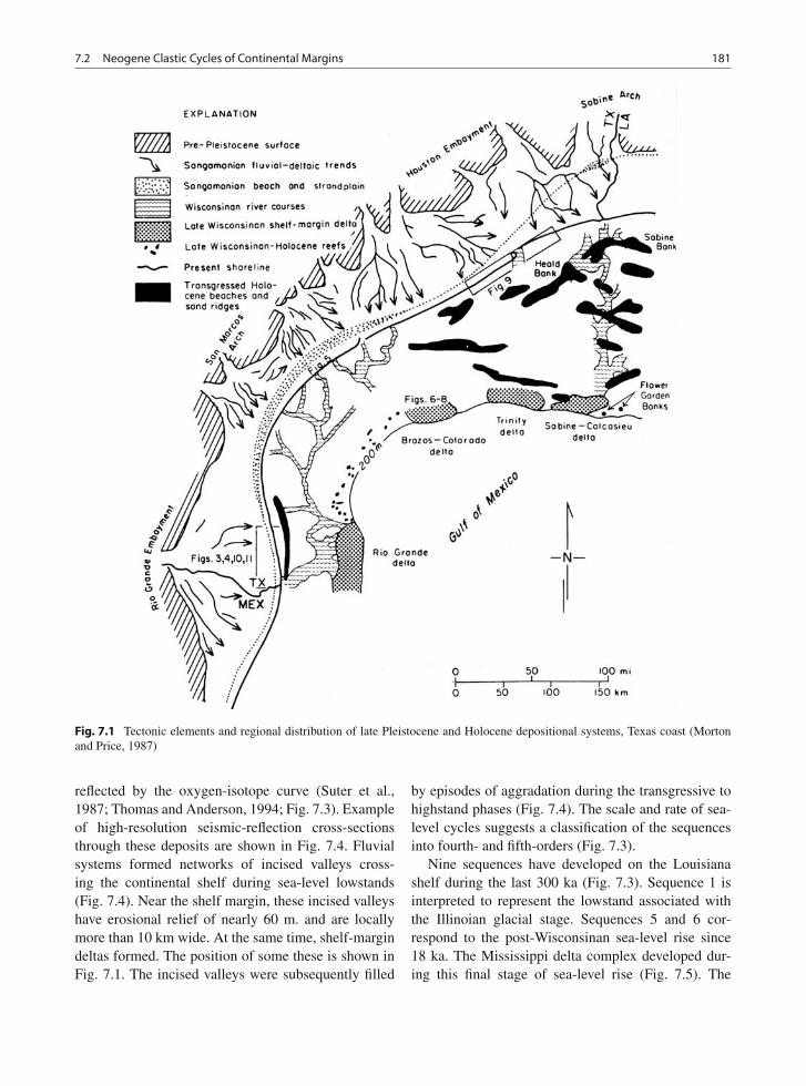
7.2 Neogene Clastic Cycles of Continental Margins 181
Fig. 7.1 Tectonic elements and regional distribution of late Pleistocene and Holocene depositional systems, Texas coast (Mortonand Price, 1987)
reflected by the oxygen-isotope curve (Suter et al.,1987; Thomas and Anderson, 1994; Fig. 7.3). Exampleof high-resolution seismic-reflection cross-sectionsthrough these deposits are shown in Fig. 7.4. Fluvialsystems formed networks of incised valleys cross-ing the continental shelf during sea-level lowstands(Fig. 7.4). Near the shelf margin, these incised valleyshave erosional relief of nearly 60 m. and are locallymore than 10 km wide. At the same time, shelf-margindeltas formed. The position of some these is shown inFig. 7.1. The incised valleys were subsequently filled
by episodes of aggradation during the transgressive tohighstand phases (Fig. 7.4). The scale and rate of sea-level cycles suggests a classification of the sequencesinto fourth- and fifth-orders (Fig. 7.3).
Nine sequences have developed on the Louisianashelf during the last 300 ka (Fig. 7.3). Sequence 1 isinterpreted to represent the lowstand associated withthe Illinoian glacial stage. Sequences 5 and 6 cor-respond to the post-Wisconsinan sea-level rise since18 ka. The Mississippi delta complex developed dur-ing this final stage of sea-level rise (Fig. 7.5). The
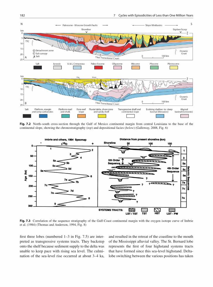
182 7 Cycles with Episodicities of Less than One Million Years
Fig. 7.2 North–south cross-section through the Gulf of Mexico continental margin from central Louisiana to the base of thecontinental slope, showing the chronostratigraphy (top) and depositional facies (below) (Galloway, 2008, Fig. 6)
Fig. 7.3 Correlation of the sequence stratigraphy of the Gulf-Coast continental margin with the oxygen isotope curve of Imbrieet al. (1984) (Thomas and Anderson, 1994, Fig. 8)
first three lobes (numbered 1–3 in Fig. 7.5) are inter-preted as transgressive systems tracts. They backsteponto the shelf because sediment supply to the delta wasunable to keep pace with rising sea level. The culmi-nation of the sea-level rise occurred at about 3–4 ka,
and resulted in the retreat of the coastline to the mouthof the Mississippi alluvial valley. The St. Bernard loberepresents the first of four highstand systems tractsthat have formed since this sea-level highstand. Delta-lobe switching between the various positions has taken
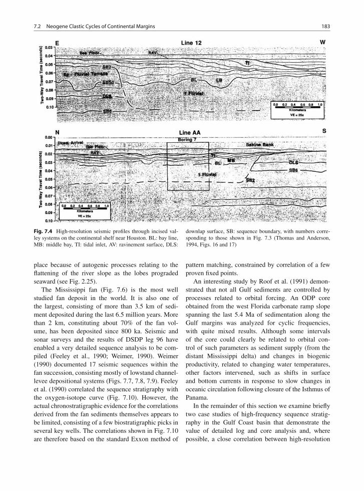
7.2 Neogene Clastic Cycles of Continental Margins 183
Fig. 7.4 High-resolution seismic profiles through incised val-ley systems on the continental shelf near Houston. BL: bay line,MB: middle bay, TI: tidal inlet, AV: ravinement surface, DLS:
downlap surface, SB: sequence boundary, with numbers corre-sponding to those shown in Fig. 7.3 (Thomas and Anderson,1994, Figs. 16 and 17)
place because of autogenic processes relating to theflattening of the river slope as the lobes progradedseaward (see Fig. 2.25).
The Mississippi fan (Fig. 7.6) is the most wellstudied fan deposit in the world. It is also one ofthe largest, consisting of more than 3.5 km of sedi-ment deposited during the last 6.5 million years. Morethan 2 km, constituting about 70% of the fan vol-ume, has been deposited since 800 ka. Seismic andsonar surveys and the results of DSDP leg 96 haveenabled a very detailed sequence analysis to be com-piled (Feeley et al., 1990; Weimer, 1990). Weimer(1990) documented 17 seismic sequences within thefan succession, consisting mostly of lowstand channel-levee depositional systems (Figs. 7.7, 7.8, 7.9). Feeleyet al. (1990) correlated the sequence stratigraphy withthe oxygen-isotope curve (Fig. 7.10). However, theactual chronostratigraphic evidence for the correlationsderived from the fan sediments themselves appears tobe limited, consisting of a few biostratigraphic picks inseveral key wells. The correlations shown in Fig. 7.10are therefore based on the standard Exxon method of
pattern matching, constrained by correlation of a fewproven fixed points.
An interesting study by Roof et al. (1991) demon-strated that not all Gulf sediments are controlled byprocesses related to orbital forcing. An ODP coreobtained from the west Florida carbonate ramp slopespanning the last 5.4 Ma of sedimentation along theGulf margins was analyzed for cyclic frequencies,with quite mixed results. Although some intervalsof the core could clearly be related to orbital con-trol of such parameters as sediment supply (from thedistant Mississippi delta) and changes in biogenicproductivity, related to changing water temperatures,other factors intervened, such as shifts in surfaceand bottom currents in response to slow changes inoceanic circulation following closure of the Isthmus ofPanama.
In the remainder of this section we examine brieflytwo case studies of high-frequency sequence stratig-raphy in the Gulf Coast basin that demonstrate thevalue of detailed log and core analysis and, wherepossible, a close correlation between high-resolution
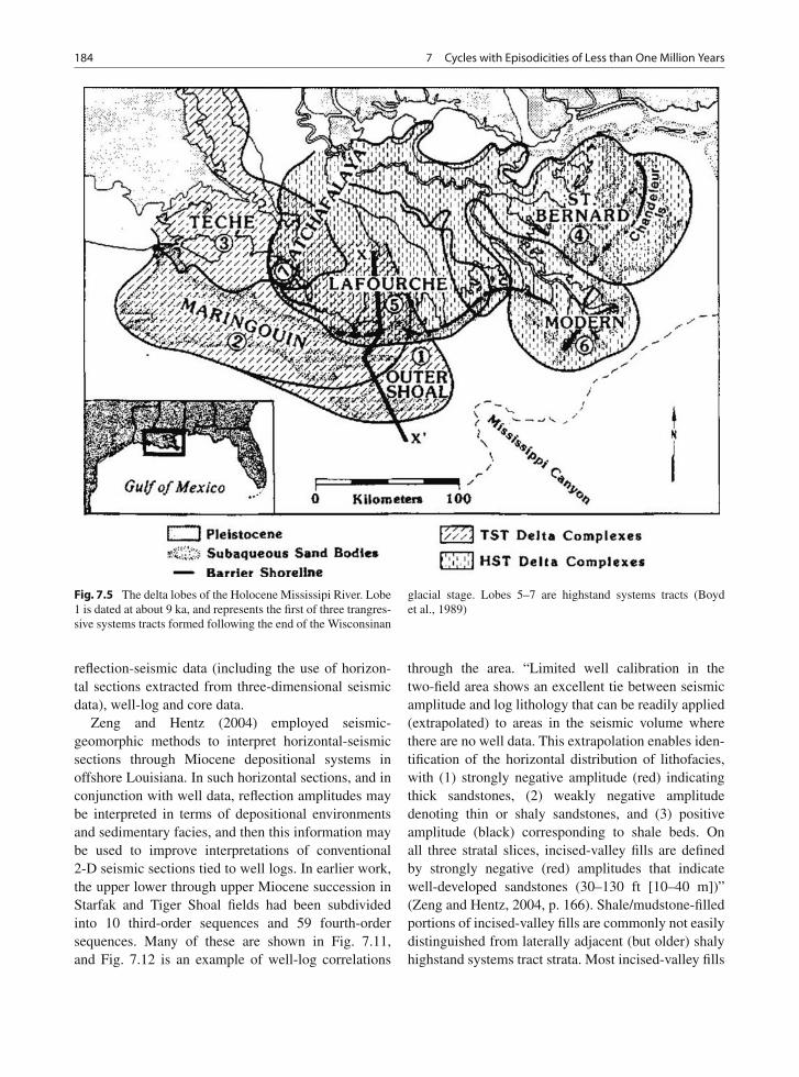
184 7 Cycles with Episodicities of Less than One Million Years
Fig. 7.5 The delta lobes of the Holocene Mississipi River. Lobe1 is dated at about 9 ka, and represents the first of three trangres-sive systems tracts formed following the end of the Wisconsinan
glacial stage. Lobes 5–7 are highstand systems tracts (Boydet al., 1989)
reflection-seismic data (including the use of horizon-tal sections extracted from three-dimensional seismicdata), well-log and core data.
Zeng and Hentz (2004) employed seismic-geomorphic methods to interpret horizontal-seismicsections through Miocene depositional systems inoffshore Louisiana. In such horizontal sections, and inconjunction with well data, reflection amplitudes maybe interpreted in terms of depositional environmentsand sedimentary facies, and then this information maybe used to improve interpretations of conventional2-D seismic sections tied to well logs. In earlier work,the upper lower through upper Miocene succession inStarfak and Tiger Shoal fields had been subdividedinto 10 third-order sequences and 59 fourth-ordersequences. Many of these are shown in Fig. 7.11,and Fig. 7.12 is an example of well-log correlations
through the area. “Limited well calibration in thetwo-field area shows an excellent tie between seismicamplitude and log lithology that can be readily applied(extrapolated) to areas in the seismic volume wherethere are no well data. This extrapolation enables iden-tification of the horizontal distribution of lithofacies,with (1) strongly negative amplitude (red) indicatingthick sandstones, (2) weakly negative amplitudedenoting thin or shaly sandstones, and (3) positiveamplitude (black) corresponding to shale beds. Onall three stratal slices, incised-valley fills are definedby strongly negative (red) amplitudes that indicatewell-developed sandstones (30–130 ft [10–40 m])”(Zeng and Hentz, 2004, p. 166). Shale/mudstone-filledportions of incised-valley fills are commonly not easilydistinguished from laterally adjacent (but older) shalyhighstand systems tract strata. Most incised-valley fills
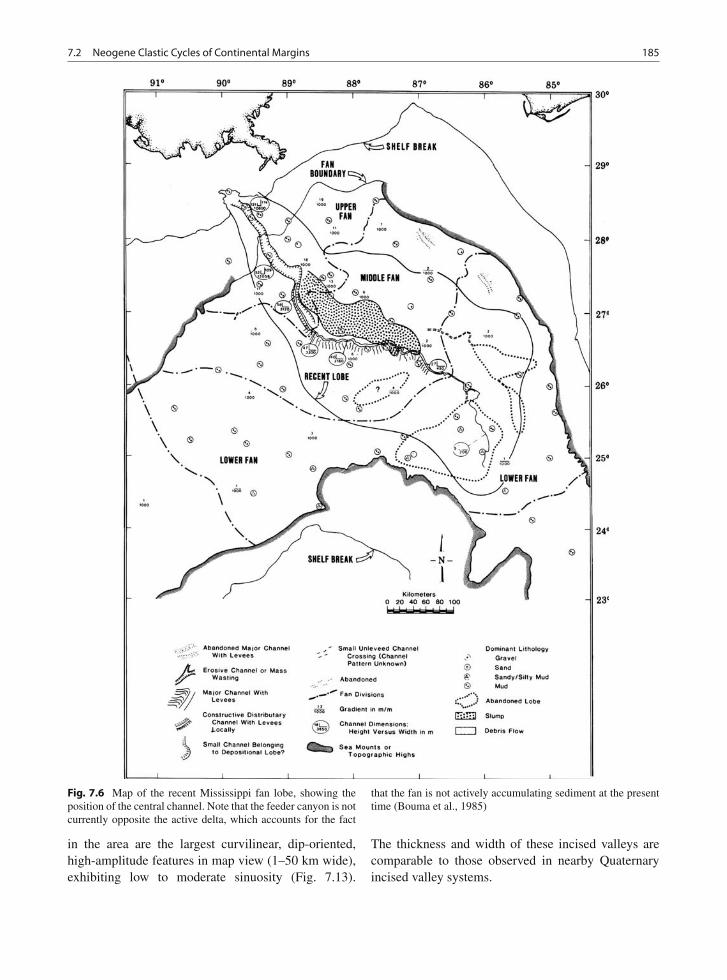
7.2 Neogene Clastic Cycles of Continental Margins 185
Fig. 7.6 Map of the recent Mississippi fan lobe, showing theposition of the central channel. Note that the feeder canyon is notcurrently opposite the active delta, which accounts for the fact
that the fan is not actively accumulating sediment at the presenttime (Bouma et al., 1985)
in the area are the largest curvilinear, dip-oriented,high-amplitude features in map view (1–50 km wide),exhibiting low to moderate sinuosity (Fig. 7.13).
The thickness and width of these incised valleys arecomparable to those observed in nearby Quaternaryincised valley systems.
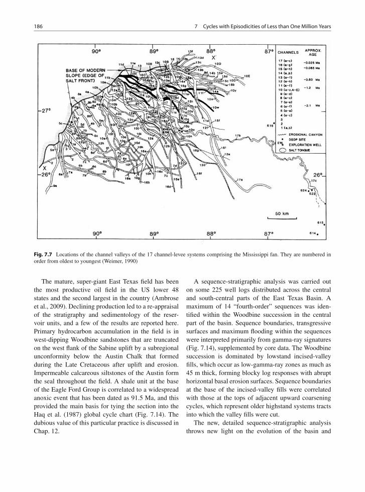
186 7 Cycles with Episodicities of Less than One Million Years
Fig. 7.7 Locations of the channel valleys of the 17 channel-levee systems comprising the Mississippi fan. They are numbered inorder from oldest to youngest (Weimer, 1990)
The mature, super-giant East Texas field has beenthe most productive oil field in the US lower 48states and the second largest in the country (Ambroseet al., 2009). Declining production led to a re-appraisalof the stratigraphy and sedimentology of the reser-voir units, and a few of the results are reported here.Primary hydrocarbon accumulation in the field is inwest-dipping Woodbine sandstones that are truncatedon the west flank of the Sabine uplift by a subregionalunconformity below the Austin Chalk that formedduring the Late Cretaceous after uplift and erosion.Impermeable calcareous siltstones of the Austin formthe seal throughout the field. A shale unit at the baseof the Eagle Ford Group is correlated to a widespreadanoxic event that has been dated as 91.5 Ma, and thisprovided the main basis for tying the section into theHaq et al. (1987) global cycle chart (Fig. 7.14). Thedubious value of this particular practice is discussed inChap. 12.
A sequence-stratigraphic analysis was carried outon some 225 well logs distributed across the centraland south-central parts of the East Texas Basin. Amaximum of 14 “fourth-order” sequences was iden-tified within the Woodbine succession in the centralpart of the basin. Sequence boundaries, transgressivesurfaces and maximum flooding within the sequenceswere interpreted primarily from gamma-ray signatures(Fig. 7.14), supplemented by core data. The Woodbinesuccession is dominated by lowstand incised-valleyfills, which occur as low-gamma-ray zones as much as45 m thick, forming blocky log responses with abrupthorizontal basal erosion surfaces. Sequence boundariesat the base of the incised-valley fills were correlatedwith those at the tops of adjacent upward coarseningcycles, which represent older highstand systems tractsinto which the valley fills were cut.
The new, detailed sequence-stratigraphic analysisthrows new light on the evolution of the basin and
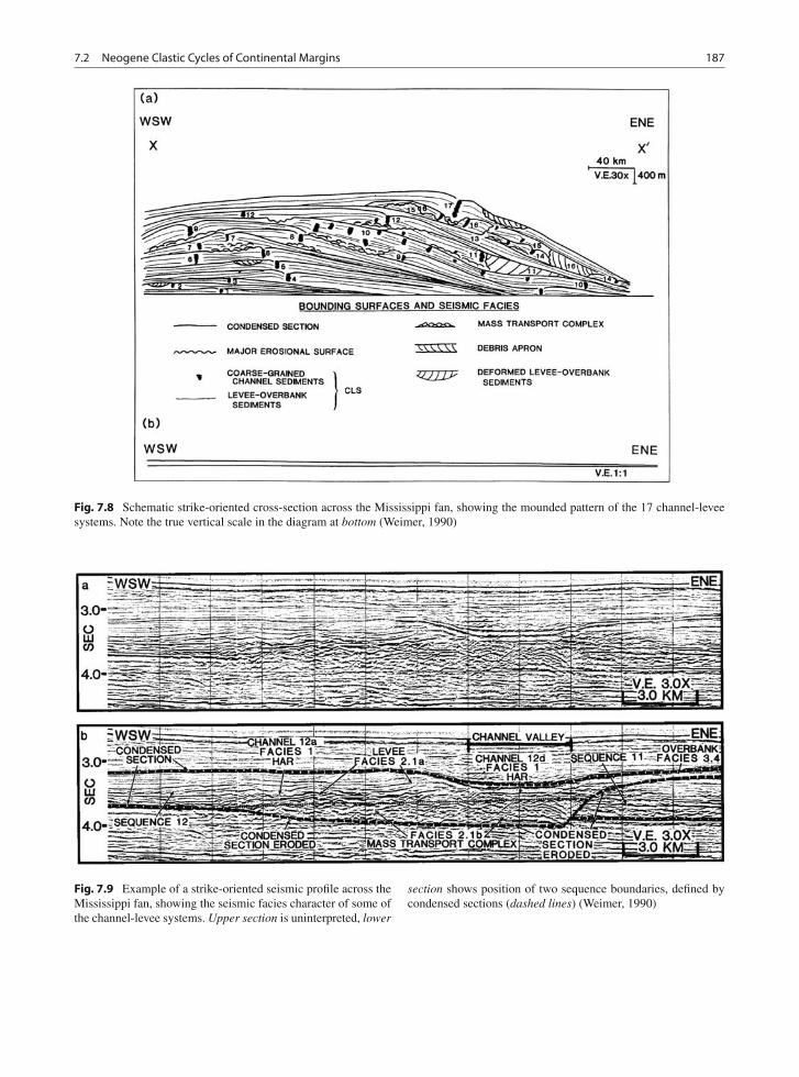
7.2 Neogene Clastic Cycles of Continental Margins 187
Fig. 7.8 Schematic strike-oriented cross-section across the Mississippi fan, showing the mounded pattern of the 17 channel-leveesystems. Note the true vertical scale in the diagram at bottom (Weimer, 1990)
Fig. 7.9 Example of a strike-oriented seismic profile across theMississippi fan, showing the seismic facies character of some ofthe channel-levee systems. Upper section is uninterpreted, lower
section shows position of two sequence boundaries, defined bycondensed sections (dashed lines) (Weimer, 1990)
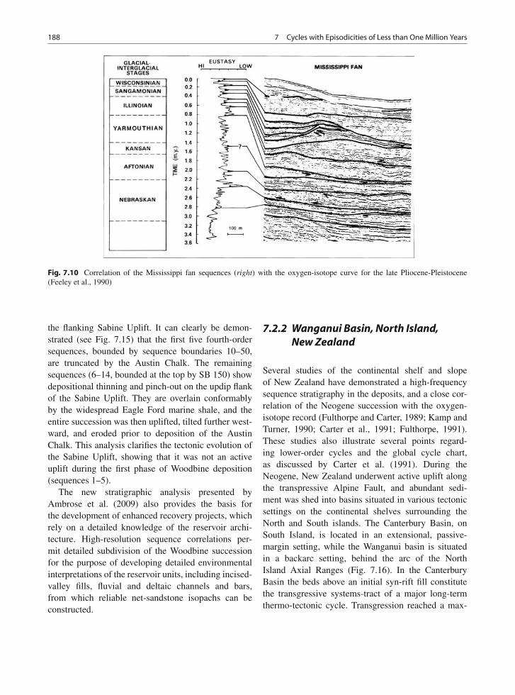
188 7 Cycles with Episodicities of Less than One Million Years
Fig. 7.10 Correlation of the Mississippi fan sequences (right) with the oxygen-isotope curve for the late Pliocene-Pleistocene(Feeley et al., 1990)
the flanking Sabine Uplift. It can clearly be demon-strated (see Fig. 7.15) that the first five fourth-ordersequences, bounded by sequence boundaries 10–50,are truncated by the Austin Chalk. The remainingsequences (6–14, bounded at the top by SB 150) showdepositional thinning and pinch-out on the updip flankof the Sabine Uplift. They are overlain conformablyby the widespread Eagle Ford marine shale, and theentire succession was then uplifted, tilted further west-ward, and eroded prior to deposition of the AustinChalk. This analysis clarifies the tectonic evolution ofthe Sabine Uplift, showing that it was not an activeuplift during the first phase of Woodbine deposition(sequences 1–5).
The new stratigraphic analysis presented byAmbrose et al. (2009) also provides the basis forthe development of enhanced recovery projects, whichrely on a detailed knowledge of the reservoir archi-tecture. High-resolution sequence correlations per-mit detailed subdivision of the Woodbine successionfor the purpose of developing detailed environmentalinterpretations of the reservoir units, including incised-valley fills, fluvial and deltaic channels and bars,from which reliable net-sandstone isopachs can beconstructed.
7.2.2 Wanganui Basin, North Island,New Zealand
Several studies of the continental shelf and slopeof New Zealand have demonstrated a high-frequencysequence stratigraphy in the deposits, and a close cor-relation of the Neogene succession with the oxygen-isotope record (Fulthorpe and Carter, 1989; Kamp andTurner, 1990; Carter et al., 1991; Fulthorpe, 1991).These studies also illustrate several points regard-ing lower-order cycles and the global cycle chart,as discussed by Carter et al. (1991). During theNeogene, New Zealand underwent active uplift alongthe transpressive Alpine Fault, and abundant sedi-ment was shed into basins situated in various tectonicsettings on the continental shelves surrounding theNorth and South islands. The Canterbury Basin, onSouth Island, is located in an extensional, passive-margin setting, while the Wanganui basin is situatedin a backarc setting, behind the arc of the NorthIsland Axial Ranges (Fig. 7.16). In the CanterburyBasin the beds above an initial syn-rift fill constitutethe transgressive systems-tract of a major long-termthermo-tectonic cycle. Transgression reached a max-
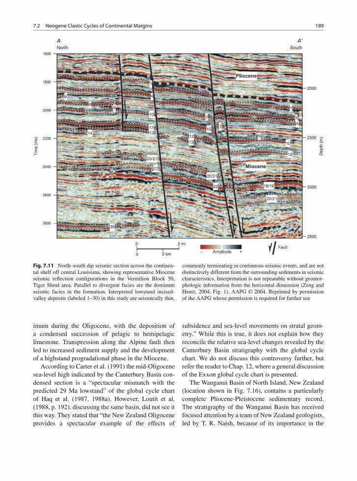
7.2 Neogene Clastic Cycles of Continental Margins 189
Fig. 7.11 North–south dip seismic section across the continen-tal shelf off central Louisiana, showing representative Mioceneseismic reflection configurations in the Vermilion Block 50,Tiger Shoal area. Parallel to divergent facies are the dominantseismic facies in the formation. Interpreted lowstand incised-valley deposits (labeled 1–30) in this study are seismically thin,
commonly terminating in continuous seismic events, and are notdistinctively different from the surrounding sediments in seismiccharacteristics. Interpretation is not repeatable without geomor-phologic information from the horizontal dimension (Zeng andHentz, 2004, Fig. 1). AAPG © 2004. Reprinted by permissionof the AAPG whose permission is required for further use
imum during the Oligocene, with the deposition ofa condensed succession of pelagic to hemipelagiclimestone. Transpression along the Alpine fault thenled to increased sediment supply and the developmentof a highstand progradational phase in the Miocene.
According to Carter et al. (1991) the mid-Oligocenesea-level high indicated by the Canterbury Basin con-densed section is a “spectacular mismatch with thepredicted 29 Ma lowstand” of the global cycle chartof Haq et al. (1987, 1988a). However, Loutit et al.(1988, p. 192), discussing the same basin, did not see itthis way. They stated that “the New Zealand Oligoceneprovides a spectacular example of the effects of
subsidence and sea-level movements on stratal geom-etry.” While this is true, it does not explain how theyreconcile the relative sea-level changes revealed by theCanterbury Basin stratigraphy with the global cyclechart. We do not discuss this controversy further, butrefer the reader to Chap. 12, where a general discussionof the Exxon global cycle chart is presented.
The Wanganui Basin of North Island, New Zealand(location shown in Fig. 7.16), contains a particularlycomplete Pliocene-Pleistocene sedimentary record.The stratigraphy of the Wanganui Basin has receivedfocused attention by a team of New Zealand geologists,led by T. R. Naish, because of its importance in the
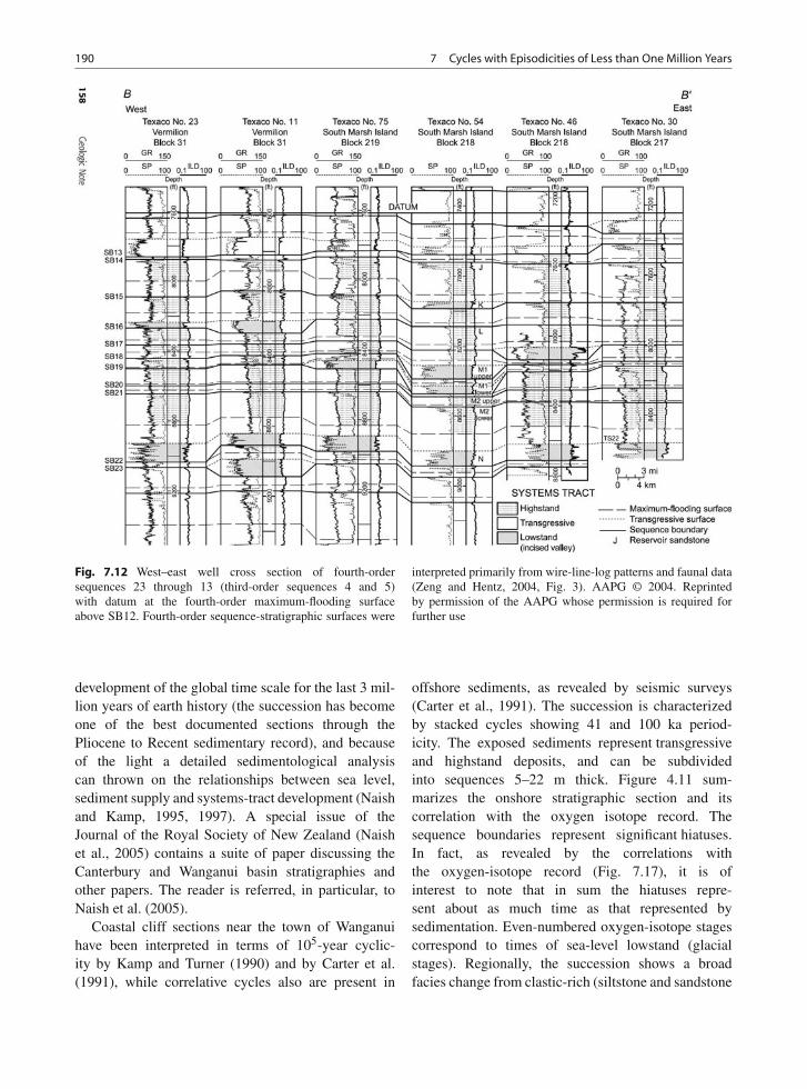
190 7 Cycles with Episodicities of Less than One Million Years
Fig. 7.12 West–east well cross section of fourth-ordersequences 23 through 13 (third-order sequences 4 and 5)with datum at the fourth-order maximum-flooding surfaceabove SB12. Fourth-order sequence-stratigraphic surfaces were
interpreted primarily from wire-line-log patterns and faunal data(Zeng and Hentz, 2004, Fig. 3). AAPG © 2004. Reprintedby permission of the AAPG whose permission is required forfurther use
development of the global time scale for the last 3 mil-lion years of earth history (the succession has becomeone of the best documented sections through thePliocene to Recent sedimentary record), and becauseof the light a detailed sedimentological analysiscan thrown on the relationships between sea level,sediment supply and systems-tract development (Naishand Kamp, 1995, 1997). A special issue of theJournal of the Royal Society of New Zealand (Naishet al., 2005) contains a suite of paper discussing theCanterbury and Wanganui basin stratigraphies andother papers. The reader is referred, in particular, toNaish et al. (2005).
Coastal cliff sections near the town of Wanganuihave been interpreted in terms of 105-year cyclic-ity by Kamp and Turner (1990) and by Carter et al.(1991), while correlative cycles also are present in
offshore sediments, as revealed by seismic surveys(Carter et al., 1991). The succession is characterizedby stacked cycles showing 41 and 100 ka period-icity. The exposed sediments represent transgressiveand highstand deposits, and can be subdividedinto sequences 5–22 m thick. Figure 4.11 sum-marizes the onshore stratigraphic section and itscorrelation with the oxygen isotope record. Thesequence boundaries represent significant hiatuses.In fact, as revealed by the correlations withthe oxygen-isotope record (Fig. 7.17), it is ofinterest to note that in sum the hiatuses repre-sent about as much time as that represented bysedimentation. Even-numbered oxygen-isotope stagescorrespond to times of sea-level lowstand (glacialstages). Regionally, the succession shows a broadfacies change from clastic-rich (siltstone and sandstone
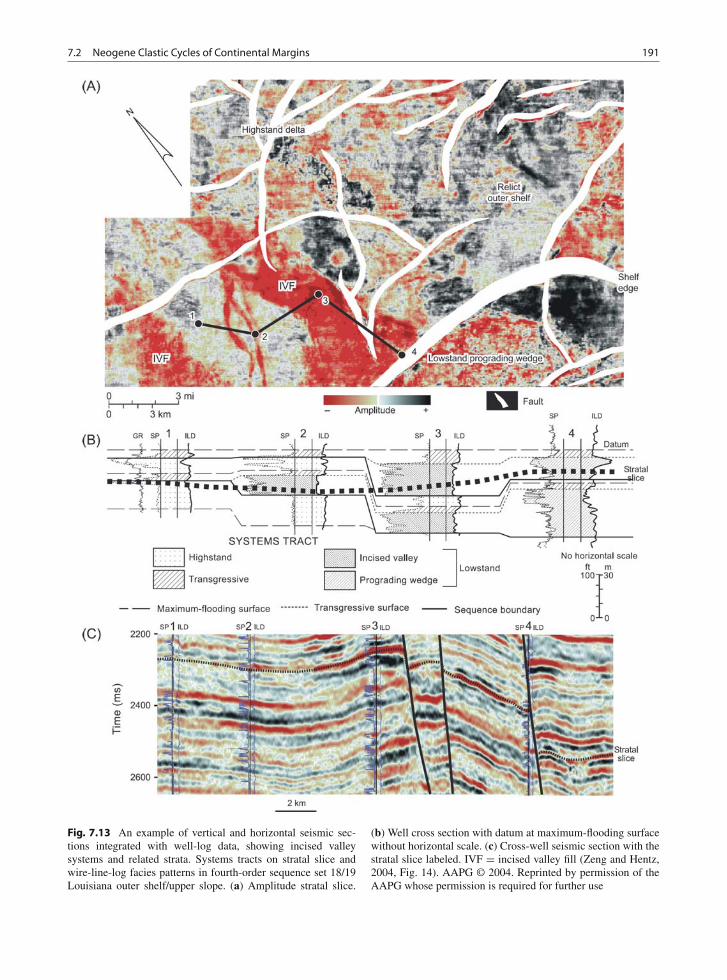
7.2 Neogene Clastic Cycles of Continental Margins 191
Fig. 7.13 An example of vertical and horizontal seismic sec-tions integrated with well-log data, showing incised valleysystems and related strata. Systems tracts on stratal slice andwire-line-log facies patterns in fourth-order sequence set 18/19Louisiana outer shelf/upper slope. (a) Amplitude stratal slice.
(b) Well cross section with datum at maximum-flooding surfacewithout horizontal scale. (c) Cross-well seismic section with thestratal slice labeled. IVF = incised valley fill (Zeng and Hentz,2004, Fig. 14). AAPG © 2004. Reprinted by permission of theAAPG whose permission is required for further use
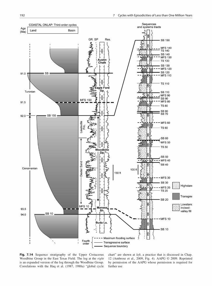
192 7 Cycles with Episodicities of Less than One Million Years
Fig. 7.14 Sequence stratigraphy of the Upper CretaceousWoodbine Group in the East Texas Field. The log at the rightis an expanded version of the log through the Woodbine Group.Correlations with the Haq et al. (1987, 1988a) “global cycle
chart” are shown at left, a practice that is discussed in Chap.12 (Ambrose et al., 2009, Fig. 4). AAPG © 2009. Reprintedby permission of the AAPG whose permission is required forfurther use
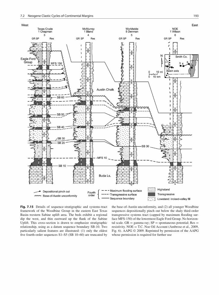
7.2 Neogene Clastic Cycles of Continental Margins 193
Fig. 7.15 Details of sequence-stratigraphic and systems-tractframework of the Woodbine Group in the eastern East TexasBasin–western Sabine uplift area. The beds exhibit a regionaldip the west, and thin eastward up the flank of the SabineUplift. This cross-section is drawn to emphasize stratigraphicrelationship, using as a datum sequence boundary SB-10. Twoparticularly salient features are illustrated: (1) only the oldestfive fourth-order sequences S1–S5 (SB 10–60) are truncated by
the base-of-Austin unconformity, and (2) all younger Woodbinesequences depositionally pinch out below the shaly third-ordertransgressive systems tract (capped by maximum flooding sur-face MFS-150) of the lowermost Eagle Ford Group. No horizon-tal scale. GR = gamma ray; SP = spontaneous potential; Res =resistivity. NOE = T.C. Noe Oil Account (Ambrose et al., 2009,Fig. 6). AAPG © 2009. Reprinted by permission of the AAPGwhose permission is required for further use
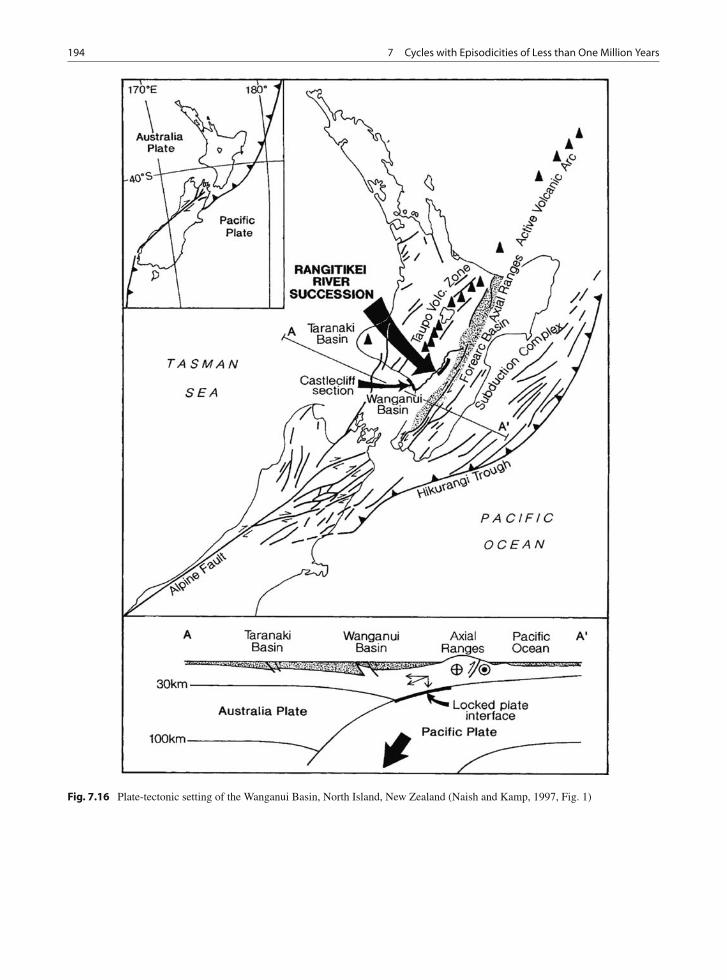
194 7 Cycles with Episodicities of Less than One Million Years
Fig. 7.16 Plate-tectonic setting of the Wanganui Basin, North Island, New Zealand (Naish and Kamp, 1997, Fig. 1)
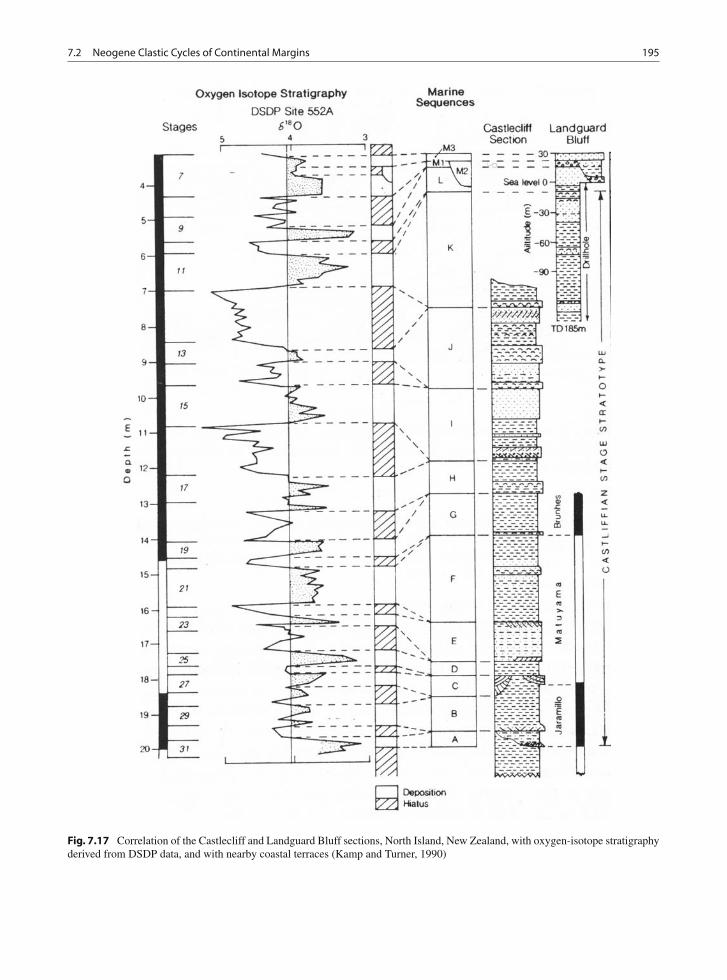
7.2 Neogene Clastic Cycles of Continental Margins 195
Fig. 7.17 Correlation of the Castlecliff and Landguard Bluff sections, North Island, New Zealand, with oxygen-isotope stratigraphyderived from DSDP data, and with nearby coastal terraces (Kamp and Turner, 1990)
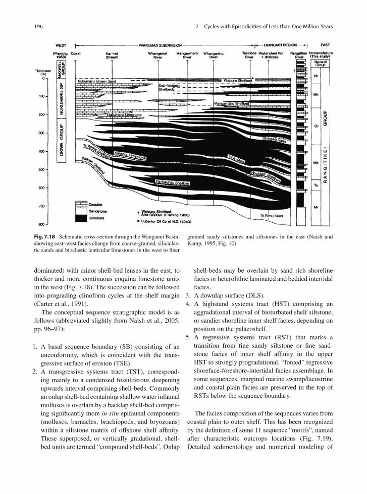
196 7 Cycles with Episodicities of Less than One Million Years
Fig. 7.18 Schematic cross-section through the Wanganui Basin,showing east–west facies change from coarse-grained, siliciclas-tic sands and bioclastic lenticular limestones in the west to finer
grained sandy siltstones and siltstones in the east (Naish andKamp, 1995, Fig. 10)
dominated) with minor shell-bed lenses in the east, tothicker and more continuous coquina limestone unitsin the west (Fig. 7.18). The succession can be followedinto prograding clinoform cycles at the shelf margin(Carter et al., 1991).
The conceptual sequence stratigraphic model is asfollows (abbreviated slightly from Naish et al., 2005,pp. 96–97):
1. A basal sequence boundary (SB) consisting of anunconformity, which is coincident with the trans-gressive surface of erosion (TSE).
2. A transgressive systems tract (TST), correspond-ing mainly to a condensed fossiliferous deepeningupwards interval comprising shell-beds. Commonlyan onlap shell-bed containing shallow water infaunalmolluscs is overlain by a backlap shell-bed compris-ing significantly more in-situ epifaunal components(molluscs, barnacles, brachiopods, and bryozoans)within a siltstone matrix of offshore shelf affinity.These superposed, or vertically gradational, shell-bed units are termed “compound shell-beds”. Onlap
shell-beds may be overlain by sand rich shorelinefacies or heterolithic laminated and bedded intertidalfacies.
3. A downlap surface (DLS).4. A highstand systems tract (HST) comprising an
aggradational interval of bioturbated shelf siltstone,or sandier shoreline inner shelf facies, depending onposition on the palaeoshelf.
5. A regressive systems tract (RST) that marks atransition from fine sandy siltstone or fine sand-stone facies of inner shelf affinity in the upperHST to strongly progradational, “forced” regressiveshoreface-foreshore-intertidal facies assemblage. Insome sequences, marginal marine swamp/lacustrineand coastal plain facies are preserved in the top ofRSTs below the sequence boundary.
The facies composition of the sequences varies fromcoastal plain to outer shelf. This has been recognizedby the definition of some 11 sequence “motifs”, namedafter characteristic outcrops locations (Fig. 7.19).Detailed sedimentology and numerical modeling of
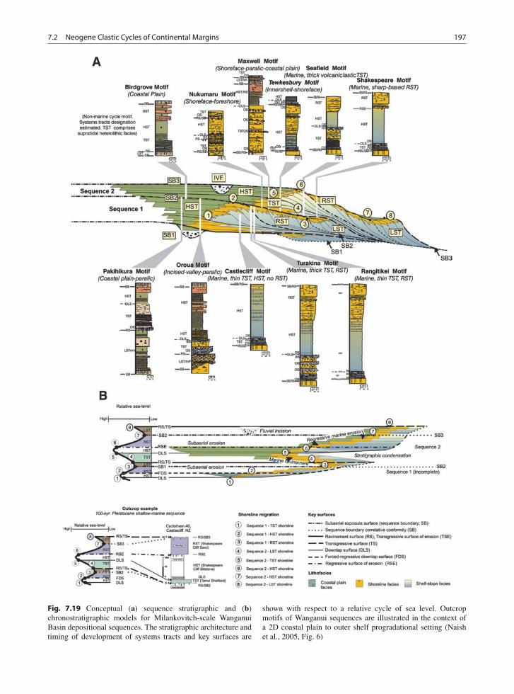
7.2 Neogene Clastic Cycles of Continental Margins 197
Fig. 7.19 Conceptual (a) sequence stratigraphic and (b)chronostratigraphic models for Milankovitch-scale WanganuiBasin depositional sequences. The stratigraphic architecture andtiming of development of systems tracts and key surfaces are
shown with respect to a relative cycle of sea level. Outcropmotifs of Wanganui sequences are illustrated in the context ofa 2D coastal plain to outer shelf progradational setting (Naishet al., 2005, Fig. 6)
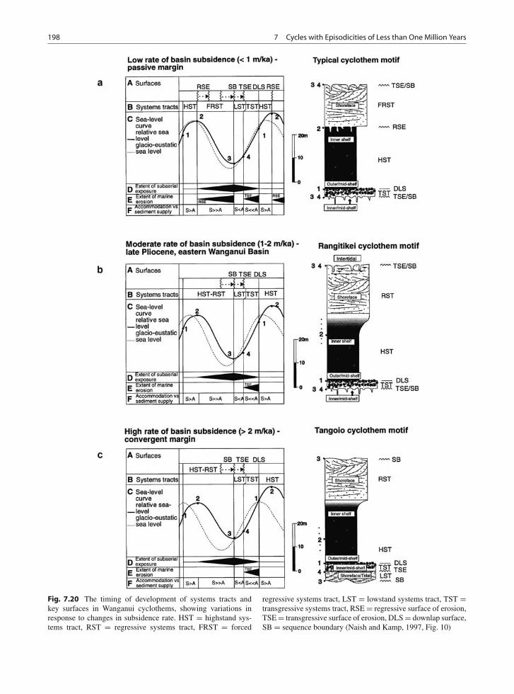
198 7 Cycles with Episodicities of Less than One Million Years
Fig. 7.20 The timing of development of systems tracts andkey surfaces in Wanganui cyclothems, showing variations inresponse to changes in subsidence rate. HST = highstand sys-tems tract, RST = regressive systems tract, FRST = forced
regressive systems tract, LST = lowstand systems tract, TST =transgressive systems tract, RSE = regressive surface of erosion,TSE = transgressive surface of erosion, DLS = downlap surface,SB = sequence boundary (Naish and Kamp, 1997, Fig. 10)
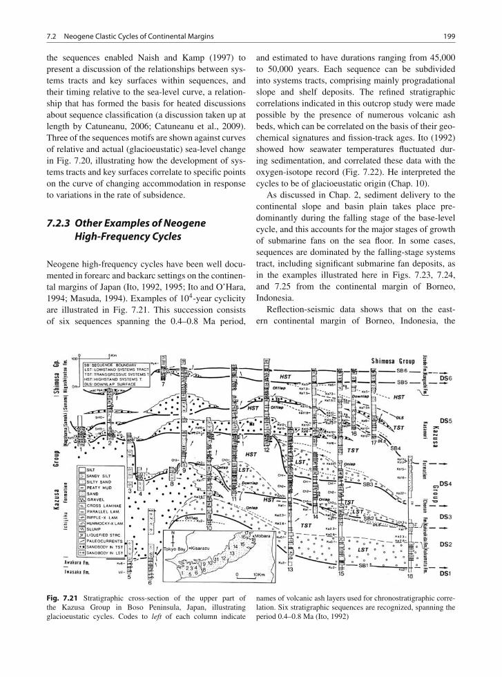
7.2 Neogene Clastic Cycles of Continental Margins 199
the sequences enabled Naish and Kamp (1997) topresent a discussion of the relationships between sys-tems tracts and key surfaces within sequences, andtheir timing relative to the sea-level curve, a relation-ship that has formed the basis for heated discussionsabout sequence classification (a discussion taken up atlength by Catuneanu, 2006; Catuneanu et al., 2009).Three of the sequences motifs are shown against curvesof relative and actual (glacioeustatic) sea-level changein Fig. 7.20, illustrating how the development of sys-tems tracts and key surfaces correlate to specific pointson the curve of changing accommodation in responseto variations in the rate of subsidence.
7.2.3 Other Examples of NeogeneHigh-Frequency Cycles
Neogene high-frequency cycles have been well docu-mented in forearc and backarc settings on the continen-tal margins of Japan (Ito, 1992, 1995; Ito and O’Hara,1994; Masuda, 1994). Examples of 104-year cyclicityare illustrated in Fig. 7.21. This succession consistsof six sequences spanning the 0.4–0.8 Ma period,
and estimated to have durations ranging from 45,000to 50,000 years. Each sequence can be subdividedinto systems tracts, comprising mainly progradationalslope and shelf deposits. The refined stratigraphiccorrelations indicated in this outcrop study were madepossible by the presence of numerous volcanic ashbeds, which can be correlated on the basis of their geo-chemical signatures and fission-track ages. Ito (1992)showed how seawater temperatures fluctuated dur-ing sedimentation, and correlated these data with theoxygen-isotope record (Fig. 7.22). He interpreted thecycles to be of glacioeustatic origin (Chap. 10).
As discussed in Chap. 2, sediment delivery to thecontinental slope and basin plain takes place pre-dominantly during the falling stage of the base-levelcycle, and this accounts for the major stages of growthof submarine fans on the sea floor. In some cases,sequences are dominated by the falling-stage systemstract, including significant submarine fan deposits, asin the examples illustrated here in Figs. 7.23, 7.24,and 7.25 from the continental margin of Borneo,Indonesia.
Reflection-seismic data shows that on the east-ern continental margin of Borneo, Indonesia, the
Fig. 7.21 Stratigraphic cross-section of the upper part ofthe Kazusa Group in Boso Peninsula, Japan, illustratingglacioeustatic cycles. Codes to left of each column indicate
names of volcanic ash layers used for chronostratigraphic corre-lation. Six stratigraphic sequences are recognized, spanning theperiod 0.4–0.8 Ma (Ito, 1992)
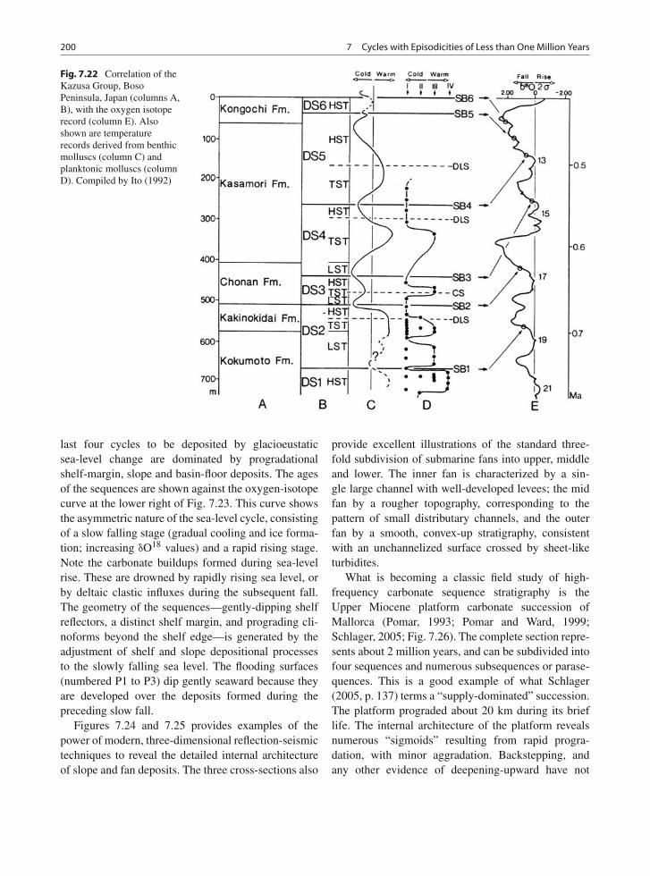
200 7 Cycles with Episodicities of Less than One Million Years
Fig. 7.22 Correlation of theKazusa Group, BosoPeninsula, Japan (columns A,B), with the oxygen isotoperecord (column E). Alsoshown are temperaturerecords derived from benthicmolluscs (column C) andplanktonic molluscs (columnD). Compiled by Ito (1992)
last four cycles to be deposited by glacioeustaticsea-level change are dominated by progradationalshelf-margin, slope and basin-floor deposits. The agesof the sequences are shown against the oxygen-isotopecurve at the lower right of Fig. 7.23. This curve showsthe asymmetric nature of the sea-level cycle, consistingof a slow falling stage (gradual cooling and ice forma-tion; increasing δO18 values) and a rapid rising stage.Note the carbonate buildups formed during sea-levelrise. These are drowned by rapidly rising sea level, orby deltaic clastic influxes during the subsequent fall.The geometry of the sequences—gently-dipping shelfreflectors, a distinct shelf margin, and prograding cli-noforms beyond the shelf edge—is generated by theadjustment of shelf and slope depositional processesto the slowly falling sea level. The flooding surfaces(numbered P1 to P3) dip gently seaward because theyare developed over the deposits formed during thepreceding slow fall.
Figures 7.24 and 7.25 provides examples of thepower of modern, three-dimensional reflection-seismictechniques to reveal the detailed internal architectureof slope and fan deposits. The three cross-sections also
provide excellent illustrations of the standard three-fold subdivision of submarine fans into upper, middleand lower. The inner fan is characterized by a sin-gle large channel with well-developed levees; the midfan by a rougher topography, corresponding to thepattern of small distributary channels, and the outerfan by a smooth, convex-up stratigraphy, consistentwith an unchannelized surface crossed by sheet-liketurbidites.
What is becoming a classic field study of high-frequency carbonate sequence stratigraphy is theUpper Miocene platform carbonate succession ofMallorca (Pomar, 1993; Pomar and Ward, 1999;Schlager, 2005; Fig. 7.26). The complete section repre-sents about 2 million years, and can be subdivided intofour sequences and numerous subsequences or parase-quences. This is a good example of what Schlager(2005, p. 137) terms a “supply-dominated” succession.The platform prograded about 20 km during its brieflife. The internal architecture of the platform revealsnumerous “sigmoids” resulting from rapid progra-dation, with minor aggradation. Backstepping, andany other evidence of deepening-upward have not
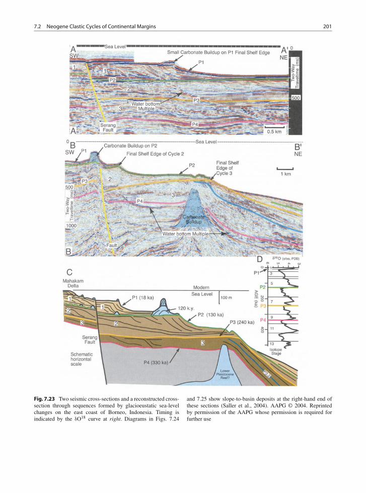
7.2 Neogene Clastic Cycles of Continental Margins 201
Fig. 7.23 Two seismic cross-sections and a reconstructed cross-section through sequences formed by glacioeustatic sea-levelchanges on the east coast of Borneo, Indonesia. Timing isindicated by the δO18 curve at right. Diagrams in Figs. 7.24
and 7.25 show slope-to-basin deposits at the right-hand end ofthese sections (Saller et al., 2004). AAPG © 2004. Reprintedby permission of the AAPG whose permission is required forfurther use
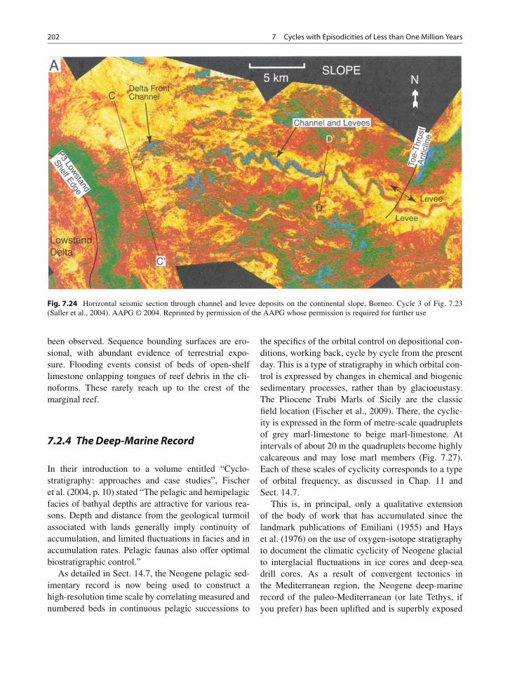
202 7 Cycles with Episodicities of Less than One Million Years
Fig. 7.24 Horizontal seismic section through channel and levee deposits on the continental slope, Borneo. Cycle 3 of Fig. 7.23(Saller et al., 2004). AAPG © 2004. Reprinted by permission of the AAPG whose permission is required for further use
been observed. Sequence bounding surfaces are ero-sional, with abundant evidence of terrestrial expo-sure. Flooding events consist of beds of open-shelflimestone onlapping tongues of reef debris in the cli-noforms. These rarely reach up to the crest of themarginal reef.
7.2.4 The Deep-Marine Record
In their introduction to a volume entitled “Cyclo-stratigraphy: approaches and case studies”, Fischeret al. (2004, p. 10) stated “The pelagic and hemipelagicfacies of bathyal depths are attractive for various rea-sons. Depth and distance from the geological turmoilassociated with lands generally imply continuity ofaccumulation, and limited fluctuations in facies and inaccumulation rates. Pelagic faunas also offer optimalbiostratigraphic control.”
As detailed in Sect. 14.7, the Neogene pelagic sed-imentary record is now being used to construct ahigh-resolution time scale by correlating measured andnumbered beds in continuous pelagic successions to
the specifics of the orbital control on depositional con-ditions, working back, cycle by cycle from the presentday. This is a type of stratigraphy in which orbital con-trol is expressed by changes in chemical and biogenicsedimentary processes, rather than by glacioeustasy.The Pliocene Trubi Marls of Sicily are the classicfield location (Fischer et al., 2009). There, the cyclic-ity is expressed in the form of metre-scale quadrupletsof grey marl-limestone to beige marl-limestone. Atintervals of about 20 m the quadruplets become highlycalcareous and may lose marl members (Fig. 7.27).Each of these scales of cyclicity corresponds to a typeof orbital frequency, as discussed in Chap. 11 andSect. 14.7.
This is, in principal, only a qualitative extensionof the body of work that has accumulated since thelandmark publications of Emiliani (1955) and Hayset al. (1976) on the use of oxygen-isotope stratigraphyto document the climatic cyclicity of Neogene glacialto interglacial fluctuations in ice cores and deep-seadrill cores. As a result of convergent tectonics inthe Mediterranean region, the Neogene deep-marinerecord of the paleo-Mediterranean (or late Tethys, ifyou prefer) has been uplifted and is superbly exposed
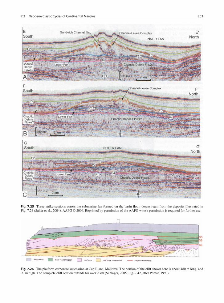
7.2 Neogene Clastic Cycles of Continental Margins 203
Fig. 7.25 Three strike-sections across the submarine fan formed on the basin floor, downstream from the deposits illustrated inFig. 7.24 (Saller et al., 2004). AAPG © 2004. Reprinted by permission of the AAPG whose permission is required for further use
Fig. 7.26 The platform carbonate succession at Cap Blanc, Mallorca. The portion of the cliff shown here is about 480 m long, and90 m high. The complete cliff section extends for over 2 km (Schlager, 2005, Fig. 7.42, after Pomar, 1993)
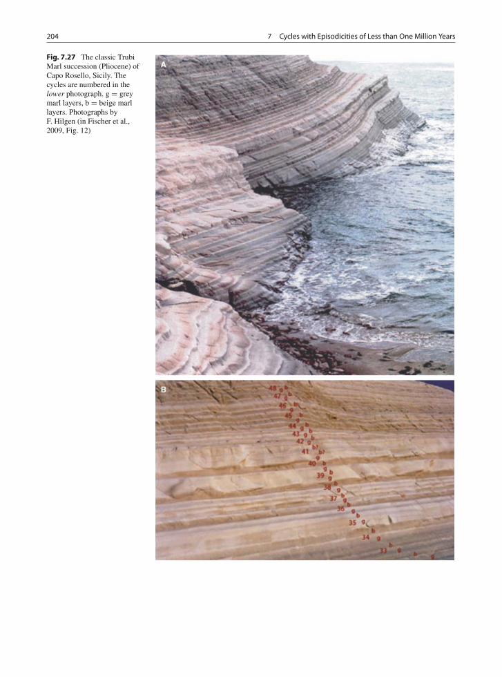
204 7 Cycles with Episodicities of Less than One Million Years
Fig. 7.27 The classic TrubiMarl succession (Pliocene) ofCapo Rosello, Sicily. Thecycles are numbered in thelower photograph. g = greymarl layers, b = beige marllayers. Photographs byF. Hilgen (in Fischer et al.,2009, Fig. 12)
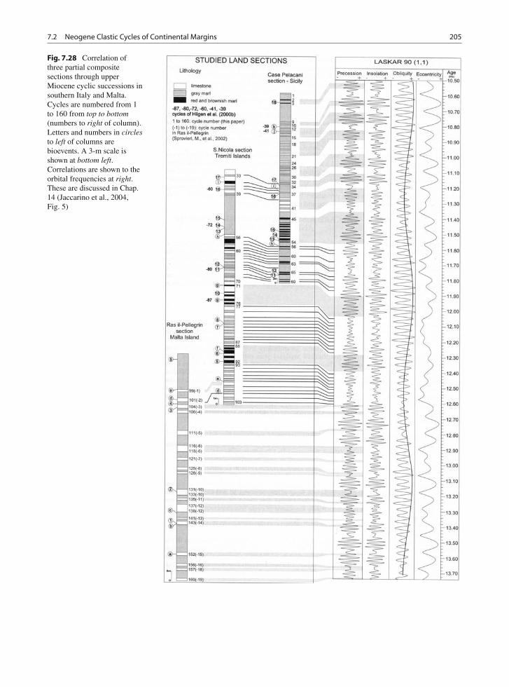
7.2 Neogene Clastic Cycles of Continental Margins 205
Fig. 7.28 Correlation ofthree partial compositesections through upperMiocene cyclic successions insouthern Italy and Malta.Cycles are numbered from 1to 160 from top to bottom(numbers to right of column).Letters and numbers in circlesto left of columns arebioevents. A 3-m scale isshown at bottom left.Correlations are shown to theorbital frequencies at right.These are discussed in Chap.14 (Jaccarino et al., 2004,Fig. 5)
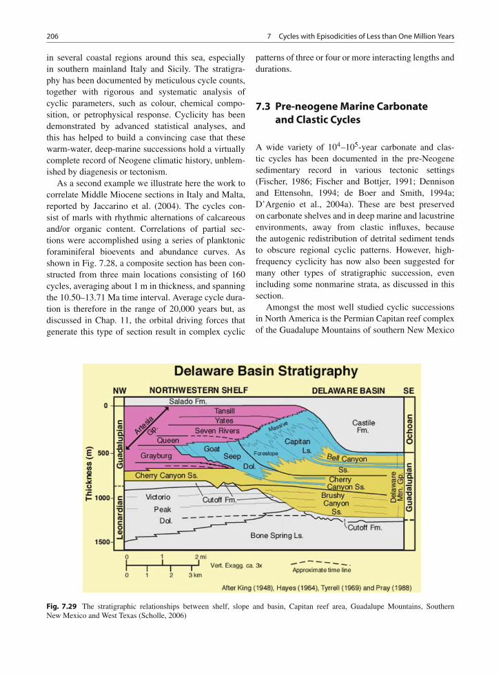
206 7 Cycles with Episodicities of Less than One Million Years
in several coastal regions around this sea, especiallyin southern mainland Italy and Sicily. The stratigra-phy has been documented by meticulous cycle counts,together with rigorous and systematic analysis ofcyclic parameters, such as colour, chemical compo-sition, or petrophysical response. Cyclicity has beendemonstrated by advanced statistical analyses, andthis has helped to build a convincing case that thesewarm-water, deep-marine successions hold a virtuallycomplete record of Neogene climatic history, unblem-ished by diagenesis or tectonism.
As a second example we illustrate here the work tocorrelate Middle Miocene sections in Italy and Malta,reported by Jaccarino et al. (2004). The cycles con-sist of marls with rhythmic alternations of calcareousand/or organic content. Correlations of partial sec-tions were accomplished using a series of planktonicforaminiferal bioevents and abundance curves. Asshown in Fig. 7.28, a composite section has been con-structed from three main locations consisting of 160cycles, averaging about 1 m in thickness, and spanningthe 10.50–13.71 Ma time interval. Average cycle dura-tion is therefore in the range of 20,000 years but, asdiscussed in Chap. 11, the orbital driving forces thatgenerate this type of section result in complex cyclic
patterns of three or four or more interacting lengths anddurations.
7.3 Pre-neogene Marine Carbonateand Clastic Cycles
A wide variety of 104–105-year carbonate and clas-tic cycles has been documented in the pre-Neogenesedimentary record in various tectonic settings(Fischer, 1986; Fischer and Bottjer, 1991; Dennisonand Ettensohn, 1994; de Boer and Smith, 1994a;D’Argenio et al., 2004a). These are best preservedon carbonate shelves and in deep marine and lacustrineenvironments, away from clastic influxes, becausethe autogenic redistribution of detrital sediment tendsto obscure regional cyclic patterns. However, high-frequency cyclicity has now also been suggested formany other types of stratigraphic succession, evenincluding some nonmarine strata, as discussed in thissection.
Amongst the most well studied cyclic successionsin North America is the Permian Capitan reef complexof the Guadalupe Mountains of southern New Mexico
Fig. 7.29 The stratigraphic relationships between shelf, slope and basin, Capitan reef area, Guadalupe Mountains, SouthernNew Mexico and West Texas (Scholle, 2006)
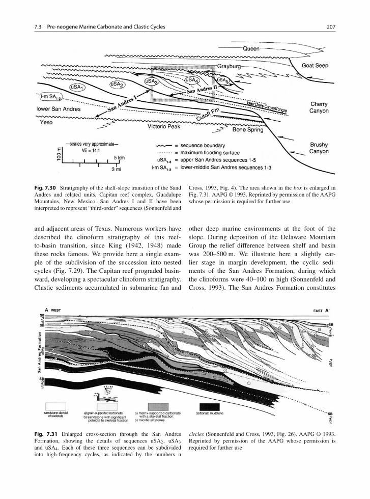
7.3 Pre-neogene Marine Carbonate and Clastic Cycles 207
Fig. 7.30 Stratigraphy of the shelf-slope transition of the SandAndres and related units, Capitan reef complex, GuadalupeMountains, New Mexico. San Andres I and II have beeninterpreted to represent “third-order” sequences (Sonnenfeld and
Cross, 1993, Fig. 4). The area shown in the box is enlarged inFig. 7.31. AAPG © 1993. Reprinted by permission of the AAPGwhose permission is required for further use
and adjacent areas of Texas. Numerous workers havedescribed the clinoform stratigraphy of this reef-to-basin transition, since King (1942, 1948) madethese rocks famous. We provide here a single exam-ple of the subdivision of the succession into nestedcycles (Fig. 7.29). The Capitan reef prograded basin-ward, developing a spectacular clinoform stratigraphy.Clastic sediments accumulated in submarine fan and
other deep marine environments at the foot of theslope. During deposition of the Delaware MountainGroup the relief difference between shelf and basinwas 200–500 m. We illustrate here a slightly ear-lier stage in margin development, the cyclic sedi-ments of the San Andres Formation, during whichthe clinoforms were 40–100 m high (Sonnenfeld andCross, 1993). The San Andres Formation constitutes
Fig. 7.31 Enlarged cross-section through the San AndresFormation, showing the details of sequences uSA2, uSA3and uSA4. Each of these three sequences can be subdividedinto high-frequency cycles, as indicated by the numbers n
circles (Sonnenfeld and Cross, 1993, Fig. 26). AAPG © 1993.Reprinted by permission of the AAPG whose permission isrequired for further use
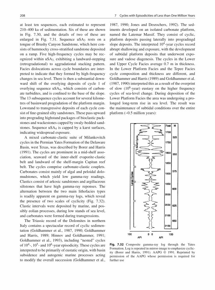
208 7 Cycles with Episodicities of Less than One Million Years
at least ten sequences, each estimated to represent210–400 ka of sedimentation. Six of these are shownin Fig. 7.30, and the details of two of these areenlarged in Fig. 7.31. Sequence uSA3 rests on atongue of Brushy Canyon Sandstone, which here con-sists of hummocky cross-stratified sandstone depositedon a ramp. Five high-frequency cycles may be rec-ognized within uSA3, exhibiting a landward-stepping(retrogradational) to aggradational stacking pattern.Facies dislocations across cycle boundaries are inter-preted to indicate that they formed by high-frequencychanges in sea level. There is then a substantial down-ward shift of the overlying deposits of cycle 1 ofoverlying sequence uSA4, which consists of carbon-ate turbidites, and is confined to the base of the slope.The 13 subsequence cycles account for several kilome-tres of basinward progradation of the platform margin.Lowstand to transgressive deposits of each cycle con-sist of fine-grained silty sandstones. These pass upwardinto prograding highstand packages of bioclastic pack-stones and wackestones capped by swaly-bedded sand-stones. Sequence uSA4 is capped by a karst surfaces,indicating widespread exposure.
A mixed carbonate-clastic suite of Milankovitchcycles in the Permian Yates Formation of the DelawareBasin, west Texas, was described by Borer and Harris(1991). The cycles are prominent in a mid-shelf asso-ciation, seaward of the inner-shelf evaporite-clasticbelt and landward of the shelf-margin Capitan reefbelt. The cycles comprise carbonate-clastic couplets.Carbonates consist mainly of algal and peloidal dolo-mudstones, which yield low gamma-ray readings.Clastics consist of arkosic sandstones and argillaceoussiltstones that have high gamma-ray reponses. Thealternation between the two main lithofacies typesis readily apparent on gamma-ray logs, which revealthe presence of two scales of cyclicity (Fig. 7.32).Clastic intervals were deposited by marine, and pos-sibly eolian processes, during low stands of sea level,and carbonates were formed during transgressions.
The Triassic record of the Dolomites in northernItaly contains a spectacular record of cyclic sedimen-tation (Goldhammer et al., 1987, 1990; Goldhammerand Harris, 1989; Hinnov and Goldhammer, 1991;Goldhammer et al., 1993), including “nested” cyclesof 104-, 105- and 106-year episodicity. These cycles areinterpreted to be primarily of eustatic origin, with basinsubsidence and autogenic marine processes actingto modify the overall succession (Goldhammer et al.,
1987, 1990; Jones and Desrochers, 1992). The sed-iments developed on an isolated carbonate platform,named the Latemar Massif. They consist of cyclic,platform deposits passing laterally into progradingdslope deposits. The interpreted 104-year cycles recordabrupt shallowing and exposure, with the developmentof subtidal platform deposits that underwent expo-sure and vadose diagenesis. The cycles in the Lowerand Upper Cycle Facies average 0.7 m in thickness.In the Lower Platform Facies and the Tepee Faciescycle composition and thickness are different, andGoldhammer and Harris (1989) and Goldhammer et al.(1987, 1990) interpreted this as a result of the overprintof slow (106-year) eustasy on the higher frequencycycles of sea-level change. During deposition of theLower Platform Facies the area was undergoing a pro-longed long-term rise in sea level. The result wasthe maintenance of subtidal conditions over the entireplatform (~0.5 million years):
Fig. 7.32 Composite gamma-ray log through the YatesFormation. Log is repeated in mirror-image to emphasize cyclic-ity (Borer and Harris, 1991). AAPG © 1991. Reprinted bypermission of the AAPG whose permission is required forfurther use
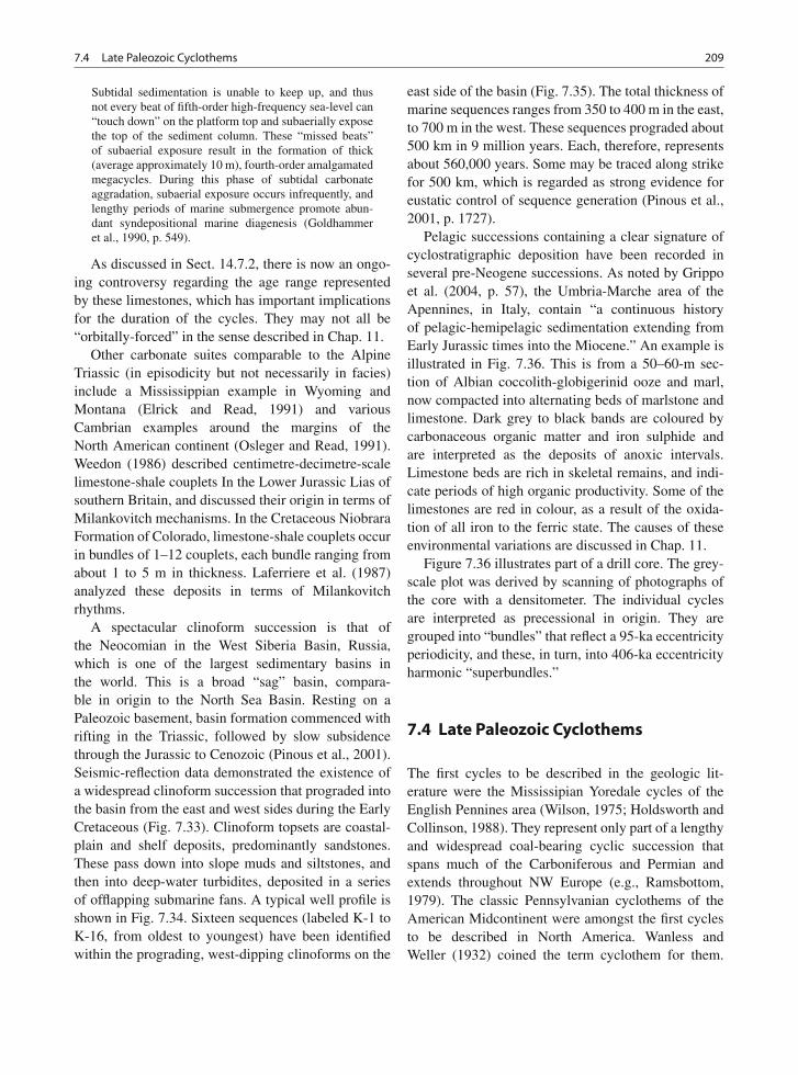
7.4 Late Paleozoic Cyclothems 209
Subtidal sedimentation is unable to keep up, and thusnot every beat of fifth-order high-frequency sea-level can“touch down” on the platform top and subaerially exposethe top of the sediment column. These “missed beats”of subaerial exposure result in the formation of thick(average approximately 10 m), fourth-order amalgamatedmegacycles. During this phase of subtidal carbonateaggradation, subaerial exposure occurs infrequently, andlengthy periods of marine submergence promote abun-dant syndepositional marine diagenesis (Goldhammeret al., 1990, p. 549).
As discussed in Sect. 14.7.2, there is now an ongo-ing controversy regarding the age range representedby these limestones, which has important implicationsfor the duration of the cycles. They may not all be“orbitally-forced” in the sense described in Chap. 11.
Other carbonate suites comparable to the AlpineTriassic (in episodicity but not necessarily in facies)include a Mississippian example in Wyoming andMontana (Elrick and Read, 1991) and variousCambrian examples around the margins of theNorth American continent (Osleger and Read, 1991).Weedon (1986) described centimetre-decimetre-scalelimestone-shale couplets In the Lower Jurassic Lias ofsouthern Britain, and discussed their origin in terms ofMilankovitch mechanisms. In the Cretaceous NiobraraFormation of Colorado, limestone-shale couplets occurin bundles of 1–12 couplets, each bundle ranging fromabout 1 to 5 m in thickness. Laferriere et al. (1987)analyzed these deposits in terms of Milankovitchrhythms.
A spectacular clinoform succession is that ofthe Neocomian in the West Siberia Basin, Russia,which is one of the largest sedimentary basins inthe world. This is a broad “sag” basin, compara-ble in origin to the North Sea Basin. Resting on aPaleozoic basement, basin formation commenced withrifting in the Triassic, followed by slow subsidencethrough the Jurassic to Cenozoic (Pinous et al., 2001).Seismic-reflection data demonstrated the existence ofa widespread clinoform succession that prograded intothe basin from the east and west sides during the EarlyCretaceous (Fig. 7.33). Clinoform topsets are coastal-plain and shelf deposits, predominantly sandstones.These pass down into slope muds and siltstones, andthen into deep-water turbidites, deposited in a seriesof offlapping submarine fans. A typical well profile isshown in Fig. 7.34. Sixteen sequences (labeled K-1 toK-16, from oldest to youngest) have been identifiedwithin the prograding, west-dipping clinoforms on the
east side of the basin (Fig. 7.35). The total thickness ofmarine sequences ranges from 350 to 400 m in the east,to 700 m in the west. These sequences prograded about500 km in 9 million years. Each, therefore, representsabout 560,000 years. Some may be traced along strikefor 500 km, which is regarded as strong evidence foreustatic control of sequence generation (Pinous et al.,2001, p. 1727).
Pelagic successions containing a clear signature ofcyclostratigraphic deposition have been recorded inseveral pre-Neogene successions. As noted by Grippoet al. (2004, p. 57), the Umbria-Marche area of theApennines, in Italy, contain “a continuous historyof pelagic-hemipelagic sedimentation extending fromEarly Jurassic times into the Miocene.” An example isillustrated in Fig. 7.36. This is from a 50–60-m sec-tion of Albian coccolith-globigerinid ooze and marl,now compacted into alternating beds of marlstone andlimestone. Dark grey to black bands are coloured bycarbonaceous organic matter and iron sulphide andare interpreted as the deposits of anoxic intervals.Limestone beds are rich in skeletal remains, and indi-cate periods of high organic productivity. Some of thelimestones are red in colour, as a result of the oxida-tion of all iron to the ferric state. The causes of theseenvironmental variations are discussed in Chap. 11.
Figure 7.36 illustrates part of a drill core. The grey-scale plot was derived by scanning of photographs ofthe core with a densitometer. The individual cyclesare interpreted as precessional in origin. They aregrouped into “bundles” that reflect a 95-ka eccentricityperiodicity, and these, in turn, into 406-ka eccentricityharmonic “superbundles.”
7.4 Late Paleozoic Cyclothems
The first cycles to be described in the geologic lit-erature were the Mississipian Yoredale cycles of theEnglish Pennines area (Wilson, 1975; Holdsworth andCollinson, 1988). They represent only part of a lengthyand widespread coal-bearing cyclic succession thatspans much of the Carboniferous and Permian andextends throughout NW Europe (e.g., Ramsbottom,1979). The classic Pennsylvanian cyclothems of theAmerican Midcontinent were amongst the first cyclesto be described in North America. Wanless andWeller (1932) coined the term cyclothem for them.
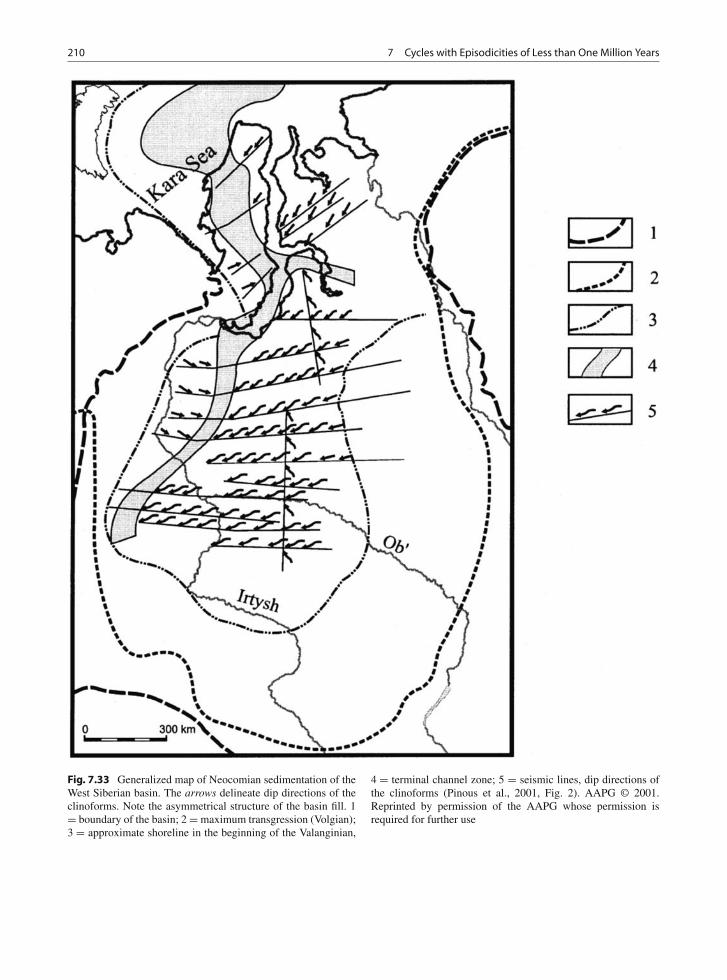
210 7 Cycles with Episodicities of Less than One Million Years
Fig. 7.33 Generalized map of Neocomian sedimentation of theWest Siberian basin. The arrows delineate dip directions of theclinoforms. Note the asymmetrical structure of the basin fill. 1= boundary of the basin; 2 = maximum transgression (Volgian);3 = approximate shoreline in the beginning of the Valanginian,
4 = terminal channel zone; 5 = seismic lines, dip directions ofthe clinoforms (Pinous et al., 2001, Fig. 2). AAPG © 2001.Reprinted by permission of the AAPG whose permission isrequired for further use
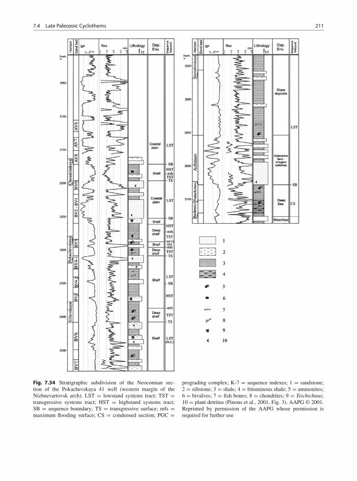
7.4 Late Paleozoic Cyclothems 211
Fig. 7.34 Stratigraphic subdivision of the Neocomian sec-tion of the Pokachevskaya 41 well (western margin of theNizhnevartovsk arch). LST = lowstand systems tract; TST =transgressive systems tract; HST = highstand systems tract;SB = sequence boundary; TS = transgressive surface; mfs =maximum flooding surface; CS = condensed section; PGC =
prograding complex; K-7 = sequence indexes; 1 = sandstone;2 = siltstone; 3 = shale; 4 = bituminous shale; 5 = ammonites;6 = bivalves; 7 = fish bones; 8 = chondrites; 9 = Teichichnus;10 = plant detritus (Pinous et al., 2001, Fig. 3). AAPG © 2001.Reprinted by permission of the AAPG whose permission isrequired for further use
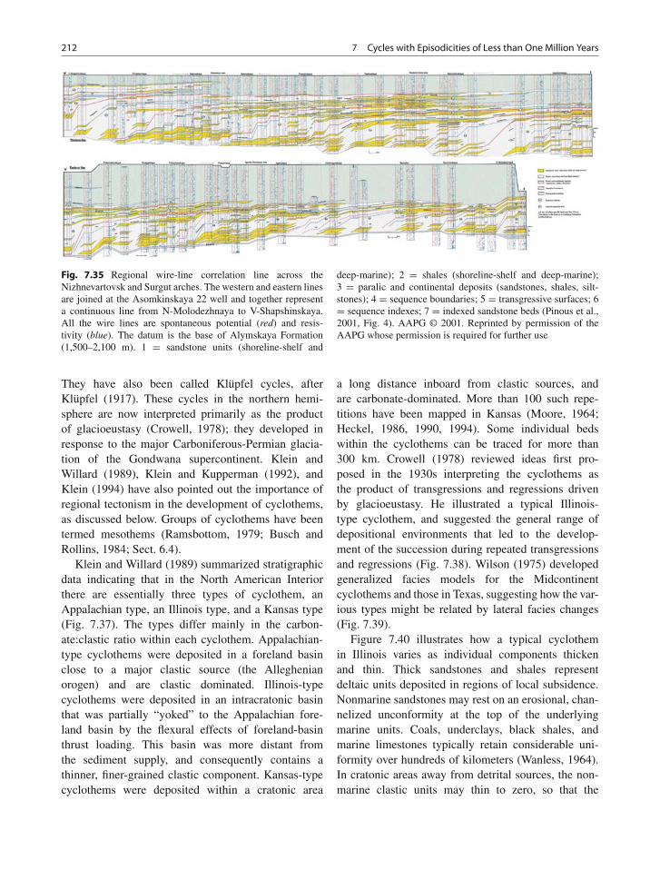
212 7 Cycles with Episodicities of Less than One Million Years
Fig. 7.35 Regional wire-line correlation line across theNizhnevartovsk and Surgut arches. The western and eastern linesare joined at the Asomkinskaya 22 well and together representa continuous line from N-Molodezhnaya to V-Shapshinskaya.All the wire lines are spontaneous potential (red) and resis-tivity (blue). The datum is the base of Alymskaya Formation(1,500–2,100 m). 1 = sandstone units (shoreline-shelf and
deep-marine); 2 = shales (shoreline-shelf and deep-marine);3 = paralic and continental deposits (sandstones, shales, silt-stones); 4 = sequence boundaries; 5 = transgressive surfaces; 6= sequence indexes; 7 = indexed sandstone beds (Pinous et al.,2001, Fig. 4). AAPG © 2001. Reprinted by permission of theAAPG whose permission is required for further use
They have also been called Klüpfel cycles, afterKlüpfel (1917). These cycles in the northern hemi-sphere are now interpreted primarily as the productof glacioeustasy (Crowell, 1978); they developed inresponse to the major Carboniferous-Permian glacia-tion of the Gondwana supercontinent. Klein andWillard (1989), Klein and Kupperman (1992), andKlein (1994) have also pointed out the importance ofregional tectonism in the development of cyclothems,as discussed below. Groups of cyclothems have beentermed mesothems (Ramsbottom, 1979; Busch andRollins, 1984; Sect. 6.4).
Klein and Willard (1989) summarized stratigraphicdata indicating that in the North American Interiorthere are essentially three types of cyclothem, anAppalachian type, an Illinois type, and a Kansas type(Fig. 7.37). The types differ mainly in the carbon-ate:clastic ratio within each cyclothem. Appalachian-type cyclothems were deposited in a foreland basinclose to a major clastic source (the Alleghenianorogen) and are clastic dominated. Illinois-typecyclothems were deposited in an intracratonic basinthat was partially “yoked” to the Appalachian fore-land basin by the flexural effects of foreland-basinthrust loading. This basin was more distant fromthe sediment supply, and consequently contains athinner, finer-grained clastic component. Kansas-typecyclothems were deposited within a cratonic area
a long distance inboard from clastic sources, andare carbonate-dominated. More than 100 such repe-titions have been mapped in Kansas (Moore, 1964;Heckel, 1986, 1990, 1994). Some individual bedswithin the cyclothems can be traced for more than300 km. Crowell (1978) reviewed ideas first pro-posed in the 1930s interpreting the cyclothems asthe product of transgressions and regressions drivenby glacioeustasy. He illustrated a typical Illinois-type cyclothem, and suggested the general range ofdepositional environments that led to the develop-ment of the succession during repeated transgressionsand regressions (Fig. 7.38). Wilson (1975) developedgeneralized facies models for the Midcontinentcyclothems and those in Texas, suggesting how the var-ious types might be related by lateral facies changes(Fig. 7.39).
Figure 7.40 illustrates how a typical cyclothemin Illinois varies as individual components thickenand thin. Thick sandstones and shales representdeltaic units deposited in regions of local subsidence.Nonmarine sandstones may rest on an erosional, chan-nelized unconformity at the top of the underlyingmarine units. Coals, underclays, black shales, andmarine limestones typically retain considerable uni-formity over hundreds of kilometers (Wanless, 1964).In cratonic areas away from detrital sources, the non-marine clastic units may thin to zero, so that the
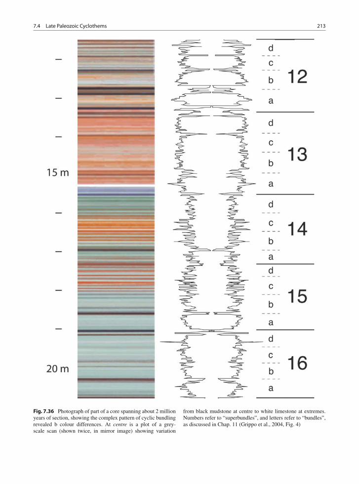
7.4 Late Paleozoic Cyclothems 213
Fig. 7.36 Photograph of part of a core spanning about 2 millionyears of section, showing the complex pattern of cyclic bundlingrevealed b colour differences. At centre is a plot of a grey-scale scan (shown twice, in mirror image) showing variation
from black mudstone at centre to white limestone at extremes.Numbers refer to “superbundles”, and letters refer to “bundles”,as discussed in Chap. 11 (Grippo et al., 2004, Fig. 4)
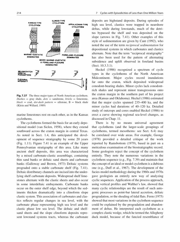
214 7 Cycles with Episodicities of Less than One Million Years
Fig. 7.37 The three major types of North American cyclothem.Dashes = gray shale, dots = sandstone, bricks = limestone,black = coal, dot-dash pattern = siltstone, B = black shale(Klein and Willard, 1989)
marine limestones rest on each other, as in the Kansascyclothems.
The cyclothems formed the basis for an early depo-sitional model (van Siclen, 1958), where they extendsouthward across the craton margin in central Texas.As noted in Sect. 1.4, this anticipated the devel-opment of sequence stratigraphy by some 20 years(Fig. 1.11). Figure 7.41 is an example of the UpperPennsylvanian stratigraphy of this area. Like manyancient shelf deposits, this area was characterizedby a mixed carbonate-clastic assemblage, containingthin sand banks or deltaic sand sheets and carbonatebanks (Galloway and Brown, 1973) Deltaic systemsprograded onto a stable carbonate shelf (Fig. 7.41).Deltaic distributary channels are incised into the under-lying shelf carbonate deposits. Widespread shelf lime-stones alternate with the clastic sheets and also occurin some interdeltaic embayments. Carbonate banksoccur on the outer shelf edge, beyond which the sed-iments thicken dramatically into a clinoform slopeclastic system. This association of carbonates and clas-tics reflects regular changes in sea level, with thecarbonate phase representing high sea level and theclastic phase low sea level. The deltaic and shelf-sand sheets and the slope clinoform deposits repre-sent lowstand systems tracts, whereas the carbonate
deposits are highstand deposits. During episodes ofhigh sea level, clastics were trapped in nearshoredeltas, while during lowstands, much of the detri-tus bypassed the shelf and was deposited on theslope (arrows in Fig. 7.41). Other examples of thisstyle of sedimentation are given by Cant (1992), whonoted the use of the term reciprocal sedimentation fordepositional systems in which carbonates and clasticsalternate. Note that the term “reciprocal stratigraphy”has also been used for the pattern of alternatingsubsidence and uplift observed in foreland basins(Sect. 10.3.3.1).
Heckel (1986) recognized a spectrum of cycletypes in the cyclothems of the North AmericanMidcontinent. Major cycles record inundationsfar onto the craton, which deposited widespreadconodont-bearing shales. Minor cycles lack conodont-rich shales and represent minor transgressions ontothe craton margin in the southern part of his projectarea (Kansas and Oklahoma). Heckel (1986) estimatedthat the major cycles spanned 235–400 ka, and theminor cycles had durations of 40–120 ka. Detailedstudy of outcrops and cores enabled Heckel (1986) toerect a curve showing regional sea-level changes, asdiscussed in Chap. 11.
There is by no means universal agreementthat cyclothems (and the larger-scale groupings ofcyclothems, termed mesothems: see Sect. 6.4) maybe correlated over wide areas. For example, George(1978) provided a detailed critique of the workreported by Ramsbottom (1979), based in part on ameticulous examination of the biostratigraphic record.Some geologists reject the concept of the cyclothementirely. They note the numerous variations in thecyclothem sequence (e.g., Fig. 7.39) and maintain thatthe concept of an ideal or model cyclothem is a dubiousone (e.g., Duff et al., 1967). The development of thefacies-model methodology during the 1960s and 1970sgave geologists an entirely new way of analyzingcyclic sequences. Application of the process approach,using vertical profiles and Walther’s law, showed thatmany cyclic relationships are the result of such auto-genic processes as point-bar lateral accretion, deltaicprogradation, or the shoaling of tidal flats. Ferm (1975)showed that most variations in the cyclothem sequencecould be explained by the progradation and abandon-ment of deltas. He interpreted each cyclothem as acomplex clastic wedge, which he termed the Alleghenyduck model, because of the fancied resemblance of
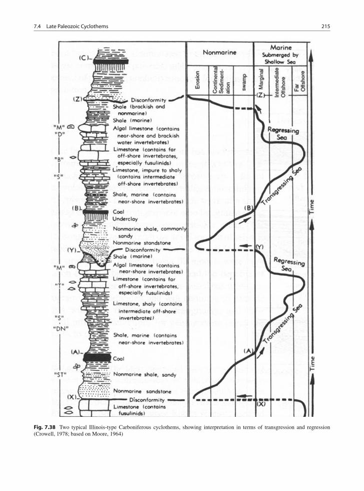
7.4 Late Paleozoic Cyclothems 215
Fig. 7.38 Two typical Illinois-type Carboniferous cyclothems, showing interpretation in terms of transgression and regression(Crowell, 1978; based on Moore, 1964)
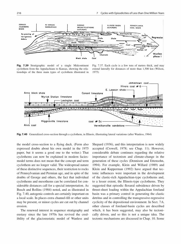
216 7 Cycles with Episodicities of Less than One Million Years
Fig. 7.39 Stratigraphic model of a single Midcontinentcyclothem from the Appalachians to Kansas, showing the rela-tionships of the three main types of cyclothem illustrated in
Fig. 7.37. Each cycle is a few tens of metres thick, and mayextend laterally for distances of more than 1,500 km (Wilson,1975)
Fig. 7.40 Generalized cross-section through a cyclothem, in Illinois, illustrating lateral variations (after Wanless, 1964)
the model cross-section to a flying duck. (Ferm alsoexpressed doubts about his own model in the 1975paper, but it seems a good one to the writer.) Thatcyclothems can now be explained in modern facies-model terms does not mean that the concept and termcyclothem are no longer valid. The widespread natureof these distinctive sequences, their restriction to rocksof Pennsylvanian and Permian age, and in spite of thedoubts of George and others, the fact that individualcyclothems and mesothems can be correlated for con-siderable distances call for a special interpretation. AsBusch and Rollins (1984) noted, and as illustrated inFig. 7.40, autogenic controls are certainly important ona local scale. In places extra channel-fill or other unitsmay be present, or minor cycles are cut out by channelerosion.
The renewed interest in sequence stratigraphy andeustasy since the late 1970s has revived the cred-ibility of the glacioeustatic model of Wanless and
Shepard (1936), and this interpretation is now widelyaccepted (Crowell, 1978; see Chap. 11). However,considerable debate continues regarding the relativeimportance of tectonism and climate-change in thegeneration of these cycles (Dennison and Ettensohn,1994). For example, Klein and Willard (1989) andKlein and Kupperman (1992) have argued that tec-tonic influences were important in the developmentof the clastic-rich Appalachian-type cyclothems and,to a lesser extent, the Illinois-type cyclothems. Theysuggested that episodic flexural subsidence driven bythrust-sheet loading within the Appalachian forelandbasin was a primary control in generating the clasticdetritus and in controlling the transgressive-regressivecyclicity of the depositional environment. In Sect. 7.6,other classes of foreland-basin cycles are describedwhich, it has been suggested, may also be tectoni-cally driven, and so this is not a unique idea. Thetectonic mechanisms are discussed in Chap. 10. Some
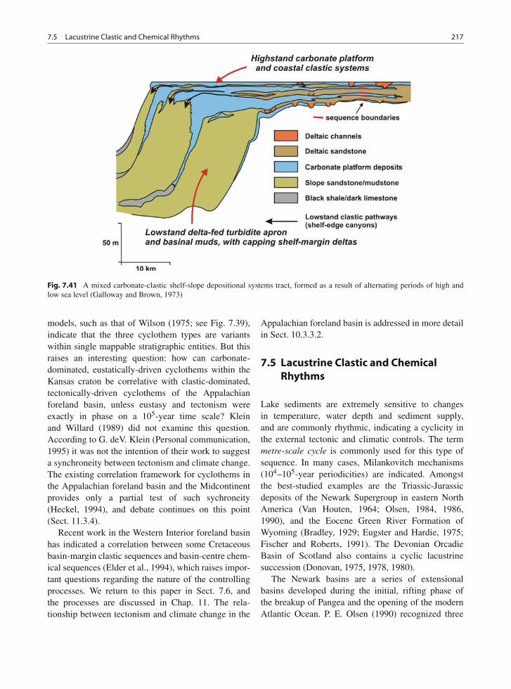
7.5 Lacustrine Clastic and Chemical Rhythms 217
Fig. 7.41 A mixed carbonate-clastic shelf-slope depositional systems tract, formed as a result of alternating periods of high andlow sea level (Galloway and Brown, 1973)
models, such as that of Wilson (1975; see Fig. 7.39),indicate that the three cyclothem types are variantswithin single mappable stratigraphic entities. But thisraises an interesting question: how can carbonate-dominated, eustatically-driven cyclothems within theKansas craton be correlative with clastic-dominated,tectonically-driven cyclothems of the Appalachianforeland basin, unless eustasy and tectonism wereexactly in phase on a 105-year time scale? Kleinand Willard (1989) did not examine this question.According to G. deV. Klein (Personal communication,1995) it was not the intention of their work to suggesta synchroneity between tectonism and climate change.The existing correlation framework for cyclothems inthe Appalachian foreland basin and the Midcontinentprovides only a partial test of such sychroneity(Heckel, 1994), and debate continues on this point(Sect. 11.3.4).
Recent work in the Western Interior foreland basinhas indicated a correlation between some Cretaceousbasin-margin clastic sequences and basin-centre chem-ical sequences (Elder et al., 1994), which raises impor-tant questions regarding the nature of the controllingprocesses. We return to this paper in Sect. 7.6, andthe processes are discussed in Chap. 11. The rela-tionship between tectonism and climate change in the
Appalachian foreland basin is addressed in more detailin Sect. 10.3.3.2.
7.5 Lacustrine Clastic and ChemicalRhythms
Lake sediments are extremely sensitive to changesin temperature, water depth and sediment supply,and are commonly rhythmic, indicating a cyclicity inthe external tectonic and climatic controls. The termmetre-scale cycle is commonly used for this type ofsequence. In many cases, Milankovitch mechanisms(104–105-year periodicities) are indicated. Amongstthe best-studied examples are the Triassic-Jurassicdeposits of the Newark Supergroup in eastern NorthAmerica (Van Houten, 1964; Olsen, 1984, 1986,1990), and the Eocene Green River Formation ofWyoming (Bradley, 1929; Eugster and Hardie, 1975;Fischer and Roberts, 1991). The Devonian OrcadieBasin of Scotland also contains a cyclic lacustrinesuccession (Donovan, 1975, 1978, 1980).
The Newark basins are a series of extensionalbasins developed during the initial, rifting phase ofthe breakup of Pangea and the opening of the modernAtlantic Ocean. P. E. Olsen (1990) recognized three
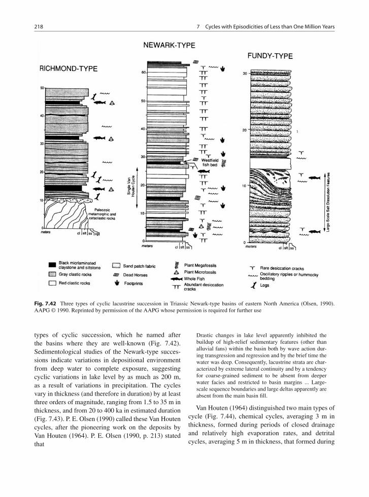
218 7 Cycles with Episodicities of Less than One Million Years
Fig. 7.42 Three types of cyclic lacustrine succession in Triassic Newark-type basins of eastern North America (Olsen, 1990).AAPG © 1990. Reprinted by permission of the AAPG whose permission is required for further use
types of cyclic succession, which he named afterthe basins where they are well-known (Fig. 7.42).Sedimentological studies of the Newark-type succes-sions indicate variations in depositional environmentfrom deep water to complete exposure, suggestingcyclic variations in lake level by as much as 200 m,as a result of variations in precipitation. The cyclesvary in thickness (and therefore in duration) by at leastthree orders of magnitude, ranging from 1.5 to 35 m inthickness, and from 20 to 400 ka in estimated duration(Fig. 7.43). P. E. Olsen (1990) called these Van Houtencycles, after the pioneering work on the deposits byVan Houten (1964). P. E. Olsen (1990, p. 213) statedthat
Drastic changes in lake level apparently inhibited thebuildup of high-relief sedimentary features (other thanalluvial fans) within the basin both by wave action dur-ing transgression and regression and by the brief time thewater was deep. Consequently, lacustrine strata are char-acterized by extreme lateral continuity and by a tendencyfor coarse-grained sediment to be absent from deeperwater facies and restricted to basin margins ... Large-scale sequence boundaries and large deltas apparently areabsent from the main basin fill.
Van Houten (1964) distinguished two main types ofcycle (Fig. 7.44), chemical cycles, averaging 3 m inthickness, formed during periods of closed drainageand relatively high evaporation rates, and detritalcycles, averaging 5 m in thickness, that formed during
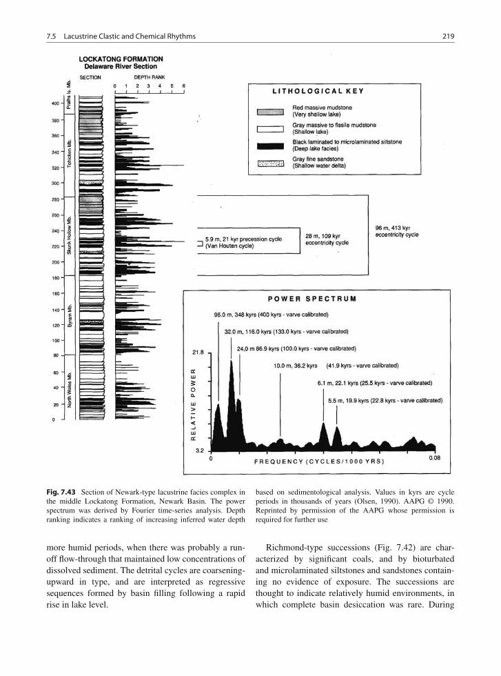
7.5 Lacustrine Clastic and Chemical Rhythms 219
Fig. 7.43 Section of Newark-type lacustrine facies complex inthe middle Lockatong Formation, Newark Basin. The powerspectrum was derived by Fourier time-series analysis. Depthranking indicates a ranking of increasing inferred water depth
based on sedimentological analysis. Values in kyrs are cycleperiods in thousands of years (Olsen, 1990). AAPG © 1990.Reprinted by permission of the AAPG whose permission isrequired for further use
more humid periods, when there was probably a run-off flow-through that maintained low concentrations ofdissolved sediment. The detrital cycles are coarsening-upward in type, and are interpreted as regressivesequences formed by basin filling following a rapidrise in lake level.
Richmond-type successions (Fig. 7.42) are char-acterized by significant coals, and by bioturbatedand microlaminated siltstones and sandstones contain-ing no evidence of exposure. The successions arethought to indicate relatively humid environments, inwhich complete basin desiccation was rare. During
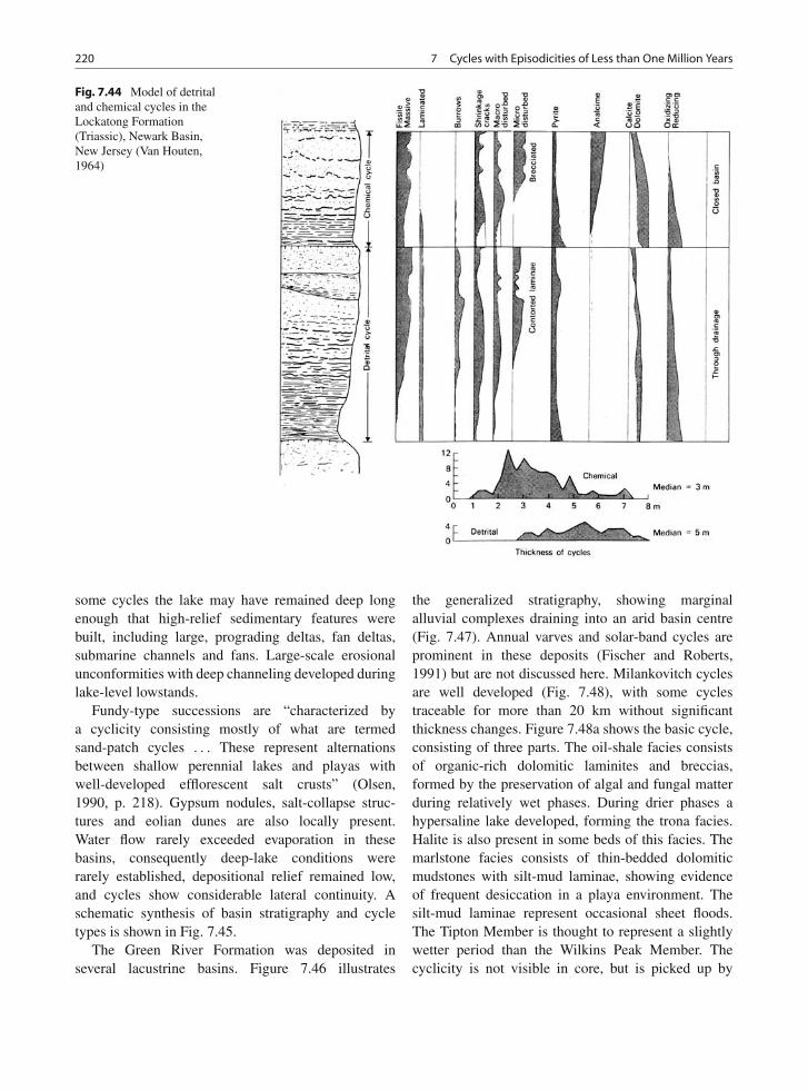
220 7 Cycles with Episodicities of Less than One Million Years
Fig. 7.44 Model of detritaland chemical cycles in theLockatong Formation(Triassic), Newark Basin,New Jersey (Van Houten,1964)
some cycles the lake may have remained deep longenough that high-relief sedimentary features werebuilt, including large, prograding deltas, fan deltas,submarine channels and fans. Large-scale erosionalunconformities with deep channeling developed duringlake-level lowstands.
Fundy-type successions are “characterized bya cyclicity consisting mostly of what are termedsand-patch cycles . . . These represent alternationsbetween shallow perennial lakes and playas withwell-developed efflorescent salt crusts” (Olsen,1990, p. 218). Gypsum nodules, salt-collapse struc-tures and eolian dunes are also locally present.Water flow rarely exceeded evaporation in thesebasins, consequently deep-lake conditions wererarely established, depositional relief remained low,and cycles show considerable lateral continuity. Aschematic synthesis of basin stratigraphy and cycletypes is shown in Fig. 7.45.
The Green River Formation was deposited inseveral lacustrine basins. Figure 7.46 illustrates
the generalized stratigraphy, showing marginalalluvial complexes draining into an arid basin centre(Fig. 7.47). Annual varves and solar-band cycles areprominent in these deposits (Fischer and Roberts,1991) but are not discussed here. Milankovitch cyclesare well developed (Fig. 7.48), with some cyclestraceable for more than 20 km without significantthickness changes. Figure 7.48a shows the basic cycle,consisting of three parts. The oil-shale facies consistsof organic-rich dolomitic laminites and breccias,formed by the preservation of algal and fungal matterduring relatively wet phases. During drier phases ahypersaline lake developed, forming the trona facies.Halite is also present in some beds of this facies. Themarlstone facies consists of thin-bedded dolomiticmudstones with silt-mud laminae, showing evidenceof frequent desiccation in a playa environment. Thesilt-mud laminae represent occasional sheet floods.The Tipton Member is thought to represent a slightlywetter period than the Wilkins Peak Member. Thecyclicity is not visible in core, but is picked up by
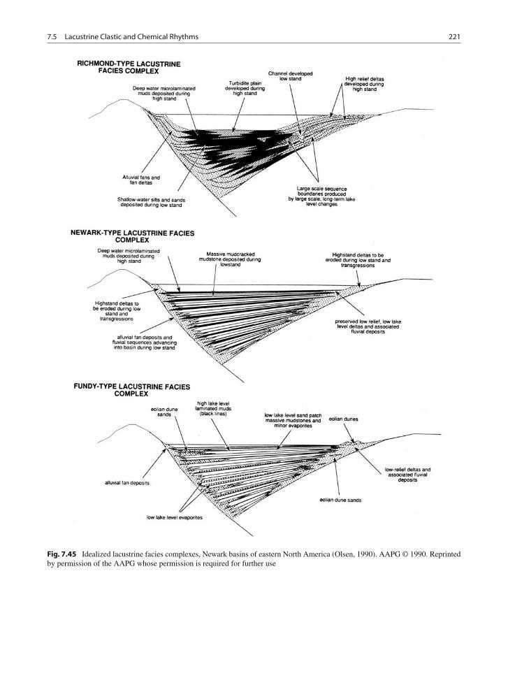
7.5 Lacustrine Clastic and Chemical Rhythms 221
Fig. 7.45 Idealized lacustrine facies complexes, Newark basins of eastern North America (Olsen, 1990). AAPG © 1990. Reprintedby permission of the AAPG whose permission is required for further use
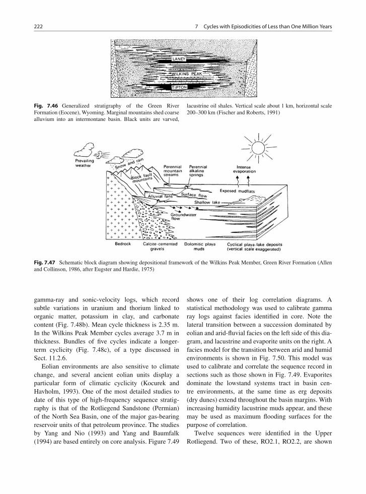
222 7 Cycles with Episodicities of Less than One Million Years
Fig. 7.46 Generalized stratigraphy of the Green RiverFormation (Eocene), Wyoming. Marginal mountains shed coarsealluvium into an intermontane basin. Black units are varved,
lacustrine oil shales. Vertical scale about 1 km, horizontal scale200–300 km (Fischer and Roberts, 1991)
Fig. 7.47 Schematic block diagram showing depositional framework of the Wilkins Peak Member, Green River Formation (Allenand Collinson, 1986, after Eugster and Hardie, 1975)
gamma-ray and sonic-velocity logs, which recordsubtle variations in uranium and thorium linked toorganic matter, potassium in clay, and carbonatecontent (Fig. 7.48b). Mean cycle thickness is 2.35 m.In the Wilkins Peak Member cycles average 3.7 m inthickness. Bundles of five cycles indicate a longer-term cyclicity (Fig. 7.48c), of a type discussed inSect. 11.2.6.
Eolian environments are also sensitive to climatechange, and several ancient eolian units display aparticular form of climatic cyclicity (Kocurek andHavholm, 1993). One of the most detailed studies todate of this type of high-frequency sequence stratig-raphy is that of the Rotliegend Sandstone (Permian)of the North Sea Basin, one of the major gas-bearingreservoir units of that petroleum province. The studiesby Yang and Nio (1993) and Yang and Baumfalk(1994) are based entirely on core analysis. Figure 7.49
shows one of their log correlation diagrams. Astatistical methodology was used to calibrate gammaray logs against facies identified in core. Note thelateral transition between a succession dominated byeolian and arid-fluvial facies on the left side of this dia-gram, and lacustrine and evaporite units on the right. Afacies model for the transition between arid and humidenvironments is shown in Fig. 7.50. This model wasused to calibrate and correlate the sequence record insections such as those shown in Fig. 7.49. Evaporitesdominate the lowstand systems tract in basin cen-tre environments, at the same time as erg deposits(dry dunes) extend throughout the basin margins. Withincreasing humidity lacustrine muds appear, and thesemay be used as maximum flooding surfaces for thepurpose of correlation.
Twelve sequences were identified in the UpperRotliegend. Two of these, RO2.1, RO2.2, are shown
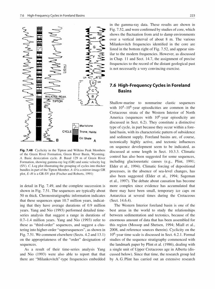
7.6 High-Frequency Cycles in Foreland Basins 223
Fig. 7.48 Cyclicity in the Tipton and Wilkins Peak Membersof the Green River Formation, Green River Basin, Wyoming.A. Basic desiccation cycle. B. Basal 129 m of Green RiverFormation, showing gamma-ray log (GR) and sonic velocity log(SV). C. Log plot illustrating the grouping of cycles into thickerbundles in part of the Tipton Member. A–D is a mirror-image GRplot, E–H is a GR-SV plot (Fischer and Roberts, 1991)
in detail in Fig. 7.49, and the complete succession isshown in Fig. 7.51. The sequences are typically about50 m thick. Chronostratigraphic information indicatesthat these sequences span 10.7 million years, indicat-ing that they have average durations of 0.9 millionyears. Yang and Nio (1993) performed detailed time-series analysis that suggest a range in durations of0.7–1.4 million years. Yang and Nio (1993) refer tothese as “third-order” sequences, and suggest a clus-tering into higher-order “supersequences”, as shown inFig. 7.51. We comment elsewhere (Sects. 4.2 and 13.1)on the appropriateness of the “order” designation ofsequences.
As a result of their time-series analysis Yangand Nio (1993) were also able to report that thatthere are “Milankovitch”-type frequencies embedded
in the gamma-ray data. These results are shown inFig. 7.52, and were confirmed by studies of core, whichshows the fluctuation from arid to damp environmentsover a vertical interval of about 8 m. The variousMilankovitch frequencies identified in the core arelisted in the bottom right of Fig. 7.52, and appear sim-ilar to the modern frequencies. However, as discussedin Chap. 11 and Sect. 14.7, the assignment of precisefrequencies to the record of the distant geological pastis not necessarily a very convincing exercise.
7.6 High-Frequency Cycles in ForelandBasins
Shallow-marine to nonmarine clastic sequenceswith 104–106-year episodicities are common in theCretaceous strata of the Western Interior of NorthAmerica (sequences with 106-year episodicity arediscussed in Sect. 6.2). They constitute a distinctivetype of cycle, in part because they occur within a fore-land basin, with its characteristic pattern of subsidenceand sediment supply. Foreland basins are, of course,tectonically highly active, and tectonic influenceson sequence development seem to be indicated, asdiscussed at some length in Sect. 10.3.3. Climaticcontrol has also been suggested for some sequences,including glacioeustatic causes (e.g., Plint, 1991;Elder et al., 1994). Climatic forcing of depositionalprocesses, in the absence of sea-level changes, hasalso been suggested (Elder et al., 1994; Sagemanet al., 1997). The debate about causation has becomemore complex since evidence has accumulated thatthere may have been small, temporary ice caps onAntarctica at several times during the Cretaceous(Sect. 14.6.4).
The Western Interior foreland basin is one of thebest areas in the world to study the relationshipsbetween sedimentation and tectonics, because of theenormous amount of data that has been assembled forthis region (Mossop and Shetsen, 1994; Miall et al.,2008, and reference sources therein). Cyclicity on the106-year time scale is discussed in Sect. 6.2.1. Formalstudies of the sequence stratigraphy commenced withthe landmark paper by Plint et al. (1986), dealing witha single unit of Upper Cretaceous age in Alberta (dis-cussed below). Since that time, the research group ledby A. G. Plint has carried out an extensive research
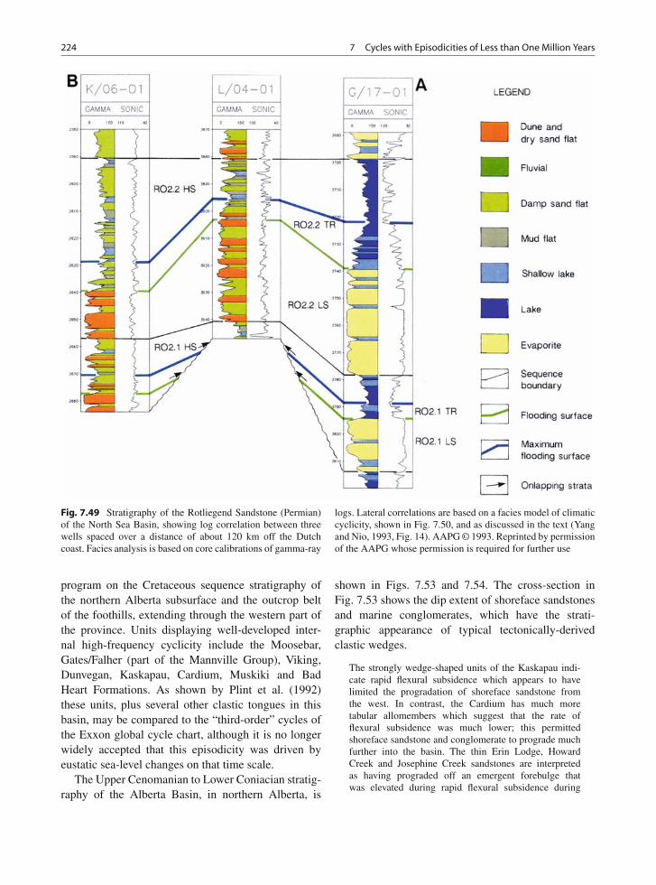
224 7 Cycles with Episodicities of Less than One Million Years
Fig. 7.49 Stratigraphy of the Rotliegend Sandstone (Permian)of the North Sea Basin, showing log correlation between threewells spaced over a distance of about 120 km off the Dutchcoast. Facies analysis is based on core calibrations of gamma-ray
logs. Lateral correlations are based on a facies model of climaticcyclicity, shown in Fig. 7.50, and as discussed in the text (Yangand Nio, 1993, Fig. 14). AAPG © 1993. Reprinted by permissionof the AAPG whose permission is required for further use
program on the Cretaceous sequence stratigraphy ofthe northern Alberta subsurface and the outcrop beltof the foothills, extending through the western part ofthe province. Units displaying well-developed inter-nal high-frequency cyclicity include the Moosebar,Gates/Falher (part of the Mannville Group), Viking,Dunvegan, Kaskapau, Cardium, Muskiki and BadHeart Formations. As shown by Plint et al. (1992)these units, plus several other clastic tongues in thisbasin, may be compared to the “third-order” cycles ofthe Exxon global cycle chart, although it is no longerwidely accepted that this episodicity was driven byeustatic sea-level changes on that time scale.
The Upper Cenomanian to Lower Coniacian stratig-raphy of the Alberta Basin, in northern Alberta, is
shown in Figs. 7.53 and 7.54. The cross-section inFig. 7.53 shows the dip extent of shoreface sandstonesand marine conglomerates, which have the strati-graphic appearance of typical tectonically-derivedclastic wedges.
The strongly wedge-shaped units of the Kaskapau indi-cate rapid flexural subsidence which appears to havelimited the progradation of shoreface sandstone fromthe west. In contrast, the Cardium has much moretabular allomembers which suggest that the rate offlexural subsidence was much lower; this permittedshoreface sandstone and conglomerate to prograde muchfurther into the basin. The thin Erin Lodge, HowardCreek and Josephine Creek sandstones are interpretedas having prograded off an emergent forebulge thatwas elevated during rapid flexural subsidence during
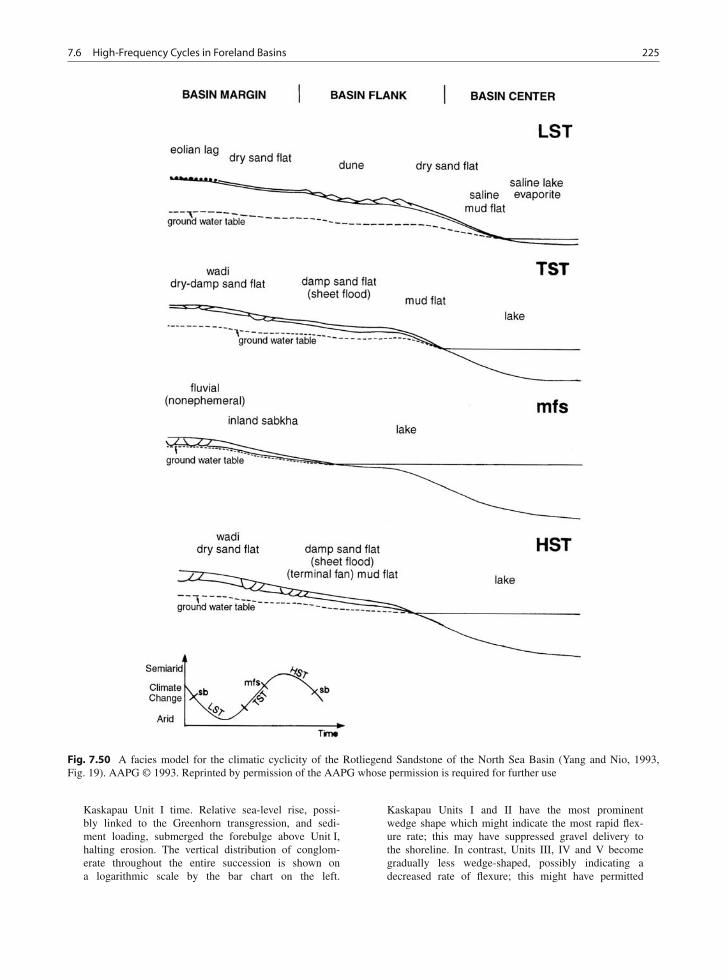
7.6 High-Frequency Cycles in Foreland Basins 225
Fig. 7.50 A facies model for the climatic cyclicity of the Rotliegend Sandstone of the North Sea Basin (Yang and Nio, 1993,Fig. 19). AAPG © 1993. Reprinted by permission of the AAPG whose permission is required for further use
Kaskapau Unit I time. Relative sea-level rise, possi-bly linked to the Greenhorn transgression, and sedi-ment loading, submerged the forebulge above Unit I,halting erosion. The vertical distribution of conglom-erate throughout the entire succession is shown ona logarithmic scale by the bar chart on the left.
Kaskapau Units I and II have the most prominentwedge shape which might indicate the most rapid flex-ure rate; this may have suppressed gravel delivery tothe shoreline. In contrast, Units III, IV and V becomegradually less wedge-shaped, possibly indicating adecreased rate of flexure; this might have permitted
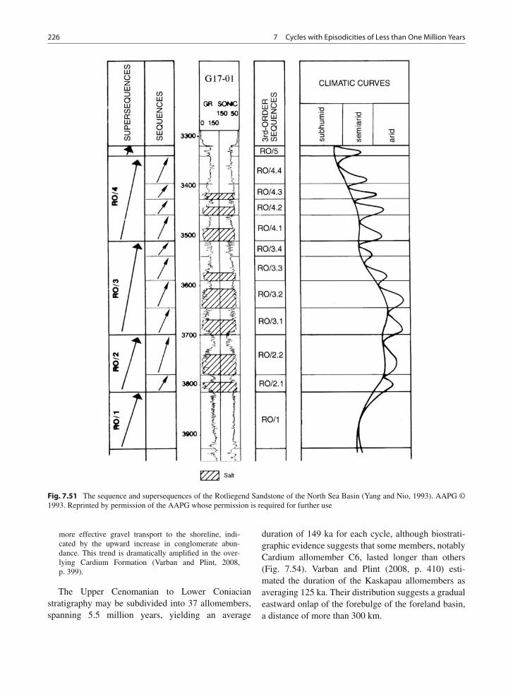
226 7 Cycles with Episodicities of Less than One Million Years
Fig. 7.51 The sequence and supersequences of the Rotliegend Sandstone of the North Sea Basin (Yang and Nio, 1993). AAPG ©1993. Reprinted by permission of the AAPG whose permission is required for further use
more effective gravel transport to the shoreline, indi-cated by the upward increase in conglomerate abun-dance. This trend is dramatically amplified in the over-lying Cardium Formation (Varban and Plint, 2008,p. 399).
The Upper Cenomanian to Lower Coniacianstratigraphy may be subdivided into 37 allomembers,spanning 5.5 million years, yielding an average
duration of 149 ka for each cycle, although biostrati-graphic evidence suggests that some members, notablyCardium allomember C6, lasted longer than others(Fig. 7.54). Varban and Plint (2008, p. 410) esti-mated the duration of the Kaskapau allomembers asaveraging 125 ka. Their distribution suggests a gradualeastward onlap of the forebulge of the foreland basin,a distance of more than 300 km.
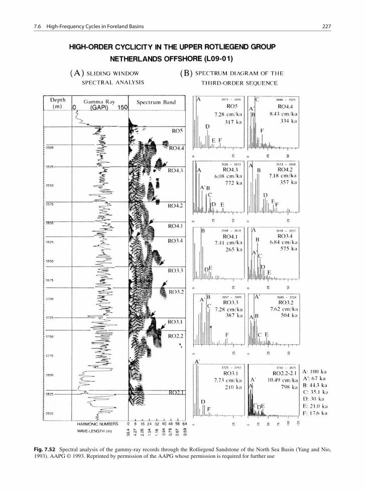
7.6 High-Frequency Cycles in Foreland Basins 227
Fig. 7.52 Spectral analysis of the gammy-ray records through the Rotliegend Sandstone of the North Sea Basin (Yang and Nio,1993). AAPG © 1993. Reprinted by permission of the AAPG whose permission is required for further use
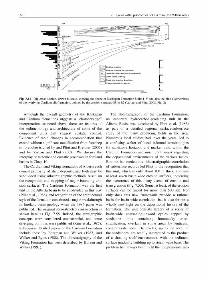
228 7 Cycles with Episodicities of Less than One Million Years
Fig. 7.53 Dip cross-section, drawn to scale, showing the shape of Kaskapau Formation Units I–V and also the nine allomembersof the overlying Cardium alloformation, defined by the erosion surfaces GS to E7 (Varban and Plint, 2008, Fig. 2)
Although the overall geometry of the Kaskapauand Cardium formations suggests a “clastic-wedge”interpretation, as noted above, there are features ofthe sedimentology and architecture of some of thecomponent units that suggest eustatic control.Evidence of rapid changes in accommodation thatextend without significant modification from foredeepto forebulge is cited by and Plint and Kreitner (2007)and by Varban and Plint (2008). We discuss theinterplay of tectonic and eustatic processes in forelandbasins in Chap. 10.
The Cardium and Viking formations of Alberta eachconsist primarily of shelf deposits, and both may besubdivided using allostratigraphic methods based onthe recognition and mapping of major bounding ero-sion surfaces. The Cardium Formation was the firstunit in the Alberta basin to be subdivided in this way(Plint et al., 1986), and recognition of the architecturalstyle of the formation constituted a major breakthroughin foreland-basin geology when the 1986 paper waspublished. His original reconstructed cross-section isshown here as Fig. 7.55. Indeed, the stratigraphicconcepts were considered controversial, and somediverging opinions were published (Rine et al., 1987).Subsequent detailed papers on the Cardium Formationinclude those by Bergman and Walker (1987) andWalker and Eyles (1988). The allostratigraphy of theViking Formation has been described by Boreen andWalker (1991).
The allostratigraphy of the Cardium Formation,an important hydrocarbon-producing unit in theAlberta Basin, was developed by Plint et al. (1986)as part of a detailed regional surface-subsurfacestudy of the many producing fields in the area.Numerous local studies had, over the years, led toa confusing welter of local informal terminologiesfor sandstone horizons and marker units within theCardium Formation and much controversy regardingthe depositional environments of the various facies.Routine but meticulous lithostratigraphic correlationof subsurface records led Plint to the recognition thatthis unit, which is only about 100 m thick, containsat least seven basin-wide erosion surfaces, indicatingthe occurrence of this many events of erosion andtransgression (Fig. 7.55). Some, at least, of the erosionsurfaces can be traced for more than 500 km. Notonly does this new framework provide a rationalbasis for basin-wide correlation, but it also throws awholly new light on the depositional history of theformation. The unit consists largely of a series ofbasin-wide coarsening-upward cycles capped bysandstone units containing hummocky cross-stratification, overlain in some areas by lenticularconglomerate beds. The cycles, up to the level ofthe sandstones, are readily interpreted as the productof a shoaling shelf environment, with the sedimentsurface gradually building up to storm wave base. Theproblem had always been to fit the conglomerate into
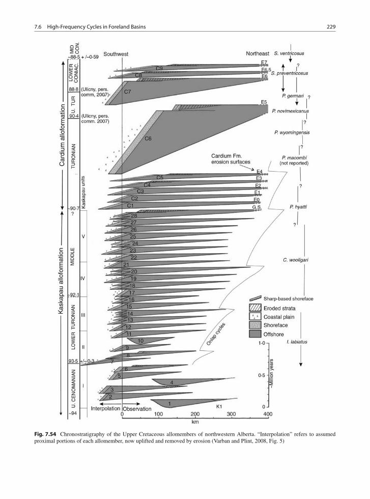
7.6 High-Frequency Cycles in Foreland Basins 229
Fig. 7.54 Chronostratigraphy of the Upper Cretaceous allomembers of northwestern Alberta. “Interpolation” refers to assumedproximal portions of each allomember, now uplifted and removed by erosion (Varban and Plint, 2008, Fig. 5)
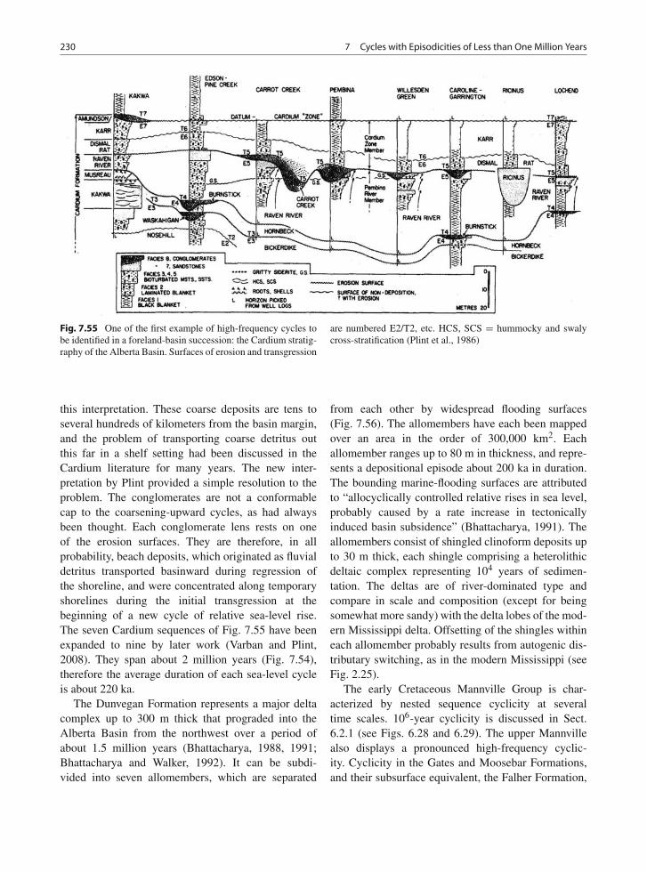
230 7 Cycles with Episodicities of Less than One Million Years
Fig. 7.55 One of the first example of high-frequency cycles tobe identified in a foreland-basin succession: the Cardium stratig-raphy of the Alberta Basin. Surfaces of erosion and transgression
are numbered E2/T2, etc. HCS, SCS = hummocky and swalycross-stratification (Plint et al., 1986)
this interpretation. These coarse deposits are tens toseveral hundreds of kilometers from the basin margin,and the problem of transporting coarse detritus outthis far in a shelf setting had been discussed in theCardium literature for many years. The new inter-pretation by Plint provided a simple resolution to theproblem. The conglomerates are not a conformablecap to the coarsening-upward cycles, as had alwaysbeen thought. Each conglomerate lens rests on oneof the erosion surfaces. They are therefore, in allprobability, beach deposits, which originated as fluvialdetritus transported basinward during regression ofthe shoreline, and were concentrated along temporaryshorelines during the initial transgression at thebeginning of a new cycle of relative sea-level rise.The seven Cardium sequences of Fig. 7.55 have beenexpanded to nine by later work (Varban and Plint,2008). They span about 2 million years (Fig. 7.54),therefore the average duration of each sea-level cycleis about 220 ka.
The Dunvegan Formation represents a major deltacomplex up to 300 m thick that prograded into theAlberta Basin from the northwest over a period ofabout 1.5 million years (Bhattacharya, 1988, 1991;Bhattacharya and Walker, 1992). It can be subdi-vided into seven allomembers, which are separated
from each other by widespread flooding surfaces(Fig. 7.56). The allomembers have each been mappedover an area in the order of 300,000 km2. Eachallomember ranges up to 80 m in thickness, and repre-sents a depositional episode about 200 ka in duration.The bounding marine-flooding surfaces are attributedto “allocyclically controlled relative rises in sea level,probably caused by a rate increase in tectonicallyinduced basin subsidence” (Bhattacharya, 1991). Theallomembers consist of shingled clinoform deposits upto 30 m thick, each shingle comprising a heterolithicdeltaic complex representing 104 years of sedimen-tation. The deltas are of river-dominated type andcompare in scale and composition (except for beingsomewhat more sandy) with the delta lobes of the mod-ern Mississippi delta. Offsetting of the shingles withineach allomember probably results from autogenic dis-tributary switching, as in the modern Mississippi (seeFig. 2.25).
The early Cretaceous Mannville Group is char-acterized by nested sequence cyclicity at severaltime scales. 106-year cyclicity is discussed in Sect.6.2.1 (see Figs. 6.28 and 6.29). The upper Mannvillealso displays a pronounced high-frequency cyclic-ity. Cyclicity in the Gates and Moosebar Formations,and their subsurface equivalent, the Falher Formation,
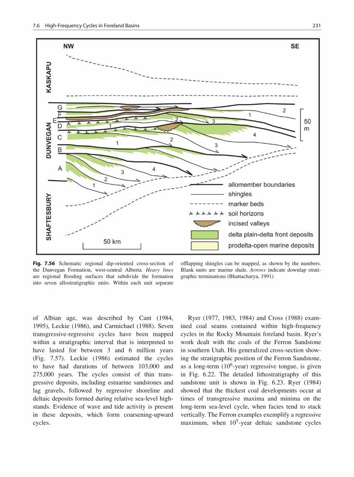
7.6 High-Frequency Cycles in Foreland Basins 231
Fig. 7.56 Schematic regional dip-oriented cross-section ofthe Dunvegan Formation, west-central Alberta. Heavy linesare regional flooding surfaces that subdivide the formationinto seven allostratigraphic units. Within each unit separate
offlapping shingles can be mapped, as shown by the numbers.Blank units are marine shale. Arrows indicate downlap strati-graphic terminations (Bhattacharya, 1991)
of Albian age, was described by Cant (1984,1995), Leckie (1986), and Carmichael (1988). Seventransgressive-regressive cycles have been mappedwithin a stratigraphic interval that is interpreted tohave lasted for between 3 and 6 million years(Fig. 7.57). Leckie (1986) estimated the cyclesto have had durations of between 103,000 and275,000 years. The cycles consist of thin trans-gressive deposits, including estuarine sandstones andlag gravels, followed by regressive shoreline anddeltaic deposits formed during relative sea-level high-stands. Evidence of wave and tide activity is presentin these deposits, which form coarsening-upwardcycles.
Ryer (1977, 1983, 1984) and Cross (1988) exam-ined coal seams contained within high-frequencycycles in the Rocky Mountain foreland basin. Ryer’swork dealt with the coals of the Ferron Sandstonein southern Utah. His generalized cross-section show-ing the stratigraphic position of the Ferron Sandstone,as a long-term (106-year) regressive tongue, is givenin Fig. 6.22. The detailed lithostratigraphy of thissandstone unit is shown in Fig. 6.23. Ryer (1984)showed that the thickest coal developments occur attimes of transgressive maxima and minima on thelong-term sea-level cycle, when facies tend to stackvertically. The Ferron examples exemplify a regressivemaximum, when 105-year deltaic sandstone cycles
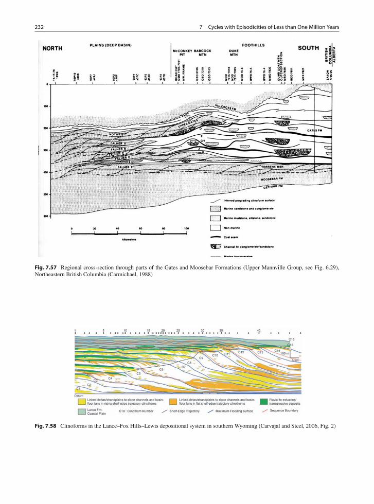
232 7 Cycles with Episodicities of Less than One Million Years
Fig. 7.57 Regional cross-section through parts of the Gates and Moosebar Formations (Upper Mannville Group, see Fig. 6.29),Northeastern British Columbia (Carmichael, 1988)
Fig. 7.58 Clinoforms in the Lance–Fox Hills–Lewis depositional system in southern Wyoming (Carvajal and Steel, 2006, Fig. 2)
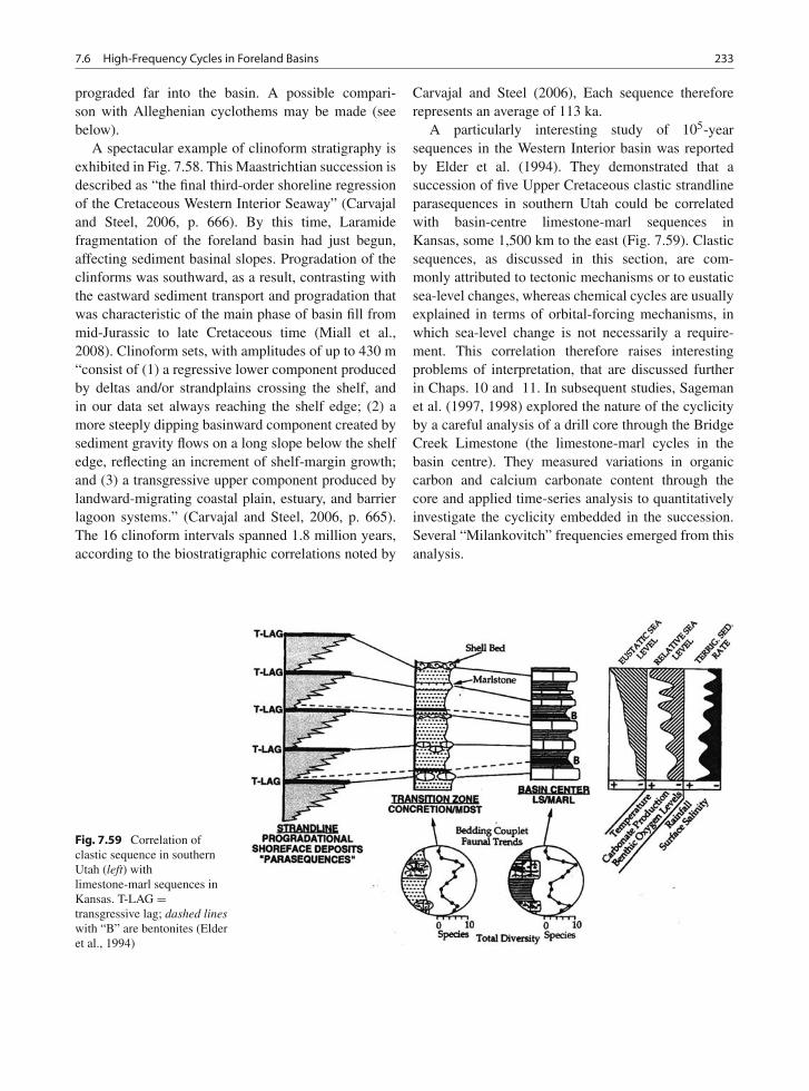
7.6 High-Frequency Cycles in Foreland Basins 233
prograded far into the basin. A possible compari-son with Alleghenian cyclothems may be made (seebelow).
A spectacular example of clinoform stratigraphy isexhibited in Fig. 7.58. This Maastrichtian succession isdescribed as “the final third-order shoreline regressionof the Cretaceous Western Interior Seaway” (Carvajaland Steel, 2006, p. 666). By this time, Laramidefragmentation of the foreland basin had just begun,affecting sediment basinal slopes. Progradation of theclinforms was southward, as a result, contrasting withthe eastward sediment transport and progradation thatwas characteristic of the main phase of basin fill frommid-Jurassic to late Cretaceous time (Miall et al.,2008). Clinoform sets, with amplitudes of up to 430 m“consist of (1) a regressive lower component producedby deltas and/or strandplains crossing the shelf, andin our data set always reaching the shelf edge; (2) amore steeply dipping basinward component created bysediment gravity flows on a long slope below the shelfedge, reflecting an increment of shelf-margin growth;and (3) a transgressive upper component produced bylandward-migrating coastal plain, estuary, and barrierlagoon systems.” (Carvajal and Steel, 2006, p. 665).The 16 clinoform intervals spanned 1.8 million years,according to the biostratigraphic correlations noted by
Carvajal and Steel (2006), Each sequence thereforerepresents an average of 113 ka.
A particularly interesting study of 105-yearsequences in the Western Interior basin was reportedby Elder et al. (1994). They demonstrated that asuccession of five Upper Cretaceous clastic strandlineparasequences in southern Utah could be correlatedwith basin-centre limestone-marl sequences inKansas, some 1,500 km to the east (Fig. 7.59). Clasticsequences, as discussed in this section, are com-monly attributed to tectonic mechanisms or to eustaticsea-level changes, whereas chemical cycles are usuallyexplained in terms of orbital-forcing mechanisms, inwhich sea-level change is not necessarily a require-ment. This correlation therefore raises interestingproblems of interpretation, that are discussed furtherin Chaps. 10 and 11. In subsequent studies, Sagemanet al. (1997, 1998) explored the nature of the cyclicityby a careful analysis of a drill core through the BridgeCreek Limestone (the limestone-marl cycles in thebasin centre). They measured variations in organiccarbon and calcium carbonate content through thecore and applied time-series analysis to quantitativelyinvestigate the cyclicity embedded in the succession.Several “Milankovitch” frequencies emerged from thisanalysis.
Fig. 7.59 Correlation ofclastic sequence in southernUtah (left) withlimestone-marl sequences inKansas. T-LAG =transgressive lag; dashed lineswith “B” are bentonites (Elderet al., 1994)
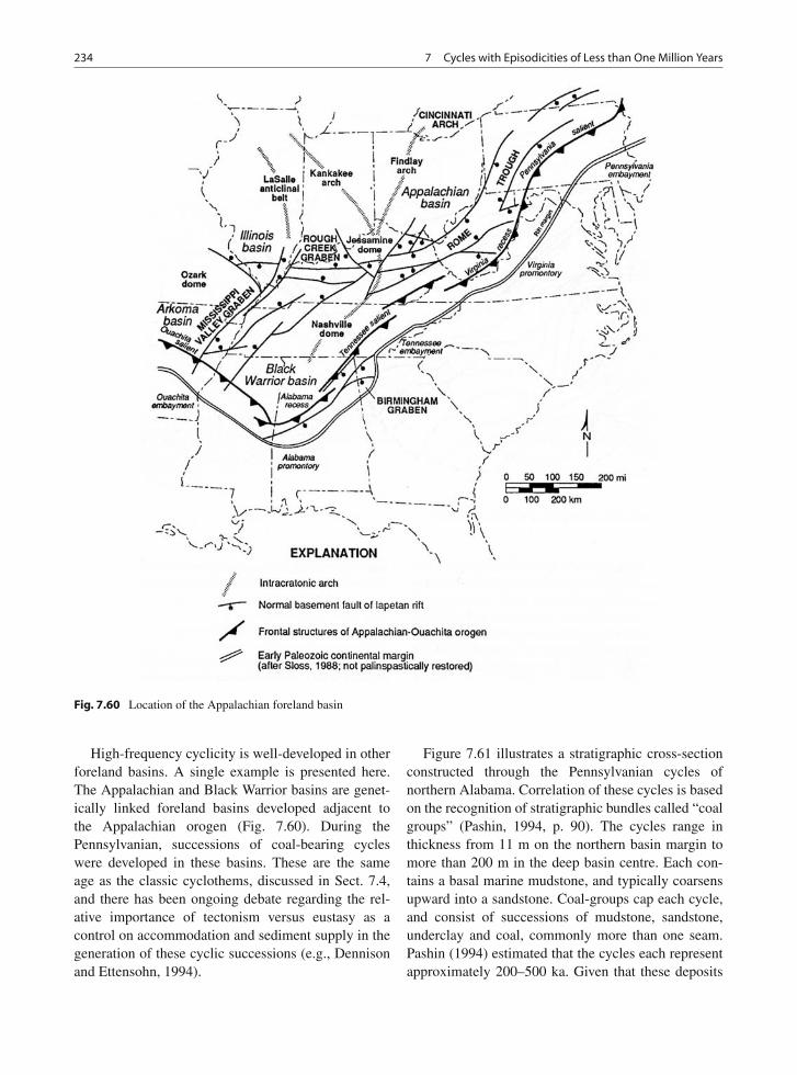
234 7 Cycles with Episodicities of Less than One Million Years
Fig. 7.60 Location of the Appalachian foreland basin
High-frequency cyclicity is well-developed in otherforeland basins. A single example is presented here.The Appalachian and Black Warrior basins are genet-ically linked foreland basins developed adjacent tothe Appalachian orogen (Fig. 7.60). During thePennsylvanian, successions of coal-bearing cycleswere developed in these basins. These are the sameage as the classic cyclothems, discussed in Sect. 7.4,and there has been ongoing debate regarding the rel-ative importance of tectonism versus eustasy as acontrol on accommodation and sediment supply in thegeneration of these cyclic successions (e.g., Dennisonand Ettensohn, 1994).
Figure 7.61 illustrates a stratigraphic cross-sectionconstructed through the Pennsylvanian cycles ofnorthern Alabama. Correlation of these cycles is basedon the recognition of stratigraphic bundles called “coalgroups” (Pashin, 1994, p. 90). The cycles range inthickness from 11 m on the northern basin margin tomore than 200 m in the deep basin centre. Each con-tains a basal marine mudstone, and typically coarsensupward into a sandstone. Coal-groups cap each cycle,and consist of successions of mudstone, sandstone,underclay and coal, commonly more than one seam.Pashin (1994) estimated that the cycles each representapproximately 200–500 ka. Given that these deposits
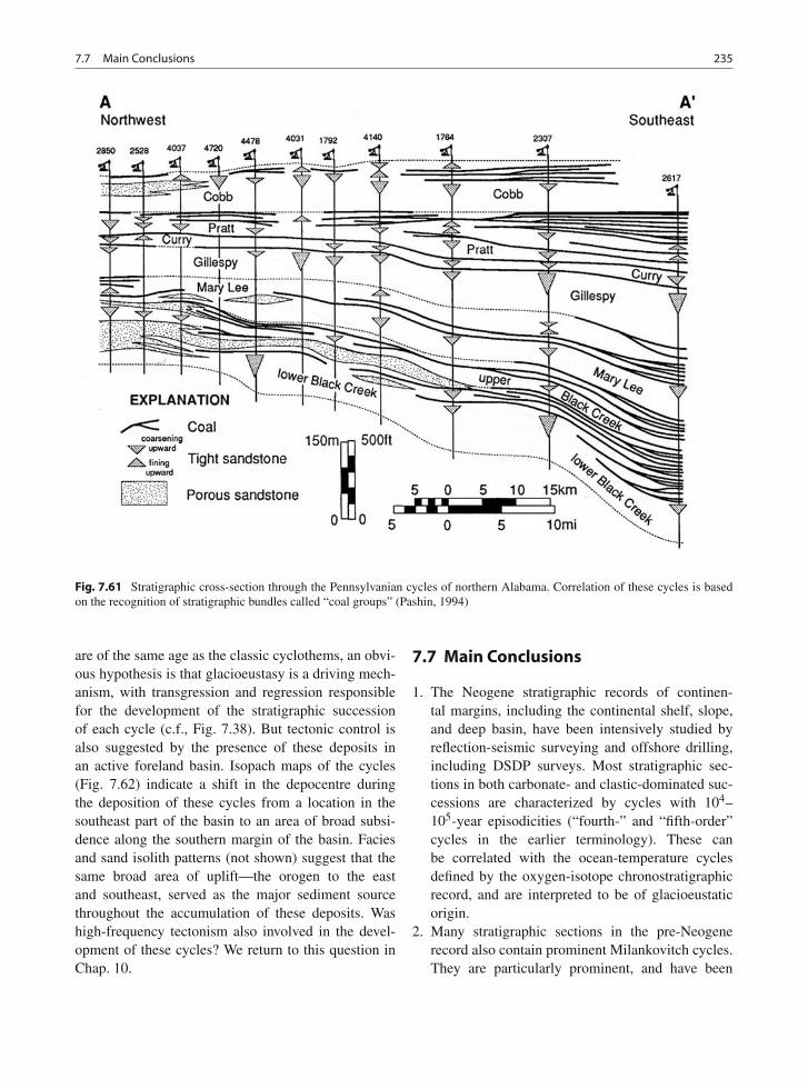
7.7 Main Conclusions 235
Fig. 7.61 Stratigraphic cross-section through the Pennsylvanian cycles of northern Alabama. Correlation of these cycles is basedon the recognition of stratigraphic bundles called “coal groups” (Pashin, 1994)
are of the same age as the classic cyclothems, an obvi-ous hypothesis is that glacioeustasy is a driving mech-anism, with transgression and regression responsiblefor the development of the stratigraphic successionof each cycle (c.f., Fig. 7.38). But tectonic control isalso suggested by the presence of these deposits inan active foreland basin. Isopach maps of the cycles(Fig. 7.62) indicate a shift in the depocentre duringthe deposition of these cycles from a location in thesoutheast part of the basin to an area of broad subsi-dence along the southern margin of the basin. Faciesand sand isolith patterns (not shown) suggest that thesame broad area of uplift—the orogen to the eastand southeast, served as the major sediment sourcethroughout the accumulation of these deposits. Washigh-frequency tectonism also involved in the devel-opment of these cycles? We return to this question inChap. 10.
7.7 Main Conclusions
1. The Neogene stratigraphic records of continen-tal margins, including the continental shelf, slope,and deep basin, have been intensively studied byreflection-seismic surveying and offshore drilling,including DSDP surveys. Most stratigraphic sec-tions in both carbonate- and clastic-dominated suc-cessions are characterized by cycles with 104–105-year episodicities (“fourth-” and “fifth-order”cycles in the earlier terminology). These canbe correlated with the ocean-temperature cyclesdefined by the oxygen-isotope chronostratigraphicrecord, and are interpreted to be of glacioeustaticorigin.
2. Many stratigraphic sections in the pre-Neogenerecord also contain prominent Milankovitch cycles.They are particularly prominent, and have been
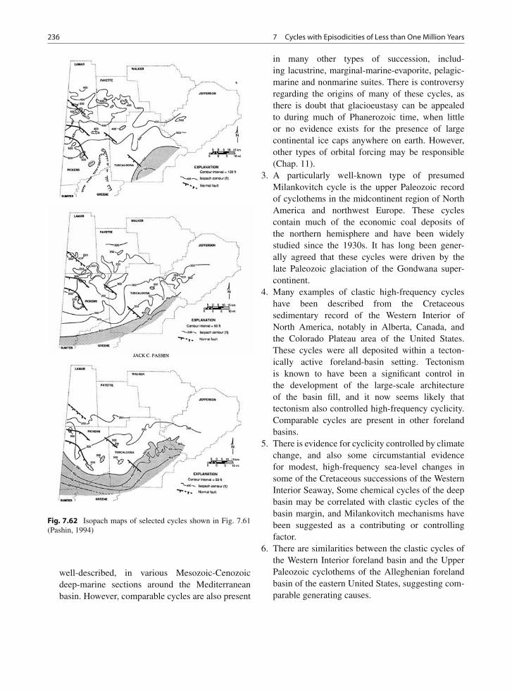
236 7 Cycles with Episodicities of Less than One Million Years
Fig. 7.62 Isopach maps of selected cycles shown in Fig. 7.61(Pashin, 1994)
well-described, in various Mesozoic-Cenozoicdeep-marine sections around the Mediterraneanbasin. However, comparable cycles are also present
in many other types of succession, includ-ing lacustrine, marginal-marine-evaporite, pelagic-marine and nonmarine suites. There is controversyregarding the origins of many of these cycles, asthere is doubt that glacioeustasy can be appealedto during much of Phanerozoic time, when littleor no evidence exists for the presence of largecontinental ice caps anywhere on earth. However,other types of orbital forcing may be responsible(Chap. 11).
3. A particularly well-known type of presumedMilankovitch cycle is the upper Paleozoic recordof cyclothems in the midcontinent region of NorthAmerica and northwest Europe. These cyclescontain much of the economic coal deposits ofthe northern hemisphere and have been widelystudied since the 1930s. It has long been gener-ally agreed that these cycles were driven by thelate Paleozoic glaciation of the Gondwana super-continent.
4. Many examples of clastic high-frequency cycleshave been described from the Cretaceoussedimentary record of the Western Interior ofNorth America, notably in Alberta, Canada, andthe Colorado Plateau area of the United States.These cycles were all deposited within a tecton-ically active foreland-basin setting. Tectonismis known to have been a significant control inthe development of the large-scale architectureof the basin fill, and it now seems likely thattectonism also controlled high-frequency cyclicity.Comparable cycles are present in other forelandbasins.
5. There is evidence for cyclicity controlled by climatechange, and also some circumstantial evidencefor modest, high-frequency sea-level changes insome of the Cretaceous successions of the WesternInterior Seaway, Some chemical cycles of the deepbasin may be correlated with clastic cycles of thebasin margin, and Milankovitch mechanisms havebeen suggested as a contributing or controllingfactor.
6. There are similarities between the clastic cycles ofthe Western Interior foreland basin and the UpperPaleozoic cyclothems of the Alleghenian forelandbasin of the eastern United States, suggesting com-parable generating causes.
Part IIIMechanisms
Although eustasy as the dominant mechanism controlling sequence architecture wasan integral part of the Vail/Exxon approach to sequence stratigraphy, L. L. Sloss,on whose work it was originally based, was always convinced that tectonism was animportant component of sedimentary controls. With the critiques of the global eustasymodel that began to appear in the 1980s and 1990s, research broadened to exploreother mechanisms that affect the generation and removal of accommodation, and thesediment supply from which sequences are built. It has been demonstrated that thereare several global tectonic mechanisms and astronomical effects that generate eustaticsea-level changes on several different time scales and of varying amplitude. Theseare discussed in this part of the book. The processes are summarized in Table 8.1 andFig. 8.1.
Research has, in addition, demonstrated that there is a range of tectonic processesthat generate relative sea-level changes on a local to regional scale. The rates andmagnitudes of change are variable, and much research remains to be conducted toquantify these effects. However, it is now clear that many forcing functions of differ-ent frequencies and amplitudes are likely to be active at the same time, and that theymay not be mutually independent; for example, tectonic uplift affects accommoda-tion and, at the same time, may affect climate, and both affect sediment supply. Suchprocesses, acting independently or together, may produce effects that are very similarto those of eustasy, but on a regional to continental scale (Table 8.2, Figs. 8.1, 8.2).This is of critical importance, because it means that sequence stratigraphies recordedin any given basin, however well documented, cannot be assumed to be global, andtherefore representative of a global framework of eustatic cycles. In fact, it calls intoquestion the very concept of the global cycle chart based on the tying together of keysections from supposedly representative areas.
The focus of the Exxon models was on eustatic sea-level change as the primarycontrol of sequence architecture. If eustasy is the primary mechanism, then it justi-fies the use of sequence stratigraphies for the purpose of constructing a global cyclechart, the assumption being that a sequence record anywhere will reflect the sameglobal eustatic controls. Tectonism is treated in the Exxon models as a slow back-ground effect that does not substantially modify the stratigraphic response to eustaticsea-level change. However, sequences of tectonic origin may be expected to vary inage from region to region, because they are generated by plate-tectonic processes andmantle effects that are progressive and diachronous. The only reliable test of a eustaticcontrol is precise correlation. If sequences in widely spaced basins of different tec-tonic setting are of the same age, they may be assumed to be of eustatic origin. This
238 Part III Mechanisms
emphasizes the need for very precise chronostratigraphic control, a subject discussedin Part IV.
Mechanisms, the range of processes that alter sea level and sediment supply, arethe subject of this part of the book.
• Nature vibrates with rhythms, climatic and diastrophic, those finding expressionranging in period from the rapid oscillation of surface waters, recorded in ripplemark, to those long-defended stirrings of the deep titans which have divided earthhistory into periods and eras (Barrell, 1917, p. 745).
• Allocyclic sequences . . . are mainly caused by variations external to the consideredsedimentary system (e.g., the basin), such as climatic changes, tectonic movementsin the source area, global sea level variations, etc. . . . Such processes often tend togenerate cyclic phenomena of a larger lateral continuity and time period than auto-cyclic processes. The most characteristic effect of some of the allocyclic processesis that they operate simultaneously in different basins in a similar way. Thus itshould be possible to correlate part of the allocyclic sequences over long distancesand perhaps even from one basin to another (Einsele et al., 1991b, p. 7).
• Sea level is an ill-defined concept that incorporates the effects of isostasy, eustasy,ice volume, passive margin subsidence, lithospheric deformation and flexure, ero-sion and consequent sediment loading, and changes in rate of plate generation andconsumption that all serve to alter the elevation of the world seafloor with respectto the elevation of the continental surface. As such, quantitatively defining a uni-versally acceptable definition of sea level to the satisfaction of all has so far provenan intractable problem (Dockal and Worsley, 1991, p. 6805).
• It is unfortunate that a change in water depth is the only parameter that we caninfer from facies analysis, because in order to isolate the effects of one of theindependent variables (eustasy, tectonics, sedimentation), we are forced to makeassumptions about the magnitude and rate of the other two variables (Plint et al.,1992, p. 16).
• In parallel to the eustasy-driven sequence stratigraphy, which held by far thelargest share of the market, other researchers went to the opposite end of the spec-trum by suggesting a methodology that favored tectonism as the main driver ofstratigraphic cyclicity. This version of sequence stratigraphy was introduced as“tectonostratigraphy” . . . The major weakness of both schools of thought is thata priori interpretation of the main allogenic control on accommodation was auto-matically attached to any sequence delineation, which gave the impression thatsequence stratigraphy is more of an interpretation artifact than an empirical, data-based method. This a priori interpretation facet of sequence stratigraphy attractedconsiderable criticism and placed an unwanted shade on a method that otherwiserepresents a truly important advance in the science of sedimentary geology. Fixingthe damaged image of sequence stratigraphy only requires the basic understandingthat base-level changes can be controlled by any combination of eustatic and tec-tonic forces, and that the dominance of any of these allogenic mechanisms shouldbe assessed on a case by case basis. It became clear that sequence stratigraphyneeded to be dissociated from the global-eustasy model, and that a more objectiveanalysis should be based on empirical evidence that can actually be observed inoutcrop or the subsurface (Catuneanu, 2006, p. 5).
Chapter 8
Summary of Sequence-Generating Mechanisms
Barrell (1917) was one of the first earth scientists tofully comprehend the full range of dynamic processesaffecting the Earth’s crust (see quote from his paper atthe beginning of this part of the book). These includedboth orogeny and epeirogeny. Orogeny is a term thatcame into general use in the mid-nineteenth century toencompass the processes of vertical and lateral motionand deformation of the earth’s crust involved in thegeneration of deformed belts and mountain ranges(Bates and Jackson, 1987). Epeirogeny is a term coinedby Gilbert (1890) to encompass the development ofthe larger features of continental interiors, includ-ing plateaus and basins, predominantly by processesof vertical motion. Eustasy was recognized by Suess(1885–1909) and formed the theoretical basis for hisstudies of global stratigraphy and orogeny (Fig. 1.7).By the 1930s, significance of glacioeustasy for under-standing parts of the ancient stratigraphic record wasrecognized by those working on the US Mid-continentcyclothems (Shepard and Wanless, 1935). A morecomplete discussion of the early search for cyclic orrhythmic mechanisms is presented in Sect. 1.4.
During a period in the 1980s, following the initialsuccess of the new seismic stratigraphy (Vail et al.,1977) there was an over-emphasis on the importanceof eustatic sea-level change as the dominant controlon stratigraphic architecture but, as summarized inSect. 1.5, Subsequent research, much of it directlystimulated by questions that Vail’s work raised, hasuncovered diverse processes that govern the generationand filling of sedimentary accommodation. Dewey andPitman (1998, p. 14) stated:
It is our contention that local or regional tectonic con-trol of sea level dominates eustatic effects, except forshort lived glacio-eustatic periods and, therefore, that
most sequences and third-order cycles are controlled tec-tonically on a local and regional scale rather than beingglobal-eustatically controlled. We suggest that eustaticsea-level changes are nowhere near as large as have beenclaimed [by Haq et al., 1987] and have been falsely cor-related and constricted into a global eustatic time scalewhereby a circular reasoning forces correlation and thenuses that correlation as a standard into which all othersequences are squeezed. . . .. We wish only to cautionagainst the belief that third order sequences can be used asa global eustatic time scale. However, we do believe thatStille’s (1924) concepts of global orogenic and eustaticsea-level episodicity need a fresh evaluation in the frame-work of the assembly and disruption of supercontinents.This evaluation will only come when really fine-scalemethods of physical/chemical stratigraphic correlationbecome widely available for Phanerozoic strata.
Figure 8.1 and Table 8.1 provide a summary of therates and durations of sedimentary processes. Thesevary in duration over fourteen orders of magnitudeof time, from the short-term processes that developripples and laminae under running water (seconds tominutes) to the long-term geological processes thatcharacterize plate-tectonic changes to Earth’s crust(tens to hundreds of millions of years). The deposi-tional products of these processes may be groupedconveniently into “groups” that each encompass pro-cesses operating within one order of magnitude oftime. Sedimentological studies are facilitated by thefact that in the rock record, each of these groups canbe defined by their architecture and by the nature ofthe bounding surfaces that enclose and define them.Figure 4.5 illustrates this point with reference to fluvialdeposits, where the numbers correspond to the num-bered bounding surfaces that can be defined at eachscale at which a fluvial deposit is examined, from asmall piece of drill core up to the scale of an entirebasin. In Table 8.1, references are provided to work
239A.D. Miall, The Geology of Stratigraphic Sequences, 2nd ed.,DOI 10.1007/978-3-642-05027-5_8, © Springer-Verlag Berlin Heidelberg 2010
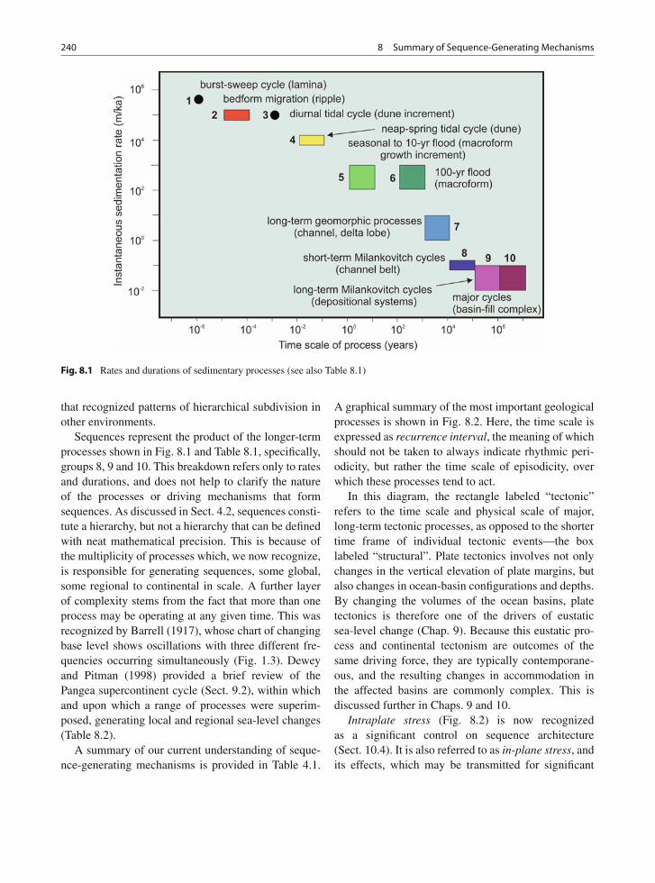
240 8 Summary of Sequence-Generating Mechanisms
Fig. 8.1 Rates and durations of sedimentary processes (see also Table 8.1)
that recognized patterns of hierarchical subdivision inother environments.
Sequences represent the product of the longer-termprocesses shown in Fig. 8.1 and Table 8.1, specifically,groups 8, 9 and 10. This breakdown refers only to ratesand durations, and does not help to clarify the natureof the processes or driving mechanisms that formsequences. As discussed in Sect. 4.2, sequences consti-tute a hierarchy, but not a hierarchy that can be definedwith neat mathematical precision. This is because ofthe multiplicity of processes which, we now recognize,is responsible for generating sequences, some global,some regional to continental in scale. A further layerof complexity stems from the fact that more than oneprocess may be operating at any given time. This wasrecognized by Barrell (1917), whose chart of changingbase level shows oscillations with three different fre-quencies occurring simultaneously (Fig. 1.3). Deweyand Pitman (1998) provided a brief review of thePangea supercontinent cycle (Sect. 9.2), within whichand upon which a range of processes were superim-posed, generating local and regional sea-level changes(Table 8.2).
A summary of our current understanding of seque-nce-generating mechanisms is provided in Table 4.1.
A graphical summary of the most important geologicalprocesses is shown in Fig. 8.2. Here, the time scale isexpressed as recurrence interval, the meaning of whichshould not be taken to always indicate rhythmic peri-odicity, but rather the time scale of episodicity, overwhich these processes tend to act.
In this diagram, the rectangle labeled “tectonic”refers to the time scale and physical scale of major,long-term tectonic processes, as opposed to the shortertime frame of individual tectonic events—the boxlabeled “structural”. Plate tectonics involves not onlychanges in the vertical elevation of plate margins, butalso changes in ocean-basin configurations and depths.By changing the volumes of the ocean basins, platetectonics is therefore one of the drivers of eustaticsea-level change (Chap. 9). Because this eustatic pro-cess and continental tectonism are outcomes of thesame driving force, they are typically contemporane-ous, and the resulting changes in accommodation inthe affected basins are commonly complex. This isdiscussed further in Chaps. 9 and 10.
Intraplate stress (Fig. 8.2) is now recognizedas a significant control on sequence architecture(Sect. 10.4). It is also referred to as in-plane stress, andits effects, which may be transmitted for significant
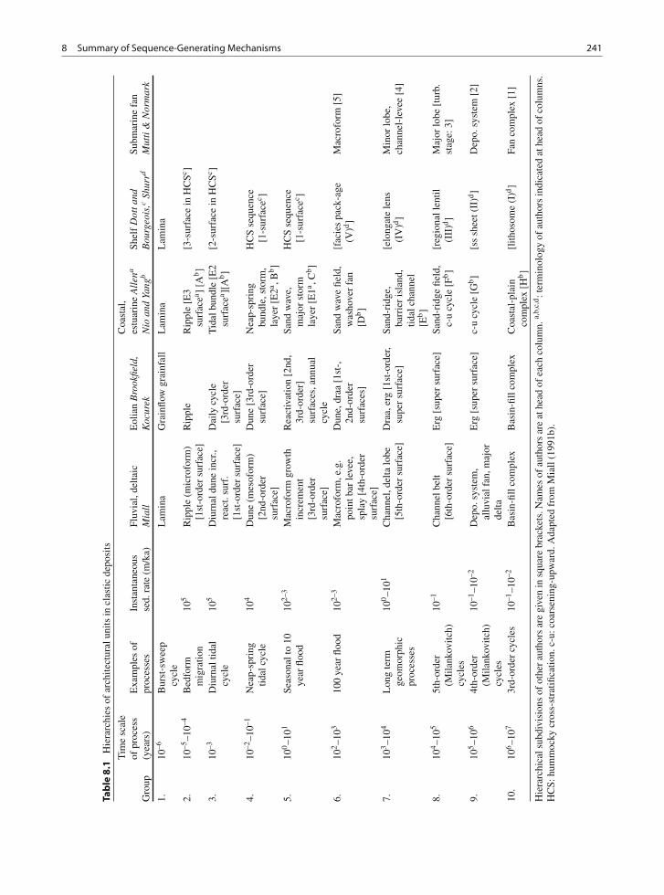
8 Summary of Sequence-Generating Mechanisms 241
Tab
le8
.1H
iera
rchi
esof
arch
itect
ural
units
incl
astic
depo
sits
Gro
up
Tim
esc
ale
ofpr
oces
s(y
ears
)E
xam
ples
ofpr
oces
ses
Inst
anta
neou
sse
d.ra
te(m
/ka)
Fluv
ial,
delta
icM
iall
Eol
ian
Bro
okfie
ld,
Koc
urek
Coa
stal
,es
tuar
ine
All
ena
Nio
and
Yang
bSh
elf
Dot
tand
Bou
rgeo
is,c
Shur
rdSu
bmar
ine
fan
Mut
ti&
Nor
mar
k
1.10
–6B
urst
-sw
eep
cycl
eL
amin
aG
rain
flow
grai
nfal
lL
amin
aL
amin
a
2.10
–5–1
0–4B
edfo
rmm
igra
tion
105
Rip
ple
(mic
rofo
rm)
[1st
-ord
ersu
rfac
e]R
ippl
eR
ippl
e[E
3su
rfac
ea ][A
b]
[3-s
urfa
cein
HC
Sc ]
3.10
–3D
iurn
altid
alcy
cle
105
Diu
rnal
dune
incr
.,re
act.
surf
.[1
st-o
rder
surf
ace]
Dai
lycy
cle
[3rd
-ord
ersu
rfac
e]
Tid
albu
ndle
[E2
surf
acea ][
Ab]
[2-s
urfa
cein
HC
Sc ]
4.10
–2–1
0–1N
eap-
spri
ngtid
alcy
cle
104
Dun
e(m
esof
orm
)[2
nd-o
rder
surf
ace]
Dun
e[3
rd-o
rder
surf
ace]
Nea
p-sp
ring
bund
le,s
torm
,la
yer
[E2a ,B
b]
HC
Sse
quen
ce[1
-sur
face
c ]
5.10
0–1
01Se
ason
alto
10ye
arflo
od10
2–3
Mac
rofo
rmgr
owth
incr
emen
t[3
rd-o
rder
surf
ace]
Rea
ctiv
atio
n[2
nd,
3rd-
orde
r]su
rfac
es,a
nnua
lcy
cle
Sand
wav
e,m
ajor
stor
mla
yer
[E1a ,
Cb]
HC
Sse
quen
ce[1
-sur
face
c ]
6.10
2–1
0310
0ye
arflo
od10
2–3
Mac
rofo
rm,e
.g.
poin
tbar
leve
e,sp
lay
[4th
-ord
ersu
rfac
e]
Dun
e,dr
aa[1
st-,
2nd-
orde
rsu
rfac
es]
Sand
wav
efie
ld,
was
hove
rfa
n[D
b]
[fac
ies
pack
-age
(V)d
]M
acro
form
[5]
7.10
3–1
04L
ong
term
geom
orph
icpr
oces
ses
100–1
01C
hann
el,d
elta
lobe
[5th
-ord
ersu
rfac
e]D
raa,
erg
[1st
-ord
er,
supe
rsu
rfac
e]Sa
nd-r
idge
,ba
rrie
ris
land
,tid
alch
anne
l[E
b]
[elo
ngat
ele
ns(I
V)d
]M
inor
lobe
,ch
anne
l-le
vee
[4]
8.10
4–1
055t
h-or
der
(Mila
nkov
itch)
cycl
es
10–1
Cha
nnel
belt
[6th
-ord
ersu
rfac
e]E
rg[s
uper
surf
ace]
Sand
-rid
gefie
ld,
c-u
cycl
e[F
b]
[reg
iona
llen
til(I
II)d
]M
ajor
lobe
[tur
b.st
age:
3]
9.10
5–1
064t
h-or
der
(Mila
nkov
itch)
cycl
es
10–1
–10–2
Dep
o.sy
stem
,al
luvi
alfa
n,m
ajor
delta
Erg
[sup
ersu
rfac
e]c-
ucy
cle
[Gb]
[ss
shee
t(II
)d]
Dep
o.sy
stem
[2]
10.
106–1
073r
d-or
der
cycl
es10
–1–1
0–2B
asin
-fill
com
plex
Bas
in-fi
llco
mpl
exC
oast
al-p
lain
com
plex
[Hb]
[lith
osom
e(I
)d]
Fan
com
plex
[1]
Hie
rarc
hica
lsub
divi
sion
sof
othe
rau
thor
sar
egi
ven
insq
uare
brac
kets
.Nam
esof
auth
ors
are
athe
adof
each
colu
mn.
a,b,
c,d:t
erm
inol
ogy
ofau
thor
sin
dica
ted
athe
adof
colu
mns
.H
CS:
hum
moc
kycr
oss-
stra
tifica
tion.
c-u:
coar
seni
ng-u
pwar
d.A
dapt
edfr
omM
iall
(199
1b).
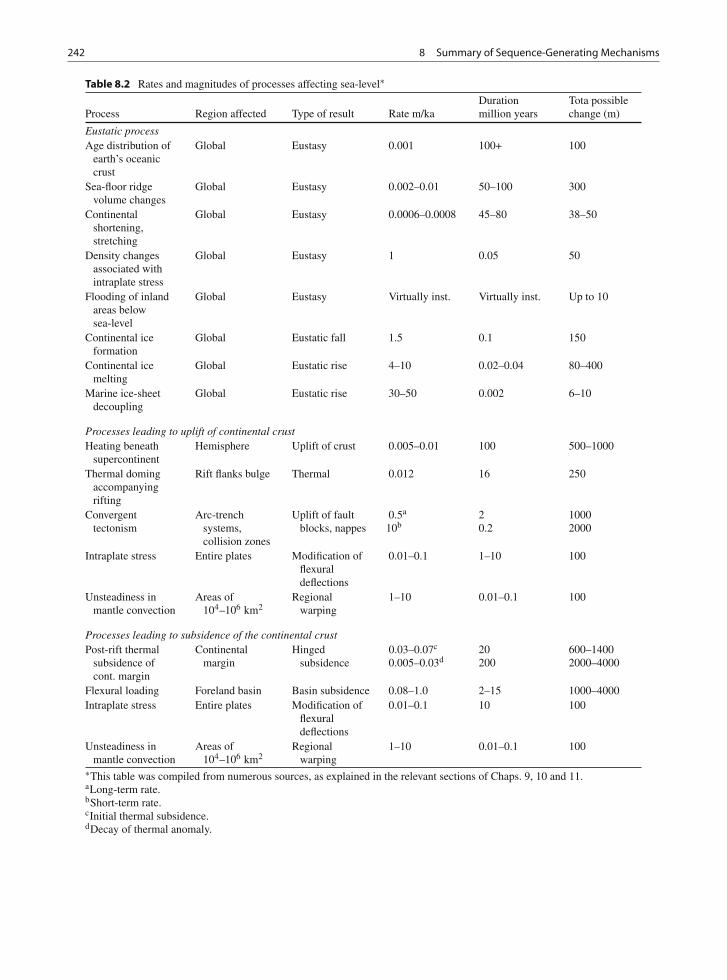
242 8 Summary of Sequence-Generating Mechanisms
Table 8.2 Rates and magnitudes of processes affecting sea-level∗
Process Region affected Type of result Rate m/kaDurationmillion years
Tota possiblechange (m)
Eustatic processAge distribution of
earth’s oceaniccrust
Global Eustasy 0.001 100+ 100
Sea-floor ridgevolume changes
Global Eustasy 0.002–0.01 50–100 300
Continentalshortening,stretching
Global Eustasy 0.0006–0.0008 45–80 38–50
Density changesassociated withintraplate stress
Global Eustasy 1 0.05 50
Flooding of inlandareas belowsea-level
Global Eustasy Virtually inst. Virtually inst. Up to 10
Continental iceformation
Global Eustatic fall 1.5 0.1 150
Continental icemelting
Global Eustatic rise 4–10 0.02–0.04 80–400
Marine ice-sheetdecoupling
Global Eustatic rise 30–50 0.002 6–10
Processes leading to uplift of continental crustHeating beneath
supercontinentHemisphere Uplift of crust 0.005–0.01 100 500–1000
Thermal domingaccompanyingrifting
Rift flanks bulge Thermal 0.012 16 250
Convergenttectonism
Arc-trenchsystems,collision zones
Uplift of faultblocks, nappes
0.5a
10b20.2
10002000
Intraplate stress Entire plates Modification offlexuraldeflections
0.01–0.1 1–10 100
Unsteadiness inmantle convection
Areas of104–106 km2
Regionalwarping
1–10 0.01–0.1 100
Processes leading to subsidence of the continental crustPost-rift thermal
subsidence ofcont. margin
Continentalmargin
Hingedsubsidence
0.03–0.07c
0.005–0.03d20200
600–14002000–4000
Flexural loading Foreland basin Basin subsidence 0.08–1.0 2–15 1000–4000Intraplate stress Entire plates Modification of
flexuraldeflections
0.01–0.1 10 100
Unsteadiness inmantle convection
Areas of104–106 km2
Regionalwarping
1–10 0.01–0.1 100
∗This table was compiled from numerous sources, as explained in the relevant sections of Chaps. 9, 10 and 11.aLong-term rate.bShort-term rate.cInitial thermal subsidence.dDecay of thermal anomaly.
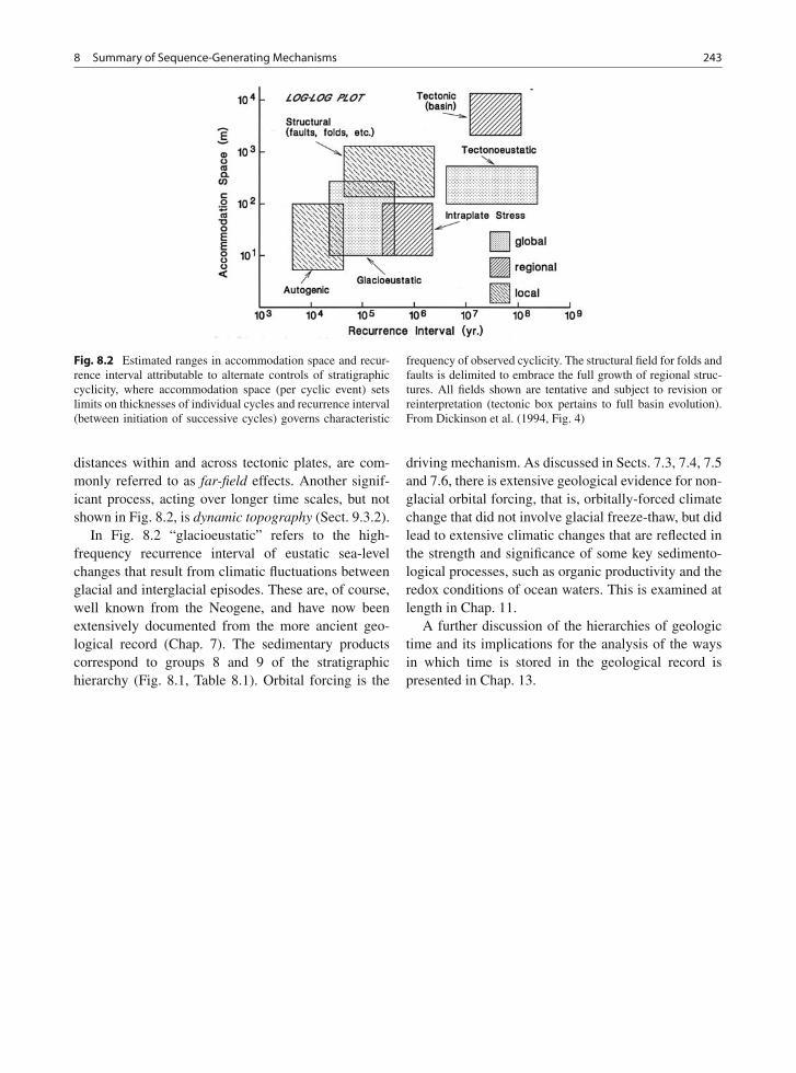
8 Summary of Sequence-Generating Mechanisms 243
Fig. 8.2 Estimated ranges in accommodation space and recur-rence interval attributable to alternate controls of stratigraphiccyclicity, where accommodation space (per cyclic event) setslimits on thicknesses of individual cycles and recurrence interval(between initiation of successive cycles) governs characteristic
frequency of observed cyclicity. The structural field for folds andfaults is delimited to embrace the full growth of regional struc-tures. All fields shown are tentative and subject to revision orreinterpretation (tectonic box pertains to full basin evolution).From Dickinson et al. (1994, Fig. 4)
distances within and across tectonic plates, are com-monly referred to as far-field effects. Another signif-icant process, acting over longer time scales, but notshown in Fig. 8.2, is dynamic topography (Sect. 9.3.2).
In Fig. 8.2 “glacioeustatic” refers to the high-frequency recurrence interval of eustatic sea-levelchanges that result from climatic fluctuations betweenglacial and interglacial episodes. These are, of course,well known from the Neogene, and have now beenextensively documented from the more ancient geo-logical record (Chap. 7). The sedimentary productscorrespond to groups 8 and 9 of the stratigraphichierarchy (Fig. 8.1, Table 8.1). Orbital forcing is the
driving mechanism. As discussed in Sects. 7.3, 7.4, 7.5and 7.6, there is extensive geological evidence for non-glacial orbital forcing, that is, orbitally-forced climatechange that did not involve glacial freeze-thaw, but didlead to extensive climatic changes that are reflected inthe strength and significance of some key sedimento-logical processes, such as organic productivity and theredox conditions of ocean waters. This is examined atlength in Chap. 11.
A further discussion of the hierarchies of geologictime and its implications for the analysis of the waysin which time is stored in the geological record ispresented in Chap. 13.
Chapter 9
Long-Term Eustasy and Epeirogeny
Contents
9.1 Mantle Processes and Dynamic Topography . . 2459.2 Supercontinent Cycles . . . . . . . . . . . . 2469.3 Cycles with Episodicities of Tens of Millions
of Years . . . . . . . . . . . . . . . . . . . 2489.3.1 Eustasy . . . . . . . . . . . . . . . . 2489.3.2 Dynamic Topography and Epeirogeny . . 2559.3.3 The Origin of Sloss Sequences . . . . . 259
9.4 Main Conclusions . . . . . . . . . . . . . . 259
9.1 Mantle Processes and DynamicTopography
The major cause of change in the Earth’s crust is theradiogenic heat engine, which drives mantle convec-tion and generates the geomagnetic field. Convectiondistributes heat and drives plate tectonics. Oceanicand continental crust are subject to heating close tosea-floor spreading centres where new, hot, oceaniccrust is generated (causing “ridge push”), and to cool-ing overlying subduction zones, where cold oceaniccrust descends to the mantle (generating “subductionpull”). Widespread cooling and subsidence occur overthe downwelling zones where continental fragmentsconverge. The same cooling and subsidence occurabove old, cold, downgoing oceanic slabs in subduc-tion zones, and partial melting of the water-saturatedrocks as they descend in the subduction zone is whatgenerates arc magmatism. The differential heat distri-bution and consequent heating and cooling of differentparts of the overlying Earth’s surface results in broadregional uplifts, downwarps and tilts, because of theeffects on crustal densities. These processes main-tain what is called dynamic topography (Fig. 9.1).
The effects of crustal heating are to cause uplift. Thisoccurs along the flanks of new continental rift systems(e.g., parts of East Africa) and above mantle plumes.Thermal doming beneath supercontinents may elevatethe crust by as much as 1 km over periods of 100 mil-lion years. Subsidence takes place over cooling areasof the Earth’s crust, such as areas of aging oceanic andcontinental crust distant from spreading centres, andover regions of mantle downwelling.
The concepts of dynamic topography are now beingexplored with the techniques of a new field, calledcomputational geodynamics, “in which computer mod-els of mantle convection are used in the interpreta-tion of contemporaneous geophysical observations likeseismic tomography and the geoid as well as of time-integrated observations from isotope geochemistry”(Gurnis, 1992). Such models are capable of integratinglarge volumes of detailed stratigraphic data using thebackstripping procedures outlined in Sect. 3.5. Thesedevelopments are of great significance, and their impli-cations for sequence stratigraphy have yet to be fullyrealized.
Vertical movement of the crust causes relativechanges in sea level on a regional or continental scale.This is true epeirogeny. However, thermal changes alsoresult in changes in the volume of the ocean basins,which lead, in turn, to eustatic changes in sea level.The same broad crust-mantle processes generate bothregional and eustatic effects that may or may not be inphase. The result is a highly complex sequence of sea-level changes, and clear global eustatic signals may notalways be present in the stratigraphic record.
Continental-scale vertical movements caused by theprocess of epeirogeny have been amply demonstratedby stratigraphers (e.g., Sloss, 1963; Bond, 1976, 1978;Burgess, 2008; see Sect. 3.4), but were only explained
245A.D. Miall, The Geology of Stratigraphic Sequences, 2nd ed.,DOI 10.1007/978-3-642-05027-5_9, © Springer-Verlag Berlin Heidelberg 2010
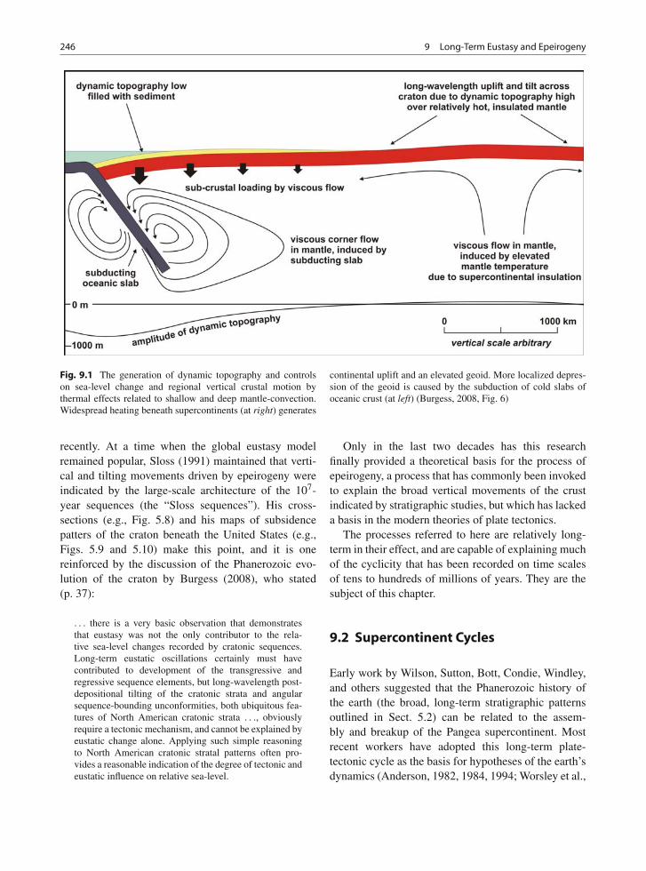
246 9 Long-Term Eustasy and Epeirogeny
Fig. 9.1 The generation of dynamic topography and controlson sea-level change and regional vertical crustal motion bythermal effects related to shallow and deep mantle-convection.Widespread heating beneath supercontinents (at right) generates
continental uplift and an elevated geoid. More localized depres-sion of the geoid is caused by the subduction of cold slabs ofoceanic crust (at left) (Burgess, 2008, Fig. 6)
recently. At a time when the global eustasy modelremained popular, Sloss (1991) maintained that verti-cal and tilting movements driven by epeirogeny wereindicated by the large-scale architecture of the 107-year sequences (the “Sloss sequences”). His cross-sections (e.g., Fig. 5.8) and his maps of subsidencepatters of the craton beneath the United States (e.g.,Figs. 5.9 and 5.10) make this point, and it is onereinforced by the discussion of the Phanerozoic evo-lution of the craton by Burgess (2008), who stated(p. 37):
. . . there is a very basic observation that demonstratesthat eustasy was not the only contributor to the rela-tive sea-level changes recorded by cratonic sequences.Long-term eustatic oscillations certainly must havecontributed to development of the transgressive andregressive sequence elements, but long-wavelength post-depositional tilting of the cratonic strata and angularsequence-bounding unconformities, both ubiquitous fea-tures of North American cratonic strata . . ., obviouslyrequire a tectonic mechanism, and cannot be explained byeustatic change alone. Applying such simple reasoningto North American cratonic stratal patterns often pro-vides a reasonable indication of the degree of tectonic andeustatic influence on relative sea-level.
Only in the last two decades has this researchfinally provided a theoretical basis for the process ofepeirogeny, a process that has commonly been invokedto explain the broad vertical movements of the crustindicated by stratigraphic studies, but which has lackeda basis in the modern theories of plate tectonics.
The processes referred to here are relatively long-term in their effect, and are capable of explaining muchof the cyclicity that has been recorded on time scalesof tens to hundreds of millions of years. They are thesubject of this chapter.
9.2 Supercontinent Cycles
Early work by Wilson, Sutton, Bott, Condie, Windley,and others suggested that the Phanerozoic history ofthe earth (the broad, long-term stratigraphic patternsoutlined in Sect. 5.2) can be related to the assem-bly and breakup of the Pangea supercontinent. Mostrecent workers have adopted this long-term plate-tectonic cycle as the basis for hypotheses of the earth’sdynamics (Anderson, 1982, 1984, 1994; Worsley et al.,
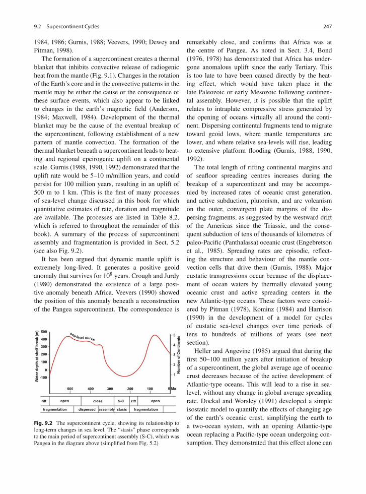
9.2 Supercontinent Cycles 247
1984, 1986; Gurnis, 1988; Veevers, 1990; Dewey andPitman, 1998).
The formation of a supercontinent creates a thermalblanket that inhibits convective release of radiogenicheat from the mantle (Fig. 9.1). Changes in the rotationof the Earth’s core and in the convective patterns in themantle may be either the cause or the consequence ofthese surface events, which also appear to be linkedto changes in the earth’s magnetic field (Anderson,1984; Maxwell, 1984). Development of the thermalblanket may be the cause of the eventual breakup ofthe supercontinent, following establishment of a newpattern of mantle convection. The formation of thethermal blanket beneath a supercontinent leads to heat-ing and regional epeirogenic uplift on a continentalscale. Gurnis (1988, 1990, 1992) demonstrated that theuplift rate would be 5–10 m/million years, and couldpersist for 100 million years, resulting in an uplift of500 m to 1 km. (This is the first of many processesof sea-level change discussed in this book for whichquantitative estimates of rate, duration and magnitudeare available. The processes are listed in Table 8.2,which is referred to throughout the remainder of thisbook). A summary of the process of supercontinentassembly and fragmentation is provided in Sect. 5.2(see also Fig. 9.2).
It has been argued that dynamic mantle uplift isextremely long-lived. It generates a positive geoidanomaly that survives for 108 years. Crough and Jurdy(1980) demonstrated the existence of a large posi-tive anomaly beneath Africa. Veevers (1990) showedthe position of this anomaly beneath a reconstructionof the Pangea supercontinent. The correspondence is
Fig. 9.2 The supercontinent cycle, showing its relationship tolong-term changes in sea level. The “stasis” phase correspondsto the main period of supercontinent assembly (S-C), which wasPangea in the diagram above (simplified from Fig. 5.2)
remarkably close, and confirms that Africa was atthe centre of Pangea. As noted in Sect. 3.4, Bond(1976, 1978) has demonstrated that Africa has under-gone anomalous uplift since the early Tertiary. Thisis too late to have been caused directly by the heat-ing effect, which would have taken place in thelate Paleozoic or early Mesozoic following continen-tal assembly. However, it is possible that the upliftrelates to intraplate compressive stress generated bythe opening of oceans virtually all around the conti-nent. Dispersing continental fragments tend to migratetoward geoid lows, where mantle temperatures arelower, and where relative sea-levels will rise, leadingto extensive platform flooding (Gurnis, 1988, 1990,1992).
The total length of rifting continental margins andof seafloor spreading centres increases during thebreakup of a supercontinent and may be accompa-nied by increased rates of oceanic crust generation,and active subduction, plutonism, and arc volcanismon the outer, convergent plate margins of the dis-persing fragments, as suggested by the westward driftof the Americas since the Triassic, and the conse-quent subduction of tens of thousands of kilometres ofpaleo-Pacific (Panthalassa) oceanic crust (Engebretsonet al., 1985). Spreading rates are episodic, reflect-ing the structure and behaviour of the mantle con-vection cells that drive them (Gurnis, 1988). Majoreustatic transgressions occur because of the displace-ment of ocean waters by thermally elevated youngoceanic crust and active spreading centers in thenew Atlantic-type oceans. These factors were consid-ered by Pitman (1978), Kominz (1984) and Harrison(1990) in the development of a model for cyclesof eustatic sea-level changes over time periods oftens to hundreds of millions of years (see nextsection).
Heller and Angevine (1985) argued that during thefirst 50–100 million years after initiation of breakupof a supercontinent, the global average age of oceaniccrust decreases because of the active development ofAtlantic-type oceans. This will lead to a rise in sea-level, without any change in global average spreadingrate. Dockal and Worsley (1991) developed a simpleisostatic model to quantify the effects of changing ageof the earth’s oceanic crust, simplifying the earth toa two-ocean system, with an opening Atlantic-typeocean replacing a Pacific-type ocean undergoing con-sumption. They demonstrated that this effect alone can
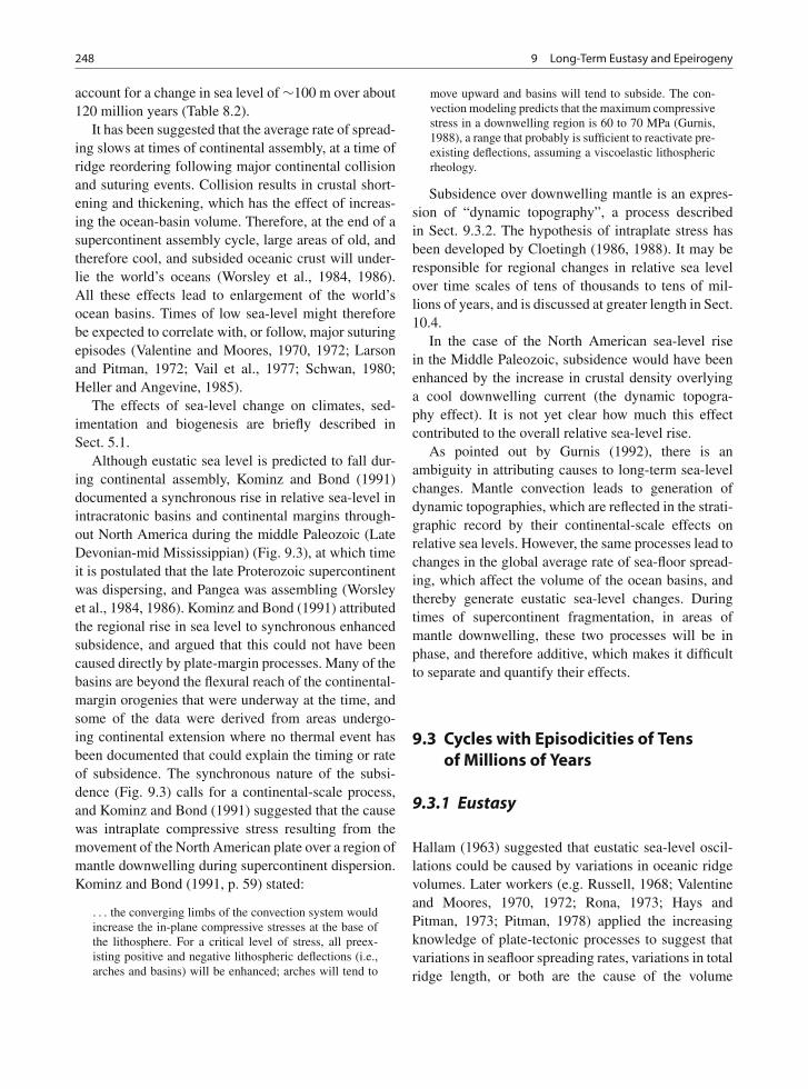
248 9 Long-Term Eustasy and Epeirogeny
account for a change in sea level of ∼100 m over about120 million years (Table 8.2).
It has been suggested that the average rate of spread-ing slows at times of continental assembly, at a time ofridge reordering following major continental collisionand suturing events. Collision results in crustal short-ening and thickening, which has the effect of increas-ing the ocean-basin volume. Therefore, at the end of asupercontinent assembly cycle, large areas of old, andtherefore cool, and subsided oceanic crust will under-lie the world’s oceans (Worsley et al., 1984, 1986).All these effects lead to enlargement of the world’socean basins. Times of low sea-level might thereforebe expected to correlate with, or follow, major suturingepisodes (Valentine and Moores, 1970, 1972; Larsonand Pitman, 1972; Vail et al., 1977; Schwan, 1980;Heller and Angevine, 1985).
The effects of sea-level change on climates, sed-imentation and biogenesis are briefly described inSect. 5.1.
Although eustatic sea level is predicted to fall dur-ing continental assembly, Kominz and Bond (1991)documented a synchronous rise in relative sea-level inintracratonic basins and continental margins through-out North America during the middle Paleozoic (LateDevonian-mid Mississippian) (Fig. 9.3), at which timeit is postulated that the late Proterozoic supercontinentwas dispersing, and Pangea was assembling (Worsleyet al., 1984, 1986). Kominz and Bond (1991) attributedthe regional rise in sea level to synchronous enhancedsubsidence, and argued that this could not have beencaused directly by plate-margin processes. Many of thebasins are beyond the flexural reach of the continental-margin orogenies that were underway at the time, andsome of the data were derived from areas undergo-ing continental extension where no thermal event hasbeen documented that could explain the timing or rateof subsidence. The synchronous nature of the subsi-dence (Fig. 9.3) calls for a continental-scale process,and Kominz and Bond (1991) suggested that the causewas intraplate compressive stress resulting from themovement of the North American plate over a region ofmantle downwelling during supercontinent dispersion.Kominz and Bond (1991, p. 59) stated:
. . . the converging limbs of the convection system wouldincrease the in-plane compressive stresses at the base ofthe lithosphere. For a critical level of stress, all preex-isting positive and negative lithospheric deflections (i.e.,arches and basins) will be enhanced; arches will tend to
move upward and basins will tend to subside. The con-vection modeling predicts that the maximum compressivestress in a downwelling region is 60 to 70 MPa (Gurnis,1988), a range that probably is sufficient to reactivate pre-existing deflections, assuming a viscoelastic lithosphericrheology.
Subsidence over downwelling mantle is an expres-sion of “dynamic topography”, a process describedin Sect. 9.3.2. The hypothesis of intraplate stress hasbeen developed by Cloetingh (1986, 1988). It may beresponsible for regional changes in relative sea levelover time scales of tens of thousands to tens of mil-lions of years, and is discussed at greater length in Sect.10.4.
In the case of the North American sea-level risein the Middle Paleozoic, subsidence would have beenenhanced by the increase in crustal density overlyinga cool downwelling current (the dynamic topogra-phy effect). It is not yet clear how much this effectcontributed to the overall relative sea-level rise.
As pointed out by Gurnis (1992), there is anambiguity in attributing causes to long-term sea-levelchanges. Mantle convection leads to generation ofdynamic topographies, which are reflected in the strati-graphic record by their continental-scale effects onrelative sea levels. However, the same processes lead tochanges in the global average rate of sea-floor spread-ing, which affect the volume of the ocean basins, andthereby generate eustatic sea-level changes. Duringtimes of supercontinent fragmentation, in areas ofmantle downwelling, these two processes will be inphase, and therefore additive, which makes it difficultto separate and quantify their effects.
9.3 Cycles with Episodicities of Tensof Millions of Years
9.3.1 Eustasy
Hallam (1963) suggested that eustatic sea-level oscil-lations could be caused by variations in oceanic ridgevolumes. Later workers (e.g. Russell, 1968; Valentineand Moores, 1970, 1972; Rona, 1973; Hays andPitman, 1973; Pitman, 1978) applied the increasingknowledge of plate-tectonic processes to suggest thatvariations in seafloor spreading rates, variations in totalridge length, or both are the cause of the volume
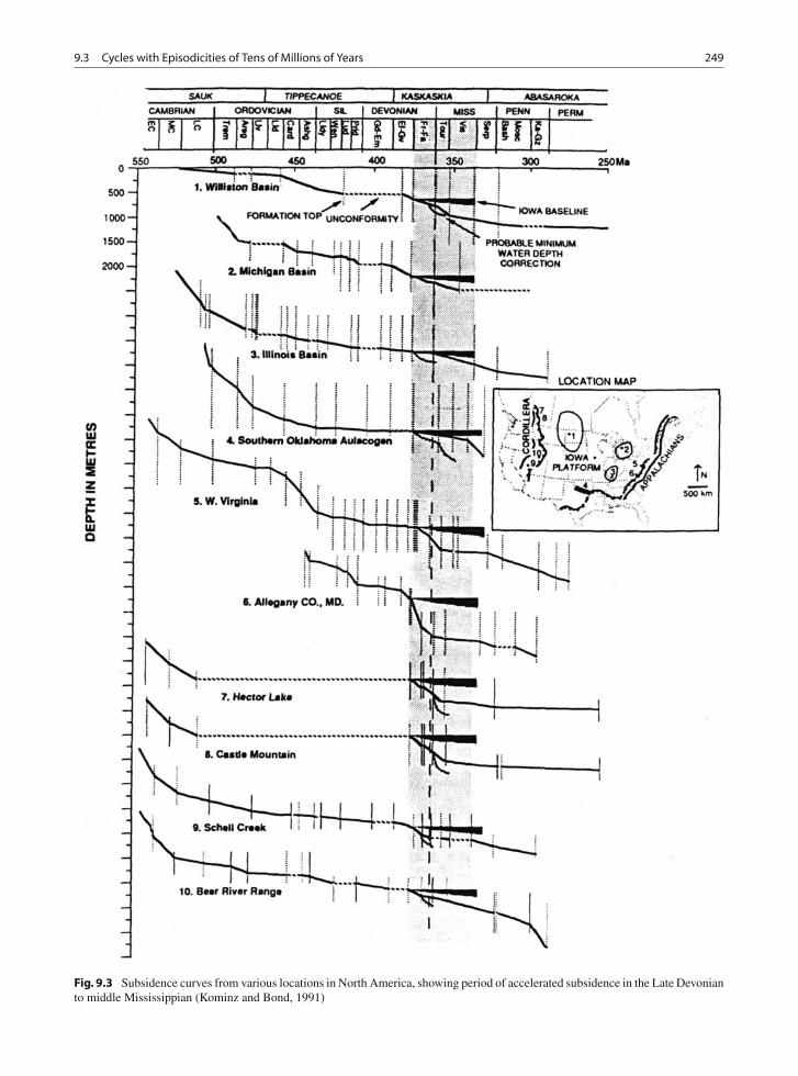
9.3 Cycles with Episodicities of Tens of Millions of Years 249
Fig. 9.3 Subsidence curves from various locations in North America, showing period of accelerated subsidence in the Late Devonianto middle Mississippian (Kominz and Bond, 1991)
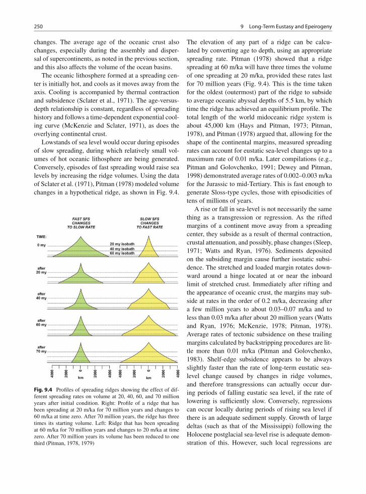
250 9 Long-Term Eustasy and Epeirogeny
changes. The average age of the oceanic crust alsochanges, especially during the assembly and disper-sal of supercontinents, as noted in the previous section,and this also affects the volume of the ocean basins.
The oceanic lithosphere formed at a spreading cen-ter is initially hot, and cools as it moves away from theaxis. Cooling is accompanied by thermal contractionand subsidence (Sclater et al., 1971). The age-versus-depth relationship is constant, regardless of spreadinghistory and follows a time-dependent exponential cool-ing curve (McKenzie and Sclater, 1971), as does theoverlying continental crust.
Lowstands of sea level would occur during episodesof slow spreading, during which relatively small vol-umes of hot oceanic lithosphere are being generated.Conversely, episodes of fast spreading would raise sealevels by increasing the ridge volumes. Using the dataof Sclater et al. (1971), Pitman (1978) modeled volumechanges in a hypothetical ridge, as shown in Fig. 9.4.
Fig. 9.4 Profiles of spreading ridges showing the effect of dif-ferent spreading rates on volume at 20, 40, 60, and 70 millionyears after initial condition. Right: Profile of a ridge that hasbeen spreading at 20 m/ka for 70 million years and changes to60 m/ka at time zero. After 70 million years, the ridge has threetimes its starting volume. Left: Ridge that has been spreadingat 60 m/ka for 70 million years and changes to 20 m/ka at timezero. After 70 million years its volume has been reduced to onethird (Pitman, 1978, 1979)
The elevation of any part of a ridge can be calcu-lated by converting age to depth, using an appropriatespreading rate. Pitman (1978) showed that a ridgespreading at 60 m/ka will have three times the volumeof one spreading at 20 m/ka, provided these rates lastfor 70 million years (Fig. 9.4). This is the time takenfor the oldest (outermost) part of the ridge to subsideto average oceanic abyssal depths of 5.5 km, by whichtime the ridge has achieved an equilibrium profile. Thetotal length of the world midoceanic ridge system isabout 45,000 km (Hays and Pitman, 1973; Pitman,1978), and Pitman (1978) argued that, allowing for theshape of the continental margins, measured spreadingrates can account for eustatic sea-level changes up to amaximum rate of 0.01 m/ka. Later compilations (e.g.,Pitman and Golovchenko, 1991; Dewey and Pitman,1998) demonstrated average rates of 0.002–0.003 m/kafor the Jurassic to mid-Tertiary. This is fast enough togenerate Sloss-type cycles, those with episodicities oftens of millions of years.
A rise or fall in sea-level is not necessarily the samething as a transgression or regression. As the riftedmargins of a continent move away from a spreadingcenter, they subside as a result of thermal contraction,crustal attenuation, and possibly, phase changes (Sleep,1971; Watts and Ryan, 1976). Sediments depositedon the subsiding margin cause further isostatic subsi-dence. The stretched and loaded margin rotates down-ward around a hinge located at or near the inboardlimit of stretched crust. Immediately after rifting andthe appearance of oceanic crust, the margins may sub-side at rates in the order of 0.2 m/ka, decreasing aftera few million years to about 0.03–0.07 m/ka and toless than 0.03 m/ka after about 20 million years (Wattsand Ryan, 1976; McKenzie, 1978; Pitman, 1978).Average rates of tectonic subsidence on these trailingmargins calculated by backstripping procedures are lit-tle more than 0.01 m/ka (Pitman and Golovchenko,1983). Shelf-edge subsidence appears to be alwaysslightly faster than the rate of long-term eustatic sea-level change caused by changes in ridge volumes,and therefore transgressions can actually occur dur-ing periods of falling eustatic sea level, if the rate oflowering is sufficiently slow. Conversely, regressionscan occur locally during periods of rising sea level ifthere is an adequate sediment supply. Growth of largedeltas (such as that of the Mississippi) following theHolocene postglacial sea-level rise is adequate demon-stration of this. However, such local regressions are
9.3 Cycles with Episodicities of Tens of Millions of Years 251
not relevant to the consideration of global stratigraphiccycles. Except on continental margins underlain byunusually old, rigid crust, which subside slowly, it isunlikely that sea-level changes caused by ridge-volumechanges could lower sea-level to beyond the shelf-break (Pitman and Golovchenko, 1983). These tectonicprocesses that control relative sea level on a regionalscale are discussed further in Chap. 10.
The spreading histories of the world oceans are nowreasonably well understood (including the recent syn-thesis of the history of the Arctic regions by Lawveret al., 2002), based on deep-sea-drilling and magnetic-reversal data. Knowledge of worldwide spreading ratesenabled Hays and Pitman (1973) to calculate ridge-volume changes and a sea-level curve for the last110 Ma. A revised version of this curve was calcu-lated for the period 85–15 Ma by Pitman (1978), basedon refinements in oceanic data. It showed a gradualdrop in sea level of 350 m at an average rate of 0.005m/ka. Sea levels rose to a maximum during a periodof fast spreading between 110 and 85 Ma (Larsonand Pitman, 1972), and the subsequent drop reflectsslower spreading rates. By calculating the relation-ship between spreading rates, subsidence rates, andfalling sea-level, Pitman (1978) was able to modela major global transgression during the Eocene, asactually documented from stratigraphic evidence byHallam (1963), and a second transgression during theMiocene. An early Oligocene regression is probablyrelated to the onset of large-scale Antarctic glaciation(Fig. 4.10). Vail et al. (1977) used Pitman’s curve tocalibrate their chart of relative changes of sea level, inthe belief that in this way they were adjusting the curveto show true eustatic sea-level change. They suggestedthat positive departures from Pitman’s curve (whereVail’s curve shows a higher sea level than Pitman)are the result of temporary increases in subsidencerates because of sediment loading. Negative depar-tures were attributed to rapid sea-level falls drivenby glacioeustasy, a process not factored into Pitman’scurve (Vail et al., 1977, p. 92). It is of interest that Vailet al. (1977) mentioned tectonic subsidence as a fac-tor in generating onlap and relative rises in sea level,because the general, indeed overriding importance ofthis process (discussed in Chap. 11) was been almostcompletely ignored in subsequent work by the Exxongroup, until very recently.
Kominz (1984) reexamined the data on whichPitman’s (1978, 1979) curve was based, carrying out
her own calculations and incorporating new data, andshowed that, because of an incomplete data base, aconsiderable error must still be allowed for in thedevelopment and use of a long-term sea-level curve.She used arbitrary, estimated spreading rates for theTethyan Ocean because, of course, this ocean hasnow been completely subducted, whereas during theMesozoic and early Tertiary it was one of the world’smajor oceans and its sea-floor spreading history wouldhave had a considerable effect on the eustatic curve.Other errors include inaccurate dating of the sea floor,and missing data; for example the spreading history ofthe Arctic Ocean was unknown at the time of her syn-thesis (and is still incompletely understood). Kominz(1984) concluded that the range of error is ∼120 mat 80 Ma, decreasing to ∼10 m at present. This hasimportant implications for the accuracy of backstrip-ping calculations used to reconstruct basin subsidencehistories. More recent work by Kominz and her col-leagues on the sea-level record is discussed below andin Sect. 14.6.
A compilation of spreading centres associated withthe breakup of Pangea is shown in Figs. 9.5, and 9.6shows the age of initiation of rifting along each seg-ment of these breakup fractures. The initiation of eachridge would have had an effect on the global aver-age spreading rates, and on the age distribution of theoceanic crust, with consequences for eustatic fluctua-tions over time periods of tens of millions of years.However, as discussed in Chap. 10, the same eventsare now also thought to have had a profound effect onregional intraplate-stress regimes, with consequencesfor regional warping and tilting, and the generationof relative sea-level changes over large continentalareas. Rifting and continental separation is also oneof the major processes involved in the development oftectonostratigraphic sequences (Sect. 10.2).
Estimates of the rate and magnitude of eustatic sea-level changes that can be attributed to volume changesin sea-floor spreading centres were made by Pitmanand Golovchenko (1991), based on their earlier workand that of Kominz (1984), and are given in Table 8.2.Dockal and Worsley (1991) examined the effects onthe age distribution of the Earth’s oceanic crust dur-ing the formation and breakup of supercontinents. Asnoted in the previous section, a two-ocean model, inwhich a Pacific-type ocean (Panthalassa) is replaced byan Atlantic-type ocean, can account for tens of metresof sea-level change over a time scale of hundreds of
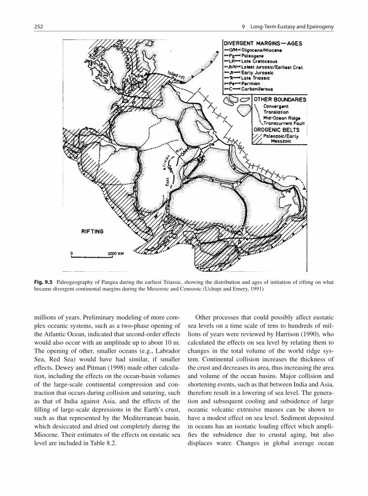
252 9 Long-Term Eustasy and Epeirogeny
Fig. 9.5 Paleogeography of Pangea during the earliest Triassic, showing the distribution and ages of initiation of rifting on whatbecame divergent continental margins during the Mesozoic and Cenozoic (Uchupi and Emery, 1991)
millions of years. Preliminary modeling of more com-plex oceanic systems, such as a two-phase opening ofthe Atlantic Ocean, indicated that second-order effectswould also occur with an amplitude up to about 10 m.The opening of other, smaller oceans (e.g., LabradorSea, Red Sea) would have had similar, if smallereffects. Dewey and Pitman (1998) made other calcula-tion, including the effects on the ocean-basin volumesof the large-scale continental compression and con-traction that occurs during collision and suturing, suchas that of India against Asia, and the effects of thefilling of large-scale depressions in the Earth’s crust,such as that represented by the Mediterranean basin,which desiccated and dried out completely during theMiocene. Their estimates of the effects on eustatic sealevel are included in Table 8.2.
Other processes that could possibly affect eustaticsea levels on a time scale of tens to hundreds of mil-lions of years were reviewed by Harrison (1990), whocalculated the effects on sea level by relating them tochanges in the total volume of the world ridge sys-tem. Continental collision increases the thickness ofthe crust and decreases its area, thus increasing the areaand volume of the ocean basins. Major collision andshortening events, such as that between India and Asia,therefore result in a lowering of sea level. The genera-tion and subsequent cooling and subsidence of largeoceanic volcanic extrusive masses can be shown tohave a modest effect on sea level. Sediment depositedin oceans has an isostatic loading effect which ampli-fies the subsidence due to crustal aging, but alsodisplaces water. Changes in global average ocean
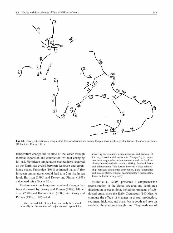
9.3 Cycles with Episodicities of Tens of Millions of Years 253
Fig. 9.6 Divergent continental margins that developed within and around Pangea, showing the age of initiation of seafloor spreading(Uchupi and Emery, 1991)
temperature change the volume of the water throughthermal expansion and contraction, without changingits load. Significant temperature changes have occurredas the Earth has cycled between icehouse and green-house states. Fairbridge (1961) estimated that a 1◦ risein ocean temperatures would lead to a 2 m rise in sealevel. Harrison (1990) and Dewey and Pitman (1998)calculated this effect at 10 m.
Modern work on long-term sea-level changes hasbeen discussed by Dewey and Pitman (1998), Mülleret al. (2008) and Kominz et al. (2008). As Dewey andPitman (1998, p. 10) noted:
. . . the rise and fall of sea level can only be viewedrationally in the context of major tectonic episodicity
involving the assembly, dismemberment and dispersal ofthe larger continental masses in “Pangea”-type super-continent megacycles, where tectonics and sea level areclosely interrelated with much buffering, feedback loopsand enhancement. This further involves a close relation-ship between continental distribution, plate kinematicsand state of stress, climate, geomorphology, sedimentaryfacies and basin stratigraphy.
Müller et al. (2008) presented a comprehensivereconstruction of the global age-area and depth-areadistribution of ocean floor, including remnants of sub-ducted crust, since the Early Cretaceous (140 Ma), tocompute the effects of changes in crustal production,sediment thickness, and ocean-basin depth and area onsea-level fluctuations through time. They made use of
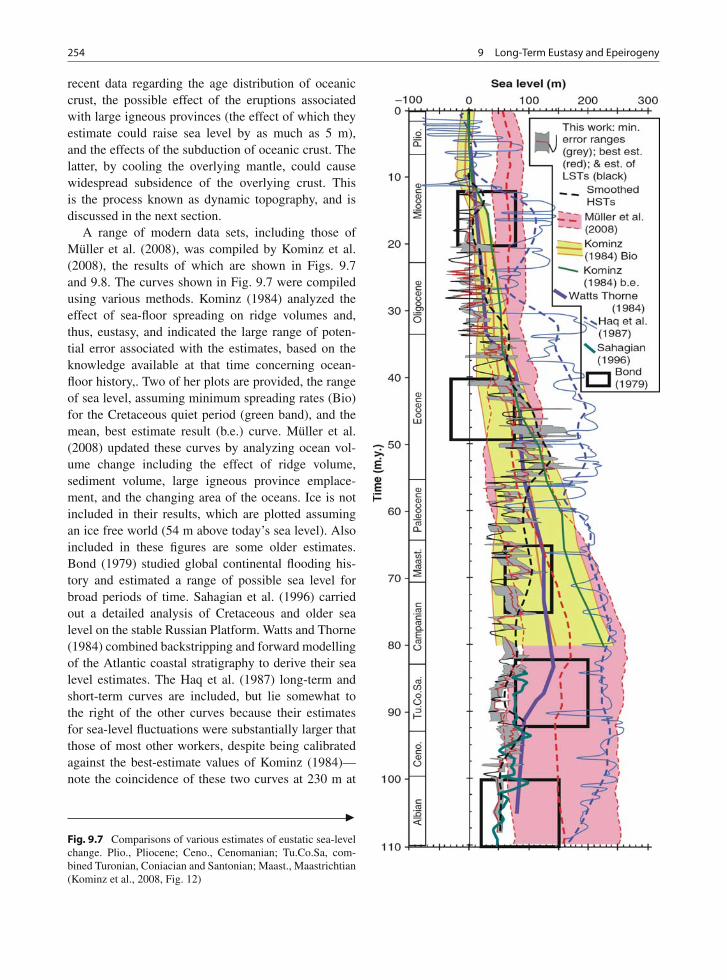
254 9 Long-Term Eustasy and Epeirogeny
recent data regarding the age distribution of oceaniccrust, the possible effect of the eruptions associatedwith large igneous provinces (the effect of which theyestimate could raise sea level by as much as 5 m),and the effects of the subduction of oceanic crust. Thelatter, by cooling the overlying mantle, could causewidespread subsidence of the overlying crust. Thisis the process known as dynamic topography, and isdiscussed in the next section.
A range of modern data sets, including those ofMüller et al. (2008), was compiled by Kominz et al.(2008), the results of which are shown in Figs. 9.7and 9.8. The curves shown in Fig. 9.7 were compiledusing various methods. Kominz (1984) analyzed theeffect of sea-floor spreading on ridge volumes and,thus, eustasy, and indicated the large range of poten-tial error associated with the estimates, based on theknowledge available at that time concerning ocean-floor history,. Two of her plots are provided, the rangeof sea level, assuming minimum spreading rates (Bio)for the Cretaceous quiet period (green band), and themean, best estimate result (b.e.) curve. Müller et al.(2008) updated these curves by analyzing ocean vol-ume change including the effect of ridge volume,sediment volume, large igneous province emplace-ment, and the changing area of the oceans. Ice is notincluded in their results, which are plotted assumingan ice free world (54 m above today’s sea level). Alsoincluded in these figures are some older estimates.Bond (1979) studied global continental flooding his-tory and estimated a range of possible sea level forbroad periods of time. Sahagian et al. (1996) carriedout a detailed analysis of Cretaceous and older sealevel on the stable Russian Platform. Watts and Thorne(1984) combined backstripping and forward modellingof the Atlantic coastal stratigraphy to derive their sealevel estimates. The Haq et al. (1987) long-term andshort-term curves are included, but lie somewhat tothe right of the other curves because their estimatesfor sea-level fluctuations were substantially larger thatthose of most other workers, despite being calibratedagainst the best-estimate values of Kominz (1984)—note the coincidence of these two curves at 230 m at
�Fig. 9.7 Comparisons of various estimates of eustatic sea-levelchange. Plio., Pliocene; Ceno., Cenomanian; Tu.Co.Sa, com-bined Turonian, Coniacian and Santonian; Maast., Maastrichtian(Kominz et al., 2008, Fig. 12)
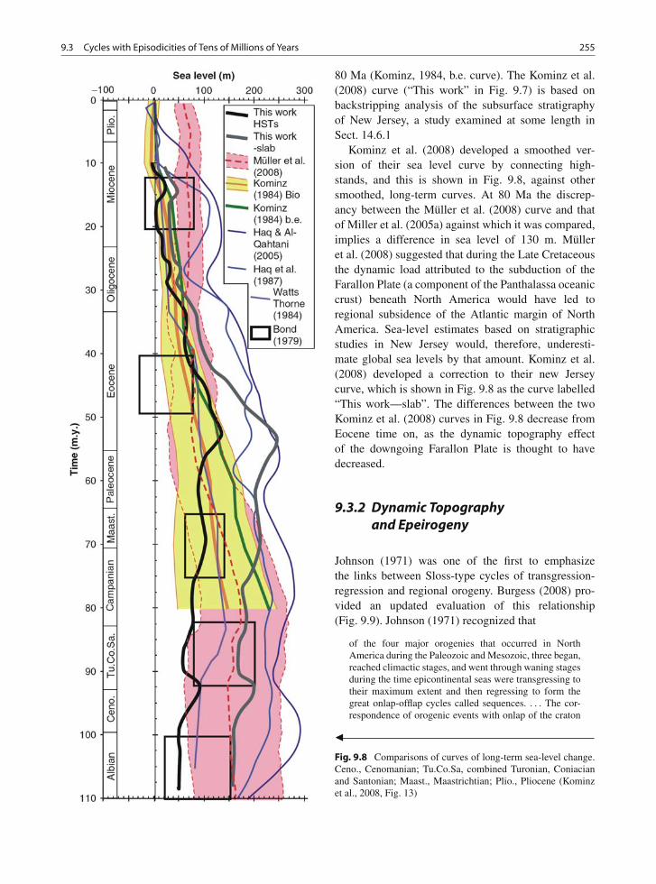
9.3 Cycles with Episodicities of Tens of Millions of Years 255
80 Ma (Kominz, 1984, b.e. curve). The Kominz et al.(2008) curve (“This work” in Fig. 9.7) is based onbackstripping analysis of the subsurface stratigraphyof New Jersey, a study examined at some length inSect. 14.6.1
Kominz et al. (2008) developed a smoothed ver-sion of their sea level curve by connecting high-stands, and this is shown in Fig. 9.8, against othersmoothed, long-term curves. At 80 Ma the discrep-ancy between the Müller et al. (2008) curve and thatof Miller et al. (2005a) against which it was compared,implies a difference in sea level of 130 m. Mülleret al. (2008) suggested that during the Late Cretaceousthe dynamic load attributed to the subduction of theFarallon Plate (a component of the Panthalassa oceaniccrust) beneath North America would have led toregional subsidence of the Atlantic margin of NorthAmerica. Sea-level estimates based on stratigraphicstudies in New Jersey would, therefore, underesti-mate global sea levels by that amount. Kominz et al.(2008) developed a correction to their new Jerseycurve, which is shown in Fig. 9.8 as the curve labelled“This work—slab”. The differences between the twoKominz et al. (2008) curves in Fig. 9.8 decrease fromEocene time on, as the dynamic topography effectof the downgoing Farallon Plate is thought to havedecreased.
9.3.2 Dynamic Topographyand Epeirogeny
Johnson (1971) was one of the first to emphasizethe links between Sloss-type cycles of transgression-regression and regional orogeny. Burgess (2008) pro-vided an updated evaluation of this relationship(Fig. 9.9). Johnson (1971) recognized that
of the four major orogenies that occurred in NorthAmerica during the Paleozoic and Mesozoic, three began,reached climactic stages, and went through waning stagesduring the time epicontinental seas were transgressing totheir maximum extent and then regressing to form thegreat onlap-offlap cycles called sequences. . . . The cor-respondence of orogenic events with onlap of the craton
�Fig. 9.8 Comparisons of curves of long-term sea-level change.Ceno., Cenomanian; Tu.Co.Sa, combined Turonian, Coniacianand Santonian; Maast., Maastrichtian; Plio., Pliocene (Kominzet al., 2008, Fig. 13)
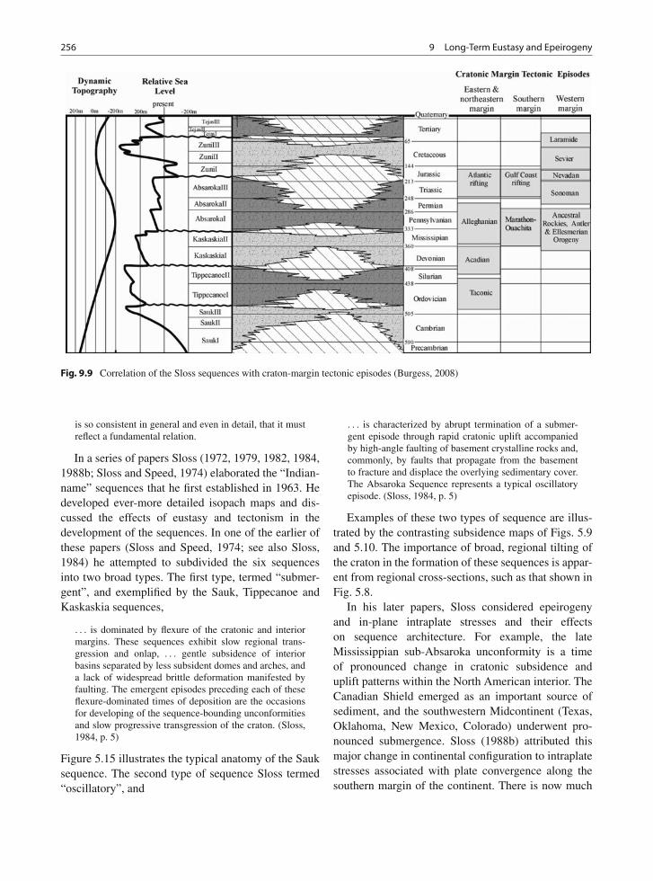
256 9 Long-Term Eustasy and Epeirogeny
Fig. 9.9 Correlation of the Sloss sequences with craton-margin tectonic episodes (Burgess, 2008)
is so consistent in general and even in detail, that it mustreflect a fundamental relation.
In a series of papers Sloss (1972, 1979, 1982, 1984,1988b; Sloss and Speed, 1974) elaborated the “Indian-name” sequences that he first established in 1963. Hedeveloped ever-more detailed isopach maps and dis-cussed the effects of eustasy and tectonism in thedevelopment of the sequences. In one of the earlier ofthese papers (Sloss and Speed, 1974; see also Sloss,1984) he attempted to subdivided the six sequencesinto two broad types. The first type, termed “submer-gent”, and exemplified by the Sauk, Tippecanoe andKaskaskia sequences,
. . . is dominated by flexure of the cratonic and interiormargins. These sequences exhibit slow regional trans-gression and onlap, . . . gentle subsidence of interiorbasins separated by less subsident domes and arches, anda lack of widespread brittle deformation manifested byfaulting. The emergent episodes preceding each of theseflexure-dominated times of deposition are the occasionsfor developing of the sequence-bounding unconformitiesand slow progressive transgression of the craton. (Sloss,1984, p. 5)
Figure 5.15 illustrates the typical anatomy of the Sauksequence. The second type of sequence Sloss termed“oscillatory”, and
. . . is characterized by abrupt termination of a submer-gent episode through rapid cratonic uplift accompaniedby high-angle faulting of basement crystalline rocks and,commonly, by faults that propagate from the basementto fracture and displace the overlying sedimentary cover.The Absaroka Sequence represents a typical oscillatoryepisode. (Sloss, 1984, p. 5)
Examples of these two types of sequence are illus-trated by the contrasting subsidence maps of Figs. 5.9and 5.10. The importance of broad, regional tilting ofthe craton in the formation of these sequences is appar-ent from regional cross-sections, such as that shown inFig. 5.8.
In his later papers, Sloss considered epeirogenyand in-plane intraplate stresses and their effectson sequence architecture. For example, the lateMississippian sub-Absaroka unconformity is a timeof pronounced change in cratonic subsidence anduplift patterns within the North American interior. TheCanadian Shield emerged as an important source ofsediment, and the southwestern Midcontinent (Texas,Oklahoma, New Mexico, Colorado) underwent pro-nounced submergence. Sloss (1988b) attributed thismajor change in continental configuration to intraplatestresses associated with plate convergence along thesouthern margin of the continent. There is now much
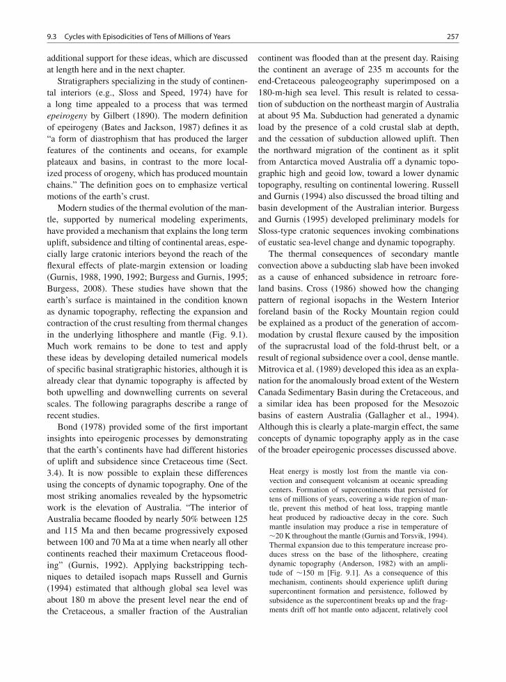
9.3 Cycles with Episodicities of Tens of Millions of Years 257
additional support for these ideas, which are discussedat length here and in the next chapter.
Stratigraphers specializing in the study of continen-tal interiors (e.g., Sloss and Speed, 1974) have fora long time appealed to a process that was termedepeirogeny by Gilbert (1890). The modern definitionof epeirogeny (Bates and Jackson, 1987) defines it as“a form of diastrophism that has produced the largerfeatures of the continents and oceans, for exampleplateaux and basins, in contrast to the more local-ized process of orogeny, which has produced mountainchains.” The definition goes on to emphasize verticalmotions of the earth’s crust.
Modern studies of the thermal evolution of the man-tle, supported by numerical modeling experiments,have provided a mechanism that explains the long termuplift, subsidence and tilting of continental areas, espe-cially large cratonic interiors beyond the reach of theflexural effects of plate-margin extension or loading(Gurnis, 1988, 1990, 1992; Burgess and Gurnis, 1995;Burgess, 2008). These studies have shown that theearth’s surface is maintained in the condition knownas dynamic topography, reflecting the expansion andcontraction of the crust resulting from thermal changesin the underlying lithosphere and mantle (Fig. 9.1).Much work remains to be done to test and applythese ideas by developing detailed numerical modelsof specific basinal stratigraphic histories, although it isalready clear that dynamic topography is affected byboth upwelling and downwelling currents on severalscales. The following paragraphs describe a range ofrecent studies.
Bond (1978) provided some of the first importantinsights into epeirogenic processes by demonstratingthat the earth’s continents have had different historiesof uplift and subsidence since Cretaceous time (Sect.3.4). It is now possible to explain these differencesusing the concepts of dynamic topography. One of themost striking anomalies revealed by the hypsometricwork is the elevation of Australia. “The interior ofAustralia became flooded by nearly 50% between 125and 115 Ma and then became progressively exposedbetween 100 and 70 Ma at a time when nearly all othercontinents reached their maximum Cretaceous flood-ing” (Gurnis, 1992). Applying backstripping tech-niques to detailed isopach maps Russell and Gurnis(1994) estimated that although global sea level wasabout 180 m above the present level near the end ofthe Cretaceous, a smaller fraction of the Australian
continent was flooded than at the present day. Raisingthe continent an average of 235 m accounts for theend-Cretaceous paleogeography superimposed on a180-m-high sea level. This result is related to cessa-tion of subduction on the northeast margin of Australiaat about 95 Ma. Subduction had generated a dynamicload by the presence of a cold crustal slab at depth,and the cessation of subduction allowed uplift. Thenthe northward migration of the continent as it splitfrom Antarctica moved Australia off a dynamic topo-graphic high and geoid low, toward a lower dynamictopography, resulting on continental lowering. Russelland Gurnis (1994) also discussed the broad tilting andbasin development of the Australian interior. Burgessand Gurnis (1995) developed preliminary models forSloss-type cratonic sequences invoking combinationsof eustatic sea-level change and dynamic topography.
The thermal consequences of secondary mantleconvection above a subducting slab have been invokedas a cause of enhanced subsidence in retroarc fore-land basins. Cross (1986) showed how the changingpattern of regional isopachs in the Western Interiorforeland basin of the Rocky Mountain region couldbe explained as a product of the generation of accom-modation by crustal flexure caused by the impositionof the supracrustal load of the fold-thrust belt, or aresult of regional subsidence over a cool, dense mantle.Mitrovica et al. (1989) developed this idea as an expla-nation for the anomalously broad extent of the WesternCanada Sedimentary Basin during the Cretaceous, anda similar idea has been proposed for the Mesozoicbasins of eastern Australia (Gallagher et al., 1994).Although this is clearly a plate-margin effect, the sameconcepts of dynamic topography apply as in the caseof the broader epeirogenic processes discussed above.
Heat energy is mostly lost from the mantle via con-vection and consequent volcanism at oceanic spreadingcenters. Formation of supercontinents that persisted fortens of millions of years, covering a wide region of man-tle, prevent this method of heat loss, trapping mantleheat produced by radioactive decay in the core. Suchmantle insulation may produce a rise in temperature of∼20 K throughout the mantle (Gurnis and Torsvik, 1994).Thermal expansion due to this temperature increase pro-duces stress on the base of the lithosphere, creatingdynamic topography (Anderson, 1982) with an ampli-tude of ∼150 m [Fig. 9.1]. As a consequence of thismechanism, continents should experience uplift duringsupercontinent formation and persistence, followed bysubsidence as the supercontinent breaks up and the frag-ments drift off hot mantle onto adjacent, relatively cool
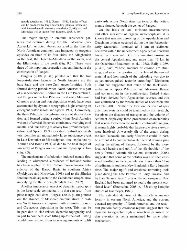
258 9 Long-Term Eustasy and Epeirogeny
mantle (Anderson, 1982; Gurnis, 1988). Similar effectscan be produced by large descending plumes interactingwith internal mantle viscosity boundaries (Pysklywec andMitrovica, 1998) (quote from Burgess, 2008, p. 40).
The major change in cratonic subsidence pat-terns that occurred during the late Paleozoic (pre-Absaroka), as noted above, occurred at the time theNorth American continent was impacted by orogenicepisodes on three of its four sides, the Alleghanianin the east, the Ouachita-Marathon in the south, andthe Ellesmerian in the north (Fig. 9.5). These werethree of the important orogenies that culminated in theconstruction of Pangea.
Burgess (2008, p. 40) pointed out that the twolongest-duration lacunae in North America are thebase-Sauk and the base-Zuni unconformities. Bothformed during periods when North America was partof a supercontinent, Rodinia in the Late Precambrian,and Pangea in the late Paleozoic and early Mesozoic.Cratonic erosion and non-deposition would have beenaccentuated by dynamic topographic highs creating anemergent craton (Sloss and Speed, 1974). Conversely,the three Paleozoic unconformities are of shorter dura-tion, and formed during a period when North Americawas one of several dispersed continents, overlying coolmantle, and thus having relatively low or “submergent”(Sloss and Speed, 1974) elevation. Subsidence anal-ysis identifies an anomalously large subsidence eventin Late Devonian to Mississippian time, explained byKominz and Bond (1991) as due to the final stages ofassembly of Pangea over a dynamic topographic low(Fig. 9.3).
The mechanism of subduction-induced mantle flowleading to widespread subsidence of foreland basinshas been applied to the Carboniferous-Triassic sub-sidence of the Karoo Basin in southern Africa(Pysklywec and Mitrovica, 1998) and to the Silurianforeland basin adjacent to the Caledonian orogen, nowunderlying the Baltic Sea (Daradich et al., 2002).
Another importance aspect of dynamic topographyis the large-scale continental tilts that can result fromplate-margin collisions. Burgess (2008, p. 40) pointedout the absence of Mesozoic cratonic strata in east-ern North America, compared with extensive Jurassicand Cretaceous deposition in the west. This may bein part due to slab-related dynamic topography andin part to continent-scale tilting up-to-the-east. Tiltingwould have resulted from increasing amounts of uplift
eastwards across North America towards the hottestmantle situated beneath the center of Pangea.
On the basis of coal moisture measurementsand other measures of organic metamorphism, it isknown that massive unroofing of the Appalachian andOuachitan orogens occurred during the late Paleozoic-early Mesozoic. Removal of 4 km of sedimentoccurred within the undeformed Appalachian forelandbasin; there was 7–13 km of cumulative erosion inthe central Appalachians, and more than 13 km inthe Ouachitas (Beaumont et al., 1988). Bally (1989,p. 430) said: “These amounts of erosion are stun-ning, and raise the question of the fate of the erodedmaterial and how much of the unloading was due toas yet unrecognised tectonic unroofing.” Dickinson(1988) had suggested that much of the thick accu-mulations of upper Paleozoic and Mesozoic fluvialand eolian strata in the southwestern United Stateshad been derived from Appalachian sources, and thiswas confirmed by the zircon studies of Dickinson andGehrels (2003). Neither the location nor scale of spe-cific river systems could be identified by this research,but given the distance of transport and the volume ofsediment displaying these provenance characteristicsthat is now located on the western continental margin,it seems highly probable that large-scale river systemswere involved. A westerly tilt of the craton duringthe late Paleozoic and early Mesozoic could, in part,be attributed to continental-scale thermal doming pre-ceding the rifting of Pangea, followed by the morelocalized heating and uplift of the rift shoulder of thenewly formed Atlantic rift system. Ettensohn (2008)suggested that some of the detritus was also shed east-ward, resulting in the accumulation of more than 5 kmof sediment in southern New England in Early Jurassictime. The major uplift and erosional unroofing tookplace during the Late Permian to Early Triassic, andby Late Triassic time “parts of the old orogen in NewEngland had been exhumed to nearly the present ero-sional level” (Ettensohn, 2008, p. 155; citing isotopicstudies of Dallmeyer, 1989).
The extended duration of the sub-Tejas uncon-formity in eastern North America, and the currentelevated topography of North America and the resul-tant predominantly erosional regime suggest that thedynamic topographic high is somehow persistent orthat elevation is being maintained by some othermechanism.
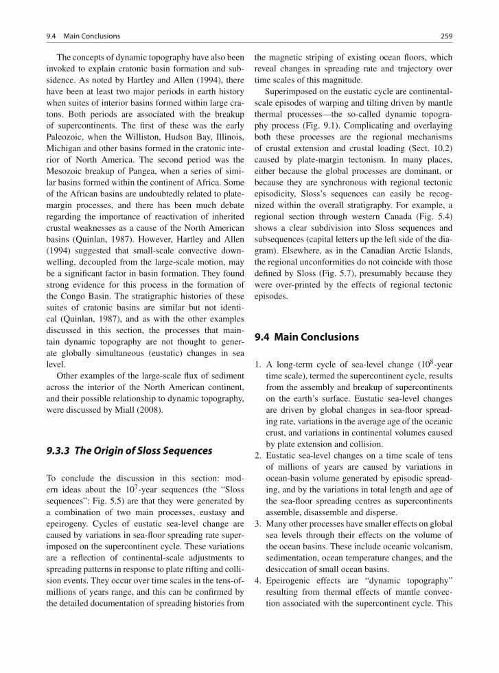
9.4 Main Conclusions 259
The concepts of dynamic topography have also beeninvoked to explain cratonic basin formation and sub-sidence. As noted by Hartley and Allen (1994), therehave been at least two major periods in earth historywhen suites of interior basins formed within large cra-tons. Both periods are associated with the breakupof supercontinents. The first of these was the earlyPaleozoic, when the Williston, Hudson Bay, Illinois,Michigan and other basins formed in the cratonic inte-rior of North America. The second period was theMesozoic breakup of Pangea, when a series of simi-lar basins formed within the continent of Africa. Someof the African basins are undoubtedly related to plate-margin processes, and there has been much debateregarding the importance of reactivation of inheritedcrustal weaknesses as a cause of the North Americanbasins (Quinlan, 1987). However, Hartley and Allen(1994) suggested that small-scale convective down-welling, decoupled from the large-scale motion, maybe a significant factor in basin formation. They foundstrong evidence for this process in the formation ofthe Congo Basin. The stratigraphic histories of thesesuites of cratonic basins are similar but not identi-cal (Quinlan, 1987), and as with the other examplesdiscussed in this section, the processes that main-tain dynamic topography are not thought to gener-ate globally simultaneous (eustatic) changes in sealevel.
Other examples of the large-scale flux of sedimentacross the interior of the North American continent,and their possible relationship to dynamic topography,were discussed by Miall (2008).
9.3.3 The Origin of Sloss Sequences
To conclude the discussion in this section: mod-ern ideas about the 107-year sequences (the “Slosssequences”: Fig. 5.5) are that they were generated bya combination of two main processes, eustasy andepeirogeny. Cycles of eustatic sea-level change arecaused by variations in sea-floor spreading rate super-imposed on the supercontinent cycle. These variationsare a reflection of continental-scale adjustments tospreading patterns in response to plate rifting and colli-sion events. They occur over time scales in the tens-of-millions of years range, and this can be confirmed bythe detailed documentation of spreading histories from
the magnetic striping of existing ocean floors, whichreveal changes in spreading rate and trajectory overtime scales of this magnitude.
Superimposed on the eustatic cycle are continental-scale episodes of warping and tilting driven by mantlethermal processes—the so-called dynamic topogra-phy process (Fig. 9.1). Complicating and overlayingboth these processes are the regional mechanismsof crustal extension and crustal loading (Sect. 10.2)caused by plate-margin tectonism. In many places,either because the global processes are dominant, orbecause they are synchronous with regional tectonicepisodicity, Sloss’s sequences can easily be recog-nized within the overall stratigraphy. For example, aregional section through western Canada (Fig. 5.4)shows a clear subdivision into Sloss sequences andsubsequences (capital letters up the left side of the dia-gram). Elsewhere, as in the Canadian Arctic Islands,the regional unconformities do not coincide with thosedefined by Sloss (Fig. 5.7), presumably because theywere over-printed by the effects of regional tectonicepisodes.
9.4 Main Conclusions
1. A long-term cycle of sea-level change (108-yeartime scale), termed the supercontinent cycle, resultsfrom the assembly and breakup of supercontinentson the earth’s surface. Eustatic sea-level changesare driven by global changes in sea-floor spread-ing rate, variations in the average age of the oceaniccrust, and variations in continental volumes causedby plate extension and collision.
2. Eustatic sea-level changes on a time scale of tensof millions of years are caused by variations inocean-basin volume generated by episodic spread-ing, and by the variations in total length and age ofthe sea-floor spreading centres as supercontinentsassemble, disassemble and disperse.
3. Many other processes have smaller effects on globalsea levels through their effects on the volume ofthe ocean basins. These include oceanic volcanism,sedimentation, ocean temperature changes, and thedesiccation of small ocean basins.
4. Epeirogenic effects are “dynamic topography”resulting from thermal effects of mantle convec-tion associated with the supercontinent cycle. This

260 9 Long-Term Eustasy and Epeirogeny
cycle has long-term consequences, including thegeneration of persistent geoid anomalies. Verticalcontinental movements are related to the ther-mal properties of large- and small-scale convectioncells, and can involve continent-wide uplift, subsi-dence, and tilts, and cratonic basin formation. Thesemovements do not correlate in sign or magnitudefrom continent to continent.
5. Comparisons of various curves of long-term sea-level change constructed using modern data setsreveal few similarities between curves. It is clearthat sea-levels were in the range of at least 200 mhigher during the Late Cretaceous than at present,and have slowly fallen since then, but the details ofsea-level history even on a 106–7-year time scale,remain unresolved.
Chapter 10
Tectonic Mechanisms
Contents
10.1 Introduction . . . . . . . . . . . . . . . . 26110.2 Rifting and Thermal Evolution of Divergent
Plate Margins . . . . . . . . . . . . . . . 26510.2.1 Basic Geophysical Models and Their
Implications for Sea-Level Change . . 26510.2.2 The Origins of Some Tectonostratigraphic
Sequences . . . . . . . . . . . . . 27110.3 Tectonism on Convergent Plate Margins
and in Collision Zones . . . . . . . . . . . 27810.3.1 Magmatic Arcs and Subduction . . . . 27810.3.2 Rates of Uplift and Subsidence
on Convergent Margins . . . . . . . 28010.3.3 Tectonism Versus Eustasy in Foreland
Basins . . . . . . . . . . . . . . . 28210.4 Intraplate Stress . . . . . . . . . . . . . . 308
10.4.1 The Pattern of Global Stress . . . . . 30810.4.2 In-Plane Stress as a Control of Sequence
Architecture . . . . . . . . . . . . 31110.4.3 In-Plane Stress and Regional Histories
of Sea-Level Change . . . . . . . . 31410.5 Basement Control . . . . . . . . . . . . . 31810.6 Sediment Supply and the Importance
of Big Rivers . . . . . . . . . . . . . . . . 32010.7 Environmental Change . . . . . . . . . . . 32510.8 Main Conclusions . . . . . . . . . . . . . 325
10.1 Introduction
Sea-level changes within a basin may be caused bymovements of the basement rather than changes inglobal sea level (eustasy). In Chap. 9 we exam-ine long-term mechanisms of basement movementdriven by deep-seated thermal processes, including thegeneration of dynamic topography, and we also dis-cuss eustatic sea-level changes driven by changes in
ocean-basin volume. These processes act over timeperiods of tens to hundreds of millions of years andare continental to global in scope. In this chapter, wediscuss relative sea-level changes caused by continen-tal tectonism that are regional to local in scope, and actover time periods of tens of millions to tens of thou-sands of years (possibly less). Tectonism of this type isdriven primarily by crustal responses to plate-tectonicprocesses. Extensional and contractional movementsaccompanying the relative motions of plates causecrustal thinning and thickening and changes in regionalthermal regimes, and this leads to regional uplift andsubsidence. These stresses and strains are generatedprimarily at plate margins but, because of the rigidityof plates, they may be transmitted into plate interiorsand affect entire continents.
By their very nature, these mechanisms of sea-level change are regional, possibly even continental inextent, but cannot be global, because they are driven byprocesses occurring within or beneath a single plate orby interaction between two plates. They affect the ele-vation of the plate itself, rather than the volume of theocean basins or the water within them. This categoryof sea-level change is therefore not eustatic. However,as described in this chapter, they can simulate eustaticeffects through the full range of geological episodic-ities over wide areas, and it is now thought by manyresearchers that tectonic mechanisms were responsi-ble for many of the events that were used to definethe global cycle charts of Vail et al. (1977), Haq et al.(1987, 1988a) and Graciansky et al. (1998). An impor-tant additional point is that because Earth is finite,regional plate-tectonic events, such as ridge reorderingor adjustments in rotation vectors, may result in simul-taneous kinematic changes elsewhere. It is possible,
261A.D. Miall, The Geology of Stratigraphic Sequences, 2nd ed.,DOI 10.1007/978-3-642-05027-5_10, © Springer-Verlag Berlin Heidelberg 2010
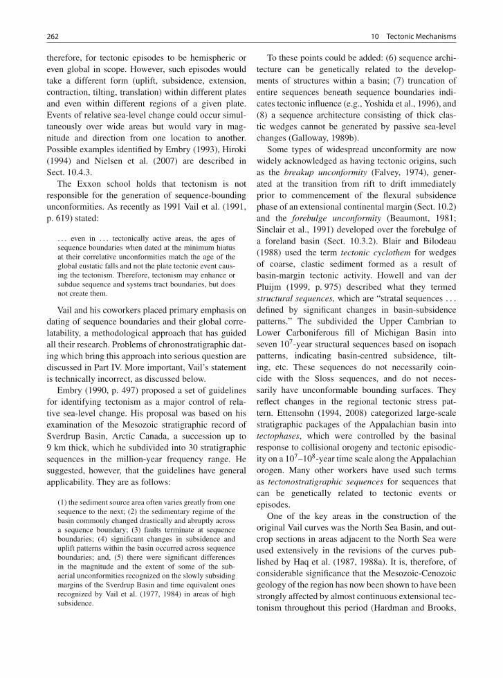
262 10 Tectonic Mechanisms
therefore, for tectonic episodes to be hemispheric oreven global in scope. However, such episodes wouldtake a different form (uplift, subsidence, extension,contraction, tilting, translation) within different platesand even within different regions of a given plate.Events of relative sea-level change could occur simul-taneously over wide areas but would vary in mag-nitude and direction from one location to another.Possible examples identified by Embry (1993), Hiroki(1994) and Nielsen et al. (2007) are described inSect. 10.4.3.
The Exxon school holds that tectonism is notresponsible for the generation of sequence-boundingunconformities. As recently as 1991 Vail et al. (1991,p. 619) stated:
. . . even in . . . tectonically active areas, the ages ofsequence boundaries when dated at the minimum hiatusat their correlative unconformities match the age of theglobal eustatic falls and not the plate tectonic event caus-ing the tectonism. Therefore, tectonism may enhance orsubdue sequence and systems tract boundaries, but doesnot create them.
Vail and his coworkers placed primary emphasis ondating of sequence boundaries and their global corre-latability, a methodological approach that has guidedall their research. Problems of chronostratigraphic dat-ing which bring this approach into serious question arediscussed in Part IV. More important, Vail’s statementis technically incorrect, as discussed below.
Embry (1990, p. 497) proposed a set of guidelinesfor identifying tectonism as a major control of rela-tive sea-level change. His proposal was based on hisexamination of the Mesozoic stratigraphic record ofSverdrup Basin, Arctic Canada, a succession up to9 km thick, which he subdivided into 30 stratigraphicsequences in the million-year frequency range. Hesuggested, however, that the guidelines have generalapplicability. They are as follows:
(1) the sediment source area often varies greatly from onesequence to the next; (2) the sedimentary regime of thebasin commonly changed drastically and abruptly acrossa sequence boundary; (3) faults terminate at sequenceboundaries; (4) significant changes in subsidence anduplift patterns within the basin occurred across sequenceboundaries; and, (5) there were significant differencesin the magnitude and the extent of some of the sub-aerial unconformities recognized on the slowly subsidingmargins of the Sverdrup Basin and time equivalent onesrecognized by Vail et al. (1977, 1984) in areas of highsubsidence.
To these points could be added: (6) sequence archi-tecture can be genetically related to the develop-ments of structures within a basin; (7) truncation ofentire sequences beneath sequence boundaries indi-cates tectonic influence (e.g., Yoshida et al., 1996), and(8) a sequence architecture consisting of thick clas-tic wedges cannot be generated by passive sea-levelchanges (Galloway, 1989b).
Some types of widespread unconformity are nowwidely acknowledged as having tectonic origins, suchas the breakup unconformity (Falvey, 1974), gener-ated at the transition from rift to drift immediatelyprior to commencement of the flexural subsidencephase of an extensional continental margin (Sect. 10.2)and the forebulge unconformity (Beaumont, 1981;Sinclair et al., 1991) developed over the forebulge ofa foreland basin (Sect. 10.3.2). Blair and Bilodeau(1988) used the term tectonic cyclothem for wedgesof coarse, clastic sediment formed as a result ofbasin-margin tectonic activity. Howell and van derPluijm (1999, p. 975) described what they termedstructural sequences, which are “stratal sequences . . .
defined by significant changes in basin-subsidencepatterns.” The subdivided the Upper Cambrian toLower Carboniferous fill of Michigan Basin intoseven 107-year structural sequences based on isopachpatterns, indicating basin-centred subsidence, tilt-ing, etc. These sequences do not necessarily coin-cide with the Sloss sequences, and do not neces-sarily have unconformable bounding surfaces. Theyreflect changes in the regional tectonic stress pat-tern. Ettensohn (1994, 2008) categorized large-scalestratigraphic packages of the Appalachian basin intotectophases, which were controlled by the basinalresponse to collisional orogeny and tectonic episodic-ity on a 107–108-year time scale along the Appalachianorogen. Many other workers have used such termsas tectonostratigraphic sequences for sequences thatcan be genetically related to tectonic events orepisodes.
One of the key areas in the construction of theoriginal Vail curves was the North Sea Basin, and out-crop sections in areas adjacent to the North Sea wereused extensively in the revisions of the curves pub-lished by Haq et al. (1987, 1988a). It is, therefore, ofconsiderable significance that the Mesozoic-Cenozoicgeology of the region has now been shown to have beenstrongly affected by almost continuous extensional tec-tonism throughout this period (Hardman and Brooks,
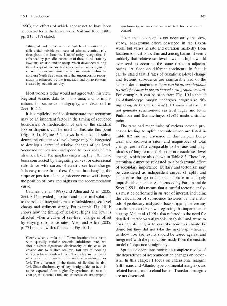
10.1 Introduction 263
1990), the effects of which appear not to have beenaccounted for in the Exxon work. Vail and Todd (1981,pp. 216–217) stated:
Tilting of beds as a result of fault-block rotation anddifferential subsidence occurred almost continuouslythroughout the Jurassic. Unconformity recognition isenhanced by periodic truncation of these tilted strata bylowstand erosion and/or onlap which developed duringthe subsequent rise. We find no evidence that the regionalunconformities are caused by tectonic events within thenorthern North Sea basins, only that unconformity recog-nition is enhanced by the truncation and onlap patternscreated by tectonic activity.
Most workers today would not agree with this view.Regional seismic data from this area, and its impli-cations for sequence stratigraphy, are discussed inSect. 10.2.2.
It is simplicity itself to demonstrate that tectonismmay be an important factor in the timing of sequenceboundaries. A modification of one of the standardExxon diagrams can be used to illustrate this point(Fig. 10.1). Figure 2.2 shows how rates of subsi-dence and eustatic sea-level change may be integratedto develop a curve of relative changes of sea level.Sequence boundaries correspond to lowstands of rel-ative sea level. The graphs comprising Fig. 10.1 havebeen constructed by integrating curves for extensionalsubsidence with curves of eustatic sea-level change.It is easy to see from these figures that changing theslope or position of the subsidence curve will changethe position of lows and highs on the accommodationcurve.
Catuneanu et al. (1998) and Allen and Allen (2005,Sect. 8.1) provided graphical and numerical solutionsto the issue of integrating rates of subsidence, sea-levelchange and sediment supply. For example, Fig. 10.1bshows how the timing of sea-level highs and lows isaffected when a curve of sea-level change is offsetby varying subsidence rates. Allen and Allen (2005,p. 271) stated, with reference to Fig. 10.1b:
Clearly when correlating different locations in a basinwith spatially variable tectonic subsidence rate, weshould expect significant diachroneity of the onset oferosion due to relative sea-level fall and of floodingduring relative sea-level rise. The delay in the onsetof erosion is a quarter of a eustatic wavelength orλ/4. The difference in the timing of flooding is alsoλ/4. Since diachroneity of key stratigraphic surfaces isto be expected from a globally synchronous eustaticchange, it is curious that the inference of stratigraphic
synchroneity is seen as an acid test for a eustaticcontrol.
Given that tectonism is not necessarily the slow,steady, background effect described in the Exxonwork, but varies in rate and duration markedly fromlocation to location, within and among basins, it seemsunlikely that relative sea-level lows and highs wouldever tend to occur at the same times in adjacentbasins, let alone on different continents. In fact, itcan be stated that if rates of eustatic sea-level changeand tectonic subsidence are comparable and of thesame order of magnitude there can be no synchronousrecord of eustasy in the preserved stratigraphic record.For example, it can be seen from Fig. 10.1a that ifan Atlantic-type margin undergoes progressive rift-ing along strike (“unzipping”), 107-year eustasy willnot generate synchronous sea-level highs and lows.Parkinson and Summerhayes (1985) made a similarpoint.
The rates and magnitudes of various tectonic pro-cesses leading to uplift and subsidence are listed inTable 8.2 and are discussed in this chapter. Long-term and short-term rates, and magnitudes of totalchange, are in fact comparable to the rates and mag-nitudes of long-term and short-term eustatic sea-levelchange, which are also shown in Table 8.2. Therefore,tectonism cannot be relegated to a background effectof secondary importance. Eustasy and tectonism maybe considered as independent curves of uplift andsubsidence that go in and out of phase in a largelyunpredictable manner. As discussed by Fortuin and deSmet (1991), this means that a careful tectonic analy-sis must be performed in an area of interest, includingthe calculation of subsidence histories by the meth-ods of geohistory analysis or backstripping, before anyconclusions can be drawn regarding the importance ofeustasy. Vail et al. (1991) also referred to the need fordetailed “tectono-stratigraphic analysis” and went toconsiderable lengths to describe how this should bedone; but they did not take the next step, which isto show how the results should be tested against andintegrated with the predictions made from the eustaticmodel of sequence stratigraphy.
Space considerations prohibit a complete review ofthe dependence of accommodation changes on tecton-ism. In this chapter I focus on extensional margins(rift basins and Atlantic-type continental margins), arcrelated basins, and foreland basins. Transform marginsare not discussed.
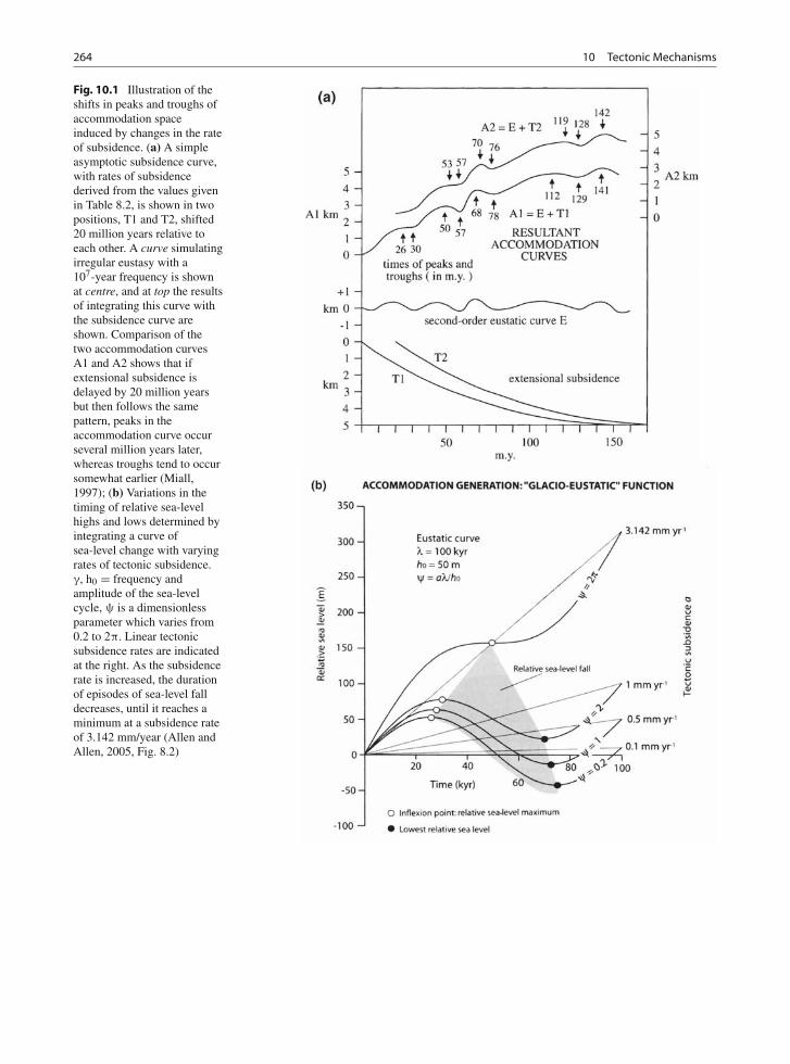
264 10 Tectonic Mechanisms
Fig. 10.1 Illustration of theshifts in peaks and troughs ofaccommodation spaceinduced by changes in the rateof subsidence. (a) A simpleasymptotic subsidence curve,with rates of subsidencederived from the values givenin Table 8.2, is shown in twopositions, T1 and T2, shifted20 million years relative toeach other. A curve simulatingirregular eustasy with a107-year frequency is shownat centre, and at top the resultsof integrating this curve withthe subsidence curve areshown. Comparison of thetwo accommodation curvesA1 and A2 shows that ifextensional subsidence isdelayed by 20 million yearsbut then follows the samepattern, peaks in theaccommodation curve occurseveral million years later,whereas troughs tend to occursomewhat earlier (Miall,1997); (b) Variations in thetiming of relative sea-levelhighs and lows determined byintegrating a curve ofsea-level change with varyingrates of tectonic subsidence.γ, h0 = frequency andamplitude of the sea-levelcycle, ψ is a dimensionlessparameter which varies from0.2 to 2π. Linear tectonicsubsidence rates are indicatedat the right. As the subsidencerate is increased, the durationof episodes of sea-level falldecreases, until it reaches aminimum at a subsidence rateof 3.142 mm/year (Allen andAllen, 2005, Fig. 8.2)
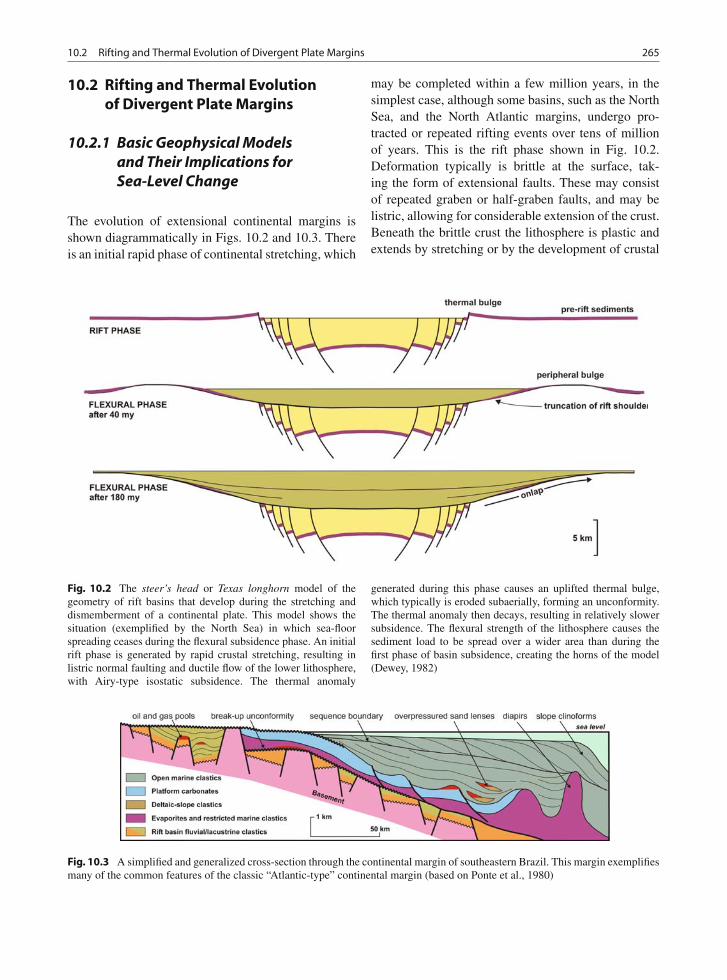
10.2 Rifting and Thermal Evolution of Divergent Plate Margins 265
10.2 Rifting and Thermal Evolutionof Divergent Plate Margins
10.2.1 Basic Geophysical Modelsand Their Implications forSea-Level Change
The evolution of extensional continental margins isshown diagrammatically in Figs. 10.2 and 10.3. Thereis an initial rapid phase of continental stretching, which
may be completed within a few million years, in thesimplest case, although some basins, such as the NorthSea, and the North Atlantic margins, undergo pro-tracted or repeated rifting events over tens of millionof years. This is the rift phase shown in Fig. 10.2.Deformation typically is brittle at the surface, tak-ing the form of extensional faults. These may consistof repeated graben or half-graben faults, and may belistric, allowing for considerable extension of the crust.Beneath the brittle crust the lithosphere is plastic andextends by stretching or by the development of crustal
Fig. 10.2 The steer’s head or Texas longhorn model of thegeometry of rift basins that develop during the stretching anddismemberment of a continental plate. This model shows thesituation (exemplified by the North Sea) in which sea-floorspreading ceases during the flexural subsidence phase. An initialrift phase is generated by rapid crustal stretching, resulting inlistric normal faulting and ductile flow of the lower lithosphere,with Airy-type isostatic subsidence. The thermal anomaly
generated during this phase causes an uplifted thermal bulge,which typically is eroded subaerially, forming an unconformity.The thermal anomaly then decays, resulting in relatively slowersubsidence. The flexural strength of the lithosphere causes thesediment load to be spread over a wider area than during thefirst phase of basin subsidence, creating the horns of the model(Dewey, 1982)
Fig. 10.3 A simplified and generalized cross-section through the continental margin of southeastern Brazil. This margin exemplifiesmany of the common features of the classic “Atlantic-type” continental margin (based on Ponte et al., 1980)
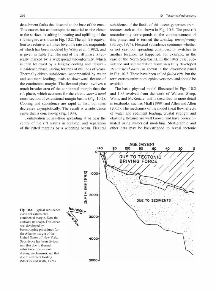
266 10 Tectonic Mechanisms
detachment faults that descend to the base of the crust.This causes hot asthenospheric material to rise closerto the surface, resulting in heating and uplifting of therift margins, as shown in Fig. 10.2. The uplift is equiva-lent to a relative fall in sea level, the rate and magnitudeof which has been modeled by Watts et al. (1982), andis given in Table 8.2. The end of the rift phase is typ-ically marked by a widespread unconformity, whichis then followed by a lengthy cooling and flexural-subsidence phase, lasting for tens of millions of years.Thermally-driven subsidence, accompanied by waterand sediment loading, leads to downward flexure ofthe continental margin. The flexural phase involves amuch broader area of the continental margin than therift phase, which accounts for the classic steer’s headcross-section of extensional-margin basins (Fig. 10.2).Cooling and subsidence are rapid at first, but ratesdecreases asymptotically. The result is a subsidencecurve that is concave-up (Fig. 10.4).
Continuation of sea-floor spreading at or near thecentre of the rift results in breakup, and separationof the rifted margins by a widening ocean. Flexural
subsidence of the flanks of this ocean generates archi-tectures such as that shown in Fig. 10.3. The post-riftunconformity corresponds to the commencement ofthis phase, and is termed the breakup unconformity(Falvey, 1974). Flexural subsidence continues whetheror not sea-floor spreading continues, or switches toanother location (as happened, for example, in thecase of the North Sea basin). In the latter case, sub-sidence and sedimentation result in a fully developedsteer’s head basin, as shown in the lowermost panelin Fig. 10.2. These have been called failed rifts, but theterm carries anthropomorphic overtones, and should beavoided.
The basic physical model illustrated in Figs. 10.2and 10.3 evolved from the work of Walcott, Sleep,Watts, and McKenzie, and is described in more detailin textbooks, such as Miall (1999) and Allen and Allen(2005). The mechanics of the model (heat flow, effectsof water and sediment loading, crustal strength andelasticity, flexure) are well known, and have been sim-ulated using numerical modeling. Stratigraphic andother data may be backstripped to reveal tectonic
Fig. 10.4 Typical subsidencecurve for extensionalcontinental margin. Note theconcave-up shape. This curvewas developed bybackstripping procedures forthe Atlantic margin of theUnited States off New York.Subsidence has been dividedinto that due to thermalsubsidence (the tectonicdriving mechanism), and thatdue to sediment loading(Steckler and Watts, 1978)
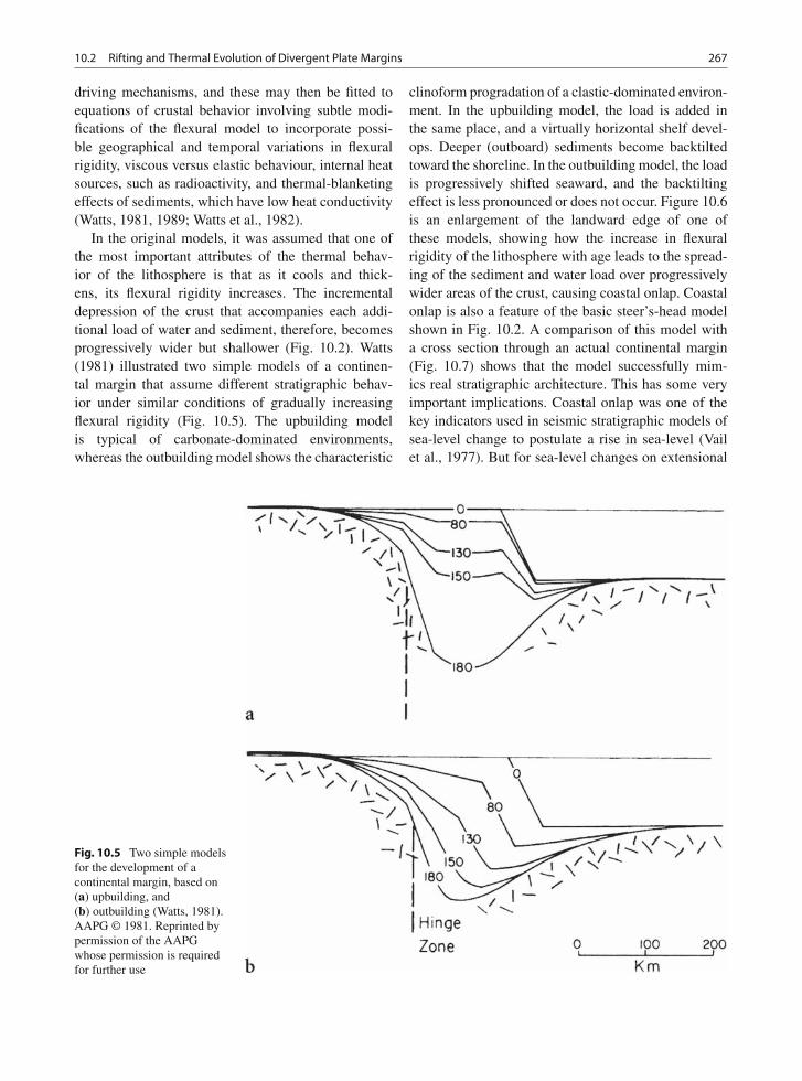
10.2 Rifting and Thermal Evolution of Divergent Plate Margins 267
driving mechanisms, and these may then be fitted toequations of crustal behavior involving subtle modi-fications of the flexural model to incorporate possi-ble geographical and temporal variations in flexuralrigidity, viscous versus elastic behaviour, internal heatsources, such as radioactivity, and thermal-blanketingeffects of sediments, which have low heat conductivity(Watts, 1981, 1989; Watts et al., 1982).
In the original models, it was assumed that one ofthe most important attributes of the thermal behav-ior of the lithosphere is that as it cools and thick-ens, its flexural rigidity increases. The incrementaldepression of the crust that accompanies each addi-tional load of water and sediment, therefore, becomesprogressively wider but shallower (Fig. 10.2). Watts(1981) illustrated two simple models of a continen-tal margin that assume different stratigraphic behav-ior under similar conditions of gradually increasingflexural rigidity (Fig. 10.5). The upbuilding modelis typical of carbonate-dominated environments,whereas the outbuilding model shows the characteristic
clinoform progradation of a clastic-dominated environ-ment. In the upbuilding model, the load is added inthe same place, and a virtually horizontal shelf devel-ops. Deeper (outboard) sediments become backtiltedtoward the shoreline. In the outbuilding model, the loadis progressively shifted seaward, and the backtiltingeffect is less pronounced or does not occur. Figure 10.6is an enlargement of the landward edge of one ofthese models, showing how the increase in flexuralrigidity of the lithosphere with age leads to the spread-ing of the sediment and water load over progressivelywider areas of the crust, causing coastal onlap. Coastalonlap is also a feature of the basic steer’s-head modelshown in Fig. 10.2. A comparison of this model witha cross section through an actual continental margin(Fig. 10.7) shows that the model successfully mim-ics real stratigraphic architecture. This has some veryimportant implications. Coastal onlap was one of thekey indicators used in seismic stratigraphic models ofsea-level change to postulate a rise in sea-level (Vailet al., 1977). But for sea-level changes on extensional
Fig. 10.5 Two simple modelsfor the development of acontinental margin, based on(a) upbuilding, and(b) outbuilding (Watts, 1981).AAPG © 1981. Reprinted bypermission of the AAPGwhose permission is requiredfor further use
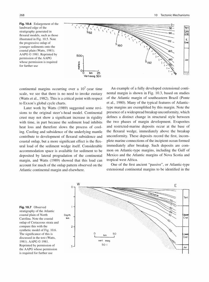
268 10 Tectonic Mechanisms
Fig. 10.6 Enlargement of thelandward edge of thestratigraphy generated inflexural models, such as thoseillustrated in Fig. 10.5. Notethe progressive onlap ofyounger sediments onto thecoastal plain (Watts, 1981).AAPG © 1981. Reprinted bypermission of the AAPGwhose permission is requiredfor further use
continental margins occurring over a 107-year timescale, we see that there is no need to invoke eustasy(Watts et al., 1982). This is a critical point with respectto Exxon’s global cycle charts.
Later work by Watts (1989) suggested some revi-sions to the original steer’s-head model. Continentalcrust may not show a significant increase in rigiditywith time, in part because the sediment load inhibitsheat loss and therefore slows the process of cool-ing. Cooling and subsidence of the underlying mantlecontribute to development of flexural subsidence andcoastal onlap, but a more significant effect is the flex-ural load of the sediment wedge itself. Considerableaccommodation space is available for sediment to bedeposited by lateral progradation of the continentalmargin, and Watts (1989) showed that this load canaccount for much of the onlap pattern observed on theAtlantic continental margin and elsewhere.
An example of a fully developed extensional conti-nental margin is shown in Fig. 10.3, based on studiesof the Atlantic margin of southeastern Brazil (Ponteet al., 1980). Many of the typical features of Atlantic-type margins are exemplified by this margin. Note thepresence of a widespread breakup unconformity, whichdefines a distinct change in structural style betweenthe two phases of margin development. Evaporitesand restricted-marine deposits occur at the base ofthe flexural wedge, immediately above the breakupunconformity. These deposits record the first, incom-plete marine connections of the incipient ocean formedimmediately after breakup. Such deposits are com-mon on Atlantic-type margins, including the Gulf ofMexico and the Atlantic margins of Nova Scotia andtropical west Africa.
One of the first ancient “passive”, or Atlantic-typeextensional continental margins to be identified in the
Fig. 10.7 Observedstratigraphy of the Atlanticcoastal plain of NorthCarolina. Note the coastalonlap of Cretaceous strata andcompare this with thesynthetic model of Fig. 10.6.The significance of this isdiscussed in the text (Watts,1981). AAPG © 1981.Reprinted by permission ofthe AAPG whose permissionis required for further use
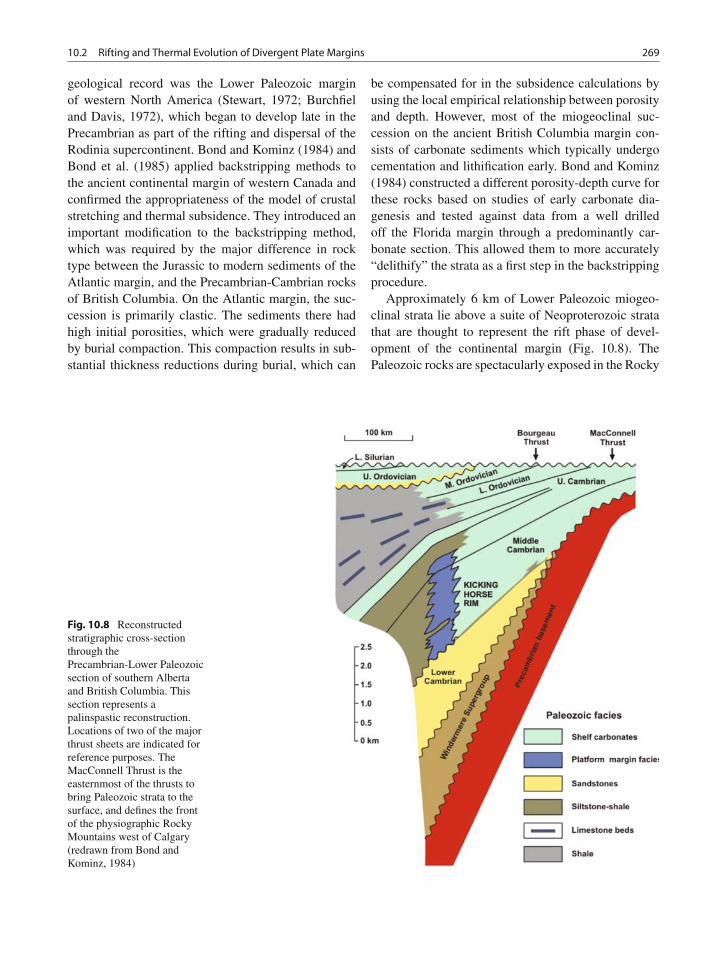
10.2 Rifting and Thermal Evolution of Divergent Plate Margins 269
geological record was the Lower Paleozoic marginof western North America (Stewart, 1972; Burchfieland Davis, 1972), which began to develop late in thePrecambrian as part of the rifting and dispersal of theRodinia supercontinent. Bond and Kominz (1984) andBond et al. (1985) applied backstripping methods tothe ancient continental margin of western Canada andconfirmed the appropriateness of the model of crustalstretching and thermal subsidence. They introduced animportant modification to the backstripping method,which was required by the major difference in rocktype between the Jurassic to modern sediments of theAtlantic margin, and the Precambrian-Cambrian rocksof British Columbia. On the Atlantic margin, the suc-cession is primarily clastic. The sediments there hadhigh initial porosities, which were gradually reducedby burial compaction. This compaction results in sub-stantial thickness reductions during burial, which can
be compensated for in the subsidence calculations byusing the local empirical relationship between porosityand depth. However, most of the miogeoclinal suc-cession on the ancient British Columbia margin con-sists of carbonate sediments which typically undergocementation and lithification early. Bond and Kominz(1984) constructed a different porosity-depth curve forthese rocks based on studies of early carbonate dia-genesis and tested against data from a well drilledoff the Florida margin through a predominantly car-bonate section. This allowed them to more accurately“delithify” the strata as a first step in the backstrippingprocedure.
Approximately 6 km of Lower Paleozoic miogeo-clinal strata lie above a suite of Neoproterozoic stratathat are thought to represent the rift phase of devel-opment of the continental margin (Fig. 10.8). ThePaleozoic rocks are spectacularly exposed in the Rocky
Fig. 10.8 Reconstructedstratigraphic cross-sectionthrough thePrecambrian-Lower Paleozoicsection of southern Albertaand British Columbia. Thissection represents apalinspastic reconstruction.Locations of two of the majorthrust sheets are indicated forreference purposes. TheMacConnell Thrust is theeasternmost of the thrusts tobring Paleozoic strata to thesurface, and defines the frontof the physiographic RockyMountains west of Calgary(redrawn from Bond andKominz, 1984)
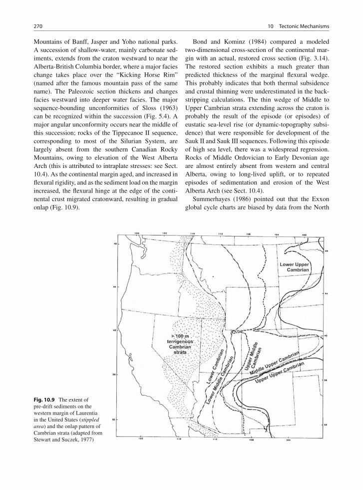
270 10 Tectonic Mechanisms
Mountains of Banff, Jasper and Yoho national parks.A succession of shallow-water, mainly carbonate sed-iments, extends from the craton westward to near theAlberta-British Columbia border, where a major facieschange takes place over the “Kicking Horse Rim”(named after the famous mountain pass of the samename). The Paleozoic section thickens and changesfacies westward into deeper water facies. The majorsequence-bounding unconformities of Sloss (1963)can be recognized within the succession (Fig. 5.4). Amajor angular unconformity occurs near the middle ofthis succession; rocks of the Tippecanoe II sequence,corresponding to most of the Silurian System, arelargely absent from the southern Canadian RockyMountains, owing to elevation of the West AlbertaArch (this is attributed to intraplate stresses: see Sect.10.4). As the continental margin aged, and increased inflexural rigidity, and as the sediment load on the marginincreased, the flexural hinge at the edge of the conti-nental crust migrated cratonward, resulting in gradualonlap (Fig. 10.9).
Bond and Kominz (1984) compared a modeledtwo-dimensional cross-section of the continental mar-gin with an actual, restored cross section (Fig. 3.14).The restored section exhibits a much greater thanpredicted thickness of the marginal flexural wedge.This probably indicates that both thermal subsidenceand crustal thinning were underestimated in the back-stripping calculations. The thin wedge of Middle toUpper Cambrian strata extending across the craton isprobably the result of the episode (or episodes) ofeustatic sea-level rise (or dynamic-topography subsi-dence) that were responsible for development of theSauk II and Sauk III sequences. Following this episodeof high sea level, there was a widespread regression.Rocks of Middle Ordovician to Early Devonian ageare almost entirely absent from western and centralAlberta, owing to long-lived uplift, or to repeatedepisodes of sedimentation and erosion of the WestAlberta Arch (see Sect. 10.4).
Summerhayes (1986) pointed out that the Exxonglobal cycle charts are biased by data from the North
Fig. 10.9 The extent ofpre-drift sediments on thewestern margin of Laurentiain the United States (stippledarea) and the onlap pattern ofCambrian strata (adapted fromStewart and Suczek, 1977)
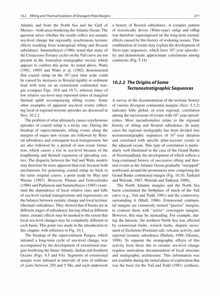
10.2 Rifting and Thermal Evolution of Divergent Plate Margins 271
Atlantic and from the North Sea and the Gulf ofMexico—both areas bordering the Atlantic Ocean. Thequestion arises whether the results reflect not eustaticsea-level change but regionally synchronous tectoniceffects resulting from widespread rifting and flexuralsubsidence. Summerhayes (1986) noted that many ofthe Cretaceous-Tertiary cycles on the Vail curve are notpresent in the Australian stratigraphic record, whichappears to confirm this point. As noted above, Watts(1981, 1989) and Watts et al. (1982) demonstratedthat coastal onlap on the 107-year time scale couldbe caused by increases in flexural rigidity or sedimentload with time on an extensional continental mar-gin (compare Figs. 10.6 and 10.7), whereas times oflow relative sea-level may represent times of marginalthermal uplift accompanying rifting events. Someother examples of apparent sea-level events reflect-ing local or regional tectonic episodes are discussed inSect. 10.2.2.
The problem of what ultimately causes synchronousepisodes of coastal onlap is a tricky one. During thebreakup of supercontinents, rifting events along themargins of major new oceans are followed by flexu-ral subsidence and consequent local transgression, butare also followed by a period of new-ocean forma-tion, which causes a rise in sea-level because of thelengthening and thermal expansion of spreading cen-ters. The disparity between the Vail and Watts modelsmay therefore be more apparent than real, because bothmechanisms for generating coastal onlap tie back tothe same original causes, a point made by May andWarme (1987). However, Pitman and Golovchenko(1988) and Parkinson and Summerhayes (1985) exam-ined the dependence of local relative rises and fallsof sea-level (actual transgressions and regressions) onthe balance between eustatic change and local tectonic(thermal) subsidence. They showed that if basins are indifferent stages of subsidence, having rifted at differenttimes, eustatic effects may be masked to the extent thatlocal sea-level changes may be completely different ineach basin. This point was made in the introduction tothis chapter, with reference to Fig. 10.1.
The breakup of the supercontinent Pangea, whichinitiated a long-term cycle of sea-level change, wasaccompanied by the development of extensional mar-gins bordering the future Atlantic, Indian and SouthernOceans (Figs. 9.5 and 9.6). Segments of extensionalmargin were initiated at intervals of tens of millionsof years between 250 and 5 Ma, and each underwent
a history of flexural subsidence. A complex patternof tectonically driven (Watts-type) onlap and offlapwas therefore superimposed on the long-term eustaticeffects caused by this history of widening oceans. Thiscombination of events may explain the development ofSloss-type sequences, which have 107-year episodic-ity and demonstrate approximate correlations amongcontinents (Fig. 5.14).
10.2.2 The Origins of SomeTectonostratigraphic Sequences
A survey of the documentation of the tectonic historyof various divergent continental margins (Sect. 5.3.2)indicates little global, or even regional, correlationamong the successions of events with 107-year episod-icities. Most unconformities relate to the regionalhistory of rifting and flexural subsidence. In manycases the regional stratigraphy has been divided intotectonostratigraphic sequences of 107-year durationand correlated with specific plate-tectonic events inthe adjacent ocean. This type of correlation is partic-ularly well illustrated in the case of the Grand Banksof Newfoundland, the development of which reflects along-continued history of successive rifting and ther-mal events as the Atlantic Ocean gradually “unzipped”northward, around the promontory now comprising theGrand Banks continental margin (Fig. 10.10; Tankardand Welsink, 1987; Welsink and Tankard, 1988).
The North Atlantic margins and the North Seabasin constituted the birthplace of much of the Vailcurve (e.g., Vail and Todd, 1981) and the controversysurrounding it (Miall, 1986). Extensional continen-tal margins are commonly termed “passive” margins,to contrast them with “active” convergent margins.However, this may be misleading. For example, dur-ing the Jurassic, the northern North Sea was affectedby extensional faults, wrench faults, diapiric move-ment of Zechstein (Permian) salt, volcanic activity, andregional isostatic subsidence (Hallam, 1988; Glennie,1998). To separate the stratigraphic effects of thisactivity from those due to eustatic sea-level changerequires meticulous documentation of local structureand stratigraphic architecture. This information wasnot available during the initial phase of exploration thatwas the basis for the Vail and Todd (1981) synthesis.
272 10 Tectonic Mechanisms
Fig. 10.10 Tectonic sequence analysis of the Jeanne d’ArcBasin, Grand Banks of Newfoundland, showing the fivemajor unconformity-bounded tectono-stratigraphic sequencesinterpreted on the basis of seismic-stratigraphic analysis, with
the Exxon global cycle chart at right, for comparison (Tankardet al., 1989). AAPG © 1989. Reprinted by permission of theAAPG whose permission is required for further use
10.2 Rifting and Thermal Evolution of Divergent Plate Margins 273
Subsequently, Badley et al. (1988) used a large seismicdata set to examine the structural evolution of the NorthViking Graben, and documented the ongoing natureof extensional tectonism during the Mesozoic. Hiscottet al. (1990) and Sinclair et al. (1994) have examinedthe Jurassic-Cretaceous rifting history of the basins ofMaritime Canada, Iberia, and the continental marginwest of the British Isles. Underhill (1991) reexaminedthe seismic data base of the Moray Firth, North Sea,on which much of the Jurassic part of the Vail curveswas based. Underhill and Partington (1993a, b) demon-strated the occurrence of a significant thermal heatingand uplift event in the mid-Jurassic. A book edited byHardman and Brooks (1990) on the tectonic evolutionof the British continental margins provides a wealth ofdata on this topic. The consensus is that vertical move-ments accompanying rift faulting and thermal effectswere ubiquitous. Badley et al. (1988, p. 460) stated:
Numerous authors have discussed unconformities andtheir causes in the northern North Sea (e.g. Vail & Todd1981; Rawson & Riley 1982; Ziegler 1982; Miall 1986).The structural evolution of the northern Viking Grabenpresented below shows extension-related tectonics tohave been the primary causal mechanism in the devel-opment of unconformities in the area. Sea-level changesappear to have played only a secondary role in uncon-formity development. Two types of tectonically-inducedunconformity are commonly recognized in extensionalbasins: regionally-developed, angular stratal relation-ships related to differential block tilting, and local strati-graphic breaks on the crests of fault blocks elevated byfootwall uplift, often involving erosion.
Badley et al. (1988) documented numerous exam-ples of unconformities related to faulting, and wedge-shaped stratigraphic units developed by onlap duringpost-rift thermal subsidence. They recognized rift-thermal subsidence phases during the Triassic-EarlyJurassic, Bathonian-Kimmeridgian, Kimmeridgian-Ryazanian, Albian, Turonian-Cenomanian and LateCretaceous-Early Tertiary. They pointed out that mostof these phases of movement were local, and shouldnot be correlated with regional tectonic pulses, such asthe Cimmerian, sub-Hercynian, Austrian or Laramidemovements, as had been suggested by some writers(e.g., Ziegler, 1982).
The documentation of repeated regional rifting andthermal-subsidence events based on extensive analysisof seismic-reflection data (e.g., Badley et al., 1988),would seem to leave little cause to invoke eustasyas a mechanism for generating the observed regional
unconformities. Indeed, it seems that, fortuitously ornot, the Exxon seismic line in the Moray Firth, offnortheast Scotland, one of two used in the major anal-ysis by Vail and Todd (1981) and Vail et al. (1984),did not cross the major faults whose movement, itis now thought, was responsible for developing theunconformities that they observed. Underhill (1991)showed that the major faults are oriented northeast-southwest in this area, and this is the orientation ofthe Exxon line! He demonstrated that rotation of faultblocks is a primary cause of unconformable onlap inthis area (Fig. 10.11). When seen perpendicular to thefault trend this is revealed by a distinctive fanningof stratigraphic units, caused by block rotation dur-ing fault-induced subsidence and sedimentary onlap(Fig. 10.11). However, this is obscure in fault-parallelsections.
Another aspect of stratigraphic architecture thatmay be of tectonic or eustatic origin or may be unre-lated to either is the downlapping pattern developedby the progradation of submarine fans. As pointedout by Miall (1986) onlapping by itself is an unre-liable indicator of a relative rise of sea level, unlessit can be demonstrated that the facies showing theonlap are coastal in origin, which is difficult to accom-plish from seismic-facies data alone. However, mostof the strata analyzed by Vail and Todd (1981) aredeep-marine fan deposits. Fan progradation may leadto onlap of tilted basement surfaces, and could beinterpreted as a product of fan growth during sea-level falling stage to lowstand (Fig. 2.8). However,fan rejuvenation may be triggered by fault movement,and fan switching can occur entirely as a result ofautogenic channel-switching processes. A quantitativemodel of half-graben subsidence that explored the vari-ables of sediment input, block rotation and isostaticresponse was offered by Roberts et al. (1993), whoshowed how the model could be applied to specificaspects of the Viking Graben. Prosser (1993) exam-ined the paleogeography of evolving rift basins andthe resulting seismic facies and architecture, and pro-posed a series of models of tectonic systems tractslinked to stages in rift evolution. White and Lovell(1997) demonstrated that the major submarine fans inthe North Sea and Shetland-Faeroes Basin were devel-oped during phases of magmatic underplating of theBritish Isles area, which caused uplift and erosion,and increased sediment delivery to the adjacent marinebasins (Fig. 10.12).
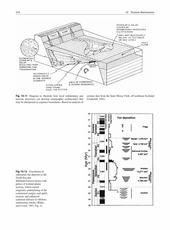
274 10 Tectonic Mechanisms
Fig. 10.11 Diagram to illustrate how local sedimentary andtectonic processes can develop stratigraphic architectures thatmay be interpreted as sequence boundaries. Based on analysis of
seismic data from the Inner Moray Firth, off northeast Scotland(Underhill, 1991)
Fig. 10.12 Correlation ofsubmarine fan deposits in theNorth Sea andShetland-Faeroes basins withpulses of Iceland plumeactivity, which causedmagmatic underplating of thecontinental margin, and uplift,erosion, and enhancedsediment delivery to offshoresedimentary basins (Whiteand Lovell, 1997, Fig. 2)
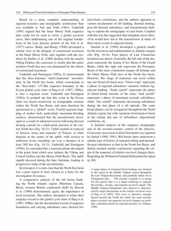
10.2 Rifting and Thermal Evolution of Divergent Plate Margins 275
Based on a more complete understanding ofregional tectonics and stratigraphic architecture thanwas available to Vail and Todd (1981), Underhill(1991) argued that the Inner Moray Firth sequencedata could not be used to verify a global sea-levelcurve, thus undermining one of the original founda-tions of the Late Jurassic portion of the Vail et al.(1977) curves. Boldy and Brealy (1990) developed asimilar view of the ubiquity of extensional tectonismin the Outer Moray Firth, and, together with the syn-thesis by Badley et al. (1988) dealing with the nearbyViking Graben, the consensus is clearly that the entirenorthern North Sea area was dominated by the effectsof extensional tectonism.
Underhill and Partington (1993a, b) demonstratedthat the intra-Aalenian “mid-Cimmerian” unconfor-mity in the North Sea basin, which corresponds tothe “first-order” 177-Ma sequence boundary in theExxon global cycle chart of Haq et al. (1987, 1988a),is also a regional event. Underhill and Partington(1993a, b) pointed out that this event in the Exxonchart was based exclusively on stratigraphic sectionswithin the North Sea Basin, and must therefore bequestioned as a “global” event. Careful regional map-ping of marker beds, particularly maximum-floodingsurfaces, demonstrated that the unconformity devel-oped as a result of subaerial erosion following thermaldoming centred on a triple-point junction in the cen-tral North Sea (Fig. 10.13). Uplift resulted in removalof Jurassic strata and exposure of Triassic or olderdeposits at the centre of the uplift, with erosion toshallower levels extending out over a distance of atleast 500 km (Fig. 10.13). Underhill and Partington(1993a, b) concluded that a transient plume developedat the point from which now radiates the Viking andCentral Graben and the Moray Firth Basin. The upliftrapidly decayed during the later Aalenian, leading toprogressive onlap of the unconformity.
In retrospect, it is now clear that the North Sea basinwas a poor region to have chosen as a basis for theinvestigation of eustasy.
A comparative analysis of the rift basins flank-ing the North Atlantic region (Maritime Canada,Iberia, western British continental shelf) by Hiscottet al. (1990) demonstrated, again, the importance oflocal tectonism. The authors attempted to relate theirsequence record to the global cycle chart of Haq et al.(1987, 1988a), but the documented record of sequenceboundaries and varying subsidence rates showed few
inter-basin correlations, and the authors appealed tovarious mechanisms of rift faulting, thermal doming,post-rift thermal subsidence, and transtensional fault-ing to explain the stratigraphy of each basin. Coupledwith this was the suggestion that intraplate stress (Sect.10.4) would have led to the transmission of many ofthese stress events to adjacent basins.
Sinclair et al. (1994) developed a general modelfor the tectonism and sedimentation in Atlantic-marginrifts (Fig. 10.14). Four phases of Late Cimmeriantectonism are shown. Generally, the left side of the dia-gram represents the Jeanne d’Arc Basin of the GrandBanks, while the right side represents the PorcupineBasin of the outer continental margin off Ireland, andthe Outer Moray Firth area of the North Sea basin.However, this range of responses can occur withinany one broad rift basin area. “Onset warp” representsa phase of regional subsidence variation without sig-nificant faulting. “Early synrift” represents the phaseof initial brittle fracture of the crust, “mid synrift”represents a phase of maximum tectonic subsidence,while “late synrift” represents decreasing subsidenceduring the last phase of a rift episode. The samebroad phases can be recognized throughout the NorthAtlantic region, but with variations from basin to basinin the timing and rate of subsidence, depositionalconditions, etc.
A detailed analysis of the sequence stratigraphyand of the tectonic-eustatic control of the Jurassic-Cretaceous succession in East Greenland was reportedby Surlyk (1990, 1991). Rift basins there underwent asimilar type of history of repeated rifting and thermal-flexural subsidence to that in the North Sea Basin, andSurlyk reached similar conclusions regarding the ori-gin of the sequence of relative sea-level changes there.Regarding the Wollaston Forland Embayment he stated(p. 80):
A major phase of rotational block-faulting was initiatedin the region in the Middle Volgian, lasted throughoutthe Late Volgian-Ryazanian, and gradually faded out inValanginian time . . . The tectonic overprint is so strongfor this period, that it is a major challenge to separatethe tectonic, eustatic, and regional sea-level signals. TheMiddle Volgian-Valanginian time interval is character-ized by major fluctuations in the eustatic sea-level curveof Haq et al (1987). This curve is, however, stronglybiased towards the North Sea where the same tectonicphase occurred; the apparent sea-level changes are prob-ably controlled mainly by regional tectonics (cf. Hallam,1988).
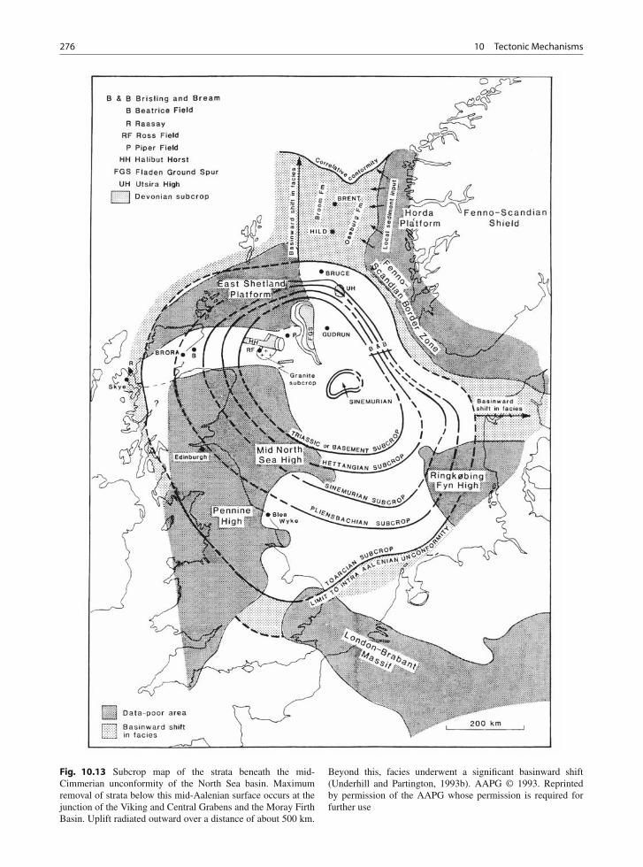
276 10 Tectonic Mechanisms
Fig. 10.13 Subcrop map of the strata beneath the mid-Cimmerian unconformity of the North Sea basin. Maximumremoval of strata below this mid-Aalenian surface occurs at thejunction of the Viking and Central Grabens and the Moray FirthBasin. Uplift radiated outward over a distance of about 500 km.
Beyond this, facies underwent a significant basinward shift(Underhill and Partington, 1993b). AAPG © 1993. Reprintedby permission of the AAPG whose permission is required forfurther use
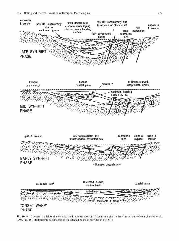
10.2 Rifting and Thermal Evolution of Divergent Plate Margins 277
Fig. 10.14 A general model for the tectonism and sedimentation of rift basins marginal to the North Atlantic Ocean (Sinclair et al.,1994, Fig. 15). Stratigraphic documentation for selected basins is provided in Fig. 5.18
278 10 Tectonic Mechanisms
Elsewhere Surlyk stated:
Substituting tectonism with sea level change as the domi-nating controlling factor on development of the WollastonForland Group is too simplistic. The basic aspects of thesystem in terms of geometry, environment, and processeswere undoubtedly controlled by tectonism. The large-scale cyclicity probably is controlled to a large extentby sea level rises. However, I suggest that the sea levelfluctuations were controlled by regional tectonism andthat each major episode of faulting is associated witha rapid relative sea level fall followed by a longer sealevel rise, reflecting increasing subsidence after rifting.This pattern would explain the presence and apparentcontemporaneity of the numerous high-amplitude, short-wavelength fluctuations in relative sea level in the NorthAtlantic region during the tectonically very active inter-val spanning the Jurassic-Cretaceous boundary. (Surlyk,1991, pp. 1483–5)
Rifting episodes can be linked directly to syn-chronous subsidence events and stratigraphicdevelopments on presently separate continents. Theopening of the present North Atlantic Ocean spanneda period of well over 100 million years, commencingduring the Early or mid-Jurassic with breakup andinitiation of sea-floor spreading between the Africanand North American continental plates, while the lastopening event occurred during Eocene time in theGreenland/Norwegian sea area (Pitman and Talwani,1972; Ziegler, 1988). “Rifting was neither continuousnor random in time and place during this long periodof Pangaean disintegration. Splitting of the Pangaeansupercontinent did not occur as a continuous migra-tion like the smooth opening of a zipper, but ratheroccurred as discrete events, with the lateral movementof diverging plates accommodated by large transfershear zones” (Sinclair et al., 1994, p. 212; see alsoFig. 9.6). As rifting preceded each breakup event(Falvey, 1974), the structural and stratigraphicresponses at the end of each widely recognized riftingevent can be related to the initiation of sea-floorspreading along a particular segment of the NorthAtlantic.
Janssen et al. (1995) showed by backstripping anal-ysis of over 200 well sections that subsidence patternsin rifted basins within and on the flanks of Africacan be related to changing intraplate stress patterns asthe oceans surrounding Africa opened between LateJurassic time and the present.
Loup and Wildi (1994) reported on a subsidenceanalysis of the Paris Basin and a comparison with othernorthwest European basins. None show the simple
concave-up subsidence-versus-time curve that wouldbe expected from a simple extensional basin (e.g.,Fig. 10.4). Most are characterized by short concavesegments, with periods of slow or no subsidence, inter-vals of accelerated subsidence, and intervals of uplift.Few of the events are synchronous over wide areasof northwest Europe. These results are interpreted asthe product of rifting, transtension, and basin inver-sion resulting from regional plate-tectonic movements,and subcrustal processes, including mantle plumes,together with intraplate stresses resulting from all theseprocesses.
Submarine erosion of continental margins reducesthe sediment load and allows for flexural rebound.Stratigraphically the result may look like a fall inrelative sea level. McGinnis et al. (1993) examinedthe supposed Late Eocene-Early Oligocene global fallin sea level, which has long been attributed to thedevelopment of an Antarctic ice sheet. They suggestedthat one important result of a global climatic cool-ing (which undoubtedly occurred in the mid-Cenozoic;see Fig. 4.10) would have been enhancement of lati-tudinal thermal gradients, leading to strengthening ofbottom currents and increased global submarine ero-sion. The amount of eustatic fall associated with thiscooling event therefore may have been significantlyexaggerated.
10.3 Tectonism on Convergent PlateMargins and in Collision Zones
10.3.1 Magmatic Arcs and Subduction
It is a truism to state that areas of convergent tectonismare areas of active tectonics. Several distinct processeslead to local and regional relative changes in sea level,which may be recorded as transgressive and regressivesedimentary cycles in the major basins overlying andflanking zones of convergence.
A study of an Upper Cretaceous volcaniclasticforearc-basin succession in Baja California led Fulfordand Busby (1993) to conclude that tectonic basin sub-sidence and source-area uplift were by far the mostimportant controls on the architecture of the basinfill. The overall succession indicates retrogradation,suggesting rapid basin subsidence along boundingfaults. The succession includes a coarsening-upward
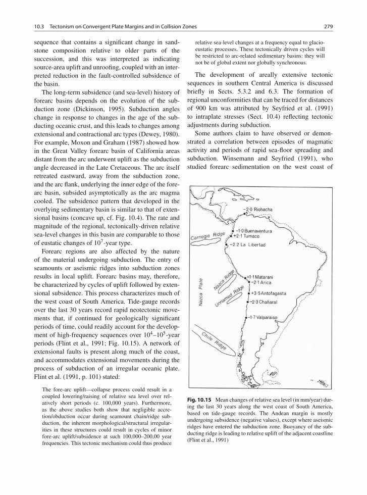
10.3 Tectonism on Convergent Plate Margins and in Collision Zones 279
sequence that contains a significant change in sand-stone composition relative to older parts of thesuccession, and this was interpreted as indicatingsource-area uplift and unroofing, coupled with an inter-preted reduction in the fault-controlled subsidence ofthe basin.
The long-term subsidence (and sea-level) history offorearc basins depends on the evolution of the sub-duction zone (Dickinson, 1995). Subduction angleschange in response to changes in the age of the sub-ducting oceanic crust, and this leads to changes amongextensional and contractional arc types (Dewey, 1980).For example, Moxon and Graham (1987) showed howin the Great Valley forearc basin of California areasdistant from the arc underwent uplift as the subductionangle decreased in the Late Cretaceous. The arc itselfretreated eastward, away from the subduction zone,and the arc flank, underlying the inner edge of the fore-arc basin, subsided asymptotically as the arc magmacooled. The subsidence pattern that developed in theoverlying sedimentary basin is similar to that of exten-sional basins (concave up, cf. Fig. 10.4). The rate andmagnitude of the regional, tectonically-driven relativesea-level changes in this basin are comparable to thoseof eustatic changes of 107-year type.
Forearc regions are also affected by the natureof the material undergoing subduction. The entry ofseamounts or aseismic ridges into subduction zonesresults in local uplift. Forearc basins may, therefore,be characterized by cycles of uplift followed by exten-sional subsidence. This process characterizes much ofthe west coast of South America. Tide-gauge recordsover the last 30 years record rapid neotectonic move-ments that, if continued for geologically significantperiods of time, could readily account for the develop-ment of high-frequency sequences over 104–105-yearperiods (Flint et al., 1991; Fig. 10.15). A network ofextensional faults is present along much of the coast,and accommodates extensional movements during theprocess of subduction of an irregular oceanic plate.Flint et al. (1991, p. 101) stated:
The fore-arc uplift—collapse process could result in acoupled lowering/raising of relative sea level over rel-atively short periods (c. 100,000 years). Furthermore,as the above studies both show that negligible accre-tion/obduction occur during seamount chain/ridge sub-duction, the inherent morphological/structural irregular-ities in these structures could result in cycles of minorfore-arc uplift/subsidence at such 100,000–200,00 yearfrequencies. This tectonic mechanism could thus produce
relative sea-level changes at a frequency equal to glacio-eustatic processes. These tectonically driven cycles willbe restricted to arc-related sedimentary basins: they willnot be of global extent nor globally synchronous.
The development of areally extensive tectonicsequences in southern Central America is discussedbriefly in Sects. 5.3.2 and 6.3. The formation ofregional unconformities that can be traced for distancesof 900 km was attributed by Seyfried et al. (1991)to intraplate stresses (Sect. 10.4) reflecting tectonicadjustments during subduction.
Some authors claim to have observed or demon-strated a correlation between episodes of magmaticactivity and periods of rapid sea-floor spreading andsubduction. Winsemann and Seyfried (1991), whostudied forearc sedimentation on the west coast of
Fig. 10.15 Mean changes of relative sea level (in mm/year) dur-ing the last 30 years along the west coast of South America,based on tide-gauge records. The Andean margin is mostlyundergoing subsidence (negative values), except where aseismicridges have entered the subduction zone. Buoyancy of the sub-ducting ridge is leading to relative uplift of the adjacent coastline(Flint et al., 1991)
280 10 Tectonic Mechanisms
Nicaragua, stated “the most striking feature is thealmost simultaneity of tectonic/volcanic activity andsecond order cycles of eustatic sea-level fluctua-tions during Late Cretaceous, Paleocene, and mid-lateEocene times.” They went on to say:
Late Cretaceous to late Eocene drift rates calculated fromthe North Atlantic Ocean correlate closely with globalorogenic phases which in turn coincide with crustalmovements in Central America. These episodes of majortectonic/volcanic activity occurred at 80–75, 63, 55–53,and 42–38 Ma and agree with major tectonic and vol-canic pulses in Central America . . . This corroboratesthat global tectonic processes play an important role ingenerating major sea-level fluctuations and hence in theformation of depositional sequences.
In and adjacent to arcs, magmatic intrusion resultsin regional doming over areas a few tens of kilome-tres across. Eruption is followed by deflation. Theresult is a lowering of relative sea level during thefilling of the magma chamber, followed by a riseaccompanying deflation of the chamber. Sloan andWilliams (1991) documented transgressive-regressivecycles in the Devonian of western Ireland, which theyinterpreted as the product of this process. Regressiveoffshore-barrier sequences a few tens-of-metres thickdeveloped during inflation of magma chambers andconsequent uplift. The sequences are capped by vol-canic intervals 1–190 m thick, recording eruptions, andthe overlying sedimentary units are deeper-water off-shore deposits indicating a rise in relative sea levelfollowing deflation and collapse of the magma cham-ber. The ages and durations of these sequences are notclear, but a 104–105-year episodicity seems probable.
10.3.2 Rates of Uplift and Subsidenceon Convergent Margins
One of the most impressive features of basins thatdevelop in regions of convergent tectonism, includ-ing arc-related basins and those within and adjacentto suture zones, is the extremely rapid rates of tec-tonic and sedimentary processes that occur in thesebasins. Figure 10.16 shows the history of subsidenceand uplift of various locations along the Banda Arc ofIndonesia, which is an area of convergence and colli-sion between Eurasia and the Australian and Pacificplates. At the bottom of this diagram is shown the
global cycle chart of Haq et al. (1987, 1988a) at thesame scale. Clearly the fluctuations indicated in thischart would be swamped by tectonic effects in an areaundergoing a tectonic evolution comparable to that ofthe Banda Arc.
Rapid rates of uplift and subsidence have beencalculated from many regions of active tectonism(rates are summarized in Table 8.2). Pedley andGrasso (1991) documented uplift rates in a subduction-accretion zone in southern Sicily, indicating localizedQuaternary uplift of up to 1 km. Bishop (1991) studiedraised terraces in the New Zealand Alps, a region char-acterized by transpressional uplift. Calculated upliftrates range from 5 to nearly 8 m/ka over periods ofabout 10 ka, with longer-term rates an order of mag-nitude smaller (1 m/ka for 100 ka). Data on rates ofmovement along the San Andreas transform systemwere summarized by May and Warme (1987), whonoted measured modern subsidence rates of 1.5 m/kain the Imperial Valley, and up to 2 m/ka in the EoceneVentura Basin. Uplift rates in the Banda Arc are illus-trated in Fig. 10.23, and range from 0.5 to 10 m/kaover periods of less than 2 million years (Fortuin andde Smet, 1991). Subsidence rates are not as rapid. Inthe Banda Arc, they range from 0.08 to 1 m/ka forperiods of up to 15 million years, resulting in a totalrecorded subsidence of up to 4 km. In the Himalayanproforeland basin of Pakistan, Johnson et al. (1986)and Burbank et al. (1986) demonstrated subsidence(actually sediment-accumulation) rates of up to 0.6m/ka persisting for 2–4 million years. The same over-all rate of sediment accumulation, 0.6 m/ka averagedover 2.5 million years, was obtained for an UpperCretaceous forearc-basin succession in Baja California(excluding possible but unknown eustatic effects) byFulford and Busby (1993), and Eocene forearc basinsin California subsided at rates between 0.1 and 0.7m/ka for periods measured over millions of years.Hiroki (1994) determined vertical changes in rela-tive sea level during the Quaternary in a forearc set-ting in coastal Japan and differentiated glacioeustaticfrom tectonic changes. He showed changes betweensubsidence and uplift over a 104–105-year interval,with considerable local variation in rates, probablyreflecting local structural controls. The maximumuplift rate, measured at one locality, was 0.29 m/ka,and the maximum subsidence rate was 0.45 m/ka.
The evidence indicates that uplift and subsidenceare spasmodic and localized, with movement rates and
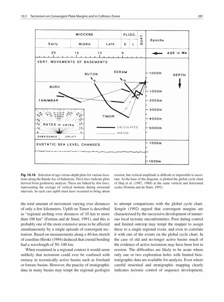
10.3 Tectonism on Convergent Plate Margins and in Collision Zones 281
Fig. 10.16 Selection of age-versus-depth plots for various loca-tions along the Banda Arc of Indonesia. Thick lines indicate plotsderived from geohistory analysis. These are linked by thin lines,representing the average of vertical motions during erosionalintervals. In each case uplift must have occurred to bring about
erosion, but vertical amplitude is difficult or impossible to ascer-tain. At the base of the diagram, is plotted the global cycle chartof Haq et al. (1987, 1988) at the same vertical and horizontalscales (Fortuin and de Smet, 1991)
the total amount of movement varying over distancesof only a few kilometres. Uplift on Timor is describedas “regional arching over distances of 10 km to morethan 100 km” (Fortuin and de Smet, 1991), and this isprobably one of the more extensive areas to be affectedsimultaneously by a single episode of convergent tec-tonism. Based on measurements along a 40-km stretchof coastline Hiroki (1994) deduced that crustal bendinghad a wavelength of 50–100 km.
When examined in a regional context it would seemunlikely that tectonism could ever be confused witheustasy in tectonically active basins such as forelandor forearc basins. However, the paucity of stratigraphicdata in many basins may tempt the regional geologist
to attempt comparisons with the global cycle chart.Sengör (1992) argued that convergent margins arecharacterized by the successive development of numer-ous local tectonic unconformities. Poor dating controland limited outcrop may tempt the mapper to assignthese to a single regional event, and even to correlateit with one of the events on the global cycle chart. Inthe case of old and no-longer active basins much ofthe evidence of active tectonism may have been lost toerosion. The difficulties are likely to be acute whereonly one or two exploration holes with limited bios-tratigraphic data are available for analysis. Even wherecareful structural and stratigraphic mapping clearlyindicates tectonic control of sequence development,
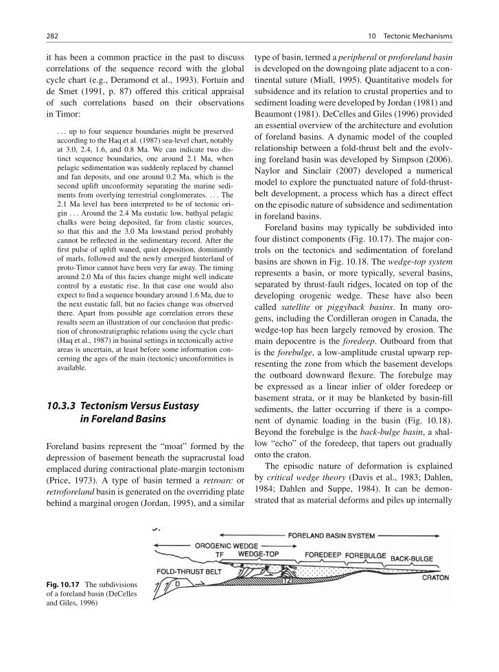
282 10 Tectonic Mechanisms
it has been a common practice in the past to discusscorrelations of the sequence record with the globalcycle chart (e.g., Deramond et al., 1993). Fortuin andde Smet (1991, p. 87) offered this critical appraisalof such correlations based on their observationsin Timor:
. . . up to four sequence boundaries might be preservedaccording to the Haq et al. (1987) sea-level chart, notablyat 3.0, 2.4, 1.6, and 0.8 Ma. We can indicate two dis-tinct sequence boundaries, one around 2.1 Ma, whenpelagic sedimentation was suddenly replaced by channeland fan deposits, and one around 0.2 Ma, which is thesecond uplift unconformity separating the marine sedi-ments from overlying terrestrial conglomerates. . . . The2.1 Ma level has been interpreted to be of tectonic ori-gin . . . Around the 2.4 Ma eustatic low, bathyal pelagicchalks were being deposited, far from clastic sources,so that this and the 3.0 Ma lowstand period probablycannot be reflected in the sedimentary record. After thefirst pulse of uplift waned, quiet deposition, dominantlyof marls, followed and the newly emerged hinterland ofproto-Timor cannot have been very far away. The timingaround 2.0 Ma of this facies change might well indicatecontrol by a eustatic rise. In that case one would alsoexpect to find a sequence boundary around 1.6 Ma, due tothe next eustatic fall, but no facies change was observedthere. Apart from possible age correlation errors theseresults seem an illustration of our conclusion that predic-tion of chronostratigraphic relations using the cycle chart(Haq et al., 1987) in basinal settings in tectonically activeareas is uncertain, at least before some information con-cerning the ages of the main (tectonic) unconformities isavailable.
10.3.3 Tectonism Versus Eustasyin Foreland Basins
Foreland basins represent the “moat” formed by thedepression of basement beneath the supracrustal loademplaced during contractional plate-margin tectonism(Price, 1973). A type of basin termed a retroarc orretroforeland basin is generated on the overriding platebehind a marginal orogen (Jordan, 1995), and a similar
type of basin, termed a peripheral or proforeland basinis developed on the downgoing plate adjacent to a con-tinental suture (Miall, 1995). Quantitative models forsubsidence and its relation to crustal properties and tosediment loading were developed by Jordan (1981) andBeaumont (1981). DeCelles and Giles (1996) providedan essential overview of the architecture and evolutionof foreland basins. A dynamic model of the coupledrelationship between a fold-thrust belt and the evolv-ing foreland basin was developed by Simpson (2006).Naylor and Sinclair (2007) developed a numericalmodel to explore the punctuated nature of fold-thrust-belt development, a process which has a direct effecton the episodic nature of subsidence and sedimentationin foreland basins.
Foreland basins may typically be subdivided intofour distinct components (Fig. 10.17). The major con-trols on the tectonics and sedimentation of forelandbasins are shown in Fig. 10.18. The wedge-top systemrepresents a basin, or more typically, several basins,separated by thrust-fault ridges, located on top of thedeveloping orogenic wedge. These have also beencalled satellite or piggyback basins. In many oro-gens, including the Cordilleran orogen in Canada, thewedge-top has been largely removed by erosion. Themain depocentre is the foredeep. Outboard from thatis the forebulge, a low-amplitude crustal upwarp rep-resenting the zone from which the basement developsthe outboard downward flexure. The forebulge maybe expressed as a linear inlier of older foredeep orbasement strata, or it may be blanketed by basin-fillsediments, the latter occurring if there is a compo-nent of dynamic loading in the basin (Fig. 10.18).Beyond the forebulge is the back-bulge basin, a shal-low “echo” of the foredeep, that tapers out graduallyonto the craton.
The episodic nature of deformation is explainedby critical wedge theory (Davis et al., 1983; Dahlen,1984; Dahlen and Suppe, 1984). It can be demon-strated that as material deforms and piles up internally
Fig. 10.17 The subdivisionsof a foreland basin (DeCellesand Giles, 1996)
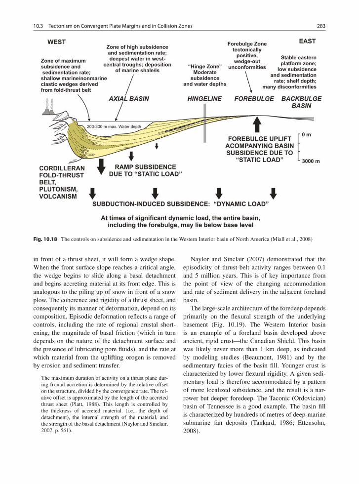
10.3 Tectonism on Convergent Plate Margins and in Collision Zones 283
Fig. 10.18 The controls on subsidence and sedimentation in the Western Interior basin of North America (Miall et al., 2008)
in front of a thrust sheet, it will form a wedge shape.When the front surface slope reaches a critical angle,the wedge begins to slide along a basal detachmentand begins accreting material at its front edge. This isanalogous to the piling up of snow in front of a snowplow. The coherence and rigidity of a thrust sheet, andconsequently its manner of deformation, depend on itscomposition. Episodic deformation reflects a range ofcontrols, including the rate of regional crustal short-ening, the magnitude of basal friction (which in turndepends on the nature of the detachment surface andthe presence of lubricating pore fluids), and the rate atwhich material from the uplifting orogen is removedby erosion and sediment transfer.
The maximum duration of activity on a thrust plane dur-ing frontal accretion is determined by the relative offseton the structure, divided by the convergence rate. The rel-ative offset is approximated by the length of the accretedthrust sheet (Platt, 1988). This length is controlled bythe thickness of accreted material. (i.e., the depth ofdetachment), the internal strength of the material, andthe strength of the basal detachment (Naylor and Sinclair,2007, p. 561).
Naylor and Sinclair (2007) demonstrated that theepisodicity of thrust-belt activity ranges between 0.1and 5 million years. This is of key importance fromthe point of view of the changing accommodationand rate of sediment delivery in the adjacent forelandbasin.
The large-scale architecture of the foredeep dependsprimarily on the flexural strength of the underlyingbasement (Fig. 10.19). The Western Interior basinis an example of a foreland basin developed aboveancient, rigid crust—the Canadian Shield. This basinwas likely never more than 1 km deep, as indicatedby modeling studies (Beaumont, 1981) and by thesedimentary facies of the basin fill. Younger crust ischaracterized by lower flexural rigidity. A given sedi-mentary load is therefore accommodated by a patternof more localized subsidence, and the result is a nar-rower but deeper foredeep. The Taconic (Ordovician)basin of Tennessee is a good example. The basin fillis characterized by hundreds of metres of deep-marinesubmarine fan deposits (Tankard, 1986; Ettensohn,2008).
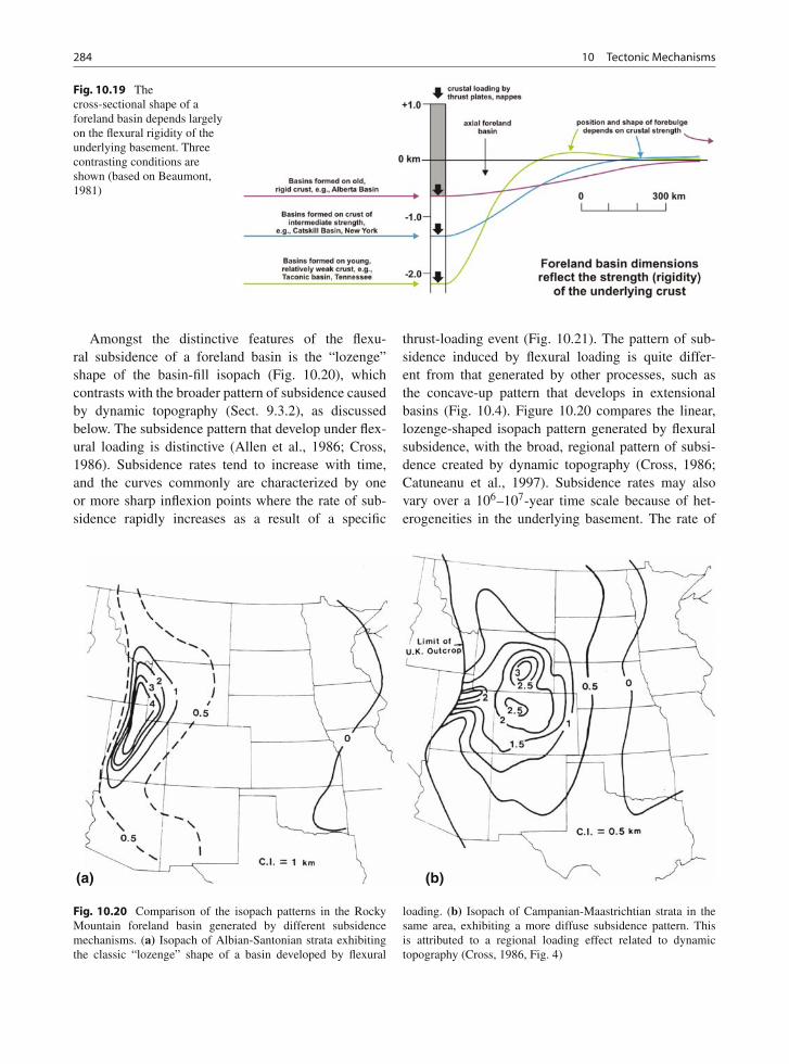
284 10 Tectonic Mechanisms
Fig. 10.19 Thecross-sectional shape of aforeland basin depends largelyon the flexural rigidity of theunderlying basement. Threecontrasting conditions areshown (based on Beaumont,1981)
Amongst the distinctive features of the flexu-ral subsidence of a foreland basin is the “lozenge”shape of the basin-fill isopach (Fig. 10.20), whichcontrasts with the broader pattern of subsidence causedby dynamic topography (Sect. 9.3.2), as discussedbelow. The subsidence pattern that develop under flex-ural loading is distinctive (Allen et al., 1986; Cross,1986). Subsidence rates tend to increase with time,and the curves commonly are characterized by oneor more sharp inflexion points where the rate of sub-sidence rapidly increases as a result of a specific
thrust-loading event (Fig. 10.21). The pattern of sub-sidence induced by flexural loading is quite differ-ent from that generated by other processes, such asthe concave-up pattern that develops in extensionalbasins (Fig. 10.4). Figure 10.20 compares the linear,lozenge-shaped isopach pattern generated by flexuralsubsidence, with the broad, regional pattern of subsi-dence created by dynamic topography (Cross, 1986;Catuneanu et al., 1997). Subsidence rates may alsovary over a 106–107-year time scale because of het-erogeneities in the underlying basement. The rate of
(a) (b)
Fig. 10.20 Comparison of the isopach patterns in the RockyMountain foreland basin generated by different subsidencemechanisms. (a) Isopach of Albian-Santonian strata exhibitingthe classic “lozenge” shape of a basin developed by flexural
loading. (b) Isopach of Campanian-Maastrichtian strata in thesame area, exhibiting a more diffuse subsidence pattern. Thisis attributed to a regional loading effect related to dynamictopography (Cross, 1986, Fig. 4)
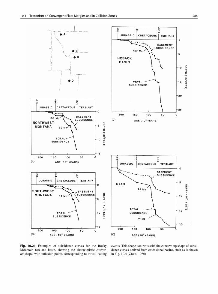
10.3 Tectonism on Convergent Plate Margins and in Collision Zones 285
Fig. 10.21 Examples of subsidence curves for the RockyMountain foreland basin, showing the characteristic convex-up shape, with inflexion points corresponding to thrust-loading
events. This shape contrasts with the concave-up shape of subsi-dence curves derived from extensional basins, such as is shownin Fig. 10.4 (Cross, 1986)
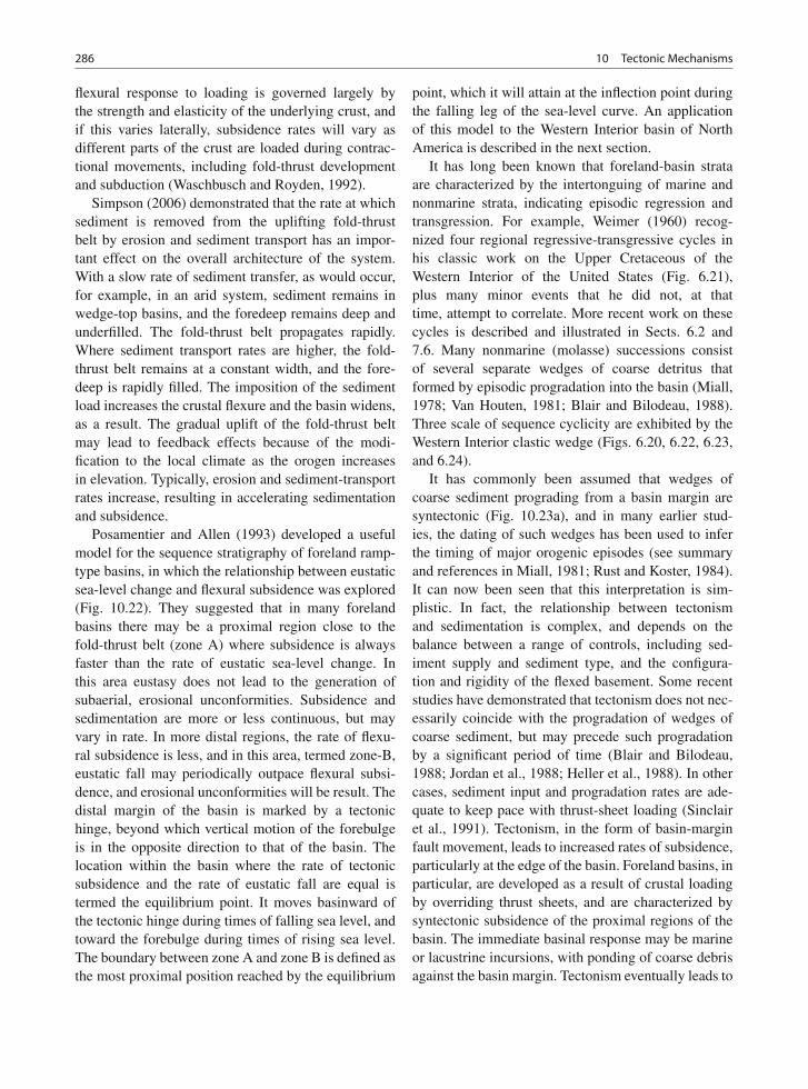
286 10 Tectonic Mechanisms
flexural response to loading is governed largely bythe strength and elasticity of the underlying crust, andif this varies laterally, subsidence rates will vary asdifferent parts of the crust are loaded during contrac-tional movements, including fold-thrust developmentand subduction (Waschbusch and Royden, 1992).
Simpson (2006) demonstrated that the rate at whichsediment is removed from the uplifting fold-thrustbelt by erosion and sediment transport has an impor-tant effect on the overall architecture of the system.With a slow rate of sediment transfer, as would occur,for example, in an arid system, sediment remains inwedge-top basins, and the foredeep remains deep andunderfilled. The fold-thrust belt propagates rapidly.Where sediment transport rates are higher, the fold-thrust belt remains at a constant width, and the fore-deep is rapidly filled. The imposition of the sedimentload increases the crustal flexure and the basin widens,as a result. The gradual uplift of the fold-thrust beltmay lead to feedback effects because of the modi-fication to the local climate as the orogen increasesin elevation. Typically, erosion and sediment-transportrates increase, resulting in accelerating sedimentationand subsidence.
Posamentier and Allen (1993) developed a usefulmodel for the sequence stratigraphy of foreland ramp-type basins, in which the relationship between eustaticsea-level change and flexural subsidence was explored(Fig. 10.22). They suggested that in many forelandbasins there may be a proximal region close to thefold-thrust belt (zone A) where subsidence is alwaysfaster than the rate of eustatic sea-level change. Inthis area eustasy does not lead to the generation ofsubaerial, erosional unconformities. Subsidence andsedimentation are more or less continuous, but mayvary in rate. In more distal regions, the rate of flexu-ral subsidence is less, and in this area, termed zone-B,eustatic fall may periodically outpace flexural subsi-dence, and erosional unconformities will be result. Thedistal margin of the basin is marked by a tectonichinge, beyond which vertical motion of the forebulgeis in the opposite direction to that of the basin. Thelocation within the basin where the rate of tectonicsubsidence and the rate of eustatic fall are equal istermed the equilibrium point. It moves basinward ofthe tectonic hinge during times of falling sea level, andtoward the forebulge during times of rising sea level.The boundary between zone A and zone B is defined asthe most proximal position reached by the equilibrium
point, which it will attain at the inflection point duringthe falling leg of the sea-level curve. An applicationof this model to the Western Interior basin of NorthAmerica is described in the next section.
It has long been known that foreland-basin strataare characterized by the intertonguing of marine andnonmarine strata, indicating episodic regression andtransgression. For example, Weimer (1960) recog-nized four regional regressive-transgressive cycles inhis classic work on the Upper Cretaceous of theWestern Interior of the United States (Fig. 6.21),plus many minor events that he did not, at thattime, attempt to correlate. More recent work on thesecycles is described and illustrated in Sects. 6.2 and7.6. Many nonmarine (molasse) successions consistof several separate wedges of coarse detritus thatformed by episodic progradation into the basin (Miall,1978; Van Houten, 1981; Blair and Bilodeau, 1988).Three scale of sequence cyclicity are exhibited by theWestern Interior clastic wedge (Figs. 6.20, 6.22, 6.23,and 6.24).
It has commonly been assumed that wedges ofcoarse sediment prograding from a basin margin aresyntectonic (Fig. 10.23a), and in many earlier stud-ies, the dating of such wedges has been used to inferthe timing of major orogenic episodes (see summaryand references in Miall, 1981; Rust and Koster, 1984).It can now been seen that this interpretation is sim-plistic. In fact, the relationship between tectonismand sedimentation is complex, and depends on thebalance between a range of controls, including sed-iment supply and sediment type, and the configura-tion and rigidity of the flexed basement. Some recentstudies have demonstrated that tectonism does not nec-essarily coincide with the progradation of wedges ofcoarse sediment, but may precede such progradationby a significant period of time (Blair and Bilodeau,1988; Jordan et al., 1988; Heller et al., 1988). In othercases, sediment input and progradation rates are ade-quate to keep pace with thrust-sheet loading (Sinclairet al., 1991). Tectonism, in the form of basin-marginfault movement, leads to increased rates of subsidence,particularly at the edge of the basin. Foreland basins, inparticular, are developed as a result of crustal loadingby overriding thrust sheets, and are characterized bysyntectonic subsidence of the proximal regions of thebasin. The immediate basinal response may be marineor lacustrine incursions, with ponding of coarse debrisagainst the basin margin. Tectonism eventually leads to
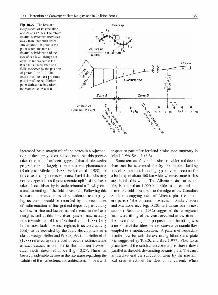
10.3 Tectonism on Convergent Plate Margins and in Collision Zones 287
H
d Eustasy
d Time= maximum
Thrus
t
Sheet
Craton
Tect
onic
Hin
ge P
oint
Location ofEquilibrium Point
[Zone of relative sea-level
rise throughout the
sea-level cycle]
[Zone of relative sea-level
fall at time T
7 ]
L
T4T3
T1T2
T5
T6T7
T9T12
T11T10
T7 T6,T8 T5,T9 T4,T10 T2,T12 T1,T13
T3,T11
T8
Eustasy
Subsidence
Zone BZone A
Fig. 10.22 The forelandramp model of Posamentierand Allen (1993a). The rate offlexural subsidence decreasesaway from the thrust sheet.The equilibrium point is thepoint where the rate offlexural subsidence and therate of sea-level change areequal. It moves across thebasin as sea level rises andfalls, as shown by the positionof points T1 to T13. Thelocation of the most proximalposition of the equilibriumpoint defines the boundarybetween zones A and B
increased basin-margin relief and hence to a rejuvena-tion of the supply of coarse sediment, but this processtakes time, and it has been suggested that clastic-wedgeprogradation is largely a post-tectonic phenomenon(Blair and Bilodeau, 1988; Heller et al., 1988). Inthis case, areally extensive coarse fluvial deposits maynot be deposited until post-tectonic uplift of the basintakes place, driven by isostatic rebound following ero-sional unroofing of the fold-thrust belt. Following thisscenario, increased rates of subsidence accompany-ing tectonism would be recorded by increased ratesof sedimentation of fine-grained deposits, particularlyshallow-marine and lacustrine sediments, at the basinmargins, and at this time river systems may actuallyflow towards the fold belt (Burbank et al., 1988). Onlyin the most fault-proximal regions is tectonic activitylikely to be recorded by the rapid development of aclastic wedge. Heller and Paola (1992) and Heller et al.(1988) referred to this model of coarse sedimentationas antitectonic, in contrast to the traditional syntec-tonic model described above (Fig. 10.23). There hasbeen considerable debate in the literature regarding thevalidity of the syntectonic and antitectonic models with
respect to particular foreland basins (see summary inMiall, 1996, Sect. 10.3.6).
Some retroarc foreland basins are wider and deeperthan can be accounted for by the flexural-loadingmodel. Supracrustal loading typically can account fora basin up to about 400 km wide, whereas some basinsare double this width. The Alberta basin, for exam-ple, is more than 1,000 km wide in its central part(from the fold-thrust belt to the edge of the CanadianShield), occupying most of Alberta, plus the south-ern parts of the adjacent provinces of Saskatchewanand Manitoba (see Fig. 10.20, and discussion in nextsection). Beaumont (1982) suggested that a regionalbasinward tilting of the crust occurred at the time ofthe flexural loading, and proposed that the tilting wasa response of the lithosphere to convective mantle flowcoupled to a subduction zone. A pattern of secondarymantle flow beneath the overriding lithospheric platewas suggested by Toksöz and Bird (1977). Flow takesplace toward the subduction zone and is drawn downparallel to the cold, descending oceanic plate. The crustis tilted toward the subduction zone by the mechan-ical drag effects of the downgoing current. When
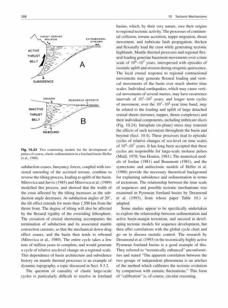
288 10 Tectonic Mechanisms
Fig. 10.23 Two contrasting models for the development ofpulses of coarse, clastic sedimentation in a foreland basin (Helleret al., 1988)
subduction ceases, buoyancy forces, coupled with ero-sional unroofing of the accreted terrane, combine toreverse the tilting process, leading to uplift of the basin.Mitrovica and Jarvis (1985) and Mitrovica et al. (1989)modelled this process, and showed that the width ofthe crust affected by the tilting increases as the sub-duction angle decreases. At subduction angles of 20◦,the tilt effect extends for more than 1,500 km from thethrust front. The degree of tilting will also be affectedby the flexural rigidity of the overriding lithosphere.The cessation of crustal shortening accompanies thetermination of subduction and its associated mantleconvection currents, so that the mechanical down-drageffect ceases, and the basin then tends to rebound(Mitrovica et al., 1989). The entire cycle takes a fewtens of million years to complete, and would generatea cycle of relative sea-level change on a regional scale.This dependence of basin architecture and subsidencehistory on mantle thermal processes is an example ofdynamic topography, a topic discussed in Sect. 9.3.2.
The question of causality of clastic large-scalecycles is particularly difficult to resolve in foreland
basins, which, by their very nature, owe their originsto regional tectonic activity. The processes of continen-tal collision, terrane accretion, nappe migration, thrustmovement, and imbricate fault propagation, thickenand flexurally load the crust while generating tectonichighlands. Mantle thermal processes and regional flex-ural loading generate basement movements over a timescale of 106–107 years, interspersed with episodes ofisostatic uplift and erosion during orogenic quiescence.The local crustal response to regional contractionalmovements may generate flexural loading and verti-cal movements of the basin over much shorter timescales. Individual earthquakes, which may cause verti-cal movements of several metres, may have recurrenceintervals of 101–102 years, and longer term cyclesof movement, over the 103–105-year time band, maybe related to the loading and uplift of large detachedcrustal sheets (terranes, nappes, thrust complexes) andtheir individual components, including imbricate slices(Fig. 10.24). Intraplate (in-plane) stress may transmitthe effects of such tectonism throughout the basin andbeyond (Sect. 10.4). These processes lead to episodiccycles of relative changes of sea-level on time scalesof 104–107 years. It has long been accepted that thesecycles are responsible for large-scale molasse pulses(Miall, 1978; Van Houten, 1981). The numerical mod-els of Jordan (1981) and Beaumont (1981), and thesyntectonic and antitectonic models of Heller et al.(1988) provide the necessary theoretical backgroundfor explaining subsidence and sedimentation in termsof tectonism. The relationship between the time scaleof sequences and possible tectonic mechanisms wasexamined in Pyrenean foreland basins by Deramondet al. (1993), from whose paper Table 10.1 isadapted.
Some studies appear to be specifically undertakento explore the relationship between sedimentation andactive basin-margin tectonism, and succeed in devel-oping tectonic models for sequence development, butthen offer correlations with the global cycle chart andgo on to discuss eustatic control. The research byDeramond et al. (1993) in the tectonically highly activePyrenean foreland basins is a good example of this.They referred to “tectonically enhanced” unconformi-ties and stated “The apparent correlation between thetwo groups of independent phenomena is an artefactof the method which calibrates the tectonic evolutionby comparison with eustatic fluctuations.” This formof “calibration” is, of course, circular reasoning.
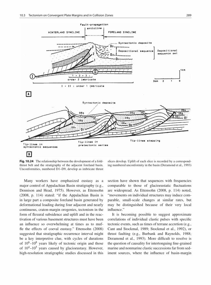
10.3 Tectonism on Convergent Plate Margins and in Collision Zones 289
Fig. 10.24 The relationship between the development of a fold-thrust belt and the stratigraphy of the adjacent foreland basin.Unconformities, numbered D1–D9, develop as imbricate thrust
slices develop. Uplift of each slice is recorded by a correspond-ing numbered unconformity in the basin (Deramond et al., 1993)
Many workers have emphasized eustasy as amajor control of Appalachian Basin stratigraphy (e.g.,Dennison and Head, 1975). However, as Ettensohn(2008, p. 114) stated: “if the Appalachian Basin isin large part a composite foreland basin generated bydeformational loading during four adjacent and nearlycontinuous, craton-margin orogenies, tectonism in theform of flexural subsidence and uplift and in the reac-tivation of various basement structures must have beenan influence so overwhelming at times as to muf-fle the effects of coeval eustasy.” Ettensohn (2008)suggested that stratigraphic recurrence interval mightbe a key interpretive clue, with cycles of durationsof 106–108 years likely of tectonic origin and thoseof 104–105 years caused by glacioeustasy. However,high-resolution stratigraphic studies discussed in this
section have shown that sequences with frequenciescomparable to those of glacioeustatic fluctuationsare widespread. As Ettensohn (2008, p. 114) noted,“movements on individual structures may induce com-parable, small-scale changes at similar rates, butmay be distinguished because of their very localinfluence.”
It is becoming possible to suggest approximatecorrelations of individual clastic pulses with specifictectonic events, such as times of terrane accretion (e.g.,Cant and Stockmal, 1989; Stockmal et al., 1992), orthrust faulting (e.g., Burbank and Raynolds, 1988;Deramond et al., 1993). More difficult to resolve isthe question of causality for intertonguing fine-grainedmarine and nonmarine clastic successions far from sed-iment sources, where the influence of basin-margin
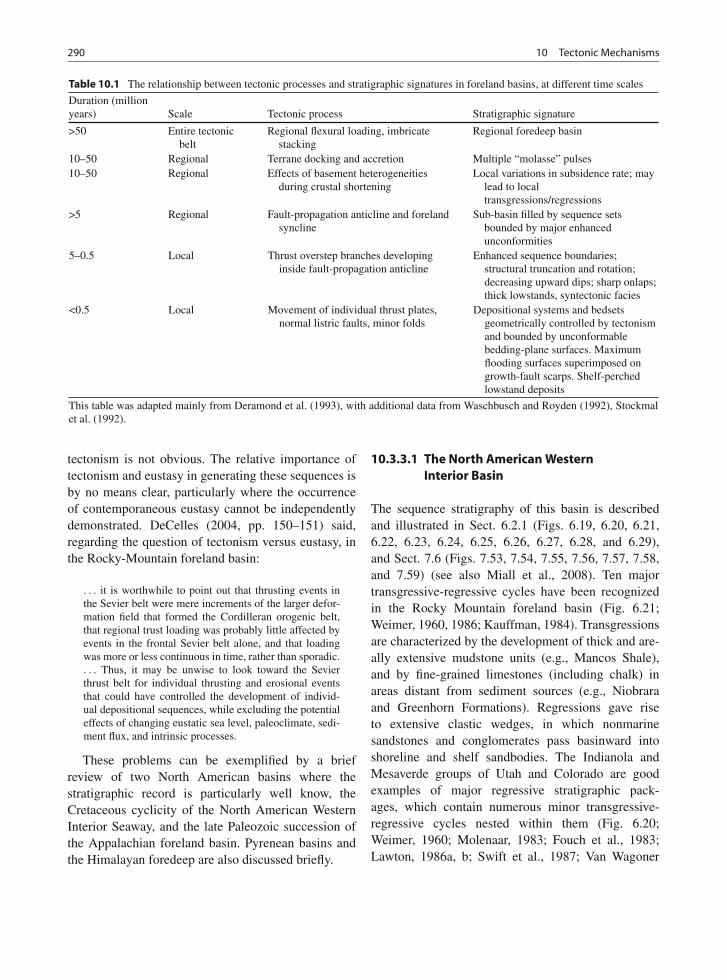
290 10 Tectonic Mechanisms
Table 10.1 The relationship between tectonic processes and stratigraphic signatures in foreland basins, at different time scales
Duration (millionyears) Scale Tectonic process Stratigraphic signature
>50 Entire tectonicbelt
Regional flexural loading, imbricatestacking
Regional foredeep basin
10–50 Regional Terrane docking and accretion Multiple “molasse” pulses10–50 Regional Effects of basement heterogeneities
during crustal shorteningLocal variations in subsidence rate; may
lead to localtransgressions/regressions
>5 Regional Fault-propagation anticline and forelandsyncline
Sub-basin filled by sequence setsbounded by major enhancedunconformities
5–0.5 Local Thrust overstep branches developinginside fault-propagation anticline
Enhanced sequence boundaries;structural truncation and rotation;decreasing upward dips; sharp onlaps;thick lowstands, syntectonic facies
<0.5 Local Movement of individual thrust plates,normal listric faults, minor folds
Depositional systems and bedsetsgeometrically controlled by tectonismand bounded by unconformablebedding-plane surfaces. Maximumflooding surfaces superimposed ongrowth-fault scarps. Shelf-perchedlowstand deposits
This table was adapted mainly from Deramond et al. (1993), with additional data from Waschbusch and Royden (1992), Stockmalet al. (1992).
tectonism is not obvious. The relative importance oftectonism and eustasy in generating these sequences isby no means clear, particularly where the occurrenceof contemporaneous eustasy cannot be independentlydemonstrated. DeCelles (2004, pp. 150–151) said,regarding the question of tectonism versus eustasy, inthe Rocky-Mountain foreland basin:
. . . it is worthwhile to point out that thrusting events inthe Sevier belt were mere increments of the larger defor-mation field that formed the Cordilleran orogenic belt,that regional trust loading was probably little affected byevents in the frontal Sevier belt alone, and that loadingwas more or less continuous in time, rather than sporadic.. . . Thus, it may be unwise to look toward the Sevierthrust belt for individual thrusting and erosional eventsthat could have controlled the development of individ-ual depositional sequences, while excluding the potentialeffects of changing eustatic sea level, paleoclimate, sedi-ment flux, and intrinsic processes.
These problems can be exemplified by a briefreview of two North American basins where thestratigraphic record is particularly well know, theCretaceous cyclicity of the North American WesternInterior Seaway, and the late Paleozoic succession ofthe Appalachian foreland basin. Pyrenean basins andthe Himalayan foredeep are also discussed briefly.
10.3.3.1 The North American WesternInterior Basin
The sequence stratigraphy of this basin is describedand illustrated in Sect. 6.2.1 (Figs. 6.19, 6.20, 6.21,6.22, 6.23, 6.24, 6.25, 6.26, 6.27, 6.28, and 6.29),and Sect. 7.6 (Figs. 7.53, 7.54, 7.55, 7.56, 7.57, 7.58,and 7.59) (see also Miall et al., 2008). Ten majortransgressive-regressive cycles have been recognizedin the Rocky Mountain foreland basin (Fig. 6.21;Weimer, 1960, 1986; Kauffman, 1984). Transgressionsare characterized by the development of thick and are-ally extensive mudstone units (e.g., Mancos Shale),and by fine-grained limestones (including chalk) inareas distant from sediment sources (e.g., Niobraraand Greenhorn Formations). Regressions gave riseto extensive clastic wedges, in which nonmarinesandstones and conglomerates pass basinward intoshoreline and shelf sandbodies. The Indianola andMesaverde groups of Utah and Colorado are goodexamples of major regressive stratigraphic pack-ages, which contain numerous minor transgressive-regressive cycles nested within them (Fig. 6.20;Weimer, 1960; Molenaar, 1983; Fouch et al., 1983;Lawton, 1986a, b; Swift et al., 1987; Van Wagoner
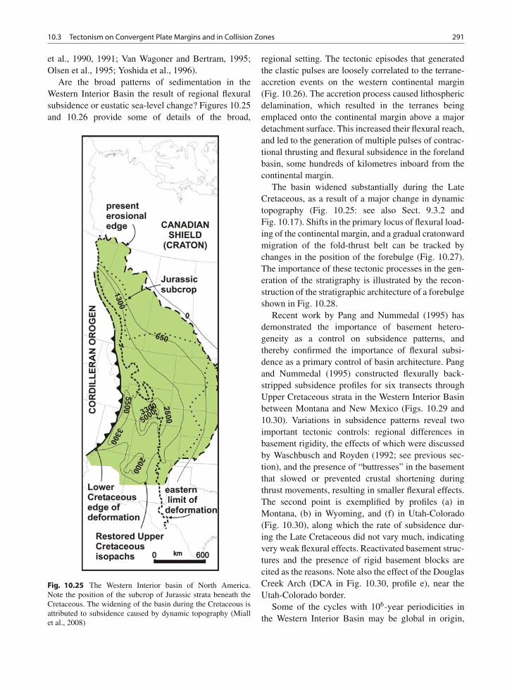
10.3 Tectonism on Convergent Plate Margins and in Collision Zones 291
et al., 1990, 1991; Van Wagoner and Bertram, 1995;Olsen et al., 1995; Yoshida et al., 1996).
Are the broad patterns of sedimentation in theWestern Interior Basin the result of regional flexuralsubsidence or eustatic sea-level change? Figures 10.25and 10.26 provide some of details of the broad,
Fig. 10.25 The Western Interior basin of North America.Note the position of the subcrop of Jurassic strata beneath theCretaceous. The widening of the basin during the Cretaceous isattributed to subsidence caused by dynamic topography (Miallet al., 2008)
regional setting. The tectonic episodes that generatedthe clastic pulses are loosely correlated to the terrane-accretion events on the western continental margin(Fig. 10.26). The accretion process caused lithosphericdelamination, which resulted in the terranes beingemplaced onto the continental margin above a majordetachment surface. This increased their flexural reach,and led to the generation of multiple pulses of contrac-tional thrusting and flexural subsidence in the forelandbasin, some hundreds of kilometres inboard from thecontinental margin.
The basin widened substantially during the LateCretaceous, as a result of a major change in dynamictopography (Fig. 10.25: see also Sect. 9.3.2 andFig. 10.17). Shifts in the primary locus of flexural load-ing of the continental margin, and a gradual cratonwardmigration of the fold-thrust belt can be tracked bychanges in the position of the forebulge (Fig. 10.27).The importance of these tectonic processes in the gen-eration of the stratigraphy is illustrated by the recon-struction of the stratigraphic architecture of a forebulgeshown in Fig. 10.28.
Recent work by Pang and Nummedal (1995) hasdemonstrated the importance of basement hetero-geneity as a control on subsidence patterns, andthereby confirmed the importance of flexural subsi-dence as a primary control of basin architecture. Pangand Nummedal (1995) constructed flexurally back-stripped subsidence profiles for six transects throughUpper Cretaceous strata in the Western Interior Basinbetween Montana and New Mexico (Figs. 10.29 and10.30). Variations in subsidence patterns reveal twoimportant tectonic controls: regional differences inbasement rigidity, the effects of which were discussedby Waschbusch and Royden (1992; see previous sec-tion), and the presence of “buttresses” in the basementthat slowed or prevented crustal shortening duringthrust movements, resulting in smaller flexural effects.The second point is exemplified by profiles (a) inMontana, (b) in Wyoming, and (f) in Utah-Colorado(Fig. 10.30), along which the rate of subsidence dur-ing the Late Cretaceous did not vary much, indicatingvery weak flexural effects. Reactivated basement struc-tures and the presence of rigid basement blocks arecited as the reasons. Note also the effect of the DouglasCreek Arch (DCA in Fig. 10.30, profile e), near theUtah-Colorado border.
Some of the cycles with 106-year periodicities inthe Western Interior Basin may be global in origin,
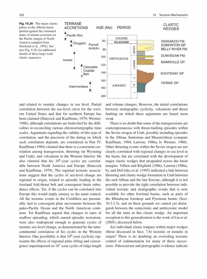
292 10 Tectonic Mechanisms
Fig. 10.26 The major clasticpulses in the Alberta basin,plotted against the estimatedtimes of terrane accretion onthe Pacific margin of NorthAmerica (adapted fromStockmal et al., 1992). Seealso Fig. 6.28, for additionaldetails of these large-scaleclastic sequences
and related to eustatic changes in sea level. Partialcorrelation between the sea-level curve for the west-ern United States and that for northern Europe hasbeen claimed (Hancock and Kauffman, 1979; Weimer,1986), although correlations are bedeviled by the diffi-culties in reconciling various chronostratigraphic timescales. Arguments regarding the validity of this type ofcorrelation, and the precision of the dating on whichsuch correlation depends, are considered in Part IV.Kauffman (1984) claimed that there is a consistent cor-relation among transgression, thrusting (in Wyomingand Utah), and volcanism in the Western Interior. Healso claimed that his 106-year cycles are correlat-able between North America and Europe (Hancockand Kauffman, 1979). The regional tectonic associa-tions suggest that the cycles of sea-level change areregional in origin, related to episodic loading in theforeland fold-thrust belt and consequent basin subsi-dence effects. Yet, if the cycles can be correlated intoEurope this would imply eustasy as the main control.All the tectonic events in the Cordillera are presum-ably tied to convergent plate movements between thepaleo-Pacific Ocean and the North American conti-nent. Yet Kauffman argued that changes in rates ofseafloor spreading, which caused episodic tectonism,were also widespread enough to generate cycles ofeustatic sea-level change, as demonstrated by the inter-continental correlation of his cycles in the WesternInterior. One possibility is that 106-year cyclicity rep-resents the effects of regional plate rifting and conver-gence superimposed on 107-year cycles of ridge length
and volume changes. However, the initial correlationsbetween stratigraphic cyclicity, volcanism and thrustfaulting on which these arguments are based seemweak.
There is no doubt that some of the transgressions arecontemporaneous with thrust-faulting episodes withinthe Sevier orogen of Utah, possibly including episodesin the Albian, Santonian and Maastrichtian (compareKauffman, 1984; Lawton, 1986a, b; Weimer, 1986).Other thrusting events within the Sevier orogen are notclearly correlated with regional changes in sea level inthe basin, but are correlated with the development ofmajor clastic wedges that prograded across the basinmargins. Villien and Kligfield (1986), Lawton (1986a,b), and DeCelles et al. (1995) indicated a link betweenthrusting and clastic-wedge formation in Utah betweenthe mid-Albian and the late Eocene, although it is notpossible to provide the tight correlation between indi-vidual tectonic and stratigraphic events that is nowavailable for other foreland basins, such as parts ofthe Himalayan foredeep and Pyrenean basins (Sect.10.3.3.3), and on these grounds we cannot yet distin-guish between the syntectonic and antitectonic modelfor all the units in this clastic wedge. An importantexception to this generalization is the work of Liu et al.(2005), discussed below.
Are individual clastic tongues within major wedges(those discussed in Sect. 7.6) tectonic or eustatic inorigin? There is no doubting an overriding tectoniccontrol of sedimentation for many of these succes-sions. Paleocurrent and petrographic evidence indicate
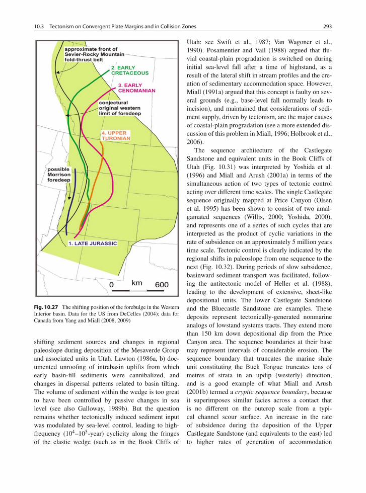
10.3 Tectonism on Convergent Plate Margins and in Collision Zones 293
Fig. 10.27 The shifting position of the forebulge in the WesternInterior basin. Data for the US from DeCelles (2004); data forCanada from Yang and Miall (2008, 2009)
shifting sediment sources and changes in regionalpaleoslope during deposition of the Mesaverde Groupand associated units in Utah. Lawton (1986a, b) doc-umented unroofing of intrabasin uplifts from whichearly basin-fill sediments were cannibalized, andchanges in dispersal patterns related to basin tilting.The volume of sediment within the wedge is too greatto have been controlled by passive changes in sealevel (see also Galloway, 1989b). But the questionremains whether tectonically induced sediment inputwas modulated by sea-level control, leading to high-frequency (104–105-year) cyclicity along the fringesof the clastic wedge (such as in the Book Cliffs of
Utah: see Swift et al., 1987; Van Wagoner et al.,1990). Posamentier and Vail (1988) argued that flu-vial coastal-plain progradation is switched on duringinitial sea-level fall after a time of highstand, as aresult of the lateral shift in stream profiles and the cre-ation of sedimentary accommodation space. However,Miall (1991a) argued that this concept is faulty on sev-eral grounds (e.g., base-level fall normally leads toincision), and maintained that considerations of sedi-ment supply, driven by tectonism, are the major causesof coastal-plain progradation (see a more extended dis-cussion of this problem in Miall, 1996; Holbrook et al.,2006).
The sequence architecture of the CastlegateSandstone and equivalent units in the Book Cliffs ofUtah (Fig. 10.31) was interpreted by Yoshida et al.(1996) and Miall and Arush (2001a) in terms of thesimultaneous action of two types of tectonic controlacting over different time scales. The single Castlegatesequence originally mapped at Price Canyon (Olsenet al. 1995) has been shown to consist of two amal-gamated sequences (Willis, 2000; Yoshida, 2000),and represents one of a series of such cycles that areinterpreted as the product of cyclic variations in therate of subsidence on an approximately 5 million yearstime scale. Tectonic control is clearly indicated by theregional shifts in paleoslope from one sequence to thenext (Fig. 10.32). During periods of slow subsidence,basinward sediment transport was facilitated, follow-ing the antitectonic model of Heller et al. (1988),leading to the development of extensive, sheet-likedepositional units. The lower Castlegate Sandstoneand the Bluecastle Sandstone are examples. Thesedeposits represent tectonically-generated nonmarineanalogs of lowstand systems tracts. They extend morethan 150 km down depositional dip from the PriceCanyon area. The sequence boundaries at their basemay represent intervals of considerable erosion. Thesequence boundary that truncates the marine shaleunit constituting the Buck Tongue truncates tens ofmetres of strata in an updip (westerly) direction,and is a good example of what Miall and Arush(2001b) termed a cryptic sequence boundary, becauseit superimposes similar facies across a contact thatis no different on the outcrop scale from a typi-cal channel scour surface. An increase in the rateof subsidence during the deposition of the UpperCastlegate Sandstone (and equivalents to the east) ledto higher rates of generation of accommodation
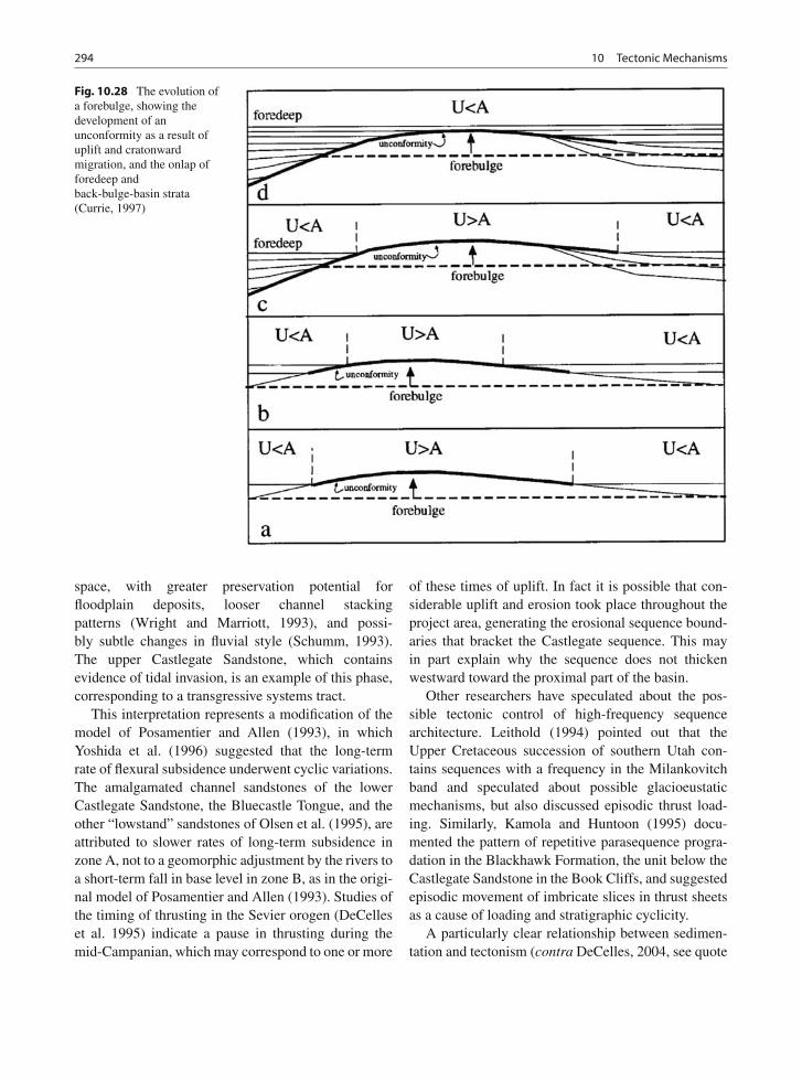
294 10 Tectonic Mechanisms
Fig. 10.28 The evolution ofa forebulge, showing thedevelopment of anunconformity as a result ofuplift and cratonwardmigration, and the onlap offoredeep andback-bulge-basin strata(Currie, 1997)
space, with greater preservation potential forfloodplain deposits, looser channel stackingpatterns (Wright and Marriott, 1993), and possi-bly subtle changes in fluvial style (Schumm, 1993).The upper Castlegate Sandstone, which containsevidence of tidal invasion, is an example of this phase,corresponding to a transgressive systems tract.
This interpretation represents a modification of themodel of Posamentier and Allen (1993), in whichYoshida et al. (1996) suggested that the long-termrate of flexural subsidence underwent cyclic variations.The amalgamated channel sandstones of the lowerCastlegate Sandstone, the Bluecastle Tongue, and theother “lowstand” sandstones of Olsen et al. (1995), areattributed to slower rates of long-term subsidence inzone A, not to a geomorphic adjustment by the rivers toa short-term fall in base level in zone B, as in the origi-nal model of Posamentier and Allen (1993). Studies ofthe timing of thrusting in the Sevier orogen (DeCelleset al. 1995) indicate a pause in thrusting during themid-Campanian, which may correspond to one or more
of these times of uplift. In fact it is possible that con-siderable uplift and erosion took place throughout theproject area, generating the erosional sequence bound-aries that bracket the Castlegate sequence. This mayin part explain why the sequence does not thickenwestward toward the proximal part of the basin.
Other researchers have speculated about the pos-sible tectonic control of high-frequency sequencearchitecture. Leithold (1994) pointed out that theUpper Cretaceous succession of southern Utah con-tains sequences with a frequency in the Milankovitchband and speculated about possible glacioeustaticmechanisms, but also discussed episodic thrust load-ing. Similarly, Kamola and Huntoon (1995) docu-mented the pattern of repetitive parasequence progra-dation in the Blackhawk Formation, the unit below theCastlegate Sandstone in the Book Cliffs, and suggestedepisodic movement of imbricate slices in thrust sheetsas a cause of loading and stratigraphic cyclicity.
A particularly clear relationship between sedimen-tation and tectonism (contra DeCelles, 2004, see quote
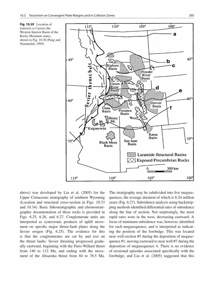
10.3 Tectonism on Convergent Plate Margins and in Collision Zones 295
Fig. 10.29 Location oftransects a–f across theWestern Interior Basin of theRocky Mountain states,shown in Fig. 10.30 (Pang andNummedal, 1995)
above) was developed by Liu et al. (2005) for theUpper Cretaceous stratigraphy of southern Wyoming(Location and structural cross-section in Figs. 10.33and 10.34). Basic lithostratigraphic and chronostrati-graphic documentation of these rocks is provided inFigs. 6.25, 6.26, and 6.27. Conglomerate units areinterpreted as syntectonic products of uplift move-ment on specific major thrust-fault plates along theSevier orogen (Fig. 6.25). The evidence for thisis that the conglomerates are cut by and rest onthe thrust faults. Sevier thrusting progressed gradu-ally eastward, beginning with the Paris-Willard thrustfrom 140 to 112 Ma, and ending with the move-ment of the Absaroka thrust from 84 to 78.5 Ma.
The stratigraphy may be subdivided into five megase-quences, the average duration of which is 6.24 millionyears (Fig. 6.27). Subsidence analysis using backstrip-ping methods identified differential rates of subsidencealong the line of section. Not surprisingly, the mostrapid rates were in the west, decreasing eastward. Alocus of minimum subsidence was, however, identifiedfor each megasequence, and is interpreted as indicat-ing the position of the forebulge. This was locatednear well-section #5 during the deposition of megase-quence #1, moving eastward to near well #7 during thedeposition of megasequence 4. There is no evidenceof erosional episodes associated specifically with theforebulge, and Liu et al. (2005) suggested that this
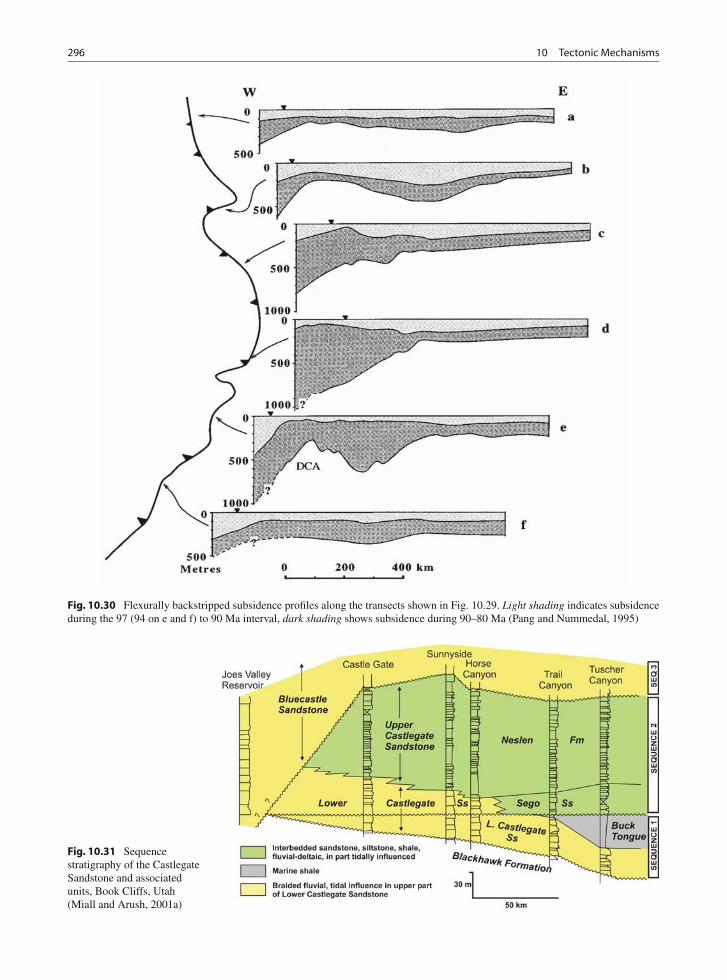
296 10 Tectonic Mechanisms
Fig. 10.30 Flexurally backstripped subsidence profiles along the transects shown in Fig. 10.29. Light shading indicates subsidenceduring the 97 (94 on e and f) to 90 Ma interval, dark shading shows subsidence during 90–80 Ma (Pang and Nummedal, 1995)
Fig. 10.31 Sequencestratigraphy of the CastlegateSandstone and associatedunits, Book Cliffs, Utah(Miall and Arush, 2001a)
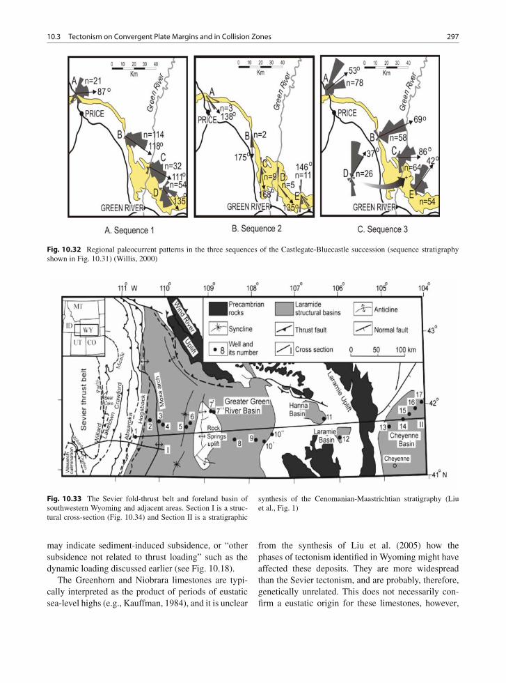
10.3 Tectonism on Convergent Plate Margins and in Collision Zones 297
Fig. 10.32 Regional paleocurrent patterns in the three sequences of the Castlegate-Bluecastle succession (sequence stratigraphyshown in Fig. 10.31) (Willis, 2000)
Fig. 10.33 The Sevier fold-thrust belt and foreland basin ofsouthwestern Wyoming and adjacent areas. Section I is a struc-tural cross-section (Fig. 10.34) and Section II is a stratigraphic
synthesis of the Cenomanian-Maastrichtian stratigraphy (Liuet al., Fig. 1)
may indicate sediment-induced subsidence, or “othersubsidence not related to thrust loading” such as thedynamic loading discussed earlier (see Fig. 10.18).
The Greenhorn and Niobrara limestones are typi-cally interpreted as the product of periods of eustaticsea-level highs (e.g., Kauffman, 1984), and it is unclear
from the synthesis of Liu et al. (2005) how thephases of tectonism identified in Wyoming might haveaffected these deposits. They are more widespreadthan the Sevier tectonism, and are probably, therefore,genetically unrelated. This does not necessarily con-firm a eustatic origin for these limestones, however,
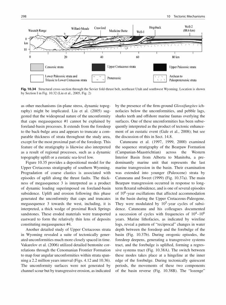
298 10 Tectonic Mechanisms
Fig. 10.34 Structural cross-section through the Sevier fold-thrust belt, northeast Utah and southwest Wyoming. Location is shownby Section I in Fig. 10.32 (Liu et al., 2005, Fig. 2)
as other mechanisms (in-plane stress, dynamic topog-raphy) might be implicated. Liu et al. (2005) sug-gested that the widespread nature of the unconformitythat caps megasequence #1 cannot be explained byforeland-basin processes. It extends from the foredeepto the back-bulge area and appears to truncate a com-parable thickness of strata throughout the study area,except for the most proximal part of the foredeep. Thisfeature of the stratigraphy is likewise also interpretedas a result of regional processes, such as a dynamictopography uplift or a eustatic sea-level low.
Figure 10.35 provides a depositional model for theUpper Cretaceous stratigraphy of southern Wyoming.Progradation of coarse clastics is associated withepisodes of uplift along the thrust faults. The thick-ness of megasequence 3 is interpreted as a productof dynamic loading superimposed on foreland-basinsubsidence. Uplift and erosion following this phasegenerated the unconformity that caps and truncatesmegasequence 3 towards the west, including, it isinterpreted, a thick wedge of proximal Rock Springssandstones. These eroded materials were transportedeastward to form the relatively thin lens of depositsconstituting megasequence #4.
Another detailed study of Upper Cretaceous stratain Wyoming revealed a suite of tectonically gener-ated unconformities much more closely spaced in time.Vakarelov et al. (2006) utilized detailed bentonite cor-relations through the Cenomanian Frontier Formationto map four angular unconformities within strata span-ning a 2.2 million years interval (Figs. 4.12 and 10.36).The unconformity surfaces were not generated bychannel scour but by transgressive erosion, as indicated
by the presence of the firm-ground Glossifungites ich-nofacies below the unconformities, and pebble lags,sharks teeth and offshore marine faunas overlying thesurfaces. One of these unconformities has been subse-quently interpreted as the product of tectonic enhance-ment of an eustatic event (Gale et al., 2008); but seethe discussion of this in Sect. 14.8.
Catuneanu et al. (1997, 1999, 2000) examinedthe sequence stratigraphy of the Bearpaw Formation(Campanian-Maastrichtian) across the WesternInterior Basin from Alberta to Manitoba, a pre-dominantly marine unit that represents the lastmarine transgression in the basin. Their examinationwas extended into younger (Paleocene) strata byCatuneanu and Sweet (1999) (Fig. 10.37a). The mainBearpaw transgression occurred in response to long-term flexural subsidence, and is one of several episodesof 106-year oscillations that affected accommodationin the basin during the Upper Cretaceous-Paleogene.They were modulated by 105-year cycles of subsi-dence. Catuneanu and his colleagues documenteda succession of cycles with frequencies of 104–106
years. Marine lithofacies, as indicated by wirelinelogs, reveal a pattern of “reciprocal” changes in waterdepth between the foredeep and the forebulge of thebasin (Fig. 10.37b). During orogenic episodes, theforedeep deepens, generating a transgressive systemstract, and the forebulge is uplifted, forming a regres-sive systems tract (Fig. 10.38A). The switch betweenthese modes takes place at a hingeline at the inneredge of the forebulge. During tectonically quiescentperiods, the movements of these two componentsof the basin reverse (Fig. 10.38B). The “lozenge”
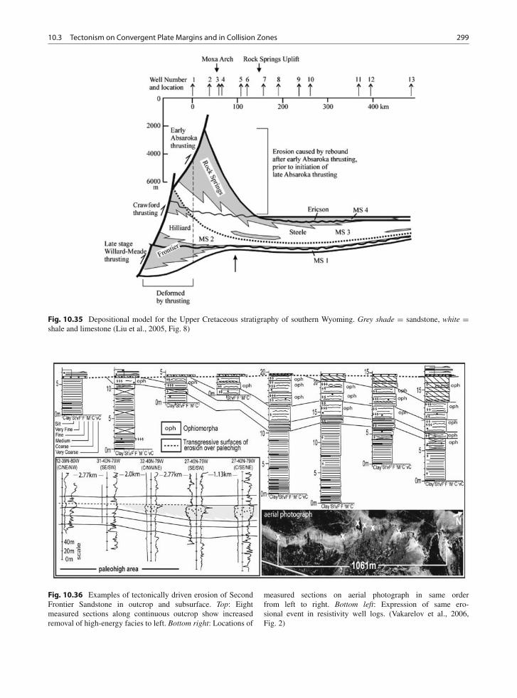
10.3 Tectonism on Convergent Plate Margins and in Collision Zones 299
Fig. 10.35 Depositional model for the Upper Cretaceous stratigraphy of southern Wyoming. Grey shade = sandstone, white =shale and limestone (Liu et al., 2005, Fig. 8)
Fig. 10.36 Examples of tectonically driven erosion of SecondFrontier Sandstone in outcrop and subsurface. Top: Eightmeasured sections along continuous outcrop show increasedremoval of high-energy facies to left. Bottom right: Locations of
measured sections on aerial photograph in same orderfrom left to right. Bottom left: Expression of same ero-sional event in resistivity well logs. (Vakarelov et al., 2006,Fig. 2)
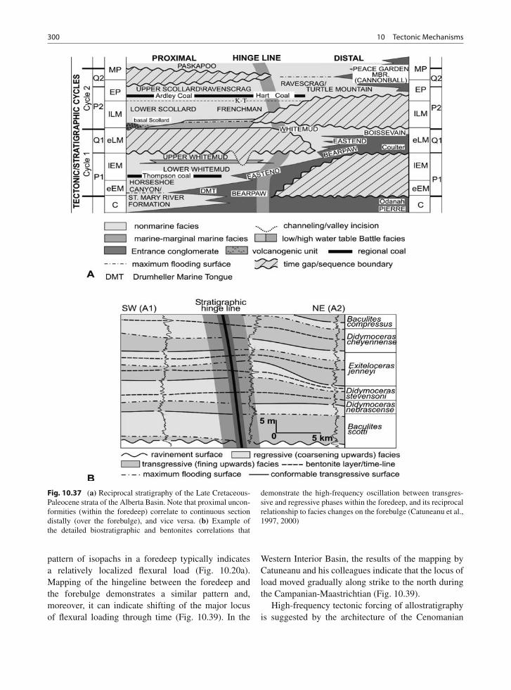
300 10 Tectonic Mechanisms
Fig. 10.37 (a) Reciprocal stratigraphy of the Late Cretaceous-Paleocene strata of the Alberta Basin. Note that proximal uncon-formities (within the foredeep) correlate to continuous sectiondistally (over the forebulge), and vice versa. (b) Example ofthe detailed biostratigraphic and bentonites correlations that
demonstrate the high-frequency oscillation between transgres-sive and regressive phases within the foredeep, and its reciprocalrelationship to facies changes on the forebulge (Catuneanu et al.,1997, 2000)
pattern of isopachs in a foredeep typically indicatesa relatively localized flexural load (Fig. 10.20a).Mapping of the hingeline between the foredeep andthe forebulge demonstrates a similar pattern and,moreover, it can indicate shifting of the major locusof flexural loading through time (Fig. 10.39). In the
Western Interior Basin, the results of the mapping byCatuneanu and his colleagues indicate that the locus ofload moved gradually along strike to the north duringthe Campanian-Maastrichtian (Fig. 10.39).
High-frequency tectonic forcing of allostratigraphyis suggested by the architecture of the Cenomanian
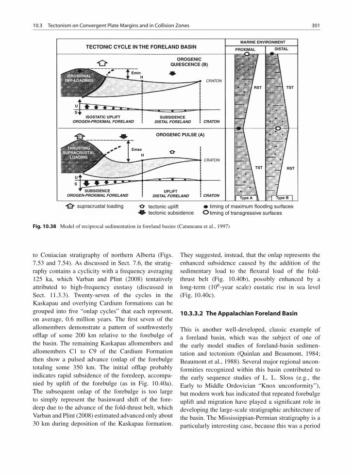
10.3 Tectonism on Convergent Plate Margins and in Collision Zones 301
supracrustal loading
SUBSIDENCEOROGEN-PROXIMAL FORELAND
ISOSTATIC UPLIFTOROGEN-PROXIMAL FORELAND
SUBSIDENCEDISTAL FORELAND
UPLIFTDISTAL FORELAND
OROGENIC PULSE (A)
OROGENICQUIESCENCE (B)
CRATON
CRATON
CRATON
CRATON
Emax
Emin
THRUSTINGSUPRACRUSTAL
LOADING
(EROSIONALOFF-LOADING)
H
H
U
U
S
S
Type A
TST
TST
RST
RST
PROXIMAL DISTAL
MARINE ENVIRONMENTTECTONIC CYCLE IN THE FORELAND BASIN
Type B
tectonic uplifttectonic subsidence
timing of maximum flooding surfacestiming of transgressive surfaces
Fig. 10.38 Model of reciprocal sedimentation in foreland basins (Catuneanu et al., 1997)
to Coniacian stratigraphy of northern Alberta (Figs.7.53 and 7.54). As discussed in Sect. 7.6, the stratig-raphy contains a cyclicity with a frequency averaging125 ka, which Varban and Plint (2008) tentativelyattributed to high-frequency eustasy (discussed inSect. 11.3.3). Twenty-seven of the cycles in theKaskapau and overlying Cardium formations can begrouped into five “onlap cycles” that each represent,on average, 0.6 million years. The first seven of theallomembers demonstrate a pattern of southwesterlyofflap of some 200 km relative to the forebulge ofthe basin. The remaining Kaskapau allomembers andallomembers C1 to C9 of the Cardium Formationthen show a pulsed advance (onlap of the forebulgetotaling some 350 km. The initial offlap probablyindicates rapid subsidence of the foredeep, accompa-nied by uplift of the forebulge (as in Fig. 10.40a).The subsequent onlap of the forebulge is too largeto simply represent the basinward shift of the fore-deep due to the advance of the fold-thrust belt, whichVarban and Plint (2008) estimated advanced only about30 km during deposition of the Kaskapau formation.
They suggested, instead, that the onlap represents theenhanced subsidence caused by the addition of thesedimentary load to the flexural load of the fold-thrust belt (Fig. 10.40b), possibly enhanced by along-term (106-year scale) eustatic rise in sea level(Fig. 10.40c).
10.3.3.2 The Appalachian Foreland Basin
This is another well-developed, classic example ofa foreland basin, which was the subject of one ofthe early model studies of foreland-basin sedimen-tation and tectonism (Quinlan and Beaumont, 1984;Beaumont et al., 1988). Several major regional uncon-formities recognized within this basin contributed tothe early sequence studies of L. L. Sloss (e.g., theEarly to Middle Ordovician “Knox unconformity”),but modern work has indicated that repeated forebulgeuplift and migration have played a significant role indeveloping the large-scale stratigraphic architecture ofthe basin. The Mississippian-Permian stratigraphy is aparticularly interesting case, because this was a period
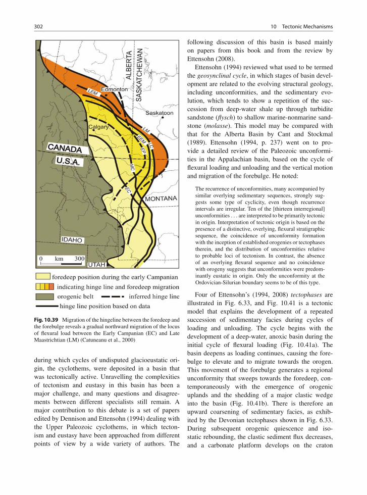
302 10 Tectonic Mechanisms
Fig. 10.39 Migration of the hingeline between the foredeep andthe forebulge reveals a gradual northward migration of the locusof flexural load between the Early Campanian (EC) and LateMaastrichtian (LM) (Catuneanu et al., 2000)
during which cycles of undisputed glacioeustatic ori-gin, the cyclothems, were deposited in a basin thatwas tectonically active. Unravelling the complexitiesof tectonism and eustasy in this basin has been amajor challenge, and many questions and disagree-ments between different specialists still remain. Amajor contribution to this debate is a set of papersedited by Dennison and Ettensohn (1994) dealing withthe Upper Paleozoic cyclothems, in which tecton-ism and eustasy have been approached from differentpoints of view by a wide variety of authors. The
following discussion of this basin is based mainlyon papers from this book and from the review byEttensohn (2008).
Ettensohn (1994) reviewed what used to be termedthe geosynclinal cycle, in which stages of basin devel-opment are related to the evolving structural geology,including unconformities, and the sedimentary evo-lution, which tends to show a repetition of the suc-cession from deep-water shale up through turbiditesandstone (flysch) to shallow marine-nonmarine sand-stone (molasse). This model may be compared withthat for the Alberta Basin by Cant and Stockmal(1989). Ettensohn (1994, p. 237) went on to pro-vide a detailed review of the Paleozoic unconformi-ties in the Appalachian basin, based on the cycle offlexural loading and unloading and the vertical motionand migration of the forebulge. He noted:
The recurrence of unconformities, many accompanied bysimilar overlying sedimentary sequences, strongly sug-gests some type of cyclicity, even though recurrenceintervals are irregular. Ten of the [thirteen interregional]unconformities . . . are interpreted to be primarily tectonicin origin. Interpretation of tectonic origin is based on thepresence of a distinctive, overlying, flexural stratigraphicsequence, the coincidence of unconformity formationwith the inception of established orogenies or tectophasestherein, and the distribution of unconformities relativeto probable loci of tectonism. In contrast, the absenceof an overlying flexural sequence and no coincidencewith orogeny suggests that unconformities were predom-inantly eustatic in origin. Only the unconformity at theOrdovician-Silurian boundary seems to be of this type.
Four of Ettensohn’s (1994, 2008) tectophases areillustrated in Fig. 6.33, and Fig. 10.41 is a tectonicmodel that explains the development of a repeatedsuccession of sedimentary facies during cycles ofloading and unloading. The cycle begins with thedevelopment of a deep-water, anoxic basin during theinitial cycle of flexural loading (Fig. 10.41a). Thebasin deepens as loading continues, causing the fore-bulge to elevate and to migrate towards the orogen.This movement of the forebulge generates a regionalunconformity that sweeps towards the foredeep, con-temporaneously with the emergence of orogenicuplands and the shedding of a major clastic wedgeinto the basin (Fig. 10.41b). There is therefore anupward coarsening of sedimentary facies, as exhib-ited by the Devonian tectophases shown in Fig. 6.33.During subsequent orogenic quiescence and iso-static rebounding, the clastic sediment flux decreases,and a carbonate platform develops on the craton
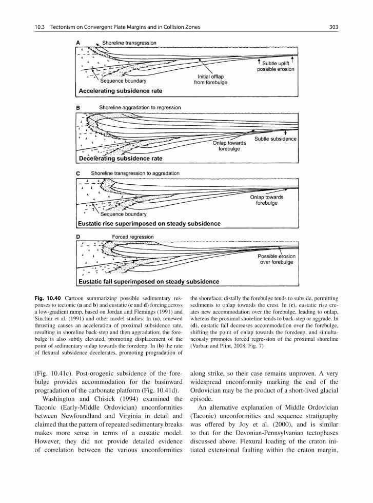
10.3 Tectonism on Convergent Plate Margins and in Collision Zones 303
Fig. 10.40 Cartoon summarizing possible sedimentary res-ponses to tectonic (a and b) and eustatic (c and d) forcing acrossa low-gradient ramp, based on Jordan and Flemings (1991) andSinclair et al. (1991) and other model studies. In (a), renewedthrusting causes an acceleration of proximal subsidence rate,resulting in shoreline back-step and then aggradation; the fore-bulge is also subtly elevated, promoting displacement of thepoint of sedimentary onlap towards the foredeep. In (b) the rateof flexural subsidence decelerates, promoting progradation of
the shoreface; distally the forebulge tends to subside, permittingsediments to onlap towards the crest. In (c), eustatic rise cre-ates new accommodation over the forebulge, leading to onlap,whereas the proximal shoreline tends to back-step or aggrade. In(d), eustatic fall decreases accommodation over the forebulge,shifting the point of onlap towards the foredeep, and simulta-neously promotes forced regression of the proximal shoreline(Varban and Plint, 2008, Fig. 7)
(Fig. 10.41c). Post-orogenic subsidence of the fore-bulge provides accommodation for the basinwardprogradation of the carbonate platform (Fig. 10.41d).
Washington and Chisick (1994) examined theTaconic (Early-Middle Ordovician) unconformitiesbetween Newfoundland and Virginia in detail andclaimed that the pattern of repeated sedimentary breaksmakes more sense in terms of a eustatic model.However, they did not provide detailed evidenceof correlation between the various unconformities
along strike, so their case remains unproven. A verywidespread unconformity marking the end of theOrdovician may be the product of a short-lived glacialepisode.
An alternative explanation of Middle Ordovician(Taconic) unconformities and sequence stratigraphywas offered by Joy et al. (2000), and is similarto that for the Devonian-Pennsylvanian tectophasesdiscussed above. Flexural loading of the craton ini-tiated extensional faulting within the craton margin,
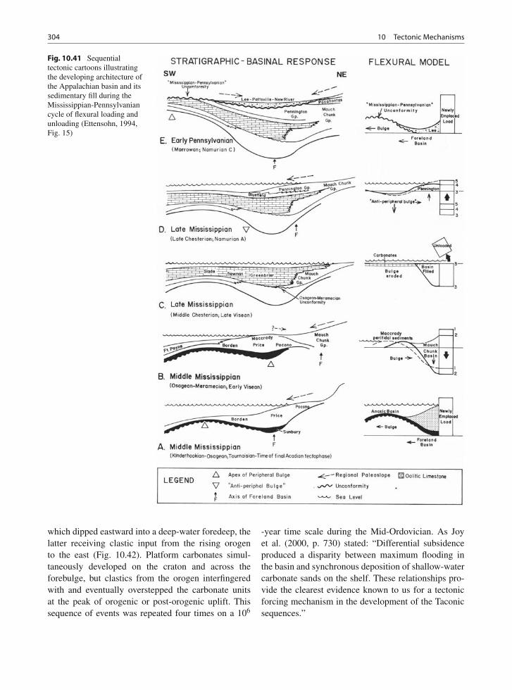
304 10 Tectonic Mechanisms
Fig. 10.41 Sequentialtectonic cartoons illustratingthe developing architecture ofthe Appalachian basin and itssedimentary fill during theMississippian-Pennsylvaniancycle of flexural loading andunloading (Ettensohn, 1994,Fig. 15)
which dipped eastward into a deep-water foredeep, thelatter receiving clastic input from the rising orogento the east (Fig. 10.42). Platform carbonates simul-taneously developed on the craton and across theforebulge, but clastics from the orogen interfingeredwith and eventually overstepped the carbonate unitsat the peak of orogenic or post-orogenic uplift. Thissequence of events was repeated four times on a 106
-year time scale during the Mid-Ordovician. As Joyet al. (2000, p. 730) stated: “Differential subsidenceproduced a disparity between maximum flooding inthe basin and synchronous deposition of shallow-watercarbonate sands on the shelf. These relationships pro-vide the clearest evidence known to us for a tectonicforcing mechanism in the development of the Taconicsequences.”
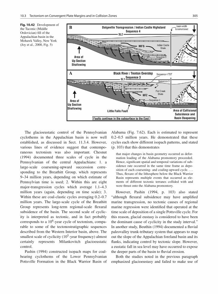
10.3 Tectonism on Convergent Plate Margins and in Collision Zones 305
Fig. 10.42 Development ofthe Taconic (MiddleOrdovician) fill of theAppalachian basin in theMohawk Valley, New York(Joy et al., 2000, Fig. 5)
The glacioeustatic control of the Pennsylvaniancyclothems in the Appalachian basin is now wellestablished, as discussed in Sect. 11.3.4. However,various lines of evidence suggest that contempo-raneous tectonism was also important. Chesnut(1994) documented three scales of cycle in thePennsylvanian of the central Appalachians: 1. alarge-scale coarsening-upward succession corre-sponding to the Breathitt Group, which represents9–34 million years, depending on which estimate ofPennsylvian time is used; 2. Within this are eightmajor-transgression cycles which average 1.1–4.3million years (again, depending on time scale); 3.Within these are coal-clastic cycles averaging 0.2–0.7million years. The large-scale cycle of the BreathittGroup represents long-term regional-scale flexuralsubsidence of the basin. The second scale of cyclic-ity is interpreted as tectonic, and in fact probablycorresponds to a 106-year cycle of tectonism, compa-rable to some of the tectonostratigraphic sequencesdescribed from the Western Interior basin, above. Thesmallest scale of cyclicity (105-year frequency) almostcertainly represents Milankovitch glacioeustaticcontrol.
Pashin (1994) constructed isopach maps for coal-bearing cyclothems of the Lower PennsylvanianPottsville Formation in the Black Warrior Basin of
Alabama (Fig. 7.62). Each is estimated to represent0.2–0.5 million years. He demonstrated that thesecycles each show different isopach patterns, and stated(p. 103) that this demonstrates
that major changes in basin geometry occurred as defor-mation loading of the Alabama promontory proceeded.Hence, significant spatial and temporal variations of sub-sidence rate occurred in the same time frame as depo-sition of each coarsening- and coaling-upward cycle. . . .
Thus, flexure of the lithosphere below the Black WarriorBasin represents multiple events that occurred as ele-ments of different tectonic terranes collided with andwere thrust onto the Alabama promontory.
However, Pashin (1994, p. 103) also stated“although flexural subsidence may have amplifiedmarine transgression, no tectonic causes of regionalmarine regression were identified that operated at thetime scale of deposition of a single Pottsville cycle. Forthis reason, glacial eustasy is considered to have beenthe dominant cause of cyclicity in the study interval.”In another study, Beuthin (1994) documented a fluvialpaleovalley trunk-tributary system that appears to mapout the slope of the Appalachian foreland basin and itsflanks, indicating control by tectonic slope. However,a eustatic fall in sea level may have occurred to exposethe deeper parts of the basin to fluvial erosion.
Both the studies noted in the previous paragraphemphasized glacioeustasy and failed to make use of
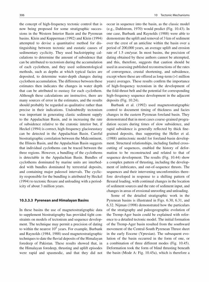
306 10 Tectonic Mechanisms
the concept of high-frequency tectonic control that isnow being proposed for some stratigraphic succes-sions in the Western Interior Basin and the Pyreneanbasins. Klein and Kupperman (1992) and Klein (1994)attempted to devise a quantitative method for dis-tinguishing between tectonic and eustatic causes ofsedimentary cyclicity. They used backstripping cal-culations to determine the amount of subsidence thatcan be attributed to tectonism during the accumulationof each cyclothem, and they used sedimentologicalmethods, such as depths at which typical facies aredeposited, to determine water-depth changes duringcyclothem accumulation. The difference between theseestimates then indicates the changes in water depththat can be attributed to eustasy for each cyclothem.Although these calculations are instructive, there aremany sources of error in the estimates, and the resultsshould probably be regarded as qualitative rather thanprecise in their indications. Undoubtedly tectonismwas important in generating clastic sediment supplyto the Appalachian Basin, and in increasing the rateof subsidence relative to the cratonic interior but, ifHeckel (1994) is correct, high-frequency glacioeustasycan be detected in the Appalachian Basin. Carefulbiostratigraphic correlation between the Midcontinent,the Illinois Basin, and the Appalachian Basin suggeststhat individual cyclothems can be traced between thethree regions. However, a bundling of the cyclothemsis detectable in the Appalachian Basin. Bundles ofcyclothems dominated by marine units are interbed-ded with bundles dominated by terrestrial deposits,and containing major paleosol intervals. The cyclic-ity responsible for the bundling is attributed by Heckel(1994) to tectonic flexure and unloading with a period-icity of about 3 million years.
10.3.3.3 Pyrenean and Himalayan Basins
In these basins the use of magnetostratigraphic datato supplement biostratigraphy has provided tight con-straints on models of tectonism and sequence develop-ment. The technique may permit a precision of datingto within the nearest 105 years. For example, Burbankand Raynolds (1984, 1988) used magnetostratigraphictechniques to date the fluvial deposits of the Himalayanforedeep of Pakistan. These results showed that, inthe Himalayan foredeep, thrusting and uplift episodeswere rapid and spasmodic, and that they did not
occur in sequence into the basin, as the classic model(e.g., Dahlstrom, 1970) would predict (Fig. 10.43). Inone case, Burbank and Raynolds (1988) were able todemonstrate the uplift and removal of 3 km of sedimentover the crest of an anticline within the basin over aperiod of 200,000 years, an average uplift and erosionrate of 1.5 cm/year. In most basins, the precision ofdating obtained by these authors cannot be attempted,and this, therefore, suggests that caution should beused in assessing published reconstructions of the ratesof convergence, crustal shortening, and subsidence,except where these are offered as long-term (>1 millionyears) averages. These results confirm the importanceof high-frequency tectonism in the development ofthe fold-thrust belt and the potential for correspondinghigh-frequency sequence development in the adjacentdeposits (Fig. 10.24).
Burbank et al. (1992) used magnetostratigraphiccontrol to document timing of thickness and facieschanges in the eastern Pyrenean foreland basin. Theydemonstrated that in most cases coarse-grained progra-dation occurs during times of slow subsidence, andrapid subsidence is generally reflected by thick fine-grained deposits, thus supporting the Heller et al.(1988) antitectonic model for foreland-basin develop-ment. Structural relationships, including faulted cross-cutting of sequences, enabled the history of defor-mation to be reconstructed and related to that ofsequence development. The results (Fig. 10.44) showa complex pattern of thrusting, including the develop-ment of imbricates, and out-of-sequence thrusts. Thesequences and their intervening unconformities there-fore developed in response to a shifting pattern offlexural loading, with continual changes in the locationof sediment sources and the rate of sediment input, andchanges in areas of erosional unroofing and unloading.
Some of the detailed stratigraphic work in thePyrenean basins is illustrated in Figs. 6.30, 6.31, and6.32. Nijman (1998) demonstrated how the particularsof the stratigraphy and paleogeographic evolution ofthe Tremp-Ager basin could be explained with refer-ence to a detailed tectonic model. The initial formationof the Tremp-Ager basin resulted from the southwardmovement of the Central-South Pyrenean Thrust sheetin the early Eocene (Ypresian). The subsequent evo-lution of the basin occurred in the form of one, ora combination of three different modes (Fig. 10.45).Deformation took the form of blind thrusting beneaththe basin (Mode A: Fig. 10.45a), which is therefore a
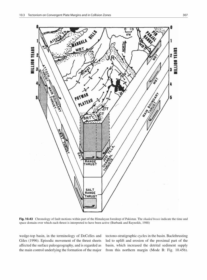
10.3 Tectonism on Convergent Plate Margins and in Collision Zones 307
Fig. 10.43 Chronology of fault motions within part of the Himalayan foredeep of Pakistan. The shaded boxes indicate the time andspace domain over which each thrust is interpreted to have been active (Burbank and Raynolds, 1988)
wedge-top basin, in the terminology of DeCelles andGiles (1996). Episodic movement of the thrust sheetsaffected the surface paleogeography, and is regarded asthe main control underlying the formation of the major
tectono-stratigraphic cycles in the basin. Backthrustingled to uplift and erosion of the proximal part of thebasin, which increased the detrital sediment supplyfrom this northern margin (Mode B: Fig. 10.45b).
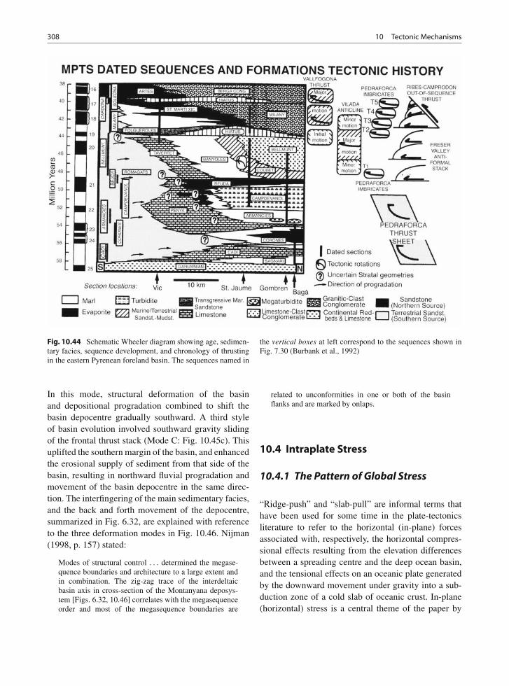
308 10 Tectonic Mechanisms
Fig. 10.44 Schematic Wheeler diagram showing age, sedimen-tary facies, sequence development, and chronology of thrustingin the eastern Pyrenean foreland basin. The sequences named in
the vertical boxes at left correspond to the sequences shown inFig. 7.30 (Burbank et al., 1992)
In this mode, structural deformation of the basinand depositional progradation combined to shift thebasin depocentre gradually southward. A third styleof basin evolution involved southward gravity slidingof the frontal thrust stack (Mode C: Fig. 10.45c). Thisuplifted the southern margin of the basin, and enhancedthe erosional supply of sediment from that side of thebasin, resulting in northward fluvial progradation andmovement of the basin depocentre in the same direc-tion. The interfingering of the main sedimentary facies,and the back and forth movement of the depocentre,summarized in Fig. 6.32, are explained with referenceto the three deformation modes in Fig. 10.46. Nijman(1998, p. 157) stated:
Modes of structural control . . . determined the megase-quence boundaries and architecture to a large extent andin combination. The zig-zag trace of the interdeltaicbasin axis in cross-section of the Montanyana deposys-tem [Figs. 6.32, 10.46] correlates with the megasequenceorder and most of the megasequence boundaries are
related to unconformities in one or both of the basinflanks and are marked by onlaps.
10.4 Intraplate Stress
10.4.1 The Pattern of Global Stress
“Ridge-push” and “slab-pull” are informal terms thathave been used for some time in the plate-tectonicsliterature to refer to the horizontal (in-plane) forcesassociated with, respectively, the horizontal compres-sional effects resulting from the elevation differencesbetween a spreading centre and the deep ocean basin,and the tensional effects on an oceanic plate generatedby the downward movement under gravity into a sub-duction zone of a cold slab of oceanic crust. In-plane(horizontal) stress is a central theme of the paper by
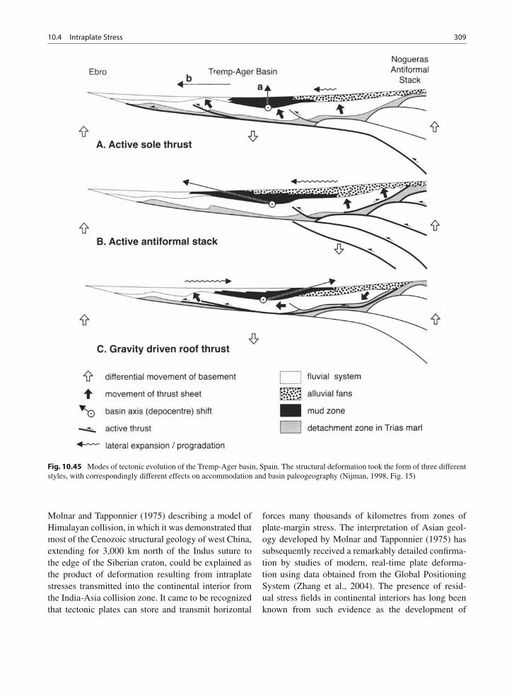
10.4 Intraplate Stress 309
Fig. 10.45 Modes of tectonic evolution of the Tremp-Ager basin, Spain. The structural deformation took the form of three differentstyles, with correspondingly different effects on accommodation and basin paleogeography (Nijman, 1998, Fig. 15)
Molnar and Tapponnier (1975) describing a model ofHimalayan collision, in which it was demonstrated thatmost of the Cenozoic structural geology of west China,extending for 3,000 km north of the Indus suture tothe edge of the Siberian craton, could be explained asthe product of deformation resulting from intraplatestresses transmitted into the continental interior fromthe India-Asia collision zone. It came to be recognizedthat tectonic plates can store and transmit horizontal
forces many thousands of kilometres from zones ofplate-margin stress. The interpretation of Asian geol-ogy developed by Molnar and Tapponnier (1975) hassubsequently received a remarkably detailed confirma-tion by studies of modern, real-time plate deforma-tion using data obtained from the Global PositioningSystem (Zhang et al., 2004). The presence of resid-ual stress fields in continental interiors has long beenknown from such evidence as the development of
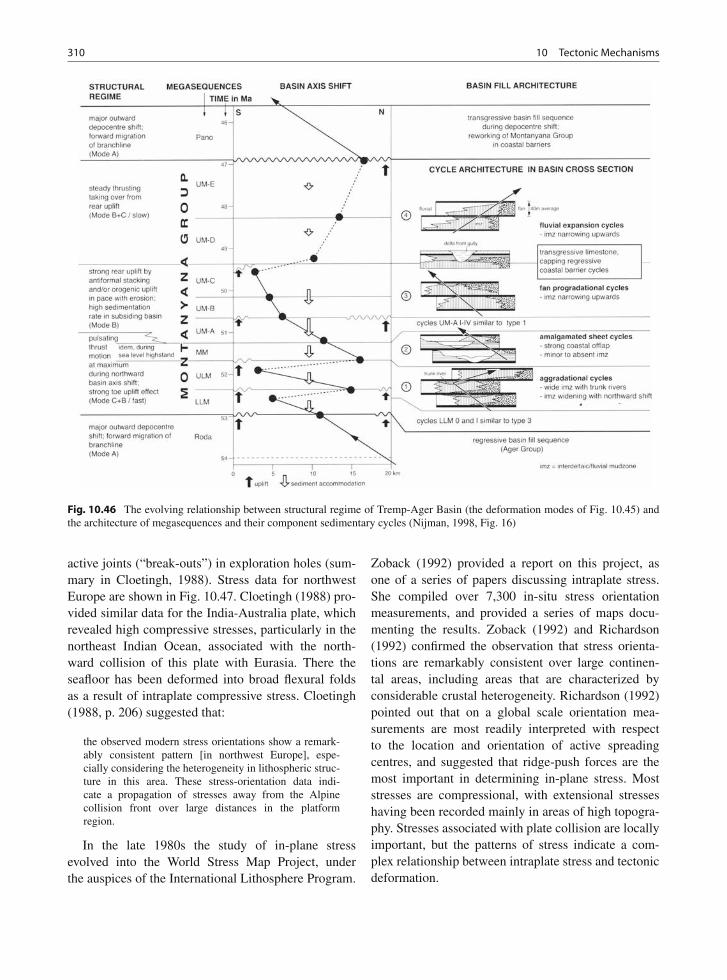
310 10 Tectonic Mechanisms
Fig. 10.46 The evolving relationship between structural regime of Tremp-Ager Basin (the deformation modes of Fig. 10.45) andthe architecture of megasequences and their component sedimentary cycles (Nijman, 1998, Fig. 16)
active joints (“break-outs”) in exploration holes (sum-mary in Cloetingh, 1988). Stress data for northwestEurope are shown in Fig. 10.47. Cloetingh (1988) pro-vided similar data for the India-Australia plate, whichrevealed high compressive stresses, particularly in thenortheast Indian Ocean, associated with the north-ward collision of this plate with Eurasia. There theseafloor has been deformed into broad flexural foldsas a result of intraplate compressive stress. Cloetingh(1988, p. 206) suggested that:
the observed modern stress orientations show a remark-ably consistent pattern [in northwest Europe], espe-cially considering the heterogeneity in lithospheric struc-ture in this area. These stress-orientation data indi-cate a propagation of stresses away from the Alpinecollision front over large distances in the platformregion.
In the late 1980s the study of in-plane stressevolved into the World Stress Map Project, underthe auspices of the International Lithosphere Program.
Zoback (1992) provided a report on this project, asone of a series of papers discussing intraplate stress.She compiled over 7,300 in-situ stress orientationmeasurements, and provided a series of maps docu-menting the results. Zoback (1992) and Richardson(1992) confirmed the observation that stress orienta-tions are remarkably consistent over large continen-tal areas, including areas that are characterized byconsiderable crustal heterogeneity. Richardson (1992)pointed out that on a global scale orientation mea-surements are most readily interpreted with respectto the location and orientation of active spreadingcentres, and suggested that ridge-push forces are themost important in determining in-plane stress. Moststresses are compressional, with extensional stresseshaving been recorded mainly in areas of high topogra-phy. Stresses associated with plate collision are locallyimportant, but the patterns of stress indicate a com-plex relationship between intraplate stress and tectonicdeformation.
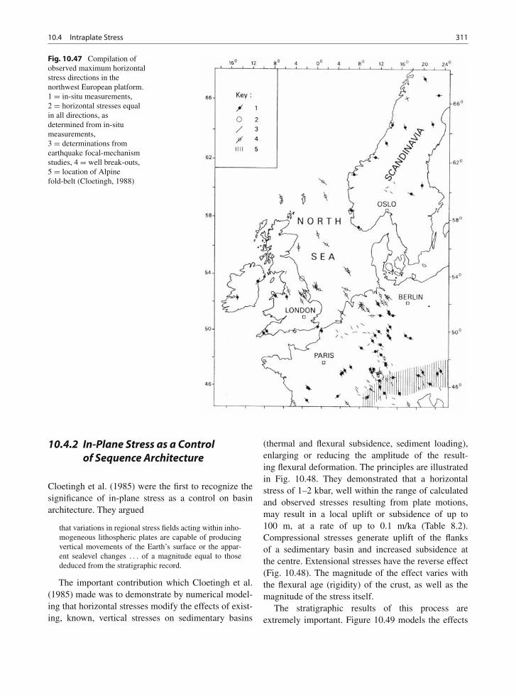
10.4 Intraplate Stress 311
Fig. 10.47 Compilation ofobserved maximum horizontalstress directions in thenorthwest European platform.1 = in-situ measurements,2 = horizontal stresses equalin all directions, asdetermined from in-situmeasurements,3 = determinations fromearthquake focal-mechanismstudies, 4 = well break-outs,5 = location of Alpinefold-belt (Cloetingh, 1988)
10.4.2 In-Plane Stress as a Controlof Sequence Architecture
Cloetingh et al. (1985) were the first to recognize thesignificance of in-plane stress as a control on basinarchitecture. They argued
that variations in regional stress fields acting within inho-mogeneous lithospheric plates are capable of producingvertical movements of the Earth’s surface or the appar-ent sealevel changes . . . of a magnitude equal to thosededuced from the stratigraphic record.
The important contribution which Cloetingh et al.(1985) made was to demonstrate by numerical model-ing that horizontal stresses modify the effects of exist-ing, known, vertical stresses on sedimentary basins
(thermal and flexural subsidence, sediment loading),enlarging or reducing the amplitude of the result-ing flexural deformation. The principles are illustratedin Fig. 10.48. They demonstrated that a horizontalstress of 1–2 kbar, well within the range of calculatedand observed stresses resulting from plate motions,may result in a local uplift or subsidence of up to100 m, at a rate of up to 0.1 m/ka (Table 8.2).Compressional stresses generate uplift of the flanksof a sedimentary basin and increased subsidence atthe centre. Extensional stresses have the reverse effect(Fig. 10.48). The magnitude of the effect varies withthe flexural age (rigidity) of the crust, as well as themagnitude of the stress itself.
The stratigraphic results of this process areextremely important. Figure 10.49 models the effects
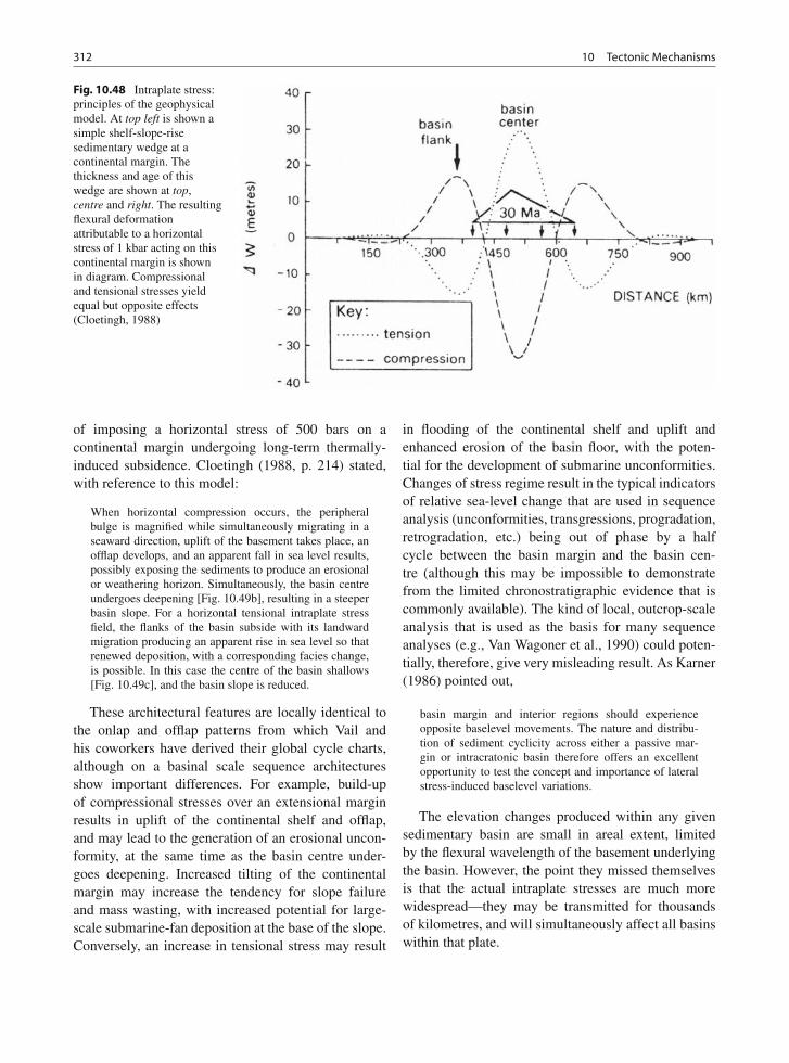
312 10 Tectonic Mechanisms
Fig. 10.48 Intraplate stress:principles of the geophysicalmodel. At top left is shown asimple shelf-slope-risesedimentary wedge at acontinental margin. Thethickness and age of thiswedge are shown at top,centre and right. The resultingflexural deformationattributable to a horizontalstress of 1 kbar acting on thiscontinental margin is shownin diagram. Compressionaland tensional stresses yieldequal but opposite effects(Cloetingh, 1988)
of imposing a horizontal stress of 500 bars on acontinental margin undergoing long-term thermally-induced subsidence. Cloetingh (1988, p. 214) stated,with reference to this model:
When horizontal compression occurs, the peripheralbulge is magnified while simultaneously migrating in aseaward direction, uplift of the basement takes place, anofflap develops, and an apparent fall in sea level results,possibly exposing the sediments to produce an erosionalor weathering horizon. Simultaneously, the basin centreundergoes deepening [Fig. 10.49b], resulting in a steeperbasin slope. For a horizontal tensional intraplate stressfield, the flanks of the basin subside with its landwardmigration producing an apparent rise in sea level so thatrenewed deposition, with a corresponding facies change,is possible. In this case the centre of the basin shallows[Fig. 10.49c], and the basin slope is reduced.
These architectural features are locally identical tothe onlap and offlap patterns from which Vail andhis coworkers have derived their global cycle charts,although on a basinal scale sequence architecturesshow important differences. For example, build-upof compressional stresses over an extensional marginresults in uplift of the continental shelf and offlap,and may lead to the generation of an erosional uncon-formity, at the same time as the basin centre under-goes deepening. Increased tilting of the continentalmargin may increase the tendency for slope failureand mass wasting, with increased potential for large-scale submarine-fan deposition at the base of the slope.Conversely, an increase in tensional stress may result
in flooding of the continental shelf and uplift andenhanced erosion of the basin floor, with the poten-tial for the development of submarine unconformities.Changes of stress regime result in the typical indicatorsof relative sea-level change that are used in sequenceanalysis (unconformities, transgressions, progradation,retrogradation, etc.) being out of phase by a halfcycle between the basin margin and the basin cen-tre (although this may be impossible to demonstratefrom the limited chronostratigraphic evidence that iscommonly available). The kind of local, outcrop-scaleanalysis that is used as the basis for many sequenceanalyses (e.g., Van Wagoner et al., 1990) could poten-tially, therefore, give very misleading result. As Karner(1986) pointed out,
basin margin and interior regions should experienceopposite baselevel movements. The nature and distribu-tion of sediment cyclicity across either a passive mar-gin or intracratonic basin therefore offers an excellentopportunity to test the concept and importance of lateralstress-induced baselevel variations.
The elevation changes produced within any givensedimentary basin are small in areal extent, limitedby the flexural wavelength of the basement underlyingthe basin. However, the point they missed themselvesis that the actual intraplate stresses are much morewidespread—they may be transmitted for thousandsof kilometres, and will simultaneously affect all basinswithin that plate.
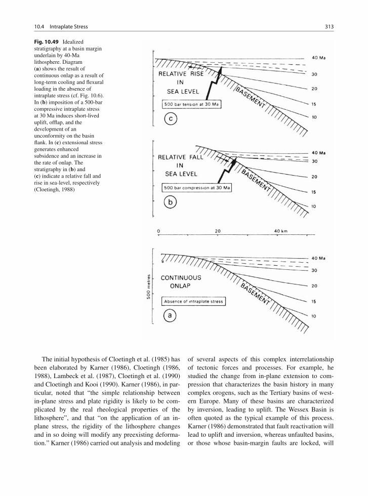
10.4 Intraplate Stress 313
Fig. 10.49 Idealizedstratigraphy at a basin marginunderlain by 40-Malithosphere. Diagram(a) shows the result ofcontinuous onlap as a result oflong-term cooling and flexuralloading in the absence ofintraplate stress (cf. Fig. 10.6).In (b) imposition of a 500-barcompressive intraplate stressat 30 Ma induces short-liveduplift, offlap, and thedevelopment of anunconformity on the basinflank. In (c) extensional stressgenerates enhancedsubsidence and an increase inthe rate of onlap. Thestratigraphy in (b) and(c) indicate a relative fall andrise in sea-level, respectively(Cloetingh, 1988)
The initial hypothesis of Cloetingh et al. (1985) hasbeen elaborated by Karner (1986), Cloetingh (1986,1988), Lambeck et al. (1987), Cloetingh et al. (1990)and Cloetingh and Kooi (1990). Karner (1986), in par-ticular, noted that “the simple relationship betweenin-plane stress and plate rigidity is likely to be com-plicated by the real rheological properties of thelithosphere”, and that “on the application of an in-plane stress, the rigidity of the lithosphere changesand in so doing will modify any preexisting deforma-tion.” Karner (1986) carried out analysis and modeling
of several aspects of this complex interrelationshipof tectonic forces and processes. For example, hestudied the change from in-plane extension to com-pression that characterizes the basin history in manycomplex orogens, such as the Tertiary basins of west-ern Europe. Many of these basins are characterizedby inversion, leading to uplift. The Wessex Basin isoften quoted as the typical example of this process.Karner (1986) demonstrated that fault reactivation willlead to uplift and inversion, whereas unfaulted basins,or those whose basin-margin faults are locked, will
314 10 Tectonic Mechanisms
experience enhanced subsidence under compressivein-plane stresses.
The importance of tectonism as a control of sea-level change, as evaluated by those who have studiedit in detail, has led to a suggestion that Vail’s work bevirtually turned on its head. Karner (1986) stated in theconclusions to his work:
Knowing the origin of the Vail curve puts its correlativepowers onto a strong theoretical basis and helps to definewhere and when the curve is of use in seismic stratigra-phy. Quite independently however, if this in-plane stressmechanism is right, it implies that the Vail curve canbe used to measure the absolute value of paleo in-planestress variations and also as a pointer to the timing of pastplate boundary reconfigurations.
Elsewhere Karner (1986) stated:
Because lateral force variations will be globally balanced(that is, an increase in relative compressive force at oneplate boundary must be balanced by a relative increasein tensile forces at another), then in-plane stress-inducedunconformities cannot be global. If there exists a causal(but undoubtedly complex) relationship between plateinteractions and in-plane stress variations, then transgres-sive/regressive sequences from a variety of basins will becorrelatable if they share the same in-plane stress sys-tem, which potentially may span a number of plates. Inessence the Vail et al. (1977) coastal onlap curve can becorrectly applied to widely spaced basins only when theabove criteria are established.
Cloetingh and his colleagues have now carried outa considerable number of modeling experiments, inwhich they have applied the concepts of intraplatestress to extensional (Kooi and Cloetingh, 1992a, b)and contractional (Peper, 1994; Peper et al., 1992;Peper and Cloetingh, 1995; Heller et al., 1993) tectonicsettings.
Kooi and Cloetingh (1992b) examined the effectof the depth at which crustal attenuation (“neck-ing”) occurs during crustal extension, and its impli-cations for sequence architecture, and they discussedthe importance of basinal tilting induced by flexuraleffects (Fig. 10.48). They showed that the stratigraphiceffects of changes in intraplate stress regime are par-ticularly pronounced and different from simple modelsof subsidence-with-eustasy in the case of extensionalmargins that undergo crustal thinning and “necking”at relatively shallow levels. Modeling experimentsdemonstrated that where necking occurs at deep levels,the resulting stratigraphic architecture is more simi-lar to that of the eustatic model. Kooi and Cloetingh(1992b) showed that the angular unconformities that
result from the warping movements driven by changesin stress regime are very subtle, typically 0.5◦ or less,and therefore difficult to detect in most data sets.They confirmed that the observations suggested byEmbry (1990) for the detection of tectonic influencesin sequence generation (Sect. 10.1) are all consis-tent with tectonism driven by changes in the regionalin-plane stress regime.
The response of foreland basins to flexural load-ing is discussed in Sect. 10.3.3. Most recent workhas been concerned with tectonism on a 106-yeartime scale. Recent studies of intraplate stress, aidedby numerical modeling, have suggested that the crustmay respond on much shorter time scales, possiblyless than 104 years (Cloetingh, 1988; Peper et al.,1992; Peper and Cloetingh, 1995; Heller et al., 1993).Peper et al. (1992) modeled responses of periodictectonic movement at time scales down to that cor-responding to the spacing of individual earthquakes(100–101 years), and made a convincing case for tec-tonic cyclicity that could explain cycles with frequen-cies of 105–104 years. Heller et al. (1993) consideredthe effects of compressional tectonism in areas con-taining crustal heterogeneities, including active faultsand inherited basement structures. They concluded thatvertical motions of metres to a few tens of metresextending over distances of tens of kilometres couldbe attributed to such stresses. This is quite enoughto overprint the effects of modest eustatic sea-levelchanges, and Heller et al. (1993) pointed to severalsubtle structural and stratigraphic features in the RockyMountain states that they suggested could be attributedto in-plane stress occurring as part of compressionaltectonism during the Jurassic to mid-Cretaceous.
10.4.3 In-Plane Stress and RegionalHistories of Sea-Level Change
Lambeck et al. (1987), and Cloetingh (1988) compiledstratigraphic and tectonic data for the North Sea Basinas a starting point for the evaluation of the impor-tance of intraplate stress in this area, and Cloetinghet al. (1990) expanded the data-base to the entire NorthAtlantic region. They chose this region in part becauseof its importance in the original establishment of theglobal cycle chart by Vail in the 1970s. Many work-ers (e.g., Glennie, 1998; Miall, 1986; Hallam, 1988)
10.4 Intraplate Stress 315
had independently noted the importance of regionaltectonism in controlling the stratigraphy of this area.Hallam (1988), in particular, noted “that a signifi-cant number of Jurassic unconformities are confinedto the flanks of North Sea Basins, consistent with thepredictions of [intraplate stress].” (Cloetingh, 1988).Such compilations are difficult to evaluate because ofthe uncertainties inherent in the positioning and rel-ative importance of each event. The analysis whichCloetingh (1988) and Lambeck et al. (1987) offeredof their own compilation is little more than “permis-sive”, in the sense that they show that all relativesea-level events in Europe and the North Atlanticcould be explained by changes in intraplate stress, butare unable to offer quantitative proof, in the form ofdetailed numerical models.
In another attempt to model paleostress Cloetinghand Kooi (1990) provided a curve of estimated changesin the paleostress field of the US Atlantic margins,based on a modification of the approach of Watts andhis colleagues (which is discussed in Sect. 10.2), inwhich they superimposed short-term intraplate stresson the long-term flexural subsidence of the conti-nental margin Changes in the stress regime of theUS Atlantic margin occurred because of the contin-ual change in the plate kinematics of the Atlanticregion as the ocean opened and the spreading centreextended and underwent various changes in config-uration. Important events, such as the initiation ofspreading in Labrador Sea, the extension of spread-ing between Greenland and Europe, and various jumpsin ridge position, brought about significant changes inplate trajectories, which would have been accompaniedby changes in the direction and intensity of intraplatestresses.
Sea-floor spreading patterns in the north and cen-tral Atlantic Ocean (Srivastava and Tapscott, 1986;Klitgord and Schouten, 1986) provide a detailed his-tory of plate motions. The reconstruction of a con-tinuous succession of matched plate margins as theAtlantic Ocean opened indicates that the rotation polesof the North American plate relative to Europe andAfrica changed at intervals of about 2–16 millionyears. This episodicity is comparable in magnitude tothe duration of 106-year stratigraphic cycles, a factthat is highly suggestive. Furthermore, some of thechanges in rotation pole can be correlated in timewith changes in the position of depocentres in theMesozoic-Cenozoic stratigraphic record of the US
Atlantic continental margin. Poag and Sevon (1989)compiled isopach maps of the post-rift sedimentaryrecord, and interpreted these in terms of the shift-ing pattern of denudation in and sediment transportfrom the Appalachian and Adirondack Mountains. Itseems likely that many of the major existing rivers thatpresently carry sediment into this region have been inexistence since the Mesozoic. Poag and Sevon (1989)were able to show many changes with time in the rela-tive importance of these various sediment sources, andit is suggestive that several of these changes occurred attimes of change in Atlantic plate kinematics. The sea-floor spreading record reveals at least fourteen changesin plate configuration in the central Atlantic since theMid-Jurassic (Klitgord and Schouten, 1986). Seven ofthese changes, at 2.5, 10, 17, 50, 59, 67 and 150 Ma,correspond to times when the major sediment dispersalroutes from the Appalachian Mountains to the conti-nental shelf underwent a major shift (data from Poagand Sevon, 1989).
Tectonism is diachronous and, in the case ofthe intraplate stresses discussed by Cloetingh (1986,1988), the effects vary across the plate. Adjacent platesmay be expected to have dissimilar tectonic histories,except where major extensional or collisional eventsaffect adjoining plates. However, there is no mech-anism for generating globally simultaneous tectonicevents of similar style and magnitude. If, as suggestedby Cloetingh (1986, 1988), many 106-year cycles aretectonic in origin, it should not be possible to constructa global cycle chart (but see below). The fact that sucha chart has been constructed suggests that we shouldexamine the basis on which it has been made. Thisexamination forms the basis for Part IV of this book.
The fact that the earth’s crust consists of a finiteseries of interacting plates suggests the possibilityfor widespread, even global tectonic episodes thatare synchronous but of different style and magnitudein different areas. A possible example of this wasnoted by Hiroki (1994), who documented tectonic andglacioeustatic movements in a forearc basin on the eastcoast of Japan during the Quaternary. He noted thata change from subsidence to uplift between 331 and122 ka B.P. occurred at about the same time as anincrease in uplift rates in New Zealand, and a decreasein uplift rates in New Guinea. He stated that “thesynchronous change in vertical crustal movement maybe explained by a change in the regional horizon-tal stress field due to rotation of the Pacific plate.”
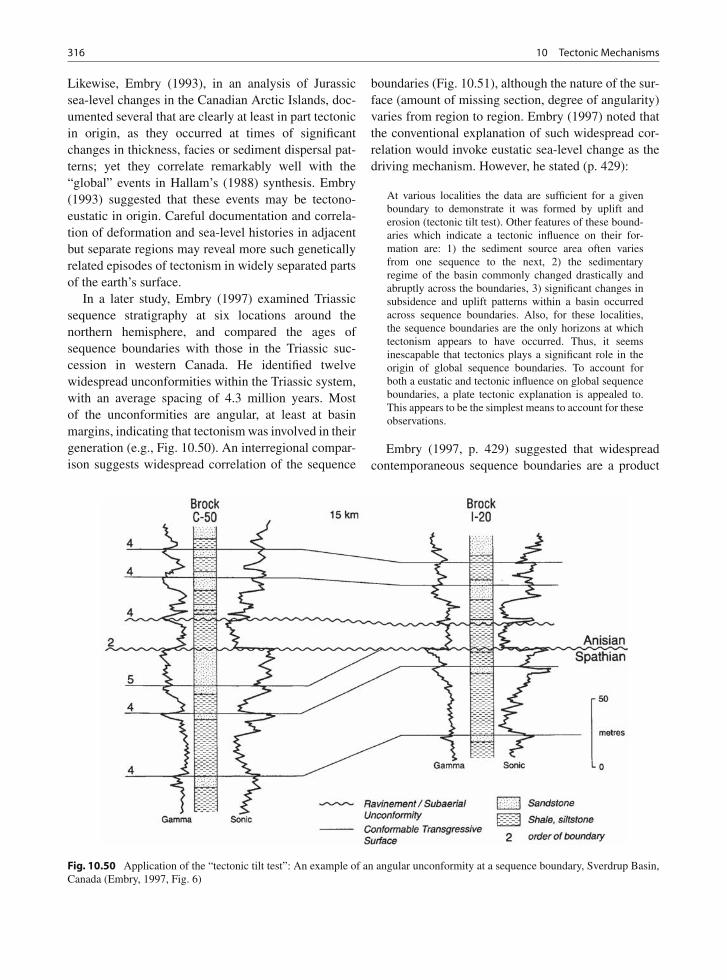
316 10 Tectonic Mechanisms
Likewise, Embry (1993), in an analysis of Jurassicsea-level changes in the Canadian Arctic Islands, doc-umented several that are clearly at least in part tectonicin origin, as they occurred at times of significantchanges in thickness, facies or sediment dispersal pat-terns; yet they correlate remarkably well with the“global” events in Hallam’s (1988) synthesis. Embry(1993) suggested that these events may be tectono-eustatic in origin. Careful documentation and correla-tion of deformation and sea-level histories in adjacentbut separate regions may reveal more such geneticallyrelated episodes of tectonism in widely separated partsof the earth’s surface.
In a later study, Embry (1997) examined Triassicsequence stratigraphy at six locations around thenorthern hemisphere, and compared the ages ofsequence boundaries with those in the Triassic suc-cession in western Canada. He identified twelvewidespread unconformities within the Triassic system,with an average spacing of 4.3 million years. Mostof the unconformities are angular, at least at basinmargins, indicating that tectonism was involved in theirgeneration (e.g., Fig. 10.50). An interregional compar-ison suggests widespread correlation of the sequence
boundaries (Fig. 10.51), although the nature of the sur-face (amount of missing section, degree of angularity)varies from region to region. Embry (1997) noted thatthe conventional explanation of such widespread cor-relation would invoke eustatic sea-level change as thedriving mechanism. However, he stated (p. 429):
At various localities the data are sufficient for a givenboundary to demonstrate it was formed by uplift anderosion (tectonic tilt test). Other features of these bound-aries which indicate a tectonic influence on their for-mation are: 1) the sediment source area often variesfrom one sequence to the next, 2) the sedimentaryregime of the basin commonly changed drastically andabruptly across the boundaries, 3) significant changes insubsidence and uplift patterns within a basin occurredacross sequence boundaries. Also, for these localities,the sequence boundaries are the only horizons at whichtectonism appears to have occurred. Thus, it seemsinescapable that tectonics plays a significant role in theorigin of global sequence boundaries. To account forboth a eustatic and tectonic influence on global sequenceboundaries, a plate tectonic explanation is appealed to.This appears to be the simplest means to account for theseobservations.
Embry (1997, p. 429) suggested that widespreadcontemporaneous sequence boundaries are a product
Fig. 10.50 Application of the “tectonic tilt test”: An example of an angular unconformity at a sequence boundary, Sverdrup Basin,Canada (Embry, 1997, Fig. 6)
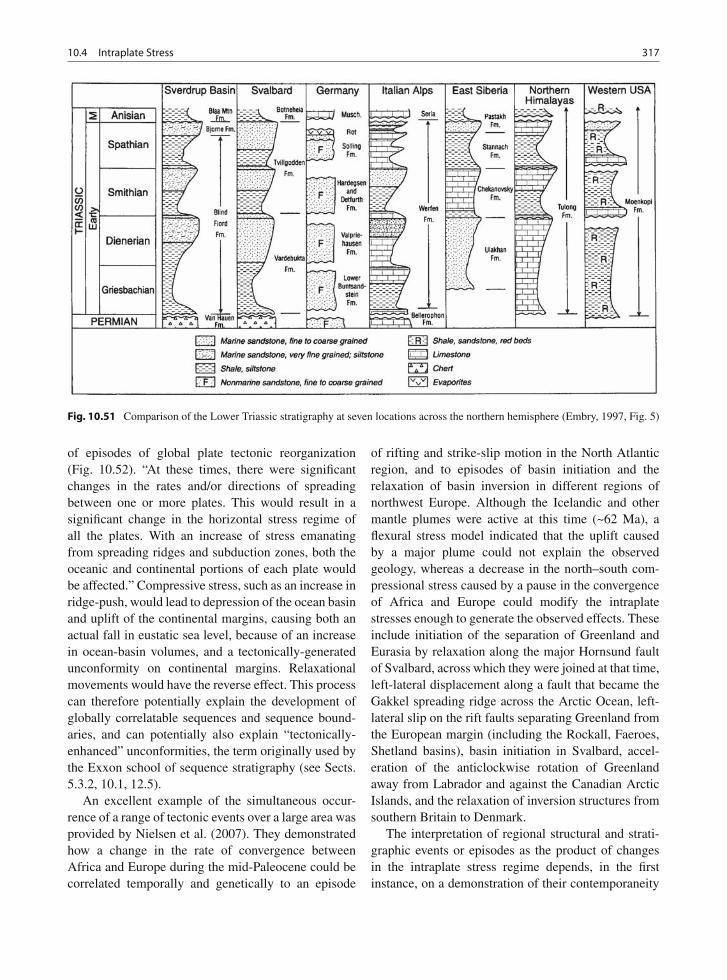
10.4 Intraplate Stress 317
Fig. 10.51 Comparison of the Lower Triassic stratigraphy at seven locations across the northern hemisphere (Embry, 1997, Fig. 5)
of episodes of global plate tectonic reorganization(Fig. 10.52). “At these times, there were significantchanges in the rates and/or directions of spreadingbetween one or more plates. This would result in asignificant change in the horizontal stress regime ofall the plates. With an increase of stress emanatingfrom spreading ridges and subduction zones, both theoceanic and continental portions of each plate wouldbe affected.” Compressive stress, such as an increase inridge-push, would lead to depression of the ocean basinand uplift of the continental margins, causing both anactual fall in eustatic sea level, because of an increasein ocean-basin volumes, and a tectonically-generatedunconformity on continental margins. Relaxationalmovements would have the reverse effect. This processcan therefore potentially explain the development ofglobally correlatable sequences and sequence bound-aries, and can potentially also explain “tectonically-enhanced” unconformities, the term originally used bythe Exxon school of sequence stratigraphy (see Sects.5.3.2, 10.1, 12.5).
An excellent example of the simultaneous occur-rence of a range of tectonic events over a large area wasprovided by Nielsen et al. (2007). They demonstratedhow a change in the rate of convergence betweenAfrica and Europe during the mid-Paleocene could becorrelated temporally and genetically to an episode
of rifting and strike-slip motion in the North Atlanticregion, and to episodes of basin initiation and therelaxation of basin inversion in different regions ofnorthwest Europe. Although the Icelandic and othermantle plumes were active at this time (~62 Ma), aflexural stress model indicated that the uplift causedby a major plume could not explain the observedgeology, whereas a decrease in the north–south com-pressional stress caused by a pause in the convergenceof Africa and Europe could modify the intraplatestresses enough to generate the observed effects. Theseinclude initiation of the separation of Greenland andEurasia by relaxation along the major Hornsund faultof Svalbard, across which they were joined at that time,left-lateral displacement along a fault that became theGakkel spreading ridge across the Arctic Ocean, left-lateral slip on the rift faults separating Greenland fromthe European margin (including the Rockall, Faeroes,Shetland basins), basin initiation in Svalbard, accel-eration of the anticlockwise rotation of Greenlandaway from Labrador and against the Canadian ArcticIslands, and the relaxation of inversion structures fromsouthern Britain to Denmark.
The interpretation of regional structural and strati-graphic events or episodes as the product of changesin the intraplate stress regime depends, in the firstinstance, on a demonstration of their contemporaneity
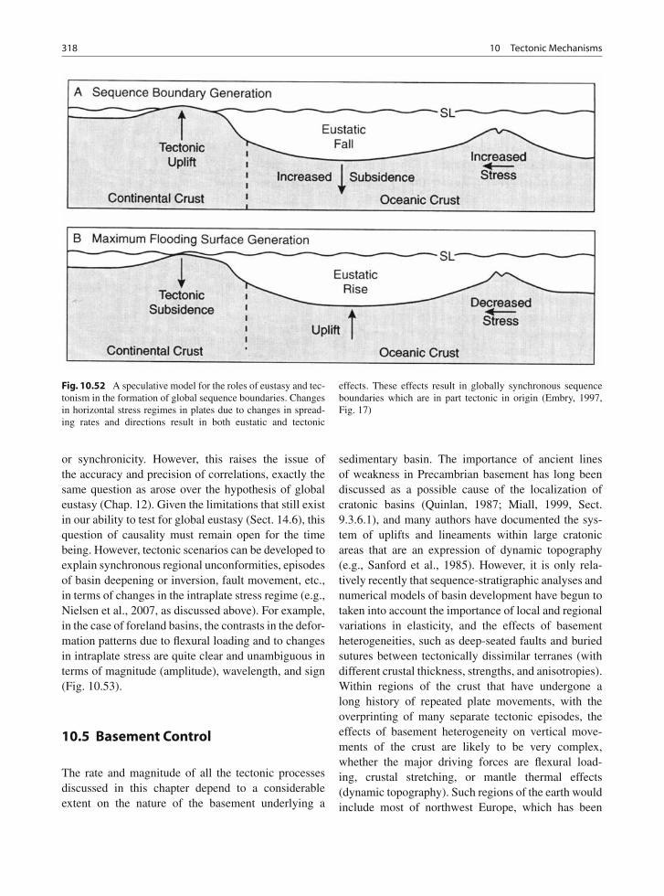
318 10 Tectonic Mechanisms
Fig. 10.52 A speculative model for the roles of eustasy and tec-tonism in the formation of global sequence boundaries. Changesin horizontal stress regimes in plates due to changes in spread-ing rates and directions result in both eustatic and tectonic
effects. These effects result in globally synchronous sequenceboundaries which are in part tectonic in origin (Embry, 1997,Fig. 17)
or synchronicity. However, this raises the issue ofthe accuracy and precision of correlations, exactly thesame question as arose over the hypothesis of globaleustasy (Chap. 12). Given the limitations that still existin our ability to test for global eustasy (Sect. 14.6), thisquestion of causality must remain open for the timebeing. However, tectonic scenarios can be developed toexplain synchronous regional unconformities, episodesof basin deepening or inversion, fault movement, etc.,in terms of changes in the intraplate stress regime (e.g.,Nielsen et al., 2007, as discussed above). For example,in the case of foreland basins, the contrasts in the defor-mation patterns due to flexural loading and to changesin intraplate stress are quite clear and unambiguous interms of magnitude (amplitude), wavelength, and sign(Fig. 10.53).
10.5 Basement Control
The rate and magnitude of all the tectonic processesdiscussed in this chapter depend to a considerableextent on the nature of the basement underlying a
sedimentary basin. The importance of ancient linesof weakness in Precambrian basement has long beendiscussed as a possible cause of the localization ofcratonic basins (Quinlan, 1987; Miall, 1999, Sect.9.3.6.1), and many authors have documented the sys-tem of uplifts and lineaments within large cratonicareas that are an expression of dynamic topography(e.g., Sanford et al., 1985). However, it is only rela-tively recently that sequence-stratigraphic analyses andnumerical models of basin development have begun totaken into account the importance of local and regionalvariations in elasticity, and the effects of basementheterogeneities, such as deep-seated faults and buriedsutures between tectonically dissimilar terranes (withdifferent crustal thickness, strengths, and anisotropies).Within regions of the crust that have undergone along history of repeated plate movements, with theoverprinting of many separate tectonic episodes, theeffects of basement heterogeneity on vertical move-ments of the crust are likely to be very complex,whether the major driving forces are flexural load-ing, crustal stretching, or mantle thermal effects(dynamic topography). Such regions of the earth wouldinclude most of northwest Europe, which has been
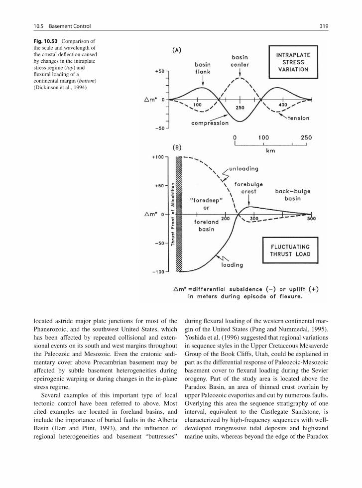
10.5 Basement Control 319
Fig. 10.53 Comparison ofthe scale and wavelength ofthe crustal deflection causedby changes in the intraplatestress regime (top) andflexural loading of acontinental margin (bottom)(Dickinson et al., 1994)
located astride major plate junctions for most of thePhanerozoic, and the southwest United States, whichhas been affected by repeated collisional and exten-sional events on its south and west margins throughoutthe Paleozoic and Mesozoic. Even the cratonic sedi-mentary cover above Precambrian basement may beaffected by subtle basement heterogeneities duringepeirogenic warping or during changes in the in-planestress regime.
Several examples of this important type of localtectonic control have been referred to above. Mostcited examples are located in foreland basins, andinclude the importance of buried faults in the AlbertaBasin (Hart and Plint, 1993), and the influence ofregional heterogeneities and basement “buttresses”
during flexural loading of the western continental mar-gin of the United States (Pang and Nummedal, 1995).Yoshida et al. (1996) suggested that regional variationsin sequence styles in the Upper Cretaceous MesaverdeGroup of the Book Cliffs, Utah, could be explained inpart as the differential response of Paleozoic-Mesozoicbasement cover to flexural loading during the Sevierorogeny. Part of the study area is located above theParadox Basin, an area of thinned crust overlain byupper Paleozoic evaporites and cut by numerous faults.Overlying this area the sequence stratigraphy of oneinterval, equivalent to the Castlegate Sandstone, ischaracterized by high-frequency sequences with well-developed trangressive tidal deposits and highstandmarine units, whereas beyond the edge of the Paradox
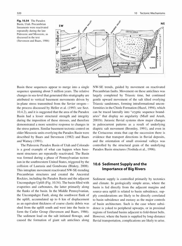
320 10 Tectonic Mechanisms
Fig. 10.54 The ParadoxBasin, Utah. Precambrianlineaments were reactivatedrepeatedly during the latePaleozoic and Mesozoic, asdiscussed in the text(Stevenson and Baars, 1986)
Basin these sequences appear to merge into a singlesequence spanning about 5 million years. The relativechanges in sea-level that generated this stratigraphy areattributed to vertical basement movements driven byin-plane stress transmitted from the Sevier orogen—the process discussed by Heller et al. (1993; see Sect.10.4.2), and it is suggested that the area of the ParadoxBasin had a lesser structural strength and integrityduring the imposition of these stresses, and thereforedemonstrated a more sensitive response to changes inthe stress pattern. Similar basement tectonic control onolder Mesozoic units overlying the Paradox Basin weredescribed by Baars and Stevenson (1982) and Baarsand Watney (1991).
The Paleozoic Paradox Basin of Utah and Coloradois a good example of what can happen when base-ment structures are repeatedly reactivated. The Basinwas formed during a phase of Pennsylvanian tecton-ism in the southwestern United States, triggered by thecollision of Laurasia and Gondwana (Blakey, 2008).This intraplate movement reactivated NW-SE-trendingPrecambrian structures and created the AncestralRockies, including the Paradox Basin and the adjacentUncompahgre Uplift (Fig. 10.54). The basin filled withevaporites and carbonates, the latter primarily alongthe flanks of the basin. In the Middle Pennsylvanian,the Uncompahgre Fault, along the southwest flank ofthe uplift, accumulated up to 6 km of displacementas an equivalent thickness of coarse clastic debris wasshed from the uplift south and west into the basin toform the Cutler Group (Stevenson and Baars, 1986).The sediment load on the salt initiated flowage, andcaused the formation of giant salt anticlines along
NW-SE trends, guided by movement on reactivatedPrecambrian faults. Movement on these anticlines waslargely completed by Triassic time, but continuedgentle upward movement of the salt tilted overlyingTriassic sandstones, forming intraformational uncon-formities in the Chinle Formation (Hazel, 1994), whichcan be traced laterally into “cryptic sequence bound-aries” that display no angularity (Miall and Arush,2001b). Jurassic fluvial systems show major changesin paleocurrent patterns as a result of underlyingdiapiric salt movement (Bromley, 1991), and even inthe Cretaceous strata that cap the succession there isevidence that transport directions in fluvial deposits,and the orientation of small erosional valleys wascontrolled by the structural grain of the underlyingParadox Basin structures (Yoshida et al., 1996).
10.6 Sediment Supply and theImportance of Big Rivers
Sediment supply is controlled primarily by tectonicsand climate. In geologically simple areas, where thebasin is fed directly from the adjacent margins andsource-area uplift is related to basin subsidence, sup-ply considerations are likely to be directly correlatedto basin subsidence and eustasy as the major controlsof basin architecture. Such is the case where subsi-dence is yoked to peripheral upwarps, or in proximalregions of foreland basins adjacent to fold-thrust belts.However, where the basin is supplied by long-distancefluvial transportation, complications are likely to arise.
10.6 Sediment Supply and the Importance of Big Rivers 321
Where the rate of sediment supply is high, it may over-whelm other influences to become a dominant controlon sequence architecture.
Many sedimentary basins were filled by river sys-tems whose drainage area has been subsequentlyremodeled by tectonism, and it may take considerablegeological investigation to reconstruct their possiblepast positions. For example, stratigraphic successionsmay occur that cannot be related to the evolution ofadjacent orogens. In North America, dynamic topo-graphic processes have generated regional uplifts andcontinental tilts that have resulted in deep erosionand large-scale continental fluxes of detrital sedi-ment (Miall, 2008, Sect. 2.2). For example, Rainbird(1992), Rainbird et al. (1992, 1997) and Hoffman andGrotzinger (1993) suggested that much of the detri-tus derived by uplift and erosion of the Grenvilleorogen of eastern North America during the latePrecambrian may have ended up contributing to thethick Neoproterozoic sedimentary wedges on the west-ern continental margin. Detailed study of detrital zir-cons from sedimentary rocks of this age in the westernCanadian Arctic indicated that 50% of them are ofGrenville age. Rainbird and his colleagues proposedthat a major west-flowing river system was estab-lished during the late Proterozoic which transportedthis detritus some 3,000 km across the continental inte-rior. Dickinson (1988) suggested that much of the thickaccumulations of late Paleozoic and Mesozoic fluvialand eolian strata in the southwestern United States hadbeen derived from Appalachian sources, and this wasconfirmed by the detrital-zircon studies of Dickinsonand Gehrels (2003). McMillan (1973) envisaged aTertiary river system draining from the continentalinterior of North America into Hudson Bay, ulti-mately delivering sediment to the Labrador Shelf.This has been supported by the studies of Cenozoiclandforms and sediments by Duk-Rodkin and Hughes(1994).
Potter (1978) pointed out that major river systemsmay cross major tectonic boundaries, feeding sedimentof a petrographic type unrelated to the receiving basin,into the basin at a rate unconnected in any way withthe subsidence history of the basin itself. The modernAmazon river is a good example. It derives from theAndean Mountains, flows across and between, and isfed from several Precambrian shields, and debouchesonto a major extensional continental margin. From thepoint of view of sequence stratigraphy, the important
point is that large sediment supplies delivered to ashoreline may overwhelm the stratigraphic effects ofvariations in sea level. A region undergoing a rela-tive or eustatic rise in sea level may still experiencestratigraphic regression if large delta complexes arebeing built by major sediment-laden rivers. Holbrooket al. (2006) provided a useful discussion of the effectsof upstream controls on the development of fluvialgraded profiles, fluvial style and the development ofnonmarine sequences downstream (Sect. 2.2).
Upstream controls may also be significant inthe case of deep-marine deposits. Major episodesof submarine-fan sedimentation in the North Seaand Shetland-Faeroes basins correlate with pulses ofIceland plume activity, which caused magmatic under-plating of the continental margin, and uplift, erosion,and enhanced sediment delivery to offshore sedimen-tary basins (Fig. 10.12: White and Lovell, 1997).
A significant example of this long-distance sedi-mentary control is the Cenozoic stratigraphic evolutionof the Texas-Louisiana coast of the Gulf of Mexico(Worrall and Snelson, 1989). This continental mar-gin is fed with sediment by rivers that have occupiedessentially the same position since the early Tertiary(Fisher and McGowen, 1967). The rivers feed intothe Gulf Coast from huge drainage basins occupyinglarge areas of the North American Interior (Fig. 10.55).Progradation has extended the continental margin ofthe Gulf by up to 350 km. This has taken place episod-ically in both time and space, developing a seriesof major clastic wedges, some hundreds of metresin thickness (Figs. 10.56 and 10.57). According tothe Exxon sequence-stratigraphy models these clasticwedges would be interpreted as highstand deposits, butGalloway (1989b, 2008) showed that their age distribu-tion shows few correlations with the global cycle chart(Fig. 10.58). The major changes along strike of thethickness of these clastic wedges (Fig. 10.57) is alsoevidence against a control by passive sea-level change.Highly suggestive are the correlations with the tectonicevents of the North American Interior; for example, thetiming of the Lower and Upper Wilcox Group wedgesrelative to the timing of the Laramide orogenic pulsesalong the Cordillera (Fig. 10.58). It seems likely thatsediment supply, driven by source-area tectonism, isthe major control on the location, timing and thick-ness of the Gulf Coast clastic wedges. A secondarycontrol is the nature of local tectonism on the continen-tal margin itself, including growth faulting, evaporite
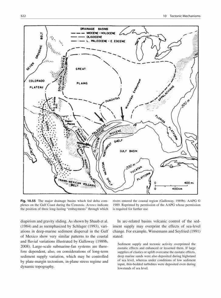
322 10 Tectonic Mechanisms
Fig. 10.55 The major drainage basins which fed delta com-plexes on the Gulf Coast during the Cenozoic. Arrows indicatethe position of three long-lasting “embayments” through which
rivers entered the coastal region (Galloway, 1989b). AAPG ©1989. Reprinted by permission of the AAPG whose permissionis required for further use
diapirism and gravity sliding. As shown by Shaub et al.(1984) and as reemphasized by Schlager (1993), vari-ations in deep-marine sediment dispersal in the Gulfof Mexico show very similar patterns to the coastaland fluvial variations illustrated by Galloway (1989b,2008). Large-scale submarine-fan systems are there-fore dependent, also, on considerations of long-termsediment supply variation, which may be controlledby plate-margin tectonism, in-plane stress regime anddynamic topography.
In arc-related basins volcanic control of the sed-iment supply may overprint the effects of sea-levelchange. For example, Winsemann and Seyfried (1991)stated:
Sediment supply and tectonic activity overprinted theeustatic effects and enhanced or lessened them. If largesupplies of clastics or uplift overcame the eustatic effects,deep marine sands were also deposited during highstandof sea level, whereas under conditions of low sedimentinput, thin-bedded turbidites were deposited even duringlowstands of sea level.
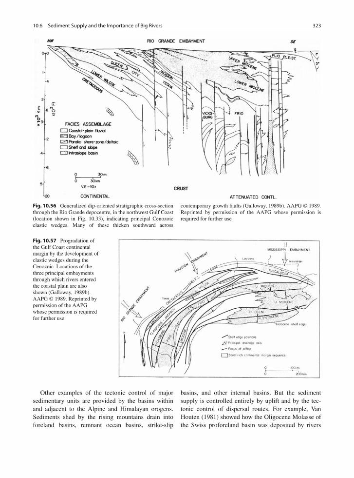
10.6 Sediment Supply and the Importance of Big Rivers 323
Fig. 10.56 Generalized dip-oriented stratigraphic cross-sectionthrough the Rio Grande depocentre, in the northwest Gulf Coast(location shown in Fig. 10.33), indicating principal Cenozoicclastic wedges. Many of these thicken southward across
contemporary growth faults (Galloway, 1989b). AAPG © 1989.Reprinted by permission of the AAPG whose permission isrequired for further use
Fig. 10.57 Progradation ofthe Gulf Coast continentalmargin by the development ofclastic wedges during theCenozoic. Locations of thethree principal embaymentsthrough which rivers enteredthe coastal plain are alsoshown (Galloway, 1989b).AAPG © 1989. Reprinted bypermission of the AAPGwhose permission is requiredfor further use
Other examples of the tectonic control of majorsedimentary units are provided by the basins withinand adjacent to the Alpine and Himalayan orogens.Sediments shed by the rising mountains drain intoforeland basins, remnant ocean basins, strike-slip
basins, and other internal basins. But the sedimentsupply is controlled entirely by uplift and by the tec-tonic control of dispersal routes. For example, VanHouten (1981) showed how the Oligocene Molasse ofthe Swiss proforeland basin was deposited by rivers
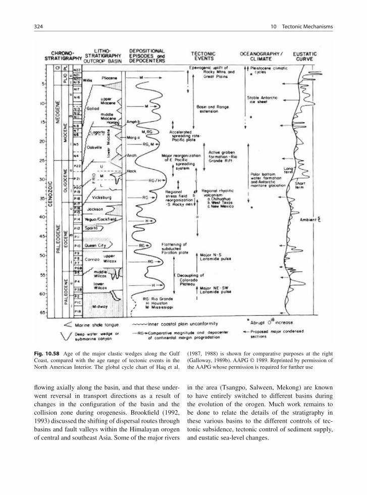
324 10 Tectonic Mechanisms
Fig. 10.58 Age of the major clastic wedges along the GulfCoast, compared with the age range of tectonic events in theNorth American Interior. The global cycle chart of Haq et al.
(1987, 1988) is shown for comparative purposes at the right(Galloway, 1989b). AAPG © 1989. Reprinted by permission ofthe AAPG whose permission is required for further use
flowing axially along the basin, and that these under-went reversal in transport directions as a result ofchanges in the configuration of the basin and thecollision zone during orogenesis. Brookfield (1992,1993) discussed the shifting of dispersal routes throughbasins and fault valleys within the Himalayan orogenof central and southeast Asia. Some of the major rivers
in the area (Tsangpo, Salween, Mekong) are knownto have entirely switched to different basins duringthe evolution of the orogen. Much work remains tobe done to relate the details of the stratigraphy inthese various basins to the different controls of tec-tonic subsidence, tectonic control of sediment supply,and eustatic sea-level changes.
10.8 Main Conclusions 325
10.7 Environmental Change
Some sequence boundaries in carbonate sediments arenot due to sea-level changes, but to environmentalchanges that ultimately are related to the tectonic evo-lution of the area. Two main processes have beendocumented. The first of these results in what Schlager(1989) termed drowning unconformities. Changes innutrient supply, water chemistry, or the clastic contentof the sea may cause a termination of carbonate-producing biogenic growth. Secondly, surfaces havingthe same character as sequence boundaries can begenerated erosively by submarine currents, such asthe Gulf Stream. Schlager (1992a) provided severalexamples of both these types of process, which are dis-cussed in more detail and illustrated in Sect. 2.3.3 ofthis book. He argued that several events in the Exxonglobal cycle chart were generated by these non-eustaticprocesses.
10.8 Main Conclusions
Regarding extensional basins and continental margins:
1. The stratigraphic architectures that have been usedby Vail and his coworkers to interpret sea-levelchanges on a 107-year time scale may be gener-ated by other processes. Coastal onlap (relativerises of sea level) may be caused by flexural down-warp of extensional continental margins. Relativefalls in sea level may be caused by thermal domingaccompanying rifting.
2. The processes which lead to long-term eustaticsea-level changes, such as changing rates of sea-floor spreading (Chap. 9) also lead to tectonicadjustments of the continents (e.g., initiation ofthe rift-thermal subsidence cycle), so that rela-tive changes in sea-level may have multiple causeswhich are not necessarily simply interpretable interms of eustasy.
3. The North Sea Basin, one of the type areas forthe Vail curves, was affected by almost continuoustectonism during the Mesozoic and Cenozoic, andmany of the sequence-boundary events and strati-graphic architectures there can now be interpreted
in terms of specific local or regional episodes ofrift faulting and thermal uplift and subsidence.
Regarding convergent plate margins and collisionzones, and their associated foreland basins:
4. Arcs are characterized by active regional tec-tonism as a result of variations in subductionhistory, arc migration, and the filling and defla-tion of magma chambers. The rates, magnitudesand episodicities of the relative changes in sealevel caused by this tectonism that have beendetermined by detailed mapping in modern arcsand other regions of convergent tectonism areconsistent with sea-level changes interpreted tohave generated stratigraphic sequences with 104–107-year frequencies that have been mapped inarc-related basins.
5. The various elements of convergent tectonismthat generate foreland basins by flexural load-ing (continental collision, terrane accretion, nappemigration, thrust movement, imbricate fault prop-agation) can cause relative changes of sea-level ona 104–107-year time scale.
6. Stratigraphic sequences of 106–107-year dura-tion in foreland basins, such as the WesternInterior of North America and Pyrenean basins,may commonly be correlated with specific tec-tonic episodes in the adjacent orogen, andthere is increasing evidence that high-frequencysequences, of 104–105-year duration, may be cor-related with local tectonic events. The correlationof any of these sequences with a global cycle chartmay, therefore, be fortuitous.
Regarding intraplate stress:
7. Stresses generated by plate-margin extension orcompression, and transmitted horizontally, haveimportant modifying effects on flexural behaviourof sedimentary basins, acting to amplify or subdueflexural deformation caused by regional tecton-ics. Changes in paleostress fields change theseupwarps and downwarps, resulting in offlap andonlap patterns comparable in stratigraphic dura-tion and magnitude to the “third-order” (106-year)stratigraphic cyclic changes of the Exxon globalcycle chart.
326 10 Tectonic Mechanisms
8. High-frequency sequences (of 104–105-year dura-tion), of limited, regional extent, may be generatedby the transmission of stresses induced by flexuralloading of individual structures and their structuralcomponents, as thrust faults and their imbricatesare propagated during contractional tectonism.
9. Stratigraphic patterns induced by intraplate stressare of opposite sign in basin margins and basincentres, and may correlate with tectonic episodes(such as fault movement, basin inversion) in adja-cent regions The proposition of intraplate stresschange as a widespread control of synchronousbasinal events is, therefore, a testable hypothe-sis, requiring detailed correlation of unconformi-ties and their correlative conformities and otherstructures across and between basins.
Regarding the importance of sediment supply:
10. The sediment supply to a basin may not be gov-erned by local tectonics but by tectonic events indistant, structurally unrelated areas, with sedimenttransported across cratons and through orogens bymajor rivers. In such cases, the distribution and ageof fluvial, coastal and submarine clastic wedgesdoes not relate to the sea-level cycle in the basin,but to the tectonic evolution of the sediment sourcearea.
Regarding the importance of environmental change:
11. Carbonate sedimentation may be interrupted bychanges in nutrients, water chemistry or clas-tic content, which inhibit carbonate production.Carbonate platforms are also susceptible to ero-sion by shifting submarine currents. The result,in all these cases, may be breaks in sedimenta-tion that appear similar to but are unrelated tosequence boundaries produced by sea-level fall.
General conclusions:
12. If tectonic subsidence varies in rate within andbetween basins, as is typically the case, but is com-parable to the rate of eustatic sea-level change,sequence boundaries and flooding surfaces will bemarkedly diachronous. No synchronous eustaticsignal can be generated in such cases.
13. The availability of tectonic mechanisms to explainstratigraphic cyclicity of all types and at all geo-logical time scales removes the need for globaleustasy as a primary mechanism for the gen-eration of stratigraphic architectures. This beingthe case, the onus is on the supporters ofeustasy to prove their case by quantitative doc-umentation of eustatic processes, and by rig-orous global correlation of supposed eustaticevents.
14. Given the finite size of Earth, major plate-tectonicevents, (e.g., collisions, ridge re-ordering events,changes in rotation vectors), and their strati-graphic responses, may be globally synchronous.The potential, therefore, exists for global strati-graphic correlation. However, the structural andstratigraphic signature would vary from region toregion, such that, for example, a relative sea-levelrise in one location may be genetically related to afall elsewhere.
15. The invocation of tectonic mechanisms to explainstratigraphic architecture has led to the sugges-tion that Vail’s charts be “inverted”, to providea source of data from which tectonic episodic-ity could be extracted. While this is an inter-esting idea, there remains the problem that theglobal accuracy and precision of the Vail curvesare in question, and tectonic arguments are inas much danger as eustatic arguments of fallinginto the trap of false correlation and circularreasoning.
Chapter 11
Orbital Forcing
Contents
11.1 Introduction . . . . . . . . . . . . . . . . 32711.2 The Nature of Milankovitch Processes . . . . 328
11.2.1 Components of Orbital Forcing . . . . 32811.2.2 Basic Climatology . . . . . . . . . . 33011.2.3 Variations with Time in Orbital
Periodicities . . . . . . . . . . . . 33211.2.4 Isostasy and Geoid Changes . . . . . 33311.2.5 Nonglacial Milankovitch Cyclicity . . 33411.2.6 The Nature of the Cyclostratigraphic Data
Base . . . . . . . . . . . . . . . . 33811.3 The Geologic Record . . . . . . . . . . . . 339
11.3.1 The Sensitivity of the Earth to Glaciation 33911.3.2 The Cenozoic Record . . . . . . . . 34111.3.3 Glacioeustasy in the Mesozoic? . . . . 34311.3.4 Late Paleozoic Cyclothems . . . . . . 346
11.4 Distinguishing Between Orbital Forcing andTectonic Driving Mechanisms . . . . . . . . 349
11.5 Main Conclusions . . . . . . . . . . . . . 352
11.1 Introduction
By the end of the nineteenth century it was rec-ognized that during the Pleistocene the earth hadundergone at least four major ice ages, and a searchwas underway for a mechanism that would alter cli-mate so dramatically (useful historical summaries aregiven by Berger, 1988; Imbrie, 1985; Huggett, 1991,Sect. 2.3; Dott, 1992a, b; de Boer and Smith, 1994b).Continued stratigraphic work during the twentieth cen-tury produced evidence for many more cycles ofice formation, advance and melting, and it is nowknown that there were more than twenty such cycles,indicating successive major fluctuations in globalclimate.
The basis of the idea of orbital forcing can be tracedback to the seventeenth century (Huggett, 1991, p. 24),
but it was an amateur geologist and newspaper pub-lisher, Charles MacLaren, who in 1842 first realizedthe implications of continental glaciation for majorchanges in sea level (Dott, 1992b). The rhythmicityin glaciation is now attributed to astronomical forcing.The Scotsman James Croll (1864) and the American G.K. Gilbert (1895) were the first to realize that variationsin the earth’s orbital behavior may affect the distribu-tion of solar radiation received at the surface, by lati-tude and by season, and could be the cause of major cli-matic variations, but the ideas were not taken seriouslyfor many years after this because of a lack of a quan-tifiable theory and supporting data. Gilbert invokedthe idea to explain oscillations in carbonate contentin some Cretaceous hemipelagic beds in Colorado(Fischer, 1986). Later, Bradley (1929) “recognizedprecessional cycles in oil shale-dolomite sequences ofthe Green River Formation in Colorado, Wyoming andUtah, using varves as an unusually precise measureof sedimentation rates” (de Boer and Smith, 1994b).Theoretical work on the distribution of insolation wascarried out by the Serbian mathematician Milankovitch(1930, 1941), who showed how orbital oscillationscould affect the distribution of solar radiation over theearth’s surface. However, it was not for some yearsthat the necessary data from the sedimentary recordwas obtained to support his model. Emiliani (1955)was the first to discover periodicities in the Pleistocenemarine isotopic record, and the work by Hays et al.(1976) is regarded by many (e.g., de Boer and Smith,1994b) as the definitive study that marked the begin-ning of a more widespread acceptance of so-calledMilankovitch processes as the cause of stratigraphiccyclicity on a 104–105-year frequency—what is nowtermed the Milankovitch band (Sect. 4.1). The modelis now firmly established, particularly since accurate
327A.D. Miall, The Geology of Stratigraphic Sequences, 2nd ed.,DOI 10.1007/978-3-642-05027-5_11, © Springer-Verlag Berlin Heidelberg 2010
328 11 Orbital Forcing
chronostratigraphic dating of marine sediments has ledto the documentation of the record of faunal variationsand temperature changes in numerous upper Cenozoicsections (Sect. 7.2 and 11.3). These show remark-ably close agreement with the predictions made fromastronomical observations.
There is an obvious link between climate and sealevel. There is no doubting the efficacy of glacialadvance and retreat as a mechanism for changing sea-level; we have the evidence of the Pleistocene glacia-tion at hand throughout the Northern Hemisphere. Ithas been calculated that during the period of maximumPleistocene ice advance the sea was lowered by about100 m (Donovan and Jones, 1979). Melting of theremaining ice caps would raise the present sea-level byabout 40–50 m (Donovan and Jones, 1979). Recent his-tory thus demonstrates a mechanism of changing sea-level by at least 150 m at a rate of about 0.01 m/year.This is fast enough to account for eustatic cycles withfrequencies in the range of tens of thousands of years.Milankovitch processes are now widely accepted asthe source of much cyclicity with cyclicities of 104–105 years in the Late Paleozoic and Late Cenozoicsedimentary record—times when continental glacia-tion is known to have been widespread (Sects. 11.3.2and Sect. 11.3.4). Other, more subtle (non-glacial)climatic variations may explain other forms of cyclic-ity of similar periodicity at times when there is noevidence for widespread continental ice sheets (Sect.11.2.5). However, there is also increasing evidence forcyclicity of a similar time periodicity generated by tec-tonic mechanisms, especially in foreland basins (Sect.10.3.3), and it is not safe to assume that sequencesof 104–105-year duration are necessarily generated byorbital forcing. This problem is examined further inSect. 11.4.
There has been a considerable increase in interestin Milankovitch processes in recent years, particu-larly since the suggestion was made by House (1985)that the regularity of the orbital forcing process couldbe exploited for the construction of a new, highlyaccurate type of time scale. This has given rise toa vigorous new subdiscipline termed cyclostratigra-phy. A number of books have appeared that treat thesubject from various points of view. The astronomi-cal processes that underpin Earth’s climatic cyclicityare dealt with by Schwarzacher (1993, 2000), andHinnov (2000), and by A. L. Berger, in a numberof books, including Berger et al. (1984) and Berger
(1988). Collections of case studies, some with papersexplaining orbital mechanics or climatic theory, havebeen edited by Fischer and Bottjer (1991), Bergeret al. (1984), de Boer and Smith (1994a), House andGale (1995) and D’Argenio et al. (2004a). Much addi-tional information is contained in the books editedby Franseen et al. (1991), Dennison and Ettensohn(1994), and Weedon (2003). A major symposiumon the cyclostratigraphic record was held by theRoyal Society of London in 1998 (Shackleton et al.,1999). This symposium, and the development of thecylostratigraphic or astronochronologic time scalefrom the ancient sedimentary record are critically eval-uated in Sect. 14.7.
11.2 The Nature of MilankovitchProcesses
11.2.1 Components of Orbital Forcing
There are several separate components of orbitalvariation (Fig. 11.1). The present orbital behaviorof the earth includes the following cyclic changes(Schwarzacher, 1993):
1. Variations in orbital eccentricity (the shape of theEarth’s orbit around the sun). Several “wobbles”,which have periods of 2,035.4, 412.8, 128.2, 99.5,94.9, and 54 ka. The major periods are those ataround 413 and 100 ka.
2. Changes of up to 3◦ in the obliquity of the ecliptic,with a major period of 41 ka, and minor periods of53.6 and 39.7 ka.
3. Precession of the equinoxes. The Earth’s orbitrotates like a spinning top, with a major period of23.7 ka. This affects the timing of the perihelion(the position of closest approach of the earth to thesun on an elliptical orbit), which changes with aperiod of 19 ka.
Imbrie (1985, p. 423) explained the effects of thesevariables as follows:
Variations in obliquity alter the income side of the radia-tion budget in two fundamental ways: they modulate theintensity of the seasonal cycle, and they alter the annuallyintegrated pole-to-equator insolation gradient on which
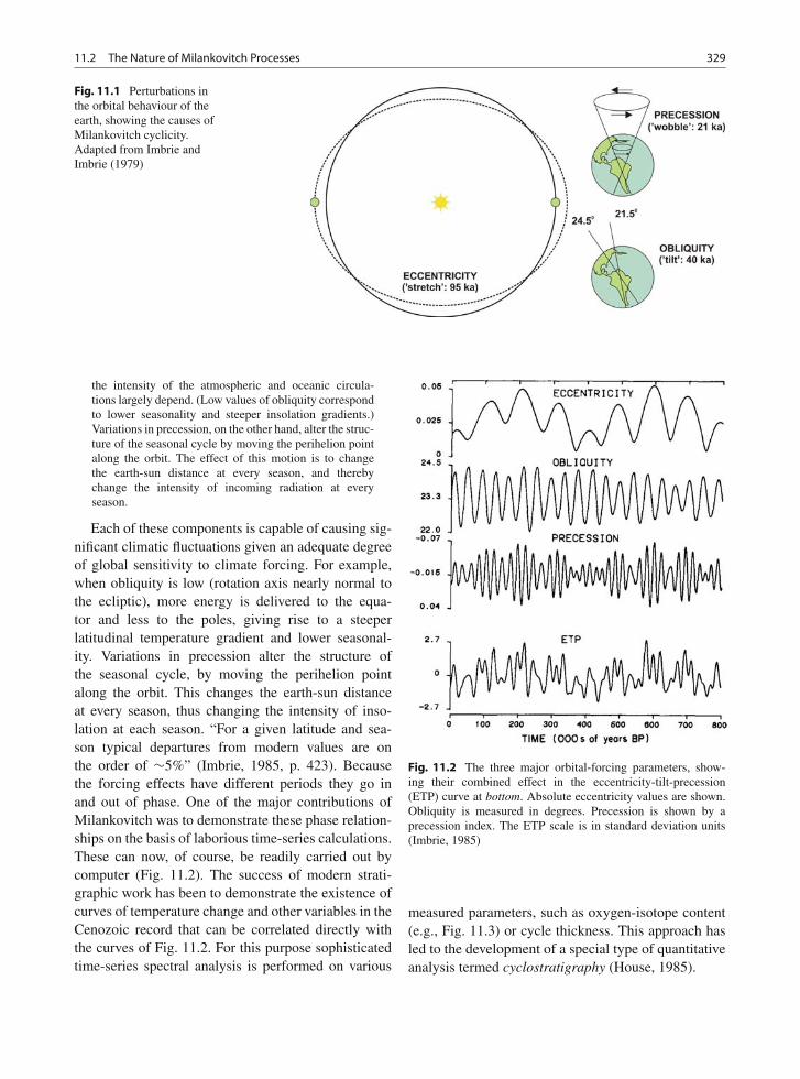
11.2 The Nature of Milankovitch Processes 329
Fig. 11.1 Perturbations inthe orbital behaviour of theearth, showing the causes ofMilankovitch cyclicity.Adapted from Imbrie andImbrie (1979)
the intensity of the atmospheric and oceanic circula-tions largely depend. (Low values of obliquity correspondto lower seasonality and steeper insolation gradients.)Variations in precession, on the other hand, alter the struc-ture of the seasonal cycle by moving the perihelion pointalong the orbit. The effect of this motion is to changethe earth-sun distance at every season, and therebychange the intensity of incoming radiation at everyseason.
Each of these components is capable of causing sig-nificant climatic fluctuations given an adequate degreeof global sensitivity to climate forcing. For example,when obliquity is low (rotation axis nearly normal tothe ecliptic), more energy is delivered to the equa-tor and less to the poles, giving rise to a steeperlatitudinal temperature gradient and lower seasonal-ity. Variations in precession alter the structure ofthe seasonal cycle, by moving the perihelion pointalong the orbit. This changes the earth-sun distanceat every season, thus changing the intensity of inso-lation at each season. “For a given latitude and sea-son typical departures from modern values are onthe order of ∼5%” (Imbrie, 1985, p. 423). Becausethe forcing effects have different periods they go inand out of phase. One of the major contributions ofMilankovitch was to demonstrate these phase relation-ships on the basis of laborious time-series calculations.These can now, of course, be readily carried out bycomputer (Fig. 11.2). The success of modern strati-graphic work has been to demonstrate the existence ofcurves of temperature change and other variables in theCenozoic record that can be correlated directly withthe curves of Fig. 11.2. For this purpose sophisticatedtime-series spectral analysis is performed on various
Fig. 11.2 The three major orbital-forcing parameters, show-ing their combined effect in the eccentricity-tilt-precession(ETP) curve at bottom. Absolute eccentricity values are shown.Obliquity is measured in degrees. Precession is shown by aprecession index. The ETP scale is in standard deviation units(Imbrie, 1985)
measured parameters, such as oxygen-isotope content(e.g., Fig. 11.3) or cycle thickness. This approach hasled to the development of a special type of quantitativeanalysis termed cyclostratigraphy (House, 1985).
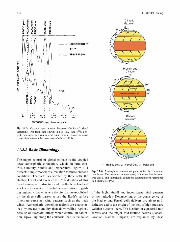
330 11 Orbital Forcing
Fig. 11.3 Variance spectra over the past 800 ka of orbitalvariations (top; from data shown in Fig. 11.2) and δ18O con-tent, measured in foraminiferal tests (bottom). Note the closecorrelation between the two curves (Imbrie, 1985)
11.2.2 Basic Climatology
The major control of global climate is the coupledocean-atmospheric circulation, which, in turn, con-trols humidity, rainfall and temperature. Figure 11.4presents simple models of circulation for three climaticconditions. The earth is encircled by three cells, theHadley, Ferrel and Polar cells. Consideration of thisbroad atmospheric structure and its effects on land andsea leads to a series of useful generalizations regard-ing regional climate. Where the circulation establishedby the three cells passes across the Earth’s surfaceit sets up persistent wind patterns such as the tradewinds. Atmospheric upwelling regions are character-ized by greater humidity than downwelling regions,because of adiabatic effects which control air satura-tion. Upwelling along the equatorial belt is the cause
Fig. 11.4 Atmospheric circulation patterns for three climaticconditions. The present climate (centre) is intermediate betweentrue glacial and interglacial conditions (adapted from Perlmutterand Matthews, 1990)
of the high rainfall and inconsistent wind patternsat low latitudes. Downwelling at the convergence ofthe Hadley and Ferrell cells delivers dry air to mid-latitudes and is the origin of the belt of high-pressureweather systems there. The location of equatorial rainforests and the major mid-latitude deserts (Sahara,Arabian, Namib, Simpson) are explained by these
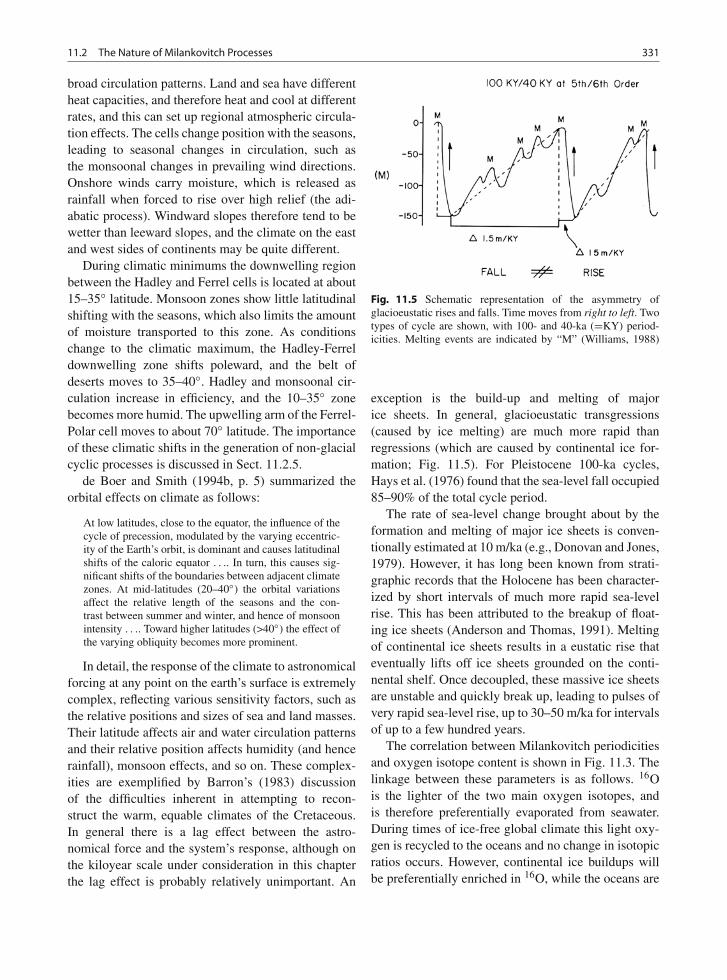
11.2 The Nature of Milankovitch Processes 331
broad circulation patterns. Land and sea have differentheat capacities, and therefore heat and cool at differentrates, and this can set up regional atmospheric circula-tion effects. The cells change position with the seasons,leading to seasonal changes in circulation, such asthe monsoonal changes in prevailing wind directions.Onshore winds carry moisture, which is released asrainfall when forced to rise over high relief (the adi-abatic process). Windward slopes therefore tend to bewetter than leeward slopes, and the climate on the eastand west sides of continents may be quite different.
During climatic minimums the downwelling regionbetween the Hadley and Ferrel cells is located at about15–35◦ latitude. Monsoon zones show little latitudinalshifting with the seasons, which also limits the amountof moisture transported to this zone. As conditionschange to the climatic maximum, the Hadley-Ferreldownwelling zone shifts poleward, and the belt ofdeserts moves to 35–40◦. Hadley and monsoonal cir-culation increase in efficiency, and the 10–35◦ zonebecomes more humid. The upwelling arm of the Ferrel-Polar cell moves to about 70◦ latitude. The importanceof these climatic shifts in the generation of non-glacialcyclic processes is discussed in Sect. 11.2.5.
de Boer and Smith (1994b, p. 5) summarized theorbital effects on climate as follows:
At low latitudes, close to the equator, the influence of thecycle of precession, modulated by the varying eccentric-ity of the Earth’s orbit, is dominant and causes latitudinalshifts of the caloric equator . . .. In turn, this causes sig-nificant shifts of the boundaries between adjacent climatezones. At mid-latitudes (20–40◦) the orbital variationsaffect the relative length of the seasons and the con-trast between summer and winter, and hence of monsoonintensity . . .. Toward higher latitudes (>40◦) the effect ofthe varying obliquity becomes more prominent.
In detail, the response of the climate to astronomicalforcing at any point on the earth’s surface is extremelycomplex, reflecting various sensitivity factors, such asthe relative positions and sizes of sea and land masses.Their latitude affects air and water circulation patternsand their relative position affects humidity (and hencerainfall), monsoon effects, and so on. These complex-ities are exemplified by Barron’s (1983) discussionof the difficulties inherent in attempting to recon-struct the warm, equable climates of the Cretaceous.In general there is a lag effect between the astro-nomical force and the system’s response, although onthe kiloyear scale under consideration in this chapterthe lag effect is probably relatively unimportant. An
Fig. 11.5 Schematic representation of the asymmetry ofglacioeustatic rises and falls. Time moves from right to left. Twotypes of cycle are shown, with 100- and 40-ka (=KY) period-icities. Melting events are indicated by “M” (Williams, 1988)
exception is the build-up and melting of majorice sheets. In general, glacioeustatic transgressions(caused by ice melting) are much more rapid thanregressions (which are caused by continental ice for-mation; Fig. 11.5). For Pleistocene 100-ka cycles,Hays et al. (1976) found that the sea-level fall occupied85–90% of the total cycle period.
The rate of sea-level change brought about by theformation and melting of major ice sheets is conven-tionally estimated at 10 m/ka (e.g., Donovan and Jones,1979). However, it has long been known from strati-graphic records that the Holocene has been character-ized by short intervals of much more rapid sea-levelrise. This has been attributed to the breakup of float-ing ice sheets (Anderson and Thomas, 1991). Meltingof continental ice sheets results in a eustatic rise thateventually lifts off ice sheets grounded on the conti-nental shelf. Once decoupled, these massive ice sheetsare unstable and quickly break up, leading to pulses ofvery rapid sea-level rise, up to 30–50 m/ka for intervalsof up to a few hundred years.
The correlation between Milankovitch periodicitiesand oxygen isotope content is shown in Fig. 11.3. Thelinkage between these parameters is as follows. 16Ois the lighter of the two main oxygen isotopes, andis therefore preferentially evaporated from seawater.During times of ice-free global climate this light oxy-gen is recycled to the oceans and no change in isotopicratios occurs. However, continental ice buildups willbe preferentially enriched in 16O, while the oceans are
332 11 Orbital Forcing
depleted in this isotope, with the result that the δ18Ocontent of the oceans is increased. Numerous stud-ies since that of Emiliani (1955) have shown that the16O/18O ratio is a sensitive indicator of global oceantemperatures and can therefore be used as an ana-log recorder of ice volumes (e.g., Matthews, 1984,1988). The measurements are made on the carbonatein foraminiferal tests. Matthews (1984) suggested acalibration value of δ18O variation of about 0.011‰per metre of sea-level change. Precise calibrations areimpossible because of uncertainties regarding the vol-ume and content of floating pack ice, and diagenesisof foraminiferal tests. It is also important to take intoaccount the lag between the maximum eustatic highand the highest surface ocean temperatures, whichoccur some 103 years later.
11.2.3 Variations with Time in OrbitalPeriodicities
It is not known how the orbital periodicities determinedfor the Holocene, and which seem to have remainedstable at least through the Neogene, might have var-ied in the distant geological past. Some studies havesuggested that small perturbations in the motions ofthe planets during geologic time may have had sig-nificant effects on the orbital behaviour of the earth(Laskar, 1989). Plint et al. (1992) stated that “overlonger periods of time, it is postulated that nonlin-ear amplifications of even very small perturbations inplanetary orbits, as well as changes in the diameterof the core, and of the earth as a whole, will leadto chaotic, unpredictable planetary motions.” Laskar(1999) stated that calculation of planetary motionscannot accurately retrodict Earth’s orbital behaviourbefore about 35 Ma, because of the long-term chaoticbehaviour of the planets and because of drag effectsrelating to the dynamics of the Earth’s interior. Others(e.g., Berger et al., 1989, 1992; Berger and Loutre,1994) reached different conclusions, suggesting thatorbital periodicities should have remained fairly sta-ble throughout the Phanerozoic. Some studies arguethat as the “eccentricity periods are the product ofinterplanetary gravitational forces, they have probablyremained stable through at least the last 600 millionyears” (Algeo and Wilkinson, 1988; after Walker andZahnle, 1986), whereas the precession and obliquityperiods have changed due to continued evolution of
the earth-moon system (Lambeck, 1980; Berger andLoutre, 1994).
Transfer of angular momentum to the moon has resultedin a decrease in the earth’s rotational velocity andan increase in the moon’s orbital velocity. The conse-quent recession of the moon has resulted in attenuationof the periods of the earth’s precession and obliquitycycles. Approximation of orbital paleoperiods (Walkerand Zahnle, 1986) indicate that the period of preces-sion was about 17,000 yrs and that of obliquity about28,000 yrs at the beginning of the Phanerozoic. (Algeoand Wilkinson, 1988)
Calculations by Berger and Loutre (1994) suggestedthat the precession periods 19 and 23 ka, would havebeen about 11.3 and 12.7 ka at 2.5 Ga, with lit-tle change in amplitude. By contrast, they suggestedthat the obliquity period would have had consider-ably greater amplitude at 2.5 Ga, but they predicted nochange in period.
Bond et al. (1993) discussed the occurrence ofMilankovitch cycles in the distant geological past andfaced the problem that we have little hard data regard-ing Milankovitch periodicities in earlier geologicaltime. In their opinion, astronomical calculations aretoo beset by assumptions and difficulties, and the bestresults may come from geological data. The gammamethod (described in Sect. 11.2.6) may be the idealmethod for examining this problem, and results fromCambrian and Cretaceous successions reported in theirpaper indicated periodicities consistent with those pre-dicted by Berger et al. (1989, 1992).
Hinnov and Ogg (2007, p. 240) stated:
Three sources of uncertainty affect the ATS [astrochrono-logical time scale]. First, lack of knowledge about Earth’spast tidal dissipation and its effect on the precessiontranslates into an accumulating bias in the timing ofobliquity and precession cycles back in time (Bergeret al. 1992). This effect is noted in [Fig. 14.22e] as a‘tidal error’ in terms of potential deficit of years in thecurrent La2004 precession model (Lourens et al. 2001,2004). A second uncertainty source lies in chaotic dif-fusion in the solar system (Laskar 1990; Laskar et al.1993, 2004). Earth’s orbital eccentricity is likely stablethroughout most of the Cenozoic; between 50–100 Ma,however, Earth-Mars orbital resonance is thought to haveundergone a transition (Laskar et al. 2004). In particular,the 2.4 m.y. amplitude modulation of the ∼100-kyr termsof Earth’s orbital eccentricity may have been affected.The precise timing of this latest transition is not known;prior to the transition, orbital behavior cannot be modeledaccurately. Fortunately, the 405-kyr orbital eccentricityterm, from gravitational interaction between Jupiter andVenus, g2-g5, is thought to have remained very stable
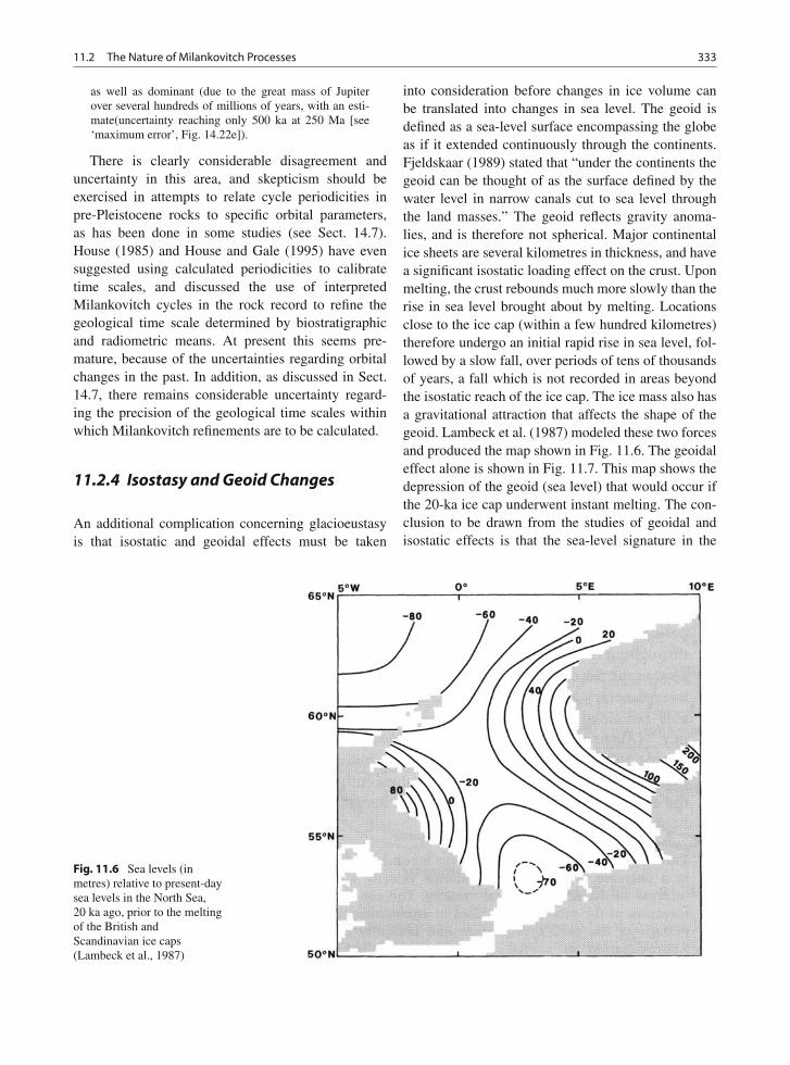
11.2 The Nature of Milankovitch Processes 333
as well as dominant (due to the great mass of Jupiterover several hundreds of millions of years, with an esti-mate(uncertainty reaching only 500 ka at 250 Ma [see‘maximum error’, Fig. 14.22e]).
There is clearly considerable disagreement anduncertainty in this area, and skepticism should beexercised in attempts to relate cycle periodicities inpre-Pleistocene rocks to specific orbital parameters,as has been done in some studies (see Sect. 14.7).House (1985) and House and Gale (1995) have evensuggested using calculated periodicities to calibratetime scales, and discussed the use of interpretedMilankovitch cycles in the rock record to refine thegeological time scale determined by biostratigraphicand radiometric means. At present this seems pre-mature, because of the uncertainties regarding orbitalchanges in the past. In addition, as discussed in Sect.14.7, there remains considerable uncertainty regard-ing the precision of the geological time scales withinwhich Milankovitch refinements are to be calculated.
11.2.4 Isostasy and Geoid Changes
An additional complication concerning glacioeustasyis that isostatic and geoidal effects must be taken
into consideration before changes in ice volume canbe translated into changes in sea level. The geoid isdefined as a sea-level surface encompassing the globeas if it extended continuously through the continents.Fjeldskaar (1989) stated that “under the continents thegeoid can be thought of as the surface defined by thewater level in narrow canals cut to sea level throughthe land masses.” The geoid reflects gravity anoma-lies, and is therefore not spherical. Major continentalice sheets are several kilometres in thickness, and havea significant isostatic loading effect on the crust. Uponmelting, the crust rebounds much more slowly than therise in sea level brought about by melting. Locationsclose to the ice cap (within a few hundred kilometres)therefore undergo an initial rapid rise in sea level, fol-lowed by a slow fall, over periods of tens of thousandsof years, a fall which is not recorded in areas beyondthe isostatic reach of the ice cap. The ice mass also hasa gravitational attraction that affects the shape of thegeoid. Lambeck et al. (1987) modeled these two forcesand produced the map shown in Fig. 11.6. The geoidaleffect alone is shown in Fig. 11.7. This map shows thedepression of the geoid (sea level) that would occur ifthe 20-ka ice cap underwent instant melting. The con-clusion to be drawn from the studies of geoidal andisostatic effects is that the sea-level signature in the
Fig. 11.6 Sea levels (inmetres) relative to present-daysea levels in the North Sea,20 ka ago, prior to the meltingof the British andScandinavian ice caps(Lambeck et al., 1987)
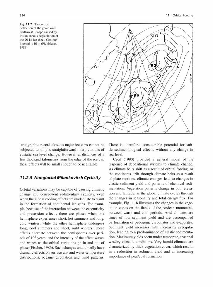
334 11 Orbital Forcing
Fig. 11.7 Theoreticaldeflection of the geoid overnorthwest Europe caused byinstantaneous deglaciation ofthe 20-ka ice sheet. Contourinterval is 10 m (Fjeldskaar,1989)
stratigraphic record close to major ice caps cannot besubjected to simple, straightforward interpretations ofeustatic sea-level change. However, at distances of afew thousand kilometres from the edge of the ice capthese effects will be small enough to be negligible.
11.2.5 Nonglacial Milankovitch Cyclicity
Orbital variations may be capable of causing climaticchange and consequent sedimentary cyclicity, evenwhen the global cooling effects are inadequate to resultin the formation of continental ice caps. For exam-ple, because of the interaction between the eccentricityand precession effects, there are phases when onehemisphere experiences short, hot summers and long,cold winters, while the other hemisphere undergoeslong, cool summers and short, mild winters. Theseeffects alternate between the hemispheres over peri-ods of 104 years, and the intensity of the effect waxesand wanes as the orbital variations go in and out ofphase (Fischer, 1986). Such changes undoubtedly havedramatic effects on surface air- and water-temperaturedistributions, oceanic circulation and wind patterns.
There is, therefore, considerable potential for sub-tle sedimentological effects, without any change insea-level.
Cecil (1990) provided a general model of theresponse of depositional systems to climate change.As climate belts shift as a result of orbital forcing, orthe continents drift through climate belts as a resultof plate motions, climate changes lead to changes inclastic sediment yield and patterns of chemical sedi-mentation. Vegetation patterns change in both eleva-tion and latitude, as the global climate cycles throughthe changes in seasonality and total energy flux. Forexample, Fig. 11.8 illustrates the changes in the vege-tation zones on the flanks of the Andean mountains,between warm and cool periods. Arid climates aretimes of low sediment yield and are accompaniedby formation of pedogenic carbonates and evaporites.Sediment yield increases with increasing precipita-tion, leading to a predominance of clastic sedimenta-tion. Maximum yields occur under temperate, seasonalwet/dry climatic conditions. Very humid climates arecharacterized by thick vegetation cover, which resultsin a reduction in sediment yield and an increasingimportance of peat/coal formation.
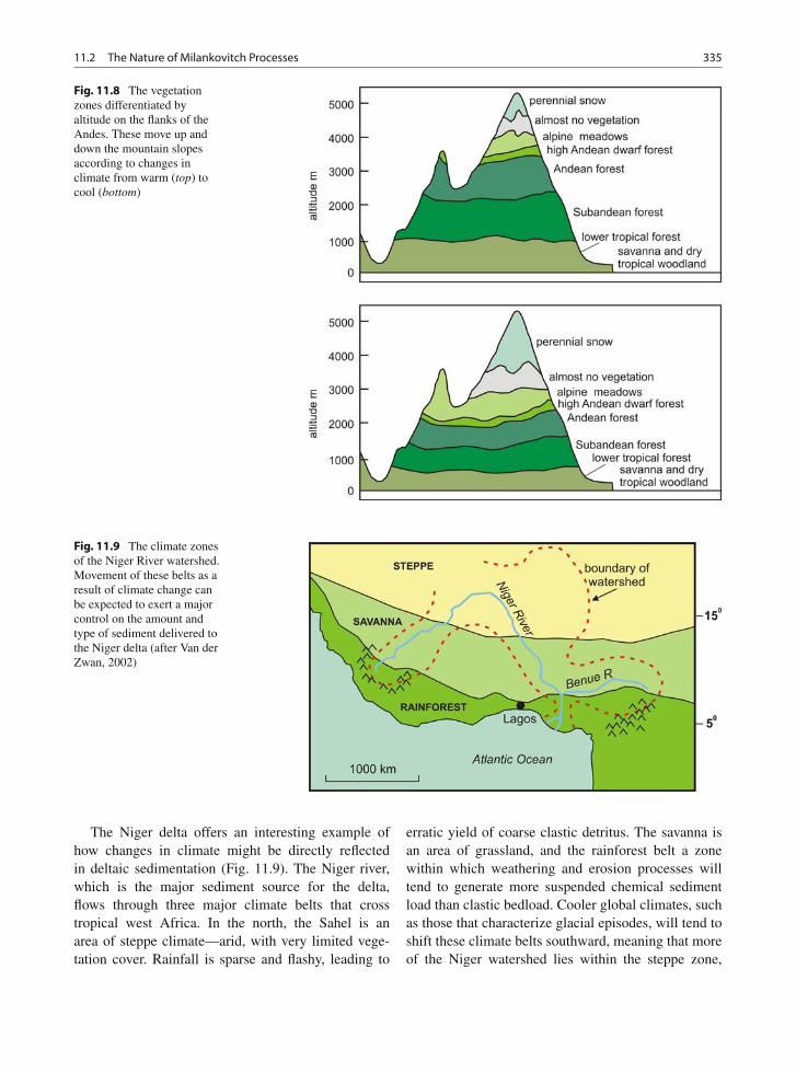
11.2 The Nature of Milankovitch Processes 335
Fig. 11.8 The vegetationzones differentiated byaltitude on the flanks of theAndes. These move up anddown the mountain slopesaccording to changes inclimate from warm (top) tocool (bottom)
Fig. 11.9 The climate zonesof the Niger River watershed.Movement of these belts as aresult of climate change canbe expected to exert a majorcontrol on the amount andtype of sediment delivered tothe Niger delta (after Van derZwan, 2002)
The Niger delta offers an interesting example ofhow changes in climate might be directly reflectedin deltaic sedimentation (Fig. 11.9). The Niger river,which is the major sediment source for the delta,flows through three major climate belts that crosstropical west Africa. In the north, the Sahel is anarea of steppe climate—arid, with very limited vege-tation cover. Rainfall is sparse and flashy, leading to
erratic yield of coarse clastic detritus. The savanna isan area of grassland, and the rainforest belt a zonewithin which weathering and erosion processes willtend to generate more suspended chemical sedimentload than clastic bedload. Cooler global climates, suchas those that characterize glacial episodes, will tend toshift these climate belts southward, meaning that moreof the Niger watershed lies within the steppe zone,
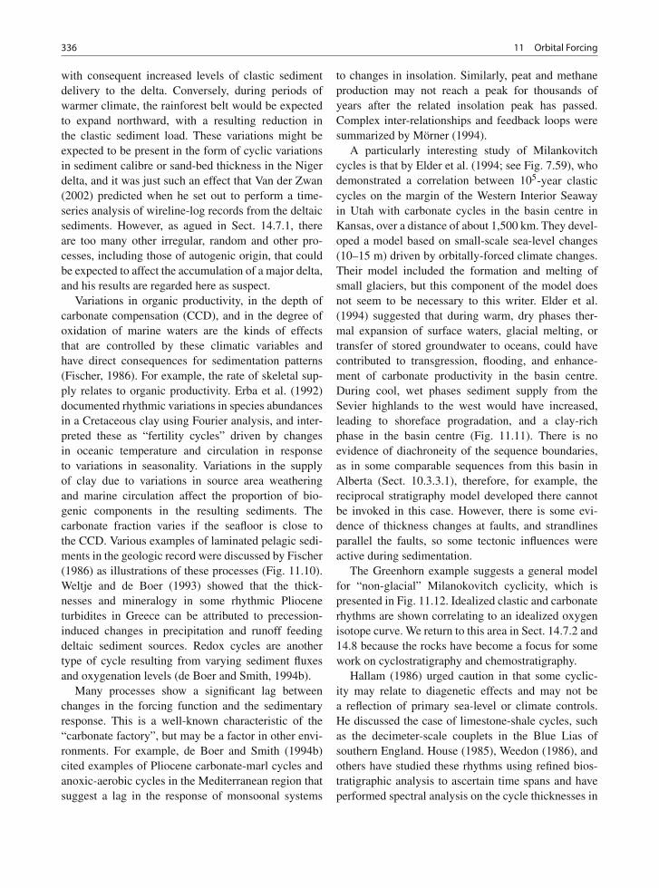
336 11 Orbital Forcing
with consequent increased levels of clastic sedimentdelivery to the delta. Conversely, during periods ofwarmer climate, the rainforest belt would be expectedto expand northward, with a resulting reduction inthe clastic sediment load. These variations might beexpected to be present in the form of cyclic variationsin sediment calibre or sand-bed thickness in the Nigerdelta, and it was just such an effect that Van der Zwan(2002) predicted when he set out to perform a time-series analysis of wireline-log records from the deltaicsediments. However, as agued in Sect. 14.7.1, thereare too many other irregular, random and other pro-cesses, including those of autogenic origin, that couldbe expected to affect the accumulation of a major delta,and his results are regarded here as suspect.
Variations in organic productivity, in the depth ofcarbonate compensation (CCD), and in the degree ofoxidation of marine waters are the kinds of effectsthat are controlled by these climatic variables andhave direct consequences for sedimentation patterns(Fischer, 1986). For example, the rate of skeletal sup-ply relates to organic productivity. Erba et al. (1992)documented rhythmic variations in species abundancesin a Cretaceous clay using Fourier analysis, and inter-preted these as “fertility cycles” driven by changesin oceanic temperature and circulation in responseto variations in seasonality. Variations in the supplyof clay due to variations in source area weatheringand marine circulation affect the proportion of bio-genic components in the resulting sediments. Thecarbonate fraction varies if the seafloor is close tothe CCD. Various examples of laminated pelagic sedi-ments in the geologic record were discussed by Fischer(1986) as illustrations of these processes (Fig. 11.10).Weltje and de Boer (1993) showed that the thick-nesses and mineralogy in some rhythmic Plioceneturbidites in Greece can be attributed to precession-induced changes in precipitation and runoff feedingdeltaic sediment sources. Redox cycles are anothertype of cycle resulting from varying sediment fluxesand oxygenation levels (de Boer and Smith, 1994b).
Many processes show a significant lag betweenchanges in the forcing function and the sedimentaryresponse. This is a well-known characteristic of the“carbonate factory”, but may be a factor in other envi-ronments. For example, de Boer and Smith (1994b)cited examples of Pliocene carbonate-marl cycles andanoxic-aerobic cycles in the Mediterranean region thatsuggest a lag in the response of monsoonal systems
to changes in insolation. Similarly, peat and methaneproduction may not reach a peak for thousands ofyears after the related insolation peak has passed.Complex inter-relationships and feedback loops weresummarized by Mörner (1994).
A particularly interesting study of Milankovitchcycles is that by Elder et al. (1994; see Fig. 7.59), whodemonstrated a correlation between 105-year clasticcycles on the margin of the Western Interior Seawayin Utah with carbonate cycles in the basin centre inKansas, over a distance of about 1,500 km. They devel-oped a model based on small-scale sea-level changes(10–15 m) driven by orbitally-forced climate changes.Their model included the formation and melting ofsmall glaciers, but this component of the model doesnot seem to be necessary to this writer. Elder et al.(1994) suggested that during warm, dry phases ther-mal expansion of surface waters, glacial melting, ortransfer of stored groundwater to oceans, could havecontributed to transgression, flooding, and enhance-ment of carbonate productivity in the basin centre.During cool, wet phases sediment supply from theSevier highlands to the west would have increased,leading to shoreface progradation, and a clay-richphase in the basin centre (Fig. 11.11). There is noevidence of diachroneity of the sequence boundaries,as in some comparable sequences from this basin inAlberta (Sect. 10.3.3.1), therefore, for example, thereciprocal stratigraphy model developed there cannotbe invoked in this case. However, there is some evi-dence of thickness changes at faults, and strandlinesparallel the faults, so some tectonic influences wereactive during sedimentation.
The Greenhorn example suggests a general modelfor “non-glacial” Milanokovitch cyclicity, which ispresented in Fig. 11.12. Idealized clastic and carbonaterhythms are shown correlating to an idealized oxygenisotope curve. We return to this area in Sect. 14.7.2 and14.8 because the rocks have become a focus for somework on cyclostratigraphy and chemostratigraphy.
Hallam (1986) urged caution in that some cyclic-ity may relate to diagenetic effects and may not bea reflection of primary sea-level or climate controls.He discussed the case of limestone-shale cycles, suchas the decimeter-scale couplets in the Blue Lias ofsouthern England. House (1985), Weedon (1986), andothers have studied these rhythms using refined bios-tratigraphic analysis to ascertain time spans and haveperformed spectral analysis on the cycle thicknesses in
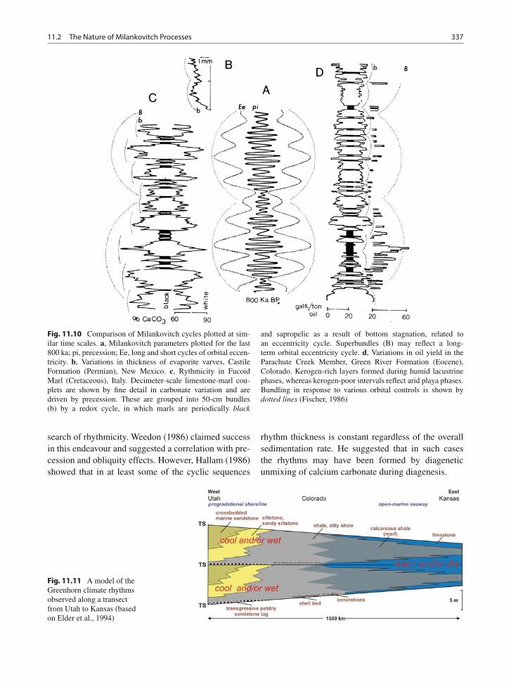
11.2 The Nature of Milankovitch Processes 337
Fig. 11.10 Comparison of Milankovitch cycles plotted at sim-ilar time scales. a, Milankovitch parameters plotted for the last800 ka; pi, precession; Ee, long and short cycles of orbital eccen-tricity. b, Variations in thickness of evaporite varves, CastileFormation (Permian), New Mexico. c, Rythmicity in FucoidMarl (Cretaceous), Italy. Decimeter-scale limestone-marl cou-plets are shown by fine detail in carbonate variation and aredriven by precession. These are grouped into 50-cm bundles(b) by a redox cycle, in which marls are periodically black
and sapropelic as a result of bottom stagnation, related toan eccentricity cycle. Superbundles (B) may reflect a long-term orbital eccentricity cycle. d, Variations in oil yield in theParachute Creek Member, Green River Formation (Eocene),Colorado. Kerogen-rich layers formed during humid lacustrinephases, whereas kerogen-poor intervals reflect arid playa phases.Bundling in response to various orbital controls is shown bydotted lines (Fischer, 1986)
search of rhythmicity. Weedon (1986) claimed successin this endeavour and suggested a correlation with pre-cession and obliquity effects. However, Hallam (1986)showed that in at least some of the cyclic sequences
rhythm thickness is constant regardless of the overallsedimentation rate. He suggested that in such casesthe rhythms may have been formed by diageneticunmixing of calcium carbonate during diagenesis.
Fig. 11.11 A model of theGreenhorn climate rhythmsobserved along a transectfrom Utah to Kansas (basedon Elder et al., 1994)
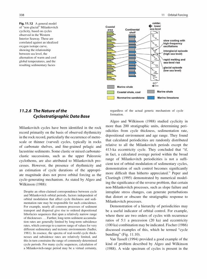
338 11 Orbital Forcing
Fig. 11.12 A general modelof “non-glacial” Milankovitchcyclicity, based on cyclesobserved in the WesternInterior Seaway. These arecorrelated against an idealizedoxygen isotope curve,showing the relationshipbetween sea level, thealternation of warm and coolglobal temperatures, and theresulting sedimentary facies
11.2.6 The Nature of theCyclostratigraphic Data Base
Milankovitch cycles have been identified in the rockrecord primarily on the basis of observed rhythmicityin the rock record, particularly the occurrence of metre-scale or thinner (varved) cycles, typically in rocksof carbonate shelves, and fine-grained pelagic andlacustrine sediments. Some clastic or mixed carbonate-clastic successions, such as the upper Paleozoiccyclothems, are also attributed to Milankovitch pro-cesses. However, the presence of rhythmicity andan estimation of cycle durations of the appropri-ate magnitude does not prove orbital forcing as thecycle-generating mechanism. As stated by Algeo andWilkinson (1988):
Despite an often-claimed correspondence between cycleand Milankovitch orbital periods, factors independent oforbital modulation that affect cycle thickness and sedi-mentation rate may be responsible for such coincidence.For example, nearly all common processes of sedimenttransport and dispersal give rise to ordered depositionallithofacies sequences that span a relatively narrow rangeof thicknesses . . . Further, long-term sediment accumula-tion rates are generally limited by long-term subsidencerates, which converge to a narrow range of values for verydifferent sedimentary and tectonic environments (Sadler,1981). In essence, the spectra of real-world cycle thick-nesses and subsidence rates are relatively limited, andthis in turn constrains the range of commonly-determinedcycle periods. For many cyclic sequences, calculation ofa Milankovitch-range period may be a virtual certainty,
regardless of the actual generic mechanism of cycleformation.
Algeo and Wilkinson (1988) studied cyclicity inmore than 200 stratigraphic units, determining peri-odicities from cycle thickness, sedimentation rate,depositional environment and age range. They foundthat calculated periodicities are randomly distributedrelative to all the Milankovitch periods except the413-ka eccentricity cycle. They concluded that “if,in fact, a calculated average period within the broadrange of Milankovitch periodicities is not a suffi-cient test of orbital modulation of sedimentary cycles,demonstration of such control becomes significantlymore difficult than hitherto appreciated.” Peper andCloetingh (1995) demonstrated by numerical model-ing the significance of the reverse problem, that certainnon-Milankovitch processes, such as slope failure andintraplate stress changes, can generate perturbationsthat distort or obscure the stratigraphic response toMilankovitch processes.
Demonstration of a hierarchy of periodicities maybe a useful indicator of orbital control. For example,where there are two orders of cycles with recurrenceratios of 5:1 a precession (20 ka) and eccentricity(100 ka) combination may be indicated. Fischer (1986)discussed examples of this, which he termed “cyclebundling” (Fig. 11.10).
Van Tassell (1994) provided a good example of thekind of problem described by Algeo and Wilkinson(1988). A wide spectrum of cycles is present in the
11.3 The Geologic Record 339
Devonian Catskill Delta of the Appalachian Basin, butproving they are of Milankovitch type (as claimed bythe author) is problematic. Their thickness and dura-tion fits that of Milankovitch and autogenic cycles, asAlgeo and Wilkinson (1988) predicted would occurin these types of rocks. Demonstration of cycle dura-tion is difficult, because of uncertainties about their agerange. No Milankovitch-type bundling can be demon-strated, and the proof of correlation of cycles acrossmajor facies boundaries is very limited. A compara-ble, partly correlative suite of cycles was describedby Filer (1994), based mainly on subsurface gamma-ray log correlations. His correlations seem unconvinc-ing to this writer. No clear cyclic signatures can betraced from well to well. These date would benefitfrom application of the gamma technique, describedbelow.
Drummond and Wilkinson (1993b) modeled car-bonate cycles to study the effect of “lag time” (the timetaken for the carbonate factory to reach full productiv-ity rates when a platform is flooded). They showed thatseveral discrete cycles could be produced during onesmooth leg of sea level rise, as the factory overcomesthe lag, races to deposit sediment, then is shut downas the platform is built to sea level. Therefore a one-for-one correspondence between sedimentary cyclesand sea-level cycles cannot be expected, and cycledurations and hierarchies cannot be directly relatedto Milankovitch frequencies. However, this is just anumerical model, and they did not offer evidence ofthis from the rock record.
The requirements for the establishment of orbitalforcing are twofold. Firstly it is necessary to demon-strate that the cycles are widespread, by examiningtheir long-distance correlation. As noted by Pratt andJames (1986) and Pratt et al. (1992), many shallow-marine cycles are generated by autogenic processes,and are laterally impersistent. Studies based on sin-gle vertical sections, however, detailed, are inadequatefor the purpose of testing models of orbital forc-ing. Tracing and correlating sequences through majorfacies changes may also be indicative of orbital con-trol. An example of this is illustrated in Fig. 7.59, andis discussed in Sect. 11.2.5. Then, given a demonstra-tion of lateral persistence, it is necessary to demon-strate a persistent regularity of cycle periods, andcycle bundling. This may be done by precise mea-surement of facies thicknesses or parameters suchas carbon or calcium content over lengthy sections
(see many examples in de Boer and Smith, 1994a).Spectral mapping methods may be particularly use-ful (Melnyk et al., 1994; Schwarzacher, 1993, 2000;Weedon, 2003). Cycle hierarchies and cycle stack-ing ratios have been discussed by Goldhammer et al.(1987, 1990) and Schwarzacher (1993). However, aspointed out in Sect. 14.7.2, in the absence of indepen-dent chronostratigraphic documentation of age, stack-ing ratios may be misleading. The use of Fischerplots for the documentation of metre-scale cycles isdiscussed in Sect. 3.7.
A method for independently testing the periodic-ity of metre-scale cycles, termed the gamma method,was devised by Kominz and Bond (1990). Cycles aresubdivided into lithofacies according to a predeter-mined classification, and the thickness of each faciesunit is measured in each cycle. It is assumed thateach facies has an approximately constant accumula-tion rate, reflecting constant depositional conditions. Avalue for gamma for each facies is given by gamma= elapsed time/thickness. If it can be assumed thateach cycle has the same duration (the absolute valueof which does not need to be known) a set of equa-tions can be written that determines the proportionof elapsed time represented by each facies in eachcycle. If these values are reasonably consistent, thenperiodicity has been demonstrated. If a method ofdetermining absolute age is available, for example byradiometric dating of bentonites that bracket the sec-tion under study, then the absolute duration of thecycle period can be determined, and if appropriate,this can be related to orbital frequencies. Given thatorbital frequencies may have changed over time (Sect.11.2.3), and that other sedimentary processes may gen-erate cycles of comparable duration, these quantitativemethods of cycle documentation are of considerablevalue.
11.3 The Geologic Record
11.3.1 The Sensitivity of the Earth toGlaciation
The modern literature on paleoclimatology (e.g.,Barron, 1983; Barron and Thompson, 1990) indicatesa considerable complexity and uncertainty in recon-structions of past climates. Although the control of
340 11 Orbital Forcing
Milankovitch mechanisms on glacial cyclicity is nowwidely accepted, it is still not entirely clear why majorglaciations start in the first place. Factors involved insensitizing the earth to climatic change include the cur-rent climate, the plate configuration of the earth, atmo-spheric content (volcanic dust, O2, CO2), vegetationcover, and the nature of oceanic and atmospheric cir-culation (Barron, 1983; Barron and Thompson, 1990).Plate-tectonics has been a major control. As Eyles(2008, p. 109) noted: “Cooling after 55 Ma is increas-ingly being related to the tectonic and bathymetricevolution of the oceans as Pangea continued to disinte-grate.”
Low levels of carbon dioxide and correspondinglyhigh oxygen levels are thought to be characteristic oftimes of low sea-level during supercontinent assemblyphases, and tend to favour icehouse climates becauseof the reduced atmospheric greenhouse effect (Worsleyet al., 1986, 1991; Worsley and Nance, 1989; seeSect. 5.1). Glaciation is favoured under such condi-tions, especially where large continental landmassesare located over polar regions, as in the case of thelate Paleozoic glaciation (Sect. 11.3.4). Eyles (1993,2008) made a strong case for the importance of tectoniccontrol in the triggering of widespread continentalglaciation. Uplift accompanying continental collision,and the widespread uplift of rift flanks during super-continent dispersal, both lead to the development ofbroad, high-altitude areas where major Alpine ice-capscan easily form. Once formed, feedback effects, suchas increased albedo, can lead to continued cooling.The geological record is replete with examples thatcan be interpreted in this way. For example, Eyles(1993, 2008) attributed the widespread late Proterozoicglaciation to tectonic uplift of rift flanks during the dis-persal of the supercontinent of which Laurentia was thecentre (see Hoffman, 1991). The assembly of Pangeawas accompanied by the uplift of many orogenic high-lands, and was followed by the long-lasting Gondwanaglaciation (Sect. 11.3.4). Orogenic highlands formedin the Miocene, such as Tibet, may also have beeninstrumental in triggering of the Late Cenozoic glacia-tion (Ruddiman, 2008). Another major contributingfactor in the case of Cenozoic glaciation was undoubt-edly the plate-tectonic separation of Australia fromAntarctica, which opened the Drake Passage and led tothe development of circumpolar currents, which essen-tially isolated Antarctic weather systems from the restof the southern hemisphere (Kennett, 1977).
Given these broad, long-term (106–107-year)regional to continental controls, Milankovitch pro-cesses then govern the amount of climate change andits periodicity within the Milankovitch time band.Considerable variation can be detected at this level.Imbrie (1985) carried out a spectral analysis of theδ18O variations in deep sea cores for the last 782 ka.It shows a change in sensitivity at about 400 ka ago.The oxygen isotope record for the 782–400-ka recordcontains a major peak corresponding to a 100-kaperiod, and a lesser peak for a 23-ka period. Theyounger part of the record shows somewhat more vari-ance, with stronger peaks in the longer-term periods,including a strongly represented 100-ka period, andan additional peak corresponding to a 41-ka period.Moore et al. (1982) studied the variation in carbonateconcentrations in Upper Miocene and Quaternarydeep-sea sediments. The variations are attributed tothe degree of preservation of calcite microfossils,which, in turn, is related to carbonate solubility andthe corrosiveness of bottom waters. Both factors areclimate dependent. Moore et al. (1982) found thatperiods of 41, 100, and 400 ka were dominant in theirspectral analyses. However, the 400-ka period is farmore strongly recorded in the Miocene data, with the100-ka period the dominant one in the Quaternaryrecord. Imbrie (1985) interpreted the strong 100-kapeak as a combination of the two distinct eccentricitypeaks at 95 and 123 ka.
Matthews and Frohlich (1991) extended Imbrie’s(1985) analysis back to 2.5 Ma, and forward to ahypothetical 2.5 million years in the future. Theydemonstrated that the 100-ka eccentricity and 19-ka precession components combined to produce a2-million years modulation, although the amplitudesof the various peaks varied according to input con-ditions. This result suggests that glacioeustasy maybe capable of explaining longer-term cyclicity withmillion-year periodicities (equivalent to Vail’s “third-order” cycles). To this analysis Matthews and Frohlich(1991) then added the effects of the presence of warm,saline waters in mid-latitude positions, such as wouldhave occurred in the Tethyan Ocean before this waterbody was eliminated by subduction of its sea floor.“Warm water upwelling adjacent to a cold continentshould create a very efficient mechanism for produc-ing ice on the continent, thereby lowering sea level.Air descending over the cold continent flows out overwarm water and picks up water vapor. Return flow aloft
11.3 The Geologic Record 341
delivers this moisture to the interior of the continentas snow” (Matthews and Frohlich, 1991). It is postu-lated that thermohaline currents would have deliveredthis water to Antarctica, and could have accountedfor large build-ups of snow there, with a calculatedepisodicity of 1.6–2.4 million years. Qualitatively,therefore, a glacioeustatic mechanism exists to explainmillion-year (“third-order” or “mesothemic”) cyclicityduring times when the earth was sensitive to glacia-tion. However, the lack of evidence for major con-tinental ice caps throughout much of geologic timemeans that this cannot be regarded as a universalexplanation.
Variations with time in the stratigraphic signalamplitude of the various Milankovitch periods mayrelate to the varying character of glacial regimes. Thecurrent view (e.g., Miller et al., 2005b) is that until theMiocene, only the Antarctic ice cap existed. This ismainly a land-based ice cap and is entirely surroundedby polar waters. Northern hemisphere ice commenceda significant buildup at about 14 Ma, with the major“ice ages” commencing at about 2.6 Ma. The NorthernHemisphere ice consisted of several continental-scaleand smaller centers, some bordered to the north orsouth (or both) by water masses, and included numer-ous Alpine-type ice caps. It seems likely that thesensitivity of the ice caps to climate forcing would havebeen quite different in these different settings, withthe large, stable Antarctic ice cap tending to respondmuch more slowly than the Northern Hemisphere icecenters.
Another example of the varying styles of glacia-tion affecting the styles of cyclicity was discussed byWright (1992). He classified platform-carbonate cyclesinto two broad types. Type 1 consist of metre-scale“keep-up” cycles dominated by peritidal carbonates.They are common in the Cambro-Ordovician, earlyDevonian and mid-Triassic to Cretaceous sedimentaryrecord. Type 2 cycles are 5–10 m thick. They con-sist mainly of shelf and deeper-water carbonates, withcommon paleokarstic and paleosol horizons (vadosecaps). They are common in the Carboniferous sed-imentary record. Wright (1992) suggested that thedifferences in cycle type may have been caused bydifferences in the type of glacial cycle, reflecting dif-ferences in the size of ice caps and their consequentsensitivity to change. He postulated that type-1 cyclesrepresent small-scale ice caps, such as those formedduring “greenhouse” climatic phases (Fig. 4.8),
When continental configuration or other factors did notfacilitate the generation of major ice sheets. Duringsuch periods the amplitudes of these climatically inducedsea-level changes were small, only slower third-orderchanges influenced the types of small cycles developed.In the absence of ice-buildups no rapid decametre-scalefalls or rises in sea-level occurred. The falls in sea-leveltriggered by changes in insolation were small in ampli-tude and slow enough to be outpaced by subsidence,creating minor accommodation space, readily filled byperitidal cyclothems. . . . The subsequent rises were slowenough to be outpaced by carbonate production to pro-duce more peritidal cyclothems. (Wright, 1992, p. 2)
As noted elsewhere (Sect. 11.3.3) there is, how-ever, doubt regarding the existence of significant icecaps for much of Phanerozoic time, and this mecha-nism for type-1 cyclothems remains unproven. Wright(1992) suggested that type-2 cyclothems developedin response to the growth of large continental icecaps during “icehouse” climatic phases, such as dur-ing the Carboniferous Gondwana glaciation, and thelate Cenozoic glaciation. At such times high-amplitudesea-level falls lead to exposure of platform tops andto extensive meteoric diagenesis. Rapid rises lead todrowning in which only reefal organisms are capableof keeping pace with sea-level rise. Platform interiorsare drowned, becoming areas of subtidal sedimenta-tion, in which peritidal and reef sedimentation arerestricted to nucleation sites on earlier topographichighs. This is the pattern of so-called “catch-up” sedi-mentation.
11.3.2 The Cenozoic Record
Many successions of Late Cenozoic age have now beencorrelated with the oxygen-isotope record, demonstrat-ing a glacioeustatic control of the sequence stratigra-phy. From numerous DSDP core records (Fig. 11.13),a standard isotopic record has been constructed, withnumbered chrons providing a standard time scale forthe Pliocene to recent (Fig. 11.14). Examples of theuse of this system in chronostratigraphic dating ofsequence records are shown in Figs. 7.3, 7.17, 7.22,14.24 and 14.25.
A widespread sea-level fall of mid-Oligocene agehas been suggested in many stratigraphic records.It appears on the Exxon global cycle charts, andalso in many stratigraphic records that have beenindependently compiled for specific basins and
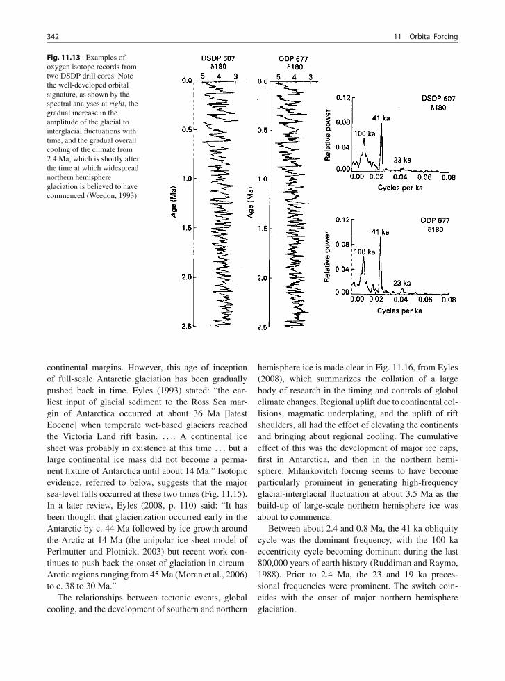
342 11 Orbital Forcing
Fig. 11.13 Examples ofoxygen isotope records fromtwo DSDP drill cores. Notethe well-developed orbitalsignature, as shown by thespectral analyses at right, thegradual increase in theamplitude of the glacial tointerglacial fluctuations withtime, and the gradual overallcooling of the climate from2.4 Ma, which is shortly afterthe time at which widespreadnorthern hemisphereglaciation is believed to havecommenced (Weedon, 1993)
continental margins. However, this age of inceptionof full-scale Antarctic glaciation has been graduallypushed back in time. Eyles (1993) stated: “the ear-liest input of glacial sediment to the Ross Sea mar-gin of Antarctica occurred at about 36 Ma [latestEocene] when temperate wet-based glaciers reachedthe Victoria Land rift basin. . . .. A continental icesheet was probably in existence at this time . . . but alarge continental ice mass did not become a perma-nent fixture of Antarctica until about 14 Ma.” Isotopicevidence, referred to below, suggests that the majorsea-level falls occurred at these two times (Fig. 11.15).In a later review, Eyles (2008, p. 110) said: “It hasbeen thought that glacierization occurred early in theAntarctic by c. 44 Ma followed by ice growth aroundthe Arctic at 14 Ma (the unipolar ice sheet model ofPerlmutter and Plotnick, 2003) but recent work con-tinues to push back the onset of glaciation in circum-Arctic regions ranging from 45 Ma (Moran et al., 2006)to c. 38 to 30 Ma.”
The relationships between tectonic events, globalcooling, and the development of southern and northern
hemisphere ice is made clear in Fig. 11.16, from Eyles(2008), which summarizes the collation of a largebody of research in the timing and controls of globalclimate changes. Regional uplift due to continental col-lisions, magmatic underplating, and the uplift of riftshoulders, all had the effect of elevating the continentsand bringing about regional cooling. The cumulativeeffect of this was the development of major ice caps,first in Antarctica, and then in the northern hemi-sphere. Milankovitch forcing seems to have becomeparticularly prominent in generating high-frequencyglacial-interglacial fluctuation at about 3.5 Ma as thebuild-up of large-scale northern hemisphere ice wasabout to commence.
Between about 2.4 and 0.8 Ma, the 41 ka obliquitycycle was the dominant frequency, with the 100 kaeccentricity cycle becoming dominant during the last800,000 years of earth history (Ruddiman and Raymo,1988). Prior to 2.4 Ma, the 23 and 19 ka preces-sional frequencies were prominent. The switch coin-cides with the onset of major northern hemisphereglaciation.
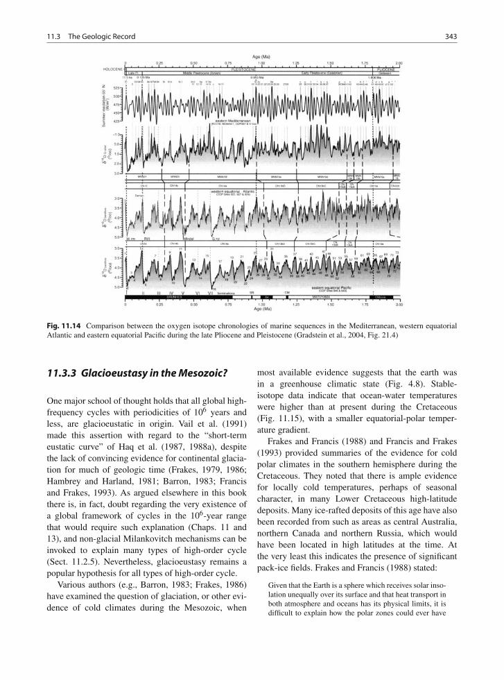
11.3 The Geologic Record 343
Fig. 11.14 Comparison between the oxygen isotope chronologies of marine sequences in the Mediterranean, western equatorialAtlantic and eastern equatorial Pacific during the late Pliocene and Pleistocene (Gradstein et al., 2004, Fig. 21.4)
11.3.3 Glacioeustasy in the Mesozoic?
One major school of thought holds that all global high-frequency cycles with periodicities of 106 years andless, are glacioeustatic in origin. Vail et al. (1991)made this assertion with regard to the “short-termeustatic curve” of Haq et al. (1987, 1988a), despitethe lack of convincing evidence for continental glacia-tion for much of geologic time (Frakes, 1979, 1986;Hambrey and Harland, 1981; Barron, 1983; Francisand Frakes, 1993). As argued elsewhere in this bookthere is, in fact, doubt regarding the very existence ofa global framework of cycles in the 106-year rangethat would require such explanation (Chaps. 11 and13), and non-glacial Milankovitch mechanisms can beinvoked to explain many types of high-order cycle(Sect. 11.2.5). Nevertheless, glacioeustasy remains apopular hypothesis for all types of high-order cycle.
Various authors (e.g., Barron, 1983; Frakes, 1986)have examined the question of glaciation, or other evi-dence of cold climates during the Mesozoic, when
most available evidence suggests that the earth wasin a greenhouse climatic state (Fig. 4.8). Stable-isotope data indicate that ocean-water temperatureswere higher than at present during the Cretaceous(Fig. 11.15), with a smaller equatorial-polar temper-ature gradient.
Frakes and Francis (1988) and Francis and Frakes(1993) provided summaries of the evidence for coldpolar climates in the southern hemisphere during theCretaceous. They noted that there is ample evidencefor locally cold temperatures, perhaps of seasonalcharacter, in many Lower Cretaceous high-latitudedeposits. Many ice-rafted deposits of this age have alsobeen recorded from such as areas as central Australia,northern Canada and northern Russia, which wouldhave been located in high latitudes at the time. Atthe very least this indicates the presence of significantpack-ice fields. Frakes and Francis (1988) stated:
Given that the Earth is a sphere which receives solar inso-lation unequally over its surface and that heat transport inboth atmosphere and oceans has its physical limits, it isdifficult to explain how the polar zones could ever have
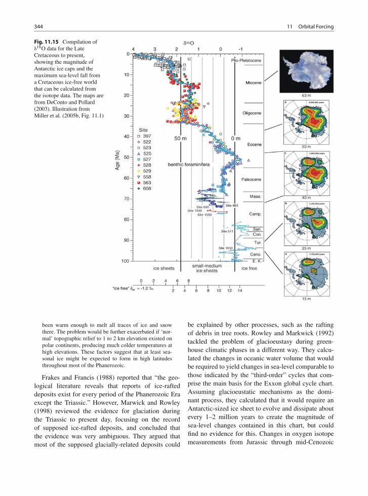
344 11 Orbital Forcing
Fig. 11.15 Compilation ofδ18O data for the LateCretaceous to present,showing the magnitude ofAntarctic ice caps and themaximum sea-level fall froma Cretaceous ice-free worldthat can be calculated fromthe isotope data. The maps arefrom DeConto and Pollard(2003). Illustration fromMiller et al. (2005b, Fig. 11.1)
been warm enough to melt all traces of ice and snowthere. The problem would be further exacerbated if ‘nor-mal’ topographic relief to 1 to 2 km elevation existed onpolar continents, producing much colder temperatures athigh elevations. These factors suggest that at least sea-sonal ice might be expected to form in high latitudesthroughout most of the Phanerozoic.
Frakes and Francis (1988) reported that “the geo-logical literature reveals that reports of ice-rafteddeposits exist for every period of the Phanerozoic Eraexcept the Triassic.” However, Marwick and Rowley(1998) reviewed the evidence for glaciation duringthe Triassic to present day, focusing on the recordof supposed ice-rafted deposits, and concluded thatthe evidence was very ambiguous. They argued thatmost of the supposed glacially-related deposits could
be explained by other processes, such as the raftingof debris in tree roots. Rowley and Markwick (1992)tackled the problem of glacioeustasy during green-house climatic phases in a different way. They calcu-lated the changes in oceanic water volume that wouldbe required to yield changes in sea-level comparable tothose indicated by the “third-order” cycles that com-prise the main basis for the Exxon global cycle chart.Assuming glacioeustatic mechanisms as the domi-nant process, they calculated that it would require anAntarctic-sized ice sheet to evolve and dissipate aboutevery 1–2 million years to create the magnitude ofsea-level changes contained in this chart, but couldfind no evidence for this. Changes in oxygen isotopemeasurements from Jurassic through mid-Cenozoic
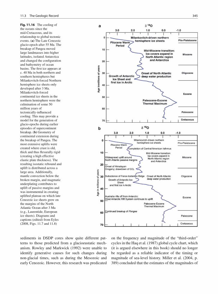
11.3 The Geologic Record 345
Fig. 11.16 The cooling ofthe oceans since themid-Cretaceous, and itsrelationship to global tectonicevents. (a) The Late Cenozoicglacio-epoch after 55 Ma. Thebreakup of Pangea movedlarge landmasses into higherlatitudes, isolated Antarcticaand changed the configurationand bathymetry of oceanbasins. The first ice appears atc. 40 Ma in both northern andsouthern hemispheres butMilankovitch-forced Northernhemisphere ice sheets onlydeveloped after 3 Ma.Milankovitch-forcedcontinental ice sheets in thenorthern hemisphere were theculmination of some 50million years oftectonically-influencedcooling. This may provide amodel for the generation ofglacio-epochs during earlierepisodes of supercontinentbreakup. (b) Geometry ofcontinental extension duringthe breakup of Pangea. Themost extensive uplifts werecreated where crust is old,thick and thus flexurally rigid(creating a high effectiveelastic plate thickness). Theresulting isostatic rebound anduplift is distributed across alarge area. Additionally,mantle convection below thebroken margin, and magmaticunderplating contributes touplift of passive margins andwas instrumental in creatinguplifted plateau on which lateCenozoic ice sheets grew onthe margins of the NorthAtlantic Ocean after 3 Ma(e.g., Laurentide, Europeanice sheets). Diagrams andcaptions (edited) from Eyles(2008, Figs. 11.7 and 11.8)
sediments in DSDP cores show quite different pat-terns to those predicted from a glacioeustatic mech-anism. Rowley and Markwick (1992) were unable toidentify generative causes for such changes duringnon-glacial times, such as during the Mesozoic andearly Cenozoic. However, this research was predicated
on the frequency and magnitude of the “third-order”cycles in the Haq et al. (1987) global cycle chart, which(it is argued elsewhere in this book) should no longerbe regarded as a reliable indicator of the timing ormagnitude of sea-level history. Miller et al. (2004, p.389) concluded that the estimates of the magnitudes of
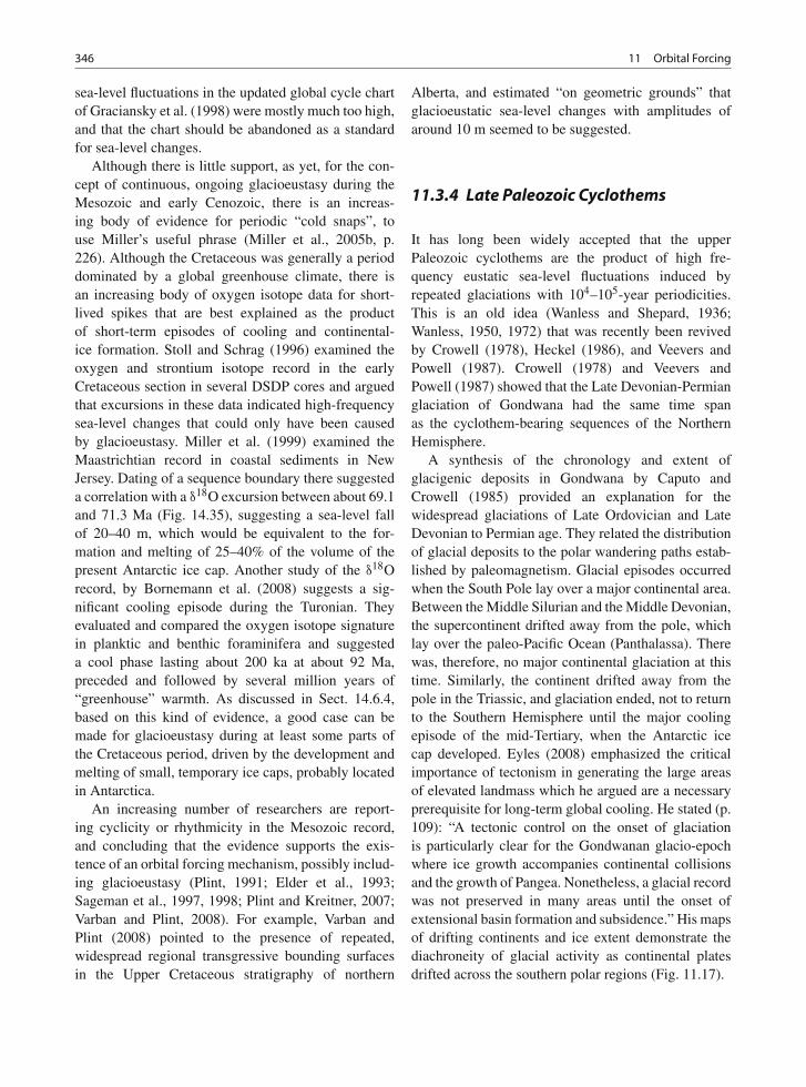
346 11 Orbital Forcing
sea-level fluctuations in the updated global cycle chartof Graciansky et al. (1998) were mostly much too high,and that the chart should be abandoned as a standardfor sea-level changes.
Although there is little support, as yet, for the con-cept of continuous, ongoing glacioeustasy during theMesozoic and early Cenozoic, there is an increas-ing body of evidence for periodic “cold snaps”, touse Miller’s useful phrase (Miller et al., 2005b, p.226). Although the Cretaceous was generally a perioddominated by a global greenhouse climate, there isan increasing body of oxygen isotope data for short-lived spikes that are best explained as the productof short-term episodes of cooling and continental-ice formation. Stoll and Schrag (1996) examined theoxygen and strontium isotope record in the earlyCretaceous section in several DSDP cores and arguedthat excursions in these data indicated high-frequencysea-level changes that could only have been causedby glacioeustasy. Miller et al. (1999) examined theMaastrichtian record in coastal sediments in NewJersey. Dating of a sequence boundary there suggesteda correlation with a δ18O excursion between about 69.1and 71.3 Ma (Fig. 14.35), suggesting a sea-level fallof 20–40 m, which would be equivalent to the for-mation and melting of 25–40% of the volume of thepresent Antarctic ice cap. Another study of the δ18Orecord, by Bornemann et al. (2008) suggests a sig-nificant cooling episode during the Turonian. Theyevaluated and compared the oxygen isotope signaturein planktic and benthic foraminifera and suggesteda cool phase lasting about 200 ka at about 92 Ma,preceded and followed by several million years of“greenhouse” warmth. As discussed in Sect. 14.6.4,based on this kind of evidence, a good case can bemade for glacioeustasy during at least some parts ofthe Cretaceous period, driven by the development andmelting of small, temporary ice caps, probably locatedin Antarctica.
An increasing number of researchers are report-ing cyclicity or rhythmicity in the Mesozoic record,and concluding that the evidence supports the exis-tence of an orbital forcing mechanism, possibly includ-ing glacioeustasy (Plint, 1991; Elder et al., 1993;Sageman et al., 1997, 1998; Plint and Kreitner, 2007;Varban and Plint, 2008). For example, Varban andPlint (2008) pointed to the presence of repeated,widespread regional transgressive bounding surfacesin the Upper Cretaceous stratigraphy of northern
Alberta, and estimated “on geometric grounds” thatglacioeustatic sea-level changes with amplitudes ofaround 10 m seemed to be suggested.
11.3.4 Late Paleozoic Cyclothems
It has long been widely accepted that the upperPaleozoic cyclothems are the product of high fre-quency eustatic sea-level fluctuations induced byrepeated glaciations with 104–105-year periodicities.This is an old idea (Wanless and Shepard, 1936;Wanless, 1950, 1972) that was recently been revivedby Crowell (1978), Heckel (1986), and Veevers andPowell (1987). Crowell (1978) and Veevers andPowell (1987) showed that the Late Devonian-Permianglaciation of Gondwana had the same time spanas the cyclothem-bearing sequences of the NorthernHemisphere.
A synthesis of the chronology and extent ofglacigenic deposits in Gondwana by Caputo andCrowell (1985) provided an explanation for thewidespread glaciations of Late Ordovician and LateDevonian to Permian age. They related the distributionof glacial deposits to the polar wandering paths estab-lished by paleomagnetism. Glacial episodes occurredwhen the South Pole lay over a major continental area.Between the Middle Silurian and the Middle Devonian,the supercontinent drifted away from the pole, whichlay over the paleo-Pacific Ocean (Panthalassa). Therewas, therefore, no major continental glaciation at thistime. Similarly, the continent drifted away from thepole in the Triassic, and glaciation ended, not to returnto the Southern Hemisphere until the major coolingepisode of the mid-Tertiary, when the Antarctic icecap developed. Eyles (2008) emphasized the criticalimportance of tectonism in generating the large areasof elevated landmass which he argued are a necessaryprerequisite for long-term global cooling. He stated (p.109): “A tectonic control on the onset of glaciationis particularly clear for the Gondwanan glacio-epochwhere ice growth accompanies continental collisionsand the growth of Pangea. Nonetheless, a glacial recordwas not preserved in many areas until the onset ofextensional basin formation and subsidence.” His mapsof drifting continents and ice extent demonstrate thediachroneity of glacial activity as continental platesdrifted across the southern polar regions (Fig. 11.17).
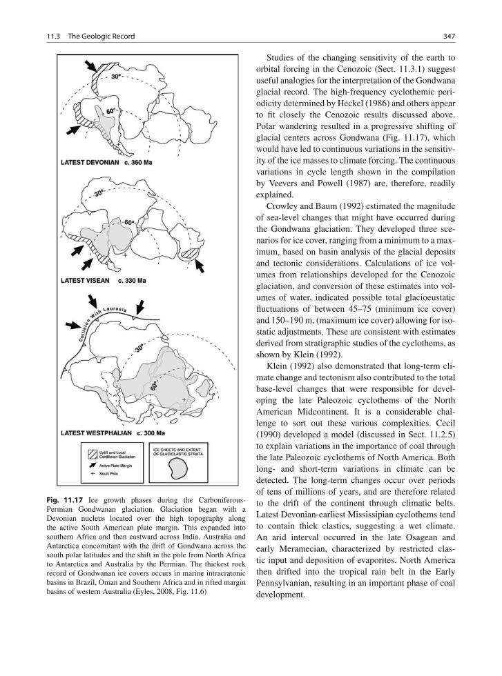
11.3 The Geologic Record 347
Fig. 11.17 Ice growth phases during the Carboniferous-Permian Gondwanan glaciation. Glaciation began with aDevonian nucleus located over the high topography alongthe active South American plate margin. This expanded intosouthern Africa and then eastward across India, Australia andAntarctica concomitant with the drift of Gondwana across thesouth polar latitudes and the shift in the pole from North Africato Antarctica and Australia by the Permian. The thickest rockrecord of Gondwanan ice covers occurs in marine intracratonicbasins in Brazil, Oman and Southern Africa and in rifted marginbasins of western Australia (Eyles, 2008, Fig. 11.6)
Studies of the changing sensitivity of the earth toorbital forcing in the Cenozoic (Sect. 11.3.1) suggestuseful analogies for the interpretation of the Gondwanaglacial record. The high-frequency cyclothemic peri-odicity determined by Heckel (1986) and others appearto fit closely the Cenozoic results discussed above.Polar wandering resulted in a progressive shifting ofglacial centers across Gondwana (Fig. 11.17), whichwould have led to continuous variations in the sensitiv-ity of the ice masses to climate forcing. The continuousvariations in cycle length shown in the compilationby Veevers and Powell (1987) are, therefore, readilyexplained.
Crowley and Baum (1992) estimated the magnitudeof sea-level changes that might have occurred duringthe Gondwana glaciation. They developed three sce-narios for ice cover, ranging from a minimum to a max-imum, based on basin analysis of the glacial depositsand tectonic considerations. Calculations of ice vol-umes from relationships developed for the Cenozoicglaciation, and conversion of these estimates into vol-umes of water, indicated possible total glacioeustaticfluctuations of between 45–75 (minimum ice cover)and 150–190 m, (maximum ice cover) allowing for iso-static adjustments. These are consistent with estimatesderived from stratigraphic studies of the cyclothems, asshown by Klein (1992).
Klein (1992) also demonstrated that long-term cli-mate change and tectonism also contributed to the totalbase-level changes that were responsible for devel-oping the late Paleozoic cyclothems of the NorthAmerican Midcontinent. It is a considerable chal-lenge to sort out these various complexities. Cecil(1990) developed a model (discussed in Sect. 11.2.5)to explain variations in the importance of coal throughthe late Paleozoic cyclothems of North America. Bothlong- and short-term variations in climate can bedetected. The long-term changes occur over periodsof tens of millions of years, and are therefore relatedto the drift of the continent through climatic belts.Latest Devonian-earliest Mississipian cyclothems tendto contain thick clastics, suggesting a wet climate.An arid interval occurred in the late Osagean andearly Meramecian, characterized by restricted clas-tic input and deposition of evaporites. North Americathen drifted into the tropical rain belt in the EarlyPennsylvanian, resulting in an important phase of coaldevelopment.
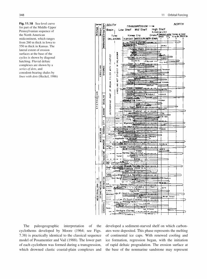
348 11 Orbital Forcing
Fig. 11.18 Sea-level curvefor part of the Middle-UpperPennsylvanian sequence ofthe North Americanmidcontinent, which rangesfrom 260 m thick in Iowa to550 m thick in Kansas. Thelateral extent of erosionsurfaces at the base of thecycles is shown by diagonalhatching. Fluvial deltaiccomplexes are shown by aseries of dots, andconodont-bearing shales bylines with dots (Heckel, 1986)
The paleogeographic interpretation of thecyclothems developed by Moore (1964; see Figs.7.38) is practically identical to the classical sequencemodel of Posamentier and Vail (1988). The lower partof each cyclothem was formed during a transgression,which drowned clastic coastal-plain complexes and
developed a sediment-starved shelf on which carbon-ates were deposited. This phase represents the meltingof continental ice caps. With renewed cooling andice formation, regression began, with the initiationof rapid deltaic progradation. The erosion surface atthe base of the nonmarine sandstone may represent
11.4 Distinguishing Between Orbital Forcing and Tectonic Driving Mechanisms 349
local deltaic channeling or widespread subaerialerosion. In Nova Scotia, calcareous paleosols occurat cyclothem sequence boundaries, formed at timesof low stands of sea level, indicating seasonally dryclimates during glacial episodes in the southern hemi-sphere. This contrasts with the humid (interglacial)climates indicated by coal-bearing deposits of thehighstand systems tracts (Tandon and Gibling, 1994).Another study of paleosols that revealed fluctuationsin climate related to the southern hemisphere glacial-interglacial cycles was reported by Miller et al. (1996).Variations in thickness and composition of the cyclicsequences were caused by local tectonic adjustments(epeirogenic warping, movement on fault blocks,etc.) and by proximity to clastic sources (Figs. 7.39and 7.40). A similar model of transgression andregression was developed for the Kansas cyclothemsby Heckel (1986). He distinguished major and minorcycles and estimated that the major cycles spanned235–400 ka, while the minor cycles had durationsof 40–120 ka. Detailed study of outcrops and coresenabled Heckel (1986, 1990) to erect a curve showingregional sea-level changes in the US Midcontinent(Fig. 11.18). However, the duration of these cyclesmay be questioned because of uncertainty regardingthe periodicity of orbital parameters in the distantgeological past, as discussed in Sect. 11.2.3.
Heckel’s (1986) sea level curve was correlated withstratigraphic successions in Texas by Boardman andHeckel (1989), and tentative correlations have beenextended into southern Arizona, northern Mexico, andthe Paradox Basin, Utah, by Dickinson et al. (1994).As pointed out by Dickinson et al. (1994), that thecycles retain similar character and thickness through-out the entire North American interior, across cratonicareas and basins characterized by very different tec-tonic styles and subsidence histories, is convincingevidence against a tectonic origin for the cycles, andtherefore supports the glacioeustatic model. We returnto this point at the end of the chapter.
Van Veen and Simonsen (1991) attempted to extracta longer-term (million-year periodicity) signature fromHeckel’s curve, and used this to suggest correla-tions into Russia based on simple sequence matching.Boardman and Heckel (1991), in their comment on thisproposal, noted the incompleteness of the data base,and expressed scepticism of the ad hoc way the correla-tions had been done, in the absence of biostratigraphiccontrol. It left out many other factors that could have
affected cycle development on longer term time scales,especially tectonism.
Major regressive events during the Devonian toPermian may correspond to times of exception-ally widespread Gondwanan glaciation. Veevers andPowell (1987) suggested that, at these times, regionalepisodes of tectonism may have uplifted broad areasof Gondwana, so that the cooling effects of elevatedaltitude were added to the climatic effects of thehigh latitudinal position of the supercontinent. Theclosure of the paleo-Tethyan Ocean as Gondwana col-lided with Laurentia, and the uplift of western SouthAmerica and eastern Australia would have been par-ticularly significant triggering events (Eyles, 1993,p. 129).
11.4 Distinguishing Between OrbitalForcing and Tectonic DrivingMechanisms
In this section we use the term cyclothem to refer tosequences generated by orbital forcing and the termcyclothemic to refer to cycles that may be similar tocyclothems in facies, thickness, and time span, but arenot necessarily generated by orbital forcing. There isan overlap in frequency between cyclothems, as thusdefined, and those attributed to high-frequency tecton-ism (Fig. 8.2). Dickinson et al. (1994) noted that thereare four types of processes that can potentially gener-ate cyclothemic-type deposits: (1) orbital forcing, (2)autogenic processes, such as delta-lobe switching, (3)movement of faults and folds and (4) flexural loadingof individual thrust plates. Criteria for distinguishingbetween these various processes are clearly essential.A summary of the comparisons and contrasts betweencyclothems and cycles of tectonic origin is presentedin Fig. 11.19.
As discussed in Sect. 2.2.2, small-scale shoaling-upward facies successions, which have been calledparasequences, may be of autogenic origin, and maypotentially be confused with true cyclothemic depositson the basis of vertical profile characteristics. However,autogenic deposits are limited in areal extent to thedepositional system which they represent. The largestdelta systems (e.g., Mississippi, Niger, Nile) are on theorder of about 100 km across. Therefore, the lateralextent of a cyclic unit is clearly an important criterion
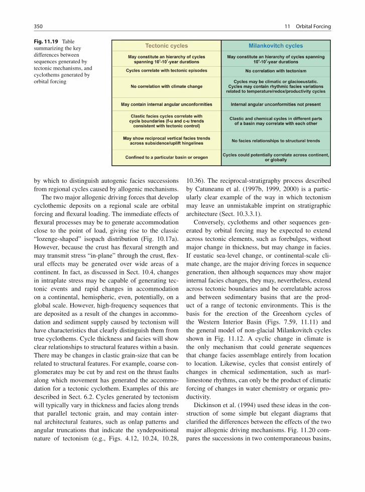
350 11 Orbital Forcing
Fig. 11.19 Tablesummarizing the keydifferences betweensequences generated bytectonic mechanisms, andcyclothems generated byorbital forcing
by which to distinguish autogenic facies successionsfrom regional cycles caused by allogenic mechanisms.
The two major allogenic driving forces that developcyclothemic deposits on a regional scale are orbitalforcing and flexural loading. The immediate effects offlexural processes may be to generate accommodationclose to the point of load, giving rise to the classic“lozenge-shaped” isopach distribution (Fig. 10.17a).However, because the crust has flexural strength andmay transmit stress “in-plane” through the crust, flex-ural effects may be generated over wide areas of acontinent. In fact, as discussed in Sect. 10.4, changesin intraplate stress may be capable of generating tec-tonic events and rapid changes in accommodationon a continental, hemispheric, even, potentially, on aglobal scale. However, high-frequency sequences thatare deposited as a result of the changes in accommo-dation and sediment supply caused by tectonism willhave characteristics that clearly distinguish them fromtrue cyclothems. Cycle thickness and facies will showclear relationships to structural features within a basin.There may be changes in clastic grain-size that can berelated to structural features. For example, coarse con-glomerates may be cut by and rest on the thrust faultsalong which movement has generated the accommo-dation for a tectonic cyclothem. Examples of this aredescribed in Sect. 6.2. Cycles generated by tectonismwill typically vary in thickness and facies along trendsthat parallel tectonic grain, and may contain inter-nal architectural features, such as onlap patterns andangular truncations that indicate the syndepositionalnature of tectonism (e.g., Figs. 4.12, 10.24, 10.28,
10.36). The reciprocal-stratigraphy process describedby Catuneanu et al. (1997b, 1999, 2000) is a partic-ularly clear example of the way in which tectonismmay leave an unmistakable imprint on stratigraphicarchitecture (Sect. 10.3.3.1).
Conversely, cyclothems and other sequences gen-erated by orbital forcing may be expected to extendacross tectonic elements, such as forebulges, withoutmajor change in thickness, but may change in facies.If eustatic sea-level change, or continental-scale cli-mate change, are the major driving forces in sequencegeneration, then although sequences may show majorinternal facies changes, they may, nevertheless, extendacross tectonic boundaries and be correlatable acrossand between sedimentary basins that are the prod-uct of a range of tectonic environments. This is thebasis for the erection of the Greenhorn cycles ofthe Western Interior Basin (Figs. 7.59, 11.11) andthe general model of non-glacial Milankovitch cyclesshown in Fig. 11.12. A cyclic change in climate isthe only mechanism that could generate sequencesthat change facies assemblage entirely from locationto location. Likewise, cycles that consist entirely ofchanges in chemical sedimentation, such as marl-limestone rhythms, can only be the product of climaticforcing of changes in water chemistry or organic pro-ductivity.
Dickinson et al. (1994) used these ideas in the con-struction of some simple but elegant diagrams thatclarified the differences between the effects of the twomajor allogenic driving mechanisms. Fig. 11.20 com-pares the successions in two contemporaneous basins,
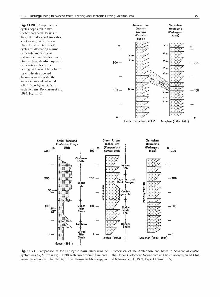
11.4 Distinguishing Between Orbital Forcing and Tectonic Driving Mechanisms 351
Fig. 11.20 Comparison ofcycles deposited in twocontemporaneous basins inthe (Late Paleozoic) AncestralRockies region of the SWUnited States. On the left,cycles of alternating marinecarbonate and terrestrialeolianite in the Paradox Basin.On the right, shoaling upwardcarbonate cycles of thePedregosa Basin. The columnstyle indicates upwarddecreases in water depthand/or increased subaerialrelief, from left to right, ineach column (Dickinson et al.,1994, Fig. 11.6)
Fig. 11.21 Comparison of the Pedregosa basin succession ofcyclothems (right; from Fig. 11.20) with two different foreland-basin successions. On the left, the Devonian-Mississippian
succession of the Antler foreland basin in Nevada; at centre,the Upper Cretaceous Sevier foreland basin succession of Utah(Dickinson et al., 1994, Figs. 11.8 and 11.9)
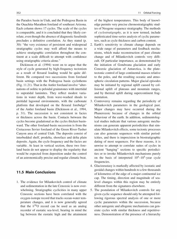
352 11 Orbital Forcing
the Paradox basin in Utah, and the Pedregosa Basin inthe Ouachita-Marathon foreland of southeast Arizona.Each column shows 17 cycles. The scale of the cyclesis comparable, and it is concluded that they likely cor-relate, even though the absence of diagnostic fusulinidsprecludes a definitive correlation. As they stated (p.30): “the very existence of persistent and widespreadstratigraphic cycles may well afford the means toachieve stratigraphic correlation throughout the con-tinent at a scale difficult to attempt with confidenceusing stratigraphic criteria alone.”
Dickinson et al. (1994) went on to argue that thestyle of cycle generated by high-frequency tectonismas a result of flexural loading would be quite dif-ferent. He compared two successions from forelandbasin settings with the Pedregosa basin cyclothems(Fig. 11.21). That in the Antler foreland involve “alter-nations of oolitic to peloidal grainstones with intertidalto supratidal laminites. They reflect modest varia-tions in water depth, from wave-washed shoals toperitidal lagoonal environments, with the carbonateplatform that developed on the flexural forebulge”of the Antler foreland basin (Dickinson et al., 1994,p. 31). The succession is not consistent in faciesor thickness across the basin. Contacts between thecycles become gradational as the cycles thicken basin-ward. The other foreland-basin succession is from theCretaceous Sevier foreland of the Green River-TusherCanyon area of central Utah. The deposits consist ofinterbedded shelf, prodelta, shoreface and delta plaindeposits. Again, the cycle frequency and the facies arevariable. At least in vertical section, these two fore-land basin do not appear to display the regularity thatwould be expected from deposition under the controlof an astronomically precise and regular climatic beat.
11.5 Main Conclusions
1. The evidence for Milankovitch control of climateand sedimentation in the late Cenozoic is now over-whelming. Stratigraphic cyclicities in many upperCenozoic sections have been correlated with theoxygen-isotope record that tracks ocean-water tem-perature changes, and it is now generally agreedthat the δ18O record can be used as an analogrecorder of eustatic sea-level, bearing in mind thelag between the eustatic high and the attainment
of the highest temperatures. This body of knowl-edge permits very precise chronostratigraphic stud-ies of Neogene sequence stratigraphy. The methodsof cyclostratigraphy, as it is now termed, includesophisticated time-series analysis of cyclic parame-ters, such as cycle thickness and carbon content.
2. Earth’s sensitivity to climate change depends ona wide range of parameters and feedback mecha-nisms, which make reconstruction of past climatechange and of Milankovitch controls very diffi-cult. Of particular importance, as demonstrated bythe initiation of Gondwana glaciation and earlyCenozoic glaciation of Antarctica, is the plate-tectonic control of large continental masses relativeto the poles, and the resulting oceanic and atmo-spheric circulation patterns. Major glacial episodesmay be initiated by regional uplift caused by col-lisional uplift of plateaus and mountain ranges,and by thermal uplift during supercontinent frag-mentation.
3. Controversy remains regarding the periodicity ofMilankovitch parameters in the geological past.Major changes may have occurred during thePhanerozoic because of changes in the orbitalbehaviour of the earth. In addition, sedimentolog-ical studies indicate that various autogenic mecha-nisms can generate apparent periodicities that sim-ulate Milankovitch effects, some tectonic processescan also generate sequences with similar period-icities, and there is imprecision in biostratigraphicdating of most sequences. For these reasons, it isunwise to attempt to correlate suites of cycles inancient “hanging” sections to specific periodici-ties or to invoke Milankovitch mechanisms purelyon the basis of interpreted 104–105-year cyclefrequencies.
4. Glacioeustasy is markedly affected by isostatic andgeoidal changes within hundreds to a few thousandsof kilometres of the edge of a major continental icecap. The timing, direction and magnitude of sea-level changes within this region may be entirelydifferent from the signatures elsewhere.
5. The postulation of Milankovitch controls for anygiven cyclic sequence should only be attempted fol-lowing rigorous spectral analysis of one or morecyclic parameters within the succession, becauseother autogenic and allogenic mechanisms can gen-erate cycles with similar thickness and repetitive-ness. Demonstration of the presence of a hierarchy
11.5 Main Conclusions 353
of cycle types with characteristic periodic ratios,such as the 1:5 precession:eccentricity combina-tion, is additional evidence of Milankovitch con-trols, although the cautions noted in paragraph 3,above, need to be borne in mind.
6. There is evidence for at least localized glaciation formost periods during the Phanerozoic, but the evi-dence for major continental glaciation and conse-quent significant glacioeustasy outside the periodsoccupied by the late Paleozoic Gondwana glacia-tion and the Neogene glaciation is at present weak.There is increasing evidence for small, short-livedcontinental ice caps at several different intervalsduring the Cretaceous.
7. Glacioeustasy is not the only cycle-forming mecha-nism driven by orbital forcing. Variations in climateand oceanic circulation have significant effects onsuch parameters as sediment yield and organic
productivity, which have generated many succes-sions of metre-scale cycles throughout the geologicpast. These are especially prominent in the depositsof many carbonate shelves and in fine-grained clas-tic deposits formed in lakes and deep seas.
8. Given the overlapping range of frequencies exhib-ited by the two major classes of high-frequencycycles, those generated by orbital forcing and thoseformed in response to tectonic processes, a range oftests needs to be performed to distinguish betweenthem. Cyclothems generated by climate changeextend regionally, potentially globally, but maychange in facies from environment to environment.Cycles generated by tectonism are likely to be localto regional in extent and will contain internal evi-dence of tectonic control, including onlap and angu-lar truncation relationships, coarse clastic facies cutby unconformities, and onlapping faults, etc.
Part IVChronostratigraphy and Correlation:An Assessment of the Current Status
of “Global Eustasy”
The purpose of this part of the book is to examine the nature of the chronostrati-graphic record of cycle correlation, to examine the potential for error, and to reviewthe various sea-level curves that have been prepared by Exxon and by other workers,in order to demonstrate the present level of uncertainty.
Are sequences in a given basin regional or global in distribution? Or are bothtypes present? If so, how do we distinguish them? The basic premise of the Exxonapproach is that there exists a globally correlatable suite of eustatic cycles, and that allstratigraphic data may be interpreted in keeping with this concept. However, this basicpremise remains unproven, and it sidesteps the issue of regional tectonic control, ofthe type demonstrated in Parts II and III of this book. Unfortunately, the global cyclechart has commonly been presented as its own proof, with many researchers usingthe chart as a guide to correlation, and then citing the result as successful test of thechart. This practice is still in evidence, despite more than a decade of skeptical workon the issue, and is discussed in Chap. 12.
One of the critical tests of global cycle charts is to demonstrate that successions ofcycles of the same age do indeed exist in many tectonically independent basins aroundthe world. The chronostratigraphic accuracy and precision of the chart and of thefield sections on which it is based are, therefore, of critical importance. This requiresindependent studies of sequence stratigraphies in tectonically unrelated basins. Weexamine this problem in Chap. 14.
The concept of the global cycle chart, as first formulated by Vail et al. (1977),has been accepted by many as a standard of geologic time. Various versions of theExxon chart have appeared as part of many key synthesis charts, despite the absenceof a rigorous, published examination of the supporting data. Such a casual approachto an apparently important new tool for correlation contrasts dramatically with theenormous effort that has been ongoing since the work of William Smith in the lateeighteenth century to refine and calibrate biostratigraphic, radiometric, and magne-tostratigraphic times scales. Revisions of these scales appear frequently (the latest in2008), whereas the updated version of the Exxon global cycle chart published in 1987continues in many quarters to be accepted as a finished product and as a standard forcross-comparison. Miall and Miall (2002) developed a set of explanations for thismethodological approach and called it the “Exxon Factor”. A newer (1998) “global”scale , based on European research, is now being used in the same way as the originalchart by many workers, as discussed in Chap. 12.
356 Part IV Chronostratigraphy and Correlation: An Assessment of the Current Status of “Global Eustasy”
• A sea-level curve may be compared with other regional data by plotting it on achronostratigraphic correlation chart for the region . . . Such a combination showsthe relations of sea-level changes to geologic age, distribution of depositionalsequences, unconformities, facies and environment, and other information. (Vailet al., 1977, p. 77)
• It is . . . important to obtain precise ages of the sequence boundaries and rate andmagnitude of apparent sea-level change to establish their global or regional nature.In this context, critical stratigraphic examination of seismic sections across theinner edge of passive margins to the seaward part is of particular importance.(Cloetingh, 1988, p. 219)
• Most refinement in correlation derives from a fuller understanding of the proper-ties of the characters employed. There is always room for improvement, howeverthere are several reasons why an apparent age will differ more or less from thetrue age. Most obvious is non-availability of appropriate characters and gaps inthe record which lead to indeterminate results. In other cases human skill or erroraffect the uncertainty as in observational and experimental errors. These can insome degree be measured as standard errors, or as systematic errors due to mis-taken assumptions (e.g. decay constant) or due to inadequate understanding of thecharacters used, taxonomic lumping, splitting, or mistakes. (Harland, 1978, p. 18)
• Biostratigraphy is not without its problem areas . . . Variations in the inferred rela-tionship between absolute time and biostratigraphic zones comprise a major areaof controversy. (Kauffman and Hazel, 1977b, p. iv)
• Without a precise time control the depositional mechanisms forming beds andsequences cannot be sufficiently understood. . . . timing has remained an elusiveproblem. Too many inaccuracies are involved in resolving stratigraphic durations,including a large range of error in radiometric age determinations, poor bios-tratigraphic as well as magnetostratigraphic resolution, and an incompleteness ofsedimentary sections. As a result, time estimates are commonly imprecise, andthe range of error is often larger than the actual time span considered . . . (Ricken,1991, p. 773).
• . . . we believe that the Haq et al. (1987) curve is a “noisy” accumulation of awide range of sea-level signals, and should not be used as a global benchmark.It should never be used as a chronostratigraphic tool by assuming a priori that acertain stratigraphic boundary has a globally synchronous and precise age, whichit is therefore safe to extrapolate into a basin with poor age control (Allen andAllen, 2005, pp. 279–280).
• Global sequence stratigraphic/cycle charts . . . were always a fudge, and they aren’tgoing to help much in chronostratigraphy at the resolution that is now needed(Christie-Blick et al., 2007, p. 223).
Chapter 12
The Concept of the Global Cycle Chart
Contents
12.1 From Vail to Haq . . . . . . . . . . . . . . 35712.2 The Two-Paradigm Problem . . . . . . . . . 363
12.2.1 The Global-Eustasy Paradigm . . . . . . 36312.2.2 The Complexity Paradigm . . . . . . . 364
12.3 Defining and Deconstructing Global Eustasy andComplexity Texts . . . . . . . . . . . . . . 364
12.4 Invisible Colleges and the Advancement ofKnowledge . . . . . . . . . . . . . . . . . 368
12.5 The Global-Eustasy Paradigm—A Revolution inTrouble? . . . . . . . . . . . . . . . . . . 373
12.6 Conclusions . . . . . . . . . . . . . . . . . 377
12.1 From Vail to Haq
The concept of eustasy dates back to the late nineteenthcentury. The term “eustatic” was coined by Suess(1885–1909) and, as discussed in Sect. 1.4, there wasconsiderable discussion and theorizing about globalprocesses, such as eustatic sea-level change, throughthe twentieth century. The topic received considerableimportance with the development of seismic stratigra-phy. One of the major theses of the Vail et al. (1977)work was that cycles of sea-level change can be cor-related around the world, signifying that sequences arenot a response to local tectonic events but the resultof global or eustatic sea-level changes (Fig. 12.1). Asnoted in Chap. 1, in the early days of seismic stratigra-phy, in the late 1970s and early 1980s, the global cyclechart was considered an inseparable part of the newmethodology.
Vail et al. (1977, p. 96) had set out this paradigmclearly in their first publication, and this has remainedtheir key concept:
One of the greatest potential applications of the globalcycle chart is its use as an instrument of geochronology.Global cycles are geochronologic units defined by asingle criterion-the global change in the relative positionof sea level through time. Determination of these cyclesis dependent on a synthesis of data from many branchesof geology. As seen on the Phanerozoic chart . . ., theboundaries of the global cycles in several cases do notmatch the standard epoch and period boundaries, butseveral of the standard boundaries have been placedarbitrarily and remain controversial. Using globalcycles with their natural and significant boundaries, aninternational system of geochronology can be developedon a rational basis. If geologists combine their efforts toprepare more accurate charts of regional cycles, and usethem to improve the global chart, it can become a moreaccurate and meaningful standard for Phanerozoic time.(Vail et al., 1977, p. 96).
It was stated that much evidence had been amassedto demonstrate this idea, but the only evidence actuallyoffered was a correlation between four Cretaceous toRecent basins in a chart reproduced here as Fig. 12.2.An important critique of this figure is that it is rare ingeology for the evidence to permit such precise cor-relation of events that they can be indicated by thestraight lines encompassing the globe (Miall, 1986).There is still much disagreement over the exact age ofmagnetic anomalies, and the absolute (numerical) ageof biostratigraphic zones. Even in the case of Cenozoicstratigraphy, the determination of chronostratigraphicage is characterized by significant observational andexperimental error, and this increases with the ageof the sediments (these problems are discussed inChap. 14). Yet there is no indication of these possibleerrors in Fig. 12.2. If such data are not provided, it isdifficult to allow for revisions and refinements.
Global correlations such as those in Fig. 12.2 per-mitted Vail et al. (1977) to construct charts showingrelative sea-level changes that, because of their
357A.D. Miall, The Geology of Stratigraphic Sequences, 2nd ed.,DOI 10.1007/978-3-642-05027-5_12, © Springer-Verlag Berlin Heidelberg 2010
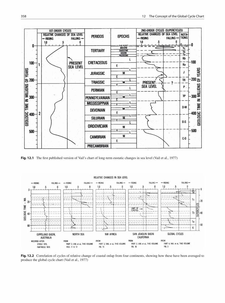
358 12 The Concept of the Global Cycle Chart
Fig. 12.1 The first published version of Vail’s chart of long-term eustatic changes in sea level (Vail et al., 1977)
Fig. 12.2 Correlation of cycles of relative change of coastal onlap from four continents, showing how these have been averaged toproduce the global cycle chart (Vail et al., 1977)
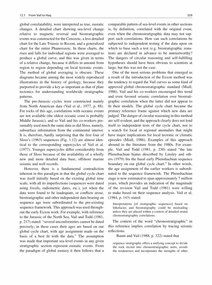
12.1 From Vail to Haq 359
global correlatability, were interpreted as true, eustaticchanges. A detailed chart showing sea-level changerelative to magnetic reversal and biostratigraphicevents was constructed for the Cenozoic, a less detailedchart for the Late Triassic to Recent, and a generalizedchart for the entire Phanerozoic. In these charts, therises and falls for individual regions were averaged toproduce a global curve, and this was given in termsof a relative change, because it differs in amount fromregion to region depending on local tectonic events.The method of global averaging is obscure. Thesediagrams became among the most widely reproducedillustrations in the history of geology, because theypurported to provide a key as important as that of platetectonics for understanding worldwide stratigraphicpatterns.
The pre-Jurassic cycles were constructed mainlyfrom North American data (Vail et al., 1977, p. 88).For rocks of this age, correlations with oceanic eventsare not available (the oldest oceanic crust is probablyMiddle Jurassic), and so Vail and his co-workers pre-sumably used much the same data as did Sloss, namely,subsurface information from the continental interior.It is, therefore, hardly surprising that the first four ofSloss’s (1963) sequences (Fig. 1.12) are almost iden-tical to the corresponding supercycles of Vail et al.(1977). Younger supercycles differ considerably fromthose of Sloss because of the availability of a whollynew and more detailed data base, offshore marineseismic and well records.
However, there is a fundamental contradictioninherent in this paradigm in that the global cycle chartwas itself initially based on the existing global timescale, with all its imperfections (sequences were datedusing fossils, radiometric dates, etc.), yet when thedata were found to be inadequate, or conflicts arose,biostratigraphic and other independent data bearing onsequence age were subordinated to the pre-existingsequence framework. This approach was used through-out the early Exxon work. For example, with referenceto the Jurassic of the North Sea, Vail and Todd (1981,p. 217) stated: “several unconformities cannot be datedprecisely; in these cases their ages are based on ourglobal cycle chart, with age assignment made on thebasis of a best fit with the data.” The assumptionwas made that important sea-level events in any givenstratigraphic section represent eustatic events. Fromthe paradigm of global eustasy it then follows that a
comparable pattern of sea-level events in other sectionsis, by definition, correlated with the original event,even when the chronostratigraphic data may not sup-port such correlations. How can such correlations besubjected to independent testing if the data upon onwhich to base such a test (e.g. biostratigraphic zona-tion) are declared in advance to be untrustworthy?The dangers of circular reasoning and self-fulfillinghypotheses should have been obvious to scientists atlarge, but this was not the case.
One of the most serious problems that emerged asa result of the introduction of the Exxon method wasthe tendency to regard the Vail curves as some kind ofapproved global chronostratigraphic standard (Miall,1986). Vail and his co-workers encouraged this trendand even favored seismic correlation over biostrati-graphic correlation when the latter did not appear tofit their models. The global cycle chart became theprimary reference frame against which new data arejudged. The danger of circular reasoning in this methodare self-evident, and the approach clearly does not lenditself to independent tests of the cycle chart, nor toa search for local or regional anomalies that mighthave major implications for local tectonic or climaticepisodes (Miall, 1986). Examples of this approachabound in the literature from the 1980s. For exam-ple, Vail and Todd (1981, p. 230) stated “the latePliensbachian hiatus described by Linsley and oth-ers (1979) fits the basal early Pliensbachian sequenceboundary on our global cycle chart.” In other words,the age assignment of the earlier workers is subordi-nated to the sequence framework. The Pliensbachianstage is now estimated to span approximately 7 millionyears, which provides an indication of the magnitudeof the revision Vail and Todd (1981) were willingto make based on their sequence analysis. Vail et al.(1984, p. 143) stated:
Interpretations [of stratigraphic sequences] based onlithofacies and biostratigraphy could be misleadingunless they are placed within a context of detailed stratalchronostratigraphic correlations.
The context of the word “chronostratigraphic” inthis reference implies correlation by tracing seismicreflections.
Baum and Vail (1988, p. 322) stated that
sequence stratigraphy offers a unifying concept to dividethe rock record into chronostratigraphic units, avoidsthe weaknesses and incorporates the strengths of other
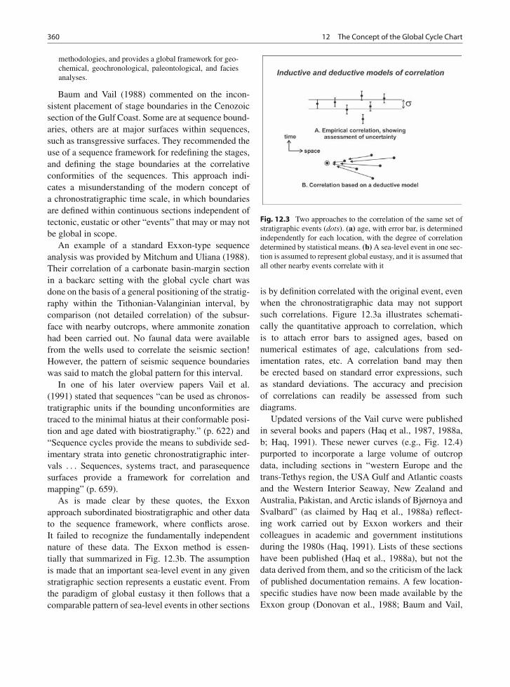
360 12 The Concept of the Global Cycle Chart
methodologies, and provides a global framework for geo-chemical, geochronological, paleontological, and faciesanalyses.
Baum and Vail (1988) commented on the incon-sistent placement of stage boundaries in the Cenozoicsection of the Gulf Coast. Some are at sequence bound-aries, others are at major surfaces within sequences,such as transgressive surfaces. They recommended theuse of a sequence framework for redefining the stages,and defining the stage boundaries at the correlativeconformities of the sequences. This approach indi-cates a misunderstanding of the modern concept ofa chronostratigraphic time scale, in which boundariesare defined within continuous sections independent oftectonic, eustatic or other “events” that may or may notbe global in scope.
An example of a standard Exxon-type sequenceanalysis was provided by Mitchum and Uliana (1988).Their correlation of a carbonate basin-margin sectionin a backarc setting with the global cycle chart wasdone on the basis of a general positioning of the stratig-raphy within the Tithonian-Valanginian interval, bycomparison (not detailed correlation) of the subsur-face with nearby outcrops, where ammonite zonationhad been carried out. No faunal data were availablefrom the wells used to correlate the seismic section!However, the pattern of seismic sequence boundarieswas said to match the global pattern for this interval.
In one of his later overview papers Vail et al.(1991) stated that sequences “can be used as chronos-tratigraphic units if the bounding unconformities aretraced to the minimal hiatus at their conformable posi-tion and age dated with biostratigraphy.” (p. 622) and“Sequence cycles provide the means to subdivide sed-imentary strata into genetic chronostratigraphic inter-vals . . . Sequences, systems tract, and parasequencesurfaces provide a framework for correlation andmapping” (p. 659).
As is made clear by these quotes, the Exxonapproach subordinated biostratigraphic and other datato the sequence framework, where conflicts arose.It failed to recognize the fundamentally independentnature of these data. The Exxon method is essen-tially that summarized in Fig. 12.3b. The assumptionis made that an important sea-level event in any givenstratigraphic section represents a eustatic event. Fromthe paradigm of global eustasy it then follows that acomparable pattern of sea-level events in other sections
Fig. 12.3 Two approaches to the correlation of the same set ofstratigraphic events (dots). (a) age, with error bar, is determinedindependently for each location, with the degree of correlationdetermined by statistical means. (b) A sea-level event in one sec-tion is assumed to represent global eustasy, and it is assumed thatall other nearby events correlate with it
is by definition correlated with the original event, evenwhen the chronostratigraphic data may not supportsuch correlations. Figure 12.3a illustrates schemati-cally the quantitative approach to correlation, whichis to attach error bars to assigned ages, based onnumerical estimates of age, calculations from sed-imentation rates, etc. A correlation band may thenbe erected based on standard error expressions, suchas standard deviations. The accuracy and precisionof correlations can readily be assessed from suchdiagrams.
Updated versions of the Vail curve were publishedin several books and papers (Haq et al., 1987, 1988a,b; Haq, 1991). These newer curves (e.g., Fig. 12.4)purported to incorporate a large volume of outcropdata, including sections in “western Europe and thetrans-Tethys region, the USA Gulf and Atlantic coastsand the Western Interior Seaway, New Zealand andAustralia, Pakistan, and Arctic islands of Bjørnoya andSvalbard” (as claimed by Haq et al., 1988a) reflect-ing work carried out by Exxon workers and theircolleagues in academic and government institutionsduring the 1980s (Haq, 1991). Lists of these sectionshave been published (Haq et al., 1988a), but not thedata derived from them, and so the criticism of the lackof published documentation remains. A few location-specific studies have now been made available by theExxon group (Donovan et al., 1988; Baum and Vail,
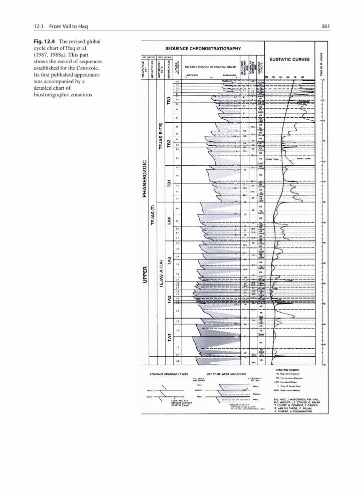
12.1 From Vail to Haq 361
Fig. 12.4 The revised globalcycle chart of Haq et al.(1987, 1988a). This partshows the record of sequencesestablished for the Cenozoic.Its first published appearancewas accompanied by adetailed chart ofbiostratigraphic zonations
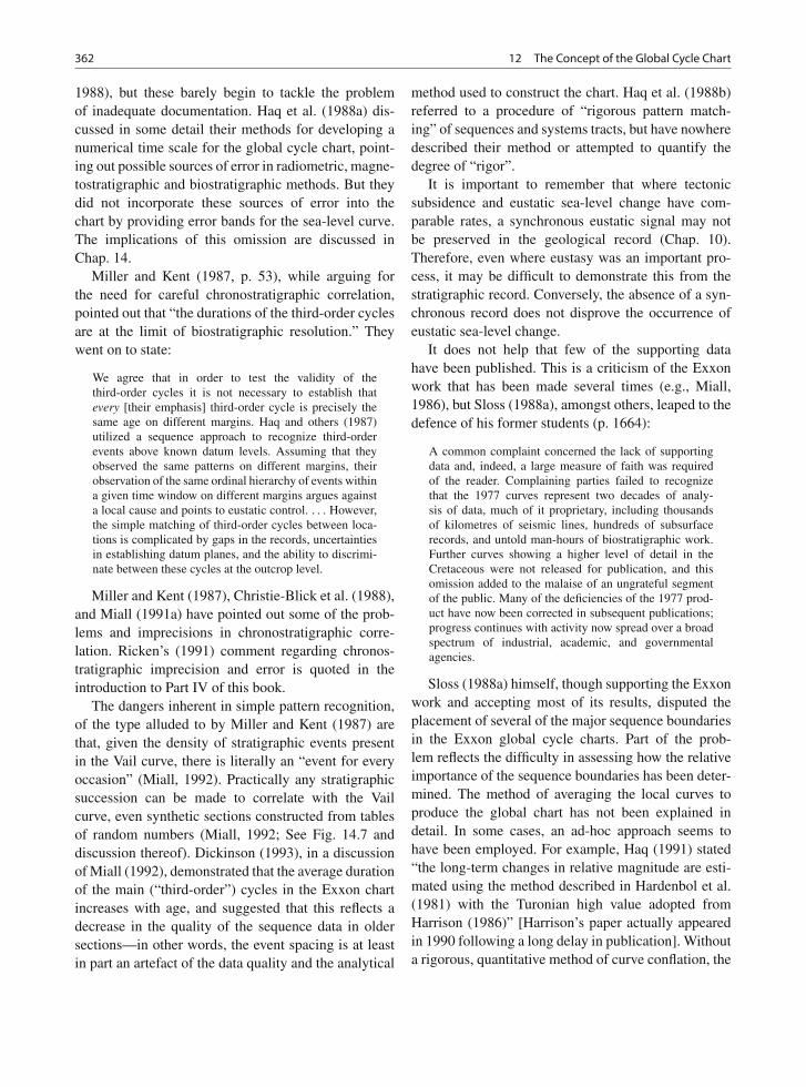
362 12 The Concept of the Global Cycle Chart
1988), but these barely begin to tackle the problemof inadequate documentation. Haq et al. (1988a) dis-cussed in some detail their methods for developing anumerical time scale for the global cycle chart, point-ing out possible sources of error in radiometric, magne-tostratigraphic and biostratigraphic methods. But theydid not incorporate these sources of error into thechart by providing error bands for the sea-level curve.The implications of this omission are discussed inChap. 14.
Miller and Kent (1987, p. 53), while arguing forthe need for careful chronostratigraphic correlation,pointed out that “the durations of the third-order cyclesare at the limit of biostratigraphic resolution.” Theywent on to state:
We agree that in order to test the validity of thethird-order cycles it is not necessary to establish thatevery [their emphasis] third-order cycle is precisely thesame age on different margins. Haq and others (1987)utilized a sequence approach to recognize third-orderevents above known datum levels. Assuming that theyobserved the same patterns on different margins, theirobservation of the same ordinal hierarchy of events withina given time window on different margins argues againsta local cause and points to eustatic control. . . . However,the simple matching of third-order cycles between loca-tions is complicated by gaps in the records, uncertaintiesin establishing datum planes, and the ability to discrimi-nate between these cycles at the outcrop level.
Miller and Kent (1987), Christie-Blick et al. (1988),and Miall (1991a) have pointed out some of the prob-lems and imprecisions in chronostratigraphic corre-lation. Ricken’s (1991) comment regarding chronos-tratigraphic imprecision and error is quoted in theintroduction to Part IV of this book.
The dangers inherent in simple pattern recognition,of the type alluded to by Miller and Kent (1987) arethat, given the density of stratigraphic events presentin the Vail curve, there is literally an “event for everyoccasion” (Miall, 1992). Practically any stratigraphicsuccession can be made to correlate with the Vailcurve, even synthetic sections constructed from tablesof random numbers (Miall, 1992; See Fig. 14.7 anddiscussion thereof). Dickinson (1993), in a discussionof Miall (1992), demonstrated that the average durationof the main (“third-order”) cycles in the Exxon chartincreases with age, and suggested that this reflects adecrease in the quality of the sequence data in oldersections—in other words, the event spacing is at leastin part an artefact of the data quality and the analytical
method used to construct the chart. Haq et al. (1988b)referred to a procedure of “rigorous pattern match-ing” of sequences and systems tracts, but have nowheredescribed their method or attempted to quantify thedegree of “rigor”.
It is important to remember that where tectonicsubsidence and eustatic sea-level change have com-parable rates, a synchronous eustatic signal may notbe preserved in the geological record (Chap. 10).Therefore, even where eustasy was an important pro-cess, it may be difficult to demonstrate this from thestratigraphic record. Conversely, the absence of a syn-chronous record does not disprove the occurrence ofeustatic sea-level change.
It does not help that few of the supporting datahave been published. This is a criticism of the Exxonwork that has been made several times (e.g., Miall,1986), but Sloss (1988a), amongst others, leaped to thedefence of his former students (p. 1664):
A common complaint concerned the lack of supportingdata and, indeed, a large measure of faith was requiredof the reader. Complaining parties failed to recognizethat the 1977 curves represent two decades of analy-sis of data, much of it proprietary, including thousandsof kilometres of seismic lines, hundreds of subsurfacerecords, and untold man-hours of biostratigraphic work.Further curves showing a higher level of detail in theCretaceous were not released for publication, and thisomission added to the malaise of an ungrateful segmentof the public. Many of the deficiencies of the 1977 prod-uct have now been corrected in subsequent publications;progress continues with activity now spread over a broadspectrum of industrial, academic, and governmentalagencies.
Sloss (1988a) himself, though supporting the Exxonwork and accepting most of its results, disputed theplacement of several of the major sequence boundariesin the Exxon global cycle charts. Part of the prob-lem reflects the difficulty in assessing how the relativeimportance of the sequence boundaries has been deter-mined. The method of averaging the local curves toproduce the global chart has not been explained indetail. In some cases, an ad-hoc approach seems tohave been employed. For example, Haq (1991) stated“the long-term changes in relative magnitude are esti-mated using the method described in Hardenbol et al.(1981) with the Turonian high value adopted fromHarrison (1986)” [Harrison’s paper actually appearedin 1990 following a long delay in publication]. Withouta rigorous, quantitative method of curve conflation, the
12.2 The Two-Paradigm Problem 363
relative magnitudes of the sea-level excursions cannotbe assigned much significance, and therefore it followsthat the assignment of certain sequence boundaries inthe Exxon curves as “supercycle” boundaries carrieslittle weight.
As noted by Miall (1992), the basic premise of theExxon work is that there exists a globally correlatablesuite of eustatic cycles, and that all field stratigraphicdata may be interpreted in keeping with this concept.However, the basic premise remains unproven becauseof the lack of published documentation. All so-calledtests of the Vail curve are suspect unless they providea rigorous treatment of potential error and a discus-sion of alternative interpretations. In fact this is almostnever done. Some examples of tests of the Vail curveare described in detail in Chap. 14.
Despite these critiques, there remains a seri-ous conceptual disagreement about the appropriateapproach to stratigraphic data. As recently as 2005,McGowran (2005, pp. 176–179), citing Loutit et al.(1988), referred to “the provision of a new physical-stratigraphic framework within which ‘sample-baseddisciplines’, such as biostratigraphy and geochemistry,can be evaluated.” By this he meant the “powerful uni-fying force” of sequence stratigraphy, with its systemof correlatable bounding unconformities: Referring to“three roots to the development of sequence stratigra-phy,” he suggested (p. 176) that the first root was therise of sequence stratigraphy.
As second root was to take unconformity-bounded strati-graphic bodies (allostratigraphic units) seriously as some-thing more than a frustratingly imperfect stratigraphicrecord. Instead of unconformities being apologized for asthe main manifestation of an all-too-imperfect geologi-cal record, they are information-rich and to be cherished,especially since Sloss et al. (1949) and Sloss (1963) pro-posed sequences and demonstrated cratonic sequencesat the Phanerozoic scale separated by continent-widebreaks.
The third root was the concept of the sedimentarycycle.
McGowran (2005) acknowledged the controversiesthat have arisen around the “global curve” but said(p. 180) “it is important to affirm that inferred eustaticconfigurations are not the core of sequence stratigra-phy which will survive any amount of eustatic/isostaticcontroversy.” I refer McGowran and his readers toCarter et al. (1991), whose useful conceptual distinc-tion provides the basis for the ensuing discussion ofthe controversies.
12.2 The Two-Paradigm Problem
Carter et al. (1991, pp. 42, 60) pointed out thatsequence stratigraphy embraces two quite distinctconcepts:
Two different conceptual models underlie the applicationof sequence stratigraphy by Vail and his coworkers: onemodel relates to presumed [global] sea-level behaviourthrough time; the other model relates to the stratigraphicrecord produced during a single sea-level cycle. Thoughthe two models are interrelated they are logically distinct,and we believe that it is important to test them separately.. . . Our studies lead us to have considerable confidencein the correctness and power of the Exxon sequence-stratigraphic model as applied to sea-level controlled,cyclothemic sequences. . . . At the same time, we suspectthat the Exxon “Global” sea-level curve, in general, rep-resents a patchwork through time of many different localrelative sea-level curves.
In his essay on the structure of scientific revolutions,Kuhn (1962, p. 65) has noted that anomalies (data thatdo not “fit”) appear only against the background pro-vided by a paradigm. In this regard, he has argued that“if an anomaly is to evoke a crisis, it must usually bemore than just an anomaly. . .. Sometimes an anomalywill clearly call into question explicit and fundamentalgeneralizations of the paradigm” (Kuhn, 1962, p. 82).As Kuhn (1962, p. 76) has also observed, however,“philosophers of science have repeatedly demonstratedthat more than one theoretical construction can alwaysbe placed upon a given collection of data.” Miall andMiall (2001) demonstrated that views about the global-eustasy model have evolved into a broad spectrumof approaches, and it is useful to consider them astwo, coexisting, end-member paradigms—the “global-eustasy paradigm” (the original concepts set out inVail et al., 1977), and what Miall and Miall (2001)labeled the “complexity paradigm.” Sequence stratig-raphy, itself, including studies of sequence architec-ture, could be said to correspond now to Gutting’s(1984) definition of a supertheory: a “wide-rangingset of fundamental beliefs about the nature of somedomain of reality and about the proper methods bywhich to study that domain.”
12.2.1 The Global-Eustasy Paradigm
Eustatic sea-level changes are global by definition, butthe word “global” is employed here in the sense of
364 12 The Concept of the Global Cycle Chart
“all-encompassing” or “universal”, because this is thesense in which the model of eustatic sea-level changeis employed by Vail and his colleagues. This group ofworkers attributes all sea-level change to eustatic pro-cesses, including changes in ocean basin volumes forthe low frequency cycles, and glacioeustasy for thoseof high frequency, although it was conceded that apartfrom specific cases, such as the Gondwana glaciationof the late Paleozoic, there is little convincing evidencefor glaciation prior to the Oligocene (Vail et al., 1977,pp. 92–94) (we return to this point in Sect. 14.6.4).Two quotes from Vail’s first major publication statesthe case succinctly. The first is at the beginning of thischapter, the second is below:
Glaciation and deglaciation are the only well-understoodcausal mechanisms that occur at the relatively rapid rateof third-order cycles (Vail et al., 1977, p. 94).
As noted above, Vail and his colleagues thoughtthat they had developed an entirely new standard ofgeologic time and a new basis for geologic correla-tion, superior to that based on conventional chronos-tratigraphic data (biostratigraphy, magnetostratigra-phy, radiometric dating)(see summary in Miall, 1997,pp. 282–284).
12.2.2 The Complexity Paradigm
This contrasting paradigm represents a body of ideasfocusing on the hypothesis that sea-level change isaffected by multiple processes operating simultane-ously at different rates and over different ranges oftime and space, possibly including eustatic sea-levelchange. No simple signal can therefore result, and theinterpretation of each event in the stratigraphic recordcan only follow very careful, detailed local work, fol-lowed by meticulous regional and global correlations.An additional, and important argument is that becauseof limitations in our techniques for testing the realityof global eustasy, no conclusions can yet be drawnregarding the vast majority of the supposed eustaticevents that have been proposed (e.g., Miall, 1997;Dewey and Pitman, 1998).
Underlying both paradigms are the principles andmethods encompassed by the sequence-architecturemodel first introduced by Vail et al. (1977), and furtherelaborated by Haq et al. (1987, 1988a), Posamentierand Vail (1988), Posamentier et al. (1988), and Van
Wagoner et al. (1990), although details of definitionand interpretation of the model remain to be resolved.The global-eustasy model and its global cycle chartcould be said to represent the paradigm against whichanomalies have arisen, and which have coalescedaround the complexity paradigm.
As others have already argued, geology is char-acterized by complexity. The concept of the mul-tiple working hypothesis originated with geologists(Gilbert, 1886; Chamberlin, 1897) and, as noted byLaw (1980, p. 16), it is not uncommon for geologists tosimultaneously consider contrasting or even conflict-ing methods and hypotheses, a condition he refers toas conceptual pluralism. Therefore, the growth of twoconflicting views about global eustasy and their mutualsurvival for more than 15 years (since the first arti-cles critical of the model appeared in the early 1980s)should not surprise historians or sociologists of sci-ence (or geologists). As Kuhn (1962, p. 149) observed,“the proponents of competing paradigms practice theirtrades in different worlds . . . practicing in differentworlds, the two groups of scientists see different thingswhen they look from the same point of view in thesame direction.”
Kuhn (1996, pp. 181–187) also clarified the conceptof the scientific paradigm by showing how it is con-structed of a set of integrated parts. First, a paradigmincorporates a system of symbolic generalizations orlaws. Second, it involves commitments or beliefs inparticular models. Third, there are ideas about val-ues, such as acceptable levels of quantitative rigor.Fourthly, predictions are implied by the paradigm.Fifth, as already discussed, there are the exemplars,or solved problems—“ways of seeing.” These compo-nents of the two paradigms under consideration hereare shown in Table 12.1. In the next section, we dis-cuss how the assumptions of these paradigms guide theobservations geologists make in “reality,” and impacton the conclusions they draw and the anomalies theydo or do not confront.
12.3 Defining and DeconstructingGlobal Eustasy and ComplexityTexts
This section discusses the use of terms and languagein sequence stratigraphy and how this use may influ-ence perceptions and analysis. This is not to deny the
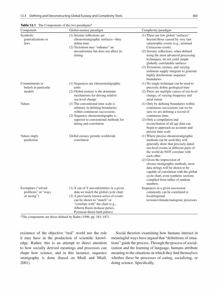
12.3 Defining and Deconstructing Global Eustasy and Complexity Texts 365
Table 12.1 The Components of the two paradigmsa
Component Global-eustasy paradigm Complexity paradigm
Symbolicgeneralizations orlaws
(1) Seismic reflections arechronostratigraphic surfaces—theydefine time
(2) Tectonism may “enhance” anunconformity but does not affect itstiming
(1) There are few global “surfaces”beyond those caused by very rarecatastrophic events (e.g., terminalCretaceous event).
(2) Seismic reflections, when definedusing the most advanced processingtechniques, do not yield simpleglobally correlatable surfaces
(3) Tectonism, eustasy, and varyingsediment supply integrate to generatehighly diachronous sequenceboundaries
Commitments orbeliefs in particularmodels
(1) Sequences are chronostratigraphicunits
(2) Global eustasy is the dominantmechanisms for driving relativesea-level change
(1) No single technique can be used toprecisely define geological time
(2) There are multiple causes of sea-levelchange, of varying frequency andareal extent
Values (1) The conventional time scale isarbitrary in defining boundarieswithin continuous successions.
(2) Sequence chronostratigraphy issuperior to conventional methods fordating and correlation
(1) Only by defining boundaries withincontinuous successions can we besure we are defining a record ofcontinuous time.
(2) Only a compilation andreconciliation of all age data canbegin to approach an accurate andprecise time scale
Values implyprediction
Global eustasy permits worldwidecorrelation
(1) Where precise chronostratigraphicmethods can be used they willgenerally show that precisely datedsea-level events in different parts ofthe world do NOT correlate witheach other
(2) Given the imprecision ofchrono-stratigraphic methods, mostdata strings will be shown to becapable of correlation with the globalcycle chart, even synthetic sectionscompiled from tables of randomnumbers.
Exemplars (“solvedproblems” or “waysof seeing”)
(1) X out of Y unconformities in a givendata set match the global cycle chart
(2) A previously known series of eventscan be shown to “match” or“correlate with” the chart (e.g.,Alberta Basin molasse pulses,Pyrenean thrust-fault pulses)
Sequences in a given successioncommonly can be correlated tolocal/regionaltectonic/climatic/autogenic processes
aThe components are those defined by Kuhn (1996, pp. 181–187).
existence of the objective “real” world nor the roleit may have in the production of scientific knowl-edge. Rather, this is an attempt to direct attentionto how socially derived meanings and processes canshape how science, and in this instance, sequencestratigraphy is done (based on Miall and Miall,2001).
Social theorists examining how humans interact inmeaningful ways have argued that “definitions of situa-tions” guide the process. Through the process of social-ization and the learning of language, humans attributemeaning to the situations in which they find themselveswhether these be processes of eating, socializing, ordoing science. Specifically,
366 12 The Concept of the Global Cycle Chart
The crucial fact about a definition of a situation is that itis cognitive – it is our idea of our location in social timeand space that constrains the way we act. When we havea definition of a situation, we cognitively configure acts,objects, and others in a way that makes sense to us as abasis for acting (Hewitt, 1997. p. 127).
These theorists have, as a central focus, the subjec-tive standpoint of individual actors. “Unlike a moreobjectivist approach, which views the social worldas a reality that exists independently of any indi-vidual’s perception of it, phenomenology sees thatreality as constituted by our view of it” (Hewitt, 1997,pp. 15–16).
Most interaction among humans takes place withinroutine situations with well-established definitionsof the situation or subjective viewpoints that guidebehaviour. According to McHugh (1968), there arethree fundamental assumptions that influence routineinteractions: (1) that the assumptions we hold abouta situation are valid; (2) that others in the situationshare our definition of the situation; and (3) that aslong as our definition of the situation works, it willnot be questioned or challenged. These theorists, there-fore, emphasize the cognitive foundations of humanconduct, manifested in language, and stress that whatpeople know about a situation and what they do areinterdependent (cf. Hewitt, 1997).
Miall and Miall (2001, p. 332) suggested thatthrough the application of these principles to the studyof science as a human activity, we can understand howdifferent groups of scientists, with different convic-tions or definitions of the situation, could emphasizeor de-emphasize particular types of data and hypothe-ses in favour of the desired goals of the research. Inthe global-eustasy model, for example, published sup-porting data are sparse, and the necessary supportinghypotheses are largely “internal” or “self-referential.”Accordingly, the language of the global-eustasy schoolincludes a number of key interpretive phrases, whichserve to turn research results toward the desired model,to define the situation confronting the geologist ina routinized way that directs his or her analyticbehaviour. Notably, these terms are not used by, orhold different meaning for, the nonmembers of thisgroup, for example, those adhering to the complex-ity paradigm, who have their own set of definitionsof the situation. Some of these terms that hold spe-cial meaning for the global-eustasy school, but areused selectively or not at all by other sequence strati-graphers, are presented in Table 12.2. They express
two of the three elements of the hermeneutic circle—the preconceptions and the presumed goals of theresearch.
In order to further understand and illustrate the con-sequences of the use of particular terms in the practiceof geology, it is useful to draw on a form of liter-ary criticism called Deconstructionism. As proposedby Jacques Derrida, who founded the approach, decon-structionism takes apart the logic of language in whichauthors make their arguments. According to Denzin(1992, p. 32), “it is a process which explores how a textis constructed and given meaning by its author or pro-ducer.” It rejects the assumption that texts have logicalmeanings and argues for “demystifying texts insteadof deciphering them” (Vogt, 1999, p. 74). To use anexample, objectivist studies of history “. . .assume thefacticity of objects of historical analysis as constitutedprior to the observer’s study of them” (Hall, 1990,p. 26). Deconstructionists challenge,
the artificial coherence of historical accounts, by showinghow to locate ‘transcendent’ staging devices in historicaldiscourses. Situated outside history, such devices ren-der historical accounts plausible to readers by providing‘history with continuity and discourse with meaning’ the-matized by ‘aboutness.’ A ‘history’ of Nixon’s Watergatecrisis, for example, can only be narrated by telescopingevents into a coherent story (Cohen, 1986:74–76). In thislight, any notion that the historical object is simply ‘outthere,’ waiting for the historian to discover and describeit, seems a self-serving conceit. (Hall, 1990, p. 26).
As Hall (1990, p. 35) further observed, “In an agewhen deconstructionists are busy assaulting texts asinternally ordered assemblages, historical narrative hasbecome suspect as a special kind of storytelling.”
Miall and Miall (2001) did not subscribe to theextreme relativism of postmodernism and deconstruc-tionism which are characterized by “an extreme orcomplete skepticism of, or disbelief in, the authenticityof human knowledge and practice” (Dawson and Prus,1995, p. 107). Rather, the tenets of deconstructionismwere used as an heuristic device to illustrate the roleof language in scientific interpretations of the “real”world.
We can illustrate how phenomenological and decon-structionist approaches inform the scientific processof stratigraphic interpretation with a simple diagram(Fig. 12.3). Two interpretations of a stratigraphic “text”are shown. The text consists of a suite of seven datapoints in a time-space universe, such as sea-level low-stands within a tectonostratigraphic province, dated
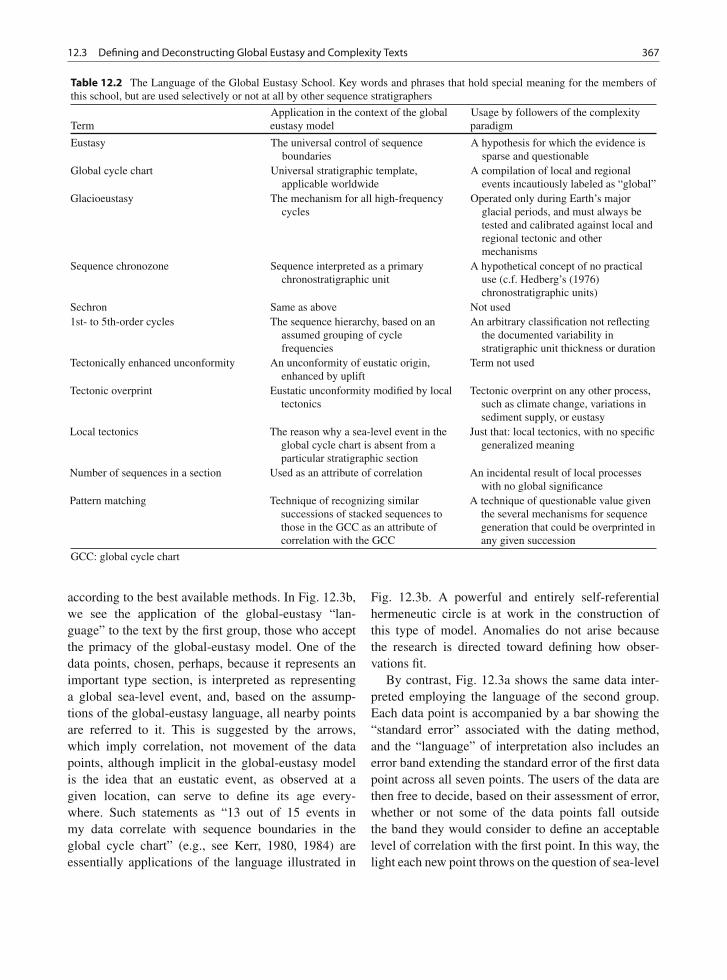
12.3 Defining and Deconstructing Global Eustasy and Complexity Texts 367
Table 12.2 The Language of the Global Eustasy School. Key words and phrases that hold special meaning for the members ofthis school, but are used selectively or not at all by other sequence stratigraphers
TermApplication in the context of the globaleustasy model
Usage by followers of the complexityparadigm
Eustasy The universal control of sequenceboundaries
A hypothesis for which the evidence issparse and questionable
Global cycle chart Universal stratigraphic template,applicable worldwide
A compilation of local and regionalevents incautiously labeled as “global”
Glacioeustasy The mechanism for all high-frequencycycles
Operated only during Earth’s majorglacial periods, and must always betested and calibrated against local andregional tectonic and othermechanisms
Sequence chronozone Sequence interpreted as a primarychronostratigraphic unit
A hypothetical concept of no practicaluse (c.f. Hedberg’s (1976)chronostratigraphic units)
Sechron Same as above Not used1st- to 5th-order cycles The sequence hierarchy, based on an
assumed grouping of cyclefrequencies
An arbitrary classification not reflectingthe documented variability instratigraphic unit thickness or duration
Tectonically enhanced unconformity An unconformity of eustatic origin,enhanced by uplift
Term not used
Tectonic overprint Eustatic unconformity modified by localtectonics
Tectonic overprint on any other process,such as climate change, variations insediment supply, or eustasy
Local tectonics The reason why a sea-level event in theglobal cycle chart is absent from aparticular stratigraphic section
Just that: local tectonics, with no specificgeneralized meaning
Number of sequences in a section Used as an attribute of correlation An incidental result of local processeswith no global significance
Pattern matching Technique of recognizing similarsuccessions of stacked sequences tothose in the GCC as an attribute ofcorrelation with the GCC
A technique of questionable value giventhe several mechanisms for sequencegeneration that could be overprinted inany given succession
GCC: global cycle chart
according to the best available methods. In Fig. 12.3b,we see the application of the global-eustasy “lan-guage” to the text by the first group, those who acceptthe primacy of the global-eustasy model. One of thedata points, chosen, perhaps, because it represents animportant type section, is interpreted as representinga global sea-level event, and, based on the assump-tions of the global-eustasy language, all nearby pointsare referred to it. This is suggested by the arrows,which imply correlation, not movement of the datapoints, although implicit in the global-eustasy modelis the idea that an eustatic event, as observed at agiven location, can serve to define its age every-where. Such statements as “13 out of 15 events inmy data correlate with sequence boundaries in theglobal cycle chart” (e.g., see Kerr, 1980, 1984) areessentially applications of the language illustrated in
Fig. 12.3b. A powerful and entirely self-referentialhermeneutic circle is at work in the construction ofthis type of model. Anomalies do not arise becausethe research is directed toward defining how obser-vations fit.
By contrast, Fig. 12.3a shows the same data inter-preted employing the language of the second group.Each data point is accompanied by a bar showing the“standard error” associated with the dating method,and the “language” of interpretation also includes anerror band extending the standard error of the first datapoint across all seven points. The users of the data arethen free to decide, based on their assessment of error,whether or not some of the data points fall outsidethe band they would consider to define an acceptablelevel of correlation with the first point. In this way, thelight each new point throws on the question of sea-level
368 12 The Concept of the Global Cycle Chart
change in this area can be assessed quantitatively, pointby point, based on assessments of the various genera-tion mechanisms. Here the definition of the situation(or hermeneutic circle) allows for greater consider-ation of anomaly in observations. Consequently, noquick conclusions are drawn by geologists using thisapproach and anomalies are more likely to be acknowl-edged. As W. I. Thomas (1931) has observed, if youdefine a situation as real, it is real in its consequences.For the protagonists of the two paradigms, each inter-pretation of the stratigraphic texts is “real” withinthe terms of their paradigm. For the adherents of theglobal-eustasy model the “consequence” is that discus-sion of the potential error in, or revision of, the age ofa given sequence boundary is typically not undertaken,whereas error and revision are an integral part of thecomplexity paradigm.
In the next section, we discuss the interaction anddegree of coexistence that the two paradigms exhibit,through an examination of the patterns of cross citationthat exist between them.
12.4 Invisible Colleges and theAdvancement of Knowledge
The study of citation patterns has long been an issuein social research on scientific knowledge and how itadvances. Price (1961, 1963), for example, observedthat some disciplines continually reference their clas-sic or foundational works. Other disciplines cite onlythe most recent papers in a rapidly advancing researchfront. Citations also reveal clusters of interrelatedresearchers and underlying social networks, what Pricereferred to as “invisible colleges.” According to Crane(1972, pp. 138–39),
Analysis of the social organization of research areas inscience has shown that social circles have invisible col-leges that help to unify areas and provide coherence anddirection to their fields. These central figures and someof their associates are closely linked by direct ties anddevelop a kind of solidarity that is useful in buildingmorale and maintaining motivation among members.
However, she goes on to argue, in order for sci-ence to advance, “the exchange of ideas is importantin generating new lines of inquiry and in producingsome integration of the findings from diverse areas”(Crane, 1972, p. 114). Indeed, she concludes, scientific
communities may become completely subjective anddogmatic if they are unable to assimilate knowledgefrom other research areas. The preceding discussiondemonstrates how the two paradigms under reviewhave been constructed to yield different kinds of obser-vations. We shall now consider the extent to whicheach addresses the anomalies arising from the researchof the other, and the consequences this may have forthe advancement of scientific knowledge (from Mialland Miall, 2001, pp. 334–340).
As a generalization, workers in the complexityparadigm cite the global-eustasy model as one ofseveral possible scenarios for geologic interpretation,but the reverse is typically not the case. Thorne(1992), in a discussion of the assumptions underlyingsequence stratigraphy, and which is generally support-ive of the methodology, noted that “The stratigraphicliterature since 1977, citing the Exxon sea-level cyclecharts, is prodigious. (An ARCO [Atlantic RichfieldCorporation] library author citation search of P.Vailcontains 983 citations between 1977 and 1988).Various stratigraphic techniques have been used totest the applicability of the global sea-level cyclechart.” Adherents of the global-eustasy paradigm maycite opposing work, but rarely make the connectionbetween that work and its implications for theirpreferred model. Even publications by basin analystsfrom other large and prestigious petroleum companies,such as British Petroleum (e.g., Hubbard, 1988)have had little effect on the use of the model by itsadherents. For example, Vail et al. (1991) discussedHubbard’s work on the tectonic origins of sequenceboundaries, but made no connection between theseresults and their implications for the generality of hisglobal-eustasy model.
An opportunity to examine the pattern of citationused by each paradigm has been offered by the appear-ance of two recent special publications of the Societyfor Sedimentary Geology (SEPM), both publishedin 1998. The first, a book entitled, “Mesozoic andCenozoic Sequence Stratigraphy of European Basins”(Graciansky et al., 1998) of which Peter Vail is aco-editor and contributing author, takes what maybe described as the classic global-eustasy approachto regional sequence studies, as clearly stated in thesecond paragraph of its Preface:
Sequence stratigraphy applies the inherent premise thateustasy represents a global signal among the variablesthat play a role in shaping depositional sequences. This
12.4 Invisible Colleges and the Advancement of Knowledge 369
global signal plays an essential role in shaping depo-sitional sequences laid down in response to changes inrelative sea level. Because of this global signal, boundingsurfaces of depositional sequences (sequence boundariesat their correlative conformities) can be expected to besynchronous between basins. To demonstrate such syn-chroneity requires a very high stratigraphic resolution anda calibration of all stratigraphic disciplines.
Although the book consists of a series of regionalstudies, in which global correlation was not a statedobjective, the assumption that eustatic control maybe demonstrated by such studies is conveyed by thisquotation, also from the Preface:
The composite stratigraphic record of higher ordereustatic sequences shows a significant increase in thenumber of sequences identified in the various Europeanbasins. Entries on the new charts include a compositestratigraphic record of 221 sequence boundaries in theMesozoic and Cenozoic, compared to 119 sequences forthe same interval identified by Haq et al. (1987, 1988a).
Published at about the same time as the Gracianskyet al. (1998) text is the book “PaleogeographicEvolution and Non-Glacial Eustasy, Northern SouthAmerica,” compiled and edited by Pindell and Drake(1998). Again, the Preface to this book sets out thephilosophical approach adopted by the editors andcontributing authors:
Our ability to isolate eustasy in most settings is seriouslyhindered by the fact that relative sea-level history in anylocation is multi-variable, comprising the net effects ofsuch components as eustasy, local and regional tectonism,local and global climatic variability and variable sedimentsupply.
One of this book’s prime conclusions . . . is thatthe eustatic component of short-term relative sea-levelchanges during non-glacial times cannot be confidentlyisolated in most settings. The inability to isolate short-term eustatic changes will preclude genetic correlationof short-term cycles and the use of short-term cycleson cycle charts as time scales of predictors of reservoirhorizons in most basins.
In Table 12.3, we list twenty-six papers that may beregarded as the critical body of work exploring prob-lems with the global-eustasy paradigm. In a few cases,some rows in this table contain more than one paper.This indicates that the relevant ideas have appearedin different form in several places. Omitted from thislist are a few contemporary publications, such asMiller and Kent (1987) that, while making importantpoints, were not published in journals normally read bypetroleum geologists, and were, therefore, not widelynoted or cited at the time of publication. Also not
included is Pitman (1978), an important early work thatdiscussed rates of sea-level change, particularly withrespect to the rapidity of the sea-level falls impliedby Vail’s first “sawtooth” curve, but did not constitutea critique of the chart itself. The list begins with thework of A. B. Watts and his coworkers, who developedthe flexural model for extensional continental margins.This model provides a powerful alternative model forpatterns of coastal onlap of “second-order” type andthus challenges the assumptions of eustatic sea-levelrise incorporated into the global cycle chart. Many ofthe authors listed in Table 12.3 also contributed to aseries of Discussions of the Haq et al. (1987) paper thatappeared in 1988, with Replies by the Exxon group(Christie-Blick et al., 1988).
Table 12.4 documents the pattern of citation ofthese critical articles by the contributing authors ofthe forty-five papers in the Graciansky et al. (1998)volume, less the one article that is published only inabstract form. The results confirm the assertion thatdata and arguments opposing the generality of theglobal-eustasy model generated by other specialistshave not been widely responded to by adherents ofthe global-eustasy paradigm. Based on this citationanalysis, the following observations may be made:
(1) Thirty-four of the 45 papers cite the global cyclechart of Haq et al. (1987, 1988a), mostly byshowing how their sequences correlate to eventsin that chart.
(2) Twenty-eight of the papers cite none of the arti-cles critical of the global-eustasy model, or anyother critical articles not on our list. None citesmore than five of those given in Table 12.3.Critical papers 2, 3, 5, 6, 8, 10, 18, 19, 20,and 24 from Table 12.3 are not cited at all. TheDiscussions and Replies of the 1987 version ofthe chart (Christie-Blick et al., 1988) are not citedanywhere in this book.
(3) Most articles acknowledge the importance oflow-frequency (“second-order”) tectonism ingenerating accommodation for sequences, butonly one cites the early work in this area (Paperrow #1 in Table 12.3). A few papers acknowl-edge the potential importance of in-plane stress(papers #4, 5, 11).
(4) Tectonic “enhancement” or “offsetting” of eusta-tic sequence boundaries is a common theme.
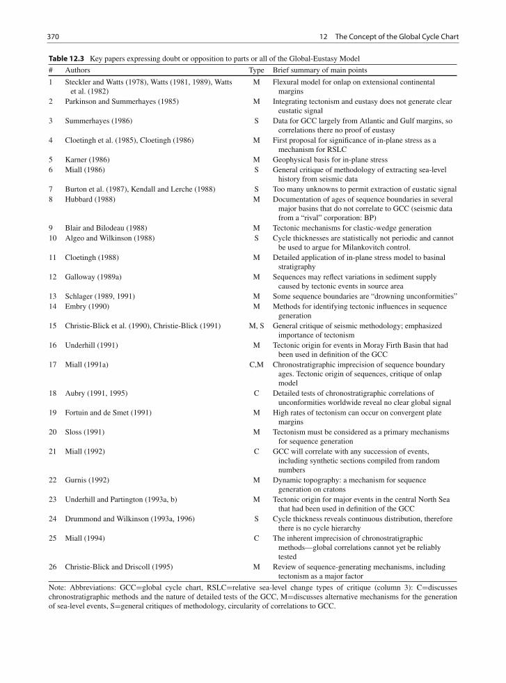
370 12 The Concept of the Global Cycle Chart
Table 12.3 Key papers expressing doubt or opposition to parts or all of the Global-Eustasy Model
# Authors Type Brief summary of main points
1 Steckler and Watts (1978), Watts (1981, 1989), Wattset al. (1982)
M Flexural model for onlap on extensional continentalmargins
2 Parkinson and Summerhayes (1985) M Integrating tectonism and eustasy does not generate cleareustatic signal
3 Summerhayes (1986) S Data for GCC largely from Atlantic and Gulf margins, socorrelations there no proof of eustasy
4 Cloetingh et al. (1985), Cloetingh (1986) M First proposal for significance of in-plane stress as amechanism for RSLC
5 Karner (1986) M Geophysical basis for in-plane stress6 Miall (1986) S General critique of methodology of extracting sea-level
history from seismic data7 Burton et al. (1987), Kendall and Lerche (1988) S Too many unknowns to permit extraction of eustatic signal8 Hubbard (1988) M Documentation of ages of sequence boundaries in several
major basins that do not correlate to GCC (seismic datafrom a “rival” corporation: BP)
9 Blair and Bilodeau (1988) M Tectonic mechanisms for clastic-wedge generation10 Algeo and Wilkinson (1988) S Cycle thicknesses are statistically not periodic and cannot
be used to argue for Milankovitch control.11 Cloetingh (1988) M Detailed application of in-plane stress model to basinal
stratigraphy12 Galloway (1989a) M Sequences may reflect variations in sediment supply
caused by tectonic events in source area13 Schlager (1989, 1991) M Some sequence boundaries are “drowning unconformities”14 Embry (1990) M Methods for identifying tectonic influences in sequence
generation15 Christie-Blick et al. (1990), Christie-Blick (1991) M, S General critique of seismic methodology; emphasized
importance of tectonism16 Underhill (1991) M Tectonic origin for events in Moray Firth Basin that had
been used in definition of the GCC17 Miall (1991a) C,M Chronostratigraphic imprecision of sequence boundary
ages. Tectonic origin of sequences, critique of onlapmodel
18 Aubry (1991, 1995) C Detailed tests of chronostratigraphic correlations ofunconformities worldwide reveal no clear global signal
19 Fortuin and de Smet (1991) M High rates of tectonism can occur on convergent platemargins
20 Sloss (1991) M Tectonism must be considered as a primary mechanismsfor sequence generation
21 Miall (1992) C GCC will correlate with any succession of events,including synthetic sections compiled from randomnumbers
22 Gurnis (1992) M Dynamic topography: a mechanism for sequencegeneration on cratons
23 Underhill and Partington (1993a, b) M Tectonic origin for major events in the central North Seathat had been used in definition of the GCC
24 Drummond and Wilkinson (1993a, 1996) S Cycle thickness reveals continuous distribution, thereforethere is no cycle hierarchy
25 Miall (1994) C The inherent imprecision of chronostratigraphicmethods—global correlations cannot yet be reliablytested
26 Christie-Blick and Driscoll (1995) M Review of sequence-generating mechanisms, includingtectonism as a major factor
Note: Abbreviations: GCC=global cycle chart, RSLC=relative sea-level change types of critique (column 3): C=discusseschronostratigraphic methods and the nature of detailed tests of the GCC, M=discusses alternative mechanisms for the generationof sea-level events, S=general critiques of methodology, circularity of correlations to GCC.
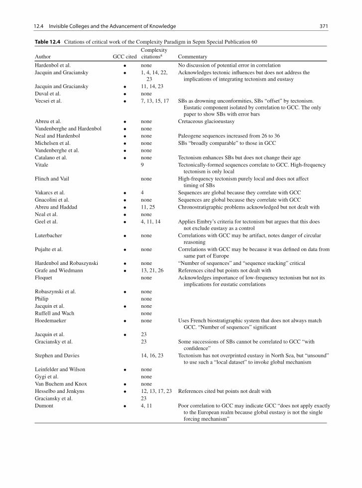
12.4 Invisible Colleges and the Advancement of Knowledge 371
Table 12.4 Citations of critical work of the Complexity Paradigm in Sepm Special Publication 60
Author GCC citedComplexitycitationsa Commentary
Hardenbol et al. • none No discussion of potential error in correlationJacquin and Graciansky • 1, 4, 14, 22,
23Acknowledges tectonic influences but does not address the
implications of integrating tectonism and eustasyJacquin and Graciansky • 11, 14, 23Duval et al. • noneVecsei et al. • 7, 13, 15, 17 SBs as drowning unconformities, SBs “offset” by tectonism.
Eustatic component isolated by correlation to GCC. The onlypaper to show SBs with error bars
Abreu et al. • none Cretaceous glacioeustasyVandenberghe and Hardenbol • noneNeal and Hardenbol • none Paleogene sequences increased from 26 to 36Michelsen et al. • none SBs “broadly comparable” to those in GCCVandenberghe et al. • noneCatalano et al. • none Tectonism enhances SBs but does not change their ageVitale 9 Tectonically-formed sequences correlate to GCC. High-frequency
tectonism is only localFlinch and Vail none High-frequency tectonism purely local and does not affect
timing of SBsVakarcs et al. • 4 Sequences are global because they correlate with GCCGnacolini et al. • none Sequences are global because they correlate with GCCAbreu and Haddad • 11, 25 Chronostratigraphic problems acknowledged but not dealt withNeal et al. • noneGeel et al. • 4, 11, 14 Applies Embry’s criteria for tectonism but argues that this does
not exclude eustasy as a controlLuterbacher • none Correlations with GCC may be artifact, notes danger of circular
reasoningPujalte et al. • none Correlations with GCC may be because it was defined on data from
same part of EuropeHardenbol and Robaszynski • none “Number of sequences” and “sequence stacking” criticalGrafe and Wiedmann • 13, 21, 26 References cited but points not dealt withFloquet none Acknowledges importance of low-frequency tectonism but not its
implications for eustatic correlationsRobaszynski et al. • nonePhilip noneJacquin et al. • noneRuffell and Wach noneHoedemaeker • none Uses French biostratigraphic system that does not always match
GCC. “Number of sequences” significantJacquin et al. • 23Graciansky et al. 23 Some successions of SBs cannot be correlated to GCC “with
confidence”Stephen and Davies 14, 16, 23 Tectonism has not overprinted eustasy in North Sea, but “unsound”
to use such a “local dataset” to invoke global mechanismLeinfelder and Wilson • noneGygi et al. noneVan Buchem and Knox • noneHesselbo and Jenkyns • 12, 13, 17, 23 References cited but points not dealt withGraciansky et al. 23Dumont • 4, 11 Poor correlation to GCC may indicate GCC “does not apply exactly
to the European realm because global eustasy is not the singleforcing mechanism”
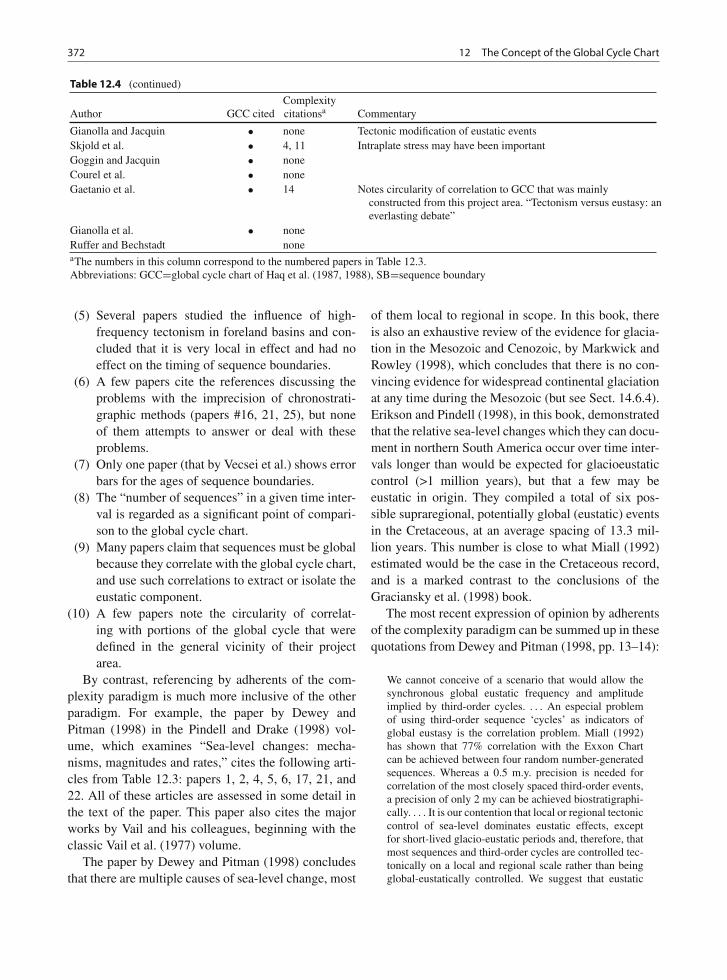
372 12 The Concept of the Global Cycle Chart
Table 12.4 (continued)
Author GCC citedComplexitycitationsa Commentary
Gianolla and Jacquin • none Tectonic modification of eustatic eventsSkjold et al. • 4, 11 Intraplate stress may have been importantGoggin and Jacquin • noneCourel et al. • noneGaetanio et al. • 14 Notes circularity of correlation to GCC that was mainly
constructed from this project area. “Tectonism versus eustasy: aneverlasting debate”
Gianolla et al. • noneRuffer and Bechstadt noneaThe numbers in this column correspond to the numbered papers in Table 12.3.Abbreviations: GCC=global cycle chart of Haq et al. (1987, 1988), SB=sequence boundary
(5) Several papers studied the influence of high-frequency tectonism in foreland basins and con-cluded that it is very local in effect and had noeffect on the timing of sequence boundaries.
(6) A few papers cite the references discussing theproblems with the imprecision of chronostrati-graphic methods (papers #16, 21, 25), but noneof them attempts to answer or deal with theseproblems.
(7) Only one paper (that by Vecsei et al.) shows errorbars for the ages of sequence boundaries.
(8) The “number of sequences” in a given time inter-val is regarded as a significant point of compari-son to the global cycle chart.
(9) Many papers claim that sequences must be globalbecause they correlate with the global cycle chart,and use such correlations to extract or isolate theeustatic component.
(10) A few papers note the circularity of correlat-ing with portions of the global cycle that weredefined in the general vicinity of their projectarea.
By contrast, referencing by adherents of the com-plexity paradigm is much more inclusive of the otherparadigm. For example, the paper by Dewey andPitman (1998) in the Pindell and Drake (1998) vol-ume, which examines “Sea-level changes: mecha-nisms, magnitudes and rates,” cites the following arti-cles from Table 12.3: papers 1, 2, 4, 5, 6, 17, 21, and22. All of these articles are assessed in some detail inthe text of the paper. This paper also cites the majorworks by Vail and his colleagues, beginning with theclassic Vail et al. (1977) volume.
The paper by Dewey and Pitman (1998) concludesthat there are multiple causes of sea-level change, most
of them local to regional in scope. In this book, thereis also an exhaustive review of the evidence for glacia-tion in the Mesozoic and Cenozoic, by Markwick andRowley (1998), which concludes that there is no con-vincing evidence for widespread continental glaciationat any time during the Mesozoic (but see Sect. 14.6.4).Erikson and Pindell (1998), in this book, demonstratedthat the relative sea-level changes which they can docu-ment in northern South America occur over time inter-vals longer than would be expected for glacioeustaticcontrol (>1 million years), but that a few may beeustatic in origin. They compiled a total of six pos-sible supraregional, potentially global (eustatic) eventsin the Cretaceous, at an average spacing of 13.3 mil-lion years. This number is close to what Miall (1992)estimated would be the case in the Cretaceous record,and is a marked contrast to the conclusions of theGraciansky et al. (1998) book.
The most recent expression of opinion by adherentsof the complexity paradigm can be summed up in thesequotations from Dewey and Pitman (1998, pp. 13–14):
We cannot conceive of a scenario that would allow thesynchronous global eustatic frequency and amplitudeimplied by third-order cycles. . . . An especial problemof using third-order sequence ‘cycles’ as indicators ofglobal eustasy is the correlation problem. Miall (1992)has shown that 77% correlation with the Exxon Chartcan be achieved between four random number-generatedsequences. Whereas a 0.5 m.y. precision is needed forcorrelation of the most closely spaced third-order events,a precision of only 2 my can be achieved biostratigraphi-cally. . . . It is our contention that local or regional tectoniccontrol of sea-level dominates eustatic effects, exceptfor short-lived glacio-eustatic periods and, therefore, thatmost sequences and third-order cycles are controlled tec-tonically on a local and regional scale rather than beingglobal-eustatically controlled. We suggest that eustatic
12.5 The Global-Eustasy Paradigm—A Revolution in Trouble? 373
sea-level changes are nowhere near as large as have beenclaimed and have been falsely correlated and constrictedinto a global eustatic time scale whereby a circular rea-soning forces correlation and then uses that correlation asa standard into which all other sequences are squeezed.
Most recent textbooks on stratigraphy reach simi-lar conclusions (e.g., see Hallam, 1998b, pp. 427–428;Nichols, 1999, p. 288).
Kuhn (1962, p. 93) has argued that “whenparadigms enter, as they must, into a debate aboutparadigm choice, their role is necessarily circular.Each group uses its own paradigm to argue in thatparadigm’s defense.” He has also stated that two sci-entific schools in disagreement will “talk througheach other when debating the relative merits of theirrespective paradigms” (Kuhn, 1962, p. 108). Whileaspects of his argument hold true here, the examina-tion of citation practices suggests that the complexityparadigm is more open to external influences in thatit directly addresses the contributions and anomaliesarising from the global-eustasy model. The global-eustasy model, however, adheres to a circular patternof observation and justification, with little attempt toaddress anomalies arising from research outside thecircle of researchers using it. The extent to whichthis practice will continue to elicit support for theparadigm is questionable. As Kuhn (1962, p. 93) hasobserved, “whatever its force, the status of the circularargument is only that of persuasion. It cannot be madelogically or even probabilistically compelling for thosewho refuse to step into the circle.”
In the next section, we address the tenets of theglobal-eustasy paradigm directly and consider its cur-rent status in the scientific community.
12.5 The Global-Eustasy Paradigm—ARevolution in Trouble?
According to Kuhn (1962, p. 93), “as in political revo-lutions, so in paradigm choice—there is no standardhigher than the assent of the relevant community.”Indeed, the most important component of a paradigmis the cognitive authority it is accorded, an authoritybased on the judgment of the scientific communitythat it deserves acceptance over other paradigms (cf.Gutting, 1984). We now examine the judgment ofthe scientific community as it pertains to the global-eustasy model itself, with particular reference to the
recent book by Graciansky et al. (1998) discussed inthe previous section.
The global-eustasy paradigm is built on the follow-ing assumptions, or hermeneutic prejudgments (Mialland Miall, 2001, p. 340):
1. That a global eustatic signal exists;2. That eustatic control generates synchronous
sequence boundaries;3. That synchroneity can be demonstrated using cur-
rent chronostratigraphic tools.
Those scientists skeptical of the global-eustasymodel would argue that none of these threeassumptions has been proven satisfactorily. Indeed, allthree have been the subject of vigorous debate. Forexample, while the existence of a low-frequency (107–109-year cyclicity) eustatic signal is now generallyacknowledged, there is no agreement on the existenceof a high-frequency global signal during periods lack-ing widespread continental glaciation (e.g., during theCretaceous). But it is not the purpose of this discus-sion to repeat the debate about these concepts andassumptions. Suffice it to note:
1. The existence of a suite of eustatic cycles of “third-order” magnitude, and global in extent—the basisfor Peter Vail’s first global cycle chart, has neverbeen satisfactorily documented or proven (Miall,1992, 1997), a crucial point largely ignored in theGraciansky et al. book, in which the Haq et al.(1987, 1988a) global cycle chart is taken as thestarting point of their work.
2. It has been pointed out that where relative sea levelis controlled by two or more processes of similarfrequency and amplitude (e.g., thermal subsidenceand second-order eustasy, or foreland basin tec-tonism and Milankovitch cyclicity), a synchronousregional (let alone global) signal cannot be gen-erated (Parkinson and Summerhayes, 1985; Miall,1997).
3. As noted earlier, conventional chronostratigraphicmethods and results have been subordinated to theglobal cycle chart by the Exxon group, and inde-pendent efforts to chronostratigraphically calibratethe sequence record, such as those by A. Hallam(many papers, starting with Hallam, 1978), havebeen largely ignored by the Exxon group.
374 12 The Concept of the Global Cycle Chart
4. It has been argued that conventional chronostrati-graphic techniques are inadequate to test the real-ity of high-frequency global synchroneity (Miall,1994), except in the late Cenozoic, for which thetechniques of cyclostratigraphy (calibration of thehigh-frequency sequence record by reference to theknown frequencies generated by orbital forcing) arenow providing a very refined time scale (Houseand Gale, 1995). Graphic correlation methods maychange this, as noted in our Conclusion.
5. Several workers have demonstrated the inherentdiachroneity of sequence boundaries, reflecting theintegrated effects of varying local to regional sub-sidence rates and rates of sediment supply (Jordanand Flemings, 1991; Catuneanu et al., 1998).
Although the members of the global-eustasy schoolrefer to “tectonic enhancement” of unconformities(Table 12.2), at the same time they effectively ruleout consideration of the tectonic and other effects onsequence timing referred to in the previous paragraph.As Vail et al. (1991, p. 638) have stated:
structure tends to enhance or subdue eustatically causedsequences and systems tract boundaries, but does notaffect the age of the boundaries when dated at the min-imum hiatus at their conformable position.
Even where studies appear to have been specifi-cally undertaken to explore the relationship betweensedimentation and tectonics, adherents of the global-eustasy school still regard correlation with the globalcycle chart as significant. Thus Deramond et al. (1993;a study not part of the SEPM volume under examina-tion in this section) explored the relationship betweensedimentation and tectonism in tectonically activePyrenean basins, and succeeded in developing tec-tonic models for sequence development. However,they then offered correlations of sequence boundarieswith the global cycle chart and went on to discusseustatic control. In referring to “tectonically enhanced”unconformities, they stated “The apparent correlationbetween the two groups of independent phenomenais an artifact of the method which calibrates the tec-tonic evolution by comparison with eustatic fluctua-tions.” This form of “calibration” is, of course, circularreasoning.
Hardenbol et al. (1998) summarized the evidenceused in the construction of a set of new chronostrati-graphic cycle charts for the Mesozoic and Cenozoic
that appeared in SEPM Special Publication 60. Theynoted that there are 221 sequence boundaries in thisnew synthesis, in contrast to the 119 that appeared inthe chart published by Haq et al. (1987, 1988a). Thisis a boundary, on average, every 1.12 million years, incontrast to the average spacing of 2.08 million yearsin the earlier chart. A spacing of 2.08 million years inthe earlier chart was already below chronostratigraphicresolution for most of the Mesozoic and Cenozoic. Apotential error of ±0.5 million years is reasonable forthe Cenozoic and parts of the Cretaceous, but potentialerrors of several millions of years must be factored intoassigned ages for older parts of the Mesozoic record(Miall, 1994). Given a potential error of ±0.5 millionyears many events—those spaced at 1 million years orless—would overlap each other and would therefore beindistinguishable.
Even that earlier chart contains more putative sea-level events than any others published for the Mesozoicand Cenozoic, leading to the question: why does theExxon global cycle chart contain so many more eventsthan other sea-level curves? The question is even moreapposite now. Miall (1997, p. 320) suggested thatthe paradigm of stratigraphic eustasy followed by theExxon group allows them to interpret virtually all sea-level events as eustatic in origin. Hallam (1992a, p. 92)said, of the Vail and Todd (1981) article on the NorthSea: “The very title of the Vail and Todd paper impliesthat, at that time at least, seismic sequence analysis ofonly one region was believed to be sufficient to obtaina global picture.” Therefore, every new sea-level eventthat is discovered, can be added to the global chart.
This points to a different question: what does theExxon chart actually represent? It undoubtedly con-stitutes a synthesis of real stratigraphic data fromaround the world. It has been suggest that most ofthe sequences are the product of regional events thatoriginated as a result of plate-margin and intraplatetectonism, including basin loading and relaxation andin-plane stresses. These may have been well docu-mented in one or more basins in areas of similarkinematic history, but their promotion to global eventsshould be questioned. Some events may be duplicatesof other events that have been miscorrelated because ofchronostratigraphic error (Miall, 1992, p. 789).
Exactly the same assumptions and methodologyappear to have been used in construction of the newcharts in Graciansky et al. (1998). Sea-level “events”
12.5 The Global-Eustasy Paradigm—A Revolution in Trouble? 375
and corresponding sequence boundaries appear to havebeen added to the synthesis charts even when evidencefrom separate regional studies in this book indicatesthat many do not appear in each of the studiedbasins. Yet they are all labeled “global”. This has beendone despite the clearly stated problems of correlat-ing between Boreal and Tethyan faunas within Europe,and the use of North American (Western Interior)chronostratigraphic standards where European data areinadequate, which potentially introduces still furthersources of error and imprecision. Finally, because thesesequences have been documented only in Europe, theycannot be defined in a blanket manner as having global(eustatic) significance.
A logical extension of this approach would be forthe eustasy school to continue to carry out similarresearch in other parts of the world and to continue toadd sequence boundaries to their “global” synthesis.We would predict a resulting chart containing manyhundreds of events, and an average spacing in the104–105-year range. This may well be what this teamhas in mind, because, as noted below, they continueto hold to the mechanism of glacioeustasy as the maincause of most of their sea-level events, and adding stillmore events would quickly bring the average eventspacing down to within the Milankovitch band, thenormal glacioeustatic frequency.
A critical question that needs to be asked in thiscontext, but has not been, concerns scientific method-ology: how can the authors know that a “new” (asin newly observed) sea-level event is in fact a true“new” event and not a replication of another, pre-viously known event, separated from it only by themargin of error inherent in the dating methods? Whilesome new observations “prove” by “correlation” (thearrows in Fig. 12.3b) that a given sea-level event hasbeen replicated, others are used to define new “events”in the global cycle chart. It is not clear how a dis-tinction is made between these two alternatives. Moreimportantly, how can the authors know that any ofthese events is eustatic, given that all their data arefrom Europe?
Correlations with the Haq et al. (1987, 1988a) curveare offered by most of the contributing authors inGraciansky et al. (1998) book (Table 12.4). Hardenbolet al. (1998) stated that this chart has been re-calibratedto the new time scale of Gradstein et al. (1995), but thishas not been done in every case. For example, several
of the Haq et al. (1978, 1988a) sequence boundaries aregiven different ages in the summary chart of Hardenboland Robaszynski (1998, Fig. 1) relative to that of Gräfeand Wiedmann (1998, Fig. 3). These errors provide anadditional source of confusion.
Although this new European synthesis is offeredas a major updating of the Haq et al. (1987) synthe-sis, the latter is still regarded as the basic referencepoint for a discussion of “global” standards in mostof the papers in this new book. For example, Vecseiet al. (1998, pp. 69–70) discussed the matching of theirsequence boundaries with those in the Haq et al. (1987,1998a) chart. Their discussion contains statementssuch as:
The brackets containing the ages of the mid-Cretaceousunconformity [and other sequence boundaries] each con-tain the age of a supersequence boundary as proposed byHaq et al. (1988a).
The age of the boundary of SS 1/2 (Late Campanian)is the same as that of a sea-level lowstand ranked betweenthe 2nd and 3rd orders by Haq et al. (1988a).
But then these authors also include statements likethis:
Four supersequence boundaries proposed by Haq et al.(1988a) to have occurred in Late Cretaceous to Miocenetime could not be recognized on the Maiella platformmargin.
In the Maiella, 3rd-order sequences can only be recog-nized in part of the succession, and age resolution is notrefined enough for their correlation with the onlap curveof Haq et al. (1988a).
Vecsei et al. (1998) employed the by-now well-known language of the eustasy school that the use ofthe Haq et al. (1987, 1988a) chart has helped to cre-ate, attributing mismatches with that chart to “regionaltectonics” or “tectonic overprint.” As noted by Miall(1997, Chap. 13), the presence of missing or extrasequences relative to the Exxon global cycle chartdoes not pose a problem for those using the chart.Such sequences are readily attributed to “local tecton-ics”. To explain non-correlation, Vecsei et al. (1998)offered an appeal to chronostratigraphic imprecisionand to the effects of local tectonics “offsetting” theglobal eustatic signal, but these authors did reasonablyconclude “considering the age brackets in our data aswell as the uncertainties in Haq et al. (1987, 1988a)curve, the supersequence boundaries can all be older
376 12 The Concept of the Global Cycle Chart
or younger than the ages given by these authors.” Oursummary of this is that the results of this study can,by themselves, neither support nor negate the validityof the Haq et al. (1988) chart, and correlation or lackof correlation with that chart cannot be taken to meananything very much. This paper is the only one in thebook to show sequence-boundary ages with error bars,and is the paper most alive to the ideas encompassedby the complexity paradigm.
Even where sequence boundaries in an individuallocal study such as that of Vecsei et al. (1998) “match”or “correlate” with that chart, it cannot be claimedthat this demonstrates the reality of the eustatic signalbecause this is only a local study, the global signifi-cance of which remains to be demonstrated. As notedby Miall (1997, p. 302), with regard to this type of ad-hoc argument: “to be rigorously objective, if sequenceX is the result of tectonics, why not the identicalsequence Y, which happens to correlate with the globalcycle chart?” An independent test of the causes ofsequence boundaries is required in order to validate theglobal-eustasy model.
In their summary of Upper Cretaceous sequencechronostratigraphy, Hardenbol and Robaszynski(1998) stated that some of the sequence boundariesin the local studies that follow “compare well” withboundaries in other local studies, while others “do notcompare well”. The total number of sequences rec-ognized over a particular time interval is regarded asimportant information, and a table is offered listing thenumber of Upper Albian to Cenomanian and Turonianto basal Coniacian sequences identified in each of thefour local studies that follow. These sequences are thenadded to each other to develop a “global” signal. Thisis very much the method that Miall (1997, Fig. 13.2)deduced from earlier Exxon work on the global cyclechart, and it helps to explain why the Exxon chartscontain so many more events than those of any otherworker in this field. It is not made clear in this or otherwork by members of the Exxon school, includingGraciansky et al. (1998), what is the significanceof the number of sequences in a particular interval,except that it suggests a similar frequency of cyclicityif different basins have roughly the same number(Table 12.2). This is, however, an integral part of thelanguage of the eustasy model. Other scientists wouldclaim that the number of sequences does not indicatecorrelation or global control because there are severalmechanisms that can generate cycles of most known
frequencies. The validity of the “stacking” method isnot explained.
Since the early work of Vail et al. (1977),glacioeustasy has been proposed by Vail and hiscoworkers as the main mechanism for generating high-frequency sea-level changes. As part of this new bookon European basins, Abreu et al. (1998) compileda new synthesis of oxygen isotope data and usedthis compilation as a basis for constructing curvesshowing interpreted low and high-frequency eustaticsea-level changes. The Cenozoic ice age is generallythought to have commenced in the Late Eocene, withthe initial build-up of the Antarctic ice cap (Eyles,1993). For the post-Late Eocene time period, high-frequency glacioeustatic fluctuations are well docu-mented in the stratigraphic record, but the evidencefor the pre-Late Eocene Cenozoic is equivocal. Allcompilations of oxygen isotope data, including that ofAbreu et al. (1998), show generally lighter isotopicvalues in the pre-Eocene record, indicating generallywarmer ocean temperatures than during the Neogene,and most based on the sedimentary and stratigraphicstudies investigating the existence of continental iceduring the Mesozoic have concluded that there was nowidespread glaciation (Eyles, 1993; see Fig. 11.16).Abreu et al. (1998) noted that, “acceptance of conti-nental ice during the Cretaceous and Paleogene is stillhighly controversial among stratigraphers,” and that“Data supporting the current consensus in the scien-tific community on the absence of continental ice inthe Cretaceous are not conclusive and may need to bechallenged.” We return to the issue of continental iceduring the Mesozoic in Sect. 14.6.4.
Hardenbol et al. (1998, p. 7) made explicit theirpreferred model, that the record of high-frequencysequences is of glacioeustatic origin. If they are cor-rect that glacioeustasy was the major controlling factor(and this is debatable; the occurrence of glacioeustasyin the pre-Neogene is discussed in Sects. 11.3.3 and14.6.4) then their cycle charts contain far too fewsequence boundaries. If only the long-term 405 kaeccentricity frequency is capable of being consistentlyrecognized in the stratigraphic record for the more dis-tant geological past, as suggested by Hinnov and Ogg(2007), the chart for the Cenozoic should contain about160 regularly-spaced sequences, far more than the 58shown in the Paleogene-Neogene charts published byHardenbol et al. (1998). The irregular spacing betweenthe events in these charts is not consistent with the
12.6 Conclusions 377
rhythmicity expected of an astrochronological control,and no attempt was made in this work to seek contin-uous sections to which time-series analysis could beapplied.
In conclusion: the differences between the twoSEPM Special Publications are marked, in terms ofthe language of the interpretations, the referents of thecontributing authors and editors, and the conclusionsreached. Both books consist of compilations of new,detailed field data, compiled using the most modernfield and laboratory methods. If the primary mech-anism of sequence-boundary generation is eustasy,then the compilations of sea-level events in the twobooks should be virtually identical, subject to the nor-mal margins of error to be expected from these typesof stratigraphic data, and allowing for differences insequence preservation in the two areas (proximal ver-sus distal successions, variable influence of tectonicoverprint, etc.) Even allowing for such differences, wesuggest that the very different sea-level event spacingsresulting from the two analyses (1.12 versus 13.3 mil-lion years), points to the completely different referenceframes of the two sets of researchers. They repre-sent values and exemplars of contrasting paradigms.Textual analysis of the works indicates that the strati-graphic texts—the field records—hold different mean-ings for the two groups of sequence stratigraphers. Inthe words of deconstructionism, the texts hold multipleconflicting interpretations. According to Kuhn (1962,p. 144),
In the sciences, the testing situation never consists, aspuzzle-solving does, simply in the comparison of a sin-gle paradigm with nature. Instead, testing occurs as partof the competition between two rival paradigms for theallegiance of the scientific community.
It remains for future analysis to determine whetherthe cognitive authority of the global-eustasy modelwill be maintained. However, there remains an activebody of workers who continue to pursue this method-ological approach. Haq and Schutter (2008) offered anew “Chronology of Paleozoic sea-level changes” builtfrom the same approach used by Vail et al. (1977), Haqet al. (1987) and Graciansky et al. (1998). Successionsof sequences from selected “Reference Districts” wereassembled into a single “global” chart. Each sequenceboundary was assigned an absolute age to the near-est 0.1 million years, but no assessments of potentialerror were provided for these ages. This chart contains
172 “discrete third-order events” averaging 1.7 millionyears per cycle. It needs to be pointed out that cur-rent estimates of potential error in the geological timescale range between ±2 and 3 million years, exceptfor the Pennsylvanian and Permian, where the stan-dard error drops to about ±1 million years (Hinnovand Ogg, 2007; see Fig. 14.22). The level of assumedaccuracy and precision of this chart is therefore beyondwhat is technically possible. None of the laborious andrigorous procedures described in Sect. 14.5 were fol-lowed in the assembly of this synthesis. As noted byRicken (1991, p. 773) with reference to earlier attemptsto date and correlate short-term events, the “range oferror is often larger than the actual time span con-sidered.” It is recommended that this “new” chart beignored.
As discussed in Chap. 10, when there is more thanone process driving accommodation change, the timingof the highs and lows is likely to vary from locationto location as a result of variations in local rates ofchange. Tectonic processes, in particular, are not con-stant in rate. As Allen and Allen (2005, p. 271) noted,when integrating a curve of eustatic sea-level changewith a variable rate of tectonic subsidence, the higherthe subsidence rate the narrower the time band duringwhich the integrated curve indicates periods of actualfall in relative sea level (Fig. 10.1b).
Clearly, when correlating different locations in a basinwith spatially variable tectonic subsidence rate, weshould expect significant diachroneity of the onset of ero-sion due to relative sea-level fall and of flooding duringrelative sea-level rise. The delay in the onset of erosion isa quarter of a eustatic wavelength or λ/4. The differencein the timing of flooding is also λ/4. Since diachroneity ofkey stratigraphic surfaces is to be expected from a glob-ally synchronous eustatic change, it is curious that theinference of stratigraphic synchroneity is seen as an acidtest for a eustatic control. [λ=frequency of the sea-levelcurve. Quote from Allen and Allen, 2005, p. 271].
12.6 Conclusions
In this Chapter, we have examined the practice of geo-logical science as it pertains to sequence stratigraphy—an example of what Dott (1998) referred to as an“historical” science. More specifically, we have exam-ined the global-eustasy model and its global cyclechart. As part of our analysis, we have examined
378 12 The Concept of the Global Cycle Chart
the nature of stratigraphic data and its importance inthe process of validating this paradigm. Through theuse of philosophical and sociological analyses of thenature of human activity, and in particular the workof Thomas Kuhn, we have also attempted to illustrate(1) that the preconceptions of geologists shape theirobservations in nature; (2) that the working environ-ment can contribute to the consensus that developsaround a theoretical approach with a concomitant dis-regard for anomalous data that may arise; (3) that atheoretical argument can be accepted by the geolog-ical community in the absence of “proofs” such asdocumentation and primary data; (4) that the defini-tion of a situation and the use or non-use of geologicallanguage “texts” can direct geological interpretive pro-cesses in one direction or another; and (5) that citationpatterns and clusters of interrelated “invisible colleges”of geologists can extend or thwart the advancement ofgeological knowledge.
We return to the question posed at the beginning ofthis book (Sect. 1.2.1): What is unique about geolog-ical reasoning? Miall and Miall (2001, p. 344) arguedthat there is nothing unique about geological reason-ing per se. As has been demonstrated in this chapter,the processes of paradigm construction and testingreflect those advanced by Kuhn in his examinationof how science proceeds. In this regard, geology isno different from the other natural sciences. Further,we have demonstrated that geological reasoning, likeall human activity, is influenced by social processesthat shape perceptions and direct discovery, influencesthat have not been commonly recognized by workingscientists.
Where geological reasoning does differ is in thenature of the reality it attempts to explain. Stratigraphicdata are, of necessity, historical and incomplete. Thisbrings to the fore processes of interpretation that con-stitute “explanations that work” and that have a “narra-tive logic,” which are consistent with all the availablefacts. Having said that, chronostratigraphic data thatbear on the problem of sequence correlation are quan-tifiable, and should be treated the way they wouldbe treated by physicists and chemists, with attentionpaid to experimental source and to both accuracy andprecision. For example, the employment of graphicalcorrelation methods in this work is to be encouraged(Mann and Lane, 1995). New research carried out withthese principles in mind, testing the nature of regional
event correlations (e.g., Aubry, 1995; Immenhauserand Scott, 1999) is revealing a complex pattern of sea-level changes that would appear to us to be inconsistentwith the global-eustasy paradigm.
Finally, we suggest that geologists must be cog-nizant of the influences that preconceptions and groupprocesses can bring to bear on scientific theorizing. Bybecoming conscious of these influences in the dailywork environment, geologists can minimize the biasin observation and interpretation that will inevitablyresult.
What if Vail and his colleagues are wrong? Whatif there is, in fact, no suite of global cycles dependenton and accurately reflecting a history of eustatic sea-level change? Vail’s basic premise has not yet beenproved. Part III of this book demonstrates in detailthat many alternative mechanisms exist for the gener-ation of regional suites of stratigraphic sequences, atcomparable rates to the major eustatic processes, andproducing stratigraphic results of identical character.There is, therefore, no reason for favouring Vail’s inter-pretation of the cycle charts over, say, regional tectonicmechanisms, unless very accurate and precise globalcorrelations among the cycles can be demonstrated.This is the only possible independent proof of Vail’sparadigm. The demonstration of global correlation ofsequence frameworks between distant and tectonicallyunrelated basins is the essential prerequisite beforeVail’s paradigm can be taken seriously as a testablegeological hypothesis although, as noted above, thereare limits to how precise we should expect such corre-lations to be. The Exxon workers have not even begunto address the serious problems that must be dealt withbefore such a proof can be developed.
Some years ago (Miall, 1992) I stated:
Stratigraphic correlation with the Exxon chart will almostalways succeed, but it is questionable what this proves.The occurrence of numerous third-order cycles during theMesozoic and Cenozoic (as implied by the Haq et al.[1988a] chart) remains to be demonstrated. The exist-ing Exxon cycle chart should be abandoned—it is tooflawed to be fixed. Its continued use drags us all fur-ther into the pit of conflicting correlations and circularreasoning. We should start again, by building a frame-work of independent sequence stratotypes, following themethods used so successfully in recent years by stratig-raphers who have been perfecting the global time scaleby the careful selection and meticulous documentationof boundary stratotypes, without preconceptions as to theresults.

12.6 Conclusions 379
It is the purpose of Part IV of this book to demon-strate that existing methods are at present not capableof providing such precise correlations for cycles withperiodicities of 106 years and less, except in certainexceptional situations. We are many years away fromeven knowing whether it will ever be possible to con-struct a chart of global cycles in the million-year range.
We do not yet know that such a framework exists.This has not inhibited other workers from attemptingto construct charts of sea-level change. For example, alarge-scale research program on the continental shelfof New Jersey has devoted substantial resources tothis objective. This and other comparable work arediscussed in Chap. 14.
Chapter 13
Time in Sequence Stratigraphy
Contents
13.1 Introduction . . . . . . . . . . . . . . . . . 38113.2 Hierarchies of Time and the Completeness of the
Stratigraphic Record . . . . . . . . . . . . 38113.3 Main Conclusions . . . . . . . . . . . . . . 389
13.1 Introduction
The purpose of this chapter is to demonstrate the exis-tence of a hierarchy of geologic time extending oversome fourteen orders of magnitude, and the importanceof time breaks in the sedimentary record.
13.2 Hierarchies of Time and theCompleteness of the StratigraphicRecord
It has become a geological truism that many sedi-mentary units accumulate as a result of short intervalsof rapid sedimentation separated by long intervals oftime when little or no sediment is deposited (Ager,1981). Time is continuous, but the stratigraphic recordof time is not; and as recorded in the stratigraphicrecord, time is discontinuous on several time scales(Fig. 13.1). Breaks in the record range from such triv-ial events as the nondeposition or erosion that takesplace in front of an advancing bedform (a few sec-onds to minutes), to the nondeposition due to dryingout at ebb tide (a few hours), to the summer dry periodsfollowing spring run-off events (several months), to the
surfaces of erosion corresponding to sequence bound-aries (tens to at least hundreds of thousands of years),to the longer breaks caused by tectonism, up to themajor regional unconformities generated by orogeny(millions of years). There is a similarly wide variationin actual rates of continuous accumulation, from therapid sandflow or grainfall accumulation of a cross-bed foreset lamina (time measured in seconds), and thedumping of graded beds from a turbidity current (timemeasured in hours to days), to the slow pelagic fill ofan oceanic abyssal plain (undisturbed for hundreds orthousands of years, or more) (Fig. 13.2).
It is now widely realized that rates of sedimenta-tion measured in modern depositional environments orthe ancient record vary in inverse proportion to thetime scale over which they are measured. Sadler (1981)documented this in detail, using 25,000 records ofaccumulation rates (Fig. 13.3). His synthesis showedthat measured sedimentation rates vary by elevenorders of magnitude, from 10−4 to 107 m/ka. Thishuge range of values reflects the increasing numberand length of intervals of nondeposition or erosionfactored into the measurements as the length of themeasured stratigraphic record increases. Miall (1991b)suggested that the sedimentary time scale constitutesa natural hierarchy corresponding to the natural hier-archy of temporal processes (diurnal, lunar, seasonal,geomorphic threshold, tectonic, etc.). Crowley (1984)determined by modeling experiments that as sedimen-tation rate decreases, the number of time lines pre-served decreases exponentially, and the completenessof the record of depositional events decreases linearly.Low-magnitude depositional events are progressivelyeliminated from the record.
Many workers, including Berggren and VanCouvering (1978), Ager (1981), Sadler (1981),
381A.D. Miall, The Geology of Stratigraphic Sequences, 2nd ed.,DOI 10.1007/978-3-642-05027-5_13, © Springer-Verlag Berlin Heidelberg 2010
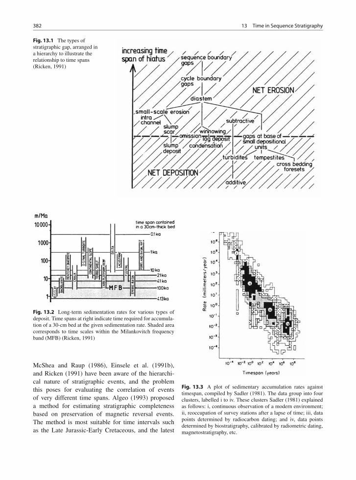
382 13 Time in Sequence Stratigraphy
Fig. 13.1 The types ofstratigraphic gap, arranged ina hierarchy to illustrate therelationship to time spans(Ricken, 1991)
Fig. 13.2 Long-term sedimentation rates for various types ofdeposit. Time spans at right indicate time required for accumula-tion of a 30-cm bed at the given sedimentation rate. Shaded areacorresponds to time scales within the Milankovitch frequencyband (MFB) (Ricken, 1991)
McShea and Raup (1986), Einsele et al. (1991b),and Ricken (1991) have been aware of the hierarchi-cal nature of stratigraphic events, and the problemthis poses for evaluating the correlation of eventsof very different time spans. Algeo (1993) proposeda method for estimating stratigraphic completenessbased on preservation of magnetic reversal events.The method is most suitable for time intervals suchas the Late Jurassic-Early Cretaceous, and the latest
Fig. 13.3 A plot of sedimentary accumulation rates againsttimespan, compiled by Sadler (1981). The data group into fourclusters, labelled i to iv. These clusters Sadler (1981) explainedas follows: i, continuous observation of a modern environment;ii, reoccupation of survey stations after a lapse of time; iii, datapoints determined by radiocarbon dating; and iv, data pointsdetermined by biostratigraphy, calibrated by radiometric dating,magnetostratigraphy, etc.
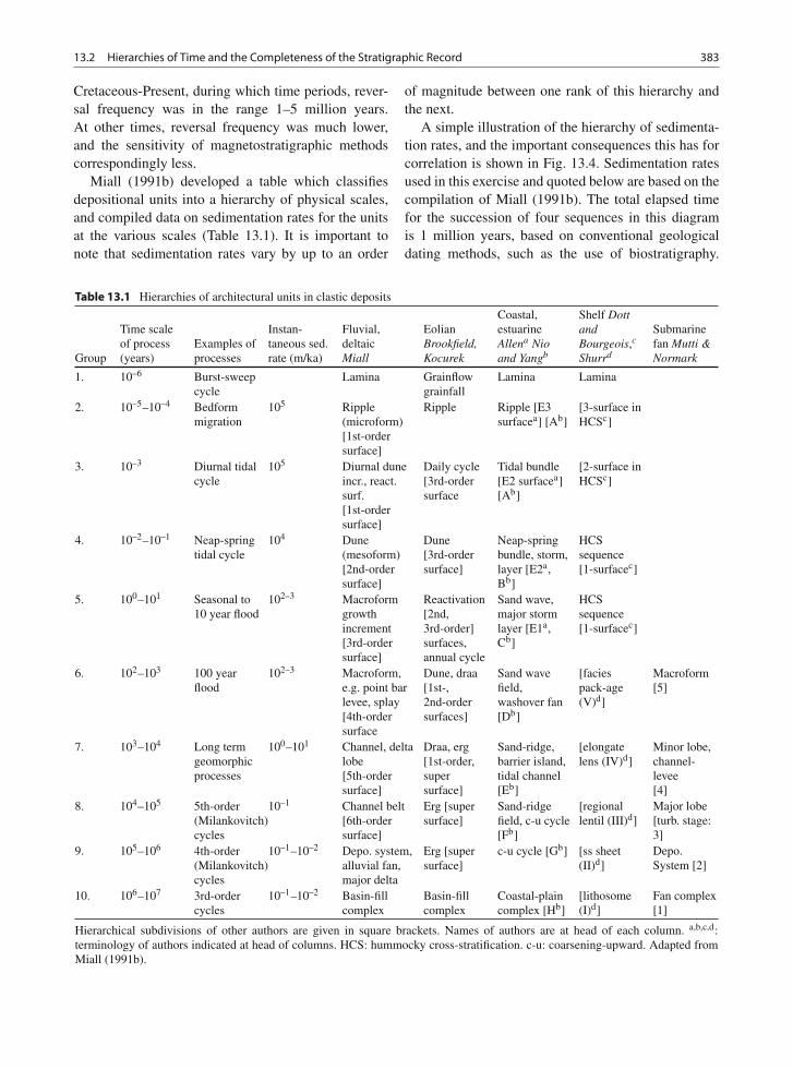
13.2 Hierarchies of Time and the Completeness of the Stratigraphic Record 383
Cretaceous-Present, during which time periods, rever-sal frequency was in the range 1–5 million years.At other times, reversal frequency was much lower,and the sensitivity of magnetostratigraphic methodscorrespondingly less.
Miall (1991b) developed a table which classifiesdepositional units into a hierarchy of physical scales,and compiled data on sedimentation rates for the unitsat the various scales (Table 13.1). It is important tonote that sedimentation rates vary by up to an order
of magnitude between one rank of this hierarchy andthe next.
A simple illustration of the hierarchy of sedimenta-tion rates, and the important consequences this has forcorrelation is shown in Fig. 13.4. Sedimentation ratesused in this exercise and quoted below are based on thecompilation of Miall (1991b). The total elapsed timefor the succession of four sequences in this diagramis 1 million years, based on conventional geologicaldating methods, such as the use of biostratigraphy.
Table 13.1 Hierarchies of architectural units in clastic deposits
Group
Time scaleof process(years)
Examples ofprocesses
Instan-taneous sed.rate (m/ka)
Fluvial,deltaicMiall
EolianBrookfield,Kocurek
Coastal,estuarineAllena Nioand Yangb
Shelf DottandBourgeois,c
Shurrd
Submarinefan Mutti &Normark
1. 10–6 Burst-sweepcycle
Lamina Grainflowgrainfall
Lamina Lamina
2. 10–5–10–4 Bedformmigration
105 Ripple(microform)[1st-ordersurface]
Ripple Ripple [E3surfacea] [Ab]
[3-surface inHCSc]
3. 10–3 Diurnal tidalcycle
105 Diurnal duneincr., react.surf.[1st-ordersurface]
Daily cycle[3rd-ordersurface
Tidal bundle[E2 surfacea][Ab]
[2-surface inHCSc]
4. 10–2–10–1 Neap-springtidal cycle
104 Dune(mesoform)[2nd-ordersurface]
Dune[3rd-ordersurface]
Neap-springbundle, storm,layer [E2a,Bb]
HCSsequence[1-surfacec]
5. 100–101 Seasonal to10 year flood
102–3 Macroformgrowthincrement[3rd-ordersurface]
Reactivation[2nd,3rd-order]surfaces,annual cycle
Sand wave,major stormlayer [E1a,Cb]
HCSsequence[1-surfacec]
6. 102–103 100 yearflood
102–3 Macroform,e.g. point barlevee, splay[4th-ordersurface
Dune, draa[1st-,2nd-ordersurfaces]
Sand wavefield,washover fan[Db]
[faciespack-age(V)d]
Macroform[5]
7. 103–104 Long termgeomorphicprocesses
100–101 Channel, deltalobe[5th-ordersurface]
Draa, erg[1st-order,supersurface]
Sand-ridge,barrier island,tidal channel[Eb]
[elongatelens (IV)d]
Minor lobe,channel-levee[4]
8. 104–105 5th-order(Milankovitch)cycles
10–1 Channel belt[6th-ordersurface]
Erg [supersurface]
Sand-ridgefield, c-u cycle[Fb]
[regionallentil (III)d]
Major lobe[turb. stage:3]
9. 105–106 4th-order(Milankovitch)cycles
10–1–10–2 Depo. system,alluvial fan,major delta
Erg [supersurface]
c-u cycle [Gb] [ss sheet(II)d]
Depo.System [2]
10. 106–107 3rd-ordercycles
10–1–10–2 Basin-fillcomplex
Basin-fillcomplex
Coastal-plaincomplex [Hb]
[lithosome(I)d]
Fan complex[1]
Hierarchical subdivisions of other authors are given in square brackets. Names of authors are at head of each column. a,b,c,d:terminology of authors indicated at head of columns. HCS: hummocky cross-stratification. c-u: coarsening-upward. Adapted fromMiall (1991b).
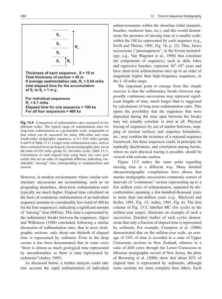
384 13 Time in Sequence Stratigraphy
Fig. 13.4 Comparison of sedimentation rates measured at twodifferent scales. The typical range of sedimentation rates forlong-term sedimentation at a geomorphic scale, comparable tothat which can be measured for many fifth-order and somefourth-order stratigraphic sequences, is 0.1–0.01 m/ka (groups8 and 9 of Table 13.1). Longer-term sedimentation rates, such asthose estimated from geological, chronostratigraphic data, are inthe order of 0.01 m/ka (group 10, 3rd-order cycles, Table 13.1).Calculations of total elapsed time using these two rates giveresults that are an order of magnitude different, indicating con-siderable “missing” time corresponding to nondeposition anderosion
However, in modern environments where similar sed-imentary successions are accumulating, such as onprograding shorelines, short-term sedimentation ratestypically are much higher. Elapsed time calculated onthe basis of continuous sedimentation of an individualsequence amounts to considerably less (total of 400 kafor the four sequences), indicating a significant amountof “missing” time (600 ka). This time is represented bythe sedimentary breaks between the sequences. Algeoand Wilkinson (1988) concluded, following a similardiscussion of sedimentation rates, that in most strati-graphic sections, only about one thirtieth of elapsedtime is represented by sediment. Even in the deepoceans it has been demonstrated that in some cases“there is almost as much geological time representedby unconformities as there is time represented bysediments”(Aubry, 1995).
As discussed below, a further analysis could takeinto account the rapid sedimentation of individual
subenvironments within the shoreline (tidal channels,beaches, washover fans, etc.), and this would demon-strate the presence of missing time at a smaller scale,within the 100 ka represented by each sequence (e.g.,Swift and Thorne, 1991, Fig. 16, p. 23). Thus, faciessuccessions (“parasequences”, in the Exxon terminol-ogy; e.g., Van Wagoner et al., 1990) that constitutethe components of sequences, such as delta lobesand regressive beaches, represent 103–104 years andhave short-term sedimentation rates up to an order ofmagnitude higher than high-frequency sequences, inthe 1–10 m/ka range.
The important point to emerge from this simpleexercise is that the sedimentary breaks between sup-posedly continuous successions may represent signif-icant lengths of time, much longer than is suggestedby calculations of long-term sedimentation rates. Thisopens the possibility that the sequences that weredeposited during the time span between the breaksmay not actually correlate in time at all. Physicaltracing of sequences by use of marker horizons, map-ping of erosion surfaces and sequence boundaries,etc., may confirm the existence of a regional sequenceframework, but these sequences could, in principal, bemarkedly diachronous, and correlation among basins,where no such physical tracing is possible, should beviewed with extreme caution.
Figure 13.5 makes the same point regardingmissing time in a different way. Many detailedchronostratigraphic compilations have shown thatmarine stratigraphic successions commonly consist ofintervals of “continuous” section representing up to afew million years of sedimentation, separated by dis-conformities spanning a few-hundred-thousand yearsto more than one-million years (e.g., MacLeod andKeller, 1991, Fig. 15; Aubry, 1991, Fig. 6). The firstcolumn of Fig. 13.5, labelled MC (for cycles in themillion-year range), illustrates an example of such asuccession. Detailed studies of such cycles demon-strate that only a fraction of elapsed time is representedby sediment. For example, Crampton et al. (2006)demonstrated that on the million-year scale, an aver-age of 24% of time is recorded in a suite of UpperCretaceous sections in New Zealand, whereas in asuite of drill cores through the Lower Cretaceous toMiocene stratigraphic record of New Jersey, the plotsof Browning et al. (2008) show that about 82% ofelapsed time is represented by sediments, althoughsome sections are more complete than others. Each
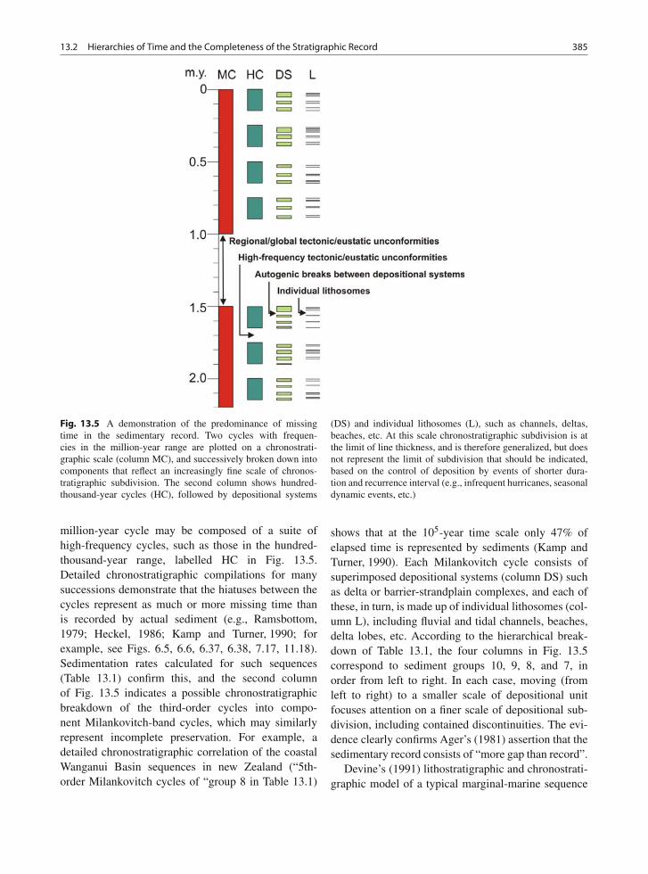
13.2 Hierarchies of Time and the Completeness of the Stratigraphic Record 385
Fig. 13.5 A demonstration of the predominance of missingtime in the sedimentary record. Two cycles with frequen-cies in the million-year range are plotted on a chronostrati-graphic scale (column MC), and successively broken down intocomponents that reflect an increasingly fine scale of chronos-tratigraphic subdivision. The second column shows hundred-thousand-year cycles (HC), followed by depositional systems
(DS) and individual lithosomes (L), such as channels, deltas,beaches, etc. At this scale chronostratigraphic subdivision is atthe limit of line thickness, and is therefore generalized, but doesnot represent the limit of subdivision that should be indicated,based on the control of deposition by events of shorter dura-tion and recurrence interval (e.g., infrequent hurricanes, seasonaldynamic events, etc.)
million-year cycle may be composed of a suite ofhigh-frequency cycles, such as those in the hundred-thousand-year range, labelled HC in Fig. 13.5.Detailed chronostratigraphic compilations for manysuccessions demonstrate that the hiatuses between thecycles represent as much or more missing time thanis recorded by actual sediment (e.g., Ramsbottom,1979; Heckel, 1986; Kamp and Turner, 1990; forexample, see Figs. 6.5, 6.6, 6.37, 6.38, 7.17, 11.18).Sedimentation rates calculated for such sequences(Table 13.1) confirm this, and the second columnof Fig. 13.5 indicates a possible chronostratigraphicbreakdown of the third-order cycles into compo-nent Milankovitch-band cycles, which may similarlyrepresent incomplete preservation. For example, adetailed chronostratigraphic correlation of the coastalWanganui Basin sequences in new Zealand (“5th-order Milankovitch cycles of “group 8 in Table 13.1)
shows that at the 105-year time scale only 47% ofelapsed time is represented by sediments (Kamp andTurner, 1990). Each Milankovitch cycle consists ofsuperimposed depositional systems (column DS) suchas delta or barrier-strandplain complexes, and each ofthese, in turn, is made up of individual lithosomes (col-umn L), including fluvial and tidal channels, beaches,delta lobes, etc. According to the hierarchical break-down of Table 13.1, the four columns in Fig. 13.5correspond to sediment groups 10, 9, 8, and 7, inorder from left to right. In each case, moving (fromleft to right) to a smaller scale of depositional unitfocuses attention on a finer scale of depositional sub-division, including contained discontinuities. The evi-dence clearly confirms Ager’s (1981) assertion that thesedimentary record consists of “more gap than record”.
Devine’s (1991) lithostratigraphic and chronostrati-graphic model of a typical marginal-marine sequence
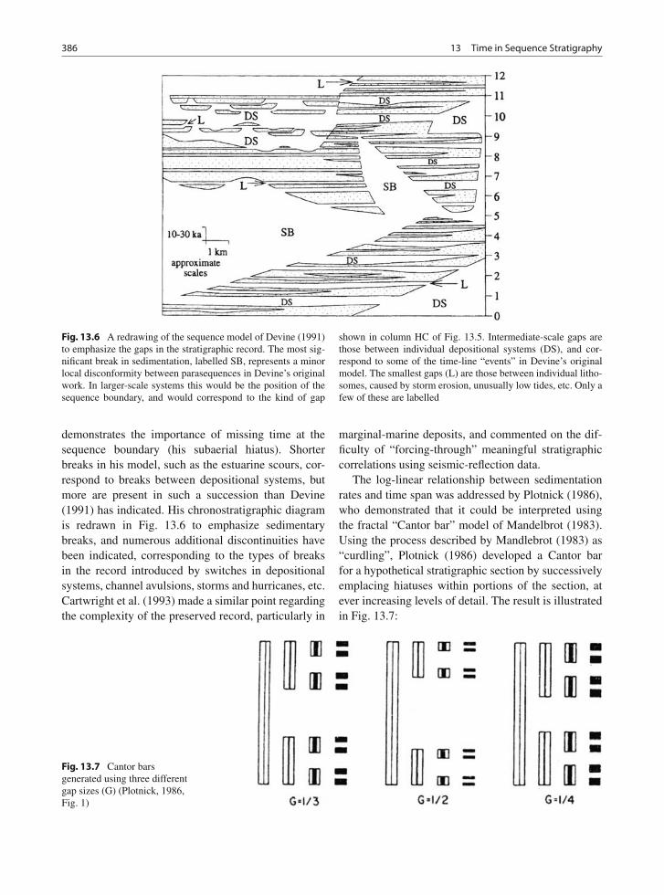
386 13 Time in Sequence Stratigraphy
Fig. 13.6 A redrawing of the sequence model of Devine (1991)to emphasize the gaps in the stratigraphic record. The most sig-nificant break in sedimentation, labelled SB, represents a minorlocal disconformity between parasequences in Devine’s originalwork. In larger-scale systems this would be the position of thesequence boundary, and would correspond to the kind of gap
shown in column HC of Fig. 13.5. Intermediate-scale gaps arethose between individual depositional systems (DS), and cor-respond to some of the time-line “events” in Devine’s originalmodel. The smallest gaps (L) are those between individual litho-somes, caused by storm erosion, unusually low tides, etc. Only afew of these are labelled
demonstrates the importance of missing time at thesequence boundary (his subaerial hiatus). Shorterbreaks in his model, such as the estuarine scours, cor-respond to breaks between depositional systems, butmore are present in such a succession than Devine(1991) has indicated. His chronostratigraphic diagramis redrawn in Fig. 13.6 to emphasize sedimentarybreaks, and numerous additional discontinuities havebeen indicated, corresponding to the types of breaksin the record introduced by switches in depositionalsystems, channel avulsions, storms and hurricanes, etc.Cartwright et al. (1993) made a similar point regardingthe complexity of the preserved record, particularly in
marginal-marine deposits, and commented on the dif-ficulty of “forcing-through” meaningful stratigraphiccorrelations using seismic-reflection data.
The log-linear relationship between sedimentationrates and time span was addressed by Plotnick (1986),who demonstrated that it could be interpreted usingthe fractal “Cantor bar” model of Mandelbrot (1983).Using the process described by Mandlebrot (1983) as“curdling”, Plotnick (1986) developed a Cantor barfor a hypothetical stratigraphic section by successivelyemplacing hiatuses within portions of the section, atever increasing levels of detail. The result is illustratedin Fig. 13.7:
Fig. 13.7 Cantor barsgenerated using three differentgap sizes (G) (Plotnick, 1986,Fig. 1)
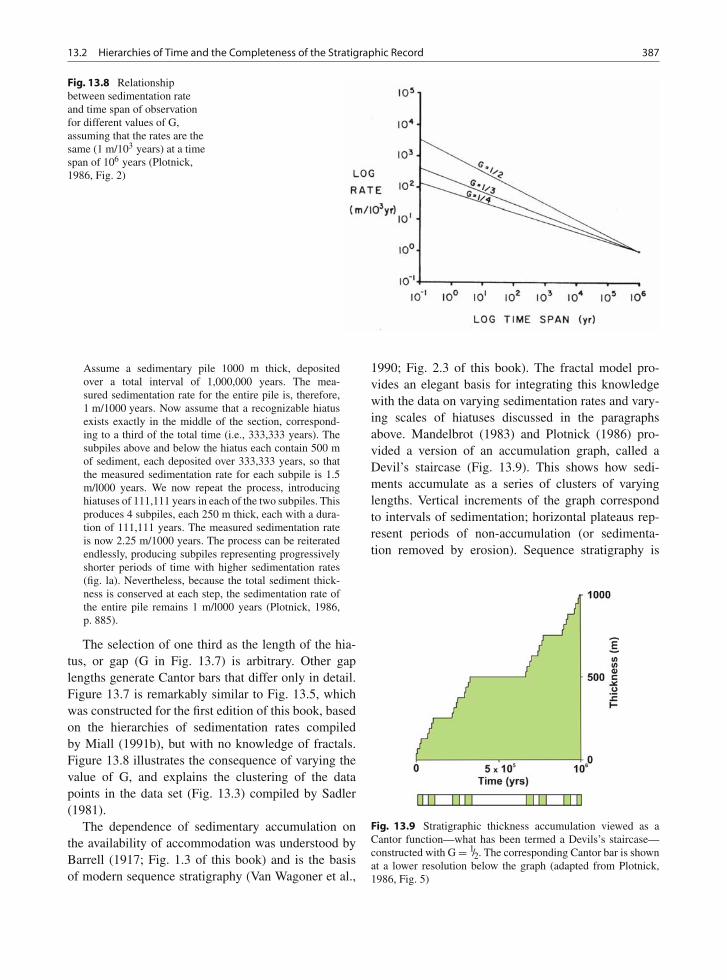
13.2 Hierarchies of Time and the Completeness of the Stratigraphic Record 387
Fig. 13.8 Relationshipbetween sedimentation rateand time span of observationfor different values of G,assuming that the rates are thesame (1 m/103 years) at a timespan of 106 years (Plotnick,1986, Fig. 2)
Assume a sedimentary pile 1000 m thick, depositedover a total interval of 1,000,000 years. The mea-sured sedimentation rate for the entire pile is, therefore,1 m/1000 years. Now assume that a recognizable hiatusexists exactly in the middle of the section, correspond-ing to a third of the total time (i.e., 333,333 years). Thesubpiles above and below the hiatus each contain 500 mof sediment, each deposited over 333,333 years, so thatthe measured sedimentation rate for each subpile is 1.5m/l000 years. We now repeat the process, introducinghiatuses of 111,111 years in each of the two subpiles. Thisproduces 4 subpiles, each 250 m thick, each with a dura-tion of 111,111 years. The measured sedimentation rateis now 2.25 m/1000 years. The process can be reiteratedendlessly, producing subpiles representing progressivelyshorter periods of time with higher sedimentation rates(fig. la). Nevertheless, because the total sediment thick-ness is conserved at each step, the sedimentation rate ofthe entire pile remains 1 m/l000 years (Plotnick, 1986,p. 885).
The selection of one third as the length of the hia-tus, or gap (G in Fig. 13.7) is arbitrary. Other gaplengths generate Cantor bars that differ only in detail.Figure 13.7 is remarkably similar to Fig. 13.5, whichwas constructed for the first edition of this book, basedon the hierarchies of sedimentation rates compiledby Miall (1991b), but with no knowledge of fractals.Figure 13.8 illustrates the consequence of varying thevalue of G, and explains the clustering of the datapoints in the data set (Fig. 13.3) compiled by Sadler(1981).
The dependence of sedimentary accumulation onthe availability of accommodation was understood byBarrell (1917; Fig. 1.3 of this book) and is the basisof modern sequence stratigraphy (Van Wagoner et al.,
1990; Fig. 2.3 of this book). The fractal model pro-vides an elegant basis for integrating this knowledgewith the data on varying sedimentation rates and vary-ing scales of hiatuses discussed in the paragraphsabove. Mandelbrot (1983) and Plotnick (1986) pro-vided a version of an accumulation graph, called aDevil’s staircase (Fig. 13.9). This shows how sedi-ments accumulate as a series of clusters of varyinglengths. Vertical increments of the graph correspondto intervals of sedimentation; horizontal plateaus rep-resent periods of non-accumulation (or sedimenta-tion removed by erosion). Sequence stratigraphy is
Fig. 13.9 Stratigraphic thickness accumulation viewed as aCantor function—what has been termed a Devils’s staircase—constructed with G = 1/2. The corresponding Cantor bar is shownat a lower resolution below the graph (adapted from Plotnick,1986, Fig. 5)
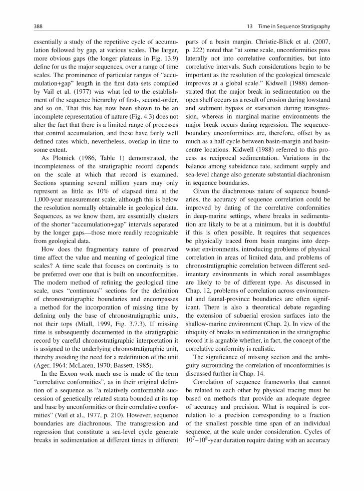
388 13 Time in Sequence Stratigraphy
essentially a study of the repetitive cycle of accumu-lation followed by gap, at various scales. The larger,more obvious gaps (the longer plateaus in Fig. 13.9)define for us the major sequences, over a range of timescales. The prominence of particular ranges of “accu-mulation+gap” length in the first data sets compiledby Vail et al. (1977) was what led to the establish-ment of the sequence hierarchy of first-, second-order,and so on. That this has now been shown to be anincomplete representation of nature (Fig. 4.3) does notalter the fact that there is a limited range of processesthat control accumulation, and these have fairly welldefined rates which, nevertheless, overlap in time tosome extent.
As Plotnick (1986, Table 1) demonstrated, theincompleteness of the stratigraphic record dependson the scale at which that record is examined.Sections spanning several million years may onlyrepresent as little as 10% of elapsed time at the1,000-year measurement scale, although this is belowthe resolution normally obtainable in geological data.Sequences, as we know them, are essentially clustersof the shorter “accumulation+gap” intervals separatedby the longer gaps—those more readily recognizablefrom geological data.
How does the fragmentary nature of preservedtime affect the value and meaning of geological timescales? A time scale that focuses on continuity is tobe preferred over one that is built on unconformities.The modern method of refining the geological timescale, uses “continuous” sections for the definitionof chronostratigraphic boundaries and encompassesa method for the incorporation of missing time bydefining only the base of chronostratigraphic units,not their tops (Miall, 1999, Fig. 3.7.3). If missingtime is subsequently documented in the stratigraphicrecord by careful chronostratigraphic interpretation itis assigned to the underlying chronostratigraphic unit,thereby avoiding the need for a redefinition of the unit(Ager, 1964; McLaren, 1970; Bassett, 1985).
In the Exxon work much use is made of the term“correlative conformities”, as in their original defini-tion of a sequence as “a relatively conformable suc-cession of genetically related strata bounded at its topand base by unconformities or their correlative confor-mities” (Vail et al., 1977, p. 210). However, sequenceboundaries are diachronous. The transgression andregression that constitute a sea-level cycle generatebreaks in sedimentation at different times in different
parts of a basin margin. Christie-Blick et al. (2007,p. 222) noted that “at some scale, unconformities passlaterally not into correlative conformities, but intocorrelative intervals. Such considerations begin to beimportant as the resolution of the geological timescaleimproves at a global scale.” Kidwell (1988) demon-strated that the major break in sedimentation on theopen shelf occurs as a result of erosion during lowstandand sediment bypass or starvation during transgres-sion, whereas in marginal-marine environments themajor break occurs during regression. The sequence-boundary unconformities are, therefore, offset by asmuch as a half cycle between basin-margin and basin-centre locations. Kidwell (1988) referred to this pro-cess as reciprocal sedimentation. Variations in thebalance among subsidence rate, sediment supply andsea-level change also generate substantial diachronismin sequence boundaries.
Given the diachronous nature of sequence bound-aries, the accuracy of sequence correlation could beimproved by dating of the correlative conformitiesin deep-marine settings, where breaks in sedimenta-tion are likely to be at a minimum, but it is doubtfulif this is often possible. It requires that sequencesbe physically traced from basin margins into deep-water environments, introducing problems of physicalcorrelation in areas of limited data, and problems ofchronostratigraphic correlation between different sed-imentary environments in which zonal assemblagesare likely to be of different type. As discussed inChap. 12, problems of correlation across environmen-tal and faunal-province boundaries are often signif-icant. There is also a theoretical debate regardingthe extension of subaerial erosion surfaces into theshallow-marine environment (Chap. 2). In view of theubiquity of breaks in sedimentation in the stratigraphicrecord it is arguable whether, in fact, the concept of thecorrelative conformity is realistic.
The significance of missing section and the ambi-guity surrounding the correlation of unconformities isdiscussed further in Chap. 14.
Correlation of sequence frameworks that cannotbe related to each other by physical tracing must bebased on methods that provide an adequate degreeof accuracy and precision. What is required is cor-relation to a precision corresponding to a fractionof the smallest possible time span of an individualsequence, at the scale under consideration. Cycles of107–108-year duration require dating with an accuracy
13.3 Main Conclusions 389
to within a few millions of years. This is not a dif-ficult requirement, at least within marine rocks ofPhanerozoic age, and a global framework of second-order cycles is within our grasp. In fact, Sloss began theprocess of establishing this framework many years ago,as described in Sect. 1.4. Whether the Exxon frame-work of “second-order” sequences is to be consideredreliable as indicators of global control is another ques-tion, which is addressed in Sect. 9.3.3.
Cycles with million-year periodicities require aprecision of ±0.5 million years, or better for reli-able correlation. As is demonstrated in Chap. 14,conventional geological techniques, such as biostratig-raphy calibrated with radiometric, chemostratigraphic,and/or magnetostratigraphic data, can rarely attain thisdegree of precision (except in the youngest Cenozoic),and it is, therefore, highly questionable whether thedata currently permit us to attempt the erection ofan interbasinal framework of “third-order” cycles. Inspecial cases, use of high-resolution correlation tech-niques, including graphic correlation, permit precisionto within about ±100 ka in rocks of early Cenozoicand Mesozoic age (Kauffman et al., 1991). In suchcases, a framework of regional correlation can be builtwith some degree of confidence. However, it is doubt-ful if we are anywhere near ready to extend suchframeworks to other basins on different continents,in different tectonic settings, and in different climaticzones.
High-frequency sequences (those with periodicitiesin the Milankovitch band) cannot yet be reliably cor-related interregionally, except for the glacioeustaticsequences of the late Cenozoic, as documented inSects. 11.3.2 and 14.6.3. For this most recent inter-val of geological time rapid changes in sea level haveclimatic causes which have left a reliable chronostrati-graphic signature in the form of the oxygen-isotoperecord.
One of the major problems with the global-eustasyparadigm is circular reasoning in placing undueemphasis on significant “events” that are presumed tobe synchronous in different areas. This presumptioncauses difficulties in performing meaningful tests ofthe global cycle chart, as shown in Chap. 14. Secondly,there is no reason why changes in sea level, whichare the events defining stratigraphic sequences, shouldshow any relationship to zone and stage boundariesthat are based on biological evolution. Changes in sealevel affect the ecology of marine environments, butthe relationship of such changes to biotic evolution andextinction is complex. We should not, therefore, expectany relationship between sequence boundaries andbiostratigraphically-based boundaries in the standardgeological time scale.
13.3 Main Conclusions
1. Only a small fraction of elapsed time normally isrepresented by sediment preserved in the geologicalrecord.
2. The hierarchy of sequences represent time spansand sedimentation rates that differ from each otherby orders of magnitude.
3. Accurate and precise estimates of time spans of thecomponent sequences and hiatuses in a successioncannot be achieved by determining bracketing agesfrom stratigraphically widely spaced marker bedsthat enclose several or many sequences.
4. Correlation of sequences requires that they be datedwith a precision, or potential error range, equal to afraction of the range of the shortest sequence in thesuccession. For example, sequences with 106-yearperiodicities (those comprising the main basis ofthe Exxon global cycle chart) require a correlationprecision of ±0.5 million years, or less.
Chapter 14
Chronostratigraphy, Correlation, and Modern Testsfor Global Eustasy
Contents
14.1 Introduction . . . . . . . . . . . . . . . . . 39114.2 Chronostratigraphic Models
and the Testing of Correlations . . . . . . . . 39214.3 Chronostratigraphic Meaning of Unconformities 39614.4 A Correlation Experiment . . . . . . . . . . 40014.5 Testing for Eustasy: The Way Forward . . . . 402
14.5.1 Introduction . . . . . . . . . . . . . . 40214.5.2 The Dating and Correlation of Stratigraphic
Events: Potential Sources of Uncertainty . 40314.5.3 The Value of Quantitative Biostratigraphic
Methods . . . . . . . . . . . . . . . 41014.5.4 Assessment of Relative Biostratigraphic
Precision . . . . . . . . . . . . . . . 41314.5.5 Correlation of Biozones with the Global
Stage Framework . . . . . . . . . . . 41514.5.6 Assignment of Absolute Ages and the
Importance of the Modern Time Scale . . 41814.6 Modern Tests of the Global-Eustasy Paradigm 425
14.6.1 Cretaceous-Paleogene SequenceStratigraphy of New Jersey . . . . . . . 426
14.6.2 Other Modern High-Resolution Studiesof Cretaceous-Paleogene SequenceStratigraphy . . . . . . . . . . . . . . 433
14.6.3 Sequence Stratigraphy of the Neogene . . 43514.6.4 The Growing Evidence for Glacioeustasy in
the Mesozoic and Early Cenozoic . . . . 43814.7 Cyclostratigraphy and Astrochronology . . . 441
14.7.1 Historical Background of Cyclostratigraphy 44114.7.2 The Building of a Time Scale . . . . . . 443
14.8 Testing Correlations with Carbon IsotopeChemostratigraphy . . . . . . . . . . . . . 453
14.9 Main Conclusions . . . . . . . . . . . . . . 458
14.1 Introduction
As discussed in Chap. 12, sequence stratigraphy iscurrently characterized by two alternative, oppos-ing paradigms, the global-eustasy paradigm, and the
complexity paradigm. McGowran (2005, p. 365) haspointed out that these are conceptual end-membersof a “broad spectrum of responses and approachesto the controversy over global eustasy.” McGowran(2005, p. 366) agreed that such markers as sequenceboundaries and maximum flooding surfaces “shouldnot be intrinsic to geochronology,” contra Vail,but he stated “I do not share the Miall-Wilsonview that sequence-surfaces have no promise incorrelation.”
Here lies the crux of the problem. What do sequencesurfaces signify? One of the major purposes of thisbook has been to demonstrate the complex, multi-faceted nature of the sequence record. Sequences havemultiple causes, only two of which, (1) changing ratesof sea-floor spreading, affecting ocean-volumes (Chap.9), and (2) glacioeustasy (Chap. 11), can be convinc-ingly demonstrated to generate global effects on thesedimentary record that potentially may be correlatedand become contributors to the global stratigraphicdata base. Other sequences are strictly local to regionalin extent. The problem is that sequence-generatingprocesses are scale independent (e.g., see Catuneanu,2006), and whether they are controlled by eustaticsea-level change or tectonic changes in accommoda-tion, such locally observable attributes as facies andthickness do not necessarily provide any clues as toultimate allogenic mechanisms. Even the key attributeof sequence thickness has been demonstrated to carryno useful signal of causation (Algeo and Wilkinson,1988; Drummond and Wilkinson, 1996), and Schlager(2004) showed that distribution of sequence durationsis fractal in character, indicating that the sequence hier-archy concept of Vail et al. (1977) cannot be supported.Schwarzacher (2000, p. 52) stated that
391A.D. Miall, The Geology of Stratigraphic Sequences, 2nd ed.,DOI 10.1007/978-3-642-05027-5_14, © Springer-Verlag Berlin Heidelberg 2010
392 14 Chronostratigraphy, Correlation, and Modern Tests for Global Eustasy
This system of ordering cycles is widely used but hasserious shortcomings. By pretending that there exists ahierarchy of cycles, repetitive patterns, which have noth-ing in common except their duration, are mixed together.Such a classification is just as meaningless as groupingelephants and fleas into an order based on their size.
The most important single test that can be per-formed on a suite of sequences is correlation. In thefirst place, the reality of a succession of sequencesmust be established by the establishment of local strati-graphic relationships, in order to distinguish faciessuccessions generated by local autogenic causes, suchas delta switching and abandonment, from those oftrue allogenic origin (this is the parasequence prob-lem discussed in Sect. 2.2.2). Sequences that can becorrelated beyond a particular basin into an adjacentbasin, into a different tectonic province, or across anocean to another tectonic plate, are clearly the prod-uct of a widespread process, and only eustatic sea-levelchange seems capable of generating global changes inaccommodation that are synchronous and in the samedirection, although, as illustrated by Fig. 10.1, and thediscussion in Sect. 10.1, where a curve of eustaticsea-level change is integrated with varying rates ofsubsidence, the timing of sea-level highs and lows maybe offset by as much as one quarter of the wavelengthof the sea-level cycle (Allen and Allen, 2005, p. 271).As discussed in Sect. 10.4, intraplate stress changesmay be capable of generating tectonic events that aresynchronous but of locally different character, but thisremains a partially tested hypothesis.
The test of global correlation is, therefore, fun-damental to the issue of sequence mechanism. Untilthere are multiple, repeated demonstrations of globalcorrelation, the ubiquity and central importance ofeustasy as a stratigraphic control must remain a largelyunproven hypothesis. But here the problem of thehermeneutic circle arises, and here lies the method-ological divide between the inductive and deductiveapproaches to stratigraphy.
McGowran (2005, p. xvi), citing Popper, argued:
As Sir Karl Popper advocated tirelessly, the inductivistmodel of science, whereby we collect data and draw con-clusions from it, is not very useful or stimulating or real-istic. No: we always have theories and biases influencingour choice of observations and our perceptions of ‘facts’,and biostratigraphy is no different. We do not simplyidentify, range, zone and correlate in tedious induction –for we have stubborn, crazy, powerful and pet ideas abouttectonism, climate change, or evolutionary relationships
whose triumph or tragedy can depend utterly on thefragility of robustness of the chronology or correlation.
The problem is that pet ideas can introduce bias.This is what Vail and Todd (1981, p. 230) wereabout when they stated “the late Pliensbachian hia-tus described by Linsley and others (1979) fits thebasal early Pliensbachian sequence boundary on ourglobal cycle chart.” (see Sect. 12.1). To allow suchadjustments to the biostratigraphic record is to renderinoperable the concept of an independent test of thehypothesis. In Sect. 12.1 I point out the obvious dan-gers of circular reasoning involved in the deductivistapproach to sequence stratigraphy. As McGowran(2005, p. 190) noted, it is a “forbiddingly difficulttask . . . [to] disentangle the triad of processes control-ling the stratigraphic record on the continental margin:namely eustasy, tectonics (including thermal subsi-dence, isostasy, compaction, flexure), and sedimentsupply.” The last thing that needs to be added as acomponent of this task is bias.
In the next section we illustrate this problem furtherwith reference to two examples.
14.2 Chronostratigraphic Modelsand the Testing of Correlations
Adherents of the global-eustasy paradigm believe thatsequence stratigraphy may be used as “an instrumentof geochronology” (Vail et al., 1977, p. 96). The defin-ing feature of the model is the belief that sequenceboundaries are global chronostratigraphic indicators,and that their ages are not influenced by the tectonicbehaviour of sedimentary basins. From this first princi-ple follows the use of pattern recognition as a means ofcorrelation. In correlation charts constructed with timeas the ordinate, correlation lines will always be parallel(“railroad correlation lines”)—this was one of the dis-tinguishing characteristics of the first published chartto show the relationship of regional cycle charts to eachother and to the derived global chart (Fig. 12.2). Thefollowing discussion of chronostratigraphic models istaken largely from Miall and Miall (2004).
Despite the considerable body of critical discus-sion about the global cycle chart that has appearedsince the mid-1980s, adherents of the global-eustasymodel continue to practice a science that emphasizesthe predominant importance of this deductive model
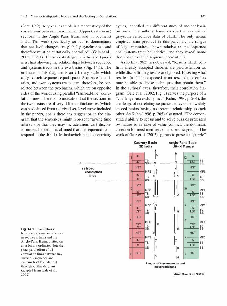
14.2 Chronostratigraphic Models and the Testing of Correlations 393
(Sect. 12.2). A typical example is a recent study of thecorrelations between Cenomanian (Upper Cretaceous)sections in the Anglo-Paris Basin and in southeastIndia. This work specifically set out “to demonstratethat sea-level changes are globally synchronous andtherefore must be eustatically controlled” (Gale et al.,2002, p. 291). The key data diagram in this short paperis a chart showing the relationships between sequenceand systems tracts in the two basins (Fig. 14.1). Theordinate in this diagram is an arbitrary scale whichassigns each sequence equal space. Sequence bound-aries, and even systems tracts, can, therefore, be cor-related between the two basins, which are on oppositesides of the world, using parallel “railroad-line” corre-lation lines. There is no indication that the sections inthe two basins are of very different thicknesses (whichcan be deduced from a derived sea-level curve includedin the paper), nor is there any suggestion in the dia-gram that the sequences might represent varying timeintervals or that they may include significant discon-formities. Indeed, it is claimed that the sequences cor-respond to the 400-ka Milankovitch-band eccentricity
cycles, identified in a different study of another basinby one of the authors, based on spectral analysis ofgrayscale reflectance data of chalk. The only actualempirical data provided in this paper are the rangesof key ammonites, shown relative to the sequenceand systems-tract boundaries, and they reveal somediscrepancies in the sequence correlations.
As Kuhn (1962) has observed, “Results which con-firm already accepted theories are paid attention to,while disconfirming results are ignored. Knowing whatresults should be expected from research, scientistsmay be able to devise techniques that obtain them.”In the authors’ eyes, therefore, their correlation dia-gram (Gale et al., 2002, Fig. 3) serves the purpose of a“challenge successfully met” (Kuhn, 1996, p. 204), thechallenge of correlating sequences of events in widelyspaced basins having no tectonic relationship to eachother. As Kuhn (1996, p. 205) also noted, “The demon-strated ability to set up and to solve puzzles presentedby nature is, in case of value conflict, the dominantcriterion for most members of a scientific group.” Thework of Gale et al. (2002) appears to present a “puzzle”
Fig. 14.1 Correlationsbetween Cenomanian sectionsin southeast India and theAnglo-Paris Basin, plotted onan arbitrary ordinate. Note theexact parallelism of allcorrelation lines between keysurfaces (sequence andsystems tract boundaries)throughout this diagram(adapted from Gale et al.,2002)
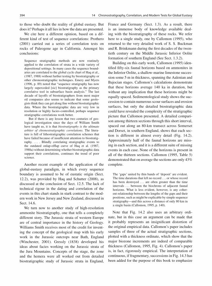
394 14 Chronostratigraphy, Correlation, and Modern Tests for Global Eustasy
to those who doubt the reality of global eustasy. Butdoes it? Perhaps it all lies in how the data are presented.
We cite here a different opinion, based on a dif-ferent kind of test of sequence correlations: Prothero(2001) carried out a series of correlation tests onrocks of Paleogene age in California. Amongst hisconclusions:
Sequence stratigraphic methods are now routinelyapplied to the correlation of strata in a wide variety ofdepositional settings. In many cases the sequence bound-aries are correlated to the global cycle chart of Haq et al.,(1987, 1988) without further testing by biostratigraphy orother chronostratigraphic techniques. Emery and Myers(1996, p. 89) noted that “sequence stratigraphy has nowlargely superceded [sic] biostratigraphy as the primarycorrelative tool in subsurface basin analysis.” The lastdecade of layoffs of biostratigraphers from most majoroil companies also seems to indicate that some geolo-gists think they can get along fine without biostratigraphicdata. Where the biostratigraphic data are very low inresolution or highly facies-controlled, perhaps sequencestratigraphic correlations work better.
But if there is any lesson that two centuries of geo-logical investigation since the days of William Smithhave taught us, it is that biostratigraphy is the ultimatearbiter of chronostratigraphic correlations. The litera-ture is full of lithostratigraphic correlation schemes thathave failed because of insufficient attention to biostratig-raphy. . . . . Blindly correlating stratigraphic events tothe outdated onlap-offlap curve of Haq et al. (1987,1988a) without determining whether biostratigraphic datasupport their correlations, continues the trend of poorscience.
Another recent example of the application of theglobal-eustasy paradigm, in which every sequenceboundary is assumed to be of eustatic origin (Sect.12.2), was provided by Haq and Schutter (2008), asdiscussed at the conclusion of Sect. 12.5. The lack oftechnical rigour in the dating and correlation of theevents in this chart stands in stark contrast to the mod-ern work in New Jersey and New Zealand, discussed inSect. 14.6.
We turn now to another study of high-resolutionammonite biostratigraphy, one that tells a completelydifferent story. The Jurassic strata of western Europeare of central importance in the history of Geology.Williams Smith receives most of the credit for invent-ing the concept of the geological map with his earlywork in the Jurassic outcrops near Bath, England(Winchester, 2001). Gressly (1838) developed hisideas about facies working on the Jurassic strata ofthe Jura Mountains. Concepts of the stage, the zoneand the hemera were all worked out from detailedbiostratigraphic study of Jurassic strata in England,
France and Germany (Sect. 1.3). As a result, thereis an immense body of knowledge available deal-ing with the biostratigraphy of these rocks. We referhere to a single study, one by Callomon (1995), whoreturned to the very detailed work of S. S. Buckmanand R. Brinkmann during the first decades of the twen-tieth century on the Middle Jurassic Inferior Ooliteformation of southern England (See Sect. 1.3.2).
Building on this early work, Callomon (1995) iden-tified fifty-six faunal horizons based on ammonites inthe Inferior Oolite, a shallow-marine limestone succes-sion some 5 m in thickness, spanning the Aalenian andBajocian stages. Callomon’s calculations demonstratethat these horizons average 140 ka in duration, butwithout any implication that these horizons might beequally spaced. Sedimentological study shows the suc-cession to contain numerous scour surfaces and erosionsurfaces, but only the detailed biostratigraphic datacould have revealed the complexity of the stratigraphicpicture that Callomon presented. A detailed compari-son among thirteen sections through this short interval,spaced out along an 80-km transect across Somersetand Dorset, in southern England, shows that each sec-tion is different in almost every detail (Fig. 14.2).Approximately half of the faunal horizons are miss-ing in each section, and it is a different suite of missingevents in each case. None of the horizons is present inall of the thirteen sections. Callomon (1995, Table 5)demonstrated that on average the sections are only 43%complete.
The ‘gaps’ united by thin bands of ‘deposit’ are evident.The time durations that left no record . . . or whose recordhas been destroyed . . . are often greater than the timeintervals . . . between the biochrons of adjacent faunalhorizons. What is less evident, however, is any coher-ent relationship between the lengths of the gaps and theirpositions, such as might be explicable by simple sequencestratigraphy—and this across a distance of only 80 km ina single basin (Callomon, 1995, p. 140).
Note that Fig. 14.2 also uses an arbitrary ordi-nate, but in this case an argument can be made thatit probably represents an insignificant distortion ofthe original empirical data. Callomon’s paper includessamples of three of the actual stratigraphic sections,plotted with a thickness ordinate, which show that themajor biozone increments are indeed of comparablethickness (Callomon, 1995, Fig. 4). Callomon’s paperis, in fact, rigorously empirical. The interpretation ofcontinuous, if fragmentary, successions in Fig. 14.3 hasbeen added for the purpose of this book to emphasize
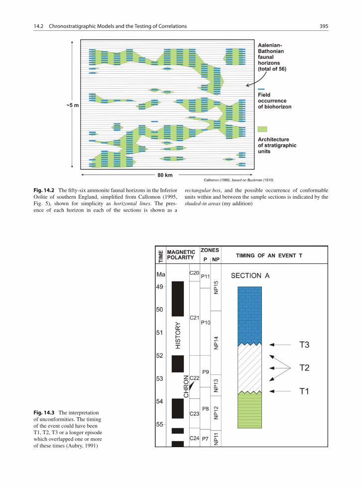
14.2 Chronostratigraphic Models and the Testing of Correlations 395
Fig. 14.2 The fifty-six ammonite faunal horizons in the InferiorOolite of southern England, simplified from Callomon (1995,Fig. 5), shown for simplicity as horizontal lines. The pres-ence of each horizon in each of the sections is shown as a
rectangular box, and the possible occurrence of conformableunits within and between the sample sections is indicated by theshaded-in areas (my addition)
Fig. 14.3 The interpretationof unconformities. The timingof the event could have beenT1, T2, T3 or a longer episodewhich overlapped one or moreof these times (Aubry, 1991)
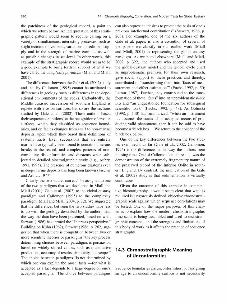
396 14 Chronostratigraphy, Correlation, and Modern Tests for Global Eustasy
the patchiness of the geological record, a point towhich we return below. An interpretation of this strati-graphic pattern would seem to require calling on avariety of simultaneous, interacting processes, such asslight tectonic movements, variations in sediment sup-ply and in the strength of marine currents, as wellas possible changes in sea-level. In other words, thisexample of the stratigraphic record would seem to bea good example to bring forth in support of what wehave called the complexity paradigm (Miall and Miall,2001).
The differences between the Gale et al. (2002) studyand that by Callomon (1995) cannot be attributed todifferences in geology, such as differences in the depo-sitional environments of the rocks. Undoubtedly, theMiddle Jurassic succession of southern England isreplete with erosion surfaces, but so are the sectionsstudied by Gale et al. (2002). These authors basedtheir sequence definitions on the recognition of erosionsurfaces, which they classified as sequence bound-aries, and on facies changes from shelf to non-marinedeposits, upon which they based their definitions ofsystems tracts. Even successions that are entirelymarine have typically been found to contain numerousbreaks in the record, and complex patterns of non-correlating disconformities and diastems when sub-jected to detailed biostratigraphic study (e.g., Aubry,1991, 1995). The presence of numerous diastems evenin deep-marine deposits has long been known (Fischerand Arthur, 1977).
Clearly, the two studies can each be assigned to oneof the two paradigms that we developed in Miall andMiall (2001): Gale et al. (2002) to the global-eustasyparadigm and Callomon (1995) to the complexityparadigm (Miall and Miall, 2004, p. 32). We suggestedthat the differences between the two studies have lessto do with the geology described by the authors thanthe way the data have been presented, based on whatStewart (1986) has termed the “Interests perspective.”Building on Kuhn (1962), Stewart (1986, p. 262) sug-gested that when there is competition between two ormore scientific theories or paradigms “the key processdetermining choices between paradigms is persuasionbased on widely shared values, such as quantitativepredictions, accuracy of results, simplicity, and scope.”The choice between paradigms “is not determined bywhich one can explain the most ‘facts’—for what isaccepted as a fact depends to a large degree on one’saccepted paradigm.” The choice between paradigms
can also represent “desires to protect the basis of one’sprevious intellectual contributions” (Stewart, 1986, p.263). For example, one of the six authors of theGale et al. paper, is also a co-author of several ofthe papers we classify in our earlier work (Mialland Miall, 2001) as representing the global-eustasyparadigm. As we noted elsewhere (Miall and Miall,2002, p. 322), the authors who accepted and usedthe global-eustasy model and the global cycle chartas unproblematic premises for their own research,gave social support to these practices and thereby,contributed to “transforming them into ‘facts of mea-surement and effect estimation’” (Fuchs, 1992, p. 50;Latour, 1987). Further, they contributed to the trans-formation of these “facts” into an unproblematic blackbox and “an unquestioned foundation for subsequentscientific work” (Fuchs, 1992, p. 48). As Golinski(1998, p. 140) has summarized, “when an instrument. . . assumes the status of an accepted means of pro-ducing valid phenomena, then it can be said to havebecome a ‘black box.’” We return to the concept of theblack box below.
One of the key differences between the two stud-ies examined thus far (Gale et al., 2002; Callomon,1995) is the difference in the way the authors treatmissing time. One of Callomon’s main results was thedemonstration of the extremely fragmentary nature ofthe preserved record of the Inferior Oolite in south-ern England. By contrast, the implication of the Galeet al. (2002) study is that sedimentation is virtuallycontinuous.
Given the outcome of this exercise in compara-tive biostratigraphy it would seem clear that what isrequired is a rigorously defined, objective chronostrati-graphic scale against which sequence correlations maybe tested. One of the major purposes of this chap-ter is to explain how the modern chronostratigraphictime scale is being assembled and used to test strati-graphic concepts, and the strengths and limitations ofthis body of work as it affects the practice of sequencestratigraphy.
14.3 Chronostratigraphic Meaningof Unconformities
Sequence boundaries are unconformities, but assigningan age to an unconformity surface is not necessarily
14.3 Chronostratigraphic Meaning of Unconformities 397
a simple matter, as illustrated in the useful theoreticaldiscussion by Aubry (1991). An unconformity repre-sents a finite time span at any one location; it may havea complex genesis, representing amalgamation of morethan one event. It may also be markedly diachronous,because the transgressions and regressions that occurduring the genesis of a stratigraphic sequence couldspan the entire duration of the sequence. As notedin Sect. 13.1, Kidwell (1988) demonstrated that thisresults in an offset in sequence-boundary unconformi-ties by as much as one half of a cycle between basincentre and basin margin.
Unconformities represent amalgamations of twosurfaces, the surface of truncation of older strata andthe surface of transgression of younger strata. Thesetwo surfaces may vary in age considerably from loca-tion to location, as indicated by chronostratigraphicdiagrams (e.g., Vail et al., 1977, Fig. 13, p. 78). Evenif the two surfaces have been dated, this still does notprovide an accurate estimate of the timing of the eventor events that generated the unconformity. As shown inFig. 14.3, a fall in relative sea level may have occurredat time T1, in which case no erosion or deposition tookplace prior to deposition of the overlying sequence. Analternative is that sedimentation continued until timeT3, followed by a rapid erosional event and transgres-sion. Or the sea-level event may have occurred at anytime T2.
A given major unconformity may represent thecombined effects of two or more unrelated sea-levelevents, of eustatic and tectonic origin (Fig. 14.4).Recognizing the occurrence of more than one eventrequires the location and dating of sections where thehiatus is short, as in the various possible sections B inFig. 14.4. As explained by Aubry (1991, p. 6646);
If an unconformity Y with a short hiatus on the shelvesof basin A can be shown to be exactly correlative(=isochronous=synchronous) in the stratigraphic sensewith an unconformity y with a short hiatus on the shelveson basin B (i.e., if the two hiatuses overlap almostexactly), it is probable, although not certain, that bothunconformities Y and y are correlative, in the geneticsense, with a unique event T. Overlap between hiatusesof stratigraphically correlatable unconformities in twowidely separated basins fulfills a condition required butinsufficient to establish global eustasy. UnconformitiesY and y will become a global eustatic signal if othercorrelative (=synchronous) unconformities . . . with shorthiatus can be recognized on as many shelves as possibleof widely separated basins.
Fig. 14.4 The generation of a single unconformity by theamalgamation of more than one event (Aubry, 1991)
Even this procedure begs the question of the inter-preted duration of sea-level events. Given the rapidevents that characterize glacioeustasy (frequency inthe 104–105-year range) this is not a trivial question.Aubry’s figures (Figs. 14.3 and 14.4) were drawn toillustrate actual problems which arose in attempts toassign ages to unconformities in Eocene sections. Thedifference between times T1 and T3 in Fig. 14.4 is2 million years, which represents a significant poten-tial range of error. It could correspond to one entiremillion-year sequence.
Vail and his coworkers assert that sequence bound-aries are the same age everywhere, despite the influ-ence of tectonism, sediment supply or other factors(e.g., Vail et al., 1991). They believe that sediment-supply factors may affect shoreline position but notthe timing of sequence boundaries, based on the mod-els of Jervey (1988). However, this conclusion isnot supported by later modeling work. Theoreticalstudies by Pitman and Golovchenko (1988) demon-strated a phase-lag between sea-level change and thestratigraphic response, particularly in areas of slowsubsidence and sea-level change, and rapid sedimentsupply. This was confirmed by the computer modelingexperiments of Jordan and Flemings (1991), who
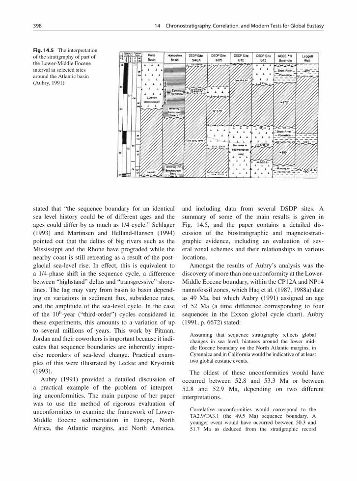
398 14 Chronostratigraphy, Correlation, and Modern Tests for Global Eustasy
Fig. 14.5 The interpretationof the stratigraphy of part ofthe Lower-Middle Eoceneinterval at selected sitesaround the Atlantic basin(Aubry, 1991)
stated that “the sequence boundary for an identicalsea level history could be of different ages and theages could differ by as much as 1/4 cycle.” Schlager(1993) and Martinsen and Helland-Hansen (1994)pointed out that the deltas of big rivers such as theMississippi and the Rhone have prograded while thenearby coast is still retreating as a result of the post-glacial sea-level rise. In effect, this is equivalent toa 1/4-phase shift in the sequence cycle, a differencebetween “highstand” deltas and “transgressive” shore-lines. The lag may vary from basin to basin depend-ing on variations in sediment flux, subsidence rates,and the amplitude of the sea-level cycle. In the caseof the 106-year (“third-order”) cycles considered inthese experiments, this amounts to a variation of upto several millions of years. This work by Pitman,Jordan and their coworkers is important because it indi-cates that sequence boundaries are inherently impre-cise recorders of sea-level change. Practical exam-ples of this were illustrated by Leckie and Krystinik(1993).
Aubry (1991) provided a detailed discussion ofa practical example of the problem of interpret-ing unconformities. The main purpose of her paperwas to use the method of rigorous evaluation ofunconformities to examine the framework of Lower-Middle Eocene sedimentation in Europe, NorthAfrica, the Atlantic margins, and North America,
and including data from several DSDP sites. Asummary of some of the main results is given inFig. 14.5, and the paper contains a detailed dis-cussion of the biostratigraphic and magnetostrati-graphic evidence, including an evaluation of sev-eral zonal schemes and their relationships in variouslocations.
Amongst the results of Aubry’s analysis was thediscovery of more than one unconformity at the Lower-Middle Eocene boundary, within the CP12A and NP14nannofossil zones, which Haq et al. (1987, 1988a) dateas 49 Ma, but which Aubry (1991) assigned an ageof 52 Ma (a time difference corresponding to foursequences in the Exxon global cycle chart). Aubry(1991, p. 6672) stated:
Assuming that sequence stratigraphy reflects globalchanges in sea level, hiatuses around the lower mid-dle Eocene boundary on the North Atlantic margins, inCyrenaica and in California would be indicative of at leasttwo global eustatic events.
The oldest of these unconformities would haveoccurred between 52.8 and 53.3 Ma or between52.8 and 52.9 Ma, depending on two differentinterpretations.
Correlative unconformities would correspond to theTA2.9/TA3.1 (the 49.5 Ma) sequence boundary. Ayounger event would have occurred between 50.3 and51.7 Ma as deduced from the stratigraphic record
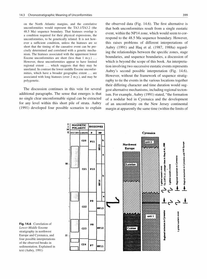
14.3 Chronostratigraphic Meaning of Unconformities 399
on the North Atlantic margins, and the correlativeunconformities would represent the TA3.1/TA3.2 (the48.5 Ma) sequence boundary. That hiatuses overlap isa condition required for their physical expressions, theunconformities, to be genetically related. It is not how-ever a sufficient condition, unless the hiatuses are soshort that the timing of the causative event can be pre-cisely determined and correlated with a genetic mecha-nism. The hiatuses associated with the uppermost lowerEocene unconformities are short (less than 1 m.y.) . . .
However, these unconformities appear to have limitedregional extent . . . which suggests that they may beunrelated. In contrast the lower middle Eocene unconfor-mities, which have a broader geographic extent . . . areassociated with long hiatuses (over 2 m.y.), and may bepolygenetic.
The discussion continues in this vein for severaladditional paragraphs. The sense that emerges is thatno single clear unconformable signal can be extractedfor any level within this short pile of strata. Aubry(1991) developed four possible scenarios to explain
the observed data (Fig. 14.6). The first alternative isthat both unconformities result from a single eustaticevent, within the NP14 zone, which would seem to cor-respond to the 48.5 Ma sequence boundary. However,this raises problems of different interpretations ofAubry (1991) and Haq et al. (1987, 1988a) regard-ing the relationships between the specific zones, stageboundaries, and sequence boundaries, a discussion ofwhich is beyond the scope of this book. An interpreta-tion involving two successive eustatic events representsAubry’s second possible interpretation (Fig. 14.6).However, without the framework of sequence stratig-raphy to tie the events in the various locations togethertheir differing character and time duration would sug-gest alternative mechanisms, including regional tecton-ism. For example, Aubry (1991) stated, “the formationof a nodular bed in Cyrenaica and the developmentof an unconformity on the New Jersey continentalmargin at apparently the same time (within the limits of
Fig. 14.6 Correlation ofLower-Middle Eocenestratigraphy in northwestEurope and Cyrenaica, andfour possible interpretationsof the observed breaks insedimentation. Explained intext (Aubry, 1991)
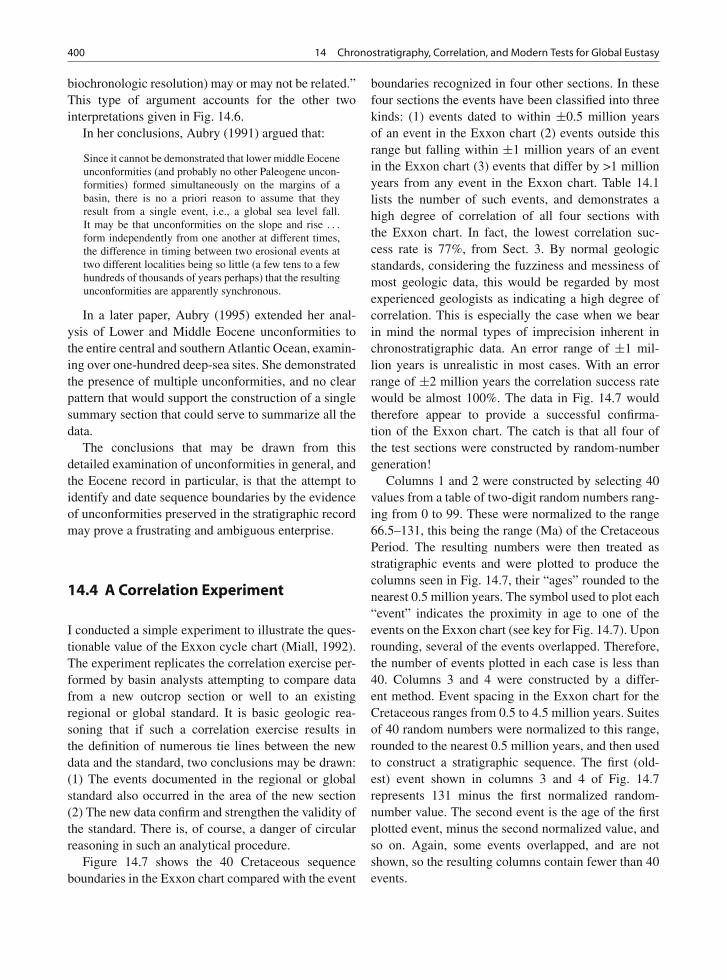
400 14 Chronostratigraphy, Correlation, and Modern Tests for Global Eustasy
biochronologic resolution) may or may not be related.”This type of argument accounts for the other twointerpretations given in Fig. 14.6.
In her conclusions, Aubry (1991) argued that:
Since it cannot be demonstrated that lower middle Eoceneunconformities (and probably no other Paleogene uncon-formities) formed simultaneously on the margins of abasin, there is no a priori reason to assume that theyresult from a single event, i.e., a global sea level fall.It may be that unconformities on the slope and rise . . .
form independently from one another at different times,the difference in timing between two erosional events attwo different localities being so little (a few tens to a fewhundreds of thousands of years perhaps) that the resultingunconformities are apparently synchronous.
In a later paper, Aubry (1995) extended her anal-ysis of Lower and Middle Eocene unconformities tothe entire central and southern Atlantic Ocean, examin-ing over one-hundred deep-sea sites. She demonstratedthe presence of multiple unconformities, and no clearpattern that would support the construction of a singlesummary section that could serve to summarize all thedata.
The conclusions that may be drawn from thisdetailed examination of unconformities in general, andthe Eocene record in particular, is that the attempt toidentify and date sequence boundaries by the evidenceof unconformities preserved in the stratigraphic recordmay prove a frustrating and ambiguous enterprise.
14.4 A Correlation Experiment
I conducted a simple experiment to illustrate the ques-tionable value of the Exxon cycle chart (Miall, 1992).The experiment replicates the correlation exercise per-formed by basin analysts attempting to compare datafrom a new outcrop section or well to an existingregional or global standard. It is basic geologic rea-soning that if such a correlation exercise results inthe definition of numerous tie lines between the newdata and the standard, two conclusions may be drawn:(1) The events documented in the regional or globalstandard also occurred in the area of the new section(2) The new data confirm and strengthen the validity ofthe standard. There is, of course, a danger of circularreasoning in such an analytical procedure.
Figure 14.7 shows the 40 Cretaceous sequenceboundaries in the Exxon chart compared with the event
boundaries recognized in four other sections. In thesefour sections the events have been classified into threekinds: (1) events dated to within ±0.5 million yearsof an event in the Exxon chart (2) events outside thisrange but falling within ±1 million years of an eventin the Exxon chart (3) events that differ by >1 millionyears from any event in the Exxon chart. Table 14.1lists the number of such events, and demonstrates ahigh degree of correlation of all four sections withthe Exxon chart. In fact, the lowest correlation suc-cess rate is 77%, from Sect. 3. By normal geologicstandards, considering the fuzziness and messiness ofmost geologic data, this would be regarded by mostexperienced geologists as indicating a high degree ofcorrelation. This is especially the case when we bearin mind the normal types of imprecision inherent inchronostratigraphic data. An error range of ±1 mil-lion years is unrealistic in most cases. With an errorrange of ±2 million years the correlation success ratewould be almost 100%. The data in Fig. 14.7 wouldtherefore appear to provide a successful confirma-tion of the Exxon chart. The catch is that all four ofthe test sections were constructed by random-numbergeneration!
Columns 1 and 2 were constructed by selecting 40values from a table of two-digit random numbers rang-ing from 0 to 99. These were normalized to the range66.5–131, this being the range (Ma) of the CretaceousPeriod. The resulting numbers were then treated asstratigraphic events and were plotted to produce thecolumns seen in Fig. 14.7, their “ages” rounded to thenearest 0.5 million years. The symbol used to plot each“event” indicates the proximity in age to one of theevents on the Exxon chart (see key for Fig. 14.7). Uponrounding, several of the events overlapped. Therefore,the number of events plotted in each case is less than40. Columns 3 and 4 were constructed by a differ-ent method. Event spacing in the Exxon chart for theCretaceous ranges from 0.5 to 4.5 million years. Suitesof 40 random numbers were normalized to this range,rounded to the nearest 0.5 million years, and then usedto construct a stratigraphic sequence. The first (old-est) event shown in columns 3 and 4 of Fig. 14.7represents 131 minus the first normalized random-number value. The second event is the age of the firstplotted event, minus the second normalized value, andso on. Again, some events overlapped, and are notshown, so the resulting columns contain fewer than 40events.
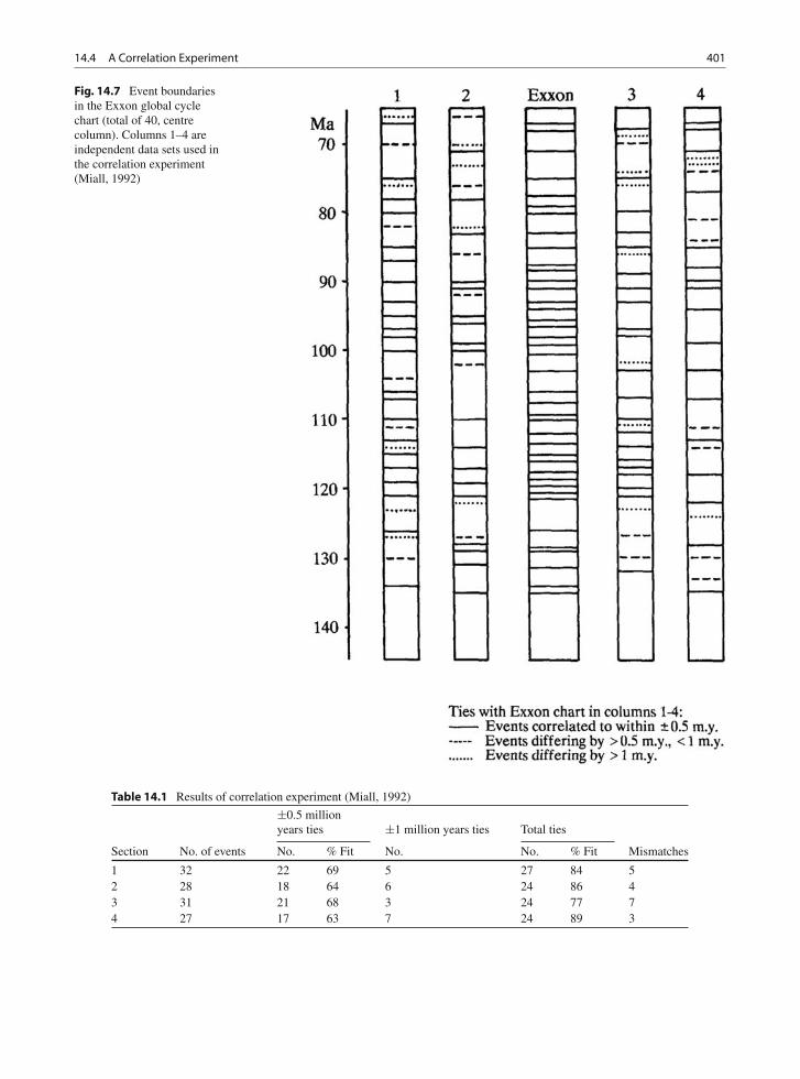
14.4 A Correlation Experiment 401
Fig. 14.7 Event boundariesin the Exxon global cyclechart (total of 40, centrecolumn). Columns 1–4 areindependent data sets used inthe correlation experiment(Miall, 1992)
Table 14.1 Results of correlation experiment (Miall, 1992)
±0.5 millionyears ties ±1 million years ties Total ties
Section No. of events No. % Fit No. No. % Fit Mismatches
1 32 22 69 5 27 84 52 28 18 64 6 24 86 43 31 21 68 3 24 77 74 27 17 63 7 24 89 3
402 14 Chronostratigraphy, Correlation, and Modern Tests for Global Eustasy
Convincing correlations have been achieved by bothrandom positioning of stratigraphic events and randomsequencing of events. Such a high degree of correla-tion must therefore be expected to exist, as a kind ofbackground noise, in any actual field test of the Exxonchart. How can we be sure that any given event on thechart is not the product of local processes and com-pounded error, if random processes can produce suchconvincing correlations? The answer is that we cannot.
This exercise was offered by Miall (1992) in thesame spirit as the classic paper “Cycles and psychol-ogy” by Zeller (1964). In that paper, Zeller succeededin convincing his colleagues to construct stratigraphiccorrelations between sections whose rock types andthicknesses had been compiled entirely from randomnumbers. As Zeller stated, his colleagues “should havefound it completely impossible to make any correla-tion . . . with plotted stratigraphic sections.” But theydid, thus demonstrating the training geologists receivein pattern-recognition techniques.
14.5 Testing for Eustasy: The WayForward
14.5.1 Introduction
In an editorial in the journal Paleoceanography, Miller(1994) set out the nature of the challenge. As he stated,during the last 5 years (he meant the time leadingup to 1994), “there has been a great deal of interestin global sea level (eustatic) changes and their rela-tionship to sequence stratigraphy.” He noted the dif-ficulty in unraveling the triad of processes that controlsedimentation, eustasy, tectonics (thermal subsidence,isostasy, compaction and flexure), and sediment sup-ply, and the challenge of approaching this problemobjectively. In order to test for the very existenceof a eustatic control on the stratigraphic record, theapproach he recommended was to undertake a verydetailed study of Neogene continental margins, forwhich time period, there is already an existing, objec-tive record of eustatic sea-level change in the form ofthe δ18O record.
The Neogene would certainly be a good placeto start, for several important reasons (1) for thismost recent portion of the stratigraphic record,there are excellent, undisturbed successions on the
world’s continental margins; (2) the chronostrati-graphic record for the Neogene is exceptionally goodbecause of the accuracy and precision of the com-bined magnetostratigraphic-biostratigraphic data-base,supplemented by the δ18O record; and (3) the δ18Orecord itself is particularly useful, precisely because itis a record of the repeated, large glacioeustatic fluctu-ations that have occurred on Earth over the last fewmillion years. In other words, we know that therewas a prominent eustatic signal during the Neogene,and it would be an important first step to test thenature of the stratigraphic record through that periodof Earth history.
However, this is only a beginning, because the mainquestion is whether the stratigraphic record is goodenough to demonstrate unequivocally the record ofeustatic sea-level change during periods for which wehave no clear, independent evidence of an eustatic con-trol. As discussed earlier (Chaps. 7 and 11) there isincreasing, but still incomplete, evidence for modest,orbitally-forced eustasy during the so-called green-house climatic era of the Mesozoic, and the recordof the Sloss cycles (Chap. 5) is by now well docu-mented. However, the evidence of what used to betermed “third-order” eustasy (106-year periodicity) ispatchy at best, the question of tectonic control remainsvery much alive, and high-resolution documentationof global correlations between pre-Neogene sequencerecords at all time scales is largely absent. Part IVof this book, leading up to this point, has attemptedto demonstrate that we must begin from scratch inthe endeavour to build a chart of global sea-levelevents. If we persist in using the Haq et al. (1987,1988a) or the Graciansky et al. (1998) curves as start-ing points, we are prejudicing the results from theoutset, because the body of work which those publica-tions represent was essentially based on an inversionof the null hypothesis (no eustatic control) from itsinception. Following Vail’s original concept which, asnoted elsewhere (Miall and Miall, 2002), he formu-lated as a graduate student in the 1950s, Vail, Haq,Graciansky and their colleagues, took it as a start-ing assumption that sequence boundaries are a recordof eustatic sea-level change, and every boundary wasinterpreted in that way (Fig. 12.3b). Christie-Blicket al. (2007, p. 217), citing Jan Hardenbol, one of theVail co-workers, stated:
As Jan Hardenbol writes in his abstract [Hardenbol et al.,1998], “A well-calibrated regional biochronostratigraphic
14.5 Testing for Eustasy: The Way Forward 403
framework is seen as an essential first step towardsan eventual demonstration [Christie-Blick’s italics] ofsychroneity of sequence in basins with different tectonichistories.” In other words, a fundamental assumption ofthe 1998 compilation, and inevitably the outcome of anew global synthesis, is that there is such a synchronouspattern to be discovered.
The test of global correlation rests on, and canonly be as good as, the chronostratigraphic data base.There are two parts to such tests: (1) The reliabilityof a correlation tests rests, in the first instance, on theaccuracy and precision of the global time scale; whatMcGowran (2005, p. 51) called the “integrated magne-tobiochronological timescale” or IMBTS; and (2) Eachtest section must be capable of being fitted to or corre-lated with the IMBTS with an accuracy and precisionadequate to demonstrate the necessary degree of con-temporaneity between the test sequence boundaries,taking into account the frequency of the eustatic sig-nal under consideration. As demonstrated in Sect. 14.2,the significance of unconformities may be ambiguous.For example, a large gap in the record may hide therecord of several high-frequency sea-level events. It isalso shown in Sect. 14.3 that the reality of correlationdepends on the relationship between dating error andevent spacing. A quote from Ricken (1991, p. 773) atthe beginning of part IV, makes the point succinctly:“the range of error is often larger than the actual timespan considered.”
The nature of the chronostratigraphic time scale isclearly critical. In the 12 years since the first edition ofthis book was published, a great deal has changed, andmuch of what was argued in Chap. 13 of that edition(based largely on a study completed in 1994) is nowout of date, and is, therefore, not repeated in this newedition of the book. Integrated time scales have beenunder development since at least the 1960s (Sect. 1.3.3;see also Miall, 1999, Chap. 3). A substantial evolutionin the quality of the scale is in evidence from the workof Berggren et al. (1995) and Gradstein et al. (2004).Nowadays, the IMBTS is managed by the InternationalCommission on Stratigraphy (ICS), the largest scien-tific body within the International Union of GeologicalSciences (IUGS), and the only organization concernedwith stratigraphy on a global scale. The website of theICS, at http://www.stratigraphy.org provides continu-ally updated references to all aspects of the developingtime scale, and detailed documentation of every com-ponent of it on a regional and global basis. A new
journal, Stratigraphy, was founded in 2004, to serve asa platform for research publications in the field, and theIUGS journal Episodes continues to provide updateson noteworthy events.
In the next section, we discuss the general methodsof correlation and dating currently in use, concludingwith a review of the accuracy and precision with whichsequences can be tied to the global time scale.
14.5.2 The Dating and Correlationof Stratigraphic Events: PotentialSources of Uncertainty
The dating and correlation of stratigraphic eventsbetween basins, where physical tracing-out of bedscannot be performed, involve the use of biostratigraphyand other chronostratigraphic methods. The process isa complex one, fraught with many possible sources oferror. What follows is an attempt to break the processdown into a series of discrete “steps”, although in prac-tice, dating successions and erecting local and globaltime scales is an iterative process, and no individualstratigrapher follows the entire procedural order as setout here. The geologist is able to draw on the accumu-lated knowledge of the geological time scale that has(as noted earlier) been undergoing improvements formore than 200 years, but each new case study presentsits own unique problems.
There are two related but distinct problems to beaddressed in the construction of a global stratigraphicframework. On the one hand, we need to test whethersimilar stratigraphic events (such as sequence bound-aries) and successions of events (e.g., successions ofsequences) have the same ages in different parts of theearth, in order to test models of global causality (e.g.,eustasy). From this perspective, precise correlation iscritical, but determination of absolute age is not. Onthe other hand, there is the ongoing effort to deter-mine the precise age of stratigraphic events, leadingto continuing refinements in the global time scale. Ineither case, the potential error, or uncertainty, involvedwith one or more of the “steps” described above mustbe acknowledged and addressed as part of a determi-nation of the level of refinement to be expected instratigraphic interpretation.
Dating and correlation methods are discussed instandard textbooks (e.g., Miall, 1999, Chap. 3; Boggs,
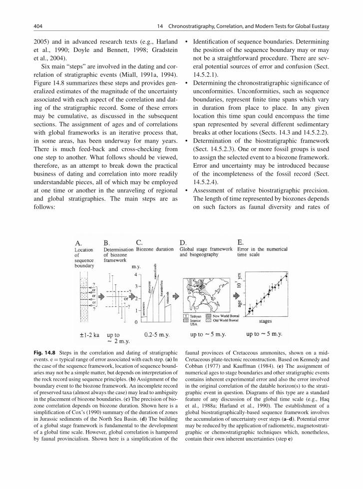
404 14 Chronostratigraphy, Correlation, and Modern Tests for Global Eustasy
2005) and in advanced research texts (e.g., Harlandet al., 1990; Doyle and Bennett, 1998; Gradsteinet al., 2004).
Six main “steps” are involved in the dating and cor-relation of stratigraphic events (Miall, 1991a, 1994).Figure 14.8 summarizes these steps and provides gen-eralized estimates of the magnitude of the uncertaintyassociated with each aspect of the correlation and dat-ing of the stratigraphic record. Some of these errorsmay be cumulative, as discussed in the subsequentsections. The assignment of ages and of correlationswith global frameworks is an iterative process that,in some areas, has been underway for many years.There is much feed-back and cross-checking fromone step to another. What follows should be viewed,therefore, as an attempt to break down the practicalbusiness of dating and correlation into more readilyunderstandable pieces, all of which may be employedat one time or another in the unraveling of regionaland global stratigraphies. The main steps are asfollows:
• Identification of sequence boundaries. Determiningthe position of the sequence boundary may or maynot be a straightforward procedure. There are sev-eral potential sources of error and confusion (Sect.14.5.2.1).
• Determining the chronostratigraphic significance ofunconformities. Unconformities, such as sequenceboundaries, represent finite time spans which varyin duration from place to place. In any givenlocation this time span could encompass the timespan represented by several different sedimentarybreaks at other locations (Sects. 14.3 and 14.5.2.2).
• Determination of the biostratigraphic framework(Sect. 14.5.2.3). One or more fossil groups is usedto assign the selected event to a biozone framework.Error and uncertainty may be introduced becauseof the incompleteness of the fossil record (Sect.14.5.2.4).
• Assessment of relative biostratigraphic precision.The length of time represented by biozones dependson such factors as faunal diversity and rates of
Fig. 14.8 Steps in the correlation and dating of stratigraphicevents. e = typical range of error associated with each step. (a) Inthe case of the sequence framework, location of sequence bound-aries may not be a simple matter, but depends on interpretation ofthe rock record using sequence principles. (b) Assignment of theboundary event to the biozone framework. An incomplete recordof preserved taxa (almost always the case) may lead to ambiguityin the placement of biozone boundaries. (c) The precision of bio-zone correlation depends on biozone duration. Shown here is asimplification of Cox’s (1990) summary of the duration of zonesin Jurassic sediments of the North Sea Basin. (d) The buildingof a global stage framework is fundamental to the developmentof a global time scale. However, global correlation is hamperedby faunal provincialism. Shown here is a simplification of the
faunal provinces of Cretaceous ammonites, shown on a mid-Cretaceous plate-tectonic reconstruction. Based on Kennedy andCobban (1977) and Kauffman (1984). (e) The assignment ofnumerical ages to stage boundaries and other stratigraphic eventscontains inherent experimental error and also the error involvedin the original correlation of the datable horizon(s) to the strati-graphic event in question. Diagrams of this type are a standardfeature of any discussion of the global time scale (e.g., Haqet al., 1988a; Harland et al., 1990). The establishment of aglobal biostratigraphically-based sequence framework involvesthe accumulation of uncertainty over steps (a–d). Potential errormay be reduced by the application of radiometric, magnetostrati-graphic or chemostratigraphic techniques which, nonetheless,contain their own inherent uncertainties (step e)
14.5 Testing for Eustasy: The Way Forward 405
evolution. It varies considerably through geologi-cal time and between different fossil groups (Sect.14.5.4).
• Correlation of biozones with the global stage frame-work. The existing stage framework was, withnotable exceptions, built from the study of macro-fossils in European type sections. Correlation withthis framework raises questions of environmentallimitations on biozone extent, our ability to inter-relate zonal schemes built from different fossilgroups, and problems of global faunal and floralprovinciality (Sect. 14.5.5).
• Assignment of absolute ages. The use of radiomet-ric and magnetostratigraphic dating methods, plusthe increasing use of chemostratigraphy (oxygenand strontium isotope concentrations) permits theassignment of absolute ages in years to the biostrati-graphic framework. Such techniques also constitutemethods of correlation in their own right, especiallywhere fossils are sparse (Sect. 14.5.6). Carbon iso-tope data have also been used in a few specializedstudies (Sect. 14.8).
14.5.2.1 Identification of Sequence Boundaries
The first step is that a well section, outcrop profileor seismic record is analyzed and the positions ofsequence boundaries are determined from the verticalsuccession of lithofacies or from the architecture of theseismic reflections.
There is substantial residual disagreement aboutthe definition of sequences, as discussed in Chap. 2(see Fig. 2.22). For example, are the falling-stagedeposits assigned to the top of one sequence or tothe base of the overlying sequence? The difference inthe placement, and therefore the age, of the sequenceboundary changes significantly, depending on thesequence model used.
In outcrop and well data, other possible errors inthis procedure arise from the potential for confusionbetween allogenic and autogenic causes for the breaksin the stratigraphic record. Autogenic causes includecondensed sequences, ravinement surfaces, and chan-nel scours. Various other processes also generate sed-imentary breaks that may be confused with sequenceboundaries, such as environmental change in carbonatesettings (e.g., drowning unconformities). The subjectis discussed at some length in Chap. 2. These errors
could lead to possible errors in boundary placement ofat least several meters. Given a typical sedimentationrate of 0.1 m/ka, a 10 m error is equal to 100 ka.
In seismic sections, poor seismic resolution mayresult in the miscorrelation of thin units (e.g.,Cartwright et al., 1993). Armentrout et al. (1993) usedpetrophysical logs tied to seismic cross-sections todevelop a correlation grid in Paleogene deposits in theNorth Sea. In this basin, where wells are up to tens ofkilometres apart, they determined that tracing markersaround correlation loops could result in mismatchesof up to 30 m. Errors of this magnitude might not beexpected in mature areas, such as the Alberta Basin orthe US Gulf Coast.
Vail et al. (1977) had proposed that sequence bound-aries could be dated more accurately by tracing theminto areas of continuous sedimentation, such as indeep-marine settings. The equivalent of the uncon-formable sequence boundary was to be termed thecorrelative conformity. However, in conformable, con-tinuous sections there is not likely to be any poten-tial for the development of recognizable reflections(changes in acoustic impedance), and so the valueof the correlative conformity concept is hypothetical.Furthermore, given the problems of tracing surfaceson seismic sections through coastal successions, aregion of substantial autogenic facies change and localscour, into the deep marine, the likelihood of beingto locate precisely the correct horizon might be ques-tioned. In any case, as Christie-Blick et al. (2007,p. 222) pointed out, the diachroneity of sequenceboundaries, the fact that they represent spans of time,rather than instantaneous events, means that “at somescale, unconformities pass laterally not into correlativeconformities, but into correlative intervals [my italics].Such considerations begin to be important as the reso-lution of the geological timescale improves at a globalscale”
14.5.2.2 Chronostratigraphic Meaningof Unconformities
Assigning an age to an unconformity surface is notnecessarily a simple matter, as discussed in Sect.14.3. An unconformity represents a finite time span; itmay have a complex genesis, representing amalgama-tion of more than one event, more than one differenttype of event (e.g., a combination of tectonism and
406 14 Chronostratigraphy, Correlation, and Modern Tests for Global Eustasy
eustasy), or even a phase-amplification effect of thesuperimposition of two or more different eustatic sig-nals. Unconformities may be markedly diachronous,because the transgressions and regressions that occurduring the genesis of a stratigraphic sequence couldspan the entire duration of the sequence. As notedin Sect. 13.1, Kidwell (1988) demonstrated that thisresults in an offset in sequence boundary unconformi-ties by as much as one half of a cycle between basincentre and basin margin.
Detailed chronostratigraphic analysis of some welldated sections (see summary in Sect. 13.1) has shownthat as little as 24% to as much as 82% of elapsedtime is stored in the sedimentary succession, with theremainder of the time span represented by the uncon-formities, in other words, the sequence boundaries.Ager (1981, 1993) argued for even greater extremesof missing time, but we concern ourselves here withthe (hopefully) more continuous sections that formthe basis for the modern definitions of key sequenceprofiles (e.g., those on the New Jersey continentalmargin, and the Wanganui Basin of New Zealand).Within tectonostratigraphic successions lasting tensof millions of years, such partial preservation of thesedimentary record could include unconformities rep-resenting many millions of years, which could meanthat lengthy portions of any high-frequency sequencerecord are entirely missing. At the 106–7-year timescale, chronostratigraphic precision should be ade-quate at least to reveal the scale of such gaps, butit is this problem of missing cycles buried withina lower-frequency record that underlies the problemof testing for a regional (let alone, global) record ofhigh-frequency sequences. The problem is particularlyacute in the case of cyclostratigraphy—the currentresearch endeavour to extend the astrochronologicaltime scale into deep geologic time, beyond the limitsof “continuous” deep-sea cores and exposed pelagicsections (e.g., Hilgen, 1991) into the realm of the“floating” section (Miall and Miall, 2004). We returnto this topic in Sect. 14.7.
14.5.2.3 Determination of the BiostratigraphicFramework
Sequence boundaries are dated and correlated bybiostratigraphic, radiometric or magnetostratigraphictechniques. The potential for error here stems from the
imperfection of the stratigraphic record, including itsfossil content. Ranges of useful biostratigraphic indi-cators are commonly denoted by the acronyms FADand LAD, which mean first- [lowest] and last- [high-est] appearance datums. First and last taxon occur-rences could vary in position by several meters to evena few tens of meters among sections of the same age.Errors in age assignment of complete biozones or halfzones are not uncommon.
The biostratigraphic data base for the global timescale has experienced an orders-of-magnitude expan-sion since microfossils began to take on increasingimportance in subsurface petroleum exploration inthe post-war years, and following the commencementof the Deep Sea Drilling Project (DSDP) in 1968(Berggren et al., 1995; McGowran, 2005). The mainbasis for the global time scale consists of the classicalmacrofossil assemblages (e.g., ammonites, graptolites)that have been in use, in many cases, since the nine-teenth century. Supplementing macrofossil and micro-fossil collections from outcrops, drilling operations onland and beneath the oceans have contributed a vastbiostratigraphic sample base over the last few decades,permitting the evaluation of a wide range of microfos-sils for biostratigraphic purposes in all the world’s tec-tonic and climatic zones. The result has been a consid-erable improvement in the flexibility and precision ofdating methods, and much incremental improvementin the global time scale. The foraminiferal and nanno-fossil record for the Cenozoic is now precise enoughthat meaningful tests of the global-eustasy paradigmcan now be attempted, and this is discussed inSect. 14.6.
As noted by Cope (1993), detailed, meticulous taxo-nomic work still holds the potential for much improvedbiostratigraphic resolution and flexibility at all lev-els of the geological column. In older Mesozoic andPaleozoic strata, such fossil groups as conodonts andgraptolites have yielded very refined biostratigraphiczonal systems. However, this potential has yet to befully tapped by sequence stratigraphers.
The various types of zones, and the methods for theerection of zonal schemes, are subjects dealt with instandard textbooks and reviews (e.g., Kauffman andHazel, 1977a; Doyle and Bennett, 1998; Miall, 1999,Chap. 3; McGowran, 2005), and are not discussedhere. The purpose of this section is to focus on twomajor problems that affect the accuracy and precisionof biostratigraphic correlation.
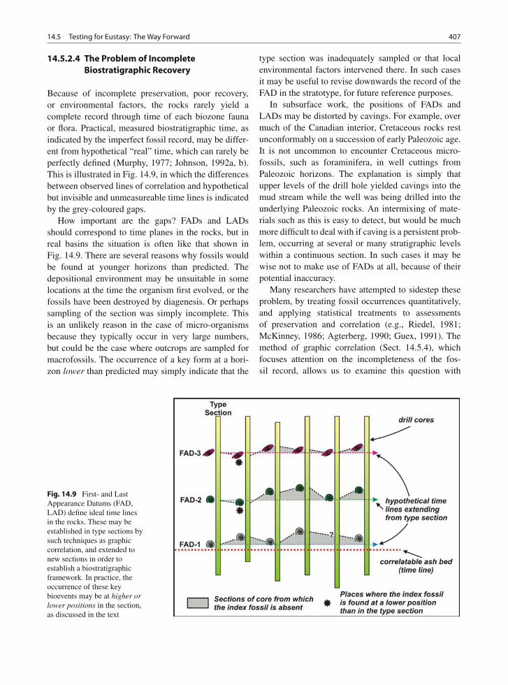
14.5 Testing for Eustasy: The Way Forward 407
14.5.2.4 The Problem of IncompleteBiostratigraphic Recovery
Because of incomplete preservation, poor recovery,or environmental factors, the rocks rarely yield acomplete record through time of each biozone faunaor flora. Practical, measured biostratigraphic time, asindicated by the imperfect fossil record, may be differ-ent from hypothetical “real” time, which can rarely beperfectly defined (Murphy, 1977; Johnson, 1992a, b).This is illustrated in Fig. 14.9, in which the differencesbetween observed lines of correlation and hypotheticalbut invisible and unmeasureable time lines is indicatedby the grey-coloured gaps.
How important are the gaps? FADs and LADsshould correspond to time planes in the rocks, but inreal basins the situation is often like that shown inFig. 14.9. There are several reasons why fossils wouldbe found at younger horizons than predicted. Thedepositional environment may be unsuitable in somelocations at the time the organism first evolved, or thefossils have been destroyed by diagenesis. Or perhapssampling of the section was simply incomplete. Thisis an unlikely reason in the case of micro-organismsbecause they typically occur in very large numbers,but could be the case where outcrops are sampled formacrofossils. The occurrence of a key form at a hori-zon lower than predicted may simply indicate that the
type section was inadequately sampled or that localenvironmental factors intervened there. In such casesit may be useful to revise downwards the record of theFAD in the stratotype, for future reference purposes.
In subsurface work, the positions of FADs andLADs may be distorted by cavings. For example, overmuch of the Canadian interior, Cretaceous rocks restunconformably on a succession of early Paleozoic age.It is not uncommon to encounter Cretaceous micro-fossils, such as foraminifera, in well cuttings fromPaleozoic horizons. The explanation is simply thatupper levels of the drill hole yielded cavings into themud stream while the well was being drilled into theunderlying Paleozoic rocks. An intermixing of mate-rials such as this is easy to detect, but would be muchmore difficult to deal with if caving is a persistent prob-lem, occurring at several or many stratigraphic levelswithin a continuous section. In such cases it may bewise not to make use of FADs at all, because of theirpotential inaccuracy.
Many researchers have attempted to sidestep theseproblem, by treating fossil occurrences quantitatively,and applying statistical treatments to assessmentsof preservation and correlation (e.g., Riedel, 1981;McKinney, 1986; Agterberg, 1990; Guex, 1991). Themethod of graphic correlation (Sect. 14.5.4), whichfocuses attention on the incompleteness of the fos-sil record, allows us to examine this question with
Fig. 14.9 First- and LastAppearance Datums (FAD,LAD) define ideal time linesin the rocks. These may beestablished in type sections bysuch techniques as graphiccorrelation, and extended tonew sections in order toestablish a biostratigraphicframework. In practice, theoccurrence of these keybioevents may be at higher orlower positions in the section,as discussed in the text
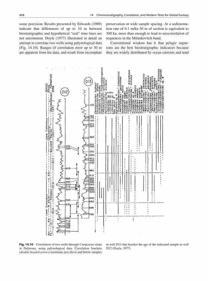
408 14 Chronostratigraphy, Correlation, and Modern Tests for Global Eustasy
some precision. Results presented by Edwards (1989)indicate that differences of up to 10 m betweenbiostratigraphic and hypothetical “real” time lines arenot uncommon. Doyle (1977) illustrated in detail anattempt to correlate two wells using palynological data(Fig. 14.10). Ranges of correlation error up to 30 mare apparent from his data, and result from incomplete
preservation or wide sample spacing. At a sedimenta-tion rate of 0.1 m/ka 30 m of section is equivalent to300 ka, more than enough to lead to miscorrelation ofsequences in the Milankovitch band.
Conventional wisdom has it that pelagic organ-isms are the best biostratigraphic indicators becausethey are widely distributed by ocean currents and tend
Fig. 14.10 Correlation of two wells through Cretaceous stratain Delaware, using palynological data. Correlation brackets(double-headed arrows) terminate just above and below samples
in well D13 that bracket the age of the indicated sample in wellD12 (Doyle, 1977)
14.5 Testing for Eustasy: The Way Forward 409
to be less environmentally sensitive. However, recentdetailed studies of nektonic and planktonic forms haveindicated a wide range of factors that lead to unevendistribution and preservation even of these more desir-able forms. Thierstein (1981) and Roth and Bowdler(1981), in studies of Cretaceous nannoplankton, dis-cussed mechanisms that affected distribution of theseorganisms. Among the most important environmen-tal factors are changes in ocean currents, which affectwater temperatures and the concentrations of oxygenand carbon dioxide and nutrients in the seas. Changesin temperature and sea level affect the position of thecarbonate compensation depth in the oceans, and henceaffect the rates of dissolution and preservability ofcalcareous forms in deep-sea sediments. Conversely,bottom dwelling faunas, which are specifically limitedin their geographical distribution because of ecologicalfactors, may exhibit a diversity and rapid evolution-ary turn-over that makes them ideal as biostratigraphicindicators in specific stratigraphic settings. For exam-ple, many corals have been found to be of greatbiostratigraphic utility in the study of reef limestonesof all ages.
14.5.2.5 Diachroneity of the BiostratigraphicRecord
Another common item of conventional wisdom isthat evolutionary changes in faunal assemblages aredispersed so rapidly that, on geological time scales,they can essentially be regarded as instantaneous.This argument is used, in particular, to justify theinterpretation of FADs as time-stratigraphic events(setting aside the problems of preservation discussedabove). However, this is not always the case. Someexamples of detailed work have demonstrated con-siderable diachroneity in important pelagic fossilgroups.
MacLeod and Keller (1991) explored the com-pleteness of the stratigraphic sections that span theCretaceous-Tertiary boundary, as a basis for an exam-ination of the various hypotheses that have beenproposed to explain the dramatic global extinctionoccurring at that time. They used graphic correla-tion methods, and were able to demonstrate thatmany foraminiferal FADs and LADs are diachronous.Maximum diachroneity at this time is indicated bythe species Subbotina pseudobulloides, the FAD of
which may vary by up to 250 ka between Texasand North Africa. However, it is not clear how muchof this apparent diachroneity is due to preservationalfactors.
An even more startling example of diachroneityis that reported by Jenkins and Gamson (1993). TheFAD of the Neogene foraminifera Globorotalia trun-catulinoides differs by 600 ka between the southeastPacific Ocean and the North Atlantic Ocean, basedon analysis of much DSDP material. This is inter-preted as indicating the time taken for the organismto migrate northward from the South Pacific followingits first evolutionary appearance there. As Jenkins andGamson (1993) concluded
The implications are that some of the well documentedevolutionary lineages in the Cenozoic may show similarpatterns of evolution being limited to discrete ocean watermasses followed by later migration into other oceans . . .
If this is true, then some of these so-called ‘datum planes’are diachronous.
This conclusion is of considerable importance,because the result is derived from excellent data, andcan, therefore, be regarded as highly reliable, andrelates to one of the most universally preferred fossilgroups for Mesozoic-Cenozoic biostratigraphic pur-poses, the foraminifera. It would appear to suggesta limit of up to about one half million years on theprecision that can be expected of any biostratigraphicevent.
The two cases reported here may or may not be afair representation of the magnitude of diachroneity ingeneral. After a great deal of study, experienced bios-tratigraphers commonly determine that some speciesare more reliable or consistent in their occurrencethan others. Such forms may be termed index fos-sils, and receive a prominence reflecting their use-fulness in stratigraphic studies. Studies may indicatethat some groups are more reliable than others asbiostratigraphic indicators. For example, Ziegler et al.(1968) demonstrated that brachiopod successions inthe Welsh Paleozoic record were facies controlled andmarkedly diachronous, based on the use of the zonalscheme provided by graptolites as the primary indica-tor of relative time. Armentrout (1981) used diatomzones to demonstrate that molluscan stages are timetransgressive in the Cenozoic rocks of the NorthwestUS. Wignall (1991) demonstrated the diachroneity ofJurassic ostracod zones.
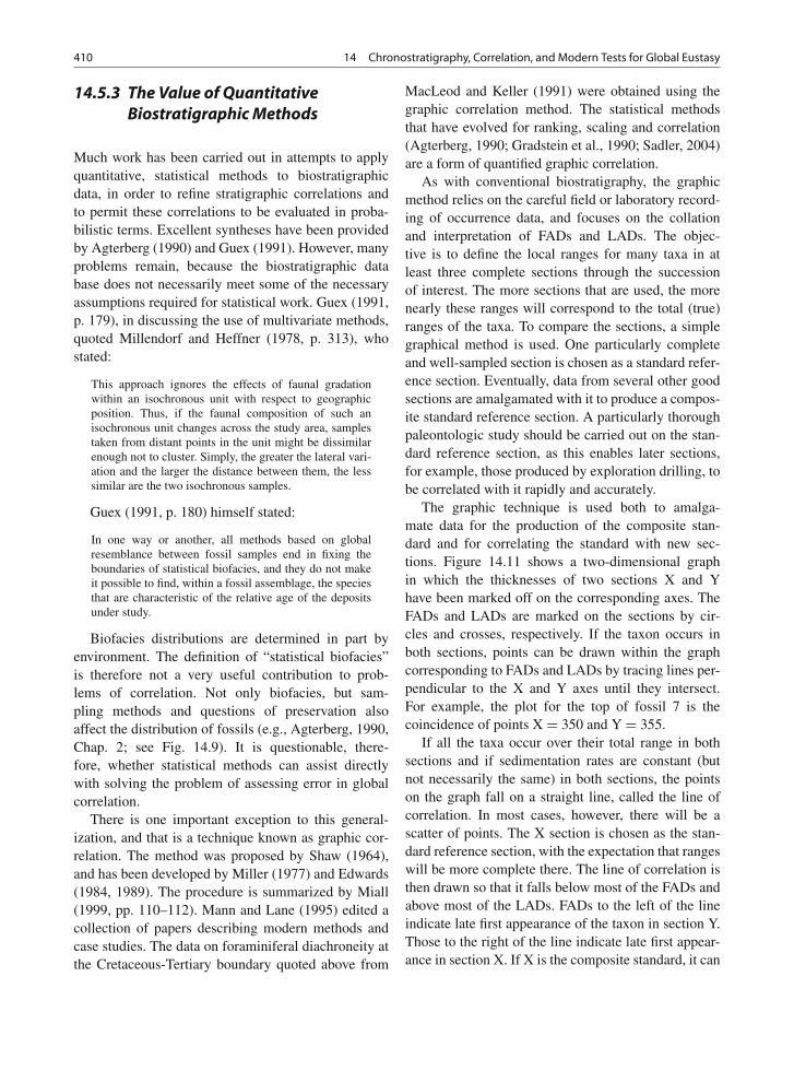
410 14 Chronostratigraphy, Correlation, and Modern Tests for Global Eustasy
14.5.3 The Value of QuantitativeBiostratigraphic Methods
Much work has been carried out in attempts to applyquantitative, statistical methods to biostratigraphicdata, in order to refine stratigraphic correlations andto permit these correlations to be evaluated in proba-bilistic terms. Excellent syntheses have been providedby Agterberg (1990) and Guex (1991). However, manyproblems remain, because the biostratigraphic database does not necessarily meet some of the necessaryassumptions required for statistical work. Guex (1991,p. 179), in discussing the use of multivariate methods,quoted Millendorf and Heffner (1978, p. 313), whostated:
This approach ignores the effects of faunal gradationwithin an isochronous unit with respect to geographicposition. Thus, if the faunal composition of such anisochronous unit changes across the study area, samplestaken from distant points in the unit might be dissimilarenough not to cluster. Simply, the greater the lateral vari-ation and the larger the distance between them, the lesssimilar are the two isochronous samples.
Guex (1991, p. 180) himself stated:
In one way or another, all methods based on globalresemblance between fossil samples end in fixing theboundaries of statistical biofacies, and they do not makeit possible to find, within a fossil assemblage, the speciesthat are characteristic of the relative age of the depositsunder study.
Biofacies distributions are determined in part byenvironment. The definition of “statistical biofacies”is therefore not a very useful contribution to prob-lems of correlation. Not only biofacies, but sam-pling methods and questions of preservation alsoaffect the distribution of fossils (e.g., Agterberg, 1990,Chap. 2; see Fig. 14.9). It is questionable, there-fore, whether statistical methods can assist directlywith solving the problem of assessing error in globalcorrelation.
There is one important exception to this general-ization, and that is a technique known as graphic cor-relation. The method was proposed by Shaw (1964),and has been developed by Miller (1977) and Edwards(1984, 1989). The procedure is summarized by Miall(1999, pp. 110–112). Mann and Lane (1995) edited acollection of papers describing modern methods andcase studies. The data on foraminiferal diachroneity atthe Cretaceous-Tertiary boundary quoted above from
MacLeod and Keller (1991) were obtained using thegraphic correlation method. The statistical methodsthat have evolved for ranking, scaling and correlation(Agterberg, 1990; Gradstein et al., 1990; Sadler, 2004)are a form of quantified graphic correlation.
As with conventional biostratigraphy, the graphicmethod relies on the careful field or laboratory record-ing of occurrence data, and focuses on the collationand interpretation of FADs and LADs. The objec-tive is to define the local ranges for many taxa in atleast three complete sections through the successionof interest. The more sections that are used, the morenearly these ranges will correspond to the total (true)ranges of the taxa. To compare the sections, a simplegraphical method is used. One particularly completeand well-sampled section is chosen as a standard refer-ence section. Eventually, data from several other goodsections are amalgamated with it to produce a compos-ite standard reference section. A particularly thoroughpaleontologic study should be carried out on the stan-dard reference section, as this enables later sections,for example, those produced by exploration drilling, tobe correlated with it rapidly and accurately.
The graphic technique is used both to amalga-mate data for the production of the composite stan-dard and for correlating the standard with new sec-tions. Figure 14.11 shows a two-dimensional graphin which the thicknesses of two sections X and Yhave been marked off on the corresponding axes. TheFADs and LADs are marked on the sections by cir-cles and crosses, respectively. If the taxon occurs inboth sections, points can be drawn within the graphcorresponding to FADs and LADs by tracing lines per-pendicular to the X and Y axes until they intersect.For example, the plot for the top of fossil 7 is thecoincidence of points X = 350 and Y = 355.
If all the taxa occur over their total range in bothsections and if sedimentation rates are constant (butnot necessarily the same) in both sections, the pointson the graph fall on a straight line, called the line ofcorrelation. In most cases, however, there will be ascatter of points. The X section is chosen as the stan-dard reference section, with the expectation that rangeswill be more complete there. The line of correlation isthen drawn so that it falls below most of the FADs andabove most of the LADs. FADs to the left of the lineindicate late first appearance of the taxon in section Y.Those to the right of the line indicate late first appear-ance in section X. If X is the composite standard, it can
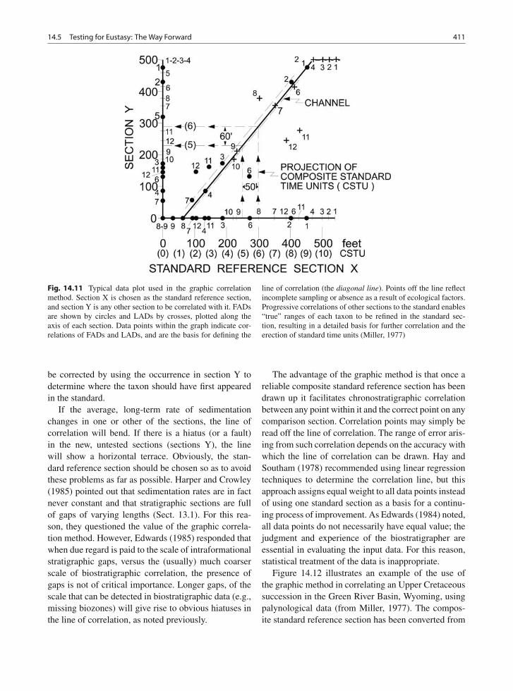
14.5 Testing for Eustasy: The Way Forward 411
Fig. 14.11 Typical data plot used in the graphic correlationmethod. Section X is chosen as the standard reference section,and section Y is any other section to be correlated with it. FADsare shown by circles and LADs by crosses, plotted along theaxis of each section. Data points within the graph indicate cor-relations of FADs and LADs, and are the basis for defining the
line of correlation (the diagonal line). Points off the line reflectincomplete sampling or absence as a result of ecological factors.Progressive correlations of other sections to the standard enables“true” ranges of each taxon to be refined in the standard sec-tion, resulting in a detailed basis for further correlation and theerection of standard time units (Miller, 1977)
be corrected by using the occurrence in section Y todetermine where the taxon should have first appearedin the standard.
If the average, long-term rate of sedimentationchanges in one or other of the sections, the line ofcorrelation will bend. If there is a hiatus (or a fault)in the new, untested sections (sections Y), the linewill show a horizontal terrace. Obviously, the stan-dard reference section should be chosen so as to avoidthese problems as far as possible. Harper and Crowley(1985) pointed out that sedimentation rates are in factnever constant and that stratigraphic sections are fullof gaps of varying lengths (Sect. 13.1). For this rea-son, they questioned the value of the graphic correla-tion method. However, Edwards (1985) responded thatwhen due regard is paid to the scale of intraformationalstratigraphic gaps, versus the (usually) much coarserscale of biostratigraphic correlation, the presence ofgaps is not of critical importance. Longer gaps, of thescale that can be detected in biostratigraphic data (e.g.,missing biozones) will give rise to obvious hiatuses inthe line of correlation, as noted previously.
The advantage of the graphic method is that once areliable composite standard reference section has beendrawn up it facilitates chronostratigraphic correlationbetween any point within it and the correct point on anycomparison section. Correlation points may simply beread off the line of correlation. The range of error aris-ing from such correlation depends on the accuracy withwhich the line of correlation can be drawn. Hay andSoutham (1978) recommended using linear regressiontechniques to determine the correlation line, but thisapproach assigns equal weight to all data points insteadof using one standard section as a basis for a continu-ing process of improvement. As Edwards (1984) noted,all data points do not necessarily have equal value; thejudgment and experience of the biostratigrapher areessential in evaluating the input data. For this reason,statistical treatment of the data is inappropriate.
Figure 14.12 illustrates an example of the use ofthe graphic method in correlating an Upper Cretaceoussuccession in the Green River Basin, Wyoming, usingpalynological data (from Miller, 1977). The compos-ite standard reference section has been converted from
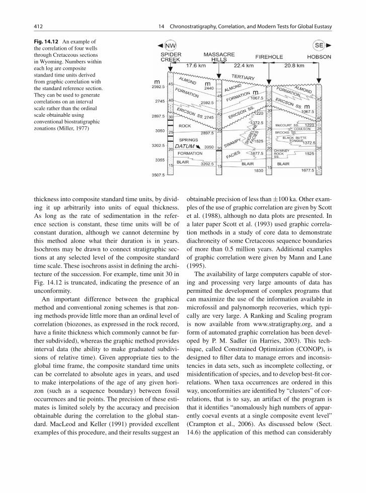
412 14 Chronostratigraphy, Correlation, and Modern Tests for Global Eustasy
Fig. 14.12 An example ofthe correlation of four wellsthrough Cretaceous sectionsin Wyoming. Numbers withineach log are compositestandard time units derivedfrom graphic correlation withthe standard reference section.They can be used to generatecorrelations on an intervalscale rather than the ordinalscale obtainable usingconventional biostratigraphiczonations (Miller, 1977)
thickness into composite standard time units, by divid-ing it up arbitrarily into units of equal thickness.As long as the rate of sedimentation in the refer-ence section is constant, these time units will be ofconstant duration, although we cannot determine bythis method alone what their duration is in years.Isochrons may be drawn to connect stratigraphic sec-tions at any selected level of the composite standardtime scale. These isochrons assist in defining the archi-tecture of the succession. For example, time unit 30 inFig. 14.12 is truncated, indicating the presence of anunconformity.
An important difference between the graphicalmethod and conventional zoning schemes is that zon-ing methods provide little more than an ordinal level ofcorrelation (biozones, as expressed in the rock record,have a finite thickness which commonly cannot be fur-ther subdivided), whereas the graphic method providesinterval data (the ability to make graduated subdivi-sions of relative time). Given appropriate ties to theglobal time frame, the composite standard time unitscan be correlated to absolute ages in years, and usedto make interpolations of the age of any given hori-zon (such as a sequence boundary) between fossiloccurrences and tie points. The precision of these esti-mates is limited solely by the accuracy and precisionobtainable during the correlation to the global stan-dard. MacLeod and Keller (1991) provided excellentexamples of this procedure, and their results suggest an
obtainable precision of less than ±100 ka. Other exam-ples of the use of graphic correlation are given by Scottet al. (1988), although no data plots are presented. Ina later paper Scott et al. (1993) used graphic correla-tion methods in a study of core data to demonstratediachroneity of some Cretaceous sequence boundariesof more than 0.5 million years. Additional examplesof graphic correlation were given by Mann and Lane(1995).
The availability of large computers capable of stor-ing and processing very large amounts of data haspermitted the development of complex programs thatcan maximize the use of the information available inmicrofossil and palynomorph recoveries, which typi-cally are very large. A Ranking and Scaling programis now available from www.stratigraphy.org, and aform of automated graphic correlation has been devel-oped by P. M. Sadler (in Harries, 2003). This tech-nique, called Constrained Optimization (CONOP), isdesigned to filter data to manage errors and inconsis-tencies in data sets, such as incomplete collecting, ormisidentification of species, and to develop best-fit cor-relations. When taxa occurrences are ordered in thisway, unconformities are identified by “clusters” of cor-relations, that is to say, an artifact of the program isthat it identifies “anomalously high numbers of appar-ently coeval events at a single composite event level”(Crampton et al., 2006). As discussed below (Sect.14.6) the application of this method can considerably
14.5 Testing for Eustasy: The Way Forward 413
facilitate the task of regional and interregional correla-tion, achieving precision in local, relative correlationsin the 105-year range.
14.5.4 Assessment of RelativeBiostratigraphic Precision
The precision of biostratigraphic zonation is partly areflection of the diversity and rate of evolution of thefossil group used to define the zonal scheme. Thisvaries considerably over time and between differentfossil groups. For example, Fig. 14.8c is a simplifiedversion of a chart provided by Cox (1990) to illustratethe time resolution of various fossil groups used in thesubsurface correlation of Jurassic strata in the NorthSea Basin. The best time resolution is obtained fromammonites, which have been subdivided into biozonesrepresenting about 0.5 million years. Hallam (1992a)and Cope (1993) quoted detailed studies of Britishammonites that yield a local resolution estimated atless than 200 ka, but such a level of accuracy can-not yet be extended globally for the purpose of testingthe global cyclicity model, and ammonites are rarelyobtainable in subsurface work. The microfossil groupsthat are typically used provide time resolution rangingfrom 1 to 4 million years. The sloping caps to each barin Fig. 14.8c illustrate the varying length of biozonesfor each fossil group through the Jurassic. For exampledinocyst zones each represent about 1 million years inthe Late Jurassic but are about 3 million years long inthe Early Jurassic.
Moore and Romine (1981), in a study of the contri-butions to stratigraphy of the DSDP project, examinedthe question of biostratigraphic resolution in detail. In1975 (the latest data examined in this paper) the reso-lution of foraminiferal zonation, as expressed by theaverage duration of biozones, varied from 4 millionyears during much of the Cretaceous, to 1 million yearsduring parts of the Neogene. Srinivasan and Kennett(1981) found that foraminiferal zones in the Neogeneranged from 0.4 to 2.0 million years. They suggestedthat
Experience shows that this resolution seems to havereached its practical limit. This . . . is largely constrainedby the evolution of important new species within dis-tinctive and useful lineages. Further subdivision of theexisting zones is of course possible when additional
criteria are employed, but further subdivision of zonesinto shorter time-intervals does not guarantee a practi-cal scheme for biostratigraphic subdivision; that is, suchzones may not be widely applicable.
Combinations of foraminiferal zones with othermicroorganisms occurring in the same sediments, suchas calcareous nannofossils and radiolaria, increasebiostratigraphic precision (Moore and Romine, 1981;Srinivasan and Kennett, 1981; Cope, 1993), but notnecessarily by a large amount. Figure 14.13 showsthe biostratigraphic resolution that was achievablein 1975 based on combinations of all three fossilgroups. The combination of three fossil groups doesincreases accuracy and precision (to a 0.3–2.0 mil-lion years range), but commonly zonal boundaries ofmore than one group coincide in time, so that noadditional precision is provided. It was not thoughtlikely that precision would increase by very much. Infact, the system of numbered microfossil zones thatwas established early during the DSDP project stillformed the basis for the Exxon global cycle chartsof the late 1980s. As noted earlier in this book, theanalysis of different fossil groups from the same strati-graphic sections may also indicate that some groupsare more facies controlled than others, and demonstratediachronism. Cross-checking between these differentgroups may therefore be important in the reduction ofbiostratigraphic uncertainty (e.g., Ziegler et al., 1968;Armentrout, 1981).
McGowran (2005, p. 245) discussed progress sincethe review of Moore and Romine (1981). He noted that“zones are not only unequal in duration but are clus-tered, so that chunks of well-resolved time contrastwith poorly resolved chunks.” His update of the datafor the Cenozoic is shown in Fig. 14.14, and showsthat the duration of microfossil biozones ranges froma minimum of 200 ka for planktonic foraminifera inthe Pliocene, to 2 million years for planktonic micro-fossils of all types in the Oligocene. All the evidenceindicates wider spacings for sequence boundaries andbioevents in the Eocene, which may reflect unknownoceanographic or climatic causes.
It has been suggested that because sequence bound-aries are dated primarily by biostratigraphic data, theyshould be referred to and correlated on this basis, with-out reference to the absolute time scale, in order tocircumvent the imprecisions associated with this scale(as discussed in the next sections). However, even
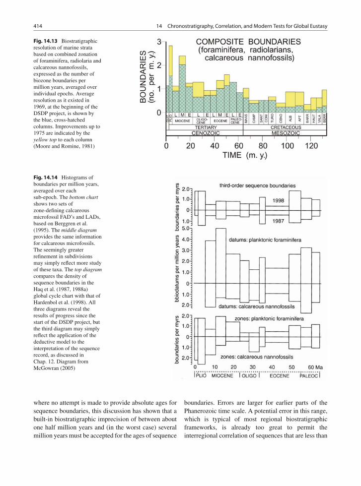
414 14 Chronostratigraphy, Correlation, and Modern Tests for Global Eustasy
Fig. 14.13 Biostratigraphicresolution of marine stratabased on combined zonationof foraminifera, radiolaria andcalcareous nannofossils,expressed as the number ofbiozone boundaries permillion years, averaged overindividual epochs. Averageresolution as it existed in1969, at the beginning of theDSDP project, is shown bythe blue, cross-hatchedcolumns. Improvements up to1975 are indicated by theyellow top to each column(Moore and Romine, 1981)
Fig. 14.14 Histograms ofboundaries per million years,averaged over eachsub-epoch. The bottom chartshows two sets ofzone-defining calcareousmicrofossil FAD’s and LADs,based on Berggren et al.(1995). The middle diagramprovides the same informationfor calcareous microfossils.The seemingly greaterrefinement in subdivisionsmay simply reflect more studyof these taxa. The top diagramcompares the density ofsequence boundaries in theHaq et al. (1987, 1988a)global cycle chart with that ofHardenbol et al. (1998). Allthree diagrams reveal theresults of progress since thestart of the DSDP project, butthe third diagram may simplyreflect the application of thedeductive model to theinterpretation of the sequencerecord, as discussed inChap. 12. Diagram fromMcGowran (2005)
where no attempt is made to provide absolute ages forsequence boundaries, this discussion has shown that abuilt-in biostratigraphic imprecision of between aboutone half million years and (in the worst case) severalmillion years must be accepted for the ages of sequence
boundaries. Errors are larger for earlier parts of thePhanerozoic time scale. A potential error in this range,which is typical of most regional biostratigraphicframeworks, is already too great to permit theinterregional correlation of sequences that are less than
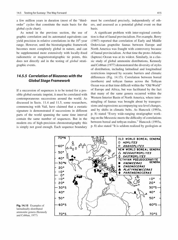
14.5 Testing for Eustasy: The Way Forward 415
a few million years in duration (most of the “third-order” cycles that constitute the main basis for theglobal cycle chart).
As noted in the previous section, the use ofgraphic correlation and its automated equivalents canyield precision in relative correlations in the 105-yearrange. However, until the biostratigraphic frameworkbecomes more completely global in nature, and canbe supplemented more extensively with locally-fixedradiometric or magnetostratigraphic tie points, thisdoes not directly aid in the testing of global strati-graphic events.
14.5.5 Correlation of Biozones with theGlobal Stage Framework
If a succession of sequences is to be tested for a pos-sible global eustatic imprint, it must be correlated withcontemporaneous successions around the world. Asdiscussed in Sects. 11.4 and 11.5, some researchers,commencing with Vail, have claimed that a eustaticsignature is demonstrated if successions in differentparts of the world spanning the same time intervalcontain the same number of sequences. But in themodern era of high-precision chronostratigraphy thisis simply not good enough. Each sequence boundary
must be correlated precisely, independently of oth-ers, and assessed as a potential global event on thatbasis.
A significant problem with inter-regional correla-tion is that of faunal provincialism. For example, Berry(1987) reported that correlation of Early and MiddleOrdovician graptolite faunas between Europe andNorth America was fraught with controversy becauseof faunal provincialism. At that time the proto-Atlantic(Iapteus) Ocean was at its widest. Similarly, in a clas-sic study of global ammonite distributions, Kennedyand Cobban (1977) demonstrated the diversity of stylesof distribution, including latitudinal and longitudinalrestrictions imposed by oceanic barriers and climaticdifferences (Fig. 14.15). Correlation between boreal(northern) and tethyan faunas across the TethyanOcean was at that time difficult within the “Old World”of Europe and Africa, but was facilitated by the factthat many of the same genera occurred within theWestern Interior Basin of North America, where inter-mingling of faunas was brought about by transgres-sions and regressions accompanying sea-level changes,and by shifts in climatic belts. As Hancock (1993a,p. 8) stated “Every wide-ranging stratigrapher work-ing on the Mesozoic meets the difficulty of correlationsbetween boreal and tethyan realms.” Hancock (1993a,p. 8) also stated “It is seldom realized by geologists at
Fig. 14.15 Examples oflatitudinally-distributedammonite genera (Kennedyand Cobban, 1977)
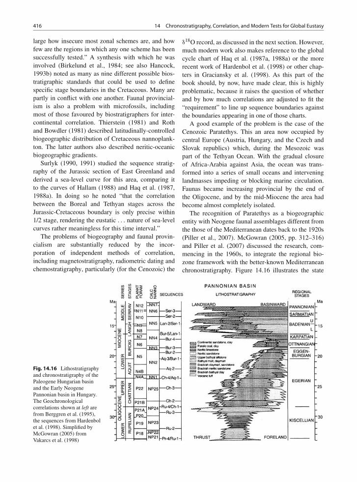
416 14 Chronostratigraphy, Correlation, and Modern Tests for Global Eustasy
large how insecure most zonal schemes are, and howfew are the regions in which any one scheme has beensuccessfully tested.” A synthesis with which he wasinvolved (Birkelund et al., 1984; see also Hancock,1993b) noted as many as nine different possible bios-tratigraphic standards that could be used to definespecific stage boundaries in the Cretaceous. Many arepartly in conflict with one another. Faunal provincial-ism is also a problem with microfossils, includingmost of those favoured by biostratigraphers for inter-continental correlation. Thierstein (1981) and Rothand Bowdler (1981) described latitudinally-controlledbiogeographic distribution of Cretaceous nannoplank-ton. The latter authors also described neritic-oceanicbiogeographic gradients.
Surlyk (1990, 1991) studied the sequence stratig-raphy of the Jurassic section of East Greenland andderived a sea-level curve for this area, comparing itto the curves of Hallam (1988) and Haq et al. (1987,1988a). In doing so he noted “that the correlationbetween the Boreal and Tethyan stages across theJurassic-Cretaceous boundary is only precise within1/2 stage, rendering the eustatic . . . nature of sea-levelcurves rather meaningless for this time interval.”
The problems of biogeography and faunal provin-cialism are substantially reduced by the incor-poration of independent methods of correlation,including magnetostratigraphy, radiometric dating andchemostratigraphy, particularly (for the Cenozoic) the
δ18O record, as discussed in the next section. However,much modern work also makes reference to the globalcycle chart of Haq et al. (1987a, 1988a) or the morerecent work of Hardenbol et al. (1998) or other chap-ters in Graciansky et al. (1998). As this part of thebook should, by now, have made clear, this is highlyproblematic, because it raises the question of whetherand by how much correlations are adjusted to fit the“requirement” to line up sequence boundaries againstthe boundaries appearing in one of those charts.
A good example of the problem is the case of theCenozoic Paratethys. This an area now occupied bycentral Europe (Austria, Hungary, and the Czech andSlovak republics) which, during the Mesozoic waspart of the Tethyan Ocean. With the gradual closureof Africa-Arabia against Asia, the ocean was trans-formed into a series of small oceans and interveninglandmasses impeding or blocking marine circulation.Faunas became increasing provincial by the end ofthe Oligocene, and by the mid-Miocene the area hadbecome almost completely isolated.
The recognition of Paratethys as a biogeographicentity with Neogene faunal assemblages different fromthe those of the Mediterranean dates back to the 1920s(Piller et al., 2007). McGowran (2005, pp. 312–316)and Piller et al. (2007) discussed the research, com-mencing in the 1960s, to integrate the regional bio-zone framework with the better-known Mediterraneanchronostratigraphy. Figure 14.16 illustrates the state
Fig. 14.16 Lithostratigraphyand chronostratigraphy of thePaleogene Hungarian basinand the Early NeogenePannonian basin in Hungary.The Geochronologicalcorrelations shown at left arefrom Berggren et al. (1995),the sequences from Hardenbolet al. (1998). Simplified byMcGowran (2005) fromVakarcs et al. (1998)
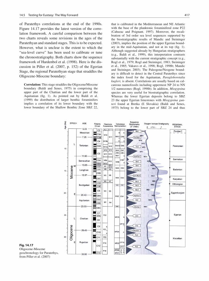
14.5 Testing for Eustasy: The Way Forward 417
of Paratethys correlations at the end of the 1990s.Figure 14.17 provides the latest version of the corre-lation framework. A careful comparison between thetwo charts reveals some revisions in the ages of theParatethyan and standard stages. This is to be expected.However, what is unclear is the extent to which the“sea-level curve” has been used to calibrate or tunethe chronostratigraphy. Both charts show the sequenceframework of Hardenbol et al. (1998). Here is the dis-cussion in Piller et al. (2007, p. 152) of the EgerianStage, the regional Paratethyan stage that straddles theOligocene-Miocene boundary:
Correlation: This stage straddles the Oligocene/Mioceneboundary (Baldi and Senes, 1975) in comprising theupper part of the Chattian and the lower part of theAquitanian (fig. 1). As pointed out by Baldi et al.(1999) the distribution of larger benthic foraminifersimplies a correlation of its lower boundary with thelower boundary of the Shallow Benthic Zone SBZ 22,
that is calibrated in the Mediterranean and NE Atlanticwith the base of the planktonic foraminiferal zone P22(Cahuzac and Poignant. 1997). Moreover, the recali-bration of 3rd order sea level sequences supported bythe biostratigraphic results of Mandic and Steininger(2003), implies the position of the upper Egerian bound-ary in the mid-Aquitanian, and not at its top (fig. 1).Although suggested already by Hungarian stratigraphers(e.g., Baldi et al., 1999), this interpretation contrastssubstantially with the current stratigraphic concept (e.g.,Rogl et al., 1979; Rogl and Steininger, 1983; Steiningeret al., 1985; Vakarcs et al., 1998; Rogl, 1998b; Mandicand Steininger, 2003). The Paleogene/Neogene bound-ary is difficult to detect in the Central Paratethys sincethe index fossil for the Aquitanian, Paragloborotaliakugleri, is absent. Correlations are usually based on cal-careous nannofossils including uppermost NP 24 to NN1/2 nannozones (Rogl, 1998b). In addition, Miogypsinaspecies are very useful for biostratigraphic correlation.Whereas the lower Egerian deposits belong to SBZ23 the upper Egerian limestones with Miogypsina gun-teri found at Bretka (E Slovakia) (Baldi and Senes,1975) belong to the lower part of SBZ 24 and thus
Fig. 14.17Oligocene-Miocenegeochronology for Paratethys,from Piller et al. (2007)
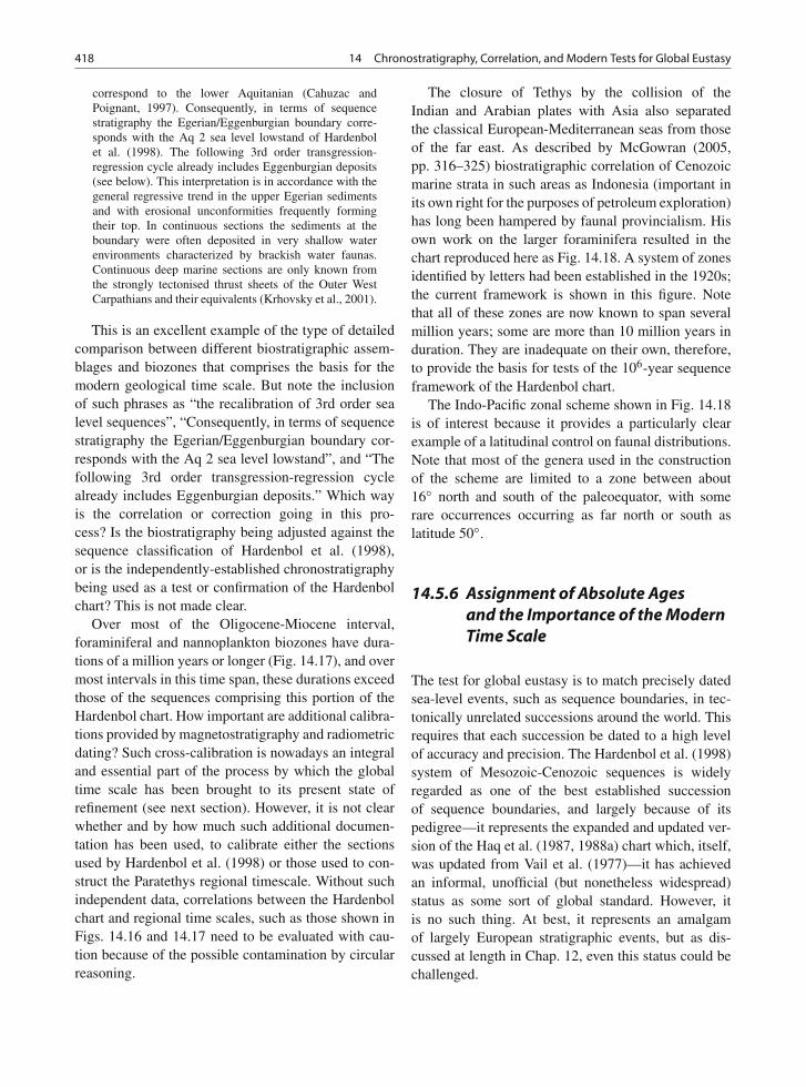
418 14 Chronostratigraphy, Correlation, and Modern Tests for Global Eustasy
correspond to the lower Aquitanian (Cahuzac andPoignant, 1997). Consequently, in terms of sequencestratigraphy the Egerian/Eggenburgian boundary corre-sponds with the Aq 2 sea level lowstand of Hardenbolet al. (1998). The following 3rd order transgression-regression cycle already includes Eggenburgian deposits(see below). This interpretation is in accordance with thegeneral regressive trend in the upper Egerian sedimentsand with erosional unconformities frequently formingtheir top. In continuous sections the sediments at theboundary were often deposited in very shallow waterenvironments characterized by brackish water faunas.Continuous deep marine sections are only known fromthe strongly tectonised thrust sheets of the Outer WestCarpathians and their equivalents (Krhovsky et al., 2001).
This is an excellent example of the type of detailedcomparison between different biostratigraphic assem-blages and biozones that comprises the basis for themodern geological time scale. But note the inclusionof such phrases as “the recalibration of 3rd order sealevel sequences”, “Consequently, in terms of sequencestratigraphy the Egerian/Eggenburgian boundary cor-responds with the Aq 2 sea level lowstand”, and “Thefollowing 3rd order transgression-regression cyclealready includes Eggenburgian deposits.” Which wayis the correlation or correction going in this pro-cess? Is the biostratigraphy being adjusted against thesequence classification of Hardenbol et al. (1998),or is the independently-established chronostratigraphybeing used as a test or confirmation of the Hardenbolchart? This is not made clear.
Over most of the Oligocene-Miocene interval,foraminiferal and nannoplankton biozones have dura-tions of a million years or longer (Fig. 14.17), and overmost intervals in this time span, these durations exceedthose of the sequences comprising this portion of theHardenbol chart. How important are additional calibra-tions provided by magnetostratigraphy and radiometricdating? Such cross-calibration is nowadays an integraland essential part of the process by which the globaltime scale has been brought to its present state ofrefinement (see next section). However, it is not clearwhether and by how much such additional documen-tation has been used, to calibrate either the sectionsused by Hardenbol et al. (1998) or those used to con-struct the Paratethys regional timescale. Without suchindependent data, correlations between the Hardenbolchart and regional time scales, such as those shown inFigs. 14.16 and 14.17 need to be evaluated with cau-tion because of the possible contamination by circularreasoning.
The closure of Tethys by the collision of theIndian and Arabian plates with Asia also separatedthe classical European-Mediterranean seas from thoseof the far east. As described by McGowran (2005,pp. 316–325) biostratigraphic correlation of Cenozoicmarine strata in such areas as Indonesia (important inits own right for the purposes of petroleum exploration)has long been hampered by faunal provincialism. Hisown work on the larger foraminifera resulted in thechart reproduced here as Fig. 14.18. A system of zonesidentified by letters had been established in the 1920s;the current framework is shown in this figure. Notethat all of these zones are now known to span severalmillion years; some are more than 10 million years induration. They are inadequate on their own, therefore,to provide the basis for tests of the 106-year sequenceframework of the Hardenbol chart.
The Indo-Pacific zonal scheme shown in Fig. 14.18is of interest because it provides a particularly clearexample of a latitudinal control on faunal distributions.Note that most of the genera used in the constructionof the scheme are limited to a zone between about16◦ north and south of the paleoequator, with somerare occurrences occurring as far north or south aslatitude 50◦.
14.5.6 Assignment of Absolute Agesand the Importance of the ModernTime Scale
The test for global eustasy is to match precisely datedsea-level events, such as sequence boundaries, in tec-tonically unrelated successions around the world. Thisrequires that each succession be dated to a high levelof accuracy and precision. The Hardenbol et al. (1998)system of Mesozoic-Cenozoic sequences is widelyregarded as one of the best established successionof sequence boundaries, and largely because of itspedigree—it represents the expanded and updated ver-sion of the Haq et al. (1987, 1988a) chart which, itself,was updated from Vail et al. (1977)—it has achievedan informal, unofficial (but nonetheless widespread)status as some sort of global standard. However, itis no such thing. At best, it represents an amalgamof largely European stratigraphic events, but as dis-cussed at length in Chap. 12, even this status could bechallenged.
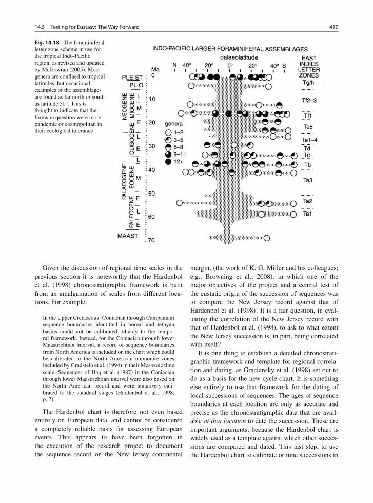
14.5 Testing for Eustasy: The Way Forward 419
Fig. 14.18 The foraminiferalletter zone scheme in use forthe tropical Indo-Pacificregion, as revised and updatedby McGowran (2005). Mostgenera are confined to tropicallatitudes, but occasionalexamples of the assemblagesare found as far north or southas latitude 50◦. This isthought to indicate that theforms in question were morepandemic or cosmopolitan intheir ecological tolerance
Given the discussion of regional time scales in theprevious section it is noteworthy that the Hardenbolet al. (1998) chronostratigraphic framework is builtfrom an amalgamation of scales from different loca-tions. For example:
In the Upper Cretaceous (Coniacian through Campanian)sequence boundaries identified in boreal and tethyanbasins could not be calibrated reliably to the tempo-ral framework. Instead, for the Coniacian through lowerMaastrichtian interval, a record of sequence boundariesfrom North America is included on the chart which couldbe calibrated to the North American ammonite zonesincluded by Gradstein et al. (1994) in their Mesozoic timescale. Sequences of Haq et al. (1987) in the Coniacianthrough lower Maastrichtian interval were also based onthe North American record and were tentatively cali-brated to the standard stages (Hardenbol et al., 1998,p. 7).
The Hardenbol chart is therefore not even basedentirely on European data, and cannot be considereda completely reliable basis for assessing Europeanevents. This appears to have been forgotten inthe execution of the research project to documentthe sequence record on the New Jersey continental
margin, (the work of K. G. Miller and his colleagues;e.g., Browning et al., 2008), in which one of themajor objectives of the project and a central test ofthe eustatic origin of the succession of sequences wasto compare the New Jersey record against that ofHardenbol et al. (1998)! It is a fair question, in eval-uating the correlation of the New Jersey record withthat of Hardenbol et al. (1998), to ask to what extentthe New Jersey succession is, in part, being correlatedwith itself?
It is one thing to establish a detailed chronostrati-graphic framework and template for regional correla-tion and dating, as Graciansky et al. (1998) set out todo as a basis for the new cycle chart. It is somethingelse entirely to use that framework for the dating oflocal successions of sequences. The ages of sequenceboundaries at each location are only as accurate andprecise as the chronostratigraphic data that are avail-able at that location to date the succession. These areimportant arguments, because the Hardenbol chart iswidely used as a template against which other succes-sions are compared and dated. This last step, to usethe Hardenbol chart to calibrate or tune successions in
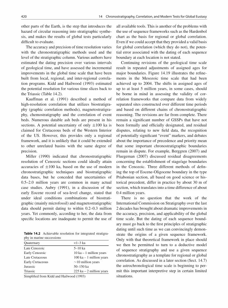
420 14 Chronostratigraphy, Correlation, and Modern Tests for Global Eustasy
other parts of the Earth, is the step that introduces thehazard of circular reasoning into stratigraphic synthe-sis, and makes the results of global tests particularlydifficult to evaluate.
The accuracy and precision of time resolution varieswith the chronostratigraphic methods used and thelevel of the stratigraphic column. Various authors haveestimated the dating precision over various intervalsof geological time, and have assessed the incrementalimprovements in the global time scale that have beenbuilt from local, regional, and inter-regional correla-tion programs. Kidd and Hailwood (1993) estimatedthe potential resolution for various time slices back tothe Triassic (Table 14.2).
Kauffman et al. (1991) described a method ofhigh-resolution correlation that utilizes biostratigra-phy (graphic correlation methods), magnetostratigra-phy, chemostratigraphy and the correlation of eventbeds. Numerous datable ash beds are present in hissections. A potential uncertainty of only ±100 ka isclaimed for Cretaceous beds of the Western Interiorof the US. However, this provides only a regionalframework, and it is unlikely that it could be extendedto other unrelated basins with the same degree ofprecision.
Miller (1990) indicated that chronostratigraphicresolution of Cenozoic sections could ideally attainaccuracies of ±100 ka, based on the use of modernchronostratigraphic techniques and biostratigraphicdata bases, but he conceded that uncertainties of0.5–2.0 million years are common in many actualcase studies. Aubry (1991), in a discussion of theearly Eocene record of sea-level change, stated thatunder ideal conditions combinations of biostrati-graphic (mainly microfossil) and magnetostratigraphicdata should permit dating to within 0.2–0.3 millionyears. Yet commonly, according to her, the data fromspecific locations are inadequate to permit the use of
Table 14.2 Achievable resolution for integrated stratigra-phy in marine successions
Quaternary <1–3 ka
Late Cenozoic 5–10 kaEarly Cenozoic 10 ka – 1 million yearsLate Cretaceous 100 ka – 1 million yearsEarly Cretaceous ∼10 million yearsJurassic 50–150 kaTriassic 225 ka – 2 million years
Simplified from Kidd and Hailwood (1993)
all available tools. This is another of the problems withthe use of sequence frameworks such as the Hardenbolchart as the basis for regional or global correlation.Even if we could accept that they provided a valid basisfor global correlation (which they do not), the poten-tial error associated with the dating of each sequenceboundary at each location is not stated.
Continuing revisions of the geological time scaleresult in repeated adjustments of assigned ages formajor boundaries. Figure 14.19 illustrates the refine-ments in the Mesozoic time scale that had beenachieved up to 2004. The shifts in assigned ages ofup to at least 5 million years, in some cases, shouldbe borne in mind in assessing the validity of cor-relation frameworks that compare data from widelyseparated sites constructed over different time periodsand based on different chains of chronostratigraphicreasoning. The revisions are far from complete. Thereremain a significant number of GSSPs that have notbeen formally and officially designated, and residualdisputes, relating to new field data, the recognitionof potentially significant “event” markers, and debatesabout the importance of precedence and priority meanthat some important chronostratigraphic boundariesremain in dispute. For example, Berggren (2007) andFluegeman (2007) discussed residual disagreementsconcerning the establishment of stage/age boundariesin the Cenozoic. Three different methods of defin-ing the top of Eocene-Oligocene boundary in the typePriabonian section, all based on good science or his-torical precedent, differ in practice by about 30 m ofsection, which translates into a time difference of about0.4 million years.
There is no question that the work of theInternational Commission on Stratigraphy over the last2 decades has brought about dramatic improvements inthe accuracy, precision, and applicability of the globaltime scale. But the dating of each sequence bound-ary must go back to the first principles of stratigraphicdating until such time as we can convincingly demon-strate the origins of a given sequence framework.Only with that theoretical framework in place shouldwe then be permitted to turn to a deductive modelof sequence stratigraphy and use a given sequencechronostratigraphy as a template for regional or globalcorrelation. As discussed in a later section (Sect. 14.7)the astrochronological time scale is beginning to per-mit this important interpretive step in certain limitedsituations.
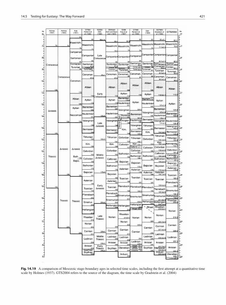
14.5 Testing for Eustasy: The Way Forward 421
Fig. 14.19 A comparison of Mesozoic stage-boundary ages in selected time scales, including the first attempt at a quantitative timescale by Holmes (1937). GTS2004 refers to the source of the diagram, the time scale by Gradstein et al. (2004)
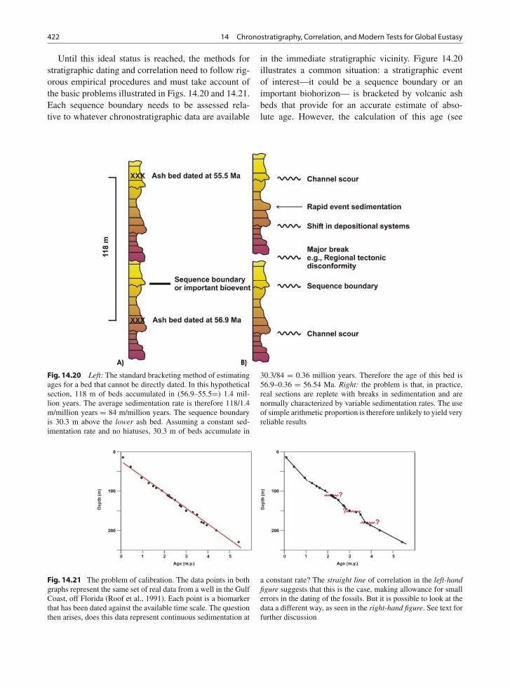
422 14 Chronostratigraphy, Correlation, and Modern Tests for Global Eustasy
Until this ideal status is reached, the methods forstratigraphic dating and correlation need to follow rig-orous empirical procedures and must take account ofthe basic problems illustrated in Figs. 14.20 and 14.21.Each sequence boundary needs to be assessed rela-tive to whatever chronostratigraphic data are available
in the immediate stratigraphic vicinity. Figure 14.20illustrates a common situation: a stratigraphic eventof interest—it could be a sequence boundary or animportant biohorizon— is bracketed by volcanic ashbeds that provide for an accurate estimate of abso-lute age. However, the calculation of this age (see
Fig. 14.20 Left: The standard bracketing method of estimatingages for a bed that cannot be directly dated. In this hypotheticalsection, 118 m of beds accumulated in (56.9–55.5=) 1.4 mil-lion years. The average sedimentation rate is therefore 118/1.4m/million years = 84 m/million years. The sequence boundaryis 30.3 m above the lower ash bed. Assuming a constant sed-imentation rate and no hiatuses, 30.3 m of beds accumulate in
30.3/84 = 0.36 million years. Therefore the age of this bed is56.9–0.36 = 56.54 Ma. Right: the problem is that, in practice,real sections are replete with breaks in sedimentation and arenormally characterized by variable sedimentation rates. The useof simple arithmetic proportion is therefore unlikely to yield veryreliable results
Fig. 14.21 The problem of calibration. The data points in bothgraphs represent the same set of real data from a well in the GulfCoast, off Florida (Roof et al., 1991). Each point is a biomarkerthat has been dated against the available time scale. The questionthen arises, does this data represent continuous sedimentation at
a constant rate? The straight line of correlation in the left-handfigure suggests that this is the case, making allowance for smallerrors in the dating of the fossils. But it is possible to look at thedata a different way, as seen in the right-hand figure. See text forfurther discussion
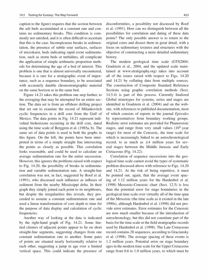
14.5 Testing for Eustasy: The Way Forward 423
caption to the figure) requires that the section betweenthe ash beds accumulated at a constant rate and con-tains no sedimentary breaks. This condition is com-monly not satisfied, and it is often difficult to ascertainthat this is the case. Inconspicuous breaks in sedimen-tation, the presence of subtle sour surfaces, surfacesof microkarst, beds indicating rapid event sedimenta-tion, such as storm beds or turbidites, all complicatethe application of simple arithmetic proportion meth-ods for determining the age of a bed of interest. Thisproblem is one that is almost universally encountered,because it is rare for a stratigraphic event of impor-tance, such as a sequence boundary, to be associatedwith accurately datable chronostratigraphic materialon the same horizon or in the same bed.
Figure 14.21 takes this problem one step further, tothe averaging that may be attempted for an entire sec-tion. The data set is from an offshore drilling projectthat set out to examine the record of Milankovitchcyclic frequencies in a drill core from the Gulf ofMexico. The data points in Fig. 14.21 represent indi-vidual biohorizons occurring in the drill core, datedusing the time scale of Berggren et al. (1985a, b). Thesame set of data points is used in both the graphs inthis figure. On the left, the points have been inter-preted in terms of a simple straight line intersectingthe points as closely as possible. This correlationlooks reasonable, and could be used to calculate anaverage sedimentation rate for the entire succession.However, this ignores the problems raised with respectto Fig. 14.20, the possibility of breaks in sedimenta-tion and variable sedimentation rate. A straight-linecorrelation was not, in fact, suggested by Roof et al.(1991), who discussed such influence as influxes ofsediment from the nearby Mississippi delta. In theirgraph they simply joined each point to its neighbours,but despite the irregularities this reveals, they pro-ceeded to assume a constant sedimentation rate andused a linear transformation of core depth to time forthe purpose of data display and calculation of cyclicfrequencies.
Another way of looking at the data is indicatedby the right-hand graph of Fig. 14.21. Some lim-ited clusters of adjacent points appear to lie on shortstraight-line segments, suggesting changes from oneconstant sedimentation rate to another. Some pairsof points are situated nearly horizontally relative toeach other, suggesting a jump in age over a limitedvertical space. This could indicate the presence of
disconformities, a possibility not discussed by Roofet al. (1991). How can we distinguish between all thepossibilities for correlation and dating of these datapoints? The only possible answer is to return to theoriginal cores and dissect them in great detail, with afocus on sedimentary textures and structures with theobjective of constructing a more detailed sedimentaryhistory.
The modern geological time scale (GTS2004:Gradstein et al., 2004, and the updated scale main-tained at www.stratigraphy.org) takes into accountall of the issues raised with respect to Figs. 14.20and 14.21 by collating data from multiple sources.The construction of Composite Standard ReferenceSections using graphic correlation methods (Sect.14.5.4) is part of this process. Currently finalizedGlobal stratotypes for systems, series and stages areidentified in Gradstein et al. (2004) and on the web-site, with references to published documentation, mostof which consists of reports in the journal Episodesby representatives from boundary working groups.Realistic error estimates are provided for Phanerozoicstages, and range from very small values (104-yearrange) for most of the Cenozoic, the time scale forwhich is increasingly linked to an astrochronologicalrecord, to as much as ±4 million years for sev-eral stages between the Middle Jurassic and EarlyCretaceous (Fig. 14.22).
Correlation of sequence successions into the geo-logical time scale cannot avoid the types of systematicproblem discussed above with reference to Figs. 14.20and 14.21. At the risk of being repetitive, it mustbe pointed out, again, that the average event spac-ing of 1.12 million years for the Hardenbol et al.(1998) Mesozoic-Cenozoic chart (Sect. 12.5) is lessthan the potential error for stage boundaries in thegeological time scale over virtually all of the time spanof the Mesozoic (the time scale as it existed in the late1990s), although Hardenbol et al. (1998) did not pro-vide error estimates. Error estimates for the Cenozoicare now much smaller because of the introduction ofastrochronology, but this did not constitute part of thebasis for the time scale or the field stratigraphic recordsused by Hardenbol et al. (1998). The Late Cretaceousrecord contains 28 sequences, according to Gracianskyet al. (1998). The average spacing of these events is1.2 million years. Potential error on stage boundaryages in the modern time scale for the Upper Cretaceousrange from 0.6 to 1.0 million years, to which must be
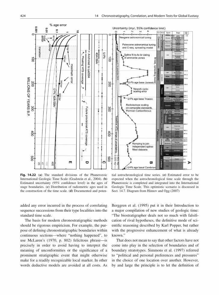
424 14 Chronostratigraphy, Correlation, and Modern Tests for Global Eustasy
Fig. 14.22 (a) The standard divisions of the PhanerozoicInternational Geologic Time Scale (Gradstein et al., 2004). (b)Estimated uncertainty (95% confidence level) in the ages ofstage boundaries. (c) Distribution of radiometric ages used inthe construction of the time scale. (d) Documented and poten-
tial astrochronological time series. (e) Estimated error to beexpected when the astrochronological time scale through thePhanerozoic is completed and integrated into the InternationalGeologic Time Scale. This optimistic scenario is discussed inSect. 14.7. Diagram from Hinnov and Ogg (2007)
added any error incurred in the process of correlatingsequence successions from their type localities into thestandard time scale.
The basis for modern chronostratigraphic methodsshould be rigorous empiricism. For example, the pur-pose of defining chronostratigraphic boundaries withincontinuous sections—where “nothing happened”, touse McLaren’s (1970, p. 802) felicitous phrase—isprecisely in order to avoid having to interpret themeaning of unconformities or the significance of aprominent stratigraphic event that might otherwisemake for a readily recognizable local marker. In otherwords deductive models are avoided at all costs. As
Berggren et al. (1995) put it in their Introduction toa major compilation of new studies of geologic time:“The biostratigrapher deals not so much with falsifi-cation of rival hypotheses, the definitive mode of sci-entific reasoning described by Karl Popper, but ratherwith the progressive enhancement of what is alreadyknown.”
That does not mean to say that other factors have notcome into play in the selection of boundaries and ofboundary stratotypes. Simmons et al. (1997) referredto “political and personal preferences and pressures”in the choice of one location over another. However,by and large the principle is to let the definition of
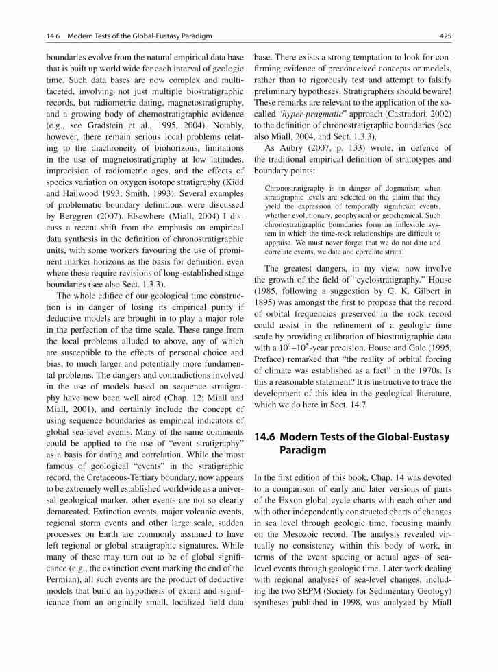
14.6 Modern Tests of the Global-Eustasy Paradigm 425
boundaries evolve from the natural empirical data basethat is built up world wide for each interval of geologictime. Such data bases are now complex and multi-faceted, involving not just multiple biostratigraphicrecords, but radiometric dating, magnetostratigraphy,and a growing body of chemostratigraphic evidence(e.g., see Gradstein et al., 1995, 2004). Notably,however, there remain serious local problems relat-ing to the diachroneity of biohorizons, limitationsin the use of magnetostratigraphy at low latitudes,imprecision of radiometric ages, and the effects ofspecies variation on oxygen isotope stratigraphy (Kiddand Hailwood 1993; Smith, 1993). Several examplesof problematic boundary definitions were discussedby Berggren (2007). Elsewhere (Miall, 2004) I dis-cuss a recent shift from the emphasis on empiricaldata synthesis in the definition of chronostratigraphicunits, with some workers favouring the use of promi-nent marker horizons as the basis for definition, evenwhere these require revisions of long-established stageboundaries (see also Sect. 1.3.3).
The whole edifice of our geological time construc-tion is in danger of losing its empirical purity ifdeductive models are brought in to play a major rolein the perfection of the time scale. These range fromthe local problems alluded to above, any of whichare susceptible to the effects of personal choice andbias, to much larger and potentially more fundamen-tal problems. The dangers and contradictions involvedin the use of models based on sequence stratigra-phy have now been well aired (Chap. 12; Miall andMiall, 2001), and certainly include the concept ofusing sequence boundaries as empirical indicators ofglobal sea-level events. Many of the same commentscould be applied to the use of “event stratigraphy”as a basis for dating and correlation. While the mostfamous of geological “events” in the stratigraphicrecord, the Cretaceous-Tertiary boundary, now appearsto be extremely well established worldwide as a univer-sal geological marker, other events are not so clearlydemarcated. Extinction events, major volcanic events,regional storm events and other large scale, suddenprocesses on Earth are commonly assumed to haveleft regional or global stratigraphic signatures. Whilemany of these may turn out to be of global signifi-cance (e.g., the extinction event marking the end of thePermian), all such events are the product of deductivemodels that build an hypothesis of extent and signif-icance from an originally small, localized field data
base. There exists a strong temptation to look for con-firming evidence of preconceived concepts or models,rather than to rigorously test and attempt to falsifypreliminary hypotheses. Stratigraphers should beware!These remarks are relevant to the application of the so-called “hyper-pragmatic” approach (Castradori, 2002)to the definition of chronostratigraphic boundaries (seealso Miall, 2004, and Sect. 1.3.3).
As Aubry (2007, p. 133) wrote, in defence ofthe traditional empirical definition of stratotypes andboundary points:
Chronostratigraphy is in danger of dogmatism whenstratigraphic levels are selected on the claim that theyyield the expression of temporally significant events,whether evolutionary, geophysical or geochemical. Suchchronostratigraphic boundaries form an inflexible sys-tem in which the time-rock relationships are difficult toappraise. We must never forget that we do not date andcorrelate events, we date and correlate strata!
The greatest dangers, in my view, now involvethe growth of the field of “cyclostratigraphy.” House(1985, following a suggestion by G. K. Gilbert in1895) was amongst the first to propose that the recordof orbital frequencies preserved in the rock recordcould assist in the refinement of a geologic timescale by providing calibration of biostratigraphic datawith a 104–105-year precision. House and Gale (1995,Preface) remarked that “the reality of orbital forcingof climate was established as a fact” in the 1970s. Isthis a reasonable statement? It is instructive to trace thedevelopment of this idea in the geological literature,which we do here in Sect. 14.7
14.6 Modern Tests of the Global-EustasyParadigm
In the first edition of this book, Chap. 14 was devotedto a comparison of early and later versions of partsof the Exxon global cycle charts with each other andwith other independently constructed charts of changesin sea level through geologic time, focusing mainlyon the Mesozoic record. The analysis revealed vir-tually no consistency within this body of work, interms of the event spacing or actual ages of sea-level events through geologic time. Later work dealingwith regional analyses of sea-level changes, includ-ing the two SEPM (Society for Sedimentary Geology)syntheses published in 1998, was analyzed by Miall
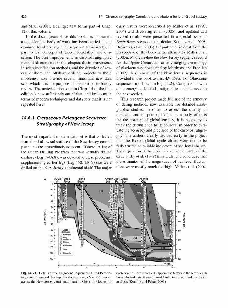
426 14 Chronostratigraphy, Correlation, and Modern Tests for Global Eustasy
and Miall (2001), a critique that forms part of Chap.12 of this volume.
In the dozen years since this book first appeared,a considerable body of work has been carried out toexamine local and regional sequence frameworks, inpart to test concepts of global correlation and cau-sation. The vast improvements in chronostratigraphicmethods documented in this chapter, the improvementsin seismic-reflection methods, and the devotion of sev-eral onshore and offshore drilling projects to theseproblems, have provide several important new datasets, which it is the purpose of this section to brieflyreview. The material discussed in Chap. 14 of the firstedition is now sufficiently out of date, and irrelevant interms of modern techniques and data sets that it is notrepeated here.
14.6.1 Cretaceous-Paleogene SequenceStratigraphy of New Jersey
The most important modern data set is that collectedfrom the shallow subsurface of the New Jersey coastalplain and the immediately adjacent offshore. A leg ofthe Ocean Drilling Program that was actually drilledonshore (Leg 174AX), was devoted to these problems,supplementing earlier legs (Leg 150, 150X) that weredrilled on the New Jersey continental shelf. The major
early results were described by Miller et al. (1998,2004) and Browning et al. (2005), and updated andrevised results were presented in a special issue ofBasin Research (see, in particular, Kominz et al., 2008;Browning et al., 2008). Of particular interest from theperspective of this book is the attempt by Miller et al.(2005a, b) to correlate the New Jersey sequence recordfor the Upper Cretaceous to an emerging chronologyof glacioeustasy postulated by Matthews and Frohlich(2002). A summary of the New Jersey sequences isprovided in this book as Fig. 4.9. Details of Oligocenesequences are shown in Fig. 14.23. Comparisons withother emerging detailed stratigraphies are discussed inthe next section.
This research project made full use of the armouryof dating methods now available for detailed strati-graphic studies. In order to assess the quality ofthe data, and its potential value as a body of testsfor the concept of global eustasy, it is necessary totrack the dating back to its sources, in order to eval-uate the accuracy and precision of the chronostratigra-phy. The authors clearly decided early in the projectthat the Exxon global cycle charts were not to befully trusted as reliable indicators of sea-level change.They questioned the accuracy of some parts of theGraciansky et al. (1998) time scale, and concluded thatthe estimates of the magnitudes of sea-level fluctua-tions were mostly much too high. Miller et al. (2004,
Fig. 14.23 Details of the Oligocene sequences O1 to O6 form-ing a set of seaward-dipping clinoforms along a NW-SE transectacross the New Jersey continental margin. Gross lithologies for
each borehole are indicated. Upper-case letters to the left of eachborehole indicate foraminiferal biofacies, identified by factoranalysis (Kominz and Pekar, 2001)
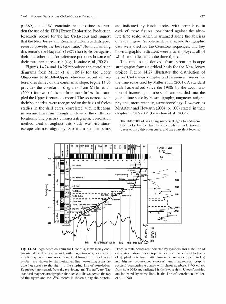
14.6 Modern Tests of the Global-Eustasy Paradigm 427
p. 389) stated “We conclude that it is time to aban-don the use of the EPR [Exxon Exploration ProductionResearch] record for the late Cretaceous and suggestthat the New Jersey and Russian Platform backstrippedrecords provide the best substitute.” Notwithstandingthis remark, the Haq et al. (1987) chart is shown againsttheir and other data for reference purposes in some oftheir most recent research (e.g., Kominz et al., 2008).
Figures 14.24 and 14.25 reproduce the correlationdiagrams from Miller et al. (1998) for the UpperOligocene to Middle/Upper Miocene record of twoboreholes drilled on the continental slope. Figure 14.26provides the correlation diagrams from Miller et al.(2004) for two of the onshore core holes that sam-pled the Upper Cretaceous record. The sequences, withtheir boundaries, were recognized on the basis of faciesstudies in the drill cores, correlated with reflectionsin seismic lines run through or close to the drill-holelocations. The primary chronostratigraphic correlationmethod used throughout this study was strontium-isotope chemostratigraphy. Strontium sample points
are indicated by black circles with error bars ineach of these figures, positioned against the abso-lute time scale, which is arranged along the abscissaof each figure. Supplementary magnetostratigraphicdata were used for the Cenozoic sequences, and keybiostratigraphic indicators were also employed, all ofwhich are indicated on the three figures.
The time scale derived from strontium-isotopestratigraphy forms a critical basis for the New Jerseyproject. Figure 14.27 illustrates the distribution ofUpper Cretaceous samples and reference sources forthe time scale used by Miller et al. (2004). A standardscale has evolved since the 1980s by the accumula-tion of increasing numbers of samples tied into theglobal time scale by biostratigraphy, magnetostratigra-phy and, more recently, astrochronology. However, asMcArthur and Howarth (2004, p. 100) stated, in theirchapter in GTS2004 (Gradstein et al., 2004):
The difficulty of assigning numerical ages to sedimen-tary rocks by the first two methods is well known.Users of the calibration curve, and the equivalent look-up
Fig. 14.24 Age-depth diagram for Hole 904, New Jersey con-tinental slope. The core record, with magnetozones, is indicatedat left. Sequence boundaries, recognized from seismic and faciesstudies, are shown by the horizontal lines extending from thecore log across to the right, to the sloping line of correlation.Sequences are named, from the top down, “m1 Tuscan”, etc. Thestandard magnetostratigraphic time scale is shown across the topof the figure and the δ18O record is shown along the bottom.
Dated sample points are indicated by symbols along the line ofcorrelation: strontium isotope values, with error bars black cir-cles), planktonic foraminifer lowest occurrences (open circles)and highest occurrences (crosses), and magnetostratigraphicreversal boundaries (squares with chron number). δ18O valuesfrom hole 904A are indicated in the box at right. Unconformitiesare indicated by wavy lines in the line of correlation (Miller,et al., 1998)
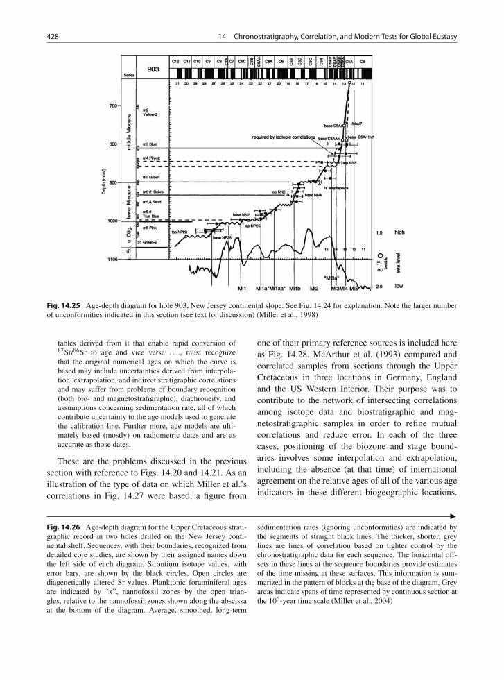
428 14 Chronostratigraphy, Correlation, and Modern Tests for Global Eustasy
Fig. 14.25 Age-depth diagram for hole 903, New Jersey continental slope. See Fig. 14.24 for explanation. Note the larger numberof unconformities indicated in this section (see text for discussion) (Miller et al., 1998)
tables derived from it that enable rapid conversion of87Sr/86Sr to age and vice versa . . .., must recognizethat the original numerical ages on which the curve isbased may include uncertainties derived from interpola-tion, extrapolation, and indirect stratigraphic correlationsand may suffer from problems of boundary recognition(both bio- and magnetostratigraphic), diachroneity, andassumptions concerning sedimentation rate, all of whichcontribute uncertainty to the age models used to generatethe calibration line. Further more, age models are ulti-mately based (mostly) on radiometric dates and are asaccurate as those dates.
These are the problems discussed in the previoussection with reference to Figs. 14.20 and 14.21. As anillustration of the type of data on which Miller et al.’scorrelations in Fig. 14.27 were based, a figure from
one of their primary reference sources is included hereas Fig. 14.28. McArthur et al. (1993) compared andcorrelated samples from sections through the UpperCretaceous in three locations in Germany, Englandand the US Western Interior. Their purpose was tocontribute to the network of intersecting correlationsamong isotope data and biostratigraphic and mag-netostratigraphic samples in order to refine mutualcorrelations and reduce error. In each of the threecases, positioning of the biozone and stage bound-aries involves some interpolation and extrapolation,including the absence (at that time) of internationalagreement on the relative ages of all of the various ageindicators in these different biogeographic locations.
�Fig. 14.26 Age-depth diagram for the Upper Cretaceous strati-graphic record in two holes drilled on the New Jersey conti-nental shelf. Sequences, with their boundaries, recognized fromdetailed core studies, are shown by their assigned names downthe left side of each diagram. Strontium isotope values, witherror bars, are shown by the black circles. Open circles arediagenetically altered Sr values. Planktonic foraminiferal agesare indicated by “x”, nannofossil zones by the open trian-gles, relative to the nannofossil zones shown along the abscissaat the bottom of the diagram. Average, smoothed, long-term
sedimentation rates (ignoring unconformities) are indicated bythe segments of straight black lines. The thicker, shorter, greylines are lines of correlation based on tighter control by thechronostratigraphic data for each sequence. The horizontal off-sets in these lines at the sequence boundaries provide estimatesof the time missing at these surfaces. This information is sum-marized in the pattern of blocks at the base of the diagram. Greyareas indicate spans of time represented by continuous section atthe 106-year time scale (Miller et al., 2004)
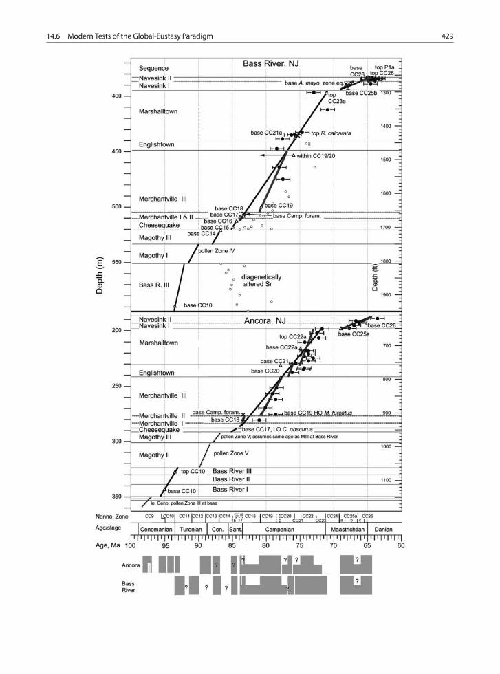
14.6 Modern Tests of the Global-Eustasy Paradigm 429

430 14 Chronostratigraphy, Correlation, and Modern Tests for Global Eustasy
Fig. 14.27 Calibration of the strontium-isotope curve for the Late Cretaceous, as used by Miller et al. (2004)
Positioning errors of chronostratigraphic boundaries ofa few metres in the sections translates into age uncer-tainties in the range of ±0.5 million years for a givenpoint within a succession of strontium measurements.Reading across the graphs in Figs. 14.27 and 14.28indicates that there are uncertainties in the age of indi-vidual measurements, if taken in isolation, of up toabout 1.6 million years. This is the width of the spreadof values relative to age in Fig. 14.27. The verticalrange of about 25 m over which any given value couldbe obtained from the Lägerdorf, Germany, section inFig. 14.28a corresponds to a time interval of about 1.6million years, according to the raw data reported inMcArthur et al. (1993).
To bring this back to the New Jersey study, thismeans that minimum error estimates of ±0.5 mil-lion years must be assumed for all sample points inFigs. 14.24, 14.25 and 14.26, and in the several caseswhere sequences have been dated by only one or twostrontium samples, errors of up to about ±0.8 millionyears must be allowed for. The coarseness of the datingof parts of the succession is indicated by the fact thatlines of correlation are drawn through several sequence
boundaries without deflection in Figs. 14.24, 14.25and 14.26. To put this another way, the constructionof a line of correlation through parts of the boreholesections does not reveal the likely presence of off-sets at these sequence boundaries. We know that thesequence boundaries are there on the basis of faciesand other studies of the core materials, but the derivedage interpretations cannot in these cases, corroboratethe existence of significant time gaps, even if they areactually present.
An examination of Figs. 14.24, 14.25 and 14.26reveals many places where the line of correlation couldhave been drawn differently. This is not to criticize theresearch, which has clearly been carried out in a mostmeticulous fashion, but to ensure that the results areused appropriately as a basis for inter-regional correla-tion. The null hypothesis regarding the New Jersey datais that there is no clear eustatic signal, and it is there-fore critically important, as the authors clearly intend,that the observed record be evaluated appropriately,taking due regard of its internal incompleteness andimprecision. The problem with the Exxon curves andtheir successors is that they always seem to be the tail
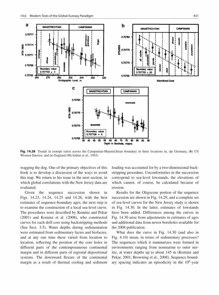
14.6 Modern Tests of the Global-Eustasy Paradigm 431
Fig. 14.28 Trends in isotope ratios across the Campanian-Maastrichtian boundary in three locations in, (a) Germany, (b) USWestern Interior, and (c) England (McArthur et al., 1993)
wagging the dog. One of the primary objectives of thisbook is to develop a discussion of the ways to avoidthis trap. We return to his issue in the next section, inwhich global correlations with the New Jersey data areevaluated.
Given the sequence succession shown inFigs. 14.23, 14.24, 14.25 and 14.26, with the bestestimates of sequence-boundary ages, the next step isto examine the construction of a local sea-level curve.The procedures were described by Kominz and Pekar(2001) and Kominz et al. (2008), who constructedcurves for each drill core using backstripping methods(See Sect. 3.5). Water depths during sedimentationwere estimated from sedimentary facies and biofacies,and at any one time these varied from location tolocation, reflecting the position of the core holes indifferent parts of the contemporaneous continentalmargin and in different parts of regional depositionalsystems. The downward flexure of the continentalmargin as a result of thermal cooling and sediment
loading was accounted for by a two-dimensional back-stripping procedure. Unconformities in the successioncorrespond to sea-level lowstands, the elevations ofwhich cannot, of course, be calculated because oferosion.
Results for the Oligocene portion of the sequencesuccession are shown in Fig. 14.29, and a complete setof sea-level curves for the New Jersey study is shownin Fig. 14.30. In the latter, estimates of lowstandshave been added. Differences among the curves inFig. 14.30 arise from adjustments in estimates of agesand additional data from newer boreholes available forthe 2008 publication.
What does the curve in Fig. 14.30 (and also inFig. 4.10) mean, in terms of sedimentary processes?The sequences which it summarizes were formed inenvironments ranging from nonmarine to outer ner-itic, at water depths up to about 145 m (Kominz andPekar, 2001; Browning et al., 2008). Sequence bound-ary spacing indicates an episodicity in the 106-year
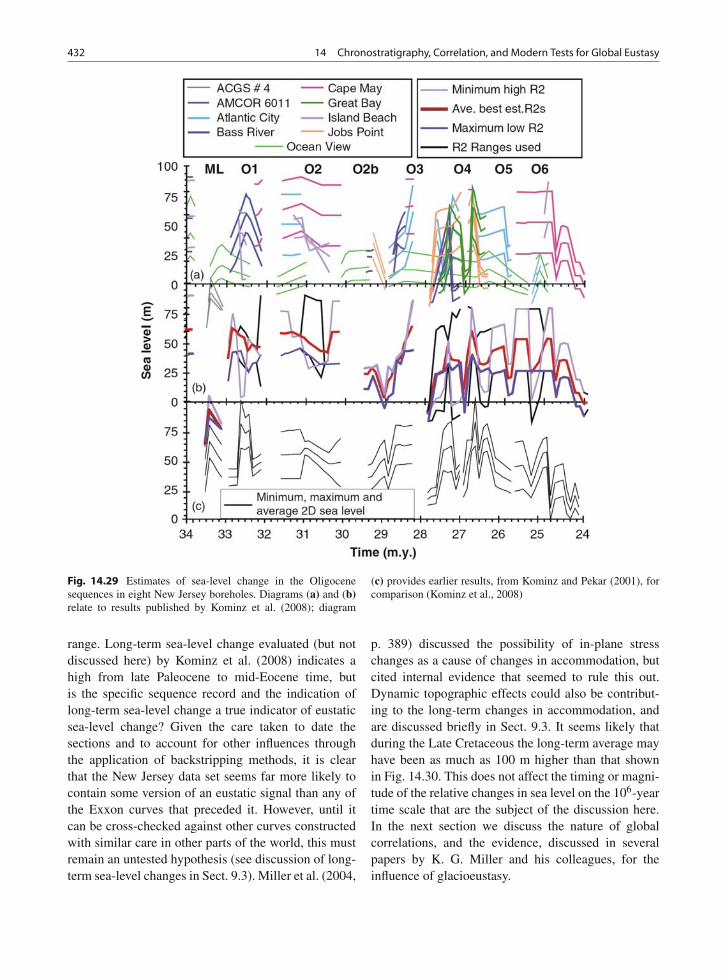
432 14 Chronostratigraphy, Correlation, and Modern Tests for Global Eustasy
Fig. 14.29 Estimates of sea-level change in the Oligocenesequences in eight New Jersey boreholes. Diagrams (a) and (b)relate to results published by Kominz et al. (2008); diagram
(c) provides earlier results, from Kominz and Pekar (2001), forcomparison (Kominz et al., 2008)
range. Long-term sea-level change evaluated (but notdiscussed here) by Kominz et al. (2008) indicates ahigh from late Paleocene to mid-Eocene time, butis the specific sequence record and the indication oflong-term sea-level change a true indicator of eustaticsea-level change? Given the care taken to date thesections and to account for other influences throughthe application of backstripping methods, it is clearthat the New Jersey data set seems far more likely tocontain some version of an eustatic signal than any ofthe Exxon curves that preceded it. However, until itcan be cross-checked against other curves constructedwith similar care in other parts of the world, this mustremain an untested hypothesis (see discussion of long-term sea-level changes in Sect. 9.3). Miller et al. (2004,
p. 389) discussed the possibility of in-plane stresschanges as a cause of changes in accommodation, butcited internal evidence that seemed to rule this out.Dynamic topographic effects could also be contribut-ing to the long-term changes in accommodation, andare discussed briefly in Sect. 9.3. It seems likely thatduring the Late Cretaceous the long-term average mayhave been as much as 100 m higher than that shownin Fig. 14.30. This does not affect the timing or magni-tude of the relative changes in sea level on the 106-yeartime scale that are the subject of the discussion here.In the next section we discuss the nature of globalcorrelations, and the evidence, discussed in severalpapers by K. G. Miller and his colleagues, for theinfluence of glacioeustasy.
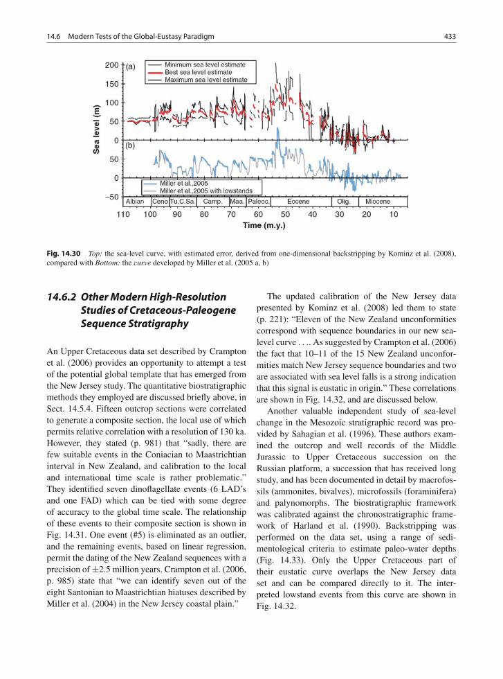
14.6 Modern Tests of the Global-Eustasy Paradigm 433
Fig. 14.30 Top: the sea-level curve, with estimated error, derived from one-dimensional backstripping by Kominz et al. (2008),compared with Bottom: the curve developed by Miller et al. (2005 a, b)
14.6.2 Other Modern High-ResolutionStudies of Cretaceous-PaleogeneSequence Stratigraphy
An Upper Cretaceous data set described by Cramptonet al. (2006) provides an opportunity to attempt a testof the potential global template that has emerged fromthe New Jersey study. The quantitative biostratigraphicmethods they employed are discussed briefly above, inSect. 14.5.4. Fifteen outcrop sections were correlatedto generate a composite section, the local use of whichpermits relative correlation with a resolution of 130 ka.However, they stated (p. 981) that “sadly, there arefew suitable events in the Coniacian to Maastrichtianinterval in New Zealand, and calibration to the localand international time scale is rather problematic.”They identified seven dinoflagellate events (6 LAD’sand one FAD) which can be tied with some degreeof accuracy to the global time scale. The relationshipof these events to their composite section is shown inFig. 14.31. One event (#5) is eliminated as an outlier,and the remaining events, based on linear regression,permit the dating of the New Zealand sequences with aprecision of ±2.5 million years. Crampton et al. (2006,p. 985) state that “we can identify seven out of theeight Santonian to Maastrichtian hiatuses described byMiller et al. (2004) in the New Jersey coastal plain.”
The updated calibration of the New Jersey datapresented by Kominz et al. (2008) led them to state(p. 221): “Eleven of the New Zealand unconformitiescorrespond with sequence boundaries in our new sea-level curve . . .. As suggested by Crampton et al. (2006)the fact that 10–11 of the 15 New Zealand unconfor-mities match New Jersey sequence boundaries and twoare associated with sea level falls is a strong indicationthat this signal is eustatic in origin.” These correlationsare shown in Fig. 14.32, and are discussed below.
Another valuable independent study of sea-levelchange in the Mesozoic stratigraphic record was pro-vided by Sahagian et al. (1996). These authors exam-ined the outcrop and well records of the MiddleJurassic to Upper Cretaceous succession on theRussian platform, a succession that has received longstudy, and has been documented in detail by macrofos-sils (ammonites, bivalves), microfossils (foraminifera)and palynomorphs. The biostratigraphic frameworkwas calibrated against the chronostratigraphic frame-work of Harland et al. (1990). Backstripping wasperformed on the data set, using a range of sedi-mentological criteria to estimate paleo-water depths(Fig. 14.33). Only the Upper Cretaceous part oftheir eustatic curve overlaps the New Jersey dataset and can be compared directly to it. The inter-preted lowstand events from this curve are shown inFig. 14.32.
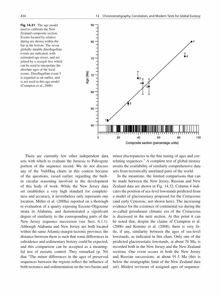
434 14 Chronostratigraphy, Correlation, and Modern Tests for Global Eustasy
Fig. 14.31 The age modelused to calibrate the NewZealand composite section.Events located by relativedating are shown within thebar at the bottom. The sevenglobally datable dinoflagellateevents are indicated, withestimated age errors, and arejoined by a straight line whichcan be used to interpolate theabsolute ages of the localevents. Dinoflagellate event 5is regarded as an outlier, andis not used in this age model(Crampton et al., 2006)
There are currently few other independent datasets with which to evaluate the Jurassic to Paleogeneportion of the sequence record. We do not discussany of the Vail/Haq charts in this context becauseof the questions, raised earlier, regarding the built-in circular reasoning involved in the developmentof this body of work. While the New Jersey dataset establishes a very high standard for complete-ness and accuracy, it nevertheless only represents onelocation. Miller et al. (2008a) reported on a thoroughre-evaluation of a quarry exposing Eocene-Oligocenestrata in Alabama, and demonstrated a significantdegree of similarity to the corresponding parts of theNew Jersey sequence succession (see Sect. 6.1.1).Although Alabama and New Jersey are both locatedwithin the same Atlantic-margin tectonic province, thedistance between them is such that some differences insubsidence and sedimentary history could be expected,and this comparison can be accepted as a meaning-ful test of eustatic control. They remarked (p. 50)that “The minor differences in the ages of preservedsequences between the regions reflect the influence ofboth tectonics and sedimentation on the two basins and
minor discrepancies in the fine tuning of ages and cor-relating sequences.” A complete test of global eustasyawaits the availability of similarly comprehensive datasets from tectonically unrelated parts of the world.
In the meantime, the limited comparisons that canbe made between the New Jersey, Russian and NewZealand data are shown in Fig. 14.32. Column 4 indi-cates the position of sea-level lowstands predicted froma model of glacioeustasy proposed for the Cretaceous(and early Cenozoic, not shown here). The increasingevidence for the existence of continental ice during theso-called greenhouse climatic era of the Cretaceousis discussed in the next section. At this point it canbe noted that, despite the claims of Crampton et al.(2006) and Kominz et al. (2008), there is very lit-tle, if any, similarity between the ages of sea-levellowstands, as indicated in this chart. Only one of thepredicted glacioeustatic lowstands, at about 76 Ma, isrecorded both in the New Jersey and the New Zealandsections. One event occurs in both the New Jerseyand Russian successions, at about 91.5 Ma (this isbelow the stratigraphic limit of the New Zealand dataset). Modest revisions of assigned ages of sequence-
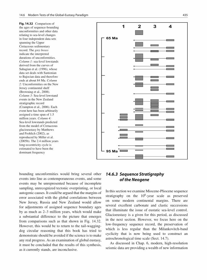
14.6 Modern Tests of the Global-Eustasy Paradigm 435
Fig. 14.32 Comparison ofthe ages of sequence-boundingunconformities and other datarelating to sea-level changesin four independent data setsspanning the UpperCretaceous sedimentaryrecord. The grey boxesindicate the interpreteddurations of unconformities.Column 1: sea-level lowstandsderived from the curves ofSahagian et al. (1996), whosedata set deals with Santonianto Bajocian data and thereforeends at about 84 Ma. Column2: Unconformities on the NewJersey continental shelf(Browning et al., 2008).Column 3: Sea-level lowstandevents in the New Zealandstratigraphic record(Crampton et al., 2006). Eachevent here has been arbitrarilyassigned a time span of 1.5million years. Column 4:Sea-level lowstands predictedfrom the model of Cretaceousglacioeustasy by Matthewsand Frohlich (2002), asreproduced by Miller et al.(2005b). The 2.4 million yearslong-eccentricity cycle isestimated to have been thedominant frequency
bounding unconformities would bring several otherevents into line as contemporaneous events, and someevents may be unrepresented because of incompletesampling, unrecognized tectonic overprinting, or localautogenic causes. It could be argued that the margins oferror associated with the global correlations betweenNew Jersey, Russia and New Zealand would allowfor adjustments of assigned sequence boundary agesby as much as 2–3 million years, which would makea substantial difference to the picture that emergesfrom comparisons such as that shown in Fig. 14.32.However, this would be to return to the tail-wagging-dog circular reasoning that this book has tried todemonstrate should be avoided if the science is to makeany real progress. As an examination of global eustasy,it must be concluded that the results of this synthesis,as it currently stands, are inconclusive.
14.6.3 Sequence Stratigraphyof the Neogene
In this section we examine Miocene-Pliocene sequencestratigraphy on the 106-year scale as preservedon some modern continental margins. There areseveral excellent carbonate and clastic successionsthat illuminate the issue of eustatic sea-level control.Glacioeustasy is a given for this period, as discussedin the next section. However, we focus here on thelow-frequency sequence record, the preservation ofwhich is less regular than the Milankovitch-bandcyclicity that is now being used to construct anastrochronological time scale (Sect. 14.7).
As discussed in Chap. 6, modern, high-resolutionseismic data are providing a wealth of new information
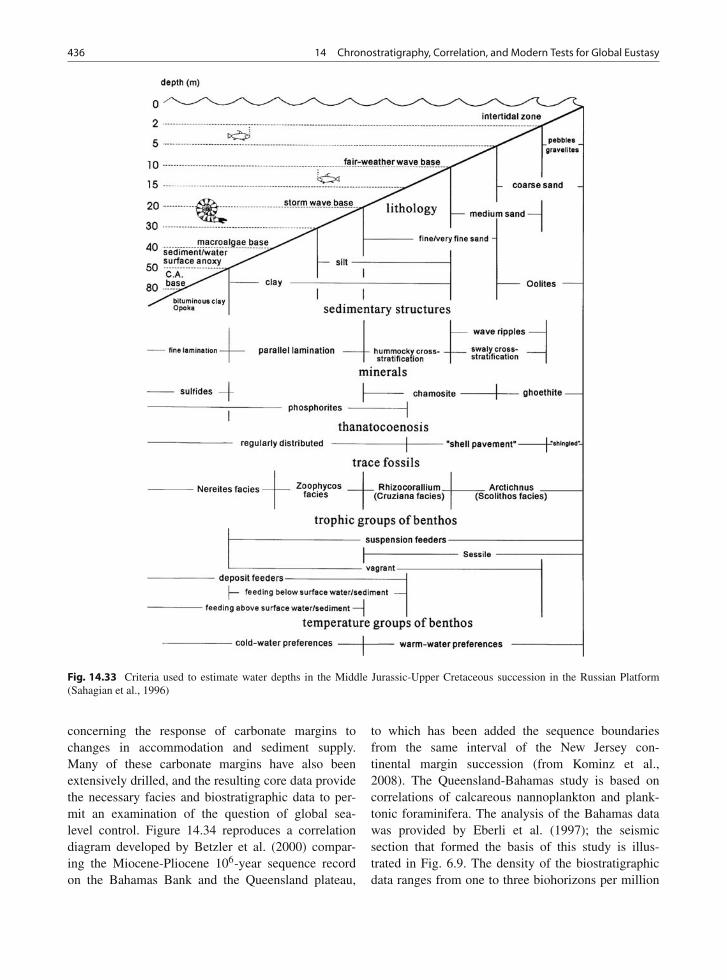
436 14 Chronostratigraphy, Correlation, and Modern Tests for Global Eustasy
Fig. 14.33 Criteria used to estimate water depths in the Middle Jurassic-Upper Cretaceous succession in the Russian Platform(Sahagian et al., 1996)
concerning the response of carbonate margins tochanges in accommodation and sediment supply.Many of these carbonate margins have also beenextensively drilled, and the resulting core data providethe necessary facies and biostratigraphic data to per-mit an examination of the question of global sea-level control. Figure 14.34 reproduces a correlationdiagram developed by Betzler et al. (2000) compar-ing the Miocene-Pliocene 106-year sequence recordon the Bahamas Bank and the Queensland plateau,
to which has been added the sequence boundariesfrom the same interval of the New Jersey con-tinental margin succession (from Kominz et al.,2008). The Queensland-Bahamas study is based oncorrelations of calcareous nannoplankton and plank-tonic foraminifera. The analysis of the Bahamas datawas provided by Eberli et al. (1997); the seismicsection that formed the basis of this study is illus-trated in Fig. 6.9. The density of the biostratigraphicdata ranges from one to three biohorizons per million
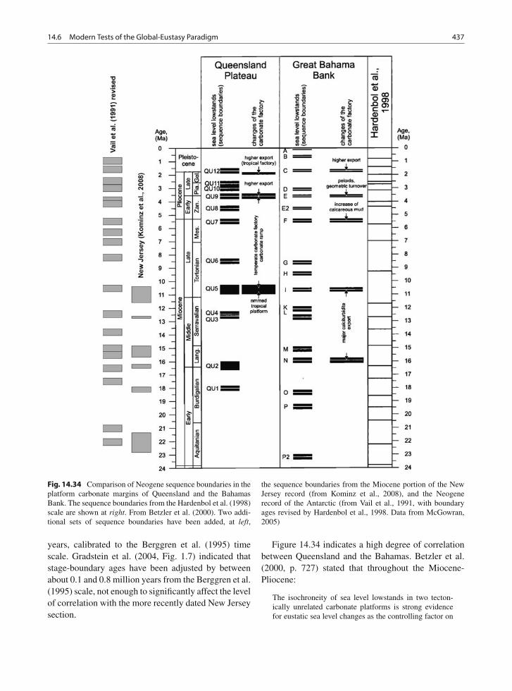
14.6 Modern Tests of the Global-Eustasy Paradigm 437
Fig. 14.34 Comparison of Neogene sequence boundaries in theplatform carbonate margins of Queensland and the BahamasBank. The sequence boundaries from the Hardenbol et al. (1998)scale are shown at right. From Betzler et al. (2000). Two addi-tional sets of sequence boundaries have been added, at left,
the sequence boundaries from the Miocene portion of the NewJersey record (from Kominz et al., 2008), and the Neogenerecord of the Antarctic (from Vail et al., 1991, with boundaryages revised by Hardenbol et al., 1998. Data from McGowran,2005)
years, calibrated to the Berggren et al. (1995) timescale. Gradstein et al. (2004, Fig. 1.7) indicated thatstage-boundary ages have been adjusted by betweenabout 0.1 and 0.8 million years from the Berggren et al.(1995) scale, not enough to significantly affect the levelof correlation with the more recently dated New Jerseysection.
Figure 14.34 indicates a high degree of correlationbetween Queensland and the Bahamas. Betzler et al.(2000, p. 727) stated that throughout the Miocene-Pliocene:
The isochroneity of sea level lowstands in two tecton-ically unrelated carbonate platforms is strong evidencefor eustatic sea level changes as the controlling factor on
438 14 Chronostratigraphy, Correlation, and Modern Tests for Global Eustasy
large. to medium-scale (1–5 Ma) stratigraphic packaging.The timing of most of the currently recognized eustaticsea level fluctuations in these independent carbonate sys-tems does, however, not seem to match as clearly withthe timing of global sea level lowstands as proposed byHaq et al. (1988) and Hardenbol et. al. (1998) in theMesozoic and Cenozoic Sequence ChronostratigraphicChart (MCSSC) (Figure 3)[Fig. 14.34 of this book].This discrepancy may relate to the resolution of bios-tratigraphic dating. The accuracy of dating depends ona number of factors: (1) the number of biostratigraphicdatum levels found, (2) the quality of the biostratigraphicevents used. Factors such as abundance of the speciesplay a role and the exact appearance or exit levels of aspecies should be quantified, which is hardly done owingto time constraints, and (3) consistency of sedimentationrates in between datum levels because the interpolationtechnique is used for the timing of a certain event.
Betzler et al. (2000) went on to note that the numberof sequence boundaries in their data does not cor-respond to the number of boundaries in the Exxonchart—an issue that, as noted earlier (see Table 11.2),constitutes one of the criteria for correlation that hasconsistently misled and confused stratigraphers. We donot consider the lack of correlation with the Hardenbolchart further, for reasons that should by now be obviousto readers of this book. Betzler et al. (2000) sug-gested that the accuracy of their sequence boundarycorrelation might be improved by more intensive bios-tratigraphic analysis. However, for our purposes, itis much more significant to evaluate the correlationswith the sequence boundary record from New Jersey(accurate sequence boundary ages for the successionyounger than 10 Ma are not available from this area).This is a comparison between two independent studiesand therefore fulfills one of the most important criteriafor a meaningful test of the global-eustasy paradigm.In this case, the evidence indicates a strong degreeof correlation between New Jersey, The Bahamas,and Queensland. Despite the small differences in thetime scales used in these two different interpretations,the comparisons between the data sets is striking.The adjustments that would be required to recalibratethe Betzler et al. (2000) study to GTS2004 would notsignificantly change the pattern visible in Fig. 14.34.The case for eustatic control of Miocene stratigraphyis considerably strengthened by this comparison.
Also shown in Fig. 14.34, for reference purposes,are the sequence boundaries documented in the “greatNeogene sedimentary wedge” (wording of McGowran,2005, p. 190) reconstructed by Vail et al. (1991), based
in part on an analysis of the Antarctic margin (Barteket al., 1991). The model of the Neogene wedge (seeFig. 6.4) claims to illustrate a global pattern of sea-level change and accompanying stratigraphic architec-ture that can be recognized worldwide. However, thereis very little correspondence between these sequenceboundaries and the New Jersey-Queensland-Bahamasevents documented in Fig. 14.34, which calls intoquestion the chronostratigraphic basis on which thewedge model was drawn. McGowran (2005, p. 191)indicated that the number and ages of the sequenceboundaries has been modified by Hardenbol et al.(1998), but the boundaries and ages indicated in hisredrawn version of the Vail et al. (1991, Fig. 12) dia-gram are the same as in that diagram, which were, inturn, based on the Haq et al. (1987) global cycle chart.
Additional data from other studies provide strongsupport for eustatic control during the Miocene,although it is also clear that this is not the onlysignificant control on platform carbonate develop-ment. Figure 6.14 is a summary diagram from thedetailed study of the Gulf of Papua carbonate plat-form by Tcherepanov et al. (2008). This diagramshows the Queensland-Bahamas sequence boundariesfrom Betzler et al. (2000), although the positionsof these boundaries have changed significantly fromthose shown in the original source (Fig. 14.34), forreasons that are unclear. They are much greater adjust-ments than would be required to revise the correlationsto GTS2004. The most important sea-level lowstand inthe Gulf of Papua data is one at 11.0 Ma, which clearlycorrelates with lowstands in New Jersey, Queenslandand the Bahamas (Fig. 14.34).
14.6.4 The Growing Evidencefor Glacioeustasy in the Mesozoicand Early Cenozoic
As noted by Vail et al. (1977, p. 93), glacioeustasyis the only process known that can generate large-amplitude eustatic changes in sea level over geologi-cally short periods of time, but they acknowledged that(at that time) there was no convincing evidence of con-tinental glaciation in the Mesozoic-Cenozoic recordprior to the Oligocene. At a time when oxygen-isotopedata were very limited, Matthews and Poore (1980)and Matthews (1984) suggested that the world wasice free until about 100 Ma, after which ice build-up
14.6 Modern Tests of the Global-Eustasy Paradigm 439
began, and proceeded in several significant steps untilthe late Cenozoic. But they acknowledged that, in gen-eral, evidence for glaciation in the Cretaceous was veryinadequate. In fact it has been widely assumed that theCretaceous was a period of continuous “greenhouse”climates (Frakes, 1979).
However, results of the Deep-Sea Drilling Project,including the gradual accumulation and calibration ofa large data-base of oxygen-isotope data, are dramat-ically changing this world view. Frakes and Francis(1988) suggested that there may never have been anentirely ice-free world, on the basis of such evidenceas the rare occurrence of erratics, dropstones and otherindicators of floating ice, in the geological record.But many of these erratics, collected from a varietyof Cretaceous marine units in Europe and Australia,may have been rafted by plants or animals (Markwickand Rowley, 1998), and cannot be taken as reliableevidence of glaciation. More convincing evidence forglacial climates preceding the late Cenozoic ice agecame from ODP Leg 119 in the Southern Ocean.Ehrmann and Mackensen (1992) reported the retrievalof diamictites of middle-Late Eocene age on this leg,interpreted as ice-rafted deposits, and suggesting theexistence of continental ice on Antarctica during theEocene.
Stoll and Schrag (1996) examined the oxygen- andstrontium-isotope record in the Lower Cretaceous sec-tion in several DSDP cores and argued that excur-sions in these data indicated high-frequency sea-level changes that could only have been caused byglacioeustasy.
Given the diametrically opposite points of viewto the question of global eustasy taken by Pindelland Drake (1998) and Graciansky et al. (1998) (seediscussion in Chap. 12), it is perhaps not surpris-ing that contributors to these volumes would arriveat different conclusions regarding the likelihood ofcontinental glaciation, and therefore the probabilityof glacioeustasy, during the Cretaceous-Paleogene.Abreu et al. (1998, p. 77), a contributor to the “globaleustasy” volume, noted negative δ18O events nearthe Cenomanian-Turonian boundary and in the UpperTuronian, and attempted to show how long-term tem-perature changes indicated by the sparse isotopic dataparalleled the long-term trends in the Hardenbol globalcycle chart. In contrast, Markwick and Rowley (1998),in the Pindell and Drake (1998) volume (which arguesfor complexity in stratigraphic controls), while also
noting the short-term spikes in oxygen isotope datafrom the Cenomanian and Turonian, concluded that formost of the Mesozoic and early Cenozoic the evidencefor glaciation is “ambiguous at best”. They devotedconsiderable space in their analysis to a demonstra-tion of the impossibility of the very large eustaticchanges in sea level required by the Haq et al. cyclechart, by calculating the volumes of continental ice thatwould have been required to account for the amountsof water from the oceans necessary to create the sea-level changes indicated in this chart. At this stagein the development of isotope geochemistry, many ofthe factors influencing the isotope signature in fos-sil organisms remained to be resolved satisfactorily,including the different chemistries of shell formationby planktonic and benthic organisms, the question ofwhether deep- or shallow-water ocean temperatureswere being indicated, the effects of post-depositionaldiagenesis, and so on.
Largely because of the large volume of oxygenisotope data acquired during ODP cruises over thelast decade, the use of this class of data to evalu-ate late Cenozoic glacioeustasy and oceanic temper-ature changes has become so much part of standardmethodology that the δ18O curve is now accepted asan independent measure of geologic time. We are notat that point for the Mesozoic-early Cenozoic yet, buthaving said that, oxygen isotope data are now pro-viding many essential new insights on climatic andoceanographic changes through that period. Severalrecent publications review this data set and argue thecase for periodic ice-cap development on the Antarcticcontinent through the so-called greenhouse period ofthe Mesozoic-early Cenozoic (e.g., Miller et al., 1999,2005a, b, 2008b). Two detailed studies focused onspecific parts of the Cretaceous record. Miller et al.(1999) examined the Maastrichtian record in coastalsediments in New Jersey, and Borneman et al. (2008)discussed the implications of a δ18O excursion duringthe Turonian.
One of the more prominent sequence boundariesexposed in the New Jersey coastal plain is an earlyMaastrichtian surface containing clear evidence ofsubaerial exposure overlain and underlain by shallow-marine deposits. Lithofacies and biofacies data wereinterpreted by Miller et al. (1999) to suggest a sea-levelchange of about 40 m associated with this boundary.Dating of the sequence boundary suggested a cor-relation with a δ18O excursion between about 69.1
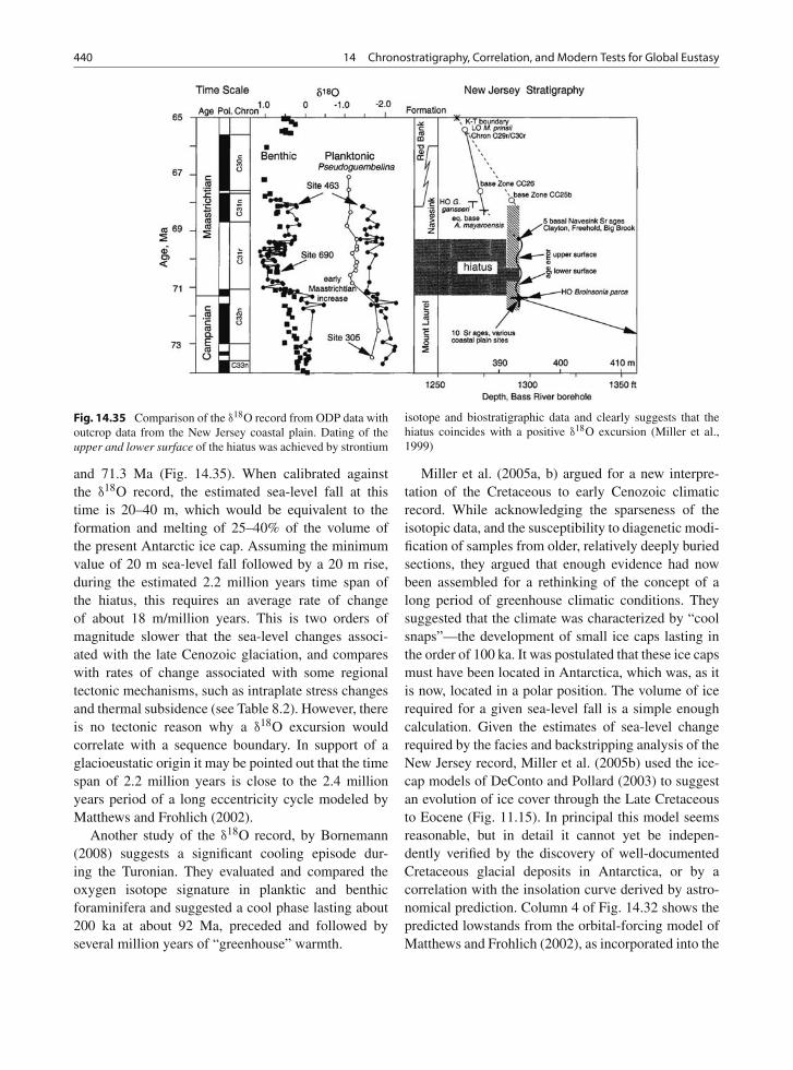
440 14 Chronostratigraphy, Correlation, and Modern Tests for Global Eustasy
Fig. 14.35 Comparison of the δ18O record from ODP data withoutcrop data from the New Jersey coastal plain. Dating of theupper and lower surface of the hiatus was achieved by strontium
isotope and biostratigraphic data and clearly suggests that thehiatus coincides with a positive δ18O excursion (Miller et al.,1999)
and 71.3 Ma (Fig. 14.35). When calibrated againstthe δ18O record, the estimated sea-level fall at thistime is 20–40 m, which would be equivalent to theformation and melting of 25–40% of the volume ofthe present Antarctic ice cap. Assuming the minimumvalue of 20 m sea-level fall followed by a 20 m rise,during the estimated 2.2 million years time span ofthe hiatus, this requires an average rate of changeof about 18 m/million years. This is two orders ofmagnitude slower that the sea-level changes associ-ated with the late Cenozoic glaciation, and compareswith rates of change associated with some regionaltectonic mechanisms, such as intraplate stress changesand thermal subsidence (see Table 8.2). However, thereis no tectonic reason why a δ18O excursion wouldcorrelate with a sequence boundary. In support of aglacioeustatic origin it may be pointed out that the timespan of 2.2 million years is close to the 2.4 millionyears period of a long eccentricity cycle modeled byMatthews and Frohlich (2002).
Another study of the δ18O record, by Bornemann(2008) suggests a significant cooling episode dur-ing the Turonian. They evaluated and compared theoxygen isotope signature in planktic and benthicforaminifera and suggested a cool phase lasting about200 ka at about 92 Ma, preceded and followed byseveral million years of “greenhouse” warmth.
Miller et al. (2005a, b) argued for a new interpre-tation of the Cretaceous to early Cenozoic climaticrecord. While acknowledging the sparseness of theisotopic data, and the susceptibility to diagenetic modi-fication of samples from older, relatively deeply buriedsections, they argued that enough evidence had nowbeen assembled for a rethinking of the concept of along period of greenhouse climatic conditions. Theysuggested that the climate was characterized by “coolsnaps”—the development of small ice caps lasting inthe order of 100 ka. It was postulated that these ice capsmust have been located in Antarctica, which was, as itis now, located in a polar position. The volume of icerequired for a given sea-level fall is a simple enoughcalculation. Given the estimates of sea-level changerequired by the facies and backstripping analysis of theNew Jersey record, Miller et al. (2005b) used the ice-cap models of DeConto and Pollard (2003) to suggestan evolution of ice cover through the Late Cretaceousto Eocene (Fig. 11.15). In principal this model seemsreasonable, but in detail it cannot yet be indepen-dently verified by the discovery of well-documentedCretaceous glacial deposits in Antarctica, or by acorrelation with the insolation curve derived by astro-nomical prediction. Column 4 of Fig. 14.32 shows thepredicted lowstands from the orbital-forcing model ofMatthews and Frohlich (2002), as incorporated into the
14.7 Cyclostratigraphy and Astrochronology 441
New Jersey studies of Miller et al. (2005a). As canbe seen in this figure, there is little correspondencebetween the predicted lowstands and the calculatedages of sequence boundaries in New Jersey and NewZealand (despite the claim to the contrary by Milleret al., 2005b, p. 228).
In conclusion: an increasing number of stratigraphicstudies (documented in Chaps. 6 and Chap. 7) isproviding strong evidence for high-frequencysequence-generating mechanisms during theCretaceous and early Cenozoic. Some sequencerecords can be explained by climate change (withoutglacioeustasy), of probable Milankovitch origin, whileother studies, some of them highlighted in this section,provide a strong case for glacioeustasy, driven by thedevelopment of small, temporary ice caps, probablylocated in Antarctica. The chronostratigraphic evi-dence for this process remains weak for the Cretaceous(Fig. 14.32), which could reflect residual errors andimprecisions in the global chronostratigraphic database. The evidence is much more convincing for theNeogene (Fig. 14.34), which has long been acceptedas a period characterized by major Antarctic icebuild-up.
14.7 Cyclostratigraphyand Astrochronology
14.7.1 Historical Backgroundof Cyclostratigraphy
The principles underlying the orbital forcing of stratig-raphy are set out in Chap. 11. The purpose of thissection is to examine the work that has been underwaysince the mid-1990s to develop a time scale based onthe “pacemaker” of orbital forcing. This is relevant toPart IV of this book in that cyclostratigraphy and theastrochronological time scale are the “new eustasy”—the time scale is being developed under the assumptionof an overriding control of the orbital “pacemaker”and the assumed regularity of the resulting stratigra-phy, which includes an interpreted driving force forhigh-frequency sequence stratigraphy.
In 1995, in a landmark volume establishing newtime scales and new methodologies for refiningthese scales, Herbert et al. (1995, p. 81) introduced
“Milankovitch cycles” with reference to the classicwork of Hays et al. (1976) and others, and stated that:
Stratigraphers may now be in a position to invert the usualargument; the “Milankovitch” hypothesis may be usedin appropriate settings to improve standard time scales.(italics as in original)
Rather than an attempt to use empirical data to “con-strain the predictions made from celestial mechanics”,as recommended by Fischer and Schwarzacher (1984),rather than a careful attempt to evaluate possi-ble differences in orbital parameters in the geo-logical past, this approach set out to confirm thereality of the Milankovitch signal by demonstrat-ing orbital parameters similar to those acting at thepresent day.
In 1998 the Royal Society of London held a sym-posium on the topic “Astronomical (Milankovitch)calibration of the geological time scale”, which wasattended by many of the leading researchers in thisfield. The results were published in the PhilosophicalTransactions of the Royal Society (Shackleton, et al.,1999; papers in this set are referred to by authorbelow, but are not listed separately in the referencesat the end of this paper). The symposium led offwith an astronomical study of orbital frequencies byLaskar. He concluded that calculation of planetarymotions cannot accurately retrodict Earth’s orbitalbehaviour before about 35 Ma, because of the long-term chaotic behaviour of the planets and because ofdrag effects relating to the dynamics of the Earth’s inte-rior. However, he suggested that “The uncertainty ofthe dissipative effects due to tidal dissipation, core-mantle interactions, and changes in dynamical ellip-ticity are real, but if the geological data are preciseenough, this should not be a real problem for the orbitalsolution.” His argument was that cyclostratigrapherscould rely on accurate data from the geologic recordin order to improve their astronomical calculations.
However, a review of the remaining papers, consti-tuting the body of the symposium proceedings, doesnot reassure us that such data are becoming avail-able. Most of the papers consist of detailed studies ofcyclic geological data which have been subject to timeseries analysis, filtering and tuning in order to high-light cycle frequencies. Most of these studies resultin the reconstruction of frequencies similar or iden-tical to those known from the present day, despitethe warnings of Laskar (1999), or earlier warnings
442 14 Chronostratigraphy, Correlation, and Modern Tests for Global Eustasy
of similar character (e.g., Berger and Loutre, 1994)that cycle frequencies could be significantly differ-ent in the more distant geological past. Having saidthis, these frequencies are not reported with any con-sistency. For example, a “long eccentricity” period isvariously reported as having a period of 400 ka (Galeet al.), 404 ka (Olsen et al., Hinnov and Park, Herbert),406 ka (Shackleton et al.), and 413 ka (Hilgen et al.),without reference to any such long-term variation infrequency.
All these individual studies represent analysis of“hanging” or “floating” sections, that is, sections thatare not rigorously tied in to any existing cyclostrati-graphic stratotype (because these do not exist forpre-Pliocene strata), but are dated according to conven-tional chronostratigraphic methods, that is, by use ofbiostratigraphy, with or without independent radiomet-ric or magnetostratigraphic calibration. The problemwith this is that even the best such chronostratigraphiccalibration is associated with significant error, as muchas ±4 Ma in the Jurassic (Weedon et al.). Thereis, therefore, no method to rigorously constrain tun-ing exercises. For example, a one-million-year errorin age range would encompass 48 potential preces-sional cycles with a frequency of 21 ka. Calibrationsmay, therefore, be affected by very large errors. Inaddition, nearly all the individual studies report vari-ations in sedimentary facies, and actual or suspectedmissing section, indicating difficulties in arriving atreliable estimates of sedimentation rate for the depth-time transformation. The interpretation of frequenciesin many of these papers is constrained by the identifica-tion of a cycle “bundling”, such as the 1:5 bundling thatis said to characterize the combined effect of eccentric-ity and precessional cycles, but such bundling is rarelyprecise and, in any case, also ignores the warnings ofLaskar and others that cycle periods may have beensignificantly different in the distant past. Individualcycles, like magnetic reversal events, are difficult toindividually characterize. As Murphy and Salvadorsaid of the latter (online version of the InternationalStratigraphic Guide by Michael A. Murphy and AmosSalvador; www.stratigraphy.org), reversals “have rel-atively little individuality, one reversal looks likeanother.” Comparisons and correlations between cyclestrings are therefore all too easy to accomplish, andthere may be little about such successions to indi-cate the presence of missing section. Torrens (2002, p.257) referred to what he called the “bar-code effect” of
dealing with “basically repetitious, often binary” dataof orbital cycles and magnetic reversals:
The problem is that, if one bar-line is missed or remainsunread, the bar-code becomes that, not of the next object,but that of a quite different object. The proximity of thenext object, becomes no proximity at all.
Miall and Miall (2004, p. 39) suggested thatattempts to develop a time scale with an accuracyand precision in the 104-year range by calibrat-ing it against conventional chronostratigraphic datesup to two orders of magnitude less precise rep-resents a fundamentally flawed methodology. Thebest that can said about the Royal Society sym-posium is that the results are “permissive”—theypoint to a possible future potential, but one that isvery far from being realized. Nonetheless, the edi-tors of the symposium proceedings, state, in theirPreface: “We believe that the calibration of at leastthe past 100 Ma is feasible over the next fewyears.”
In another incident of the “tail wagging the dog”,Van der Zwan (2002) generated orbital signals fromsubsurface digital gamma-ray data run on fluvial,deltaic and turbidite sediments from the Niger Delta.The potential for climate change to affect the sedi-ments of the delta is discussed in Sect. 11.2.5. Thedelta plain and delta front are sedimentary environ-ments characterized by frequent breaks in sedimen-tation and by very large fluctuations in sedimenta-tion rate as a result of changes in river and tidalenergy, storm activity, submarine landslides, etc.—not environments conducive to the preservation ofrhythmic regularity generated by an external sig-nal. Nevertheless, his time-series analysis generated apower spectrum and, with the aid of dates providedby biostratigraphy, he converted the cycles to a timefrequency, claiming that these demonstrated the peri-odicity of orbital eccentricity. When questioned aboutthis methodology, Van der Zwan responded (e-mailcorrespondence, 2003):
With respect to the key question, the validity of themethod, for me the ultimate test is whether it is possi-ble to forward model the stratigraphy of the calibrationwell correctly using these climatic input signals. In thisrespect, the fact that Milankovitch cyclicity is recorded inboth pollen spectra and gamma ray records convinced meof the presence of such climatic signals in the geologicalrecord.
14.7 Cyclostratigraphy and Astrochronology 443
And this:
An ultimate final control is whether the input parametersused make geological sense.
An analysis of a Paleocene pelagic rhythmic suc-cession in Italy (Polletti et al., 2004) provides a goodexample of the “inversion” of the Milankovitch argu-ment. These researchers extracted cyclic frequenciesfrom their data by spectral analysis, using a constantsedimentation rate calculated from the age range ofthe section (using the biostratigraphic time scale ofBerggren et al., 1995). They commented:
The apparent disagreement with eccentricity, obliquityand precession periods does not imply a stochastic dis-tribution. Parts of the succession may actually be missingdue to hiatuses not detectable by the traditional biostratig-raphy and the calculated sedimentation rate may thus notreflect the real deposition history and account for theapparent disagreement.
Their next step was to adjust the sedimentationrate so that the resultant cyclic frequencies matchedpresent-day orbital frequencies. The ratios of some ofthe cycle lengths in the adjusted cycle spectrum thenmatched the ratios between some of the Milankovitchfrequencies, although the relative strengths of thecyclic signals varied considerably from those of thepresent day.
Here is one of the problems with Frodeman’s“narrative logic” (Sect. 1.2.4). How do we tellwhen the logically elegant is, nonetheless, wrong?Experimentation that makes use of numerical mod-els is commonly used in the Earth Sciences to verifyor validate a quantitative model. However, Oreskeset al. (1994) have pointed out the logical fallacyinvolved in “affirming the consequent”—the demon-stration by numerical modeling of a predicted rela-tionship. This does not constitute confirmation of themodel; it merely indicates a certain probability that onefamily of solutions to a problem is feasible. Denzin(1970, p. 9) defined the “fallacy of objectivism” asthe researcher’s belief that if “formulations are the-oretically or methodologically sound they must haverelevance in the empirical world.”
To summarize this section, between the time ofthe initial, cautious work of Hays et al. (1976)and Berger et al. (1984) and the present day, the“Milankovitch theory” has been inverted. At first,researchers attempted to use geological data to explorethe range of cyclic climatic periodicities in the
geological past, with a view to testing the evidencefor the presence of an orbital-forcing signature. Now,the demonstration of cyclic periods falling some-where within the “Milankovitch band” is enough forresearchers to assert that the controlling mechanismwas orbital forcing. Initial cautions based on an under-standing of the incompleteness of the geological recordhave given way to a predisposition to respect the powerof time series analysis to generate the expected sig-nals. At least one astronomer has even suggested thatgeological data may be used to constrain the astronom-ical calculations (Laskar, 1999). For Laskar, geologicaldata had become a “black box” of unquestioned verac-ity. Geologists experienced in the incompleteness andinconsistencies of field data and knowledgeable aboutthe warnings associated with the use of time seriesanalysis offered by signal theorists (Rial, 1999, 2004),would be very skeptical about this last approach. Rial(1999) warned that “chronologies based on orbital tun-ing cannot be used because orbital tuning subtly forcesthe astronomical signal into the data.” As Dott (1992b,p. 13) pointed out, “the Milankovitch theory is veryaccommodating, for it provides a period to suit nearlyevery purpose.”
14.7.2 The Building of a Time Scale
The tuning of stratigraphic records with the use ofpreserved orbital signals has become a fruitful areaof research (House and Gale 1995; Hinnov, 2000;Weedon, 2003), but much remains to be done to clar-ify possible changes with time in orbital frequencies,and the broad framework of absolute ages withinwhich refined cyclostratigraphic determinations can becarried out.
Cyclostratigraphic studies depend on a hierarchy offive theoretical assumptions (Miall and Miall, 2004,p. 40):
1. The section is continuous, or2. (alternate): Discontinuities in the section can be
recognized and accounted for in the subsequentanalysis;
3. Sedimentation rate was constant, or events (suchas turbidites) beds can all be recognized and dis-counted.
444 14 Chronostratigraphy, Correlation, and Modern Tests for Global Eustasy
4. Orbital frequencies can be predicted for the dis-tant geological past, based on independent age-bracketing of the section;
5. Thickness can be converted to time using a simplesedimentation-rate transformation;
6. The variabilities in stratigraphic preservation(facies changes, hiatuses) can be effectively man-aged by pattern-matching techniques.
Do we have reliable tests of any of these assump-tions? At present there are still many questions.“Bundling” of three to six cycles into larger group-ings has been suggested as one distinctive featureof orbital control, indicating nesting of obliquity orprecessional cycles within the longer eccentricitycycles (Fischer, 1986; Cotillon, 1995), but given thenatural variability in the record, and the tendency ofgeologists to “see” cycles in virtually any data string(Zeller, 1964), this approach needs to be used withcaution.
Few researchers refer to the possibility of varia-tions in orbital behaviour through geologic time; yeta considerable amount of work has been carried outon this problem by astrophysicists, and some of thisis published in mainstream geological literature. Forexample, Laskar (1999) concluded that calculation ofplanetary motions cannot accurately retrodict Earth’sorbital behaviour before about 35 Ma. Berger andLoutre (1994) suggested that the obliquity and preces-sional periods have steadily lengthened through geo-logic time. Taking only their calculations for the LateCretaceous-Cenozoic, and omitting any considerationof chaotic behaviour, they indicated that the 19,000-year precessional period would have been 18,645 yearsat 72 Ma, and the 41,000-year obliquity period wouldhave been 39,381 years. What this means is that at72 Ma, the Earth, over a 10-million years time period,would have experienced ten more precessional andobliquity cycles than the present-day periods wouldhave predicted. This represents a very significant dif-ference, and one that cannot be ignored if cyclostrati-graphic data are to be used to refine the geologic timescale. Yet no mention of this is made in current liter-ature on this topic. And this may not be all. Murrayand Holman (1999) demonstrated that the orbits of thegiant outer planets are chaotic on a 107-year time scale.The implications of this result for the inner planets,including Earth, have yet to be resolved, but Murray(pers. comm., 2003) suggested that Earth’s orbit has
undoubtedly been affected by similar gravitationaleffects on a comparable time scale.
A reliable cyclostratigraphic (astrochronologic)time scale was first established for the youngestCenozoic strata, back to about 5 Ma (Hilgen, 1991;Berggren et al., 1995; Hilgen et al., 2006; seeFigs. 14.36 and 14.37). At the time of writing, astro-nomically calibrated sections have been used to extendthe astrochronological time scale back to 14.84 Ma,the base of the Serravallian stage, in the mid-Miocene(www.stratigraphy.org), and research is proceeding toextend the time scale not only to the base of theCenozoic, but through at least the Mesozoic (Hinnovand Ogg, 2007). However, Westphal et al. (2008)offered a sharply critical review of the field data baseon which part of the astrochronological time scaleis based, pointing to problems of diagenesis and dif-ferential compaction of contrasting lithologies, thatrender direct one-for-one correlations between the crit-ical field sections problematic. A careful comparisonof the correlations between two critical field sec-tions shows that the correlations of the astronomicalcycles are not always supported by the correlations ofbioevents. In some cases, there are different numbersof cycles between the occurrences of key bioevents(Fig. 14.38).
The problem, as we perceive it (Miall and Miall,2004), is that a powerful model may, once again, asin the case of the Vail curves, be used to drive thedevelopment of correlations rather than the empiri-cal data being used to test the model. Remarks aboutorbital control being a demonstrated “fact” temptgeologists to ignore the null hypothesis and to readilyassume that cyclic successions were deposited underthe influence of orbital forcing. Cyclostratigraphycan only work in continuous sections or where theexistence of hiatuses has been carefully evaluated. As Ihave attempted to demonstrate (Sect. 14.3; see also, inparticular, Aubry, 1991, 1995), evaluation of unconfor-mities is one of the most difficult and most neglectedaspects of stratigraphic study. One approach developedspecifically for cyclostratigraphic successions has beenoffered by Meyers and Sageman (2004). It requires thatthe stratigraphy be expressed as a numerical parame-ter that can be subjected to time-series analysis, suchas the optical densitometry gray-scale analysis of theBridge Creek Limestone used as a test in this paper.The data string for the section are then sampled in amoving window and subjected to a harmonic analysis.
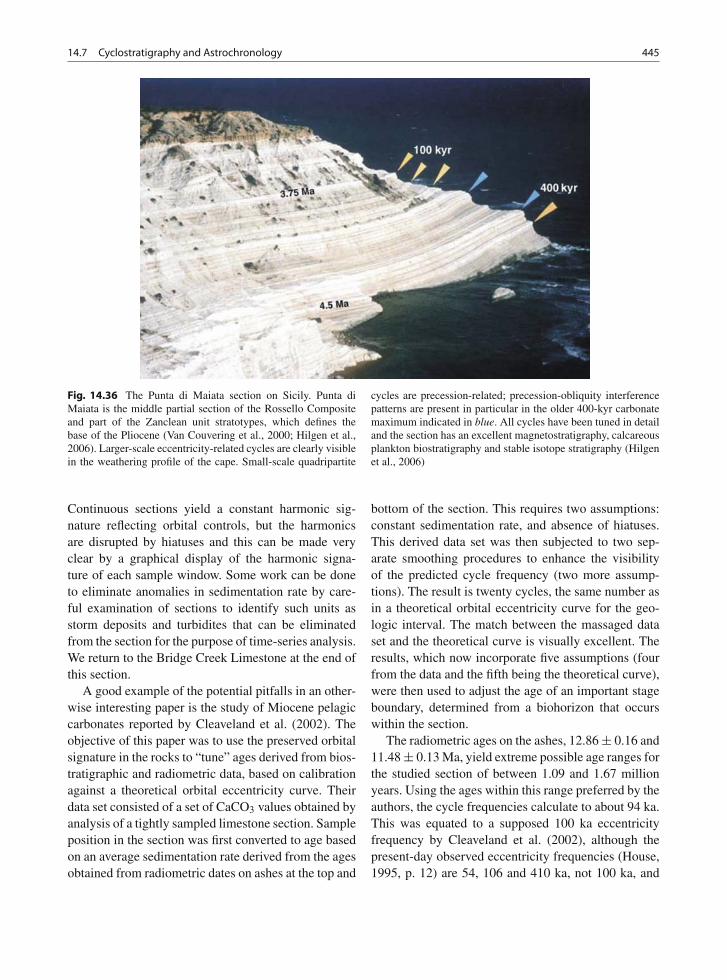
14.7 Cyclostratigraphy and Astrochronology 445
Fig. 14.36 The Punta di Maiata section on Sicily. Punta diMaiata is the middle partial section of the Rossello Compositeand part of the Zanclean unit stratotypes, which defines thebase of the Pliocene (Van Couvering et al., 2000; Hilgen et al.,2006). Larger-scale eccentricity-related cycles are clearly visiblein the weathering profile of the cape. Small-scale quadripartite
cycles are precession-related; precession-obliquity interferencepatterns are present in particular in the older 400-kyr carbonatemaximum indicated in blue. All cycles have been tuned in detailand the section has an excellent magnetostratigraphy, calcareousplankton biostratigraphy and stable isotope stratigraphy (Hilgenet al., 2006)
Continuous sections yield a constant harmonic sig-nature reflecting orbital controls, but the harmonicsare disrupted by hiatuses and this can be made veryclear by a graphical display of the harmonic signa-ture of each sample window. Some work can be doneto eliminate anomalies in sedimentation rate by care-ful examination of sections to identify such units asstorm deposits and turbidites that can be eliminatedfrom the section for the purpose of time-series analysis.We return to the Bridge Creek Limestone at the end ofthis section.
A good example of the potential pitfalls in an other-wise interesting paper is the study of Miocene pelagiccarbonates reported by Cleaveland et al. (2002). Theobjective of this paper was to use the preserved orbitalsignature in the rocks to “tune” ages derived from bios-tratigraphic and radiometric data, based on calibrationagainst a theoretical orbital eccentricity curve. Theirdata set consisted of a set of CaCO3 values obtained byanalysis of a tightly sampled limestone section. Sampleposition in the section was first converted to age basedon an average sedimentation rate derived from the agesobtained from radiometric dates on ashes at the top and
bottom of the section. This requires two assumptions:constant sedimentation rate, and absence of hiatuses.This derived data set was then subjected to two sep-arate smoothing procedures to enhance the visibilityof the predicted cycle frequency (two more assump-tions). The result is twenty cycles, the same number asin a theoretical orbital eccentricity curve for the geo-logic interval. The match between the massaged dataset and the theoretical curve is visually excellent. Theresults, which now incorporate five assumptions (fourfrom the data and the fifth being the theoretical curve),were then used to adjust the age of an important stageboundary, determined from a biohorizon that occurswithin the section.
The radiometric ages on the ashes, 12.86 ± 0.16 and11.48 ± 0.13 Ma, yield extreme possible age ranges forthe studied section of between 1.09 and 1.67 millionyears. Using the ages within this range preferred by theauthors, the cycle frequencies calculate to about 94 ka.This was equated to a supposed 100 ka eccentricityfrequency by Cleaveland et al. (2002), although thepresent-day observed eccentricity frequencies (House,1995, p. 12) are 54, 106 and 410 ka, not 100 ka, and
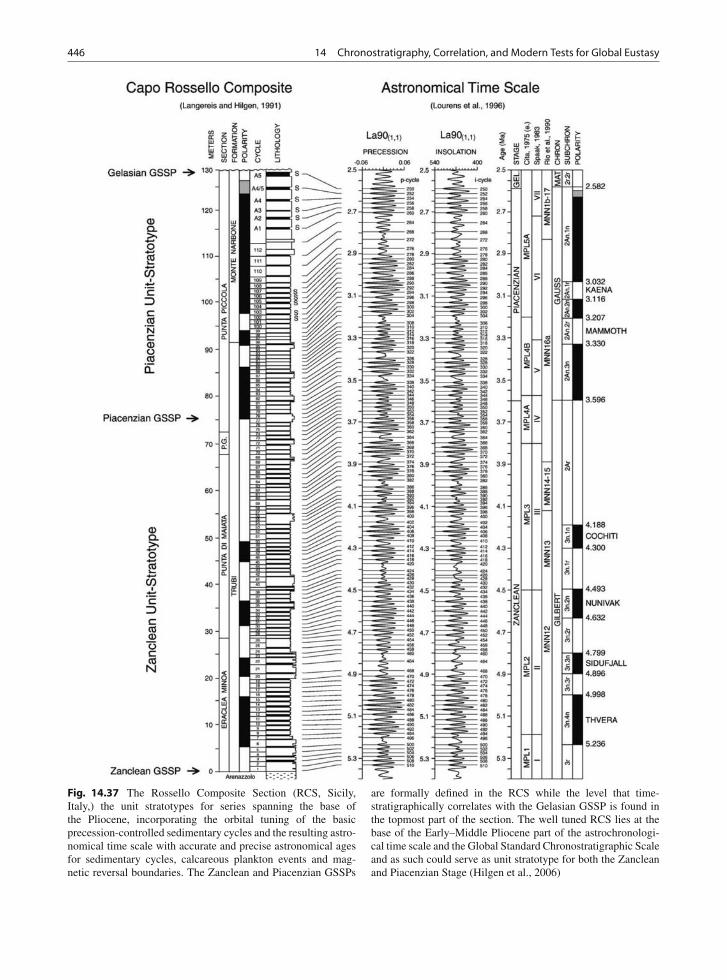
446 14 Chronostratigraphy, Correlation, and Modern Tests for Global Eustasy
Fig. 14.37 The Rossello Composite Section (RCS, Sicily,Italy,) the unit stratotypes for series spanning the base ofthe Pliocene, incorporating the orbital tuning of the basicprecession-controlled sedimentary cycles and the resulting astro-nomical time scale with accurate and precise astronomical agesfor sedimentary cycles, calcareous plankton events and mag-netic reversal boundaries. The Zanclean and Piacenzian GSSPs
are formally defined in the RCS while the level that time-stratigraphically correlates with the Gelasian GSSP is found inthe topmost part of the section. The well tuned RCS lies at thebase of the Early–Middle Pliocene part of the astrochronologi-cal time scale and the Global Standard Chronostratigraphic Scaleand as such could serve as unit stratotype for both the Zancleanand Piacenzian Stage (Hilgen et al., 2006)
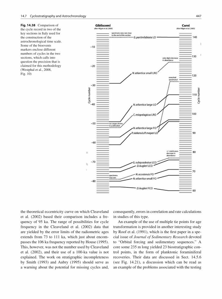
14.7 Cyclostratigraphy and Astrochronology 447
Fig. 14.38 Comparison ofthe cycle record in two of thekey sections in Italy used forthe construction of theastrochronological time scale.Some of the bioeventsmarkers enclose differentnumbers of cycles in the twosections, which calls intoquestion the precision that isclaimed for this methodology(Westphal et al., 2008,Fig. 10)
the theoretical eccentricity curve on which Cleavelandet al. (2002) based their comparison includes a fre-quency of 95 ka. The range of possibilities for cyclefrequency in the Cleaveland et al. (2002) data thatare yielded by the error limits of the radiometric agesextends from 73 to 111 ka, which just about encom-passes the 106 ka frequency reported by House (1995).This, however, was not the number used by Cleavelandet al. (2002), and their use of a 100-ka value is notexplained. The work on stratigraphic incompletenessby Smith (1993) and Aubry (1995) should serve asa warning about the potential for missing cycles and,
consequently, errors in correlation and rate calculationsin studies of this type.
An example of the use of multiple tie points for agetransformation is provided in another interesting studyby Roof et al. (1991), which is the first paper in a spe-cial issue of Journal of Sedimentary Research devotedto “Orbital forcing and sedimentary sequences.” Acore some 235 m long yielded 23 biostratigraphic con-trol points, in the form of planktonic foraminiferalrecoveries. Their data are discussed in Sect. 14.5.6(see Fig. 14.21), a discussion which can be read asan example of the problems associated with the testing
448 14 Chronostratigraphy, Correlation, and Modern Tests for Global Eustasy
of the assumptions listed at the beginning this section.Most ages are expressed in the Roof et al. (1991) paper(their Table 1) to the nearest 10,000 years, althoughno error ranges are indicated. A simple, linear arith-metic transformation is assumed throughout the rest oftheir paper, in that all core logs are plotted with timeas the ordinate instead of depth, based on the calcu-lated average. The data, once transformed, were takenas an empirical standard against which other measure-ments were plotted, and were then used in time seriesanalysis to extract orbital frequencies. These authorschose not to tune their data, with the result that spec-tral analysis generated a wide range of frequencies fordifferent intervals of the core. In only some of the coredo these frequencies compare with those suspected tobe the result of orbital forcing.
Based on the poor correlation with predictedMilankovitch frequencies, Roof et al. (1991) con-cluded that shifts in ocean currents and sedimentdelivery in their sample area (Gulf of Mexico), espe-cially that delivered by the nearby Mississippi River,accounted for much of the variability in sedimentationrate, and that this overprinted climatic effects withinmuch of the core.
There is nothing wrong with the science in thesepapers in so far as they are reports of specific fieldcase studies. Problems may arise, however, whenresults of this type are used as confirming evidence forthe general model of orbital control of sedimentationand astronomical calibration of the geological timescale. For example, the presentation by Cleavelandet al. (2002) of their correlations is followed by thisstatement:
Our astronomical correlation is made based on a com-bination of pattern matching between the carbonate andeccentricity curves, radiometric age constraints providedby the two volcanic ashes in the section, and resultsfrom spectral analysis of the tuned data set. Of otherpossible correlations consistent with the radiometric ageconstraints, we found greatest enhancement in the obliq-uity and precessional bands when the correlation shownin Fig. 3 is applied, and so favor this correlation overother possibilities, despite some discrepancies betweenthe amplitudes of corresponding carbonate and eccentric-ity peaks.
These authors have made use of the qualitative “pat-tern matching” method, which is easily susceptible tobias and error. However, they did note internal dis-crepancies and possible alternative correlations. Theassumptions of the model, therefore, must be contin-uously borne in mind.
A practical problem with dating and correlation atthe very fine scale required by cyclostratigraphy is theproblem of disturbance and mixing by bioturbation,and diagenetic modification of the sedimentary record.Anderson (2001) and Zalasiewicz et al. (2007) dis-cussed these problems. Gale et al. (2005) reported anobliquity and eccentricity signal in Eocene-Oligocenepaleosols based on illite abundance, a product of dia-genetic modification of smectite soils. Such alternationmay (but may not) reflect the product of actual orbitalclimatic changes, but as Zalasiewicz et al. (2007, p.142) remarked, the offset between deposition and dia-genesis may be hundreds to thousands of years. Hallam(1986) suspected that many cyclic limestone-shaledeposits, such as the Lower Jurassic Lias Formation ofsouthern Britain, are largely, if not entirely, the prod-uct of diagenetic unmixing, and therefore contain nomeaningful cyclostratigraphic signal.
McGowran (2005, pp. 65–84) and Hinnov and Ogg(2007) discussed the modern work underway to extendthe astrochronological time scale back through deeperand deeper geologic time. As McGowran (2005, p. 70)noted: “The power of the Cenozoic IMBS [integratedmagneto-biostratigraphic time scale] lies in the inces-sant triangulating between bio-, magneto- and radio-chronologies against the linearizer, seafloor spreading.Astrochronology now is an integral part of this pro-cedure.” As noted by Hinnov and Ogg (2007, p. 240)astrochronology can improve the precision of localcorrelation by an order of magnitude where continuoussections of orbitally-forced cycles can be indepen-dently fixed in time by radiometric or magnetostrati-graphic dating. Radiometric dating can now achieveprecision of ±0.1%, although this is still inadequate tofirmly fix the position of floating sections. A potential±0.1% error at 100 Ma amounts to ±100 ka, which isenough to prevent accurate correlations of successionsof precessional or obliquity cycles. Hinnov and Ogg(2007), citing recent astronomical work, suggest thatthe 405 ka eccentricity cycle might be the only reliablecyclic frequency to carry the time scale back into theMesozoic.
Because of its use in improving local correlationsby an order of magnitude (to a 104-year scale), cali-brating marine cyclic sections by astrochronology can“liberate” a great deal of biostratigraphic detail, suchas abundance data and minor evolutionary changes thathad previously been little more than noise in the data(McGowran, 2005, p. 78). This can potentially increase
14.7 Cyclostratigraphy and Astrochronology 449
the accuracy and precision of regional biostratigraphiccorrelation where the other forms of high-resolutioncorrelation and dating, such as magnetostratigraphy,are unavailable. However, given the problems withfaunal provincialism discussed in Sect. 14.5.6, it isunlikely that such additional detail would be of use inintercontinental correlation.
Does astrochronology offer any potential for thetesting of sequence models? In that the presence of104–5-year cyclicity in the rock record is itself ademonstration of the importance of orbital forcing asa driver of climate and, potentially, glacioeustasy (seediscussion in previous section), the answer is yes.Three examples from Europe and one from the USare briefly discussed here to illustrate both the natureof the contribution astrochronology can make, and thepitfalls that can surround it. The first example exempli-fies the way in which a refined astrochonological timescale may be employed to carry out refined tests ofgeological hypotheses. The second example illustratesthe pitfalls of building cyclostratigraphic interpreta-tions based on incomplete evidence. The third examplediscusses interpretive practices that this writer findsproblematic. The fourth example demonstrates that thecloser one looks and the more refined the data andmethodology, the more irregular the rocks appear to be,which calls into question our ability to apply routinizedstatistical methods to the ancient record.
Hilgen et al. (2007) examined the age and correla-tion of the Messinian evaporites in the MediterraneanSea in order to explore the several different hypothe-ses concerning the origin of the dramatic desiccationof this large marine basin. Alternative models for theisolation of the basin include glacioeustatic loweringof sea level below the Gibralter Strait sill, and tectonicclosure of the marine connection through this strait.Astrochronological correlation of sections throughoutthe basin suggests that the commencement of evapora-tion of the sea began at the identical time throughoutthe basin. Careful correlation of Mediterranean sec-tions with the oxygen isotope record from the NorthAtlantic Ocean indicates that initiation of evaporationcoincided with an episode of glacioeustatic sea-levelrise, not fall. Likewise, the termination of evaporation,as a result of re-flooding of the basin, does not corre-late to a glacioeustatic sea-level rise, which, accordingto Hilgen et al. (2007, p. 234) lends credibility toother hypotheses for the flooding of the basin, such asheadward erosion of rivers incising the Gibralter Straitfrom the Mediterranean side.
A more problematic area of research concerns thewell-known Middle-Upper Triassic carbonate cyclesof the Italian Dolomites. These were first knownby the work carried out on the so-called LoferCycles, named after the Dachstein Limestone in theLofer district of the Northern Calcareous Alps—the Dolomites—in Italy (Fischer, 1964; Enos andSamankassou, 1998). The Middle Triassic Latemarcarbonate buildup, nearby, is also a well knownarea of high-frequency cyclicity (Goldhammer et al.,1987; Hinnov and Goldhammer, 1991; Preto et al.,2001). The sedimentology and cyclicity of these cyclesare described briefly in Sect. 7.3. The problematicnature of this area of research is that independentwork to accurately date the rocks indicates a timespan for the cyclic succession that is not consistentwith Milankovitch frequencies. U-Pb dating of zir-cons from interbedded volcaniclastic rocks suggesteda shorter time span than expected for the succes-sion, making it difficult to fit the successions toMilankovitch frequencies. This problem triggered theso-called “Latemar controversy,” which included sug-gestions that the cycles represent previously unknownsub-Milankovitch frequencies, or even that they are notallocyclic in origin (Zühlke et al., 2003).
Following the development of these concernsregarding the chronostratigraphy of the Latemarcycles, Preto et al. (2001) resampled the field sec-tions, measuring a more complete (longer) section andemploying a more detailed classification of the car-bonate facies into four depth-related categories. Usingavailable radiometric ages, they recalculated the agerange of the disputed succession, and by tuning thesedimentation rate to a precessional index they foundthat three expected eccentricity frequencies and anexpected (but weakly recorded) obliquity frequencywere extracted by time series analysis. The 1:5 cyclestacking pattern, which it has been suggested is char-acteristic of orbitally forced successions (Chap. 11),was also recognized. However, Zühlke et al. (2003)insisted that their own even more detailed sectionmeasurements and correlations, coupled with high-precision U-Pb dating (Mundil et al., 2003) and inte-grated biostratigraphy yielded cycle periods of 2.20–2.89 ka (up to 6.4 ka when calculated using maximumuncertainties), which cannot be reconciled with theexpected Triassic “standard” precessional periodicityof 18–21 ka. They then experimented with variousmathematical models for tuning the data series, andarrived at a most-likely solution, consistent with the
450 14 Chronostratigraphy, Correlation, and Modern Tests for Global Eustasy
chronostratigraphic data, that if the basic cycle periodis set at 4.2 ka, then the various higher frequenciesand bundling ratios appear to fall into place. Spectralanalysis with the basic cycle set at 4.2 ka yielded a setof higher frequencies that can be assigned to predictedMilankovitch frequencies, including a 1: 4.7 ratio witha frequency in the 18.1–21.5 ka range, assumed to bea precessional frequency. This result was later essen-tially confirmed by independent statistical testing byMeyers (2008). Sedimentation (carbonate production)rates for the Latemar buildup calculated from thisrevised chronostratigraphic model yield values com-parable to “moderately prolific (sub)recent carbonateplatforms” (Zühlke et al., 2003, p. 76). The time-scale of cyclicity raised speculations about possiblecomparisons to the millennial climatic fluctuationsof the Quaternary era, which included such high-frequency events as the Dansgaard-Oeschger cycles(Broecker and Denton, 1989) and Heinrich events(Heinrich, 1988). However, it was recognized thatunder the assumed greenhouse climatic conditionsof the Triassic, a quite different regimen of hemi-spheric and global climatic oscillations would havebeen expected to occur.
The implications of the Latemar controversy are,as Zühlke et al. (2003, p. 79) pointed out, that in thecase of high-frequency cyclicity, simple cycle stackingratios cannot automatically be assigned to eccentricity-obliquity or eccentricity-precessional bundling. In fact,this highlights the entire questionable issue of auto-matically assigning Milankovitch frequencies to cyclicsuccessions deposited during the remote geologicalpast simply on the basis of bracketing ages that indicatefrequencies in the order of 104–105 years. Enormouscare will be required to extend the astrochronologicaltime scale back through the Cenozoic, and this authorremains very skeptical that it will ever be possible toaccurately assign floating sections to an astrochrono-logical time scale in the pre-Neogene.
The third example discussed here deals with thecyclostratigraphic analysis of some shallow-waterAptian-Albian carbonates in the southern Apennine,Italy, by D’Argenio et al. (2004b). Four sections ofthe carbonates were studied, consisting mainly ofsuccessions of subtidal to peritidal wackestones andgrainstones. Cycle boundaries were recognized onthe basis of microkarst or pedogenesis. The authorsclaim that statistical analysis of recurring sedimentaryfeatures generated ratios that match those of orbital
frequencies with a high degree of statistical probabil-ity, However, their stratigraphic sections show cycleswith highly variable thicknesses (Fig. 14.39). In one ofthe sections cycle thickness ranges from 0.3 to 5.55 m.Nevertheless, the analysis goes on to erect a system of“superbundles,” each consisting of two or three cycles.Three to five of the superbundles are said to definetransgressive-regressive sets. Correlations between thesections show that in some locations some of the cyclesare missing, which is attributed to low accommodation.From these sections a regional correlation frameworkwas constructed, using carbon isotope data as a sup-plementary means of correlation. The next step of theanalysis was to construct a regional “orbital chronos-tratigraphy,” although “in each section both locationand time of missing intervals are variable.” This isexplained in terms of “accommodation space as wellas bed thickness and facies of time-equivalent cyclesare controlled predominantly by regional changes insubsidence and carbonate productivity. Therefore aminor number of missing bundles is recorded in suc-cessions formed on more open carbonate-platformenvironments (hence producing higher sediment vol-umes) and vice versa.” (D’Argenio et al., 2004b, p.115). In fact, in the composite chronostratigraphic col-umn (Fig. 14.40) about one third of the bundles aremissing. This composite section, with its carbon iso-tope curve, was then correlated to a standard isotopecurve and tied into the eustatic “third-order” sequencesof Jacquin et al. (in Graciansky et al., 1998).
The expected standard error for the Aptian-Albianis about ±1 million years (Fig. 14.22) and there seemsto be good reasons to expect a more precise correlationof the composite section than this, given the match-ing of the carbon isotope curve to a standard curvefor the Aptian-Albian (not shown here). However, theproposed correlations of the eustatic events with theorbital chronology seems highly unrealistic to thiswriter. No range of potential error is indicated for the“third-order” events in the Graciansky et al. (1998)cycle chart, including that portion of it shown inFig. 14.22. Nor, given the numerous missing bundlesin the composite section, should the correlation withthis section be regarded as definitive. A potential errorof ±1 million years in the cycle chart allows for mis-correlation by one or two superbundles. The pattern ofmissing bundles in the Apennines section is reminis-cent of the pattern of missing faunal horizons in theInferior Oolite of southern England (Fig. 14.2), and
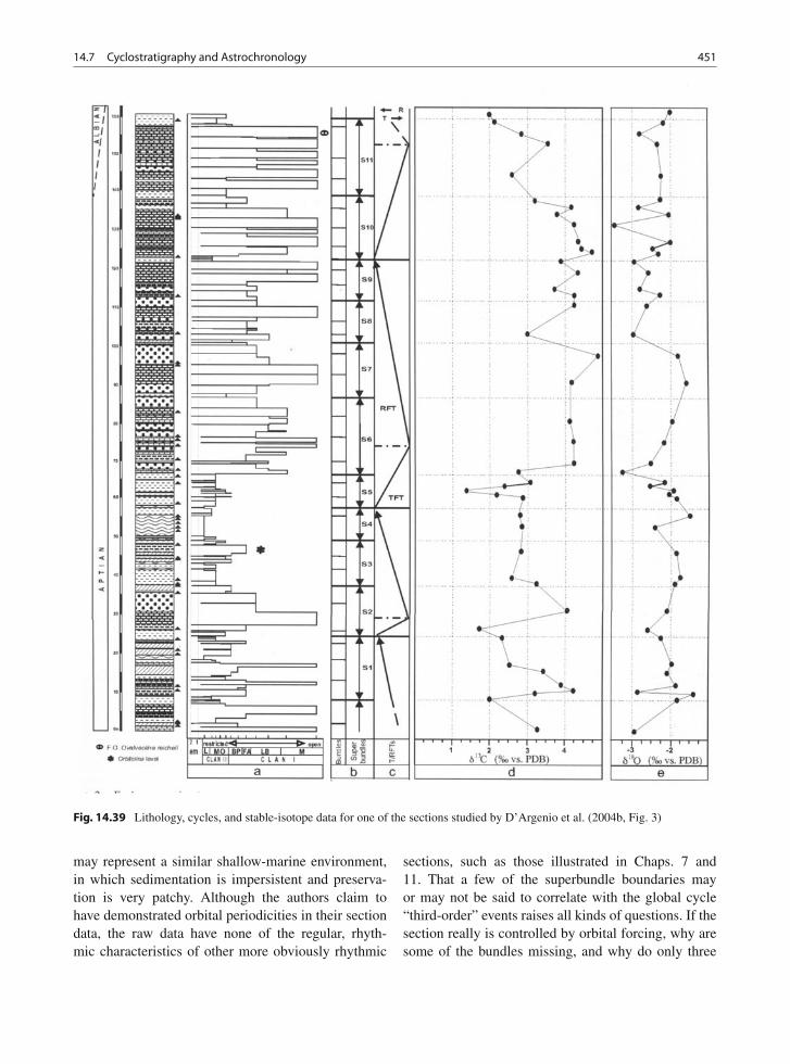
14.7 Cyclostratigraphy and Astrochronology 451
Fig. 14.39 Lithology, cycles, and stable-isotope data for one of the sections studied by D’Argenio et al. (2004b, Fig. 3)
may represent a similar shallow-marine environment,in which sedimentation is impersistent and preserva-tion is very patchy. Although the authors claim tohave demonstrated orbital periodicities in their sectiondata, the raw data have none of the regular, rhyth-mic characteristics of other more obviously rhythmic
sections, such as those illustrated in Chaps. 7 and11. That a few of the superbundle boundaries mayor may not be said to correlate with the global cycle“third-order” events raises all kinds of questions. If thesection really is controlled by orbital forcing, why aresome of the bundles missing, and why do only three
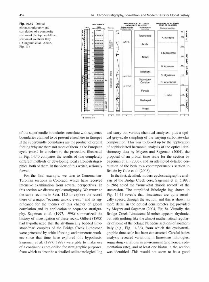
452 14 Chronostratigraphy, Correlation, and Modern Tests for Global Eustasy
Fig. 14.40 Orbitalchronostratigraphy andcorrelation of a compositesection of the Aptian-Albiansection of southern Italy(D’Argenio et al., 2004b,Fig. 11)
of the superbundle boundaries correlate with sequenceboundaries claimed to be present elsewhere in Europe?If the superbundle boundaries are the product of orbitalforcing why are there not more of them in the Europeancycle chart? In conclusion, the procedure illustratedin Fig. 14.40 compares the results of two completelydifferent methods of developing local chronostratigra-phies, both of them, in the view of this writer, seriouslyflawed.
For the final example, we turn to Cenomanian-Turonian sections in Colorado, which have receivedintensive examination from several perspectives. Inthis section we discuss cyclostratigraphy. We return tothe same sections in Sect. 14.8 to explore the recordthere of a major “oceanic anoxic event.” and its sig-nificance for the themes of this chapter of globalcorrelation and its application to sequence stratigra-phy. Sageman et al. (1997, 1998) summarized thehistory of investigation of these rocks. Gilbert (1895)had hypothesized that the rhythmically bedded lime-stone/marl couplets of the Bridge Creek Limestonewere generated by orbital forcing, and numerous work-ers since that time have explored this hypothesis.Sageman et al. (1997, 1998) were able to make useof a continuous core drilled for stratigraphic purposes,from which to describe a detailed sedimentological log
and carry out various chemical analyses, plus a opti-cal grey-scale sampling of the varying carbonate-claycomposition. This was followed up by the applicationof sophisticated harmonic analysis of the optical den-sitometry data by Meyers and Sageman (2004), theproposal of an orbital time scale for the section bySageman et al. (2006), and an attempted detailed cor-relation of the beds to a contemporaneous section inBritain by Gale et al. (2008).
In the first, detailed, modern cyclostratigraphic anal-ysis of the Bridge Creek core, Sageman et al. (1997,p. 286) noted the “somewhat chaotic record” of thesuccession. The simplified lithologic log shown inFig. 14.41 reveals that limestones are quite errati-cally spaced through the section, and this is shown inmore detail in the optical densitometer log providedby Meyers and Sageman (2004, Fig. 8). Visually, theBridge Creek Limestone Member appears rhythmic,but with nothing like the almost mathematical regular-ity of some of the pelagic Neogene sections of southernItaly (e.g., Fig. 14.36), from which the cyclostrati-graphic time scale has been constructed. Careful faciesanalysis revealed variations in limestone lithologies,suggesting variations in environment (and hence, sedi-mentation rate), and at least one hiatus in the sectionwas identified. This would not seem to be a good
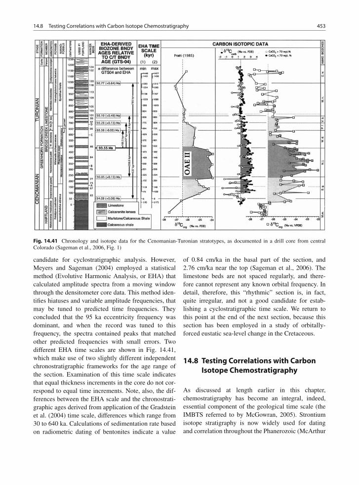
14.8 Testing Correlations with Carbon Isotope Chemostratigraphy 453
Fig. 14.41 Chronology and isotope data for the Cenomanian-Turonian stratotypes, as documented in a drill core from centralColorado (Sageman et al., 2006, Fig. 1)
candidate for cyclostratigraphic analysis. However,Meyers and Sageman (2004) employed a statisticalmethod (Evolutive Harmonic Analysis, or EHA) thatcalculated amplitude spectra from a moving windowthrough the densitometer core data. This method iden-tifies hiatuses and variable amplitude frequencies, thatmay be tuned to predicted time frequencies. Theyconcluded that the 95 ka eccentricity frequency wasdominant, and when the record was tuned to thisfrequency, the spectra contained peaks that matchedother predicted frequencies with small errors. Twodifferent EHA time scales are shown in Fig. 14.41,which make use of two slightly different independentchronostratigraphic frameworks for the age range ofthe section. Examination of this time scale indicatesthat equal thickness increments in the core do not cor-respond to equal time increments. Note, also, the dif-ferences between the EHA scale and the chronostrati-graphic ages derived from application of the Gradsteinet al. (2004) time scale, differences which range from30 to 640 ka. Calculations of sedimentation rate basedon radiometric dating of bentonites indicate a value
of 0.84 cm/ka in the basal part of the section, and2.76 cm/ka near the top (Sageman et al., 2006). Thelimestone beds are not spaced regularly, and there-fore cannot represent any known orbital frequency. Indetail, therefore, this “rhythmic” section is, in fact,quite irregular, and not a good candidate for estab-lishing a cyclostratigraphic time scale. We return tothis point at the end of the next section, because thissection has been employed in a study of orbitally-forced eustatic sea-level change in the Cretaceous.
14.8 Testing Correlations with CarbonIsotope Chemostratigraphy
As discussed at length earlier in this chapter,chemostratigraphy has become an integral, indeed,essential component of the geological time scale (theIMBTS referred to by McGowran, 2005). Strontiumisotope stratigraphy is now widely used for datingand correlation throughout the Phanerozoic (McArthur
454 14 Chronostratigraphy, Correlation, and Modern Tests for Global Eustasy
and Howarth, 2004; see discussion of its uses inSect. 14.6.1). Oxygen-isotope chemostratigraphy is anessential underpinning of the Neogene chronostrati-graphic scale (Gradstein et al., 2004), and is beinginterpreted to suggest the occurrence of glacioeustaticevents during the Cretaceous and Paleogene (Sect.14.6.4). These methods rely on the assumption, provenby multiple practical studies and tests, that isotopiclevels in the world’s marine waters become thor-oughly mixed over geologically short time periods,and that therefore isotopic signatures may be reliabletime markers. Correlations using these methods aretypically achieved by pattern recognition—the estab-lishment of standard curves for intervals of geologictime, based on detailed sampling (e.g., in DSDP cores;see Figs. 11.13 and 11.14). In the case of strontiumisotopes, the absolute values of the 87Sr/86Sr ratio mayin some cases be enough to provide a tight constrainton geological age, as these values have proven to beconsistent worldwide.
A parallel body of work has explored the varia-tion in carbon isotopic concentrations through geologictime, with a view to understanding the global carboncycle and to provide a supplementary tool for globalcorrelation (Scholle and Arthur, 1980; Veizer et al.,1999; Stoll and Schrag, 2000; Swart and Eberli, 2005;Katz et al., 2005). This is, however, a rather differentstory.
The δ13C composition of what Katz et al. (2005,p. 323) termed the “ocean’s mobile carbon reser-voir” is controlled by biological productivity, vol-canic and hydrothermal outgassing and weathering,and by oceanic mixing patterns. Different organismsshow different patterns of carbon isotope fractionation.Stratigraphic δ13C signatures are therefore typicallydetermined from bulk sediment samples, rather thanfrom specific microorganisms, as in the case of theoxygen isotope record. However, this signature may beaffected by changes in the redox state of the oceans(which affects the distribution of oxidized carbonateand reduced organic matter), by differences in burialrate, and by diagenesis. It has also been demonstratedthat samples of the same age from shallow- and deep-water water platform carbonates and from the openocean may have dissimilar δ13C values. Swart andEberli (2005) published curves showing quite differentδ13C histories for Bahamas Bank platform, slope andopen-ocean samples back through the last 25 Ma(Fig. 14.42). One reason for this may be the different
isotopic fractionation patterns generated by photo-synthesis of shallow-water versus deep-water pelagicmicroorganisms.
The pattern of carbon 13C variations illustratedin Fig. 14.42, and its explanation, might be thoughtto have discouraged any attempt to develop a car-bon isotope chronostratigraphy. Not so. Given thecontinual changes in Earth’s climate, changes in tec-tonic conditions, additions to atmospheric carbonreservoir from volcanic emissions, and so on, the car-bon reservoir is in constant flux, and it can be shownthat the changes are more or less well reflected bychanges in the sedimentary record worldwide. Anevent stratigraphy based on the δ13C record has beenconstructed for several intervals of the geological col-umn, but as discussed below, many problems andquestions remain. I focus here on the Cenomanian-Turonian interval of the Late Cretaceous, during whicha major Oceanic Anoxic Event occurred (Schlangerand Jenkyns, 1976). Detailed studies of this event havebeen carried out in southeast England (Gale et al.,1993), Italy (Parente et al., 2008; Scopelli et al., 2008;Galeotti et al., 2009), the Western Interior Seaway(Sageman et al., 2006; Gale et al., 2008), New Jersey(Bowman and Bralower, 2005), and China (Li et al.,2006), and intercontinental comparisons have beenpresented by Tsikos et al. (2004), Gale et al. (2008),and Galeotti et al. (2009).
The Cenomanian-Turonian anoxic event, known asOAE2, is recorded by the “excess burial of organiccarbon” (Tsikos et al., 2004, p. 711) and is well rep-resented in black shales, such as the Livello Bonarelliof the Apennines in central Italy. The “event” spansapproximately 2–15 m of section in each location, andhas been recorded in a variety of rock types, includ-ing chalks, pelagic carbonates, shales and siltstones.The total carbon content varies over a considerablerange between these various facies and locations, buta significant positive δ13C excursion spanning nearly 1million years in the upper Cenomanian and lowermostTuronian has been recorded in all the studied sections(Fig. 14.43). Although there is a broad match of high13C spanning the latter part of the Cenomanian and theCenomanian-Turonian boundary, “the most organic-rich and/or carbonate-poor horizons may be signifi-cantly diachronous when considered against integratedchemo- and biostratigraphy . . . probably reflecting theunique interaction between local palaeoceanographicand diagenetic conditions at each site and the global
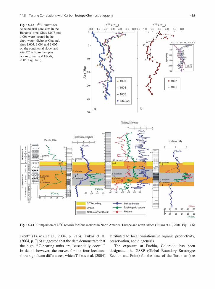
14.8 Testing Correlations with Carbon Isotope Chemostratigraphy 455
Fig. 14.42 δ13C curves forselected drill core sites in theBahamas area. Sites 1,007 and1,006 were located in thedeep-water Nicholas Channel,sites 1,003, 1,004 and 1,005on the continental slope, andsite 525 is from the openocean (Swart and Eberli,2005, Fig. 14.6)
Fig. 14.43 Comparison of δ13C records for four sections in North America, Europe and north Africa (Tsikos et al., 2004, Fig. 14.6)
event” (Tsikos et al., 2004, p. 716). Tsikos et al.(2004, p. 716) suggested that the data demonstrate thatthe high 13C-bearing units are “essentially coeval.”In detail, however, the curves for the four locationsshow significant differences, which Tsikos et al. (2004)
attributed to local variations in organic productivity,preservation, and diagenesis.
The exposure at Pueblo, Colorado, has beendesignated the GSSP (Global Boundary StratotypeSection and Point) for the base of the Turonian (see
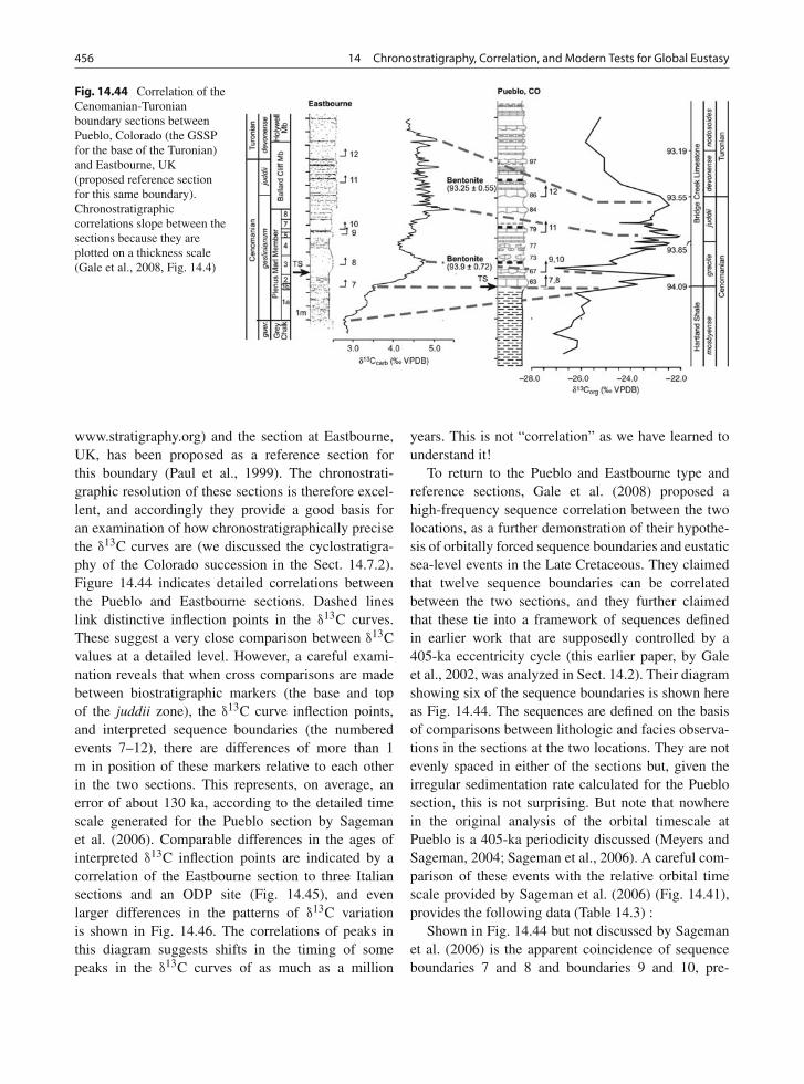
456 14 Chronostratigraphy, Correlation, and Modern Tests for Global Eustasy
Fig. 14.44 Correlation of theCenomanian-Turonianboundary sections betweenPueblo, Colorado (the GSSPfor the base of the Turonian)and Eastbourne, UK(proposed reference sectionfor this same boundary).Chronostratigraphiccorrelations slope between thesections because they areplotted on a thickness scale(Gale et al., 2008, Fig. 14.4)
www.stratigraphy.org) and the section at Eastbourne,UK, has been proposed as a reference section forthis boundary (Paul et al., 1999). The chronostrati-graphic resolution of these sections is therefore excel-lent, and accordingly they provide a good basis foran examination of how chronostratigraphically precisethe δ13C curves are (we discussed the cyclostratigra-phy of the Colorado succession in the Sect. 14.7.2).Figure 14.44 indicates detailed correlations betweenthe Pueblo and Eastbourne sections. Dashed lineslink distinctive inflection points in the δ13C curves.These suggest a very close comparison between δ13Cvalues at a detailed level. However, a careful exami-nation reveals that when cross comparisons are madebetween biostratigraphic markers (the base and topof the juddii zone), the δ13C curve inflection points,and interpreted sequence boundaries (the numberedevents 7–12), there are differences of more than 1m in position of these markers relative to each otherin the two sections. This represents, on average, anerror of about 130 ka, according to the detailed timescale generated for the Pueblo section by Sagemanet al. (2006). Comparable differences in the ages ofinterpreted δ13C inflection points are indicated by acorrelation of the Eastbourne section to three Italiansections and an ODP site (Fig. 14.45), and evenlarger differences in the patterns of δ13C variationis shown in Fig. 14.46. The correlations of peaks inthis diagram suggests shifts in the timing of somepeaks in the δ13C curves of as much as a million
years. This is not “correlation” as we have learned tounderstand it!
To return to the Pueblo and Eastbourne type andreference sections, Gale et al. (2008) proposed ahigh-frequency sequence correlation between the twolocations, as a further demonstration of their hypothe-sis of orbitally forced sequence boundaries and eustaticsea-level events in the Late Cretaceous. They claimedthat twelve sequence boundaries can be correlatedbetween the two sections, and they further claimedthat these tie into a framework of sequences definedin earlier work that are supposedly controlled by a405-ka eccentricity cycle (this earlier paper, by Galeet al., 2002, was analyzed in Sect. 14.2). Their diagramshowing six of the sequence boundaries is shown hereas Fig. 14.44. The sequences are defined on the basisof comparisons between lithologic and facies observa-tions in the sections at the two locations. They are notevenly spaced in either of the sections but, given theirregular sedimentation rate calculated for the Pueblosection, this is not surprising. But note that nowherein the original analysis of the orbital timescale atPueblo is a 405-ka periodicity discussed (Meyers andSageman, 2004; Sageman et al., 2006). A careful com-parison of these events with the relative orbital timescale provided by Sageman et al. (2006) (Fig. 14.41),provides the following data (Table 14.3) :
Shown in Fig. 14.44 but not discussed by Sagemanet al. (2006) is the apparent coincidence of sequenceboundaries 7 and 8 and boundaries 9 and 10, pre-
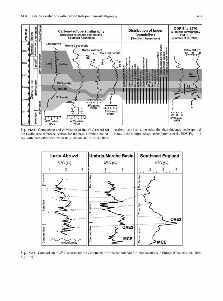
14.8 Testing Correlations with Carbon Isotope Chemostratigraphy 457
Fig. 14.45 Comparison and correlation of the δ13C record forthe Eastbourne reference section for the base-Turonian bound-ary, with three other sections in Italy, and an ODP site. All these
sections have been adjusted so that their thickness scale approxi-mates to the interpreted age scale (Parente, et al., 2008, Fig. 14.1)
Fig. 14.46 Comparison of δ13C records for the Cenomanian-Coniacian interval for three locations in Europe (Galeotti et al., 2009,Fig. 14.9)
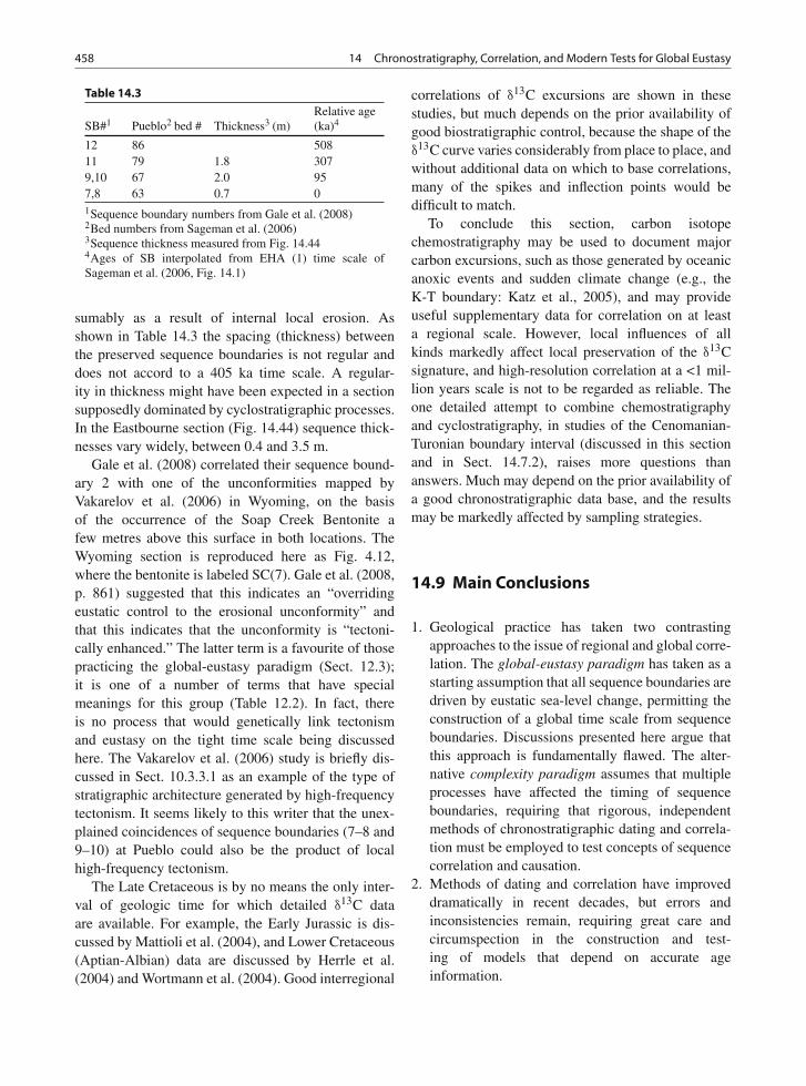
458 14 Chronostratigraphy, Correlation, and Modern Tests for Global Eustasy
Table 14.3
SB#1 Pueblo2 bed # Thickness3 (m)Relative age(ka)4
12 86 50811 79 1.8 3079,10 67 2.0 957,8 63 0.7 01Sequence boundary numbers from Gale et al. (2008)2Bed numbers from Sageman et al. (2006)3Sequence thickness measured from Fig. 14.444Ages of SB interpolated from EHA (1) time scale ofSageman et al. (2006, Fig. 14.1)
sumably as a result of internal local erosion. Asshown in Table 14.3 the spacing (thickness) betweenthe preserved sequence boundaries is not regular anddoes not accord to a 405 ka time scale. A regular-ity in thickness might have been expected in a sectionsupposedly dominated by cyclostratigraphic processes.In the Eastbourne section (Fig. 14.44) sequence thick-nesses vary widely, between 0.4 and 3.5 m.
Gale et al. (2008) correlated their sequence bound-ary 2 with one of the unconformities mapped byVakarelov et al. (2006) in Wyoming, on the basisof the occurrence of the Soap Creek Bentonite afew metres above this surface in both locations. TheWyoming section is reproduced here as Fig. 4.12,where the bentonite is labeled SC(7). Gale et al. (2008,p. 861) suggested that this indicates an “overridingeustatic control to the erosional unconformity” andthat this indicates that the unconformity is “tectoni-cally enhanced.” The latter term is a favourite of thosepracticing the global-eustasy paradigm (Sect. 12.3);it is one of a number of terms that have specialmeanings for this group (Table 12.2). In fact, thereis no process that would genetically link tectonismand eustasy on the tight time scale being discussedhere. The Vakarelov et al. (2006) study is briefly dis-cussed in Sect. 10.3.3.1 as an example of the type ofstratigraphic architecture generated by high-frequencytectonism. It seems likely to this writer that the unex-plained coincidences of sequence boundaries (7–8 and9–10) at Pueblo could also be the product of localhigh-frequency tectonism.
The Late Cretaceous is by no means the only inter-val of geologic time for which detailed δ13C dataare available. For example, the Early Jurassic is dis-cussed by Mattioli et al. (2004), and Lower Cretaceous(Aptian-Albian) data are discussed by Herrle et al.(2004) and Wortmann et al. (2004). Good interregional
correlations of δ13C excursions are shown in thesestudies, but much depends on the prior availability ofgood biostratigraphic control, because the shape of theδ13C curve varies considerably from place to place, andwithout additional data on which to base correlations,many of the spikes and inflection points would bedifficult to match.
To conclude this section, carbon isotopechemostratigraphy may be used to document majorcarbon excursions, such as those generated by oceanicanoxic events and sudden climate change (e.g., theK-T boundary: Katz et al., 2005), and may provideuseful supplementary data for correlation on at leasta regional scale. However, local influences of allkinds markedly affect local preservation of the δ13Csignature, and high-resolution correlation at a <1 mil-lion years scale is not to be regarded as reliable. Theone detailed attempt to combine chemostratigraphyand cyclostratigraphy, in studies of the Cenomanian-Turonian boundary interval (discussed in this sectionand in Sect. 14.7.2), raises more questions thananswers. Much may depend on the prior availability ofa good chronostratigraphic data base, and the resultsmay be markedly affected by sampling strategies.
14.9 Main Conclusions
1. Geological practice has taken two contrastingapproaches to the issue of regional and global corre-lation. The global-eustasy paradigm has taken as astarting assumption that all sequence boundaries aredriven by eustatic sea-level change, permitting theconstruction of a global time scale from sequenceboundaries. Discussions presented here argue thatthis approach is fundamentally flawed. The alter-native complexity paradigm assumes that multipleprocesses have affected the timing of sequenceboundaries, requiring that rigorous, independentmethods of chronostratigraphic dating and correla-tion must be employed to test concepts of sequencecorrelation and causation.
2. Methods of dating and correlation have improveddramatically in recent decades, but errors andinconsistencies remain, requiring great care andcircumspection in the construction and test-ing of models that depend on accurate ageinformation.
14.9 Main Conclusions 459
3. A few excellent modern data sets are now avail-able that provide rigorous examination of subsi-dence and sedimentation histories calibrated againsta refined chronostratigraphic record. However,there is still an inadequate data base fromwhich to come to reliable conclusions regard-ing the prevalence or importance of eustasy dur-ing the Mesozoic and Paleogene. Correlationsof sequence boundaries for the Neogene haveprovided an emerging picture of global sea-level control, almost certainly driven primarily byglacioeustasy.
4. Limited evidence is being assembled forepisodic glaciation and glacioeustasy during theCretaceous.
5. A global time scale is now being constructed fromthe record of orbital forcing. Termed astrochronol-ogy or cyclostratigraphy, the technique can only beregarded as reliable where it is based on continuous
sections or composite sections that provide a com-plete record extending backwards from the presentday. Currently a reliable scale extends back to themid-Miocene. Many attempts to develop partialscales for earlier time periods, or to explain olderstratigraphic successions in terms of orbital forcing,have involved questionable practices, and many ofthe results need to be evaluated with caution andskepticism.
6. Lessons learned from an examination of the global-eustasy paradigm, and from the more recentresearch trends in cyclostratigraphy, suggest thatextreme caution needs to be employed in the appli-cation of the deductive approach to stratigraphicinterpretation. While hypothesis building and test-ing is fundamental to the scientific method, it hasbeen too commonly the case that the attractivenessof models has overwhelmed a lack of supportingdata.
Chapter 15
Future Directions
Contents
15.1 Research Methods . . . . . . . . . . . . . . 46115.2 Remaining Questions . . . . . . . . . . . . 463
15.2.1 Future Advances in Cyclostratigraphy? . 46315.2.2 Tectonic Mechanisms of Sequence
Generation . . . . . . . . . . . . . . 46415.2.3 Orbital Forcing . . . . . . . . . . . . 46415.2.4 The Codification of Sequence
Nomenclature . . . . . . . . . . . . 464
15.1 Research Methods
Whether the objective of research is to explore regionalbasin history and plate kinematics, or to focus onpetroleum potential, the exploration of a new areasrequires that logical procedures be followed, to ensuremaximum efficiency. This is discussed in the conclud-ing section of Chap. 3 (Sect. 3.8). Vail et al. (1991)had suggested a series of steps that commenced witha determination of the physical chronostratigraphicframework by interpreting sequences, systems tractsand parasequences and/or simple sequences on out-crops, well logs and seismic data and age date withhigh resolution biostratigraphy.
A problem with this approach is that it is built onthe assumption that a chronostratigraphic frameworkcan be constructed as the first step of the analysis.This, of course, arises directly from the assump-tions of the global eustasy paradigm, amongst whichis the central idea that all sequence boundaries arechronostratigraphic surfaces. Given this assumption,the ability to then immediately carry out a geohistory(backstripping) analysis would follow logically.
Following a discussion of the application of Exxonsequence analysis methods and concepts to two basinexamples, Miall (1997, Sect. 17.3.3) suggested a mod-ified set of research procedures:
1. Develop an allostratigraphic framework based ondetailed lithostratigraphic well correlation and/orseismic facies analysis.
2. Develop a suite of possible stratigraphic modelsthat conform with available stratigraphic and faciesdata.
3. Establish a regional sequence framework with theuse of all available chronostratigraphic information.
4. Determine the relationships between sequenceboundaries and tectonic events by tracing sequenceboundaries into areas of structural deformation,and documenting the architecture of onlap/offlaprelationships, fault offsets, unconformable discor-dancies, etc.
5. Establish the relationship between sequence bound-aries and regional tectonic history, based on plate-kinematic reconstructions.
6. Refine the sequence-stratigraphic model. Subdividesequences into depositional systems tracts andinterpret facies.
7. Construct regional structural, isopach, and faciesmaps, interpret paleogeographic evolution, anddevelop plays and prospects based on this analysis.
8. Develop detailed subsidence and thermal-maturation history by backstripping/geohistoryanalysis.
It was suggested that subsidence and maturationanalysis (Step 8) be carried out at the conclusion
461A.D. Miall, The Geology of Stratigraphic Sequences, 2nd ed.,DOI 10.1007/978-3-642-05027-5_15, © Springer-Verlag Berlin Heidelberg 2010
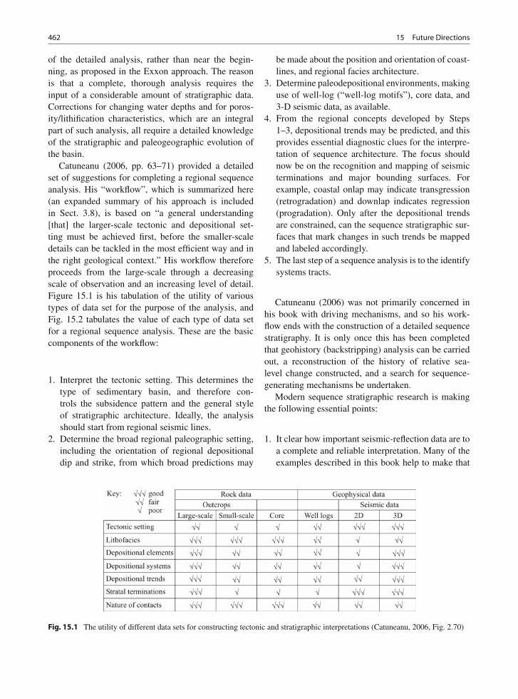
462 15 Future Directions
of the detailed analysis, rather than near the begin-ning, as proposed in the Exxon approach. The reasonis that a complete, thorough analysis requires theinput of a considerable amount of stratigraphic data.Corrections for changing water depths and for poros-ity/lithification characteristics, which are an integralpart of such analysis, all require a detailed knowledgeof the stratigraphic and paleogeographic evolution ofthe basin.
Catuneanu (2006, pp. 63–71) provided a detailedset of suggestions for completing a regional sequenceanalysis. His “workflow”, which is summarized here(an expanded summary of his approach is includedin Sect. 3.8), is based on “a general understanding[that] the larger-scale tectonic and depositional set-ting must be achieved first, before the smaller-scaledetails can be tackled in the most efficient way and inthe right geological context.” His workflow thereforeproceeds from the large-scale through a decreasingscale of observation and an increasing level of detail.Figure 15.1 is his tabulation of the utility of varioustypes of data set for the purpose of the analysis, andFig. 15.2 tabulates the value of each type of data setfor a regional sequence analysis. These are the basiccomponents of the workflow:
1. Interpret the tectonic setting. This determines thetype of sedimentary basin, and therefore con-trols the subsidence pattern and the general styleof stratigraphic architecture. Ideally, the analysisshould start from regional seismic lines.
2. Determine the broad regional paleographic setting,including the orientation of regional depositionaldip and strike, from which broad predictions may
be made about the position and orientation of coast-lines, and regional facies architecture.
3. Determine paleodepositional environments, makinguse of well-log (“well-log motifs”), core data, and3-D seismic data, as available.
4. From the regional concepts developed by Steps1–3, depositional trends may be predicted, and thisprovides essential diagnostic clues for the interpre-tation of sequence architecture. The focus shouldnow be on the recognition and mapping of seismicterminations and major bounding surfaces. Forexample, coastal onlap may indicate transgression(retrogradation) and downlap indicates regression(progradation). Only after the depositional trendsare constrained, can the sequence stratigraphic sur-faces that mark changes in such trends be mappedand labeled accordingly.
5. The last step of a sequence analysis is to the identifysystems tracts.
Catuneanu (2006) was not primarily concerned inhis book with driving mechanisms, and so his work-flow ends with the construction of a detailed sequencestratigraphy. It is only once this has been completedthat geohistory (backstripping) analysis can be carriedout, a reconstruction of the history of relative sea-level change constructed, and a search for sequence-generating mechanisms be undertaken.
Modern sequence stratigraphic research is makingthe following essential points:
1. It clear how important seismic-reflection data are toa complete and reliable interpretation. Many of theexamples described in this book help to make that
Fig. 15.1 The utility of different data sets for constructing tectonic and stratigraphic interpretations (Catuneanu, 2006, Fig. 2.70)
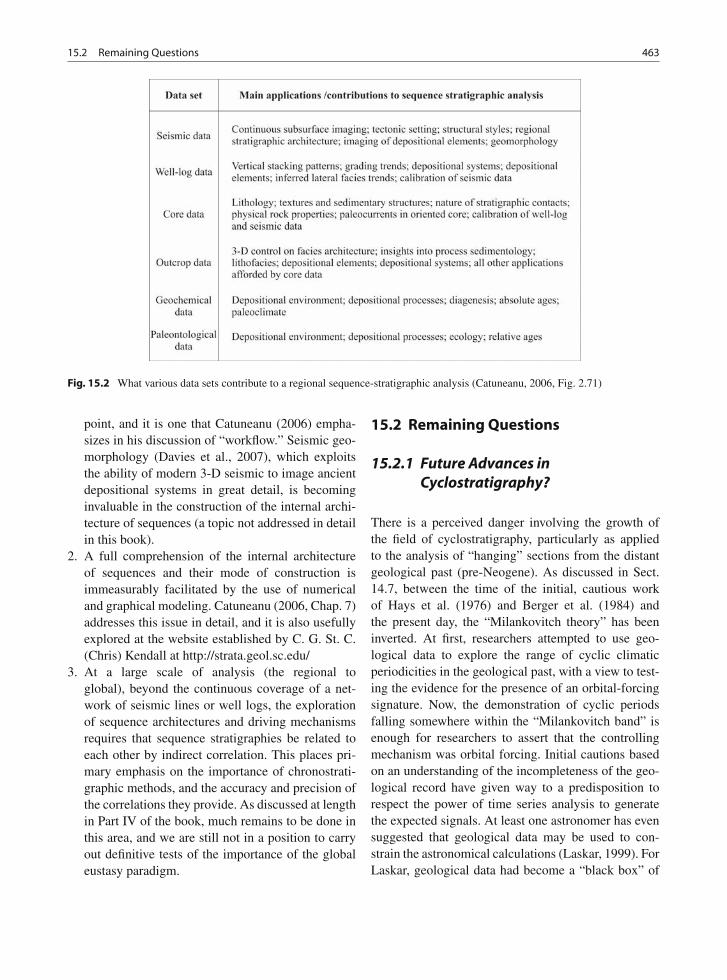
15.2 Remaining Questions 463
Fig. 15.2 What various data sets contribute to a regional sequence-stratigraphic analysis (Catuneanu, 2006, Fig. 2.71)
point, and it is one that Catuneanu (2006) empha-sizes in his discussion of “workflow.” Seismic geo-morphology (Davies et al., 2007), which exploitsthe ability of modern 3-D seismic to image ancientdepositional systems in great detail, is becominginvaluable in the construction of the internal archi-tecture of sequences (a topic not addressed in detailin this book).
2. A full comprehension of the internal architectureof sequences and their mode of construction isimmeasurably facilitated by the use of numericaland graphical modeling. Catuneanu (2006, Chap. 7)addresses this issue in detail, and it is also usefullyexplored at the website established by C. G. St. C.(Chris) Kendall at http://strata.geol.sc.edu/
3. At a large scale of analysis (the regional toglobal), beyond the continuous coverage of a net-work of seismic lines or well logs, the explorationof sequence architectures and driving mechanismsrequires that sequence stratigraphies be related toeach other by indirect correlation. This places pri-mary emphasis on the importance of chronostrati-graphic methods, and the accuracy and precision ofthe correlations they provide. As discussed at lengthin Part IV of the book, much remains to be done inthis area, and we are still not in a position to carryout definitive tests of the importance of the globaleustasy paradigm.
15.2 Remaining Questions
15.2.1 Future Advances inCyclostratigraphy?
There is a perceived danger involving the growth ofthe field of cyclostratigraphy, particularly as appliedto the analysis of “hanging” sections from the distantgeological past (pre-Neogene). As discussed in Sect.14.7, between the time of the initial, cautious workof Hays et al. (1976) and Berger et al. (1984) andthe present day, the “Milankovitch theory” has beeninverted. At first, researchers attempted to use geo-logical data to explore the range of cyclic climaticperiodicities in the geological past, with a view to test-ing the evidence for the presence of an orbital-forcingsignature. Now, the demonstration of cyclic periodsfalling somewhere within the “Milankovitch band” isenough for researchers to assert that the controllingmechanism was orbital forcing. Initial cautions basedon an understanding of the incompleteness of the geo-logical record have given way to a predisposition torespect the power of time series analysis to generatethe expected signals. At least one astronomer has evensuggested that geological data may be used to con-strain the astronomical calculations (Laskar, 1999). ForLaskar, geological data had become a “black box” of
464 15 Future Directions
unquestioned veracity. House and Gale (1995, Preface)remarked that “the reality of orbital forcing of climatewas established as a fact.” Counting the number ofcycles in a succession has become a criterion for cor-relation, a simplistic method reminiscent of that usedin support of the global eustasy model (Table 12.2),and which may lead to over-simplifications regardingmissing section (Westphal et al., 2008).
In Sect. 12.1, I point out the obvious dangers of cir-cular reasoning involved in the deductivist approach tosequence stratigraphy. Miall and Miall (2004, p. 39)suggested that attempts to develop a time scale withan accuracy and precision in the 104-year range bycalibrating it against conventional chronostratigraphicdates up to two orders of magnitude less preciserepresents a fundamentally flawed methodology.
Geologists experienced in the incompleteness andinconsistencies of field data and knowledgeable aboutthe warnings associated with the use of time seriesanalysis offered by signal theorists (Rial, 1999,2004), should be skeptical. Rial (1999) warned that“chronologies based on orbital tuning cannot be usedbecause orbital tuning subtly forces the astronomicalsignal into the data.” As Dott (1992b, p. 13) pointedout, “the Milankovitch theory is very accommodating,for it provides a period to suit nearly every purpose.”
15.2.2 Tectonic Mechanisms of SequenceGeneration
There is scope for much work in the investigationof tectonic mechanisms for specific sequence sets. Inparticular, the detailed stratigraphic work now beingcarried out in foreland basins demonstrates a consid-erable sensitivity of the depositional process to high-frequency tectonic control (Sect. 10.3.3), and an oppor-tunity to test models of tectonic control against alterna-tives, particularly models based on orbital forcing (seebelow).
Another potential area of fruitful study is the modelof regional to global intraplate stress change pro-posed by Embry (1997). He suggested in his study(p. 429) that widespread contemporaneous sequenceboundaries are a product of episodes of global platetectonic reorganization (Fig. 10.52). “At these times,there were significant changes in the rates and/or direc-tions of spreading between one or more plates. This
would result in a significant change in the horizon-tal stress regime of all the plates. With an increase ofstress emanating from spreading ridges and subduc-tion zones, both the oceanic and continental portionsof each plate would be affected.” What would appearto be an excellent example of this mechanism is thesimultaneous occurrence of a range of tectonic eventsover a large area of the North Atlantic region docu-mented by Nielsen et al. (2007). They demonstratedhow a change in the rate of convergence betweenAfrica and Europe during the mid-Paleocene could becorrelated temporally and genetically to an episodeof rifting and strike-slip motion in the North Atlanticregion, and to episodes of basin initiation and therelaxation of basin inversion in different regions ofnorthwest Europe (Sect. 10.4.3).
15.2.3 Orbital Forcing
Despite the cautions expressed above in Sect. 15.2.1,it seems likely that much fruitful research can becarried out to explore the influence of orbital forc-ing on the geological record. There is increasingevidence from the stable isotope record for the occa-sional development of small-scale ice-caps during theCretaceous (Sect. 14.6.4), and several workers com-piling very detailed stratigraphic documentation of thehigh-frequency sequence record of the pre-Neogene,such as A. G. Plint, are finding increasingly convinc-ing evidence for sea-level changes of small amplitudebut widespread extent, that could best be explainedas result of glacioeustasy (Sect. 11.3.3). Other work-ers (e.g., W. P. Elder, B. B. Sageman) are docu-menting marine cycles that can best be explainedas the product of other processes of orbital forc-ing, including changes temperature and precipitationregimes that affect organic productivity and sedimentdelivery.
15.2.4 The Codification of SequenceNomenclature
Catuneanu et al. (2009, p. 3) stated: “The processof standardization is hampered mainly because con-sensus needs to be reached between “schools” that

15.2 Remaining Questions 465
promote rather different approaches (or models) withrespect to how the sequence stratigraphic methodshould be applied to the rock record.” However, asargued by Catuneanu (2006, p. 340) “standardizingsequence stratigraphy is in fact within reach.” In theconcluding chapter of his 2006 book he has sectionsentitled “Theory vs. Reality in Sequence Stratigraphy”and “Uses and Abuses in Sequence Stratigraphy” inwhich he suggests that “the greatest danger in sequence
stratigraphy is dogma.” The present book has delib-erately not entered the debate about the definitionof sequences, largely because this debate has beenvery effectively explored by Catuneanu (2006) andCatuneanu et al. (2009), but progress of the type thatcan be expected in the near future, as discussed inthe preceding sections of this chapter, requires thatcommunication between specialists improve, and thisfurther requires the use of a common language.
References
Abreu, V. S., Hardenbol, J., Haddad, G. A, Baum, G. R.,Droxler, A. W., and Vail, P. R., 1998, Oxygen isotopesynthesis: a cretaceous ice-house? in Graciansky, P.-C. de,Hardenbol, J., Jacquin, T., and Vail, P. R., eds., Mesozoic andCenozoic sequence stratigraphy of European basins: Societyfor Sedimentary Geology (SEPM) Special Publication 60,pp. 75–80.
Ager, D. V., 1964, The British Mesozoic Committee: Nature,203, p. 1059.
Ager, D. V., 1973, The nature of the stratigraphical record: JohnWiley, New York, 114p.
Ager, D. V., 1981, The nature of the stratigraphical record,Second edition: John Wiley, New York, 122p.
Ager, D. V., 1993, The new catastrophism: CambridgeUniversity Press, Cambridge, 231p.
Agterberg, F. P., 1990, Automated stratigraphic correlation:Elsevier, Amsterdam, 424p.
Aitken, J. D., 1966, Middle Cambrian to Middle Ordoviciancyclic sedimentation, southern Rocky Mountains of Alberta:Bulletin of Canadian Petroleum Geology, 14, pp. 405–441.
Aitken, J. D., 1978, Revised models for depositional grandcycles, Cambrian of the southern Rocky Mountains,Canada: Bulletin of Canadian Petroleum Geology, 26,pp. 515–542.
Algeo, T. J., 1993, Quantifying stratigraphic completeness: aprobabilistic approach using paleomagnetic data: Journal ofGeology, 101, pp. 421–433.
Algeo, T. J., and Seslavinsky, K. B., 1995, The Paleozoic world:continental flooding, hypsometry, and sealevel: AmericanJournal of Science, 295, pp. 787–822.
Algeo, T. J., and Wilkinson, B. H., 1988, Periodicity ofmesoscale Phanerozoic sedimentary cycles and the role ofMilankovitch orbital modulation: Journal of Geology, 96,pp. 313–322.
Allen, J. R. L., 1980, Sand waves: a model of origin and internalstructure: Sedimentary Geology, 26, pp. 281–328.
Allen, P. A., and Allen, J. R., 2005, Basin analysis, principles andapplications, Second edition: Wiley-Blackwell, Hoboken,New Jersey, 500p.
Allen, P. A., and Collinson, J. D., 1986, Lakes, in Reading,H. G., ed., Sedimentary environments and facies: BlackwellScientific Publications, Oxford, pp. 63–94.
Allen, P. A., and Etienne, J. L., 2008, Sedimentary challenge toSnowball Earth: Nature Geoscience, 1, pp. 817–825.
Allen, P. A., Homewood, P., and Williams, G. D., 1986,Foreland basins: an introduction, in Allen, P. A., andHomewood, P., eds., Foreland basins: InternationalAssociation of Sedimentologists Special Publication 8,pp. 3–12.
Ambrose, W. A., Hentz, T. F., Bonaffé, F., Loucks, R. G., Brown,L. F., Jr., Wang, F. P., and Potter, E. C., 2009, Sequence-stratigraphic controls on complex reservoir architecture ofhighstand fluvial-dominated deltaic and lowstand valley-filldeposits in the Upper Cretaceous (Cenomanian) WoodbineGroup, East Texas field: regional and local perspectives:American Association of Petroleum Geologists Bulletin, 93,pp. 231–269.
Anadón, P., Cabrera, L., Colombo, F., Marzo, M., and Riba, O.,1986, Syntectonic intraformational unconformities in allu-vial fan deposits, eastern Ebro basin margins (NE Spain),in Allen, P. A., and Homewood, P., eds., Foreland basins:International Association of Sedimentologists SpecialPublication 8, pp. 259–271.
Anderson, D. L., 1982, Hotspots, polar wander, Mesozoic con-vection, and the geoid: Nature, 297, pp. 391–393.
Anderson, D. L., 1984, The earth as a planet: paradigms andparadoxes: Science, 223, pp. 347–355.
Anderson, D. L., 1989, Theory of the Earth: Blackwell ScientificPublications, Oxford, 366p.
Anderson, D. L., 1994, Superplumes or supercontinents?Geology, 22, pp. 39–42.
Anderson, D. M., 2001, Attenuation of millennial-scale eventsby bioturbation in marine sediments: Paleoceanography, 16,pp. 352–357.
Anderson, J. B., and Thomas, M. A., 1991, Marine ice-sheetdecoupling as a mechanism for rapid, episodic sea-levelchange: the record of such events and their influence onsedimentation: Sedimentary Geology, 70, pp. 87–104.
Arkell, W. J., 1946, Standard of the European Jurassic:Geological Society of America Bulletin, 57, pp. 1–34.
Armentrout, J. M., 1981, Correlation and ages of Cenozoicchronostratigraphic units in Oregon and Washington:Geological Society of America Special Paper 184,pp. 137–148.
Armentrout, J. M., Malecek, S. J., Fearn, L. B., Sheppard, C. E.,Naylor, P. H., Miles, A. W., Desmarais, R. J., and Dunay,R. E., 1993, Log-motif analysis of Paleogene depositionalsystems tracts, central and northern North Sea: defined
467A.D. Miall, The Geology of Stratigraphic Sequences, 2nd ed.,DOI 10.1007/978-3-642-05027-5, © Springer-Verlag Berlin Heidelberg 2010
468 References
by sequence stratigraphic analysis, in Parker, J. R., ed.,Petroleum geology of northwest Europe: Proceedings of 4thConference: Geological Society, London, pp. 45–57.
Armentrout, J. M., and Perkins, B. F., eds., 1991, Sequencestratigraphy as an exploration tool: Concepts and practicesin the Gulf Coast: Eleventh Annual Research Conference,Society of Economic Paleontologists and Mineralogists,417p.
Aubry, M.-P., 1991, Sequence stratigraphy: eustasy or tec-tonic imprint: Journal of Geophysical Research, 96B,pp. 6641–6679.
Aubry, M.-P., 1995, From chronology to stratigraphy: interpret-ing the Lower and Middle Eocene stratigraphic record inthe Atlantic Ocean, in Berggren, W. A., Kent, D. V., Aubry,M.-P., and Hardenbol, J., eds., Geochronology, time scalesand global stratigraphic correlation: Society for SedimentaryGeology Special Publication 54, pp. 213–274.
Aubry, M.-P., 2007, Chronostratigraphy beyond the GSSP:Stratigraphy, 4, pp. 127–137.
Aubry, M.-P., Van Couvering, J., Berggren, W. A., andSteininger, F., 1999, Problems in chronostratigraphy: stages,series, unit and boundary stratotype section and pointand tarnished golden spikes: Earth-Science Reviews, 46,pp. 99–148.
Aubry, M.-P., Van Couvering, J., Berggren, W. A., andSteininger, F., 2000, Should the gold spike glitter: Episodes,23, pp. 203–210.
Autin, W. J., 1992, Use of alloformations for definition ofHolocene meander belts in the middle Amite River, south-eastern Louisiana: Geological Society of America Bulletin,104, pp. 233–241.
Baars, D. L., and Stevenson, G. M., 1982, Subtle stratigraphictraps in Paleozoic rocks of Paradox Basin, in Halbouty,M. T., ed., The deliberate search for the subtle trap:American Association of Petroleum Geologists Memoir 32,pp. 131–158.
Baars, D. L., and Watney, W. L., 1991, Paleotectonic con-trol of reservoir facies, in Franseen, E. K., Watney, W. L.,and Kendall, C. G. St.C., eds., Sedimentary modeling:computer simulations and methods for improved param-eter definition: Kansas Geological Survey Bulletin 233,pp. 253–262.
Badley, M. E., Price, J. D., Dahl, C. R., and Agdestein,T., 1988, The structural evolution of the northern VikingGraben and its bearing upon extensional modes of basinformation: Journal of the Geological Society, London, 145,pp. 455–472.
Bally, A. W., ed., 1987, Atlas of seismic stratigraphy: AmericanAssociation of Petroleum Geologists Studies in Geology 27,in 3 vols.
Bally, A. W., 1989, Phanerozoic basins of North America, inBally, A. W., and Palmer, A. R., eds., The geology of NorthAmerica—an overview: The geology of North America,Geological Society of America, A, pp. 397–446.
Bally, A. W., and Snelson, S., 1980, Realms of subsidence, inMiall, A. D., ed., Facts and principles of world petroleumoccurrence: Canadian Society of Petroleum GeologistsMemoir 6, pp. 9–94.
Barnes, B., Bloor, D., and Henry, J., 1996, Scientific knowledge:a sociological analysis: The University of Chicago press,Chicago, 230p.
Barrell, J., 1917, Rhythms and the measurement of geo-logic time: Geological Society of America Bulletin, 28,pp. 745–904.
Barron, E. J., 1983, A warm, equable Cretaceous: the nature ofthe problem: Earth Science Reviews, 19, pp. 305–338.
Barron, E. J., and Thompson, S. L., 1990, Sea level and cli-mate change, in Revelle, R., ed., Sea-level change: NationalResearch Council, Studies in Geophysics, National AcademyPress, Washington pp. 185–192.
Bartek, L. R., Vail, P. R., Anderson, J. B., Emmet, P. A., andWu, S., 1991, Effect of Cenozoic ice sheet fluctuations inAntarctica on the stratigraphic signature of the Neogene:Journal of Geophysical Research, 96B, pp. 6753–6778.
Bates, R. L., and Jackson, J. A., 1987, Glossary of geology, Thirdedition: American Geological Institute, Alexandria, 788p.
Bassett, M. G., 1985, Towards a “common language” in stratig-raphy: Episodes, 8, pp. 86–92.
Baum, G. R., and Vail, P. R., 1988, Sequence stratigraphicconcepts applied to Paleogene outcrops, Gulf and Atlanticbasins, in Wilgus, C. K., Hastings, B. S., Kendall, C. G. St.C., Posamentier, H. W., Ross, C. A., and Van Wagoner, J. C.,eds., Sea-level changes: an integrated approach: Societyof Economic Paleontologists and Mineralogists SpecialPublication 42, pp. 309–327.
Beaumont, C., 1981, Foreland basins: Geophysical Journal ofthe Royal Astronomical Society, 65, pp. 291–329.
Beaumont, C., 1982, Platform sedimentation: InternationalAssociation of Sedimentologists, 11th InternationalSedimentology Congress, Hamilton, Ontario, Abstracts,p. 132.
Beaumont, C., Quinlan, G., and Hamilton, J., 1988, Orogenyand stratigraphy: numerical models of the Paleozoic inthe eastern interior of North America: Tectonics, 7,pp. 389–416.
Beaumont, C., Quinlan, G. M., and Stockmal, G. S., 1993,The evolution of the Western Interior Basin: Causes, con-sequences and unsolved problems, in Caldwell, W. G. E.,and Kauffman, E. G., eds., Evolution of the Western InteriorBasin: Geological Association of Canada Special Paper 39,pp. 97–117.
Belopolsky, A. V., and Droxler, A. W., 2004, Seismic expres-sion of prograding carbonate bank margins: middle Mioceneprogradation in the Maldives, Indian Ocean, in Eberli, G. P.,et al., ed., Seismic imaging of carbonate reservoirs andsystems: American Association of Petroleum Geologistsmemoir 81, pp. 267–290.
Berger, A., 1988, Milankovitch theory and climate: Reviews ofGeophysics, 26, pp. 624–657.
Berger, A. L., Imbrie, J., Hays, J., Kukla, G., and Saltzman,B., eds., 1984, Milankovitch and climate: NATO ASISeries, D: Reidel Publishing Company, Dordrecht, 2 vols.,895p.
Berger, A. L., and Loutre, M. F., 1994, Astronomical forcingthrough geological time, in de Boer, P. L., and Smith, D. G.,eds., Orbital forcing and cyclic sequences: InternationalAssociation of Sedimentologists Special Publication 19,pp. 15–24.
Berger, A. L., Loutre, M. F., and Dehant, V., 1989, Influenceof the changing lunar orbit on the astronomical frequenciesof pre-Quaternary insolation patterns: Paleoceanography, 4,pp. 555–564.
References 469
Berger, A. L., Loutre, M. F., and Laskar, J., 1992, Stabilityof the astronomical frequencies over the earth’s history forpaleoclimate studies: Science, 255, pp. 560–566.
Berggren, W. A., 1972, A Cenozoic time-scale-some impli-cations for regional geology and paleobiology: Lethaia, 5,pp. 195–215.
Berggren, W. A., 1998, The Cenozoic era: Lyellian(chrono)stratigraphy and nomenclatural record at themillennium, in Blundell, D. J., and Scott, A. C., eds., Lyell:The past is the key to the present: Geological Society ofLondon Special Publication 143, pp. 111–132.
Berggren, W. A., 2007, Status of the hierarchical subdivisionof higher order marine Cenozoic chronostratigraphic units:Stratigraphy, 4, pp. 99–108.
Berggren, W. A., Kent, D. V., Flynn, J. J., and Van Couvering,J. A., 1985a, The Neogene, part 2. Neogene geochronologyand chronostratigraphy, in Snelling, N. J., ed., The chronol-ogy of the Geologic record: Geological Society of Americamemoir, 10, pp. 211–260.
Berggren, W. A., Kent, D. V., Flynn, J. J., andVan Couvering, J. A., 1985b, Cenozoic geochronology:Geological Society of America Bulletin, 96, pp. 1407–1418.
Berggren, W. A., Kent, D. V., Aubry, M.-P., and Hardenbol, J.,eds., 1995, Geochronology, time scales and global strati-graphic correlation: Society for Sedimentary GeologySpecial Publication 54, 386p.
Berggren, W. A., and Van Couvering, J. A., 1978,Biochronology, in Cohee, G. V., Glaessner, M. F., andHedberg, H. D., eds., Contributions to the geologic timescale: American Association of Petroleum GeologistsStudies in Geology 6, pp. 39–55.
Bergman, K. M., and Walker, R. G., 1987, The impor-tance of sea level fluctuations in the formation of lin-ear conglomerate bodies: Carrot Creek Member of theCardium Formation, Cretaceous Western Interior Seaway,Alberta, Canada: Journal of Sedimentary Petrology, 57,pp. 651–665.
Berner, R. A., Lasaga, A. C., and Garrels, R. M., 1983, Thecarbonate-silicate geochemical cycle and its effect on atmo-spheric carbon dioxide over the past 100 million years:American Journal of Science, 283, pp. 641–683.
Berry, E. W., 1929, Shall we return to cataclysmical geology?American Journal of Science, 5th Series, 17, pp. 1–12.
Berry, W. B. N., 1987, Growth of prehistoric time scale basedon organic evolution, Revised edition: Blackwell Science,Oxford, 202p.
Betzler, C., Kroon, D., and Reijmer, J. G. J., 2000, Sychroneityof major late Neogene sea level fluctuations and paleoceano-graphically controlled changes as recorded by two carbonateplatforms: Paleoceanography, 15, pp. 722–730.
Betzler, C., Reijmer, J. J. G., Bernet, K., Eberli, G. P., andAnselmetti, F. S., 1999, Sedimentary patterns and geome-tries of the Bahamian outer carbonate ramp (Miocene-Lower Pliocene, Great Bahama Bank): Sedimentology, 46,pp. 1127–1143.
Beuthin, J. D., 1994, A sub-Pennyslvanian paleovalley sys-tem in the central Appalachian basin and its implica-tions for tectonic and eustatic controls on the originof the regional Mississippian-Pennyslvanian unconformity,in Dennison, J. M., and Ettensohn, F. R., eds., Tectonicand eustatic controls on sedimentary cycles: Society for
Sedimentary Geology, Concepts in Sedimentology andPaleontology, 4, pp. 107–120.
Bhattacharya, J., 1988, Autocyclic and allocyclic sequences inriver- and wave-dominated deltaic sediments of the UpperCretaceous Dunvegan Formation, Alberta: core examples, inJames, D. P., and Leckie, D. A., eds., Sequences, stratigraphy,sedimentology: surface and subsurface: Canadian Society ofPetroleum Geologists Memoir 15, pp. 25–32.
Bhattacharya, J., 1991, Regional to sub-regional facies architec-ture of river-dominated deltas, Upper Cretaceous DunveganFormation, Alberta subsurface, in Miall, A. D., andTyler, N., eds., The three-dimensional facies architec-ture of terrigenous clastic sediments and its implica-tions for hydrocarbon discovery and recovery, Society ofEconomic Paleontologists and Mineralogists, Concepts inSedimentology and Paleontology, 3, pp. 189–206.
Bhattacharya, J. P., 1993, The expression and interpretationof marine flooding surfaces and erosional surfaces incore; examples from the Upper Cretaceous DunveganFormation, Alberta foreland basin, Canada, in Posamentier,H. W., Summerhayes, C. P., Haq, B. U., and Allen,G. P., eds., Sequence stratigraphy and facies associa-tions: International Association of Sedimentologists SpecialPublication 18, pp. 125–160.
Bhattacharya, J., and Walker, R. G., 1991, Allostratigraphic sub-division of the Upper Cretaceous Dunvegan, Shaftesbury, andKaskapau formations in the northwestern Alberta subsurface:Bulletin of Canadian Petroleum Geology, 39, pp. 145–164.
Bhattacharya, J., and Walker, R. G., 1992, Deltas, inWalker, R. G., and James, N. P., eds., Facies models:response to sea level change: Geological Association ofCanada, pp. 157–177.
Biddle, K. T., and Schlager, W., eds., 1991, The record of sea-level fluctuations: Sedimentary Geology, 70, No. 2/4 (specialissue), pp. 85–270.
Birkelund, T., Hancock, J. M., Hart. M. B., Rawson, P. F.,Remane, J., Robaszynski, F., Schmid, F., and Surlyk, F.,1984, Cretaceous stage boundaries-proposals: Bulletin of theGeological Society of Denmark, 33, pp. 3–20.
Bishop, D. G., 1991, High-level marine terraces in westernand southern New Zealand: indicators of the tectonictempo of an active continental margin, in Macdonald,D. I. M., ed., 1991, Sedimentation, tectonics and eustasy:sea-level changes at active margins: InternationalAssociation of Sedimentologists Special Publication 12,p. 69–78.
Bjørlykke, D., Elvsborg, A., and Hoy, R., 1976, LatePrecambrian sedimentation in the central Sparagmitebasin of south Norway: Norsk Geologisk Tidskrift, 56,pp. 233–290.
Blackwelder, E., 1909, The valuation of unconformities: Journalof Geology, 17, pp. 289–299.
Blair, T. C., and Bilodeau, W. L., 1988, Development of tec-tonic cyclothems in rift, pull-apart, and foreland basins:sedimentary response to episodic tectonism: Geology, 16, pp.517–520.
Blakey, R., 2008, Pennsylvanian-Jurassic sedimentary basins ofthe Colorado Plateau and Southern Rocky Mountains, inMiall, A. D., ed., The Phanerozoic sedimentary basins of theUnited States and Canada: Sedimentary Basins of the World,Elsevier, Amsterdam, vol. 5, pp. 245–296.
470 References
Blum, M. D., 1994, Genesis and architecture of incised val-ley fill sequences: a late Quaternary example from theColorado River, Gulf Coastal Plain of Texas, in Weimer, P.,and Posamentier, H. W., eds., Siliciclastic sequence stratig-raphy: Recent developments and applications: AmericanAssociation of Petroleum Geologists Memoir 58, p. 259–283.
Boardman, D. R., and Heckel, P. H., 1989, Glacial-eustatic sea-level curve for early Late Pennsylvanian sequence in north-central Texas and biostratigraphic correlation with curve formidcontinent North America: Geology, 17, pp. 802–805.
Boardman, D. H., and Heckel, P. H., 1991, Reply to comment on“glacial-eustatic sea-level curve for early late Pennsylvaniansequence in north-central Texas and biostratigraphic correla-tion with curve for midcontinent North America”: Geology,19, pp. 92–94.
Boggs, S., 2005, Principles of sedimentology and stratigraphy,Fourth Edition: Prentice-Hall, Englewood Cliffs, New Jersey,662p.
Bohacs, K., and Suter, J., 1997, Sequence stratigraphic dis-tribution of coaly rocks: fundamental controls and paralicexamples: American Association of Petroleum GeologistsBulletin, 81, pp. 1612–1639.
Boldy, S. A. R., and Brealey, S., 1990, Timing, nature and sed-imentary result of Jurassic tectonism in the Outer MorayFirth, in Hardman, R. F. P., and Brooks, J., eds., Tectonicevents responsible for Britains’s oil and gas reserves:Geological Society, London, Special Publication 55, pp.259–279.
Bond, G., 1976, Evidence for continental subsidence in NorthAmerica during the Late Cretaceous global submergence:Geology, 4, pp. 557–560.
Bond, G., 1978, Speculations on real sea-level changes and verti-cal motions of continents at selected times in the Cretaceousand Tertiary periods: Geology, 6, pp. 247–250.
Bond, G. C., Christie-Blick, N., Kominz, M. A., andDevlin, W. J., 1985, An Early Cambrian rift to post-rift tran-sition in the Cordillera of western North America: Nature,315, pp. 742–746.
Bond, G. C., Devlin, W. J., Kominz, M., Beavan, J., andMcManus, J., 1993, Evidence of astronomical forcing ofthe Earth’s climate in Cretaceous and Cambrian times:Tectonophysics, 222, pp. 295–315.
Bond, G. C., and Kominz, M. A., 1984, Construction oftectonic subsidence curves for the early Paleozoic mio-geocline, southern Canadian Rocky Mountains: implica-tions for subsidence mechanisms, age of breakup, andcrustal thinning: Geological Society of America Bulletin, 95,pp. 155–173.
Bond, G. C., and Kominz, M. A., 1991a, Disentangling MiddlePaleozoic sea level and tectonic events in cratonic mar-gins and cratonic basins of North America: Journal ofGeophysical Research, 96B, pp. 6619–6639.
Bond, G. C., and Kominz, M. A., 1991b, Some comments onthe problem of using vertical facies changes to infer accom-modation and eustatic sea-level histories with examples fromUtah and the southern Canadian Rockies, in Franseen, E. K.,Watney, W. L., and Kendall, C. G. St.C., eds., Sedimentarymodeling: computer simulations and methods for improvedparameter definition: Kansas Geological Survey Bulletin233, pp. 273–291.
Bond, G. C., Kominz, M. A., Steckler, M. S., andGrotzinger, J. P., 1989, Role of thermal subsidence, flexure,and eustasy in the evolution of early Paleozoic passivemargin carbonate platforms, in Crevello, P., Wilson, J., Sarg,R., and Read, F., eds., Controls on evolution of carbonateplatforms and basin development: Society of EconomicPaleontologists and Mineralogists Special Publication 44,pp. 39–61.
Boreen, T., and Walker, R. G., 1991, Definition of allomem-bers and their facies assemblages in the Viking Formation,Willesden Green area, Alberta: Bulletin of CanadianPetroleum Geology, 39, pp. 123–144.
Borer, J. M., and Harris, P. M., 1991, Lithofacies and cyclic-ity of the Yates Formation, Permian Basin: implications forreservoir heterogeneity: American Association of PetroleumGeologists Bulletin, 75, pp. 726–779.
Bornemann, A., Norris, R. J., Friedrich, O., Beckmann,B., Schouten, S., Damste, J. S, Vogel, J., Hofmann, P.,and Wagner, T., 2008, Isotopic evidence for glaciationduring the Cretaceous supergreenhouse: Science, 319, pp.189–192.
Boss, S. K., and Rasmussen, K. A., 1995, Misuse of Fischer plotsas sea-level curves: Geology, 23, pp. 221–224.
Bosellini, A., 1984, Progradation geometries of carbonateplatforms: examples from the Triassic of the Dolomites,Northern Italy: Sedimentology, 31, pp. 1–24.
Bouma, A. H., Normark, W. R., and Barnes, N. E., eds., 1985,Submarine fans and related turbidite systems: Springer-Verlag Inc., Berlin and New York, 351p.
Bowman, A. R., and Bralower, T. J., 2005, Paleoceanographicsignificance of high-resolution carbon isotope records acrossthe Cenomanian-Turonian bin the western inerior and NewJersey coastl plain, USA: Marine Geology, 217, pp. 305–321.
Boyd, R., and Penland, S., 1988, A geomorphic model forMississippi delta evolution: Gulf Coast Association ofGeological Societies, Transactions, 38, pp. 443–452.
Boyd, R., Suter, J., and Penland, S., 1989, Sequence stratigra-phy of the Mississippi delta: Transactions of the Gulf CoastAssociation of Geological Societies, 39, pp. 331–340.
Bradley, W. B., 1929, The varves and climate of the Green Riverepoch: U. S. Geological Survey Professional Paper 158,pp. 87–110.
Broecker, W. S., and Denton, G. H., 1989, The role of ocean-atmosphere reorganization in glacial cycles: GeochimicaCosmochimica Acta, 53, pp. 2465–2501.
Bromley, M. H., 1991, Architectural features of the KayentaFormation (Lower Jurassic), Colorado Plateau, USA: rela-tionship to salt tectonics in the Paradox Basin: SedimentaryGeology, 73, pp. 77–99.
Bronn, H. G., 1858, On the laws of evolution of the organicworld during the formation of the crust of the Earth: Annalsand Magazine of Natural History, series 3, 4, pp. 89–90.
Brookfield, M. E., 1977, The origin of bounding surfaces inancient aeolian sandstones: Sedimentology, 24, pp. 303–332.
Brookfield, M. E., 1992, The paleorivers of central Asia: theinterrelationship of Cenozoic tectonism, erosion and sedi-mentation: 29th International Geological Congress, Kyoto,Japan, Abstracts, 2, p. 292.
Brookfield, M. E., 1993, The interrelations of post-collision tec-tonism and sedimentation in Central Asia, in Frostick, L.E., and Steel, R. J., eds., Tectonic controls and signatures
References 471
in sedimentary successions: International Association ofSedimentologists Special Publication 20, pp. 13–35.
Brown, L. F., Jr., and Fisher, W. L., 1977, Seismic-stratigraphicinterpretation of depositional systems: examples fromBrazilian rift and pull-apart basins, in Payton, C. E.,ed., Seismic stratigraphy ö applications to hydrocarbonexploration: American Association of Petroleum GeologistsMemoir 26, pp. 213–248.
Browning, J. V., Miller, K. G., Sugarman, P. J., Kominz, M. A.,McLaughlin, P. P. Kulpecz, A. A., and Feigenson, M. D.,2008, 100 Myr record of sequences, sedimentary facies andsea level changes from Ocean Drilling Program onshorecoreholes, US Mid-Atlantic coastal plain: Basin Research,20, pp. 227–248.
Browning, J. V., Miller, K. G., McLaughlin, P. P.,Kominz, M. A., Sugarman, P. J., Monteverde, D. H.,Feigenson, M. D., and Hernandez, J. C., 2005, Quantificationof the effects of eustasy, subsidence, and sediment supplyon Miocene sequences, mid-Atlantic margin of the UnitedStates: Geological Society of America Bulletin, 118,pp. 567–588.
Buchanan, R. C., and Maples, C. G., 1992, R. C. Mooreand concepts of sea-level change in the midcontinent, inDott, R. H., Jr., ed., Eustasy: the ups and downs of a majorgeological concept: Geological Society of America Memoir180, pp. 73–81.
Buckman, S. S., 1893, On the Bajocian of the Sherbourne distri-ct: its relation to subjacent and superjacent strata: Geologi-cal Society of London, Quarterly Journal, 49, pp. 479–522.
Buckman, S. S., 1898, On the grouping of some divisionsof so-called Jurassic time: Geological Society of London,Quarterly Journal, 54, pp. 442–462.
Buckman, S. S., 1910, Certain Jurassic (‘Inferior Oolite’)species of ammonites and brachiopoda: Geological Societyof London, Quarterly Journal, 66, pp. 90–110.
Burbank, D. W., Puigdefábregas, C., and Muñoz, J. A., 1992,The chronology of the Eocene tectonic and stratigraphicdevelopment of the eastern Pyrenean foreland basin, north-east Spain: Geological Society of America Bulletin, 104,pp. 1101–1120.
Burbank, D. W., Beck, R. A., Raynolds, R. G. H., Hobbs, R., andTahirkheli, R. A. K., 1988, Thrusting and gravel progradationin foreland basins: a test of post-thrusting gravel dispersal:Geology, 16, pp. 1143–1146.
Burbank, D. W., and Raynolds, R. G. H., 1984, Sequential lateCenozoic structural disruption of the northern Himalayanforedeep: Nature, 311, pp. 114–118.
Burbank, D. W., and Raynolds, R. G. H., 1988, Stratigraphickeys to the timing of thrusting in terrestrial forelandbasins: applications to the northwestern Himalaya, inKleinspehn, K. L., and Paola, C., eds., New perspectives inbasin analysis: Springer-Verlag, New York, pp. 331–351.
Burbank, D. W., Raynolds, R. G. H., and Johnson, G. D.,1986, Late Cenozoic tectonics and sedimentation in thenorth-western Himalayan foredeep: II. Eastern limb of theNorthwest Syntaxis and regional synthesis, in Allen, P.A., and Homewood, P., eds., Foreland basins: InternationalAssociation of Sedimentologists Special Publication 8,pp. 293–306.
Burchfiel, B. C., and Davis, G. A., 1972, Structural frameworkand evolution of the southern part of the Cordilleran Orogen,
western United States: American Journal of Science, 272, pp.97–118.
Burgess, P. M., 2008, Phanerozoic evolution of the sedimentarycover of the North American craton, in Miall, A. D., ed.,The Sedimentary Basins of the United States and Canada:Sedimentary basins of the World, vol. 5, K. J. Hsü, SeriesEditor, Elsevier Science, Amsterdam, pp. 31–63.
Burgess, P. M., and Gurnis, M., 1995, Mechanisms for theformation of cratonic stratigraphic sequences: Earth andPlanetary Science Letters, 136, pp. 647–663.
Burgess, P. M., and Hovius, N., 1998, Rates of delta progradationduring highstands; consequences for timing of deposition indeep-marine systems: Geological Society, London, Journal,155, pp. 217–222.
Burton, R., Kendall, C. G. St. C., and Lerche, I., 1987, Outof our depth: on the impossibility of fathoming eustasyfrom the stratigraphic record: Earth Science Reviews, 24,pp. 237–277.
Busch, R. M., and Rollins, H. B., 1984, Correlation ofCarboniferous strata using a hierarchy of transgressive-regressive units: Geology, 12, pp. 471–474.
Butterworth, P. J., 1991, The role of eustasy in the developmentof a regional shallowing event in a tectonically active basin:Fossil Bluff Group (Jurassic-Cretaceous), Alexander Island,Antarctica, in Macdonald, D. I. M., ed., 1991, Sedimentation,tectonics and eustasy: sea-level changes at active mar-gins: International Association of Sedimentologists SpecialPublication 12, pp. 307–329.
Callomon, J. H., 1995, Time from fossils: S. S. Buckman andJurassic high-resolution geochronology, in Le Bas, M. J.,ed., Milestones in Geology: Geological Society of LondonMemoir 16, pp. 127–150.
Callomon, J. H., 2001, Fossils as geological clocks, in C. L.E. Lewis and S. J. Knell, eds., The age of the Earth: from4004 BC to AD 2002: Geological Society of London SpecialPublication 190, pp. 237–252.
Campbell, C. V., 1967, Lamina, laminaset, bed and betset:Sedimentology, 8, pp. 7–26.
Cant, D. J., 1979, Storm-dominated shallow marine sedimentsof the Arisaig Group (Silurian-Devonian) of Nova Scotia:Canadian Journal of Earth Sciences, 17, pp. 120–131.
Cant, D. J., 1984, Development of shoreline-shelf sand bodiesin a Cretaceous epeiric sea deposit: Journal of SedimentaryPetrology, 54, pp. 541–556.
Cant, D. J., 1992, Subsurface facies analysis, in Walker, R. G.,and James, N. P., eds., Facies models: response to sea levelchange: Geological Association of Canada, pp. 27–45.
Cant, D. J., 1995, Sequence stratigraphic analysis of individ-ual depositional successions: effects of marine/nonmarinesediment partitioning and longitudinal sediment trans-port, Mannville Group, Alberta foreland basin, Canada:American Association of Petroleum Geologists Bulletin, 79,pp. 749–762.
Cant, D. J., 1996, Sedimentological and stratigraphic organi-zation of a foreland basin clastic wedge, Mannville Group,western Canada basin: Journal of Sedimentary Research, 66,pp. 1137–1147.
Cant, D. J., 1998, Sequence stratigraphy, subsidence rates, andalluvial facies, Mannville Group, Alberta foreland basin, inShanley, K. W., and McCabe, P. J., eds., Relative role ofeustasy, climate, and tectonism in continental rocks: Society
472 References
for Sedimentary Geology (SEPM) Special Publication 59,pp. 49–63.
Cant, D. J., and Stockmal, G. S., 1989, The Alberta fore-land basin: relationship between stratigraphy and terrane-accretion events: Canadian Journal of Earth Sciences, 26,pp. 1964–1975.
Caputo, M. V., and Crowell, J. C., 1985, Migration of glacialcenters across Gondwana during Paleozoic era: GeologicalSociety of America Bulletin, 96, pp. 1020–1036.
Carmichael, S. M. M., 1988, Linear estuarine conglomeratebodies formed during a mid-Albian marine transgression;“Upper Gates” Formation, Rocky Mountain Foothills ofnortheastern British Columbia, in James, D. P., andLeckie, D. A., eds., Sequences, stratigraphy, sedimentology:surface and subsurface: Canadian Society of PetroleumGeologists Memoir 15, pp. 49–62.
Carter, R. M., 2007, Stratigraphy into the 21st century:Stratigraphy, 4, pp. 187–193.
Carter, R. M., Abbott, S. T., Fulthorpe, C. S., Haywick, D. W.,and Henderson, R. A., 1991, Application of global sea-leveland sequence-stratigraphic models in southern hemisphereNeogene strata from New Zealand, in Macdonald, D. I. M.,ed., 1991, Sedimentation, tectonics and eustasy: sea-levelchanges at active margins: International Association ofSedimentologists Special Publication 12, pp. 41–65.
Cartwright, J. A., Haddock, R. C., and Pinheiro, L. M., 1993,The lateral extent of sequence boundaries, in Williams, G. D.,and Dobb, A., eds., Tectonics and seismic sequence stratig-raphy: Geological Society, London, Special Publication 71,pp. 15–34.
Carvajal, C. R., and Steel, R. J., 2006, Thick turbidite suc-cessions from supply-dominated shelves during sea-levelhighstand: Geology, 34, pp. 665–668.
Castradori, D., 2002, A complete standard chronostratigraphicscale: how to turn a dream into reality? Episodes, 25, pp.107–110.
Catuneanu, O., 2006, Principles of sequence stratigraphy:Elsevier, Amsterdam, 375p.
Catuneanu, O., Abreu, V., Bhattacharya, J. P., Blum, M.D., Dalrymple, R. W., Eriksson, P. G., Fielding, C. R.,Fisher, W. L., Galloway, W. E., Gibling, M. R., Giles, K.A., Holbrook, J. M., Jordan, R., Kendall, C. G. St. C.,Macurda, B., Martinsen, O. J., Miall, A. D., Neal, J. E.,Nummedal, D., Pomar, L., Posamentier, H. W., Pratt, B. R,.Sarg, J. F., Shanley, K. W., Steel, R. J., Strasser, A., Tucker,M. E., and Winker, C., 2009, Toward the Standardization ofSequence Stratigraphy: Earth Science Reviews, 92, pp. 1–33.
Catuneanu, O., Beaumont, C., and Waschbusch, P., 1997a,Interplay of static loads and subduction dynamics in forelandbasins: reciprocal stratigraphies and the “missing” peripheralbulge: Geology, 25, pp. 1087–1090.
Catuneanu, O., and Eriksson, P. G., 1999, The sequence strati-graphic concept and the Precambrian rock record: an exam-ple from the 2.7-2.1 Ga Transvaal Supergroup, Kaapvaalcraton: Precambrian Research, 97, pp. 215–251.
Catuneanu, O, and Sweet, A. R., 1999, Maastrichtian-Paleoceneforeland basin stratigraphies, Western Canada: a reciprocalsequence architecture: Canadian Journal of Earth Sciences,36: pp. 685–703.
Catuneanu, O., Sweet, A. R., and Miall, A. D., 1997b,Reciprocal architecture of Bearpaw T-R sequences,
uppermost Cretaceous, Western Canada Sedimentary Basin:Bulletin of Canadian Petroleum Geology, 45, pp. 75–94.
Catuneanu, O., Sweet, A., and Miall, A. D., 1999, Concept andstyles of reciprocal stratigraphies: Western Canada forelandsystem: Terra Nova, 11, pp. 1–8.
Catuneanu, O., Sweet, A., and Miall, A. D., 2000, Reciprocalstratigraphy of the Campanian-Paleocene WesternInterior of North America: Sedimentary Geology, 134,pp. 235–255.
Catuneanu, O., Willis, A., and Miall, A. D., 1998, Temporalsignificance of sequence boundaries: Sedimentary Geology,121, pp. 157–178.
Cecil, C. B., 1990, Paleoclimate controls on stratigraphic rep-etition of chemical and siliciclastic rocks: Geology, 18,pp. 533–536.
Célérier, B., 1988, Paleobathymetry and geodynamic models forsubsidence: Palaios, 3, pp. 454–463.
Chamberlin, T. C., 1897, The method of multiple workinghypotheses: Journal of Geology, 5, pp. 837–845.
Chamberlin, T. C., 1898, The ulterior basis of time divisions andthe classification of geologic history: Journal of Geology, 6,pp. 449–462.
Chamberlin, T. C., 1909, Diastrophism as the ultimate basis ofcorrelation: Journal of Geology, 17, pp. 685–693.
Chang, K. H., 1975, Unconformity-bounded stratigraphic units:Geological Society of America Bulletin, 86, pp. 1544–1552.
Chesnut, D. R., Jr., 1994, Eustatic and tectonic controlof deposition of the Lower and Middle Pennsylvanianstrata of the central Appalachian Basin, in Dennison,J. M., and Ettensohn, F. R., eds., Tectonic and eustaticcontrols on sedimentary cycles: Society for SedimentaryGeology, Concepts in Sedimentology and Paleontology, 4,pp. 51–64.
Chlupác, I., 1972, The Silurian-Devonian boundary in theBarrandian: Bulletin of Canadian Petroleum Geology, 20,pp. 104–174.
Christie-Blick, N., 1991, Onlap, offlap, and the originof unconformity-bounded depositional sequences: MarineGeology, 97, pp. 35–56.
Christie-Blick, N., and Driscoll, N. W., 1995, Sequence stratig-raphy: Annual Review of Earth and Planetary Sciences, 23,pp. 451–478.
Christie-Blick, N., Mountain, G. S., Miller, K. G.,Matthews, R. K., Gradstein, F. M., Agterberg, F. P.,Aubry, M.-P., Berggren, W. A., Flynn, J. J., Hewitt,R., Kent, D. V., Klitgord, K. D., Obradovitch, J., Ogg,J. G., Haq, B. U., Vail, P. R., Hardenbol, J., and VanWagoner, J. C., 1988, Sea-level history (Discussions andreplies): Science, 241, pp. 596–602.
Christie-Blick, N., Mountain, G. S., and Miller, K. G.,1990, Seismic stratigraphy: record of sea-level change,in Revelle, R., ed., Sea-level change: National ResearchCouncil, Studies in Geophysics: National Academy Press,Washington, pp. 116–140.
Christie-Blick, N., Pekar, S. F., and Madof, A. S., 2007, Isthere a role for sequence stratigraphy in chronostratigraphy?Stratigraphy, 4, pp. 217–229.
Clarke, A., and Gerson, E., 1990, Symbolic interactionism insocial studies of science, in Becker, H., and McCall, M.,eds., Symbolic Interaction and Cultural Studies: Universityof Chicago Press, Chicago, Illinois, pp. 179–214.
References 473
Cleaveland, L. C., Jensen, J., Goese, S., Bice, D. M.,and Montanari, A., 2002, Cyclostratigraphic analysis ofpelagic carbonates at Monte dei Corvi (Ancona, Italy)and astronomical correlation of the Serravallian-Tortonianboundary: Geology, 30, pp. 931–934.
Cloetingh, S., 1986, Intraplate stresses: a new tectonic mech-anism for fluctuations of relative sea-level: Geology, 14,pp. 617–621.
Cloetingh, S., 1988, Intraplate stresses: a new element inbasin analysis, in Kleinspehn K., and Paola, C., eds., NewPerspectives in basin analysis: Springer-Verlag, New York,pp. 205–230.
Cloetingh, S., ed., 1991, Measurement, causes, and con-sequences of long-term sea-level changes: Journalof Geophysical Research, 96, No. B4, special issue,pp. 6584–6949.
Cloetingh, S., Gradstein, F. M., Kooi, H., Grant, A. C., andKaminski, M., 1990, Plate reorganization: a cause of rapidlate Neogene subsidence and sedimentation around the NorthAtlantic? Journal of the Geological Society, London, 147,pp. 495–506.
Cloetingh, S., and Kooi, H., 1990, Intraplate stresses: anew perspective on QDS and Vail’s third-order cycles, inCross, T. A., ed., Quantitative dynamic stratigraphy:Prentice-Hall, Englewood Cliffs, pp. 127–148.
Cloetingh, S., McQueen, H., and Lambeck, K., 1985, On a tec-tonic mechanism for regional sea-level variations: Earth andPlanetary Science Letters, 75, pp. 157–166.
Coe, A. L., 2003, The sedimentary record of sea-level change:Cambridge University press, New York, 287p.
Cohen, S., 1986, Historical culture: on the recoding ofan academic discipline: University of California Press,Berkley, 329p
Cole, S., 1992, Making science: Harvard University Press,Cambridge, MA, USA, 290p.
Cole, S. A., 1996, Which came first, the fossil or the fuel? SocialStudies of Science, 26, pp. 733–766.
Collinson, J. D., ed., 1989, Correlation in hydrocarbon explo-ration: Graham and Trotman, London, 381p.
Conkin, B. M., and Conkin, J. E., eds., 1984, Stratigraphy: foun-dations and concepts: Benchmark Papers in Geology: VanNostrand Reinhold, New York, 363p.
Cope, J. C. W., 1993, High resolution biostratigraphy, inHailwood, E. A., and Kidd, R. B., eds., High reso-lution stratigraphy: Geological Society, London, SpecialPublication 70, pp. 257–265.
Cotillon, P., 1995, Constraints for using high-frequency sedi-mentary cycles in cyclostratigraphy, in House. M. R., andGale, A. S., eds., Orbital forcing timescales and cyclostratig-raphy: Geological Society, London, Special Publication 85,pp. 133–141.
Covault, J. A., Normark, W. R., Romans, B. W., andGraham, S. A., 2007, Highstand fans in the California bor-derland: the overlooked deep-water depositional systems:Geology, 35, pp. 783–786.
Cowie, J. W., 1986, Guidelines for boundary stratotypes:Episodes, 9, pp. 78–82.
Cox, B. M., 1990, A review of Jurassic chronostratigraphy andage indicators for the UK, in Hardman, R. F. P., and Brooks,J., eds., Tectonic events responsible for Britain’s oil and gas
reserves: Geological Society, London, Special Publication55, pp. 169–190.
Cózar, P., Somerville, I. D., Rodríguez, S., Mas, R., andMedina-Varea, P., 2006, Development of a late Visean(Mississippian mixed carbonate/siliciclastic platform in theGuadalmellato Valley (southwestern Spain): SedimentaryGeology, 183, pp. 269–295.
Crampton, J. S., Schiøler, P., and Roncaglia, L., 2006, Detectionof Late Cretaceous eustatic signatures using quantitativebiostratigraphy: Geological Society of America Bulletin,118, pp. 975–990.
Crane, D., 1972, Invisible colleges: diffusion of knowledgein scientific communities: University of Chicago Press,Chicago, Illinois.
Croll, J., 1864, On the physical cause of the change of cli-mate during geological epochs: Philosophical Magazine, 28,pp. 435–436.
Cross, T. A., 1986, Tectonic controls of foreland basin sub-sidence and Laramide style deformation, western UnitedStates, in Allen, P. A., and Homewood, P., eds., Forelandbasins: International Association of SedimentologistsSpecial Publication 8, pp. 15–39.
Cross, T. A., 1988, Controls on coal distribution in transgressive-regressive cycles, Upper Cretaceous, Western Interior,U.S.A., in Wilgus, C. K., Hastings, B. S., Kendall,C. G. St. C., Posamentier, H. W., Ross, C. A., andVan Wagoner, J. C., eds., Sea-level Changes: an inte-grated approach: Society of Economic Paleontologists andMineralogists Special Publication 42, pp. 371–380.
Cross, T. A., ed., 1990, Quantitative dynamic stratigraphy:Prentice-Hall, Englewood Cliffs, New Jersey, 625p.
Cross, T. A., and Lessenger, M. A., 1988, Seismic stratigra-phy: Annual Review of Earth and Planetary Sciences, 16,pp. 319–354.
Crough, S. T., and Jurdy, D. M., 1980, Subducted lithosphere,hotspots, and the geoid: Earth and Planetary Science Letters,48, pp. 15–22.
Crowell, J. C., 1978, Gondwanan glaciation, cyclothems, conti-nental positioning, and climate change: American Journal ofScience, 278, pp. 1345–1372.
Crowley, K. D., 1984, Filtering of depositional events andthe completeness of sedimentary sequences: Journal ofSedimentary Petrology, 54, pp. 127–136.
Crowley, T. J., and Baum, S. K., 1992, Modeling late Paleozoicglaciation: Geology, 20, pp. 507–510.
Curray, J. R., 1964, Transgressions and regressions, inMiller, R. L., ed., Papers in marine geology, ShepardCommemorative volume: MacMillan Press, New York,pp. 175–203.
Currie, B. S., 1997, Sequence stratigraphy of nonmarineJurassic-Cretaceous rocks, central Cordilleran foreland-basinsystem: Geological Society of America Bulletin, 109,pp. 1206–1222.
Curtis, D. M., 1970, Miocene deltaic sedimentation, LouisianaGulf Coast, in Morgan, J. P., ed., Deltaic sedimentation mod-ern and ancient: Society of Economic Paleontologists andMineralogists Special Publication 15, pp. 293–308.
Dahlen, F. A., 1984, Non-cohesive critical Coulomb Wedges:an exact solution. Journal of Geophysical Research, 89,pp. 10125–10133.
474 References
Dahlen, F. A., and Suppe, J., 1984, Mechanics of fold-and-thrustbelts and accretionary wedges: Cohesive Coulomb Theory.Journal of Geophysical Research, 89, pp. 10087–10101.
Dahlstrom, C. D. A., 1970, Structural geology in the eastern mar-gin of the Canadian Rocky Mountains: Bulletin of CanadianPetroleum Geology, 18, pp. 332–406.
Dallmeyer, R. D., 1989, Late Paleozoic thermal evolution ofcrystalline terranes within portions of the U.S. Appalachianorogen; Chapter 9, in Hatcher, R. D. Jr., Thomas, W. A.,and Viele, G. W. eds., The Appalachian–Ouachita oro-gen in the United States, The geology of North America,Geological Society of America, Boulder, CO, vol. F-2,pp. 417–444.
Dalrymple, R. W., Boyd, R., and Zaitlin, B. A., eds.,1994, Incised-valley systems: origin and sedimentarysequences: SEPM (Society for Sedimentary Geology)Special Publication 51, 391p.
Dalziel, I. W. D., 1991, Pacific margins of Laurentia and EastAntarctica-Australia as a conjugate rift pair: evidence andimplications for an Eocambrian supercontinent: Geology, 19,pp. 598–601.
Daradich, A., Pysklywec, R. N., and Mitrovica, J. X., 2002,Mantle flow modeling of the anomalous subsidence of theSilurian Baltic Basin: Geophysical Research Letters, 29,no. 6, pp. 20-1–20-4.
D’Argenio, B., Fischer, A. G., Silva, I. P., Weissert, H., andFerreri, V., eds., 2004a, Cyclostratigraphy: approaches andcase histories: Society for Sedimentary Geology (SEPM)Special Publication 81, 311p.
D’Argenio, B., Ferreri, V., Weissert, H., Amodio, A.,Buonocunto, F. P., and Wissler, L., 2004b,A multidisciplinary approach to global correlation andgeochronology. The Cretaceous shallow-water carbon-ates of southern Apennines, Italy, in D’Argenio, B.,Fischer, A. G., Silva, I. P., Weissert, H., and Ferreri, V., eds.,Cyclostratigraphy: approaches and case histories: Societyfor Sedimentary Geology (SEPM) Special Publication 81,pp. 103–122.
Davies, R. J., Posamentier, H. W., Wood, L. J., andCartwright, J. A., eds., 2007, Seismic geomorphology:applications to hydrocarbon exploration and production:Geological Society, London, Special Publication 277.
Davis, D., Suppe, J. and Dahlen, F. A. 1983, Mechanics offold-and-thrust belts and accretionary wedges. Journal ofGeophysical Research, 88, pp. 1153–1172.
Dawson, L., and Prus, R., 1995, Postmodernism and linguisticreality versus symbolic interactionism and obdurate reality,in N. K. Denzin, ed., Studies in Symbolic Interaction, 17:JAI Press, Greenwich, Connecticut, pp. 105–124.
de Boer, P. L., and Smith, D. G., eds., 1994a, Orbital forc-ing and cyclic sequences: International Association ofSedimentologists Special Publication 19, 559p.
de Boer, P. L., and Smith, D. G., 1994b, Orbital forcing andcyclic sequences, in de Boer, P. L., and Smith, D. G.,eds., Orbital forcing and cyclic sequences: InternationalAssociation of Sedimentologists Special Publication 19,pp. 1–14.
DeCelles, P. G., 2004, Late Jurassic to Eocene evolutionof the Cordilleran thrust belt and foreland basin sys-tem, western U.S.A.: American Journal of Science, 304,pp. 105–168.
DeCelles, P. G., and Giles, K. A., 1996, Foreland basin systems:Basin Research, 8, pp. 105–123.
DeCelles, P.G., Lawton, T.F., and Mitra, G., 1995, Thrust timing,growth of structural culminations, and synorogenic sedimen-tation in the type Sevier orogenic belt, western United States:Geology, 23, pp. 699–702.
DeConto, R. M., and Pollard, D., 2003, Rapid Cenozoic glacia-tion of Antarctica induced by declining atmospheric CO2:Nature, 421, pp. 245–249.
DeLapparant, A. A. C., 1885, Traité de Géologie: Savy, Paris,1504p.
Dennison, J. M., and Ettensohn, F. R., eds., 1994, Tectonicand eustatic controls on sedimentary cycles: Society forSedimentary Geology (SEPM), Concepts in Sedimentologyand Paleontology, 4, p. 264.
Dennison, J. M., and Head, J. W., 1975, Sea-level varia-tions interpreted from the Appalachian basin Silurianand Devonian: American Journal of Science, 275,pp. 1089–1120.
Denzin, N. K., ed., 1970, Sociological methods: a sourcebook:Aldine, Chicago.
Denzin, N. K., 1992, Symbolic interactionism and cultural stud-ies: the politics of interpretation: Blackwell, Oxford, 217p.
Deramond, J., Souquet, P., Fondecave-Wallez, M.-J., andSpecht, M., 1993, Relationships between thrust tectonicsand sequence stratigraphy surfaces in foredeeps: model andexamples from the Pyrenees (Cretaceous-Eocene, France,Spain), in Williams, G. D., and Dobb, A., eds., Tectonics andseismic sequence stratigraphy: Geological Society, London,Special Publication 71, pp. 193–219.
Devine, P. E., 1991, Transgressive origin of channeled estu-arine deposits in the Point Lookout Sandstone, northwest-ern New Mexico: a model for Upper Cretaceous, cyclicregressive parasequences of the U. S. Western Interior:American Association of Petroleum Geologists Bulletin, 75,pp. 1039–1063.
Dewey, J. F., 1980, Episodicity, sequence, and style at conver-gent plate boundaries, in Strangway, D. W., ed., The conti-nental crust and its mineral deposits: Geological Associationof Canada Special Paper 20, pp. 553–573.
Dewey, J. F., 1982, Plate tectonics and the evolution of theBritish Isles: Journal of the Geological Society, London, 139,pp. 371–412.
Dewey, J. F., and Pitman, W. C., 1998, Sea-level changes:mechanisms, magnitudes and rates, in Pindell, J. L., andDrake, C. L., eds., Paleogeographic evolution and non-glacial eustasy, northern South America: Society forSedimentary Geology (SEPM) Special Publication 58,pp. 1–16.
Dickinson, W. R., 1974, Plate tectonics and sedimentation, inDickinson, W. R., ed., Tectonics and sedimentation: Societyof Economic Paleontologists and Mineralogists SpecialPublication 22, pp. 1–27.
Dickinson, W. R., 1980, Plate tectonics and key petrologic asso-ciations, in Strangway, D. W., ed., The continental crustand its mineral deposits: Geological Association of CanadaSpecial Paper 20, pp. 341–360.
Dickinson, W. R., 1981, Plate tectonics and the continentalmargin of California, in Ernst, W. G., ed., The geotectonicdevelopment of California: Prentice-Hall Inc., EnglewoodCliffs, New Jersey, pp. 1–28.
References 475
Dickinson, W. R., 1988, Provenance and sediment dispersal inrelation to paleotectonics and paleogeography of sedimen-tary basins, in Kleinspehn, K. L., and Paola, C., eds., Newperspectives in basin analysis: Springer Verlag, New York,pp. 1–25.
Dickinson, W. R., 1993, The Exxon global cycle chart:an event for every occasion? Discussion: Geology, 21,pp. 282–283.
Dickinson, W. R., 1995, Forearc basins, in Busby, C. J., andIngersoll, R. V., eds., Tectonics of sedimentary basins:Blackwell Science, Oxford, pp. 221–261.
Dickinson, W. R., Armin, R. A., Beckvar, N., Goodlin, T. C.,Janecke, S. U., Mark, R. A., Norris, R. D., Radel, G., andWortman, A. A., 1987, Geohistory analysis of rates of sed-iment accumulation and subsidence for selected Californiabasins, in Ingersoll, R. V., and Ernst, W. G., eds., Cenozoicbasin development of coastal California: Rubey VolumeVI; Prentice-Hall Inc., Englewood Cliffs, New Jersey,pp. 1–23.
Dickinson, W. R., and Gehrels, G. E., 2003, U-Pb ages of detritalzircons from Permian and Jurassic eolian sandstones fromthe Colorado Plateau, USA: paleogeographic implications:Sedimentary Geology, 163, pp. 29–66.
Dickinson, W. R., Soreghan, G. S., and Giles, K. A., 1994,Glacio-eustatic origin of Permo-Carboniferous stratigraphiccycles: evidence from the southern Cordilleran forelandregion, in Dennison, J. M., and Ettensohn, F. R., eds.,Tectonic and eustatic controls on sedimentary cycles: Societyfor Sedimentary Geology, Concepts in Sedimentology andPaleontology, 4, pp. 25–34.
Dixon, J., and Dietrich, J. R., 1988, The nature of depositionaland seismic sequence boundaries in Cretaceous-Tertiarystrata of the Beaufort-Mackenzie basin, in James, D. P.,and Leckie, D. A., eds., Sequences, stratigraphy, sedimentol-ogy: surface and subsurface: Canadian Society of PetroleumGeologists Memoir 15, pp. 63–72.
Dixon, J., and Dietrich, J. R., 1990, Canadian Beaufort Seaand adjacent land areas, in Grantz, A., Johnson, L., andSweeney, J. F., eds., The Arctic Ocean Region: Boulder,Colorado, Geological Society of America, The Geology ofNorth America, L, pp. 239–256.
Dockal, J. A., and Worsley, T. R., 1991, Modeling sea levelchanges as the Atlantic replaces the Pacific: submergent ver-sus emergent observers: Journal of Geophysical Research,96B, pp. 6805–6810.
Dolan, J. F., 1989, Eustatic and tectonic controls on depo-sition of hybrid siliciclastic/carbonate basinal cycles:American Association of Petroleum Geologists Bulletin, 73,pp. 1233–1246.
Donovan, A. D., Baum, G. R., Blechschmidt, G. L.,Loutit, T. S., Pflum, C. E., and Vail, P. R., 1988,Sequence stratigraphic setting of the Cretaceous-Tertiaryboundary in central Alabama, in Wilgus, C. K., Hastings,B. S., Kendall, C. G. St. C., Posamentier, H. W.,Ross, C. A., and Van Wagoner, J. C., eds., Sea-levelChanges: an integrated approach: Society of EconomicPaleontologists and Mineralogists Special Publication 42,pp. 299–307.
Donovan, D. T., and Jones, E. J. W., 1979, Causes of world-wide changes in sea level: Journal of the Geological Society,London, 136, pp. 187–192.
Donovan, R. N., 1975, Devonian lacustrine limestones at themargin of the Orcadian Basin, Scotland: Journal of theGeological Society, London, 131, pp. 489–510.
Donovan, R. N., 1978, The Middle Old Red Sandstone ofthe Orcadian Basin, in Friend, P. F., ed., The Devonian ofScotland: International Symposium on the Devonian System,Field Guide: Palaeontological Association, London, U.K.,pp. 37–53.
Donovan, R. N., 1980, Lacustrine cycles, fish ecology, andstratigraphic zonation in the Middle Devonian of Caithness:Scottish Journal of Geology, 16, pp. 35–50 .
Dott, R. H., Jr., 1998, What is unique about geological reason-ing? GSA Today, 10, pp. 15–18.
Dott, R. H., Jr., ed., 1992a, Eustasy: the ups and downs of a majorgeological concept: Geological Society of America Memoir,180, 111p.
Dott, R. H., Jr., 1992b, An introduction to the ups and downs ofeustasy, in Dott, R. H., Jr., ed., Eustasy: the historical ups anddowns of a major geological concept: Geological Society ofAmerica Memoir 180, pp. 1–16.
Dott, R. H., Jr., 1992c, T. C. Chamberlin’s hypothesis ofdiastrophic control of worldwide changes of sea level: aprecursor of sequence stratigraphy, in Dott, R. H., Jr.,ed., Eustasy: the ups and downs of a major geologi-cal concept: Geological Society of America Memoir 180,pp. 31–41.
Dott, R. H., Jr., and Bourgeois, J., 1982, Hummocky strat-ification: significance of its variable bedding sequences:Geological Society of America Bulletin, 93, pp. 663–680.
Doyle, J. A., 1977, Spores and pollen: the Potomac Group(Cretaceous) Angiosperm sequence, in Kauffman, E. G.,and Hazel, J. E., eds., Concepts and methods of biostratig-raphy: Dowden, Hutchinson and Ross Inc., Stroudsburg,Pennsylvania, pp. 339–364.
Doyle, P., and Bennett, M. R., eds., 1998, Unlocking the strati-graphical record: Advances in modern stratigraphy: JohnWiley and Sons, Chichester, 532p.
Drummond, C. N., and Wilkinson, B. H., 1993a, On the useof cycle thickness diagrams as records of long-term sealevelchange during accumulation of carbonate sequences: Journalof Geology, 101, pp. 687–702.
Drummond, C. N., and Wilkinson, B. H., 1993b, Carbonatecycle stacking patterns and hierarchies of orbitally forcedeustatic sealevel change: Journal of Sedimentary Petrology,63, pp. 369–377.
Drummond, C. N., and Wilkinson, B. H., 1996, Stratal thicknessfrequencies and the prevalence of orderedness in strati-graphic sequences: Journal of Geology, 104, pp. 1–18.
Duff, P. M. D., Hallam, A., and Walton, E. K., 1967, Cyclicsedimentation: Developments in Sedimentology, Elsevier,Amsterdam, 10, 280p.
Duk-Rodkin, A., and Hughes, O. L., 1994, Tertiary-Quaternarydrainage of the pre-glacial Mackenzie Basin: QuaternaryInternational, 22/23, pp. 221–241.
Dunbar, G. B., Dickens, G. R. and Carter, R. M., 2000, Sedimentflux across the Great Barrier reef to the Queensland Troughover the last 300 ky: Sedimentary Geology, 133, pp. 49–92.
Eardley, A. J., 1951, Structural Geology of North America:Harper, New York, 624p.
Eberli, G., and Ginsburg, R. N., 1988, Aggrading and prograd-ing infill of buried Cenozoic seaways, northwestern Great
476 References
Bahama Bank, in Bally, A. W., ed., Atlas of seismic stratigra-phy: American Association of Petroleum Geologists Studiesin Geology 27, 2, pp. 97–103.
Eberli, G., and Ginsburg, R. N., 1989, Cenozoic prograda-tion of northwestern Great Bahama Bank, a record of lat-eral platform growth and sea-level fluctuations, in Crevello,P. D., Wilson, J. L., Sarg, J. F., and Read, J. F., eds.,Controls on carbonate platform and basin development:Society of Economic Paleontologists and MineralogistsSpecial Publication 44, pp. 339–351.
Eberli, G. P., Swart, P. K., McNeill D. F., Kenter, J. A. M.,Anselmetti, F. S., Melim, L. A., and Ginsburg, R. N., 1997,A synopsis of the Bahamas drilling project: results fromtwo deep core borings drilled on the Great Bahama Bank:Proceedings of the Ocean Drilling Program, Initial Reports,vol. 166, pp. 23–41.
Edwards, L. E., 1984, Insights on why graphic correla-tion (Shaw’s method) works: Journal of Geology, 92,pp. 583–597.
Edwards, L. E., 1985, Insights on why graphic correlation(Shaw’s method) works: A reply [to discussion]: Journal ofGeology, 93, pp. 507–509.
Edwards, L. E., 1989, Supplemented graphic correlation: apowerful tool for paleontologists and nonpaleontologists:Palaios, 4, pp. 127–143.
Ehrmann, W. U., and Mackensen, A., 1992, Sedimentologicalevidence for the formation of an East Antarctic icesheet in Eocene/Oligocene time: Palaeogeography,Palaeoclimatology, Palaeoecology, 93, pp. 85–112.
Einsele, G., and Ricken, W., 1991, Larger cycles and sequences:Introductory remarks, in Einsele, G., Ricken, W., andSeilacher, A., eds., Cycles and events in stratigraphy:Springer-Verlag, Berlin, pp. 611–616.
Einsele, G., Ricken, W., and Seilacher, A., eds., 1991a, Cyclesand events in stratigraphy: Springer-Verlag, Berlin, 955p.
Einsele, G., Ricken, W., and Seilacher, A., 1991b, Cycles andevents in stratigraphy—basic concepts and terms, in Einsele,G., Ricken, W., and Seilacher, A., eds., Cycles and events instratigraphy: Springer-Verlag, Berlin, pp. 1–19.
Einsele, G., and Seilacher, A., eds., 1982, Cyclic and eventstratification: Springer-Verlag, Berlin, 536p.
Elder, W. P., Gustason, E. R., and Sageman, B. B., 1994,Correlation of basinal carbonate cycles to nearshore parase-quences in the Late Cretaceous Greenhorn seaway, WesternInterior, U.S.A.: Geological Society of America Bulletin,106, pp. 892–902.
Elrick, M., and Read, J. F., 1991, Cyclic ramp-to-basin carbon-ate deposits, Lower Mississippian, Wyoming and Montana:a combined field and computer modeling study: Journal ofSedimentary Petrology, 61, pp. 1194–1224.
Embry, A. F., 1990, A tectonic origin for third-order depo-sitional sequences in extensional basins – implications forbasin modeling, in Cross, T. A., ed., Quantitative dynamicstratigraphy: Prentice-Hall, Englewood Cliffs, New Jersy,pp. 491–501.
Embry, A. F., 1993, Transgressive-regressive (T-R) sequenceanalysis of the Jurassic succession of the Sverdrup Basin,Canadian Arctic Archipelago: Canadian Journal of EarthSciences, 30, pp. 301–320.
Embry, A. F., 1995, Sequence boundaries and sequencehierarchies: problems and proposals, in Steel, R. J.,
Felt, V. L., Johannessen, E. P., and Mathieu, C., eds.,Sequence stratigraphy on the Northwest European margin:Norsk Petroleumsforening Special Publication 5, Elsevier,Amsterdam, pp. 1–11.
Embry, A. F., 1997, Global sequence boundaries of the Triassicand their identification in the Western Canadian SedimentaryBasin: Bulletin of Canadian Petroleum Geology, 45,pp. 415–433.
Embry, A. F., and Johannessen, E. P., 1992, T-R sequencestratigraphy, facies analysis and reservoir distribution inthe uppermost Triassic-Lower Jurassic succession, westernSverdrup Basin, Arctic Canada, in Vorren, T. O., Bergsager,E., Dahl-Stamnes, O. A., Holter, E., Johansen, B., Lie, E.,and Lund, T. B., eds., Arctic geology and petroleum poten-tial: Norwegian Petroleum Society Special Publication 2, pp.121–146.
Emery, D., and Myers, K. J., 1996, Sequence stratigraphy:Blackwell, Oxford, 297p.
Emiliani, C., 1955, Pleistocene temperatures: Journal ofGeology, 63, pp. 538–578.
Engebretson, D. C., Cox, A., and Gordon, R. G., 1985, Relativemotions between oceanic and continental plates in the Pacificbasin: Geological Society of America Special paper 206,59p.
Engel, A. E. G., and Engel, C. B., 1964, Continental accre-tion and the evolution of North America, in SubramaniamA. P., and Balakrishna, S., eds., Advancing frontiers in geol-ogy and geophysics: Indian Geophysical Union, Hyderabad,pp. 17–37.
Enos, P., and Samankassou, E., 1998, Lofer cyclothems revis-ited (Late Triassic, Northern Alps, Austria): Facies, 38,pp. 207–227.
Epting, M., 1989, Miocene carbonate buildups of centralLuconia, offshore Sarawak, in Bally, A. W., ed., Atlas ofseismic stratigraphy: American Association of PetroleumGeologists Studies in Geology 27, 3, pp. 168–173.
Erba, E., Castradori, D., Guasti, G., and Ripepe, M., 1992,Calcareous nannofossils and Milankovitch cycles: the exam-ple of the Albian Gault Clay Formation (southern England):Palaeogeography, Palaeoclimatology, Palaeoecology, 93,pp. 47–69.
Erikson, J. P., and Pindell, J. L., 1998, Sequence stratigraphy andrelative sea-level history of the Cretaceous to Eocene passivemargin of northeastern Venezuela and the possible tectonicand eustatic causes of stratigraphic development, in Pindell,J. L., and Drake, C. L., eds., Paleogeographic evolutionand non-glacial eustasy, northern South America: Societyfor Sedimentary Geology (SEPM) Special Publication 58,pp. 261–281.
Erlich, R. N., Longo, A. P., Jr., and Hyare, S., 1993, Responseof carbonate platform margins to drowning: evidence of envi-ronmental collapse, in Loucks, R. G., and Sarg, J. F., Jr., eds.,Carbonate sequence stratigraphy – recent developments andapplications: American Association of Petroleum Geologists,memoir 57, pp. 241–266.
Eschard, R. and Doligez, B., eds., 1993, Subsurface reservoircharacterization from outcrop observations: Institut Françaisdu Petrole. Éditions Technip, Paris, 189p.
Ettensohn, F. R., 1994, Tectonic control on formation and cyclic-ity of major Appalachian unconformities and associatedstratigraphic sequences, in Dennison, J. M., and Ettensohn,
References 477
F. R., eds., Tectonic and eustatic controls on sedimentarycycles, SEPM Concepts in Sedimentology and Paelontology,4, pp. 217–242.
Ettensohn, F. R., 2008, The Appalachian foreland basin in east-ern United States, in Miall, A. D., ed., The Phanerozoicsedimentary basins of the United States and Canada:Sedimentary Basins of the World, Elsevier, Amsterdam, vol.5, pp. 105–179.
Eugster, H. P., and Hardie, L. A., 1975, Sedimentation in anancient playa-lake complex: The Wilkins Peak Member ofthe Green River Formation of Wyoming: Geological Societyof America Bulletin, 86, pp. 319–334.
Eyles, N., 1993, Earth’s glacial record and its tectonic setting:Earth Science Reviews, 35, pp. 1–248.
Eyles, N., 2008, Glacio-epochs and the supercontinent cycleafter ~3.0 Ga: Tectonic boundary conditions for glaciation:Palaeogeography, Palaeoclimatology, Palaeoecology, 258,pp. 89–129.
Eyles, N., and Januszczak, N., 2004, ‘Zipper-rift’: a tectonicmodel for Neoproterozoic glaciations during the breakupof Rodinia after 750 Ma: Earth-Science Reviews, 65pp. 1–73.
Fairbridge, R. W., 1961, Eustatic changes in sea level, inAhrens, L. H., Press, F., Rankama, K., and Runcorn, S. K.,eds., Physics and chemistry of the Earth: Pergamon Press,London, pp. 99–185.
Falvey, D. A., 1974, The development of continental marginsin plate tectonic theory: Australian Petroleum AssociationJournal, 14, pp. 95–106.
Feeley, M. H., Moore, T. C., Jr., Loutit, T. S., and Bryant, W. R.,1990, Sequence stratigraphy of Mississippi fan related tooxygen isotope sea level index: American Association ofPetroleum Geologists Bulletin, 74, pp. 407–424.
Ferm, J. C., 1975, Pennsylvanian cyclothems of the AppalachianPlateau, a retrospective view: U.S. Geological SurveyProfessional Paper 853, pp. 57–64.
Filer, J. K., 1994, High frequency eustatic and siliciclasticsedimentation cycles in a foreland basin, Upper Devonian,Appalachian Basin, in Dennison, J. M., and Ettensohn,F. R., eds., Tectonic and eustatic controls on sedimen-tary cycles: Society for Sedimentary Geology, Concepts inSedimentology and Paleontology, 4, pp. 133–145.
Fischer, A. G., 1964, The Lofer cyclothems of the AlpineTriassic: Kansas Geological Survey Bulletin, 169,pp. 107–149.
Fischer, A. G., 1981, Climatic oscillations in the biosphere, inNitecki, M. H., ed., Biotic crises in ecological and evolution-ary time: Academic Press, New York, pp. 102–131.
Fischer, A. G., 1984, The two Phanerozoic supercycles, inBerggren, W. A., and Van Couvering, J., eds., Catastrophesand earth history: Princeton University Press, Princeton,New Jersey, pp. 129–150.
Fischer, A. G., 1986, Climatic rhythms recorded in strata:Annual Review of Earth and Planetary Sciences, 14,pp. 351–376.
Fischer, A. G., and Arthur, M. A., 1977, Secular variationsin the pelagic realm, in Cook, H. E., and Enos, P., eds.,Deep-water carbonate environments: Society of EconomicPaleontologists and Mineralogists, Special Publication 25,pp. 19–50.
Fischer, A. G., and Bottjer, D. J., 1991, Orbital forcing and sed-imentary sequences (introduction to Special Issue): Journalof Sedimentary Petrology, 61, pp. 1063–1069.
Fischer, A. G., D’Argenio, B., Silva, I. P., Weissert, H., andFerreri, V., 2004, Cyclostratigraphic approach to Earth’s his-tory: an introduction, in D’Argenio, B., Fischer, A. G., Silva,I. P., Weissert, H., and Ferreri, V., eds., Cyclostratigraphy:approaches and case histories: Society for SedimentaryGeology (SEPM) Special Publication 81, pp. 5–16.
Fischer, A. G., Hilgen, F. J., and Garrison, R. E., 2009,Mediterranean contributions to cyclostratigraphy andastrochronology: Sedimentology, 56, pp. 63–94.
Fischer, A. G., and Roberts, L. T., 1991, Cyclicity in the GreenRiver Formation (lacustrine Eocene) of Wyoming: Journal ofSedimentary Petrology, 61, pp. 1146–1154.
Fischer, A. G., and Schwarzacher, W., 1984, Cretaceous bed-ding rhythms under orbital control, in Berger, A., Imbrie, J.,Hays, J., Kukla, G., and Saltzman, B., eds., Milankovitch andclimate: NATO ASI Series, D. Reidel Publishing Company,Dordrecht, pp. 163–175.
Fisher, W. L., and McGowen, J. H., 1967, Depositional sys-tems in the Wilcox Group of Texas and their relationshipto occurrence of oil and gas: Transactions of the Gulf CoastAssociation of Geological Societies, 17, pp. 105–125.
Fisk, H. N., 1939, Depositional terrace slopes in Louisiana:Journal of Geomorphology, 2, pp. 181–200.
Fisk, H. N., 1944, Geological investigations of the alluvialvalley of the lower Mississippi River: U. S. Army Corpsof Engineers, Mississippi River Commission, Vicksburg,Mississippi, 78p.
Fjeldskaar, W., 1989, Rapid eustatic change—never globallyuniform, in Collinson, J. D., ed., Correlation in hydrocarbonexploration: Graham and Trotman, London, pp. 13–19.
Flint, S. S., Turner, P., and Jolley, E. J., 1991, Depositionalarchitecture of Quaternary fan-delta deposits of the Andeanfore-arc: relative sea-level changes as a response toaseismic ridge subduction, in Macdonald, D. I. M.,ed., 1991, Sedimentation, tectonics and eustasy: sea-levelchanges at active margins: International Association ofSedimentologists Special Publication 12, pp. 91–103.
Fluegeman, R. H., 2007, Unresolved issues in Cenozoicchronostratigraphy: Stratigraphy, 4, pp. 109–116.
Fortuin, A. R., and de Smet, M. E. M., 1991, Rates and magni-tudes of late Cenozoic vertical movements in the IndonesianBanda Arc and the distinction of eustatic effects, inMacdonald, D. I. M., ed., 1991, Sedimentation, tectonics andeustasy: sea-level changes at active margins: InternationalAssociation of Sedimentologists Special Publication 12,pp. 79–89.
Fouch, T. D., Lawton, T. F., Nichols, D. J., Cashion, W. B., andCobban, W. A., 1983, Patterns and timing of synorogenicsedimentation in Upper Cretaceous rocks of central andnortheast Utah, in Reynolds, M., and Dolly, E., eds.,Mesozoic paleogeography of west-central United States:Society of Economic Paleontologists and Mineralogists,Rocky Mountain Section, Symposium, 2, pp. 305–334.
Frakes, L. A., 1979, Climates throughout geologic time:Elsevier, Amsterdam, 310p.
Frakes, L. A., 1986, Mesozoic-Cenozoic climatic history andcauses of the glaciation, in Hsü, K. J., ed., Mesozoic
478 References
and Cenozoic oceans: Geodynamics Series, AmericanGeophysical Union, Washington, vol. 15, pp. 33–48.
Frakes, L. A., and Francis, J. E., 1988, A guide to Phanerozoiccold polar climates from high-latitude ice-rafting in theCretaceous: Nature, 333, pp. 547–549.
Francis, J.E., and Frakes, L. A., 1993, Cretaceous climates:Sedimentology Review, 1, pp. 17–30.
Franseen, E. K., Goldstein, R. H., and Whitesell, T. E., 1993,Sequence stratigraphy of Miocene carbonate complexes, LasNegras area, southeastern Spain: implications for quantifi-cation of changes in relative sea level, in Loucks, R. G.,and Sarg, J. F., eds., Carbonate sequence stratigraphy:American Association of Petroleum Geologists Memoir 57,pp. 409–434.
Franseen, E. K., Watney, W. L., and Kendall, C. G. St.C.,eds., 1991, Sedimentary modeling: computer simulationsand methods for improved parameter definition: KansasGeological Survey Bulletin, 233, 524p.
Frazier, D. E., 1974, Depositional episodes: their relationshipto the Quaternary stratigraphic framework in the northwest-ern portion of the Gulf Basin: Bureau of EconomicGeology, University of Texas, Geological Circular,74–1, 26p.
Fritz, W. H., Cecile, M. Norford, B. S., Morrow, D. W., andGeldsetzer, H. H. J., 1992, Cambrian to Middle Devonianassemblages, in Gabrielse, H., and Yorath, C. J., eds.,Geology of the Cordilleran Orogen in Canada, GeologicalSurvey of Canada, Geology of Canada, 4, pp. 153–218.
Frodeman, R., 1995, Geological reasoning: geology as an inter-pretive and historical science: Geological Society of AmericaBulletin, 107, pp. 960–968.
Fuchs, S., 1992,. The Professional quest for truth: a social the-ory of science and knowledge: State University of New YorkPress, Albany, NY.
Fulford, M. M., and Busby, C. J., 1993, Tectonic controls onnon-marine sedimentation in a Cretaceous fore-arc basin,Baja California, Mexico, in Frostick, L. E., and Steel, R. J.,eds., Tectonic controls and signatures in sedimentary succes-sions: International Association of Sedimentologists SpecialPublication 20, pp. 301–333.
Fulthorpe, C. S., Camoin, G., Miller, K. G., and Droxler, A.,eds., 2008, Pre-Quaternary sea-level changes: records andprocesses: Basin Research, 20, pp. 161–162.
Fulthorpe, C. S., 1991, Geological controls on seismic sequenceresolution: Geology, 19, pp. 61–65.
Fulthorpe, C. S., and Carter, R. M., 1989, Test of seismicsequence methodology on a southern hemisphere passivemargin: the Canterbury Basin, New Zealand: Marine andPetroleum Geology, 6, pp. 348–359.
Funnell, B. M., 1981, Mechanisms of autocorrelation: Journal ofthe Geological Society, London, 138, pp. 177–182.
Gale, A. S., Hardenbol, J., Hathaway, B., Kennedy, W. J.,Young, J. R., and Phansalkar, V., 2002, Global correlationof Cenomanian (Upper Cretaceous) sequence: evidence forMilankovitch control on sea level: Geology, 30, pp. 291–294.
Gale, A. S., Huggett, J. M., Palike, H., Laurie, E., Hailwood,E. A., and Hardenbol, J., 2005, Correlation of Eocene-Oligocene marine and continental records: orbital cyclic-ity, magnetostratigraphy and sequence stratigraphy of theSolent Group, Isle of Wight, U.K.: Journal of the GeologicalSociety, London, 162, pp. 1–15.
Gale, A. S., Jenkyns, H. C., Kennedy, W. J., and Corfield, R. M.,1993, Chemostratigraphy versus biostratigraphy: data fromaround the Ceonomanian/Turonian boundary: Journal of theGeological Society, London, 150, pp. 29–32.
Gale, A. S., Voigt, S., Sageman, B. B., and Kennedy, W. J.,2008, Eustatic sea-level record for the Cenomanian (LateCretaceous)—Extension to the Western Interior Basin, USA:Geology, 36, pp. 859–862.
Galeotti, S., Rusciadelli, G., Sprovieri, M., Lanci, L.,Gaudio, Al and Pekar, S., 2009, Sea-level controlon facies architecture in the Cenomanian-ConiacianApulian margin (Western Tethys): a record of glacio-eustatic fluctuations during the Cretaceous greenhouse?Palaeogeography, Paleoclimatology, Palaeoecology, 276,pp. 196–205.
Gallagher, K., Dumitru, T. A., and Gleadow, A. J. W., 1994,Constraints on the vertical motion of eastern Australia duringthe Mesozoic: Basin Research, 6, pp. 77–94.
Galloway, W. E., 1989a, Genetic stratigraphic sequences inbasin analysis I: Architecture and genesis of flooding-surface bounded depositional units: American Association ofPetroleum Geologists Bulletin, 73, p. 125–142.
Galloway, W. E., 1989b, Genetic stratigraphic sequencesin basin analysis II: Application to northwest Gulf ofMexico Cenozoic basin: American Association of PetroleumGeologists Bulletin, 73, pp. 143–154.
Galloway, W. E., 2008, Depositional evolution of the Gulfof Mexico sedimentary basin, in Miall, A. D., ed., TheSedimentary Basins of the United States and Canada:Sedimentary basins of the World, vol. 5, K. J. Hsü, SeriesEditor, Elsevier Science, Amsterdam, pp. 505–549.
Galloway, W. E., and Brown, L. F., Jr., 1973, Depositionalsystems and shelf-slope relations on cratonic basin mar-gin, uppermost Pennsylvanian of north-central Texas:American Association of Petroleum Geologists Bulletin, 57,pp. 1185–1218.
Galloway, W. E., 2008, Depositional evolution of the Gulf ofMexico sedimentary basin, in Miall, A. D., ed., SedimentaryBasins of the United States and Canada: Sedimentary basinsof the World, vol. 5, K. J. Hsü, Series Editor, ElsevierScience, Amsterdam, pp. 505–549.
Geological Society of London, 1964, Geological SocietyPhanerozoic time-scale 1964, in The Phanerozoic time scale:Geological Society of London Quarterly Journal, 120, sup-plement, pp. 260–262.
George, T. N., 1978, Eustasy and tectonics: sedimentary rhythmsand stratigraphical units in British Dinantian correlation:Proceedings of the Yorkshire Geological Society, 42,pp. 229–253.
Gibling, M. R., and Bird, D. J., 1994, Late Carboniferouscyclothems and alluvial paleovalleys in the Sydney Basin,Nova Scotia: Geological Society of America Bulletin, 106,pp. 105–117.
Gilbert, G. K., 1886, The inculcation of scientific method byexample, with an illustration drawn from the Quaternarygeology of Utah: American Journal of Science, 31,pp. 284–299.
Gilbert, G. K., 1890, Lake Bonneville, U. S. Geological SurveyMonograph 1,438p.
Gilbert, G. K., 1895, Sedimentary measurement of geologictime: Journal of Geology, 3, pp. 121–127.
References 479
Ginsburg, R. N., and Beaudoin, B., eds., 1990, Cretaceousresources, events and rhythms: NATO ASI Series C,vol. 304, Kluwer Academic Publishers, Dordrecht, TheNetherlands, 352p.
Glennie, K. W., ed., 1998, Petroleum geology of the North Sea,Fourth edition: Blackwell Science, Oxford, 636p.
Goldhammer, R. K., Dunn, P. A., and Hardie, L. A., 1987,High-frequency glacio-eustatic sea level oscillations withMilankovitch characteristics recorded in Middle Triassicplatform carbonates in northern Italy: American Journal ofScience, 287, pp. 853–892.
Goldhammer, R. K., Dunn, P. A., and Hardie, L. A.,1990, Depositional cycles, composite sea-level changes,cycle stacking patterns, and the hierarchy of stratigraphicforcing: examples from Alpine Triassic platform car-bonates: Geological Society of America Bulletin, 102,pp. 535–562.
Goldhammer, R. K., and Harris, M. T., 1989, Eustatic con-trols on the stratigraphy and geometry of the Latemarbuildup (Middle Triassic), the Dolomites of northern Italy,in Crevello, P. D., Wilson, J. L., Sarg, J. F., and Read, J. F.,eds., Controls on carbonate platform and basin development:Society of Economic Paleontologists and MineralogistsSpecial Publication 44, pp. 323–338.
Goldhammer, R. K., Harris, M. T., Dunn, P. A., and Hardie,L. A., 1993, Sequence stratigraphy and systems tract devel-opment of the Latemar Platform, Middle Triassic of theDolomites (northern Italy): outcrop calibration keyed bycycle stacking patterns, in Loucks, R. G., and Sarg, J. F., eds.,Carbonate sequence stratigraphy: American Association ofPetroleum Geologists Memoir 57, pp. 353–387.
Goldstein, R. H., and Franseen, E. K., 1995, Pinning points:a method providing quantitative constraints on relative sea-level history: Sedimentary Geology, 95, pp. 1–10.
Golinski, J., 1998,. Making natural knowledge: constructivismand the history of science: Cambridge University Press,Cambridge.
Grabau, A. W., 1906, Types of sedimentary overlap: GeologicalSociety of America Bulletin, 17, pp. 567–636.
Grabau, A. W., 1913, Principles of stratigraphy: A. G. Seiler andCompany, New York.
Grabau, A. W., 1936a, Revised classification of the PaleozoicSystem in the light of the pulsation theory: GeologicalSurvey of China Bulletin, 15, pp. 23–51.
Grabau, A. W., 1936b, Oscillation or pulsation: InternationalGeological Congress, Report of the 16th Session, USA,1933, vol. 1, pp. 539–553.
Grabau, A. W., 1940, The rhythm of the ages: Henri Vetch,Peking, 561p.
Graciansky, P.-C. de, Hardenbol, J., Jacquin, T., and Vail, P. R.,eds., 1998, Mesozoic and Cenozoic sequence stratigraphy ofEuropean basins, Society for Sedimentary Geology (SEPM)Special Publication 60, 786p.
Gradstein, F. M., Agterberg, F. P., and D’Iorio, M. A., 1990,Time in quantitative stratigraphy, in Cross, T. A., ed.,Quantitative dynamic stratigraphy: Prentice Hall, EnglewoodCliffs, New Jersy, pp. 519–542.
Gradstein, F. M., Agterberg, F. P., Ogg, J. G., Hardenbol, J.,Van Veen, P., Thierry, J., and Zehui Zhang, 1995, A Triassic,Jurassic and Cretaceous time scale, in Berggren, W. A.,Kent, D. V., Aubry, M.-P., and Hardenbol, J., eds.,
Geochronology, time scales and global stratigraphic corre-lation: Society for Sedimentary Geology Special Publication54, pp. 95–126.
Gradstein, F. M., Ogg, J. G., and Smith, A. G., eds.,2004, A geologic time scale: Cambridge University Press,Cambridge, 610p.
Gradstein, F. M., Sandvik, K. O., and Milton, N. J.,eds., 1998, Sequence stratigraphy: concepts and applica-tions: Norwegian Petroleum Society Special Publication 8,Elsevier, Amsterdam, 437p.
Gräfe, K., and Wiedmann, J., 1998, Sequence stratigraphy ona carbonate ramp: the late Cretaceous Basco-CantabrianBasin (northern Spain), in Graciansky, P.-C. de, Hardenbol,J., Jacquin, T., and Vail, P. R., eds., Mesozoic andCenozoic sequence stratigraphy of European basins, Societyfor Sedimentary Geology (SEPM) Special Publication 60,pp. 333–341.
Gressly, A., 1838, Observations geologiques sur le JuraSoleurois: Nouv. Mem. Soc. Helv. Sci. Nat, 2, pp. 1–112.
Grippo, A., Fischer, A. G., Hinnov, L. A., Herbert, T. D.,and Silva, I. P., 2004, Cyclostratigraphy and chronology ofthe Albian stage (Piobbico core, Italy), in D’Argenio, B.,Fischer, A. G., Silva, I. P., Weissert, H., ,and Ferreri, V., eds.,Cyclostratigraphy: approaches and case histories: Societyfor Sedimentary Geology (SEPM) Special Publication 81,pp. 57–81.
Guex, J., 1991, Biochronological correlations: Springer-Verlag,Berlin, 252p.
Gurnis, M., 1988, Large-scale mantle convection and theaggregation and dispersal of supercontinents: Nature, 332,pp. 695–699.
Gurnis, M., 1990, Bounds on global dynamic topography fromPhanerozoic flooding of continental platforms: Nature, 344,pp. 754–756.
Gurnis, M., 1992, Long-term controls on eustatic andepeirogenic motions by mantle convection: GSA Today, 2,pp. 141–157.
Gurnis, M., and Torsvik, T. H., 1994, Rapid drift of largecontinents during the Late Precambrian and Paleozoic:Paleomagnetic constraints and dynamic models. Geology,22, pp. 1023–1026.
Gutting, G., 1984, Paradigms, revolutions, and technology, inLaudan, R., ed., The nature of technological knowledge: aremodels of scientific change relevant? D. Reidel PublishingCompany, Dordrecht, pp. 47–65.
Hailwood, E. A., and Kidd, R. B., eds., 1993, High resolutionsequence stratigraphy: Geological Society, London, SpecialPublication 70, 357p.
Hall, J. R., 1990, Social interaction, culture, and historical stud-ies, in Becker, H. S., and McCall, M. M., eds., Symbolicinteraction and cultural studies: The University of ChicagoPress, Chicago, pp. 2–45.
Hallam, A., 1963, Major epeirogenic and eustatic changessince the Cretaceous and their possible relationship tocrustal structure: American Journal of Science, 261,pp. 397–423.
Hallam, A., 1975, Jurassic environments: Cambridge UniversityPress, London and New York, 269p.
Hallam, A., 1978, Eustatic cycles in the Jurassic:Palaeogeography, Palaeoclimatology, Palaeoecology,23, pp. 1–32.
480 References
Hallam, A., 1981, A revised sea-level curve for the earlyJurassic: Journal of the Geological Society, London, 138,pp. 735–743.
Hallam, A., 1984, Pre-Quaternary sea-level changes: AnnualReview of Earth and Planetary Sciences, 12, pp. 205–243.
Hallam, A., 1986, Origin of minor limestone-shale cycles: cli-matically induced or diagenetic? Geology, 14, pp. 609–612.
Hallam, A., 1988, A reevaluation of Jurassic eustasy in the lightof new data and the revised Exxon curve, in Wilgus, C. K.,Hastings, B. S., Kendall, C. G. St. C., Posamentier, H. W.,Ross, C. A., and Van Wagoner, J. C., eds., Sea-level Changes:an integrated approach: Society of Economic Paleontologistsand Mineralogists Special Publication 42, pp. 261–273.
Hallam, A., 1989, Great geological controversies, second edi-tion: Oxford University Press, Oxford, 244p.
Hallam, A., 1991, Relative importance of regional tectonicsand eustasy for the Mesozoic of the Andes, in Macdonald,D. I. M., ed., Sedimentation, tectonics and eustasy: sea-level changes at active margins: International Association ofSedimentologists Special Publication 12, pp. 189–200.
Hallam, A., 1992a, Phanerozoic sea-level changes: ColumbiaUniversity Press, Irvington, New York, 224p.
Hallam, A., 1992b, Eduard Suess and European thought onPhanerozoic eustasy, in Dott, R. H., Jr., ed., Eustasy: the upsand downs of a major geological concept: Geological Societyof America Memoir 180, pp. 25–29.
Hallam, A., 1998a, Lyells’ views on organic progression, evolu-tion and extinction, in Blundell, D. J., and Scott, A. C., eds.,Lyell: The past is the key to the present: Geological Societyof London Special Publication 143, pp. 133–136.
Hallam, A., 1998b, Interpreting sea level, in Doyle, P., andBennett, M. R., eds., Unlocking the stratigraphical record:John Wiley and Sons, Chichester, pp. 421–439.
Hambrey, M. J., and Harland, W. B., eds., 1981, Earth’sPre-Pleistocene glacial record: Cambridge University Press,Cambridge, 1004p.
Hampson, G., Stollhofen, H., and Flint, S., 1999, A sequencestratigraphic model for the Lower Coal measures (UpperCarboniferous) of the Ruhr district, north-west Germany:Sedimentology, 46, pp. 1199–1231.
Hancock, J. M., 1977, The historic development of biostrati-graphic correlation, in Kauffman, E. G. and Hazel, J. E.,eds., Concepts and methods of biostratigraphy: Dowden,Hutchinson and Ross Inc., Stroudsburg, Pennsylvania,pp. 3–22.
Hancock, J. M., 1993a, Comments on the EXXON cycle chartfor the Cretaceous system: Madrid, Cuadernos de GeologiaIb, Rica, No. 17, pp 3–24.
Hancock, J. M., 1993b, Transatlantic correlations in theCampanian-Maastrichtian stages by eustatic changes of sea-level, in Hailwood, E. A., and Kidd, R. B., eds., Highresolution stratigraphy: Geological Society, London, SpecialPublication 70, pp. 241–256.
Hancock, J. M., and Kauffman, E. G., 1979, The great trans-gressions of the Late Cretaceous: Journal of the GeologicalSociety, London, 136, pp. 175–186.
Haq, B. U., 1991, Sequence stratigraphy, sea-level change,and significance for the deep sea, in Macdonald, D. I. M.,ed., 1991, Sedimentation, tectonics and eustasy: sea-levelchanges at active margins: International Association ofSedimentologists Special Publication 12, pp. 3–39.
Haq, B. U., Hardenbol, J., and Vail, P. R., 1987, Chronology offluctuating sea levels since the Triassic (250 million yearsago to present): Science, 235, pp. 1156–1167.
Haq, B. U., Hardenbol, J., and Vail, P. R., 1988a, Mesozoic andCenozoic chronostratigraphy and cycles of sea-level change,in Wilgus, C. K., Hastings, B. S., Kendall, C. G. St. C.,Posamentier, H. W., Ross, C. A., and Van Wagoner, J. C.,eds., Sea-level Changes: an integrated approach: Societyof Economic Paleontologists and Mineralogists SpecialPublication 42, pp. 71–108.
Haq, B. U., Vail, P. R., Hardenbol, J., and Van Wagoner, J. C.,1988b, Sea level history: Science, 241, pp. 596–602.
Haq, B. U., and Schutter, S. R., 2008, A chronology of Paleozoicsea-level changes: Science, 322, pp. 64–68.
Hardenbol, J., and Robaszynski, F., 1998, Introduction tothe Upper Cretaceous, in Graciansky, P.-C. de, Hardenbol,J., Jacquin, T., and Vail, P. R., eds., Mesozoic andCenozoic sequence stratigraphy of European basins, Societyfor Sedimentary Geology (SEPM) Special Publication 60,pp. 329–332.
Hardenbol, J., Thierry, J., Farley, M. B., Jacquin, T.,Graciansky, P.-C., and Vailo, P. R., 1998, Mesozoicand Cenozoic sequence chronostratigraphic framework ofEuropean basins, in Graciansky, P.-C. de, Hardenbol, J.,Jacquin, T., and Vail, P. R., eds., Mesozoic and Cenozoicsequence stratigraphy of European basins, Society forSedimentary Geology (SEPM) Special Publication 60,pp. 3–13.
Hardenbol, J., Vail, P. R., and Ferrer, J., 1981, Interpretingpaleoenvironments, subsidence history and sea-level changes of passive margins from seismic andbiostratigraphy: Oceanologica Acta Supplement, 3,pp. 33–44.
Hardman, R. F. P., and Brooks, J., eds., 1990, Tectonic eventsresponsible for Britain’s oil and gas reserves: GeologicalSociety, London, Special Publication 55, 404p.
Harland, W. B., 1978, Geochronologic scales, in Cohee, G. V.,Glaessner, M. F., and Hedberg, H. D., eds., Contributions tothe geologic time scale: American Association of PetroleumGeologists Studies in Geology 6, pp. 9–32.
Harland, W. B., Armstrong, R. L., Cox, A. V., Craig, L. E.,Smith, A. G., and Smith, D. G., 1990, A geologic timescale, 1989: Cambridge Earth Science Series, CambridgeUniversity Press, Cambridge, 263p.
Harper, C. W., Jr., and Crowley, K. D., 1985, Insights on whygraphic correlation (Shaw’s method) works: A discussion:Journal of Geology, 93, pp. 503–506.
Harries, P., ed., 2003, High resolution approaches in strati-graphic paleontology: Kluwer Academic Publications,Dordrecht, 474p.
Harrison, C. G. A., 1990, Long-term eustasy and epeirogeny incontinents, in Revelle, R., ed., Sea-level change: NationalResearch Council, Studies in Geophysics, National AcademyPress: Washington, pp. 141–158.
Hart, B. S., and Plint, A. G., 1993, Tectonic influence on deposi-tion in a ramp setting: Upper Cretaceous Cardium Formation,Alberta foreland basin: American Association of PetroleumGeologists Bulletin, 77, pp. 2092–2107.
Hartley, R. W., and Allen, P. A., 1994, Interior cratonic basinsof Africa: relation to continental break-up and role of mantleconvection: Basin Research, 6, pp. 95–113.
References 481
Hay, W. W., and Southam, J. R., 1978, Quantifying biostrati-graphic correlation: Annual Review of Earth and PlanetarySciences, 6, pp. 353–375.
Hays, J. D., Imbrie, J., and Shackleton, N. J., 1976, Variationsin the earth’s orbit: pacemaker of the ice ages: Science, 194,pp. 1121–1132.
Hays, J. D., and Pitman, W. C., III, 1973, Lithospheric platemotion, sea level changes and climatic and ecological con-sequences: Nature, 246, pp. 18–22.
Hazel, J. E., Jr., 1994, Sedimentary response to intrabasi-nal salt tectonism in the Upper Triassic Chinle Formation,Paradox Basin, Utah. U.S. Geological Survey Bull., 2000-F,34p.
Heckel, P. H., 1986, Sea-level curve for Pennsylvanian eustaticmarine transgressive-regressive depositional cycles alongmidcontinent outcrop belt, North America: Geology, 14,pp. 330–334.
Heckel, P. H., 1990, Evidence for global (glacio-eustatic) con-trol over Upper Carboniferous (Pennsylvanian) cyclothemsin midcontinent North America, in Hardman, R. F. P., andBrooks, J., eds., Tectonic events responsible for Britains’soil and gas reserves: Geological Society, London, SpecialPublication 55, pp. 35–47.
Heckel, P. H., 1994, Evaluation of evidence for glacio-eustaticcontrol over marine Pennsylvanian cyclothems in NorthAmerica and consideration of possible tectonic effects,in Dennison, J. M., and Ettensohn, F. R., eds., Tectonicand eustatic controls on sedimentary cycles: Society forSedimentary Geology, Concepts in Sedimentology andPaleontology, 4, pp. 65–87.
Hedberg, H. D., 1948, Time-stratigraphic classification:Geological Society of America Bulletin, 59, pp. 447–462.
Hedberg, H. D., ed., 1976, International stratigraphic guide: JohnWiley and Sons, New York, 200p.
Heidegger, M., 1927, Sein und zeit: Neomarius Verlag,Tübingen, 488p.
Heidegger, M., 1962, Being and time: Macquarrie, J., andRobinson, E., translators, Harper and Row, New York, 589p.
Heinrich, H., 1988, Origin and consequences of cyclic ice-rafting in the Northeast Atlantic Ocean during the past130,000 years: Quaternary Research, 29, pp. 142–152.
Heller, P. L., and Angevine, C. L., 1985, Sea-level cycles dur-ing the growth of Atlantic-type oceans: Earth and PlanetaryScience Letters, 75, pp. 417–426.
Heller, P. L., Angevine, C. L., Winslow, N. S., and Paola,C., 1988, Two-phase stratigraphic model of foreland-basinsequences: Geology, 16, pp. 501–504.
Heller, P. L., Beekman, F., Angevine, C. L., and Cloetingh, S.A. P. L., 1993, Cause of tectonic reactivation and subtleuplifts in the Rocky Mountain region and its effect on thestratigraphic record: Geology, 21, pp. 1003–1006.
Heller, P. L., and Paola, C., 1989, The paradox of LowerCretaceous gravels and the initiation of thrusting inthe Sevier orogenic belt, United States Western Interior:Geological Society of America Bulletin, 101, pp. 864–875.
Heller, P. L., and Paola, C., 1992, The large-scale dynamicsof grain-size variation in alluvial basins, 2: applicationto syntectonic conglomerate: Basin Research, 4,pp. 91–102.
Herbert, T. D., Premoli Silva, I, Erba, E., and Fischer, A. G.,1995, Orbital chronology of Cretaceous-Paleocene marine
sediments, in Berggren, W. A., Kent, D. V., Aubry, M.-P., andHardenbol, J., eds., Geochronology, time scales and globalstratigraphic correlation: Society for Sedimentary GeologySpecial Publication 54, pp. 81–93.
Herrle, J. O., Köβler, P., Friedrich, O., Erlenkeuser, H., andHemleben, C., 2004, High-resolution carbon isotope recordsof the Aptian to Lower Albian from SE France and theMazagan plateau (DSDP Site 545): a stratigraphic tool forpaleoceanographic and paleobiologic reconstruction: Earthand Planetary Science Letters, 218, pp. 149–161.
Hewitt, J. P., 1997, Self and Society: a symbolic interaction-ist social psychology, Seventh edition: Allyn and Bacon,Boston, 263p.
Hilgen, F. J., 1991, Extension of the astronomically calibrated(polarity) time scale to the Miocene/Pliocene boundary:Earth and Planetary Sciences Letters, 107, pp. 349–368.
Hilgen, F., Brinkhuis, H., and Zachariasse, W.-J., 2006, Unitstratotypes for global stages: The Neogene perspective: EarthScience Reviews, 74, pp. 113–125.
Hilgen, F., Kuiper, K., Krijgsman, W., Snel, E., andvan der Laan, E., 2007, Astronomical tuning as the basis forhigh resolution chronostratigraphy: the intricate history ofthe Messinian Salinity Crisis: Stratigraphy, 4, pp. 231–238.
Hinnov, L. A., 2000, New perspectives on orbitally forcedstratigraphy: Annual Review of Earth and PlanetarySciences, 28, pp. 419–475.
Hinnov, L. A., and Goldhammer, R. K., 1991, Spectral analysisof the Triassic Latemar Limestone: Journal of SedimentaryPetrology, 61, pp. 1173–1193.
Hinnov, L. A., and Ogg, J. G., 2007, Cyclostratigraphy and theastronomical time scale: Stratigraphy, 4, pp. 239–251.
Hiroki, Y., 1994, Quaternary crustal movements from facies dis-tribution in the Atsumi and Hamana areas, central Japan:Sedimentary Geology, 93, pp. 223–235.
Hiscott, R. N., Wilson, R. C. L., Gradstein, F. M.,Pujalte, V., Garc¡a-Mondéjar, J., Boudreau, R. R., andWishart, H. A., 1990, Comparative stratigraphy and sub-sidence history of Mesozoic rift basins of North Atlantic:American Association of Petroleum Geologists Bulletin, 74,pp. 60–76.
Hoffman, P. F., 1989, Speculations on Laurentia’s first gigayear(2.0 to 1.0 Ga): Geology, 17, pp. 135–138.
Hoffman, P. F., 1991, Did the breakout of Laurentia turnGondwanaland inside-out? Science, 252, pp. 1409–1412.
Hoffman, P. F., and Grotzinger, J. P., 1993, Orographic precipi-tation, erosional unloading, and tectonic style: Geology, 21,pp. 195–198.
Hoffman, P. F., and Schrag, D. P., 2000, Snowball Earth:Scientific American, 282, pp. 62–75.
Holbrook, J., Scott, R. W., and Oboh-Ikuenobe, F. E., 2006,Base-level buffers and buttresses: a model for upstreamversus downstream control on fluvial geometry and architec-ture within sequences: Journal of Sedimentary Research, 76,pp. 162–174.
Holdsworth, B. K., and Collinson, J. D., 1988, Millstone Gritcyclicity revisited, in Besly, B. M., and Kelling, G., 1988,Sedimentation in a synorogenic basin complex: the UpperCarboniferous of northwest Europe: Blackie, Glasgow,pp. 132–152.
Holland, C. H., 1986, Does the golden spike still glitter? Journalof the Geological Society, London, 143, pp. 3–21.
482 References
Holland, C. H., 1998, Chronostratigraphy (global standardstratigraphy): A personal perspective, in Doyle, P., andBennett, M. R., eds., Unlocking the stratigraphical record:John Wiley and Sons, Chichester, pp. 383–392.
Holmes, A., 1937, The age of the Earth: Harper, London.House, M. R., 1985, A new approach to an absolute timescale
from measurements of orbital cycles and sedimentarymicrorhythms: Nature, 315, pp. 721–725.
House, M. R., 1995, Orbital forcing timescales: an introduc-tion, in House. M. R., and Gale, A. S., eds., Orbital forc-ing timescales and cyclostratigraphy: Geological Society,London, Special Publication 85, pp. 1–18.
House, M. R., and Gale, A. S., eds., 1995, Orbital forc-ing timescales and cyclostratigraphy: Geological Society,London, Special Publication 85, 210p.
Howell, P. D., and van der Pluijm, B. A., 1999, Structuralsequences and styles of subsidence in the MichiganBasin: Geological Society of America Bulletin, 111,pp. 974–991.
Hubbard, R. J., 1988, Age and significance of sequence bound-aries on Jurassic and Early Cretaceous rifted continentalmargins: American Association of Petroleum GeologistsBulletin, 72, pp. 49–72.
Huggett, R. J., 1991, Climate, earth processes and earth history:Springer-Verlag, New York, 281p.
Hunt, D., and Gawthorpe, R. L., eds., 2000, Sedimentaryresponses to forced regressions, Geological Society, London,Special Publication 172, 383p.
Hunt, D., and Tucker, M. E., 1992, Stranded parasequences anthe forced regressive wedge systems tract: deposition duringbase-level fall: Sedimentary Geology, 81, pp. 1–9.
Imbrie, J., 1985, A theoretical framework for the Pleistoceneice ages: Journal of the Geological Society, London, 142,pp. 417–432.
Imbrie, J., and Imbrie, K. P., 1979, Ice ages: solving the mystery:Enslow, Hillside, New Jersey, 224p.
Imbrie, J., Hays, J. D., Martinson, D. G., McIntyre, A.,Mix, A. C., Morley, J. J., Pisias, N. G., Prell, W. L., andShackleton, N. J., 1984, The orbital theory of Pleistoceneclimate: support from a revised chronology of the marineëO18 record, in Berger, A., Imbrie, J., Hays, J., Kukla, G.,and Saltzman, B., eds., Milankovitch and climate: D. Reidel,Amsterdam, pp. 269–305.
Immenhauser, A., and Scott, R. W., 1999, Global correla-tion of middle Cretaceous sea-level events: Geology, 27,pp. 551–554.
Ingersoll, R. V., 1988, Tectonics of sedimentary basins:Geological Society of America Bulletin, 100, pp.1704–1719.
International Subcommission on Stratigraphic Classification,1987 Unconformity-bounded stratigraphic units: GeologicalSociety of America Bulletin, 98, pp. 232–237.
Ito, M., 1992, High-frequency depositional sequences of theupper part of the Kazusa Group, a middle Pleistocene forearcbasin fill on Boso Peninsula, Japan: Sedimentary Geology,76, pp. 155–175.
Ito, M., 1995, Volcanic ash layers facilitate high-resolutionsequence stratigraphy at convergent plate margins: an exam-ple from the Plio-Pleistocene forearc basin fill in the BosoPeninsula, Japan: Sedimentary Geology, 95, pp. 187–206.
Ito, M., and Masuda, F., 1988, Late Cenozoic deep-sea tofan-delta sedimentation in an arc-arc collision zone, central
Honshu, Japan; sedimentary response to varying plate-tectonic regime, in Nemec, W., and Steel, R. J., eds., Fandeltas; sedimentology and tectonic settings: Blackie and Son,Glasgow, UK, pp. 400–418.
Ito, M., and O’Hara, S., 1994, Diachronous evolution of systemstracts in a depositional sequence from the middle Pleistocenepaleo-Tokyo Bay, Japan: Sedimentology, 41, pp. 677–698.
Jaccarino, S. M., Lirer, F., Bonomo, S., Caruso, A., Stefano, A.,Stefano, E., Foresi, L. M., Mazzel, R., Salvatorini, G.,Sprovieri, M., Sprovieri, R., and Turco, E., 2004,Astrochronology of late Middle Miocene Mediterraneansections, in D’Argenio, B., Fischer, A. G., Silva, I. P.,Weissert, H.,and Ferreri, V., eds., Cyclostratigraphy:approaches and case histories: Society for SedimentaryGeology (SEPM) Special Publication 81, pp. 27–44.
James, D. P., and Leckie, D. A., eds., 1988, Sequences, stratig-raphy, sedimentology: surface and subsurface: CanadianSociety of Petroleum Geologists Memoir 15, 586p.
James, N. P., 1983, Reef environment, in Scholle, P. A., Bebout,G., and Moore, C. H., eds., Carbonate depositional envi-ronments: American Association of Petroleum Geologists,memoir 33, pp. 345–444.
James, N. P., and Kendall, A. C., 1992, Introduction to carbon-ate and evaporite facies models, in Walker, R. G., and James,N. P., eds., Facies models: response to sea level change:Geological Association of Canada, Geotext 1, pp. 265–275.
Janssen, M. E., Stephenson, R. A., and Cloetingh, S.,1995, Temporal and spatial correlations between changesin plate motions and the evolution of rifted basins inAfrica: Geological Society of America Bulletin, 107,pp. 1317–1332.
Jenkins, D. G., and Gamson, P., 1993, The late CenozoicGloborotalia truncatulinoides datum plane in the Atlantic,Pacific and Indian Oceans, in Hailwood, E. A., and Kidd,R. B., eds., High resolution stratigraphy: Geological Society,London, Special Publication 70, pp. 127–130.
Jervey, M. T., 1988, Quantitative geological modeling of sili-ciclastic rock sequences and their seismic expression, inWilgus, C. K., Hastings, B. S., Kendall, C. G. St. C.,Posamentier, H. W., Ross, C. A., and Van Wagoner, J. C.,eds., Sea level changes – an integrated approach: Societyof Economic Paleontologists and Mineralogists SpecialPublication 42, pp. 47–69.
Johnson, D., 1933, Role of analysis in scientific investigation:Geological Society of America Bulletin, 44, pp. 461–493.
Johnson, G. D., Raynolds, R. G. H., and Burbank, D. W.,1986, Late Cenozoic tectonics and sedimentation in thenorth-western Himalayan foredeep: I. Thrust ramping andassociated deformation in the Potwar region, in Allen, P. A.,and Homewood, P., eds., Foreland basins: InternationalAssociation of Sedimentologists Special Publication 8,pp. 273–291.
Johnson, J. G., 1971, Timing and coordination of orogenic,epeirogenic, and eustatic events: Geological Society ofAmerica Bulletin, 82, pp. 3263–3298.
Johnson, J. G., 1992a, Belief and reality in biostratigraphiczonation: Newsletters in Stratigraphy, 26, pp. 41–48.
Johnson, M. E., 1992b, A. W. Grabau’s embryonic sequencestratigraphy and eustatic curve, in Dott, R. H., Jr., ed.,Eustasy: the ups and downs of a major geological concept:Geological Society of America Memoir 180, pp. 43–54.
References 483
Joly, J., 1930, The surface-history of the earth, Second edition:Clarendon Press, Oxford, 211p.
Jones, B., and Desrochers, A., 1992, Shallow platform car-bonates, in Walker, R. G., and James, N. P., eds., Faciesmodels: response to sea level change: Geological Associationof Canada, Geotext 1, pp. 277–301.
Jordan, T. E., 1981, Thrust loads and foreland basin evo-lution, Cretaceous, Western United States: AmericanAssociation of Petroleum Geologists Bulletin, 65,pp. 2506–2520.
Jordan, T. E., 1995, Retroarc foreland and related basins,in Busby, C. J., and Ingersoll, R. V., eds., Tectonicsof sedimentary basins: Blackwell Science, Oxford,pp. 331–362.
Jordan, T. E., and Flemings, P. B., 1991, Large-scalestratigraphic architecture, eustatic variation, and unsteadytectonism: a theoretical evaluation: Journal of GeophysicalResearch, 96B, pp. 6681–6699.
Jordan, T. E., Flemings, P. B., and Beer, J. A., 1988, Datingthrust-fault activity by use of foreland-basin strata, inKleinspehn, K. L., and Paola, C., eds., New perspectives inbasin analysis: Springer Verlag, New York, pp. 307–330.
Joy, M. P., Mitchell, C. E., and Adhya, S., 2000, Evidenceof a tectonically driven sequence succession in the MiddleOrdovician Taconic foredeep: Geology, 28, pp. 727–730.
Kamola, D. L., and Huntoon, J. E., 1995, Repetitive stratal pat-terns in a foreland basin sandstone and their possible tectonicsignificance: Geology, 23, pp. 177–180.
Kamp, P. J. J., and Turner, G. M., 1990, Pleistoceneunconformity-bounded shelf sequences (Wanganui Basin,New Zealand) correlated with global isotope record:Sedimentary Geology, 68, pp. 155–161.
Karner, G. D., 1986, Effects of lithospheric in-plane stress onsedimentary basin stratigraphy: Tectonics, 5, pp. 573–588.
Katz, M. E., Wright J. D., Miller, K. G., Cramer, B. S.,Fennel, K., and Falkowski, P. G., 2005, Biological overprinton the geological carbon cycle: Marine Geology, 217, pp.323–338.
Kauffman, E. G., 1984, Paleobiogeography and evolutionaryresponse dynamic in the Cretaceous Western Interior Seawayof North America, in Westerman, G. E., ed., Jurassic-Cretaceous biochronology and paleogeography of NorthAmerica: Geological Association of Canada Special Paper27, pp. 273–306.
Kauffman, E. G., and Caldwell, W. G. E., 1993, The WesternInterior Basin in space and time, in Caldwell, W. G. E.,and Kauffman, E. G., eds., Evolution of the Western InteriorBasin: Geological Association of Canada Special Paper 39,pp. 1–30.
Kauffman, E. G., Elder, W. P., and Sageman, B. B., 1991,High-resolution correlation: a new tool in chronostratigra-phy, in Einsele, G., Ricken, W., and Seilacher, A., eds.,Cycles and events in stratigraphy: Springer-Verlag, Berlin,pp. 795–819.
Kauffman, E. G., and Hazel, J. E., eds., 1977a, Concepts andmethods of biostratigraphy: Dowden, Hutchinson and RossInc., Stroudsburg, Pennsylvania, 658p.
Kauffman, E. G., and Hazel, J. E., 1977b, Preface, inKauffman, E. G., and Hazel, J. E., eds., Concepts and meth-ods of biostratigraphy: Dowden, Hutchinson and Ross Inc.,Stroudsburg, Pennsylvania, pp. iii–v.A.
Kay, M., 1951, North American geosynclines: GeologicalSociety of America, 48, p. 143.
Kendall, C. G. St.C., and Lerche, I., 1988, The riseand fall of eustasy, in Wilgus, C. K., Hastings, B.S., Kendall, C. G. St. C., Posamentier, H. W., Ross, C.A., and Van Wagoner, J. C., eds., Sea-level Changes: anintegrated approach: Society of Economic Paleontologistsand Mineralogists Special Publication 42, pp. 3–17.
Kennedy, W. J., and Cobban, W. A., 1977, The role ofammonites in biostratigraphy, in Kauffman, E. G., andHazel, J. E., eds., Concepts and methods of biostratig-raphy: Dowden, Hutchinson and Ross Inc., Stroudsburg,Pennsylvania, pp. 309–320.
Kennett, J. P., 1977, Cenozoic evolution of Antarctic glacia-tion, the circum-Antarctic Ocean, and their impact on globalpaleoceanography: Journal of Geophysical Research, 82, pp.3843–3860.
Kerr, R. A., 1980, Changing global sea levels as a geologicindex: Science, 209, pp. 483–486.
Kerr, R. A., 1984, Vail’s sea-level curves aren’t going away:Science, 226, pp. 677–678.
Kidd, R. B., and Hailwood, E. A., 1993, High resolution stratig-raphy in modern and ancient marine sequences: ocean sed-iment cores to Paleozoic outcrop, in Hailwood, E. A., andKidd, R. B., eds., High resolution stratigraphy: GeologicalSociety, London, Special Publication 70, pp. 1–8.
Kidwell, S. M., 1988, Reciprocal sedimentation and noncorrela-tive hiatuses in marine-paralic siliciclastics: Miocene outcropevidence: Geology, 16, pp. 609–612.
King, P. B., 1942, Permean of west Texas and southeaster NewMexico: American Association of Petroleum GeologistsBulletin, 26, pp. 535–763.
King, P. B., 1948, Geology of the southern Gudalupe Mountains,Texas, U. S. Geological Survey Professional Paper 215,183p.
Klein, G. deV., 1992, Climatic and tectonic sea-level gaugefor Midcontinent Pennsylvanian cyclothems: Geology, 20,pp. 363–366.
Klein, G. deV., 1994, Depth determination and quantita-tive distinction of the influence of tectonic subsidenceand climate on changing sea level during deposition ofmidcontinent Pennsylvanian cyclothems, in Dennison, J.M., and Ettensohn, F. R., eds., Tectonic and eustaticcontrols on sedimentary cycles: Society for SedimentaryGeology, Concepts in Sedimentology and Paleontology, 4,pp. 35–50.
Klein, G. deV., and Willard, D. A., 1989, Origin of thePennsylvanian coal-bearing cyclothems of North America:Geology, 17, pp. 152–155.
Klein, G. deV., and Kupperman, J. B., 1992, Pennsylvaniancyclothems: methods of distinguishing tectonicallyinduced changes in sea level from climatically inducedchanges: Geological Society of America Bulletin, 104,pp. 166–175.
Klitgord, K. D., and Schouten, H., 1986, Plate kinematics ofthe central Atlantic, in Vogt, P. R., and Tucholke, B. E.,eds., The Western North Atlantic region, The Geology ofNorth America Volume M: Geological Society of America,pp. 351–378.
Klüpfel, W., 1917, Über die sedimente der flachsee imLothringer Jura: Geologisch Rundschau, 7, pp. 98–109.
484 References
Kocurek, G., 1981, Significance of interdune deposits andbounding surfaces in aeolian dune sands: Sedimentology, 28,pp. 753–780.
Kocurek, G., ed., 1988a, Late Paleozoic and Mesozoic eoliandeposits of the Western Interior of the United States:Sedimentary Geology, 56, 413p. (special issue).
Kocurek, G. A., 1988b, First-order and super bounding sur-faces in eolian sequences – bounding surfaces revisited:Sedimentary Geology, 56, pp. 193–206.
Kocurek, G., and Havholm, K. G., 1993, Eolian sequencestratigraphy—a conceptual framework, in Weimer, P., andPosamentier, H. W., eds., Siliciclastic sequence stratigraphy:American Association of Petroleum Geologists Memoir 58,pp. 393–409.
Kolb, W., and Schmidt, H., 1991, Depositional sequencesassociated with equilibrium coastlines in the Neogeneof southwestern Nicaragua, in Macdonald, D. I. M.,ed., 1991, Sedimentation, tectonics and eustasy: sea-levelchanges at active margins: International Association ofSedimentologists Special Publication 12, pp. 259–272.
Kolla, V., Posamentier, H. W., and Eichenseer, H., 1995,Stranded parasequences and the forced regressive wedgesystems tract: deposition during base-level fall—discussion:Sedimentary Geology, 95, pp. 139–145.
Kominz, M. A., 1984, Ocean ridge volumes and sea-level change – an error analysis, in Schlee, J. S., ed.,Interregional unconformities and hydrocarbon accumulation:American Association of Petroleum Geologists Memoir 36,pp. 108–127.
Kominz, M. A., and Bond, G. C., 1990, A new method oftesting periodicity in cyclic sediments: application to theNewark Supergroup: Earth and Planetary Science Letters, 98,pp. 233–244.
Kominz, M. A., and Bond, G. C., 1991, Unusually large sub-sidence and sea-level events during middle Paleozoic time:new evidence supporting mantle convection models forsupercontinent assembly: Geology, 19, pp. 56–60.
Kominz, M. A., Browning, J. V., Miller, K. G., Sugarman, P. J.,Mizintserva, S., and Scotese, C. R., 2008, late Cretaceousto Miocene sea-level estimates from the New Jersey andDelaware coastal plain coreholes: an error analysis: BasinResearch, 20, pp. 211–226.
Kominz, M. A., and Pekar, S. F., 2001, Oligocene eustasyfrom two-dimensional sequence stratigraphic backstrip-ping: Geological Society of America Bulletin, 113,pp. 291–304.
Kooi, H., and Cloetingh, S., 1992a, Lithospheric necking andregional isostasy at extensional basins 1. Subsidence andgravity modeling with an application to the Gulf of Lionsmargin (SE France): Journal of Geophysical Research, 97B,pp. 17553–17571.
Kooi, H., and Cloetingh, S., 1992b, Lithospheric necking andregional isostasy at extensional basins 2. Stress-induced ver-tical motions and relative sea level changes: Journal ofGeophysical Research, 97B, pp. 17573–17591.
Korus, J. T., Kvale, E. P., Eriksson, K. A., and Joeckel,R. M., 2008, Compound paleovalleys fills in the LowerPennyslvanian New River Formation, West Virginia, USA:Sedimentary Geology, 208, pp. 15–26.
Kuhn, T. S., 1962, The structure of scientific revolutions:Harvard University Press, Cambridge, 172p.
Kuhn, T. S., 1996, The structure of scientific revolutions, Thirdedition: The University of Chicago press, Chicago, 212p.
Laferriere, A. P., Hattin, D. E., and Archer, A. W., 1987, Effectsof climate, tectonics, and sea-level changes on rhythmic bed-ding patterns in the Niobrara Formation (Upper Cretaceous),U.S. Western Interior: Geology, 15, pp. 233–236.
Lambeck, K., 1980, The earth’s variable rotation: CambridgeUniversity Press, Cambridge, 449p.
Lambeck, K., Cloetingh, S., and McQueen, H., 1987, Intraplatestresses and apparent changes in sea level: the basins ofnorthwestern Europe, in Beaumont, C., and Tankard, A. J.,eds., Sedimentary basins and basin-forming mechanisms:Canadian Society of Petroleum Geologists Memoir 12,pp. 259–268.
Langenheim, R. L., Jr., and Nelson, J. W., 1992, The cyclothemicconcept in the Illinois Basin: A review, in Dott, R. H., Jr., ed.,Eustasy: the ups and downs of a major geological concept:Geological Society of America Memoir 180, pp. 55–71.
Lapworth, C., 1879, On the tripartite classification of the LowerPalaeozoic rocks: Geological Magazine, new series, vol. 6,pp. 1–15.
Larson, R. L., 1991, Geological consequences of superplumes:Geology, 19, pp. 963–966.
Larson, R. L., and Pitman, W. C., III, 1972, World-wide cor-relation of Mesozoic magnetic anomalies and its impli-cations: Geological Society of America Bulletin, 83,pp. 3645–3662.
Laskar, J., 1989, A numerical experiment on the chaoticbehaviour of the Solar System: Nature, 338, pp. 237–238.
Laskar, J., 1999, The limits of Earth orbital calculations forgeological time-scale use: Philosophical Transactions of theRoyal Society, London, Series A, v. 357, pp. 1735–1759.
Latour, B., 1987, Science in Action: How to Follow Scientistsand Engineers through Society: Open University Press,Milton Keynes, UK.
Law, J., 1980, Fragmentation and investment in sedimentology:Social Studies of Science, 10, pp. 1–22.
Law, J., and Lodge, P., 1984, Science for Social Scientists:MacMillan Press, London.
Lawton, T. F., 1986a, Compositional trends within a clas-tic wedge adjacent to a fold-thrust belt: Indianola Group,central Utah, U.S.A., in Allen, P. A., and Homewood,P., eds., Foreland basins: International Association ofSedimentologists Special Publication 8, pp. 411–423.
Lawton, T. F., 1986b, Fluvial systems of the Upper CretaceousMesaverde Group and Paleocene North Horn Formation,central Utah: a record of transition from thin-skinnedto thick-skinned deformation in the foreland region,in Peterson, J. A., ed., Paleotectonics and sedimen-tation in the Rocky Mountain region, United States:American Association of Petroleum Geologists Memoir 41,pp. 423–442.
Lawver, L. A., Grantz, A., and Gahagan, L. M., 2002,Plate kinematic evolution of the present Arctic regionsince the Ordovician: in Miller, E. L., Grantz, A., andKlemperer, S. L., eds., Tectonic evolution of the BeringShelf-Chukchi Sea-Arctic margin and adjacent landmasses:Geological Society of America Special Paper 360, pp.333–358.
Leckie, D. A., 1986, Rates, controls, and sand-body geometriesof transgressive-regressive cycles: Cretaceous Moosebar and
References 485
Gates Formations, British Columbia: American Associationof Petroleum Geologists Bulletin, 70, pp. 516–535.
Leckie, D. A., 1994, Canterbury Plains, New Zealand—implications for sequence stratigraphic models: AmericanAssociation of Petroleum Geologists Bulletin, 78,pp. 1240–1256.
Leckie, D. A., and Krystinik, L. F., 1993, Sequence stratigraphy:fact, fantasy, or work in progress (?): Canadian Society ofPetroleum Geologists, Reservoir, 20, No. 8, pp. 2–3.
Leeder, M. R., 1988, Recent developments in Carboniferousgeology: a critical review with implications for the BritishIsles and N.W. Europe: Proceedings of the Geologists’Association, 99, pp. 73–100.
Legarreta, L., and Uliana, M., 1991, Jurassic-Cretaceousmarine oscillations and geometry of back-arc basin fill,central Argentine Andes, in Macdonald, D. I. M., ed.,1991, Sedimentation, tectonics and eustasy: sea-levelchanges at active margins: International Association ofSedimentologists Special Publication 12, pp. 429–450.
Leggett, J. K., McKerrow, W. S., Cocks, L. R. M., andRickards, R. B., 1981, Periodicity in the Lower Paleozoicmarine realm: Journal of the Geological Society, London,138, pp. 167–176.
Leithold, E. L., 1994, Stratigraphical architecture at the muddymargin of the Cretaceous Western Interior Seaway, southernUtah: Sedimentology, 41, pp. 521–542.
Levorsen, A. I., 1943, Discovery thinking: American Asso-ciation of Petroleum Geologists Bulletin, 27, pp. 887–928.
Lincoln, J. M., and Schlanger, S. O., 1991, Atoll stratigraphy asa record of sea level change: problems and prospects: Journalof Geophysical Research, 96B, pp. 6727–6752.
Linsley, P. N., Potter, H. C., McNab, G., and Racher,D., 1979, Beatrice field, Moray Firth, North Sea (abs.):American Association of Petroleum Geologists Bulletin,63, p. 487.
Liu, S. F., Nummedal, D., Yin, P. G., and Luo, H. J., 2005,Linkage of Sevier thrusting episodes and Late Cretaceousforeland basin megasequences across southern Wyoming(USA): Basin Research, 17, pp. 487–506.
Loucks, R. G., and Sarg, J. F., eds., 1993, Carbonate sequencestratigraphy: American Association of Petroleum GeologistsMemoir 57, 545p.
Loup, B., and Wildi, W., 1994, Subsidence analysis in the ParisBasin: a key to Northwest European intracontinental basins:Basin Research, 6, pp. 159–177.
Loutit, T. S., Hardenbol, J., Vail, P. R., and Baum, G. R.,1988, Condensed sections: the key to age dating and cor-relation of continental margin sequences, in Wilgus, C. K.,Hastings, B. S., Kendall, C. G. St. C., Posamentier, H. W.,Ross, C. A., and Van Wagoner, J. C., eds., Sea-level Changes:an integrated approach: Society of Economic Paleontologistsand Mineralogists Special Publication 42, pp. 183–213.
Lumsden, D. N., 1985, Secular variations in dolomite abundancein deep marine sediments: Geology, 13, pp. 766–769.
Lyell, C., 1830–1833, Principles of Geology, 3 vols.: JohnMurray, London (reprinted by Johnson Reprint Corp.,New York, 1969).
Macdonald, D. I. M., ed., 1991, Sedimentation, tectonics andeustasy: sea-level changes at active margins: InternationalAssociation of Sedimentologists Special Publication 12,518p.
Mackenzie, F. T., and Pigott, J. D., 1981, Tectonic controlsof Phanerozoic sedimentary rock cycling: Journal of theGeological Society, London, 138, pp. 183–196.
MacLaren, C., 1842, Art. XVI—The glacial theory of Prof.Agassiz: Reprinted in American Journal of Science, 42,pp. 346–365.
MacLeod, N., and Keller, G., 1991, How complete areCretaceous/Tertiary boundary sections? A chronostrati-graphic estimate based on graphic correlation: GeologicalSociety of America Bulletin, 103, pp. 1439–1457.
Mandelbrot, B. B., 1983, The fractal geometry of nature:Freeman, New York, 468p.
Mann, K. O., and Lane, H. R., eds., 1995, Graphic corre-lation: Society for Sedimentary Geology (SEPM), SpecialPublication 53, 263p.
Markwick, P. J., and Rowley, D. B., 1998, The geologicevidence for Triassic to Pleistocene glaciations: implica-tions for eustasy, in Pindell, J. L., and Drake, C. L., eds.,Paleogeographic evolution and non-glacial eustasy, NorthernSouth America: Society for Sedimentary Geology (SEPM)Special Publication 58, pp. 17–43.
Martinsen, O. J., 1993, Namurian (Late Carboniferous) depo-sitional systems of the Craven-Askrigg area, northernEngland: implications for sequence-stratigraphic models, inPosamentier, H. W., Summerhayes, C. P., Haq, B. U., andAllen, G. P., eds., Sequence stratigraphy and facies associa-tions: International Association of Sedimentologists SpecialPublication 18, pp. 247–281.
Martinsen, O. J., and Helland-Hansen, W., 1994, Sequencestratigraphy and facies model of an incised valleyfill: the Gironde Estuary, France—discussion: Journal ofSedimentary Research, B64, pp. 78–80.
Martinsen, O. J., Martinsen, R. S., and Steidtmann, J. R.,1993, Mesaverde Group (Upper Cretaceous), southeasternWyoming: allostratigraphy versus sequence stratigraphy in atectonically active area: American Association of PetroleumGeologists Bulletin, 77, pp. 1351–1373.
Marwick, P. J., and Rowley, D. B., 1998, The geologicalevidence for Triassic to Pleistocene glaciation: implica-tions for eustasy, in Pindell, J. L., and Drake, C. L., eds.,Paleogeographic evolution and non-glacial eustasy, northernSouth America: Society for Sedimentary Geology (SEPM)Special Publication 58, pp. 17–43.
Mascle, A., Puigdefàbregas, C., Luterbacher, H. P., andFernàndez, M., eds., 1998, Cenozoic foreland basins of west-ern Europe: Geological Society, London, Special Publication134, 427p.
Masuda, F., 1994, Onlap and downlap patterns in Plio-Pleistocene forearc and backarc basin-fill successions, Japan:Sedimentary Geology, 93, pp. 237–246.
Matthews, R. K., 1984, Oxygen-isotope record of ice-volumehistory: 100 million years of glacio-isostatic sea-levelfluctuation, in Schlee, J. S., ed., Interregional uncon-formities and hydrocarbon accumulation: AmericanAssociation of Petroleum Geologists Memoir 36,pp. 97–107.
Matthews, R. K., 1988, Sea level history: Science, 241,pp. 597–599.
Matthews, R. K., and Frohlich, C., 1991, Orbital forcing of low-frequency glacioeustasy: Journal of Geophysical Research,96 (B), pp. 6797–6803.
486 References
Matthews, R. K., and Frohlich, C., 2002, Maximumflooding surfaces and sequence boundaries: compar-isons between observations and orbital forcing in theCretaceous and Jurassic (65–190 Ma): GeoArabia, 7,pp. 503–538.
Matthews, R. K., and Poore, R. Z., 1980, Tertiary δ18Orecord and glacioeustatic sea-level fluctuations: Geology, 8,pp. 501–504.
Matthews, S. C., and Cowie, J. W., 1979, Early Cambrian trans-gression: Journal of the Geological Society, London, 136,pp. 133–135.
Mattioli, E., Pittet, B., Palliani, R. B., Röhl, H-J., Schmid-Röhl,A., and Morettini, E., 2004, Phytoplankton evidence forthe timing and correlation of palaeoceanographical changesduring the early Toarcian oceanic anoxic events (EarlyJurassic): Journal of the Geological Society, London, 161,pp. 685–693.
Maxwell, J. C., 1984, What is the lithosphere? Eos, 65,pp. 321–325.
May, J. A., and Warme, J. E., 1987, Synchronous depositionalphases in west coast basins: eustasy or regional tectonics, inIngersoll, R. V., and Ernst, W. G., eds., Cenozoic basin devel-opment of coastal California: Prentice-Hall Inc., EnglewoodCliffs, New Jersey, pp. 25–46.
Mayer, L., 1987, Subsidence analysis of the Los AngelesBasin, in Ingersoll, R. V., and Ernst, W. G., eds., Cenozoicbasin development of coastal California, Rubey VolumeVI: Prentice-Hall Inc., Englewood Cliffs, New Jersey, pp.299–320.
McArthur, J. M., and Howarth, R. J., 2004, Strontium iso-tope stratigraphy, in Gradstein, F. M., Ogg, J. G., andSmith, A. G., eds., A geologic time scale: CambridgeUniversity Press, Cambridge, pp. 96–105.
McArthur, J. M., Thirlwall, M. F., Chen, M., Gale, A. S, andKennedy, W. J., 1993, Strontium isotope stratigraphy in theLate Cretaceous: numerical calibration of the Sr isotopecurve and intercontinental correlation for the Campanian:Paleoceanography, 8, pp. 859–873.
McCarthy, P. J., 2002, Micromorphology and development ofinterfluve paleosols: a case study from the CenomanianDunvegan Formation, NE British Columbia, Canada:Bulletin of Canadian Petroleum Geology, v. 50, pp. 158–177.
McCarthy, P. J., Faccini, U. F., and Plint, A. G., 1999, Evolutionof an ancient coastal plain: palaeosols, interfluves and allu-vial architecture in a sequence stratigraphic framework,Cenomanian Dunvegan Formation, NE British Columbia,Canada: Sedimentology, 46, pp. 861–891.
McCrossan, R. G., and Glaister, R. P., eds., 1964, Geologicalhistory of Western Canada: Alberta Society of PetroleumGeologists, 232p.
McDonough, K. J., and Cross, T. A., 1991, Late Cretaceoussea level from a paleoshoreline: Journal of GeophysicalResearch, 96B, pp. 6591–6607.
McGinnis, J. P., Driscoll, N. W., Karner, G. D.,Brumbaugh, W. D., and Cameron, N., 1993, Flexuralresponse of passive margins to deep-sea erosion and sloperetreat: implications for relative sea-level change: Geology,21, pp. 893–896.
McGowran, B., 2005, Biostratigraphy: Microfossils and geolog-ical time: Cambridge University Press, Cambridge, 459p.
McHugh, P., 1968, Defining the situation: Boobs-Merrill,Indianapolis.
McKenzie, D. P., 1978, Some remarks on the development ofsedimentary basins: Earth and Planetary Science Letters, 40,pp. 25–32.
McKenzie, D. P., and Sclater, J. G., 1971, The evolution of theIndian Ocean since the Late Cretaceous: Geophysical Journalof the Royal Astronomical Society, 25, pp. 437–528.
McKerrow, W. S., 1979, Ordovician and Silurian changes insea level: Journal of the Geological Society, London, 136,pp. 137–146.
McKinney, M. L., 1986, Biostratigraphic gap analysis: Geology,14, pp. 36–38.
McLaren, D. J., 1970, Presidential address: time, life and bound-aries: Journal of Paleontology, 44, pp. 801–813.
McLaren, D. J., 1973, The Silurian-Devonian boundary:Geological Magazine, 110, pp. 302–303.
McLaren, D. J., 1977, The Silurian-Devonian Boundary:Committee: a final report, in Martinsson, A., et al.,The Silurian-Devonian boundary: International Union ofGeological Sciences, pp. 1–34.
McLaren, D. J., 1978, Dating and correlation: A review, inCohee, G. V., Glaessner, M. F., and Hedberg, H. D.,eds., Contributions to the geologic time scale: AmericanAssociation of Petroleum Geologists, Studies in Geology 6,pp. 1–7.
McLuhan, M., 1962, The Gutenberg Galaxy: University ofToronto Press, Toronto, Ontario, Canada.
McMillan, N. J., 1973, Shelves of Labrador Sea and BaffinBay, Canada, in The Future Petroleum Provinces of Canada;Their Geology and Potential: Canadian Society of PetroleumMemoir 1, pp. 473–517.
McMillen, K. M., and Winn, R. D., Jr., 1991, Seismic facies ofshelf, slope, and submarine fan environments of the LewisShale, Upper Cretaceous, Wyoming, in Weimer, P., andLink, M. H., eds., Seismic facies and sedimentary processesof submarine fans and turbidite systems: Springer-Verlag,New York, pp. 273–287.
McShea, D. W., and Raup, D. M., 1986, Completeness of thegeological record: Journal of Geology, 94, pp. 569–574.
Melnyk, D. H., Smith, D. G., and Amiri-Garroussi, K., 1994,Filtering and frequency mapping as tools in subsurfacecyclostratigraphy, with examples from the Wessex Basin,UK, in de Boer, P. L., and Smith, D. G., eds., Orbitalforcing and cyclic sequences: International Association ofSedimentologists Special Publication 19, pp. 35–46.
Merriam, D. F., ed., 1964, Symposium on cyclic sedimentation:Kansas Geological Survey Bulletin 169, 636p.
Meyers, S. R., 2008, resolving Milakovitch controversies: theLatemar Limestone and the Eocene Green River Formation:Geology, 36, pp. 319–322.
Meyers, S. R., and Sageman, B. B., 2004, detection, quantifica-tion, and significance of hiatuses in pelagic and hemipelagicstrata: Earth and Planetary Science Letters, 224, pp. 55–72.
Miall, A. D., 1978, Tectonic setting and syndepositionaldeformation of molasse and other nonmarine-paralic sed-imentary basins: Canadian Journal of Earth Sciences, 15,pp. 1613–1632.
Miall, A. D., 1981, Alluvial sedimentary basins: tectonic settingand basin architecture, in Miall, A. D., ed., Sedimentationand tectonics in alluvial basins: Geological Association ofCanada Special Paper 23, pp. 1–33.
Miall, A. D., 1984, Principles of sedimentary basin analysis:Springer-Verlag Inc., New York, 490p.
References 487
Miall, A. D., 1986, Eustatic sea-level change interpretedfrom seismic stratigraphy: a critique of the methodologywith particular reference to the North Sea Jurassic record:American Association of Petroleum Geologists Bulletin, 70,pp. 131–137.
Miall, A. D., 1988, Reservoir heterogeneities in fluvial sand-stones: lessons from outcrop studies: American Associationof Petroleum Geologists Bulletin, 72, pp. 682–697.
Miall, A. D., 1991a, Stratigraphic sequences and their chronos-tratigraphic correlation: Journal of Sedimentary Petrology,61, pp. 497–505.
Miall, A. D., 1991b, Hierarchies of architectural units interrigenous clastic rocks, and their relationship to sedi-mentation rate, in Miall, A. D., and Tyler, N., eds., Thethree-dimensional facies architecture of terrigenous clasticsediments and its implications for hydrocarbon discoveryand recovery: Society of Economic Paleontologists andMineralogists, Concepts in Sedimentology and Paleontology,3, pp. 6–12.
Miall, A. D., 1992, The Exxon global cycle chart: an event forevery occasion? Geology, 20, pp. 787–790.
Miall, A. D., 1994, Sequence stratigraphy and chronostratigra-phy: problems of definition and precision in correlation, andtheir implications for global eustasy: Geoscience Canada, 21,pp. 1–26.
Miall, A. D., 1995a, Whither stratigraphy? SedimentaryGeology, 100, pp. 5–20.
Miall, A. D., 1995b, Chapter 11: Collision-related fore-land basins, in Busby, C. J., and Ingersoll, R. V., eds.,Tectonics of sedimentary basins: Blackwell Science, Oxford,pp. 393–424.
Miall, A. D., 1996, The geology of fluvial deposits: sedimen-tary facies, basin analysis and petroleum geology: Springer-Verlag Inc., Heidelberg, 582p.
Miall, A. D., 1997, The geology of stratigraphic sequences, Firstedition: Springer-Verlag, Berlin, 433p.
Miall, A. D., 1999, Principles of sedimentary basin analysis,Third edition: Springer-Verlag Inc., New York, 616p.
Miall, A. D., 2004, Empiricism and model building instratigraphy: the historical roots of present-day practices.Stratigraphy: American Museum of Natural History, 1,pp. 3–25.
Miall, A. D., 2008, Postscript: what have we learned, and wheredo we go from here?, in Miall, A. D., ed., The SedimentaryBasins of the United States and Canada: Sedimentary basinsof the World, 5, K. J. Hsü, Series Editor, Elsevier Science,Amsterdam, pp. 573–591.
Miall, A. D., and Arush, M., 2001a, The Castlegate Sandstoneof the Book Cliffs, Utah: sequence stratigraphy, paleogeogra-phy, and tectonic controls: Journal of Sedimentary Research,71, pp. 536–547.
Miall, A. D, and Arush, M., 2001b, Cryptic sequence bound-aries in braided fluvial successions: Sedimentology, 48,pp. 971–985.
Miall, A. D., and Blakey, R. C., 2008, The Phanerozoic tectonicand sedimentary evolution of North America, in Miall, A. D.,ed., The Sedimentary Basins of the United States andCanada: Sedimentary basins of the World, vol. 5, K. J. Hsü,Series Editor, Elsevier Science, Amsterdam, pp. 1–29.
Miall, A. D., Catuneanu, O., Vakarelov, B., and Post,R., 2008, The Western Interior Basin, in Miall, A. D.,
ed., The Sedimentary Basins of the United States andCanada: Sedimentary basins of the World, vol. 5, K.J. Hsü, Series Editor, Elsevier Science, Amsterdam,pp. 329–362.
Miall, A. D., and Miall, C. E., 2001, Sequence stratigraphy as ascientific enterprise: the evolution and persistence of conflict-ing paradigms: Earth Science Reviews, 54, #4, pp. 321–348.
Miall, A. D., and Miall, C. E., 2004, Empiricism and Model-Building in stratigraphy: Around the Hermeneutic Circlein the Pursuit of Stratigraphic Correlation. Stratigraphy:American Museum of Natural History, 1, pp. 27–46.
Miall, C. E., and Miall, A. D., 2002, The Exxon factor: theroles of academic and corporate science in the emergence andlegitimation of a new global model of sequence stratigraphy:Sociological Quarterly, 43, pp. 307–334.
Milankovitch, M., 1930, Mathematische klimalehre undastronomische theorie der klimaschwankungen, inKoppen, W., and Geiger, R., eds., Handbuch derklimatologie, I (A): Gebruder Borntraeger, Berlin.
Milankovitch, M., 1941, Kanon der Erdbestrahlung und seineAnwendung auf das Eiszeitenproblem: Akad. Royale Serbe,133, 633p.
Millendorf, S. A., and Heffner, T., 1978, FORTRAN pro-gram for lateral tracing of time-stratigraphic units basedon faunal assemblage zones: Computers and Geoscience, 4,pp. 313–318.
Miller, F. X., 1977, The graphic correlation method in biostratig-raphy, in Kauffman, E. G., and Hazel, J. E., eds., Conceptsand methods in biostratigraphy: Dowden, Hutchinson andRoss, Inc., Stroudsburg, Pennsylvania, pp. 165–186.
Miller, K. B., McCahon, T. J., and West, R. R., 1996, LowerPermian (Wolfcampian) paleosol-bearing cycles of the U.S.midcontinent: evidence of climatic cyclicity: Journal ofSedimentary Research, 66, pp. 71–84.
Miller, K. G., 1990, Recent advances in Cenozoic marine strati-graphic resolution: Palaios, 5, pp. 301–302.
Miller, K. G., 1994, The rise and fall of sea level studies: are weat a stillstand? Paleoceanography, 9, pp. 183–184.
Miller, K. G., and Kent, D. V., 1987, Testing Cenozoic eustaticchanges: the critical role of stratigraphic resolution, in Ross,C. A., and Haman, D., eds., Timing and depositional historyof eustatic sequences: constraints on seismic stratigraphy:Cushman Foundation for Foraminiferal Research, SpecialPublication 24, pp. 51–56.
Miller, K. G., Mountain, G. S., Browning, J. V., Kominz,M., Sugarman, P. J., Christi-Blick, N., Katz, M. E., andWright, J. D., 1998, Cenozoic global sea level, sequences,and the New Jersey transect: results from coastal plainand continental slope drilling: Reviews of Geophysics, 36,pp. 569–601.
Miller, K. G., Barrera, E., Olsson, R. K., Sugarman, P. J.,and Savin, S. S., 1999, Does ice drive early Maastrichtianeustasy? Geology, 27, pp. 783–786.
Miller, K. G., Sugarman, P. J., Browning, J. V., Kominz, M. A.,Olsson, R. K., Feigenson, M. D., and Hernández, J. C.,2004, Upper Cretaceous sequences and sea-level history,New Jersey Coastal Plain: Geological Society of AmericaBulletin, 116, pp. 368–393.
Miller, K. G., Kominz, M. A., Browning, J. V., Wright, J. D.,Mountain, G. S., Katz, M. E., Sugarman, P. J., Cramer,B. S., Christie-Blick, N., and Pekar, S. F., 2005a, The
488 References
Phanerozoic record of global sea-level change: Science, 310,pp. 1293–1298.
Miller, K. G., Wright, J. D., and Browning, J. V., 2005b, Visionsof ice sheets in a greenhouse world: Marine Geology, 217,pp. 215–231.
Miller, K. G., Browning, J. V., Aubry, M.-P., Wade, B.,Katz, M. E., Kulpecz, A. A., and Wright, J. D., 2008a,Eocene-Oligocene global climate and sea-level changes: St.Stephens Quarry, Alabama: Geological Society of AmericaBulletin, 120, pp. 34–53.
Miller, K. G., Wright, J. D., Katz, M. E., Browning, J. V.,Cramer, B. S., Wade, B. S., and Mizintseva, S. F., 2008b,A view of Antarctic ice-sheet evolution from sea-leveland deep-sea isotope changes during the Late Cretaceous-Cenozoic, in Cooper, A. K., Barrett, P. J., Stagg, H.,Storey, B., Stump, E., Wise, W., and the 10th ISAES edi-torial team, eds., Antarctica: A keystone in a changingworld: Proceedings of the 10th International Symposium onAntarctic Earth Sciences: The National Academies Press,Washington, DC, pp. 55–70.
Mitchum, R. M., Jr., and Uliana, M. A., 1988, Regionalseismic stratigraphic analysis of Upper Jurassic-LowerCretaceous carbonate depositional sequences, NeuquénBasin, Argentina, in Bally, A. W., ed., Atlas of seismicstratigraphy: American Association of Petroleum GeologistsStudies in Geology 27, 2, pp. 206–212.
Mitchum, R. M., Jr., Vail, P. R., and Sangree, J. B., 1977a,Seismic stratigraphy and global changes of sea level, Partsix: Stratigraphic interpretation of seismic reflection pat-terns in depositional sequences, in Payton, C. E., ed.,Seismic stratigraphy—applications to hydrocarbon explo-ration; American Association of Petroleum GeologistsMemoir 26, pp. 117–133.
Mitchum, R. M., Jr., Vail, P. R., and Thompson, S. III,1977b, Seismic stratigraphy and global changes of sealevel, Part 2, The depositional sequence as a basicunit for stratigraphic analysis, in Payton, C. E., ed.,Seismic stratigraphy—applications to hydrocarbon explo-ration: American Association of Petroleum GeologistsMemoir 26, pp. 53–62.
Mitchum, R. M., Jr., and Van Wagoner, J. C., 1991, High-frequency sequences and their stacking patterns: sequence-stratigraphic evidence of high-frequency eustatic cycles:Sedimentary Geology, 70, pp. 131–160.
Mitrovica, J. X., and Jarvis, G. T., 1985, Surface deflec-tions due to transient subduction in a convecting mantle:Tectonophysics, 120, pp. 211–237.
Mitrovica, J. X., Beaumont, C., and Jarvis, G. T., 1989, Tilting ofcontinental interiors by the dynamical effects of subduction:Tectonics, 8, pp. 1079–1094.
Molenaar, C. M., 1983, Principle reference section and corre-lation of Gallup Sandstone, northwestern New Mexico, inHook, S. C., compiler, Contributions to mid-Cretaceous pale-ontology and stratigraphy of New Mexico – Part II: NewMexico Bureau of Mines and Mineral Resources Circular185, pp. 29–40.
Molenaar, C. M., and Rice, D. D., 1988, Cretaceous rocks ofthe Western Interior Basin, in Sloss, L. L., ed., Sedimentarycover-North American Craton: U.S., The Geology of NorthAmerica: Boulder, Colorado, Geological Society of America,D-2, pp. 77–82.
Molnar, P., and Tapponnier, P., 1975, Cenozoic tectonics of Asia:effects of a continental collision: Science, 189, pp. 419–426.
Montañez, I. P., and Read, J. F., 1992, Eustatic control onearly dolomitization of cyclic peritidal carbonates: evi-dence from the early Ordovician Upper Knox Group,Appalachians: Geological Society of America Bulletin, 104,pp. 872–886.
Monty, C. L. V., 1968, D’Orbigny’s concepts of stage and zone:Journal of Paleontology, 42, pp. 689–701.
Moore, R. C., 1936, Stratigraphic classification of thePennsylvanian rocks of Kansas: Kansas Geological SurveyBulletin 22, p. 256.
Moore, R. C., 1964, Paleoecological aspects of KansasPennsylvanian and Permian cyclothems, in Merriam, D. F.,ed., Symposium on cyclic sedimentation: Kansas GeologicalSurvey Bulletin 169, pp. 287–380.
Moore, T. C., Jr., Pisias, N. G., and Dunn, D. A., 1982, Carbonatetime series of the Quaternary and late Miocene sediments inthe Pacific Ocean: a spectral comparison: Marine Geology,46, pp. 217–233.
Moore, T. C., Jr., and Romine, K., 1981, In search of bios-tratigraphic resolution, in Warme, J. E., Douglas, R. G.,and Winterer, E. L., eds., The Deep Sea Drilling Project: Adecade of progress: Society of Economic Paleontologists andMineralogists Special Publication 32, pp. 317–334.
Moran, K., Backman, J., Brinkhuis, H., Clemens, S., Cronin, T.,Dickens, G., Eynaud, F., Gattacceca, J., Jakobsson, M.,Jordan, R., Kaminski, M., King, J., Koc, N., Krylov, A.,Martinez, N., Matthiessen, J., Moore, T., Onodera, J.,O’Regan, M., Pälike, H., Rea, B., Rio, D., Sakamoto, T.,Smith, D., Stein, R., St. John, K., Suto, I., Suzuki, N.,Takahashi, K., Watanabe, M., Yamamoto, M., Frank, M.,Kubik, P., Jokat, W., Kristoffersen, Y., McInroy, D.,Farrell, J., 2006, The Cenozoic palaeoenvironment of theArctic Ocean, Nature, 441, pp. 601–605.
Mörner, N.-A., 1994, Internal response to orbital forcingand external cyclic sedimentary sequences, in de Boer,P. L., and Smith, D. G., eds., Orbital forcing and cyclicsequences: International Association of SedimentologistsSpecial Publication 19, pp. 25–33.
Morton, R. A., and Price, W. A., 1987, late Quaternary sea-levelfluctuations and sedimentary phases of the Texas coastalplain and shelf, in Nummedal, D., Pilkey, O. H., and Howard,J. D., eds., 1987, Sea-level fluctuation and coastal evolu-tion: Society of Economic Paleontologists and MineralogistsSpecial Publication 41, pp. 181–198.
Mossop, G. D., and Shetsen, I., compilers, 1994, GeologicalAtlas of the Western Canada Sedimentary Basin: CanadianSociety of Petroleum Geologists, 510p.
Moxon, I. W., and Graham, S. A., 1987, History and controlsof subsidence in the Late Cretaceous-Tertiary Great Valleyforearc basin, California: Geology, 15, pp. 626–629.
Mulkay, M., 1979, Science and the Sociology of Knowledge:George Allen and Unwin, London.
Müller, D., Sdrolias, M., Gaina, C., Steinberger, B. and Heine,C., 2008, Long-term sea level fluctuations driven by oceanbasin dynamics. Science, 319, pp. 1357–1362.
Mundil, R., Zühlke, R., Bechstädt, T., Peterhänsel, A., Egenhoff,S. O., Oberli, F., Meier, M., Brack, P., and Reiber, H., 2003,Cyclicities in Triassic platform carbonates: synchronizingradio-isotopic and orbital clocks: Terra Nova, 15, pp. 81–87.
References 489
Murphy, M. A., 1977, On time-stratigraphic units: Journal ofPaleontology, 51, pp. 213–219.
Murphy, M. A., 1988, Unconformity-bounded stratigraphicunits: Discussion: Geological Society of America Bulletin,100, pp. 155.
Murray, N., and Holman, M., 1999, The origin of chaos in theouter solar system: Science, 283, Issue 5409 (March 19),pp. 1877–1881.
Mutti, E., and Normark, W. R., 1987, Comparing examples ofmodern and ancient turbidite systems: problems and con-cepts; in Leggett, J. K., and Zuffa, G. G., eds., Marineclastic sedimentology: concepts and case studies: Grahamand Trotman, London, pp. 1–38.
Naish, T. R., Field, B. D., Melhuish, A., Carter, R. M.,Abbott, S. T., Edwards, S., Alloway, B. V., Wilson, G. S.,Niessen, F., Barker, A., Browne, G. H., and Maslen, G.,2005, Integrated outcrop, drill core, borehole and seismicstratigraphic architecture of a cyclothemic, shallow-marinedepositional system, Wanganui Basin, New Zealand, Journalof the Royal Society of New Zealand, 35, pp. 91–122.
Naish, T. R., and Kamp, P. J. J., 1995, Pliocene-Pleistocenemarine cyclothems, Wanganui Basin, New Zealand: a lithos-tratigraphic framework: New Zealand Journal of Geologyand Geophysics, 38, pp. 223–243.
Naish, T. R., and Kamp, P. J. J., 1997, Sequence stratigra-phy of sixth-order (41 k.y.) Pliocene-Pleistocene cyclothems,Wanganui basin, new Zealand: a case for the regressive sys-tems tract: Geological Society of America Bulletin, 109,pp. 978–999.
Naylor, M., and Sinclair, H. D., 2007, Punctuated thrust defor-mation in the context of doubly vergent thrust wedges:Implications for the localization of uplift and exhumation:Geology, 35, pp. 559–562.
Newell, N. D., 1962, Paleontological gaps and geochronology:Journal of Paleontology, 36, pp. 592–610.
Nichols, G., 1999, Sedimentology and Stratigraphy. BlackwellScience: Oxford, 355p.
Nielsen, S., Stephenson, R., and Thomsen, E., 2007, Dyna-mics of mid-Palaeocene north Atlantic rifting linkedwith European intra-plate deformations: Nature, 450,pp. 1071–1074.
Nijman, W., 1998, Cyclicity and basin axis shift in a piggybackbasin: toward modeling of the Eocene Tremp-Ager basin,south Pyrenees, Spain, in Mascle, A., Puigdefàbregas, C.,Luterbacher, H. P., and Fernàndez, M., eds., Cenozoic fore-land basins of western Europe: Geological Society, London,Special Publication 134, pp. 135–162.
Nio, S. D., and Yang, C. S., 1991, Sea-level fluctuationsand the geometric variability of tide-dominated sandbodies:Sedimentary Geology, 70, pp. 161–193.
North American Commission on Stratigraphic Nomenclature,1983, North American Stratigraphic Code: American Asso-ciation of Petroleum Geologists Bulletin, 67, pp. 841–875.
Nummedal, D., 1987, Preface, in Nummedal, D., Pilkey, O. H.,and Howard, J. D., eds., Sea-level fluctuation andcoastal evolution: Society of Economic Paleontologists andMineralogists Special Publication 41, pp. iii–iv.
Nummedal, D., 1990, Sequence stratigraphic analysis of UpperTuronian and Coniacian strata in the San Juan Basin, NewMexico, USA, in Ginsburg, R. N., and Beaudoin, B., eds.,Cretaceous resources, events and rhythms: Background and
plans for research: Kluwer Academic Publishers, Dordrecht,p. 33–46.
Nummedal, D., and Molenaar, C. M., 1995, Sequence stratig-raphy of ramp-type setting strand plain succession: theGallup Sandstone, New Mexico, in Van Wagoner, J. C.,and Bertram, G. T., eds., Sequence stratigraphy of fore-land basins: American Association of Petroleum GeologistsMemoir 64, pp. 277–310.
Nummedal, D., Pilkey, O. H., and Howard, J. D., eds., 1987, Sea-level fluctuation and coastal evolution: Society of EconomicPaleontologists and Mineralogists Special Publication 41,267p.
Nummedal, D., and Swift, D. J. P., 1987, Transgressivestratigraphy at sequence-bounding unconformities: someprinciples derived from Holocene and Cretaceous examples,in Nummedal, D., Pilkey, O. H., and Howard, J. D., eds., Sea-level fluctuation and coastal evolution; Society of EconomicPaleontologists and Mineralogists Special Publication 41, pp.241–260.
Nummedal, D., Wright, R., Swift, D. J. P., Tillman, R. W.,and Wolter, N. R., 1989, Depositional systems architec-ture of shallow marine sequences, in Nummedal, D., andWright, R., eds., Cretaceous shelf sandstones and shelf depo-sitional sequences, Western Interior Basin, Utah, Coloradoand New Mexico: Field Trip Guidebook T119, 28thInternational Geological Congress, American GeophysicalUnion, pp. 35–79.
Nystuen, J. P., 1998, History and development of sequencestratigraphy, in Gradstein, F. M., Sandvik, K. O., andMilton, N. J., eds., Sequence stratigraphy: conceptsand applications: Norwegian Petroleum Society SpecialPublication 8, Elsevier, Amsterdam, pp. 31–116.
Oldale. H. S., and Munday, R. J., 1994, Devonian BeaverhillLake Group of the Western Canada Sedimentary Basin, inMossop, G. D., and Shetsen, I., compilers, Geological Atlasof the Western Canada Sedimentary Basin: Canadian Societyof Petroleum Geologists, pp. 149–163.
Olsen, P. E., 1984, Periodicity of lake-level cycles in the LateTriassic Lockatong Formation of the Newark Basin (NewarkSupergroup, New Jersey and Pennsylvania), in Berger, A.,Imbrie, J., Hays, J., Kukla, G., and Saltzman, B., eds.,Milankovitch and climate: NATO ASI Series, D. ReidelPublishing Company, Dordrecht, Part 1, pp. 129–146.
Olsen, P. E., 1986, A 40-million year lake record ofEarly Mesozoic orbital climatic forcing: Science, 234,pp. 842–848.
Olsen, P. E., 1990, Tectonic, climatic, and biotic modu-lation of lacustrine ecosystems—examples from NewarkSupergroup of eastern North America, in Katz, B. J.,ed., Lacustrine basin exploration: case studies and mod-ern analogs: American Association of Petroleum GeologistsMemoir 50, pp. 209–224.
Olsen, T., Steel, R. J., Høgseth, K., Skar, T., and Røe, S.-L.,1995, Sequential architecture in a fluvial succession:sequence stratigraphy in the Upper Cretaceous MesaverdeGroup, Price Canyon, Utah: Journal of SedimentaryResearch, B65, pp. 265–280.
Oppel, A., 1856–1858, Die Juraformation Englands, Frankreichsund des südwestlichen Deutschlands: Württemb. Naturwiss.Verein Jahresh., vol. xii–xiv (pp. 1–438, 1856; pp. 439–694,1857; pp. 695–857, 1858), Stuttgart.
490 References
Orbigny, A. d’, 1842–1843, Paléontologie Française.Description zoologique et géologique des tous les animauxmollusques et rayonnés fossiles de France. 2 (Gastropoda).Paris: Victor Masson, 456p.
Orbigny, A. d’, 1849–1852, Cours élémentaire de paléontologieet de géologie stratigraphique: Victor Masson: Paris.
Oreskes, N., Shrader-Frechette, K., and Belitz, K., 1994,Verification, validation, and confirmation of numer-ical models in the earth sciences: Science, 263,pp. 641–646.
Osleger, D., and Read, J. F., 1991, Relation of eustasy tostacking patterns of meter-scale carbonate cycles, LateCambrian, U.S.A.: Journal of Sedimentary Petrology, 61,pp. 1225–1252.
Osleger, D. A., and Read, J. F., 1993, Comparative analysis ofmethods used to define eustatic variations in outcrop: LateCambrian interbasinal sequence development: AmericanJournal of Science, 293, pp. 157–216.
Pang, M., and Nummedal, D., 1995, Flexural subsidence andbasement tectonics of the Cretaceous Western Interior Basin,United States: Geology, 23, pp. 173–176.
Paola, C., 2000, Quantitative models of sedimentary basin fill-ing: Sedimentology, 47 (supplement 1), pp. 121–178.
Parente, M., Frijia, G., Di Lucia, M., Jenkyns, H. C., Woodfine,R. G., and Baroncini, F., 2008, Stepwise extinction oflarger foraminifers at the Cenomanian-Turonian boundary:a shallow-water perspective on nutrient fluctuations duringOceanic Anoxic Event 2 (Bonarelli Event): Geology, 2008,pp. 715–718.
Parkinson, N., and Summerhayes, C., 1985, Synchronous globalsequence boundaries: American Association of PetroleumGeologists Bulletin, 69, pp. 685–687.
Pashin, J. C., 1994, Flexurally-influenced eustatic cyclesin the Pottsville Formation (Lower Pennsylvanian),Black Warrior Basin, Alabama, in Dennison, J. M., andEttensohn, F. R., eds., Tectonic and eustatic controls onsedimentary cycles: Society for Sedimentary Geology(SEPM), Concepts in Sedimentology and Paleontology, 4,89–105.
Paul, C. R. C., Lamolda, M. A., Mitchell, S. F., Vaziri, M. R.,Gorostidi, A. and Marshall, J. D., 1999, The Ceno-manian/Turonian boundary at Eastbourne (Sussex, UK):a proposed European reference section: Palaeogeography,Paleoclimatology, Palaeoecology, 150, pp. 83–121.
Payton, C. E., ed., 1977, Seismic stratigraphy—applicationsto hydrocarbon exploration: American Association ofPetroleum Geologists Memoir 26, 516p.
Peat, F. D., 1989, Cold fusion: the making of a scientificcontroversy: Contemporary Books: Chicago, 188p.
Pedley, M., and Grasso, M., 1991, Sea-level changes aroundthe margins of the Catania-Gela Trough, and HybleanPlateau, southeast Sicily (African-European plate conver-gence zone): a problem of Plio-Quaternary plate buoy-ancy? in Macdonald, D. I. M., ed., 1991, Sedimentation,tectonics and eustasy: sea-level changes at active mar-gins: International Association of Sedimentologists SpecialPublication 12, pp. 451–464.
Peper, T., 1994, Tectonic and eustatic control on Late Albianshallowing (Viking and Paddy formations) in the WesternCanada Foreland Basin: Geological Society of AmericaBulletin, 106, pp. 254–263.
Peper, T., Beekman, F., and Cloetingh, S., 1992, Consequencesof thrusting and intraplate stress fluctuations for verticalmotions in foreland basins and peripheral areas: GeophysicalJournal International, 111, pp. 104–126.
Peper, T., and Cloetingh, S., 1995, Autocyclic perturbations oforbitally forced signals in the sedimentary record: Geology,23, pp. 937–940.
Perlmutter, M. A., and Matthews, M. D., 1990, Globalcyclostratigraphy—a model, in Cross, T. A., ed., Quantitativedynamic stratigraphy: Prentice Hall, Englewood Cliffs, NewJersey, pp. 233–260.
Perlmutter, M. A., and Plotnick, R. E., 2003, Hemispheric asym-metry of the marine stratigraphic record: conceptual proofof a unipolar ice cap, in: Cecil, C. B., and Edgar, N. T.,eds., Climate controls on stratigraphy, Society of EconomicPaleontologists and Mineralogists Special Publication 77,pp. 51–66.
Petrobras Exploration Department, 1988, Pará-Maranhâo Basin,Brazil, in Bally, A. W., ed., Atlas of seismic stratigraphy:American Association of Petroleum Geologists Studies inGeology 27, 2, pp. 179–183.
Phillips, J., 1860, Anniversary Address of the President:Geological Society of London, Quarterly Journal, 16,pp. xxxi–xlv.
Piller, W. E., Harzhauser, M., and Mandic, O., 2007, MioceneCentral Paratethys stratigraphy – current status and futuredirections: Stratigraphy, 4, pp. 145–149.
Pindell, J. L., and Drake, C. L., eds., 1998, Paleogeographicevolution and non-glacial eustasy, Northern SouthAmerica: Society for Sedimentary Geology (SEPM)Special Publication 58, 324p.
Pinous, O. V., Levchuk, M. A., and Sahagian, D. L., 2001,regional synthesis of the productive Neocomian com-plex of West Siberia: sequence stratigraphic framework:American Association of Petroleum Geologists Bulletin, 85,pp. 1713–1730.
Piper, D. J. W., and Normark, W. R., 2001, Sandy fans; fromAmazon to Hueneme and beyond: American Association ofPetroleum Geologists Bulletin, 85, pp. 1407–1438.
Pitman, W.C., III, 1978, Relationship between eustacy and strati-graphic sequences of passive margins: Geological Society ofAmerica Bulletin, 89, pp. 1389–1403.
Pitman, W C., III, 1979, The effect of eustatic sea levelchanges on stratigraphic sequences at Atlantic margins, inWatkins, J. S., Montadert, L., and Dickerson, P. W., eds.,Geological and geophysical investigations of continentalmargins: American Association of Petroleum GeologistsMemoir 29, pp. 453–460.
Pitman, W.C., III, and Golovchenko, X., 1988, Sea-level changesand their effect on the stratigraphy of Atlantic-type margins,in Sheridan, R. E., and Grow, J. A., eds., The Atlantic conti-nental margin, The geology of North America, United States:Boulder, Colorado, Geological Society of America, vol. I-2,pp. 429–436.
Pitman, W. C., III, and Talwani, M., 1972, Sea-floor spreading inthe North Atlantic, Geological Society of America Bulletin,83, pp. 619–646.
Platt, J. P., 1988, The mechanics of frontal imbrication—A 1st-order analysis: Geologische Rundschau, 77, pp. 577–589.
Plint, A. G., 1988, Sharp-based shoreface sequences and “off-shore bars” in the Cardium Formation of Alberta: their
References 491
relationship to relative changes in sea level, in Wilgus, C. K.,Hastings, B. S., Kendall, C. G. St. C., Posamentier, H. W.,Ross, C. A., and Van Wagoner, J. C., eds., Sea-level Changes:an integrated approach: Society of Economic Paleontologistsand Mineralogists Special Publication 42, pp. 357–370.
Plint, A. G., 1990, An allostratigraphic correlation of theMuskiki and Marshybank Formations (Coniacian-Santonian)in the foothills and subsurface of the Alberta Basin: Bulletinof Canadian Petroleum Geology, 38, pp. 288–306.
Plint, A. G., 1991, High-frequency relative sea-level oscillationsin Upper Cretaceous shelf clastics of the Alberta fore-land basin: possible evidence for a glacio-eustatic control?in Macdonald, D. I. M., ed., Sedimentation, tectonics andeustasy: sea-level changes at active margins: InternationalAssociation of Sedimentologists Special Publication 12,pp. 409–428.
Plint, A. G., and Kreitner, M. A., 2007, Extensive thinsequences spanning Cretaceous foredeep suggest high-frequency eustatic control: Late Cenomanian WesternCanada foreland basin: Geology, 35, pp. 735–738.
Plint, A. G., McCarthy, P. J., and Faccini, U. F., 2001, Nonmarinesequence stratigraphy: updip expression of sequence bound-aries and systems tracts in a high-resolution framework:Cenomanian Dunvegan Formation, Alberta foreland basin,Canada: American Association of Petroleum GeologistsBulletin, 85, pp. 1967–2001.
Plint, A. G., Walker, R. G., and Bergman, K. M., 1986, CardiumFormation 6. Stratigraphic framework of the Cardium insubsurface: Bulletin of Canadian Petroleum Geology, 34,pp. 213–225.
Plint, A. G., Eyles, N., Eyles, C. H., and Walker, R. G., 1992,Control of sea level change, in Walker, R. G., and James,N. P., eds., Facies models: response to sea level change:Geological Association of Canada, pp. 15–25.
Plotnick, R. E., 1986, A fractal model for the distribution ofstratigraphic hiatuses: Journal of Geology, 94, pp. 885–890.
Poag, C. W., and Sevon, W. D., 1989, A record of Appalachiandenudation in postrift Mesozoic and Cenozoic sedimentarydeposits of the U. S. Middle Atlantic continental margin:Geomorphology, 2, pp. 119–157.
Polletti, L., Premoli-Silva, I., Masetti, D., Pipan, M., and Claps,M., 2004, Orbitally driven fertility cycles in the Palaeocenepelagic sequences of the Southern Alps (Northern Italy):Sedimentary Geology, 164, pp. 35–54.
Pomar, L., 1993, High-resolution sequence stratigraphy in pro-grading Miocene carbonates: application to seismic interpre-tation, in Loucks, R. G., and Sarg, J. F., eds., Carbonatesequence stratigraphy: American Association of PetroleumGeologists Memoir 57, pp. 389–407.
Pomar, L., and Ward, W. C., 1999, reservoir-scale hetero-geneity in depositional packages and diagenetic patternson a reef-rimmed platform, Upper Miocene, Mallorca,Spain: American Association of Petroleum Geologists, 83,pp. 1759–1773.
Ponte, F. C., Fonseca, J. dR., and Carozzi, A. V., 1980, Petroleumhabitats in the Mesozoic-Cenozoic of the continental mar-gin of Brazil, in Miall, A. D., ed., Facts and principles ofworld petroleum occurrence: Canadian Society of PetroleumGeologists Memoir 6, pp. 857–886.
Popper, K. R., 1959, the logic of scientific discovery:Hutchinson, London, 479p.
Porebski, S. J., and Steel, R. J., 2003, Shelf-margin deltas: theirstratigraphic significance and relation to deepwater sands:Earth-Science Reviews, 62, p. 283–326.
Porebski, S. J., and Steel, R. J., 2006, Deltas and sea-levelchange: Journal of Sedimentary Research, 76, pp. 390–403.
Posamentier, H. W., 2002, Ancient shelf ridges—a potentiallysignificant component of the transgressive systems tract: casestudy from offshore northwest Java: American Association ofPetroleum Geologists Bulletin, 86, pp. 75–106.
Posamentier, H. W., and Allen, G. P., 1993, Siliciclastic sequencestratigraphic patterns in foreland ramp-type basins: Geology,21, pp. 455–458.
Posamentier, H. W., and Allen, G. P., 1999, Siliciclasticsequence stratigraphy—concepts and applications: Societyfor Sedimentary Geology (SEPM), Concepts in sedimentol-ogy and paleontology 7, 210p.
Posamentier, H. W., Allan, G. P., and James, D. P., 1992, High-resolution sequence stratigraphy – the East Coulee Delta,Alberta: Journal of Sedimentary Petrology, 62, pp. 310–317.
Posamentier, H. W., Jervey, M. T., and Vail, P. R., 1988, Eustaticcontrols on clastic deposition I—Conceptual framework,in Wilgus, C. K., Hastings, B. S., Kendall, C. G. St. C.,Posamentier, H. W., Ross, C. A., and Van Wagoner, J. C.,eds., Sea level Changes – an integrated approach: Societyof Economic Paleontologists and Mineralogists SpecialPublication 42, pp. 109–124.
Posamentier, H. W., Summerhayes, C. P., Haq, B. U., andAllen, G. P., eds., 1993, Sequence stratigraphy and faciesassociations: International Association of SedimentologistsSpecial Publication 18, 644p.
Posamentier, H. W., and Vail, P. R., 1988, Eustatic controlson clastic deposition II—sequence and systems tract mod-els, in Wilgus, C. K., Hastings, B. S., Kendall, C. G. St.C., Posamentier, H. W., Ross, C. A., and Van Wagoner,J. C., eds., Sea level Changes – an integrated approach:Society of Economic Paleontologists and MineralogistsSpecial Publication 42, pp. 125–154.
Potma, K., Wong, P. K., Weissenberger, J. A. W., andGilhooly, M. G., 2001, Toward a sequence stratigraphicframework for the Frasnian of the Western Canada Basin,Bulletin of Canadian Petroleum Geology, 49, pp. 37–85.
Potter, P. E., 1978, Significance and origin of big rivers: Journalof Geology, 86, pp. 13–33.
Pratt, B. R., and James, N. P., 1986, The St. George Group(Lower Ordovician) of western Newfoundland: tidal flatisland model for carbonate sedimentation in shallow epeiricseas: Sedimentology, 33, pp. 313–343.
Pratt, B. R., James, N. P., and Cowan, C. A., 1992, Peritidal car-bonates, in Walker, R. G. and James, N. P., eds., Facies mod-els: response to sea-level change: Geological Association ofCanada, Geotext 1, pp. 303–322.
Preto, N., Hinnnov, L. A., Hardie, L. A., and De Zanche, V.,2001, Middle Triassic orbital signature recorded in theshallow-marine latemar carbonate buildup (Dolomites,Italy): Geology, 29, pp. 1123–1126.
Price, D. J. de S., 1961, Science Since Babylon: Yale UniversityPress, New Haven, Conn.
Price, D. J. de S., 1963, Little Science, Big Science: ColumbiaUniversity Press, New York.
Price, R. A., 1973, Large-scale gravitational flow of supracrustalrocks, southern Canadian Rockies, in DeJong, K. A., and
492 References
Scholten, R. A., eds., Gravity and tectonics: John Wiley, NewYork, pp. 491–502.
Price, R. A., Balkwill, H. R., Charlseworth, H. A. K.,Cook, D. G., and Simony, P. S., 1972, The CanadianRockies and tectonic evolution of the southeastern CanadianCordillera, Excursion AC15, XXIV International GeologicalCongress, Montreal, 129p.
Prosser, S., 1993, Rift-related linked depositional systemsand their seismic expression, in Williams, G. D., andDobb, A., eds., Tectonics and seismic sequence stratigra-phy: Geological Society, London, Special Publication 71,pp. 35–66.
Prothero, D. R., 2001, Magnetostratigraphic tests of sequencestratigraphic correlations from the southern California Paleo-gene: Journal of Sedimentary Research, 71,pp. 526–536.
Pysklywec, R. N., and Mitrovica, J. X., 1999, The Role ofSubduction-Induced Subsidence in the Evolution of theKaroo Basin, Journal of Geology, 107, pp. 155–164.
Quinlan, G. M., 1987, Models of subsidence mechanismsin intracratonic basins, and their applicability to NorthAmerican examples, in Beaumont, C., and Tankard, A. J.,eds., Sedimentary basins and basin-forming mechanisms:Canadian Society of Petroleum Geologists Memoir 12,pp. 463–481.
Quinlan, G. M., and Beaumont, C., 1984, Appalachian thrust-ing, lithospheric flexure, and the Paleozoic stratigraphy ofthe eastern interior of North America: Canadian Journal ofEarth Sciences, 21, pp. 973–996.
Pysklywec, R. N., and Mitrovica, J. X., 1998, Mantle flow mech-anisms for the large scale subsidence of continental interiors.Geology, 26, pp. 687–690.
Rainbird, R. H., 1992, Anatomy of a large-scale braid-plain quartzarenite from the Neoproterozoic Shaler Group,Victoria Island, Northwest Territories, Canada: CanadianJournal of Earth Sciences, 29, pp. 2537–2550.
Rainbird, R. H., Heaman, L. M., and Young, G. M., 1992,Sampling Laurentia: detrital zircon geochronology offersevidence for an extensive Neoproterozoic river system origi-nating from the Grenville orogen: Geology, 20, pp. 351–354.
Rainbird, R. H., McNicoll, V. J., Heaman, L. M., Abbott, J. G.,Long, D. G. F., and Thorkelson, D. J., 1997, Pan-continentalriver system draining Grenville Orogen recorded by U-Pband Sm-Nd geochronology of Neoproterozoic quartzarenitesand mudrocks, northwestern Canada: Journal of Geology,105, pp. 1–17.
Ramane, J., 2000, Should the golden spike glitter?—Commentsto the paper of M.-P. Aubry et al.: Episodes, 23, pp. 211–213.
Ramsbottom, W. H. C., 1979, Rates of transgression and regres-sion in the Carboniferous of NW Europe: Journal of theGeological Society, London, 136, pp. 147–153.
Rawson, P. F., and Riley, L. A., 1982, Latest Jurassic—EarlyCretaceous events and the ‘late Cimmerian unconformity’in the North Sea: American Association of PetroleumGeologists Bulletin, 66, pp. 2628–2648.
Ray, R. R., 1982, Seismic stratigraphic interpretation of theFort Union Formation, western Wind River Basin: exam-ple of subtle trap exploration in a nonmarine sequence, inHalbouty, M. T., ed., The deliberate search for the subtle trap:American Association of Petroleum Geologists Memoir 32,pp. 169–180.
Read, J. F., and Goldhammer, R. K., 1988, Use of Fischerplots to define third-order sea-level curves in Ordovicianperitidal cyclic carbonates, Appalachians: Geology, 16,pp. 895–899.
Reinson, G. E., 1992, Transgressive barrier island and estuarinesystems, in Walker, R. G. and James, N. P., eds., Facies mod-els: response to sea-level change: Geological Association ofCanada, Geotext 1, pp. 179–194.
Revelle, R., ed., 1990, Sea-level change: National ResearchCouncil, Studies in Geophysics: National Academy Press,Washington, 234p.
Rial, J. A., 1999, Pacemaking the ice ages by frequencymodulation of Earth’s orbital eccentricity: Science, 285,pp. 564–568.
Rial, J. A., 2004, Earth’s orbital eccentricity and the rhythm ofthe Pleistocene ice ages: the concealed pacemaker: Globaland Planetary Change, 41, pp. 81–93.
Riba, O., 1976, Syntectonic unconformities of the AltoCardener, Spanish Pyrenees, a genetic interpretation:Sedimentary Geology, 15, pp. 213–233.
Rich, J. L., 1951, Three critical environments of deposition andcriteria for recognition of rocks deposited in each of them:Geological Society of America Bulletin, 62, pp. 1–20.
Richardson, R. M., 1992, Ridge forces, absolute plate motions,and the intraplate stress field: Journal of GeophysicalResearch, 97B, pp. 11739–11748.
Ricken, W., 1991, Time span assessment—an overview,in Einsele, G., Ricken, W., and Seilacher, A., eds.,Cycles and events in stratigraphy: Springer-Verlag, Berlin,pp. 773–794.
Riedel, W. R., 1981, DSDP biostratigraphy in retrospect andprospect, in Warme, J. E., Douglas, R. G., and Winterer,E. L., eds., The Deep Sea Drilling Project: A decadeof progress: Society of Economic Paleontologists andMineralogists Special Publication 32, pp. 253–315.
Rine, J. M., Helmold, K. P., Bartlett, G. A., Hayes,B. J. R., Smith, D. G., Plint, A. G., Walker, R. G., andBergman, K. M., 1987, Cardium Formation 6. Stratigraphicframework of the Cardium in subsurface: Discussionsand reply: Bulletin of Canadian Petroleum Geology, 35,pp. 362–374.
Roberts, A. M., Yielding, G., and Badley, M. E., 1993,Tectonic and bathymetric controls on stratigraphic sequenceswithin evolving half-grabens, in Williams, G. D., andDobb, A., eds., Tectonics and seismic sequence stratigra-phy: Geological Society, London, Special Publication 71,pp. 87–121.
Roberts, H. H., 1987, Modern carbonate-siliciclastic transitions:humid and arid tropical examples: Sedimentary Geology, 50,pp. 25–66.
Robertson, A. H. F., Eaton, S., Follows, E. J., andMcCallum, J. E., 1991, The role of tectonics versusglobal sea-level change in the Neogene evolution ofthe Cyprus active margin, in Macdonald, D. I. M.,ed., 1991, Sedimentation, tectonics and eustasy: sea-levelchanges at active margins: International Association ofSedimentologists Special Publication 12, pp. 331–369.
Rogers, J. J. W., 1996, A history of continents in the past threebillion years: Journal of Geology, 104, pp. 91–107.
Rogers, J. J. W., and Santosh, M., 2004, Continents and super-continents, Oxford University Press, Oxford, 304p.
References 493
Rona, P. A., 1973, Relations between rates of sediment accumu-lation on continental shelves, sea-floor spreading and eustacyinferred from the central North Atlantic: Geological Societyof America Bulletin, 84, pp. 2851–2872.
Ronov, A. B., 1994, Phanerozoic transgressions and regres-sions on the continents: a quantitative approach based onareas flooded by the sea and areas of marine and continentaldeposition: American Journal of Sciences, 294, pp. 777–801.
Roof, S. R., Mullins, H. T., Gartner, S., Huang, T. C., Joyce, E.,Prutzman, J., and Tjalmsa, L., 1991, Climatic forcing ofcyclic carbonate sedimentation during the last 5.4 millionyears along the west Florida continental margin: Journal ofSedimentary Research, 61, pp. 1070–1088.
Ross, C. A. and Ross, J. R. P., 1988, Late Paleozoictransgressive-regressive deposition, in Wilgus, C. K.,Hastings, B. S., Kendall, C. G. St. C., Posamentier, H. W.,Ross, C. A., and Van Wagoner, J. C., eds., Sea-level Changes:an integrated approach: Society of Economic Paleontologistsand Mineralogists Special Publication 42, pp. 227–247.
Ross, W. C., 1991, Cyclic stratigraphy, sequence stratigraphy,and stratigraphic modeling from 1964 to 1989: twenty-fiveyears of progress?, in Franseen, E. K., Watney, W. L., andKendall, C. G. St.C., Sedimentary modeling: computer sim-ulations and methods for improved parameter definition:Kansas Geological Survey Bulletin 233, pp. 3–8.
Roth, P. H., and Bowdler, J. L., 1981, Middle Cretaceous cal-careous nannoplankton biogeography and oceanography ofthe Atlantic Ocean, in Warme, J. E., Douglas, R. G., andWinterer, E. L., eds., The Deep Sea Drilling Project: Adecade of progress: Society of Economic Paleontologists andMineralogists Special Publication 32, pp. 517–546.
Rowley, D. B., and Markwick, P. J., 1992, Haq et al. eustaticsea level curve: implications for sequestered water volumes:Journal of Geology, 100, pp. 703–715.
Ruddiman, W. F., 2008, earth’s climate: past and future,Second edition: W. H. Freeman and Company, New York,388p.
Ruddiman, W. F., and Prell, W. L., 1997, Introduction tothe uplift-climate connection, in Ruddiman, W. F., ed.,Tectonic uplift and climate change, Plenum Press, New York,pp. 3–19.
Ruddiman, W. F., and Raymo, M. E., 1988, Northern hemisphereclimatic regimes during the last 3 Ma: possible tectonic con-nections: Philosophical Transactions of the Royal Society,London, 318B, pp. 411–430.
Rudwick, M. J. S., 1982, Cognitive styles in geology, in Douglas,M., ed., Essays in the sociology of perception: Routledge andKean Paul: London, pp. 219–241.
Rudwick, M., 1996, Geological travel and theoretical innova-tion: the role of ‘Liminal’ experience: Social Studies ofScience, 26, pp. 143–159.
Rudwick, M., J. S., 1998, Lyell and the Principles of Geology,in Lyell: The past is the key to the present, edited byD. Blundell, and A. Scott. Geological Society of LondonSpecial Publication 143, pp. 3–15.
Runkel, A. C., Miller, J. F., McKay, R. M., Palmer, A. R., andTaylor, J. F., 2007, High-resolution sequence stratigraphy oflower Paleozoic sheet sandstones in central North America:the role of special conditions of cratnic interiors in develop-ment of stratal architecture: Geological Society of AmericaBulletin, 119, pp. 860–881.
Runkel, A. C., Miller, J. F., McKay, R. M., Palmer, A. R.,and Taylor, J. F., 2008, The record of time in cratonic inte-rior strata: does exceptionally slow subsidence necessarilyresult in exceptionally poor stratigraphic completeness? inPratt, B. R., and Holmden, C., eds., Dynamics of epeiricseas: Geological Association of Canada Special Paper 48,pp. 341–362.
Russell, L. K., 1968, Oceanic ridges and eustatic changes in sealevel: Nature, 218, pp. 861–862.
Russell, M., and Gurnis, M., 1994, The planform of epeirogeny:vertical motions of Australia during the Cretaceous: BasinResearch, 6, pp. 63–76.
Rust, B. R., and Koster, E. H., 1984, Coarse alluvial deposits,in Walker, R. G., ed., Facies models, second edition:Geoscience Canada Reprint Series 1, pp. 53–69.
Ryer, T. A., 1977, Patterns of Cretaceous shallow-marine sed-imentation, Coalville and Rockport areas, Utah: GeologicalSociety of America Bulletin, 88, pp. 177–188
Ryer, T. A., 1983, Transgressive-regressive cycles and the occur-rence of coal in some Upper Cretaceous strata of Utah:Geology, 11, pp. 201–210.
Ryer, T. A., 1984, Transgressive-regressive cycles and theoccurrence of coal in some Upper Cretaceous strata ofUtah, U. S. A., in Rahmani, R. A., and Flores, R. M.,eds., Sedimentology of coal and coal-bearing sequences:International Association of Sedimentologists SpecialPublication 7, pp. 217–227.
Sadler, P. M., 1981, Sedimentation rates and the completeness ofstratigraphic sections: Journal of Geology, 89, pp. 569–584.
Sadler, P. M., 2004, Quantitative biostratigraphy—Achievingfiner resolution in global correlation: Annual Review of Earthand Planetary Sciences, 32, pp. 187–213.
Sadler, P. M., Osleger, D. A., and Montañez, I. P., 1993, On thelabeling, length, and objective basis of Fischer plots: Journalof Sedimentary Petrology, 63, pp. 360–368.
Sageman, B. B., Myers, S. R., and Arthur, M. A., 2006, Orbitaltime scale and new C-isotope record for Cenomanian-Turonian boundary stratotype: Geology, 34, pp. 125–128.
Sageman, B. B., Rich, J., Arthur, M. A., Birchfield, G. E., andDean, W. E., 1997, Evidence for Milankovitch periodicitiesin Cenomanian-Turonian lithologic and geochemical cycles,western interior, U.S.A.: Journal of Sedimentary Research,67, pp. 286–302.
Sageman, B. Rich, J., Savrada, C. E., Bralower, T.,Arthur, M. A., and Dean, W. E., 1998, Multiple Milankovitchcycles in the Bridge Creek Limestone (Cenomanian-Turonian), Western Interior Basin, in Arthur. M. A.,and Dean, W. E., eds., Stratigraphy and paleoenviron-ments of the Cretaceous Western Interior Seaway, SEPMConcepts in Sedimentology and Paleontology, n. 6,pp. 153–171.
Sahagian, D. L., 1987, Epeirogeny and eustatic sea level changesas inferred from Cretaceous shoreline deposits: applica-tions to the central and western United States: Journal ofGeophysical Research, 92, pp. 4895–4904.
Sahagian, D., L., 1988, Epeirogenic movements of Africa asinferred from Cretaceous shoreline deposits: Tectonics, 7,pp. 125–138.
Sahagian, D. L., and Holland, S. M., 1991, Eustatic sea-levelcurve based on a stable frame of reference: preliminaryresults: Geology, 19, pp. 1209–1212.
494 References
Sahagian, D. L., Pinous, O., Olferiev, A., and Zakharov, V., 1996,Eustatic curve for the Middle Jurassic-Cretaceous based onRussian Platform and Siberian stratigraphy: zonal resolution:American Association of Petroleum Geologists Bulletin, 80,pp. 1433–1458.
Sahagian, D. L., and Watts, A. B., 1991, Introduction to thespecial section on measurement, causes, and consequencesof long-term sea level changes: Journal of GeophysicalResearch, 96B, pp. 6585–6589.
Saller, A. H., Noah, J. T., Ruzuar, A. P., and Schneider, R., 2004,Linked lowstand delta to basin-floor fan deposition, off-shore Indonesia: an analog for deep-water reservoir systems:American Association of Petroleum Geologists Bulletin, 88,pp. 21–46.
Salvador, A., ed., 1994, International Stratigraphic Guide,Second edition: International Union of Geological Sciences,Trondheim, Norway, and Geological Society of America,Boulder, Colorado, 214p.
Sandberg, P. A., 1983, An oscillating trend in Phanerozoic non-skeletal carbonate mineralogy: Nature, 305, pp. 19–22.
Sanford, B. V., Thompson, F. J., and McFall, F. J., 1985, Platetectonics – a possible controlling mechanism in the develop-ment of hydrocarbon traps in southwestern Ontario: Bulletinof Canadian Petroleum Geology, 33, pp. 52–71.
Sangree, J. B., and Widmier, J. M., 1977, Seismic stratig-raphy and global changes of sea level, part 9: seismicinterpretation of clastic depositional facies: AmericanAssociation of Petroleum Geologists Memoir 26,pp. 165–184.
Sarg, J. F., 1988, Carbonate sequence stratigraphy, in Wilgus,C. K., Hastings, B. S., Kendall, C. G. St. C.,Posamentier,H. W., Ross, C. A., and Van Wagoner, J. C., eds., Sea levelChanges – an integrated approach: Society of EconomicPaleontologists and Mineralogists Special Publication 42,pp. 155–181.
Schenk, H. G., and Muller, S. W., 1941, Stratigraphic ter-minology: Geological Society of America Bulletin, 52,pp. 1419–1426.
Schlager, W., 1989, Drowning unconformities on carbonateplatforms, in Crevello, P. D., Wilson, J. L., Sarg, J. F.,and Read, J. F., eds., Controls on carbonate platforms andbasin development: Society of Economic Paleontologists andMineralogists Special Publication 44, pp. 15–25.
Schlager, W., 1991, Depositional bias and environmen-tal change—important factors in sequence stratigraphy:Sedimentary Geology, 70, pp. 109–130.
Schlager, W., 1992, Sedimentology and sequence stratigraphyof reefs and carbonate platforms: American Association ofPetroleum Geologists Continuing Education Course NotesSeries 34, 71p.
Schlager, W., 1993, Accommodation and supply—a dual con-trol on stratigraphic sequences: Sedimentary Geology, 86,pp. 111–136.
Schlager, W., 2004, Fractal nature of stratigraphic sequences,Geology, 32, pp. 185–188.
Schlager, W., 2005, Carbonate sedimentology and sequencestratigraphy: Society for Sedimentary Geology (SEPM)Concepts in Sedimentology and Paleontology #8, 200p.
Schlanger, S. O., and Jenkyns, H. C., 1976, Cretaceousoceanic anoxic events: causes and consequences: Geologieen Mijnbouw, 55, pp. 179–184.
Schlee, J. S., ed., 1984, Interregional unconformities and hydro-carbon accumulation: American Association of PetroleumGeologists Memoir 36, 184p.
Schmidt, H., and Seyfried, H., 1991, Depositional sequencesand sequence boundaries in fore-arc coastal embayments:case histories from Central America, in Macdonald, D. I. M.,ed., 1991, Sedimentation, tectonics and eustasy: sea-levelchanges at active margins: International Association ofSedimentologists Special Publication 12, pp. 241–258.
Scholle, P., 2006, An introduction and virtual fieldtrip to the Permian reef complex, Guadalupe andDelaware Mountains, New Mexico-West Texas.http://geoinfo.nmt.edu/staff/scholle/guadalupe.html
Scholle, P., and Arthur, M. A., 1980, Carbon isotopic fluc-tuations in Cretaceous pelagic limestones: potentialstratigraphic and petroleum exploration tool: AmericanAssociation of Petroleum Geologists Bulletin, 64,pp. 67–87.
Schopf, T. J. M., 1974, Permo-Triassic extinctions: rela-tion to sea-floor spreading: Journal of Geology, 82,pp. 129–143.
Schumm, S. A., 1993, River response to baselevel change: impli-cations for sequence stratigraphy: Journal of Geology, 101,pp. 279–294.
Schwan, W., 1980, Geodynamic peaks in Alpinotype orogeniesand changes in ocean-floor spreading during Late Jurassic—Late Tertiary time: American Association of PetroleumGeologists Bulletin, 64, pp. 359–373.
Sclater, J. G., and Christie, P. A. F., 1980, Continental stretching:an explanation of the post-mid-Cretaceous subsidence of thecentral North Sea Basin: Journal of Geophysical Research,85, no. B7, pp. 3711–3739.
Schwarzacher, W., 1993, Cyclostratigraphy and theMilankovitch theory: Elsevier, Amsterdam, Developmentsin Sedimentology 52, 225p.
Schwarzacher, A., 2000, Repetition and cycles in stratigraphy:Earth Science Reviews, 50, pp. 51–75.
Sclater, J. G., Anderson, R. N., and Bell, M. L., 1971, The eleva-tion of ridges and the evolution of the central eastern Pacific:Journal of Geophysical Research, 76, pp. 7888–7915.
Scopelli, G., Bellanca, A., Erba, E., Jenkyns, H. C.,Neri, R., Tamagnini, P., Luciani, V., and Masetti, D., 2008,Cenomanian-Turonian carbonate and organiz-carbon isotoperecords, biostratigraphy and prevenance of a key sectionin NE Sicily, Italy: palaeoceanographic and palaeogeo-graphic implications: Palaeogeography, Paleoclimatology,Palaeoecology, 265, pp. 59–77.
Scott, R. W., Evetts, M. J., and Stein, J. A., 1993, Areseismic/depositional sequences time units? Testing bySHADS cores and graphic correlation: Offshore TechnologyConference, Houston, Paper OTC 7110, pp. 269–276.
Scott, R. W., Frost, S. H., and Shaffer, B. L., 1988,Early Cretaceous sea-level curves, Gulf Coast and south-eastern Arabia, in Wilgus, C. K., Hastings, B. S.,Kendall, C. G. St. C., Posamentier, H. W., Ross, C. A.,and Van Wagoner, J. C., eds., Sea-level Changes: an inte-grated approach: Society of Economic Paleontologists andMineralogists Special Publication 42, pp. 275–284.
Sengör, A. M. C., 1992, Unconformities in mountain belts: doesthe sequence stratigraphy make sense? 29th InternationalGeological Congress, Kyoto, Japan, Abstracts, p. 294.
References 495
Seyfried, H., Astorga, A., Amann, H., Calvo, C., Kolb, W.,Schmidt, H., and Winsemann, J., 1991, Anatomy ofan evolving island arc: tectonic control in the southCentral American fore-arc area, in Macdonald, D. I. M.,ed., 1991, Sedimentation, tectonics and eustasy: sea-levelchanges at active margins: International Association ofSedimentologists Special Publication 12, pp. 217–240.
Shackleton, N. J., Crowhurst, S. J., Weedon G. P., and Laskar, J.,1999, Astronomical calibration of Oligocene-Miocene time,Philosophical Transactions of the Royal Society, London,Series A, 357, pp. 1907–1929.
Shanley, K. W., and McCabe, P. J., 1991, Predicting facies archi-tecture through sequence stratigraphy—an example from theKaiparowits Plateau, Utah: Geology, 19, pp. 742–745.
Shanley, K. W., and McCabe, P. J., 1994, Perspectives on thesequence stratigraphy of continental strata: American Asso-ciation of Petroleum Geologists Bulletin, 78, pp. 544–568.
Shanmugam, G., and Moiola, R. J., 1982, Eustatic control of tur-bidites and winnowed turbidites: Geology, 10, pp. 231–235.
Shaub, E. J., Buffler, R. T., and Parsons, J. G., 1984, Seismicstratigraphic framework of deep central Gulf of MexicoBasin: American Association of Petroleum GeologistsBulletin, 68, pp. 1790–1802.
Shaw, A. B., 1964, Time in stratigraphy: McGraw-Hill, NewYork, 365p.
Shepard, F. P., and Wanless, H. R., 1935, Permo-Carboniferouscoal series related to southern hemisphere glaciation:Science, 81, pp. 521–522.
Shurr, G. W., 1984, Geometry of shelf-sandstone bodiesin the Shannon Sandstone of southeastern Montana, inTillman, R. W., and Siemers, C. T., eds., Siliciclasticshelf sediments: Society of Economic Paleontologists andMineralogists Special Publication 34, pp. 63–83.
Simmons, M. D., Berggren, W. A., Koshkarly, R. O.,O’Neill, B. J. Scott, R. W., and Ziegler, W., 1997,Biostratigraphy and geochronology in the 21st century, inPaleontology in the 21st Century: International SenckenbergConference, Frankfurt, 1977, Kleine Senckenbergreihe 25,pp. 87–97.
Simpson, G. H. D., 2006, Modelling interactions between fold-thrust belt deformation, foreland flexure and surface masstransport: Basin Research, 18, pp. 125–143.
Sinclair, H. D., Coakley, B. J., Allen, P. A., and Watts, A. B.,1991, Simulation of foreland basin stratigraphy using adiffusion model of mountain belt uplift and erosion: anexample from the central Alps , Switzerland: Tectonics, 10,pp. 599–620.
Sinclair, I. K., Shannon, P. M., Williams, B. P. J., Harker, S. D.,and Mooren, J. G., 1994, Tectonic control on sedimen-tary evolution of three North Atlantic borderland Mesozoicbasins: Basin Research, 6, pp. 193–217.
Sleep, N. H., 1971, Thermal effects of the formation of Atlanticcontinental margins by continental breakup: GeophysicalJournal of the Royal Astronomical Society, 24, pp. 325–350.
Sleep, N. H., 1976, Platform subsidence mechanisms and“eustatic” sea level changes: Tectonophysics, 36, pp. 45–56.
Sloan, R. J., and Williams, B. P. J., 1991, Volcano-tectoniccontrol of offshore to tidal-flat regressive cycles fromthe Dunquin Group (Silurian) of southwest Ireland, inMacdonald, D. I. M., ed., 1991, Sedimentation, tectonics andeustasy: sea-level changes at active margins: International
Association of Sedimentologists Special Publication 12,pp. 105–119.
Sloss, L. L., 1962, Stratigraphic models in exploration:American Association of Petroleum Geologists Bulletin, 46,pp. 1050–1057.
Sloss, L. L., 1963, Sequences in the cratonic interior ofNorth America: Geological Society of America Bulletin, 74,pp. 93–113.
Sloss, L. L., 1972, Synchrony of Phanerozoic sedimentary-tectonic events of the North American craton and the Russianplatform: 24th International Geological Congress, Montreal,Section 6, pp. 24–32.
Sloss, L. L., 1979, Global sea level changes: a view from the cra-ton, in Watkins, J. S., Montadert, L., and Dickerson, P. W.,eds., Geological and geophysical investigations of continen-tal margins: American Association of Petroleum GeologistsMemoir 29, pp. 461–468.
Sloss, L. L., 1982, The Midcontinent Province: UnitedStates, in Palmer, A. R., ed., Perspectives in regionalgeological syntheses: Geological Society of America,Decade of North American Geology Special Publication 1,pp. 27–39.
Sloss, L. L., 1984, Comparative anatomy of cratonic uncon-formities, in Schlee, J. S., ed., Interregional unconformitiesand hydrocarbon accumulation: American Association ofPetroleum Geologists Memoir 36, pp. 1–6.
Sloss, L. L., 1988a, Forty years of sequence stratig-raphy: Geological Society of America Bulletin, 100,pp. 1661–1665.
Sloss, L. L., 1988b, Tectonic evolution of the craton inPhanerozoic time, in Sloss, L. L., ed., Sedimentary cover—North American Craton: U.S.: The Geology of NorthAmerica, Boulder, Colorado, Geological Society of America,D-2, pp. 25–51.
Sloss, L. L., 1991, The tectonic factor in sea level change: acountervailing view: Journal of Geophysical Research, 96B,pp. 6609–6617.
Sloss, L. L., Krumbein, W. C., and Dapples, E. C., 1949,Integrated facies analysis; in Longwell, C. R., ed.,Sedimentary facies in geologic history: Geological Societyof America Memoir 39, pp. 91–124.
Sloss, L. L., and Speed, R. C., 1974, Relationships of cra-tonic and continental margin episodes, in Dickinson, W. R.,ed., Tectonics and sedimentation, Society of EconomicPaleontologists and Mineralogists Special Publication 22,pp. 98–119.
Smith, A. G., 1993, Methods for improving the chronometrictime scale, in Hailwood, E. A., and Kidd, R. B., eds., Highresolution stratigraphy: Geological Society, London, SpecialPublication 70, pp. 9–25.
Smith, G. A., 1994, Climatic influences on continental deposi-tion during late-stage filling of an extensional basin, south-eastern Arizona: Geological Society of America Bulletin,106, pp. 1212–1228.
Smith, W., 1815, A memoir to the map and delineation of thestrata of England and Wales, with part of Scotland: JohnCarey, London, 51p.
Soares, P. C., Landim, P. M. B., and Fulfaro, V. J., 1978, Tectoniccycles and sedimentary sequences in the Brazilian intracra-tonic basins: Geological Society of America Bulletin, 89,pp. 181–191.
496 References
Sonnenfeld, M. D., and Cross, T. A., 1993, Volumetric parti-tioning and facies differentiation within the Permian UpperSand Andres Formation of Last Change Canyon, GuadalupeMountains, New Mexico, in Loucks, R. G., and Sarg, J. F.,eds., Carbonate sequence stratigraphy, American Associationof Petroleum Geologists memoir 57, pp. 435–474.
Southgate, P. N., Kennard, J. M., Jackson, M. J., O’Brien, P. E.,and Sexton, M. J., 1993, Reciprocal lowstand clastic andhighstand carbonate sedimentation, subsurface Devonianreef complex, Canning Basin, Western Australia, in Loucks,R. G., and Sarg, J. F., eds., Carbonate sequence stratigraphy:American Association of Petroleum Geologists Memoir 57,pp. 157–179.
Srinivasan, M. S., and Kennett, J. P., 1981, A review ofplanktonic foraminiferal biostratigraphy: applications in theequatorial and South Pacific, in Warme, J. E., Douglas,R. G., and Winterer, E. L., eds., The Deep Sea DrillingProject: A decade of progress: Society of EconomicPaleontologists and Mineralogists Special Publication 32,pp. 395–432.
Srivastava, S. P., and Tapscott, C. R., 1986, Plate kinematics ofthe North Atlantic, in Vogt, P. R., and Tucholke, B. E., eds.,The Western North Atlantic region, The Geology of NorthAmerica: Boulder, Colorado, Geological Society of America,M, pp. 379–404.
Steckler, M. S., and Watts, A. B., 1978, Subsidence of theAtlantic-type continental margin off New York: Earth andPlanetary Science Letters, 41, pp. 1–13.
Steel, R. J., Felt, V. L., Johannessen, E. P., and Mathieu, C., eds.,1995, Sequence stratigraphy on the Northwest EuropeanMargin, Norwegian Petroleum Society Special Publication5, Elsevier, Amsterdam, 608p.
Stevenson, G. M., and Baars, D. L., 1986, The Paradox: a pull-apart basin of Pennsylvanian age, in Peterson, J. A., ed.,Paleotectonics and sedimentation in the Rocky Mountainregion, United States: American Association of PetroleumGeologists Memoir 41, pp. 513–539.
Stewart, J. A., 1986, Drifting continents and colliding interests:a quantitative application of the interests perspective: SocialStudies of Science, 16, pp. 261–279.
Stewart, J. H., 1972, Initial deposits in the Cordilleran geosyn-cline: evidence of a Late Precambrian (<850 m.y.) continen-tal separation: Geological Society of America Bulletin, 83,pp. 1345–1360.
Stewart, J. H., and Suczek, C. A., 1977, Cambrian and lat-est Precambrian paleogeography and tectonics in the west-ern United States, in Stewart, J. H., Stevens, C. H., andFritsche, A. E., eds., Paleozoic paleogeography of the west-ern United States: Society of Economic Paleontologists andMineralogists, Pacific Section, Pacific Coast PaleogeographySymposium 1, pp. 1–17.
Stille, H., 1924, Grudfragen der vergleichenden Tektonik:Bornstraeger, Berlin, 443p.
Stoakes, F. A., 1988, Evolution of the Upper Devonian ofWestern Canada, in, Bloy, G. R., and Charest, M., eds.,Principles and Concepts for the Exploration of Reefs inthe Western Canada Basin, Short Course Notes, CanadianSociety of Petroleum Geologists, Calgary.
Stockmal, G. S., Cant, D. J., and Bell, J. S., 1992, Relationshipof the stratigraphy of the Western Canada foreland basin toCordilleran tectonics: insights from geodynamic models, in
Macqueen, R. W., and Leckie, D. A., eds., Foreland basin andfold belts: American Association of Petroleum GeologistsMemoir 55, pp. 107–124.
Stoll, H. M., and Schrag, D. P., 1996, Evidence for glacialcontrol of rapid sea level changes in the Early Cretaceous:Science, 272, pp. 1771–1774.
Stoll, H. M., and Schrag, D. P., 2000, High-resolution stable iso-tope records from the Upper Cretaceous rocks of Italy andSpain: glacial episodes in a greenhouse planet? GeologicalSociety of America Bulletin, 112, pp. 308–319.
Swart, P. K., and Eberli, G. P., 2005, The nature of theδ13C of periplatform sediments: Implications for stratigra-phy and the global carbon cycle: Sedimentary Geology, 175,pp. 115–129.
Switzer, S. B., Holland, W. G., Christie, D. S., Graf, G. C.,Hedinger, A. S., McAuley, R. J., Wierzbicki, R. A., andPackard, J. J., 1994, Devonian Woodbend-Winterburn strataof the Western Canada Sedimentary Basin, in Mossop, G. D.,and Shetsen, I., compilers, Geological Atlas of the WesternCanada Sedimentary Basin: Canadian Society of PetroleumGeologists, pp. 165–202.
Suess, E., 1885–1909, Das antlitz der erde: Vienna: F.Tempsky.
Suess, E., 1906, The face of the Earth, translated by Sollas, W. J.,Clarendon Press, Oxford, vol. 2, 556p.
Summerhayes, C. P., 1986, Sea level curves based on seis-mic stratigraphy: their chronostratigraphic significance:Palaeogeography, Palaeoclimatology, Palaeoecology, 57,pp. 27–42.
Surlyk, F., 1990, A Jurassic sea-level curve for East Greenland:Palaeogeography, Palaeoclimatology, Palaeoecology, 78,pp. 71–85.
Surlyk, F., 1991, Sequence stratigraphy of the Jurassic-lowermost Cretaceous of east Greenland: American Asso-ciation of Petroleum Geologists Bulletin, 75, pp. 1468–1488.
Suter, J. R., Berryhill, H. L., Jr., and Penland, S., 1987,Late Quaternary sea-level fluctuations and depositionalsequences, southwest Louisiana continental shelf, inNummedal, D., Pilkey, O. H., and Howard, J. D., eds.,1987, Sea-level fluctuation and coastal evolution: Societyof Economic Paleontologists and Mineralogists SpecialPublication 41, pp. 199–219.
Swart, P. K., and Eberli, G. P., 2005, The nature of the δ13Cof periplatform sediments: Implications for stratigraphy andthe global carbon cycle: Sedimentary Geology, 175, pp.115–129.
Swift, D. J. P., Hudelson, P. M., Brenner, R. L., and Thompson,P., 1987, Shelf construction in a foreland basin: storm beds,shelf sandbodies, and shelf-slope depositional sequences inthe Upper Cretaceous Mesaverde Group, Book Cliffs, Utah:Sedimentology, 34, pp. 423–457.
Swift, D. J. P., Oertel, G. F., Tillman, R. W., and Thorne, J. A.,eds., 1991a, Shelf sand and sandstone bodies: InternationalAssociation of Sedimentologists Special Publication 14,532p.
Swift, D. J. P., and Thorne, J. A., 1991, Sedimentation on conti-nental margins, I: a general model for shelf sedimentation, inSwift, D. J. P., Oertel, G. F., Tillman, R. W., and Thorne,J. A., eds., Shelf sand and sandstone bodies: geometry,facies and sequence stratigraphy: International Associationof Sedimentologists Special Publication 14, pp. 3–31.
References 497
Tandon, S. K., and Gibling, M. R., 1994, Calcrete andcoal in late Carboniferous cyclothems of Nova Scotia,Canada: climate and sea-level changes linked: Geology, 22,pp. 755–758.
Tankard, A. J., 1986, On the depositional response to thrustingand lithospheric flexure: examples from the Appalachian andRocky Mountain basins, in Allen, P. A., and Homewood,P., eds., Foreland basins: International Association ofSedimentologists Special Publication 8, pp. 369–392.
Tankard, A. J., and Welsink, H. J., 1987, Extensional tec-tonics and stratigraphy of Hibernia oil field, GrandBanks, Newfoundland: American Association of PetroleumGeologists Bulletin, 71, pp. 1210–1232.
Tankard, A. J., Welsink, H. J., and Jenkins, W. A. M., 1989,Structural styles and stratigraphy of the Jeanne d’Arc Basin,Grand Banks of Newfoundland, in Tankard, A. J., andBalkwill, H. R., eds., Extensional tectonics and stratigra-phy of the North Atlantic margins: American Association ofPetroleum Geologists Memoir 46, pp. 265–282.
Tcherepanov, E. N., Droxler, A. W., Lapointe, P., andMohn, K., 2008, Carbonate seismic stratigraphy of theGulf of Papua mixed depositional system: Neogene strati-graphic signature and eustatic control: Basin Research, 20,pp. 185–209.
Teichert, C., 1958, Some biostratigraphical concepts: GeologicalSociety of America Bulletin, 69, pp. 99–120.
Thierstein, H. R., 1981, Late Cretaceous nannoplankton and thechange at the Cretaceous-Tertiary boundary, in Warme, J. E.,Douglas, R. G., and Winterer, E. L., eds., The Deep SeaDrilling Project: A decade of progress: Society of EconomicPaleontologists and Mineralogists Special Publication 32,pp. 355–394.
Thomas, M. A., and Anderson, J. B., 1994, Sea-level controlson the facies architecture of the Trinity/Sabine incised-valleysystem, Texas continental shelf, in Dalrymple, R. W., Boyd,R., and Zaitlin, B. A., eds., Incised-valley systems: originand sedimentary sequences: SEPM (Society for SedimentaryGeology) Special Publication 51, pp. 63–82.
Thomas, W. I., 1931, The unadjusted girl: Little Brown andCompany: Boston.
Thorne, J. A., 1992, An analysis of the implicit assump-tions of the methodology of seismic sequence stratigra-phy, in Watkins, J. S., Zhiqiang, F., and McMillen, K.J., eds., Geology and geophysics of continental margins:American Association of Petroleum Geologists Memoir 53,pp. 375–396.
Törnqvist, T. E., 1993, Holocene alternation of meander-ing and anastomosing fluvial systems in the Rhine-Meusedelta (central Netherlands) controlled by sea-level rise andsubsoil erodibility: Journal of Sedimentary Petrology, 63,pp. 683–693.
Törnqvist, T. E., van Ree, M. H. M., and Faessen, E. L. J. H.,1993, Longitudinal facies architectural changes of a MiddleHolocene anastomosing distributary system (Rhine-Meusedelta, central Netherlands): Sedimentary Geology, 85,pp. 203–219.
Torrens, H. S., 2001, Timeless order: William Smith(1769–1839) and the search for raw materials 1800–1820, in Lewis, C. L. E., and Knell, S. J., The age of theEarth: from 4004 BC to AD 2002: Geological Society ofLondon Special Publication 190, pp. 61–83.
Toksöz, M. N., and Bird, P., 1977, Formation and evolution ofmarginal basins and continental plateaus, in Talwani, M.,and Pitman, W. C., III, eds., Island arcs, deep-sea trenchesand back-arc basins: Maurice Ewing Series 1, AmericanGeophysical Union, pp. 379–393.
Torrens, H. S., 2002, Some personal thoughts on stratigraphicprecision in the twentieth century, in Oldroyd, D. R., ed., TheEarth inside and out: some major contributions to geology inthe twentieth century: Geological Society of London SpecialPublication 192, pp. 251–272.
Trettin, H. P., ed., 1991, Geology of the Innuitian oro-gen and Arctic Platform of Canada and Greenland:Ottawa: Geological Survey of Canada, Geology of Canada,3,569p.
Tsikos, H. Jenkyns, H. C., Walsworth-Bell, B., Petrizzo, M. R.,Forster, A., Kolonic, S., Erba, E., Premoli-Silva, I., Baas,M., Wagner, T., and Sinninghe Damste, J. S., 2004, Carbon-isotope stratigraphy recorded by the Cenomanian-TuronianOceanic Anoxic Event: correlation and implications basedon three key localities: Journal of the Geological Society,London, 161, pp. 711–719.
Turner, G. M., Kamp, P. J. J., McIntyre, A. P., Hayton, S.,McGuire, D. M., and Wilson, G. S., 2005, A coherentmiddle-Pliocene magnetostratigraphy, Wanganui Basin, NewZealand: Journal of the Royal Society of New Zealand, 35,pp. 197–228.
Uchupi, E., and Emery, K. O., 1991, Pangaean divergent mar-gins: historical perspective: Marine Geology, 102, pp. 1–28.
Udden, J. A., 1912, Geology and mineral resources of the PeoriaQuadrangle: U. S. Geological Survey Bulletin 506, 103p.
Ulrich, E. O., 1911, Revision of the Paleozoic systems:Geological Society of America Bulletin, 22, pp. 281–680.
Umbgrove, J. H. F., 1947, The pulse of the earth: Nijhoff: TheHague, 358p.
Umbgrove, J. H. F., 1950, Symphony of the earth: Nijhoff: TheHague, 220p.
Underhill, J. R., 1991, Controls on Late Jurassic seismicsequences, Inner Moray Firth, UK North Sea: A critical testof a key segment of Exxon’s original global cycle chart:Basin Research, 3, p. 79–98.
Underhill, J R., and Partington, M. A., 1993a, Jurassic ther-mal doming and deflation in the North Sea: implicationsof the sequence stratigraphy evidence, in Parker, J. R., ed.,Petroleum geology of northwest Europe: Proceedings of the4th Conference, Bath, Geological Society, London, vol. 1,pp. 337–346.
Underhill, J R., and Partington, M. A., 1993b, Use of geneticsequence stratigraphy in defining and determining a regionaltectonic control on the “Mid-Cimmerian unconformity”—implications for North Sea basin development and the globalsea level chart, in Weimer, P., and Posamentier, H. W., eds.,Siliciclastic sequence stratigraphy: American Association ofPetroleum Geologists Memoir 58, pp. 449–484.
Vai, G. B., 2001, GSSP, IUGS and IGC: an endless story towarda common language in the Earth Sciences: Episodes, 24,pp. 29–31.
Vai, G. B., 2007, A history of chronostratigraphy: Stratigraphy,4, pp. 83–97.
Vail, P. R., 1975, Eustatic cycles from seismic data for globalstratigraphic analysis (abstract): American Association ofPetroleum Geologists Bulletin, 59, pp. 2198–2199.
498 References
Vail, P. R., 1987, Seismic stratigraphy interpretation usingsequence stratigraphy, Part 1: seismic stratigraphy interpre-tation procedure, in Bally, A. W., ed., Atlas of seismicstratigraphy: American Association of Petroleum GeologistsStudies in Geology 27, 1, pp. 1–10.
Vail, P. R., 1992, The evolution of seismic stratigraphy andthe global sea-level curve, in Dott, R. H., Jr., ed., Eustasy:the historical ups and downs of a major geological concept:Geological Society of America Memoir 180, pp. 83–91.
Vail, P. R., Audemard, F., Bowman, S. A., Eisner, P. N., andPerez-Crus, C., 1991, The stratigraphic signatures of tecton-ics, eustasy and sedimentology—an overview, in Einsele, G.,Ricken, W., and Seilacher, A., eds., Cycles and events instratigraphy: Springer-Verlag, Berlin, pp. 617–659.
Vail, P. R., Hardenbol, J., and Todd, R. G., 1984, Jurassic uncon-formities, chronostratigraphy and sea-level changes fromseismic stratigraphy and biostratigraphy, in Schlee, J. S., ed.,Interregional unconformities and hydrocarbon exploration:American Association of Petroleum Geologists Memoir 36,pp. 129–144.
Vail, P. R., Mitchum, R. M., Jr., Todd, R. G., Widmier,J. M., Thompson, S., III, Sangree, J. B., Bubb, J. N.,and Hatlelid, W. G., 1977, Seismic stratigraphy and globalchanges of sea-level, in Payton, C. E., ed., Seismicstratigraphy – applications to hydrocarbon exploration:American Association of Petroleum Geologists Memoir 26,pp. 49–212.
Vail, P. R., and Todd, R. G., 1981, Northern North Sea Jurassicunconformities, chronostratigraphy and sea-level changesfrom seismic stratigraphy, in Illing, L. V., and Hobson, G. D.,eds., Petroleum Geology of the continental shelf of northwestEurope: Institute of Petroleum, London, pp. 216–235.
Vail, P. F., and Wilbur, P. O., 1966, Onlap, key to worldwideunconformities and depositional cycles (abstract): AmericanAssociation of Petroleum Geologists Bulletin, 50, p. 638.
Vakarcs, G., Hardenbol, J., Abreu, V. A., Várnai, P., and Tari,G., 1998, Oligocene-Miocene depositional sequences of theCentral Paratethys and their correlation with regional stages,in Graciansky, P.-C. de, Hardenbol, J., Jacquin, T., and Vail,P. R., eds., Mesozoic and Cenozoic sequence stratigraphy ofEuropean basins, Society for Sedimentary Geology (SEPM)Special Publication 60, pp. 209–232.
Vakarelov, B. K., Bhattacharya, J. P., and Nebrigic, D. D., 2006,Importance of high-frequency tectonic sequences duringgreenhouse times of earth history: Geology, 34, pp. 797–800.
Valentine, J. W., and Moores, E., 1970, Plate tectonic regulationof faunal diversity and sea level: Nature, 228, pp. 657–669.
Valentine, J. W., and Moores, E., 1972, Global tectonics and thefossil record: Journal of Geology, 80, pp. 167–184.
Van Couvering, J. A., Castradori, D., Cita, M. B., Hilgen, F. J.,and Rio, D., 2000, The base of the Zanclean Stage and of thePliocene Series: Episodes, 23, pp. 179–187.
Van der Zwan, C. J., 2002, The impact of Milankovitch-scaleclimatic forcing on sediment supply: Sedimentary Geology,147, pp. 271–294.
Vandenberghe, J., 1993, Changing fluvial processes underchanging periglacial conditions: Z. Geomorph, N.F., 88,pp. 17–28.
Vandenberghe, J., Kasse, C., Bohnke, S., and Kozarski, S., 1994,Climate-related river activity at the Weichselian-Holocene
transition: a comparative study of the Warta and Maas rivers:Terra Nova, 6, pp. 476–485.
Van Hinte, J. E., 1976a, A Jurassic time scale: AmericanAssociation of Petroleum Geologists Bulletin, 60,pp. 489–497.
Van Hinte, J. E., 1976b, A Cretaceous time scale: AmericanAssociation of Petroleum Geologists Bulletin, 60, pp. 498–516.
Van Houten, F. B., 1964, Cyclic lacustrine sedimentation, UpperTriassic Lockatong Formation, central New Jersey and adja-cent Pennsylvania, in Merriam, D. F., ed., Symposium oncyclic sedimentation: Geological Survey of Kansas Bulletin169, pp. 495–531.
Van Houten, F.B., 1981, The odyssey of molasse, inMiall, A. D., ed., Sedimentation and tectonics in alluvialbasins: Geological Association of Canada Special Paper 23,pp. 35–48.
Van Siclen, D. C., 1958, Depositional topography—examplesand theory: American Association of Petroleum GeologistsBulletin, 42, pp. 1897–1913.
Van Tassell, J., 1994, Evidence for orbitally-driven sedimentarycycles in the Devonian Catskill Delta complex, in Dennison,J. M., and Ettensohn, F. R., eds., Tectonic and eustaticcontrols on sedimentary cycles: Society for SedimentaryGeology, Concepts in Sedimentology and Paleontology, 4,pp. 121–131.1
van Veen, P. M., and Simonsen, B. T., 1991, Comment on“glacial-eustatic sea-level curve for early late Pennsylvaniansequence in north-central Texas and biostratigraphic correla-tion with curve for midcontinent North America”: Geology,19, pp. 91–92.
Van Wagoner, J. C., and Bertram, G. T., eds., 1995,Sequence stratigraphy of foreland basin deposits: AmericanAssociation of Petroleum Geologists Memoir 64, 487 p.
Van Wagoner, J. C., Mitchum, R. M., Campion, K. M. andRahmanian, V. D. 1990, Siliciclastic sequence stratigraphyin well logs, cores, and outcrops: American Associationof Petroleum Geologists Methods in Exploration Series7, 55p.
Van Wagoner, J. C., Nummedal, D., Jones, C. R., Taylor, D. R.,Jennette, D. C., and Riley, G. W., 1991, Sequence stratig-raphy applications to shelf sandstone reservoirs: AmericanAssociation of Petroleum Geologists Field ConferenceGuidebook.
Van Wagoner, J. C., Mitchum, R. M., Jr., Posamentier, H. W., andVail, P. R., 1987, Seismic stratigraphy interpretation usingsequence stratigraphy, Part 2: key definitions of sequencestratigraphy, in Bally, A. W., ed., Atlas of seismic stratigra-phy: American Association of Petroleum Geologists Studiesin Geology 27, 1, pp. 11–14.
Varban, B. L., and Plint, A., 2008, Sequence stacking pat-terns in the Western Canada foredeep: influence of tec-tonics, sediment loading and eustasy on deposition ofthe Upper Cretaceous Kaskapau and Cardium formations:Sedimentology, 55, pp. 395–421.
Vecsei, A., Sanders, D. G. K., Bernoulli, D., Eberli, G. P., andPignatti, J. S., 1998, Cretaceous to Miocene sequence stratig-raphy and evolution of the Maiella carbonate platform mar-gin, Italy, in Graciansky, P.-C. de, Hardenbol, J., Jacquin, T.,and Vail, P. R., eds., Mesozoic and Cenozoic sequence
References 499
stratigraphy of European basins, Society for SedimentaryGeology (SEPM) Special Publication 60, pp. 53–74.
Veeken, P. C. H., 2007, Seismic stratigraphy, basin analysisand reservoir characterization: Elsevier, Amsterdam, SeismicExploration, vol. 37, 509p.
Veevers, J. J., 1990, Tectonic-climatic supercycle in the billion-year plate-tectonic eon: Permian Pangean icehouse alter-nates with Cretaceous dispersed-continents greenhouse:Sedimentary Geology, 68, pp. 1–16.
Veevers, J. J., and Powell, C. McA., 1987, Late Paleozoicglacial episodes in Gondwanaland reflected in transgressive-regressive depositional sequences in Euramerica: GeologicalSociety of America Bulletin, 98, pp. 475–487.
Veizer, J., Ala, D., Azmy, K., Bruckschen, P., Buhl, D., Bruhn, F.et.al., 1999, 87Sr/86Sr, δ13C, δ18O evolution of Phanerozoicseawater Chemical Geology, 161, pp. 59–88.
Villien, A., and Kligfield, R. M., 1986, Thrusting and synoro-genic sedimentation in central Utah, in Peterson, J. A., ed.,Paleotectonics and sedimentation in the Rocky Mountainregion, United States: American Association of PetroleumGeologists Memoir 41, pp. 281–307.
Vinogradov, A. P., and Nalivkin, V. D., eds., 1960, Atlas oflithopaleogeographical maps of the Russian Platform andits geosynclinal framing, Part 1—Late Precambrian andPaleozoic: Academy of Science, Moscow.
Vinogradov, A. P., Ronov, A. B., and Khain, V. E., eds.,1961, Atlas of lithopaleogeographical maps of the RussianPlatform and its geosynclinal framing, Part II—Mesozoicand Cenozoic: Academy of Science, U.S.S.R, Moscow.
Vogt, W. P., 1999, Dictionary of statistics and methodology,Second edition: Sage Publications, Thousand Oaks, 318p.
Wagner, H. C., 1964, Pennsylvanian megacyclothems of WilsonCounty, Kansas, and speculations concerning their deposi-tional environments: Kansas Geological Survey Bulletin 169,pp. 565–591.
Walker, J. C. G., and Zahnle, K. J., 1986, Lunar nodal tide anddistance to the Moon during the Precambrian: Nature, 320,pp. 600–602.
Walker, R. G., 1973, Mopping up the turbidite mess, in Ginsburg,R. N., ed., Evolving concepts in sedimentology: JohnsHopkins University Press, Baltimore, pp. 1–37.
Walker, R. G., 1992, Facies, facies models and modern strati-graphic concepts, in Walker, R. G. and James, N. P., eds.,Facies models: response to sea-level change: GeologicalAssociation of Canada, pp. 1–14.
Walker, R. G., and Eyles, C. H., 1988, Geometry and facies ofstacked shallow-marine sandier upward sequences dissectedby an erosion surface, Cardium Formation, Willesden Green,Alberta: American Association of Petroleum GeologistsBulletin, 72, pp. 1469–1494.
Walker, R. G. and James, N. P., eds., 1992, Facies models:response to sea-level change: Geological Association ofCanada, 409p.
Wallace, W. L., 1969, Sociological theory: An introduction:Aldine de Gruyter: New York.
Wanless, H. R., 1950, Late Paleozoic cycles of sedimentationin the United States: 18th International Geological Congress,Algiers, pt. 4, pp. 17–28.
Wanless, H. R., 1964, Local and regional factors inPennsylvanian cyclic sedimentation, in Merriam, D. F., ed.,
Symposium on cyclic sedimentation: Kansas GeologicalSurvey Bulletin 169, pp. 593–606.
Wanless, H. R., 1972, Eustatic shifts in sea level during thedeposition of Late Paleozoic sediments in the central UnitedStates, in Elam, J. G., and Chuber, S., eds., Cyclic sedimen-tation in the Permian Basin: West Texas Geological SocietySymposium, pp. 41–54.
Wanless, H. R., 1991, Observational foundation for sequencemodeling, in Franseen, E. K., Watney, W. L., and Kendall,C. G. St.C., eds., Sedimentary modeling: computer simula-tions and methods for improved parameter definition: KansasGeological Survey Bulletin 233, pp. 43–62.
Wanless, H. R., and Shepard, E. P., 1936, Sea level and climaticchanges related to Late Paleozoic cycles: Geological Societyof America Bulletin, 47, pp. 1177–1206.
Wanless, H. R., and Weller, J. M., 1932, Correlation andextent of Pennsylvanian cyclothems: Geological Society ofAmerica Bulletin, 43, pp. 1003–1016.
Waschbusch, P. J., and Royden, L. H., 1992, Episodicity inforedeep basins: Geology, 20, pp. 915–918.
Washington, P. A., and Chisick, S. A., 1994, Foundering ofthe Cambro-Ordovician shelf margin: onset of Taconianorogenesis or eustatic drowning, in Dennison, J. M., andEttensohn, F. R., eds., Tectonic and eustatic controls on sedi-mentary cycles: Society for Sedimentary Geology, Conceptsin Sedimentology and Paleontology, 4, pp. 203–216.
Watson, R. A., 1983, A critique [of] chronostratigraphy:American Journal of Science, 283, pp. 173–177.
Watts, A. B., 1981, The U. S. Atlantic margin: subsidencehistory, crustal structure and thermal evolution: AmericanAssociation of Petroleum Geologists, Education CourseNotes Series #19, Chap. 2, 75p.
Watts, A. B., 1989, Lithospheric flexure due to prograding sed-iment loads: implications for the origin of offlap/onlap pat-terns in sedimentary basins: Basin Research, 2, pp. 133–144.
Watts, A. B., Karner, G. D., and Steckler, M. S., 1982,Lithospheric flexure and the evolution of sedimentarybasins, in Kent, P., Bott, M. H. P., McKenzie, D. P., andWilliams, C. A., eds., The evolution of sedimentary basins:Philosophical Transactions of the Royal Society, London,A305, pp. 249–281.
Watts, A. B., and Ryan, W. B. F., 1976, Flexure of the litho-sphere and continental margin basins: Tectonophysics, 36,pp. 24–44.
Watts, A. B., and Thorne, J., 1984, Tectonics, global changesin sea level and their relationship to the stratigraphicalsequences at the US Atlantic continental margin: Marine andPetroleum Geology, 1, pp. 319–321.
Weber, M. E., Wiedicke, M. H., Kudrass, H. R., Huebscher,C., and Erlenkeuser, H., 1997, Active growth of the BengalFan during sea-level rise and highstand: Geology, 25,pp. 315–318.
Weedon, G. P., 1986, Hemipelagic shelf sedimentation and cli-matic cycles: the basal Jurassic (Blue Lias) of South Britain:Earth and Planetary Science Letters, 76, pp. 321–335.
Weedon, G. P., 1993, The recognition and stratigraphic impli-cations of orbital-forcing of climate and sedimentary cycles:Sedimentology Review, 1, pp. 31–50.
Weedon, G., 2003, Time series analysis and cyclostratigraphy,Cambridge University Press, Cambridge, 259p.
500 References
Weimer, P., 1990, Sequence stratigraphy, facies geometries, anddepositional history of the Mississippi fan, Gulf of Mexico:American Association of Petroleum Geologists Bulletin, 74,pp. 425–453.
Weimer, P., and Posamentier, H. W., eds., 1993, Siliciclasticsequence stratigraphy: American Association of PetroleumGeologists Memoir 58, 492p.
Weimer, R. J., 1960, Upper Cretaceous stratigraphy, RockyMountain area: American Association of PetroleumGeologists Bulletin, 44, pp. 1–20.
Weimer, R. J., 1970, Rates of deltaic sedimentation and intra-basin deformation, Upper Cretaceous of Rocky Mountainregion, in Morgan, J. P., ed., Deltaic sedimentation mod-ern and ancient: Society of Economic Paleontologists andMineralogists Special Publication 15, pp. 270–292.
Weimer, R. J., 1986, Relationship of unconformities, tec-tonics, and sea level change in the Cretaceous of theWestern Interior, United States, in Peterson, J. A., ed.,Paleotectonics and sedimentation in the Rocky Mountainregion, United States: American Association of PetroleumGeologists Memoir 41, pp. 397–422.
Weller, J. M., 1930, Cyclical sedimentation of the PennsylvanianPeriod and its significance: Journal of Geology, 38,pp. 97–135.
Welsink, H. J., Srivastava, S. P., and Tankard, A. J., 1989,Basin architecture of the Newfoundland continental marginand its relationship to ocean crust fabric during extension,in Tankard, A. J., and Balkwill, H. R., eds., Extensionaltectonics and stratigraphy of the North Atlantic margins:American Association of Petroleum Geologists Memoir 46,pp. 197–213.
Welsink, H. J., and Tankard, A. J., 1988, Structural and strati-graphic framework of the Jeanne d’Arc Basin, Grand Banks,in Bally, A. W., ed., Atlas of seismic stratigraphy: AmericanAssociation of Petroleum Geologists Studies in Geology 27,2, pp. 14–21.
Weltje, G., and de Boer, P. L., 1993, Astronomically inducedpaleoclimatic oscillations reflected in Pliocene turbiditedeposits on Corfu (Greece): implications for the interpreta-tion of higher order cyclicity in ancient turbidite systems:Geology, 21, pp. 307–310.
Wescott, W. A., 1993, Geomorphic thresholds and complexresponse of fluvial systems—some implications for sequencestratigraphy: American Association of Petroleum GeologistsBulletin, 77, pp. 1208–1218.
Westphal, H., Munnecke, A., and Brandano, M., 2008, Effectsof diagenesis on the astrochronological approach of defin-ing stratigraphic boundaries in calcareous rhythmites: TheTortonian GSSP: Lethaia, 41, pp. 461–476.
Wheeler, H. E., 1958, Time-stratigraphy: American Associationof Petroleum Geologists Bulletin, 42, pp. 1047–1063.
Wheeler, H. E., 1959a, Note 24—unconformity-bounded units instratigraphy: American Association of Petroleum GeologistsBulletin, 43, pp. 1975–1977.
Wheeler, H. E., 1959b, Stratigraphic units in time and space:American Journal of Science, 257, pp. 692–706.
Wheeler, H. E., 1963, Post-Sauk and pre-Absaroka Paleozoicstratigraphic patterns in North America: American Asso-ciation of Petroleum Geologists Bulletin, 47, pp. 1497–1526.
Whewell, W., 1872, The two antagonist doctrines of geol-ogy: Chapter 8, in History of the Inductive Sciences from
the Earliest to the Present Time, vol. 2, Appleton-Century-Crofts, New York, pp. 586–598.
White, N., and Lovell, B., 1997, Measuring the pulse of a plumewith the sedimentary record: Nature, 387, pp. 888–891.
Wignall, P. B., 1991, Ostracod and foraminifera micropaleontol-ogy and its bearing on biostratigraphy: a case study from theKimmeridgian (Late Jurassic) of north west Europe: Palaios,5, pp. 219–226.
Wilgus, C. K., Hastings, B. S., Kendall, C. G. St. C.,Posamentier, H. W., Ross, C. A., and Van Wagoner, J. C.,eds., 1988, Sea level changes – an integrated approach:Society of Economic Paleontologists and MineralogistsSpecial Publication 42, 407p.
Williams, D. F., 1988, Evidence for and against sea-levelchanges from the stable isotopic record of the Cenozoic,in Wilgus, C. K., Hastings, B. S., Kendall, C. G. St. C.,Posamentier, H. W., Ross, C. A., and Van Wagoner, J. C.,eds., Sea level Changes – an integrated approach: Societyof Economic Paleontologists and Mineralogists SpecialPublication 42, pp. 31–36.
Williams, G. D., and Dobb, A., eds., 1993, Tectonics and seismicsequence stratigraphy: Geological Society, London, SpecialPublication 71, 226p.
Williams, G. E., 1981, Megacycles, Benchmark papers inGeology, vol. 57: Hutchinson Ross Publishing Company,Stroudsberg, Pennsylvania, 434p.
Williams, H. S., 1893, The elements of the geological time scale:Journal of Geology, 1, pp. 283–295.
Williams, H. S., 1894, Dual nomenclature in geological classifi-cation: Journal of Geology, 2, pp. 145–160.
Willis, A. J., 2000, Tectonic control of nested sequence archi-tecture in the Sego Sandstone, Neslen Formation, andUpper Castlegate Sandstone (Upper Cretaceous), SevierForeland Basin, Utah, USA: Sedimentary Geology, 136,pp. 277–317.
Wilson, J. L., 1967, Cyclic and reciprocal sedimentation inVirgilian strata of southern New Mexico: Geological Societyof America Bulletin, 78, pp. 805–818.
Wilson, J. L., 1975, Carbonate facies in geologic history:Springer-Verlag, New York, 471p.
Wilson, R. C. L., 1998, Sequence stratigraphy: a revolution with-out a cause? in Blundell, D. J., and Scott, A. C., eds., Lyell:the past is the key to the present: Geological Society ofLondon, Special Publication 143, pp. 303–314.
Winchester, S., 2001, The map that changed the world: WilliamsSmith and the birth of modern geology: Harper Collins, NewYork, 329p.
Winsemann, J., and Seyfried, H., 1991, Response of deep-water fore-arc systems to sea-level changes, tectonicactivity and volcaniclastic input in Central America, inMacdonald, D. I. M., ed., 1991, Sedimentation, tectonics andeustasy: sea-level changes at active margins: InternationalAssociation of Sedimentologists Special Publication 12, pp.273–292.
Wise, D. U., 1974, Continental margins, freeboard and the vol-umes of continents and oceans through time, in Burk, C. A.,and Drake, C. L., eds., The geology of continental margins:Springer-Verlag, New York, pp. 45–58.
Wood, L. J., Ethridge, F. G., and Schumm, S. A., 1993, Theeffects of rate of base-level fluctuations on coastal plain, shelfand slope depositional systems: an experimental approach,
References 501
in Posamentier, H. W., Summerhayes, C. P., Haq, B. U., andAllen, G. P., eds., Sequence stratigraphy and facies associa-tions: International Association of Sedimentologists SpecialPublication 18, pp. 43–53.
Worrall, D. M., and Snelson, S., 1989, Evolution of the northernGulf of Mexico, with emphasis on Cenozoic growth faultingand the role of salt, in Bally, A. W., and Palmer, A. R., eds.,The geology of North America—an overview: GeologicalSociety of America, The geology of North America, A, pp.97–138.
Worsley, T. R., and Nance, R. D., 1989, Carbon redox and cli-mate control through earth history: a speculative reconstruc-tion: Palaeogeography, Palaeoclimatology, Palaeoecology,75, pp. 259–282.
Worsley, T. R., Nance, D., and Moody, J. B., 1984, Globaltectonics and eustasy for the past 2 billion years: MarineGeology, 58, pp. 373–400.
Worsley, T. R., Nance, D., and Moody, J. B., 1986,Tectonic cycles and the history of the earth’s biogeochem-ical and paleoceanographic record: Paleoceanography, 1,pp. 233–263.
Worsley, T. R., Nance, R. D., and Moody, J. B., 1991, Tectonics,carbon, life, and climate for the last three billion years:a unified system? in Schneider, S. H., and Boston, P. J.,eds., Scientists on Gaia: The MIT Press, Cambridge,Massachusetts, pp. 200–210.
Wortmann, U. G., Herrle, J. O., and Weissert, H., 2004, Alteredcarbon cycliign and couplped changes in Early Cretaceouswethering patterns: Evidence from integrated carbon iso-tope and sandstone records of the western Tethys: Earth andPlanetary Science Letters, 220, pp. 69–82.
Wright, V. P., 1992, Speculations on the controls on cyclicperitidal carbonates: ice-house versus greenhouse eustaticcontrols: Sedimentary Geology, 76, pp. 1–5.
Wright, V. P., and Marriott, S. B., 1993, The sequence stratig-raphy of fluvial depositional systems: the role of floodplainsediment storage: Sedimentary Geology, 86, pp. 203–210.
Li, X., Jenkyns, H. C., Wang, C., Hu, X., Chen, X., Wei, Y.,Huang, Y., and Cui, J., 2006, Upper Cretaceous carbon-and oxygen-isotope stratigraphy of hemipelagic carbonatefacies from southern Tibet, China: Journal of the GeologicalSociety, London, 163, pp. 375–382.
Yang, C.-S., and Nio, S.-D., 1993, Application of high-resolution sequence stratigraphy to the Upper Rotliegendin the Netherlands offshore, in Weimer, P., andPosamentier, H. W., eds., Siliciclastic sequence stratig-raphy: Recent developments and applications: AmericanAssociation of Petroleum Geologists Memoir 58, pp.285–316.
Yang, C.-S., and Baumfalk, Y. A., 1994, Milankovitch cyclicityin the Upper Rotliegend Group of the Netherlands off-shore, in de Boer, P. L., and Smith, D. G., eds., Orbitalforcing and cyclic sequences: International Association ofSedimentologists, Special Publication 19, pp. 47–61.
Yongtai Y., and Miall, A. D., 2008, Marine transgression inthe Mid-Cretaceous of the Cordilleran foreland basin reinter-preted as orogenic unloading deposits: Bulletin of CanadianPetroleum Geology, 56, pp. 179–198.
Yongtai Y., and Miall, A. D., 2009, Evolution of thenorthern Cordilleran foreland basin during the middleCretaceous: Geological Society of America Bulletin, 121.pp. 483–501.
Yoshida, S., 2000, Sequence stratigraphy and facies architectureof the upper Blackhawk Formation and the Lower CastlegateSandstone (Upper Cretaceous), Book Cliffs, Utah, USA:Sedimentary Geology, 136, pp. 239–276.
Yoshida, S., Willis, A., and Miall, A. D., 1996, Tectoniccontrol of nested sequence architecture in the CastlegateSandstone (Upper Cretaceous), Book Cliffs, Utah: Journal ofSedimentary Research, 66, pp. 737–748.
Yoshida, S., Steel, R. S, and Dalrymple, R. W., 2007, Changesin depositional processes – an ingredient in a new generationof sequence stratigraphic models: Journal of SedimentaryResearch, 77, pp. 447–460.
Youle, J. C., Watney, W. L., and Lambert, L. L., 1994,Stratal hierarchy and sequence stratigraphy—MiddlePennsylvanian, southwestern Kansas, U.S.A., inKlein G. deV., ed., Pangea: Paleoclimate, tectonics, andsedimentation during accretion, zenith, and breakup of asupercontinent: Geological Society of America SpecialPaper 288, pp. 267–285.
Zalasiewicz, J., Smith, A., Brenchley, P., Evans, J., Knox, R.,Riley, N., Gale, A., Gregory, F. J., Rushton, A., Gibbard, P.,Hesselbo, S., Marshall, J., Oates, M., Rawson, P., andTrewin, N., 2004, Simplifying the stratigraphy of time:Geology, 32, pp. 1–4.
Zalasiewicz, J., Smith, A., Hounslow, M., Williams, M., Gale,A., Powell, J., Waters, C., Barry, T. L., Bown, P. R.,Brenchley, P., Cantrill, D., Gibbard, P., Gregory, F. J.,Knox, R., Marshall, J., oates, M., Rawson, P., Stone, P.,and Trewin, N., 2007, The scale-dependence of strata-time relations: implications for stratigraphic classification:Stratigraphy, 4, pp. 139–144.
Zeng, H., and Hentz, T. F., 2004, High-frequency sequencestratigraphy from seismic sedimentology: applied toMicoene, Vermilion Block 50, Tiger Shoal area, offshoreLouisiana: American Association of Petroleum GeologistsBulletin, 88, pp. 153–174.
Zhang, P-Z., Shen, A., Wang, M., Gan, W., Burgmann, R.,Molnar, P., Wang, Q., Niu, Z., Sun, J., Wu, J., Hanrong,S., and Xinzhao, Y., 2004, Continuous deformation ofthe Tibetan Plateau from global positioning system data:Geology, 32, pp. 809–812.
Ziegler, A. M., 1965, Silurian marine communitiesand their environmental significance: Nature, 207,pp. 270–272.
Ziegler, A. M., Cocks, L. R. M., and McKerrow, W. S., 1968,The Llandovery transgression of the Welsh borderland:Paleontology, 11, pp. 736–782.
Ziegler, P. A., 1982, Geological atlas of western and centralEurope: Shell Internationale Petroleum Maatschappij B.V.,The Hague, The Netherlands.
Ziegler, P. A., 1988, Evolution of the Arctic-North Atlanticand the Western Tethys: American Association of PetroleumGeologists, Memoir 43, 198p.
Zeller, E. J., 1964, Cycles and psychology: Geological Survey ofKansas Bulletin, 169, pp. 631–636.
Zoback, M. L., 1992, First- and second-order patterns of stressin the lithosphere: the world stress map project: Journal ofGeophysical Research, 97B, pp. 11703–11728.
Zühlke, R., Bechstädt, T., and Mundil, R., 2003, Sub-Milankovitch and Milankovitch forcing on a modelMesozoic carbonate platform—the Latemar (MiddleTriassic, Italy): Terra Nova, 15, pp. 69–80.

Author Index
AAbreu, V. S., 167, 371, 376, 439Ager, D. V., 17, 23, 381–382, 385, 388, 406Agterberg, F. P., 407, 410Algeo, T. J., 83, 332, 338–339, 370,
382–384, 391Allen, G. P., 57, 286–287, 294Allen, J. R., 148, 263–266, 356, 377, 392Allen, J. R. L., 241Allen, P. A., 123, 148, 222, 263–266, 284, 356, 377,
392Ambrose, W. A., 186, 188, 192–193Anadón, P., 50Anderson, D. L., 27, 181–182, 246–247, 257–258Anderson, D. M., 448Anderson, J. B., 183, 331Angevine, C. L., 112, 247–248Arkell, W. J., 18–19Armentrout, J. M., 42, 80, 405, 409, 413Armstrong, R. L., 161Arthur, M. A., 31, 120–121, 396, 454Arush, M., 293, 296, 320Aubry, M.-P., 15, 25–26, 370, 378, 384, 395–400,
420, 425, 447Autin, W. J., 44
BBaars, D. L., 320Badley, M. E., 273, 275Bally, A. W., 41, 124, 258Barnes, B., 8–9, 11–12Barrell, J., 2–3, 17–18, 28–30, 35, 49–51, 74,
239–240, 283, 387Barron, E. J., 331, 339–340, 343Bartek, L. R., 143, 146, 156, 438Bassett, M. G., 24, 388
Bates, R. L., 81, 239, 257Baumfalk, Y. A., 222Baum, G. R., 13, 147, 359–360Baum, S. K., 347Beaudoin, B., 42Beaumont, C., 5, 130, 258, 262, 282–284, 287–288,
301Bennett, M. R., 404, 406Berger, A., 328Berger, A. L., 41, 327–328, 332, 442,
443–444, 463Berggren, W. A., 16, 22, 147, 403, 406, 414, 416, 420,
423–425, 437, 443–444Bergman, K. M., 228Berner, R. A., 120Berry, E. W., 33Berry, W. B. N., 13–14, 18, 21, 415Bertram, G. T., 42, 291Betzler, C., 152, 155, 436–438Beuthin, J. D., 305Bhattacharya, J., 58, 76, 110, 230–231Bhattacharya, J. P., 76, 230Biddle, K. T., 42Bilodeau, W. L., 262, 286–287, 370Bird, P., 287Birkelund, T., 416Bishop, D. G., 280Blackwelder, E., 3, 18, 28, 33, 35, 48Blair, T. C., 262, 286–287, 370Blakey, R., 128, 320Blakey, R. C., 126Blum, M. D., 64, 66Boardman, D. H., 349Boardman, D. R., 78, 349Boggs, S., 403–404Bohacs, K., 62–63
503
504 Author Index
Boldy, S. A. R., 275Bond, G., 82–83, 245, 247, 257Bond, G. C., 86–91, 123, 248–249, 254, 258,
269–270, 332, 339Boreen, T., 228Borer, J. M., 208Bornemann, A., 346, 440Bosellini, A., 149Boss, S. K., 94, 96Bottjer, D. J., 42, 103, 180, 206, 328Bouma, A. H., 185Bourgeois, J., 241, 383Bowdler, J. L., 409, 416Bowman, A. R., 454Boyd, R., 76, 180, 184Bradley, W. B., 217, 327Bralower, T. J., 454Broecker, W. S., 450Bromley, M. H., 320Bronn, H. G., 16Brookfield, M. E., 241, 324, 383Brooks, J., 262, 273Browning, J. V., 115, 147–149, 384, 419, 426,
431, 435Brown, L. F., Jr., 36, 55, 70, 214, 217Buchanan, R. C., 30Buckman, S. S., 16–17, 394Burbank, D. W., 280, 287, 289, 306–308Burchfiel, B. C., 269Burgess, P. M., 63, 112, 245–246,
255–258Burton, R., 43, 77, 82–83, 370Busby, C. J., 278, 280Busch, R. M., 212, 216Butterworth, P. J., 171–173
CCaldwell, W. G. E., 131Callomon, J. H., 16, 21, 24, 394–396Cant, D. J., 79–80, 167–168, 214, 231, 289, 302Caputo, M. V., 123, 173, 346Carmichael, S. M. M., 231–232Carter, R. M., 25, 28, 42, 104, 188–190, 196, 363Cartwright, J. A., 37, 386, 405Carvajal, C. R., 62, 232–233Castradori, D., 25–26, 425Catuneanu, O., 41, 43, 45, 47–48, 55, 57, 73–74, 97,
99, 114, 199, 238, 263, 284, 298, 300–302, 350,374, 391, 462–465
Cecil, C. B., 119, 334, 347Célérier, B., 86Chamberlin, T. C., 2–3, 23, 27–29, 32–33,
35, 364Chang, K. H., 20–21, 44Chesnut, D. R., Jr., 305Chisick, S. A., 303Chlupác, I., 24–25Christie-Blick, N., 37, 40, 43, 45, 50, 63, 114, 143,
356, 362, 369–370, 388, 402, 405Christie, P. A. F., 83Clarke, A., 11Cleaveland, L. C., 447–448Cloetingh, S., 42, 86, 248, 310–315, 338,
356, 370Cobban, W. A., 404, 415Coe, A. L., 41Cohen, S., 366Cole, S., 7–8, 12Collinson, J. D., 42, 173, 175–176, 209, 222Conkin, B. M., 13–14, 16, 27Conkin, J. E., 13–14, 16, 27Cope, J. C. W., 406, 413Cotillon, P., 444Covault, J. A., 63Cowie, J. W., 24, 123Cózar, P., 176–177Crampton, J. S., 384, 412, 433–435Crane, D., 68Croll, J., 27, 327Cross, T. A., 42–43, 91, 94, 207, 231, 257, 284–285Crough, S. T., 247Crowell, J. C., 31, 123, 173, 212,
215–216, 346Crowley, K. D., 381, 411Crowley, T. J., 347Curray, J. R., 35Currie, B. S., 66, 294Curtis, D. M., 35, 37
DDahlen, F. A., 282Dahlstrom, C. D. A., 306Dallmeyer, R. D., 258Dalrymple, R. W., 61Dalziel, I. W. D., 112Dapples, E. C., 3, 20Daradich, A., 258D’Argenio, B., 43, 206, 328, 450–452
Author Index 505
Davies, R. J., 463Davis, D., 282Davis, G. A., 269Dawson, L., 366de Boer, P. L., 43, 206, 327–328, 331, 336, 339DeCelles, P. G., 160–161, 282, 290,
292–294, 307DeConto, R. M., 344, 440DeLapparant, A. A. C., 16Dennison, J. M., 206, 216, 234, 289,
302, 328Denton, G. H., 450Denzin, N. K., 366, 443Deramond, J., 282, 288–290, 374de Smet, M. E. M., 263, 280–282, 370Desrochers, A., 71–72, 208Devine, P. E., 385–386Dewey, J. F., 6, 239–240, 247, 250, 252–253, 265,
279, 364, 372Dickinson, W. R., 5–6, 83, 243, 258, 279, 319, 321,
349–352, 362Dietrich, J. R., 138Dixon, J., 138Dobb, A., 42Dockal, J. A., 238, 247, 251Dolan, J. F., 70Doligez, B., 42Donovan, A. D., 360Donovan, D. T., 123, 328, 331Donovan, R. N., 217Dott, R. H., 3, 7, 11–12, 26–27, 29, 31–32, 327, 341,
377, 383, 443, 464Doyle, J. A., 408Doyle, P., 404, 406Drake, C. L., 340, 369, 372, 439Driscoll, N. W., 43, 370Drummond, C. N., 94–96, 102–104, 112, 179, 339,
370, 391Duff, P. M. D., 214Duk-Rodkin, A., 321Dunbar, G. B., 70
EEardley, A. J., 128Eaton, S., 14Eberli, G. P., 149–152, 436, 454–455Edwards, L. E., 408, 410–411Ehrmann, W. U., 439Einsele, G., 42, 45, 102–105, 238, 382
Elder, W. P., 217, 223, 233, 336–337,346, 464
Elrick, M., 209Embry, A. F., 73–75, 105, 111, 133, 262, 314,
316–318, 370–371, 464Emery, D., 41, 57, 160, 394Emery, K. O., 124, 252–253Emiliani, C., 202, 327, 332Engebretson, D. C., 247Engel, C. B., 113Engel, A. E. G., 113Enos, P., 449Epting, M., 149–150Erba, E., 336Erikson, J. P., 372Eriksson, P. G., 114Eschard, R., 42Etienne, J. L., 123Ettensohn, F. R., 166, 170, 206, 216, 234, 258, 262,
283, 289, 302, 304, 328Eugster, H. P., 217, 222Eyles, C. H., 228Eyles, N., 121, 123, 173, 340, 342, 345–347, 349, 376
FFalvey, D. A., 262, 266, 278Feeley, M. H., 180, 183, 188Ferm, J. C., 214, 216Filer, J. K., 339Fischer, A. G., 31, 42–43, 93, 102–103, 113, 119–121,
180, 202, 204, 206, 217, 220, 222–223, 327–328,334, 336–338, 396, 441, 444, 449
Fisher, W. L., 36, 55, 180, 321Fisk, H. N., 180Fjeldskaar, W., 333–334Flemings, P. B., 303, 374, 398Flint, S. S., 279Fluegeman, R. H., 420Fortuin, A. R., 263, 280–282, 370Fouch, T. D., 8, 160, 290Frakes, L. A., 343–344, 439Francis, J. E., 343–344, 439Franseen, E. K., 42, 92, 95, 328Frazier, D. E., 36, 38, 55, 75, 180Fritz, W. H., 131Frodeman, R., 4, 7, 9, 11, 443Frohlich, C., 340–341, 426, 435, 440Fuchs, S., 396Fulford, M. M., 278, 280
506 Author Index
Fulthorpe, C. S., 42, 188Funnell, B. M., 120
GGaleotti, S., 454, 457Gale, A. S., 43, 298, 328, 333, 374, 393, 396, 425,
442–443, 448, 452, 454, 456, 458, 464Gallagher, K., 257Galloway, W. E., 53, 55, 70, 73, 75, 180, 214, 217,
262, 293, 321–324, 370Gamson, P., 409Gawthorpe, R. L., 42, 57Gehrels, G. E., 258, 321George, T. N., 214Gerson, E., 11Gibling, M. R., 349Gilbert, G. K., 239, 257, 327, 364,
425, 452Giles, K. A., 282, 307Ginsburg, R. N., 42, 149–152Glaister, R. P., 113Glennie, K. W., 271, 314Goldhammer, R. K., 93, 149, 208–209,
339, 449Goldstein, R. H., 92, 95Golinski, J., 396Golovchenko, X., 250–251, 271, 397Grabau, A.W., 3, 18, 21, 31–33Graciansky, P.-C. de, 115, 261, 346, 348, 368–369,
371–377, 402, 416, 419, 423, 426, 439, 450Gradstein, F. M., 10, 22, 42, 343, 375, 403–404, 410,
419, 421, 423–425, 427, 437, 453Gräfe, K., 371, 375Graham, S. A., 279Grasso, M., 280Gressly, A., 14, 394Grippo, A., 209, 213Grotzinger, J. P., 321Guex, J., 407, 410Gurnis, M., 87, 112, 245, 247–248,
257–258, 370Gutting, G., 363, 373
HHaddad, G. A., 371Hailwood, E. A., 42, 420, 425Hallam, A., 4, 21, 27, 31, 35–36, 41, 83, 102,
114–115, 139, 173, 248, 251, 271, 275, 314–315,336–337, 373–374, 413, 416, 448
Hall, J. R., 366Hambrey, M. J., 343Hampson, G., 176Hancock, J. M., 13–16, 18–19, 25, 292, 415–416Haq, B. U., 5, 71, 83, 89, 105, 114, 143, 147, 166,
172–174, 183, 189, 192, 239, 254, 261–262, 275,280–282, 324, 343, 360, 362, 364, 369, 372–378,394, 398–399, 404, 416, 418–419, 427, 434,438–439
Hardenbol, J., 143, 147, 362, 371, 374–376, 402, 414,416–419, 423, 437–439
Hardie, L. A., 217, 222Hardman, R. F. P., 262, 273Harland, W. B., 10, 22, 343, 356, 404, 433Harper, C. W., Jr., 411Harries, P., 412Harris, M. T., 208Harrison, C. G. A., 247, 252–253Harris, P. M., 208Hart, B. S., 319Hartley, R. W., 259Havholm, K. G., 222Hays, J. D., 202, 248, 250–251, 327, 331, 441, 443,
463Hay, W. W., 411Hazel, J. E., Jr., 320, 356, 406Head, J. W., 289Heckel, P. H., 77–78, 106, 173, 212, 214, 217, 306,
346–349, 385Hedberg, H. D., 15–16, 19, 21–26Heffner, T., 410Heidegger, M., 4, 9Helland-Hansen, W., 398Heller, P. L., 112, 164, 247–248, 286–288, 293, 306,
314, 320Hentz, T. F., 184, 189–191Herbert, T. D., 441Herrle, J. O., 458Hesselbo, S., 371Hewitt, J. P., 366Hilgen, F. J., 204, 406, 442, 444–445, 449Hinnov, L. A., 208, 328, 332, 376–377, 424, 442–444,
448–449Hiroki, Y., 262, 280–281, 315Hiscott, R. N., 273, 275Hoffman, P. F., 112, 123, 125, 321, 340Holbrook, J. M., 49, 66–68, 293, 321Holdsworth, B. K., 173, 175–176, 209Holland, C. H., 10, 22
Author Index 507
Holland, S. M., 87Holman, M., 444Holmes, A., 421House, M. R., 43, 328–329, 333, 336, 374, 425, 443,
447, 464Hovius, N., 63Howarth, R. J., 427, 454Howell, P. D., 262Hubbard, R. J., 138, 140, 368, 370Huggett, R. J., 327Hughes, O. L., 321Hunt, D., 42, 57, 73–75Huntoon, J. E., 294
IImbrie, J., 182, 327–330, 340Immenhauser, A., 378Ingersoll, R. V., 5Ito, M., 63, 199
JJaccarino, S. M., 205–206Jackson, J. A., 81, 239, 257Jacquin, T., 371–372, 450James, D. P., 42James, N. P., 41, 68–69, 339Janssen, M. E., 278Januszczak, N., 121Jarvis, G. T., 288Jenkins, D. G., 409Jenkyns, H. C., 371, 454Jervey, M. T., 17, 41, 49, 64, 397Johannessen, E. P., 73Johnson, D., 4Johnson, G. D., 280Johnson, J. G., 19, 31, 255, 407Johnson, M. E., 31, 407Jones, B., 71–72, 208Jones, E. J. W., 123, 328, 331Jordan, T. E., 282, 286, 288, 303, 374, 398Joy, M. P., 303–305Jurdy, D. M., 247
KKamola, D. L., 294Kamp, P. J. J., 188, 190, 194–196, 198–199,
385Karner, G. D., 312–314, 370Katz, M. E., 454, 458
Kauffman, E. G., 131, 160, 167, 290, 292, 297, 356,389, 404, 406, 420
Kay, M., 5Keller, G., 384, 409–410, 412Kendall, A. C., 68–69Kendall, C. G. St. C., 43, 370, 463Kennedy, W. J., 404, 415Kennett, J. P., 11, 340, 413Kent, D. V., 362, 369Kerr, R. A., 11, 367Kidd, R. B., 42, 420, 425Kidwell, S. M., 388, 397, 406King, P. B., 207Klein, G. deV., 97, 119, 212, 214, 216–217, 306, 347Kligfield, R. M., 292Klitgord, K. D., 315Klüpfel, W., 212Knox, R., 301, 371Kocurek, G., 123, 222, 241, 383Kolb, W., 168–169, 171Kolla, V., 75Kominz, M. A., 86–90, 123, 147, 149, 247–249, 251,
253–255, 258, 269–270, 339, 426–427, 431–434,436–437
Kooi, H., 313–315Korus, J. T., 58, 60Koster, E. H., 286Kreitner, M. A., 228, 346Krumbein, W. C., 3, 20Krystinik, L. F., 398Kuhn, T. S., 6, 8–12, 363–365, 373, 377–378, 393,
396Kupperman, J. B., 97, 212, 216, 306
LLaferriere, A. P., 209Lambeck, K., 313–315, 332–333Lane, H. R., 378, 410, 412Langenheim, R. L., Jr., 30Lapworth, C., 16, 23Larson, R. L., 121, 124, 248, 251Laskar, J., 332, 441–444, 463Latour, B., 396Law, J., 7, 11, 364Lawton, T. F., 290, 292–293Lawver, L. A., 251Leckie, D. A., 42, 57, 231, 398Leeder, M. R., 176Legarreta, L., 139, 173
508 Author Index
Leggett, J. K., 120Leithold, E. L., 294Lerche, I., 370Lessenger, M. A., 43Levorsen, A. I., 20, 28, 33, 48Lincoln, J. M., 89, 91–94Linsley, P. N., 359, 392Liu, S. F., 161–162, 165, 166–167, 292Li, X., 454Lodge, P., 161–162, 165–167, 292, 295, 297–299Loucks, R. G., 42, 149Loup, B., 278Loutit, T. S., 11, 49, 61, 189, 363Loutre, M. F., 332, 442, 444Lovell, B., 63, 273–274, 321Lumsden, D. N., 121Luterbacher, H. P., 371Lyell, C., 3, 6–7, 16, 27
MMacdonald, D. I. M., 42Mackensen, A., 439Mackenzie, F. T., 112, 121MacLaren, C., 31, 327MacLeod, N., 384, 409–410, 412Mandelbrot, B. B., 386–387Mandic, O., 417Mann, K. O., 378, 410, 412Maples, C. G., 30Markwick, P. J., 344–345, 372, 439Marriott, S. B., 64–65, 294Martinsen, O. J., 45, 75, 398Marwick, P. J., 344Mascle, A., 164Masuda, F., 63, 199Matthews, M. D., 119, 330Matthews, R. K., 332, 340–341, 426, 435,
438, 440Matthews, S. C., 123Mattioli, E., 458Maxwell, J. C., 247Mayer, L., 84May, J. A., 271, 280McArthur, J. M., 427–428, 430, 453McCabe, P. J., 64–65, 160McCarthy, P. J., 60, 64McCrossan, R. G., 113McDonough, K. J., 91, 94McGinnis, J. P., 278
McGowen, J. H., 55, 180, 321McGowran, B., 146, 363, 391–392, 403, 406,
413–414, 416, 418–419, 437–438, 448, 453McHugh, P., 366McKenzie, D. P., 5, 83, 86, 250, 266McKerrow, W. S., 78–79McKinney, M. L., 407McLaren, D. J., 21, 23–24, 388McLuhan, M., 6McMillan, N. J., 321McMillen, K. M., 63McShea, D. W., 382Melnyk, D. H., 339Merriam, D. F., 3Meyers, S. R., 450, 452, 456Miall, C. E., 4–9, 11–12, 24–25, 27, 355, 363,
365–366, 368, 373, 378, 392, 396, 402, 406,425–426, 442–443,444, 464
Miall, A. D., 4–9, 11–12, 22, 24–25, 27, 37, 40, 43,55, 64, 77, 103, 106–107, 110, 126–127, 130, 139,143, 148, 160, 223, 233, 239, 241, 259, 264, 266,271, 273, 282–283, 286–288, 290, 293, 296, 314,318, 320–321, 355, 357, 359, 362–366, 368, 370,372–376, 378, 381, 383, 387–388, 392, 396,400–404, 406, 425–426, 442–443, 444,461, 464
Milankovitch, M., 179Millendorf, S. A., 410Miller, K. B., 349Miller, K. G., 115, 143, 146–149, 255, 341, 344–346,
362, 402, 419–420, 426–428, 432–435, 439–440Miller, F. X., 410–412Mitchum, R. M., Jr., 39, 45, 48, 50, 52–54, 103, 106,
108, 110, 149, 360Mitrovica, J. X., 257–258, 288Moiola, R. J., 119–120Molenaar, C. M., 160–161, 290Molnar, P., 309Montañez, I. P., 93Monty, C. L. V., 13–15Moore, R. C., 173, 212, 215, 348Moores, E., 248Moore, T. C., Jr., 340, 413–414Moran, K., 342Morton, R. A., 35, 180–181Mossop, G. D., 223Moxon, I. W., 279Mulkay, M., 8
Author Index 509
Müller, D., 253–255Muller, S. W., 16, 18Munday, R. J., 156Mundil, R., 449Murphy, M. A., 21, 24, 44, 407, 442Murray, N., 444Mutti, E., 241, 383Myers, K. J., 41, 57, 394
NNaish, T. R., 116, 190, 194, 196–198Nalivkin, V. D., 113Nance, R. D., 119–120, 340Naylor, M., 282–283Neal, J. E., 371Nelson, J.W., 30Newell, N. D., 22, 121Nichols, G., 22, 373Nielsen, S., 262, 317–318, 464Nijman, W., 164–165, 168–170, 306, 308–310Nio, S. D., 103, 106, 110, 222–227Normark, W. R., 63, 241, 383Nummedal, D., 2, 41, 62, 161, 164, 291, 295–296,
319Nystuen, J. P., 42
OOgg, J. G., 332, 376–377, 424, 444, 448O’Hara, S., 199Oldale, H. S., 156Olsen, P. E., 217–221Olsen, T., 65, 291, 293–294Oppel, A., 14–15Orbigny, A. d’, 14–15, 24Oreskes, N., 443Osleger, D. A., 87, 93, 97, 98, 209
PPang, M., 291, 295–296, 319Paola, C., 47, 164, 287Parente, M., 454, 457Parkinson, N., 263, 271, 370, 373Partington, M. A., 75, 273, 275–276,
370Pashin, J. C., 234–236, 305Paul, C. R. C., 456Payton, C. E., 36, 38, 41, 44Peat, F. D., 7, 60, 62Pedley, M., 280
Pekar, S. F., 431–432Penland, S., 76Peper, T., 314, 338Perkins, B. F., 42Perlmutter, M. A., 119, 330, 342Phillips, J., 6, 16–17Pigott, J. D., 121Piller, W. E., 416–417Pindell, J. L., 369, 372, 439Pinous, O. V., 209–212Piper, D. J. W., 63Pitman, W. C., 114, 120, 239–240, 247–248,
250–253, 271, 278, 364, 369, 372, 397–398Platt, J. P., 283Plint, A. G., 44–45, 58–60, 74, 76, 223–224, 226,
228–230, 238, 301, 303, 319, 332, 346,464
Plotnick, R. E., 342, 386–388Poag, C. W., 315Pollard, D., 344, 440Polletti, L., 443Pomar, L., 200, 203Ponte, F. C., 265, 268Poore, R. Z., 438Popper, K. R., 7, 392, 424Porebski, S. J., 57, 59, 63Posamentier, H. W., 6, 35, 41–42, 47, 55, 57, 61–62,
73, 75, 286, 293–294, 348, 364Potma, K., 156–159Potter, P. E., 321Powell, C., 173, 346–347, 349Pratt, B. R., 72–73, 96, 339Prell, W. L., 120Preto, N., 449Price, D. J. de S., 368Price, R. A., 126, 282, 368Price, W. A., 35, 180–181Prosser, S., 273Prothero, D. R., 394Prus, R., 366Pujalte, V., 371Pysklywec, R. N., 258
QQuinlan, G. M., 259, 301, 318
RRainbird, R. H., 321Ramane, J., 25
510 Author Index
Ramsbottom, W. H. C., 106, 173, 175–177, 209,212, 385
Rasmussen, K. A., 94, 96Raup, D. M., 382Rawson, P. F., 273Raymo, M. E., 342Raynolds, R. G. H., 289, 306–307Ray, R. R., 65Read, J. F., 87, 93, 97–98, 209Reinson, G. E., 61Remane, J., 26Revelle, R., 42Rial, J. A., 443, 464Riba, O., 50Richardson, R. M., 310Rich, J., 33–35, 52, 57Rich, J. L., 33–35, 52, 57Ricken, W., 102, 356, 377, 382, 403Riedel, W. R., 407Riley, L. A., 273Rine, J. M., 228Rio, D., 323Robaszynski, F., 371, 375–376Roberts, H. H., 68Roberts, L. T., 217, 220, 222–223Roberts, A. M., 273Robertson, A. H. F., 173–174Rogers, J. J. W., 112, 119, 121,
125Rollins, H. B., 212, 216Romine, K., 413–414Rona, P. A., 248Ronov, A. B., 81Roof, S. R., 183, 422–423, 447–448Ross, C. A., 173, 178Ross, J. R. P., 173, 178Ross, W. C., 3, 36Roth, P. H., 409, 416Rowley, D. B., 344–345, 372, 439Royden, L. H., 286, 290–291Ruddiman, W. F., 120, 340, 342Rudwick, M., 9Rudwick, M. J. S., 27Runkel, A. C., 133Russell, L. K., 248Russell, M., 87, 257Rust, B. R., 286Ryan, W. B. F., 83, 250Ryer, T. A., 160, 163, 231
SSadler, P. M., 94–97, 338, 381–382, 387, 410, 412Sageman, B. B., 223, 233, 346, 444, 452–454, 456,
458, 464Sahagian, D. L., 77, 87, 91, 254, 433, 435–436Saller, A. H., 201–203Salvador, A., 16, 21, 24, 44, 442Samankassou, E., 449Sandberg, P. A., 121Sanford, B. V., 318Sangree, J. B., 52Sangree, J. B., 52Santosh, M., 119, 121, 125Sarg, J. F., 42, 68, 149Schenk, H. G., 16, 18Schlager, W., 37, 41–43, 57, 68–71, 74, 102, 104–106,
112, 149, 200, 203, 322, 325Schlanger, S. O., 89, 91–94, 454Schlee, J. S., 41Schmidt, H., 168–169, 171Scholle, P., 206, 454Schopf, T. J. M., 123Schouten, H., 315Schrag, D. P., 123, 346, 439, 454Schumm, S. A., 58, 64, 294Schutter, S. R., 377, 394Schwan, W., 248Schwarzacher, A., 102, 104, 391Schwarzacher, W., 43, 179, 328, 391, 441Sclater, J. G., 83, 250Scopelli, G., 454Scott, R. W., 378, 412Seilacher, A., 45Sengör, A. M. C., 281Sevon, W. D., 315Seyfried, H., 139, 141, 168–169, 279, 322Shackleton, N. J., 43, 328, 441Shanley, K. W., 64–65, 160Shanmugam, G., 119–120Shaub, E. J., 322Shaw, A. B., 410Shepard, E. P., 216Shetsen, I., 223Shurr, G. W., 241, 383Simmons, M. D., 424Simpson, G. H. D., 282, 286Sinclair, H. D., 262, 282–283, 286, 303Sinclair, I. K., 137, 273, 275, 277–278Sleep, N. H., 83, 90–91, 250, 266
Author Index 511
Sloan, R. J., 280Sloss, L. L., 1–3, 9–10, 19–20, 27–28, 33, 35–38, 43,
48, 73, 80–82, 106, 113–114, 125–127, 129–131,142, 160, 176, 237, 245–246, 256–258, 270, 301,362, 363, 370
Smith, D. G., 43, 206, 327–328, 331, 336, 339Smith, A. G., 425, 447Smith, G. A., 65Smith, W., 6, 13, 16, 355, 394Snelson, S., 124, 321Soares, P. C., 36, 130, 132–133Sonnenfeld, M. D., 207Southam, J. R., 411Southgate, P. N., 70Speed, R. C., 112, 256–258Srinivasan, M. S., 413Srivastava, S. P., 315Steckler, M. S., 83–84, 266, 370Steel, R. J., 57, 59, 62–63, 232–233Steininger, F., 417Stevenson, G. M., 320Stewart, J. A., 269Stewart, J. H., 7, 10, 396Stille, H., 31Stoakes, F. A., 156Stockmal, G. S., 141, 289–290, 292, 302Stoll, H. M., 346, 439, 454Suczek, C. A., 270Suess, E., 3, 27, 29, 239, 357Summerhayes, C. P., 263, 270–271, 370, 373Suppe, J., 282Surlyk, F., 275, 278, 416Suter, J., 62–63Suter, J. R., 180–181Swart, P. K., 454–455Sweet, A. R., 298Swift, D. J. P., 42, 62, 161, 290, 293, 384Switzer, S. B., 156
TTalwani, M., 278Tandon, S. K., 349Tankard, A. J., 134–136, 140, 271–272, 283Tapponnier, P., 309Tapscott, C. R., 315Tcherepanov, E. N., 149, 153–155, 438Teichert, C., 13–15, 19Thierstein, H. R., 409, 416Thomas, M. A., 181–183, 331
Thomas, W. I., 368Thompson, S. L., 339–340Thorne, J., 254Thorne, J. A., 368, 384Todd, R. G., 9, 13, 74, 263, 271, 273, 275, 359, 374,
392Toksöz, M. N., 287Törnqvist, T. E., 66Torrens, H. S., 13, 442Torsvik, T. H., 257Trettin, H. P., 125, 128Tsikos, H., 454–455Tucker, M. E., 73–75Turner, G. M., 116, 188, 190, 195, 385Turner, P., 188
UUchupi, E., 124, 252–253Udden, J. A., 30Uliana, M., 139, 173Uliana, M. A., 149, 360Ulrich, E. O., 27–29, 32–33, 35Umbgrove, J. H. F., 31Underhill, J. R., 75, 273–276, 370
VVai, G. B., 13, 15–18, 25–26Vail, P. F., 4Vail, P. R., 4–6, 9–13, 28, 31, 35–37, 42–43, 50, 52,
56, 59–60, 68, 73, 75, 81, 92, 97, 99, 102, 104,106, 110–114, 120, 143, 146, 147, 156, 163, 239,248, 251, 261–263, 267, 271, 273, 275, 293, 312,348, 357, 359, 363, 374, 388, 392, 418, 438
Vakarelov, B. K., 117, 298–299, 458Valentine, J. W., 248Van Couvering, J. A., 381, 445Vandenberghe, J., 66–67, 371van der Pluijm, B. A., 262Van der Zwan, C. J., 335–336, 442Van Houten, F. B., 217–218, 220, 286, 288, 323Van Siclen, D. C., 3, 33–34, 214Van Tassell, J., 338Van Veen, P., 349Van Wagoner, J. C., 6, 8, 35, 41–42, 50–51, 54–55,
73–74, 76, 106, 108, 110, 312, 364, 384, 387Varban, B. L., 45, 226, 228–230, 301, 303, 346Vecsei, A., 371–372, 375–376Veeken, P. C. H., 144–145Veevers, J. J., 123–125, 247, 346–347, 349
512 Author Index
Veizer, J., 454Villien, A., 292Vinogradov, A. P., 113Vogt, W. P., 366
WWagner, H. C., 173Walker, J. C. G., 332Walker, R. G., 7, 41, 44–45, 55, 75, 110,
228, 230Wallace, W. L., 4Wanless, H. R., 30–31, 106, 173, 209, 212, 216, 239,
346Ward, W. C., 200Warme, J. E., 271, 280Waschbusch, P. J., 286, 290–291Washington, P. A., 303Watney, W. L., 320Watson, R. A., 19Watts, A. B., 83–86, 250, 254, 266–268, 271, 315,
369–370Weber, M. E., 63, 165Weedon, G., 443Weedon, G. P., 43, 209, 336–337,
339, 342Weimer, P., 43, 180, 183, 186–187Weimer, R. J., 78, 160, 162, 286, 290,
292Weller, J. M., 31, 106, 173Welsink, H. J., 134, 136, 140, 271Weltje, G., 336Wescott, W. A., 64Westphal, H., 444, 464Wheeler, H. E., 17, 19–20, 22, 35–36,
39, 173Whewell, W., 23White, N., 63, 273–274, 321Widmier, J. M., 52Wiedmann, J., 371, 375
Wignall, P. B., 409Wilbur, P. O., 4Wildi, W., 278Wilgus, C. K., 41Wilkinson, B. H., 94–96, 102, 104, 179, 332,
338–339, 370, 384, 391Willard, D. A., 167, 212, 214,
216–217, 295Williams, B. P. J., 280Williams, G. D., 42Williams, G. E., 112Williams, H. S., 17, 28Willis, A. J., 293, 297Wilson, J. L., 70, 209, 212, 216–217Wilson, R. C. L., 43Winchester, S., 13, 294Winsemann, J., 168–169, 279, 322Wood, L. J., 47Worrall, D. M., 321Worsley, T. R., 112–113, 119–123, 125, 238,
246–248, 251, 340Wortmann, U.G., 458Wright, V. P., 64–65, 294, 341
YYang, C.-S., 103–104, 106, 110, 222–227, 293Yoshida, S., 8, 57, 65, 262, 291, 293–294, 319Youle, J. C., 176
ZZahnle, K. J., 332Zalasiewicz, J., 25–26, 448Zeller, E. J., 2, 26–27, 402, 444Zeng, H., 184, 189–191Zhang, P.-Z., 309Ziegler, A. M., 79, 409Ziegler, P. A., 273, 278Zoback, M. L., 310Zühlke, R., 449–450
Subject Index
AAbsaroka sequence, 36, 124, 126–128, 130, 133,
256, 258Absolute age, 22–23Abstract research style, 6Accommodation, 17, 49–52, 56, 60, 65–66, 88–89,
94, 96, 118, 152, 161, 243, 293, 350, 369cycle, 143–144
Acme zone, 17Actualism, 5Adiabatic effect, 330Age, definition of, 17Aggradational systems tract, 66Aggradation, defined, 36–37Airy-type isostasy, 83, 265Alabama, 147–148, 234–235, 434Alberta, Devonian of, 156–159Allegheny duck model, 214Allocyclic/allogenic controls, 49, 230Allostratigraphy, 21, 44, 48, 110, 226, 228–229Alpine foreland basin, 164–166Amazon fan, 63Andros Island, 57Anoxic-aerobic cycle, 336Antarctic
ice-cap, 147, 223, 340–341, 344, 346, 439–440margin, 146Peninsula, 171–173
Antitectonic model, 287, 292–293, 306Appalachian
basin, 166, 170, 234–235, 301–306-type cyclothems, 212, 214
Assembly phase, 123Astrochronology, 328, 332, 377, 406, 420, 423–424,
441–453See also Cyclostratigraphy
Astronomical forcing, see Orbital, forcingAtlantic
coast/margin, 35, 134, 137, 147–148, 254–255,264, 266, 268–269, 271, 275, 277, 315, 370,398–399, 434
ocean, 50, 123–124, 137–138, 143, 217, 252, 271,278, 280, 314–315, 317, 343, 345, 360, 395,400, 409, 415, 417, 449, 464
plate kinematics, 315rift system, 258
Atlantic-typemargin, 143, 173, 252, 263, 265, 268–271, 268ocean, 123, 125, 143, 247, 251
Atmospheric circulation, 330–331Atoll, sea-level history, 89, 91–94Autocorrelation, 120Autogenic process, 4, 7, 36, 55, 58, 63, 68–70, 76, 96,
110, 149, 216, 273, 339, 349, 392
BBackarc spreading, 123Back-bulge basin, 282–283Backstep (carbonates), 72, 153Backstripping, 49, 83–89, 147, 250, 255, 266, 278,
296, 431, 461–462Bahamas Platform, 57, 70, 96, 149–153, 155,
436–438, 454–455Banda arc, 280–281Bar-code effect, 442Basal surface of forced regression, 58, 73–74Base level control/cycle, 17–18, 27–29, 48, 58, 63, 73,
241Basement tectonism, 289, 291, 318–320Beaufort-Mackenzie Basin, 138, 140Bed, definition of, 109Bedset, definition of, 109
513
514 Subject Index
Big rivers, 320–324Biochronologic unit, 19Biofacies, 79Biogeography, 404, 415
See also Faunal province/provincialityBiohorizon/biomarker, 24–25, 422–423, 425,
436, 445Biostratigraphic unit, definition of, 19Biostratigraphy, definition of, 15Biosychroneity, see SynchroneityBiotic crisis, 121Biozone, definition of, 18–19Black box, 396, 443, 463Black Warrior Basin, 234BLAG hypothesis, 120Blind thrusting, 306Book Cliffs, Utah, 8, 293–294, 296, 319Boreal realm, 375, 415–416Boundaries, chronostratigraphic, 21, 23Boundary stratotype, see Stratotype, concept ofBounding surface, 41, 45, 55, 64, 66–67, 73, 104,
106–107, 109–110, 112, 152, 202, 239, 262,346, 369, 462
Brazil, sequence record, 36, 130, 132–133, 138–139,142, 265, 268
Breakout, well, 310–311Breakup unconformity, 134, 262, 265–266Bridge Creek Limestone, 452Buffer, 66, 68Bundle, cycle, 209, 213, 306–339, 442,
444, 450Buttress, 66
CCalendar band, 103, 179Cantor bar, 386–387Capitan reef, 206–208Capo Rosello, Sicily, 204, 445Carbon
dioxide, 29, 120–121, 340isotope chemostratigraphy, 453–458
Carbonatecompensation depth, 336depositional systems, 68–73, 148–153factory, 68, 73, 148, 336, 339productivity, 336, 450sequence model, 68–73
Cardium Formation, 226, 228, 228–230, 301Castlecliff, New Zealand, 116, 195
Castlegate Sandstone, 65, 293–294, 296–297Catch-up cycle, 72, 341Catskill delta, 166, 170, 339Caving, 407Chemical cycle/sequence, 217–223, 233Chemostratigraphy, 4, 10, 24, 336, 389, 404–405,
416, 420, 425, 427, 453–458Chronostratigraphic
method, 10, 13, 19, 21–26, 359–360,392, 394
time scale, 4–5unit, definition of, 19, 22–26
Chronostratigraphy, history of, 14, 16–26Chronozone, definition of, 19Cimmerian Tectonism/unconformity, 273, 275–276Circular reasoning, 239, 288, 359, 370–374, 378, 389,
392, 400, 418, 420, 434–435, 464Classification, sequence, 106Clastic wedge, 119, 130, 139, 141, 153, 160–161, 167,
228, 262, 286–287, 289, 292, 321, 323–324Climate change, 65Climatic control, 66–67, 117, 121, 223Climatology, 330–332Climatology, and glaciations, 340Clinoform/clinothem, 34–35, 52–53, 57, 70, 110, 119,
133, 152, 207, 209, 212, 214, 265Coal, 62–63, 65, 212, 214–216, 219, 234–235,
305Coastal
onlap, 267–268, 270–271, 274, 312–313plain, 56, 58
Cognitive research style, 6Cold snap, 346, 440Colorado River, Texas, 64Compaction, 83–85, 92, 96, 148Complexity paradigm, 363–364, 372–373, 376, 391,
396Composite
sequence, 106, 108standard reference section, 410–412
Concrete research style, 6Condensation, 52Condensed section, 49, 53, 61, 69, 80Conodont shale, 77, 214, 348Constructive deposits, 110Contourite, 120, 152Convergent plate margin, 278–282Cool snap, see Cold snapCordillera, miogeocline, 86, 127, 269–271
Subject Index 515
Correlationbiostratigraphic, 29, 164, 233, 306, 359, 406, 411,
417–418, 448chronostratigraphic, 10, 114, 146, 199, 359, 362,
370, 384, 388, 394, 411, 427, 456graphic, 374, 389, 407, 409–413, 415, 420, 423lithostratigraphic, 177, 228, 394stratigraphic, 12, 35, 141, 148, 199, 239, 352, 378,
386, 394, 402, 410, 428Correlative conformity, 45, 48, 50, 56, 60, 75, 388,
398, 405Cratonic
basin, 81, 86, 112, 123, 130, 173, 248, 259, 318,347
cycle, 113record/stratigraphy, 35, 81, 87, 90, 125, 128–130,
132–134, 178, 212, 246, 256–258, 312, 319,349, 363
Crisis, in research, 9, 10Critical-wedge theory, 282–283Cryptic sequence boundary, 293, 320Cyclicity, in Earth history, 26–27, 38, 120–121, 124Cyclic sedimentation, 3, 26, 48, 93–98, 183, 217–236,
239, 243, 286, 290Cyclostratigraphy, 25, 40, 202–206, 328–329,
338–339, 374, 406, 425, 441–453, 463–464See also Astrochronology
Cyclothem, 3, 5, 30–31, 33–35, 77–78, 106, 112, 118,173–178, 198, 209, 212, 214–217, 234, 302,305–306, 338, 341, 346–349, 350
DDakota Group, 67Decompaction, 83, 86Deconstructionism, 366, 377Deductive methodology, 4, 9, 18, 25, 38, 147, 360,
392, 424–425Deglaciation, 331, 334Degradation systems tract, 66Delamination, lithospheric, 291Deltaic sedimentation, 56–58Depositional
episode, 75sequence, 73–74system/systems tract, 36, 55–57
Destructive deposits, 110Devil’s staircase, 387Diachroneity, 37, 45, 50, 65, 315, 336, 346, 374, 377,
384, 388, 397, 406, 409, 425
Diagenesis, 336–337, 448, 454Diastem, definition of, 18Diastrophism, 17, 27–30Disconformity, definition of, 18Divergent plate margins, 265–271Dolomites, 208, 449Downlap, definition, 52Downstream controls, 64, 66Driving
concept, 10mechanism, 83, 86
Drowning unconformity, 50, 69, 71–72,325, 370
Dunvegan delta, 57–58, 76, 108, 110, 230–231Dynamic
load, 282–283, 295topography, 87, 114, 121, 243, 245–246, 248,
255–259, 284, 287–288, 291, 295, 298,321, 432
EEarly lowstand, 74East Texas field, 186, 192–193Eccentricity, 209, 219, 328–332, 334, 337–338, 340,
342, 435, 440–442, 444, 447–448, 450, 453Empirical
method, 4–5, 13, 15, 23, 25–26, 31, 38, 394, 425paradigm, 5
Eolian sequences, 222–227Epeirogenic cycle, 132Epeirogeny, 31, 87, 114, 123, 133, 239, 245–246,
255–259, 319, 349Episodes, 26, 423Episodicity, 103–104, 283, 315Equilibrium point, 286–287Error
chronostratigraphic, 147, 160, 251, 282, 357, 360,362–363, 367–368, 371–372, 374–375, 377,397, 400, 402–405, 408, 412–414, 423–424,428, 430, 433, 442, 446, 450
correlation, 80, 408in eustasy estimation, 251, 254, 306in orbital frequencies, 332–333in subsidence analysis, 89
Estuary/estuarine sedimentation, 61, 64Eustasy
history of ideas, 10, 29, 31–33, 35, 238, 268,357–363
rate of, 79, 242
516 Subject Index
as sequence control, 48, 114, 117, 171, 228,233–234, 239–240, 242, 247–255, 259, 262,273, 275, 278, 289, 292, 297, 302, 303, 318,357–379
Eustaticdefinition of, 3, 27, 239, 357sea-level change, estimate of, 86, 87–90, 115, 243,
250–255, 432, 435Evaporites, 68, 69, 134, 219, 221, 268, 320–321Event stratigraphy, 25, 45, 425, 454Evolutive harmonic analysis, 453Exemplar, 11–12, 364–365Explanations that work, 7, 11Extinction, faunal, 121Exxon
factor, 12global cycle chart, see Vail/Haq/Exxon
curves/global cycle chartsequence model, see Vail/Exxon sequence model
FFacies
analysis, 7–8concept, 5, 14–15cycle, 77–80model, 5, 7, 14, 214succession, 55
FAD, see First-appearance datum (FAD)Failed rift, 266Falher Formation, 164, 224, 230Fallacy of objectivism, 443Falling-stage systems tract, 55–56, 58–59Far-field effect, 126, 243Faunal
assemblage, 79, 409, 416association, 29data, 20, 190, 360diversity, 121, 328, 404, 410horizon, 394–395, 450niche, 121province/provinciality, 388, 404–405, 415–416,
418, 449succession, 14, 17zone, 78
Ferrell Cell, 330–331Ferron Sandstone, 160–161, 163, 231Fertility cycle, 336First-appearance datum (FAD), 406–407, 410–411,
414, 433
Fischer plot, 93–98Flexure, continental, 83, 86–87, 92, 118, 139, 216,
242, 248, 257, 262, 265–268, 271, 284,286–288, 290–291, 303–305, 310–314, 349,350, 352, 369–370, 431
Floating section, 442Flooding surface, 52–54, 56, 76Fluvial style, 65–66Flysch, 302Fondoform/fondothem, 34–35Forced regression, 56, 58–59, 73, 75, 196Forearc basin, 278–280Forebulge, 282–283, 286, 293–295, 298, 301–302,
304, 350, 352unconformity, 262, 294, 302–303
Foreland basins, 282–308Forestructure, 9–10Fourier analysis, see Time-series/Fourier analysisFractal distribution, 105–106, 179, 387,
391Fragmentation phase, 123FSST, see Falling-stage systems tractFundy-type cycle, 220–221
GGallup Sandstone, 160, 164Gamma method, 332, 339Gamma-ray spike, 75, 80Genetic sequence, 73, 75Geohistory analysis, see BackstrippingGeoid, 245–247, 257, 333–334Geosycline theory, 5Geosynclinal cycle, 302Glaciations
causes of, 339–341in earth history, 121, 123, 303
Glacioeustasy, 10, 17, 31, 41, 60, 117, 202, 223, 235,239–240, 242–243, 289, 294, 302–303,305–306, 328, 331, 336, 338, 340–341,344–347, 367, 372, 397
Cenozoic, 147–148, 152–153, 155–156, 168, 199,251, 280, 328, 331, 341–343, 345, 376, 434,438–441, 448, 450
late Paleozoic, 31, 123, 173, 212, 236, 340–341,346–347, 349, 364
Mesozoic, 343–346, 371–372, 376, 433, 438–441,448, 464
Global boundary section stratotype and point (GSSP),420, 446, 455
Subject Index 517
Global cycle chartand chronostratigraphy, 9, 370–371concept, 6, 12, 38, 89, 357–379, 363, 367, 370, 373See also Vail/Haq/Exxon curves
Global-eustasy model/paradigm, 6–7, 12, 138,359–360, 363–377, 391–392, 396, 438, 461
Global time scale, 22, 328, 332, 403, 420–421, 423,446
Glossfungites ichnofacies, 298Golden spike, 23–26Gondwana
glaciation, 31, 123, 173, 212, 236, 340–341,346–347, 349, 364
tectonism of, 125, 153, 320Goniatite band, 75Grand Banks, Newfoundland, 134–137, 140,
271–273, 275Grand cycle, 130–131Graphic correlation, see Correlation, graphicGraptolitic fauna, 79Great Barrier Reef, 70Great Valley Basin, 279Greenhorn Limestone, 62, 162, 225, 290, 297,
336–337, 350Greenhouse climate, 121, 340–341, 343, 346,
439–440Green River Formation, 220, 222–223, 327Growth fault, 321GSSP, see Global boundary section stratotype and
point (GSSP)Gulf Coast Basin, 180–188, 321–324Gulf of Papua, 153–155
HHadley Cell, 330–331Hanging sections, 442Haq et al. curve/cycle chart, see Vail/Haq/Exxon
curves/global cycle chartHardground, 69, 151Harmonic, orbital, 445, 452Hemera, definition of, 17–18Hermeneutic circle, 4, 9–11, 366–368,
392Hierarchy (rank-order), of sequences, 29, 44–45,
103–112, 149, 156, 223, 240–241, 338–339,352, 362, 370, 381–389, 391
Highstanddelta, 398downlap, 75
sequence set, 54, 108, 176shedding, 70, 72, 119, 151systems tract, 8, 40, 49, 54–58, 60, 62–63, 65–66,
69, 74, 110, 158, 162, 164, 171, 181–182,184, 186, 190, 196, 198, 208, 211, 214, 255,293, 319, 321–322, 349
meaning of, 55Himalayan foredeep, 306–307Holostrome, 20Homotaxis, 16Horizon, definition of, 15HST, see Highstand, systems tractHyper-pragmatic method, 25–26, 425Hypsometric curve, 77, 81–83, 257
IIapetus ocean, 123Icehouse climate, 121, 147, 340Ideal cycle, 3, 214Illinois-type cyclothem, 212, 214–215IMBTS, see Integrated magnetobiochronological
timescale (IMBTS)Incised valley, 56, 58, 60, 66, 75, 78, 181, 183–185Index fossil, 409, 417Inductive methodology, 4, 15, 23, 26, 28, 31, 360, 392Inferior Oolite, 394–398In-plane stress, see Intraplate/in-plane stressIntegrated magnetobiochronological timescale
(IMBTS), 403, 448, 453Interfluve, 60, 64, 75International Commission on Stratigraphy, 19, 26, 420Interpretive method, 4Interregional correlation, 19, 38Intraplate/in-plane stress, 86, 114, 123, 138, 240, 242,
247–248, 256, 288, 308–318, 338, 350, 370,372, 374, 392, 432, 440, 464
Inversion, 313, 317, 464Invisible college, 368–373Iowa baseline, 86–88, 91Isostasy, 83–84, 252, 302, 333–334, 345
JJeanne d’Arc Basin, 135–136, 272, 275
KKansas-type cyclothem, 77, 212, 214, 349Karoo basin, 258Karst, 68, 72, 78, 157Kaskapau Formation, 224–226, 228–229, 301
518 Subject Index
Kaskaskia sequence, 36, 124–128, 133, 256Kazusa Group, Japan, 199–200Keep-up cycle, 72, 148, 341Kicking Horse Rim, 270Klüpfel cycle, 212Knox unconformity, 301
LLacustrine cycle/rhythm, 217LAD, see Last-appearance datum (LAD)Lamina, definition of, 109Laminaset, definition of, 109Lance-Fox Hills-Lewis depositional system, 232Lapout, 52Last-appearance datum (LAD), 406–407, 410–411,
414, 433Late highstand, 64, 73–74Latemar limestone/massif, 208–209, 449–450Law of superposition, 13, 15Layers-of-geology concept, 33, 133Leduc formation/reef, 156–158Limestone-marl cycle, 233, 336, 350Lithostratigraphy, 7–8Loading, 92Lockatong Formation, 219–220Lofer cycles, 449Log motif, 80, 462Longitudinal profile, of rivers, 64Loop correlation, 80Lowstand systems tract, 49, 54–56, 60Lowstand wedge systems tract, 49LST, see Lowstand systems tract
MMagma underplating, 63, 273–274, 280, 342, 345Magnetostratigraphy, 4, 19, 22, 24–25, 40, 147, 164,
306, 362, 364, 382–383, 389, 398, 402,404–406, 415–416, 418, 420, 425, 427–428,442, 445, 448
Mannville Group, 163, 167–168, 230–232Mantle
downwelling, 124, 246, 248, 259plume, 245, 278, 317
Marine flooding surface, see Flooding surfaceMarl-limestone cycle, see Limestone-marl cycleMaximum
dispersal phase, 123flooding surface, 53, 56–57, 62, 74–75
Megasequence, 152, 161, 165–167, 295, 298
Mesothem, 106, 173–178, 212, 214, 341Messinian evaporation/sea-level change, 449Methods in geology, 4–13Metre-scale cycle, 77, 93–98, 152, 202, 217, 339,
341MFS, see Maximum, flooding surfaceMidcontinent cyclothem, 3, 173, 209, 212, 214,
216–217, 236Milankovitch
band, 93, 103, 327, 340, 375, 385, 393, 408, 443,463
cycle, 106, 197, 220, 241, 294, 383process/mechanism/model, 12, 73, 96, 117, 179,
217, 233, 327–353, 441–453, 463–464See also Orbital, forcing
Millennial cycle, 450Million-year episodicity, 114–117Missed beat, 209Missing time, 5Mississippi River/delta, 57, 60, 64, 181–183, 250,
349Model-building paradigm, 5, 31Model cycle, 3, 214Molasse, 286, 288, 290, 302, 323Monsoon, 331, 336Moray Firth, 137, 273–276, 370Motif, sequence, 196–198
NNarrative logic, 11, 443Natural law, 12Net-to-gross ratio, 65Neuquén basin, 173Newark basins, 217, 219Newark-type cycle, 218, 221New Jersey, 115, 118, 146–149, 384, 406, 419,
426–440Nicaragua, 168–169, 171Niger River/delta, 335–336, 442Niobrara Formation, 162, 209, 290, 297Nonmarine systems/sequences, 64–68Normal regression, 57, 60North American Commission on Stratigraphic
Nomenclature, 44–45, 111North Sea, 9, 11, 42, 63, 80, 83, 209, 222, 224–227,
262–263, 265–266, 271, 273–276, 314–315,321, 333, 359, 370–371, 374, 404–405, 413
Numerical modeling, 7Nutrient poisoning, 72
Subject Index 519
OObliquity, 328–332, 342, 444, 448–449Observations in geology, 7–9Ocean basin volume change, 10, 31, 123, 240, 245,
248–255, 261, 317, 364Ocean Drilling Program (ODP), 118, 426, 439–440Oceanic anoxic event, 71, 452, 454Offlap, definition, 52Oil shale, 220Oligotaxic fauna, 121Onlap, definition, 52Optical densitometry, 452Orbital
forcing, 30–31, 65, 116–118, 134, 179, 183, 206,233, 243, 327–353, 425, 441–453, 464
See also Milankovitch, process/mechanism/model
periodicities, 332–333, 442, 449, 451Orcadie basin, 217Orogenic
episodes, 31, 255–256, 289wedge, 138, 140
Orogeny, 239Outgassing, 120Oxygen isotope record, 116, 147–148, 155, 182, 195,
200–202, 329–332, 338, 342, 344–346, 376,402, 416, 425, 439–440, 454
PPaleobathymetry, 78, 83–85, 97Paleontological autocrat, 29Paleo-Pacific ocean, see PanthalassaPaleoshoreline, 77, 87, 90–93Paleosol, 60, 75, 78Paleovalley, 60Pangea, 124–125, 246–248, 252–253, 258–259, 271,
278, 340, 345–346Panthalassa, 247, 251, 255, 346Paradigm
conflicting, 5, 7definition of, 6, 9in sequence stratigraphy, 5, 7, 11–13, 359, 363–377
Paradox basin, 319–320, 351–352Parasequence, 51, 54–55, 76, 103, 104, 108, 110, 157,
349, 384, 392Paratethys, 416–418Paris basin, 13, 278, 393Pattern recognition, 26, 38, 367, 448, 454Peat, 62
Periodicityin Earth history, 27, 29, 31, 338sequence, 103–111, 328
Peripheral basin, 282Petrotectonic assemblage, 5Phase lag, 397–398Piggyback basin, 282Pinnacle reef, 157Pinning point, 92–93, 95Plate-tectonic models, 5Plate tectonics, 6, 12, 248Playa, 220, 222Polar Cell, 330–331Polytaxic fauna, 121Porosity, 84Power spectrum, 219Precambrian
basement, effects of, 318–320erosion, 321glaciation, 121sequence stratigraphy, 114, 143supercontinent, 112–113, 121, 123, 125, 258, 269
Precession, 209, 219, 327, 328–331, 332, 334,336–338, 340, 342, 442, 444–445, 448–450
Prejudgement, 9Preservation space, 66, 68Process-response model, 4, 7, 14Productivity cycle, 360Proforeland basin, 282Progradation, defined, 36–37, 52Provincialism, faunal, 415–418Pseudo-unconformity, 37Pulsations, diastrophic, 21Pulse of the Earth, 5, 23, 26–38Pyrenean foreland basin, 164, 166, 168, 288, 290,
292, 306–310, 365, 374
RR1, R2, R3 analysis, 87–90Radiometric dating, 4, 10, 16, 21–22, 24–25, 333,
339, 359, 362, 364, 382, 389, 404–406,415–416, 418, 424–425, 428, 442, 447–449,453
Railroad correlation lines, 392–393Rank-order, see Hierarchy (rank-order), of sequencesRates of processes, 240–243, 280–281, 328Ravinement, 42, 56, 62, 74, 76, 183, 405Reciprocal sedimentation, 70, 214, 298, 300–301,
336, 350, 388
520 Subject Index
Recurrence interval, 240, 243Redox cycle, 336–337, 350Reefs, 68, 72, 121, 156–159Regressive surface of marine erosion, 58–59, 73Relative sea-level change, 48, 51Remanent magnetism, 22Reservoir, petroleum, 42, 99, 158, 186, 188, 222, 369Resolution, biostratigraphic, 413–415Retroarc basin, 282, 287Retrodiction, 332Retroforeland basin, 282Retrogradation, defined, 36–37Rhine-Meuse river system, 67Richmond-type cycle, 218–219, 221Ridge-push, 245, 308, 310, 317Ridge-volume changes, 242, 248, 250–251,
254Rift basins, 265–266, 272–273, 275, 277–278Rock-time duality, 5, 15–21, 26, 29Rocky Mountain foreland basin, 284–285
See also Western, Interior Seaway/BasinRodinia, 125Root bed, 78Rossello composite section, 445–446Rotliegend Sandstone, 222–227Russian Platform, 80–81, 87, 113–114, 125, 133, 173,
178, 254, 427, 433, 436
SSand-shale ratio, 65Santos basin, 138Sarawak, 149–150, 153Satellite basin, 282Sauk sequence, 36, 124–131, 133, 256, 258, 270Sawtooth curve, 369SB, see Sequence, boundaryScale independence, 47Sea-floor spreading, 35, 114, 120, 245, 247–248,
250–253, 259, 279Sea-level change, 3, 10, 17, 23, 27, 31, 34–35, 39–40,
48, 50, 52, 63–64, 68, 71–73, 77–79, 82–84,86, 90–93, 96–97, 112, 115, 120–121, 123,147–148, 230, 233, 313, 333, 431–432
Seasonality, 329, 331, 334Sechron, 367Sedimentary controls, 35–36Sedimentation rate, 243, 381–389, 411, 422–423,
453Sediment bypass, 52, 63, 158
Seismicfacies, 52stratigraphy, beginning of, 4, 6–7, 9–10, 36–38terminations, see Stratigraphic, terminations
Self-fulfilling prediction, 12Sequence
boundary, 56, 59–60, 62, 73–76, 405definition of, 20, 43–45, 108model, standard, 48–56terminology, 43–45
Sequence-set, 106, 108Sequence stratigraphy
early history of, 26–38literature on, 41–43research issues, 38–41
Sevier orogen/orogeny, 160–161, 290, 292, 294–295,297–298, 319–320, 336, 351–352
Sharp-based sandstone, 58–59Shelf-margin wedge systems tract, 49Shelf sedimentation, 56–57, 63Shelly fauna, 78Shingles, 53, 57, 76, 110Shoaling-upward succession, 76, 157, 351Slab pull, 308Slope-onlap surface, 74Sloss-sequence, 33, 35–36, 80–81, 113–114,
125–133, 142, 256–257, 359Small-circle rotation, 138Solar band, 103, 179South Island, New Zealand, 57Spectral analysis, 227, 336, 340, 342, 448, 450
See also Time-series/Fourier analysisStacking pattern, 36, 49, 65, 104, 339, 371, 376,
449–450Stage, definition of, 14–15, 17–19, 24Static load, 283Steer’s head model, 265–266, 268
See also Texas longhorn modelStratigraphic
architecture, 50–55, 56code/guide, 16, 21, 26, 44nomenclature/terminology, definition of, 18,
464–465order, 5terminations, 37, 48, 50, 52, 92
Stratigraphy, history of, 13–26Stratotype, concept of, 14–15, 23–26
See also Global boundary section stratotype andpoint (GSSP)
Subject Index 521
Stretching, crustal, 83Strontium isotope stratigraphy, 147, 427–428, 430,
454Structural sequence, 262Subaerial exposure/unconformity, 48, 53, 60, 73–75Subduction-hinge roll-back, 123Subduction pull, 112, 245Submarine canyon, 56, 58, 63, 120, 185Submarine erosion, 48, 71, 149, 325Submarine fan, 56, 58–60, 63, 75, 120, 185–188, 203,
273–274, 322Sub-Milankovitch cycle, 118, 449Subsidence
calculation of, 49, 81, 83, 86–90, 94, 129–130,249, 251, 266–268, 278–281
curve, 266, 278, 281, 285Superbundle, 209, 213, 337, 450Supercontinent cycle, 112–113, 119, 120–125,
246–248, 251Supercycle, 106, 125, 359, 363Supersequence, 223, 226, 375Supply-dominated sedimentation, 200Supply, sediment, 49, 56, 59, 65, 320–324Synchroneity, 16, 263, 369, 373–374, 377, 389,
392–393, 397, 402, 437Syndepositional unconformity, 50Synorogenic conglomerate, 165, 295Synrift sedimentation, 275Syntectonic model, 287, 292Synthem, 20–21, 44Synthetic science, 7
TTectonic
control, 39–40, 49, 50, 55, 64, 66–68, 73, 86, 97,212, 223, 235, 239–243, 245–259, 261–326
early ideas, 12, 20–21, 27, 31cyclothem, 262, 350enhancement, 139, 262, 288, 290, 298, 317, 367,
369, 371–372, 374, 458setting, 83systems tract, 273tilt test, 316
Tectonismand sequence boundaries, 10, 262–264tests for, 262, 316
Tectonostratigraphicanalysis, 263sequence, 133–142, 251, 262, 271–278, 307
Tectophase, 166, 170, 262, 302–303Tejas sequence, 36, 124, 126, 133, 256,
258Tethyan realm/fauna, 375, 415–416, 419Tethys, 124, 202, 251, 340, 349, 360, 415–416,
418Texas longhorn model, see Steer’s head modelThermal
properties (crust, mantle), 83, 86, 112, 114, 123,125, 245, 247, 257–258, 267, 271, 273, 275,288, 318
relaxation/subsidence, 87–89, 106, 113–114, 119,134–135, 137, 242, 245, 250, 265, 270, 273,312, 373
Thermohaline circulation, 341Tidal sedimentation, 56, 60, 65, 106, 119, 294Time-rock duality, 5, 15–21, 26, 29Time scale, global, see Global time scaleTime-series/Fourier analysis, 219, 223, 329, 336,
444See also Spectral analysis
Time-stratigraphic unit, 19Tippecanoe sequence, 36, 124, 126–129, 133, 256,
270Toplap, definition, 52–53Topless stage, 24, 26Topset, 57Transcontinental Arch, 128–130Transfer fault, 134Transgressive
erosion, 298lag, 233-regressive cycle, see T-R sequence/cyclesequence set, 54, 108shoreline, 398surface, 8, 40, 60, 74–76, 80, 186, 196, 198, 211,
346, 360systems tract, 8, 36, 40, 49, 53–57, 60–66, 70, 74,
76, 80, 110, 112, 156, 158–159, 162, 164,173, 175, 181–182, 188, 190, 193, 196, 198,208, 211, 231, 233, 246, 294, 298, 300
Transitional systems tract, 66Tremp-Ager basin, 164–166, 168–170,
306–310T-R sequence/cycle, 73, 75, 98, 160, 173, 176, 216,
231, 278, 280, 286, 290, 314Trubi Marls, 204Truncation, 52TST, see Transgressive, systems tract
522 Subject Index
Tuning, orbital, 443–445, 447–449, 452, 464Type section, concept of, 14–15Types 1, 2 unconformity, 74
UUnconformity, meaning of, 18–21, 23, 28, 50,
396–400, 403–406Undaform/undathem, 33–35, 57Upstream controls, 48, 64–67, 321Upwelling
atmospheric, 330–331mantle, 124, 257oceanic, 340
VVail/Exxon sequence model, 6, 37, 73, 75, 106, 147,
321, 357Vail/Haq/Exxon curves/global cycle chart, 5, 11–13,
38, 40, 84, 86, 113, 122, 147, 160, 169, 173,189, 239, 254, 255, 268, 271, 275, 280, 314,341, 343, 357–379, 375, 402, 418, 419, 425,427, 437
Vail, memoirs, 10–11Valley-fill, see Incised valleyVariance spectra, 330Varve, 105, 180, 219–220, 222, 327,
337–338Viking Formation, 228Volcanism, 121, 123, 139, 247, 257, 292
WWalther’s law, 14, 77, 214Wanganui Basin, 116, 188–199, 385, 406Water depth, see PaleobathymetryWedge-top basin, 282, 286, 307Wessex Basin, 313Western
Boundary Undercurrent, 50Canada Sedimentary Basin, 80–81, 113–114, 126,
139, 257Interior Seaway/Basin, 62, 78, 81, 118, 128, 142,
160–167, 223–233, 283–286, 290–301, 336,338, 350
West Siberian Basin, 209–212Wheeler diagram/plot, 19–20, 22, 36, 39, 173, 308Workflow, 97–99, 461–463www.stratigraphy.org, 22, 26, 43, 403, 412, 423, 442,
456
YYates Formation, 208Yellow River delta, 57Yoked basin, 212, 320Yoredale cycles, 209
ZZone, definition of, 14–15, 18–19Zuni sequence, 36, 124, 126, 128, 130–131, 133,
256, 258


