Ecological Modelling 193 (2006) 629–644

Metamodelling: Theory, concepts and applicationto nitrate leaching modelling

J.D. Pineros Garceta, A. Ordonezb, J. Roosenb, M. Vancloosterc,∗a Department of Environmental Sciences and Land Use Planning, Universite catholique de Louvain, Belgium

b Unite d’economie rurale, Universite catholique de Louvain, Belgiumc Unite de Genie rural, Universite catholique de Louvain, Croix-du-Sud 2/2, 1348 Louvain-la-Neuve, Belgium

Received 7 May 2004; received in revised form 6 August 2005; accepted 31 August 2005Available online 13 December 2005

Abstract

Nutrient fate and balance models for the root zone of agricultural crops are powerful instruments for the assessment of theimpacts of agricultural management on nutrient leaching and groundwater quality. Deterministic nutrient balance models allowto estimate the space-time course of nutrients in terms of soil-crop typology, climatic boundary condition and geo-hydrologicalboundary condition. However, due to computational time and parameterisation constraints (the large number of parametersneeded), the use of deterministic modelling in large scale applications or optimisation studies is prohibited. As an alternative,metamodels can be constructed for specific applications from a limited number of deterministic simulations. Presently, no generalmathematical definition of a metamodel is available. In this paper, a mathematical definition for a metamodel as well as for its cal-

. In a firstb-samplel networkging wase proba-

are donepology.

ce-ngtivelity

ibration and validation is developed. Next, a metamodelling analysis for the nitrogen leaching model WAVE is presentedstep two metamodelling techniques, i.e. multidimensional kriging and neural network modelling were compared on a suof generated deterministic modelling results. For this application, multidimensional kriging surpasses radial based neuramodelling, in terms of root mean square error, maximal error and model efficiency. In a second step, multidimensional krisuccessfully implemented for the full data set of available deterministic simulations. Metamodels are constructed for thbility of annual nitrate leaching concentration exceeding the 50 mg/l regulatory (legal) end-point. End-point calculationstaking into account the mineral and organic nitrogen fertilisation amount, the soil and crop typology, and crop rotation ty© 2005 Elsevier B.V. All rights reserved.

Keywords: Metamodel; Numerical model; Neural network; Kriging; Nitrate; Crop rotation

∗ Corresponding author. Tel.: +32 10 473710; fax: +32 10 473833.E-mail addresses: pinerosgarcet@geru.ucl.ac.be (J.D. Pineros

Garcet), vanclooster@geru.ucl.ac.be (M. Vanclooster).

1. Introduction

Given the complexity of the system, and the spatime variability of the involved processes, modelliis needed for assessing the impact of alternaagricultural management strategies on water qua

0304-3800/$ – see front matter © 2005 Elsevier B.V. All rights reserved.doi:10.1016/j.ecolmodel.2005.08.045

630 J.D. Pineros Garcet et al. / Ecological Modelling 193 (2006) 629–644

(Vanclooster et al., 1996a). As compared to field stud-ies, modelling studies give the opportunity to analysethe possible impact of different alternative agriculturalpractices for a wide range of environmental settings.

A wide range of nutrient balance models based ondeterministic process, in particular N balance models,have been developed, validated and compared in pre-vious studies (e.g.Diekkruger et al., 1995). Yet, theuse of process based deterministic models for the de-sign of agricultural management policies suffers fromdrawbacks related to model complexity, computationalefficiency and parameterisation efficiency (i.e. the largenumber of parameters needed). This is a critical is-sue when process based deterministic models are to beused with the purpose of optimisation, sensitivity anal-ysis, spatial regionalisation, or when models have tobe included in decision support systems. Indeed, in allthose cases, a large number of simulations must be per-formed, which is often constrained by the slow calcu-lation time of the available codes. Furthermore, in suchapplications, the most common case is that not enoughparameters are available for a deterministic model. Away to circumvent the problems of process based deter-ministic N models is to create a “model of the model”,which is called a metamodel(Kleijnen, 1987). Meta-models map the deterministic modelling codes in sta-tistical significant relationships, thereby limiting themodel to the description of the significant relationshipswithin the considered system, with a significant reduc-tion in calculation time and parameter requirements.U ticald

ourk ars1 re-s ) ap-p ing,. es:c ivenp odelsa emst rmso lida-t ypeso ; (6)e nt ofa the-o eric

equations, generic steps to develop them, or large lit-erature reviews.

This paper contributes to some of this research ar-eas: it is a particular application of metamodelling (ni-trates leaching); it is also a contribution to a general the-ory of metamodelling (generic equations are proposed,as well as metamodel development steps). Moreover,two metamodels are compared for a single problem(radial basis function neural networks versus kriging).Finally, a little contribution is also made to experimen-tal designs: in the system we consider, input variablesfor the metamodel are subject to complex constrains,where feasible values of one variable are dependenton the values of other variables. In consequence; thefeasible region is not an hypercube. This problem isconsidered byGreenwood et al. (1998), for a simplecase, with two variables and a single dependency be-tween two variables. We use a more general approach,by adapting a grid design to constrained design regions.This is described in Section3.4.

Our proposal for a generic metamodel mathematicalequation is presented in Section2 and it is compared inSection4.6to present literature. Regarding metamodelscomparison,Barton (1998)quoted the small number ofcomparisons available in the literature.Jin et al. (2001)presents a comparison of various metamodelling tech-niques for different applications in structural optimisa-tion. Until now, however, a comparison of approacheswas not yet addressed for environmental applications.

Various metamodelling techniques have been pre-s anal-y ri-a sion,k ofm

lingi s them r ofp lica-t pot,t utern toysm andc ehi-c thera ent( toryo st

nfortunately, a general and satisfactory mathemaefinition of a metamodel is presently lacking.

After a large review (more than 120 papers tonowledge, including some of them written in the ye970), we propose the following classification forearch areas and papers about metamodelling: (1lications of metamodels (environment, engineer. . ); (2) comparison of metamodels performancomparison of different metamodels against a groblem, or adequacy and performances of metams a function of the characteristics of various syst

o be modelled; (3) comparison of mathematical fof metamodels; (4) metamodels calibration and va

ion procedures; (5) proposals of new metamodel tr improvements to particular types of metamodelsxperimental designs for metamodels: developmemethod or comparison of methods; (7) general

ry of metamodels: definition of a metamodel, gen

ented in the literature such as response surfacessis, artificial neural network modelling, multivate adaptive spline regression, polynomial regresriging, etc. A brief introduction to various typesetamodels is given byBarton (1998).Regarding the domains to which metamodel

s applied, engineering and computing representost important part of the literature. The numbeapers is too high to cite them here (there are app

ions in circuit design, network technology, coal deransportation, container terminus model, competworks, maintenance systems, float system,odels, nuclear fusion, manufacture scheduling

ontrol, car repair centres, structural designs, vles design, client-server computer systems). Opplications exists for economy and managemqueuing systems, economical optimisation, invenptimisation, shop flow, highway life-cycle co

J.D. Pineros Garcet et al. / Ecological Modelling 193 (2006) 629–644 631

analysis, capital project valuation). Metamodels wherealso applied to psychometry.

In relation to environmental modelling, domainswere metamodels are presently applied are climatol-ogy and agro-ecosystems. In this domains, the num-ber of papers is relatively small. For climatic research,seeBowman et al. (1993), Chapman et al. (1994),Gough and Welch (1994). Regarding agro-ecosystemresearch,Bouzaher et al. (1993)presents metamod-els for diffuse pollution (see alsoGoetz and Keusch,2005andJohansson et al., 2004for soil erosion andphosphor reduction policies).Bouzaher et al. (1995)described the use of regression metamodels inside anintegrated model of soil degradation and agriculturepolicies.Sahoo et al. (2005)used neural networks forpesticides prediction in groundwater. There are a fewapplications of metamodelling to nitrate pollution, toour knowledge:Teague et al. (1994)implemented ametamodel for nitrogen leaching using a Tobit model(Wu and Babcock, 1999estimated leaching and runoffusing also a Tobit regression).Burkart et al. (1999)studied groundwater vulnerability to pesticides and ni-trates.Akkermans (2000)presented a neural networkmetamodel to predict nitrate pollution of surface wa-ters.Børgesen et al. (2001)describes a linear regressionmetamodel for nitrogen leaching from different soilsand with different irrigation, climates and farm types,while Haberlandt et al. (2002)describes a fuzzy rulebased metamodel for predicting N-losses from arableland. None of the papers we found (related to nitratel rig-i

ni-t ali-d mainp bero romw m am ingN reao leana plyc situ-a ndsa ater-n ilsd eat,s ected

with minor field crops such as barley, chicory, potatoesand other diverse crops. Given the unconfined nature ofthe vulnerable aquifer(Laurent, 1980), it is subjectedto a range of non point source pollution hazards.

We compare in this paper two metamodelling meth-ods for modelling N leaching in the Brusselean aquiferarea: a metamodelling technique (MKM) that can bedescribed as a multidimensional kriging(Sacks etal., 1989), and radial basis functions neural networks(RBF NN). The multi-dimensional kriging metamod-elling method has previously been used in variousmetamodelling analysis (Bowman et al., 1993; Jin etal., 2001; Simpson et al., 1997) but was not imple-mented so far for diffuse pollution problems. The per-formances of both modelling approaches are measuredin statistical terms and the best performing methodis fully implemented to define rotation specific meta-models of N groundwater load for the consideredarea.

2. Metamodel mathematical definition

In order to define formally a metamodel, let’s con-sider a given numerical modelfN :

−→yN = fN (

−→xN ), (1)

where−→yN is the numerical model output;

−→xN

is the vector of the numerical model inputs,−→ −→

ir

f So,−

lei -p af

x

I gen-e byl llyt n

( l-

e xt

eaching to groundwater) used neural networks or kng metamodels.

In this paper, we first develop a theoretical defiion for a metamodel, metamodel calibration and vation. These developments take into account theurpose of a metamodel: the reduction of the numf parameters in reference to the numerical model fhich it is developed. In a second step, we perforetamodelling analysis with the purpose of describgroundwater load from agricultural soils in the a

f the Brusselean aquifer in Belgium. The Brussequifer, which is exploited by different water supompanies covers an area of 134.000 ha and isted within tertiary sandy deposits. The tertiary sare overlain in many places by a permeable quary loamy deposit, within which fertile loamy soevelop. Major field crops in the area are winter whpring wheat, sugar beets and grassland, inters

xN = (x1N ; . . . ; xi

N ; . . . ; xnN ) with xN ∈ Rn (xi

N denot-

ng components of−→xN ; n is the dimension of

−→xN ).

Not all the elements ofRn are possible inputs foN : some inputs must be positive for example.→

xN ∈ χN , with χN being the set of all the possibnputs of the numerical modelfN . Having a given inut vector

−→xN,i, it is possible to transform it using

unctiong:

−→M,i = g(

−→xN,i) (2)

n the metamodelling process, the purpose is inral to decrease the dimensionality of the problem

owering the number of input variables, so generagransforms

−→xN,i on a vector

−→xM,i of a lower dimensio

−→xM,i ∈ Rm with m < n) by excluding some of the e

ments of−→xN,i (Eq. (3)) but g can be a more comple

ransformation.

632 J.D. Pineros Garcet et al. / Ecological Modelling 193 (2006) 629–644

Fig. 1. Definition of a metamodel. A numerical modelfN can be viewed as a function between a set of inputsχN and outputsγ. A metamodelfM is a function between a set of inputsχM andγ, such that a functiong exists between the inputs offN andfM : generallyg is a reduction in thenumber of inputs variables offN , soχN ∈ Rn andχM ∈ Rm, with m < n. In such a definition,fM is a simplification offN : �yN,i = �yM,i + ε.In many cases,fM is a statistical model or a neural network, but tools like decision trees, fuzzy logic or simplified conceptual models are alsoused.

−→xM,i = (x1

M ; . . . ; xmM) = g(

−→xN,i) = g(x1

N ; . . . ; xnN )

(3)

A metamodelfM is a simplification of a numericalmodelfN using either a subset of the numerical inputs(Eq.(4)) or functions of a subset of the inputs (Eq.(5)):

−→yN = fM(x1

N ; . . . ; xmN ) + ε; with m < n (4)

or

−→yN = fM(g(x1

N ; . . . ; xmN )) + ε; with m < n (5)

whereε is an error term pooling both the error comingfrom the exclusion ofn − m factors (i.e. the error dueto g) and the error of fitting the metamodel.Fig. 1illus-trates the relations between metamodels and numericalmodels.

Typically, the construction of a metamodelfM fol-lows 8 steps: (1) Choose the input variables of the meta-model and eventually the form of theg function. (2)Choose the mathematical form offM . (3) Create (Fig.2) a calibration set{ −→

xM,1, . . . ,−→xM,k, . . . ,

−→xM,p} of input

vectors following a chosen experimental design. Each−→xM,k must be included in a chosen subset ofχM, re-ferred to as the design regionδM (Atkinson and Donev,1992). δM is such that∀k,

−→xM,k ∈ δM . (4) Create (Fig.

2) a validation set{ −→xM,p+1, . . . ,

−→xM,p+k, . . . ,

−→xM,r} of

input vectors following a chosen experimental design.

Here again∀l,−→xM,l ∈ δM . (5) Perform a numerical ex-

periment: runfN on the validation and calibration sets,to obtain the corresponding calibration and validationoutputs { −→

yN,1, . . . ,−→yN,k, . . . ,

−→yN,p}, { −→

yN,p+1, . . . ,

Fig. 2. Obtaining calibration and validation data for a metamodelfM , starting from a sampling in the input spaceχM of the metamodel.Following a chosen experimental design, calibration and validationinputs{�xM,1, . . . , �xM,p, . . . , �xM,r} are sampled into a design regionδM . Using a functiong−1, the sample is used to create inputs (scenar-ios) for the numerical model:{�xN,1, . . . , �xN,p, . . . , �xN,r}. Then thenumerical modelfN is ran and the output calibration and validationset{�yN,1, . . . , �yN,p, . . . , �yN,r} is obtained.

J.D. Pineros Garcet et al. / Ecological Modelling 193 (2006) 629–644 633

−→yN,p+k, . . . ,

−→yN,r} where

−→yN,i = fN (g−1(

−→xM,i)); (6)

Calibrate fM using { −→xM,1, . . . ,

−→xM,k, . . . ,

−→xM,p} and

{ −→yN,1, . . . ,

−→yN,k, . . . ,

−→yN,p}. (7) Using the calibrated

model, calculate { −→yM,p+1, . . . ,

−→yM,p+k, . . . ,

−→yM,r},

where ∀i = p + 1, . . . , r,−→yM,i = fM(

−→xM,i). (8) Val-

idatefM using model indicators calculated from thedifference (

−→yM,i − −→

yN,i), ∀i = p + 1, . . . , r.The eight steps to calibrate and validate a metamodel

are represented inFig. 2.The presented eight steps for calibration and vali-

dation are followed in this work. However, the inverseprocess could have been followed (example when sce-narios for the numerical modelfN are already availablebefore calibrating the metamodel): from the scenarios,using g, the input calibration and validation sets areobtained.

3. Materials and methods

The method consists basically in two steps: (1) theselection of an appropriate metamodelling type, basedon the comparison of performances of MKM and aRBF NN, for the same test data; (2) the calibrationand validation of the selected metamodel for varioussoils and crop rotations. In total, 10 metamodels arecalibrated and validated, one for each soil and croprotation combination. The calibration and validation oft singt re or7 uctedt tionp

thes .,1 s ofm nvi-r tedm anda ns-p ow,1 on)a ingt uleu by

Vereecken et al. (1991)and named Simulating WA-Ter and NITrogen (SWATNIT). The nitrogen moduledescribes the transformation processes for the organicand inorganic nitrogen in the soil. Also, the uptake ofnitrogen by plants is described by means of a sink termadded to the transport equation. The potential transfor-mation rates, which are model inputs, are reduced fortemperature and moisture content in the soil profile.

The use of the WAVE model, which as been ex-tensively validated, is conditioning the validity ofthe metamodel which is developed on top of it. Anoverview of validation studies done with the WAVEmodel is given by inMunoz Carpena et al. (2001). Themodel parameterisation in our study was based on fieldexperiments, realised within our study area(Ducheyneet al., 2001). The use of parameters adapted to the studyzone and the use of a validated numerical model guar-antees that reliable simulation data of nitrate leachingwill be available for the metamodel calibration and val-idation. However, it must be said that the purpose ofour paper is to validate metamodels against simulateddata from WAVE and not against ground truth data ofnitrogen leaching.

3.1. Metamodels used

Two kinds of metamodels were used: multidimen-sional kriging metamodels and radial basis functionsneural networks metamodels. Multidimensional krig-ing metamodels were presented in detail bySacks eta inB epto

Y dela l ata

y

h dβ

y

d( or

he metamodels is performed with data obtained uhe deterministic leaching model WAVE(Vancloostet al., 1996b). WAVE simulations were performed f94 created scenarios. The scenarios are constr

o represent the soils, crop rotations and fertilisaractices in the Brusselean zone.

The WAVE model (Water and Agrochemicals inoil, crop and Vadose Environment,Vanclooster et al996b) describes the transport and transformationatter and energy in the soil, crop and vadose e

onment. It is a deterministic, numerical and integraodel that simulates the behavior of water, heatgrochemicals in the vertical direction. Physical traort equations (1D Richards equation for water flD non-equilibrium convection dispersion equatire implemented which are solved numerically us

he finite difference techniques. The nitrogen modsed in the WAVE-model, was originally developed

l. (1989), while RBF NN are described in detailishop (1995). We present here only the main concf the MKM and RBF NN approaches.

Regarding the MKM, let’s considerXc the input andc the output calibration matrices of the metamond

−→xM, yM the input and output of the metamode

n unknown point.yM is a scalar output.The MKM used are of the form

M = βh(−→xM ) + Z(

−→xM ), (6)

is a polynomial function,Z is a random function, anis a constant.In the present application we choseh(

−→xM ) = 1, so

M = β + Z(−→xM ). (7)

Starting from Eq. (7), it can be demonstrateBowman et al., 1993)that the best linear predict

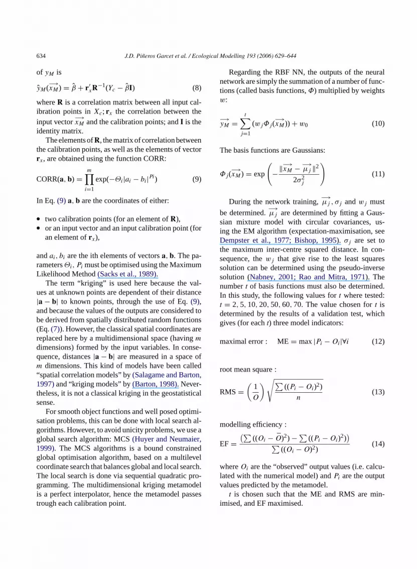
634 J.D. Pineros Garcet et al. / Ecological Modelling 193 (2006) 629–644

of yM is

yM(−→xM ) = β + r′

xR−1(Yc − βI) (8)

whereR is a correlation matrix between all input cal-ibration points inXc; rx the correlation between theinput vector

−→xM and the calibration points; andI is the

identity matrix.The elements ofR, the matrix of correlation between

the calibration points, as well as the elements of vectorrx, are obtained using the function CORR:

CORR(a, b) =m∏

i=1

exp(−Θi|ai − bi|Pi) (9)

In Eq.(9) a, b are the coordinates of either:

• two calibration points (for an element ofR),• or an input vector and an input calibration point (for

an element ofrx),

andai, bi are the ith elements of vectorsa, b. The pa-rametersΘi, Pi must be optimised using the MaximumLikelihood Method(Sacks et al., 1989).

The term “kriging” is used here because the val-ues at unknown points are dependent of their distance|a − b| to known points, through the use of Eq.(9),and because the values of the outputs are considered tobe derived from spatially distributed random functions(Eq.(7)). However, the classical spatial coordinates arereplaced here by a multidimensional space (havingm

d se-q ofm lled“ n,1t ticals

mi-s h al-g se ag r,1 edg velc arch.T pro-g deli ssest

Regarding the RBF NN, the outputs of the neuralnetwork are simply the summation of a number of func-tions (called basis functions,Φ) multiplied by weightsw:

−→yM =

t∑j=1

(wjΦj(−→xM )) + w0 (10)

The basis functions are Gaussians:

Φj(−→xM ) = exp

(−‖−→

xM − −→µj ‖2

2σ2j

)(11)

During the network training,−→µj , σj andwj must

be determined.−→µj are determined by fitting a Gaus-

sian mixture model with circular covariances, us-ing the EM algorithm (expectation-maximisation, seeDempster et al., 1977; Bishop, 1995). σj are set tothe maximum inter-centre squared distance. In con-sequence, thewj that give rise to the least squaressolution can be determined using the pseudo-inversesolution (Nabney, 2001; Rao and Mitra, 1971). Thenumbert of basis functions must also be determined.In this study, the following values fort where tested:t = 2, 5, 10, 20, 50, 60, 70. The value chosen fort isdetermined by the results of a validation test, whichgives (for eacht) three model indicators:

m

r

R

m

E

w cu-l tv

in-i

imensions) formed by the input variables. In conuence, distances|a − b| are measured in a spacedimensions. This kind of models have been ca

spatial correlation models” by(Salagame and Barto997)and “kriging models” by(Barton, 1998). Never-

heless, it is not a classical kriging in the geostatisense.

For smooth object functions and well posed optiation problems, this can be done with local searcorithms. However, to avoid unicity problems, we ulobal search algorithm: MCS(Huyer and Neumaie999). The MCS algorithms is a bound constrainlobal optimisation algorithm, based on a multileoordinate search that balances global and local sehe local search is done via sequential quadraticramming. The multidimensional kriging metamo

s a perfect interpolator, hence the metamodel parough each calibration point.

aximal error : ME= max|Pi − Oi|∀i (12)

oot mean square :

MS =(

1

O

)√∑((Pi − Oi)2)

n(13)

odelling efficiency :

F =(∑

((Oi − O)2) −∑ ((Pi − Oi)2))

∑((Oi − O)2)

(14)

hereOi are the “observed” output values (i.e. calated with the numerical model) andPi are the outpualues predicted by the metamodel.

t is chosen such that the ME and RMS are mmised, and EF maximised.

J.D. Pineros Garcet et al. / Ecological Modelling 193 (2006) 629–644 635

3.2. Representative soils and crop rotations

The details of the crop rotations (dates of applica-tion, dates of plough, etc.) as well as the crops androtations themselves are case specific and were cho-sen to be representative for the study area according tothe survey made byLambert et al. (2002). Six cropsare considered : winter wheat (WW), winter barley(WB), sugar beet (BE), maize (MZ), ray grass fallow(FA), and rape as winter catch crop (CC). The consid-ered crops are part of five representative crop rotations:BEWWWB, BEWwWBCc, BEWwFA, BEWwMZWw,MZMZMZ. The crop rotations last 3–4 years. For themetamodelling purpose, only WW, WB, BE and MZare considered to have variable nitrogen fertilisation.FA and CC are fertilised with a fixed amount. FA isfertilised using a mineral fertilisation of 80 kg N/ha the15th August of year 2 and 80 kg N/ha the 15th Augustof year 3, while CC receives a mineral fertilisation of50 kg N/ha. Such fertilisations are used by the farm-ers to allow a better growth of FA and CC (Lambert etal., 2002). Some rotations differ only in terms of catchcrops.

For each rotation, two representative soils wherechosen (Aba: Haplic Luvisol, well drained, loamy, de-veloped on quaternary loess, with a Bt horizon and Zbx:Arenosol, well drained, sandy, developed on tertiarymarine sands, showing sometimes an albic E horizon).One metamodel is developed for each combination ofsoil and crop rotation.

3

st en-t

y

T sa i-s tionb e it ist r byt

s thes putv he

crops of each rotation. As it can be seen inTable 1,the metamodels have, depending the case, three or fourinput variables (xM,i vectors of three or four elements)representing the crops fertilisation amount in kgN/haduring the rotation.

Regarding the design region, the input variablesrange (i.e. the maximal and minimal fertilisation) werechosen following the results of theLambert et al. (2002)survey. The fertilisation was chosen identical for thetwo soil types, for a given crop rotation. The designregion δM is complex since the physical system thatthe metamodels describe presents constraints in it’s in-put variables spaceχM . A minimum and a maximumfertilisation per plant and for the whole rotation mustbe taken into account to avoid unrealistic fertilisations.A typical unrealistic fertilisation scheme in a crop ro-tation consists for instance in choosing the maximalfertilisation encountered in surveys for each year ofthe rotation. In practice, farmers put a large organicfertilisation only on the first year of a rotation, but noteach year. In consequence,δM is not standard (not ahypercube nor a hypersphere).Table 1presentsδM foreach metamodel. RegardingδM , the maximal and mini-mal fertilisation per crop encountered has been derivedfromLambert et al. (2002), while the maximal fertilisa-tion for the whole rotation has been derived from legallyauthorised amounts(Comitenitrates, 1998). The mini-mal fertilisation for the whole rotation has been chosenas the sum of the minimal fertilisation per crop.

The design regionδM defines the possible values fort r then is isd herea

3c

f iceo ra-t ustg thes ei ace.O bero r onen can

.3. Metamodels inputs, output and design region

The metamodels output variableyM is defined ahe probability for the annual nitrate leaching concrationc to be greater than 50 mg/l:

M = P [c > 50 mg/l] , (15)

he annual leaching concentrationc is considered arealisation of a random variableC and each real

ation is considered independent (no time correlaetween years). 50 mg/l has been chosen becaus

he maximal concentration admitted in groundwatehe European Union(EEC, 1991).

Table 1presents the 10 metamodels and defineignificance and units of their input variables. The inectors

−→xM,i are constituted by the fertilisation of t

he input variables, but the actual values chosen foumerical experiment must still be determined. Thone through an experimental design (presentedfter) which allows to sample insideδM .

.4. Experimental design, numerical experiment,alibration and validation

The sampling of the metamodel design regionδM

ollowing a chosen sampling design (i.e. the chof the fertilisations) is critical to obtain a good calib

ion and validation of the metamodels. The design mive realistic cases for the study zone (i.e. followingurvey ofLambert et al., 2002) and at the same timt must represent a good sampling of the input spn the other hand, there is a limitation in the numf samples of the input space because the time foumerical calculation for a 30 years crop rotation

636 J.D. Pineros Garcet et al. / Ecological Modelling 193 (2006) 629–644

Table 1Metamodels description: soil, crop rotation, input variables and design region

Metamodel Soila Crop rotationb Metamodel input variables (kg N/ha)b,c Design regionδM

yM = f1(x1M

, x2M

, x3M

, x4M

) Aba BEWWWB x1M

BE 1st year min-N;x2M

BE 1st year org-N;x3

MWW 2nd year min-N;x4

MWB 3rd year

min-N

80 ≤ (x1M

+ x2M

) ≤ 520; 100≤ x3M

≤ 320;80 ≤ x4

M≤ 300;x2

M≥ 80;

260≤ x1M

+ x2M

+ x3M

+ xM4 ≤ 920

yM = f2(x5M

, x6M

, x7M

, x8M

) Aba BEWwWBCc x5M

BE 1st year min-N;x6M

BE 1st year org-N;x7

MWW 2nd min-N fertiliz;x8

MWB 3rd min-N

fertiliz.

80 ≤ (x5M

+ x6M

) ≤ 520; 100≤ x7M

≤ 320;80 ≤ x8

M≤ 300;x6

M≥ 80;

260≤ x5M

+ x6M

+ x7M

+ x8M

≤ 920

yM = f3(x9M

, x10M

, x11M

) Aba BEWwFA x9M

BE 1st min-N fertiliz.;x10M

BE 1st org-Nfertiliz.; x11

MWW 2nd min-N fertiliz.

80 ≤ (x9M

+ x10M

) ≤ 520; 100≤ x11M

≤ 320;x10

M≥ 80; 180≤ x9

M+ x10

M+ x11

M≤ 840

yM = f4(x12M

, x13M

) Aba MZMZMZ x12M

MZ 1st, 2nd and 3rd year min-N fertiliz.;x13

MMZ 1st org-N fertiliz.

0 ≤ x12M

≤ 360; 120≤ x13M

≤ 480;120≤ x12

M+ x13

M≤ 1200

yM = f5(x14M

, x15M

, x16M

, x17M

, x18M

) Aba BEWwMZWw x14M

BE 1st min-N fertiliz.;x15M

BE 1st org-Nfertiliz.; x16

MWW 2nd and 4th year min-N

fertiliz.; x17M

MZ 3rd min-N fertiliz.;x18M

MZ 3rdorg-N fertiliz.

80 ≤ x14M

+ x15M

≤ 560; 100≤ x16M

≤ 340;120≤ x17

M+ x18

M≤ 600;x15

M≥ 80;x18

M≥ 120;

400≤ x14M

+ x15M

+ 2 · x16M

+ x17M

+ x18M

≤ 1360

yM = f6(x19M

, x20M

, x21M

, x22M

) Zbx BEWWWB x19M

BE 1st min-N fertiliz.;x20M

BE 1st org-Nfertiliz.; x21

MWW 2nd min-N fertiliz.;x22

MWB

3rd min-N fertiliz.

80 ≤ (x19M

+ x20M

) ≤ 520; 100≤ x21M

≤ 320;80 ≤ x22

M≤ 300;x20

M≥ 80;

260≤ x19M

+ x20M

+ x21M

+ x22M

≤ 920

yM = f7(x23M

, x24M

, x25M

, x26M

) Zbx BEWwWBCc x23M

BE 1st min-N fertiliz.;x24M

BE 1st org-Nfertiliz.; x25

MWW 2nd min-N fertiliz.;x26

MWB

3rd min-N fertiliz.

80 ≤ (x23M

+ x24M

) ≤ 520; 100≤ x25M

≤ 320;80 ≤ x26

M≤ 300;x24

M≥ 80;

260≤ x23M

+ x24M

+ x25M

+ x26M

≤ 920

yM = f8(x27M

, x28M

, x29M

) Zbx BEWwFA x27M

BE 1st min-N fertiliz.;x28M

BE 1st org-Nfertiliz.; x29

MWW 2nd min-N fertiliz.

80 ≤ (x27M

+ x28M

) ≤ 520; 100≤ x29M

≤ 320;x28

M≥ 80; 180≤ x27

M+ x28

M+ x29

M≤ 840

yM = f9(x30M

, x31M

) Zbx MZMZMZ x30M

MZ 1st, 2nd and 3rd year min-N fertiliz.;x31

MMZ 1st org-N fertiliz.

0 ≤ x30M

≤ 360; 120≤ x31M

≤ 480;120≤ x30

M+ x31

M≤ 1200

yM = f10(x32M

, x33M

, x34M

, x35M

, x36M

) Zbx BEWwMZWw x32M

BE 1st min-N fertiliz.;x33M

BE 1st org-Nfertiliz.; x34

MWW 2nd and 4th year min-N

fertiliz.; x35M

MZ 3rd min-N fertiliz.;x36M

MZ 3rdorg-N fertiliz.

80 ≤ x32M

+ x33M

≤ 560; 100≤ x34M

≤ 340;120≤ x35

M+ x36

M≤ 600;x33

M≥ 80;x36

M≥ 120;

400≤ x32M

+ x33M

+ 2 · x34M

+ x35M

+ x36M

≤ 1360

a Aba :Haplic Luvisol; Zbx: Arenosol.b WW winter wheat; WB winter barley; BE sugar beet; MZ maize; CC winter catch crop; FA ray-grass fallow.c org-N fertiliz.: organic nitrogen fertilisation, min-N fertiliz: mineral nitrogen fertilisation.

be of 12 min with a Pentium III © 800 MHz computer.Additionally, the design regionδM is not standard. Insuch cases, standard designs like Latin hypercubes arenot convenient. For linear models, some alternativesare available(Atkinson and Donev, 1992), neverthe-less, for non-linear models (MKM or RBF NN in ourcase), the optimal design depends on an estimation ofthe unknown parameters of the model. Especially forkriging, optimal designs have been proposed(Sacks etal., 1989), but there is still no clear evidence of the

superiority of such a design over more classic designs(Bowman et al., 1993).

In this work, a grid experimental design is used toobtain the calibration set{ −→

xM,1, . . . ,−→xM,k, . . . ,

−→xM,p}

for each metamodel, taking into account the fact thatδM is not standard. The chosen experimental design isattempting to fill the design region rather than takingreplicates like in traditional physical experiments de-sign since the numerical model is deterministic. Thedesign is a modified grid and allows to fill the corners

J.D. Pineros Garcet et al. / Ecological Modelling 193 (2006) 629–644 637

of the design region, which is one of the objectivesof an experimental design(Koehler and Owen, 1996).The grid is obtained by sampling first the total fertili-sation (F) of the entire crop rotation. Then, for each F,a second variable is sampled between its minimum andmaximum value given the chosen values of F. Havinga value of F and of a first variable, the same process isrepeated for a second variable, taking into account theconstraints represented by the values of F and the firstvariable.

Regarding the validation sets, two different sam-pling designs are used corresponding to two kinds ofvalidation. In a first step, the purpose of the validationis to chose from one of the two alternative metamod-els proposed (MKM or RBF NN). In a second step,the validation purpose is to obtain model indicators toasses the quality of the chosen metamodels. For the firststep, a random sampling into the design region has beenperformed using independent continuous uniform dis-tributions for each componentxi

M . The complex formof δM is taken into account by eliminating the resultsof the random sampling (a set of vectors

−→xM,i) which

are outsideδM .For the second step, the following cross-validation

procedure has been used: (1) starting from the completemetamodel calibration set already obtained,p meta-models are calibrated excluding one calibration vectorat a time (2) for each input vector eliminated from thecalibration, the output is calculated using the corre-sponding metamodel and using the numerical model;( them odelv

am-pbm t beo s ofn al-u ned.F atict oft , fore -a en-d ted).FE

4. Results and discussion

4.1. Stratified sampling design for calibration andnumerical experiment

The results of the sampling for thef3 metamodel,according to the design region inTable 1, is presentedin Fig. 3.

Each sampling point is comprised inside theδM ofthe correspondent metamodel (compare withTable 1).It can also be seen that the design fills well the design re-gionδM , including its corners. The number of samples(i.e. the number of WAVE simulations) per metamodelis 2× 116 forf1 andf6, 2× 116 forf2 andf7, 2× 45for f3 andf8, 2× 15 forf4 andf9, 2× 78 forf5 andf10. The total is 740 samples.

For each sampling point (i.e. each soil, each ro-tation and each fertilisation), a numerical calculationof the annual nitrate leaching during 30 years (Fig. 4)is performed with WAVE.Fig. 4 shows large interan-nual variability of the nitrate leaching. Additionally,the effect of the fertilisation on the winter barley issharp.

The time series resulting from the numerical sim-ulations are used to calculateyN,i following Eq. (15).For the case off1, Fig. 5 presentsyN,i as a functionof x1

M and x2M . Fig. 5 shows that for the calibration

sample,yN,i are high, between 0.8 and 1 for most ofthe samples. This is interpreted as the result of highfertilisations.

Fm s tot8

3) the p differences between the numerical andetamodel outputs are used to calculate metam

alidation indicators.Once the calibration and validation points are s

led into the input space, an estimate ofyM muste obtained. For such a purpose, a sample ofC (theean annual nitrate leaching concentration) musbtained. For each scenario, 30 years time serieitrate leaching are calculated with WAVE and 30 ves of annual nitrate leaching concentration obtaior the top boundary conditions a 30 year clim

ime series for the area was used. At the bottomhe soil profile, free drainage was considered. Soach scenario

−→xN,i (i = 1, . . . , 740), we have 30 re

lisations ofC, each one being considered indepent (time correlation between years is neglecrom the realisations ofC, yM is calculated followingq.(15).

ig. 3. Sampling design for metamodelf3 calibration. Theodified grid design used allows to respect the constrain

he design region: 80≤ (x9M + x10

M ) ≤ 520; 100≤ x11M ≤ 320;x10

M ≥0; 180≤ x9

M + x10M + x11

M ≤ 840 (xiM are in kg N/ha).

638 J.D. Pineros Garcet et al. / Ecological Modelling 193 (2006) 629–644

Fig. 4. Thirty years time series of annual mean nitrate leach-ing concentration calculated with the WAVE numerical model.Soil: Aba; crop rotation: BEWWWB (sugar beet; winter wheat;winter barley). ( ) Fertilisation (kg N/ha) is x1

M = 0;x2M =

80;x3M = 100;x4

M = 80. ( ) Fertilisation (kg N/ha) is x1M =

0;x2M = 80;x3

M = 210;x4M = 80.

4.2. Comparison between multidimensionalkriging and neural networks

Using the results of the numerical experiment corre-sponding to the Aba soil and the BEWWWB crop rota-tion, a MKM,fK and a RBF NN,fRBF were calibrated.Calibration forfK is presented inFig. 6.

As expected,Fig. 6shows that the kriging is a perfectinterpolator: it goes trough all the calibration points.

Fig. 5. Numerical simulations with the model WAVE. Soil: Aba;crop rotation: BEWWWB (sugar beet; winter wheat; winter barley).x1

M : BE mineral N fertilisation during the first year of the crop rota-tion. x2

M : BE organic N fertilisation during the first year (xiM are in

kg N/ha).yN : the probability for the annual nitrate leaching concen-tration to be greater that 50�g/l.

Fig. 6. Calibration results for thefK kriging metamodel: ob-served (numerical) vs. predicted values. Soil: Aba, crop rotation:BEWWWB.

This characteristic of the kriging metamodel preventsa comparison between the two metamodels based onthe calibration results. The calibration results offRBFare dependent on the numbert of basis functions cho-sen. Seven different neural networks where calibrated,corresponding tot = 2, 5, 10, 20, 50, 60, 70. The scat-ter plot fort = 50 is presented inFig. 7.

SincefK andfRBF can not be compared using thecalibration results, we will use validation indicators tocompare them. For such a purpose, a random sampleof 21 input vectors is taken into the design region off1 (seeTable 1for a description of the design region).The random sample is taken intoδM using a uniformrandom distribution, and by eliminating values whichfalls outsideδM until 21 samples are obtained. Fromthis sample, 3× 21 simulations ofyM are obtained,using the kriging metamodel, the neural network andthe numerical model (i.e. 21 simulations for each typeof model).

For the case of thefRBF metamodel, seven valuesof t where tested. The model validation indicators cal-culated from the random validation sample are depen-dent fromt, as presented inFig. 8. A value of t = 50has been chosen as the best compromise between ahigh EF and low RMS and ME. The simulations with

J.D. Pineros Garcet et al. / Ecological Modelling 193 (2006) 629–644 639

Fig. 7. Calibration results for thefRBF neural network metamodel:observed (numerical) vs. predicted values. Soil: Aba, crop rotation:BEWWWB, 50 basis functions in the network.

the kriging metamodel and the RBF neural network(t = 50) are compared to the numerical model usingscatter plots and model indicators inFigs. 9 and 10. Ascompared tofK, thefRBF seems to overestimateyM .It can be seen that the best neural network obtained(t = 50) and the kriging metamodel have similar indi-cators values, with a little advantage for the kriging. Inconsequence, kriging was the method chosen for creat-ing metamodelsf1 to f10 for all the crop rotations andsoils.

4.3. Kriging metamodels calibration

Since the MKM kriging metamodels perform bet-ter than the rbf metamodel, we choose the MKM fordeveloping our metamodels for all the considered soilsand crop rotations. Following the methodology pre-sented inBowman et al. (1993), an optimal fit to thedata is obtained by maximizing the likelihood. The cal-ibration leads to a set ofθi, pi parameters for eachmetamodel (i = 1, . . . , m, m: number of input vari-ables). The bounds chosen to constrain the searchfor optimal values ofθi, pi are θi ∈ [0.01, 2] andpi

∈ [0, 2].

Fig. 8. Validation model indicators for thefRBF neural network.Seven networks where validated, with seven different values oft

(the number of basis functions of the network). Values of modelefficiency (EF), maximal error (ME) and root mean square (RMS)are given for each network.

The calibrated parameters values are presented inTable 2for thef1 metamodel.

The results ofTable 2as well as the results for theother metamodels (not shown here) indicates that theoptimisation procedure tends to chose small values forθi. This is in agreement with results fromLim et al.

Fig. 9. Validation results for thefRBF neural network metamodelwith 50 basis functions (t = 50): observed (numerical) vs. predictedvalues. Soil: Aba, crop rotation: BEWWWB.

640 J.D. Pineros Garcet et al. / Ecological Modelling 193 (2006) 629–644

Fig. 10. Validation results for thefK kriging metamodel: ob-served (numerical) vs. predicted values. Soil: Aba, crop rotation:BEWWWB.

(2002)which founds thatθi tends to small values whenthe polynomial term of Eq.(6) is omitted.Fig. 11showsresponse surfaces ofyM,i = f1(xM,i) depicting the de-pendency ofyM with the fertilisation as calculated withthe kriging metamodelf1.

Fig. 12shows that, forf1, the partial derivative ofyM with respect tox1

M (δ(yM)/δ(x1M)) is not always pos-

Table 2Calibration parametersθi, pi for thef1 metamodel

x1M x2

M x3M x4

M

θ1 = 0.0088 θ2 = 0.0001 θ3 = 0.0069 θ4 = 0.0101p1 = 0.8931 p2 = 0.3753 p3 = 1.0215 p4 = 0.9372

To each input variablexiM corresponds oneθi, and onepi.

Fig. 12. Response of the metamodelf1 to x1M with x2

M, x3M, x4

M

inputs kept constant (x2M = 80 kg/ha, x3

M = 320 kg/ha, x4M =

190 kg/ha). (—) Metamodel output (�) and calibration points.

itive: for an increasing mineral fertilisationx1M of the

sugar beet,yM decreases between 110 and 220 kg/haand the increases between 220 and 330 kg/ha. Thisgives the possibility to optimize the fertilisation sincea local minima exists.

Fig. 11. Response surfaces off1 metamodel:yM = f1(x1M, x2

M, x3M, x4

M ). x1M is the BE mineral N fertilisation during the first year of the crop

rotation,x2M is the BE organic N fertilisation during the first year,x3

M is the WW mineral N fertilisation during the second year andx4M is the

WB mineral N fertilisation during the third year (xiM are in kg N/ha). ( ) Metamodel output and (�) metamodel calibration points.

J.D. Pineros Garcet et al. / Ecological Modelling 193 (2006) 629–644 641

Table 3Cross-validation indicators for the kriging metamodelsf1 to f10

Metamodel Soil Crop rotation Maximal error MEa Root mean square RMSa Modelling efficiency EFa

f1 Aba BEWWWB 0.14 0.0468 0.89f2 Aba BEWwWBCc 0.18 0.0496 0.92f3 Aba BEWwFA 0.11 0.0491 0.94f4 Aba MZMZMZ 0.16 0.1155 0.94f5 Aba BEWwMZWw 0.10 0.0267 0.98f6 Zbx BEWWWB 0.08 0.0244 0.93f7 Zbx BEWWWBCC 0.10 0.1053 0.95f8 Zbx BEWwFA 0.07 0.0266 0.88f9 Zbx MZMZMZ 0.17 0.1076 0.93f10 Zbx BEWwMZWw 0.08 0.0363 0.94

a See Eqs.(12)–(14).

4.4. Kriging metamodels cross-validation

For the metamodelsf1 to f10, a validation has beenperformed using a cross-validation. The results of thecross-validation are presented inTable 3, which showsacceptable values for ME, EF and RMS for all the10 metamodels. Despite the good RMS, some meta-models (f2, f4, f9) presents maximal errors between0.16 and 0.18, which are high compared to the rangeof the output variableyM (between 0 and 1). This mustbe taken into account when the metamodels are used,for example by calculating prediction confidence in-tervals derived from the RMS values. FollowingJin etal. (2001), the kriging metamodels are very sensitiveto noisy data because it is an interpolator. Our data,coming from WAVE numerical model simulations, arenot very noisy. This can be an explanation for the goodresults obtained with MKM in terms of EF and RMS.

4.5. Calculation time improvement

The numerical model takes 12 min to run one single30-years crop rotation, while the MKM takes around0.8 s and the RBF NN around 0.1 s (using the same800 MHz computer).

The time-consuming step in the presented method-ology is the creation of the numerical model scenar-ios and also the numerical simulations themselves. Thecalibration and validation step is also heavy in terms ofdata management: 15 GB of data where generated; thisi nedb eta-m

4.6. Discussion of the proposed mathematicaldefinition of a metamodel

Despite the relatively large number of metamod-elling papers we found, few of them attempt to builda general theory of metamodelling (to our knowledge,mainlyBarton, 1998andKleijnen and Sargent, 2000).Sacks et al. (1989)is also a fundamental paper butdoes not consider the wide variety of metamodellingmethods. Moreover, only a limited number of papersamongst those we have read gives a mathematical def-inition of a metamodel by means of a generic equation(Barton, 1998; Huber et al., 1996; Hussain et al., 2002;Kilmer et al., 1999).

If a generic equation is to be able to represent thewhole variety of metamodels encountered in the liter-ature, it should be generic enough to take into accountat least the following: replicated observations of theinput variables; multidimensional outputs and dimen-sions of the input/outputs spaces; highlight the dimen-sionality reduction of the inputs space, as well as thefunction used for such a reduction; input variables con-strains; design constrains; the fact that designs can bemade from the inputs space of the numerical modelor the metamodel; ensembles to describe calibrationand validation sets; metamodel calibration and vali-dation description; errors: lack of fit, error due to thefunction used to dimensionality reduction, error dueto the stochastic character of the considered numeri-cal model and modeled phenomenon; pseudo-randomn

erice sal.

mplies high capacity storage and specially desigatch programs to retrieve the data needed for the models construction.

umber seed for the computations.Table 4shows a comparison between the gen

quations we found in the literature and our propo

642 J.D. Pineros Garcet et al. / Ecological Modelling 193 (2006) 629–644

Tabl

e4

Com

paris

onbe

twee

nm

etam

odel

gene

riceq

uatio

nsfo

und

inth

elit

erat

ure

and

the

equa

tions

prop

osed

inth

ispa

per

Ref

eren

ceR

eplic

ated

obse

rvat

ions

ofin

puts

Ran

dom

seed

Mul

ti-di

men

sion

alou

tput

s

Set

sar

eco

nsid

ered

Dim

ensi

onof

inpu

tsan

dou

tput

ssp

aces

Dim

ensi

onre

duct

ion

Inpu

tsco

nstr

ains

Des

ign

cons

trai

nsC

alib

ratio

nan

dva

lidat

ion

Fun

ctio

nto

redu

cedi

men

sion

ality

Des

ign

both

from

num

eric

alm

odel

and

met

amod

elin

puts

pace

Poo

led

lack

offit

and

dim

ensi

onre

duct

ion

erro

rs

Lack

offit

erro

rN

umer

ical

mod

elan

dun

derly

ing

syst

emst

ocha

stic

erro

rH

uber

etal

.(19

96)

Yes

Bar

ton

(199

8)Y

esY

esK

ilmer

etal

.(19

99)

Yes

Yes

Hus

sain

etal

.(20

02)

Equ

atio

nsin

Sec

tion

2of

this

pape

rY

esY

esY

esY

esY

esY

esY

esY

esY

esY

es

A“y

es”

ina

colu

mn

mea

nsth

atth

eco

rres

pond

ing

met

amod

elch

arac

teris

tic(c

olum

nhe

ader

)is

take

nin

toac

coun

tby

the

gene

ricfo

rmul

a.

5. Conclusion

A mathematical definition for a metamodel has beenproposed. This definition is more general than the mainobject of this paper (metamodelling of nitrate leach-ing): it proved to be operational and useful to describemathematically the essential operations of metamod-elling: parameters reduction, metamodelling error es-timation, design region definition, calibration and val-idation. The mathematical equation proposed to rep-resent a metamodel is generic and can represent alarge part of the existing metamodels. However, thereis still potential to improve it, for example by takinginto account replicated observations of inputs, and ran-dom seeds. Another improvement should be to sep-arate explicitly lack of fit errors, dimension reduc-tion errors and the stochastic error of the modelledsystem.

The comparison between the two tested metamodels– multidimensional kriging and radial basis functionsneural networks – shows that, for the particular case ofmodelling nitrate leaching from agricultural origin inthe area of the Brusselean aquifer in Belgium, MKMis the best method. However, the values of the modelindicators for the RBF NN are close to the MKM ones,and the performances of the different techniques arecase dependent.

The objective of developing fast and reliable meta-models of nitrogen leaching from soils and crop rota-tions in the Brusselean region has been reached: highm MSa on ofo a se-r dedf aret timem arep

er,w elsw s ofa delsa inter-v ed tot eta-m dento cht the

odel efficiencies where attained (close to 1), low Rre observed, and the time needed for the calculatine output with the kriging metamodel representsious improvement. The numerical simulations neeor the calibration and validation of the metamodelshe time consuming step in the procedure, but thisust be compared to the total of simulations thatlaned to be done with the metamodels.

However, it must be reaffirmed that, in this pape concentrate on the reliability of the metamodith respect to their ability to reproduce the resultnumerical model, we did not validate the metamogainst measurements. Further more, confidenceals of the metamodel response must be comparhe precision required to a particular usage of the models. The metamodels reliability remains depenn the validity of the numerical models from whi

hey are derived, and are limited to the domain of

J.D. Pineros Garcet et al. / Ecological Modelling 193 (2006) 629–644 643

input space for which they have been derived: they areinterpolators.

In addition to the development of theoretical con-cepts about metamodelling, the work presented is ori-ented to develop a tool useful for modelling the im-pact of fertilisation on the nitrate concentration in wa-ter leaving the bottom of the soil profile. In a previ-ous study(Pineros Garcet et al., 2001), the impact ofvarious simulated land use on the groundwater of theBrusselean region was already modelled. However, thesimulations, made with a numerical model, were basedon the use of a limited number of fertilisation scenar-ios, due to the long CPU time demanded by the numer-ical model. The area considered (two farms) was alsopartially limited by the CPU time. Another importantpoint is that the numerical model could not use directlythe GIS data. The metamodels presented here have thepotential to improve the results of such land use im-pact studies, by allowing to test a higher number offertilisation schemes, by allowing to extend the anal-ysis to larger areas, and by integrating the metamodeldirectly into the GIS. It also opens the possibility toperform montecarlo simulations based on very largeGIS datasets.

The mathematical framework and the methodologypresented here can be adapted to other research top-ics than nitrate leaching, like climate change, werehigh amounts of simulations are required. The mathe-matical form of the obtained metamodels (matrices)allows to incorporate them easily into already ex-i ls,w ta-m

R

A dictshop

A ign.

B f theiety

B Ox-

B tingeld

Bouzaher, A., Lakshminarayan, P.G., Cabe, R., Carriquiry, A.,Gassman, P.W., Shogren, J.F., 1993. Metamodels and nonpointpollution policy in agriculture. Water Resour. Res. (29) 1579–1587.

Bouzaher, A., Shogren, J.F., Holtkamp, D., Gassman, P., Archer, D.,Lskshminarayan, P., Carriquiry, A., Reese, R., Kakani, D., Fur-tan, W.H., Izaurralde, R.C., Kiniry, J., 1995. Agricultural poli-cies and soil degradation in western Canada: an agro-ecologicaleconomic assessment. Technical Report 2/95, Center for Agri-cultural and Rural Development.

Bowman, K.P., Sacks, J., Chang, Y.F., 1993. Design and analysis ofnumerical experiments. J. Atmos. Sci. (50) 1267–1278.

Burkart, M.R., Kolpin, D.W., James, D.E., 1999. Assessing ground-water vulnerability to agrichemical contamination in the mid-west. Water Sci. Technol. 39, 103–112.

Chapman, W.L., Welch, W.J., Bowman, K.P., Sacks, J., Walsh,J.E., 1994. Arctic sea-ice variability—model sensitivities anda multidecadal simulation. J. Geophys. Res. -Oceans 99, 919–935.

Comite nitrates, 1998. Code de bonnes pratiques agricoles, proposi-tion de revision. Technical Report, Gembloux, Belgium.

Dempster, A.P.N., Laird, N.M., Rubin, D.B., 1977. Maximum likeli-hood from incomplete data via the em algorithm. J. R. Stat. Soc.B 39 (1), 1–38.

Diekkruger, B., Sondgerath, D., Kersebaum, K.C., McVoy, C.W.,1995. Validity of agro-ecosystem models—a comparison of dif-ferent models applied to the same data set. Ecol. Modell. 81 (13),3–29.

Ducheyne, S., Schadeck, N., Vanongeval, L., Vandendriessche, H.,Feyen, J., 2001. Assessment of the parameters of a mechanisticsoil-crop-nitrogen simulation model using historic data of ex-perimental field sites in Belgium. Agric. Water Manage. (51)53–78.

EEC. Council directive 91/676/eec of 12 December 1991 concerningthe protection of waters against pollution caused by nitrates from

G sionbio-

G on ofixing

G on of. Res.

H ofrt ii:

dell.

H sim-orm.

H : Ra-138,

H vel

sting modular models or linear optimisation toohich is an important field of applications of meodelling.

eferences

kkermans, W., 2000. Using an artificial neural network to presimulation model outcomes: a case study. In: EPSRC Workat Gregynog, Wales, UK, 10–14 April.

tkinson, A.C., Donev, A.N., 1992. Optimum Experimental DesOxford University Press.

arton, R.R., 1998. Simulation metamodels. In: Proceedings oWinter Simulation Conference 1998, IEEE Computer SocPress, Washington, DC, United States, pp. 167–174.

ishop, C.M., 1995. Neural Networks for Pattern Recognition.ford University Press.

ørgesen, C.D., Djurhuus, J., Kyllingsbaek, A., 2001. Estimathe effect of legislation on nitrogen leaching by upscaling fisimulations. Ecol. Modell. (136) 31–48.

agricultural sources. Official J. L. (375): 0001–0008, 1991.oetz, R.U., Keusch, A., 2005. Dynamic efficiency of soil ero

and phosphor reduction policies combining economic andphysical models. Ecol. Econ. 52, 201–218.

ough, W.A., Welch, W.J., 1994. Parameter space exploratian ocean general-circulation model using an isopycnic mparameterization. J. Mar. Res. 52, 773–796.

reenwood, A.G., Rees, L.P., Siochi, F.C., 1998. An investigatithe behavior of simulation response surfaces. Eur. J. Oper110, 282–313.

aberlandt, U., Krysanova, V., Bardossi, A., 2002. Assessmentnitrogen leaching from arable land in large river basins. Paregionalisation using fuzzy rule based modelling. Ecol. Mo277–294.

uber, K.P., Berthold, M.R., Szczerbicka, H., 1996. Analysis ofulation models with fuzzy graph based metamodeling. PerfEval. 27–8, 473–490.

ussain, M.F., Barton, R.R., Joshi, S.B., 2002. Metamodelingdial basis functions, versus polynomials. Eur. J. Oper. Res.142–154.

uyer, W., Neumaier, A., 1999. Global optimization by multilecoordinate search. J. Global Optimization 331–355.

644 J.D. Pineros Garcet et al. / Ecological Modelling 193 (2006) 629–644

Jin, R., Chen, W., Simpson, T.W., 2001. Comparative studies of meta-modeling techniques under multiple modeling criteria. J. Struct.Optimization (23) 1–13.

Johansson, R.C., Gowda, P.H., Mulla, D.J., Dalzell, B.J., 2004. Meta-modelling phosphorus best management practices for policy use:a frontier approach. Agric. Econ. 30, 63–74.

Kilmer, R.A., Smith, A.E., Shuman, L.J., 1999. Computing confi-dence intervals for stochastic simulation using neural networkmetamodels. Comput. Ind. Eng. 36, 391–407.

Kleijnen, J.P.C., Sargent, R.G., 2000. A methodology for fitting andvalidating metamodels in simulation. Eur. J. Oper. Res. 120, 14–29.

Kleijnen, J.P.C., 1987. Statistical Tools for Simulation Practitioners.Marcel Dekker, New York.

Koehler, J.R., Owen, A.B., 1996. Computer experiments. In: Ghosh,S., Rao, C.R. (Eds.), Handbook of Statistics, vol. 13. ElsevierScience, New York 261–308.

Lambert, R., Van Bol, V., Maljean, J.-F., 2002. Peeters, A., Prop’eau-sable, projet pilote pour la protection des eaux de la nappe dessables bruxelliens, rapport final. Technical Report. Laboratoired’Ecologie des Prairies, Universite catholique de Louvain, Bel-gium.

Laurent, E., 1980. Monographie de la dyle. Technical Report. Min-istere de la sante publique et de l’environnement.

Lim, Y.B., Sacks, J., Studden, W.J., Welch, W.J., 2002. Design andanalysis of computer experiments when the output is highly cor-related over the input space. Can. J. Stat. (30) 109–126.

Munoz Carpena, R., Vanclooster, M., Villace-Reyes, E., 2001. Eval-uation of the wave model. In: Thomas, D.L., Parsons, J.E.,Huffman, R.L. (Eds.), Agricultural Non-point Source WaterQuality Models: Their Use and Application, Southern Coop.Ser. Bul. 38. Southern Region Agricultural Experiment Sta-tions, http://www3.bae.ncsu.edu/Regional-Bulletins/Modeling-Bulletin/waveval.htm.

Nabney, I.T., 2001. Netlab: Algorithms for Pattern Recognition.

P 001.port-

ing fertilizer management at the farm scale. In: Shaffer, M.J., Ma,L., Hansen, S. (Eds.), Modeling Carbon and Nitrogen Dynamicsfor Soil Management. Lewis Publishers, CRC Press LCC, pp.571–596.

Rao, C.R., Mitra, S.K., 1971. Generalized Inverse of Matrices andits Applications. John Wiley, New York.

Sacks, J., Welch, J.W., Mitchell, T.J., Wynn, H.P., 1989. Design andanalysis of computer experiments. Stat. Sci. (4) 409–435.

Sahoo, G.B., Ray, C., Wade, H.F., 2005. Pesticide prediction inground water in North Carolina domestic wells using artificialneural networks. Ecol. Modell. 183, 29–46.

Salagame, R.R., Barton, R.R., 1997. Factorial hypercube designs forspatial correlation regression. J. Appl. Stat. 24 (4), 453–473.

Simpson, T.W., Peplinski, J., Koch, P.N., Allen, J.K., 1997. On theuse of statistics in design and the implications for determinis-tic computer experiments, design theory and methodology. In:DTM’97, ASME, Paper No. DETC97/DTM-3881. Sacramento,CA.

Teague, M.L., Bernardo, D.J., Sabbagh, G.J., Geleta, S., 1994. Es-timating nitrogen percolation relationships—an application oftobit analysis. Agricultural Systems 45 (2), 155–173.

Vanclooster, M., Feyen, J., Persoons, E., 1996a. Nitrogen transportin soils: what do we know. In: Currie, L., Loganathan, P. (Eds.),Recent developments in contaminant transport in soils. Fertilizerand Lime Research Centre, Massey University, New Zealand, pp.127–141.

Vanclooster, M., Viaene, P., Christiaens, K., Ducheyne, S., 1996b.Wave: a mathematical model for simulating water and agrochem-icals in the soil and vadose environment, reference and user’smanual (release 2.1). Technical Report. Institute for Land andWater Management, Katholieke Universiteit Leuven, Leuven,Belgium.

Vereecken, H., Vanclooster, M., Swerts, M., Diels, J., 1991. Simu-lating water and nitrogen behaviour in soil cropped with winterwheat. Fert. Res. (2) 233–243.

W ater16–

Springer-Verlag, New York.ineros Garcet, J.D., Tilmant, A., Javaux, M., Vanclooster, M., 2

Modeling n behavior in the soil and vadoze environment sup

u, J.J., Babcock, B.A., 1999. Metamodeling potential nitrate wpollution in the central United states. J. Environ. Qual. 28, 191928.