Measurement Based Optimal Source Shaping with a Shaping+Multiplexing Delay Constraint

Natwar Modani, Parijat Dube and Anurag Kumar Dept. of Electrical Communication Engg.

Indian Institute of Science, Bangalore 560 012, INDIA

e-mail: pdube, anurag@ece.iisc.ernet.in Ph. (+91)-80-334 0855, F ~ x (+91)-80-334 7991

Abstract- Most on-line (i.e., not stored) Variable Bit Rate sources would find it difficult to a priori declare the traffic pa- rameters required by a connection admission control strategy. There is thus the problem of measurement based on-line estima- tion of source parameters. In this paper we address the problem of selection of source parameters based on minimising a buffer- bandwidth cost function in the network, for a specified delay QoS Violation Probability. We consider the shaping delay plus first hop multiplexing delay; this is adequate, for example, for n statis- tically identical packet voice sources being multiplexed at a PBX, or in approaches where the end-to-end delay bound is broken into per hop delay bounds. Our approach yields a leaky bucket rate parameter p’ , and the sum of the shaper buffer and leaky bucket depth (B, + a). We show that, for a fluid source model, for a linear buffer-bandwidth cost function, and for lossless multiplex- ing, a sustainable rate parameter of p* and burst parameter of 0 yields the minimum cost. We propose and study a stochastic approximation algorithm for on-line estimation of p*. We then use buffer-bandwidth cost considerations to arrive at an optimal leaky bucket depth 0’ > 0 for lossy multiplexing of several statis- tically identical sources. The computation of o* must be done at the network node. We show, by an example, the improvement in cost that is possible by lossy multiplexing and a positive U*.

Keywords-optimal leaky bucket, renegotiation, stochastic approxha- tion

I. INTRODUCTION

In an integrated services packet network, the proper func- tioning of Connection Admission Control (CAC) procedures depends critically on the source parameter declaration, and invariably a source would need to shape its output in order to conform to its declared parameters. A standard procedure that is used for this purpose is the Leaky Bucket (LB) algo- rithm [l]. There is, however, the important question of how a source determines its leaky bucket parameters. An on-line source (i.e., not stored; e.g., a packet voice phone call, or a live video broadcast) would need to estimate its source parameters. In general, even for a stationary source these parameters would be nonunique. What should be the criterion for choosing a spe- cific set of parameters? The need to learn the parameters on- line, and the practical reality of nonstationarity would require renegotiation of the connection parameters. In this paper we are motivated by this problem, and we develop an approach to

This work is based on research supported by Nortel Networks. Natwar Modmi is now with IBM India Research Lab, New Delhi, India

(email: mnatwar@in.ibm.com).

determine a set of optimal leaky bucket parameters, and mea- surement based estimation of these parameters.

network node - access:‘

Pig. 1. The network scenario under consideration

We consider the network scenario shown in Figure 1. There are n sources, assumed to be statistically identical (e.g., voice sources using the same coding and silence suppression scheme). Each source is shaped by a LB, and then the sources are multiplexed at a network node. Such a situation would arise, for example, between the packet voice “PBXs” of two enterprise locations connected by a serial link. The basic model is also relevant to end-to-end delay QoS approaches in which the QoS is managed by breaking it into a per-hop de- lay bound, and traffic is reshaped at each hop (in this case, of course, statistical homogeneity cannot be assumed after the first hop).

The detailed model that we work with is shown in Figure 2. Each source is shaped by a LB. We are interested in choos- ing the shaper parameters p, LT and B, so as to minimise the network resources required for providing a certain QoS. The network resources comprise the network link capacity and the buffers at the node. It is these network resources that are scarce and expensive (the shaping resources are in the client comput- ers), and hence we consider a linear network buffer-capacity cost. The QoS constraint is that the shaping delay (in the source shaper buger) plus the multiplexing dehy can exceed T only with a small probability q.

There are three notable references that are related to our work in this paper. In [2] the authors study the problem of finding an optimal sustainable rate parameter based on network buffer-bandwidth cost considerations. They do not, however,

0-7803-5880-5/00/$10.00 (c) 2000 IEEE 1807 IEEE INFOCOM 2000

e .z shaper plus multiplexer delay to be bounded by T with probablllty q

Fig. 2. The network model, showing the LB shapers and the network node.

consider any delay constraint, as we do in our paper. Another related paper is [3]. The objectives of the research reported in this paper are similar to ours, i.e., to choose optimal leaky bucket parameters subject to a QoS constraint. The approach and results are different, however. Whereas in [3] the author only considers delay in the LB buffer, we consider the problem of choosing LB parameters under a shaping plus multiplexing delay constraint. We derive the LB parameters for minimum network resource (buffer and bandwidth) cost. In addition, we demonstrate the efficacy of a stochastic approximation based technique for estimating the optimal sustainable rate parame- ter, and for tracking slow changes in the source statistics. We also propose, and demonstrate the efficacy of an approach for choosing an optimal token bucket depth when several sources are multiplexed at the network node.

A recently published related work is reported in [4]. The authors minimise a network cost function, but have only put a constraint on the shaping delay. Also their network cost is sim- ply the capacity required for a given network buffer, whereas ours considers the capacity-buffer tradeoff.

This paper is organized as follows. In Section 11, we review the leaky bucket shaper. In Section III, we formulate and solve the problem of finding the optimal sustainable cell rate param- eter p * , and show that for lossless multiplexing and a linear buffer-bandwidth cost function, p" and U = 0 yields the op- timal LB parameters. In Section N, we provide an on-line estimation scheme to determine p*. We present some simula- tion results in Section V. In Section VI we consider a cost- based formulation for determining the optimal token bucket depth U*.

11. THE LEAKY BUCKET SHAPER: A REVIEW Figure 3 shows the leaky bucket (LB) controller/shaper. and

the associated notation that we shall use. We shall not con- cern ourselves with peak rate control, assuming that the input is already peak rate controlled to the rate R (e.g., a PCM voice coder, with activity detection, would emit bits at 64Kbps dur-

token buffer

cell buffer

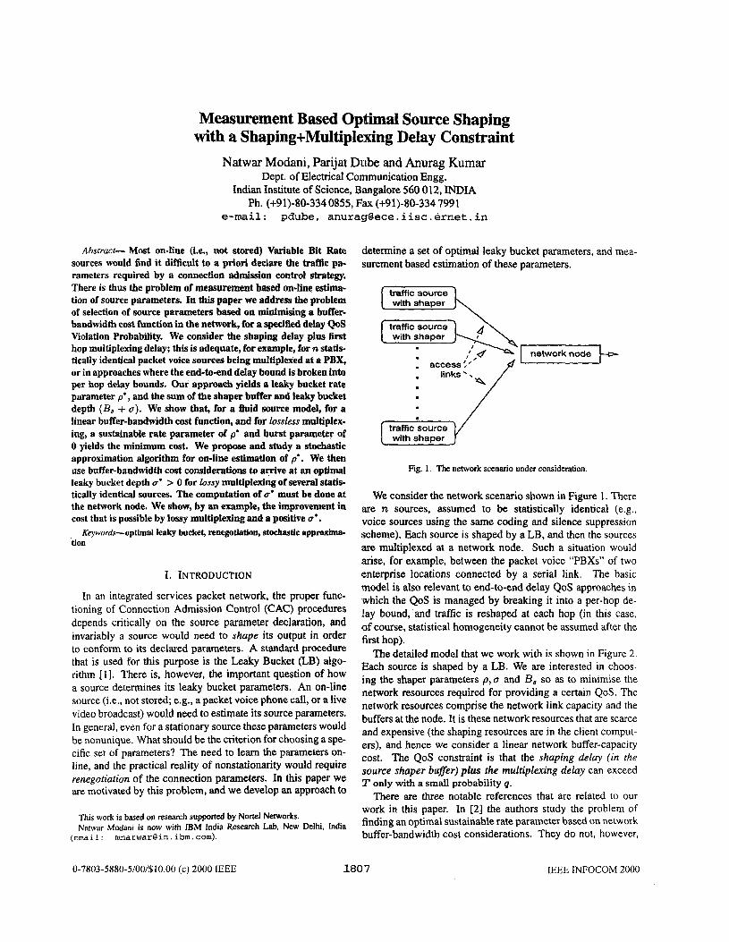
Fig. 3. The Leaky Bucket shaper. The buffer is infinite, but we want the probability of exceeding the buffer level B, to be very small.

ing active periods). The processes S(t) and W ( t ) shown in Figure 3 are to be viewed as rate processes. In the analysis we will assume fluid processes, whereas the simulations will be done with discrete fixed length packets, or cells.

We note that when there are cells in the cell buffer, since tokens are arriving at the rate p, the cell buffer is depleted at the rate p. If the cell buffer level exceeds B,, and since the source would not drop its own cells, we view this as a QoS violation; i.e., B, does not represent a memory limitation, but a delay bound of 9. Thus our view is that the cell buffer "behind" the LB is infinite but the buffer level exceeds B, with a small probability; we call this the QoS Violation Probability (QVP).

Fig. 4. A single server queuing system, with service rate p and infinite buffer, that is equivalent to the (a, p ) leaky bucket shaper from the QVP (see text) point of view.

With reference to Figure 3, define X ( t ) = XI (t ) - Xz (t) -t- o. The QVP is then just P ( X > B, + u) , where X is the sta- tionary marginal buffer occupancy (see Figure 4). For a fluid model, this system is equivalent to the leaky bucket shown in Figure 3 from the QVP point of view (see also [5 ] , [I]). Thus for a given p, the QVP depends on U and B, only through their sum. We will use the notation p , to denote P(X > B, + 0). Writing B := B, + U, for fixed p,, we denote the B vs p trade- off function by gp. (p) = B. Let h,, (.) denote the inverse of gP, (e) (an example of hp8 ( e ) is in Figure 5).

111. SHAPING FOR MINIMUM COST LOSSLESS

OPTlMAL VALUE OF p MULTIPLEXING: CHARACTERISATION OF AN

In this section we consider several statistically identical sources (SI (t), S,(t), . . . , S,,(t). see Figure 2). each shaped by the same LB parameters, feeding a buffered multiplexer. Each source requires a shaping plus muxing delay bound of TI which can be violated with the QVP of q. For this scenario, we develop the notion of an optimal LB token rate parame-

0-7803-5880-5/00/$10.00 (c) 2000 IEEE 1808 IEEE INFOCOM 2000

' ' O I B = T p

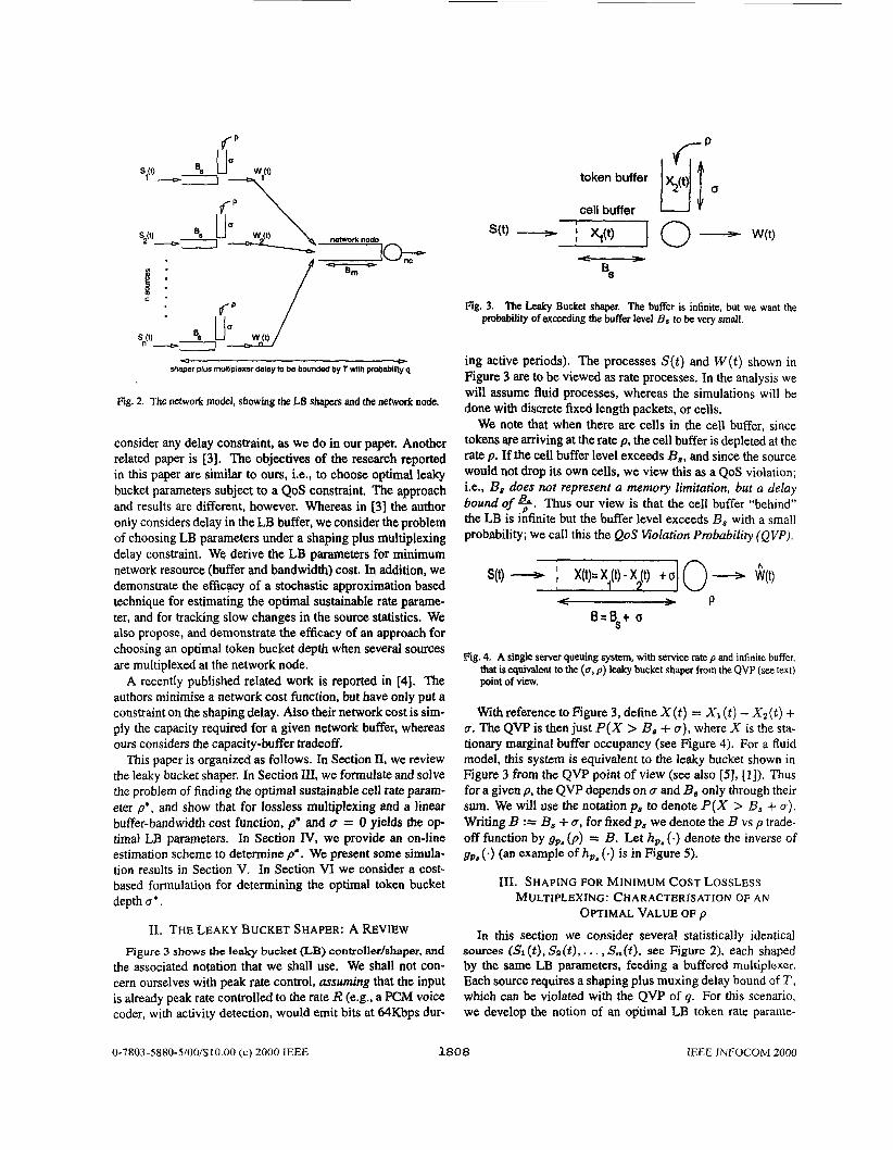
Fig. 5. A typical (8, -i- U ) vs p trade-off curve; i.e., the function h,, (B) . Two state Markovian on-off source with mean on-time 5/3, mean off tune 5/2, and peak rate R = 170; p a =

ter p* . The optimality will be in the sense of minimising the multiplexer service rate (link bandwidth) required for lossless multiplexing of the superposition of the LB controlled sources, with the constraint that the shaping plus multiplexing delay bound T is violated with a probability 5 q.

For an isolated (a, p, R) source fed into a buffered server with service rate c, the maximum (over all conforming sources) buffer occupancy b is related to c by

U b = - ( R - c ) R - p

This occupancy is achieved by an on-off extrema1 periodic source with on-time To, = & (at peak rate) and off-time T o f f = 5 (see [6]). It is also easily seen that (see Lo Presti et a1 [7] for a more general result) the lossless multiplexing of n such sources will require a buffer of nb and capacity nc; i.e., for lossless multiplexing the segregated and aggregated systems are identical for resource requirements. Thus, for loss- less service at the multiplexer, we need to consider each source with its own network queue of service rate c and buffer size b. With these ingredients, we will develop an optimization prob- lem.

For given (U, p, R), for lossless service it is necessary that the capacity at the multiplexer c 2 p. Also, we need to have

a b b 2 - ( R - c ) + C > R - ff - ( R - p ) R-P

It follows that, for lossless multiplexing, given b 2 0, we need

Now consider the shaping and multiplexing delay constraint T. Suppose we allow a target shaping delay of a ( 5 T) . Hence the delay bound T is met provided the bouni on the network node delay $ = (T - +), i.e., b = c(T- a). Since our QVP is q, we can permit the buffer level in the sgaper to exceed B, with probability p , = q. We seek the values of p, 0, b and B to minimise the multiplexer capacity c. Recalling some notation

token rate p - Fig. 6. Characterisation of p* ; 7 is the mean rate of the source

from Section I1 (in particular that B = B, + U), we have the lfollowing optimisation problem:

Subject to: multiplexer delay constraint:

b = c ( T - 7 )

shaper delay constraint and delay QVP:

< T B - f f P -

and

and, by definition

05 U < B

Equivalently, eliminating b between the multiplexer delay con- straint and the objective function, we obtain

Subject to

B = gq(p) , 0 5 ~7 5 B and B 5 T p + The solution to the above problem is provided by the following theorem.

Theorem III. 1: For g q ( p ) a convex and decreasing function, the optimal value of the problem described above is given by the unique p* that solves the equation

T P = d P > (3)

Further, the optimal value of B, + = Tp*, and for 0 5 U <_ Tp*, the value of b = U. Proof : See Appendix I. The geometry of the solution is de- picted in Figure 6.

0-7803-5880-5/00/$10.00 ( c ) 2000 IEEE 1809 IEEE INFOCOM 2000

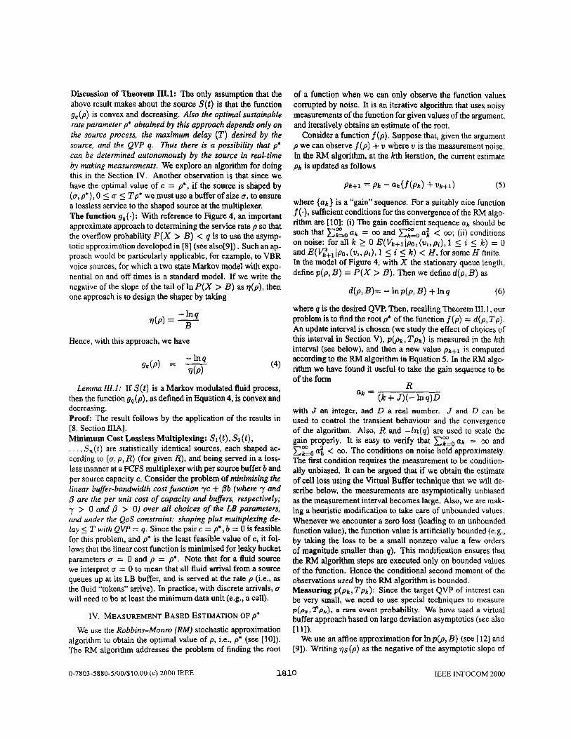
Discussion of Theorem III.1: The only assumption that the above result makes about the source S(t) is that the function g&) is convex and decreasing. Also the optimal sustainable rate parameter p* obtained by this approach depends only on the source process, the maximum delay (T) desired by the source, and the QVP q. Thus there is a possibility that p* can be determined autonomously by the source in real-time by making measurements. We explore an algorithm for doing this in the Section IV. Another observation is that since we have the optimal value of c = p*, if the source is shaped by (0, p * ) , 0 5 CT 5 Tp’ we must use a buffer of size LT, to ensure a lossless service to the shaped source at the multiplexer. The function gq ( -) : With reference to Figure 4, an important approximate approach to determining the service rate p so that the overflow probability P(X > B) < q is to use the asymp- totic approximation developed in [8] (see also[9]). Such an ap- proach would be particularly applicable, for example, to VBR voice sources, for which a two state Markov model with expo- nential on and off times is a standard model. If we write the negative of the slope of the tail of In P(X > B) as ~ ( p ) , then one approach is to design the shaper by taking

Hence, with this approach, we have

(4)

Lenirna III. 1: If S(t ) is a Markov modulated fluid process, then the function gq(p) , as defined in Equation 4, is convex and decreasing. Proof: The result follows by the application of the results in [8, Section IIIA]. Minimum Cost Lossless Multiplexing: SI ( t ) , Sz ( t ) , . . . , S,(t) are statistically identical sources, each shaped ac- cording to (LT, p , R) (for given R), and being served in a loss- less manner at a FCFS multiplexer with per source buffer b and per source capacity c. Consider the problem of minimising the linear buffer-bandwidth cost function yc + Pb (where 7 and 0 are the per Knit cost of capacity and buffers, respectively; y > 0 and /? > 0 ) over all choices of the LB parameters, and under the QoS constraint: shaping plus multiplexing de- lay 5 T with QVP = q. Since the pair c = p* , b = 0 is feasible for this problem, and p* is the least feasible value of c, it fol- lows that the linear cost function is minimised for leaky bucket parameters CT = 0 and p = p*. Note that for a fluid source we interpret CT = 0 to mean that all fluid arrival from a source queues up at its LB buffer, and is served at the rate p (i.e., as the fluid “tokens” arrive). In practice, with discrete arrivals, LT will need to be at least the minimum data unit (e.g., a cell).

Iv. MEASUREMENT BASED ESTIMATION OF p‘

We use the Robbins-Monro (RM) stochastic approximation algorithm to obtain the optimal value of p, i.e., p* (see [lo]). The RM algorithm addresses the problem of finding the root

of a function when we can only observe the function values corrupted by noise. It is an iterative algorithm that uses noisy measurements of the function for given values of the argument. and iteratively obtains an estimate of the root.

Consider a function f(p). Suppose that, given the argument p we can observe f ( p ) + IJ where t~ is the measurement noise. [n the RM algorithm, at the lcth iteration, the current estimate pk is updated as follows

P k + i = P k - ak(f(Pk) -k %+I) (5 )

where {uk} is a “gain” sequence. For a suitably nice function f(.), sufficient conditions for the convergence of the RM algo- rithm are [lo]: (i) The gain coefficient sequence ab should be such that CEO at = 00 and E,”=, a; < 00; (ii) conditions on noise: for all IC 1 0 E(Vk+l [ P O , (U%, p i ) , 1 5 i 5 I C ) = 0 and E(V;+, Ipo, (U*, pi) , 1 5 e’ 5 k) < H, for some H finite. ‘In the model of Figure 4, with X the stationary queue length, definep(p, B) = P(X > B). Then we define d(p, B) as

d(P, B)= - Inp(p, B ) -t lnq (6)

where q is the desired QVP. Then, recalling Theorem 111.1, our problem is to find the root p* of the function f(p) = d(p, Tp). An update interval is chosen (we study the effect of choices of this interval in Section V), p(pk, Tpk) is measured in the lcth interval (see below), and then a new value pk+l is computed according to the FUvl algorithm in Equation 5. In the RM algo- rithm we have found it useful to take the gain sequence to be of the form

V

with J an integer, and D a real number. J and D can be used to control the transient behaviour and the convergence of the algorithm. Also, R and -In(q) are used to scale the gain properly. It is easy to verify that C E o a t = 00 and CEO a; < 00. The conditions on noise hold approximately. The first condition requires the measurement to be condition- ally unbiased. It can be argued that if we obtain the estimate of cell loss using the Virtual Buffer technique that we will de- scribe below, the measurements are asymptotically unbiased as the measurement interval becomes large. Also, we are mak- ing a heuristic modification to take care of unbounded values. Whenever we encounter a zero loss (leading to an unbounded function value), the function value is artificially bounded (e.g., by taking the loss to be a small nonzero value a few orders of magnitude smaller than q). This modification ensures that the RM algorithm steps are executed only on bounded values of the function. Hence the conditional second moment of the observations used by the RM algorithm is bounded. Measuring p ( p t l T p k ) : Since the target QVP of interest can be very small, we need to use special techniques to measure p ( p k , T p k ) , a rare event probability. We have used a virtual buffer approach based on large deviation asymptotics (see also

We use an affine approximation for Inp(p, B) (see [12] and (91). Writing ~ s ( p ) as the negative of the asymptotic slope of

[Ill).

0-7803-5880-5/00/$10.00 (c) 2000 IEEE 1810 IEEE INFOCOM 2000

0,

higher loss

low loss

J log P(X > B)

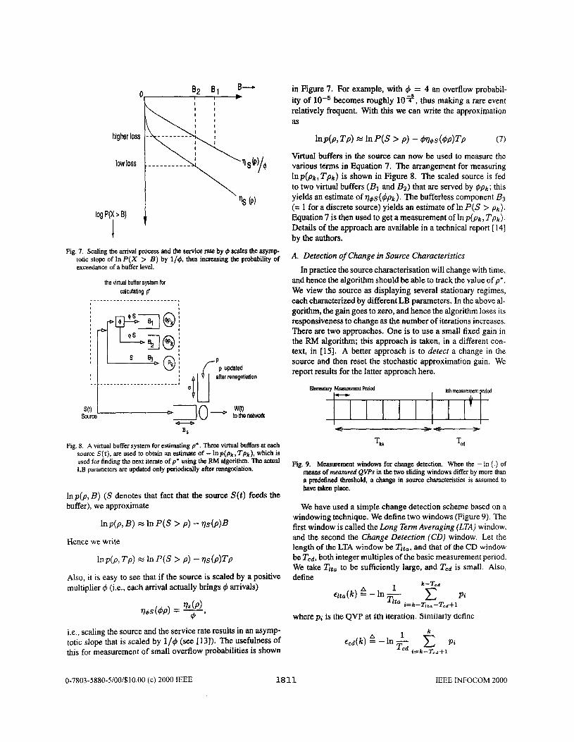
I Fig. 7. Scaling the arrival process and the service rate by Q scales the asymp-

totic slope of In P ( X > B ) by ~ / c # J , thus incmsing the probability of exceedance of a buffer level.

the virtual buffer system for calculating C

____________-____---------, I

U

Fig. 8. A virtual buffer system for estimating p'. Three virtual buffers at each source S( t ) , are used to obtain an estimate of - Inp(pk,Tpk), which is used for finding the next iterate of p' using the RM algorithm. The actual LB parameters are updated only periodically after renegotiation.

lnp(p, B) (S denotes that fact that the source S(t) feeds the buffer), we approximate

In P(P, B ) s3 In P(S > P ) - rlS(P)B

l n P ( P , TP) 25 In P(S > P ) - rlS(P)TP

Hence we write

Also, it is easy to see that if the source is scaled by a positive multiplier 4 (i.e., each arrival actually brings 4 arrivals)

i.e., scaling the source and the service rate results in an asymp- totic slope that is scaled by l/q5 (see [13]). The usefulness of this for measurement of small overflow probabilities is shown

in Figure 7. For example, with r$ = 4 an overflow probabil- ity of becomes roughly 1 0 3 , thus making a rare event relatively frequent. With this we can write the approximation as

lnP(P> TP) = In P(S > PI - h+S(q5P)TP (7)

Virtual buffers in the source can now be used to measure the various terms in Equation 7. The arrangement for measuring lnp(pk, Tpk) is shown in Figure 8. The scaled source is fed to two virtual buffers (B1 and Bz) that are served by 4pk ; this yields an estimate of q+s(r$pk). The bufferless component B3 (= 1 for a discrete source) yields an estimate of In P(S > p k ) .

Equation 7 is then used to get a measurement of lnp(pk, T p k ) . Details of the approach are available in a technical report [ 141 by the authors.

A. Detection of Change in Source Characteristics In practice the source characterisation will change with time,

and hence the algorithm should be able to track the value of p* . We view the source as displaying several stationary regimes, each characterized by different LB parameters. In the above al- gorithm, the gain goes to zero, and hence the algorithm loses its responsiveness to change as the number of iterations increases. There are two approaches. One is to use a small fixed gain in the RM algorithm; this approach is taken, in a different con- text, in [15]. A better approach is to detect a change in the source and then reset the stochastic approximation gain. We report results for the latter approach here.

< >- TI,

Fig. 9. Measurement windows for change detection. When the - In (.) of means of memured QVPs in the two sliding windows differ by more than a predefined threshold, a change in source characteristics is assumed to have taken place.

We have used a simple change detection scheme based on a windowing technique. We define two windows (Figure 9). The first window is called the Long Term Averaging (LTA) window, and the second the Change Detection (CD) window. Let the length of the LTA window be Tlta, and that of the CD window be Ted, both integer multiples of the basic measurement period. We take Tit, to be sufficiently large, and Tcd is small. Also, define

where p; is the QVP at ith iteration. Similarly define

A 1 E c d ( k ) = - In -

i=k-T,d+l

IEEE INFOCOM 2000 0-7803-5880-5/00/$10.00 ( c ) 2000 IEEE 1811

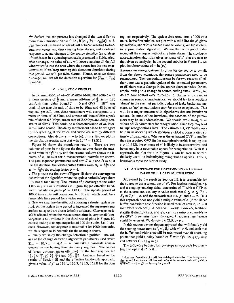
We declare that the process has changed if the two differ by more than a threshold value 6; i.e., if lelta(Cc) - e,d(k)l > 6. The choice of 6 is based on a trade off between reacting to mea- surement errors, and thus causing false alarms, and a delayed response to actual changes in the source statistics (an analysis of such issues in a queueing context is presented in [ 161). Also, after a change, the value of q t a will keep changing till the full window shifts into the area where the source has the new char- acteristics; if we keep running this detection algorithm during that period, we will get false alarms. Hence, once we detect a change, we turn off the detection algorithm for (Tit, + Ted) iterations.

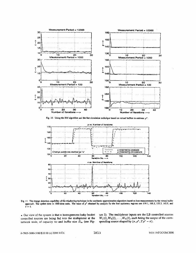
v. SIMULATION RESULTS In the simulation, an on-off Markov Modulated source with

a mean on-time of and a mean off-time of R = 170 cellshnit time, delay bound T = 5 and QVP = was used. If we take the unit of time to be lOms and 48 bytes of payload per cell, then these parameters will correspond to a mean on-time of 16.67ms, and a mean off-time of 25ms, peak rate of about 6.5 Mbps, mean rate of 2.6Mbps and delay con- straint of 50ms. This could be a characterization of an inter- active video source. The delay requirement has to be stringent for lip-synching, if the voice and video are sent by different connections. Also define E = - In (q ) ; it is E that we plot in the simulation results; note that - In lo-' = 11.513.

There are two columns of plots in the figure; the first column shows the mea- sured value of QVP (E), and the second column shows the it- erates of p. Results for 3 measurement intervals are shown. The gain sequence parameters used are: J = 3 and D = 4; at the kth iteration, the virtual buffer values were B1 = 9 and Bz = %; the scaling factor C$ = 4.

The plots in the first row of Figure 10 show the convergence behavior of the algorithm when the update period is large (here it is 10000 time units). The iterates of p converge to the value 138.9 in just 2 or 3 iterations in Figure 10; (an effective band- width calculation gives p* = 139.1). The update period of 10000 time units will correspond to 100 sec, which could be a reasonable time period for a video source.

Next we examine the effect of choosing a shorter update pe- riod. As the update time period is increased the measurements are less noisy and are closer to being unbiased. Convergence it- self is affected when the measurement time is very small (con- vergence is not evident in the third row of plots in Figure 10, corresponding to an update period of 100 time units, Le., 1 sec- ond). However, convergence is reasonable for 1000 time units, which is equal to 10 seconds for the example above.

Finally we study the change detection algorithm. The val- ues of the change detection algorithm parameters used were: Tlta = 10,Tcd = 4,6 = 4. We take a two-state nonsta- tionary. source having four stationary regimes. The values of [mean on-time, mean off-time) for the four regimes are (g,g),($!,g),(g,y) and (y,y). Analysis, based on the results of Section I11 and the effective bandwidth approach, gives a value of p* as 139.1, 166.3, 135.3, 165.8 for the four

Figure I O shows the simulation results.

regimes respectively. The update time used here is 1000 time units, In the first subplot, we plot with a solid line the p* given by analysis, and with a dashed line the value given by stochas- tic approximation algorithm. We see that our algorithm de- tected all the changes without any false alarm. The stochastic approximation algorithm gives estimate of p' that are near to that given by analysis. In the second subplot in Figure 1 1, we plot the observations of - In (pa), ]Remark on renegotiation: In order for the source to benefit from the above technique, the source parameters need to be renegotiated. The renegotiations can be for two reasons, (i) ei- ther there was a periodic update of the estimated parameters, or (ii) there was a change in the source characteristics (for ex- ample, owing to a change in source coding rate). While, we do not have control over 'direction' of change in the case of change in source characteristics, we should try to renegotiate 'down' in the event of periodic update of leaky bucket param- eters, as 'up' renegotiations may be prone to rejection. This will be a major concern with algorithms that are iterative in nature. In some of the iterations, the estimate of the param- eters may be an underestimate. We should avoid using these values of LB parameters for renegotiation, since they may lead lo 'up' renegotiations later. The estimated QVP values may help us in deciding which iteration yielded a conservative es- timate of parameters. Whenever the estimated QVP is smaller than the required QVP (in the example above this is saying that E > 11.513), the estimate of p* is likely to be conservative, and hence may be a reasonable epoch for renegotiation. With this approach, the plot for E in Figure 11 can be seen to be par- ticularly useful in indentifying renegotiation epochs. This is, however, a topic for further study.

VI. AN APPROACH FOR DETERMINING AN OPTIMAL VALUE OF 0: LOSSY MULTIPLEXING

Motivated by the result in Section 111, it is reasonable for the source to use a token rate of p*. For lossless multiplexing, and a shaping+muxing delay constraint of T with a QVP = q, the source can use any a value such that 0 5 0 5 Tp', €I, = Tp' - a, and the network sets c = p* and b = U. Thus this approach does not yield a unique value of U (if the linear buffer-bandwidth cost function is used then, of course, u* = 0 minimises such cost). A positive 0 would, however, facilitate statistical multiplexing, and a cell loss ratio comparable to lhe QVP' is permitted then the network resource requirement could be reduced. We denote the CLR by p, .

In this section we develop an approach that will finally yield the shaping parameters (a*, p', R) with U* > 0, and such that the buffer-bandwidth cost will be minimised over all operating points that yield a delay bound of T with QVP % q (p, = q and network CLR pm = 4).

The following bulleted list develops an approach for identi- lying an optimal CJ' > 0.

'Note that if we think of a cell that is delayed more than T as bang equiv- alent to cell loss, then a cell loss ratio of q at the network node still yields a QVPof1 - (I - q)2 M 2q M p forqsmdl.

0-7803-5880-5/00/$10.00 (c ) 2000 IEEE 1812 IEEE INFOCOM 2000

Measurement Period = 10000 30 I I

;S.

251.. . . . . . . . . . . . i . . . . . . . . . . . . . j . . . . . . . . . . . . .J

. . . . . . . . . . . . j . I . . . . . : . . . . . . . . . . . . . . . . . . . A

I - Y . - - Y

w i *O\

A . . . . . . . . ; . . . . . . . . . . . . . . . . . . . . . . . . . . . .

n' . . . . . . . . . . . . . . . . . . . I

10 x - m..= A ' h w

, .

150\ ., . . . . .e. .;. . . . . . . . ,J 0

140 . . . . . . . . . . . . i . . . . . . . . . . . . . i . . . . . . . . . . . . .

1 . . . . . . . . . . . . . .

130 * - - - - !o '/ -

p obtained by analysis -

Change points are marked as '0" - - - p obtained by simulations I I I

Measurement Period = 10000 1601 1

150

0. 140

130' I 0 10 20 30

Measurement Period = 1000 160 I

0 1 0 10 20 30

Measurement Period = 100

"0 10 20 30 40 Number of Iterations -->

1301

160

0 10 20 30 Measurement Period = 100

i5oL. :-.#: . , . .---I 130

0 10 20 30 40

f a140 . . . . . . . i . . . . . . . . i. . . . . . . . i . . . . : . . . .

Number of Iterations -->

Fig. 10. Using the RM algorithm and the fast simulation technique. based on virtual buffers to estimate p* .

p vs. Number of Iterations 1701

1 6 0 1 . . , I : , .-.- - -\T.: I : I : . . . . . . . . ...........IT : I . . . ..I I\ 150 .................... !... ..: ............ !.i . . . . . . . . . . . . ..> .... . ...................... . . . . . . . . . . . . I : I .

1 : 1 ; I f

O-140 . . . . . . . . . . . . . . o. ... .j.. . . ........ 1.:. . . . . . . . . . . . . .:. . . . . 1.. . . . . . . . . . . . . . . . . . . . . ; . . . . . . . . . . . .

. . . . . . . . . . . . . . . . . . . . . . . . . . . . . . . . . . . . . . .

. . . . . . . . . . . . . . . . .

"0 20 40 60 80 100 120 140 Iteration No. --5

Fig. 1 1. The change detection capability of &e windowing technique in the stochastic approximation algorithm based on loss measurements by the virtual buffer approach. The update time is lo00 time units. The value of p* obtained by analysis for the four stationary regimes are 139.1, 166.3. 135.3, 165.8. and 6 = 4.

Our view of the system is that n homogeneous leaky bucket controlled sources are being fed into the multiplexer at the network node, of capacity nc and buffer size B, (see Fig-

ure 2). The multiplexer inputs are the LB controlled sources Wl(t), Wz(t) , , . . , W,(t), each being the output of the corre- sponding source shaped by ( a , p * , T p * - (T).

0-7803-5880-5/00/$10.00 (c) 2000 IEEE 1813 IEEE INFOCOM 2000

defining the multiplexer CLR for the superposition process E:=, W, by Ax" w, (B,, nc), we will use the effective bandwidths (EBM=gpproach, and assume the following ad- ditivity property of effective bandwidths

n o i 7 5

iff

where A(c,p.)(B,, c ) is (- In of) the cell loss ratio for the out- put of a (0, p* Tp* - a) shaped source fed into a multiplexer with buffer B, and capacity c. This says that if we scale the capacity with the number of sources n, with the same buffer, then the CLR does not change. Hence we only work with the total multiplexer buffer and per source capacity. Notice that, this is a conservative assumption because the EBW approach ignores the statistical multiplexing gain.

A(o,p*)(&") = - In @m>1

P* (Bm, c) trade-off curve for lossless senrice -----I-- B--K given (em, c) oand trade-off cell loss curve ratio for = pm

c : per source capauly reqmt. 3

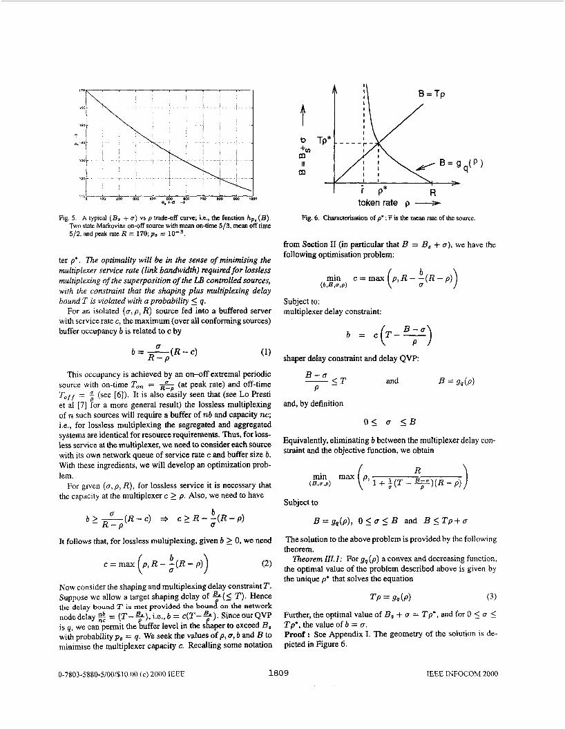
Fig. 12. Network buffer (B,) vs. per source capacity (c) trade-off curves at the multiplexer for given u. 0 5 u 5 Tp'. Shown are the lossless trade-off curve, the network delay constraint curve, and the lossy trade- of f curve.

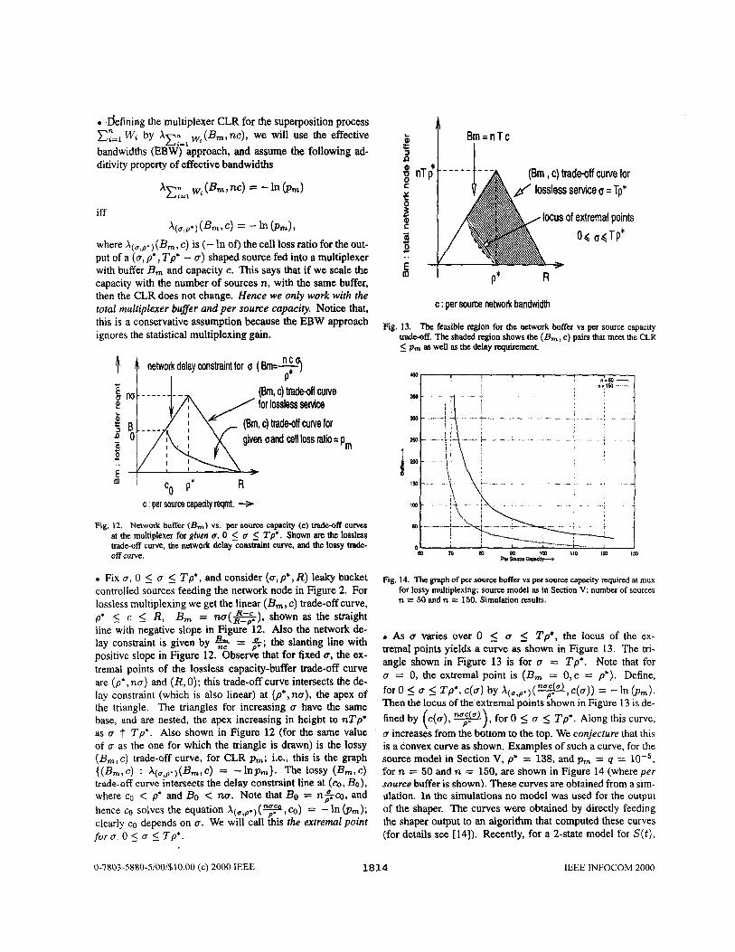
Fix U , 0 5 a 5 T p * , and consider (c,p+,R) leaky bucket controlled sources feeding the network node in Figure 2. For lossless multiplexing we get the linear (Bml c) trade-off curve, p* 5 c 5 R, B, = no(&), shown as the straight line with negative slope in Figure 12. Also the network de- lay constraint is given by % = s; the slanting line with positive slope in Figure 12. Observe that for fixed o, the ex- tremal points of the lossless capacity-buffer trade-off curve are ( p ' , no) and (R, 0); this trade-off curve intersects the de- lay constraint (which is also linear) at (p*,no), the apex of the triangle. The triangles for increasing o have the same base, and are nested, the apex increasing in height to nTp* as o t Tp*. Also shown in Figure 12 (for the same value of U as the one for which the triangle is drawn) is the lossy (Bm,c) trade-off curve, for CLR p,; i.e., this is the graph {(B,,c) : A(o!p*)(%lc) = -lnp,}. The lossy (&,cl trade-off curve intersects the delay constraint line at (CO, Bo). where CO < p* and BO C no. Note that BO = n$;s, and hence co solves the equation Fl CO) = - In (XI,,,); clearly CO depends on LT. We will call this the extremal poinr f o r o , 0 5 U 5 Tp*.

P* R

c : per source network bandwidth

Fig. 13. The feasible region for the network buffer vs per source capacity trade-off. The shaded region shows the (B,, c) pairs that meet the CLR 5 pm as well as the delay requirement.

0

Pig. 14. The graph of per source buffer vs per source capacity required at mux for lossy multiplexing; source model as in Section V; number of sources n = 50 and n = 150. Simulation results.

a As U varies over 0 5 U 5 T p * , the locus of the ex- tremal points yields a curve as shown in Figure 13. The tri- angle shown in Figure 13 is for o = Tp* . Note that for CJ = 0, the extremal point is (B, = 0 ,c = p* ) . Define, fo ro< U < T ~ * , c ( c J ) b y A ( u , p . ) ( y l ~ ( c ) ) = -h(pm). Then the locus of the extremal points shown in Figure 13 is de- fined by ( c ( ~ ) ~ -), for 0 5 LT < Tp'. Along this curve, CJ increases from the bottom to the top. We conjecture that this is a convex curve as shown. Examples of such a curve, for the source model in Section V, p' = 138, and pm = q = for n = 50 and n = 150, are shown in Figure 14 (where per source buffer is shown). These curves are obtained from a sim- ulation. In the simulations no model was used for the output of the shaper. The curves were obtained by directly feeding the shaper output to an algorithm that computed these curves {for details see [14]). Recently, for a 2-state model for S ( t ) ,

0-7803-5880-5/00/$10.00 ( c ) 2000 IEEE 1814 IEEE INFOCOM 2000

we have used an approximate 3-state model for the output of the LB shaper (see [SI), and have also obtained these curves analytically. The curves match very well with those obtained from simulation.

The shaded area in Figure 13 is bounded by the curves

{(B,,c) : B, = nTc,O 5 c 5 p * } , and {(B, ,c) : Bm = n T p * - H l } . This shaded region is the set of (Bmlc) pairs for each of which there exists a Q, 0 5 Q 5 Tp', such that the CLR and the delay requirement are met if the sources are controlled by (U, p') .

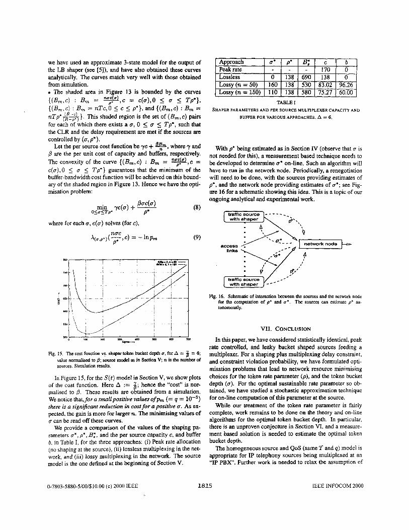
Let the per source cost function be 7 c + 5, where 7 and p are the per unit cost of capacity and buffers, respectively. The convexity of the curve {(B, ,c) : B m = T,c = c(a),O 5 o 5 T p * } guarantees that the minimum of the buffer-bandwidth cost function will be achieved on this bound- ary of the shaded region in Figure 13. Hence we have the opti- misation problem:

{ ( B ~ , c ) : Bm = T 1 c = c ( Q ) , O 5 U 5 2 ' ~ ' ) ~

Lossless 0 138 690 138 Lossy(n = 50) 160 138 530 83.02 LOSSY (n = 150) 110 138 580 75.27

where for each a, c(u) solves (for c) ,

0 ' 96.26 60.00

(9)

Fig. 15. The cost function vs. shaper token bucket depth U, for A = 8 = 6; value normalised to p; source model as in Section V; n is the number of sources. Simulation results.

In Figure 15, for the S( t ) model in Section V, we show plots of the cost function. Here A := 5; hence the "cost" is nor- malised to 0. These results are obtained from a simulation. We notice that, for a small positive values of Pm (= q = lo-') there is a signijcant reduction in cost for a positive U. As ex- pected, the gain is more for larger n. The minimising values of o can be read off these curves.

We provide a comparison of the values of the shaping pa- rameters o*, p*, B,*, and the per source capacity c, and buffer 6. in Table I, for the three approaches: (i) Peak rate allocation (no shaping at the source), (ii) lossless multiplexing in the net- work, and (iii) lossy multiplexing in the network. The source model is the one defined at the beginning of Section V.

Approach I o * I p ' I B , ' ( c b Peak rate 1 - I - ( - 1 1 7 0 1 0

TABLE I SHAPER PARAMETERS A N D PER SOURCE MULTIPLEXER CAPACITY AND

BUFFER FOR VARIOUS APPROACHES. A = 6.

With p' being estimated as in Section IV (observe that a is not needed for this), a measurement based technique needs to be developed to determine U* on-line. Such an algorithm will have to run in the network node. Periodically, a renegotiation will need to be done, with the sources providing estimates of p*, and the network node providing estimates of U'; see Fig- ure 16 for a schematic showing this idea. This is a topic of our ongoing analytical and experimental work.

traffic source - - - - - I . w i t h shaper -'F;..

traffic source

Fig. 16. Schematic of interaction between the sources and the network node for the computation of p' and U * . The sources can estimate p' au- tonomously.

VII. CONCLUSION In this paper, we have considered statistically identical, peak

rate controlled, and leaky bucket shaped sources feeding a multiplexer. For a shaping plus multiplexing delay constraint, and constraint violation probability, we have formulated opti- misation problems that lead to network resource minimising choices for the token rate parameter (p), and the token bucket depth (a). For the optimal sustainable rate parameter so ob- tained, we have studied a stochastic approximation technique for on-line computation of this parameter at the source.

While our treatment of the token rate parameter is fairly complete, work remains to be done on the theory and on-line algorithms for the optimal token bucket depth. In particular, there is an unproven conjecture in Section VI, and a measure- ment based solution is needed to estimate the optimal token bucket depth.

The homogeneous source and QoS (same T and q) model is appropriate for IP telephony sources being multiplexed at an "IP PBX'. Further work is needed to relax the assumption of

0-7803-5880-5/00/$10.00 (c) 2000 IEEE 1815 IEEE INFOCOM 2000

source homogeneity, and the requirement that all the sources need the same QoS.

APPENDIX

1. PROOF OF THEOREM 111.1

T P* B : total buffer size at LB

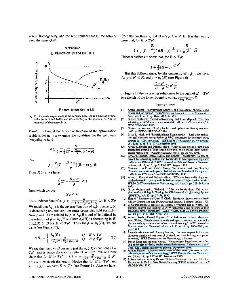
Fig. 17. Capacity requirement at the network node (c) as a knction of total buffer (sum of cell buffer and token buffer) at the shaper (B); F is the mean rate of the source S( t) .

Proof Looking at the objective function of the optimization problem, let us first examine the condition for the following inequality to hold

R 1 + $(T - y ) ( R - p) P S

i.e.,

Since R 2 p , we have

from which we get T P I B

for B < Tp. Thus, independent of g, p > 1+3(T-v) (R-p)

We recall that h, (.) is the inverse function of gq (-); since gq ( a )

is decreasing and convex, the same properties hold for hq(-) . Now p and B are related by p = h,(B), and p’ is defined by the solution of p = hq(Tp). Since h,(B) is decreasing in B, Th,(B) > B for B < Tp’. Thus for p = hq(B), we can write (see Figure 17),

R

We see that the c vs B curve is just the h,(B) curve upto B = Tp’, and is hence decreasing upto B = Tp’. We will now

This will establish the result. Notice that for B > Tp*, and B = g q ( p ) , we have B > T p (see Figure 6). Also we have,

show that for B > Tp’, c(B) = l + + ( T - y ) ( R - p ) R > - p’.

from the constraints, that B - T p 5 o seen that, for B > Tp’

R

B. It is then easily

R > 1 + i ( T - V ) ( R - p) - 1 + g ( R - p)

Hence it suffices to show that, for B > Tp’, R ’ P* l + % ( R - p ) -

But this follows since, by the convexity of h,(.), we have, for p < p’ < R, and p = h,(B) (see Figure 6)

R - p’ T - > p*- R - p - B

In Figure 17 the increasing solid curve to the right of B = Tp’

REFERENCES

is a sketch of the lower bound to c, i.e., +. 1+ ( R - p ) 0

Arthur Berger, “Performance analysis of a rate-control throttle where tokens and job queue:’ lEEE Journal on Selected Areus in Cr~mmunicu- tions, vol. 9, no. 2, pp. 165-170, Feb 1991. Fabrice Guillemin, Catherine Rosenberg, and Josee Mignault, “On char- acterizing an ATM source via sustainable cell rate traffic descriptor,” in IEEE INFOCOM, 1995. Gustavo de Veciana, “Leaky buckets and optimal self-tuning rate con- trol,” in IEEE GLOBECOM, 1994. Brian L. Mark and Gopalakrishnan Ramamurthy, “Real-time estima- tion and dynamic renegotiation of UPC parameters for arbitrary traffic sources in ATM networks,” IEEWACM Transactions on Neworking, vol. 6, no. 6, pp. 81 1-827, December 1998. Anwar I. Elwalid and Debasis Mitra, “Analysis and design of rate based congestion control of high speed networks, i: stochastic fluid models, access regulatiom,” Queueing Sysrems, vol. 9, pp. 29-64, 1991. Anwar I. Elwalid, Debasis Mitra, and Robert H. Wentworth, “A new ap- proach for allocating buffers and bandwidth to heterogeneous regulated traffc in an ATM node:’ IEEE Journal on Selected Areas in Communi- carions, vol. 13, no. 6, pp. 1115-1127, August 1995. Francesco Lo Presti, Zhi-Li Zhang, Jim Kurose. and Don Towsley. “Source time scale and optimal bufferhandwidth trade-off for regulated traffic in an ATM node,” in IEEE INFOCOM, 1997. Anwar I. Elwalid and Debasis Mitra, ‘‘Effwtive bandwidth of general markovian traffic sources and admission control of high speed networks,” IEEWACMTransactions on Networking, vol. 1. no. 3, pp. 329-343, June 1993. G. de Veciana and J. Walrand, “Effective bandwidths: Call admis- sion, traffic policing & filtering for ATM networks:’ Queueing Systems

Harold J. Kushner and Dean S. Clark, Stochastic Approximuriun Merh- ods for Construined and Unconstrained Systems, Springer-Verlag, 1978. C. Courcoubetis, G. Ke-sidis, A. Ridder, J. Walrand. and R. Weber, “Ad- mission control and routing in ATM networks using inferences from measured buffer occupancy:’ IEEE Transactions on Communicutions.

Anwar Elwalid, Daniel Heyman, T. V. Lakshman. Debasis Mitra, and Alan Weiss, “Fundamental bounds and approximations for atm multi- plexers with applications to video teleconferencing,” IEEE Journul o n Selected Areas in Communicarions, vol. 13, no. 6, pp. 1004-1016, Au- gust 1995. Santosh Abraham and Anurag Kumar, “A new approach for asyn- chronous distributed rate control of elastic sessions in integrated packet networks,” IEEE Transactions on Networking. submitted. Parijat Dube and Anurag Kumar, “Measurement based selection of to- ken buffer size for leaky bucket controlled sources: A simulation study,’’ Tech. Rep., Indian Institute of Science, November 1998. Anurag Kumar, “Adaptive load control of the central processor in a dis- tributed system with a star topology,” IEEE Transucrions on Computers. vol. 38, no. 11. pp. 1502-1512. November 1989. S.Amamath and Anurag Kumar. “A New Technique for Link Utilization Estimation in Packet Data Networks using SNMP variables,” in lEEE GLOBECOM. 1997.

(QUESTAJ, vol. 20. pp. 37-59.1995.

vol. 43, pp. 1778-1784, April 1995.

0-7803-5880-5/00/$10.00 ( c ) 2000 IEEE 1816 IEEE INFOCOM 2000