arX

iv:c

ond-

mat

/051

1033

v1 [

cond

-mat

.sup

r-co

n] 2

Nov

200

5

Magnetic and electrical characterization of lanthanum

superconductors with dilute Lu and Pr impurities.

Felix Soto, Lucia Cabo, Jesus Mosqueira, and Felix Vidal∗

Laboratorio de Baixas Temperaturas e Superconductividade

(Unidad Asociada al ICMM-CSIC, Spain),

Departamento de Fısica da Materia Condensada,

Universidade de Santiago de Compostela, E-15782 Spain

Abstract

In this work we present measurements of the electrical conductivity and of the magnetization

of La and of La-Pr and La-Lu dilute (up to 2 at.%) alloys, from which we determine, very in

particular, the influence of dilute magnetic impurities on the upper critical magnetic field amplitude

[and then on the superconducting coherence length amplitude ξ(0)] and on the Ginzburg-Landau

parameter κ.

PACS numbers: 74.25.Ha; 74.70.Ad; 74.81.-g

1

As it is well known since the pioneering experiments of Matthias and coworkers1,2, the

La-Pr and La-Lu alloys are very well suited to study the different aspects of the interplay

of superconductivity with magnetic impurities.3 However, even today some of the main

superconducting characteristics of these alloys are still not well settled or even they have

not been measured at all. This is, for instance, the case of a so-central parameter as the

Ginzburg-Landau superconducting coherence length amplitude, ξ(0). Here we will present

detailed magnetic and electrical measurements in La and La-Pr and La-Lu dilute (up to

2 at. %) alloys, from which we will obtain, very in particular, ξ(0) and the Ginzburg-Landau

parameter, κ.

All the samples (pure La and La-Pr and La-Lu alloys) used in this work are commercial

(Goodfellow and Alfa Aesar, 99.9% purity). The manufacturers warrant that the impurity

concentrations are below 100 ppm (by weight) for any of the following ions: Al, Ca, Fe, Mg,

Nd, Ni, Pr, Si, and Y. X-ray diffraction analyses revealed that the pure La samples consist in

a randomly-oriented mixture of two crystallographic phases, double-hexagonal-close-packed

(α-La) and face-centered-cubic (β-La), which is a common feature in most of the La samples

studied in other works.4,5,6,7,8,9,10 For the alloys, we indicate in the last column in Table I

the average distance between Pr or Lu impurities, dimp, obtained from the samples’ densities

and nominal compositions. The values are between 12 and 19 A.

A first magnetic characterization of the different samples has been done through mea-

surements of the field-cooled magnetic susceptibility versus temperature curves, χFC(T ).

Some examples of the obtained curves are shown in Fig. 1(a). These measurements were

performed with a high resolution, superconducting quantum interference device (SQUID)

based, magnetometer (Quantum Design’s MPMS). For that, each sample was first cut as a

cylinder of 6 mm height and 6.5 mm diameter, and care was taken just before each measure-

ment of removing the possible superficial insulating oxide layer with sandpaper (Buehler,

600 grit) and then immersing the samples in an acetone ultrasonic bath for several min-

utes. The external magnetic field applied in the measurements was µ0H = 0.5 mT, much

smaller than the lower critical magnetic field amplitude (see Refs. [4,5,6,7,8,9,10] and also

below). For each sample, the resulting magnetic susceptibility was corrected for demagne-

tizing effects through the ellipsoidal approximation and then normalized to the ideal value

-1 at low temperatures. Other details of these last measurements are similar to those we

have followed in magnetization experiments in other superconductors.11 In the Fig. 2(b)

2

the solid lines are fits to the experimental dχFC/dT points of a Gaussian distribution,

(√

(π/2)∆TC0)−1exp[−2(T − TC0)

2/∆T 2C0] with TC0 and ∆TC0 as free parameters. We will

see below that these TC0 temperatures, that are summarized in Table I, are consistent with

the transition temperatures that may be obtained from resistivity versus temperature curves.

The ∆TC0 values, which are also summarized in Table I, provide a good indication of how

much the structural and stoichiometric inhomogeneities at long length scales [well larger

than ξ(0)] affect the normal-superconducting transition temperature of each sample. It is

also worth noting here that in the case of the nominally pure La samples their TC0 values

are well between the ones for pure α-La (∼ 5.0 K) and β-La (∼ 6.0 K),4,5,6,7,8,9,10 but no

traces were observed of diamagnetic transitions near these last temperatures (which would

manifest themselves as steps in the χFC curve). This is consistent with a mixing of both

crystallographic phases at lengths of the order or smaller than ξ(0).5 We note also that the

TC0 values of Table I are consistent with both the experimental results of Matthias and

coworkers1,2 and the Abrikosov-Gor’kov predictions12. These last aspects will be analyzed

in detail elsewhere.

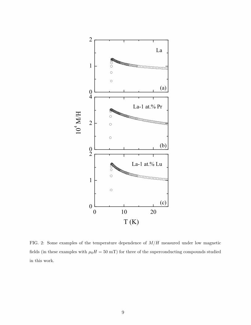
In Fig. 2 we present measurements, corresponding to three of the superconducting

compound studied in this work, of the magnetization under a constant magnetic field of

µ0H = 50 mT and including temperatures well above the superconducting transition. These

measurements may be useful, e.g., to analyze the superconducting fluctuations above TC in

these samples, as it will be reported elsewhere. Note that the absolute values of M(T ) above

the transition increase with the Pr content but, for instance, in the La-1 at.%Pr alloy the

magnetization at 1.5TC is only around 5 times larger than the one of the optimally-doped

YBa2Cu3O7−δ.14 As for the T -dependence of these magnetization curves, they present a

Curie-like curvature, ressembling the one of optimally-doped YBa2Cu3O7−δ. We have also

performed measurements of the magnetization versus applied magnetic field at a constant

temperature above the transition; however, the understanding of the resulting M(H)T curves

is complicated by the existence of an upturn at low fields, perhaps related to the presence

of small amounts of inhomogeneities which do not affect the M(T )H dependence.13

To perform measurements of the resistivity against temperature, thin slabs (typically

5× 1× 0.1 mm3) were cut from the same rods used in the magnetization experiments. The

electrical contacts were made by attaching to the samples four Al-Si wires (25µm diameter)

with an in-line geometry by using an ultrasonic micro-wire bonder (Kulicke & Soffa, model

3

4523). Just before attaching the contacts the possible superficial insulating oxide layer was

again removed with sandpaper and an acetone ultrasonic bath. The final resistance was typ-

ically 50 mΩ per contact. The ac (34 Hz) current supplied to measure the samples’ resistance

was 2 mA, and the longitudinal voltage was measured by using a lock-in amplifier (EG&G

Princeton Applied Research, model 5210) which has a resolution of 0.05% up to 1 nV. The

main uncertainty in these measurements comes from the samples’ dimensions and is around

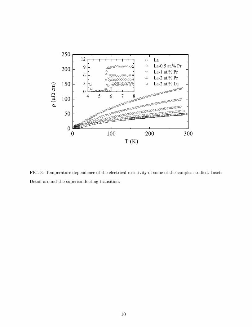
15%. A general view of the resulting resistivity versus temperature curves is presented in

Fig. 2 for some of the samples. The nominally pure La samples have a room-temperature

resistivity (∼ 50 µΩcm) and a temperature dependence comparable to the one of pure α-La

and β-La samples.9 Note also that the room-temperature resistivity increases monotonically

with the Pr concentration. The inset of Fig. 2 presents a detail of these measurements

around the superconducting transition. By taking into account that the resistivity falls to

zero at the temperature at which a superconducting path exists through the sample (i.e.,

when the superconducting volume fraction exceeds ∼ 15%15) the transition temperature

obtained from those measurements are in good agreement with the ones obtained from the

low-field χFC measurements presented in Fig. 1. The values of ℓ, the normal-state electronic

mean field path extrapolated to T = 0 K, were estimated from the residual resistivities ρres

through a simple Drude-model relation,16 and compiled in Table I. By comparing these ℓ

values with the corresponding ξ(0) (see below), one may conclude that all the samples are

in the dirty limit. In the case of nominally pure La, this is consistent with the presence

in these samples of a small amount of impurities. The relaxation time of normal electrons

corresponding to those ℓ values are of the order of τ ∼ 10−14 s.

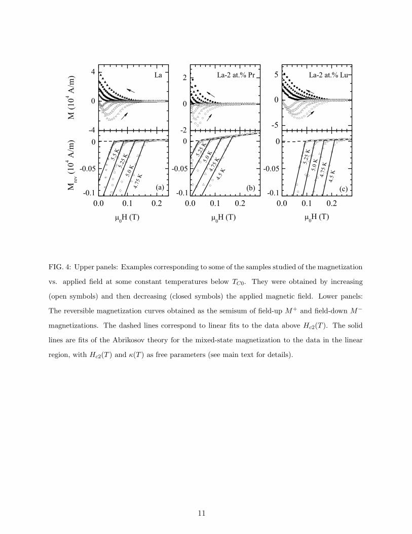
Other basic superconducting parameters were obtained from measurements of the magne-

tization against magnetic field at different constant temperatures below the superconducting

transition. Some examples of these measurements are shown in Fig. 4. These curves are,

even in the case of the pure La, typical of type II superconductors, in agreement with the

earlier results of Pan and coworkers10 which showed that even high-purity α-La is a type

II superconductor with a Ginzburg-Landau parameter κ ≈ 2.4. For all the compounds

studied here we found that the mixed-state magnetization is highly irreversible up to the

upper critical field, Hc2(T ). To overcome this difficulty in determining Hc2(T ), the re-

versible magnetization was approximated as Mrev = (M+ + M−)/2, where M+ and M− are

the magnetization when increasing and decreasing the external magnetic field respectively.

4

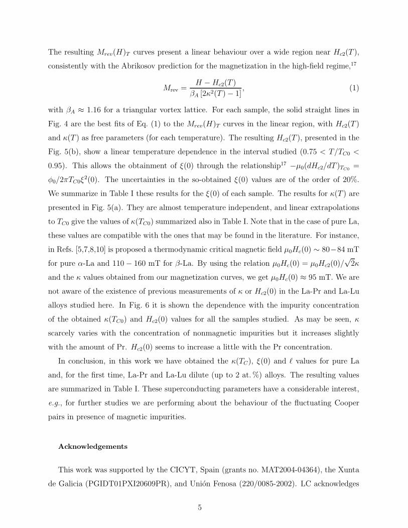
The resulting Mrev(H)T curves present a linear behaviour over a wide region near Hc2(T ),

consistently with the Abrikosov prediction for the magnetization in the high-field regime,17

Mrev =H − Hc2(T )

βA [2κ2(T ) − 1], (1)

with βA ≈ 1.16 for a triangular vortex lattice. For each sample, the solid straight lines in

Fig. 4 are the best fits of Eq. (1) to the Mrev(H)T curves in the linear region, with Hc2(T )

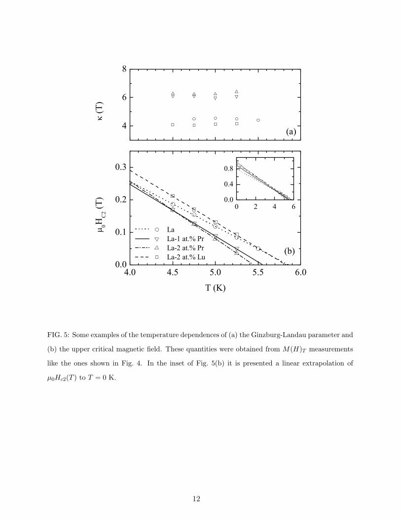
and κ(T ) as free parameters (for each temperature). The resulting Hc2(T ), presented in the

Fig. 5(b), show a linear temperature dependence in the interval studied (0.75 < T/TC0 <

0.95). This allows the obtainment of ξ(0) through the relationship17 −µ0(dHc2/dT )TC0=

φ0/2πTC0ξ2(0). The uncertainties in the so-obtained ξ(0) values are of the order of 20%.

We summarize in Table I these results for the ξ(0) of each sample. The results for κ(T ) are

presented in Fig. 5(a). They are almost temperature independent, and linear extrapolations

to TC0 give the values of κ(TC0) summarized also in Table I. Note that in the case of pure La,

these values are compatible with the ones that may be found in the literature. For instance,

in Refs. [5,7,8,10] is proposed a thermodynamic critical magnetic field µ0Hc(0) ∼ 80−84 mT

for pure α-La and 110 − 160 mT for β-La. By using the relation µ0Hc(0) = µ0Hc2(0)/√

2κ

and the κ values obtained from our magnetization curves, we get µ0Hc(0) ≈ 95 mT. We are

not aware of the existence of previous measurements of κ or Hc2(0) in the La-Pr and La-Lu

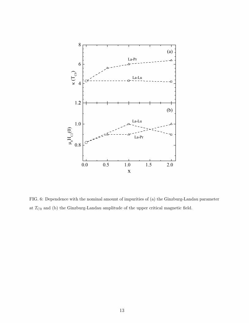
alloys studied here. In Fig. 6 it is shown the dependence with the impurity concentration

of the obtained κ(TC0) and Hc2(0) values for all the samples studied. As may be seen, κ

scarcely varies with the concentration of nonmagnetic impurities but it increases slightly

with the amount of Pr. Hc2(0) seems to increase a little with the Pr concentration.

In conclusion, in this work we have obtained the κ(TC), ξ(0) and ℓ values for pure La

and, for the first time, La-Pr and La-Lu dilute (up to 2 at. %) alloys. The resulting values

are summarized in Table I. These superconducting parameters have a considerable interest,

e.g., for further studies we are performing about the behaviour of the fluctuating Cooper

pairs in presence of magnetic impurities.

Acknowledgements

This work was supported by the CICYT, Spain (grants no. MAT2004-04364), the Xunta

de Galicia (PGIDT01PXI20609PR), and Union Fenosa (220/0085-2002). LC acknowledges

5

financial support from Spain’s Ministerio de Educacion y Ciencia through a FPU grant.

∗ Electronic address: fmvidal@usc.es

1 B.T. Matthias et al., Phys. Rev. Lett. 1, 92 (1958).

2 R.A. Hein, R.L. Falge Jr., B.T. Matthias and C. Corenzwit, Phys. Rev. Lett. 2, 500 (1959).

3 Ø. Fisher, Magnetic Superconductors. Edited by K.H.J. Buschov and E.P. Wohlfarth, “Ferro-

magnetic Materials”, vol. 5 (Elsevier, Amsterdam, 1990).

4 J.D. Leslie et al., Phys. Rev. 134, A309 (1964).

5 G.S. Anderson, S. Legvold and F.H. Spedding, Phys. Rev. 109, 243 (1958).

6 A. Berman, M.W. Zemansky and H.A. Boorse, Phys. Rev. 109, 70 (1958).

7 D.K. Finnemore, D.L. Johnson, J.E. Ostenson, F.H. Spedding and B.J. Beaudry, Phys. Rev.

137, A550 (1965).

8 D.L. Johnson and D.K. Finnemore, Phys. Rev. 158, 376 (1967).

9 S. Legvold, P. Burgardt, B.J. Beaudry and K.A. Gschneidner Jr., Phys. Rev. B 16, 2479

(1977).

10 P.H. Pan et al., Phys. Rev. B 21, 2809 (1980).

11 J. Mosqueira et al., Phys. Rev. B 53, 1527 (1996). See also references therein.

12 A.A. Abrikosov and L.P. Gor’kov, Sov. Phys. JETP 12, 1243 (1961).

13 L. Cabo et al., to be published.

14 See, e.g., F. Vidal and M.V. Ramallo, in The gap symmetry and fluctuations in high-TC super-

conductors, edited by J. Bok et al., p. 443 (Plenum,N.Y.1998) and references therein.

15 S. Kirkpatrick, in J.C. Garland and D.B. Tanner (Eds.), Proceedings of the First Conference

on the Electrical Transport and Optical Properties of Inhomogeneous Media, p. 99 (American

Institute of Physics, New York, 1978).

16 For the relation between ρres and ℓ see, e.g., N.W. Ashcroft and N.D. Mermim, “Solid State

Physics”, p.5 (Saunders College, Philadelphia, 1976).

17 See, e.g., M. Tinkham, Introduction to Superconductivity (McGraw-Hill, New York, 1996), ch. 4

and ch. 8.

6

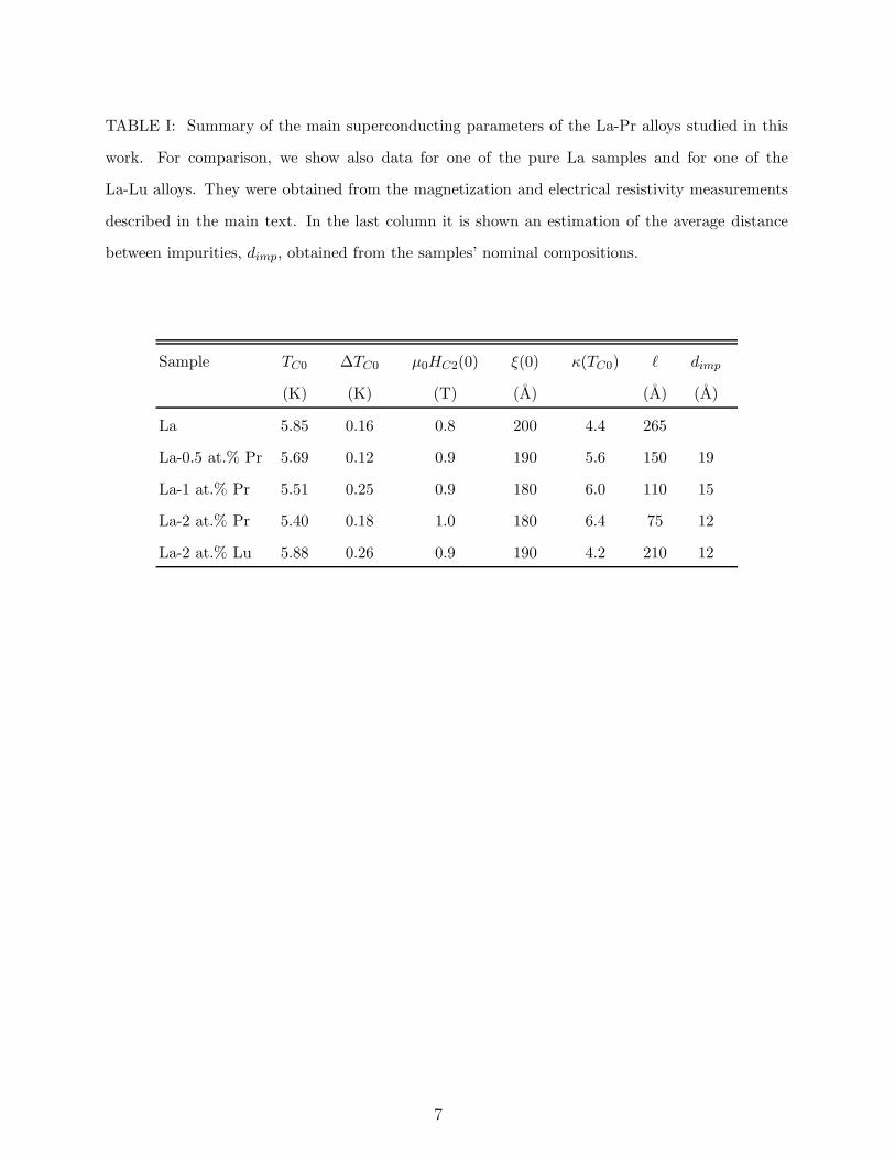
TABLE I: Summary of the main superconducting parameters of the La-Pr alloys studied in this

work. For comparison, we show also data for one of the pure La samples and for one of the

La-Lu alloys. They were obtained from the magnetization and electrical resistivity measurements

described in the main text. In the last column it is shown an estimation of the average distance

between impurities, dimp, obtained from the samples’ nominal compositions.

Sample TC0 ∆TC0 µ0HC2(0) ξ(0) κ(TC0) ℓ dimp

(K) (K) (T) (A) (A) (A)

La 5.85 0.16 0.8 200 4.4 265

La-0.5 at.% Pr 5.69 0.12 0.9 190 5.6 150 19

La-1 at.% Pr 5.51 0.25 0.9 180 6.0 110 15

La-2 at.% Pr 5.40 0.18 1.0 180 6.4 75 12

La-2 at.% Lu 5.88 0.26 0.9 190 4.2 210 12

7

5.0 5.5 6.00

2

4

6

8

10(b)

dFC

/dT

(K-1

)

T (K)

La La-2 at.% PrLa-1 at.% Pr La-2 at.% Lu

-1.0

-0.5

0.0

FC

(a)

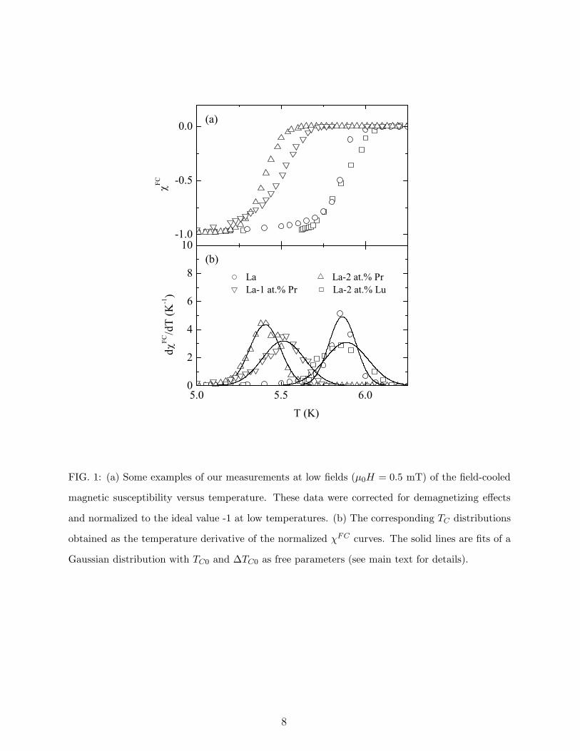
FIG. 1: (a) Some examples of our measurements at low fields (µ0H = 0.5 mT) of the field-cooled

magnetic susceptibility versus temperature. These data were corrected for demagnetizing effects

and normalized to the ideal value -1 at low temperatures. (b) The corresponding TC distributions

obtained as the temperature derivative of the normalized χFC curves. The solid lines are fits of a

Gaussian distribution with TC0 and ∆TC0 as free parameters (see main text for details).

8

0

1

2

La

104 M

/H

T (K)

(a)

0 10 200

1

2

(c)

La-1 at.% Lu

0

2

4

(b)

La-1 at.% Pr

FIG. 2: Some examples of the temperature dependence of M/H measured under low magnetic

fields (in these examples with µ0H = 50 mT) for three of the superconducting compounds studied

in this work.

9

0 100 200 3000

50

100

150

200

250 La La-0.5 at.% Pr La-1 at.% Pr La-2 at.% Pr La-2 at.% Lu

(

cm

)

4 5 6 7 80

3

6

9

12

T (K)

FIG. 3: Temperature dependence of the electrical resistivity of some of the samples studied. Inset:

Detail around the superconducting transition.

10

-2

0

2 La-2 at.% Pr

0.0 0.1 0.2

0

5.25

K5.

0 K

4.75

K4.

5 K

(b)

-5

0

5 La-2 at.% Lu

0.0 0.1 0.2

0H (T)

0

0H (T)

5.25

K5.

0 K

4.75

K4.

5 K

(c)

0H (T)

-4

0

4 LaM

(104 A

/m)

0.0 0.1 0.2

-0.05-0.05

-0.1-0.1-0.1

-0.05

5.5

K5.

25 K

5.0

K4.

75 K

(a)Mre

v (104 A

/m) 0

FIG. 4: Upper panels: Examples corresponding to some of the samples studied of the magnetization

vs. applied field at some constant temperatures below TC0. They were obtained by increasing

(open symbols) and then decreasing (closed symbols) the applied magnetic field. Lower panels:

The reversible magnetization curves obtained as the semisum of field-up M+ and field-down M−

magnetizations. The dashed lines correspond to linear fits to the data above Hc2(T ). The solid

lines are fits of the Abrikosov theory for the mixed-state magnetization to the data in the linear

region, with Hc2(T ) and κ(T ) as free parameters (see main text for details).

11

4

6

8

(a)

(T)

4.0 4.5 5.0 5.5 6.00.0

0.1

0.2

0.3

(b)

0HC

2 (T)

T (K)

La La-1 at.% Pr La-2 at.% Pr La-2 at.% Lu

0 2 4 60.0

0.4

0.8

FIG. 5: Some examples of the temperature dependences of (a) the Ginzburg-Landau parameter and

(b) the upper critical magnetic field. These quantities were obtained from M(H)T measurements

like the ones shown in Fig. 4. In the inset of Fig. 5(b) it is presented a linear extrapolation of

µ0Hc2(T ) to T = 0 K.

12

2

4

6

8

(TC

0)

La-Pr

La-Lu

(a)

0.0 0.5 1.0 1.5 2.0

0.8

1.0

1.2(b)

La-Pr

La-Lu

0HC

2(0)

x

FIG. 6: Dependence with the nominal amount of impurities of (a) the Ginzburg-Landau parameter

at TC0 and (b) the Ginzburg-Landau amplitude of the upper critical magnetic field.

13