arX

iv:0

905.

4082

v1 [

gr-q

c] 2

5 M

ay 2

009

LQG propagator from the new spin foams

Eugenio Bianchi a, Elena Magliaro ab, Claudio Perini ac

aCentre de Physique Theorique de Luminy∗, case 907, F-13288 Marseille, EUbDipartimento di Fisica, Universita degli Studi Roma Tre, I-00146 Roma, EU

cDipartimento di Matematica, Universita degli Studi Roma Tre, I-00146 Roma, EU

May 25, 2009

Abstract

We compute metric correlations in loop quantum gravity with the dynamics defined by thenew spin foam models. The analysis is done at the lowest order in a vertex expansion and atthe leading order in a large spin expansion. The result is compared to the graviton propagatorof perturbative quantum gravity.

1 Introduction

In this paper we compute metric correlations in Loop Quantum Gravity (LQG) [1, 2, 3] and wecompare them with the scaling and the tensorial structure of the graviton propagator in perturbativeQuantum Gravity [4, 5, 6]. The strategy is the one introduced in [7] and developed in [8, 9, 10,11, 12, 13, 14, 15]. In particular, we use the boundary amplitude formalism [1, 16, 17, 18]. Thedynamics is implemented in terms of (the group field theory expansion of) the new spin foammodels introduced by Engle, Pereira, Rovelli and Livine (EPRLγ model) [19] and by Freidel andKrasnov (FKγ model) [20]. We restrict attention to Euclidean signature and Immirzi parametersmaller than one: 0 < γ < 1. In this case the two models coincide.

Previous attempts to derive the graviton propagator from LQG adopted the Barrett-Crane spinfoam vertex [21] as model for the dynamics [7, 8, 9, 10, 11, 12, 13, 14, 15] (see also [22, 23, 24]for investigations in the three-dimensional case). The analysis of [12, 13] shows that the Barrett-Crane model fails to give the correct scaling behavior for off-diagonal components of the gravitonpropagator. The problem can be traced back to a missing coherent cancellation of phases betweenthe intertwiner wave function of the semiclassical boundary state and the intertwiner dependence ofthe model. The attempt to correct this problem was part of the motivation for the lively search ofnew spin foam models with non-trivial intertwiner dependence [25, 26, 19, 20, 27]. The intertwinerdynamics of the new models was investigated numerically in [28, 29, 30, 31]. The analysis of thelarge spin asymptotics of the vertex amplitude of the new models was performed in [32, 33, 34]

∗Unite mixte de recherche (UMR 6207) du CNRS et des Universites de Provence (Aix-Marseille I), de laMediterranee (Aix-Marseille II) et du Sud (Toulon-Var); laboratoire affilie a la FRUMAM (FR 2291).

1

and in [35]. In [14], the obstacle that prevented the Barrett-Crane model from yielding the correctbehaviour of the propagator was shown to be absent for the new models: the new spin foamsfeature the correct dependence on intertwiners to allow a coherent cancellation of phases with theboundary semiclassical state. In this paper we restart from scratch the calculation and derive thegraviton propagator from the new spin foam models.

In this introduction we briefly describe the quantity we want to compute. We consider a manifoldR with the topology of a 4-ball. Its boundary is a 3-manifold Σ with the topology of a 3-sphereS3. We associate to Σ a boundary Hilbert space of states: the LQG Hilbert space HΣ spanned by(abstract) spin networks. We call |Ψ〉 a generic state in HΣ. A spin foam model for the region Rprovides a map from the boundary Hilbert space to C. We call this map 〈W |. It provides a sumover the bulk geometries with a weight that defines our model for quantum gravity. The dynamicalexpectation value of an operator O on the state |Ψ〉 is defined via the following expression1

〈O〉 =〈W |O|Ψ〉〈W |Ψ〉 . (2)

The operator O can be a geometric operator as the area, the volume or the length [36, 37, 38,39, 40, 41, 42]. The geometric operator we are interested in here is the (density-two inverse-)metric operator qab(x) = δijEai (x)E

bj (x). We focus on the connected two-point correlation function

Gabcd(x, y) on a semiclassical boundary state |Ψ0〉. It is defined as

Gabcd(x, y) = 〈qab(x) qcd(y)〉 − 〈qab(x)〉 〈qcd(y)〉 . (3)

The boundary state |Ψ0〉 is semiclassical in the following sense: it is peaked on a given configurationof the intrinsic and the extrinsic geometry of the boundary manifold Σ. In terms of Ashtekar-Barbero variables these boundary data correspond to a couple (E0, A0). The boundary data arechosen so that there is a solution of Einstein equations in the bulk which induces them on theboundary. A spin foam model has good semiclassical properties if the dominant contribution to theamplitude 〈W |Ψ0〉 comes from the bulk configurations close to the classical 4-geometries compatiblewith the boundary data (E0, A0). By classical we mean that they satisfy Einstein equations.

The classical bulk configuration we focus on is flat space. The boundary configuration that weconsider is the following: we decompose the boundary manifold S3 in five tetrahedral regions withthe same connectivity as the boundary of a 4-simplex; then we choose the intrinsic and the extrinsicgeometry to be the ones proper of the boundary of a Euclidean 4-simplex. By construction, theseboundary data are compatible with flat space being a classical solution in the bulk.

For our choice of boundary configuration, the dominant contribution to the amplitude 〈W |Ψ0〉 isrequired to come from bulk configurations close to flat space. The connected two-point correlation

1This expression corresponds to the standard definition in (perturbative) quantum field theory where the vacuum

expectation value of a product of local observables is defined as

〈O(x1) · · ·O(xn)〉0 =

Z

D[ϕ]O(x1) · · ·O(xn)eiS[ϕ]

Z

D[ϕ]eiS[ϕ]≡

Z

D[φ]W [φ]O(x1) · · ·O(xn)Ψ0[φ]Z

D[φ]W [φ]Ψ0[φ]

. (1)

The vacuum state Ψ0[φ] codes the boundary conditions at infinity.

2

function Gabcd(x, y) probes the fluctuations of the geometry around the classical configuration givenby flat space. As a result it can be compared to the graviton propagator computed in perturbativequantum gravity.

The plan of the paper is the following: in section 2 we introduce the metric operator andconstruct a semiclassical boundary state; in section 3 we recall the form of the new spin foammodels; in section 4 we define the LQG propagator and provide an integral formula for it at thelowest order in a vertex expansion; in section 5 we compute its large spin asymptotics; in section6 we discuss expectation values of metric operators; in section 7 we present our main result: thescaling and the tensorial structure of the LQG propagator at the leading order of our expansion; insection 8 we attempt a comparison with the graviton propagator of perturbative quantum gravity.

2 Semiclassical boundary state and the metric operator

Semiclassical boundary states are a key ingredient in the definition of boundary amplitudes. Herewe describe in detail the construction of a boundary state peaked on the intrinsic and the extrinsicgeometry of the boundary of a Euclidean 4-simplex. The construction is new: it uses the coherentintertwiners of Livine and Speziale [27] (see also [34]) together with a superposition over spins asdone in [7, 8]. It can be considered as an improvement of the boundary state used in [12, 13, 14]where Rovelli-Speziale gaussian states [43] for intertwiners were used.

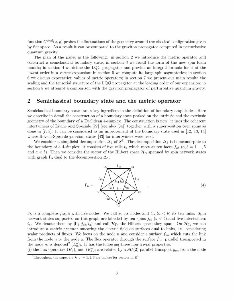
We consider a simplicial decomposition ∆5 of S3. The decomposition ∆5 is homeomorphic tothe boundary of a 4-simplex: it consists of five cells ta which meet at ten faces fab (a, b = 1, . . , 5and a < b). Then we consider the sector of the Hilbert space HΣ spanned by spin network stateswith graph Γ5 dual to the decomposition ∆5,

Γ5 =b b

b

b b

v1

v2

v3

v4v5

l12 l23

l34

l13l25

l14 l35

l24

l15

l45

. (4)

Γ5 is a complete graph with five nodes. We call va its nodes and lab (a < b) its ten links. Spinnetwork states supported on this graph are labelled by ten spins jab (a < b) and five intertwinersia. We denote them by |Γ5, jab, ia〉 and call HΓ5 the Hilbert space they span. On HΓ5 we canintroduce a metric operator smearing the electric field on surfaces dual to links, i.e. consideringscalar products of fluxes. We focus on the node n and consider a surface fna which cuts the linkfrom the node n to the node a. The flux operator through the surface fna, parallel transported inthe node n, is denoted2 (Ean)i. It has the following three non-trivial properties:(i) the flux operators (Ean)i and (Ena )i are related by a SU(2) parallel transport gan from the node

2Throughout the paper i, j, k . . . = 1, 2, 3 are indices for vectors in R3.

3

a to the node n together with a change of sign which takes into account the different orientationof the face fan,

(Ean)i = −(Ran)ij (Ena )j , (5)

where Ran is the rotation which corresponds to the group element gan associated to the link lan,i.e. Ran = D(1)(gab);(ii) the commutator of two flux operators for the same face fna is3

[ (Ean)i , (Ean)j ] = iγεijk (Ean)k ; (6)

(iii) a spin network state is annihilated by the sum of the flux operators over the faces bounding anode

∑

c 6=n

(Ecn)i|Γ5, jab, ia〉 = 0 . (7)

This last property follows from the SU(2) gauge invariance of the spin network node.Using the flux operator we can introduce the density-two inverse-metric operator at the node n,

projected in the directions normal to the faces fna and fnb. It is defined as Ean ·Ebn = δij(Ean)i(Ebn)j .

Its diagonal components Ean ·Ean measure the area square of the face fna,

Ean ·Ean |Γ5, jab, ia〉 =(

γ√

jna(jna + 1))2

|Γ5, jab, ia〉 . (8)

Spin network states are eigenstates of the diagonal components of the metric operator. On theother hand, the off-diagonal components Ean ·Ebn with a 6= b measure the dihedral angle betweenthe faces fna and fnb (weighted with their areas). It reproduces the angle operator [40]. Using therecoupling basis for intertwiner space, we have that in general the off-diagonal components of themetric operator have non-trivial matrix elements

Ean ·Ebn |Γ5, jab, ia〉 =∑

i′c

(

Ean ·Ebn)

ic

i′c |Γ5, jab, i′a〉 . (9)

We refer to [12, 13] for a detailed discussion. In particular, from property (ii), we have that someoff-diagonal components of the metric operator at a node do not commute [39]

[Ean ·Ebn , Ean ·Ecn ] 6= 0 . (10)

From this non-commutativity an Heisenberg inequality for dispersions of metric operators follows.Here we are interested in states which are peaked on a given value of all the off-diagonal componentsof the metric operator and which have dispersion of the order of Heisenberg’s bound. Such statescan be introduced using the technique of coherent intertwiners [27, 34]. A coherent intertwinerbetween the representations j1, . . , j4 is defined as4

Φm1···m4(~n1, . . , ~n4) =1

√

Ω(~n1, . . , ~n4)

∫

SU(2)dh

4∏

a=1

〈ja,ma|D(ja)(h)|ja, ~na〉 (11)

3Throughout the paper we put c = ~ = GNewton = 1.4The state |j, ~n〉 is a spin coherent state. It is labelled by a unit vector ~n or equivalently by a point on the unit

sphere. Given a SU(2) transformation g which acts on the vector +~ez sending it to the vector ~n = Rez, a spincoherent state is given by |j, ~n〉 = D(j)(g)|j, +j〉. As a result, it is defined up to a phase eiαj corresponding to atransformation exp(iα~n · ~J)|j, ~n〉 = eiαj |j, ~n〉. A phase ambiguity in the definition of the coherent intertwiner (11)follows. Such ambiguity becomes observable when a superposition over j is considered.

4

and is labelled by four unit vectors ~n1, . . , ~n4 satisfying the closure condition

j1~n1 + · · · + j4~n4 = 0 . (12)

The function Ω(~n1, . . , ~n4) provides normalization to one of the intertwiner. The function Φm1···m4

is invariant under rotations of the four vectors ~n1, . . , ~n4. In the following we always assume thatthis invariance has been fixed with a given choice of orientation5.

Nodes of the spin network can be labelled with coherent intertwiners. In fact such states providean overcomplete basis of HΓ5 . Calling vm1···m4

i the standard recoupling basis for intertwiners, wecan define the coefficients

Φi(~n1, . . , ~n4) = vm1···m4i Φm1···m4(~n1, . . , ~n4) . (13)

We define a coherent spin network |Γ5, jab,Φa〉 as the state labelled by ten spins jab and 4 × 5normals ~nab and given by the superposition

|Γ5, jab,Φa(~n)〉 =∑

i1···i5

(

5∏

a=1

Φia(~nab))

|Γ5, jab, ia〉 . (14)

The expectation value of the metric operator on a coherent spin network is simply

〈Γ5, jab,Φa|Eac ·Ebc |Γ5, jab,Φa〉 ≃ γ2jcajcb ~nca · ~ncb (15)

in the large spin limit. As a result we can choose the normals ~nab so that the coherent spin networkstate is peaked on a given intrinsic geometry of Σ.

Normals in different tetrahedra cannot be chosen independently if we want to peak on a Reggegeometry [44]. The relation between normals is provided by the requirement that they are computedfrom the lengths of the edges of the triangulation ∆5. In fact, a state with generic normals(satisfying the closure condition (12)) is peaked on a discontinuous geometry. This fact can be seenin the following way: let us consider an edge of the triangulation ∆5; this edge is shared by threetetrahedra; for each tetrahedron we can compute the expectation value of the length operator foran edge in its boundary [42]; however in general the expectation value of the length of an edge seenfrom different tetrahedra will not be the same; this fact shows that the geometry is discontinuous.The requirement that the semiclassical state is peaked on a Regge geometry amounts to a numberof relations between the labels ~nab. In the case of the boundary of a Euclidean 4-simplex (excludingthe ‘rectangular’ cases discussed in [45]), the normals turn out to be completely fixed once we givethe areas of the ten triangles or equivalently the ten spins jab,

~nab = ~nab(jcd) . (16)

This assignment of normals guarantees that the geometry we are peaking on is Regge-like. Inparticular, in this paper we are interested in the case of a 4-simplex which is approximately regular.

5For instance we can fix this redundancy assuming that the sum j1~n1 + j2~n2 is in the positive z direction whilethe vector ~n1 × ~n2 in the positive y direction. Once chosen this orientation, the four unit-vectors ~n1, . . , ~n4 (whichsatisfying the closure condition) depend only on two parameters. These two parameters can be chosen to be the

dihedral angle cos θ12 = ~n1 · ~n2 and the twisting angle tan φ(12)(34) = (~n1×~n2)·(~n3×~n4)|~n1×~n2| |~n3×~n4|

.

5

In this case the spins labelling the links are of the form jab = j0 + δjab with δjab

j0≪ 1 and a

perturbative expression for the normals solving the continuity condition is available:

~nab(j0 + δj) = ~nab(j0) +∑

cd

v(ab)(cd)δjcd . (17)

The coefficients v(ab)(cd) can be computed in terms of the derivative of the normals ~nab (for a givenchoice of orientation, see footnote 5) with respect to the ten edge lengths, using the Jacobian ofthe transformation from the ten areas to the ten edge lengths of the 4-simplex.

In the following we are interested in superpositions over spins of coherent spin networks. Ascoherent intertwiners are defined only up to a spin-dependent arbitrary phase, a choice is in order.We make the canonical choice of phases described in [35]. We briefly recall it here. Consider anon-degenerate Euclidean 4-simplex; two tetrahedra ta and tb are glued at the triangle fab ≡ fba.Now, two congruent triangles fab and fba in R

3 can be made to coincide via a unique rotationRab ∈ SO(3) which, together with a translation, takes one outward-pointing normal to minus theother one,

Rab~nab = −~nba . (18)

The canonical choice of phase for the spin coherent states |jab, ~nab〉 and |jab, ~nba〉 entering thecoherent intertwiners Φa and Φb is given by lifting the rotation Rab to a SU(2) transformation gaband requiring that

|jab, ~nba〉 = D(jab)(gab)J |jab, ~nab〉 (19)

where J : Hj → Hj is the standard antilinear map for SU(2) representations defined by

〈ǫ|(

|α〉 ⊗ J |β〉)

= 〈β|α〉 with |α〉, |β〉 ∈ Hj (20)

and 〈ǫ| is the unique intertwiner in Hj ⊗ Hj. In the following we will always work with coherentspin networks |Γ5, jab,Φa(~n(j))〉 satisfying the continuity condition, and with the canonical choicefor the arbitrary phases of coherent states. From now on we use the shorter notation |j,Φ(~n)〉.

Coherent spin networks are eigenstates of the diagonal components of the metric operator,namely the area operator for the triangles of ∆5. The extrinsic curvature to the manifold Σmeasures the amount of change of the 4-normal to Σ, parallel transporting it along Σ. In a piecewise-flat context, the extrinsic curvature has support on triangles, that is it is zero everywhere exceptthat on triangles. For a triangle fab, the extrinsic curvature Kab is given by the angle between the4-normals Nµ

a and Nµb to two tetrahedra ta and tb sharing the face fab. As the extrinsic curvature

is the momentum conjugate to the intrinsic geometry, we have that a semiclassical state cannotbe an eigenstate of the area as it would not be peaked on a given extrinsic curvature. In orderto define a state peaked both on intrinsic and extrinsic geometry, we consider a superposition ofcoherent spin networks,

|Ψ0〉 =∑

jab

ψj0,φ0(j)|j,Φ(~n)〉 , (21)

with coefficients ψj0,φ0(j) given by a gaussian times a phase,

ψj0,φ0(j) =1

Nexp

(

−∑

ab,cd

α(ab)(cd) jab − j0ab√j0ab

jcd − j0cd√j0cd

)

exp(

−i∑

ab

φab0 (jab − j0ab))

. (22)

6

As we are interested in a boundary configuration peaked on the geometry of a regular 4-simplex,we choose all the background spins to be equal, j0ab ≡ j0. Later we will consider an asymptoticexpansion for large j0. The phases φab0 are also chosen to be equal. The extrinsic curvature at theface fab in a regular 4-simplex is Kab = arccosNa ·Nb = arccos(−1

4 ). In Ashtekar-Barbero variables(E0, A0) we have

φ0 ≡ φab0 = γKab = γ arccos(−1/4) . (23)

The 10 × 10 matrix α(ab)(cd) is assumed to be complex with positive definite real part. Moreover

we require that it has the symmetries of a regular 4-simplex. We introduce the matrices P(ab)(cd)k

with k = 0, 1, 2 defined as

P(ab)(cd)0 = 1 if (ab) = (cd) and zero otherwise, (24)

P(ab)(cd)1 = 1 if a = c, b 6= d or a permutation of it and zero otherwise, (25)

P(ab)(cd)2 = 1 if (ab) 6= (cd) and zero otherwise. (26)

Their meaning is simple: a couple (ab) identifies a link of the graph Γ5; two links can be either

coincident, or touching at a node, or disjoint. The matrices P(ab)(cd)k correspond to these three

different cases. Using the basis P(ab)(cd)k we can write the matrix α(ab)(cd) as

α(ab)(cd) =

2∑

k=0

αk P(ab)(cd)k . (27)

As a result our ansatz for a semiclassical boundary state |Ψ0〉 is labelled by a (large) half-integerj0 and has only three complex free parameters, the numbers αk.

3 The new spin foam dynamics

The dynamics is implemented in terms of a spin foam functional 〈W |. Here we are interestedin its components on the Hilbert space spanned by spin networks with graph Γ5. The sum overtwo-complexes can be implemented in terms of a formal perturbative expansion in the parameterλ of a Group Field Theory [46]:

〈W |Γ5, jab, ia〉 =∑

σ

λNσW (σ) (28)

The sum is over spinfoams (colored 2-complexes) whose boundary is the spin network (Γ5, jab, ia),W (σ) is the spinfoam amplitude

W (σ) =∏

f⊂σ

Wf

∏

v⊂σ

Wv (29)

where Wv and Wf are the vertex and face amplitude respectively. The quantity Nσ in (28) isthe number of vertices in the spin foam σ, therefore the formal expansion in λ is in fact a vertex

expansion.

7

The spin foam models we consider here are the EPRLγ [19] and FKγ [20] models. We restrictattention to 0 < γ < 1; in this case the two models coincide. The vertex amplitude is given by

Wv(jab, ia) =∑

i+a i−a

15j(

j+ab, i+a

)

15j(

j−ab, i−a

)

∏

a

f iai+a i

−a(jab) (30)

where the unbalanced spins j+, j− are

j±ab = γ±jab, γ± =1 ± γ

2. (31)

This relation puts restrictions6 on the value of γ and of jab. The fusion coefficients f iai+a i

+a(jab) are

defined in [19] (see also [47]) and built out of the intertwiner vm1···m4i in Hj1 ⊗ · · ⊗Hj4 and the

intertwiners vm±

1 ···m±4

i±in Hj±1

⊗ · · · ⊗ Hj±4. Defining a map Y : Hj → Hj+ ⊗ Hj− with matrix

elements Y mm+m− = 〈j+,m+; j−,m−|Y |j,m〉 given by Clebsh-Gordan coefficients, we have that the

fusion coefficients f iai+a i

+a

are given by

f iai+a i

+a

= Ym1m+1 m

−1· · ·Ym4m

+4 m

−4vm1···m4i v

m+1 ···m+

4i+

vm−

1 ···m−4

i−. (32)

Indices are raised and lowered with the Wigner metric.Throughout this paper we will restrict attention to the lowest order in the vertex expansion.

To this order, the boundary amplitude of a spin network state with graph Γ5 is given by

〈W |Γ5, jab, ia〉 = µ(jab)Wv(jab, ia) , (33)

i.e. it involves a single spin foam vertex.The function µ is defined as µ(j) =

∏

abWfab(j). A natural choice for the face amplitude is

Wf (j+, j−) = (2j+ + 1)(2j− + 1) = (1 − γ2)j2 + 2j + 1. Other choices can be considered. We

assume that µ(λjab) scales as λp for some p for large λ. We will show in the following that, at theleading order in large j0, the LQG propagator (3) is in fact independent from the choice of faceamplitude, namely from the function µ(j).

4 LQG propagator: integral formula

In this section we define the LQG propagator and then provide an integral formula for it. The dy-namical expectation value of an operator O on the state |Ψ0〉 is defined via the following expression

〈O〉 =〈W |O|Ψ0〉〈W |Ψ0〉

. (34)

6Formula (30) is well-defined only for j± half-integer. As a result, for a fixed value of γ, there are restrictions onthe boundary spin j. For instance, if we choose γ = 1/n with n integer, then we have that j has to be integer andj ≥ n, i.e. j ∈ n, n + 1, n + 2, · · · .

8

The geometric operator we are interested in is the metric operator Ean · Ebn discussed in section 2.We focus on the connected two-point correlation function Gabcdnm on a semiclassical boundary state|Ψ0〉. It is defined as

Gabcdnm = 〈Ean ·Ebn Ecm ·Edm〉 − 〈Ean ·Ebn〉 〈Ecm ·Edm〉 . (35)

We are interested in computing this quantity using the boundary state |Ψ0〉 introduced in section2 and the spin foam dynamics (30). This is what we call the LQG propagator. As the boundarystate is a superposition of coherent spin networks, the LQG propagator involves terms of the form〈W |O|j,Φ(~n)〉. Its explicit formula is

Gabcdnm =P

j ψ(j)〈W |Ean·E

bnE

cm·Ed

m|j,Φ(~n)〉P

j ψ(j)〈W |j,Φ(~n)〉 −P

j ψ(j)〈W |Ean·E

bn|j,Φ(~n)〉

P

j ψ(j)〈W |j,Φ(~n)〉

P

j ψ(j)〈W |Ecm·Ed

m|j,Φ(~n)〉P

j ψ(j)〈W |j,Φ(~n)〉 (36)

In the following two subsections we recall the integral formula for the amplitude of a coherent spinnetwork 〈W |j,Φ(~n)〉 [32, 34],[35] and derive analogous integral expressions for the amplitude withmetric operator insertions 〈W |Ean ·Ebn|j,Φ(~n)〉 and 〈W |Ean ·EbnEcm ·Edm|j,Φ(~n)〉.

4.1 Integral formula for the amplitude of a coherent spin network

The boundary amplitude of a coherent spin network |j,Φ(~n)〉 admits an integral representation[32, 34],[35]. Here we go through its derivation as we will use a similar technique in next section.

The boundary amplitude 〈W |j,Φ(~n)〉 can be written as an integral over five copies of SU(2) ×SU(2) (with respect to the Haar measure):

〈W |jab,Φa(~n)〉 =∑

ia

(

∏

a

Φia(~n))

〈W |jab, ia〉 = µ(j)

∫ 5∏

a=1

dg+a dg−a

∏

ab

P ab(g+, g−) . (37)

The function P ab(g+, g−) is given by

P ab(g+, g−) = 〈jab,−~nba|Y †D(j+ab

)(

(g+a )−1g+

b

)

⊗D(j−ab

)(

(g−a )−1g−b)

Y |jab, ~nab〉 . (38)

where the map Y is defined in section 3. Using the factorization property of spin coherent states,

Y |j, ~n〉 = |j+, ~n〉 ⊗ |j−, ~n〉 , (39)

we have that the function P ab(g+, g−) factorizes as

P ab(g+, g−) = P ab+(g+)P ab−(g−) (40)

with

P ab± = 〈jab,−~nba|D(j±ab)(

(g±a )−1g±b)

|jab, ~nab〉 =(

〈12,−~nba|(g±a )−1g±b |

1

2, ~nab〉

)2j±ab. (41)

In the last equality we have used (again) the factorization property of spin coherent states toexponentiate the spin j±ab. In the following we will drop the 1/2 in |12 , ~nab〉 and write always |~nab〉for the coherent state in the fundamental representation.

9

The final expression we get is

〈W |j,Φ(~n)〉 = µ(j)

∫ 5∏

a=1

dg+a dg−a e

S (42)

where the “action” S is given by the sum S = S+ + S−, with

S± =∑

ab

2j±ab log〈−~nab|(g±a )−1g±b |~nba〉 . (43)

4.2 LQG operators as group integral insertions

In this section we use a similar technique to derive integral expressions for the expectation value ofmetric operators. In particular we show that

〈W |Ean ·Ebn|jab,Φa(~n)〉 = µ(j)

∫ 5∏

a=1

dg+a dg−a qabn (g+, g−) eS (44)

and that

〈W |Ean ·Ebn Ecm ·Edm|jab,Φa(~n)〉 = µ(j)

∫ 5∏

a=1

dg+a dg−a qabn (g+, g−) qcdm(g+, g−) eS (45)

where we assume7 n 6= m and a, b, c, d 6= n,m. The expression for the insertions qabn (g+, g−) in theintegral is derived below.

We start focusing on 〈Ean·Ebn〉 in the case a 6= b. The metric field (Eba)i acts on a state |jab,mab〉as γ times the generator Ji of SU(2). As a result we can introduce a quantity Qabi defined as

Qabi (g+, g−) = 〈jab,−~nba|Y †D(j+ab

)(

(g+a )−1g+

b

)

⊗D(j−ab

)(

(g−a )−1g−b)

Y (Eba)i|jab, ~nab〉 , (46)

so that

〈W |Ena ·Enb|j,Φ(~n)〉 =

∫ 5∏

a=1

dg+a dg−a δ

ijQnai Qnbj

∏

cd

′P cd(g+, g−) . (47)

The product∏′ is over couples (cd) different from (na), (nb). Thanks to the invariance properties

of the map Y , we have that

Y Jabi |jab,mab〉 = (Jab+i + Jab−i )Y |jab,mab〉 . (48)

Thus Qabi can be written asQabi = Qab+i P ab− + P ab+Qab−i (49)

withQab±i = γ 〈j±ab,−~nba|D(j±

ab)(

(g±a )−1g±b)

Jab±i |j±ab, ~nab〉 . (50)

7Similar formulae can be found also in the remaining cases but are not needed for the calculation of the LQGpropagator.

10

Now we show that Qab±i is given by a function Aab±i linear in the spin j±ab, times the quantity P ab±

defined in (41),Qab±i = Aab±i P ab± . (51)

The function Aab±i is determined as follows. The generator Jab±i of SU(2) in representation j±ab canbe obtained as the derivative

i∂

∂αiD(j±

ab)(

h(α))

∣

∣

∣

∣

αi=0

= Jab±i (52)

where the group element h(α) is defined via the canonical parametrization h(α) = exp(−iαi σi

2 ).

Therefore, we can write Qab±i as

Qab±i = i γ∂

∂αi

(

〈j±ab,−~nba|D(j±ab

)(

(g±a )−1g±b)

D(j±ab

)(

h(α))

|j±ab, ~nab〉)

∣

∣

∣

∣

αi=0

= i γ∂

∂αi

(

γ 〈−~nba|(g±a )−1g±b h(α)|~nab〉)2j±

ab

∣

∣

∣

∣

αi=0

= γ j±ab 〈−~nba|(g±a )−1g±b σi|~nab〉

(

〈−~nba|(g±a )−1g±b |~nab〉)2j±ab−1

. (53)

Comparing expression (53) with (51) and (41), we find that Ana±i is given by

Ana±i = γj±na〈−~nan|(g±a )−1g±n σ

i|~nna〉〈−~nan|(g±a )−1g±n |~nna〉

. (54)

A vectorial expression for Ana±i can be given, introducing the rotation R±a = D(1)(g±a ),

Ana±i = γj±na (R±n )−1R

±n nna −R±

a nan − i(R±n nna ×R±

a nan)

1 − (R±a nan) · (R±

n nna). (55)

Thanks to (49) and (51), we have that the expression for Qabi simplifies to

Qabi = Aabi P ab (56)

withAabi = Aab+i +Aab−i . (57)

As a result, equation (47) reduces to

〈W |Ean ·Ebn|j,Φ(~n)〉 =

∫ 5∏

a=1

dg+a dg−a δijAnai A

nbj

∏

cd

P cd(g+, g−) , (58)

which is of the form (42) with the insertion Ana · Anb. Therefore, comparing with equation (44),we have that

qabn (g+, g−) = Ana · Anb (59)

for a 6= b. The case with a = b can be computed using a similar technique but the result is rathersimple and expected, thus we just state it

qaan (g+, g−) = γ2jna(jna + 1) . (60)

11

As far as 〈Ean·EbnEcm·Edm〉 a similar result can be found. In particular, for n 6= m and a, b, c, d 6=n,m the result is stated at the beginning of this section, equation (45), with the same expressionfor the insertion qabn (g+, g−) as in equation (59) and equation (60).

Substituting (44)-(45) in (36) we obtain a new expression for the propagator in terms of groupintegrals:

Gabcdnm =

∑

j µ(j)ψ(j)∫

dg± qabn qcdm eS∑

j µ(j)ψ(j)∫

dg± eS−

∑

j µ(j)ψ(j)∫

dg± qabn eS∑

j µ(j)ψ(j)∫

dg± eS

∑

j µ(j)ψ(j)∫

dg± qcdm eS∑

j µ(j)ψ(j)∫

dg± eS. (61)

This expression with metric operators written as insertions in an integral is the starting point forthe large j0 asymptotic analysis of next section.

5 LQG propagator: stationary phase approximation

The correlation function (61) depends on the scale j0 fixed by the boundary state. We are interestedin computing its asymptotic expansion for large j0. The technique we use is an (extended) stationaryphase approximation of a multiple integral over both spins and group elements. In 5.1 we putexpression (61) in a form to which this approximation can be applied. Then in 5.2 we recall astandard result in asymptotic analysis regarding connected two-point functions and in 5.3-5.4 weapply it to our problem.

5.1 The total action and the extended integral

We introduce the “total action” defined as Stot = logψ + S or more explicitly as

Stot(jab, g+a , g

−a ) = − 1

2

∑

ab,cd

α(ab)(cd) jab − j0ab√j0ab

jcd − j0cd√j0cd

− i∑

ab

φab0 (jab − j0ab)

+ S+(jab, g+a ) + S−(jab, g

−a ) . (62)

Notice that the action S+ + S− is a homogeneous function of the spins jab therefore, rescaling thespins j0ab and jab by an interger λ so that j0ab → λj0ab and jab → λjab, we have that the totalaction goes to Stot → λStot. We recall also that qabn → λ2qabn . In the large λ limit, the sums overspins in expression (61) can be approximated with integrals over continuous spin variables8:

∑

j

µ

∫

d5g± qabn eλStot =

∫

d10j d5g± µ qabn eλStot +O(λ−N ) ∀N > 0 . (63)

Moreover, notice that the action, the measure and the insertions in (61) are invariant under a SO(4)symmetry that makes an integration dg+dg− redundant. We can factor out one SO(4) volume,e.g. putting g+

1 = g−1 = 1, so that we end up with an integral over d4g± =∏5a=2dg

+a dg−a .

8The remainder, i.e. the difference between the sum and the integral, can be estimated via Euler-Maclaurinsummation formula. This approximation does not affect any finite order in the computation of the LQG propagator.

12

As a result we can re-write expression (61) in the following integral form

Gabcdnm = λ4(

∫

d10j d4g±µ qabn qcdm eλStot

∫

d10j d4g±µ eλStot−

∫

d10j d4g±µ qabn eλStot

∫

d10j d4g±µ eλStot

∫

d10j d4g±µ qcdm eλStot

∫

d10j d4g±µ eλStot) . (64)

To this expression we can apply the standard result stated in the following section.

5.2 Asymptotic formula for connected two-point functions

Consider the integral

F (λ) =

∫

dx f(x) eλS(x) (65)

over a region of Rd, with S(x) and f(x) smooth complex-valued functions such that the real part

of S is negative or vanishing, ReS ≤ 0. Assume also that the stationary points x0 of S are isolatedso that the Hessian at a stationary point H = S′′(x0) is non-singular, detH 6= 0. Under thesehypothesis an asymptotic expansion of the integral F for large λ is available: it is an extension ofthe standard stationary phase approximation that takes into account the fact that the action S iscomplex [48]. A key role is played by critical points, i.e. stationary points x0 for which the realpart of the action vanishes, ReS(x0) = 0. Here we assume that there is a unique critical point.Then the asymptotic expansion of F (λ) for large λ is given by

F (λ) =

(

2π

λ

)d2 ei IndHeλS(x0)

√

|detH|

(

f(x0) +1

λ

(1

2f ′′ij(x0)(H

−1)ij +D)

+ O( 1λ2 )

)

(66)

with f ′′ij = ∂2f/∂xi∂xj and IndH is the index9 of the Hessian. The term D does not contain second

derivatives of f , it contains only10 f(x0) and f ′i(x0). Now we consider three smooth complex-valuedfunctions g, h and µ. A connected 2-point function relative to the insertions g and h and w.r.t. themeasure µ is defined as

G =

∫

dxµ(x) g(x)h(x) eλS(x)

∫

dxµ(x) eλS(x)−

∫

dxµ(x) g(x) eλS(x)

∫

dxµ(x) eλS(x)

∫

dxµ(x)h(x) eλS(x)

∫

dxµ(x) eλS(x). (68)

Using (66) it is straightforward to show that the (leading order) asymptotic formula for the con-nected 2-point function is simply

G =1

λ(H−1)ij g′i(x0)h

′j(x0) + O( 1

λ2 ) . (69)

Notice that both the measure function µ and the disconnected term D do not appear in the leadingterm of the connected 2-point function; nevertheless they are present in the higher orders (loop

9The index is defined in terms of the eigenvalues of hk of the Hessian as IndH = 12

P

k arg(hk) with −π2

≤arg(hk) ≤ +π

2.

10More explicitly, the term D is given by

D = f ′i(x0)R

′′′jkl(x0)(H

−1)ij(H−1)kl +5

2f(x0)R

′′′ijk(x0)R

′′′mnl(x0)(H

−1)im(H−1)jn(H−1)kl (67)

with R(x) = S(x) − S(x0) −12Hij(x0)(x − x0)

i(x − x0)j .

13

contributions). The reason we are considering the quantity G, built from integrals of the type(65), is that the LQG propagator has exactly this form. Specifically, in sections 5.3 we determinethe critical points of the total action, in 5.4 we compute the Hessian of the total action and thederivative of the insertions evaluated at the critical points, and in 7 we state our result.

5.3 Critical points of the total action

The real part of the total action is given by

ReStot = −∑

ab,cd

(Reα)(ab)(cd)jab − j0ab√

j0ab

jcd − j0cd√j0cd

+ (70)

+∑

ab

j−ab log1 − (R−

a nab) · (R−b nba)

2+

∑

ab

j+ab log1 − (R+

a nab) · (R+b nba)

2. (71)

Therefore, having assumed that the matrix α in the boundary state has positive definite real part,we have that the real part of the total action is negative or vanishing, ReStot ≤ 0. In particularthe total action vanishes for the configuration of spins jab and group elements g±a satisfying

jab = j0ab , (72)

g±a such that R±a nab(j) = −R±

b nba(j) . (73)

Now we study the stationary points of the total action and show that there is a unique stationarypoint for which ReStot vanishes.

The analysis of stationary points of the action S+ + S− with respect to variations of the groupvariables g±a has been performed in full detail by Barrett et al. in [35]. Here we briefly summarizetheir result as they apply unchanged to the total action. We invite the reader to look at the originalreference for a detailed derivation and a geometrical interpretation of the result.

The requirement that the variation of the total action with respect to the group variables g±avanishes, δgStot = 0, leads to the two sets of equations (respectively for the real and the imaginarypart of the variation):

∑

b6=a

j±abR±a nab −R±

b nba

1 − (R±a nab) · (R±

b nba)= 0 ,

∑

b6=a

j±ab(R±

a nab) × (R±b nba)

1 − (R±a nab) · (R±

b nba)= 0 . (74)

When evaluated at the maximum point (73), these two sets of equations are trivially satisfied.Infact the normals ~nab in the boundary state are chosen to satisfy the closure condition (12) ateach node. Therefore the critical points in the group variables are given by all the solutions ofequation (73).

For normals ~nab which define non-degenerate tetrahedra and satisfy the continuity condition(16), the equation Ranab = −Rbnba admits two distinct sets of solutions, up to global rotations.These two sets are related by parity. The two sets can be lifted to SU(2). We call them g+

a andg−a . Out of them, four classes of solutions for the couple (g+

a , g−a ) can be found. They are given by

(g+a , g

−a ), (g−a , g

+a ), (g+

a , g+a ), (g−a , g

−a ) . (75)

14

The geometrical interpretation is the following. The couples (jab~nab, jab~nab) are interpreted as theselfdual and anti-selfdual parts (with respect to some “time” direction, e.g. (0, 0, 0, 1)) of areabivectors associated to triangles in 4-dimensions; since these bivectors are diagonal, they live in the3-dimensional subspace of R

4 orthogonal to the chosen “time” direction. Because of the closurecondition (12), for a fixed n the four bivectors (jna~nna, jna~nna) define an embedding of a tetrahedronin R

4. The two group elements g+a and g−a of the action (43) define an SO(4) element which rotates

the “initial” tetrahedron. The system (73) is a gluing condition between tetrahedra. The firsttwo classes of solutions in (75) glue five tetrahedra into two Euclidean non-degenerate 4-simplicesrelated by a reflection, while the second two classes correspond to degenerate configurations withthe 4-simplex living in the three-dimensional plane orthogonal to the chosen “time” direction.

The evaluation of the action S(jab, g+a , g

−a ) = S+(jab, g

+a ) + S−(jab, g

−a ) on the four classes of

critical points gives

S(jab, g+a , g

−a ) = + SRegge(jab) , (76)

S(jab, g−a , g

+a ) = − SRegge(jab) , (77)

S(jab, g+a , g

+a ) = + γ−1SRegge(jab) , (78)

S(jab, g−a , g

−a ) = − γ−1SRegge(jab) , (79)

where SRegge(jab) is Regge action for a single 4-simplex with triangle areas Aab = γjab and dihedralangles φab(j) written in terms of the areas

SRegge(jab) =∑

ab

γjabφab(j) . (80)

Now we focus on stationarity of the total action with respect to variations of the spin labels jab.We fix the group elements (g+

a , g−a ) to belong to one of the four classes (75). For the first class we

find

0 =∂Stot

∂jab

∣

∣

∣

∣

(g+a ,g−a )

= −∑

cd

α(ab)(cd)(jcd − j0cd)√j0ab

√j0cd

− iφab0 + i∂SRegge

∂jab. (81)

The quantity ∂SRegge/∂jab is γ times the extrinsic curvature at the triangle fab of the boundary ofa 4-simplex with triangle areas Aab = γjab. As the phase φab0 in the boundary state is choosen to beexactly γ times the extrinsic curvature, we have that equation (81) vanishes for jab = j0ab. Noticethat, besides being a stationary point, this is also a critical point of the total action as stated in(72).

On the other hand, if equation (81) is evaluated on group elements belonging to the classes(g−a , g

+a ), (g−a , g

−a ), (g+

a , g+a ), we have that there is no cancellation of phases and therefore no sta-

tionary point with respect to variations of spins. This is the feature of the phase of the boundarystate: it selects a classical contribution to the asymptotics of a spin foam model, a fact first noticedby Rovelli for the Barrett-Crane model in [7].

5.4 Hessian of the total action and derivatives of the insertions

Here we compute the Hessian matrix of the total action Stot at the critical point jab = j0ab,(g+a , g

−a ) = (g+

a , g−a ). We introduce a local chart of coordinates (~p+

a , ~p−a ) in a neighborhood of the

15

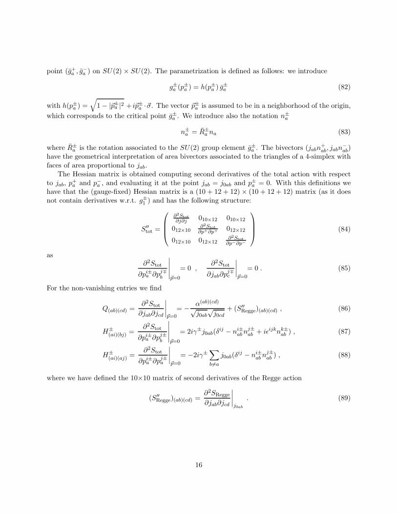
point (g+a , g

−a ) on SU(2) × SU(2). The parametrization is defined as follows: we introduce

g±a (p±a ) = h(p±a ) g±a (82)

with h(p±a ) =√

1 − |~p±a |2 + i~p±a ·~σ. The vector ~p±a is assumed to be in a neighborhood of the origin,

which corresponds to the critical point g±a . We introduce also the notation n±a

n±a = R±a na (83)

where R±a is the rotation associated to the SU(2) group element g±a . The bivectors (jabn

+ab, jabn

−ab)

have the geometrical interpretation of area bivectors associated to the triangles of a 4-simplex withfaces of area proportional to jab.

The Hessian matrix is obtained computing second derivatives of the total action with respectto jab, p

+a and p−a , and evaluating it at the point jab = j0ab and p±a = 0. With this definitions we

have that the (gauge-fixed) Hessian matrix is a (10 + 12 + 12) × (10 + 12 + 12) matrix (as it doesnot contain derivatives w.r.t. g±1 ) and has the following structure:

S′′tot =

∂2Stot∂j∂j

010×12 010×12

012×10∂2Stot∂p+∂p+

012×12

012×10 012×12∂2Stot∂p−∂p−

(84)

as∂2Stot

∂pi±a ∂pj∓b

∣

∣

∣

∣

∣

~p=0

= 0 ,∂2Stot

∂jab∂pj∓c

∣

∣

∣

∣

~p=0

= 0 . (85)

For the non-vanishing entries we find

Q(ab)(cd) =∂2Stot

∂jab∂jcd

∣

∣

∣

∣

~p=0

= − α(ab)(cd)

√j0ab

√j0cd

+ (S′′Regge)(ab)(cd) , (86)

H±(ai)(bj) =

∂2Stot

∂pi±a ∂pj±b

∣

∣

∣

∣

∣

~p=0

= 2iγ±j0ab(δij − ni±abn

j±ab + iǫijknk±ab ) , (87)

H±(ai)(aj) =

∂2Stot

∂pi±a ∂pj±a

∣

∣

∣

∣

~p=0

= −2iγ±∑

b6=a

j0ab(δij − ni±abn

j±ab ) , (88)

where we have defined the 10×10 matrix of second derivatives of the Regge action

(S′′Regge)(ab)(cd) =

∂2SRegge

∂jab∂jcd

∣

∣

∣

∣

j0ab

. (89)

16

We report also the first derivatives of the insertion qabn (g+, g−) evaluated at the critical point:

∂qabn∂~p±a

∣

∣

∣

∣

~p=0

= iγ2γ±j0naj0nb(~n±nb − ~nna · ~nnb ~n±na + i ~n±na × ~n±nb) , (90)

∂qabn∂~p±n

∣

∣

∣

∣

~p=0

= −iγ2γ±j0naj0nb(~n±na + ~n±nb)(1 − ~nna · ~nnb) , (91)

∂qabn∂jcd

∣

∣

∣

∣

~p=0

= γ2∂(jna~nna · jnb~nnb)∂jcd

∣

∣

∣

∣

j0ab

. (92)

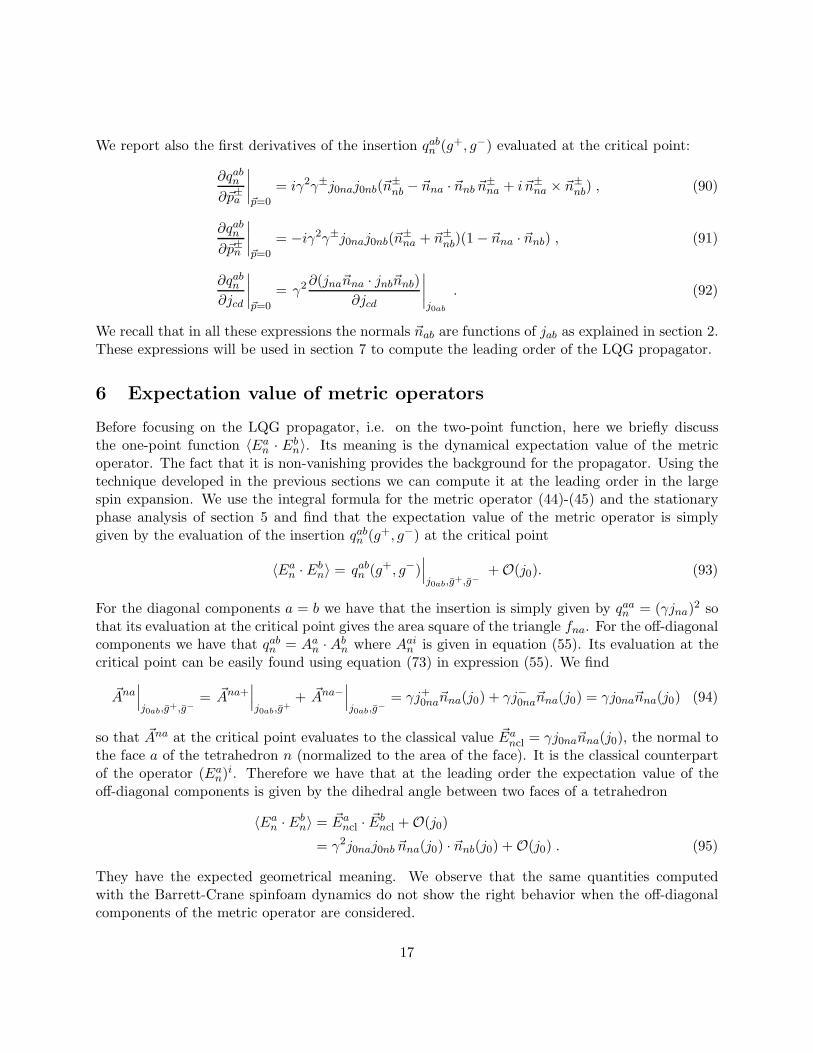
We recall that in all these expressions the normals ~nab are functions of jab as explained in section 2.These expressions will be used in section 7 to compute the leading order of the LQG propagator.

6 Expectation value of metric operators

Before focusing on the LQG propagator, i.e. on the two-point function, here we briefly discussthe one-point function 〈Ean · Ebn〉. Its meaning is the dynamical expectation value of the metricoperator. The fact that it is non-vanishing provides the background for the propagator. Using thetechnique developed in the previous sections we can compute it at the leading order in the largespin expansion. We use the integral formula for the metric operator (44)-(45) and the stationaryphase analysis of section 5 and find that the expectation value of the metric operator is simplygiven by the evaluation of the insertion qabn (g+, g−) at the critical point

〈Ean · Ebn〉 = qabn (g+, g−)∣

∣

∣

j0ab,g+,g−

+ O(j0). (93)

For the diagonal components a = b we have that the insertion is simply given by qaan = (γjna)2 so

that its evaluation at the critical point gives the area square of the triangle fna. For the off-diagonalcomponents we have that qabn = Aan · Abn where Aain is given in equation (55). Its evaluation at thecritical point can be easily found using equation (73) in expression (55). We find

~Ana∣

∣

∣

j0ab,g+,g−

= ~Ana+∣

∣

∣

j0ab,g+

+ ~Ana−∣

∣

∣

j0ab,g−

= γj+0na~nna(j0) + γj−0na~nna(j0) = γj0na~nna(j0) (94)

so that ~Ana at the critical point evaluates to the classical value ~Eancl = γj0na~nna(j0), the normal tothe face a of the tetrahedron n (normalized to the area of the face). It is the classical counterpartof the operator (Ean)

i. Therefore we have that at the leading order the expectation value of theoff-diagonal components is given by the dihedral angle between two faces of a tetrahedron

〈Ean · Ebn〉 = ~Eancl · ~Ebncl + O(j0)

= γ2j0naj0nb ~nna(j0) · ~nnb(j0) + O(j0) . (95)

They have the expected geometrical meaning. We observe that the same quantities computedwith the Barrett-Crane spinfoam dynamics do not show the right behavior when the off-diagonalcomponents of the metric operator are considered.

17

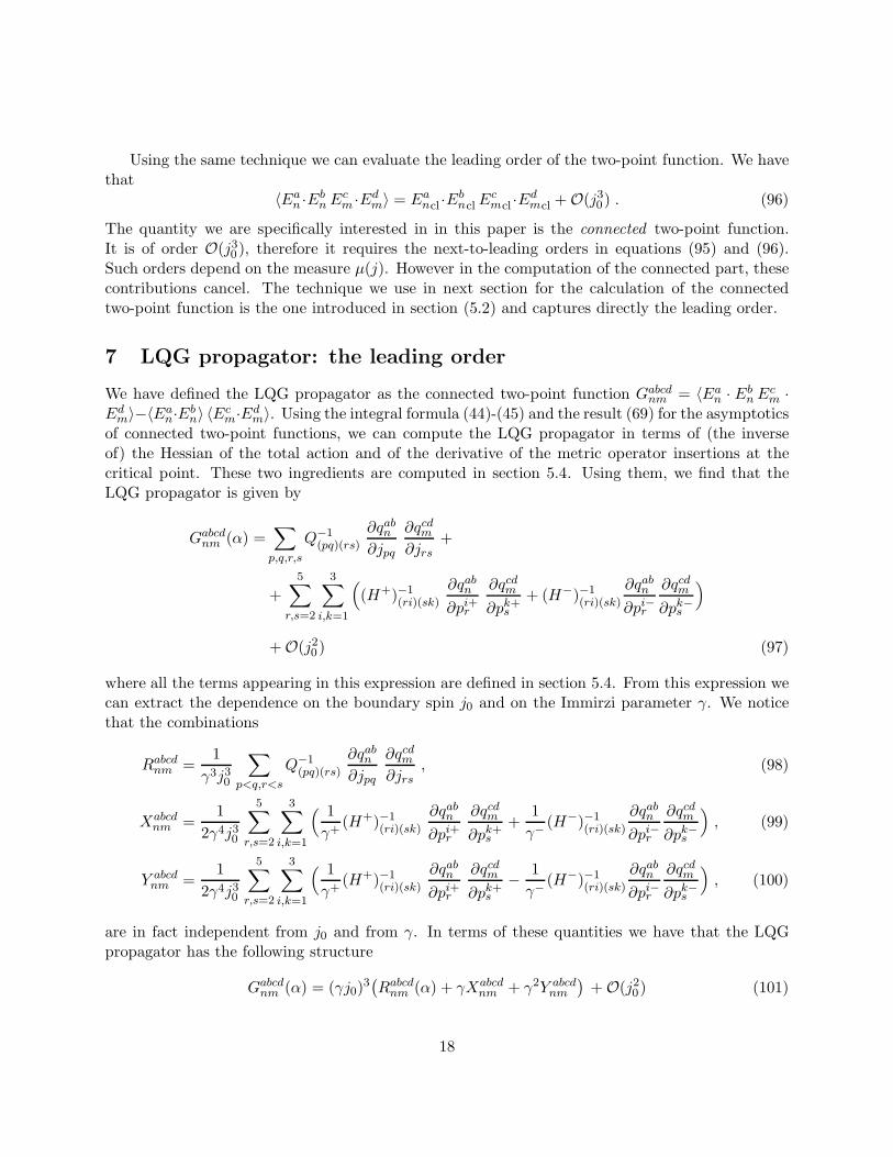
Using the same technique we can evaluate the leading order of the two-point function. We havethat

〈Ean ·Ebn Ecm ·Edm〉 = Eancl ·EbnclEcmcl ·Edmcl + O(j30) . (96)

The quantity we are specifically interested in in this paper is the connected two-point function.It is of order O(j30 ), therefore it requires the next-to-leading orders in equations (95) and (96).Such orders depend on the measure µ(j). However in the computation of the connected part, thesecontributions cancel. The technique we use in next section for the calculation of the connectedtwo-point function is the one introduced in section (5.2) and captures directly the leading order.

7 LQG propagator: the leading order

We have defined the LQG propagator as the connected two-point function Gabcdnm = 〈Ean · EbnEcm ·Edm〉−〈Ean·Ebn〉 〈Ecm·Edm〉. Using the integral formula (44)-(45) and the result (69) for the asymptoticsof connected two-point functions, we can compute the LQG propagator in terms of (the inverseof) the Hessian of the total action and of the derivative of the metric operator insertions at thecritical point. These two ingredients are computed in section 5.4. Using them, we find that theLQG propagator is given by

Gabcdnm (α) =∑

p,q,r,s

Q−1(pq)(rs)

∂qabn∂jpq

∂qcdm∂jrs

+

+

5∑

r,s=2

3∑

i,k=1

(

(H+)−1(ri)(sk)

∂qabn∂pi+r

∂qcdm∂pk+s

+ (H−)−1(ri)(sk)

∂qabn∂pi−r

∂qcdm∂pk−s

)

+ O(j20 ) (97)

where all the terms appearing in this expression are defined in section 5.4. From this expression wecan extract the dependence on the boundary spin j0 and on the Immirzi parameter γ. We noticethat the combinations

Rabcdnm =1

γ3j30

∑

p<q,r<s

Q−1(pq)(rs)

∂qabn∂jpq

∂qcdm∂jrs

, (98)

Xabcdnm =

1

2γ4j30

5∑

r,s=2

3∑

i,k=1

( 1

γ+(H+)−1

(ri)(sk)

∂qabn∂pi+r

∂qcdm∂pk+s

+1

γ−(H−)−1

(ri)(sk)

∂qabn∂pi−r

∂qcdm∂pk−s

)

, (99)

Y abcdnm =

1

2γ4j30

5∑

r,s=2

3∑

i,k=1

( 1

γ+(H+)−1

(ri)(sk)

∂qabn∂pi+r

∂qcdm∂pk+s

− 1

γ−(H−)−1

(ri)(sk)

∂qabn∂pi−r

∂qcdm∂pk−s

)

, (100)

are in fact independent from j0 and from γ. In terms of these quantities we have that the LQGpropagator has the following structure

Gabcdnm (α) = (γj0)3(

Rabcdnm (α) + γXabcdnm + γ2Y abcd

nm

)

+ O(j20) (101)

18

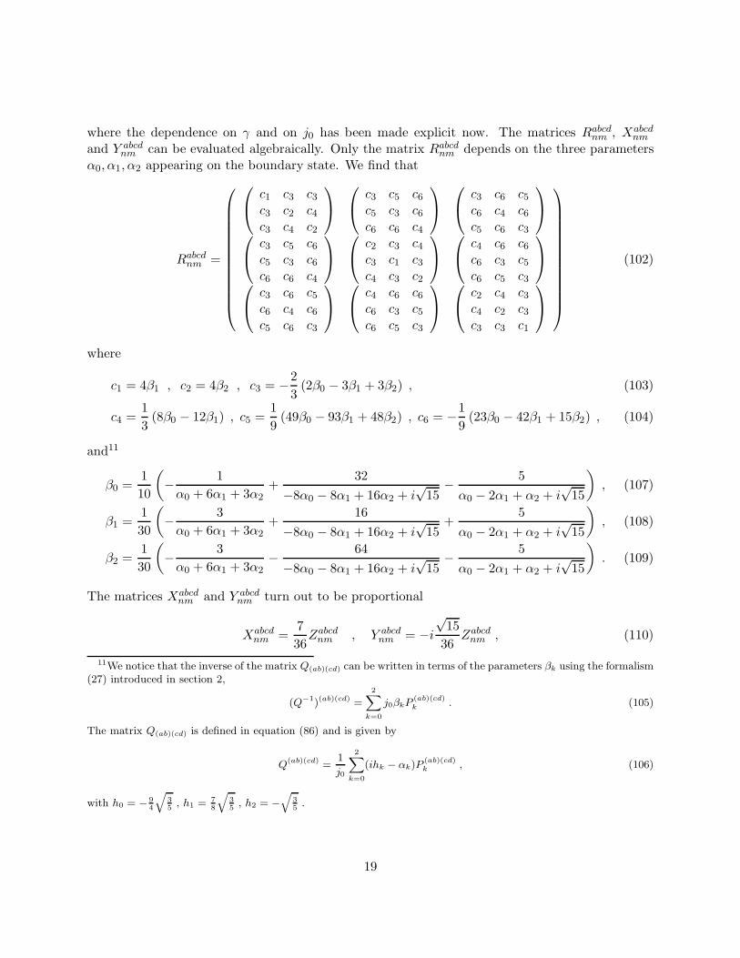
where the dependence on γ and on j0 has been made explicit now. The matrices Rabcdnm , Xabcdnm

and Y abcdnm can be evaluated algebraically. Only the matrix Rabcdnm depends on the three parameters

α0, α1, α2 appearing on the boundary state. We find that

Rabcdnm =

c1 c3 c3c3 c2 c4c3 c4 c2

c3 c5 c6c5 c3 c6c6 c6 c4

c3 c6 c5c6 c4 c6c5 c6 c3

c3 c5 c6c5 c3 c6c6 c6 c4

c2 c3 c4c3 c1 c3c4 c3 c2

c4 c6 c6c6 c3 c5c6 c5 c3

c3 c6 c5c6 c4 c6c5 c6 c3

c4 c6 c6c6 c3 c5c6 c5 c3

c2 c4 c3c4 c2 c3c3 c3 c1

(102)

where

c1 = 4β1 , c2 = 4β2 , c3 = −2

3(2β0 − 3β1 + 3β2) , (103)

c4 =1

3(8β0 − 12β1) , c5 =

1

9(49β0 − 93β1 + 48β2) , c6 = −1

9(23β0 − 42β1 + 15β2) , (104)

and11

β0 =1

10

(

− 1

α0 + 6α1 + 3α2+

32

−8α0 − 8α1 + 16α2 + i√

15− 5

α0 − 2α1 + α2 + i√

15

)

, (107)

β1 =1

30

(

− 3

α0 + 6α1 + 3α2+

16

−8α0 − 8α1 + 16α2 + i√

15+

5

α0 − 2α1 + α2 + i√

15

)

, (108)

β2 =1

30

(

− 3

α0 + 6α1 + 3α2− 64

−8α0 − 8α1 + 16α2 + i√

15− 5

α0 − 2α1 + α2 + i√

15

)

. (109)

The matrices Xabcdnm and Y abcd

nm turn out to be proportional

Xabcdnm =

7

36Zabcdnm , Y abcd

nm = −i√

15

36Zabcdnm , (110)

11We notice that the inverse of the matrix Q(ab)(cd) can be written in terms of the parameters βk using the formalism(27) introduced in section 2,

(Q−1)(ab)(cd) =2

X

k=0

j0βkP(ab)(cd)k . (105)

The matrix Q(ab)(cd) is defined in equation (86) and is given by

Q(ab)(cd) =1

j0

2X

k=0

(ihk − αk)P(ab)(cd)k , (106)

with h0 = − 94

q

35

, h1 = 78

q

35

, h2 = −q

35

.

19

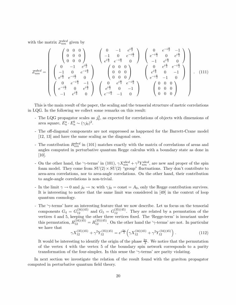
with the matrix Zabcdnm given by

Zabcdnm =

0 0 00 0 00 0 0

0 −1 eiπ3

−1 0 e−iπ3

eiπ3 e−i

π3 0

0 e−iπ3 −1

e−iπ3 0 ei

π3

−1 eiπ3 0

0 −1 eiπ3

−1 0 e−iπ3

eiπ3 e−i

π3 0

0 0 00 0 00 0 0

0 eiπ3 e−i

π3

eiπ3 0 −1

e−iπ3 −1 0

0 e−iπ3 −1

e−iπ3 0 ei

π3

−1 eiπ3 0

0 eiπ3 e−i

π3

eiπ3 0 −1

e−iπ3 −1 0

0 0 00 0 00 0 0

. (111)

This is the main result of the paper, the scaling and the tensorial structure of metric correlationsin LQG. In the following we collect some remarks on this result:

- The LQG propagator scales as j30 , as expected for correlations of objects with dimensions ofarea square, Ean · Ebn ∼ (γj0)

2.

- The off-diagonal components are not suppressed as happened for the Barrett-Crane model[12, 13] and have the same scaling as the diagonal ones.

- The contribution Rabcdnm in (101) matches exactly with the matrix of correlations of areas andangles computed in perturbative quantum Regge calculus with a boundary state as done in[10].

- On the other hand, the ‘γ-terms’ in (101), γXabcdnm + γ2Y abcd

nm , are new and proper of the spinfoam model. They come from SU(2)×SU(2) “group” fluctuations. They don’t contribute toarea-area correlations, nor to area-angle correlations. On the other hand, their contributionto angle-angle correlations is non-trivial.

- In the limit γ → 0 and j0 → ∞ with γj0 = const = A0, only the Regge contribution survives.It is interesting to notice that the same limit was considered in [49] in the context of loopquantum cosmology.

- The ‘γ-terms’ have an interesting feature that we now describe. Let us focus on the tensorial

components G4 = G(34)(45)12 and G5 = G

(35)(45)12 . They are related by a permutation of the

vertices 4 and 5, keeping the other three vertices fixed. The ‘Regge-term’ is invariant under

this permutation, R(34)(45)12 = R

(35)(45)12 . On the other hand the ‘γ-terms’ are not. In particular

we have thatγX

(35)(45)12 + γ2Y

(35)(45)12 = ei

2π3

(

γX(34)(45)12 + γ2Y

(34)(45)12

)

. (112)

It would be interesting to identify the origin of the phase 2π3 . We notice that the permutation

of the vertex 4 with the vertex 5 of the boundary spin network corresponds to a paritytransformation of the four-simplex. In this sense the ‘γ-terms’ are parity violating.

In next section we investigate the relation of the result found with the graviton propagatorcomputed in perturbative quantum field theory.

20

8 Comparison with perturbative quantum gravity

The motivation for studying the LQG propagator comes from the fact that it probes a regime ofthe theory where predictions can be compared to the ones obtained perturbatively in a quantumfield theory of gravitons on flat space [4, 5, 6]. Therefore it is interesting to investigate this relationalready at the preliminary level of a single spin foam vertex studied in this paper. In this sectionwe investigate this relation within the setting discussed in [12, 13, 14].

In perturbative quantum gravity12, the graviton propagator in the harmonic gauge is given by

〈hµν(x)hρσ(y)〉 =−1

2|x− y|2 (δµρδνσ + δµσδνρ − δµνδρσ). (113)

Correlations of geometrical quantities can be computed perturbatively in terms of the gravitonpropagator. For instance the angle at a point xn between two intersecting surfaces fna and fnb isgiven by13

qabn = gµν(xn)gρσ(xn)Bµρna(xn)B

νσnb (xn) (114)

where Bµν is the bivector associated to the surface14. As a result the angle fluctuation can bewritten in terms of the graviton field

δqabn = hµν(xn) (T abn )µν , (116)

where we have defined the tensor (T abn )µν = 2δρσBµρna(xn)B

νσnb (xn). The angle correlation (Gabcdnm )qft

is simply given by(Gabcdnm )qft = 〈hµν(xn)hρσ(xm)〉 (T abn )µν(T cdm )ρσ . (117)

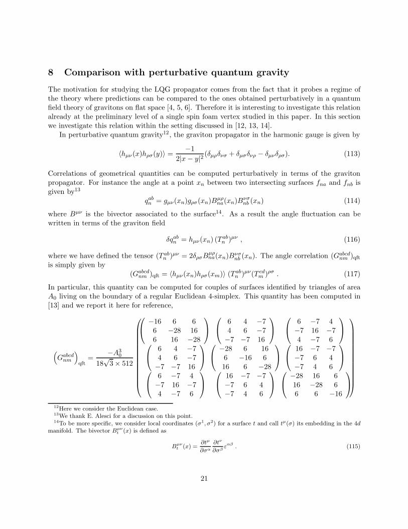
In particular, this quantity can be computed for couples of surfaces identified by triangles of areaA0 living on the boundary of a regular Euclidean 4-simplex. This quantity has been computed in[13] and we report it here for reference,

(

Gabcdnm

)

qft=

−A30

18√

3 × 512

−16 6 66 −28 166 16 −28

6 4 −74 6 −7−7 −7 16

6 −7 4−7 16 −74 −7 6

6 4 −74 6 −7−7 −7 16

−28 6 166 −16 616 6 −28

16 −7 −7−7 6 4−7 4 6

6 −7 4−7 16 −74 −7 6

16 −7 −7−7 6 4−7 4 6

−28 16 616 −28 66 6 −16

12Here we consider the Euclidean case.13We thank E. Alesci for a discussion on this point.14To be more specific, we consider local coordinates (σ1, σ2) for a surface t and call tµ(σ) its embedding in the 4d

manifold. The bivector Bµνt (x) is defined as

Bµνt (x) =

∂tµ

∂σα

∂tν

∂σβεαβ . (115)

21

The question we want to answer here is if the quantity (Gabcdnm )qft and the leading order of the LQGpropagator given by equation (101) can match. As we can identify γj0 with the area A0, we havethat the two have the same scaling. The non-trivial part of the matching is the tensorial structure.Despite the fact that we have 9 × 9 tensorial components, only six of them are independent as theothers are related by symmetries of the configuration we are considering. On the other hand thesemiclassical boundary state |Ψ0〉 we used in the LQG calculation has only three free parameters,α0, α1, α2. Therefore we can ask if there is a choice of these 3 parameters such that we can satisfythe 6 independent equations given by the matching condition

(

Gabcdnm (α))

lqg=

(

Gabcdnm

)

qft. (118)

We find that a solution in terms of the parameters αk can be found only in the limit of vanishingImmirzi parameter, keeping constant the product γj0 = A0. In this limit we find a unique solutionfor αk given by

α0 =1

100(495616

√3 − 45

√15 i) , (119)

α1 =1

200(−299008

√3 + 35

√15 i) , (120)

α2 =1

25(31744

√3 − 5

√15 i) . (121)

Therefore the matching condition (118) can be satisfied, at least in the specific limit considered.Having found a non-trivial solution, it is interesting to study the real part of the matrix α(ab)(cd)

in order to determine if it is positive definite. Its eigenvalues (with the associated degeneracy) are

λ5 = 9216√

3 , deg = 5 , (122)

λ4 =4608

√3

5, deg = 4 , (123)

λ1 = − 1024√

3

5, deg = 1 . (124)

We notice that all the eigenvalues are positive except one, λ1. The corresponding eigenvectorrepresents conformal rescalings of the boundary state, j0ab → λj0ab. It would be interesting todetermine its origin and to understand how the result depends on the choice of gauge made for thegraviton propagator (113).

9 Conclusions

In this paper we have studied correlation functions of metric operators in loop quantum gravity.The analysis presented involves two distinct ingredients:

• The first is a setting for defining correlation functions. The setting is the boundary amplitudeformalism. It involves a boundary semiclassical state |Ψ0〉 which identifies the regime of

22

interest, loop quantum gravity operators Ean · Ebn which probe the quantum geometry on theboundary, a spin foam model 〈W | which implements the dynamics. The formalism allows todefine semiclassical correlation functions in a background-independent context.

• The second ingredient consists in an approximation scheme applied to the quantity definedabove. It involves a vertex expansion and a large spin expansion. It allows to estimate thecorrelation functions explicitly. The explicit result can then be compared to the gravitonpropagator of perturbative quantum gravity. In this paper we focused on the lowest order inthe vertex expansion and the leading order in the large spin expansion.

The results found in the paper can be summarized as follows:

1. In section 2 we have introduced a semiclassical state |Ψ0〉 peaked on the intrinsic and theextrinsic geometry of the boundary of a regular Euclidean 4-simplex. The technique used tobuild this state is the following: (i) we use the coherent intertwiners introduced in [27, 34]to define coherent spin networks as in [35]; (ii) we choose the normals labelling intertwinersso that they are compatible with a simplicial 3-geometry (16). This addresses the issueof discontinuous lengths identified in [42]; (iii) then we take a gaussian superposition overcoherent spin networks in order to peak on extrinsic curvature as in [7, 8]. This state is animprovement of the ansatz used in [12, 13, 14], as it depends only on the three free parametersα0, α1, α2.

2. In section 4 we have defined expectation values of geometric observables on a semiclassicalstate. The LQG propagator is defined in equation (35) as a connected correlation functionfor the product of two metric operators

Gabcdnm = 〈Ean ·Ebn Ecm ·Edm〉 − 〈Ean ·Ebn〉 〈Ecm ·Edm〉 . (125)

This is the object that in principle can be compared to the graviton propagator on flatspace: the background is coded in the expectation value of the geometric operators and thepropagator measures correlations of fluctuations over this background.

3. In section 4.2 we have introduced a technique which allows to write LQG metric operatorsas insertions in a SO(4) group integral. It can be interpreted as the covariant version of theLQG operators. The formalism works for arbitrary fixed triangulation. Having an integralformula for expectation values and correlations of metric operators allows to formulate thelarge spin expansion as a stationary phase approximation. The problem is studied in detailrestricting attention to the lowest order in the vertex expansion, i.e. at the single-vertex level.

4. The analysis of the large spin asymptotics is performed in section 5. The technique used isthe one introduced by Barrett et al in [35]. There, the large spin asymptotics of the boundaryamplitude of a coherent spin network is studied and four distinct critical points are found tocontribute to the asymptotics. Two of them are related to different orientations of a 4-simplex.The other two come from selfdual configurations. Here, our boundary state is peaked alsoon extrinsic curvature. The feature of this boundary state is that it selects only one of thecritical points, extracting exp iSRegge from the asymptotics of the EPRL spin foam vertex.

23

This is a realization of the mechanism first identified by Rovelli in [7] for the Barrett-Cranemodel.

6. In 6 we compute expectation values of LQG metric operators at leading order and find thatthey reproduce the intrinsic geometry of the boundary of a regular 4-simplex.

7. Computing correlations of geometric operators requires going beyond the leading order in thelarge spin expansion. In section 5.2 we derive a formula for computing directly the connected

two-point correlation function to the lowest non-trivial order in the large spin expansion. Theformula is used in section 5.4.

8. The result of the calculation, the LQG propagator, is presented in section 7. We find that theresult is the sum of two terms: a “Regge term” and a “γ-term”. The Regge term coincideswith the correlations of areas and angles computed in Regge calculus with a boundary state[10]. It comes from correlations of fluctuations of the spin variables and depends on theparameters αk of the boundary state. The “γ-term” comes from fluctuations of the SO(4)group variables. An explicit algebraic calculation of the tensorial components of the LQGpropagator is presented.

9. The LQG propagator can be compared to the graviton propagator. This is done in section 8.We find that the LQG propagator has the correct scaling behaviour. The three parametersαk appearing in the semiclassical boundary state can be chosen so that the tensorial structureof the LQG propagator matches with the one of the graviton propagator. The matching isobtained in the limit γ → 0 with γj0 fixed.

Now we would like to put these results in perspective with respect to the problem of extracting thelow energy regime of loop quantum gravity and spin foams (see in particular [50]).

Deriving the LQG propagator at the level of a single spin foam vertex is certainly only a firststep. Within the setting of a vertex expansion, an analysis of the LQG propagator for a finitenumber of spinfoam vertices is needed. Some of the techniques developed in this paper generalizeto this more general case. In particular superpositions of coherent spin networks can be used to buildsemiclassical states peaked on the intrinsic and the extrinsic curvature of an arbitrary boundaryRegge geometry. Moreover, the expression of the LQG metric operator in terms of SO(4) groupintegrals presented in this paper works for an arbitrary number of spin foam vertices and allows toderive an integral representation of the LQG propagator in the general case, analogous to the oneof [32] but with non-trivial insertions. This representation is the appropriate one for the analysisof the large spin asymptotics along the lines discussed for Regge calculus in [51]. The non-trivialquestion which needs to be answered then is if the semiclassical boundary state is able to enforcesemiclassicality in the bulk. Another feature identified in this paper which appears to be general isthat, besides the expected Regge contribution, correlations of LQG metric operators have a non-Regge contribution which is proper of the spin foam model. It would be interesting to investigateif this contribution propagates when more than a single spin foam vertex is considered.

24

Acknowledgments

We thank Carlo Rovelli for many useful discussions. We also thank Emanuele Alesci, John W.Barrett, Florian Conrady, Richard J. Dowdall, Winston J. Fairbairn, Henrique Gomes, Frank Hell-mann, Leonardo Modesto, Roberto Pereira and Alejandro Satz for comments and suggestions. E.B.gratefully acknowledges support from Fondazione A. Della Riccia.

References

[1] C. Rovelli, “Quantum gravity”, Cambridge, UK: Univ. Pr. (2004).

[2] T. Thiemann, “Modern canonical quantum general relativity”, Cambridge, UK: Univ. Pr.(2007).

[3] A. Ashtekar and J. Lewandowski, “Background independent quantum gravity: A statusreport”, Class. Quant. Grav. 21 (2004) R53, gr-qc/0404018.

[4] M. J. G. Veltman, “Quantum Theory of Gravitation”, in Les Houches 1975, Proceedings,Methods In Field Theory, Amsterdam 1976, 265-327.

[5] J. F. Donoghue, “General relativity as an effective field theory: The leading quantumcorrections”, Phys. Rev. D50 (1994) 3874–3888, gr-qc/9405057.

[6] C. P. Burgess, “Quantum gravity in everyday life: General relativity as an effective fieldtheory”, Living Rev. Rel. 7 (2004) 5, gr-qc/0311082.

[7] C. Rovelli, “Graviton propagator from background-independent quantum gravity”, Phys.

Rev. Lett. 97 (2006) 151301, gr-qc/0508124.

[8] E. Bianchi, L. Modesto, C. Rovelli, and S. Speziale, “Graviton propagator in loop quantumgravity”, Class. Quant. Grav. 23 (2006) 6989–7028, gr-qc/0604044.

[9] E. R. Livine and S. Speziale, “Group integral techniques for the spinfoam gravitonpropagator”, JHEP 11 (2006) 092, gr-qc/0608131.

[10] E. Bianchi and L. Modesto, “The perturbative Regge-calculus regime of Loop QuantumGravity”, Nucl. Phys. B796 (2008) 581–621, 0709.2051.

[11] J. D. Christensen, E. R. Livine, and S. Speziale, “Numerical evidence of regularizedcorrelations in spin foam gravity”, Phys. Lett. B670 (2009) 403–406, 0710.0617.

[12] E. Alesci and C. Rovelli, “The complete LQG propagator: I. Difficulties with theBarrett-Crane vertex”, Phys. Rev. D76 (2007) 104012, 0708.0883.

[13] E. Alesci and C. Rovelli, “The complete LQG propagator: II. Asymptotic behavior of thevertex”, Phys. Rev. D77 (2008) 044024, 0711.1284.

[14] E. Alesci, E. Bianchi, and C. Rovelli, “LQG propagator: III. The new vertex”, 0812.5018.

25

[15] S. Speziale, “Background-free propagation in loop quantum gravity”, Adv. Sci. Lett. 2 (2009)280–290, 0810.1978.

[16] R. Oeckl, “A ’general boundary’ formulation for quantum mechanics and quantum gravity”,Phys. Lett. B575 (2003) 318–324, hep-th/0306025.

[17] R. Oeckl, “General boundary quantum field theory: Foundations and probabilityinterpretation”, Adv. Theor. Math. Phys. 12 (2008) 319–352, hep-th/0509122.

[18] F. Conrady, L. Doplicher, R. Oeckl, C. Rovelli, and M. Testa, “Minkowski vacuum inbackground independent quantum gravity”, Phys. Rev. D69 (2004) 064019, gr-qc/0307118.

[19] J. Engle, E. Livine, R. Pereira, and C. Rovelli, “LQG vertex with finite Immirzi parameter”,Nucl. Phys. B799 (2008) 136–149, 0711.0146.

[20] L. Freidel and K. Krasnov, “A New Spin Foam Model for 4d Gravity”, Class. Quant. Grav.

25 (2008) 125018, 0708.1595.

[21] J. W. Barrett and L. Crane, “Relativistic spin networks and quantum gravity”, J. Math.

Phys. 39 (1998) 3296–3302, gr-qc/9709028.

[22] S. Speziale, “Towards the graviton from spinfoams: The 3d toy model”, JHEP 05 (2006) 039,gr-qc/0512102.

[23] E. R. Livine, S. Speziale, and J. L. Willis, “Towards the graviton from spinfoams: Higherorder corrections in the 3d toy model”, Phys. Rev. D75 (2007) 024038, gr-qc/0605123.

[24] V. Bonzom, E. R. Livine, M. Smerlak, and S. Speziale, “Towards the graviton fromspinfoams: the complete perturbative expansion of the 3d toy model”, Nucl. Phys. B804

(2008) 507–526, 0802.3983.

[25] J. Engle, R. Pereira, and C. Rovelli, “The loop-quantum-gravity vertex-amplitude”, Phys.

Rev. Lett. 99 (2007) 161301, 0705.2388.

[26] J. Engle, R. Pereira, and C. Rovelli, “Flipped spinfoam vertex and loop gravity”, Nucl. Phys.

B798 (2008) 251–290, 0708.1236.

[27] E. R. Livine and S. Speziale, “A new spinfoam vertex for quantum gravity”, Phys. Rev. D76

(2007) 084028, 0705.0674.

[28] E. Magliaro, C. Perini, and C. Rovelli, “Numerical indications on the semiclassical limit ofthe flipped vertex”, Class. Quant. Grav. 25 (2008) 095009, 0710.5034.

[29] E. Alesci, E. Bianchi, E. Magliaro, and C. Perini, “Intertwiner dynamics in the flippedvertex”, 0808.1971.

[30] I. Khavkine, “Evaluation of new spin foam vertex amplitudes”, 0809.3190.

26

[31] I. Khavkine, “Evaluation of new spin foam vertex amplitudes with boundary states”,0810.1653.

[32] F. Conrady and L. Freidel, “Path integral representation of spin foam models of 4d gravity”,Class. Quant. Grav. 25 (2008) 245010, 0806.4640.

[33] F. Conrady and L. Freidel, “On the semiclassical limit of 4d spin foam models”, Phys. Rev.

D78 (2008) 104023, 0809.2280.

[34] F. Conrady and L. Freidel, “Quantum geometry from phase space reduction”, 0902.0351.

[35] J. W. Barrett, R. J. Dowdall, W. J. Fairbairn, H. Gomes, and F. Hellmann, “Asymptoticanalysis of the EPRL four-simplex amplitude”, 0902.1170.

[36] C. Rovelli and L. Smolin, “Discreteness of area and volume in quantum gravity”, Nucl. Phys.

B442 (1995) 593–622, gr-qc/9411005.

[37] A. Ashtekar and J. Lewandowski, “Quantum theory of geometry. I: Area operators”, Class.

Quant. Grav. 14 (1997) A55–A82, gr-qc/9602046.

[38] A. Ashtekar and J. Lewandowski, “Quantum theory of geometry. II: Volume operators”, Adv.

Theor. Math. Phys. 1 (1998) 388–429, gr-qc/9711031.

[39] A. Ashtekar, A. Corichi, and J. A. Zapata, “Quantum theory of geometry. III:Non-commutativity of Riemannian structures”, Class. Quant. Grav. 15 (1998) 2955–2972,gr-qc/9806041.

[40] S. A. Major, “Operators for quantized directions”, Class. Quant. Grav. 16 (1999) 3859–3877,gr-qc/9905019.

[41] T. Thiemann, “A length operator for canonical quantum gravity”, J. Math. Phys. 39 (1998)3372–3392, gr-qc/9606092.

[42] E. Bianchi, “The length operator in Loop Quantum Gravity”, 0806.4710. To appear in Nucl.

Phys. B.

[43] C. Rovelli and S. Speziale, “A semiclassical tetrahedron”, Class. Quant. Grav. 23 (2006)5861–5870, gr-qc/0606074.

[44] T. Regge, “General Relativity without coordinates”, Nuovo Cim. 19 (1961) 558–571.

[45] J. W. Barrett, M. Rocek, and R. M. Williams, “A note on area variables in Regge calculus”,Class. Quant. Grav. 16 (1999) 1373–1376, gr-qc/9710056.

[46] L. Freidel, “Group field theory: An overview”, Int. J. Theor. Phys. 44 (2005) 1769–1783,hep-th/0505016.

[47] E. Alesci, E. Bianchi, E. Magliaro, and C. Perini, “Asymptotics of LQG fusion coefficients”,0809.3718.

27

[48] L. Hormander, “The analysis of linear partial differential operators. I”, Springer, 1990.

[49] M. Bojowald, “The semiclassical limit of loop quantum cosmology”, Class. Quant. Grav. 18

(2001) L109–L116, gr-qc/0105113.

[50] A. Ashtekar, L. Freidel, C. Rovelli, International Loop Quantum Gravity Seminar,“Recovering low energy physics: A Discussion”, May 5th, 2009.http://relativity.phys.lsu.edu/ilqgs/

[51] E. Bianchi and A. Satz, “Semiclassical regime of Regge calculus and spin foams”, Nucl. Phys.

B808 (2009) 546–568, 0808.1107.

28