arX

iv:h

ep-l

at/0

2030

01v1

1 M

ar 2

002

FSU-CSIT-02-10ADP-02-67/T507

Lattice quark propagator with staggered quarks in Landau and Laplacian gauges

Patrick O. Bowman and Urs M. HellerDepartment of Physics and School for Computational Science and Information Technology,

Florida State University, Tallahassee FL 32306-4120, USA

Anthony G. WilliamsSpecial Research Centre for the Subatomic Structure of Matter and

The Department of Physics and Mathematical Physics, Adelaide University, Australia 5005

(Dated: February 1, 2008)

We report on the lattice quark propagator using standard and improved Staggered quark actions,with the standard, Wilson gauge action. The standard Kogut-Susskind action has errors of O(a2)while the “Asqtad” action has O(a4), O(a2g2) errors. The quark propagator is interesting forstudying the phenomenon of dynamical chiral symmetry breaking and as a test-bed for improvement.Gauge dependent quantities from lattice simulations may be affected by Gribov copies. We explorethis by studying the quark propagator in both Landau and Laplacian gauges. Landau and Laplaciangauges are found to produce very similar results for the quark propagator.

I. INTRODUCTION

The quark propagator lies at the heart of most QCDphysics. In the low momentum region it exhibits dy-namical chiral symmetry breaking (which cannot be seenfrom perturbation theory) and at high momentum canbe used to extract the running quark mass [1, 2] (whichcannot be extracted directly from experiment). In lat-tice QCD, quark propagators are tied together to extracthadron masses. Lattice gauge theory provides a way tostudy the quark propagator nonperturbatively, possiblyas a way of calculating the chiral condensate and ΛQCD,and in turn, such a study can provide technical insightinto lattice gauge theory.

We study the quark propagator using the Kogut-Susskind (KS) fermion action, which has O(a2) errors,and an improved staggered action, Asqtad [3], whichhas errors of O(a4), O(a2g2). These choices comple-ment other studies using Clover [4, 5] and Overlap [6]quarks. We are required to gauge fix and we choose theever popular Landau gauge and the interesting Laplaciangauge [7, 8]. Laplacian gauge fixing is an unambiguousgauge fixing and, although it is difficult to understandperturbatively, it is equivalent to Landau gauge in theasymptotic region. It has been used to study the gluonpropagator [9, 10, 11].

In SU(N) there are various ways to implement a Lapla-cian gauge fixing. Three varieties of Laplacian gauge fix-ing are used, and these form three different, but relatedgauges. This is briefly discussed in section III. For amore detailed discussion, see Ref. [11].

The quark propagator was calculated on 80, 163 × 32configurations generated with the standard Wilson gluonaction at β = 5.85 (a = 0.130 fm)[17]. We have used sixquark masses: am = 0.075, 0.0625, 0.05, 0.0375, 0.025and 0.0125 (114 to 19 MeV).

II. LATTICE QUARK PROPAGATOR

In the continuum, Lorentz invariance allows us to de-compose the full propagator into Dirac vector and scalarpieces

S−1(p2) = iA(p2)γ · p + B(p2) (1)

or, alternatively,

S−1(p2) = Z−1(p2)[iγ · p + M(p2)]. (2)

This is the bare propagator which, once regularized, is re-lated to the renormalized propagator through the renor-malization constant

S(a; p2) = Z2(a; µ)Sren(µ; p2), (3)

where a is some regularization parameter, e.g. latticespacing. Asymptotic freedom implies that, as p2 → ∞,S(p2) reduces to the free propagator

S−1(p2) → iγ · p + m0, (4)

where m0 is the bare quark mass.The tadpole improved, tree-level form of the KS quark

propagator is

S−1αβ (p; m) = u0i

∑

µ

(γµ)αβ

sin(pµ) + mδαβ (5)

where pµ is the discrete lattice momentum given by

pµ =2πnµ

aLµ

nµ ∈[−Lµ

4,Lµ

4

)

. (6)

For the tadpole factor, we employ the plaquette measure,

u0 =(1

3ReTr〈Pµν〉

)14

. (7)

We give a detailed discussion of the notation used for thestaggered quark actions in an appendix. As a convienient

2

short-hand we define a new momentum variable for theKS quark propagator,

qµ ≡ sin(pµ). (8)

We can then decompose the inverse propagator[18]

Z−1(q) =1

16Nciq2Tr{γ · qS−1} (9)

M(q) =1

16Nc

Tr{S−1}, (10)

where the factor of 16 comes from the trace over thespin-flavor indices of the staggered quarks and Nc fromthe trace over color. Comparing Eqs. (4) and (5) we seethat dividing out q2 in Eq. (9) is analagous to dividingout p2 in the continuum and ensures that that Z hasthe correct asymptotic behavior. So by considering thepropagator as a function of qµ, we ensure that the latticequark propagator has the correct tree-level form, i.e.,

Stree(qµ) =1

iγ · q + m(11)

and hopefully better approximates its continuum behav-ior. This is the same philosophy that has been used instudies of the gluon propagator [12] and Eq. (8) was usedto define the momentum in Ref. [2].

The Asqtad quark action [3] is a fat-link Staggeredaction using three-link, five-link and seven-link staplesto minimize flavor changing interactions along with thethree-link Naik term [13] (to correct the dispersion rela-tion) and planar five-link Lepage term [14] (to correct theIR). The coefficients are tadpole improved and tuned toremove all tree-level O(a2) errors. This action was moti-vated by the desire to improve flavor symmetry, but hasalso been reported to have good rotational properties.

The quark propagator with this action has the tree-level form

S−1αβ (p; m) = u0i

∑

µ

(γµ)αβ

sin(pµ)[

1+1

6sin2(pµ)

]

+mδαβ ,

(12)so we repeat the above analysis, this time defining

qµ ≡ sin(pµ)[

1 +1

6sin2(pµ)

]

. (13)

Finally, it should be noted that both actions get contri-butions from tadpoles, which can be seen in the tree-levelbehaviors of the two invariants

Ztree =1

u0(14)

M tree =m0

u0(15)

so inserting the tadpole factors provides the correct nor-malization.

III. GAUGE FIXING

We consider the quark propagator in Landau andLaplacian gauges. Landau gauge fixing is performed byenforcing the Lorentz gauge condition,

∑

µ ∂µAµ(x) =0 on a configuration by configuration basis. This isachieved by maximizing the functional,

F =1

2

∑

x,µ

Tr{

Uµ(x) + U †µ(x)

}

, (16)

by, in this case, a Fourier accelerated, steepest-descentsalgorithm [15]. There are, in general, many such maximaand these are called lattice Gribov copies. While thisambiguity has produced no identified artefacts in QCD,in principle it remains a source of uncontrolled systematicerror.

Laplacian gauge is a nonlinear gauge fixing that re-spects rotational invariance, has been seen to be smooth,yet is free of Gribov ambiguity. It is also computation-ally cheaper then Landau gauge. There is, however, morethan one way of obtaining such a gauge fixing in SU(N).The three implementations of Laplacian gauge fixing em-ployed here are (in our notation):

1. ∂2(I) gauge (QR decomposition), used by Alexan-drou et al. [9].

2. ∂2(II) gauge, where the Laplacian gauge transfor-mation is projected onto SU(3) by maximising itstrace [11].

3. ∂2(III) gauge (Polar decomposition), the originalprescription described in Ref. [7] and tested inRef. [8].

All three versions reduce to the same gauge in SU(2). Fora more detailed discussion, see Ref. [11].

IV. ANALYSIS OF LATTICE ARTEFACTS

A. Tree-level Correction

As mentioned above, the idea of “kinematic” or “tree-level” correction has been used widely in studies of thegluon propagator [12] and the quark propagator [4, 5, 6]and we investigate its application to our quark propa-gators. For the moment we shall restrict ourselves toLandau gauge. To help us understand the lattice arte-facts, we separate the data into momenta lying entirelyon a spatial cartesian direction (squares), along the tem-poral direction (triangles), the four-diagonal (diamonds)or some other combination of directions (circles).

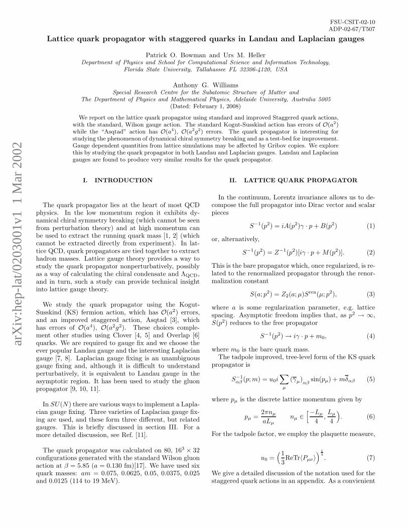
The Z function is plotted for the KS action in Fig. 1,comparing the results using p and q. In the top of Fig. 1we see substantial hypercubic artefacts (in particular lookat the difference between the diamond and the triangle ataround 2.5 GeV). We can suggest that this is caused by

3

FIG. 1: Z function for quark mass ma = 0.05 (m ≃ 76 MeV)for the KS action in Landau gauge. Top figure is plotted usingthe standard lattice momentum, p and the bottom uses the“action” momentum, q. Note that this choice affects only thehorizontal scale.

violation of rotational symmetry because the agreementbetween triangles and squares suggests that finite volumeeffects are small in the region of interest. In the plotbelow, where q has been used, we see some restoration ofrotational symmetry.

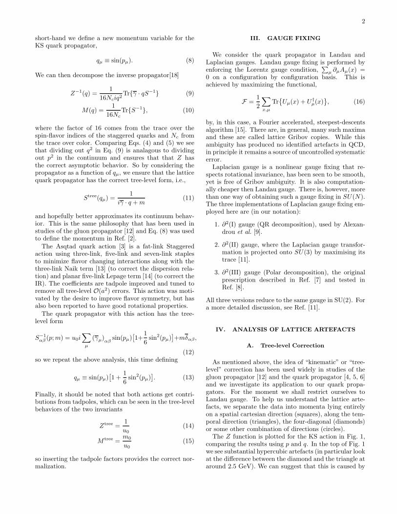
The same study is made for the Asqtad action in Fig. 2.In both cases this action shows a substantial improve-ment over the KS action, and when we plot using q, themomentum defined by the action, rotational asymmetryis reduced to the level of the statistical errors.

It is less clear which momentum variable should beused for the mass function, so for consistency we use q,as for the Z function. The effect of this is shown in Fig. 3.For ease of comparison, both sets of data have been cylin-der cut [12]. In the case of the mass function, the choiceof momentum will actually make little difference to ourresults.

FIG. 2: Z function for quark mass ma = 0.05 (m ≃ 76 MeV)for the Asqtad action in Landau gauge. Top figure is plottedusing the standard lattice momentum, p and the bottom usesthe “action” momentum, q.

B. Comparison of the actions

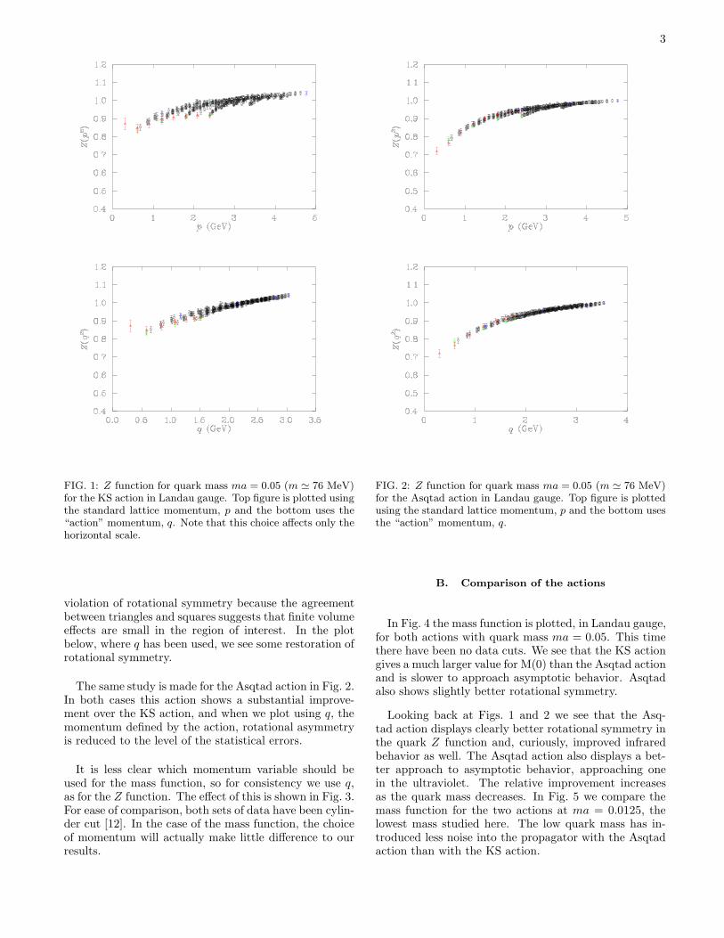
In Fig. 4 the mass function is plotted, in Landau gauge,for both actions with quark mass ma = 0.05. This timethere have been no data cuts. We see that the KS actiongives a much larger value for M(0) than the Asqtad actionand is slower to approach asymptotic behavior. Asqtadalso shows slightly better rotational symmetry.

Looking back at Figs. 1 and 2 we see that the Asq-tad action displays clearly better rotational symmetry inthe quark Z function and, curiously, improved infraredbehavior as well. The Asqtad action also displays a bet-ter approach to asymptotic behavior, approaching onein the ultraviolet. The relative improvement increasesas the quark mass decreases. In Fig. 5 we compare themass function for the two actions at ma = 0.0125, thelowest mass studied here. The low quark mass has in-troduced less noise into the propagator with the Asqtadaction than with the KS action.

4

FIG. 3: The quark mass function for quark mass ma = 0.05(m ≃ 76 MeV) for the KS action (open circles) and the Asqtadaction (solid triangles) in Landau gauge. Top figure is plottedusing the standard lattice momentum, and the bottom usingthe “action” momentum.

C. Comparitive performance of Landau and

Laplacian gauges

Fig. 6 shows the mass function for the Asqtad actionin ∂2(I) and ∂2(II) gauges and it should be comparedwith the equivalent Landau gauge result in Fig. 4. Wesee firstly that these three gauges give very similar re-sults (we shall investigate this in more detail later) andsecondly that they give similar performance in terms ofrotational symmetry and statistical noise. Looking moreclosely, we can see that the Landau gauge gives a slightlycleaner signal at this lattice spacing.

Landau gauge seems to respond somewhat better than∂2(II) gauge to vanishing quark mass; compare Fig. 7with Fig. 5. In Fig. 7 we see large errors in the infraredregion and points along the temporal axis lying belowthe bulk of the data. These are indicators of finite vol-ume effects, an unexpected result given that earlier gluonpropagator studies [9, 10] appear to conclude that Lapla-cian gauge is less sensitive to volume than Landau gauge.

∂2(III) performs very poorly: see Figs. 8 and 9. The

FIG. 4: Mass function for quark mass ma = 0.05 (m ≃ 76MeV), KS action (top) and Asqtad action (bottom) in Landaugauge.

gauge fixing procedure failed for four of the configura-tions and eight of the remaining configurations producedZ and M functions with pathological negative values. Wehave seen that this type of gauge fixing fails to producea gluon propagator that has the correct asymptotic be-havior [11]. It seems likely that we are dealing with ma-trices with vanishing determinants, which are destroy-ing the projection onto SU(3). We expect the degree towhich this problem occurs to be dependent on the sim-ulation parameters and the numerical precision used (inthis work the gauge transformations were calculated insingle precision).

V. GAUGE DEPENDENCE

Now we investigate the quark mass and Z functionsin Landau, ∂2(I) and ∂2(II) gauges. Fig. 10 shows theZ function for the Asqtad action in Landau and ∂2(I)gauges. They are in excellent agreement in the ultraviolet- as they ought - but differ significantly in the infrared.The Z function in the Laplacian gauges is more stronglyinfrared suppressed than in the Landau gauge. There

5

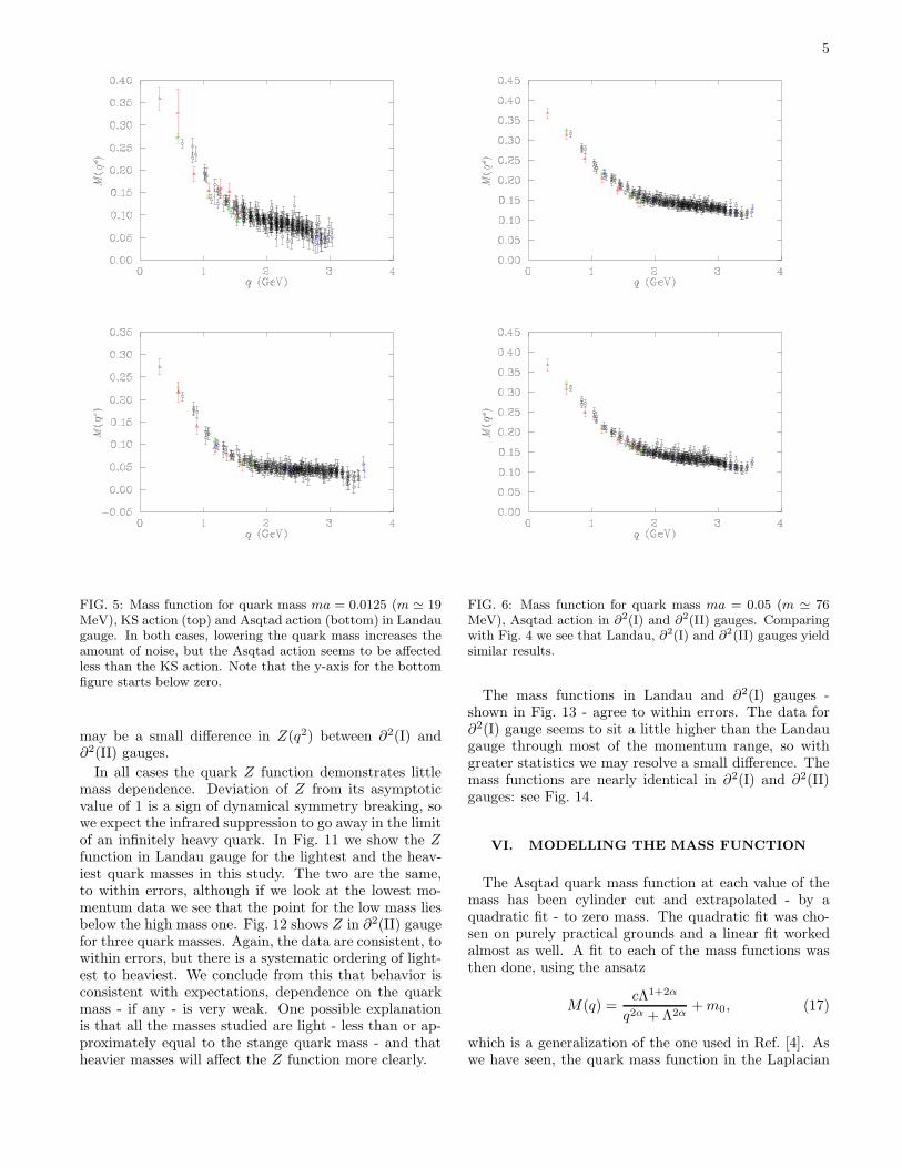
FIG. 5: Mass function for quark mass ma = 0.0125 (m ≃ 19MeV), KS action (top) and Asqtad action (bottom) in Landaugauge. In both cases, lowering the quark mass increases theamount of noise, but the Asqtad action seems to be affectedless than the KS action. Note that the y-axis for the bottomfigure starts below zero.

may be a small difference in Z(q2) between ∂2(I) and∂2(II) gauges.

In all cases the quark Z function demonstrates littlemass dependence. Deviation of Z from its asymptoticvalue of 1 is a sign of dynamical symmetry breaking, sowe expect the infrared suppression to go away in the limitof an infinitely heavy quark. In Fig. 11 we show the Zfunction in Landau gauge for the lightest and the heav-iest quark masses in this study. The two are the same,to within errors, although if we look at the lowest mo-mentum data we see that the point for the low mass liesbelow the high mass one. Fig. 12 shows Z in ∂2(II) gaugefor three quark masses. Again, the data are consistent, towithin errors, but there is a systematic ordering of light-est to heaviest. We conclude from this that behavior isconsistent with expectations, dependence on the quarkmass - if any - is very weak. One possible explanationis that all the masses studied are light - less than or ap-proximately equal to the stange quark mass - and thatheavier masses will affect the Z function more clearly.

FIG. 6: Mass function for quark mass ma = 0.05 (m ≃ 76MeV), Asqtad action in ∂2(I) and ∂2(II) gauges. Comparingwith Fig. 4 we see that Landau, ∂2(I) and ∂2(II) gauges yieldsimilar results.

The mass functions in Landau and ∂2(I) gauges -shown in Fig. 13 - agree to within errors. The data for∂2(I) gauge seems to sit a little higher than the Landaugauge through most of the momentum range, so withgreater statistics we may resolve a small difference. Themass functions are nearly identical in ∂2(I) and ∂2(II)gauges: see Fig. 14.

VI. MODELLING THE MASS FUNCTION

The Asqtad quark mass function at each value of themass has been cylinder cut and extrapolated - by aquadratic fit - to zero mass. The quadratic fit was cho-sen on purely practical grounds and a linear fit workedalmost as well. A fit to each of the mass functions wasthen done, using the ansatz

M(q) =cΛ1+2α

q2α + Λ2α+ m0, (17)

which is a generalization of the one used in Ref. [4]. Aswe have seen, the quark mass function in the Laplacian

6

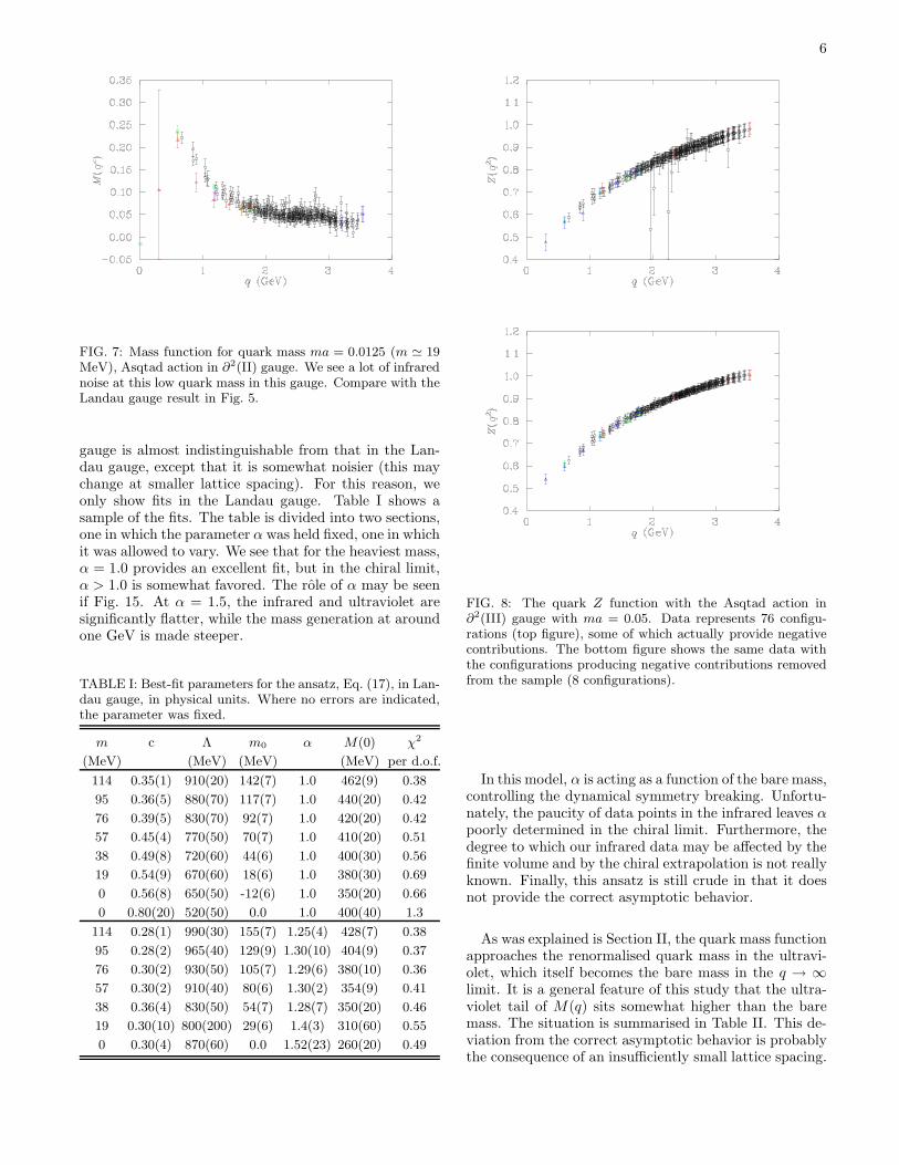
FIG. 7: Mass function for quark mass ma = 0.0125 (m ≃ 19MeV), Asqtad action in ∂2(II) gauge. We see a lot of infrarednoise at this low quark mass in this gauge. Compare with theLandau gauge result in Fig. 5.

gauge is almost indistinguishable from that in the Lan-dau gauge, except that it is somewhat noisier (this maychange at smaller lattice spacing). For this reason, weonly show fits in the Landau gauge. Table I shows asample of the fits. The table is divided into two sections,one in which the parameter α was held fixed, one in whichit was allowed to vary. We see that for the heaviest mass,α = 1.0 provides an excellent fit, but in the chiral limit,α > 1.0 is somewhat favored. The role of α may be seenif Fig. 15. At α = 1.5, the infrared and ultraviolet aresignificantly flatter, while the mass generation at aroundone GeV is made steeper.

TABLE I: Best-fit parameters for the ansatz, Eq. (17), in Lan-dau gauge, in physical units. Where no errors are indicated,the parameter was fixed.

m c Λ m0 α M(0) χ2

(MeV) (MeV) (MeV) (MeV) per d.o.f.

114 0.35(1) 910(20) 142(7) 1.0 462(9) 0.38

95 0.36(5) 880(70) 117(7) 1.0 440(20) 0.42

76 0.39(5) 830(70) 92(7) 1.0 420(20) 0.42

57 0.45(4) 770(50) 70(7) 1.0 410(20) 0.51

38 0.49(8) 720(60) 44(6) 1.0 400(30) 0.56

19 0.54(9) 670(60) 18(6) 1.0 380(30) 0.69

0 0.56(8) 650(50) -12(6) 1.0 350(20) 0.66

0 0.80(20) 520(50) 0.0 1.0 400(40) 1.3

114 0.28(1) 990(30) 155(7) 1.25(4) 428(7) 0.38

95 0.28(2) 965(40) 129(9) 1.30(10) 404(9) 0.37

76 0.30(2) 930(50) 105(7) 1.29(6) 380(10) 0.36

57 0.30(2) 910(40) 80(6) 1.30(2) 354(9) 0.41

38 0.36(4) 830(50) 54(7) 1.28(7) 350(20) 0.46

19 0.30(10) 800(200) 29(6) 1.4(3) 310(60) 0.55

0 0.30(4) 870(60) 0.0 1.52(23) 260(20) 0.49

FIG. 8: The quark Z function with the Asqtad action in∂2(III) gauge with ma = 0.05. Data represents 76 configu-rations (top figure), some of which actually provide negativecontributions. The bottom figure shows the same data withthe configurations producing negative contributions removedfrom the sample (8 configurations).

In this model, α is acting as a function of the bare mass,controlling the dynamical symmetry breaking. Unfortu-nately, the paucity of data points in the infrared leaves αpoorly determined in the chiral limit. Furthermore, thedegree to which our infrared data may be affected by thefinite volume and by the chiral extrapolation is not reallyknown. Finally, this ansatz is still crude in that it doesnot provide the correct asymptotic behavior.

As was explained is Section II, the quark mass functionapproaches the renormalised quark mass in the ultravi-olet, which itself becomes the bare mass in the q → ∞limit. It is a general feature of this study that the ultra-violet tail of M(q) sits somewhat higher than the baremass. The situation is summarised in Table II. This de-viation from the correct asymptotic behavior is probablythe consequence of an insufficiently small lattice spacing.

7

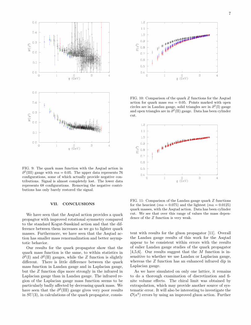
FIG. 9: The quark mass function with the Asqtad action in∂2(III) gauge with ma = 0.05. The upper data represents 76configurations, some of which actually provide negative con-tributions. Signal is almost completely lost. The lower datarepresents 68 configurations. Removing the negative contri-butions has only barely restored the signal.

VII. CONCLUSIONS

We have seen that the Asqtad action provides a quarkpropagtor with improved rotational symmetry comparedto the standard Kogut-Susskind action and that the dif-ference between them increases as we go to lighter quarkmasses. Furthermore, we have seen that the Asqtad ac-tion has smaller mass renormalization and better asymp-totic behavior.

Our results for the quark propagator show that thequark mass function is the same, to within statistics in∂2(I) and ∂2(II) gauges, while the Z function is slightlydifferent. There is little difference between the quarkmass function in Landau gauge and in Laplacian gauge,but the Z function dips more strongly in the infrared inLaplacian gauge than in Landau gauge. The infrared re-gion of the Laplacian gauge mass function seems to beparticularly badly affected by decreasing quark mass. Wehave seen that the ∂2(III) gauge gives very poor resultsin SU(3), in calculations of the quark propagator, consis-

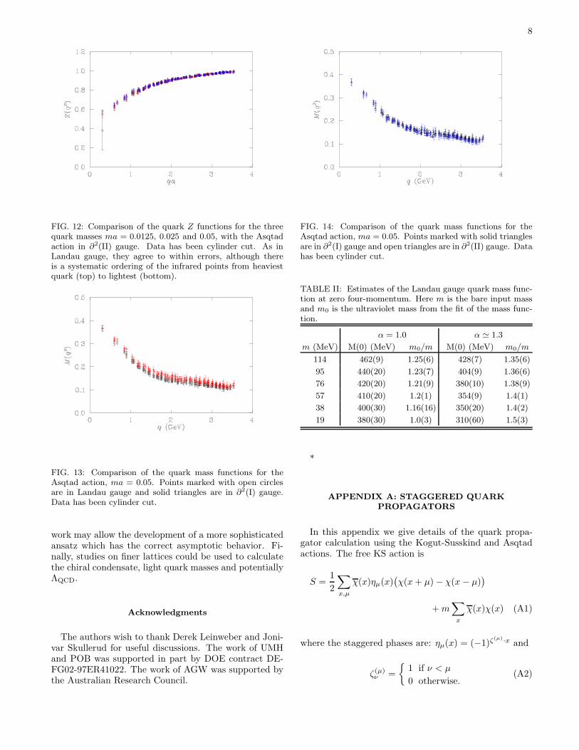
FIG. 10: Comparison of the quark Z functions for the Asqtadaction for quark mass ma = 0.05. Points marked with opencircles are in Landau gauge, solid triangles are in ∂2(I) gaugeand open triangles are in ∂2(II) gauge. Data has been cylindercut.

FIG. 11: Comparison of the Landau gauge quark Z functionsfor the heaviest (ma = 0.075) and the lightest (ma = 0.0125)quark masses, with the Asqtad action. Data has been cylindercut. We see that over this range of values the mass depen-dence of the Z function is very weak.

tent with results for the gluon propagator [11]. Overallthe Landau gauge results of this work for the Asqtadappear to be consistent within errors with the resultsof ealier Landau gauge studies of the quark propagator[4,5,6]. Our results suggest that the M function is in-sensitive to whether we use Landau or Laplacian gauge,whereas the Z function has an enhanced infrared dip inLaplacian gauge.

As we have simulated on only one lattice, it remainsto do a thorough examination of discretization and fi-nite volume effects. The chiral limit was obtained byextrapolation, which may provide another source of sys-tematic error. It will also be interesting to investigate theO(a4) errors by using an improved gluon action. Further

8

FIG. 12: Comparison of the quark Z functions for the threequark masses ma = 0.0125, 0.025 and 0.05, with the Asqtadaction in ∂2(II) gauge. Data has been cylinder cut. As inLandau gauge, they agree to within errors, although thereis a systematic ordering of the infrared points from heaviestquark (top) to lightest (bottom).

FIG. 13: Comparison of the quark mass functions for theAsqtad action, ma = 0.05. Points marked with open circlesare in Landau gauge and solid triangles are in ∂2(I) gauge.Data has been cylinder cut.

work may allow the development of a more sophisticatedansatz which has the correct asymptotic behavior. Fi-nally, studies on finer lattices could be used to calculatethe chiral condensate, light quark masses and potentiallyΛQCD.

Acknowledgments

The authors wish to thank Derek Leinweber and Joni-var Skullerud for useful discussions. The work of UMHand POB was supported in part by DOE contract DE-FG02-97ER41022. The work of AGW was supported bythe Australian Research Council.

FIG. 14: Comparison of the quark mass functions for theAsqtad action, ma = 0.05. Points marked with solid trianglesare in ∂2(I) gauge and open triangles are in ∂2(II) gauge. Datahas been cylinder cut.

TABLE II: Estimates of the Landau gauge quark mass func-tion at zero four-momentum. Here m is the bare input massand m0 is the ultraviolet mass from the fit of the mass func-tion.

α = 1.0 α ≃ 1.3

m (MeV) M(0) (MeV) m0/m M(0) (MeV) m0/m

114 462(9) 1.25(6) 428(7) 1.35(6)

95 440(20) 1.23(7) 404(9) 1.36(6)

76 420(20) 1.21(9) 380(10) 1.38(9)

57 410(20) 1.2(1) 354(9) 1.4(1)

38 400(30) 1.16(16) 350(20) 1.4(2)

19 380(30) 1.0(3) 310(60) 1.5(3)

*

APPENDIX A: STAGGERED QUARK

PROPAGATORS

In this appendix we give details of the quark propa-gator calculation using the Kogut-Susskind and Asqtadactions. The free KS action is

S =1

2

∑

x,µ

χ(x)ηµ(x)(

χ(x + µ) − χ(x − µ))

+ m∑

x

χ(x)χ(x) (A1)

where the staggered phases are: ηµ(x) = (−1)ζ(µ)·x and

ζ(µ)ν =

{

1 if ν < µ

0 otherwise.(A2)

9

FIG. 15: Mass function extrapolated to the chiral limit. Er-rors are Jack-knife. Fit parameters are top: c = 0.080(20),Λ = 520(50) MeV, m0 = 0.0, α = 1.0, χ2 / dof = 1.3 andbottom: c = 0.030(4), Λ = 870(60) MeV, m0 = 0.0, α =1.52(23), χ2 / dof = 0.49.

To Fourier transform, write

kµ =2πnµ

Lµ

| nµ = 0, . . . , Lµ − 1 (A3)

as kµ = pµ + παµ, where

pµ =2πmµ

Lµ

| mµ = 0, . . . ,Lµ

2− 1 (A4)

αµ = 0, 1, (A5)

and define∫

k≡ 1

V

∑

k. Then

∫

k

=

∫

p

1∑

αµ=0

(A6)

χ(x) =

∫

k

eik·xχ(k) =

∫

p

∑

α

ei(p+πα)·xχα(p). (A7)

Defining

δαβ = Πµδαµβµ| mod 2 (A8)

(γµ)αβ

= (−1)αµδα+ζ(µ),β (A9)

where the γµ satisfy

{γµ, γν} = 2δµνδαβ (A10)

ㆵ = γT

µ = γ∗µ = γµ, (A11)

forming a “staggered” Dirac algebra. Putting all thistogether, we can derive a momentum space expressionfor the KS action,

S =

∫

p

∑

αβ

χα(p)[

i∑

µ

(γµ)αβ

sin(pµ) + mδαβ

]

χβ(p).

(A12)

From this we can see that, in momentum space, thetadpole improved, tree-level form of the quark propagatoris

S−1αβ (p; m) = u0i

∑

µ

(γµ)αβ

sin(pµ) + mδαβ (A13)

where pµ is the discrete lattice momentum given byEq. (A4). Assuming that the full propagator retains thisform (in analogy to the continuum case) we write

S−1αβ (p) = i

∑

µ

(γµ)αβ

sin(pµ)A(p) + B(p)δαβ (A14)

= Z−1(p)[

i∑

µ

(γµ)αβ

sin(pµ) + M(p)δαβ

]

.

(A15)

For the KS action, it is convenient to define

qµ ≡ sin(pµ) (A16)

as a shorthand.

Numerically, we calculate the quark propagator in co-ordinate space,

G(x, y) =⟨

χ(x)χ(y)⟩

=∑

αβ

∫

p,r

exp{

i(p + πα)x − i(r + πβ)y}

×⟨

χα(p)χβ(r)⟩

=∑

αβ

∫

p,r

exp{

i(p + πα)x − i(r + πβ)y}

× δprSαβ(p)

=∑

αβ

∫

p

exp{

ip(x − y)}

× exp{

iπ(αx − βy)}

Sαβ(p). (A17)

To obtain the quark propagator in momentum space, wetake the Fourier transform of G(x, 0) and, decomposing

10

the momenta as kµ = rµ + πδµ | 0 ≤ rµ < π, get

G(k) = G(r + πδ) ≡ Gδ(r) =∑

x

e−ikxG(x, 0)

=∑

αβ

∫

p

∑

x

exp{

−i(r + πδ)x}

× exp{

i(p + πα)x}

Sαβ(p)

=∑

αβ

∫

p

δprδαδSαβ(p). (A18)

Thus, in terms of the KS momenta, q,

Gδ(q) =∑

β

Sδβ(q) = Z(q)−i

∑

µ(−1)δµqµ + M(q)

q2 + M2(q),

(A19)from which we obtain

∑

δ

TrGδ(q) = 16Nc

Z(q)M(q)

q2 + M2(q)

= 16NcB(q), (A20)

and

i∑

δ

∑

ρ

(−1)δρqρTr[Gδ(q)] = 16Ncq2 Z(q)

q2 + M2(q)

= 16Ncq2A(q). (A21)

Note: we could determine

A(p) = Z−1(p)

=−i

16Nc

∑

ν sin2(pν)

×∑

αβ

∑

ρ

(γρ)αβsin(pρ)Tr

[

S−1βα (p)

]

(A22)

B(p) =M(p)

Z(p)=

1

16Nc

∑

α

Tr[

S−1αα(p)

]

, (A23)

but we would rather avoid inverting Sαβ(p).Putting it all together we get

A(q) = Z−1(q) =A(q)

A2(q)q2 + B2(qµ)(A24)

B(q) =M(q)

Z(q)=

B(p)

A2(q)q2 + B2(p)(A25)

M(q) =B(q)

A(q). (A26)

The tadpole improved, tree-level behavior of the Z andmass functions are simply

Z0 =1

u0(A27)

and

M0 =m

u0(A28)

respectively.

The Asqtad quark action [3] is a fat-link Staggeredaction using three-link, five-link and seven-link staplesalong with the three-link Naik term [13] and five-link Lep-age term [14], with tadpole improved coefficients tunedto remove all tree-level O(a2) errors. This action was mo-tivated by the desire to minimize quark flavour changinginteractions, but has also been reported to have goodrotational symmetry.

At tree-level (i.e. no interations, links set to the iden-tity), the staples in this action make no contribution, sothe action reduces to the Naik action.

S =1

2

∑

x,µ

χ(x)ηµ(x)[9

8

(

χ(x + µ) − χ(x − µ))

−1

24

(

χ(x + 3µ) − χ(x − 3µ))

]

+ m∑

x

χ(x)χ(x)

(A29)

The quark propagator with this action has the tree-levelform

S−1αβ (p; m) = u0i

∑

µ

(γµ)αβ

sin(pµ)[9

8sin(pµ)

−1

24sin(3pµ)

]

+ mδαβ (A30)

so we choose

qµ(pµ) ≡9

8sin(pµ) −

1

24sin(3pµ) (A31)

= sin(pµ)[

1 +1

6sin2(pµ)

]

. (A32)

Having identified the correct momentum for this action,we can calculate the invariant functions as before. Nofurther tree-level correction is required.

[1] S. Aoki et al., Phys. Rev. Lett. 82, 4392 (1999).[2] D. Becirevic et al., Phys. Rev. D 61, 114507 (2000).[3] K. Orginos, D. Toussaint and R.L. Sugar, Phys. Rev. D

60, 054503 (1999).[4] J-I. Skullerud and A.G. Williams, Phys. Rev. D 63,

054508 (2001).

11

[5] J-I. Skullerud, D.B. Leinweber and A.G. Williams, Phys.Rev. D 64, 074508 (2001).

[6] F.D.R. Bonnet, P.O. Bowman, D.B. Leinweber,A.G. Williams and J. Zhang, hep-lat/0202003.

[7] J.C. Vink and U-J. Wiese, Phys. Lett. B 289, 122 (1992).[8] J.C. Vink, Phys. Rev. D 51, 1292 (1995).[9] C. Alexandrou, Ph. de Forcrand and E. Follana, Phys.

Rev. D 63, 094504 (2001).[10] C. Alexandrou, Ph. de Forcrand and E. Follana, hep-

lat/0112043.[11] P.O. Bowman, U.M. Heller, D.B. Leinweber and

A.G. Williams, In preparation.

[12] F.D.R. Bonnet, P.O. Bowman, D.B. Leinweber,A.G. Williams and J.M. Zanotti, Phys. Rev. D 64,

034501 (2001) and references contained therein.[13] S. Naik, Nucl. Phys. B 316, 238 (1989).[14] G.P. Lepage, Phys. Rev. D 59, 074502 (1999).[15] C.T.H. Davies et al., Phys. Rev. D 37, 1581 (1988).[16] P.O. Bowman, U.M. Heller and A.G. Williams, Nucl.

Phys. B (Proc. Suppl.) 106, 820 (2002); P.O. Bowman,U.M. Heller and A.G. Williams, hep-lat/0112027.

[17] Some of numbers in this report differ slightly from thosepublished elsewhere [16] due to a revised value for thelattice spacing.

[18] This is intended to be merely illustrative; in practice wenever actually invert the propagator. See appendix fordetails.