arX

iv:1

408.

2551

v1 [

cs.S

Y]

11

Aug

201

4

Optimal Control for LQG Systems on

Graphs—Part I: Structural Results

Ashutosh Nayyar Laurent Lessard

Abstract

In this two-part paper, we identify a broad class of decentralized output-feedbackLQG systems for which the optimal control strategies have a simple intuitive esti-mation structure and can be computed efficiently. Roughly, we consider the class ofsystems for which the coupling of dynamics among subsystems and the inter-controllercommunication is characterized by the same directed graph. Furthermore, this graphis assumed to be a multitree, that is, its transitive reduction can have at most onedirected path connecting each pair of nodes. In this first part, we derive sufficientstatistics that may be used to aggregate each controller’s growing available informa-tion. Each controller must estimate the states of the subsystems that it affects (itsdescendants) as well as the subsystems that it observes (its ancestors). The optimalcontrol action for a controller is a linear function of the estimate it computes as wellas the estimates computed by all of its ancestors. Moreover, these state estimates maybe updated recursively, much like a Kalman filter.

1

Contents

1 Introduction 3

1.1 Prior work . . . . . . . . . . . . . . . . . . . . . . . . . . . . . . . . . . . . . . . 4

1.2 Organization . . . . . . . . . . . . . . . . . . . . . . . . . . . . . . . . . . . . . 6

2 Preliminaries 6

2.1 Basic notation . . . . . . . . . . . . . . . . . . . . . . . . . . . . . . . . . . . . 6

2.2 Graphs . . . . . . . . . . . . . . . . . . . . . . . . . . . . . . . . . . . . . . . . . 7

2.3 System model . . . . . . . . . . . . . . . . . . . . . . . . . . . . . . . . . . . . . 8

2.4 Assumptions . . . . . . . . . . . . . . . . . . . . . . . . . . . . . . . . . . . . . 9

3 Main result and examples 11

4 Proof preliminaries 14

4.1 Proof outline . . . . . . . . . . . . . . . . . . . . . . . . . . . . . . . . . . . . . 15

4.2 New definitions for multitrees . . . . . . . . . . . . . . . . . . . . . . . . . . . 16

4.3 Aggregated graph and dynamics . . . . . . . . . . . . . . . . . . . . . . . . . . 17

4.4 The six-node centralized problem . . . . . . . . . . . . . . . . . . . . . . . . . 18

4.5 A partial separation result for the aggregated graph . . . . . . . . . . . . . . 19

5 Proof of main results 20

5.1 Leaf nodes: proof of P (0) . . . . . . . . . . . . . . . . . . . . . . . . . . . . . . 21

5.2 Induction step: proof of P (s) Ô⇒ P (s + 1) . . . . . . . . . . . . . . . . . . 22

6 Proof modification under Assumption A2’ 28

7 Concluding remarks 29

A Proof of Theorem 3 30

B Proof of Lemma 3 30

C Proof of Lemma 4 33

D Proof of Lemma 5 34

2

1 Introduction

With the advent of large scale systems such as the internet or power networks and in-creasing applications of networked control systems, the past decade has seen a resurgenceof interest in decentralized control. In decentralized control problems, control decisionsmust be made using only local or partial information. A key specification of a decentral-ized control problem is its information structure. Intuitively, the information structureof a problem describes for each control decision what information is available for makingthat decision. The investigation of decentralized control problems available in the currentliterature has largely been a study of information structures and their implications forthe characterization and computation of optimal decentralized control strategies. Twoquestions that have played a central role in this study are:

Q1 Can the ever-growing information history available to controllers be aggregated with-out compromising achievable performance? In other words, are there sufficient statis-tics for the controllers?

Q2 Can optimal decentralized strategies be efficiently computed?

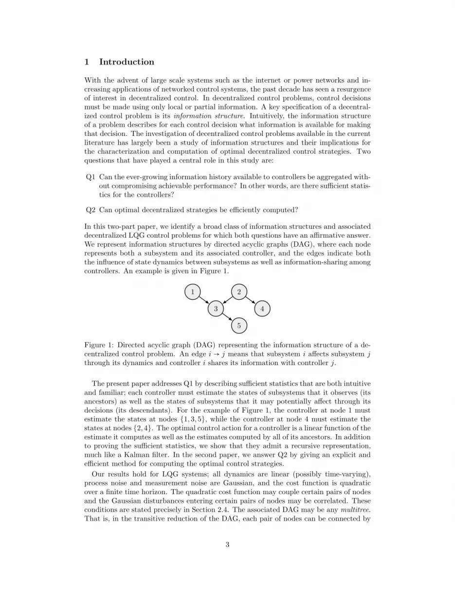
In this two-part paper, we identify a broad class of information structures and associateddecentralized LQG control problems for which both questions have an affirmative answer.We represent information structures by directed acyclic graphs (DAG), where each noderepresents both a subsystem and its associated controller, and the edges indicate boththe influence of state dynamics between subsystems as well as information-sharing amongcontrollers. An example is given in Figure 1.

1 2

3 4

5

Figure 1: Directed acyclic graph (DAG) representing the information structure of a de-centralized control problem. An edge i → j means that subsystem i affects subsystem j

through its dynamics and controller i shares its information with controller j.

The present paper addresses Q1 by describing sufficient statistics that are both intuitiveand familiar; each controller must estimate the states of subsystems that it observes (itsancestors) as well as the states of subsystems that it may potentially affect through itsdecisions (its descendants). For the example of Figure 1, the controller at node 1 mustestimate the states at nodes {1,3,5}, while the controller at node 4 must estimate thestates at nodes {2,4}. The optimal control action for a controller is a linear function of theestimate it computes as well as the estimates computed by all of its ancestors. In additionto proving the sufficient statistics, we show that they admit a recursive representation,much like a Kalman filter. In the second paper, we answer Q2 by giving an explicit andefficient method for computing the optimal control strategies.

Our results hold for LQG systems; all dynamics are linear (possibly time-varying),process noise and measurement noise are Gaussian, and the cost function is quadraticover a finite time horizon. The quadratic cost function may couple certain pairs of nodesand the Gaussian disturbances entering certain pairs of nodes may be correlated. Theseconditions are stated precisely in Section 2.4. The associated DAG may be any multitree.That is, in the transitive reduction of the DAG, each pair of nodes can be connected by

3

at most one directed path. A key aspect of this work is that we consider output feedback.While the presence of measurement noise makes the problem considerably more difficultto solve than the state-feedback case, we will nevertheless see that the optimal controllerhas a simple and intuitive structure.

1.1 Prior work

The available literature on decentralized control problems can be classified into two cat-egories based on the underlying conceptual perspective and the associated techniquesemployed:

1. Decentralized control as a team theory problem: This perspective of decentralizedcontrol problems starts with a description of primitive random variables that repre-sent all the uncertainties in the evolution and observations of a dynamic system. Theinformation structure is specified in terms of the observables available to each con-troller, where an observable is a function of the primitive random variables and pastdecisions. The observables may be explicitly defined in terms of primitive randomvariables and control decisions or they may be defined using intermediate variablesas in a state-space description. Similarly, the control objective can also be viewedas a (either explicit or implicit) function of the primitive random variables and thecontrol decisions.

The controllers select (measurable) functions that map their information to theirdecisions. Once such a selection of strategies has been made, the control objectivebecomes a well-defined random variable. The design problem is to identify a choiceof strategies that minimizes the expected value of the control objective.

2. Decentralized control as closed-loop norm optimization: This perspective focuses oncases when the plant and the controllers are linear time-invariant (LTI) systems. Theplant has two inputs: an exogenous input vector w and a control input vector u. Theplant has two outputs: a performance-related vector z and an observation vector y.The controller is a LTI system with y as its input and u as its output. The informationstructure is described in terms of structural constraints on the transfer function ofthe controller. For a fixed choice of the controller, the closed loop LTI system canbe described in terms of its transfer function from the exogenous input w to theperformance related vector z. The design problem is to minimize a norm (such asthe H2-norm) of this transfer function.

Both of these approaches have acknowledged the difficulty of a general decentralizedcontrol problem with arbitrary information structure [2, 32]. Therefore, there has beenconsiderable interest in identifying classes of information structures that may be “easier”to solve. In the team-theoretic approach, partial nestedness of an information structurehas been identified as a key simplifying feature [5]. A decentralized LQG control problemwith a partially nested (PN) information structure admits a linear control strategy as theglobally optimal strategy choice. Further, it can be reduced (at least for finite horizonproblems) to a static LQG team problem for which person-by-person optimal strategiesare globally optimal [24]. While the results of [5] have been generalized to certain infinite-horizon problems [20], a universal and computationally efficient methodology for findingoptimal strategies for all partially nested problems remains elusive.

In the norm optimization framework, some properties of the plant and the informa-tion constraint have been identified as simplifying conditions. These properties implyconvexity of the transfer function norm optimization problem in decentralized control.Examples of such properties include quadratic invariance (QI) [25], funnel causality [1],

4

and certain hierarchical architectures [23]. Interestingly, many of the systems consideredin the literature using these properties have a partially nested information structure aswell. Despite the convexity, the optimization problem in general is infinite dimensionaland therefore hard to solve.

For decentralized problems that do not belong to the class of PN or QI problems,linearity of globally optimal strategies is not guaranteed and the optimization of strategiesis in general a non-convex problem. These problems present unique features such assignaling (that is, communication through control actions) that make them particularlydifficult. We refer the reader to [4, 19, 21, 32, 34] for some examples and results for suchproblems.

The decentralized control problems considered in this paper are a subset of the class ofPN and QI problems. The relation between problem classes is illustrated in Figure 2.

Decentralized:•not linear•not convex• generally hard

PN and QI:• linear optimal• convexifiable•∞-dimensional

Multitree:• sufficient statistics• structural result• efficient solution

Centralized:• certainty equivalent• separation principle

Figure 2: Venn diagram showing a complexity hierarchy of decentralized control prob-lems. The present paper establishes the multitree class, which shares many structuralcharacteristics with centralized problems, but is more computationally tractable thangeneral partially nested and quadratically invariant problems.

In decentralized control problems with multiple subsystems that each have an associatedcontroller, partial nestedness is typically manifested in two ways:

1. If a subsystem i affects another subsystem j, then the controller at subsystem i sharesall information with the controller at subsystem j. In other words, the informationflow obeys the sparsity constraints of the dynamics. State-feedback problems of thiskind were considered in [28] for a two-controller case and in [27] for controllers com-municating over a DAG. Similar results and partial extensions to output feedbackwere addressed in [6, 29, 22]. The first solution to a problem with output feed-back at every subsystem appeared in [15, 16] for a DAG with two subsystems. Thetwo-subsystem output feedback results were generalized to star-shaped (broadcast)graphs in [12] and linear chain graphs in [30].

2. If subsystem i affects subsystem j after some delay d, then the controller at subsys-tem i shares its information with controller at subsystem j with delay not exceedingd. In other words, the information flow obeys the delay constraints of the dynam-ics. Among the earlier problems of this type were the discrete-time LQG problemswith one-step delayed sharing information structure [8, 26, 31, 33]. More recently,problems where communication delay between controllers is characterized in termsof distance on a DAG were addressed in [9] for the state feedback case and in [10]for the output feedback case. In both these works, it is assumed that the under-lying DAG is strongly connected, so every measurement eventually finds its way toevery decision-maker. This fact allows the optimal strategy to be decomposed intoa component acting on the common past information together with a finite impulseresponse (FIR) portion acting on newer information. A similar model with statefeedback but completely general DAG was addressed in [11]. The state-feedback as-sumption allows the control problem to decouple into smaller centralized problemsthat can be solved separately.

5

The output-feedback works with sparsity constraints [12, 15, 16, 30] use a closed-loopnorm optimization framework and employ a spectral factorization approach to solve forthe optimal controller. This approach yields an observer-controller structure and showshow to jointly solve for the appropriate estimation and control gains. While this approachdoes not provide an immediate way to interpret the states of the optimal controller asminimum mean-squared error (MMSE) estimates of the plant state, such an interpretationwas obtained for the two-subsystem case in [17].

An alternative approach is to use the team-theoretic perspective. The two-subsystemoutput feedback problem was solved in this manner in [18]. We use a similar approachin the present work to extend the output feedback results to a broader class of DAGs.The advantage of a team-theoretic approach is that structural results emerge naturally,and one can deduce the optimal controller’s sufficient statistics without solving for gainsexplicitly. Indeed, the paper [18] derives structural results for a finite-horizon formulationwith a linear time-varying plant, whereas the works [12, 15, 16, 17, 30] address linear time-invariant plants and find the infinite-horizon steady-state optimal controller.

1.2 Organization

In Section 2, we explain notations, conventions, and assumptions. Section 3 presents themain structural result as well as some examples. The proof spans Sections 4, 5 and 6.We conclude in Section 7.

2 Preliminaries

2.1 Basic notation

Real vectors and matrices are represented by lower- and upper-case letters respectively.Boldface symbols denote random vectors, and their non-boldface counterparts denoteparticular realizations. xT denotes the transpose of vector x. The probability densityfunction of x evaluated at x is denoted P(x = x), and conditional densities are writtenas P(x ∣y = y). E denotes the expectation operator. We write x ∼ N(µ,Σ) when x isnormally distributed with mean µ and covariance Σ.

We consider discrete time stochastic processes over a finite time interval [0, T ]. Time isindicated using subscripts, and we use the colon notation to denote ranges. For example:

x0∶T−1 = {x0, x1, . . . , xT−1}In general, all symbols are time-varying. In an effort to present general results whilekeeping equations clear and concise, we introduce a new notation to represent a family ofequations. For example, when we write:

x+t= Ax +w,

we mean that xt+1 = Atxt + wt holds for 0 ≤ t ≤ T − 1. Note that the subscript “+”indicates that we increment to t+ 1 for the associated symbol. We similarly overload thesummation symbol by writing for example

∑t

xTQx to meanT−1

∑t=0

xT

t Qtxt

Whenever the symbol t is written above a binary relation or below a summation, it isimplied that 0 ≤ t ≤ T −1. There is no ambiguity because we use the same time horizon T

throughout this paper.

6

We denote subvectors by using superscripts. Subvectors may also be referenced byusing a subset of indices as superscripts. For example, for a vector

x =

⎡⎢⎢⎢⎢⎢⎣x1

x2

x3

⎤⎥⎥⎥⎥⎥⎦and s = {1,3}, we will use the concise notation

xs = x{1,3} = [x1

x3]When writing sub-vectors, we will always arrange the components in increasing order

of indices. Thus, in the above example, xs is [x1

x3] and not [x3

x1]. Given a collection

of random vectors, we will at times treat the collection as a concatentation of vectorsarranged in increasing order of node index.

For a matrix A, Aij denotes its (i, j)-block whose dimensions are inferred from thecontext. Given two sets of indices s and r, As,r is a matrix composed of blocks Aij withi ∈ s and j ∈ r. The blocks Ai,j in a row (column) of As,r are arranged in increasing orderof column (row) indices.

We will write a ∈ lin(p1, . . . , pm) to mean that a is a linear function of p1, . . . , pm. Inother words, a = A1p1 + ⋅ ⋅ ⋅ +Ampm for some appropriately chosen matrices A1, . . . ,Am.

2.2 Graphs

Let G(V ,E) be a directed acyclic graph (DAG). The nodes are labeled 1 to n, so V ={1, . . . , n}. If there is an edge from i to j, we write (i, j) ∈ E .We write i → j if there is a directed path from i to j. That is, if there exists a sequence

of nodes v1, . . . , vm with v1 = i and vm = j such that (vk, vk+1) ∈ E for all k. By convention,every node has a directed path (of length zero) to itself. So it is always true that i → i.We write i↔ j if i and j are path-connected, that is, if i→ j or j → i. Otherwise, we saythey are path-disconnected, and we write i↮ j. We can express the path-connectednessof G using the sparsity matrix, which is the binary matrix S ∈ {0,1}n×n defined by

Sij =⎧⎪⎪⎨⎪⎪⎩1 if j → i

0 otherwise

Note that different graphs may have the same sparsity matrix. In general, S is theadjacency matrix of the transitive closure of G. So graphs with the same transitiveclosure also share the same sparsity matrix.

By convention, we assign a topological ordering to the node labels. That is, we choose alabeling such that if j → i, then j ≤ i. This is possible for any DAG [3, §22.4]. Therefore, Sis always lower-triangular. See Figure 3 for a simple example of a DAG and its associatedsparsity matrix.

Given a node i ∈ V , we define its ancestors as the set of nodes that have a directedpath to i. Similarly, we define the descendants as the set of nodes that i can reach via adirected path. We use the following notation for ancestors and descendants respectively.

i↑ = {j ∈ V ∶ j → i} i↓ = {j ∈ V ∶ i→ j}Ancestors and descendants of i always include i itself. We define the strict ancestors andstrict descendants when we mean to exclude i. Specifically, i⇈ = i↑ ∖ {i} and i⇊ = i↓ ∖ {i}.

7

1 2

3 4

5

S =

⎡⎢⎢⎢⎢⎢⎢⎢⎢⎢⎣

1 0 0 0 00 1 0 0 01 1 1 0 00 1 0 1 01 1 1 0 1

⎤⎥⎥⎥⎥⎥⎥⎥⎥⎥⎦Figure 3: Simple DAG and its associated sparsity matrix.

Notation Meaning

i↑ {j ∈ V ∶ j → i}i↓ {j ∈ V ∶ i→ j}i↕ i↑ ∪ i↓i⇈ i↑ ∖ ii⇊ i↓ ∖ i

Table 1: Ancestors, descendants and related definitions

We use the notation i↕ = i↑ ∪ i↓ for the set of all nodes that are path-connected to node i.Note that i↕ is partitioned as i⇈ ∪ {i} ∪ i⇊. In the graph of Figure 3, for example,

3↑ = {1,2,3} 3⇈ = {1,2} 3↓ = {3,5} 3⇊ = {5} 3↕ = {1,2,3,5}We summarize these notations in Table 1.

Remark 1. Note that while i↑, i↓, etc. are defined as subsets, it is convenient to think ofthem as ordered lists in which the node indices are arranged in increasing order. Thus,in Figure 3, 3↑ will always be written as {1,2,3} and not as any other permutation of{1,2,3}.Remark 2. A node with no strict descendants is called a leaf node and a node with nostrict ancestors is called a root node.

2.3 System model

The system we consider consists of n subsystems that may affect one another according tothe structure of an underlying DAG, G(V ,E). The ith subsystem has state xi, input ui,measurement yi, process noise wi, and measurement noise vi. We assume these arediscrete-time random processes that satisfy the following state-space dynamics for alli ∈ V .

xi+

t= ∑j∈i↑(Aijx

j +Bijuj) +wi

yi t= ∑j∈i↑(Cijx

j) + vi(1)

The relative timing of ith state, control action and observation at time t is as shown inFigure 4. Note that the observation yi

t is generated after control action uit is taken. Each

of the matrices in (1) may be time-varying, and may even change dimensions with time.In an effort to make our notation more concise, we concatenate the various symbols aboveand simply write

x+t= Ax +Bu +w

yt= Cx + v (2)

8

t t + 1xit ui

t yit

Figure 4: Relative timing of state, action and observation at time t

In this condensed notation, the matrices A, B, and C have blocks that conform to S, thesparsity matrix for G(V ,E). In other words, if Sij = 0 then Aij = 0, Bij = 0, and Cij = 0.The random vectors in the collection

{x0, [w0

v0

] , . . . , [wT−1

vT−1]} , (3)

referred to as the primitive random variables, are mutually independent and jointly Gaus-sian with the following known probability density functions

x0 = N (0,Σinit)[wv] t= N(0, [W UT

U V]) (4)

There are n controllers, one responsible for each of the ui, i = 1, . . . , n. We define thelocally generated information at node i at time t as

iit ∶= {yi0∶t−1,u

i0∶t−1} (5)

The information available to controller i at time t is

ii↑

t ∶= ⋃j∈i↑

ijt = ⋃j∈i↑{yj

0∶t−1,uj0∶t−1}. (6)

In other words, each controller knows the past measurements and decisions of its ancestors.So the directed edges of G may be thought of as representing the flow of informationbetween subsystems. Crucially, the same graph G represents both how the dynamicspropagate as well as how information is shared in the system. The controllers selectactions according to control strategy f i ∶= (f i

0, fi1, . . . , f

iT−1) for i ∈ V . That is,

uit = f

it ( ii↑t ) for 0 ≤ t ≤ T − 1 (7)

Given a control strategy profile f = (f1, f2, . . . , fn), performance is measured by thefinite horizon expected quadratic cost

J0(f) = Ef(∑t

[xu]T

[Q S

ST R][x

u] + xT

TPfinalxT) (8)

The expectation is taken with respect to the joint probability measure on (x0∶T ,u0∶T−1)induced by the choice of f .

It is assumed that all system parameters are universally known. Specifically, Σinit, Pfinal,as well as the values of A,B,C,Q,R,S,U,V,W for all t, are known by all controllers.

2.4 Assumptions

In addition to the problem specifications (2)–(8), we will make some additional assump-tions about the underlying DAG and the noise and cost parameters used in (4) and (8)respectively. First, we require some definitions.

9

Definition 1 (multitree). The nodes i, a, b, j ∈ V form a diamond if i → a → j andi→ b→ j, and a↮ b. A multitree is a directed acyclic graph that contains no diamonds.

For example, the graph of Figure 3 is a multitree. However, if we add the edge (4,5),then the nodes (2,3,4,5) form a diamond and the graph ceases to be a multitree.

Definition 2 (decoupled cost). Let X = {Q0∶T−1,R0∶T−1, S0∶T−1, Pfinal} denote the setof matrices associated with the cost function. We say that nodes i, j ∈ V havedecoupled cost if Xij = 0 for all X ∈ X .

Definition 3 (uncorrelated noise). Let Y = {W0∶T−1, V0∶T−1, U0∶T−1,Σinit} denote the setof matrices associated with the noise and initial state statistics. We say that nodes i, j ∈ Vhave uncorrelated noise if Yij = 0 for all Y ∈ Y.

The notions of decoupled cost and uncorrelated noise have intuitive interpretations. Iftwo nodes have decoupled cost, then the instantaneous cost at any time has no “cross-terms” that involve both the nodes. If two nodes have uncorrelated noise, then the processand measurement noises affecting one node are statistically independent of those affectingthe other. Our assumptions are as follows.

(A1) The DAG G(V ,E) is a multitree.

(A2) For every pair of nodes i, j ∈ V , we have some combination of decoupled cost anduncorrelated noise, depending on whether these nodes have a common ancestor or acommon descendant. We state the requirements in the following table.

i and j have... a common ancestor no common ancestor

a common descendant no restrictions uncorrelated noise

no common descendant decoupled cost decoupled cost anduncorrelated noise

(A2’) This assumption is a relaxed version of A2, defined by the following table.

i and j have... a common ancestor no common ancestor

a common descendant no restrictions uncorrelated noise

no common descendant decoupled cost decoupled cost oruncorrelated noise

For the graph of Figure 3, nodes 1 and 4 have neither a common ancestor nor a commondescendant. Therefore, A2 would require that this pair of nodes have both decoupled costand uncorrelated noise. However, A2’ would only require one of the two.

Note that because of the multitree assumption, the only way i and j can have both acommon ancestor and a common descendant is if i↔ j. Assumption A2 may be expressedin terms of the sparsity pattern S using the following observations

1. (SST)ij = 0 if and only if i↑ ∩ j↑ = ∅ (i and j have no common ancestor)

2. (STS)ij = 0 if and only if i↓ ∩ j↓ = ∅ (i and j have no common descendant)

So A2 may be stated concisely as follows: all matrices in X (see Definition 2) have thesame sparsity as S

TS and all matrices in Y (see Definition 3) have the same sparsity as

10

SST. For the graph of Figure 3, these sparsity patterns are

SST ∼

⎡⎢⎢⎢⎢⎢⎢⎢⎢⎢⎣

1 0 1 0 10 1 1 1 11 1 1 1 10 1 1 1 11 1 1 1 1

⎤⎥⎥⎥⎥⎥⎥⎥⎥⎥⎦STS ∼

⎡⎢⎢⎢⎢⎢⎢⎢⎢⎢⎣

1 1 1 0 11 1 1 1 11 1 1 0 10 1 0 1 01 1 1 0 1

⎤⎥⎥⎥⎥⎥⎥⎥⎥⎥⎦Assumption A2’ is less restrictive than A2, but cannot be as easily expressed in terms ofthe sparsity pattern S.

Remark 3. Note that both assumptions A2 and A2’ are more general than the assumptionthat all cost matrices in X and covariance matrices in Y are block-diagonal.

3 Main result and examples

The problem addressed in this paper is as follows.

Problem 1 (n-player LQG). For the model (2)–(7), and subject to Assumptions A1and either A2 or A2’, find a control strategy profile f = (f1, f2, . . . , fn) that minimizesthe expected cost (8).

The information structure of our problem is partially nested and therefore, without lossof optimality, we will restrict attention to linear control strategies [5].

The main result of this paper is a description of sufficient statistics required for anoptimal solution of Problem 1. We first define the following conditional expectation:

zj↕

t ∶= E(xj↕

t ∣ ij↑t ).In other words, zj

↕

t is the conditional mean of the state of all nodes that are path connectedto node j based on the information available to node j (recall the notations defined inTable 1). Our first result is the following.

Theorem 1 (Control Result). In Problem 1, there is no loss in optimality in jointlyrestricting all nodes i ∈ V to strategies of the form

uit = ∑

j∈i↑K

ijt zj

↕

t (9)

where zj↕

t ∶= E(xj↕

t ∣ ij↑t ).Recall that ii

↑

t defined in (5)–(6) is the information available to node i at time t, and thisset grows with time as more measurements are observed and more decisions are made.Theorem 1 states that controllers need not remember this entire information history.

Instead, each node j may compute the aggregated statistic zj↕

, which is an estimate ofthe current states of its ancestors and descendants. The optimal decision at node i, ui,is then a linear function of the estimates maintained by all of its ancestors.

An alternative way of stating the result of Theorem 1 is to stack the decisions andestimates and obtain one large linear equation.

11

Corollary 1. In Problem 1, there is no loss in optimality in jointly restricting the strate-gies of all the nodes to the form

⎡⎢⎢⎢⎢⎢⎣u1t⋮

unt

⎤⎥⎥⎥⎥⎥⎦=

⎡⎢⎢⎢⎢⎢⎣K11

t ⋯ K1nt

⋮ ⋱ ⋮Kn1

t ⋯ Knnt

⎤⎥⎥⎥⎥⎥⎦´¹¹¹¹¹¹¹¹¹¹¹¹¹¹¹¹¹¹¹¹¹¹¹¹¹¹¹¹¹¹¹¹¹¹¹¹¹¹¹¹¹¹¹¹¹¹¹¹¹¹¸¹¹¹¹¹¹¹¹¹¹¹¹¹¹¹¹¹¹¹¹¹¹¹¹¹¹¹¹¹¹¹¹¹¹¹¹¹¹¹¹¹¹¹¹¹¹¹¹¹¹¶Kt

⎡⎢⎢⎢⎢⎢⎣E(x1

↕

t ∣ i1↑t )⋮

E(xn↕

t ∣ in↑t )⎤⎥⎥⎥⎥⎥⎦

for 0 ≤ t ≤ T − 1 (10)

where Kt is a matrix with block-sparsity conforming to S.

Our second result addresses the evolution of the estimates zj↕

t . In order to state thisresult, we need to define the following linear operation.

Definition 4. Consider nodes i and j with i ∈ j⇊. Let i↕ = {k1, k2, . . . , k∣i↕ ∣} and j↕ ={l1, l2, . . . , l∣j↕ ∣}. Define a matrix Ei,j with ∣i↕∣ block rows and ∣j↕∣ block columns as follows:

For a = 1,2, . . . , ∣i↕∣,1. If ka ∉ j↕, then the ath block row of Ei,j is 0.

2. If ka ∈ j↕ and ka = lb, then the (a, b) block of Ei,j is identity and the rest of ath blockrow is 0.

For example, in Figure 3, 3↕ = {1,2,3,5} and 2↕ = {2,3,4,5}, then

E3,2 =

⎡⎢⎢⎢⎢⎢⎢⎢⎣

0 0 0 0I 0 0 00 I 0 00 0 0 I

⎤⎥⎥⎥⎥⎥⎥⎥⎦.

We can now state our second result.

Theorem 2 (Estimation Result). If the control strategy is as given in Theorem 1, then

the evolution of zj↕

t is described as follows:

zj↕

0= 0

zj↕

+t= Aj

↕j↕

zj↕ +Bj

↕j↕ [ uj↑

{uij}i∈j⇊] −Lj (yj

↑ −Cj↑j↑

zj↑) (11)

for some matrices Ljt , 0 ≤ t ≤ T − 1, with

uij t= ∑a∈j↑

Kiaza↕ + ∑

b∈i↑∩j⇊KibEb,jzj

↕

for i ∈ j⇊. (12)

Remark 4. For linear control strategies described by Theorem 2, uijt as defined in (12)

is in fact equal to E(uit ∣ ij↑t ).

The above theorems provide finite dimensional sufficient statistics for all controllersin the system. These results should be viewed as structural results of optimal controlstrategies since they postulate the existence of optimal controllers and estimators of theform presented above without specifying how the matrices Kij , Lj used in control andestimation can be computed.

A detailed proof of Theorems 1 and 2 will be developed in Sections 4.3–5. In theremainder of this section, we will give examples that illustrate the applicability of ourmain result.

12

Example 1. (Centralized case) The classical LQG problem is the case where V = {1}.Theorem 1 then yields the classical separation result; ut =KtE(xt ∣ it) and Theorem 2reduces to the standard Kalman filter.

Example 2. (Disconnected systems) Consider several subsystems with decoupled dy-namics. In this case, the underlying graph has no edges and S = I. Under Assump-tion A2’, if each pair of nodes has either decoupled cost or uncorrelated noise, thenby Theorem 1, the optimal strategy for node i is of the form ui

t = Kit E(xi

t ∣ iit). Sonode i need only estimate its local state and by Theorem 2, this estimate is updatedby a standard Kalman filter. This result can be intuitively explained as follows:

1. If nodes i and j have uncorrelated noise but coupled cost, there is value inestimating xj , but this estimate is zero because of the uncoupled dynamics anduncorrelated noise.

2. If nodes i and j have decoupled cost but correlated noise, the estimate of xj

would be non-zero, but the information it provides is of no use because the stateand decisions xj and uj do not affect the cost associated with node i.

Remark 5. If we violate Assumption A2’ by allowing both coupled cost and correlatednoise, then Theorem 1 no longer holds. An instance of such a problem was solvedfor the state feedback case [13, 14], and it was found that depending on the systemparameters, the optimal infinite-horizon controller may have up to n2 states, where n

is the global plant’s dimension. This result suggests a new controller that lies outsidethe scope of Theorem 1.

Example 3. (Two-player and linear chain cases) Consider the two-player problem cor-responding to the graph and sparsity pattern given below.

1 2 S = [1 01 1]

Figure 5: DAG and associated sparsity matrix for the two-player problem.

This problem was solved in a prior version of this work [18], where the optimalcontroller was found to be of the form

u1

t =K11

t E(xt ∣ i1t) u2

t =K21

t E(xt ∣ i1t) +K22

t E(xt ∣ i{1,2}t )In other words, both players must estimate the global state xt using their availableinformation. Additionally, the second player makes use of the estimate that thefirst player computed. This result agrees perfectly with Theorem 1. Note that here,Assumptions A1 and A2 are not restrictive. In other words, the structural resultholds even when cost is coupled and noise is correlated. Infinite-horizon continuous-time versions of this problem were solved in [15] and a similar structure was foundthere as well. While these works only address the two-player version, it is clear howthe structural result extends to a linear chain with n nodes. For such a case, theoptimal controller is of the form

ukt =

k

∑j=1

Kkjt E(xt ∣ i{1,...,j}t ) for k = 1, . . . , n

Example 4. (Broadcast cases) We define a broadcast DAG to be a graph with n nodes,one of which is the hub. The n = 4 cases are illustrated in Figure 6.

Note that all pairs of nodes have either a common ancestor or a common descendant,so Assumptions A2 and A2’ are equivalent. Theorem 1 provides the following.

13

1

2 3 4

S =

⎡⎢⎢⎢⎢⎢⎢⎢⎣

1 0 0 01 1 0 01 0 1 01 0 0 1

⎤⎥⎥⎥⎥⎥⎥⎥⎦

1 2 3

4

S =

⎡⎢⎢⎢⎢⎢⎢⎢⎣

1 0 0 00 1 0 00 0 1 01 1 1 1

⎤⎥⎥⎥⎥⎥⎥⎥⎦Figure 6: DAG and associated sparsity matrix for the broadcast-out (left) and broadcast-in (right) architectures for n = 4 nodes.

1. In the broadcast-out case, we require that nodes {2, . . . , n} have pairwise-decoupled cost. In this case, the optimal controller has the form

u1

t =K11

t E(xt ∣ i1t )ukt =K

k1t E(xt ∣ i1t ) +Kkk

t E(x{1,k}t ∣ i{1,k}t ) for k = 2, . . . , n

2. In the broadcast-in case, we require that the nodes {1, . . . , n − 1} have havepairwise-uncorrelated noise. In this case, the optimal controller has the form

ukt =K

kkt E(x{k,n}t ∣ ikt ) for k = 1, . . . , n − 1

unt =

n−1

∑j=1

Knjt E(x{j,n}t ∣ ijt) +Knn

t E(xt ∣ i{1,...,n}t )A similar architecture was studied in [12] for the continuous-time infinite-horizoncase, and a structure identical to the one above was found.

Example 5. (Simple graph) Consider the simple five-node graph of Figure 3. Becauseof Assumption A2’, we have the following restrictions:

• Nodes (3,4) and (4,5) have decoupled cost.

• Nodes (1,2) have uncorrelated noise.

• Nodes (1,4) have either decoupled cost or uncorrelated noise.

Theorem 1 provides the following optimal controller structure, which we expressusing the formulation of Corollary 1.

⎡⎢⎢⎢⎢⎢⎢⎢⎢⎢⎢⎢⎣

u1t

u2t

u3t

u4t

u5t

⎤⎥⎥⎥⎥⎥⎥⎥⎥⎥⎥⎥⎦=

⎡⎢⎢⎢⎢⎢⎢⎢⎢⎢⎢⎢⎣

K11

t 0 0 0 0

0 K22t 0 0 0

K31

t K32

t K33

t 0 0

0 K42t 0 K44

t 0

K51t K52

t K53t 0 K55

t

⎤⎥⎥⎥⎥⎥⎥⎥⎥⎥⎥⎥⎦´¹¹¹¹¹¹¹¹¹¹¹¹¹¹¹¹¹¹¹¹¹¹¹¹¹¹¹¹¹¹¹¹¹¹¹¹¹¹¹¹¹¹¹¹¹¹¹¹¹¹¹¹¹¹¹¹¹¹¹¹¹¹¹¹¹¹¹¹¹¹¹¹¹¹¹¹¹¹¹¹¹¹¹¹¹¹¹¹¹¹¹¹¹¹¹¹¹¹¹¹¹¹¹¹¹¹¸¹¹¹¹¹¹¹¹¹¹¹¹¹¹¹¹¹¹¹¹¹¹¹¹¹¹¹¹¹¹¹¹¹¹¹¹¹¹¹¹¹¹¹¹¹¹¹¹¹¹¹¹¹¹¹¹¹¹¹¹¹¹¹¹¹¹¹¹¹¹¹¹¹¹¹¹¹¹¹¹¹¹¹¹¹¹¹¹¹¹¹¹¹¹¹¹¹¹¹¹¹¹¹¹¹¹¶Kt

⎡⎢⎢⎢⎢⎢⎢⎢⎢⎢⎢⎢⎣

E(x{1,3,5}t ∣ i1t )E(x{2,3,4,5}t ∣ i2t)

E(x{1,2,3,5}t ∣ i{1,2,3}t )E(x{2,4}t ∣ i{2,4}t )

E(x{1,2,3,5}t ∣ i{1,2,3,5}t )

⎤⎥⎥⎥⎥⎥⎥⎥⎥⎥⎥⎥⎦

Note that the matrix of control gains Kt has a block-sparsity pattern that conformsto S, the sparsity matrix for this problem.

4 Proof preliminaries

The main results of this paper, Theorems 1 and 2, will be proved in the several sectionsthat follow. In this section, we give an outline of the proof method and introduce requiredconcepts that will be used later in the formal proof. Throughout this section and Section 5,we will make assumptions A1 and A2 described in Section 2.4.

14

4.1 Proof outline

Our proof technique may be thought of as a sequence of refinements that traverse theunderlying DAG starting from the leaf nodes and finishing at the root nodes. To illustratethe process, consider the following four-node graph.

1 2

3

4

S =

⎡⎢⎢⎢⎢⎢⎢⎢⎣

1 0 0 01 1 0 01 1 1 01 1 0 1

⎤⎥⎥⎥⎥⎥⎥⎥⎦Figure 7: A four-node DAG and its associated sparsity pattern.

The most basic structural form of control strategies for the system illustrated in Figure 7is simply our initial information constraint (7), namely,

u1

t = f1

t (i1t ) u2

t = f2

t (i{1,2}t ) u3

t = f3

t (i{1,2,3}t ) u4

t = f4

t (i{1,2,4}t )where the f i

t are linear functions. To prove Theorems 1 and 2 for this graph, we canproceed as follows:

Step 1: leaf nodes. Our first step examines the leaf nodes. We fix strategies of allnodes except a single leaf node, say node 4 in our current example. We consider node 4’scentralized control problem and find a structural result for its optimal control strategy.We repeat the process for all leaf nodes. This step, described in detail in Section 5.1,yields the following structural result for optimal strategies in the example of Figure 7:

u1

t = f1

t (i1t ) u2

t = f2

t (i{1,2}t ) u3

t = h3

t (i{1,2}t ,z3↑

t ) u4

t = h4

t (i{1,2}t ,z4↑

t )where the hi

t are new linear functions.

Step 2: parents of leaf nodes. For the next step, we jointly consider the leaf nodesand their parent nodes (that is, the nodes whose strict descendants are leaf nodes). Forthe example of Figure 7, we consider nodes {2,3,4} together. The strategies of these

nodes depend on the common information i{1,2}t as well as the estimates computed in the

previous step which are used only by the leaf nodes. We introduce a “coordinator” thatknows the common information and selects the part of control actions that depends onlyon common information. The coordinator’s problem is a centralized control problem forwhich we can find a structural result. This yields a refined structural result for optimalstrategies:

u1

t = f1

t (i1t ) u2

t =m2

t (i1t ,z2↕t ) u3

t =m3

t (i1t ,z2↕t ,z3↑

t ) u4

t =m4

t (i1t ,z2↕t ,z4↑

t )where the mi

t are new linear functions.

Step 3: all other nodes. The pattern is now clear. The next step is to look at nodes{1,2,3,4} which together have i1t as the common information. By introducing a newcoordinator that selects the part of control actions that depend only on this commoninformation, we once again obtain a centralized problem that yields our final result.

u1

t = g1

t (z1↕t ) u2

t = g2

t (z1↕t ,z2↕

t ) u3

t = g3

t (z1↕t ,z2↕

t ,z3↑

t ) u4

t = g4

t (z1↕t ,z2↕

t ,z4↑

t )

15

where the git are new linear functions. Note that in the above example although 1↕ = 2↕ ={1,2,3,4}, the estimates z1

↕

t and z2↕

t are different. The latter is node 2’s estimate, which

uses i{1,2}t , while the former is node 1’s estimate, which uses only i1t .

To summarize, we began with controllers that depend on an information history thatgrows with time (e.g. i1t ), and finished with controllers that only depend on conditional

estimates (e.g. z1↕

t ). These conditional estimates are sufficient statistics that aggregatethe information history. They only require finite storage, and may be computed recur-sively. In Section 5.2, the process described above is formalized using induction, thusproving the structural result for any multitree.

4.2 New definitions for multitrees

New notation and concepts are required to make the leap from a simple graph like theexample in Figure 7 to a general multitree. A general multitree may have multiple rootand leaf nodes, as well as multiple branches of varying lengths. We handle such cases bydefining the concept of a generation.

Definition 5. Suppose G(V ,E) is a multitree. Define generations recursively as follows.

G0 = {i ∈ V ∶ i⇊ = ∅}Gk = {i ∈ V ∖⋃j<kG

j ∶ i⇊ ⊆ ⋃j<kGj} for k = 1,2, . . .

For the example of Figure 7, we have:

G0 = {3,4} G1 = {2} G2 = {1} G3 = G4 = ⋅ ⋅ ⋅ = ∅For the example of Figure 3, we have:

G0 = {4,5} G1 = {3} G2 = {1,2} G3 = G4 = ⋅ ⋅ ⋅ = ∅The nodes in G0 are precisely the leaf nodes. It is clear that the Gk sets are a partition of V .Furthermore, for some m ≤ n, the first m generations are nonempty and all subsequentones are empty. For convenience, we use the notation

G≤m ∶= ⋃i≤m

Gi and G≥m ∶= ⋃i≥m

Gi

The proof of our main results will make use of a graph traversal that proceeds generation-by-generation rather than node-by-node as we did in the example of Figure 7. We willalso require some new definitions in order to capture the features of more complicatedmultitrees.

Definition 6 (siblings, co-parents and non-relatives). Suppose G(V ,E) is a multitree.Given j ∈ V, define the following subsets of V.

(i) The siblings of j: j∧ = ⋃i∈j↑ i↓ ∖ j↕.

(ii) The co-parents of j: j∨ = ⋃i∈j↓ i↑ ∖ j↕.

(iii) The non-relatives of j: j∼ = V ∖ (j↕ ∪ j∨ ∪ j∧)In other words, the siblings of j are the nodes that are neither ancestors nor descen-

dants of j, but that share a common ancestor with j. Similarly, the co-parents of j are thenodes that are neither ancestors nor descendants of j, but that share a common descen-dant with j. The non-relatives of j are all the remaining nodes once we have excludeddescendants, ancestors, siblings, and co-parents of j. We now observe that V may bepartitioned using Definition 6.

16

Lemma 1. Suppose G(V ,E) is a multitree. For every j ∈ V, the six sets {j}, j⇈, j⇊, j∧,j∨, j∼ are a partition of V.

Proof. Recall from Section 2 that {j}, j⇈, and j⇊ form a partition of j↕. Next, we showthat j∧ and j∨ are disjoint. Suppose to the contrary that there exists some k ∈ j∧ ∩ j∨.Then (i) j and k have both a common ancestor a and a common descendant d and (ii)k ∉ j↕, it follows that k ↮ j. Therefore {a, j, k, d} form a diamond, which violates themultitree assumption. Therefore, j∧∩j∨ = ∅. By Definition 6, j∼ completes the partition,as required.

4.3 Aggregated graph and dynamics

A key ingredient mentioned in the proof outline of Section 4.1 is the identification ofcentralized subproblems hidden within decentralized architectures. To make such identi-fications more transparent in the proof to come, we define aggregated representations ofG(V ,E) that highlight the structures that are relevant for the various decision-makers.

Definition 7 (six-node aggregated graph). Suppose G(V ,E) is a multitree. For everyj ∈ V, we define the six-node aggregated graph centered at j, denoted Gj(Vj,Ej), asthe multitree of Figure 8.

1 ∶ j⇈ 2 ∶ j∨

3 ∶ j 4 ∶ j∼

5 ∶ j⇊ 6 ∶ j∧

Figure 8: Diagram of Gj(Vj ,Ej), the six-node aggregate graph centered at j.

The cloud-shaped nodes inGj indicate the aggregation of several nodes from the originalgraph G(V ,E). Thus, a node s in Gj represents a subset s ⊆ V . A directed edge (s1, s2) ∈Ej means that the multitree structure of the original graph G(V ,E) permits the existenceof nodes i ∈ s1, k ∈ s2 with (i, k) ∈ E . On the other hand, (s1, s2) ∉ Ej if and only if themultitree nature of the original graph rules out the existence of nodes i ∈ s1, k ∈ s2 with(i, k) ∈ E . For example, consider the nodes j∨ and j∧ in the aggregated graph. Sincethere is an edge j∨ → j∧ but no edge j∧ → j∨, we conclude that there may be nodes i ∈ j∨

and k ∈ j∧ with (i, k) ∈ E , but we will never have (k, i) ∈ E . This relationship betweenGj(Vj ,Ej) and G(V ,E) is proved in the following lemma.

Lemma 2. Suppose G(V ,E) is a multitree. For any j ∈ V, let Gj(Vj,Ej) be the corre-sponding six-node aggregated graph centered at j. For all s1, s2 ∈ Vj, if (s1, s2) ∉ Ej thenthere do not exist i ∈ s1, k ∈ s2 with (i, k) ∈ E.Proof. The lemma is essentially a consequence of the multitree nature of G(V ,E) andthe definition of Gj(Vj ,Ej). For example, consider s1 = j⇈, s2 = j∨. There is no edgeconnecting these nodes in Gj . Now, suppose i, k are nodes in the original graph G withi ∈ j⇈ and k ∈ j∨. We cannot have (i, k) ∈ E , for this would create a diamond {i, j, k, d},where d is the common descendant of j and k. We cannot have (k, i) ∈ E either, since thenk would be an ancestor of j, and then k should belong to j⇈, a contradiction. Similar

17

arguments can be made with all other pairs of nodes to establish the result of the lemma.

The aggregated graph centered at node j will serve as the basis for aggregating statesand dynamics of the overall system when we want to focus on node j. We define aggre-gated states {xm ∶m = 1, . . . ,6} corresponding to each node in Gj(Vj ,Ej) as follows:

x1 = xj⇈ x2 = xj∨ x3 = xj x4 = xj∼ x5 = xj⇊ x6 = xj∧

and define u, y, w, and v in a similar fashion. Once this is done, the aggregated dynamicscentered at j may be written compactly as

x+t= Ax + Bu + w

yt= Cx + v (13)

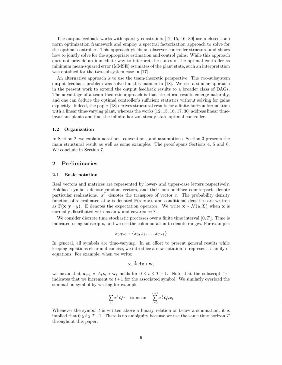
Note that all vectors and matrices in (13) are merely rearrangements of correspondingvectors and matrices in (2). However, the new expression of (13) has an importantstructural property. Namely, if we split A, B, and C into blocks according to the sixstates of the aggregated system, they will have a sparsity pattern that conforms to thegraph of Figure 8. We will show that despite being a coarser representation of the systemdynamics, Figure 8 captures the structure that is relevant to node j for the purpose ofdetermining optimal decisions.

1 2

3 4

5 6

S =

⎡⎢⎢⎢⎢⎢⎢⎢⎢⎢⎢⎢⎣

1 0 0 0 0 00 1 0 0 0 01 0 1 0 0 00 1 0 1 0 01 1 1 0 1 01 1 0 1 0 1

⎤⎥⎥⎥⎥⎥⎥⎥⎥⎥⎥⎥⎦Figure 9: Six-node aggregated DAG and associated sparsity pattern.

4.4 The six-node centralized problem

If we adopt the aggregated representation of systems dynamics based on the aggregatedgraph centered at j, the overall multitree “looks like” the six-node graph of Figure 9. Thesix-node graph and the corresponding sparsity pattern S given in Figure 9 are universalin the sense that we get the same sparsity pattern regardless of which j ∈ V is chosen tocenter the aggregation Gj . Of course, some nodes in the aggregated graph may be empty.For example, if j is a leaf node, then nodes j⇊, j∨ are empty.

Motivated by the universality of the graph in Figure 9, we will now investigate aninstance of Problem 1 corresponding to this graph. We will however assume that node 3is the only decision-maker, and that all observation processes other than the measurementat node 3 is identically zero.

Therefore, we may write the dynamics of the six-node problem as

⎡⎢⎢⎢⎢⎢⎢⎢⎢⎢⎢⎢⎣

x1

+

x2+

x3+

x4+

x5+

x6

+

⎤⎥⎥⎥⎥⎥⎥⎥⎥⎥⎥⎥⎦

t=

⎡⎢⎢⎢⎢⎢⎢⎢⎢⎢⎢⎢⎣

A11 0 0 0 0 00 A22 0 0 0 0

A31 0 A33 0 0 00 A42 0 A44 0 0

A51 A52 A53 0 A55 0A61 A62 0 A64 0 A66

⎤⎥⎥⎥⎥⎥⎥⎥⎥⎥⎥⎥⎦

⎡⎢⎢⎢⎢⎢⎢⎢⎢⎢⎢⎢⎣

x1

x2

x3

x4

x5

x6

⎤⎥⎥⎥⎥⎥⎥⎥⎥⎥⎥⎥⎦+⎡⎢⎢⎢⎢⎢⎢⎢⎢⎢⎢⎢⎣

00

B33

0B53

0

⎤⎥⎥⎥⎥⎥⎥⎥⎥⎥⎥⎥⎦u3 +

⎡⎢⎢⎢⎢⎢⎢⎢⎢⎢⎢⎢⎣

w1

w2

w3

w4

w5

w6

⎤⎥⎥⎥⎥⎥⎥⎥⎥⎥⎥⎥⎦y3 t= C31x

1 +C33x3 + v3

(14)

18

Controller 3 selects its actions according to a control strategy f3 ∶= (f3

0 , . . . , f3

T−1) of theform

u3

t = f3

t ( i3t ) = f3

t (y3

1∶t−1,u3

1∶t−1 ) for 0 ≤ t ≤ T − 1 (15)

The performance of control strategy f3 is measured by the finite horizon expectedquadratic cost given by

J0(f3) = Ef3(∑t

[xu]T

[Q S

ST R][x

u] + xT

TPfinalxT) (16)

The expectation is taken with respect to the joint probability measure on (x0∶T ,u0∶T−1)induced by the choice of f3. The six-node problem of interest is as follows.

Problem 2 (Six-node centralized LQG). For the model of (3)–(4) and (14)–(15), andsubject to Assumption A2, find a control strategy f3 that minimizes the cost (16).

Problem 2 is clearly a centralized control problem because there is a single decision-maker. The classical LQG result [7] states that the optimal control law is of the formu3t = h

3t (zt) where h3

t is a linear function, and zt = E(xt ∣ i3t ) is the estimate of the globalstate. The additional structure imposed in (14) together with Assumption A2 allows usto refine the classical result. In particular, it suffices to estimate x1

t , x3t , and x5

t .

Theorem 3. The optimal control strategy in Problem 2 is of the form

u3

t = h3

t (z3↕t ) (17)

where z3↕

t = (z1t ,z3t ,z5t ) = E(x3↕

t ∣ i3t ) and h3

t is a linear function. Further, z3↕

has a linearupdate equation of the form

z3↕

+t=

⎡⎢⎢⎢⎢⎢⎣A11 0 0A31 A33 0A51 A53 A55

⎤⎥⎥⎥⎥⎥⎦z3↕ +⎡⎢⎢⎢⎢⎢⎣

0B33

B53

⎤⎥⎥⎥⎥⎥⎦u3 −L(y3 − [C31 C33]z3↑) (18)

where the matrix gain L does not depend on the choice of h3.

Proof. See Appendix A.

Note that the optimal strategies h3t as well as the gains Lt can be explicitly computed

by algebraic Riccati recursions. This fact will not be needed in this paper, but we willmake use of it in Part II.

4.5 A partial separation result for the aggregated graph

Our final preliminary step before the formal proof is to establish a partial separationresult for Problem 1. The classical separation result for centralized LQG control statesthat a controller’s posterior belief on the state is independent of its control strategy [7]. Inparticular, for any two (linear) control strategies f and g in the centralized LQG problem,the conditional mean and the conditional covariance matrix are the same:

Ef (xt∣y0∶t−1, u0∶t−1) = Eg (xt∣y0∶t−1, u0∶t−1) , (19)

Ef ((xt − xt)(xt − xt)T∣y0∶t−1, u0∶t−1) = Eg ((xt − xt)(xt − xt)T∣y0∶t−1, u0∶t−1) , (20)

where xt = Ef (xt∣y0∶t−1, u0∶t−1) = Eg (xt∣y0∶t−1, u0∶t−1).This complete separation of estimation from control strategies does not hold, in general,

for our problem. The following lemma shows how estimation at node j can be separatedfrom some parts of the control strategy profile.

19

Lemma 3. Consider any node j. Consider any fixed choice f = (f1, f2, . . . , fn) of linearcontrol strategies of all n controllers. Then,

1. Ef (xj∨

t , ij∨

t ∣ij↑t ) = 0 and Ef (xj∼

t , ij∼

t ∣ij↑t ) = 0.2. Group the control strategies of the n nodes according to the aggregated graph centered

at j, that is, write f as f = (f j⇈ , f j∨ , f j , f j∼ , f j⇊ , f j∧). Let g be another linear

strategy profile given as g = (gj⇈ , gj∨ , gj , gj∼ , f j⇊ , gj∧). Note that the descendants of

node j have the same control strategies under f and g. Then,

Ef (xj↕

t , ij↕

t ∣ij↑t = ij↑t ) = Eg (xj↕

t , ij↕

t ∣ij↑t = ij↑t ) .

3. Further, let g = (gj⇈ , gj∨ , gj , gj∼ , gj⇊ , gj∧) be any linear control strategy that satisfies

git(ii↑t ) = f it(ii↑t ) +mi

t(ij∨t ), for all i ∈ j⇊. Then,

Ef (xj↕

t , ij↕

t ∣ij↑t = ij↑t ) = Eg (xj↕

t , ij↕

t ∣ij↑t = ij↑t ) .

4. Let g = (gj⇈ , gj∨ , gj , gj∼ , gj⇊ , gj∧) be any linear control strategy that satisfies

git(ii↑t ) = f it(ii↑t ) + ℓit(ij↑t ), for all i ∈ j⇊.

Then, the conditional covariance matrix of (xj↕

t , ij↕

t ,yj↑

t ) given ij↑

t is the same underf and g.

5. Let h = (hj⇈ , hj∨ , hj , hj∼ , hj⇊ , hj∧) be any linear control strategy that satisfies

hit(ii↑t ) = f i

t(ii↑t ) +mit(ij∨t ) + ℓit(ij↑t ), for all i ∈ j⇊.

Then, the conditional covariance matrix of yj↑

t given ij↑

t as well as the conditional

cross covariance between (xj↕

t , ij↕

t ) and yj↑

t given ij↑

t are the same under f and h.

Proof. See Appendix B.

5 Proof of main results

As explained in Section 4.1, we prove the structural results of Theorems 1 and 2 bytraversing the graph from leaf nodes to root nodes. The proof uses mathematical induc-tion, so we begin by stating the induction hypothesis P (s). Recall that G≤s is the unionof G0,G1, . . . ,Gs (see Definition 5).

Proposition P (s).1. There is no loss in optimality in jointly restricting all nodes j ∈ G≤s to strategies of

the form

ujt = ∑

a∈j↑∩G≤sgjat (za↕t ) + ∑

b∈j⇈∩G≥s+1hjbt (ibt) (21)

where gjat (⋅) and h

jbt (⋅) are linear functions and za

↕

t = E(xa↕

t ∣ ia↑t ).

20

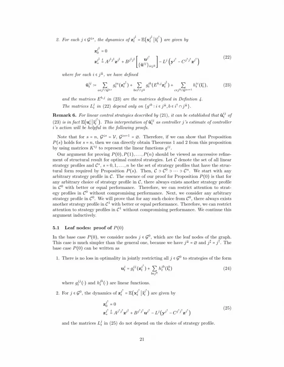
2. For each j ∈ G≤s, the dynamics of zj↕

t = E(xj↕

t ∣ ij↑t ) are given by

zj↕

0= 0

zj↕

+t= Aj↕j↕zj

↕ +Bj↕j↕ [ uj↑

{uij}i∈j⇊] −Lj (yj↑ −Cj↑j↑zj

↑) (22)

where for each i ∈ j⇊, we have defined

uijt ∶= ∑

a∈j↑∩G≤sgiat (za↕t ) + ∑

b∈i↑∩j⇊gibt (Eb,jzj

↕

t ) + ∑c∈j⇈∩G≥s+1

hict (ict), (23)

and the matrices Eb,j in (23) are the matrices defined in Defintion 4.

The matrices Ljt in (22) depend only on {gib ∶ i ∈ j⇊, b ∈ i↑ ∩ j⇊}.

Remark 6. For linear control strategies described by (21), it can be established that uijt of

(23) is in fact E(uit ∣ ij↑t ). This interpretation of uij

t as controller j’s estimate of controlleri’s action will be helpful in the following proofs.

Note that for s = n, G≤s = V , G≥s+1 = ∅. Therefore, if we can show that PropositionP (s) holds for s = n, then we can directly obtain Theorems 1 and 2 from this propositionby using matrices Kij to represent the linear functions gij .

Our argument for proving P (0), P (1), . . . , P (n) should be viewed as successive refine-ment of structural result for optimal control strategies. Let C denote the set of all linearstrategy profiles and Cs, s = 0,1, . . . , n be the set of strategy profiles that have the struc-tural form required by Proposition P (s). Then, C ⊃ C0 ⊃ ⋅ ⋅ ⋅ ⊃ Cn. We start with anyarbitrary strategy profile in C. The essence of our proof for Proposition P (0) is that forany arbitrary choice of strategy profile in C, there always exists another strategy profilein C0 with better or equal performance. Therefore, we can restrict attention to strat-egy profiles in C0 without compromising performance. Next, we consider any arbitrarystrategy profile in C0. We will prove that for any such choice from C0, there always existsanother strategy profile in C1 with better or equal performance. Therefore, we can restrictattention to strategy profiles in C1 without compromising performance. We continue thisargument inductively.

5.1 Leaf nodes: proof of P (0)In the base case P (0), we consider nodes j ∈ G0, which are the leaf nodes of the graph.This case is much simpler than the general one, because we have j⇊ = ∅ and j↕ = j↑. Thebase case P (0) can be written as

1. There is no loss in optimality in jointly restricting all j ∈ G0 to strategies of the form

ujt = g

jjt (zj↑t ) + ∑

b∈j⇈

hjbt (ibt) (24)

where gjjt (⋅) and h

jbt (⋅) are linear functions.

2. For j ∈ G0, the dynamics of zj↑

t = E(xj↑

t ∣ ij↑t ) are given by

zj↑

0= 0

zj↑

+t= Aj

↑j↑

zj↕ +Bj

↑j↑

uj↑ −Lj(yj

↑ −Cj↑j↑

zj↑) (25)

and the matrices Ljt in (25) do not depend on the choice of strategy profile.

21

To prove the above statements, consider any node j ∈ G0 and fix arbitrary linear controlstrategies for all nodes except node j. We will consider the problem of finding the bestcontrol strategy for node j in response to the arbitrary choice of linear control strategiesof all other controllers. We will consider the aggregated graph centered at j and arguethat controller j’s problem can be viewed as an instance of the centralized Problem 2.

Lemma 4. In Problem 1, pick any j ∈ G0 and any fixed linear strategies for all nodesi ≠ j. Then controller j’s optimization problem is an instance of the six-node centralizedproblem with states, measurements, and inputs given by

x1

t =⎡⎢⎢⎢⎢⎣xj⇈

t

ij⇈

t

⎤⎥⎥⎥⎥⎦x2

t = ∅ x3

t = xjt

x4

t = [xj∼

t

ij∼

t

] x5

t = ∅ x6

t =⎡⎢⎢⎢⎣xj∧

t

ij∧

t

⎤⎥⎥⎥⎦y3

t =

⎡⎢⎢⎢⎢⎢⎢⎣

yjt

yj⇈

t

uj⇈

t

⎤⎥⎥⎥⎥⎥⎥⎦u3

t = ujt (26)

Proof. See Appendix C.

Because of Lemma 4 , we can apply the result of Theorem 3 to controller j’s problem.

Therefore, the optimal ujt is a linear function of E(x1

t , x3t ∣ ij↑t ) = E(xj⇈

t , ij⇈

t ,xjt ∣ ij↑t ). Since

ij⇈

t ⊂ ij↑

t , E(ij⇈t ∣ ij↑t ) = ij⇈

t . Therefore, any linear function of E(xj⇈

t , ij⇈

t ,xjt ∣ ij↑t ) can be

written in the form of (24) .

Further, since the (xj↑

t ,yj↑

t ) dynamics are of the form

xj↑

+t= Aj↑j↑xj↑ +Bj↑j↑uj↑

t +wj↑

yj↑ t= Cj

↑j↑

xj↑ + vj

↑

and uj↑

t is a function of yj↑

0∶t−1,uj↑

0∶t−1, it follows that the estimate zj↑

t = E(xj↑

t ∣yj↑

0∶t−1,uj↑

0∶t−1)obeys the standard Kalman estimator update equations given in (25). We can repeat theabove arguments for all leaf nodes. This completes the proof of P (0).5.2 Induction step: proof of P (s) Ô⇒ P (s + 1)Suppose that P (s) holds for some s ≥ 0. We will prove P (s+1) by sequentially consideringeach of the nodes in Gs+1. Note that if Gs+1 is empty then P (s) and P (s+1) are equivalentand the induction step is trivially complete1. Therefore, we focus on the case Gs+1 ≠ ∅.We now focus on a particular node k ∈ Gs+1 and its descendants. Note that uk

t = fkt (ik↑t ),

which can be written asukt = ∑

b∈k↑

hkb(ibt), (27)

for some linear functions hkb(⋅).If j ∈ k⇊, then, by definition of Gs+1, we must have j ∈ G≤s. Therefore, by our induction

hypothesis, controller j’s strategy has the structure specified by (21). Decomposing thesecond summation in (21), we obtain

ujt = ∑

a∈j↑∩G≤sgjat (za↕t ) + ∑

b∈j⇈∩G≥s+1hjbt (ibt)

= ∑a∈j↑∩G≤s

gjat (za↕t ) + ∑

b∈k↑

hjbt (ibt) + ∑

b∈j⇈∩G≥s+1∖k↑hjbt (ibt)

= ∑a∈j↑∩G≤s

gjat (za↕t ) + ujk

t + ∑b∈j⇈∩G≥s+1∖k↑

hjbt (ibt) (28)

1In fact, if Gs+1 is empty, then it is easy to show that all subsequent generations are empty as well and

hence G≤s = V . This implies that Theorems 1 and 2 can be directly obtained from P (s).

22

where we definedujkt ∶= ∑

b∈k↑

hjbt (ibt). (29)

Note that ujkt is the part of the decision uj

t that depends on information available tonode k. Using this observation, we will proceed as follows:

(i) For all j ∈ k⇊, we fix the gja and hjb functions in (28) to arbitrary linear functions.

(ii) We will focus on the control problem of optimally selecting ukt ,{ujk

t }j∈k⇊ based on

the information ik↑

t , which is the information common among node k and all its de-scendants. In other words, we want to optimize the functions hkb(⋅), hjb(⋅) appearingin (27) and (29) while keeping all other parts of the strategy profile fixed.

(iii) Since ukt ,{ujk

t }j∈k⇊ are all to be selected based on the same information ik↑

t , we canview this problem as a coordinated system in which there is a single coordinator at

node k who knows ik↑

t and decides ukt ,{ujk

t }j∈k⇊ .We will make one more observation before analyzing the coordinator’s problem. Note

that for i ∈ j⇊ and j ∈ k⇊, uijt in (23) may be expressed in terms of uik

t as follows.

uijt = ∑

a∈j↑∩G≤sgiat (za↕t ) + ∑

b∈i↑∩j⇊gibt (Eb,jzj

↕

t ) + ∑c∈j⇈∩G≥s+1

hict (ict) (30)

= ∑a∈j↑∩G≤s

giat (za↕t ) + ∑b∈i↑∩j⇊

gibt (Eb,jzj↕

t ) +⎡⎢⎢⎢⎢⎣∑c∈k↑

hict (ict) + ∑

c∈j⇈∩G≥s+1∖k↑hict (ict)

⎤⎥⎥⎥⎥⎦= ∑

a∈j↑∩G≤sgiat (za↕t ) + ∑

b∈i↑∩j⇊gibt (Eb,jzj

↕

t ) +⎡⎢⎢⎢⎢⎣uikt + ∑

c∈j⇈∩G≥s+1∖k↑hict (ict)

⎤⎥⎥⎥⎥⎦, (31)

where we used the definition of uikt from (29). This is permitted because node i too

belongs to k⇊.

As stated in the following lemma, the coordinator’s problem may be viewed as aninstance of the centralized Problem 2.

Lemma 5. In Problem 1, assume that all nodes in G≤s are using strategies of the formprescribed by Proposition P (s). Pick any k ∈ Gs+1. Fix the linear strategies for all nodesa ∉ k↓. For j ∈ k⇊, also fix the gja and hjb in (28). Then the optimization problem forthe coordinator at node k is an instance of the six-node centralized problem with states,measurements, and inputs given by

x1

t = [xk⇈

t

ik⇈

t

] x2

t = [xk∨

t

ik∨

t

] x3

t = xkt

x4

t = [xk∼

t

ik∼

t

] x5

t = [ xk⇊

t{zi↕t }i∈k⇊] x6

t = [xk∧

t

ik∧

t

]y3

t =

⎡⎢⎢⎢⎢⎢⎣ykt

yk⇈

t

uk⇈

t

⎤⎥⎥⎥⎥⎥⎦u3

t = [ ukt{uik

t }i∈k⇊] (32)

Proof. See Appendix D.

Lemma 5 establishes the coordinator’s problem at node k to be a six-node centralizedproblem. This allows us to prove a precursor to P (s+1); a refinement of P (s) that takesinto account the node k ∈ Gs+1.

Lemma 6. Suppose P (s) holds and all nodes in G≤s are using strategies of the formprescribed by P (s). Consider a node k ∈ Gs+1. Then

23

1. There is no loss in optimality in (further) restricting all j ∈ k↓ to strategies of theform

ujt = ∑

a∈j↑∩(G≤s∪{k})

gjat (za↕t ) + ∑

b∈j⇈∩(G≥s+1∖{k})

hjbt (ibt)

2. For each j ∈ k↓, the dynamics of zj↕

t = E(xj↕

t ∣ ij↑t ) are given by

zj↕

0= 0

zj↕

+t= Aj↕j↕zj

↕ +Bj↕j↕ [ uj↑

{uij}i∈j⇊] −Lj (yj↑ −Cj↑j↑zj

↑) (33)

where for each i ∈ j⇊,

uijt = ∑

a∈j↑∩(G≤s∪{k})

giat (za↕t ) + ∑b∈i↑∩j⇊

gibt (Eb,jzj↕

t ) + ∑c∈j⇈∩(G≥s+1∖k)

hict (ict) (34)

and the matrices Ljt in (33) depend only on {gib ∶ i ∈ j⇊, b ∈ i↑ ∩ j⇊}.

Proof. By Lemma 5, the coordinator’s problem at node k is a six-node centralizedproblem. We may therefore apply Theorem 3. It follows that uk

t ,{ujkt }j∈k⇊ are linear

functions of

E(x1

t , x3

t , x5

t ∣ ik↑t ) = E(xk⇈

t , ik⇈

t ,xkt ,x

k⇊

t ,{zi↕t }i∈k⇊ ∣ ik↑t ) (35)

Rearranging the random vectors in the conditional expectation on the right hand side of

(35), we can state that ukt ,{ujk

t }j∈k⇊ are linear functions of (i) E(xk↕

t ∣ ik↑t ), (ii) E(ik⇈t ∣ ik↑t )and (iii) E({zi↕t }i∈k⇊ ∣ ik↑t ). We look at each of the three terms separately. The first term

is, by definition, zk↕

t . The second term is ik⇈

t because ik⇈

t ⊂ ik↑

t . For the third term,

since zi↕

t = E(xi↕

t ∣ ii↑t ) and ii↑

t ⊃ ik↑

t for i ∈ k⇊, it follows from the smoothing property of

conditional expectations that E(zi↕t ∣ ik↑t ) = E[E(xi↕

t ∣ ii↑t ) ∣ ik↑t ] = E(xi↕

t ∣ ik↑t ). Furthermore, if

we partition the ancestors of i as i↑ = k↑ ∪ (i↑ ∩ k⇊) ∪ (i⇈ ∖ k↕), we have

E(xi↕

t ∣ ik↑t ) = (E(xi⇊

t ∣ ik↑t ),E(xk↑

t ∣ ik↑t ),E(xi↑∩k⇊

t ∣ ik↑t ),E(xi⇈∖k↕

t ∣ ik↑t ))= (E(xi⇊

t ∣ ik↑t ),E(xk↑

t ∣ ik↑t ),E(xi↑∩k⇊

t ∣ ik↑t ),0) , (36)

where we used the fact that E(xi⇈∖k↕

t ∣ ik↑t ) = 0 because of the uncorrelated noise conditionin Assumption A2. (Note that node k and a node a ∈ i⇈ ∖ k↕ have a common descendantnamely node i but cannot have a common ancestor by Assumption A1. The same con-clusion could also be inferred from inspecting the aggregated graph centered at node k.)

The remaining non-zero terms in (36) are components from the vector zk↕

t .

We therefore conclude that ukt ,{ujk

t }j∈k⇊ are linear functions of zk↕

t and ik⇈

t . That is,the optimal form of (27) and (29) is

ukt = g

kkt (zk↕t ) + ∑

b∈k⇈

hkb(ibt)ujkt = g

jkt (zk↕t ) + ∑

b∈k⇈

hjb(ibt), for j ∈ k⇊, (37)

24

for some linear functions gkkt (⋅), gjkt (⋅) and {hkbt (⋅), hjb

t (⋅)}b∈k⇈ . Therefore, we havefrom (28) that for j ∈ k⇊,

ujt = ∑

a∈j↑∩G≤sgjat (za↕t ) + ujk

t + ∑b∈j⇈∩G≥s+1∖k↑

hjbt (ibt)

= ∑a∈j↑∩G≤s

gjat (za↕t ) + [gjkt (zk↕t ) + ∑

b∈k⇈

hjbt (ibt)] + ∑

b∈j⇈∩G≥s+1∖k↑hjbt (ibt)

= ∑a∈j↑∩(G≤s∪{k})

gjat (za↕t ) + ∑

b∈j⇈∩G≥s+1∖{k}

hjbt (ibt) (38)

This completes the proof of the first part of Lemma 6.

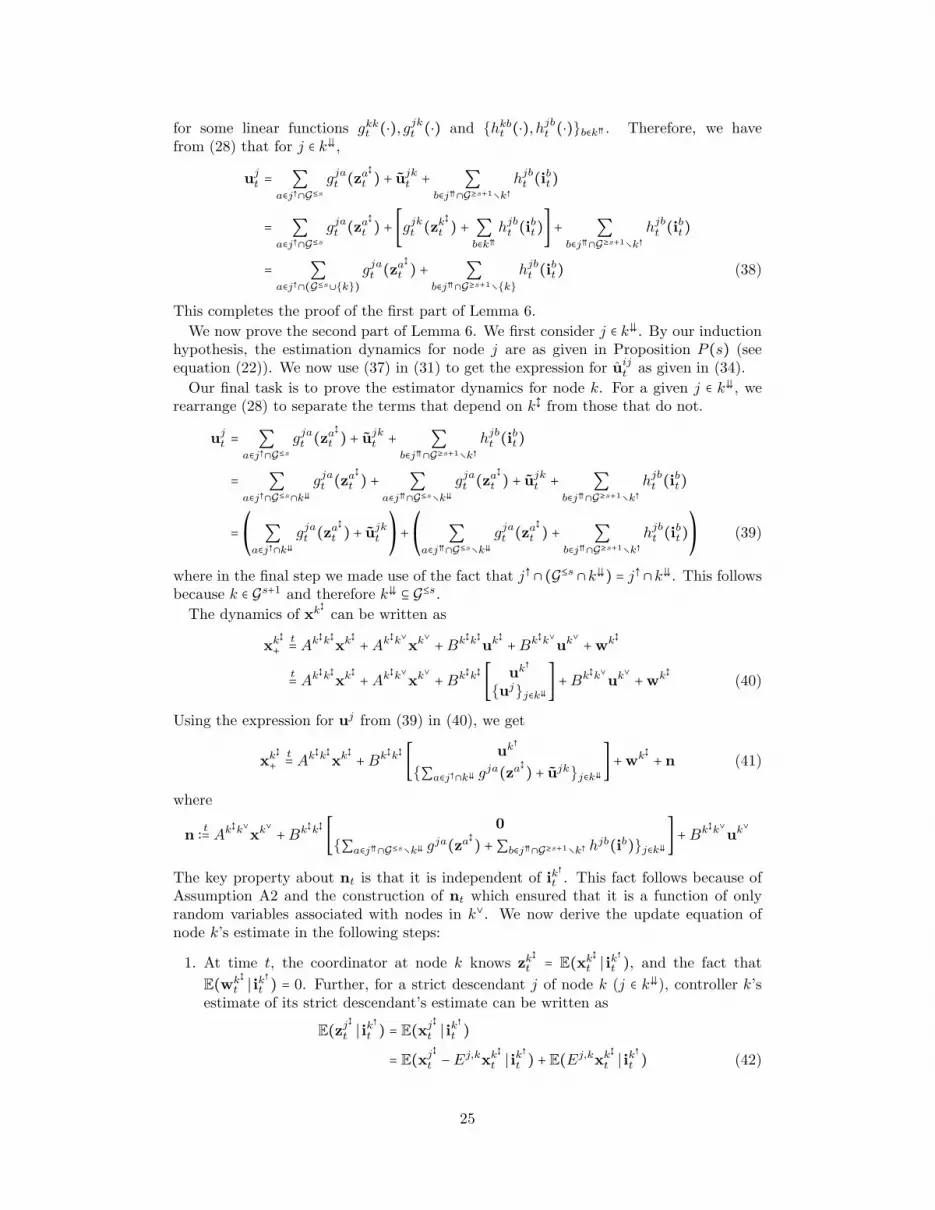
We now prove the second part of Lemma 6. We first consider j ∈ k⇊. By our inductionhypothesis, the estimation dynamics for node j are as given in Proposition P (s) (seeequation (22)). We now use (37) in (31) to get the expression for uij

t as given in (34).

Our final task is to prove the estimator dynamics for node k. For a given j ∈ k⇊, werearrange (28) to separate the terms that depend on k↕ from those that do not.

ujt = ∑

a∈j↑∩G≤sgjat (za↕t ) + ujk

t + ∑b∈j⇈∩G≥s+1∖k↑

hjbt (ibt)

= ∑a∈j↑∩G≤s∩k⇊

gjat (za↕t ) + ∑

a∈j⇈∩G≤s∖k⇊gjat (za↕t ) + ujk

t + ∑b∈j⇈∩G≥s+1∖k↑

hjbt (ibt)

=⎛⎝ ∑a∈j↑∩k⇊

gjat (za↕t ) + ujk

t

⎞⎠ +⎛⎝ ∑a∈j⇈∩G≤s∖k⇊

gjat (za↕t ) + ∑

b∈j⇈∩G≥s+1∖k↑hjbt (ibt)⎞⎠ (39)

where in the final step we made use of the fact that j↑ ∩(G≤s ∩k⇊) = j↑ ∩k⇊. This followsbecause k ∈ Gs+1 and therefore k⇊ ⊆ G≤s.The dynamics of xk

↕

can be written as

xk↕

+t= Ak↕k↕xk↕ +Ak↕k∨xk∨ +Bk↕k↕uk↕ +Bk↕k∨uk∨ +wk↕

t= Ak↕k↕xk↕ +Ak↕k∨xk∨ +Bk↕k↕ [ uk↑

{uj}j∈k⇊] +Bk↕k∨uk∨ +wk↕ (40)

Using the expression for uj from (39) in (40), we get

xk↕

+t= Ak↕k↕xk↕ +Bk↕k↕ [ uk↑

{∑a∈j↑∩k⇊ gja(za↕) + ujk}j∈k⇊] +w

k↕ + n (41)

where

n ∶ t= Ak↕k∨xk∨ +Bk↕k↕ [ 0

{∑a∈j⇈∩G≤s∖k⇊ gja(za↕) +∑b∈j⇈∩G≥s+1∖k↑ h

jb(ib)}j∈k⇊] +Bk↕k∨uk∨

The key property about nt is that it is independent of ik↑

t . This fact follows because ofAssumption A2 and the construction of nt which ensured that it is a function of onlyrandom variables associated with nodes in k∨. We now derive the update equation ofnode k’s estimate in the following steps:

1. At time t, the coordinator at node k knows zk↕

t = E(xk↕

t ∣ ik↑t ), and the fact that

E(wk↕

t ∣ ik↑t ) = 0. Further, for a strict descendant j of node k (j ∈ k⇊), controller k’sestimate of its strict descendant’s estimate can be written as

E(zj↕t ∣ ik↑t ) = E(xj↕

t ∣ ik↑t )= E(xj↕

t −Ej,kxk↕

t ∣ ik↑t ) +E(Ej,kxk↕

t ∣ ik↑t ) (42)

25

where we used the matrices Ej,k of Definition 4 in (42). The term xj↕

t −Ej,kxk↕

t in

(42) is nonzero only for components of xj↑

t that correspond to nodes a ∈ j↕ ∖k↕. Notethat since j ∈ k⇊ and a ∈ j↕ ∖k↕, we have a ∈ k∨. Therefore, by the uncorrelated noiseconditions of Assumption A2, the first conditional expectation in (42) is 0. Thus,

E(zj↕t ∣ ik↑t ) = E(Ej,kxk↕

t ∣ ik↑t ) = Ej,kzk↕

t (43)

2. Let ukt and u

jkt be realizations of the decisions made by the coordinator at node k.

3. The coordinator at node k gets a new vector of observations at time t, yk↑

t . Because

yk↑

t = Ck↑k↑

t xk↑

t + vk↑

t , (44)

this observation vector is correlated with xk↑

t , wk↕

t , and {zj↕t }j∈k⇊ . Using the fact

that E(yk↑

t ∣ ik↑t ) = E(Ck↑k↑

t xk↑

t + vk↑

t ∣ ik↑t ) = Ck↑k↑

t zk↑

t , the controller can use the new

observation vector to obtain the quantities ζxt , ζwt , {ζzj

t }j∈k⇊ defined below.

ζxt ∶= E(xk↕

t ∣ ik↑t ,yk↑

t )= E(xk↕

t ∣ ik↑t ) −Lxt (yk↑

t −Ck↑k↑

t zk↑

t )= zk

↕

t −Lxt (yk↑

t −Ck↑k↑

t zk↑

t )

ζwt ∶= E(wk↕

t ∣ ik↑t ,yk↑

t )= E(wk↕

t ∣ ik↑t ) −Lwt (yk↑

t −Ck↑k↑

t zk↑

t )= 0 −Lwt (yk↑

t −Ck↑k↑

t zk↑

t )ζz

j

t ∶= E(zj↕t ∣ ik↑t ,yk↑

t )= E(zj↕t ∣ ik↑t ) −Lzj

t (yk↑

t −Ck↑k↑

t zk↑

t )= Ej,kzk

↕

t −Lzj

t (yk↑

t −Ck↑k↑

t zk↑

t ) for j ∈ k⇊

(45)

where the matrices Lxt ,Lwt ,L

zj

t depend on the conditional covariance matrices of yk↑

t

given ik↑

t and the conditional cross-covariance of (xk↕

t ,wk↕

t ,zj↕

t ) and yk↑

t given ik↑

t .

The conditional cross-covariance of wk↕

t and yk↑

t can be easily shown to be equal

to the unconditional covariance of wk↕

t and vk↑

t . Because of Lemma 3 part 5, the

conditional covariance matrices of yk↑

t given ik↑

t and the conditional cross-covariance

of (xk↕

t ,zj↕

t ) and yk↑

t given ik↑

t depend only on {gjb ∶ j ∈ k⇊, b ∈ j↑ ∩ k⇊} since all the

other functions in descendants’ strategies either use only ik↑

t or only ik∨

t . This step isthe basic conditional mean update equation of a Gaussian random vector.

4. The state xk↕ evolves according to (41). Therefore,

zk↕

t+1 = E(xk↕

t+1 ∣ ik↑t ,yk↑

t )= Ak↕k↕ζxt +Bk↕k↕ [ uk↑

{∑a∈j↑∩k⇊ gjat (ζza

t ) + ujkt }j∈k⇊] + ζ

wt , (46)

Using (45) in (46) and rearranging the terms that involve (yk↑

t −Ck↑k↑zk↑), we obtain

the estimator dynamics

zk↕

+t= Ak↕k↕zk

↕ +Bk↕k↕ [ uk↑

{∑a∈j↑∩k⇊ gja(Ea,kzk

↕) + ujk}j∈k⇊] −Lk (yk↑ −Ck↑k↑zk

↑)(47)

where the matrices Lkt in (47) depend only on {gjb ∶ j ∈ k⇊, b ∈ j↑ ∩ k⇊}.

26

Substituting ujk = gjkt (zk↕t ) + ∑b∈k⇈ h

jbt (ibt), we obtain that the estimator dynamics for

node k conform to (33). This establishes the required estimator dynamics for node k.

We will now show how to recursively apply Lemma 6 to prove P (s + 1). Suppose thatGs+1 = {k1, . . . , kℓ}. We start with using the result of Lemma 6 for k1. Now considerk2. If k⇊

2∩ k⇊

1= ∅, we can repeat the argument of Lemma 6 to get an analogous result.

Consider then the case when there exists some j ∈ k⇊2∩ k⇊

1. Lemma 6 implies that the

control strategy for j can be written as

ujt = ∑

a∈j↑∩(G≤s∪{k1})

gjat (za↕t ) + ∑

b∈j⇈∩(G≥s+1∖{k1})

hjbt (ibt)

= ∑a∈j↑∩(G≤s∪{k1})

gjat (za↕t ) + ujk2

t + ∑b∈j⇈∩(G≥s+1∖{k1,k

↑2})

hjbt (ibt)

where we defined

ujk2

t ∶= ∑b∈k↑

2

hjbt (ibt)

Similarly, uijt of (34) can be written as

uijt = ∑

a∈j↑∩(G≤s∪{k1})

giat (za↕t ) + ∑b∈i↑∩j⇊

gibt (Eb,jzj↕

t ) + ujk2

t + ∑b∈j⇈∩(G≥s+1∖{k1,k

↑2})

hjbt (ibt)

We can now consider a coordinator at node k2 that selects uk2

t ,{uik2

t }i∈k⇊2

and use the

same argument as in Lemma 6 to argue that uk2

t ,{uik2

t }i∈k⇊2

can be optimally chosen as

functions of zk↕2

t , ik⇈2

t and that the estimator dynamics for zk↕2

t are analogous to the estimatordynamics given in Lemma 6 . Note that because the estimator for the coordinator at nodek1 depended only on {gpq ∶ p, q ∈ k⇊

1}, varying the strategy for coordinator at node k2 will

have no effect on estimation at node k1. The result is that ujt is of the form

ujt = ∑

a∈j↑∩(G≤s∪{k1,k2})

gjat (za↕t ) + ∑

b∈j⇈∩(G≥s+1∖{k1,k2})

hjbt (ibt)

and uijt in the estimation dynamics for j ∈ G≤s are now

uijt = ∑

a∈j↑∩(G≤s∪{k1,k2})

giat (za↕t ) + ∑b∈i↑∩j⇊

gibt (Eb,jzj↕

t ) + ∑b∈j⇈∩(G≥s+1∖{k1,k2})

hjbt (ibt)

It is now clear that the above argument can be repeated for {k3, . . . , kℓ}. We then obtain

ujt = ∑

a∈j↑∩G≤s+1gjat (za↕t ) + ∑

b∈j⇈∩G≥s+2hjbt (ibt)

for j ∈ G≤s+1 and uijt in the estimation dynamics for j ∈ G≤s+1 as

uijt = ∑

a∈j↑∩G≤s+1giat (za↕t ) + ∑

b∈i↑∩j⇊gibt (Eb,jzj

↕

t ) + ∑b∈j⇈∩G≥s+2

hjbt (ibt)

and this establishes P (s + 1).

27

6 Proof modification under Assumption A2’

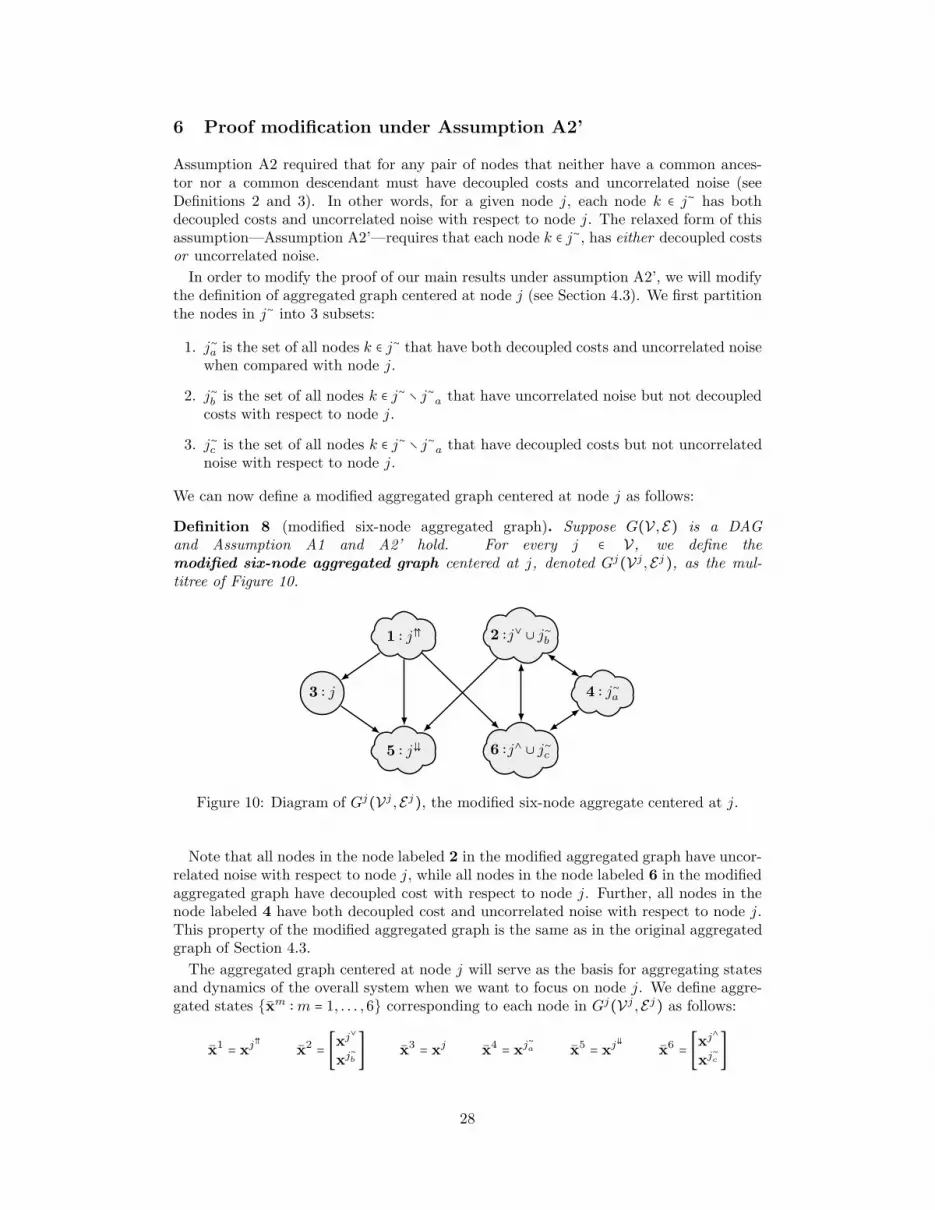
Assumption A2 required that for any pair of nodes that neither have a common ances-tor nor a common descendant must have decoupled costs and uncorrelated noise (seeDefinitions 2 and 3). In other words, for a given node j, each node k ∈ j∼ has bothdecoupled costs and uncorrelated noise with respect to node j. The relaxed form of thisassumption—Assumption A2’—requires that each node k ∈ j∼, has either decoupled costsor uncorrelated noise.

In order to modify the proof of our main results under assumption A2’, we will modifythe definition of aggregated graph centered at node j (see Section 4.3). We first partitionthe nodes in j∼ into 3 subsets:

1. j∼a is the set of all nodes k ∈ j∼ that have both decoupled costs and uncorrelated noisewhen compared with node j.

2. j∼b is the set of all nodes k ∈ j∼ ∖ j∼a that have uncorrelated noise but not decoupledcosts with respect to node j.

3. j∼c is the set of all nodes k ∈ j∼ ∖ j∼a that have decoupled costs but not uncorrelatednoise with respect to node j.

We can now define a modified aggregated graph centered at node j as follows:

Definition 8 (modified six-node aggregated graph). Suppose G(V ,E) is a DAGand Assumption A1 and A2’ hold. For every j ∈ V, we define themodified six-node aggregated graph centered at j, denoted Gj(Vj,Ej), as the mul-titree of Figure 10.

1 ∶ j⇈ 2 ∶j∨ ∪ j∼b

3 ∶ j 4 ∶ j∼a

5 ∶ j⇊ 6 ∶j∧ ∪ j∼c

Figure 10: Diagram of Gj(Vj ,Ej), the modified six-node aggregate centered at j.

Note that all nodes in the node labeled 2 in the modified aggregated graph have uncor-related noise with respect to node j, while all nodes in the node labeled 6 in the modifiedaggregated graph have decoupled cost with respect to node j. Further, all nodes in thenode labeled 4 have both decoupled cost and uncorrelated noise with respect to node j.This property of the modified aggregated graph is the same as in the original aggregatedgraph of Section 4.3.

The aggregated graph centered at node j will serve as the basis for aggregating statesand dynamics of the overall system when we want to focus on node j. We define aggre-gated states {xm ∶m = 1, . . . ,6} corresponding to each node in Gj(Vj ,Ej) as follows:

x1 = xj⇈

x2 = [xj∨

xj∼b] x3 = xj x4 = xj

∼a x5 = xj

⇊

x6 = [xj∧

xj∼c]

28

and define u, y, w, and v in a similar fashion. Once this is done, the aggregated dynamicscentered at j may be written compactly as

x+t= Ax + Bu + w

yt= Cx + v (48)

If we split the matrices A, B and C into blocks according to the states of the modi-fied aggregated graph, they will have a sparsity pattern corresponding to the graph ofFigure 10.

With this redefinition of the aggregated graph, we can proceed along the same steps asin Sections 4 and 5 to establish Theorems 1 and 2 under Assumption A2’.

7 Concluding remarks

In this first part of the paper, we described a broad class of decentralized output feedbackLQG control problems that admit simple and intuitive sufficient statistics. Each controllermust estimate the state of its ancestors and descendants in the underlying DAG. Theoptimal control action for each controller is a linear function of the estimate it computesas well as the estimates computed by all of its ancestors. Moreover, we proved thatestimates can be computed recursively much like a Kalman filter.

Several aspects of the problem architecture influence the structure of the optimal controlstrategies. These are:

F1. measurement type: output feedback or state feedback?

F2. DAG topology: is it a multitree or not?

F3. noise structure: which correlations between subsystems are permitted?

F4. cost structure: which cost couplings between subsystems are permitted?

These items delineate a subset of PN and QI problems, as in Figure 2. In the present work,we assumed output feedback for all subsystems (item F1), but we imposed restrictions onthe DAG topology, noise, and cost via Assumptions A1 and A2 or A2’ (items F2–F4).

The prior works discussed in Section 1 can be classified based on which features F1–F4are strengthened and which are relaxed. For example, the poset-causal framework of [27]considers a fully general DAG topology and quadratic cost (items F2 and F4), but thiscomes at the expense of requiring state-feedback for all nodes and uncorrelated noiseamong subsystems (items F1 and F3).

The complete understanding of which assumptions on features F1–F4 lead to simpleoptimal controllers remains an open issue. Indeed, some seemingly restrictive assumptionsmay still lead to controllers with complicated structures. For example, consider two fullydecoupled subsystems, each with state feedback (items F1 and F2). Then assume theprocess noise is correlated between subsystems and the cost is also coupled (items F3 andF4). This problem was studied in [13, 14], where it was shown that the optimal controllermay have state dimension up to n2, where n is the global state dimension of the plant.

Part II of the paper takes the results of the present paper one step further and derives anexplicit and efficiently computable state-space representation for the optimal controller.As with centralized LQG control problems, the optimal estimation and control gains maybe be computable offline, and the computational complexity is similar as well.

29

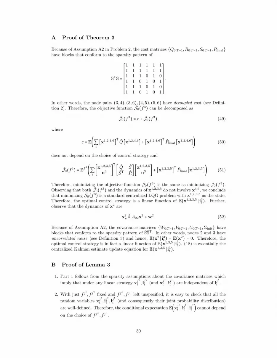
A Proof of Theorem 3

Because of Assumption A2 in Problem 2, the cost matrices {Q0∶T−1,R0∶T−1, S0∶T−1, Pfinal}have blocks that conform to the sparsity pattern of

STS =

⎡⎢⎢⎢⎢⎢⎢⎢⎢⎢⎢⎢⎣

1 1 1 1 1 11 1 1 1 1 11 1 1 0 1 01 1 0 1 0 11 1 1 0 1 01 1 0 1 0 1

⎤⎥⎥⎥⎥⎥⎥⎥⎥⎥⎥⎥⎦.

In other words, the node pairs (3,4), (3,6), (4,5), (5,6) have decoupled cost (see Defini-tion 2). Therefore, the objective function J0(f3) can be decomposed as

J0(f3) = c + J0(f3), (49)

where

c = E(∑t

[x1,2,4,6]T Q [x1,2,4,6] + [x1,2,4,6]T Pfinal [x1,2,4,6]) (50)

does not depend on the choice of control strategy and

J0(f3) = Ef3(∑t

[x1,2,3,5

u3 ]T

[ Q S

ST R] [x1,2,3,5

u3 ] + [x1,2,3,5]T Pfinal [x1,2,3,5]) (51)

Therefore, minimizing the objective function J0(f3) is the same as minimizing J0(f3).Observing that both J0(f3) and the dynamics of x1,2,3,5 do not involve x4,6, we concludethat minimizing J0(f3) is a standard centralized LQG problem with x1,2,3,5 as the state.Therefore, the optimal control strategy is a linear function of E(x1,2,3,5 ∣ i3t ). Further,observe that the dynamics of x2 are

x2

+t= A22x

2 +w2. (52)

Because of Assumption A2, the covariance matrices {W0∶T−1, V0∶T−1, U0∶T−1,Σinit} haveblocks that conform to the sparsity pattern of SST. In other words, nodes 2 and 3 haveuncorrelated noise (see Definition 3) and hence, E(x2 ∣ i3t ) = E(x2) = 0. Therefore, theoptimal control strategy is in fact a linear function of E(x1,3,5 ∣ i3t ). (18) is essentially thecentralized Kalman estimate update equation for E(x1,3,5 ∣ i3t ).

B Proof of Lemma 3

1. Part 1 follows from the sparsity assumptions about the covariance matrices which

imply that under any linear strategy xj∨

t , ij∨

t (and xj∼

t , ij∼

t ) are independent of ij↑

t .

2. With just f j↕ , f j∨ fixed and f j∧ , f j∼ left unspecified, it is easy to check that all the

random variables xj↕

t , ij↕

t , ij↑

t (and consequently their joint probability distribution)

are well-defined. Therefore, the conditional expectation E(xj↕

t , ij↕

t ∣ ij↑t ) cannot dependon the choice of f j∧ , f j∼ .

30

We will now write xj↕

t , ij↕

t in terms of the primitive random variables and the controldecisions:

(xj↕

t , ij↕

t ) ∈ lin(xj↕

0,wj↕

1∶t−1,vj↕

1∶t−1,uj↕

1∶t−1,xj∨

0,wj∨

1∶t−1,vj∨

1∶t−1,uj∨

1∶t−1)∈ lin(xj↕

0,wj↕

1∶t−1,vj↕

1∶t−1,uj↑

1∶t−1,xj∨

0,wj∨

1∶t−1,vj∨

1∶t−1,uj∨

1∶t−1) + lin(uj⇊

1∶t−1) (53)

where the linear functions lin depend only on system parameters. Given the strategy

f j⇊ , we can write

uj⇊

1∶t−1 ∈ linfj⇊ (xj

↕

0,wj

↕

1∶t−1,vj↕

1∶t−1,uj↑

1∶t−1,xj∨

0,wj

∨

1∶t−1,vj∨

1∶t−1,uj∨

1∶t−1) (54)

where the linear function linfj⇊

depends on f j⇊ . Combining (53) and (54) andregrouping terms, we can write

(xj↕

t , ij↕

t ) ∈ linfj⇊ (xj↕

0,wj↕

1∶t−1,vj↕

1∶t−1,uj↑

1∶t−1) + linfj⇊ (xj∨

0,wj∨

1∶t−1,vj∨

1∶t−1,uj∨

1∶t−1) (55)

Because of the sparsity assumptions about covariance matrices, the second term in

(55) is independent of ij↑

t . Therefore, under any linear strategy f , the conditional

expectation of the second term in (55) given ij↑

t is 0.

By linearity of conditional expectation,

E(xj↕

t , ij↕

t ∣ ij↑t ) ∈ linfj⇊ (E(xj↕

0,wj↕

0∶t−1,vj↕

0∶t−1,uj↑

0∶t−1 ∣ ij↑t ))∈ linfj⇊ (E(xj↕

0,wj↕

0∶t−1,vj↕

0∶t−1,uj↑

0∶t−1 ∣ yj↑0∶t−1, uj↑

0∶t−1))∈ linfj⇊ (uj↑

0∶t−1,E(xj↕

0,wj↕

0∶t−1,vj↕

0∶t−1 ∣ yj↑0∶t−1, uj↑

0∶t−1)) (56)

Note that yj↑

0∶t−1 can be written as F

⎡⎢⎢⎢⎢⎢⎢⎣xj↑

0

wj↑

0∶t−1

vj↑

0∶t−1

⎤⎥⎥⎥⎥⎥⎥⎦+ Guj↑

0∶t−1, where F ,G depend only on

system parameters and not on any node’s strategy. Therefore,

E(xj↕

0,wj

↕

0∶t−1,vj↕

0∶t−1 ∣yj↑0∶t−1, uj↑

0∶t−1)

= E⎛⎜⎜⎝x

j↕

0,wj↕

0∶t−1,vj↕

0∶t−1

RRRRRRRRRRRRRRRRRF

⎡⎢⎢⎢⎢⎢⎢⎣

xj↑

0

wj↑

0∶t−1

vj↑

0∶t−1

⎤⎥⎥⎥⎥⎥⎥⎦+ Guj↑

0∶t−1 = yj↑

0∶t−1,uj↑

0∶t−1 = uj↑

0∶t−1

⎞⎟⎟⎠

= E⎛⎜⎜⎝x

j↕

0,wj↕

0∶t−1,vj↕

0∶t−1

RRRRRRRRRRRRRRRRRF

⎡⎢⎢⎢⎢⎢⎢⎣

xj↑

0

wj↑

0∶t−1

vj↑

0∶t−1

⎤⎥⎥⎥⎥⎥⎥⎦+ Guj↑

0∶t−1 = yj↑

0∶t−1

⎞⎟⎟⎠ (57)

= E⎛⎜⎜⎝x

j↕

0,wj↕

0∶t−1,vj↕

0∶t−1

RRRRRRRRRRRRRRRRRF

⎡⎢⎢⎢⎢⎢⎢⎣xj↑

0

wj↑

0∶t−1

vj↑

0∶t−1

⎤⎥⎥⎥⎥⎥⎥⎦= yj

↑

0∶t−1 − Guj↑

0∶t−1

⎞⎟⎟⎠ (58)

where we removed uj↑

0∶t−1 from conditioning in (57) since it is a function of yj↑

0∶t−1

which is already included in the conditioning. Since all random variables appearingin (58) are only primitive random variables, the conditional expectation does not

31

depend on the choice of strategy f . Recall that the linear function in (56) depends

only on f j⇊

. Therefore, if gj⇊

= f j⇊

, then

Eg (xj

↕

t , ij↕

t ∣ij↑t = ij↑t ) = Ef (xj↕

t , ij↕

t ∣ij↑t = ij↑t )3. Under the new strategy g, we can write (54) as

uj⇊

1∶t−1 ∈ linfj⇊ (xj↕

0,wj↕

1∶t−1,vj↕

1∶t−1,uj↑

1∶t−1,xj∨

0,wj∨

1∶t−1,vj∨

1∶t−1,uj∨

1∶t−1)+ linmj⇊ (xj∨

0,wj∨

1∶t−1,vj∨

1∶t−1,uj∨

1∶t−1) (59)

and combine this with (53) to get

(xj↕

t , ij↕

t ) ∈ linfj⇊ (xj↕

0,wj↕

1∶t−1,vj↕

1∶t−1,uj↑

1∶t−1) + linfj⇊ (xj∨

0,wj∨

1∶t−1,vj∨

1∶t−1,uj∨

1∶t−1)+ linmj⇊ (xj∨

0,wj∨

1∶t−1,vj∨

1∶t−1,uj∨

1∶t−1) (60)

By the same argument as in part 2, the last term is independent of ij↑

and therefore

its estimate is 0 for any choice of mj⇊ . The rest of the proof is the same as in part 2.

4. To prove Part 4, we make the following observation about conditional means: Con-sider jointly Gaussian random vectors A and B. Define linear combinations of theseas follows.

C ∶= K(A), D ∶= C +L(B),where K,L are linear functions. Then, with probability 1,

C − E(C ∣B) =D −E(D ∣B)and hence the conditional distribution of the random vector (C − E(C ∣B)) givenB = b is the same as the conditional distribution of the random vector (D−E(D ∣B))given B = b. In other words, when the difference between C and D is measurablewith respect to B, the conditional distribution of the estimation error of C given B

and D given B are the same.

In Part 4, the difference between the strategy profiles f and g is due to the functions

ℓit(ij↑t ) in the strategies of descendants of j. Because this function is measurable withrespect to j’s information, node j can account for its effect without changing theerror. More precisely, under the new strategy g, we can write

uj⇊

1∶t−1 ∈ linfj⇊ (xj↕

0,wj↕

1∶t−1,vj↕

1∶t−1,uj↑

1∶t−1,xj∨

0,wj∨

1∶t−1,vj∨

1∶t−1,uj∨

1∶t−1) + linℓj⇊ (ij↑t ) (61)

and use it with with (53) and the observation equation from (1) to get that understrategy g

(xj↕

t , ij↕

t ,yj↑

t ) ∈ linfj⇊ (xj↕

0,wj

↕

1∶t−1,vj↕

1∶t,uj↑

1∶t−1) + linfj⇊ (xj∨

0,wj

∨

1∶t−1,vj∨

1∶t−1,uj∨

1∶t−1)+ linℓj

⇊ (ij↑t ) (62)

Under the original strategy f , (62) would have been

(x∗,j↕t , i∗,j↕

t ,y∗,j↑

t ) ∈ linfj⇊ (xj↕

0,wj↕

1∶t−1,vj↕

1∶t,uj↑

1∶t−1)+linfj⇊ (xj∨

0,wj∨

1∶t−1,vj∨

1∶t−1,uj∨

1∶t−1),(63)

32

where we use ∗ to indicate that these random variables are defined under a differentstrategy than those in (62).

Then, using the argument above with ij↑

t playing the role of random vector B andthe right hand sides of (63) and (62) playing the roles of C and D respectively, wecan state that the conditional distribution of the vector

((x∗,j↕t , i∗,j↕

t ,y∗,j↑

t )) −Ef (x∗,j↕t , i∗,j↕

t ,y∗,j↑

t ∣ij↑t = ij↑t ))given i

j↑

t when the strategy profile is f is the same as the the conditional distributionof the vector ((xj↕

t , ij↕

t ,yj↑

t )) − Eg (xj↕

t , ij↕

t ,yj↑

t ∣ij↑t = ij↑t ))given i

j↑

t when the strategy profile is g. Consequently, the corresponding conditionalcovariance matrices are the same.

5. Because of Part 4, we can remove the functions ℓit(ij↑t ) while computing conditionalcovariances.

The random vector yj↑

t , ij↑

t can be written in terms of primitive random variables andcontrol decisions as

(yj↑

t , ij↑

t ) ∈ lin(xj↑

0,wj↑

1∶t−1,vj↑

1∶t,uj↑

1∶t−1),where the lin function depends only on system parameters. Using arguments similarto those used to get (57), (58), it can be seen that the conditional distribution of

yj↑

t given ij↑

t does not depend on the strategy profile. Therefore, the conditional

covariance of yj↑

t given ij↑

t will not depend on the choice of mit(ij∨t ), i ∈ j⇊.

For the cross-covariance matrix between (xj↕

t , ij↕

t ) and yj↑

t given ij↑

t , we use (60) for

computing (xj↕

t , ij↕

t )yj↑,Tt and once again use the independence of ij

∨

t and yj↑

t , ij↑

t to

remove the terms that depend on the functions mit(ij∨t ).

C Proof of Lemma 4

For a leaf node j, since j⇊ = j∨ = ∅, the aggregated graph centered at j looks likeFigure 11. If strategies of all nodes except node j are fixed, then controller j’s optimizationproblem is a centralized problem. We will now show that with the state, measurement andcontrol definitions of (26), the system dynamics, the cost and the information structureof controller j’s problem are identical to the centralized Problem 2.

1 ∶ j⇈

3 ∶ j

4 ∶ j∼

6 ∶ j∧

Figure 11: The aggregated graph centered at leaf node j.

Given a node i ∈ V , the state equations (1) and information structure (5) imply that

xit+1 ∈ lin(xi↑

t ,ui↑

t ,wit) yi

t ∈ lin(xi↑

t ,vit) iit+1 ∈ lin(iit,yi

t,uit) (64)

33

Given the fixed strategies for nodes i ≠ j, the input definition (7) implies that uit ∈ lin(ii↑t )

for all i ≠ j which further implies that ui↑

t ∈ lin(ii↑t ). Combining these facts, we deducethat

[xit+1

iit+1] ∈ lin([xi↑

t

ii↑

t

] , [wit

vit

]) for i ≠ j (65)

We now apply (65) to different possible subsets of V as identified in Figure 11. Forexample, since j⇈ and j∼ are equal to their respective ancestral sets,

x1

t+1 ∈ lin⎛⎝x1

t ,

⎡⎢⎢⎢⎢⎣wj

⇈

t

vj⇈

t

⎤⎥⎥⎥⎥⎦⎞⎠ and x4

t+1 ∈ lin(x4

t , [wj∼

t

vj∼

t

]) (66)

For the sibling set, if k ∈ j∧, then k↑ ⊆ j⇈ ∪ j∧ ∪ j∼. Therefore we obtain

x6

t+1 ∈ lin⎛⎝x1

t , x4

t , x6

t ,⎡⎢⎢⎢⎣wj

∧

t

vj∧

t

⎤⎥⎥⎥⎦⎞⎠ (67)

For xjt , we have xj

t+1 ∈ lin(xj↑

t ,uj↑

t ,wjt ). Splitting j↑ = {j} ∪ j⇈, we obtain

x3

t+1 ∈ lin(x1

t , x3

t ,ujt ,w

jt) (68)

A similar argument can be used to conclude that

y3

t ∈ lin(x1

t , x3

t ,vj↑

t ) (69)

It follows from (66)–(69) that the dynamics of controller j’s problem have the samestructure as the dynamics of Problem 2 given in (14).

It is clear that the information available to controller j can be written as {y3

0∶t−1, u3

0∶t−1}.Further, the cost and covariance matrices have the sparsity structure required in Prob-lem 2.

D Proof of Lemma 5

We will show that with the state, measurement and control definitions of (32), the systemdynamics, the cost and the information structure of the coordinator’s problem are identi-cal to the centralized Problem 2. As in the proof of Lemma 4, (64) still holds. Followingan argument analogous to the one used in proving Lemma 4, it follows that

x1

t+1 ∈ lin(x1

t , [wk⇈

t

vk⇈

t

]) , x2

t+1 ∈ lin(x2

t , [wk∨

t

vk∨

t

]) (70)

x4

t+1 ∈ lin(x2

t , x4

t , [wk∼

t

vk∼

t

]) , x6

t+1 ∈ lin(x1

t , x2

t , x4

t , x6

t , [wk∧

t

vk∧

t

]) (71)

x3

t+1 ∈ lin(x1

t , x3

t ,ukt ,w

kt ) and y3

t ∈ lin(x1

t , x3

t ,vk↑

t ) (72)

Consider j ∈ k⇊. We have that

xjt+1 ∈ lin(xj↑

t ,uj↑

t ,wjt) (73)

34

Note that j↑ ⊆ k⇊ ∪ {k} ∪ k⇈ ∪ k∨. Therefore, (73) can be written as

xjt+1 ∈ lin(xj↑

t ,uj↑

t ,wjt )

∈ lin(xk⇊

t ,uk⇊

t ,xkt ,u

kt ,x

k⇈

t ,uk⇈

t ,xk∨

t ,uk∨

t ,wjt ) (74)

Using (28) for uk⇊

t and the fact that for c ∈ k∨ ∩ G≤s, zc↕t ∈ lin(ik∨t ) in (74), we get

xjt+1 ∈ lin(xk

⇊

t ,{zi↕t , uikt }i∈k⇊ , ik∨t ,xk

t ,ukt ,x

k⇈

t ,uk⇈

t ,xk∨

t ,uk∨

t ,wjt)

∈ lin(xk⇊

t ,{zi↕t , uikt }i∈k⇊ , ik∨t ,xk

t ,ukt ,x

k⇈

t , ik⇈

t ,xk∨

t ,wjt ) (75)

where we used the fact that given the linear strategy of k⇈, k∨, uk⇈

t ∈ lin(ik⇈t ) and uk∨

t ∈lin(ik∨t ). Grouping the various terms in (75) gives

xjt+1 ∈ lin(x1

t , x2

t , x3

t , x5

t , u3

t ,wjt) (76)

Now we turn to the dynamics of zj↕

for j ∈ k⇊. From (22) we have

zj↕

t+1 ∈ lin(zj↕t ,uj↑

t ,{uijt }i∈j⇊ ,yj↑

t ) (77)

We will focus on the terms uj↑

t ,{uijt }i∈j⇊ ,yj↑

t appearing in (77).

• uj↑

t : Using arguments similar to those used to get (75), we get

uj↑

t ∈ lin({zi↕t , uikt }i∈k⇊ , ik∨t , ik

⇈

t ,ukt ) (78)

• {uijt }i∈j⇊ : Using (31), we get

{uijt } ∈ lin({za↕t , uak

t }a∈k⇊ , ik∨t ) (79)

• yj↑

t : From the system model, we can write

yj↑

t ∈ lin(xk⇈

t ,xkt ,x

k⇊

t ,xk∨

t vj↑

t ) (80)

Combining (77)-(80), we get

zj↕

t+1 ∈ lin(zj↕t ,{zi↕t , uikt }i∈k⇊ , ik∨t , ik

⇈

t ,ukt ,x

k⇈

t ,xkt ,x

k⇊

t ,xk∨

t vj↑

t ) (81)

Grouping the various terms in (81), we get

zj↕

t+1 ∈ lin(x1

t , x2

t , x3

t , x5

t , u3

t ,vj↑

t ) (82)

Combining (76) and (82), we conclude that x5t+1 ∈ lin(x1

t , x2t , x

3t , x

5t , u

3t , wt), as required,

where wt ∈ lin(wjt ,v

j↑

t ), j ∈ k⇊ is an aggregated noise term. Therefore, the dynamicsof coordinator’s problem are identical to the dynamics of Problem 2 given in (14). Itis clear that the information available to the coordinator at node j can be written as

{y30∶t−1, u

30∶t−1}. Further, the cost and covariance matrices have the sparsity structure

required in Problem 2.

35

References

[1] B. Bamieh and P. G. Voulgaris. A convex characterization of distributed controlproblems in spatially invariant systems with communication constraints. Systems &Control Letters, 54(6):575–583, 2005.

[2] V. D. Blondel and J. N. Tsitsiklis. A survey of computational complexity results insystems and control. Automatica, 36(9):1249–1274, 2000.

[3] T. H. Cormen, C. E. Leiserson, R. L. Rivest, and C. Stein. Introduction to algorithms,volume 2. MIT press Cambridge, 2001.

[4] P. Grover, S. Y. Park, and A. Sahai. Approximately optimal solutions to the finite-dimensional Witsenhausen counterexample. IEEE Transactions on Automatic Con-trol, 58(9):2189–2204, Sept 2013.

[5] Y.-C. Ho and K.-C. Chu. Team decision theory and information structures in optimalcontrol problems—Part I. IEEE Transactions on Automatic Control, 17(1):15–22,1972.

[6] J.-H. Kim and S. Lall. Separable optimal cooperative control problems. In AmericanControl Conference, pages 5868–5873, 2012.

[7] P. Kumar and P. Varaiya. Stochastic Systems: Estimation, Identification and Adap-tive Control. Prentice-Hall, 1986.

[8] B.-Z. Kurtaran and R. Sivan. Linear-quadratic-gaussian control with one-step-delaysharing pattern. Automatic Control, IEEE Transactions on, 19(5):571–574, 1974.

[9] A. Lamperski and J. C. Doyle. Dynamic programming solutions for decentralizedstate-feedback LQG problems with communication delays. In American ControlConference, pages 6322–6327, 2012.

[10] A. Lamperski and J. C. Doyle. Output feedbackH2 model matching for decentralizedsystems with delays. arXiv preprint, Sept 2012. http://arxiv.org/abs/1209.3600.

[11] A. Lamperski and L. Lessard. Optimal state-feedback control under sparsity anddelay constraints. In IFAC Workshop on Distributed Estimation and Control inNetworked Systems, pages 204–209, 2012.

[12] L. Lessard. Decentralized LQG control of systems with a broadcast architecture. InIEEE Conference on Decision and Control, pages 6241–6246, 2012.

[13] L. Lessard. Optimal control of a fully decentralized quadratic regulator. In AllertonConference on Communication, Control, and Computing, pages 48–54, 2012.

[14] L. Lessard. A separation principle for decentralized state-feedback optimal control.In Allerton Conference on Communication, Control, and Computing, pages 528–534,2013.

[15] L. Lessard and S. Lall. A state-space solution to the two-player decentralized op-timal control problem. In Allerton Conference on Communication, Control, andComputing, pages 1559–1564, 2011.

[16] L. Lessard and S. Lall. Optimal controller synthesis for the decentralized two-playerproblem with output feedback. In American Control Conference, pages 6314–6321,2012.

[17] L. Lessard and S. Lall. Optimal control of two-player systems with output feedback.arXiv preprint, Mar 2013. http://arxiv.org/abs/1303.3644.

36

[18] L. Lessard and A. Nayyar. Structural results and explicit solution for two-player LQGsystems on a finite time horizon. In IEEE Conference on Decision and Control, pages6542–6549, 2013.

[19] A. Mahajan, N. Martins, M. Rotkowitz, and S. Yuksel. Information structures inoptimal decentralized control. In IEEE Conference on Decision and Control, pages1291–1306, 2012.

[20] A. Mahajan, N. C. Martins, and S. Yuksel. Static LQG teams with countably infiniteplayers. In IEEE Conference on Decision and Control, pages 6765–6770, 2013.

[21] A. Nayyar, A. Mahajan, and D. Teneketzis. Decentralized stochastic control withpartial history sharing: A common information approach. IEEE Transactions onAutomatic Control, 58(7):1644–1658, 2013.

[22] N. Nayyar, D. Kalathil, and R. Jain. Optimal decentralized control in unidirec-tional one-step delayed sharing pattern. In Allerton Conference on Communication,Control, and Computing, pages 374–380, 2013.

[23] X. Qi, M. Salapaka, P. Voulgaris, and M. Khammash. Structured optimal and robustcontrol with multiple criteria: a convex solution. IEEE Transactions on AutomaticControl, 49(10):1623–1640, 2004.

[24] R. Radner. Team decision problems. The Annals of Mathematical Statistics,33(3):857–881, 1962.

[25] M. Rotkowitz and S. Lall. A characterization of convex problems in decentralizedcontrol. IEEE Transactions on Automatic Control, 51(2):274–286, 2006.

[26] N. Sandell, Jr. and M. Athans. Solution of some nonclassical LQG stochastic decisionproblems. IEEE Transactions on Automatic Control, 19(2):108–116, 1974.

[27] P. Shah and P. Parrilo. H2-optimal decentralized control over posets: A state-spacesolution for state-feedback. IEEE Transactions on Automatic Control, 58(12):3084–3096, Dec 2013.

[28] J. Swigart and S. Lall. An explicit state-space solution for a decentralized two-player optimal linear-quadratic regulator. In American Control Conference, pages6385–6390, 2010.

[29] J. Swigart and S. Lall. Optimal controller synthesis for a decentralized two-playersystem with partial output feedback. In American Control Conference, pages 317–323, 2011.

[30] T. Tanaka and P. A. Parrilo. Optimal output feedback architecture for triangularLQG problems. In American Control Conference, pages 5730–5735, 2014.

[31] P. Varaiya and J. Walrand. On delayed sharing patterns. IEEE Transactions onAutomatic Control, 23(3):443–445, 1978.

[32] H. S. Witsenhausen. A counterexample in stochastic optimum control. SIAM Journalon Control, 6(1):131–147, 1968.

[33] T. Yoshikawa. Dynamic programming approach to decentralized stochastic controlproblems. In IEEE Conference on Decision and Control, volume 13, pages 185–190,1974.

[34] S. Yuksel. Stochastic nestedness and the belief sharing information pattern. IEEETransactions on Automatic Control, 54(12):2773–2786, Dec 2009.

37