AEI-2011-076

Coherent states in quantum gravity:a construction based on the flux representation of LQG

Daniele Oritia, Roberto Pereiraa,b and Lorenzo Sindonia

a) Max Planck Institute for Gravitational Physics, Albert Einstein Institute,Am Muehlenberg 1, 14467 Golm, Germany, EU

b) Instituto de Cosmologia Relatividade Astrofisica ICRA - CBPF,

Rua Dr. Xavier Sigaud, 150, CEP 22290-180, Rio de Janeiro, Brazil

(Dated: April 23, 2012)

As part of a wider study of coherent states in (loop) quantum gravity, we introduce a modification tothe standard construction, based on the recently introduced (non-commutative) flux representation.The resulting quantum states have some welcomed features, in particular concerning peakednessproperties, when compared to other coherent states in the literature.

I. INTRODUCTION

Coherent states are an essential tool in the study of any quantum system, being best suited to studythe correspondence with the underlying classical description of the same system, and the role ofquantum fluctuations that modify it. A general review of coherent states, applied to a variety ofphysical phenomena can be found in [1]. In a quantum gravity context, when a concrete definitionof the (kinematical) state space of the theory is available, they are then the natural tool for testingthe semi-classical limit. Indeed, in the context of loop quantum gravity [2], they have been usedextensively both in the canonical [3, 4, 6, 7] and in the spin foam (see, for example, [9, 11]) settings,where they define boundary states that can approximate discrete classical geometries.

Loop quantum gravity states are generically given by superpositions of states which have support ongraphs, which can be thought of as embedded in a smooth spatial manifold or not, depending on thecontext1; each graph represents a truncation of the geometric degrees of freedom of the full, continuumtheory. Looking at the classical phase space of the theory, this comes about as follows (we refer to [2]for more details). The continuum canonical phase space is parametrized by a pair of fields (e(x), A(x)),representing the triad field and the (Ashtekar) connection field. In order to pass to a set of variableswith nicer transformation properties under gauge transformations and easier to deal with from theanalytic point of view, one then considers all possible piecewise-analytic paths γ and 2-surfaces Sembedded in the spatial manifold and smeared canonical variables given by parallel transports hγ(path-ordered exponentials) of the connection along the paths, and fluxes ES , i.e. integrals of the(dualized and densitized) triad field over the surfaces. The resulting commutation relations are very

1 The canonical approach starts off in a continuum setting, and works with embedded graphs, even though most of theembedding, continuum information is then removed by the imposition of diffeomorphism invariance. The spin foamformulation is usually framed in a simplicial context, where the graphs used are dual to simplicial decompositions ofa spatial manifold, but no embedding is assumed; often they are also interpreted as abstract, purely combinatorialgraphs. These different interpretations and settings do not affect our analysis, which applies to all of them.

arX

iv:1

110.

5885

v2 [

gr-q

c] 2

0 A

pr 2

012

2

complicated in general, as one has to keep track of the intersections between paths and surfaces. Stillone recognizes in them the conjugate nature of holonomies of the connection and fluxes of triad. Also,one sees that the flux variables do not (Poisson) commute, indicating a fundamental non-commutativenature of such variables already at the classical level, which should then be taken into account in thequantum theory [12]. This is the classical motivation for the non-commutative flux representation[23] for LQG quantum states we use in this paper (and used in a spin foam and GFT [17] context in[18, 19]). From generic paths embedded in the spatial manifold one then passes to graphs formed bysuch paths and their intersection points, which allows to have a better control over the local gaugetransformations acting on the canonical variables (which act, indeed, at such intersection points). Toeach such graph (with N links) one then associates the Hilbert space, in the connection representation,L2(SU(2)×N/SU(2)×V ) defined by dividing by the action of the internal group on the nodes V of thegraph. The canonical structure simplifies when one considers individual links of the graphs andelementary surfaces intersecting such link at single points (so that there is a 1-1 correspondencebetween link e and surface S). In this case, the canonical brackets become:[

Eie, he

]= i~(8πGγ)Ri . h,[

Eie, Eje′

]= i~(8πGγ)εijk δe,e′E

ke ,[

he′ , he

]= 0,

where ~(8πGγ) = 8πl2pγ has the dimension of a length squared2. One recognizes the (quantization of)the canonical brackets of the cotangent bundle of SU(2), T ∗SU(2), for each link e of the graph.

Given that we are going to work with functions and operators on functions defined on group manifoldswithout connecting them to physical measurements, at least at this level, it is convenient to workwith dimensionless variables, reabsorbing the dimensionful quantity 8πGγ~ into the definition ofdimensionless flux operators, which will still be denoted as Eie, in such a way that the fundamentalalgebra reads [

Eie, he

]= iωRi . h,[

Eie, Eje′

]= iωεijk δe,e′E

ke ,[

he′ , he

]= 0,

where ω is an arbitrary dimensionless parameter.

The construction of coherent states in such setting has then as main goal the identification of kine-matical states that are semi-classical in the sense that they peak, with minimal uncertainties, aroundclassical phase space points of the continuum theory. It is then clear that one has to face severalconceptual and technical issues, among which: a) the detail of the approximation of continuum ge-ometries by data associated to graphs and thus approximating at best discrete truncation of the samecontinuum geometries; b) the definition of coherent states for such discrete geometries; c) the roleand treatment of the sum over graphs to recover continuum configurations; d) the role of severalapproximation scales in the same procedure; e) the identification of the appropriate set of observ-

2 We are using units in which c = 1.

3

ables with respect to which the approximation is best obtained; f) the construction of quantum statesthat are coherent with respect to such observables. The list is not exhaustive. Many such issues arediscussed in [3, 4, 6, 7]. However, because of the structure of the kinematical state space of LQG,the construction of coherent states for quantum gravity necessarily has as starting point the study ofsuitably defined semi-classical states for the degrees of freedom associated to individual edges of thegraphs on which such states are based, that is for coherent states based on a T ∗SU(2) phase space.

More precisely, the standard construction is based on work by Hall [5], who defines a coherent statetransform for compact Lie groups, in analogy to the Segal–Bargmann transform for the real line. Onethen lifts this construction to theories of connections based on graphs by taking tensor products ofHall states, one per edge of the graph, as explained in [6]. The properties of those states have beenextensively studied in a series of papers [3, 4, 7]. The essential properties are already present whenrestricting to a single edge, and we will focus on this case for most of this paper. We leave the nextsteps in the construction of proper coherent states for quantum gravity, based on complete graphs andsuperposition thereof, and on more interesting, and complicated observables, to future publications.

We start then our analysis by reviewing the construction of coherent states on a single copy of T ∗SU(2).As we will see, the definition of a coherent state involves two main ingredients: 1) the choice of aGaussian on the group manifold, peaked on the origin of the phase space T ∗SU(2), and 2) a procedurefor shifting the peak to a generic point in the same phase space, while maintaining the coherenceproperties. Our construction will be mostly generic on the first ingredient, even if we will refer oftento the heat kernel states used by Hall in [3] as a specific example, while it will define a new procedurefor what concerns the second ingredient, based on the flux representation of LQG states.

In order to appreciate these ingredients and to warm up for the forthcoming discussion, let us brieflyrecall the simple example of a coherent state for a particle on the real line, thus with phase spaceR× R. The straightforward Gaussian

ψt(0,0)(x) = (2πt)−1/2 e−x2/2t, (1)

with t the semi-classicality parameter3, is a good coherent state peaking on the origin (x0, p0) = (0, 0)of phase space, and has the further nice property of having as Fourier transform a similar Gaussianin momentum representation4. In order to peak on a generic point in phase space one first translatesthe above Gaussian from x to x− q, obtaining a coherent state peaked on (x0, p0) = (q, 0), and finallyanalytically continues q to z = q − ip. The resulting coherent state peaked on a phase space point(q, p) is defined as:

ψtz(x) = (2πt)−1/2 e−(x−z)2/2t. (2)

In this case, moreover, one can also understand the analytic continuation as equivalent to a translation

3 Throughut we use dimensionless coordinates and thus t is also dimensionless.

4 Note that the Fourier transform has to be defined by:

F(ψ)(k) =1

√2πt

∫dx eikx/t ψ(x).

4

in momentum space with parameter p, or, which is the same (up to constants) as multiplying theGaussian peaked on (q, 0) by a phase eixp/t (the plane wave defining the Fourier transform). Indeed:

(2πt)−1/2e−(x−z)2/2t = (2πt)−1/2e(p

2+2ipq)/2t e−(x−q)2/2te−ixp/t, (3)

where the terms that do not depend on x are absorbed in the normalization.

It is this second way of shifting the peak of the coherent state peaked on the identity that we adoptin this paper, as an alternative to Hall’s analytic continuation.

After reviewing the standard construction (section II), we introduce the non-commutative flux repre-sentation for states on single edge (section III) , based on the group Fourier transform [13]. We willbe then ready to construct new types of coherent states, and to study their peakedness properties(section IV).

II. HALL STATES

We start now with Hall’s coherent state transform. We stress once more that this is currently thetemplate for all coherent states defined in a quantum gravity context, if the Casimir operator ischosen as ‘complexifier’[3, 7], as we recall at the end of this section. The idea is to generalize theSegal–Bargmann transform for the real line to compact groups.

As we have seen, one has to first define a good notion of Gaussian on the group manifold. Hall’schoice for the Gaussian is the solution to the heat kernel equation on the group:

dψt

dt=

1

2∆ψt, (4)

where ψt is a function on a Lie group K, s.t. ψ0(h) = δ(h), h ∈ K, and ∆ is (up to sign) the Casimir(Laplace) operator on the group. Following Peter–Weyl’s theorem, the solution can be written interms of a sum over representations as

ψt(h) =∑j

dj e−tCj/2 χj(h). (5)

j labels the irreducible representations of K. While this is general, from now on we will restrict thediscussion to the case of K = SU(2). Consequently, j is half integer, dj = 2j + 1 is the dimension ofthe representation j, Cj = j(j + 1) is the value of the Casimir on this representation and χj(h) is thecharacter in the representation j. This state is peaked on the identity on the group and on the zerovalue for the conjugate flux variable, that is on the origin of the classical phase space. To peak outsidethe identity in configuration space (holonomy), one simply translates using the group multiplication:

ψth0(h) =

∑j

dj e−tCj/2 χj(hh−10 ). (6)

The second ingredient is the analytic continuation; as we have seen, this is needed to peak thecoherent state on a value E0 for the conjugate variable (flux) different from zero. To do this considerthe complexification KC of K. An element g ∈ KC can be written as g = eiyh, where h ∈ K and y isin the Lie algebra of K, that we denote l. Parametrizing like that we see that KC is identified withthe cotangent bundle over the group T ∗(K) ∼ K× l, and the phase space point is labelled by the pair

5

(h, y) ∈ K × l. The analytic continuation is then defined by the formula:

ψt(h0,y0)(h) =

∑j

dj e−tCj/2 χj(hh−10 e−iy0). (7)

The character is still the one for K, evaluated on analytic continued group elements. Notice alsothat the analytic continuation of SU(2) is the group SL(2,C), so that the variables (h0, y0) define anelement H0 = h0e

iy0 ∈ SL(2,C) in the Cartan decomposition. This analytic continuation is proved tobe unique in [5]. This defines coherent states for a single copy of the group.

The main properties satisfied by such states, among others [3, 5, 7], which make them good candidatesfor being (building blocks of) quantum gravity coherent states, are the following;

1. peakedness properties: they peak on the appropriate points of the classical phase space:

〈ψt(h0,y0)| Ei |ψt(h0,y0)

〉 = y0 + O(t) 〈ψt(h0,y0)| hi |ψt(h0,y0)

〉 = (h0)i + O(t) (8)

where E is the flux operator (left-invariant vector field on the group manifold) and h is anappropriate operator identifying the holonomy, for example a set of coordinates on the samegroup manifold (we will come back to the issue of choosing such operators in the following).

2. saturation of the (unquenched) Heisenberg uncertainties relations for the fundamental operators:the states should minimize uncertainties in both the fundamental conjugate variables

3. over-completeness: the coherent states should form an over-complete basis for the Hilbert spaceof states; this also means that the coherent state transform from generic states to coherent statesis a unitary map.

A comment is in order to qualify better these properties. In principle the spread t and the parameterω appearing in the algebra of the operators we are working with are two independent parameters.However, in order for the saturation of the Heisenberg relations to be properly satisfied with minimalfluctuations the choice t = ω has to be made. This is the choice that we make from now on, andtherefore t should not be thought as a free independent parameter, being essentially determined bythe choice of the fundamental algebra of operators.

Concerning the analytic continuation, the fact that, in the simple case of phase space R × R, thisis equivalent to a translation in momentum space suggests an alternative to the usual procedure,based on the properties of the Fourier transform of functions on SU(2). Indeed, we will take this factas our guiding principle to introducing momentum dependence on the coherent state. We will alsoshow that our alternative construction leads to coherent states satisfying the same main propertieslisted above, and, beside aesthetic appeal and convenience in formal manipulations, improves on thestandard construction by achieving a better peakedness property in the flux observables, in the sensethat the new states will peak exactly on the corresponding classical flux, with not corrections of ordert, contrary to Hall’s states.

Before moving on to our new construction, let us recall briefly the relation between Hall states andother coherent states used in the quantum gravity literature. The coherent states used in the spin foamcontext, e.g. for calculations of lattice correlators [10], are Gaussians in the SU(2) representations(spin) j peaked on some classical large value j0 with spread t (up to constant factors) and with a phasefactor eijθ0 , where θ0 represents the class angle of the SU(2) group element (connection) on which thestate peaks. The representation parameter j0 has the interpretation of the eigenvalue for the modulusof the flux (area of elementary surface associated to the link). The dependence on the remainingcomponents of the flux is encoded in a function of the representation j and of a vector ~n ∈ S2 labeling

6

an over-complete basis of states in the representation space corresponding to j. It is easy to show[11] that the Hall coherent state reduces to the states defined this way for large values of the peakarea j0, i.e. in a semi-classical limit. The vectors |j, ~n〉 entering the same construction, in turn, arethe Perelomov coherent states [24] for SU(2) and define a good approximation to the flux vectors,for given modulus (area), for large values of the same. As recalled in the introduction, starting fromthese building blocks one then constructs coherent states associated to vertices of a graph, and thento the whole graph, by tensoring coherent states associated to links and imposing gauge invariance atthe vertices of the graph. The result is the complexifier coherent states [3, 7] if one starts from Hallstates, the most general ones, in which one sees clearly the geometry behind the state and the point inthe classical phase space one is peaking on, the so-called ‘coherent spin networks’[11], used as said inmany spin foam computations (in a simplicial setting), in turn based on the so-called Livine-Spezialecoherent intertwiners [25], obtained as gauge invariant tensors of Perelomov coherent states.

III. NON-COMMUTATIVE GROUP FOURIER TRANSFORM AND FLUXREPRESENTATION OF LQG

We now review briefly the (non-commutative) Fourier transform for the group SU(2) [13], which isthe basis of the non-commutative flux representation of Loop Quantum Gravity [23].

The goal is to define a transform F mapping isometrically L2(SU(2), µH) where µH is the Haarmeasure on the group, onto a space L2

?(R3,dx) of functions over R3 ∼ su(2) equipped with a non-commutative ?-product and the Lebesgue measure. As we anticipated, the interpretation of the Liealgebra elements conjugate to the group elements is that of elementary fluxes (smeared triad fields,conjugate to holonomies of the Ashtekar connection). The first ingredient is the definition of the planewaves:

eκg : R3 × SU(2)→ U(1) , eκg (x) := exp

(i

κξg · x

), (9)

where ξg := (ξ1g , ξ2g , ξ

3g) is a choice of coordinates on the group manifold and x = xiσi is a Lie algebra

element. More precisely, we choose coordinates on the group as follows:

ξig = −1

2Tr(|g|iσi) , |g| := sign(Trg)g. (10)

Parametrizing a group element by g = eiθσ·n = cos θ + i sin θσ · n, one has that

ξig = ε sin θni, (11)

where ε = sign(Trg) = sign(cos θ).

It is clear therefore that the definition of plane waves depends on a specific choice of coordinates on thegroup. The immediate consequence is that, for topological reasons, the group Fourier transform we areabout to introduce will not be defined (as an invertible map) on the whole SU(2), as it is impossible tocover the whole group manifold by a single coordinate patch. We will discuss below how to overcomethis limitation. The plane wave is labelled by a parameter κ that will be related, later on, to thespread of the semiclassical states, denoted by t. Indeed, from the algebra of fundamental operatorsin LQG, one can already expect t = κ. We will provide below a motivation for this identification. Inorder not to overload notations we will anyway leave it implicit for most of the equations.

7

Some relations for the plane waves will be useful later on:

eh(x) = eh(−x) = eh−1(x). (12)

The group Fourier transform is then defined as:

F(f)(x) :=

∫dg eg(x) f(g). (13)

Notice that the plane waves so-defined do not distinguish between g and −g. As a consequence, theabove Fourier transform is not invertible for functions on SU(2), but only for functions on SU(2)that are also invariant under the same discrete symmetry. These can be identified with functions onSO(3)'SU(2)/Z2, for which the above is a proper Fourier transform.

The definition of the plane wave induces a natural algebra structure on the image of the Fouriertransform. The product is defined on plane waves by:

eg1 ? eg2 := eg1g2 . (14)

The scalar product in L2?(R3,dx) is defined by:

〈u, v〉? :=1

8π

∫dx3(u ? v)(x), (15)

and the inverse Fourier transform is given by:

f(g) =1

8π

∫dx3(F(f) ? eg−1)(x). (16)

Normalizations are for SO(3), in which case ε is always equal to one. One can show [23] that withthis scalar product the Fourier transform defines an unitary map between the spaces L2

?(R3,dx) andL2(SO(3)). The same can be extended to generic cylindrical functions associated to arbitrary graphembedded in a 3-manifold, and thus to the whole kinematical Hilbert space of LQG (restricted toSO(3)), in a way that, moreover, preserves cylindrical consistency requirements [23].

The restriction to SO(3) is somewhat unsatisfactory for some applications, and it is useful to lift it,especially for a proper comparison between our construction and the usual coherent states previouslydefined in the literature, in particular Hall coherent states, which use the full SU(2) manifold. Thisgeneralization can be achieved in more than one way [14–16]. We describe here, briefly, the extensiondefined in [14], to which we refer for more details.

Given that main obstruction to a 1-1 map between SU(2) and R3 is topological, we define three subsetsof SU(2) ' S3, corresponding to its northern hemisphere U+, southern hemisphere U− and equator

U0: Uε = {g(~Pg, P0g ) ∈ SU(2)|sign(P0) = ε}, with ~Pg = ε~ξg = sin θ~n, P 0

g = cos θ and sign(0) = 0

(this is the standard coordinate system on the 3-sphere embedded in R4, with (~P , P0) such thatP 20 + P 2

1 + P 22 + P 2

3 = 1). In other words, we decompose the space of generalised functions on SU(2)into subspaces:

8

C(SU(2))∗ ' C(U+)∗ ⊕ C(U−)∗ ⊕ C(U0)

so that, for any f ∈ C(SU(2))∗, f = f+ ⊕ f− ⊕ f0, with f±,0 = f I±,0, where I±,0 are characteristicfunctions on U±,0. Clearly, the elements of C(U0) have necessarily distributional nature (with respectto the Haar measure). Therefore, ordinary functions on SU(2) have only components in C(U±). Thedecomposition is characterized by projections that can be associated to polarization vectors:

ξ+ = 1⊕ 0⊕ 0 , ξ− = 0⊕ 1⊕ 0 , ξ0 = 0⊕ 0⊕ 1

The Fourier transform F that is bijective on the full C(SU(2))∗ and respects the above decompositionis then defined in terms of the plane waves (generalizing the above ones):

eκg,ε : R3 × SU(2)→ U(1) , eκg,ε(x) := exp

(i

κPg · x

)ξε , (17)

and maps generalised functions f = f+ ⊕ f− ⊕ f0 on SU(2) into a multiplet of functions F(f) = f =

f+ ⊕ f− ⊕ f0 on su(2) ' R3, which can be denoted Cκ(su(2)).

For ordinary functions on SU(2) it looks simply as:

f±(x) ξ± =

∫U±

dg f±(g) exp

(i

κPg · x

)ξ± =

=

∫d3 ~Pg

1

2√

1− |~P 2g |f

(~Pg,±

√1− |~Pg|2

)exp

(i

κPg · x

)ξ±. (18)

The function f0 can be obtained similarly by integration over the equator of SU(2), as discussed in[14].

This map from C(SU(2))∗ and C(R3)∗κ is invertible and the inverse map can be expressed using a?-product [14].

The ?-product between plane waves eg(x), inducing a product on general elements of C(SU(2))∗

by linearity, takes into account the decomposition of the domain and target spaces of the Fouriertransform, and is defined as:

(eg1,ε1 ? eg2,ε2) (x) = exp

(i

κPg1 · x

)ξε1 ? exp

(i

κPg2 · x

)ξε1 ≡

≡ exp

(i

κPg1g2 · x

)ξε12 = eg1g2,ε12(x) (19)

where explicitly [14]:

~Pg1g2 = ε2

√1− (κ|~Pg2 |)2 ~Pg1 + ε1

√1− (κ|~Pg1 |)2 ~Pg2 + κ ~Pg1 ∧ ~Pg2 (20)

ε12 = sign

(ε1ε2

√1− (κ|~Pg1 |)2

√1− (κ|~Pg2 |)2 − κ ~Pg1 · ~Pg2

). (21)

The ?-product between two arbitrary functions Φ1,2 = F(φ1,2) is defined to be dual to the convolutionproduct ◦ for functions on the group, and then implicitly defined by the formula:

9

Φ1 ? Φ2 = F(F−1(Φ1) ◦ F−1(Φ2)

), (22)

which can in turn be expressed as a nonlocal integral as [14]:

(Φ1 ? Φ2) (x) =∑ε1,ε2

∫R3

dydz Kε1ε2(x, y, z) ?y,z Φ1ε1(y)Φ2ε2(z), (23)

with

Kε1ε2(x, y, z) =

∫SU(2)

dg1 dg2 ei(P (g1)·y+P (g2)·z+P (g1g2)·x) ξε12 .

Another useful property, following from the above definition, is that∫dx (Φ1 ? Φ2) (x) =

∫dx (Φ1+ξ+ ? Φ2+ξ+ + Φ1−ξ− ? Φ2−ξ−) (x) =

∫dg (Φ1 Φ2) (g). (24)

More details on this ?-product for generic functions can be found in [14]. One main feature of thisdefinition of Fourier transform on SU(2) is that it is covariant under the standard linear action ofDSU(2), the Drinfeld double, a quantum group deformation of the 3d euclidean Poincare group. Inparticular, this allows a nice definition of (non-commutative) translation in the su(2) algebra forC(R3), a feature that we are going to exploit in the following. This is the main advantage of thisparticular definition, with respect to other proposals in the literature [15, 16], beside the role it plays inthe applications to spin foam models and group field theories [18–20]. While the split into subregionsof SU(2), and thus the use of a multiplet structure for the target functions, is quite natural from thetopological point of view, one may still want, instead of such multiplets, a unique function on R3 asa target. This is what, for example, the definition of [16] achieves.

In any case, using this definition of Fourier transform, the split of the SU(2) manifold into subspacesis needed in order to define, via the above procedure, an invertible Fourier map, at the cost ofcomplicating slightly the notation (with polarization vectors, characteristic functions etc). Therefore,in the following we will make use of it whenever calculations are performed and reported in the non-commutative Fourier space. For standard manipulations of functions on SU(2), instead, we will stickto the usual, simpler notation.

IV. A MODIFIED CONSTRUCTION OF COHERENT STATES ON SU(2)

We now proceed, using also the flux (Lie algebra) representation introduced above, to give a modifieddefinition of coherent states peaked on an arbitrary point of the phase space T ∗SU(2) ' su(2)×SU(2).The starting point is a Gaussian state on SU(2) that is peaked on the origin (p0, h0) = (0, e).

One good choice is, as for the Hall state, the heat kernel on SU(2), that we already introduced,decomposed in representations as:

ψt(h) =∑j

dj e−tCj/2 χj(h).

10

Its Gaussian form in group space is made apparent by its expression in coordinates on SU(2):

ψt(h) =−1

(4πt)32

∞∑n=−∞

(θ(h) + 4πn

2 sin( θ(h)2 )exp

[− 1

2t

(θ(h) + 4πn

)2 − t

8

]). (25)

where the sum is over geodesics over the group manifold, connecting the relevant point to the ‘northpole’ (group identity), and is required to ensure the correct periodicity [21].

Using the noncommutative Fourier transform introduced in the previous section, one can make appar-ent also its Gaussian form in Lie algebra (flux) space. To show this, let us use the mentioned split ofthe SU(2) manifold into upper and lower hemispheres (each isomorphic to the SO(3) group manifold:ψt = ψt+ξ+ + ψt−ξ−. The restriction ψt±(h) of the heat kernel to each such hemisphere gives then theheat kernel on SO(3), also obtained from the one on SU(2) as ψt+(θ) = ψt(θ) + ψt(2π − θ) [21]. TheFourier transform of this function is then computed as

F [ψt](x) =∑ε

F [ψt,ε](x) ξε =∑ε

∫SU(2)

dg ψtε(g) eiκPg·x ξε . (26)

A simple calculation (see [15]5) shows that the resulting function on the algebra is:

F [ψt,ε](x) = e− t

4κ2x?2

? = e− t

4κ2x?x

? (27)

where the non-commutative exponential is defined (see also [22]) by power series expansion into ?-products of the coordinate functions, and the dependence on t and κ suggests to identify the two(possibly up to constants), as we will in fact motivate further in the following. We see, therefore, thatthe heat kernel on the group is indeed the obvious Gaussian in Lie algebra space, centered again onthe phase space point (x0, h0) = (0, e).

Another possible Gaussian, defined in [15], that would lead to a different definition of coherent states,and that should be kept in mind for an alternative concrete implementation of our construction, isgiven by:

gtI(h) := exp

(2

tχ(h)

). (28)

Having defined a suitable Gaussian state centered on the origin of the classical phase space, the taskbecomes that of defining from it a new state centered around an arbitrary phase space point. In orderto center it around an arbitrary value of the classical holonomy, one can use the translation on thegroup manifold, as in the standard LQG definition of coherent states, and as it is suggested by thevery definition of the classical phase space (see also [22]).

5 In the same paper it is also shown that the same result is obtained by solving directly the Lie algebra expression forthe heat kernel equation, which one can also see as the definition of a Gaussian function on Lie algebra space.

11

One gets then again to the state:

ψth0(h) = ψt(hh−10 ) =

∑j

dj e−tCj/2 χj(hh−10 ). (29)

The expression of the same state in Fourier space further elucidates the relation between the transla-tions on the group manifold and the plane waves:

ψth0(x) =

∑ε

ψth0,ε(x) ξε =∑ε

F[ψth0

Iε]

(x) ξε =∑ε

∫dh(ψt( ·h−10 ) Iε(·) ξε(·)

)(h) e

iκ P (h)·x =

=∑ε

∫dh(ψt( ·h−10 ) Iε(·) ξε(·)

)(hh0) e

iκ P (hh0)·x =

=∑ε

∫dhψt(h) Iε(hh0) ξε(hh0) e

iκ P (hh0)·x =

=∑ε

∫dhψt(h) Iε(hh0) e

iκ P (h)·xξε(h) ? e

iκ P (h0)·x ξε(h0) =

∑ε

(ψt ? eκh0,ε0

)ε(x) ξε =

=(ψt ? eκh0

)(x) = ψt(x) ? e

iκ P (h0)·x. (30)

Indeed, it is given by the ?-multiplication of the state centered in (0, e), which we have seen to bethe natural Gaussian state at the origin, by the plane wave (phase) corresponding to the argument(conjugate variable) h0.

Apart from its re-expression in non-commutative flux variables, if one chooses the heat kernel on thegroup manifold as an initial Gaussian, the above state is the usual (complexifier) coherent state usedin LQG [3, 7], for zero flux. The next task is to shift the location of the peak of the coherent statefrom the origin of the Lie algebra (flux) coordinates to a generic flux. As we have discussed, thisstep is achieved in the usual construction by analytic continuation of the peak group element h0 fromSU(2) to SL(2,C).

The alternative we propose is the one that is naturally suggested by the non-commutative flux repre-sentation itself, and amounts to performing a simple translation in Lie algebra space. This is achievedby multiplying the original state, expressed in group variables, by a plane wave with Lie algebraargument −x0, if x0 is the value on the algebra where we want our new state to be peaked.

Denoting ψt(h0,x0)(h) := ψth0

(h)eh(−x0) and going to Fourier space, one has:

F(ψt(h0,x0))(x) =

∑ε

∫dh eh(x)eh(−x0)

(ψth0

Iε)

(h) ξε =

=∑ε

∫dh eh(x− x0)ψth0

(h)Iε(h)ξε = F(ψth0)(x− x0). (31)

The same state can be written, with a certain, suggestive abuse of notation, as:

F(ψt(h0,x0))(x) ∝ e

− t4κ2

(x− x0)2

∗ ? eiκ P (h0)·x (32)

indicating once more its natural construction as a coherent state on phase space (as it is obvious, wehave dropped, in the above formula, a factor function of h0, x0 and κ, to highlight the dependence onx only).

12

We have thus shown that our general procedure produces at least one very reasonable candidate fora coherent state on a single edge of the group, very closely related to, but still different from, thestandard complexifier coherent state of Thiemann and collaborators. We will now analyze the generalproperties of the coherent states so constructed. Some of them would follow quite generically from theconstruction itself, and will not depend on specific examples. Others would instead rely on specificchoices. When a specific choice has to be made to carry out the calculation, we will choose the oneillustrated in detail above.

A. Expectation values

Let us now compute the expectation value of the flux operator on this state. Note that we are usingdimensionless operators.The action of the flux operator on group space is given by:

Ei . f(g) = itRi . f(g) = itd

dsf(eisσ

i

g)

∣∣∣∣s=0

. (33)

The t comes from the commutator:

[Ei, h] = itRi . h. (34)

On Fourier space this action is given by:

F(Ei . f)(x) = F

(∑ε

(Ei . f)ε

)(x) ξε = it

∑ε

∫dg

d

dsf(eisσ

i

g) Iε(g) eg(x) ξε(g)

∣∣∣∣s=0

=

= it∑ε

d

ds

∫dg Iε(e

−isσig) ee−isσig(x)ξε(e−isσig) f(g)

∣∣∣∣s=0

=

= it∑ε

∫dg Iε(e

−isσig)d

dsee−isσig(x)ξε(e−isσig)

∣∣∣∣s=0

f(g) =

= it∑ε

∫dg Iε(e

−isσig)d

dsee−isσi (x) ξε(e−isσi )

∣∣∣∣s=0

? eg(x) ξε(g) f(g) =

= it

κ

∑ε

∫dg Iε(g) (−ixi) ? eg(x)f(g)ξε(g) =

=t

κ

∑ε

xi ? F(fε)(x) ξε =t

κxi ? F(f)(x), (35)

which justifies the choice κ = t, which we make from now on.

13

The expectation value is then computed on Fourier space6:

〈ψt(h0,y0)|Ei|ψt(h0,y0)

〉 =

∫dxF(ψt(h0,y0)

)(x) ? xi ? F(ψt(h0,y0))(x) =

=

∫dxF(ψth0

)(x− y0) ? xi ? F(ψth0)(x− y0) =

=

∫dxF(ψth0

)(x) ? (x+ y0)i ? F(ψth0)(x) =

= yi0||ψth0||2 +

∫dxF(ψth0

)(x) ? xi ? F(ψth0)(x) =

= yi0||ψth0||2 + 〈ψth0

|Ei|ψth0〉. (36)

Remarking that ||ψth0||2 = ||ψt(h0,y0)

||2, we see that the condition for the expectation value being equal

to the classical value y0 is that it is zero for the original Gaussian. Let us see what properties ofthe Gaussian ensure that this condition is satisfied. From the already assumed property ψth0

(h) =

ψtI(hh−10 ) it follows that, since the action of Ei is right invariant, it commutes with right translation

on the group and the condition on the expectation value can be asked for the state peaked on theidentity.

〈ψt(h0,0)|Ei|ψt(h0,0)

〉 =

∫dhψt(e,0)(hh

−10 ) Ei ψt(e,0)(hh

−10 )

=

∫dhψt(e,0)(h) Ei ψt(e,0)(h) = 〈ψt(e,0)|E

i|ψt(e,0)〉. (37)

Finally, assuming that this state is a class function, which implies it is a function on the characterson the group, finally implies that the expectation value of Ei is zero.

Those conditions are met, for example, by the heat kernel used to define the Hall states, as well asby the alternative Gaussian state mentioned in the previous section. Once more, we will keep thediscussion as general as possible, assuming the conditions described above, and restrict to a specificGaussian only when necessary.

As a welcome result, these states are then peaked exactly on the classical value of the flux that is usedto define the state itself.

The next task is to compute the expectation value, in our coherent states, of the conjugate operatorto the flux. As stated, this is an ill-posed question, because there is no operator defined in thekinematical Hilbert space of LQG, whose commutation relations with the flux are exactly canonical.The natural conjugate operators are however the holonomies of the Ashtekar connection along thesame link of the graph, whose commutator with the flux is proportional to the holonomy itself. Still,the question remains to be better defined, as one has to choose a specific function on the group torepresent the holonomy at the quantum level. Any such function will act by multiplication in the

6 Recall that F(f)(x) is always intended to be defined as F(f)(x) =∑ε F(fε)(x)ξε, and that the integral of the ?-

product of two functions is a sum over the integrals of the product of their positive and negative components, withno mixed terms, as shown in the previous section.

14

connection representation and by (generalized) translation in the flux representation [23]. The usualchoice is to consider characters of the group element representing the holonomy, in the fundamentalrepresentation. Here we make a different choice and consider instead coordinate functions on thegroup manifold, as the appropriate operators to be used to represent holonomies at the quantumlevel. We need first to choose a good coordinate system for the group manifold. A natural one is givenby equation (10). As we have already pointed out, since those coordinates are related to SO(3) andwill be insensitive to the fact that the configuration space is indeed SU(2), it will be more convenientto use instead the P s defined as

P i(h) = − i2

tr(hσi) = sin θ ni, (38)

with the label of the corresponding hemisphere being controlled by

P0(h) = cos θ. (39)

In this way, all the integrations can be straightforwardly performed on SU(2).

For the following calculations, it is useful to remind the composition formula for the coordinates

P ihh0= cos θ0P

ih + cos θP ih0

− εijkP jhPkh0. (40)

Let us then compute 〈P ih〉 for a normalized state:

〈ψt(h0,y0)|P ih|ψ

t(h0,y0)

〉 =

∫dhψt(h0,y0)

(h)P ihψt(h0,y0)

(h) =

=

∫dhψth0

(h)P ihψth0

(h) =

∫dhψtI(h)P i(hh0)

ψtI(h) =

=

∫dh|ψtI(h)|2P i(hh0)

=

∫dh|ψtI(h)|2(Ph ⊕ Ph0

)i =

=

∫dh|ψtI(h)|2 (cos(θ)Ph0 + cos θ0Ph − Ph ∧ Ph0)

i

=

(∫dh|ψtI(h)|2 cos θ

)P ih0

. (41)

Here we are using the fact that, due to the symmetry properties7 of the heat kernel (and as an explicitintegration can easily show), ∫

dh|ψtI(h)|2P ih = 0. (42)

7 The result can be obtained observing that, being the heat kernel a class function, the expectation value

vi =

∫dh|ψ(h)|2P i(h) =

∫dh|ψ(g−1hg)|2P i(h) =

∫dh′|ψ(h′)|2P i(ghg−1) = Rij(g)v

j

is an invariant vector under the adjoint action of the group (that is, due to the definition (38), SO(3) rotations), andhence it must be the null vector.

15

The net result is that

〈P ih〉 = a(t)P ih0, −1 < a(t) = 〈cos(θ)〉 = 〈P 0

h 〉 < 1, (43)

as it follows from analyticity properties of the heat kernel (we will describe the behavior of a(t) whendealing with the fluctuations).

Therefore, the expectation value cannot be exactly equal to the classical value unless h0 = I, eventhough one can make it arbitrarily close to it, by making the semiclassical parameter t small enough.To correct this behavior, in particular the fact that the expectation value in the state ψth0

depends onthe parameter t, one needs to use different coordinates on the group.

It is instructive to see how generic is this result. In evaluating the expectation value of a certain func-tion of the holonomy, O(h), that we assume to be regular enough to admit a Peter–Weyl decompositionin representations

O(h) =∑j

dj(Oj)ab (Dj(h))ba, (44)

the result is, straightforwardly

〈O(h)〉h0 =∑j

dj(Oj)ab

∫dh|ψtI(h)|2(Dj(hh0))ba =

∑j

dj(Oj)ab (T j)bc(D

j(h0))ca ,

(T j)ba =

∫dh|ψtI(h)|2(Dj(h))ba . (45)

Now, if the Gaussian chosen to build the state is a class function (and hence more general than theheat kernel), this integral is left invariant by the adjoint action of the group SU(2):

(T j)cd = (D†j(g))cb(Tj)ba(Dj(g))ad =

∫dh|ψtI(h)|2(Dj(g†hg))cd = (T j)cd, (46)

which implies that

(T j)ab = Ij(t)δab , Ij(t) =

1

dj

∫dh|ψtI(h)|2χj(h) =

1

dj〈χj(h)〉 . (47)

Therefore, the expectation value reads:

〈O(h)〉h0=∑j

djIj(t)(Oj)ab (Dj(h0))ba = Ot(h0), (48)

which is stating that the expectation value is a function of the position of the peak in the SU(2)configuration space, but that it is a different function, which, in addition, depends on t. This shouldnot come as a surprise. Indeed, for the particular Gaussians given by the heat kernel coherent state[7], it has been shown that the state is an eigenstate of an annihilation operator

A = exp

(+t

24)h exp

(− t

24), (49)

which is a nonpolynomial function of the holonomies and fluxes. Therefore, there is no guarantee thatthe expectation values of holonomy operators do match the value of the operator evaluated on thepeak, a result that holds only for polynomial functions of the creation and annihilation operators.

However, it might be possible to introduce operators (functions of the holonomy) whose expectationvalues are given by the corresponding classical phase space function the SU(2) element specifying

16

the peak. To show this, it is convenient to consider functions of the coordinates P ih that we haveintroduced before. We will try to find operators such that

〈ϕi(h)〉h0 ≈ ϕi(h0) +O(P 2h0

), |Ph0 | � 1 (50)

which is the kinematical regime in which the holonomies are close to the identity matrix. Physically,this regime might correspond to a low curvature region (or to a very fine grained decomposition of agenerically curved space).

We start from an ansatz

ϕi(Ph) = f(P 2h )P ih (51)

The form is completely dictated by the tensorial structure: we do not have enough vectors to constructanything else.

Under composition:

Ph → cos(θ0)Ph + cos θPh0− (Ph ∧ Ph0

). (52)

Now, working at first order in θ0,

Ph → Ph + cos θPh0− (Ph ∧ Ph0

), (53)

whence ∫dh|ψth0

(h)|2f(P 2h )P ih ≈

∫dh|ψtI(h)|2

(f(P 2

h )P ih + f(P 2h )[cos θP ih0

− (Ph ∧ Ph0))i]

+2f ′(P 2h )P ihP

jh [cos θP jh0

− (Ph ∧ Ph0)j ]). (54)

Expanding the products, the first and third terms average to zero, the second gives a contributionproportional to Ph0

, as the fourth, though the tensorial structure is a bit less trivial. The fifth termis obviously identically zero. Define the following integrals∫

dh|ψtI(h)|2f(P 2h ) cos θ = J1(t) (55)

2

∫dh|ψtI(h)|2f ′(P 2

h )P ihPjh cos θ = J2(t)δij (56)

J2 =2

3

∫dh|ψtI(h)|2f ′(P 2

h )P 2h cos θ (57)

These are the only integrals contributing to the result, at this order in the expansion in θ0 ≈ |Ph0|.

At first order in θ0 we get:∫dh|ψth0

(h)|2f(P 2h )P ih ≈ 0 + (J1(t) + J2(t))P ih0

(58)

and we want it to be equal to

f(P 2h0

)Ph0 ≈ f(0)Ph0 (59)

at this order, and with f(0) independent from t. This implies, as a first condition, that

d

dt(J1(t) + J2(t)) = 0, (60)

17

which is a complicated integro-differential equation for f . While giving a necessary and sufficientcondition for f to be a solution of this equation clearly stands beyond the scope of this paper, we canprovide a sufficient condition of the form

f(x) +2

3xf ′(x) =

λ√1− x

, (61)

which comes from the requirement that the integrand of J1 + J2 is just the modulus square of the(normalized!) Gaussian, up to an arbitrary constant, λ (independent from t). The only solution tothis differential equation regular at x = 0 is

f(x) = 3λ

(arcsin(

√x)−

√x(1− x)

2x3/2

)(62)

Taylor-expanding around the origin we get

f(x) ≈ λ(

1 +3

10x+O(x2)

), f(0) = λ. (63)

A function like this8 satisfies, at small angles, the requirement

〈ϕi(h)〉h0 = ϕi(h0) (64)

by construction.

In fact, these operators are much more interesting. Indeed, when we look for the commutation withthe fluxes, we can fix λ such that

[Ri, ϕj(Ph)] = Ri . ϕj(Ph) = δij +O(|Ph|2), (65)

where Ri is the right invariant vector field on the group.

Expanding (65) we get:

Ri . ϕj(ξh) =1

2i

d

dsϕj(tr(~σeisσ

i

h))|s=0 =1

2i∂kϕ

j(h)tr(σkiσih) =

= ∂kϕj(δki cos θ − εkilP lh). (66)

Using the ansatz (51) with the result (62) , the commutation relation with the fluxes

[Ri, ϕj(h)] =(f(P 2

h )δjk + 2f ′(P 2h )P jhP

kh

) (δik cos θ − εkijP lh

)≈ λδij +O(P 2

h ) (67)

Consequently, by asking that the holonomies are close to the identity, we put ourselves in the regimewhere the coordinates ϕi are the canonically conjugated variables to the fluxes (choosing λ = 1).

It is interesting then to look at the behavior of the expectation value of this commutator. The

8 In fact, a one parameter family of functions controlled by λ.

18

calculation is straightforward but tedious. We only report the result:

〈[Ri, ϕj(h)]〉h0 ≈ (J1(t) + J2(t))δij + εijlf(P 2h0

)P lh0(68)

where we recognize the integrals J1(t) and J2(t) which we have already introduced. Rememberingthat we have designed the function f(x) in such a way that

J1(t) + J2(t) = f(0) = λ = 1, (69)

and that the flux is related to the right invariant vector field by

Ei = itRi (70)

we conclude that, for small t, θ0

〈[Ei, ϕj(h)]〉h0≈ it

(δij + εijlf(P 2

h0)P lh0

)+O(θ20) . (71)

Furthermore, they have the correct expectation values and hence they really represent a seriousdefinition for (approximate) canonically conjugated variables to the fluxes (even though only in theregime where the holonomies are close to the identity). As we have already said, this is not extendibleto a statement over the entire phase space, and holds only in certain special circumstances which,nonetheless, are physically relevant.

B. Fluctuations

Let us now look at the fluctuations. We recall that the fluctuations of both flux and holonomy operatorsare nicely saturating the uncertainty relations for the Hall states. We start with the fluctuation for themomentum variables. It is enough to compute the fluctuation ∆E :=

∑i〈(Ei)2−〈Ei〉2〉 = 〈E2〉−〈E〉2.

Again working at Fourier space, and under the same assumptions used to compute the expectationvalue of the flux operator, we have (the ?-products are all with respect to the variable x):

〈E2〉 = 〈ψt(h0,y0)|E2|ψt(h0,y0)

〉 =

∫dxF(ψt(h0,y0)

)(x) ? x2 ? F(ψt(h0,y0))(x) =

=

∫dxF(ψth0

)(x− y0) ? x2 ? F(ψth0)(x− y0) =

=

∫dxF(ψth0

)(x) ? (x+ y0)2 ? F(ψth0)(x) =

= y20 ||ψth0||2 + 2yi0〈ψth0

|Ei|ψth0〉+ 〈ψth0

|E2|ψth0〉 =

= y20 + 〈ψth0|E2|ψth0

〉, (72)

which implies

∆E = 〈ψth0|E2|ψth0

〉 = 〈ψtI |E2|ψtI〉, (73)

the same that was found for the state peaked on the identity. We know already [3, 7], then, that thechoice of ψth0

as the heat kernel state leads to fluctuations of order t, for t small.

19

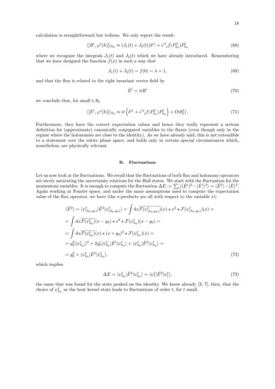
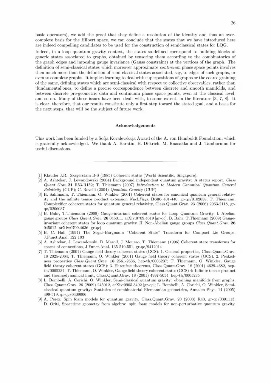
1 2 3 4t

0.2

0.4

0.6

0.8

!1

1 2 3 4t

0.2

0.4

0.6

0.8

!2

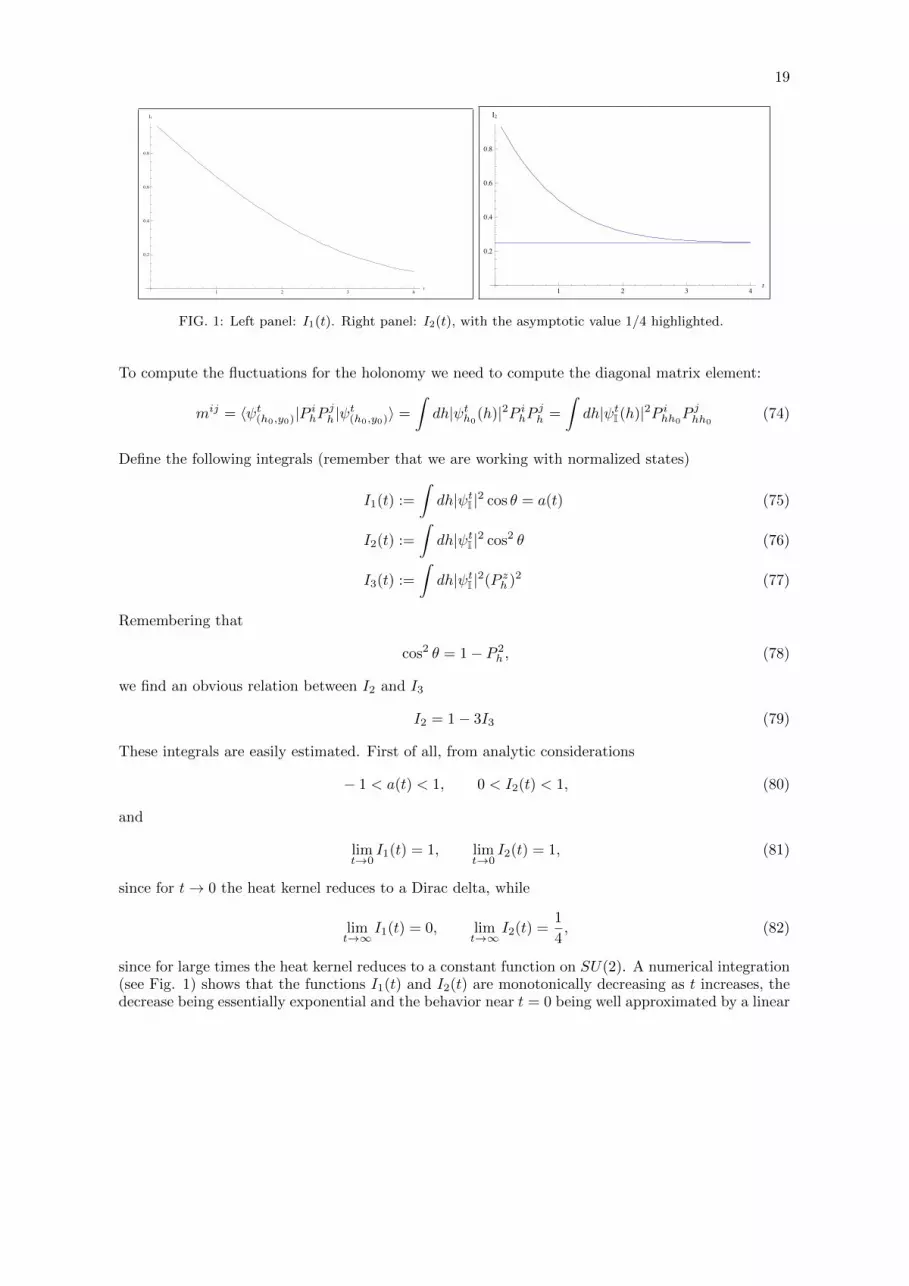
FIG. 1: Left panel: I1(t). Right panel: I2(t), with the asymptotic value 1/4 highlighted.

To compute the fluctuations for the holonomy we need to compute the diagonal matrix element:

mij = 〈ψt(h0,y0)|P ihP

jh |ψ

t(h0,y0)

〉 =

∫dh|ψth0

(h)|2P ihPjh =

∫dh|ψtI(h)|2P ihh0

P jhh0(74)

Define the following integrals (remember that we are working with normalized states)

I1(t) :=

∫dh|ψtI |2 cos θ = a(t) (75)

I2(t) :=

∫dh|ψtI |2 cos2 θ (76)

I3(t) :=

∫dh|ψtI |2(P zh )2 (77)

Remembering that

cos2 θ = 1− P 2h , (78)

we find an obvious relation between I2 and I3

I2 = 1− 3I3 (79)

These integrals are easily estimated. First of all, from analytic considerations

− 1 < a(t) < 1, 0 < I2(t) < 1, (80)

and

limt→0

I1(t) = 1, limt→0

I2(t) = 1, (81)

since for t→ 0 the heat kernel reduces to a Dirac delta, while

limt→∞

I1(t) = 0, limt→∞

I2(t) =1

4, (82)

since for large times the heat kernel reduces to a constant function on SU(2). A numerical integration(see Fig. 1) shows that the functions I1(t) and I2(t) are monotonically decreasing as t increases, thedecrease being essentially exponential and the behavior near t = 0 being well approximated by a linear

20

function

Ia(t) ≈ 1− µat, µa = O(1), a = 1, 2. (83)

The desired correlators can be written in terms of these integrals. It is easy to see that, for rotationalinvariance (but it can be checked with a direct computation)∫

dh|ψtI |2P ihPjh = I3(t)δij (84)

After straightforward manipulations we obtain

mij = (I2 − I3)P ih0P jh0

+ I3δij =

4I2 − 1

3P ih0

P jh0+

(1− I2)

3δij (85)

Given that:

〈ψt(h0,y0)|P ih|ψt(h0,y0)

〉 = I1(t)P ih0(86)

we see that the correlations are

〈P ihPjh〉 − 〈P

ih〉〈P

jh〉 =

(4I2 − 1

3− I21

)P ih0

P jh0+

(1− I2)

3δij (87)

The dependence on t is hidden in the integrals I1, I2, I3. However, we can say that, for h0 close to theidentity, or, equivalently, θ0 � 1, the correlation can be well approximated by

〈P ihPjh〉 − 〈P

ih〉〈P

jh〉 ≈

(1− I2)

3δij +O(θ20) (88)

This approximation is valid for any value of t. However, if we use the behavior of the function neart = 0,

〈P ihPjh〉 − 〈P

ih〉〈P

jh〉 ≈

µ2

3tδij +O(θ20) +O(t2), (89)

matching the fact that, for small t, the state is well peaked around the mean value.

We might also compute the fluctuations for the coordinates introduced in the previous subsection.We will have to deal with the following integral

M ij =

∫dh|ψtI(hh0)|ϕi(Ph)ϕj(Ph) =

∫dh|ψtI(hh0)|f2(Ph)P ihP

jh . (90)

Expanding again for small θ0 we get

M ij ≈∫dh|ψtI(h)|f2(Ph)P ihP

jh +

∫dh|ψtI(h)|f2(Ph)

(P ihδP

jh + P jhδP

ih

)+

+4

∫dh|ψtI(h)|f(Ph)f ′(Ph)P ihP

jhP

kh δP

kh . (91)

Let us consider the term

P ihδPjh = P ih

(cos θP jh0

− εjrsP rhP sh0

). (92)

The first term averages to zero, under integration, while the second gives rise to a contribution of

21

1 2 3 4t

0.2

0.4

0.6

0.8

1.0

1.2

J

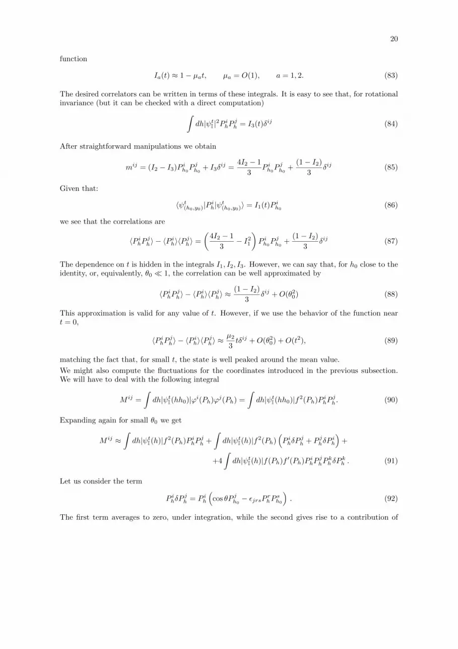
FIG. 2: Plot of J(t).

the form H(t)δirεjrsPsh0

. However, this term cancels with the one coming from the evaluation of the

integral with P jhδPih.

Finally, the last term involves:

P ihPjhP

kh δP

kh = P ihP

jhP

kh

(cos θP kh0

− εkrsP rhP sh0

). (93)

Both of them give zero contribution, for symmetry arguments. Therefore the fluctuation is entirelydetermined by the first integral∫

dh|ψtI(h)|f2(Ph)P ihPjh = J(t)δij , J(t) =

1

3

∫dh|ψtI(h)|f2(Ph)P 2

h . (94)

Of course, given that we are truncating at the linear order in θ0, this is the only contribution to thefluctuation in the new variables ϕ(Ph). Again, notice that, for small t, this is of order t.

This integral is clearly different from the I1, I2, I3 introduced previously (see Fig. 2 for the plot of anumerical estimate). However, for small values of t the difference disappears: for small t the Gaussianstend to the common behavior of a Dirac delta, and hence only the domain of integration near theidentity gives a significant contribution. In this domain, the difference between the coordinate Ph andthe operators ϕ(Ph) tends to zero (of course, if λ = 1), and J(t)→ I3(t). Given that, in this regime,the fluctuation of the new coherent states are identical to those of the Hall states, we can say that thefluctuations will be minimal as well.

These results collected so far tell us that, for states peaked on holonomies close to the identity(physically relevant situation for low curvature geometries), the statistical properties are essentiallydetermined by the statistical properties of the coherent states constructed with the heat kernel, andhence show that the coherent states introduced here are indeed another (related) class of states thatcan be of interest for the investigation of the semiclassical limit of LQG.

C. Resolution of the identity

We now want to show that the coherent states we have constructed define an (over)complete basis forthe space L2(G, dµ(g)), and thus give a resolution of the identity.

That is, we would like to ask the following condition:∫SU(2)×R3

µ(h0, y0) ψt(h0,y0)(h) ?y0 ψ

t(h0,y0)

(h) = |ψtI |2δ(h, h), (95)

22

for a certain measure on the classical phase space to be defined.

Recalling that:

ψt(h0,y0)(h) =

∑ε

ψt(h0,0)(h) eh(y0) Iε(h)ξε(h)

and expanding the expression on the l.h.s. of (95), we have (we neglect the characteristic functionsfrom the expression for better simplicity of notation):

∫SU(2)×R3

µ(h0, y0) ψt(h0,y0)(h) ?y0 ψ

t(h0,y0)

(h) =

=

∫µ(h0, y0) eh(−y0)ξε(h) ?y0 eh(−y0)ξε(h) ψ

t(h0,0)

(h)ψt(h0,0)(h) =

=

∫µ(h0, y0)eh−1h(y0) ξε(h−1h) ψ

t(e,0)(hh

−10 )ψt(e,0)(hh

−10 ). (96)

where we have assumed once more that ψt(h0,0)(h) = ψt(e,0)(hh

−10 ).

We now make, for the measure on phase space, the natural assumption: µ(h0, y0) = dh0 dy0, with thestandard Haar and Lebesgue mesaures on SU(2) and R3 respectively.

This gives the desired result:∫SU(2)×R3

µ(h0, y0) ψt(h0,y0)(h) ?y0 ψ

t(h0,y0)

(h) =

=

∫µ(h0, y0)eh−1h(y0) ξε(h−1h) ψ

t(e,0)(hh

−10 )ψt(e,0)(hh

−10 ) =

=

∫SU(2)

dh0 δ(h−1 h

)ψt(e,0)(hh

−10 )ψt(e,0)(hh

−10 ) = δ

(h−1 h

)|ψt(e,0)|

2 . (97)

Note that this result, with the given measure on phase space, holds for any choice of Gaussian and isa direct consequence of the choice of Fourier transform defining the coherent states.

It is interesting to compare this result with the corresponding analysis of the resolution of the identityfor the Hall states. There, in the case of states on SU(2) analytically continued to SL(2,C), themeasure on the the Lie algebra su(2) is not simply the Lebesgue measure on R3 as in this case, buthas to be supplemented by an additional factor (see especially the second paper in [7], equation 4.82)

2√

2e−t/4

(2πt)3/2sinh ||y||||y||

exp

(−y

2

2

), (98)

so that the overcompleteness relation can be recovered. The crucial difference between these two casesis that, while in the case of Hall states all the functions involved are seen as ordinary functions on R3

(isomorphic to the Lie algebra as vector space), the coherent states that we are proposing here arenoncommutative functions on the Lie algebra.

Incidentally, the integration on the algebra of the star product of two functions can be seen as theordinary integration on R3, provided that the (nonlocal) differential operator

√1 +∇2 is inserted∫

d3xf(x) ? g(x) =

∫d3xf(x)

√1 +∇2g(x) (99)

All these observations also imply that, when seen as ordinary functions on R3, our coherent states are

23

very different, especially in their asymptotic behaviour, with respect to the (analytically continued)Hall states, also used in LQG9.

D. Overlap

Another important property10 needed for the characterization of the coherent states is the behaviourof the overlap between two states peaked on different phase space points. For this, we need to considerthe whether they satisfy

|〈ψt(x1,h1)|ψt(x2,h2)〉|

2

||ψt(x1,h1)||2||ψt(x2,h2)

||2≈

1 (x1, h1) ≈ (x2, h2),

0 (x1, h1) 6= (x2, h2),(100)

i.e. that, while two coherent states might have a large overlap when the peaks are sufficiently close,their scalar product becomes smaller and smaller (and, ideally, goes to zero) as the distance betweenthe peaks increases.

Before proving the statement, let us remark that the reasoning will hold for any choice of x1, x2 and,consequently, of ∆x = x2 − x1.

As said, we need to understand the behavior of∣∣∣∫ dhψt(x1,h1)(h)ψt(x2,h2)

(h)∣∣∣2(∫

dh|ψt(x1,h1)(h)|2

)(∫dh|ψt(x2,h2)

(h)|2) . (101)

It turns out that, if we construct our states with Hall coherent states on the group, the denominatorof this expression is a constant independent from (x1, h1) and (x2, h2). For instance, in consideringthe norm of the first state, the multiplication of the plane wave with its complex conjugate leads toan expression independent from the Lie algebra element x1,∫

dh|ψt(x1,h1)(h)|2 =

∫dh(ψtI(hh

−11 ))2, (102)

which, in turn (using the fact that the heat kernel is a class function and that it has a nice behaviourunder convolution) leads to∫

dh(ψtI(hh−11 ))2 =

∫dhψtI(hh

−11 )ψtI(h1h

−1) = ψ2tI (I). (103)

Consequently, we will need just to address the behaviour of the numerator of the overlap.

Let us start by considering the case in which h1, h2 are very different (with respect to the scale set byt). In this case, we can use an estimate for the numerator of (100).

9 We would like to thank J. P. Gazeau and an anonymous referee for pointing this out to us.

10 We would like to thank an anonymous referee for this point.

24

|∫dh eh(x1)ψtI(hh

−11 )eh(x2)ψtI(hh

−12 )| ≤ 2

∫dhψtI(hh

−11 )ψtI(hh

−12 ) = ψ2t

I (h1h−12 ) (104)

where we have used the fact that the Gaussian that we are using is the heat kernel on SU(2), itsreality and the convolution property. Therefore, if h1h

−12 is sufficiently far away from the identity

of SU(2), with respect to the (angular) scale set by the parameter t, the decay of the heat kernel isensuring that the overlap goes to zero as we increase the angle θ12 (measuring the separation on thesphere S3 of the two group elements h1 and h2).

The only nontrivial case, then, is when the two group elements h1 and h2 are similar. In this case, weneed to massage the integrals in a different way. First of all,∫

dh eh(x1)ψtI(hh−11 )eh(x2)ψtI(hh

−12 ) =

∫dh eh(∆x)ψtI(hh

−11 )ψtI(hh

−12 ) (105)

where ∆x = x2 − x1. The fact that we are now considering the regime h1 ≈ h2 allows us to use theestimate

ψtI(hh−11 ) ≈ ψtI(hh−12 ). (106)

Therefore, our integral becomes:∫dh eh(∆x)(ψtI(hh

−11 ))2 =

∫dh ehh1

(∆x)(ψtI(h))2 (107)

after a change of variable of integration. Following the definition

ehh1(∆x) = exp(iP i(hh1)∆xi), (108)

and remembering that

P i(hh1) = P i(h) cos θ1 + P i(h1) cos(θ)− εijkPj(h)Pk(h1) (109)

we obtain

ehh1(∆x) = exp(iP i(hh1)∆xi) = exp(iP (h1) ·∆x cos(θ)) exp(iv(∆x, h1) · P (h)), (110)

where we have introduced the vector

vi(∆x, h1) =(cos θ1δij + εijkP

k(h1))

∆xj . (111)

Notice that it is independent from the variable of integration. At this point we can proceed with theintegration, by choosing Euler angles on S3 in such a way that the integral reduces to

I =1

8π

∫dθdφdψ sin2 θ sinφ exp(iP (h1) ·∆x cos(θ)) exp(i||v|| sin θ cosφ)F 2

t (cos(θ)), (112)

where we have used the fact that the heat kernel is a class function, ψtI(h) = Ft(cos(θ)). Performingthe integration on the angles φ and ψ one obtains

I =2

π

1

||v||

∫dθ sin θ exp(−iP (h1) ·∆x cos(θ)) sin(||v|| sin θ)Ft(cos(θ))2. (113)

The remaining integral can be bounded, in modulus, by a positive function f(t). Hence, for ourpurposes, it is enough to examine the prefactor 1/||v||. From the general expression of the vector v,

25

it is clear that, if we assume that h1 = cos θ1I + iP i(h1)σi, with θ1 � 1,

|I| ≤ f(t)

||∆x||+O(sin2 θ1), (114)

where we are neglecting corrections (also depending on ∆x) that would be anyway proportional tosin2 θ1, and hence negligible provided that h1 is not too far away from the identity of SU(2). Therefore,while this result does not hold for generic h1, h2 in SU(2), it is valid in the regime in which we areinterested, given that it is the only region in which holonomies and fluxes can be approximately beconsidered as a pair of canonical variables.

In conclusion, the overlap decreases with the inverse of the square of the separation ||∆x|| of theposition of the peaks in the Lie algebra. Combining this result with the previous one and with theobservation that, for the case in which the two peaks coincide, the overlap is obviously one, we getthat the states that we are presenting here are indeed characterized by an overlap that genericallydecreases with the increase in the distance between the points in the classical phase space associatedto the peaks of the states themselves, at least in the regime in which we are interested in (smallholonomies but generic fluxes).

Together with the right peakedness properties on phase space, the minimization of the fluctuations offundamental operators and the resolution of the identity, this last property completes the minimal setof requirements we see fulfilled by our new coherent states based on the flux representation of LQG.

V. CONCLUSION

We have proposed an alternative definition of coherent states on the cotangent bundle of a compactgroup, in particular for the SU(2) case, T ∗SU(2), of direct interest for quantum gravity. In fact,this work is a contribution to the ongoing, crucial efforts to develop appropriate tools to study thecontinuum and semi-classical approximation of quantum gravity states defined by (superpositions of)discrete structures labeled by pre-geometric, algebraic data. While the idea behind is more general, ifthe starting point is a specific choice of Gaussian on the group manifold given by the heat kernel, itamounts to a simple modification of Hall’s construction based on the analytic continuation of groupcoordinates to peak on generic phase space points.

Using the non-commutative flux representation for the relevant Hilbert space, we propose instead touse non-commutative translations on the Lie algebra to achieve the same result. For the new typeof coherent states, we have then shown several welcome properties, in particular sharp peakednesswith respect to classical phase space points, at least in the very specific regime of holonomies closeto the identity. On this point, the improvement with respect to standard Hall states is representedby expectation values that are exactly equal to the classical values in the flux/Lie algebra variable,and that are close to them in a way that is independent of the semi-classicality parameter in theholonomy/group variables (when specific coordinates on the group are chosen).

Besides the improvement on the expectation values, the fluctuations of the operators around theirmean values also display very nice properties. We have shown that, for t small, ∆ϕ(Ph) ∼ t andthat the relation with the heat kernel states ensures automatically that ∆E ∼ t, a result that hasbeen established for these special states. Putting these results together with the evaluation of theexpectation value (71) of the commutator between the fluxes and the coordinates ϕ, we see that thatthe states we have introduced have fluctuations whose behavior closely resembles the one of ordinarycoherent states (in particular, the simultaneous minimality of these fluctuations), even with respectto the Heisenberg uncertainty relations

(∆E∆ϕ(P ))1/2 ∼ t ∼ |〈[E,ϕ]〉|. (115)

In addition to these results concerning the statistical properties (mean values and fluctuations of the

26

basic operators), we add the proof that they define a resolution of the identity and thus an over-complete basis for the Hilbert space, we can conclude that the states that we have introduced hereare indeed compelling candidates to be used for the construction of semiclassical states for LQG.

Indeed, in a loop quantum gravity context, the states so-defined correspond to building blocks ofgeneric states associated to graphs, obtained by tensoring them according to the combinatorics ofthe graph edges and imposing gauge invariance (Gauss constraint) at the vertices of the graph. Thedefinition of semi-classical states which moreover approximate continuum phase space points involvesthen much more than the definition of semi-classical states associated, say, to edges of such graphs, oreven to complete graphs. It implies learning to deal with superpositions of graphs or the coarse grainingof the same, defining states which are semi-classical with respect to collective observables, rather than‘fundamental’ones, to define a precise correspondence between discrete and smooth manifolds, andbetween discrete pre-geometric data and continuum phase space points, even at the classical level,and so on. Many of these issues have been dealt with, to some extent, in the literature [3, 7, 8]. Itis clear, therefore, that our results constitute only a first step toward the stated goal, and a basis forthe next steps, that will be the subject of future work.

Acknowledgements

This work has been funded by a Sofja Kovalevskaja Award of the A. von Humboldt Foundation, whichis gratefully acknowledged. We thank A. Baratin, B. Dittrich, M. Raasakka and J. Tambornino foruseful discussions.

[1] Klauder J.R., Skagerstam B-S (1985) Coherent states (World Scientific, Singapore).[2] A. Ashtekar, J. Lewandowski (2004) Background independent quantum gravity: A status report, Class

Quant Grav 21 R53-R152; T. Thiemann (2007) Introduction to Modern Canonical Quantum GeneralRelativity (CUP); C. Rovelli (2004) Quantum Gravity (CUP)

[3] H. Sahlmann, T. Thiemann, O. Winkler (2001) Coherent states for canonical quantum general relativ-ity and the infinite tensor product extension Nucl.Phys. B606 401-440, gr-qc/0102038; T. Thiemann,Complexifier coherent states for quantum general relativity, Class.Quant.Grav. 23 (2006) 2063-2118, gr-qc/0206037

[4] B. Bahr, T.Thiemann (2009) Gauge-invariant coherent states for Loop Quantum Gravity. I. Abeliangauge groups Class.Quant.Grav. 26 045011, arXiv:0709.4619 [gr-qc]; B. Bahr, T.Thiemann (2009) Gauge-invariant coherent states for loop quantum gravity. II. Non-Abelian gauge groups Class.Quant.Grav. 26045012, arXiv:0709.4636 [gr-qc]

[5] B. C. Hall (1994) The Segal–Bargmann ”Coherent State” Transform for Compact Lie Groups,J.Funct.Anal. 122 103

[6] A. Ashtekar, J. Lewandowski, D. Marolf, J. Mourao, T. Thiemann (1996) Coherent state transforms forspaces of connections, J.Funct.Anal. 135 519-551, gr-qc/9412014

[7] T. Thiemann (2001) Gauge field theory coherent states (GCS): 1. General properties, Class.Quant.Grav.18 2025-2064; T. Thiemann, O. Winkler (2001) Gauge field theory coherent states (GCS). 2. Peaked-ness properties Class.Quant.Grav. 18 2561-2636, hep-th/0005237; T. Thiemann, O. Winkler, Gaugefield theory coherent states (GCS): 3. Ehrenfest theorems, Class.Quant.Grav. 18 (2001) 4629-4682, hep-th/0005234; T. Thiemann, O. Winkler, Gauge field theory coherent states (GCS) 4: Infinite tensor productand thermodynamical limit, Class.Quant.Grav. 18 (2001) 4997-5054, hep-th/0005235

[8] L. Bombelli, A. Corichi, O. Winkler, Semi-classical quantum gravity: obtaining manifolds from graphs,Class.Quant.Grav. 26 (2009) 245012, arXiv:0905.3492 [gr-qc]; L. Bombelli, A. Corichi, O. Winkler, Semi-classical quantum gravity: Statistics of combinatorial Riemannian geometries, Annalen Phys. 14 (2005)499-519, gr-qc/0409006

[9] A. Perez, Spin foam models for quantum gravity, Class.Quant.Grav. 20 (2003) R43, gr-qc/0301113;D. Oriti, Spacetime geometry from algebra: spin foam models for non-perturbative quantum gravity,

27

Rept.Prog.Phys. 64 (2001) 1703-1756, gr-qc/0106091[10] E. Bianchi, L. Modesto, C. Rovelli, S. Speziale, Graviton propagator in loop quantum gravity,

Class.Quant.Grav. 23 (2006) 6989-7028, arXiv:gr-qc/0604044 [gr-qc]E. Alesci and C. Rovelli, “The Complete LQG propagator. I. Difficulties with the Barrett-Crane vertex”Phys. Rev. D 76, 104012 (2007) [arXiv:0708.0883 [gr-qc]];E. Bianchi, E. Magliaro and C. Perini, “LQG propagator from the new spin foams” Nucl. Phys. B 822,245 (2009) [arXiv:0905.4082 [gr-qc]].

[11] E. Bianchi, E. Magliaro, C. Perini, Coherent spin networks, Phys.Rev. D82 (2010) 024012, arXiv:0912.4054[gr-qc]

[12] A. Ashtekar, A. Corichi, J. A. Zapata, Quantum theory of geometry III: Noncommutativity of Riemannianstructures, Class.Quant.Grav. 15 (1998) 2955-2972, gr-qc/9806041

[13] L.Freidel, E. R. Livine (2006) Ponzano-Regge model revisited III: Feynman diagrams and effective fieldtheory Class.Quant.Grav. 23 2021-2062, hep-th/0502106

[14] E. Joung, J. Mourad, K. Noui (2009) Three Dimensional Quantum Geometry and Deformed PoincareSymmetry J.Math.Phys. 50 052503.

[15] L. Freidel, S. Majid (2008) Noncommutative harmonic analysis, sampling theory and the Duflo map in2+1 quantum gravity Class.Quant.Grav. 25 045006, hep-th/0601004

[16] M. Dupuis, F. Girelli, E. Livine, Spinors and Voros star-product for Group Field Theory: First Contact,arXiv:1107.5693 [gr-qc]

[17] D. Oriti, The group field theory approach to quantum gravity, in D. Oriti (ed.) Approaches to quantumgravity, CUP (2009), gr-qc/0607032; D. Oriti, The microscopic structure of quantum space as a groupfield theory, in G. Ellis, J. Murugan, A. Weltman (eds) Foundations of space and time, CUP (2011),arXiv:1110.5606 [hep-th]

[18] A. Baratin, D. Oriti, Group field theory with non-commutative metric variables, Phys.Rev.Lett. 105(2010) 221302, arXiv:1002.4723 [hep-th]

[19] A. Baratin, D. Oriti, Quantum simplicial geometry in the group field theory formalism: reconsidering theBarrett-Crane model, to appear in New J. Phys., arXiv:1108.1178 [gr-qc]

[20] A. Baratin, F. Girelli, D. Oriti, Diffeomorphisms in group field theories, Phys.Rev. D83 (2011) 104051,arXiv:1101.0590 [hep-th]

[21] R. Camporesi, Harmonic analysis and propagators on homogeneous spaces, Phys.Rept. 196 (1990) 1-134[22] D. Oriti, M. Raasakka, Quantum mechanics on SO(3) via non-commutative dual Variables, Phys.Rev.

D84 (2011) 025003, arXiv:1103.2098 [hep-th][23] A. Baratin, B. Dittrich, D. Oriti, J. Tambornino (2010) Non-commutative flux representation for loop

quantum gravity, Class.Quant.Grav. 28 (2011) 175011, arXiv:1004.3450 [hep-th].[24] A. Perelomov, Generalized coherent states and their applications, Springer (1986)[25] E. Livine, S. Speziale, A new spin foam vertex for quantum gravity, Phys.Rev. D76 (2007) 084028,

arXiv:0705.0674 [gr-qc]