Electronic copy available at: http://ssrn.com/abstract=2052159

Local Business Cycles and Local Liquidity*

Gennaro Bernile George Korniotis

Alok Kumar University of Miami

Qin Wang University of Michigan at Dearborn

July 1, 2012

Abstract – This paper shows that the geographical location of a firm affects its liquidity. We

find that there is an economically significant local component in firm liquidity that is induced by

local economic conditions. The future firm liquidity is higher (lower) when the local economy

performs well (poorly) and this effect is more pronounced among larger firms. Further, the

impact of local economic conditions on local firm liquidity is stronger when local financing

constraints are more binding, the local information environment is more opaque, and local

institutional ownership levels and trading intensity are higher. This geographical variation in

local liquidity generates predictable patterns in local stock returns. Local stock prices decline and

future returns are higher when expected local liquidity is lower. A trading strategy based on the

geographical variation in firm-level liquidity generates an annual risk-adjusted performance of

over six percent.

Keywords: Market segmentation, U.S. state business cycle, liquidity, local bias, capital

constraints, institutional investors, return predictability.

* Please address correspondence to Alok Kumar, Department of Finance, University of Miami, School of Business Administration, Coral Gables, FL 33124, USA; Phone: 305-284-1882, Email: akumar@miami.edu. Gennaro Bernile can be reached at gbernile@bus.miami.edu or 305-284-6690. George Korniotis can be reached at gkorniotis@miami.edu or 305-284-5728. Qin Wang can be reached at qinw@umd.umich.edu or 313-583-6487. We thank Tarun Chordia, Shane Corwin, Ralitsa Petkova, Alessio Sarretto, Johan Sulaeman, Annette Vissing-Jorgensen, Fernando Zapatero (discussant), and participants at the 1st ITAM Finance Conference for helpful comments and suggestions. We are responsible for all remaining errors and omissions.

Electronic copy available at: http://ssrn.com/abstract=2052159

Local Business Cycles and Local Liquidity

Abstract

This paper shows that the geographical location of a firm affects its liquidity. We find that there is

an economically significant local component in firm liquidity that is induced by local economic

conditions. The future firm liquidity is higher (lower) when the local economy performs well

(poorly) and this effect is more pronounced among larger firms. Further, the impact of local

economic conditions on local firm liquidity is stronger when local financing constraints are more

binding, the local information environment is more opaque, and local institutional ownership

levels and trading intensity are higher. This geographical variation in local liquidity generates

predictable patterns in local stock returns. Local stock prices decline and future returns are higher

when expected local liquidity is lower. A trading strategy based on the geographical variation in

firm-level liquidity generates an annual risk-adjusted performance of over six percent.

1

1. Introduction

An emerging literature in finance suggests that the U.S. financial markets may be

segmented. For example, Becker (2007) shows that U.S. bank loan markets are segmented since

local loan supply and the level of local economic activity depend on the level of local deposits.

Consistent with the idea of geographical segmentation, Korniotis (2008) shows that heterogeneity

in economic conditions across the U.S. states can explain the variation in the cross-section of

expected returns. Similarly, Gomez, Priestley, and Zapatero (2011) show that the risk premium

varies across the nine U.S. Census divisions due to differences in investors’ relative wealth

concerns. Most recently, Korniotis and Kumar (2012) show that a strong investor preference for

holding local stocks and incomplete risk sharing across U.S. states generate geographical

segmentation in equity markets. Consequently, state-level stock returns vary with the local

business cycle, where future stock returns are higher (lower) when the local economy is

contracting (expanding).

In this paper, we extend this literature on geography-induced economic segmentation and

investigate whether the geographical location of a firm affects its liquidity. Our main conjecture is

that local macroeconomic variables would influence the liquidity of local firms. In particular, local

firm liquidity would be lower when the local economy performs poorly and local liquidity would

improve as the local economic environment improves.

This conjecture is motivated by the recent evidence in Korniotis and Kumar (2012), who

demonstrate that the local economic conditions rather than the aggregate U.S. macroeconomic

climate is more salient to local investors. The second key motivation for our analysis is the

previous finding that portfolio allocations and trading activities of retail and institutional investors

are tilted toward local stocks (e.g., Coval and Moskowitz (1999, 2001)).

2

Beyond these two broad strands of finance literature, our conjecture is motivated by recent

studies in liquidity. This literature finds that firm-level liquidity exhibits a significant market-wide

component and suspects that changes in macroeconomic conditions are likely to induce this

commonality in liquidity.1

A key innovation in our study is to recognize that state-level economic conditions may be a

significant source of commonality in firm-level liquidity. That is, we shift the focus from the

aggregate country-level to the state-level and identify local macroeconomic conditions as novel

determinants of the common variation in liquidity across firms. Just as state-level macroeconomic

variables are stronger predictors of local stock returns than aggregate U.S.-level macroeconomic

indicators, state-level macroeconomic variables may be more appropriate predictors of firm

liquidity.

Although this is an intuitive conjecture and country-level studies find a

link between aggregate liquidity and monetary policy (e.g., Chordia, Sarkar, and Subrahmanyam

(2005), Sauer (2007)), the empirical evidence that liquidity varies systematically with real

aggregate economic factors is weak (e.g., Fujimoto (2003), Choi and Cook (2005)).

The idea that the geographical location of a firm could affect its liquidity is not entirely

new and has been examined in Loughran and Schultz (2005). Their study, however, focuses on

liquidity differences between firms in rural and urban regions that arise from differences in

familiarity and access to information. They do not examine the impact of local economic

conditions on firm liquidity and the potential asset pricing implications of this relation, which are

the main focus of our study.

Our main conjecture is based on the key implicit assumption that commonality in firm-

level liquidity is at least partly local. Therefore, before proceeding with our core analysis, we

1 For example, see Chordia, Roll, and Subrahmanyam (2000), Huberman and Halka (2001), Hasbrouck and Seppi (2001), Brockman and Chung (2002), Korajczyk and Sadka (2008), Brockman, Chung, and Pérignon (2009).

3

assess the validity of this assumption. Specifically, we augment the main tests in Chordia, Roll,

and Subrahmanyam (2000) and add a local liquidity factor to their baseline specification.

Consistent with our key implicit assumption, we find that liquidity has an economically sizeable

and statistically significant local component, which is stronger than the industry-induced

component in liquidity. This local liquidity component is incremental over commonalities in

liquidity induced by market-wide and industry factors documented in earlier studies.

Encouraged by this important evidence, we test our key prediction that local economic

conditions affect the liquidity of local stocks and also assess whether this relation depends on local

capital market conditions. Consistent with our key conjecture, using multiple measures of

liquidity, we show that the liquidity of local firms dries up (increases) following a deterioration

(improvement) in local economic conditions. Further, consistent with studies that find that

liquidity commonality is stronger for larger firms (e.g., Chordia, Roll, and Subrahmanyam (2000);

Kamara, Lou, and Sadka (2008)), we show that the relation between local economic conditions

and subsequent liquidity is more pronounced among larger firms.

Next, we identify the channels through which local business cycles may affect local

liquidity. We rely on recent studies to determine this set of potential channels. Specifically,

Korniotis and Kumar (2012) document a strong state-level component in holdings and trading of

local stocks. They find that more than 15% of trading in a typical firm can be attributed to state-

based institutional investors and trades of local investors are more strongly correlated (i.e., herding

tendencies are stronger) than trades of institutions located far from each other. The mean within-

region trading correlation is 0.141, which is more than three times higher than the mean across-

region trading correlation of 0.046.

Further, Chordia, Roll, and Subrahmanyam (2000) and Kamara, Lou, and Sadka (2008)

posit that commonality in the composition of the institutional investor base or similarities in their

4

trading strategies would be an important channel through which liquidity commonality across

firms arises. Other recent liquidity studies suggest that investors’ funding constraints and firms’

information environment should influence liquidity (e.g., Eisfeldt (2004), Taddei (2007),

Brunnermeier and Pedersen (2009), Hameed, Kang, and Viswanathan (2010)).

A natural implication of the arguments in these earlier studies is that the relation between

liquidity and local economic conditions is likely to be stronger in states where local ownership and

local trading levels are relatively higher. Further, local economic conditions should influence local

liquidity more strongly when local financing constraints are more binding and the local

information environment is more opaque. Consistent with these conjectures, we find that local

economic conditions affect local liquidity more strongly when (i) local financing constraints are

more binding, (ii) the local information environment is more opaque, (iii) local ownership levels

are higher, and (iv) the trading intensity of local investors is relatively high.

In the last part of the paper, we study whether geographical variation in expected local

liquidity generates predictable patterns in local stock returns. The local component in liquidity

may affect prices of local stocks because the local macroeconomic variables affect the liquidity of

local firms in a systematic manner and make them riskier. Alternatively, local macroeconomic

variables may generate mispricing among local stocks through the impact of local trading. In

either instance, local stock prices would be lower when expected local liquidity is lower and,

consequently, average future returns would be higher.

To test this asset pricing conjecture, we use the liquidity predictability regression estimates

to construct Long−Short portfolios. The Long portfolio includes firms located in states predicted

to have the lowest common liquidity and the Short portfolio includes firms located in states

predicted to have the highest common liquidity. We find that this Long−Short trading strategy

5

based on the geographical variation in expected firm-level liquidity generates an annual risk-

adjusted performance of over six percent.

These results make several important contributions to the finance literature. In particular,

these findings improve our understanding of the sources of commonality in liquidity. Previous

liquidity studies provide strong evidence of commonality in liquidity but the mechanisms that

induce such commonality have been harder to identify. Our paper not only identifies a new

geography-based component in liquidity but also identifies its main determinants.

Specifically, we show that geographical heterogeneity in macroeconomic conditions

generates geographical patterns in firm liquidity, i.e., a significant component of firm-level

liquidity can be traced to local economic factors. Examining why local economic factors affect

local firm liquidity, we find that local funding constraints, opacity of local information

environment, and commonalities in local institutional ownership and trading are important

channels through which local economic conditions influence the liquidity of local firms.

Beyond these contributions to the liquidity literature, we show that the impact of local

macroeconomic variables on local liquidity generates predictable patterns in stock returns. This

evidence indicates that either market participants do not react optimally to changes in local

economic environment or the existing asset pricing models are unable to account for the time-

varying local liquidity risks induced by local economic conditions. Overall, the asset pricing

results improve our understanding of the role of geography in the price formation process.

The rest of the paper is organized as follows. In Section 2, we discuss the related literature

and develop our main hypotheses. In Section 3, we describe the data sources. We present the main

empirical results in Section 4 and discuss the robustness of these results in Section 5. We conclude

in Section 6.

6

2. Related Literature and Testable Hypotheses

We study the relation between local liquidity and local macroeconomic conditions by

organizing our empirical analysis around four hypotheses, which are developed in this section.

The primary motivation for our study comes from the recent literature in liquidity commonality.

Several studies document significant evidence of commonality in liquidity across equity securities

(see footnote 1). In addition, Chordia Roll, and Subrahmanyam (2000) suggest that because firms

have common investor base and those investors may use common trading strategies, changes in

aggregate economic conditions may induce correlated trading patterns and have a common effect

on firm liquidity.

Although this is an intuitive conjecture, unfortunately, except for some monetary policy

variables, prior studies find little or no support for the posited relation between aggregate liquidity

and macroeconomic factors (e.g., Fujimoto (2003), Choi and Cook (2005), Chordia, Sarkar, and

Subrahmanyam (2005), Sauer (2007)). Our main innovation is to recognize that a significant

source of commonality in firm-level liquidity may be local. This idea is motivated by a growing

finance literature, which finds that the U.S. financial markets may be segmented.

In particular, Becker (2007) shows U.S. bank loan markets are highly segmented.

Korniotis (2008) shows that differences in economic conditions across the U.S. states can explain

variation in the cross-section of expected returns. Similarly, Gomez, Priestley, and Zapatero

(2011) show that the risk premium varies across the nine U.S. Census divisions due to

geographical variation in relative wealth concerns of investors. Most recently, Korniotis and

Kumar (2012) demonstrate that the local economic environment rather than aggregate U.S.

macroeconomic climate is more salient to local investors and, thus, more relevant for local stock

returns. Based on these observations, our main hypothesis posits that:

7

H1: There is a positive relation between local macroeconomic conditions and subsequent

liquidity of local stocks.

Earlier studies also show that the degree of liquidity commonality varies systematically

across securities. In particular, Chordia Roll, and Subrahmanyam (2000) find that liquidity

commonality increases with firm size, as large firm spreads are more sensitive to market-wide

changes in spreads. They suggest that this evidence may be due to a greater prevalence of

institutional herd trading among larger stocks.

Kamara, Lou, and Sadka (2008) build upon these findings and analyze the evolution of

systematic liquidity in the cross-section of US stocks from 1963 through 2005. They find that

liquidity commonality has increased for large firms and declined for small firms. They conjecture

that this finding may be due to changes in the US equity investor base. Consistent with this

conjecture, they show that differences in the level of institutional ownership (especially ownership

of investment companies and investment advisors) across stock-size groups can explain the

differences in systematic liquidity across those groups.

Motivated by the findings in these two recent studies, our second hypothesis posits:

H2: The impact of local macroeconomic environment on local liquidity increases with firm

size.

Next, we focus on the mechanisms through which local commonalities in liquidity may

arise. We consider three broad sets of factors, which may generate state-level variation in firm

liquidity: (i) local institutional ownership and trading, (ii) local funding constraints, and (iii)

information environments of local firms.

The choice of the first potential channel is motivated by the evidence in Korniotis and

Kumar (2012), who show that holdings and trading levels of both retail and institutional investors

8

are substantially higher for local firms and exhibit substantial cross-state variation. More than 15%

of trading in a typical firm can be attributed to state-based institutional investors, which is

considerably higher than the expected trading levels of 6-8%. In addition, the trades of local

investors are more strongly correlated (i.e., herding tendencies are stronger) than trades of

institutions located far from each other. The mean state-level trading correlation among

institutions located within the same Census region is 0.141, which is more than three times higher

than the mean across-region trading correlation of 0.046. Given this prior evidence of concentrated

local trading and strong local trading correlations, the relation between local economic conditions

and local liquidity is likely to vary with the degree of local stock ownership and trading.

Next, we conjecture that financial constraints should affect the relation between real

economic conditions and liquidity. Existing theories suggest that market liquidity drops after large

negative market-wide shocks because financial intermediaries’ collateral values decrease and

funding constraints become more binding, forcing asset holders to liquidate (e.g., Kyle and Xiong

(2001), Gromb and Vayanos (2002), Anshuman and Viswanathan (2005), Brunnermeier and

Pedersen (2009)). Hameed, Kang and Viswanathan (2007) find that commonality in liquidity

increases during periods of market decline, and that liquidity commonality is positively related to

market volatility. Along similar lines, we expect local funding constraints to amplify the relation

between liquidity and local economic conditions.

Our last channel is motivated by the observation that higher levels of adverse selection

negatively affect liquidity and this relation is magnified when the information environment of a

firm is more opaque. Recent theories suggest this would result in pro-cyclical systematic liquidity.

Eisfeldt (2004), for instance, models a dynamic economy in which high productivity leads to

higher investment in risky assets and hence more rebalancing trades. This mechanism mitigates

(exacerbates) adverse selection and improves (deteriorates) liquidity of risky asset markets in good

9

(bad) economic times. Taddei (2007) derives a similar prediction for the relation between liquidity

and economic fluctuations when firms endogenously choose capital structure to finance

investment opportunities where they have private information. These arguments suggest that

greater opacity of the local information environment would amplify the relation between liquidity

and local economic conditions.

Overall, motivated by the evidence from these previous studies, our third hypothesis posits

that:

H3: The effect of local economic conditions on local liquidity is amplified when (i) local

financing constraints are more binding, (ii) the local information environment is more

opaque, (iii) the shareholder base is more local, and (iv) stock trading is relatively more

localized.

In the last part of the paper, we study the potential asset pricing implications of

geographical variation in expected liquidity that is induced by local business cycles. The local

component of liquidity could affect the prices of local stocks in two distinct ways. The first

possibility is that local macroeconomic variables affect the liquidity of local firms in a systematic

manner and make them riskier, commanding a higher risk premium. Alternatively, local

macroeconomic variables may generate mispricing among local stocks through the impact of local

trading. In either instance, local stock prices would be lower when expected local liquidity is

lower and, consequently, expected returns would be higher. Specifically, our key asset pricing

hypothesis posits that:

H4: When local economic conditions are poor, local liquidity falls, depressing local stock

prices and leading to higher average future returns.

10

To test the asset pricing hypothesis, similar to Korniotis and Kumar (2012), we form

Long−Short trading strategies, where the Long portfolio includes firms located in states predicted

to have the lowest common liquidity and the Short portfolio includes firms located in states

predicted to have the highest common liquidity. If the impact of local macroeconomic variables on

the liquidity of local firms is economically significant, these trading strategies would earn

significant risk-adjusted returns.

3. Data Sources and Summary Statistics

3.1 State-Level Liquidity Measures

We use various common measures of liquidity in our empirical analysis: (i) Amihud

(2002) illiquidity measure; (ii) relative spreads; (iii) Corwin-Schultz (2012) spreads; (iv)

Lesmond, Ogden, and Trzcinka (1999) (LOT) measure; and (v) stock turnover. Goyenko and

Ukhov (2009) and Goyenko, Holden, and Trzcinka (2009) find that “low-frequency” liquidity

measures do well in capturing the spread cost and price impact estimated using intraday data. In

particular, the Amihud (2002) illiquidity measure is based on Kyle’s (1985) lambda and calculated

as the ratio of the absolute value of daily stock return to its daily dollar volume. It measures the

daily price impact of the order flow.

Among the other liquidity measures, relative spread is the ratio of the daily closing bid-ask

spread divided by the midpoint of the daily closing bid-ask spread. The Corwin-Schultz spread,

developed from daily high and low prices, is the daily spread estimated for each stock based on

equations (14) and (18) in Corwin and Schultz (2012). Negative daily spread estimates are set to

zero. The LOT measure is the ratio of the number of zero daily returns to the total number of daily

returns within a quarter for each firm. This variable reflects the notion that “harder-to-trade” (i.e.,

less liquid) stocks are more likely to have zero-volume and, thus, zero return days. Last, turnover

11

is the ratio of quarterly trading volume to the number of shares outstanding at the beginning of the

quarter for each firm.

Atkins and Dyl (1997) show that trading volume on the NASDAQ is overstated due to

trades between dealers. Therefore, we divide trading volume on NASDAQ-listed stocks by two

when calculating the Amihud (2002) and turnover measures. For the Amihud (2002) illiquidity

measure, relative spread, Corwin-Schultz spread, and LOT measures, higher values imply lower

liquidity. For turnover, higher values imply higher liquidity. All the liquidity measures are

calculated using data from the Center for Research in Security Prices (CRSP).

Hasbrouck (2009) shows that Amihud (2002) illiquidity measure is most highly correlated

with benchmark price impact measures based on intraday data. The correlation is 0.82. Thus, we

focus the discussion of our tests on this particular measure, although all our inferences are

qualitatively similar when we use any of the other four liquidity measures to conduct our empirical

analysis.

We conduct our main tests using state-quarter observations. To obtain an estimate of the

Amihud (2002), relative spread, and Corwin and Schultz (2012) spread measures in state j and

quarter q, we use the following log-average index:

𝑆𝑡𝑎𝑡𝑒 𝐿𝑖𝑞 (𝑗, 𝑞) = 𝐿𝑜𝑔 �∑ 𝜔𝑖,𝑞−1𝑗 �

∑ 𝐿𝑖𝑞𝑖,𝑑,𝑞𝑗𝑄

𝑑=1

𝑄�𝑁

𝑖=1 �.

To estimate the LOT and turnover measures in state j and quarter q, we use the following log-

average index:

𝑆𝑡𝑎𝑡𝑒 𝐿𝑖𝑞 (𝑗, 𝑞) = 𝐿𝑜𝑔�∑ 𝜔𝑖,𝑞−1𝑗 𝐿𝑖𝑞𝑖,𝑞

𝑗𝑁𝑖=1 �.

In both instances, 𝐿𝑖𝑞𝑖,𝑑,𝑞𝑗 is the daily liquidity estimate for stock i headquartered in state j on day d

in quarter q; Q is the total number of trading days for stock i in quarter q; 𝐿𝑖𝑞𝑖,𝑞𝑗 is the quarterly

12

liquidity estimate for stock i headquartered in state j in quarter q; 𝜔𝑖,𝑞−1𝑗 is stock i’s market

capitalization scaled by the aggregate market capitalization of all firms located in the same state at

the end of quarter q−1; N is the number of stocks headquartered in state j; and Log indicates the

natural logarithm function. Due to the non-normality of state-quarter liquidity measures, we use

the natural logarithm of these measures in all empirical tests.

3.2 Measures of Local Economic Activity

We use various macroeconomic data in our analysis. Specifically, following Korniotis and

Kumar (2012), we focus on three measures of macroeconomic activity: the relative unemployment

rate (US Rel Un, State Rel Un), the labor income growth rate (US Inc Gr, State Inc Gr), and the

housing collateral ratio (US hy, State hy). The choice of these economic indicators is motivated by

previous studies (e.g., Boyd, Hu, and Jagannathan (2005), Jagannathan and Wang (1996),

Campbell (1996), Lustig and van Nieuwerburgh (2005, 2010)), which suggest that unemployment,

income growth, and the housing collateral ratio capture macroeconomic information that is

relevant for asset returns. In some of our tests, we combine these three measures and define an

economic activity index (US Econ Act, State Econ Act).

Using unemployment rates data from the Bureau of Labor Statistics (BLS), we measure the

relative unemployment rate as the current unemployment rate divided by the moving average

unemployment rate over the previous 16 quarters. We use labor income data from the Bureau of

Economic Analysis (BEA) to measure quarterly labor income growth. Last, we follow Lustig and

van Nieuwerburgh (2005) method to measure state-level housing collateral ratios and we

download the U.S. hy directly from Stijn van Nieuwerburgh’s website.

Each variable is standardized to have zero (sample) mean and standard deviation equal to

one. The U.S. and state-level economic activity indices are computed by adding the corresponding

13

standardized values of income growth and hy, and subtracting the standardized value of relative

unemployment, and dividing the result by three.

Following earlier studies on U.S.-level liquidity (e.g., Chordia, Sarkar, and Subrahmanyam

(2005), Sauer (2007)), we also control for national monetary policy and credit conditions using the

term spread (ten-year government bond yield minus one-year government bond yield) and default

spread (Baa-rated corporate bond yield minus ten-year government bond yield). The two spreads

measures are based on quarterly data obtained from the Board of Governors of the Federal

Reserve System web site.

In some of our tests, we examine the predictability of local stock returns and form various

trading strategies. For this analysis, we follow Korniotis and Kumar (2012) and use the

macroeconomic variables from quarter t − 2 because these measures are reported with a lag.2

We use the macroeconomic series for the 1980 to 2008 time period. The choice of the

sample period is dictated by various data constraints. State-level macroeconomic data are available

from 1975 onward but state-level data before 1980 are very noisy since they are based on various

approximations. Further, the housing collateral series is unavailable after 2008.

Other U.S.-level predictors (i.e., term spread and default spread) are measured in quarter t − 1

because they are reported without any lag.

3.3 Measures of Local Funding Constraints, Opacity, Ownership and Trading

We use data from several sources to identify the channels through which local

macroeconomic variables affect the liquidity of local firms. We retrieve price and shares

outstanding data from the CRSP database to compute each firm equity market capitalization at the

2 For robustness, we use state macroeconomic variables from quarter t − 1 and find very similar results. See the evidence in Section 5.2.

14

beginning of every quarter. Then, we rank firms into size terciles and form three separate

portfolios of firms for each state, i.e., small, medium, and large.

We classify states based on four indicator variables: (i) funding constraint indicator; (ii)

state opacity indicator; (iii) indicator for high local institutional ownership; and (iv) indicator for

high local stock trading differentials between local institutions and non-local ones. These state-

quarter indicators are set equal to one when, in the relevant quarter, the state is subject to funding

constraints, the information environment of firms headquartered in the state is more opaque, local

institutions hold larger fractions of local stocks, and local stock trading absolute differentials

between local institutions and non-local ones are large, respectively.

We follow Hameed, Kang, and Viswanathan (2010) to construct the state funding

constraint indicator. First, we retrieve data from the CRSP database to compute the state-level

value-weighted daily portfolio returns of NYSE-listed investment banks and securities brokers and

dealers (i.e., SIC = 6211) headquartered in each state. Then, we obtain daily excess returns of the

state investment banking portfolios defined as the residuals from one-factor market model

regressions. Finally, we compute the arithmetic mean of daily excess returns within each state-

quarter. The state funding constraint indicator is set to one when the mean daily excess return for

the state-quarter is negative, i.e., the state is considered capital constrained in that quarter, and zero

otherwise.

To construct the state opacity dummy, we follow an approach that is similar to Anderson,

Duru, and Reeb (2009). We begin by sorting stocks each quarter into deciles independently by

dollar volume, analyst following, and analyst forecast error. Decile 1 contains least opaque firms

(high volume, high analyst following, and low forecast error), while decile 10 contains most

opaque firms (low volume, low analyst following, and high forecast error). Each firm-quarter, the

15

independent rankings across the three characteristics are summed and divided by 30 to provide a

firm opacity index ranging from 0.1 to 1.0.

The state opacity index is the value-weighted mean opacity index of firms headquartered in

the state. The state opacity dummy is set to one, if the value of the state opacity index for the state-

quarter is above the sample median, and zero, otherwise. We use the state opacity dummy

measured in quarter t − 1 in the baseline empirical tests to avoid any contemporaneous correlations

between the state opacity dummy and the state liquidity measures.

Among the individual components of the state opacity measure, dollar volume is the daily

dollar volume aggregated within the quarter using data from the CRSP database. Analyst

following is the number of analysts following the firm within the quarter. Analyst forecast error is

the absolute difference between the mean analysts’ earnings forecast and the actual firm earnings

within the quarter divided by the firm’s stock price. Both the analyst following and analyst

forecast error variables use data from the Institutional Brokers’ Estimate System (I/B/E/S)

database.

We create a dummy variable that captures the degree of local institutional ownership each

quarter. We measure the local institutional ownership each firm-quarter as the aggregate

percentage ownership of 13(f) filers reporting a business address located in the same state where

the firm is headquartered. State local institutional ownership is defined as the value-weighted

mean of local firms’ local institutional ownership. The data on the 13(f) institutional holdings are

from Thomson Reuters, while 13(f) filers’ business address locations are obtained using a web

crawling application from WRDS (SEC Analytics Suite). The state-quarter local ownership

indicator is set to one if local institutional holdings for the state-quarter are above the sample

median, and zero, otherwise.

16

Finally, using the same 13(f) data as above and CRSP prices, we create a dummy variable

that reflects extreme trading in local stocks by local institutions relative to non-local ones. Each

quarter, we measure the change in the dollar value of local stock holdings due to changes in the

number of shares held by local (non-local) institutions, i.e., using constant market prices measured

at the beginning of the quarter. Then, we compute the percentage change in holdings by dividing

the change in the dollar value of local (non-local) investors’ local stock holdings by the aggregate

value of institutional holdings at the beginning of the quarter. Next, we compute the difference

between the percentage local and percentage non-local local stock holding changes. Finally, we

rank the resulting state-quarter measure of relative trading into quintiles and create a dummy that

takes on a value of one for the top and bottom state-quarter quintiles, i.e., in state-quarters where

local institutions buying or selling of local stocks is high relative to non-local institutions.

3.4 Other Data Sources

For our asset pricing tests, we obtain the monthly time series of the RMRF, SMB, HML,

UMD, STR, and LTR factors from Kenneth French’s data library available at

http://mba.tuck.dartmouth.edu/pages/faculty/ken.french. The liquidity factor (LIQ) is from the

data library of Lubos Pastor available at http://faculty.chicagobooth.edu/lubos.pastor/research. The

three industry factors are calculated using the Pastor and Stambaugh (2002) method and are

designed to capture industry momentum (Grinblatt and Moskowitz (1999), Hong, Torous, and

Valkanov (2007)). Specifically, we estimate two time-series regressions for each of the 48

industry portfolios. In these regressions, the dependent variable is either the current or the lagged

return of the industry portfolio. The independent variables include the three Fama and French

(1992, 1993) factors, and the momentum factor (Jegadeesh and Titman (1993), Carhart (1997)).

17

The industry factors are defined as the first three principal components of the residuals from these

96 regressions.

3.5 Summary Statistics and Correlations

Table 1 presents the summary statistics for the sample of state-quarter observations. From

the table, we observe that the average of the state Amihud measure is −15.813 and is close to its

median value of −15.843. The state relative spread has a mean of −4.664 and a median of −4.338.

This evidence shows that the distribution of the natural logarithm of the state liquidity measures is

roughly symmetric. The liquidity measures are also quite persistent, especially the relative spread

with an autocorrelation coefficient of 90 basis points. Therefore, in our regression estimation, the

standard errors for the coefficient estimates account for serial autocorrelation.

Table 2 reports unconditional correlations between all the variables used in the main

analysis, including the liquidity measures and the lagged local and U.S. macroeconomic variables.

The liquidity proxies are measured in quarter t, all real economic variables are measured in quarter

t−2, and term spread and default spread are measured in quarter t–1. The table reports Pearson

(Spearman-rank) correlations above (below) the main diagonal.

As expected, the State Amihud and State Relative Spread measures are positively

correlated, and the correlation estimates are large in magnitude (above 0.65) as well as statistically

significant at the 1% level. The lagged state economic activity index is negatively correlated with

current levels of both the State Amihud and State Relative Spread measures. This evidence implies

that better local economic conditions are associated with higher liquidity (i.e., less illiquidity) of

local stocks in the subsequent quarter.

Examining the individual components of the state economic activity index, we find that, as

predicted, both state income growth and state hy are negatively correlated with the two liquidity

18

measures. The correlation between state relative unemployment and the liquidity measures is

negative, which is contrary to our expectation. However, these correlations are weaker and often

insignificant. Similarly, the lagged U.S. economic activity index is significantly, negatively

correlated with both liquidity measures. But, consistent with our basic conjecture, the correlations

between the liquidity measures and the local economic variables are notably stronger.

We also find that liquidity varies significantly across U.S. states. Figure 1 plots the time-

series of the state-level means of the quarterly Amihud liquidity measure for the 1980 to 2008

sample period. The figure shows that local stocks in the state of Wyoming (WY) are the least

liquid, on average, followed by Montana (MT). In contrast, Connecticut (CT), District of

Columbia (DC), Delaware (DE), and New York (NY) are among the states with the most liquid

local stocks, on average.

4. Main Empirical Results

4.1 Local Component in Liquidity

We begin our empirical analysis by showing that there exists an economically significant

local component in firm liquidity that is orthogonal to market- and industry-wide liquidity factors.

To test this conjecture, we augment equation (2) in Chordia, Roll, and Subrahmanyam (2000)

using our equal-weighted local liquidity factor and examine whether local liquidity betas are

significantly positive when we account for market- and industry-wide liquidity factors. In

particular, we use the following augmented model:

𝐷𝐿𝑗,𝑡 = 𝛼𝑗 + 𝛽𝑗,𝐿𝑜𝑐𝑎𝑙𝐷𝐿𝐿𝑜𝑐𝑎𝑙,𝑡 + 𝛽𝑗,𝑀𝐷𝐿𝑀,𝑡 + 𝛽𝑗,𝐼𝐷𝐿𝐼,𝑡 + 𝜀𝑗,𝑡, (7)

where 𝐷𝐿𝑗,𝑡 is the percentage change (D) from trading day t-1 to t in the liquidity variable L for

stock j on day t, 𝐷𝐿𝐿𝑜𝑐𝑎𝑙,𝑡 is the concurrent change in a state-specific average liquidity variable,

19

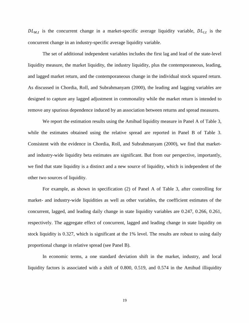
𝐷𝐿𝑀,𝑡 is the concurrent change in a market-specific average liquidity variable, 𝐷𝐿𝐼,𝑡 is the

concurrent change in an industry-specific average liquidity variable.

The set of additional independent variables includes the first lag and lead of the state-level

liquidity measure, the market liquidity, the industry liquidity, plus the contemporaneous, leading,

and lagged market return, and the contemporaneous change in the individual stock squared return.

As discussed in Chordia, Roll, and Subrahmanyam (2000), the leading and lagging variables are

designed to capture any lagged adjustment in commonality while the market return is intended to

remove any spurious dependence induced by an association between returns and spread measures.

We report the estimation results using the Amihud liquidity measure in Panel A of Table 3,

while the estimates obtained using the relative spread are reported in Panel B of Table 3.

Consistent with the evidence in Chordia, Roll, and Subrahmanyam (2000), we find that market-

and industry-wide liquidity beta estimates are significant. But from our perspective, importantly,

we find that state liquidity is a distinct and a new source of liquidity, which is independent of the

other two sources of liquidity.

For example, as shown in specification (2) of Panel A of Table 3, after controlling for

market- and industry-wide liquidities as well as other variables, the coefficient estimates of the

concurrent, lagged, and leading daily change in state liquidity variables are 0.247, 0.266, 0.261,

respectively. The aggregate effect of concurrent, lagged and leading change in state liquidity on

stock liquidity is 0.327, which is significant at the 1% level. The results are robust to using daily

proportional change in relative spread (see Panel B).

In economic terms, a one standard deviation shift in the market, industry, and local

liquidity factors is associated with a shift of 0.800, 0.519, and 0.574 in the Amihud illiquidity

20

measure, respectively.3

4.2 Liquidity Panel Predictability Regressions: Baseline Estimates

This evidence indicates that the market factor has the strongest effect on

firm liquidity, but the impact of local liquidity factor is comparable and somewhat stronger than

the effect of the industry factor. Overall, our evidence indicates that state liquidity is a new source

of commonality in liquidity, which is independent from the effects of market- and industry-wide

liquidity.

In this section, we test the first hypothesis. Specifically, we estimate panel regressions that

pool on both the time-series and cross-sectional dimensions, where current state liquidity is the

dependent variable and all economic activity measures are lagged as described earlier. State fixed

effects are included in all regressions, but their coefficients are suppressed to conserve space. The

liquidity regression estimates are presented in Table 4. In Panel A, we use the Amihud’s illiquidity

measure while, in Panel B, the dependent variable is the relative spread measure.

Consistent with our main conjecture (H1), we find that lagged state income growth and

state housing collateral (hy) are negatively related to current state liquidity, regardless of whether

we control for the level of overall U.S. economic activity. The statistical significance of state

relative unemployment variable is weaker, consistent with the unconditional correlations.

Specifically, lagged state relative unemployment is positively correlated with the current State

Amihud measure when we control for other U.S. macroeconomic variables. However, the

coefficient estimate is positive but statistically insignificant when State Relative Spread is the

dependent variable.

When we examine the joint effects of all local macroeconomic variables, we find that the

lagged state economic activity index is significantly negatively related to current state liquidity,

3 The standard deviations of the market, industry, and liquidity factors are 0.871, 0.933, and 1.756, respectively.

21

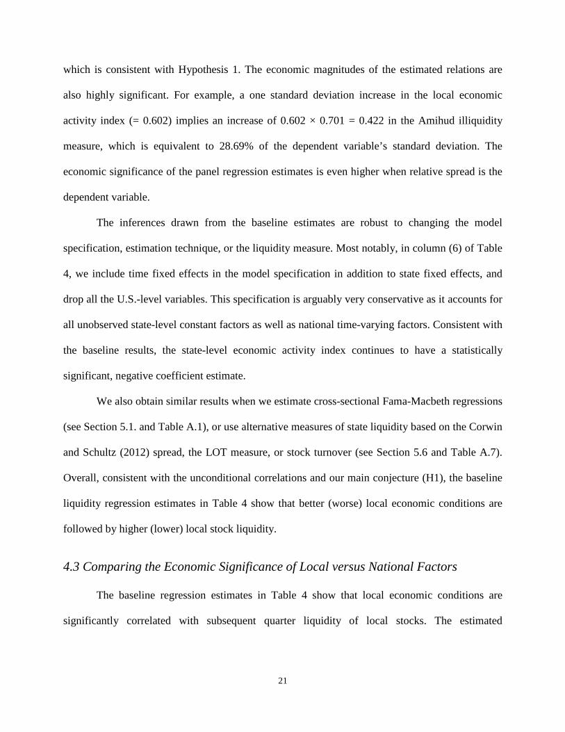
which is consistent with Hypothesis 1. The economic magnitudes of the estimated relations are

also highly significant. For example, a one standard deviation increase in the local economic

activity index (= 0.602) implies an increase of 0.602 × 0.701 = 0.422 in the Amihud illiquidity

measure, which is equivalent to 28.69% of the dependent variable’s standard deviation. The

economic significance of the panel regression estimates is even higher when relative spread is the

dependent variable.

The inferences drawn from the baseline estimates are robust to changing the model

specification, estimation technique, or the liquidity measure. Most notably, in column (6) of Table

4, we include time fixed effects in the model specification in addition to state fixed effects, and

drop all the U.S.-level variables. This specification is arguably very conservative as it accounts for

all unobserved state-level constant factors as well as national time-varying factors. Consistent with

the baseline results, the state-level economic activity index continues to have a statistically

significant, negative coefficient estimate.

We also obtain similar results when we estimate cross-sectional Fama-Macbeth regressions

(see Section 5.1. and Table A.1), or use alternative measures of state liquidity based on the Corwin

and Schultz (2012) spread, the LOT measure, or stock turnover (see Section 5.6 and Table A.7).

Overall, consistent with the unconditional correlations and our main conjecture (H1), the baseline

liquidity regression estimates in Table 4 show that better (worse) local economic conditions are

followed by higher (lower) local stock liquidity.

4.3 Comparing the Economic Significance of Local versus National Factors

The baseline regression estimates in Table 4 show that local economic conditions are

significantly correlated with subsequent quarter liquidity of local stocks. The estimated

22

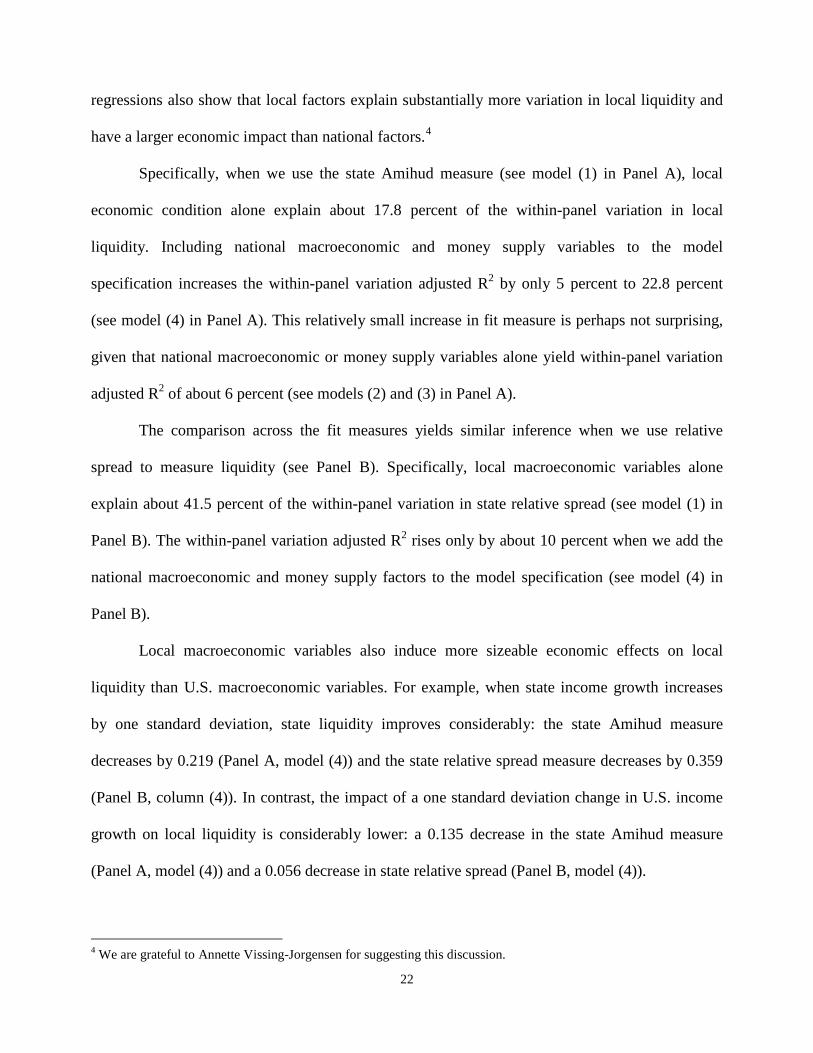
regressions also show that local factors explain substantially more variation in local liquidity and

have a larger economic impact than national factors.4

Specifically, when we use the state Amihud measure (see model (1) in Panel A), local

economic condition alone explain about 17.8 percent of the within-panel variation in local

liquidity. Including national macroeconomic and money supply variables to the model

specification increases the within-panel variation adjusted R2 by only 5 percent to 22.8 percent

(see model (4) in Panel A). This relatively small increase in fit measure is perhaps not surprising,

given that national macroeconomic or money supply variables alone yield within-panel variation

adjusted R2 of about 6 percent (see models (2) and (3) in Panel A).

The comparison across the fit measures yields similar inference when we use relative

spread to measure liquidity (see Panel B). Specifically, local macroeconomic variables alone

explain about 41.5 percent of the within-panel variation in state relative spread (see model (1) in

Panel B). The within-panel variation adjusted R2 rises only by about 10 percent when we add the

national macroeconomic and money supply factors to the model specification (see model (4) in

Panel B).

Local macroeconomic variables also induce more sizeable economic effects on local

liquidity than U.S. macroeconomic variables. For example, when state income growth increases

by one standard deviation, state liquidity improves considerably: the state Amihud measure

decreases by 0.219 (Panel A, model (4)) and the state relative spread measure decreases by 0.359

(Panel B, column (4)). In contrast, the impact of a one standard deviation change in U.S. income

growth on local liquidity is considerably lower: a 0.135 decrease in the state Amihud measure

(Panel A, model (4)) and a 0.056 decrease in state relative spread (Panel B, model (4)).

4 We are grateful to Annette Vissing-Jorgensen for suggesting this discussion.

23

Overall, consistent with our main conjecture, we find that local macroeconomic factors

explain more variation in state liquidity than the U.S. aggregates. In addition, our results

demonstrate that the economic impact of changes in local conditions on local liquidity is

substantially larger than that of the U.S. business cycle.

4.4 Local Stock Liquidity Predictability and Firm Size

In the next set of tests, we assess our second hypothesis (H2) by examining whether the

relation between local economic conditions and stock liquidity varies with firm size. Within each

state-quarter, we sort stocks into size terciles based on the firm most recent (i.e., beginning of the

current quarter) market capitalization of equity. Then, for each state-quarter-size tercile, we repeat

the tests presented Table 4. The panel regression estimates for each size tercile are reported in

Table 5, together with p-values from tests of no differences in the coefficient estimates across the

size terciles.

We find that the coefficient estimates of lagged state economic activity index decrease

monotonically across firm size terciles and these differences are statistically significant at

conventional levels. Two of the three components of the state economic activity index (lagged

state income growth and state hy) display similar patterns. The estimates of state relative

unemployment instead display no clear pattern.

When we combine the local macroeconomic variables into an index, we find that the

coefficient estimates of the state economic activity index exhibit a monotonically decreasing

pattern. It is significantly positive or weakly negative for smaller firms but strongly negative and

highly significant, both economically and statistically, for medium and large size firm terciles.5

5 The state economic activity index has a positive coefficient estimate in Panel A, where the dependent variable is the Amihud measure. This evidence suggests that the liquidity for smaller firms increase when the local economic

24

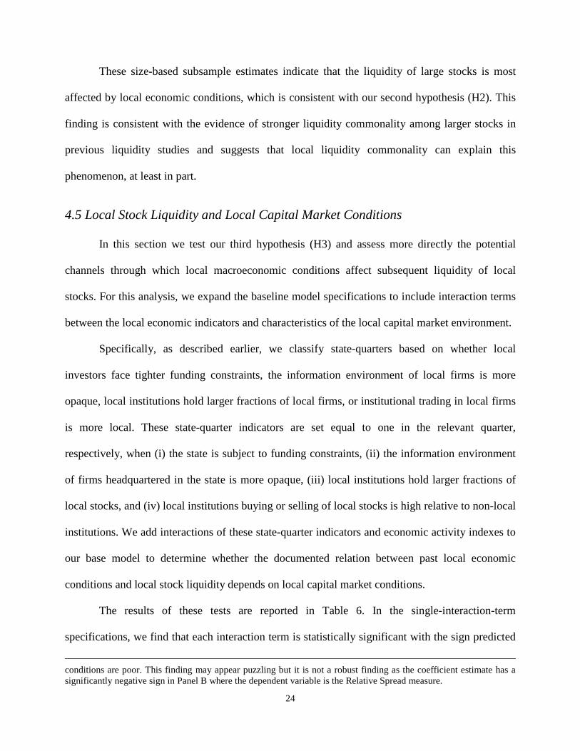
These size-based subsample estimates indicate that the liquidity of large stocks is most

affected by local economic conditions, which is consistent with our second hypothesis (H2). This

finding is consistent with the evidence of stronger liquidity commonality among larger stocks in

previous liquidity studies and suggests that local liquidity commonality can explain this

phenomenon, at least in part.

4.5 Local Stock Liquidity and Local Capital Market Conditions

In this section we test our third hypothesis (H3) and assess more directly the potential

channels through which local macroeconomic conditions affect subsequent liquidity of local

stocks. For this analysis, we expand the baseline model specifications to include interaction terms

between the local economic indicators and characteristics of the local capital market environment.

Specifically, as described earlier, we classify state-quarters based on whether local

investors face tighter funding constraints, the information environment of local firms is more

opaque, local institutions hold larger fractions of local firms, or institutional trading in local firms

is more local. These state-quarter indicators are set equal to one in the relevant quarter,

respectively, when (i) the state is subject to funding constraints, (ii) the information environment

of firms headquartered in the state is more opaque, (iii) local institutions hold larger fractions of

local stocks, and (iv) local institutions buying or selling of local stocks is high relative to non-local

institutions. We add interactions of these state-quarter indicators and economic activity indexes to

our base model to determine whether the documented relation between past local economic

conditions and local stock liquidity depends on local capital market conditions.

The results of these tests are reported in Table 6. In the single-interaction-term

specifications, we find that each interaction term is statistically significant with the sign predicted

conditions are poor. This finding may appear puzzling but it is not a robust finding as the coefficient estimate has a significantly negative sign in Panel B where the dependent variable is the Relative Spread measure.

25

by our third hypothesis (H3). In particular, in models (1a) and (1b), the coefficient estimates of the

“State Econ Act × State Fund Const Dummy” interaction term are negative. Consistent with the

notion that binding capital constraints induce commonality in liquidity during economic

downturns, the effect of local economic conditions on local stock liquidity is predominant in

states-quarters characterized by tighter funding constraints.

In columns (2a) and (2b), the coefficient estimates of the “State Econ Act × State Opac

Dummy” interaction term are negative, indicating that the impact of state economic conditions on

local stock liquidity is stronger in states characterized by more opaque information environments.

This finding is consistent with the notion that the liquidity of stocks depends more heavily on local

investors in more opaque local information environments, where adverse selection is likely to be a

more severe concern.

In columns (3a) and (3b), the coefficients estimates of the “State Econ Act × Local IO

Dummy” interaction term are negative. Thus, the predicted relation between the state economic

conditions and local stock liquidity is indeed stronger where local institutions hold larger stakes in

local companies. This is consistent with the idea that a common local investor base determines the

systematic impact of state-level macroeconomic conditions on local stock liquidity.

In columns (4a) and (4b), the coefficients estimates of the “State Econ Act × Rel Local

Trading Dummy” interaction term are negative, suggesting that the relation between state

economic conditions and local stock liquidity is stronger where trading in local stocks is more

heavily local. This evidence is consistent with our conjecture that correlated trading of local

investor affects the systematic impact of state-level macroeconomic conditions on local stock

liquidity.

In the full model specifications (columns (5a) and (5b)), we find that the coefficient

estimates of three of the four interaction terms become only marginally statistically significant,

26

although all estimates retain the predicted sign. The full specification results, however, should be

interpreted with caution given the severe reduction in sample size due to the availability of the

funding constraint data before 1993 and limited presence of NYSE-listed broker-dealers across

various states. In models (6a) and (6b), we drop the funding constraint indicator from the

specification. This more parsimonious specification estimated for the larger sample again provides

strong support for our third hypothesis (H3).

Next, we re-examine whether the effect of local macroeconomic conditions on liquidity

varies by firm size, after conditioning on local capital market conditions. The specification of

these tests is similar to those in Tables 5 and 6. In particular, for each size tercile, Table 7 reports

panel regression coefficient estimates for the three-interaction specification of model (6) in Table

6, which excludes the funding constraint indicator to increase sample size. The table also reports

p-values from tests of no differences in the coefficient estimates across size terciles.

In both Panels A and B, the main interaction terms have larger negative coefficient

estimates for the medium and large size firm groups and the differences across subsamples are

highly statistically significant. In contrast, the interaction variables defined using the U.S.-level

economic indicators do not exhibit a similar pattern. This evidence is consistent with the results in

Tables 5 and 6, and indicates that local liquidity predictability is stronger for larger firms and so

are the effects of the local information environment opaqueness and the degree of local

institutional ownership and trading.

Collectively, the evidence from the expanded liquidity regression specifications shows that

the relation between local economic conditions and subsequent local stock liquidity critically

depends upon the existing conditions of local capital markets. These results provide strong support

to our third hypothesis (H3).

27

4.6 Performance of Trading Strategies Based on Predicted Local Liquidity

In this section, we test our fourth hypothesis, which focuses on the asset pricing

implications of the geographical variation in liquidity. Similar to Korniotis and Kumar (2012), we

use the liquidity predictability regressions to develop trading strategies and examine their risk-

adjusted performance.

To form the trading portfolios, we use the state rankings implied by the recursive estimates

with no look-ahead bias from model (4) in Table 4 and obtain quarterly state rankings. Then, we

form four portfolios: (i) a value-weighted “Long” portfolio of stocks located in the three U.S.

states with the lowest predicted liquidity at the beginning of the relevant quarter; (ii) a value-

weighted “Short” portfolio of stocks located in the three U.S. states with the highest predicted

liquidity at the beginning of the relevant quarter; (iii) a “Long−Short” portfolio, which captures

the difference in returns of the Long and Short portfolios, and (iv) a “Others” portfolio, which

includes all stocks that are neither in the Long nor the Short portfolios.

We evaluate the performance of these portfolios using monthly returns. Because all

portfolios are formed at the beginning of each quarter when new data on state- and U.S.-level

economic activity become available, the portfolio composition does not change every month. For

each portfolio, we compute the raw, market-adjusted, and characteristic-adjusted returns of Daniel,

Grinblatt, Titman, and Wermers (1997) method. We use three years for our pre-estimation period.

Therefore, the trading periods are from 1983 to 2008 for portfolios formed based on the State

Amihud measure and from 1993 to 2008 for portfolios formed based on State Relative Spread

measure. We use a shorter period of the latter measure because most stocks only have data on

closing bid and ask spreads since 1990 in CRSP.

We report the portfolio performance estimates in Table 8. We find that only the Long

portfolio generates significantly positive mean monthly raw, market-adjusted, and characteristic-

28

adjusted returns. The Short portfolio has positive mean raw returns but insignificantly negative

risk adjusted returns. More importantly, the Long−Short portfolio generates positive and

significant mean monthly raw, market-adjusted, as well as characteristic-adjusted returns. The

positive risk-adjusted performance of the liquidity based trading strategy supports our fourth

hypothesis (H4) and indicates that local macroeconomic variables affect local stock prices through

their impact on the liquidity of local firms.6

4.7 Local Business Cycles and Performance of Trading Strategies

It is possible that the performance of the liquidity-based trading strategy is driven only by

periods when the local economy is in a recession as liquidity may deteriorate dramatically during

those periods. To assess this possibility, we test the performance of the liquidity-based trading

strategy conditional on the local business cycle.

We conduct this analysis as follows. First, in each quarter t, we sort states into terciles of

state economic activity. Tercile 1 contains states with the smallest values of the state economic

index at quarter t, i.e., contracting states. Tercile 3 contains states with the largest values of state

economic index in quarter t, i.e., expanding states. Then, within each tercile, we use the recursive

liquidity prediction model from model (4) in Table 6 to rank state-portfolios based on their

predicted liquidity. Table 9 reports mean monthly raw, market-adjusted, and characteristic-

adjusted returns of liquidity-based state-portfolios, separately for contracting and expanding states.

As in the previous table, we require a three-year window for the pre-estimation period. Thus, the

evaluation periods are from 1983 to 2008 for the State Amihud measure and from 1993 to 2008

for the State Relative Spread measure.

6 Korniotis and Kumar (2012) define geography-based trading strategies to examine if local economic variables predict local returns. In unreported results, we find our liquidity based strategy is not a repackaging of the evidence in Korniotis and Kumar (2012). The correlation between the characteristic-adjusted returns from the two strategies is very low (0.10) and statistically insignificant, indicating that the two predictability phenomena are distinct.

29

The evidence shows that, when we use the State Amihud illiquidity measure, the

Long−Short portfolio generates positive and significant mean monthly returns during both local

expansions and local contractions. The Long-Short average monthly returns following contraction

quarters, however, are larger than those following expansions. Moreover, when we use the State

Relative Spread measure of liqudity, the Long−Short portfolio generates positive and significant

returns only during local contractions. Overall, the evidence indeed suggests that local recessions

have a larger effect on the performance of local liquidity-based trading strategies.

4.8 Performance of Trading Strategies Using Factor Models

Next, to better account for risk, we evaluate the economic significance of liquidity-based

trading strategies using various factor models. We consider several unconditional factor models as

well as two conditional factor modes. The unconditional factor models contain some combination

of the market factor (RMRF), the size factor (SMB), the value factor (HML), the momentum

factor (UMD), three industry factors (IND1, IND2, and IND3), short-term reversal factor (STR),

long-term reversal factor (LTR), and the liquidity (LIQ) factor. The conditional models include the

three Fama-French factors (RMRF, SMB, and HML), the momentum factor (UMD), and the

interactions of these factors with either the Lettau and Ludvigson (2001a, b) lagged cay residual or

the NBER recession indicator. As before, the evaluation period is from 1983 to 2008 for the State

Amihud iliiquidity measure and from 1993 to 2008 for the State Relative Spread measure.

The estimation results from the unconditional models are reported in Table 10 and, to

conserve space, we report the results from the conditional models in Appendix Table A9. We find

that, for all factor models, the Long portfolio has positive and significant alpha estimates, the

Short portfolio has negative and significant alpha estimates, and the Long−Short portfolio has

positive and significant alpha estimates. For example, the CAPM monthly alpha for the

30

Long−Short portfolio is about 80 basis points and the monthly alpha estimate for the expanded

factor models is about 60 basis points. Even when we consider conditional factor models that

include both the interaction terms with the cay residual and the NBER recession indicator, the

monthly alpha estimates remain high, at least 50 basis points, and statistically significant –

Appendix Table A.9.

Overall, the alpha estimates from various factor models indicate that the impact of local

business cycles on local liquidity is economically significant. This evidence is consistent with our

main asset pricing hypothesis (H4), which posits that poor local economic conditions will lead to

higher future average returns.

5. Supplemental Evidence and Robustness Checks

In this section, we report evidence from additional tests that examine the robustness of our

main results. For brevity, the results from all these tests are provided in Appendix tables.

5.1 Fama-MacBeth Estimation and Sub-Period Results

First, we re-examine the relation between local economic conditions and liquidity using the

Fama and MacBeth (1973) predictive regressions. Specifically, we estimate state-level cross-

sectional regressions each quarter over the sample period. In the regression, the current state-level

stock liquidity is regressed either on the lagged state income growth, lagged state relative

unemployment, and lagged state hy, or on the lagged state economic activity index. We then report

the time-series coefficient averages and their respective Newey-West (1987) corrected t-statistics.

These results are in Appendix Table A.1. These estimates are qualitatively similar to the baseline

results reported in Table 4 and support our first main hypothesis.

Next, we report the Fama-MacBeth regression estimates for different sub-periods to test if

the relation between local economic conditions and local stock liquidity is persistent. We split our

31

full sample period into six sub-periods and re-estimate the Fama-MacBeth regressions. For each

sub-period, Appendix Table A.2 reports the time-series coefficient averages of quarterly Fama and

MacBeth (1973) regressions, together with Newey-West (1987) corrected t-statistics. The sub-

period estimates indicate that the relation between local liquidity and local economic conditions is

consistently in the same direction and statistically significant.

5.2 Panel Regression Estimates Using Alternative Lag Length

Appendix Table A.3 replicates the baseline results reported in Table 4 using one-lag

realizations of both the state and U.S.-level economic activity variables instead of the two-lag

realizations used in the baseline specifications. We find that our main results and inferences

remain virtually identical when we use the shorter lag for the economic activity measures, which is

not very surprising given the persistence in local economic conditions. Interestingly, however, all

estimated models consistently have somewhat higher adjusted-R2, suggesting that more recent

variation in economic conditions is a better predictor of local stock liquidity.

5.3 Panel Regression Estimates Excluding Large States and One-Firm States

Appendix Table A.4 replicates the baseline results reported in Table 4 after excluding large

states (California, New York, and Texas) and one-firm states (Arkansas, the home of Walmart,

and, Washington, the home of Microsoft) from the sample. We find that, even after we exclude

these five states, local economic conditions are a strong predictor of subsequent local stock

liquidity.

5.4 Panel Regression Estimates Using Industry-Adjusted Local Stock Liquidity

Given the known geographical clustering of industries, one potential concern with our

results is that the evidence of commonality in local liquidity is merely another manifestation of the

32

previously documented commonality in industry-level liquidity, first documented in Chordia, Roll,

and Subrahmanyam (2000). Table A.5 replicates the baseline results reported in Table 4 using

industry-quarter mean-adjusted Amihud and relative spread measures to construct the aggregate

state-level liquidity measures.

The results are in line with those reported in Table 4, although the adjusted R2 values and

the economic magnitudes implied by the coefficient estimates are smaller than the baseline results.

For example, a one standard deviation change in the local activity index is now associated with a

change in the Amihud (relative spreads) illiquidity measure that is equivalent to about 10% (35%)

of the measure’s standard deviation, rather than 30% (50%) as in the baseline model. Thus, the

local and industry liquidity phenomena are partly related, which is consistent with the motivation

for these tests. However, it is important to highlight that the relation between local economic

conditions and local liquidity is not merely a “dominant local industry” effect.

5.5 Regional Analysis

Our analysis so far is based on state-level liquidity measures and state-level economic

activity estimates. If local liquidity commonality is truly a state-level phenomenon, aggregating

states into regions should weaken the results. We use the four divisions of U.S. Census Bureau as

regions and average the state liquidity and state economic conditions across the states within each

region. We then regress the current regional liquidity on the lagged regional macroeconomic

variables with or without U.S. macroeconomic control variables. Appendix Table A.6 reports

these results. The evidence shows that lagged regional macroeconomic variables do not predict

current regional liquidity at conventional significance levels, regardless of whether we control for

U.S. macroeconomic factors or not. Similarly, the regional economic activity index does not

predict regional liquidity.

33

5.6 Panel Regression Estimates Using Alternative Liquidity Measures

Table A.7 replicates the baseline results reported in Table 4 using alternative measures of

state liquidity. They are the spread measure of Corwin and Schultz (2012), the Lesmond, Ogden,

and Trzcinka (LOT) (1999) measure, and the turnover of local stocks. Unlike the other liquidity

measures used in this paper, higher state turnover is associated with higher liquidity. The results

from these tests are largely and robustly consistent with our baseline results, indicating that local

economic conditions are strong predictors of the liquidity of local firms.

5.7 Lagged Local Capital Market Conditions and Local Liquidity Predictability

Table A.8 replicates the baseline results reported in Table 6, where we measure all state-

level capital market conditions indicators with a one-quarter lag, as opposed to doing so for only

the state opacity indicator. Our goal is to ensure that the significance of the interaction terms is not

driven by omitted contemporaneous common shocks. The evidence in Table A.8 is very similar to

the results reported in Table 6. This evidence provides further support to the notion that the

opacity of the local information environment and the prevalence of local institutional ownership

and trading jointly determine whether and to what extent local economic conditions induce

liquidity commonality among local stocks.

5.8 Performance Estimates Using Alternative Factor Models

In the last test, we examine the robustness of our trading strategy performance estimates.

Table A.9 reports conditional factor model estimates, where the factor models include interactions

of factor returns with both cay and a NBER recession dummy indicator. The alpha estimates from

these augmented models remain positive and significant, both economically and statistically. This

34

finding indicates that the Long−Short portfolio alphas do not reflect portfolios’ time-varying

exposures to the underlying risk factors.

6. Summary and Conclusion

Understanding the determinants of commonality of liquidity across firms and over time is

important because it has direct implications for investors’ ability to diversify volatility and

liquidity shocks. In this paper, we show that the geographical location of a firm affects its

liquidity. Specifically, there is an economically significant local component in firm liquidity that is

induced by local economic conditions. The firm liquidity is higher (lower) when the local

economy performs well (poorly) and the magnitude of this effect increases with firm size. Further,

the impact of local economic conditions on local firm liquidity is stronger when local financing

constraints are more binding, the local information environment is more opaque, and local

institutional hold larger stakes of or trade more heavily in stocks of local firms.

This geographical variation in local liquidity generates systematic patterns in local stock

returns. Current local stock prices decline and future average returns are higher when expected

local liquidity is lower. A trading strategy based on the geographical variation in firm-level

liquidity generates an annual risk-adjusted performance of over six percent. Taken together, these

results significantly improve our understanding of the sources of commonality in liquidity and

support our broad conjecture that geographical heterogeneity in macroeconomic conditions

generates geographical patterns in firm liquidity.

In future work, it may be useful to examine other asset pricing implications of

geographical variation in firm liquidity. For example, one natural implication of our findings is

that local macroeconomic variables generate commonality in local liquidity that is priced. It would

also be useful to study whether the geographical variation in firm liquidity is associated with a

35

geographical variation in firm-level volatility. It is likely that local macroeconomic variables

affect the liquidity as well as the volatility of local firms. In this scenario, the pricing of firm-level

volatility and the time-series patterns in volatility may also vary geographically across the U.S.

states.

References Amihud, Yakov, 2002, Illiquidity and stock returns: Cross-section and time-series effects, Journal

of Financial Markets 5, 31-56.

Anderson, Ronald C., Augustine Duru, and David M. Reeb, 2009, Founders, heirs, and corporate

opacity in the United States, Journal of Financial Economics 92, 205-222.

Atkins, Allen B., and Edward A. Dyl, 1997, Market structure and reported trading volume:

Nasdaq versus the NYSE, Journal of Financial Research 20, 291-304.

Becker, Bo, 2007, Geographical Segmentation of U.S. Capital Markets, Journal of Financial

Economics 85, 151-178.

Boyd, John H., Jian Hu, and Ravi Jagannathan, 2005, The stock market’s reaction to

unemployment news: Why bad news is usually good for stocks?, Journal of Finance 60,

649-672.

Brockman, Paul, and Dennis Y. Chung, 2002, Commonality in liquidity: Evidence from an order-

driven market structure, Journal of Financial Research 25, 521-539.

Brockman, Paul, Dennis Y. Chung, and Christophe Pérignon, 2009, Commonality in liquidity: A

global perspective, Journal of Financial and Quantitative Analysis 44, 851-882.

Brunnermeier, Markus K., and Lasse Heje Pedersen, 2009, Market liquidity and funding liquidity,

Review of Financial Studies 22, 2201-2238.

Campbell, John Y., 1996, Understanding risk and return, Journal of Political Economy 104, 298-

345.

Carhart, Mark M., 1997, On persistence in mutual fund performance, Journal of Finance 52, 57-

82.

Choi, Woon Gyu, and David Cook, 2005, Stock market liquidity and the macroeconomy:

Evidence from Japan, Working Paper, IMF.

36

Chordia, Tarun, Richard Roll, and Avanidhar Subrahmanyam, 2000, Commonality in liquidity,

Journal of Financial Economics 56, 3-28.

Chordia, Tarun, Asani Sarkar, and Avanidhar Subrahmanyam, 2005, An empirical analysis of

stock and bond market liquidity, Review of Financial Studies 18, 85-130.

Corwin, Shane A., and Paul Schultz, 2012, A simple way to estimate bid-ask spreads from daily

high and low prices, Journal of Finance 67, 719-759.

Coval, Joshua D., and Tobias J. Moskowitz, 1999, Home bias at home: Local equity preference in

domestic portfolios, Journal of Finance 54, 2045-2073.

Coval, Joshua D., and Tobias J. Moskowitz, 2001, The geography of investment: Informed trading

and asset prices, Journal of Political Economy 109, 811-841.

Daniel, Kent D., Mark Grinblatt, Sheridan Titman, and Russell Wermers, 1997, Measuring mutual

fund performance with characteristic-based benchmarks, Journal of Finance 52, 1035-

1058.

Eisfeldt, Andrea L., 2004, Endogenous Liquidity in Asset Markets, Journal of Finance 59, 1-30.

Fama, Eugene F., and Kenneth R. French, 1992, The cross-section of expected stock returns,

Journal of Finance 47, 427-465.

Fama, Eugene F., and Kenneth R. French,1993, Common risk factors in returns on stocks and

bonds, Journal of Financial Economics 33, 3-56.

Fama, Eugene F., and James D. MacBeth, 1973, Risk, return, and equilibrium: empirical tests,

Journal of Political Economy 81, 607-636.

Fujimoto, Akiko, 2003, Macroeconomic sources of systematic liquidity, Working Paper, Yale

University.

Gomez, J.-P., Priestley, R. and F. Zapatero, 2011, Labor Income, Relative Wealth Concerns, and

the Cross-section of Stock Returns, Working Paper, University of Southern California.

Goyenko, Ruslan Y., Craig W. Holden, and Charles A. Trzcinka, 2009, Do liquidity measures

measure liquidity? Journal of Financial Economics 92, 153-181.

Goyenko, Ruslan Y., and Andrey D. Ukhov, 2009, Stock and bond market liquidity: A long-run

empirical analysis, Journal of Financial and Quantitative Analysis 44, 189-212.

Grinblatt, Mark, and Tobias J. Moskowitz, 1999, Do industries explain momentum? Journal of

Finance 54, 1249-1290.

37

Hameed, Allaudeen, Wenjin Kang, and S. Viswanathan, 2010, Stock market declines and

liquidity, Journal of Finance 65, 257-293.

Hasbrouck, Joel, and Duane Seppi, 2001, Common factors in prices, order flows, and liquidity,

Journal of Financial Economics 59, 383-411.

Hasbrouck, Joel, 2009, Trading costs and returns for U.S. equities: Estimating effective costs from

daily data, Journal of Finance 64, 1445-1477.

Hong, Harrison, Walter Torous, and Rossen Valkanov, 2007, Do industries lead stock markets?

Journal of Financial Economics 83, 367-396.

Huberman, Gur, and Dominika Halka, 2001, Systematic liquidity, Journal of Financial Research

24, 161-178.

Jagannathan, Ravi, and Zhenyu Wang, 1996, The conditional CAPM and the cross-section of

expected returns, Journal of Finance 51, 3-53.

Jegadeesh, Narasimhan, and Sheridan Titman, 1993, Returns to buying winners and selling losers:

Implications for market efficiency, Journal of Finance 48, 65-91.

Kamara, Avraham, Xiaoxia Lou, and Ronnie Sadka, 2008, The divergence of liquidity

commonality in the cross-section of stocks, Journal of Financial Economics 89, 444-466.

Korajczyk, Robert A., and Ronnie Sadka, 2008, Pricing the commonality across alternative

measures of liquidity, Journal of Financial Economics 87, 45-72.

Korniotis, George M., 2008, Habit Formation, Incomplete Markets, and the Significance of

Regional Risk for Expected Returns, Review of Financial Studies 21, 2139 – 2172.

Korniotis, George M., and Alok Kumar, 2012, State-level business cycles and local return

predictability, Journal of Finance, Forthcoming.

Kyle, Albert, 1985, Continous auctions and insider trading, Econometrica 53, 1315-1335.

Lesmond, David A., Joseph P. Ogden, and Charles A. Trzcinka, 1999, A new estimate of

transaction costs, Review of Financial Studies 12, 1113-1141.

Lettau, Martin, and Sydney Ludvigson, 2001a, Consumption, aggregate wealth, and expected

stock returns, Journal of Finance 21, 815-849.

Lettau, Martin, and Sydney Ludvigson, 2001b, Resurrecting the (C)CAPM: A cross-sectional test

when risk premia are time-varying, Journal of Political Economy 109, 1238-1286.

Loughran, Timothy, and Paul H. Schultz, 2005, Liquidity: Urban versus rural firms, Journal of

Financial Economics 78, 341-374.

38

Lustig, Hanno, and Stijn van Nieuwerburgh, 2005, Housing collateral, consumption insurance, and

risk premia: An empirical perspective, Journal of Finance 60, 1167-1219.

Lustig, Hanno, and Stijn van Nieuwerburgh, 2010, How much does household collateral constrain

regional risk sharing? Review of Economic Dynamics 13, 265-294.

Newey, Whitney K., and Kenneth D. West, 1987, A simple positive semi-definite,

heteroskedasticity and autocorrelation consistent covariance matrix, Econometrica 55, 703-

708.

Pástor, Lubos, and Robert F. Stambaugh, 2002, Mutual fund performance and seemingly unrelated

assets, Journal of Financial Economics 63, 315-349.

Pástor, Lubos, and Robert F. Stambaugh, 2003, Liquidity risk and expected stock returns, Journal

of Political Economy 111, 642-685.

Sauer, Stephan, 2007, Liquidity risk and monetary policy, Munich Economic Discussion Papers

2007-27.

Taddei, Filippo, 2007, Liquidity and Economic Fluctuations, Working Paper, Columbia

University.

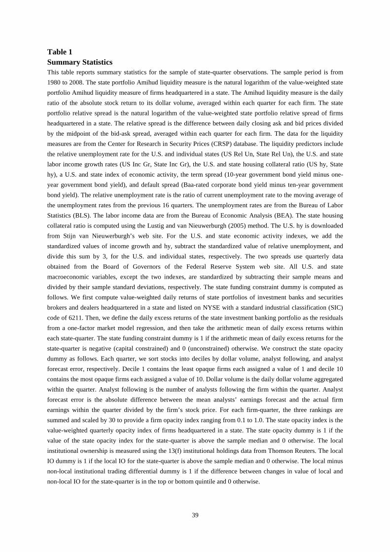
39

Table 1 Summary Statistics This table reports summary statistics for the sample of state-quarter observations. The sample period is from 1980 to 2008. The state portfolio Amihud liquidity measure is the natural logarithm of the value-weighted state portfolio Amihud liquidity measure of firms headquartered in a state. The Amihud liquidity measure is the daily ratio of the absolute stock return to its dollar volume, averaged within each quarter for each firm. The state portfolio relative spread is the natural logarithm of the value-weighted state portfolio relative spread of firms headquartered in a state. The relative spread is the difference between daily closing ask and bid prices divided by the midpoint of the bid-ask spread, averaged within each quarter for each firm. The data for the liquidity measures are from the Center for Research in Security Prices (CRSP) database. The liquidity predictors include the relative unemployment rate for the U.S. and individual states (US Rel Un, State Rel Un), the U.S. and state labor income growth rates (US Inc Gr, State Inc Gr), the U.S. and state housing collateral ratio (US hy, State hy), a U.S. and state index of economic activity, the term spread (10-year government bond yield minus one-year government bond yield), and default spread (Baa-rated corporate bond yield minus ten-year government bond yield). The relative unemployment rate is the ratio of current unemployment rate to the moving average of the unemployment rates from the previous 16 quarters. The unemployment rates are from the Bureau of Labor Statistics (BLS). The labor income data are from the Bureau of Economic Analysis (BEA). The state housing collateral ratio is computed using the Lustig and van Nieuwerburgh (2005) method. The U.S. hy is downloaded from Stijn van Nieuwerburgh’s web site. For the U.S. and state economic activity indexes, we add the standardized values of income growth and hy, subtract the standardized value of relative unemployment, and divide this sum by 3, for the U.S. and individual states, respectively. The two spreads use quarterly data obtained from the Board of Governors of the Federal Reserve System web site. All U.S. and state macroeconomic variables, except the two indexes, are standardized by subtracting their sample means and divided by their sample standard deviations, respectively. The state funding constraint dummy is computed as follows. We first compute value-weighted daily returns of state portfolios of investment banks and securities brokers and dealers headquartered in a state and listed on NYSE with a standard industrial classification (SIC) code of 6211. Then, we define the daily excess returns of the state investment banking portfolio as the residuals from a one-factor market model regression, and then take the arithmetic mean of daily excess returns within each state-quarter. The state funding constraint dummy is 1 if the arithmetic mean of daily excess returns for the state-quarter is negative (capital constrained) and 0 (unconstrained) otherwise. We construct the state opacity dummy as follows. Each quarter, we sort stocks into deciles by dollar volume, analyst following, and analyst forecast error, respectively. Decile 1 contains the least opaque firms each assigned a value of 1 and decile 10 contains the most opaque firms each assigned a value of 10. Dollar volume is the daily dollar volume aggregated within the quarter. Analyst following is the number of analysts following the firm within the quarter. Analyst forecast error is the absolute difference between the mean analysts’ earnings forecast and the actual firm earnings within the quarter divided by the firm’s stock price. For each firm-quarter, the three rankings are summed and scaled by 30 to provide a firm opacity index ranging from 0.1 to 1.0. The state opacity index is the value-weighted quarterly opacity index of firms headquartered in a state. The state opacity dummy is 1 if the value of the state opacity index for the state-quarter is above the sample median and 0 otherwise. The local institutional ownership is measured using the 13(f) institutional holdings data from Thomson Reuters. The local IO dummy is 1 if the local IO for the state-quarter is above the sample median and 0 otherwise. The local minus non-local institutional trading differential dummy is 1 if the difference between changes in value of local and non-local IO for the state-quarter is in the top or bottom quintile and 0 otherwise.

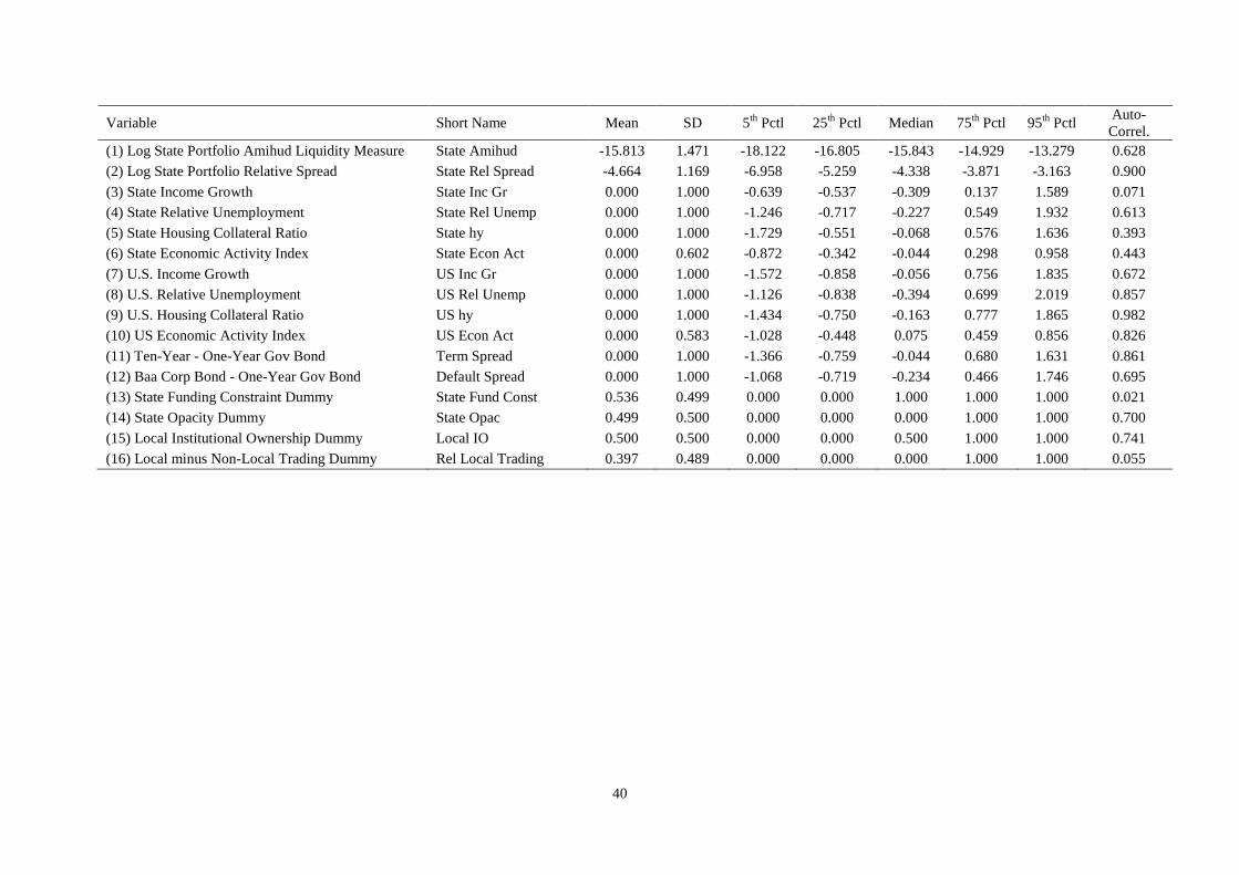
40

Variable Short Name Mean SD 5th Pctl 25th Pctl Median 75th Pctl 95th Pctl Auto- Correl.

(1) Log State Portfolio Amihud Liquidity Measure State Amihud -15.813 1.471 -18.122 -16.805 -15.843 -14.929 -13.279 0.628 (2) Log State Portfolio Relative Spread State Rel Spread -4.664 1.169 -6.958 -5.259 -4.338 -3.871 -3.163 0.900 (3) State Income Growth State Inc Gr 0.000 1.000 -0.639 -0.537 -0.309 0.137 1.589 0.071 (4) State Relative Unemployment State Rel Unemp 0.000 1.000 -1.246 -0.717 -0.227 0.549 1.932 0.613 (5) State Housing Collateral Ratio State hy 0.000 1.000 -1.729 -0.551 -0.068 0.576 1.636 0.393 (6) State Economic Activity Index State Econ Act 0.000 0.602 -0.872 -0.342 -0.044 0.298 0.958 0.443 (7) U.S. Income Growth US Inc Gr 0.000 1.000 -1.572 -0.858 -0.056 0.756 1.835 0.672 (8) U.S. Relative Unemployment US Rel Unemp 0.000 1.000 -1.126 -0.838 -0.394 0.699 2.019 0.857 (9) U.S. Housing Collateral Ratio US hy 0.000 1.000 -1.434 -0.750 -0.163 0.777 1.865 0.982 (10) US Economic Activity Index US Econ Act 0.000 0.583 -1.028 -0.448 0.075 0.459 0.856 0.826 (11) Ten-Year - One-Year Gov Bond Term Spread 0.000 1.000 -1.366 -0.759 -0.044 0.680 1.631 0.861 (12) Baa Corp Bond - One-Year Gov Bond Default Spread 0.000 1.000 -1.068 -0.719 -0.234 0.466 1.746 0.695 (13) State Funding Constraint Dummy State Fund Const 0.536 0.499 0.000 0.000 1.000 1.000 1.000 0.021 (14) State Opacity Dummy State Opac 0.499 0.500 0.000 0.000 0.000 1.000 1.000 0.700 (15) Local Institutional Ownership Dummy Local IO 0.500 0.500 0.000 0.000 0.500 1.000 1.000 0.741 (16) Local minus Non-Local Trading Dummy Rel Local Trading 0.397 0.489 0.000 0.000 0.000 1.000 1.000 0.055

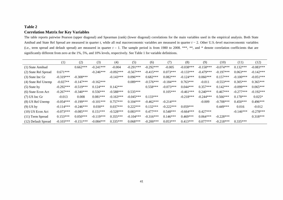
41

Table 2 Correlation Matrix for Key Variables The table reports pairwise Pearson (upper diagonal) and Spearman (rank) (lower diagonal) correlations for the main variables used in the empirical analysis. Both State Amihud and State Rel Spread are measured in quarter t, while all real macroeconomic variables are measured in quarter t − 2. Other U.S.-level macroeconomic variables (i.e., term spread and default spread) are measured in quarter t – 1. The sample period is from 1980 to 2008. ***, **, and * denote correlation coefficients that are significantly different from zero at the 1%, 5%, and 10% levels, respectively. See Table 1 for variable definitions.

(1) (2) (3) (4) (5) (6) (7) (8) (9) (10) (11) (12) (1) State Amihud 0.662*** -0.241*** -0.004 -0.291*** -0.292*** -0.005 -0.038*** -0.158*** -0.074*** 0.132*** -0.083*** (2) State Rel Spread 0.671*** -0.246*** -0.092*** -0.567*** -0.415*** 0.073*** -0.133*** -0.479*** -0.197*** 0.063*** -0.142*** (3) State Inc Gr -0.319*** -0.308*** -0.143*** 0.096*** 0.682*** 0.082*** -0.124*** 0.066*** 0.157*** -0.100*** -0.051*** (4) State Rel Unemp -0.027** -0.147*** -0.162*** 0.089*** -0.576*** -0.184*** 0.763*** -0.011 -0.553*** 0.305*** 0.365*** (5) State hy -0.292*** -0.519*** 0.124*** 0.142*** 0.558*** -0.073*** 0.044*** 0.357*** 0.142*** -0.099*** 0.065*** (6) State Econ Act -0.267*** -0.340*** 0.556*** -0.588*** 0.535*** 0.105*** -0.461*** 0.240*** 0.467*** -0.277*** -0.192*** (7) US Inc Gr -0.013 0.008 0.081*** -0.163*** -0.045*** 0.133*** -0.218*** -0.244*** 0.566*** 0.178*** 0.025* (8) US Rel Unemp -0.054*** -0.199*** -0.101*** 0.757*** 0.104*** -0.462*** -0.214*** -0.009 -0.708*** 0.450*** 0.496*** (9) US hy -0.114*** -0.246*** 0.030** 0.037*** 0.222*** 0.132*** -0.222*** 0.059*** 0.449*** 0.016 -0.012 (10) US Econ Act -0.073*** -0.085*** 0.151*** -0.528*** 0.083*** 0.477*** 0.548*** -0.664*** 0.427*** -0.146*** -0.278*** (11) Term Spread 0.153*** 0.050*** -0.119*** 0.355*** -0.104*** -0.316*** 0.146*** 0.469*** 0.064*** -0.228*** 0.318*** (12) Default Spread -0.103*** -0.151*** -0.084*** 0.335*** 0.068*** -0.200*** 0.053*** 0.413*** 0.077*** -0.218*** 0.335***

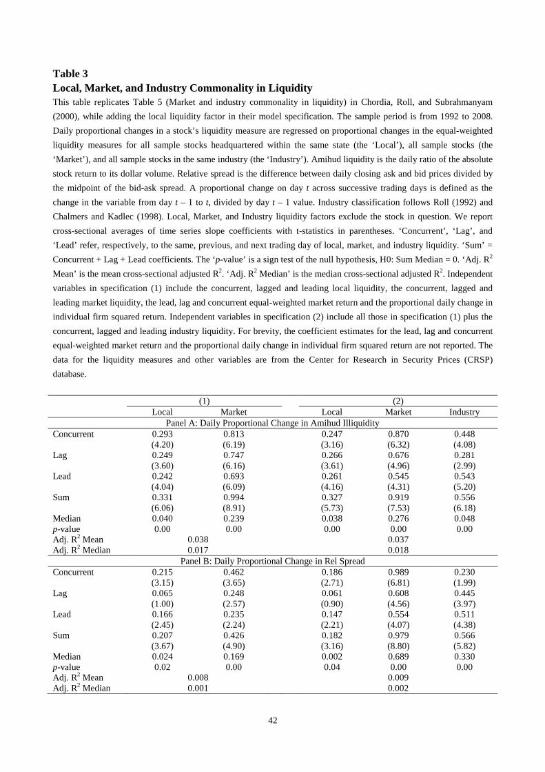
42

Table 3 Local, Market, and Industry Commonality in Liquidity This table replicates Table 5 (Market and industry commonality in liquidity) in Chordia, Roll, and Subrahmanyam (2000), while adding the local liquidity factor in their model specification. The sample period is from 1992 to 2008. Daily proportional changes in a stock’s liquidity measure are regressed on proportional changes in the equal-weighted liquidity measures for all sample stocks headquartered within the same state (the ‘Local’), all sample stocks (the ‘Market’), and all sample stocks in the same industry (the ‘Industry’). Amihud liquidity is the daily ratio of the absolute stock return to its dollar volume. Relative spread is the difference between daily closing ask and bid prices divided by the midpoint of the bid-ask spread. A proportional change on day t across successive trading days is defined as the change in the variable from day t – 1 to t, divided by day t – 1 value. Industry classification follows Roll (1992) and Chalmers and Kadlec (1998). Local, Market, and Industry liquidity factors exclude the stock in question. We report cross-sectional averages of time series slope coefficients with t-statistics in parentheses. ‘Concurrent’, ‘Lag’, and ‘Lead’ refer, respectively, to the same, previous, and next trading day of local, market, and industry liquidity. ‘Sum’ = Concurrent + Lag + Lead coefficients. The ‘p-value’ is a sign test of the null hypothesis, H0: Sum Median = 0. ‘Adj. R2 Mean’ is the mean cross-sectional adjusted R2. ‘Adj. R2 Median’ is the median cross-sectional adjusted R2. Independent variables in specification (1) include the concurrent, lagged and leading local liquidity, the concurrent, lagged and leading market liquidity, the lead, lag and concurrent equal-weighted market return and the proportional daily change in individual firm squared return. Independent variables in specification (2) include all those in specification (1) plus the concurrent, lagged and leading industry liquidity. For brevity, the coefficient estimates for the lead, lag and concurrent equal-weighted market return and the proportional daily change in individual firm squared return are not reported. The data for the liquidity measures and other variables are from the Center for Research in Security Prices (CRSP) database.

(1) (2) Local Market Local Market Industry

Panel A: Daily Proportional Change in Amihud Illiquidity Concurrent 0.293 0.813 0.247 0.870 0.448 (4.20) (6.19) (3.16) (6.32) (4.08) Lag 0.249 0.747 0.266 0.676 0.281 (3.60) (6.16) (3.61) (4.96) (2.99) Lead 0.242 0.693 0.261 0.545 0.543 (4.04) (6.09) (4.16) (4.31) (5.20) Sum 0.331 0.994 0.327 0.919 0.556 (6.06) (8.91) (5.73) (7.53) (6.18) Median 0.040 0.239 0.038 0.276 0.048 p-value 0.00 0.00 0.00 0.00 0.00 Adj. R2 Mean 0.038 0.037 Adj. R2 Median 0.017 0.018

Panel B: Daily Proportional Change in Rel Spread Concurrent 0.215 0.462 0.186 0.989 0.230 (3.15) (3.65) (2.71) (6.81) (1.99) Lag 0.065 0.248 0.061 0.608 0.445 (1.00) (2.57) (0.90) (4.56) (3.97) Lead 0.166 0.235 0.147 0.554 0.511 (2.45) (2.24) (2.21) (4.07) (4.38) Sum 0.207 0.426 0.182 0.979 0.566 (3.67) (4.90) (3.16) (8.80) (5.82) Median 0.024 0.169 0.002 0.689 0.330 p-value 0.02 0.00 0.04 0.00 0.00 Adj. R2 Mean 0.008 0.009 Adj. R2 Median 0.001 0.002

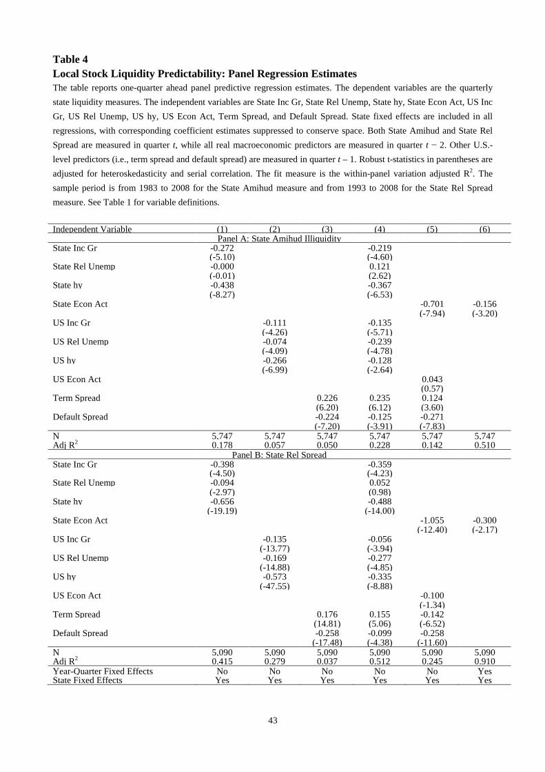
43

Table 4 Local Stock Liquidity Predictability: Panel Regression Estimates The table reports one-quarter ahead panel predictive regression estimates. The dependent variables are the quarterly state liquidity measures. The independent variables are State Inc Gr, State Rel Unemp, State hy, State Econ Act, US Inc Gr, US Rel Unemp, US hy, US Econ Act, Term Spread, and Default Spread. State fixed effects are included in all regressions, with corresponding coefficient estimates suppressed to conserve space. Both State Amihud and State Rel Spread are measured in quarter t, while all real macroeconomic predictors are measured in quarter t − 2. Other U.S.-level predictors (i.e., term spread and default spread) are measured in quarter t – 1. Robust t-statistics in parentheses are adjusted for heteroskedasticity and serial correlation. The fit measure is the within-panel variation adjusted R2. The sample period is from 1983 to 2008 for the State Amihud measure and from 1993 to 2008 for the State Rel Spread measure. See Table 1 for variable definitions. Independent Variable (1) (2) (3) (4) (5) (6)

Panel A: State Amihud Illiquidity State Inc Gr -0.272 -0.219 (-5.10) (-4.60) State Rel Unemp -0.000 0.121 (-0.01) (2.62) State hy -0.438 -0.367 (-8.27) (-6.53) State Econ Act -0.701 -0.156 (-7.94) (-3.20) US Inc Gr -0.111 -0.135 (-4.26) (-5.71) US Rel Unemp -0.074 -0.239 (-4.09) (-4.78) US hy -0.266 -0.128 (-6.99) (-2.64) US Econ Act 0.043 (0.57) Term Spread 0.226 0.235 0.124 (6.20) (6.12) (3.60) Default Spread -0.224 -0.125 -0.271 (-7.20) (-3.91) (-7.83) N 5,747 5,747 5,747 5,747 5,747 5,747 Adj R2 0.178 0.057 0.050 0.228 0.142 0.510

Panel B: State Rel Spread State Inc Gr -0.398 -0.359 (-4.50) (-4.23) State Rel Unemp -0.094 0.052 (-2.97) (0.98) State hy -0.656 -0.488 (-19.19) (-14.00) State Econ Act -1.055 -0.300 (-12.40) (-2.17) US Inc Gr -0.135 -0.056 (-13.77) (-3.94) US Rel Unemp -0.169 -0.277 (-14.88) (-4.85) US hy -0.573 -0.335 (-47.55) (-8.88) US Econ Act -0.100 (-1.34) Term Spread 0.176 0.155 -0.142 (14.81) (5.06) (-6.52) Default Spread -0.258 -0.099 -0.258 (-17.48) (-4.38) (-11.60) N 5,090 5,090 5,090 5,090 5,090 5,090 Adj R2 0.415 0.279 0.037 0.512 0.245 0.910 Year-Quarter Fixed Effects No No No No No Yes State Fixed Effects Yes Yes Yes Yes Yes Yes

44

Table 5 Local Stock Liquidity Predictability Regression Estimates: Firm Size Based Subsamples The table reports one-quarter ahead panel predictive regression estimates by size groups. To define the size subsamples, we use the most recent market capitalization (size) of each stock. Then, we sort stocks into terciles by size and calculate value-weighted state liquidity measures within each tercile. The dependent variable is the quarterly state liquidity measure for the relevant size group. The independent variables are State Inc Gr, State Rel Unemp, State hy, State Econ Act, US Inc Gr, US Rel Unemp, US hy, US Econ Act, Term Spread, and Default Spread. State fixed effects are included in all regressions. Both the State Amihud and State Rel Spread are measured in quarter t, while all real macroeconomic predictors are measured in quarter t − 2. Other U.S.-level predictors (i.e., term spread and default spread) are measured in quarter t – 1. Robust t-statistics in parentheses are adjusted for heteroskedasticity and serial correlation. The fit measure is the within-panel variation adjusted R2. The p-values for the test of difference in coefficients between each pair of size groups are in square brackets. The sample period is from 1983 to 2008 for the State Amihud measure and from 1993 to 2008 for the State Rel Spread measure. See Table 1 for variable definitions.

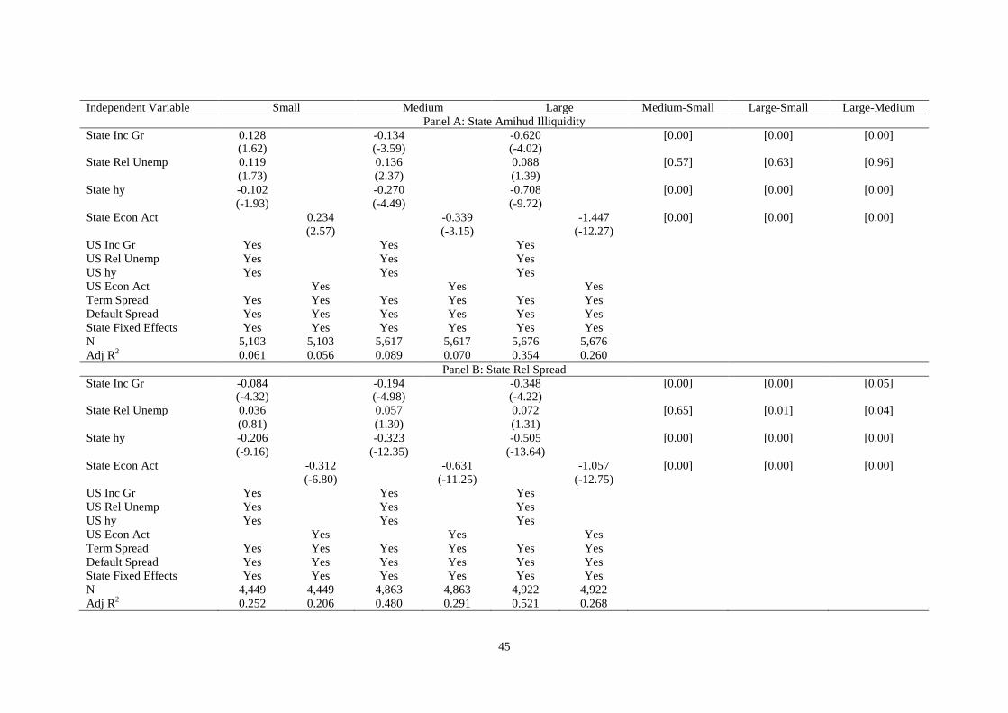
45

Independent Variable Small Medium Large Medium-Small Large-Small Large-Medium

Panel A: State Amihud Illiquidity State Inc Gr 0.128 -0.134 -0.620 [0.00] [0.00] [0.00] (1.62) (-3.59) (-4.02) State Rel Unemp 0.119 0.136 0.088 [0.57] [0.63] [0.96] (1.73) (2.37) (1.39) State hy -0.102 -0.270 -0.708 [0.00] [0.00] [0.00] (-1.93) (-4.49) (-9.72) State Econ Act 0.234 -0.339 -1.447 [0.00] [0.00] [0.00] (2.57) (-3.15) (-12.27) US Inc Gr Yes Yes Yes US Rel Unemp Yes Yes Yes US hy Yes Yes Yes US Econ Act Yes Yes Yes Term Spread Yes Yes Yes Yes Yes Yes Default Spread Yes Yes Yes Yes Yes Yes State Fixed Effects Yes Yes Yes Yes Yes Yes N 5,103 5,103 5,617 5,617 5,676 5,676 Adj R2 0.061 0.056 0.089 0.070 0.354 0.260

Panel B: State Rel Spread State Inc Gr -0.084 -0.194 -0.348 [0.00] [0.00] [0.05] (-4.32) (-4.98) (-4.22) State Rel Unemp 0.036 0.057 0.072 [0.65] [0.01] [0.04] (0.81) (1.30) (1.31) State hy -0.206 -0.323 -0.505 [0.00] [0.00] [0.00] (-9.16) (-12.35) (-13.64) State Econ Act -0.312 -0.631 -1.057 [0.00] [0.00] [0.00] (-6.80) (-11.25) (-12.75) US Inc Gr Yes Yes Yes US Rel Unemp Yes Yes Yes US hy Yes Yes Yes US Econ Act Yes Yes Yes Term Spread Yes Yes Yes Yes Yes Yes Default Spread Yes Yes Yes Yes Yes Yes State Fixed Effects Yes Yes Yes Yes Yes Yes N 4,449 4,449 4,863 4,863 4,922 4,922 Adj R2 0.252 0.206 0.480 0.291 0.521 0.268

46

Table 6 Local Stock Liquidity Predictability Variation and Local Capital Market Conditions The table reports one-quarter ahead panel predictive regression estimates for expanded specifications. The dependent variables are the quarterly state liquidity measures. The independent variables are State Inc Gr, State Rel Unemp, State hy, State Econ Act, US Inc Gr, US Rel Unemp, US hy, US Econ Act, Term Spread, and Default Spread. The additional independent variables include the State Fund Const Dummy, the State Opac Dummy, the Local Excess IO Dummy, and Rel Local Trading Dummy interacted with the State Econ Act and US Econ Act indices, respectively. State Fixed Effects and lagged Terms and Default Spreads are included in all specifications, with the corresponding estimates suppressed to conserve space. Both State Amihud and State Rel Spread are measured in quarter t, while all real macroeconomic predictors are measured in quarter t − 2. Other U.S.-level predictors (i.e., term spread and default spread) are measured in quarter t – 1. State Fund Const Dummy, Local Excess IO Dummy, and Rel Local Trading Dummy are measured in quarter t, while the State Opac Dummy is measured in quarter t − 1. Robust t-statistics in parentheses are adjusted for heteroskedasticity and serial correlation. The fit measure is the within-panel variation adjusted R2. The sample period is from 1983 to 2008 for the State Amihud measure and from 1993 to 2008 for the State Rel Spread measure. See Table 1 for variable definitions.

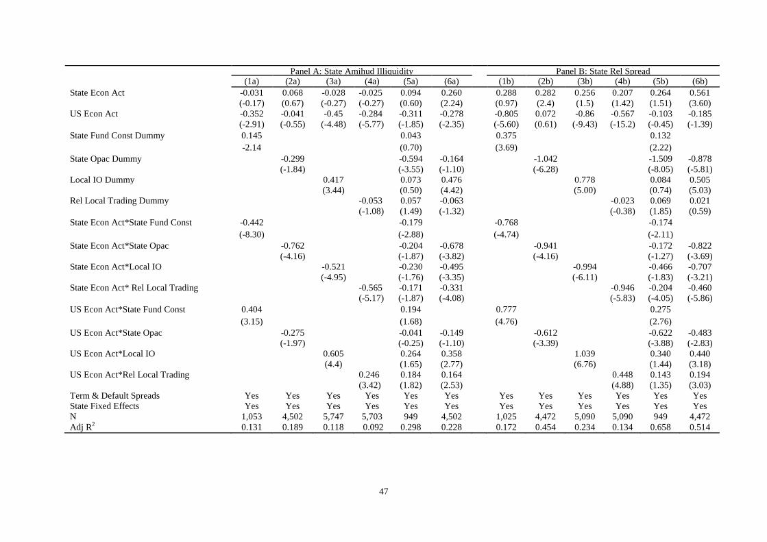
47

Panel A: State Amihud Illiquidity Panel B: State Rel Spread (1a) (2a) (3a) (4a) (5a) (6a) (1b) (2b) (3b) (4b) (5b) (6b) State Econ Act -0.031 0.068 -0.028 -0.025 0.094 0.260 0.288 0.282 0.256 0.207 0.264 0.561 (-0.17) (0.67) (-0.27) (-0.27) (0.60) (2.24) (0.97) (2.4) (1.5) (1.42) (1.51) (3.60) US Econ Act -0.352 -0.041 -0.45 -0.284 -0.311 -0.278 -0.805 0.072 -0.86 -0.567 -0.103 -0.185 (-2.91) (-0.55) (-4.48) (-5.77) (-1.85) (-2.35) (-5.60) (0.61) (-9.43) (-15.2) (-0.45) (-1.39) State Fund Const Dummy 0.145 0.043 0.375 0.132 -2.14 (0.70) (3.69) (2.22) State Opac Dummy -0.299 -0.594 -0.164 -1.042 -1.509 -0.878 (-1.84) (-3.55) (-1.10) (-6.28) (-8.05) (-5.81) Local IO Dummy 0.417 0.073 0.476 0.778 0.084 0.505 (3.44) (0.50) (4.42) (5.00) (0.74) (5.03) Rel Local Trading Dummy -0.053 0.057 -0.063 -0.023 0.069 0.021 (-1.08) (1.49) (-1.32) (-0.38) (1.85) (0.59) State Econ Act*State Fund Const -0.442 -0.179 -0.768 -0.174 (-8.30) (-2.88) (-4.74) (-2.11) State Econ Act*State Opac -0.762 -0.204 -0.678 -0.941 -0.172 -0.822 (-4.16) (-1.87) (-3.82) (-4.16) (-1.27) (-3.69) State Econ Act*Local IO -0.521 -0.230 -0.495 -0.994 -0.466 -0.707 (-4.95) (-1.76) (-3.35) (-6.11) (-1.83) (-3.21) State Econ Act* Rel Local Trading -0.565 -0.171 -0.331 -0.946 -0.204 -0.460 (-5.17) (-1.87) (-4.08) (-5.83) (-4.05) (-5.86) US Econ Act*State Fund Const 0.404 0.194 0.777 0.275 (3.15) (1.68) (4.76) (2.76) US Econ Act*State Opac -0.275 -0.041 -0.149 -0.612 -0.622 -0.483 (-1.97) (-0.25) (-1.10) (-3.39) (-3.88) (-2.83) US Econ Act*Local IO 0.605 0.264 0.358 1.039 0.340 0.440 (4.4) (1.65) (2.77) (6.76) (1.44) (3.18) US Econ Act*Rel Local Trading 0.246 0.184 0.164 0.448 0.143 0.194 (3.42) (1.82) (2.53) (4.88) (1.35) (3.03) Term & Default Spreads Yes Yes Yes Yes Yes Yes Yes Yes Yes Yes Yes Yes State Fixed Effects Yes Yes Yes Yes Yes Yes Yes Yes Yes Yes Yes Yes N 1,053 4,502 5,747 5,703 949 4,502 1,025 4,472 5,090 5,090 949 4,472 Adj R2 0.131 0.189 0.118 0.092 0.298 0.228 0.172 0.454 0.234 0.134 0.658 0.514

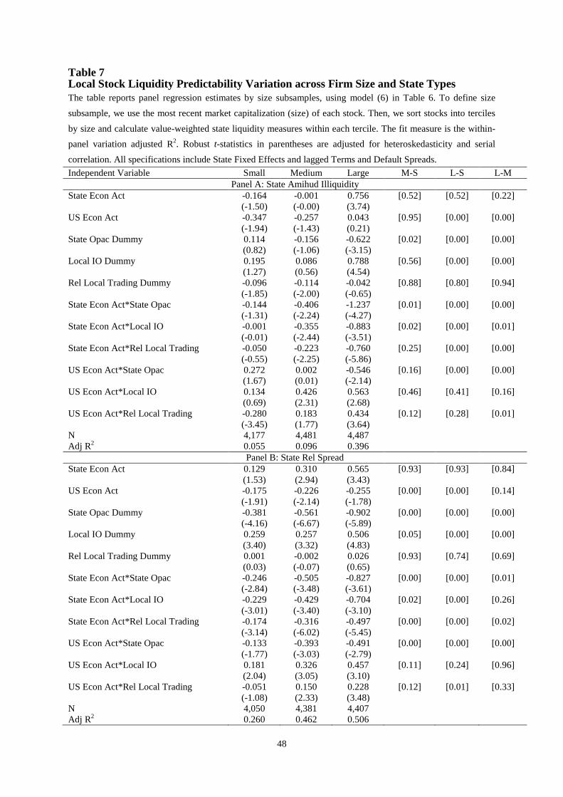
48

Table 7 Local Stock Liquidity Predictability Variation across Firm Size and State Types The table reports panel regression estimates by size subsamples, using model (6) in Table 6. To define size subsample, we use the most recent market capitalization (size) of each stock. Then, we sort stocks into terciles by size and calculate value-weighted state liquidity measures within each tercile. The fit measure is the within-panel variation adjusted R2. Robust t-statistics in parentheses are adjusted for heteroskedasticity and serial correlation. All specifications include State Fixed Effects and lagged Terms and Default Spreads. Independent Variable Small Medium Large M-S L-S L-M

Panel A: State Amihud Illiquidity State Econ Act -0.164 -0.001 0.756 [0.52] [0.52] [0.22] (-1.50) (-0.00) (3.74) US Econ Act -0.347 -0.257 0.043 [0.95] [0.00] [0.00] (-1.94) (-1.43) (0.21) State Opac Dummy 0.114 -0.156 -0.622 [0.02] [0.00] [0.00] (0.82) (-1.06) (-3.15) Local IO Dummy 0.195 0.086 0.788 [0.56] [0.00] [0.00] (1.27) (0.56) (4.54) Rel Local Trading Dummy -0.096 -0.114 -0.042 [0.88] [0.80] [0.94] (-1.85) (-2.00) (-0.65) State Econ Act*State Opac -0.144 -0.406 -1.237 [0.01] [0.00] [0.00] (-1.31) (-2.24) (-4.27) State Econ Act*Local IO -0.001 -0.355 -0.883 [0.02] [0.00] [0.01] (-0.01) (-2.44) (-3.51) State Econ Act*Rel Local Trading -0.050 -0.223 -0.760 [0.25] [0.00] [0.00] (-0.55) (-2.25) (-5.86) US Econ Act*State Opac 0.272 0.002 -0.546 [0.16] [0.00] [0.00] (1.67) (0.01) (-2.14) US Econ Act*Local IO 0.134 0.426 0.563 [0.46] [0.41] [0.16] (0.69) (2.31) (2.68) US Econ Act*Rel Local Trading -0.280 0.183 0.434 [0.12] [0.28] [0.01] (-3.45) (1.77) (3.64) N 4,177 4,481 4,487 Adj R2 0.055 0.096 0.396

Panel B: State Rel Spread State Econ Act 0.129 0.310 0.565 [0.93] [0.93] [0.84] (1.53) (2.94) (3.43) US Econ Act -0.175 -0.226 -0.255 [0.00] [0.00] [0.14] (-1.91) (-2.14) (-1.78) State Opac Dummy -0.381 -0.561 -0.902 [0.00] [0.00] [0.00] (-4.16) (-6.67) (-5.89) Local IO Dummy 0.259 0.257 0.506 [0.05] [0.00] [0.00] (3.40) (3.32) (4.83) Rel Local Trading Dummy 0.001 -0.002 0.026 [0.93] [0.74] [0.69] (0.03) (-0.07) (0.65) State Econ Act*State Opac -0.246 -0.505 -0.827 [0.00] [0.00] [0.01] (-2.84) (-3.48) (-3.61) State Econ Act*Local IO -0.229 -0.429 -0.704 [0.02] [0.00] [0.26] (-3.01) (-3.40) (-3.10) State Econ Act*Rel Local Trading -0.174 -0.316 -0.497 [0.00] [0.00] [0.02] (-3.14) (-6.02) (-5.45) US Econ Act*State Opac -0.133 -0.393 -0.491 [0.00] [0.00] [0.00] (-1.77) (-3.03) (-2.79) US Econ Act*Local IO 0.181 0.326 0.457 [0.11] [0.24] [0.96] (2.04) (3.05) (3.10) US Econ Act*Rel Local Trading -0.051 0.150 0.228 [0.12] [0.01] [0.33] (-1.08) (2.33) (3.48) N 4,050 4,381 4,407 Adj R2 0.260 0.462 0.506

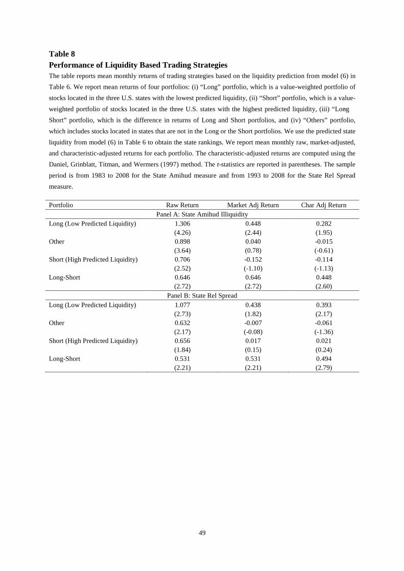
49

Table 8 Performance of Liquidity Based Trading Strategies The table reports mean monthly returns of trading strategies based on the liquidity prediction from model (6) in Table 6. We report mean returns of four portfolios: (i) “Long” portfolio, which is a value-weighted portfolio of stocks located in the three U.S. states with the lowest predicted liquidity, (ii) “Short” portfolio, which is a value-weighted portfolio of stocks located in the three U.S. states with the highest predicted liquidity, (iii) “Long − Short” portfolio, which is the difference in returns of Long and Short portfolios, and (iv) “Others” portfolio, which includes stocks located in states that are not in the Long or the Short portfolios. We use the predicted state liquidity from model (6) in Table 6 to obtain the state rankings. We report mean monthly raw, market-adjusted, and characteristic-adjusted returns for each portfolio. The characteristic-adjusted returns are computed using the Daniel, Grinblatt, Titman, and Wermers (1997) method. The t-statistics are reported in parentheses. The sample period is from 1983 to 2008 for the State Amihud measure and from 1993 to 2008 for the State Rel Spread measure. Portfolio Raw Return Market Adj Return Char Adj Return

Panel A: State Amihud Illiquidity Long (Low Predicted Liquidity) 1.306 0.448 0.282 (4.26) (2.44) (1.95) Other 0.898 0.040 -0.015 (3.64) (0.78) (-0.61) Short (High Predicted Liquidity) 0.706 -0.152 -0.114 (2.52) (-1.10) (-1.13) Long-Short 0.646 0.646 0.448 (2.72) (2.72) (2.60)

Panel B: State Rel Spread Long (Low Predicted Liquidity) 1.077 0.438 0.393 (2.73) (1.82) (2.17) Other 0.632 -0.007 -0.061 (2.17) (-0.08) (-1.36) Short (High Predicted Liquidity) 0.656 0.017 0.021 (1.84) (0.15) (0.24) Long-Short 0.531 0.531 0.494 (2.21) (2.21) (2.79)

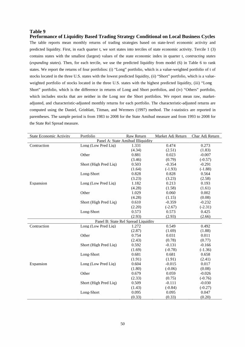
50

Table 9 Performance of Liquidity Based Trading Strategy Conditional on Local Business Cycles The table reports mean monthly returns of trading strategies based on state-level economic activity and predicted liquidity. First, in each quarter t, we sort states into terciles of state economic activity. Tercile 1 (3) contains states with the smallest (largest) values of the state economic index in quarter t, contracting states (expanding states). Then, for each tercile, we use the predicted liquidity from model (6) in Table 6 to rank states. We report the returns of four portfolios: (i) “Long” portfolio, which is a value-weighted portfolio of t of stocks located in the three U.S. states with the lowest predicted liquidity, (ii) “Short” portfolio, which is a value-weighted portfolio of stocks located in the three U.S. states with the highest predicted liquidity, (iii) “Long − Short” portfolio, which is the difference in returns of Long and Short portfolios, and (iv) “Others” portfolio, which includes stocks that are neither in the Long nor the Short portfolios. We report mean raw, market-adjusted, and characteristic-adjusted monthly returns for each portfolio. The characteristic-adjusted returns are computed using the Daniel, Grinblatt, Titman, and Wermers (1997) method. The t-statistics are reported in parentheses. The sample period is from 1983 to 2008 for the State Amihud measure and from 1993 to 2008 for the State Rel Spread measure. State Economic Activity Portfolio Raw Return Market Adj Return Char Adj Return

Panel A: State Amihud Illiquidity Contraction Long (Low Pred Liq) 1.331 0.474 0.273 (4.34) (2.51) (1.83) Other 0.881 0.023 -0.007 (3.46) (0.79) (-0.57) Short (High Pred Liq) 0.503 -0.354 -0.291 (1.64) (-1.93) (-1.88) Long-Short 0.828 0.828 0.564 (3.23) (3.23) (2.58) Expansion Long (Low Pred Liq) 1.182 0.213 0.193 (4.28) (1.58) (1.61) Other 1.029 0.060 0.002 (4.28) (1.15) (0.08) Short (High Pred Liq) 0.610 -0.359 -0.232 (2.20) (-2.67) (-2.31) Long-Short 0.573 0.573 0.425

(2.93) (2.93) (2.66) Panel B: State Rel Spread Liquidity

Contraction Long (Low Pred Liq) 1.272 0.549 0.492 (2.87) (1.69) (1.88) Other 0.754 0.031 0.011 (2.43) (0.78) (0.77) Short (High Pred Liq) 0.592 -0.131 -0.166 (1.69) (-0.78) (-1.36) Long-Short 0.681 0.681 0.658 (1.91) (1.91) (2.41) Expansion Long (Low Pred Liq) 0.604 -0.015 0.017 (1.80) (-0.06) (0.08) Other 0.679 0.059 -0.026 (2.33) (0.75) (-0.76) Short (High Pred Liq) 0.509 -0.111 -0.030 (1.43) (-0.84) (-0.27) Long-Short 0.095 0.095 0.047

(0.33) (0.33) (0.20)

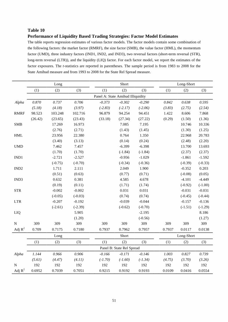
51

Table 10 Performance of Liquidity Based Trading Strategies: Factor Model Estimates The table reports regression estimates of various factor models. The factor models contain some combination of the following factors: the market factor (RMRF), the size factor (SMB), the value factor (HML), the momentum factor (UMD), three industry factors (IND1, IND2, and IND3), two reversal factors (short-term reversal (STR), long-term reversal (LTR)), and the liquidity (LIQ) factor. For each factor model, we report the estimates of the factor exposures. The t-statistics are reported in parentheses. The sample period is from 1983 to 2008 for the State Amihud measure and from 1993 to 2008 for the State Rel Spread measure.

Long Short Long-Short (1) (2) (3) (1) (2) (3) (1) (2) (3) Panel A: State Amihud Illiquidity

Alpha 0.870 0.737 0.706 -0.373 -0.302 -0.290 0.842 0.638 0.595 (5.18) (4.18) (3.97) (-2.83) (-2.17) (-2.06) (3.83) (2.75) (2.54)

RMRF 98.523 103.248 102.716 96.879 94.254 94.451 1.422 8.606 7.868 (26.42) (23.65) (23.43) (33.18) (27.34) (27.22) (0.29) (1.50) (1.36) SMB 17.269 16.973 7.085 7.195 10.746 10.336 (2.76) (2.71) (1.43) (1.45) (1.30) (1.25) HML 23.956 22.380 0.764 1.350 22.968 20.783 (3.40) (3.13) (0.14) (0.24) (2.48) (2.20) UMD 7.462 7.457 -6.399 -6.398 13.700 13.693 (1.70) (1.70) (-1.84) (-1.84) (2.37) (2.37) IND1 -2.721 -2.527 -0.956 -1.029 -1.861 -1.592 (-0.75) (-0.70) (-0.34) (-0.36) (-0.39) (-0.33) IND2 1.711 2.111 2.049 1.900 -0.352 0.203 (0.51) (0.63) (0.77) (0.71) (-0.08) (0.05) IND3 0.632 0.381 4.585 4.678 -4.101 -4.449 (0.19) (0.11) (1.71) (1.74) (-0.92) (-1.00) STR -0.002 -0.002 0.031 0.031 -0.031 -0.031 (-0.05) (-0.03) (0.74) (0.74) (-0.45) (-0.44) LTR -0.207 -0.192 -0.039 -0.044 -0.157 -0.136 (-2.61) (-2.39) (-0.62) (-0.70) (-1.51) (-1.29) LIQ 5.905 -2.195 8.186

(1.20) (-0.56) (1.27) N 309 309 309 309 309 309 309 309 309 Adj R2 0.709 0.7175 0.7180 0.7937 0.7962 0.7957 0.7937 0.0117 0.0138

Long Short Long-Short (1) (2) (3) (1) (2) (3) (1) (2) (3) Panel B: State Rel Spread

Alpha 1.144 0.966 0.906 -0.166 -0.171 -0.146 1.003 0.827 0.739 (5.61) (4.47) (4.11) (-1.70) (-1.60) (-1.34) (4.75) (3.70) (3.26) N 192 192 192 192 192 192 192 192 192 Adj R2 0.6952 0.7039 0.7051 0.9215 0.9192 0.9193 0.0109 0.0416 0.0554

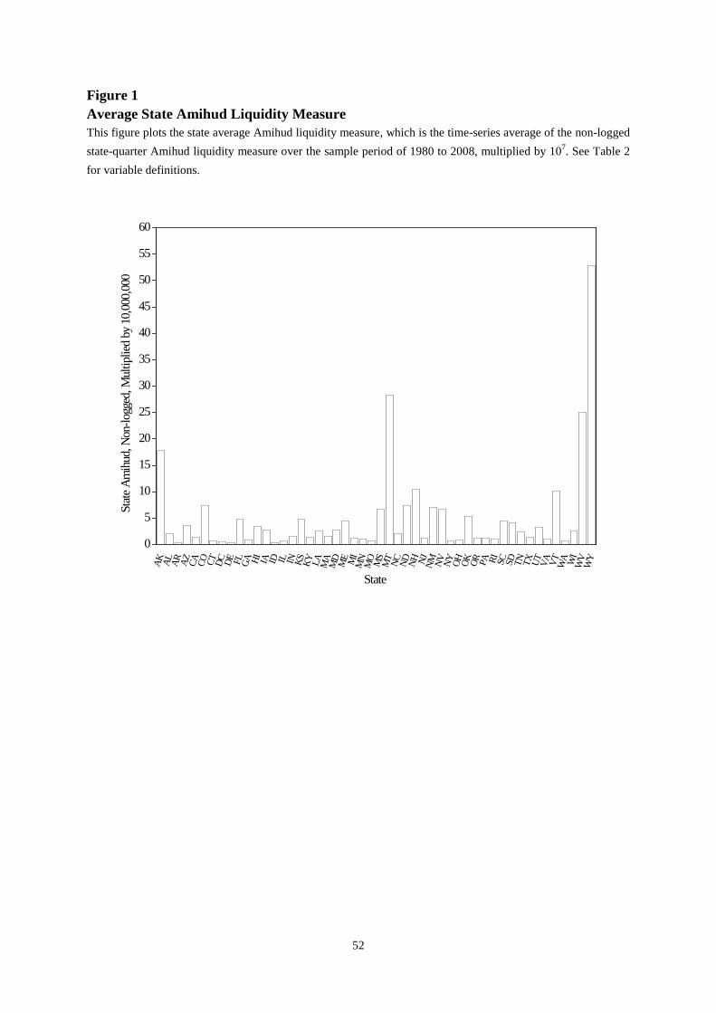
52

Figure 1 Average State Amihud Liquidity Measure This figure plots the state average Amihud liquidity measure, which is the time-series average of the non-logged state-quarter Amihud liquidity measure over the sample period of 1980 to 2008, multiplied by 107. See Table 2 for variable definitions.

AK AL AR AZ CA CO CT DC DE FL GA HI IA ID IL IN KS KY LA MA

MD ME MI

MN

MO MS

MT NC ND NH NJ NM NV NY OH OK OR PA RI SC SD TN TX UT VA VT WA WI

WV

WY

0

5

10

15

20

25

30

35

40

45

50

55

60

State

Am

ihud

, Non

-logg

ed, M

ultip

lied

by 1

0,00

0,00

0

State

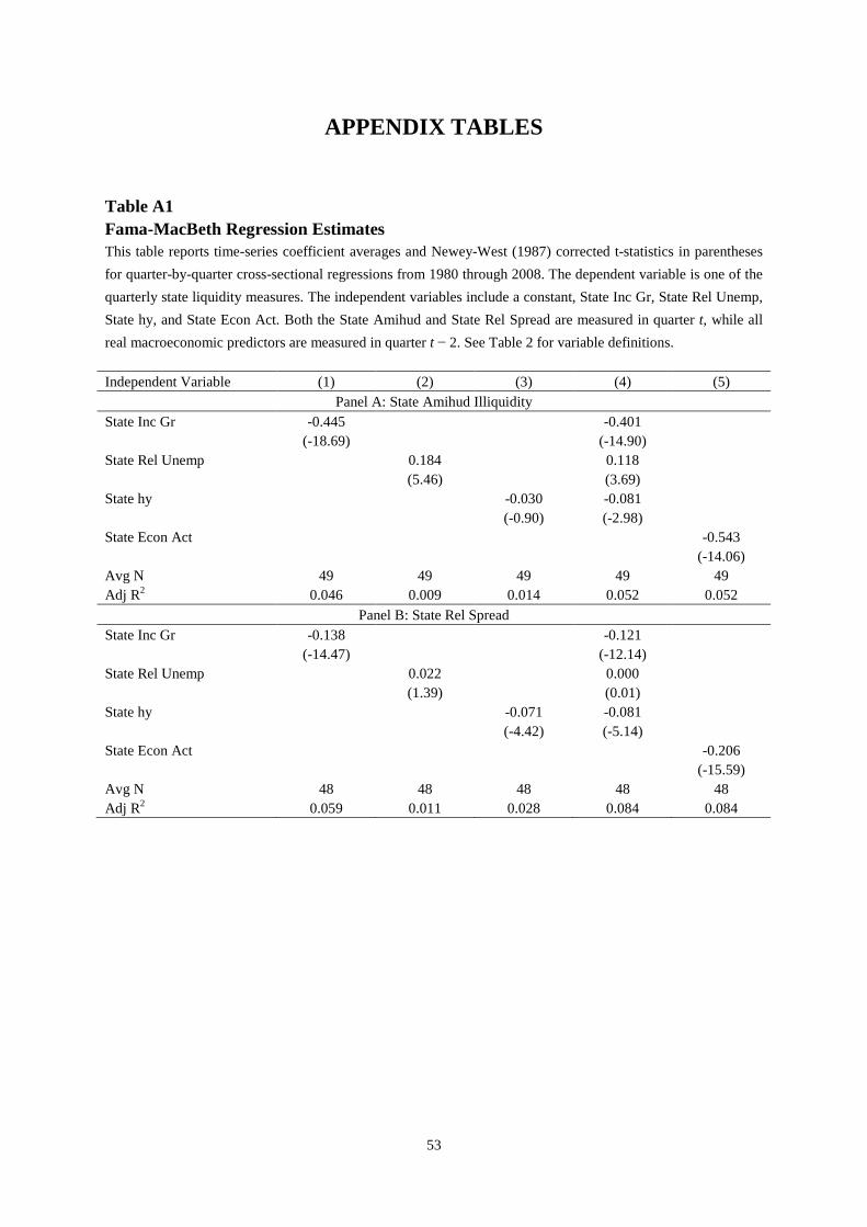
53

APPENDIX TABLES

Table A1 Fama-MacBeth Regression Estimates This table reports time-series coefficient averages and Newey-West (1987) corrected t-statistics in parentheses for quarter-by-quarter cross-sectional regressions from 1980 through 2008. The dependent variable is one of the quarterly state liquidity measures. The independent variables include a constant, State Inc Gr, State Rel Unemp, State hy, and State Econ Act. Both the State Amihud and State Rel Spread are measured in quarter t, while all real macroeconomic predictors are measured in quarter t − 2. See Table 2 for variable definitions. Independent Variable (1) (2) (3) (4) (5)

Panel A: State Amihud Illiquidity State Inc Gr -0.445 -0.401 (-18.69) (-14.90) State Rel Unemp 0.184 0.118 (5.46) (3.69) State hy -0.030 -0.081 (-0.90) (-2.98) State Econ Act -0.543 (-14.06) Avg N 49 49 49 49 49 Adj R2 0.046 0.009 0.014 0.052 0.052

Panel B: State Rel Spread State Inc Gr -0.138 -0.121 (-14.47) (-12.14) State Rel Unemp 0.022 0.000 (1.39) (0.01) State hy -0.071 -0.081 (-4.42) (-5.14) State Econ Act -0.206 (-15.59) Avg N 48 48 48 48 48 Adj R2 0.059 0.011 0.028 0.084 0.084

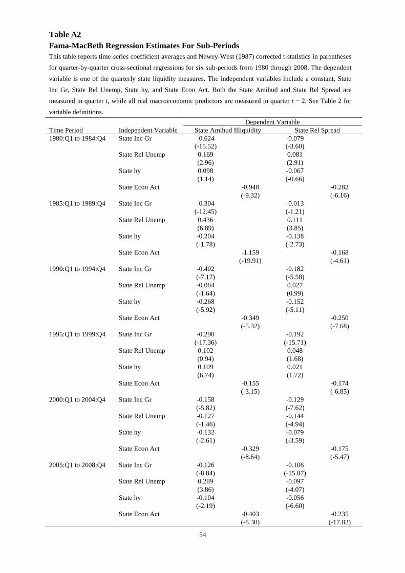
54

Table A2 Fama-MacBeth Regression Estimates For Sub-Periods This table reports time-series coefficient averages and Newey-West (1987) corrected t-statistics in parentheses for quarter-by-quarter cross-sectional regressions for six sub-periods from 1980 through 2008. The dependent variable is one of the quarterly state liquidity measures. The independent variables include a constant, State Inc Gr, State Rel Unemp, State hy, and State Econ Act. Both the State Amihud and State Rel Spread are measured in quarter t, while all real macroeconomic predictors are measured in quarter t − 2. See Table 2 for variable definitions.

Dependent Variable Time Period Independent Variable State Amihud Illiquidity State Rel Spread 1980:Q1 to 1984:Q4 State Inc Gr -0.624 -0.079 (-15.52) (-3.60) State Rel Unemp 0.169 0.081 (2.96) (2.91) State hy 0.098 -0.067 (1.14) (-0.66) State Econ Act -0.948 -0.282 (-9.32) (-6.16) 1985:Q1 to 1989:Q4 State Inc Gr -0.304 -0.013 (-12.45) (-1.21) State Rel Unemp 0.436 0.111 (6.89) (3.85) State hy -0.204 -0.138 (-1.78) (-2.73) State Econ Act -1.159 -0.168 (-19.91) (-4.61) 1990:Q1 to 1994:Q4 State Inc Gr -0.402 -0.182 (-7.17) (-5.58) State Rel Unemp -0.084 0.027 (-1.64) (0.99) State hy -0.268 -0.152 (-5.92) (-5.11) State Econ Act -0.349 -0.250 (-5.32) (-7.68) 1995:Q1 to 1999:Q4 State Inc Gr -0.290 -0.192 (-17.36) (-15.71) State Rel Unemp 0.102 0.048 (0.94) (1.68) State hy 0.109 0.021 (6.74) (1.72) State Econ Act -0.155 -0.174 (-3.15) (-6.85) 2000:Q1 to 2004:Q4 State Inc Gr -0.158 -0.129 (-5.82) (-7.62) State Rel Unemp -0.127 -0.144 (-1.46) (-4.94) State hy -0.132 -0.079 (-2.61) (-3.59) State Econ Act -0.329 -0.175 (-8.64) (-5.47) 2005:Q1 to 2008:Q4 State Inc Gr -0.126 -0.106 (-8.84) (-15.87) State Rel Unemp 0.289 -0.097 (3.86) (-4.07) State hy -0.104 -0.056 (-2.19) (-6.60) State Econ Act -0.403 -0.235 (-8.30) (-17.82)

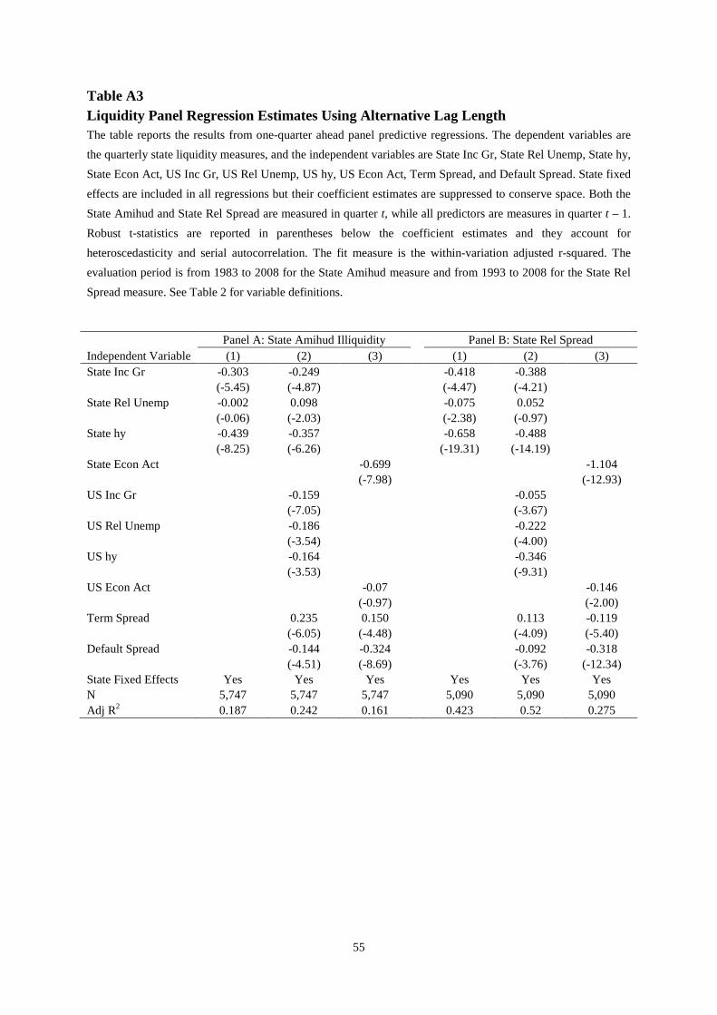
55

Table A3 Liquidity Panel Regression Estimates Using Alternative Lag Length The table reports the results from one-quarter ahead panel predictive regressions. The dependent variables are the quarterly state liquidity measures, and the independent variables are State Inc Gr, State Rel Unemp, State hy, State Econ Act, US Inc Gr, US Rel Unemp, US hy, US Econ Act, Term Spread, and Default Spread. State fixed effects are included in all regressions but their coefficient estimates are suppressed to conserve space. Both the State Amihud and State Rel Spread are measured in quarter t, while all predictors are measures in quarter t – 1. Robust t-statistics are reported in parentheses below the coefficient estimates and they account for heteroscedasticity and serial autocorrelation. The fit measure is the within-variation adjusted r-squared. The evaluation period is from 1983 to 2008 for the State Amihud measure and from 1993 to 2008 for the State Rel Spread measure. See Table 2 for variable definitions.

Panel A: State Amihud Illiquidity Panel B: State Rel Spread

Independent Variable (1) (2) (3) (1) (2) (3) State Inc Gr -0.303 -0.249 -0.418 -0.388 (-5.45) (-4.87) (-4.47) (-4.21) State Rel Unemp -0.002 0.098 -0.075 0.052 (-0.06) (-2.03) (-2.38) (-0.97) State hy -0.439 -0.357 -0.658 -0.488 (-8.25) (-6.26) (-19.31) (-14.19) State Econ Act -0.699 -1.104 (-7.98) (-12.93) US Inc Gr -0.159 -0.055 (-7.05) (-3.67) US Rel Unemp -0.186 -0.222 (-3.54) (-4.00) US hy -0.164 -0.346 (-3.53) (-9.31) US Econ Act -0.07 -0.146 (-0.97) (-2.00) Term Spread 0.235 0.150 0.113 -0.119 (-6.05) (-4.48) (-4.09) (-5.40) Default Spread -0.144 -0.324 -0.092 -0.318 (-4.51) (-8.69) (-3.76) (-12.34) State Fixed Effects Yes Yes Yes Yes Yes Yes N 5,747 5,747 5,747 5,090 5,090 5,090 Adj R2 0.187 0.242 0.161 0.423 0.52 0.275

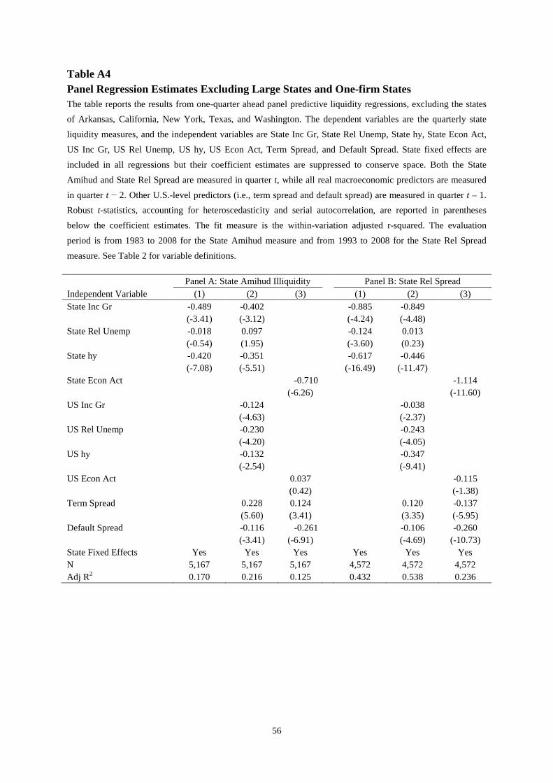
56

Table A4 Panel Regression Estimates Excluding Large States and One-firm States The table reports the results from one-quarter ahead panel predictive liquidity regressions, excluding the states of Arkansas, California, New York, Texas, and Washington. The dependent variables are the quarterly state liquidity measures, and the independent variables are State Inc Gr, State Rel Unemp, State hy, State Econ Act, US Inc Gr, US Rel Unemp, US hy, US Econ Act, Term Spread, and Default Spread. State fixed effects are included in all regressions but their coefficient estimates are suppressed to conserve space. Both the State Amihud and State Rel Spread are measured in quarter t, while all real macroeconomic predictors are measured in quarter t − 2. Other U.S.-level predictors (i.e., term spread and default spread) are measured in quarter t – 1. Robust t-statistics, accounting for heteroscedasticity and serial autocorrelation, are reported in parentheses below the coefficient estimates. The fit measure is the within-variation adjusted r-squared. The evaluation period is from 1983 to 2008 for the State Amihud measure and from 1993 to 2008 for the State Rel Spread measure. See Table 2 for variable definitions.

Panel A: State Amihud Illiquidity Panel B: State Rel Spread

Independent Variable (1) (2) (3) (1) (2) (3) State Inc Gr -0.489 -0.402 -0.885 -0.849 (-3.41) (-3.12) (-4.24) (-4.48) State Rel Unemp -0.018 0.097 -0.124 0.013 (-0.54) (1.95) (-3.60) (0.23) State hy -0.420 -0.351 -0.617 -0.446 (-7.08) (-5.51) (-16.49) (-11.47) State Econ Act -0.710 -1.114 (-6.26) (-11.60) US Inc Gr -0.124 -0.038 (-4.63) (-2.37) US Rel Unemp -0.230 -0.243 (-4.20) (-4.05) US hy -0.132 -0.347 (-2.54) (-9.41) US Econ Act 0.037 -0.115 (0.42) (-1.38) Term Spread 0.228 0.124 0.120 -0.137 (5.60) (3.41) (3.35) (-5.95) Default Spread -0.116 -0.261 -0.106 -0.260 (-3.41) (-6.91) (-4.69) (-10.73) State Fixed Effects Yes Yes Yes Yes Yes Yes N 5,167 5,167 5,167 4,572 4,572 4,572 Adj R2 0.170 0.216 0.125 0.432 0.538 0.236

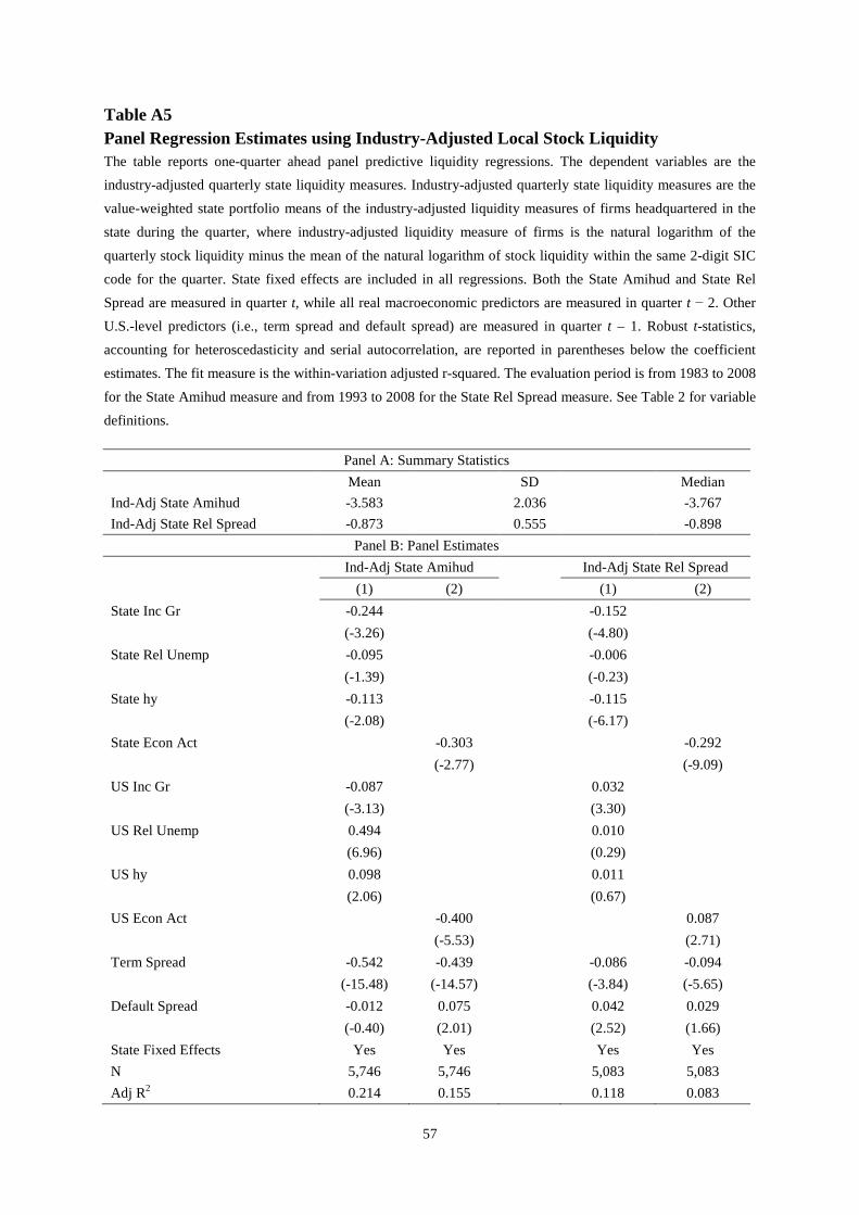
57

Table A5 Panel Regression Estimates using Industry-Adjusted Local Stock Liquidity The table reports one-quarter ahead panel predictive liquidity regressions. The dependent variables are the industry-adjusted quarterly state liquidity measures. Industry-adjusted quarterly state liquidity measures are the value-weighted state portfolio means of the industry-adjusted liquidity measures of firms headquartered in the state during the quarter, where industry-adjusted liquidity measure of firms is the natural logarithm of the quarterly stock liquidity minus the mean of the natural logarithm of stock liquidity within the same 2-digit SIC code for the quarter. State fixed effects are included in all regressions. Both the State Amihud and State Rel Spread are measured in quarter t, while all real macroeconomic predictors are measured in quarter t − 2. Other U.S.-level predictors (i.e., term spread and default spread) are measured in quarter t – 1. Robust t-statistics, accounting for heteroscedasticity and serial autocorrelation, are reported in parentheses below the coefficient estimates. The fit measure is the within-variation adjusted r-squared. The evaluation period is from 1983 to 2008 for the State Amihud measure and from 1993 to 2008 for the State Rel Spread measure. See Table 2 for variable definitions.

Panel A: Summary Statistics Mean SD Median Ind-Adj State Amihud -3.583 2.036 -3.767 Ind-Adj State Rel Spread -0.873 0.555 -0.898

Panel B: Panel Estimates Ind-Adj State Amihud Ind-Adj State Rel Spread (1) (2) (1) (2) State Inc Gr -0.244 -0.152 (-3.26) (-4.80) State Rel Unemp -0.095 -0.006 (-1.39) (-0.23) State hy -0.113 -0.115 (-2.08) (-6.17) State Econ Act -0.303 -0.292 (-2.77) (-9.09) US Inc Gr -0.087 0.032 (-3.13) (3.30) US Rel Unemp 0.494 0.010 (6.96) (0.29) US hy 0.098 0.011 (2.06) (0.67) US Econ Act -0.400 0.087 (-5.53) (2.71) Term Spread -0.542 -0.439 -0.086 -0.094 (-15.48) (-14.57) (-3.84) (-5.65) Default Spread -0.012 0.075 0.042 0.029 (-0.40) (2.01) (2.52) (1.66) State Fixed Effects Yes Yes Yes Yes N 5,746 5,746 5,083 5,083 Adj R2 0.214 0.155 0.118 0.083

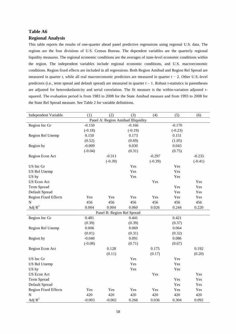
58

Table A6 Regional Analysis This table reports the results of one-quarter ahead panel predictive regressions using regional U.S. data. The regions are the four divisions of U.S. Census Bureau. The dependent variables are the quarterly regional liquidity measures. The regional economic conditions are the averages of state-level economic conditions within the region. The independent variables include regional economic conditions, and U.S. macroeconomic conditions. Region fixed effects are included in all regressions. Both Region Amihud and Region Rel Spread are measured in quarter t, while all real macroeconomic predictors are measured in quarter t − 2. Other U.S.-level predictors (i.e., term spread and default spread) are measured in quarter t – 1. Robust t-statistics in parentheses are adjusted for heteroskedasticity and serial correlation. The fit measure is the within-variation adjusted r-squared. The evaluation period is from 1983 to 2008 for the State Amihud measure and from 1993 to 2008 for the State Rel Spread measure. See Table 2 for variable definitions. Independent Variable (1) (2) (3) (4) (5) (6)

Panel A: Region Amihud Illiquidity Region Inc Gr -0.150 -0.166 -0.170 (-0.18) (-0.19) (-0.23) Region Rel Unemp 0.150 0.173 0.151 (0.52) (0.69) (1.05) Region hy -0.009 0.030 0.043 (-0.04) (0.31) (0.75) Region Econ Act -0.311 -0.297 -0.235 (-0.39) (-0.39) (-0.41) US Inc Gr Yes Yes US Rel Unemp Yes Yes US hy Yes Yes US Econ Act Yes Yes Term Spread Yes Yes Default Spread Yes Yes Region Fixed Effects Yes Yes Yes Yes Yes Yes N 456 456 456 456 456 456 Adj R2 0.004 0.004 0.060 0.026 0.244 0.220

Panel B: Region Rel Spread Region Inc Gr 0.481 0.441 0.421 (0.39) (0.39) (0.37) Region Rel Unemp 0.006 0.069 0.064 (0.01) (0.31) (0.32) Region hy -0.040 0.091 0.086 (-0.08) (0.71) (0.67) Region Econ Act 0.128 0.175 0.192 (0.11) (0.17) (0.20) US Inc Gr Yes Yes US Rel Unemp Yes Yes US hy Yes Yes US Econ Act Yes Yes Term Spread Yes Yes Default Spread Yes Yes Region Fixed Effects Yes Yes Yes Yes Yes Yes N 420 420 420 420 420 420 Adj R2 -0.003 -0.002 0.266 0.036 0.304 0.092

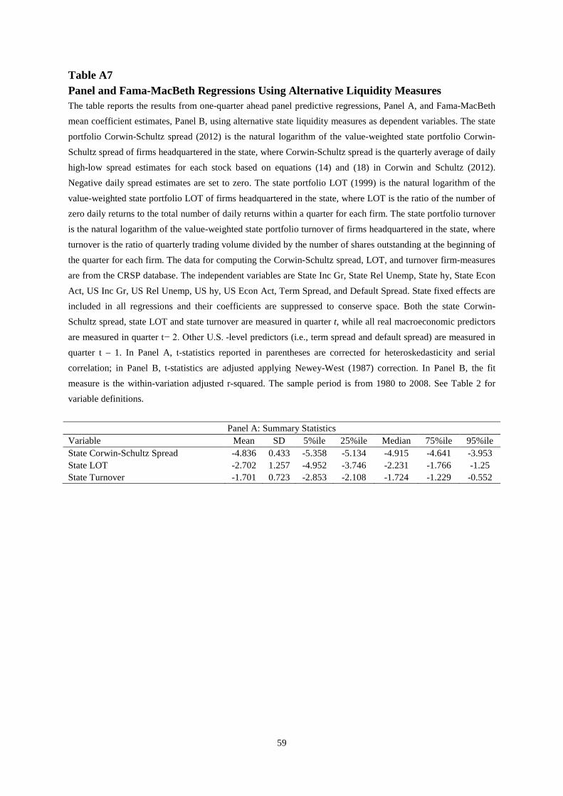
59

Table A7 Panel and Fama-MacBeth Regressions Using Alternative Liquidity Measures The table reports the results from one-quarter ahead panel predictive regressions, Panel A, and Fama-MacBeth mean coefficient estimates, Panel B, using alternative state liquidity measures as dependent variables. The state portfolio Corwin-Schultz spread (2012) is the natural logarithm of the value-weighted state portfolio Corwin-Schultz spread of firms headquartered in the state, where Corwin-Schultz spread is the quarterly average of daily high-low spread estimates for each stock based on equations (14) and (18) in Corwin and Schultz (2012). Negative daily spread estimates are set to zero. The state portfolio LOT (1999) is the natural logarithm of the value-weighted state portfolio LOT of firms headquartered in the state, where LOT is the ratio of the number of zero daily returns to the total number of daily returns within a quarter for each firm. The state portfolio turnover is the natural logarithm of the value-weighted state portfolio turnover of firms headquartered in the state, where turnover is the ratio of quarterly trading volume divided by the number of shares outstanding at the beginning of the quarter for each firm. The data for computing the Corwin-Schultz spread, LOT, and turnover firm-measures are from the CRSP database. The independent variables are State Inc Gr, State Rel Unemp, State hy, State Econ Act, US Inc Gr, US Rel Unemp, US hy, US Econ Act, Term Spread, and Default Spread. State fixed effects are included in all regressions and their coefficients are suppressed to conserve space. Both the state Corwin-Schultz spread, state LOT and state turnover are measured in quarter t, while all real macroeconomic predictors are measured in quarter t − 2. Other U.S. -level predictors (i.e., term spread and default spread) are measured in quarter t – 1. In Panel A, t-statistics reported in parentheses are corrected for heteroskedasticity and serial correlation; in Panel B, t-statistics are adjusted applying Newey-West (1987) correction. In Panel B, the fit measure is the within-variation adjusted r-squared. The sample period is from 1980 to 2008. See Table 2 for variable definitions.

Panel A: Summary Statistics Variable Mean SD 5%ile 25%ile Median 75%ile 95%ile State Corwin-Schultz Spread -4.836 0.433 -5.358 -5.134 -4.915 -4.641 -3.953 State LOT -2.702 1.257 -4.952 -3.746 -2.231 -1.766 -1.25 State Turnover -1.701 0.723 -2.853 -2.108 -1.724 -1.229 -0.552

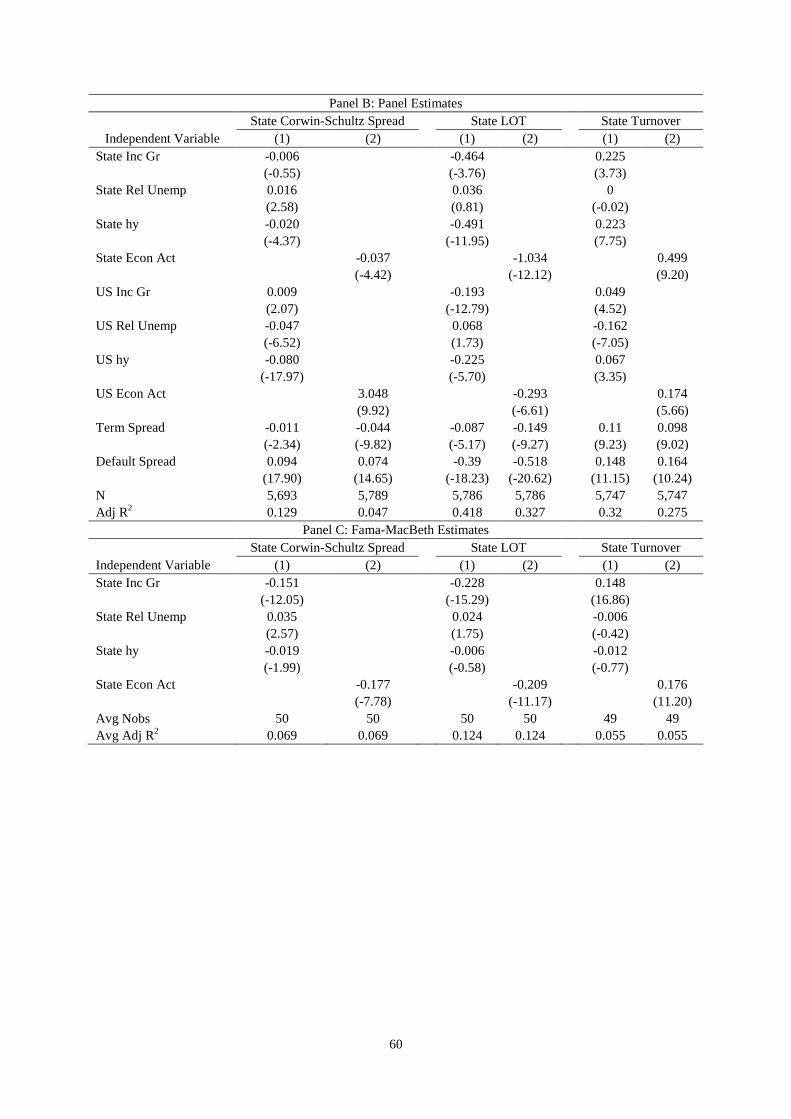
60

Panel B: Panel Estimates State Corwin-Schultz Spread State LOT State Turnover

Independent Variable (1) (2) (1) (2) (1) (2) State Inc Gr -0.006 -0.464 0.225 (-0.55) (-3.76) (3.73) State Rel Unemp 0.016 0.036 0 (2.58) (0.81) (-0.02) State hy -0.020 -0.491 0.223 (-4.37) (-11.95) (7.75) State Econ Act -0.037 -1.034 0.499 (-4.42) (-12.12) (9.20) US Inc Gr 0.009 -0.193 0.049 (2.07) (-12.79) (4.52) US Rel Unemp -0.047 0.068 -0.162 (-6.52) (1.73) (-7.05) US hy -0.080 -0.225 0.067 (-17.97) (-5.70) (3.35) US Econ Act 3.048 -0.293 0.174 (9.92) (-6.61) (5.66) Term Spread -0.011 -0.044 -0.087 -0.149 0.11 0.098 (-2.34) (-9.82) (-5.17) (-9.27) (9.23) (9.02) Default Spread 0.094 0.074 -0.39 -0.518 0.148 0.164 (17.90) (14.65) (-18.23) (-20.62) (11.15) (10.24) N 5,693 5,789 5,786 5,786 5,747 5,747 Adj R2 0.129 0.047 0.418 0.327 0.32 0.275

Panel C: Fama-MacBeth Estimates State Corwin-Schultz Spread State LOT State Turnover

Independent Variable (1) (2) (1) (2) (1) (2) State Inc Gr -0.151 -0.228 0.148 (-12.05) (-15.29) (16.86) State Rel Unemp 0.035 0.024 -0.006 (2.57) (1.75) (-0.42) State hy -0.019 -0.006 -0.012 (-1.99) (-0.58) (-0.77) State Econ Act -0.177 -0.209 0.176 (-7.78) (-11.17) (11.20) Avg Nobs 50 50 50 50 49 49 Avg Adj R2 0.069 0.069 0.124 0.124 0.055 0.055

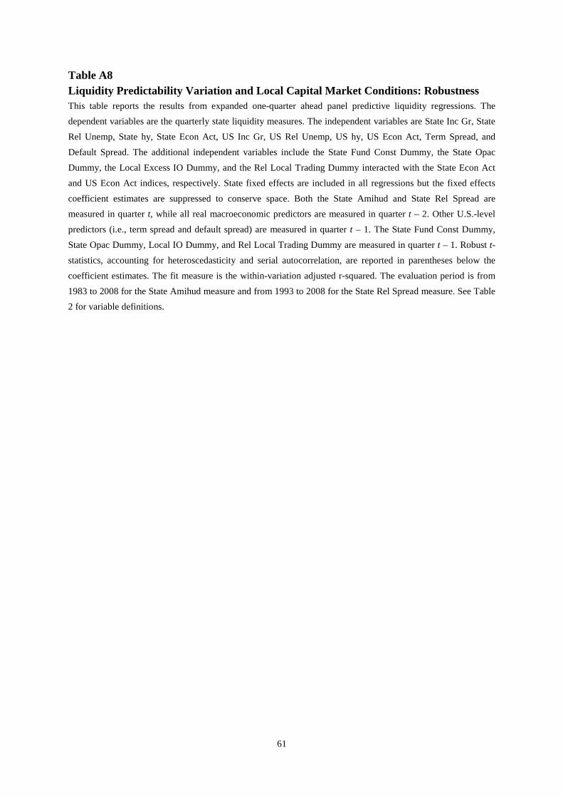
61

Table A8 Liquidity Predictability Variation and Local Capital Market Conditions: Robustness This table reports the results from expanded one-quarter ahead panel predictive liquidity regressions. The dependent variables are the quarterly state liquidity measures. The independent variables are State Inc Gr, State Rel Unemp, State hy, State Econ Act, US Inc Gr, US Rel Unemp, US hy, US Econ Act, Term Spread, and Default Spread. The additional independent variables include the State Fund Const Dummy, the State Opac Dummy, the Local Excess IO Dummy, and the Rel Local Trading Dummy interacted with the State Econ Act and US Econ Act indices, respectively. State fixed effects are included in all regressions but the fixed effects coefficient estimates are suppressed to conserve space. Both the State Amihud and State Rel Spread are measured in quarter t, while all real macroeconomic predictors are measured in quarter t – 2. Other U.S.-level predictors (i.e., term spread and default spread) are measured in quarter t – 1. The State Fund Const Dummy, State Opac Dummy, Local IO Dummy, and Rel Local Trading Dummy are measured in quarter t – 1. Robust t-statistics, accounting for heteroscedasticity and serial autocorrelation, are reported in parentheses below the coefficient estimates. The fit measure is the within-variation adjusted r-squared. The evaluation period is from 1983 to 2008 for the State Amihud measure and from 1993 to 2008 for the State Rel Spread measure. See Table 2 for variable definitions.

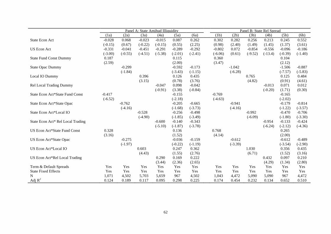
62

Panel A: State Amihud Illiquidity Panel B: State Rel Spread (1a) (2a) (3a) (4a) (5a) (6a) (1b) (2b) (3b) (4b) (5b) (6b) State Econ Act -0.028 0.068 -0.023 -0.015 0.087 0.262 0.302 0.282 0.256 0.213 0.245 0.552 (-0.15) (0.67) (-0.22) (-0.15) (0.55) (2.25) (0.98) (2.40) (1.49) (1.45) (1.37) (3.61) US Econ Act -0.331 -0.041 -0.451 -0.291 -0.289 -0.292 -0.802 0.072 -0.854 -0.556 -0.096 -0.186 (-3.00) (-0.55) (-4.51) (-5.38) (-2.01) (-2.41) (-6.06) (0.61) (-9.52) (-13.4) (-0.39) (-1.40) State Fund Const Dummy 0.187 0.115 0.360 0.104 (2.59) (2.00) (3.47) (2.12) State Opac Dummy -0.299 -0.592 -0.173 -1.042 -1.506 -0.887 (-1.84) (-3.43) (-1.15) (-6.28) (-7.57) (-5.83) Local IO Dummy 0.396 0.126 0.435 0.765 0.125 0.484 (3.15) (0.78) (3.76) (4.82) (0.91) (4.61) Rel Local Trading Dummy -0.047 0.098 -0.042 -0.013 0.071 0.012 (-0.91) (3.38) (-0.84) (-0.20) (1.71) (0.30) State Econ Act*State Fund Const -0.417 -0.155 -0.769 -0.165 (-6.52) (-2.18) (-4.63) (-2.02) State Econ Act*State Opac -0.762 -0.205 -0.665 -0.941 -0.179 -0.814 (-4.16) (-1.68) (-3.73) (-4.16) (-1.22) (-3.57) State Econ Act*Local IO -0.528 -0.256 -0.498 -0.992 -0.470 -0.706 (-4.90) (-1.85) (-3.49) (-6.09) (-1.80) (-3.30) State Econ Act* Rel Local Trading -0.600 -0.140 -0.343 -0.954 -0.133 -0.424 (-5.10) (-1.87) (-3.78) (-6.24) (-2.12) (-4.36) US Econ Act*State Fund Const 0.328 0.136 0.768 0.265 (3.16) (1.52) (4.14) (2.00) US Econ Act*State Opac -0.275 -0.036 -0.159 -0.612 -0.612 -0.489 (-1.97) (-0.22) (-1.19) (-3.39) (-3.54) (-2.90) US Econ Act*Local IO 0.603 0.247 0.362 1.030 0.356 0.435 (4.43) (1.55) (2.76) (6.71) (1.52) (3.16) US Econ Act*Rel Local Trading 0.290 0.169 0.222 0.432 0.097 0.210 (3.44) (2.36) (2.65) (4.29) (1.34) (2.80) Term & Default Spreads Yes Yes Yes Yes Yes Yes Yes Yes Yes Yes Yes Yes State Fixed Effects Yes Yes Yes Yes Yes Yes Yes Yes Yes Yes Yes Yes N 1,071 4,502 5,703 5,659 967 4,502 1,043 4,472 5,090 5,090 967 4,472 Adj R2 0.124 0.189 0.117 0.095 0.298 0.225 0.174 0.454 0.232 0.134 0.652 0.510

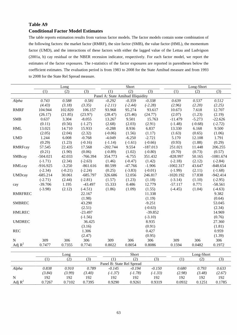
63

Table A9 Conditional Factor Model Estimates The table reports estimation results from various factor models. The factor models contain some combination of the following factors: the market factor (RMRF), the size factor (SMB), the value factor (HML), the momentum factor (UMD), and the interactions of these factors with either the lagged value of the Lettau and Ludvigson (2001a, b) cay residual or the NBER recession indicator, respectively. For each factor model, we report the estimates of the factor exposures. The t-statistics of the factor exposures are reported in parentheses below the coefficient estimates. The evaluation period is from 1983 to 2008 for the State Amihud measure and from 1993 to 2008 for the State Rel Spread measure.

Long Short Long-Short (1) (2) (3) (1) (2) (3) (1) (2) (3)

Panel A: State Amihud Illiquidity Alpha 0.743 0.588 0.581 -0.292 -0.359 -0.338 0.639 0.537 0.512 (4.43) (3.18) (3.35) (-2.11) (-2.44) (-2.28) (2.96) (2.20) (2.25) RMRF 104.944 102.820 106.157 93.968 95.274 93.617 10.673 7.618 12.707 (26.17) (21.85) (23.97) (28.47) (25.46) (24.77) (2.07) (1.23) (2.19) SMB 0.637 3.304 -8.055 13.267 9.501 15.763 -11.479 -5.273 -22.626 (0.11) (0.56) (-1.27) (2.68) (2.03) (2.91) (-1.48) (-0.68) (-2.72) HML 13.021 14.710 15.933 -0.288 8.936 6.837 13.330 6.168 9.500 (2.05) (2.04) (2.32) (-0.06) (1.56) (1.17) (1.63) (0.65) (1.06) UMD 1.244 6.008 -0.768 -4.049 -6.250 -2.721 5.170 12.108 1.791 (0.29) (1.23) (-0.16) (-1.14) (-1.61) (-0.66) (0.93) (1.88) (0.29) RMRFcay 57.545 22.435 17.568 -202.744 9.554 -187.013 251.021 11.448 206.255 (0.21) (1.90) (0.06) (-0.89) (1.02) (-0.80) (0.70) (0.73) (0.57) SMBcay -504.021 42.033 -766.394 354.773 -6.755 351.432 -828.997 50.165 -1081.674 (-1.71) (2.34) (-2.63) (1.46) (-0.47) (1.42) (-2.18) (2.12) (-2.84) HMLcay -916.925 -3.250 -861.616 80.599 -47.766 -1.906 -1002.317 43.647 -848.654 (-2.34) (-0.21) (-2.24) (0.25) (-3.83) (-0.01) (-1.99) (2.11) (-1.68) UMDcay -685.214 30.061 -685.797 326.686 12.056 246.817 -1020.192 17.838 -942.414 (-2.71) (2.44) (-2.81) (1.57) (1.23) (1.18) (-3.14) (1.10) (-2.95) cay -39.706 1.195 -43.497 15.333 0.486 12.779 -57.117 0.771 -58.561 (-3.98) (2.12) (-4.51) (1.86) (1.09) (1.55) (-4.45) (1.04) (-4.63) RMRFREC 22.167 11.338 9.382 (1.98) (1.19) (0.64) SMBREC 43.290 -9.251 53.045 (2.51) (-0.63) (2.34) HMLREC -23.497 -39.852 14.969 (-1.56) (-3.10) (0.76) UMDREC 36.425 8.935 27.360 (3.16) (0.91) (1.81) REC 1.306 0.427 0.959 (2.47) (0.95) (1.39) N 309 306 306 309 306 306 309 306 306 Adj R2 0.7477 0.7355 0.7741 0.8022 0.8054 0.8086 0.1594 0.0482 0.1972 Long Short Long-Short (1) (2) (3) (1) (2) (3) (1) (2) (3)

Panel B: State Rel Spread Alpha 0.838 0.910 0.789 -0.145 -0.194 -0.150 0.680 0.793 0.633 (3.84) (3.99) (3.40) (-1.37) (-1.78) (-1.33) (2.98) (3.48) (2.67) N 192 192 192 192 192 192 192 192 192 Adj R2 0.7267 0.7102 0.7395 0.9290 0.9261 0.9319 0.0932 0.1251 0.1785