Landscape Influences on Headwater Streams on Fort Stewart,Georgia, USA

Henriette I. Jager • Mark S. Bevelhimer •

Roy L. King • Katy A. Smith

Received: 23 June 2010 / Accepted: 24 June 2011

� Springer Science+Business Media, LLC (outside the USA) 2011

Abstract Military landscapes represent a mixture of

undisturbed natural ecosystems, developed areas, and lands

that support different types and intensities of military

training. Research to understand water-quality influences of

military landscapes usually involves intensive sampling in a

few watersheds. In this study, we developed a survey design

of accessible headwater watersheds intended to improve our

ability to distinguish land–water relationships in general,

and training influences, in particular, on Fort Stewart, GA.

We sampled and analyzed water from watershed outlets.

We successfully developed correlative models for total

suspended solids (TSS), total nitrogen (TN), organic carbon

(OC), and organic nitrogen (ON), which dominated in this

blackwater ecosystem. TSS tended to be greater in samples

after rainfall and during the growing season, and models

that included %Wetland suggested a ‘‘build-and-flush’’

relationship. We also detected a positive association

between TSS and tank-training, which suggests a need to

intercept sediment-laden runoff from training areas. Models

for OC showed a negative association with %Grassland.

TN and ON both showed negative associations with

%Grassland, %Wetland, and %Forest. Unexpected positive

associations were observed between OC and equipment-

training activity and between ON and %Bare ground ?

Roads. Future studies that combine our survey-based

approach with more intensive monitoring of the timing and

intensity of training would be needed to better understand

the mechanisms for these empirical relationships involving

military training. Looking beyond local effects on Fort

Stewart streams, we explore questions about how exports of

OC and nitrogen from coastal military installations ulti-

mately influence estuaries downstream.

Keywords Blackwater river � Build-and-flush � Coastal

plain � Headwater watershed � Land use �Military training �Stream-water quality � Survey design

Introduction

The primary mission of military installations is to ensure

military readiness. Because large tracts of lands have been

set aside for this purpose, United States (US) military

installations harbor significant areas of natural ecosystems

that support and, in some cases, provide refuge for fish and

wildlife species (Warren and others 2007; Efroymson and

others 2009). Research is needed to understand how the

primary mission of military installations (training) can be

supported while minimizing adverse effects on ecosystems,

both within the boundaries of the installations themselves

and downstream.

Two significant water-quality concerns for aquatic biota

in United States (US) rivers and streams impacted by

human activities are high suspended-sediment loadings and

nutrient enrichment leading to low dissolved oxygen (DO;

United States Environmental Protection Agency [USEPA]

Electronic supplementary material The online version of thisarticle (doi:10.1007/s00267-011-9722-4) contains supplementarymaterial, which is available to authorized users.

H. I. Jager (&) � M. S. Bevelhimer

Oak Ridge National Laboratory, Oak Ridge, TN 37831-6036,

USA

e-mail: jagerhi@ornl.gov

R. L. King

Oak Ridge Associated Universities, Fort Stewart, GA, USA

K. A. Smith

University Georgia Marine Extension Service, Brunswick, GA,

USA

123

Environmental Management

DOI 10.1007/s00267-011-9722-4

1994). Sedimentation is considered the single most

important factor leading to imperilment of freshwater

fishes and mussels in the southeastern United States

(Pringle and others 2000). Regional studies of watershed

influences typically find that agricultural and urban areas

contribute more sediment and nutrients than forest and

wetland areas do (Hunsaker and Levine 1995; Jones and

others 2001; Weller and others 2003). Wetland areas typ-

ically accumulate sediments and nutrients generated in

upland areas (Craft and Casey 2000). The effects of land

cover can depend on rainfall. According to the ‘‘build-and-

flush’’ hypothesis, larger watersheds have more depressions

that retain sediments and nutrients, some of which are

flushed during major precipitation and runoff events (Lewis

and Grimm 2007).

Although many studies have examined relationships

between natural land use and cover (LULC) and water

quality, land uses typical of military installation are not as

well studied. Gradients in training disturbance intensity

have been linked with depletion of soil carbon and soil

microbial activity (Silveira and others 2010), with maxi-

mum plant diversity at intermediate levels of disturbance

that permitted coexistence of early and late-successional

species (Leis and others 2005). One of the main effects of

military training activities that repeatedly denuded vege-

tation is sedimentation of streams (Maloney and others

2005a, b; DeBusk and others 2005; Houser and others

2006; Bhat and others 2006).

A second potential stressor of concern is low DO. Fort

Stewart is located in an area with blackwater rivers, which

are rivers that flow through forested swamps and wetlands

and contain tannin-stained dark waters. Blackwater rivers

are particularly susceptible to hypoxic conditions that are

stressful to resident aquatic life (Mallin and others 2004).

During summer months, levels of DO in many Coastal

Plain streams fall below Georgia and USEPA standards

(Utley and others 2008), and this is also true for the Can-

oochee River and its tributaries on Fort Stewart. Several

streams on Fort Stewart have been listed by the USEPA as

impaired because of low DO content (USEPA 2005).

Because blackwater streams naturally contain high levels

of organic matter, they are sensitive to nutrient additions

(Meyer and Edwards 1990; Meyer 1990).

Our study examined the influence of watershed attri-

butes, including military training activities, on water

quality in headwater streams on Fort Stewart, an Army

installation that occupies 1100 km2 in the Coastal Plain of

Georgia. Little is known about the influences of land-

management practices on Fort Stewart on water quality in

streams that drain its watersheds. The installation is dom-

inated by forest, grassland, and wetlands and appears to

support more natural vegetation than surrounding land.

However, satellite imagery shows areas that lack

vegetation due to urban development; an extensive network

of dirt roads; and military training activities. Prescribed

growing-season burns of mid-story vegetation are used to

restore and maintain habitat for the red-cockaded wood-

pecker and the flatwood salamander in pine forest and also

provides troops adequate room to maneuver (Draft Envi-

ronmental Impact Statement [DEIS] 2010). Heavy training

activities involving armor and mechanized infantry forces

conducting unrestricted maneuvers, using all types of

vehicles (tracked and wheeled) and equipment, occur in the

western portion of Fort Stewart, where our study is focused

(DEIS 2010). This area is in a red-cockaded woodpecker-

management area with no restrictions on training (DEIS

2010).

The purpose of this study was to understand how water

quality is influenced by military landscapes that include a

mixture of undisturbed, natural ecosystems and areas that

support training. We designed a survey of headwater streams

draining watersheds on Fort Stewart, GA. Our approach

differed from previous studies in that we increased the

number of watersheds sampled at the expense of temporal

sampling intensity. Our survey design minimized correla-

tions among watershed attributes considered a priori to be

likely predictors of water quality. We characterized military

training activities, road densities, and vegetation cover

classes for each sample watershed and measured water

quality from stream samples collected on six dates. These

data were used to develop statistical models to better

understand watershed influences on water quality. Based on

earlier studies, we expected to find elevated suspended

sediment concentrations in watersheds that support training

activities and lower levels in those with a high percentage of

natural vegetation (e.g., forest and grassland). We also

expected watersheds dominated by wetlands to act as sinks

for sediment and nutrients and to potentially offset the effects

of military training on sediment loadings.

Methods

Sampling Design

Our study focused on headwater drainages, which are

desirable for detecting the influences of watershed cover

and training activities. Therefore, we selected as our sam-

pling unit drainages of approximately 200 ha on a

1:50,000-ha map. We used the Soil and Water Assessment

Tool (Gassman and others 2007), with elevation and stream

data, to delineate watersheds within Fort Stewart’s

boundaries that ultimately drain to the Canoochee River.

We used ARCGIS software (ESRI, Redlands, CA) to

identify and exclude non-headwater watersheds, water-

sheds in inaccessible training areas (in the eastern half of

Environmental Management

123

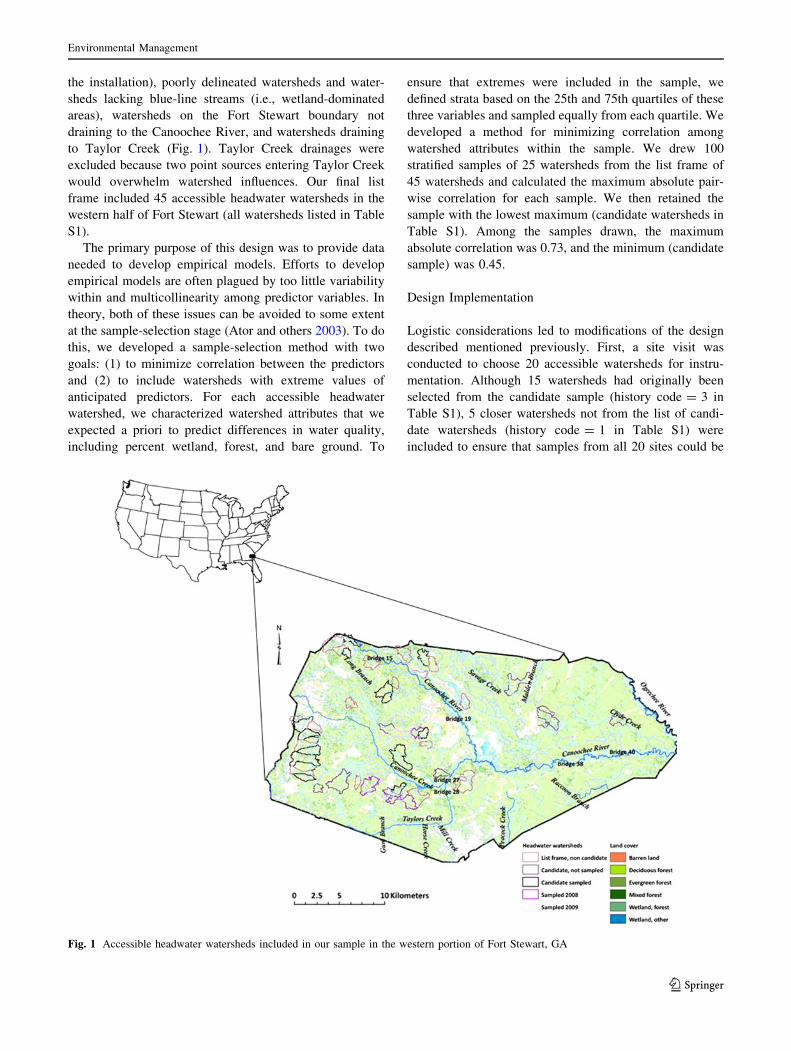
the installation), poorly delineated watersheds and water-

sheds lacking blue-line streams (i.e., wetland-dominated

areas), watersheds on the Fort Stewart boundary not

draining to the Canoochee River, and watersheds draining

to Taylor Creek (Fig. 1). Taylor Creek drainages were

excluded because two point sources entering Taylor Creek

would overwhelm watershed influences. Our final list

frame included 45 accessible headwater watersheds in the

western half of Fort Stewart (all watersheds listed in Table

S1).

The primary purpose of this design was to provide data

needed to develop empirical models. Efforts to develop

empirical models are often plagued by too little variability

within and multicollinearity among predictor variables. In

theory, both of these issues can be avoided to some extent

at the sample-selection stage (Ator and others 2003). To do

this, we developed a sample-selection method with two

goals: (1) to minimize correlation between the predictors

and (2) to include watersheds with extreme values of

anticipated predictors. For each accessible headwater

watershed, we characterized watershed attributes that we

expected a priori to predict differences in water quality,

including percent wetland, forest, and bare ground. To

ensure that extremes were included in the sample, we

defined strata based on the 25th and 75th quartiles of these

three variables and sampled equally from each quartile. We

developed a method for minimizing correlation among

watershed attributes within the sample. We drew 100

stratified samples of 25 watersheds from the list frame of

45 watersheds and calculated the maximum absolute pair-

wise correlation for each sample. We then retained the

sample with the lowest maximum (candidate watersheds in

Table S1). Among the samples drawn, the maximum

absolute correlation was 0.73, and the minimum (candidate

sample) was 0.45.

Design Implementation

Logistic considerations led to modifications of the design

described mentioned previously. First, a site visit was

conducted to choose 20 accessible watersheds for instru-

mentation. Although 15 watersheds had originally been

selected from the candidate sample (history code = 3 in

Table S1), 5 closer watersheds not from the list of candi-

date watersheds (history code = 1 in Table S1) were

included to ensure that samples from all 20 sites could be

Fig. 1 Accessible headwater watersheds included in our sample in the western portion of Fort Stewart, GA

Environmental Management

123

accessed within a half day. Water-quality samples were

taken at the outlets of all 20 watersheds in summer of 2008.

After this, we relocated three of the sites to the outlets of

alternative watersheds because water levels in these

streams were too low to sample at base-flow. These flows

may have been atypical during mid-summer 2008, which

ended a multiyear drought in the southeast. Three suitable

alternatives were identified and sampled in subsequent

efforts (designated by ‘‘B’’ in Table S1). The maximum

absolute correlation of the final sample, including

replacement samples, was 0.533. Watersheds ranged in size

from 105 to 471 ha.

Headwater-Stream Sample Collection and Analysis

Water samples were collected by hand under base-flow

conditions and using rising-stage samplers for rain events.

Rising-stage samplers were installed at the outlets of 20

watersheds (Fig. 1) to capture chemistry during rain events.

Rising stage samplers consisted of I-CHEM stormwater

sample bottles (335 9 100 mm; I-CHEM, Rockwood, TN)

placed inside mounting tubes. Pairs of mounting tubes

(350-mm length–120-mm diameter perforated polyvinyl

chloride pipe) were attached with metal hose clamps to the

fence posts secured in the stream bed and covered with

plastic to prevent rain and debris from interfering with

stream-water collection. The I-CHEM bottle collected a

1-L sample of rising water caused by a significant rain

event. A floating ball valve sealed off the sample collection

port once the bottle was full. Water flowed through the

sampler’s collection funnel directly into a Nalgene sample

bottle, which could be removed from the reusable mount-

ing tube and sealed with a regular cap on collection.

Water samples were collected on August 22, 2008, after

Hurricane Faye (4.9 cm rainfall) and on December 12,

2008 (0.4 cm rainfall). Water samples were collected

manually on four other occasions. For the samples col-

lected manually on May 7, 2009, 0.83 cm antecedent

rainfall was recorded across five stations on Fort Stewart.

Base-flow samples were collected manually in spring of

2009 (February 12, March 30, and June 16).

Samples were all collected on the same half day, stored

on ice, and transported to the laboratory for filtration

subsampling and storage before analysis. Samples col-

lected on August 29, 2008, and all samples collected in

2009 were filtered within 1 day. Samples collected in 2008

were stored on ice for 2 days before processing. Water

samples were analyzed for total suspended solids (TSS [mg

L-1]), total organic carbon (TOC [mg L-1]), dissolved

organic carbon (DOC [mg C L-1]), TN (mg N L-1), nitrate

(NO3 [mg N L-1]), ammonium (NH4? [mg N L-1]), total

phosphorus (TP [mg P L-1]), and soluble reactive phos-

phate (SRP [mg P L-1]). DOC, TOC, and TN were not

measured for the February 2009 samples due to concern

about holding times.

Fort Stewart-base samples were collected in 1.5-L acid-

washed (10% HCl) polypropylene containers. Fort Stewart

event samples were collected in two separate 1-L acid-

washed polypropylene containers and mixed in an acid-

washed 2-L container before subsampling.

Three unfiltered 125-mL subsamples were transferred

into prewashed amber glass bottles with Teflon-lined open-

cap tops. The contents of two bottles were acidified. All

unfiltered samples were frozen until analysis. An Apollo

9000 was used to analyze acidified samples for TN (high-

temperature catalytic oxidation with chemiluminescent

detection) and TOC (sparge-combustion). The nonacidified

sample was analyzed for TP using the ascorbic acid-

molybdenum blue method (QuickChem method 31-115-

01-3-A; Lachat, Milwaukee, WI).

Samples were filtered for analysis of dissolved nutrients

and carbon (125-mL samples through a 0.45-lm filter).

Those to be used for nitrogen and phosphorus analysis were

frozen in polypropylene bottles, whereas those intended for

DOC analysis were refrigerated in amber-glass bottles.

SRP concentration was determined using the ascorbic acid-

molybdenum blue method (QuickChem method 31-115-

01-3-A; Lachat). We measured NO3 concentration using

cadmium reduction of nitrate, followed by azo-dye color-

imetry (QuickChem method 31-107-04-1-C; Lachat).

Ammonium concentration was determined by phenate

colorimetry (QuickChem method 31-107-06-1-E; Lachat).

The remaining unfiltered sample was used for analysis of

TSS. TSS concentrations were determined gravimetrically

on 200-mL subsamples filtered using 0.45-lm filters. TSS

mass was determined using a Sartorius analytical balance

after drying for 2.5 h at 105�C.

We conducted quality-assurance checks on the data to

ensure that the sum of constituents did not exceed total

values. DOC represented a high percentage of TOC and, in

a few cases, exceeded measured TOC. As another check,

we compared total inorganic nitrogen with TN. We

removed one high NH4? measurement that exceeded TN

from our analyses for NH4? and ON, which is calculated

by difference.

Characterization of Watershed Attributes

We summarized LULC watershed attributes used as

potential predictors, including areas (ha) of various land

cover types, time since last managed burn (months before

January 1, 2008), length of road (m), and a variety of

variables measuring training activity in a watershed. Area

(ha) of land cover in each watershed was characterized by

the 2001 National Land Cover Database (NLCD; Homer

and others 2004) for four dominant cover types: barren,

Environmental Management

123

forest, grassland, and wetland. NLCD categories were

derived using hierarchical classification (Vogelmann and

others 1998) from Thematic Mapper images with multiple

spectra and conditional rules. NLCD barren areas (espe-

cially clear-cuts and quarries) are spectrally similar to other

land-cover classes and were resolved using visual inspec-

tion of the images. Road length (m) was calculated using

global information system (GIS) methods. All roads except

for the main highway on Fort Stewart are unpaved. We

defined the following LULC predictors in models for

stream chemistry, percent forest (%Forest), percent grass-

land (%Grassland), percent wetland (%Wetland), time

since managed burn (Burn), and the sum of percent barren

and road density (BareRd). Burn history and road cover-

ages were acquired from the Natural Resources Division at

Fort Stewart. LULC attributes for the list frame of acces-

sible, headwater watersheds and those watersheds sampled

are listed in Table S1 and summarized in Table 1.

Fort Stewart is partitioned into training areas that

completely cover the installation. Fort Stewart’s training

land infrastructure supports Abrams Tank, Bradley Fight-

ing Vehicle, live-fire training, including aerial gunnery and

artillery, and maneuver training. The western portion of

Fort Stewart supports heavy training activities that involve

all kinds of vehicles and equipment, including tracked

vehicles (DEIS 2010). Our study focused on two categories

of training activities: use of off-road vehicles (Tanks) and

heavy equipment training (Equipment). We assessed

training intensity based on a survey filled out by two

individuals familiar with training activities on the instal-

lation. These estimates were consistent with average

numbers of hours that training areas were reserved for each

of these training activities during the years 2001–2005 as

recorded in the Range Facility Management Support Sys-

tem database maintained by Fort Stewart.

Modeling Patterns in Headwater Chemistry

We developed empirical models for each of the water-

quality analytes. The response variable in each model was

a concentration, incremented by one, and loge-transformed

to improve homogeneity of residual variability. Most pre-

dictor variables we included were static watershed attri-

butes characterizing land cover (ha), military training

activity, and months since burning.

Antecedent rainfall and growing season both varied

during time, but not space. We quantified antecedent

rainfall (Rainfall [in cm]) by summing spatially averaged

daily rainfall for all dates between the last date of dry

weather (zero rainfall) and the date of sample collection,

inclusive. Each date’s total rainfall represents an average of

five locations on Fort Stewart. We also defined two indi-

cator variables (Event), which was set equal to one for

sampling dates with rainfall [0 (zero otherwise), and

GrSeason, which was set equal to one for samples taken

during the growing season (April–October) and to zero for

winter samples.

We considered a class of linear mixed models with two

components: one for fixed effects and one for error struc-

ture (random component). The random component allowed

us to account for spatial and temporal dependence among

samples. We followed the recommendation of Zuur and

others (2009) by incorporating temporal covariates into the

fixed component of the mixed models. For the random

component of the model, we considered models with dif-

ferent error variance for sampling date and Event, and we

considered models with and without correlation between

samples collected from the same watershed.

For each analyte, we followed the approach described

by Zuur and others (2009, pp. 120–122), which begins by

comparing error models (random component) and a fixed

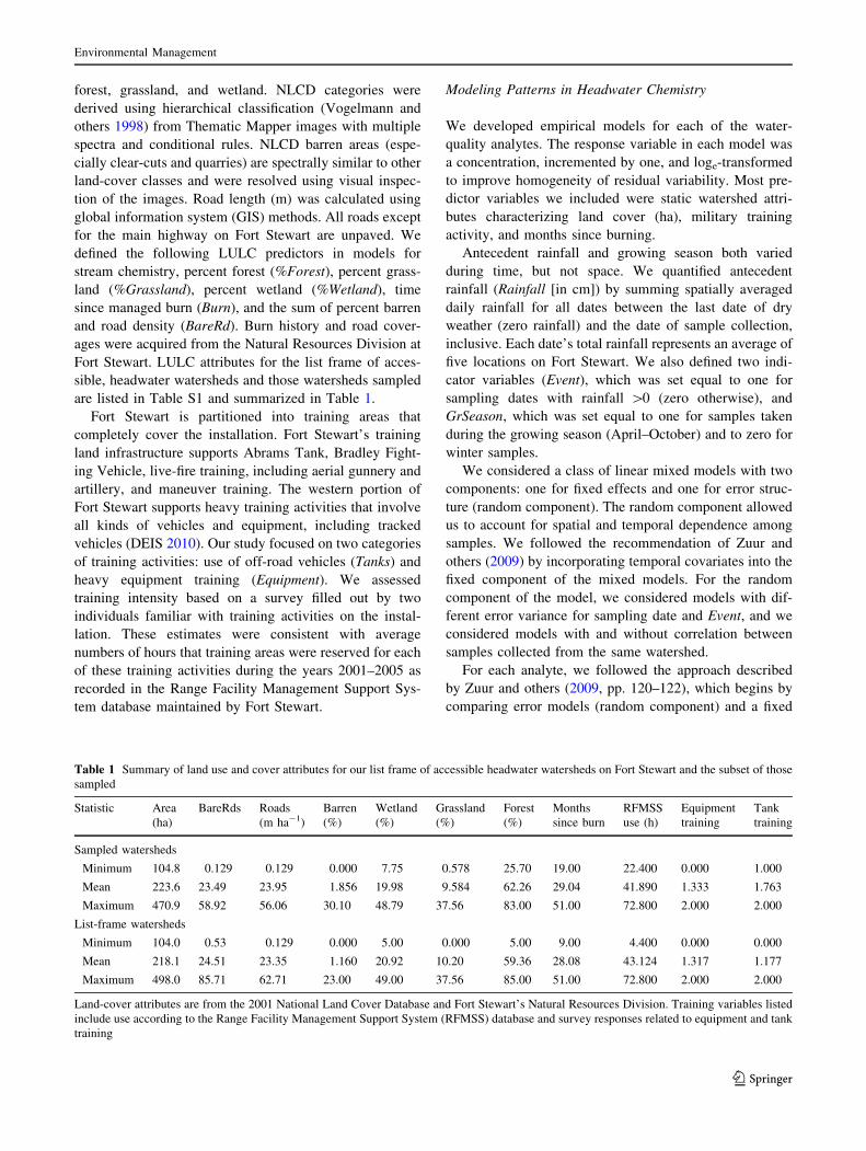
Table 1 Summary of land use and cover attributes for our list frame of accessible headwater watersheds on Fort Stewart and the subset of those

sampled

Statistic Area

(ha)

BareRds Roads

(m ha-1)

Barren

(%)

Wetland

(%)

Grassland

(%)

Forest

(%)

Months

since burn

RFMSS

use (h)

Equipment

training

Tank

training

Sampled watersheds

Minimum 104.8 0.129 0.129 0.000 7.75 0.578 25.70 19.00 22.400 0.000 1.000

Mean 223.6 23.49 23.95 1.856 19.98 9.584 62.26 29.04 41.890 1.333 1.763

Maximum 470.9 58.92 56.06 30.10 48.79 37.56 83.00 51.00 72.800 2.000 2.000

List-frame watersheds

Minimum 104.0 0.53 0.129 0.000 5.00 0.000 5.00 9.00 4.400 0.000 0.000

Mean 218.1 24.51 23.35 1.160 20.92 10.20 59.36 28.08 43.124 1.317 1.177

Maximum 498.0 85.71 62.71 23.00 49.00 37.56 85.00 51.00 72.800 2.000 2.000

Land-cover attributes are from the 2001 National Land Cover Database and Fort Stewart’s Natural Resources Division. Training variables listed

include use according to the Range Facility Management Support System (RFMSS) database and survey responses related to equipment and tank

training

Environmental Management

123

component with all predictors (‘‘global’’ model). In our

case, the global model did not include interactions. After

selecting the error (random) model with the lowest AICc,

we compared fixed-effect models fitted using maximum

likelihood. Interactions were added as the last step. Models

were fitted using generalized least squares (R-routine gls in

the ‘‘nlme’’ package, Pinheiro and Bates 2000) and com-

pared using aicctab (‘‘AICcmodavg’’ package).

Burnham and Anderson (2002) recommended proposing

and comparing candidate models, each a subset of the full

model, including only predictors reasonably expected to

have an influence. Our goal was to identify a subset of

models supported by Akaike’s Information Criterion,

AICc ¼ 2LLþ 2k þ 2k kþ1ð Þn�k�1

; where LL is the log-likelihood

of a candidate model given the data, k is the number of

parameters fitted (including error variance), and n is sample

size. Choosing models with low AICc balances the need for

additional predictors to achieve a close fit against the need

for a robust, parsimonious model that will generalize to

explain patterns in new data sets (Burnham and Anderson

2002).

We compared the global fixed model with each of six

error models with parameters fitted by restricted maximum

likelihood (REML). Six error models considered were (1)

errors independent and homogeneous variance, (2) errors

correlated within watershed and homogeous variance, (3)

errors correlated within watershed and variance different

for event samples, (4) errors uncorrelated and variance

different for event samples, (5) errors correlated within

watershed and variances by sampling date, and (6) errors

uncorrelated and variances by sampling date. We selected

the error model with the lowest AICc and proceeded to the

next step, selecting fixed effects.

We compared all reasonable models involving subsets

of the nine predictors. Because watershed influences of

LULC predictors often depend on rainfall, we also con-

sidered a candidate model adding relevant interactions

between LULC predictors and Rainfall for those LULC

predictors retained in the best-supported models (Rainfall

was always important).

We identified sets of supported models based on AICc-

derived model weights for each of m models, wm ¼ e�AICcmPie�AICci

:

We find these weights to be intuitive and useful. In addition,

models are considered to have information-theoretic support

if the difference in AICc (DAICc) between the model of

interest and the minimum-AICc model is low (substantial

support: DAICc \ 2, moderate support 4 \DAICc \ 7, low

support DAICc [ 10; Anderson 2008, p. 170).

We present model results for TSS, DOC, TN, and ON,

which had unstructured residuals, but not those for NH4?,

NO3, TP, or PO4. We calculated an index of importance for

each predictors as the sum of model weights, wm, for

models that included this variable (Burnham and Anderson

2002). This was calculated from the full set without

interaction terms to ensure that each predictor had the

opportunity to be included in the same number of models.

We analyzed residuals and determined that samples

from December, 2008, tended to be identified as outliers

(large-magnitude standardized residuals). Because these

samples were collected on a Friday, we had concerns about

holding times for these samples for some analytes and

decided to exclude them from the analysis. We decided to

remove all of them, rather than just those indicated as

residuals. In addition, one high value of NH4? was

removed from analysis of NH4? and ON (calculated by

difference). Residual plots will be presented for the best-

supported models.

Results

Headwater-Stream Chemistry

We examined the statistical distributions of water chem-

istry analytes measured in headwater watersheds on all

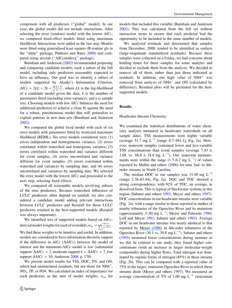
sample dates. TSS measurements were highly variable

(average 51.7 mg L-1 [range 0.7–941.1], Fig. 2a). How-

ever, nonevent samples contained lower and less-variable

TSS concentrations than event samples (average 7.43 ±

1.68 vs. 68.8 ± 18.8 mg L-1). Our nonevent measure-

ments were within the range (1.7–6.2 mg L-1) of values

reported by Mallin and others (2006) for nine 2nd- to 4th-

order streams in North Carolina.

The median DOC in our samples was 31.08 mg L-1

(range 2.76–63.94), Fig. 2a). DOC and TOC showed a

strong correspondence, with 92% of TOC, on average, in

dissolved form. This is typical of blackwater systems in this

region (Sabater and others 1993; Meyer and others 1997).

DOC concentrations in our headwater streams were variable

(Fig. 2a), with a range similar to those reported in studies of

nearby tributaries of the Ogeechee River and its mainstem

(approximately 3–50 mg L-1; Meyer and Edwards 1990;

Leff and Meyer 1991; Sabater and others 1993). Average

DOC in our headwater streams was nearly identical to that

reported by Meyer (1986) in 4th-order tributaries of the

Ogeechee River (30.1 vs. 30.8 mg L-1). Sabater and others

(1993) measured lower concentrations during summer as

we did. In contrast to our study, they found higher con-

centrations (with an increase in larger molecular-weight

compounds) during higher flows. Total nitrogen was dom-

inated by organic forms of nitrogen (85%) in these streams

(Fig. 2b). This can be compared with a reported value of

75% in the larger, mainstem Ogeechee River to which these

streams drain (Meyer and others 1997). We measured an

average concentration of TN of 1.00 mg L-1 (maximum

Environmental Management

123

4.71). Inorganic nitrogen was primarily in the form of

ammonium, NH4? (Fig. 2b), with an average 0.111 mg L-1

(maximum 1.825). All but two of our measured NH4?

concentrations exceeded the USEPA’s threshold range of

0.02–0.03 mg L-1 (Wang and others 2007). Nitrate levels

were variable with an average of 0.031 ± 0.067 mg L-1

(maximum 0.354), which can be compared with the USEPA

(2000) reference criterion of 0.02 mg L-1 for the southern

Coastal Plain ecoregion.

Average TP concentration measured in our headwater

streams was 0.063 mg L-1 (maximum 1.46). Median val-

ues of both TSS and TP were high after tropical storm Faye

in August 2008. On average, SRP represented approxi-

mately one third of total phosphorus (Fig. 2b). In our

samples, 36% exceeded the USEPA (2000) criterion of

0.04 mg L-1 TP, and 22% exceeded levels associated with

decreased health of fish populations of approximately

0.06 mg L-1 (Miltner and Rankin 1998; Weigel and

Robertson 2007).

Headwater Chemistry Correlations and Correlations

Between Watershed Attributes

The highest positive correlations between pairs of measured

water-chemistry concentrations were between TN and its

main constituents, ON (0.895) and NH4? (0.668), TN and

SRP (0.707), TP and SRP (0.772), and TSS and NO3 (0.553).

We found a strong positive association between DOC and

TOC (0.960) and, as expected, between ON and TOC

(0.598). The highest negative correlations were between

DOC and NO3 (-0.499), and between DOC and TSS

(-0.424). Among watershed attributes, percent forest

showed high correlations with %Grassland (-0.790),

%Wetland (-0.501), Equipment (0.523), and months since

burning (0.484). Months since burning also showed associ-

ations with %Wetland (-0.525) and Equipment (0.348).

Training variables, Equipment and Tanks, also showed a

positive association (0.516).

Modeling Influences on Headwater Chemistry

We describe modeling results for each of five analytes

deemed to have reasonably good models (indicated by

unstructured standardized residuals between -3 and 3):

TSS, DOC, TOC, TN, and ON. For TSS, our procedure

selected an error structure with a different error variance

for event samples (approximately twice as high) and

nonevent samples, but there were no residual correlation

among samples from the same watershed (i.e., sampled on

different dates). The models with support, as indicated by

AICc weights (AICcWt in Table 2), tended to predict

log(TSS ? 1) based on Rainfall, GrSeason, %Wetland,

%Forest, and Tanks. Variables Rainfall and GrSeason

occurred in all supported models. Generally, TSS was

higher in water samples taken after rainfall and those

taken during the growing season. There was no strongly

favored model. Several of the best-supported models

included a negative term for %Wetland. The best-sup-

ported model with a Rainfall interaction included an

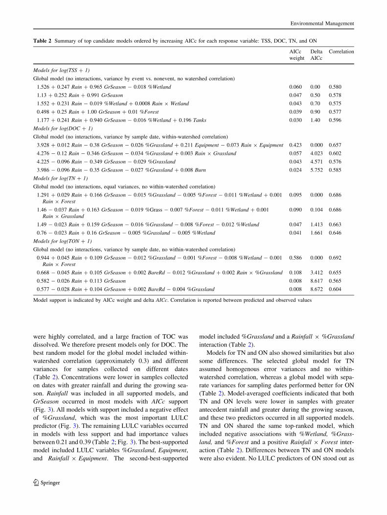
interaction with %Wetland (Table 2). The importance

values showed %Wetland to be the most important LULC

predictor, followed by %Forest and Tanks (Fig. 3).

Coefficients of both %Forest and Tanks had positive

signs.

We obtained similar models for DOC and TOC. This

similarity is not surprising because the two forms of OC

Fig. 2 Water-chemistry measurements from headwater watersheds

on Fort Stewart, GA, for event (open) and base-flow (shaded)

samples. Each box extends from the lower 25th to the 75th percentile

with the median and mean shown as solid and dashed horizontal lines,

respectively. Upper and lower whiskers indicate 5th and 95th

percentiles, and symbols show extreme values. Two groups are

shown. a Concentrations of TSS, DOC, and TOC are reported in

mg L-1. b Concentrations of NH4?, NO3, and ON are reported in

mg N L-1. Concentrations of SRP and TP are reported in mg P L-1

Environmental Management

123

were highly correlated, and a large fraction of TOC was

dissolved. We therefore present models only for DOC. The

best random model for the global model included within-

watershed correlation (approximately 0.3) and different

variances for samples collected on different dates

(Table 2). Concentrations were lower in samples collected

on dates with greater rainfall and during the growing sea-

son. Rainfall was included in all supported models, and

GrSeason occurred in most models with AICc support

(Fig. 3). All models with support included a negative effect

of %Grassland, which was the most important LULC

predictor (Fig. 3). The remaining LULC variables occurred

in models with less support and had importance values

between 0.21 and 0.39 (Table 2; Fig. 3). The best-supported

model included LULC variables %Grassland, Equipment,

and Rainfall 9 Equipment. The second-best-supported

model included %Grassland and a Rainfall 9 %Grassland

interaction (Table 2).

Models for TN and ON also showed similarities but also

some differences. The selected global model for TN

assumed homogenous error variances and no within-

watershed correlation, whereas a global model with sepa-

rate variances for sampling dates performed better for ON

(Table 2). Model-averaged coefficients indicated that both

TN and ON levels were lower in samples with greater

antecedent rainfall and greater during the growing season,

and these two predictors occurred in all supported models.

TN and ON shared the same top-ranked model, which

included negative associations with %Wetland, %Grass-

land, and %Forest and a positive Rainfall 9 Forest inter-

action (Table 2). Differences between TN and ON models

were also evident. No LULC predictors of ON stood out as

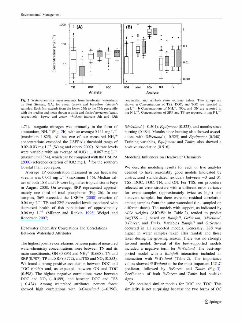
Table 2 Summary of top candidate models ordered by increasing AICc for each response variable: TSS, DOC, TN, and ON

AICc

weight

Delta

AICc

Correlation

Models for log(TSS ? 1)

Global model (no interactions, variance by event vs. nonevent, no watershed correlation)

1.526 ? 0.247 Rain ? 0.965 GrSeason - 0.018 %Wetland 0.060 0.00 0.580

1.13 ? 0.252 Rain ? 0.991 GrSeason 0.047 0.50 0.578

1.552 ? 0.231 Rain - 0.019 %Wetland ? 0.0008 Rain 9 Wetland 0.043 0.70 0.575

0.498 ? 0.25 Rain ? 1.00 GrSeason ? 0.01 %Forest 0.039 0.90 0.577

1.177 ? 0.241 Rain ? 0.940 GrSeason - 0.016 %Wetland ? 0.196 Tanks 0.030 1.40 0.596

Models for log(DOC ? 1)

Global model (no interactions, variance by sample date, within-watershed correlation)

3.928 ? 0.012 Rain - 0.38 GrSeason - 0.026 %Grassland ? 0.211 Equipment - 0.073 Rain 9 Equipment 0.423 0.000 0.657

4.276 - 0.12 Rain - 0.346 GrSeason - 0.034 %Grassland ? 0.003 Rain 9 Grassland 0.057 4.023 0.602

4.225 - 0.096 Rain - 0.349 GrSeason - 0.029 %Grassland 0.043 4.571 0.576

3.986 - 0.096 Rain - 0.35 GrSeason - 0.027 %Grassland ? 0.008 Burn 0.024 5.752 0.585

Models for log(TN ? 1)

Global model (no interactions, equal variances, no within-watershed correlation)

1.291 ? 0.029 Rain ? 0.166 GrSeason - 0.015 %Grassland - 0.005 %Forest - 0.011 %Wetland ? 0.001

Rain 9 Forest0.095 0.000 0.686

1.46 - 0.037 Rain ? 0.163 GrSeason - 0.019 %Grass - 0.007 %Forest - 0.011 %Wetland ? 0.001

Rain 9 Grassland0.090 0.104 0.686

1.49 - 0.023 Rain ? 0.159 GrSeason - 0.016 %Grassland - 0.008 %Forest - 0.012 %Wetland 0.047 1.413 0.663

0.76 - 0.023 Rain ? 0.16 GrSeason - 0.005 %Grassland - 0.005 %Wetland 0.041 1.661 0.646

Models for log(TON ? 1)

Global model (no interactions, variance by sample date, no within-watershed correlation)

0.944 ? 0.045 Rain ? 0.109 GrSeason - 0.012 %Grassland - 0.001 %Forest - 0.008 %Wetland - 0.001

Rain 9 Forest0.586 0.000 0.692

0.668 - 0.045 Rain ? 0.105 GrSeason ? 0.002 BareRd - 0.012 %Grassland ? 0.002 Rain 9 %Grassland 0.108 3.412 0.655

0.582 - 0.026 Rain ? 0.113 GrSeason 0.008 8.617 0.565

0.577 - 0.028 Rain ? 0.104 GrSeason ? 0.002 BareRd - 0.004 %Grassland 0.008 8.672 0.604

Model support is indicated by AICc weight and delta AICc. Correlation is reported between predicted and observed values

Environmental Management

123

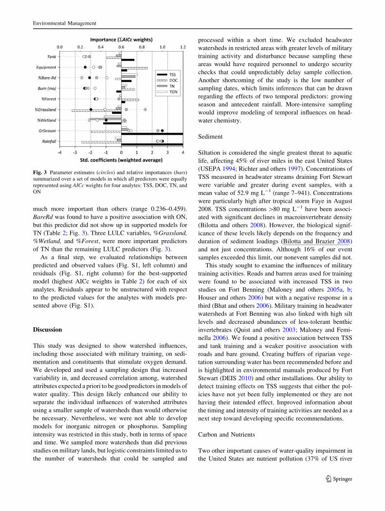
much more important than others (range 0.236–0.459).

BareRd was found to have a positive association with ON,

but this predictor did not show up in supported models for

TN (Table 2; Fig. 3). Three LULC variables, %Grassland,

%Wetland, and %Forest, were more important predictors

of TN than the remaining LULC predictors (Fig. 3).

As a final step, we evaluated relationships between

predicted and observed values (Fig. S1, left column) and

residuals (Fig. S1, right column) for the best-supported

model (highest AICc weights in Table 2) for each of six

analytes. Residuals appear to be unstructured with respect

to the predicted values for the analytes with models pre-

sented above (Fig. S1).

Discussion

This study was designed to show watershed influences,

including those associated with military training, on sedi-

mentation and constituents that stimulate oxygen demand.

We developed and used a sampling design that increased

variability in, and decreased correlation among, watershed

attributes expected a priori to be good predictors in models of

water quality. This design likely enhanced our ability to

separate the individual influences of watershed attributes

using a smaller sample of watersheds than would otherwise

be necessary. Nevertheless, we were not able to develop

models for inorganic nitrogen or phosphorus. Sampling

intensity was restricted in this study, both in terms of space

and time. We sampled more watersheds than did previous

studies on military lands, but logistic constraints limited us to

the number of watersheds that could be sampled and

processed within a short time. We excluded headwater

watersheds in restricted areas with greater levels of military

training activity and disturbance because sampling these

areas would have required personnel to undergo security

checks that could unpredictably delay sample collection.

Another shortcoming of the study is the low number of

sampling dates, which limits inferences that can be drawn

regarding the effects of two temporal predictors: growing

season and antecedent rainfall. More-intensive sampling

would improve modeling of temporal influences on head-

water chemistry.

Sediment

Siltation is considered the single greatest threat to aquatic

life, affecting 45% of river miles in the east United States

(USEPA 1994; Richter and others 1997). Concentrations of

TSS measured in headwater streams draining Fort Stewart

were variable and greater during event samples, with a

mean value of 52.9 mg L-1 (range 7–941). Concentrations

were particularly high after tropical storm Faye in August

2008. TSS concentrations [80 mg L-1 have been associ-

ated with significant declines in macroinvertebrate density

(Bilotta and others 2008). However, the biological signif-

icance of these levels likely depends on the frequency and

duration of sediment loadings (Bilotta and Brazier 2008)

and not just concentrations. Although 16% of our event

samples exceeded this limit, our nonevent samples did not.

This study sought to examine the influences of military

training activities. Roads and barren areas used for training

were found to be associated with increased TSS in two

studies on Fort Benning (Maloney and others 2005a, b;

Houser and others 2006) but with a negative response in a

third (Bhat and others 2006). Military training in headwater

watersheds at Fort Benning was also linked with high silt

levels and decreased abundances of less-tolerant benthic

invertebrates (Quist and others 2003; Maloney and Femi-

nella 2006). We found a positive association between TSS

and tank training and a weaker positive association with

roads and bare ground. Creating buffers of riparian vege-

tation surrounding water has been recommended before and

is highlighted in environmental manuals produced by Fort

Stewart (DEIS 2010) and other installations. Our ability to

detect training effects on TSS suggests that either the pol-

icies have not yet been fully implemented or they are not

having their intended effect. Improved information about

the timing and intensity of training activities are needed as a

next step toward developing specific recommendations.

Carbon and Nutrients

Two other important causes of water-quality impairment in

the United States are nutrient pollution (37% of US river

Fig. 3 Parameter estimates (circles) and relative importances (bars)

summarized over a set of models in which all predictors were equally

represented using AICc weights for four analytes: TSS, DOC, TN, and

ON

Environmental Management

123

miles) and organic enrichment leading to low DO (24% of

US river miles) (USEPA 1994; Richter and others 1997). In

blackwater rivers of the southeastern United States,

including several on or near Fort Stewart, DO is lower than

levels favorable for biota during a significant portion of the

summer (Jager and others 2011).

Researchers are starting to recognize the important role

played by organic forms of nitrogen and carbon in black-

water-stream metabolism (Kaushal and Lewis 2005). Algal

growth and subsequent decomposition plays a smaller role

in oxygen depletion than direct consumption of OC by

heterotrophic bacteria (Mallin and others 2004). Typical of

blackwater systems (Meyer 1990), organic forms domi-

nated both nitrogen and carbon in headwater streams on

Fort Stewart. Concentrations of OC were high and pre-

dominantly dissolved, with a high ratio of DOC to ON. Our

models for both OC and ON suggested a dilution effect

after rainfall.

Our correlation analysis showed a negative association

between NO3 and DOC (-0.50). Goodale and others

(2005) found such a relation in an analysis of streams

across the northeast United States potentially driven by two

processes that use OC as an energy source: (1) microbial

nitrogen immobilization in sediments and (2) loss of

nitrogen to the atmosphere. Alternate drying (aerobic) and

wetting (anaerobic) phases in wetlands reduce nitrate to

ammonium, which is converted by denitrification to

nitrogen gas (Goodale and others 2005). Consequently, a

high percentage of organic nitrogen is typical of streams

draining wetlands and forested watersheds in the Coastal

Plain (Pellerin and others 2004; Lehrter 2006).

Nitrogen limitation is not uncommon in blackwater

streams (Mallin and others 2004). Inorganic nitrogen in our

headwater streams was dominated by ammonium. It is

likely that nitrification is inhibited by high DOC (see

negative correlation in Table 2), low pH (range 5.6–7.7 in

the Canoochee River), and low DO from groundwater

inputs (Strauss and others 2002). In addition to its direct

toxicity to fishes, NH4? remove DO. NH4

? exerts nitrog-

enous oxygen demand and is also readily assimilated by

algae and other autotrophs, which then decay. Relatively

small amounts of nitrate (0.5–1.0 mg L-1) can stimulate

significant increases in chlorophyll a and BOD in black-

water systems (Mallin and others 2004). In our study,

levels of NH4? were high enough to be a potential concern

in these streams, but NO3 levels were low. The average

ratio of inorganic nitrogen to TP in Fort Stewart headwater

streams was similar to that in two creeks in the Mallin

study (35.5 vs. 31 and 33). We observed a positive corre-

lation between NH4? and SRP in our headwater streams

(?0.353). This correlation, which has been observed in

other coastal blackwater rivers in Georgia, is consistent

with release of SRP associated with sediment and organic

particles during anoxic conditions (Golladay and Battle

2002). Previous studies have found greater ON in streams

draining watersheds dominated by forest and wetland

(Lehrter 2006). In our study, both TN and ON tended to be

lower in streams draining watersheds with a greater per-

centage of forest or wetlands (or grassland).

The strongest LULC influence found in our study was a

tendency for greater OC in streams draining watersheds

with a large percentage of grassland area. The second-best-

supported model for DOC (AICc weight = 0.06) included

an interaction between rainfall and grassland area. Few

studies have focused on the role of grasslands as a source

or sink of OC. Deep-rooted, perennial native grasses are

known to retain sediment and build soil OC. These grasses

promote development of carbon-rich soils during time,

which could, when disturbed or inundated, result in greater

OC export compared with some other land cover types.

Don and Schulze (2008) found that DOC exports from

grasslands were largely mediated by soil properties, with

greater exports from sandy, acidic soils than from clay

soils.

Our models also indicated that streams draining water-

sheds supporting more frequent heavy-equipment training

were associated with greater OC concentrations and lower

TN and ON concentrations. Bhat and others (2006) also

found a negative response of TN to the percent of military

land and disturbance. However, the response we estimated

for DOC differed from that of two previous studies finding

lower stream DOC in more disturbed watersheds (Maloney

and others 2005a; Bhat and others 2006). Disturbance

should erode soil OC during time (DeBusk and others

2005), suggesting that watersheds supporting equipment

training may have had greater initial soil OC on Fort

Stewart. Organic content of soils is greater in low-lying,

poorly drained areas, which abound on Fort Stewart, than

in sandy soils and upland areas (Mallin 2009), although

mechanized equipment and tanks cannot travel on soils that

are frequently inundated (DEIS 2010). Our analysis indi-

cated a positive response of stream ON to barren land and

roads, BareRd, which is similar to a result of a study at

Marine Corps Base Camp LeJeune (Baker, unpublished

data), but nevertheless is unexpected. One explanation

might be that more ON is available for surface runoff in

barren areas (P. Halpin [Duke University] personal com-

munication to H. Jager, June 21, 2011).

To better explore the effects of training, future studies

might focus on understanding how soil carbon and nitrogen

characteristics differ among areas used for training and

those with undisturbed forest, grassland, floodplain, or

wetlands. We would also expect interactions between

vegetation and training levels. For example, areas fre-

quently disturbed by heavy training activities tended to

support annual, early succession, and pioneer species of

Environmental Management

123

plants rather than deep-rooted perennial grasses (Jentsch

and others 2009). Garten and Ashwood (2004) developed a

simple restoration model to predict thresholds for recovery

and recovery times for soil carbon levels in soils disturbed

by military training.

Although this study focused on headwaters, ultimately,

the implications of military activities and their effects

downstream in the Ogeechee River and estuary are of

interest. The Ogeechee River is one of several well-mixed

estuaries of the southeastern United States that has expe-

rienced long-term trends of increased nutrients and

decreased DO (Verity and others 2006). Anthropogenic

point sources of nutrients and carbon are labile and can

therefore have a disproportionate effect on processes that

deplete oxygen in blackwater estuaries (Mallin and others

2006; Hendrickson and others 2007). The concern is that

watershed influences that increase nutrient and carbon

levels in headwaters will manifest themselves as low DO

downstream during summer months (Conrads and Roehl

1999). In blackwater rivers, oxygen is depleted by

decomposition of OC by heterotrophic bacteria (Meyer and

Edwards 1990; Mallin and others 2004; Sun and others

1997). Jager and others (2011) determined that 20% of

DOC would likely flocculate on exposure to saltwater

where it would become available to benthic heterotrophs

and stimulate oxygen demand. Free-living bacterial cells

also feed directly on DOC in the water column (Hamdan

and Jonas 2006).

The value of correlative studies, such as this one, is to

detect land–water relationships by studying a diverse

collection of watersheds. To understand the mechanisms for

associations related to training identified here will require

more intensive studies of the timing and intensity of various

training activities. Ideally, this would be conducted at the

diverse collection of sampled watersheds studied here. Our

study suggests that Fort Stewart headwater watersheds are

not an important source of nitrate. High organic fractions of

carbon and nitrogen, such as those we measured in this study,

are typical of less-disturbed watersheds. Nevertheless, fur-

ther studies are needed to understand whether OC and

nutrients originating on Fort Stewart have could have

adverse effects further downstream.

Acknowledgements This research was performed at Oak Ridge

National Laboratory (ORNL) and sponsored by the United States

Department of Defense Strategic Environmental Research and

Development Program (SERDP) through military interagency pur-

chase requisition no. W74RDV83465697. ORNL is managed by UT-

Battelle, LLC, for the United States Department of Energy under

contract DE-AC05-00OR22725. Many people contributed to this

effort, starting with our SERDP program manager, John Hall. Special

thanks are due to Patrick Mulholland who provided his considerable

expertise and advice in the planning and execution of a hydrology and

water chemistry study. Tim Beatty (CIV USA FORSCOM) served as

our primary contact in the Natural Resources Division, Fort Stewart,

and facilitated all of our sampling. We also appreciate the efforts of

others at Fort Stewart, including Larry Carlisle, Ron Owens, and

Robert Gosling. We thank Keith Gates (UGA Marine Extension) for

arranging for laboratory analysis of water chemistry and sharing

water-quality data for the Ogeechee River. GIS data and expertise

were provided by Latha Baskaran (ORNL) and Steve Campbell

(ORISE). We thank Chuck Garten and Pat Mulholland for collegial

reviews of this manuscript and extremely helpful reviews from five

reviewers.

References

Anderson DR (2008) Model based inference in the life sciences: a

primer on evidence. Springer, New York

Ator SW, Olsen AR, Pitchford AM, Denver JM (2003) Application of

a multi-purpose unequal-probability stream survey in the Mid-

Atlantic Coastal Plain. Journal of the American Water Resources

Association 39:873–886

Baker B (2011) A decision support tool for predicting water quality

based on land cover Masters project. Duke University, Durham

Bhat S, Jacobs JM, Hatfield K, Prenger J (2006) Relationships

between stream water chemistry and military land use in forested

watersheds in Fort Benning, Georgia. Ecological Indicators

6:458–466

Bilotta GS, Brazer RE (2008) Understanding the influence of suspended

solids on water quality and aquatic biota. Water Research 42:

2849–2861

Bilotta GS, Brazier RE, Haygarth PM, Macleod CJA, Butler R,

Granger S, Krueger T, Freer J , Quinton JN (2008) Rethinking

the contribution of drained and undrained grasslands to sedi-

ment-related water quality problems. Journal of Environment

Quality 37:906–914

Burnham KP, Anderson DR (2002) Model selection and multimodel

inference: a practical information-theoretic approach, 2nd edn.

Springer-Verlag, New York

Conrads PA, Roehl EA Jr (1999) Comparing physics-based and

neural network models for simulating salinity, temperature, and

dissolved oxygen in a complex, tidally affected river basin. In:

Proceedings of the South Carolina environmental conference,

15–16 Mar 1999. http://sc.water.usgs.gov/publications/abstracts/

NN-modelcomparison-Abstract.html. Accessed 2 Mar 2010

Craft CB, Casey WP (2000) Sediment and nutrient accumulation in

floodplain and depressional freshwater wetlands of Georgia,

USA. Wetlands 20(2):323–332

DeBusk WF, Skulnick BL, Prenger JP, Reddy KR (2005) Response of

soil organic carbon dynamics to disturbance from military

training. Journal of Soil and Water Conservation 60:163–171

Don A, Schulze ED (2008) Controls on fluxes and export of dissolved

organic carbon in grasslands with contrasting soil types. Biogeo-

chemistry 91:117–131

Draft Environmental Impact Statement (2010) The DEIS for training

range and garrison support facilities construction and operation

at Fort Stewart, Georgia, chap 3, Mar 2010.

Efroymson RA, Jager HI, Dale VH, Westerveld J (2009) A

framework for developing management goals for species at risk

with examples from military installations in the United States.

Environmental Management 44:1163–1179

Garten CT, Ashwood TL (2004) Modeling soil quality thresholds to

ecosystem recovery at Fort Benning, GA, USA. Ecological

Engineering 23:351–369

Gassman PW, Reyes MR, Green CH, Arnold JG (2007) The soil and

water assessment tool: historical development, applications, and

future research directions. Transactions of the American Society

Environmental Management

123

of Agricultural and Biological Engineering (ASABE) 50:

1211–1250

Golladay SW, Battle J (2002) Effects of flooding and drought on

water quality on Gulf Coastal Plain streams in Georgia. Journal

of Environment Quality 31:1266–1272

Goodale CL, Aber JD, Vitousek PM, McDowell WH (2005) Long-

term decreases in stream nitrate: successional causes unlikely;

possible links to DOC? Ecosystems 8:334–337

Hamdan LJ, Jonas RB (2006) Seasonal and interannual dynamics of

free-living bacterioplankton and microbially labile organic

carbon along the salinity gradient of the Potomac River.

Estuaries and Coasts 29:40–53

Hendrickson J, Trahan N, Gordon E, Ouyang Y (2007) Estimating

relevance of organic carbon, nitrogen, and phosphorus loads to a

blackwater river estuary. Journal of the American Water

Resources Association 43:264–279

Homer CCH, Yang L, Wylie B, Coan M (2004) Development of a

2001 National Landcover Database for the United States.

Photogrammetric Engineering and Remote Sensing 70:829–840

Houser JN, Mulholland PJ, Maloney KO (2006) Upland disturbance

affects headwater stream nutrients and suspended sediments

during baseflow and stormflow. Journal of Environment Quality

35:352–365

Hunsaker CT, Levine DA (1995) Hierarchical approaches to the study

of water-quality in rivers. BioScience 45:193–203

Jager HI, Bevelhimer MS, Peterson DL (2011) Population viability

analysis of the endangered shortnose sturgeon. Final report to

SERDP. ORNL/TM-2011/48 (in review). http://www.osti.gov/

Jentsch A, Friedrich S, Steinlein T, Beyschlag W, Nezadal W (2009)

Assessing conservation action for substitution of missing

dynamics on former military training areas in central Europe.

Restoration Ecology 17:107–116

Jones KB, Neale AC, Nash MS, Van Remortel RD, Wickham JD,

Riitters KH et al (2001) Predicting nutrient and sediment loadings

to streams from landscape metrics: a multiple watershed study

from the United States Mid-Atlantic region. Landscape Ecology

16:301–312

Kaushal SS, Lewis WM Jr (2005) Fate and transport of organic

nitrogen in minimally disturbed montane streams of Colorado,

USA. Biogeochemistry 74:303–321

Leff LG, Meyer JL (1991) Biological availability of dissolved organic

matter along the Ogeechee River. Limnology and Oceanography

36(2):315–323

Lehrter JC (2006) Effects of land use and land cover, stream

discharge, and interannual climate on the magnitude and timing

of nitrogen, phosphorus, and organic carbon concentrations in

three Coastal Plain watersheds. Water Environment Research

78:2356–2368

Leis SA, Engle DM, Leslie DM, Fehmi JS (2005) Effects of short-

and long-term disturbance resulting from military maneuvers on

vegetation and soils in a mixed prairie area. Environmental

Management 36:849–861

Lewis DB, Grimm NB (2007) Hierarchical regulation of N export

from urban catchments: interactions of storms and landscapes.

Ecological Applications 17:2347–2364

Mallin MA (2009) Comparative impacts of stormwater runoff on water

quality of an urban, a suburban, and a rural stream. Environmental

Monitoring and Assessment 159:475–491

Mallin MA, McIver MR, Ensign SH, Cahoon LB (2004) Photosyn-

thetic and heterotrophic impacts of nutrient loading to blackwa-

ter streams. Ecological Applications 14:823–838

Mallin MA, Johnson VL, Ensign SH, MacPherson TA (2006) Factors

contributing to hypoxia in rivers, lakes, and streams. Limnology

and Oceanography 51(1):690–701

Maloney KO, Feminella JW (2006) Evaluation of single- and multi-

metric benthic macroinvertebrate indicators of catchment

disturbance over time at the Fort Benning Military Installation,

Georgia, USA. Ecological Indicators 6:469–484

Maloney KO, Mulholland PJ, Feminella JW (2005a) Influence of

catchment-scale military land use on stream physical and organic

matter variables in small Southeastern Plain catchments (USA).

Environmental Management 35:677–691

Maloney KO, Mulholland PJ, Feminella JW (2005b) ERRATUM:

influence of catchment-scale military land use on stream

physical and organic matter variables in small Southeastern

Plain catchments (USA). Environmental Management 36:918

Meyer JL (1986) Dissolved organic carbon dynamics in two subtropical

blackwater rivers. Archiv fur Hydrobiologie 108:119–134

Meyer JL (1990) A blackwater perspective on riverine ecosystems.

BioScience 40:643–651

Meyer JL, Edwards RT (1990) Ecosystem metabolism and turnover

of organic-carbon along a blackwater river continuum. Ecology

71:668–677

Meyer JL, Benke AC, Edwards RT, Wallace JB (1997) Organic

matter dynamics in the Ogeechee River, a blackwater river in

Georgia, USA. Journal of the North American Benthological

Society 16:82–87

Miltner RJ, Rankin ET (1998) Primary nutrients and the biotic

integrity of rivers and streams. Freshwater Biology 40:145–158

Pellerin BA, Wollheim WM, Hopkinson CS, McDowell WH,

Williams MR, Vorosmarty CJ et al (2004) Role of wetlands

and developed land use on dissolved organic nitrogen concen-

trations and DON/TDN in northeastern US rivers and streams.

Limnology and Oceanography 49:910–918

Pinheiro JC, Bates DM (2000) Mixed-effects models in S and S-Plus.

Springer-Verlag, New York

Pringle CM, Freeman MC, Freeman BJ (2000) Regional effects of

hydrologic alterations on riverine macrobiota in the new world:

tropical-temperate comparisons. BioScience 50:807–823

Quist MC, Fay PA, Guy CS, Knapp AK, Rubenstein BN (2003) Military

training effects on terrestrial and aquatic communities on a

grassland military installation. Ecological Applications 13:

432–442

Richter BD, Braun DP, Mendelson MA, Master LL (1997) Threats to

imperiled freshwater fauna. Conservation Biology 11(5):1081–1093

Sabater F, Meyer JL, Edwards RT (1993) Longitudinal patterns of

dissolved organic carbon concentration and suspended bacterial

density along a blackwater river. Biogeochemistry 21:73–93

Silveira ML, Comerford NB, Reddy KR, Prenger J, DeBusk WF

(2010) Influence of military land uses on soil carbon dynamics in

forest ecosystems of Georgia, USA. Ecological Indicators 10:

905–909

Strauss EA, Mitchell NL, Lamberti GA (2002) Factors regulating

nitrification in aquatic sediments: effects of organic carbon,

nitrogen availability, and pH. Canadian Journal of Fisheries and

Aquatic Sciences 59(3):554–563

Sun L, Perdue EM, Meyer JL, Weis J (1997) Use of elemental

composition to predict bioavailability of dissolved organic

matter in a Georgia river. Limnology and Oceanography 42:

714–721

United States Environmental Protection Agency (1994) The quality of

our nation’s water: 1992. EPA 841-S-94-002. EPA Office of

Water, Washington, DC

United States Environmental Protection Agency (2000) Ambient

water quality criteria recommendations: rivers and streams in

nutrient ecoregion XII. EPA-822-B-00-021

United States Environmental Protection Agency (2005) Total max-

imum daily load evaluation for twenty-three stream segments in

the Ogeechee River Basin for dissolved oxygen. EPA 841-S-94-

002. EPA Office of Water, Washington, DC

Utley BC, Vellidis G, Lowrance R, Smith MC (2008) Factors

affecting sediment oxygen demand dynamics in blackwater

Environmental Management

123

streams of Georgia’s coastal plain. Journal of the American

Water Resources Association 44:742–753

Verity PG, Alber M, Bricker MB (2006) Development of hypoxia in

well-mixed sub-tropical estuaries in the southeastern USA.

Estuaries and Coasts 29:665–673

Vogelmann JE, Sohl TL, Campbell PV, Shaw DM (1998) Regional

land cover characterization using Landsat Thematic Mapper data

and ancillary data sources. Environmental Monitoring and

Assessment 51(1–2):415–428

Wang LZ, Robertson DM, Garrison PJ (2007) Linkages between

nutrients and assemblages of macroinvertebrates and fish in

wadeable streams: implication to nutrient criteria development.

Environmental Management 39:194–212

Warren SD, Holbrook SW, Dale DA, Whelan NL, Elyn M, Grimm W

et al (2007) Biodiversity and the heterogeneous disturbance regime

on military training lands. Restoration Ecology 15:606–612

Weigel BM, Robertson DM (2007) Identifying biotic integrity and

water chemistry relations in non-wadable rivers of Wisconsin:

toward the development of nutrient criteria. Environmental

Management 40:691–708

Weller DE, Jordan TE, Correll DL, Liu ZJ (2003) Effects of land-use

change on nutrient discharges from the Patuxent River watershed.

Estuaries 26:244–266

Zuur AF, Leno EN, Walker N, Saveliev AA, Smith GM (2009) Mixed

effects models and extensions in ecology with R, 1st edn.

Springer-Verlag, New York

Environmental Management

123