Composition and structure of headwater riparian forests

THE ECOLOGY AND MANAGEMENT OF HEADWATER RIPARIAN AREAS IN THE ERIE GORGES ECOREGION OF NORTHEASTERN OHIO

DISSERTATION

Presented in Partial Fulfillment of the Requirements for

the Degree Doctor of Philosophy in the Graduate

School of The Ohio State University

By Kathryn Lynn Holmes, M.S.

*****

The Ohio State University

2008

Dissertation Committee:

P. Charles Goebel, Advisor Approved by

Robert D. Davic

David M. Hix ______________________________

Richard H. Moore Advisor

Deborah H. Stinner Natural Resources Graduate Program

ii

ABSTRACT

Riparian areas are dynamic components of the landscape that promote many

ecosystem functions vital to the health and productivity of forested watersheds.

Unfortunately, many riparian areas have been damaged or altered and they no longer

function properly to provide these valuable ecosystem services. This is particularly true

in Ohio landscapes where past land use activities have significantly altered current

riparian areas. Because restoring function to riparian areas will have a positive impact on

many current ecological problems, particularly in headwater systems which dominate a

watershed network, stream and riparian restoration projects have become quite common.

Before active management of riparian areas occurs, research is needed to better

understand the ecology of these unique ecotones and to establish reference conditions in

all ecoregions. Using hierarchy theory as our basis, we studied the ecological processes

and relationships that characterize headwater riparian areas in order to develop reference

conditions for the Erie Gorges Ecoregion (Woods et al. 1998) in northeastern Ohio.

Ground-flora composition and structure was influenced by stream geomorphology

transversely across stream valleys as well as longitudinally across watersheds by

hydrologic processes reflected in watershed position, representing the importance of

hierarchical ecological processes in the ecoregion. The characteristics and distribution of

downed wood across headwater riparian areas varied in relation to hydrogeomorphology

iii

with the length of pieces significantly longer as well as the surface area and mean total

volume of all downed wood pieces higher outside the bankfull channel than inside,

except when standardized by area sampled and mean total volume (m3/ha) is higher

inside the bankfull channel than outside. The composition and structure of

macroinvertebrate assemblages is strongly related to site-level physical habitat, including

aquatic and riparian forest, as well as hydrologic processes reflected in distinct faunas

and differing species diversity across watershed positions.

Using our understanding of the ecology of headwater riparian areas, we began to

develop management plans to initiate scientifically-based restoration efforts and improve

long-term sustainability in managed riparian areas and watersheds. Incorporating our

knowledge of hierarchical factors and their influence on stream channel structure and

riparian function, we functionally delineated riparian areas across a landscape using

geospatial tools. Using the functional delineation approach, riparian function is protected

as it varies across a landscape, as opposed to a fixed-width buffer approach that may

protect land not necessarily riparian along headwater areas and under-protect areas along

large order streams and rivers. Finally, we address the need for a prioritization

mechanism to maximize restoration efforts across a landscape and develop a model for

riparian restoration prioritization. The model integrates ecological knowledge of riparian

areas to assess current riparian function and incorporates management objectives to

prioritize restoration on a landscape scale.

iv

DEDICATED TO FAMILY, WHICH SUPPORTS ME ALWAYS

v

ACKNOWLEDGMENTS

I’d like to thank my advisor Charles Goebel for his guidance and friendship over

the past seven years and the patient prodding that lead me to where I am today. Thank

you also to my advisory committee including Bob Davic, David Hix, Richard Moore, and

Deb Stinner for their invaluable comments and direction when I needed it.

I was fortunate to have numerous funding sources that allowed me to complete

the research described within this dissertation, including two OARDC SEED grants, the

USDI National Park Service, an Ohio Sea Grant, the 2007 OARDC Charles E. Thorne

Memorial Fellowship, and the School of Environment and Natural Resources.

I have several co-authors on the following manuscripts I wish to acknowledge

including Arthur E.L. Morris, Marie Schrecengost, Marie Semko-Duncan, and Lance R.

Williams. Several individuals helped with data collection including Victoria Cambell-

Arvai, Emily Cunningham, Clay Dygert, Rachel Morris, Ryan Watson, Marsha Williams,

and Thomas Wise. Additionally, I’d like to thank Lisa Petit and Kevin Skerl at

Cuyahoga Valley National Park for their cooperation, patience, and interest in my

research.

Finally I need to thank my husband Aaron whose encouragement always keeps

me motivated to do my best.

vi

VITA May 15, 1979………………………………..Born-Sylvania, OH 2001………………………………………….B.S. Biology,

Ohio Northern University 2004…………………………………………M.S. Natural Resources,

The Ohio State University 2004-2005…………………………………...Research Associate,

Ohio Agricultural Research and Development Center

2005-2008…………………………………...Graduate Teaching and Research Associate,

The Ohio State University

PUBLICATIONS

Research Publications 1. Holmes, K.L., P.C. Goebel, and D.M. Hix. 2007. Influence of landform and soil characteristics

on canopy and ground-flora composition and structure of first and second order headwater riparian forests in unglaciated Ohio. In: D.S. Buckley and W.K. Clatterbuck (Editors), Proceedings. 15th Central Hardwoods Forest Conference: February 28-March 1, 2006, Knoxville, TN.

2.Holmes, K. L., P. C. Goebel, D. M. Hix, C. E. Dygert, M. E. Semko-Duncan. 2005. Ground-flora composition and structure of floodplain and upland landforms of an old-growth headwater forest in north-central Ohio. Journal of the Torrey Botanical Society 132 (1): 62-71.

3.Holmes, K. L., M. E. Semko-Duncan, P. C. Goebel. 2004. Temporal changes in spring ground-

flora communities across riparian areas in a north-central Ohio old-growth forest. In: D. A. Yaussy, D. M. Hix, R. L. Long, P. C. Goebel (Editors). Proceedings. 14th Central Hardwoods Forest Conference; March 16-19, 2004, Wooster, OH. Gen. Tech. Rep. NE-316, Newtown Square, PA. U.S. Department of Agriculture, Forest Service, Northeastern Research Station. 539 p.

vii

4.Goebel, P. C., D. M. Hix, C. E. Dygert, K. L. Holmes. 2003. Ground-flora communities of headwater riparian areas in an old-growth Central Hardwood Forest. Pp. 136-145, In: Van Sambeek, J. W. Dawson, F. Ponder, Jr., E. F. Lowenstein, J.S. Fralish (Editors), Proceedings, 13th Central Hardwood Forest Conference; April 1-3, 2002, Urbana, IL. Gen. Tech. Rep. NC-234, St. Paul, MN. U.S. Department of Agriculture, Forest Service, North Central Research Station. 565 p.

FIELDS OF STUDY Major Field: Natural Resources

viii

TABLE OF CONTENTS

Page Abstract ............................................................................................................................... ii Dedication……………...………………………………………………………………....iv Acknowledgments................................................................................................................v Vita ………………………………………………………………………………………vi List of Tables ..................................................................................................................... xi List of Figures .................................................................................................................. xiv Chapters: 1. Introduction..................................................................................................................1

1.1 Objectives ............................................................................................................. 4 1.2 Cuyahoga Valley National Park............................................................................ 6 1.3 References............................................................................................................. 9

2. Composition and Structure of Headwater Riparian Forests Across Watershed

Positions in the Erie Gorges Ecoregion .....................................................................14

2.1 Introduction......................................................................................................... 14 2.2 Study Area ......................................................................................................... 16 2.3 Methods............................................................................................................... 18

2.3.1 Field Methods .............................................................................. 18 2.3.2 Data Analysis ............................................................................... 20

2.4 Results................................................................................................................. 22 2.5 Discussion ........................................................................................................... 25 2.6 References........................................................................................................... 27

3. The Distribution and Characteristics of Downed Wood across Headwater Riparian

Ecotones: Integrating the Stream with the Riparian Area .........................................43

3.1 Introduction......................................................................................................... 43 3.2 Methods............................................................................................................... 46

3.2.1 Study Area ................................................................................... 46 3.2.2 Sampling Methodology................................................................ 47 3.2.3 Statistical Analyses ...................................................................... 48

3.3 Results................................................................................................................. 51 3.3.1 Downed Wood Pieces Across the Riparian Area ........................ 51

ix

3.3.2 Downed Wood Pieces by Hydrogeomorphic Zone ..................... 52 3.3.3 Downed Wood Total Volume by Hydrogeomorphic Zone ......... 53

3.4 Discussion ........................................................................................................... 53 3.5 Conclusions......................................................................................................... 57 3.6 References........................................................................................................... 58

4. Environmental Influences on Macroinvertebrate Assemblages on Headwater

Streams of Northeastern Ohio....................................................................................75

4.1 Introduction......................................................................................................... 75 4.2 Study Site ............................................................................................................ 77 4.3 Methods............................................................................................................... 78

4.3.1 Macroinvertebrates ...................................................................... 78 4.3.2 Riparian Forest Habitat ................................................................ 80 4.3.3 Aquatic Habitat ............................................................................ 81 4.3.4 Vertebrate Sampling .................................................................... 81 4.3.5 Macroinvertebrate Assemblage-Environment Analyses.............. 82

4.4 Results................................................................................................................. 84 4.5 Discussion ........................................................................................................... 88 4.6 Potential Limitations of this Study ..................................................................... 91 4.7 References........................................................................................................... 91

5. A Functional Approach to Riparian Delineation Using Geospatial Methods..........106

5.1 Introduction....................................................................................................... 106 5.2 A Functional Geospatial Approach to Riparian Delineation ............................ 107 5.3 Implementing the Functional Approach in the Cuyahoga Valley National Park................................................................................................................................. 108 5.4 Using GIS to Functionally Delineate Riparian Areas....................................... 110 5.5 Functional Riparian Areas versus Fixed-Width Buffers in CVNP................... 112 5.6 Implications for Management ........................................................................... 113 5.7 Conclusions....................................................................................................... 114 5.8 References......................................................................................................... 115

6. Prioritizing Riparian Restoration by Integrating Ecological Function and

Management Objectives across a Landscape...........................................................126

6.1 Introduction....................................................................................................... 126 6.2 Our Approach.................................................................................................... 128 6.3 Study Area ........................................................................................................ 130 6.4 Methods............................................................................................................. 131

x

6.4.1 Assessing Riparian Function...................................................... 131 6.4.1.1 Vegetative Cover ................................................................ 132 6.4.1.2 Potential Plant Habitat ........................................................ 132 6.4.1.3 Sediment Delivery .............................................................. 133 6.4.1.4 Buffering Capacity.............................................................. 134 6.4.1.5 Potential Wildlife Habitat ................................................... 134 6.4.1.6 Streamflow Regulation ....................................................... 134 6.4.1.7 Wetland Quality .................................................................. 135

6.4.2 Riparian Function Index ............................................................ 136 6.4.3 Management Filters ................................................................... 137 6.4.4 Riparian Restoration Priority Index........................................... 138

6.5 Results............................................................................................................... 139 6.5 Discussion ......................................................................................................... 141 6.6 References......................................................................................................... 143

List of References ............................................................................................................169

xi

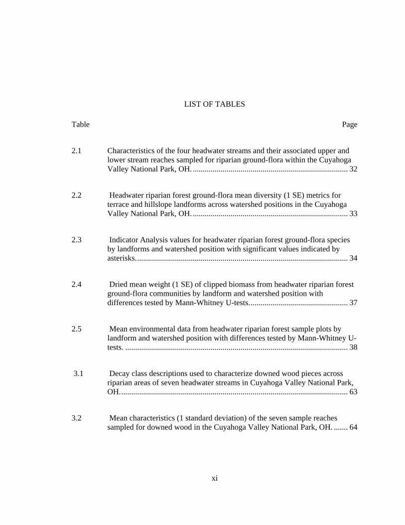
LIST OF TABLES Table Page

2.1 Characteristics of the four headwater streams and their associated upper and lower stream reaches sampled for riparian ground-flora within the Cuyahoga Valley National Park, OH. .............................................................................. 32

2.2 Headwater riparian forest ground-flora mean diversity (1 SE) metrics for terrace and hillslope landforms across watershed positions in the Cuyahoga Valley National Park, OH. .............................................................................. 33

2.3 Indicator Analysis values for headwater riparian forest ground-flora species by landforms and watershed position with significant values indicated by asterisks........................................................................................................... 34

2.4 Dried mean weight (1 SE) of clipped biomass from headwater riparian forest ground-flora communities by landform and watershed position with differences tested by Mann-Whitney U-tests.................................................. 37

2.5 Mean environmental data from headwater riparian forest sample plots by landform and watershed position with differences tested by Mann-Whitney U-tests. ................................................................................................................ 38

3.1 Decay class descriptions used to characterize downed wood pieces across riparian areas of seven headwater streams in Cuyahoga Valley National Park, OH................................................................................................................... 63

3.2 Mean characteristics (1 standard deviation) of the seven sample reaches sampled for downed wood in the Cuyahoga Valley National Park, OH. ....... 64

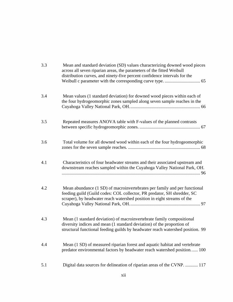
xii

3.3 Mean and standard deviation (SD) values characterizing downed wood pieces across all seven riparian areas, the parameters of the fitted Weibull distribution curves, and ninety-five percent confidence intervals for the Weibull c parameter with the corresponding curve type. ............................... 65

3.4 Mean values (1 standard deviation) for downed wood pieces within each of the four hydrogeomorphic zones sampled along seven sample reaches in the Cuyahoga Valley National Park, OH.............................................................. 66

3.5 Repeated measures ANOVA table with F-values of the planned contrasts between specific hydrogeomorphic zones. ..................................................... 67

3.6 Total volume for all downed wood within each of the four hydrogeomorphic zones for the seven sample reaches. ............................................................... 68

4.1 Characteristics of four headwater streams and their associated upstream and downstream reaches sampled within the Cuyahoga Valley National Park, OH.......................................................................................................................... 96

4.2 Mean abundance (1 SD) of macroinvertebrates per family and per functional feeding guild (Guild codes: COL collector, PR predator, SH shredder, SC scraper), by headwater reach watershed position in eight streams of the Cuyahoga Valley National Park, OH.............................................................. 97

4.3 Mean (1 standard deviation) of macroinvertebrate family compositional diversity indices and mean (1 standard deviation) of the proportion of structural functional feeding guilds by headwater reach watershed position. 99

4.4 Mean (1 SD) of measured riparian forest and aquatic habitat and vertebrate predator environmental factors by headwater reach watershed position. ..... 100

5.1 Digital data sources for delineation of riparian areas of the CVNP. ........... 117

xiii

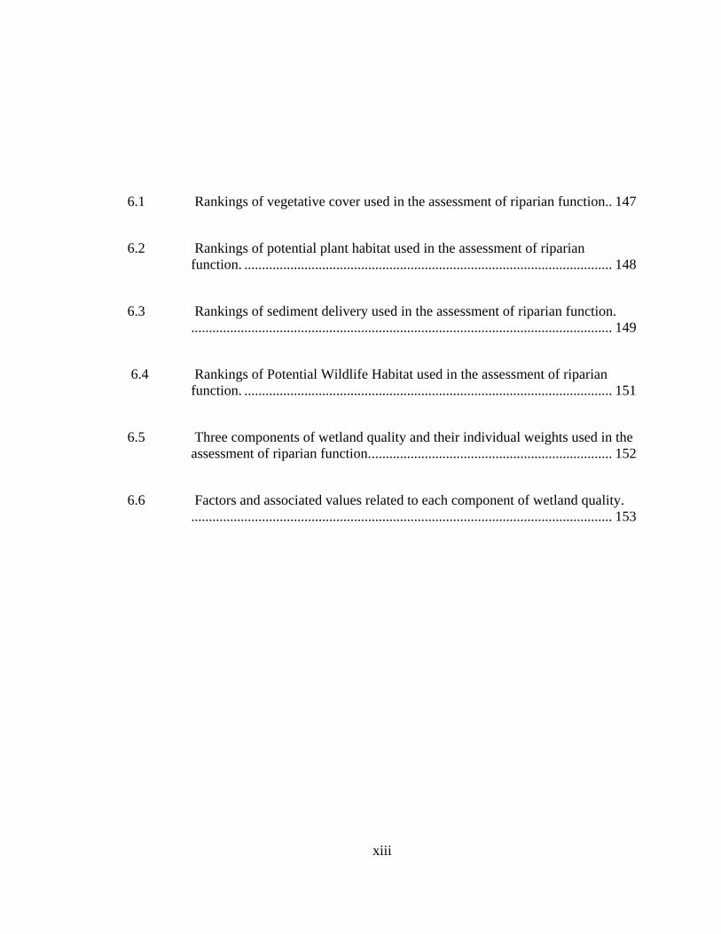
6.1 Rankings of vegetative cover used in the assessment of riparian function.. 147

6.2 Rankings of potential plant habitat used in the assessment of riparian function. ........................................................................................................ 148

6.3 Rankings of sediment delivery used in the assessment of riparian function........................................................................................................................ 149

6.4 Rankings of Potential Wildlife Habitat used in the assessment of riparian function. ........................................................................................................ 151

6.5 Three components of wetland quality and their individual weights used in the assessment of riparian function..................................................................... 152

6.6 Factors and associated values related to each component of wetland quality........................................................................................................................ 153

xiv

LIST OF FIGURES Figure Page

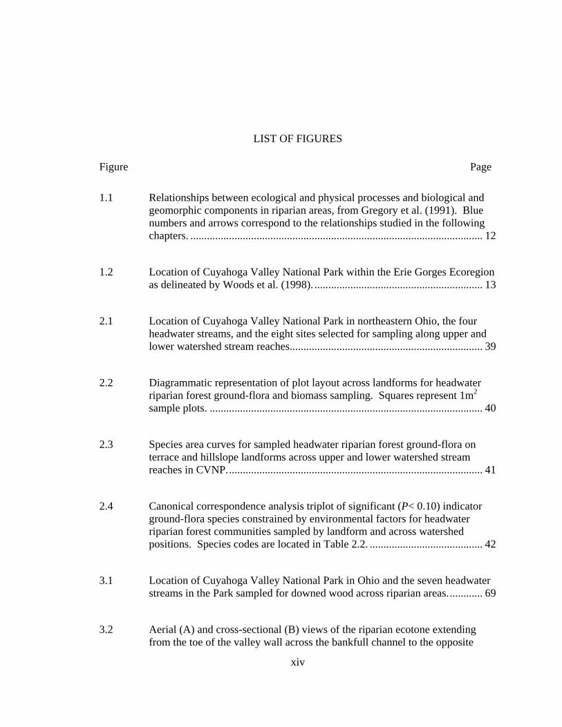
1.1 Relationships between ecological and physical processes and biological and geomorphic components in riparian areas, from Gregory et al. (1991). Blue numbers and arrows correspond to the relationships studied in the following chapters. .......................................................................................................... 12

1.2 Location of Cuyahoga Valley National Park within the Erie Gorges Ecoregion as delineated by Woods et al. (1998). ............................................................. 13

2.1 Location of Cuyahoga Valley National Park in northeastern Ohio, the four headwater streams, and the eight sites selected for sampling along upper and lower watershed stream reaches...................................................................... 39

2.2 Diagrammatic representation of plot layout across landforms for headwater riparian forest ground-flora and biomass sampling. Squares represent 1m2 sample plots. ................................................................................................... 40

2.3 Species area curves for sampled headwater riparian forest ground-flora on terrace and hillslope landforms across upper and lower watershed stream reaches in CVNP............................................................................................. 41

2.4 Canonical correspondence analysis triplot of significant (P< 0.10) indicator ground-flora species constrained by environmental factors for headwater riparian forest communities sampled by landform and across watershed positions. Species codes are located in Table 2.2. ......................................... 42

3.1 Location of Cuyahoga Valley National Park in Ohio and the seven headwater streams in the Park sampled for downed wood across riparian areas............. 69

3.2 Aerial (A) and cross-sectional (B) views of the riparian ecotone extending from the toe of the valley wall across the bankfull channel to the opposite

xv

valley wall that was used for sampling downed wood characteristics across seven sample reaches in Cuyahoga Valley National Park, OH. ..................... 70

3.3 Cross-sectional depiction of hydrogeomorphic zones used to stratify sampling of downed wood across seven sample reaches in the Cuyahoga Valley National Park. ................................................................................................. 71

3.4 Frequency distributions with fitted Weibull distribution curves of entire downed wood piece length (A), volume (B), length per square meter sampled (C), and volume per square meter sampled (D) across the seven sample reaches............................................................................................................. 72

3.5 Frequency distributions with fitted Weibull distribution curves of downed wood piece minimum (A) and maximum (B) diameters and decay class (C) across the seven sample reaches. .................................................................... 73

3.6 Mean total volume (A) and mean total volume per hectare sampled (B) of all downed wood pieces for each of the four hydrogeomorphic zones sampled across seven sample reaches in the Cuyahoga Valley National Park, OH. .... 74

4.1 Location of the four sample streams and eight reaches (black circles) within the Cuyahoga Valley National Park, OH...................................................... 101

4.2 The partition of variance within the macroinvertebrate assemblages among the three measured environmental components and their variation shared between components. .................................................................................................. 102

4.3 Canonical correspondence analysis (CCA) triplots between macroinvertebrate family composition and measured environmental factors (A-C) and macroinvertebrate functional feeding guilds and measured environmental factors (D-F) along four headwater streams of Cuyahoga Valley National Park, OH. Black circles refer to upstream reaches while gray circles refer to downstream reaches. ..................................................................................... 103

xvi

4.4 Partial canonical correspondence analysis (pCCA) Venn diagram indicating explained variance partitioned for macroinvertebrate composition by environmental components. .......................................................................... 104

4.5 Partial canonical correspondence analysis (pCCA) Venn diagram indicating explained variance partitioned for macroinvertebrate trophic structure by environmental components. .......................................................................... 105

5.1 Graphical representation of the functional riparian ecotone following Ilhardt et al. (2000). ...................................................................................................... 118

5.2 Cuyahoga Valley National Park is characterized by tributary streams and the Cuyahoga River. The subset shows the location of the park in Ohio. ......... 119

5.3 Watersheds and reference streams used in the functional riparian delineation in the Cuyahoga Valley National Park.......................................................... 120

5.4 Key used to identify stream type and delineate riparian areas for streams (from Verry et al. 2004). ......................................................................................... 121

5.5 An example of Type I and Type II stream valley walls as delineated following topographic lines........................................................................................... 122

5.6 Functional delineated riparian areas of Cuyahoga Valley National Park. ... 123

5.7 Comparison of riparian delineation methods, fixed-width buffers versus the functional approach, by area delineated (A) and the percent of CVNP land considered riparian (B). .................................................................................... 1

5.8 A comparison of riparian delineation methods along streams of the CVNP and the Cuyahoga River................................................................................ 125

xvii

6.1 Location of Cuyahoga Valley National Park in Ohio and the numerous tributary streams to the Cuyahoga River flowing through the center of the park. .............................................................................................................. 154

6.2 Components of the Riparian Restoration Priority Index Model. .................. 155

6.3 Seven ecological functions of riparian areas assessed for condition relative to an unaltered reference condition for each function. When added together, these seven functions comprise the Riparian Function Index component of the Riparian Restoration Priority Index Model................................................... 156

6.4 Vegetative cover function relative to an unaltered reference condition for functional riparian areas of the CVNP and adjacent areas. .......................... 157

6.5 Potential plant habitat function relative to an unaltered reference condition for functional riparian areas of the CVNP and adjacent areas. .......................... 158

6.6 Sediment delivery function relative to an unaltered reference condition for functional riparian areas of the CVNP and adjacent areas. .......................... 159

6.7 Buffering capacity function relative to an unaltered reference condition for functional riparian areas of the CVNP and adjacent areas. .......................... 160

6.8 Potential wildlife habitat function relative to an unaltered reference condition for functional riparian areas of the CVNP and adjacent areas...................... 161

6.9 Streamflow regulation function relative to an unaltered reference condition for functional riparian areas of the CVNP and adjacent areas. .......................... 162

6.10 Wetland quality function relative to an unaltered reference condition for functional riparian areas of the CVNP and adjacent areas. .......................... 163

xviii

6.11 Riparian Function Index for riparian areas of the CVNP and adjacent areas........................................................................................................................ 164

6.12 Management filters created for the restoration priority index including ownership classifications and the functional riparian area of the Cuyahoga River.............................................................................................................. 165

6.13 Riparian Restoration Priority Index based only on riparian function without the addition of a management filter for the CVNP and adjacent areas......... 166

6.14 Example prioritization showing the riparian function index and the area within the functional riparian area of the Cuyahoga River for a subwatershed within the study area (A) and split for the different ownership classes (B-D). ....... 167

6.15 Example prioritization of areas with poor and moderate riparian function for the three ownership classes in a subwatershed of the study area.................. 168

CHAPTER 1

INTRODUCTION


ecosystem functions vital to the health and productivity of forested watersheds. Not only

do riparian areas regulate the flow of water, sediments and nutrients across system

boundaries, they also contribute organic matter to the aquatic system, increase bank

stability, reduce erosion, and provide unique wildlife habitat (Gregory et al. 1991, Ilhardt

et al. 2000). Additionally, riparian areas serve important roles in mitigating many of the

negative impacts of land-use on aquatic systems, as well as promoting species diversity in

watersheds, providing potential dispersal corridors for wildlife, and mitigating flood

waters (O'Laughlin & Belt 1995, Ilhardt et al. 2000, Goebel et al. 2003).

Over the past several decades, our understanding of the valuable ecological

services that riparian areas provide and their importance to overall watershed health has

increased greatly (Costanza et al. 1997, Hitzhusen 2007). Unfortunately, many riparian

areas have been damaged or altered, and they no longer function properly to provide

these valuable ecosystem services. This is particularly true in Ohio landscapes where

past land use activities have significantly altered current riparian areas or removed them

1

entirely. Because restoring function to riparian areas will have positive impact on many

current ecological problems, such as water quality and stream bank erosion, stream and

riparian restoration projects have become quite common. The ecosystem services

provided by riparian areas, however, often exhibit considerable year to year variation,

driven largely by natural ecological processes such as flooding, drought, landslides, and

wildfire that alter habitat structure and biodiversity (Naiman 1998, Ilhardt et al. 2000).

Human disturbances also alter riparian areas in complex and often synergistic ways

(Gregory et al. 1991). Consequently, in order to develop management plans that maintain

and promote these varied ecosystem functions, it is important to be able to distinguish

between the natural variation of ecological processes and their influence on riparian area

structure and function versus those changes induced by human alterations to the

watershed at multiple scales.

Before active management of riparian areas occurs, research is needed to better

understand the ecology of these unique ecotones. Although riparian research has

increased greatly in the past 20 years, there are considerable gaps in our understanding of

how riparian areas function ecologically. Additionally, much of the existing scientific

research has occurred primarily in the Pacific Northwest, which makes direct application

to other ecoregions difficult. Research to establish reference conditions and restoration

benchmarks is needed in all ecoregions, including Ohio and the Erie Gorges Ecoregion.

Of particular concern to watershed management are riparian areas associated with

headwater systems. Although often overlooked due to their small drainage area (less than

20 square miles), recent research suggests that headwater streams comprise up to 80% of

a watershed’s stream network (Meyer et al. 2003) and the majority of the streams at this

2

scale do not even appear as blue lines on 1:24K USGS topographic maps (Hansen 2001).

For example, the Ohio Environmental Protection Agency (OEPA) estimates there are

approximately 33,800 km (21,000 miles) of named streams, represented as blue-lines on

USGS maps, and approximately 185,000 km (115,000 miles) of unnamed, headwater

streams in Ohio (OEPA 2002). Ecologically, the tight connectivity between the

terrestrial and aquatic ecosystems is particularly strong in headwater systems where

closed tree canopies regulate light and temperature as well as provide allocthononus

inputs from riparian areas that sustain aquatic biota (Vannote et al. 1991). Additionally,

undisturbed headwater streams may have significant impacts on watershed quality

because they have been shown to be capable of retaining and processing nitrate (Peterson

et al. 2001), a significant component of freshwater water pollution. With such a

dominant presence on the landscape, important ecological role, and the potential for high

restoration value, research is needed to understand the ecology of headwater riparian

areas.

Because of their complexity, Gregory et al. (1991) emphasize that research of

these unique terrestrial-aquatic ecotones needs to be framed in an ecosystem perspective,

analyzing the physical and ecological processes and their interrelationships with

geomorphic and biological components (Figure 1.1). The conceptual basis to understand

these interrelationships among riparian areas and multi-scale environmental factors is

hierarchy theory (Allen and Starr 1982, O’Neill et al. 1986). When applied to riparian

areas, hierarchy theory predicts that the upper levels of the hierarchy (e.g., climate,

physiographic setting, and stream valley characteristics) constrain a complex array of

hydrologic and geomorphic processes that in turn mediate the dynamics of lower

3

hierarchical levels (e.g., landforms, soil characteristics, and vegetation development).

Using the Gregory et al. (1991) model of ecological processes and relationships in

riparian areas, we can begin to understand the hierarchical relationships characterizing

headwater systems. This information can be used to develop reference conditions for

riparian areas, which are necessary for establishing management and restoration

benchmarks within an ecoregion (Aronson et al. 1995). Finally, we can incorporate our

understanding of the ecology of headwater systems into management plans leading to

scientifically based restoration efforts and improved long-term sustainability in managed

and restored riparian areas and watersheds.

1.1 Objectives

The primary objectives of this research were to investigate the hierarchical

relationships characterizing headwater riparian areas in the Erie Gorges Ecoregion

(Woods et al. 1998, Figure 1.2) and establish reference conditions that can be used to

develop restoration and management plans for the ecoregion. Relationships between

processes and components of riparian areas as modeled by Gregory et al (1991) were

studied in headwater riparian areas of the Cuyahoga Valley National Park located in

northeastern Ohio. Specifically, the following relationships were studied:

In chapter 2, we examine how the composition and structure of the ground-flora

in headwater riparian forests is related to stream geomorphology, specifically landforms

and their associated soil characteristics. Additionally, we examine how hydrological

processes, specifically watershed position, influence the composition and structure of the

ground-flora in headwater riparian forests.

4

In chapter 3, we examine downed wood characteristics across the entire riparian

ecotone, including the stream channel and stream valley, in order to better understand

how the structure of downed wood changes across headwater riparian areas. To further

understand the influence of hydrogeomorphology on downed wood we sampled the

riparian areas forests by geomorphic zones, specifically the wetted channel, the bankfull

channel, and the area outside the bankfull channel to the base of the stream valley wall.

In chapter 4, we quantify the relationships between macroinvertebrate

assemblages and their biotic and abiotic habitat in headwater streams. Specifically, we

determined composition and trophic structure of macroinvertebrate assemblages, as well

as examined how environmental factors, such as riparian forest and aquatic habitat and

vertebrate predators, influence these assemblages. Additionally, to understand how

watershed position and hydrologic processes affects these relationships, sampling

occurred in both upstream and downstream headwater stream reaches.

In chapter 5, we incorporate our knowledge of hierarchical factors, their influence

on stream channel structure, and riparian function to functionally delineate riparian areas

across a landscape with geospatial tools following a probabilistic approach rather than a

fixed-width approach. Areas delineated are those likely to be riparian, thus protecting the

valuable functional ecosystem services riparian areas provide, as opposed to a more

traditional fixed-width approach that may result in significant errors and does not reflect

the actual riparian area on the ground.

Finally, in chapter 6, we address the challenge of managing riparian areas across a

landscape scale and the need for a prioritization mechanism to maximize restoration

efforts. Using the entire suite of relationships described by Gregory et al. (1991), we

5

develop a model for riparian restoration prioritization that assesses current riparian

function in relation to reference condition and incorporates management objectives to

prioritize restoration on a landscape scale. The model integrates both ecological

information of riparian areas as well as local restoration goals and objectives encouraging

collaborative efforts between scientists and land managers.

1.2 Cuyahoga Valley National Park

Cuyahoga Valley National Park (CVNP) in northeastern Ohio protects over

13,355 ha (33,000 acres) for both conservation as well as recreation, including 35 km (22

miles) of the Cuyahoga River and over 306 km (190 miles) of ephemeral and perennial

tributary streams. The valley of the Cuyahoga River has seen significant human activity

beginning with Native Americans who valued the Portage Path between the Cuyahoga

and Tuscarawas Rivers and maintained several important trading routes through the area.

While Native Americans are known to have established villages in the valley and along

the Portage Path, they are not thought to have greatly influenced the ecological processes

in the area other than through hunting and clearing small areas within the virgin forest for

corn planting (Platt 2006). The significance of the Portage Path that allowed travel

between the Lake Erie watershed and the Ohio River Watershed was also noted by both

the British and French in their colonization of the Americas and the path was noted on

early maps. In 1795 following the Treaty of Greenville, the Portage Path formed the

western boundary of the United States and a year later Moses Cleveland began surveying

the region known as the Western Reserve of Connecticut. White settlers from the eastern

United States soon followed and began to clear the wilderness for homesteads.

6

The valley experienced rapid growth between 1817 and 1825 with the villages of

Hudson and Brandywine Falls boasting grist mills, a distillery, a cheese farm, and a post

office (Platt 2006). However, the transportation of goods and communication into and

out of the region was difficult, leading state and national legislators to consider building a

canal that would connect the region to the eastern United States and Europe, as well as

the southern United States. In 1825, work began to build the Ohio and Erie Canal, which

eventually connected the Cuyahoga and Tuscarawas Rivers with a permanent waterway

resulting in the canal boom years from 1827-1840. The Cuyahoga Valley was an

important transportation route with mills and boat yards, as well as an important area for

settlement and agriculture with as much as 90% of the land estimated to have been

farmed during this time (Platt 2006). By the 1850s, railroads began to dominate the

transportation sector due to their speed and ability to run year-round, leading to the

demise of the canal era and general prosperity in the valley.

While the Cuyahoga Valley retained a few small industries following the canal

era, many settlers left and the abandoned farms began to revert to forest allowing the area

to become a green space retreat from the soot and grime of the nearby cities of Akron and

Cleveland (Platt 2006). As early as 1905, prominent leaders in Cleveland began to

discuss the need for additional green space to be preserved in the region. Following a

survey of the area in 1925, the Cuyahoga Valley was noted for its significance as a

bucolic retreat, beginning the process of preserving land within the valley as metroparks

(Platt 2006). Grassroots organizations worked throughout the 20th century to protect the

valuable green space within the valley from development, and after much deliberation in

the United States Congress, Cuyahoga Valley was designated a National Recreation Area

7

in 1974. In 2000, this designation was changed to National Park. Park officials are

charged with protecting and preserving the historical as well as the natural and

recreational values of the Cuyahoga Valley as green space in an otherwise urban region

(Platt 2006).

The history of the Cuyahoga Valley is similar to much of Ohio in that forests

were cleared for homesteads and industry in the 1800s, but by the 1900s forests began to

slowly recover abandoned areas and establish second-growth forests across the state.

While the floodplain of the Cuyahoga River continues to be the center of activity within

the valley with active farms, small municipalities, and several recreational areas such as

ski areas and golf courses, the large remainder of the park is relatively undeveloped and

characterized by steep, forested alluvial ravine systems along the multiple tributaries to

the Cuyahoga River (Hacker 2003). The forests flanking these ravine systems are

composed of mixed-mesophytic species (e.g. sugar maple, Acer saccharum Marsh;

American beech, Fagus grandifolia Ehrh.; northern red oak, Quercus rubra L.; shagbark

hickory, Carya ovata (P.Mill)K. Koch; and yellow poplar, Liriodendron tulipifera L.)

similar to those described by early surveyors and settlers in their journals (McGovern

1996, Bobel and Bobel 1998).

Due to its history and unique rural-urban interface with large areas minimally

impacted by current human activities, the CVNP is an excellent location to study

hierarchical relationships within headwater stream ecosystems to establish reference

conditions for the Erie Gorges Ecoregion. While these reference conditions are not

representative of pre-European settlement conditions, these headwater stream ecosystems

represent the least disturbed areas within the current landscape and information from

8

these systems can be used to restore and manage similar ecosystems within the ecoregion.

It is our belief that restoring to pre-European conditions is not sustainable in most areas,

including this ecoregion, and utilizing the least disturbed areas as reference conditions is

a valid and sustainable approach to restoration and management in areas with historical

as well as current human activities. As a result we believe CVNP is a model system for

the objectives of this research and dissertation.

1.3 References

Allen, T.F.H., and T.B. Starr. 1982. Hierarchy: Perspectives for Ecological Complexity.

University of Chicago Press, Chicago, IL, USA, pp.310.

Aronson, J., S. Dhillion, and E. Le Floc’h. 1995. On the need to select an ecosystem of reference however imperfect: A reply to Pickett and Parker. Restoration Ecology 3(1): 1-3.

Bobel, P. and R. Bobel. 1998. The Nature of the Towpath: A Natural History Guide to the Ohio and Erie Canal Towpath Trail. Cuyahoga Valley Trails Council, Inc., pp. 151.

Costanza, R., R. d’Arge, R. de Groot, S. Farber, M. Grasso, B. Hannon, K. Limburg, S. Naeem, R.V. O’Neill, J. Paruelo, R.G. Raskin, P. Sutton, and M. van den Belt. 1997. The value of the world’s ecosystem services and natural capital. Nature 387: 253-260.

Goebel, P.C., B.J. Palik, and K.S. Pregitzer. 2003. Plant diversity contributions of riparian areas in watersheds of the northern Lake States, USA. Ecological Applications 13: 1595-1609.

Gregory, S.V., F.J. Swanson, W.A. McKee, and K.W. Cummins. 1991. An ecosystem perspective of riparian zones. BioScience 41: 540-551.

9

Hansen, W.F. 2001. Identifying stream types and management implications. Forest Ecology and Management 143: 39-46.

Hitzhusen, F.J. 2007. Economic valuation of river systems: New horizons in environmental economic series. Edward Elgar Publishing: Northampton, MA, pp. 217.

Ilhardt, B.L., E.S. Verry, and B.J. Palik. 2000. Defining riparian areas. pp. 23-42, In: E.S. Verry, J.W. Hornbeck, and C.A. Dolloff, editors. Riparian Management in Forests of the Continental Eastern United States. Lewis Publishers, New York, pp.402.

Meyer, J.L. and J.B. Wallace. 2000. Lost linkages and lotic ecology: rediscovering small streams. pp. 295-317 In: M.C. Press, N.J. Huntly, and S.A. Levin editors, Ecology: An achievement and challenge. Blackwell Science, Ames, IA, pp. 406.

McGovern, F. 1996. Written on the Hills: The Making of the Akron Landscape. The University of Akron Press: Akron, OH, pp. 241.

Naiman, R.J. 1998. Riparian forests. pp. 289-323 in R.J. Naiman and R.E. Bilby, editors, River Ecology and Management: Lessons from the Pacific Coastal Ecoregion Springer-Verlag, New York, pp.705.

O'Laughlin,J. and G.H. Belt. 1995. Functional approaches to riparian buffer strip design. Journal of Forestry 93: 29-32.

O’Neill, R.V., D.L. DeAngelis, J.B. Waide, and T.F.H. Allen. 1986. A Hierarchical Concept of Ecosystems. Princeton University Press, Princeton, NJ, USA, pp.253.

Ohio Environmental Protection Agency. 2002. Field evaluation manual for Ohio’s primary headwater habitat streams, Version 1.0, July 2002. Division of Surface Water, Columbus, Ohio.

Peterson, B.J., W.M. Wollheim, P.J. Mullolland, J.R. Webster, J.L. Meyer, J.L. Tank, E. Marti, W.B. Bowden, H.M. Valett, A.E. Hershey, W.H. McDowell, W.K. Dodds, S.K. Hamilton, S. Gregory, and D.D. Morrell. 2001. Control of nitrogen export from watersheds by headwater streams. Science 292:86-89.

10

11

Platt, C.V. 2006. Cuyahoga Valley National Park Handbook. The Kent State University Press: Kent, OH, pp. 60.

Woods, A., J. Omernik, S. Brockman, T. Gerber, W. Hosteter, and S. Azevedo. 1998. Level III and IV Ecoregions of Ohio and Indiana. 1st Edition, Map. United States Geological Survey: Reston, VA.

Vannote, R.L., G.W. Minshall, K.W. Cummins, J.R. Sedell, and C.E. Cushing. 1980. The river continuum concept. Canadian Journal of Fisheries and Aquatic Sciences 37:130-137.

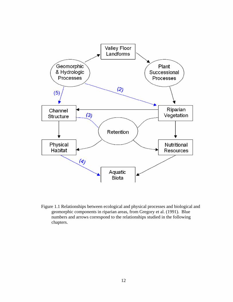
Figure 1.1 Relationships between ecological and physical processes and biological and

geomorphic components in riparian areas, from Gregory et al. (1991). Blue numbers and arrows correspond to the relationships studied in the following chapters.

12

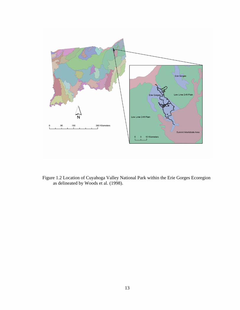
Figure 1.2 Location of Cuyahoga Valley National Park within the Erie Gorges Ecoregion as delineated by Woods et al. (1998).

13

CHAPTER 2

COMPOSITION AND STRUCTURE OF HEADWATER RIPARIAN FORESTS ACROSS WATERSHED POSITIONS IN THE ERIE GORGES ECOREGION

2.1 Introduction


ecosystem functions vital to the health and productivity of forested watersheds. Not only

do riparian areas regulate the flow of water, sediments and nutrients across system

boundaries, they contribute organic matter to the aquatic system, increase bank stability,

reduce erosion, and provide unique wildlife habitat (Gregory et al. 1991, Ilhardt et al.

2000). Additionally, riparian areas serve important roles in mitigating many of the

negative impacts of land-use on aquatic systems, as well as promoting species diversity in

watersheds, providing potential dispersal corridors for wildlife, and mitigating flood

waters (O'Laughlin & Belt 1995, Ilhardt et al. 2000, Goebel et al. 2003a). These

ecosystem services provided by riparian areas, however, often exhibit considerable year-

to-year variation, driven largely by natural ecological processes such as flooding,

drought, landslides, and wildfire that alter habitat structure and biodiversity (Naiman

1998, Ilhardt et al. 2000). Human disturbances also alter riparian forests in complex and

14

15

often synergistic ways (Gregory et al. 1991). Consequently, in order to develop

management systems that maintain and promote these varied ecosystem functions, it is

important to be able to distinguish between the natural variation of ecological processes

and their influence on riparian forest structure and function versus those changes induced

by human alterations to the watershed at multiple scales.

The conceptual basis for our approach to understanding these interrelationships

among riparian forests and multi-scale environmental factors is hierarchy theory (Allen

and Starr 1982, O’Neill et al. 1986). When applied to riparian areas, hierarchy theory

predicts that the upper levels of the hierarchy (e.g., climate, physiographic setting, and

stream valley characteristics) constrain a complex array of hydrologic and geomorphic

processes that in turn mediate the dynamics of lower hierarchical levels (e.g., landforms,

soil characteristics, and vegetation development). There are a variety of examples of the

influence of hierarchical factors on riparian plant communities from across North

America (e.g., Baker and Barnes 1998, Pabst and Spies 1998, Bendix and Hupp 2000,

Goebel et al. 2003a, Holmes et al. 2005).

Little is known, however, about the relationships among landscape factors and

riparian forests south of Lake Erie within the Erie Gorges Ecoregion (Woods et al. 1998),

a highly disturbed landscape with many streams and riparian environments that require

some form of restoration. Understanding how landscape hierarchies influence the

structure and function of riparian plant communities has immediate relevance to issues of

watershed health and riparian and aquatic habitat restoration. It is common for stream

and watershed restoration programs to focus on restoring native riparian plant

communities, but these restoration programs are rarely based on scientific understanding

of the structural characteristics of riparian plant communities, which are often influenced

by ecological processes that are framed by landscape hierarchies. Moreover, many take

a one-size-fits-all approach, as opposed to understanding how hydrologic and geomorphic

properties influence not only the composition and structure of riparian forests, but also

important ecosystem functions such as providing energy in the form of organic matter to

the aquatic ecosystem (Goebel et al. 2003b). For improved restoration and management

of these unique landscapes, the hierarchical effects of climate, glacial geology,

hydrology, landforms, soil characteristics, and vegetation structure need to be better

quantified for the ecoregion.

In this paper, we examine the influence of landscape hierarchies on the ground-flora

of riparian forests along tributary streams of the Cuyahoga River in northeastern Ohio.

We examine how the composition and structure of the ground-flora in headwater riparian

forests is related to stream geomorphology, specifically landforms and their associated

soil characteristics. Additionally, we examine how hydrological processes, specifically

watershed position, influence the composition and structure of ground-flora in headwater

riparian forests. Ultimately, it is our expectation that answers to these questions will

improve the scientific basis for ecological process-based riparian and stream restoration

for the entire Erie Gorges Ecoregion.

2.2 Study Area

We conducted our research in the Cuyahoga River watershed of northeastern

Ohio, which drains approximately 2,100 km2, within the Cuyahoga Valley National Park

(CVNP). Twenty-two miles (35.4 km) of the Cuyahoga River as well as over 190 miles

(305 km) of perennial and ephemeral streams flow through the CVNP (Figure 2.1).

16

Many of these stream valleys are dominated by diverse mature, second-growth mixed-

mesophytic forest ecosystems interspersed among a mosaic of early successional upland

ecosystems. These areas provide us with a baseline system within which to examine our

questions on the hierarchical landscape controls on riparian plant communities and their

effects on ecosystem processes.

The Erie Gorges Ecoregion, located within the Erie Ontario Drift and Lake Plain, is a

unique glaciated area characterized by steeply, dissected valleys along the Cuyahoga,

Chagrin, and Grand Rivers with rocky outcroppings and high rates of erosion (Woods et

al. 1998). Most soils on the hillslopes are characterized as deep, moderately well-drained

to well-drained soils, while soils on narrow flood plains and small terraces are dominated

by alluvial and colluvial deposits (Ritchie and Steiger 1990). Some streams have cut

down below the level of the alluvial deposits, which are now preserved as terraces along

the valley sides. Above the floodplains may be higher terraces of valley-train outwash

(White 1984).

Clear distinctions between seasons are characteristic of the climate of the study area.

Winters are typically cold and cloudy with a mean January minimum temperature of -

18.9° C while summers are moderately warm and humid with a mean July maximum

temperature of 32.8° C (Ritchie and Steiger 1990). Precipitation also varies widely with

average annual precipitation approximately 89 cm, 51cm of which normally fall from

April to September with fall typically the driest season (Ritchie and Steiger 1990).

Average annual snowfall decreases southward from Lake Erie with about 183 cm in the

extreme north to 107 cm in the south (Ritchie and Steiger 1990).

17

2.3 Methods

2.3.1 Field Methods

Our study focused on four perennial headwater streams, specifically Boston Run,

Langes Run, Riding Run, and an unnamed stream that will be referred to as Perkins Trail

Run (Figure 2.1, Table 2.1). We defined headwater streams as those draining less than

51.8 km2 (20 mi2), usually 1st, 2nd, or 3rd stream order on 1:24,000 topographic maps

following Strahler (1952). Streams were selected with second-growth riparian forests that

have been minimally disturbed by human impact. To determine how watershed position

affects riparian forest composition and structure, sampling occurred on both upper (1st or

2nd order) and lower (2nd or 3rd order) reaches of these streams in their watersheds.

Transects were established in August and September 2003 on eight sites throughout the

CVNP.

At each site, a 100-m stream reach was randomly chosen and three transects each

separated by 30-m were established perpendicular to the general stream valley

orientation. Each transect extended across the entire stream valley from streamside to the

top of the valley walls on each side of the stream channel and included floodplain,

terrace, and hillslope landforms. For each transect, circular plots (400 m2; 11.4 m radius)

were centered on each landform encountered of sufficient size (~ 12 m radius) to

characterize overstory composition and structure, which is not included in this analysis.

To ensure sampling of riparian vegetation on hillslope landforms, plots were established

10 m from the base of the slope instead of centered. Across all eight sites sampled, none

of the floodplain landforms encountered were of sufficient size for plot establishment and

18

therefore were not sampled. A total of 77 plots distributed among four landform types

(upper terraces, upper hillslopes, lower terraces, lower hillslopes) were sampled.

Ground-flora vegetation (vascular plants less than 1 m tall, including woody species)

was sampled by visually estimating percent cover of all species in three 1-m2 quadrats,

each located 5 m from the plot center at 0°, 120°, and 240° (Figure 2.2). Within each

quadrat, the total cover of each species was estimated and placed into the appropriate

cover class (<1 percent, 1-5 percent, 6-10 percent, 11-20 percent, 21-40 percent, 41-70

percent, and 71-100 percent). Portions of plants that overhung the plot boundary but

were rooted outside of the plot were not included in cover estimates. Bare ground (BG)

was also estimated within each 1 m2 quadrat. Overstory cover over the quadrat was

measured at the center of each 1-m2 quadrat using a spherical densiometer held at breast

height (1.4m) following methods described in Lemmon (1956). Finally, we estimated

total ground-flora biomass by clipping all of the live and dead vegetation within a 1-m2

quadrat located at the center of each 400 m2 plot. Clipped vegetation was bagged and

transported to the laboratory where it was sorted by functional lifeform guild (annual

forb, perennial forb, graminoid, pteridophyte, woody vine, woody shrub, and woody tree

seedling), dried at 70°C for 48 h, and then weighed. Nomenclature and lifeform

categories follow USDA PLANTS database (2007).

Characteristics of the upper soil surface were analyzed from soil samples collected

using a Giddings® soil corer to a depth of 30 cm at the approximate center of each 400-

m2 plot. Soil samples were transported to the laboratory for physical and chemical

analyses. USDA Particle Size fractions, sand (particle size <2000-50µm), silt (particle

size <50µm– 2µm), and clay (particle size < 2µm) were determined after air drying using

19

the hydrometer method (Gee and Bauder 1986). Percent soil organic matter (% OM) was

determined by loss on ignition (Storer 1984) and pH was measured using Corning®

Model 440 pH meter in a soil and water (1:1) slurry.

In terms of stream valley geomorphology, channel flood-prone width was measured

for each transect and averaged across the three transects to characterize the hydrology of

each site. Flood-prone width was measured by determining bankfull height, multiplying

by two, and extending this height level across the valley where its span was measured

across the valley cross-section.

2.3.2 Data Analysis

Ground-flora species diversity per m2 was calculated in terms of richness (S; number

of species per plot), Shannon’s Diversity Index (H’; H’= S*ln(ri) where ri is the relative

importance of the ith species; Ludwig and Reynolds 1988), and evenness (E; E = H’ / ln

S). Mann-Whitney U-tests were used to test for mean differences in species diversity

between terrace and hillslope landforms across watershed positions. Alpha equal to 0.10

was used to indicate statistical significance for all analyses. Species area curves and

jack-knife estimates of species were calculated for the four landform types: upper and

lower stream reach terraces and upper and lower stream reach hillslopes.

To diminish the influence of rare species on the results, only those species occurring

on greater than 5 percent of the sample plots were used in the remaining analyses.

Multi-response permutation procedure (MRPP) in PC-ORD version 5 (McCune and

Mefford 2006) was used to test the hypothesis that the species compositions of the

landform types at each watershed position were not different. MRPP was performed on

ground-flora cover using a natural weighting factor and Sorenson distance as

20

recommended by Mielke (1984) and McCune and Mefford (1995), respectively. To

determine which ground-flora species were characteristic of each landform type, we used

Indicator Analysis in PC-ORD (McCune and Mefford 1995).

We characterized ground-flora structure (i.e. the organization of species into growth

form groups, Kimmins 1987) using biomass summarized by functional growth form

guilds for the four landform types. These growth forms included woody seedlings,

woody shrubs, woody vines, forbs, pteridophytes, and graminoids. Differences in mean

total biomass between terrace and hillslope landforms on both upper and lower stream

reaches were tested with Mann-Whitney U-tests. MRPP was used to test the hypothesis

that the functional growth form guild structure was not different between the landform

types at each watershed position. Finally, Indicator Analysis was used to determine if

certain functional growth form guilds were characteristic of landform types.

Soil particle size fractions (percent sand, silt, and clay), organic matter content (OM),

and pH, as well as bare ground and overstory cover were summarized by landform type

for each watershed position. Differences between landform types were tested with

Mann-Whitney U-tests for each watershed position.

To examine the relationships between the ground-flora composition and

environmental factors, canonical correspondence analysis (CCA) was performed using

CANOCO software (ter Braak and Šmilauer 1997). Canonical correspondence analysis

is an eigenvector ordination technique that provides a multivariate direct gradient

analysis that helps to visualize patterns of community variation and the influence of

environmental factors on species distribution (ter Braak and Prentice 1988). Only

ground-flora species that had significant indicator values (P< 0.10) were included in the

21

CCA. Environmental factors used to constrain and explain the variation in ground-flora

composition included bare ground, overstory cover, soil pH and OM, percent sand, silt,

and clay, and flood-prone width. The resulting triplot allows individual species and plots

to be related to all major environmental factors (Kent and Coker 1992) with plots and

species represented by points, and environmental variables represented by vector arrows

(ter Braak 1986), the lengths of which are determined by the importance of the

environmental variable (ter Braak 1986).

2.4 Results

Ground-flora species composition varied between terrace and hillslope landforms

and watershed position. Along upper stream reaches, terraces had lower species richness

than hillslopes (W= 129.0, P= 0.09), while Shannon Diversity Index values did not differ

between landform types (W=182.5, P=0.95; Table 2.2). Along lower stream reaches,

species richness and Shannon Diversity Indexes were not significantly different between

terraces and hillslopes (W=330.5, P=0.83; W= 372.0, P= 0.14, respectively), but terraces

had more evenly distributed communities than hillslopes (W= 476.0, P<0.01). Species

area curves for the four landform types show increasing species richness from upper to

lower watershed positions for terraces, while more species were encountered per quadrat

sampled on upper hillslopes than lower hillslopes (Figure 2.3). The results of MRPP

indicate community composition is significantly different between landform types across

both upper and lower watershed positions (upper reaches R=0.0135, P<0.01; lower

reaches R=0.0165, P< 0.01). Indicator Analysis reveals terraces along upper stream

reaches are characterized by Geum spp., Laportea canadensis, Lindera benzoin,

Potentilla simplex, and Tiarella cordifolia (Table 2.3). Hillslopes along upper stream

22

reaches are characterized by Aster spp. and Viburnum acerifolium. Terraces along lower

stream reaches are characterized by Blephilia hirstuta, Crataegus spp., Geum spp., Rosa

multiflora, Sanicula marilandica, Smilax rotundifolia, Tovara virginiana, Verbesina

alternifolia, and Viola spp.. Hillslopes along lower stream reaches are characterized by

Aster spp., Fraxinus americana, Hamamelis virginiana, Sanguinaria canadensis, Senecio

obovatus, and Solidago spp. (Table 2.3).

Structure of ground-flora communities varied widely between landform types at

each watershed position resulting in no significant differences in mean biomass values

(Table 2.4). Along upper stream reaches, pteridophytes were found primarily on

hillslopes with only one plant recorded on the terraces. MRPP indicated that functional

growth form guild structure was not significantly different between landforms along

upper stream reaches (R= -0.0039, P= 0.53), however structure was significantly

different between landforms along lower stream reaches (R= 0.0175, P= 0.09). Indicator

analysis detected no significant indicator functional growth form guilds (P<0.10) for

landforms along upper stream reaches (Table 2.4), however, along lower stream reaches,

forbs and pteridophytes are characteristic of terraces and hillslopes, respectively (P= 0.04

for both, Table 2.4).

Soil characteristics followed similar differentiations between landforms at both

upper and lower watershed positions (Table 2.5). Along upper reach streams, terraces

had higher mean sand content and pH (W= 255.5, P= 0.01; W= 236.0, P= 0.06,

respectively) than hillslopes, which had higher mean clay and silt contents (W= 124.0,

P<0.01; W= 80.5, P= 0.06, respectively). Similarly along lower reach streams, terraces

had higher mean sand contents (W= 461.5, P< 0.001) while hillslopes had higher mean

23

clay and silt content (W= 178.0, P= 0.03; W= 252.5, P<0.001 respectively). Percent

overstory cover and bare ground were not significantly different between landforms or

across watershed positions (upper reaches W=110.0, P=0.94; W=99.0, P=0.55,

respectively; lower reaches W=322.0, P=0.99; W=319.5, P=0.93, respectively, Table

2.5).

CCA constrained the spatial distribution of indicator species of landforms across

upper and lower watershed positions (from Table 2.3) for 67 sample plots by the eight

environmental factors (eigenvalues are 0.237 for the first axis and 0.115 for the second

axis). The total inertia for the analysis was 3.234 while the sum of all canonical

eigenvalues was 0.641. Axis 1 explained 7.3% of the variation in the species matrix and

Axis 2 an additional 3.7%. The Monte Carlo permutation test for significance of the first

canonical axis was significant (F= 4.590, P= 0.001) as well as the test for significance of

all canonical axes (F= 1.791, P= 0.001). A triplot of the linear combinations of species

and environmental variables in biplot scaling reveals separation by both landform and

watershed position (Figure 2.4). Hillslopes along upper stream reaches most clearly

separate from terraces along lower stream reaches. Hillslopes along upper reaches are

positively associated with increasing overstory cover while terraces along lower slopes

are positively associated with increasing pH and channel floodprone widths. Terraces

along upper stream reaches and hillslopes along lower stream reaches are ordinated

together in the center of the triplot indicating strong similarity (Figure 2.4). However,

Blephilia hirstuta, Geum spp., Sanicula marilandica, and Verbesina alternifolia are

positively associated with increased floodprone width, percent sand, and terraces along

lower stream reaches, while Laportea canadensis is positively associated with increased

24

pH and terraces along lower stream reaches. Senecio obovatus, Viburnum acerifolium,

Aster spp., and Lindera benzoin are positively associated with percent silt, sand, and bare

ground (BG) as well as hillslope landforms. Potentilla simplex, Fraxinus americana,

Crategeus spp., and Sanguinaria canadensis are positively associated with increased

overstory cover and hillslope landforms. The remaining indicator species are ordinated

in the center of the triplot and are not strongly associated with any environmental factors,

but they may be associated with the upper stream reach terraces and lower stream reach

hillslopes that are also ordinated in the center (Figure 2.4).

2.5 Discussion

Based upon research primarily conducted in the Pacific Northwest, riparian areas

have been shown to be ecotones with high species richness in comparison to the adjacent

upland forest ecosystems (Naiman et al. 1993, Richardson and Danehy 2007). However,

research in other regions has demonstrated that high riparian species richness is only

apparent at a multiple reach or watershed scale, as opposed to the scale of single stream

reaches (Goebel et al. 2003a). A global literature survey of riparian species richness

indicated that the alpha species richness of riparian areas is not necessarily higher than

the adjacent uplands, but that the suite of species is different contributing to beta species

richness (Sabo et al. 2005). Our study of ground-flora communities along forested

headwater riparian areas in the Erie Gorges Ecoregion indicated that species richness

increased further downstream in the watershed, supporting the conclusion of Goebel et al.

(2003a) and lending credence to the idea that riparian species richness peaks in the center

of the watershed (Dunn et al. 2006) .

25

We also observed differences transversely across the stream valley in both the

species composition and the structure of ground-flora communities. Across watershed

positions, species composition was different between terrace and hillslope landforms.

Similar differences in vegetation composition between landforms were also found by

Goebel et al. (2006) and Hagan et al. (2006). While species composition was different

between landforms across watershed positions, differences in structure of ground-flora

communities was only evident at the downstream watershed position. CCA also showed

that upstream terraces were spatially similar to downstream hillslopes, which may reflect

structural as well as compositional similarities. This may reflect the change in hydrology

associated with larger stream channels and broader landforms that develop with increased

flow downstream. Upstream landforms tend to be narrower with full overstory cover

restricting the growth of forbs, which dominate the terrace landforms downstream.

Interestingly, along these headwater stream riparian areas differences in soil

characteristics, percent bare ground, and mean percent overstory cover between

landforms do not change across watershed positions. Terraces upstream and downstream

have higher percent sand and pH while hillslopes upstream and downstream have higher

percent clay, silt, bare ground, and overstory cover. While these environmental

characteristics do not change, the composition and structure of the ground-flora

communities exhibit differences between watershed positions. Hydrology does change

across watershed positions and may be a primary driver of differences in the ground-flora

communities, which supports the idea that hierarchy theory drives ecological processes

within riparian areas (Poole 2002, Leyer 2005, Goebel et al. 2006).

26

Research on headwater streams has increased in recent years with emphasis

placed on the large extent of these streams within a watershed network (Meyer and

Wallace 2000, Hansen 2001), as well as their differences in structure and function as

compared to larger streams and rivers (Moore and Richardson 2003, Richardson et al.

2005, Richardson and Danehy 2007). Our research indicates that even within headwater

streams there are differences longitudinally, i.e. watershed positions, as well as

transversely across stream valleys, i.e. landforms, in both composition and structure of

headwater riparian forest ground-flora communities. Restoration and management of

these systems on the landscape should incorporate these differences to mimic the natural

variation created by hierarchical ecological processes. One size does not fit all riparian

areas and variation should be incorporated in managed systems to reflect the natural

longitudinal and transverse differences created by geomorphology in these unique

ecotones.

2.6 References

Allen, T.F.H., and T.B. Starr. 1982. Hierarchy: Perspectives for Ecological Complexity. University of Chicago Press, Chicago, IL, pp.310.

Baker, M.E. and B.V. Barnes. 1998. Landscape ecosystem diversity of river floodplains in northwestern lower Michigan, USA. Canadian Journal of Forest Research 28:1405-1418.

Bendix, J. and C.R. Hupp. 2000. Hydrological and geomorphical impacts on riparian plant communities. Hydrological Processes 14: 2977-2990.

Dunn, R.R., R.K. Colwell, and C. Nilsson. 2006. The river domain: why are there more species halfway up the river? Ecography 29: 251-259.

27

Gee, G.W. and J.W. Bauder. 1986. Particle size analysis. pp. 383-411 In: Methods of Soil Analysis, Part 1 Physical and Mineralogical methods, 2nd edition. American Society of Agronomy and Soil Science Society of America: Madison, WI

Goebel, P.C., B.J. Palik, and K.S. Pregitzer. 2003a. Plant diversity contributions of riparian areas in watersheds of the northern Lake States, USA. Ecological Applications 13:1595-1609.

Goebel, P.C., K.S. Pregitzer, and B.J. Palik. 2003b. Geomorphic influences on large wood dam loadings, particulate organic matter and dissolved organic matter in an old-growth northern hardwood watershed. Journal of Freshwater Ecology 18:479-490.

Goebel, P.C., K.S. Pregitzer, and B.J. Palik. 2006. Landscape hierarchies influence ground-flora communities in Wisconsin, USA. Forest Ecology and Management 230: 43-54.


Hagan, J.M., S .Pealer, and A.A. Whitman. 2006. Do small headwater streams have a riparian zone defined by plant communities? Canadian Journal of Forest Research 36: 2131-2140.


Holmes, K.L., P.C. Goebel, D.M. Hix, C.E. Dygert, and M.E. Semko-Duncan. 2005. Ground-flora composition and structure of floodplain and upland landforms of an old-growth headwater forest in north-central Ohio. Journal of the Torrey Botanical Society 132: 62-71.

Ilhardt, B.L., E.S. Verry, and B.J. Palik. 2000. Defining riparian areas. pp. 23-42 In: E.S. Verry, J.W. Hornbeck, and C.A. Dolloff, editors. Riparian Management in Forests of the Continental Eastern United States. Lewis Publishers, New York, pp. 402.

Kent, M. and P. Coker. 1992. Basic statistical analysis of vegetation and environmental data. In: Vegetation Description and Analysis, John Wiley and Sons, New York, pp. 112-161.

28

Kimmins, J.P. 1987. Forest Ecology. Macmillan, New York, pp.531.

Lemmon, P. 1956. A spherical densiometer for estimating forest overstory density. Forest Science 2, 314-320.

Leyer, I. 2005. Predicting plant species’ responses to river regulation: the role of water level fluctuations. Journal of Applied Ecology 42: 239-250.

Lugwig, J.A. and J.F. Reynolds. 1988. Statistical Ecology: A Primer on Methods and Computing. John Wiley and Sons, New York, pp. 337.

McCune, B. and M.J. Mefford. 2006. PC-ORD: multivariate analysis of ecological data. Version 5.0. MjM Software Design, Gleneden Beach, OR.

Meyer, J.L. and J.B. Wallace. 2000. Lost linkages and lotic ecology: rediscovering small streams. pp. 295-317 In M.C. Press, N.J. Huntly, and S.A. Levin editors, Ecology: An achievement and challenge. Blackwell Science, Ames, IA, pp. 406.

Mielke, P.W., 1984. Handbook of statistics, Vol. 4: Nonparametric methods. North-Holland, Amsterdam, pp. 813-830.

Moore, R.D. and J.S. Richardson. 2003. Progress towards understanding the structure, function, and ecological significance of small stream channels and their riparian zones. Canadian Journal of Forest Research 33: 1349-1351.

Naiman, R.J. 1998. Riparian forests. pp. 289-323 In: R.J. Naiman and R.E. Bilby, editors, River ecology and management: Lessons from the Pacific Coastal Ecoregion Springer-Verlag, New York, pp.705.

Naiman, R.J., H. Décamps, and M. Pollock. 1993. The role of riparian corridors in maintaining regional biodiversity. Ecological Applications 3(2): 209-212.



29

Pabst, R. J. and T. A. Spies. 1998. Distribution of herbs and shrubs in relation to landform and canopy cover in riparian forests of coastal Oregon. Canadian Journal of Botany 76: 298-315.

Poole, G.C. 2002. Fluvial landscape ecology: addressing uniqueness within the river discontinuum. Freshwater Biology 47: 641-660.

Richardson, J.S. and R.J. Danehy. 2007. A synthesis of the ecology of headwater streams and their riparian zones in temperate forests. Forest Science 53(2): 131-147.

Richardson, J.S., R.J. Naiman, F.J. Swanson, and D.E. Hibbs. 2005. Riparian communities associated with Pacific Northwest headwater streams: assemblages, processes, and uniqueness. Journal of the American Water Resources Association 41(4): 935-947.

Ritchie, A. and J.R. Steiger. 1990. Soil Survey of Summit County, Ohio. United States Department of Agriculture, Soil Conservation Service.

Sabo, J.L., R. Sponseller, M. Dixon, K. Gade, T. Harms, J. Heffernan, A. Jani, G. Katz, C. Soykan, J. Watts, and J. Welter. 2005. Riparian zones increase regional species richness by harboring different, not more, species. Ecology 86(1): 56-62.

Strahler, A. N. 1952. Dynamic basis of geomorphology. Bulletin of the Geological Society of America 83: 923- 938.

Storer, D.A., 1984. A simple high sample volume ashing procedure for determining soil organic matter. Communications in Soil Science and Plant Analysis 15: 759-772.

ter Braak, C.J.F., 1986. Canonical correspondence analysis: a new eigenvector technique for multivariate direct gradient analysis. Ecology 67: 1167-1179.

ter Braak, C.J.F. and I.C. Prentice. 1988. A theory of gradient analysis. Advances in Ecological Research 18: 271-317.

ter Braak, C.J.F. and P. Šmilauer. 1997. Canoco for Windows version 4.02. Centre for Biometry. Wageningen, Netherlands.

30

31

USDA, NRCS. 2007. The PLANTS Database (http://plants.usda.gov). National Plant Data Center, Baton Rouge, LA 70874-4490 USA.

White, G.W. 1984. Glacial geology of Summit County, Ohio. Ohio Department of Natural Resources, Division of Geological Survey: Columbus.


Zar, J.H., 1974. Biostatistical Analysis. Prentice-Hall, Inc., Englewood Cliffs, N.J., 620 pp.

http://plants.usda.gov/

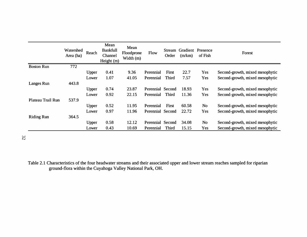
Watershed Area (ha) Reach

Mean Bankfull Channel

Height (m)

Mean Floodprone Width (m)

Flow Stream Order

Gradient (m/km)

Presence of Fish Forest

Boston Run 772Upper 0.41 9.36 Perennial First 22.7 Yes Second-growth, mixed mesophyticLower 1.07 41.05 Perennial Third 7.57 Yes Second-growth, mixed mesophytic

Langes Run 443.8Upper 0.74 23.87 Perennial Second 18.93 Yes Second-growth, mixed mesophyticLower 0.92 22.15 Perennial Third 11.36 Yes Second-growth, mixed mesophytic

Plateau Trail Run 537.9Upper 0.52 11.95 Perennial First 60.58 No Second-growth, mixed mesophyticLower 0.97 11.96 Perennial Second 22.72 Yes Second-growth, mixed mesophytic

Riding Run 364.5Upper 0.58 12.12 Perennial Second 34.08 No Second-growth, mixed mesophyticLower 0.43 10.69 Perennial Third 15.15 Yes Second-growth, mixed mesophytic

Table 2.1 Characteristics of the four headwater streams and their associated upper and lower stream reaches sampled for riparian ground-flora within the Cuyahoga Valley National Park, OH.

Table 2.1 Characteristics of the four headwater streams and their associated upper and lower stream reaches sampled for riparian ground-flora within the Cuyahoga Valley National Park, OH.

32



Height (m)


Flow Stream Order

Gradient (m/km)






32

32

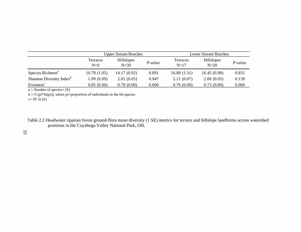
P-value P-value

Species Richnessa 10.78 (1.05) 14.17 (0.92) 0.091 16.88 (1.31) 16.45 (0.98) 0.831Shannon Diversity Indexb 1.99 (0.09) 2.01 (0.05) 0.947 2.11 (0.07) 2.00 (0.05) 0.139Evennessc 0.85 (0.00) 0.78 (0.00) 0.000 0.76 (0.00) 0.73 (0.00) 0.000a = Number of species= (S)b =-S (pi*ln(pi)), where pi=proportion of individuals in the ith speciesc= H'/ ln (S)

Upper Stream Reaches Lower Stream ReachesTerraces

N=9Hillslopes

N=30Terraces

N=17Hillslopes

N=20

Table 2.2 Headwater riparian forest ground-flora mean diversity (1 SE) metrics for terrace and hillslope landforms across watershed positions in the Cuyahoga Valley National Park, OH. 33

33

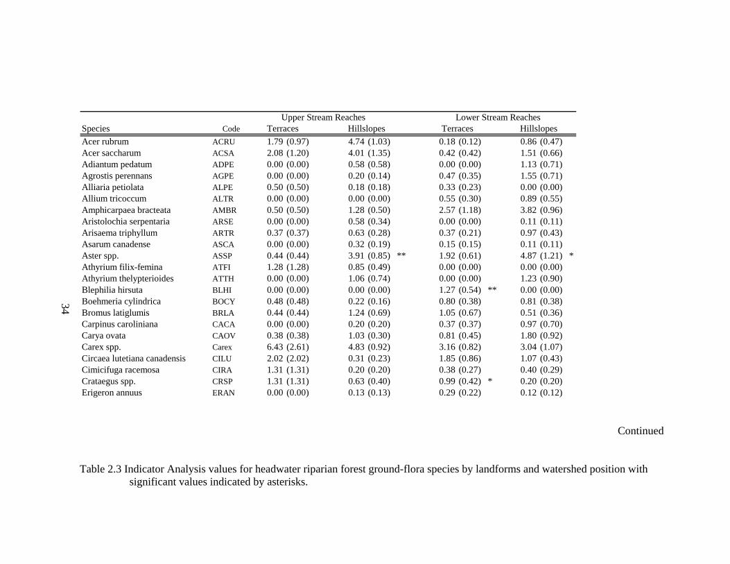
Species CodeAcer rubrum ACRU 1.79 (0.97) 4.74 (1.03) 0.18 (0.12) 0.86 (0.47)Acer saccharum ACSA 2.08 (1.20) 4.01 (1.35) 0.42 (0.42) 1.51 (0.66)Adiantum pedatum ADPE 0.00 (0.00) 0.58 (0.58) 0.00 (0.00) 1.13 (0.71)Agrostis perennans AGPE 0.00 (0.00) 0.20 (0.14) 0.47 (0.35) 1.55 (0.71)Alliaria petiolata ALPE 0.50 (0.50) 0.18 (0.18) 0.33 (0.23) 0.00 (0.00)Allium tricoccum ALTR 0.00 (0.00) 0.00 (0.00) 0.55 (0.30) 0.89 (0.55)Amphicarpaea bracteata AMBR 0.50 (0.50) 1.28 (0.50) 2.57 (1.18) 3.82 (0.96)Aristolochia serpentaria ARSE 0.00 (0.00) 0.58 (0.34) 0.00 (0.00) 0.11 (0.11)Arisaema triphyllum ARTR 0.37 (0.37) 0.63 (0.28) 0.37 (0.21) 0.97 (0.43)Asarum canadense ASCA 0.00 (0.00) 0.32 (0.19) 0.15 (0.15) 0.11 (0.11)Aster spp. ASSP 0.44 (0.44) 3.91 (0.85) ** 1.92 (0.61) 4.87 (1.21) *Athyrium filix-femina ATFI 1.28 (1.28) 0.85 (0.49) 0.00 (0.00) 0.00 (0.00)Athyrium thelypterioides ATTH 0.00 (0.00) 1.06 (0.74) 0.00 (0.00) 1.23 (0.90)Blephilia hirsuta BLHI 0.00 (0.00) 0.00 (0.00) 1.27 (0.54) ** 0.00 (0.00)Boehmeria cylindrica BOCY 0.48 (0.48) 0.22 (0.16) 0.80 (0.38) 0.81 (0.38)Bromus latiglumis BRLA 0.44 (0.44) 1.24 (0.69) 1.05 (0.67) 0.51 (0.36)Carpinus caroliniana CACA 0.00 (0.00) 0.20 (0.20) 0.37 (0.37) 0.97 (0.70)Carya ovata CAOV 0.38 (0.38) 1.03 (0.30) 0.81 (0.45) 1.80 (0.92)Carex spp. Carex 6.43 (2.61) 4.83 (0.92) 3.16 (0.82) 3.04 (1.07)Circaea lutetiana canadensis CILU 2.02 (2.02) 0.31 (0.23) 1.85 (0.86) 1.07 (0.43)Cimicifuga racemosa CIRA 1.31 (1.31) 0.20 (0.20) 0.38 (0.27) 0.40 (0.29)Crataegus spp. CRSP 1.31 (1.31) 0.63 (0.40) 0.99 (0.42) * 0.20 (0.20)Erigeron annuus ERAN 0.00 (0.00) 0.13 (0.13) 0.29 (0.22) 0.12 (0.12)

Upper Stream Reaches Lower Stream ReachesTerraces Hillslopes Terraces Hillslopes

34

Continued Table 2.3 Indicator Analysis values for headwater riparian forest ground-flora species by landforms and watershed position with

significant values indicated by asterisks. 34

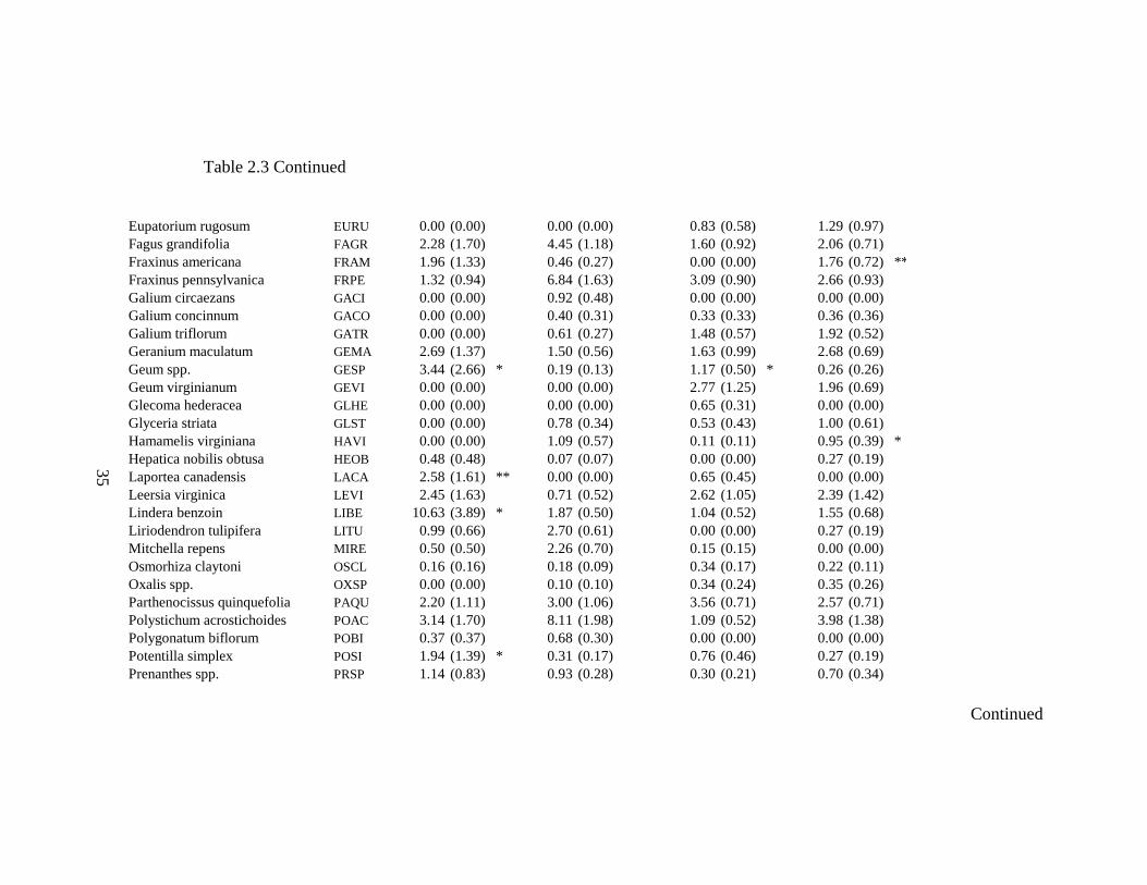
Table 2.3 Continued Eupatorium rugosum EURU 0.00 (0.00) 0.00 (0.00) 0.83 (0.58) 1.29 (0.97)Fagus grandifolia FAGR 2.28 (1.70) 4.45 (1.18) 1.60 (0.92) 2.06 (0.71)Fraxinus americana FRAM 1.96 (1.33) 0.46 (0.27) 0.00 (0.00) 1.76 (0.72) **Fraxinus pennsylvanica FRPE 1.32 (0.94) 6.84 (1.63) 3.09 (0.90) 2.66 (0.93)Galium circaezans GACI 0.00 (0.00) 0.92 (0.48) 0.00 (0.00) 0.00 (0.00)Galium concinnum GACO 0.00 (0.00) 0.40 (0.31) 0.33 (0.33) 0.36 (0.36)Galium triflorum GATR 0.00 (0.00) 0.61 (0.27) 1.48 (0.57) 1.92 (0.52)Geranium maculatum GEMA 2.69 (1.37) 1.50 (0.56) 1.63 (0.99) 2.68 (0.69)Geum spp. GESP 3.44 (2.66) * 0.19 (0.13) 1.17 (0.50) * 0.26 (0.26)Geum virginianum GEVI 0.00 (0.00) 0.00 (0.00) 2.77 (1.25) 1.96 (0.69)Glecoma hederacea GLHE 0.00 (0.00) 0.00 (0.00) 0.65 (0.31) 0.00 (0.00)Glyceria striata GLST 0.00 (0.00) 0.78 (0.34) 0.53 (0.43) 1.00 (0.61)Hamamelis virginiana HAVI 0.00 (0.00) 1.09 (0.57) 0.11 (0.11) 0.95 (0.39) *Hepatica nobilis obtusa HEOB 0.48 (0.48) 0.07 (0.07) 0.00 (0.00) 0.27 (0.19)Laportea canadensis LACA 2.58 (1.61) ** 0.00 (0.00) 0.65 (0.45) 0.00 (0.00)Leersia virginica LEVI 2.45 (1.63) 0.71 (0.52) 2.62 (1.05) 2.39 (1.42)Lindera benzoin LIBE 10.63 (3.89) * 1.87 (0.50) 1.04 (0.52) 1.55 (0.68)Liriodendron tulipifera LITU 0.99 (0.66) 2.70 (0.61) 0.00 (0.00) 0.27 (0.19)Mitchella repens MIRE 0.50 (0.50) 2.26 (0.70) 0.15 (0.15) 0.00 (0.00)Osmorhiza claytoni OSCL 0.16 (0.16) 0.18 (0.09) 0.34 (0.17) 0.22 (0.11)Oxalis spp. OXSP 0.00 (0.00) 0.10 (0.10) 0.34 (0.24) 0.35 (0.26)Parthenocissus quinquefolia PAQU 2.20 (1.11) 3.00 (1.06) 3.56 (0.71) 2.57 (0.71)Polystichum acrostichoides POAC 3.14 (1.70) 8.11 (1.98) 1.09 (0.52) 3.98 (1.38)Polygonatum biflorum POBI 0.37 (0.37) 0.68 (0.30) 0.00 (0.00) 0.00 (0.00)Potentilla simplex POSI 1.94 (1.39) * 0.31 (0.17) 0.76 (0.46) 0.27 (0.19)Prenanthes spp. PRSP 1.14 (0.83) 0.93 (0.28) 0.30 (0.21) 0.70 (0.34)

35

Continued

35

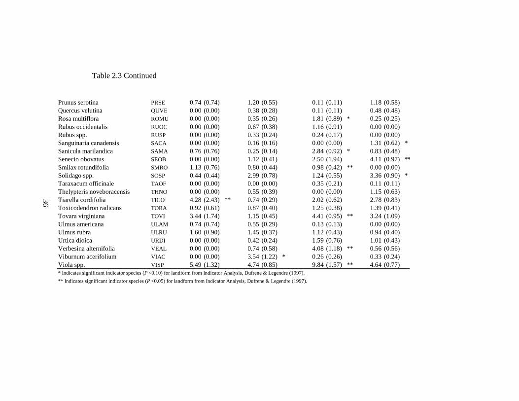
Table 2.3 Continued Prunus serotina PRSE 0.74 (0.74) 1.20 (0.55) 0.11 (0.11) 1.18 (0.58)Quercus velutina QUVE 0.00 (0.00) 0.38 (0.28) 0.11 (0.11) 0.48 (0.48)Rosa multiflora ROMU 0.00 (0.00) 0.35 (0.26) 1.81 (0.89) * 0.25 (0.25)Rubus occidentalis RUOC 0.00 (0.00) 0.67 (0.38) 1.16 (0.91) 0.00 (0.00)Rubus spp. RUSP 0.00 (0.00) 0.33 (0.24) 0.24 (0.17) 0.00 (0.00)Sanguinaria canadensis SACA 0.00 (0.00) 0.16 (0.16) 0.00 (0.00) 1.31 (0.62) *Sanicula marilandica SAMA 0.76 (0.76) 0.25 (0.14) 2.84 (0.92) * 0.83 (0.48)Senecio obovatus SEOB 0.00 (0.00) 1.12 (0.41) 2.50 (1.94) 4.11 (0.97) **Smilax rotundifolia SMRO 1.13 (0.76) 0.80 (0.44) 0.98 (0.42) ** 0.00 (0.00)Solidago spp. SOSP 0.44 (0.44) 2.99 (0.78) 1.24 (0.55) 3.36 (0.90) *Taraxacum officinale TAOF 0.00 (0.00) 0.00 (0.00) 0.35 (0.21) 0.11 (0.11)Thelypteris noveboracensis THNO 0.00 (0.00) 0.55 (0.39) 0.00 (0.00) 1.15 (0.63)Tiarella cordifolia TICO 4.28 (2.43) ** 0.74 (0.29) 2.02 (0.62) 2.78 (0.83)Toxicodendron radicans TORA 0.92 (0.61) 0.87 (0.40) 1.25 (0.38) 1.39 (0.41)Tovara virginiana TOVI 3.44 (1.74) 1.15 (0.45) 4.41 (0.95) ** 3.24 (1.09)Ulmus americana ULAM 0.74 (0.74) 0.55 (0.29) 0.13 (0.13) 0.00 (0.00)Ulmus rubra ULRU 1.60 (0.90) 1.45 (0.37) 1.12 (0.43) 0.94 (0.40)Urtica dioica URDI 0.00 (0.00) 0.42 (0.24) 1.59 (0.76) 1.01 (0.43)Verbesina alternifolia VEAL 0.00 (0.00) 0.74 (0.58) 4.08 (1.18) ** 0.56 (0.56)Viburnum acerifolium VIAC 0.00 (0.00) 3.54 (1.22) * 0.26 (0.26) 0.33 (0.24)Viola spp. VISP 5.49 (1.32) 4.74 (0.85) 9.84 (1.57) ** 4.64 (0.77)* Indicates significant indicator species (P <0.10) for landform from Indicator Analysis, Dufrene & Legendre (1997). ** Indicates significant indicator species (P <0.05) for landform from Indicator Analysis, Dufrene & Legendre (1997).

36

36

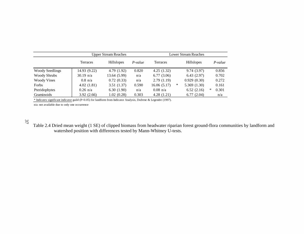
Table 2.4 Dried mean weight (1 SE) of clipped biomass from headwater riparian forest ground-flora communities by landform and watershed position with differences tested by Mann-Whitney U-tests.

37

P-value P-value

Woody Seedlings 14.93 (9.22) 4.79 (1.92) 0.820 4.25 (1.32) 9.74 (3.97) 0.856Woody Shrubs 30.19 n/a 13.64 (5.99) n/a 6.77 (3.06) 6.43 (2.97) 0.702Woody Vines 0.8 n/a 0.72 (0.33) n/a 2.79 (1.19) 0.929 (0.30) 0.272Forbs 4.02 (1.81) 3.51 (1.37) 0.590 16.06 (5.17) * 5.369 (1.30) 0.161Pteridophytes 0.26 n/a 6.30 (1.90) n/a 0.08 n/a 6.52 (2.16) * 0.301Graminoids 3.92 (2.66) 1.02 (0.28) 0.303 4.28 (1.21) 6.77 (2.04) n/a* Indicates significant indicator guild (P<0.05) for landform from Indicator Analysis, Dufrene & Legendre (1997). n/a: not available due to only one occurrence

Upper Stream Reaches Lower Stream Reaches

Terraces Hillslopes Terraces Hillslopes

37

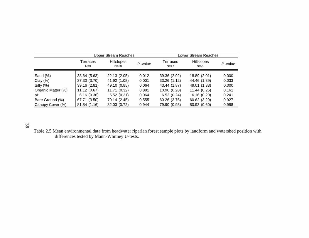
P -value P -value

Sand (%) 38.64 (5.63) 22.13 (2.05) 0.012 39.36 (2.92) 18.89 (2.01) 0.000Clay (%) 37.30 (3.70) 41.92 (1.08) 0.001 33.26 (1.12) 44.46 (1.39) 0.033Silty (%) 39.16 (2.81) 49.10 (0.85) 0.064 43.44 (1.87) 49.01 (1.33) 0.000Organic Matter (%) 11.12 (0.67) 11.71 (0.32) 0.881 10.90 (0.28) 11.44 (0.26) 0.161pH 6.16 (0.36) 5.52 (0.21) 0.064 6.52 (0.24) 6.16 (0.20) 0.241Bare Ground (%) 67.71 (3.50) 70.14 (2.45) 0.555 60.26 (3.76) 60.62 (3.29) 0.927Canopy Cover (%) 81.84 (1.16) 82.03 (0.72) 0.944 79.90 (0.93) 80.93 (0.60) 0.988

Upper Stream Reaches Lower Stream ReachesTerraces

N=9Hillslopes

N=30Terraces

N=17Hillslopes

N=20

38

Table 2.5 Mean environmental data from headwater riparian forest sample plots by landform and watershed position with differences tested by Mann-Whitney U-tests.

38

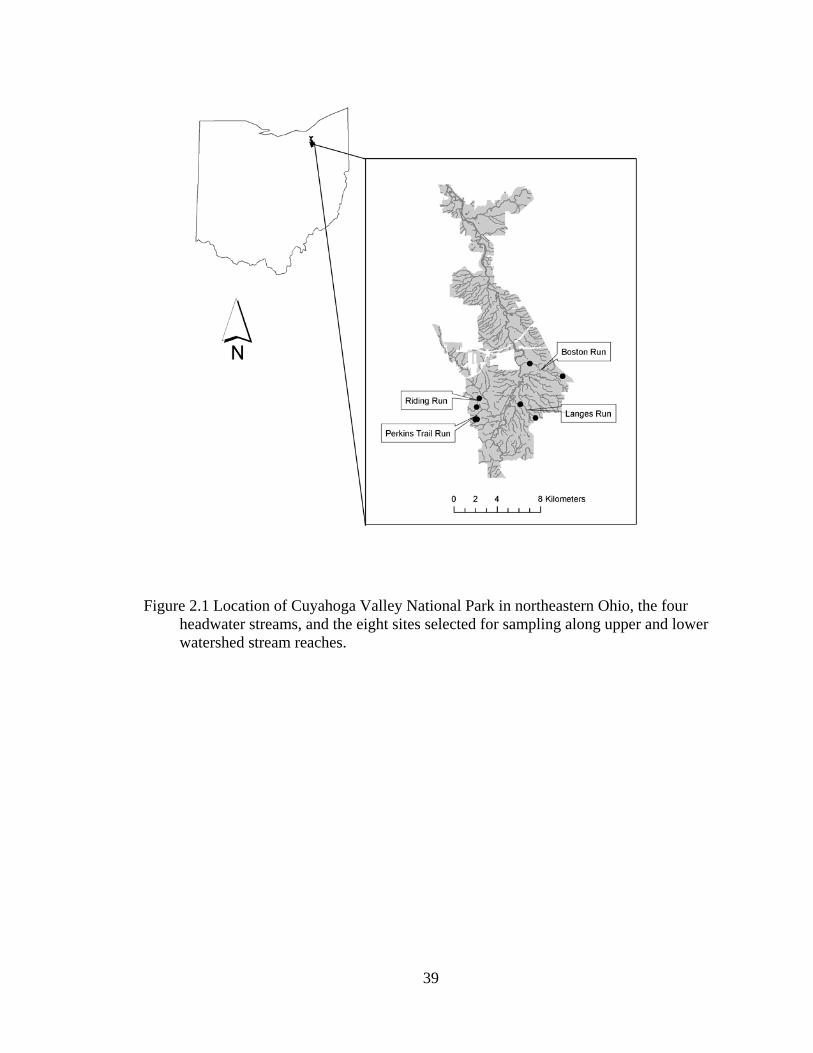
Figure 2.1 Location of Cuyahoga Valley National Park in northeastern Ohio, the four headwater streams, and the eight sites selected for sampling along upper and lower watershed stream reaches.

39

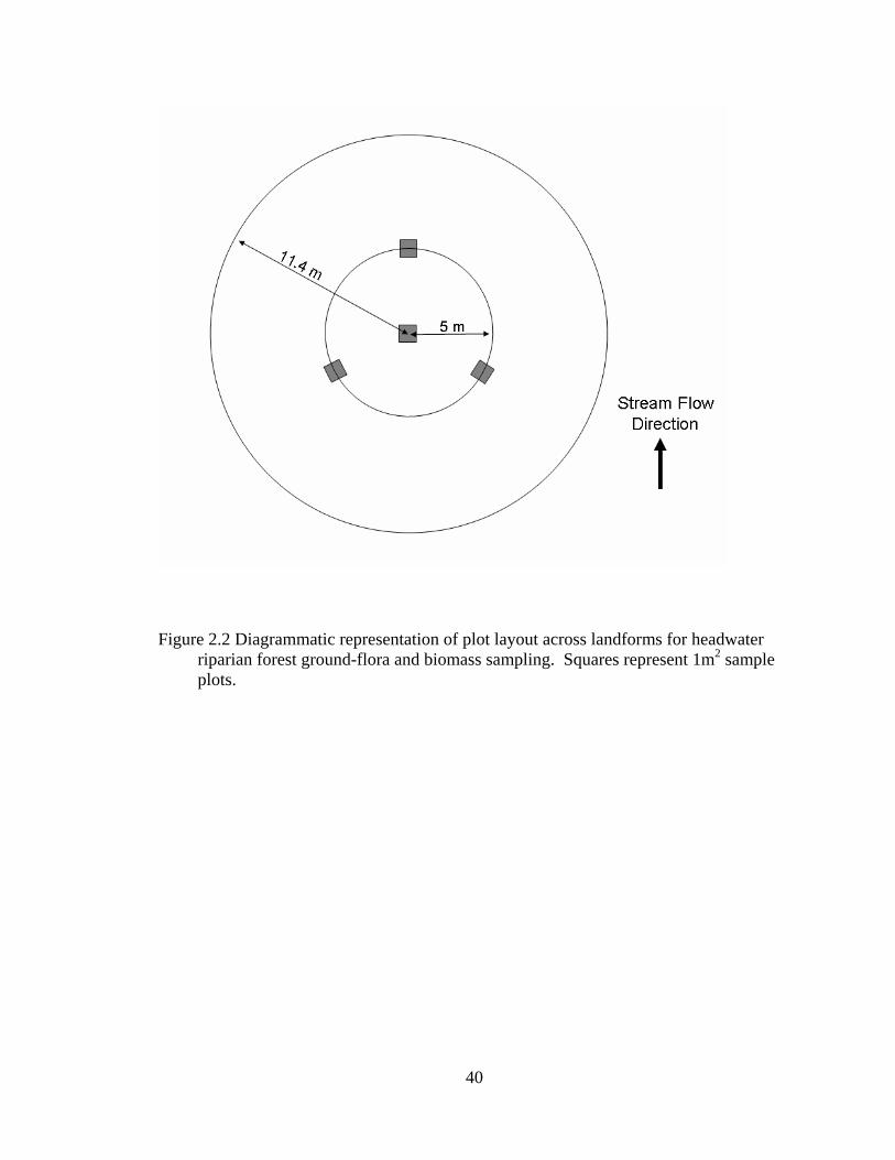
Figure 2.2 Diagrammatic representation of plot layout across landforms for headwater riparian forest ground-flora and biomass sampling. Squares represent 1m2 sample plots.

40

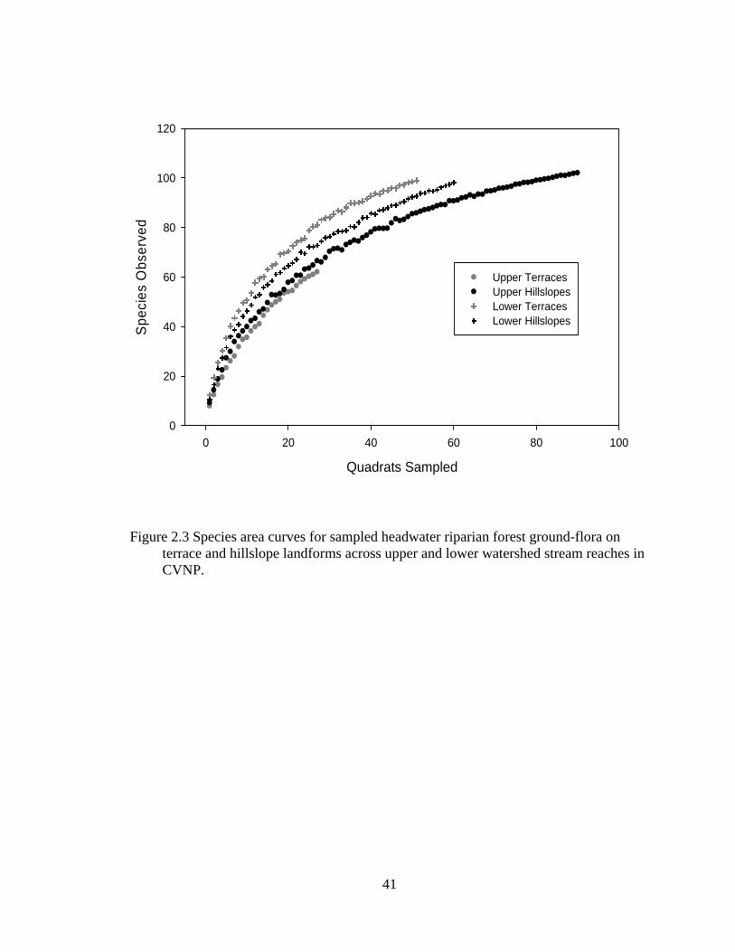
Quadrats Sampled

0 20 40 60 80 100

Spe

cies

Obs

erve

d

0

20

40

60

80

100

120

Upper TerracesUpper HillslopesLower TerracesLower Hillslopes

Figure 2.3 Species area curves for sampled headwater riparian forest ground-flora on terrace and hillslope landforms across upper and lower watershed stream reaches in CVNP.

41

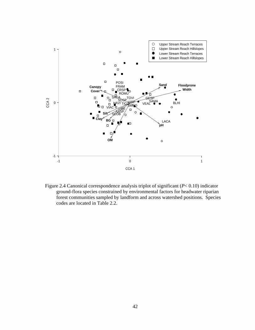
CCA 1

-1 0 1

CC

A 2

-1

0

1

BLHI

LACApH

FloodproneWidth

Sand

BG

CanopyCover

OM

SiltClay

GESPVEAL

POSI

SACA

SEOB ASSP

TICOLIBE

SAMATOVI

SMROVISP

ROMUCRSP

FRAM

SOSPHAVI

VIAC

Upper Stream Reach TerracesUpper Stream Reach HillslopesLower Stream Reach TerracesLower Stream Reach Hillslopes

Figure 2.4 Canonical correspondence analysis triplot of significant (P< 0.10) indicator

ground-flora species constrained by environmental factors for headwater riparian forest communities sampled by landform and across watershed positions. Species codes are located in Table 2.2.

42

CHAPTER 3

THE DISTRIBUTION AND CHARACTERISTICS OF DOWNED WOOD ACROSS HEADWATER RIPARIAN ECOTONES: INTEGRATING THE STREAM WITH THE

RIPARIAN AREA

3.1 Introduction

Downed wood comprises a significant structural component of riparian areas that

links the aquatic and terrestrial ecosystems (Gurnell et al. 1995; Butts and McComb

2000) providing numerous ecosystem services. In stream ecosystems, downed wood

affects many physical and chemical processes including sediment storage, flow diversion,

channel morphology, and nutrient uptake (Bilby and Likens 1980, Bilby and Ward 1989,

Montgomery et al. 1995, Gurnell et al. 2002, Hassan et al. 2005, Warren et al. 2007), as

well as creating habitat and food retention for fish and invertebrate assemblages (Bilby

and Likens 1980, Wallace et al. 1995, Gregory et al. 2003, Dolloff and Warren 2003,

Morris et al. 2006). In terrestrial ecosystems, downed wood is an important component

of decomposition and nutrient cycling, a fuel source for fire, and habitat for many

organisms including small mammals, amphibians, and invertebrates (Lang and Forman

43

1978, Harmon et al. 1986, Franklin et al. 1987, Harmon and Hua 1991). The resulting

habitat is often unique and patchy (Morris et al. 2006) and utilized by a variety of

organisms, including small mammals, invertebrates, fish, and amphibians (Wondzell and

Bisson 2003). While the connection between riparian areas and aquatic ecosystems has

been demonstrated (Gregory et al. 1991, Richardson and Danehy 2007), most research on

downed wood focuses either solely on coarse woody debris (CWD) in upland forests or

in-stream large wood (LW), with relatively few studies analyzing downed wood in both

stream channels and their adjacent riparian areas (O’Connor and Ziemer 1989, McClure

et al. 2004, Young et al. 2006, Keeton et al. 2007). The extent of influence of riparian

areas on stream channels and vice-versa cannot be clearly delineated on the landscape,

yet we are unaware of any research on the changing structure of downed wood across the

entire riparian area, including the stream channel. Characterizing a gradient from

terrestrial to aquatic ecosystems, riparian areas are unique components of the landscape

referred to as ecotones (Gregory et al. 1991) where distinct demarcation between the two

ecosystems is difficult. In these riparian ecotones, downed wood physically links

riparian areas and stream channels and is regulated by a variety of hydrogeomorphic and

plant successional processes, including the hydroperiod and hydrogeomorphology of the

stream valley.

As we work to manage and restore riparian areas, we need to increase our

understanding of riparian structure and function, including that of downed wood

(Gregory et al. 2003). This is especially true in headwater systems where the tight

connectivity between the terrestrial and aquatic ecosystems is particularly strong with

closed tree canopies that regulate light and temperature as well as provide allocthononus

44

inputs from riparian areas that sustain aquatic biota (Vannote et al. 1991). Headwater

streams also differ from larger order streams in that they tend to have more downed wood

(m3/100 m2) as a result of narrower bankfull channel widths that restrict downstream

movement (Gomi et al. 2006) providing for unique habitat (Bilby and Likens 1980,

Smock et al. 1989). Additionally, sources of downed wood in headwater systems tend to

be more colluvial than the alluvial sources typical of larger streams (May and Gresswell

2003), further indicating the importance of riparian areas in headwater systems. Research

on downed wood structure and function should reflect the tight connection between

riparian areas and their stream channels through integration across the entire ecotone,

particularly in headwater systems. Because downed wood physically spans the ecotone

between terrestrial and aquatic systems in riparian areas, research should reflect that

natural integration.

In order to better understand how the structure of downed wood changes across

headwater riparian areas, we sampled downed wood characteristics across the entire

riparian ecotone, including the stream channel and stream valley, of seven headwater

streams (1st, 2nd, 3rd order following 1:24K topographic blue lines) in the Cuyahoga River

watershed of northeastern Ohio. For this study, we define downed wood as pieces of

wood with maximum diameter greater than 7 cm and no minimum length in order to

capture pieces that could be used as potential habitat for smaller organisms (e.g. small

mammals and amphibians). To further understand the influence of hydrogeomorphology

on downed wood we sampled the riparian areas by geomorphic zones, specifically the

wetted channel, the bankfull channel, and the area outside the bankfull channel to the

base of the stream valley wall. We hypothesize that the structure of downed wood will

45

change based upon differing functions associated with hydrogeomorphic zones across the

riparian ecotone. Specifically, 1) aquatic zones are more dynamic than the terrestrial

zone and the resulting downed wood structure will be different between the two; 2) the

wetted channel, as the true aquatic ecosystem during baseflow conditions, will have

different structure than the bankfull zone, which is an ecotone between the aquatic and

terrestrial ecosystems during baseflow conditions; and 3) the bankfull zone will have

different structure than the terrestrial ecosystem outside the bankfull channel.

3.2 Methods

3.2.1 Study Area

The research was conducted in Cuyahoga Valley National Park (CVNP), OH,

USA, an area of over 13,400 ha (33,000 acres) comprised of relatively undeveloped land

along 35 kilometers (22 miles) of the Cuyahoga River and over 360 kilometers (190

miles) of tributaries between the cities of Cleveland and Akron, OH (Figure 3.1). Much

of the park is characterized by steep, forested ravine systems formed along the multiple

tributaries to the Cuyahoga River. The forests are second-growth (>70 years old) and

composed of mixed-mesophytic species (e.g. sugar maple, Acer saccharum Marsh;

American beech, Fagus grandifolia Ehrh.; northern red oak, Quercus rubra L.; shagbark

hickory, Carya ovata (P.Mill)K. Koch; and yellow poplar, Liriodendron tulipifera L.).

The area is located in the Erie Gorges Ecoregion, part of the Erie Ontario Drift and Lake

Plain, is a unique glaciated area characterized by steeply, dissected valleys along the

Cuyahoga, Chagrin, and Grand Rivers with rocky outcroppings and high rates of erosion

(Woods et al. 1998). The riparian areas along these streams include a diverse array of

46

geomorphic settings representative of watersheds in the glaciated region (Rau 1969).

Soils on the hillslopes are characterized as deep, moderately well-drained to well-drained

soils, while soils on narrow flood plains and small terraces are dominated by alluvial

deposits (Ritchie and Steiger 1974). Some streams have cut down below the level of the

alluvial deposits, which are now preserved as terraces along the valley sides.

3.2.2 Sampling Methodology

During the summer of 2006, riparian areas along seven headwater stream reaches

were selected and sampled in CVNP. Headwater streams in this study are defined as

draining less than 51.8 km2 (20 mi2), usually 1st, 2nd, or 3rd stream order following

Strahler (1952). Streams were selected based on similar riparian forest age (mature

second-growth > 70 years old), riparian forest composition and structure, fluvial

landforms (presence of floodplains and terraces), stream gradient (1-5%) and substrate

(minimal siltation). For the purpose of this study, riparian areas are defined as the area

beginning at the base of the stream valley wall and extending across fluvial terraces and

floodplain, including the channel, and across to the opposite valley wall base (Figure

3.2). This definition follows the ecotonal approach to riparian ecology described by

Illhardt et al. (2000). A randomly selected sample reach length of 30 channel

geomorphic units (CGU: riffle, run, pool) was used to delineate the longitudinal length of

the sample area, while the width was determined by the undulating base of the stream

valley wall. For each CGU, the wetted channel and bankfull channel width were

recorded, as well as the length of the CGU longitudinally along the channel. Valley width

was recorded for every fifth CGU.

47

For each sample reach, all downed wood with end diameter greater than 7 cm was

sampled within the riparian area, capturing all wood inside the valley walls and stream

channel. Pieces extending up the valley wall slope were only characterized for the

portion inside the base of the valley wall. Each piece of wood encountered of size was

recorded for total length, minimum and maximum end diameters, and decay class (Table

3.1). Decay class was assigned based on the condition of the majority of a piece. To

understand the influence of hydrogeomorphic features on downed wood structure and

function, the riparian area was subdivided into three zones, similar to those of Robison

and Beschta (1990). However in our study, Zone 1 comprised the wetted channel, Zone 2

comprised the area inside the bankfull channel not including the wetted channel, and

Zone 3 comprised the area outside the bankfull channel to the toe of the valley wall

(Figure 3.3). The length of each piece of downed wood within each zone as well as the

percent surface contact of the piece within each zone was recorded.

3.2.3 Statistical Analyses

Mean channel geomorphic unit length and the mean widths of the wetted and

bankfull channels and valley were summarized for each sample reach, and the ratio of

mean bankfull channel width to mean valley width was determined for each sample

reach. Total area sampled for each sample reach was calculated by summarizing the area

encompassed between each fifth CGU valley width measurement and the longitudinal

distance along the channel for the previous five CGUs. The area of each zone was

calculated for each sample reach using the total longitudinal distance along the channel

sampled and the mean wetted width for zone 1, the mean bankfull channel width minus

48

the wetted width for zone 2, and the mean valley width minus the bankfull channel width

for zone 3. Because the area encompassed by both zones 1 and 2 is hypothetically the

most dynamic in terms of wood function, a fourth zone was created termed zone 1+2.

Mean values for zone 1+2 were calculated as the sum of the means for zones 1 and 2. In

order to verify the similarity between the seven sample reaches in terms of site

conditions, Principal Components Analysis (PCA) of the means of CGU length, wetted

width, bankfull channel width, valley width, and the bankfull channel/valley width ratio

were used to ordinate the seven sample reaches in PCA using a correlation matrix in PC-

ORD version 5 (McCune and Mefford 2006). Randomization tests (N=2000) were used

to test for significance of the PCA axes. Alpha level of 0.10 was used to indicate

significant differences for all analyses.

Characteristics of downed wood measured for entire pieces of wood were

summarized across the entire riparian area. The volume of each piece of downed wood

was calculated as a cylinder using the Smalian method,

Lengthareaendareaend

Volume ×+

=2

)( 21 , and the volume per piece per square meter sampled

(volume/m2) of each piece of downed wood was calculated using the area sampled for

each site. Length per piece per square meter sampled (length/m2) was also determined in

a similar manner. Mean length, volume, minimum and maximum diameters, and decay

class for pieces were calculated across all seven streams. Frequency distributions for

length, length/m2, volume, volume/m2, minimum and maximum end diameters, and

decay class were generated and Weibull distribution curves using quick estimation

methods (Shifley and Lentz 1985) were fitted to each frequency distribution except decay

class in order to characterize all downed wood sampled. Ninety-five percent confidence

49

intervals were constructed for the shape of the Weibull distribution, parameter c, using

Thoman et al. (1969).

Characteristics of downed wood measured for pieces by zone were summarized

across all seven sample reaches for each of the four hydrogeomorphic zones. Volume of

each piece of downed wood was calculated for each zone using the mean end diameter

and the length of the piece in the specific zone. Volume per piece per square meter was

calculated for each of the four zones using the mean area of each zone at each of the

seven sample reaches. Length per piece per square meter was calculated for each of the

four zones in a similar manner. Mean length per piece and percent contact with the

surface, either soil or channel substrate, was also calculated for each of the zones.

Normality of mean values by zone for the seven sample reaches was verified using

Kolmogorov-Smirnov tests. To test for differences in downed wood structure across the

four hydrogeomorphic zones, a repeated measures analysis of variance (ANOVA) was

used. Repeated measures ANOVA is an appropriate analysis in this instance because the

hydrogeomorphic zones do not occur in a random manner within the riparian area, but

rather occur in a predictable pattern. For example, the wetted channel is always within

the bankfull channel and the terrestrial terraces associated with our zone 3 are always

adjacent the bankfull channel. We also used planned contrasts to test our specific

hypotheses regarding differences in structure and function between the four

hydrogeomorphic zones.

Total volume for all pieces was summarized for the seven sample reaches by the

four hydrogeomorphic zones. Repeated measures ANOVA was used to test for

differences in total volume between zones and site. Mean total volume for each zone

50

across all seven sample reaches was also calculated and a one-way ANOVA was used to

test for differences by zone.

3.3 Results

Total sample reach length ranged from the shortest reach (52 m) at Boston Run III

to the longest reach (222 m) at Dickerson Run (Table 3.2). Riparian area sampled for

downed wood pieces follows reach length with the most area sampled along Dickerson

Run, 5,887 m2, and the smallest area sampled along Boston Run III, 647 m2, (Table 3.2).

While there is variation between the seven sample reaches in mean CGU length, wetted

width, bankfull channel width, valley width, and bankfull channel-to-valley width ratio

(Table 3.2), PCA indicates that the variation is not enough to separate reaches from one

another with all seven clustering near one another. Eigenvalues for axis one and two,

which are significant following the broken-stick rule, were 2.7124 and 1.796,

respectively. This suggests that while there are significant gradients along each axis, the

variation between reaches is small and that the reaches represent similar riparian

environments.

3.3.1 Downed Wood Pieces Across the Riparian Area

For individual pieces of downed wood across the entire riparian area, mean total

piece length is 2.9 m with the majority of pieces having a length of less than 2 m (Figure

3.4a). The distribution of mean length follows a reverse-J Weibull distribution (Figure

3.4a, Table 3.3). While mean piece volume is 0.064 m3, the majority of pieces have a

51

volume less than 0.01 m3 (Figure 3.4b) and follow a reverse-J Weibull distribution (Table

3.3). Both length/m2 and volume/m2 of individual pieces also follow a reverse-J Weibull

distribution (Figure 3.3c and d, respectively). While mean minimum diameter of downed

wood pieces is 9 cm, the majority of pieces have minimum diameters between 6 to 8 cm

and the distribution follows a positively-skewed Weibull distribution (Figure 3.5a).

Similarly, the mean maximum diameter of downed wood pieces is 13 cm while the

distribution follows a positively-skewed Weibull distribution (Figure 3.5b) and the

majority of pieces have maximum diameters from 7 to 10 cm. The majority of pieces

exhibit a decay class 4 condition with the distribution following a negatively-skewed

Weibull distribution (Figure 3.5c) and a mean decay class of 3.7 (Table 3.2).

3.3.2 Downed Wood Pieces by Hydrogeomorphic Zone

Mean length of downed wood pieces within each zone ranged from 1.82 m in

Zone 2 to 2.78 m in Zone 3 (Table 3.4) with no significant difference among the four

zones (Table 3.5). Additionally, there was no significant difference in length for any of

the three planned contrasts (Table 3.5). Mean length/m2 was significantly different

between the four zones (Table 3.5) with a significant difference between Zones 1 and 2

(Table 3.5) each having mean length/m2 of 0.009 m/m2 versus 0.0039 m/m2, respectively

(Table 3.4). Mean volume per piece of downed wood within each zone ranged from

0.043 m3 in Zone 2 to 0.061 m3 in Zone 3 (Table 3.4). Although the difference in mean

volume between the four zones approaches significance (Table 3.5), there were no

significant differences for any of the planned contrasts. Similarly, volume/m2 was not

significantly different among the four zones or for any of the planned contrasts. Percent

52

surface contact of downed wood pieces was significantly different between the four zones

(Table 3.5) with mean percent surface contact ranging from 40.6% in Zone 1 to 68.34%

in Zone 3 (Table 3.4). There is a significant difference in mean percent surface contact

between the combined Zones 1 and 2, the pieces within the bankfull channel, versus

pieces in Zone 3, the pieces outside the bankfull channel (Table 3.5). Additionally, there

is a significant difference in mean percent surface contact between Zone 2 and Zone 3

(Table 3.5).

3.3.3 Downed Wood Total Volume by Hydrogeomorphic Zone

Mean total volume of all downed wood pieces within each of the zones differed

(Figure 3.6a), with Zone 3 having a mean total volume of 11.00 m3 while zones 1 and 2

had mean volumes of 2.04 and 3.36 m3, respectively (Table 3.6). However, due to high

variability no statistical difference in total volume was found between the zones or

planned contrasts (Table 3.5). When total volume is standardized by area sampled, mean

total volume (m3/ha) is higher inside the bankfull channel than outside the channel

(Figure 3.5b) with Zones 1 + 2 having 83.03 m3/ha and Zone 3 having 62.82 m3/ha. This

difference in total volume is not significant between the four zones or the planned

contrasts (Table 3.5).

3.4 Discussion

While the connection, both physical and biological, between streams and their

associated riparian areas is well documented, our study is one of the first to analyze

downed wood structure across the entire riparian area, including the stream channel. In

53

headwater systems this approach seems particularly relevant as riparian areas and streams

are tightly linked. Downed wood often physically links the riparian area and stream,

particularly in headwater systems where the gradient between terrestrial and aquatic

ecosystems can be quite narrow depending on the fluvial processes of the system. It is

widely accepted that the hydrology of a system strongly influences riparian area

processes and geomorphology (Gregory et al. 1991) and we found that downed wood

structure did vary between the three hydrogeomorphic zones analyzed.

The hydrogeomorphic zones inside the bankfull channel, zones 1 and 2, are the

most hydrologically dynamic allowing for potential downstream distribution and

changing ecological function during periods of high streamflow. We found that mean

downed wood piece length was smaller than the mean bankfull channel width for all of

the seven sample reaches. Mean length of downed wood pieces was wider than the

wetted width, except on the largest stream, but mean length was shorter than the bankfull

channel width at all sites indicating that changes in streamflow levels has the potential to

move downed wood as well as change the function of the wood during high streamflow

events. Other studies of downed wood usually have a minimum length requirement,

typically 1 m, so the mean length of pieces in those studies is considerably higher than in

our study. However, McClure et al. (2004) sampled downed wood with a minimum

length and maximum diameter of 10 cm each and found that downed wood pieces inside

the bankfull channel of Kentucky streams had an approximate mean length of 2.8 m.

Downed wood pieces in their 70 year old riparian forest had an approximate mean length

of 2.4 m (McClure et al. 2004). Our mean lengths of 2.35 m for zones 1+2 and 2.78 m

54

for zone 3 correspond to those found by McClure et al. (2004) and our study sites had

similar riparian forest composition and age.

Because we did not specify a minimum length or diameter for inclusion in our

sampling, many of our downed wood pieces are quite small in comparison to most other

studies, yet the volumes both per piece and per area sampled seem to be comparable to

other eastern U.S. riparian areas, as well as some areas in the western U.S. In terms of

total volume (m3/ha), we found much higher mean total volume in our zone 3 than in a

Montana riparian forest, 63 m3/ha versus 10 m3/ha respectively (Young et al. 2006), a

difference most likely related to riparian forest composition. While our second-growth

riparian areas have less mean total volume in zone 3 than that found in old-growth

riparian forests in the Adirondacks (Keeton et al. 2007), the mean total volume in our

zone 3 is similar to that found on old-growth riparian terraces of Zoar Canyon, NY (Pfeil

et al. 2007) . Additionally, the mean total volume of downed wood inside the bankfull

channel was much smaller in our streams than those of undisturbed Kentucky streams, 83

versus 500 m3/ha, respectively (McClure et al. 2004). Finally, while Young et al. (2006)

sampled downed wood with minimum length of 2 m and maximum diameter greater than

10 cm, the mean volume of wood per piece (m3) in fourteen headwater riparian areas in

Montana is similar to the volume that we found in our headwater stream sample reaches.

In our study, we found that mean total volume of downed wood (m3) was higher

in zone 3 than the other three zones (zones 1, 2, 1+2), but the volume of wood in zone 3

was much more variable than wood inside the bankfull channel. However, when mean

total volume was analyzed by the total area sampled (m3/ha), we observed no difference

between the four zones. Additionally, there was more downed wood volume inside the

55

bankfull channel than outside on a per area basis. While our planned contrasts between

the zones were not statistically significant, these patterns in volume likely reflect the

hydrologic influence on downed wood distribution where pieces inside the bankfull

channel are much more dynamic and have a consistent rate of input and movement

compared to those pieces outside the bankfull channel that have a more stochastic rate of

input and will only move during periods of flooding.

Another important aspect of our results are that most downed wood pieces

regardless of the zone located were short, less than 1 m, had maximum diameters less

than 10 cm, and had volumes less than 0.01 m3. While other studies have minimum

requirements for downed wood sizes for inclusion in sampling, the majority of downed

wood sampled in these studies have the smallest minimum diameter and length within

these sampling requirements (Young et al. 2006, Pfeil et al. 2007, and Webster et al.

2008), indicating that small downed wood dominates the size distribution across riparian

ecotones. This may be an under-recognized habitat resource for small organisms other

than fish, such as mammals, amphibians, and macroinvertebrates. Additionally, we

found significant differences in the percent surface contact of downed wood pieces across

the hydrogeomorphic zones with zone 3 having the highest surface contact. The mean

decay class of downed wood in our study was also quite high across the riparian ecotone,

which is similar to what was observed in other studies (Robison and Beschta 1990,

McClure et al. 2004, and Webster et al. 2008). Organisms, such as salamanders, may be

able to utilize downed wood pieces characterized by high surface contact and the moist,

punky texture found in decay class 4 as shelter or habitat to disperse across the riparian

ecotone because wood often forms a physical link between the hydrogeomorphic zones.

56

We are not aware of any research on the actual utilization or significance of these

physical links across riparian ecotones to organisms and this is an area of potential future

research.

3.5 Conclusions

The results of this study can serve as a reference condition for downed wood

structure across second-growth riparian areas in the Erie Gorges Ecoregion and the

Lower Lake States. We found that most wood was small with a high decay class and the

volume of wood outside of the bankfull channel inside the valley wall (zone 3) was

higher but more variable than the volume of wood inside the bankfull channel (zone 1 +

2). However, in terms of area, the volume was not different between the channel and

terraces. The physical link created by downed wood is an interesting concept,

particularly in terms of potential utilization for dispersal by species such as streamside

and forest salamanders, as well as invertebrate species. Additionally, the linkage

provided by downed wood across riparian ecotones is temporal, with wood inside the

channel more dynamic than that outside the channel as a result of hydrologic flow

patterns in riparian ecotones. Research on the temporal distribution of downed wood

across the riparian ecotone following flooding events would further our understanding of

the linkages between the terrestrial and aquatic ecosystems. Our ecotone approach to

sampling downed wood characteristics reflects the hydrogeomorphic processes that are

integral to riparian ecology (Gregory et al. 1991, Illhardt et al. 2000), particularly in

headwater systems where the riparian ecotone is relatively narrow compared to larger

stream orders (Gregory et al. 2003, Richardson and Danehy 2007). As we move towards

57

improved research and management of ecosystems we need to move beyond our

individual discipline traditions and view ecosystems holistically, such as in our unique

ecotone approach to studying riparian areas which span the gradient from terrestrial to

aquatic ecosystems. These interdisciplinary approaches will be required for improved

understanding and management of ecosystems.

3.6 References

Bilby, R.E. and G.E. Likens. 1980. Importance of organic debris dams in the structure and function of stream ecosystems. Ecology 61 (5): 1107-1113.

Bilby, R.E. and J.W. Ward. 1989. Changes in characteristics and function of woody debris with increasing size of streams in western Washington. Transactions of the American Fisheries Society 118: 368-378.

Butts, S.R. and W.C. McComb. (2000) Associations of forest-floor vertebrates with course woody debris in managed forests of western Oregon. Journal of Wildlife Management 64: 95-104.

Dolloff, C.A. and J.L. Warren Jr. 2003. Fish relationships with large wood in small streams. American Fisheries Society Symposium 37: 179-193.

Franklin, J.F., H.H. Shugart, M.E. Harmon. 1987. Tree death as an ecological process. BioScience 37 (8): 550-556.

Gregory, S.V., F.J. Swanson, W.A. McKee, and K.W. Cummins. (1991) An ecosystem perspective of riparian zones. BioScience 41: 540-551.

Gregory, S.V., K.L. Boyer, and A.M. Gurnell, editors. 2003 The Ecology and Management of Wood in World Rivers. American Fisheries Society, Bethesda, Maryland, USA, pp.431.

Gomi, T., A.C. Johnson, R.L. Deal, P.E. Hennon, E.H. Orlikowska, and M.S. Wipfli. 2006. Factors affecting distribution of wood, detritus, and sediment in headwater

58

streams draining managed young-growth red alder-conifer forests in southeast Alaska. Canadian Journal of Forest Research 36: 725-737.

Gurnell, A.M., G.E. Petts, and C.T. Hill. (1995) The role of coarse woody debris in forest aquatic habitats: implications for management. Journal of Aquatic Conservation: Marine and Freshwater Ecosystems 5: 1-24.

Gurnell, A.M., H. Piégay, F.J. Swanson, and S.V.Gregory. 2002. Large wood and fluvial processes. Freshwater Biology 47: 601-619.

Harmon, M.E., J.F. Franklin, F.J. Swanson, P. Sollins, S.V. Gregory, J.D. Lattin, N.H. Anderson, S.P. Cline, N.G. Aumen, J.R. Sedell, G.W. Lienkaemper, K. Cromack Jr., and K.W. Cummins. 1986. Ecology of coarse woody debris in temperate ecosystems. Advances in Ecological Research 15: 1460-1473.

Harmon, M.E. and C. Hua. 1991. Coarse Woody Debris Dynamics in Two Old-Growth Ecosystems. BioScience 41 (9): 604-610.

Hassan, M.A., M. Church, T.E. Lisle, F. Brardinoni, L. Benda, and G.E. Grant. 2005. Sediment transport and channel morphology of small, forested streams. Journal of the American Water Resources Association 41 (4): 853-876.

Ilhardt, B.L., E.S. Verry, and B.J. Palik. 2000. Defining riparian areas. pp. 23-42 In: E.S. Verry, J.W. Hornbeck, and C.A. Dolloff, editors. Riparian Management in Forests of the Continental Eastern United States. Lewis Publishers, New York, pp.402.

Keeton, W.S., C.E. Kraft, and D.R. Warren. 2007. Mature and old-growth riparian forests: Structure, dynamics, and effects on Adirondack stream habitats. Ecological Applications 17 (3): 852-868.

Lang, G.E. and R.T.T. Forman. 1978. Detrital dynamics in a mature oak forest: Hutcheson Memorial Forest, New Jersey. Ecology 59 (3): 580-595.

May, C. L. and R.E. Gresswell. 2003. Large wood recruitment and redistribution in headwater streams in the southern Oregon Coast Range, U.S.A. Canadian Journal of Forest Research 33: 1352-1362.

59

McCune, B. and M.J. Mefford. 2006. PC-ORD: Multivariate analysis of ecological data. Version 5.0. MjM Software Design, Gleneden Beach, OR.

McClure, J.M., R.K. Kolka, and A. White. 2004. Effect of forest harvesting best management practices on coarse woody debris distribution in stream and riparian zones in three Appalachian watersheds. Water, Air, and Soil Pollution 4: 245-261.

Montgomery, D.R., J.M. Buffington, R.D. Smith, K.M. Schmidt, and G. Pess. 1995. Pool spacing in forest pools. Water Resources Research 31: 1097-1105.

Morris, A.E.L., P.C. Goebel, L.R. Williams, and B.J. Palik. 2006. Influence of land-scape geomorphology on large wood jams and salmonids in an old-growth river of Upper Michigan. Hydrobiologia 56:149-161.

O’Connor, M.D. and R.R. Ziemer. 1989. Coarse woody debris ecology in second-growth Sequoia sempervirens forest stream. USDA Forest Service General Technical Report PSW-110: 165-171.

Pfeil, E.K., N. Casacchia, G.J. Kerns, and T.P. Diggins. 2007. Distribution, composition, and orientation of down deadwood in riparian old-growth woodlands of Zoar Valley Canyon, western New York State, USA. Forest Ecology and Management 239: 159-168.

Rau, J.L. 1969. The evolution of the Cuyahoga River: It’s geomorphology and environmental geology. pp. 9-39. In J.P. Cooke (eds.), The Cuyahoga River Watershed. Institute of Limnology and Department of Biological Sciences, Kent State University, Kent, Ohio. Also found as Contribution No. 43, Department of Geology, Kent State University, Kent, Ohio.

Reeves, G.H., K.M. Burnett, and E.V. McGarry. 2003. Sources of large wood in the main stem of a fourth-order watershed in coastal Oregon. Canadian Journal of Forest Research 33: 1363-1370.

Richardson, J.S. and R.J. Danehy. 2007. A synthesis of the ecology of headwater streams and their riparian zones in temperate forests. Forest Science 53 (2): 131-147.

Ritchie, A. and Steiger, J.R. 1990. Soil Survey of Summit County, Ohio. United States Department of Agriculture, Soil Conservation Service.

60

Robison, E.G. and R.L. Beschta. 1990. Characteristics of coarse woody debris for several coastal streams of southeast Alaska, USA. Canadian Journal of Fisheries and Aquatic Science 47: 1684-1693.

Shifley, S. and E. Lentz. 1985. Quick estimation of the three-parameter Weibull to describe tree size distributions. Forest Ecology and Management 13: 195-203.


Smock, L.A., G.M. Metzler, and J.E. Gladden. 1989. Role of debris dams in the structure and functioning of low-gradient headwater streams. Ecology 70(3): 764-775.

Thoman, D.R., L.J. Bain, and C.E. Antle. 1969. Inferences on the parameters of the Weibull distribution. Technometrics 11(3): 445-460.

Vannote, R.L., G.W. Minshall, K.W. Cummins, J.R. Sedell, and C.E. Cushing. 1980. The river continuum concept. Canadian Journal of Fisheries and Aquatic Sciences. 37:130-137.

Wallace, J.B., J.R. Webster, and J.L. Meyer. 1995. Influence of log additions on physical and biotic characteristics of a mountain stream. Canadian Journal of Fisheries and Aquatic Science 52: 2120-2137.

Warren, D. R., E.S. Bernhardt, R.O. Hall Jr., and G.E. Likens. 2007. Forest age, wood, and nutrient dynamics in headwater streams of the Hubbard Brook Experimental Forest, New Hampshire, USA. Earth Surface Process and Landforms 32(8): 1154-1163.

Webster, C.R., C.J.F. Huckins, and J.M. Shields. 2008. Spatial distribution of riparian zone coarse woody debris in a managed northern temperate watershed. American Midland Naturalist 159: 225-237.

Wondzell, S.M. and P.A. Bisson. 2003. Influence of wood on aquatic biodiversity. Pp. 249-263 in Gregory, S.V., Boyer, K.L. & Gurnell, A.M. (eds) The Ecology and Management of Wood in World Rivers. American Fisheries Society, Bethesda, Maryland, USA.

61

Young, M.K., E.A. Mace, E.T. Ziegler, and E.K. Sutherland. 2006. Characterizing and contrasting instream and riparian coarse wood in western Montana basins. Forest Ecology and Management 226: 26-40.

62

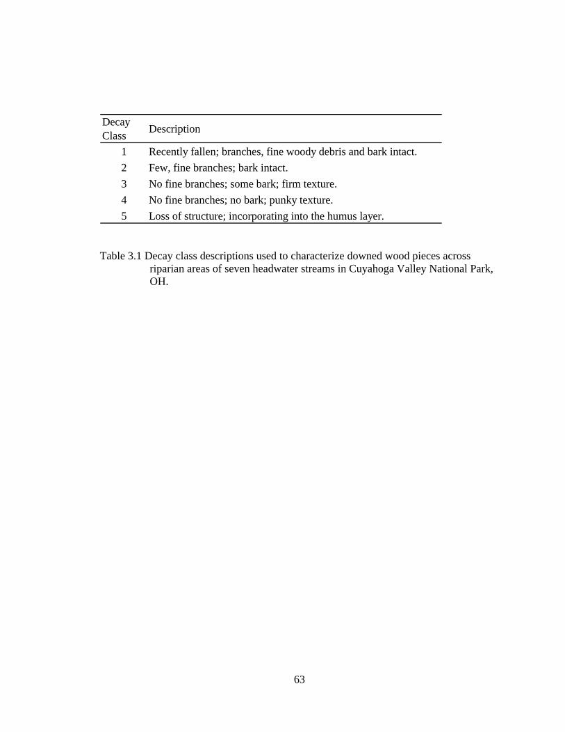
Decay Class Description

1 Recently fallen; branches, fine woody debris and bark intact.2 Few, fine branches; bark intact.3 No fine branches; some bark; firm texture.4 No fine branches; no bark; punky texture.5 Loss of structure; incorporating into the humus layer.

Table 3.1 Decay class descriptions used to characterize downed wood pieces across

riparian areas of seven headwater streams in Cuyahoga Valley National Park, OH.

63

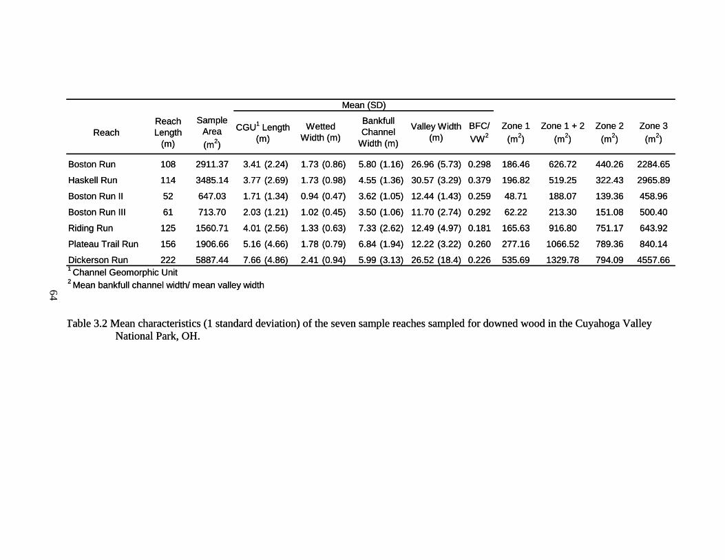
ReachReach Length

(m)

Sample Area (m2)

BFC/ VW2

Zone 1 (m2)

Zone 1 + 2 (m2)

Zone 2 (m2)

Zone 3 (m2)

Boston Run 108 2911.37 3.41 (2.24) 1.73 (0.86) 5.80 (1.16) 26.96 (5.73) 0.298 186.46 626.72 440.26 2284.65

Haskell Run 114 3485.14 3.77 (2.69) 1.73 (0.98) 4.55 (1.36) 30.57 (3.29) 0.379 196.82 519.25 322.43 2965.89

Boston Run II 52 647.03 1.71 (1.34) 0.94 (0.47) 3.62 (1.05) 12.44 (1.43) 0.259 48.71 188.07 139.36 458.96

Boston Run III 61 713.70 2.03 (1.21) 1.02 (0.45) 3.50 (1.06) 11.70 (2.74) 0.292 62.22 213.30 151.08 500.40

Riding Run 125 1560.71 4.01 (2.56) 1.33 (0.63) 7.33 (2.62) 12.49 (4.97) 0.181 165.63 916.80 751.17 643.92

Plateau Trail Run 156 1906.66 5.16 (4.66) 1.78 (0.79) 6.84 (1.94) 12.22 (3.22) 0.260 277.16 1066.52 789.36 840.14

Dickerson Run 222 5887.44 7.66 (4.86) 2.41 (0.94) 5.99 (3.13) 26.52 (18.4) 0.226 535.69 1329.78 794.09 4557.661 Channel Geomorphic Unit2 Mean bankfull channel width/ mean valley width

Mean (SD)

CGU1 Length (m)

Wetted Width (m)

Bankfull Channel

Width (m)

Valley Width (m)

Table 3.2 Mean characteristics (1 standard deviation) of the seven sample reaches sampled for downed wood in the Cuyahoga Valley

National Park, OH. Table 3.2 Mean characteristics (1 standard deviation) of the seven sample reaches sampled for downed wood in the Cuyahoga Valley

National Park, OH.

64

ReachReach Length

(m)

Sample Area (m2)

BFC/ VW2

Zone 1 (m2)

Zone 1 + 2 (m2)

Zone 2 (m2)

Zone 3 (m2)

Boston Run 108 2911.37 3.41 (2.24) 1.73 (0.86) 5.80 (1.16) 26.96 (5.73) 0.298 186.46 626.72 440.26 2284.65

Haskell Run 114 3485.14 3.77 (2.69) 1.73 (0.98) 4.55 (1.36) 30.57 (3.29) 0.379 196.82 519.25 322.43 2965.89

Boston Run II 52 647.03 1.71 (1.34) 0.94 (0.47) 3.62 (1.05) 12.44 (1.43) 0.259 48.71 188.07 139.36 458.96

Boston Run III 61 713.70 2.03 (1.21) 1.02 (0.45) 3.50 (1.06) 11.70 (2.74) 0.292 62.22 213.30 151.08 500.40

Riding Run 125 1560.71 4.01 (2.56) 1.33 (0.63) 7.33 (2.62) 12.49 (4.97) 0.181 165.63 916.80 751.17 643.92

Plateau Trail Run 156 1906.66 5.16 (4.66) 1.78 (0.79) 6.84 (1.94) 12.22 (3.22) 0.260 277.16 1066.52 789.36 840.14

Dickerson Run 222 5887.44 7.66 (4.86) 2.41 (0.94) 5.99 (3.13) 26.52 (18.4) 0.226 535.69 1329.78 794.09 4557.661 Channel Geomorphic Unit2 Mean bankfull channel width/ mean valley width

Mean (SD)

CGU1 Length (m)

Wetted Width (m)

Bankfull Channel

Width (m)

Valley Width (m)

64

64

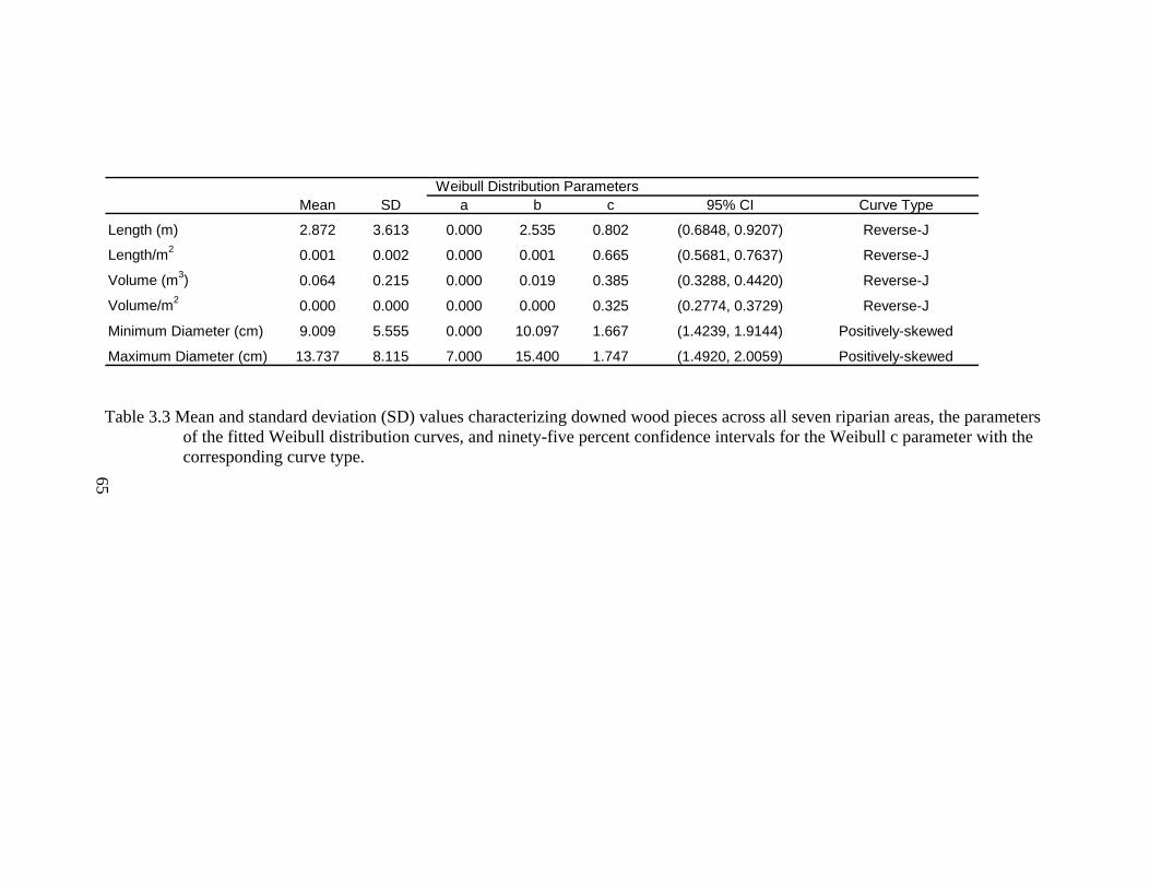
Mean SD a b c 95% CI Curve Type

Length (m) 2.872 3.613 0.000 2.535 0.802 (0.6848, 0.9207) Reverse-J

Length/m2 0.001 0.002 0.000 0.001 0.665 (0.5681, 0.7637) Reverse-J

Volume (m3) 0.064 0.215 0.000 0.019 0.385 (0.3288, 0.4420) Reverse-J

Volume/m2 0.000 0.000 0.000 0.000 0.325 (0.2774, 0.3729) Reverse-J

Minimum Diameter (cm) 9.009 5.555 0.000 10.097 1.667 (1.4239, 1.9144) Positively-skewed

Maximum Diameter (cm) 13.737 8.115 7.000 15.400 1.747 (1.4920, 2.0059) Positively-skewed

Weibull Distribution Parameters

Table 3.3 Mean and standard deviation (SD) values characterizing downed wood pieces across all seven riparian areas, the parameters

of the fitted Weibull distribution curves, and ninety-five percent confidence intervals for the Weibull c parameter with the corresponding curve type.

65

65

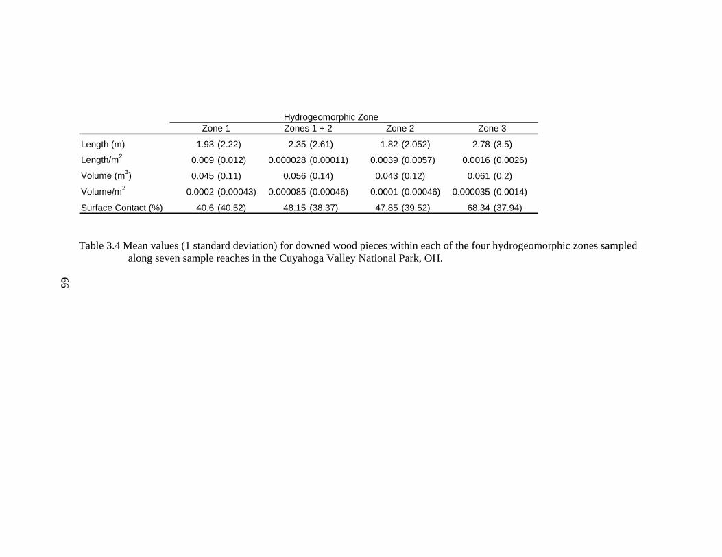
Length (m) 1.93 (2.22) 2.35 (2.61) 1.82 (2.052) 2.78 (3.5)

Length/m2 0.009 (0.012) 0.000028 (0.00011) 0.0039 (0.0057) 0.0016 (0.0026)

Volume (m3) 0.045 (0.11) 0.056 (0.14) 0.043 (0.12) 0.061 (0.2)

Volume/m2 0.0002 (0.00043) 0.000085 (0.00046) 0.0001 (0.00046) 0.000035 (0.0014)

Surface Contact (%) 40.6 (40.52) 48.15 (38.37) 47.85 (39.52) 68.34 (37.94)

Hydrogeomorphic ZoneZone 1 Zones 1 + 2 Zone 2 Zone 3

Table 3.4 Mean values (1 standard deviation) for downed wood pieces within each of the four hydrogeomorphic zones sampled

along seven sample reaches in the Cuyahoga Valley National Park, OH. 66

66

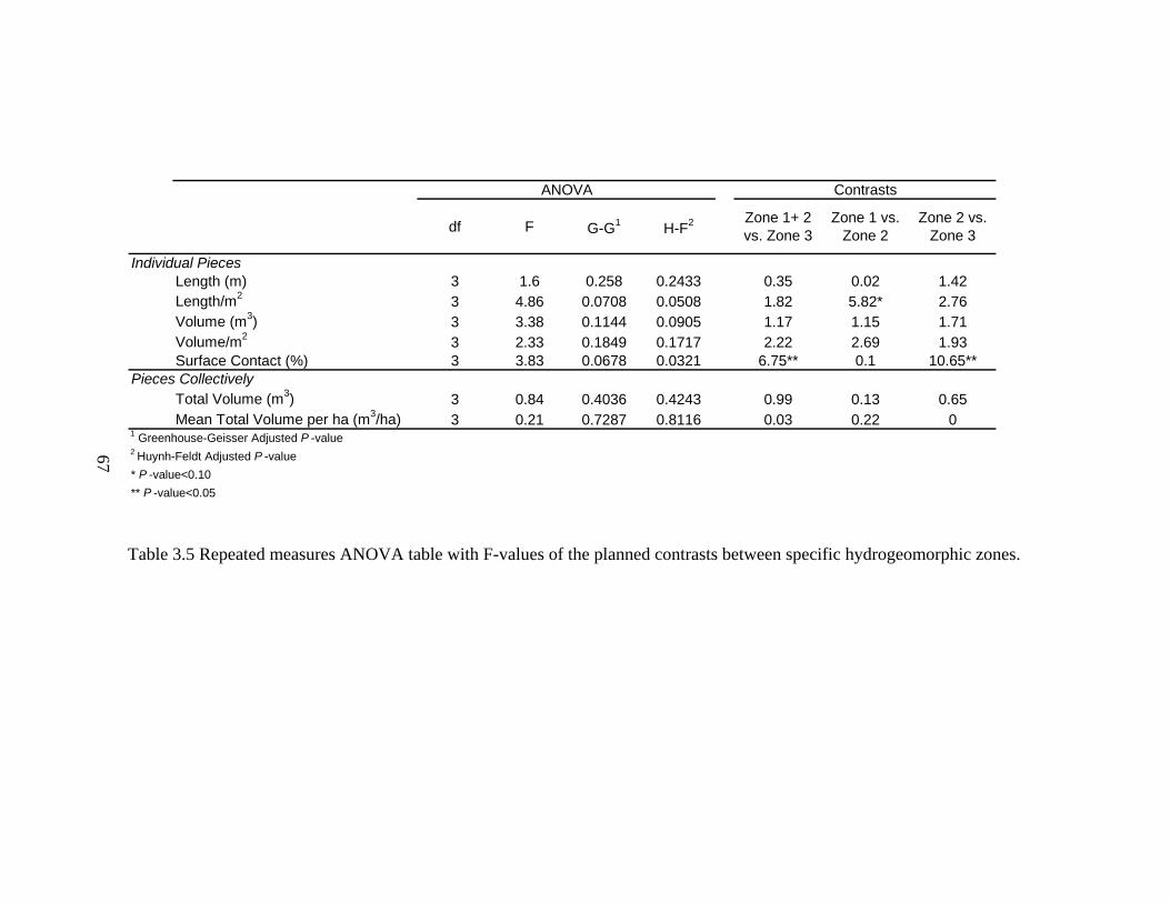
67

df F G-G1 H-F2 Zone 1+ 2 vs. Zone 3

Zone 1 vs. Zone 2

Zone 2 vs. Zone 3

Individual PiecesLength (m) 3 1.6 0.258 0.2433 0.35 0.02 1.42Length/m2 3 4.86 0.0708 0.0508 1.82 5.82* 2.76Volume (m3) 3 3.38 0.1144 0.0905 1.17 1.15 1.71Volume/m2 3 2.33 0.1849 0.1717 2.22 2.69 1.93Surface Contact (%) 3 3.83 0.0678 0.0321 6.75** 0.1 10.65**

Pieces CollectivelyTotal Volume (m3) 3 0.84 0.4036 0.4243 0.99 0.13 0.65Mean Total Volume per ha (m3/ha) 3 0.21 0.7287 0.8116 0.03 0.22 0

1 Greenhouse-Geisser Adjusted P -value2 Huynh-Feldt Adjusted P -value* P -value<0.10** P -value<0.05

ANOVA Contrasts

Table 3.5 Repeated measures ANOVA table with F-values of the planned contrasts between specific hydrogeomorphic zones.

67

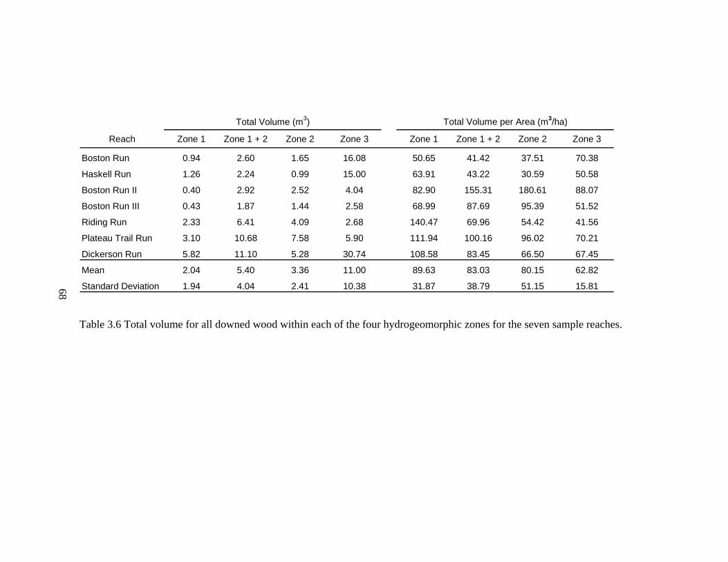
Reach Zone 1 Zone 1 + 2 Zone 2 Zone 3 Zone 1 Zone 1 + 2 Zone 2 Zone 3

Boston Run 0.94 2.60 1.65 16.08 50.65 41.42 37.51 70.38

Haskell Run 1.26 2.24 0.99 15.00 63.91 43.22 30.59 50.58

Boston Run II 0.40 2.92 2.52 4.04 82.90 155.31 180.61 88.07

Boston Run III 0.43 1.87 1.44 2.58 68.99 87.69 95.39 51.52

Riding Run 2.33 6.41 4.09 2.68 140.47 69.96 54.42 41.56

Plateau Trail Run 3.10 10.68 7.58 5.90 111.94 100.16 96.02 70.21

Dickerson Run 5.82 11.10 5.28 30.74 108.58 83.45 66.50 67.45

Mean 2.04 5.40 3.36 11.00 89.63 83.03 80.15 62.82

Standard Deviation 1.94 4.04 2.41 10.38 31.87 38.79 51.15 15.81

Total Volume (m3) Total Volume per Area (m3/ha)

68

Table 3.6 Total volume for all downed wood within each of the four hydrogeomorphic zones for the seven sample reaches.

68

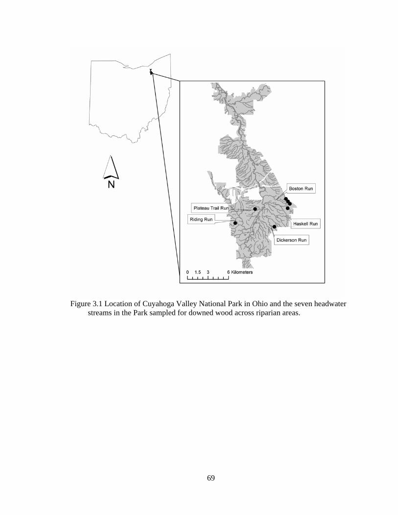
Figure 3.1 Location of Cuyahoga Valley National Park in Ohio and the seven headwater

streams in the Park sampled for downed wood across riparian areas.

69

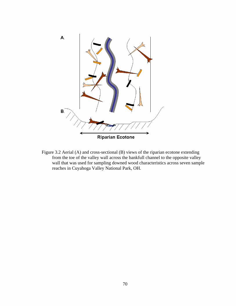
Figure 3.2 Aerial (A) and cross-sectional (B) views of the riparian ecotone extending

from the toe of the valley wall across the bankfull channel to the opposite valley wall that was used for sampling downed wood characteristics across seven sample reaches in Cuyahoga Valley National Park, OH.

70

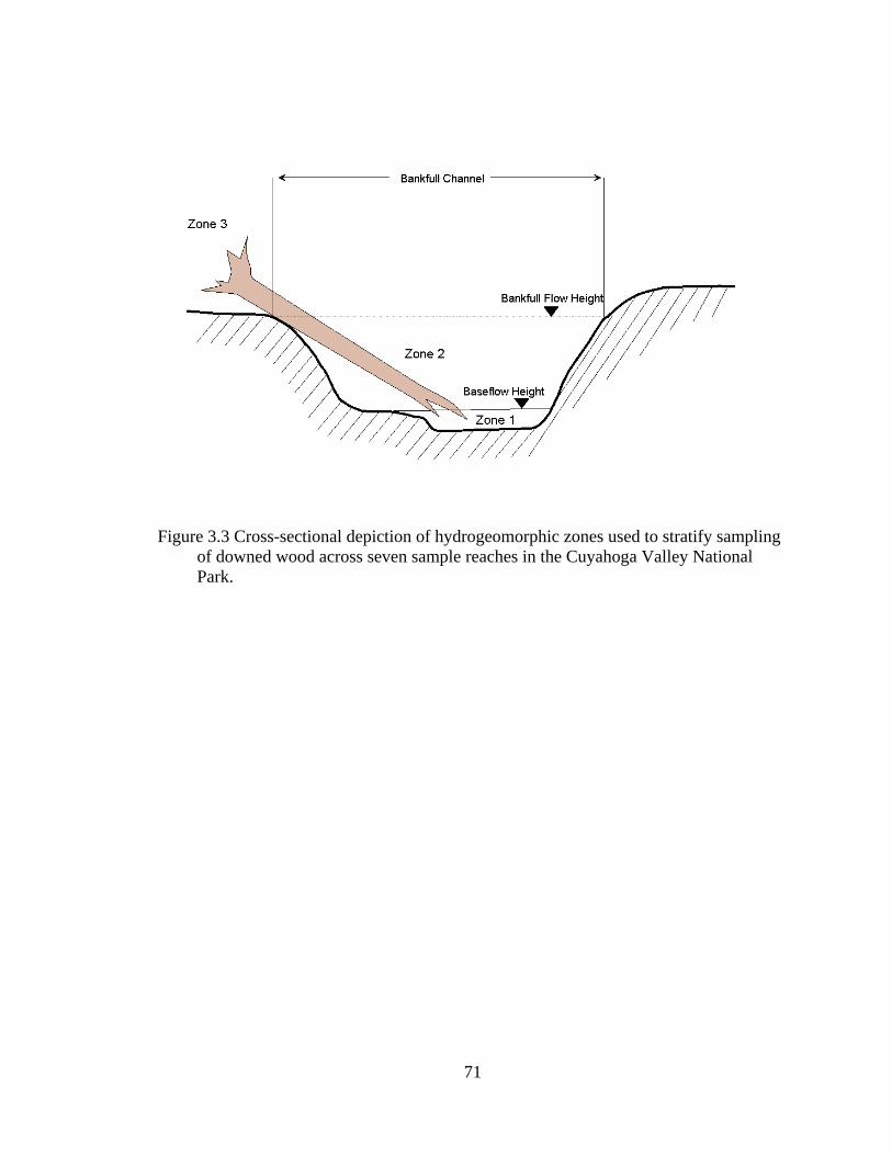
Figure 3.3 Cross-sectional depiction of hydrogeomorphic zones used to stratify sampling

of downed wood across seven sample reaches in the Cuyahoga Valley National Park.

71

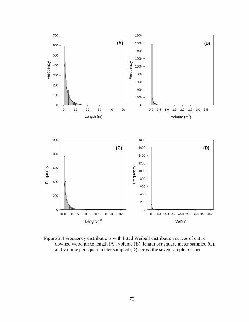
Length (m)

0 10 20 30 40 50

Freq

uenc

y

0

100

200

300

400

500

600

700

Volume (m3)

0.0 0.5 1.0 1.5 2.0 2.5 3.0 3.5

Freq

uenc

y

0

200

400

600

800

1000

1200

1400

1600

1800

Length/m2

0.000 0.005 0.010 0.015 0.020 0.025

Freq

uenc

y

0

200

400

600

800

1000

Vol/m2

0 5e-4 1e-3 2e-3 2e-3 2e-3 3e-3 3e-3 4e-3

Freq

uenc

y

0

200

400

600

800

1000

1200

1400

1600

1800

(A)

(C)

(B)

(D)

Figure 3.4 Frequency distributions with fitted Weibull distribution curves of entire

downed wood piece length (A), volume (B), length per square meter sampled (C), and volume per square meter sampled (D) across the seven sample reaches.

72

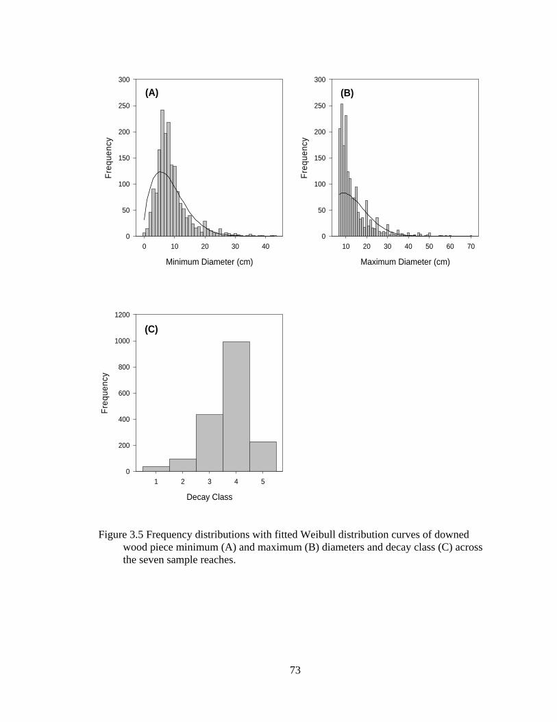
Maximum Diameter (cm)

10 20 30 40 50 60 70

Freq

uenc

y

0

50

100

150

200

250

300

Minimum Diameter (cm)

0 10 20 30 40

Freq

uenc

y

0

50

100

150

200

250

300

Decay Class

1 2 3 4 5

Freq

uenc

y

0

200

400

600

800

1000

1200

(A) (B)

(C)

Figure 3.5 Frequency distributions with fitted Weibull distribution curves of downed

wood piece minimum (A) and maximum (B) diameters and decay class (C) across the seven sample reaches.

73

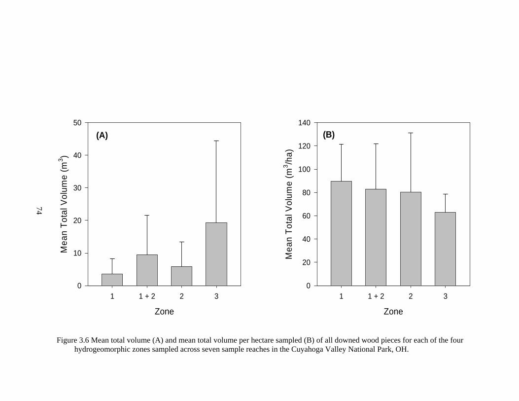
Zone

1 1 + 2 2 3M

ean

Tota

l Vol

ume

(m3 /h

a)0

20

40

60

80

100

120

140

Zone

1 1 + 2 2 3

Mea

n To

tal V

olum

e (m

3 )

0

10

20

30

40

50

(A) (B)

74

Figure 3.6 Mean total volume (A) and mean total volume per hectare sampled (B) of all downed wood pieces for each of the four

hydrogeomorphic zones sampled across seven sample reaches in the Cuyahoga Valley National Park, OH.

74

CHAPTER 4

ENVIRONMENTAL INFLUENCES ON MACROINVERTEBRATE ASSEMBLAGES ON HEADWATER STREAMS OF NORTHEASTERN OHIO

4.1 Introduction

It has long been recognized that streams and rivers are integrally tied to riparian

areas, especially in the headwaters of most watersheds (Minshall 1967, Nakano et al.

1999, Richards et al. 1996, Vannote et al. 1980, Wallace et al. 1997). In these headwater

streams biota are largely dependent on allochthonous inputs from surrounding riparian

forests for nutrients and habitat (Richards et al. 1996, Vannote et al. 1980). Recent

research suggest that headwater streams comprise up to 80% of a watershed’s stream

network (Meyer et al. 2001) and the majority of the streams at this scale do not appear as

blue lines on 1:24000 USGS topographic maps (Hansen 2001). For example, the Ohio

Environmental Protection Agency (OEPA) estimates there are approximately 33,800 km

(21,000 miles) of named streams, represented as blue-lines on USGS maps, and

approximately 185,000 km (115,000 miles) of unnamed streams in Ohio (OEPA 2002).

Recent research has suggested that these small headwater streams should be the focus of

restoration efforts because of their potential importance for nutrient processing (Peterson

et al. 2001). Historically, however, many of the headwater systems in Ohio and

75

elsewhere in the northeastern United States have received little attention from researchers

and have all but been ignored by land managers and developers.

As headwater streams often do not have pools of sufficient depth to sustain fish

populations, OEPA has been using macroinvertebrate and salamander assemblages to

monitor water quality in these systems (OEPA 2002). Although macroinvertebrates,

salamanders, and fish all can be found in stream ecosystems in at least some portion of

their life, they have very different physiologies and life histories, therefore, they may

react differently to various disturbances or processes at different scales (Karr 1981).

Macroinvertebrates are influenced strongly by microhabitat variables (Kaller and

Hartman 2004, Sandin and Johnson 2004, Stewart et al. 2003, Vinson and Hawkins

1998), and thus have been described as good indicators of local habitat conditions

(Lammert and Allan 1999, Plafkin et al. 1989). Salamanders are influenced by both

microhabitat and variables operating at larger (e.g., sub-basin) scales (Hyde and Simons

2001, Lowe and Bolger 2001, Welsh and Ollivier 1998, Wilson and Dorcas 2003), and

replace fish as the top vertebrate predator in many headwater stream systems (OEPA

2002). Although more common in recent years (e.g., Jackson and Harvey 1993, Lammert

and Allan 1999, Williams et al. 2003a), studies that examine how multiple taxa interact

with each other, and are in turn structured by habitat, are lacking for many types of

stream systems, especially headwater streams. Knowledge of factors affecting

assemblage structure of biota inhabiting headwater streams is necessary to better guide

restoration and management.

76

In 2004, we initiated a study to quantify the relationships between macroinvertebrate

assemblages and their biotic and abiotic habitat in headwater streams of northeastern

Ohio. The objective of the study was to investigate species-environment relationships

between macroinvertebrate assemblages and their environment in relatively undisturbed

headwater streams. Specifically, we determined composition and trophic structure of

macroinvertebrate assemblages, as well as, examined how environmental factors, such as

riparian forest and aquatic habitat and vertebrate predators, influence these assemblages.

Additionally, to understand how watershed position affects these relationships, sampling

occurred in both upstream and downstream headwater stream reaches.

4.2 Study Site

This study was conducted in Cuyahoga Valley National Park, OH, USA, an area

of over 13,400 ha (33,000 acres) comprised of relatively undeveloped land along 35

kilometers (22 miles) of the Cuyahoga River between the cities of Cleveland and Akron,

OH. The park’s location between two major metropolitan areas creates unique

management implications because of the urban-rural interface. Much of the park is

characterized by steep, forested ravine systems formed along the multiple tributaries to

the Cuyahoga River. The forests are second-growth (>70 years old) and composed of

mixed-mesophytic species (e.g., sugar maple, Acer saccharum Marsh; American beech,

Fagus grandifolia Ehrh.; northern red oak, Quercus rubra L.; shagbark hickory, Carya

ovata (P.Mill)K. Koch; and yellow poplar, Liriodendron tulipifera L..), representative of

the Erie Gorges Ecoregion. Our study focused on four perennial headwater streams,

specifically Boston Run, Langes Run, Riding Run, and an unnamed stream that will be

77

referred to as Perkins Trail Run (Figure 4.1). We defined headwater streams as those

draining less than 51.8 km2 (20 mi2), usually 1st, 2nd, or 3rd stream order following

Strahler (1952). Streams were selected as replicates based upon similar riparian forest age

(mature second-growth), riparian forest composition and structure (native species in a

multi-cohort stand), geomorphic landforms (the presence of fluvial floodplains and

terraces), stream gradient (1-5%), and substrate (minimal siltation observed) (Table 4.1).

4.3 Methods

To examine variation in the composition and trophic structure of

macroinvertebrate assemblages across watershed position, we sampled upstream and

downstream reaches of each stream in the summer of 2004, for a total of four upstream

(1st or 2nd stream order) stream reaches and four downstream (2nd or 3rd stream order)

stream reaches. Each 100 m reach was randomly selected and sampled for benthic

macroinvertebrates, riparian forest and aquatic habitat, fishes, and salamanders.

4.3.1 Macroinvertebrates

Each reach was sub-divided into three segments (approximately 33.33 m each)

and sampled for macroinvertebrates within each segment using both a surber sampler and

D-frame kicknet. A surber sampler was placed in flowing water and substrate was sifted

within a 0.25 m square area for three to five minutes. Riffles, runs, pools, and margins of

the stream within each segment were then jabbed with the D-frame kicknet for five

minutes. The samples were preserved in a 95% ethanol and rose bengal stain solution in

the field prior to transport back to the Stream Ecology Laboratory at The Ohio State

78

University, Columbus, OH. In the lab, samples were sorted and identified to Family level

of taxonomy. Recent studies indicate that identification to the family level is sufficient

for many ecological studies (Bowman and Bailey 1997, Dolédec et al. 2000, Hewlett

2000).

Abundance for each macroinvertebrate family was summarized by reach and

diversity indices were calculated, specifically, richness (S = number of families present),

Evenness (E = ), and Shannon Diversity Index

( ). Anderson-Darling

normality tests indicated non-normality of the assemblage composition data, so Mann-

Whitney U-tests were run to test for differences between mean diversity indices between

watershed positions (upstream versus downstream stream reaches). An alpha level equal

to 0.10 was used to indicate significant differences in all statistical analyses conducted.

SH ln/′

wherepi , speciesitheofproportiontheisppH thii ln∑=′

To analyze trophic structure, each family was categorized into one of four

functional feeding guilds (Allan 1995, Merritt and Cummins 1984, Williams et al. 2002;

Table 4.2): Collectors (collector-gatherers and collector-filterers), Predators (engulfers

and piercers), Scrapers (scrapers and grazers), or Shredders. Functional feeding guilds

were summarized for each stream reach and checked for normality with Anderson-

Darling normality tests. Following square root transformation to achieve normality,

student t-tests were used to test for differences in the number of individuals per guild

between watershed positions.

79

4.3.2 Riparian Forest Habitat

To characterize the riparian forest adjacent each sample reach, transects were

established perpendicular to stream-flow across the stream valley at 33, 66, and 100 m

within each reach. For each transect, circular plots (400-m2) were centered on stream

valley landforms (e.g. floodplain, terrace, valley toe-slope) and all overstory trees (woody

stems greater than 10 cm DBH, diameter at breast height = 1.4 m) were identified by

species and measured. Using a concave spherical densiometer held at DBH, percent

riparian forest cover was estimated from the center of the stream for each segment and

averaged for the entire stream reach.

Basal area of the riparian overstory, stem density (trees per hectare), and riparian

overstory species diversity indices were calculated for each plot and summarized for each

sample reach. Initial analyses suggested that several variables were not normally

distributed, consequently percent riparian forest cover was arc-sin square root

transformed, stem density was natural log transformed, and basal area was square root

transformed. Differences in mean riparian forest cover, basal area, and stem density

between watershed positions were tested with student t-tests. Riparian overstory species

diversity indices for each stream reach were non-normal and no transformations

adequately normalized these variables, so differences were tested between watershed

positions using Mann-Whitney U-tests.

80

4.3.3 Aquatic Habitat

To characterize the aquatic habitat of each sample stream reach, channel substrate

type (percent sand, silt, gravel, cobble, and boulder) was estimated visually within a 1 m

wide area of stream channel bottom at the end of each segment (0m, 33, 66, and 100 m),

and averaged for the entire stream reach (Williams et al. 2003b). The proportion of large

wood habitat was estimated visually for each segment and averaged for the entire stream

reach. Additionally, the width of the bankfull channel was measured at the end of each

segment and averaged for the entire sample reach to determine the approximate area

sampled.

Channel substrate and large wood habitat percent data were arc-sin square root

transformed for normally distributed data and tested for significant differences in mean

values between watershed positions using student t-tests.

4.3.4 Vertebrate Sampling

Fishes and salamanders are vertebrate predators of the headwater stream

macroinvertebrates studied and were sampled at all sample stream reaches. At all sites

where present, fish were sampled with single-pass electrofishing using a backpack unit

(Smith Root, Inc. Model LR-24 Electrofisher), encompassing the entire 100 m reach.

The fish were preserved in the field prior to transport back to the laboratory where they

were identified. Following protocols established by Ohio EPA (OEPA 2002),

salamanders were sampled within a randomly selected 30 m section of each stream reach

by turning over rocks and sifting leaf packs within the stream and the adjacent stream

81

bank. Sampling took place for a minimum of 30 min or the length of time it took to

search the entire section. When a salamander was found, it was identified to species and

released at the site of capture. Only salamander species with aquatic larval life-stages

were considered to be vertebrate predators of the macroinvertebrates studied. Because of

their close association with the stream during larval stages as well as for streamside adult

habitat usage, these species can be significant predators on invertebrates in headwater

streams (Petranka, 1998).

Fish and salamander species abundance was summarized for each sample stream

reach and density (fishes/m2 and salamanders/m2) was calculated. Fish and salamander

abundance data was combined to represent vertebrate predators of macroinvertebrate

assemblages and vertebrate diversity indices were calculated for each sample stream

reach. Density and diversity indices were square root transformed and tested for mean

differences between watershed positions using student t-tests.

4.3.5 Macroinvertebrate Assemblage-Environment Analyses

We used a form of direct gradient analysis, canonical correspondence analysis

(CCA), to examine the relationships between macroinvertebrate assemblages, both

compositional and trophic structure, and the measured environmental factors, both biotic

and abiotic. CCA is an ordination analysis comparable to multiple regression, where

variation in a dependent multivariate matrix is constrained and explained by a second

multivariate matrix (McCune and Grace 2002, ter Braak and Šmilauer 1997). To

characterize relationships between variation in macroinvertebrate assemblage

composition and each group of environmental factors, three separate CCAs were

82

conducted, one for each group of environmental factors analyzed: riparian forest habitat,

aquatic habitat, and vertebrates. The macroinvertebrate composition matrix for all three

CCAs contained abundance data for all macroinvertebrate families sampled per sample

reach. The riparian forest habitat matrix included percent riparian forest cover, basal

area, overstory diversity, and stem density, while the aquatic habitat matrix included

percent silt, sand, gravel, cobble, boulders, and large wood, and the vertebrate matrix

included fish/m2, salamanders/m2, and predator diversity.

A second series of three CCAs were conducted to characterize the relationships

between variation in macroinvertebrate assemblage trophic structure and each group of

environmental factors. The macroinvertebrate trophic structure matrix contained the

abundance of individuals per guild at each sample reach, while the riparian forest and

aquatic habitat and vertebrate matrices were the same as those used for the

macroinvertebrate composition CCA analyses.

For each of the CCA analyses, macroinvertebrate assemblage composition and

trophic structure were analyzed with each group of environmental factors separately.

However, the measured environmental factors spatially occur together and often interact.

To understand the influence of each group of environmental factors and their interactions

on the composition and trophic structure of macroinvertebrate assemblages, partial CCA

was used to further partition macroinvertebrate assemblage variation (Borcard et al. 1992;

Williams et al. 2002) into seven variance components: riparian forest habitat, aquatic

habitat, vertebrate predators, and the shared variation between the components that

cannot be partitioned into pure effects (Figure 4.2). Variance partitioning is done through

83

a series of CCAs where pure effects of each variable are determined by treating the other

variables as covariates. In partial CCA, the number of variables in the second

multivariate matrix used must equal N-1, where N equals the number of variance

components to be explained to avoid over-fitting the model. Six variables were selected

based on the individual CCA biplot scores, two from each group of measured

environmental factors with the two highest scores in each group selected. To partition

variation in the macroinvertebrate composition, the following environmental variables

were used: basal area, stem density, percent silt, percent sand, salamander density, and

fish density. To partition variation in the macroinvertebrate trophic structure, the

following environmental variables were used: percent riparian forest cover, basal area,

percent silt, percent boulder, salamander density, and fish density.

4.4 Results

A total of 12,691 individuals comprising twelve orders and 45 families of

macroinvertebrates were collected in the eight sample reaches (Table 4.2). Diversity

indices indicated downstream reaches have higher mean richness of macroinvertebrate

families, higher mean Shannon Diversity Index values, and assemblages that on average

are more evenly distributed than the upstream reaches (Table 4.3), though none are

statistically different (Mann-Whitney W= 15.5, P= 0.561; W= 14.0, P= 0.312; W= 17.0,

P= 0.885, respectively). The mean abundance of macroinvertebrates collected was

higher in downstream reaches than upstream, 1892 versus 1280 individuals, respectively

(Appendix). Functional feeding guild proportions also differed between upstream and

downstream reaches (Table 4.3). Specifically, mean percent of shredder species was

significantly higher in upstream reaches than downstream (5.76% ± 4.55 versus 0.78% ±

84

0.28; T-value= 2.81, = 0.04). Very few scraper species were collected and proportions

were similar between watershed positions (Table 4.3). Collector species were dominant

in both upstream and downstream reaches, but there was no significant difference

between upstream and downstream reaches (92.67% ± 1.15 and 86.24% ± 5.06,

respectively; T-value= -1.08; P= 0.33).

Riparian forest habitat differed between watershed positions with downstream

reach riparian forests having higher mean species richness and higher mean Shannon

Diversity Index values than upstream reach forests, however these differences were not

significant (W=529.0, P= 0.13; W= 538.5, P= 0.17, respectively) (Table 4.4). Upstream

and downstream reach riparian forests were not significantly different in species

distribution evenness (W= 630.0, P= 1.00) (Table 4.4). Mean basal area of riparian

overstory trees was higher along upstream reaches than downstream, but not significantly

different (10.38 m2/ha ± 7.73 and 8.60 m2/ha ± 6.17, respectively; W= 666.0, P = 0.60).

Mean stem density was higher along downstream reaches than upstream, but not

significantly different (161 trees/ ha ± 99 and 125 trees/ha ± 49, respectively; W= 550.5,

P= 0.23). Mean percent riparian forest cover was significantly higher along upstream

reaches than downstream (80.00% ± 7 and 55.31% ± 16.78, respectively; T-value= 2.81,

P= 0.05).

Aquatic habitat also differed between watershed positions with downstream

reaches having higher mean percent silt, sand, and gravel in channel substrates than

upstream reaches (Table 4.4), though differences were not significant (T-value= -1.42,

P= 0.23; T-value= -1.42, P= 0.21; T-value= -0.98, P= 0.38, respectively). Upstream

reaches had higher mean percent cobble and boulder in the channel than downstream

85

reaches (Table 4.4), though differences were again not significant (T-value= 0.38, P=

0.72; T-value= 1.44, P= 0.21, respectively). Mean percentage of large wood habitat was

higher in upstream reaches than downstream but the difference was not significant

(15.00% ± 3.95 versus 12.19% ± 3.29, T-value= 1.07, P= 0.33).

Vertebrate predators were present in all eight sample reaches, however

salamanders and fish were not located together at all reaches. Salamanders were present

at seven of the eight stream reaches, specifically all four upstream and three downstream

reaches. Two salamander species with aquatic larval stages were collected: the northern

dusky salamander (Desmognathus fuscus fuscus) and the two-lined salamander (Eurycea

bislineatea). Fish were present at five of the eight stream reaches, specifically one

upstream reach and all four downstream reaches. While thirteen fish species were

collected, two species were most abundant and present at all sample reaches with fish: the

black-nosed dace (Rhinichthys atratulus) and the northern creek chub (Semotilus

atromaculatus). Vertebrates had higher richness in downstream reaches, had higher

evenness, and were more diverse than in upstream reaches (Table 4.4); however, the

differences were not statistically significant (T-value= -1.63, P= 0.202; T-value= -1.78, P

=0.173; and T-value= -2.04, P=0.111, respectively). Salamander density tended to be

higher in upstream reaches than downstream but this difference was not significant (0.10/

m2± 0.11 and 0.02/ m2 ± 0.02, respectively; T-value= 2.13, P= 0.100). Fish density was

significantly higher downstream (0.14/ m2± 0.11 vs. 0.02/ m2± 0.05, respectively; T-

value= -2.45, P= 0.058).

86

The CCAs reveal the measured environmental factors are indicators of upstream

and downstream reach differences, while macroinvertebrate assemblage composition are

relatively homogenous in their distribution and may be more related to site specific

differences than the measured environmental factors (Figure 4.3, A-C). Similarly,

macroinvertebrate trophic structure is not well explained by the measured environmental

factors, however, the factors successfully discriminated between the upstream from

downstream reaches (Figure 4.3, D-F). For riparian forest habitat, upstream reaches were

positively associated with increased percent riparian forest cover and basal area, while

downstream reaches were positively associated with increased stem density and higher

overstory species diversity (Figure 4.3, A and D). Upstream sample reach aquatic

habitat had more boulders, while downstream reaches were positively associated with silt

and gravel (Figure 4.3, B and E). Reaches positively associated with percent cobble and

boulders were negatively associated with percent sand. Upstream reaches were positively

associated with higher salamander density, while downstream reaches are positively

associated with higher fish density and predator diversity (Figure 4.3, CCA C and F).

Variance partitioning between the three groups of measured environmental factors

indicates that 89% percent of the variation in macroinvertebrate assemblage composition

can be explained by the three factor groups, with 25.5% explained by the shared variation

between aquatic habitat and vertebrate predators and 24.3% explained by vertebrate

predators alone (Figure 4.4). While variation in composition can be explained by shared

variation and individual groups, variation in macroinvertebrate trophic structure is

explained primarily by the individual groups of environmental factors with essentially no

shared variation (Figure 4.5). Aquatic habitat explains the most variation in structure

87

with 37.2% explained followed by riparian forest habitat with 27.9% explained. The

three groups of environmental factors explain 93% of the variation in the trophic

structure of macroinvertebrate assemblages (Figure 4.5).

4.5 Discussion

Overall, we found a trend of higher richness, diversity, and abundance of

macroinvertebrates in downstream reaches, though this trend was not statistically

significant. This pattern of higher species richness downstream is consistent with stream

models, such as the River Continuum Concept (Vannote et al. 1980), that predict more

complex assemblage structure of macroinvertebrates in downstream reaches. These

models also predict higher proportion of shredder taxa upstream, which process leaf litter

that enters the system (Minshall et al. 1985). Also predicted by the models is the pattern

that fewer scrapers are found in upstream areas. Scrapers tend to become more abundant

when canopies are open allowing periphyton growth due to increased sunlight on the

water column. Most of the sites we sampled had relatively closed riparian forest

overstories, and thus, did not allow for sufficient growth of periphyton to permit greater

abundances of scrapers. Sites in our study area were dominated by collector taxa,

specifically chironimids. It may be that the high degree of disturbance from surrounding

urbanization is creating an environment that allows chironomid taxa to dominate the

assemblages similar to rural-urban interface headwater streams in Connecticut (Urban et

al. 2006). This pattern is corroborated by the increased dominance of finer substrata in

downstream reaches.

88

Ordination analyses show a distinct separation of upstream and downstream

macroinvertebrate faunas. Variance partitioning suggests this may be because of the

strong effects that predatory fishes and salamanders have in upstream areas. When water

levels in headwater stream reaches are low, especially in the dry periods of the summer,

predators can act to structure the macroinvertebrate assemblages, particularly in the

smallest streams (Williams et al. 2003b). Variance partitioning also suggests that aquatic

habitat may be a strong determinant of macroinvertebrate composition and structure in

these headwater streams, which follows what has been found in other headwater systems

(Angradi 1996, Johnson et al. 2003). However, the macroinvertebrate taxa tend to

concentrate towards the center of the CCA ordination diagrams, suggesting that local site

fidelity may be an even larger controlling factor on assemblage composition and structure

than the measured environmental factors in this study. This may indicate that there is

strong site-level fidelity in the assemblages. Thus, the spatial location of sites may have

a stronger influence than the local environmental conditions. This pattern has been

documented in other headwater systems (Williams et al. 2002, Williams et al. 2005). In

previous work, this has been because of the overriding influence of refugia areas during

low water. The location of refugia habitat, in this case deep pools, may be critically

important areas of future recolonization and may override many species-environment

relationships.

Because of the importance of aquatic habitat, particularly the availability of

refugia habitat, to macroinvertebrate assemblage composition and functional feeding

guild structure, high quality aquatic habitat needs to be a priority for ecological

restoration and management of these headwater systems. Additionally, the effects of

89

surrounding urbanization may be more far reaching than known as these headwater

stream sample reaches were selected due to their relatively undisturbed condition, yet, the

macroinvertebrate fauna was still dominated by chironimid species. The effects of

human disturbance may be affecting micro-habitat variables not sampled in this study and

resulting in high site-fidelity among assemblages. Further work to assess the effect of

human disturbances on macroinvertebrate assemblages is needed in these headwater

systems.

In addition to aquatic habitat, riparian forest habitat also explained a large portion

of variation in macroinvertebrate functional feeding guild structure, emphasizing the

connection between terrestrial and aquatic ecosystems in these headwater stream systems.

For example, in this study, large wood was considered a component of the aquatic habitat

even though its source is the riparian forest. Also, the nearly complete riparian forest

cover that is characteristic of headwater streams is responsible for regulating temperature

as well as organic matter and sediment input into the aquatic system, all critical to the

quality of aquatic habitat and macroinvertebrate assemblages. Additional research is

needed on the connections between riparian areas and their adjacent streams. While the

traditional reductionist approach to science tends to treat the two as discrete ecosystems,

each influences the other and research should be collaborative so that common patterns

can be revealed, especially across landscapes and ecoregions. This type of holistic

approach will be needed for effective restoration and management of headwater stream

systems.

90

4.6 Potential Limitations of this Study

Following completion of this study, several limitations were noted in hindsight

that we encourage reviewers to consider when reading this chapter. Because the

macroinvertebrates assemblages were identified only to the Family level of taxonomy

and not to the Genus or Species level, the results and conclusions presented in this study

are coarse and may have been significantly different if further identification of the

collected macroinvertebrates had been done. Additionally, using Family level taxonomy

in functional feeding guild categorization is also coarse and may have changed our results

and conclusions had finer taxonomy work been done. Further, we assume that streamside

salamanders are preying upon macroinvertebrates, comprising our predator component of

the analyses, yet we did not confirm this assumption with salamander gut analyses. As a

result, the results and conclusions of this chapter should not be used on their own as a

reference condition for headwater stream management without additional scientific

results from the region. However, while the macroinvertebrate data may be weak, the

statistical analyses utilized in this study are novel and can be applied to other studies of

species-environment relationships where the influence of specific components of the

relationships can be determined in relation to other components.

4.7 References

Allan, J.D. 1995. Stream ecology: structure and function of running waters. Chapman and

Hall, London. 388p.

91

Angradi, T.R. 1996. Inter-habitat variation in benthic community structure, function, and organic matter storage in 3 Appalachian headwater streams. Journal of the North American Benthological Society 15(1): 42-63.

Borcard, D., P. Legendre, and P. Drapeau. 1992. Partialling out the spatial component of ecological variation. Ecology 73(3):1045-1055.

Bowman, M.F. and R.C. Bailey. 1997. Does taxonomic resolution affect the multivariate description of the structure of freshwater benthic macroinvertebrate communities? Canadian Journal of Fisheries and Aquatic Sciences 54: 1802-1807.

Dolédec, S., J.M. Olivier, and B. Statzer. 2000. Accurate description of the abundance of taxa and their biological traits in stream invertebrate communities: effects of taxonomic and spatial resolution. Archiv fur Hydrobiologie 148: 25-43.

Dufrene, M. and P. Legendre. 1997. Species assemblages and indicator species: the need for a flexible asymmetrical approach. Ecological Monographs 67: 345-366.

Hewlett, R. 2000. Implications of taxonomic resolution and sample habitat for stream classification at a broad geographic scale. Journal of the North American Benthological Society 19: 352-361.

Hyde, E.J. and T.R. Simons. 2001. Sampling plethodontid salamanders: Sources of variability. Journal of Wildlife Management 65: 624-632.

Jackson, D.A. and H.H. Harvey. 1993. Fish and benthic invertebrates: community concordance and community-environment relationships. Canadian Journal of Fisheries and Aquatic Sciences 50: 2641-2651.

Johnson, L.B., D.H. Breneman, and C. Richards. 2003. Macroinvertebrate community structure and function associated with large wood in low gradient streams. River Research and Applications 19: 199-218.

Kaller, M.D. and K.J. Hartman. 2004. Evidence of a threshold level of fine sediment accumulation for altering benthic macroinvertebrate communities. Hydrobiologia 518: 95-104.

Karr, J.R. 1981. Assessment of biotic integrity using fish communities. Fisheries 6:21-27.

92

Lammert, M. and J.D. Allan. 1999. Assessing biotic integrity of streams: effects of scale in measuring the influence of land use/cover and habitat structure on fish and macroinvertebrates. Environmental Management 23: 257-270.

Lowe, W.H., and D.T. Bolger. 2002. Local and landscape-scale predictors of salamander abundance in New Hampshire headwater streams. Conservation Biology 16: 183-193.

Merritt, R.W. and K.W. Cummins. 1984. Introduction to the aquatic insects of North America. Kendall/ Hunt Publishing: Dubuque, IA, pp. 722.

Meyer, J.L. and J.B. Wallace. 2000. Lost linkages and lotic ecology: rediscovering small streams. pp. 295-317 In M.C. Press, N.J. Huntly, and S.A. Levin editors, Ecology: An achievement and challenge. Blackwell Science, Ames, IA, pp. 406.

Minshall, G.W. 1967. Role of allochthonous detritus in the trophic structure of a woodland springbrook community. Ecology 48: 139-149.

Minshall, G.W., K.W. Cummins, R.C. Petersen, D.A. Bruns, and C.E. Cushing. 1985. Developments in stream ecosystem theory. Canadian Journal of Fisheries and Aquatic Science 42: 1045-1055.

Nakano, S., H. Miyasaka, and N. Kuhara. 1999. Terrestrial-aquatic linkages: riparian arthropod inputs alter trophic cascades in a stream food web. Ecology 80: 2435-2441.


Peterson, B.J., W.M. Wollheim, P.J. Mullolland, J.R. Webster, J.L. Meyer, J.L. Tank, E. Marti, W.B. Bowden, H.M. Valett, A.E. Hershey, W.H. McDowell, W.K. Dodds, S.K. Hamilton, S. Gregory, and D.D. Morrell. 2001. Control of nitrogen export from watersheds by headwater streams. Science 292: 86-89.

Plafkin, J.L, M.T. Barbour, K.D. Porter, S.K. Gross, and R.M. Hughes. 1989. Rapid bioassessment protocols for use in stream and rivers: macroinvertebrates and fish. EPA/444/4-89-011. U.S. Environmental Protection Agency, Washington D.C.

93

Richards, C., L.B. Johnson, and G.E. Host. 1996. Landscape-scale influences on stream habitats and biota. Canadian Journal of Fisheries and Aquatic Sciences 53: 295-311.

Sandin, L. and R.K. Johnson. 2004. Local, landscape and regional factors structuring benthic macroinvertebrate assemblages in Swedish streams. Landscape Ecology 19:501-514.

Stewart, T.W., T.L. Shumaker, and T.A. Radzio. 2003. Linear and nonlinear effects of habitat structure on composition and abundance in the macroinvertebrate community of a large river. The American Midland Naturalist 149: 293-305.


ter Braak, C. J .F. and P. Šmilauer. 1997. Canoco for Windows version 4.02. Centre for Biometry. Wageningen, Netherlands.

Urban, M.C., D.K. Skelly, D. Burchsted, W. Price, and S. Lowry. 2006. Stream communities across a rural-urban landscape gradient. Diversity and Distributions 12: 337-350.

Vannote, R.L., G.W. Minshall, K.W. Cummins, J.R. Sedell, and C.E. Cushing. 1980. The river continuum concept. Canadian Journal of Fisheries and Aquatic Sciences. 37:130-137.

Vinson, M.R. and C.P. Hawkins. 1998. Biodiversity of stream insects: variation at local, basin, and regional scales. Annual Review of Entomology 43: 271-293.

Wallace, J.B., S.L. Eggert, J.L. Meyer, and J.R. Webster. 1997. Multiple trophic levels of a forest stream linked to terrestrial litter inputs. Science 277:102-104.

Welsh, H.H. and L.M. Ollivier. 1998. Stream amphibians as indicators of ecosystem stress: a case study from California’s redwoods. Ecological Applications 8: 1118-1132.

Williams. L.R., C.M. Taylor, M.L. Warren Jr., and J.A. Clingenpeel. 2002. Large-scale effects of timber harvesting on stream systems in the Ouachita Mountains, Arkansas. Environmental Management 29: 76-87.

94

95

Williams, L.R., C.M. Taylor, M.L. Warren Jr., and J.A. Clingenpeel. 2003a. Environmental variability, historical contingency, and the structure of regional fish and macroinvertebrate faunas in Ouachita Mountain stream systems. Environmental Biology of Fishes 67: 203-216.

Williams, L.R., C.M. Taylor, and M.L. Warren, Jr. 2003b. Influence of fish predation on assemblage structure of macroinvertebrates in an intermittent stream. Transactions of the American Fisheries Society 132: 120-130.

Williams, L.R., T.H. Bonner, J.D. Hudson III, M.G. Williams, T.R. Leavy, and C.S. Williams. 2005. Interactive effects of environmental variability and military training on stream biota of three headwater drainages in Western Louisiana. Transactions of the American Fisheries Society 134: 192-206.

Wilson, J.D. and M.E. Dorcas. 2003. Effects of habitat disturbance on stream salamanders: implications for buffer zones and watershed management. Conservation Biology 17: 763-771.

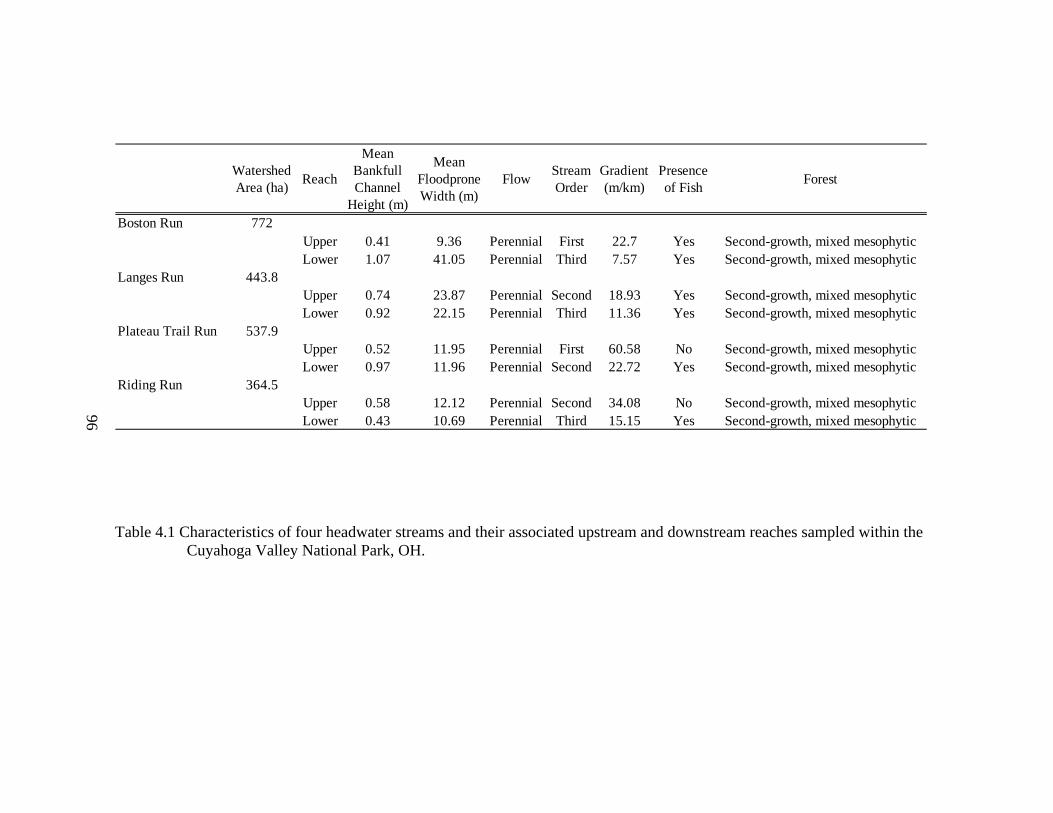
96



Height (m)


Flow Stream Order

Gradient (m/km)






96

Table 4.1 Characteristics of four headwater streams and their associated upstream and downstream reaches sampled within the Cuyahoga Valley National Park, OH.

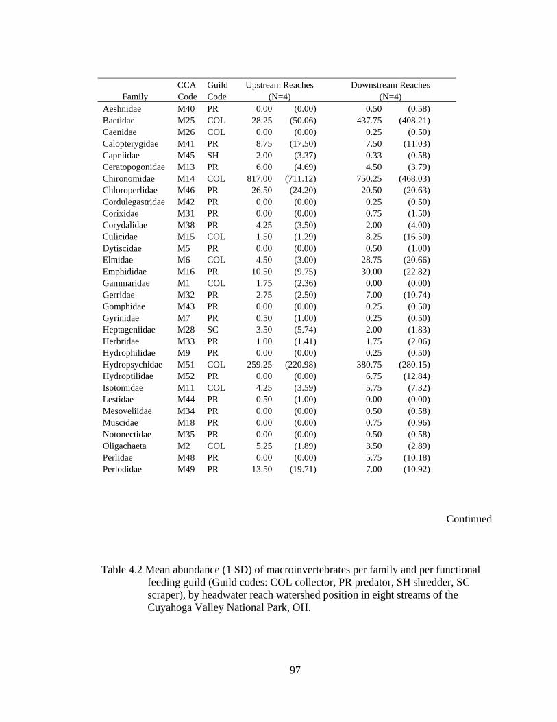
CCA Guild Upstream Reaches Downstream Reaches

Family Code Code (N=4) (N=4) Aeshnidae M40 PR 0.00 (0.00) 0.50 (0.58) Baetidae M25 COL 28.25 (50.06) 437.75 (408.21) Caenidae M26 COL 0.00 (0.00) 0.25 (0.50) Calopterygidae M41 PR 8.75 (17.50) 7.50 (11.03) Capniidae M45 SH 2.00 (3.37) 0.33 (0.58) Ceratopogonidae M13 PR 6.00 (4.69) 4.50 (3.79) Chironomidae M14 COL 817.00 (711.12) 750.25 (468.03) Chloroperlidae M46 PR 26.50 (24.20) 20.50 (20.63) Cordulegastridae M42 PR 0.00 (0.00) 0.25 (0.50) Corixidae M31 PR 0.00 (0.00) 0.75 (1.50) Corydalidae M38 PR 4.25 (3.50) 2.00 (4.00) Culicidae M15 COL 1.50 (1.29) 8.25 (16.50) Dytiscidae M5 PR 0.00 (0.00) 0.50 (1.00) Elmidae M6 COL 4.50 (3.00) 28.75 (20.66) Emphididae M16 PR 10.50 (9.75) 30.00 (22.82) Gammaridae M1 COL 1.75 (2.36) 0.00 (0.00) Gerridae M32 PR 2.75 (2.50) 7.00 (10.74) Gomphidae M43 PR 0.00 (0.00) 0.25 (0.50) Gyrinidae M7 PR 0.50 (1.00) 0.25 (0.50) Heptageniidae M28 SC 3.50 (5.74) 2.00 (1.83) Herbridae M33 PR 1.00 (1.41) 1.75 (2.06) Hydrophilidae M9 PR 0.00 (0.00) 0.25 (0.50) Hydropsychidae M51 COL 259.25 (220.98) 380.75 (280.15) Hydroptilidae M52 PR 0.00 (0.00) 6.75 (12.84) Isotomidae M11 COL 4.25 (3.59) 5.75 (7.32) Lestidae M44 PR 0.50 (1.00) 0.00 (0.00) Mesoveliidae M34 PR 0.00 (0.00) 0.50 (0.58) Muscidae M18 PR 0.00 (0.00) 0.75 (0.96) Notonectidae M35 PR 0.00 (0.00) 0.50 (0.58) Oligachaeta M2 COL 5.25 (1.89) 3.50 (2.89) Perlidae M48 PR 0.00 (0.00) 5.75 (10.18) Perlodidae M49 PR 13.50 (19.71) 7.00 (10.92)

Continued

Table 4.2 Mean abundance (1 SD) of macroinvertebrates per family and per functional feeding guild (Guild codes: COL collector, PR predator, SH shredder, SC scraper), by headwater reach watershed position in eight streams of the Cuyahoga Valley National Park, OH.

97

98

Table 4.2 Continued

Philopotamidae M54 COL 0.25 (0.50) 0.25 (0.50) Polycentropodidae M56 COL 0.00 (0.00) 0.50 (0.58) Psephenidae M10 SC 0.00 (0.00) 2.50 (3.00) Psychodidae M19 COL 0.25 (0.50) 0.00 (0.00) Pyralidae M37 SH 0.25 (0.50) 0.50 (0.58) Rhyacophilidae M57 PR 0.50 (0.58) 0.00 (0.00) Sialidae M39 PR 3.25 (2.75) 1.25 (1.50) Simuliidae M21 COL 9.50 (13.18) 132.25 (162.67) Sminthuridae M12 COL 0.50 (1.00) 0.00 (0.00) Stratiomyidae M22 COL 1.50 (2.38) 0.25 (0.50) Tabanidae M23 PR 9.50 (8.39) 9.25 (7.50) Tipulidae M24 SH 48.50 (19.16) 16.00 (15.56) Veliidae M36 PR 5.00 (2.94) 14.75 (20.16) Individuals 1,280.50 (816.29) 1,892.25 (1,080.84) Shredders 50.8 (22.1) 16.75 (15.65) Scrapers 3.5 (5.74) 4.5 (3.32) Collectors 1134 (761) 1749 (984) Predators 92.5 (53.7) 122.5 (80.6)

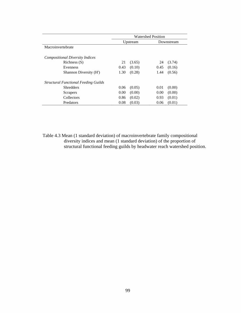
Watershed Position Upstream Downstream Macroinvertebrate Compositional Diversity Indices Richness (S) 21 (3.65) 24 (3.74) Evenness 0.43 (0.10) 0.45 (0.16) Shannon Diversity (H') 1.30 (0.28) 1.44 (0.56) Structural Functional Feeding Guilds Shredders 0.06 (0.05) 0.01 (0.00) Scrapers 0.00 (0.00) 0.00 (0.00) Collectors 0.86 (0.02) 0.93 (0.01) Predators 0.08 (0.03) 0.06 (0.01)

Table 4.3 Mean (1 standard deviation) of macroinvertebrate family compositional diversity indices and mean (1 standard deviation) of the proportion of structural functional feeding guilds by headwater reach watershed position.

99

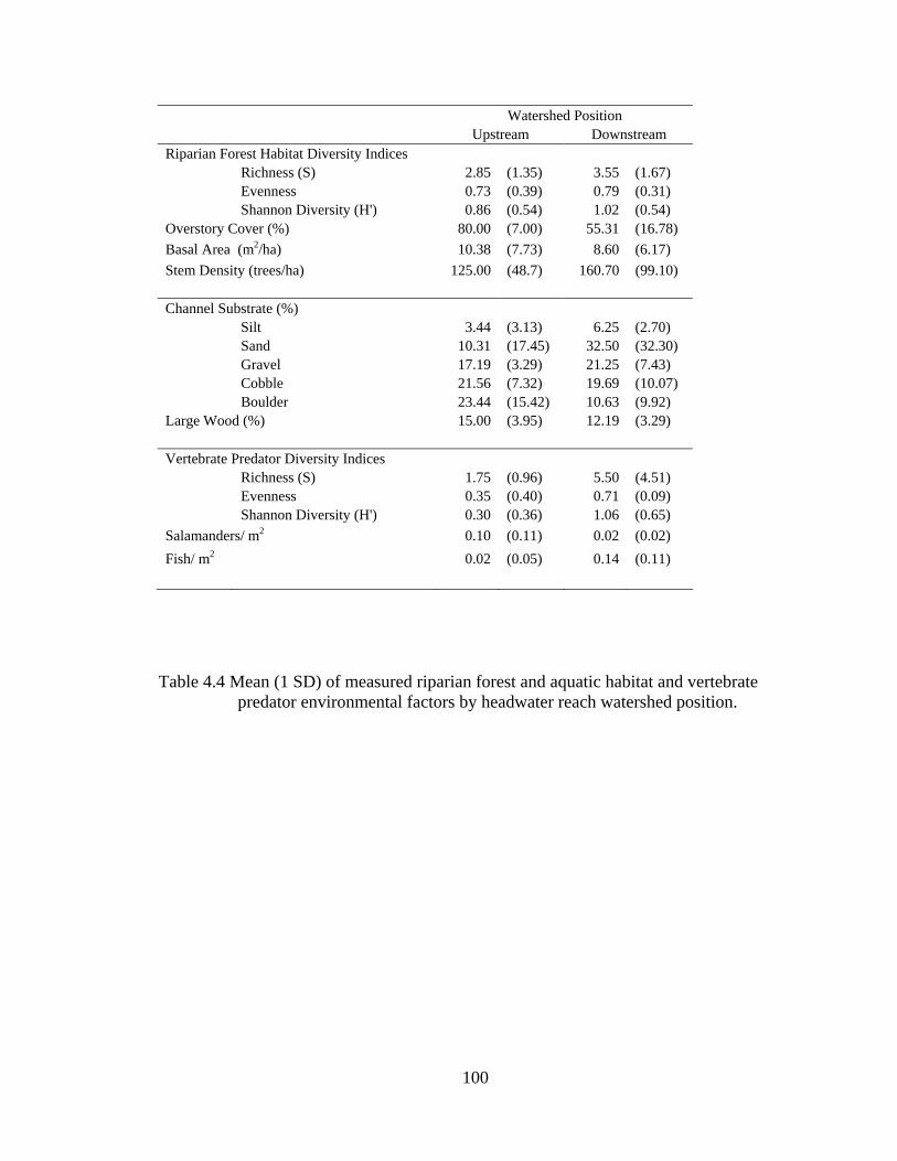
Watershed Position Upstream Downstream Riparian Forest Habitat Diversity Indices Richness (S) 2.85 (1.35) 3.55 (1.67) Evenness 0.73 (0.39) 0.79 (0.31) Shannon Diversity (H') 0.86 (0.54) 1.02 (0.54) Overstory Cover (%) 80.00 (7.00) 55.31 (16.78) Basal Area (m2/ha) 10.38 (7.73) 8.60 (6.17) Stem Density (trees/ha) 125.00 (48.7) 160.70 (99.10) Channel Substrate (%) Silt 3.44 (3.13) 6.25 (2.70) Sand 10.31 (17.45) 32.50 (32.30) Gravel 17.19 (3.29) 21.25 (7.43) Cobble 21.56 (7.32) 19.69 (10.07) Boulder 23.44 (15.42) 10.63 (9.92) Large Wood (%) 15.00 (3.95) 12.19 (3.29) Vertebrate Predator Diversity Indices Richness (S) 1.75 (0.96) 5.50 (4.51) Evenness 0.35 (0.40) 0.71 (0.09) Shannon Diversity (H') 0.30 (0.36) 1.06 (0.65) Salamanders/ m2 0.10 (0.11) 0.02 (0.02) Fish/ m2 0.02 (0.05) 0.14 (0.11)

Table 4.4 Mean (1 SD) of measured riparian forest and aquatic habitat and vertebrate predator environmental factors by headwater reach watershed position.

100

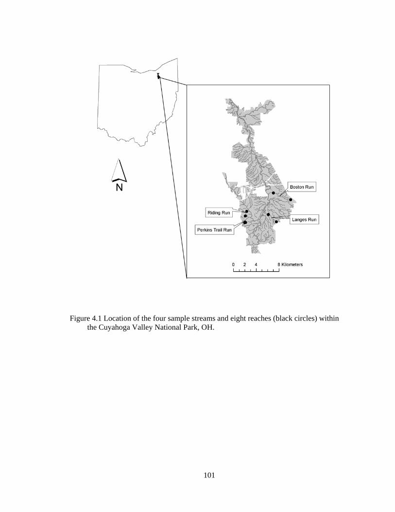
Figure 4.1 Location of the four sample streams and eight reaches (black circles) within the Cuyahoga Valley National Park, OH.

101

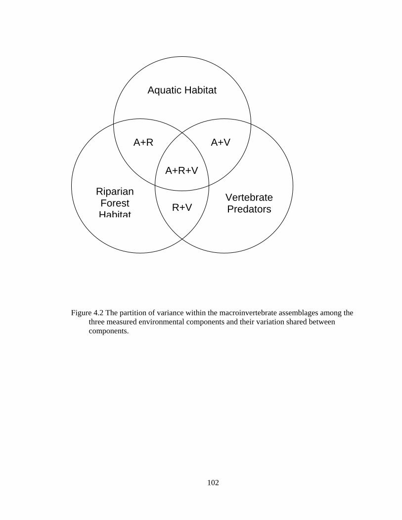
A+R A+V

Riparian Forest Habitat

Vertebrate Predators R+V

A+R+V

Aquatic Habitat

Figure 4.2 The partition of variance within the macroinvertebrate assemblages among the three measured environmental components and their variation shared between components.

102

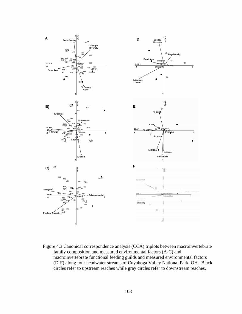
103

A

B)

C)

D

E

F

Figure 4.3 Canonical correspondence analysis (CCA) triplots between macroinvertebrate family composition and measured environmental factors (A-C) and macroinvertebrate functional feeding guilds and measured environmental factors (D-F) along four headwater streams of Cuyahoga Valley National Park, OH. Black circles refer to upstream reaches while gray circles refer to downstream reaches.

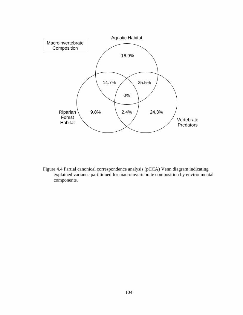
25.5%14.7%

24.3%

0%

2.4% 9.8%

16.9%

Macroinvertebrate Composition

Vertebrate Predators


Aquatic Habitat

Figure 4.4 Partial canonical correspondence analysis (pCCA) Venn diagram indicating explained variance partitioned for macroinvertebrate composition by environmental components.

104

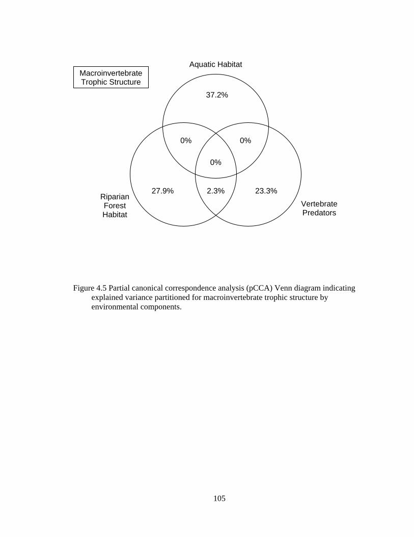
0%

0% 0%


Vertebrate Predators

27.9% 2.3% 23.3%

Aquatic Habitat Macroinvertebrate Trophic Structure

37.2%

Figure 4.5 Partial canonical correspondence analysis (pCCA) Venn diagram indicating explained variance partitioned for macroinvertebrate trophic structure by environmental components.

105

CHAPTER 5

A FUNCTIONAL APPROACH TO RIPARIAN DELINEATION USING GEOSPATIAL METHODS

5.1 Introduction

Historically, there have been a variety of methods used to delineate riparian areas.

These include those based upon physical attributes such as erosion (e.g., Trimble and

Sartz 1957, Sparovek et al. 2002), streamside shading based on tree heights (Brown

1980), hydric soils (USDA Forest Service, 1994), and hydrologic processes (Hupp and

Osterkamp 1996). Others have proposed using biological attributes to delineate riparian

areas including amphibian habitat use (Crawford and Semlitsch 2007, Perkins and Hunter

2006, Semlitsch and Bodie 2003), freshwater metazoan species (Ward et al. 1998), plant

community vegetation patterns (Hagan et al. 2006, Xang 2007), the presence of wetland

or wetland facultative species (Dall et al. 1998) and the minimum width to conserve

maximum species richness (Spackman and Hughes 1995).

Despite these efforts, we often attempt to determine the “minimum width” of

riparian areas and use this value to set aside riparian buffers. Riparian areas, however,

are more than just floodplains or the near-stream environments. Characterized as

biologically diverse ecotones between aquatic and terrestrial ecosystems, riparian areas

106

provide numerous important ecological services, including regulating the flow of water,

sediments and nutrients across system boundaries, contributing organic matter to the

aquatic system, increasing bank stability, reducing erosion, and creating key plant and

wildlife habitat (Gregory et al. 1991). As a result, these unique ecotones often cannot be

encompassed using a common, simple fixed-width approach (e.g., a 50 ft buffer; 1 pixel

buffers using LANDSAT imagery). Fixed-width approaches may result in significant

errors when determining riparian extent and characteristics and are questionable as they

are not based on the functional relationships of riparian areas and do not reflect the actual

riparian area on the ground. For example, areas that are clearly riparian, such as broad

floodplains associated with the larger rivers, may extend beyond a fixed buffer width.

Alternatively, lands that are arguably not riparian might be included in a fixed-width

buffer, especially along headwater streams.

5.2 A Functional Geospatial Approach to Riparian Delineation

In order to properly manage, restore, and conserve riparian areas for their unique

ecological functions, riparian delineation methods need to incorporate a more holistic

view of riparian areas to be more accurate and representative of the complexity and

functions provided by these ecotones (Swanson and Franklin 1992). Ilhardt et al. (2000)

and Verry et al. (2004) suggested a hydrogeomorphic delineation model that uses stream

valley geomorphology to predict flood-prone area and the likely extent of the riparian

area surrounding a stream or river. This functional definition includes a variety of

ecosystem functions, including those occurring in aquatic (e.g., channel), flood prone

(e.g., flood dispersal of sediment, plants, and animals) and upland zones (e.g., slumps,

107

slides, subsurface water and nutrient flow) that interact strongly with the surface water

during average, bankfull, and flood flow conditions (Verry et al. 2004). This method is a

probabilistic approach rather than a fixed approach as areas delineated are those likely to

be riparian, thus protecting the valuable functional ecosystem services riparian areas

provide (Figure 5.1).

When developing landscape management plans, geospatial methods are ideal for

landscape-scale analyses such as riparian areas because of their connection to the

terrestrial and aquatic ecosystems across watersheds. Typical geospatial approaches to

riparian delineation require accurate stream channel data around which buffers are

created to determine riparian setbacks, etc. However, due to the dynamic constructive

and destructive fluvial processes characterized by riparian areas, stream channel data

must be frequently updated and have high resolution in order to be considered accurate.

While Verry et al. (2004) developed the functional approach to riparian delineation to be

used in the field, because this approach is based upon stream valley geomorphology

rather than the stream channel it is possible to use digital data sources to delineate

riparian areas remotely on a landscape scale. When planning riparian management across

a large landscape, remote delineation is efficient and ideal.

5.3 Implementing the Functional Approach in the Cuyahoga Valley National Park

The Cuyahoga Valley National Park (CVNP) in northeastern Ohio encompasses

over 13,355 ha (33,000 acres) for both conservation as well as recreation, including 35.4

km (22 miles) of the Cuyahoga River and over 306 km (190 miles) of ephemeral and

108

perennial tributary streams (Figure 5.2). The CVNP was first designated a National

Recreation Area in 1974 and became a National Park in 2000. The park’s location

between the two major metropolitan areas of Cleveland and Akron, OH creates unique

management implications due to the diverse urban-rural interface that characterizes the

landscape, including balancing ecological conservation with recreation that serves

approximately 3 million visitors annually. Much of the development in the park has

occurred in the floodplain of the Cuyahoga River, including past and current agriculture,

a municipality (Peninsula), and several high-impact recreational areas such as ski areas

and golf courses. The large remainder of the park is undeveloped land characterized by

steep, forested ravine systems formed along the multiple tributaries to the Cuyahoga

River. The forests are mature second-growth (>70 years old) and composed of mixed-

mesophytic species (e.g. sugar maple, Acer saccharum Marsh; American beech, Fagus

grandifolia Ehrh.; northern red oak, Quercus rubra L.; shagbark hickory, Carya ovata

(P.Mill)K. Koch; and yellow poplar, Liriodendron tulipifera L.).

With the large number of riparian areas, all in various conditions, CVNP

managers and ecologists desire to develop a comprehensive riparian management plan

that moves beyond the fixed-width method to a more functional riparian delineation

approach. The first step in creating a management plan involves delineating riparian

areas. Using the functional approach of Ilhardt et al. (2000) and Verry et al (2004), we

used geospatial methods to functionally delineate riparian areas within CVNP.

109

5.4 Using GIS to Functionally Delineate Riparian Areas

To aid in the digital delineation of riparian areas in the CVNP, we utilized several

digital data sources available from national sources, county engineers, and the park itself

(Table 1). All GIS analyses were done using ArcGIS® software, ESRI (Redlands, CA).

Using a one mile buffer around the CVNP boundary, we determined which areas to

include for riparian area delineation within the park as well as areas just upstream from

the park. For ease of digital delineation, we divided the area by twenty-seven

subwatersheds each flowing into the Cuyahoga River (Figure 5.3). Because the

functional riparian area is based upon stream valley geomorphology, riparian areas could

be delineated with topographic data only. However, for ease and improved accuracy,

several additional files were used to help delineate riparian areas including aerial photos

and local roads. Additionally, we created a 100 cell drainage layer from a 30 meter

Digital Elevation Model (DEM) and used this stream layer for reference on natural

drainage flow patterns when delineating riparian areas.

Following the on-the-ground riparian area delineation of Verry et al. (2004)

(Figure 5.4), we used digital topography to determine the stream valley type associated

with the various streams and river segments. The topographic layer (10 ft contours)

determined the location of fluvial geomorphic landforms, specifically floodplains and

terraces, as well as stream valley walls. Tight, successive contour lines indicated stream

valley wall slopes while floodplain and terrace landforms were identified by widely

spaced contour lines between the stream valley wall slopes. When just valley walls and a

narrow channel were present, riparian areas were delineated at the top of the valley wall

(Type I valley, Fig. 5.4, e.g. Fig. 5.5). However when widely spaced contour lines were

110

present between valley walls, thereby indicating floodplain and terrace landforms, the

riparian area was delineated at the base of the valley wall (Type II valley, Fig. 5.4, e.g.

Fig. 5.5).

Using this approach, riparian areas were delineated in a continuous manner across

stream valleys in each of the watershed basins at a 1:5000 scale wherever 100 cell

drainage streams were present. When fluvial geomorphology changed between stream

types (Type I to Type II), the riparian area delineation changed from the base of a stream

valley wall to the top of a valley wall by delineating along a valley wall ridge.

Ephemeral stream valleys were also included in the delineation process and were

distinguished by topographic valley walls but lacked a 100 cell drainage stream. In

headwater areas where topography became more gently sloping or nearly level and

stream valley walls were no longer evident from the contour lines (Type IV stream

valley, Figure 5.4), the delineated riparian area should only include the stream channel

according to Verry et al. (2004). We created a new stream layer that followed

topography using on-screen digitizing drawing from the edge of the stream valley walls

to where the 100 cell drainage stream ended. After each watershed basin had been

completed, the Cuyahoga River riparian areas were delineated following the base of the

valley walls (Type II stream, Fig. 5.4).

Once the riparian areas of each basin and the Cuyahoga River had been

delineated, all delineated riparian areas were merged into a single GIS layer. Following

Verry et al. (2004), a one tree length wide buffer was added, which our previous research

in mature riparian forests of CVNP suggests an average tree height of 60 feet (18.29m).

The new stream layer that was created in headwater areas was also buffered in the same

111

manner. Finally, we merged the buffered stream layer to the buffered delineated riparian

areas, creating the final functional riparian areas of CVNP (Figure 5.6).

5.5 Functional Riparian Areas versus Fixed-Width Buffers in CVNP

The functionally delineated riparian areas of Cuyahoga Valley National Park

comprise 18,052 acres (7,305 ha) or 53% of the land area within the park boundary. In

contrast, the more traditional fixed-width buffer approach to riparian delineation

comprises significantly less area of the Park (Figure 5.7). Commonly used fixed-width

buffer sizes (e.g. 50 ft [15.24 m], 75 ft [22.86 m], 120 ft [36.58 m]) are significantly

narrower and fail to protect many riparian functions that the functional ecotone

delineation protects. A fixed-width buffer of 300 ft (91.44 m) most closely delineates a

similar amount of area with 16,573 acres (6,707 ha) or 49% of the Park area delineated as

riparian. However, the fixed-width buffer of 300 ft has significant spatial differentiations

from the functional riparian areas. For example, areas along the broad Cuyahoga River

floodplain are significantly under-delineated in terms of function with the 300 foot buffer

compared to the functional delineation (Figure 5.8). Conversely, fixed width buffers may

over delineate land as riparian in headwaters when compared to our functional riparian

delineation approach in these areas (Figure 5.8).

Using the functional riparian area delineation approach, riparian function is

protected, which varies based on stream valley type and the corresponding volume and

positioning in the watershed, upstream versus downstream. A fixed-width buffer

approach may result in the protection of land not necessarily riparian, particularly in

headwater areas. Additionally, a fixed-width buffer may under-protect riparian areas and

112

their critical landscape functions especially those areas along large order streams and

rivers.

5.6 Implications for Management

Incorporating ecological concepts such as riparian function into riparian

delineation poses new challenges for management implementation. Traditionally,

riparian areas are managed by eliminating any activity within the buffer to protect aquatic

resources, especially water quality. With the functional riparian approach, there is an

increase in the amount of land delineated as riparian. However, instead of recommending

total restriction of activities within these functional riparian areas, we propose a gradient

of permissible management with no activity allowed immediately adjacent the stream to

increasingly permissible activities away from the stream towards the edge of the

delineated riparian area. Permissible activities within riparian areas should correspond

with the protected riparian function. For example, it may be possible to selectively

harvest trees inside the riparian area at a specified distance from the stream that was

determined to still protect riparian functions such as organic matter input and shading to

the stream.

In addition to potential challenges with a gradient of management, functionally

delineated riparian areas will vary in width across a landscape based upon the stream

valley type. As a result, large tracts of land or private parcels may have very different

functional riparian areas within a single ownership causing confusion for land managers

and owners. By emphasizing the ecological approach to riparian function, landowners

and industries may be more receptive to functionally delineated riparian areas once the

113

holistic approach and its implications are understood and accepted. Programs tailored

towards specific interest groups should emphasize riparian and watershed ecology and

their relationships to that specific interest group.

5.7 Conclusions

As we work to incorporate ecological concepts into management, the functionally

delineated riparian area approach can lead to improved protection and restoration of

riparian function across landscapes. When planning riparian management across a large

scale, geospatial methods can be used to functionally delineate riparian areas. This

approach can be used and adapted as necessary to any location where geospatial data

exists, particularly topographical data. However, it should be emphasized that this

geospatial method is not a substitute for on-the-ground delineation. Rather this

geospatial method is a remote tool with associated remote data accuracy that should be

used for planning only. Actual on the ground delineation (Verry et al. 2004) should

always be used for accurate measurement, such as that required for restoration. With

education and implementation of the functional approach, management can improve

protection of the unique and valuable ecological functions provided by riparian areas.

114

5.8 References

Brown, G.W.1980. Forestry and Water Quality. Oregon State Book Stores: Corvallis, OR. 124pp.

Crawford, J.A. and R. D. Semlitsch. 2007. Estimation of core terrestrial habitat for stream-breeding salamanders and delineation of riparian buffers for protection of biodiversity. Conservation Biology 21(1): 152-158.

Dall, D., C. Elliott, and D. Peters. 1998. A system for mapping riparian areas in the western United States. National Wetlands Inventory, USDI Fish and Wildlife Service: Lakewood, CO.15pp.

Gregory, S.V., F.J. Swanson, W.A. McKee, and K.W. Cummins. 1991. An ecosystem perspective of riparian zones. Bioscience 41(8): 540-551.

Hagan, J.M., S. Pealer, and A.A. Whitman. 2006. Do small headwater streams have a riparian zone defined by plant communities? Canadian Journal of Forest Research 36(9): 2131-2140.

Hupp, C.R. and W.R. OsterKamp. 1996. Riparian vegetation and fluvial geomorphic processes. Geomorphology 14: 277-295.

Illhardt, B.L., E.S. Verry, and B.J. Palik. 2000. Defining riparian areas. pp. 23-42 In: E.S. Verry, J.W. Hornbeck, and C.A. Dollof, editors. Riparian Management in Forests of the Continental Eastern United States. Lewis Publishers: New York, pp.402.

Perkins, D. W. and M. L. Hunter. 2006. Use of amphibians to define riparian zones of headwater streams. Canadian Journal of Forest Research 36 (9): 2124-2130.

Semlitsch, R. D. and J. R. Bodie. 2003. Biological criteria for buffer zones around wetlands and riparian habitats for amphibians and reptiles. Conservation Biology 17(5): 1219-1228.

Spackman, S.C. and J.W. Hughes. 1995. Assessment of minimum stream corridor width for biological conservation: species richness and distribution along mid-order streams in Vermont, USA. Biological Conservation 71: 325-332.

115

116

Sparovek, G., S.B.L. Ranieri, A. Gassner, I.C. De Maria, E. Schnug, R.F.D. Santos, and A. Joubert. 2002. A conceptual framework for the definition of the optimal width of riparian forests. Agriculture, Ecosystems, and Environment 90: 169-175.

Swanson, F J and J. F. Franklin. 1992. New forestry principles from ecosystem analysis of Pacific Northwest forests. Ecological Applications 2(3):262-274.

Trimble, G.R., Jr., and R.S. Sartz. 1957. How far from a stream should a logging road be located? Journal of Forestry 55(5): 339-341.

USDA Forest Service. 1994. Watershed Protection and Management. Forest Service Manual Chapter 2520. WOAmendment 2500-94-3, pp.26.

Verry, E.S., Dolloff, C.A, and Manning, M.E. 2004. Riparian ecotone: A functional definition and delineation for resource assessment. Water Air and Soil Pollution: Focus 4: 67-94.

Yang, X. 2007. Integrated use of remote sensing and geographic information systems in riparian vegetation delineation and mapping. International Journal of Remote Sensing 28(1-2): 353-370.

Data Source Topography United States Geological Survey National Park Boundary Cuyahoga Valley National Park Aerial Photography Ohio: Summit and Cuyahoga County Engineers Digital Elevation Model United States Geological Survey Roads United States Geological Survey Hydrography United States Geological Survey Table 5.1 Digital data sources for delineation of riparian areas of the CVNP.

117

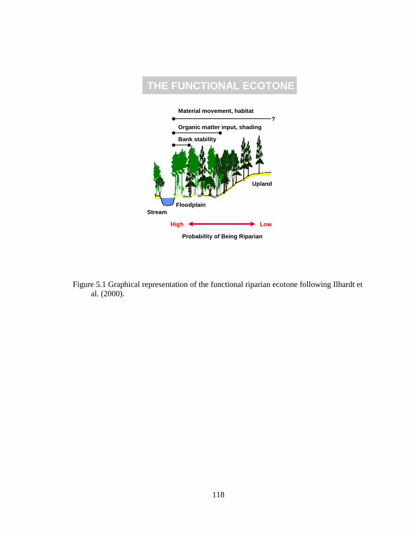
Floodplain Stream

Organic matter input, shading

Material movement, habitat

Bank stability

Upland

Probability of Being Riparian

High Low

THE FUNCTIONAL ECOTONE

?

Figure 5.1 Graphical representation of the functional riparian ecotone following Ilhardt et

al. (2000).

118

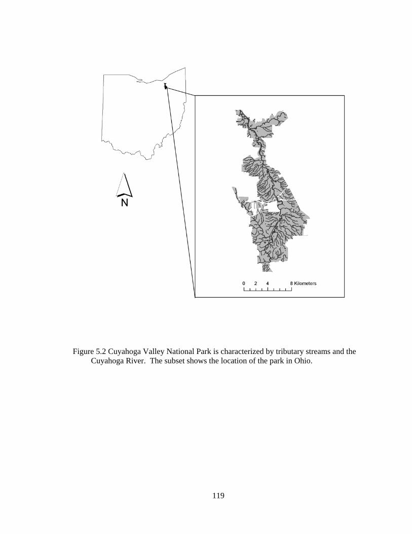
Figure 5.2 Cuyahoga Valley National Park is characterized by tributary streams and the Cuyahoga River. The subset shows the location of the park in Ohio.

119

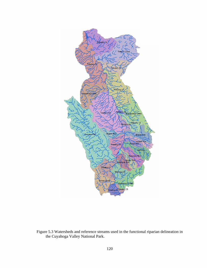
120

Figure 5.3 Watersheds and reference streams used in the functional riparian delineation in the Cuyahoga Valley National Park.

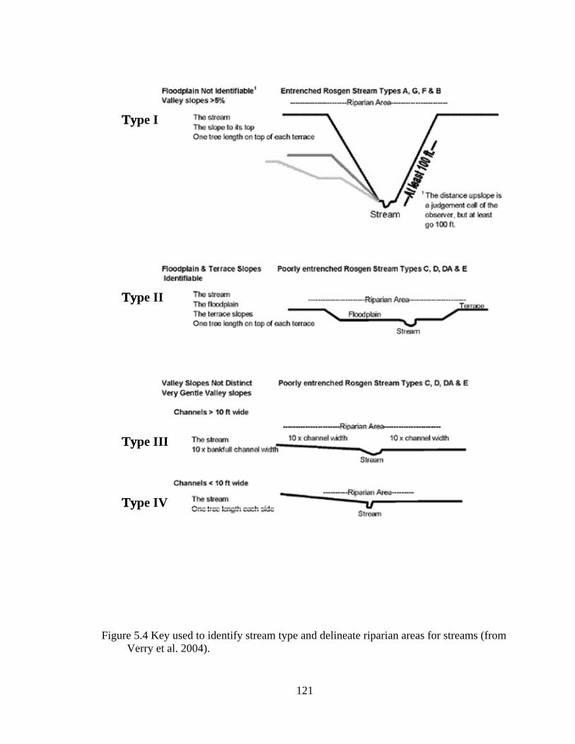
Type I

Type II

Type III

Type IV

Type I

Type II

Type III

Type IV

Figure 5.4 Key used to identify stream type and delineate riparian areas for streams (from Verry et al. 2004).

121

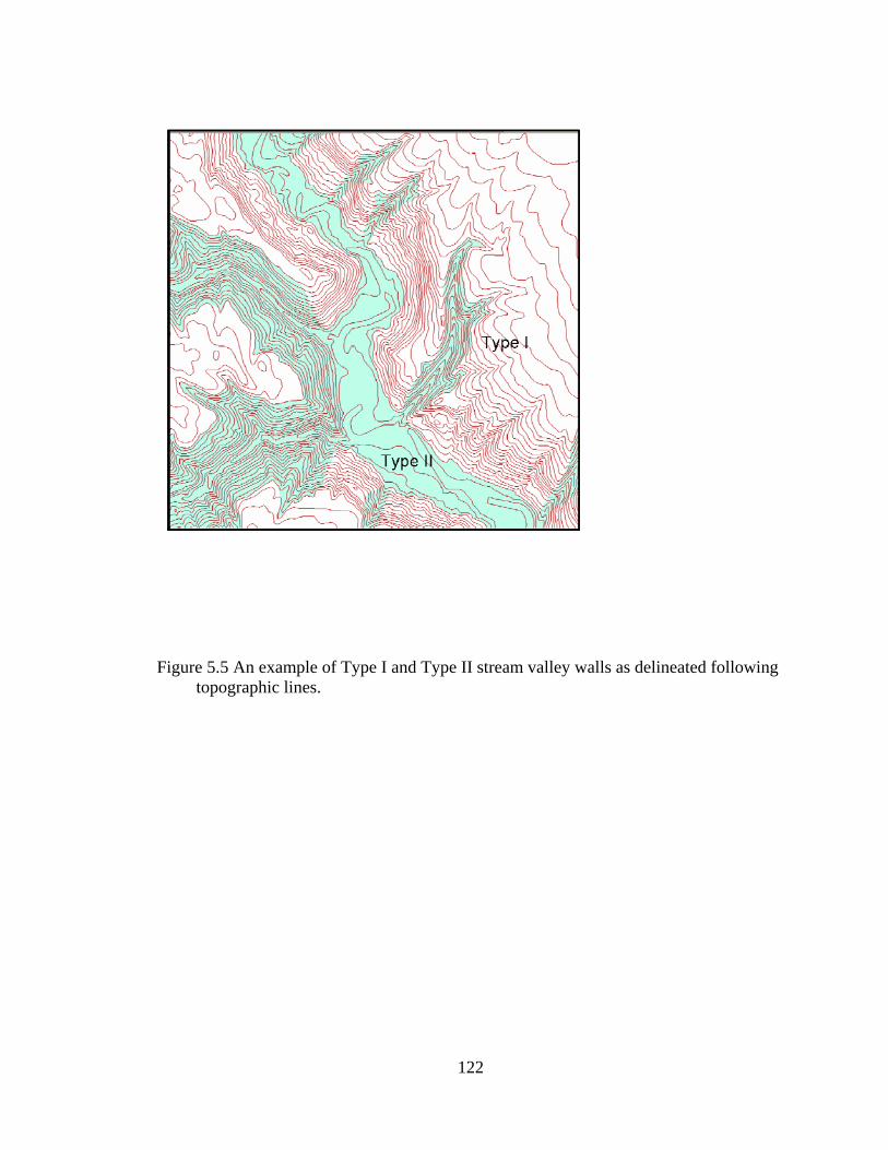
Figure 5.5 An example of Type I and Type II stream valley walls as delineated following topographic lines.

122

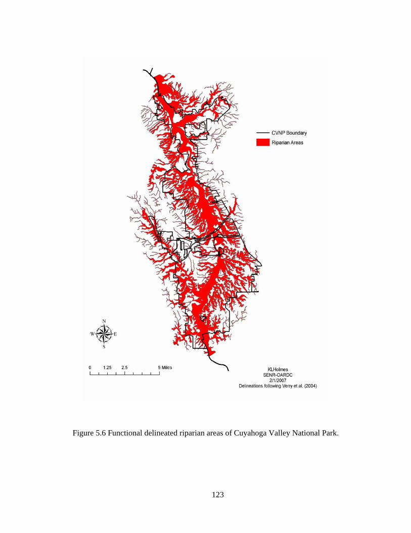
123

Figure 5.6 Functional delineated riparian areas of Cuyahoga Valley National Park.

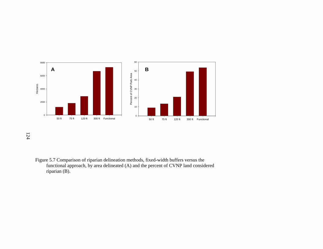
124

Figure 5.7 Comparison of riparian delineation methods, fixed-width buffers versus the

functional approach, by area delineated (A) and the percent of CVNP land considered riparian (B).

50 ft 75 ft 120 ft 300 ft Functional

Hec

tare

s

0

2000

4000

6000

8000


Perc

ent o

f CVN

P Pa

rk A

rea

0

10

20

30

40

50

60

A B


Hec

tare

s

0

2000

4000

6000

8000


Perc

ent o

f CVN

P Pa

rk A

rea

0

10

20

30

40

50

60


Hec

tare

s

0

2000

4000

6000

8000


Perc

ent o

f CVN

P Pa

rk A

rea

0

10

20

30

40

50

60

A B

124

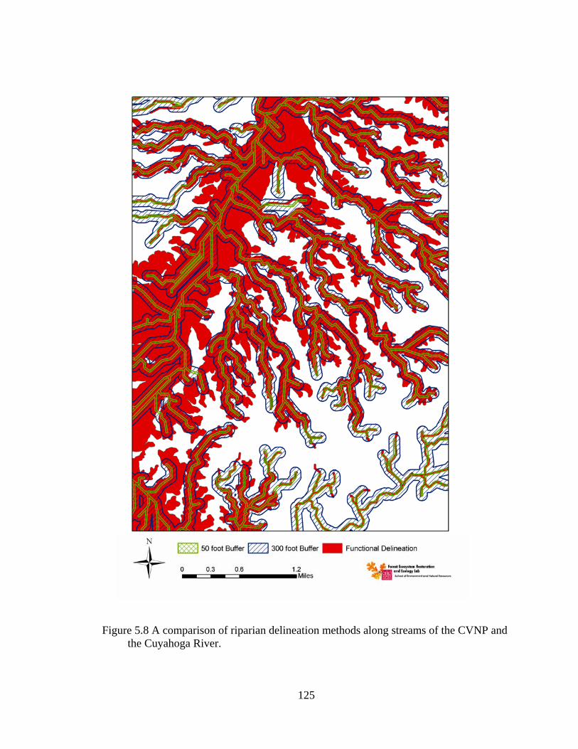
Figure 5.8 A comparison of riparian delineation methods along streams of the CVNP and

the Cuyahoga River.

125

CHAPTER 6

PRIORITIZING RIPARIAN RESTORATION BY INTEGRATING ECOLOGICAL FUNCTION AND MANAGEMENT OBJECTIVES ACROSS A LANDSCAPE

6.1 Introduction

Over the past several decades, our understanding of the valuable ecological

services that riparian areas provide, and their importance to overall watershed health, has

increased greatly (Costanza et al. 1997, Hitzhusen 2007). As a result, stream and riparian

restoration projects have become quite common. However, because riparian areas are

integral components of watershed networks, restoration of riparian areas should be done

within the context of a landscape scale management plan. The scale and scope of

restoration across a landscape poses significant challenges to land managers who often

have limited funds and resources at their disposal. In many instances, restoration occurs

without a framework to prioritize restoration efforts often resulting in uncertainty

associated with policy decisions, poor and random implementation, and questionable

success in terms of restoring important ecosystem functions (Timm et al. 2004). A

126

mechanism for restoration prioritization is needed for effective and efficient restoration

of riparian areas across a landscape.

In order to increase the likelihood of restoration success, prioritization and

restoration should be scientifically based (Sutherland et al. 2004, Kondolf 2006) and

involve land managers (Berhardt et al. 2007). A mechanism for prioritization should also

be flexible with ease of use and interpretation by land managers and stakeholders. There

have been many recent attempts to develop procedures for prioritizing restoration efforts

(e.g., Palik et al. 2000, Hulse and Gregory 2004, Timm et al. 2004, Cipollini et al. 2005,

Goebel et al. 2005, Carter and Bigas 2007, Rheinhardt et al. 2007). Many of these

approaches compare sites to a reference condition (e.g. Aronson et al. 1995, Palik et al.

2000) in order to assess current condition as well as utilize a geographic information

system (GIS) to prioritize sites at a coarse, landscape scale (e.g. Host et al. 2005, Petty

and Thorne 2005, Vanreusel and Van Dyck 2007).

One area in need of a comprehensive riparian management plan that prioritizes

restoration across a landscape is the Cuyahoga Valley National Park in northeastern

Ohio. With over 306 km (190 miles) of tributaries and 35 km (22 miles) of the Cuyahoga

River managed by the park (Figure 6.1), land managers struggle to distribute their limited

funding and volunteer labor effectively across the large area. Additionally, land

managers seek to incorporate our scientific knowledge of riparian area ecology into their

management to improve the likelihood of watershed restoration success. The objective of

this study was to work with land managers of the park to create an ecologically based

riparian restoration priority index for the National Park and adjacent areas.

127

6.2 Our Approach

Riparian areas provide numerous valuable ecosystem functions including

regulating the flow of water, sediments and nutrients across system boundaries,

contributing organic matter to the aquatic system, increasing bank stability and reducing

erosion, as well as providing unique habitat with high species diversity that can be used

as potential dispersal corridors and refugia for wildlife species (Gregory et al. 1991,

O'Laughlin & Belt 1995, Ilhardt et al. 2000, Goebel et al. 2003). Our approach to

prioritizing riparian restoration on a landscape scale, such as for CVNP, is based on a

spatially explicit model created in a geographic information system (GIS) called the

riparian restoration priority index comprised of two integrated components, including: 1)

a riparian function index and 2) management filters (Figure 6.2). When both components

of the riparian restoration priority index (RPI) are utilized, the model is best used as a

prioritization tool within the GIS to target restoration across a landscape. If management

filters are not included in the model, then the riparian RPI can be based solely on the

riparian function index.

Although not inclusive of all riparian functions, our riparian function index (RFI)

attempts to quantify seven primary ecological functions for riparian areas on a landscape

scale using easily available geospatial data and tools (Figure 6.3). Specifically, we assess

vegetative cover, sediment delivery, buffering capacity, streamflow regulation, potential

plant and wildlife habitat, and wetland quality functions in relation to reference condition

for riparian areas. Following the example of Stoddard et al. (2006), our reference

condition represents the least disturbed condition on the landscape for each of the riparian

functions assessed. Vegetative cover across the riparian area is important for organic

128

matter input, stream temperature regulation, biodiversity, and nutrient cycling (Gregory

et al. 1991). In terms of sediment delivery, highly erodible slopes (>12%) in conjunction

with land use containing high concentrations of impermeable surfaces are likely to erode.

These sources of sediment into the riparian area and aquatic ecosystem can significantly

degrade aquatic habitat and water quality (Cooper et al. 1987). Buffering capacity

captures the ability of a riparian area to regulate surface runoff or other material flow

from upland areas through infiltration and retention and is often related to the amount of

impervious surface within an area (Schuler 1994). Riparian areas, as ecotones between

upland terrestrial and aquatic ecosystems, provide unique habitat for both plants, which

contribute significantly to plant species diversity at a variety of scales (Goebel et al.

2003), and wildlife (Wondzell and Bisson 2003). Hydrology is also a significant

landscape-level process related to geomorphic landforms and riparian species

distributions (Goebel et al. 2003, Holmes et al. 2005). If streamflow is regulated by

dams, then surface flows, plant community dynamics, and aquatic habitat are negatively

affected both upstream and downstream of the dam. Finally, functioning wetlands retain

and process nutrients as well as provide flood control above the floodplain, and are often

linked to groundwater or surface water flow, particularly in riparian areas (Lowrance et

al. 1984).

The second component of our riparian RPI model allows for land managers to

focus on specific management objectives through the inclusion of management filters.

For example, land managers may wish to focus their restoration activities on those areas

adjacent to roads and trails because of ease of volunteer and equipment access, or in areas

with known invasive species, or in areas under a particular ownership or conservation

129

status. Spatially explicit management filters can be created for each of these scenarios to

further prioritize riparian areas for restoration based on specific management objectives.

Additionally, multiple management filters can be utilized in the model at one time if

desired.

Finally, it should be emphasized that this model is designed to help identify areas

with poor riparian function within the context of important management objectives so as

to 1) help target specific areas that require restoration and 2) help prioritize those areas in

need of restoration within the parameters specified by land managers. Our model is

intended to be used as a landscape-level planning tool and not as a substitute for on-the-

ground investigation and design of restoration practices, which should be accomplished at

the local or reach scale.

6.3 Study Area

Cuyahoga Valley National Park (CVNP) in northeastern Ohio protects over

13,355 ha (33,000 acres) for both conservation as well as recreation, including 35 km (22

miles) of the Cuyahoga River and over 306 km (190 miles) of ephemeral and perennial

tributary streams. Cuyahoga Valley was first designated a National Recreation Area in

1974 and later changed designation to become a National Park in 2000. The park’s

location between the two major metropolitan areas of Cleveland and Akron, OH, creates

unique management implications due to the urban-rural interface, including balancing

ecological conservation with recreation that serves approximately 3 million visitors

annually. The floodplain of the Cuyahoga River has seen significant human activity

starting with Native American trading routes and camps, through the canal era in the mid

130

1800s, to more recent activities including past and current agriculture, a municipality

(Peninsula), and several recreational areas such as ski areas and golf courses (Hacker

2003). The large remainder of the park is comprised of undeveloped land characterized

by steep, forested alluvial ravine systems along the multiple tributaries to the Cuyahoga

River formed in glacial deposits shortly after the end of the Wisconsin glaciation (Hacker

2003). The forests flanking these ravine systems are mature second-growth (>70 years

old) and composed of mixed-mesophytic species (e.g. sugar maple, Acer saccharum

Marsh; American beech, Fagus grandifolia Ehrh.; northern red oak, Quercus rubra L.;

shagbark hickory, Carya ovata (P.Mill)K. Koch; and yellow poplar, Liriodendron

tulipifera L.).

6.4 Methods

Both components of the riparian RPI model were created using geospatial data in

a geographic information system using ArcGIS® (ESRI, Redlands, CA). Functional

riparian areas were delineated on the landscape previously (see Chapter 5) and all

analyses were conducted within these areas.

6.4.1 Assessing Riparian Function

Each function of the RFI was assessed by grids on a cell-by-cell basis with each

cell representing a 30m pixel. Because the goal was to assess current riparian function in

relation to the reference condition, each cell was ranked from unaltered (reference

condition) to altered. In this particular study for CVNP, mature second-growth riparian

forest represents the condition least disturbed by humans and was selected as our

131

reference condition. Due to the history of human activities and land use in the region as

well as the current unique rural-urban interface characterizing CVNP, we selected a

reference condition that was both attainable through restoration and sustainable for the

region. For ease of interpretation, ranking of riparian function was done on a scale from

0, representing an unaltered or reference condition, to -10,000, representing an altered or

significant deviation from reference condition.

6.4.1.1 Vegetative Cover In terms of vegetative cover which regulates important stream characteristics

(e.g., temperature, organic matter inputs), the National Land Cover Database (NLCD) for

the area of analysis was downloaded from the MRLC Consortium

(http://gisdata.usgs.net/Website/MRLC/) and the grid was clipped to the delineated

functional riparian areas. Land cover classes were classified on an equal gradient from 0,

unaltered condition, to -10,000, altered condition (Table 6.1) according to deviation from

our reference conditions for vegetative cover function, specifically, deciduous forest,

evergreen forest, mixed forest, and woody wetlands. Developed medium and high

intensity cover and open water were considered the most significantly altered in terms of

providing vegetative cover function.

6.4.1.2 Potential Plant Habitat The clipped NLCD used for vegetative cover was reclassified for potential plant

habitat function by creating another equal gradient grid with values ranging from 0 to -

10,000 (Table 6.2). Deciduous forest, evergreen forest, mixed forest, and woody

wetlands land cover classes were considered supportive of unaltered potential plant

habitat function in riparian areas (value of 0). Those land cover classes representing a

132

significant deviation from reference condition and considered non-supportive of potential

plant habitat function in riparian areas (value of -10,000) were cultivated crops,

developed-low intensity, developed-medium intensity, and developed-high intensity. The

remaining classes were ranked according to potential plant habitat function compared to

the unaltered condition.

6.4.1.3 Sediment Delivery The objective of this riparian function was to distinguish between naturally occurring

sediment delivery and increased likelihoods for sediment delivery due to interactions

between land cover classes and soil erodibility rankings. SSURGO soils for the region

were downloaded from the United States Department of Agriculture Geospatial Gateway

(http://datagateway.nrcs.usda.gov/) and clipped to the delineated functional riparian

areas. Because sediment delivery is related to both Highly Erodible Land (HEL) rating

and land use, soil erodibility ratings were related to each of the NLCD land cover classes

within the riparian areas. Several soil types lacked ratings for HEL and the United States

Department of Agriculture Soil Surveys for the counties of interest (Cuyahoga and

Summit counties) were consulted (Musgrave and Holloran 1980, Ritchie and Steiger

1994) to determine an HEL rating for each soil type within the riparian areas and added

to the corresponding spatial data. Each of the combined land cover classes/HEL ratings

was ranked with equal interval from 0 to -10,000 (Table 6.3), with natural cover or

reference conditions ranked as 0 and cultivated crops on highly erodible land ranked with

the highest sediment delivery and a value of -10,000. It was assumed that sediment

delivery off of slopes with vegetative cover was natural and not the result of land cover

133

class and soil erodibility interactions. In riparian areas representing reference conditions

there is an expected natural level of sediment delivery.

6.4.1.4 Buffering Capacity To estimate the ability of riparian areas to regulate surface runoff through infiltration

and retention, the NLCD Impervious Surface data for the area of analysis was

downloaded from the MRLC Consortium (http://gisdata.usgs.net/Website/MRLC/),

clipped to the delineated functional riparian areas, and scaled from 0 to -10,000 by

multiplying by -100. Grid cells with the highest impermeability had a value of -10,000

and those with the lowest impermeability, the most permeable cells, had a value of 0.

6.4.1.5 Potential Wildlife Habitat To assess the potential of each cell to provide wildlife habitat in a similar manner as

the reference condition, the clipped NLCD used for vegetative cover and potential plant

habitat was reclassified for potential wildlife habitat function by creating another equal

gradient grid with values ranging from 0 to -10,000 (Table 6.4). Land cover classes

were ranked according to their deviation from reference condition for wildlife habitat

function in riparian areas, which we considered to be open water, deciduous forest,

evergreen forest, mixed forest, and woody and emergent herbaceous wetlands. High

intensity development was considered to represent a significant deviation from reference

condition and non-supportive of potential wildlife habitat function in riparian areas.

6.4.1.6 Streamflow Regulation Because ponds and lakes are not representative of the reference condition of riparian

areas in the study area, all ponds and lakes within the functionally delineated riparian

areas were assumed to be the result of regulated streamflow, primarily dams. A 2002

134

Land Cover shapefile developed by the National Park Service containing pond and lake

polygons was clipped to the delineated functional riparian areas. All pond and lake

polygons were queried, selected, and saved as a separate file. To ensure that known

wetlands were not misclassified as ponds and lakes, all polygons known to be wetlands

were removed from the file. Finally, these regulated streamflow polygons were merged

with the delineated functional riparian areas to match the spatial data extent of the other

riparian functions, and rasterized into 30 m pixels with streamflow regulated areas (ponds

and lakes) classified as -10,000 and unaltered areas classified as 0.

6.4.1.7 Wetland Quality In 2001, an assessment of wetlands greater than one acre in size within the CVNP

was conducted and the corresponding shapefile was clipped to the functionally delineated

riparian areas. Using the data on wetland quality gathered from this assessment, wetland

quality was determined based upon three weighted components (Table 6.5): hydrologic

source, water quality, and wetland condition. Each of these components was determined

from one or more factors recorded by the wetland assessment (Table 6.6) with each

wetland recorded as positive, yes, or negative, no, for that factor. To determine wetland

quality, factor values within each component were summed, each potentially equaling -1,

and each component was weighted in accordance with its importance to wetland quality

(Table 6.5). The values for each of the three weighted components were summed to

determine quality for each wetland, scaled from 0 to -10,000, and added to the spatial

data. To match the spatial extent of the other riparian functions, a union between the

wetland shapefile and the delineated functional riparian areas was created. The resulting

135

file was rasterized into 30m pixels with non-wetland cells classified as 0 and wetland

cells classified according to their wetland quality rating.

6.4.2 Riparian Function Index

All seven riparian function grids were added together to create the spatially explicit

RFI for the CVNP. The RFI represents the range of riparian function assessed from 0,

representing unaltered function or reference condition, to a potential of -70,000,

representing severely altered function or a significant deviation from reference condition.

Using ecological benchmarks, a categorical scale of riparian function was created to ease

both interpretation of the large range of conditions and prioritization for restoration

across the entire study area. The four categories of riparian function and their

accompanying RFI values include high function (0 to -5,000), moderate function (-5,001

to -17,500), poor function (-17,500 to -35,000), and very poor function (-35,000 to -

70,000). For a cell to be considered to have high riparian function, at a minimum only

one riparian function can be operating at 50% function (50% reduction in function). For

a cell to be considered to have moderate riparian function, at a minimum all seven

riparian functions must be operating at 75% function (25% reduction in function), or, one

riparian function could operate at 0% function (100% reduction in function) and another

riparian function could operate at 25% function (75% reduction in function). For a cell to

be considered to have poor function, at a minimum three riparian functions could operate

at 0% function (100% reduction in function) and another riparian function could operate

at 50% function (50% reduction in function). Cells with two riparian functions operating

136

at 0% function would also fall into this category. All remaining cells are considered to

have very poor riparian function.

6.4.3 Management Filters

For this study, we developed two management filters to be used in conjunction

with the RFI in the riparian RPI model. However, because of the availability of

geospatial data and the relative ease of creation, an unlimited number of management

filters can be created and used as additional layers over the RFI for prioritizing riparian

restoration based upon local management objectives. Prioritization should be done

within the GIS when management filters are added as layers over the RFI to visualize

spatial changes in the riparian RPI model, particularly at a local scale where changes may

not be evident at the landscape scale.

As a result of its location in relation to the Akron-Cleveland metropolitan areas,

the unique rural-urban interface characterized by the CVNP is a complex landscape with

different ownership types that will affect the type and extent of management that can be

done by the park. Because ownership is a significant component of park management

objectives, a management filter reflecting four ownership classes was created for on-

screen prioritization of restoration. The ownership classes included: 1) National Park

Service Land, which is owned and managed by the park and where it has the most

freedom for management implementation; 2) Other Pubic Land, which is owned by other

public entities, such as county parks, where there is a high potential for coordinated

management implementation; 3) Institutional Land, which is comprised of large tracts

owned by private landowners, such as golf courses and ski areas, where passive

137

management may be possible but more active management may be difficult yet possible

with extended engagement of parties; 4) Private Land, which is comprised of small tracts

owned by private landowners, such as single-family homes or small farms, where

management of any form will likely be difficult. A CVNP-provided shapefile of the four

ownership classes was clipped to the delineated functional riparian areas and used as a

management filter for on-screen prioritization of restoration.

A second management filter comprising the functional riparian areas associated

with the Cuyahoga River was created to address the dominance of the river as a natural

landmark and its associated focus of recreation and development within the CVNP. The

functional riparian area of the river was hand-digitized in the GIS following the methods

for functional delineation (see Chapter 5) and used as a management layer over the RFI

for on-screen prioritization of restoration.

6.4.4 Riparian Restoration Priority Index

Using only the RFI, a riparian RPI was generated for the study area based solely

on riparian function. Using both the RFI and the management filters, an example on-

screen prioritization was conducted for a subwatershed within the study area, Haskell-

Ritchie Run watershed, using the ownership filter as the primary filter and the Cuyahoga

River functional riparian filter as a secondary filter.

138

6.5 Results

Riparian function was assessed at a landscape scale across the CVNP study region

using readily available geospatial data. The assessment of each of the seven riparian

functions included in the development of the RFI demonstrate that large portions of the

CVNP study region have significantly altered function relative to an unaltered reference

condition (Figures 6.4-6.10) with values ranging from 0 (high function, shown in green)

to -10,000 (significantly altered function, shown in red) with the gradient of conditions

between the two shown as various shades of green to red. When the seven assessed

riparian functions are spatially added together, the resulting riparian function index

(Figure 6.11) reveals that large portions of the area have high function (green) while

areas with poor (yellow) and very poor (red) riparian function are focused near

municipalities (Peninsula in the center and Garfield Heights to the north), along the

Cuyahoga River in the center of the study area, and in the headwater streams of the

northern portion of the study area.

Two management filters were created for use in the restoration priority index

following local management objectives to prioritize restoration first by ownership,

working primarily within land owned by the National Park Service, and second to focus

efforts within the functional riparian area of the Cuyahoga River, where the objective is

to restore function as well as increase education and visibility of riparian ecology within a

region of the park with high visitation. Ownership was classified into four categories for

land within the park boundary and overlain with the delineated functional riparian area of

the Cuyahoga River (Figure 6.12) to serve as the management filter portion of the RPI

model.

139

Using only the RFI component of the riparian RPI model, areas with high riparian

function are categorized as low priority for restoration while areas with very poor riparian

function are categorized as very high priority for restoration (Figure 6.13). While the

implementation of the complete riparian RPI is best done on-screen within the GIS, using

an example subwatershed within the CVNP study region we clipped the RFI for the

subwatershed by the four ownership classes and overlaid the functional riparian areas of

the Cuyahoga River (Figure 6.14). Within the subwatershed, the majority of NPS land is

in the headwaters and has high riparian function (Figure 6.14b). The area with the

poorest riparian function is held by institutional owners, in this case a municipal golf

course, and lies within the Cuyahoga River functional riparian area raising its priority for

restoration (Figure 6.14c). The center of the subwatershed is dominated by private

landowners and areas with moderate and poor riparian function (Figure 6.14d), in this

case the result of dammed reaches forming lakes for Boy Scouts of America camps.

Restoration within this subwatershed can be further prioritized by focusing on areas with

moderate and poor riparian function assuming that areas with very poor riparian function

are not likely to return to a reference condition and areas with high function do not need

restoration (Hobbs and Kristjanson 2004). National Park Service land managers should

collaborate with institutional land owners within the functional riparian area of the

Cuyahoga River to restore function across areas with poor riparian function held by both

parties (Figure 6.15). Additionally, in the center of the subwatershed the large amount of

moderately and poorly functioning areas held by private landowners should be

considered for possible collaboration or educational outreach with the intent to improve

function in these reaches.

140

6.5 Discussion

The need for riparian restoration is increasingly recognized in our global efforts

towards sustainable watersheds and improved water quality. Yet, land managers often

have limited funding and labor available for restoration and do not have the appropriate

tools needed to prioritize their efforts for maximum ecological result. We have

developed a riparian restoration priority index model that assesses current riparian

function in relation to reference condition and incorporates management objectives to

prioritize restoration on a landscape scale. The model integrates both ecological

information of riparian areas as well as local restoration goals and objectives encouraging

collaborative efforts between scientists and land managers, which should lead to

improved restoration success (Sutherland et al. 2004, Barnhardt et al. 2007).

With the increasing availability and accuracy of geospatial data, it has become

possible to assess the condition of a landscape remotely at a coarse scale. We have

assessed riparian function as a snapshot of the current conditions using a variety of

geospatial data, primarily land cover. This is an appropriate method to assess condition

because cover often reflects the suite of controlling hierarchical ecological factors (Allan

and Starr 1982, Gregory et al. 1991) and the likelihood of usage by a suite of species

indicative of condition (Drielsma and Ferrier 2006). Current condition was assessed

relative to a selected reference condition based on our knowledge of the study area. The

CVNP has a long history of human activity and subsequent disturbance affecting

ecological function. Additionally, the relatively rural nature of the park is uniquely

located between two major metropolitan areas. As a result, reference conditions

141

representing minimally disturbed conditions (Stoddard et al. 2006) are not present and

seeking to restore historical conditions through restoration within the study area is not

feasible. In previous research (see Chapters 2, 3, and 4) we have studied areas within the

park that represent the least disturbed condition (Stoddard et al. 2006) and selected the

functions associated with these areas as our reference condition for each of the seven

assessed riparian functions used in our riparian function index. In this way, we have

incorporated the local ecology of riparian areas and tailored our assessment towards

function that is attainable through restoration based on the characteristics of the study

region.

Our riparian restoration priority index model can prioritize restoration across a

landscape using only the riparian function index. However, the addition of management

filters further involves land managers in the prioritization process and increases the

ability of the model to be tailored to local conditions. Because the riparian RPI model is

best suited for analysis within the GIS, it allows for the development of multiple

scenarios that can be considered for prioritization using combinations of management

filters developed to reflect local goals and objectives. Additionally, analyses done within

the GIS can quickly and simply identify potential areas for collaboration or outreach with

partner agencies or landowners, particularly for the CVNP study region. The strengths of

geospatial analysis across a landscape create dynamic opportunities for the potential to

restore riparian function in a continuous manner across the landscape and maximize both

the restoration effort and the cumulative ecological effect within a watershed.

While our riparian RPI model was developed for the CVNP, this approach can be

transferred to any other riparian restoration occurring across a landscape scale where

142

prioritization is necessary prior to the selection and planning of on-the-ground restoration

activities at a local scale. Our selection of widely available geospatial data (e.g. National

Land Cover database) as well as the flexibility of the model to incorporate additional

data, such as Index of Biotic Integrity or Qualitative Habitat Evaluation Index data from

the United States Environmental Protection Agency, allows the model to remain flexible

to local objectives and easy to update with the availability of new data.

6.6 References

Allen, T.F.H., and T.B. Starr. 1982. Hierarchy: Perspectives for Ecological Complexity. University of Chicago Press, Chicago, pp.310.


Bernhardt, E.S., E.B. Sudduth, M.A. Palmer, J.D. Allan, J.L. Meyer, G. Alexander J. Follastad-Shah, B. Hassett, R. Jenkinson, R. Lave, J. Rumps, and L. Pagano. 2007. Restoring rivers one reach at a time: Results from a survey of U.S. river restoration practitioners. Restoration Ecology 15(3): 482-493.

Carter, J. and J. Biagas. 2007. Prioritizing bottomland hardwood forest sites for protection and augmentation. Natural Areas Journal 27(1): 72-82.

Cipollini, K.A., A.L. Maruyama, and C.L. Zimmerman. 2005. Planning for restoration: a decision analysis approach to prioritization. Restoration Ecology 13:460-470.


143

Cooper, J.R., J.W. Gilliam, R.B. Daniels, and J.M. Laflen. 1987. Riparian areas as filters for agricultural sediment. Soil Science Society of America Journal 51: 416-420.

Drielsma, M. and S. Ferrier. 2006. Landscape scenario modeling of vegetation condition. Ecological Management and Restoration 7 (S1): S45-S52.

Goebel, P.C., B.J. Palik, and K.S. Pregitzer. 2003. Plant diversity contributions of riparian areas in watersheds of the northern Lake States, USA. Ecological Applications 13:1595-1609.

Goebel, P. C., T.C. Wyse, and R.G. Corace. 2005. Determining reference ecosystem conditions for disturbed landscapes within the context of contemporary resource management issues. Journal of Forestry 103:351-356.

Gregory, S.V., F.J. Swanson, W.A. McKee, and K.W. Cummins. (1991) An ecosystem perspective of riparian zones. BioScience 41: 540-551.

Hacker, D.B. 2003. Cuyahoga Valley National Park. pp.163-186. In: Geology of National Parks. Editors: Harris, A.G., E. Tuttle, and S.D. Tuttle. Kendall/Hunt Publishing: Dubuque, IA, pp.882.



Hobbs, R.J. and L.J. Kristjanson. 2003. Triage: How do we prioritize health care for landscapes? Ecological Management and Restoration 4 Supplement: S39-S45.

Host, G.E., J. Schuldt, J.J.H. Ciborowski, L.B. Johnson, T. Hollenhorst, and C. Richards. 2005. Use of GIS and remotely sensed data for a priori identification of reference areas for Great Lakes coastal ecosystems. International Journal of Remote Sensing 26(23): 5325-5342.

Hulse, D. and S. Gregory. 2004. Integrating resilience into floodplain restoration. Urban Ecosystems 7: 295-314.

144

Illhardt, B.L., E.S. Verry, and B.J. Palik. 2000. Defining riparian areas. pp. 23-42 In: E.S. Verry, J.W. Hornbeck, and C.A. Dolloff, editors. Riparian Management in Forests of the Continental Eastern United States. Lewis Publishers: New York, pp.402.

Kondolf, G.M. 2006. River restoration and meanders. Ecology and Society 11(2): 42.

Lowrance, R., R.Todd, J. Fail Jr., O. Hendrickson Jr., R. Leonard, and J.L. Baker. 1984. Riparian forests as nutrient filters in agricultural watershed. BioScience 34(6): 374-377.

Musgrave, D.K. and D.M. Holloran. 1980. Soil Survey of Cuyahoga County, Ohio. United States Department of Agriculture, Soil Conservation Service and Ohio Department of Natural Resources.


Palik, B.J., P.C. Goebel, L.K. Kirkman, and L. West. 2000. Using landscape hierarchies to guide restoration of disturbed ecosystems. Ecological Applications 10: 189-202.

Petty, J.T. and D. Thorne. 2005. An ecologically based approach to identifying restoration priorities in an acid-impacted watershed. Restoration Ecology 13(2): 348-357.

Ritchie, A. and Steiger, J.R. 1990. Soil Survey of Summit County, Ohio. United States Department of Agriculture, Soil Conservation Service and Ohio Department of Natural Resources.

Rheinhardt, R., M. Brinson, R. Brooks, M. McKenney-Easterling, J.M. Rubbo, J. Hite, and B. Armstrong. 2007. Development of a reference-based method for identifying and scoring indicators of condition for coastal plain riparian reaches. Ecological Indicators 7: 339-361.

Schueler, T. 1994. The importance of imperviousness. Watershed Protection Techniques. 1(3): 100-111.

145

Stoddard, J.L., D.P. Larsen, C.P. Hawkins, R.K. Johnson, and R.H. Norris. Setting expectations for the ecological condition of streams: The concept for reference condition. Ecological Applications 16(4): 1267-1276.

Sutherland, W.J., A.S. Pullin, P.M. Dolman, and T.M. Knight. 2004. The need for evidence-based conservation. Trends in Ecology and Evolution 19(6): 305-308.

Timm, R.K., R.C. Wissmar, J.W. Small, T.M. Leschine, and G. Lucchetti. 2004. A screening procedure for prioritizing riparian management. Environmental Management 33: 151-161.

Vanreusel, W. and H. Van Dyck. 2007. When functional habitat does not match vegetation types: A resource-based approach to map butterfly habitat. Biological Conservation 135: 202-211.

Wondzell, S.M. and P.A. Bisson. 2003. Influence of wood on aquatic biodiversity. pp. 249-263 In: Gregory, S.V., K.L. Boyer, and A.M. Gurnell, editors. The Ecology and Management of Wood in World Rivers. American Fisheries Society, Bethesda, Maryland, USA, pp.431.

146

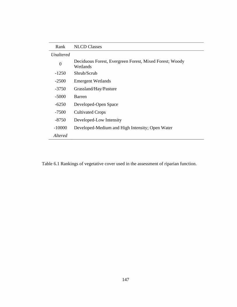
147

Rank NLCD Classes

Unaltered

0 Deciduous Forest, Evergreen Forest, Mixed Forest; Woody Wetlands

-1250 Shrub/Scrub

-2500 Emergent Wetlands

-3750 Grassland/Hay/Pasture

-5000 Barren

-6250 Developed-Open Space

-7500 Cultivated Crops

-8750 Developed-Low Intensity

-10000 Developed-Medium and High Intensity; Open Water

Altered

Table 6.1 Rankings of vegetative cover used in the assessment of riparian function.

Rank NLCD Classes

Unaltered

0 Deciduous Forest, Evergreen Forest, Mixed Forest; Woody Wetlands

-1429 Shrub/Scrub

-2858 Emergent Herbaceous Wetlands

-4287 Barren

-5716 Open Water

-7145 Grassland/Hay/Pasture -8574 Developed-Open Space

-10000 Cultivated Crops; Developed-Low Intensity; Developed-Medium and High Intensity

Altered

148

Table 6.2 Rankings of potential plant habitat used in the assessment of riparian function.

148

Table 6.3 Rankings of sediment delivery used in the assessment of riparian function.

149

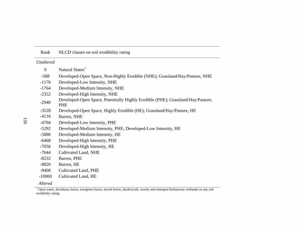
Rank NLCD classes on soil erodibility rating

Unaltered

0 Natural States1 -588 Developed-Open Space, Non-Highly Erodible (NHE); Grassland/Hay/Pasture, NHE

-1176 Developed-Low Intensity, NHE -1764 Developed-Medium Intensity, NHE -2352 Developed-High Intensity, NHE

-2940 Developed-Open Space, Potentially Highly Erodible (PHE); Grassland/Hay/Pasture, PHE

-3528 Developed-Open Space, Highly Erodible (HE); Grassland/Hay/Pasture, HE -4116 Barren, NHE -4704 Developed-Low Intensity, PHE -5292 Developed-Medium Intensity, PHE; Developed-Low Intensity, HE -5880 Developed-Medium Intensity, HE -6468 Developed-High Intensity, PHE -7056 Developed-High Intensity, HE -7644 Cultivated Land, NHE -8232 Barren, PHE -8820 Barren, HE -9408 Cultivated Land, PHE -10000 Cultivated Land, HE Altered

1 Open water, deciduous forest, evergreen forest, mixed forest, shrub/scrub, woody and emergent herbaceous wetlands on any soil erodibility rating.

150

150

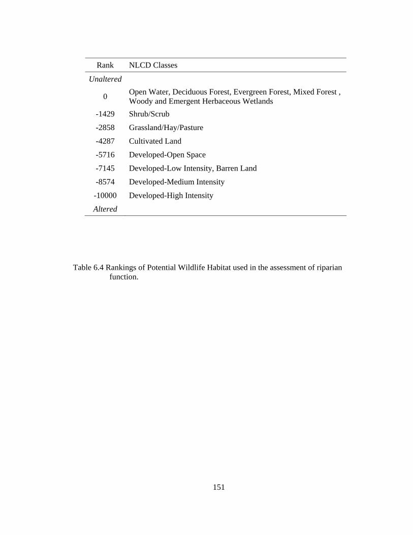
Rank NLCD Classes

Unaltered

0 Open Water, Deciduous Forest, Evergreen Forest, Mixed Forest , Woody and Emergent Herbaceous Wetlands

-1429 Shrub/Scrub

-2858 Grassland/Hay/Pasture

-4287 Cultivated Land

-5716 Developed-Open Space

-7145 Developed-Low Intensity, Barren Land

-8574 Developed-Medium Intensity

-10000 Developed-High Intensity

Altered

Table 6.4 Rankings of Potential Wildlife Habitat used in the assessment of riparian function.

151

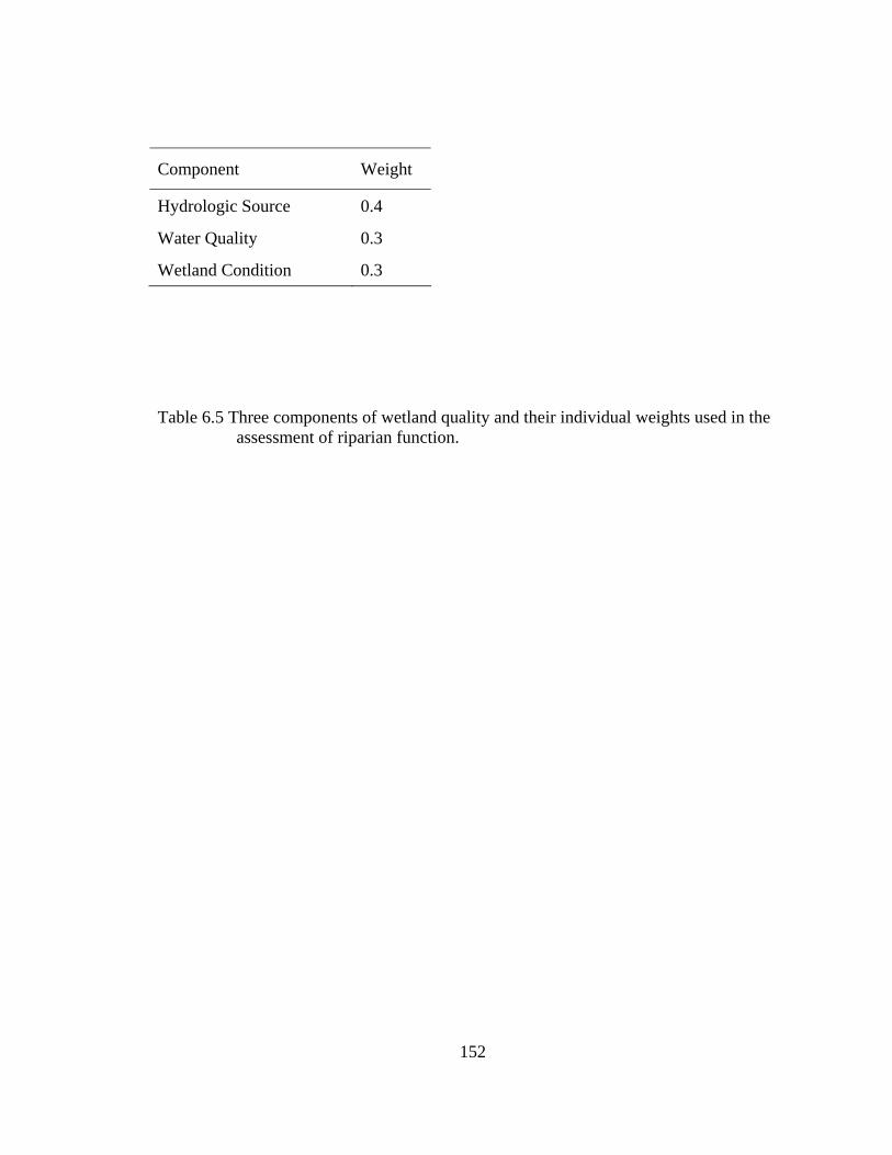
Component Weight

Hydrologic Source 0.4

Water Quality 0.3

Wetland Condition 0.3

Table 6.5 Three components of wetland quality and their individual weights used in the assessment of riparian function.

152

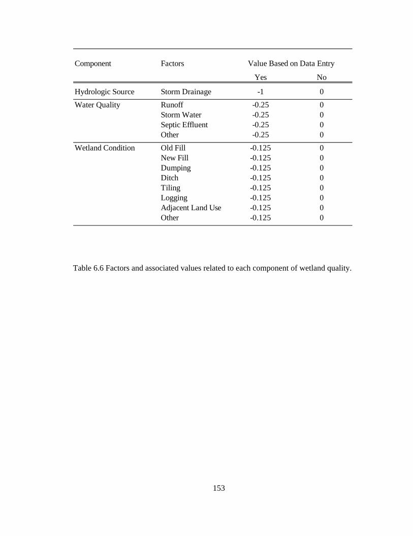
Component Factors

Yes No

Hydrologic Source Storm Drainage -1 0Water Quality Runoff -0.25 0

Storm Water -0.25 0Septic Effluent -0.25 0Other -0.25 0

Wetland Condition Old Fill -0.125 0New Fill -0.125 0Dumping -0.125 0Ditch -0.125 0Tiling -0.125 0Logging -0.125 0Adjacent Land Use -0.125 0Other -0.125 0

Value Based on Data Entry

Table 6.6 Factors and associated values related to each component of wetland quality.

153

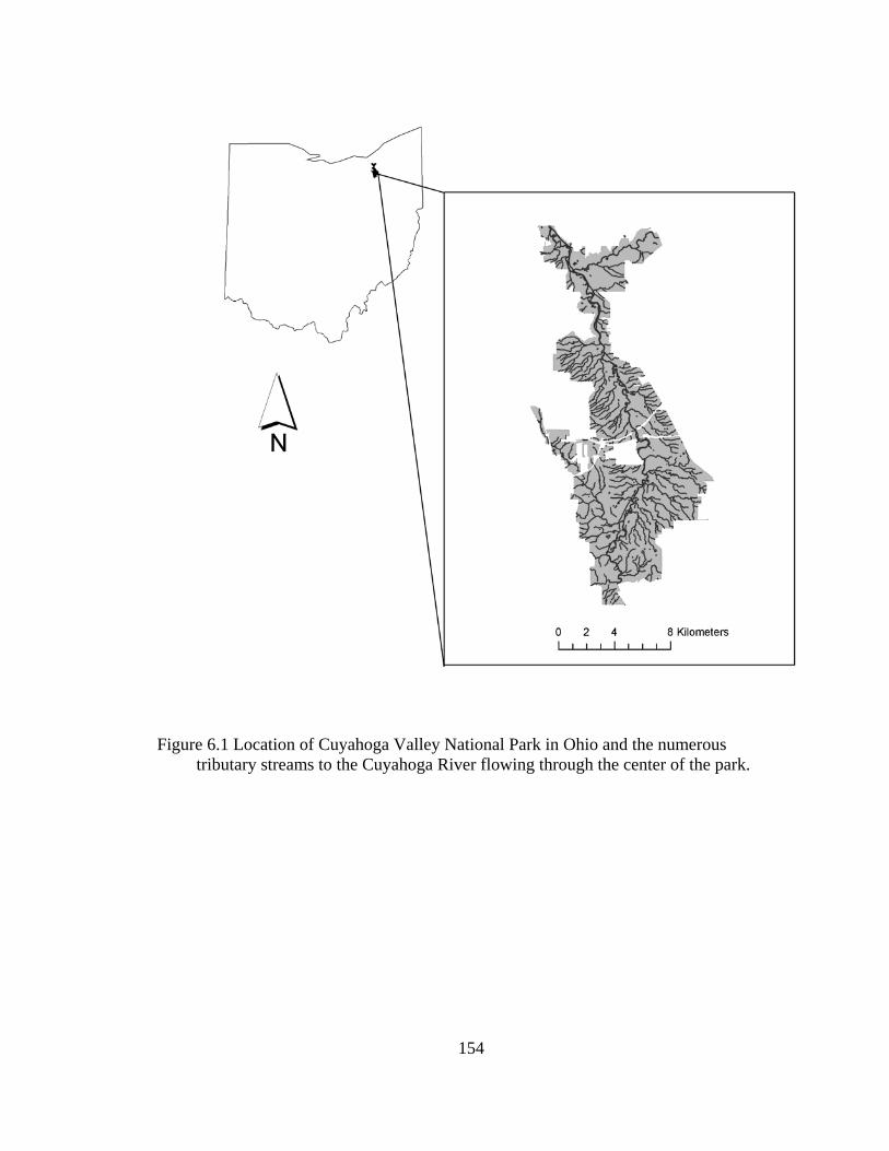
Figure 6.1 Location of Cuyahoga Valley National Park in Ohio and the numerous tributary streams to the Cuyahoga River flowing through the center of the park.

154

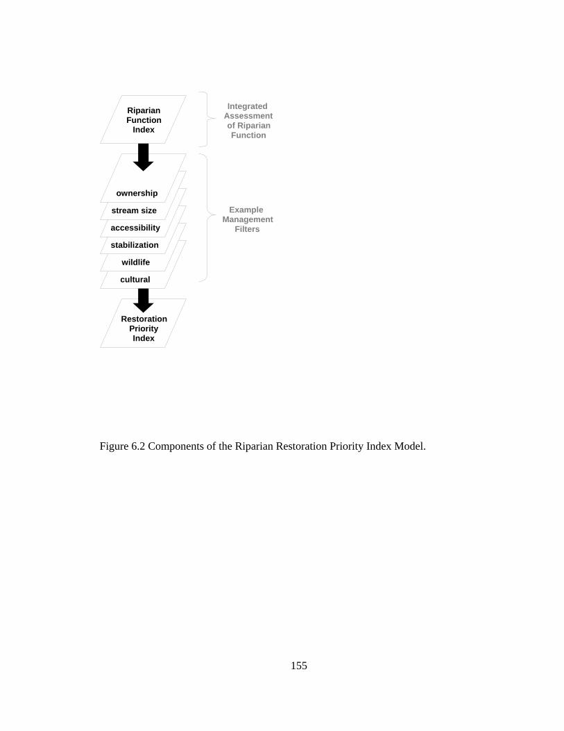
wildlife

accessibility stream size

Riparian Function

Index

ownership

stabilization

cultural

RestorationPriority Index

IntegratedAssessmentof RiparianFunction

Example Management

Filters

Figure 6.2 Components of the Riparian Restoration Priority Index Model.

155

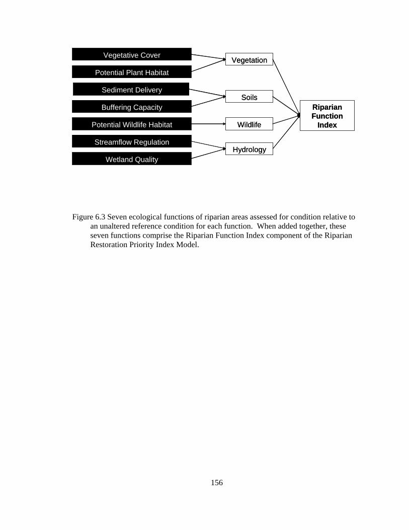
Vegetative Cover

Sediment Delivery

Buffering Capacity

Potential Wildlife Habitat

Potential Plant Habitat

Streamflow Regulation

Wetland Quality

RiparianFunction

Index

Hydrology

Soils

Wildlife

VegetationVegetative Cover

Sediment Delivery

Buffering Capacity

Potential Wildlife Habitat

Potential Plant Habitat

Streamflow Regulation

Wetland Quality

RiparianFunction

Index

Hydrology

Soils

Wildlife

Vegetation

Figure 6.3 Seven ecological functions of riparian areas assessed for condition relative to an unaltered reference condition for each function. When added together, these seven functions comprise the Riparian Function Index component of the Riparian Restoration Priority Index Model.

156

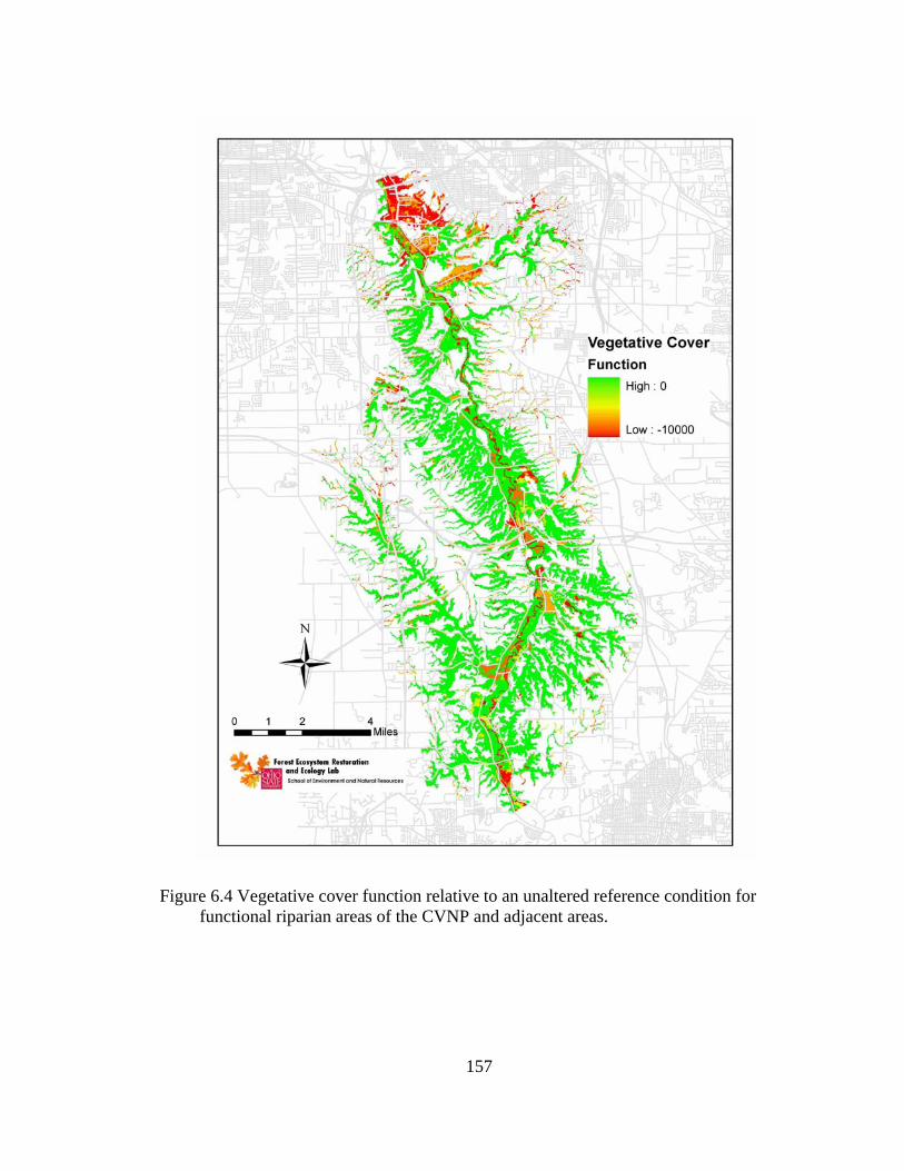
Figure 6.4 Vegetative cover function relative to an unaltered reference condition for functional riparian areas of the CVNP and adjacent areas.

157

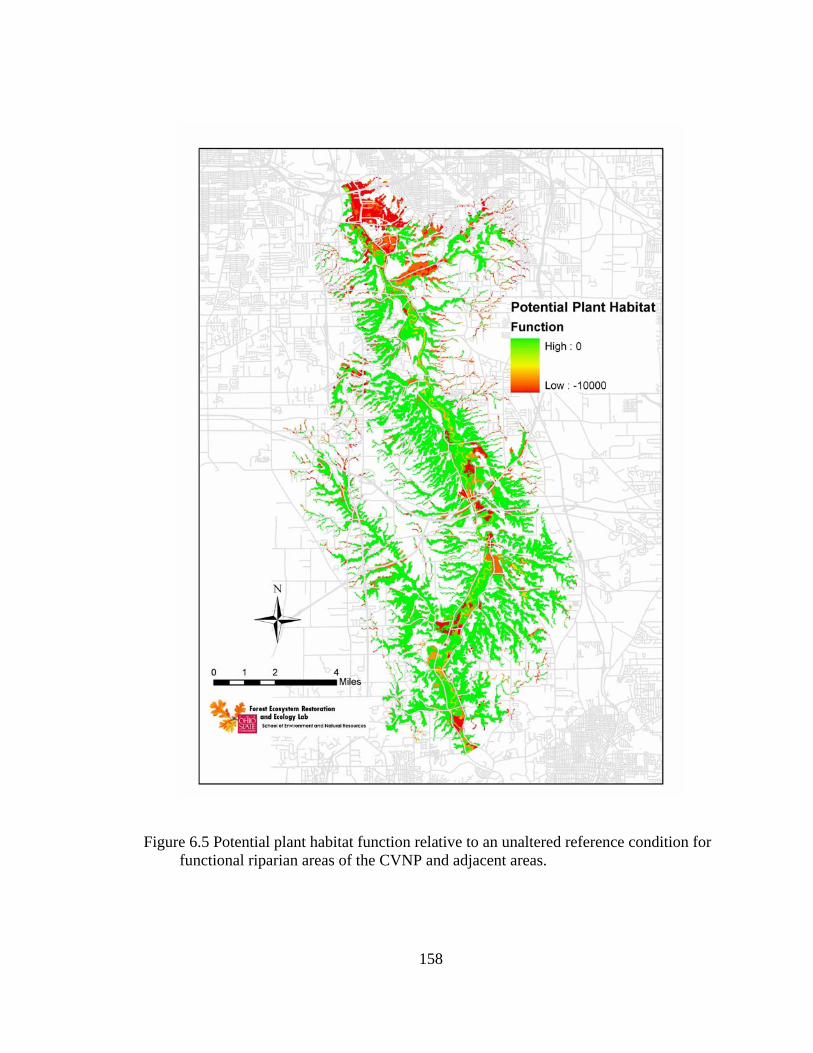
Figure 6.5 Potential plant habitat function relative to an unaltered reference condition for functional riparian areas of the CVNP and adjacent areas.

158

Figure 6.6 Sediment delivery function relative to an unaltered reference condition for functional riparian areas of the CVNP and adjacent areas.

159

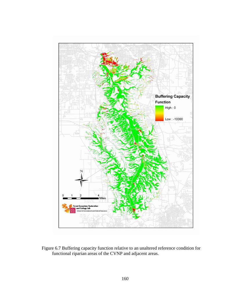
Figure 6.7 Buffering capacity function relative to an unaltered reference condition for functional riparian areas of the CVNP and adjacent areas.

160

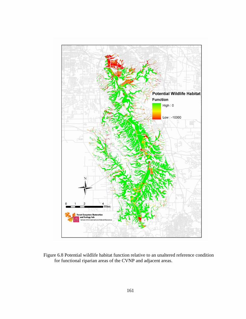
Figure 6.8 Potential wildlife habitat function relative to an unaltered reference condition for functional riparian areas of the CVNP and adjacent areas.

161

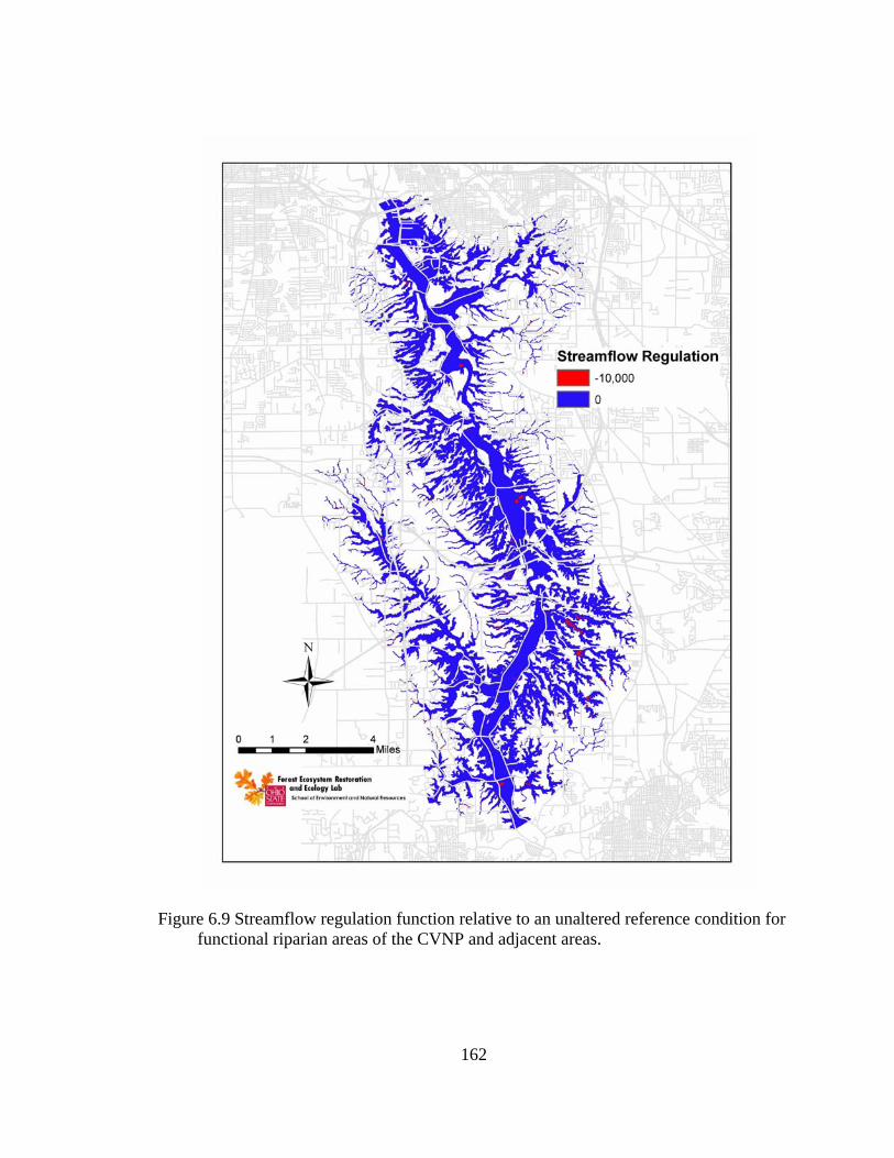
Figure 6.9 Streamflow regulation function relative to an unaltered reference condition for functional riparian areas of the CVNP and adjacent areas.

162

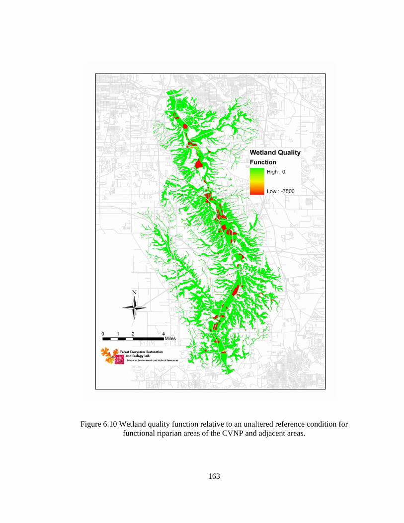
Figure 6.10 Wetland quality function relative to an unaltered reference condition for functional riparian areas of the CVNP and adjacent areas.

163

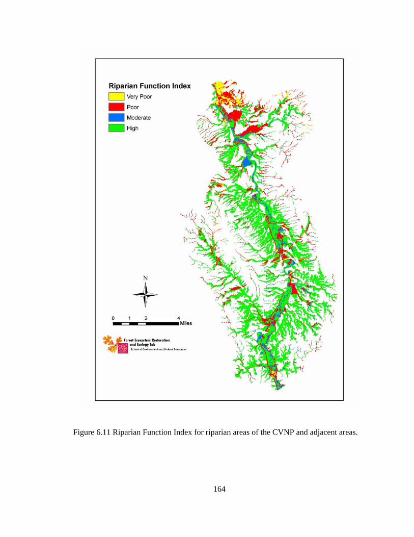
164

Figure 6.11 Riparian Function Index for riparian areas of the CVNP and adjacent areas.

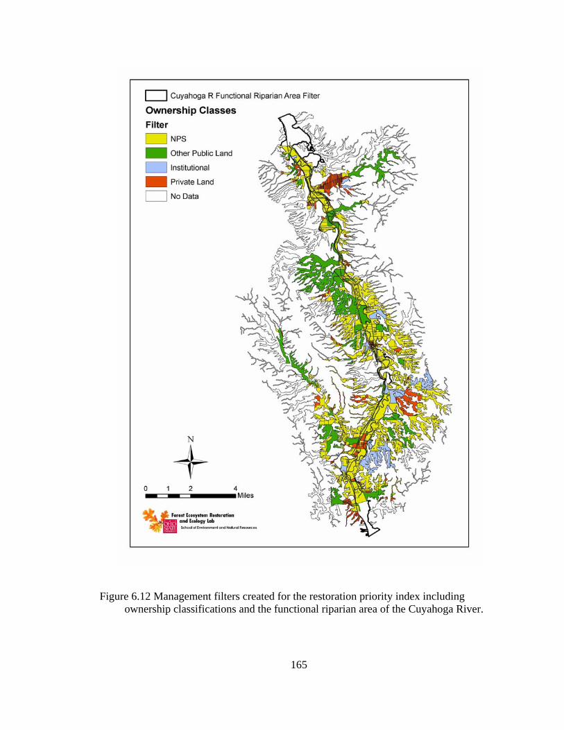
Figure 6.12 Management filters created for the restoration priority index including

ownership classifications and the functional riparian area of the Cuyahoga River.

165

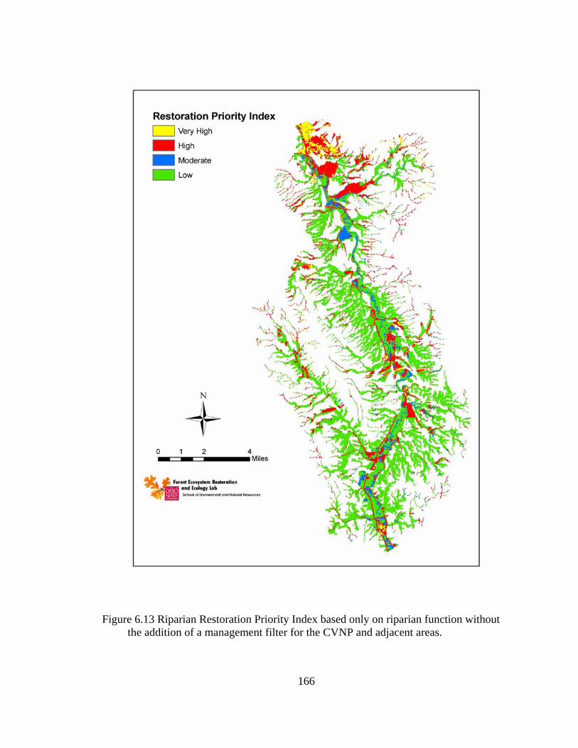
Figure 6.13 Riparian Restoration Priority Index based only on riparian function without

the addition of a management filter for the CVNP and adjacent areas.

166

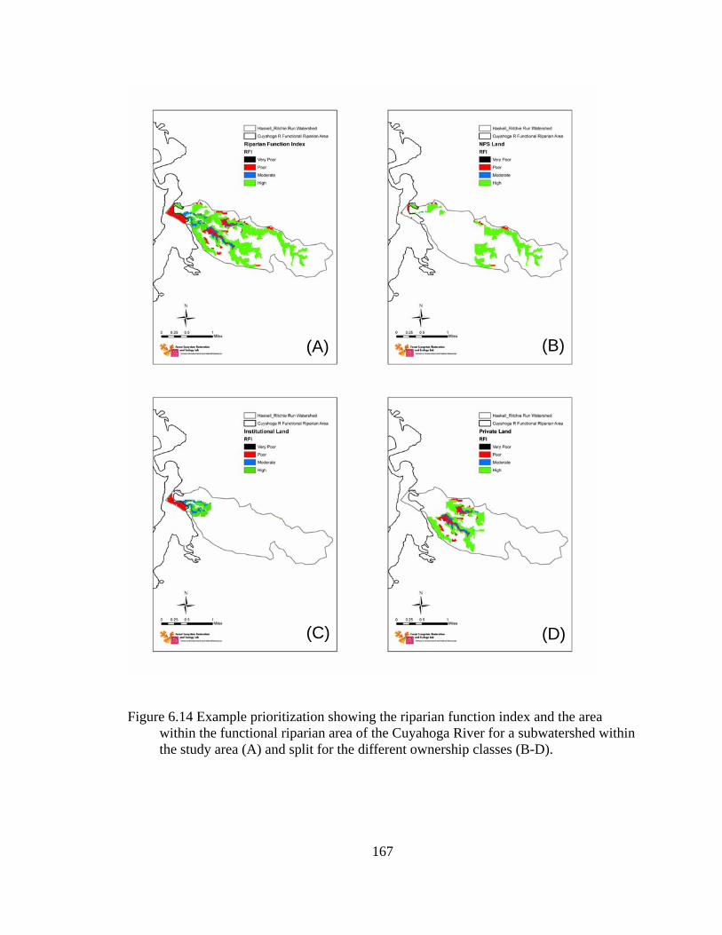
167

(D) (C)

(B) (A)

Figure 6.14 Example prioritization showing the riparian function index and the area

within the functional riparian area of the Cuyahoga River for a subwatershed within the study area (A) and split for the different ownership classes (B-D).

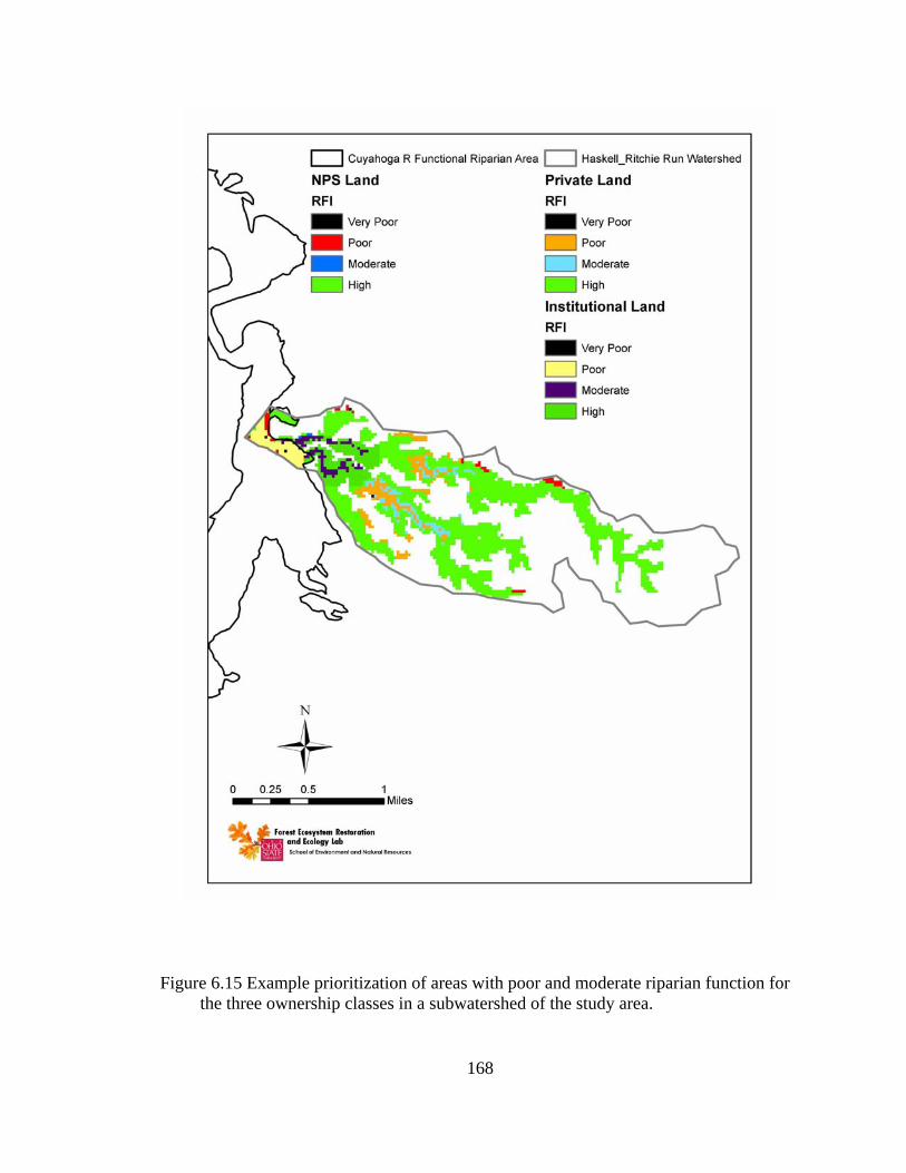
Figure 6.15 Example prioritization of areas with poor and moderate riparian function for the three ownership classes in a subwatershed of the study area.

168

LIST OF REFERENCES Allan, J.D. 1995. Stream ecology: structure and function of running waters. Chapman and

Hall: London, pp.388.

Allen, T.F.H., and T.B. Starr. 1982. Hierarchy: Perspectives for Ecological Complexity. University of Chicago Press, Chicago, IL, pp.310.

Angradi, T.R. 1996. Inter-habitat variation in benthic community structure, function, and organic matter storage in 3 Appalachian headwater streams. Journal of the North American Benthological Society 15(1): 42-63.


Baker, M.E. and B.V. Barnes. 1998. Landscape ecosystem diversity of river floodplains in northwestern lower Michigan, USA. Canadian Journal of Forest Research 28:1405-1418.

Bendix, J. and C.R. Hupp. 2000. Hydrological and geomorphical impacts on riparian plant communities. Hydrological Processes 14: 2977-2990.

Bernhardt, E.S., E.B. Sudduth, M.A. Palmer, J.D. Allan, J.L. Meyer, G. Alexander J. Follastad-Shah, B. Hassett, R. Jenkinson, R. Lave, J. Rumps, and L. Pagano. 2007. Restoring rivers one reach at a time: Results from a survey of U.S. river restoration practitioners. Restoration Ecology 15(3): 482-493.

Bilby, R.E. and G.E. Likens. 1980. Importance of organic debris dams in the structure and function of stream ecosystems. Ecology 61 (5): 1107-1113.

169

Bilby, R.E. and J.W. Ward. 1989. Changes in characteristics and function of woody debris with increasing size of streams in Western Washington. Transactions of the American Fisheries Society 118: 368-378.

Bobel, P. and R. Bobel. 1998. The Nature of the Towpath: A Natural History Guide to the Ohio and Erie Canal Towpath Trail. Cuyahoga Valley Trails Council, Inc., pp. 151.

Borcard, D., P. Legendre, and P. Drapeau. 1992. Partialing out the spatial component of ecological variation. Ecology 73(3):1045-1055.

Bowman, M.F. and R.C. Bailey. 1997. Does taxonomic resolution affect the multivariate description of the structure of freshwater benthic macroinvertebrate communities? Canadian Journal of Fisheries and Aquatic Sciences 54: 1802-1807.

Brown, G.W.1980. Forestry and Water Quality. Oregon State Book Stores: Corvallis, OR, pp.124.

Butts, S.R. and W.C. McComb. 2000. Associations of forest-floor vertebrates with course woody debris in managed forests of western Oregon. Journal of Wildlife Management 64: 95-104.

Carter, J. and J. Biagas. 2007. Prioritizing bottomland hardwood forest sites for protection and augmentation. Natural Areas Journal 27(1): 72-82.

Cipollini, K.A., A.L. Maruyama, and C.L. Zimmerman. 2005. Planning for restoration: a decision analysis approach to prioritization. Restoration Ecology 13:460-470.


Cooper, J.R., J.W. Gilliam, R.B. Daniels, and J.M. Laflen. 1987. Riparian areas as filters for agricultural sediment. Soil Science Society of America Journal 51: 416-420.

Crawford, J.A. and R. D. Semlitsch. 2007. Estimation of core terrestrial habitat for stream-breeding salamanders and delineation of riparian buffers for protection of biodiversity. Conservation Biology 21(1): 152-158.

170

Dall, D., C. Elliott, and D. Peters. 1998. A system for mapping riparian areas in the western United States. National Wetlands Inventory, USDO Fish and Wildlife Service: Lakewood, CO.15pp.

Dolédec, S., J.M. Olivier, and B. Statzer. 2000. Accurate description of the abundance of taxa and their biological traits in stream invertebrate communities: effects of taxonomic and spatial resolution. Archiv fur Hydrobiologie 148:25-43.

Dolloff, C.A. and J.L. Warren Jr. 2003. Fish relationships with large wood in small streams. American Fisheries Society Symposium 37: 179-193.

Drielsma, M. and S. Ferrier. 2006. Landscape scenario modeling of vegetation condition. Ecological Management and Restoration 7 (S1): S45-S52.

Dufrene, M. and P. Legendre. 1997. Species assemblages and indicator species: the need for a flexible asymmetrical approach. Ecological Monographs 67:345-366.

Dunn, R.R., R.K. Colwell, and C. Nilsson. 2006. The river domain: why are there more species halfway up the river? Ecography 29: 251-259.

Franklin, J.F., H.H. Shugart, M.E. Harmon. 1987. Tree death as an ecological process. BioScience 37 (8): 550-556.

Gee, G.W. and J.W. Bauder. 1986. Particle Size Analysis. pp. 383-411. In: Methods of Soil Analysis, Part 1 Physical and Mineralogical Methods, 2nd Edition. American Society of Agronomy and Soil Science Society of America: Madison, WI.

Goebel, P.C., B.J. Palik, and K.S. Pregitzer. 2003a. Plant diversity contributions of riparian areas in watersheds of the northern Lake States, USA. Ecological Applications 13:1595-1609.

Goebel, P.C., K.S. Pregitzer, and B.J. Palik. 2003b. Geomorphic influences on large wood dam loadings, particulate organic matter and dissolved organic matter in an old-growth northern hardwood watershed. Journal of Freshwater Ecology 18:479-490.

Goebel, P.C., K.S. Pregitzer, and B.J. Palik. 2006. Landscape hierarchies influence ground-flora communities in Wisconsin, USA. Forest Ecology and Management 230: 43-54.

171

Goebel, P. C., T.C. Wyse, and R.G. Corace. 2005. Determining reference ecosystem conditions for disturbed landscapes within the context of contemporary resource management issues. Journal of Forestry 103: 351-356.


Gregory, S.V., K.L. Boyer, and A.M. Gurnell , editors. 2003. The Ecology and Management of Wood in World Rivers. American Fisheries Society, Bethesda, Maryland, USA, pp.431.

Gomi, T., A.C. Johnson, R.L. Deal, P.E. Hennon, E.H. Orlikowska, and M.S. Wipfli. 2006. Factors affecting distribution of wood, detritus, and sediment in headwater streams draining managed young-growth red alder-conifer forests in southeast Alaska. Canadian Journal of Forest Research 36: 725-737.

Gurnell, A.M., G.E. Petts, and C.T. Hill. 1995. The role of coarse woody debris in forest aquatic habitats: implications for management. Journal of Aquatic Conservation: Marine and Freshwater Ecosystems 5: 1-24.

Gurnell, A.M., H. Piégay, F.J. Swanson, and S.V. Gregory. 2002. Large wood and fluvial processes. Freshwater Biology 47: 601-619.

Hacker, D.B. 2003. Cuyahoga Valley National Park. pp.163-186. In: Geology of National Parks. Editors: Harris, A.G., E. Tuttle, and S.D. Tuttle. Kendall/Hunt Publishing: Dubuque, IA, pp.882.

Hagan, J.M., S. Pealer, and A.A. Whitman. 2006. Do small headwater streams have a riparian zone defined by plant communities? Canadian Journal of Forest Research 36(9): 2131-2140.


Harmon, M.E., J.F. Franklin, F.J. Swanson, P. Sollins, S.V. Gregory, J.D. Lattin, N.H. Anderson, S.P. Cline, N.G. Aumen, J.R. Sedell, G.W. Lienkaemper, K. Cromack Jr., and K.W. Cummins. 1986. Ecology of coarse woody debris in temperate ecosystems. Advances in Ecological Research 15: 1460-1473.

172

Harmon, M.E. and C. Hua. 1991. Coarse Woody Debris Dynamics in Two Old-Growth Ecosystems. Bioscience 41 (9): 604-610.

Hassan, M.A., M. Church, T.E. Lisle, F. Brardinoni, L. Benda, and G.E. Grant. 2005. Sediment transport and channel morphology of small, forested streams. Journal of the American Water Resources Association 41 (4): 853-876.

Hewlett, R. 2000. Implications of taxonomic resolution and sample habitat for stream classification at a broad geographic scale. Journal of the North American Benthological Society 19: 352-361.


Hobbs, R.J. and L.J. Kristjanson. 2003. Triage: How do we prioritize health care for landscapes? Ecological Management and Restoration 4 Supplement: S39-S45.


Host, G.E., J. Schuldt, J.J.H. Ciborowski, L.B. Johnson, T. Hollenhorst, and C. Richards, 2005. Use of GIS and remotely sensed data for a priori identification of reference areas for Great Lakes coastal ecosystems. International Journal of Remote Sensing 26(23): 5325-5342.

Hulse, D. and S. Gregory. 2004. Integrating resilience into floodplain restoration. Urban Ecosystems 7: 295-314.

Hupp, C.R. and W.R. OsterKamp. 1996. Riparian vegetation and fluvial geomorphic processes. Geomorphology 14: 277-295.

Hyde, E.J. and T.R. Simons. 2001. Sampling plethodontid salamanders: Sources of variability. Journal of Wildlife Management 65: 624-632.

173

Ilhardt, B.L., E.S. Verry, and B.J. Palik. 2000. Defining riparian areas. pp. 23-42. In: E.S. Verry, J.W. Hornbeck, and C.A. Dolloff, editors. Riparian Management in

Forests of the Continental Eastern United States. Lewis Publishers, New York, pp.402.

Jackson, D.A. and H.H. Harvey. 1993. Fish and benthic invertebrates: community concordance and community-environment relationships. Canadian Journal of Fisheries and Aquatic Sciences 50: 2641-2651.

Johnson, L.B., D.H. Breneman, and C. Richards. 2003. Macroinvertebrate community structure and function associated with large wood in low gradient streams. River Research and Applications 19: 199-218.

Kaller, M.D. and K.J. Hartman. 2004. Evidence of a threshold level of fine sediment accumulation for altering benthic macroinvertebrate communities. Hydrobiologia 518:95-104.

Karr, J.R. 1981. Assessment of biotic integrity using fish communities. Fisheries 6:21-27.

Keeton, W.S., C.E. Kraft, and D.R. Warren. 2007. Mature and old-growth riparian forests: Structure, dynamics, and effects on Adirondack stream habitats. Ecological Applications 17 (3): 852-868.

Kent, M. and P. Coker. 1992. Basic statistical analysis of vegetation and environmental data. pp. 112-161. In: Vegetation Description and Analysis, John Wiley and Sons, New York, pp.363.

Kimmins, J.P. 1987. Forest Ecology. Macmillan, New York, pp.531.

Kondolf, G.M. 2006. River restoration and meanders. Ecology and Society 11(2): 42.

Lammert, M. and J.D. Allan. 1999. Assessing biotic integrity of streams: effects of scale in measuring the influence of land use/cover and habitat structure on fish and macroinvertebrates. Environmental Management 23: 257-270.

Lang, G.E. and R.T.T. Forman. 1978. Detrital dynamics in a mature oak forest: Hutcheson Memorial Forest, New Jersey. Ecology 59 (3): 580-595.

Lemmon, P., 1956. A spherical densiometer for estimating forest overstory density. Forest. Science 2: 314-320.

174

Leyer, I. 2005. Predicting plant species’ responses to river regulation: the role of water level fluctuations. Journal of Applied Ecology 42: 239-250.

Lowe, W.H., and D.T. Bolger. 2002. Local and landscape-scale predictors of salamander abundance in New Hampshire headwater streams. Conservation Biology 16:183-193.

Lowrance, R., R.Todd, J. Fail Jr., O. Hendrickson Jr., R. Leonard, J.L. Baker. 1984. Riparian forests as nutrient filters in agricultural watershed. BioScience 34(6): 374-377.

Lugwig, J.A. and J.F. Reynolds. 1988. Statistical Ecology: a primer on methods and computing. John Wiley and Sons, New York, 337 pp.

May, C. L. and R.E. Gresswell. 2003. Large wood recruitment and redistribution in headwater streams in the southern Oregon Coast Range, U.S.A. Canadian Journal of Forest Research 33: 1352-1362.

McClure, J.M., R.K. Kolka, and A. White. 2004. Effect of forest harvesting best management practices on coarse woody debris distribution in stream and riparian zones in three Appalachian watersheds. Water, Air, and Soil Pollution 4: 245-261.

McCune, B. and M.J. Mefford, 2006. PC-ORD: multivariate analysis of ecological data. Version 5.0. MjM Software Design, Gleneden Beach, OR.

McGovern, F. 1996. Written on the Hills: The Making of the Akron Landscape. The University of Akron Press: Akron, OH, pp. 241.

Merritt, R.W. and K.W. Cummins. 1984. Introduction to the aquatic insects of North America. Kendall/ Hunt Publishing: Dubuque, IA, pp. 722.

Meyer, J.L. and J.B. Wallace. 2000. Lost linkages and lotic ecology: rediscovering small streams. pp. 295-317. In: M.C. Press, N.J. Huntly, and S.A. Levin editors, Ecology: An achievement and challenge. Blackwell Science: Ames, IA, pp.406.

Mielke, P.W., 1984. Handbook of Statistics, Vol. 4: Nonparametric Methods. North-Holland, Amsterdam, pp. 813-830.

175

Minshall, G.W. 1967. Role of allochthonous detritus in the trophic structure of a woodland springbrook community. Ecology 48: 139-149.

Minshall, G.W., K.W. Cummins, R.C. Petersen, D.A. Bruns, and C.E. Cushing. 1985. Developments in stream ecosystem theory. Canadian Journal of Fisheries and Aquatic Science 42: 1045-1055.

Montgomery, D.R., J.M. Buffington, R.D. Smith, K.M. Schmidt, and G. Pess. 1995. Pool spacing in forest pools. Water Resources Research 31: 1097-1105.

Morris, A.E.L., P.C. Goebel, L.R. Williams, and B.J. Palik. 2006. Influence of landscape geomorphology on large wood jams and salmonids in an old-growth river of Upper Michigan. Hydrobiologia. 56:149-161.

Moore, R.D. and J.S. Richardson. 2003. Progress towards understanding the structure, function, and ecological significance of small stream channels and their riparian zones. Canadian Journal of Forest Research 33: 1349-1351.

Musgrave, D.K. and D.M. Holloran. 1980. Soil Survey of Cuyahoga County, Ohio. United States Department of Agriculture, Soil Conservation Service and Ohio Department of Natural Resources.

Naiman, R.J. 1998. Riparian forests. pp. 289-323. In: R.J. Naiman and R.E. Bilby, editors, River Ecology and Management: Lessons from the Pacific Coastal Ecoregion Springer-Verlag, New York, pp.705.

Naiman, R.J., H. Décamps, and M. Pollock. 1993. The role of riparian corridors in maintaining regional biodiversity. Ecological Applications 3(2): 209-212.

Nakano, S., H. Miyasaka, and N. Kuhara. 1999. Terrestrial-aquatic linkages: riparian arthropod inputs alter trophic cascades in a stream food web. Ecology 80:2435-2441.

O’Connor, M.D. and R.R. Ziemer. 1989. Coarse woody debris ecology in second-growth Sequoia sempervirens forest stream. USDA Forest Service General Technical Report PSW-110: 165-171.

O'Laughlin,J. and G.H. Belt. 1995. Functional approaches to riparian buffer strip design. Journal of Forestry 93:29-32.

176



Pabst, R. J. and T. A. Spies. 1998. Distribution of herbs and shrubs in relation to landform and canopy cover in riparian forests of coastal Oregon. Canadian Journal of Botany 76: 298-315.

Palik, B.J., P.C. Goebel, L.K. Kirkman, and L. West. 2000. Using landscape hierarchies to guide restoration of disturbed ecosystems. Ecological Applications 10:189-202.

Perkins, D. W. and M. L. Hunter. 2006. Use of amphibians to define riparian zones of headwater streams. Canadian Journal of Forest Research 36(9): 2124-2130.

Peterson, B.J., W.M. Wollheim, P.J. Mullolland, J.R. Webster, J.L. Meyer, J.L. Tank, E. Marti, W.B. Bowden, H.M. Valett, A.E. Hershey, W.H. McDowell, W.K. Dodds, S.K. Hamilton, S. Gregory, and D.D. Morrell. 2001. Control of nitrogen export from watersheds by headwater streams. Science 292: 86-89.

Petty, J.T. and D. Thorne. 2005. An ecologically based approach to identifying restoration priorities in an acid-impacted watershed. Restoration Ecology 13(2): 348-357.

Pfeil, E.K., N. Casacchia, G.J. Kerns, T.P. Diggins. 2007. Distribution, composition, and orientation of down deadwood in riparian old-growth woodlands of Zoar Valley Canyon, western New York State, USA. Forest Ecology and Management 239: 159-168.

Plafkin, J.L, M.T. Barbour, K.D. Porter, S.K. Gross, and R.M. Hughes. 1989. Rapid bioassessment protocols for use in stream and rivers: macroinvertebrates and fish. EPA/444/4-89-011. U.S. Environmental Protection Agency, Washington D.C.

Platt, C.V. 2006. Cuyahoga Valley National Park Handbook. The Kent State University Press: Kent, OH, pp. 60.

177

Poole, G.C. 2002. Fluvial landscape ecology: addressing uniqueness within the river discontinuum. Freshwater Biology 47: 641-660.

Rau, J.L., 1969. The evolution of the Cuyahoga River: it’s geomorphology and environmental geology. pp. 9-39. In: J.P. Cooke, editor, The Cuyahoga River Watershed. Institute of Limnology and Department of Biological Sciences, Kent State University, Kent, Ohio. Also found as Contribution No. 43, Department of Geology, Kent StateUniversity, Kent, Ohio.

Reeves, G.H., K.M. Burnett, and E.V. McGarry. 2003. Sources of large wood in the main stem of a fourth-order watershed in coastal Oregon. Canadian Journal of Forest Research 33: 1363-1370.

Rheinhardt, R., M. Brinson, R. Brooks, M. McKenney-Easterling, J.M. Rubbo, J. Hite, and B. Armstrong. 2007. Development of a reference-based method for identifying and scoring indicators of condition for coastal plain riparian reaches. Ecological Indicators 7: 339-361.

Richards, C., L.B. Johnson, and G.E. Host. 1996. Landscape-scale influences on stream habitats and biota. Canadian Journal of Fisheries and Aquatic Sciences 53: 295-311.

Richardson, J.S. and R.J. Danehy. 2007. A synthesis of the ecology of headwater streams and their riparian zones in temperate forests. Forest Science 53 (2): 131-147.

Richardson, J.S., R.J. Naiman, F.J. Swanson, and D.E. Hibbs. 2005. Riparian communities associated with Pacific Northwest headwater streams: assemblages, processes, and uniqueness. Journal of the American Water Resources Association 41(4): 935-947.

Ritchie, A. and J.R. Steiger. 1990. Soil Survey of Summit County, Ohio. United States Department of Agriculture, Soil Conservation Service.

Robison, E.G. and R.L. Beschta. 1990. Characteristics of coarse woody debris for several coastal streams of southeast Alaska, USA. Canadian Journal of Fisheries and Aquatic Science 47: 1684-1693.

Sabo, J.L., Sponseller, R., Dixon, M., Gade, K., Harms, T., Heffernan, J., Jani, A., Katz, G., Soykan, C., Watts, J., and Welter, J. 2005. Riparian zones increase regional species richness by harboring different, not more, species. Ecology 86(1): 56-62.

178

Sandin, L. and R.K. Johnson. 2004. Local, landscape and regional factors structuring benthic macroinvertebrate assemblages in Swedish streams. Landscape Ecology 19:501-514.

Schueler, T. 1994. The importance of imperviousness. Watershed Protection Techniques. 1(3): 100-111.

Semlitsch, R. D. and J. R. Bodie. 2003. Biological criteria for buffer zones around wetlands and riparian habitats for amphibians and reptiles. Conservation Biology 17(5): 1219-1228.

Shifley, S. and E. Lentz. 1985. Quick estimation of the three-parameter Weibull to describe tree size distributions. Forest Ecology and Management 13: 195-203

Smock, L.A., G.M. Metzler, J.E. Gladden. 1989. Role of debris dams in the structure and functioning of low-gradient headwater streams. Ecology 70 (3): 764-775.

Spackman, S.C. and J.W. Hughes. 1995. Assessment of minimum stream corridor width for biological conservation: species richness and distribution along mid-order streams in Vermont, USA. Biological Conservation 71: 325-332.

Sparovek, G., S.B.L. Ranieri, A. Gassner, I.C. De Maria, E. Schnug, R.F.D. Santos, and A. Joubert. 2002. A conceptual framework for the definition of the optimal width of riparian forests. Agriculture, Ecosystems, and Environment 90: 169-175.

Stewart, T.W., T.L. Shumaker, and T.A. Radzio. 2003. Linear and nonlinear effects of habitat structure on composition and abundance in the macroinvertebrate community of a large river. The American Midland Naturalist 149:293-305.

Stoddard, J.L., D.P. Larsen, C.P. Hawkins, R.K. Johnson, and R.H. Norris. 2006. Setting expectations for the ecological condition of streams: The concept for reference condition. Ecological Applications 16(4): 1267-1276.

Storer, D.A., 1984. A simple high sample volume ashing procedure for determining soil organic matter. Communications in Soil Science and Plant Analysis 15: 759-772.

Strahler, A.N. 1952. Dynamic basis of geomorphology. Bulletin of the Geological Society of America 83: 923- 938.

179

Sutherland, W.J., A.S. Pullin, P.M. Dolman, and T.M. Knight. 2004. The need for evidence-based conservation. Trends in Ecology and Evolution 19(6): 305-308.

Swanson, F J and J. F. Franklin. 1992. New forestry principles from ecosystem analysis of Pacific Northwest forests. Ecological Applications 2(3):262-274.

ter Braak, C.J.F., 1986. Canonical correspondence analysis: a new eigenvector technique for multivariate direct gradient analysis. Ecology 67: 1167-1179.

ter Braak, C.J.F. and I.C. Prentice. 1988. A theory of gradient analysis. Advances in Ecological Research 18: 271-317.

ter Braak, C.J.F. and P. Šmilauer. 1997. Canoco for Windows version 4.02. Centre for Biometry. Wageningen, Netherlands.

Thoman, D.R., L.J. Bain, and C.E. Antle. 1969. Inferences on the parameters of the Weibull distribution. Technometrics 11(3): 445-460.

Timm, R.K., R.C. Wissmar, J.W. Small, T.M. Leschine, and G. Lucchetti. 2004. A screening procedure for prioritizing riparian management. Environmental Management 33:151-161.

Trimble, G.R., Jr., and R.S. Sartz. 1957. How far from a stream should a logging road be located? Journal of Forestry 55(5): 339-341.

Urban, M.C., D.K. Skelly, D. Burchsted, W. Price, and S. Lowry. 2006. Stream communities across a rural-urban landscape gradient. Diversity and Distributions 12: 337-350.

USDA Forest Service. 1994. Watershed Protection and Management. Forest Service Manual Chapter 2520. WOAmendment 2500-94-3, pp. 26.

USDA, NRCS. 2007. The PLANTS Database (http://plants.usda.gov). National Plant Data Center, Baton Rouge, LA 70874-4490, USA.

Vannote, R.L., G.W. Minshall, K.W. Cummins, J.R. Sedell, and C.E. Cushing. 1980. The river continuum concept. Canadian Journal of Fisheries and Aquatic Sciences 37: 130-137.

180

http://plants.usda.gov/

Vanreusel, W. and H. Van Dyck. 2007. When functional habitat does not match vegetation types: A resource-based approach to map butterfly habitat. Biological Conservation 135: 202-211.

Verry, E.S., C.A. Dolloff, and M.E. Manning. 2004. Riparian ecotone: A functional definition and delineation for resource assessment. Water Air and Soil Pollution: Focus 4: 67-94.

Vinson, M.R. and C.P. Hawkins. 1998. Biodiversity of stream insects: variation at local, basin, and regional scales. Annual Review of Entomology 43:271-293.

Wallace, J.B., S.L. Eggert, J.L. Meyer, and J.R. Webster. 1997. Multiple trophic levels of a forest stream linked to terrestrial litter inputs. Science 277:102-104.

Wallace, J.B., J.R. Webster, and J.L. Meyer. 1995. Influence of log additions on physical and biotic characteristics of a mountain stream. Canadian Journal of Fisheries and Aquatic Science 52: 2120-2137.

Warren, D. R., E.S. Bernhardt, R.O. Hall Jr., and G.E. Likens. 2007. Forest age, wood, and nutrient dynamics in headwater streams of the Hubbard Brook Experimental Forest, New Hampshire, USA. Earth Surface Process and Landforms 32(8): 1154-1163.

Webster, C.R., C.J.F. Huckins, and J.M. Shields. 2008. Spatial distribution of riparian zone coarse woody debris in a managed northern temperate watershed. American Midland Naturalist 159: 225-237.

Welsh, H.H. and L.M. Ollivier. 1998. Stream amphibians as indicators of ecosystem stress: a case study from California’s redwoods. Ecological Applications 8: 1118-1132.

White, G.W. 1984. Glacial geology of Summit County, Ohio. Ohio Department of Natural Resources, Division of Geological Survey: Columbus.

Williams. L.R., C.M. Taylor, M.L. Warren Jr., and J.A. Clingenpeel. 2002. Large-scale effects of timber harvesting on stream systems in the Ouachita Mountains, Arkansas. Environmental Management 29:76-87.

181

182

Williams, L.R., C.M. Taylor, M.L. Warren Jr., and J.A. Clingenpeel. 2003a. Environmental variability, historical contingency, and the structure of regional fish and macroinvertebrate faunas in Ouachita Mountain stream systems. Environmental Biology of Fishes 67: 203-216.

Williams, L.R., C.M. Taylor, and M.L. Warren, Jr. 2003b. Influence of fish predation on assemblage structure of macroinvertebrates in an intermittent stream. Transactions of the American Fisheries Society 132: 120-130.

Williams, L.R., T.H. Bonner, J.D. Hudson III, M.G. Williams, T.R. Leavy, and C.S. Williams. 2005. Interactive effects of environmental variability and military training on stream biota of three headwater drainages in Western Louisiana. Transactions of the American Fisheries Society 134: 192-206.

Wilson, J.D. and M.E. Dorcas. 2003. Effects of habitat disturbance on stream salamanders: implications for buffer zones and watershed management. Conservation Biology 17:763-771.

Wondzell, S.M. and P.A. Bisson. 2003. Influence of wood on aquatic biodiversity. pp. 249-263. In: Gregory, S.V., K.L. Boyer, and A.M. Gurnell, editors. The Ecology and Management of Wood in World Rivers. American Fisheries Society, Bethesda, Maryland, USA, pp.431.


Yang, X. 2007. Integrated use of remote sensing and geographic information systems in riparian vegetation delineation and mapping. International Journal of Remote Sensing 28(1-2): 353-370.

Young, M.K., E.A. Mace, E.T. Ziegler, and E.K. Sutherland. 2006. Characterizing and contrasting instream and riparian course wood in western Montana basins. Forest Ecology and Management 226: 26-40.

Zar, J.H., 1974. Biostatistical Analysis. Prentice-Hall, Inc: Englewood Cliffs, N.J., pp.620.

Documents

Composition and structure of headwater riparian forests